Concise Linux//An Introduction To Linux Use And Administration Lxk1 En Manual
User Manual:
Open the PDF directly: View PDF ![]() .
.
Page Count: 484 [warning: Documents this large are best viewed by clicking the View PDF Link!]
- Contents
- List of Tables
- List of Figures
- Preface
- Introduction
- Using the Linux System
- Who's Afraid Of The Big Bad Shell?
- Getting Help
- The vi Editor
- Files: Care and Feeding
- Standard I/O and Filter Commands
- More About The Shell
- The File System
- System Administration
- User Administration
- Access Control
- Process Management
- Hard Disks (and Other Secondary Storage)
- File Systems: Care and Feeding
- Booting Linux
- System-V Init and the Init Process
- Systemd
- Time-controlled Actions—*cron and *at
- System Logging
- System Logging with Systemd and ``The Journal''
- TCP/IP Fundamentals
- Linux Network Configuration
- Network Troubleshooting
- The Secure Shell
- Software Package Management Using Debian Tools
- Package Management with RPM and YUM
- Sample Solutions
- Example Files
- LPIC-1 Certification
- Command Index
- Index

L
i
n
u
x
P
r
o
f
e
s
s
i
o
n
a
l
I
n
s
t
i
t
u
t
e
A
p
p
r
o
v
e
d
T
r
a
i
n
i
n
g
M
a
t
e
r
i
a
l
Concise Linux
An Introduction to Linux Use and
Administration
$ echo tux
tux
$ ls
hallo.c
hallo.o
$ /bin/su -
Password:
tuxcademy – Linux and Open Source learning materials for everyone
www.tuxcademy.org ⋅info@tuxcademy.org

L
i
n
u
x
P
r
o
f
e
s
s
i
o
n
a
l
I
n
s
t
i
t
u
t
e
A
p
p
r
o
v
e
d
T
r
a
i
n
i
n
g
M
a
t
e
r
i
a
l
These training materials have been certied by the Linux Professional Institute (LPI) under the
auspices of the LPI ATM programme. They are suitable for preparation for the LPIC-1 certication.
The Linux Professional Institute does not endorse specic exam preparation materials or
techniques—refer to
info@lpi.org
for details.
The tuxcademy project aims to supply freely available high-quality training materials on
Linux and Open Source topics – for self-study, school, higher and continuing education
and professional training.
Please visit
http://www.tuxcademy.org/
! Do contact us with questions or suggestions.
Concise Linux An Introduction to Linux Use and Administration
Revision:
lxk1:807d647231c25323:2015-08-21
adm1:33e55eeadba676a3:2015-08-08
10–18, 26–27
adm2:0cd20ee1646f650c:2015-08-21
20–25
grd1:be27bba8095b329b:2015-08-04
1–9, B
grd2:6eb247d0aa1863fd:2015-08-05
19
lxk1:qPeeTb2oHiy6EUuPrr0DT
© 2015 Linup Front GmbH Darmstadt, Germany
© 2016 tuxcademy (Anselm Lingnau) Darmstadt, Germany
http://www.tuxcademy.org
⋅
info@tuxcademy.org
Linux penguin “Tux” © Larry Ewing (CC-BY licence)
All representations and information contained in this document have been com-
piled to the best of our knowledge and carefully tested. However, mistakes cannot
be ruled out completely. To the extent of applicable law, the authors and the tux-
cademy project assume no responsibility or liability resulting in any way from the
use of this material or parts of it or from any violation of the rights of third parties.
Reproduction of trade marks, service marks and similar monikers in this docu-
ment, even if not specially marked, does not imply the stipulation that these may
be freely usable according to trade mark protection laws. All trade marks are used
without a warranty of free usability and may be registered trade marks of third
parties.
This document is published under the “Creative Commons-BY-SA 4.0 Interna-
tional” licence. You may copy and distribute it and make it publically available as
long as the following conditions are met:
Attribution You must make clear that this document is a product of the tux-
cademy project.
Share-Alike You may alter, remix, extend, or translate this document or modify
or build on it in other ways, as long as you make your contributions available
under the same licence as the original.
Further information and the full legal license grant may be found at
http://creativecommons.org/licenses/by-sa/4.0/
Authors: Tobias Elsner, Thomas Erker, Anselm Lingnau
Technical Editor: Anselm Lingnau ⟨
anselm.lingnau@linupfront.de
⟩
Typeset in Palatino, Optima and DejaVu Sans Mono

$ echo tux
tux
$ ls
hallo.c
hallo.o
$ /bin/su -
Password:
Contents
1 Introduction 15
1.1 What is Linux? . . . . . . . . . . . . . . . . . . . . . 16
1.2 Linux History . . . . . . . . . . . . . . . . . . . . . 16
1.3 Free Software, “Open Source” and the GPL . . . . . . . . . . 18
1.4 Linux—The Kernel . . . . . . . . . . . . . . . . . . . 21
1.5 Linux Properties . . . . . . . . . . . . . . . . . . . . 23
1.6 Linux Distributions . . . . . . . . . . . . . . . . . . . 26
2 Using the Linux System 31
2.1 Logging In and Out . . . . . . . . . . . . . . . . . . . 32
2.2 Switching On and O . . . . . . . . . . . . . . . . . . 34
2.3 The System Administrator. . . . . . . . . . . . . . . . . 34
3 Who’s Afraid Of The Big Bad Shell? 37
3.1 Why?........................38
3.1.1 What Is The Shell? . . . . . . . . . . . . . . . . . 38
3.2 Commands . . . . . . . . . . . . . . . . . . . . . . 40
3.2.1 Why Commands?. . . . . . . . . . . . . . . . . . 40
3.2.2 Command Structure. . . . . . . . . . . . . . . . . 40
3.2.3 Command Types . . . . . . . . . . . . . . . . . . 41
3.2.4 Even More Rules . . . . . . . . . . . . . . . . . . 42
4 Getting Help 45
4.1 Self-Help . . . . . . . . . . . . . . . . . . . . . . . 46
4.2 The
help
Command and the
--help
Option . . . . . . . . . . . 46
4.3 The On-Line Manual . . . . . . . . . . . . . . . . . . 46
4.3.1 Overview . . . . . . . . . . . . . . . . . . . . 46
4.3.2 Structure . . . . . . . . . . . . . . . . . . . . . 47
4.3.3 Chapters . . . . . . . . . . . . . . . . . . . . . 48
4.3.4 Displaying Manual Pages . . . . . . . . . . . . . . . 48
4.4 Info Pages . . . . . . . . . . . . . . . . . . . . . . 49
4.5 HOWTOs.......................50
4.6 Further Information Sources . . . . . . . . . . . . . . . . 50
5 The
vi
Editor 53
5.1 Editors........................54
5.2 The Standard—
vi
....................54
5.2.1 Overview . . . . . . . . . . . . . . . . . . . . 54
5.2.2 Basic Functions . . . . . . . . . . . . . . . . . . 55
5.2.3 Extended Commands . . . . . . . . . . . . . . . . 58
5.3 Other Editors . . . . . . . . . . . . . . . . . . . . . 60

4 Contents
6 Files: Care and Feeding 63
6.1 File and Path Names. . . . . . . . . . . . . . . . . . . 64
6.1.1 File Names . . . . . . . . . . . . . . . . . . . . 64
6.1.2 Directories . . . . . . . . . . . . . . . . . . . . 65
6.1.3 Absolute and Relative Path Names . . . . . . . . . . . 66
6.2 Directory Commands . . . . . . . . . . . . . . . . . . 67
6.2.1 The Current Directory:
cd
& Co. . . . . . . . . . . . . 67
6.2.2 Listing Files and Directories—
ls
............68
6.2.3 Creating and Deleting Directories:
mkdir
and
rmdir
. . . . . . 69
6.3 File Search Patterns . . . . . . . . . . . . . . . . . . . 70
6.3.1 Simple Search Patterns . . . . . . . . . . . . . . . . 70
6.3.2 Character Classes. . . . . . . . . . . . . . . . . . 72
6.3.3 Braces . . . . . . . . . . . . . . . . . . . . . . 73
6.4 Handling Files . . . . . . . . . . . . . . . . . . . . . 74
6.4.1 Copying, Moving and Deleting—
cp
and Friends. . . . . . . 74
6.4.2 Linking Files—
ln
and
ln -s
..............76
6.4.3 Displaying File Content—
more
and
less
..........80
6.4.4 Searching Files—
find
................81
6.4.5 Finding Files Quickly—
locate
and
slocate
.........84
7 Standard I/O and Filter Commands 87
7.1 I/O Redirection and Command Pipelines . . . . . . . . . . . 88
7.1.1 Standard Channels . . . . . . . . . . . . . . . . . 88
7.1.2 Redirecting Standard Channels . . . . . . . . . . . . . 89
7.1.3 Command Pipelines. . . . . . . . . . . . . . . . . 92
7.2 Filter Commands . . . . . . . . . . . . . . . . . . . . 94
7.3 Reading and Writing Files. . . . . . . . . . . . . . . . . 94
7.3.1 Outputting and Concatenating Text Files—
cat
and
tac
. . . . 94
7.3.2 Beginning and End—
head
and
tail
............96
7.3.3 Just the Facts, Ma’am—
od
and
hexdump
...........97
7.4 Text Processing. . . . . . . . . . . . . . . . . . . . . 100
7.4.1 Character by Character—
tr
,
expand
and
unexpand
. . . . . . . 100
7.4.2 Line by Line—
fmt
,
pr
and so on . . . . . . . . . . . . . 103
7.5 Data Management . . . . . . . . . . . . . . . . . . . 108
7.5.1 Sorted Files—
sort
and
uniq
..............108
7.5.2 Columns and Fields—
cut
,
paste
etc. . . . . . . . . . . . 113
8 More About The Shell 119
8.1 Simple Commands:
sleep
,
echo
, and
date
............120
8.2 Shell Variables and The Environment. . . . . . . . . . . . . 121
8.3 Command Types—Reloaded. . . . . . . . . . . . . . . . 123
8.4 The Shell As A Convenient Tool. . . . . . . . . . . . . . . 124
8.5 Commands From A File . . . . . . . . . . . . . . . . . 128
8.6 The Shell As A Programming Language. . . . . . . . . . . . 129
8.6.1 Foreground and Background Processes . . . . . . . . . . 132
9 The File System 137
9.1 Terms........................138
9.2 File Types. . . . . . . . . . . . . . . . . . . . . . . 138
9.3 The Linux Directory Tree . . . . . . . . . . . . . . . . . 139
9.4 Directory Tree and File Systems. . . . . . . . . . . . . . . 147
9.5 Removable Media. . . . . . . . . . . . . . . . . . . . 148
10 System Administration 151
10.1 Introductory Remarks . . . . . . . . . . . . . . . . . . 152
10.2 The Privileged
root
Account . . . . . . . . . . . . . . . . 152
10.3 Obtaining Administrator Privileges . . . . . . . . . . . . . 154
10.4 Distribution-specic Administrative Tools . . . . . . . . . . . 156

5
11 User Administration 159
11.1Basics........................160
11.1.1 Why Users? . . . . . . . . . . . . . . . . . . . . 160
11.1.2 Users and Groups . . . . . . . . . . . . . . . . . 161
11.1.3 People and Pseudo-Users . . . . . . . . . . . . . . . 163
11.2 User and Group Information. . . . . . . . . . . . . . . . 163
11.2.1 The
/etc/passwd
File.................163
11.2.2 The
/etc/shadow
File.................166
11.2.3 The
/etc/group
File .................168
11.2.4 The
/etc/gshadow
File.................169
11.2.5 The
getent
Command . . . . . . . . . . . . . . . . 170
11.3 Managing User Accounts and Group Information . . . . . . . . 170
11.3.1 Creating User Accounts . . . . . . . . . . . . . . . 171
11.3.2 The
passwd
Command . . . . . . . . . . . . . . . . 172
11.3.3 Deleting User Accounts . . . . . . . . . . . . . . . 174
11.3.4 Changing User Accounts and Group Assignment . . . . . . 174
11.3.5 Changing User Information Directly—
vipw
.........175
11.3.6 Creating, Changing and Deleting Groups . . . . . . . . . 175
12 Access Control 179
12.1 The Linux Access Control System . . . . . . . . . . . . . . 180
12.2 Access Control For Files And Directories . . . . . . . . . . . 180
12.2.1 The Basics . . . . . . . . . . . . . . . . . . . . 180
12.2.2 Inspecting and Changing Access Permissions. . . . . . . . 181
12.2.3 Specifying File Owners and Groups—
chown
and
chgrp
. . . . . 182
12.2.4 The umask . . . . . . . . . . . . . . . . . . . . 183
12.3 Access Control Lists (ACLs) . . . . . . . . . . . . . . . . 185
12.4 Process Ownership . . . . . . . . . . . . . . . . . . . 185
12.5 Special Permissions for Executable Files . . . . . . . . . . . . 185
12.6 Special Permissions for Directories . . . . . . . . . . . . . 186
12.7 File Attributes . . . . . . . . . . . . . . . . . . . . . 188
13 Process Management 191
13.1 What Is A Process? . . . . . . . . . . . . . . . . . . . 192
13.2 Process States . . . . . . . . . . . . . . . . . . . . . 193
13.3 Process Information—
ps
.................194
13.4 Processes in a Tree—
pstree
................195
13.5 Controlling Processes—
kill
and
killall
............196
13.6
pgrep
and
pkill
.....................197
13.7 Process Priorities—
nice
and
renice
..............199
13.8 Further Process Management Commands—
nohup
and
top
. . . . . 199
14 Hard Disks (and Other Secondary Storage) 201
14.1 Fundamentals . . . . . . . . . . . . . . . . . . . . . 202
14.2 Bus Systems for Mass Storage . . . . . . . . . . . . . . . 202
14.3 Partitioning . . . . . . . . . . . . . . . . . . . . . . 205
14.3.1 Fundamentals . . . . . . . . . . . . . . . . . . . 205
14.3.2 The Traditional Method (MBR) . . . . . . . . . . . . . 206
14.3.3 The Modern Method (GPT) . . . . . . . . . . . . . . 207
14.4 Linux and Mass Storage . . . . . . . . . . . . . . . . . 208
14.5 Partitioning Disks. . . . . . . . . . . . . . . . . . . . 210
14.5.1 Fundamentals . . . . . . . . . . . . . . . . . . . 210
14.5.2 Partitioning Disks Using
fdisk
.............212
14.5.3 Formatting Disks using GNU
parted
...........215
14.5.4
gdisk
......................216
14.5.5 More Partitioning Tools . . . . . . . . . . . . . . . 217
14.6 Loop Devices and
kpartx
.................217
14.7 The Logical Volume Manager (LVM) . . . . . . . . . . . . . 219

6 Contents
15 File Systems: Care and Feeding 223
15.1 Creating a Linux File System. . . . . . . . . . . . . . . . 224
15.1.1 Overview . . . . . . . . . . . . . . . . . . . . 224
15.1.2 The
ext
File Systems . . . . . . . . . . . . . . . . . 226
15.1.3 ReiserFS . . . . . . . . . . . . . . . . . . . . . 234
15.1.4XFS.......................235
15.1.5 Btrfs . . . . . . . . . . . . . . . . . . . . . . 237
15.1.6 Even More File Systems . . . . . . . . . . . . . . . 238
15.1.7 Swap space . . . . . . . . . . . . . . . . . . . . 239
15.2 Mounting File Systems . . . . . . . . . . . . . . . . . . 240
15.2.1 Basics . . . . . . . . . . . . . . . . . . . . . . 240
15.2.2 The
mount
Command . . . . . . . . . . . . . . . . . 240
15.2.3 Labels and UUIDs . . . . . . . . . . . . . . . . . 242
15.3 The
dd
Command....................244
16 Booting Linux 247
16.1 Fundamentals . . . . . . . . . . . . . . . . . . . . . 248
16.2 GRUB Legacy . . . . . . . . . . . . . . . . . . . . . 251
16.2.1 GRUB Basics . . . . . . . . . . . . . . . . . . . 251
16.2.2 GRUB Legacy Conguration. . . . . . . . . . . . . . 252
16.2.3 GRUB Legacy Installation . . . . . . . . . . . . . . . 253
16.2.4 GRUB 2 . . . . . . . . . . . . . . . . . . . . . 254
16.2.5 Security Advice . . . . . . . . . . . . . . . . . . 255
16.3 Kernel Parameters . . . . . . . . . . . . . . . . . . . 255
16.4 System Startup Problems . . . . . . . . . . . . . . . . . 257
16.4.1 Troubleshooting . . . . . . . . . . . . . . . . . . 257
16.4.2 Typical Problems . . . . . . . . . . . . . . . . . . 257
16.4.3 Rescue systems and Live Distributions . . . . . . . . . . 259
17 System-V Init and the Init Process 261
17.1 The Init Process . . . . . . . . . . . . . . . . . . . . 262
17.2 System-V Init . . . . . . . . . . . . . . . . . . . . . 262
17.3 Upstart . . . . . . . . . . . . . . . . . . . . . . . 268
17.4 Shutting Down the System . . . . . . . . . . . . . . . . 270
18 Systemd 275
18.1 Overview. . . . . . . . . . . . . . . . . . . . . . . 276
18.2 Unit Files . . . . . . . . . . . . . . . . . . . . . . . 277
18.3 Unit Types . . . . . . . . . . . . . . . . . . . . . . 281
18.4 Dependencies . . . . . . . . . . . . . . . . . . . . . 282
18.5 Targets. . . . . . . . . . . . . . . . . . . . . . . . 284
18.6 The
systemctl
Command . . . . . . . . . . . . . . . . . 286
18.7 Installing Units. . . . . . . . . . . . . . . . . . . . . 289
19 Time-controlled Actions—
cron
and
at
291
19.1 Introduction. . . . . . . . . . . . . . . . . . . . . . 292
19.2 One-Time Execution of Commands . . . . . . . . . . . . . 292
19.2.1
at
and
batch
....................292
19.2.2
at
Utilities . . . . . . . . . . . . . . . . . . . . 294
19.2.3 Access Control. . . . . . . . . . . . . . . . . . . 294
19.3 Repeated Execution of Commands . . . . . . . . . . . . . 295
19.3.1 User Task Lists. . . . . . . . . . . . . . . . . . . 295
19.3.2 System-Wide Task Lists . . . . . . . . . . . . . . . 296
19.3.3 Access Control. . . . . . . . . . . . . . . . . . . 297
19.3.4 The
crontab
Command . . . . . . . . . . . . . . . . 297
19.3.5 Anacron . . . . . . . . . . . . . . . . . . . . . 298
20 System Logging 301

7
20.1 The Problem . . . . . . . . . . . . . . . . . . . . . 302
20.2 The Syslog Daemon . . . . . . . . . . . . . . . . . . . 302
20.3 Log Files . . . . . . . . . . . . . . . . . . . . . . . 305
20.4 Kernel Logging . . . . . . . . . . . . . . . . . . . . 306
20.5 Extended Possibilities: Rsyslog . . . . . . . . . . . . . . . 306
20.6 The “next generation”: Syslog-NG. . . . . . . . . . . . . . 310
20.7 The
logrotate
Program . . . . . . . . . . . . . . . . . . 314
21 System Logging with Systemd and “The Journal” 319
21.1 Fundamentals . . . . . . . . . . . . . . . . . . . . . 320
21.2 Systemd and journald . . . . . . . . . . . . . . . . . . 321
21.3 Log Inspection . . . . . . . . . . . . . . . . . . . . . 323
22 TCP/IP Fundamentals 329
22.1 History and Introduction . . . . . . . . . . . . . . . . . 330
22.1.1 The History of the Internet . . . . . . . . . . . . . . 330
22.1.2 Internet Administration . . . . . . . . . . . . . . . 330
22.2 Technology . . . . . . . . . . . . . . . . . . . . . . 332
22.2.1 Overview . . . . . . . . . . . . . . . . . . . . 332
22.2.2 Protocols . . . . . . . . . . . . . . . . . . . . . 333
22.3 TCP/IP . . . . . . . . . . . . . . . . . . . . . . . 335
22.3.1 Overview . . . . . . . . . . . . . . . . . . . . 335
22.3.2 End-to-End Communication: IP and ICMP . . . . . . . . 336
22.3.3 The Base for Services: TCP and UDP . . . . . . . . . . . 339
22.3.4 The Most Important Application Protocols. . . . . . . . . 342
22.4 Addressing, Routing and Subnetting . . . . . . . . . . . . . 344
22.4.1 Basics . . . . . . . . . . . . . . . . . . . . . . 344
22.4.2 Routing . . . . . . . . . . . . . . . . . . . . . 345
22.4.3 IP Network Classes . . . . . . . . . . . . . . . . . 346
22.4.4 Subnetting . . . . . . . . . . . . . . . . . . . . 346
22.4.5 Private IP Addresses . . . . . . . . . . . . . . . . 347
22.4.6 Masquerading and Port Forwarding . . . . . . . . . . . 348
22.5IPv6.........................349
22.5.1 IPv6 Addressing . . . . . . . . . . . . . . . . . . 350
23 Linux Network Conguration 355
23.1 Network Interfaces . . . . . . . . . . . . . . . . . . . 356
23.1.1 Hardware and Drivers . . . . . . . . . . . . . . . . 356
23.1.2 Conguring Network Adapters Using
ifconfig
. . . . . . . 357
23.1.3 Conguring Routing Using
route
............358
23.1.4 Conguring Network Settings Using
ip
..........360
23.2 Persistent Network Conguration . . . . . . . . . . . . . . 361
23.3DHCP........................364
23.4 IPv6 Conguration . . . . . . . . . . . . . . . . . . . 365
23.5 Name Resolution and DNS . . . . . . . . . . . . . . . . 366
24 Network Troubleshooting 371
24.1 Introduction. . . . . . . . . . . . . . . . . . . . . . 372
24.2 Local Problems. . . . . . . . . . . . . . . . . . . . . 372
24.3 Checking Connectivity With
ping
..............372
24.4 Checking Routing Using
traceroute
And
tracepath
........375
24.5 Checking Services With
netstat
And
nmap
...........378
24.6 Testing DNS With
host
And
dig
...............381
24.7 Other Useful Tools For Diagnosis . . . . . . . . . . . . . . 383
24.7.1
telnet
and
netcat
..................383
24.7.2
tcpdump
......................385
24.7.3
wireshark
.....................385
25 The Secure Shell 387

8 Contents
25.1 Introduction. . . . . . . . . . . . . . . . . . . . . . 388
25.2 Logging Into Remote Hosts Using
ssh
............388
25.3 Other Useful Applications:
scp
and
sftp
............391
25.4 Public-Key Client Authentication . . . . . . . . . . . . . . 392
25.5 Port Forwarding Using SSH . . . . . . . . . . . . . . . . 394
25.5.1 X11 Forwarding . . . . . . . . . . . . . . . . . . 394
25.5.2 Forwarding Arbitrary TCP Ports . . . . . . . . . . . . 395
26 Software Package Management Using Debian Tools 399
26.1 Overview. . . . . . . . . . . . . . . . . . . . . . . 400
26.2 The Basis:
dpkg
.....................400
26.2.1 Debian Packages . . . . . . . . . . . . . . . . . . 400
26.2.2 Package Installation . . . . . . . . . . . . . . . . . 401
26.2.3 Deleting Packages . . . . . . . . . . . . . . . . . 402
26.2.4 Debian Packages and Source Code . . . . . . . . . . . 403
26.2.5 Package Information. . . . . . . . . . . . . . . . . 403
26.2.6 Package Verication . . . . . . . . . . . . . . . . . 406
26.3 Debian Package Management: The Next Generation . . . . . . . 407
26.3.1 APT . . . . . . . . . . . . . . . . . . . . . . 407
26.3.2 Package Installation Using
apt-get
............407
26.3.3 Information About Packages. . . . . . . . . . . . . . 409
26.3.4
aptitude
.....................410
26.4 Debian Package Integrity . . . . . . . . . . . . . . . . . 412
26.5 The debconf Infrastructure . . . . . . . . . . . . . . . . 413
26.6
alien
: Software From Dierent Worlds . . . . . . . . . . . . 414
27 Package Management with RPM and YUM 417
27.1 Introduction. . . . . . . . . . . . . . . . . . . . . . 418
27.2 Package Management Using
rpm
...............419
27.2.1 Installation and Update . . . . . . . . . . . . . . . 419
27.2.2 Deinstalling Packages . . . . . . . . . . . . . . . . 419
27.2.3 Database and Package Queries . . . . . . . . . . . . . 420
27.2.4 Package Verication . . . . . . . . . . . . . . . . . 422
27.2.5 The
rpm2cpio
Program . . . . . . . . . . . . . . . . 422
27.3YUM........................423
27.3.1 Overview . . . . . . . . . . . . . . . . . . . . 423
27.3.2 Package Repositories . . . . . . . . . . . . . . . . 423
27.3.3 Installing and Removing Packages Using YUM . . . . . . . 424
27.3.4 Information About Packages. . . . . . . . . . . . . . 426
27.3.5 Downloading Packages. . . . . . . . . . . . . . . . 428
A Sample Solutions 429
B Example Files 449
C LPIC-1 Certication 453
C.1 Overview. . . . . . . . . . . . . . . . . . . . . . . 453
C.2 Exam LPI-101 . . . . . . . . . . . . . . . . . . . . . 453
C.3 Exam LPI-102 . . . . . . . . . . . . . . . . . . . . . 454
C.4 LPI Objectives In This Manual . . . . . . . . . . . . . . . 455
D Command Index 469
Index 475

$ echo tux
tux
$ ls
hallo.c
hallo.o
$ /bin/su -
Password:
List of Tables
4.1 Manualpagesections........................... 47
4.2 ManualPageTopics............................ 48
5.1 Insert-mode commands for
vi
...................... 56
5.2 Cursor positioning commands in
vi
................... 57
5.3 Editing commands in
vi
......................... 58
5.4 Replacement commands in
vi
...................... 58
5.5
ex
commands in
vi
............................. 60
6.1 Some le type designations in
ls
.................... 68
6.2 Some
ls
options.............................. 68
6.3 Options for
cp
............................... 74
6.4 Keyboard commands for
more
...................... 80
6.5 Keyboard commands for
less
...................... 81
6.6 Test conditions for
find
.......................... 82
6.7 Logical operators for
find
......................... 83
7.1 Standard channels on Linux . . . . . . . . . . . . . . . . . . . . . . . 89
7.2 Options for
cat
(selection) ........................ 94
7.3 Options for
tac
(selection) ........................ 95
7.4 Options for
od
(excerpt).......................... 97
7.5 Options for
tr
...............................100
7.6 Characters and character classes for
tr
.................101
7.7 Options for
pr
(selection).........................104
7.8 Options for
nl
(selection).........................105
7.9 Options for
wc
(selection).........................107
7.10 Options for
sort
(selection)........................110
7.11 Options for
join
(selection)........................115
8.1 Important Shell Variables . . . . . . . . . . . . . . . . . . . . . . . . 122
8.2 Key Strokes within
bash
..........................127
8.3 Options for
jobs
..............................134
9.1 Linuxletypes ..............................138
9.2 Directory division according to the FHS . . . . . . . . . . . . . . . . 146
12.1 The most important le attributes . . . . . . . . . . . . . . . . . . . . 188
14.1 Dierent SCSI variants . . . . . . . . . . . . . . . . . . . . . . . . . . 204
14.2 Partition types for Linux (hexadecimal) . . . . . . . . . . . . . . . . 206
14.3 Partition type GUIDs for GPT (excerpt) . . . . . . . . . . . . . . . . 208
18.1 Common targets for systemd (selection) . . . . . . . . . . . . . . . . 284
18.2 Compatibility targets for System-V init . . . . . . . . . . . . . . . . . 285
20.1
syslogd
facilities ..............................303
20.2
syslogd
priorities (with ascending urgency) . . . . . . . . . . . . . . 303

10 List of Tables
20.3 Filtering functions for Syslog-NG . . . . . . . . . . . . . . . . . . . . 312
22.1 Common application protocols based on TCP/IP . . . . . . . . . . . 343
22.2Addressingexample ...........................345
22.3 Traditional IP Network Classes . . . . . . . . . . . . . . . . . . . . . 346
22.4SubnettingExample............................347
22.5 Private IP address ranges according to RFC 1918 . . . . . . . . . . . 347
23.1 Options within
/etc/resolv.conf
.....................367
24.1 Important
ping
options ..........................374

$ echo tux
tux
$ ls
hallo.c
hallo.o
$ /bin/su -
Password:
List of Figures
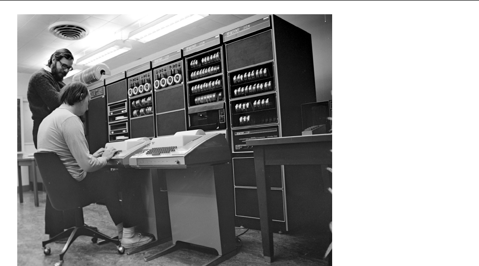
1.1 Ken Thompson and Dennis Ritchie with a PDP-11 . . . . . . . . . . 17
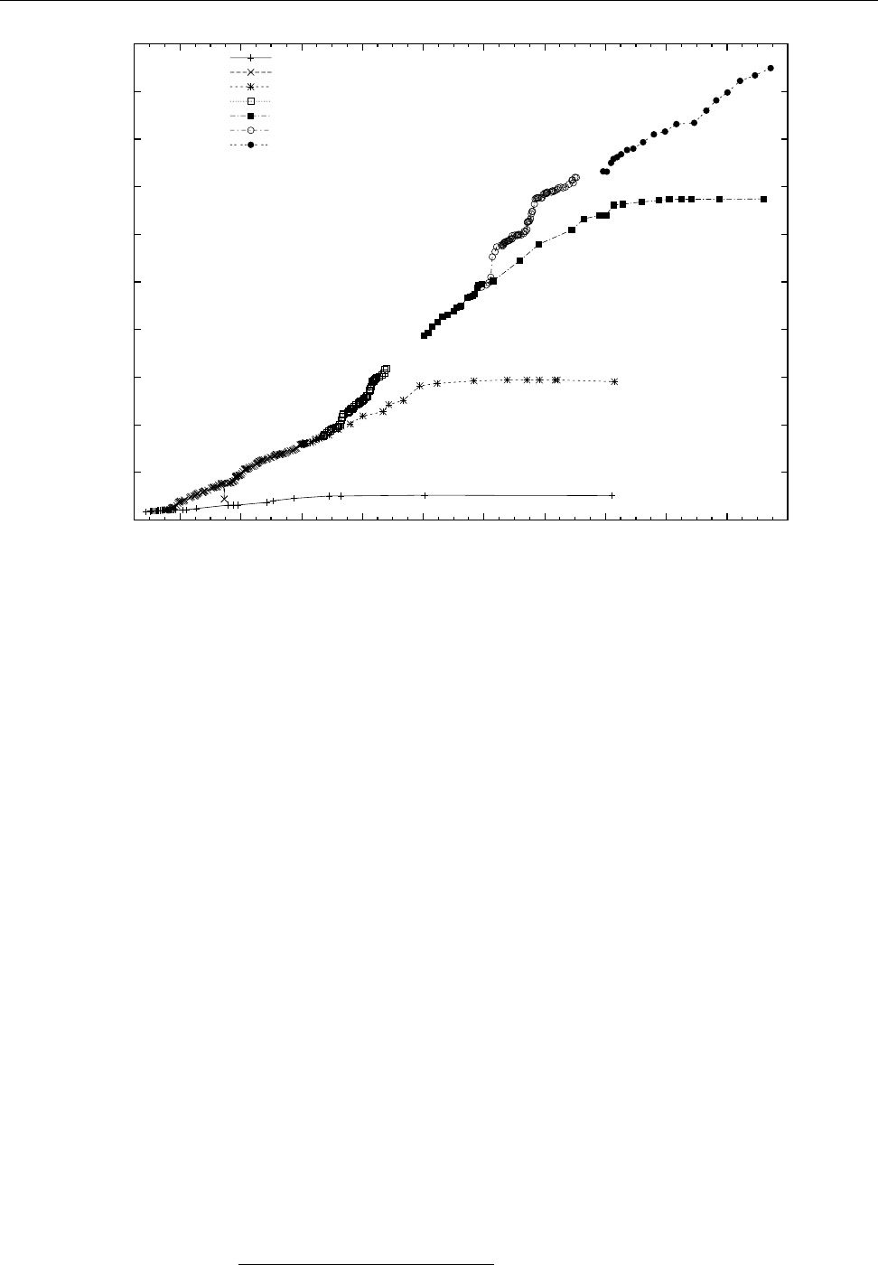
1.2 Linuxdevelopment............................ 18
1.3 Organizational structure of the Debian project . . . . . . . . . . . . 27
2.1 The login screens of some common Linux distributions . . . . . . . 32
2.2 Running programs as a dierent user in KDE . . . . . . . . . . . . . 35
4.1 Amanualpage .............................. 48
5.1
vi
’smodes ................................. 56
7.1 Standard channels on Linux . . . . . . . . . . . . . . . . . . . . . . . 88
7.2 The
tee
command............................. 93
8.1 Synchronous command execution in the shell . . . . . . . . . . . . . 133
8.2 Asynchronous command execution in the shell . . . . . . . . . . . . 133
9.1 Content of the root directory (SUSE) . . . . . . . . . . . . . . . . . . 140
13.1 The relationship between various process states . . . . . . . . . . . 193
15.1 The
/etc/fstab
le(example).......................241
17.1 A typical
/etc/inittab
le(excerpt) ...................263
17.2 Upstart conguration le for job
rsyslog
................269
18.1 A systemd unit le:
console-getty.service
................279
20.1 Example conguration for
logrotate
(Debian GNU/Linux 8.0) . . . 315
21.1 Complete log output of
journalctl
....................326
22.1 Protocols and service interfaces . . . . . . . . . . . . . . . . . . . . . 334
22.2 ISO/OSI reference model . . . . . . . . . . . . . . . . . . . . . . . . 334
22.3 Structure of an IP datagram . . . . . . . . . . . . . . . . . . . . . . . 337
22.4 Structure of an ICMP packet . . . . . . . . . . . . . . . . . . . . . . . 338
22.5 Structure of a TCP Segment . . . . . . . . . . . . . . . . . . . . . . . 339
22.6 Starting a TCP connection: The Three-Way Handshake . . . . . . . 340
22.7 Structure of a UDP datagram . . . . . . . . . . . . . . . . . . . . . . 341
22.8 The
/etc/services
le(excerpt)......................342
23.1
/etc/resolv.conf
example .........................367
23.2 The
/etc/hosts
le(SUSE).........................368
26.1 The
aptitude
program...........................411

$ echo tux
tux
$ ls
hallo.c
hallo.o
$ /bin/su -
Password:
Preface
This manual oers a concise introduction to the use and administration of Linux.
It is aimed at students who have had some experience using other operating sys-
tems and want to transition to Linux, but is also suitable for use at schools and
universities.
Topics include a thorough introduction to the Linux shell, the
vi
editor, and the
most important le management tools as well as a primer on basic administration
tasks like user, permission, and process management. We present the organisation
of the le system and the administration of hard disk storage, describe the system
boot procedure, the conguration of services, the time-based automation of tasks
and the operation of the system logging service. The course is rounded out by
an introduction to TCP/IP and the conguration and operation of Linux hosts as
network clients, with particular attention to troubleshooting, and chapters on the
Secure Shell and printing to local and network printers.
Together with the subsequent volume, Concise Linux—Advanced Topics, this
manual covers all of the objectives of the Linux Professional Institute’s LPIC-1 cer-
ticate exams and is therefore suitable for exam preparation.
This courseware package is designed to support the training course as e-
ciently as possible, by presenting the material in a dense, extensive format for
reading along, revision or preparation. The material is divided in self-contained
chapters detailing a part of the curriculum; a chapter’s goals and prerequisites chapters
goals
prerequisites
are summarized clearly at its beginning, while at the end there is a summary and
(where appropriate) pointers to additional literature or web pages with further
information.
BAdditional material or background information is marked by the “light-
bulb” icon at the beginning of a paragraph. Occasionally these paragraphs
make use of concepts that are really explained only later in the courseware,
in order to establish a broader context of the material just introduced; these
“lightbulb” paragraphs may be fully understandable only when the course-
ware package is perused for a second time after the actual course.
AParagraphs with the “caution sign” direct your attention to possible prob-
lems or issues requiring particular care. Watch out for the dangerous bends!
CMost chapters also contain exercises, which are marked with a “pencil” icon exercises
at the beginning of each paragraph. The exercises are numbered, and sam-
ple solutions for the most important ones are given at the end of the course-
ware package. Each exercise features a level of diculty in brackets. Exer-
cises marked with an exclamation point (“!”) are especially recommended.
Excerpts from conguration les, command examples and examples of com-
puter output appear in
typewriter type
. In multiline dialogs between the user and
the computer, user input is given in
bold typewriter type
in order to avoid misun-
derstandings. The “” symbol appears where part of a command’s output
had to be omitted. Occasionally, additional line breaks had to be added to make
things t; these appear as “
”. When command syntax is discussed, words enclosed in angle brack-
ets (“⟨Word⟩”) denote “variables” that can assume dierent values; material in

14 Preface
brackets (“[
-f
⟨le⟩]”) is optional. Alternatives are separated using a vertical bar
(“
-a
|
-b
”).
Important concepts are emphasized using “marginal notes” so they can be eas-Important concepts
ily located; denitions of important terms appear in bold type in the text as well
definitions as in the margin.
References to the literature and to interesting web pages appear as “[GPL91]”
in the text and are cross-referenced in detail at the end of each chapter.
We endeavour to provide courseware that is as up-to-date, complete and error-
free as possible. In spite of this, problems or inaccuracies may creep in. If you
notice something that you think could be improved, please do let us know, e.g.,
by sending e-mail to
info@tuxcademy.org
(For simplicity, please quote the title of the courseware package, the revision ID
on the back of the title page and the page number(s) in question.) Thank you very
much!
LPIC-1 Certification
These training materials are part of a recommended curriculum for LPIC-1 prepa-
ration. Refer to Appendix C for further information.

$ echo tux
tux
$ ls
hallo.c
hallo.o
$ /bin/su -
Password:
1
Introduction
Contents
1.1 What is Linux? . . . . . . . . . . . . . . . . . . . . . 16
1.2 Linux History . . . . . . . . . . . . . . . . . . . . . 16
1.3 Free Software, “Open Source” and the GPL . . . . . . . . . . 18
1.4 Linux—The Kernel . . . . . . . . . . . . . . . . . . . 21
1.5 Linux Properties . . . . . . . . . . . . . . . . . . . . 23
1.6 Linux Distributions . . . . . . . . . . . . . . . . . . . 26
Goals
• Knowing about Linux, its properties and its history
• Dierentiating between the Linux kernel and Linux distributions
• Understanding the terms “GPL”, “free software”, and “open-source soft-
ware”
Prerequisites
• Knowledge of other operating systems is useful to appreciate similarities
and dierences
grd1-einfuehrung.tex
(
be27bba8095b329b
)

16 1 Introduction
1.1 What is Linux?
Linux is an operating system. As such, it manages a computer’s basic function-
ality. Application programs build on the operating system. It forms the interface
between the hardware and application programs as well as the interface between
the hardware and people (users). Without an operating system, the computer is
unable to “understand” or process our input.
Various operating systems dier in the way they go about these tasks. The
functions and operation of Linux are inspired by the Unix operating system.
1.2 Linux History
The history of Linux is something special in the computer world. While most other
operating systems are commercial products produced by companies, Linux was
started by a university student as a hobby project. In the meantime, hundreds of
professionals and enthusiasts all over the world collaborate on it—from hobbyists
and computer science students to operating systems experts funded by major IT
corporations to do Linux development. The basis for the existence of such a project
is the Internet: Linux developers make extensive use of services like electronic
mail, distributed version control, and the World Wide Web and, through these,
have made Linux what it is today. Hence, Linux is the result of an international
collaboration across national and corporate boundaries, now as then led by Linus
Torvalds, its original author.
To explain about the background of Linux, we need to digress for a bit: Unix,
the operating system that inspired Linux, was begun in 1969. It was developed by
Ken Thompson and his colleagues at Bell Laboratories (the US telecommunicationBell Laboratories
giant AT&T’s research institute)1. Unix caught on rapidly especially at universi-
ties, because Bell Labs furnished source code and documentation at cost (due to
an anti-trust decree, AT&T was barred from selling software). Unix was, at rst,
an operating system for Digital Equipment’s PDP-11 line of minicomputers, but
was ported to other platforms during the 1970s—a reasonably feasible endeavour,
since the Unix software, including the operating system kernel, was mostly writ-
ten in Dennis Ritchie’s purpose-built Cprogramming language. Possibly mostC
important of all Unix ports was the one to the PDP-11’s successor platform, the
VAX, at the University of California in Berkeley, which came to be distributed asVAX
“BSD” (short for Berkeley Software Distribution). By and by, various computer man-
ufacturers developed dierent Unix derivatives based either on AT&T code or on
BSD (e. g., Sinix by Siemens, Xenix by Microsoft (!), SunOS by Sun Microsystems,
HP/UX by Hewlett-Packard or AIX by IBM). Even AT&T was nally allowed to
market Unix—the commercial versions System III and (later) System V. This led toSystem V
a fairly incomprehensible multitude of dierent Unix products. A real standardi-
sation never happened, but it is possible to distinguish roughly between BSD-like
and System-V-like Unix variants. The BSD and System V lines of development
were mostly unied by “System V Release 4”, which exhibited the characteristicsSVR4
of both factions.
The very rst parts of Linux were developed in 1991 by Linus Torvalds, then
a 21-year-old student in Helsinki, Finland, when he tried to fathom the capabil-
ities of his new PC’s Intel 386 processor. After a few months, the assembly lan-
guage experiments had matured into a small but workable operating system ker-
nel that could be used in a Minix system—Minix was a small Unix-like operatingMinix
system that computer science professor Andrew S. Tanenbaum of the Free Uni-
versity of Amsterdam, the Netherlands, had written for his students. Early Linux
had properties similar to a Unix system, but did not contain Unix source code.
Linus Torvalds made the program’s source code available on the Internet, and the
1The name “Unix” is a pun on “Multics”, the operating system that Ken Thompson and his col-
leagues worked on previously. Early Unix was a lot simpler than Multics. How the name came to be
spelled with an “x” is no longer known.
1.2 Linux History 17
Figure 1.1: Ken Thompson (sitting) and Dennis Ritchie (standing) with a
PDP-11, approx. 1972. (Photograph courtesy of Lucent Technologies.)
idea was eagerly taken up and developed further by many programmers. Version
0.12, issued in January, 1992, was already a stable operating system kernel. There
was—thanks to Minix—the GNU C compiler (
gcc
), the
bash
shell, the
emacs
editor
and many other GNU tools. The operating system was distributed world-wide by
anonymous FTP. The number of programmers, testers and supporters grew very
rapidly. This catalysed a rate of development only dreamed of by powerful soft-
ware companies. Within months, the tiny kernel grew into a full-blown operating
system with fairly complete (if simple) Unix functionality.
The “Linux” project is not nished even today. Linux is constantly updated
and added to by hundreds of programmers throughout the world, catering to
millions of satised private and commercial users. In fact it is inappropriate to
say that the system is developed “only” by students and other amateurs—many
contributors to the Linux kernel hold important posts in the computer industry
and are among the most professionally reputable system developers anywhere.
By now it is fair to claim that Linux is the operating system with the widest sup-
ported range of hardware ever, not just with respect to the platforms it is running
on (from PDAs to mainframes) but also with respect to driver support on, e. g., the
Intel PC platform. Linux also serves as a research and development platform for
new operating systems ideas in academia and industry; it is without doubt one of
the most innovative operating systems available today.
Exercises
C1.1 [4] Use the Internet to locate the famous (notorious?) discussion between
Andrew S. Tanenbaum and Linus Torvalds, in which Tanenbaum says that,
with something like Linux, Linus Torvalds would have failed his (Tanen-
baum’s) operating systems course. What do you think of the controversy?
C1.2 [2] Give the version number of the oldest version of the Linux source
code that you can locate.
18 1 Introduction
5MiB
10MiB
15MiB
20MiB
25MiB
30MiB
35MiB
40MiB
45MiB
50MiB
55MiB
1997 1998 1999 2000 2001 2002 2003 2004 2005 2006 2007
Linux 2.0
Linux 2.1
Linux 2.2
Linux 2.3
Linux 2.4
Linux 2.5
Linux 2.6
Figure 1.2: Linux development, measured by the size of
linux-*.tar.gz
. Each marker corresponds to a Linux
version. During the 10 years between Linux 2.0 and Linux 2.6.18, the size of the compressed Linux
source code has roughly increased tenfold.
1.3 Free Software, “Open Source” and the GPL
From the very beginning of its development, Linux was placed under the GNU
General Public License (GPL) promulgated by the Free Software Foundation (FSF).GPL
Free Software Foundation The FSF was founded by Richard M. Stallman, the author of the Emacs editor
and other important programs, with the goal of making high-quality software
“freely” available—in the sense that users are “free” to inspect it, to change itFree Software
and to redistribute it with or without changes, not necessarily in the sense that
it does not cost anything2. In particular, he was after a freely available Unix-like
operating system, hence “GNU” as a (recursive) acronym for “GNU’s Not Unix”.
The main tenet of the GPL is that software distributed under it may be changed
as well as sold at any time, but that the (possibly modied) source code must
always be passed along—thus Open Source—and that the recipient must receiveOpen Source
the same rights of modication and redistribution. Thus there is little point in
selling GPL software “per seat”, since the recipient must be allowed to copy and
install the software as often as wanted. (It is of course permissible to sell support
for the GPL software “per seat”.) New software resulting from the extension or
modication of GPL software must, as a “derived work”, also be placed under the
GPL.
Therefore, the GPL governs the distribution of software, not its use, and al-
lows the recipient to do things that he would not be allowed to do otherwise—for
example, the right to copy and distribute the software, which according to copy-
right law is the a priori prerogative of the copyright owner. Consequently, it diers
markedly from the “end user license agreements” (EULAs) of “proprietary” soft-
ware, whose owners try to take away a recipient’s rights to do various things. (For
example, some EULAs try to forbid a software recipient from talking critically—or
2The FSF says “free as in speech, not as in beer”

1.3 Free Software, “Open Source” and the GPL 19
at all—about the product in public.)
BThe GPL is a license, not a contract, since it is a one-sided grant of rights
to the recipient (albeit with certain conditions attached). The recipient of
the software does not need to “accept” the GPL explicitly. The common
EULAs, on the other hand, are contracts, since the recipient of the software
is supposed to waive certain rights in exchange for being allowed to use the
software. For this reason, EULAs must be explicitly accepted. The legal
barriers for this may be quite high—in many jurisdictions (e. g., Germany),
any EULA restrictions must be known to the buyer before the actual sale in
order to become part of the sales contract. Since the GPL does not in any
way restrict a buyer’s rights (in particular as far as use of the software is
concerned) compared to what they would have to expect when buying any
other sort of goods, these barriers do not apply to the GPL; the additional
rights that the buyer is conferred by the GPL are a kind of extra bonus.
BCurrently two versions of the GPL are in widespread use. The newer ver-
sion 3 (also called “GPLv3”) was published in July, 2007, and diers from the GPLv3
older version 2 (also “GPLv2”) by more precise language dealing with ar-
eas such as software patents, the compatibility with other free licenses, and
the introduction of restrictions on making changes to theoretically “free”
devices impossible by excluding them through special hardware (“Tivoisa-
tion”, after a Linux-based personal video recorder whose kernel is impossi-
ble to alter or exchange). In addition, GPLv3 allows its users to add further
clauses. – Within the community, the GPLv3 was not embraced with unan-
imous enthusiasm, and many projects, in particular the Linux kernel, have
intentionally stayed with the simpler GPLv2. Many other projects are made
available under the GPLv2 “or any newer version”, so you get to decide
which version of the GPL you want to follow when distributing or modify-
ing such software.
Neither should you confuse GPL software with “public-domain” software. Public Domain
The latter belongs to nobody, everybody can do with it what he wants. A GPL
program’s copyright still rests with its developer or developers, and the GPL
states very clearly what one may do with the software and what one may not.
BIt is considered good form among free software developers to place contri-
butions to a project under the same license that the project is already using,
and in fact most projects insist on this, at least for code that is supposed to
become part of the “ocial” version. Indeed, some projects insist on “copy-
right assignments”, where the code author signs the copyright over to the
project (or a suitable organisation). The advantage of this is that, legally,
only the project is responsible for the code and that licensing violations—
where only the copyright owner has legal standing—are easier to prose-
cute. A side eect that is either desired or else explicitly unwanted is that
copyright assignment makes it easier to change the license for the complete
project, as this is an act that only the copyright owner may perform.
BIn case of the Linux operating system kernel, which explicitly does not re-
quire copyright assignment, a licensing change is very dicult to impossible
in practice, since the code is a patchwork of contributions from more than
a thousand authors. The issue was discussed during the GPLv3 process,
and there was general agreement that it would be a giant project to ascer-
tain the copyright provenance of every single line of the Linux source code,
and to get the authors to agree to a license change. In any case, some Linux
developers would be violently opposed, while others are impossible to nd
or even deceased, and the code in question would have to be replaced by
something similar with a clear copyright. At least Linus Torvalds is still in
the GPLv2 camp, so the problem does not (yet) arise in practice.

20 1 Introduction
The GPL does not stipulate anything about the price of the product. It is utterlyGPL and Money
legal to give away copies of GPL programs, or to sell them for money, as long
as you provide source code or make it available upon request, and the software
recipient gets the GPL rights as well. Therefore, GPL software is not necessarily
“freeware”.
You can nd out more by reading the GPL [GPL91], which incidentally must
accompany every GPLlicensed product (including Linux).
There are other “free” software licenses which give similar rights to the soft-Other “free” licenses
ware recipient, for example the “BSD license” which lets appropriately licensed
software be included in non-free products. The GPL is considered the most thor-
ough of the free licenses in the sense that it tries to ensure that code, once pub-
lished under the GPL, remains free. Every so often, companies have tried to include
GPL code in their own non-free products. However, after being admonished by
(usually) the FSF as the copyright holder, these companies have always complied
with the GPL’s requirements. In various jurisdictions the GPL has been validated
in courts of law—for example, in the Frankfurt (Germany) Landgericht (state court),
a Linux kernel developer obtained a judgement against D-Link (a manufacturer of
network components, in this case a Linux-based NAS device) in which the latter
was sued for damages because they did not adhere to the GPL conditions when
distributing the device [GPL-Urteil06].
BWhy does the GPL work? Some companies that thought the GPL condi-
tions onerous have tried to declare or have it declared it invalid. For exam-
ple, it was called “un-American” or “unconstitutional” in the United States;
in Germany, anti-trust law was used in an attempt to prove that the GPL
amounts to price xing. The general idea seems to be that GPL-ed soft-
ware can be used by anybody if something is demonstrably wrong with the
GPL. All these attacks ignore one fact: Without the GPL, nobody except the
original author has the right to do anything with the code, since actions like
sharing (let alone selling) the code are the author’s prerogative. So if the
GPL goes away, all other interested parties are worse o than they were.
BA lawsuit where a software author sues a company that distributes his GPL
code without complying with the GPL would approximately look like this:
Judge What seems to be the problem?
Software Author Your Lordship, the defendant has distributed my soft-
ware without a license.
Judge (to the defendant’s counsel) Is that so?
At this point the defendant can say “yes”, and the lawsuit is essentially over
(except for the verdict). They can also say “no” but then it is up to them
to justify why copyright law does not apply to them. This is an uncom-
fortable dilemma and the reason why few companies actually do this to
themselves—most GPL disagreements are settled out of court.
BIf a manufacturer of proprietary software violates the GPL (e. g., by includ-
ing a few hundreds of lines of source code from a GPL project in their prod-
uct), this does not imply that all of that product’s code must now be released
under the terms of the GPL. It only implies that they have distributed GPL
code without a license. The manufacturer can solve this problem in various
ways:
• They can remove the GPL code and replace it by their own code. The
GPL then becomes irrelevant for their software.
• They can negotiate with the GPL code’s copyright holder (if he is avail-
able and willing to go along) and, for instance, agree to pay a license
fee. See also the section on multiple licenses below.
• They can release their entire program under the GPL voluntarily and
thereby comply with the GPL’s conditions (the most unlikely method).

1.4 Linux—The Kernel 21
Independentlyof this there may be damages payable for the prior violations.
The copyright status of the proprietary software, however, is not aected in
any way.
When is a software package considered “free” or “open source”? There are Freedom criteria
no denite criteria, but a widely-accepted set of rules are the Debian Free Software Debian Free Software Guidelines
Guidelines [DFSG]. The FSF summarizes its criteria as the Four Freedoms which
must hold for a free software package:
• The freedom to use the software for any purpose (freedom 0)
• The freedom to study how the software works, and to adapt it to one’s re-
quirements (freedom 1)
• The freedom to pass the software on to others, in order to help one’s neigh-
bours (freedom 2)
• The freedom to improve the software and publish the improvements, in or-
der to benet the general public (freedom 3)
Access to the source code is a prerequisite for freedoms 1 and 3. Of course, com-
mon free-software licenses such as the GPL or the BSD license conform to these
freedoms.
In addition, the owner of a software package is free to distribute it under dif- Multiple licenses
ferent licenses at the same time, e.g., the GPL and, alternatively, a “commercial”
license that frees the recipient from the GPL restrictions such as the duty to make
available the source code for modications. This way, private users and free soft-
ware authors can enjoy the use of a powerful programming library such as the
“Qt” graphics package (published by Qt Software—formerly Troll Tech—, a Nokia
subsidiary), while companies that do not want to make their own source code
available may “buy themselves freedom” from the GPL.
Exercises
C1.3 [!2] Which of the following statements concerning the GPL are true and
which are false?
1. GPL software may not be sold.
2. GPL software may not be modied by companies in order to base their
own products on it.
3. The owner of a GPL software package may distribute the program un-
der a dierent license as well.
4. The GPL is invalid, because one sees the license only after having ob-
tained the software package in question. For a license to be valid, one
must be able to inspect it and accept it before acquiring the software.
C1.4 [4] Some software licenses require that when a le from a software distri-
bution is changed, it must be renamed. Is software distributed under such a
license considered “free” according to the DFSG? Do you think this practice
makes sense?
1.4 Linux—The Kernel
Strictly speaking, the name “Linux” only applies to the operating system “kernel”,
which performs the actual operating system tasks. It takes care of elementary
functions like memory and process management and hardware control. Applica-
tion programs must call upon the kernel to, e.g., access les on disk. The kernel
validates such requests and in doing so can enforce that nobody gets to access

22 1 Introduction
other users’ private les. In addition, the kernel ensures that all processes in the
system (and hence all users) get the appropriate fraction of the available CPU time.
Of course there is not just one Linux kernel, but there are many dierent ver-Versions
sions. Until kernel version 2.6, we distinguished stable “end-user versions” and
unstable “developer versions” as follows:
• In version numbers such as 1.𝑥.𝑦or 2.𝑥.𝑦,𝑥denotes a stable version if it isstable version
even. There should be no radical changes in stable versions; mistakes should
be corrected, and every so often drivers for new hardware components or
other very important improvements are added or “back-ported” from the
development kernels.
• Versions with odd 𝑥are development versions which are unsuitable for pro-development version
ductive use. They may contain inadequately tested code and are mostly
meant for people wanting to take active part in Linux development. Since
Linux is constantly being improved, there is a constant stream of new ker-
nel versions. Changes concern mostly adaptations to new hardware or the
optimization of various subsystems, sometimes even completely new exten-
sions.
The procedure has changed in kernel 2.6: Instead of starting version 2.7 for newkernel 2.6
development after a brief stabilisation phase, Linus Torvalds and the other kernel
developers decided to keep Linux development closer to the stable versions. This
is supposed to avoid the divergence of developer and stable versions that grew to
be an enormous problem in the run-up to Linux 2.6—most notably because corpo-
rations like SUSE and Red Hat took great pains to backport interesting properties
of the developer version 2.5 to their versions of the 2.4 kernel, to an extent where,
for example, a SUSE 2.4.19 kernel contained many hundreds of dierences to the
“vanilla” 2.4.19 kernel.
The current procedure consists of “test-driving” proposed changes and en-
hancements in a new kernel version which is then declared “stable” in a shorter
timeframe. For example, after version 2.6.37 there is a development phase during
which Linus Torvalds accepts enhancements and changes for the 2.6.38 version.
Other kernel developers (or whoever else fancies it) have access to Linus’ internal
development version, which, once it looks reasonable enough, is made available
as the “release candidate” 2.6.38-rc1. This starts the stabilisation phase, whererelease candidate
this release candidate is tested by more people until it looks stable enough to be
declared the new version 2.6.38 by Linus Torvalds. Then follows the 2.6.39 devel-
opment phase and so on.
BIn parallel to Linus Torvalds’ “ocial” version, Andrew Morton maintains
a more experimental version, the so-called “
-mm
tree”. This is used to test
-mm
tree
larger and more sweeping changes until they are mature enough to be taken
into the ocial kernel by Linus.
BSome other developers maintain the “stable” kernels. As such, there might
be kernels numbered 2.6.38.1, 2.6.38.2, …, which each contain only small
and straightforward changes such as xes for grave bugs and security is-
sues. This gives Linux distributors the opportunity to rely on kernel ver-
sions maintained for longer periods of time.
On 21 July 2011, Linus Torvalds ocially released version 3.0 of the Linux ker-version 3.0
nel. This was really supposed to be version 2.6.40, but he wanted to simplify the
version numbering scheme. “Stable” kernels based on 3.0 are accordingly num-
bered 3.0.1, 3.0.2, …, and the next kernels in Linus’ development series are 3.1-rc1,
etc. leading up to 3.1 and so forth.
BLinus Torvalds insists that there was no big dierence in functionality be-
tween the 2.6.39 and 3.0 kernels—at least not more so than between any
two other consecutive kernels in the 2.6 series—, but that there was just a
renumbering. The idea of Linux’s 20th anniversary was put forward.

1.5 Linux Properties 23
You can obtain source code for “ocial” kernels on the Internet from
ftp.
kernel.org
. However, only very few Linux distributors use the original kernel
sources. Distribution kernels are usually modied more or less extensively, e. g.,
by integrating additional drivers or features that are desired by the distribution
but not part of the standard kernel. The Linux kernel used in SUSE’s Linux Enter-
prise Server 8, for example, reputedly contained approximately 800 modications
to the “vanilla” kernel source. (The changes to the Linux development process
have succeeded to an extent where the dierence is not as great today.)
Today most kernels are modular. This was not always the case; former kernels Kernel structure
consisted of a single piece of code fullling all necessary functions such as the
support of particular devices. If you wanted to add new hardware or make use
of a dierent feature like a new type of le system, you had to compile a new
kernel from sources—a very time-consuming process. To avoid this, the kernel
was endowed with the ability to integrate additional features by way of modules.
Modules are pieces of code that can be added to the kernel dynamically (at run- Modules
time) as well as removed. Today, if you want to use a new network adapter, you do
not have to compile a new kernel but merely need to load a new kernel module.
Modern Linux distributions support automatic hardware recognition, which can hardware recognition
analyze a system’s properties and locate and congure the correct driver modules.
Exercises
C1.5 [1] What is the version number of the current stable Linux kernel? The
current developer kernel? Which Linux kernel versions are still being sup-
ported?
1.5 Linux Properties
As a modern operating system kernel, Linux has a number of properties, some
of which are part of the “state of the art” (i. e., exhibited by similar systems in an
equivalent form) and some of which are unique to Linux.
• Linux supports a large selection of processors and computer architectures, processors
ranging from mobile phones (the very successful “Android” operating sys-
tem by Google, like some other similar systems, is based on Linux) through
PDAs and tablets, all sorts of new and old PC-like computers and server
systems of various kinds up to the largest mainframe computers (the vast
majority of the machines on the list of the fastest computers in the world is
running Linux).
BA huge advantage of Linux in the mobile arena is that, unlike Mi-
crosoft Windows, it supports the energy-ecient and powerful ARM
processors that most mobile devices are based upon. In 2012, Microsoft
released an ARM-based, partially Intel-compatible, version of Win-
dows 8 under the name of “Windows RT”, but that did not exactly
prove popular in the market.
• Of all currently available operating systems, Linux supports the broadest
selection of hardware. For the very newest components there may not be hardware
drivers available immediately, but on the other hand Linux still works with
devices that systems like Windows have long since left behind. Thus, your
investments in printers, scanners, graphic boards, etc. are protected opti-
mally.
• Linux supports “preemptive multitasking”, that is, several processes are multitasking
running—virtually or, on systems with more than one CPU, even actually—
in parallel. These processes cannot obstruct or damage one another; the ker-
nel ensures that every process is allotted CPU time according to its priority.

24 1 Introduction
BThis is nothing special today; when Linux was new, this was much
more remarkable.
On carefully congured systems this may approach real-time behaviour,
and in fact there are Linux variants that are being used to control industrial
plants requiring “hard” real-time ability, as in guaranteed (quick) response
times to external events.
• Linux supports several users on the same system, even at the same timeseveral users
(via the network or serially connected terminals, or even several screens,
keyboards, and mice connected to the same computer). Dierent access per-
missions may be assigned to each user.
• Linux can eortlessly be installed alongside other operating systems on the
same computer, so you can alternately start Linux or another system. By
means of “virtualisation”, a Linux system can be split into independentvirtualisation
parts that look like separate computers from the outside and can run Linux
or other operating systems. Various free or proprietary solutions are avail-
able that enable this.
• Linux uses the available hardware eciently. The dual-core CPUs commonefficiency
today are as fully utilised as the 4096 CPU cores of a SGI Altix server. Linux
does not leave working memory (RAM) unused, but uses it to cache data
from disk; conversely, available working memory is used reasonably in or-
der to cope with workloads that are much larger than the amount of RAM
inside the computer.
• Linux is source-code compatible with POSIX, System V and BSD and hencePOSIX, System V and BSD
allows the use of nearly all Unix software available in source form.
• Linux not only oers powerful “native” le systems with properties suchfile systems
as journaling, encryption, and logical volume management, but also allows
access to the le systems of various other operating systems (such as the
Microsoft Windows FAT, VFAT, and NTFS le systems), either on local disks
or across the network on remote servers. Linux itself can be used as a le
server in Linux, Unix, or Windows networks.
• The Linux TCP/IP stack is arguably among the most powerful in the indus-TCP/IP
try (which is due to the fact that a large fraction of R&D in this area is done
based on Linux). It supports IPv4 and IPv6 and all important options and
protocols.
• Linux oers powerful and elegant graphical environments for daily workgraphical environments
and, in X11, a very popular network-transparent base graphics system. Ac-
celerated 3D graphics is supported on most popular graphics cards.
• All important productivity applications are available—oce-type pro-productivity applications
grams, web browsers, programs to access electronic mail and other com-
munication media, multimedia tools, development environments for a di-
verse selection of programming languages, and so on. Most of this software
comes with the system at no cost or can be obtained eortlessly and cheaply
over the Internet. The same applies to servers for all important Internet pro-
tocols as well as entertaining games.
The exibility of Linux not only makes it possible to deploy the system on all
sorts of PC-class computers (even “old chestnuts” that do not support current
Windows can serve well in the kids’ room, as a le server, router, or mail server),
but also helps it make inroads in the “embedded systems” market, meaning com-embedded systems
plete appliances for network infrastructure or entertainment electronics. You will,
for example, nd Linux in the popular AVM FRITZ!Box and similar WLAN, DSL
or telephony devices, in various set-top boxes for digital television, in PVRs, digi-
tal cameras, copiers, and many other devices. Your author has seen the bottle bank

1.5 Linux Properties 25
in the neighbourhood supermarket boot Linux. This is very often not trumpeted
all over the place, but, in addition to the power and convenience of Linux itself
the manufacturers appreciate the fact that, unlike comparable operating systems,
Linux does not require licensing fees “per unit sold”.
Another advantage of Linux and free software is the way the community deals
with security issues. In practice, security issues are as unavoidable in free software security issues
as they are in proprietary code—at least nobody so far has written and published
a software system of interesting size that proved completely free of them in the
long run. In particular, it would be improper to claim that free software has no
security issues. The dierences are more likely to be found on a philosophical
level:
• As a rule, a vendor of proprietary software has no interest in xing security
issues in their code—they will try to cover up problems and to talk down
possible dangers for as long as they possibly can, since constantly publish-
ing “patches” means, in the best case, terrible PR (“where there is smoke,
there must be a re”; the competition, which just happens not to be in the
spotlight of scrutiny at the moment, is having a secret laugh), and, in the
worst case, great expense and lots of hassle if exploits are around that make
active use of the security holes. Besides, there is the usual danger of intro-
ducing three new errors while xing one known one, which is why xing
bugs in released software is normally not an econonomically viable propo-
sition.
• A free-software publisher does not gain anything by sitting on information
about security issues, since the source code is generally available, and ev-
erybody can nd the problems. It is, in fact, a matter of pride to x known
security issues as quickly as possible. The fact that the source code is pub-
lically available also implies that third parties nd it easy to audit code for
problems that can be repaired proactively. (A common claim is that the
availability of source code exerts a very strong attraction on crackers and
other unsavoury vermin. In fact, these low-lifes do not appear to have major
diculties identifying large numbers of security issues in proprietary sys-
tems such as Windows, whose source code is not generally available. Thus
any dierence, if it exists, must be minute indeed.)
• Especially as far as software dealing with cryptography (the encryption and
decryption of condential information) is concerned, there is a strong argu-
ment that availability of source code is an indispensable prerequisite for
trust that a program really does what it is supposed to do, i. e., that the
claimed encryption algorithm has been implemented completely and cor-
rectly. Linux does have an obvious advantage here.
Linux is used throughout the world by private and professional users— Linux in companies
companies, research establishments, universities. It plays an important role par-
ticularly as a system for web servers (Apache), mail servers (Sendmail, Postx),
le servers (NFS, Samba), print servers (LPD, CUPS), ISDN routers, X terminals,
scientic/engineering workstations etc. Linux is an essential part of industrial IT
departments. Widespread adoption of Linux in public administration, such as the Public administration
city of Munich, also serves as a signal. In addition, many reputable IT companies Support by IT companies
such as IBM, Hewlett-Packard, Dell, Oracle, Sybase, Informix, SAP, Lotus etc. are
adapting their products to Linux or selling Linux versions already. Furthermore,
ever more computers (“netbooks”)— come with Linux or are at least tested for
Linux compability by their vendors.
Exercises
C1.6 [4] Imagine you are responsible for IT in a small company (20–30 employ-
ees). In the oce there are approximately 20 desktop PCs and two servers (a
le and printer server and a mail and Web proxy server). So far everything
runs on Windows. Consider the following scenarios:

26 1 Introduction
• The le and printer server is replaced by a Linux server using Samba
(a Linux/Unix-based server for Windows clients).
• The mail and proxy server is replaced by a Linux server.
• The twenty oce desktop PCs are replaced by Linux machines.
Comment on the dierent scenarios and draw up short lists of their advan-
tages and disadvantages.
1.6 Linux Distributions
Linux in the proper sense of the word only consists of the operating system ker-
nel. To accomplish useful work, a multitude of system and application programs,
libraries, documentation etc. is necessary. “Distributions” are nothing but up-to-Distributions
date selections of these together with special programs (usually tools for instal-
lation and maintenance) provided by companies or other organisations, possibly
together with other services such as support, documentation, or updates. Distri-
butions dier mostly in the selection of software they oer, their administration
tools, extra services, and price.
“Fedora” is a freely available Linux distribution developed under the guid-Red Hat and Fedora
ance of the US-based company, Red Hat. It is the successor of the “Red Hat
Linux” distribution; Red Hat has withdrawn from the private end-user mar-
ket and aims their “Red Hat” branded distributions at corporate customers.
Red Hat was founded in 1993 and became a publically-traded corporation
in August, 1999; the rst Red Hat Linux was issued in 1994, the last (ver-
sion 9) in late April, 2004. “Red Hat Enterprise Linux” (RHEL), the current
product, appeared for the rst time in March, 2002. Fedora, as mentioned, is
a freely available oering and serves as a development platform for RHEL;
it is, in eect, the successor of Red Hat Linux. Red Hat only makes Fedora
available for download; while Red Hat Linux was sold as a “boxed set” with
CDs and manuals, Red Hat now leaves this to third-party vendors.
The SUSE company was founded 1992 under the name “Gesellschaft fürSUSE
Software und Systementwicklung” as a Unix consultancy and accordingly
abbreviated itself as “S.u.S.E.” One of its products was a version of Patrick
Volkerding’s Linux distribution, Slackware, that was adapted to the Ger-
man market. (Slackware, in turn, derived from the rst complete Linux
distribution, “Softlanding Linux System” or SLS.) S.u.S.E. Linux 1.0 came
out in 1994 and slowly dierentiated from Slackware, for example by taking
on Red Hat features such as the RPM package manager or the
/etc/ sysconfig
le. The rst version of S.u.S.E. Linux that no longer looked like Slackware
was version 4.2 of 1996. SuSE (the dots were dropped at some point) soon
gained market leadership in German-speaking Europe and published SuSE
Linux in a “box” in two avours, “Personal” and “Professional”; the latter
was markedly more expensive and contained more server software. Like
Red Hat, SuSE oered an enterprise-grade Linux distribution called “SuSE
Linux Enterprise Server” (SLES), with some derivatives like a specialised
server for mail and groupware (“SuSE Linux OpenExchange Server” or
SLOX). In addition, SuSE endeavoured to make their distribution available
on IBM’s mid-range and mainframe computers.
In November 2003, the US software company Novell announced their in-Novell takeover
tention of taking over SuSE for 210 million dollars; the deal was concluded
in January 2004. (The “U” went uppercase on that occasion). Like Red Hat,
SUSE has by now taken the step to open the “private customer” distribution
and make it freely available as “openSUSE” (earlier versions appeared for
public download only after a delay of several months). Unlike Red Hat,
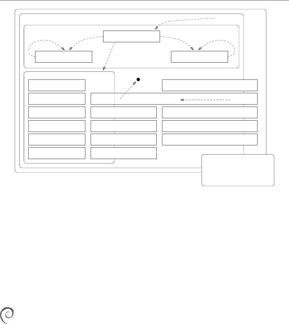
1.6 Linux Distributions 27
elect
Volunteers
Project leader
Technical committee Project secretary
Officers
appoints appoints
Release team
FTP masters
Security team
Press contacts
Administrators
etc.
Delegates
Developers
appoints/approves
Users
approve
Maintainers / porters
etc.
etc.CD team
Web/list/...masters
Policy group
Quality assurance
Documentation / i18n teams
Software in the
Public Interest
(SPI)
DAM NM team / advocates applicants
apply
Figure 1.3: Organizational structure of the Debian project. (Graphic by Martin F. Krat.)
Novell/SUSE still oers a “boxed” version containing additional propri-
etary software. Among others, SUSE still sells SLES and a corporate desktop
platform called “SUSE Linux Enterprise Desktop” (SLED).
In early 2011, Novell was acquired by Attachmate, which in turn was taken Attachmate
over by Micro Focus in 2014. Both are companies whose main eld of busi- Micro Focus
ness is traditional mainframe computers and which so far haven not distin-
guished themselves in the Linux and open-source arena. These maneuver-
ings, however, have had fairly little inuence on SUSE and its products.
A particular property of SUSE distributions is “YaST”, a comprehensive YaST
graphical administration tool.
Unlike the two big Linux distribution companies Red Hat and Novell/SUSE,
the Debian project is a collaboration of volunteers whose goal is to make Debian project
available a high-quality Linux distribution called “Debian GNU/Linux”.
The Debian project was announced on 16 August 1993 by Ian Murdock; the
name is a contraction of his rst name with that of his then-girlfriend (now
ex-wife) Debra (and is hence pronounced “debb-ian”). By now the project
includes more than 1000 volunteers.
Debian is based on three documents:
• The Debian Free Software Guidelines (DFSG) dene which software the
project considers “free”. This is important, since only DFSG-free soft-
ware can be part of the Debian GNU/Linux distribution proper. The
project also distributes non-free software, which is strictly separated
from the DFSG-free software on the distribution’s servers: The latter
is in subdirectory called
main
, the former in
non- free
. (There is an inter-
mediate area called
contrib
; this contains software that by itself would
be DFSG-free but does not work without other, non-free, components.)

28 1 Introduction
• The Social Contract describes the project’s goals.
• The Debian Constitution describes the project’s organisation.
At any given time there are at least three versions of Debian GNU/Linux:versions
New or corrected versions of packages are put into the
unstable
branch.
If, for a certain period of time, no grave errors have appeared in a pack-
age, it is copied to the
testing
branch. Every so often the content of
test-
ing
is “frozen”, tested very thoroughly, and nally released as
stable
. A
frequently-voiced criticism of Debian GNU/Linux is the long timespan be-
tween
stable
releases; many, however, consider this an advantage. The De-
bian project makes Debian GNU/Linux available for download only; media
are available from third-party vendors.
By virtue of its organisation, its freedom from commercial interests, and its
clean separation between free and non-free software, Debian GNU/Linux is
a sound basis for derivative projects. Some of the more popular ones includederivative projects
Knoppix (a “live CD” which makes it possible to test Linux on a PC without
having to install it rst), SkoleLinux (a version of Linux especially adapted to
the requirements of schools), or commercial distributions such as Xandros.
Limux, the desktop Linux variant used in the Munich city administration,
is also based on Debian GNU/Linux.
One of the most popular Debian derivatives is Ubuntu, which is oeredUbuntu
by the British company, Canonical Ltd., founded by the South African
entrepreneur Mark Shuttleworth. (“Ubuntu” is a word from the Zulu lan-
guage and roughly means “humanity towards others”.) The goal of Ubuntugoal
is to oer, based on Debian GNU/Linux, a current, capable, and easy-to-
understand Linux which is updated at regular intervals. This is facilitated,
for example, by Ubuntu being oered on only three computer architec-
tures as opposed to Debian’s ten, and by restricting itself to a subset of the
software oered by Debian GNU/Linux. Ubuntu is based on the
unstable
branch of Debian GNU/Linux and uses, for the most part, the same tools
for software distribution, but Debian and Ubuntu software packages are
not necessarily mutually compatible.
Some Ubuntu developers are also active participants in the Debian project,Ubuntu vs. Debian
which ensures a certain degree of exchange. On the other hand, not all De-
bian developers are enthusiastic about the shortcuts Ubuntu takes every so
often in the interest of pragmatism, where Debian might look for more com-
prehensive solutions even if these require more eort. In addition, Ubuntu
does not appear to feel as indebted to the idea of free software as does De-
bian; while all of Debian’s infrastructure tools (such as the bug management
system) are available as free software, this is not always the case for those
of Ubuntu.
Ubuntu not only wants to oer an attractive desktop system, but also takeUbuntu vs. SUSE/Red Hat
on the more established systems like RHEL or SLES in the server space, by
oering stable distributions with a long life cycle and good support. It is
unclear how Canonical Ltd. intends to make money in the long run; for the
time being the project is mostly supported out of Mark Shuttleworth’s pri-
vate coers, which are fairly well-lled since he sold his Internet certicate
authority, Thawte, to Verisign …
In addition to these distributions there are many more, such as Mageia or LinuxMore distributions
Mint as smaller “generally useful” distributions, various “live systems” for dif-
ferent uses from rewalls to gaming or multimedia platforms, or very compact
systems usable as routers, rewalls, or rescue systems.
Even though there is a vast number of distributions, most look fairly similar inCommonalities
daily life. This is due, on the one hand, to the fact that they use the same basic
programs—for example, the command line interpreter is nearly always
bash
. On

1.6 Bibliography 29
the other hand, there are standards that try to counter rank growth. The “Filesys-
tem Hierarchy Standard” (FHS) or “Linux Standard Base” (LSB) must be men-
tioned.
Exercises
C1.7 [2] Some Linux hardware platforms have been enumerated above. For
which of those platforms are there actual Linux distributions available?
(Hint:
http://www.distrowatch.org/
)
Summary
• Linux is a Unix-like operating system.
• The rst version of Linux was developed by Linus Torvalds and made avail-
able on the Internet as “free software”. Today, hundreds of developers all
over the world contribute to updating and extending the system.
• The GPL is the best-known “free software” license. It tries to ensure that
the recipients of software can modify and redistribute the package, and that
these “freedoms” are passed on to future recipients. GPL software may also
be sold.
• To the user, “open source” means approximately the same as “free soft-
ware”.
• There are other free licenses besides the GPL. Software may also be dis-
tributed by the copyright owner under several licenses at the same time.
• Linux is actually just the operating system kernel. We distinguish “stable”
and “development kernels”; with the former, the second part of the version
number is even and with the latter, odd. Stable kernels are meant for end
users, while development kernels are not necessarily functional, represent-
ing interim versions of Linux development.
• There are numerous Linux distributions bringing together a Linux kernel
and additional software, documentation and installation and administra-
tion tools.
Bibliography
DFSG “Debian Free Software Guidelines”.
http://www.debian.org/social_contract
GPL-Urteil06 Landgericht Frankfurt am Main. “Urteil 2-6 0 224/06”, July 2006.
http://www.jbb.de/urteil_lg_frankfurt_gpl.pdf
GPL91 Free Software Foundation, Inc. “GNU General Public License, Version 2”,
June 1991.
http://www.gnu.org/licenses/gpl.html
LR89 Don Libes, Sandy Ressler. Life with UNIX: A Guide for Everyone. Prentice-
Hall, 1989. ISBN 0-13-536657-7.
Rit84 Dennis M. Ritchie. “The Evolution of the Unix Time-sharing System”.
AT&T Bell Laboratories Technical Journal, October 1984. 63(6p2):1577–93.
http://cm.bell-labs.com/cm/cs/who/dmr/hist.html
RT74 Dennis M. Ritchie, Ken Thompson. “The Unix Time-sharing System”. Com-
munications of the ACM, July 1974. 17(7):365–73. The classical paper on Unix.
TD02 Linus Torvalds, David Diamond. Just For Fun: The Story of an Accidental
Revolutionary. HarperBusiness, 2002. ISBN 0-066-62073-2.

$ echo tux
tux
$ ls
hallo.c
hallo.o
$ /bin/su -
Password:
2
Using the Linux System
Contents
2.1 Logging In and Out . . . . . . . . . . . . . . . . . . . 32
2.2 Switching On and O . . . . . . . . . . . . . . . . . . 34
2.3 The System Administrator. . . . . . . . . . . . . . . . . 34
Goals
• Logging on and o the system
• Understanding the dierence between normal user accounts and the system
administrator’s account
Prerequisites
• Basic knowledge of using computers is helpful
grd1-bedienung.tex
(
be27bba8095b329b
)

32 2 Using the Linux System
Figure 2.1: The login screens of some common Linux distributions
2.1 Logging In and Out
The Linux system distinguishes between dierent users. Consequently, it may
be impossible to start working right after the computer has been switched on.
First you have to tell the computer who you are—you need to “log in” (or “on”).
Based on the information you provide, the system can decide what you may do
(or may not do). Of course you need access rights to the system (an “account”) –access rights
the system administrator must have entered you as a valid user and assigned you
a user name (e. g.,
joe
) and a password (e. g.,
secret
). The password is supposed to
ensure that only you can use your account; you must keep it secret and should not
make it known to anybody else. Whoever knows your user name and password
can pretend to be you on the system, read (or delete) all your les, send electronic
mail in your name and generally get up to all kinds of shenanigans.
BModern Linux distributions want to make it easy on you and allow you to
skip the login process on a computer that only you will be using anyway. If
you use such a system, you will not have to log in explicitly, but the computer
boots straight into your session. You should of course take advantage of this
only if you do not foresee that third parties have access to your computer;
refrain from this in particular on laptop computers or other mobile systems
that tend to get lost or stolen.
Logging in in a graphical enviroment These days it is common for Linux worksta-
tions to present a graphical environment (as they should), and the login process
takes place in a graphical environment as well. Your computer shows a dialog
2.1 Logging In and Out 33
that lets you enter your user name and password (Figure 2.1 shows some repre-
sentative examples.)
BDon’t wonder if you only see asterisks when you’re entering your password.
This does not mean that your computer misunderstands your input, but that
it wants to make life more dicult for people who are watching you over
your shoulder in order to nd out your password.
After you have logged in, the computer starts a graphical session for you, in
which you have convenient access to your application programs by means of
menus and icons (small pictures on the “desktop” background). Most graphical
environments for Linux support “session management” in order to restore your
session the way it was when you nished it the time before (as far as possible,
anyway). That way you do not need to remember which programs you were
running, where their windows were placed on the screen, and which les you
had been using.
Logging out in a graphical environment If you are done with your work or want
to free the computer for another user, you need to log out. This is also important
because the session manager needs to save your current session for the next time.
How logging out works in detail depends on your graphical environment, but as
a rule there is a menu item somewhere that does everything for you. If in doubt,
consult the documentation or ask your system administrator (or knowledgeable
buddy).
Logging in on a text console Unlike workstations, server systems often support
only a text console or are installed in draughty, noisy machine halls, where you
don’t want to spend more time than absolutely necessary. So you will prefer to log
into such a computer via the network. In both cases you will not see a graphical
login screen, but the computer asks you for your user name and password directly.
For example, you might simply see something like
computer login: _
(if we stipulate that the computer in question is called “
computer
”). Here you must
enter your user name and nish it o with the ↩key. The computer will con-
tinue by asking you for your password:
Password: _
Enter your password here. (This time you won’t even see asterisks—simply noth-
ing at all.) If both the user name and password were correct, the system will ac-
cept your login. It starts the command line interpreter (the shell), and you can
enter commands and invoke programs. After logging in you will be placed in
your “home directory”, where you will be able to nd your les.
BIf you use the “secure shell”, for example, to log in to another machine over
the network, the user name question is usually skipped, since unless you
specify otherwise the system will assume that your user name on the re-
mote computer will be the same as on the computer you are initiating the
session from. The details are beyond the scope of this manual; the secure
shell is discussed in detail in the Linup Front training manual Linux Admin-
istration II.
Logging out on a text console On the text console, you can log out using, for
example, the
logout
command:
$logout

34 2 Using the Linux System
Once you have logged out, on a text console the system once more displays the
start message and a login prompt for the next user. With a secure shell session,
you simply get another command prompt from your local computer.
Exercises
C2.1 [!1] Try logging in to the system. After that, log out again. (You will nd
a user name and password in your system documentation, or—in a training
centre—your instructor will tell you what to use.)
C2.2 [!2] What happens if you give (a) a non-existing user name, (b) a wrong
password? Do you notice anything unusual? What reasons could there be
for the system to behave as it does?
2.2 Switching On and Off
A Linux computer can usually be switched on by whoever is able to reach the
switch (local policy may vary). On the other hand, you should not switch o a
Linux machine on a whim—there might be data left in main memory that really
belong on disk and will be lost, or—which would be worse—the data on the hard
disk could get completely addled. Besides, other users might be logged in to the
machine via the network, be surprised by the sudden shutdown, and lose valu-
able work. For this reason, important computers are usually only “shut down”
by the system administrator. Single-user workstations, though, can usually be
shut down cleanly via the graphical desktop; depending on the system’s settings
normal user privileges may suce, or you may have to enter the administrator’s
password.
Exercises
C2.3 [2] Check whether you can shut down your system cleanly as a normal
(non-administrator) user, and if so, try it.
2.3 The System Administrator
As a normal user, your privileges on the system are limited. For example, you may
not write to certain les (most les, actually—mostly those that do not belong to
you) and not even read some les (e. g., the le containing the encrypted pass-
words of all users). However, there is a user account for system administration
which is not subject to these restrictions—the user “
root
” may read and write all
les, and do various other things normal users aren’t entitled to. Having admin-
istrator (or “root”) rights is a privilege as well as a danger—therefore you should
only log on to the system as
root
if you actually want to exercise these rights, not
just to read your mail or surf the Internet.
ASimply pretend you are Spider-Man: “With great power comes great re-
sponsibility”. Even Spider-Man wears his Spandex suit only if he must …
In particular, you should avoid logging in as
root
via the graphical user inter-
face, since all of the GUI will run with
root
’s privileges. This is a possible security
risk—GUIs like KDE contain lots of code which is not vetted as thoroughly forGUI as
root
: risky
security holes as the textual shell (which is, by comparison, relatively compact).
Normally you can use the command “
/bin/su -
” to assume
root
’sidentity (and thusAssuming
root
’s identity
root
’s privileges).
su
asks for
root
’s password and then starts a new shell, which
lets you work as if you had logged in as
root
directly. You can leave the shell again
using the
exit
command.
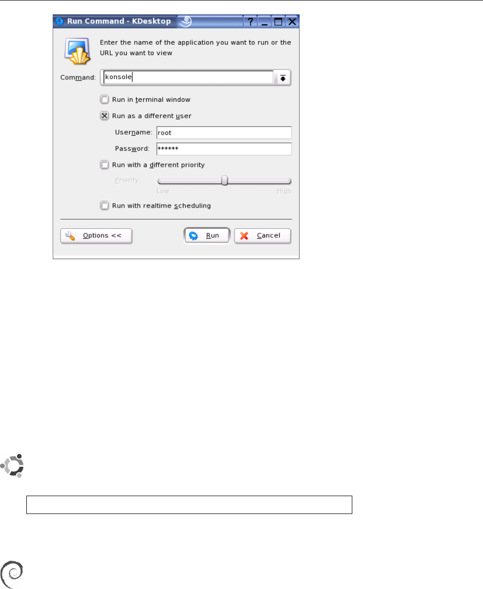
2.3 The System Administrator 35
Figure 2.2: Running programs as a dierent user in KDE
EYou should get used to invoking
su
via its full path name—“
/bin/su -
”. Oth-
erwise, a user could trick you by calling you to her computer, getting you to
enter “
su
” in one of her windows and to input the
root
password. What you
don’t realize at that moment is that the clever user wrote her own “Trojan”
su
command—which doesn’t do anything except write the password to a
le, output the “wrong password” error message and remove itself. When
you try again (gritting your teeth) you get the correct
su
—and your user
possesses the coveted administrator’s privileges …
You can usually tell that you actually have administrator privileges by look-
ing at the shell prompt—for
root
, it customarily ends with the “
#
” character. (For
root
’s shell prompt
normal users, the shell prompt usually ends in “
$
” or “
>
”).
In Ubuntu you can’t even log in as
root
by default. Instead, the system al-
lows the rst user created during installation to execute commands with
administrator privileges by prexing them with the
sudo
command. With
$sudo chown joe file.txt
for example, he could sign over the
file.txt
le to user
joe
– an operation
that is restricted to the system administrator.
Recent versions of Debian GNU/Linux oer a similar arrangement to
Ubuntu.
BIncidentally, with the KDE GUI, it is very easy to start arbitrary programs
root
and KDE
as
root
: Select “Run command” from the “KDE” menu (usually the entry
at the very left of the command panel—the “Start” menu on Windows sys-
tems), and enter a command in the dialog window. Before executing the
command, click on the “Settings” button; an area with additional settings
appears, where you can check “As dierent user” (
root
is helpfully set up as
the default value). You just have to enter the
root
password at the bottom
(Figure 2.2).

36 2 Using the Linux System
BAlternatively, you can put “
kdesu
” in front of the actual command in the dia-
kdesu
log window (or indeed any shell command line in a KDE session). This will
ask you for
root
’s password before starting the command with administrator
privileges.
Exercises
C2.4 [!1] Use the
su
command to gain administrator privileges, and change
back to your normal account.
C2.5 [5] (For programmers.) Write a convincing “Trojan”
su
program. Use it
to try and fool your system administrator.
C2.6 [2] Try to run the
id
program as
root
in a terminal session under KDE, us-
ing “Run command …”. Check the appropriate box in the extended settings
to do so.
Commands in this Chapter
exit
Quits a shell
bash
(1) 34
kdesu
Starts a program as a dierent user on KDE KDE:
help:/kdesu
35
logout
Terminates a shell session
bash
(1) 33
su
Starts a shell using a dierent user’s identity
su
(1) 34
sudo
Allows normal users to execute certain commands with administrator
privileges
sudo
(8) 35
Summary
• Before using a Linux system, you have to log in giving your user name and
password. After using the system, you have to log out again.
• Normal access rights do not apply to user
root
, who may do (essentially)
everything. These privileges should be used as sparingly as possible.
• You should not log in to the GUI as
root
but use (e. g.)
su
to assume admin-
istrator privileges if necessary.

$ echo tux
tux
$ ls
hallo.c
hallo.o
$ /bin/su -
Password:
3
Who’s Afraid Of The Big Bad
Shell?
Contents
3.1 Why?........................38
3.1.1 What Is The Shell? . . . . . . . . . . . . . . . . . 38
3.2 Commands . . . . . . . . . . . . . . . . . . . . . . 40
3.2.1 Why Commands?. . . . . . . . . . . . . . . . . . 40
3.2.2 Command Structure. . . . . . . . . . . . . . . . . 40
3.2.3 Command Types . . . . . . . . . . . . . . . . . . 41
3.2.4 Even More Rules . . . . . . . . . . . . . . . . . . 42
Goals
• Appreciating the advantages of a command-line user interface
• Knowing about common Linux shells
• Working with Bourne-Again Shell (Bash) commands
• Understanding the structure of Linux commands
Prerequisites
• Basic knowledge of using computers is helpful
grd1-shell1.tex
(
be27bba8095b329b
)

38 3 Who’s Afraid Of The Big Bad Shell?
3.1 Why?
More so than other modern operating systems, Linux (like Unix) is based on the
idea of entering textual commands via the keyboard. This may sound antediluvial
to some, especially if one is used to systems like Windows, who have been trying
for 15 years or so to brainwash their audience into thinking that graphical user
interfaces are the be-all and end-all. For many people who come to Linux from
Windows, the comparative prominence of the command line interface is at rst
a “culture shock” like that suered by a 21-century person if they suddenly got
transported to King Arthur’s court – no cellular coverage, bad table manners, and
dreadful dentists!
However, things aren’t as bad as all that. On the one hand, nowadays there
are graphical interfaces even for Linux, which are equal to what Windows or Ma-
cOS X have to oer, or in some respects even surpass these as far as convenience
and power are concerned. On the other hand, graphical interfaces and the text-
oriented command line are not mutually exclusive, but in fact complementary
(according to the philosophy “the right tool for every job”).
At the end of the day this only means that you as a budding Linux user will
do well to also get used to the text-oriented user interface, known as the “shell”.
Of course nobody wants to prevent you from using a graphical desktop for every-
thing you care to do. The shell, however, is a convenient way to perform many
extremely powerful operations that are rather dicult to express graphically. To
reject the shell is like rejecting all gears except rst in your car1. Sure, you’ll get
there eventually even in rst gear, but only comparatively slowly and with a hor-
rible amount of noise. So why not learn how to really oor it with Linux? And if
you watch closely, we’ll be able to show you another trick or two.
3.1.1 What Is The Shell?
Users cannot communicate directly with the operating system kernel. This is only
possible through programs accessing it via “system calls”. However, you must be
able to start such programs in some way. This is the task of the shell, a special user
program that (usually) reads commands from the keyboard and interprets them
(for example) as commands to be executed. Accordingly, the shell serves as an
“interface” to the computer that encloses the actual operating system like a shell
(as in “nutshell”—hence the name) and hides it from view. Of course the shell is
only one program among many that access the operating system.
BEven today’s graphical “desktops” like KDE can be considered “shells”. In-
stead of reading text commands via the keyboard, they read graphical com-
mands via the mouse—but as the text commands follow a certain “gram-
mar”, the mouse commands do just the same. For example, you select ob-
jects by clicking on them and then determine what to do with them: open-
ing, copying, deleting, …
Even the very rst Unix—end-1960s vintage—had a shell. The oldest shell to
be found outside museums today was developed in the mid-1970s for “Unix ver-
sion 7” by Stephen L. Bourne. This so-called “Bourne shell” contains most basicBourne shell
functions and was in very wide-spread use, but is very rarely seen in its original
form today. Other classic Unix shells include the C shell, created at the UniversityC shell
of California in Berkeley and (very vaguely) based on the C programming lan-
guage, and the largely Bourne-shell compatible, but functionally enhanced, KornKorn shell
shell (by David Korn, also at AT&T).
Standard on Linux systems is the Bourne-again shell,
bash
for short. It wasBourne-again shell
developed under the auspices of the Free Software Foundation’s GNU project by
Brian Fox and Chet Ramey and unies many functions of the Korn and C shells.
1This metaphor is for Europeans and other people who can manage a stick shift; our American
readers of course all use those wimpy automatic transmissions. It’s like they were all running Win-
dows.

3.1 Why? 39
BBesides the mentioned shells, there are many more. On Unix, a shell is sim- shells: normal programs
ply an application program like all others, and you need no special privi-
leges to write one—you simply need to adhere to the “rules of the game”
that govern how a shell communicates with other programs.
Shells may be invoked interactively to read user commands (normally on a “ter-
minal” of some sort). Most shells can also read commands from les containing
pre-cooked command sequences. Such les are called “shell scripts”. shell scripts
A shell performs the following steps:
1. Read a command from the terminal (or the le)
2. Validate the command
3. Run the command directly or start the corresponding program
4. Output the result to the screen (or elsewhere)
5. Continue at step 1.
In addition to this standard command loop, a shell generally contains further fea-
tures such as a programming language. This includes complex command struc- programming language
tures involving loops, conditions, and variables (usually in shell scripts, less fre-
quently in interactive use). A sophisticated method for recycling recently used
commands also makes a user’s life easier.
Shell sessions can generally be terminated using the
exit
command. This also Terminating shell sessions
applies to the shell that you obtained immediately after logging in.
Although, as we mentioned, there are several dierent shells, we shall concen-
trate here on
bash
as the standard shell on most Linux distributions. The LPI exams
also refer to
bash
exclusively.
BIf there are several shells available on the system (the usual case), you can Changing shell
use the following commands to switch between them:
sh
for the classic Bourne shell (if available—on most Linux systems,
sh
refers
to the Bourne-again shell).
bash
for the Bourne-again shell (bash).
ksh
for the Korn shell.
csh
for the C shell.
tcsh
for the “Tenex C shell”, an extended and improved version of the nor-
mal C shell. On many Linux systems, the
csh
command really refers to
tcsh
.
BIn case you cannot remember which shell you are currently running, the
“
echo $0
” command should work in any shell and output the current shell’s
name.
Exercises
C3.1 [2] How many dierent shells are installed on your system? Which ones?
(Hint: Check the le
/etc/shells
.)
C3.2 [2] Log o and on again and check the output of the “
echo $0
” command
in the login shell. Start a new shell using the “
bash
” command and enter
“
echo $0
” again. Compare the output of the two commands. Do you notice
anything unusual?

40 3 Who’s Afraid Of The Big Bad Shell?
3.2 Commands
3.2.1 Why Commands?
A computer’s operation, no matter which operating system it is running, can be
loosely described in three steps:
1. The computer waits for user input
2. The user selects a command and enters it via the keyboard or mouse
3. The computer executes the command
In a Linux system, the shell displays a “prompt”, meaning that commands can be
entered. This prompt usually consists of a user and host (computer) name, the
current directory, and a nal character:
joe@red:/home > _
In this example, user
joe
works on computer
red
in the
/home
directory.
3.2.2 Command Structure
A command is essentially a sequence of characters which is ends with a press
of the ↩key and is subsequently evaluated by the shell. Many commands are
vaguely inspired by the English language and form part of a dedicated “command
language”. Commands in this language must follow certain rules, a “syntax”, forsyntax
the shell to be able to interpret them.
To interpret a command line, the shell rst tries to divide the line into words.words
Just like in real life, words are separated by spaces. The rst word on a line is usu-First word: command
ally the actual command. All other words on the line are parameters that explainparameters
what is wanted in more detail.
ADOS and Windows users may be tripped up here by the fact that the shell
distinguishes between uppercase and lowercase letters. Linux commands
are usually spelled in lowercase letters only (exceptions prove the rule) and
not understood otherwise. See also Section 3.2.4.
BWhen dividing a command into words, one space character is as good as
many – the dierence does not matter to the shell. In fact, the shell does
not even insist on spaces; tabulator characters are also allowed, which is
however mostly of importance when reading commands from les, since
the shell will not let you enter tab character directly (not without jumping
through hoops, anyway).
BYou may even use the line terminator ( ↩) to distribute a long command
across several input lines, but you must put a “Token\” immediately in front
of it so the shell will not consider your command nished already.
A command’s parameters can be roughly divided into two types:
• Parameters starting with a dash (“
-
”) are called options. These are usually,options
er, optional—the details depend on the command in question. Figuratively
spoken they are “switches” that allow certain aspects of the command to
be switched on or o. If you want to pass several options to a command,
they can (often) be accumulated behind a single dash, i. e., the options se-
quence “
-a -l -F
” corresponds to “
-alF
”. Many programs have more options
than can be conveniently mapped to single characters, or support “long op-
tions” for readability (frequently in addition to equivalent single-character
options). Long options most often start with two dashes and cannot be ac-
cumulated: “
foo --bar --baz
”.

3.2 Commands 41
• Parameters with no leading dash are called arguments. These are often the arguments
names of les that the command should process.
The general command structure can be displayed as follows: command structure
• Command—“What to do?”
• Options—“How to do it?”
• Arguments—“What to do it with?”
Usually the options follow the command and precede the arguments. However,
not all commands insist on this—with some, arguments and options can be mixed
arbitrarily, and they behave as if all options came immediately after the command.
With others, options are taken into account only when they are encountered while
the command line is processed in sequence.
AThe command structure of current Unix systems (including Linux) has
grown organically over a period of almost 40 years and thus exhibits vari-
ous inconsistencies and small surprises. We too believe that there ought to
be a thorough clean-up, but 30 years’ worth of shell scripts are dicult to
ignore completely … Therefore be prepared to get used to little weirdnesses
every so often.
3.2.3 Command Types
In shells, there are essentially two kinds of commands:
Internal commands These commands are made available by the shell itself. The
Bourne-again shell contains approximately 30 such commands, which can
be executed very quickly. Some commands (such as
exit
or
cd
) alter the state
of the shell itself and thus cannot be provided externally.
External commands The shell does not execute these commands by itself but
launches executable les, which within the le system are usually found
in directories like
/bin
or
/usr/bin
. As a user, you can provide your own pro-
grams, which the shell will execute like all other external commands.
You can use the
type
command to nd out the type of a command. If you pass External or internal?
a command name as the argument, it outputs the type of command or the corre-
sponding le name, such as
$type echo
echo is a shell builtin
$type date
date is /bin/date
(
echo
is an interesting command which simply outputs its parameters:
$echo Thou hast it now, king, Cawdor, Glamis, all
Thou hast it now, king, Cawdor, Glamis, all
date
displays the current date and time, possibly adjusted to the current time zone
and language setup:
$date
Mon May 7 15:32:03 CEST 2012
You will nd out more about
echo
and
date
in Chapter 8.)
You can obtain help for internal Bash commands via the
help
command: help

42 3 Who’s Afraid Of The Big Bad Shell?
$help type
type: type [-afptP] name [name ...]
For each NAME, indicate how it would be interpreted if used as a
command name.
If the -t option is used, `type' outputs a single word which is one of
`alias', `keyword', `function', `builtin', `file' or `', if NAME is an
Exercises
C3.3 [2] With bash, which of the following programs are provided externally
and which are implemented within the shell itself:
alias
,
echo
,
rm
,
test
?
3.2.4 Even More Rules
As mentioned above, the shell distinguishes between uppercase and lowercase
letters when commands are input. This does not apply to commands only, but
consequentially to options and parameters (usually le names) as well.
Furthermore, you should be aware that the shell treats certain characters in the
input specially. Most importantly, the already-mentioned space character is usedspace character
to separate words on teh command line. Other characters with a special meaning
include
$&;(){}[]*?!<>"'
If you want to use any of these characters without the shell interpreting according
to its the special meaning, you need to “escape” it. You can use the backslash “
\
”“Escaping” characters
to escape a single special character or else single or double quotes (
'
…
'
,
"
…
"
) to
excape several special characters. For example:
$touch 'New File'
Due to the quotes this command applies to a single le called
New File
. Without
quotes, two les called
New
and
File
would have been involved.
BWe can’t explain all the other special characters here. Most of them will
show up elsewhere in this manual – or else check the Bash documentation.
Commands in this Chapter
bash
The “Bourne-Again-Shell”, an interactive command interpreter
bash
(1) 38, 39
csh
The “C-Shell”, an interactive command interpreter
csh
(1) 39
date
Displays the date and time
date
(1) 41
echo
Writes all its parameters to standard output, separated by spaces
bash
(1),
echo
(1) 41
help
Displays on-line help for
bash
commands
bash
(1) 41
ksh
The ”‘Korn shell”’, an interactive command interpreter
ksh
(1) 39
sh
The “Bourne shell”, an interactive command interpreter
sh
(1) 39
tcsh
The “Tenex C shell”, an interactive command interpreter
tcsh
(1) 39
type
Determines the type of command (internal, external, alias)
bash
(1) 41

3.2 Commands 43
Summary
• The shell reads user commands and executes them.
• Most shells have programming language features and support shell scripts
containing pre-cooked command sequences.
• Commands may have options and arguments. Options determine how the
command operates, and arguments determine what it operates on.
• Shells dierentiate between internal commands, which are implemented in
the shell itself, and external commands, which correspond to executable les
that are started in separate processes.

$ echo tux
tux
$ ls
hallo.c
hallo.o
$ /bin/su -
Password:
4
Getting Help
Contents
4.1 Self-Help . . . . . . . . . . . . . . . . . . . . . . . 46
4.2 The
help
Command and the
--help
Option . . . . . . . . . . . 46
4.3 The On-Line Manual . . . . . . . . . . . . . . . . . . 46
4.3.1 Overview . . . . . . . . . . . . . . . . . . . . 46
4.3.2 Structure . . . . . . . . . . . . . . . . . . . . . 47
4.3.3 Chapters . . . . . . . . . . . . . . . . . . . . . 48
4.3.4 Displaying Manual Pages . . . . . . . . . . . . . . . 48
4.4 Info Pages . . . . . . . . . . . . . . . . . . . . . . 49
4.5 HOWTOs.......................50
4.6 Further Information Sources . . . . . . . . . . . . . . . . 50
Goals
• Being able to handle manual and info pages
• Knowing about and nding HOWTOs
• Being familiar with the most important other information sources
Prerequisites
• Linux Overview
• Basic command-line Linux usage (e. g., from the previous chapters)
grd1-hilfe.tex
(
be27bba8095b329b
)

46 4 Getting Help
4.1 Self-Help
Linux is a powerful and intricate system, and powerful and intricate systems are,
as a rule, complex. Documentation is an important tool to manage this complex-
ity, and many (unfortunately not all) aspects of Linux are documented very exten-
sively. This chapter describes some methods to access this documentation.
B“Help” on Linux in many cases means “self-help”. The culture of free soft-
ware implies not unnecessarily imposing on the time and goodwill of other
people who are spending their free time in the community by asking things
that are obviously explained in the rst few paragraphs of the manual. As
a Linux user, you do well to have at least an overview of the available doc-
umentation and the ways of obtaining help in cases of emergency. If you
do your homework, you will usually experience that people will help you
out of your predicament, but any tolerance towards lazy individuals who
expect others to tie themselves in knots on their behalf, on their own time,
is not necessarily very pronounced.
BIf you would like to have somebody listen around the clock, seven days a
week, to your not-so-well-researched questions and problems, you will have
to take advantage of one of the numerous “commercial” support oerings.
These are available for all common distributions and are oered either by
the distribution vendor themselves or else by third parties. Compare the
dierent service vendors and pick one whose service level agreements and
pricing suit you.
4.2 The
help
Command and the
--help
Option
In
bash
, internal commands are described in more detail by the
help
command,Internal
bash
commands
giving the command name in question as an argument:
$help exit
exit: exit [n]
Exit the shell with a status of N.
If N is omitted, the exit status
is that of the last command executed.
$ _
BMore detailed explanations are available from the shell’s manual page and
info documentation. These information sources will be covered later in this
chapter.
Many external commands (programs) support a
--help
option instead. Most
commands display a brief listing of their parameters and syntax.
BNot every command reacts to
--help
; frequently the option is called
-h
or
-?
,
or help will be output if you specify any invalid option or otherwise illegal
command line. Unfortunately there is no universal convention.
4.3 The On-Line Manual
4.3.1 Overview
Nearly every command-line program comes with a “manual page” (or “man
page”), as do many conguration les, system calls etc. These texts are generally
installed with the software, and can be perused with the “
man
⟨name⟩” command.Command
man

4.3 The On-Line Manual 47
Table 4.1: Manual page sections
Section Content
NAME Command name and brief description
SYNOPSIS Description of the command syntax
DESCRIPTION Verbose description of the command’s eects
OPTIONS Available options
ARGUMENTS Available Arguments
FILES Auxiliary les
EXAMPLES Sample command lines
SEE ALSO Cross-references to related topics
DIAGNOSTICS Error and warning messages
COPYRIGHT Authors of the command
BUGS Known limitations of the command
Here, ⟨name⟩is the command or le name that you would like explained. “
man
bash
”, for example, produces a list of the aforementioned internal shell commands.
However, the manual pages have some disadvantages: Many of them are only
available in English; there are sets of translations for dierent languages which are
often incomplete. Besides, the explanations are frequently very complex. Every
single word can be important, which does not make the documentation accessi-
ble to beginners. In addition, especially with longer documents the structure can
be obscure. Even so, the value of this documentation cannot be underestimated.
Instead of deluging the user with a large amount of paper, the on-line manual is
always available with the system.
BMany Linux distributions pursue the philosophy that there should be a
manual page for every command that can be invoked on the command line.
This does not apply to the same extent to programs belonging to the graph-
ical desktop environments KDE and GNOME, many of which not only do
not come with a manual page at all, but which are also very badly docu-
mented even inside the graphical environment itself. The fact that many of
these programs have been contributed by volunteers is only a weak excuse.
4.3.2 Structure
The structure of the man pages loosely follows the outline given in Table 4.1, even Man page outline
though not every manual page contains every section mentioned there. In partic-
ular, the EXAMPLES are frequently given short shrift.
BThe BUGS heading is often misunderstood: Read bugs within the imple-
mentation get xed, of course; what is documented here are usually restric-
tions which follow from the approach the command takes, which are not able
to be lifted with reasonable eort, and which you as a user ought to know
about. For example, the documentation for the
grep
command points out
that various constructs in the regular expression to be located may lead to
the
grep
process using very much memory. This is a consequence of the way
grep
implements searching and not a trivial, easily xed error.
Man pages are written in a special input format which can be processed for text
display or printing by a program called
groff
. Source code for the manual pages is
stored in the
/usr/share/man
directory in subdirectories called
man
𝑛, where 𝑛is one
of the chapter numbers from Table 4.2.
BYou can integrate man pages from additional directories by setting the
MAN-
PATH
environment variable, which contains the directories which will be
searched by
man
, in order. The
manpath
command gives hints for setting up
MANPATH
.
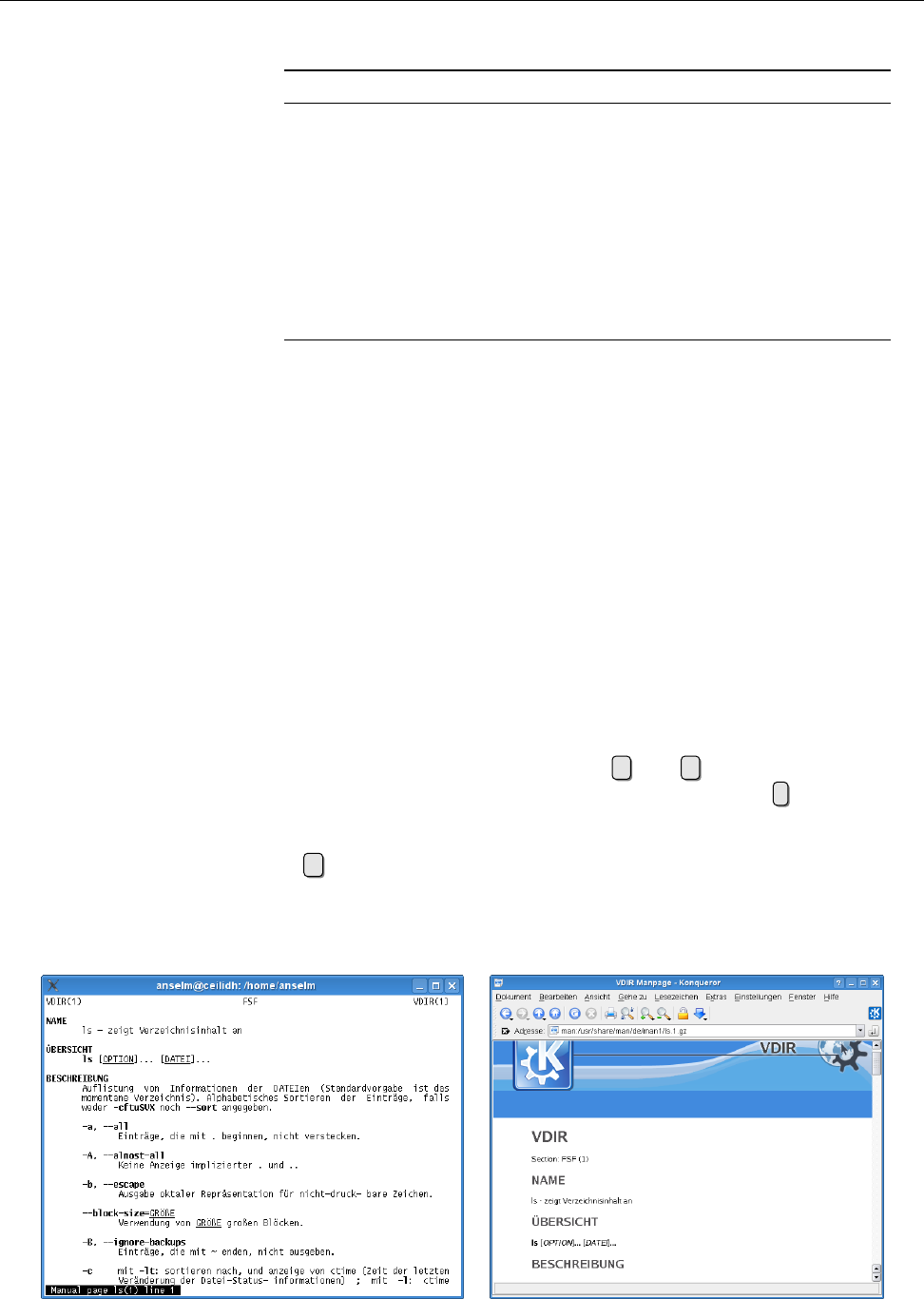
48 4 Getting Help
Table 4.2: Manual Page Topics
No. Topic
1 User commands
2 System calls
3 C language library functions
4 Device les and drivers
5 Conguration les and le formats
6 Games
7 Miscellaneous (e. g.
groff
macros, ASCII tables, …)
8 Administrator commands
9 Kernel functions
n »New« commands
4.3.3 Chapters
Every manual page belongs to a “chapter” of the conceptual “manual” (Table 4.2).Chapters
Chapters 1, 5 and 8 are most important. You can give a chapter number on the
man
command line to narrow the search. For example, “
man 1 crontab
” displays the
man page for the
crontab
command, while “
man 5 crontab
” explains the format of
crontab
les. When referring to man pages, it is customary to append the chap-
ter number in parentheses; we dierentiate accordingly between
crontab
(1), the
crontab
command manual, and
crontab
(5), the description of the le format.
With the
-a
option,
man
displays all man pages matching the given name; with-
man -a
out this option, only the rst page found (generally from chapter 1) will be dis-
played.
4.3.4 Displaying Manual Pages
The program actually used to display man pages on a text terminal is usually
less
, which will be discussed in more detail later on. At this stage it is important
to know that you can use the cursor keys ↑and ↓to navigate within a man
page. You can search for keywords inside the text by pressing /—after entering
the word and pressing the return key, the cursor jumps to the next occurrence of
the word (if it does occur at all). Once you are happy, you can quit the display
using qto return to the shell.
BUsing the KDE web browser, Konqueror, it is convenient to obtain nicely for-
matted man pages. Simply enter the URL “
man:/
⟨name⟩” (or even “
#
⟨name⟩”)
Figure 4.1: A manual page in a text terminal (left) and in Konqueror (right)

4.4 Info Pages 49
in the browser’s address line. This also works on the KDE command line
(Figure 2.2).
Before rummaging aimlessly through innumerable man pages, it is often sen-
sible to try to access general information about a topic via
apropos
. This command Keyword search
works just like “
man -k
”; both search the “NAME” sections of all man pages for
a keyword given on the command line. The output is a list of all manual pages
containing the keyword in their name or description.
A related command is
whatis
. This also searches all manual pages, but for a
whatis
command (le, …) name rather than a keyword—in other words, the part of the
“NAME” section to the left of the dash. This displays a brief description of the
desired command, system call, etc.; in particular the second part of the “NAME”
section of the manual page(s) in question.
whatis
is equivalent to “
man -f
”.
Exercises
C4.1 [!1] View the manual page for the
ls
command. Use the text-based
man
command and—if available—the Konqueror browser.
C4.2 [2] Which manual pages on your system deal (at least according to their
“NAME” sections) with processes?
C4.3 [5] (Advanced.) Use a text editor to write a manual page for a hypotheti-
cal command. Read the
man
(7) man page beforehand. Check the appearance
of the man page on the screen (using “
groff -Tascii -man
⟨le⟩
| less
”) and
as printed output (using something like “
groff -Tps -man
⟨le⟩
| gv -
”).
4.4 Info Pages
For some commands—often more complicated ones—there are so-called “info
pages” instead of (or in addition to) the more usual man pages. These are usu-
ally more extensive and based on the principles of hypertext, similar to the World hypertext
Wide Web.
BThe idea of info pages originated with the GNU project; they are therefore
most frequently found with software published by the FSF or otherwise be-
longing to the GNU project. Originally there was supposed to be only info
documentation for the “GNU system”; however, since GNU also takes on
board lots of software not created under the auspices of the FSF, and GNU
tools are being used on systems pursuing a more conservative approach,
the FSF has relented in many cases.
Analogously to man pages, info pages are displayed using the “
info
⟨command⟩”
command (the package containing the
info
program may have to be installed
explicitly). Furthermore, info pages can be viewed using the
emacs
editor or dis-
played in the KDE web browser, Konqueror, via URLs like “
info:/
⟨command⟩”.
BOne advantage of info pages is that, like man pages, they are written in
a source format which can conveniently be processed either for on-screen
display or for printing manuals using PostScript or PDF. Instead of
groff
,
the T
EX typesetting program is used to prepare output for printing.
Exercises
C4.4 [!1] Look at the info page for the
ls
program. Try the text-based
info
browser and, if available, the Konqueror browser.
C4.5 [2] Info les use a crude (?) form of hypertext, similar to HTML les on
the World Wide Web. Why aren’t info les written in HTML to begin with?

50 4 Getting Help
4.5 HOWTOs
Both manual and info pages share the problem that the user must basically know
the name of the program to use. Even searching with
apropos
is frequently nothing
but a game of chance. Besides, not every problem can be solved using one sin-
gle command. Accordingly, there is “problem-oriented” rather than “command-Problem-oriented
documentation oriented” documentation is often called for. The HOWTOs are designed to help
with this.
HOWTOs are more extensive documents that do not restrict themselves to sin-
gle commands in isolation, but try to explain complete approaches to solving
problems. For example, there is a “DSL HOWTO” detailing ways to connect a
Linux system to the Internet via DSL, or an “Astronomy HOWTO” discussing as-
tronomy software for Linux. Many HOWTOs are available in languages other
than English, even though the translations often lag behind the English-language
originals.
Most Linux distributions furnish the HOWTOs (or signicant subsets) as pack-HOWTO packages
ages to be installed locally. They end up in a distribution-specic directory—
/usr/
share/doc/howto
for SUSE distributions,
/usr/share/doc/HOWTO
for Debian GNU/Linux—
, typically either als plain text or else HTML les. Current versions of all HOWTOsHOWTOs on the Web
and other formats such as PostScript or PDF can be found on the Web on the site
of the “Linux Documentation Project” (
http://www.tldp.org
) which also oers other
Linux documentation.
4.6 Further Information Sources
You will nd additional documentation and example les for (nearly) every in-Additional information
stalled software package under
/usr/share/doc
or
/usr/share/doc/packages
(depend-
ing on your distribution). Many GUI applications (such as those from the KDE or
GNOME packages) oer “help” menus. Besides, many distributions oer special-
ized “help centers” that make it convenient to access much of the documentation
on the system.
Independently of the local system, there is a lot of documentation available on
the Internet, among other places on the WWW and in USENET archives.WWW
USENET Some of the more interesting web sites for Linux include:
http://www.tldp.org/
The “Linux Documentation Project”, which is in charge of
man pages and HOWTOs (among other things).
http://www.linux.org/
A general “portal” for Linux enthusiasts.
http://www.linuxwiki.de/
A “free-form text information database for everything
pertaining to Linux” (in German).
http://lwn.net/
Linux Weekly News—probably the best web site for Linux news of
all sorts. Besides a daily overview of the newest developments, products,
security holes, Linux advocacy in the press, etc., on Thursdays there is an
extensive on-line magazine with well-researched background reports about
the preceding week’s events. The daily news are freely available, while the
weekly issues must be paid for (various pricing levels starting at US-$ 5 per
month). One week after their rst appearance, the weekly issues are made
available for free as well.
http://freecode.com/
This site publishes announcements of new (predominantly
free) software packages, which are often available for Linux. In addition to
this there is a database allowing queries for interesting projects or software
packages.
http://www.linux-knowledge-portal.de/
A site collecting “headlines” from other in-
teresting Linux sites, including LWN and Freshmeat.

4.6 Further Information Sources 51
If there is nothing to be found on the Web or in Usenet archives, it is possible to
ask questions in mailing lists or Usenet groups. In this case you should note that
many users of these forums consider it very bad form to ask questions answered
already in the documentation or in a “FAQ” (frequently answered questions) re-
source. Try to prepare a detailed description of your problem, giving relevant
excerpts of log les, since a complex problem like yours is dicult to diagnose at
a distance (and you will surely be able to solve non-complex problems by your-
self).
BA news archive is accessible on
http://groups.google.com/
(formerly De-
jaNews)
BInteresting news groups for Linux can be found in the English-language
comp.os.linux.*
or the German-language
de.comp.os.unix.linux.*
hierarchies.
Many Unix groups are appropriate for Linux topics; a question about the
shell should be asked in a group dedicated to shell programming rather
than a Linux group, since shells are usually not specic to Linux.
BLinux-oriented mailing lists can be found, for example, at
majordomo@vger.
kernel.org
. You should send an e-mail message including “
subscribe LIST
” to
this address in order to subscribe to a list called LIST. A commented list of
all available mailing lists on the system may be found at
http://vger.kernel.
org/vger-lists.html
.
BAn established strategy for dealing with seemingly inexplicable problems is
to search for the error message in question using Google (or another search search engine
engine you trust). If you do not obtain a helpful result outright, leave out
those parts of your query that depend on your specic situation (such as
domain names that only exist on your system). The advantage is that Google
indexes not just the common web pages, but also many mailing list archives,
and chances are that you will encounter a dialogue where somebody else
had a problem very like yours.
Incidentally, the great advantage of open-source software is not only the large
amount of documentation, but also the fact that most documentation is restricted Free documentation
as little as the software itself. This facilitates collaboration between software
developers and documentation authors, and the translation of documentation
into dierent languages is easier. In fact, there is ample opportunity for non-
programmers to help with free software projects, e. g., by writing good documen-
tation. The free-software scene should try to give the same respect to documen-
tation authors that it does to programmers—a paradigm shift that has begun but
is by no means nished yet.
Commands in this Chapter
apropos
Shows all manual pages whose NAME sections contain a given keyword
apropos
(1) 49
groff
Sophisticated typesetting program
groff
(1) 47, 49
help
Displays on-line help for
bash
commands
bash
(1) 46
info
Displays GNU Info pages on a character-based terminal
info
(1) 49
less
Displays texts (such as manual pages) by page
less
(1) 48
man
Displays system manual pages
man
(1) 46
manpath
Determines the search path for system manual pages
manpath
(1) 47
whatis
Locates manual pages with a given keyword in its description
whatis
(1) 49

52 4 Getting Help
Summary
• “
help
⟨command⟩” explains internal
bash
commands. Many external com-
mands support a
--help
option.
• Most programs come with manual pages that can be perused using
man
.
apropos
searches all manual pages for keywords,
whatis
looks for manual
page names.
• For some programs, info pages are an alternative to manual pages.
• HOWTOs form a problem-oriented kind of documentation.
• There is a multitude of interesting Linux resources on the World Wide Web
and USENET.

$ echo tux
tux
$ ls
hallo.c
hallo.o
$ /bin/su -
Password:
5
The
vi
Editor
Contents
5.1 Editors........................54
5.2 The Standard—
vi
....................54
5.2.1 Overview . . . . . . . . . . . . . . . . . . . . 54
5.2.2 Basic Functions . . . . . . . . . . . . . . . . . . 55
5.2.3 Extended Commands . . . . . . . . . . . . . . . . 58
5.3 Other Editors . . . . . . . . . . . . . . . . . . . . . 60
Goals
• Becoming familiar with the
vi
editor
• Being able to create and change text les
Prerequisites
• Basic shell operation (qv. Chapter 2)
grd1-editoren-opt.tex
[
!emacs
] (
be27bba8095b329b
)

54 5 The
vi
Editor
5.1 Editors
Most operating systems oer tools to create and change text documents. Such
programs are commonly called “editors” (from the Latin “edire”, “to work on”).
Generally, text editors oer functions considerably exceeding simple text input
and character-based editing. Good editors allow users to remove, copy or insert
whole words or lines. For long les, it is helpful to be able to search for partic-
ular sequences of characters. By extension, “search and replace” commands can
make tedious tasks like “replace every
x
by a
u
” considerably easier. Many editors
contain even more powerful features for text processing.
In contrast to widespread “word processors” such as OpenOce.org Writer orDifference to word processors
Microsoft Word, text editors usually do not oer markup elements such as various
fonts (Times, Helvetica, Courier, …), type attributes (boldface, italic, underlined,
…), typographical features (justied type, …) and so on—they are predominantly
intended for the creation and editing of pure text les, where these things would
really be a nuisance.
BOf course there is nothing wrong with using a text editor to prepare input
les for typesetting systems such as
groff
or L
A
T
EX that oer all these typo-
graphic features. However, chances are you won’t see much of these in your
original input—which can really be an advantage: After all, much of the ty-
pography serves as a distraction when writing, and authors are tempted to
ddle with a document’s appearance while inputting text, rather than con-
centrating on its content.
BMost text editors today support syntax highlighting, that is, identifying cer-Syntax highlighting
tain elements of a program text (comments, variable names, reserved words,
strings) by colours or special fonts. This does look spiy, even though the
question of whether it really helps with programming has not yet been an-
swered through suitable psychological studies.
In the rest of the chapter we shall introduce the possibly most important Linux
editor,
vi
. However, we shall restrict ourselves to the most basic functionality; it
would be easy to conduct multi-day training courses for each of the two. As with
the shells, the choice of text editor is up to a user’s own personal preference.
Exercises
C5.1 [2] Which text editors are installed on your system? How can you nd
out?
5.2 The Standard—
vi
5.2.1 Overview
The only text editor that is probably part of every Linux system is called
vi
(from
“visual”, not Roman 6—usually pronounced “vee-i”). For practical reasons, this
usually doesn’t mean the original
vi
(which was part of BSD and is decidedly long
vi
: today a clone
in the tooth today), but more modern derivatives such as
vim
(from “
vi
improved”)
or
elvis
; these editors are, however, suciently close to the original
vi
, to be all
lumped together.
vi
, originally developed by Bill Joy for BSD, was one of the rst “screen-
oriented” editors in widespread use for Unix. This means that it allowed users to
use the whole screen for editing rather than let them edit just one line at a time.
This is today considered a triviality, but used to be an innovation—which is not to
say that earlier programmers were too stupid to gure it out, but that text termi-
nals allowing free access to arbitrary points on the screen (a mandatory feature for
programs like
vi
) had only just become aordable. Out of consideration for older

5.2 The Standard—
vi
55
systems using teletypes or “glass ttys” (terminals that could only add material at
the bottom of the screen),
vi
also supports a line-oriented editor under the name
of
ex
.
Even with the advanced terminals of that time, one could not rely on the
availability of keyboards with special keys for cursor positioning or advanced Keyboard restrictions
functions—today’s standard PC keyboards would have been considered luxuri-
ous, if not overloaded. This justies
vi
’s unusual concepts of operation, which
today could rightly be considered antediluvian. It cannot be taken amiss if peo-
ple reject
vi
because of this. In spite of this, having rudimentary knowledge of
vi
cannot possibly hurt, even if you select a dierent text editor for your daily
work—which you should by all means do if
vi
does not agree with you. It is not
as if there was no choice of alternatives, and we shall not get into childish games
such as “Whoever does not use
vi
is not a proper Linux user”. Today’s graphical
desktops such as KDE do contain very nice and powerful text editors.
BThere is, in fact, an editor which is even cruder than
vi
—the
ed
program.
The title “the only editor that is guaranteed to be available on any Unix sys-
tem” rightfully belongs to
ed
instead of
vi
, but
ed
as a pure line editor with
a teletype-style user interface is too basic for even hardcore Unix advocates.
(
ed
can be roughly compared with the DOS program,
EDLIN
;
ed
, however, is
vastly more powerful than the Redmond oering.) The reason why
ed
is still
available in spite of the existence of dozens of more convenient text editors
is unobvious, but very Unix-like:
ed
accepts commands on its standard input
and can therefore be used in shell scripts to change les programmatically.
ed
allows editing operations that apply to the whole le at once and is, thus,
more powerful than its colleague, the “stream editor”
sed
, which copies its
standard input to its standard output with certain modications; normally
one would use
sed
and revert to
ed
for exceptional cases, but
ed
is still useful
every so often.
5.2.2 Basic Functions
The Buffer Concept
vi
works in terms of so-called buers. If you invoke
vi
with buffers
a le name as an argument, the content of that le will be read into a buer. If no
le exists by that name, an empty buer is created.
All the modications made with the editor are only applied inside the buer.
To make these modications permanent, the buer content must be explicitly
written back to the le. If you really want to discard the modications, simply
leave
vi
without storing the buer content—the le on the storage medium will
remain unchanged.
In addition to a le name as an argument, you can pass options to
vi
as usual.
Refer to the documentation for the details.
Modes As mentioned earlier, one of the characteristics of
vi
is its unusual man-
ner of operation.
vi
supports three dierent working “modes”:
Command mode All keyboard input consists of commands that do not appear
on screen and mostly do not need to be nalized using the return key. Af-
ter invoking
vi
, you end up in this mode. Be careful: Any key press could
invoke a command.
Insert mode All keyboard input is considered text and displayed on the screen.
vi
behaves like a “modern” editor, albeit with restricted navigation and cor-
rection facilities.
Command-line mode This is used to enter long commands. These usually start
with a colon (“
:
”) and are nished using the return key.
In insert mode, nearly all navigation or correction commands are disabled, which
requires frequent alternation between insert and command modes. The fact that
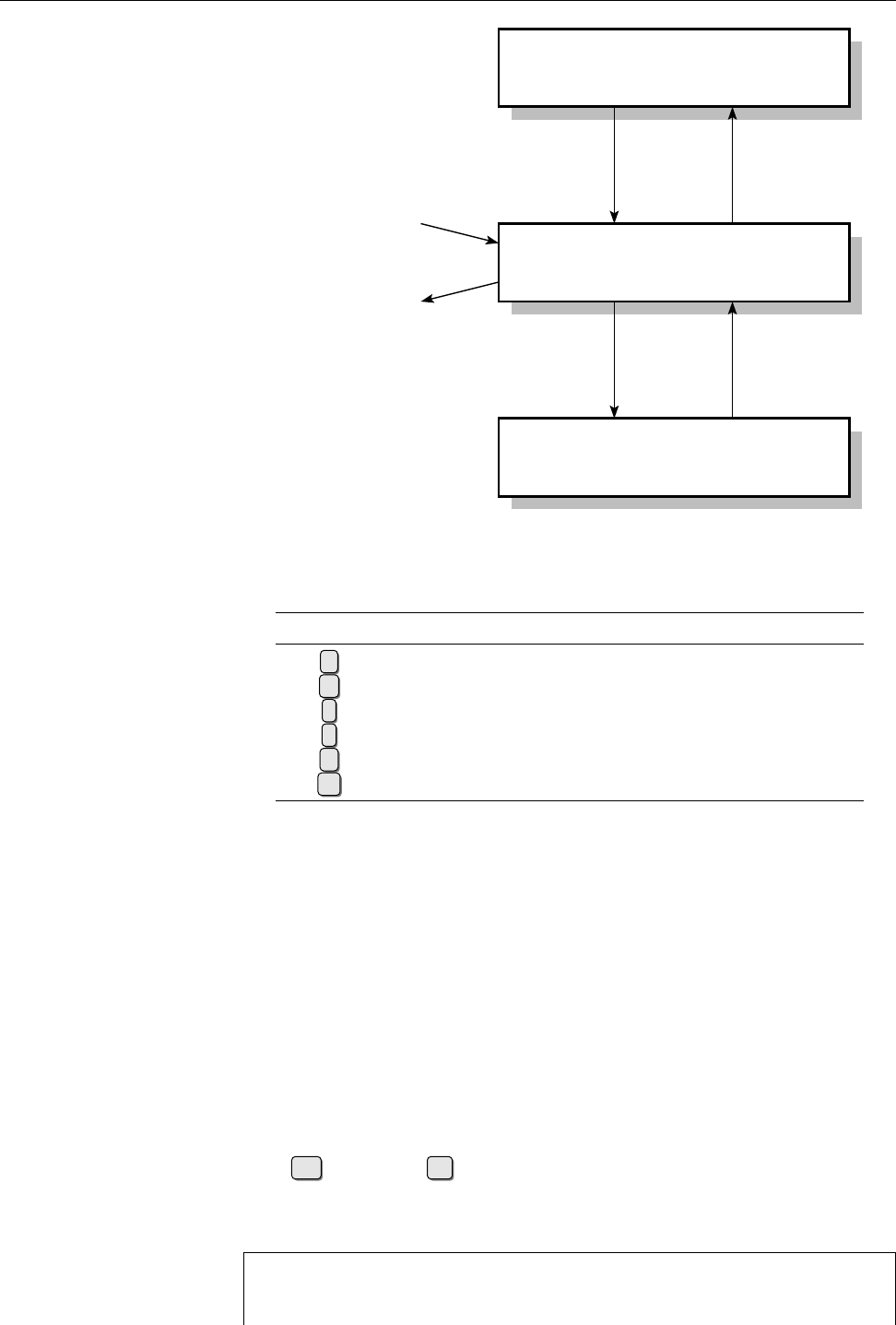
56 5 The
vi
Editor
Insert Mode
Command Mode
Command-Line Mode
[Esc] a, i, o, ...
: [Return]
vi command
ZZ, ...
Figure 5.1:
vi
’s modes
Table 5.1: Insert-mode commands for
vi
Command Result
aAppends new text after the cursor
AAppends new text at the end of the line
iInserts new text at the cursor position
IInserts new text at the beginning of the line
oInserts a new line below the line containing the cursor
OInserts a new line above the line containing the cursor
it may be dicult to nd out which mode the editor is currently in (depending on
the
vi
implementation used and its conguration) does not help to make things
easier for beginners. An overview of
vi
modes may be found in Figure 5.1.
BConsider:
vi
started when keyboards consisting only of the “letter block” of
modern keyboards were common (127 ASCII characters). There was really
no way around the scheme used in the program.
After invoking
vi
without a le name you end up in command mode. In con-command mode
trast to most other editors, direct text input is not possible. There is a cursor at the
top left corner of the screen above a column lled with tildes. The last line, also
called the “status line”, displays the current mode (maybe), the name of the le
currently being edited (if available) and the current cursor position.
BIf your version of
vi
does not display status information, try your luck with
Esc
:set showmode
↩.
Shortened by a few lines, this looks similar to Das sieht (um einige Zeilen
verkürzt) etwa so aus:
_
~
~
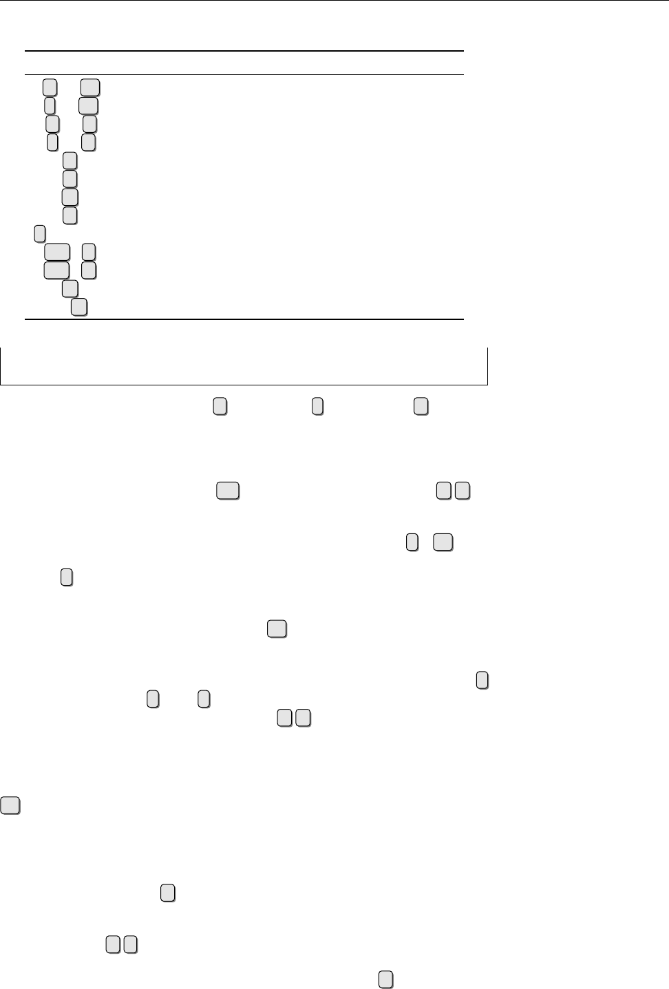
5.2 The Standard—
vi
57
Table 5.2: Cursor positioning commands in
vi
Command Cursor moves …
hor ←one character to the left
lor →one character to the right
kor ↑one character up
jor ↓one character down
0to the beginning of the line
$to the end of the line
wto the next word
bto the previous word
f⟨character⟩to the next ⟨character⟩on the line
Strg +Fto the next page (screenful)
Strg +Bto the previous page
Gto the last line of the le
⟨n⟩Gto line no. ⟨n⟩
~
Empty Buffer 0,0-1
Only after a command such as a(“append”), i(“insert”), or o(“open”)
will
vi
change into “insert mode”. The status line displays something like “
--
insert mode
INSERT --
”, and keyboard input will be accepted as text.
The possible commands to enter insert mode are listed in Table 5.1; note that
lower-case and upper-case commands are dierent. To leave insert mode and go
back to command mode, press the Esc key. In command mode, enter Z Z to
write the buer contents to disk and quit
vi
.
If you would rather discard the modications you made, you need to quit the
editor without saving the buer contents rst. Use the command :
q!
↩. The
leading colon emphasises that this is a command-line mode command.
When :is entered in command mode,
vi
changes to command-line mode. command-line mode
You can recognize this by the colon appearing in front of the cursor on the bottom
line of the screen. All further keyboard input is appended to that colon, until the
command is nished with the return key ( ↩);
vi
executes the command and
reverts to command mode. In command-line mode,
vi
processes the line-oriented
commands of its alter ego, the
ex
line editor.
There is an
ex
command to save an intermediate version of the buer called :
w
(“write”). Commands :
x
and :
wq
save the buer contents and quit the editor;
both commands are therefore identical to the Z Z command.
Movement Through the Text In insert mode, newly entered characters will be put
into the current line. The return key starts a new line. You can move about the text
using cursor keys, but you can remove characters only on the current line using
⇐—an inheritance of
vi
’s line-oriented predecessors. More extensive navigation
is only possible in command mode (Table 5.2).
Once you have directed the cursor to the proper location, you can begin cor-
recting text in command mode.
Deleting characters The dcommand is used to delete characters; it is always
followed by another character that species exactly what to delete (Table 5.3). To
make editing easier, you can prex a repeat count to each of the listed commands. repeat count
For example; the 3 x command will delete the next three characters.
If you have been too eager and deleted too much material, you can revert the
last change (or even all changes one after the other) using the u(“undo”) com- undo
58 5 The
vi
Editor
Table 5.3: Editing commands in
vi
Command Result
xDeletes the character below the cursor
XDeletes the character to the left of the cursor
r⟨char⟩Replaces the character below the cursor by ⟨char⟩
d w Deletes from cursor to end of current word
d $ Deletes from cursor to end of current line
d 0 Deletes from cursor to start of current line
d f ⟨char⟩Deletes from cursor to next occurrence of ⟨char⟩on the
current line
d d Deletes current line
d G Deletes from current line to end of text
d 1 G Deletes from current line to beginning of text
Table 5.4: Replacement commands in
vi
Command Result
c w Replace from cursor to end of current word
c $ Replace from cursor to end of current line
c 0 Replace from cursor to start of current line
c f ⟨char⟩Replace from cursor to next occurrence of ⟨char⟩on the
current line
c /
abc
Replace from cursor to next occurrence of character se-
quence
abc
mand. This is subject to appropriate conguration settings.
Replacing characters The ccommand (“change”) serves to overwrite a selectedOverwriting
part of the text. cis a “combination command” similar to d, requiring an addi-
tional specication of what to overwrite.
vi
will remove that part of the text before
changing to insert mode automatically. You can enter new material and return to
command mode using Esc . (Table 5.4).
5.2.3 Extended Commands
Cutting, Copying, and Pasting Text A frequent operation in text editing is to move
or copy existing material elsewhere in the document.
vi
oers handy combination
commands to do this, which take specications similar to those for the ccom-
mand. y(“yank”) copies material to an interim buer without changing the
original text, whereas dmoves it to the interim buer, i. e., it is removed from
its original place and only available in the interim buer afterwards. (We have
introduced this as “deletion” above.)
Of course there is a command to re-insert (or “paste”) material from an interim
buer. This is done using p(to insert after the current cursor position) or P(to
insert at the current cursor position).
A peculiarity of
vi
is that there is not just one interim buer but 26. This makes26 buffers
it easy to paste dierent texts (phrases, …) to dierent places in the le. The in-
terim buers are called “
a
” through “
z
” and can be invoked using a combination
of double quotes and buer names. The command sequence ” c y 4 w , for
instance, copies the next four words to the interim buer called
c
; the command
sequence ” g p inserts the contents of interim buer
g
after the current cursor
position.

5.2 The Standard—
vi
59
Regular-Expression Text Search Like every good editor,
vi
oers well-thought-
out search commands. “Regular expressions” make it possible to locate character
sequences that t elaborate search patterns. To start a search, enter a slash /in
command mode. This will appear on the bottom line of the terminal followed by
the cursor. Enter the search pattern and start the search using the return key.
vi
will start at the current cursor position and work towards the end of the docu-
ment. To search towards the top, the search must be started using ?instead of /
. Once
vi
has found a matching character sequence, it stops the search and places
the cursor on the rst character of the sequence. You can repeat the same search
towards the end using n(“next”) or towards the beginning using N.
Searching and Replacing Since locating character sequences is often not all that is
desired. Therefore,
vi
also allows replacing found character sequences by others.
The following
ex
command can be used:
:[⟨start line⟩
,
⟨end line⟩]
s/
⟨regexp⟩
/
⟨replacement⟩[
/q
]
The parts of the command within square brackets are optional. What do the dif-
ferent components of the command mean?
⟨Start line⟩and ⟨end line⟩determine the range of lines to be searched. Without range of lines
these, only the current line will be looked at! Instead of line numbers, you can
use a dot to specify the current line or a dollar sign to specify the last line—but do
not confuse the meanings of these characters with their meanings within regular
expressions:
:5,$s/red/blue/
replaces the rst occurrence of
red
on each line by
blue
, where the rst four lines
are not considered.
:5,$s/red/blue/g
replaces every occurrence of
red
in those lines by
blue
. (Watch out: Even
Fred Flint-
stone
will become
Fblue Flintstone
.)
BInstead of line numbers, “
.
”, and “
$
”,
vi
also allows regular expressions
within slashes as start and end markers:
:/^BEGIN/,/^END/s/red/blue/g
replaces
red
by
blue
only in lines located between a line starting with
BEGIN
After the command name sand a slash, you must enter the desired regular
expression. After another slash, ⟨replacement⟩gives a character sequence by which
the original text is to be replaced.
There is a special function for this argument: With a
&
character you can “ref- Back reference
erence back” to the text matched by the ⟨regexp⟩in every actual case. That is, “
:
s/bull/& frog
” changes every bull within the search range to a bull frog—a task
which will probably give genetic engineers trouble for some time to come.
Command-line Mode Commands So far we have described some command-line
mode (or “
ex
mode”) commands. There are several more, all of which can be
accessed from command mode by prexing them with a colon and nishing them
with the return key (Table 5.5).
Exercises
C5.2 [5] (For systems with
vim
, e. g., the SUSE distributions.) Find out how to
access the interactive
vim
tutorial and work through it.

60 5 The
vi
Editor
Table 5.5:
ex
commands in
vi
Command Result
:
w
⟨le name⟩Writes the complete buer content to the
designated le
:
w!
⟨le name⟩Writes to the le even if it is write-
protected (if possible)
:
e
⟨le name⟩Reads the designated le into the buer
:
e #
Reads the last-read le again
:
r
⟨le name⟩Inserts the content of the designated le
after the line containing the cursor
:
!
⟨shell command⟩Executes the given shell command and re-
turns to
vi
afterwards
:
r!
⟨shell command⟩Inserts the output of ⟨shell command⟩after
the line containing the cursor
:
s/
⟨regexp⟩
/
⟨replacement⟩Searches for ⟨regexp⟩and replaces by
⟨replacement⟩
:
q
Quits
vi
:
q!
Quits
vi
even if the buer contents is un-
saved
:
x
oder :e
wq
Saves the buer contents and quits
vi
5.3 Other Editors
We have already alluded to the fact that your choice of editor is just as much down
to your personal preferences and probably says as much about you as a user as
your choice of car: Do you drive a polished BMW or are you happy with a dented
Astra? Or would you rather prefer a Land Rover? As far as choice is concerned,
the editor market oers no less than the vehicle market. We have presented the
possibly most important Linux editor, but of course there are many others.
kate
on KDE and
gedit
on GNOME, for example, are straightforward and easy-to-learn
editors with a graphical user interface that are perfectly adequate for the require-
ments of a normal user. GNU Emacs, however, is an extremely powerful and cus-
tomisable editor for programmers and authors, and its extensive “ecosystem” of
extensions leaves few desires uncatered for. Do browse through the package lists
of your distribution and check whether you will nd the editor of your dreams
there.
Commands in this Chapter
ed
Primitive (but useful) line-oriented text editor
ed
(1) 55
elvis
Popular “clone” of the
vi
editor
elvis
(1) 54
ex
Powerful line-oriented text editor (really
vi
)
vi
(1) 54
sed
Stream-oriented editor, copies its input to its output making changes in
the process
sed
(1) 55
vi
Screen-oriented text editor
vi
(1) 54
vim
Popular “clone” of the
vi
editor
vim
(1) 54

5.3 Other Editors 61
Summary
• Text editors are important for changing conguration les and program-
ming. They often oer special features to make these tasks easier.
•
vi
is a traditional, very widespread and powerful text editor with an id-
iosyncratic user interface.

$ echo tux
tux
$ ls
hallo.c
hallo.o
$ /bin/su -
Password:
6
Files: Care and Feeding
Contents
6.1 File and Path Names. . . . . . . . . . . . . . . . . . . 64
6.1.1 File Names . . . . . . . . . . . . . . . . . . . . 64
6.1.2 Directories . . . . . . . . . . . . . . . . . . . . 65
6.1.3 Absolute and Relative Path Names . . . . . . . . . . . 66
6.2 Directory Commands . . . . . . . . . . . . . . . . . . 67
6.2.1 The Current Directory:
cd
& Co. . . . . . . . . . . . . 67
6.2.2 Listing Files and Directories—
ls
............68
6.2.3 Creating and Deleting Directories:
mkdir
and
rmdir
. . . . . . 69
6.3 File Search Patterns . . . . . . . . . . . . . . . . . . . 70
6.3.1 Simple Search Patterns . . . . . . . . . . . . . . . . 70
6.3.2 Character Classes. . . . . . . . . . . . . . . . . . 72
6.3.3 Braces . . . . . . . . . . . . . . . . . . . . . . 73
6.4 Handling Files . . . . . . . . . . . . . . . . . . . . . 74
6.4.1 Copying, Moving and Deleting—
cp
and Friends. . . . . . . 74
6.4.2 Linking Files—
ln
and
ln -s
..............76
6.4.3 Displaying File Content—
more
and
less
..........80
6.4.4 Searching Files—
find
................81
6.4.5 Finding Files Quickly—
locate
and
slocate
.........84
Goals
• Being familiar with Linux conventions concerning le and directory names
• Knowing the most important commands to work with les and directories
• Being able to use shell lename search patterns
Prerequisites
• Using a shell (qv. Chapter 2)
• Use of a text editor (qv. Chapter 5)
grd1-dateien.tex
(
be27bba8095b329b
)

64 6 Files: Care and Feeding
6.1 File and Path Names
6.1.1 File Names
One of the most important services of an operating system like Linux consists
of storing data on permanent storage media like hard disks or USB keys and re-
trieving them later. To make this bearable for humans, similar data are usually
collected into “les” that are stored on the medium under a name.files
BEven if this seems trivial to you, it is by no means a given. In former times,
some operating systems made it necessary to know abominations like track
numbers on a disk in order to retrieve one’s data.
Thus, before we can explain to you how to handle les, we need to explain to
you how Linux names les.
In Linux le names, you are essentially allowed to use any character that yourAllowed characters
computer can display (and then some). However, since some of the characters
have a special meaning, we would recommend against their use in le names.
Only two characters are completely disallowed, the slash and the zero byte (the
character with ASCII value 0). Other characters like spaces, umlauts, or dollar
signs may be used freely, but must usually be escaped on the command line by
means of a backslash or quotes in order to avoid misinterpretations by the shell.
AAn easy trap for beginners to fall into is the fact that Linux distinguishes
uppercase and lowercase letters in le names. Unlike Windows, where up-Letter case
percase and lowercase letters in le names are displayed but treated the
same, Linux considers
x-files
and
X-Files
two dierent le names.
Under Linux, le names may be “quite long”—there is no denite upper
bound, since the maximum depends on the “le system”, which is to say the
specic way bytes are arranged on the medium (there are several methods on
Linux). A typical upper limit is 255 characters—but since such a name would
take somewhat more than three lines on a standard text terminal this shouldn’t
really cramp your style.
A further dierence from DOS and Windows computers is that Linux does not
use suxes to characterise a le’s “type”. Hence, the dot is a completely ordi-suffixes
nary character within a le name. You are free to store a text as
mumble.txt
, but
mumble
would be just as acceptable in principle. This should of course not turn you
o using suxes completely—you do after all make it easier to identify the le
content.
BSome programs insist on their input les having specic suxes. The C
compiler,
gcc
, for example, considers les with names ending in “
.c
” C
source code, those ending in “
.s
” assembly language source code, and
those ending in “
.o
” precompiled object les.
You may freely use umlauts and other special characters in le names. How-special characters
ever, if les are to be used on other systems it is best to stay away from special
characters in le names, as it is not guaranteed that they will show up as the same
characters elsewhere.
AWhat happens to special characters also depends on your locale settings,locale settings
since there is no general standard for representing characters exceeding the
ASCII character set (128 characters covering mostly the English language,
digits and the most common special characters). Widely used encodings
are, for example, ISO 8859-1 and ISO 8859-15 (popularly know as ISO-Latin-
1 and ISO-Latin-9, respectively … don’t ask) as well as ISO 10646, casually
and not quite correctly called “Unicod” and usually encoded as “UTF-8”.
File names you created while encoding 𝑋was active may look completely
dierent when you look at the directory while encoding 𝑌is in force. The
whole topic is nothing you want to think about during meals.

6.1 File and Path Names 65
AShould you ever nd yourself facing a pile of les whose names are encoded
according to the wrong character set, the
convmv
program, which can con-
convmv
vert le names between various character encodings, may be able to help
you. (You will probably have to install it yourself since it is not part of
the standard installation of most distributions.) However, you should re-
ally get down to this only after working through the rest of this chapter, as
we haven’t even explained the regular
mv
yet …
All characters from the following set may be used freely in le names: Portable file names
ABCDEFGHIJKLMNOPQRSTUVWXYZ
abcdefghijklmnopqrstuvwxyz
0123456789+-._
However, you should pay attention to the following hints:
• To allow moving les between Linux and older Unix systems, the length of
a le name should be at most 14 characters. (Make that “ancient”, really.)
• File names should always start with one of the letters or a digit; the other
four characters can be used without problems only inside a le name.
These conventions are easiest to understand by looking at some examples. Allow-
able le names would be, for instance:
X-files
foo.txt.bak
50.something
7_of_9
On the contrary, problems would be possible (if not likely or even assured) with:
-10°F
Starts with ‘‘
-
’’, includes special character
.profile
Will be hidden
3/4-metre
Contains illegal character
Smörrebröd
Contains umlauts
As another peculiarity, le names starting with a dot (“
.
”) will be skipped in Hidden files
some places, for example when the les within a directory are listed—les with
such names are considered “hidden”. This feature is often used for les contain-
ing settings for programs and which should not distract users from more impor-
tant les in directory listings.
BFor DOS and Windows experts: These systems allow “hiding” les by
means of a “le attribute” which can be set independently of the le’s
name. Linux and Unix do not support such a thing.
6.1.2 Directories
Since potentially many users may work on the same Linux system, it would be
problematic if each le name could occur just once. It would be dicult to make
clear to user Joe that he cannot create a le called
letter.txt
since user Sue already
has a le by that name. In addition, there must be a (convenient) way of ensuring
that Joe cannot read all of Sue’s les and the other way round.
For this reason, Linux supports the idea of hierarchical “directories” which are
used to group les. File names do not need to be unique within the whole system,
but only within the same directory. This means in particular that the system can
assign dierent directories to Joe and Sue, and that within those they may call
their les whatever they please without having to worry about each other’s les.

66 6 Files: Care and Feeding
In addition, we can forbid Joe from accessing Sue’s directory (and vice versa) and
no longer need to worry about the individual les within them.
On Linux, directories are simply les, even though you cannot access them
using the same methods you would use for “plain” les. However, this implies
that the rules we discussed for le names (see the previous section) also apply to
the names of directories. You merely need to learn that the slash (“
/
”) serves toslash
separate le names from directory names and directory names from one another.
joe/letter.txt
would be the le
letter.txt
in the directory
joe
.
Directories may contain other directories (this is the term “hierarchical” we
mentioned earlier), which results in a tree-like structure (inventively called a “di-directory tree
rectory tree”). A Linux system has a special directory which forms the root of the
tree and is therefore called the “root directory”. Its name is “
/
” (slash).
BIn spite of its name, the root directory has nothing to do with the system
administrator,
root
. It’s just that their names are similar.
BThe slash does double duty here—it serves both as the name of the root
directory and as the separator between other directory names. We’ll come
back to this presently.
The basic installation of common Linux distributions usually contains tens of
thousands of les in a directory hierarchy that is mostly structured according to
certain conventions. We shall tell you more about this directory hierarchy in Chap-
ter 9.
6.1.3 Absolute and Relative Path Names
Every le in a Linux system is described by a name which is constructed by start-
ing at the root directory and mentioning every directory down along the path to
the one containing the le, followed by the name of the le itself. For example,
/home/joe/letter.txt
names the le
letter.txt
, which is located within the
joe
direc-
tory, which in turn is located within the
home
directory, which in turn is a direct
descendant of the root directory. A name that starts with the root directory is
called an “absolute path name”—we talk about “path names” since the name de-absolute path name
scribes a “path” through the directory tree, which may contain directory and le
names (i. e., it is a collective term).
Each process within a Linux system has a “current directory” (often also called
“working directory”). File names are searched within this directory;
letter.txt
is thus a convenient abbreviation for “the le called
letter.txt
in the current di-
rectory”, and
sue/letter.txt
stands for “the le
letter.txt
within the
sue
directory
within the current directory”. Such names, which start from the current directory,
are called “relative path names”.relative path names
BIt is trivial to tell absolute from relative path names: A path name starting
with a “
/
” is absolute; all others are relative.
BThe current directory is “inherited” between parent and child processes. So
if you start a new shell (or any program) from a shell, that new shell uses
the same current directory as the shell you used to start it. In your new
shell, you can change into another directory using the
cd
command, but the
current directory of the old shell does not change—if you leave the new
shell, you are back to the (unchanged) current directory of the old shell.
There are two convenient shortcuts in relative path names (and even absoluteshortcuts
ones): The name “
..
” always refers to the directory above the directory in question
in the directory tree—for example, in the case of
/home/joe
,
/home
. This frequently
allows you to refer conveniently to les in a “side branch” of the directory tree
as viewed from the current directory, without having to resort to absolute path
names. Assume
/home/joe
has the subdirectories
letters
and
novels
. With
letters
as the current directory, you could refer to the
ivanhoe.txt
le within the
novels

6.2 Directory Commands 67
directory by means of the relative path name
../novels/ivanhoe.txt
, without having
to use the unwieldy absolute path name
/home/joe/novels/ivanhoe.txt
.
The second shortcut does not make quite as obvious sense: the “
.
” name within
a directory always stands for the directory itself. It is not immediately clear why
one would need a method to refer to a directory which one has already reached,
but there are situations where this comes in quite handy. For example, you may
know (or could look up in Chapter 8) that the shell searches program les for
external commands in the directories listed in the environment variable
PATH
. If
you, as a software developer, want to invoke a program, let’s call it
prog
, which (a)
resides in a le within the current directory, and (b) this directory is not listed in
PATH
(always a good idea for security reasons), you can still get the shell to start
your le as a program by saying
$./prog
without having to enter an absolute path name.
BAs a Linux user you have a “home directory” which you enter immediately
after logging in to the system. The system administrator determines that
directory’s name when they create your user account, but it is usually called
the same as your user name and located below
/home
—something like
/home/
joe
for the user
joe
.
6.2 Directory Commands
6.2.1 The Current Directory:
cd
& Co.
You can use the
cd
shell command to change the current directory: Simply give Changing directory
the desired directory as a parameter:
$cd letters
Change to the
letters
directory
$cd ..
Change to the directory above
If you do not give a parameter you will end up in your home directory:
$cd
$pwd
/home/joe
You can output the absolute path name of the current directory using the
pwd
current directory
(“print working directory”) command.
Possibly you can also see the current directory as part of your prompt: Depend- prompt
ing on your system settings there might be something like
joe@red:~/letters> _
where
~/letters
is short for
/home/joe/letters
; the tilde (“
~
”) stands for the current
user’s home directory.
BThe “
cd -
” command changes to the directory that used to be current before
the most recent
cd
command. This makes it convenient to alternate between
two directories.
Exercises
C6.1 [2] In the shell, is
cd
an internal or an external command? Why?
C6.2 [3] Read about the
pushd
,
popd
, and
dirs
commands in the
bash
man page.
Convince yourself that these commands work as described there.

68 6 Files: Care and Feeding
Table 6.1: Some le type designations in
ls
File type Colour Sux (
ls -F
) Type letter (
ls -l
)
plain le black none
-
executable le green
* -
directory blue
/ d
link cyan
@ l
Table 6.2: Some
ls
options
Option Result
-a
or
--all
Displays hidden les as well
-i
or
--inode
Displays the unique le number (inode number)
-l
or
--format=long
Displays extra information
-o
or
--no-color
Omits colour-coding the output
-p
or
-F
Marks le type by adding a special character
-r
or
--reverse
Reverses sort order
-R
or
--recursive
Recurses into subdirectories (DOS:
DIR/S
)
-S
or
--sort=size
Sorts les by size (longest rst)
-t
or
--sort=time
Sorts le by modication time (newest rst)
-X
or
--sort=extension
Sorts le by extension (“le type”)
6.2.2 Listing Files and Directories—
ls
To nd one’s way around the directory tree, it is important to be able to nd out
which les and directories are located within a directory. The
ls
(“list”) command
does this.
Without options, this information is output as a multi-column table sorted byTabular format
le name. With colour screens being the norm rather than the exception today, it
has become customary to display the names of les of dierent types in various
colours. (We have not talked about le types yet; this topic will be mentioned in
Chapter 9.)
BThankfully, by now most distributions have agreed about the colours to use.
Table 6.1 shows the most common assignment.
BOn monochrome monitors—which can still be found—, the options
-F
or
-p
recommend themselves. These will cause special characters to be appended
to the le names according to the le’s type. A subset of these characters is
given in Table 6.1.
You can display hidden les (whose names begin with a dot) by giving the
-a
Hidden files
(“all”) option. Another very useful option is
-l
(a lowercase “L”, for “long”, rather
than the digit “1”). This displays not only the le names, but also some additionalAdditional information
information about each le.
BSome Linux distributions pre-set abbreviations for some combinations of
helpful options; the SUSE distributions, for example, use a simple
l
as an
abbreviation of “
ls -alF
”. “
ll
” and “
la
” are also abbreviations for
ls
variants.
Here is an example of
ls
without and with
-l
:
$ls
file.txt
file2.dat
$ls -l

6.2 Directory Commands 69
-rw-r--r-- 1 joe users 4711 Oct 4 11:11 file.txt
-rw-r--r-- 1 joe users 333 Oct 2 13:21 file2.dat
In the rst case, all visible (non-hidden) les in the directory are listed; the second
case adds the extra information.
The dierent parts of the long format have the following meanings: The rst Long format
character gives the le type (see Chapter 9); plain les have “
-
”, directories “
d
”
and so on (“type character” in Table 6.1).
The next nine characters show the access permissions. Next there are a refer-
ence counter, the owner of the le (
joe
here), and the le’s group (
users
). After the
size of le in bytes, you can see the date and time of the last modication of the
le’s content. On the very right there is the le’s name.
ADepending on the language you are using, the date and time columns in par-
ticular may look completely dierent than the ones in our example (which
we generated using the minimal language environment “
C
”). This is usu-
ally not a problem in interactive use, but may prove a major nuisance if you
try to take the output of “
ls -l
” apart in a shell script. (Without wanting to
anticipate the training manual Advanced Linux, we recommend setting the
language environment to a dened value in shell scripts.)
BIf you want to see the extra information for a directory (such as
/tmp
), “
ls -l
/tmp
” doesn’t really help, because
ls
will list the data for all the les within
/tmp
. Use the
-d
option to suppress this and obtain the information about
/tmp
itself.
ls
supports many more options than the ones mentioned here; a few of the
more important ones are shown in Table 6.2.
In the LPI exams, Linux Essentials and LPI-101, nobody expects you to know
all 57 varieties of
ls
options by heart. However, you may wish to commit the
most import half dozen or so—the content of Table 6.2, approximately—to
memory.
Exercises
C6.3 [1] Which les does the
/boot
directory contain? Does the directory have
subdirectories and, if so, which ones?
C6.4 [2] Explain the dierence between
ls
with a le name argument and
ls
with a directory name argument.
C6.5 [2] How do you tell
ls
to display information about a directory rather
than the les in that directory, if a directory name is passed to the program?
(Hint: Documentation.)
6.2.3 Creating and Deleting Directories:
mkdir
and
rmdir
To keep your own les in good order, it makes sense to create new directories. You
can keep les in these “folders” according to their subject matter (for example).
Of course, for further structuring, you can create further directories within such
directories—your ambition will not be curbed by arbitrary limits.
To create new directories, the
mkdir
command is available. It requires one or Creating directories
more directory names as arguments, otherwise you will only obtain an error mes-
sage instead of a new directory. To create nested directories in a single step, you
can use the
-p
option, otherwise the command assumes that all directories in a
path name except the last one already exist. For example:

70 6 Files: Care and Feeding
$mkdir pictures/holiday
mkdir: cannot create directory `pictures/holiday': No such file
or directory
$mkdir -p pictures/holiday
$cd pictures
$ls -F
holiday/
Sometimes a directory is no longer required. To reduce clutter, you can removeRemoving directories
it using the
rmdir
(“remove directory”) command.
As with
mkdir
, at least one path name of a directory to be deleted must be given.
In addition, the directories in question must be empty, i. e., they may not contain
entries for les, subdirectories, etc. Again, only the last directory in every name
will be removed:
$rmdir pictures/holiday
$ls -F
pictures/
With the
-p
option, all empty subdirectories mentioned in a name can be removed
in one step, beginning with the one on the very right.
$mkdir -p pictures/holiday/summer
$rmdir pictures/holiday/summer
$ls -F pictures
pictures/holiday/
$rmdir -p pictures/holiday
$ls -F pictures
ls: pictures: No such file or directory
Exercises
C6.6 [!2] In your home directory, create a directory
grd1-test
with subdirecto-
ries
dir1
,
dir2
, and
dir3
. Change into directory
grd1-test/dir1
and create (e. g.,
using a text editor) a le called
hello
containing “
hello
”. In
grd1-test/dir2
,
create a le
howdy
containing “
howdy
”. Check that these les do exist. Delete
the subdirectory
dir3
using
rmdir
. Next, attempt to remove the subdirectory
dir2
using
rmdir
. What happens, and why?
6.3 File Search Patterns
6.3.1 Simple Search Patterns
You will often want to apply a command to several les at the same time. For
example, if you want to copy all les whose names start with “
p
” and end with
“
.c
” from the
prog1
directory to the
prog2
directory, it would be quite tedious to
have to name every single le explictly—at least if you need to deal with more
than a couple of les! It is much more convenient to use the shell’s search patterns.search patterns
If you specify a parameter containing an asterisk on the shell command line—
asterisk like
prog1/p*.c

6.3 File Search Patterns 71
—the shell replaces this parameter in the actual program invocation by a sorted list
of all le names that “match” the parameter. “Match” means that in the actual le
name there may be an arbitrary-length sequence of arbitrary characters in place
of the asterisk. For example, names like
prog1/p1.c
prog1/polly.c
prog1/pop-rock.c
prog1/p.c
are eligible (note in particular the last name in the example—“arbitrary length”
does include “length zero”!). The only character the asterisk will not match is—
can you guess it?—the slash; it is usually better to restrict a search pattern like the
asterisk to the current directory.
BYou can test these search patterns conveniently using
echo
. The
$echo prog1/p*.c
command will output the matching le names without any obligation or
consequence of any kind.
BIf you really want to apply a command to all les in the directory tree starting
with a particular directory, there are ways to do that, too. We will discuss
this in Section 6.4.4.
The search pattern “
*
” describes “all les in the current directory”—excepting All files
hidden les whose name starts with a dot. To avert possibly inconvenient sur-
prises, search patterns diligently ignore hidden les unless you explicitly ask for
them to be included by means of something like “
.*
”.
AYou may have encountered the asterisk at the command line of operating
systems like DOS or Windows1and may be used to specifying the “
*.*
”
pattern to refer to all les in a directory. On Linux, this is not correct—the
“
*.*
” pattern matches “all les whose name contains a dot”, but the dot isn’t
mandatory. The Linux equivalent, as we said, is “
*
”.
A question mark as a search pattern stands for exactly one arbitrary character question mark
(again excluding the slash). A pattern like
p?.c
thus matches the names
p1.c
pa.c
p-.c
p..c
(among others). Note that there must be one character—the “nothing” option
does not exist here.
You should take particular care to remember a very important fact: The expan-
sion of search pattern is the responsibility of the shell! The commands that you ex-
ecute usually know nothing about search patterns and don’t care about them,
either. All they get to see are lists of path names, but not where they come
from—i. e., whether they have been typed in directly or resulted from the ex-
pansion of search patterns.
1You’re probably too young for CP/M.

72 6 Files: Care and Feeding
BIncidentally, nobody says that the results of search patterns always need to
be interpreted as path names. For example, if a directory contains a le
called “
- l
”, a “
ls *
” in that directory will yield an interesting and perhaps
surprising result (see Exercise 6.9).
BWhat happens if the shell cannot nd a le whose name matches the search
pattern? In this case the command in question is passed the search pattern
as such; what it makes of that is its own aair. Typically such search patterns
are interpreted as le names, but the “le” in question is not found and an
error message is issued. However, there are commands that can do useful
things with search patterns that you pass them—with them, the challenge
is really to ensure that the shell invoking the command does not try to cut
in with its own expansion. (Cue: quotes)
6.3.2 Character Classes
A somewhat more precise specication of the matching characters in a search pat-
tern is oered by “character classes”: In a search pattern of the form
prog[123].c
the square brackets match exactly those characters that are enumerated within
them (no others). The pattern in the example therefore matches
prog1.c
prog2.c
prog3.c
but not
prog.c
There needs to be exactly one character
prog4.c 4
was not enumerated
proga.c a
neither
prog12.c
Exactly one character, please
As a more convenient notation, you may specify ranges as inranges
prog[1-9].c
[A-Z]bracadabra.txt
The square brackets in the rst line match all digits, the ones in the second all
uppercase letters.
ANote that in the common character encodings the letters are not contiguous:
A pattern like
prog[A-z].c
not only matches
progQ.c
and
progx.c
, but also
prog_.c
. (Check an ASCII table,
e. g. using “
man ascii
”.) If you want to match “uppercase and lowercase
letters only”, you need to use
prog[A-Za-z].c
AA construct like
prog[A-Za-z].c
does not catch umlauts, even if they look suspiciously like letters.

6.3 File Search Patterns 73
As a further convenience, you can specify negated character classes, which are negated classes
interpreted as “all characters except these”: Something like
prog[!A-Za-z].c
matches all names where the character between “
g
” and “
.
” is not a letter. As
usual, the slash is excepted.
6.3.3 Braces
The expansion of braces in expressions like
{red,yellow,blue}.txt
is often mentioned in conjunction with shell search patterns, even though it is
really just a distant relative. The shell replaces this by
red.txt yellow.txt blue.txt
In general, a word on the command line that contains several comma-separated
pieces of text within braces is replaced by as many words as there are pieces of
text between the braces, where in each of these words the whole brace expression
is replaced by one of the pieces. This replacement is purely based on the command
line text and is completely independent of the existence or non-existence of any les or
directories—unlike search patterns, which always produce only those names that
actually exist as path names on the system.
You can have more than one brace expression in a word, which will result in
the cartesian product, in other words all possible combinations: cartesian product
{a,b,c}{1,2,3}.dat
produces
a1.dat a2.dat a3.dat b1.dat b2.dat b3.dat c1.dat c2.dat c3.dat
This is useful, for example, to create new directories systematically; the usual
search patterns cannot help there, since they can only nd things that already
exist:
$mkdir -p revenue/200{8,9}/q{1,2,3,4}
Exercises
C6.7 [!1] The current directory contains the les
prog.c prog1.c prog2.c progabc.c prog
p.txt p1.txt p21.txt p22.txt p22.dat
Which of these names match the search patterns (a)
prog*.c
, (b)
prog?.c
, (c)
p?*.txt
, (d)
p[12]*
, (e)
p*
, (f)
*.*
?
C6.8 [!2] What is the dierence between “
ls
” and “
ls *
”? (Hint: Try both in a
directory containing subdirectories.)
C6.9 [2] Explain why the following command leads to the output shown:

74 6 Files: Care and Feeding
Table 6.3: Options for
cp
Option Result
-b
(backup) Makes backup copies of existing target les by appending a tilde to their
names
-f
(force) Overwrites existing target les without prompting
-i
(engl. interactive) Asks (once per le) whether existing target les should be overwritten
-p
(engl. preserve) Tries to preserve all attributes of the source le for the copy
-R
(engl. recursive) Copies directories with all their content
-u
(engl. update) Copies only if the source le is newer than the target le (or the target le
doesn’t exist)
-v
(engl. verbose) Displays all activity on screen
$ls
-l file1 file2 file3
$ls *
-rw-r--r-- 1 joe users 0 Dec 19 11:24 file1
-rw-r--r-- 1 joe users 0 Dec 19 11:24 file2
-rw-r--r-- 1 joe users 0 Dec 19 11:24 file3
C6.10 [2] Why does it make sense for “
*
” not to match le names starting with
a dot?
6.4 Handling Files
6.4.1 Copying, Moving and Deleting—
cp
and Friends
You can copy arbitrary les using the
cp
(“copy”) command. There are two basicCopying files
approaches:
If you tell
cp
the source and target le names (two arguments), then a 1∶1copy1 ∶ 1 copy
of the content of the source le will be placed in the target le. Normally
cp
does
not ask whether it should overwrite the target le if it already exists, but just does
it—caution (or the
-i
option) is called for here.
You can also give a target directory name instead of a target le name. The
source le will then be copied to that directory, keeping its old name.
$cp list list2
$cp /etc/passwd .
$ls -l
-rw-r--r-- 1 joe users 2500 Oct 4 11:11 list
-rw-r--r-- 1 joe users 2500 Oct 4 11:25 list2
-rw-r--r-- 1 joe users 8765 Oct 4 11:26 passwd
In this example, we rst created an exact copy of le
list
under the name
list2
.
After that, we copied the
/etc/passwd
le to the current directory (represented by
the dot as a target directory name). The most important
cp
options are listed in
Table 6.3.
Instead of a single source le, a longer list of source les (or a shell wildcardList of source files
pattern) is allowed. However, this way it is not possible to copy a le to a dierent
name, but only to a dierent directory. While in DOS it is possible to use “
COPY
*.TXT *.BAK
” to make a backup copy of every
TXT
le to a le with the same name
and a
BAK
sux, the Linux command “
cp *.txt *.bak
” usually fails with an error
message.

6.4 Handling Files 75
BTo understand this, you have to visualise how the shell executes this com-
mand. It tries rst to replace all wildcard patterns with the corresponding
le names, for example
*.txt
by
letter1.txt
and
letter2.txt
. What happens
to
*.bak
depends on the expansion of
*.txt
and on whether there are match-
ing le names for
*.bak
in the current directory—but the outcome will al-
most never be what a DOS user would expect! Usually the shell will pass
the
cp
command the unexpanded
*.bak
wildcard pattern as the nal argu-
ment, which fails from the point of view of
cp
since this is (unlikely to be)
an existing directory name.
While the
cp
command makes an exact copy of a le, physically duplicating the
le on the storage medium or creating a new, identical copy on a dierent storage
medium, the
mv
(“move”) command serves to move a le to a dierent place or Move/rename files
change its name. This is strictly an operation on directory contents, unless the le
is moved to a dierent le system—for example from a hard disk partition to a
USB key. In this case it is necessary to move the le around physically, by copying
it to the new place and removing it from the old.
The syntax and rules of
mv
are identical to those of
cp
—you can again specify
a list of source les instead of merely one, and in this case the command expects
a directory name as the nal argument. The main dierence is that
mv
lets you
rename directories as well as les.
The
-b
,
-f
,
-i
,
-u
, and
-v
options of
mv
correspond to the eponymous ones de-
scribed with
cp
.
$mv passwd list2
$ls -l
-rw-r--r-- 1 joe users 2500 Oct 4 11:11 list
-rw-r--r-- 1 joe users 8765 Oct 4 11:26 list2
In this example, the original le
list2
is replaced by the renamed le
passwd
. Like
cp
,
mv
does not ask for conrmation if the target le name exists, but overwrites
the le mercilessly.
The command to delete les is called
rm
(“remove”). To delete a le, you must Deleting files
have write permission in the corresponding directory. Therefore you are “lord of
the manor” in your own home directory, where you can remove even les that do
not properly belong to you.
AWrite permission on a le, on the other hand, is completely irrelevant as far
as deleting that le is concerned, as is the question to which user or group
the le belongs.
rm
goes about its work just as ruthlessly as
cp
or
mv
—the les in question are Deleting is forever!
obliterated from the le system without conrmation. You should be especially
careful, in particular when shell wildcard patterns are used. Unlike in DOS, the
dot in a Linux le name is a character without special signicance. For this rea-
son, the “
rm *
” command deletes all non-hidden les from the current directory.
Subdirectories will remain unscathed; with “
rm -r *
” they can also be removed.
AAs the system administrator, you can trash the whole system with a com-
mand such as “
rm -rf /
”; utmost care is required! It is easy to type “
rm -rf
foo *
” instead of “
rm -rf foo*
”.
Where
rm
removes all les whose names are passed to it, “
rm -i
” proceeds a little
more carefully:
$rm -i lis*
rm: remove 'list'? n
rm: remove 'list2'? y
$ls -l
-rw-r--r-- 1 joe users 2500 Oct 4 11:11 list

76 6 Files: Care and Feeding
The example illustrates that, for each le,
rm
asks whether it should be removed
(“
y
” for “yes”) or not (“
n
” for “no”).
BDesktop environments such as KDE usually support the notion of a “dust-
bin” which receives les deleted from within the le manager, and which
makes it possible to retrieve les that have been removed inadvertently.
There are similar software packages for the command line.
In addition to the
-i
and
-r
options,
rm
allows
cp
’s
-v
and
-f
options, with similar
results.
Exercises
C6.11 [!2] Create, within your home directory, a copy of the le
/etc/services
called
myservices
. Rename this le to
srv.dat
and copy it to the
/tmp
directory
(keeping the new name intact). Remove both copies of the le.
C6.12 [1] Why doesn’t
mv
have an
-R
option (like
cp
has)?
C6.13 [!2] Assume that one of your directories contains a le called “
- file
”
(with a dash at the start of the name). How would you go about removing
this le?
C6.14 [2] If you have a directory where you do not want to inadvertently fall
victim to a “
rm *
”, you can create a le called “
- i
” there, as in
$> -i
(will be explained in more detail in Chapter 7). What happens if you now
execute the “
rm *
” command, and why?
6.4.2 Linking Files—
ln
and
ln -s
Linux allows you to create references to les, so-called “links”, and thus to assign
several names to the same le. But what purpose does this serve? The applica-
tions range from shortcuts for le and directory names to a “safety net” against
unwanted le deletions, to convenience for programmers, to space savings for
large directory trees that should be available in several versions with only small
dierences.
The
ln
(“link”) command assigns a new name (second argument) to a le in
addition to its existing one (rst argument):
$ln list list2
$ls -l
-rw-r--r-- 2 joe users 2500 Oct 4 11:11 list
-rw-r--r-- 2 joe users 2500 Oct 4 11:11 list2
The directory now appears to contain a new le called
list2
. Actually, there areA file with multiple names
just two references to the same le. This is hinted at by the reference counter in
reference counter the second column of the “
ls -l
” output. Its value is 2, denoting that the le really
has two names. Whether the two le names really refer to the same le can only be
decided using the “
ls -i
” command. If this is the case, the le number in the rst
column must be identical for both les. File numbers, also called inode numbers,inode numbers
identify les uniquely within their le system:
$ls -i
876543 list 876543 list2

6.4 Handling Files 77
B“Inode” is short for “indirection node”. Inodes store all the information that
the system has about a le, except for the name. There is exactly one inode
per le.
If you change the content of one of the les, the other’s content changes as well,
since in fact there is only one le (with the unique inode number 876543). We only
gave that le another name.
BDirectories are simply tables mapping le names to inode numbers. Obvi-
ously there can be several entries in a table that contain dierent names but
the same inode number. A directory entry with a name and inode number
is called a “link”.
You should realise that, for a le with two links, it is quite impossible to nd
out which name is “the original”, i. e., the rst parameter within the
ln
command.
From the system’s point of view both names are completely equivalent and indis-
tinguishable.
AIncidentally, links to directories are not allowed on Linux. The only excep-
tions are “
.
” and “
..
”, which the system maintains for each directory. Since
directories are also les and have their own inode numbers, you can keep
track of how the le system ts together internally. (See also Exercise 6.19).
Deleting one of the two les decrements the number of names for le no.
876543 (the reference counter is adjusted accordingly). Not until the reference
counter reachers the value of 0will the le’s content actually be removed.
$rm list
$ls -li
876543 -rw-r--r-- 1 joe users 2500 Oct 4 11:11 list2
BSince inode numbers are only unique within the same physical le system
(disk partition, USB key, …), such links are only possible within the same
le system where the le resides.
BThe explanation about deleting a le’s content was not exactly correct: If the
last le name is removed, a le can no longer be opened, but if a process is
still using the le it can go on to do so until it explicitly closes the le or ter-
minates. In Unix software this is a common idiom for handling temporary
les that are supposed to disappear when the program exits: You create
them for reading and writing and “delete” them immediately afterwards
without closing them within your program. You can then write data to the
le and later jump back to the beginning to reread them.
BYou can invoke
ln
not just with two le name arguments but also with one
or with many. In the rst case, a link with the same name as the original
will be created in the current directory (which should really be dierent
from the one where the le is located), in the second case all named les
will be “linked” under their original names into the diréctory given as the
last argument (think
mv
).
You can use the “
cp -l
” command to create a “link farm”. This means that link farm
instead of copying the les to the destination (as would otherwise be usual), links
to the originals will be created:
$mkdir prog-1.0.1
New directory
$cp -l prog-1.0/* prog-1.0.1

78 6 Files: Care and Feeding
The advantage of this approach is that the les still exist only once on the disk, and
thus take up space only once. With today’s prices for disk storage this may not be
compellingly necessary—but a common application of this idea, for example, con-
sists of making periodic backup copies of large le hierarchies which should ap-
pear on the backup medium (disk or remote computer) as separate, date-stamped
le hierarchies. Experience teaches that most les only change very rarely, and
if these les then need to be stored just once instead of over and over again, this
tends to add up over time. In addition, the les do not need to be written to the
backup medium time and again, and that can save considerable time.
BBackup packages that adopt this idea include, for example, Rsnapshot (
http:
//www.rsnapshot.org/
) or Dirvish (
http://www.dirvish.org/
).
AThis approach should be taken with a certain amount of caution. Using
links may let you “deduplicate” identical les, but not identical directo-
ries. This means that for every date-stamped le hierarchy on the backup
medium, all directories must be created anew, even if the directories only
contain links to existing les. This can lead to very complicated directory
structures and, in the extreme case, to consistency checks on the backup
medium failing because the computer does not have enough virtual mem-
ory to check the directory hierarchy.
AYou will also need to watch out if – as alluded to in the example – you make
a “copy” of a program’s source code as a link farm (which in the case of,
e. g., the Linux source code could really pay o): Before you can modify a
le in your newly-created version, you will need to ensure that it is really a
separate le and not just a link to the original (which you will very probably
not want to change). This means that you either need to manually replace
the link to the le by an actual copy of the le, or else use an editor which
writes modied versions as separate les automatically2.
This is not all, however: There are two dierent kinds of link in Linux systems.
The type explained above is the default case for the
ln
command and is called a
“hard link”. It always uses a le’s inode number for identication. In addition,
there are symbolic links (also called “soft links” in contrast to “hard links”). Sym-symbolic links
bolic links are really les containing the name of the link’s “target le”, together
with a ag signifying that the le is a symbolic link and that accesses should be
redirected to the target le. Unlike with hard links, the target le does not “know”
about the symbolic link. Creating or deleting a symbolic link does not impact the
target le in any way; when the target le is removed, however, the symbolic link
“dangles”, i.e., points nowhere (accesses elicit an error message).
In contrast to hard links, symbolic links allow links to directories as well as lesLinks to directories
on dierent physical le systems. In practice, symbolic links are often preferred,
since it is easier to keep track of the linkage by means of the path name.
BSymbolic links are popular if le or directory names change but a certain
backwards compatibility is desired. For example, it was agreed that user
mailboxes (that store unread e-mail) should be stored in the
/var/mail
di-
rectory. Traditionally, this directory was called
/var/spool/mail
, and many
programs hard-code this value internally. To ease a transition to
/var/mail
,
a distribution can set up a symbolic link under the name of
/var/spool/mail
which points to
/var/mail
. (This would be impossible using hard links, since
hard links to directories are not allowed.)
To create a symbolic link, you must pass the
-s
option to
ln
:
$ln -s /var/log short
$ls -l
2If you use Vim (a. k.a
vi
, you can add the “
set backupcopy=auto,breakhardlink
” command to the
.vimrc
le in your home directory.

6.4 Handling Files 79
-rw-r--r-- 1 joe users 2500 Oct 4 11:11 liste2
lrwxrwxrwx 1 joe users 14 Oct 4 11:40 short -> /var/log
$cd short
$pwd -P
/var/log
Besides the
-s
option to create “soft links”, the
ln
command supports (among oth-
ers) the
-b
,
-f
,
-i
, and
-v
options discussed earlier on.
To remove symbolic links that are no longer required, delete them using
rm
just
like plain les. This operation applies to the link rather than the link’s target.
$cd
$rm short
$ls
liste2
As you have seen above, “
ls -l
” will, for symbolic links, also display the le
that the link is pointing to. With the
-L
and
-H
options, you can get
ls
to resolve
symbolic links directly:
$mkdir dir
$echo XXXXXXXXXX >dir/file
$ln -s file dir/symlink
$ls -l dir
total 4
-rw-r--r-- 1 hugo users 11 Jan 21 12:29 file
lrwxrwxrwx 1 hugo users 5 Jan 21 12:29 symlink -> file
$ls -lL dir
-rw-r--r-- 1 hugo users 11 Jan 21 12:29 file
-rw-r--r-- 1 hugo users 11 Jan 21 12:29 symlink
$ls -lH dir
-rw-r--r-- 1 hugo users 11 Jan 21 12:29 file
lrwxrwxrwx 1 hugo users 5 Jan 21 12:29 symlink -> file
$ls -l dir/symlink
lrwxrwxrwx 1 hugo users 5 Jan 21 12:29 dir/symlink -> file
$ls -lH dir/symlink
-rw-r--r-- 1 hugo users 11 Jan 21 12:29 dir/symlink
The dierence between
-L
and
-H
is that the
-L
option always resolves symbolic links
and displays information about the actual le (the name shown is still always the
one of the link, though). The
-H
, as illustrated by the last three commands in the
example, does that only for links that have been directly given on the command
line.
By analogy to “
cp -l
”, the “
cp -s
” command creates link farms based on sym-
cp
and symbolic links
bolic links. These, however, are not quite as useful as the hard-link-based ones
shown above. “
cp -a
” copies directory hierarchies as they are, keeping symbolic
links as they are; “
cp -L
” arranges to replace symbolic links by their targets in the
copy, and “
cp -P
” precludes that.
Exercises
C6.15 [!2] In your home directory, create a le with arbitrary content (e. g.,
using “
echo Hello >~/hello
” or a text editor). Create a hard link to that le
called
link
. Make sure that the le now has two names. Try changing the
le with a text editor. What happens?
C6.16 [!2] Create a symbolic link called
~/symlink
to the le in the previous ex-
ercise. Check whether accessing the le via the symbolic link works. What
happens if you delete the le (name) the symbolic link is pointing to?
80 6 Files: Care and Feeding
Table 6.4: Keyboard commands for
more
Key Result
↩Scrolls up a line
Scrolls up a screenful
bScrolls back a screenful
hDisplays help
qQuits
more
/⟨word⟩↩Searches for ⟨word⟩
!⟨command⟩↩Executes ⟨command⟩in a subshell
vInvokes editor (
vi
)
Ctrl +lRedraws the screen
C6.17 [!2] What directory does the
..
link in the “
/
” directory point to?
C6.18 [3] Consider the following command and its output:
$ls -ai /
2 . 330211 etc 1 proc 4303 var
2 .. 2 home 65153 root
4833 bin 244322 lib 313777 sbin
228033 boot 460935 mnt 244321 tmp
330625 dev 460940 opt 390938 usr
Obviously, the
/
and
/home
directories have the same inode number. Since
the two evidently cannot be the same directory—can you explain this phe-
nomenon?
C6.19 [3] We mentioned that hard links to directories are not allowed. What
could be a reason for this?
C6.20 [3] How can you tell from the output of “
ls -l ~
” that a subdirectory of
~
contains no further subdirectories?
C6.21 [2] How do “
ls -lH
” and “
ls -lL
” behave if a symbolic link points to a
dierent symbolic link?
C6.22 [3] What is the maximum length of a “chain” of symbolic links? (In
other words, if you start with a symbolic link to a le, how often can you
create a symbolic link that points to the previous symbolic link?)
C6.23 [4] (Brainteaser/research exercise:) What requires more space on disk,
a hard link or a symbolic link? Why?
6.4.3 Displaying File Content—
more
and
less
A convenient display of text les on screen is possible using the
more
command,display of text files
which lets you view long documents page by page. The output is stopped after
one screenful, and “
--More--
” appears in the nal line (possibly followed by the
percentage of the le already displayed). The output is continued after a key press.
The meanings of various keys are explained in Table 6.4.
more
also understands some options. With
-s
(“squeeze”), runs of empty linesOptions
are compressed to just one, the
-l
option ignores page ejects (usually represented
by “
^L
”) which would otherwise stop the output. The
-n
⟨number⟩option sets the
number of screen lines to ⟨number⟩, otherwise
more
takes the number from the
terminal denition pointed to by
TERM
.
more
’s output is still subject to vexing limitations such as the general impossibil-
ity of moving back towards the beginning of the output. Therefore, the improved
6.4 Handling Files 81
Table 6.5: Keyboard commands for
less
Key Result
↓or eor jor ↩Scrolls up one line
for Scrolls up one screenful
↑or yor kScrolls back one line
bScrolls back one screenful
Home or gJumps to the beginning of the text
End or Shift ⇑+gJumps to the end of the text
p⟨percent⟩↩Jumps to position ⟨percent⟩(in %) of the text
hDisplays help
qQuits
less
/⟨word⟩↩Searches for ⟨word⟩towards the end
nContinues search towards the end
?⟨word⟩↩Searches for ⟨word⟩towards the beginning
Shift ⇑+nContinues search towards the beginning
!⟨command⟩↩Executes ⟨command⟩in subshell
vInvokes editor (
vi
)
ror Ctrl +lRedraws screen
version
less
(a weak pun—think “less is more”) is more [sic!] commonly seen to-
less
day.
less
lets you use the cursor keys to move around the text as usual, the search
routines have been extended and allow searching both towards the end as well
as towards the beginning of the text. The most common keyboard commands are
summarised in Table 6.5.
As mentioned in Chapter 4,
less
usually serves as the display program for man-
ual pages via
man
. All the commands are therefore available when perusing man-
ual pages.
6.4.4 Searching Files—
find
Who does not know the following feeling: “There used to be a le
foobar
… but
where did I put it?” Of course you can tediously sift through all your directories
by hand. But Linux would not be Linux if it did not have something handy to help
you.
The
find
command searches the directory tree recursively for les matching a
set of criteria. “Recursively” means that it considers subdirectories, their subdirec-
tories and so on.
find
’s result consists of the path names of matching les, which
can then be passed on to other programs. The following example introduces the
command structure:
$find . -user joe -print
./list
This searches the current directory including all subdirectories for les belonging
to the user
joe
. The
-print
command displays the result (a single le in our case)
on the terminal. For convenience, if you do not specify what to do with matching
les,
-print
will be assumed.
Note that
find
needs some arguments to go about its task.
Starting Directory The starting directory should be selected with care. If you
pick the root directory, the required le(s)—if they exist—will surely be found,
but the search may take a long time. Of course you only get to search those les
where you have appropriate privileges.

82 6 Files: Care and Feeding
BAn absolute path name for the start directory causes the le names in theAbsolute or relative path names?
output to be absolute, a relative path name for the start directory accord-
ingly produces relative path names.
Instead of a single start directory, you can specify a list of directories that willDirectory list
be searched in turn.
Test Conditions These options describe the requirements on the les in detail.
Table 6.6 shows the most important tests. The
find
documentation explains many
more.
Table 6.6: Test conditions for
find
Test Description
-name
Species a le name pattern. All shell search pattern characters
are allowed. The
-iname
option ignores case dierences.
-type
Species a le type (see Section 9.2). This includes:
b
block device le
c
character device le
d
directory
f
plain le
l
symbolic link
p
FIFO (named pipe)
s
Unix domain socket
-user
Species a user that the le must belong to. User names as well
as numeric UIDs can be given.
-group
Species a group that the le must belong to. As with
-user
, a
numeric GID can be specied as well as a group name.
-size
Species a particular le size. Plain numbers signify 512-byte
blocks; bytes or kibibytes can be given by appending
c
or
k
, re-
spectively. A preceding plus or minus sign stands for a lower or
upper limit;
-size +10k
, for example, matches all les bigger than
10 KiB.
-atime
(engl. access) allows searching for les based on the time of last
access (reading or writing). This and the next two tests take their
argument in days; …
min
instead of …
time
produces 1-minute ac-
curacy.
-mtime
(engl. modication) selects according to the time of modication.
-ctime
(engl. change) selects according to the time of the last inode
change (including access to content, permission change, renam-
ing, etc.)
-perm
Species a set of permissions that a le must match. The per-
missions are given as an octal number (see the
chmod
command.
To search for a permission in particular, the octal number must
be preceded by a minus sign, e.g.,
-perm -20
matches all les with
group write permission, regardless of their other permissions.
-links
Species a reference count value that eligible les must match.
-inum
Finds links to a le with a given inode number.
If multiple tests are given at the same time, they are implicitly ANDed together—Multiple tests
all of them must match.
find
does support additional logical operators (see Ta-
ble 6.7).
In order to avoid mistakes when evaluating logical operators, the tests are best
enclosed in parentheses. The parentheses must of course be escaped from the
shell:
$find . \( -type d -o -name "A*" \) -print
./.

6.4 Handling Files 83
Table 6.7: Logical operators for
find
Option Operator Meaning
!
Not The following test must not match
-a
And Both tests to the left and right of
-a
must match
-o
Or At least one of the tests to the left and right of
-o
must match
./..
./bilder
./Attic
$ _
This example lists all names that either refer to directories or that begin with “
A
”
or both.
Actions As mentioned before, the search results can be displayed on the screen
using the
-print
option. In addition to this, there are two options,
-exec
and
-
ok
, which execute commands incorporating the le names. The single dierence Executing commands
between
-ok
and
-exec
is that
-ok
asks the user for conrmation before actually exe-
cuting the command; with
-exec
, this is tacitly assumed. We will restrict ourselves
to discussing
-exec
.
There are some general rules governing the
-exec
option:
• The command following
-exec
must be terminated with a semicolon (“
;
”).
Since the semicolon is a special character in most shells, it must be escaped
(e.g., as “
\\;
” or using quotes) in order to make it visible to
find
.
• Two braces (“
{}
”) within the command are replaced by the le name that
was found. It is best to enclose the braces in quotes to avoid problems with
spaces in le names.
For example:
$find . -user joe -exec ls -l '{}' \;
-rw-r--r-- 1 joe users 4711 Oct 4 11:11 file.txt
$ _
This example searches for all les within the current directory (and below) be-
longing to user
test
, and executes the “
ls -l
” command for each of them. The
following makes more sense:
$find . -atime +13 -exec rm -i '{}' \;
This interactively deletes all les within the current directory (and below) that
have not been accessed for two weeks.
BSometimes—say, in the last example above—it is very inecient to use
-
exec
to start a new process for every single le name found. In this case,
the
xargs
command, which collects as many le names as possible before
actually executing a command, can come in useful:
$find . -atime +13 | xargs -r rm -i
xargs
reads its standard input up to a (congurable) maximum of characters
or lines and uses this material as arguments for the specied command (here
rm
). On input, arguments are separated by space characters (which can be
escaped using quotes or “
\
”) or newlines. The command is invoked as often

84 6 Files: Care and Feeding
as necessary to exhaust the input.—The
-r
option ensures that
rm
is executed
only if
find
actually sends a le name; otherwise it would be executed at least
once.
BWeird lenames can get the
find
/
xargs
combination in trouble, for example
ones that contain spaces or, indeed, newlines which may be mistaken as
separators. The silver bullet consists of using the “
-print0
” option to
find
,
which outputs the le names just as “
-print
” does, but uses null bytes to
separate them instead of newlines. Since the null byte is not a valid character
in path names, confusion is no longer possible.
xargs
must be invoked using
the “
-0
” option to understand this kind of input:
$find . -atime +13 -print0 | xargs -0r rm -i
Exercises
C6.24 [!2] Find all les on your system which are longer than 1 MiB, and
output their names.
C6.25 [2] How could you use
find
to delete a le with an unusual name (e. g.,
containing invisible control characters or umlauts that older shells cannot
deal with)?
C6.26 [3] (Second time through the book.) How would you ensure that les
in
/tmp
which belong to you are deleted once you log out?
6.4.5 Finding Files Quickly—
locate
and
slocate
The
find
command searches les according to many dierent criteria but needs to
walk the complete directory tree below the starting directory. Depending on the
tree size, this may take considerable time. For the typical application—searching
les with particular names—there is an accelerated method.
The
locate
command lists all les whose names match a given shell wildcard
pattern. In the most trivial case, this is a simple string of characters:
$locate letter.txt
/home/joe/Letters/letter.txt
/home/joe/Letters/grannyletter.txt
/home/joe/Letters/grannyletter.txt~
AAlthough
locate
is a fairly important service (as emphasised by the fact that
it is part of the LPIC1 curriculum), not all Linux distributions include it as
part of the default installation.
For example, if you are using a SUSE distribution, you must explicitly install
the
findutils-locate
package before being able to use
locate
.
The “
*
”, “
?
”, and “
[
…
]
” characters mean the same thing to
locate
as they do to
the shell. But while a query without wildcard characters locates all le names that
contain the pattern anywhere, a query with wildcard characters returns only those
names which the pattern describes completely—from beginning to end. Therefore
pattern queries to
locate
usually start with “
*
”:
$locate "*/letter.t*"
/home/joe/Letters/letter.txt
/home/joe/Letters/letter.tab

6.4 Handling Files 85
BBe sure to put quotes around
locate
queries including shell wildcard char-
acters, to keep the shell from trying to expand them.
The slash (“
/
”) is not handled specially:
$locate Letters/granny
/home/joe/Letters/grannyletter.txt
/home/joe/Letters/grannyletter.txt~
locate
is so fast because it does not walk the le system tree, but checks a
“database” of le names that must have been previously created using the
updat-
edb
program. This means that
locate
does not catch les that have been added to
the system since the last database update, and conversely may output the names
of les that have been deleted in the meantime.
BYou can get
locate
to return existing les only by using the “
-e
” option, but
this negates
locate
’s speed advantage.
The
updatedb
program constructs the database for
locate
. Since this may take
considerable time, your system administrator usually sets this up to run when the
system does not have a lot to do, anyway, presumably late at night.
BThe
cron
service which is necessary for this will be explained in detail in
Advanced Linux. For now, remember that most Linux distributions come
with a mechanism which causes
updatedb
to be run every so often.
As the system administrator, you can tell
updatedb
which les to consider when
setting up the database. How that happens in detail depends on your distribution:
updatedb
itself does not read a conguration le, but takes its settings from the
command line and (partly) environment variables. Even so, most distributions
call
updatedb
from a shell script which usually reads a le like
/etc/updatedb.conf
or
/etc/sysconfig/locate
, where appropriate environment variables can be set up.
BYou may nd such a le, e.g., in
/etc/cron.daily
(details may vary according
to your distribution).
You can, for instance, cause
updatedb
to search certain directories and omit oth-
ers; the program also lets you specify “network le systems” that are used by sev-
eral computers and that should have their own database in their root directories,
such that only one computer needs to construct the database.
BAn important conguration setting is the identity of the user that runs
up-
datedb
. There are essentially two possibilities:
•
updatedb
runs as
root
and can thus enter every le in its database. This
also means that users can ferret out le names in directories that they
would not otherwise be able to look into, for example, other users’
home directories.
•
updatedb
runs with restricted privileges, such as those of user
nobody
. In
this case, only names within directories readable by
nobody
end up in
the database.
BThe
slocate
program—an alternative to the usual
locate
—circumvents this
problem by storing a le’s owner, group and permissions in the database in
addition to the le’s name. It outputs a le name only if the user who runs
slocate
can, in fact, access the le in question.
slocate
comes with an
updatedb
program, too, but this is merely another name for
slocate
itself.
BIn many cases,
slocate
is installed such that it can also be invoked using the
locate
command.

86 6 Files: Care and Feeding
Exercises
C6.27 [!1]
README
is a very popular le name. Give the absolute path names of
all les on your system called
README
.
C6.28 [2] Create a new le in your home directory and convince yourself by
calling
locate
that this le is not listed (use an appropriately outlandish le
name to make sure). Call
updatedb
(possibly with administrator privileges).
Does
locate
nd your le afterwards? Delete the le and repeat these steps.
C6.29 [1] Convince yourself that the
slocate
program works, by searching for
les like
/etc/shadow
as normal user.
Commands in this Chapter
cd
Changes a shell’s current working directory
bash
(1) 67
convmv
Converts le names between character encodings
convmv
(1) 64
cp
Copies les
cp
(1) 74
find
Searches les matching certain given criteria
find
(1), Info:
find
81
less
Displays texts (such as manual pages) by page
less
(1) 80
ln
Creates (“hard” or symbolic) links
ln
(1) 76
locate
Finds les by name in a le name database
locate
(1) 84
ls
Lists le information or directory contents
ls
(1) 67
mkdir
Creates new directories
mkdir
(1) 69
more
Displays text data by page
more
(1) 80
mv
Moves les to dierent directories or renames them
mv
(1) 75
pwd
Displays the name of the current working directory
pwd
(1),
bash
(1) 67
rm
Removes les or directories
rm
(1) 75
rmdir
Removes (empty) directories
rmdir
(1) 70
slocate
Searches le by name in a le name database, taking le permissions into
account
slocate
(1) 85
updatedb
Creates the le name database for
locate updatedb
(1) 85
xargs
Constructs command lines from its standard input
xargs
(1), Info:
find
83
Summary
• Nearly all possible characters may occur in le names. For portability’s sake,
however, you should restrict yourself to letters, digits, and some special
characters.
• Linux distinguishes between uppercase and lowercase letters in le names.
• Absolute path names always start with a slash and mention all directories
from the root of the directory tree to the directory or le in question. Relative
path names start from the “current directory”.
• You can change the current directory of the shell using the
cd
command.
You can display its name using
pwd
.
•
ls
displays information about les and directories.
• You can create or remove directories using
mkdir
and
rmdir
.
• The
cp
,
mv
and
rm
commands copy, move, and delete les and directories.
• The
ln
command allows you to create “hard” and “symbolic” links.
•
more
and
less
display les (and command output) by pages on the terminal.
•
find
searches for les or directories matching certain criteria.

$ echo tux
tux
$ ls
hallo.c
hallo.o
$ /bin/su -
Password:
7
Standard I/O and Filter
Commands
Contents
7.1 I/O Redirection and Command Pipelines . . . . . . . . . . . 88
7.1.1 Standard Channels . . . . . . . . . . . . . . . . . 88
7.1.2 Redirecting Standard Channels . . . . . . . . . . . . . 89
7.1.3 Command Pipelines. . . . . . . . . . . . . . . . . 92
7.2 Filter Commands . . . . . . . . . . . . . . . . . . . . 94
7.3 Reading and Writing Files. . . . . . . . . . . . . . . . . 94
7.3.1 Outputting and Concatenating Text Files—
cat
and
tac
. . . . 94
7.3.2 Beginning and End—
head
and
tail
............96
7.3.3 Just the Facts, Ma’am—
od
and
hexdump
...........97
7.4 Text Processing. . . . . . . . . . . . . . . . . . . . . 100
7.4.1 Character by Character—
tr
,
expand
and
unexpand
. . . . . . . 100
7.4.2 Line by Line—
fmt
,
pr
and so on . . . . . . . . . . . . . 103
7.5 Data Management . . . . . . . . . . . . . . . . . . . 108
7.5.1 Sorted Files—
sort
and
uniq
..............108
7.5.2 Columns and Fields—
cut
,
paste
etc. . . . . . . . . . . . 113
Goals
• Mastering shell I/O redirection
• Knowing the most important lter commands
Prerequisites
• Shell operation (see Chapter 2)
• Use of a text editor (see Chapter 5)
• File and directory handling (see Chapter 6)
grd1-filter-opt.tex
[
!complex
] (
be27bba8095b329b
)
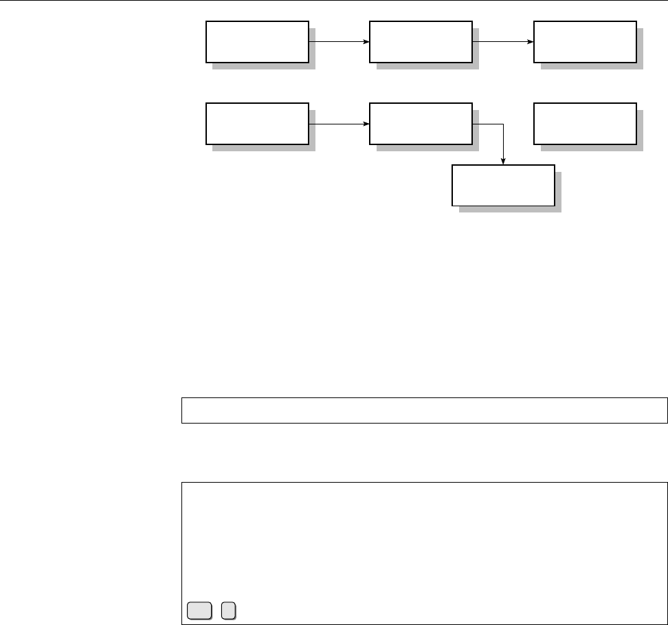
88 7 Standard I/O and Filter Commands
Keyboard Process Screen
Keyboard Process Screen
File
stdin stdout
stdin stdout
Figure 7.1: Standard channels on Linux
7.1 I/O Redirection and Command Pipelines
7.1.1 Standard Channels
Many Linux commands—like
grep
and friends—are designed to read input data,
manipulate it in some way, and output the result of these manipulations. For
example, if you enter
$grep xyz
you can type lines of text on the keyboard, and
grep
will only let those pass that
contain the character sequence, “xyz”:
$grep xyz
abc def
xyz 123
xyz 123
aaa bbb
YYYxyzZZZ
YYYxyzZZZ
Ctrl
+
d
(The key combination at the end lets
grep
know that the input is at an end.)
We say that
grep
reads data from “standard input”—in this case, the keyboard—standard input
and writes to “standard output”—in this case, the console screen or, more likely,
standard output a terminal program in a graphical desktop environment. The third of these
“standard channels” is “standard error output”; while the “payload data”
grep
standard error output
produces are written to standard output, standard error output takes any error
messages (e.g., about a non-existent input le or a syntax error in the regular
expression).
In this chapter you will learn how to redirect a program’s standard output to
a le or take a program’s standard input from a le. Even more importantly, you
will learn how to feed one program’s output directly (without the detour via a
le) into another program as that program’s input. This opens the door to using
the Linux commands, which taken on their own are all fairly simple, as building
blocks to construct very complex applications. (Think of a Lego set.)
BWe will not be able to exhaust this topic in this chapter. Do look forward
to the manual, Advanced Linux, where constructing shell scripts with the
commands from the Unix “toolchest” plays a very important rôle! Here is
where you learn the very important fundamentals of cleverly combining
Linux commands even on the command line.

7.1 I/O Redirection and Command Pipelines 89
Table 7.1: Standard channels on Linux
Channel Name Abbreviation Device Use
0 standard input
stdin
keyboard Input for programs
1 standard output
stdout
screen Output of programs
2 standard error output
stderr
screen Programs’ error messages
The standard channels are summarised once more in Table 7.1. In the pa- standard channels
tois, they are normally referred to using their abbreviated names—
stdin
,
stdout
and
stderr
for standard input, standard output, and standard error output. These
channels are respectively assigned the numbers 0, 1, and 2, which we are going to
use later on.
The shell can redirect these standard channels for individual commands, with- Redirection
out the programs in question noticing anything. These always use the standard
channels, even though the output might no longer be written to the screen or ter-
minal window but some arbitrary other le. That le could be a dierent device,
like a printer—but it is also possible to specify a text le which will receive the
output. That le does not even have to exist but will be created if required.
The standard input channel can be redirected in the same way. A program no
longer receives its input from the keyboard, but takes it from the specied le,
which can refer to another device or a le in the proper sense.
BThe keyboard and screen of the “terminal” you are working on (no matter
whether this is a Linux text console, a “genuine” terminal on a serial port,
a terminal window in a graphical environment, or a network session using,
say, the secure shell) can be accessed by means of the
/dev/tty
le—if you
want to read data this means the keyboard, for output the screen (the other
way round would be quite silly). The
$grep xyz /dev/tty
would be equivalent to our example earlier on in this section. You can nd
out more about such “special les” from Chapter 9.)
7.1.2 Redirecting Standard Channels
You can redirect the standard output channel using the shell operator “
>
” (the Redirecting standard output
“greater-than” sign). In the following example, the output of “
ls -laF
” is redi-
rected to a le called
filelist
; the screen output consists merely of
$ls -laF >filelist
$ __
If the
filelist
le does not exist it is created. Should a le by that name exist,
however, its content will be overwritten. The shell arranges for this even before
the program in question is invoked—the output le will thus be created even if
the actual command invocation contained typos, or if the program did not indeed
write any output at all (in which case the
filelist
le will remain empty).
BIf you want to avoid overwriting existing les using shell output redirection, Protecting existing files
you can give the
bash
command “
set -o noclobber
”. In this case, if output is
redirected to an existing le, an error occurs.
You can look at the
filelist
le in the usual way, e. g., using
less
:
$less inhalt
total 7

90 7 Standard I/O and Filter Commands
drwxr-xr-x 12 joe users 1024 Aug 26 18:55 ./
drwxr-xr-x 5 root root 1024 Aug 13 12:52 ../
drwxr-xr-x 3 joe users 1024 Aug 20 12:30 photos/
-rw-r--r-- 1 joe users 0 Sep 6 13:50 filelist
-rw-r--r-- 1 joe users 15811 Aug 13 12:33 pingu.gif
-rw-r--r-- 1 joe users 14373 Aug 13 12:33 hobby.txt
-rw-r--r-- 2 joe users 3316 Aug 20 15:14 chemistry.txt
If you look closely at the content of
filelist
, you can see a directory entry for
filelist
with size 0. This is due to the shell’s way of doing things: When parsing
the command line, it notices the output redirection rst and creates a new
filelist
le (or removes its content). After that, the shell executes the command, in this
case
ls
, while connecting
ls
’s standard output to the
filelist
le instead of the
terminal.
BThe le’s length in the
ls
output is 0because the
ls
command looked at the
le information for
filelist
before anything was written to that le – even
though there are three other entries above that of
filelist
. This is because
ls
rst reads all directory entries, then sorts them by le name, and only
then starts writing to the le. Thus
ls
sees the newly created (or emptied)
le
filelist
, with no content so far.
If you want to append a command’s output to an existing le without replacingAppending stan-
dard output to a file its previous content, use the
>>
operator. If that le does not exist, it will be created
in this case, too.
$date >> filelist
$less filelist
total 7
drwxr-xr-x 12 joe users 1024 Aug 26 18:55 ./
drwxr-xr-x 5 root root 1024 Aug 13 12:52 ../
drwxr-xr-x 3 joe users 1024 Aug 20 12:30 photos/
-rw-r--r-- 1 joe users 0 Sep 6 13:50 filelist
-rw-r--r-- 1 joe users 15811 Aug 13 12:33 pingu.gif
-rw-r--r-- 1 joe users 14373 Aug 13 12:33 hobby.txt
-rw-r--r-- 2 joe users 3316 Aug 20 15:14 chemistry.txt
Wed Oct 22 12:31:29 CEST 2003
In this example, the current date and time was appended to the
filelist
le.
Another way to redirect the standard output of a command is by using “back-
ticks” (
`
…
`
). This is also called command substitution: The standard output of acommand substitution
command in backticks will be inserted into the command line instead of the com-
mand (and backticks); whatever results from the replacement will be executed.
For example:
$cat dates
Our little diary
22/12 Get presents
23/12 Get Christmas tree
24/12 Christmas Eve
$date +%d/%m
What’s the date?
23/12
$grep `̂date +%d/%m.` dates
What’s up?
23/12 Get Christmas tree
BA possibly more convenient syntax for “
`date`
” is “
$(date)
”. This makes it
easier to nest such calls. However, this syntax is only supported by modern
shells such as
bash
.
You can use
<
, the “less-than” sign, to redirect the standard input channel. ThisRedirecting standard input
will read the content of the specied le instead of keyboard input:

7.1 I/O Redirection and Command Pipelines 91
$wc -w <frog.txt
1397
In this example, the
wc
lter command counts the words in le
frog.txt
.
BThere is no
<<
redirection operator to concatenate multiple input les; to
pass the content of several les as a command’s input you need to use
cat
:
$cat file1 file2 file3 | wc -w
(We shall nd out more about the “
|
” operator in the next section.) Most
programs, however, do accept one or more le names as command line ar-
guments.
BYou can, however, use the
<<
operator to take input data for a command
from the lines following the command invocation in the shell. This is less
interesting for interactive use than it is for shell scripts, but must be men-
tioned here for completeness. The feature is called a “here document”. For
example, in
$grep Linux <<END
Roses are red,
Violets are blue,
Linux is lovely,
I know this is true.
END
the input to
grep
consists of the lines following the
grep
call up to the line
containing only “
END
”. The output of the command is
Linux is lovely,
BIf you specify the “end string” of a here document without quotes, shell
variables will be evaluated and command substitution (using
`
…
`
or
$(
…
)
)
will be performed on the lines of the here document. However, if the end
string is quoted (single or double quotes), the here document will be pro-
cessed verbatim. Compare the output of
$cat <<EOF
Today's date: `date`
EOF
to that of
$cat <<"EOF"
Today's date: `date`
EOF
Finally: If the here document is introduced by “
<<-
” instead of “
<<
”, all tab
characters will be removed from the beginning of the here document’s lines.
This lets you indent here documents properly in shell scripts.
Of course, standard input and standard output may be redirected at the same Simultaneous redirection
time. The output of the word-count example is written to a le called
wordcount
here:
$wc -w <frog.txt >wordcount
$cat wordcount
1397

92 7 Standard I/O and Filter Commands
Besides the standard input and standard output channels, there is also the stan-standard error output
dard error output channel. If errors occur during a program’s operation, the cor-
responding messages will be written to that channel. That way you will see them
even if standard output has been redirected to a le. If you want to redirect stan-
dard error output to a le as well, you must state the channel number for the
redirection operator—this is optional for
stdin
(
0<
) and
stdout
(
1>
) but mandatory
for
stderr
(
2>
).
You can use the
>&
operator to redirect a channel to a dierent one:
make >make.log 2>&1
redirects standard output and standard error output of the
make
command to
make.
log
.
BWatch out: Order is important here! The two commands
make >make.log 2>&1
make 2>&1 >make.log
lead to completely dierent results. In the second case, standard error out-
put will be redirected to wherever standard output goes (
/dev/tty
, where
standard error output would go anyway), and then standard output will
be sent to
make.log
, which, however, does not change the target for standard
error output.
Exercises
C7.1 [2] You can use the
-U
option to get
ls
to output a directory’s entries with-
out sorting them. Even so, after “
ls -laU >filelist
”, the entry for
filelist
in
the output le gives length zero. What could be the reason?
C7.2 [!2] Compare the output of the commands “
ls /tmp
” and “
ls /tmp >ls-
tmp.txt
” (where, in the second case, we consider the content of the
ls-tmp.txt
to be the output). Do you notice something? If so, how could you explain
the phenomenon?
C7.3 [!2] Why isn’t it possible to replace a le by a new version in one step,
for example using “
grep xyz file >file
”?
C7.4 [!1] And what is wrong with “
cat foo >>foo
”, assuming a non-empty le
foo
?
C7.5 [2] In the shell, how would you output an error message such that it goes
to standard error output?
7.1.3 Command Pipelines
Output redirection is frequently used to store the result of a program in order to
continue processing it with a dierent command. However, this type of interme-
diate storage is not only quite tedious, but you must also remember to get rid of
the intermediate les once they are no longer required. Therefore, Linux oers a
way of linking commands directly via pipes: A program’s output automaticallypipes
becomes another program’s input.
This direct connection of several commands into a pipeline is done using thedirect connection of
several commands
pipeline
|
operator. Instead of rst redirecting the output of “
ls -laF
” to a le and then
looking at that le using
less
, you can do the same thing in one step without an
intermediate le:
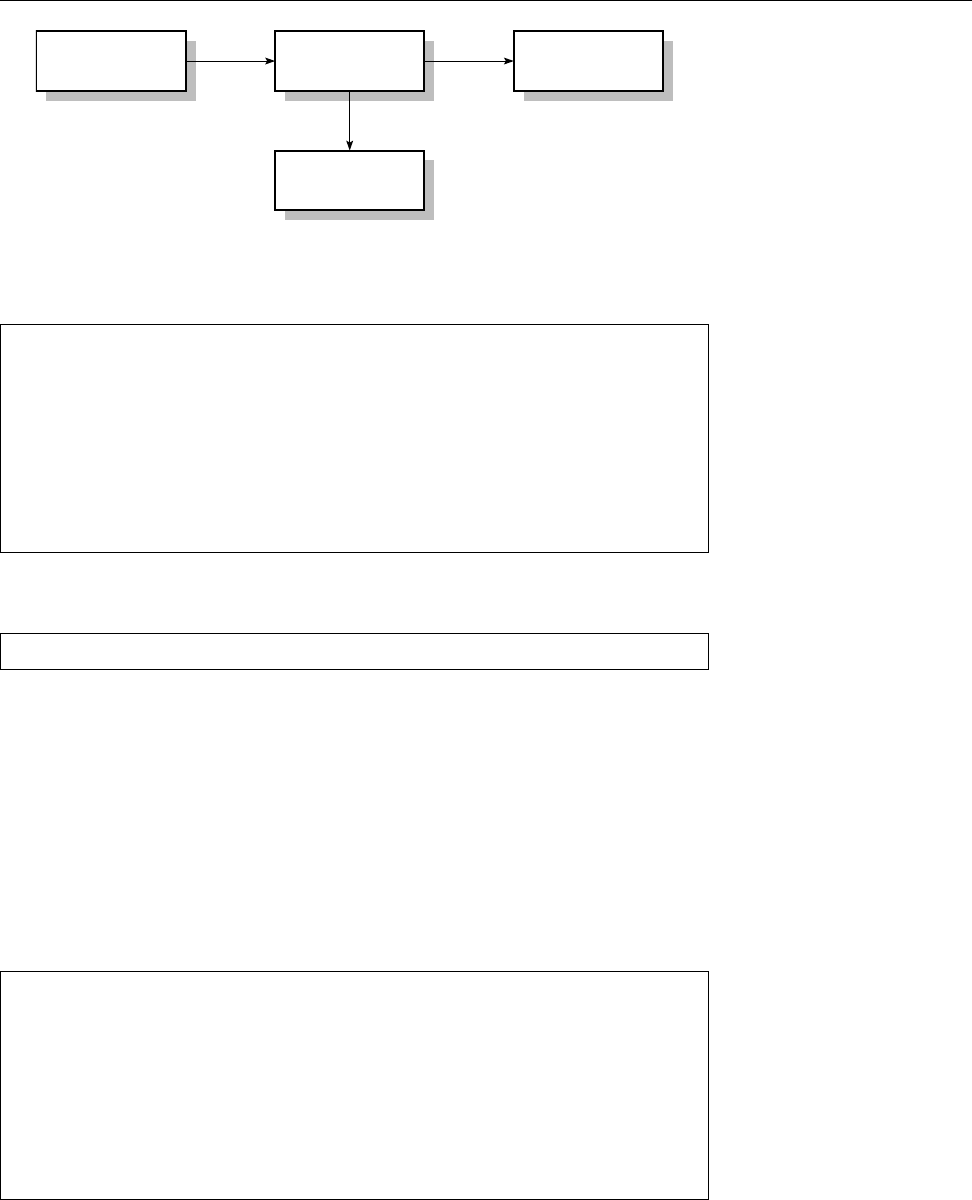
7.1 I/O Redirection and Command Pipelines 93
Command tee Command
File
stdin stdout
Figure 7.2: The
tee
command
$ls -laF | less
total 7
drwxr-xr-x 12 joe users 1024 Aug 26 18:55 ./
drwxr-xr-x 5 root root 1024 Aug 13 12:52 ../
drwxr-xr-x 3 joe users 1024 Aug 20 12:30 photos/
-rw-r--r-- 1 joe users 449 Sep 6 13:50 filelist
-rw-r--r-- 1 joe users 15811 Aug 13 12:33 pingu.gif
-rw-r--r-- 1 joe users 14373 Aug 13 12:33 hobby.txt
-rw-r--r-- 2 joe users 3316 Aug 20 15:14 chemistry.txt
These command pipelines can be almost any length. Besides, the nal result can
be redirected to a le:
$cut -d: -f1 /etc/passwd | sort | pr -2 >userlst
This command pipeline takes all user names from the rst comma-separated col-
umn of
/etc/passwd
le, sorts them alphabetically and writes them to the
userlst
le in two columns. The commands used here will be described in the remainder
of this chapter.
Sometimes it is helpful to store the data stream inside a command pipeline at
a certain point, for example because the intermediate result at that stage is useful intermediate result
for dierent tasks. The
tee
command copies the data stream and sends one copy
to standard output and another copy to a le. The command name should be
obvious if you know anything about plumbing (see Figure 7.2).
The
tee
command with no options creates the specied le or overwrites it if it
exists; with
-a
(“append”), the output can be appended to an existing le.
$ls -laF | tee list | less
total 7
drwxr-xr-x 12 joe users 1024 Aug 26 18:55 ./
drwxr-xr-x 5 root root 1024 Aug 13 12:52 ../
drwxr-xr-x 3 joe users 1024 Aug 20 12:30 photos/
-rw-r--r-- 1 joe users 449 Sep 6 13:50 content
-rw-r--r-- 1 joe users 15811 Aug 13 12:33 pingu.gif
-rw-r--r-- 1 joe users 14373 Aug 13 12:33 hobby.txt
-rw-r--r-- 2 joe users 3316 Aug 20 15:14 chemistry.txt
In this example the content of the current directory is written both to the
list
le
and the screen. (The
list
le does not show up in the
ls
output because it is only
created afterwards by
tee
.)
Exercises
C7.6 [!2] How would you write the same intermediate result to several les
at the same time?

94 7 Standard I/O and Filter Commands
Table 7.2: Options for
cat
(selection)
Option Result
-b
(engl. number non-blank lines) Numbers all non-blank lines in
the output, starting at 1.
-E
(engl. end-of-line) Displays a
$
at the end of each line (useful
to detect otherwise invisible space characters).
-n
(engl. number) Numbers all lines in the output, starting at 1.
-s
(engl. squeeze) Replaces sequences of empty lines by a single
empty line.
-T
(engl. tabs) Displays tab characters as “
^I
”.
-v
(engl. visible) Makes control characters 𝑐visible as “
^
𝑐”, char-
acters 𝛼with character codes greater than 127 as “
M-
𝛼”.
-A
(engl. show all) Same as
-vET
.
7.2 Filter Commands
One of the basic ideas of Unix—and, consequently, Linux—is the “toolkit princi-toolkit principle
ple”. The system comes with a great number of system programs, each of which
performs a (conceptually) simple task. These programs can be used as “building
blocks” to construct other programs, to save the authors of those programs from
having to develop the requisite functions themselves. For example, not every pro-
gram contains its own sorting routines, but many programs avail themselves of
the
sort
command provided by Linux. This modular structure has several advan-
tages:
• It makes life easier for programmers, who do not need to develop (or incor-
porate) new sorting routines all the time.
• If
sort
receives a bug x or performance improvement, all programs using
sort
benet from it, too—and in most cases do not even need to be changed.
Tools that take their input from standard input and write their output to standard
output are called “lter commands” or “lters” for short. Without input redirec-
tion, a lter will read its input from the keyboard. To nish o keyboard input for
such a program, you must enter the key sequence Ctrl +d, which is interpreted
as “end of le” by the terminal driver.
BNote that the last applies to keyboard input only. Files on the disk may of
course contain the Ctrl +dcharacter (ASCII 4), without the system believ-
ing that the le ended at that point. This as opposed to a certain very pop-
ular operating system, which traditionally has a somewhat quaint notion of
the meaning of the Control-Z (ASCII 26) character even in text les …
Many “normal” commands, such as the aforementioned
grep
, operate like l-
ters if you do not specify input le names for them to work on.
In the remainder of the chapter you will become familiar with a selection of the
most important such commands. Some commands have crept in that are not tech-
nically genuine lter commands, but all of them form important building blocks
for pipelines.
7.3 Reading and Writing Files
7.3.1 Outputting and Concatenating Text Files—
cat
and
tac
The
cat
(“concatenate”) command is really intended to join several les named onconcatenating files
the command line into one. If you pass just a single le name, the content of that

7.3 Reading and Writing Files 95
Table 7.3: Options for
tac
(selection)
Option Result
-b
(engl. before) The separator is considered to occur (and be
output) in front of a part, not behind it.
-r
(engl. regular expression) The separator is interpreted as a reg-
ular expression.
-s
𝑠(engl. separator) Denes a dierent separator 𝑠(in place of
\n
)
an. The separator may be several characters long.
le will be written to standard output. If you do not pass a le name at all,
cat
reads its standard input—this may seem useless, but
cat
oers options to number
lines, make line ends and special characters visible or compress runs of blank lines
into one (Table 7.2).
BIt goes without saying that only text les lead to sensible screen output with text files
cat
. If you apply the command to other types of les (such as the binary le
/bin/cat
), it is more than probable—on a text terminal at least—that the shell
prompt will consist of unreadable characters once the output is done. In this
case you can restore the normal character set by (blindly) typing
reset
. If you
redirect
cat
output to a le this is of course not a problem.
BThe “Useless Use of
cat
Award” goes to people using
cat
where it is extra-
neous. In most cases, commands do accept lenames and don’t just read
their standard input, so
cat
is not required to pass a single le to them on
standard input. A command like “
cat data.txt | grep foo
” is unnecessary if
you can just as well write “
grep foo data.txt
”. Even if
grep
could only read its
standard input, “
grep foo <data.txt
” would be shorter and would not involve
an additional
cat
process.However, the whole issue is a bit more subtle; see
Exercise 7.21.
The
tac
command’s name is “
cat
backwards”, and it works like that, too: It Output a file’s lines in reverse
order
reads a number of named les or its standard input and outputs the lines it has
read in reverse order:
$tac <<END
Alpha
Beta
Gamma
END
Gamma
Beta
Alpha
However, this is where the similarity ends already:
tac
does not support the same
options as
cat
but features its own (Table 7.3). For example, you can use the
-s
op-
tion to set up an alternative separator which the program will use when reversing separator
the input—normally the separator is a newline character, so the input is reversed
line by line. Consider, for example
$echo A:B:C:D | tac -s :
D
C:B:A:$ _
(where the new shell prompt is appended directly to the last output line). This
output, which at rst glance looks totally weird, can be explained as follows: The
input consists of the four parts “
A:
”, “
B:
”, “
C:
”, and “
D\n
” (the separator, here “
:
”
is considered to belong to the immediately preceding part, and the nal newline

96 7 Standard I/O and Filter Commands
character is contributed by
echo
). These parts are output in reverse order, i. e.,
“
D\n
” comes rst and then the other three, with no other intervening separators
(since every part contains a perfectly workable separator already); the next shell
prompt is appended immediately (without a new line) to the output. The
-b
option
considers the separator to belong to the following part rather than the preceding
one; with “
tac -s : -b
”, our example would produce the following output:
:D
:C:BA$ _
(think it through!).
Exercises
C7.7 [2] How can you check whether a directory contains les with “weird”
names (e. g., ones with spaces at the end or invisible control characters in
the middle)?
7.3.2 Beginning and End—
head
and
tail
Sometimes you are only interested in part of a le: The rst few lines to check
whether it is the right le, or, in particular with log les, the last few entries. The
head
and
tail
commands deliver exactly that—by default, the rst ten and the last
ten lines of every le passed as an argument, respectively (or else as usual the rst
or last ten lines of their standard input). The
-n
option lets you specify a dierent
number of lines: “
head -n 20
” returns the rst 20 lines of its standard input, “
tail
-n 5 data.txt
” the last 5lines of le
data.txt
.
BTradition dictates that you can specify the number 𝑛of desired lines directly
as “
-
𝑛”. Ocially this is no longer allowed, but the Linux versions of
head
and
tail
still support it.
You can use the
-c
option to specify that the count should be in bytes, not lines:
“
head -c 20
” displays the rst 20 bytes of standard input, no matter how many
lines they occupy. If you append a “
b
”, “
k
”, or “
m
” (for “blocks”, “kibibytes”, and
“mebibytes”, respectively) to the count, the count will be multiplied by 512,1024,
or 1048576, respectively.
B
head
also lets you use a minus sign: “
head -c -20
” displays all of its standard
input but the last 20 bytes.
BBy way of revenge,
tail
can do something that
head
does not support: If the
number of lines starts with “
+
”, it displays everything starting with the given
line:
$tail -n +3 file
Everything from line 3
The
tail
command also supports the important
-f
option. This makes
tail
wait
after outputting the current end of le, to also output data that is appended later
on. This is very useful if you want to keep an eye on some log les. If you pass
several le names to
tail -f
, it puts a header line in front of each block of output
lines telling what le the new data was written to.
Exercises
C7.8 [!2] How would you output just the 13th line of the standard input?
C7.9 [3] Check out “
tail -f
”: Create a le and invoke “
tail -f
” on it. Then,
from another window or virtual console, append something to the le us-
ing, e. g., “
echo >>…
”, and observe the output of
tail
. What does it look like
when
tail
is watching several les simultaneously?

7.3 Reading and Writing Files 97
Table 7.4: Options for
od
(excerpt)
Option Result
-A
𝑟Base of the oset at the beginning of the line. Valid values are:
d
(decimal),
o
(octal),
x
(hexadecimal),
n
(no oset at all).
-j
𝑜Skip 𝑜bytes at the beginning of the input, then start writing output.
-N
𝑛Output at most 𝑛bytes.
-t
𝑡Use type specication 𝑡. Several
-t
options may occur, and one line will be output for
each of them in the requisite format.
Possible values for 𝑡:
a
(named character),
c
(ASCII character),
d
(signed decimal number),
f
(oating-point number),
o
(octal number),
u
(unsigned decimal number),
x
(hexadeci-
mal number).
You can append a digit to all options except
a
and
c
. This species how many bytes
of the input should be interpreted as a unit. Details for this and for letter-based width
speciers can be found in
od
(1).
If you append a
z
to an option, the printable characters of that line will be displayed to
the right.
-v
Outputs all duplicate lines as well.
-w
𝑤Writes 𝑤bytes per line; default value is 16.
C7.10 [3] What happens to “
tail -f
” if the le being observed shrinks?
C7.11 [3] Explain the output of the following commands:
$echo Hello >/tmp/hello
$echo "Hiya World" >/tmp/hello
when you have started the command
$tail -f /tmp/hello
in a dierent window after the rst
echo
above.
7.3.3 Just the Facts, Ma’am—
od
and
hexdump
cat
,
tac
,
head
, and
tail
work best with text les: Arbitrary binary les can in prin-
ciple be processed, but the last three programs in particular prefer dealing with
les that consist of noticeable lines. Even so, it is often useful to be able to check
exactly what is in a le. A suitable tool is the
od
(“octal dump”) command, which
od
can display arbitrary data in dierent formats. Binary data can be displayed byte
by byte or word by word in octal, hexadecimal, decimal or ASCII coding. The
standard display style of
od
is as follows:
$od /etc/passwd | head -3
0000000 067562 072157 074072 030072 030072 071072 067557 035164
0000020 071057 067557 035164 061057 067151 061057 071541 005150
0000040 060563 064163 067562 072157 074072 030072 030072 071072
At the very left there is the (octal) oset in the le where the output line starts. Line format
The eight following numbers each correspond to two bytes from the le, printed
in octal. This is only useful in very specic circumstances.
Fortunately
od
supports options that let you change the output format in very
many ways (Table 7.4). Most important is the
-t
option, which describes the for-
-t
mat of the data lines. For byte-by-byte hexadecimal output, you could use, for
example,

98 7 Standard I/O and Filter Commands
$od -txC /etc/passwd
0000000 72 6f 6f 74 3a 78 3a 30 3a 30 3a 72 6f 6f 74 3a
0000020 2f 72 6f 6f 74 3a 2f 62 69 6e 2f 62 61 73 68 0a
0000040 73 61 73 68 72 6f 6f 74 3a 78 3a 30 3a 30 3a 72
(the oset remains octal). Here,
x
species “hexadecimal”, and
C
species “byte-
wise”. If you want to see the characters themselves in addition to the hexadecimal
numbers, you can append a
z
:
$od -txCz /etc/passwd
0000000 72 6f 6f 74 3a 78 3a 30 3a 30 3a 72 6f 6f 74 3a >root:x:0:0:root:<
0000020 2f 72 6f 6f 74 3a 2f 62 69 6e 2f 62 61 73 68 0a >/root:/bin/bash.<
0000040 73 61 73 68 72 6f 6f 74 3a 78 3a 30 3a 30 3a 72 >sashroot:x:0:0:r<
Non-printable characters (here the
0a
—a newline character—at the end of the sec-
ond line) are replaced by “
.
”.
You can also concatenate several type speciers or put them into separate
-t
several type specifiers
options. This gives you one line per type specier:
$od -txCc /etc/passwd
0000000 72 6f 6f 74 3a 78 3a 30 3a 30 3a 72 6f 6f 74 3a
r o o t : x : 0 : 0 : r o o t :
0000020 2f 72 6f 6f 74 3a 2f 62 69 6e 2f 62 61 73 68 0a
/ r o o t : / b i n / b a s h \n
0000040 73 61 73 68 72 6f 6f 74 3a 78 3a 30 3a 30 3a 72
s a s h r o o t : x : 0 : 0 : r
(which is identical to »
od -txC -tc /etc/passwd
«).
A sequence of lines that would be equal to the last previously-output line isidentical output lines
replaced by an asterisk (“
*
”) at the left margin:
$od -tx -N 64 /dev/zero
0000000 00 00 00 00 00 00 00 00 00 00 00 00 00 00 00 00
*
0000100
(
/dev/zero
produces an unlimited supply of null bytes, and the
-N
option to
od
limits
the output to 64 of them.) The
-v
option suppresses the abbreviation:
$od -tx -N 64 -v /dev/zero
0000000 00 00 00 00 00 00 00 00 00 00 00 00 00 00 00 00
0000020 00 00 00 00 00 00 00 00 00 00 00 00 00 00 00 00
0000040 00 00 00 00 00 00 00 00 00 00 00 00 00 00 00 00
0000060 00 00 00 00 00 00 00 00 00 00 00 00 00 00 00 00
0000100
The
hexdump
(or
hd
) program does a very similar job. It supports output formats
hexdump
that are very like those of
od
, even though the corresponding options are com-
pletely dierent. For example, the
$hexdump -o -s 446 -n 64 /etc/passwd
is mostly equivalent to the rst
od
example above. Most
od
options have fairly
similar counterparts in
hexdump

7.3 Reading and Writing Files 99
A major dierence between
hexdump
and
od
is
hexdump
’s support for output for- output formats
mats. These let you specify in much more detail than is possible with
od
what the
output should look like. Consider the following example:
$cat hexdump.txt
0123456789ABC
XYZabc
xyz
$hexdump -e '"%x-"' hexdump.txt
33323130-37363534-
-a7a79-$
The following points are notable:
• The “
"%x"
” output format writes 4 bytes’ worth of the input in a hexadeci-
mal representation—“
30
” is the hexadecimal equivalent of 48, the numerical
value of the “
0
” character according to the ASCII. The “
-
” sux is output
as-is.
• The 4 bytes are output in reverse order. This is an artefact of the Intel pro-
cessor architecture.
• The double quotes are part of the syntax of
hexdump
and need to be protected
using single quotes (or equivalent) lest the shell remove them.
• The $ at the end is the next command prompt;
hexdump
does not output new-
line characters of its own.
Conveniently for programmers, the possible output formats derive from those
used by the
printf
(3) function found in programming languages like C, Perl,
awk
,
and so on (even
bash
supports a
printf
command). Check the documentation for
details!
hexdump
output formats are much more sophisticated than the simple example
shown above. As usual with
printf
, you get to specify a “eld width” for the
output:
$hexdump -e '"%10x-"' hexdump.txt
33323130- 37363534-
a7a79-$
(In this case every sequence of hexadecimal digits—eight characters in length—
appears ush-right in a ten-character eld.)
You can also specify how often a format will be “executed”: repeat count
$hexdump -e '4 "%x-" "\n"' hexdump.txt
33323130-37363534-42413938-46454443-
4a494847-4e4d4c4b-5251504f-56555453-
5a595857-64636261-68676665-6c6b6a69-
706f6e6d-74737271-78777675-a7a79-
The
4
preceding the commands in this section says that the “
"%x"
” format is to be
applied four times. After that, we continue with the next format—“
"\n"
”—, which
produces a newline character. After that,
hexdump
starts again from the front. newline character
In addition, you can determine how many bytes a format should process (with byte count
the numerical formats you usually have a choice of 1, 2, and 4):
$hexdump -e '/2 "%x-" "\n"' hexdump.txt
3130-
3332-
7a79-
a-
(“
/2
” is an abbreviation for “
1/2
”, which is why every
%x
format appears just once
per line.) Repeat count and byte count may be combined:

100 7 Standard I/O and Filter Commands
Table 7.5: Options for
tr
Option Result
-c
(complement) Replaces all characters not in ⟨s1⟩by characters from ⟨s2⟩
-d
(delete) Removes all characters in ⟨s1⟩without substitution
-s
(squeeze) Runs of identical characters from ⟨s2⟩are replaced by a single character
$hexdump -e '4/2 "%x-" "\n"' hexdump.txt
3130-3332-3534-3736-
3938-4241-4443-4645-
7675-7877-7a79-a-
And you may also mix dierent output formats:
$hexdump -e '"%2_ad" "%2.2s" 3/2 " %x" " %1.1s" "\n"'
hexdump.txt
0 01 3332 3534 3736 8
9 9A 4342 4544 4746 H
In this case we output the rst two characters from the le as characters (rather
than numerical codes) (“
"%2.2s"
”), then three times the codes of two characters
in hexadecimal form (“
3/2 " %x"
”) followed by another character as a character
(“
"%1.1s"
”) and a newline character. Then we start again from the front. The
“
"%2_ad"
” at the beginning of the line outputs the current oset in the le (counted
in bytes from the start of the le) in decimal form in a 2-character eld.
Exercises
C7.12 [2] What is the dierence between the “
a
” and “
c
” type speciers of
od
?
C7.13 [3] The
/dev/random
“device” returns random bytes (see Section 9.3). Use
od
with
/dev/random
to assign a decimal random number from 0to 65535 to
the shell variable
r
.
7.4 Text Processing
7.4.1 Character by Character—
tr
,
expand
and
unexpand
The
tr
command is used to replace single characters by dierent ones inside a text,
or to delete them outright.
tr
is strictly a lter command, it does not take lename
arguments but works with the standard channels only.
For substitutions, the command syntax is “
tr
⟨s1⟩ ⟨s2⟩”. The two parameterssubstitutions
are character strings describing the substitution: In the simplest case the rst char-
acter in ⟨s1⟩will be substituted by the rst character in ⟨s2⟩, the second character
in ⟨s1⟩by the second in ⟨s2⟩, and so on. If ⟨s1⟩is longer than ⟨s2⟩, the “excess”
characters in ⟨s1⟩are replaced by the nal character in ⟨s2⟩; if ⟨s2⟩is longer than
⟨s1⟩, the extra characters in ⟨s2⟩are ignored.
A little example by way of illustration:
$tr AEiu aey <example.txt >new1.txt

7.4 Text Processing 101
Table 7.6: Characters and character classes for
tr
Class Meaning
\a
Control-G (ASCII 7), audible alert
\b
Control-H (ASCII 8), backspace
\f
Control-L (ASCII 12), form feed
\n
Control-J (ASCII 10), line feed
\r
Control-M (ASCII 13), carriage return
\t
Control-I (ASCII 9), tabulator character
\v
Control-K (ASCII 11), vertical tabulator
\
𝑘𝑘𝑘 the character with octal code 𝑘𝑘𝑘
\\
a backslash
[
𝑐
*
𝑛
]
in ⟨s2⟩:𝑛times character 𝑐
[
𝑐
*]
in ⟨s2⟩: character 𝑐as often as needed to make ⟨s2⟩as long as ⟨s1⟩
[:alnum:]
all letters and digits
[:alpha:]
all letters
[:blank:]
all horizontal whitespace characters
[:cntrl:]
all control characters
[:digit:]
all digits
[:graph:]
all printable characters (excluding space)
[:lower:]
all lowercase letters
[:print:]
all printable characters (including space)
[:punct:]
all punctuation characters
[:space:]
all horizontal or vertical whitespace characters
[:upper:]
all capital letters
[:xdigit:]
alle hexadecimal letters (
0
–
9
,
A
–
F
,
a
–
f
)
[:
𝑐
:]
alle characters equivalent to 𝑐(at this point only 𝑐itself)
This command reads le
example.txt
and replaces all “A” characters by “a”, all “E”
characters by “e”, and all “i” and “u” characters by “y”. The result is stored in le
new1.txt
.
It is permissible to express sequences of characters by ranges of the form “𝑚
-
𝑛”, ranges
where 𝑚must precede 𝑛in the character collating order. With the
-c
option,
tr
does not replace the content of ⟨s1⟩but its “complement”, all characters not con-
tained in ⟨s1⟩. The command
$tr -c A-Za-z ' ' <example.txt >new1.txt
replaces all non-letters in
example.txt
by spaces.
BIt is also possible to use character classes of the form
[:
𝑘
:]
(the valid class character classes
names are shown in Table 7.6); in many cases this makes sense in order
to construct commands that work in dierent language environments. In
a German-language environment, the character class “
[:alpha:]
”, for exam-
ple, contains the umlauts, a “home-cooked” class like “
A-Za-z
”, which works
for English, doesn’t. There are some other restrictions on character classes
which you can look up in the
tr
documentation (see “
info tr
”).
To delete characters, you need only specify ⟨s1⟩: The Deleting characters
$tr -d a-z <example.txt >new2.txt
command removes all lowercase letters from
example.txt
. Furthermore, you can
replace runs of equivalent input characters by a single output character: The
$tr -s '\n' <example.txt >new3.txt

102 7 Standard I/O and Filter Commands
command removes empty lines by replacing sequences of newline characters by
a single one.
The
-s
option (“squeeze”) also makes it possible to substitute two dierent in-
put characters by two identical ones, and to replace them by a single one (as with
-s
with a single argument). The following turns all “A” and “E” characters (and
sequences of those) into a single “X” in
new3.txt
:
$tr -s AE X <example.txt >new3.txt
The “tabulator”—a good old typewriter feature—is a convenient way of pro-tabulator
ducing indentation when programming (or entering text in general). By conven-
tion, “tabulator stops” are set in certain columns (usually every 8columns, i. e.,
at positions 8,16,24, …), and common editors move to the next tabulator stop
to the right when the Tab key is pressed—if you press Tab when the cursor is
at column 11 on the screen, the cursor goes to column 16. In spite of this, the
resulting “tabulator characters” (or “tabs”) will be written to the le verbatim,
and many programs cannot interpret them correctly. The
expand
command helpsExpanding tabs
here: It reads the les named as its parameters (or else—you knew it—its stan-
dard input) and writes them to its standard output with all tabs removed by the
appropriate number of spaces to keep the tabulator stops every 8columns. With
the
-t
you can dene a dierent “scale factor” for the tabulator stops; a common
value is, e. g., “
-t 4
”, which sets up tabulator stops at columns 4,8,12,16, etc.
BIf you give several comma-separated numbers with
-t
, tabulator stops will
be set at the named columns exactly: “
expand -t 4,12,32
” sets tabulator stops
at columns 4,12 and 32. Additional tabs in an input line will be replaced by
spaces.
BThe
-i
(“initial”) option causes only tabs at the beginning of the line to be
expanded to spaces.
The
unexpand
more or less reverses the eect of
expand
: All runs of tabs and spacesIntroducing tabs
at the beginning of the input lines (as usual taken from named les or standard in-
put) are replaced by the shortest sequence of tabs and spaces resulting in the same
indentation. A line starting with a tab, two spaces, another tab and nine spaces
will, for example—assuming standard tabulator stops every eight columns—be
replaced by a line starting with three tabs and a space. The
-a
(“all”) option causes
all sequences of two or more tabs and spaces to be “optimized”, not just those at
the beginning of a line.
Exercises
C7.14 [!2] The famous Roman general Julius Caesar supposedly used the fol-
lowing cipher to transmit secret messages: The letter “A” was replaced by
“D”, “B” by “E” and so on; “X” was replaced by “A”, “Y” by “B” and “Z”
by “C” (if we start from today’s 26-letter alphabet, disregarding the fact that
the ancient Romans did not use J, K, W, or Y). Imagine you are are program-
mer in Caesar’s legion. Which
tr
commands would you use to encrypt the
general’s messages and to decrypt them again?
C7.15 [3] What
tr
command would you use to replace all vowels in a text by
a single one? Consider the (German) children’s game:
DREI CHINESEN MIT DEM KONTRABASS
DRAA CHANASAN MAT DAM KANTRABASS
C7.16 [3] How would you transform a text le such that all punctuation is
removed and every word appears on a line on its own?

7.4 Text Processing 103
C7.17 [2] Give a
tr
command to remove the characters “
a
”, “
z
”, and “
-
” from
the standard input.
C7.18 [1] How would you convince yourself that
unexpand
really replaces
spaces and tabulator characters by an “optimal” sequence?
7.4.2 Line by Line—
fmt
,
pr
and so on
While the commands from the previous section considered their input characters
singly or in small groups, Linux also contains many commands that deal with
whole input lines. Some of them are introduced in this and the subsequent sec-
tions.
The
fmt
program wraps the input lines (as usual taken from the les mentioned Line wrapping
on the command line, or the standard input) such that they have a given maximal
line—75 characters, unless otherwise specied using the
-w
option. It is quite con-
cerned with producing pleasant-looking output.
Let us consider some examples of
fmt
(the
frog0.txt
le is equivalent to
frog.txt
,
except that the rst line of each paragraph is indented by two spaces):
$head frog0.txt
The Frog King, or Iron Henry
In olden times when wishing still helped one, there lived a king
whose daughters were all beautiful, but the youngest was so beautiful
that the sun itself, which has seen so much, was astonished whenever
it shone in her face.
Close by the king's castle lay a great dark forest, and under an old
lime-tree in the forest was a well, and when the day was very warm,
the king's child went out into the forest and sat down by the side of
In the rst example we reduce the line length to 40 characters:
$fmt -w 40 frog0.txt
The Frog King, or Iron Henry
In olden times when wishing still
helped one, there lived a king
whose daughters were all beautiful,
but the youngest was so beautiful that
the sun itself, which has seen so much,
was astonished whenever it shone in
Note that the second line of the rst paragraph is indented by spaces for no ap-
parent reason. This is due to the fact that
fmt
usually only considers those ranges
of lines for wrapping that are indented the same. The indented rst line of the
rst paragraph of the example le is therefore considered its own paragraph, and
all resulting lines are indented like the input paragraph’s rst (and only) line.
The second and subsequent input lines are considered an independent, additional
“paragraph”, and wrapped accordingly (using the indentation of the second line).
B
fmt
tries to keep empty lines, the word spacing, and the indentation from
the input. It prefers line breaks at the end of a sentence and tries to avoid
them after the rst and before the last word of a sentence. The “end of a
sentence” according to
fmt
is either the end of a paragraph or a word ending
with “
.
”, “
?
”, or “
!
”, followed by two (!) spaces.
BThere is more information about the way
fmt
works in the info page of the
program (Hint to nd it:
fmt
is part of the GNU “coreutils” collection.)

104 7 Standard I/O and Filter Commands
Table 7.7: Options for
pr
(selection)
Option Result
-
𝑛Creates 𝑛-column output (any positive integer value is permissible, but only 2to 5usu-
ally make sense)
-h
𝑡(engl. header) Outputs 𝑡instead of the source le name at the top of each page
-l
𝑛(engl. length) Sets the number of lines per page, default value is 66
-n
(engl. number) Labels each line with a ve-digit line number separated from the rest of
the line by a tab character
-o
𝑛(engl. oset) Indents the text 𝑛characters from the left margin
-t
(engl. omit) Suppresses the header and footer lines (5each)
-w
𝑛(engl. width) Sets the number of characters per line, default value is 72
In the next example we use the
-c
(“crown-margin mode”) option to avoid the
phenomenon we just explained:
$fmt -c -w 40 frog0.txt
The Frog King, or Iron Henry
In olden times when wishing still
helped one, there lived a king whose
daughters were all beautiful, but the
youngest was so beautiful that the
sun itself, which has seen so much,
was astonished whenever it shone in
Here the indentation of the (complete) paragraph is taken from the rst two lines
of the input; their indentation is kept, and the subsequent input lines follow the
indentation of the second.
Finally, an example featuring long lines:
$fmt -w 100 frog0.txt
The Frog King, or Iron Henry
In olden times when wishing still helped one, there lived a king
whose daughters were all beautiful, but the youngest was so beautiful that the sun itself,
which has seen so much, was astonished whenever it shone in her face.
Close by the king's castle lay a great dark forest, and under an old
lime-tree in the forest was a well, and when the day was very warm, the king's child went out
into the forest and sat down by the side of the cool fountain, and when she was bored she took
a golden ball, and threw it up on high and caught it, and this ball was her favourite plaything.
We could have used
-c
here as well to avoid the “short” rst lines of the para-
graphs. Without this option, the rst line is once more considered a paragraph of
its own, and not amalgamated with the subsequent lines.
The name of the
pr
(“print”) command may be misleading at rst. It does not,
as might be surmised, output les to the printer—this is the domain of the
lpr
command. Instead,
pr
manages formatting a text for printed output, including
page breaks, indentation and header and footer lines. You can either specify input
les on the command line or have
pr
process its standard input (Table 7.7).
Here is a somewhat more complex example to illustrate
pr
’s workings:
$fmt -w 34 frog.txt | pr -h "Grimm Fairy-Tales" -2

7.4 Text Processing 105
Table 7.8: Options for
nl
(selection)
Option Result
-b
𝑠(body style) Numbers the body lines according to 𝑠. Possible values for 𝑠are
a
(num-
ber all lines),
t
(number only non-blank lines),
n
(number no lines at
all), and
p
⟨regex⟩(number only the lines matching regular expression
⟨regex⟩). The default value is
t
.
-d
𝑝[𝑞] (delimiter) Use the two characters 𝑝𝑞 instead of “
\:
” in delimiter lines. If only 𝑝is
given, 𝑞remains set to “
:
”.
-f
𝑠(footer style) Formats the footer lines according to 𝑠. The possible values of 𝑠corre-
spond to those of
-b
. The default value is
n
.
-h
𝑠(header style) Similar to
-f
, for header lines.
-i
𝑛(increment) Increments the line number by 𝑛for every line.
-n
𝑓(number format) Determines the line number format. Possible values for 𝑓:
ln
(ush-
left with no leading zeroes),
rn
(ush-right with no leading zeroes),
rz
(ush-right with leading zeroes).
-p
(page) Does not reset the line number to its original value between logical
pages.
-v
𝑛Starts numbering at line number 𝑛.
-w
𝑛(width) Output a 𝑛-character line number (according to
-n
).
2004-09-13 08:42 Grimm Fairy-Tales Page 1
The Frog King, or Iron Henry >>Whatever you will have, dear
frog,« said she, >>My clothes, my
In olden times when wishing pearls and jewels, and even the
still helped one, there lived a golden crown which I am wearing.«
king whose daughters were all
beautiful, but the youngest The frog answered, >>I do not care
was so beautiful that the sun for your clothes, your pearls
itself, which has seen so much, and jewels, nor for your golden
was astonished whenever it shone crown, but if you will love me
in her face. and let me be your companion and
Here we use
fmt
to format the text of the Frog King in a long narrow column, and
pr
to display the text in two columns.
The
nl
command specialises in line numbering. If nothing else is specied, it line numbering
numbers the non-blank lines of its input (which as usual will be taken from named
les or else standard input) in sequence:
$nl frog.txt
1 The Frog King, or Iron Henry
2 In olden times when wishing still helped one, there lived a king whose
3 daughters were all beautiful, but the youngest was so beautiful that
4 the sun itself, which has seen so much, was astonished whenever it
5 shone in her face.
6 Close by the king's castle lay a great dark forest, and under an old
This by itself is nothing you would not manage using “
cat -b
”. For one, though,
nl
allows for much closer control of the line numbering process:

106 7 Standard I/O and Filter Commands
$nl -b a -n rz -w 5 -v 1000 -i 10 frog.txt
01000 The Frog King, or Iron Henry
01010
01020 In olden times when wishing still helped one, there lived a king whose
01030 daughters were all beautiful, but the youngest was so beautiful that
01040 the sun itself, which has seen so much, was astonished whenever it
01050 shone in her face.
01060
01070 Close by the king's castle lay a great dark forest, and under an old
01080 lime-tree in the forest was a well, and when the day was very warm,
01090 the king's child went out into the forest and sat down by the side of
Taken one by one, the options imply the following (see also Table 7.8): “
-b a
” causes
all lines to be numbered, not just—as in the previous example—the non-blank
ones. “
-n rz
” formats line numbers ush-right with leading zeroes, “
-w 5
” caters
for a ve-column line number, and “
-i 10
” increments the line number by 10 per
line (not, as usual, 1).
In addition,
nl
can also handle per-page line numbers. This is organized usingPer-page line numbers
the “magical” strings “
\:\:\:
”, “
\:\:
” und “
\:
”, as shown in the previous example:
$cat nl-test
\:\:\:
Header of first page
\:\:
First line of first page
Second line of first page
Last line of first page
\:
Footer of first page
\:\:\:
Footer of second page
(Two lines high)
\:\:
First line of second page
Second line of second page
Second-to-last line of second page
Last line of second page
\:
Header of second page
(Two lines high)
Each (logical) page has a header and footer as well as a “body” containing the textheader and footer
proper. The header is introduced using “
\:\:\:
”, and separated from the body
using “
\:\:
”. The body, in turn, ends at a “
\:
” line. Header and footer may also
be omitted.
By default,
nl
numbers the lines on each page starting at 1; header and footer
lines are not numbered:
$nl nl-test
Header of first page
1 First line of first page
2 Second line of first page
3 Last line of first page
Footer of first page

7.4 Text Processing 107
Table 7.9: Options for
wc
(selection)
Option Wirkung
-l
(lines) outputs line count
-w
(words) outputs word count
-c
(characters) outputs character count
Footer of second page
(Two lines high)
1 First line of second page
2 Second line of second page
3 Second-to-last line of second page
4 Last line of second page
Header of second page
(Two lines high)
The “
\:
…” separator lines are replaced by blank lines in the output.
The name of the
wc
command is an abbreviation of “word count”. In spite of
this moniker, not just a word count can be determined, but also a count of total Count lines, words, characters
characters and lines in the input (les, standard input). This is done using the
options in Table 7.9. A “word”, from
wc
’s point of view, is a sequence of one or
more letters. Without an option, all three values are output in the order given in
Table 7.9:
$wc frog.txt
144 1397 7210 frog.txt
With the options in Table 7.9, you can limit
wc
’s output to only some of the values:
$ls | wc -l
13
The example shows how to use
wc
to determine the number of entries in the current
directory by counting the lines in the output of the
ls
command.
Exercises
C7.19 [1] Number the lines of le
frog.txt
with an increment of 2per line
starting at 100.
C7.20 [3] How can you number the lines of a le in reverse order, similar to
144 The Frog King, or Iron Henry
143
142 In olden times when wishing still helped one, there lived a king whose
141 daughters were all beautiful, but the youngest was so beautiful that
(Hint: Two reversals give the original)?
C7.21 [!2] How does the output of the “
wc a.txt b.txt c.txt
” command dier
from that of the “
cat a.txt b.txt c.txt | wc
” command?

108 7 Standard I/O and Filter Commands
7.5 Data Management
7.5.1 Sorted Files—
sort
and
uniq
The
sort
command lets you sort the lines of text les according to predetermined
criteria. The default setting is ascending (from A to Z) according to the ASCIIdefault setting
values1of the rst few characters of each line. This is why special characters such
as German umlauts are frequently sorted incorrectly. For example, the character
code of “Ä” is 143, so that character ends up far beyond “Z” with its character code
of 91. Even the lowercase latter “a” is considered “greater than” the uppercase
letter “Z”.
BOf course,
sort
can adjust itself to dierent languages and cultures. To sort
according to German conventions, set one of the environment variables
LANG
,
LC_ALL
, or
LC_COLLATE
to a value such as “
de
”, “
de_DE
”, or “
de_DE@UTF-8
” (the
actual value depends on your distribution). If you want to set this up for
a single
sort
invocation only, do
$ … | LC_COLLATE=de_DE.UTF-8 sort
The value of
LC_ALL
has precedence over the value of
LC_COLLATE
and that,
again, has precedence over the value of
LANG
. As a side eect, German sort
order causes the case of letters to be ignored when sorting.
Unless you specify otherwise, the sort proceeds “lexicographically” considering
all of the input line. That is, if the initial characters of two lines compare equal,
the rst diering character within the line governs their relative positioning. Of
course
sort
can sort not just according to the whole line, but more specically ac-
cording to the values of certain “columns” or elds of a (conceptual) table. FieldsSorting by fields
are numbered starting at 1; with the “
-k 2
” option, the rst eld would be ignored
and the second eld of each line considered for sorting. If the values of two lines
are equal in the second eld, the rest of the line will be looked at, unless you spec-
ify the last eld to be considered using something like “
-k 2,3
”. Incidentally, it is
permissible to specify several
-k
options with the same
sort
command.
BIn addition,
sort
supports an obsolete form of position specication: Here
elds are numbered starting at 0, the initial eld is specied as “
+
𝑚” and
the nal eld as “
-
𝑛”. To complete the dierences to the modern form, the
nal eld is specied “exclusively”—you give the rst eld that should not
be taken into account for sorting. The examples above would, respectively,
be “
+1
”, “
+1 -3
”, and “
+1 -2
”.
The space character serves as the separator between elds. If several spaces occurseparator
in sequence, only the rst is considered a separator; the others are considered
part of the value of the following eld. Here is a little example, namely the list
of participants for the annual marathon run of the Lameborough Track & Field
Club. To start, we ensure that we use the system’s standard language environment
(“
POSIX
”) by resetting the corresponding environment variables. (Incidentally, the
fourth column gives a runner’s bib number.)
$unset LANG LC_ALL LC_COLLATE
$cat participants.dat
Smith Herbert Pantington AC 123 Men
Prowler Desmond Lameborough TFC 13 Men
Fleetman Fred Rundale Sportsters 217 Men
Jumpabout Mike Fairing Track Society 154 Men
1Of course ASCII only goes up to 127. What is really meant here is ASCII together with whatever
extension for the characters with codes from 128 up is currently used, for example ISO-8859-1, also
known as ISO-Latin-1.

7.5 Data Management 109
de Leaping Gwen Fairing Track Society 26 Ladies
Runnington Vivian Lameborough TFC 117 Ladies
Sweat Susan Rundale Sportsters 93 Ladies
Runnington Kathleen Lameborough TFC 119 Ladies
Longshanks Loretta Pantington AC 55 Ladies
O'Finnan Jack Fairing Track Society 45 Men
Oblomovsky Katie Rundale Sportsters 57 Ladies
Let’s try a list sorted by last name rst. This is easy in principle, since the last
names are at the front of each line:
$sort participants.dat
Fleetman Fred Rundale Sportsters 217 Men
Jumpabout Mike Fairing Track Society 154 Men
Longshanks Loretta Pantington AC 55 Ladies
O'Finnan Jack Fairing Track Society 45 Men
Oblomovsky Katie Rundale Sportsters 57 Ladies
Prowler Desmond Lameborough TFC 13 Men
Runnington Kathleen Lameborough TFC 119 Ladies
Runnington Vivian Lameborough TFC 117 Ladies
Smith Herbert Pantington AC 123 Men
Sweat Susan Rundale Sportsters 93 Ladies
de Leaping Gwen Fairing Track Society 26 Ladies
You will surely notice the two small problems with this list: “Oblomovsky” should
really be in front of “O’Finnan”, and “de Leaping” should end up at the front of
the list, not the end. These will disappear if we specify “English” sorting rules:
$LC_COLLATE=en_GB sort participants.dat
de Leaping Gwen Fairing Track Society 26 Ladies
Fleetman Fred Rundale Sportsters 217 Men
Jumpabout Mike Fairing Track Society 154 Men
Longshanks Loretta Pantington AC 55 Ladies
Oblomovsky Katie Rundale Sportsters 57 Ladies
O'Finnan Jack Fairing Track Society 45 Men
Prowler Desmond Lameborough TFC 13 Men
Runnington Kathleen Lameborough TFC 119 Ladies
Runnington Vivian Lameborough TFC 117 Ladies
Smith Herbert Pantington AC 123 Men
Sweat Susan Rundale Sportsters 93 Ladies
(
en_GB
is short for “British English”;
en_US
, for “American English”, would also work
here.) Let’s sort according to the rst name next:
$sort -k 2,2 participants.dat
Smith Herbert Pantington AC 123 Men
Sweat Susan Rundale Sportsters 93 Ladies
Prowler Desmond Lameborough TFC 13 Men
Fleetman Fred Rundale Sportsters 217 Men
O'Finnan Jack Fairing Track Society 45 Men
Jumpabout Mike Fairing Track Society 154 Men
Runnington Kathleen Lameborough TFC 119 Ladies
Oblomovsky Katie Rundale Sportsters 57 Ladies
de Leaping Gwen Fairing Track Society 26 Ladies
Longshanks Loretta Pantington AC 55 Ladies
Runnington Vivian Lameborough TFC 117 Ladies
This illustrates the property of
sort
mentioned above: The rst of a sequence of
spaces is considered the separator, the others are made part of the following eld’s

110 7 Standard I/O and Filter Commands
Table 7.10: Options for
sort
(selection)
Option Result
-b
(blank) Ignores leading blanks in eld contents
-d
(dictionary) Sorts in “dictionary order”, i. e., only letters, digits and spaces are taken
into account
-f
(fold) Makes uppercase and lowercase letters equivalent
-i
(ignore) Ignores non-printing characters
-k
⟨eld⟩[
,
⟨eld’⟩] (key) Sort according to ⟨eld⟩(up to and including ⟨eld’⟩)
-n
(numeric) Considers eld value as a number and sorts according to its numeric
value; leading blanks will be ignored
-o datei
(output) Writes results to a le, whose name may match the original input le
-r
(reverse) Sorts in descending order, i. e., Z to A
-t
⟨char⟩(terminate) The ⟨char⟩character is used as the eld separator
-u
(unique) Writes only the rst of a sequence of equal output lines
value. As you can see, the rst names are listed alphabetically but only within the
same length of last name. This can be xed using the
-b
option, which treats runs
of space characters like a single space:
$sort -b -k 2,2 participants.dat
Prowler Desmond Lameborough TFC 13 Men
Fleetman Fred Rundale Sportsters 217 Men
Smith Herbert Pantington AC 123 Men
O'Finnan Jack Fairing Track Society 45 Men
Runnington Kathleen Lameborough TFC 119 Ladies
Oblomovsky Katie Rundale Sportsters 57 Ladies
de Leaping Gwen Fairing Track Society 26 Ladies
Longshanks Loretta Pantington AC 55 Ladies
Jumpabout Mike Fairing Track Society 154 Men
Sweat Susan Rundale Sportsters 93 Ladies
Runnington Vivian Lameborough TFC 117 Ladies
This sorted list still has a little blemish; see Exercise 7.24.
The sort eld can be specied in even more detail, as the following exampleMore detailed field specification
shows:
$sort -br -k 2.2 participants.dat
Sweat Susan Rundale Sportsters 93 Ladies
Fleetman Fred Rundale Sportsters 217 Men
Longshanks Loretta Pantington AC 55 Ladies
Runnington Vivian Lameborough TFC 117 Ladies
Jumpabout Mike Fairing Track Society 154 Men
Prowler Desmond Lameborough TFC 13 Men
Smith Herbert Pantington AC 123 Men
de Leaping Gwen Fairing Track Society 26 Ladies
Oblomovsky Katie Rundale Sportsters 57 Ladies
Runnington Kathleen Lameborough TFC 119 Ladies
O'Finnan Jack Fairing Track Society 45 Men
Here, the
participants.dat
le is sorted in descending order (
-r
) according to the
second character of the second table eld, i. e., the second character of the rst
name (very meaningful!). In this case as well it is necessary to ignore leading
spaces using the
-b
option. (The blemish from Exercise 7.24 still manifests itself
here.)
With the
-t
(“terminate”) option you can select an arbitrary character in place
of the eld separator. This is a good idea in principle, since the elds then mayfield separator

7.5 Data Management 111
contain spaces. Here is a more usable (if less readable) version of our example le:
Smith:Herbert:Pantington AC:123:Men
Prowler:Desmond:Lameborough TFC:13:Men
Fleetman:Fred:Rundale Sportsters:217:Men
Jumpabout:Mike:Fairing Track Society:154:Men
de Leaping:Gwen:Fairing Track Society:26:Ladies
Runnington:Vivian:Lameborough TFC:117:Ladies
Sweat:Susan:Rundale Sportsters:93:Ladies
Runnington:Kathleen:Lameborough TFC:119:Ladies
Longshanks:Loretta: Pantington AC:55:Ladies
O'Finnan:Jack:Fairing Track Society:45:Men
Oblomovsky:Katie:Rundale Sportsters:57:Ladies
Sorting by rst name now leads to correct results using “
LC_COLLATE=en_GB sort -t:
-k2,2
”. It is also a lot easier to sort, e.g., by a participant’s number (now eld 4, no
matter how many spaces occur in their club’s name:
$sort -t: -k4 participants0.dat
Runnington:Vivian:Lameborough TFC:117:Ladies
Runnington:Kathleen:Lameborough TFC:119:Ladies
Smith:Herbert:Pantington AC:123:Men
Prowler:Desmond:Lameborough TFC:13:Men
Jumpabout:Mike:Fairing Track Society:154:Men
Fleetman:Fred:Rundale Sportsters:217:Men
de Leaping:Gwen:Fairing Track Society:26:Ladies
O'Finnan:Jack:Fairing Track Society:45:Men
Longshanks:Loretta: Pantington AC:55:Ladies
Oblomovsky:Katie:Rundale Sportsters:57:Ladies
Sweat:Susan:Rundale Sportsters:93:Ladies
Of course the “number” sort is done lexicographically, unless otherwise specied—“117”
and “123” are put before “13”, and that in turn before “154”. This can be xed by
giving the
-n
option to force a numeric comparison: numeric comparison
$sort -t: -k4 -n participants0.dat
Prowler:Desmond:Lameborough TFC:13:Men
de Leaping:Gwen:Fairing Track Society:26:Ladies
O'Finnan:Jack:Fairing Track Society:45:Men
Longshanks:Loretta: Pantington AC:55:Ladies
Oblomovsky:Katie:Rundale Sportsters:57:Ladies
Sweat:Susan:Rundale Sportsters:93:Ladies
Runnington:Vivian:Lameborough TFC:117:Ladies
Runnington:Kathleen:Lameborough TFC:119:Ladies
Smith:Herbert:Pantington AC:123:Men
Jumpabout:Mike:Fairing Track Society:154:Men
Fleetman:Fred:Rundale Sportsters:217:Men
These and some more important options for
sort
are shown in Table 7.10; studying
the program’s documentation is well worthwhile.
sort
is a versatile and powerful
command which will save you a lot of work.
The
uniq
command does the important job of letting through only the rst of a
uniq
command
sequence of equal lines in the input (or the last, just as you prefer). What is con-
sidered “equal” can, as usual, be specied using options.
uniq
diers from most
of the programs we have seen so far in that it does not accept an arbitrary number
of named input les but just one; a second le name, if it is given, is considered
the name of the desired output le (if not, standard output is assumed). If no le
is named in the
uniq
call,
uniq
reads standard input (as it ought).

112 7 Standard I/O and Filter Commands
uniq
works best if the input lines are sorted such that all equal lines occur one
after another. If that is not the case, it is not guaranteed that each line occurs only
once in the output:
$cat uniq-test
Hipp
Hopp
Hopp
Hipp
Hipp
Hopp
$uniq uniq-test
Hipp
Hopp
Hipp
Hopp
Compare this to the output of “
sort -u
”:
$sort -u uniq-test
Hipp
Hopp
Exercises
C7.22 [!2] Sort the list of participants in
participants0.dat
(the le with colon
separators) according to the club’s name and, within clubs, the last and rst
names of the runners (in that order).
C7.23 [3] How can you sort the list of participants by club name in ascending
order and, within clubs, by number in descending order? (Hint: Read the
documentation!)
C7.24 [!2] What is the “blemish” alluded to in the examples and why does it
occur?
C7.25 [2] A directory contains les with the following names:
01-2002.txt 01-2003.txt 02-2002.txt 02-2003.txt
03-2002.txt 03-2003.txt 04-2002.txt 04-2003.txt
11-2002.txt 11-2003.txt 12-2002.txt 12-2003.txt
Give a
sort
command to sort the output of
ls
into “chronologically correct”
order:
01-2002.txt
02-2002.txt
12-2002.txt
01-2003.txt
12-2003.txt
C7.26 [3] How can you produce a sorted list of all words in a text le? Each
word should occur only once in the list. (Hint: Exercise 7.16)

7.5 Data Management 113
7.5.2 Columns and Fields—
cut
,
paste
etc.
While you can locate and “cut out” lines of a text le using
grep
, the
cut
command Cutting columns
works through a text le “by column”. This works in one of two ways:
One possibility is the absolute treatment of columns. These columns corre- Absolute columns
spond to single characters in a line. To cut out such columns, the column number
must be given after the
-c
option (“column”). To cut several columns in one step,
these can be specied as a comma-separated list. Even column ranges may be
specied.
$cut -c 12,1-5 participants.dat
SmithH
ProwlD
FleetF
JumpaM
de LeG
In this example, the rst letter of the rst name and the rst ve letters of the
last name are extracted. It also illustrates the notable fact that the output always
contains the columns in the same order as in input. Even if the selected column
ranges overlap, every input character is output at most once:
$cut -c 1-5,2-6,3-7 participants.dat
Smith
Prowler
Fleetma
Jumpabo
de Leap
The second method is to cut relative elds, which are delimited by separator Relative fields
characters. If you want to cut delimited elds,
cut
needs the
-f
(“eld”) option
and the desired eld number. The same rules as for columns apply. The
-c
and
-f
options are mutually exclusive.
The default separator is the tab character; other separators may be specied separators
with the
-d
option (“delimiter”):
$cut -d: -f 1,4 participants0.dat
Smith:123
Prowler:13
Fleetman:217
Jumpabout:154
de Leaping:26
In this way, the participants’ last names (column 1) and numbers (column 4) are
taken from the list. For readability, only the rst few lines are displayed.
BIncidentally, using the
--output-delimiter
option you can specify a dierent
separator character for the output elds than is used for the input elds:
$cut -d: --output-delimiter=': ' -f 1,4 participants0.dat
Smith: 123
Prowler: 13
Fleetman: 217
Jumpabout: 154
de Leaping: 26

114 7 Standard I/O and Filter Commands
BIf you really want to change the order of columns and elds, you have to
bring in the big guns, such as
awk
or
perl
; you could do it using the
paste
command, which will be introduced presently, but that is rather tedious.
When les are treated by elds (rather than columns), the
-s
option (“sepa-Suppressing no-field lines
rator”) is helpful. If “
cut -f
” encounters lines that do not contain the separator
character, these are normally output in their entirety;
-s
suppresses these lines.
The
paste
command joins the lines of the specied les. It is thus frequentlyJoining lines of files
used together with
cut
. As you will have noticed immediately,
paste
is not a lter
command. You may however give a minus sign in place of one of the input le-
names for
paste
to read its standard input at that point. Its output always goes to
standard output.
As we said,
paste
works by lines. If two le names are specied, the rst lineJoin files “in parallel”
of the rst le and the rst of the second are joined (using a tab character as the
separator) to form the rst line of the output. The same is done with all other lines
in the les. To specify a dierent separator, use the
-d
option.separator
By way of an example, we can construct a version of the list of marathon run-
ners with the participants’ numbers in front:
$cut -d: -f4 participants0.dat >number.dat
$cut -d: -f1-3,5 participants0.dat \
>| paste -d: number.dat - >p-number.dat
$cat p-number.dat
123:Smith:Herbert:Pantington AC:Men
13:Prowler:Desmond:Lameborough TFC:Men
217:Fleetman:Fred:Rundale Sportsters:Men
154:Jumpabout:Mike:Fairing Track Society:Men
26:de Leaping:Gwen:Fairing Track Society:Ladies
117:Runnington:Vivian:Lameborough TFC:Ladies
93:Sweat:Susan:Rundale Sportsters:Ladies
119:Runnington:Kathleen:Lameborough TFC:Ladies
55:Longshanks:Loretta: Pantington AC:Ladies
45:O'Finnan:Jack:Fairing Track Society:Men
57:Oblomovsky:Katie:Rundale Sportsters:Ladies
This le may now conveniently be sorted by number using “
sort -n p-number.dat
”.
With
-s
(“serial”), the given les are processed in sequence. First, all the linesJoin files serially
of the rst le are joined into one single line (using the separator character), then
all lines from the second le make up the second line of the output etc.
$cat list1
Wood
Bell
Potter
$cat list2
Keeper
Chaser
Seeker
$paste -s list*
Wood Bell Potter
Keeper Chaser Seeker
All les matching the
list*
wildcard pattern—in this case,
list1
and
list2
—are
joined using
paste
. The
-s
option causes every line of these les to make up one
column of the output.
The
join
command joins the lines of les, too, but in a much more sophisticated“Relational” joining of files
manner. Instead of just joining the rst lines, second lines, …, it considers one
designated eld per line and joins two lines only if the values in these elds are
equal. Hence,
join
implements the eponymous operator from relational algebra,

7.5 Data Management 115
Table 7.11: Options for
join
(selection)
Option Result
-j1
𝑛Uses eld 𝑛of the rst le as the “join eld” (𝑛 ≥ 1). Synonym:
-1
𝑛.
-j2
𝑛Uses eld 𝑛of the second le as the “join eld” (𝑛 ≥ 1). Synonym:
-2
𝑛.
-j
𝑛(join) Abbreviation for “
-j1
𝑛
-j2
𝑛”
-o
𝑓(output) Output line specication. 𝑓is a comma-separated sequence of eld specica-
tions, where each eld specication is either the digit “
0
” or a eld number 𝑚.𝑛.
“
0
” is the “join eld”, 𝑚is 1or 2, and 𝑛is a eld number in the rst or second
le.
-t
𝑐The 𝑐character will be used as the eld separator for input and output.
as seen in SQL databases—even though the actual operation is a lot cruder and
more inecient than with a “real” database.
Even so, Examplethe
join
command does come in useful. Imagine that the Example
big day has arrived and the Lameborough TFC’s marathon has been run. The
umpires have been diligent and not only have timed how long everybody took, but
also entered them into a le
times.dat
. The rst columns is always a participant’s
number, the second the time achieved (in whole seconds, for simplicity):
$cat times.dat
45:8445
123:8517
217:8533
93:8641
154:8772
119:8830
13:8832
117:8954
57:9111
26:9129
Now we want to join this le with the list of participants, in order to assign each
time to the corresponding participant. To do so, we must rst sort the result le
by participant number:
$sort -n times.dat >times-s.dat
Next we can use
join
to join the lines of le
times-s.dat
to the corresponding lines of
the modied list of participants from the
paste
example—
join
presumes by default
that the input les are sorted by the value of the “join eld”, and that the “join
eld” is the rst eld of each line.
$cat p-number.dat
123:Smith:Herbert:Pantington AC:Men
13:Prowler:Desmond:Lameborough TFC:Men
217:Fleetman:Fred:Rundale Sportsters:Men
154:Jumpabout:Mike:Fairing Track Society:Men
26:de Leaping:Gwen:Fairing Track Society:Ladies
117:Runnington:Vivian:Lameborough TFC:Ladies
93:Sweat:Susan:Rundale Sportsters:Ladies
119:Runnington:Kathleen:Lameborough TFC:Ladies
55:Longshanks:Loretta: Pantington AC:Ladies
45:O'Finnan:Jack:Fairing Track Society:Men
57:Oblomovsky:Katie:Rundale Sportsters:Ladies
$sort -n p-number.dat \
>| join -t: times-s.dat - >p-times.dat

116 7 Standard I/O and Filter Commands
$cat p-times.dat
13:8832:Prowler:Desmond:Lameborough TFC:Men
26:9129:de Leaping:Gwen:Fairing Track Society:Ladies
45:8445:O'Finnan:Jack:Fairing Track Society:Men
57:9111:Oblomovsky:Katie:Rundale Sportsters:Ladies
93:8641:Sweat:Susan:Rundale Sportsters:Ladies
117:8954:Runnington:Vivian:Lameborough TFC:Ladies
119:8830:Runnington:Kathleen:Lameborough TFC:Ladies
123:8517:Smith:Herbert:Pantington AC:Men
154:8772:Jumpabout:Mike:Fairing Track Society:Men
217:8533:Fleetman:Fred:Rundale Sportsters:Men
The resulting le
p-times.dat
now just needs to be sorted by time:
$sort -t: -k2,2 p-times.dat
45:8445:O'Finnan:Jack:Fairing Track Society:Men
123:8517:Smith:Herbert:Pantington AC:Men
217:8533:Fleetman:Fred:Rundale Sportsters:Men
93:8641:Sweat:Susan:Rundale Sportsters:Ladies
154:8772:Jumpabout:Mike:Fairing Track Society:Men
119:8830:Runnington:Kathleen:Lameborough TFC:Ladies
13:8832:Prowler:Desmond:Lameborough TFC:Men
117:8954:Runnington:Vivian:Lameborough TFC:Ladies
57:9111:Oblomovsky:Katie:Rundale Sportsters:Ladies
26:9129:de Leaping:Gwen:Fairing Track Society:Ladies
This is a nice example of how Linux’s standard tools make even fairly complicated
text and data processing possible. In “real life”, one would use shell scripts to
prepare these processing steps and automate them as far as possible.
Exercises
C7.27 [!2] Generate a new version of the
participants.dat
le (the one with
xed-width columns) in which the participant numbers and club aliations
do not occur.
C7.28 [!2] Generate a new version of the
participants0.dat
le (the one with
elds separated using colons) in which the participant numbers and club
aliations do not occur.
C7.29 [3] Generate a version of
participants0.dat
in which the elds are not
separated by colons but by the string “
,␣
” (a comma followed by a space
character).
C7.30 [3] How many groups are used as primary groups by users on your
system? (The primary group of a user is the fourth eld in
/etc/passwd
.)

7.5 Data Management 117
Commands in this Chapter
cat
Concatenates les (among other things)
cat
(1) 94
cut
Extracts elds or columns from its input
cut
(1) 112
expand
Replaces tab characters in its input by an equivalent number of spaces
expand
(1) 102
fmt
Wraps the lines of its input to a given width
fmt
(1) 103
hd
Abbreviation for
hexdump hexdump
(1) 98
head
Displays the beginning of a le
head
(1) 96
hexdump
Displays le contents in hexadecimal (octal, …) form
hexdump
(1) 98
join
Joins the lines of two les according to relational algebra
join
(1) 114
od
Displays binary data in decimal, octal, hexadecimal, … formats
od
(1) 97
paste
Joins lines from dierent input les
paste
(1) 114
pr
Prepares its input for printing—with headers, footers, etc.
pr
(1) 104
reset
Resets a terminal’s character set to a “reasonable” value
tset
(1) 95
sort
Sorts its input by line
sort
(1) 107
tac
Displays a le back to front
tac
(1) 95
tail
Displays a le’s end
tail
(1) 96
tr
Substitutes or deletes characters on its standard input
tr
(1) 100
unexpand
“Optimises” tabs and spaces in its input lines
unexpand
(1) 102
uniq
Replaces sequences of identical lines in its input by single specimens
uniq
(1) 111
wc
Counts the characters, words and lines of its input
wc
(1) 107
Summary
• Every Linux program supports the standard I/O channels
stdin
,
stdout
, and
stderr
.
• Standard output and standard error output can be redirected using opera-
tors
>
and
>>
, standard input using operator
<
.
• Pipelines can be used to connect the standard output and input of programs
directly (without intermediate les).
• Using the
tee
command, intermediate results of a pipeline can be stored to
les.
• Filter commands (or “lters”) read their standard input, manipulate it, and
write the results to standard output.
• The
tr
command substitutes or deletes single characters.
expand
and
unexpand
convert tabs to spaces and vice-versa.
• With
pr
, you can prepare data for printing—not actually print it.
•
wc
can be used to count the lines, words and characters of the standard input
(or a number of named les).
•
sort
is a versatile program for sorting.
• The
cut
command cuts specied ranges of columns or elds from every line
of its input.
• With
paste
, the lines of les can be joined.

$ echo tux
tux
$ ls
hallo.c
hallo.o
$ /bin/su -
Password:
8
More About The Shell
Contents
8.1 Simple Commands:
sleep
,
echo
, and
date
............120
8.2 Shell Variables and The Environment. . . . . . . . . . . . . 121
8.3 Command Types—Reloaded. . . . . . . . . . . . . . . . 123
8.4 The Shell As A Convenient Tool. . . . . . . . . . . . . . . 124
8.5 Commands From A File . . . . . . . . . . . . . . . . . 128
8.6 The Shell As A Programming Language. . . . . . . . . . . . 129
8.6.1 Foreground and Background Processes . . . . . . . . . . 132
Goals
• Knowing about shell variables and evironment variables
• Handling foreground and background processes
Prerequisites
• Basic shell knowledge (Chapter 3)
• File management and simple lter commands (Chapter 6, Chapter 7)
• Use of a text editor (Chapter 5)
grd1-shell2.tex
(
be27bba8095b329b
)

120 8 More About The Shell
8.1 Simple Commands:
sleep
,
echo
, and
date
To give you some tools for experiments, we shall now explain some very simple
commands:
sleep This command does nothing for the number of seconds specied as the
argument. You can use it if you want your shell to take a little break:
$sleep 10
Nothing happens for approximately 10 seconds
$ _
echo The command
echo
outputs its arguments (and nothing else), separated byOutput arguments
spaces. It is still interesting and useful, since the shell replaces variable references
(see Section 8.2) and similar things rst:
$p=Planet
$echo Hello $p
Hello Planet
$echo Hello ${p}oid
Hello Planetoid
(The second
echo
illustrates what to do if you want to append something directly
to the value of a variable.)
BIf
echo
is called with the
-n
option, it does not write a line terminator at the
end of its output:
$echo -n Hello
Hello_
date The
date
command displays the current date and time. You have consider-date and time
able leeway in determining the format of the output—call “
date --help
”, or read
the online documentation using “
man date
”.
B(When reading through this manual for the second time:) In particular,
date
serves as a world clock, if you rst set the
TZ
environment variable to the
name of a time zone or important city (usually capital):
$date
Thu Oct 5 14:26:07 CEST 2006
$export TZ=Asia/Tokyo
$date
Tue Oct 5 21:26:19 JST 2006
$unset TZ
You can nd out about valid time zone and city names by rooting around
in
/usr/share/zoneinfo
.
While every user is allowed to read the system time, only the system administra-Set the system time
tor
root
may change the system time using the
date
command and an argument of
the form
MMDDhhmm
, where
MM
is the calendar month,
DD
the calendar day,
hh
the hour,
and
mm
the minute. You can optionally add two digits the year (plus possibly an-
other two for the century) and the seconds (separated with a dot), which should,
however, prove necessary only in very rare cases.

8.2 Shell Variables and The Environment 121
$date
Thu Oct 5 14:28:13 CEST 2006
$date 08181715
date: cannot set date: Operation not permitted
Fri Aug 18 17:15:00 CEST 2006
BThe
date
command only changes the internal time of the Linux system. This
time will not necessarily be transferred to the CMOS clock on the computer’s
mainboard, so a special command may be required to do so. Many distri-
butions will do this automatically when the system is shut down.
Exercises
C8.1 [!3] Assume now is 22 October 2003, 12:34 hours and 56 seconds. Study
the
date
documentation and state formatting instructions to achieve the fol-
lowing output:
1.
22-10-2003
2.
03-294 (WK43)
(Two-digit year, number of day within year, calendar
week)
3.
12h34m56s
C8.2 [!2] What time is it now in Los Angeles?
8.2 Shell Variables and The Environment
Like most common shells,
bash
has features otherwise found in programming lan-
guages. For example, it is possible to store pieces of text or numbers in variables
and retrieve them later. Variables also control various aspects of the operation of
the shell itself.
Within the shell, a variable is set by means of a command like “
foo=bar
” (this Setting variables
command sets the
foo
variable to the textual value
bar
). Take care not to insert
spaces in front of or behind the equals sign! You can retrieve the value of the
variable by using the variable name with a dollar sign in front:
$foo=bar
$echo foo
foo
$echo $foo
bar
(note the dierence).
We distinguish environment variables from shell variables. Shell variables environment variables
shell variables
are only visible in the shell in which they have been dened. On the other hand,
environment variables are passed to the child process when an external command
is started and can be used there. (The child process does not have to be a shell;
every Linux process has environment variables). All the environment variables of
a shell are also shell variables but not vice versa.
Using the
export
command, you can declare an existing shell variable an envi-
export
ronment variable:
$foo=bar foo
is now a shell variable
$export foo foo
is now an environment variable
Or you dene a new variable as a shell and environment variable at the same time:

122 8 More About The Shell
Table 8.1: Important Shell Variables
Variable Meaning
PWD
Name of the current directory
EDITOR
Name of the user’s favourite editor
PS1
Shell command prompt template
UID
Current user’s user name
HOME
Current user’s home directory
PATH
List of directories containing executable programs that are
eligible as external commands
LOGNAME
Current user’s user name (again)
$export foo=bar
The same works for several variables simultaneously:
$export foo baz
$export foo=bar baz=quux
You can display all environment variables using the
export
command (with no
parameters). The
env
command (also with no parameters) also displays the cur-
rent environment. All shell variables (including those which are also environment
variables) can be displayed using the
set
command. The most common variables
and their meanings are shown in Table 8.1.
BThe
set
command also does many other strange and wonderful things. You
will encounter it again in the Linup Front training manual Advanced Linux,
which covers shell programming.
B
env
, too, is actually intended to manipulate the process environment rather
than just display it. Consider the following example:
$env foo=bar bash
Launch child shell with
foo
$echo $foo
bar
$exit
Back to the parent shell
$echo $foo
Not dened
$ _
BAt least with
bash
(and relations) you don’t really need
env
to execute com-
mands with an extended environment – a simple
$foo=bar bash
does the same thing. However,
env
also allows you to remove variables from
the environment temporarily (how?).
If you have had enough of a shell variable, you can delete it using the
unset
Delete a variable
command. This also removes it from the environment. If you want to remove a
variable from the environment but keep it on as a shell variable, use “
export -n
”:
$export foo=bar foo
is an environment variable
$export -n foo foo
is a shell variable (only)
$unset foo foo
is gone and lost forever

8.3 Command Types—Reloaded 123
8.3 Command Types—Reloaded
One application of shell variables is controlling the shell itself. Here’s another ex- Controlling the shell
ample: As we discussed in Chapter 3, the shell distinguishes internal and external
commands. External commands correspond to executable programs, which the
shell looks for in the directories that make up the value of the
PATH
environment
variable. Here is a typical value for
PATH
:
$echo $PATH
/home/joe/bin:/usr/local/bin:/usr/bin:/bin:/usr/games
Individual directories are separated in the list by colons, therefore the list in the
example consists of ve directories. If you enter a command like
$ls
the shell knows that this isn’t an internal command (it knows its internal com-
mands) and thus begins to search the directories in
PATH
, starting with the leftmost
directory. In particular, it checks whether the following les exist:
/home/joe/bin/ls
Nope …
/usr/local/bin/ls
Still no luck …
/usr/bin/ls
Again no luck …
/bin/ls
Gotcha!
The directory
/usr/games
is not checked.
This implies that the
/bin/ls
le will be used to execute the
ls
command.
BOf course this search is a fairly involved process, which is why the shell
prepares for the future: If it has once identied the
/bin/ls
le as the im-
plementation of the
ls
command, it remembers this correspondence for the
time being. This process is called “hashing”, and you can see that it did take
place by applying
type
to the
ls
command.
$type ls
ls is hashed (/bin/ls)
BThe
hash
command tells you which commands your
bash
has “hashed” and
how often they have been invoked in the meantime. With “
hash -r
” you can
delete the shell’s complete hashing memory. There are a few other options
which you can look up in the
bash
manual or nd out about using “
help hash
”.
BStrictly speaking, the
PATH
variable does not even need to be an environment
variable—for the current shell a shell variable would do just ne (see Exer-
cise 8.5). However it is convenient to dene it as an environment variable so
the shell’s child processes (often also shells) use the desired value.
If you want to nd out exactly which program the shell uses for a given external
command, you can use the
which
command:
$which grep
/bin/grep
which
uses the same method as the shell—it starts at the rst directory in
PATH
and
checks whether the directory in question contains an executable le with the same
name as the desired command.

124 8 More About The Shell
B
which
knows nothing about the shell’s internal commands; even though
something like “
which test
” returns “
/usr/bin/test
”, this does not imply
that this program will, in fact, be executed, since internal commands have
precedence. If you want to know for sure, you need to use the “
type
” shell
command.
The
whereis
command not only returns the names of executable programs, but
also documentation (man pages), source code and other interesting les pertain-
ing to the command(s) in question. For example:
$whereis passwd
passwd: /usr/bin/passwd /etc/passwd /etc/passwd.org /usr/share/passwd
/usr/share/man/man1/passwd.1.gz /usr/share/man/man1/passwd.1ssl.gz
/usr/share/man/man5/passwd.5.gz
This uses a hard-coded method which is explained (sketchily) in
whereis
(1).
Exercises
C8.3 [!2] Convince yourself that passing (or not passing) environment and
shell variables to child processes works as advertised, by working through
the following command sequence:
$foo=bar foo
is a shell variable
$bash
New shell (child process)
$echo $foo
foo
is not dened
$exit
Back to the parent shell
$export foo foo
is an environment variable
$bash
New shell (child process)
$echo $foo
bar
Environment variable was passed along
$exit
Back to the parent shell
C8.4 [!2] What happens if you change an environment variable in the child
process? Consider the following command sequence:
$foo=bar foo
is a shell variable
$bash
New shell (child process)
$echo $foo
bar
Environment variable was passed along
$foo=baz
New value
$exit
Back to the parent shell
$echo $foo
What do we get??
C8.5 [2] Make sure that the shell’s command line search works even if
PATH
is
a “only” simple shell variable rather than an environment variable. What
happens if you remove
PATH
completely?
C8.6 [!1] Which executable programs are used to handle the following com-
mands:
fgrep
,
sort
,
mount
,
xterm
C8.7 [!1] Which les on your system contain the documentation for the
“
crontab
” command?
8.4 The Shell As A Convenient Tool
Since the shell is the tool many Linux users use most often, its developers have
spared no trouble to make its use convenient. Here are some more useful tries:

8.4 The Shell As A Convenient Tool 125
Command Editor You can edit command lines like in a simple text editor. Hence,
you can move the cursor around in the input line and delete or add characters
arbitrarily before nishing the input using the return key. The behaviour of this
editor can be adapted to that of the most popular editors on Linux (Chapter 5)
using the “
set -o vi
” and “
set -o emacs
” commands.
Aborting Commands With so many Linux commands around, it is easy to con-
fuse a name or pass a wrong parameter. Therefore you can abort a command
while it is being executed. You simply need to press the Ctrl +ckeys at the same
time.
The History The shell remembers ever so many of your most recent commands as
part of the “history”, and you can move through this list using the ↑and ↓cur-
sor keys. If you nd a previous command that you like you can either re-execute
it unchanged using ↩, or else edit it as described above. You can search the list
“incrementally” using Ctrl +r—simply type a sequence of characters, and the
shell shows you the most recently executed command containing this sequence.
The longer your sequence, the more precise the search.
BWhen you log out of the system, the shell stores the history in the hidden
le
~/.bash_history
and makes it available again after your next login. (You
may use a dierent le name by setting the
HISTFILE
variable to the name in
question.)
BA consequence of the fact that the history is stored in a “plain” le is that you
can edit it using a text editor (Chapter 5 tells you how). So in case you acci-
dentally enter your password on the command line, you can (and should!)
remove it from the history manually—in particular, if your system is one of
the more freewheeling ones where home directories are visible to anybody.
BBy default, the shell remembers the last 500 commands; you can change this
by putting the desired number into the
HISTSIZE
variable. The
HISTFILESIZE
command species how many commands to write to the
HISTFILE
le – usu-
ally 500 as well.
Besides the arrow keys you can access the history also via “magical” character
sequences in new commands. The shell replaces these character sequences rst,
immediately after the command line has been read. Replacement proceeds in two
stages:
• At rst the shell determines which command from the history to use for
the replacement. The
!!
sequence stands for the immediately preceding
command,
!-
𝑛refers to the 𝑛th command before the current one (
!-2
, for
example, to the penultimate one), and
!
𝑛to the command with number 𝑛
in the history. (The
history
command outputs the whole history including
numbers for the commands.)
!xyz
selects the most recent command starting
with
xyz
, and
!?xyz
the most recent command containing
xyz
.
• After that, the shell decides which part of the selected command will be
“recycled” and how. If you do not specify anything else, the complete com-
mand will be inserted; otherwise there are various selection methods. All
these selection methods are separated from the command selection charac-
ter sequence by a colon (“
:
”).
𝑛Selects the 𝑛-th word. Word 0 is the command itself.
^
Selects the rst word (immediately after the command).
$
Selects the nal word.
𝑚
-
𝑛Selects words 𝑚through 𝑛.

126 8 More About The Shell
𝑛
*
Selects all words starting at word 𝑛.
𝑛
-
Selects all words starting at word 𝑛except for the nal one.
Some examples for clarity:
!-2:$
Picks the nal word of the penultimate command.
!!:0-
Picks the complete immediately preceding command except for the
nal word.
!333^
Picks the rst word from command 333.
The nal example, incidentally, is not a typo; if the rst character from
the intra-command selection is from the list
^$*-%
you may leave out the
colon.—If you like, look at the
bash
documentation (section HISTORY) to
nd out what else the shell has in store. As far as we (and the LPI) are con-
cerned you do not need to learn all of this o by heart.
BThe history is one of the things that
bash
took over from the C shell, and
whoever did not use Unix during the 1980s may have some trouble imag-
ining what the world looked like before interactive command line editing
was invented. (For Windows users, this time doesn’t even go that far back.)
During that time, the history with all its
!
selectors and transformations was
widely considered the best idea since sliced bread; today its documentation
exudes the sort of morbid fascination one would otherwise associate with
the user manual for a Victorian steam engine.
BSome more remarks concerning the
history
command: An invocation like
$history 33
(with a number as the parameter) only outputs that many history lines.
“
history -c
” empties the history completely. There are some more options;
check the
bash
documentation or try “
help history
”.
Autocompletion A massive convenience is
bash
’s ability to automatically com-Completing com-
mand and file names plete command and le names. If you hit the Tab key, the shell completes an
incomplete input if the continuation can be identied uniquely. For the rst word
of a command,
bash
considers all executable programs, within the rest of the com-
mand line all the les in the current or specied directory. If several commands
or les exist whose names start out equal, the shell completes the name as far as
possible and then signals acoustically that the command or le name may still be
incomplete. Another Tab press then lists the remaining possibilities.
BIt is possible to adapt the shell’s completion mechanism to specic pro-
grams. For example, on the command line of a FTP client it might oer
the names of recently visited FTP servers in place of le names. Check the
bash
documentation for details.
Table 8.2 gives an overview of the most important key strokes within
bash
.
Multiple Commands On One Line You are perfectly free to enter several com-
mands on the same input line. You merely need to separate them using a semi-
colon:
$echo Today is; date
Today is
Fri 5 Dec 12:12:47 CET 2008
In this instance the second command will be executed once the rst is done.
8.4 The Shell As A Convenient Tool 127
Table 8.2: Key Strokes within
bash
Key Stroke Function
↑or ↓Scroll through most recent commands
Ctrl +rSearch command history
←bzw. →Move cursor within current command line
Home oder Ctrl +aJump to the beginning of the command line
End oder Ctrl +eJump to the end of the command line
⇐bzw. Del Delete character in front of/under the cursor,
respectively
Ctrl +tSwap the two characters in front of and under
the cursor
Ctrl +lClear the screen
Ctrl +cInterrupt a command
Ctrl +dEnd the input (for login shells: log o)
Conditional Execution Sometimes it is useful to make the execution of the second
command depend on whether the rst was executed correctly or not. Every Unix
process yields a return value which states whether it was executed correctly or return value
whether errors of whatever kind have occurred. In the former case, the return
value is 0; in the latter, it is dierent from 0.
BYou can nd the return value of a child process of your shell by looking at
the
$?
variable:
$bash
Start a child shell …
$exit 33
… and exit again immediately
exit
$echo $?
33
The value from our
exit
above
$ _
But this really has no bearing on the following.
With
&&
as the “separator” between two commands (where there would other-
wise be the semicolon), the second command is only executed when the rst has
exited successfully. To demonstrate this, we use the shell’s
-c
option, with which
you can pass a command to the child shell on the command line (impressive, isn’t
it?):
$bash -c "exit 0" && echo "Successful"
Successful
$bash -c "exit 33" && echo "Successful"
Nothing -- 33 isn’t success!
Conversely, with
||
as the “separator”, the second command is only executed
if the rst did not nish successfully:
$bash -c "exit 0" || echo "Unsuccessful"
$bash -c "exit 33" || echo "Unsuccessful"
Unsuccessful
Exercises
C8.8 [3] What is wrong about the command “
echo "Hello!"
”? (Hint: Experi-
ment with commands of the form “
!-2
” or “
!ls
”.)

128 8 More About The Shell
8.5 Commands From A File
You can store shell commands in a le and execute them en bloc. (Chapter 5 ex-
plains how to conveniently create les.) You just need to invoke the shell and pass
the le name as a parameter:
$bash my-commands
Such a le is also called a shell script, and the shell has extensive programmingshell script
features that we can only outline very briey here. (The Linup Front training
manual Advanced Linux explains shell programming in great detail.)
BYou can avoid having to prepend the
bash
command by inserting the magical
incantation
#!/bin/bash
as the rst line of your le and making the le “executable”:
$chmod +x my-commands
(You will nd out more about
chmod
and access rights in Chapter 12.) After
this, the
$./my-commands
command will suce.
If you invoke a shell script as above, whether with a prepended
bash
or as an
executable le, it is executed in a subshell, a shell that is a child process of thesubshell
current shell. This means that changes to, e. g., shell or environment variables
do not inuence the current shell. For example, assume that the le
assignment
contains the line
foo=bar
Consider the following command sequence:
$foo=quux
$bash assignment
Contains
foo=bar
$echo $foo
quux
No change; assignment was only in subshell
This is generally considered a feature, but every now and then it would be quite
desirable to have commands from a le aect the current shell. That works, too:
The
source
command reads the lines in a le exactly as if you would type them
directly into the current shell—all changes to variables (among other things) hence
take eect in your current shell:
$foo=quux
$source assignment
Contains
foo=bar
$echo $foo
bar
Variable was changed!
A dierent name for the
source
command, by the way, is “
.
”. (You read correctly
– dot!) Hence
$source assignment

8.6 The Shell As A Programming Language 129
is equivalent to
$. assignment
BLike program les for external commands, the les to be read using
source
or
.
are searched in the directories given by the
PATH
variable.
8.6 The Shell As A Programming Language
Being able to execute shell commands from a le is a good thing, to be sure.
However, it is even better to be able to structure these shell commands such that
they do not have to do the same thing every time, but—for example—can ob-
tain command-line parameters. The advantages are obvious: In often-used pro-
cedures you save a lot of tedious typing, and in seldom-used procedures you can
avoid mistakes that might creep in because you accidentally leave out some im-
portant step. We do not have space here for a full explanation of the shell als a
programming language, but fortunately there is enough room for a few brief ex-
amples.
Command-line parameters When you pass command-line parameters to a shell
script, the shell makes them available in the variables
$1
,
$2
, …. Consider the Single parameters
following example:
$cat hello
#!/bin/bash
echo Hello $1, are you free $2?
$./hello Joe today
Hello Joe, are you free today?
$./hello Sue tomorrow
Hello Sue, are you free tomorrow?
The
$*
contains all parameters at once, and the number of parameters is in
$#
:All parameters
$cat parameter
#!/bin/bash
echo $# parameters: $*
$./parameter
0 parameters:
$./parameter dog
1 parameters: dog
$./parameter dog cat mouse tree
4 parameters: dog cat mouse tree
Loops The
for
command lets you construct loops that iterate over a list of words
(separated by white space):
$for i in 1 2 3
>do
>echo And $i!
>done
And 1!
And 2!
And 3!
Here, the
i
variable assumes each of the listed values in turn as the commands
between
do
and
done
are executed.
This is even more fun if the words are taken from a variable:

130 8 More About The Shell
$list='4 5 6'
$for i in $list
>do
>echo And $i!
>done
And 4!
And 5!
And 6!
If you omit the “
in
…”, the loop iterates over the command line parameters:Loop over parameters
$cat sort-wc
#!/bin/bash
# Sort files according to their line count
for f
do
echo `wc -l <"$f» lines in $f
done | sort -n
$./sort-wc /etc/passwd /etc/fstab /etc/motd
(The “
wc -l
” command counts the lines of its standard input or the le(s) passed
on the command line.) Do note that you can redirect the standard output of a loop
to
sort
using a pipe line!
Alternatives You can use the aforementioned
&&
and
||
operators to execute cer-
tain commands only under specic circumstances. The
#!/bin/bash
# grepcp REGEX
rm -rf backup; mkdir backup
for f in *.txt
do
grep $1 "$f" && cp "$f" backup
done
script, for example, copies a le to the
backup
directory only if its name ends with
.txt
(the
for
loop ensures this) and which contain at least one line matching the
regular expression that is passed as a parameter.
A useful tool for alternatives is the
test
command, which can check a large
test
variety of conditions. It returns an exit code of 0(success), if the condition holds,
else a non-zero exit code (failure). For example, consider
#!/bin/bash
# filetest NAME1 NAME2 ...
for name
do
test -d "$name" && echo $name: directory
test -f "$name" && echo $name: file
test -L "$name" && echo $name: symbolic link
done
This script looks at a number of le names passed as parameters and outputs for
each one whether it refers to a directory, a (plain) le, or a symbolic link.
AThe
test
command exists both as a free-standing program in
/bin/test
and
as a built-in command in
bash
and other shells. These variants can dier
subtly especially as far as more outlandish tests are concerned. If in doubt,
read the documentation.

8.6 The Shell As A Programming Language 131
You can use the
if
command to make more than one command depend on a
if
condition (in a convenient and readable fashion). You may write “
[
…
]
” instead
of “
test
…”:
#!/bin/bash
# filetest2 NAME1 NAME2 ...
for name
do
if [ -L "$name" ]
then
echo $name: symbolic link
elif [ -d "$name" ]
echo $name: directory
elif [ -f "$name" ]
echo $name: file
else
echo $name: no idea
fi
done
If the command after the
if
signals “success” (exit code 0), the commands after
then
will be executed, up to the next
elif
,
else
, or
fi
. If on the other hand it sig-
nals “failure”, the command after the next
elif
will be evaluated next and its exit
code will be considered. The shell continues the pattern until the matching
fi
is
reached. Commands after the
else
are executed if none of the
if
or
elif
commands
resulted in “success”. The
elif
and
else
branches may be omitted if they are not
required.
More loops With the
for
loop, the number of trips through the loop is xed at
the beginning (the number of words in the list). However, we often need to deal
with situations where it is not clear at the beginning how often a loop should be
executed. To handle this, the shell oers the
while
loop, which (like
if
) executes
while
a command whose success or failure determines what to do about the loop: On
success, the “dependent” commands will be executed, on failure execution will
continue after the loop.
The following script reads a le like
Aunt Maggie:maggie@example.net:the delightful tea cosy
Uncle Bob:bob@example.com:the great football
(whose name is passed on the command line) and constructs a thank-you e-mail
message from each line (Linux is very useful in daily life):
#!/bin/bash
# birthday FILE
IFS=:
while read name email present
do
(echo $name
echo ""
echo "Thank you very much for $present!"
echo "I enjoyed it very much."
echo ""
echo "Best wishes"
echo "Tim") | mail -s "Many thanks!" $email
done <$1
The
read
command reads the input le line by line and splits each line at the colons
read

132 8 More About The Shell
(variable
IFS
) into the three elds
name
,
email
, and
present
which are then made avail-
able as variables inside the loop. Somewhat counterintuitively, the input redirec-
tion for the loop can be found at the very end.
APlease test this script with innocuous e-mail addresses only, lest your rela-
tions become confused!
Exercises
C8.9 [1] What is the dierence (as far as loop execution is concerned) between
for f; do …; done
and
for f in $*; do …; done
? (Try it, if necessary)
C8.10 [2] In the
sort-wc
script, why do we use the
wc -l <$f
instead of
wc -l $f
C8.11 [2] Alter the
grepcp
such that the list of les to be considered is also
taken from the command line. (Hint: The
shift
shell command removes the
rst command line parameter from
$
and pulls all others up to close the gap.
After a
shift
, the previous
$2
is now
$1
,
$3
is
$2
and so on.)
C8.12 [2] Why does the
filetest
script output
$./filetest foo
foo: file
foo: symbolic link
for symbolic links (instead of just »
foo: symbolic link
«)?
8.6.1 Foreground and Background Processes
After a command has been entered, it is processed by the shell. The shell exe-
cutes internal commands directly; for external commands, the shell generates a
child process, which is used to execute the command and terminates itself af-child process
terwards. In Unix, a process is a running programm; the same program can be
executed several times simultaneously (e.g., by dierent users) and corresponds
with several processes. Every process can generate child processes (even if most
of them—unlike shells—don’t).
Usually, the shell waits until the child process has done its work and termi-
nates. You can tell by the fact that no new shell prompt is displayed while the
child process is running. After the child process has exited, the shell reads and
processes its return value, and only after that it displays a new shell prompt. The
execution of the shell and the child process is, so to speak, synchronised. This
“synchronous” manner of processing commands is displayed in Figure 8.1; from
the user’s point of view it looks like the following:
$sleep 10
Nothing happens for approximately 10 seconds
$ _
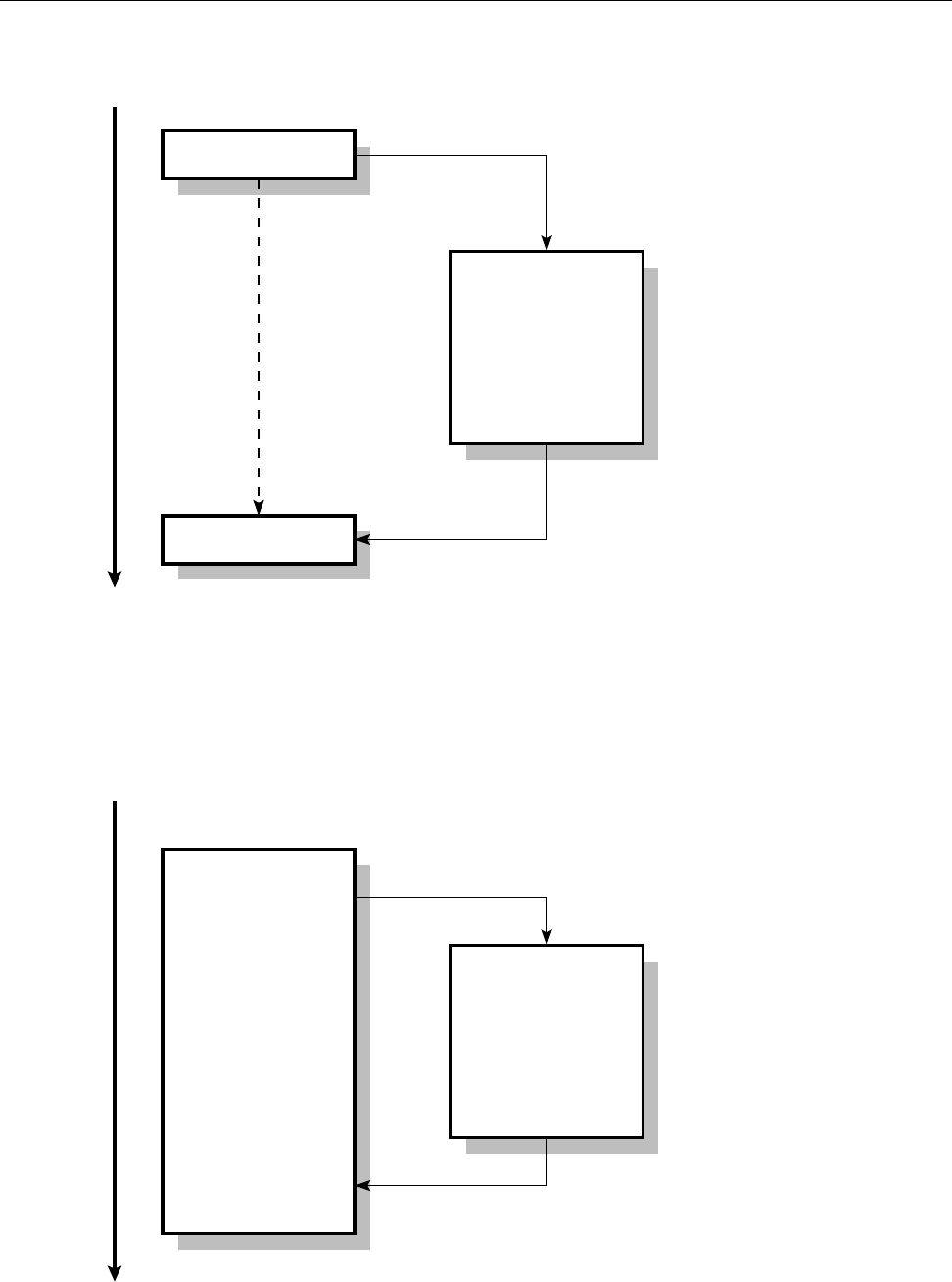
8.6 The Shell As A Programming Language 133
Time
Shell
Shell
Child
Process
Start
End
waits
Figure 8.1: Synchronous command execution in the shell
Time
Shell Child
Process
Start
End
Figure 8.2: Asynchronous command execution in the shell

134 8 More About The Shell
Table 8.3: Options for
jobs
Option Meaning
-l
(long) Adds PIDs to the output
-n
(notify) Displays only processes that have been terminated since
the last invocation of
jobs
-p
(process) Displays only PIDs
If you do not want the shell to wait until the child process has nished, you
have to append an ampersand (
&
) to the command line. Then, while the child
process is executed in the background, a short message appears on the terminal,
immediately followed by the shell’s command prompt:
$sleep 10 &
[2] 6210
And then immediately:
$ _
This mode of operation is called “asynchronous”, since the shell does not wait
idly for the child process to nish (qv. Figure 8.2).
BThe “
[2] 6210
” means that the system has created the process with the num-
ber (or “process ID”) 6210 as “job” number 2. These numbers will probably
dier on your system.
BSyntactically, the
&
really acts like a semicolon, and can therefore serve as a
separator between commands. See Exercise 8.14.
Here are some hints for successful background process operation:
• The background process should not expect keyboard input, since the shell
cannot determine to which process—foreground or background—any key-
board input should be assigned. If necessary, input can be taken from a le.
This is covered more extensively in Chapter 7.
• The background process should not direct output to the terminal, since
these may be mixed up with the output of foreground processes or dis-
carded altogether. Again, there is more about this in Chapter 7.
• If the parent process (the shell) is aborted, all its children (and consequently
their children etc.) will in many cases be terminated as well. Only processes
that completely disawov their parents are exempted from this; this applies,
e. g., to processes that perform system services in the background.
When several processes are executed in the background from the same shell,Job control
it is easy to lose track. Therefore the shell makes available an (internal) command
that you can use to nd out about the state of background processes—
jobs
. If
jobs
is invoked without options, its output consists of a list of job numbers, process
states and command lines. This looks approximately like the following:
$jobs
[1] Done sleep
$ _
In this case, job number 1 has already nished (“Done”), otherwise the message
“
Running
” would have appeared. The
jobs
command supports various options, the
most important of which are shown in Table 8.3.
The shell makes it possible to stop a foreground process using Ctrl +z. This
process is displayed by
jobs
with a “
Stopped
” status and can be continued as a back-
ground process using the
bg
command. (Otherwise, processes stay stopped until

8.6 The Shell As A Programming Language 135
hell freezes over, or the next system restart, whichever occurs earlier.) For exam-
ple, “
bg %5
” will send job 5 to the background, where it will continue to run.
Conversely, you can select one of a number of background processes and fetch
it back to the foreground using the
fg
command. The syntax of the
fg
command
is equivalent to that of the
bg
command.
You can terminate a foreground process from the shell with the Ctrl +ckey
sequence. A background process can be terminated directly using the
kill
com-
mand followed by a job number with a leading percent character (similar to
bg
).
Exercises
C8.13 [2] Use a suitably spectacular program (such as the OpenGL demo
gears
under X11 in the SUSE distributions, alternatively, for example, “
xclock -
update 1
”) to experiment with background processes and job control. Make
sure that you are able to start background processes, to stop foreground
processes using Ctrl +zand send them to the background using
bg
, to list
background processes using
jobs
and so on.
C8.14 [3] Describe (and explain) the dierences between the following three
command lines:
$ sleep 5 ; sleep 5
$ sleep 5 ; sleep 5 &
$ sleep 5 & sleep 5 &
Commands in this Chapter
.
Reads a le containing shell commands as if they had been entered on
the command line
bash
(1) 128
bg
Continues a (stopped) process in the background
bash
(1) 134
date
Displays the date and time
date
(1) 120
env
Outputs the process environment, or starts programs with an adjusted
environment
env
(1) 122
export
Denes and manages environment variables
bash
(1) 121
fg
Fetches a background process back to the foreground
bash
(1) 134
gears
Displays turning gears on X11
gears
(1) 135
hash
Shows and manages ”‘seen”’ commands in
bash bash
(1) 123
history
Displays recently used
bash
command lines
bash
(1) 125
jobs
Reports on background jobs
bash
(1) 134
kill
Terminates a background process
bash
(1),
kill
(1) 135
set
Manages shell variables and options
bash
(1) 122
source
Reads a le containing shell commands as if they had been entered on
the command line
bash
(1) 128
test
Evaluates logical expressions on the command line
test
(1),
bash
(1) 130
unset
Deletes shell or environment variables
bash
(1) 122
whereis
Searches executable programs, manual pages, and source code for given
programs
whereis
(1) 123
which
Searches programs along
PATH which
(1) 123
xclock
Displays a graphical clock
xclock
(1x) 135

136 8 More About The Shell
Summary
• The
sleep
command waits for the number of seconds specied as the argu-
ment.
• The
echo
command outputs its arguments.
• The date and time may be determined using
date
• Various
bash
features support interactive use, such as command and le
name autocompletion, command line editing, alias names and variables.
• External programs can be started asynchronously in the background. The
shell then immediately prints another command prompt.

$ echo tux
tux
$ ls
hallo.c
hallo.o
$ /bin/su -
Password:
9
The File System
Contents
9.1 Terms........................138
9.2 File Types. . . . . . . . . . . . . . . . . . . . . . . 138
9.3 The Linux Directory Tree . . . . . . . . . . . . . . . . . 139
9.4 Directory Tree and File Systems. . . . . . . . . . . . . . . 147
9.5 Removable Media. . . . . . . . . . . . . . . . . . . . 148
Goals
• Understanding the terms “le” and “le system”
• Recognising the dierent le types
• Knowing your way around the directory tree of a Linux system
• Knowing how external le systems are integrated into the directory tree
Prerequisites
• Basic Linux knowledge (from the previous chapters)
• Handling les and directories (Chapter 6)
grd1-dateisystem.tex
(
be27bba8095b329b
)

138 9 The File System
Table 9.1: Linux le types
Type
ls -l ls -F
Create using …
plain le
- name
diverse programs
directory
d name/ mkdir
symbolic link
l name@ ln -s
device le
b
or
c name mknod
FIFO (named pipe)
p name| mkfifo
Unix-domain socket
s name=
no command
9.1 Terms
Generally speaking, a le is a self-contained collection of data. There is no re-file
striction on the type of the data within the le; a le can be a text of a few letters
or a multi-megabyte archive containing a user’s complete life works. Files do not
need to contain plain text. Images, sounds, executable programs and lots of other
things can be placed on a storage medium as les. To guess at the type of data
contained in a le you can use the
file
command:
file
$file /bin/ls /usr/bin/groups /etc/passwd
/bin/ls: ELF 32-bit LSB executable, Intel 80386,
version 1 (SYSV), for GNU/Linux 2.4.1,
dynamically linked (uses shared libs), for GNU/Linux 2.4.1, stripped
/usr/bin/groups: Bourne shell script text executable
/etc/passwd: ASCII text
B
file
guesses the type of a le based on rules in the
/usr/share/file
directory.
/usr/share/file/magic
contains a clear-text version of the rules. You can dene
your own rules by putting them into the
/etc/magic
le. Check
magic
(5) for
details.
To function properly, a Linux system normally requires several thousand dierent
les. Added to that are the many les created and owned by the system’s various
users.
Ale system determines the method of arranging and managing data on afile system
storage medium. A hard disk basically stores bytes that the system must be able
to nd again somehow—and as eciently and exibly as possible at that, even
for very huge les. The details of le system operation may dier (Linux knows
lots of dierent le systems, such as
ext2
,
ext3
,
ext4
, ReiserFS, XFS, JFS, btrfs, …)
but what is presented to the user is largely the same: a tree-structured hierarchy
of le and directory names with les of dierent types. (See also Chapter 6.)
BIn the Linux community, the term “le system” carries several meanings. In
addition to the meaning presented here—“method of arranging bytes on a
medium”—, a le system is often considered what we have been calling a
“directory tree”. In addition, a specic medium (hard disk partition, USB
key, …) together with the data on it is often called a “le system”—in the
sense that we say, for example, that hard links (Section 6.4.2) do not work
“across le system boundaries”, that is, between two dierent partitions on
hard disk or between the hard disk and a USB key.
9.2 File Types
Linux systems subscribe to the basic premise “Everything is a le”. This may seem
confusing at rst, but is a very useful concept. Six le types may be distinguished
in principle:

9.3 The Linux Directory Tree 139
Plain les This group includes texts, graphics, sound les, etc., but also exe-
cutable programs. Plain les can be generated using the usual tools like
editors,
cat
, shell output redirection, and so on.
Directories Also called “folders”; their function, as we have mentioned, is to help
structure storage. A directory is basically a table giving le names and as-
sociated inode numbers. Directories are created using the
mkdir
command.
Symbolic links Contain a path specication redirecting accesses to the link to
a dierent le (similar to “shortcuts” in Windows). See also Section 6.4.2.
Symbolic links are created using
ln -s
.
Device les These les serve as interfaces to arbitrary devices such as disk drives.
For example, the le
/dev/fd0
represents the rst oppy drive. Every write
or read access to such a le is redirected to the corresponding device. De-
vice les are created using the
mknod
command; this is usually the system
administrator’s prerogative and is thus not explained in more detail in this
manual.
FIFOs Often called “named pipes”. Like the shell’s pipes, they allow the direct
communication between processes without using intermediate les. A pro-
cess opens the FIFO for writing and another one for reading. Unlike the
pipes that the shell uses for its pipelines, which behave like les from a pro-
gram’s point of view but are “anonymous”—they do not exist within the le
system but only between related processes—, FIFOs have le names and can
thus be opened like les by arbitrary programs. Besides, FIFOs may have
access rights (pipes may not). FIFOs are created using the
mkfifo
command.
Unix-domain sockets Like FIFOs, Unix-domain sockets are a method of inter-
process communication. They use essentially the same programming in-
terface as “real” network communications across TCP/IP, but only work
for communication peers on the same computer. On the other hand, Unix-
domain sockets are considerably more ecient than TCP/IP. Unlike FIFOs,
Unix-domain sockets allow bi-directional communications—both partici-
pating processes can send as well as receive data. Unix-domain sockets are
used, e. g., by the X11 graphic system, if the X server and clients run on the
same computer. There is no special program to create Unix-domain sockets.
Exercises
C9.1 [3] Check your system for examples of the various le types. (Table 9.1
shows you how to recognise the les in question.)
9.3 The Linux Directory Tree
A Linux system consists of hundreds of thousands of les. In order to keep track,
there are certain conventions for the directory structure and the les comprising a
Linux system, the Filesystem Hierarchy Standard (FHS). Most distributions adhere FHS
to this standard (possibly with small deviations). The FHS describes all directories
immediately below the le system’s root as well as a second level below
/usr
.
The le system tree starts at the root directory, “
/
” (not to be confused with root directory
/root
, the home directory of user
root
). The root directory contains either just sub-
directories or else additionally, if no
/boot
directory exists, the operating system
kernel.
You can use the “
ls -la /
” command to list the root directory’s subdirectories.
The result should look similar to Figure 9.1. The individual subdirectories follow
FHS and therefore contain approximately the same les on every distribution. We
shall now take a closer look at some of the directories:

140 9 The File System
$cd /
$ls -l
insgesamt 125
drwxr-xr-x 2 root root 4096 Dez 20 12:37 bin
drwxr-xr-x 2 root root 4096 Jan 27 13:19 boot
lrwxrwxrwx 1 root root 17 Dez 20 12:51 cdrecorder
-> /media/cdrecorder
lrwxrwxrwx 1 root root 12 Dez 20 12:51 cdrom -> /media/cdrom
drwxr-xr-x 27 root root 49152 Mär 4 07:49 dev
drwxr-xr-x 40 root root 4096 Mär 4 09:16 etc
lrwxrwxrwx 1 root root 13 Dez 20 12:51 floppy -> /media/floppy
drwxr-xr-x 6 root root 4096 Dez 20 16:28 home
drwxr-xr-x 6 root root 4096 Dez 20 12:36 lib
drwxr-xr-x 6 root root 4096 Feb 2 12:43 media
drwxr-xr-x 2 root root 4096 Mär 21 2002 mnt
drwxr-xr-x 14 root root 4096 Mär 3 12:54 opt
dr-xr-xr-x 95 root root 0 Mär 4 08:49 proc
drwx------ 11 root root 4096 Mär 3 16:09 root
drwxr-xr-x 4 root root 4096 Dez 20 13:09 sbin
drwxr-xr-x 6 root root 4096 Dez 20 12:36 srv
drwxrwxrwt 23 root root 4096 Mär 4 10:45 tmp
drwxr-xr-x 13 root root 4096 Dez 20 12:55 usr
drwxr-xr-x 17 root root 4096 Dez 20 13:02 var
Figure 9.1: Content of the root directory (SUSE)
BThere is considerable consensus about the FHS, but it is just as “binding”
as anything on Linux, i. e., not that much. On the one hand, there certainly
are Linux systems (for example the one on your broadband router or PVR)
that are mostly touched only by the manufacturer and where conforming
to every nook and cranny of the FHS does not gain anything. On the other
hand, you may do whatever you like on your own system, but must be pre-
pared to bear the consequences—your distributor assures you to keep to his
side of the FHS bargain, but also expects you not to complain if you are not
playing completely by the rules and problems do occur. For example, if you
install a program in
/usr/bin
and the le in question gets overwritten during
the next system upgrade, this is your own fault since, according to the FHS,
you are not supposed to put your own programs into
/usr/bin
(
/usr/local/bin
would have been correct).
The Operating System Kernel—
/boot
The
/boot
directory contains the actual op-
erating system:
vmlinuz
is the Linux kernel. In the
/boot
directory there are also
other les required for the boot loader (usually GRUB).
On some systems,
/boot
is placed on its own separate partition. This can be
necessary if the actual le system is encrypted or otherwise dicult to reach for
the boot loader, possibly because special drivers are required to access a hardware
RAID system.
General Utilities—
/bin
In
/bin
there are the most important executable programs
(mostly system programs) which are necessary for the system to boot. This in-
cludes, for example,
mount
and
mkdir
. Many of these programs are so essential
that they are needed not just during system startup, but also when the system
is running—like
ls
and
grep
.
/bin
also contains programs that are necessary to get
a damaged system running again if only the le system containing the root direc-
tory is available. Additional programs that are not required on boot or for system

9.3 The Linux Directory Tree 141
repair can be found in
/usr/bin
.
Special System Programs—
/sbin
Like
/bin
,
/sbin
contains programs that are nec-
essary to boot or repair the system. However, for the most part these are system
conguration tools that can really be used only by
root
. “Normal” users can use
some of these programs to query the system, but can’t change anything. As with
/bin
, there is a directory called
/usr/sbin
containing more system programs.
System Libraries—
/lib
This is where the “shared libraries” used by programs
in
/bin
and
/sbin
reside, as les and (symbolic) links. Shared libraries are pieces
of code that are used by various programs. Such libraries save a lot of resources,
since many processes use the same basic parts, and these basic parts must then be
loaded into memory only once; in addition, it is easier to x bugs in such libraries
when they are in the system just once and all programs fetch the code in question
from one central le. Incidentally, below
/lib/modules
there are kernel modules,kernel modules
i. e., kernel code which is not necessarily in use—device drivers, le systems, or
network protocols. These modules can be loaded by the kernel when they are
needed, and in many cases also be removed after use.
Device Files—
/dev
This directory and its subdirectories contain a plethora of en-
tries for device les. Device les form the interface between the shell (or, gener- Device files
ally, the part of the system that is accessible to command-line users or program-
mers) to the device drivers inside the kernel. They have no “content” like other
les, but refer to a driver within the kernel via “device numbers”.
BIn former times it was common for Linux distributors to include an entry in
/dev
for every conceivable device. So even a laptop Linux system included
the device les required for ten hard disks with 63 partitions each, eight
ISDN adapters, sixteen serial and four parallel interfaces, and so on. Today
the trend is away from overfull
/dev
directories with one entry for every
imaginable device and towards systems more closely tied to the running
kernel, which only contain entries for devices that actually exist. The magic
word in this context is
udev
(short for userspace
/dev
) and will be discussed in
more detail in Linux Administration I.
Linux distinguishes between character devices and block devices. A character character devices
block devices
device is, for instance, a terminal, a mouse or a modem—a device that provides
or processes single characters. A block device treats data in blocks—this includes
hard disks or oppy disks, where bytes cannot be read singly but only in groups
of 512 (or some such). Depending on their avour, device les are labelled in “
ls
-l
” output with a “
c
” or “
b
”:
crw-rw-rw- 1 root root 10, 4 Oct 16 11:11 amigamouse
brw-rw---- 1 root disk 8, 1 Oct 16 11:11 sda1
brw-rw---- 1 root disk 8, 2 Oct 16 11:11 sda2
crw-rw-rw- 1 root root 1, 3 Oct 16 11:11 null
Instead of the le length, the list contains two numbers. The rst is the “major
device number” specifying the device’s type and governing which kernel driver
is in charge of this device. For example, all SCSI hard disks have major device
number 8. The second number is the “minor device number”. This is used by the
driver to distinguish between dierent similar or related devices or to denote the
various partitions of a disk.
There are several notable pseudo devices. The null device,
/dev/null
, is like a pseudo devices
“dust bin” for program output that is not actually required, but must be directed
somewhere. With a command like
$program >/dev/null

142 9 The File System
the program’s standard output, which would otherwise be displayed on the ter-
minal, is discarded. If
/dev/null
is read, it pretends to be an empty le and returns
end-of-le at once.
/dev/null
must be accessible to all users for reading and writ-
ing.
The “devices”
/dev/random
and
/dev/urandom
return random bytes of “crypto-
graphic quality” that are created from “noise” in the system—such as the in-
tervals between unpredictable events like key presses. Data from
/dev/random
is
suitable for creating keys for common cryptographic algorithms. The
/dev/zero
le returns an unlimited supply of null bytes; you can use these, for example, to
create or overwrite les with the
dd
command.
Configuration Files—
/etc
The
/etc
directory is very important; it contains the
conguration les for most programs. Files
/etc/inittab
and
/etc/init.d/*
, for ex-
ample, contain most of the system-specic data required to start system services.
Here is a more detailed descriptionof the most important les—except for a few
of them, only user
root
has write permission but everyone may read them.
/etc/fstab
This describes all mountable le systems and their properties (type,
access method, “mount point”).
/etc/hosts
This le is one of the conguration les of the TCP/IP network. It maps
the names of network hosts to their IP addresses. In small networks and on
freestanding hosts this can replace a name server.
/etc/inittab
The
/etc/inittab
le is the conguration le for the
init
program and
thus for the system start.
/etc/init.d/*
This directory contains the “init scripts” for various system services.
These are used to start up or shut down system services when the system is
booted or switched o.
On Red Hat distributions, this directory is called
/etc/rc.d/init.d
.
/etc/issue
This le contains the greeting that is output before a user is asked to
log in. After the installation of a new system this frequently contains the
name of the vendor.
/etc/motd
This le contains the “message of the day” that appears after a user has
successfully logged in. The system administrator can use this le to notify
users of important facts and events1.
/etc/mtab
This is a list of all mounted le systems including their mount points.
/etc/mtab
diers from
/etc/fstab
in that it contains all currently mounted le
systems, while
/etc/fstab
contains only settings and options for le systems
that might be mounted—typically on system boot but also later. Even that
list is not exhaustive, since you can mount le systems via the command
line where and how you like.
BWe’re really not supposed to put that kind of information in a le
within
/etc
, where les ought to be static. Apparently, tradition has
carried the day here.
/etc/passwd
In
/etc/passwd
there is a list of all users that are known to the system, to-
gether with various items of user-specic information. In spite of the name
of the le, on modern systems the passwords are not stored in this le but
in another one called
/etc/shadow
. Unlike
/etc/passwd
, that le is not readable
by normal users.
1There is a well-known claim that the only thing all Unix systems in the world have in common is
the “message of the day” asking users to remove unwanted les since all the disks are 98% full.

9.3 The Linux Directory Tree 143
Accessories—
/opt
This directory is really intended for third-party software—
complete packages prepared by vendors that are supposed to be installable with-
out conicting with distribution les or locally-installed les. Such software pack-
ages occupy a subdirectory
/opt/
⟨package⟩. By rights, the
/opt
directory should be
completely empty after a distribution has been installed on an empty disk.
“Unchanging Files”—
/usr
In
/usr
there are various subdirectories containing
programs and data les that are not essential for booting or repairing the system
or otherwise indispensable. The most important directories include:
/usr/bin
System programs that are not essential for booting or otherwise impor-
tant
/usr/sbin
More system programs for
root
/usr/lib
Further libraries (not used for programs in
/bin
or
/sbin
/usr/local
Directory for les installed by the local system administrator. Corre-
sponds to the
/opt
directory—the distribution may not put anything here
/usr/share
Architecture-independent data. In principle, a Linux network consist-
ing, e. g., of Intel, SPARC and PowerPC hosts could share a single copy of
/usr/share
on a central server. However, today disk space is so cheap that no
distribution takes the trouble of actually implementing this.
/usr/share/doc
Documentation, e. g., HOWTOs
/usr/share/info
Info pages
/usr/share/man
Manual pages (in subdirectories)
/usr/src
Source code for the kernel and other programs (if available)
BThe name
/usr
is often erroneously considered an acronym of “Unix system
resources”. Originally this directory derives from the time when computers
often had a small, fast hard disk and another one that was bigger but slower.
All the frequently-used programs and les went to the small disk, while the
big disk (mounted as
/usr
) served as a repository for les and programs
that were either less frequently used or too big. Today this separation can
be exploited in another way: With care, you can put
/usr
on its own partition
and mount that partition “read-only”. It is even possible to import
/usr
from Read-only
/usr
a remote server, even though the falling prices for disk storage no longer
make this necessary (the common Linux distributions do not support this,
anyway).
A Window into the Kernel—
/proc
This is one of the most interesting and impor-
tant directories.
/proc
is really a “pseudo le system”: It does not occupy space on pseudo file system
disk, but its subdirectories and les are created by the kernel if and when someone
is interested in their content. You will nd lots of data about running processes
as well as other information the kernel possesses about the computer’s hardware.
For instance, in some les you will nd a complete hardware analysis. The most
important les include:
/proc/cpuinfo
This contains information about the CPU’s type and clock frequency.
/proc/devices
This is a complete list of devices supported by the kernel including
their major device numbers. This list is consulted when device les are cre-
ated.
/proc/dma
A list of DMA channels in use. On today’s PCI-based systems this is
neither very interesting nor important.

144 9 The File System
/proc/interrupts
A list of all hardware interrupts in use. This contains the inter-
rupt number, number of interrupts triggered and the drivers handling that
particular interrupt. (An interrupt occurs in this list only if there is a driver
in the kernel claiming it.)
/proc/ioports
Like
/proc/interrupts
, but for I/O ports.
/proc/kcore
This le is conspicuous for its size. It makes available the computer’s
complete RAM and is required for debugging the kernel. This le requires
root
privileges for reading. You do well to stay away from it!
/proc/loadavg
This le contains three numbers measuring the CPU load during
the last 1, 5 and 15 minutes. These values are usually output by the
uptime
program
/proc/meminfo
Displays the memory and swap usage. This le is used by the
free
program
/proc/mounts
Another list of all currently mounted le systems, mostly identical to
/etc/mtab
/proc/scsi
In this directory there is a le called
scsi
listing the available SCSI de-
vices. There is another subdirectory for every type of SCSI host adapter in
the system containing a le
0
(
1
,
2
, …, for multiple adapters of the same type)
giving information about the SCSI adapter.
/proc/version
Contains the version number and compilation date of the current
kernel.
BBack when
/proc
had not been invented, programs like the process status
display tool,
ps
, which had to access kernel information, needed to include
considerable knowledge about internal kernel data structures as well as the
appropriate access rights to read the data in question from the running ker-
nel. Since these data structures used to change fairly rapidly, it was often
necessary to install a new version of these programs along with a new ver-
sion of the kernel. The
/proc
le system serves as an abstraction layer be-
tween these internal data structures and the utilities: Today you just need
to ensure that after an internal change the data formats in
/proc
remain the
same—and
ps
and friends continue working as usual.
Hardware Control—
/sys
The Linux kernel has featured this directory since ver-
sion 2.6. Like
/proc
, it is made available on demand by the kernel itself and al-
lows, in an extensive hierarchy of subdirectories, a consistent view on the available
hardware. It also supports management operations on the hardware via various
special les.
BTheoretically, all entries in
/proc
that have nothing to do with individual
processes should slowly migrate to
/sys
. When this strategic goal is going
to be achieved, however, is anybody’s guess.
Dynamically Changing Files—
/var
This directory contains dynamically changing
les, distributed across dierent directories. When executing various programs,
the user often creates data (frequently without being aware of the fact). For ex-
ample, the
man
command causes compressed manual page sources to be uncom-
pressed, while formatted man pages may be kept around for a while in case they
are required again soon. Similarly, when a document is printed, the print data
must be stored before being sent to the printer, e. g., in
/var/spool/cups
. Files in
/var/log
record login and logout times and other system events (the “log les”),log files
/var/spool/cron
contains information about regular automatic command invoca-
tions, and users’ unread electronic mail is kept in
/var/mail
.

9.3 The Linux Directory Tree 145
BJust so you heard about it once (it might be on the exam): On Linux, the
system log les are generally handled by the “syslog” service. A program
called
syslogd
accepts messages from other programs and sorts these ac-
cording to their origin and priority (from “debugging help” to “error” and
“emergency, system is crashing right now”) into les below
/var/log
, where
you can nd them later on. Other than to les, the syslog service can also
write its messages elsewhere, such as to the console or via the network to
another computer serving as a central “management station” that consoli-
dates all log messages from your data center.
BBesides the
syslogd
, some Linux distributions also contain a
klogd
service.
Its job is to accept messages from the operating system kernel and to pass
them on to
syslogd
. Other distributions do not need a separate
klogd
since
their
syslogd
can do that job itself.
BThe Linux kernel emits all sorts of messages even before the system is booted
far enough to run
syslogd
(and possibly
klogd
) to accept them. Since the mes-
sages might still be important, the Linux kernel stores them internally, and
you can access them using the
dmesg
command.
Transient Files—
/tmp
Many utilities require temporary le space, for example
some editors or
sort
. In
/tmp
, all programs can deposit temporary data. Many
distributions can be set up to clean out
/tmp
when the system is booted; thus you
should not put anything of lasting importance there.
BAccording to tradition,
/tmp
is emptied during system startup but
/var/tmp
isn’t. You should check what your distribution does.
Server Files—
/srv
Here you will nd les oered by various server programs,
such as
drwxr-xr-x 2 root root 4096 Sep 13 01:14 ftp
drwxr-xr-x 5 root root 4096 Sep 9 23:00 www
This directory is a relatively new invention, and it is quite possible that it does
not yet exist on your system. Unfortunately there is no other obvious place for
web pages, an FTP server’s documents, etc., that the FHS authors could agree on
(the actual reason for the introduction of
/srv
), so that on a system without
/srv
,
these les could end up somewhere completely dierent, e. g., in subdirectories
of
/usr/local
or
/var
.
Access to CD-ROM or Floppies—
/media
This directory is often generated auto-
matically; it contains additional empty directories, like
/media/cdrom
and
/media/
floppy
, that can serve as mount points for CD-ROMs and oppies. Depending
on your hardware setup you should feel free to add further directories such as
/media/dvd
, if these make sense as mount points and have not been preinstalled by
your distribution vendor.
Access to Other Storage Media—
/mnt
This directory (also empty) serves as a
mount point for short-term mounting of additional storage media. With some
distributions, such as those by Red Hat, media mountpoints for CD-ROM, oppy,
… might show up here instead of below
/media
.
User Home Directories—
/home
This directory contains the home directories of
all users except
root
(whose home directory is located elsewhere).
BIf you have more than a few hundred users, it is sensible, for privacy protec-
tion and eciency, not to keep all home directories as immediate children
of
/home
. You could, for example, use the users’ primary group as a criterion
for further subdivision:

146 9 The File System
Table 9.2: Directory division according to the FHS
static dynamic
local
/etc
,
/bin
,
/sbin
,
/lib /dev
,
/var/log
remote
/usr
,
/opt /home
,
/var/mail
/home/support/jim
/home/develop/bob
Administrator’s Home Directory—
/root
The system administrator’s home direc-
tory is located in
/root
. This is a completely normal home directory similar to that
of the other users, with the marked dierence that it is not located below
/home
but
immediately below the root directory (
/
).
The reason for this is that
/home
is often located on a le system on a separate
partition or hard disk. However,
root
must be able to access their own user envi-
ronment even if the separate
/home
le system is not accessible for some reason.
Lost property—
lost+found
(
ext
le systems only; not mandated by FHS.) This di-
rectory is used for les that look reasonable but do not seem to belong to any
directory. The le system consistency checker creates liks to such les in the
lost+found
directory on the same le system, so the system administrator can g-
ure out where the le really belongs;
lost+found
is created “on the o-chance” for
the le system consistency checker to nd in a xed place (by convention, on the
ext
le systems, it always uses inode number 11).
BAnother motivation for the directory arrangement is as follows: The FHS di-
vides les and directories roughly according to two criteria—do they need
to be available locally or can they reside on another computer and be ac-
cessed via the network, and are their contents static (do les only change
by explicit administrator action) or do they change while the system is run-
ning? (Table 9.2)
The idea behind this division is to simplify system administration: Direc-
tories can be moved to le servers and maintained centrally. Directories
that do not contain dynamic data can be mounted read-only and are more
resilient to crashes.
Exercises
C9.2 [1] How many programs does your system contain in the “usual”
places?
C9.3 [I]f
grep
is called with more than one le name on the command line,
it outputs the name of the le in question in front of every matching line.
This is possibly a problem if you invoke
grep
with a shell wildcard pattern
(such as “
*.txt
”), since the exact format of the
grep
output cannot be fore-
seen, which may mess up programs further down the pipeline. How can
you enforce output of the le name, even if the search pattern expands to a
single le name only? (Hint: There is a very useful “le” in
/dev
.)
C9.4 [T]he “
cp foo.txt /dev/null
” command does basically nothing, but the
“
mv foo.txt /dev/null
”—assuming suitable access permissions—replaces
/dev/null
by
foo.txt
. Why?

9.4 Directory Tree and File Systems 147
C9.5 [2] On your system, which (if any) software packages are installed below
/opt
? Which ones are supplied by the distribution and which ones are third-
party products? Should a distribution install a “teaser version” of a third-
party product below
/opt
or elsewhere? What do you think?
C9.6 [1] Why is it inadvisable to make backup copies of the directory tree
rooted at
/proc
?
9.4 Directory Tree and File Systems
A Linux system’s directory tree usually extends over more than one partition on
disk, and removable media like CD-ROM disks, USB keys as well as portable MP3
players, digital cameras and so on must be taken into account. If you know your
way around Microsoft Windows, you are probably aware that this problem is
solved there by means of identifying dierent “drives” by means of letters—on
Linux, all available disk partitions and media are integrated in the directory tree
starting at “
/
”.
In general, nothing prevents you from installing a complete Linux system
on a single hard disk partition. However, it is common to put at least the
/home
partitioning
directory—where users’ home directories reside—on its own partition. The ad-
vantage of this approach is that you can re-install the actual operating system,
your Linux distribution, completely from scratch without having to worry about
the safety of your own data (you simply need to pay attention at the correct mo-
ment, namely when you pick the target partition(s) for the installation in your
distribution’s installer.) This also simplies the creation of backup copies.
On larger server systems it is also quite usual to assign other directories, typi- server systems
cally
/tmp
,
/var/tmp
, or
/var/spool
, their own partitions. The goal is to prevent users
from disturbing system operations by lling important partitions completely. For
example, if
/var
is full, no protocol messages can be written to disk, so we want to
keep users from lling up the le system with large amounts of unread mail, un-
printed print jobs, or giant les in
/var/tmp
. On the other hand, all these partitions
tend to clutter up the system.
BMore information and strategies for partitioning are presented in the Linup
Front training manual, Linux Administration I.
The
/etc/fstab
le describes how the system is assembled from various disk
/etc/fstab
partitions. During startup, the system arranges for the various le systems to be
made available—the Linux insider says “mounted”—in the correct places, which
you as a normal user do not need to worry about. What you may in fact be inter-
ested in, though, is how to access your CD-ROM disks and USB keys, and these
need to be mounted, too. Hence we do well to cover this topic briey even though
it is really administrator country.
To mount a medium, you require both the name of the device le for the
medium (usually a block device such as
/dev/sda1
) and a directory somewhere in
the directory tree where the content of the medium should appear—the so-called
mount point. This can be any directory.
BThe directory doesn’t even have to be empty, although you cannot access the
original content once you have mounted another medium “over” it. (The
content reappears after you unmount the medium.)
AIn principile, somebody could mount a removable medium over an impor-
tant system directory such as
/etc
(ideally with a le called
passwd
containing
a
root
entry without a password). This is why mounting of le systems in
arbitrary places within the directory tree is restricted to the system adminis-
trator, who will have no need for shenanigans like these, as they are already
root
.

148 9 The File System
BEarlier on, we called the “device le for the medium”
/dev/sda1
. This is really
the rst partition on the rst SCSI disk drive in the system—the real name
may be completely dierent depending on the type of medium you are us-
ing. Still it is an obvious name for USB keys, which for technical reasons are
treated by the system as if they were SCSI devices.
With this information—device name and mount point—a system administra-
tor can mount the medium as follows:
#mount /dev/sda1 /media/usb
This means that a le called
file
on the medium would appear as
/media/usb/file
in the directory tree. With a command such as
#umount /media/usb
Note: no ‘‘n’’
the administrator can also unmount the medium again.
9.5 Removable Media
The explict mounting of removable media is a tedious business, and the explicit
unmounting before removing a medium even more so—but especially the latter
can lead to problems if you remove the medium physically before Linux is com-
pletely nished with it. Linux does try to speed up the system by not executing
slow operations like writing to media immediately but later, when the “right mo-
ment” has arrived, and if you pull out your USB key before the data have actually
been written there, you have in the best case gained nothing, and in the worst case
the data on there have descended into chaos.
As a user of a graphical desktop interface on a modern Linux system, you have
it easy: If you insert or plug in a medium—no matter whether it is an audio CD,
USB key, or digital camera—, a dialog appears suggesting various interesting ac-
tions that you can perform on the medium. “Mounting” is usually one of those,
and the system also gures out a nice mount point for you. It is just as easy to
remove the medium later by means of an icon on the desktop background or the
desktop environment’s control panel. We don’t need to cover this in detail here.
Things look dierent on the command line, though, where you must mount
and unmount removable media explicitly as discussed in the previous section.
As we said, as a normal user you are not allowed to do this for arbitrary media in
arbitrary places, but only for media that your system administrator has prepared
for this and then only at “pre-cooked” mount points. You can recognise these
because they have been marked with the
user
or
users
options:
$grep user /etc/fstab
/dev/hdb /media/cdrom0 udf,iso9660 ro,user,noauto 0 0
/dev/sda1 /media/usb auto user,noauto 0 0
/dev/mmcblk0p1 /media/sd auto user,noauto 0 0
For the details of
/etc/fstab
entries we need to refer you to the Linup Front training
manual, Linux Administration I (O. K.,
fstab
(5) also works, but our manual is nicer);
here and now we shall restrict ourselves to pointing out that in our example three
types of removable media are available, namely CD-ROM disks (the rst entry),
USB-based media such as USB keys, digital cameras or MP3 players (the second
entry), and SD cards (the third entry). As a “normal user”, you have to stick to the
given mount points and can (after inserting the medium in question) say things
like
$mount /dev/hdb
for the CD-ROM
$mount /media/cdrom0
ditto

9.5 Removable Media 149
$mount /dev/sda1
for the USB key
$mount /media/sd
for the SD card
That is, Linux expects either the device name or the mount point; the matching
counterpart always derives from the
/etc/fstab
entry. Unmounting using
umount
works similarly.
BThe
user
option in
/etc/fstab
makes this work (it also produces some other ef-
fects that we shall not be treating in detail here). The
users
option is roughly
the same; the dierence between the two—and you may want to remem-
ber this, as it may occur on the exam—is that, with
user
, only the user who
mounted the le system originally may unmount it again. With
users
, any
user may do so (!). (And
root
can do it all the time, anyway.)
Exercises
C9.7 [1] Insert a oppy in the drive, mount it, copy a le (like
/etc/passwd
) to
the oppy, and unmount the oppy again. (If your system is “legacy-free”
and no longer sports a oppy disk drive, then do the same with a USB key
or a similar suitable removable medium.)
Commands in this Chapter
dmesg
Outputs the content of the kernel message buer
dmesg
(8) 145
file
Guesses the type of a le’s content, according to rules
file
(1) 138
free
Displays main memory and swap space usage
free
(1) 144
klogd
Accepts kernel log messages
klogd
(8) 145
mkfifo
Creates FIFOs (named pipes)
mkfifo
(1) 139
mknod
Creates device les
mknod
(1) 139
syslogd
Handles system log messages
syslogd
(8) 145
uptime
Outputs the time since the last system boot as well as the system load
averages
uptime
(1) 144
Summary
• Files are self-contained collections of data stored under a name. Linux uses
the “le” abstraction also for devices and other objects.
• The method of arranging data and administrative information on a disk is
called a le system. The same term covers the complete tree-structured hi-
erarchy of directories and les in the system or a specic storage medium
together with the data on it.
• Linux le systems contain plain les, directories, symbolic links, device les
(two kinds), FIFOs, and Unix-domain sockets.
• The Filesystem Hierarchy Standard (FHS) describes the meaning of the most
important directories in a Linux system and is adhered to by most Linux
distributions.
• Removable media must be mounted into the Linux directory tree to be ac-
cessible, and be unmounted after use. The
mount
and
umount
commands are
used to do this. Graphical desktop enviroments usually oer more conve-
nient methods.

$ echo tux
tux
$ ls
hallo.c
hallo.o
$ /bin/su -
Password:
10
System Administration
Contents
10.1 Introductory Remarks . . . . . . . . . . . . . . . . . . 152
10.2 The Privileged
root
Account . . . . . . . . . . . . . . . . 152
10.3 Obtaining Administrator Privileges . . . . . . . . . . . . . 154
10.4 Distribution-specic Administrative Tools . . . . . . . . . . . 156
Goals
• Reviewing a system administrator’s tasks
• Being able to log on as the system administrator
• Being able to assess the advantages and disadvantage of (graphical) admin-
istration tools
Prerequisites
• Basic Linux skills
• Administration skills for other operating systems are helpful
adm1-grundlagen.tex
(
33e55eeadba676a3
)

152 10 System Administration
10.1 Introductory Remarks
As a mere user of a Linux system, you are well o: You sit down in front of your
computer, everything is congured correctly, all the hardware is supported and
works. You have no care in the world since you can call upon a system adminis-
trator who will handle all administrative tasks for you promptly and thoroughly
(that’s what we wish your environment is like, anyway).
Should you be (or strive to be) the system administrator yourself—within your
company or the privacy of your home—then you have your work cut out for you:
You must install and congure the system and connect any peripherals. Having
done that, you need to keep the system running, for example by checking the sys-
tem logs for unusual events, regularly getting rid of old log les, making backup
copies, installing new software and updating existing programs, and so on.
Today, in the age of Linux distributions with luxurious installation tools, sys-
tem installation is no longer rocket science. However, an ambitious administrator
can spend lots of time mobilising every last resource on their system. In general,
system administration mostly takes place when a noticeable change occurs, forchanges
example when new hardware or software is to be integrated, new users arrive or
existing ones disappear, or hardware problems arise.
BMany Linux distributions these days contain specialised tools to facilitateTools
system administration. These tools perform dierent tasks ranging from
user management and creating le systems to complete system updates.
Utilities like these can make these tasks a lot easier but sometimes a lot more
dicult. Standard procedures are simplied but for specialised settings you
should know the exact relationships between system components. Further-
more, most of these tools are only available for certain distributions.
The administration of a Linux system, as of any other computer system, re-
quires a considerable amount of responsibility and care. You should not see your-responsibility
self as a demigod (at least) but as a service provider. No matter whether you are
the only system administrator—say, on your own computer—or working in a team
of colleagues to support a company network: communication is paramount. Youcommunication
should get used to documenting conguration changes and other administrative
decisions in order to be able to retrace them later. The Linux way of directly edit-
ing text les makes this convenient, since you can comment conguration settings
right where they are made (a luxury not usually enjoyed with graphical adminis-
tration tools). Do so.
10.2 The Privileged
root
Account
For many tasks, the system administrator needs special privileges. Accordingly,
he can make use of a special user account called
root
. As
root
, a user is the so-called
super user. In brief: He may do anything.super user
The normal le permissions and security precautions do not apply to
root
. He
has allowing him nearly unbounded access to all data, devices and system compo-unlimited privileges
nents. He can institute system changes that all other users are prohibited from by
the Linux kernel’s security mechanisms. This means that, as
root
, you can change
every le on the system no matter who it belongs to. While normal users cannot
wreak damage (e.g., by destroying le systems or manipulating other users’ les),
root
is not thus constrained.
BIn many cases, these extensive system administrator privileges are really
a liability. For example, when making backup copies it is necessary to be
able to read all les on the system. However, this by no means implies that
the person making the backup (possibly an intern) should be empowered to
open all les on the system with a text editor, to read them or change them—
or start a network service which might be accessible from anywhere in the

10.2 The Privileged
root
Account 153
world. There are various ways of giving out administrator privileges only in
controlled circumstances (such as
sudo
, a system which lets normal users ex-
sudo
ecute certain commands using administrator privileges), of selectively giv-
ing particular privileges to individual process rather than operating on an
“all or nothing” principle (cue POSIX capabilities), or of doing away with POSIX capabilities
the idea of an “omnipotent” system administrator completely (for instance,
SELinux—“security-enhanced Linux”—a freely available software package SELinux
by the American intelligence agency, NSA, contains a “role-based” access
control system that can get by without an omnipotent system administra-
tor).
Why does Linux contain security precautions in the rst place? The most im- Why Security?
portant reason is for users to be able to determine the access privileges that apply
to their own les. By setting permission bits (using the
chmod
command), users
can ascertain that certain les may be read, written to or executed by certain oth-
ers (or no) users. This helps safeguard the privacy and integrity of their data. You
would certainly not approve of other users being able to read your private e-mail
or change the source code of an important program behind your back.
The security mechanisms are also supposed to keep users from damaging the
system. Access to many of the device les in
/dev
corresponding to hardware com- Access control for devices
ponents such as hard disks is constrained by the system. If normal users could ac-
cess disk storage directly, all sorts of mayhem might occur (a user might overwrite
the complete content of a disk or, having obtained information about the layout
of the lesystem on the disk, access les that are none of his business). Instead,
the system forces normal users to access the disks via the le system and protects
their data in that way.
It is important to stress that damage is seldom caused on purpose. The system’s
security mechanisms serve mostly to save users from unintentional mistakes and
misunderstandings; only in the second instance are they meant to protect the pri-
vacy of users and data.
On the system, users can be pooled into groups to which you may assign their groups
own access privileges. For example, a team of software developers could have
read and write permission to a number of les, while other users are not allowed
to change these les. Every user can determine for their own les how permissive
or restrictive access to them should be.
The security mechanisms also prevent normal users from performing certain
actions such as the invocation of specic system calls from a program. For exam- Privileged system calls
ple, there is a system call that will halt the system, which is executed by programs
such as
shutdown
when the system is to be powered down or rebooted. If normal
users were allowed to invoke this routine from their own programs, they could
inadvertently (or intentionally) stop the system at any time.
The administrator frequently needs to circumvent these security mechanisms
in order to maintain the system or install updated software versions. The
root
account is meant to allow exactly this. A good administrator can do his work
without regard for the usual access permissions and other constraints, since these
do not apply to
root
. The
root
account is not better than a normal user account
because it has more privileges; the restriction of these privileges to
root
is a secu-
rity measure. Since the operating system’s reasonable and helpful protection and
security mechanisms do not apply to the system administrator, working as
root
is very risky. You should therefore use
root
to execute only those commands that
really require the privileges.
BMany of the security problems of other popular operating systems can be
traced back to the fact that normal users generally enjoy administrator priv-
ileges. Thus, programs such as “worms” or “Trojan horses”, which users
often execute by accident, nd it easy to establish themselves on the sys-
tem. With a Linux system that is correctly installed and operated, this is
hardly possible since users read their e-mail without administrator privi-

154 10 System Administration
leges, but administrator privileges are required for all system-wide cong-
uration changes.
BOf course, Linux is not magically immune against malicious pests like
“mail worms”; somebody could write and make popular a mail program
that would execute “active content” such as scripts or binary programs
within messages like some such programs do on other operating systems.
On Linux, such a “malicious” program from elsewhere could remove all
the caller’s les or try to introduce “Trojan” code to his environment, but
it could not harm other users nor the system itself—unless it exploited a
security vulnerability in Linux that would let a local user gain administrator
privileges “through the back door” (such vulnerabilities are detected now
and again, and patches are promptly published which you should install in
a timely manner).
Exercises
C10.1 [2] What is the dierence between a user and an administrator? Name
examples for tasks and actions (and suitable commands) that are typically
performed from a user account and the
root
account, respectively.
C10.2 [!1] Why should you, as a normal user, not use the
root
account for your
daily work?
C10.3 [W]hat about access control on your computer at home? Do you work
from an administrator account?
10.3 Obtaining Administrator Privileges
There are two ways of obtaining administrator privileges:
1. You can log in as user
root
directly. After entering the correct
root
password
you will obtain a shell with administrator privileges. However, you should
avoid logging in to the GUI as
root
, since then all graphical applications in-
cluding the X server would run with
root
privileges, which is not necessary
and can lead to security problems. Nor should direct
root
logins be allowed
across the network.
BYou can determine which terminals are eligible for direct
root
login
by listing them in the
/etc/securetty
le. The default setting is usually
“all virtual consoles and
/dev/ttyS0
” (the latter for users of the “serial
console”).
2. You can, from a normal shell, use the
su
command to obtain a new shell with
administrator privileges.
su
, like
login
, asks for a password and opens the
root
shell only after the correct
root
password has been input. In GUIs like
KDE there are similar methods.
(See also Introduction to Linux for Users and Administrators.)
Even if a Linux system is used by a single person only, it makes sense to createSingle-user systems, too!
a normal account for this user. During everyday work on the system as
root
, most
of the kernel’s normal security precautions are circumvented. That way errors can
occur that impact on the whole system. You can avoid this danger by logging into
your normal account and starting a
root
shell via “
/bin/su -
” if and when required.
BUsing
su
, you can also assume the identity of arbitrary other users (here
hugo
)
by invoking it like
$/bin/su - hugo

10.3 Obtaining Administrator Privileges 155
You need to know the target user’s password unless you are calling
su
as
user
root
.
The second method is preferable to the rst for another reason, too: If you use
the
su
command to become
root
after logging in to your own account,
su
creates a
message like
Apr 1 08:18:21 HOST su: (to root) user1 on /dev/tty2
in the system log (such as
/var/log/messages
). This entry means that user
user1
suc- system log
cessfully executed
su
to become
root
on terminal 2. If you log in as
root
directly,
no such message is logged; there is no way of guring out which user has fooled
around with the
root
account. On a system with several administrators it is often
important to retrace who entered the
su
command when.
Ubuntu is one of the “newfangled” distributions that deprecate–and, in the
default setup, even disable—logging in as
root
. Instead, particular users
may use the
sudo
mechanism to execute individual commands with admin-
istrator privileges. Upon installation, you are asked to create a “normal”
user account, and that user account is automatically endowed with “indi-
rect” administrator privileges.
When installing Debian GNU/Linux, you can choose between assigning a
password to the
root
account and thereby enabling direct administrator lo-
gins, and declining this and, as on Ubuntu, giving
sudo
-based administrator
privileges to the rst unprivileged user account created as part of the instal-
lation process.
On many systems, the shell prompt diers between
root
and the other users. shell prompt
The classic
root
prompt contains a hash mark (
#
), while other users see a prompt
containing a dollar sign (
$
) or greater-than sign (
>
). The
#
prompt is supposed
to remind you that you are
root
with all ensuing privileges. However, the shell
prompt is easily changed, and it is your call whether to follow this convention or
not.
BOf course, if you are using
sudo
, you never get to see a prompt for
root
.
Like all powerful tools, the
root
account can be abused. Therefore it is impor- Misuse of
root
tant for you as the system administrator too keep the
root
password secret. It
should only be passed on to users who are trusted both professionally and per-
sonally (or who can be held responsible for their actions). If you are the sole user
of the system this problem does not apply to you.
Too many cooks spoil the broth! This principle also applies to system admin- Administration: alone or by
many
istration. The main benet of “private” use of the
root
account is not that the
possibility of misuse is minimised (even though this is surely a consequence).
More importantly,
root
as the sole user of the
root
account knows the complete
system conguration. If somebody besides the administrator can, for example,
change important system les, then the system conguration could be changed
without the administrator’s knowledge. In a commercial environment, it is nec-
essary to have several suitably privileged employees for various reasons—for ex-
ample, safeguarding system operation during holidays or sudden severe illness
of the administrator—; this requires close cooperation and communication.
If there is only one system administrator who is responsible for system con-
guration, you can be sure that one person really knows what is going on on the
system (at least in theory), and the question of accountability also has an obvi- accountability
ous asnwer. The more users have access to
root
, the greater is the probability that
somebody will commit an error as
root
at some stage. Even if all users with
root
access possess suitable administration skills, mistakes can happen to anybody.
Prudence and thorough training are the only precautions against accidents.

156 10 System Administration
There are a few other useful tools for team-based system administration.
For example, Debian GNU/Linux and Ubuntu support a package called
etckeeper
, which allows storing the complete content of the
/etc
directory in
a revision control system such as Git or Mercurial. Revision control systems
(which we cannot cover in detail here) make it possible to track changes to
les in a directory hierarchy in a very detailed manner, to comment them
and, if necessary, to undo them. With Git or Mercurial it is even possible to
store a copy of the
/etc
directory on a completely dierent computer and to
keep it in sync automatically—great protection from accidents.
Exercises
C10.4 [2] What methods exist to obtain administrator rights? Which method
is better? Why?
C10.5 [!2] On a conventionally congured system, how can you recognise
whether you are working as
root
?
C10.6 [2] Log in as a normal user (e. g.,
test
). Change over to
root
and back to
test
. How do you work best if you frequently need to change between both
these accounts (for example, to check on the results of a new conguration)?
C10.7 [!2] Log in as a normal user and change to
root
using
su
. Where do you
nd a log entry documenting this change? Look at that message.
10.4 Distribution-specific Administrative Tools
Many Linux distributions try to stand out in the crowd by providing more or less
ingenious tools that are supposed to simplify system administration. These tools
are usually tailored to the distributions in question. Here are a few comments
about typical specimens:
A familiar sight to SUSE administrators is “YaST”, the graphical adminis-
tration interface of the SUSE distributions (it also runs on a text screen). It
allows the extensive conguration of many aspects of the system either by
directly changing the conguration les concerned or by manipulating ab-
stract conguration les below
/etc/sysconfig
which are then used to adapt
the real conguration les by means of the
SuSEconfig
tool. For some tasks
such as network conguration, the les below
/etc/sysconfig
are the actual
conguration les.
Unfortunately, YaST is not a silver bullet for all problems of system admin-
istration. Even though many aspects of the system are amenable to YaST-
based administration, important settings may not be accessible via YaST, or
the YaST modules in question simply do not work correctly. The danger
zone starts where you try to administer the computer partly through YaST
and partly through changing conguration les manually: Yast does exer-
cise some care not to overwrite your changes (which wasn’t the case in the
past—up till SuSe 6 or so, YaST and SuSEcong used to be quite reckless),
but will then not perform its own changes such that they really take eect in
the system. In other places, manual changes to the conguration les will
actually show up in YaST. Hence you have to have some “insider knowl-
edge” and experience in order to assess which conguration les you may
change directly and which your grubby ngers had better not touch.
Some time ago, Novell released the YaST source code under the GPL (in
SUSE’s time it used to be available but not under a “free” licence). However,
so far no other distribution of consequence has adapted YaST to its purposes,
let alone made it a standard tool (SUSE fashion).

10.4 Distribution-specific Administrative Tools 157
BThe Webmin package by Jamie Cameron (
http://www.webmin.com/
) allows the
convenient administration of various Linux distributions (or Unix versions)
via a web-based interface. Webmin is very extensive and oers special fa-
cilities for administering “virtual” servers (for web hosters and their cus-
tomers). However you may have to install it yourself, since most distribu-
tions do not provide it. Webmin manages its own users, which means that
you can extend administrator privileges to users who do not have interac-
tive system access. (Whether that is a smart idea is a completely dierent
question.)
Most administration tools like YaST and Webmin share the same disadvan-
tages:
• They are not extensive enough to take over all aspects of system administra-
tions, and as an administrator you have to have detailed knowledge of their
limits in order to be able to decide where to intervene manually.
• They make system administration possible for people whose expertise is
not adequate to assess the possible consequences of their actions or to nd
and correct mistakes. Creating a user account using an administration tool
is certainly not a critical job and surely more convenient than editing four
dierent system les using
vi
, but other tasks such as conguring a re-
wall or mail server are not suitable for laypeople even using a convenient
administration tool. The danger is that inexperienced administrators will
use an administration tool to attempt tasks which do not look more com-
plicated than others but which, without adequate background knowledge,
may endanger the safety and/or reliability of the system.
• They usually do not oer a facility to version control or document any
changes made, and thus complicate teamwork and auditing by requiring
logs to be kept externally.
• They are often intransparent, i. e., they do not provide documentation about
the actual steps they take on the system to perform administrative tasks.
This keeps the knowledge about the necessary procedures buried in the pro-
grams; as the administrator you have no direct way of “learning” from the
programs like you could by observing an experienced administrator. Thus
the adminstration tools keep you articially stupid.
• As an extension of the previous point: If you need to administer several
computers, common administration tools force you to execute the same
steps repeatedly on every single machine. Many times it would be more
convenient to write a shell script automating the required procedure, and to
execute it automatically on every computer using, e. g., the “secure shell”,
but the administration tool does not tell you what to put into this shell
script. Therefore, viewed in a larger context, their use is inecient.
From various practical considerations like these we would like to recommend
against relying too much on the “convenient” administration tools provided by
the distributions. They are very much like training wheels on a bicycle: They
work eectively against falling over too early and provide a very large sense of
achievement very quickly, but the longer the little ones zoom about with them, the
more dicult it becomes to get them used to “proper” bike-riding (here: doing
administration in the actual conguration les, including all advantages such as
documentation, transparency, auditing, team capability, transportability, …).
Excessive dependence on an administration tool also leads to excessive depen-
dence on the distribution featuring that tool. This may not seem like a real liabil-
ity, but on the other hand one of the more important advantages of Linux is the fact
that there are multiple independent vendors. So, if one day you should be fed up
with the SUSE distributions (for whatever reason) and want to move over to Red
Hat or Debian GNU/Linux, it would be very inconvenient if your administrators

158 10 System Administration
knew only YaST and had to relearn Linux administration from scratch. (Third-
party administration tools like Webmin do not exhibit this problem to the same
degree.)
Exercises
C10.8 [!2] Does your distribution provide an administration tool (such as
YaST)? What can you do with it?
C10.9 [3] (Continuation of the previous exercise—when working through the
manual for the second time.) Find out how your administration tool works.
Can you change the system conguration manually so the administration
tool will notice your changes? Only under some circumstances?
C10.10 [!1] Administration tools like Webmin are potentially accessible to ev-
erybody with a browser. Which advantages and disadvantages result from
this?
Commands in this Chapter
su
Starts a shell using a dierent user’s identity
su
(1) 154
sudo
Allows normal users to execute certain commands with administrator
privileges
sudo
(8) 152
Summary
• Every computer installation needs a certain amount of system administra-
tion. In big companies, universities and similar institutions these services
are provided by (teams of) full-time administrators; in smaller companies
or private households, (some) users usually serve as administrators.
• Linux systems are, on the whole, straightforward to administer. Work arises
mostly during the initial installation and, during normal operation, when
the conguration changes noticeably.
• On Linux systems, there usually is a privileged user account called
root
, to
which the normal security mechanisms do not apply.
• As an administrator, one should not work as
root
exclusively, but use a nor-
mal user account and assume
root
privileges only if necessary.
• Administration tools such as YaST or Webmin can help perform some ad-
ministrative duties, but are no substitute for administrator expertise and
may have other disadvantages as well.

$ echo tux
tux
$ ls
hallo.c
hallo.o
$ /bin/su -
Password:
11
User Administration
Contents
11.1Basics........................160
11.1.1 Why Users? . . . . . . . . . . . . . . . . . . . . 160
11.1.2 Users and Groups . . . . . . . . . . . . . . . . . 161
11.1.3 People and Pseudo-Users . . . . . . . . . . . . . . . 163
11.2 User and Group Information. . . . . . . . . . . . . . . . 163
11.2.1 The
/etc/passwd
File.................163
11.2.2 The
/etc/shadow
File.................166
11.2.3 The
/etc/group
File .................168
11.2.4 The
/etc/gshadow
File.................169
11.2.5 The
getent
Command . . . . . . . . . . . . . . . . 170
11.3 Managing User Accounts and Group Information . . . . . . . . 170
11.3.1 Creating User Accounts . . . . . . . . . . . . . . . 171
11.3.2 The
passwd
Command . . . . . . . . . . . . . . . . 172
11.3.3 Deleting User Accounts . . . . . . . . . . . . . . . 174
11.3.4 Changing User Accounts and Group Assignment . . . . . . 174
11.3.5 Changing User Information Directly—
vipw
.........175
11.3.6 Creating, Changing and Deleting Groups . . . . . . . . . 175
Goals
• Understanding the user and group concepts of Linux
• Knowing how user and group information is stored on Linux
• Being able to use the user and group administration commands
Prerequisites
• Knowledge about handling conguration les
adm1-benutzer.tex
(
33e55eeadba676a3
)

160 11 User Administration
11.1 Basics
11.1.1 Why Users?
Computers used to be large and expensive, but today an oce workplace without
its own PC (“personal computer”) is nearly inconceivable, and a computer is likely
to be encountered in most domestic “dens” as well. And while it may be sucient
for a family to agree that Dad, Mom and the kids will put their les into dierent
directories, this will no longer do in companies or universities—once shared disk
space or other facilities are provided by central servers accessible to many users,
the computer system must be able to distinguish between dierent users and to
assign dierent access rights to them. After all, Ms Jones from the Development
Division has as little business looking at the company’s payroll data as Mr Smith
from Human Resources has accessing the detailed plans for next year’s products.
And a measure of privacy may be desired even at home—the Christmas present
list or teenage daughter’s diary (erstwhile tted with a lock) should not be open
to prying eyes as a matter of course.
BWe shall be discounting the fact that teenage daughter’s diary may be visible
to the entire world on Facebook (or some such); and even if that is the case,
the entire world should surely not be allowed to write to teenage daughter’s
dairy. (Which is why even Facebook supports the notion of dierent users.)
The second reason for distinguishing between dierent users follows from the
fact that various aspects of the system should not be visible, much less change-
able, without special privileges. Therefore Linux manages a separate user iden-
tity (
root
) for the system administrator, which makes it possible to keep informa-
tion such as users’ passwords hidden from “common” users. The bane of older
Windows systems—programs obtained by e-mail or indiscriminate web surng
that then wreak havoc on the entire system—will not plague you on Linux, since
anything you can execute as a common user will not be in a position to wreak
system-wide havoc.
AUnfortunately this is not entirely correct: Every now and then a bug comes
to light that enables a “normal user” to do things otherwise restricted to
administrators. This sort of error is extremely nasty and usually corrected
very quickly after having been found, but there is a considerable chance that
such a bug has remained undetected in the system for an extended period
of time. Therefore, on Linux (as on all other operating systems) you should
strive to run the most current version of critical system parts like the kernel
that your distributor supports.
AEven the fact that Linux safeguards the system conguration from unau-
thorised access by normal users should not entice you to shut down your
brain. We do give you some advice (such as not to log in to the graphical
user interface as
root
), but you should keep thinking along. E-mail messages
asking you to view web site 𝑋and enter your credit card number and PIN
there can reach you even on Linux, and you should disregard them in the
same way as everywhere else.
Linux distinguishes between dierent users by means of dierent user ac-user accounts
counts. The common distributions typically create two user accounts during
installation, namely
root
for administrative tasks and another account for a “nor-
mal” user. You (as the administrator) may add more accounts later, or, on a client
PC in a larger network, they may show up automatically from a user account
database stored elsewhere.
BLinux distinguishes between user accounts, not users. For example, no one
keeps you from using a separate user account for reading e-mail and surf-
ing the web, if you want to be 100% sure that things you download from the

11.1 Basics 161
Net have no access to your important data (which might otherwise happen
in spite of the user/administrator divide). With a little cunning you can
even display a browser and e-mail program running under your “surng
account” among your “normal” programs1.
Under Linux, every user account is assigned a unique number, the so-called
user ID (or UID, for short). Every user account also features a textual user name UID
user name
(such as
root
or
joe
) which is easier to remember for humans. In most places where
it counts—e. g., when logging in, or in a list of les and their owners—Linux will
use the textual name whenever possible.
BThe Linux kernel does not know anything about textual user names; process
data and the ownership data in the lesystem use the UID exclusively. This
may lead to diculties if a user is deleted while he still owns les on the
system, and the UID is reassigned to a dierent user. That user “inherits”
the previous UID owner’s les.
BThere is no technical problem with assigning the same (numerical) UID to
dierent user names. These users have equal access to all les owned by that
UID, but every user can have his own password. You should not actually
use this (or if you do, use it only with great circumspection).
11.1.2 Users and Groups
To work with a Linux computer you need to log in rst. This allows the system
to recognise you and to assign you the correct access rights (of which more later).
Everything you do during your session (from logging in to logging out) happens
under your user account. In addition, every user has a home directory, where home directory
only they can store and manage their own les, and where other users often have
no read permission and very emphatically no write permission. (Only the system
administrator—
root
—may read and write all les.)
ADepending on which Linux distribution you use (cue: Ubuntu) it may be
possible that you do not have to log into the system explicitly. This is be-
cause the computer “knows” that it will usually be you and simply assumes
that this is going to be the case. You are trading security for convenience; this
particular deal probably makes sense only where you can stipulate with rea-
sonable certainty that nobody except you will switch on your computer—
and hence should be restricted by rights to the computer in your single-
person household without a cleaner. We told you so.
Several users who want to share access to certain system resources or les can
form a group. Linux identies group members either xedly by name or tran- group
siently by a login procedure similar to that for users. Groups have no “home di-
rectories” like users do, but as the administrator you can of course create arbitrary
directories meant for certain groups and having appropriate access rights.
Groups, too, are identied internally using numerical identiers (“group IDs”
or GIDs).
BGroup names relate to GIDs as user names to UIDs: The Linux kernel only
knows about the former and stores only the former in process data or the
le system.
Every user belongs to a primary group and possibly several secondary or addi-
tional groups. In a corporate setting it would, for example, be possible to introduce
project-specic groups and to assign the people collaborating on those projects
to the appropriate group in order to allow them to manage common data in a
directory only accessible to group members.
1Which of course is slightly more dangerous again, since programs runninig on the same screen
can communicate with one another

162 11 User Administration
For the purposes of access control, all groups carry equivalent weight—every
user always enjoys all rights deriving from all the groups that he is a member of.
The only dierence between the primary and secondary groups is that les newly
created by a user are usually2assigned to his primary group.
BUp to (and including) version 2.4 of the Linux kernel, a user could be a mem-
ber of at most 32 additional groups; since Linux 2.6 the number of secondary
groups is unlimited.
You can nd out a user account’s UID, the primary and secondary groups and
the corresponding GIDs by means of the
id
program:
$id
uid=1000(joe) gid=1000(joe) groups=24(cdrom),29(audio),44(video),
1000(joe)
$id root
uid=0(root) gid=0(root) groups=0(root)
BWith the options
-u
,
-g
, and
-G
,
id
lets itself be persuaded to output just the
account’s UID, the GID of the primary group, or the GIDs of the secondary
groups. (These options cannot be combined.) With the additional option
-n
you get names instead of numbers:
$id -G
1000 24 29 44
$id -Gn
joe cdrom audio video
BThe
groups
command yields the same result as the ”‘
id -Gn
”’ command.
You can use the
last
command to nd who logged into your computer and
last
when (and, in the case of logins via the network, from where):
$last
joe pts/1 pcjoe.example.c Wed Feb 29 10:51 still logged in
bigboss pts/0 pc01.example.c Wed Feb 29 08:44 still logged in
joe pts/2 pcjoe.example.c Wed Feb 29 01:17 - 08:44 (07:27)
sue pts/0 :0 Tue Feb 28 17:28 - 18:11 (00:43)
reboot system boot 3.2.0-1-amd64 Fri Feb 3 17:43 - 13:25 (4+19:42)
For network-based sessions, the third column species the name of the
ssh
client
computer. “
:0
” denotes the graphical screen (the rst X server, to be exact—there
might be more than one).
BDo also note the
reboot
entry, which tells you that the computer was started.
The third column contains the version number of the Linux operating sys-
tem kernel as provided by “
uname -r
”.
With a user name,
last
provides information about a particular user:
$last
joe pts/1 pcjoe.example.c Wed Feb 29 10:51 still logged in
joe pts/2 pcjoe.example.c Wed Feb 29 01:17 - 08:44 (07:27)
2The exception occurs where the owner of a directory has decreed that new les and subdirectories
within this directory are to be assigned to the same group as the directory itself. We mention this
strictly for completeness.

11.2 User and Group Information 163
BYou might be bothered (and rightfully so!) by the fact that this somewhat
sensitive information is apparently made available on a casual basis to arbi-
trary system users. If you (as the administrator) want to protect your users’
privacy somewhat better than you Linux distribution does by default, you
can use the
#chmod o-r /var/log/wtmp
command to remove general read permissions from the le that
last
con-
sults for the telltale data. Users without administrator privileges then get to
see something like
$last
last: /var/log/wtmp: Permission denied
11.1.3 People and Pseudo-Users
Besides “natural” persons—the system’s human users—the user and group con-
cept is also used to allocate access rights to certain parts of the system. This means
that, in addition to the personal accounts of the “real” users like you, there are fur-
ther accounts that do not correspond to actual human users but are assigned to pseudo-users
administrative functions internally. They dene functional “roles” with their own
accounts and groups.
After installing Linux, you will nd several such pseudo-users and groups in
the
/etc/passwd
and
/etc/group
les. The most important role is that of the
root
user
(which you know) and its eponymous group. The UID and GID of
root
are 0(zero).
B
root
’s privileges are tied to UID 0; GID 0does not confer any additional
access privileges.
Further pseudo-users belong to certain software systems (e. g.,
news
for Usenet
news using INN, or
postfix
for the Postx mail server) or certain components or
devices (such as printers, tape or oppy drives). You can access these accounts,
if necessary, like other user accounts via the
su
command. These pseudo-users pseudo-users for privileges
are helpful as le or directory owners, in order to t the access rights tied to le
ownership to special requirements without having to use the
root
account. The
same appkies to groups; the members of the
disk
group, for example, have block-
level access to the system’s disks.
Exercises
C11.1 [1] How does the operating system kernel dierentiate between various
users and groups?
C11.2 [2] What happens if a UID is assigned to two dierent user names? Is
that allowed?
C11.3 [1] What is a pseudo-user? Give examples!
C11.4 [2] (On the second reading.) Is it acceptable to assign a user to group
disk
who you would not want to trust with the
root
password? Why (not)?
11.2 User and Group Information
11.2.1 The
/etc/passwd
File
The
/etc/passwd
le is the system user database. There is an entry in this le for
every user on the system—a line consisting of attributes like the Linux user name,

164 11 User Administration
“real” name, etc. After the system is rst installed, the le contains entries for
most pseudo-users.
The entries in
/etc/passwd
have the following format:
⟨user name⟩
:
⟨password⟩
:
⟨UID⟩
:
⟨GID⟩
:
⟨GECOS⟩
:
⟨home directory⟩
:
⟨shell⟩
⟨user name⟩This name should consist of lowercase letters and digits; the rst char-
acter should be a letter. Unix systems often consider only the rst eight
characters—Linux does not have this limitation but in heterogeneous net-
works you should take it into account.
AResist the temptation to use umlauts, punctuation and similar special
characters in user names, even if the system lets you do so—not all
tools that create new user accounts are picky, and you could of course
edit
/etc/passwd
by hand. What seems to work splendidly at rst glance
may lead to problems elsewhere later.
BYou should also stay away from user names consisting of only upper-
case letters or only digits. The former may give their owners trouble
logging in (see Exercise 11.6), the latter can lead to confusion, espe-
cially if the numerical user name does not equal the account’s numeri-
cal UID. Commands such as ”‘
ls -l
”’ will display the UID if there is no
corresponding entry for it in
/etc/passwd
, and it is not exactly straight-
forward to tell UIDs from purely numerical user names in
ls
output.
⟨password⟩Traditionally, this eld contains the user’s encrypted password. Today,
most Linux distributions use “shadow passwords”; instead of storing the
password in the publically readable
/etc/passwd
le, it is stored in
/etc/shadow
which can only be accessed by the administrator and some privileged pro-
grams. In
/etc/passwd
, a “
x
” calls attention to this circumstance. Every user
can avail himself of the
passwd
program to change his password.
⟨UID⟩The numerical user identier—a number between 0and 232 − 1. By con-
vention, UIDs from 0to 99 (inclusive) are reserved for the system, UIDs
from 100 to 499 are for use by software packages if they need pseudo-user
accounts. With most popular distributions, “real” users’ UIDs start from
500 (or 1000).
Precisely because the system dierentiates between users not by name but
by UID, the kernel treats two accounts as completely identical if they con-
tain dierent user names but the same UID—at least as far as the access
privileges are concerned. Commands that display a user name (e.g., ”‘
ls
-l
”’ or
id
) show the one used when the user logged in.
⟨GID⟩The GID of the user’s primary group after logging in.primary group
The Novell/SUSE distributions (among others) assign a single group
such as
users
as the shared primary group of all users. This method is
quite established as well as easy to understand.
Many distributions, such as those by Red Hat or Debian GNU/Linux,
create a new group whenever a new account is created, with the GID
equalling the account’s UID. The idea behind this is to allow more
sophisticated assignments of rights than with the approach that puts
all users into the same group
users
. Consider the following situation:
Jim (user name
jim
) is the personal assistant of CEO Sue (user name
sue
). In this capacity he sometimes needs to access les stored inside
Sue’s home directory that other users should not be able to get at. The
method used by Red Hat, Debian & co., “one group per user”, makes it
straightforward to put user
jim
into group
sue
and to arrange for Sue’s

11.2 User and Group Information 165
les to be readable for all group members (the default case) but not oth-
ers. With the “one group for everyone” approach it would have been
necessary to introduce a new group completely from scratch, and to
recongure the
jim
and
sue
accounts accordingly.
By virtue of the assignment in
/etc/passwd
, every user must be a member of
at least one group.
BThe user’s secondary groups (if applicable) are determined from en-
tries in the
/etc/group
le.
⟨GECOS⟩This is the comment eld, also known as the “GECOS eld”.
BGECOS stands for “General Electric Comprehensive Operating Sys-
tem” and has nothing whatever to do with Linux, except that in the
early days of Unix this eld was added to
/etc/passwd
in order to keep
compatibility data for a GECOS remote job entry service.
This eld contains various bits of information about the user, in particular
his “real” name and optional data such as the oce number or telephone
number. This information is used by programs such as
mail
or
finger
. The
full name is often included in the sender’s address by news and mail soft-
ware.
BTheoretically there is a program called
chfn
that lets you (as a user)
change the content of your GECOS eld. Whether that works in any
particular case is a dierent question, since at least in a corporate set-
ting one does not necessarily want to allow people to change their
names at a whim.
⟨home directory⟩This directory is that user’s personal area for storing his own les.
A newly created home directory is by no means empty, since a new user
normally receives a number of “prole” les as his basic equipment. When
a user logs in, his shell uses his home directory as its current directory, i. e.,
immediately after logging in the user is deposited there.
⟨shell⟩The name of the program to be started by
login
after successful authentication—
this is usually a shell. The seventh eld extends through the end of the line.
BThe user can change this entry by means of the
chsh
program. The
eligible programs (shells) are listed in the
/etc/shells
le. If a user is
not supposed to have an interactive shell, an arbitrary program, with
arguments, can be entered here (a common candidate is
/bin/true
). This
eld may also remain empty, in which case the standard shell
/bin/sh
will be started.
BIf you log in to a graphical environment, various programs will be
started on your behalf, but not necessarily an interactive shell. The
shell entry in
/etc/passwd
comes into its own, however, when you in-
voke a terminal emulator such as
xterm
or
konsole
, since these programs
usually check it to identify your preferred shell.
Some of the elds shown here may be empty. Absolutely necessary are only the
user name, UID, GID and home directory. For most user accounts, all the elds
will be lled in, but pseudo-users might use only part of the elds.
The home directories are usually located below
/home
and take their name from home directories
their owner’s user name. In general this is a fairly sensible convention which
makes a given user’s home directory easy to nd. In theory, a home directory
might be placed anywhere in the le system under a completely arbitrary name.
BOn large systems it is common to introduce one or more additional levels
of directories between
/home
and the “user name” directory, such as

166 11 User Administration
/home/hr/joe
Joe from Human Resources
/home/devel/sue
Sue from Development
/home/exec/bob
Bob the CEO
There are several reasons for this. On the one hand this makes it easier to
keep one department’s home directory on a server within that department,
while still making it available to other client computers. On the other hand,
Unix (and some Linux) le systems used to be slow dealing with directories
containing very many les, which would have had an unfortunate impact
on a
/home
with several thousand entries. However, with current Linux le
systems (
ext3
with
dir_index
and similar) this is no longer an issue.
Note that as an administrator you should not really be editing
/etc/passwd
by
hand. There is a number of programs that will help you create and maintain usertools
accounts.
BIn principle it is also possible to store the user database elsewhere than in
/etc/passwd
. On systems with very many users (thousands), storing user
data in a relational database is preferable, while in heterogeneous networks
a shared multi-platform user database, e. g., based on an LDAP directory,
might recommend itself. The details of this, however, are beyond the scope
of this course.
11.2.2 The
/etc/shadow
File
For security, nearly all current Linux distributions store encrypted user passwords
in the
/etc/shadow
le (“shadow passwords”). This le is unreadable for normal
users; only
root
may write to it, while members of the
shadow
group may read it in
addition to
root
. If you try to display the le as a normal user an error occurs.
BUse of
/etc/shadow
is not mandatory but highly recommended. However
there may be system congurations where the additional security aorded
by shadow passwords is nullied, for example if NIS is used to export user
data to other hosts (especially in heterogeneous Unix environments).
Again, this le contains one line for each user, with the following format:format
⟨user name⟩
:
⟨password⟩
:
⟨change⟩
:
⟨min⟩
:
⟨max⟩
:
⟨warn⟩
:
⟨grace⟩
:
⟨lock⟩
:
⟨reserved⟩
For example:
root:gaY2L19jxzHj5:10816:0:10000::::
daemon:*:8902:0:10000::::
joe:GodY6c5pZk1xs:10816:0:10000::::
Here is the meaning of the individual elds:
⟨user name⟩This must correspond to an entry in the
/etc/passwd
le. This eld
“joins” the two les.
⟨password⟩The user’s encrypted password. An empty eld generally means that
the user can log in without a password. An asterisk or an exclamation point
prevent the user in question from logging in. It is common to lock user’s ac-
counts without deleting them entirely by placing an asterisk or exclamation
point at the beginning of the corresponding password.
⟨change⟩The date of the last password change, in days since 1 January 1970.

11.2 User and Group Information 167
⟨min⟩The minimal number of days that must have passed since the last password
change before the password may be changed again.
⟨max⟩The maximal number of days that a password remains valid without hav-
ing to be changed. After this time has elapsed the user must change his
password.
⟨warn⟩The number of days before the expiry of the ⟨max⟩period that the user will
be warned about having to change his password. Generally, the warning
appears when logging in.
⟨grace⟩The number of days, counting from the expiry of the ⟨max⟩period, after
which the account will be locked if the user does not change his password.
(During the time from the expiry of the ⟨max⟩period and the expiry of this
grace period the user may log in but must immediately change his pass-
word.)
⟨lock⟩The date on which the account will be denitively locked, again in days
since 1 January 1970.
Some brief remarks concerning password encryption are in order. You might password encryption
think that if passwords are encrypted they can also be decrypted again. This would
open all of the system’s accounts to a clever cracker who manages to obtain a copy
of
/etc/shadow
. However, in reality this is not the case, since password “encryption”
is a one-way street. It is impossible to recover the decrypted representation of a
Linux password from the “encrypted” form because the method used for encryp-
tion prevents this. The only way to “crack” the encryption is by encrypting likely
passwords and checking whether they match what is in
/etc/shadow
.
BLet’s assume you select the characters of your password from the 95 vis-
ible ASCII characters (uppercase and lowercase letters are distinguished).
This means that there are 95 dierent one-character passwords, 952= 9025
two-character passwords, and so on. With eight characters you are already
up to 6.6 quadrillion (6.6 ⋅ 1015) possibilities. Stipulating that you can trial-
encrypt 10 million passwords per second (not entirely unrealistic on current
hardware), this means you would require approximately 21 years to work
through all possible passwords. If you are in the fortunate position of own-
ing a modern graphics card, another acceleration by a factor of 50–100 is
quite feasible, which makes that about two months. And then of course
there are handy services like Amazon’s EC2, which will provide you (or
random crackers) with almost arbitrary CPU power, or the friendly neigh-
bourhood Russian bot net … so don’t feel too safe.
BThere are a few other problems. The traditional method (usually called
“crypt” or “DES”—the latter because it is based on, but not identical to, the
eponymous encryption method3) should no longer be used if you can avoid
it. It has the unpleasant property of only looking at the rst eight characters
of the entered password, and clever crackers can nowadays buy enough disk
space to build a pre-encrypted cache of the 50 million (or so) most common
passwords. To “crack” a password they only need to search their cache for
the encrypted password, which can be done extremely quickly, and read o
the corresponding clear-text password.
BTo make things even more laborious, when a newly entered password is
encrypted the system traditionally adds a random element (the so-called
3If you must know exactly: The clear-text password is used as the key (!) to encrypt a constant
string (typically a sequence of zero bytes). A DES key is 56 bits, which just happens to be 8 characters
of 7 bits each (as the leftmost bit in each character is ignored). This process is repeated for a total of
25 rounds, with the previous round’s output serving as the new input. Strictly speaking the encryption
scheme used isn’t quite DES but changed in a few places, to make it less feasible to construct a special
password-cracking computer from commercially available DES encryption chips.

168 11 User Administration
“salt”) which selects one of 4096 dierent possibilities for the encrypted
password. The main purpose of the salt is to avoid random hits result-
ing from user 𝑋, for some reason or other, getting a peek at the content
of
/etc/shadow
and noting that his encrypted password looks just like that
of user 𝑌(hence letting him log into user 𝑌’s account using his own clear-
text password). For a pleasant side eect, the disk space required for the
cracker’s pre-encrypted dictionary from the previous paragraph is blown
up by a factor of 4096.
BNowadays, password encryption is commonly based on the MD5 algorithm,
allows for passwords of arbitrary length and uses a 48-bit salt instead of
the traditional 12 bits. Kindly enough, the encryption works much more
slowly than “crypt”, which is irrelevant for the usual purpose (checking a
password upon login—you can still encrypt several hundred passwords per
second) but does encumber clever crackers to a certain extent. (You should
not let yourself be bothered by the fact that cryptographers poo-poo the
MD5 scheme as such due to its insecurity. As far as password encryption is
concerned, this is fairly meaningless.)
AYou should not expect too much of the various password administration pa-
rameters. They are being used by the text console login process, but whether
other parts of the system (such as the graphical login screen) pay them any
notice depends on your setup. Nor is there usually an advantage in forc-
ing new passwords on users at short intervals—this usually results in a se-
quence like
bob1
,
bob2
,
bob3
, …, or users alternate between two passwords.
Aminimal interval that must pass before a user is allowed to change their
password again is outright dangerous, since it may give a cracker a “win-
dow” for illicit access even though the user knows their password has been
compromised.
The problem you need to cope with as a system administrator is usually not
people trying to crack your system’s passwords by “brute force”. It is much more
promising, as a rule, to use “social engineering”. To guess your password, the
clever cracker does not start at
a
,
b
, and so on, but with your spouse’s rst name,
your kids’ rst names, your car’s plate number, your dog’s birthday et cetera. (We
do not in any way mean to imply that you would use such a stupid password. No,
no, not you by any means. However, we are not quite so positive about your boss
…) And then there is of course the time-honoured phone call approach: “Hi, this
is the IT department. We’re doing a security systems test and urgently require
your user name and password.”
There are diverse ways of making Linux passwords more secure. Apart from
the improved encryption scheme mentioned above, which by now is used by de-
fault by most Linux distributions, these include complaining about (too) weak
passwords when they are rst set up, or proactively running software that will
try to identify weak encrypted passwords, just like clever crackers would (Cau-
tion: Do this in your workplace only with written (!) pre-approval from your
boss!). Other methods avoid passwords completely in favour of constantly chang-
ing magic numbers (as in SecurID) or smart cards. All of this is beyond the scope
of this manual, and therefore we refer you to the Linup Front manual Linux Secu-
rity.
11.2.3 The
/etc/group
File
By default, Linux keeps group information in the
/etc/group
le. This le containsgroup database
one-line entry for each group in the system, which like the entries in
/etc/passwd
consists of elds separated by colons (
:
). More precisely,
/etc/group
contains four
elds per line.
⟨group name⟩
:
⟨password⟩
:
⟨GID⟩
:
⟨members⟩

11.2 User and Group Information 169
Their meaning is as follows:
⟨group name⟩The name of the group, for use in directory listings, etc.
⟨password⟩An optional password for this group. This lets users who are not mem-
bers of the group via
/etc/shadow
or
/etc/group
assume membership of the
group using
newgrp
. A “
*
” as an invalid character prevents normal users
from changing to the group in question. A “
x
” refers to the separate pass-
word le
/etc/gshadow
.
⟨GID⟩The group’s numerical group identier.
⟨Members⟩A comma-separated list of user names. This list contains all users who
have this group as a secondary group, i. e., who are members of this group
but have a dierent value in the GID eld of their
/etc/passwd
entry. (Users
with this group as their primary group may also be listed here but that is
unnecessary.)
A
/etc/group
le could, for example, look like this:
root:x:0:root
bin:x:1:root,daemon
users:x:100:
project1:x:101:joe,sue
project2:x:102:bob
The entries for the
root
and
bin
groups are entries for administrative groups, sim- administrative groups
ilar to the system’s pseudo-user accounts. Many les are assigned to groups like
this. The other groups contain user accounts.
Like UIDs, GIDs are counted from a specic value, typically 100. For a valid GID values
entry, at least the rst and third eld (group name and GID) must be lled in.
Such an entry assigns a GID (which might occur in a user’s primary GID eld in
/etc/passwd
) a textual name.
The password and/or membership elds must only be lled in for groups that
are assigned to users as secondary groups. The users listed in the membership membership list
list are not asked for a password when they want to change GIDs using the
newgrp
command. If an encrypted password is given, users without an entry in the mem- group password
bership list can authenticate using the password to assume membership of the
group.
BIn practice, group passwords are hardly if ever used, as the administrative
overhead barely justies the benets to be derived from them. On the one
hand it is more convenient to assign the group directly to the users in ques-
tion (since, from version 2.6 of the Linux kernel on, there is no limit to the
number of secondary groups a user can join), and on the other hand a single
password that must be known by all group members does not exactly make
for bullet-proof security.
BIf you want to be safe, ensure that there is an asterisk (“
*
”) in every group
password slot.
11.2.4 The
/etc/gshadow
File
As for the user database, there is a shadow password extension for the group
database. The group passwords, which would otherwise be encrypted but read-
able for anyone in
/etc/group
(similar to
/etc/passwd
), are stored in the separate le
/etc/gshadow
. This also contains additional information about the group, for ex-
ample the names of the group administrators who are entitled to add or remove
members from the group.

170 11 User Administration
11.2.5 The
getent
Command
Of course you can read and process the
/etc/passwd
,
/etc/shadow
, and
/etc/group
les,
like all other text les, using programs such as
cat
,
less
or
grep
(OK, OK, you need
to be
root
to get at
/etc/shadow
). There are, however, some practical problems:
• You may not be able to see the whole truth: Your user database (or parts of
it) might be stored on an LDAP server, SQL database, or a Windows domain
controller, and there really may not be much of interest in
/etc/passwd
.
• If you want to look for a specic user’s entry, it is slightly inconvenient to
type this using
grep
if you want to avoid “false positives”.
The
getent
command makes it possible to query the various databases for user and
group information directly. With
$getent passwd
you will be shown something that looks like
/etc/passwd
, but has been assembled
from all sources of user information that are currently congured on your com-
puter. With
$getent passwd hugo
you can obtain user
hugo
’s entry, no matter where it is actually stored. Instead
of
passwd
, you may also specify
shadow
,
group
, or
gshadow
to consult the respective
database. (Naturally, even with
getent
you can only access
shadow
and
gshadow
as
user
root
.)
BThe term “database” is understood as “totality of all sources from where
the C library can obtain information on that topic (such as users)”. If you
want to know exactly where that information comes from (or might come
from), then read
nsswitch.conf
(5) and examine the
/etc/nsswitch.conf
le on
your system.
BYou may also specify several user or group names. In that case, information
on all the named users or groups will be output:
$getent passwd hugo susie fritz
Exercises
C11.5 [1] Which value will you nd in the second column of the
/etc/passwd
le? Why do you nd that value there?
C11.6 [2] Switch to a text console (using, e. g., Alt +F1 ) and try logging in
but enter your user name in uppercase letters. What happens?
C11.7 [2] How can you check that there is an entry in the
shadow
database for
every entry in the
passwd
database? (
pwconv
only considers the
/etc/passwd
and
/etc/shadow
les, and also rewrites the
/etc/shadow
le, which we don’t want.
11.3 Managing User Accounts and Group Information
After a new Linux distribution has been installed, there is often just the
root
ac-
count for the system administrator and the pseudo-users’ accounts. Any other
user accounts must be created rst (and most distributions today will gently but
rmly nudge the installing person to create at least one “normal” user account).
As the administrator, it is your job to create and manage the accounts for all
required users (real and pseudo). To facilitate this, Linux comes with several toolstools for user management
for user management. With them, this is mostly a straightforward task, but it is
important that you understand the background.

11.3 Managing User Accounts and Group Information 171
11.3.1 Creating User Accounts
The procedure for creating a new user account is always the same (in principle)
and consists of the following steps:
1. You must create entries in the
/etc/passwd
(and possibly
/etc/shadow
) les.
2. If necessary, an entry (or several) in the
/etc/group
le is necessary.
3. You must create the home directory, copy a basic set of les into it, and
transfer ownership of the lot to the new user.
4. If necessary, you must enter the user in further databases, e. g., for disk quo-
tas, database access privilege tables and special applications.
All les involved in adding a new account are plain text les. You can perform
each step manually using a text editor. However, as this is a job that is as tedious
as it is elaborate, it behooves you to let the system help you, by means of the
useradd
program.
In the simplest case, you pass
useradd
merely the new user’s user name. Op-
useradd
tionally, you can enter various other user parameters; for unspecied parameters
(typically the UID), “reasonable” default values will be chosen automatically. On
request, the user’s home directory will be created and endowed with a basic set of
les that the program takes from the
/etc/skel
directory. The
useradd
command’s
syntax is:
useradd
[⟨options⟩] ⟨user name⟩
The following options (among others) are available:
-c
⟨comment⟩GECOS eld entry
-d
⟨home directory⟩If this option is missing,
/home/
⟨user name⟩is assumed
-e
⟨date⟩On this date the account will be deactivated automatically (format
“YYYY-MM-DD”)
-g
⟨group⟩The new user’s primary group (name or GID). This group must exist.
-G
⟨group⟩[,⟨group⟩]…Supplementary groups (names or GIDs). These groups
must also exist.
-s
⟨shell⟩The new user’s login shell
-u
⟨UID⟩The new user’s numerical UID. This UID must not be already in use,
unless the “
-o
” option is given
-m
Creates the home directory and copies the basic set of les to it. These les
come from
/etc/skel
, unless a dierent directory was named using “
-k
⟨directory⟩”.
For instance, the
#useradd -c "Joe Smith" -m -d /home/joe -g devel \
>-k /etc/skel.devel
command creates an account by the name of
joe
for a user called Joe Smith, and
assigns it to the
devel
group.
joe
’s home directory is created as
/home/joe
, and the
les from
/etc/skel.devel
are being copied into it.
BWith the
-D
option (on SUSE distributions,
--show-defaults
) you may set de-
fault values for some of the properties of new user accounts. Without addi-
tional options, the default values are displayed:
172 11 User Administration
#useradd -D
GROUP=100
HOME=/home
INACTIVE=-1
EXPIRE=
SHELL=/bin/sh
SKEL=/etc/skel
CREATE_MAIL_SPOOL=no
You can change these values using the
-g
,
-b
,
-f
,
-e
, and
-s
options, respec-
tively:
#useradd -D -s /usr/bin/zsh zsh
as the default shell
The nal two values in the list cannot be changed.
B
useradd
is a fairly low-level tool. In real life, you as an experienced adminis-
trator will likely not be adding new user accounts by means of
useradd
, but
through a shell script that incorporates your local policies (just so you don’t
have to remember them all the time). Unfortunately you will have to come
up with this shell script by yourself—at least unless you are using Debian
GNU/Linux or one of its derivatives (see below).
Watch out: Even though every serious Linux distribution comes with a program
called
useradd
, the implementations dier in their details.
The Red Hat distributions include a fairly run-of-the-mill version of
useradd
,
without bells and whistles, which provides the features discussed above.
The SUSE distributions’
useradd
is geared towards optionally adding users to
a LDAP directory rather than the
/etc/passwd
le. (This is why the
-D
option
cannot be used to query or set default values like it can elsewhere—it is
already spoken for to do LDAPy things.) The details are beyond the scope
of this manual.
On Debian GNU/Linux and Ubuntu,
useradd
does exist but the recom-
mended method to create new user accounts is a program called
adduser
(thankfully this is not confusing). The advantage of
adduser
is that it plays
according to Debian GNU Linux’s rules, and furthermore makes it possible
to execute arbitrary other actions for a new account besides creating the
actual account. For example, one might create a directory in a web server’s
document tree so that the new user (and nobody else) can publish les
there, or the user could automatically be authorised to access a database
server. You can nd the details in
adduser
(8) and
adduser.conf
(5).
After it has been created using
useradd
, the new account is not yet accessible;
the system administrator must rst set up a password. We shall be explaining thispassword
presently.
11.3.2 The
passwd
Command
The
passwd
command is used to set up passwords for users. If you are logged in as
root
, then
#passwd joe
asks for a new password for user
john
(You must enter it twice as it will not be
echoed to the screen).
The
passwd
command is also available to normal users, to let them change their
own passwords (changing other users’ passwords is
root
’s prerogative):

11.3 Managing User Accounts and Group Information 173
$passwd
Changing password for joe.
(current) UNIX password: secret123
Enter new UNIX password: 321terces
Retype new UNIX password: 321terces
passwd: password updated successfully
Normal users must enter their own password correctly once before being allowed
to set a new one. This is supposed to make life dicult for practical jokers that
play around on your computer if you had to step out very urgently and didn’t
have time to engage the screen lock.
On the side,
passwd
serves to manage various settings in
/etc/shadow
. For exam-
ple, you can look at a user’s “password state” by calling the
passwd
command with
the
-S
option:
#passwd -S bob
bob LK 10/15/99 0 99999 7 0
The rst eld in the output is (once more) the user name, followed by the password
state: “
PS
” or “
P
” if a password is set, “
LK
” or “
L
” for a locked account, and “
NP
” for
an account with no password at all. The other elds are, respectively, the date of
the last password change, the minimum and maximum interval for changing the
password, the expiry warning interval and the “grace period” before the account
is locked completely after the password has expired. (See also Section 11.2.2.)
You can change some of these settings by means of
passwd
options. Here are a
few examples:
#passwd -l joe
Lock the account
#passwd -u joe
Unlock the account
#passwd -n 7 joe
Password change at most every 7 days
#passwd -x 30 joe
Password change at least every 30 days
#passwd -w 3 joe
3 days grace period before password expires
ELocking and unlocking accounts by means of
-l
and
-u
works by putting
a “
!
” in front of the encrypted password in
/etc/shadow
. Since “
!
” cannot
result from password encryption, it is impossible to enter something upon
login that matches the “encrypted password” in the user database—hence
access via the usual login procedure is prevented. Once the “
!
” is removed,
the original password is back in force. (Astute, innit?) However, you should
keep in mind that users may be able to gain access to the system by other
means that do not refer to the encrypted password in the user database,
such as the secure shell with public-key authentication.
Changing the remaining settings in
/etc/shadow
requires the
chage
command:
#chage -E 2009-12-01 joe
Lock account from 1 Dec 2009
#chage -E -1 joe
Cancel expiry date
#chage -I 7 joe
Grace period 1 week from password expiry
#chage -m 7 joe
Like
passwd -n
(Grr.)
#chage -M 7 joe
Like
passwd -x
(Grr, grr.)
#chage -W 3 joe
Like
passwd -w
(Grr, grr, grr.)
(
chage
can change all settings that
passwd
can change, and then some.)
BIf you cannot remember the option names, invoke
chage
with the name of
a user account only. The program will present you with a sequence of the
current values to change or conrm.

174 11 User Administration
You cannot retrieve a clear-text password even if you are the administrator.
Even checking
/etc/shadow
doesn’t help, since this le stores all passwords already
encrypted. If a user forgets their password, it is usually sucient to reset their
password using the
passwd
command.
BShould you have forgotten the
root
password and not be logged in as
root
by
any chance, your last option is to boot Linux to a shell, or boot from a rescue
disk or CD. (See Chapter 16.) After that, you can use an editor to clear the
⟨password⟩eld of the
root
entry in
/etc/passwd
.
Exercises
C11.8 [3] Change user
joe
’s password. How does the
/etc/shadow
le change?
Query that account’s password state.
C11.9 [!2] The user
dumbo
has forgotten his password. How can you help him?
C11.10 [!3] Adjust the settings for user
joe
’s password such that he can change
his password after at least a week, and must change it after at most two
weeks. There should be a warning two days before the two weeks are up.
Check the settings afterwards.
11.3.3 Deleting User Accounts
To delete a user account, you need to remove the user’s entries from
/etc/passwd
and
/etc/shadow
, delete all references to that user in
/etc/group
, and remove the user’s
home directory as well as all other les created or owned by that user. If the
user has, e. g., a mail box for incoming messages in
/var/mail
, that should also be
removed.
Again there is a suitable command to automate these steps. The
userdel
com-
userdel
mand removes a user account completely. Its syntax:
userdel
[
-r
] ⟨user name⟩
The
-r
option ensures that the user’s home directory (including its content) and
his mail box in
/var/mail
will be removed; other les belonging to the user—e. g.,
crontab
les—must be delete manually. A quick way to locate and remove les
belonging to a certain user is the
find / -uid
⟨UID⟩
-delete
command. Without the
-r
option, only the user information is removed from the
user database; the home directory remains in place.
11.3.4 Changing User Accounts and Group Assignment
User accounts and group assignments are traditionally changed by editing the
/etc/passwd
and
/etc/group
les. However, many systems contain commands like
usermod
and
groupmod
for the same purpose, and you should prefer these since they
are safer and—mostly—more convenient to use.
The
usermod
program accepts mostly the same options as
useradd
, but changes
usermod
existing user accounts instead of creating new ones. For example, with
usermod -g
⟨group⟩ ⟨user name⟩
you could change a user’s primary group.
Caution! If you want to change an existing user account’s UID, you could editChanging UIDs
the ⟨UID⟩eld in
/etc/passwd
directly. However, you should at the same time trans-
fer that user’s les to the new UID using
chown
: “
chown -R tux /home/tux
” re-confers

11.3 Managing User Accounts and Group Information 175
ownership of all les below user
tux
’s home directory to user
tux
, after you have
changed the UID for that account. If “
ls -l
” displays a numerical UID instead of
a textual name, this implies that there is no user name for the UID of these les.
You can x this using
chown
.
11.3.5 Changing User Information Directly—
vipw
The
vipw
command invokes an editor (
vi
or a dierent one) to edit
/etc/passwd
di-
rectly. At the same time, the le in question is locked in order to keep other users
from simultaneously changing the le using, e. g.,
passwd
(which changes would
be lost). With the
-s
option,
/etc/shadow
can be edited.
BThe actual editor that is invoked is determined by the value of the
VISUAL
environment variable, alternatively that of the
EDITOR
environment variable;
if neither exists,
vi
will be launched.
Exercises
C11.11 [!2] Create a user called
test
. Change to the
test
account and create a
few les using
touch
, including a few in a dierent directory than the home
directory (say,
/tmp
). Change back to
root
and change
test
’s UID. What do
you see when listing user
test
’s les?
C11.12 [!2] Create a user called
test1
using your distribution’s graphical tool
(if available),
test2
by means of the
useradd
command, and another,
test3
,
manually. Look at the conguration les. Can you work without problems
using any of these three accounts? Create a le using each of the new ac-
counts.
C11.13 [!2] Delete user
test2
’s account and ensure that there are no les left
on the system that belong to that user.
C11.14 [2] Change user
test1
’s UID. What else do you need to do?
C11.15 [2] Change user
test1
’s home directory from
/home/test1
to
/home/user/
test1
.
11.3.6 Creating, Changing and Deleting Groups
Like user accounts, you can create groups using any of several methods. The
“manual” method is much less tedious here than when creating new user ac-
counts: Since groups do not have home directories, it is usually sucient to edit
the
/etc/group
le using any text editor, and to add a suitable new line (see be-
low for
vigr
). When group passwords are used, another entry must be added to
/etc/gshadow
.
Incidentally, there is nothing wrong with creating directories for groups.
Group members can place the fruits of their collective labour there. The approach
is similar to creating user home directories, although no basic set of conguration
les needs to be copied.
For group management, there are, by analogy to
useradd
,
usermod
, and
userdel
,
the
groupadd
,
groupmod
, and
groupdel
programs that you should use in favour of edit-
ing
/etc/group
and
/etc/gshadow
directly. With
groupadd
you can create new groups
groupadd
simply by giving the correct command parameters:
groupadd
[
-g
⟨GID⟩] ⟨group name⟩
The
-g
option allows you to specify a given group number. As mentioned be-
fore, this is a positive integer. The values up to 99 are usually reserved for system
groups. If
-g
is not specied, the next free GID is used.
You can edit existing groups with
groupmod
without having to write to
/etc/group groupmod
directly:

176 11 User Administration
groupmod
[
-g
⟨GID⟩] [
-n
⟨name⟩] ⟨group name⟩
The “
-g
⟨GID⟩” option changes the group’s GID. Unresolved le group assign-
ments must be adjusted manually. The “
-n
⟨name⟩” option sets a new name for the
group without changing the GID; manual adjustments are not necessary.
There is also a tool to remove group entries. This is unsurprisingly called
groupdel
:
groupdel
groupdel
⟨group name⟩
Here, too, it makes sense to check the le system and adjust “orphaned” group
assignments for les with the
chgrp
command. Users’ primary groups may not be
removed—the users in question must either be removed beforehand, or they must
be reassigned to a dierent primary group.
The
gpasswd
command is mainly used to manipulate group passwords in a way
gpasswd
similar to the
passwd
command. The system administrator can, however, delegate
the administration of a group’s membership list to one or more group adminis-group administrator
trators. Group administrators also use the
gpasswd
command:
gpasswd -a
⟨user⟩ ⟨group⟩
adds the ⟨user⟩to the ⟨group⟩, and
gpasswd -d
⟨user⟩ ⟨group⟩
removes him again. With
gpasswd -A
⟨user⟩
,…
⟨group⟩
the system administrator can nominate users who are to serve as group adminis-
trators.
The SUSE distributions haven’t included
gpasswd
for some time. Instead
there are modied versions of the user and group administration tools that
can handle an LDAP directory.
As the system administrator, you can change the group database directly using
the
vigr
command. It works like
vipw
, by invoking an editor for “exclusive” access
vigr
to
/etc/group
. Similarly, “
vigr -s
” gives you access to
/etc/gshadow
.
Exercises
C11.16 [2] What are groups needed for? Give possible examples.
C11.17 [1] Can you create a directory that all members of a group can access?
C11.18 [!2] Create a supplementary group
test
. Only user
test1
should be a
member of that group. Set a group password. Log in as user
test1
or
test2
and try to change over to the new group.

11.3 Managing User Accounts and Group Information 177
Commands in this Chapter
adduser
Convenient command to create new user accounts (Debian)
adduser
(8) 172
chfn
Allows users to change the GECOS eld in the user database
chfn
(1) 165
getent
Gets entries from administrative databases
getent
(1) 170
gpasswd
Allows a group administrator to change a group’s membership and up-
date the group password
gpasswd
(1) 176
groupadd
Adds user groups to the system group database
groupadd
(8) 175
groupdel
Deletes groups from the system group database
groupdel
(8) 176
groupmod
Changes group entries in the system group database
groupmod
(8) 175
groups
Displays the groups that a user is a member of
groups
(1) 162
id
Displays a user’s UID and GIDs
id
(1) 162
last
List recently-logged-in users
last
(1) 162
useradd
Adds new user accounts
useradd
(8) 171
userdel
Removes user accounts
userdel
(8) 174
usermod
Modies the user database
usermod
(8) 174
vigr
Allows editing
/etc/group
or
/etc/gshadow
with “le locking”, to avoid con-
icts
vipw
(8) 176
Summary
• Access to the system is governed by user accounts.
• A user account has a numerical UID and (at least) one textual user name.
• Users can form groups. Groups have names and numerical GIDs.
• “Pseudo-users” and “pseudo-groups” serve to further rene access rights.
• The central user database is (normally) stored in the
/etc/passwd
le.
• The users’ encrypted passwords are stored—together with other password
parameters—in the
/etc/shadow
le, which is unreadable for normal users.
• Group information is stored in the
/etc/group
and
/etc/gshadow
les.
• Passwords are managed using the
passwd
program.
• The
chage
program is used to manage password parameters in
/etc/shadow
.
• User information is changed using
vipw
or—better—using the specialised
tools
useradd
,
usermod
, and
userdel
.
• Group information can be manipulated using the
groupadd
,
groupmod
,
groupdel
and
gpasswd
programs.

$ echo tux
tux
$ ls
hallo.c
hallo.o
$ /bin/su -
Password:
12
Access Control
Contents
12.1 The Linux Access Control System . . . . . . . . . . . . . . 180
12.2 Access Control For Files And Directories . . . . . . . . . . . 180
12.2.1 The Basics . . . . . . . . . . . . . . . . . . . . 180
12.2.2 Inspecting and Changing Access Permissions. . . . . . . . 181
12.2.3 Specifying File Owners and Groups—
chown
and
chgrp
. . . . . 182
12.2.4 The umask . . . . . . . . . . . . . . . . . . . . 183
12.3 Access Control Lists (ACLs) . . . . . . . . . . . . . . . . 185
12.4 Process Ownership . . . . . . . . . . . . . . . . . . . 185
12.5 Special Permissions for Executable Files . . . . . . . . . . . . 185
12.6 Special Permissions for Directories . . . . . . . . . . . . . 186
12.7 File Attributes . . . . . . . . . . . . . . . . . . . . . 188
Goals
• Understanding the Linux access control/privilege mechanisms
• Being able to assign access permissions to les and directories
• Knowing about the “umask”, SUID, SGID and the “sticky bit”
• Knowing about le attributes in the
ext
le systems
Prerequisites
• Knowledge of Linux user and group concepts (see Chapter 11)
• Knowledge of Linux les and directories
adm1-rechte.tex
(
33e55eeadba676a3
)

180 12 Access Control
12.1 The Linux Access Control System
Whenever several users have access to the same computer system there must be
an access control system for processes, les and directories in order to ensure thataccess control system
user 𝐴cannot access user 𝐵’s private les just like that. To this end, Linux imple-
ments the standard system of Unix privileges.
In the Unix tradition, every le and directory is assigned to exactly one user
(its owner) and one group. Every le supports separate privileges for its owner,separate privileges
the members of the group it is assigned to (“the group”, for short), and all other
users (“others”). Read, write and execute privileges can be enabled individually
for these three sets of users. The owner may determine a le’s access privileges.
The group and others may only access a le if the owner confers suitable privileges
to them. The sum total of a le’s access permissions is also called its access mode.access mode
In a multi-user system which stores private or group-internal data on a gen-
erally accessible medium, the owner of a le can keep others from reading or
modifying his les by instituting suitable access control. The rights to a le can beaccess control
determined separately and independently for its owner, its group and the others.
Access permissions allow users to map the responsibilities of a group collabora-
tive process to the les that the group is working with.
12.2 Access Control For Files And Directories
12.2.1 The Basics
For each le and each directory in the system, Linux allows separate access rights
for each of the three classes of users—owner, members of the le’s group, others.
These rights include read permission, write permission, and execute permission.
As far as les are concerned, these permissions control approximately whatfile permissions
their names suggest: Whoever has read permission may look at the le’s content,
whoever has write permission is allowed to change its content. Execute permis-
sion is necessary to launch the le as a process.
BExecuting a binary “machine-language program” requires only execute per-
mission. For les containing shell scripts or other types of “interpreted”
programs, you also need read permission.
For directories, things look somewhat dierent: Read permission is requireddirectory permissions
to look at a directory’s content—for example, by executing the
ls
command. You
need write permission to create, delete, or rename les in the directory. “Execute”
permission stands for the possibility to “use” the directory in the sense that you
can change into it using
cd
, or use its name in path names referring to les farther
down in the directory tree.
BIn directories where you have only read permission, you may read the le
names but cannot nd out anything else about the les. If you have only “ex-
ecute permission” for a directory, you can access les as long as you know
their names.
Usually it makes little sense to assign write and execute permission to a directory
separately; however, it may be useful in certain special cases.
AIt is important to emphasise that write permission on a le is completely
immaterial if the le is to be deleted—you need write permission to the direc-
tory that the le is in and nothing else! Since “deleting” a le only removes
a reference to the actual le information (the inode) from the directory, this
is purely a directory operation. The
rm
command does warn you if you’re
trying to delete a le that you do not have write permission for, but if you
conrm the operation and have write permission to the directory involved,
nothing will stand in the way of the operation’s success. (Like any other

12.2 Access Control For Files And Directories 181
Unix-like system, Linux has no way of “deleting” a le outright; you can
only remove all references to a le, in which case the Linux kernel decides
on its own that no one will be able to access the le any longer, and gets rid
of its content.)
BIf you do have write permission to the le but not its directory, you cannot
remove the le completely. You can, however, truncate it down to 0bytes
and thereby remove its content, even though the le itself still exists in prin-
ciple.
For each user, Linux determines the “most appropriate” access rights. For ex-
ample, if the members of a le’s group do not have read permission for the le
but “others” do, then the group members may not read the le. The (admittedly
enticing) rationale that, if all others may look at the le, then the group members,
who are in some sense also part of “all others”, should be allowed to read it as
well, does not apply.
12.2.2 Inspecting and Changing Access Permissions
You can obtain information about the rights, user and group assignment that ap- information
ply to a le using “
ls -l
”:
$ls -l
-rw-r--r-- 1 joe users 4711 Oct 4 11:11 datei.txt
drwxr-x--- 2 joe group2 4096 Oct 4 11:12 testdir
The string of characters in the rst column of the table details the access permis-
sions for the owner, the le’s group, and others (the very rst character is just the
le type and has nothing to do with permissions). The third column gives the
owner’s user name, and the fourth that of the le’s group.
In the permissions string, “
r
”, “
w
”, and “
x
” signify existing read, write, and
execute permission, respectively. If there is just a “
-
” in the list, then the corre-
sponding category does not enjoy the corresponding privilege. Thus, “
rw-r--r--
”
stands for “read and write permission for the owner, but read permission only for
group members and others”.
As the le owner, you may set access permissions for a le using the
chmod
com-
chmod
command
mand (from “change mode”). You can specify the three categories by means of the
abbreviations “
u
” (user) for the owner (yourself), “
g
” (group) for the le’s group’s
members, and “
o
” (others) for everyone else. The permissions themselves are
given by the already-mentioned abbreviations “
r
”, “
w
”, and “
x
”. Using “
+
”, “
-
”,
and “
=
”, you can specify whether the permissions in question should be added to
any existing permissions, “subtracted” from the existing permissions, or used to
replace whatever was set before. For example:
$chmod u+x file
Execute permission for owner
$chmod go+w file
sets write permission for group and others
$chmod g+rw file
sets read and write permission for group
$chmod g=rw,o=r file
sets read and write permission,
removes group execute permission;
sets just read permission for others
$chmod a+w file
equivalent to
ugo+w
BIn fact, permission specications can be considerably more complex. Con-
sult the
info
documentation for
chmod
to nd out all the details.
A le’s owner is the single user (apart from
root
) who is allowed to change a
le’s or directory’s access permissions. This privilege is independent of the actual
permissions; the owner may take away all their own permissions, but that does
not keep them from giving them back later.
The general syntax of the
chmod
command is

182 12 Access Control
chmod
[⟨options⟩] ⟨permissions⟩ ⟨name⟩
…
You can give as many le or directory names as desired. The most important
options include:
-R
If a directory name is given, the permissions of les and directories inside this
directory will also be changed (and so on all the way down the tree).
--reference=
⟨name⟩Uses the access permissions of le ⟨name⟩. In this case no
⟨permissions⟩must be given with the command.
BYou may also specify a le’s access mode “numerically” instead of “symbol-
ically” (what we just discussed). In practice this is very common for setting
all permissions of a le or directory at once, and works like this: The three
permission triples are represented as a three-digit octal number—the rst
digit describes the owner’s rights, the second those of the le’s group, and
the third those that apply to “others”. Each of these digits derives from
the sum of the individual permissions, where read permission has value 4,
write permission 2, and execute permission 1. Here are a few examples for
common access modes in “
ls -l
” and octal form:
rw-r--r--
644
r--------
400
rwxr-xr-x
755
BUsing numerical access modes, you can only set all permissions at once—
there is no way of setting or removing individual rights while leaving the
others alone, like you can do with the “
+
” and “
-
” operators of the symbolic
representation. Hence, the command
$chmod 644 file
is equivalent to the symbolic
$chmod u=rw,go=r file
12.2.3 Specifying File Owners and Groups—
chown
and
chgrp
The
chown
command lets you set the owner and group of a le or directory. This
command takes the desired owner’s user name and/or group name and the le
or directory name the change should apply to. It is called like
chown
⟨user name⟩[
:
][⟨group name⟩] ⟨name⟩
…
chown :
⟨group name⟩ ⟨name⟩
…
If both a user and group name are given, both are changed; if just a user name is
given, the group remains as it was; if a user name followed by a colon is given,
then the le is assigned to the user’s primary group. If just a group name is given
(with the colon in front), the owner remains unchanged. For example:
#chown joe:devel letter.txt
#chown www-data foo.html
new user
www-data
#chown :devel /home/devel
new group
devel
B
chown
also supports an obsolete syntax where a dot is used in place of the
colon.

12.2 Access Control For Files And Directories 183
To “give away” les to other users or arbitrary groups you need to be
root
. The
main reason for this is that normal users could otherwise annoy one another if
the system uses quotas (i.e., every user can only use a certain amount of storage
space).
Using the
chgrp
command, you can change a le’s group even as a normal
user—as long as you own the le and are a member of the new group:
chgrp
⟨group name⟩ ⟨name⟩
…
BChanging a le’s owner or group does not change the access permissions
for the various categories.
chown
and
chgrp
also support the
-R
option to apply changes recursively to part
of the directory hierarchy.
BOf course you can also change a le’s permissions, group, and owner using
most of the popular le browsers (such as Konqueror or Nautilus).
Exercises
C12.1 [!2] Create a new le. What is that le’s group? Use
chgrp
to assign the
le to one of your secondary groups. What happens if you try to assign the
le to a group that you are not a member of?
C12.2 [4] Compare the mechanisms that various le browsers (like Kon-
queror, Nautilus, …) oer for setting a le’s permissions, owner, group, …
Are there notable dierences?
12.2.4 The umask
New les are usually created using the (octal) access mode 666 (read and write
permission for everyone). New directories are assigned the access mode 777.
Since this is not always what is desired, Linux oers a mechanism to remove cer-
tain rights from these access modes. This is called “umask”.
BNobody knows exactly where this name comes from—even though there
are a few theories that all sound fairly implausible.
The umask is an octal number whose complement is ANDed bitwise to the
standard access mode—666 or 777—to arrive at the new le’s or directory’s actual
access mode. In other words: You can consider the umask an access mode contain- umask interpretation
ing exactly those rights that the new le should not have. Here’s an example—let
the umask be 027:
1. Umask value: 027
----w-rwx
2. Complement of umask value: 750
rwxr-x---
3. A new le’s access mode: 666
rw-rw-rw-
4. Result (2 and 3 ANDed together): 640
rw-r-----
The third column shows the octal value, the fourth a symbolic representation. The
AND operation in step 4 can also be read o the fourth column of the second and
third lines: In the fourth line ther e is a letter in each position that had a letter in
the second and the third line—if there is just one dash (“
-
”), the result will be a
dash.
BIf you’d rather not bother with the complement and AND, you can simply
imagine that each digit of the umask is subtracted from the corresponding
digit of the actual access mode and negative results are considered as zero
(so no “borrowing” from the place to the left). For our example—access
mode 666 and umask 027—this means something like
666 ⊖ 027 = 640,
since 6 ⊖ 0 = 6,6 ⊖ 4 = 2, and 6 ⊖ 7 = 0.

184 12 Access Control
The umask is set using the umask shell command, either by invoking it di-umask shell command
rectly or via a shell startup le—typically
~/.profile
,
~/.bash_profile
, or
~/.bashrc
.
The umask is a process attribute similar to the current directory or the processprocess attribute
environment, i. e., it is passed to child processes, but changes in a child process do
not modify the parent process’s settings.
The
umask
command takes a parameter specifying the desired umask:syntax
umask
[
-S
|⟨umask⟩]
The umask may be given as an octal number or in a symbolic representation sim-symbolic representation
ilar to that used by
chmod
—deviously enough, the symbolic form contains the per-
missions that should be left (rather than those to be taken away):
$umask 027
… is equivalent to …
$umask u=rwx,g=rx,o=
This means that in the symbolic form you must give the exact complement of the
value that you would specify in the octal form—exactly those rights that do not
occur in the octal specication.
If you specify no value at all, the current umask is displayed. If the
-S
option
is given, the current umask is displayed in symbolic form (where, again, the re-
maining permissions are set):
$umask
0027
$umask -S
u=rwx,g=rx,o=
Note that you can only remove permissions using the umask. There is no wayexecute permission?
of making les executable by default.
Incidentally, the umask also inuences the
chmod
command. If you invoke
chmod
umask and
chmod
with a “
+
” mode (e. g., “
chmod +w file
”) without referring to the owner, group or oth-
ers, this is treated like “
a+
”, but the permissions set in the umask are not modied.
Consider the following example:
$umask 027
$touch file
$chmod +x file
$ls -l file
-rwxr-x--- 1 tux users 0 May 25 14:30 file
The “
chmod +x
” sets execute permission for the user and group, but not the others,
since the umask contains the execute bit for “others”. Thus with the umask you
can take precautions against giving overly excessive permissions to les.
BTheoretically, this also works for the
chmod
operators “
-
” and “
=
”, but this
does not make a lot of sense in practice.
Exercises
C12.3 [!1] State a numerical umask that leaves the user all permissions, but
removes all permissions from group members and others? What is the cor-
responding symbolic umask?
C12.4 [2] Convince yourself that the “
chmod +x
” and “
chmod a+x
” commands
indeed dier from each other as advertised.

12.3 Access Control Lists (ACLs) 185
12.3 Access Control Lists (ACLs)
As mentioned above, Linux allows you to assign permissions for a le’s owner,
group, and all others separately. For some applications, though, this three-tier
system is too simple-minded, or the more sophisticated permission schemes of
other operating systems must be mapped to Linux. Access control lists (ACLs)
can be used for this.
On most le systems, Linux supports “POSIX ACLs” according to IEEE 1003.1e
(draft 17) with some Linux-specic extensions. This lets you specify additional
groups and users for les and directories, who then can be assigned read, write,
and execute permissions that dier from those of the le’s group and “others”.
Other rights, such as that to assign permissions, are still restricted to a le’s owner
(or
root
) and cannot be delegated even wiht ACLs. The
setfacl
and
getfacl
com-
mands are used to set and query ACLs.
ACLs are a fairly new and rarely-used addition to Linux, and their use is subject
to certain restrictions. The kernel does oversee compliance with them, but, for
instance, not every program is able to copy ACLs along with a le’s content—you
may have to use a specially-adapted
tar
(
star
) for backups of a le system using
ACLs. ACLs are supported by Samba, so Windows clients get to see the correct
permissions, but if you export le systems to other (proprietary) Unix systems, it
may be possible that your ACLs are ignored by Unix clients that do not support
ACLs.
BYou can read up on ACLs on Linux on
http://acl.bestbits.at/
and in
acl
(5)
as well as
getfacl
(1) and
setfacl
(1).
Detailed knowledge of ACLs is not required for the LPIC-1 exams.
12.4 Process Ownership
Linux considers not only the data on a storage medium as objects that can be
owned. The processes on the system have owners, too.
Many commands create a process in the system’s memory. During normal use,
there are always several processes that the system protects from each other. Every
process together with all data within its virtual address space is assigned to a Processes have owners
user, its owner. This is most often the user who started the process—but processes
created using administrator privileges may change their ownership, and the SUID
mechanism (Section 12.5) can also have a hand in this.
The owners of processes are displayed by the
ps
program if it is invoked using
the
-u
option.
#ps -u
USER PID %CPU %MEM SIZE RSS TTY STAT START TIME COMMAND
bin 89 0.0 1.0 788 328 ? S 13:27 0:00 rpc.portmap
test1 190 0.0 2.0 1100 28 3 S 13:27 0:00 bash
test1 613 0.0 1.3 968 24 3 S 15:05 0:00 vi XF86.tex
nobody 167 0.0 1.4 932 44 ? S 13:27 0:00 httpd
root 1 0.0 1.0 776 16 ? S 13:27 0:03 init [3]
root 2 0.0 0.0 0 0 ? SW 13:27 0:00 (kflushd)
12.5 Special Permissions for Executable Files
When listing les using the “
ls -l
” command, you may sometimes encounter per-
mission sets that dier from the usual
rwx
, such as
-rwsr-xr-x 1 root shadow 32916 Dec 11 20:47 /usr/bin/passwd

186 12 Access Control
What does that mean? We have to digress here for a bit:
Assume that the
passwd
program carries the usual access mode:
-rwxr-xr-x 1 root shadow 32916 Dec 11 20:47 /usr/bin/passwd
A normal (unprivileged) user, say
joe
, wants to change his password and invokes
the
passwd
program. Next, he receives the message “permission denied”. What is
the reason? The
passwd
process (which uses
joe
’s privileges) tries to open the
/etc/
shadow
le for writing and fails, since only
root
may write to that le—this cannot
be dierent since otherwise, everybody would be able to manipulate passwords
arbitrarily and, for example, change the
root
password.
By means of the set-UID bit (frequently called “SUID bit”, for short) a programSUID bit
can be caused to run not with the invoker’s privileges but those of the le owner—
here,
root
. In the case of
passwd
, the process executing
passwd
has write permission
to
/etc/shadow
, even though the invoking user, not being a system administrator,
generally doesn’t. It is the responsibility of the author of the
passwd
program to en-
sure that no monkey business goes on, e. g., by exploiting programming errors to
change arbitrary les except
/etc/shadow
, or entries in
/etc/shadow
except the pass-
word eld of the invoking user. On Linux, by the way, the set-UID mechanism
works only for binary programs, not shell or other interpreter scripts.
BBell Labs used to hold a patent on the SUID mechanism, which was invented
by Dennis Ritchie [SUID]. Originally, AT&T distributed Unix with the
caveat that license fees would be levied after the patent had been granted;
however, due to the logistical diculties of charging hundreds of Unix in-
stallations small amounts of money retroactively, the patent was released
into the public domain.
By analogy to the set-UID bit there is a SGID bit, which causes a process to beSGID bit
executed with the program le’s group and the corresponding privileges (usually
to access other les assigned to that group) rather than the invoker’s group setting.
The SUID and SGID modes, like all other access modes, can be changed using
chmod
syntax
the
chmod
program, by giving symbolic permissions such as
u+s
(sets the SUID bit)
or
g-s
(deletes the SGID bit). You can also set these bits in octal access modes by
adding a fourth digit at the very left: The SUID bit has the value 4, the SGID bit
the value 2—thus you can assign the access mode 4755 to a le to make it readable
and executable to all users (the owner may also write to it) and to set the SUID bit.
You can recognise set-UID and set-GID programs in the output of “
ls -l
” by
ls
output
the symbolic abbreviations “
s
” in place of “
x
” for executable les.
12.6 Special Permissions for Directories
There is another exception from the principle of assigning le ownership accord-
ing to the identity of its creator: a directory’s owner can decree that les created
in that directory should belong to the same group as the directory itself. This can
be specied by setting the SGID bit on the directory. (As directories cannot beSGID for directories
executed, the SGID bit is available to be used for such things.)
A directory’s access permissions are not changed via the SGID bit. To create a
le in such a directory, a user must have write permission in the category (owner,
group, others) that applies to him. If, for example, a user is neither the owner of a
directory nor a member of the directory’s group, the directory must be writable for
“others” for him to be able to create les there. A le created in a SGID directory
then belongs to that directory’s group, even if the user is not a member of that
group at all.
BThe typical application for the SGID bit on a directory is a directory that is
used as le storage for a “project group”. (Only) the members of the project
group are supposed to be able to read and write all les in the directory, and

12.6 Special Permissions for Directories 187
to create new les. This means that you need to put all users collaborating
on the project into a project group (a secondary group will suce):
#groupadd project
Create new group
#usermod -a -G project joe joe
into the group
#usermod -a -G project sue sue
too
Now you can create the directory and assign it to the new group. The owner
and group are given all permissions, the others none; you also set the SGID
bit:
#cd /home/project
#chgrp project /home/project
#chmod u=rwx,g=srwx /home/project
Now, if user
hugo
creates a le in
/home/project
, that le should be assigned
to group
project
:
$id
uid=1000(joe) gid=1000(joe) groups=101(project),1000(joe)
$touch /tmp/joe.txt
Test: standard directory
$ls -l /tmp/joe.txt
-rw-r--r-- 1 joe joe 0 Jan 6 17:23 /tmp/joe.txt
$touch /home/project/joe.txt
project directory
$ls -l /home/project/joe.txt
-rw-r--r-- 1 joe project 0 Jan 6 17:24 /home/project/joe.txt
There is just a little y in the ointment, which you will be able to discern by
looking closely at the nal line in the example: The le does belong to the
correct group, but other members of group
project
may nevertheless only
read it. If you want all members of group
project
to be able to write to it as
well, you must either apply
chmod
after the fact (a nuisance) or else set the
umask such that group write permission is retained (see Exercise 12.6).
The SGID mode only changes the system’s behaviour when new les are cre-
ated. Existing les work just the same as everywhere else. This means, for in-
stance, that a le created outside the SGID directory keeps its existing group as-
signment when moved into it (whereas on copying, the new copy would be put
into the directory’s group).
The
chgrp
program works as always in SGID directories, too: the owner of a
le can assign it to any group he is a member of. Is the owner not a member of
the directory’s group, he cannot put the le into that group using
chgrp
—he must
create it afresh within the directory.
BIt is possible to set the SUID bit on a directory—this permission does not
signify anything, though.
Linux supports another special mode for directories, where only a le’s owner
may delete or remove les within that directory:
drwxrwxrwt 7 root root 1024 Apr 7 10:07 /tmp
This
t
mode, the “sticky bit”, can be used to counter a problem which arises when
public directories are in shared use: Write permission to a directory lets a user
delete other users’ les, regardless of their access mode and owner! For example,
the
/tmp
directories are common ground, and many programs create their tempo-
rary les there. To do so, all users have write permission to that directory. This
implies that any user has permission to delete les there.

188 12 Access Control
Table 12.1: The most important le attributes
Attribute Meaning
A
atime is not updated (interesting for mobile computers)
a
(append-only) The le can only be appended to
c
The le’s content is compressed transparently (not implemented)
d
The le will not be backed up by
dump
i
(immutable) The le cannot be changed at all
j
Write operations to the le’s content are passed through the journal
(
ext3
only)
s
File data will be overwritten with zeroes on deletion (not imple-
mented)
S
Write operations to the le are performed “synchronously”, i. e.,
without buering them internally
u
The le may be “undeleted” after deletion (not implemented)
Usually, when deleting or renaming a le, the system does not consider that
le’s access permissions. If the “sticky bit” is set on a directory, a le in that di-
rectory can subsequently be deleted only by its owner, the directory’s owner, or
root
. The “sticky bit” can be set or removed by specifying the symbolic
+t
and
-t
modes; in the octal representation it has value 1in the same digit as SUID and
SGID.
BThe “sticky bit” derives its name from an additional meaning it used to have
in earlier Unix systems: At that time, programs were copied to swap space
in their entirety when started, and removed completely after having termi-
nated. Program les with the sticky bit set would be left in swap space
instead of being removed. This would accelerate subsequent invocations of
those programs since no copy would have to be done. Like most current
Unix systems, Linux uses demand paging, i. e., it fetches only those parts
of the code from the program’s executable le that are really required, and
does not copy anything to swap space at all; on Linux, the sticky bit never
had its original meaning.
Exercises
C12.5 [2] What does the special “
s
” privilege mean? Where do you nd it?
Can you set this privilege on a le that you created yourself?
C12.6 [!1] Which
umask
invocation can be used to set up a umask that would, in
the project directory example above, allow all members of the
project
group
to read and write les in the project directory?
C12.7 [2] What does the special “
t
” privilege mean? Where do you nd it?
C12.8 [4] (For programmers.) Write a C program that invokes a suitable com-
mand (such as
id
). Set this program SUID
root
(or SGID
root
) and observe
what happens when you execute it.
C12.9 [I]f you leave them alone for a few minutes with a
root
shell, clever
users might try to stash a SUID
root
shell somewhere in the system, in order
to assume administrator privileges when desired. Does that work with
bash
?
With other shells?
12.7 File Attributes
Besides the access permissions, the
ext2
and
ext3
le systems support further lefile attributes

12.7 File Attributes 189
attributes enabling access to special le system features. The most important le
attributes are summarised in Table 12.1.
Most interesting are perhaps the “append-only” and “immutable” attributes,
a
and
i
attributes
which you can use to protect log les and conguration les from modication;
only
root
may set or reset these attributes, and once set they also apply to processes
running as
root
.
BIn principle, an attacker who has gained
root
privileges may reset these at-
tributes. However, attackers do not necessarily consider that they might be
set.
The
A
attribute may also be useful; you can use it on mobile computers to ensure
A
attribute
that the disk isn’t always running, in order to save power. Usually, whenever
a le is read, its “atime”—the time of last access—is updated, which of course
entails an inode write operation. Certain les are very frequently looked at in
the background, such that the disk never gets to rest, and you can help here by
judiciously applying the
A
attribute.
BThe
c
,
s
and
u
attributes sound very nice in theory, but are not (yet) sup-
ported by “normal” kernels. There are some more or less experimental en-
hancements making use of these attributes, and in part they are still pipe
dreams.
You can set or reset attributes using the
chattr
command. This works rather
chattr
like
chmod
: A preceding “
+
” sets one or more attributes, “
-
” deletes one or more
attributes, and “
=
” causes the named attributes to be the only enabled ones. The
-R
option, as in
chmod
, lets
chattr
operate on all les in any subdirectories passed
as arguments and their nested subdirectories. Symbolic links are ignored in the
process.
#chattr +a /var/log/messages
Append only
#chattr -R +j /data/important
Data journaling …
#chattr -j /data/important/notso
… with exception
With the
lsattr
command, you can review the attributes set on a le. The pro-
lsattr
gram behaves similar to “
ls -l
”:
#lsattr /var/log/messages
-----a----------- /var/log/messages
Every dash stands for a possible attribute.
lsattr
supports various options such
as
-R
,
-a
, and
-d
, which generally behave like the eponymous options to
ls
.
Exercises
C12.10 [!2] Convince yourself that the
a
and
i
attributes work as advertised.
C12.11 [2] Can you make all dashes disappear in the
lsattr
output for a given
le?

190 12 Access Control
Commands in this Chapter
chattr
Sets le attributes for
ext2
and
ext3
le systems
chattr
(1) 189
chgrp
Sets the assigned group of a le or directory
chgrp
(1) 182
chmod
Sets access modes for les and directories
chmod
(1) 181
chown
Sets the owner and/or assigned group of a le or directory
chown
(1) 182
getfacl
Displays ACL data
getfacl
(1) 185
lsattr
Displays le attributes on
ext2
and
ext3
le systems
lsattr
(1) 189
setfacl
Enables ACL manipulation
setfacl
(1) 185
star
POSIX-compatible tape archive with ACL support
star
(1) 185
Summary
• Linux supports le read, write and execute permissions, where these per-
missions can be set separately for a le’s owner, the members of the le’s
group and “all others”.
• The sum total of a le’s permissions is also called its access mode.
• Every le (and directory) has an owner and a group. Access rights—read,
write, and execute permission—are assigned to these two categories and
“others” separately. Only the owner is allowed to set access rights.
• Access rights do not apply to the system administrator (
root
). He may read
or write all les.
• File permissions can be manipulated using the
chmod
command.
• Using
chown
, the system administrator can change the user and group as-
signment of arbitrary les.
• Normal users can use
chgrp
to assign their les to dierent groups.
• The umask can be used to limit the standard permissions when les and
directories are being created.
• The SUID and SGID bits allow the execution of programs with the privileges
of the le owner or le group instead of those of the invoker.
• The SGID bit on a directory causes new les in that directory to be assigned
the directory’s group (instead of the primary group of the creating user).
• The “sticky bit” on a directory lets only the owner (and the system admin-
istrator) delete les.
• The
ext
le systems support special additional le attributes.
Bibliography
SUID Dennis M. Ritchie. “Protection of data le contents”. US patent 4,135,240.

$ echo tux
tux
$ ls
hallo.c
hallo.o
$ /bin/su -
Password:
13
Process Management
Contents
13.1 What Is A Process? . . . . . . . . . . . . . . . . . . . 192
13.2 Process States . . . . . . . . . . . . . . . . . . . . . 193
13.3 Process Information—
ps
.................194
13.4 Processes in a Tree—
pstree
................195
13.5 Controlling Processes—
kill
and
killall
............196
13.6
pgrep
and
pkill
.....................197
13.7 Process Priorities—
nice
and
renice
..............199
13.8 Further Process Management Commands—
nohup
and
top
. . . . . 199
Goals
• Knowing the Linux process concept
• Using the most important commands to query process information
• Knowing how to signal and stop processes
• Being able to inuence process priorities
Prerequisites
• Linux commands
adm1-prozesse.tex
(
33e55eeadba676a3
)

192 13 Process Management
13.1 What Is A Process?
A process is, in eect, a “running program”. Processes have code that is executed,
and data on which the code operates, but also various attributes the operating uses
to manage them, such as:
• The unique process number (PID or “process identity”) serves to identifyprocess number
the process and can only be assigned to a single process at a time.
• All processes know their parent process number, or PPID. Every process canparent process number
spawn others (“children”) that then contain a reference to their procreator.
The only process that does not have a parent process is the “pseudo” process
with PID 0, which is generated during system startup and creates the “init”
process with a PID of 1, which in turn is the ancestor of all other processes
in the system.
• Every process is assigned to a user and a set of groups. These are impor-user
groups tant to determine the access the process has to les, devices, etc. (See Sec-
tion 12.4.) Besides, the user the process is assigned to may stop, terminate,
or otherwise inuence the process. The owner and group assignments are
passed on to child processes.
• The system splits the CPU time into little chunks (“time slices”), each of
which lasts only for a fraction of a second. The current process is entitled to
such a time slice, and afterwards the system decides which process should
be allowed to execute during the next time slice. This decision is made by
the appropriate “scheduler” based on the priority of a process.priority
BIn multi-processor systems, Linux also takes into account the particu-
lar topology of the computer in question when assigning CPU time to
processes—it is simple to run a process on any of the dierent cores
of a multi-core CPU which share the same memory, while the “migra-
tion” of a process to a dierent processor with separate memory entails
a noticeable administrative overhead and is therefore less often worth-
while.
• A process has other attributes—a current directory, a process environment,other attributes
…—which are also passed on to child processes.
You can consult the
/proc
le system for this type of information. This process leprocess file system
system is used to make available data from the system kernel which is collected at
run time and presented by means of directories and les. In particular, there are
various directories using numbers as names; every such directory corresponds to
one process and its name to the PID of that process. For example:
dr-xr-xr-x 3 root root 0 Oct 16 11:11 1
dr-xr-xr-x 3 root root 0 Oct 16 11:11 125
dr-xr-xr-x 3 root root 0 Oct 16 11:11 80
In the directory of a process, there are various “les” containing process informa-
tion. Details may be found in the
proc
(5) man page.
BThe job control available in many shells is also a form of process management—job control
a “job” is a process whose parent process is a shell. From the corresponding
shell, its jobs can be controlled using commands like
jobs
,
bg
, and
fg
, as well
as the key combinations Ctrl +zand Ctrl +c(among others). More in-
formation is available from the manual page of the shell in question, or
from the Linup Front training manual, Introduction to Linux for Users and
Administrators.
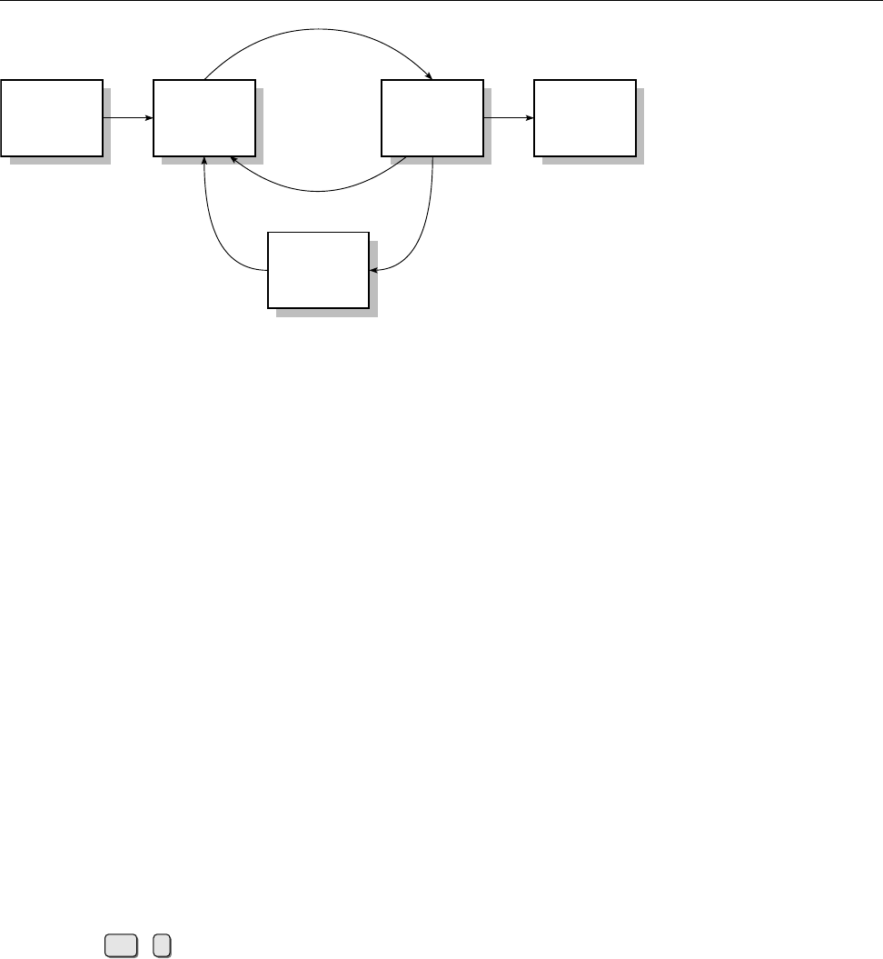
13.2 Process States 193
Process
is
created
runnable operating Process
terminates
sleeping
Figure 13.1: The relationship between various process states
Exercises
C13.1 [3] How can you view the environment variables of any of your pro-
cesses? (Hint:
/proc
le system.)
C13.2 [2] (For programmers.) What is the maximum possible PID? What hap-
pens when this limit is reached? (Hint: Look for the string “
PID_MAX
” in the
les below
/usr/include/linux
.)
13.2 Process States
Another important property of a process is its process state. A process in mem- process state
ory waits to be executed by the CPU. This state is called “runnable”. Linux uses
pre-emptive multitasking, i. e., a scheduler distributes the available CPU time to pre-emptive multitasking
waiting processes in pieces called “time slices”. If a process is actually execut-
ing on the CPU, this state is called “operating”, and after its time slice is over the
process reverts to the “runnable” state.
BFrom an external point of view, Linux does not distinguish between these
two process states; the process in question is always marked “runnable”.
It is quite possible that a process requires further input or needs to wait for
peripheral device operations to complete; such a process cannot be assigned CPU
time, and its state is considered to be “sleeping”. Processes that have been stopped
by means of Ctrl +zusing the shell’s job control facility are in state “stopped”.
Once the execution of a process is over, it terminates itself and makes a return return code
code available, which it can use to signal, for example, whether it completed suc-
cessfully or not (for a suitable denition of “success”).
Once in a while processes appear who are marked as zombies using the “Z” zombies
state. These “living dead” usually exist only for a brief instant. A process becomes
a zombie when it nishes and dies for good once its parent process has queried
its return code. If a zombie does not disappear from the process table this means
that its parent should really have picked up the zombie’s return code but didn’t.
A zombie cannot be removed from the process table. Because the original pro-
cess no longer exists and cannot take up neither RAM nor CPU time, a zombie
has no impact on the system except for an unattractive entry in the system state.
Persistent or very numerous zombies usually indicate programming errors in the
parent process; when the parent process terminates they should do so as well.
BZombies disappear when their parent process disappears because “or-
phaned” processes are “adopted” by the init process. Since the init process

194 13 Process Management
spends most of its time waiting for other processes to terminate so that it
can collect their return code, the zombies are then disposed of fairly quickly.
BOf course, zombies take up room in the process table that might be required
for other processes. If that proves a problem, look at the parent process.
Exercises
C13.3 [2] Start a
xclock
process in the background. In the
$!
shell variable you
will nd the PID of that process (it always contains the PID of the most re-
cently launched background process). Check the state of that process by
means of the “
grep ^State: /proc/$!/status
” command. Stop the
xclock
by
moving it to the foreground and stopping it using Ctrl +z. What is the
process state now? (Alternatively, you may use any other long-running pro-
gram in place of
xclock
.)
C13.4 [4] (When going over this manual for the second time.) Can you create
a zombie process on purpose?
13.3 Process Information—
ps
You would normally not access the process information in
/proc
directly but use
the appropriate commands to query it.
The
ps
(“process status”) command is available on every Unix-like system.
Without any otions, all processes running on the current terminal are output. The
resulting list contains the process number
PID
, the terminal
TTY
, the process state
STAT
, the CPU time used so far
TIME
and the command being executed.
$ps
PID TTY STAT TIME COMMAND
997 1 S 0:00 -bash
1005 1 R 0:00 ps
$ _
There are two processes currently executing on the
tty1
terminal: Apart from the
bash
with PID 997, which is currently sleeping (state “
S
”), a
ps
command is executed
using PID 1005 (state “
R
”). The “operating” state mentioned above is not being
displayed in
ps
output.
The syntax of
ps
is fairly confusing. Besides Unix98-style options (like
-l
) and
GNU-style long options (such as
--help
), it also allows BSD-style options without
a leading dash. Here is a selection out of all possible parameters:
a
(“all”) displays all processes with a terminal
--forest
displays the process hierarchy
l
(“long”) outputs extra information such as the priority
r
(“running”) displays only runnable processes
T
(“terminal”) displays all processes on the current terminal
U
⟨name⟩(“user”) displays processes owned by user ⟨name⟩
x
also displays processes without a terminal
BThe unusual syntax of
ps
derives from the fact that AT&T’s
ps
traditionally
used leading dashes on options while BSD’s didn’t (and the same option
can have quite dierent results in both avours). When the big reunication
came in System V Release 4, one could hang on to most options with their
customary meaning.

13.4 Processes in a Tree—
pstree
195
If you give
ps
a PID, only information pertaining to the process in question will
be displayed (if it exists):
$ps 1
PID TTY STAT TIME COMMAND
1 ? Ss 0:00 init [2]
With the
-C
option,
ps
displays information about the process (or processes) based
on a particular command:
$ps -C konsole
PID TTY TIME CMD
4472 ? 00:00:10 konsole
13720 ? 00:00:00 konsole
14045 ? 00:00:14 konsole
(Alternatively,
grep
would help here as well.)
Exercises
C13.5 [!2] What does the information obtainable with the
ps
command mean?
Invoke
ps
without an option, then with the
a
option, and nally with the
ax
option. What does the
x
option do?
C13.6 [3] The
ps
command allows you to determine the output format your-
self by means of the
-o
option. Study the
ps
(1) manual page and specify a
ps
command line that will output the PID, PPID, the process state and the
command.
13.4 Processes in a Tree—
pstree
If you do not want to obtain every bit of information about a process but are rather
interested in the relationships between processes, the
pstree
command is helpful.
pstree
pstree
displays a process tree in which the child processes are shown as depending
on their parent process. The processes are displayed by name:
$pstree
init-+-apache---7*[apache]
|-apmd
|-atd
|-cannaserver
|-cardmgr
|-chronyd
|-cron
|-cupsd
|-dbus-daemon-1
|-events/0-+-aio/0
| |-kblockd/0
| `-2*[pdflush]
|-6*[getty]
|-ifd
|-inetd
|-kapmd
|-kdeinit-+-6*[kdeinit]
| |-kdeinit-+-bash---bash
| | |-2*[bash]
| | |-bash---less

196 13 Process Management
| | |-bash-+-pstree
| | | `-xdvi---xdvi.bin---gs
| | `-bash---emacs---emacsserver
| |-kdeinit---3*[bash]
| |-kteatime
| `-tclsh
|-10*[kdeinit]
|-kdeinit---kdeinit
Identical processes are collected in brackets and a count and “*” are displayed.
The most important options of
pstree
include:
-p
displays PIDs along with process names
-u
displays process owners’ user name
-G
makes the display prettier by using terminal graphics characters—whether this
is in fact an improvement depends on your terminal
BYou can also obtain an approximated tree structure using “
ps --forest
”. The
tree structure is part of the
COMMAND
column in the output.
13.5 Controlling Processes—
kill
and
killall
The
kill
command sends signals to selected processes. The desired signal can besignals
specied either numerically or by name; you must also pass the process number
in question, which you can nd out using
ps
:
$kill -15 4711
Send signal
SIGTERM
to process 4711
$kill -TERM 4711
Same thing
$kill -SIGTERM 4711
Same thing again
$kill -s TERM 4711
Same thing again
$kill -s SIGTERM 4711
Same thing again
$kill -s 15 4711
Guess what
Here are the most important signals with their numbers and meaning:
SIGHUP
(1, “hang up”) causes the shell to terminate all of its child processes that
use the same controlling terminal as itself. For background processes with-
out a controlling terminal, this is frequently used to cause them to re-read
their conguration les (see below).
SIGINT
(2, “interrupt”) Interrupts the process; equivalent to the Ctrl +ckey com-
bination.
SIGKILL
(9, “kill”) Terminates the process and cannot be ignored; the “emergency
brake”.
SIGTERM
(15, “terminate”) Default for
kill
and
killall
; terminates the process.
SIGCONT
(18, “continue”) Lets a process that was stopped using
SIGSTOP
continue.
SIGSTOP
(19, “stop”) Stops a process temporarily.
SIGTSTP
(20, “terminal stop”) Equivalent to the Ctrl +zkey combination.
AYou shouldn’t get hung up on the signal numbers, which are not all guaran-
teed to be the same on all Unix versions (or even Linux platforms). You’re
usually safe as far as 1, 9, or 15 are concerned, but for everything else you
should rather be using the names.

13.6
pgrep
and
pkill
197
Unless otherwise specied, the signal
SIGTERM
(“terminate”) will be sent, which
(usually) ends the process. Programs can be written such that they “trap” signals
(handle them internally) or ignore them altogether. Signals that a process neither
traps nor ignores usually cause it to crash hard. Some (few) signals are ignored
by default.
The
SIGKILL
and
SIGSTOP
signals are not handled by the process but by the kernel
and hence cannot be trapped or ignored.
SIGKILL
terminates a process without
giving it a chance to object (as
SIGTERM
would), and
SIGSTOP
stops the process such
that it is no longer given CPU time.
kill
does not always stop processes. Background processes which provide sys-
tem services without a controlling terminal—daemons—usually reread their con- daemons
guration les without a restart if they are sent
SIGHUP
(“hang up”).
You can apply
kill
, like many other Linux commands, only to processes that
you actually own. Only
root
is not subject to this restriction.
Sometimes a process will not even react to
SIGKILL
. The reason for this is ei-
ther that it is a zombie (which is already dead and cannot be killed again) or else
blocked in a system call. The latter situation occurs, for example, if a process waits
for a write or read operation on a slow device to nish.
An alternative to the
kill
command is the
killall
command.
killall
acts just
killall
like
kill
—it sends a signal to the process. The dierence is that the process must
be named instead of addressed by its PID, and that all processes of the same name
are signalled. If no signal is specied, it sends
SIGTERM
by default (like
kill
).
killall
outputs a warning if there was nothing to signal to under the specied name.
The most important options for
killall
include:
-i killall
will query you whether it is actually supposed to signal the process in
question.
-l
outputs a list of all available signals.
-w
waits whether the process that was signalled actually terminates.
killall
checks every second whether the process still exists, and only terminates
once it is gone.
ABe careful with
killall
if you get to use Solaris or BSD every now and then.
On these systems, the command does exactly what its name suggests—it
kills all processes.
Exercises
C13.7 [2] Which signals are being ignored by default? (Hint:
signal
(7))
13.6
pgrep
and
pkill
As useful as
ps
and
kill
are, as dicult can it be sometimes to identify exactly the
right processes of interest. Of course you can look through the output of
ps
using
grep
, but to make this “foolproof” and without allowing too many false positives
is at least inconvenient, if not tricky. Nicely enough, Kjetil Torgrim Homme has
taken this burden o us and developed the
pgrep
program, which enables us to
search the process list conveniently. A command like
$pgrep -u root sshd
will, for example, list the PIDs of all
sshd
processes belonging to
root
.
BBy default,
pgrep
restricts itself to outputting PIDs. Use the
-l
option to get it
to show the command name, too. With
-a
it will list the full command line.
BThe
-d
option allows you to specify a separator (the default is “
\n
”):

198 13 Process Management
$pgrep -d, -u hugo bash
4261,11043,11601,12289
You can obtain more detailed information on the processes by feeding the
PIDs to
ps
:
$ps up $(pgrep -d, -u hugo bash)
(The
p
option lets you give
ps
a comma-separated list of PIDs of interest.)
pgrep
’s parameter is really an (extended) regular expression (consider
egrep
)
which is used to examine the process names. Hence something like
$pgrep '^([bd]a|t?c|k|z|)sh$'
will look for the common shells.
BNormally
pgrep
considers only the process name (the rst 15 characters of the
process name, to be exact). Use the
-f
option to search the whole command
line.
You can add search criteria by means of options. Here is a small selection:
-G
Consider only processes belonging to the given group(s). (Groups can be spec-
ied using names or GIDs.)
-n
Only display the newest (most recently started) of the found processes.
-o
Only display the oldest (least recently started) of the found processes.
-P
Consider only processes whose parent processes have one of the given PIDs.
-t
Consider only processes whose controlling terminal is listed. (Terminal names
should be given without the leading “
/dev/
”.)
-u
Consider only processes with the given (eective) UIDs.
BIf you specify search criteria but no regular expression for the process name,
all processes matching the search criteria will be listed. If you omit both you
will get an error message.
The
pkill
command behaves like
pgrep
, except that it does not list the found
processes’ PIDs but sends them a signal directly (by default,
SIGTERM
). As in
kill
you can specify another signal:
#pkill -HUP syslogd
The
--signal
option would also work:
#pkill --signal HUP syslogd
BThe advantage of
pkill
compared to
killall
is that
pkill
can be much more
specic.
Exercises
C13.8 [!1] Use
pgrep
to determine the PIDs of all processes belonging to user
hugo
. (If you don’t have a user
hugo
, then specify some other user instead.)
C13.9 [2] Use two separate terminal windows (or text consoles) to start one
“
sleep 60
” command each. Use
pkill
to terminate (a) the rst command
started, (b) the second command started, (c) the command started in one
of the two terminal windows.

13.7 Process Priorities—
nice
and
renice
199
13.7 Process Priorities—
nice
and
renice
In a multi-tasking operating system such as Linux, CPU time must be shared
among various processes. This is the scheduler’s job. There is normally more
than one runnable process, and the scheduler must allot CPU time to runnable
processes according to certain rules. The deciding factor for this is the priority priority
of a process. The priority of a process changes dynamically according to its prior
behaviour—“interactive” processes, i. e, ones that do I/O, are favoured over those
that just consume CPU time.
As a user (or administrator) you cannot set process priorities directly. You can
merely ask the kernel to prefer or penalise processes. The “nice value” quanties
the degree of favouritism exhibited towards a process, and is passed along to child
processes.
A new process’s nice value can be specied with the
nice
command. Its syntax
nice
is
nice
[
-
⟨nice value⟩] ⟨command⟩ ⟨parameter⟩
…
(
nice
is used as a “prex” for another command).
The possible nice values are numbers between −20 and +19. A negative nice possible nice values
value increases the priority, a positive value decreases it (the higher the value, the
“nicer” you are towards the system’s other users by giving your own processes a
lower priority). If no nice value is specied, the default value of +10 is assumed.
Only
root
may start processes with a negative nice value (negative nice value are
not generally nice for other users).
The priority of a running process can be inuenced using the
renice
command.
renice
You call
renice
with the desired new nice value and the PID (or PIDs) of the pro-
cess(es) in question:
renice
[
-
⟨nice value⟩] ⟨PID⟩
…
Again, only the system administrator may assign arbitrary nice values. Normal
users may only increase the nice value of their own processes using
renice
—for
example, it is impossible to revert a process started with nice value 5back to nice
value 0, while it is absolutely all right to change its nice value to 10. (Think of a
ratchet.)
Exercises
C13.10 [2] Try to give a process a higher priority. This may possibly not
work—why? Check the process priority using
ps
.
13.8 Further Process Management Commands—
nohup
and
top
When you invoke a command using
nohup
, that command will ignore a
SIGHUP
sig- Ignoring
SIGHUP
nal and thus survive the demise of its parent process:
nohup
⟨command⟩
…
The process is not automatically put into the background but must be placed there
by appending a
&
to the command line. If the program’s standard output is a ter-
minal and the user has not specied anything else, the program’s output together
with its standard error output will be redirected to the
nohup.out
le. If the current
directory is not writable for the user, the le is created in the user’s home directory
instead.

200 13 Process Management
top
unies the functions of many process management commands in a single
top
program. It also provides a process table which is constantly being updated. You
can interactively execute various operations; an overview is available using h.
For example, it is possible to sort the list according to several criteria, send signals
to processes ( k), or change the nice value of a process ( r).
Commands in this Chapter
kill
Terminates a background process
bash
(1),
kill
(1) 196
killall
Sends a signal to all processes matching the given name
killall
(1) 197
nice
Starts programs with a dierent nice value
nice
(1) 199
nohup
Starts a program such that it is immune to
SIGHUP
signals
nohup
(1) 199
pgrep
Searches processes according to their name or other criteria
pgrep
(1) 197
pkill
Signals to processes according to their name or other criteria
pkill
(1) 198
ps
Outputs process status information
ps
(1) 194
pstree
Outputs the process tree
pstree
(1) 195
renice
Changes the nice value of running processes
renice
(8) 199
top
Screen-oriented tool for process monitoring and control
top
(1) 199
Summary
• A process is a program that is being executed.
• Besides a program text and the corresponding data, a process has attributes
such as a process number (PID), parent process number (PPID), owner,
groups, priority, environment, current directory, …
• All processes derive from the
init
process (PID 1).
•
ps
can be used to query process information.
• The
pstree
command shows the process hierarchy as a tree.
• Processes can be controlled using signals.
• The
kill
and
killall
commands send signals to processes.
• The
nice
and
renice
commands are used to inuence process priorities.
ulimit
limits the resource usage of a process.
•
top
is a convenient user interface for process management.

$ echo tux
tux
$ ls
hallo.c
hallo.o
$ /bin/su -
Password:
14
Hard Disks (and Other Secondary
Storage)
Contents
14.1 Fundamentals . . . . . . . . . . . . . . . . . . . . . 202
14.2 Bus Systems for Mass Storage . . . . . . . . . . . . . . . 202
14.3 Partitioning . . . . . . . . . . . . . . . . . . . . . . 205
14.3.1 Fundamentals . . . . . . . . . . . . . . . . . . . 205
14.3.2 The Traditional Method (MBR) . . . . . . . . . . . . . 206
14.3.3 The Modern Method (GPT) . . . . . . . . . . . . . . 207
14.4 Linux and Mass Storage . . . . . . . . . . . . . . . . . 208
14.5 Partitioning Disks. . . . . . . . . . . . . . . . . . . . 210
14.5.1 Fundamentals . . . . . . . . . . . . . . . . . . . 210
14.5.2 Partitioning Disks Using
fdisk
.............212
14.5.3 Formatting Disks using GNU
parted
...........215
14.5.4
gdisk
......................216
14.5.5 More Partitioning Tools . . . . . . . . . . . . . . . 217
14.6 Loop Devices and
kpartx
.................217
14.7 The Logical Volume Manager (LVM) . . . . . . . . . . . . . 219
Goals
• Understanding how Linux deals with secondary storage devices based on
ATA, SATA, and SCSI.
• Understanding MBR-based and GPT-based partitioning
• Knowing about Linux partitioning tools and how to use them
• Being able to use loop devices
Prerequisites
• Basic Linux knowledge
• Knowledge about Linux hardware support
adm1-platten.tex
(
33e55eeadba676a3
)

202 14 Hard Disks (and Other Secondary Storage)
14.1 Fundamentals
RAM is fairly cheap these days, but even so not many computers can get by with-
out the permanent storage of programs and data on mass storage devices. These
include (among others):
• Hard disks with rotating magnetic platters
• “Solid-state disks” (SSDs) that look like hard disks from the computer’s
point of view, but use ash memory internally
• USB thumb drives, SD cards, CF cards, and other interchangeable media
based on ash memory
• RAID systems that aggregate hard disks and present them as one big storage
medium
• SAN devices which provide “virtual” disk drives on the network
• File servers that oer le access at an abstract level (CIFS, NFS, …)
In this chapter we shall explain the basics of Linux support for the rst three en-
tries in the list—hard disks, SSDs and ash-based portable media like USB thumb
drives. RAID sstems and SAN are discussed in the Linup Front training man-
ual, Linux Storage and File Systems, le servers are discussed in Linux Infrastructure
Services.
14.2 Bus Systems for Mass Storage
IDE, ATA and SATA Until not so long ago, hard disks and optical drives such
as CD-ROM and DVD readers and writers used to be connected via a “IDE con-IDE
troller”, of which self-respecting PCs had at least two (with two “channels” each).
B“IDE” is really an abbreviation of “Integrated Drive Electronics”. The “inte-
grated drive electronics” alluded to here lets the computer see the disk as a
sequence of numbered blocks without having to know anything about sec-
tors, cylinders, and read/write heads, even though this elaborate charade
is still kept up between the BIOS, disk controller, and disks. However, for a
long time this description has applied to all hard disks, not just those with
the well-known “IDE” interface, which by now is ocially called “ATA”,
short for “AT Attachment”1.
Computers bought new these days usually still contain IDE interfaces, but the
method of choice to connect hard disks and optical drives today is a serial ver-
sion of the ATA standard, imaginatively named “Serial ATA” (SATA, for short).Serial ATA
Since SATA (i. e., approximately 2003), traditional ATA (or “IDE”) is commonly
called “P-ATA”, an abbreviation of “parallel ATA”. The dierence applies to the
cable, which for traditional ATA is an inconvenient-to-place and electrically not
100% fortunate 40- or 80-lead ribbon cable which can transfer 16 data bits in par-
allel, and which links several devices at once to the controller. SATA, on the other
hand, utilises narrow at seven-lead cables for serial transmission, one per device
(usually produced in a cheerful orange colour).
BSATA cables and connectors are much more sensitive mechanically than the
corresponding P-ATA hardware, but they make up for that through other
advantages: They are less of an impediment to air ow in a PC case, cannot
be installed wrongly due to their dierent connectors on each end, which
furthermore cannot be plugged in the wrong way round. In addition, the il-
logical separation between 2.5-inch and 3.5-inch diskdrives, which required
dierent connectors for P-ATA, goes away.
1Anyone remember the IBM PC/AT?

14.2 Bus Systems for Mass Storage 203
BInterestingly, serial ATA allows considerably faster data transfers than tra-
ditional ATA, even though with the former all bits are transferred in “single
le” rather than 16 at a go in parallel. This is due to the electrical proper-
ties of the interface, which uses dierential transmission and a signalling
voltage of only 0.5 V instead of 5 V. (This is why cables may be longer, too—
1 m instead of formerly 45 cm.) Current SATA interfaces can theoretically
transfer up to 16 GiBit/s (SATA 3.2) which due to encoding and other im-
pediments comes out as approximately 2 MiB/s—rather more than single
disk drives can keep up with at sustained rates, but useful for RAID sys-
tems that access multiple disk drives at the same time, and for fast SSDs. It
is unlikely that SATA speeds will evolve further, since the trend with SSDs
is towards connecting them directly via PCIe2.
BBesides the higher speed and more convenient cabling, SATA also oers
the advantage of “hot-swapping”: It is possible to disconnect a SATA disk
drive and connect another one in its place, without having to shut down the
computer. This of course presupposes that the computer can do without
the data on the drive in question—typically because it is part of a RAID-1
or RAID-5, where the the data on the new drive can be reconstructed based
on other drives in the system. With traditional ATA, this was impossible (or
only possible by jumping through hoops).
BExternal SATA (“eSATA”) is a derivative of SATA for use with external eSATA
drives. It has dierent connectors and electrical specications, which are
much more robust mechanically and better suited for hot-swapping. In
the meantime, it has been almost completely ousted from the market by
USB 3.𝑥, but can still be found in older hardware.
SCSI and SAS The “Small Computer System Interface” or SCSI (customary pro-
nunciation: “SCUZ-zy”) has served for more than 25 years to connect hard disks,
tape drives and other mass storage devices, but also peripherals such as scanners,
to “small” computers3. SCSI buses and connectors exist in a confusing variety,
beginning with the “traditional” 8-bit bus and ranging from the fast 16-bit vari-
eties to new, even faster serial implementations (see below). They also dier in
the maximum number of devices per bus, and in physical parameters such as the
maximum cable length and the allowable distances between devices on the cable.
Nicely enough, most of the variants are compatible or can be made compatible
(possibly with loss of eciency!). Varieties such as FireWire (IEEE-1394) or Fiber-
Channel are treated like SCSI by Linux.
BNowadays, most work goes into the serial SCSI implementations, most no-
tably “Serial Attached SCSI” (SAS). As with SATA, data transfer is poten-
tially faster (at the moment, SAS is slightly slower than the fastest parallel
SCSI version, Ultra-640 SCSI) and electrically much less intricate. In partic-
ular, the fast parallel SCSI versions are plagued by clocking problems that
derive from the electrical properties of the cables and termination, and that
do not exist with SAS (where the pesky termination is no longer necessary
at all).
BSAS and SATA are fairly closely related; the most notable dierences are that
SAS allows things like accessing a drive via several cable paths for redun-
dancy (“multipath I/O”; SATA requires jumping through hoops for this),
supports more extensive diagnosis and logging functions, and is based on
a higher signalling voltage, which allows for longer cables (up to 8 m) and
physically larger servers.
2SATA in a strict sense allows speeds up to 6 GiBit/s; the higher speed of SATA 3.2 is already
achieved by means of PCIe. This “SATA Express” specication denes an interface that can carry
SATA signals as well as PCIe, such that compatible devices can be connected not only to SATA Express
controllers, but also to older hosts which support “only” SATA with up to 6 GiBit/s.
3Nobody has ever dened the meaning of “small” in this context, but it must be something like
“can be bodily lifted by at most two people”

204 14 Hard Disks (and Other Secondary Storage)
Table 14.1: Dierent SCSI variants
Name Width Transfer rate Devices Explanation
SCSI-1 8 bit ≤ 5 MiB/s 8 “Ancestor”
SCSI-2 »Fast« 8 bit 10 MiB/s 8
SCSI-2 »Wide« 16 bit 20 MiB/s 16
SCSI-3 »Ultra« 8 bit 20 MiB/s 8
SCSI-3 »Ultrawide« 16 bit 40 MiB/s 16
Ultra2 SCSI 16 bit 80 MiB/s 16 LVD busa
Ultra-160 SCSIb16 bit 160 MiB/s 16 LVD bus
Ultra-320 SCSIc16 Bit 320 MiB/s 16 LVD bus
Ultra-640 SCSI 16 Bit 640 MiB/s 16 LVD bus
BSATA and SAS are compatible to an extent where you can use SATA disk
drives on a SAS backplane (but not vice-versa).
“Pure-bred” SCSI, as far as PCs are concerned, is found mostly in servers; workVorkommen
stations and “consumer PCs” tend to use IDE or SATA for mass storage and USB
for other devices. Devices based on IDE and USB are much cheaper to manu-
facture than SCSI-based devices—IDE disks, for example, cost about a third or a
fourth of the price of comparatively large SCSI disks.
BWe do need to mention that SCSI disks are usually designed especially for
use in servers, and are therefore optimised for high speed and longevity.
SATA disks for workplace PCs do not come with the same warranties, are
not supposed to rival a jet ghter for noise, and should support fairly fre-
quent starting and stopping.
As a Linux administrator, you should know about SCSI even if you do not run
any SCSI-based systems, since from the point of view of the Linux kernel, in ad-
dition to SATA many USB or FireWire devices are accessed like SCSI devices and
use the same infrastrucure.
BEvery device on a SCSI bus requires a unique “SCSI ID”. This numberSCSI ID
between 0 and 7 (15 on the wide buses) is used to address the device.
Most “true” SCSI devices sport jumpers or a switch to select it; with Fibre-
Channel, USB, or SATA devices that are accessed via the SCSI infrastructure,
the system arranges for suitable unique SCSI IDs to be assigned.
BTo use SCSI, a PC needs at least one host adapter (or “host”). Motherboard-host adapter
based and better expansion card host adapters contain a SCSI BIOS which
SCSI BIOS lets the system boot from a SCSI device. You can also use this to check which
SCSI IDs are available and which are used, and which SCSI device, if any,
should be used for booting.
BThe host adapter counts as a device on the SCSI bus—apart from itself you
can connect 7 (or 15) other devices.
BIf your BIOS can boot from SCSI devices, you can also select in the boot orderboot order
whether the ATA disk
C:
should be preferred to any (potentially) bootable
SCSI devices.
BMost important for the correct function of a parallel SCSI system is appro-
priate termination of the SCSI bus. This can either be ensured via a specialtermination
plug (“terminator”) or switched on or o on individual devices. Erroneous
termination is the possible origin of all sorts of SCSI problems. If you do
experience diculties with SCSI, always check rst that termination is in
order. SAS does not require termination.

14.3 Partitioning 205
USB With the new fast USB variants, few if any compromises will be needed
when connecting mass storage devices—reading and writing speeds are bounded
by the storage device, not (as with USB 1.1 and USB 2.0) by the bus. Linux manages
USB-based storage devices exactly like SCSI devices.
Exercises
C14.1 [1] How many hard disks or SSDs does your computer contain? What
is their capacity? How are they connected to the computer (SATA, …)?
14.3 Partitioning
14.3.1 Fundamentals
Mass storage devices such as hard disks or SSDs are commonly “partitioned”, i. e.,
subdivided into several logical storage devices that the operating system can then
access independently. This does not only make it easier to use data structures that
are appropriate to the intended use—sometimes partitioning is the only way to
make a very large storage medium fully accessible, if limits within the operating
system preclude the use of the medium “as a whole” (even though this sort of
problem tends to be rare today).
Advantages of partitioning include the following:
• Logically separate parts of the system may be separated. For example, you
could put your users’ data on a dierent partition from that used by the op-
erating system itself. This makes it possible to reinstall the operating system
from scratch without endangering your users’ data. Given the often rudi-
mentary “upgrade” functionality of even current distributions this is very
important. Furthermore, if inconsistencies occur in a le system then only
one partition may be impacted at rst.
• The structure of the le system may be adapted to the data to be stored.
Most le systems keep track of data by means of xed-size “blocks”, where
every le, no matter how small, occupies at least a single block. With a 4 KiB
block size this implies that a 500-byte le only occupies 1/8 of its block—the
rest goes to waste. If you know that a directory will contain mostly small
les (cue: mail server), it may make sense to put this directory on a parti-
tion using smaller blocks (1 or 2 KiB). This can reduce waste considerably.
Some database servers, on the other hand, like to work on “raw” partitions
(without any le system) that they manage themselves. An operating sys-
tem must make that possible, too.
• “Runaway” processes or incautious users can use up all the space available
on a le system. At least on important server systems it makes sense to
allow user data (including print jobs, unread e-mail, etc.) only on partitions
that may get lled up without getting the system itself in trouble, e.g., by
making it impossible to append information to important log les.
There are currently two competing methods to partition hard disks for PCs.
The traditional method goes back to the 1980s when the rst hard disks (with
awesome sizes like 5 or 10 MB) appeared. Recently a more modern method was
introduced; this does away with various limitations of the traditional approach,
but in some cases requires special tools.
BHard disks are virtually always partitioned, even though at times only one
partition will be created. With USB thumb drives, one sometimes eschews
partitioning altogether.

206 14 Hard Disks (and Other Secondary Storage)
Table 14.2: Partition types for Linux (hexadecimal)
Type Description
81
Linux data
82
Linux swap space
86
RAID super block (old style)
8E
Linux LVM
E8
LUKS (encrypted partition)
EE
“Protective partition” for GPT-partitioned disk
FD
RAID super block with autodetection
FE
Linux LVM (old style)
14.3.2 The Traditional Method (MBR)
The traditional method stores partitioning information inside the “master boot
record” (MBR), the rst sector (number 0) of a hard disk. (Traditionally, PC hard
disk sectors are 512 bytes long, but see below.) The space there—64 bytes starting
at oset 446—is sucient for four primary partitions. If you want to create moreprimary partitions
than four partitions, you must use one of these primary partitions as an extended
extended partition
partition. An extended partition may contain further logical partitions.
logical partitions
BThe details about logical partitions are not stored inside the MBR, but at the
start of the partition (extended or logical) in question, i. e., they are scattered
around the hard disk.
Partition entries today usually store the starting sector number of the partition on
the disk as well as the length of the partition in question in sectors4. Since these
values are 32-bit numbers, given the common 512-byte sectors this results in a
maximum partition size of 2 TiB.
BThere are hard disks available today which are larger than 2 TiB. Such disks
cannot be made fully accessible using MBR partitioning. One common ruse
consists in using disks whose sectors are 4096 bytes long instead of 512. This
will let you have 16-TiB disks even with MBR, but not every operating sys-
tem supports such “4Kn” drives (Linux from kernel 2.6.31, Windows from
8.1 or Server 2012).
B4-KiB sectors are useful on hard disks even without considering partitions.
The larger sectors are more ecient for storing larger les and allow better
error correction. Therefore the market oers “512e” disks which use 4-KiB
sectors internally but pretend to the outside that they really have 512-byte
sectors. This means that if a single 512-byte sector needs to be rewritten, the
adjoining 7 sectors must be read and also rewritten (a certain, but usually
bearable, loss of eciency, since data is most often written in larger chunks).
When partitioning, you will have to pay attention that the 4-KiB blocks that
Linux uses internally for hard disk access coincide with the disk’s internal
4-KiB sectors—if that is not the case, then to write one 4-KiB Linux block two
4-KiB disk sectors might have to be read and rewritten, and that would not
be good. (Fortunately, the partitioning tools help you watch out for this.)
Besides the starting address and length of the (primary) partitions, the parti-
tion table contains a partition type which loosely describe the type of data man-partition type
agement structure that might appear on the partition. A selection of Linux parti-
tion types appears in Table 14.2.
4In former times, partitions used to be described in terms of the cylinder, head, and sector addresses
of the sectors in question, but this has been deprecated for a very long time.

14.3 Partitioning 207
14.3.3 The Modern Method (GPT)
In the late 1990s, Intel developed a new partitioning method that should do away
with the limitations of the MBR approach, namely “GUID Partition Table” or GPT.
BGPT was developed hand-in-hand with UEFI and is part of the UEFI spec-
ication today. You can, however, use a BIOS-based Linux system to access
GPT-partitioned disks and vice-versa.
BGPT uses 64-bit sector addresses and thus allows a maximum disk size of
8 ZiB—zebibyte, in case you haven’t run into that prex. 1 ZiB are 270 bytes,
or, roughly speaking, about one million million tebibytes. This should last
even the NSA for a while. (Disk manufactures, who prefer to talk powers of
ten rather than powers of two, will naturally sell you an 8-ZiB disk as a 9.4
zettabyte disk.)
With GPT, the rst sector of the disk remains reserved as a “protective MBR”
which designates the whole disk as partitioned from a MBR point of view. This
avoids problems if a GPT-partitioned disk is connected to a computer that can’t
handle GPT.
The second sector (address 1) contains the “GPT header” which stores man-
agement information for the whole disk. Partitioning information is usually con-
tained in the third and subsequent sectors.
BThe GPT header points to the partitioning information, and therefore they
could be stored anywhere on the disk. It is, however, reasonable to place
them immediately after the GPT header. The UEFI header stipulates a min-
imum of 16 KiB for partitioning information (regardless of the disk’s sector
size).
BOn a disk with 512-byte sectors, with a 16 KiB space for partitioning infor-
mation the rst otherwise usable sector on the disk is the one at address 34.
You should, however, avoid placing the disk’s rst partition at that address
because that will get you in trouble with 512e disks. The next correctly-
aligned sector is the one at address 40.
BFor safety reasons, GPT replicates the partitioning information at the end of
the disk.
Traditionally, partition boundaries are placed at the start of a new “track” on
the disk. Tracks, of course, are a relic from the hard disk paleolithic, since con-
temporary disks are addressed linearly (in other words, the sectors are numbered
consecutively from the start of the disk to the end)—but the idea of describing a
disk by means of a combination of a number of read/write heads, a number of
“cylinders”, and a number of sectors per “track” (a track is the concentric circle a
single head describes on a given cylinder) has continued to be used for a remark-
ably long time. Since the maximum number of sectors per track is 63, this means
that the rst partition would start at block 63, and that is, of course, disastrous for
512e disks.
BSince Windows Vista it is common to have the rst partition start 1 MiB after
the start of the disk (with 512-byte sectors, at sector 2048). This isn’t a bad
idea for Linux, either, since the ample free space between the partition table
and the rst partition can be used to store the GRUB boot loader. (The space
between the MBR and sector 63 was quite sucient earlier, too.)
Partition table entries are at least 128 bytes long and, apart from 16-byte GUIDs
for the partition type and the partition itself and 8 bytes each for a starting and
ending block number, contains 8 bytes for “attributes” and 72 bytes for a partition
name. It is debatable whether 16-byte GUIDs are required for partition types, but
on the one hand the scheme is called “GUID partition table” after all, and on the
other hand this ensures that we won’t run out of partition types anytime soon. A
selection is displayed in Table 14.3.

208 14 Hard Disks (and Other Secondary Storage)
GUID Description
00000000-0000-0000-0000-000000000000
Unused entry
C12A7328-F81F-11D2-BA4B-00A0C93EC93B
EFI system partition (ESP)
21686148-6449-6E6F-744E-656564454649
BIOS boot partition
0FC63DAF-8483-4772-8E79-3D69D8477DE4
Linux le system
A19D880F-05FC-4D3B-A006-743F0F84911E
Linux RAID partition
0657FD6D-A4AB-43C4-84E5-0933C84B4F4F
Linux swap space
E6D6D379-F507-44C2-A23C-238F2A3DF928
Linux LVM
933AC7E1-2EB4-4F13-B844-0E14E2AEF915 /home
partition
3B8F8425-20E0-4F3B-907F-1A25A76F98E8 /srv
partition
7FFEC5C9-2D00-49B7-8941-3EA10A5586B7 dm-crypt
partition
CA7D7CCB-63ED-4C53-861C-1742536059CC
LUKS partition
Table 14.3: Partition type GUIDs for GPT (excerpt)
BLinux can use GPT-partitioned media. This needs the “EFI GUID Partition
support” option enabled in the kernel, but with current distributions this
is the case. Whether the installation procedure allows you to create GPT-
partitioned disks is a dierent question, just like the question of whether
the boot loader will be able to deal with them. But that is neither here nor
there.
14.4 Linux and Mass Storage
If a mass storage device is connected to a Linux computer, the Linux kernel tries
to locate any partitions. It then creates block-oriented device les in
/dev
for the
device itself and its partitions. You can subsequently access the partitions’ device
les and make the directory hierarchies there available as part of the computer’s
le system.
BA new mass storage device may have no partitions at all. In this case you
can use suitable tools to create partitions. This will be explained later in this
chapter. The next step after partitioning consists of generating le systems
on the partitions. This is explained in detail in Chapter 15.
The device names for mass storage are usually
/dev/sda
,
/dev/sdb
, …, in the order
the devices are recognised. Partitions are numbered, the
/dev/sda
device therefore
contains partitions like
/dev7sda1
,
/dev/sda2
, … A maximum of 15 partitions per de-
vice is possible. If
/dev/sda
is partitioned according to the MBR scheme,
/dev/sda1
to
/dev/sda4
correspond to the primary partitions (possibly including an extended
partition), while any logical partitions are numbered starting with
/dev/sda5
(re-
gardless of whether there are four primary partitions on the disk or fewer).
BThe “
s
” in
/dev/sda
derives from “SCSI”. Today, almost all mass storage de-
vices in Linux are managed as SCSI devices.
BFor P-ATA disks there is another, more specic mechanism. This accesses
the IDE controllers inside the computer directly—the two drives connected
to the rst controller are called
/dev/hda
and
/dev/hdb
, the ones connected to
the second
/dev/hdc
and
/dev/hdd
. (These names are used independently of
whether the drives actually exist or not—if you have a single hard disk and
a CD-ROM drive on your system, you do well to connect the one to one
controller and the other to the other so they will not be in each other’s way.
Therefore you will have
/dev/hda
for the disk and
/dev/hdc
for the CD-ROM
drive.) Partitions on P-ATA disks are, again, called
/dev/hda1
,
/dev/hda2
and
so on. In this scheme, 63 (!) partitions are allowed.

14.4 Linux and Mass Storage 209
BIf you still use a computer with P-ATA disks, you will notice that in the
vast majority of cases the SCSI infrastructure is used for those, too (note the
/dev/sda
style device names). This is useful for convenience and consistency.
Some very few P-ATA controllers are not supported by the SCSI infrastruc-
ture, and must use the old P-ATA specic infrastructure.
BThe migration of an existing Linux system from “traditional” P-ATA drivers
to the SCSI infrastructure should be well-considered and involve changing
the conguration in
/etc/fstab
such that le systems are not mounted via
their device les but via volume labels or UUIDs that are independent of
the partitions’ device le names. (See Section 15.2.3.)
The Linux kernel’s mass storage subsystem uses a three-tier architecture. At architecture
the bottom there are drivers for the individual SCSI host adapters, SATA or USB
controllers and so on, then there is a generic “middle layer”, on top of which there
are drivers for the various devices (disks, tape drives, …) that you might encounter
on a SCSI bus. This includes a “generic” driver which is used to access devices
without a specialised driver such as scanners or CD-ROM recorders. (If you can
still nd any of those anywhere.)
BEvery SCSI host adapter supports one or more buses (“channels”). Up to
7 (or 15) other devices can be connected to each bus, and every device can
support several “local unit numbers” (or LUNs), such as the individual CDs LUNs
in a CD-ROM changer (rarely used). Every SCSI device in the system can
thus be describe by a quadrupel (⟨host⟩,⟨channel⟩,⟨ID⟩,⟨LUN⟩). Usually
(⟨host⟩,⟨channel⟩,⟨ID⟩) are sucient.
BIn former times you could nd information on SCSI devices within the
/proc/
scsi/scsi
directory. This is no longer available on current systems unless the
kernel was compiled using “Legacy
/proc/scsi
support”.
BNowadays, information about “SCSI controllers” is available in
/sys/class/
scsi_host
(one directory per controller). This is unfortunately not quite as
accessible as it used to be. You can still snoop around:
#cd /sys/class/scsi_host/host0/device
#ls
power scsi_host subsystem target0:0:0 uevent
#cd target0:0:0; ls
0:0:0:0 power subsystem uevent
#ls 0:0:0:0/block
sda
A peek into
/sys/bus/scsi/devices
will also be instructive:
#ls /sys/bus/scsi/devices
0:0:0:0 10:0:0:0 host1 host2 host4 target0:0:0 target10:0:0
1:0:0:0 host0 host10 host3 host5 target1:0:0
Device names such as
/dev/sda
,
/dev/sdb
, etc. have the disadvantage of not being
very illuminating. In addition, they are assigned to devices in the order of their
appearance. So if today you connect rst your MP3 player and then your digital
camera, they might be assigned the device les
/dev/sdb
and
/dev/sdc
; if tomorrow
you start with the digital camera and continue with the MP3 player, the names
might be the other way round. This is of course a nuisance. Fortunately,
udev
assigns some symbolic names on top of the traditional device names. These can
be found in
/dev/block
:

210 14 Hard Disks (and Other Secondary Storage)
#ls -l /dev/block/8:0
lrwxrwxrwx 1 root root 6 Jul 12 14:02 /dev/block/8:0 -> ../sda
#ls -l /dev/block/8:1
lrwxrwxrwx 1 root root 6 Jul 12 14:02 /dev/block/8:1 -> ../sda1
#ls -l /dev/disk/by-id/ata-ST9320423AS_5VH5TBTC
lrwxrwxrwx 1 root root 6 Jul 12 14:02 /dev/disk/by-id/
ata-ST9320423AS_5VH5TBTC -> ../../sda
#ls -l /dev/disk/by-id/ata-ST9320423AS_5VH5TBTC-part1
lrwxrwxrwx 1 root root 6 Jul 12 14:02 /dev/disk/by-id/
ata-ST9320423AS_5VH5TBTC-part1 -> ../../sda1
#ls -l /dev/disk/by-path/pci-0000:00:1d.0-usb-
0:1.4:1.0-scsi-0:0:0:0
lrwxrwxrwx 1 root root 6 Jul 12 14:02 /dev/disk/by-path/
pci-0000:00:1d.0-usb-0:1.4:1.0-scsi-0:0:0:0 -> ../../sdb
#ls -l /dev/disk/by-uuid/c59fbbac-9838-4f3c-830d-b47498d1cd77
lrwxrwxrwx 1 root root 10 Jul 12 14:02 /dev/disk/by-uuid/
c59fbbac-9838-4f3c-830d-b47498d1cd77 -> ../../sda1
#ls -l /dev/disk/by-label/root
lrwxrwxrwx 1 root root 10 Jul 12 14:02 /dev/disk/by-label/root
-> ../../sda1
These device names are derived from data such as the (unique) serial number of
the disk drive, its position on the PCIe bus, or the UUID or name of the le system,
and are independent of the name of the actual device le.
Exercises
C14.2 [!2] On your ssytem there are two SATA hard disks. The rst disk has
two primary and two logical partitions. The second disk has one primary
and three logical partitions. Which are the device names for these partitions
on Linux?
C14.3 [!1] Examine the
/dev
directory on your system. Which storage me-
dia are available and what are the corresponding device les called? (Also
check
/dev/block
and
/dev/disk
.)
C14.4 [1] Plug a USB thumb drive into your computer. Check whether new
device les have been added to
/dev
. If so, which ones?
14.5 Partitioning Disks
14.5.1 Fundamentals
Before you partition the (possibly sole) disk on a Linux system, you should briey
consider what a suitable partitioning scheme might look like and how big the
partitions ought to be. Changes after the fact are tedious and inconvenient at best
and may at worst necessitate a complete re-install of the system (which would be
exceedingly tedious and inconvenient). (See Section 14.7 for an alternative, much
less painful approach.)
Here are a few basic suggestions for partitioning:
• Apart from the partition with the root directory
/
, you should provide at
least one spearate partition for the le system containing the
/home
directory.
This lets you cleanly separate the operating system from your own data, and
facilitates distribution upgrades or even switching from one Linux distribu-
tion to a completely dierent one.

14.5 Partitioning Disks 211
BIf you follow this approach, you should probably also use symbolic
links to move the
/usr/local
and
/opt
directories to (for example)
/home/
usr-local
and
/home/opt
. This way, these directories, which also contain
data provided by you, are on “your” partition and can more easily be
included in regular backups.
• It is absolutely possible to t a basic Linux system into a 2 GiB partition, but,
considering today’s (low) costs per gigabyte for hard disk storage, there is
little point in scrimping and saving. With something like 30 GiB, you’re sure
to be on the safe side and will have enough room for log les, downloaded
distribution packages during a larger update, and so on.
• On server systems, it may make sense to provide separate partitions for
/tmp
,
/var
, and possibly
/srv
. The general idea is that arbitrary users can put data
into these directories (besides outright les, this could include unread or
unsent e-mail, queued print jobs, and so on). If these directories are on
separate partitions, users cannot ll up the system in general and thereby
create problems.
• You should provide swap space of approximately the same size as the com-
puter’s RAM, up to a maximum of 8 GiB or thereabouts. Much more is
pointless, but on workstations and mobile computers you may want to avail
yourself of the possibility to “suspend” your computer instead of shutting
it down, in order to speed up a restart and end up exactly where you were
before—and the infrastructures enabling this like to use the swap space to
save the RAM content.
BThere used to be a rule of thumb saying that the swap space should be
about twice or three times the available RAM size. This rule of thumb
comes from traditional Unix systems, where RAM works as “cache”
for the swap space. Linux doesn’t work that way, instead RAM and
swap space are added—on a computer with 4 GiB of RAM and 2 GiB
of swap space, you get to run processes to the tune of 6 GiB or so. With
8 GiB of RAM, providing 16 to 24 GiB of swap space would be absurd.
BYou should dimension the RAM of a computer (especially a server) to
be big enough that practically no swap space is necessary during nor-
mal operations.; on an 8-GiB server, you won’t usually need 16 GiB of
swap space, but a gigabyte or two to be on the safe side will certainly
not hurt (especially considering today’s prices for disk storage). That
way, if RAM gets tight, the computer will slow down before processes
crash outright because they cannot get memory from the operating sys-
tem.
• If you have several (physical) hard disks, it can be useful to spread the sys-
tem across the available disks in order to increase the access speeed to indi-
vidual components.
BTraditionally, one would place the root le system (
/
with the essential
subdirectories
/bin
,
/lib
,
/etc
, and so on) on one disk and the
/usr
direc-
tory with its subdirectories on a separate le system on another disk.
However, the trend on Linux is decisively away from the (articial)
separation between
/bin
and
/usr/bin
or
/lib
and
/usr/lib
and towards
a root le system which is created as a RAM disk on boot. Whether the
traditional separation of
/
and
/usr
will gain us a lot in the future is up
for debate.
BWhat will certainly pay o is to spread swap space across several disks.
Linux always uses the least-used disk for swapping.

212 14 Hard Disks (and Other Secondary Storage)
Provided that there is enough empty space on the medium, new partitions
can be created and included (even while the system is running). This procedure
consists of the following steps:
1. Backup the current boot sectors and data on the hard disk in question
2. Partition the disk using
fdisk
(or a similar program)
3. Possibly create le systems on the new partitions (“formatting”)
4. Making the new le systems accessible using
mount
or
/etc/fstab
BItems 3 and 4 on this list will be considered in more detail in Chapter 15.
Data and boot-sector contents can be saved using the
dd
program (among others).
#dd if=/dev/sda of=/dev/st0
will, for example, save all of the
sda
hard disk to magnetic tape.
You should be aware that the partitioning of a storage medium has nothing to
do with the data stored on it. The partition table simply species where on the
disk the Linux kernel can nd the partitions and hence the le structures. Once the
Linux kernel has located a partition, the content of the partition table is irrelevant
until it searches again, possibly during the next system boot. This gives you—
if you are courageous (or foolhardy)—far-reaching opportunities to tweak your
system while it is running. For example, you can by all means enlarge partitions
(if after the end of the partition there is unused space or a partition whose contents
you can do without) or make them smaller (and possibly place another partition
in the space thus freed up). As long as you exercise appropriate care this will be
reasonably safe.
BThis should of course in no way discourage you from making appropriate
backup copies before doing this kind of open-heart surgery.
BIn addition, the le systems on the disks must play along with such shenani-
gans (many Linux le systems can be enlarged without loss of data, and
some of them even be made smaller), or you must be prepared to move the
data out of the way, generate a new le system, and then fetch the data back.
14.5.2 Partitioning Disks Using
fdisk
fdisk
is an interactive program for manipulating disk partition tables. It can also
fdisk
create “foreign” partition types such as DOS partitions. Drives are addressed us-
ing the corresponding device les (such as
/dev/sda
for the rst disk).
B
fdisk
connes itself to entering a partition into the partition table and setting
the correct partition type. If you create a DOS or NTFS partition using
fdisk
,
this means just that the partition exists in the partition table, not that you can
boot DOS or Windows NT now and write les to that partition. Before doing
that, you must create a le system, i. e., write the appropriate management
data structures to the disk. Using Linux-based tools you can do this for
many but not all non-Linux le systems.
After invoking “
fdisk
⟨device⟩”, the program comes back with a succinct prompt
of
#fdisk /dev/sdb
Neue (leere) Platte
Welcome to fdisk (util-linux 2.25.2).
Changes will remain in memory only, until you decide to write them.
Be careful before using the write command.
Device does not contain a recognized partition table.

14.5 Partitioning Disks 213
Created a new DOS disklabel with disk identifier 0x68d97339.
Command (m for help): _
The mcommand will display a list of the available commands.
B
fdisk
lets you partition hard disks according to the MBR or GPT schemes.
It recognises an existing partition table and adjusts itself accordingly. On
an empty (unpartitioned) disk
fdisk
will by default create an MBR partition
table, but you can change this afterwards (we’ll show you how in a little
while).
You can create a new partition using the “
n
” command:
Command (m for help): n
Partition type
p primary (0 primary, 0 extended, 4 free)
e extended (container for logical partitions)
Select (default p): p
Partition number (1-4, default 1): 1
First sector (2048-2097151, default 2048):
↩
Last sector, +sectors or +sizeK,M,G,T,P (2048-2097151,
default 2097151): +500M
Created a new partition 1 of type 'Linux' and of size 500 MiB.
Command (m for help): _
The
p
command displays the current partition table. This could look like this:
Command (m for help): p
Disk /dev/sdb: 1 GiB, 1073741824 bytes, 2097152 sectors
Units: sectors of 1 * 512 = 512 bytes
Sector size (logical/physical): 512 bytes / 512 bytes
I/O size (minimum/optimal): 512 bytes / 512 bytes
Disklabel type: dos
Disk identifier: 0x68d97339
Device Boot Start End Sectors Size Id Type
/dev/sdb1 2048 1026047 1024000 500M 83 Linux
BYou can change the partition type using the
t
command. You must select the
desired partition and can then enter the code (as a hexadecimal number).
L
displays the whole list.
You can delete a partition you no longer want by means of the
d
command. When
you’re done, you can write the partition table to disk and quit the program using
w
. With
q
, you can quit the program without rewriting the partition table.
BAfter storing the partition table,
fdisk
tries to get the Linux kernel to reread
the new partition table; this works well with new or unused disks, but fails
if a partition on the disk is currently in use (as a mounted le system, active
swap space, …). This lets you repartition the disk with the
/
le system only
with a system reboot. One of the rare occasions when a Linux system needs
to be rebooted …
Like all Linux commands,
fdisk
supports a number of command-line options. Options
The most important of those include:

214 14 Hard Disks (and Other Secondary Storage)
-l
displays the partition table of the selected disk and then terminates the pro-
gram.
-u
(“units”) lets you select the units of measure used when displaying partition
tables. The default is “sectors”; if you specify “
-u=cylinders
”, cylinders will
be used instead (but there is no good reason for that today).
BIf you use
fdisk
in MBR mode, it tries to observe the usual conventions and
arrange the partitions such that they work properly on 4Kn and 512e hard
disks. You should follow the program’s suggestions wherever possible, and
not deviate from them unless there are very compelling reasons.
If you partition a hard disk according to the GPT standard and there is no GPT-
style partition table on the disk yet, you can generate one using the
g
command
(Warning: A possibly existing MBR partition table will be overwritten in the pro-
cess):
Command (m for help): g
Created a new GPT disklabel (GUID: C2A556FD-7C39-474A-B383-963E09AA7269)
(The GUID shown here applies to the disk as a whole.) Afterwards you can use the
n
command to create partitions in the usual way, even if the dialog looks slightly
dierent:
Command (m for help): n
Partition number (1-128, default 1): 1
First sector (2048-2097118, default 2048):
↩
Last sector, +sectors or +sizeK,M,G,T,P (2048-2097118, default
2097118): +32M
Created a new partition 1 of type 'Linux filesystem' and of size 32 MiB.
The partition type selection is dierent, too, because it is about GUIDs rather than
two-digit hexadecimal numbers:
Command (m for help): t
Selected partition 1
Partition type (type L to list all types): L
1 EFI System C12A7328-F81F-11D2-BA4B-00A0C93EC93B
14 Linux swap 0657FD6D-A4AB-43C4-84E5-0933C84B4F4F
15 Linux filesystem 0FC63DAF-8483-4772-8E79-3D69D8477DE4
16 Linux server data 3B8F8425-20E0-4F3B-907F-1A25A76F98E8
17 Linux root (x86) 44479540-F297-41B2-9AF7-D131D5F0458A
18 Linux root (x86-64) 4F68BCE3-E8CD-4DB1-96E7-FBCAF984B709
Partition type (type L to list all types): _
Exercises
C14.5 [!2] Create an empty 1 GiB le using the
#dd if=/dev/zero of=$HOME/test.img bs=1M count=1024
command. Use
fdisk
to “partition” the le according to the MBR scheme:
Create two Linux partitions of 256 MiB and 512 MiB, respectively, and create
a swap space partitions using the balance.
C14.6 [!2] Repeat the following exercise, but create a GPT partition table in-
stead. Assume that the 512-MiB partition will contain a
/home
directory.

14.5 Partitioning Disks 215
14.5.3 Formatting Disks using GNU
parted
Another popular program for partitioning storage media is the GNU project’s
parted
. Featurewise, it is roughly comparable with
fdisk
, but it has a few useful
features.
BUnlike
fdisk
,
parted
does not come pre-installed with most distributions, but
can generally be added after the fact from the distribution’s servers.
Similar to
fdisk
,
parted
must be started with the name of the medium to be
partitioned as a parameter.
#parted /dev/sdb
GNU Parted 3.2
Using /dev/sdb
Welcome to GNU Parted! Type 'help' to view a list of commands.
(parted) _
You can create a new partition using
mkpart
. This works either interactively …
(parted) mkpart
Partition name? []? Test
File system type? [ext2]? ext4
Start? 211MB
End? 316MB
… or directly when the command is invoked:
(parted) mkpart primary ext4 211MB 316MB
BYou can abbreviate the commands down to an unambiguous prex. Hence,
mkp
will work instead of
mkpart
(
mk
would collide with the
mklabel
command).
BThe le system type will only be used to guess a partition type. You will
still need to manually create a le system on the partition later on.
You can examine the partition table using the
print
command:
(parted) p
Model: ATA VBOX HARDDISK (scsi)
Disk /dev/sdb: 1074MB
Sector size (logical/physical): 512B/512B
Partition Table: gpt
Disk Flags:
Number Start End Size File system Name Flags
1 1049kB 106MB 105MB
2 106MB 211MB 105MB
3 211MB 316MB 105MB ext4 primary
(parted) _
(This also shows you where the magic numbers “
211MB
” and “
316MB
” came from,
earlier on.)
B
print
has a few interesting subcommands: “
print devices
” lists all available
block devices, “
print free
” displays free (unallocated) space, and “
print all
”
outputs the partition tables of all block devices.
You can get rid of unwanted partitions using
rm
. Use
name
to give a name to a
partition (only for GPT). The
quit
command stops the program.

216 14 Hard Disks (and Other Secondary Storage)
AImportant: While
fdisk
updates the partition table on the disk only once you
leave the program,
parted
does it on an ongoing basis. This means that the
addition or removal of a partition takes eect on the disk immediately.
If you use
parted
on a new (unpartitioned) disk, you must rst create a partition
table.
(parted) mklabel gpt
creates a GPT-style partition table, and
(parted) mklabel msdos
one according to the MBR standard. There is no default value; without a partition
table,
parted
will refuse to execute the
mkpart
command.
If you inadvertently delete a partition that you would rather have kept,
parted
can help you nd it again. You will just need to tell it approximately where on the
disk the partition used to be:
(parted) rm 3
Oops.
(parted) rescue 200MB 350MB
Information: A ext4 primary partition was found at 211MB -> 316MB.
Do you want to add it to the partition table?
Yes/No/Cancel? yes
For this to work, there must be a le system on the partition, because
parted
looks
for data blocks that appear to be the start of a le system.
In addition to the interactive mode,
parted
allows you to pass commands im-
mediately on the Linux command line, like this:
#parted /dev/sdb mkpart primary ext4 316MB 421MB
Information: You may need to update /etc/fstab.
Exercises
C14.7 [!2] Repeat Exercise 14.5 using
parted
rather than
fdisk
, for the MBR as
well as the GPT scheme.
C14.8 [2] (If you have worked through Chapter 15 already.) Generate Linux
le systems on the partitions on the “disk” from the earlier exercises. Re-
move these partitions. Can you restore them using
parted
’s
rescue
command?
14.5.4
gdisk
The
gdisk
program specialises in GPT-partitioned disks and can do a few useful
things the previously explained programs can’t. You may however have to install
it specially.
The elementary functions of
gdisk
correspond to those of
fdisk
and
parted
, and
we will not reiterate those (read the documentation and do a few experiments). A
few features of
gdisk
, however, are of independent interest:
• You can use
gdisk
to convert an MBR-partitioned medium to a GPT-partitioned
medium. This presupposes that there is enough space at the start and the
end of the medium for GPT partition tables. With media where, according
to current conventions, the rst partition starts at sector 2048, the former is
not a problem, but the latter may be. You will possibly have to ensure that
the last 33 sectors on the medium are not assigned to a partition.

14.6 Loop Devices and
kpartx
217
For the conversion it is usually sucient to start
gdisk
with the device le
name of the medium in question as a parameter. You will either receive
a warning that no GPT partition table was found and
disk
used the MPT
partition table instead (at this point you can quit the program using
w
and
you’re done), or that an intact MBR, but a damaged GPT partition table was
found (then you tell
gdisk
to follow the MBR, and can then quit the program
using
w
and you’re done).
• The other direction is also possible. To do this, you must use the
r
command
in
gdisk
to change to the menu for “recovery/transformation commands”,
and select the
g
command there (“convert GPT into MBR and exit”). After-
wards you can quit the program using
w
and convert the storage medium
this way.
Exercises
C14.9 [!2] Repeat Exercise 14.5 using
gdisk
rather than
fdisk
and generate a
GPT partition table.
C14.10 [2] Create (e. g., using
fdisk
) an MBR-partitioned “disk” and use
gdisk
to convert it to GPT partitioning. Make sure that a correct “protective MBR”
was created.
14.5.5 More Partitioning Tools
Most distributions come with alternative ways of partitioning disks. Most of them distributions
oer the
cfdisk
program as an alternative to
fdisk
. This is screen-oriented and thus
somewhat more convenient to use. Even easier to use are graphical programs,
such as SUSE’s YaST or “DiskDruid” on Red Hat distributions.
BAlso worth mentioning is
sfdisk
, a completely non-interactive partitioning
program.
sfdisk
takes partitioning information from an input le and is
therefore useful for unattended partitioning, e. g., as part of an automated
installation procedure. Besides, you can use
sfdisk
to create a backup copy
of your partitioning information and either print it as a table or else store it
on a disk or CD as a le. If the worst happens, this copy can then be restored
using
sfdisk
.
B
sfdisk
only works for MBR-partitioned disks. There is a corresponding pro-
gram called
sgdisk
which does an equivalent job for GPT-partitioned disks.
However,
sfdisk
and
sgdisk
are not compatible—their option structures are
completely dierent.
14.6 Loop Devices and
kpartx
Linux has the useful property of being able to treat les like storage media. This
means that if you have a le you can partition it, generate le systems, and gener-
ally treat the “partitions” on that le as if they were partitions on a “real” hard
disk. In real life, this can be useful if you want to access CD-ROMs or DVDs
without having a suitable drive in your computer (it is also faster). For learn-
ing purposes, it means that you can perform various experiments without having
to obtain extra hard disks or mess with your computer.
A CD-ROM image can be created straightforwardly from an existing CD-ROM CD-ROM image
using
dd
:
#dd if=/dev/cdrom of=cdrom.iso bs=1M
You can subsequently make the image directly accessible:

218 14 Hard Disks (and Other Secondary Storage)
#mount -o loop,ro cdrom.iso /mnt
In this example, the content of the CD-ROM will appear within the
/mnt
directory.
You can also use the
dd
command to create an empty le:
#dd if=/dev/zero of=disk.img bs=1M count=1024
That le can then be “partitioned” using one of the common partitioning tools:
#fdisk disk.img
Before you can do anything with the result, you will have to ensure that there are
device les available for the partitions (unlike with “real” storage media, this is
not automatic for simulated storage media in les). To do so, you will rst need a
device le for the le as a whole. This—a so-called “loop device”—can be created
using the
losetup
command:
#losetup -f disk.img
#losetup -a
/dev/loop0: [2050]:93 (/tmp/disk.img)
losetup
uses device le names of the form “
/dev/loop
𝑛”. The “
-f
” option makes the
program search for the rst free name. “
losetup -a
” outputs a list of the currently
active loop devices.
Once you have assigned your disk image to a loop device, you can create device
les for its partitions. This is done using the
kpartx
command.
BYou may have to install
kpartx
rst. On Debian and Ubuntu, the package is
called
kpartx
.
The command to create device les for the partitions on
/dev/loop0
is
#kpartx -av /dev/loop0
add map loop0p1 (254:0): 0 20480 linear /dev/loop0 2048
add map loop0p2 (254:1): 0 102400 linear /dev/loop0 22528
(without the “
-v
” command,
kpartx
keeps quiet). The device les then appear in
the
/dev/mapper
directory:
#ls /dev/mapper
control loop0p1 loop0p2
Now nothing prevents you from, e. g., creating le systems on these “partitions”
and mounting them into your computer’s directory structure. See Chapter 15.
When you no longer need the device les for the partitions, you can remove
them again using the
#kpartx -dv /dev/loop0
del devmap : loop0p2
del devmap : loop0p1
command. An unused loop device can be released using
#losetup -d /dev/loop0
BThe
#losetup -D
command releases all loop devices.

14.7 The Logical Volume Manager (LVM) 219
Exercises
C14.11 [!2] Use the test “disk” from Exercise 14.5. Assign it a loop device
using
losetup
and make its partitions accessible with
kpartx
. Convince your-
self that the correct device les show up in
/dev/mapper
. Then release the
partitions and the loop device again.
14.7 The Logical Volume Manager (LVM)
Partitioning a disk and creating le systems on it seems like a simple and obvious
thing to do. On the other hand, you are committing yourself: The partition scheme
of a hard disk can only be changed with great diculty and, if the disk in question
contains the root le system, may even involve the use of a “rescue system”. In
addition, there is no compelling reason why you should be constrained in your
system architecture by trivialities such as the limited capacity of hard disks and
the fact that le system can be at most as large as the partitions they are sitting on.
One method to transcend these limitations is the use of the “Logical Volume
Manager” (LVM). LVM provides an abstraction layer between disks (and disk par-
titions) and le systems—instead of creating le systems directly on partitions,
you can contribute partitions (or whole disks) to a “pool” of disk space and then
allocate space from that pool to create le systems. Single le systems can freely
use space which is located on more than one physical disk.
In LVM terminology, disks and disk partitions are considered “physical vol-
umes” (PV) which are made part of a “volume group” (VG). There may be more
than one VG on the same computer. The space within a VG is available for cre-
ating “logical volumes” (LV), which can then hold arbitrary le systems or swap
space.
BWhen creating LVs, you can cause their storage space to be spread deviously
across several physical disks (“striping”) or multiple copies of their data to
be stored in several places within the VG at the same time (“mirroring”).
The former is supposed to decrease retrieval time (even if there is a danger
of losing data whenever any of the disks in the volume group fail), the latter
is supposed to reduce the risk of losing data (even if you are paying for this
with increased access times). In real life, you will probably prefer to rely on
(hardware or software) RAID instead of using LVM’s features.
One of the nicer properties of LVM is that LVs can be changed in size while the
system is running. If a le system is running out of space, you can rst enlarge
the underlying LV (as long as your VG has unused space available—otherwise you
would rst need to install another disk and add it to the VG). Afterwards you can
enlarge the le system on the LV in question.
BThis presumes that the le system in question enables size changes after the
fact. With the popular le systems, e. g.,
ext3
or
ext4
, this is the case. They
even allow their size to be increased while the le system is mounted. (You
will need to unmount the le system to reduce the size.)
BIf you use a le system that does not let itself be enlarged, you will have
to bite the bullet, copy the data elsewhere, recreate the le system with the
new size, and copy the data back.
If a disk within your VG should start acting up, you can migrate the LVs from
that disk to another within the VG (if you still have or can make enough space).
After that, you can withdraw the aky disk from the VG, install a new disk, add
that to the VG and migrate the LVs back.
BYou can do that, too, while the system is running and with your users none
the wiser—at least as long as you have invested enough loose change into
making your hard disks “hot-swappable”.

220 14 Hard Disks (and Other Secondary Storage)
Also nice are “snapshots”, which you can use for backup copies without hav-“snapshots”
ing to take your system oine for hours (which would otherwise be necessary
to ensure that nothing changes while the backup is being performed). You can
“freeze” the current state of an LV on another (new) LV—which takes a couple of
seconds at most—and then make a copy of that new LV in your own time while
normal operations continue on the old LV.
BThe “snapshot” LV only needs to be big enough to hold the amount of
changes to the original LV you expect while the backup is being made (plus
a sensible safety margin), since only the changes are being stored inside the
new LV. Hence, nobody prevents you from making a snapshot of your 10 TB
le system even if you don’t have another 10 TB of free disk space: If you
only expect 10 GB of data to be changed while you’re writing the copy to
tape, a snapshot LV of 20–30 GB should be fairly safe.
BAs a matter of fact it is now possible to create writable snapshots. This is
useful, for example, if you are working with “virtual machines” that share
a basic OS installation but dier in details. Writable snapshots make it pos-
sible to make the basic installation in one LV for all virtual machines and
then store the conguration specic to each virtual machine in one LV with
a writable snapshot each. (You shouldn’t overstretch this approach, though;
if you change the LV with the basic installation the virtual machines won’t
notice.)
On Linux, LVM is a special application of the “device mapper”, a system com-
ponent enabling the exible use of block devices. The device mapper also pro-
vides other useful features such as encrypted disks or space-saving storage provi-
sioning for “virtual servers”. Unfortunately we do not have room in this training
manual to do LVM and the device mapper justice, and refer you to the manual,
Linux Storage and File Systems (STOR).
Commands in this Chapter
cfdisk
Character-screen based disk partitioner
cfdisk
(8) 217
gdisk
Partitioning tool for GPT disks
gdisk
(8) 216
kpartx
Creates block device maps from partition tables
kpartx
(8) 218
losetup
Creates and maintains loop devices
losetup
(8) 218
sfdisk
Non-interactive hard disk partitioner
sfdisk
(8) 217
sgdisk
Non-interactive hard disk partitioning tool for GPT disks
sgdisk
(8) 217

14.7 Bibliography 221
Summary
• Linux supports all notable types of mass storage device—magnetic hard
disks (SATA, P-ATA, SCSI, SAS, Fibre Channel, USB, …), SSDs, USB thumb
drives, SD cards, …
• Storage media such as hard disks may be partitioned. Partitions allow the
independent management of parts of a hard disk, e. g., with dierent le
systems or operating systems.
• Linux can deal with storage media partitioned according to the MBR and
GPT schemes.
• Linux manages most storage media like SCSI devices. There is an older
infrastructure for P-ATA disks which is only rarely used.
• Linux oers various tools for partitioning such as
fdisk
,
parted
,
gdisk
,
cfdisk
,
or
sfdisk
. Various distributions also provide their own tools.
• Loop devices make block-oriented devices from les. Partitions on loop de-
vices can be made accessible using
kpartx
.
• The Logical Volume Manager (LVM) decouples physical storage space on
media from logical storage structures. It enables the exible management
of mass storage, e. g., to create le systems which are larger than a single
physical storage medium. Snapshots help create backup copies and provi-
sion storage space for virtual machines.
Bibliography
SCSI-2.4-HOWTO03 Douglas Gilbert. “The Linux 2.4 SCSI subsystem HOWTO”,
May 2003.
http://www.tldp.org/HOWTO/SCSI-2.4-HOWTO/

$ echo tux
tux
$ ls
hallo.c
hallo.o
$ /bin/su -
Password:
15
File Systems: Care and Feeding
Contents
15.1 Creating a Linux File System. . . . . . . . . . . . . . . . 224
15.1.1 Overview . . . . . . . . . . . . . . . . . . . . 224
15.1.2 The
ext
File Systems . . . . . . . . . . . . . . . . . 226
15.1.3 ReiserFS . . . . . . . . . . . . . . . . . . . . . 234
15.1.4XFS.......................235
15.1.5 Btrfs . . . . . . . . . . . . . . . . . . . . . . 237
15.1.6 Even More File Systems . . . . . . . . . . . . . . . 238
15.1.7 Swap space . . . . . . . . . . . . . . . . . . . . 239
15.2 Mounting File Systems . . . . . . . . . . . . . . . . . . 240
15.2.1 Basics . . . . . . . . . . . . . . . . . . . . . . 240
15.2.2 The
mount
Command . . . . . . . . . . . . . . . . . 240
15.2.3 Labels and UUIDs . . . . . . . . . . . . . . . . . 242
15.3 The
dd
Command....................244
Goals
• Knowing the most important le systems for Linux and their properties
• Being able to generate le systems on partitions and storage media
• Knowing about le system maintenance tools
• Being able to manage swap space
• Being able to mount local le systems
• Knowing how to set up disk quotas for users and groups
Prerequisites
• Competent use of the commands to handle les and directories
• Knowledge of mass storage on Linux and partitioning (Chapter 14)
• Existing knowledge about the structure of PC disk storage and le systems
is helpful
adm1-dateisysteme-opt.tex
[
!quota
] (
33e55eeadba676a3
)

224 15 File Systems: Care and Feeding
15.1 Creating a Linux File System
15.1.1 Overview
After having created a new partition, you must “format” that partition, i. e., write
the data structures necessary to manage les and directories onto it. What these
data structures look like in detail depends on the “le system” in question.
BUnfortunately, the term “le system” is overloaded on Linux. It means, for
example:
1. A method to arrange data and management information on a medium
(“the
ext3
le system”)
2. Part of the le hierarchy of a Linux system which sits on a particular
medium or partition (“the root le system”, “the
/var
le system”)
3. All of the le hierarchy, across media boundaries
The le systems (meaning 1 above) common on Linux may dier considerably.
On the one hand, there are le systems that were developed specically for Linux,
such as the “
ext
lesystems” or the Reiser le system, and on the other hand there
are le systems that originally belonged to other operating systems but that Linux
supports (to a greater or lesser degree) for compatibility. This includes the le
systems of DOS, Windows, OS X, and various Unix variants as well as “network
le systems” such as NFS or SMB which allow access to le servers via the local
network.
Many le systems “native” to Linux are part of the tradition of le systems com-
mon on Unix, like the Berkeley Fast Filesystem (FFS), and their data structures are
based on those. However, development did not stop there; more modern inu-
ences are constantly being integrated in order to keep Linux current with the state
of the art.
BBtrfs (pronounced “butter e ess”) by Chris Mason (Fusion-IO) is widely
considered the answer to the famous ZFS of Solaris. (The source code for
ZFS is available but cannot be integrated in the Linux directly, due to li-
censing considerations.) Its focus is on “fault tolerance, repairs and simple
administration”. By now it seems to be mostly usable, at least some distri-
butions rely on it.
With Linux le systems it is common to have a superblock at the beginningsuperblock
of the le system. This contains information pertaining to the le system as a
whole—such as when it was last mounted or unmounted, whether it was un-
mounted “cleanly” or because of a system crash, and so on. The superblock nor-
mally also points to other parts of the management data structures, like where the
inodes or free/occupied block lists are to be found and which parts of the medium
are available for data.
BIt is usual to keep spare copies of the superblock elsewhere on the le sys-
tem, in case something happens to the original. This is what the
ext
le
systems do.
BOn disk, there is usually a “boot sector” in front of the superblock, into
which you can theoretically put a boot loader (Chapter 16). This makes it
possible to, e. g., install Linux on a computer alongside Windows and use
the Windows boot manager to start the system.
On Linux, le systems (meaning 2 above) are created using the
mkfs
command.
mkfs
mkfs
is independent of the actual le system (meaning 1) desired; it invokes the real
routine specic to the le system (meaning 1) in question,
mkfs.
⟨le system name⟩.
You can select a le system type by means of the
-t
option—with “
mkfs -t ext2
”,
for example, the
mkfs.ext2
program would be started (another name for
mke2fs
).

15.1 Creating a Linux File System 225
When the computer has been switched o inadvertently or crashed, you have
to consider that the le system might be in an inconsistent state (even though this inconsistent state
happens very rarely in real life, even on crashes). File system errors can occur
because write operations are cached inside the computer’s RAM and may be lost
if the system is switched o before they could be written to disk. Other errors can
come up when the system gives up the ghost in the middle of an unbuered write
operation.
Besides data loss, problems can include errors within the le system manage- structural errors
ment structure. These can be located and repaired using suitable programs and
include
• Erroneous directory entries
• Erroneous inode entries
• Files that do not occur in any directory
• Data blocks belonging to several dierent les
Most but not all such problems can be repaired automatically without loss of data;
generally, the le system can be brought back to a consistent state.
BOn boot, the system will nd out whether it has not been shut down cor-
rectly by checking a le system’s state. During a regular shutdown, the le
systems are unmounted and the “valid ag” in every le system’s super valid flag
block will be set. On boot, this super block information may be used to au-
tomatically check these possibly-erroneous le systems and repair them if
necessary—before the system tries to mount a le system whose valid ag
is not set, it tries to do a le system check.
BWith all current Linux distributions, the system initialisation scripts exe-
cuted by
init
after booting contain all necessary commands to perform a
le system check.
If you want to check the consistency of a le system you do not need to wait
for the next reboot. You can launch a le system check at any time. Should a le file system check
contain errors, however, it can only be repaired if it is not currently mounted. This
restriction is necessary so that the kernel and the repair program do not “collide”.
This is another argument in favour of the automatic le system checks during
booting.
Actual consistency checks are performed using the
fsck
command. Like
mkfs
,
depending on the type of the le system to be checked this command uses a spe-
cic sub-command called
fsck.
⟨type⟩—e.g.,
fsck.ext2
for
ext2
.
fsck
identies the
required sub-command by examining the le system in question. Using the
#fsck /dev/sdb1
command, for example, you can check the le system on
/dev/sdb1
.
BThe simple command
#fsck
checks all le systems listed in
/etc/fstab
with a non-zero value in the sixth
(last) column in sequence. (If several dierent values exist, the le systems
are checked in ascending order.)
/etc/fstab
is explained in more detail in
Section 15.2.2.
B
fsck
supports a
-t
option which at rst sight resembles
mkfs
but has a dif-
ferent meaning: A command like

226 15 File Systems: Care and Feeding
#fsck -t ext3
checks all le systems in
/etc/fstab
that are marked as type
ext3
there.
The most important options of
fsck
include:options
-A
(All) causes
fsck
to check all le systems mentioned in
/etc/fstab
.
BThis obeys the checking order in the sixth column of the le. If several
le systems share the same value in that column, they are checked in
parallel if they are located on dierent physical disks.
-R
With
-A
, the root le system is not checked (which is useful if it is already
mounted for writing).
-V
Outputs verbose messages about the check run.
-N
Displays what
fsck
would do without actually doing it.
-s
Inhibits parallel checking of multiple le systems. The “
fsck
” command with-
out any parameters is equivalent to “
fsck -A -s
”.
Besides its own options, you can pass additional options to
fsck
which it will
forward to the specic checking program. These must occur after the name of the
le system(s) to be checked and possibly a “
--
” separator. The
-a
,
-f
,
-p
and
-v
options are supported by most such programs. Details may be found within the
documentation for the respective programs. The
#fsck /dev/sdb1 /dev/sdb2 -pv
for example would check the le systems on the
/dev/sdb1
and
/dev/sdb2
partitions
automatically, x any errors without manual intervention and report verbosely on
its progress.
BAt program termination,
fsck
passes information about the le system state
to the shell:
0
No error was found in the le system
1
Errors were found and corrected
2
Severe errors were found and corrected. The system should be rebooted
4
Errors were found but not corrected
8
An error occurred while the program was executed
16
Usage error (e.g., bad command line)
128
Error in a shared library function
It is conceivable to analyse these return values in an init script and deter-
mine how to continue with the system boot. If several le systems are being
checked (using the
-A
option), the return value of
fsck
is the logical OR of
the return values of the individual checking programs.
15.1.2 The
ext
File Systems
History and Properties The original “extended le system” for Linux was imple-
mented in April, 1992, by Rémy Card. It was the rst le system designed specif-
ically for Linux (although it did take a lot of inspiration from general Unix le
systems) and did away with various limitations of the previously popular Minix
le system.

15.1 Creating a Linux File System 227
BThe Minix le system had various nasty limits such as a maximum le sys-
tem size of 64 MiB and le names of at most 14 characters. (To be fair, Minix
was introduced when the IBM PC XT was considered a hot computer and
64 MiB, for PCs, amounted to an unimaginably vast amount of disk storage.
By 1990, that assumption had begun to crumble.)
ext
allowed le systems
of up to 2 GiB—quite useful at the time, but naturally somewhat ridiculous
today.
BThe arrival of the
ext
le system marks another important improvement
to the Linux kernel, namely the introduction of the “virtual le system
switch”, or VFS. The VFS abstracts le system operations such as the open-
ing and closing of les or the reading and writing of data, and as such
enables the coexistence of dierent le system implementations in Linux.
AThe original
ext
le system is no longer used today. From here on, when we
talk about “the
ext
le systems”, we refer to
ext2
and everything newer than
that.
The subsequent version,
ext2
(the “second extended le system”), which was
begun by Rémy Card in January, 1993, amounted to a considerable rework of the
original “extended le system”. The development of
ext2
made use of many ideas
from the BSD “Berkeley Fast Filesystem”.
ext2
is still being maintained and makes
eminent sense for certain applications.
BCompared to
ext
,
ext2
pushes various size limits—with the 4 KiB block size
typical for Intel-based Linux systems, le systems can be 16 TiB and single
les 2 TiB in size. Another important improvement in
ext2
was the intro-
duction of separate timestamps for the last access, last content modication
and last inode modication, which achieved compatibility to “traditional”
Unix in this respect.
BFrom the beginning,
ext2
was geared towards continued development and
improvement: Most data structures contained surplus space which was
later used for important extensions. These include ACLs and “extended
attributes”.
Since the end of the 1990s, Stephen Tweedie worked on a successor to
ext2
,
which was made part of the Linux kernel at the end of 2001 under the name of
ext3
. (That was Linux 2.4.15.) The most important dierences between
ext2
and
ext3
include:
•
ext3
supports Journaling.
•
ext3
allows enlarging le systems while they are mounted.
•
ext3
supports more ecient internal data structures for directories with
many entries.
Even so it is largely compatible with
ext2
. It is usually possible to access
ext3
le
systems as
ext2
le systems (which implies that the new features cannot be used)
and vice-versa.
B“Journaling” solves a problem that can be very tedious with the increasing
size of le systems, namely that an unforeseen system crash makes it neces-
sary to do a complete consistency check of the le system. The Linux kernel
does not perform write operations immediately, but buers the data in RAM
and writes them to disk when that is convenient (e. g., when the read/write
head of the disk drive is in the appropriate place). In addition, many write
operations involve writing data to various places on the disk, e. g., one or
more data blocks, the inode table, and the list of available blocks on the
disk. If the power fails in the right (or wrong) moment, such an operation
can remain only half-done—the le system is “inconsistent” in the sense
that a data block can be assigned to a le in the inode, but not marked used
in the free-block list. This can lead to serious problems later on.

228 15 File Systems: Care and Feeding
BA journaling le system like
ext3
considers every write access to the disk
as a “transaction” which must be performed completely or not at all. By
denition, the le system is consistent before and after a transaction is per-
formed. Every transaction is rst written into a special area of the le sys-
tem called the journal. If it has been entirely written, it is marked “complete”
and, as such, it is ocial. The Linux kernel can do the actual write opera-
tions later.—If the system crashes, a journaling le system does not need to
undergo a complete le system check, which with today’s le system sizes
could take hours or even days. Instead, the journal is considered and any
transactions marked “complete” are transferred to the actual le system.
Transactions not marked “complete” are thrown out.
AMost journaling le systems use the journal to log changes to the le sys-
tem’s “metadata”, i.e., directories, inodes, etc. For eciency, the actual le
data are normally not written to the journal. This means that after a crash
and reboot you will have a consistent le system without having to spend
hours or days on a complete consistency check. However, your le contents
may have been scrambled—for example, a le might contain obsolete data
blocks because the updated ones couldn’t be written before the crash. This
problem can be mitigated by writing the data blocks to disk rst and then
the metadata to the journal, but even that is not without risk.
ext3
gives
you the choice between three operating modes—writing everything to the
journal (mount option
data=journal
), writing data blocks directly and then
metadata to the journal (
data=ordered
), or no restrictions (
data=writeback
). The
default is
data=ordered
.
BWriting metadata or even le data twice—once to the journal, and then later
to the actual le system—involves a certain loss of performance compared
to le systems like
ext2
, which ignore the problem. One approach to x
this consists of log-structured le systems, in which the journal makes up the
actual le system. Within the Linux community, this approach has so far not
prevailed. Another approach is exemplied by “copy-on-write lesystems”
like Btrfs.
AUsing a journaling le system like
ext3
does not absolve you from having to
perform complete consistency checks every so often. Errors in a le system’s
data structures might arise through disk hardware errors, cabling problems,
or the dreaded cosmic rays (don’t laugh) and might otherwise remain un-
noticed until they wreak havoc. For this reason, the
ext
le systems force a
le system check every so often when the system is booted (usually when
you can least aord it). You will see how to tweak this later in this chapter.
AWith server systems that are rarely rebooted and that you cannot simply
take oine for a few hours or days for a prophylactic le system check, you
may have a big problem. We shall also come back to this.
The apex of
ext
le system evolution is currently represented by
ext4
, which has
been developed since 2006 under the guidance of Theodore Ts’o. This has been
considered stable since 2008 (Kernel version 2.6.28). Like
ext3
and
ext2
, backward
compatibility was an important goal:
ext2
and
ext3
le systems can be mounted
as
ext4
le systems and will prot from some internal improvements in
ext4
. On
the other hand, the
ext4
code introduces some changes that result in le systems
no longer being accessible as
ext2
and
ext3
. Here are the most important improve-
ments in
ext4
as compared to
ext3
:
• Instead of maintaining the data blocks of individual les as lists of block
numbers,
ext4
uses “extents”, i. e., groups of physically contiguous blocks
on disk. This leads to a considerable simplication of space management
and to greater eciency, but makes le systems using extents incompatible
to
ext3
. It also avoids fragmentation, or the wild scattering of blocks belong-
ing to the same le across the whole le system.

15.1 Creating a Linux File System 229
• When data is written, actual blocks on the disk are assigned as late as pos-
sible. This also helps prevent fragmentation.
• User programs can advise the operating system how large a le is going
to be. Again, this can be used to assign contiguous le space and mitigate
fragmentation.
•
Ext4
uses checksums to safeguard the journal. This increases reliability and
avoids some hairy problems when the journal is replayed after a system
crash.
• Various optimisations of internal data structures increase the speed of con-
sistency checks.
• Timestamps now carry nanosecond resolution and roll over in 2242 (rather
than 2038).
• Some size limits have been increased—directories may now contain 64,000
or more subdirectories (previously 32,000), les can be as large as 16 TiB,
and le systems as large as 1 EiB.
In spite of these useful improvements, according to Ted Ts’o
ext4
is not to be con-
sidered an innovation, but rather a stopgap until even better le systems like Btrfs
become available.
All
ext
le systems include powerful tools for consistency checks and le sys-
tem repairs. This is very important for practical use.
Creating
ext
file systems To create a
ext2
or
ext3
le system, it is easiest to use the
mkfs
command with a suitable
-t
option:
#mkfs -t ext2 /dev/sdb1 ext2
le system
#mkfs -t ext3 /dev/sdb1 ext3
le system
#mkfs -t ext4 /dev/sdb1 ext4
le system
After the
-t
option and its parameter, you can specify further parameters which
will be passed to the program performing the actual operation—in the case of the
ext
le systems, the
mke2fs
program. (In spite of the
e2
in its name, it can also create
ext3
and
ext4
le systems.)
BThe following commands would also work:
#mkfs.ext2 /dev/sdb1 ext2
le system
#mkfs.ext3 /dev/sdb1 ext3
le system
#mkfs.ext4 /dev/sdb1 ext4
le system
These are exactly the commands that
mkfs
would invoke. All three com-
mands are really symbolic links referring to
mke2fs
;
mke2fs
looks at the name
used to call it and behaves accordingly.
BYou can even call the
mke2fs
command directly:
mke2fs
#mke2fs /dev/sdb1
(Passing no options will get you a
ext2
le system.)
The following options for
mke2fs
are useful (and possibly important for the
exam):
-b
⟨size⟩determines the block size. Typical values are 1024,2048, or 4096. On
partitions of interesting size, the default is 4096.

230 15 File Systems: Care and Feeding
-c
checks the partition for damaged blocks and marks them as unusable.
BCurrent hard disks can notice “bad blocks” and replace them by blocks
from a “secret reserve” without the operating system even noticing (at
least as long as you don’t ask the disk directly). While this is going on,
“
mke2fs -c
”) does not provide an advantage. The command will only
nd bad blocks when the secret reserve is exhausted, and at that point
you would do well to replace the disk, anyway. (A completely new
hard disk would at this point be a warranty case. Old chestnuts are
only t for the garbage.)
-i
⟨count⟩determines the “inode density”; an inode is created for every ⟨count⟩
bytes of space on the disk. The value must be a multiple of the block size
(option
b
); there is no point in selecting a ⟨count⟩that is less than the block
size. The minimum value is 1024, the default is the current block size.
-m
⟨percentage⟩sets the percentage of data blocks reserved for
root
(default: 5%)
-S
causes
mke2fs
to rewrite just the super blocks and group descriptors and leave
the inodes intact
-j
creates a journal and, hence, an
ext3
or
ext4
le system.
BIt is best to create an
ext4
le system using one of the precooked calls
like “
mkfs -t ext4
”, since
mke2fs
then knows what it is suppsed to do. If
you must absolutely do it manually, use something like
#mke2fs -j -O extents,uninit_bg,dir_index /dev/sdb1
The
ext
le systems (still) need at least one complete data block for every le, no
matter how small. Thus, if you create an
ext
le system on which you intend
to store many small les (cue: mail or Usenet server), you may want to select a
smaller block size in order to avoid internal fragmentation. (On the other hand,internal fragmentation
disk space is really quite cheap today.)
BThe inode density (
-i
option) determines how many les you can create on
the le system—since every le requires an inode, there can be no more
les than there are inodes. The default, creating an inode for every single
data block on the disk, is very conservative, but from the point of view of
the developers, the danger of not being able to create new les for lack of
inodes seems to be more of a problem than wasted space due to unused
inodes.
BVarious le system objects require inodes but no data blocks—such as de-
vice les, FIFOs or short symbolic links. Even if you create as many inodes
as data blocks, you can still run out of inodes before running out of data
blocks.
BUsing the
mke2fs -F
option, you can “format” le system objects that are not
block device les. For example, you can create CD-ROMs containing an
ext2
le system by executing the command sequence
#dd if=/dev/zero of=cdrom.img bs=1M count=650
#mke2fs -F cdrom.img
#mount -o loop cdrom.img /mnt
#
… copy stu to
/mnt
…
#umount /mnt
#cdrecord -data cdrom.img
(
/dev/zero
is a “device” that produces arbitrarily many zero bytes.) The re-
sulting CD-ROMs contain “genuine”
ext2
le systems with all permissions,
attributes, ACLs etc., and can be mounted using

15.1 Creating a Linux File System 231
#mount -t ext2 -o ro /dev/scd0 /media/cdrom
(or some such command); you should replace
/dev/scd0
by the device name
of your optical drive. (It is best to avoid using an
ext3
le system here, since
the journal would be an utter waste of space. An
ext4
le system, though,
can be created without a journal.)
Repairing
ext
file systems
e2fsck
is the consistency checker for
ext
le systems.
e2fsck
There are usually symbolic links such as
fsck.ext2
so it can be invoked from
fsck
.
BLike
mke2fs
,
e2fsck
also works for
ext3
and
ext4
le systems.
BYou can of course invoke the program directly, which might save you a little
typing when passing options. On the other hand, you can only specify the
name of one single partition (strictly speaking, one single block device).
The most important options for
e2fsck
include: options
-b
⟨number⟩reads the super block from block ⟨number⟩of the partition (rather
than the rst super block)
-B
⟨size⟩gives the size of a block group between two copies of the super block;
with the
ext
le systems, backup copies of the super block are usually placed
every 8192 blocks, on larger disks every 32768 blocks. (You can query this
using the
tune2fs
command explained below; look for “blocks per group” in
the output of “
tune2fs -l
”.)
-f
forces a le system to be checked even if its super block claims that it is clean
-l
⟨le⟩reads the list of bad blocks from the ⟨le⟩and marks these blocks as “used”
-c
(“check”) searches the le system for bad blocks
-p
(“preen”) causes errors to be repaired automatically with no further user in-
teraction
-v
(“verbose”) outputs information about the program’s execution status and the
le system while the program is running
The device le species the partition whose le system is to be checked. If that
partition does not contain an
ext
le system, the command aborts.
e2fsck
performs
the following steps: steps
1. The command line arguments are checked
2. The program checks whether the le system in question is mounted
3. The le system is opened
4. The super block is checked for readability
5. The data blocks are checked for errors
6. The super block information on inodes, blocks and sizes are compared with
the current system state
7. Directory entries are checked against inodes
8. Every data block that is marked“used” is checked forexistence and whether
it is referred to exactly once by some inode
9. The number of links within directories is checked with the inode link coun-
ters (must match)

232 15 File Systems: Care and Feeding
10. The total number of blocks must equal the number of free blocks plus the
number of used blocks
B
e2fsck
returns an exit code with the same meaning as the standard
fsck
exitexit code
codes..
It is impossible to list all the le system errors that
e2fsck
can handle. Here are
a few important examples:
• Files whose inodes are not referenced from any directory are placed in the
le system’s
lost+found
directory using the inode number as the le name
and can be moved elsewhere from there. This type of error can occur, e.g.,
if the system crashes after a le has been created but before the directory
entry could be written.
• An inode’s link counter is greater than the number of links pointing to this
inode from directories.
e2fsck
corrects the inode’s link counter.
•
e2fsck
nds free blocks that are marked used (this can occur, e. g., when the
system crashes after a le has been deleted but before the block count and
bitmaps could be updated).
• The total number of blocks is incorrect (free and used blocks together are
dierent from the total number of blocks).
Not all errors are straightforward to repair. What to do if the super block iscomplicated errors
unreadable? Then the le system can no longer be mounted, and
e2fsck
often fails
as well. You can then use a copy of the super block, one of which is included with
every block group on the partition. In this case you should boot a rescue system
and invoke
fsck
from there. With the
-b
option,
e2fsck
can be forced to consider a
particular block as the super block. The command in question then becomes, for
example:
#e2fsck -f -b 8193 /dev/sda2
BIf the le system cannot be automatically repaired using
fsck
, it is pos-
sible to modify the le system directly. However, this requires very de-
tailed knowledge of le system structures which is beyond the scope of
this course.—There are two useful tools to aid with this. First, the
dumpe2fs
program makes visible the internal management data structures of a
ext
le system. The interpretation of its output requires the aforementioned
detailed knowledge. An
ext
le system may be repaired using the
debugfs
le system debugger.
AYou should keep your hands o programs like
debugfs
unless you know ex-
actly what you are doing. While
debugfs
enables you to manipulate the le
system’s data structures on a very low level, it is easy to damage a le sys-
tem even more by using it injudiciously. Now that we have appropriately
warned you, we may tell you that
#debugfs /dev/sda1
will open the
ext
le system on
/dev/sda1
for inspection (
debugfs
, reasonably,
enables writing to the le system only if it was called with the
-w
option).
debugfs
displays a prompt; “
help
” gets you a list of available commands.
These are also listed in the documentation, which is in
debugfs
(8).

15.1 Creating a Linux File System 233
Querying and Changing
ext
File System Parameters If you have created a parti-
tion and put an
ext
le system on it, you can change some formatting parameters changing format parameters
after the fact. This is done using the
tune2fs
command, which should be used with
utmost caution and should never be applied on a le system mounted for writing:
tune2fs
[⟨options⟩] ⟨device⟩
The following options are important:
-c
⟨count⟩sets the maximum number of times the le system may be mounted
between two routine le system checks. The default value set by
mke2fs
is a
random number somewhere around 30 (so that not all le systems are pre-
emptively checked at the same time). The value 0means “innitely many”.
-C
⟨count⟩sets the current “mount count”. You can use this to cheat
fsck
or (by
setting it to a larger value than the current maximum set up using
-c
) force
a le system check during the next system boot.
-e
⟨behaviour⟩determines the behaviour of the system in case of errors. The fol-
lowing possibilities exist:
continue
Go on as normal
remount-ro
Disallow further writing to the le system
panic
Force a kernel panic
In every case, a le system consistency check will be performed during the
next reboot.
-i
⟨interval⟩⟨unit⟩sets the maximum time between two routine le system checks.
⟨interval⟩is an integer; the ⟨unit⟩is
d
for days,
w
for weeks and
m
for months.
The value 0means “innitely long”.
-l
displays super block information.
-m
⟨percent⟩sets the percentage of data blocks reserved for
root
(or the user speci-
ed using the
-u
option). The default value is 5%.
-L
⟨name⟩sets a partition name (up to 16 characters). Commands like
mount
and
fsck
make it possible to refer to partitions by their names rather than the
names of their device les.
To upgrade an existing
ext3
le system to an
ext4
le system, you need to exe-
cute the commands
#tune2fs -O extents,uninit_bg,dir_index /dev/sdb1
#e2fsck -fDp /dev/sdb1
(stipulating that the le system in question is on
/dev/sdb1
). Make sure to change
/etc/fstab
such that the le system is mounted as
ext4
later on (see Section 15.2).
BDo note, though, that all existing les will still be using
ext3
structures—
improvements like extents will only be used for les created later. The
e4defrag
defragmentation tool is supposed to convert older les but is not
quite ready yet.
BIf you have the wherewithal, you should not upgrade a le system “in place”
but instead backup its content, recreate the le system as
ext4
, and the re-
store the content. The performance of
ext4
is considerably better on “native”
ext4
le systems than on converted
ext3
le systems—this can amount to a
factor of 2.

234 15 File Systems: Care and Feeding
BIf you have
ext2
le systems lying around that you would like to convert into
ext3
le systems: This is easily done by creating a journal.
tune2fs
will do
that for you, too:
#tune2fs -j /dev/sdb1
Again, you will have to adjust
/etc/fstab
if necessary.
Exercises
C15.1 [!2] Generate an
ext4
le system on a suitable medium (hard disk par-
tition, USB thumb drive, le created using
dd
).
C15.2 [2] Change the maximum mount count of the lesystem created in Ex-
ercise 15.1 to 30. In addition, 30% of the space available on the le system
should be reserved for user
test
.
15.1.3 ReiserFS
Overview ReiserFS is a Linux le system meant for general use. It was developed
by a team under the direction of Hans Reiser and debuted in Linux 2.4.1 (that was
in 2001). This made it the rst journaling le system available for Linux. ReiserFS
also contained some other innovations that the most popular Linux le system at
the time,
ext2
, did not oer:
• Using a special tool, ReiserFS le systems could be changed in size. Enlarge-
ment was even possible while the le system was mounted.
• Small les and the ends of larger les could be packed together to avoid
“internal fragmentation” which arises in le systems like
ext2
because space
on disk is allocated based on the block size (usually 4 KiB). With
ext2
and
friends, even a 1-byte le requires a full 4-KiB block, which could be consid-
ered wasteful (a 4097-byte le requires two data blocks, and that is almost
as bad). With ReiserFS, several such les could share one data block.
BThere is nothing in principle that would keep the
ext
developers to add
this “tail packing” feature to the
ext
le systems. This was discussed
and the consensus was that by now, disk space is cheap enough that
the added complexity would be worth the trouble.
• Inodes aren’t pregenerated when the le system is created, but are allocated
on demand. This avoids a pathological problem possible with the
ext
le
systems, where there are blocks available in the le system but all inodes
are occupied and no new les can be generated.
BThe
ext
le systems mitigate this problem by allocating one inode per
data block per default (the inode density corresponds to the block size).
This makes it dicult to provoke the problem.
• ReiserFS uses trees instead of lists (like
ext2
) for its internal management
data structures. This makes it more ecient for directories with many les.
B
Ext3
and in particular
ext4
can by now do that too.
As a matter of fact, ReiserFS uses the same tree structure not just for di-
rectory entries, but also for inodes, le metadata and le block lists, which
leads to a performance increase in places but to a decrease in others.
For a long time, ReiserFS used to be the default le system for the SUSE
distributions (and SUSE contributed to the project’s funding). Since 2006,
Novell/SUSE has moved from ReiserFS to
ext3
; very new SLES versions use
Btrfs for their root le system.

15.1 Creating a Linux File System 235
AIn real life you should give the Reiser le system (and its designated succes-
sor, Reiser4) a wide berth unless you need to manage older systems using
it. This is less to do with the fact that Hans Reiser was convicted of his
wife’s murder (which of course does not speak in his favour as a human
being, but things like these do happen not just among Linux kernel devel-
opers), but more with the fact that the Reiser le system does have its good
points but is built on a fairly brittle base. For example, certain directory
operations in ReiserFS break basic assumptions that are otherwise univer-
sally valid for Unix-like le systems. This means, for instance, that mail
servers storing mailboxes on a ReiserFS le system are less resilient against
system crashes than ones using dierent le systems. Another grave prob-
lem, which we will talk about briey later on, is the existence of technical
aws in the le system repair program. Finally—and that may be the most
serious problem—nobody seems to maintain the code any longer.
Creating ReiserFS file systems
mkreiserfs
serves to create a ReiserFS le system.
mkreiserfs
The possible specication of a logical block size is currently ignored, the size is
always 4 KiB. With
dumpreiserfs
you can determine information about ReiserFS
dumpreiserfs
le systems on your disk.
resize_reiserfs
makes it possible to change the size of
resize_reiserfs
currently-unused ReiserFS partitions. Mounted partitions may be resized using a
command like “
mount -o remount,resize=
⟨block count⟩ ⟨mount point⟩”.
Consistency Checks for ReiserFS For the Reiser le system, too, there is a check- Reiser file system
ing and repair program, namely
reiserfsck
.
reiserfsck
performs a consistency check and tries to repair any errors found,
much like
e2fsck
. This program is only necessary if the le system is really dam-
aged. Should a Reiser le system merely have been unmounted uncleanly, the
kernel will automatically try to restore it according to the journal.
A
reiserfsck
has some serious issues. One is that when the tree structure needs
to be reconstructed (which may happen in certain situations) it gets com-
pletely mixed up if data les (!) contain blocks that might be misconstrued
as another ReiserFS le system’s superblock. This will occur if you have
an image of a ReiserFS le system in a le used as a ReiserFS-formatted
“virtual” hard disk for a virtualisation environment such as VirtualBox or
VMware. This eectively disqualies the ReiserFS le system for serious
work. You have been warned.
Exercises
C15.3 [!1] What is the command to create a Reiser le system on the rst
logical partition of the second disk?
15.1.4 XFS
The XFS le system was donated to Linux by SGI (the erstwhile Silicon Graphics, XFS
Inc.); it is the le system used by SGI’s Unix variant, IRIX, which is able to handle
very large les eciently. All Linux distributions of consequence oer XFS sup-
port, even though few deploy it by default; you may have to install the XFS tools
separately.
BIn some circles, “XFS” is the abbreviation of “X11 Font Server”. This can
occur in distribution package names. Don’t let yourself be confused.
You can create an XFS le system on an empty partition (or le) using the
#mkfs -t xfs /dev/sda2

236 15 File Systems: Care and Feeding
command (insert the appropriate device name). Of course, the real work is done
by a program called
mkfs.xfs
. You can control it using various options; consult the
documentation (
xfs
(5) and
mkfs.xfs
(8)).
BIf performance is your goal, you can, for example, create the journal on an-
other (physical) storge medium by using an option like “
-l logdev=/dev/sdb1,size=10000b
”.
(The actual le system should of course not be on
/dev/sdb
, and the partition
for the journal should not otherwise be used.)
The XFS tools contain a
fsck.xfs
(which you can invoke using “
fsck -t xfs
”), but
this program doesn’t really do anything at all—it is merely there to give the sys-
tem something to call when “all” le systems are to be checked (which is easier
than putting a special exception for XFS into
fsck
). In actual fact, XFS le sys-
tems are checked automatically on mounting if they have not been unmounted
cleanly. If you want to check the consistency of an XFS or have to repair one, use
the
xfs_repair
(8) program—“
xfs_repair -n
” checks whether repairs are required;
without the option, any repairs will be performed outright.
BIn extreme cases
xfs_repair
may not be able to repair the le system. In such a
situation you can use
xfs_metadump
to create a dump of the lesystem’s meta-
data and send that to the developers:
#xfs_metadump /dev/sdb1 sdb1.dump
(The le system must not be mounted when you do this.) The dump is a
binary le that does not contain actual le data and where all le names
have been obfuscated. Hence there is no risk of inadvertently passing along
condential data.
BA dump that has been prepared using
xfs_metadump
can be written back
to a le system (on a “real” storage medium or an image in a le) using
xfs_mdrestore
. This will not include le contents as these aren’t part of the
dump to begin with. Unless you are an XFS developer, this command will
not be particularly interesting to you.
The
xfs_info
command outputs information about a (mounted) XFS le system:
#xfs_info /dev/sdb1
meta-data=/dev/sdb1 isize=256 agcount=4, agsize=16384 blks
= sectsz=512 attr=2, projid32bit=1
= crc=0 finobt=0
data = bsize=4096 blocks=65536, imaxpct=25
= sunit=0 swidth=0 blks
naming =version 2 bsize=4096 ascii-ci=0 ftype=0
log =Intern bsize=4096 blocks=853, version=2
= sectsz=512 sunit=0 blks, lazy-count=1
realtime =keine extsz=4096 blocks=0, rtextents=0
You can see, for example, that the le system consists of 65536 blocks of 4 KiB each
(
bsize
and
blocks
in the
data
section), while the journal occupies 853 4-KiB blocks
in the same le system (
Intern
,
bsize
and
blocks
in the
log
section).
BThe same information is output by
mkfs.xfs
after creating a new XFS le
system.
You should avoid copying XFS le systems using
dd
(or at least proceed very
cautiously). This is because every XFS le system contains a unique UUID, and
programs like
xfsdump
(which makes backup copies) can get confused if they run
into two independent le systems using the same UUID. To copy XFS le systems,
use
xfsdump
and
xfsrestore
or else
xfs_copy
instead.

15.1 Creating a Linux File System 237
15.1.5 Btrfs
Btrfs is considered the up-and-coming Linux le system for the future. It com-
bines the properties traditionally associated with a Unix-like le system with some
innovative ideas that are partly based on Solaris’s ZFS. Besides some features oth-
erwise provided by the Logical Volum Manager (LVM; Section 14.7)—such as the
creation of le systems that span several physical storage media—or provided
by the Linux kernel’s RAID support—such as the redundant storage of data on
several physical media—this includes transparent data compression, consistency
checks on data blocks by means of checksums, and various others. The “killer
feature” is probably snapshots that can provide views of dierent versions of les
or complete le hierarchies simultaneously.
BBtrfs is several years younger than ZFS, and its design therefore contains a
few neat ideas that hadn’t been invented yet when ZFS was rst introduced.
ZFS is currently considered the “state of the art” in le systems, but it is to
be expected that some time in the not-too-distant future it will be overtaken
by Btrfs.
BBtrfs is based, in principle, on the idea of “copy on write”. This means that
if you create a snapshot of a Btrfs le system, nothing is copied at all; the
system only notes that a copy exists. The data is accessible both from the
original le system and the snapshot, and as long as data is just being read,
the le systems can share the complete storage. Once write operations hap-
pen either in the original le system or the snapshot, only the data blocks
being modied are copied. The data itself is stored in ecient data struc-
tures called B-trees.
Btrfs le systems are created with
mkfs
, as usual:
#mkfs -t btrfs /dev/sdb1
BYou can also mention several storage media, which will all be made part
of the new le system. Btrfs stores metadata such as directory information
redundantly on several media; by default, data is spread out across various
disks (“striping”) in order to accelerate access1. You can, however, request
other storage arrangements:
#mkfs -t btrfs -L MyBtrfs -d raid1 /dev/sdb1 /dev/sdc1
This example generates a Btrfs le system which encompasses the
/dev/sdb1
and
/dev/sdc1
disks and is labeled “MyBtrfs”. Data is stored redundantly on
both disks (“
-d raid1
”).
BWithin Btrfs le systems you can create “subvolumes”, which serve as a type
of partition at the le system level. Subvolumes are the units of which you
will later be able to make snapshots. If your system uses Btrfs as its root le
system, the command
#btrfs subvolume create /home
would, for instance, allow you to keep your own data within a separate sub-
volume. Subvolumes do not take a lot of space, so you should not hesitate
to create more of them rather than fewer—in particular, one for every direc-
tory of which you might later want to create independent snapshots, since
it is not possible to make directories into subvolumes after the fact.
1In other words, Btrfs uses RAID-1 for metadata and RAID-0 for data.

238 15 File Systems: Care and Feeding
BYou can create a snapshot of a subvolume using
#btrfs subvolume snapshot /mnt/sub /mnt/sub-snap
The snapshot (here,
/mnt/sub-snap
) is at rst indistinguishable from the origi-
nal subvolume (here,
/mnt/sub
); both contain the same les and are writable.
At rst no extra storage space is being used—only if you change les in the
original or snapshot or create new ones, the system copies whatever is re-
quired.
Btrfs makes on-the-y consistency checks and tries to x problems as they are
detected. The “
btrfs scrub start
” command starts a house-cleaning operation that
recalculates the checksums on all data and metadata on a Btrfs le system and
repairs faulty blocks according to a dierent copy if required. This can, of course,
take a long time; with “
btrfs scrub status
” you can query how it is getting on, with
“
btrfs scrub cancel
” you can interrupt it, and restart it later with “
btrfs scrub resume
”.
There is a
fsck.btrfs
program, but it does nothing beyond outputting a message
that it doesn’t do anything. The program is required because something needs
to be there to execute when all le systems are checked for consistency during
startup. To really check or repair Btrfs le systems there is the “
btrfs check
” com-
mand. By default this does only a consistency check, and if it is invoked with the
“
--repair
” it tries to actually repair any problems it found.
Btrfs is very versatile and complex and we can only give you a small glimpse
here. Consult the documentation (starting at
btrfs
(8)).
Exercises
C15.4 [!1] Generate a Btrfs le system on an empty partition, using “
mkfs -t
btrfs
”.
C15.5 [2] Within your Btrfs le system, create a subvolume called
sub0
. Create
some les within
sub0
. Then create a snapshot called
snap0
. Convince your-
self that
sub0
and
snap0
have the same content. Remove or change a few les
in
sub0
and
snap0
, and make sure that the two subvolumes are independent
of each other.
15.1.6 Even More File Systems
tmpfs
is a exible implementation of a “RAM disk le system”, which stores les
tmpfs
not on disk, but in the computer’s virtual memory. They can thus be accessed
more quickly, but seldom used les can still be moved to swap space. The size of
a
tmpfs
is variable up to a set limit. There is no special program for generating a
tmpfs
, but you can create it simply by mounting it: For example, the
#mount -t tmpfs -o size=1G,mode=0700 tmpfs /scratch
command creates a
tmpfs
of at most 1 GiB under the name of
/scratch
, which can
only be accessed by the owner of the
/scratch
directory. (We shall be coming back
to mounting le systems in Section 15.2.)
A popular le system for older Windows PCs, USB sticks, digital cameras, MP3
players and other “storage devices” without big ideas about eciency and exi-
bility is Microsoft’s venerable VFAT le system. Naturally, Linux can mount, read,VFAT
and write media formatted thusly, and also create such le systems, for example
by
#mkfs -t vfat /dev/mcblk0p1

15.1 Creating a Linux File System 239
(insert the appropriate device name again). At this point you will no longer be sur-
prised to hear that
mkfs.vfat
is just another name for the
mkdosfs
program, which
can create all sorts of MS-DOS and Windows le systems—including the le sys-
tem used by the Atari ST of blessed memory. (As there are Linux variants running
on Atari computers, this is not quite as far-fetched as it may sound.)
B
mkdosfs
supports various options allowing you to determine the type of le
system created. Most of these are of no practical consequence today, and
mkdosfs
will do the Right Thing in most cases, anyway. We do not want to
disgress into a taxonomy of FAT le system variants and restrict ourselves to
pointing out that the main dierence between FAT and VFAT is that le sys-
tems of the latter persuasion allow le names that do not follow the older,
strict 8 + 3 scheme. The “le allocation table”, the data structure that re-
members which data blocks belong to which le and that gave the le sys-
tem its name, also exists invarious avours, of which
mkdosfs
selects the one
most suitable to the medium in question—oppy disks are endowed with a
12-bit FAT, and hard disk (partitions) or (today) USB sticks of considerable
capacity get 32-bit FATs; in the latter case the resulting le system is called
“VFAT32”.
NTFS, the le system used by Windows NT and its successors including Win- NTFS
dows Vista, is a bit of an exasperating topic. Obviously there is considerable
interest in enabling Linux to handle NTFS partitions—everywhere but on Mi-
crosoft’s part, where so far one has not deigned to explain to the general public
how NTFS actually works. (It is well-known that NTFS is based on BSD’s “Berke-
ley Fast Filesystem”, which is reasonably well understood, but in the meantime
Microsoft butchered it into something barely recognisable.) In the Linux com-
munity there have been several attempts to provide NTFS support by trying to
understand NTFS on Windows, but complete success is still some way o. At
the moment there is a kernel-based driver with good support for reading, but
questionable support for writing, and another driver running in user space which
according to the grapevine works well for reading and writing. Finally, there are
the “ntfsprogs”, a package of tools for managing NTFS le systems, which also
allow rudimentary access to data stored on them. Further information is available
from
http://www.linux-ntfs.org/
.
15.1.7 Swap space
In addition to the le system partitions, you should always create a swap parti- swap partition
tion. Linux can use this to store part of the content of system RAM; the eective
amount of working memory available to you is thus greater than the amount of
RAM in your computer.
Before you can use a swap partition you must “format” it using the
mkswap
com-
mand:
#mkswap /dev/sda4
This writes some administrative data to the partition.
When the system is started, it is necessary to “activate” a swap partition. This
corresponds to mounting a partition with a le system and is done using the
swapon
command:
#swapon /dev/sda4
The partition should subsequently be mentioned in the
/proc/swaps
le:
#cat /proc/swaps
Filename Type Size Used Priority
/dev/sda4 partition 2144636 380 -1

240 15 File Systems: Care and Feeding
After use the swap partition can be deactivated using
swapoff
:
#swapoff /dev/sda4
BThe system usually takes care of activating and deactivating swap parti-
tions, as long as you put them into the
/etc/fstab
le. See Section 15.2.2.
You can operate up to 32 swap partitions (up to and including kernel version
2.4.10: 8) in parallel; the maximum size depends on your computer’s architecture
and isn’t documented anywhere exactly, but “stupendously gigantic” is a reason-
able approximation. It used to be just a little less than 2 GiB for most Linux plat-
forms.
BIf you have several disks, you should spread your swap space across all of
them, which should increase speed noticeably.
BLinux can prioritise swap space. This is worth doing if the disks containing
your swap space have dierent speeds, because Linux will prefer the faster
disks. Read up on this in
swapon
(8).
BBesides partitions, you can also use les as swap space. Since Linux 2.6 this
isn’t even any slower! This allows you to temporarily provide space for rare
humongous workloads. You must initially create a swap le as a le full of
zeros, for instance by using
#dd if=/dev/zero of=swapfile bs=1M count=256
before preparing it using the
mkswap
command and activating it with
swapon
.
(Desist from tricks using
dd
or
cp
; a swap le may not contain “holes”.)
BYou can nd information about the currently active swap areas in the
/proc/
swaps
le.
15.2 Mounting File Systems
15.2.1 Basics
To access data stored on a medium (hard disk, USB stick, oppy, …), it would in
principle be possible to access the device les directly. This is in fact being done,
for example when accessing tape drives. However, the well-known le manage-
ment commands (
cp
,
mv
, and so on) can only access les via the directory tree.
To use these commands, storage media must be made part of the directory tree
(“mounted”) using their device les. This is done using the
mount
command.
The place in the directory tree where a le system is to be mounted is called a
mount point. This can be any directory; it does not even have to be empty, but youmount point
will not be able to access the original directory content while another le system
is mounted “over” it.
BThe content reappears once the le system is unmounted using
umount
. Even
so you should restrain yourself from mounting stu on
/etc
and other im-
portant system directories …
15.2.2 The
mount
Command
The
mount
command mounts le systems into the directory tree. It can also be
used to display the currently mounted le systems, simply by calling it without
parameters:

15.2 Mounting File Systems 241
proc /proc proc defaults 0 0
/dev/sda2 / ext3 defaults,errors=remount-ro 0 1
/dev/sda1 none swap sw 0 0
/dev/sda3 /home ext3 defaults,relatime 0 1
/dev/sr0 /media/cdrom0 udf,iso9660 ro,user,exec,noauto 0 0
/dev/sdb1 /media/usb auto user,noauto 0 0
/dev/fd0 /media/floppy auto user,noauto,sync 0 0
Figure 15.1: The
/etc/fstab
le (example)
$mount
/dev/sda2 on / type ext3 (rw,relatime,errors=remount-ro)
tmpfs on /lib/init/rw type tmpfs (rw,nosuid,mode=0755)
proc on /proc type proc (rw,noexec,nosuid,nodev)
sysfs on /sys type sysfs (rw,noexec,nosuid,nodev)
To mount a medium, for example a hard disk partition, you must specify its
device le and the desired mount point:
#mount -t ext2 /dev/sda5 /home
It is not mandatory to specify the le system type using the
-t
option, since the
kernel can generally gure it out for itself. If the partition is mentioned in
/etc/
fstab
, it is sucient to give either the mount point or the device le:
#mount /dev/sda5
One possibility …
#mount /home
… and another
Generally speaking, the
/etc/fstab
le describes the composition of the whole
/etc/fstab
le system structure from various le systems that can be located on dierent
partitions, disks etc. In addition to the device names and corresponding mount
points, you can specify various options used to mount the le systems. The allow-
able options depend on the le system; many options are to be found in
mount
(8).
A typical
/etc/fstab
le could look similar to Figure 15.1. The root partition
usually occupies the rst line. Besides the “normal” le systems, pseudo le sys-
tems such as
devpts
or
proc
and the swap areas are mentioned here.
The third eld describes the type of the le system in question. Entries like
ext3
type
and
iso9660
speak for themselves (if
mount
cannot decide what to do with the type
specication, it tries to delegate the job to a program called
/sbin/mount.
⟨type⟩),
swap
refers to swap space (which does not require mounting), and
auto
means that
mount
should try to determine the le system’s type.
BTo guess,
mount
utilises the content of the
/etc/filesystems
le, or, if that le
does not exist, the
/proc/filesystems
le. (
/proc/filesystems
is also read if
/etc/
filesystems
ends with a line containing just an asterisk.) In any case,
mount
processes only those lines that are not marked
nodev
. For your edication,
here is a snippet from a typical
/proc/filesystems
le:
nodev sysfs
nodev rootfs
nodev usbfs
ext3
nodev nfs
vfat

242 15 File Systems: Care and Feeding
xfs
BThe kernel generates
/proc/filesystems
dynamically based on those le sys-
tems for which it actually contains drivers.
/etc/filesystems
is useful if you
want to specify an order for
mount
’s guesswork that deviates from the one
resulting from
/proc/filesystems
(which you cannot inuence).
BBefore
mount
refers to
/etc/filesystems
, it tries its luck with the
libblkid
and
libvolume_id
libraries, both of which are (among other things) able to deter-
mine which type of le system exists on a medium. You can experiment
with these libraries using the command line programs
blkid
and
vol_id
:
#blkid /dev/sdb1
/dev/sdb1: LABEL="TESTBTRFS" UUID="d38d6bd1-66c3-49c6-b272-eabdae
877368" UUID_SUB="3c093524-2a83-4af0-8290-c22f2ab44ef3"
TYPE="btrfs" PARTLABEL="Linux filesystem"
PARTUUID="ade1d2db-7412-4bc1-8eab-e42fdee9882b"
The fourth eld contains the options, including:options
defaults
Is not really an option, but merely a place holder for the standard options
(see
mount
(8)).
noauto
Opposite of
auto
, keeps a le system from being mounted automatically
when the system is booted.
user
In principle, only
root
can mount storage devices (normal users may only
use the simple
mount
command to display information), unless the
user
op-
tion is set. In this case, normal users may say “
mount
⟨device⟩” or “
mount
⟨mount point⟩”; this will mount the named device on the designated mount
point. The
user
option will allow the mounting user to unmount the device
(
root
, too); there is a similar option
users
that allows any user to unmount
the device.
sync
Write operations are not buered in RAM but written to the medium directly.
The end of the write operation is only signaled to the application program
once the data have actually been written to the medium. This is useful for
oppies or USB thumb drives, which might otherwise be inadvertently re-
moved from the drive while unwritten data is still buered in RAM.
ro
This le system is mounted for reading only, not writing (opposite of
rw
)
exec
Executable les on this le system may be invoked. The opposite is
noexec
;
exec
is given here because the
user
option implies the
noexec
option (among
others).
As you can see in the
/dev/sdb
entry, later options can overwrite earlier ones:
user
implies the
noexec
option, but the
exec
farther on the right of the line overwrites
this default.
15.2.3 Labels and UUIDs
We showed you how to mount le systems using device names such as
/dev/hda1
.
This has the disadvantage, though, that the correspondence between device les
and actual devices is not necessarily xed: As soon as you remove or repartition a
disk or add another, the correspondence may change and you will have to adjust
the conguration in
/etc/fstab
. With some device types, such as USB media, you
cannot by design rely on anything. This is where labels and UUIDs come in.
Alabel is a piece of arbitrary text of up to 16 characters that is placed in a lelabel
system’s super block. If you have forgotten to assign a label when creating the

15.2 Mounting File Systems 243
le system, you can add one (or modify an existing one) at any time using
e2label
.
The command
#e2label /dev/sda3 home
(for example) lets you refer to
/dev/sda3
as
LABEL=home
, e. g., using
#mount -t ext2 LABEL=home /home
The system will then search all available partitions for a le system containing this
label.
BYou can do the same using the
-L
option of
tune2fs
:
#tune2fs -L home /dev/sda3
BThe other le systems have their ways and means to set labels, too. With
Btrfs, for example, you can either specify one when the le system is gener-
ated (option “
-L
”) or use
#btrfs filesystem label /dev/sdb1 MYLABEL
If you have very many disks or computers and labels do not provide the re-
quired degree of uniqueness, you can fall back to a “universally unique identier”
or UUID. An UUID typically looks like UUID
$uuidgen
bea6383f-22a7-453f-8ef5-a5b895c8ccb0
and is generated automatically and randomly when a le system is created. This
ensures that no two le systems share the same UUID. Other than that, UUIDs
are used much like labels, except that you now need to use
UUID=bea6383f-22a7-
453f-8ef5-a5b895c8ccb0
(Gulp.) You can also set UUIDs by means of
tune2fs
, or create
completely new ones using
#tune2fs -U random /dev/hda3
This should seldom prove necessary, though, for example if you replace a disk or
have cloned a le system.
BIncidentally, you can determine a le system’s UUID using
#tune2fs -l /dev/hda2 | grep UUID
Filesystem UUID: 4886d1a2-a40d-4b0e-ae3c-731dd4692a77
BWith other le systems (XFS, Btrfs) you can query a le system’s UUID (
blkid
is your friend) but not necessarily change it.
BThe
#lsblk -o +UUID
command gives you an overview of all your block devices and their UUIDs.
BYou can also access swap partitions using labels or UUIDs:
#swapon -L swap1
#swapon -U 88e5f06d-66d9-4747-bb32-e159c4b3b247

244 15 File Systems: Care and Feeding
You can nd the UUID of a swap partition using
blkid
or
lsblk
, or check the
/dev/disk/by-uuid
directory. If your swap partition does not have a UUID nor
a label, you can use
mkswap
to assign one.
You can also use labels and UUIDs in the
/etc/fstab
le (one might indeed claim
that this is the whole point of the exercise). Simply put
LABEL=home
or
UUID=bea6383f-22a7-453f-8ef5-a5b895c8ccb0
into the rst eld instead of the device name. Of course this also works for swap
space.
Exercises
C15.6 [!2] Consider the entries in les
/etc/fstab
and
/etc/mtab
. How do they
dier?
15.3 The
dd
Command
dd
is a command for copying les “by block”. It is used with particular preference
to create “images”, that is to say complete copies of le systems—for example,
when preparing for the complete restoration of the system in case of a catastrophic
disk failure.
dd
(short for “copy and convert”2) reads data block by block from an input le
and writes it unchanged to an output le. The data’s type is of no consequence.
Neither does it matter to
dd
whether the les in question are regular les or device
les.
Using
dd
, you can create a quickly-restorable backup copy of your system par-
tition as follows:
#dd if=/dev/sda2 of=/data/sda2.dump
This saves the second partition of the rst SCSI disk to a le called
/data/sda2.
dump
—this le should of course be located on another disk. If your rst disk is
damaged, you can easily and very quickly restore the original state after replacing
it with an identical (!) drive:
#dd if=/data/sda2.dump of=/dev/sda2
(If
/dev/sda
is your system disk, you must of course have booted from a rescue or
live system.)
For this to work, the new disk drive’s geometry must match that of the old one.
In addition, the new disk drive needs a partition table that is equivalent to the oldpartition table
one. You can save the partition table using
dd
as well (at least for MBR-partitioned
disks):
#dd if=/dev/sda of=/media/floppy/mbr_sda.dump bs=512 count=1
Used like this,
dd
does not save all of the hard disk to oppy disk, but writes every-
thing in chunks of 512 bytes (
bs=512
)—one chunk (
count=1
), to be exact. In eect, all
of the MBR is written to the oppy. This kills two birds with the same stone: the
boot loader’s stage 1 also ends up back on the hard disk after the MBR is restored:
2Seriously! The
dd
command is inspired by a corresponding command on IBM mainframes (hence
the parameter syntax, which according to Unix standards is quite quaint), which was called
CC
(as in
“copy and convert”), but on Unix the
cc
name was already spoken for by the C compiler.

15.3 The
dd
Command 245
#dd if=/media/floppy/mbr_sda.dump of=/dev/sda
You do not need to specify a chunk size here; the le is just written once and is
(hopefully) only 512 bytes in size.
ACaution: The MBR does not contain partitioning information for logical par-
titions! IF you use logical partitions, you should use a program like
sfdisk
to save all of the partitioning scheme—see below.
BTo save partitioning information for GPT-partitioned disks, use, for exam-
ple,
gdisk
(the
b
command).
B
dd
can also be used to make the content of CD-ROMs or DVDs permanently
accessible from hard disk. The “
dd if=/dev/cdrom of=/data/cdrom1.iso
” places
the content of the CD-ROM on disk. Since the le is an ISO image, hence
contains a le system that the Linux kernel can interpret, it can also be
mounted. After “
mount -o loop,ro /data/cdrom.iso /mnt
” you can access the
image’s content. You can of course make this permanent using
/etc/fstab
.
Commands in this Chapter
blkid
Locates and prints block device attributes
blkid
(8) 242
dd
“Copy and convert”, copies les or le systems block by block and does
simple conversions
dd
(1) 244
debugfs
File system debugger for xing badly damaged le systems. For gurus
only!
debugfs
(8) 232
dumpe2fs
Displays internal management data of the
ext2
le system. For gurus
only!
dumpe2fs
(8) 232
dumpreiserfs
Displays internal management data of the Reiser le system. For
gurus only!
dumpreiserfs
(8) 235
e2fsck
Checks
ext2
and
ext3
le systems for consistency
e2fsck
(8) 231
e2label
Changes the label on an ext2/3 le system
e2label
(8) 242
fsck
Organises le system consistency checks
fsck
(8) 225
lsblk
Lists available block devices
lsblk
(8) 243
mkdosfs
Creates FAT-formatted le systems
mkfs.vfat
(8) 238
mke2fs
Creates
ext2
or
ext3
le systems
mke2fs
(8) 229
mkfs
Manages le system creation
mkfs
(8) 224
mkfs.vfat
Creates FAT-formatted le systems
mkfs.vfat
(8) 238
mkfs.xfs
Creates XFS-formatted le systems
mkfs.xfs
(8) 235
mkreiserfs
Creates Reiser le systems
mkreiserfs
(8) 235
mkswap
Initialises a swap partition or le
mkswap
(8) 239
mount
Includes a le system in the directory tree
mount
(8),
mount
(2) 240
reiserfsck
Checks a Reiser le system for consistency
reiserfsck
(8) 235
resize_reiserfs
Changes the size of a Reiser le system
resize_reiserfs
(8) 235
swapoff
Deactivates a swap partition or le
swapoff
(8) 239
swapon
Activates a swap partition or le
swapon
(8) 239
tune2fs
Adjusts
ext2
and
ext3
le system parameters
tunefs
(8) 232, 243
vol_id
Determines le system types and reads labels and UUIDs
vol_id
(8) 242
xfs_mdrestore
Restores an XFS metadata dump to a lesystem image
xfs_mdrestore
(8) 236
xfs_metadump
Produces metadata dumps from XFS le systems
xfs_metadump
(8) 236

246 15 File Systems: Care and Feeding
Summary
• After partitioning, a le system must be created on a new partition before
it can be used. To do so, Linux provides the
mkfs
command (with a number
of le-system-specic auxiliary tools that do the actual work).
• Improperly unmounted le systems may exhibit inconsistencies. If Linux
notes such le systems when it boots, these will be checked automatically
and, if possible, repaired. These checks can also be triggered manually us-
ing programs such as
fsck
and
e2fsck
.
• The
mount
command serves to integrate le systems into the directory tree.
• With
dd
, partitions can be backed up at block level.

$ echo tux
tux
$ ls
hallo.c
hallo.o
$ /bin/su -
Password:
16
Booting Linux
Contents
16.1 Fundamentals . . . . . . . . . . . . . . . . . . . . . 248
16.2 GRUB Legacy . . . . . . . . . . . . . . . . . . . . . 251
16.2.1 GRUB Basics . . . . . . . . . . . . . . . . . . . 251
16.2.2 GRUB Legacy Conguration. . . . . . . . . . . . . . 252
16.2.3 GRUB Legacy Installation . . . . . . . . . . . . . . . 253
16.2.4 GRUB 2 . . . . . . . . . . . . . . . . . . . . . 254
16.2.5 Security Advice . . . . . . . . . . . . . . . . . . 255
16.3 Kernel Parameters . . . . . . . . . . . . . . . . . . . 255
16.4 System Startup Problems . . . . . . . . . . . . . . . . . 257
16.4.1 Troubleshooting . . . . . . . . . . . . . . . . . . 257
16.4.2 Typical Problems . . . . . . . . . . . . . . . . . . 257
16.4.3 Rescue systems and Live Distributions . . . . . . . . . . 259
Goals
• Knowing the GRUB Legacy and GRUB 2 boot loaders and how to congure
them
• Being able to diagnose and x system start problems
Prerequisites
• Basic knowledge of the PC startup procedure
• Handling of conguration les
adm1-boot.tex
(
33e55eeadba676a3
)

248 16 Booting Linux
16.1 Fundamentals
When you switch on a Linux computer, an interesting and intricate process takes
place during which the computer initialises and tests itself before launching the
actual operating system (Linux). In this chapter, we consider this process in some
detail and explain how to adapt it to your requirements and to nd and repair
problems if necessary.
BThe word “to boot” is short for “to pull oneself up by one’s bootstraps”.
While, as Newton tells us, this is a physical impossibility, it is a good image
for what goes on, namely that the computer gets itself started from the most
basic beginnings.
Immediately after the computer is switched on, its rmware—depending on
the computer’s age, either the “basic input/output system” (BIOS) or “unied
extensible rmware interface” (UEFI) takes control. What happens next depends
on the rmware.
BIOS startup On BIOS-based systems, the BIOS searches for an operating system
on media like CD-ROM or hard disk, depending on the boot order specied in the
BIOS setup. On disks (hard or oppy), the rst 512 bytes of the boot medium will
be read. These contain special information concerning the system start. Generally,
this area is called the boot sector; a hard disk’s boot sector is also called the masterboot sector
master boot record boot record (MBR).
BWe already came across the MBR when discussing the eponymous disk par-
titioning scheme in Chapter 14. We’re now looking at the part of the MBR
that does not contain partitioning information.
The rst 446 bytes of the MBR contain a minimal startup program which in
turn is responsible for starting the operating system—the boot loader. The restboot loader
is occupied by the partition table. 446 bytes are not enough for the complete boot
loader, but they suce for a small program which can fetch the rest of the boot
loader from disk using the BIOS. In the space between the MBR and the start of
the rst partition—at least sector 63, today more likely sector 2048 there is enough
room for the rest of the boot loader. (We shall come back to that topic presently.)
Modern boot loaders for Linux (in particular, the “Grand Unied Boot loader”
or GRUB) can read common Linux le systems and are therefore able to nd theGRUB
operating system kernel on a Linux partition, load it into RAM and start it there.
BGRUB serves not just as a boot loader, but also as a boot manager. As such,boot manager
it can, according to the user’s preferences, launch various Linux kernels or
even other operating systems.
BBootable CD-ROMs or DVDs play an important role for the installation or
update of Linux systems, or as the basis of “live systems” that run directly
from read-only media without having to be installed on disk. To boot a
Linux computer from CD, you must in the simplest case ensure that the
CD-ROM drive is ahead of the rmware’s boot order than the hard disk,
and start the computer while the desired CD is in the drive.
BIn the BIOS tradition, booting o CD-ROMs follows dierent rules than
booting o hard disk (or oppy disk). The “El Torito” standard (which
species these rules) basically denes two approaches: One method is to
include an image of a bootable oppy disk on the CD-ROM (it may be as big
as 2.88 MiB), which the BIOS nds and boots; the other method is to boot
directly o the CD-ROM, which requires a specialised boot loader (such as
ISOLINUX
for Linux).

16.1 Fundamentals 249
BWith suitable hardware and software (usually part of the rmware today),
a PC can boot via the network. The kernel, root le system, and everything
else can reside on a remote server, and the computer itself can be diskless
and hence ear-friendly. The details would be a bit too involved and are irrel-
evant for LPIC-1 in any case; if necessary, look for keywords such as “PXE”
or “Linux Terminal Server Project”.
UEFI boot procedure UEFI-based systems do not use boot sectors. Instead, the
UEFI rmware itself contains a boot manager which exploits information about
the desired operating system which is held in non-volatile RAM (NVRAM). Boot
loaders for the dierent operating systems on the computer are stored as regular
les on an “EFI system partition” (ESP), where the rmware can read and start
them. The system either nds the name of the desired boot loader in NVRAM, or
else falls back to the default name,
/EFI/BOOT/BOOTX64.EFI
. (The
X64
here stands for
“64-bit Intel-style PC”. Theoretically, UEFI also works for 32-bit systems, but that
doesn’t mean it is a great idea.) The operating-system specic boot loader then
takes care of the rest, as in the BIOS startup procedure.
BThe ESP must ocially contain a FAT32 le system (there are Linux distri-
butions that use FAT16, but that leads to problems with Windows 7, which
requires FAT32). A size of 100 MiB is generally sucient, but some UEFI
implementations have trouble with FAT32 ESPs which are smaller than
512 MiB, and the Linux
mkfs
command will default to FAT16 for partitions
of up to 520 MiB. With today’s prices for hard disks, there is little reason
not to play it safe and create an ESP of around 550 MiB.
BIn principle it is possible to simply write a complete Linux kernel as
BOOTX64.
EFI
on the ESP and thus manage without any boot loader at all. PC-based
Linux distributions don’t usually do this, but this approach is interesting for
embedded systems.
BMany UEFI-based systems also allow BIOS-style booting from MBR-parti-
tioned disks, i. e., with a boot sector. This is called “compatibility support
module” or CSM. Sometimes this method is used automatically if a tradi-
tional MBR is found on the rst recognised hard disk. This precludes an
UEFI boot from an ESP on an MBR-partitioned disk and is not 100% ideo-
logically pure.
BUEFI-based systems boot from CD-ROM by looking for a le called
/EFI/
BOOT/BOOTX64.EFI
—like they would for disks. (It is feasible to produce CD-
ROMs that boot via UEFI on UEFI-based systems and via El Torito on BIOS-
based systems.)
“UEFI Secure Boot” is supposed to prevent computers being infected with UEFI Secure Boot
“root kits” that usurp the startup procedure and take over the system before the
actual operating system is being started. Here the rmware refuses to start boot
loaders that have not been cryptographically signed using an appropriate key. Ap-
proved boot loaders, in turn, are responsible for only launching operating system
kernels that have been cryptographically signed using an appropriate key, and
approved operating system kernels are expected to insist on correct digital sig-
natures for dynamically loadable drivers. The goal is for the system to run only
“trusted” software, at least as far as the operating system is concerned.
BA side eect is that this way one gets to handicap or exclude potentially un-
desirable operating systems. In principle, a company like Microsoft could
exert pressure on the PC industry to only allow boot loaders and operating
systems signed by Microsoft; since various anti-trust agencies would take a
dim view to this, it is unlikely that such a step would become part of o-
cial company policy. It is more likely that the manufacturers of PC mother-
boards and UEFI implementations concentrate their testing and debugging

250 16 Booting Linux
eorts on the “boot Windows” application, and that Linux boot loaders will
be dicult or impossible to get to run simply due to inadvertent rmware
bugs.
Linux supports UEFI Secure Boot in various ways. There is a boot loader called
“Shim” (developed by Matthew Garrett) which a distributor can have signed byShim
Microsoft. UEFI starts Shim and Shim then starts another boot loader or operating
system kernel. These can be signed or unsigned; the security envisioned by UEFI
Secure Boot is, of course, only obtainable with the signatures. You can install your
own keys and then sign your own (self-compiled) kernels.
BThe details for this would be carrying things too far. Consult the Linup
Front training manual Linux System Customisation
An alternative to Shim is “PreLoader” (by James Bottomley, distributed by thePreLoader
Linux Foundation). PreLoader is simpler than Shim and makes it possible to ac-
credit a (possibly unsigned) subsequent boot loader with the system, and boot it
later without further enquiries.
Hard disks: MBR vs. GPT The question of which partitioning scheme a hard
disk is using and the question of whether the computer boots via the BIOS (or
CSM) or UEFI really don’t have a lot to do with each other. At least with Linux it
is perfectly possible to boot a BIOS-based system from a GPT-partitioned disk or
a UEFI-based system from an MBR-partitioned disk (the latter possibly via CSM).
BTo start a BIOS-based system from a GPT-partitioned disk it makes sense to
create a “BIOS boot partition” to hold that part of the boot loader that does
not t into the MBR. The alternative—using the empty space between the
MBR and the start of the rst partition—is not reliable for GPT-partitioned
disks, since the GPT partition table takes up at least part of this space and/
or the rst partition might start immediately after the GPT partition table.
The BIOS boot partition does not need to be huge at all; 1 MiB is probably
amply enough.
After the boot loader The boot loader loads the Linux operating system kernel
and passes the control to it. With that, it is itself extraneous and can be removed
from the system; the rmware, too, will be ignored from now on—the kernel is
left to its own devices. In particular, it must be able to access all drivers required
to initialise the storage medium containing the root le system, as well as that le
system itself (the boot loader used the rmware to access the disk), typically at
least a driver for an IDE, SATA, or SCSI controller and the le system in question.
These drivers must be compiled into the kernel or—the preferred method today—
will be taken from “early userspace”, which can be congured without having to
recompile the kernel. (As soon as the root le system is available, everything is
peachy because all drivers can be read from there.) The boot loader’s tasks also
include reading the early-userspace data.
BThe “early userspace” used to be called an “initial RAM disk”, because the
data was read into memory en bloc as a (usually read-only) medium, and
treated by the kernel like a block-oriented disk. There used to be special
compressed le systems for this application. The method most commonly
used today stipulates that the early-userspace data is available as a
cpio
archive which the kernel extracts directly into the disk block cache, as if
you had read each le in the archive directly from a (hypothetical) storage
medium. This makes it easier to get rid of the early userspace once it is no
longer required.
BThe kernel uses
cpio
instead of
tar
because
cpio
archives in the format used
by the kernel are better-standardised and easier to unpack than
tar
archives.

16.2 GRUB Legacy 251
As soon as the “early userspace” is available, a program called
/init
is invoked.
This is in charge of the remaining system initialisation, which includes tasks such
as the identication of the storage medium that should be made available as the
root le system, the loading of any required drivers to access that medium and the
le system (these drivers, of course, also come from early userspace), possibly the
(rudimentary) conguration of the network in case the root le system resides on
a remote le server, and so on. Subsequently, the early userspace puts the desired
root le system into place at “
/
” and transfers control to the actual init program—
today most often either System-V init (Chapter 17) or systemd (Chapter 18), in
each case under the name of
/sbin/init
. (You can juse the kernel command line
option
init=
to pick a dierent program.)
BIf no early userspace exists, the operating system kernel makes the storage
medium named on its command line using the
root=
option available as the
root le system, and starts the program given by the
init=
option, by default
/sbin/init
.
Exercises
C16.1 [2] Whereabouts on an MBR-partitioned hard disk may a boot loader
reside? Why?
16.2 GRUB Legacy
16.2.1 GRUB Basics
Many distributions nowadays use GRUB as their standard boot loader. It has var-
ious advantages compared to LILO, most notably the fact that it can handle the
common Linux le systems. This means that it can read the kernel directly from a
le such as
/boot/vmlinuz
, and is thus immune against problems that can develop if
you install a new kernel or make other changes to your system. Furthermore, on
the whole GRUB is more convenient—for example oering an interactive GRUB GRUB shell
shell featuring various commands and thus allowing changes to the boot setup
for special purposes or in case of problems.
AThe GRUB shell allows access to the le system without using the usual
access control mechanism. It should therefore never be made available to
unauthorised people, but be protected by a password (on important com-
puters, at least). See also Section 16.2.5.
Right now there are two widespread versions of GRUB: The older version
(“GRUB Legacy”) is found in older Linux distributions—especially those with an
“enterprise” avour’—, while the newer distributions tend to rely on the more
modern version GRUB 2 (Section 16.2.4).
The basic approach taken by GRUB Legacy follows the procedure outlined in
Section 16.1. During a BIOS-based startup, the BIOS nds the rst part (“stage 1”)
of the boot loader in the MBR of the boot disk (all 446 bytes of it). Stage 1 is able
to nd the next stage based on sector lists stored inside the program (as part of
the 446 bytes) and the BIOS disk access functions1.
The “next stage” is usually stage 1.5, which is stored in the otherwise un-
used space immediately after the MBR and before the start of the rst partition.
Stage 1.5 has rudimentary support for Linux le systems and can nd GRUB’s
“stage 2” within the le system (normally below
/boot/grub
). Stage 2 may be any-
where on the disk. It can read le systems, too, and it fetches its conguration
le, displays the menu, and nally loads and starts the desired operating system
(in the case of Linux, possibly including the “early userspace”).
1At least as long as the next stage can be found within the rst 1024 “cylinders” of the disk. There
are historical reasons for this and it can, if necessary, be enforced through appropriate partitioning.

252 16 Booting Linux
BStage 1 could read stage 2 directly, but this would be subject to the same
restrictions as reading stage 1.5 (no le system access and only within the
rst 1024 cylinders). This is why things aren’t usually arranged that way.
BGRUB can directly load and start most Unix-like operating systems for x86
computers, including Linux, Minix, NetBSD, GNU Hurd, Solaris, Reac-
tOS, Xen, and VMware ESXi2. The relevant standard is called “multiboot”.
GRUB starts multiboot-incompatible systems (notably Windows) by invok-
ing the boot loader of the operating system in question—a procedure called
“chain loading”.
To make GRUB Legacy work with GPT-partitioned disks, you need a BIOS boot
partition to store its stage 1.5. There is a version of GRUB Legacy that can deal with
UEFI systems, but for UEFI boot you are generally better o using a dierent boot
loader.
16.2.2 GRUB Legacy Configuration
The main conguration le for GRUB Legacy is usually stored as
/boot/grub/menu./boot/grub/menu.lst
lst
. It contains basic conguration as well as the settings for the operating systems
to be booted. This le might look as follows:
default 1
timeout 10
title linux
kernel (hd0,1)/boot/vmlinuz root=/dev/sda2
initrd (hd0,1)/boot/initrd
title failsafe
kernel (hd0,1)/boot/vmlinuz.bak root=/dev/sda2 apm=off acpi=off
initrd (hd0,1)/initrd.bak
title someothersystem
root (hd0,2)
makeactive
chainloader +1
title floppy
root (fd0)
chainloader +1
The individual parameters have the following meaning:
default
Denotes the default system to be booted. Caution: GRUB counts from 0!
Thus, by default, the conguration above launches the
failsafe
entry.
timeout
This is how many seconds the GRUB menu will be displayed before the
default
entry will be booted.
title
Opens an operating system entry and species its name, which will be dis-
played within the GRUB menu.
kernel
Species the Linux kernel to be booted.
(hd0,1)/boot/vmlinuz
, for example,
means that the kernel is to be found in
/boot/vmlinuz
on the rst partition of
the zeroth hard disk, thus in our example, for
linux
, on
/dev/hda2
. Caution:
The zeroth hard disk is the rst hard disk in the BIOS boot order! There is
no distinction between IDE and SCSI! And: GRUB starts counting at 0 …
Incidentally, GRUB takes the exact mapping of the individual drives from
the
device.map
le.
After the kernel location, arbitrary kernel parameters can be passed. This
includes the
boot=
entry.
2The “U” in GRUB must stand for something, after all.

16.2 GRUB Legacy 253
initrd
Denotes the location of the
cpio
archive used for the “early userspace”.
root
Determines the system partition for foreign operating systems. You can also
specify media that only occasionally contain something bootable, such as
the oppy disk drive—this will let you boot from oppy even though the
oppy disk is disabled in the BIOS boot order.
chainloader +1
Denotes the boot loader to be loaded from the foreign system’s sys-
tem partition. Generally this is the content of that partition’s boot loader.
makeactive
Marks the specied partition temporarily as “bootable”. Some operat-
ing systems (not Linux) require this in order to be able to boot o the par-
tition in question. By the way: GRUB supports a few more such directives,
for example
map
, which makes it possible to fool a system into believing it
is installed on a dierent hard disk (than, e. g., the often disdained second
disk) than it actually is.
16.2.3 GRUB Legacy Installation
Here “installation” does not refer to the installation of an RPM package but the
installation of the GRUB boot sector, or stage 1 (and very likely the stage 1.5). This
is very seldom required, for example during the original installation of the system
(where the installation procedure of your distribution will do it for you).
The installation is done using the
grub
command, which invokes the GRUB
shell. It is most convenient to use a “batch” le, since otherwise you would have to
start from the very beginning after an erroneous input. Some distributions (e. g.,
those by SUSE/Novell) already come with a suitable le. In this case, the instal-
lation procedure might look like
#grub --batch --device-map=/boot/grub/device.map < /etc/grub.inst
The
--device-map
option creates a
device.map
le under the specied name, if none
exists already.
The
/etc/grub.inst
le could have the following content:
/etc/grub.inst
root (hd0,1)
setup (hd0)
quit
Here,
root
denotes the partition containing GRUB’s “home directory” (usually
/boot/grub
—the other parts of GRUB necessary for the installation will be looked
for in this directory).
AThe partition you specify using
root
here has nothing to do with the partition
containing your Linux distribution’s root directory, which you specify using
root=
in your Linux kernels’ menu entries. At least not necessarily. See also
Section 16.3.
setup
installs GRUB on the specied device, here in
hd0
’s MBR. GRUB’s
setup
command is a simplied version of a more general command called
install
, which
should work in most cases.
BAlternatively, you may use the
grub-install
script to install the GRUB com-
grub-install
ponents. This comes with some distributions.
Inside the GRUB shell it is straightforward to gure out how to specify a hard disk specification
disk in the
root
or
kernel
directives. The GRUB shell command
find
is useful here:
#grub
grub> find /boot/vmlinuz
(hd0,1)

254 16 Booting Linux
16.2.4 GRUB 2
GRUB 2 is a completely new implementation of the boot loader that did not makenew implementation
particular concessions to GRUB-Legacy compatibility. GRUB 2 was ocially re-
leased in June 2012, even though various distributions used earlier versions by
default.
The LPIC-1 certicate requires knowledge of GRUB 2 from version 3.5 of the
exam (starting on 2 July 2012).
As before, GRUB 2 consists of several stages that build on each other:
• Stage 1 (
boot.img
) is placed inside the MBR (or a partition’s boot sector) on
BIOS-based systems. It can read the rst sector of stage 1.5 by means of the
BIOS, and that in turn will read the remainder of stage 1.5.
• Stage 1.5 (
core.img
) goes either between the MBR and the rst partition
(on MBR-partitioned disks) or else into the BIOS boot partition (on GPT-
partitioned disks). Stage 1.5 consists of a rst sector which is tailored to
the boot medium (disk, CD-ROM, network, …) as well as a “kernel” that
provides rudimentary functionality like device and le access, processing
a command line, etc., and an arbitrary list of modules.
BThis modular structure makes it easy to adapt stage 1.5 to size restric-
tions.
• GRUB 2 no longer includes an explicit stage 2; advanced functionality will
be provided by modules and loaded on demand by stage 1.5. The modules
can be found in
/boot/grub
, and the conguration le in
/boot/grub/grub.cfg
.
BOn UEFI-based systems, the boot loader sits on the ESP in a le called
EFI/
⟨operating system⟩
/grubx64.efi
, where ⟨operating system⟩is something
like
debian
or
fedora
. Have a look at the
/boot/efi/EFI
directory on your
UEFI”=based Linux system.
BAgain, the “
x64
” in “
grubx64.efi
” stands for “64-bit PC”.
The conguration le for GRUB 2 looks markedly dierent from that for GRUBconfiguration file
Legacy, and is also rather more complicated (it resembles a bash script more than
a GRUB Legacy conguration le). The GRUB 2 authors assume that system man-
agers will not create and maintain this le manually. Instead there is a command
called
grub-mkconfig
which can generate a
grub.cfg
le. To do so, it makes use of
grub-mkconfig
a set of auxiliary tools (shell scripts) in
/etc/grub.d
, which, e. g., search
/boot
for
Linux kernels to add to the GRUB boot menu. (
grub-mkconfig
writes the new con-
guration le to its standard output; the
update-grub
command calls
grub-mkconfigupdate-grub
and redirects its output to
/boot/grub/grub.cfg
.)
You should therefore not modify
/boot/grub/grub.cfg
directly, since your distri-
bution is likely to invoke
update-grub
after, e.g., installing a kernel update, which
would overwrite your changes to
grub.cfg
.
Usually you can, for instance, add more items to the GRUB 2 boot menu by
editing the
/etc/grub.d/40_custom
le.
grub-mkconfig
will copy the content of this le
verbatim into the
grub.cfg
le. As an alternative, you could add your conguration
settings to the
/boot/grub/custom.cfg
le, which will be read by
grub.cfg
if it exists.
For completeness’ sake, here is an excerpt from a typical
grub.cfg
le. By anal-
ogy to the example in Section 16.2.2, a menu entry to start Linux might look like
this for GRUB 2:
menuentry 'Linux' --class gnu-linux --class os {
insmod gzio
insmod part_msdos
insmod ext2

16.3 Kernel Parameters 255
set root='(hd0,msdos2)'
linux /boot/vmlinuz root=/dev/hda2
initrd /boot/initrd.img
}
(
grub-mkconfig
usually produces more complicated stu.) Do note that the GRUB
modules for decompression (
gzio
), for MS-DOS-like partitioning support (
part_msdos
)
and the
ext2
le system must be loaded explicitly. With GRUB 2, partition num-
bering starts at 1 (it used to be 0 for GRUB Legacy), so
(hd0,msdos2)
refers to the
second MS-DOS partition on the rst hard disk. Instead of
kernel
,
linux
is used to
start a Linux kernel.
16.2.5 Security Advice
The GRUB shell oers many features, in particular access to the le system with-
out the
root
password! Even entering boot parameters may prove dangerous since boot parameters
it is easy to boot Linux directly into a
root
shell. GRUB makes it possible to close
these loopholes by requiring a password. password
For GRUB Legacy, the password is set in the
menu.lst
le. Here, the entry
“
password --md5
⟨encrypted password⟩” must be added to the global section. You
can obtain the encrypted password via the
grub-md5-crypt
command (or “
md5crypt
”
within the GRUB shell) and then use, e. g., the GUI to “copy and paste” it to the le.
Afterwards, the password will need to be input whenever something is changed
interactively in the GRUB menu.
BYou can also prevent particular systems from being booted by adding the
lock
option to the appropriate specic section within
menu.lst
. GRUB will
query for the password when that system is to be booted. All other systems
can still be started without a password.
Exercises
C16.2 [2] Which le contains your boot loader’s conguration? Create a new
entry that will launch another operating system. Make a backup copy of the
le rst.
C16.3 [!3] Prevent a normal user from circumventing
init
and booting directly
into a shell. How do you generate a password request when a particular
operating system is to be booted?
16.3 Kernel Parameters
Linux can accept a command line from the boot loader and evaluate it during the
kernel start procedure. The parameters on this command line can congure de-
vice drivers and change various kernel options. This mechanism for Linux kernel Linux kernel runtime configura-
tion
runtime conguration is particularly helpful with the generic kernels on Linux
distribution boot disks, when a system with problematic hardware needs to be
booted. To do this, LILO supports the
append=
…option, while GRUB lets you ap-
pend parameters to the
kernel
specication.
Alternatively, you can enter parameters interactively as the system is being
booted. You may have to grab GRUB’s attention quickly enough (e. g., by press-
ing a cursor or shift key while the boot menu or splash screen is displayed). Af-
terwards you can navigate to the desired menu entry and type e. GRUB then
presents you with the desired entry, which you can edit to your heart’s content
before continuing the boot operation.
There are various types of parameters. The rst group overwrites hardcoded
defaults, such as
root
or
rw
. Another group of parameters serves to congure de- configuring device drivers

256 16 Booting Linux
vice drivers. If one of these parameters occurs on the command line, the initial-
isation function for the device driver in question is called with the arguments
specied there rather than the built-in default values.
BNowadays most Linux distributions use modular kernels that have only
very few device drivers built in. Modular device drivers cannot be con-
gured from the kernel command line.
BDuring booting, if there are problems with a device driver that is built into
the kernel, you can usually disable this driver by specifying the number 0
as the parameter for the corresponding boot parameter.
Finally, there are parameters governing general settings. These include, e. g.,general settings
init
or
reserve
. We shall be discussing some typical parameters from the multitude
of possible settings. Further parameters can be found within the kernel sources’
documentation area. Specic details for particular hardware must be researched
in the manual or on the Internet.
ro
This causes the kernel to mount the root partition read-only
rw
This causes the kernel to mount the root partition with writing enabled, even if
the kernel executable or the boot loader conguration le specify otherwise
init=
⟨program⟩Runs ⟨program⟩(e. g.,
/bin/bash
) instead of the customary
/sbin/init
⟨runlevel⟩Boots into runlevel ⟨runlevel⟩, where ⟨runlevel⟩is generally a number
between 1 and 5. Otherwise the initial runlevel is taken from
/etc/inittab
.
(Irrelevant for computers running systemd.)
single
Boots to single-user mode.
maxcpus=
⟨number⟩On a multi-processor (or, nowadays, multi-core) system, use
only as many CPUs as specied. This is useful for troubleshooting or per-
formance measurements.
mem=
⟨size⟩Species the amount of memory to be used. On the one hand, this is
useful if the kernel cannot recognise the correct size by itself (fairly unlikely
these days) or you want to check how the system behaves with little mem-
ory. The ⟨size⟩is a number, optionally followed by a unit (“TokenG” for
gibibytes, “
M
” for mebibytes, or “
K
” for kibibytes).
AA typical mistake is something like
mem=512
. Linux is thrifty about sys-
tem resources, but even it can’t quite squeeze itself into 512 bytes (!) of
RAM.
panic=
⟨seconds⟩Causes an automatic reboot after ⟨seconds⟩in case of a catastrophic
system crash (called a “kernel panic” in the patois, Edsger Dijkstra’s dictum,
“The use of anthropomorphic terminology when dealing with computing
systems is a symptom of professional immaturity”, notwithstanding).
hd
𝑥
=noprobe
Causes the kernel to ignore the disk-like device
/dev/hd
𝑥(IDE disk, CD-
ROM, …) completely. It is not sucient to disable the device in the BIOS, as
Linux will nd and access it even so.
noapic
and similar parameters like
nousb
,
apm=off
, and
acpi=off
tell Linux not to use
certain kernel features. These options can help getting Linux to run at all
on unusual computers, in order to analyse problems in these areas more
thoroughly and sort them out.
A complete list of all parameters available on the kernel command line is given in
the le
Documentation/kernel-parameters.txt
, which is part of the Linux source code.
(However, before you install kernel sources just to get at this le, you should prob-
ably look for it on the Internet.)

16.4 System Startup Problems 257
BIncidentally, if the kernel notices command-line options that do not corre-
spond to kernel parameters, it passes them to the
init
process as environ-
init
environment variables
ment variables.
16.4 System Startup Problems
16.4.1 Troubleshooting
Usually things are simple: You switch on the computer, stroll over to the coee
machine (or not—see Section 17.1), and when you come back you are greeted by
the graphical login screen. But what to do if things don’t work out that way?
The diagnosis of system startup problems sometimes isn’t all that easy—all
sorts of messages zoom by on the screen or (with some distributions) are not dis-
played at all, but hidden behind a nice little picture. The system logging service
(
syslogd
) is also started only after a while. Fortunately, though, Linux does not
leave you out in the cold if you want to look at the kernel boot messages at leisure.
For logging purposes, the system startup process can be divided into two
phases. The “early” phase begins with the rst signs of life of the kernel and
continues up to the instant where the system logging service is activated. The
“late” phase begins just then and nishes in principle when the computer is shut
down.
The kernel writes early-phase messages into an internal buer that can be dis-
played using the
dmesg
command. Various distributions arrange for these messages
to be passed on to the system logging service as soon as possible so they will show
up in the “ocial” log.
The system logging service, which we are not going to discuss in detail here,
runs during the “late” phase. It will be covered in the Linup Front training man-
ual, Linux Administration II (and the LPI-102 exam). For now it will be sucient
to know that most distribution place most messages sent to the system logging
service into the
/var/log/messages
le. This is also where messages from the boot
process end up if they have been sent after the logging service was started.
On Debian GNU/Linux,
/var/log/messages
contains only part of the system
messages, namely anything that isn’t a grave error message. If you would
like to see everything you must look at
/var/log/syslog
—this contains all mes-
sages except (for privacy reasons) those dealing with authentication. The
“early phase” kernel messages, too, incidentally.
BTheoretically, messages sent after
init
was started but before the system log-
ging service was launched might get lost. This is why the system logging
service is usually among the rst services started after
init
.
16.4.2 Typical Problems
Here are some of the typical snags you might encounter on booting:
The computer does not budge at all If your computer does nothing at all, it
probably suers from a hardware problem. (If you’re diagnosing such a
case by telephone, then do ask the obvious questions such as “Is the power
cable plugged into the wall socket?”—perhaps the cleaning squad was des-
perate to nd a place to plug in their vacuum cleaner—, and “Is the power
switch at the back of the case switched to On?”. Sometimes the simple
things will do.) The same is likely when it just beeps or ashes its LEDs
rhythmically but does not appear to actually start booting.
BThe beeps or ashes can allow the initiated to come up with a rough di-
agnosis of the problem. Details of hardware troubleshooting, though,
are beyond the scope of this manual.

258 16 Booting Linux
Things go wrong before the boot loader starts The rmware performs various
self-tests and outputs error messages to the screen if things are wrong (such
as malfunctioning RAM chips). We shall not discuss how to x these prob-
lems. If everything works ne, your computer ought to identify the boot
disk and launch the boot loader.
The boot loader does not nish This could be because the operating system can-
not nd it (e. g., because the drive it resides on does not show up in the
rmware boot order) or it is damaged. In the former case you should ensure
that your rmware does the Right Thing (not our topic). In the latter case
you should receive at least a rudimentary error message, which together
with the boot loader’s documentation should allow you to come up with an
explanation.
BGRUB as a civilised piece of software produces clear-text error mes-
sages which are explained in more detail in the GRUB info documen-
tation.
The cure for most of the fundamental (as opposed to conguration-related)
boot loader problems, if they cannot be obviously reduced to disk or BIOS
errors, consist of booting the system from CD-ROM—the distribution’s
“rescue system” or a “live distribution” such as Knoppix recommend
themselves—and to re-install the boot loader.
BThe same applies to problems like a ruined partition table in the MBR.
Should you ever accidentally overwrite your MBR, you can restore a
backup (you do have one, don’t you?) using
dd
or re-instate the par-
titioning using
sfdisk
(you do have a printout of your partition table
stashed away somewhere, don’t you?) and rewrite the boot loader.
BIn case of the ultimate worst-case partition table scenario, there are
programs which will search the whole disk looking for places that look
like le system superblocks, and (help) recover the partition scheme
that way. We’re keeping our ngers crossed on your behalf that you
will never need to run such a program.
The kernel doesn’t start Once the boot loader has done its thing the kernel
should at least start (which generally leads to some activity on the screen).
Distribution kernels are generic enough to run on most PCs, but there may
still be problems, e. g., if you have a computer with extremely modern hard-
ware which the kernel doesn’t yet support (which is fatal if, for example, a
driver for the disk controller is missing) or you have messed with the initial
RAM disk (Shame, if you didn’t know what you were doing!). It may be
possible to recongure the BIOS (e. g., by switching a SATA disk controller
into a “traditional” IDE-compatible mode) or to deactivate certain parts of
the kernel (see Section 16.3) in order to get the computer to boot. It makes
sense to have another computer around so you can search the Internet for
help and explanations.
BIf you are fooling around with the kernel or want to install a new ver-
sion of your distribution kernel, do take care to have a known-working
kernel around. If you always have a working kernel in your boot
loader menu, you can save yourself from the tedious job of slinging
CDs about.
Other problems Once the kernel has nished its initialisations, it hands control
o to the “init” process. You will nd out more about this in Chapter 17.
However, you should be out of the woods by then.

16.4 System Startup Problems 259
16.4.3 Rescue systems and Live Distributions
As a system administrator, you should always keep a “rescue system” for your
distribution handy, since usually you need it exactly when you are least in a posi-
tion to obtain it quickly. (This applies in particular if your Linux machine is your
only computer.) A rescue system is a pared-down version of your distribution
which you can launch from a CD or DVD (formerly a oppy disk or disks) and
which runs in a RAM disk.
BShould your Linux distribution not come with a separate rescue system on
oppy disk or CD, then get a “live distribution” such as Knoppix. Live dis-
tributions are started from CD (or DVD) and work on your computer with-
out needing to be installed rst. You can nd Knoppix as an ISO image on
http://www.knoppix.de/
or, every so often, as a freebie with computer maga-
zines.
The advantage of rescue systems and live distributions consists in the fact that
they work without involving your hard disk. Thus you can do things like
fsck
your root le system, which are forbidden while your system is running from
hard disk. Here are a few problems and their solutions:
Hosed the kernel? Boot the rescue system and re-install the corresponding pack-
age. In the simplest case, you can enter your installed system’s root le from
the rescue system like so:
# mount -o rw /dev/sda1 /mnt
Device name may dier
# chroot /mnt
# _
We are now seeing the installed distribution
After this you can activate the network interface or copy a kernel package
from a USB key or CD-ROM and install it using the package management
tool of your distribution.
Forgot the
root
password? Boot the rescue system and change to the installed dis-
tribution as above. Then do
#passwd
(You could of course x this problem without a rescue system by restarting
your system with “
init=/bin/bash rw
” as a kernel parameter.)
BLive distributions such as Knoppix are also useful to check in the computer
store whether Linux supports the hardware of the computer you have been
drooling over for a while already. If Knoppix recognises a piece of hardware,
you can as a rule get it to run with other Linux distributions too. If Knoppix
does not recognise a piece of hardware, this may not be a grave problem
(there might be a driver for it somewhere on the Internet that Knoppix does
not know about) but you will at least be warned.
BIf there is a matching live version of your distribution—with Ubuntu, for
example, the live CD and the installation CD are identical—, things are es-
pecially convenient, since the live distribution will typically recognise the
same hardware that the installable distribution does.

260 16 Booting Linux
Commands in this Chapter
dmesg
Outputs the content of the kernel message buer
dmesg
(8) 257
grub-md5-crypt
Determines MD5-encrypted passwords for GRUB Legacy
grub-md5-crypt
(8) 255
Summary
• A boot loader is a program that can load and start an operating system.
• A boot manager is a boot lader that lets the user pick one of several operating
systems or operating system installations.
• GRUB is a powerful boot manager with special properties—such as the pos-
sibility of accessing arbitrary les and a built-in command shell.
• The GRUB shell helps to install GRUB as well as to congure individual boot
procedures.

$ echo tux
tux
$ ls
hallo.c
hallo.o
$ /bin/su -
Password:
17
System-V Init and the Init Process
Contents
17.1 The Init Process . . . . . . . . . . . . . . . . . . . . 262
17.2 System-V Init . . . . . . . . . . . . . . . . . . . . . 262
17.3 Upstart . . . . . . . . . . . . . . . . . . . . . . . 268
17.4 Shutting Down the System . . . . . . . . . . . . . . . . 270
Goals
• Understanding the System-V Init infrastructure
• Knowing
/etc/inittab
structure and syntax
• Understanding runlevels and init scripts
• Being able to shut down or restart the system orderly
Prerequisites
• Basic Linux system administration knowledge
• Knowledge of system start procedures (Chapter 16)
adm1-init.tex
(
33e55eeadba676a3
)

262 17 System-V Init and the Init Process
17.1 The Init Process
After the rmware, the boot loader, the operating system kernel and (possibly)
the early userspace have done their thing, the “init process” takes over the reins.
Its job is to nish system initialisation and supervise the ongoing operation of the
system. For this, Linux locates and starts a program called
/sbin/init
.
/sbin/init
BThe init process always has process ID 1. If there is an early userspace, it in-
herits this from the process that was created to run
/init
, and subsequently
goes on to replace its program text by that of the init process.
BIncidentally, the init process enjoys a special privilege: it is the only pro-
cess that cannot be aborted using “
kill -9
”. (It can decide to shue o this
mortal coil of its own accord, though.)
BIf the init process really quits, the kernel keeps running. There are purists
who start a program as the init process that will set up packet ltering rules
and then exit. Such a computer makes a practically impregnable rewall,
but is somewhat inconvenient to recongure without a rescue system …
BYou can tell the Linux kernel to execute a dierent program as the init pro-
cess by specifying an option like “
init=/sbin/myinit
” on boot. There are no
special properties that this program must have, but you should remember
that, if it ever nishes, you do not get another one without a reboot.
17.2 System-V Init
Basics The traditional infrastructure that most Linux distributions used to use
is called “System-V init” (pronounced “sys-ve init”). The “V” is a roman nu-System-V init
meral 5, and it takes its name from the fact that it mostly follows the example of
Unix System V, where something very similar showed up for the rst time. That
was during the 1980s.
BFor some time there was the suspicion that an infrastructure designed ap-
proximately 30 years ago was no longer up to today’s demands on a Linux
computer’s init system. (Just as a reminder: When System-V init was new,
the typical Unix system was a VAX with 30 serial terminals.) Modern com-
puters must, for example, be able to deal with frequent changes of hardware
(cue USB), and that is something that System-V init nds relatively dicult
to handle. Hence there were several suggestions for alternatives to System-V
init. One of these—systemd by Lennart Poettering and Kay Sievers—seems
to have won out and is the current or upcoming standard of practically all
Linux distributions of importance (we discuss it in more detail in Chap-
ter 18). Another is Upstart by Scott James Remnant (see Section 17.3).
One of the characteristic features of System-V init are runlevels, which describerunlevels
the system’s state and the services that it oers. Furthermore, the init process en-
sures that users can log in on virtual consoles, directly-connected serial terminals,
etc., and manages system access via modems if applicable. All of this is congured
by means of the
/etc/inittab
le
The syntax of
/etc/inittab
(Figure 17.1), like that of many other Linux congu-
/etc/inittab
ration les, is somewhat idiosyncratic (even if it is really AT&T’s fault). All lines
that are not either empty or comments— starting with “
#
” as usual—consist of
four elds separated by colons:
Label The rst eld’s purpose is to identify the line uniquely. You may pick an
arbitrary combination of up to four characters. (Do yourself a favour and
stick with letters and digits.) The label is not used for anything else.

17.2 System-V Init 263
# Standard runlevel
id:5:initdefault
# First script to be executed
si::bootwait:/etc/init.d/boot
# runlevels
l0:0:wait:/etc/init.d/rc 0
l1:1:wait:/etc/init.d/rc 1
l2:2:wait:/etc/init.d/rc 2
l3:3:wait:/etc/init.d/rc 3
#l4:4:wait:/etc/init.d/rc 4
l5:5:wait:/etc/init.d/rc 5
l6:6:wait:/etc/init.d/rc 6
ls:S:wait:/etc/init.d/rc S
~~:S:respawn:/sbin/sulogin
# Ctrl-Alt-Del
ca::ctrlaltdel:/sbin/shutdown -r -t 4 now
# Terminals
1:2345:respawn:/sbin/mingetty --noclear tty1
2:2345:respawn:/sbin/mingetty tty2
3:2345:respawn:/sbin/mingetty tty3
4:2345:respawn:/sbin/mingetty tty4
5:2345:respawn:/sbin/mingetty tty5
6:2345:respawn:/sbin/mingetty tty6
# Serial terminal
# S0:12345:respawn:/sbin/agetty -L 9600 ttyS0 vt102
# Modem
# mo:235:respawn:/usr/sbin/mgetty -s 38400 modem
Figure 17.1: A typical
/etc/inittab
le (excerpt)

264 17 System-V Init and the Init Process
BThis is not 100% true for lines describing terminals, where according
to convention the label corresponds to the name of the device le in
question, but without the “
tty
” at the beginning, hence
1
for
tty1
or
S0
for
ttyS0
. Nobody knows exactly why.
Runlevels The runlevels this line applies to. We haven’t yet explained in detail
how runlevels work, so excuse us for the moment for limiting ourselves to
telling you that they are usually named with digits and the line in question
will be considered in all runlevels whose digit appears in this eld.
BIn addition to the runlevels with digits as names there is one called “
S
”.
More details follow below.
Action The third eld species how to handle the line. The most important pos-
sibilities include
respawn
The process described by this line will immediately be started again
once it has nished. Typically this is used for terminals which, after the
current user is done with their session, should be presented brand-new
to the next user.
wait
The process described by this line is executed once when the system
changes to the runlevel in question, and
init
waits for it to nish.
bootwait
The process described by this line will be executed once during
system startup.
init
waits for it to nish. The runlevel eld on this line
will be ignored.
initdefault
The runlevel eld of this line species which runlevel the system
shoud try to reach after booting.
BWith LSB-compliant distributions, this eld usually says “
5
” if the
system should accept logins on the graphical screen, otherwise
“
3
”. See below for details.
BIf this entry (or the whole le
/etc/inittab
) is missing, you will need
to state a run level on the console.
ctrlaltdel
Species what the system should do if the init process is being
sent a
SIGINT
—which usually happens if anyone presses the Ctrl +Alt
+Del combination. Normally this turns out to be some kind of
shutdown
(see Section 17.4).
BThere are a few other actions.
powerwait
,
powerfail
,
powerokwait
, and
powerfailnow
, for example, are used to interface System-V init with
UPSs. The details are in the documentation (
init
(8) and
inittab
(5)).
Command The fourth eld describes the command to be executed. It extends to
the end of the line and you can put whatever you like.
If you have made changes to
/etc/inittab
, these do not immediately take eect.
You must execute the “
telinit q
” command rst in order to get
init
to reread the
conguration le.
The Boot Script With System-V init, the init process starts a shell script, the boot
script, typically
/etc/init.d/boot
(Novell/SUSE),
/etc/rc.d/init.d/boot
(Red Hat), or
/etc/init.d/rcS
(Debian). (The exact name occurs in
/etc/inittab
; look for an entry
whose action is
bootwait
.)
The boot script performs tasks such as checking and possibly correcting the
le systems listed in
/etc/fstab
, initialising the system name and Linux clock, and
other important prerequisites for stable system operation. Next, kernel modules
will be loaded if required, le systems mounted and so on. The specic actions
and their exact order depend on the Linux distribution in use.

17.2 System-V Init 265
BToday,
boot
usually connes itself to executing the les in a directory such as
/etc/init.d/boot.d
(SUSE) in turn. The les are executed in the order of their
names. You can put additional les in this directory in order to execute
custom code during system initialisation.
Exercises
C17.1 [2] Can you nd out where your distribution keeps the scripts that the
boot script executes?
C17.2 [!2] Name a few typical tasks performed by the boot script. In which
order should these be executed?
Runlevels After executing the boot script, the init process attempts to place the
system in one of the various runlevels. Exactly which one is given by
/etc/inittab
runlevels
or determined at the system’s boot prompt and passed through to
init
by the
kernel.
The various runlevels and their meaning have by now been standardised across standardised runlevels
most distributions roughly as follows:
1Single-user mode with no networking
2Multi-user mode with no network servers
3Multi-user mode with network servers
4Unused; may be congured individually if required
5As runlevel 3, but with GUI login
6Reboot
0System halt
BThe system runs through the
S
(or
s
) runlevel during startup, before it
changes over to one out of runlevels 2 to 5. If you put the system into
runlevel 1 you will nally end up in runlevel
S
.
When the system is started, the preferred runlevels are 3 or 5—runlevel 5 is typical
for workstations running a GUI, while runlevel 3 makes sense for server systems
that may not even contain a video interface. In runlevel 3 you can always start a
GUI afterwards or redirect graphics output to another computer by logging into
your server from that machine over the network.
These predened runlevels derive from the LSB standard. Not all distribu-
tions actually enforce them; Debian GNU/Linux, for example, mostly leaves
runlevel assignment to the local administrator.
BYou may use runlevels 7 to 9 but you will have to congure them yourself.
During system operation, the runlevel can be changed using the
telinit
com-
telinit
command
mand. This command can only be executed as
root
: “
telinit 5
” changes imme-
diately to runlevel ⟨runlevel⟩. All currently running services that are no longer
required in the new runlevel will be stopped, while non-running services that are
required in the new runlevel will be started.
BYou may use
init
in place of
telinit
(the latter is just a symbolic link to the
former, anyway). The program checks its PID when it starts, and if it is not 1,
it behaves like
telinit
, else
init
.
The
runlevel
command displays the previous and current runlevel:
runlevel

266 17 System-V Init and the Init Process
#runlevel
N 5
Here the system is currently in runlevel 5, which, as the value “
N
” for the “previous
runlevel” suggests, was entered right after the system start. Output such as “
5 3
”
would mean that the last runlevel change consisted of bringing the system from
runlevel 5 to runlevel 3.
BWe have concealed some more runlevels from you, namely the “on-demand
runlevels”
A
,
B
, and
C
. You may make entries in
/etc/inittab
which are meant
for any of these three runlevels and use the
ondemand
action, such as
xy:AB:ondemand:…
If you say something like
#telinit A
these entries are executed, but the actual runlevel does not change: If you
were in runlevel 3 before the
telinit
command, you will still be there when
it nishes.
a
,
b
, and
c
are synonyms for
A
,
B
, and
C.
Exercises
C17.3 [!2] Display the current runlevel. What exactly is being output? Change
to runlevel 2. Check the current runlevel again.
C17.4 [2] Try the on-demand runlevels: Add a line to
/etc/inittab
which ap-
plies to, e. g., runlevel
A
. Make
init
reread the
inittab
le. Then enter the
»
telinit A
« command.
Init Scripts The services available in the various runlevels are started and
stopped using the scripts in the
/etc/init.d
(Debian, Ubuntu, SUSE) or
/etc/
rc.d/init.d
(Red Hat) directories. These scripts are executed when changing from
one runlevel to another, but may also be invoked manually. You may also add
your own scripts. All these scripts are collectively called init scripts.init scripts
The init scripts>parametersinit scripts usually support parameters such as
start
,
stop
,
status
,
restart
, or
reload
, which you can use to start, stop, …, the correspond-
ing services. The “
/etc/init.d/network restart
” command might conceivably deac-
tivate a system’s network cards and restart them with an updated conguration.
Of course you do not need to start all services manually when the system is
started or you want to switch runlevels. For each runlevel 𝑟there is a
rc
𝑟
.d
di-runlevel directories
rectory in
/etc
(Debian and Ubuntu),
/etc/rc.d
(Red Hat), or
/etc/init.d
(SUSE).
The services for each runlevel and the runlevel transitions are dened in terms of
these directories, which contain symbolic links to the scripts in the
init.d
direc-
tory. These links are used by a script, typically called
/etc/init.d/rc
, to start and
stop services when a runlevel is entered or exited.
This is done according to the names of the links, in order to determine the start-
ing and stopping order of the services. There are dependencies between various
services—there would not be much point in starting network services such as the
Samba or web servers before the system’s basic networking support has been ac-
tivated. The services for a runlevel are activated by calling all symbolic links inActivating services
its directory that start with the letter “
S
”, in lexicographical order with the
start
parameter. Since the link names contain a two-digit number after the “
S
”, you
can predetermine the order of invocation by carefully choosing these numbers.
Accordingly, to deactivate the services within a runlevel, all the symbolic links
starting with the letter “
K
” are called in lexicographical order with the
stop
pa-
rameter.

17.2 System-V Init 267
If a running service is also supposed to run in the new run level, an extraneous
restart can be avoided. Therefore, before invoking a
K
link, the
rc
script checks
whether there is an
S
link for the same service in the new runlevel’s directory. If
so, the stopping and immediate restart are skipped.
Debian GNU/Linux takes a dierent approach: Whenever a new runlevel
𝑟is entered, all symbolic links in the new directory (
/etc/rc
𝑟
.d
) are executed.
Links beginning with a “
K
” are passed
stop
and links beginning with a “
S
”
are passed
start
as the parameter.
To congure services in a runlevel or to create a new runlevel, you can in princi- Configuring services
ple manipulate the symbolic links directly. However, most distributions deprecate
this.
The Red Hat distributions use a program called
chkconfig
to congure run-
levels. “
chkconfig quota 35
”, for example, inserts the quota service not in run-
level 35, but runlevels 3 and 5. “
chkconfig -l
” gives a convenient overview
of the congured runlevels.
The SUSE distributions use a program called
insserv
to order the services
in each runlevel. It uses information contained in the init scripts to calcu-
late a sequence for starting and stopping the services in each runlevel that
takes the dependencies into account. In addition, YaST2 oers a graphical
“runlevel editor”, and there is a
chkconfig
program which however is just a
front-end for
insserv
.
Nor do you have to create links by hand on Debian GNU/Linux—you
may use the
update-rc.d
program. However, manual intervention is still
allowed—
update-rc.d
’s purpose is really to allow Debian packages to inte-
grate their init scripts into the boot sequence. With the
#update-rc.d mypackage defaults
command, the
/etc/init.d/mypackage
script will be started in runlevels 2, 3, 4,
and 5 and stopped in runlevels 0, 1 and 6. You can change this behaviour by
means of options. If you do not specify otherwise,
update-rc.d
uses the se-
quence number 20 to calculate the position of the service—contrary to SUSE
and Red Hat, this is not automated.—The
insserv
command is available on
Debian GNU/Linux as an optional package; if it is installed, it can man-
age at least those init scripts that do contain the necessary metadata like it
would on the SUSE distributions. However, this has not been implemented
throughout.
Exercises
C17.5 [!2] What do you have to do to make the
syslog
service reread its con-
guration?
C17.6 [1] How can you conveniently review the current runlevel congura-
tion?
C17.7 [!2] Remove the
cron
service from runlevel 2.
Single-User Mode In single-user mode (runlevel
S
), only the system administra- single-user mode
tor may work on the system console. There is no way of changing to other virtual
consoles. The single-user mode is normally used for administrative work, espe-
cially if the le system needs to be repaired or the quota system set up.

268 17 System-V Init and the Init Process
BYou can mount the root le system read-only on booting, by passing the
S
option on the kernel command line. If you boot the system to single-user
mode, you can also disable writing to the root le system “on the y”, using
the
remount
and
ro
mount options: “
mount -o remount,ro /
” remounts the root
partition read-only; “
mount -o remount,rw /
” undoes it again.
BTo remount a le system “read-only” while the system is running, no pro-
cess may have opened a le on the le system for writing. This means that
all such programs must be terminated using
kill
. These are likely to be
daemons such as
syslogd
or
cron
.
It depends on your distribution whether or not you get to leave single-user
mode, and how.
To leave single-user mode, Debian GNU/Linux recommends a reboot
rather than something like »
telinit 2
«. This is because entering single-
user mode kills all processes that are not required in signle-user mode.
This removes some essential background processes that were started when
the system passed through runlevel
S
during boot, which is why it is unwise
to change from runlevel
S
to a multi-user runlevel.
Exercises
C17.8 [!1] Put the system into single-user mode (Hint:
telinit
). What do you
need to do to actually enter single-user mode?
C17.9 [1] Convince yourself that you really are the single user on the sys-
tem while single-user mode is active, and that no background processes are
running.
17.3 Upstart
While System-V init traditionally stipulates a “synchronous” approach—the init
system changes its state only through explicit user action, and the steps taken
during a state change, like init scripts, are performed in sequence—, Upstart uses
an “event-based” philosophy. This means that the system is supposed to react to
external events (like plugging in an USB device). This happens “asynchronously”.
Starting and stopping services creates new events, so that—and that is one of the
most important dierences between System-V init and Upstart—a service can be
restarted automatically if it crashes unexpectedly. (System-V init, on the other
hand, wouldn’t be bothered at all.)
Upstart has been deliberately designed to be compatible with System-V init, at
least to a point where init scripts for services can be reused without changes.
Upstart was developed by Scott James Remnant, at the time an employee of
Canonical (the company behind Ubuntu) and accordingly debuted in that
distributon. Since Ubuntu 6.10 (“Edgy Eft”) it is the standard init system on
Ubuntu, although it used to be run in a System-V compatible mode at rst;
since Ubuntu 9.10 (“Karmic Koala”) it is running in “native” mode.
It turns out that Ubuntu is currently in the process of switching over to sys-
temd (see Chapter 18).
Since version 3.5 of the LPIC-1 certicate exams (as of 2 July 2012) you are
expected to know that Upstart exists and what its major properties are. Con-
guration and operational details are not required.

17.3 Upstart 269
# rsyslog - system logging daemon
#
# rsyslog is an enhanced multi-threaded replacement for the traditional
# syslog daemon, logging messages from applications
description "system logging daemon"
start on filesystem
stop on runlevel [06]
expect fork
respawn
exec rsyslogd -c4
Figure 17.2: Upstart conguration le for job
rsyslog
BUpstart is also purported to accelerate the boot process by being able to
initialise servides in parallel. In actual practice this isn’t the case, as the
limiting factor during booting is, for the most part, the speed with which
blocks of data can be moved from disk to RAM. At the Linux Plumbers
Conference 2008, Arjan van de Ven and Auke Kok demonstrated that it is
possible to boot an Asus EeePC all the way to a usable desktop (i. e., not a
Windows-like desktop with a churning hard disk in the background) within
5 seconds. This work was based on System-V init rather than Upstart.
Upstart conguration is based on the idea of “Jobs” that take on the role of Jobs
init scripts (although init scripts, as we mentioned, are also supported). Upstart
distinguishes “tasks”—jobs that run for a limited time and then shut themselves
down—and “services”—jobs that run permanently “in the background”.
BTasks can be long-running, too. The main criterion is that services—think
of a mail, database, or web server—do not terminate of their own accord
while tasks do.
Jobs are congured using les within the
/etc/init
directory. The names of these
les derive from the job name and the “
.conf
” sux. See Figure 17.2 for an exam-
ple.
One of the main objectives of Upstart is to avoid the large amounts of template-
like code typical for most System-V init scripts. Accordingly, the Upstart congu-
ration le connes itself to stating how the service is to be started (“
exec rsyslogd
-c4
”). In addition, it species that the service is to be restarted in case it crashes
(“
respawn
”) and how Upstart can nd out which process to track (“
expect fork
” says
that the
rsyslog
process puts itself into the background by creating a child process
and then exiting—Upstart must then watch out for that child process).—Compare
this to
/etc/init.d/syslogd
(or similar) on a typical Linux based on System-V init.
While with “classic” System-V init the system administrator assigns a “global”
order in which the init scripts for a particular runlevel are to be executed, with
Upstart the jobs decide “locally” where they want to place themselves within a
network of dependencies. The “
start on
…” and “
stop on
…” lines stipulate events
that lead to the job being started or stopped. In our example,
rsyslog
is started as
soon as the le system is available, and stopped when the system transitions to
the “runlevels” 0 (halt) or 6 (reboot). System-V init’s runlevel directories with
symbolic links are no longer required.
BUpstart supports runlevels mostly for compatibility with Unix tradition and
to ease the migration of System-V init based systems to Upstart. They are

270 17 System-V Init and the Init Process
not required in principle, but at the moment are still necessary to shut down
the system (!).
BNewer implementations of System-V init also try to provide dependencies
between services in the sense that init script 𝑋is always executed after init
script 𝑌and so on. (This amounts to a scheme for automatic assignment
of the priority numbers within the runlevel directories.) This is done using
metadata contained in standardised comments at the beginning of the init
scripts. The facilities that this approach provides do fall short of those of
Upstart, though.
On system boot, Upstart creates the
startup
event as soon as its own initialisa-
tion is complete. This makes it possible to execute other jobs. The complete boot
sequence derives from the
startup
event and from events being created through
the execution of further jobs and expected by others.
BFor example, on Ubuntu 10.04 the
startup
event invokes the
mountall
task
which makes the le systems available. Once that is nished, the
filesystem
event is created (among others), which in turn triggers the start of the
rsyslog
service from Figure 17.2.
With Upstart, the
initctl
command is used to interact with the
init
process:
#initctl list
Which jobs are running now?
alsa-mixer-save stop/waiting
avahi-daemon start/running, process 578
mountall-net stop/waiting
rc stop/waiting
rsyslog start/running, process 549
#initctl stop rsyslog
Stop a job
rsyslog stop/waiting
#initctl status rsyslog
What is its status?
rsyslog stop/waiting
#initctl start rsyslog
Restart a job
rsyslog start/running, process 2418
#initctl restart rsyslog
Stop and start
rsyslog start/running, process 2432
BThe “
initctl stop
”, “
initctl start
”, “
initctl status
”, and “
initctl stop
” can
be abbreviated to “
stop
”, “
start
”, ….
17.4 Shutting Down the System
A Linux computer should not simply be powered o, as that could lead to data
loss—possibly there are data in RAM that ought to be written to disk but are still
waiting for the proper moment in time. Besides, there might be users logged in on
the machine via the network, and it would be bad form to surprise them with an
unscheduled system halt or restart. The same applies to users taking advantage
of services that the computer oers on the Net.
BIt is seldom necessary to shut down a Linux machine that should really run
continuously. You can install or remove software with impunity and also re-
congure the system fairly radically without having to restart the operating
system. The only cases where this is really necessary include kernel changes
(such as security updates) or adding new or replacing defective hardware
inside the computer case.

17.4 Shutting Down the System 271
BThe rst case (kernel changes) is being worked on. The
kexec
infrastructure
makes it possible to load a second kernel into memory and jump into it
directly (without the detour via a system reboot). Thus it is quite possible
that in the future you will always be able to run the newest kernel without
actually having to reboot your machine.
BWith the correct kind of (expensive) hardware you can also mostly sort out
the second case: Appropriate server systems allow you to swap CPUs, RAM
modules, and disks in and out while the computer is running.
There are numerous ways of shutting down or rebooting the system:
• By valiantly pushing the system’s on/o switch. If you keep it pressed until on/off switch
the computer is audibly shutting down the system will be switched o. You
should only do this in cases of acute panic (re in the machine hall or a
sudden water inux).
• Using the
shutdown
command. This is the cleanest method of shutting down
shutdown
or rebooting.
• For System-V init: The “
telinit 0
” command can be used to switch to run-
level 0. This is equivalent to a shutdown.
• Using the
halt
command. This is really a direct order to the kernel to halt the
system, but many distributions arrange for
halt
to call
shutdown
if the system
is not in runlevels 0 or 6 already.
BThere is a
reboot
command for reboots, which like
halt
usually relies on
reboot
shutdown
. (In fact,
halt
and
reboot
are really the same program.)
The commands are all restricted to the system administrator.
BThe key combination Ctrl +Alt +Del may also work if it is congured ap-
propriately in
/etc/inittab
(see Section 17.1).
BGraphical display managers often oer an option to shut down or reboot
the system. You may have to congure whether the
root
password must be
entered or not.
BFinally, modern PCs may interpret a (short) press on the on/o switch as
“Please shut down cleanly” rather than “Please crash right now”.
Normally you will be using the second option, the
shutdown
command. It en-
sures that all logged-in users are made aware of the impending system halt, pre-
vents new logins, and, according to its option, performs any requisite actions to
shut down the system:
#shutdown -h +10
for example will shut down the system in ten minutes’ time. With the
-r
option,
the system will be restarted. With no option, the system will go to single-user
mode after the delay has elapsed.
BYou may also give the time of shutdown/reboot as an absolute time:
#shutdown -h 12:00
High Noon
BFor
shutdown
, the
now
keyword is a synonym of “
+0
”—immediate action. Do
it only if you are sure that nobody else is using the system.
Here is exactly what happens when the
shutdown
command is given:

272 17 System-V Init and the Init Process
1. All users receive a broadcast message saying that the system will be shutbroadcast message
down, when, and why.
2. The
shutdown
command automatically creates the
/etc/nologin
le, which is
checked by
login
(or, more precisely, the PAM infrastructure); its existence
prevents new user logins (except for
root
).
BFor consolation, users that the system turns away are being shown the
content of the
/etc/nologin
le.
The le is usually removed automatically when the system starts up again.
3. The system changes to runlevel 0 or 6. All services will be terminated by
means of their init scripts (more exactly, all services that do not occur in
runlevels 0 or 6, which is usually all of them).
4. All still-running processes are rst sent
SIGTERM
. They may intercept this sig-
nal and clean up after themselves before terminating.
5. Shortly afterwards, all processes that still exist are forcibly terminated by
SIGKILL
.
6. The le systems are unmounted and the swap spaces are deactivated.
7. Finally, all system activities are nished. Then either a warm start is initi-
ated or the computer shut o using APM or ACPI. If that doesn’t work, the
message “
System halted
” is displayed on the console. At that point you can
hit the switch yourself.
BYou may pass some text to
shutdown
after the shut-down delay time, which
is displayed to any logged-in users:
#shutdown -h 12:00 '
System halt for hardware upgrade.
Sorry for the inconvenience!
'
BIf you have executed
shutdown
and then change your mind after all, you can
cancel a pending shutdown or reboot using
#shutdown -c "No shutdown after all"
(of course you may compose your own explanatory message).
By the way: The mechanism that
shutdown
uses to notify users of an impending
system halt (or similar) is available for your use. The command is called
wall
(short
wall
for “write to all”):
$wall "Cake in the break room at 3pm!"
will produce a message of the form
Broadcast message from hugo@red (pts/1) (Sat Jul 18 00:35:03 2015):
Cake in the break room at 3pm!
on the terminals of all logged-in users.
BIf you send the message as a normal user, it will be received by all users who
haven’t blocked their terminal for such messages using “
mesg n
”. If you want
to reach those users, too, you must send the message as
root
.

17.4 Shutting Down the System 273
BEven if you’re not logged in on a text terminal but are instead using a graphi-
cal environment: Today’s desktop environments will pick up such messages
and show them in an extra window (or something; that will depend on the
desktop environment).
BIf you’re
root
and the parameter of
wall
looks like the name of an existing
le, that le will be read and its content sent as the message:
#echo "Cake in the break room at 3pm!" >cake.txt
#wall cake.txt
You don’t get to do this as an ordinary user, but you can still pass the mes-
sage on
wall
’s standard input. (You can do that as
root
, too, of course.) Don’t
use this for War and Peace.
BIf you’re
root
, you can suppress the header line “
Broadcast message
…” using
the
-n
option (short for
--nobanner
).
Exercises
C17.10 [!2] Shut down your system 15 minutes from now and tell your users
that this is simply a test. How do you prevent the actual shutdown (so that
it really is simply a test)?
BWhat happens if you (as
root
) pass
wall
the name of a non-existent le as its
parameter?
C17.11 [2]
wall
is really a special case of the
write
command, which you can use
to “chat” with other users of the same computer in an unspeakably primitive
fashion. Try
write
, in the easiest case between two dierent users in dierent
windows or consoles. (
write
was a lot more interesting back when one had
a VAX with 30 terminals.)
Commands in this Chapter
chkconfig
Starts or shuts down system services (SUSE, Red Hat)
chkconfig
(8) 267
halt
Halts the system
halt
(8) 271
initctl
Supervisory tool for Upstart
initctl
(8) 270
insserv
Activates or deactivates init scripts (SUSE)
insserv
(8) 267
reboot
Restarts the computer
reboot
(8) 271
runlevel
Displays the previous and current run level
runlevel
(8) 265
shutdown
Shuts the system down or reboots it, with a delay and warnings for
logged-in users
shutdown
(8) 271
update-rc.d
Installs and removes System-V style init script links (Debian)
update-rc.d
(8) 267

274 17 System-V Init and the Init Process
Summary
• After starting, the kernel initialises the system and then hands o control to
the
/sbin/init
program as the rst userspace process.
• The
init
process controls the system and takes care, in particular, of acti-
vating background services and managing terminals, virtual consoles, and
modems.
• The system distinguishes various “runlevels” (operating states) that are de-
ned through dierent sets of running services.
• A single-user mode is available for large or intrusive administrative tasks.
• The
shutdown
command is a convenient way of shutting down or rebooting
the system (and it’s friendly towards other users, too).
• You can use the
wall
command to send a message to all logged-in users.
• Linux systems seldom need to be rebooted—actually only when a new op-
erating system kernel or new hardware has been installed.

$ echo tux
tux
$ ls
hallo.c
hallo.o
$ /bin/su -
Password:
18
Systemd
Contents
18.1 Overview. . . . . . . . . . . . . . . . . . . . . . . 276
18.2 Unit Files . . . . . . . . . . . . . . . . . . . . . . . 277
18.3 Unit Types . . . . . . . . . . . . . . . . . . . . . . 281
18.4 Dependencies . . . . . . . . . . . . . . . . . . . . . 282
18.5 Targets. . . . . . . . . . . . . . . . . . . . . . . . 284
18.6 The
systemctl
Command . . . . . . . . . . . . . . . . . 286
18.7 Installing Units. . . . . . . . . . . . . . . . . . . . . 289
Goals
• Understanding the systemd infrastructure
• Knowing the structure of unit les
• Understanding and being able to congure targets
Prerequisites
• Knowledge of Linux system administration
• Knowledge of system start procedures (Chapter 16)
• Knowledge about System-V init (Chapter 17)
adm1-systemd.tex
(
33e55eeadba676a3
)

276 18 Systemd
18.1 Overview
Systemd, by Lennart Poettering and Kay Sievers, is another alternative to the old-
fashioned System-V init system. Like Upstart, systemd transcends the rigid lim-
itations of System-V init, but implements various concepts for the activation and
control of services with much greater rigour than Upstart.
BSystemd is considered the future standard init system by all mainstream
distributions. On many of them—such as Debian, Fedora, RHEL, CentOS,
openSUSE, and SLES—it is now provided by default. Even Ubuntu, origi-
nally the main instigator of Upstart, has by now declared for systemd.
While System-V init and Upstart use explicit dependencies among services—
for instance, services using the system log service can only be started once that
service is running—, systemd turns the dependencies around. A service requiringdependencies
the system log service doesn’t do this because the log service needs to be running,
but because it itself wants to send messages to the system log. This means it must
access the communication channel that the system log service provides. Hence it
is sucient if systemd itself creates that communication channel and passes it to
the system log service once that becomes available—the service wanting to send
messages to the log will wait until its messages can actually be accepted. Hence,
systemd can in principle create all communication channels rst and then start
all services simultaneously without regard to any dependencies whatsoever. The
dependencies will sort themselves out without any explicit conguration.
BThis approach also works when the system is running: If a service is ac-
cessed that isn’t currently running, systemd can start it on demand.
BThe same approach can in principle also be used for le systems: If a service
wants to open a le on a le system that is currently unavailable, the access
is suspended until the le system can actually be accessed.
Systemd uses “units” as an abstraction for parts of the system to be managedunits
such as services, communication channels, or devices. “Targets” replace SysVtargets
init’s runlevels and are used to collect related units. For example, there is a target
multiuser.target
that corresponds to the traditional runlevel 3. Targets can depend
on the availability of devices—for instance, a
bluetooth.target
could be requested
when a USB Bluetooth adapter is plugged in, and it could launch the requisite
software. (System-V init starts the Bluetooth software as soon as it is congured,
irrespective of whether Bluetooth hardware is actually available.)
In addition, systemd oers more interesting properties that System-V init and
Upstart cannot match, including:
• Systemd supports service activation “on demand”, not just depending on
hardware that is recognised (as in the Bluetooth example above), but also
via network connections, D-Bus requests or the availability of certain paths
within the le system.
• Systemd allows very ne-grained control of the services it launches, con-
cerning, e. g., the process environment, resource limits, etc. This includes
security improvements, e. g., providing only a limited view on the le sys-
tem for certain services, or providing services with a private
/tmp
directory
or networking environment.
BWith SysV init this can be handled on a case-by-case basis within the
init scripts, but by comparison this is very primitive and tedious.
• Systemd uses the Linux kernel’s
cgroups
mechanism to ensure, e. g., that
stopping a service actually stops all related processes.
• If desired, systemd handles services’ logging output; the services only need
to write messages to standard output.

18.2 Unit Files 277
• Systemd makes conguration maintenance easier, by cleanly separating dis-
tribution default and local customisations.
• Systemd contains a number of tools in C that handle system initialisation
and do approximately what distribution-specic “runlevel S” scripts would
otherwise do. Using them can speed up the boot process considerably and
also improves cross-distribution standardisation.
Systemd is designed to oer maximum compatibility with System-V init and other
“traditions”. For instance, it supports the init scripts of System-V init if no na-
tive conguration le is available for a service, or it takes the le systems to be
mounted on startup from the
/etc/fstab
le.
You can use the
systemctl
command to interact with a running systemd, e. g.,
to start or stop services explicitly:
#systemctl status rsyslog.service
● rsyslog.service - System Logging Service
Loaded: loaded (/lib/systemd/system/rsyslog.service; enabled)
Active: active (running) since Do 2015-07-16 15:20:38 CEST;
3h 12min ago
Docs: man:rsyslogd(8)
http://www.rsyslog.com/doc/
Main PID: 497 (rsyslogd)
CGroup: /system.slice/rsyslog.service
└─497 /usr/sbin/rsyslogd -n
#systemctl stop rsyslog.service
Warning: Stopping rsyslog.service, but it can still be activated by:
syslog.socket
#systemctl start rsyslog.service
Systemd calls such change requests for the system state “jobs”, and puts them into
a queue.
BSystemd considers status change requests “transactions”. If a unit is being transactions
started or stopped, it (and any units that depend on it) are put into a tempo-
rary transaction. Then systemd checks that the transaction is consistent—in
particular, that no circular dependencies exist. If that isn’t the case, systemd
tries to repair the transaction by removing jobs that are not essential in order
to break the cycle(s). Non-essential jobs that would lead to running services
being stopped are also removed. Finally, systemd checks whether the jobs
within the transaction would conict with other jobs that are already in the
queue, and refuses the transaction if that is the case. Only if the transaction
is consistent and the minimisation of its impact on the system is complete,
will its jobs be entered into the queue.
Exercises
C18.1 [!1] Use “
systemctl status
” to get a picture of the units that are active on
your computer. Check the detailed status of some interesting-looking units.
18.2 Unit Files
One of the more important advantages of systemd is that it uses a unied le
format for all conguration les—no matter whether they are about services to
be started, devices, communication channels, le systems, or other artefacts that
systemd manages.

278 18 Systemd
BThis is in stark contrast to the traditional infrastructure based on System-V
init, where almost every functionality is congured in a dierent way: per-
manently running background services in
/etc/inittab
, runlevels and their
services via init scripts, le systems in
/etc/fstab
, services that are run on
demand in
/etc/inetd.conf
, … Every single such le is syntactically dierent
from all others, while with systemd, only the details of the possible (and
sensible) conguration settings dier—the basic le format is always the
same.
A very important observation is: Unit les are “declarative”. This means that
they simply describe what the desired conguration looks like—unlike System V
init’s init scripts, which contain executable code that tries to achieve the desired
conguration.
BInit scripts usually consider of huge amounts of boilerplate code which de-
pends on the distribution in question, but which you still need to read and
understand line-per-line if there is a problem or you want to do something
unusual. For somewhat more complex background services, init scripts of a
hundred lines or more are not unusual. Unit les for systemd, though, usu-
ally get by with a dozen lines or two, and these lines are generally pretty
straightforward to understand.
BOf course unit les occasionally contain shell commands, for example to
explain how a specic service should be started or stopped. These, however,
are generally fairly obvious one-liners.
Syntax The basic syntax of unit les is explained in
systemd.unit
(5). You can nd
an example for a unit le in Figure 18.1. A typical characteristic is the subdivision
into sections that start with a title in square brackets1. All unit les (no matter
what they are supposed to do) can include
[Unit]
and
[Install]
sections (see be-
low). Besides, there are sections that are specic to the purpose of the unit.
As usual, blank lines and comment lines are ignored. Comment lines can start
with a
#
or
;
. Over-long lines can be wrapped with a
\
at the end of the line,
which will be replaced by a space character when the le is read. Uppercase and
lowercase letters are important!
Lines which are not section headers, empty lines, nor comment lines contain
“options” according to a “⟨name⟩
=
⟨value⟩” pattern. Various options may occuroptions
several times, and systemd’s handling of that depends on the option: Multiple
options often form a list; if you specify an empty value, all earlier settings will be
ignored. (If that is the case, the documentation will say so.)
BOptions that are not listed in the documentation will be agged with a warn-
ing by systemd and otherwise ignored. If a section or option name starts
with “
X-
”, it is ignored completely (options in an “
X-
” section do not need
their own “
X-
” prex).
BYes/no settings in unit les can be given in a variety of ways.
1
,
true
,
yes
,
and
on
stand for “yes”,
0
,
false
,
no
, and
off
for “no”.
BTimes can also be specied in various ways. Simple integers will be inter-
preted as seconds2. If you append a unit, then that unit applies (allowed
units include
us
,
ms
,
s
,
min
,
h
,
d
,
w
in increasing sequence from microseconds
to weeks—see
systemd.time
(7)). You can concatenate several time specica-
tions with units (as in “
10min 30s
”), and these times will be added (here,
630 seconds).
1The syntax is inspired by the
.desktop
les of the “XDG Desktop Entry Specication” [XDG-DS14],
which in turn have been inspired by the INI les of Microsoft Windows.
2Most of the time, anyway—there are (documented) exceptions.

18.2 Unit Files 279
# This file is part of systemd.
#
# systemd is free software; you can redistribute it and/or modify
# it under the terms of the GNU Lesser General Public License as
# published by the Free Software Foundation; either version 2.1
# of the License, or (at your option) any later version.
[Unit]
Description=Console Getty
Documentation=man:agetty(8)
After=systemd-user-sessions.service plymouth-quit-wait.service
After=rc-local.service
Before=getty.target
[Service]
ExecStart=-/sbin/agetty --noclear --keep-baud console
115200,38400,9600 $TERM
Type=idle
Restart=always
RestartSec=0
UtmpIdentifier=cons
TTYPath=/dev/console
TTYReset=yes
TTYVHangup=yes
KillMode=process
IgnoreSIGPIPE=no
SendSIGHUP=yes
[Install]
WantedBy=getty.target
Figure 18.1: A systemd unit le:
console-getty.service

280 18 Systemd
Searching and finding settings Systemd tries to locate unit les along a list of
directories that is hard-coded in the program. Directories nearer the front of the
list have precedence over directories nearer the end.
BThe details are system-dependent, at least to a certain degree. The usual list
is normally something like
/etc/systemd/system
Local conguration
/run/systemd/system
Dynamically generated unit les
/lib/systemd/system
Unit les for distribution packages
Systemd oers various clever methods for customising settings without havingLocal customisation
to change the unit les generally provided by your distribution—which would be
inconvenient if the distribution updates the unit les. Imagine you want to change
a few settings in the
example.service
le:
• You can copy the distribution’s
example.service
le from
/lib/systemd/system
to
/etc/systemd/system
and make any desired customisations. The unit le
furnished by the distribution will then not be considered at all.
• You can create a directory
/etc/systemd/system/example.service.d
containing a
le—for example,
local.conf
. The settings in that le override settings with
the same name in
/lib/systemd/system/example.service
, but any settings not
mentioned in
local.conf
stay intact.
BTake care to include any required section titles in
local.conf
, such that
the options can be identied correctly.
BNobody keeps you from putting several les into
/etc/systemd/system/
example.service.d
. The only prerequisite is that le names must end in
.conf
. Systemd makes no stipulation about the order in which these
les are read—it is best to ensure that every option occurs in just one
single le.
Template unit files Sometimes several services can use the same or a very similar
unit le. In this case it is convenient not to have to maintain several copies of
the same unit le. Consider, for example, the terminal denition lines in
/etc/
inittab
—it would be good not to have to have one unit le per terminal.
Systemd supports this by means of unit les with names like
example@.service
.
You could, for example, have a le called
getty@.service
and then congure a vir-Instantiation
tual console on
/dev/tty2
simply by creating a symbolic link from
getty@tty2.service
to
getty@.service
. When this console is to be activated, systemd reads the
getty@
.service
le and replaces the
%I
key, wherever it nds it, by whatever comes be-
tween
@
and
.
in the name of the unit le, i. e.,
tty2
. The result of that replacement
is then put into force as the conguration.
BIn fact, systemd replaces not just
%I
but also some other sequences (and that
not just in template unit les). The details may be found in
systemd.unit
(5),
in the “Speciers” section.
Basic settings All unit les may contain the
[Unit]
and
[Install]
sections. The
former contains general information about the unit, the latter provides details for
its installation (for example, to introduce explicit dependencies—which we shall
discuss later).
Here are some of the more important options from the
[Unit]
section (the com-
plete list is in
systemd.unit
(5)):
Description
A description of the unit (as free text). Will be used to make user in-
terfaces more friendly.

18.3 Unit Types 281
Documentation
A space-separated list of URLs containing documentation for the
unit. The allowed protocol schemes include
http:
,
https:
,
file:
,
info:
, and
man:
(the latter three refer to locally-installed documentation). An empty
value clears the list.
OnFailure
A space-separated list of other units which will be activated if this unit
transitions into the
failed
state.
SourcePath
The path name of a conguration le from which this unit le has been
generated. This is useful for tools that create unit les for systemd from
external conguration les.
ConditionPathExists
Checks whether there is a le (or directory) under the given
absolute path name. If not, the unit will be classed as
failed
. If there is a
!
in front of the path name, then a le (or directory) with that name must
not exist. (There are loads of other “
Condition
…” tests—for example, you can
have the execution of units depend on whether the system has a particular
computer architecture, is running in a virtual environment, is running on
AC or battery power or on a computer with a particular name, and so on.
Read up in
systemd.unit
(5).)
Exercises
C18.2 [!2] Browse the unit les of your system under
/lib/systemd/system
(or
/usr/lib/systemd/system
, depending on the distribution). How many dierent
Condition
… options can you nd?
18.3 Unit Types
Systemd supports a wide variety of “units”, or system components that it can
manage. These are easy to tell apart by the extensions of the names of the corre-
sponding unit les. As mentioned in Section 18.2, all units share the same basic
le format. Here is a list of the most important unit types:
.service
A process on the computer that is executed and managed by systemd.
This includes both background services that stay active for a long time (pos-
sibly until the system is shut down), and processes that are only executed
once (for example when the system is booting).
BWhen a service is invoked by name (such as
example
) but no correspond-
ing unit le (here,
example.service
) can be found, systemd looks for a
System-V init script with the same name and generates a service unit
for that on the y. (The compatibility is fairly wide-ranging but not
100% complete.)
.socket
A TCP/IP or local socket, i. e., a communication end point that client pro-
grams can use to contact a server. Systemd uses socket units to activate
background services on demand.
BSocket units always come with a corresponding service unit which will
be started when systemd notes activity on the socket in question.
.mount
A “mount point” on the system, i. e., a directory where a le system should
be mounted.
BThe names of these units are derived from the path name by means
of replacing all slashes (“
/
”) with hyphens (“
-
”) and all other non-
alphanumeric (as per ASCII) characters with a hexadecimal replace-
ment such as
\x2d
(“
.
” is only converted if it is the rst charac-
ter of a path name). The name of the root directory (“
/
”) becomes

282 18 Systemd
“
-
”, but slashes at the start or end of all other names are removed.
The directory name
/home/lost+found
, for instance, becomes
home-lost\
textbackslash x2bfound
.
BYou can try this replacement using the “
systemd-escape -p
” command:
$systemd-escape -p /home/lost+found
-home-lost\x2bfound
$systemd-escape -pu home-lost\\x2bfound
/home/lost+found
The “
-p
” option marks the parameter as a path name. The “
-u
” option
undoes the replacement.
.automount
Declares that a mount point should be mounted on demand (instead
of prophylactically when the system is booted). The names of these units
result from the same path name transformation. The details of mounting
must be described by a corresponding mount unit.
.swap
Describes swap space on the system. The names of these units result from
the path name transformation applied to the device or le name in question.
.target
A “target”, or synchronisation point for other units during system boot
or when transitioning into other system states. Vaguely similar to System-V
init’s runlevels. See Section 18.5.
.path
Observes a le or a directory and starts another unit (by default, a service
unit of the same name) when, e. g., changes to the le have been noticed or
a le has been added to an otherwise empty directory.
.timer
Starts another unit (by default, a service unit of the same name) at a cer-
tain point in time or repeatedly at certain intervals. This makes systemd a
replacement for
cron
and
at
.
(There are a few other unit types, but to explain all of them here would be carrying
things too far.)
Exercises
C18.3 [!2] Look for examples for all of these units on your system. Examine
the unit les. If necessary, consult the manpages for the various types.
18.4 Dependencies
As we have mentioned before, systemd can mostly get by without explicit depen-
dencies because it is able to exploit implicit dependencies (e. g., on communication
channels). Even so, it is sometimes necessary to specify explicit dependencies.
Various options in the
[Unit]
section of a service le (e.g.,
example.service
) allow
you to do just that. For example:
Requires
Species a list of other units. If the current unit is activated, the listed
units are also activated. If one of the listed units is deactivated or its acti-
vation fails, then the current unit will also be deactivated. (In other words,
the current unit “depends on the listed units”.)
BThe
Requires
dependencies have nothing to do with the order in which
the units are started or stopped—you will have to congure that sepa-
rately with
After
or
Before
. If no explicit order has been specied, sys-
temd will start all units at the same time.

18.4 Dependencies 283
BYou can specify these dependencies without changing the unit le, by
creating a directory called
/etc/systemd/system/example.service.requires
and adding symbolic links to the desired unit les to it. A directory
like
#ls -l /etc/systemd/system/example.service.requires
lrwxrwxrwx 1 root root 34 Jul 17 15:56 network.target ->
/lib/systemd/system/network.target
lrwxrwxrwx 1 root root 34 Jul 17 15:57 syslog.service ->
/lib/systemd/system/syslog.service
corresponds to the setting
[Unit]
Requires = network.target syslog.service
in
example.service
.
Wants
A weaker form of
Requires
. This means that the listed units will be started to-
gether with the current unit, but if their activation fails this has no inuence
on the process as a whole. This is the recommended method of making the
start of one unit depend on the start of another one.
BHere, too, you can specify the dependencies “externally” by creating a
directory called
example.service.wants
.
Conflicts
The reverse of
Requires
—the units listed here will be stopped when the
current unit is started, and vice versa.
BLike
Requires
,
Conflicts
makes no stipulation to the order in which units
are started or stopped.
BIf a unit 𝑈conicts with another unit 𝑉and both are to be started at
the same time, this operation fails if both units are an essential part of
the operation. If one (or both) units are not essential parts of the op-
eration, the operation is modied: If only one unit is not mandatory,
that one will not be started, if both are not mandatory, the one men-
tioned in
Conflicts
will be started and the one whose unit le contains
the
Conflicts
option will be stopped.
Before
(and
After
) These lists of units determine the starting order. If
example.
service
contains the “
Before=example2.service
” option and both units are be-
ing started, the start of
example2.service
will be delayed until
example.service
has been started.
After
is the converse of
Before
, i. e., if
example2.service
con-
tains the option “
After=example.service
” and both units are being started, the
same eect results—
example2.service
will be delayed.
BNotably, this has nothing to do with the dependencies in
Requires
and
Conflicts
. It is common, for example, to list units in both
Requires
and
After
. This means that the listed unit will be started before the one
whose unit le contains these settings.
When deactivating units, the reverse order is observed. If a unit with a
Before
or
After
dependency on another unit is deactivated, while the other is being
started, then the deactivation takes place before the activation no matter in
which direction the dependency is pointing. If there is no
Before
or
After
dependency between two units, they will be started or stopped simultane-
ously.

284 18 Systemd
Table 18.1: Common targets for systemd (selection)
Target Description
basic.target
Basic system startup is nished (le systems, swap
space, sockets, timers etc.)
ctrl-alt-del.target
Is executed when Ctrl +Alt +Del was pressed. Often
the same as
reboot.target
.
default.target
Target which systemd attempts to reach on sys-
tem startup. Usually either
multi-user.target
or
graphical.target
.
emergency.target
Starts a shell on the system console. For emer-
gencies. Is usually activated by means of the
“
systemd.unit=emergency.target
” on the kernel command
line.
getty.target
Activates the statically-dened
getty
instances (for ter-
minals). Corresponds to the
getty
lines in
/etc/inittab
on System-V init.
graphical.target
Establishes a graphical login prompt. Depends on
multi-user.target
.
halt.target
Stops the system (without powering it down).
multi-user.target
Establishes a multi-user system without a graphical lo-
gin prompt. Used by
graphical.target
.
network-online.target
Serves as a dependency for units that require network
services (not ones that provide network services), such
as mount units for remote le systems. How exactly the
system determines whether the network is available de-
pends on the method for network conguration.
poweroff.target
Stops the system and powers it down.
reboot.target
Restarts the system.
rescue.target
Performs basic system initialisation and then starts a
shell.
Exercises
C18.4 [!1] What advantage do we expect from being able to congure depen-
dencies via symbolic links in directories like
example.service.requires
instead
of the
example.service
unit le?
C18.5 [2] Check your system conguration for examples of
Requires
,
Wants
and
Conflicts
dependencies, with or without corresponding
Before
and
After
de-
pendencies.
18.5 Targets
Targets in systemd are roughly similar to runlevels in System-V init: a possibil-
ity of conveniently describing a set of services. While System-V init allows only
a relatively small number of runlevels and their conguration is fairly involved,
systemd makes it possible to dene various targets very easily.
Unit les for targets have no special options (the standard set of options for
[Unit]
and
[Install]
should be enough). Targets are only used to aggregate other
units via dependencies or create standardised names for synchronisation points in
dependencies (
local-fs.target
, for example, can be used to start units depending
on local le systems only once these are actually available). An overview of the
most important targets is in Table 18.1.
In the interest of backwards compatibility to System-V init, systemd denes a
number of targets that correspond to the classical runlevels. Consider Table 18.2.

18.5 Targets 285
Table 18.2: Compatibility targets for System-V init
Ziele Äquivalent
runlevel0.target poweroff.target
runlevel1.target rescue.target
runlevel2.target multi-user.target
(recommended)
runlevel3.target graphical.target
(recommended)
runlevel4.target graphical.target
(recommended)
runlevel5.target graphical.target
(recommended)
runlevel6.target reboot.target
You can set the default target which systemd will attempt to reach on system default target
boot by creating a symbolic link from
/etc/systemd/system/default.target
to the de-
sired target’s unit le:
#cd /etc/systemd/system
#ln -sf /lib/systemd/system/multi-user.target default.target
(This is the moral equivalent to the
initdefault
line in the
/etc/inittab
le of System-
V init.) A more convenient method is the “
systemctl set-default
” command:
#systemctl get-default
multi-user.target
#systemctl set-default graphical
Removed symlink /etc/systemd/system/default.target.
Created symlink from /etc/systemd/system/default.target to
/lib/systemd/system/graphical.target.
#systemctl get-default
graphical.target
(As you can see, that doesn’t do anything other than tweak the symbolic link,
either.)
To activate a specic target (like changing to a specic runlevel on System-V Activate specific target
init), use the “
systemctl isolate
” command:
#systemctl isolate multi-user
(“File*.target” will be appended to the parameter if necessary). This command
starts all units that the target depends upon and stops all other units.
B“
systemctl isolate
” works only for units in whose
[Unit]
sections the “
AllowIsolate
”
option is switched on.
To stop the system or to change to the rescue mode (System-V init acionados
would call this “single-user mode”) there are the shortcuts
#systemctl rescue
#systemctl halt
#systemctl poweroff
Like
halt
, but with power-down
#systemctl reboot
These commands correspond roughly to their equivalents using “
systemctl isolate
”,
but also output a warning to logged-in users. You can (and should!) of course
keep using the
shutdown
command.
You can return to the default operating state using
#systemctl default

286 18 Systemd
Exercises
C18.6 [!2] Which other services does the
multi-user.target
depend on? Do
these units depend on other units in turn?
C18.7 [2] Use “
systemctl isolate
” to change your system to the rescue (single-
user) mode, and “
systemctl default
” to come back to the standard mode.
(Hint: Do this from a text console.)
C18.8 [2] Restart your system using “
systemctl reboot
” and then once again
with
shutdown
. Consider the dierence.
18.6 The
systemctl
Command
The
systemctl
command is used to control systemd. We have already seen a few
applications, and here is a more systematic list. This is, however, still only a small
excerpt of the complete description.
The general structure of
systemctl
invocations is
#systemctl
⟨subcommand⟩ ⟨parameters⟩
…
systemctl
supports a fairly large zoo of subcommands. The allowable parameters
(and options) depend on the subcommand in question.
BOften unit names are expected as parameters. These can be speciedunit names as parameters
either with a le name extension (like, e. g.,
example.service
) or without
(
example
). In the latter case, systemd appends an extension that it considers
appropriate—with the
start
command, for example, “
.service
”, with the
isolate
command on the other hand, “
.target
”.
Commands for units The following commands deal with units and their man-
agement:
list-units
Displays the units systemd knows about. You may specify a unit type
(
service
,
socket
, …) or a comma-separated list of unit types using the
-t
op-
tion, in order to conne the output to units of the type(s) in question. You
can also pass a shell search pattern in order to look for specic units:
#systemctl list-units "ssh*"
UNIT LOAD ACTIVE SUB DESCRIPTION
ssh.service loaded active running OpenBSD Secure Shell server
LOAD = Reflects whether the unit definition was properly loaded.
ACTIVE = The high-level unit activation state, i.e. generalization
of SUB.
SUB = The low-level unit activation state, values depend on
unit type.
1 loaded units listed. Pass --all to see loaded but inactive units,
too. To show all installed unit files use 'systemctl
list-unit-files'.
BAs usual, quotes are a great idea here, so the shell will not vandalise
the search patterns that are meant for systemd.
start
Starts one or more units mentioned as parameters.

18.6 The
systemctl
Command 287
BYou can use shell search patterns here, too. The search patterns only
work for units that systemd knows about; inactive units that are not
in a failed state will not be searched, nor will units instantiated from
templates whose exact names are not known before the instantiation.
You should not overtax the search patterns.
stop
Stops one or more units mentioned as parameters (again with search pat-
terns).
reload
Reloads the conguration for the units mentioned as parameters (if the pro-
grams underlying these units go along). Search patterns are allowed.
BThis concerns the conguration of the background services them-
selves, not the conguration of the services from systemd’s point of
view. If you want systemd to reload its own conguration with respect
to the background services, you must use the “
systemctl daemon-reload
”
command.
BWhat exactly happens on a “
systemctl reload
” depends on the back-
ground service in question (it usually involves a
SIGHUP
). You can con-
gure this in the unit le for the service.
restart
Restarts the units mentioned as parameters (search patterns are allowed).
If a unit doesn’t yet run, it is simply started.
try-restart
Like
restart
, but units that don’t run are not started.
reload-or-restart
(and
reload-or-try-restart
) Reloads the conguration of the
named units (as per
reload
), if the units allow this, or restarts them (as
per
restart
or
try-restart
) if they don’t.
BInstead of
reload-or-try-restart
you can say
force-reload
for convenience
(this is at least somewhat shorter).
isolate
The unit in question is started (including its dependencies) and all other
units are stopped. Corresponds to a runlevel change on System-V init.
kill
Sends a signal to one or several processes of the unit. You can use the
--kill-who
option to specify which process is targeted. (The options include
main
,
control
, and
all
—the latter is the default—, and
main
and
control
are
explained in more detail in
systemctl
(1).) Using the
--signal
option (
-s
for
short) you can determine which signal is to be sent.
status
Displays the current status of the named unit(s), followed by its most recent
log entries. If you do not name any units, you will get an overview of all
units (possibly restricted to particular types using the
-t
option).
BThe log excerpt is usually abridged to 10 lines, and long lines will be
shortened. You can change this using the
--lines
(
-n
) and
--full
(
-l
)
options.
B“
status
” is used for human consumption. If you want output that is
easy to process by other programs, use “
systemctl show
”.
cat
Displays the conguration le(s) for one or more units (including fragments
in conguration directories specically for that unit). Comments with the
le names in question are inserted for clarity.
help
Displays documentation (such as man pages) for the unit(s) in question: For
example,
$systemctl help syslog

288 18 Systemd
invokes the manual page for the system log service, regardless of which
program actually provides the log service.
BWith most distributions, commands like
#service example start
#service example stop
#service example restart
#service example reload
work independently of whether the system uses systemd or System-V init.
In the next section, there are a few commands that deal with installing and
deinstalling units.
Other commands Here are a few commands that do not specically deal with
particular units (or groups of units).
daemon-reload
This command causes systemd to reload its conguration. This in-
cludes regenerating unit les that have been created at runtime from other
conguration les on the system, and reconstructing the dependency tree.
BCommunication channels that systemd manages on behalf of back-
ground services will persist across the reload.
daemon-reexec
Restarts the
systemd
program. This saves systemd’s internal state and
restores it later.
BThis command is mostly useful if a new version of
systemd
has been
installed (or for debugging
systemd
. Here, too, communication channels
that systemd manages on behalf of background services will persist
across the reload.
is-system-running
Outputs the current state of the system. Possible answers in-
clude:
initializing
The system is in the early boot stage (the
basic.target
,
rescue.target
,
or
emergency.target
targets have not yet been reached).
starting
The system is in the late boot stage (there are still jobs in the queue).
running
The system is running normally.
degraded
The system is running normally, but one or more units are in a
failed state.
maintenance
One of the
rescue.target
or
emergency.target
targets are active.
stopping
The system is being shut down.
Exercises
C18.9 [!2] Use
systemctl
to stop, start, and restart a suitably innocuous service
(such as
cups.service
) and to reload its conguration.
C18.10 [2] The
runlevel
command of System-V init outputs the system’s cur-
rent runlevel. What would be an approximate equivalent for systemd?
C18.11 [1] What is the advantage of
#systemctl kill example.service
versus
#killall example
(or “
pkill example
”)?

18.7 Installing Units 289
18.7 Installing Units
To make a new background service available using systemd, you need a unit le,
for example
example.service
. (Thanks to backwards compatibility, a System-V init
script would also do, but we won’t go there just now.) You need to place this in a
suitable le (we recommend
/etc/systemd/system
. Next, it should appear when you
invoke “
systemctl list-unit-files
”:
#systemctl list-unit-files
UNIT FILE STATE
proc-sys-fs-binfmt_misc.automount static
org.freedesktop.hostname1.busname static
org.freedesktop.locale1.busname static
example.service disabled
The
disabled
state means that the unit is available in principle, but is not being
started automatically.
You can “activate” the unit, or mark it to be started when needed (e. g., during Activating units
system startup or if a certain communication channel is being accessed), by issuing
the “
systemctl enable
” command:
#systemctl enable example
Created symlink from /etc/systemd/system/multi-user.target.wants/
example.service to /etc/systemd/system/example.service.
The command output tells you what happens here: A symbolic link to the ser-
vice’s unit le from the
/etc/systemd/system/multi-user.target.wants
directory en-
sures that the unit will be started as a dependency of the
multi-user.target
.
BYou may ask yourself how systemd knows that the
example
unit should be
integrated in the
multi-user.target
(and not some other target). The answer
to that is: The
example.service
le has a section saying
[Install]
WantedBy=multi-user.target
After an
enable
, systemd does the equivalent of a “
systemctl daemon-reload
”. How-
ever, no units will be started (or stopped).
BYou could just as well create the symbolic links by hand. You would, how-
ever, have to take care of the “
systemctl daemon-reload
” yourself, too.
BIf you want the unit to be started immediately, you can either give the
#systemctl start example
command immediately afterwards, or you invoke “
systemctl enable
” with the
--now
option.
BYou can start a unit directly (using “
systemctl start
”) without rst activating
it with “
systemctl enable
”. The former actually starts the service, while the
latter only arranges for it to be started at an appropriate moment (e. g., when
the system is booted, or a specic piece of hardware is connected).
You can deactivate a unit again with “
systemctl disable
”. As with
enable
, sys-
temd does an implicit
daemon-reload
.

290 18 Systemd
BHere, too, the unit will not be stopped if it is currently running. (You are
just preventing it from being activated later on.) Use the
--now
option or an
explicit “
systemctl stop
”.
BThe “
systemctl reenable
” command is equivalent to a “
systemctl disable
” im-
mediately followed by a “
systemctl enable
” for the units in question. This lets
you do a “factory reset” of units.
The “
systemctl mask
” command lets you “mask” a unit. This means to block itMasking a unit
completely. This will not only prevent it from starting automatically, but will also
keep it from being started by hand. “
systemctl unmask
” reverts that operation.
BSystemd implements this by linking the name of the unit le in
/etc/systemd/
system
symbolically to
/dev/null
. Thus, eponymous les in directories that
systemd considers later (like
/lib/systemd/system
) will be completely ignored.
Exercises
C18.12 [!2] What happens if you execute “
systemctl disable cups
”? (Watch the
commands being output.) Reactivate the service again.
C18.13 [2] How can you “mask” units whose unit les are in
/etc/systemd/
system
?
Commands in this Chapter
systemctl
Main control utility for systemd
systemctl
(1) 277, 286
Summary
• Systemd is a modern alternative to System-V init.
• “Units” are system components managed by systemd. They are congured
using unit les.
• Unit les bear a vague resemblance to Microsoft Windows INI les.
• Systemd supports exible mechanisms for local conguration and the au-
tomatic creation of similar unit les from “templates”.
• Systemd lets you manage a multitude of dierent units—services, mount
points, timers, …
• Dependencies between units can be expressed in various ways.
• “Targets” are units that vaguely correspond to System-V init’s runlevels.
They are used to group related services and for synchronisation.
• You can use the
systemctl
command to control systemd.
• Systemd contains powerful tools to install and deinstall units.
Bibliography
systemd “systemd System and Service Manager”.
http://www.freedesktop.org/wiki/Software/systemd/
XDG-DS14 Preston Brown, Jonathan Blandford, Owen Taylor, et al. “Desktop
Entry Specication”, April 2014.
http://standards.freedesktop.org/desktop-entry-spec/latest/

$ echo tux
tux
$ ls
hallo.c
hallo.o
$ /bin/su -
Password:
19
Time-controlled Actions—
cron
and
at
Contents
19.1 Introduction. . . . . . . . . . . . . . . . . . . . . . 292
19.2 One-Time Execution of Commands . . . . . . . . . . . . . 292
19.2.1
at
and
batch
....................292
19.2.2
at
Utilities . . . . . . . . . . . . . . . . . . . . 294
19.2.3 Access Control. . . . . . . . . . . . . . . . . . . 294
19.3 Repeated Execution of Commands . . . . . . . . . . . . . 295
19.3.1 User Task Lists. . . . . . . . . . . . . . . . . . . 295
19.3.2 System-Wide Task Lists . . . . . . . . . . . . . . . 296
19.3.3 Access Control. . . . . . . . . . . . . . . . . . . 297
19.3.4 The
crontab
Command . . . . . . . . . . . . . . . . 297
19.3.5 Anacron . . . . . . . . . . . . . . . . . . . . . 298
Goals
• Executing commands at some future time using
at
• Executing commands periodically using
cron
• Knowing and using
anacron
Prerequisites
• Using Linux commands
• Editing les
grd2-automatisierung.tex
(
6eb247d0aa1863fd
)

292 19 Time-controlled Actions—
cron
and
at
19.1 Introduction
An important component of system administration consists of automating re-
peated procedures. One conceivable task would be for the mail server of the
company network to dial in to the ISP periodically to fetch incoming messages.
In addition, all members of a project group might receive a written reminder half
an hour before the weekly project meeting. Administrative tasks like le system
checks or system backups can protably be executed automatically at night when
system load is noticably lower.
To facilitate this, Linux oers two services which will be discussed in the fol-
lowing sections.
19.2 One-Time Execution of Commands
19.2.1
at
and
batch
Using the
at
service, arbitrary shell commands may be executed once at some time
in the future (time-shifted). If commands are to be executed repeatedly, the use
of
cron
(Section 19.3) is preferable.
The idea behind
at
is to specify a time at which a command or command se-
quence will be executed. Roughly like this:
$at 01:00
warning: commands will be executed using /bin/sh
at> tar cvzf /dev/st0 $HOME
at> echo "Backup done" | mail -s Backup $USER
at>
Ctrl
+
D
Job 123 at 2003-11-08 01:00
This would write a backup copy of your home directory to the rst tape drive at
1 A.M. (don’t forget to insert a tape) and then mail a completion notice to you.
at
’s argument species when the command(s) are to be run. Times liketime specification
“⟨HH⟩
:
⟨MM⟩” denote the next possible such time: If the command “
at 14:00
”
is given at 8 A.M., it refers to the same day; if at 4 P. M., to the next.
BYou can make these times unique by appending
today
or
tomorrow
: “
at 14:00
today
”, given before 2 P. M., refers to today, “
at 14:00 tomorrow
”, to tomorrow.
Other possibilities include Anglo-Saxon times such as
01:00am
or
02:20pm
as well as
the symbolic names
midnight
(12 A. M.),
noon
(12 P. M.), and
teatime
(4 P. M.) (!); the
symbolic name
now
is mostly useful together with relative times (see below).
In addition to times,
at
also understands date specications in the formatdate specifications
“⟨MM⟩⟨DD⟩⟨YY⟩” and “⟨MM⟩
/
⟨DD⟩
/
⟨YY⟩” (according to American usage, with
the month before the day) as well as “⟨DD⟩
.
⟨MM⟩
.
⟨YY⟩” (for Europeans). Be-
sides, American-style dates like “⟨month name⟩ ⟨day⟩” and “⟨month name⟩ ⟨day⟩
⟨year⟩” may also be spelled out. If you specify just a date, commands will be
executed on the day in question at the current time; you can also combine a date
and time specication but must give the date after the time:
$at 00:00 January 1 2005
warning: commands will be executed using /bin/sh
at> echo 'Happy New Year!'
at>
Ctrl
+
D
Job 124 at 2005-01-01 00:00
Besides “explicit” time and date specication, you can give “relative” times
and dates by passing an oset from some given point in time:

19.2 One-Time Execution of Commands 293
$at now + 5 minutes
executes the command(s) ve minutes from now, while
$at noon + 2 days
refers to 12 P. M. on the day after tomorrow (as long as the
at
command is given
before 12 P. M. today).
at
supports the units
minutes
,
hours
,
days
and
weeks
.
BA single oset by one single measurement unit must suce: Combinations
such as
$at noon + 2 hours 30 minutes
or
$at noon + 2 hours + 30 minutes
are, unfortunately, disallowed. Of course you can express any reasonable
oset in minutes …
at
reads the commands from standard input, i. e., usually the keyboard; with commands
the “
-f
⟨le⟩” option you can specify a le instead.
B
at
tries to run the commands in an environment that is as like the one current
when
at
was called as possible. The current working directory, the umask,
and the current environment variables (excepting
TERM
,
DISPLAY
, and
_
) are
saved and reactivated before the commands are executed.
Any output of the commands executed by
at
—standard output and standard error output
output—is sent to you by e-mail.
BIf you have assumed another user’s identity using
su
before calling
at
, the
commands will be executed using that identity. The output mails will still
be sent to you, however.
While you can use
at
to execute commands at some particular point in time,
the (otherwise analogous)
batch
command makes it possible to execute a command
sequence “as soon as possible”. When that will actually be depends on the current ASAP execution
system load; if the system is very busy just then,
batch
jobs must wait.
BAn
at
-style time specication on
batch
is allowed but not mandatory. If it is
given, the commands will be executed “some time after” the specied time,
just as if they had been submitted using
batch
at that time.
B
batch
is not suitable for environments in which users compete for resources
such as CPU time. Other systems must be employed in these cases.
Exercises
C19.1 [!1] Assume now is 1 March, 3 P. M. When will the jobs submitted using
the following commands be executed?
1.
at 17:00
2.
at 02:00pm
3.
at teatime tomorrow
4.
at now + 10 hours
C19.2 [1] Use the
logger
command to write a message to the system log 3 min-
utes from now.

294 19 Time-controlled Actions—
cron
and
at
19.2.2
at
Utilities
The system appends
at
-submitted jobs to a queue. You can inspect the contents
of that queue using
atq
(you will see only your own jobs unless you are
root
):Inspect
at
queue
$atq
123 2003-11-08 01:00 a hugo
124 2003-11-11 11:11 a hugo
125 2003-11-08 21:05 a hugo
BThe “
a
” in the list denotes the “job class”, a letter between “
a
” and “
z
”. You
can specify a job class using the
-q
option to
at
; jobs in classes with “later”
letters are executed with a higher
nice
value. The default is “
a
” for
at
jobs
and “
b
” for
batch
jobs.
BA job that is currently being executed belongs to the special job class “
=
”.
You can use
atrm
to cancel a job. To do so you must specify its job number,Cancelling jobs
which you are told on submission or can look up using
atq
. If you want to check
on the commands making up the job, you can do that with “
at -c
⟨job number⟩”.
The entity in charge of actually executing
at
jobs is a daemon called
atd
. It isdaemon
generally started on system boot and waits in the background for work. When
starting
atd
, several options can be specied:
-b
(“batch”) Determines the minimum interval between two
batch
job executions.
The default is 60 seconds.
-l
(“load”) Determines a limit for the system load, above which
batch
jobs will not
be executed. The default is 0.8.
-d
(“debug”) Activates “debug” mode, i. e., error messages will not be passed to
syslogd
but written to standard error output.
The
atd
daemon requires the following directories:
•
at
jobs are stored in
/var/spool/atjobs
. Its access mode should be 700, the
owner is
at
.
• The
/var/spool/atspool
directory serves to buer job output. Its owner should
be
at
and access mode 700, too.
Exercises
C19.3 [1] Submit a few jobs using
at
and display the job queue. Cancel the
jobs again.
C19.4 [2] How would you create a list of
at
jobs which is not sorted according
to job number but according to execution time (and date)?
19.2.3 Access Control
The
/etc/at.allow
and
/etc/at.deny
les determine who may submit jobs using
at/etc/at.allow
/etc/at.deny
and
batch
. If the
/etc/at.allow
le exists, only the users listed in there are entitled
to submit jobs. If the
/etc/at.allow
le does not exist, the users not listed in
/etc/
at.deny
may submit jobs. If neither one nor the other exist,
at
and
batch
are only
available to
root
.
Debian GNU/Linux comes with a
/etc/at.deny
le containing the names of
various system users (including
alias
,
backup
,
guest
, and
www-data
). This pre-
vents these users from using
at
.
Here, too, the Ubuntu defaults correspond to the Debian GNU/Linux de-
faults.

19.3 Repeated Execution of Commands 295
Red Hat includes an empty
/etc/at.deny
le; this implies that any user may
submit jobs.
The openSUSE default corresponds (interestingly) to that of Debian GNU/Linux
and Ubuntu—various system users are not allowed to use
at
. (The explic-
itly excluded user
www-data
, for example, doesn’t exist on openSUSE; Apache
uses the identity of the
wwwrun
user.)
Exercises
C19.5 [1] Who may use
at
and
batch
on your system?
19.3 Repeated Execution of Commands
19.3.1 User Task Lists
Unlike the
at
commands, the
cron
daemon’s purpose is to execute jobs at periodic
intervals.
cron
, like
atd
, should be started during system boot using an init script.
No action is required on your side, though, because
cron
and
atd
are essential parts
of a Linux system. All major distributions install them by default.
Every user has their own task list (commonly called
crontab
), which is stored in task list
the
/var/spool/cron/crontabs
(on Debian GNU/Linux and Ubuntu; on SUSE:
/var/
spool/cron/tabs
, on Red Hat:
/var/spool/cron
) directory under that user’s name. The
commands described there are executed with that user’s permissions.
BYou do not have direct access to your task lists in the
cron
directory, so you
will have to use the
crontab
utility instead (see below). See also: Exercise 19.6.
crontab
les are organised by lines; every line describes a (recurring) point in syntax
time and a command that should be executed at that time. Empty lines and com-
ments (starting with a “
#
”) will be ignored. The remaining lines consist of ve time time fields
elds and the command to be executed; the time elds describe the minute (0–59), command
hour (0–23), day of month (1–31), month (1–12 or the English name), and weekday
(0–7, where 0and 7stand for Sunday, or the English name), respectively, at which
the command is to be executed. Alternatively, an asterisk (“
*
”) is allowed, which
means “whatever”. For example,
58 17 * * * echo "News is coming on soon"
that the command will be executed daily at 5.58 P. M. (day, month and weekday
are arbitrary).
BThe command will be executed whenever hour, minute, and month match
exactly and at least one of the two day specications—day of month or
weekday—applies. The specication
1 0 13 * 5 echo "Shortly after midnight"
says that the message will be output on any 13th of the month as well as
every Friday, not just every Friday the 13th.
BThe nal line of a
crontab
le must end in a newline character, lest it be ig-
nored.
In the time elds,
cron
accepts not just single numbers, but also comma-
separated lists. The “
0,30
” specication in the minute eld would thus lead to the lists
command being executed every “full half” hour. Besides, ranges can be specied:
“
8-11
” is equivalent to “
8,9,10,11
”, “
8-10,14-16
” corresponds to “
8,9,10,14,15,16
”.

296 19 Time-controlled Actions—
cron
and
at
Also allowed is a “step size” in ranges. “
0-59/10
” in the minute eld is equivalent
to “
0,10,20,30,40,50
”. If—like here—the full range of values is being covered, you
could also write “
*/10
”.
The names allowed in month and weekday specications each consist of themonth and week-
day specifications rst three letters of the English month or weekday name (e. g.,
may
,
oct
,
sun
, or
wed
).
Ranges and lists of names are not permissible.
The rest of the line denotes the command to be executed, which will be passedcommand
by
cron
to
/bin/sh
(or the shell specied in the
SHELL
variable, see below).
BPercent signs (
%
) within the command must be escaped using a backslash
(as in “
\%
”), lest they be converted to newline characters. In that case, the
command is considered to extend up to the rst (unescaped) percent sign;
the following “lines” will be fed to the command as its standard input.
BBy the way: If you as the system administrator would rather not (as
cron
is
wont to do) a command execution be logged using
syslogd
, you can suppress
this by putting a “
-
” as the rst character of the line.
Besides commands with repetition specications,
crontab
lines may also include
assignments to environment variables. These take the form “⟨variable⟩
=
⟨value⟩”assignments to en-
vironment variables (where, unlike in the shell, there may be spaces before and after the “
=
”). If the
⟨value⟩contains spaces, it should be surrounded by quotes. The following vari-
ables are pre-set automatically:
SHELL
This shell is used to execute the commands. The default is
/bin/sh
, but other
shells are allowed as well.
LOGNAME
The user name is taken from
/etc/passwd
and cannot be changed.
HOME
The home directory is also taken from
/etc/passwd
. However, changing its
value is allowed.
MAILTO cron
sends e-mail containing command output to this address (by default,
they go to the owner of the
crontab
le). If
cron
should send no messages at
all, the variable must be set to a null value, i. e.,
MAILTO=""
.
19.3.2 System-Wide Task Lists
In addition to the user-specic task lists, there is also a system-wide task list. This
resides in
/etc/crontab
and belongs to
root
, who is the only user allowed to change
/etc/crontab
it.
/etc/crontab
’s syntax is slightly dierent from that of the user-specic
crontab
les; between the time elds and the command to be executed there is the name
of the user with whose privileges the command is supposed to be run.
BVarious Linux distributions support a
/etc/cron.d
directory; this directory
may contain les which are considered “extensions” of
/etc/crontab
. Soft-
ware packages installed via the package management mechanism nd it
easier to make use of
cron
if they do not have to add or remove lines to
/etc/crontab
.
BAnother popular extension are les called
/etc/cron.hourly
,
/etc/cron.daily
and so on. In these directories, software packages (or the system admin-
istrator) can deposit les whose content will be executed hourly, daily, …
These les are “normal” shell scripts rather than
crontab
-style les.
cron
reads its task lists—from user-specic les, the system-wide
/etc/crontab
,
and the les within
/etc/cron.d
, if applicable—once on starting and then keeps
them in memory. However, the program checks every minute whether any
crontabcrontab
changes and
cron
les have changed. The “mtime”, the last-modication time, is used for this. If
cron
does notice some modication, the task list is automatically reconstructed. In
this case, no explicit restart of the daemon is necessary.

19.3 Repeated Execution of Commands 297
Exercises
C19.6 [2] Why are users not allowed to directly access their task lists in
/var/
spool/cron/crontabs
(or wherever your distribution keeps them)? How does
crontab
access these les?
C19.7 [1] How can you arrange for a command to be executed on Friday, the
13th, only?
C19.8 [3] How does the system ensure that the tasks in
/etc/cron.hourly
,
/etc/
cron.daily
, … are really executed once per hour, once per day, etc.?
19.3.3 Access Control
Which users may work with
cron
to begin with is specied, in a manner similar
to that of
at
, in two les. The
/etc/cron.allow
le (sometimes
/var/spool/cron/allow
)
lists those users who are entitled to use
cron
. If that le does not exist but the
/etc/
cron.deny
(sometimes
/var/spool/cron/deny
) le does, that le lists those users who
may not enjoy automatic job execution. If neither of the les exists, it depends on
the conguration whether only
root
may avail himself of
cron
’s services or whether
cron
is “free for all”, and any user may use it.
19.3.4 The
crontab
Command
Individual users cannot change their
crontab
les manually, because the system
hides these les from them. Only the system-wide task list in
/etc/crontab
is subject
to
root
’s favourite text editor.
Instead of invoking an editor directly, all users should use the
crontab
com- managing task lists
mand. This lets them create, inspect, modify, and remove task lists. With
$crontab -e
you can edit your
crontab
le using the editor which is mentioned in the
VISUAL
or
EDITOR
environment variables—alternatively, the
vi
editor. After the editor termi-
nates, the modied
crontab
le is automatically installed. Instead of the
-e
option,
you may also specify the name of a le whose content will be installed as the task
list. The “
-
” le name stands for standard input.
With the
-l
option,
crontab
outputs your
crontab
le to standard output; with
the
-r
option, an existing task list is deleted with prejudice.
BWith the “
-u
⟨user name⟩” option, you can refer to another user (expect to
be
root
to do so). This is particularly important if you are using
su
; in this
case you should always use
-u
to ensure that you are working on the correct
crontab
le.
Exercises
C19.9 [!1] Use the
crontab
program to register a cron job that appends the
current date to the le
/tmp/date.log
once per minute. How can you make it
append the date every other minute?
C19.10 [1] Use
crontab
to print the content of your task list to the standard
output. Then delete your task list.
C19.11 [2] (For administrators:) Arrange that user
hugo
may not use the
cron
service. Check that your modication is eective.

298 19 Time-controlled Actions—
cron
and
at
19.3.5 Anacron
Using
cron
you can execute commands repeatedly at certain points in time. This
obviously works only if the computer is switched on at the times in question –
there is little point in conguring a 2am
cron
job on a workstation PC when that
PC is switched o outside business hours to save electricity. Mobile computers,
too, are often powered on or o at odd times, which makes it dicult to schedule
the periodic automated clean-up tasks a Linux system needs.
The
anacron
program (originally by Itai Tzur, now maintained by Pascal Hakim),
like
cron
, can execute jobs on a daily, weekly, or monthly basis. (In fact, arbitrary
periods of 𝑛days are ne.) The only prerequisite is that, on the day in question,
the computer be switched on long enough for the jobs to be executed—the exact
time of day is immaterial. However,
anacron
is activated at most once a day; if you
need a higher frequency (hours or minutes) there is no way around
cron
.
BUnlike
cron
,
anacron
is fairly primitive as far as job management is concerned.
With
cron
, potentially every user can create jobs; with
anacron
, this is the
system administrator’s privilege.
The jobs for
anacron
are specied in the
/etc/anacrontab
le. In addition to the
customary comments and blank lines (which will be ignored) it may contain as-
signments to environment variables of the form
SHELL=/bin/sh
and job descriptions of the form
7 10 weekly run-parts /etc/cron.weekly
where the rst number (here
7
) stands for the period (in days) between invocations
of the job. The second number (
10
) denotes how many minutes after the start of
anacron
the job should be launched. Next is a name for the job (here,
weekly
) and
nally the command to be executed. Overlong lines can be wrapped with a “
\
” at
the end of the line.
BThe job name may contain any characters except white space and the slash.
It is used to identify the job in log messages, and
anacron
also uses it as the
name of the le in which it logs the time the job was last executed. (These
les are usually placed in
/var/spool/anacron
.)
When
anacron
is started, it reads
/etc/anacrontab
and, for each job, checks
whether it was run within the last 𝑡days, where 𝑡is the period from the job
denition. If not, then
anacron
waits the number of minutes given in the job
denition and then launches the shell command.
BYou can specify a job name on
anacron
’s command line to execute only that
job (if any). Alternatively, you can specify shell search patterns on the com-
mand line in order to launch groups of (skilfully named) jobs with one
anacron
invocation. Not specifying any job names at all is equivalent to the
job name, “
*
”.
BYou may also specify the time period between job invocations symbolically:
Valid values include
@daily
,
@weekly
,
@monthly
,
@yearly
and
@annually
(the last
two are equivalent).
BIn the denition of an environment variable, white space to the left of the “
=
”
is ignored. To the right of the “
=
”, it becomes part of the variable’s value.
Denitions are valid until the end of the le or until the same variable is
redened.

19.3 Repeated Execution of Commands 299
BSome “environment variables” have special meaning to
anacron
. With
RANDOM_DELAY
, you can specify an additional random delay1for the job launches:
When you set the variable to a number 𝑡, then a random number of minutes
between 0and 𝑡will be added to the delay given in the job description.
START_HOURS_RANGE
lets you denote a range of hours (on a clock) during which
jobs will be started. Something like
START_HOURS_RANGE=10-12
allows new jobs to be started only between 10am and 12pm. Like
cron
,
anacron
sends job output to the address given by the
MAILTO
variable, oth-
erwise to the user executing
anacron
(usually
root
).
Usually
anacron
executes the jobs independently and without attention to over-
laps. Using the
-s
option, jobs are executed “serially”, such that
anacron
starts a
new job only when the previous one is nished.
Unlike
cron
,
anacron
is not a background service, but is launched when the sys-
tem is booted in order to execute any leftover jobs (the delay in minutes is used to
postpone the jobs until the system is running properly, in order to avoid slowing
down the start procedure). Later on you can execute
anacron
once a day from
cron
in order to ensure that it does its thing even if the system is running for a longer
period of time than normally expected.
BIt is perfectly feasible to install
cron
and
anacron
on the same system. While
anacron
usually executes the jobs in
/etc/cron.daily
,
/etc/cron.weekly
, and
/etc/
cron.monthly
that are really meant for
cron
, the system ensures that
anacron
does nothing while
cron
is active. (See also Exercise 19.13.)
Exercises
C19.12 [!2] Convince yourself that
anacron
is working as claimed. (Hint: If
you don’t want to wait for days, try cleverly manipulating the time stamps
in
/var/spool/anacron
.)
C19.13 [2] On a long-running system that has both
cron
and
anacron
installed,
how do you avoid
anacron
interfering with
cron
? (Hint: Examine the content
of
/etc/cron.daily
and friends.)
Commands in this Chapter
anacron
Executes periodic job even if the computer does not run all the time
anacron
(8) 298
at
Registers commands for execution at a future point in time
at
(1) 292
atd
Daemon to execute commands in the future using
at atd
(8) 294
atq
Queries the queue of commands to be executed in the future
atq
(1) 293
atrm
Cancels commands to be executed in the future
atrm
(1) 294
batch
Executes commands as soon as the system load permits
batch
(1) 293
crontab
Manages commands to be executed at regular intervals
crontab
(1) 297
1Duh!

300 19 Time-controlled Actions—
cron
and
at
Summary
• With
at
, you can register commands to be executed at some future (xed)
point in time.
• The
batch
command allows the execution of commands as soon as system
load allows.
•
atq
and
atrm
help manage job queues. The
atd
daemon causes the actual
execution of jobs.
• Access to
at
and
batch
is controlled using the
/etc/at.allow
and
/etc/at.deny
les.
• The
cron
daemon allows the periodic repetition of commands.
• Users can maintain their own task lists (
crontab
s).
• A system-wide task list exists in
/etc/crontab
and—on many distribu-
tions—in the
/etc/cron.d
directory.
• Access to
cron
is managed similarly to
at
, using the
/etc/cron.allow
and
/etc/
cron.deny
les.
• The
crontab
command is used to manage
crontab
les.

$ echo tux
tux
$ ls
hallo.c
hallo.o
$ /bin/su -
Password:
20
System Logging
Contents
20.1 The Problem . . . . . . . . . . . . . . . . . . . . . 302
20.2 The Syslog Daemon . . . . . . . . . . . . . . . . . . . 302
20.3 Log Files . . . . . . . . . . . . . . . . . . . . . . . 305
20.4 Kernel Logging . . . . . . . . . . . . . . . . . . . . 306
20.5 Extended Possibilities: Rsyslog . . . . . . . . . . . . . . . 306
20.6 The “next generation”: Syslog-NG. . . . . . . . . . . . . . 310
20.7 The
logrotate
Program . . . . . . . . . . . . . . . . . . 314
Goals
• Knowing the syslog daemon and how to congure it
• Being able to manage log le using
logrotate
• Understanding how the Linux kernel handles log messages
Prerequisites
• Basic knowledge of the components of a Linux system
• Handling conguration les
adm2-syslog.tex
(
0cd20ee1646f650c
)

302 20 System Logging
20.1 The Problem
Application programs need to tell their users something now and then. The com-
pletion of a task or an error situation or warning must be reported in a suitable
manner. Text-oriented programs output appropriate messages on their “termi-
nal”; GUI-based programs might use “alert boxes” or status lines whose content
changes.
The operating system kernel and the system and network services running in
the background, however, are not connected to user terminals. If such a process
wants to output a message, it might write it to the system console’s screen; on X11,
such messages might show up in the
xconsole
window.
In multi-user mode, writing a system message to the system console only is
not sucient. Firstly, it is not clear that the message will actually be read by
root
,
secondly, these screen messages cannot be saved and may easily get lost.
20.2 The Syslog Daemon
The solution of this problem consists of the syslog daemon or
syslogd
. Instead of
outputting a message directly, system messages with a specic meaning can be
output using the
syslog()
function, which is part of the Linux C runtime library.
Such messages are accepted by
syslogd
via the local socket
/dev/log
.
BKernel messages are really handled by a dierent program called
klogd
.
This program preprocesses the messages and usually passes them along to
syslogd
. See Section 20.4.
syslogd
proves very useful when debugging. It logs the dierent system messageslog
and is—as its name suggests—a daemon program. The
syslogd
program is usually
started via an init script while the system is booted. When it receives messages, it
can write them to a le or sends them on across the network to another computer
which manages a centralised log.
BThe common distributions (Debian GNU/Linux, Ubuntu, Red Hat Enter-
prise Linux, Fedora, openSUSE, …) have all been using, for various lengths
of time, a package called “Rsyslog”, which is a more modern implementa-
tion of a
syslogd
with more room for conguration. The additional capabil-
ities are, however, not essential for getting started and/or passing the LPI
exam. If you skip the rst part of the Rsyslog conguration le, the remain-
der corresponds, to a very large extent, to what is discussed in this chapter.
There is more about Rsyslog in Section 20.5.
Instead of
syslogd
, certain versions of the Novell/SUSE distributions, in par-
ticular the SUSE Linux Enterprise Server, use the Syslog-NG package in-
stead of
syslogd
. This is congured in a substantially dierent manner. For
the LPIC-1 exam, you need to know that Syslog-NG exists and roughly what
it does; see Section 20.6.
The administrator decides what to do with individual messages. The congu-
ration le
/etc/syslog.conf
species which messages go where.
/etc/syslog.conf
BBy default, Rsyslog uses
/etc/rsyslog.conf
as its conguration le. This is
largely compatible to what
syslogd
would use. Simply ignore all lines start-
ing with a dollar sign (
$
).
The conguration le consists of two columns and might look like this:
kern.warn;*.err;authpriv.none /dev/tty10
kern.warn;*.err;authpriv.none |/dev/xconsole
*.emerg *

20.2 The Syslog Daemon 303
Table 20.1:
syslogd
facilities
Facility Meaning
authpriv
Condential security subsystem messages
cron
Messages from
cron
and
at
daemon
Messages from daemon programs with no more specic facility
ftp
FTP daemon messages
kern
System kernel messages
lpr
Printer subsystem messages
mail
Mail subsystem messages
news
Usenet news subsystem messages
syslog syslogd
messages
user
Messages about users
uucp
Messages from the UUCP subsystem
local
𝑟(0≤𝑟≤7) Freely usable for local messages
Table 20.2:
syslogd
priorities (with ascending urgency)
Priority Meaning
none
No priority in the proper sense—serves to exclude all messages from
a certain facility
debug
Message about internal program states when debugging
info
Logging of normal system operations
notice
Documentation of particularly noteworthy situations during normal
system operations
warning
(or
warn
) Warnings about non-serious occurrences which are not se-
rious but still no longer part of normal operations
err
Error messages of all kinds
crit
Critical error messages (the dividing line between this and
err
is not
strictly dened)
alert
“Alarming” messages requiring immediate attention
emerg
Final message before a system crash
*.=warn;*.=err -/var/log/warn
*.crit /var/log/warn
*.*;mail.none;news.none -/var/log/messages
The rst column of each line determines which messages will be selected, and the
second line says where these messages go. The rst column’s format is
⟨facility⟩
.
⟨priority⟩[
;
⟨facility⟩
.
⟨priority⟩]
…
where the ⟨facility⟩denotes the system program or component giving rise to the facilities
message. This could be the mail server, the kernel itself or the programs managing
access control to the system. Table 20.1 shows the valid facilities. If you specify
an asterisk (“
*
”) in place of a facility, this serves as placeholder for any facility. It
is not easily possible to dene additional facilities; the “local” facilities
local0
to
local7
should, however, suce for most purposes.
The ⟨priority⟩species how serious the message is. The valid priorities are priorities
summarised in Table 20.2.
BWho gets to determine what facility or priority is attached to a message?
The solution is simple: Whoever uses the
syslog()
function, namely the de-
veloper of the program in question, must assign a facility and priority to
their code’s messages. Many programs allow the administrator to at least
redene the message facility.

304 20 System Logging
A selection criterion of the form
mail.info
means “all messages of the mail sub-selection criteria
system with a priority of
info
and above”. If you just want to capture messages
of a single priority, you can do this using a criterion such as
mail.=info
. The as-
terisk (“
*
”) stands for any priority (you could also specify “
debug
”). A preceding
!
implies logical negation:
mail.!info
deselects messages from the mail subsystem
at a priority of
info
and above; this makes most sense in combinations such as
mail.*;mail.!err
, to select certain messages of low priority.
!
and
=
may be com-
bined;
mail.!=info
deselects (exactly) those messages from the mail subsystem with
priority
info
.
You may also specify multiple facilites with the same priority like
mail,news.info
;Multiple facilities—same priority
this expression selects messages of priority
info
and above that belong to the
mail
or
news
facilities.
Now for the right-hand column, the messages’ targets. Log messages can beactions
handled in dierent ways:
• They can be written to a le. The le name must be specied as an absolute
path. If there is a
-
in front of the path, then unlike normal
syslogd
opera-
tion, the le will not immediately be written to on disk. This means that
in case of a system crash you might lose pending log messages—for fairly
unimportant messages such as those of priority
notice
and below, or for mes-
sages from “chatty” facilities such as mail and news, this may not really be
a problem.
The le name may also refer to a device le (e.g.,
/dev/tty10
in the example
above).
• Log messages can be written to a named pipe (FIFO). The FIFO name must
be given as an absolute path with a preceding “
|
”. One such FIFO is
/dev/
xconsole
.
• They can be passed across the network to another
syslogd
. This is specied
as the name or IP address of the target system with a preceding
@
character.
This is especially useful if a critical system state occurs that renders the local
log le inaccessible; to deprive malicious crackers from a way to hide their
traces; or to collect the log messages of all hosts in a network on a single
computer and process them there.
On the target host, the
syslogd
must have been started using the
-r
(“remote”)
option in order to accept forwarded messages. How to do that depends on
your Linux distribution.
• They can be sent directly to users. The user names in question must be given
as a comma-separated list. The message will be displayed on the listed
users’ terminals if they are logged in when the message arrives.
• They can be sent to all logged-in users by specifying an asterisk (“
*
”) in place
of a login name.
As a rule, after installation your system already contains a running
syslogd
andChanging configuration
a fairly usable
/etc/syslog.conf
. If you want to log more messages, for example
because specic problems are occurring, you should edit the
syslog.conf
le and
then send
syslogd
a
SIGHUP
signal to get it to re-read its conguration le.
BYou can test the
syslogd
mechanism using the
logger
program. An invocation
of the form
$logger -p local0.err -t TEST "Hello World"
produces a log message of the form
Aug 7 18:54:34 red TEST: Hello World
Most modern programming languages make it possible to access the
syslog()
function.

20.3 Log Files 305
Exercises
C20.1 [2] Find out when somebody last assumed
root
’s identity using
su
.
C20.2 [!2] Recongure
syslogd
such that, in addition to the existing congu-
ration, it writes all (!) messages to a new le called
/var/log/test
. Test your
answer.
C20.3 [3] (Requires two computers and a working network connection.) Re-
congure
syslogd
on the rst computer such that it accepts log messages
from the network. Recongure
syslogd
on the second computer such that it
sends messages from facility
local0
to the rst computer. Test the congu-
ration.
C20.4 [2] How can you implement a logging mechanism that is safe from
attackers that assume control of the logging computer? (An attacker can
always pretend further messages from being logged. We want to ensure
that the attacker cannot change or delete messages that have already been
written.)
20.3 Log Files
Log les are generally created below
/var/log
. The specic le names vary—refer
/var/log
to the
syslog.conf
le if you’re in doubt. Here are some examples:
Debian GU/Linux collects all messages except those to do with authentica-
tion in the
/var/log/syslog
le. There are separate log les for the
auth
,
daemon
,
kern
,
lpr
,
mail
,
user
, and
uucp
facilities, predictably called
auth.log
etc. On top
of that, the mail system uses les called
mail.info
,
mail.warn
, and
mail.err
,
which respectively contain only those messages with priority
info
etc. (and
above). Debugging messages from all facilities except for
authpriv
,
news
, and
mail
end up in
/var/log/debug
, and messages of priority
info
,
notice
, and
warn
from all facilities except those just mentioned as well as
cron
and
daemon
in
/var/log/messages
.
The defaults on Ubuntu correspond to those on Debian GNU/Linux.
On Red Hat distributions, all messages with a priority of
info
or above,
except those from
authpriv
and
cron
, are written to
/var/log/messages
, while
messages from
authpriv
are written to
/var/log/secure
and those from
cron
to
/var/log/cron
. All messages from the mail system end up in
/var/log/maillog
.
OpenSUSE logs all messages except those from
iptables
and the
news
and
mail
facilities to
/var/log/messages
. Messages from
iptables
go to
/var/log/
firewall
. Messages that are not from
iptables
and have priority
warn
,
err
,
or
crit
are also written to
/var/log/warn
. Furthermore, there are the
/var/
log/localmessages
le for messages from the
local*
facilities, the
/var/log/
NetworkManager
le for messages from the
NetworkManager
program, and the
/var/log/acpid
le for messages from the ACPI daemon. The mail sys-
tem writes its log both to
/var/log/mail
(all messages) and to the les
mail.info
,
mail.warn
, and
mail.err
(the latter for the priorities
err
and
crit
),
while the news system writes its log to
news/news.notice
,
news/news.err
, and
news/news.crit
(according to the priority)—there is no overview log le for
news. (If you think this is inconsistent and confusing, you are not alone.)
ASome log les contain messages concerninig users’ privacy and should thus
only be readable by
root
. In most cases, the distributions tend to err towards
caution and restrict the access rights to all log les.

306 20 System Logging
You can peruse the log les created by
syslogd
using
less
;
tail
lends itself toInspecting log files
long les (possibly using the
-f
option). There are also special tools for reading
log les, the most popular of which include
logsurfer
and
xlogmaster
.
The messages written by
syslogd
normally contain the date and time, the hostmessages
name, a hint about the process or component that created the message, and the
message itself. Typical messages might look like this:
Mar 31 09:56:09 red modprobe: modprobe: Can't locate ...
Mar 31 11:10:08 red su: (to root) user1 on /dev/pts/2
Mar 31 11:10:08 red su: pam-unix2: session started for ...
You can remove an overly large log le using
rm
or save it rst by renaming it
with an extension like
.old
. A new log le will be created when
syslogd
is next
restarted. However, there are more convenient methods.
20.4 Kernel Logging
The Linux kernel does not send its log messages to
syslogd
but puts them into
an internal “ring buer”. They can be read from there in various ways—via a
specialised system call, or the
/proc/kmsg
“le”. Traditionally, a program called
klogd
is used to read
/proc/kmsg
and pass the messages on to
syslogd
.
BRsyslog gets by without a separate
klogd
program, because it takes care of
kernel log messages directly by itself. Hence, if you can’t nd a
klogd
on your
system, this may very likely be because it is using rsyslog.
During system startup,
syslogd
and possibly
klogd
are not immediately available—
they must be started as programs and thus cannot handle the kernel’s start mes-
sages directly. The
dmesg
command makes it possible to access the kernel log buer
retroactively and look at the system start log. With a command such as
#dmesg >boot.msg
you can write these messages to a le and send it to a kernel developer.
BUsing the
dmesg
command you can also delete the kernel ring buer (
-c
op-
tion) and set a priority for direct notications: messages meeting or exceed-
ing this priority will be sent to the console immediately (
-n
option). Kernel
messages have priorities from 0to 7corresponding to the
syslogd
priorities
from
emerg
down to
debug
. The command
#dmesg -n 1
for example causes only
emerg
messages to be written to the console directly.
All messages will be written to
/proc/kmsg
in every case—here it is the job of
postprocessing software such as
syslogd
to suppress unwanted messages.
Exercises
C20.5 [2] What does
dmesg
output tell you about the hardware in your com-
puter?
20.5 Extended Possibilities: Rsyslog
Rsyslog by Rainer Gerhards has replaced the traditional BSD
syslogd
on most com-
mon Linux distributions. Besides greater eciency, rsyslog’s goal is supporting
various sources and sinks for log messages. For example, it writes messages not
just to text les and terminals, but also a wide selection of databases.

20.5 Extended Possibilities: Rsyslog 307
BAccording to its own web site, “rsyslog” stands for “rocket-fast syslog”.
Of course one should not overestimate the value of that kind of self-
aggrandisement, but in this case the self-praise is not entirely unwarranted.
The basic ideas behind rsyslog are basically as follows:
• “Sources” pass messages on to “rulesets”. There is one standard built-in
ruleset (
RSYSLOG_DefaultRuleset
), but you as the user get to dene others.
• Every ruleset may contain arbitrarily many rules (even none at all, even
though that does not make a great deal of sense).
• A rule consists of a “lter” and an “action list”. Filters make yes-no deci-
sions about whether the corresponding action list will be executed.
• For each message, all the rules in the ruleset will be executed in order from
the rst to the last (and no others). All rules will always be executed, no
matter how the lter decisions go, although there is a “stop processing”
action.
• An action list may contain many actions (at least one). Within an action
list, no further lters are allowed. The actions determine what happens to
matching log messages.
• The exact appearance of log messages in the output may be controlled
through “templates”.
Rsyslog’s conguration can be found in the
/etc/rsyslog.conf
le. In this le you
may use three dierent styles of conguration setting in parallel:
• The traditional
/etc/syslog.conf
syntax (“sysklogd”).
• An obsolete rsyslog syntax (“legacy rsyslog”). You can recognise this by the
commands that start with dollar signs (
$
).
• The current rsyslog syntax (“RainerScript”). This is best suited for complex
situations.
The rst two avours are line-based. In the current syntax, line breaks are irrele-
vant.
For very simple applications you can still—and should!—use the sysklogd syn-
tax (as discussed in the previous sections). If you want to set conguration pa-
rameters or express complex control ows, RainerScript is more appropriate. You
should avoid the obsolete rsyslog syntax (even if various Linux distributions don’t
do this in their default congurations), except that various features of rsyslog are
only accessible using that syntax.
BAs usual, empty lines and comment lines will be ignored. Comment lines
include both lines (and parts of lines) that start with a
#
(the comment then
stops at the end of the line) and C-style comments that reach from a
/*
,
disregarding line breaks, until a
*/
.
BC-style comments may not be nested1, but
#
comments may occur inside C-
style comments. That makes C-style comments particularly useful to “com-
ment out” large swathes of a conguration le in order to make it invisible
to rsyslog.
Rsyslog oers various features that surpass those of BSD
syslogd
. For example,
you can use extended lter expressions for messages:
:msg, contains, "FOO" /var/log/foo.log
1You don’t get to do that in C, either, so it shouldn’t be a major nuisance.

308 20 System Logging
Extended lter expressions always consist of a colon at the left margin, a “prop-
erty” that rsyslog takes from the message, a lter operator (here,
contains
), and a
search term. In our example, all log messages whose text contains the character
sequence
FOO
will be written to the
/var/log/foo.log
le.
BApart from
msg
(the log message proper), the “properties” you may use
include, for example,
hostname
(the name of the computer sending the mes-
sage),
fromhost
(the name of the computer that forwarded the message to
rsyslog),
pri
(the category and priority of the message as an undecoded
number),
pri-text
(the category and priority as a text string, with the num-
ber appended, as in “
local0.err<133>
”),
syslogfacility
and
syslogseverity
as
well as
syslogfacility-text
and
syslogseverity-text
for direct access to the
category and priority,
timegenerated
(when the message was received) or
inputname
(the rsyslog module name of the source of the message). There are
various others; look at rsyslog’s documentation.
BThe allowable comparison operators are
contains
,
isequal
,
startswith
,
regex
,
and
eregex
. These speak for themselves, except for the latter two—
regex
con-
siders its parameter as a simple and
eregex
as an “extended” regular expres-
sion according to POSIX. All comparison operators take upper and lower
case into account.
AThe
startswith
comparison is useful because it is considerably more ecient
than a regular expression that is anchored to the start of the message (as
long as you’re looking for a constant string, anyway). You should, however,
be careful, because what you consider the start of the message and what
rsyslog thinks of that can be quite dierent. If rsyslog receives a message
via the syslog service, this will, for example, look like
<131>Jul 22 14:25:50 root: error found
As far as rsyslog is concerned,
msg
does not start (as one might naively as-
sume) at the
e
of
error
, but with the space character in front of it. So if you
are looking for messages that start with
error
, you should say
:msg, startswith, " error" /var/log/error.log
BThere is a nice addition on the “action side” of simple rules: With traditional
syslogd
, you have already seen that an entry like
local0.* @red.example.com
will forward log messages to a remote host via the (UDP-based) syslog pro-
tocol. With rsyslog, you may also write
local0.* @@red.example.com
to transmit log messages via TCP. This is potentially more reliable, especially
if rewalls are involved.
BAt the other end of the TCP connection, of course, there must be a suitably
congured rsyslog listening for messages. You can ensure this, for example,
via
module(load="imtcp" MaxSessions="500")
input(type="imtcp" port="514")
In the obsolete syntax,

20.5 Extended Possibilities: Rsyslog 309
$ModLoad imtcp
$InputTCPMaxSessions 500
$InputTCPServerRun 514
does the same thing.
ADo consider that only the UDP port 514 is ocially reserved for the syslog
protocol. The TCP port 514 is really used for a dierent purpose2. You can
specify a dierent port just in case:
local0.* @@red.example.com:10514
(and that works for UDP, too, if necessary). The changes required on the
server side will be easy for you to gure out on your own.
The next level of complexity are lters based on expressions that may contain
arbitrary Boolean, arithmetic, or string operations. These always start with an
if
at the very left of a new line:
if $syslogfacility-text == "local0" and $msg startswith " FOO"
and ($msg contains "BAR" or $msg contains "BAZ")
then /var/log/foo.log
(in your le this should all be on one line). With this rule, messages of category
local0
will be written to the
/var/log/foo.log
le as long as they start with
FOO
and
also contain either
BAR
or
BAZ
(or both). (Watch for the dollar signs at the start of
the property names.)
Rsyslog supports a large number of modules that determine what should hap-
pen to log messages. You might, for example, forward important messages by
e-mail. To do so, you might put something like
module(load="ommail")
template(name="mailBody" type="string" string="ALERT\\r\\n%msg%")
if $msg contains "disk error" then {
action(type="ommail" server="mail.example.com" port="25"
mailfrom="rsyslog@example.com" mailto="admins@example.com"
subject.text="disk error detected"
body.enable="on" template="mailBody"
action.execonlyonceeveryinterval="3600")
}
into your
/etc/rsyslog.conf
.
BIf you have an older version of rsyslog (before 8.5.0) you will need to use the
obsolete syntax to congure the
ommail
module. That might, for example,
look like
$ModLoad ommail
$ActionMailSMTPServer mail.example.com
$ActionMailFrom rsyslog@example.com
$ActionMailTo admins@example.com
$template mailSubject,"disk error detected"
$template mailBody,"ALERT\\r\\n%msg%"
$ActionMailSubject mailSubject
$ActionExecOnlyOnceEveryInterval 3600
if $msg contains "disk error" then :ommail:;mailBody
$ActionExecOnlyOnceEveryInterval 0q
2… even though nobody nowadays is still interested in the remote-shell service. Nobody reason-
able, anyway.

310 20 System Logging
BRsyslog’s SMTP implementation is fairly primitive, since it supports neither
encryption nor authentication. This means that the mail server you specify
in the rsyslog conguration must be able to accept mail from rsyslog even
without encryption or authentication.
By the way, rsyslog can handle Linux kernel log messages directly. You simply
need to enable the
imklog
input module:
module(load="imklog")
or (obsolete syntax)
$ModLoad imklog
A separate
klogd
process is not necessary.
Detailed information on rsyslog is available, for example, in the online docu-
mentation [rsyslog].
Exercises
C20.6 [!3] (If your distribution doesn’t use rsyslog already.) Install rsyslog
and create a conguration that is as close to your existing
syslogd
congura-
tion as possible. Test it with (for example)
logger
. Where do you see room
for improvement?
C20.7 [2] PAM, the login and authentication system, logs sign-ons and sign-
os in the following format:
kdm: :0[5244]: (pam_unix) session opened for user hugo by (uid=0)
kdm: :0[5244]: (pam_unix) session closed for user hugo
Congure rsyslog such that whenever a particular user (e. g. you) logs on
or o, a message is displayed on the system administrator’s (
root
’s) terminal
if they are logged on. (Hint: PAM messages appear in the
authpriv
category.)
C20.8 [3] (Cooperate with another class member if necessary.) Congure
rsyslog such that all log messages from one computer are passed to another
computer by means of a TCP connection. Test this connection using
logger
.
20.6 The “next generation”: Syslog-NG
Syslog-NG (“NG” for “new generation”) is a compatible, but extended reim-
plementation of a syslog daemon by Balazs Scheidler. The main advantages ofmain advantages
Syslog-NG compared to the traditional
syslogd
include:
• Filtering of messages based on their content (not just categories and priori-
ties)
• Chaining of several lters is possible
• A more sophisticated input/output system, including forwarding by TCP
and to subprocesses
The program itself is called
syslog-ng
.
BFor syslog clients there is no dierence: You can replace a
syslogd
with
Syslog-NG without problems.
You can nd information about Syslog-NG in its manual pages as well as on
[syslog-ng]. This includes documentation as well as a very useful FAQ collection.

20.6 The “next generation”: Syslog-NG 311
Configuration file Syslog-NG reads its conguration from a le, normally
/etc/
syslog-ng/syslog-ng.conf
. Unlike
syslogd
, Syslog-NG distinguishes various “entry entry types
types” in its conguration le.
Global options These settings apply to all message sources or the Syslog-NG
daemon itself.
Message sources Sylog-NG can read messages in various ways: from Unix-
domain sockets or UDP like
syslogd
, but also, for example, from les, FIFOs,
or TCP sockets. Every message source is assigned a name.
Filters Filters are Boolean expressions based on internal functions that can, for
example, refer to the origin, category, priority, or textual content of a log
message. Filters are also named.
Message sinks Syslog-NG includes all logging methods of
syslogd
and then some.
Log paths A “log path” connects one or several message sources, lters, and
sinks: If messages arrive from the sources and pass the lter (or lters),
they will be forwarded to the specied sink(s). At the end of the day, the
conguration le consists of a number of such log paths.
Options You can specify various “global” options that control Syslog-NG’s gen-
eral behaviour or determine default values for individual message sources or
sinks (specic options for the sources or sinks take priority). A complete list is
part of the Syslog-NG documentation. The general options include various set-
tings for handling DNS and the forwarding or rewriting of messages’ sender host
names.
BIf Syslog-NG on host 𝐴receives a message from host 𝐵, it checks the
keep_hostnames()
option. If its value is
yes
,𝐵will be kept as the host name for
the log. If not, the outcome depends on the
chain_hostnames()
option; if this
is
no
, then 𝐴will be logged as the host name, if it is
yes
, then Syslog-NG will
log 𝐵
/
𝐴. This is particularly important if the log is then forwarded to yet
another host.
Message Sources In Syslog-NG, message sources are dened using the
source
keyword. A message source collects one or more “drivers”. To accomplish the
same as a “normal”
syslogd
, you would include the line
source src { unix-stream("/dev/log"); internal(); };
in your conguration; this tells Syslog-NG to listen to the Unix-domain socket
/dev/log
.
internal()
refers to messages that Syslog-NG creates by itself.
BA Syslog-NG message source corresponding to the
-r
option of
syslogd
might
look like this:
source s_remote { udp(ip(0.0.0.0) port(514)); };
Since that is the default setting,
source s_remote { udp(); };
would also do.
BWith
ip()
, you can let Syslog-NG listen on specic local IP addresses only.
With
syslogd
, this isn’t possible.
The following source specication lets Syslog-NG replace the
klogd
program:
source kmsg { file("/proc/kmsg" log_prefix("kernel: ")); };
BAll message sources support another parameter,
log_msg_size()
, which spec-
ies the maximum message length in bytes.

312 20 System Logging
Table 20.3: Filtering functions for Syslog-NG
Syntax Description
facility(
⟨category⟩[
,
⟨category⟩
…
]
)
Matches messages with one of the listed
categories
level(
⟨priority⟩[
,
⟨priority⟩
…
]
)
Matches messages with one of the listed
priorities
priority(
⟨priority⟩[
,
⟨priority⟩
…
]
)
Same as
level()
program(
⟨regex⟩
)
Matches messages where the name of the
sending program matches ⟨regex⟩
host(
⟨regex⟩
)
Matches messages whose sending host
matches ⟨regex⟩
match(
⟨regex⟩
)
Matches messages which match the ⟨regex⟩
themselves
filter(
⟨name⟩
)
Invokes another ltering rule and returns
its value
netmask(
⟨IP address⟩
/
⟨netmask⟩
)
Checks whether the IP address is in the
given network
Filters Filters are used to sift through log messages or distribute them to various
sinks. They rely on internal functions that consider specic aspects of messages;
these functions can be joined using the logical operators,
and
,
or
, and
not
. A list of
possible functions is shown in Table ??.
You might, for example, dene a lter that matches all messages from host
green
containing the text
error
:
filter f_green { host("green") and match("error"); };
BWith the
level()
(or
priority()
function, you can specify either one or more
priorities separated by commas, or else a range of priorities like “
warn ..
emerg
”.
Message Sinks Like sources, sinks consist of various “drivers” for logging meth-
ods. For example, you can write messages to a le:
destination d_file { file("/var/log/messages"); };
You can also specify a “template” that describes in which format the message
should be written to the sink in question. When doing so, you can refer to
“macros” that make various parts of the message accessible. For instance:
destination d_file {
file("/var/log/$YEAR.$MONTH.$DAY/messages"
template("$HOUR:$MIN:$SEC $TZ $HOST [$LEVEL] $MSG\n")
template_escape(no)
create_dirs(yes)
);
};
The
$YEAR
,
$MONTH
, etc. macros will be replaced by the obvious values.
$TZ
is the cur-
rent time zone,
$LEVEL
the message priority, and
$MSG
the messaeg itself (including
the sender’s process ID). A complete list of macros is part of Syslog-NG’s docu-
mentation.
BThe
template_escape()
parameter controls whether quotes (
'
and
"
) should
be “escaped” in the output. This is important if you want to feed the log
messages to, say, an SQL server.

20.6 The “next generation”: Syslog-NG 313
Unlike
syslogd
, Syslog-NG allows forwarding messages using TCP. This is not
just more convenient when rewalls are involved, but also ensures that no log
messages can get lost (which might happen with UDP). You could dene a TCP
forwarding sink like this:
destination d_tcp { tcp("10.11.12.13" port(514); localport(514)); };
BAlso very useful is forwarding messages to programs using
program()
.
Syslog-NG starts the program when it is started itself, and keeps it run-
ning until itself is stopped or it receives a
SIGHUP
. This is not just to increase
eciency, but serves as a precaution against denial-of-service attacks—if
a new process is started for every new message, an attacker could shut o
logging by sending large amounts of matching log messages. (Other mes-
sages that would point to these shenanigans might then be dropped to the
oor.)
Log paths Log paths serve to bring sources, lters, and sinks together and to ac-
tually evaluate messages. They always start with the
log
keyword. Here are a few
examples based on rules you know already from our
/etc/syslog.conf
discussion:
# Prerequisites
source s_all { internal(); unix-stream("/dev/log"); };
filter f_auth { facility(auth, authpriv); };
destination df_auth { file("/var/log/auth.log"); };
# auth,authpriv.* /var/log/auth.log
log {
source(s_all);
filter(f_auth);
destination(df_auth);
};
This rule causes all messages to do with authentication to be written to the
/var/
log/auth.log
le. Of course, with
syslogd
, this can be done in one line …
Here is a somewhat more complex example:
# kern.warn;*.err;authpriv.none /dev/tty10
filter f_nearly_all {
(facility(kern) and priority(warn .. emerg))
or (not facility(authpriv,kern));
};
destination df_tty { file("/dev/tty10"); };
log {
source(s_all);
filter(f_nearly_all);
destination(df_tty);
};
Here, too,
syslogd
’s version is a little more compact, but on the other hand this
description might be easier to follow.
BEvery message passes through all log paths, and will be logged by all match-
ing ones (this behaviour equals that of
syslogd
). If you want a message to not
be further considered after it has passed a particular log path, you can add
the
flags(final)
option to that path.
B
flags(final)
does not mean that the message is logged just once; it might
have been logged by other paths before the path in question.

314 20 System Logging
BWith
flags(fallback)
, you can declare a path to be the “default path”. This
path will only be considered for log messages that did not match any paths
that were not marked
flags(fallback)
.
Exercises
C20.9 [!3] Install Syslog-NG and create a conguration that is as close to your
existing
syslogd
conguration as possible. Test it with (for example)
logger
.
Where do you see room for improvement?
C20.10 [2] PAM, the login and authentication system, logs sign-ons and sign-
os in the following format:
kdm: :0[5244]: (pam_unix) session opened for user hugo by (uid=0)
kdm: :0[5244]: (pam_unix) session closed for user hugo
Congure Syslog-NG such that whenever a particular user (e. g. you) logs
on or o, a message is displayed on the system administrator’s (
root
’s) ter-
minal if they are logged on. (Hint: PAM messages appear in the
authpriv
category.)
C20.11 [3] (Cooperate with another class member if necessary.) Congure
rsyslog such that all log messages from one computer are passed to another
computer by means of a TCP connection. Test this connection using
logger
.
Experiment with dierent settings for
keep_hostnames()
and
chain_hostnames()
.
20.7 The
logrotate
Program
Depending on the number of users and the number and type of running services,
the log les can grow fairly large fairly quickly. To keep the system from inun-
dation by garbage, you should on the one hand try to put the relevant directories
(e. g.,
/var/log
or
/var
) on their own partitions. On the other hand there is software
which checks the log les periodically according to various criteria such as the
size, truncates them and removes or archives old log les. This process is called
“rotation”, and one such program is
logrotate
.
logrotate
is not a daemon, but will usually be executed once a day (or so) using
cron
—or a similar service.
B
logrotate
refuses to modify a log le more than once a day, except if the
decision depend on the size of the log le, you’re using the
hourly
criterion,
or the
--force
option (
-f
for short) was specied with
logrotate
.
According to convention,
logrotate
is congured using the
/etc/logrotate.conf/etc/logrotate.conf
le and the les within the
/etc/logrotate.d
directory. The
/etc/logrotate.conf
/etc/logrotate.d
le sets up general parameters, which can be overwritten by the les in
/etc/
logrotate.d
if necessary. In
/etc/logrotate.conf
, there is in particular the “
include
/etc/logrotate.d
” parameter, which causes the les from that directory to be read
in that place as if they were part of the
/etc/logrotate.conf
le.
BIn principle,
logrotate
reads all the les named on the command line as con-
guration les, and the content of les mentioned later overwrites that of
les mentioned earlier. The
/etc/logrotate.conf
thing is just a (reasonable)
convention which is put into action by means of a suitable invocation of
logrotate
in
/etc/cron.daily/logrotate
(or something equivalent).

20.7 The
logrotate
Program 315
/var/log/syslog
{
rotate 7
daily
missingok
notifempty
delaycompress
compress
postrotate
invoke-rc.d rsyslog rotate >/dev/null
endscript
}
Figure 20.1: Example conguration for
logrotate
(Debian GNU/Linux 8.0)
BWe mention this here because it gives you the basic possibility to perform,
without undue hassle, separate
logrotate
runs for log les which aren’t part
of the regular conguration. If, for example, you have an extremely fast-
growing log le of, say, a popular web server, you can manage this using a
separate
logrotate
instance that runs more often than once a day.
logrotate
watches all les that it is told about by the aforementioned congura-
tion les, not just those created by
syslogd
. By way of example, Figure 20.1 shows
an excerpt of a conguration le for rsyslog from Debian GNU/Linux 8.
The rst line of the example species the les that this conguration applies
to (here,
/var/log/syslog
). You may enumerate several les or specify shell search
patterns. After that, inside curly braces, there is a block of directives that dene
how
logrotate
should deal with the given les.
BTypically,
/etc/logrotate.conf
contains directives that are outside of a brace-
delimited block. These directives serve as defaults that apply to all log les
in the conguration, unless something more specic is given in their own
blocks of directives.
“
rotate 7
” means that at most seven old versions of each log le will be kept. old versions
When this maximum is reached, the oldest version of the log le will be deleted.
BIf you specify an address using
mail
, les will not be deleted but instead be
sent to the address in question.
B“
rotate 0
” deletes “rotated” log messages outright without keeping them at
all.
The rotated les are numbered in sequence, this means that if the current version
of the le is called
/var/log/syslog
, the immediately preceding version will be
/var/
log/syslog.1
, the version preceding that will be
/var/log/syslog.2
, and so on.
BYou may use the date instead of the sequential numbers. This means that
if today is July 20, 2015, and your
logrotate
run takes place daily in the
wee hours, the immediately preceding version of the le is not called
/var/
log/syslog.1
but
/var/log/syslog-20150720
, the version preceding that will be
called
/var/log/syslog-20150719
, and so on. To use this you must specify the
“
dateext
” directive.
BUsing “
dateformat
”, you can control exactly how the date-based le exten-
sion should look like. To do so, you need to specify a string that may con-
tain the
%Y
,
%m
,
%d
, and
%s
keys. These stand for the (four-digit) year, calendar
month, and calendar day (in each case two digits and, if necessary, with a
leading zero) and the seconds since 1st January 1970, 12:00 am UTC. As you
can surmise from the previous paragraph, the default is “
-%Y%m%d
”.

316 20 System Logging
BWhen you use
dateformat
, you should note that
logrotate
does a lexicographic
sort of le names when rotating in order to nd out which le is the oldest.
This works with “
-%Y%m%d
”, but not with “
-%d%m%Y
”.
“
daily
” means that log les should be rotated daily. Together with “
rotate 7
”Time periods
this implies that you always have access to last week’s logs.
BThere are also
weekly
,
monthly
, and
yearly
. With
weekly
, the le will be rotated
when the current day of the week is earlier than the day of the week of the
last rotation, or more than one week has passed since the last rotation (in
the end, this means that rotation will take place on the rst day of the week,
which according to US custom is the Sunday). With
monthly
, the le will be
rotated on the rst
logrotate
run of the month (usually on the rst of the
month). With
yearly
, rotation takes place on the rst
logrotate
run of the
year. Theoretically,
hourly
rotates the log le every hour, but since
logrotate
is normally only run once a day, you will have to arrange for it to be run
frequently enough.
BAn alternative criterion is “
size
”. This will rotate a log le when a certain
size has been exceeded. The le size is given as a parameter—without a
unit, it will be taken to mean bytes, while the units
k
(or
K
),
M
, and
G
stand for
kibibytes (210 bytes), mebibytes (220 bytes), or gibibytes (230 bytes), respec-
tively.
B“
size
” and the time-based criteria are mutually exclusive. This means that
if you specify a “
size
” criterion, rotation will depend solely on le size, no
matter when the le was last rotated.
BFile size and time can be used together by means of the “
maxsize
” and
“
minsize
” criteria. With “
maxsize
”, you can specify a size which will cause
logrotate
to rotate the le even if the next ocial date has not been reached.
With “
minsize
”, the le will only be rotated at the specied point in time if
it has exceeded the given size (small les will be skipped).
“
missingok
” suppresses error messages if a log le could not be found. (The defaulterror messages
is “
nomissingok
”.) “
notifempty
” does not rotate a le if it is empty (the default here
is “
ifempty
”).
“
compress
” lets you specify that rotated versions of the log le should be com-
pressed.
BThis is by default done with
gzip
unless you request a dierent command
using “
compresscmd
”. Options for that command (which you would otherwise
pass on its command line) can be dened with “
compressoptions
”. The default
for
gzip
is “
-6
”.
The “
delaycompress
” directive ensures that a freshly rotated le is not compressed
immediately after the rotation but only on the next run. While usually the se-
quence of les would look like
/var/log/syslog /var/log/syslog.1.gz /var/log/syslog.2.gz …
“
delaycompress
” would get you the sequence
/var/log/syslog /var/log/syslog.1 /var/log/syslog.2.gz …
(in other words,
/var/log/syslog.1
remains uncompressed). You need this setting
if there is a chance that the logging program (like rsyslog) might append data
to the le after it has been renamed (rotated)—this can happen because rsyslog
keeps the logle open, and renaming the le is irrelevant as far as writing to it is
concerned.
This implies that you need to notify rsyslog that there is a new log le. This is
what the

20.7 The
logrotate
Program 317
postrotate
invoke-rc.d rsyslog rotate >/dev/null
endscript
directive is for. The shell commands between “
postrotate
” and “
endscript
” are ex-
ecuted by
logrotate
whenever the log le has been rotated.
The command itself is basically irrelevant (the idea counts), but what hap-
pens in the end is that rsyslog’s init script will be invoked, and it will send
SIGHUP
to the program. Other distributions also have their ways and means.
BThe
SIGHUP
then causes rsyslog to reread its conguration le and close and
reopen all log les. Since
/var/log/syslog
was renamed earlier on, rsyslog
opens a new log le under that name.—At this point,
logrotate
could com-
press the
/var/log/syslog.1
le, but it has no way of knowing when rsyslog
is really done with the le. This is why this is postponed until the le gets
rotated again.
Between “
postrotate
” and “
endscript
” there may be several lines with commands.
logrotate
concatenates them all and passes them to the shell (
/bin/sh
) as a whole.
The commands is passed the name of the log le as a parameter, and that is avail-
able there in the customary fashion as “
$1
”.
BThe
postrotate
commands are executed once for every log le enumerated at
the start of the conguration block. This means that the commands will per-
haps be executed several times. You can use the “
sharedscripts
” directive to
ensure that the commands are executed at most once for all les that match
the search pattern (or not at all, if none of the les needed to be rotated).
You can use “
create
” to make sure that the log le is recreated immediately after
the rotation and before the
postrotate
commands are executed. This uses the name
of the old le. The le mode, owner, and group derive from the parameters to
create
; the three possibilities are
create 600 root adm
File mode, user, and group
create root adm
Just user and group
create
Nothing at all
Unspecied le properties are taken from the previous version of the le.
This is just a selection of the most important conguration parameters. Study
logrotate
(8) to see the full list.
Exercises
C20.12 [!1] Which system-wide defaults does
logrotate
establish in your dis-
tribution?
C20.13 [C]onsult
/etc/logrotate.conf
(and possibly
logrotate
(8)).
C20.14 [3] Congure
logrotate
such that your new
/var/log/test
log le will
be rotated once it exceeds a length of 100 bytes. 10 rotated versions should
be kept, these older versions should be compressed and should use a name
containing the date of their creation. Test your conguration.

318 20 System Logging
Commands in this Chapter
klogd
Accepts kernel log messages
klogd
(8) 302, 306
logger
Adds entries to the system log les
logger
(1) 304
logrotate
Manages, truncates and “rotates” log les
logrotate
(8) 314
logsurfer
Searches the system log les for important events
www.cert.dfn.de/eng/logsurf/
305
syslogd
Handles system log messages
syslogd
(8) 302
tail
Displays a le’s end
tail
(1) 305
xconsole
Displays system log messages in an X window
xconsole
(1) 302
xlogmaster
X11-based system monitoring program
xlogmaster
(1),
www.gnu.org/software/xlogmaster/
305
Summary
• The
syslogd
daemon can accept log messages from various system compo-
nents, write them to les, or pass them on to users or other computers.
• Log messages may belong to diverse facilities and can have various priori-
ties.
• Messages can be sent to
syslogd
using the
logger
command.
• Log les are generally placed in the
/var/log
directory.
• Syslog-NG is a compatible, but extended, reimplementation of a syslog dae-
mon.
•
logrotate
can be used to manage and archive log les.
Bibliography
RFC3164 C. Lonvick. “The BSD syslog Protocol”, August 2001.
http://www.ietf.org/rfc/rfc3164.txt
rsyslog “Welcome to Rsyslog”.
http://www.rsyslog.com/doc/v8-stable/index.html
syslog-ng “syslog-ng – Log Management Software”.
http://www.balabit.com/products/syslog_ng/

$ echo tux
tux
$ ls
hallo.c
hallo.o
$ /bin/su -
Password:
21
System Logging with Systemd and
“The Journal”
Contents
21.1 Fundamentals . . . . . . . . . . . . . . . . . . . . . 320
21.2 Systemd and journald . . . . . . . . . . . . . . . . . . 321
21.3 Log Inspection . . . . . . . . . . . . . . . . . . . . . 323
Goals
• Understanding the fundamentals of journald
• Being able to congure journald
• Being able to issue simple journal queries
• Understanding how journald handles log les
Prerequisites
• Basic knowledge of Linux system components
• Ability to handle conguration les
• Knowledge of the traditional system log service (Chapter 20)
• Knowledge about systemd
adm2-journald.tex
(
0cd20ee1646f650c
)

320 21 System Logging with Systemd and “The Journal”
21.1 Fundamentals
Systemd is a far-reaching renewal of the software that ensures the basic operation
of a Linux computer. In a stricter sense, systemd is about starting and tracking
services and managing resources. Systemd also contains an approach to system
logging that is markedly dierent from the traditional syslogd method, the “jour-
nal”, and the software components necessary to implement it.
While in the traditional approach the syslog daemon accepts log messages on
UDP port 514 or the
/dev/log
socket, and (typically) writes them to text les (or
forwards them to other hosts where they are written to text les), in the systemd
world background services can simply write log messages to their standard error
output channel and systemd will arrange for them to be passed to the logging
service1. With systemd, log les are not text les (where every message is possibly
written to several les), but messages are written to a (binary) database that can
then be queried according to diverse criteria.
BFor example, it is quite easy to display all messages logged by a specic
service during a specic period of time. In the traditional system this is
fairly dicult.
BIn fairness, we should point out that the modern syslog implementations
such as Rsyslog or Syslog-NG are, in principle, capable of writing log mes-
sages to a database. However, it will be your own responsibility to come
up with a suitable database schema, to congure Rsyslog or Syslog-NG ac-
cordingly, and to develop software that allows you convenient access to the
log messages. Systemd includes all this “out of the box”.
BThe Journal isn’t conned to textual log messages. It is, for instance, per-
fectly possible to store core dumps of crashed programs in the Journal (as
long as they aren’t ginormously oversized). Whether that is a unqualied
great idea is, of course, debatable, and the systemd developers have already
thought of an alternative method.
Systemd’s log system can also interoperate with the traditional approach. If de-
sired, it logs messages that arrive on
/dev/log
or UDP port 512, and can pass mes-
sages on to a traditional syslog daemon (or a modern reimplementation).
You have the Journal to thank, too, for the (very convenient) circumstance that
“
systemctl status
” will show you the most recent log messages by the service in
question:
#systemctl status ssh
● ssh.service - OpenBSD Secure Shell server
Loaded: loaded (/lib/systemd/system/ssh.service; enabled)
Active: active (running) since Mo 2015-07-27 13:37:22 CEST; 8h ago
Main PID: 428 (sshd)
CGroup: /system.slice/ssh.service
└─428 /usr/sbin/sshd -D
Jul 27 13:37:23 blue sshd[428]: Server listening on 0.0.0.0 port 22.
Jul 27 13:37:23 blue sshd[428]: Server listening on :: port 22.
Jul 27 13:56:50 blue sshd[912]: Accepted password for hugo from ...sh2
Jul 27 13:56:50 blue sshd[912]: pam_unix(sshd:session): session ...=0)
Hint: Some lines were ellipsized, use -l to show in full.
As the nal line of the output suggests, overlong lines are shortened such that they
just t on the screen. If you want to see them in full, you must invoke
systemctl
with the
-l
option.
1Systemd also oers its own API for log messages

21.2 Systemd and journald 321
Exercises
C21.1 [2] What are the advantages and disadvantages of the traditional ap-
proach (text les in
/var/log
) compared to the database-like approach of the
Journal?
21.2 Systemd and journald
The Journal is an integrated part of systemd. In the simplest case, systemd uses
a limited-size ring buer in
/run/log/journal
to store a certain number of log mes-
sages in RAM (which is sucient if you want to pass the messages to a traditional
log service). To take advantage of all Journal features, you should ensure that the
log messages are permanently stored on disk. This is simply done by creating the
directory for storage:
#mkdir -p /var/log/journal
#systemctl --signal=USR1 kill systemd-journald
(the
SIGUSR1
gets systemd to transfer the RAM-based Journal to the new le on
disk).
BThe systemd component that takes care of the Journal is called
systemd-journald
(or journald to its friends).
The Journal is congured by means of the
/etc/systemd/journald.conf
le. The
[Journal]
section of this le (the only one) contains, for example, the
Storage
pa-
rameter, which can assume any of the following values:
volatile
Log messages are stored only in RAM (in
/run/log/journal
), even if
/var/
log/journal
exists.
persistent
Log messages are preferably stored on disk (in
/var/log/journal
). The
directory will be created if it doesn’t exist. During early boot and if the disk
is not writable, systemd falls back onto
/run/log/journal
.
auto
Similar to
persistent
, but the existence of the
/var/log/journal
directory deter-
mines whether a persistent Journal will be written—if the directory does
not exist, the volatile Journal in RAM will have to do.
none
No log messages will be stored in the Journal at all. You can still pass mes-
sages to a traditional syslog service.
BThere are a few other interesting parameters.
Compress
species whether
log les (at least those exceeding a certain size) will be transparently com-
pressed; the default value is
yes
.
Seal
lets you ensure that persistent Journal
les are protected against clandestine manipulation by means of a crypto-
graphic signature. You will only need to furnish a key (the document ex-
plains how).
BThe
RateLimitInterval
and
RateLimitBurst
parameters are supposed to make
it more dicult to ood the log with messages. If a service produces more
than
RateLimitBurst
messages during a period of time given by
RateLimitInterval
,
then all further messages until that period of time is over will be ignored
(the log will contain only one message detailing the number of ignored
messages). By default, the limit is 1000+messages in 30 seconds; if you set
either of the parameters to zero, the limitation will be lifted.
B
SyncIntervalSec
species how often the Journal will be synced to disk. The
Journal will always be saved immediately after a message of priority
crit
(or
above) has been logged; as long as no such message arrives, journald will
wait for the interval specied by
SyncIntervalSec
before saving it again. The
default value is “5 minutes”.

322 21 System Logging with Systemd and “The Journal”
Use the
journalctl
command to inspect the log:
#journalctl
-- Logs begin at Mo 2015-07-27 13:37:14 CEST, end at Mo 2015-07-27
22:20:47 CEST. --
Jul 27 13:37:14 blue systemd-journal[138]: Runtime journal is using 4.
Jul 27 13:37:14 blue systemd-journal[138]: Runtime journal is using 4.
Jul 27 13:37:14 blue kernel: Initializing cgroup subsys cpuset
Jul 27 13:37:14 blue kernel: Initializing cgroup subsys cpu
Jul 27 13:37:14 blue kernel: Initializing cgroup subsys cpuacct
Jul 27 13:37:14 blue kernel: Linux version 3.16.0-4-amd64 (debian-kern
Jul 27 13:37:14 blue kernel: Command line: BOOT_IMAGE=/boot/vmlinuz-3.
The output strongly resembles what you would nd in
/var/log/messages
, but in
fact includes various improvements (which are, unfortunately, less than obvious
in a printed training manual):
• The log is displayed using your favourite display program for text les (typ-
ically
less
). Using
less
, you can look at the ends of over-long lines by using
the horizontal arrow keys.
BThis is determined by the value of the
SYSTEMD_PAGER
environment
variable, failing that the value of
PAGER
, failing that
less
. Using the
SYSTEMD_LESS
environment variable you can specify options for
less
(if
you don’t use the system default, this variable is ignored, but then
again you can put options into
SYSTEMD_PAGER
directly).
BIf you invoke
journalctl
with the
--no-pager
option or set
SYSTEMD_PAGER
to
cat
or an empty string, the output will not be displayed page by page.
• The output includes all accessible log les, even rotated ones (we’ll talk
more about that later).
• Time stamps are in local (zone) time, not UTC.
• Log messages of priority
notice
or
warning
are displayed in bold face.
• Log messages of priority
error
(or higher) appear in red.
systemd-journald
tries to make sensible use of the available space. This means
that new messages are normally appended to the Journal, but if a certain upper
limit for the size of the Journal is reached, it tries to remove old log messages.
BYou can specify the
SystemMaxUse
and
RuntimeMaxUse
parameters in the
/etc/
systemd/journald.conf
le. These parameters describe how much space the
Journal may take up under
/var/log/journal
and
/run/log/journal
, respec-
tively. The
SystemKeepFree
and
RuntimeKeepFree
parameters, on the other hand,
determine how much space must be kept free on the le systems in ques-
tion.
systemd-journald
takes into account both values (
…MaxUse
and
…KeepFree
)
and connes itself to the minimum size dictated by both.
BThe
Runtime
… values are used when the system is booting or no persistent
Journal is used. The
System
… values apply to the persistent Journal if the
system has been booted far enough. When determining the space used by
the Journal, only les whose names end in
.journal
will be considered.
BYou may specify amounts in bytes or append one of the (binary) units
K
,
M
,
G
,
T
,
P
or
E
2.
2We assume it will still be some time before you will have to specify a limit for the Journal in
exbibytes (260 bytes), but it is reassuring that the systemd developers are apparently planning for the
future.

21.3 Log Inspection 323
BThe default value for
…MaxUse
is 10% and the one for
…KeepFree
is 15% of the
le system in question. If there is less space available when
systemd-journald
starts than the
…KeepFree
value dictates, the limit is reduced even further such
that space for other material remains.
Like
logrotate
, systemd “rotates” the Journal to make room for new messages.
To do so, the available space is subdivided into a number of les, so the oldest
can be discarded from time to time. This rotation is transparent to users, because
systemd-journald
does it of its own accord when required and
journalctl
always eval-
uates the full Journal, no matter how many les it consists of.
BThe subdivision is governed by the
SystemMaxFileSize
and
RuntimeMaxFileSize
parameters within the
/etc/systemd/journald.conf
le. They specify how large
individual Journal les may become—the default is “one eighth of the total
space available for the Journal”, so you will always have a “prehistory” of
seven les and the current le.
BYou may also make the log le rotation depend on time:
MaxFileSec
deter-
mines the maximum time period before systemd starts a new log le. (Usu-
ally the size-based rotation is perfectly adequate.) You can use
MaxRetentionSec
to specify an upper limit for how long old log messages are kept around.
The default value for
MaxFileSec
is
1month
(
0
means “unlimited”) and that for
MaxRetentionSec
is 0 (the mechanism is disabled).
In
/etc/systemd/journald.conf
you can also congure log forwarding to a tradi- log forwarding
tional syslog system. To do so, simply set
[Journal]
ForwardToSyslog=yes
Exercises
C21.2 [!2] Congure your computer such that the Journal is stored persis-
tently on disk. Ensure that this really works (e. g., by writing a message
to the log using
logger
, rebooting the computer and then checking that the
message is still there).
C21.3 [2] Does your computer still have a traditional syslog daemon? If not,
then install one (BSD
syslogd
or Rsyslog suggest themselves) and cause log
messages to be forwarded to it. Convince yourself (e. g., using
logger
) that it
works.
21.3 Log Inspection
You may use
journalctl
to direct very detailed queries to the Journal. We will
investigate this further in this section, but here are a few introductory remarks.
Access rights While as
root
you get to see the complete log, as an ordinary user
you will only be able to peruse your own log, namely the messages submitted by
programs that you started yourself (or that the computer started on your behalf).
If you want to have full access even as an ordinary user—we do recommend that
even as an administrator you should, as far as possible, use a non-privileged user
account, after all—you will need to ensure that you are part of the
adm
group:
#usermod -a -G adm hugo
BYou must log out and in again before this change will actually become ef-
fective.

324 21 System Logging with Systemd and “The Journal”
Real-time Journal monitoring By analogy to the popular “
tail -f
” command, you
can watch new messages being written to the Journal:
$journalctl -f
This, too, will display 10 lines’ worth of output before
journalctl
waits for further
messages to arrive. As with the good old
tail
, you can set the number of lines
using the
-n
option, and that works even without the
-f
.
Services and priorities You can use the
-u
option to restrict the output to those
log messages written by a specic systemd unit:
$journalctl -u ssh
-- Logs begin at Mo 2015-07-27 13:37:14 CEST, end at Di 2015-07-28
09:32:08 CEST. --
Jul 27 13:37:23 blue sshd[428]: Server listening on 0.0.0.0 port 22.
Jul 27 13:37:23 blue sshd[428]: Server listening on :: port 22.
Jul 27 13:56:50 blue sshd[912]: Accepted password for hugo from 192.16
Jul 27 13:56:50 blue sshd[912]: pam_unix(sshd:session): session opened
BInstead of a specic unit name you can also give a shell search pattern to
include several units. Or simply specify several
-u
options.
To only display messages of certain priorities, use the
-p
option. This takes ei-
ther a single numerical or textual priority (
emerg
has the numerical value 0,
debug
7)
and limits the output to messages of that priority or above (below, if you go for
numerical values). Or specify a range in the form
$journalctl -p warning..crit
to see only those messages whose priority is in that range.
BOf course you may combine the
-u
and
-p
options, too:
$journalctl -u apache2 -p err
displays all error messages (or worse) from Apache.
The
-k
option limits the output to messages logged by the operating system
kernel. This considers only messages written since the last system boot.
Time If you’re only interested in messages from a certain period of time, you
can limit the output accordingly. The
--since
and
--until
options let you specify a
date or time in the “
2015-07-27 15:36:11
” format, and only messages written since
or until that point in time will be output.
BYou can leave o the time completely, in which case “
00:00:00
” will be as-
sumed. Or leave o just the seconds, then “
:00
” is implied. If you leave
o the date (which of course requires a time, with or without seconds),
journalctl
will assume “today”.
BThe
yesterday
,
today
, and
tomorrow
keywords stand for “
00:00:00
” yesterday,
today, or tomorrow, respectively.
BRelative time specications are also allowed: “
-30m
” stands for “half an hour
ago”. (“
+1h
” stands for “in one hour”, but it is unlikely that your system log
will contain entries from the future3.
3Unless you’re the Doctor and are querying the Journal of the TARDIS.

21.3 Log Inspection 325
Every system boot is assigned a unique identier, and you can limit your search
to the part of the Journal between one boot and the next. In the simplest case,
“
journalctl -b
” will consider only messages from the current run:
$journalctl -b -u apache2
With the
--list-boots
option,
journalctl
will output a list of boot identiers to be
found in the current Journal, together with the periods of time for which there are
log entries:
$journalctl --list-boots
-1 30eb83c06e054feba2716a1512f64cfc Mo 2015-07-27 22:45:08 CEST—
Di 2015-07-28 10:03:31 CEST
0 8533257004154353b45e99d916d66b20 Di 2015-07-28 10:04:22 CEST—
Di 2015-07-28 10:04:27 CEST
You may refer to specic boots by passing to
-b
their index (
1
stands for the chrono-
logically rst boot in the log,
2
for the second, and so on) or the negative oset in
the rst column of the output of “
journalctl --list-boots
” (
0
refers to the current
boot,
-1
the one before, and so on).
BYou may also specify the 32-character alphanumeric boot ID from the sec-
ond column of “
journalctl --list-boots
” to search the Journal for that boot
only. That, too, lets you add a positive or negative oset to identify boots
before or after it: In the example above,
$journalctl -b 8533257004154353b45e99d916d66b20-1
is a roundabout way of saying
$journalctl -b 1
Arbitrary search operations If you specify a path name as a parameter,
journalctl
tries to do something reasonable with it:
• If it refers to an executable le, it looks for Journal entries made by that
program.
• If it refers to a device le, it looks for entries concerning the device in ques-
tion.
These search operations are special cases of a more general search mechanism
oered by the Journal. Systemd does in fact log much more information than
the traditional syslog mechanism4. You see that by invoking
journalctl
with the
--output=verbose
option (see Figure 21.1.)
BThe rst line in Figure 21.1 is a time stamp for the message together with
a “cursor”. The cursor identies the message inside the Journal and is
needed, for example, to store log entries on remote computers.
BThe subsequent lines are Journal elds that refer to the message in question.
Field names without a leading underscore derive from information submit-
ted by the logging program, and as such are not necessarily trustworthy
(the program could, for example, attempt to lie about its PID or its name—
in
SYSLOG_IDENTIFIER
). Field names with a leading underscore are supplied by
systemd and cannot be manipulated by the logging program.
4Again, in fairness, we must mention that these can do rather more than they must—even if they
have sometimes acquired that functionality only very recently, in order to catch up with systemd’s
Journal.

326 21 System Logging with Systemd and “The Journal”
Mo 2015-07-27 13:37:23.580820 CEST [s=89256633e44649848747d32096fb42
68;i=1ca;b=30eb83c06e054feba2716a1512f64cfc;m=11a1309;t=51bd9c6f
8812e;x=f3d8849a4bcc3d87]
PRIORITY=6
_UID=0
_GID=0
_SYSTEMD_SLICE=system.slice
_BOOT_ID=30eb83c06e054feba2716a1512f64cfc
_MACHINE_ID=d2a0228dc98041409d7e68858cac6aba
_HOSTNAME=blue
_CAP_EFFECTIVE=3fffffffff
_TRANSPORT=syslog
SYSLOG_FACILITY=4
SYSLOG_IDENTIFIER=sshd
SYSLOG_PID=428
MESSAGE=Server listening on 0.0.0.0 port 22.
_PID=428
_COMM=sshd
_EXE=/usr/sbin/sshd
_CMDLINE=/usr/sbin/sshd -D
_SYSTEMD_CGROUP=/system.slice/ssh.service
_SYSTEMD_UNIT=ssh.service
_SOURCE_REALTIME_TIMESTAMP=1437997043580820
Figure 21.1: Complete log output of
journalctl
B
PRIORITY
,
SYSLOG_FACILITY
,
SYSLOG_IDENTIFIER
,
SYSLOG_PID
, and
MESSAGE
derive from
the syslog protocol and are pretty self-explanatory.
_UID
,
_GID
,
_HOSTNAME
,
_PID
,
and
_SYSTEMD_UNIT
also explain themselves.
_BOOT_ID
is the identier of the
current boot, and
_MACHINE_ID
identies the logging computer according to
its entry in
/etc/machine-id
.
_CAP_EFFECTIVE
species the special capabilities of
the logging process, and
_TRANSPORT
describes how the message reached sys-
temd (apart from
syslog
, common sources are
stdout
for messages that the
program wrote to its standard output or standard error output, or
kernel
for messages submitted by the operating system kernel via
/dev/klog
).
_COMM
,
_EXE
, and
_CMDLINE
all describe the command being executed.
_SYSTEMD_SLICE
and
_SYSTEMD_CGROUP
specify where in systemd’s internal process manage-
ment the logging process may be found. A more detailed explanation is
available from
systemd.journal-fields
(7).
You may search for all of these elds simply by specifying them on
journalctl
’s
command line:
$journalctl _HOSTNAME=red _SYSTEMD_UNIT=apache2.service
BSearch terms using dierent elds are implicitly joined using AND. If the
same eld appears in several search terms, these are implicitly joined using
OR.
BThere is also an explicit OR:
$journalctl _HOSTNAME=red _UID=70 + _HOSTNAME=blue _UID=80
shows all processes with the UID 70 on the host
red
as well as all processes
with the UID 80 on the host
blue
. (Naturally this only works if you consoli-
date both these Journals on your computer.)
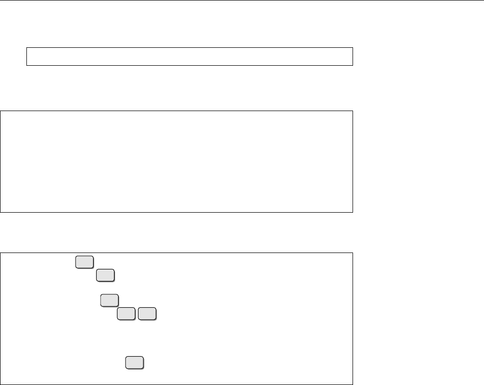
21.3 Log Inspection 327
BOf course you can combine these search terms freely with options, e.g., to
set up time limits or save typing:
$journalctl -u apache2 _HOSTNAME=red
If (like us) you can never remember which values a search term could assume,
you can simply ask the Journal:
$journalctl -F _SYSTEMD_UNIT
session-2.scope
udisks2.service
session-1.scope
polkitd.service
dbus.service
user@1000.service
As a further simplication, command line completion works for eld names and
values:
$journalctl _SYS
Tab becomes
$journalctl _SYSTEMD_
Tab
_SYSTEMD_CGROUP= _SYSTEMD_OWNER_UID= _SYSTEMD_SESSION= _SYSTEMD_UNIT=
$journalctl _SYSTEMD_U
Tab becomes
$journalctl _SYSTEMD_UNIT=
Tab Tab
acpid.service lightdm.service ssh.service
anacron.service networking.service systemd-journald.service
$journalctl _SYSTEMD_UNIT=ss
Tab becomes
$journalctl _SYSTEMD_UNIT=ssh.service
The Journal and
journald
are immensely exible and powerful and let the tra-
ditional method (text les in
/var/log
) appear pretty primitive in comparison.
.
Exercises
C21.4 [!2] Experiment with
journalctl
. How many dierent user identities
have sent messages to the Journal on your computer? Did anything inter-
esting happen yesterday between 1 p. m and 2 p. m.? What were the last
10 messages of priority
warning
? Think of some interesting questions your-
self and answer them.
Summary
• The “Journal” is a modern system logging service made available by sys-
temd. It relies on binary, database-like log les.
• The Journal is stored either in
/run/log/journal
or (for persistent logging to
disk) in
/var/log/journal
.
• Within systemd,
systemd-journald
takes care of the Journal. You can access
the Journal using
journalctl
.
•
journalctl
allows very sophisticated queries of the Journal

$ echo tux
tux
$ ls
hallo.c
hallo.o
$ /bin/su -
Password:
22
TCP/IP Fundamentals
Contents
22.1 History and Introduction . . . . . . . . . . . . . . . . . 330
22.1.1 The History of the Internet . . . . . . . . . . . . . . 330
22.1.2 Internet Administration . . . . . . . . . . . . . . . 330
22.2 Technology . . . . . . . . . . . . . . . . . . . . . . 332
22.2.1 Overview . . . . . . . . . . . . . . . . . . . . 332
22.2.2 Protocols . . . . . . . . . . . . . . . . . . . . . 333
22.3 TCP/IP . . . . . . . . . . . . . . . . . . . . . . . 335
22.3.1 Overview . . . . . . . . . . . . . . . . . . . . 335
22.3.2 End-to-End Communication: IP and ICMP . . . . . . . . 336
22.3.3 The Base for Services: TCP and UDP . . . . . . . . . . . 339
22.3.4 The Most Important Application Protocols. . . . . . . . . 342
22.4 Addressing, Routing and Subnetting . . . . . . . . . . . . . 344
22.4.1 Basics . . . . . . . . . . . . . . . . . . . . . . 344
22.4.2 Routing . . . . . . . . . . . . . . . . . . . . . 345
22.4.3 IP Network Classes . . . . . . . . . . . . . . . . . 346
22.4.4 Subnetting . . . . . . . . . . . . . . . . . . . . 346
22.4.5 Private IP Addresses . . . . . . . . . . . . . . . . 347
22.4.6 Masquerading and Port Forwarding . . . . . . . . . . . 348
22.5IPv6.........................349
22.5.1 IPv6 Addressing . . . . . . . . . . . . . . . . . . 350
Goals
• Knowing the basic structure of the TCP/IP protocol family
• Knowing the fundamentals of IP addressing
• Understanding the concepts of subnetting and routing
• Knowing the most important properties of and dierences between TCP,
UDP, and ICMP
• Knowing about the most important TCP and UDP services
• Knowing the most relevant dierences between IPv4 and IPv6
Prerequisites
• Basic knowledge of computer networks and TCP/IP services from a user’s
point of view is helpful
adm2-internet.tex
(
0cd20ee1646f650c
)

330 22 TCP/IP Fundamentals
22.1 History and Introduction
22.1.1 The History of the Internet
The history of networking computers reaches back almost to the beginning of the
“computer age”. Most of the early techniques are all but forgotten today—the “In-
ternet” has won the day. But what is “the Internet”, anyway, and where does it
come from? In this section, we give a brief overview of its history and the devel-
opment of world-wide computer communications. If you already know this from
elsewhere, feel free to skip to the next section. Thank you very much.
The progenitor of today’s Internet is ARPAnet, whose development wasARPAnet
funded by the American defence department. It’s the late 1960s.
BThe original object was not, as is often claimed, the construction of a com-
munication infrastructure for the eventuality of nuclear war, but merely re-
search into data communications, while at the same time improving com-
munications between the corporations and universities engaged in defence
research.
In 1969, the ARPAnet consisted of 4 nodes; from 1970 until 1972 the Network Con-
trol Protocol (NCP) was implemented as the basic communication standard on theNCP
ARPAnet. The most important service at the time was electronic mail.
In the 1970s, the idea of an “internet” that was supposed to connect already
existing networks gained traction. Researchers tried to implement “TCP”, a reli-
able communication protocol based on an unreliable transmission protocol (the
idea of making available an unreliable communication protocol in the shape of
UDP only came along later, which explains where the name “TCP/IP” (rather
than “TCP/UDP/IP” or something similar) comes from). The rst TCP imple-
mentations appeared in the early 1970s on “large” systems such as TOPS-20 or
Tenex; shortly afterwards it was proved that it was possible to implement TCP
even on workstation-class computers like the Xerox Alto, such that these comput-
ers could also be part of the Internet. The rst ethernet was also developed at
Xerox PARC in 1973.
Today’s basic TCP/IP standards appeared in the early 1980s. They were trialled
in BSD—the Unix variant developed at the University of California at Berkeley–,
which led to its popularity among users and computer manufacturers. On 1 Jan-“TCP/IP Flag Day”
uary 1983, the ARPAnet was converted from NCP to TCP/IP. Soon afterwards, the
original ARPAnet was divided administratively into the two components, MILnetMILnet
(for military applications) and ARPAnet (for defence research). Also in 1983, theARPAnet
development of DNS laid the groundworks for future expansion. In the subse-
quent years—1984 to 1986—, more TCP/IP-based networks were created, such as
the National Science Foundation’s NSFNET, and the notion of “the Internet” asNSFNET
the totality of all interconnected TCP/IP networks established itself.
At the end of 1989, Australia, Germany, Israel, Italy, Japan, Mexico, the Nether-
lands, New Zealand, and the United Kingdom were connected to the Internet. It
now consisted of more than 160,000 nodes.
In 1990 the ARPAnet was ocially decommissioned (it had been assimiliated
into the Internet for a very long time), and in 1991 NFSNET was opened to com-
mercial users. Commercial providers mushroomed. Today most of the network
infrastructure is privately held.
Today we have a global network of interconnections with a uniform address
space. We use open protocols and uniform communication methods, so everyone
can join in the development and the net is available to anybody. Development of
the Internet is far from nished, though; future improvements will try to address
pressing problems such as address scarcity and the increased need for security.
22.1.2 Internet Administration
A global network like the Internet cannot function without administrative struc-
tures. These started out in the USA, since in the beginning most interconnected

22.1 History and Introduction 331
networks were deployed in that country. It still remains there today, more pre-
cisely with the American Department of Commerce.
BVarious people are irked by the dominance of the USA as far as the Inter-
net is concerned. Unfortunately it is very dicult to gure out what to do
about it, as the Americans are not willing to pass the baton formally. On
the other hand, the Department of Commerce pursues a marked laissez-faire
approach, so the opponents can arrange themselves to a certain degree with
the status quo.
Theoretically, control of the Internet rests in the hands of the “Internet Society” Internet Society
(ISOC), an international non-prot organisation founded in 1992. Its members
consist of governments, corporations, universities, other organisations and even
individuals (anybody may join).
BThe main goal of ISOC was to give a formal framework to somewhat vaguely
dened institutions such as the IETF (see below) as well as to ensure their
nancial support. In addition, ISOC holds copyright to the RFCs, the nor-
mative documents for the Internet, which are freely available to everybody
who is interested.
ISOC’s activities fall into three broad categories:
Standards ISOC is the overarching structure for a number of organisations deal-
ing with the technical development of the Internet. These include:
• The Internet Architecture Board (IAB) is the committee in charge of over-
seeing technical development of the Internet. The IAB takes care of
publishing the RFCs and counsels ISOC leadership on technical mat-
ters.
BThe IAB currently has about a dozen members (humans) who have
been selected by the “IETF nominating committee”, one chairper-
son also selected by the IETF nominating committee, and a few
ex-ocio members and representatives of other organisations.
• The Internet Engineering Task Force (IETF) is tasked with actually devel-
oping Internet standards and, while doing so, cooperates closely with
institutions like ISO/IEC and the World Wide Web Consortium (W3C).
The IETF is an open organisation without membership, which is oper-
ated by “volunteers” (whose employers usually foot the bill). Within
IETF there is a large number of “working groups” that arrange them-
selves into “areas” according to their subject matter. Every area has one
or two “area directors” who together with the IETF chair form the In-
ternet Engineering Steering Group (IESG). This committee is responsible
for the IETF’s activities.
BOwing to its amorphous structure it is dicult to say how large
IETF is at any given time. In the rst years after its institution in
1986, attendance at its regular meetings changed between 30 and
120 people. Since the explosive growth of the Internet in the 1990s
the circle has become somwhat larger, even though after the burst-
ing of the “dot-com bubble” it dropped from 3000 people in 2000
down to about 1200 today.
BThe IETF’s mantra is “rough consensus and running code”—it
does not require unanimous decisions but does want to see most
of the group behind winning ideas. There is also a big empha-
sis on solutions that actually work in practice. This and the fact
that most of the work is performed by volunteers can lead to IETF
working groups taking very long to deliver results—especially
if there are too few or too many interested people who want to
contribute.

332 22 TCP/IP Fundamentals
• The Internet Corporation for Assigned Names and Numbers, ICANN for
short, is another non-prot organisation that was incorporated in 1998
to take over some things that, previously, other organisations (in par-
ticular IANA, see the next bullet) had been taking care of on behalf of
the US government. In particular, this means the assignment of IP ad-
dresses and DNS top-level domain names. Especially the latter is an
extremely political issue and every so often brooks conict.
• The Internet Assigned Numbers Authority (IANA) is in charge of actually
assigning IP addresses and operating the DNS root servers. Adminis-
tratively, IANA is part of ICANN. In addition, IANA is responsible for
the management of all globally unique names and numbers in Internet
protocols published as RFCs. In that respect it cooperates closely with
IETF and the RFC editors.
BIANA delegates the assignment of IP addresses further to so-
called Regional Internet Registries (RIRs), which each handle “dis-
tribution” (usually) to ISPs in some part of the world. Currently
there are ve RIRs, with RIPE NCC being in charge of Europe.
Education ISOC runs conferences, seminars, and workshops on important Inter-
net issues, supports local Internet organisations and, through nancial aid,
enables experts in developing countries to take part in the discussion and
development of the Internet.
Political Lobbying ISOC cooperates with governments and national and inter-
national bodies in order to further its ideas and values. The declared goal
of ISO is “a future in which people in all parts of the world may use the
Internet to improve their quality of life”.
22.2 Technology
22.2.1 Overview
Computers process digital information. In the “real world”, however, this infor-
mation is represented by means of physical phenomena such as voltage, charge, or
light, and the real world remains ercely “analogue”. The rst challenge of data
communication, then, is to transform the digital information inside the computer
into something analogue—like, for example, a sequence of electrical impulses on
a wire—for transmission to another computer, and transforms that back to digital
information at the other end. The next challenge is to make this work if the rst
computer is in Berlin and the other one in New Zealand.
BYou can divide data networks very roughly, and without actually looking
at the technology involved, into two groups: Local area networks (LANs)Local area networks
connect a small number of nodes in a geographically limited area, wide areawide area networks
networks (WANs) a potentially large number of nodes in a geographically
very large ara.
BWith LANs, the owner (a company or other organisation or—frequently
today—a household) is usually also the operator and the sole user, and the
network oers high bandwidth (100 MBit/s and more). WANs, on the other
hand, connect a multitude of dierent users who generally do not own the
network, bandwidth is less, and usage more expensive.
There are many dierent networking technologies for very diverse require-
ments, ranging from very-short-range wireless connections (Bluetooth) and typi-
cal LAN technology like Ethernet to ber connections based on ATM for WANs.
As programmers and system administrators we do not want to be bothered with
their gory electrical engineering details. Hence we talk about a “protocol stack”

22.2 Technology 333
and try to separate cleanly its individual components—the “electrical” part, the
basic communication between computers on the same network, the basic commu-
nication between computers on dierent networks, and nally concrete “services”
such as electronic mail or the World Wide Web. But rst things rst.
22.2.2 Protocols
A “protocol” is an agreed scheme governing how two (or more) nodes on a net-
work talk to one another. The spectrum of possible protocols ranges from rules
for electrical signals on an Ethernet cable or radio signals in a WLAN up to (for
example) protocols governing access to an SQL database server. Protocols can be
roughly divided into three classes:
Transmission protocols (often also called “access methods”) govern data trans-
mission essentially at the level of network cards and physical connections.
Their make-up depends on the physical properties and restrictions arising
from their implementation in “hardware”. For example, the communica-
tion between two computers across a serial “null modem cable” is com-
pletely dierent from the transmission of data via a radio connection on
a WLAN, and the transmission protocols used follow completely dierent
requirements.
BThe most common transmission protocol in LANs is Ethernet, even
though current Ethernet has hardly anything to do with the epony-
mous original of 1973 (O. K,̇ both involve electricity, but the resem-
blance stops about there). Other standards such as token-ring or eld
bus systems only come up for special applications. Also popular today
are WLAN access methods like IEEE 802.11.
Communication protocols serve to organise the communication between com-
puters in dierent networks without presupposing detailed knowledge of
the medium access methods used. To use your home PC in Germany to
view a web site on kangaroos served by a server at a university in Australia,
you do not want to have to know that your PC is connected via Ethernet
to your home router, which talks ATM to the DSLAM in the telecom shed
across the road, which passes data through ber around a few corners to
Australia and so on—you just enter
www.roos-r-us.au
in your browser. It is
thanks to communications protocols that your PC can nd the remote web
server and exchange data with it.
BCommunication protocols are supposed to prevent you from having to
mess with transmission protocols, but of course they cannot exist with-
out those. The goal of communication protocols is to hide the transmis-
sion protocols’ gory details from you—just like your car’s accelerator
pedal is used to protect you from having to know the precise control
data for its electronic fuel injection control system.
BThe communication protocols of interest to us are, of course, IP, TCP,
and UDP. We shall also look at ICMP as an “infrastructure protocol”
providing diagnosis, control, and error notication.
Application protocols implement actual services like electronic mail, le trans-
fer, or Internet telephony based on communication protocols. If communi-
cation protocols are useful to send random bits and bytes to Australia and
get others back, application protocols let you make sense of these bits and
bytes.
BTypical application protocols that you as a Linux administrator might
be confronted with include SMTP, FTP, SSH, DNS, HTTP, POP3, or
IMAP, possibly with “secure”, that is, authenticated and encrypted,

334 22 TCP/IP Fundamentals
Layer 𝑛+1 ⟵Layer 𝑛+1protocol ⟶Layer 𝑛+1
⇕Service Interface Service Interface ⇕
Layer 𝑛⟵Layer 𝑛protocol ⟶Layer 𝑛
⇕Service Interface Service Interface ⇕
Layer 𝑛−1 ⟵Layer 𝑛−1protocol ⟶Layer 𝑛−1
⇕ ⇕
Physical medium
Figure 22.1: Protocols and service interfaces
Station 1 OSI Layers Station 2
Application Application Application
protocols Presentation protocols
(FTP, HTTP, …) Session (FTP, HTTP, …)
Communication Transport Communication
protocols (IP, TCP) Network protocols (IP, TCP)
Medium access Data Link Medium access
(Ethernet, …) Physical (Ethernet, …)
Figure 22.2: ISO/OSI reference model
oshoots. All of these protocols are used by application programs such
as mail clients or web browsers, and are based on communication pro-
tocols such as TCP or UDP.
BThe data exchanged via a protocol are abstractly called protocol data units—protocol data units
depending on the protocol they may have more specic names like “pack-
ets”, “datagrams”, “segments”, or “frames”.
The fact that communication protocols are meant to hide the details of trans-
mission protocols, and that application protocols are meant to hide the details of
communication protocols lets us construct a “layer model” (Figure 22.1) where thelayer model
transmission protocols take up the lowest and the application protocols the high-
est layer. (This is incidentally where the term “protocol stack” comes from.) Every
layer on the sender’s side receives data “from above” and passes it “below”; on
the receiver’s side it is received “from below” and passed on “above”. Conceptu-
ally we still say that two nodes communicate “via HTTP”, when in fact the HTTP
data ow across TCP, IP, and a whole zoo of possible transmission protocols from
one node to the next and still must pass the IP and TCP layers upwards before
becoming visible again as HTTP data.
Technically, within each layer on the sender side, the corresponding protocol
receives a “protocol data unit” at its service interface from the layer above and
adds a “header” containing all the information important for its operation beforeheader
passing it on across the service interface of the layer below. The layer below con-
siders everything it receives on the service interface as data; the previous proto-
col’s header is of no concern to the lower layer. On the receiving side, packets pass
through the same layers in reverse order, and every layer removes “its” header be-
fore passing the “payload data” upwards.
The most well-known layer model is the “ISO/OSI reference model” (Fig-ISO/OSI reference model
ure 22.2). ISO/OSI (short for “Internation Organisation for Standardisation/Open
Systems Interconnection”) used to be the basis of a protocol family proposed by
CCITT, the world organisation of telecommunications agencies and corporations.
BThe ISO/OSI network standards never caught on—they were too baroque
and impractical to be useful, and the standards documents were dicult to

22.3 TCP/IP 335
get hold of—, but the reference model with its seven (!) layers has remained
and is popularly used to explain the goings-on of data transmission.
Many protocol stacks cannot be directly mapped to the ISO/OSI reference
model. On the one hand, this results from the fact that not every manufacturer
adheres to the denitions made by the model, on the other hand various protocol
stacks predate the OSI model. Nor should you commit the mistake of confus-
ing the ISO/OSI reference model with a binding “standard” for the structure of
networking software, or even a set of instructions for networking software imple-
mentation. The ISO/OSI reference model is merely a clarication of the concepts
involved and makes them easier to discuss. Even so, here is a brief overview of
the layers in the model:
• Layers 1 and 2 (physical and data link layers) describe how data is sent on
the “wire”. This includes the medium access scheme as well as the encoding
of the data.
• Layer 3 (the network layer) denes the functions required for routing, in-
cluding requisite addressing.
• The transport of application data is described in layer 4 (transport layer).
This distinguishes between connection-oriented and connectionless ser-
vices.
• The layers 5, 6 and 7 (session, presentation, and application layers) are often
not explicitly discriminated in practice (e. g., with the TCP/IP protocols).
These describe the system-independent representation of data within the
network and the interfaces to application protocols.
• In addition, Andy Tanenbaum [Tan02] postulates ĺayers 8 and 9 (the nan-
cial and political layers). While these layers are well-known in practice, they
have so far not been incorporated into the ocial ISO/OSI reference model.
Exercises
C22.1 [2] Review briey the dierences between transmission, communica-
tion, and application protocols. Name examples for the various types. (Do
you know ones that are not part of the TCP/IP world?)
C22.2 [1] What is the main dierence between ISO/OSI layers 2 and 3?
22.3 TCP/IP
22.3.1 Overview
TCP/IP stands for “Transmission Control Protocol/Internet Protocol” and is cur-
rently the most wide-spread method of transferring data in computer networks
ranging from two computers in a local network up to the world-wide Internet.
TCP/IP is not just a single protocol but a plethora of dierent protocols built upon
one another with possibly very dierent applications. This is called a “protocol
family”.
The protocols from the TCP/IP protocol family can roughly be placed in the
context of the ISO/OSI layer model shown in Figure 22.2. Here, in brief, are the
most important ones:
Medium access layer Ethernet, IEEE 802.11, PPP (these are, strictly speaking, not
TCP/IP protocols)
Internet layer IP, ICMP, ARP
Transport layer TCP, UDP, …

336 22 TCP/IP Fundamentals
Application layer HTTP, DNS, FTP, SSH, NIS, NFS, LDAP, …
In order tounderstand better the process of data communication, and to be able
to localise and nd errors that may occur, it is very useful to know the structure of
the most important protocols and the make-up of the protocol data units involved.
We shall now explain the most important TCP/IP protocols from the internet and
transport layers.
Exercises
C22.3 [2] Which other protocols of the TCP/IP protocol family can you think
of? Which of the four layers do they belong to?
22.3.2 End-to-End Communication: IP and ICMP
IP IP connects two nodes. As an ISO/OSI layer 3 protocol it is responsible for
the data nding its way across the Internet from the sender to the receiver. The
catch is that this way can involve very long distances consisting of diverse inde-
pendent sections using markedly dierent networking technologies and exhibit-
ing markedly dierent communication parameters. Consider a user “surng” the
Internet at home. Their computer is connected via an analogue modem and the
phone network, using PPP, to a dial-in computer on an ISP’s premises which pro-ISP
vides the actual connection to the Internet. The user’s web requests are then sent
half-way around the world by means of ATM on ber optics lines before arriving
in a university’s computing center, from where they are passed across the FDDI-
based campus network to a departmental router, which transmits the data to the
web server connected by Ethernet. The web page content then takes the reverse
way back. The various parts of the route use not only dierent networking tech-
nologies, but also dierent “local” addresses—-while no addressing is necessary
at all using PPP (there are only two communication stations), Ethernet is based
on 48-bit “MAC” addresses.
One of the achievements of IP is to make available a “global” address spaceaddress space
which assigns a unique address to every node connected to the Internet, by which
that node can be identied. IP also provides routing from one system to anotherrouting
without regard to the actual networking technology in use.
IP is a connectionless protocol, that is, unlike the traditional telephony net-connectionless protocol
work (for example) it provides no xed connection (a “wire”) for two systems to
communicate1, but the data to be transmitted is divided up in small pieces, the
so-called datagrams, which can then be addressed and delivered independentlydatagrams
from each other. In principle, every datagram can take a dierent path to the re-
ceiver than the previous one; this makes IP resilient to failure of connections or
routers as long as one route can be found from the source to the target node. IP
does not give guarantees that all transmitted data will actually reach the receiving
system, nor does it guarantee that the data which does in fact arrive will do so in
the order in which it was sent. It is up to “higher-level” protocols to sort this out
if the application requires it.
BImagine you want to send a long body of text to your aunt in Australia2. To
do this “à la IP”, you would write the text on a large number of individual
postcards. Chances are that on the way down under your postcards will be
mixed up, and the postman there is unlikely to drop them in your aunt’s
letter box in precisely the same order that you posted them here. It is also
quite possible for the odd postcard to be delayed or lost somewhere on the
way.
1Even the telephone network—aectionately called POTS (for “plain old telephone system”)—no
longer works this way.
2Read “Germany” if you are reading this in Australia.

22.3 TCP/IP 337
0 3 47815 16 18 19 31
Version Hdr
Len Type of Service Total length
Identication Flags Fragment Oset
Time to Live Protocol Header checksum
Source Address
Target Address
Options (optional)
⎫
⎪
⎪
⎪
⎪
⎪
⎪
⎪
⎬
⎪
⎪
⎪
⎪
⎪
⎪
⎪
⎭
Header
Data
hhhhhhhhhhhhhhhhhhhhhhhhhhhh
h
h
h
h
h
h
h
h
h
h
h
h
h
h
h
h
h
h
h
h
h
h
h
h
h
h
h
h
h
h
Figure 22.3: Structure of an IP datagram. Every line corresponds to 32 bits.
BWhy is this an advantage? The traditional telephone network with its wires
connected from one end to the other was very susceptible to disturbances—
if any segment on the way failed, the whole conversation broke down and
needed to be reconstructed (a big deal, back in the days of manually pre-
pared connections). If a problem or interruption develops during connec-
tionless transmission, the network can look for alternative routes for future
datagrams that detour around the damaged part. Methods like TCP make
it possible to detect which data was lost due to the problem and arrange for
it to be retransmitted.
Besides, IP takes care of fragmentation. IP datagrams may be up to 65535 fragmentation
bytes long, but most transmission protocols only allow much shorter protocol data
units—with Ethernet, for example, at most 1500 bytes. Thus longer datagrams
need to be “fragmented”—for transmission across such a medium the datagram is
taken apart, split up into numbered fragments, and reassembled later. IP ensures
that only datagrams with no missing fragments are ocially considered received.
BThe ocial specication of IP is [RFC0791]. You do not need to read this but
it may be helpful against insomnia.
BFigure 22.3 shows the structure of an IP datagram. We should briey ex-
plain at least two of the elds:
• The “time to live” (or TTL) states the maximum life span of the data-
gram. It is set by the sender and decremented (reduced by 1) by each
node the datagram passes through on its way to the recipient. If the
TTL reaches zero, the datagram is dropped, and the sender is noti-
ed. This serves to prevent “ying Dutchmen”—datagrams that due
to routing errors run in circles on the Internet without ever reaching
their destination. (A common default value is 64, which considering
the current extent of the Internet is usually more than enough.)
• The “type of service” (TOS) species the quality of service desired for
the datagram. Theoretically you get to pick, in addition to one of seven
precedence levels (which will be ignored), any of the attributes “low la-
tency”, “high throughput”, “high reliability”, or “low cost”. Whether
this makes any dierence whatsoever as far as the actual transmission
is concerned is anybody’s guess, since these options are only advisory
and routers like to ignore them altogether. (If that wasn’t the case,

338 22 TCP/IP Fundamentals
07815 16 23 24 31
Type Code Checksum
Type-dependent data structure
Type-dependent data structure
Figure 22.4: Structure of an ICMP packet
then probably all datagrams would have all these desirable options
switched on.)
ICMP Another important protocol, is the “Internet Control Message Protocol”,
or ICMP for short (see Figure 22.4). It is used for network management and to
report network problems, such as a failed connection or an unreachable subnet.
The very well-known
ping
program, for example, uses two special ICMP messages
(
echo request
and
echo reply
). The ICMP packet is encapsulated as data inside an
IP datagram and contains further data elds depending on the code.
IP and Transmission Protocols To be able to use IP to transmit data regardless
of the actual network technology used, we need to dene on a case-by-case basis
how IP datagrams are forwarded across the network in question—whether that is
Ethernet, PPP over an analogue telephone line, ATM, WLAN, …
With Ethernet, for example, all nodes are connected (if only conceptually) to a
shared medium—in “classic” Ethernet, a single long coaxial cable running from
one node to the next, today more often using twisted-pair cables and a common
star hub or switch. Everything a node sends is received by all the other nodes, but
these usually pick up only those protocol data units that are actually addressed to
them (today, switches help by “pre-sorting” the trac). If two nodes transmit si-
multaneously, a collision occurs, which is handled by both nodes stopping trans-collision
mission, waiting for a random period of time, and trying again. Such a shared
Ethernet medium is also called a “segment”.segment
Every Ethernet interface has a unique address, the 48-bit “MAC address” (short
MAC address for “medium access control”). Ethernet protocol data units, the so-called frames,
frames can be sent either to particular other nodes within the segment by specifying their
MAC address as the recipient—the frame will be seen by all nodes but ignored by
all but the addressed node—, or else broadcast to all other nodes on the segment.broadcast
BEthernet adapters usually also support a so-called “promiscuous mode”,
in which all frames—even the ones that would otherwise be ignored as
uninteresting—are passed to the operating system. This is used by inter-
esting applications such as network analysis programs and cracker tools.
This is used to integrate IP and Ethernet. If a node (let’s call it 𝐴) wants to
communicate with another node (𝐵) whose IP address it knows, but whose MAC
address it doesn’t know, it asks all connected nodes by Ethernet broadcast:
Node 𝐴: Who here has IP address
203.177.8.4
?
Node 𝐵: I do, and my MAC address is
00:06:5B:D7:30:6F
This procedure follows the “Address Resolution Protocol” (ARP, [RFC0826]).ARP
Once node 𝐴has received node 𝐵’s MAC address, it stores it for a certain time
in its “ARP cache” in order to not have to repeat the query for every frame; IPARP cache
datagrams to nodes whose IP and MAC addresses are part of the ARP cache can
be addressed directly at the Ethernet level by embeddng them as “payload data”
into Ethernet frames. You can access the ARP cache using the
arp
command—not
just to read, but also to write new entries.
arp
output could look like this:

22.3 TCP/IP 339
0 3 4910 11 12 13 14 15 16 23 24 31
Source Port Destination Port
Sequence Number
Acknowledgement Number
Oset Reserved U
R
G
A
C
K
P
S
H
R
S
T
S
Y
N
F
I
NWindow
Checksum Urgent Pointer
Options Padding
Data
hhhhhhhhhhhhhhhhhhhhhhhhhhhh
h
h
h
h
h
h
h
h
h
h
h
h
h
h
h
h
h
h
h
h
h
h
h
h
h
h
h
h
h
h
Figure 22.5: Structure of a TCP Segment
#arp
Address Hwtype Hwaddress Flags Mask Iface
server.example.org ether 00:50:DB:63:62:CD C eth0
Datagrams addressed to IP addresses that do not belong to nodes on the same
Ethernet segment must be routed (Section 22.4.2). Routing
Exercises
C22.4 [3] Estimate the minimal TTL that is necessary to be able to reach all
other nodes on the Internet from your computer. How would you go about
determining the minimal TTL required to reach a specic node? Is that
number constant?
22.3.3 The Base for Services: TCP and UDP
TCP The “Transmission Control Protocol” (TCP) is a reliable, connection-oriented
protocol dened in [RFC0793] (among others). Unlike the connectionless IP, TCP
supports operations to open and tear down connections, which arrange for a “vir-
tual” connection between the source and destination nodes—since TCP data, like
all other data, is transmitted based on IP, the actual data transmission still hap-
pens unreliably and on a connectionless basis. TCP achieves reliability by means
of the destination node acknowledging the receipt of each packet (“segment”, in
TCP parlance). Each of the two communicating nodes annotates its segments with
sequence numbers, which the other node declares “received” in one of its next sequence numbers
segments. If there is no such acknowlegement within a certain dened period of
time, the sending node retries sending the segment in order to perhaps receive
an acknowledgement then. To avoid loss of performance, a “sliding window”
protocol is used so a number of segments can remain unacknowledged at the
same time. Even so, TCP is considerably slower than IP.
BIn point of fact, TCP acknowledgements are based on octets (popularly
known as bytes) rather than segments—but for our purposes the dierence
is mostly academic.
Every TCP segment contains a header of at least 20 bytes (Figure 22.5) in ad-
dition to the IP header. (Remember: The TCP segment including the TCP header

340 22 TCP/IP Fundamentals
SENDER RECIPIENT
-
Synchronisation request
Flags:
SYN
Acknowledgement and Synchronisation
Flags:
ACK
,
SYN
-
Acknowledgement (and Data)
Flags:
ACK
Acknowledgement and Data
Flags:
ACK
Figure 22.6: Starting a TCP connection: The Three-Way Handshake
is considered “data” by IP, the protocol of the layer below.) Errors in the data
can be detected based on a checksum. Every system supports many independent,
simultaneous TCP connections distinguished based on port numbers.port numbers
BThe combination of an IP address and a port number together with the IP
address and the port number of the “peer” is called a “socket”. (The same
TCP port on a node may take part in several TCP connections to dierent
peers—dened by the peer’s IP address and port number.)
The virtual connection is built using the three-way handshake (see Fig-three-way handshake
ure 22.6). Using the three-way handshake, the communication peers agree on
the sequence numbers to be used. Two ags in the TCP header,
SYN
and
ACK
, playflags
an important role in this. The rst data segment sent to the recipient has the
SYN
ag set and the
ACK
ag cleared. Such a segment indicates a connection request.
The recipient acknowledges this using a TCP segment that has both the
SYN
and
ACK
ags set. The sender in turn acknowledges this segment using one that has the
ACK
ag set but not the
SYN
ag. At this point the connection has been established.
Subsequent TCP segments also have the
ACK
ag set only.—At the end of the com-
munication, the connection is torn down by means of a two-way handshake using
the
FIN
ag.
BThe two nodes need to agree about the start of a connection, but a connection
can be torn down unilaterally. In fact this feature is required for commands
like the following to work:
$cat bla | ssh blue sort
This uses the Secure Shell (see Chapter 25) to run the
sort
command on node
blue
, and feeds data into its standard input. (
ssh
reads its standard input lo-
cally, forwards the data to the remote computer, and passes it to the
sort
command on its standard input.)
sort
, however, works by reading all of its
standard input, then sorting the data it read, and writing the sorted data to
its standard output, which is then passed by
ssh
back to the local computer
(and the screen).—The problem is that
ssh
needs to signal the remote
sort
that all the input has been read, and that it can start sorting and outputting
the data. This happens by closing the connection “to” the remote computer.
The part of the connection reading “from” the remote computer, however,
remains open and can transport the
sort
output back—if a connection tear-
down always aected both directions, this application would not work.

22.3 TCP/IP 341
015 16 31
Source Port Destination Port
Length Checksum
Data
hhhhhhhhhhhhhhhhhhhhhhhhhhhh
h
h
h
h
h
h
h
h
h
h
h
h
h
h
h
h
h
h
h
h
h
h
h
h
h
h
h
h
h
h
Figure 22.7: Structure of a UDP datagram
BOf course, after a unilateral teardown data are still passed between the
nodes in both directions, since the node that tore down the connection
must still acknowledge the data it receives via the remaining part of the
connection. It can no longer send payload data across the connection,
though.
UDP Unlike TCP, the “User Datagram Protocol” (UDP) [RFC0768] is a connec-
tionless and unreliable protocol. In fact it isn’t much more than “IP with ports”,
since, like TCP, a node can support at most 65535 communication end points (UDP
and TCP may use the same port number simultaneously for dierent purposes).
UDP requires neither the connection initialisiation of TCP nor the acknowledge-
ments, hence the protocol is much “faster”—the price to pay is that, as with IP,
data can get lost or mixed up.
BUDP is used either where there is only very little data to transmit, so that
the cost of a TCP connection initialisation is very high in comparison—cue
DNS—or where not every single bit counts but delays are unacceptable.
With Internet telephony or video transmission, lost datagrams call attention
to themselves through cracking noises or “snow” in the picture; a longer
hiatus like the ones common with TCP would be much more obnoxious.
Ports TCP and UDP support the idea of ports, which allow a system to maintain
more than one connection at any given time (OK, there are no “connections” with
UDP, but even so …). There are 65536 ports each for TCP and UDP, which however
cannot all be used sensibly: Port number 0is a signal to the system’s TCP/IP stack
to pick an otherwise unused port.
Most ports are freely available to users of the system, but various ports are o-
cially asigned to particular services. We distinguish well-known ports and reg- well-known ports
registered ports
istered ports. For example, the rules say that TCP port 25 on a system is reserved
for its mail server, which is listening there to accept connections according to the
“Simple Mail Transfer Protocol” (SMTP). Similarly, the TCP port 21 is reserved
for the FTP server and so on. These assignments are published on a regular basis
by IANA and can be found, for example, at
http://www.iana.org/assignments/port-
numbers
.
BAccording to IANA, the “well-known ports” are ports 0to 1023, while the
“registered ports” are ports 1024 to 49151. If you want to release a program
oering a new service, you should request one or more port numbers from
IANA.
BThe remaining ports—from 49152 up to 65535—are called “dynamic and/or
private ports” in IANA jargon. These are used for the client side of connec-
tions (it is unlikely that your system will need to maintain more than 16.000

342 22 TCP/IP Fundamentals
# Network services, Internet style
echo 7/tcp
echo 7/udp
discard 9/tcp sink null
discard 9/udp sink null
systat 11/tcp users
daytime 13/tcp
daytime 13/udp
netstat 15/tcp
qotd 17/tcp quote
chargen 19/tcp ttytst source
chargen 19/udp ttytst source
ftp-data 20/tcp
ftp 21/tcp
fsp 21/udp fspd
ssh 22/tcp # SSH Remote Login Protocol
ssh 22/udp # SSH Remote Login Protocol
telnet 23/tcp
smtp 25/tcp mail
Figure 22.8: The
/etc/services
le (excerpt)
connection to TCP servers at the same time) or for the implementation of
“private” servers.
BWhen IANA reserves a port number for a TCP-based protocol, it tends to
reserve the same port number for UDP as well, even though the TCP pro-
tocol in question makes no sense with UDP, and vice versa. For example,
port 80 is reserved for HTTP both as a TCP and a UDP port, even though
UDP-based HTTP is not currently an interesting topic. This leaves elbow
room for future extensions.
On a Linux system, a table of assignments is available in the
/etc/services
le
(Figure 22.8). This table is used, for example, by the Internet daemon (
inetd
or
xinetd
) or the C library function
getservbyname()
to nd the port corresponding to
a given service name.
BYou can change
/etc/services
, e. g., to support your own services. Do watch
for updates of the le by your distribution.
On Unix-like systems, ports 0to 1023 are privileged—only
root
may open them.privileged ports
This is a security precaution against arbitrary users launching, e. g., their own web
server on an otherwise unused port 80 in order to appear ocial.
22.3.4 The Most Important Application Protocols
In the previous section we introduced the idea of a “service”. While communica-
tion protocols like TCP and UDP are concerned with moving data from one node
to another, “services” usually rely on application protocols that assign meaning
to the data exchanged using the communication protocol. If, for example, you
send an e-mail message using SMTP, your computer contacts the remote SMTP
server (via TCP on port 25), identies itself, sends your address as well as that of
the recipient (or recipients) and the actual message—in each case after the remote
server prompted for them. The details of this conversation are specied by the
application protocol, SMTP.

22.3 TCP/IP 343
Table 22.1: Common application protocols based on TCP/IP
Port C Prot Name Explanation
20 TCP FTP File transfer (data connections)
21 TCP FTP File transfer (control connections)
22 TCP SSH Secure (authenticated and encrypted) login to remote computers;
secure le transfer
23 TCP TELNET Login to remote computers (insecure and obsolete)
25 TCP SMTP Electronic mail transfer
53 UDP/TCP DNS Name and address resolution and related directory services
80 TCP HTTP World Wide Web resource access
110 TCP POP3 Access to remote e-mail mailboxes
123 UDP/TCP NTP Network Time Protocol (time synchronisation)
137 UDP NETBIOS NetBIOS name service
138 UDP NETBIOS NetBIOS datagram service
139 TCP NETBIOS NetBIOS session service
143 TCP IMAP Access to e-mail stored remotely
161 UDP SNMP Network management
162 UDP SNMP Traps for SNMP
389 TCP LDAP Directory service
443 TCP HTTPS HTTP via SSL (authenticated/encrypted)
465 TCP SSMTP SMTP via SSL (obsolete, don’t use!)*
514 UDP Syslog Logging service
636 TCP LDAPS LDAP via SSL (authenticated/encrypted)*
993 TCP IMAPS IMAP via SSL (authenticated/encrypted)*
995 TCP POP3S POP3 via SSL (authenticated/encrypted)*
* These services may also be accessed via connections that are rst established in the clear and then
“upgraded” to authenticated and encrypted connections later on.
344 22 TCP/IP Fundamentals
B“Services” and “protocols” are not exactly equivalent. A “service” is some-
thing you want to use the computer for, such as e-mail, web access, or print-
ing on a remote printer server. For many services on the Internet there are
“canonical” protocols that recommend themselves—for e-mail, for exam-
ple, there are hardly any alternatives to SMTP—, but some services use the
same underlying protocol as others. The Web is usually accessed via HTTP
and remote printer servers via the “Internet Printing Protocol” (IPP). How-
ever, if you look closely enough you will notice that IPP, as used today, is
really gloried HTTP. The only dierence is that HTTP uses TCP port 80
while IPP uses TCP port 631.
Table 22.1 shows a summary of some important application protocols. We will
encounter several of them later on in this manual; others will covered in other
Linup Front training manuals.
Bad news for LPIC-1 candidates: LPI wants you to know the port numbers
and services from Table 22.1 by heart (LPI objective 109.1). Have fun swot-
ting up.
22.4 Addressing, Routing and Subnetting
22.4.1 Basics
Every network interface in a system on a TCP/IP network has at least one IP ad-
dress. In this case, an “interface” is that part of a system that is able to send and
receive IP datagrams. A single system can contain more than one such interface
and then generally uses more than one IP address. With
$/sbin/ifconfig
or
$/sbin/ip addr show
you can list the congured interfaces or network devices.
IP addresses are 32 bits long and are usually written as “dotted quads”—theyIP addresses
are viewed as a sequence of four eight-bit numbers written in decimal notation as
values between 0 and 255, like “
203.177.8.4
”3. Each IP address is assigned to be
globally unique and denotes a node in a particular network on the Internet. To do
so, IP addresses are split into a network and a host part. This split is variable and
can be adapted to the number of node addresses required in a network. If the host
part takes 𝑛bits, 32 − 𝑛 bits remain for the network part. The split is documented
by the network mask, which contains a binary 1for each bit in the IP addressnetwork mask
belonging to the network part, and a binary 0for each bit of the host part. The
network mask is notated either as a dotted quad or—frequently—as the number
of ones. “
203.177.8.4/24
” is thus an address in a network with a network mask of
“
255.255.255.0
”.
By way of an example, let’s assume a 28-node network. The next higher power
of 2is 32 = 25. This means that 5bits are required to number all the nodes. The
remaining 27 bits (32 − 5) identify the network and are the same in all systems on
that network. The network mask is
255.255.255.224
, since the top three bits are set
in the nal “quad”—those with values 128,64, and 32, or 224 altogether.
By convention, the rst and last IP addresses in a network are reserved for
special purposes: The rst address (host part all binary zeroes) is the networknetwork address
address, the last address (host part all binary ones) the broadcast address. In thebroadcast address
3Incidentally, it is quite legal and supported by most programs to give an IP address as a decimal
number that has been “multiplied out”—in our example, 3417376772 instead of
203.177.8.4
. This is the
key ingredient to “trick URLs” of the form
http://www.microsoft.com@3417376772/foo.html
.

22.4 Addressing, Routing and Subnetting 345
Table 22.2: Addressing example
IP Address
Meaning binary decimal
Network mask
11111111 11111111 11111111 11100000 255.255.255.224
Network address
11001011 10110001 00001000 00000000 203.177.8.0
Host addresses
11001011 10110001 00001000 00000001 203.177.8.1
⋮ ⋮ ⋮
11001011 10110001 00001000 00011110 203.177.8.30
Broadcast address
11001011 10110001 00001000 00011111 203.177.8.31
example above,
203.177.8.0
is the network address and
203.177.8.31
the broadcast
address. The numbers 1 to 30 are available for nodes (Table 22.2).
BThe address
255.255.255.255
is a broadcast address, but not for all of the In-
ternet, but the local network segment (for example, all the stations on the
same Ethernet). This address is used if no more precise address is known,
for example if a node wants to obtain an IP address and network mask via
DHCP.
22.4.2 Routing
Routing is used to send IP datagrams that cannot be delivered directly within
the local network on to the correct destination4. In fact, you might argue that
routing is the central property that sets TCP/IP apart from “toy protocols” such
as NetBEUI and Appletalk, and which made the Internet, as we know it, possible
in the rst place.
Routing applies where the recipient of an IP datagram cannot be found within
the same network as the sender. The sender can gure this out straightforwardly
based on the desired recipient’s IP address, by considering that part of the desti-
nation address that is “covered” by its own network mask and checking whether
this matches its own network address. If this is the case, the recipient is “local”
and can be reached directly (Section 22.3.2 on page 338).
If the recipient cannot be reached directly, the node (at least if it is a Linux host)
consults a routing table which should contain at least a “default gateway”, i. e., a routing table
node that takes care of forwarding datagrams that cannot be delivered outright.
(This node usually needs to be reachable directly.) Such a node is called a “router”
and is either a computer in its own right or else a special appliance manufactured
for the purpose.
BIn principle, the router proceeds just like we described: It contains vari-
ous network interfaces, each of which is assigned an address and a network
mask, and can deliver datagrams immediately to nodes that according to
the network masks of its interfaces can be identied as being part of one of
“its” networks. Other directly reachable nodes acting as routers are called
upon for more forwarding if necessary.
BIn real life, routing tables can be considerably more complex. For example,
it is possible to forward datagrams directed to particular nodes or networks
to other routers that are not the default gateway.
An important observation is that a node (PC or router) usually determines just
the directly following routing step (also called “hop”), instead of specifying the
complete path from the original sender of the datagram to the nal recipient. This
4This was already foreseen in the Old Testament: “He leadeth me in the paths of righteousness for
his name’s sake.” (Psalm 23:3) Of course on the Internet there are few better methods of completely
ruining your reputation than a spectacularly wrong router misconguration.

346 22 TCP/IP Fundamentals
Table 22.3: Traditional IP Network Classes
Class Network part Number of networks Hosts per network Addresses
Class A 8 Bit 128 – 126 usable 16.777.214 (224 − 2)
0.0.0.0
–
127.255.255.255
Class B 16 Bit 16.384 (214) 65.534 (216 − 2)
128.0.0.0
–
191.255.255.255
Class C 24 Bit 2.097.152 (221)254 (28− 2)
192.0.0.0
–
223.255.255.255
Class D - - -
224.0.0.0
–
239.255.255.255
Class E - - -
240.0.0.0
–
254.255.255.255
means that it is up to each router between the sender and recipient to pick that
hop that it considers most sensible. Well-congured routers talk to their “neigh-
bours” and can base their routing decisions on information about network load
and possibly known blockages elsewhere in the network. A detailed discussion
of this topic is beyond the scope of this manual.
BIn fact it is possible for a datagram to specify the complete path it wants
to take to its destination. This is called “source routing”, is universally
frowned upon, and will be completely ignored by large parts of the net-
work infrastructure, because on the one hand it is at odds with the idea of
dynamic load distribution, and on the other hand it is a common vehicle for
security issues.
22.4.3 IP Network Classes
Traditionally, the set of IP addresses from
0.0.0.0
to
255.255.255.0
was divided into
several network classes which were called “class A”, “class B”, and “class C”.network classes
BThere are also “class D” (multicast addresses) and “class E” (experimental)
addresses, but these are of little interest to the assignment of IP addresses
to nodes.
Classes A to C dier by their network masks, which amounts to the number of
networks available per class and the number of hosts available in these networks.
While a class A address has an 8-bit network part, a class B address uses 16 bits,
and a class C address 24. A xed range of IP addresses was assigned to each of
the network classes. (Table 22.3)
Due to the increasing scarcity of IP addresses the division of the IP address
space into the three address classes was abandoned during the 1990s. Now we
are using “classless inter-domain routing” (CIDR) according to [RFC1519]. While
according to the “old” scheme the boundary between the network and host ad-
dresses could only occur in one of three dierent places, CIDR makes it possible
to assign arbitrary network masks and thus ne-tune the size of the address range
made available to a customer (usually an ISP) as well as work against the “explo-
sion” of routing tables. An installation with sixteen adjacent “class C” networks
(network mask “
/24
” can be viewed for routing purposes as one network with a
/20
netmask—a considerable simplication, since routing tables can be that much
simpler. On the Internet, addresses whose network part is more than 19 bits long
are no longer routed directly; in general you must arrange for a provider to man-
age all of the addresses and forwards the IP datagrams suitably.
22.4.4 Subnetting
Frequently a large network is too imprecise or makes no sense otherwise. Hence
operators often divide their networks into several smaller networks. This hap-
pens by adding another xed part to the xed network part of an IP address. In
our previous example,
subnetting
might work approximately like this: Instead of a
“large” network with 32 addresses (for 30 nodes) you might prefer two “smaller”

22.4 Addressing, Routing and Subnetting 347
Table 22.4: Subnetting Example
IP Address
Meaning binary decimal
Network mask
11111111 11111111 11111111 11110000 255.255.255.240
Network address (1)
11001011 10110001 00001000 00000000 203.177.8.0
Host addresses (1)
11001011 10110001 00001000 00000001 203.177.8.1
⋮ ⋮ ⋮
11001011 10110001 00001000 00001110 203.177.8.14
Broadcast address (1)
11001011 10110001 00001000 00001111 203.177.8.15
Network address (2)
11001011 10110001 00001000 00010000 203.177.8.16
Host addresses (2)
11001011 10110001 00001000 00010001 203.177.8.17
⋮ ⋮ ⋮
11001011 10110001 00001000 00011110 203.177.8.30
Broadcast address (2)
11001011 10110001 00001000 00011111 203.177.8.31
Table 22.5: Private IP address ranges according to RFC 1918
Adressraum from to
Class A
10.0.0.0
–
10.255.255.255
Class B
172.16.0.0
–
172.31.255.255
Class C
192.168.0.0
–
192.168.255.255
networks with up to 16 addresses (up to 14 nodes), for example to be able to de-
ploy separate Ethernet cables for security. You can lengthen the network mask
by 1 bit; the network, host, and broadcast addresses can be derived from this as
above (Table 22.4).
BIt isn’t necessary for all subnets to have the same size. The
203.177.8.0/24
net- subnets of different size
work, for example, could straightforwardly be subdivided into one subnet
with 126 host addresses (e. g.,
203.177.8.0/25
with the host addresses
203.177.
8.1
to
203.177.8.126
and the broadcast address
203.177.8.127
) and two subnets
with 62 host addresses (e. g.,
203.177.8.128/26
and
203.177.8.192/26
with the
respective host addresses of
203.177.8.192
up to
203.177.8.190
as well as
203.
177.8.193
up to
203.177.8.255
and the broadcast addresses
203.177.8.191
and
203.177.8.255
).
BThe smallest possible IP network has a 30-bit network part and a 2 bit station smallest possible IP network
part. This amounts to a total of four addresses, one of which is the network
address and one is the broadcast address, so two addresses are left over for
statues. You will nd this arrangement every so often with point-to-point
links via modem or ISDN.
22.4.5 Private IP Addresses
IP addresses are globally unique and must therefore be administered centrally. Globally unique distribution of
IP addresses
Hence you cannot pick your own e-mail address arbitrarily, but must apply for
one—usually to your ISP, who in turn has been assigned a block of IP addresses
by a national or international body (Section 22.1.2). The number of internationally
possible network addresses is, of course, limited.
BAt the beginning of February 2011, IANA assigned the last ve available
/8
address ranges to the ve regional registries. It is probable that APNIC
(Asia Pacic Network Information Centre) will run out of IP addresses rst,
possibly in mid-2011. After that, the only solutions will be begging or IPv6.
According to [RFC1918], special IP address ranges, the private addresses, are private addresses

348 22 TCP/IP Fundamentals
reserved for systems that are not connected to the Internet. These addresses will
not be routed on the Internet at large (Table 22.5).
You can use these addresses with impunity within your local networks—
including subnetting and all other bells and whistles.
22.4.6 Masquerading and Port Forwarding
IP addresses are a scarce resource today, and that will remain so until we have
all converted to IPv6 (Section 22.5). Therefore it is highly probable that you will
be assigned only one “ocial” (i.e., non-RFC 1918) address to connect all of your
network to the Internet—with home networks or ones in small companies this is
even the rule. The solution (an euphemism for “lame kludge”) consists of “mas-
querading” as well as “port forwarding”. Both approaches are based on the fact
that only your router is connected to the Internet by means of a public IP address.
All other nodes within your network use addresses according to [RFC1918]. Mas-Masquerading
querading implies that your router rewrites datagrams that nodes within your
network send “outside” in order to replace those nodes’ IP addresses by its own,
and forwards the corresponding response datagrams to the proper senders. Both
the nodes inside your network and “the Internet” are not aware of the fact—the
former assume that they are talking directly to the Internet, while the latter only
gets to see the (ocial) IP address of your router. Conversely, port forwardingport forwarding
enables nodes on the Internet to connect to services such as DNS, e-mail or HTTP
through their respective ports on the router, while the router forwards the data-
grams in question to a node on the inside that performs the actual service.
AYou should resist the temptation of making your router simultaneously your
web, mail, or DNS server; the danger of an intruder compromising your
router through one of the large server programs and therefore, in the worst
case, getting access to all of your local network, is much too great.
BPort forwarding and masquerading are two examples of a concept that is
generally called NAT (network address translation). In particular, we canNAT
think of masquerading as “source NAT”, since the sender address of outgo-
ing datagrams is modied5, while port forwarding is an instance of “desti-
nation NAT”—since the destination address of datagrams addressed to us
is changed.
Exercises
C22.5 [1] Can the following IP addresses with the given network mask be
used as host addresses in the appropriate IP network? If not, why not?
IP Address Network mask
a)
172.55.10.3 255.255.255.252
b)
138.44.33.12 255.255.240.0
c)
10.84.13.160 255.255.255.224
C22.6 [2] Which reasons could you have to divide the address range your ISP
assigned to you into subnets?
C22.7 [T]he network at IP address
145.2.0.0
, with the network mask
255.255.
0.0
, was divided, using the subnet mask
255.255.240.0
, into the following
subnets:
•
145.2.128.0
•
145.2.64.0
5The fact that we also need to rewrite the recipient address of incoming datagrams will be ignored
for convenience.

22.5 IPv6 349
•
145.2.192.0
•
145.2.32.0
•
145.2.160.0
Which other subnets are also possible? Which subnet contains the station
145.2.195.13
?
22.5 IPv6
The most popular incarnation of IP is version 4, or “IPv4” for short. Due to the IPv4
explosive growth of the Internet, this version comes up against various limits—the
main problems are the increasing scarcity of addresses, the chaotic assignment of
addresses, and the highly complex routing resulting from this, as well as a fairly
sketchy support of security mechanisms and tools for ensuring quality of service.
IPv6 is supposed to sort this out. IPv6
The most important properties of IPv6 include: properties
• The length of addresses was increased from 32 to 128 bits, resulting in a
total of 3.4 ⋅ 1038 addresses. This would suce to assign approximately
50.000 quadrillion6IP addresses (a 28-digit number) to each living person
on Earth. That should be enough for the foreseeable future.
• IPv6 stations can automatically obtain conguration parameters from a
router when they are connected to a network. If necessary, there is still a
DHCPv6 protocol.
• There are only 7 elds in an IP header, so routers can process datagrams
more quickly. You get get to use several headers if necessary.
• Extended support for options and extensions, which also contributes to
router processing speed.
• Improved transmission of audio and video data and better support for re-
altime applications.
• Increased security by means of secured data transmission and mechanisms
for authentication and integrity protection.
• Extensibility to ensure the future of the protocol. The protocol does not try
to cover all possiblities, since the future brings new ideas that cannot be
foreseen today. Instead, the protocol is open to the integration of additional
functionality in a backwards-compatible manner.
Even though the standardisation of IPv6 has been nished for some time, the gen-
eral implementation leaves much to be desired. In particular the service providers implementation
are still acting coyly. Linux already supports IPv6, so the conversion of a Linux-
based infrastructure to the new standard will not present big problems. You can
also transport IPv6 datagrams via IPv4 for testing purposes, by embedding them
into IPv4 datagrams (“tunnelling”). Thus a company could base its internal net-
work on IPv6 and even connect several premises via a “virtual” IPv6 network
within the traditional IPv4 network.
We should also stress that IPv6 is a targeted replacement for IPv4. Most IP-
based protocols—starting with TCP and UDP—remain unchanged. Only at the
“infrastructure level” will some protocols become extraneous or be replaced by
IPv6-based versions.
6What our American friends would call a “septillion”

350 22 TCP/IP Fundamentals
22.5.1 IPv6 Addressing
IPv6 supports 2128 distinct addresses—an unimaginably large number. Essen-
tially, every grain of sand on Earth could be assigned several addresses, but that
isn’t even the goal: The large address space enables much more exible address
assignment for various purposes, as well as much simplied routing.
Unlike IPv4 addresses, IPv6 addresses are not notated as decimal numbers, butNotation
instead as hexadecimal (base-16) numbers. Four hexadecimal digits are grouped
and these groups are separated by colons. For example, an IPv6 address might
look like
fe80:0000:0000:0000:025a:b6ff:fe9c:406a
Leading zeroes in a group may be omitted, and (at most) one run of “zero blocks”
may be replaced by two colons. Hence, an abbreviated rendition of the address
from the previous example might be
fe80::25a:b6ff:fe9c:406a
The IPv6 address
::1
—an abbreviation of
0000:0000:0000:0000:0000:0000:0000:0001
—corresponds to the IPv4 loopback address,
127.0.0.1
. IPv6 does not support
“broadcast addresses” à la
192.168.1.255
—of which more anon.
IPv6 addresses may be divided into a 64-bit “network” part and a 64-bit “sta-
tion” part. This implies that every IPv6 subnet contains 264 addresses, i. e.,
232 times as many as the whole IPv4 internet! Subnetting using variable pre-Subnetting
x lengths, as used in IPv4 (Section 22.4.4), is not supposed to be part of IPv6.
However, it is assumed that your ISP will provide you with a “
/56
” address prex
so that you can use 256 subnets with 264 addresses each, which shouldn’t really
cramp your style. (You can specify network prexes by appending a slash and
the decimal prex length to an address—an address like
fe80::/16
describes the
network where addresses start with
fe80
and then continue arbitrarily.)
There are three basic types of IPv6 addresses:types of IPv6 addresses
• “Unicast” addresses apply to one particular network interface (a station may
be equipped with several network interfaces, which will each have their own
addresses).
• “Anycast” addresses refer to a group of network interfaces. These typically
belong to dierent stations, and the “closest” station is supposed to answer.
For example, you may address all routers in an IPv6 network by using the
address resulting from appending an all-zero station part to the (64-bit) ad-
dress prex of the network.
• “Multicast” addresses are used to deliver the same packets to several net-
work interfaces. As we said, IPv6 does not use broadcast; broadcast is a
special case of multicast. The address
ff02::1
, for example, refers to all sta-
tions on the local network.
In addition, we can distinguish various scopes:scopes
• “Global” scope applies to addresses that are routed within the whole (IPv6)
internet.
• “Link-local” scope applies to addresses that are not routed and are only
valid within the same network. Such addresses are commonly used for
internal administrative purposes. Link-local addresses are always located
within the
fe80::/64
network; the other 64 bits are, in the most straightfor-
ward instance, derived from the MAC address of the interface.

22.5 IPv6 351
• “Site-local” scope applies to addresses that are only routed within one
“site”. Nobody knows exactly what this is supposed to mean, and site-local
addresses have accordingly been deprecated (again). Site-local addresses
use the
fec0::/10
prex.
• “Unique-local” addresses are similar to site-local addresses and correspond
roughly to the RFC 1918 addresses (
192.168.
𝑥.𝑦etc.) of IPv4. However, IPv6
does make it easy to use “proper”, i. e., globally visible, addresses, so you
do not have to resort to using unique-local addresses in order to assign your
stations any addresses at all. Hence there is no compelling reason to use
unique-local addresses in the rst place, other than as a fallback position if
something is terribly wrong with your “real” prex. Unique-local addresses
use the
fd00::/8
prex, and you are allowed to pick your own next 40 bits
for a
/48
network (but don’t pick
fd00::/48
).
It is important to stress that, with IPv6, every network interface can have several several addresses
addresses. It gets an automatic link-local address, but can have several unique-
local or global addresses on top of that with no problems whatsoever. All of these
addresses carry equal weight.
BA useful command for the harried IPv6 administrator is
ipv6calc
, which
ipv6calc
makes handling IPv6 addresses easier. For instance, it will output infor-
mation about an address:
$ipv6calc --showinfo fe80::224:feff:fee4:1aa1
No input type specified, try autodetection... found type: ipv6addr
No output type specified, try autodetection... found type: ipv6addr
Address type: unicast, link-local
Error getting registry string for IPv6 address:
reserved(RFC4291#2.5.6)
Interface identifier: 0224:feff:fee4:1aa1
EUI-48/MAC address: 00:24:fe:e4:1a:a1
MAC is a global unique one
MAC is an unicast one
OUI is: AVM GmbH
The address in question is a link-local unicast address whose station part
hints at a device manufactured by AVM GmbH (in point of fact a FRITZ!Box,
a type of DSL router/PBX/home server very popular in Germany).
B
ipv6calc
also serves to convert addresses from one format into another. For
example, you might simulate the method used to derive the station part of
an IPv6 address (also called “EUI-64”) from a MAC address:
$ipv6calc --in mac --out eui64 00:24:fe:e4:1a:a1
No action type specified, try autodetection... found type: geneui64
0224:feff:fee4:1aa1
Commands in this Chapter
arp
Allows access to the ARP cache (maps IP to MAC adresses)
arp
(8) 338
inetd
Internet superserver, supervises ports and starts services
inetd
(8) 342
ipv6calc
Utility for IPv6 address calculations
ipv6calc
(8) 351
xinetd
Improved Internet super server, supervises ports and starts services
xinetd
(8) 342

352 22 TCP/IP Fundamentals
Summary
• The Internet has its roots in the initial ARPAnet of the 1960s, was put on its
present technological basis in the early 1980s, and experienced incredible
growth in the 1980s and 1990s.
• The ISO/OSI reference model serves to provide terminology for the struc-
ture of computer communications.
• Today TCP/IP is the most popular protocol family for data transmission
across computer networks.
• ICMP is used for network management and problem reporting.
• TCP provides a connection-oriented and reliable transport service based on
IP.
• Like IP, UDP is connectionless and unreliable, but much simpler and faster
than TCP.
• TCP and UDP use port numbers to distinguish between dierent connec-
tions on the same computer.
• Dierent TCP/IP services have xed port numbers assigned for them. This
assignment may be inspected in the
/etc/services
le.
• IP addresses identify nodes world-wide. They are 32 bits long and consist
of a network and a host part. The network mask species the split between
these.
• In former times, the available IP addresses were divided into classes. Today
we use classless routing with variable-length network masks.
• IP networks can be further subdivided into subnetworks by adjusting the
network mask.
• Some IP address ranges are reserved for use in local networks. They will
not be routed by ISPs.
• IPv6 lifts various restrictions of the IPv4 common today, but so far has not
been widely adopted.
Bibliography
IPv6-HOWTO05 Peter Bieringer. “Linux IPv6 HOWTO”, October 2005.
http://www.tldp.org/HOWTO/Linux+IPv6-HOWTO/
RFC0768 J. Postel. “User Datagram Protocol”, August 1980.
http://www.ietf.org/rfc/rfc0768.txt
RFC0791 Information Sciences Institute. “Internet Protocol”, September 1981.
http://www.ietf.org/rfc/rfc0791.txt
RFC0793 Information Sciences Institute. “Transmission Control Protocol”,
September 1981.
http://www.ietf.org/rfc/rfc0793.txt
RFC0826 David C. Plummer. “An Ethernet Address Resolution Protocol – or –
Converting Network Protocol Addresses to 48.bit Ethernet Addresses for
Transmission on Ethernet Hardware”, November 1982.
http://www.ietf.org/rfc/rfc0826.txt
RFC1519 V. Fuller, T. Li, J. Yu, et al. “Classless Inter-Domain Routing (CIDR): an
Address Assignment and Aggregation Strategy”, September 1993.
http://www.ietf.org/rfc/rfc1519.txt
RFC1918 Y. Rekhter, B. Moskowitz, D. Karrenberg, et al. “Address Allocation for
Private Internets”, February 1996.
http://www.ietf.org/rfc/rfc1918.txt
RFC4291 R. Hinden, S. Deering. “IP Version 6 Addressing Architecture”, Febru-
ary 2006.
http://www.ietf.org/rfc/rfc4291.txt
Ste94 W. Richard Stevens. TCP/IP Illustrated, Volume 1: The Protocols. Addison-
Wesley Professional Computing Series. Boston etc.: Addison-Wesley, 1994.

22.5 Bibliography 353
Tan02 Andrew S. Tanenbaum. Computer Networks. Prentice Hall PTR, 2002, third
edition.

$ echo tux
tux
$ ls
hallo.c
hallo.o
$ /bin/su -
Password:
23
Linux Network Configuration
Contents
23.1 Network Interfaces . . . . . . . . . . . . . . . . . . . 356
23.1.1 Hardware and Drivers . . . . . . . . . . . . . . . . 356
23.1.2 Conguring Network Adapters Using
ifconfig
. . . . . . . 357
23.1.3 Conguring Routing Using
route
............358
23.1.4 Conguring Network Settings Using
ip
..........360
23.2 Persistent Network Conguration . . . . . . . . . . . . . . 361
23.3DHCP........................364
23.4 IPv6 Conguration . . . . . . . . . . . . . . . . . . . 365
23.5 Name Resolution and DNS . . . . . . . . . . . . . . . . 366
Goals
• Knowing the network conguration mechanisms of the most important dis-
tributions
• Being able to congure network interfaces
• Being able to set up static routes
• Being able to congure Linux as a DHCP and DNS client
Prerequisites
• Knowledge about Linux system administration
• Knowledge about TCP/IP fundamentals (Chapter 22)
adm2-netconf.tex
(
0cd20ee1646f650c
)

356 23 Linux Network Configuration
23.1 Network Interfaces
23.1.1 Hardware and Drivers
Depending on the technology and medium access scheme used, Linux computers
access the network by means of modems, ISDN adapters, Ethernet or WLAN cards
or similar devices. The following sections concentrate mostly on the conguration
of Ethernet adapters.
Like other hardware, a network interface on Linux is controlled by the kernel—
today usually by means of modular drivers that are loaded dynamically on de-
mand. Unlike, for example, hard disk partitions or printers, network interfaces do
not appear as device les in the
/dev
directory, but are accessed via “interfaces”.interfaces
These interfaces are “virtual” in the sense that the kernel makes them available af-
ter a suitable driver has been loaded, and that a network interface can be accessed
through more than one (mostly) independent interface. The interfaces are named;
a typical name for an Ethernet interface would be
eth0
.
Nowadays network adapters are recognised by the kernel when the system is
booted; it can identify the correct driver by means of the adapter’s PCI ID. It is up
to the
udev
infrastructure to name the device and actually load the driver.
One obstacle that modern Linux distributions present here is that the interface
name is tied to the adapter’s MAC address. (Every network adapter has a globally
unique MAC address which is set by the manufacturer.) Thus if you replace the
network adapter inside a computer without resetting the information
udev
keeps
about network adapters it has seen, chances are that your new adapter will be
called
eth1
, and the conguration, which is based on an adapter called
eth0
, will
not apply.
BA typical place where such information ends up is the
/etc/udev/rules.d
di-
rectory. In a le like
70-persistent-net.rules
there might be lines such as
SUBSYSTEM=="net", DRIVERS=="?*",
ATTRS{address}=="00:13:77:01:e5:4a", NAME="eth0"
which assign the name
eth0
to the adapter with the MAC address
00:13:77:01:e5:4a
.
You can x the MAC address by hand, or remove the line completely and
have
udev
adapt the entry to the changed reality during the next system
boot.
BDon’t tie yourself in knots if you are running Linux in a virtual machine
and can’t nd the
70-persistent-net.rules
le. For most “virtual” network
interfaces, it may not be created in the rst place.
BFormerly (before
udev
) it was up to the installation procedures provided by
the distribution to come up with the correct drivers for network adapters,
and to make these known to the system. Typically this was done by means
of the
/etc/modules.conf
le, where entries such as
alias eth0 3c59x
needed to be placed—this would tell the kernel to load the driver module
3c59x.o
upon the rst access to the
eth0
interface. But no more …
BOf course the Linux kernel is not necessarily modular, even though the stan-
dard kernels in most distributions can’t do without modules. If you compile
your own kernel (see, for example, Linux System Conguration), you can put
the drivers for your network interfaces directly into the kernel.
BFor special requirements, typically for computers with increased security
needs such as packet-ltering routers or servers that are exposed to the In-
ternet, you can even remove the module-loading infrastructure from the
kernel completely. This makes it harder (albeit not impossible) for crackers
to take over the system without being noticed.

23.1 Network Interfaces 357
23.1.2 Configuring Network Adapters Using
ifconfig
Before you can use a network interface to access the network, it must be assigned
an IP address, a network mask, and so on. Traditionally, this is done by hand
using the
ifconfig
command:
#ifconfig eth0 192.168.0.75 up
#ifconfig eth0
eth0 Link encap:Ethernet HWaddr 00:A0:24:56:E3:73
inet addr:192.168.0.75 Bcast:192.168.0.255 Mask:255.255.255.0
inet6 addr: fe80::2a0:24ff:fe56:e373/64 Scope:Link
UP BROADCAST RUNNING MULTICAST MTU:1500 Metric:1
RX packets:0 errors:0 dropped:0 overruns:0 frame:0
TX packets:6 errors:0 dropped:0 overruns:0 carrier:6
collisions:0 txqueuelen:100
RX bytes:0 (0.0 b) TX bytes:460 (460.0 b)
Interrupt:5 Base address:0xd800
After an IP address has been assigned, you can view the status of an interface by
invoking the same command without specifying an IP address. This displays not
only the current IP address but also the hardware type, the MAC (or hardware)
address, the broadcast address, the network mask, the IPv6 address, and many
other data. In the example you can see that the kernel will set items such as the
network mask and broadcast address to default values (here those of a class C
network, according to the rst octet of the IP address) if no explicit values are
given. Should the desired values deviate from the default you must specify them
explicitly.
#ifconfig eth0 192.168.0.75 netmask 255.255.255.192 textbackslash
>broadcast 192.168.0.64
#ifconfig eth0
eth0 Link encap:Ethernet HWaddr 00:A0:24:56:E3:73
inet addr:192.168.0.75 Bcast:192.168.0.64 Mask:255.255.255.192
inet6 addr: fe80::2a0:24ff:fe56:e373/64 Scope:Link
BUsing the parameters
up
and
down
, you can switch individual interfaces on
and o with
ifconfig
.
BBy convention, the loopback interface has the IP address
127.0.0.1
and will loopback interface
be congured automatically. Should this not happen for some reason, or
should the conguration be lost, you can do it yourself using
#ifconfig lo 127.0.0.1 up
For testing or for special requirements it may make sense to dene an alias for alias
an interface, using a dierent IP address, network mask, etc. This is no problem
using
ifconfig
:
#ifconfig eth0:0 192.168.0.111
#ifconfig eth0:0
eth0:0 Link encap:Ethernet HWaddr 00:A0:24:56:E3:72
inet addr:192.168.0.111 Bcast:192.168.0.255 Mask:255.255.255.0
UP BROADCAST MULTICAST MTU:1500 Metric:1
Interrupt:5 Base address:0xd800
The alias name is constructed from the interface name by adding an extension
separated by a colon. What the extension looks like is immaterial (there is nothing
wrong with
eth0:Mr.X
), but by convention alias names are numbered sequentially:
eth0:0
,
eth0:1
, …

358 23 Linux Network Configuration
Exercises
C23.1 [1] Which kernel module applies to your network adapter? Is it
loaded?
C23.2 [!1] Check whether your network adapter is running, and which IP
address is assigned to it.
C23.3 [!2] Assign a new IP address to your network adapter (possibly accord-
ing to your instructor’s directions). Check whether you can still reach other
computers on the network.
23.1.3 Configuring Routing Using
route
Every computer in a TCP/IP network requires routing, since even the simplest
node contains at least two network interfaces—the loopback interface and the in-
terface leading to the rest of the network, like an Ethernet or WLAN card or an
Internet connection. The routes for the loopback interface and the networks that
are directly connected to the network adapters are set up automatically by current
Linux kernels when the adapters are initialised. Other routes—in particular, the
“default route” which species where datagrams are sent in the absence of more
specic instructions—must be congured explicitly.
BIn principle we are distinguishing between static and dynamic routing. With
the former, routes are set up manually and seldom if ever changed. With the
latter, the system talks to other routers in its vicinity and adapts its routes to
the current state of the network. Dynamic routing requires the installation
of a “routing daemon” such as
gated
or
routed
and will not be discussed fur-
ther here. The rest of this section connes itself to explaining static routing.
The kernel maintains a routing table summarising the current routing cong-routing table
uration. It contains rules (the routes) that describe which datagrams should be
sent where, based on their destination address. You can inspect the routing table
using the
route
command:
#ifconfig eth0 192.168.0.75
#route
Kernel IP routing table
Destination Gateway Genmask Flags Metric Ref Use Iface
192.168.0.0 * 255.255.255.0 U 0 0 0 eth0
The columns in this table have the following meaning:
• The rst column contains the destination address. This can be network or
node addresses or the entry for the default route (called
default
). The defaultdefault route
route gives the address for all datagrams to which no other routes apply.
• The second column denes a router that the datagrams in question will be
passed to. Valid entries at this point include node addresses or the “
*
” entry
if the datagrams do not need to go to another router.
• The third column contains the network mask for the destination address. If
the destination address is a single node, the value
255.255.255.255
appears.
The default route has the value
0.0.0.0
.
• The fourth column contains ags describing the route in more detail, in-
cluding:
U
The route is active (“up”)
G
The route is a “gateway route”, that is, it points to a router (rather than a
network that is connected directly, as in “
*
”).

23.1 Network Interfaces 359
H
The route is a “host route”, that is, the destination is a specic node.
G
and
H
are not mutually exclusive and may occur together.
• The fth and sixth columns contain data which is important for dynamic
routing: The “metric” in the fth column gives the number of “hops” to the
destination; it is not evaluated by the Linux kernel, but mostly useful for
programs such as
gated
. The value in the sixth column is not used on Linux.
• The seventh column details how often the route has been used.
• Finally, the eighth column optionally contains the name of the interface that
should be used to forward the datagrams. This mostly applies to routers
that contain several interfaces, such as Ethernet adapters in dierent net-
work segments or an Ethernet adapter and an ISDN adapter.
The example illustrates that, when
ifconfig
is used to assign an IP address, the
kernel not only sets up the network mask and broadcast address, but also assigns
at least one route—that which forwards all datagrams whose destination address
is within the network that is directly connected to that interface.
A more complicated example for a routing table might look like
#route
Kernel IP Routentabelle
Ziel Router Genmask Flags Metric Ref Use Iface
192.168.0.0 * 255.255.255.0 U 0 0 0 eth0
192.168.2.0 * 255.255.255.0 U 0 0 0 eth1
10.10.3.0 192.168.0.1 255.255.255.0 UG 0 0 0 eth0
112.22.3.4 * 255.255.255.255 UH 0 0 0 ppp0
default 112.22.3.4 0.0.0.0 UG 0 0 0 ppp0
The computer in this example is apparently a router containing three network
interfaces. The rst three routes are network routes, and according to their des-
tination addresses datagrams will be routed either via
eth0
,
eth1
, or the router
192.168.0.1
(which may be reached via the rst route). The fourth route is a “host
route” enabling a point-to-point connection to an ISP’s computer via the modem,
ppp0
. The fth route is the corresponding default route forwarding all datagrams
not addressed to the local networks
192.168.0.0/24
,
192.168.2.0/24
, or
10.10.3.0/24
to
the world via the modem.
The
route
command serves not just to inspect but also to manipulate the rout-
ing table. To establish the example above (three local Ethernet segments and the
PPP connection) the routing table must be constructed according to the following
commands:
#route add -net 192.168.0.0 netmask 255.255.255.0 dev eth0
#route add -net 192.168.2.0 netmask 255.255.255.0 dev eth1
#route add -net 10.10.3.0 netmask 255.255.255.0 gw 192.168.0.1
#route add -host 112.22.3.4 dev ppp0
#route add default dev ppp0
BThe rst two lines in the example are not strictly necessary, as the corre-
sponding routes will be set up automatically when the interfaces are as-
signed their addresses.
More generally,
route
supports the following syntax to add and delete routes:
route add
[
-net
|
-host
] ⟨destination⟩ [
netmask
⟨netmask⟩]
[
gw
⟨gateway⟩] [[
dev
] ⟨interface⟩]
route del
[
-net
|
-host
] ⟨destination⟩ [
netmask
⟨netmask⟩]
[
gw
⟨gateway⟩] [[
dev
] ⟨interface⟩]

360 23 Linux Network Configuration
To add a route, you must specify the corresponding parameter (
add
); then you
specify whether the route is a host or network route (
-host
or
-net
), followed by
the destination. For a network route, a netmask must be specied either via the
netmask
⟨netmask⟩option or by appending a CIDR-style netmask to the destination
address. For each route there must be either a router (⟨gateway⟩) or a destination
interface covering the next hop.
The example routes could be deleted like this:
#route del -net 192.168.0.0 netmask 255.255.255.0
#route del -net 192.168.2.0 netmask 255.255.255.0
#route del -net 10.0.3.0 netmask 255.255.255.0
#route del -host 112.22.3.4
#route del default
To delete a route you need to specify the same parameters as when adding it—only
the gateway or interface specications may be left o. With duplicate destinations,
e. g., the same destination network via two dierent interfaces, the newest (least
recently inserted) route will be removed.
BIf a station is to be used as a gateway between several networks (as in the
example), the kernel should forward incoming IP datagrams not intended
for the station itself according to the routing table. This feature, known as
IP forwarding, is disabled by default. Its current state can be inspectedIP forwarding
and changed using the
/proc/sys/net/ipv4/ip_forward
(pseudo) le. It con-
tains only one character—a zero (disabled) or one (enabled)—, and is usu-
ally written to using
echo
:
#cat /proc/sys/net/ipv4/ip_forward
0
#echo 1 > /proc/sys/net/ipv4/ip_forward
#cat /proc/sys/net/ipv4/ip_forward
1
AAttention: Like the other command-based settings, this is lost when the
computer is shut down. (Distributions have ways of making this setting per-
manent; for Debian GNU/Linux, include a line containing “
ip_forward=yes
”
in the
/etc/network/options
le, for the Novell/SUSE distributions, put
“
IP_FORWARD="yes"
” in
/etc/sysconfig/sysctl
. For Red Hat distributions, add a
line containing
net.ipv4.ip_forward = 1
to the
/etc/sysctl.conf
le.)
23.1.4 Configuring Network Settings Using
ip
The
ip
command can be used to set up both network interfaces and routes. It is
the designated successor to the commands described above. Its syntax is roughly
like
ip
[⟨options⟩] ⟨object⟩ [⟨command⟩ [⟨parameters⟩]]
Possible ⟨object⟩s include
link
(parameters of a network interface),
addr
(IP address
and other addresses of a network interface), and
route
(querying, adding, and
deleting routes). There are specic commands for each object type.
If no command is given, the current settings are displayed according to the
list
and
show
commands. Other typical commands are
set
for
link
objects as well as
add
and
del
for
addr
and
route
objects.

23.2 Persistent Network Configuration 361
Most commands require additional parameters, since if you want to assign an
IP address using “
ip addr add
”, you will have to specify what address you are talk-
ing about.
You can nd out more about the requisite syntax by invoking
ip
using the
help
subcommand. Thus, “
ip help
” displays all possible objects, while “
ip link help
”
shows all parameters pertaining to
link
objects including their syntax. Unfortu-
nately the syntax is not always straightforward.
BIf you know your way around Cisco routers you will have noted a certain
similarity to the Cisco
ip
command. This similarity is deliberate.
For example: If you wanted to assign an IP address to a network interface, you
might use the following command:
#ip addr add local 192.168.2.1/24 dev eth0 brd +
Unlike
ifconfig
,
ip
requires the netmask and broadcast address to be present (even
if specied indirectly using
brd +
). The
local
parameter is used to specify that an IP
address for a local interface is forthcoming, but since this is the default parameter
for “
ip addr add
”, the
local
may also be left o. You can nd out about default
parameters from the
ip
(8) manual page.
Caution: Unlike
ifconfig
, after having been assigned an IP address, the interface
is not yet activated. This must be done separately:
#ip addr show dev eth0
2: eth0: <BROADCAST,MULTICAST> mtu 1500 qdisc pfifo-fast qlen 100
link/ether 00:a0:24:56:e3:72 brd ff:ff:ff:ff:ff:ff
inet 192.168.2.1/24 brd 192.168.2.255 scope global eth0
#ip link set up dev eth0
#ip addr show dev eth0
2: eth0: <BROADCAST,MULTICAST,UP> mtu 1500 qdisc pfifo-fast qlen 100
link/ether 00:a0:24:56:e3:72 brd ff:ff:ff:ff:ff:ff
inet 192.168.2.1/24 brd 192.168.2.255 scope global eth0
inet6 fe80::2a0:24ff:fe56:e372/64 scope link
You can also assign interface aliases using
ip
:
#ip addr add 192.168.0.222/24 dev eth0 brd + label eth0:0
It is useful to learn about
ip
, not only because it is the upcoming standard,
but also because it is often more straightforward to use than the alternatives. For
example, setting and deleting routes is easier than it is with
route
:
#ip route add 192.168.2.1 via 192.168.0.254
#ip route del 192.168.2.1
23.2 Persistent Network Configuration
One thing is for sure: Once you have gured out the correct network conguration
for your system, you do not want to set it up over and over again. Unfortunately,
though, the Linux kernel forgets all about it when it is shut down.
The various Linux distributions have solved this problem in dierent ways:
On Debian GNU/Linux and its derivatives, the network conguration is
stored in the
/etc/network/interfaces
le. This le is mostly self-explanatory:

362 23 Linux Network Configuration
#cat /etc/network/interfaces
auto lo eth0
iface lo inet loopback
iface eth0 inet static
or ‘‘…
inet dhcp
’’
address 192.168.0.2
netmask 255.255.255.0
network 192.168.0.0
broadcast 192.168.0.255
up route add -net 10.10.3.0/24 gw 192.168.0.1
down route del -net 10.10.3.0/24 gw 192.168.0.1
In the le there is an entry for each interface. Using the
ifup
and
ifdown
com-
mands, the interfaces can be activated or deactivated individually or (with
the
-a
) collectively; when the system is booted, the
/etc/init.d/networking
script takes care of initialising the interfaces. (Alternatively,
udev
will do
it, provided the interfaces in question are listed in a line like “
allow-hotplug
eth0
”. This is mostly interesting for network adapters that are not always
available, like USB-based Ethernet or UMTS adapters.)—Lines starting with
up
contain commands that will be run when the interface is being brought
up (in the order they are in the le); conversely, lines startign with
down
give commands to be executed when the interface is being shut down.
You can nd more examples for the strange and wonderful things that are
possible with the Debian network conguration mechanism by looking at
interfaces
(5) and the
/usr/share/doc/ifupdown/examples/network-interfaces.gz
le.
YaST, the central conguration tool for the Novell/SUSE distributions, natu-
rally contains modules to congure network adapters. Settings made using
YaST are commonly stored as variables in les below
/etc/sysconfig
, where
init scripts or the
SuSEconfig
program can pick them up. Network congura-
tion settings in particular are stored in the
/etc/sysconfig/network
directory,
and you can even modify the les in there manually. There is a le called
ifcfg-
⟨interface⟩for each interface (e. g.,
ifcfg-eth0
) which contains the set-
tings for that particular interface. This could look like
BOOTPROTO='static'
or
dhcp
(among others)
BROADCAST='192.168.0.255'
ETHTOOL_OPTIONS=''
IPADDR='192.168.0.2'
MTU=''
NAME='79c970 [PCnet32 LANCE]'
Name inside YaST
(VMware says hello)
NETMASK='255.255.255.0'
Or
PREFIXLEN=24
NETWORK='192.168.0.0'
REMOTE_IPADDR=''
Remote peer with PPP
STARTMODE='auto'
or
manual
,
hotplug
, …
USERCONTROL='no'
(a more detailed explanation can be found in
ifcfg
(5)). More general net-
work settings go into
/etc/sysconfig/network/config
.—The SUSE distribu-
tions, too, support commands called
ifup
and
ifdown
, whose function, how-
ever, is subtly dierent from those on Debian GNU/Linux. At least the basic
invocations like “
ifup eth0
” are the same, but even “
ifup -a
” doesn’t work—
to start or stop all interfaces, you must call “
rcnetwork start
” or “
rcnetwork
stop
”. (As a consolation prize, “
rcnetwork start eth0
” also works.) Typically
23.2 Persistent Network Configuration 363
for SUSE,
rcnetwork
is nothing but a symbolic link to the
/etc/init.d/network
init script.
On the Novell/SUSE distributions you can congure routes using the
/etc/
sysconfig/network/routes
le. The content of this le (shown here to match
the example above) resembles the output of the
route
command:
#cat /etc/sysconfig/network/routes
10.10.3.0 192.168.0.1 255.255.255.0 eth0
112.22.3.4 0.0.0.0 255.255.255.255 ppp0
default 112.22.3.4 - -
If no gateway is to be used, the correct value is “
0.0.0.0
”, unset network
masks or interface names are represented by a “
-
” character. Routes, too,
are set by means of the “
rcnetwork restart
” command. As far as the last two
routes in the example are concerned, it turns out that point-to-point routes
for dialup connections are usually set up dynamically by the daemons in
question (such as
pppd
).—If you want to dene routes for specic interfaces,
you can also put the lines in question into a le called
ifroute-
⟨interface⟩
(such as
ifroute-eth0
) rather than the
routes
le. The fourth column (the one
containing the interface names) will then be replaced by the interface name
if you leave it blank in the le.
Like SUSE, Fedora and the other Red Hat distributions use les inside a
/etc/sysconfig
directory to set various variables. As on SUSE, there are les
like
ifcfg-eth0
for the conguration of each interface, but they are stored in a
directory called
/etc/sysconfig/network-scripts
. However, SUSE les are not
directly transferable, since their internal structure diers from the Red Hat
les. On Red Hat, you might implement our example conguration for
eth0
as follows: The
/etc/sysconfig/network-scripts/ifcg-eth0
le contains
DEVICE=eth0
BOOTPROTO=none
ONBOOT=yes
NETWORK=192.168.0.0
NETMASK=255.255.255.0
IPADDR=192.168.0.2
USERCTL=no
The
ifup
and
ifdown
commands exist on Fedora, too, but as on SUSE you can
only bring up or shut down one interface at any one time.
On Red Hat, static routes can be placed in a le inside
/etc/sysconfig/network-
scripts
called
route-
⟨interface⟩(for example,
route-eth0
). In this case, the for-
mat is like
ADDRESS0=10.10.3.0
NETMASK0=255.255.255.0
GATEWAY0=192.168.0.1
(additional routes use
ADDRESS1
,
NETMASK1
, …,
ADDRESS2
and so on). There is an
older le format according to which every line of the le is simply appended
to “
ip route add
”, which lends itself to lines like
10.10.3.0/24 via 192.168.0.1
Finally, you can dene static routes in
/etc/sysconfig/static-routes
without
having to refer to individual interfaces. Lines in this le are only taken into
account if they start with the
any
keyword; the remainder of the line is ap-
pended to “
route add -
” (Consistency? We don’t need no steenkin’ consis-
tency!), such that a line like
364 23 Linux Network Configuration
any net 10.10.3.0 netmask 255.255.255.0 gw 192.168.0.1
executes the
route add -net 10.10.3.0 netmask 255.255.255.0 gw 192.168.0.1
command.
23.3 DHCP
DHCP, the “Dynamic Host Conguration Protocol” is used to save you as the ad-
ministrator from having to dene network parameters on every single host in the
network. Instead, a Linux machine fetches its network parameters—apart from
its IP address and accessories, typically the address of a default router and one
or more DNS servers—from a remote DHCP server when the network adapter is
brought up.
BThe prerequisite for this to work is, of course, an existing DHCP server. Ex-
plaining the installation and maintenance of a DHCP server is, sadly, be-
yond the scope of this manual, but if you are using one of the common DSL
routers for Internet access or, at work, can avail yourself of the services of a
competent IT department, this isn’t really your problem—the required func-
tionality will be readily available and/or can be straightforwardly activated.
Most Linux distributions make it very easy to use DHCP for conguration:
On Debian GNU/Linux or Ubuntu, simply replace, in
/etc/network/interfaces
,
the line
iface eth0 inet static
and any following lines containing address or routing information by the
line
iface eth0 inet dhcp
This causes the computer to obtain its address, network mask, and default
route from the DHCP server. You can still use
up
and
down
to execute com-
mands once the link has been brought up or before it is torn down.
On the Novell/SUSE distributions, change the
BOOTPROTO='static'
parameter in the le containing the conguration for the interface in ques-
tion (
ifcfg-eth0
or whatever) to
BOOTPROTO='dhcp'
You may leave the
BROADCAST
,
IPADDR
,
NETMASK
, and
NETWORK
settings empty.
To use DHCP on Fedora and the other Red Hat distributions, change the
conguration le of the interface to read
BOOTPROTO=none
instead of

23.4 IPv6 Configuration 365
BOOTPROTO=dhcp
You can simply omit the address parameters.
Generally, the distribution-specic network conguration methods support
various other options such as VLAN (several “virtual” networks on the same wire
that cannot see one another), encryption, or bonding (several network adapters
work in parallel, for more capacity and/or fault tolerance). Another important
use case is for a mobile computer to take part in several networks, such as at home
and at the oce. The options actually oered dier greatly between distributions
and cannot be discussed here in detail.
23.4 IPv6 Configuration
To integrate your computer into an IPv6 network, in the ideal case you need to do
nothing at all: The mechanism of “stateless address autoconguration” (SLAAC) SLAAC
makes it possible for everything to take place automatically. With IPv6, SLAAC
plays approximately the role that DHCP would in IPv4, at least for simple appli-
cations.
If a new IPv6 network interface is activated, the station rst generates the ap- Procedure
propriate link-local address. This assumes the
fe80::/64
prex and derives the
station part from the MAC address of the interface in question1. After that, the
station sends a link-local “router solicitation” (RS) on that interface to the mul-
ticast address,
ff02::2
, which refers to all routers in the subnet. This causes the
router (or routers) on the physical network of the interface to emit “router adver-
tisements” (RA) containing the prexes they are routing. On that basis, the station
constructs additional (possibly globally visible) addresses for the interface.—RS
and RA are part of the “Neighbor Discovery Protocol” (NDP), which in turn be-
longs to ICMPv6, the IPv6 counterpart to ICMP. RAs and the IPv6 addresses de-
rived from them only remain valid for a certain time if they are not refreshed.
Hence, routers send unsolicited RAs every so often; the RS only serves to avoid
having to wait for the next unsolicited RA when a new interface is brought up, by
making it possible to obtain the necessary information at once.
The advantage of this approach is that it does not require explicit conguration Advantages
within a DHCP server. It is also straightforward to obtain redundancy by cong-
uring several routers within the same subnet. In addition, routers do not need to
remember (as they would with DHCP) which station is currently using which IP
address (hence, “stateless”). All of this does not mean, however, that in IPv6 you
can do without DHCP altogether (there is DHCPv6), since there are important bits
of information that can’t be obtained via SLAAC (think “DNS server”—although
there is a new, not yet widely supported, standard to x that).
You can check the addresses the system has assigned to an interface: Querying addresses
#ip addr show eth0
2: eth0: <BROADCAST,MULTICAST,UP,LOWER_UP> mtu 1500
qdisc pfifo_fast state UP qlen 1000
link/ether 70:5a:b6:9c:40:6a brd ff:ff:ff:ff:ff:ff
inet 192.168.178.130/24 brd 192.168.178.255 scope global eth0
inet6 2001:db8:56ee:0:725a:b6ff:fe9c:406a/64 scope global dynamic
valid_lft 6696sec preferred_lft 3096sec
inet6 fe80::725a:b6ff:fe9c:406a/64 scope link
valid_lft forever preferred_lft forever
1The method for this is as follows: Consider the MAC address, 𝑚𝑛:𝑜𝑝:𝑞𝑟:𝑠𝑡:𝑢𝑣:𝑤𝑥. The 3rd bit of 𝑛
(counting from the left), which in a MAC address is always zero, is set to one (we shall call the result 𝑛′),
and the station address is then 𝑚𝑛′𝑜𝑝:𝑞𝑟
ff:fe
𝑠𝑡:𝑢𝑣𝑤𝑥. The MAC address
70:5a:b6:9c:40:6a
, for example,
becomes the station address
725a:b6ff:fe9c:406a
.

366 23 Linux Network Configuration
This contains both the link-local address (“
scope link
”, starting with
fe80::
) and a
globally visible address (“
scope global dynamic
”, beginning with
2001:
) which the
interface has obtained via SLAAC. If you look closely, you can also correlate the
MAC address (in the
link/ether
line) with the station parts of the IPv6 addresses.
Incidentally, the station parts of your IPv6 addresses, which are derived from
your MAC addresses, are a potential problem for your privacy. If you always useprivacy
the same source address to surf the ’net, it is trivial to correlate your activities (web
sites visited and so on) with that address. Even if, as people will say, you have
nothing to hide, nobody can fault you for the queasy feeling this might give you
as a matter of principle. One way of ameliorating the problem are the “privacy
extensions”, which add a random, otherwise unused, station part for outgoing
trac and pick a new one every so often. The privacy extensions can be activated
for an interface (here
eth0
) using
sysctl
:
#sysctl -w net.ipv6.conf.eth0.use_tempaddr=2
#ip link set dev eth0 down
#ip link set dev eth0 up
To make this setting permanent, enter it in
/etc/sysctl.conf
.
Finally, it is still possible to assign IP adresses manually. You can do this eitherManual configuration
using
ifconfig
:
#ifconfig eth0 inet6 add 2001:db8:abcd::1/64
or using
ip
:
#ip addr add 2001:db8:abcd::1/64 dev eth0
How to make this conguration permanent will depend on your distribution; the
techniques for this largely correspond to those discussed in Section 23.2.
23.5 Name Resolution and DNS
The DNS or “Domain Name System” is one of the fundamental ingredients for the
scalability of the Internet. Its job is to assign human-readable names to network
nodes and to nd the corresponding IP addresses (or vice versa). It does this by
means of a worldwide distributed “database” of DNS servers.
BBy now, DNS takes care of many other jobs, from guring out the mail
servers for a domain to helping with spam avoidance.
Programs on a Linux machine usually do not talk to the DNS directly, but avail
themselves of the services of a “resolver”. This is usually part of the C runtimeresolver
library. The central conguration le for the resolver is called
/etc/resolv.conf
. It
is used, e. g., to dene the DNS servers that the resolver is to consult. There are
ve main directives:
domain
⟨Name⟩(local domain) This is the domain name that the resolver tries to
append to incomplete names (typically, those that do not contain a period).
BExactly which names are considered incomplete is governed by the
ndots
option (see Table 23.1).
search
⟨Domain1⟩ ⟨Domain2⟩
…
(search list) As an alternative to a single entry us-
ing
domain
, you can specify a list of several domain names to be appended to
incomplete names. The entries in the list are separated by spaces. At rst
the resolver tries the unchanged name. If this fails, the list entries are ap-
pended in order and these names are tried.
domain
and
search
are mutually
exclusive; if both occur in a conguration, whichever line is last in the le
wins.

23.5 Name Resolution and DNS 367
Table 23.1: Options within
/etc/resolv.conf
Option Result
debug
Regular log messages are output to
stdout
(commonly
unimplemented).
ndots
⟨n⟩The minimum number of dots within a name which
will cause the resolver to perform a direct query with-
out accessing the search list.
attempts
⟨n⟩The number of times the resolver will query a server
before giving up. The maximum value is 5.
timeout
⟨n⟩The initial time out for query attempts in seconds. The
maximum value is 30.
rotate
Not only the rst, but all specied servers will be
queried in rotation.
no-check-names
Deactivates the standard check whether returned host
names only contain allowable characters.
nameserver 192.168.10.1
nameserver 192.168.0.99
search foo.example.com bar.example.com example.com
Figure 23.1:
/etc/resolv.conf
example
nameserver
⟨IP address⟩(local DNS server) The local resolver will consult the DNS
server given here. You may dene up to three name servers in separate
nameserver
directives, which will be consulted in sequence if required.
sortlist
⟨IP address⟩[
/
⟨network mask⟩] (sort order) If several addresses are re-
turned for a name, the one matching the specication here will be preferred.
In the sort list there is room for up to ten entries.
options
⟨Option⟩(options) This is used for specic resolver settings which are de-
tailed (together with their default values) in Table 23.1. In practice these are
seldom, if ever, changed.
You can see a typical
/etc/resolv.conf
le in Figure 23.1.
An alternative to DNS is the “local” resolution of host names and IP addresses
by means of the
/etc/hosts
le. As the sole method for name resolution this is
only of interest for small networks that are not connected to the Internet, but we
should mention it nevertheless—if you only need to deal with a few computers, it
is conceivably more straightforward to simply congure the DNS client side and
assign names and addresses to your own computers using
/etc/hosts
. You do have
to take care that the le is the same on all your computers.
BFor small networks we recommend the
dnsmasq
program, which makes the
content of an
/etc/hosts
le available via DNS, while passing all other DNS
queries on to the “real” DNS. It even works as a DHCP server on the side.
The content of the
/etc/hosts
le is plain ASCII text which may contain line-
based entries as well as comments starting with “
#
”. These entries contain an IP
address in the rst column and the “fully qualied domain name” (FQDN) of a
host in the second. It is also permissible to add more names on the same line.
Spaces or tabs can be used to separate columns. Figure 23.2 shows the content of
a typical
/etc/hosts
le.
BWhen the Internet was new—until the early 1980s—there was essentially
one big
/etc/hosts
le for everybody, and domains hadn’t been invented yet.
At that time the Internet consisted of fewer nodes (thousands instead of

368 23 Linux Network Configuration
#
# hosts This file describes a number of hostname-to-address
# mappings for the TCP/IP subsystem. It is mostly
# used at boot time, when no name servers are running.
# On small systems, this file can be used instead of a
# "named" name server.
# Syntax:
#
# IP-Address Full-Qualified-Hostname Short-Hostname
#
# special IPv6 addresses
127.0.0.1 localhost
192.168.0.99 linux.example.com linux
Figure 23.2: The
/etc/hosts
le (SUSE)
gazillions), but the maintenance and distribution of current versions of the
le came to be a growing problem. Hence, DNS.
The exact mechanisms the C library uses for name resolution are controlled
by means of a le called
/etc/nsswitch.conf
. This determines, for example, which
name resolution services are used in which order. In addition there are rules forname resolution services
the resolution of user names, groups, etc., which will not concern us at this point.
You can refer to
nsswitch.conf
(5) for a detailed description of its syntax and func-
tion.
The part of
/etc/nsswitch.conf
pertinent to host name resolution could look like:
hosts: files dns
This means that the C library will try to resolve host names based on the local les
(namely,
/etc/hosts
). Only if this fails will it query DNS.
Commands in this Chapter
dnsmasq
A lightweight DHCP and caching DNS server for small installations
dnsmasq
(8) 367
ifconfig
Congures network interfaces
ifconfig
(8) 356
ifdown
Shuts down a network interface (Debian)
ifdown
(8) 362
ifup
Starts up a network interface (Debian)
ifup
(8) 362
ip
Manages network interfaces and routing
ip
(8) 360
route
Manages the Linux kernel’s static routing table
route
(8) 358

23.5 Name Resolution and DNS 369
Summary
• Nowadays the Linux kernel loads networking drivers on demand using the
udev
infrastructure.
• The
ifconfig
command is used for low-level conguration of network inter-
face parameters. You can use it to congure the loopback interface and to
assign alias names for interfaces.
• Routes specify how IP datagrams should be forwarded to their destinations.
• The
route
command is used to congure routes.
• The
ip
command is a convenient replacement for
ifconfig
and
route
.
• The various Linux distributions oer dierent methods of persistent net-
work conguration
• DHCP lets Linux hosts obtain networking parameters dynamically from a
central server.
• Common name resolution mechanisms are based on DNS or local congu-
ration les.
• The order of name resolution is specied in the
/etc/nsswitch.conf
le.

$ echo tux
tux
$ ls
hallo.c
hallo.o
$ /bin/su -
Password:
24
Network Troubleshooting
Contents
24.1 Introduction. . . . . . . . . . . . . . . . . . . . . . 372
24.2 Local Problems. . . . . . . . . . . . . . . . . . . . . 372
24.3 Checking Connectivity With
ping
..............372
24.4 Checking Routing Using
traceroute
And
tracepath
........375
24.5 Checking Services With
netstat
And
nmap
...........378
24.6 Testing DNS With
host
And
dig
...............381
24.7 Other Useful Tools For Diagnosis . . . . . . . . . . . . . . 383
24.7.1
telnet
and
netcat
..................383
24.7.2
tcpdump
......................385
24.7.3
wireshark
.....................385
Goals
• Knowing strategies for network troubleshooting
• Being able to use tools like
ping
,
traceroute
, and
netstat
for problem analysis
• Being able to x simple network conguration errors
Prerequisites
• Knowledge about Linux system administration
• Knowledge about TCP/IP fundamentals (Chapter 22)
• Knowledge about Linux network conguration (Chapter 23)
adm2-netprobleme.tex
(
0cd20ee1646f650c
)

372 24 Network Troubleshooting
24.1 Introduction
System administrators love this: No sooner have you settled in comfortably in
front of your computer with a nice cup of coee or tea, looking forward to perus-
ing the newest news on LWN.net, that a noxious person stands in the doorway: “I
can’t get on the network!” Alas for the peace and quiet. But what to do?
Computer networking is a dicult topic, and therefore you should not be sur-
prised when All Sorts Of Things Go Wrong. In this chapter we show you the most
important tools and strategies to nd and iron out problems.
24.2 Local Problems
The rst order of the day is to convince yourself that the network adapter is present
and recognised. (For starters, do take a discreet look at the back of the computer
to ascertain that the cable is still sitting in the correct socket, and that the ladies
and gentlemen of the cleaning squad have not played “creative reconguration”.)
Check the output of “
ifconfig -a
”. With this parameter, the program gives you
an overview of all network interfaces inside the computer, even the ones that are
not currently congured. At least
lo
and
eth0
(if the computer is networked using
Ethernet) should be visible. If this isn’t the case, you have already found the rst
problem: Possibly there is something wrong with the driver, or the adapter is not
being recognised.
BIf, instead of
eth0
, you only see something like
eth1
, it is possible that the
network card was replaced, and
udev
assigned a new interface name to the
card on account of its new MAC address. This shouldn’t really happen
with network cards that are reasonably rmly attached to the computer
(or, if it does, it should happen because you, being the administrator, did it
yourself), but perhaps your colleagues have surreptitiously swapped their
PC(MCIA) network adapters or USB-based UMTS dongles. The remedy is
to delete the line referring to the old device from the
/etc/udev/rules.d/70-
persistent-net.rules
(or some such), and to correct the interface name in the
line referring to the new device. Restart
udev
afterwards.
BIf the output of
ifconfig
shows nothing remotely resembling your network
adapter, then check, using
lsmod
, whether the driver module in question was
loaded at all. If you do not know what the driver module in question is to
begin with, you can search the output of “
lspci -k
” for the stanza pertaining
to your network adapter. This might look like
02.00.0 Ethernet controller: Broadcom Corporation NetXtreme
BCM5751 Gigabit Ethernet PCI Express (rev 01)
Kernel driver in use: tg3
Kernel modules: tg3
In this case you should ascertain that the
tg3
module has been loaded.
24.3 Checking Connectivity With
ping
If the output of
ifconfig
shows the interface and the parameters displayed with it
look reasonable, too (check the IP address, the network mask—very important—
, and the broadcast address, in particular), then it is time for some connectivity
tests. The simplest tool for this is a program called
ping
, which takes an IP address
(or a DNS name) and tries to send an ICMP
ECHO REQUEST
datagram to the host in
question. That host should reply with an ICMP
ECHO REPLY
datagram, which
ping
receives and reports.
First, you should check whether the computer can talk to itself:

24.3 Checking Connectivity With
ping
373
#ping 127.0.0.1
PING 127.0.0.1 (127.0.0.1) 56(84) bytes of data.
64 bytes from 127.0.0.1: icmp_seq=1 ttl=64 time=0.039 ms
64 bytes from 127.0.0.1: icmp_seq=2 ttl=64 time=0.039 ms
64 bytes from 127.0.0.1: icmp_seq=3 ttl=64 time=0.032 ms
64 bytes from 127.0.0.1: icmp_seq=4 ttl=64 time=0.040 ms
Interrupt using Ctrl +c…
--- 127.0.0.1 ping statistics ---
4 packets transmitted, 4 received, 0% packet loss, time 2997ms
rtt min/avg/max/mdev = 0.032/0.037/0.040/0.006 ms
The output tells you that the “other host” (in this case merely the loopback inter-
face on
127.0.0.1
) can be reached reliably (no packets were lost).
BWhat about “
56(84) bytes of data
”? Easy: An IP datagram header with-
out options is 20 bytes long. Added to that is the header of an ICMP
ECHO
REQUEST
datagram at 8 bytes. This explains the dierence between 56 and 84.
The magic number 56 results from the fact that
ping
normally ensures that
exactly 64 bytes of payload data are transmitted inside each IP datagram,
namely the 8-byte ICMP header and 56 bytes of “padding”. If “enough”
padding is available, namely at least the size of a
struct timeval
in C (eight
bytes or so),
ping
uses the start of the padding for a timestamp to measure
the packet round-trip time.
The next step should be to “ping” your network card interface. The output
there should look approximately like the other one.
BIf you have arrived here without running into error messages, chances are
that the basic networking functionality of your computer is working. The
remaining possible sources of trouble rest elsewhere in the network or else
farther up your computer’s protocol stack.
The next ping goes to the default gateway (or another host on the local net-
work). If this does not work at all, the network mask might be set up wrong (pos-
sibly on the other host!?). Other possibilities include hardware trouble, such as a
kink in the cable or a broken plug—which would also explain a connection that
sometimes works and sometimes doesn’t.
BThe common rectangular plugs for Ethernet cables are kept in place using
a plastic thingamajig which likes to break o, in which case contact is often
aky to impossible.
B“Free-ying” cables are prone to accidents with sharp implements and do
not like being run over with oce chairs. If you suspect that a cable is faulty
you can corroborate or deny that by exchanging it for a known-working one
or testing it using an Ethernet cable tester. Of course cables should really
be strung inside a proper conduit, on top of the false ceiling, or below the
raised oor.
Now you can continue pinging hosts outside your local network. If this works
this is a good sign; if you get no answers at all, you might be dealing with a rout-
ing problem or else an overzealous rewall that lters ICMP trac à la
ping
at
least partly (which it shouldn’t, but some people do throw out the baby with the
bathwater).
ping
supports a great number of options that extend the testing possibilities
or change the way the program works. The most important options for the pur-
poses of testing are probably
-f
(ood ping) for quickly checking out intermittent
network problems, and
-s
to specify a size for the datagrams.

374 24 Network Troubleshooting
Table 24.1: Important
ping
options
Option Meaning
-a
Audible pings
-b
⟨network address⟩Broadcast ping
-c
⟨count⟩Number of datagrams to be sent (
ping
will exit
afterwards)
-f
“Flood ping”: A dot is output for every
ECHO
REQUEST
datagram sent, and a backspace charac-
ter for every
ECHO REPLY
received. The result is a
row of dots that tells you how many datagrams
have been dropped during transmission. If you
haven’t simultaneously specied the
-i
option,
ping
transmits at least 100 datagrams per second
(more if the network can handle more). Only
root
may do that, though; normal users are limited to
a minimum interval of 0.2 seconds.
-i
⟨time⟩Waits for ⟨time⟩seconds between sending two
datagrams. The default is one second, except
when ood pinging as
root
.
-I
⟨sender⟩Sets the sender address for the datagrams. The
⟨sender⟩may be an IP address or the name of an
interface (in which case the IP address of that in-
terface will be used).
-n
Display without DNS name resolution
-s
⟨size⟩Determines the size of the “padding” in bytes;
the default value is 56. Sometimes there are
problems with very large datagrams that must
be fragmented, and
ping
can help diagnose these
by means of this option. (Long ago it used to be
possible to crash computers using very large
ping
datagrams—the dreaded “ping of death”.)

24.4 Checking Routing Using
traceroute
And
tracepath
375
B
-a
can come in useful if you have to creep around under a table to nd a
loose cable.
The corresponding command to test IPv6 is called
ping6
and is invoked in a
ping6
manner very similar to that of
ping
. You just need to take care to specify the inter-
face you want to use. Watch for the “
%eth0
” at the end of the IPv6 address:
$ping6 fe80::224:feff:fee4:1aa1%eth0
PING fe80::224:feff:fee4:1aa1%eth0(fe80::224:feff:fee4:1aa1)
56 data bytes
64 bytes from fe80::224:feff:fee4:1aa1: icmp_seq=1 ttl=64 time=3.65 ms
64 bytes from fe80::224:feff:fee4:1aa1: icmp_seq=2 ttl=64 time=4.30 ms
With link-local addresses, in particular, it is possible for several interfaces to use
the same address, and ambiguities must thus be avoided. Other than that, the
options of
ping6
correspond for the most part to those of
ping
.
Exercises
C24.1 [!2] Compare the packet round-trip times of a
ping
to
127.0.0.1
to those
of a
ping
to a remote host (another computer on the LAN or the default gate-
way/DSL router/…).
C24.2 [2] How long does your system take to send a million datagrams to
itself in ood-ping mode?
C24.3 [2] (If your local network supports IPv6.) Use
ping6
to check the con-
nectivity to any IPv6 routers on your LAN (multicast address
ff02::2
). What
answers do you receive?
24.4 Checking Routing Using
traceroute
And
tracepath
If you cannot reach a station outside your local network using
ping
, this could be
due to a routing problem. Programs like
traceroute
and
tracepath
help you pinpoint
these problems.
BThe typical case is that you can in fact reach all hosts on the local network but
none beyond. The usual suspects are your default route on the one hand and
the host the default route points to on the other. Make sure that the output
of
route
(or “
ip route list
”) shows the correct default route. If a
ping
to the de-
fault gateway works but a
ping
to a host beyond the default gateway doesn’t,
then something may be wrong with the gateway. Check whether another
host can reach other hosts beyond the gateway, and whether your host is
reachable from the gateway. (Also keep in mind that the default router may
be running a packet lter that blocks ICMP.)
BA dierent sort of problem can arise if you are not connected directly to the
router that in turn connects you to the internet, but must go across a dif-
ferent router. In that case it is possible that you can send
ping
datagrams to
the Internet router, but that its replies cannot reach you because it does not
have a route that will direct trac for “your” network to the intermediate
router.
traceroute
is basically an extended form of
ping
. This does not merely check a
remote node for signs of life, but displays the route that datagrams take through
the network. It keeps track of the routers the datagram passes through and the
quality of the connection to the routers in question.

376 24 Network Troubleshooting
Unlike
ping
, this is not based on ICMP, but (traditionally) on UDP.
traceroute
sends three UDP datagrams to arbitrary ports on the destination node (one hopes
that not all three of these have servers listening on them). The rst three data-
grams have a TTL of 1, the next three a TTL of 2, and so on. The rst router on
the way to the destination decrements the TTL by 1. For the rst round of data-
grams, which only had a TTL of 1in the rst place, this means curtains—they
are dropped, and the sender gets an ICMP
TIME EXCEEDED
message, which (being
an IP datagram) contains the router’s IP address. The second three datagrams
are dropped by the second router and so on. That way you can follow the exact
route of the datagrams towards the destination. Of course, the destination node
itself doesn’t send
TIME EXCEEDED
but
PORT UNREACHABLE
, so
traceroute
can notice that it
is done.
The procedure looks roughly like this:
$traceroute www.linupfront.de
traceroute to www.linupfront.de (31.24.175.68), 30 hops max,
60 byte packets
1 fritz.box (192.168.178.1) 5.959 ms 5.952 ms 5.944 ms
2 217.0.119.34 (217.0.119.34) 28.889 ms 30.625 ms 32.575 ms
3 87.186.202.242 (87.186.202.242) 35.163 ms 36.961 ms 38.551 ms
4 217.239.48.134 (217.239.48.134) 41.413 ms 43.002 ms 44.908 ms
5 xe-11-0-1.fra29.ip4.gtt.net (141.136.101.233) 46.769 ms
49.231 ms 51.282 ms
6 xe-8-1-2.fra21.ip4.gtt.net (141.136.110.101) 53.412 ms
xe-0-2-3.fra21.ip4.gtt.net (89.149.129.37) 49.198 ms
xe-8-1-2.fra21.ip4.gtt.net (141.136.110.101) 52.314 ms
7 21cloud-gw.ip4.gtt.net (77.67.76.90) 52.547 ms 30.822 ms
30.018 ms
8 s0a.linupfront.de (31.24.175.68) 38.127 ms 38.406 ms 38.402 ms
The output consists of several numbered lines. One line corresponds to a group
of three datagrams. It shows the node sending the
TIME EXCEEDED
message as well
as the transmission time of the three datagrams.
BAsterisks in the output mean that there was no answer for one of the data-
grams within (usually) ve seconds. That happens.
BMaybe you are wondering why the output nishes with
s0a.linupfront.de
even though we wanted to reach
www.linupfront.de
. This is not a problem;
the
www.linupfront.de
web site—together with a few other useful services—is
hosted on a machine we call
s0a.linupfront.de
, and that happens to be the
answer that DNS provides if you ask it for the name belonging to the IP
address,
31.24.175.68
.
AThe fact that IP networks use packet switching implies, theoretically, that
the output of
traceroute
is just a momentary snapshot. If you try it again,
the new datagrams might in principle take a completely dierent route to
the destination. However, this does not occur very often in practice.
The traditional technique based on UDP datagrams doesn’t work in all cases
today, as there are overzealous rewalls that drop datagrams addressed to “un-
likely” UDP ports. You can use the
-I
option to get
traceroute
to use ICMP instead
of UDP (it then works essentially like
ping
). If you need to deal with an especially
overzealous rewall that lters ICMP as well, you can use a TCP-based technique
by means of the
-T
option (short for “
-M tcp
”). This tries to address port 80 on the
destination node and recommends itself particularly if the destination node is a
web server. (You can request a dierent port by means of the
-p
option.)
BThe “TCP-based technique” does not actually open a connection to the
destination node and thus stays invisible to application programs there.
traceroute
also oers some other methods.

24.4 Checking Routing Using
traceroute
And
tracepath
377
BYou can use
traceroute
with IPv6 by giving the
-6
option. A convenient ab-
breviation for this is
traceroute6
. Everything else stays the same.
traceroute6
The
tracepath
program does basically the same thing as
traceroute
, but does not
tracepath
oer most of the tricky options and can be invoked by regular users (without
root
privileges). In addition, it determines the “path MTU” (of which more anon).
Here is some exemplary output produced by
tracepath
:
$tracepath www.linupfront.de
1?: [LOCALHOST] pmtu 1500
1: fritz.box 13.808ms
1: fritz.box 5.767ms
2: p5B0FFBB4.dip0.t-ipconnect.de 11.485ms pmtu 1492
2: 217.0.119.34 48.297ms
3: 87.186.202.242 46.817ms asymm 4
4: 217.239.48.134 48.607ms asymm 5
5: xe-11-0-1.fra29.ip4.gtt.net 47.635ms
6: xe-7-1-0.fra21.ip4.gtt.net 49.070ms asymm 5
7: 21cloud-gw.ip4.gtt.net 48.792ms asymm 6
8: s0a.linupfront.de 57.063ms reached
Resume: pmtu 1492 hops 8 back 7
Just like
traceroute
,
tracepath
outputs the addresses of all routers on the route to the
destination node. The remainder of the line shows the time the datagrams took
as well as additional iinformation; “
asymm 5
”, for example, means that the router’s
answer took 5 hops instead of the 4 hops of the request, but this information isn’t
always reliable.
This brings us to the “path MTU” problem, which can be explained as follows:
Fundamentally, IP allows datagrams of up to 65535 bytes, but not every medium
access scheme can actually transmit these datagrams in one piece. Ethernet, for
example, allows frames of at most 1518 bytes, including 14 bytes for the frame
header and 4 bytes for a checksum at the end of the frame. This means that an
Ethernet frame can carry at most 1500 bytes of payload, and if the IP layer above
wants to transmit a larger datagram, that datagram must be “fragmented”, that
is, split across several frames. We say that the “maximum transmission unit”, or
MTU, for Ethernet is 1500.
Of course the IP implementation of the sending node cannot foresee which
medium access schemes will be used on the way to the destination and whether
fragmentation will be necessary (and, if so, how large the fragments may be). This
only comes out when data are actually transmitted. Routers should really be han-
dling this transparently—if a datagram arrives at one end that is too big to be
sent out in its entirety at the other end, the router could fragment it—, but router
manufacturers like to shirk this resource-intensive work. Instead, datagrams are
typically sent with the “don’t fragment” bit in the header switched on, which for-
bids other routers to break them up further. If such a datagram arrives at a point
where it is too big for the next hop, the router in question uses ICMP to send a
“destination unreachable; fragmentation needed but forbidden; MTU would be
𝑛” message. In this case the sending node can try again using smaller fragments.
This method is called “path MTU discovery”.
The whole thing can still go gloriously wrong, namely if an overzealous rewall
along the way blocks ICMP trac. In this case the error messages concerning the
required MTU never reach the sender of the datagrams, who consequently hasn’t
the faintest idea of what is going on. In practice this leads to web pages not being
displayed correctly, and/or connections that simply “hang”. The problem arises
most conspicuously where “Deutsche Telekom”-style ADSL is in use, since that
uses a protocol called “PPP over Ethernet” (PPPoE), which subtracts 8 bytes from
the usual 1500-byte Ethernet MTU for management purposes. The problems nor-
mally disappear if you set the MTU for the interface in question to 1492 manually.
The remote node then adheres to that value.
378 24 Network Troubleshooting
On Debian GNU/Linux (and Ubuntu) you can set the MTU for a statically
congured interface by adding a
mtu
clause to the interface denition in
/etc/
network/interfaces
:
iface eth0 inet static
mtu 1492
This value should then become eective the next time the interface is started.
If your interface is congured via DHCP and the DHCP server sends the
wrong MTU (which might happen), then you can remove the
interface-mtu
clause from the
request
entry in the
/etc/dhcp/dhclient.conf
le. This will
make Linux default to the standard value of 1500 during the next DHCP
negotiation. You can specify a dierent value explicitly using
iface eth0 inet dhcp
post-up /sbin/ifconfig eth0 mtu 1492
The alternative command
iface eth0 inet dhcp
post-up /sbin/ip link set dev eth0 mtu 1492
also works.
On the SUSE distributions you can set the MTU in the
ifcfg-
le corre-
sponding to the interface in question (there is an
MTU=
line). Alternatively
you can use the “
/etc/sysconfig
editor” oered by YaST, under “Hardware/
Network”. You then need to restart the network interface manually (using
ifdown
/
ifup
) or reboot the computer.
Like SUSE, the Red Hat distributions allow an MTU setting in the
ifcfg-
le
of the interface in question. Here, too, you need to restart the interface to
make the new setting eective.
If you’re using IPv6:
tracepath6
is to
tracepath
what
traceroute6
is to
traceroute
.
24.5 Checking Services With
netstat
And
nmap
If you would like to run a service but client hosts cannot connect to it, being re-
jected with error messages like
Unable to connect to remote host: Connection refused
you should ensure that the service actually “listens” for connections as it should.
You can do this, for example, with the
netstat
program:
$netstat -tul
Active Internet connections (only servers)
Proto Recv-Q Send-Q Local Address Foreign Address State
tcp 0 0 red.example.com:www *:* LISTEN
tcp 0 0 red.example.com:ftp *:* LISTEN
tcp 0 0 red.example.com:ssh *:* LISTEN

24.5 Checking Services With
netstat
And
nmap
379
The
-l
option causes
netstat
to display “listening” programs only. With the
-t
and
-u
options you can conne
netstat
’s output to TCP-based and UDP-based services,
respectively.
In the output, the columns have the following meanings:
Proto
The protocol (
tcp
,
udp
,
raw
, …) used by the socket.
Recv-Q
The number of bytes of data that have been received but not been picked
up by the application program.
Send-Q
The number of bytes sent out that have not yet been acknowledged by the
remote host.
Local Address
Local address and port number of the socket. An asterisk (“
*
”) in
this place for “listening” sockets means they are listening on all available
addresses, e. g., on
127.0.0.1
and the IP address of the Ethernet card.
Foreign Address
The address and port number of the socket on the remote host.
State
The state of the socket.
raw
sockets do not have states and
udp
sockets usually
not either. States dened for
tcp
sockets include the following:
ESTABLISHED
A connection is established.
SYN_SENT
The socket tries to establish a connection and has sent the rst
packet of the three-way handshake, but not yet received a reply.
SYN_RECV
The socket (a “listening” one) has received and acknowledged a
connection request.
FIN_WAIT1
The socket is closed, the connection is in the process of being torn
down.
FIN_WAIT2
The connection is torn down and the socket waits for conrmation
from the remote host.
TIME_WAIT
After the connection has been torn down, the socket waits to pro-
cess packets that may still remain in the network.
CLOSE
The socket is not being used.
CLOSE_WAIT
The remote host has closed the connection and waits for the local
host to close it too.
LISTEN
The socket “listens” for incoming connections. Such sockets are only
displayed if you have specied the
-l
or
-a
options.
BWithout
-t
or
-u
,
netstat
, in addition to its TCP and UDP listings, outputs
information about active Unix domain sockets. These are largely uninter-
esting.
BIf you leave o the
-l
option, you get a list of active network connections
instead (those where your computer operates as a server as well as those
where it acts as the client).
If your service does not show up in the output of “
netstat -tul
”, this indicates
that the program in question isn’t running. If the service does occur in the list,
one possibility is that clients are rejected by a rewall conguration before they
even reach it. On the other hand, it is possible that the port in question is blocked
by another program which for some reason does not work correctly. In this case
you can use “
netstat -tulp
” to display the process ID and name of the the program
serving the port. This takes
root
privileges, however.
netstat
assumes that you have at least shell access, if not
root
privileges, on
the computer where you want to execute the program. But what about check-
ing “from outside” which ports are available on a host? There are solutions for
this, too. The
nmap
program is a port scanner which checks for open, ltered, and port scanner
unused TCP and UDP ports on a computer over the network. Of course the “com-
puter” can just as well be a rewall infrastructure, thus
nmap
can help you uncover
gaps in your security strategy.

380 24 Network Troubleshooting
B
nmap
is not automatically part of a Linux installation. You will probably have
to install it manually.
BThe scanning of computers that are not part of your immediate jurisdiction
can be a crime! (In some places—like Germany—, even owning “hacker”
tools like
nmap
can get you in trouble if you are unlucky and/or make some
bad moves.) Therefore do restrict yourself to computers where it is abun-
dantly clear that you are allowed to use
nmap
. For additional security, get
your client or suciently exalted boss to sign o on it in writing.
In the simplest case you give
nmap
the name or IP address of the computer to be
examined (be prepared for a certain delay):
#nmap blue.example.com
Starting Nmap 4.68 ( http://nmap.org ) at 2009-02-04 00:09 CET
Interesting ports on blue.example.com (172.16.79.2):
Not shown: 1710 closed ports
PORT STATE SERVICE
22/tcp open ssh
25/tcp open smtp
53/tcp open domain
80/tcp open http
443/tcp open https
MAC Address: 00:50:56:FE:05:04 (VMWare)
Nmap done: 1 IP address (1 host up) scanned in 9.751 seconds
nmap
considers ports “open” if a service can be reached. Ports for which the target
host returns an error message are marked “closed”, while ports where there is
no reaction at all (e. g., because the inquiry packets are simply thrown away by
the target host or a rewall, and not even an error message is sent in reply) are
designated “ltered”.
BIf you do not specify otherwise,
nmap
analyses the target host’s TCP ports
using a “SYN scan”. For each of the ports under consideration, the pro-
gram sends a TCP segment with the SYN ag set (as if it wanted to start a
new connection). If the target host answers with a TCP segment that has
the SYN and ACK ags set,
nmap
assumes that the port is in use. However,
it takes no further action (in particular, it does not acknowledge the seg-
ment), so the “half-open” connection is thrown out by the target host after
the statutory timeouts have occurred. If instead the target host answers with
a segment with the RST ag set, the port is “closed”. If after several tries
there is no answer or only ICMP unreachability messages, the port is set to
“ltered”.—SYN scans require
root
privileges.
BOther techniques that
nmap
oers include the “TCP connect scan” (which
does not require special privileges but is clumsy and easily recognised by
the target host), the “UDP scan” and several other variants of TCP-based
scans, e. g., to discover rewall rulesets. Consult the documentation in
nmap
(1).
B
nmap
can not only identify the active ports on a host, but can in many cases
even tell you which software is used to serve the ports. For this, you need
to specify the
-A
option and be very patient indeed. For this,
nmap
relies on a
database of “signatures” of diverse programs that comes with the software.
BThe features of
nmap
surpass by far what we can present in this training man-
ual. Read the documentation (in
nmap
(1)) and at all times be aware on the
legal restriction mentioned earlier.

24.6 Testing DNS With
host
And
dig
381
24.6 Testing DNS With
host
And
dig
If connections to hosts addressed by name take ages to set up or fail to be estab-
lished after some delay, while trying to make the same connection based on the
IP address is as quick as usual, the DNS may be to blame. Conversely, your com-
puter may take a long time to connect because the remote host tries to nd a name
for your IP address and runs into some problem or other there. To test DNS, you
can, for instance, use the
host
and
dig
programs.
B“And what about
nslookup
?” we hear you say. Sorry, but
nslookup
has been
deprecated for a while and is only still supported for compassionate reasons.
host
is a very simple program, which in the most straightforward case accepts
a DNS name and outputs the IP address(es) that derive from it:
$host www.linupfront.de
www.linupfront.de is an alias for s0a.linupfront.de.
s0a.linupfront.de has address 31.24.175.68
And it also works the other way round:
$host 193.99.144.85
85.144.99.193.in-addr.arpa domain name pointer www.heise.de
(Don’t ask.)
You can compare the output of several DNS servers by specifying the IP ad-
dress (or the name, but the IP address is safer) as part of your query:
$host www.linupfront.de 127.0.0.1
Using domain server:
Name: 127.0.0.1
Address: 127.0.0.1#53
Aliases:
www.linupfront.de is an alias for s0a.linupfront.de.
s0a.linupfront.de has address 31.24.175.68
In this way you can check whether a DNS server gives the correct answers.
BYou can request particular types of DNS record by using the
-t
option, as in
$host -t mx linupfront.de
MX record desired
linupfront.de mail is handled by 10 s0a.linupfront.de
BWith
-l
you can obtain a list of the most important names in a domain—at
least if you’re allowed. Together with the
-a
option, this gives you a list of
all names.
The
dig
program does essentially what
host
does, but allows for more detailed
analysis. It provides more extensive output than
host
:
$dig www.linupfront.de
; <<>> DiG 9.9.5-10-Debian <<>> www.linupfront.de
;; global options: +cmd
;; Got answer:
;; ->>HEADER<<- opcode: QUERY, status: NOERROR, id: 1443
;; flags: qr rd ra; QUERY: 1, ANSWER: 2, AUTHORITY: 0, ADDITIONAL: 0

382 24 Network Troubleshooting
;; QUESTION SECTION:
;www.linupfront.de. IN A
;; ANSWER SECTION:
www.linupfront.de. 3600 IN CNAME s0a.linupfront.de.
s0a.linupfront.de. 3600 IN A 31.24.175.68
;; Query time: 51 msec
;; SERVER: 127.0.0.1#53(127.0.0.1)
;; WHEN: Wed Jul 22 18:00:34 CEST 2015
;; MSG SIZE rcvd: 69
To resolve IP addresses into names, you must specify the
-x
option:
$dig -x 31.24.175.68
; <<>> DiG 9.9.5-10-Debian <<>> -x 31.24.175.68
;; global options: +cmd
;; Got answer:
;; ->>HEADER<<- opcode: QUERY, status: NOERROR, id: 63823
;; flags: qr rd ra; QUERY: 1, ANSWER: 1, AUTHORITY: 0, ADDITIONAL: 0
;; QUESTION SECTION:
;68.175.24.31.in-addr.arpa. IN PTR
;; ANSWER SECTION:
68.175.24.31.in-addr.arpa. 86400 IN PTR s0a.linupfront.de.
;; Query time: 50 msec
;; SERVER: 127.0.0.1#53(127.0.0.1)
;; WHEN: Wed Jul 22 18:01:31 CEST 2015
;; MSG SIZE rcvd: 74
To query a specic DNS server, give its address after a
@
:
$dig www.linupfront.de @192.168.20.254
BYou can specify a DNS record type after the name you’re looking for:
$dig linupfront.de mx
; <<>> DiG 9.9.5-10-Debian <<>> linupfront.de mx
;; global options: +cmd
;; Got answer:
;; ->>HEADER<<- opcode: QUERY, status: NOERROR, id: 15641
;; flags: qr rd ra; QUERY: 1, ANSWER: 1, AUTHORITY: 0, ADDITIONAL: 0
;; QUESTION SECTION:
;linupfront.de. IN MX
;; ANSWER SECTION:
linupfront.de. 3600 IN MX 10 s0a.linupfront.de.
;; Query time: 49 msec
;; SERVER: 127.0.0.1#53(127.0.0.1)
;; WHEN: Wed Jul 22 17:59:36 CEST 2015
;; MSG SIZE rcvd: 51

24.7 Other Useful Tools For Diagnosis 383
In principle, you can also use the
getent
command to test name resolution:
getent
$getent hosts www.linupfront.de
31.24.175.68 s0a.linupfront.de www.linupfront.de
The dierence between
host
and
dig
on the one side and
getent
on the other side
is that the former two query the DNS directly. The latter command, however,
queries the C library. This means on the one hand that the lookup order given in
/etc/nsswitch.conf
is obeyed. On the other hand you will receive the answer in the
form that you would otherwise encounter in
/etc/hosts
.
BIn
/etc/nsswitch.conf
there is usually a line like
hosts: files dns
This means that
/etc/hosts
will be looked at rst, then DNS. The advantage is
that you get to see exactly what application programs using the C library get
to see. For example, for some reason there might be a denition in
/etc/hosts
for some name, which then has precedence over the DNS (because the DNS
will no longer be consulted after a match in
/etc/hosts
).
BFrom other
getent
applications, you may be used to something like
$getent passwd
giving you a list of all users known to the system, in
/etc/passwd
format, even
if the users aren’t all listed in the local password le. This may work for
users but doesn’t have to (if you are working in a large enterprise, your user
database administrators may have prevented this). For DNS, a command
like
$getent hosts
will denitely not lead to all names in the worldwide DNS being listed.
(Which is probably for the best, all things considered.)
DNS is a very intricate topic with ample room for mistakes. However, the
detailed diagnosis of DNS problems requires considerable knowledge. DNS is
treated in detail in the Linup Front training manual, The Domain Name System.
24.7 Other Useful Tools For Diagnosis
24.7.1
telnet
and
netcat
The
telnet
command is used to log on to a remote host using the TELNET pro-
tocol or—more generally—to contact an arbitrary TCP port. TELNET should no
longer be used for remote access, as no strong authentication is used and data is
transmitted in the clear (without encryption). The Secure Shell (
ssh
, Chapter 25)
is a reasonable alternative.
The
telnet
client program, however, is very suitable to test many other ser-
vices. With “
telnet
⟨address⟩ ⟨service⟩
''
, a connection to any port can be estab-
lished (“⟨service⟩” is either a port number or a service name from “
/etc/services
”).
Therefore “
telnet 192.168.0.100 80
” opens a connection to a web server. In this
case it would even be possible to request resources from the server using suitable
HTTP commands. Here’s a dierent example:

384 24 Network Troubleshooting
$telnet 192.168.0.1 22
Trying 192.168.0.1...
Connected to 192.168.0.1.
Escape character is ']̂'.
SSH-2.0-OpenSSH_6.7p1 Debian-6
In this case,
telnet
connects to the SSH port on a remote host, the remote
sshd
answers with its protocol and program version.
BThe “escape character” lets you take a “time-out” from the TCP connection
in order to enter
telnet
commands. The most interesting commands are
probably
close
(terminates the connection),
status
(displays the connection
status), and
!
(can be used to execute commands on the local computer
while the connection is ongoing):
$telnet 192.168.0.1 22
Trying 192.168.0.1...
Connected to 192.168.0.1.
Escape character is ']̂'.
SSH-2.0-OpenSSH_6.7p1 Debian-6
Ctrl
+
Esc
telnet> status
Connected to 192.168.0.1.
Operating in obsolete linemode
Local character echo
Escape character is ']̂'.
_
BThe “
!
” command may be deactivated in your copy of
telnet
. In that case
you can still suspend the
telnet
program to the background using the
z
com-
mand (think “shell job control”), and reactivate it again later with the shell’s
fg
command.
An alternative to the TELNET client,
telnet
, is the
netcat
program. In the sim-
plest case,
netcat
behaves like
telnet
(even though it is much less chatty):
$netcat 192.168.0.1 22
SSH-2.0-OpenSSH_6.7p1 Debian-6
BThe command is frequently called
nc
instead of (or in addition to)
netcat
.
The rest stays the same, though.
BThere are two popular versions of
netcat
in circulation, a “traditional” ver-
sion (by somebody called “Hobbit”) and one from the OpenBSD system.
The latter has many more features (such as support for IPv6 or Unix do-
main sockets). For the rest of this section we are assuming the OpenBSD
netcat
.
On Debian GNU/Linux, the default
netcat
is the traditional version (from
the
netcat-traditional
package). If you want to use the souped-up version,
you need to install the
netcat-openbsd
package. The OpenBSD
netcat
installs
itself under the
nc
name only; the traditional version remains accessible as
netcat
unless you deinstall that package.
In addition to the client side of a TCP connection,
netcat
also implements the
server side if desired (it doesn’t do anything particularly useful by itself, though).
For example, you can make it listen to a connection on port 4711 using the
24.7 Other Useful Tools For Diagnosis 385
$nc -l 4711
command. You can then, in a dierent window, use
$nc localhost 4711
to connect to your “server”. Whatever you type on the client side appears on the
server and vice-versa. The poor person’s le transfer works as follows: On the poor person’s file transfer
target host, type
$nc -l 4711 >myfile
and on the source host, type
$nc red.example.com 4711 <myfile
24.7.2
tcpdump
The
tcpdump
program is a network snier which analyses the packets moving network sniffer
through a network interface. The network adapter is switched to “promiscuous
mode”, where it reads and reports all packets (and not, as usual, only those ad-
dressed to the local interface). Therefore the command can only be used by the
root
user.
Here is a brief example of its use:
#tcpdump -ni eth0
tcpdump: listening on eth0
14:26:37.292993 arp who-has 192.168.0.100 tell 192.168.0.1
14:26:37.293281 arp reply 192.168.0.100 is-at 00:A0:24:56:E3:75
14:26:37.293311 192.168.0.1.35993 > 192.168.0.100.21: S 140265170:
140265170(0) ...
14:26:37.293617 192.168.0.100.21 > 192.168.0.1.35993: S 135130228:
135130228(0) ack 140265171 ...
14:26:37.293722 192.168.0.1.35993 > 192.168.0.100.21: . ack 1 ...
Program interrupted
5 packets received by filter
0 packets dropped by kernel
This example shows how a connection to an FTP server is assembled. The “
-ni
eth0
” parameters switch o DNS and port name resolution and involve the
eth0
interface only. For each packet, the program displays the exact time, source and
destination hosts, any ags in the TCP header (S:
SYN
bit), the sequence number of
the data, a possibly-set
ACK
bit, the expected sequence number of the next segment,
and so on.
The rst packet shown here does not contain a destination address, it is an
ARP query: The computer with the
192.168.0.100
address is asked for its MAC
address—which it presents in the second packet. The next few packets show a
typical three-way handshake.
24.7.3
wireshark
wireshark
is a network snier like
tcpdump
. However,
wireshark
comes with a much
more impressive feature set. It is a GUI program which allows for detailed analy-
sis of all network packets. Its output consists of three window panes: The topmost
displays incoming packets, the bottommost decodes the data in hexadecimal nota-
tion, and the center pane allows the convenient and detailed dissection of header
information (and payload data).

386 24 Network Troubleshooting
Like
nmap
,
wireshark
is not a standard Unix tool and usually needs to be installed
specically. Both
tcpdump
and
wireshark
must be used with care, since it is easy to
break existing law even within a LAN. After all, there might be data displayed
which are nobody’s business.
BUntil some years ago, the
wireshark
program was called
ethereal
and may
conceivably be found under this name on older machines.
Commands in this Chapter
getent
Gets entries from administrative databases
getent
(1) 382
host
Searches for information in the DNS
host
(1) 381
nmap
Network port scanner, analyses open ports on hosts
nmap
(1) 379
ping
Checks basic network connectivity using ICMP
ping
(8) 372
ping6
Checks basic network connectivity (for IPv6)
ping
(8) 373
tcpdump
Network snier, reads and analyzes network trac
tcpdump
(1) 385
telnet
Opens connections to arbitrary TCP services, in particular TELNET (re-
mote access)
telnet
(1) 383
tracepath
Traces path to a network host, including path MTU discovery
tracepath
(8) 377
tracepath6
Equivalent to
tracepath
, but for IPv6
tracepath
(8) 378
traceroute
Analyses TCP/IP routing to a dierent host
traceroute
(8) 375
Summary
• Programs like
netstat
,
telnet
,
nmap
,
tcpdump
or
wireshark
provide powerful tools
to diagnose problems with network services.

$ echo tux
tux
$ ls
hallo.c
hallo.o
$ /bin/su -
Password:
25
The Secure Shell
Contents
25.1 Introduction. . . . . . . . . . . . . . . . . . . . . . 388
25.2 Logging Into Remote Hosts Using
ssh
............388
25.3 Other Useful Applications:
scp
and
sftp
............391
25.4 Public-Key Client Authentication . . . . . . . . . . . . . . 392
25.5 Port Forwarding Using SSH . . . . . . . . . . . . . . . . 394
25.5.1 X11 Forwarding . . . . . . . . . . . . . . . . . . 394
25.5.2 Forwarding Arbitrary TCP Ports . . . . . . . . . . . . 395
Goals
• Knowing how to use and congure the Secure Shell (SSH)
Prerequisites
• Knowledge about Linux system administration
• Knowledge about TCP/IP fundamentals (Chapter 22)
• Knowledge about Linux network conguration (Chapter 23)
• A basic awareness of cryptography is helpful
adm2-ssh.tex
(
0cd20ee1646f650c
)

388 25 The Secure Shell
25.1 Introduction
SSH (“Secure Shell”) is a TCP/IP-based networking protocol. It provides data
transmission in a public network using strong authentication and encryption. Its
applications include interactive sessions, le transfer, and the secure forwarding
of other protocols (“tunneling”).
BEncryption is important to keep unauthorised people listening to the net-
work trac from being able to read the content being transferred. Authen-
tication ensures one the one hand that you as the user are talking to the
correct server, and on the other hand that the server lets you access the cor-
rect user account.
OpenSSH, which comes with most Linux distributions, is a freely availableOpenSSH
implementation of this protocol. This implementation contains some SSH clients
as well as an SSH server (
sshd
).
Used properly, SSH can prevent the following attacks:attacks
• “DNS spoong”, i. e., forged or adulterated DNS entries.
• “IP spoong”, where an attacker sends datagrams from one host which pre-
tend that they come from another (trusted) host.
• IP source routing, where a host can pretend that datagrams come from an-
other (trusted) host.
• Sning of passwords and content transmitted in the clear on hosts along
the transmission path.
• Manipulation of transmitted data by hosts along the transmission path.
• Attacks on the X11 server by means of snied authentication data and
spoofed connections to the X11 server.
BSSH oers a complete replacement for the insecure TELNET, RLOGIN andUse
RSH protocols. In addition, it enables users to copy les from or to remote
hosts and is thus a secure replacement for RCP and many applications of
FTP.
AThere are two versions of the SSH protocol, 1 and 2. Most servers can ac-protocol versions
cept connections using both versions. Still, please do avoid version 1, which
exhibits various security vulnerabilities.
25.2 Logging Into Remote Hosts Using
ssh
To log into a remote host using SSH, you need to invoke the
ssh
command, for
example like
$ssh blue.example.com
hugo@blue.example.com's password: geHe1m
Last login: Mon Feb 2 10:05:25 2009 from 192.168.33.1
Debian GNU/Linux (etch/i686) blue.example.com
hugo@blue:~$ _
ssh
assumes that your user name on the remote host is the same as the local one.
If this isn’t the case, you can set your remote user name like
$ssh hschulz@blue.example.com

25.2 Logging Into Remote Hosts Using
ssh
389
Under the hood, approximately the following steps take place to establish the con-
nection:
• Client and server send each other information about their host keys, sup-
ported cryptographic schemes, and so on. The client checks whether the
server’s public key is the same as it used to (see below for more informa-
tion) and negotiates a shared secret with the server, which then serves as
the (symmetric) key to encrypt the connection. At the same time the client
checks the server’s authenticity and breaks the connection if there is any
doubt. The (gory) details are in [RFC4253].
• The server checks the client’s authenticity using one of several dierent
methods (in this case it asks for a password). The password is already sent
over the encrypted connection and, unlike other protocols like FTP or TEL-
NET, cannot be “snied” by people who listen in.
The rst step is quite important. The following example shows what happens if
you contact the remote host for the rst time:
$ssh blue.example.com
The authenticity of host 'blue.example.com (192.168.33.2)' can't be
established.
RSA key fingerprint is 81:24:bf:3b:29:b8:f9:f3:46:57:18:1b:e8:40:5a
:09.
Are you sure you want to continue connecting (yes/no)? _
The host
blue.example.com
is still unknown here, and
ssh
asks you to verify its host
key. This is to be taken seriously. If you skip this verication step, you lose the
guarantee that nobody is listening in to your connection.
BThe danger is here that somebody will intercept your connection request
and pretend that they are
blue.example.com
. Behind the scenes they can estab-
lish their own connection to
blue.example.com
and pass everything along that
you (naively) send to them, and conversely forward
blue
’s answers back to
you. You don’t see the dierence, but the attacker can read everything that
you transmit. This is called a “man-in-the-middle attack”.
BTo check, you need to contact the remote system’s administrator (e. g., by
telephone) and ask them to read their public host key’s “ngerprint”. This
can be displayed using “
ssh-keygen -l
” and must be identical to the “
RSA key
fingerprint
” from the SSH login dialogue.
BThe SSH key pairs of a host can be found in the
ssh_host_
𝑥
_key
and
ssh_
SSH key pairs
host_
𝑥
_key.pub
les within the
/etc/ssh
directory. 𝑥stands for a specic cryp-
tographic method which clients can use to check the server’s authenticity.
BPossible values for 𝑥include (July 2015):
rsa
The RSA algorithm. This is secure (according to the current state of the
art), as long as you use keys that are longer than 1024 bits. (2048 bits
sound good. Use 4096 bits if you’re Edward Snowden or are oth-
erwise assuming that organisations like the NSA have it in for you
specically—and not only accidentally at random.)
dsa
The DSA algorithm. This only allows 1024-bit keys and should be
avoided today, also because it is susceptible to weaknesses in random
number generation.
ecdsa
The DSA algorithm based on elliptic curves. This lets you pick be-
tween 256, 384, and 521 bits1. (Elliptic curves do not need as many
bits, so the lower numbers are unproblematic.)
1Yes, indeed 521, this is not a typo for 512. (2521 − 1 is a Mersenne prime number, and that makes
the implementation faster. 521 bits are pretty much overkill, though.

390 25 The Secure Shell
ed25519
A fast and (according to current knowledge) very secure method
invented by Daniel J. Bernstein. Within the Secure Shell context this is
still fairly new.
You probably won’t go wrong with 2048-bit RSA, at least for the next few
years. If you’re sure that your clients and servers support Ed25519, then
that is a suitable alternative.
BA “key pair”, just so we mention this, is a set of two matching keys (!), one
private and one public. The public key may be told to everyone as long as
the private key stays condential. Whatever is encrypted using the public
key can only be decrypted using the private key from the same pair, and vice
versa.
If the remote host’s public key is authentic, then reply to the question with
“
yes
”.
ssh
then stores the public key in the
~/.ssh/known_hosts
le to use as a base
for comparison during future connection requests.
Should you ever see a message like
$ssh blue.example.com
@@@@@@@@@@@@@@@@@@@@@@@@@@@@@@@@@@@@@@@@@@@@@@@@@@@@@@@@@@@
@ WARNING: REMOTE HOST IDENTIFICATION HAS CHANGED! @
@@@@@@@@@@@@@@@@@@@@@@@@@@@@@@@@@@@@@@@@@@@@@@@@@@@@@@@@@@@
IT IS POSSIBLE THAT SOMEONE IS DOING SOMETHING NASTY!
Someone could be eavesdropping on you right now (man-in-the-middle
attack)!
It is also possible that the RSA host key has just been changed.
The fingerprint for the RSA key sent by the remote host is
38:fa:2e:d3:c7:c1:0f:26:2e:59:e8:16:a4:0a:0b:94.
Please contact your system administrator.
Add correct host key in /home/hugo/.ssh/known_hosts to get rid of
this message.
Offending key in /home/hugo/.ssh/known_hosts:4
RSA host key for blue.example.com has changed and you have requested
strict checking.
Host key verification failed.
when trying to establish an
ssh
connection, you may be about to become the victim
of a man-in-the-middle attack—the public key that the server presents does not
equal the one stored for the server in the
known_hosts
le. You should contact the
remote host’s administrator to nd out what is going on—perhaps the host key
needed to be changed for other reasons.
BYou can change this behaviour by changing the appropriate setting in the
~/.ssh/config
le:
StrictHostKeyChecking ask
default setting
StrictHostKeyChecking no
always accept everything
StrictHostKeyChecking yes
never accept anything new
When “
StrictHostKeyChecking yes
” is set, you can only establish connections
to hosts that are already in your
known_hosts
le. All others will be refused.
After having established a connection using
ssh
, you can use the remote host
as if you sat in front of it. You can close the connection using
exit
or Ctrl +d.
BUnless you specify otherwise, during interactive
ssh
sessions the tilde (“
~
”)
will be considered a special “escape character” if it occurs immediately after
a newline character. This lets you control
ssh
during an ongoing session. In
particular, the “
~.
” sequence will close the connection, which may come in
useful if a program has become stuck at the “other end”. You can do other
interesting things—look at the “ESCAPE CHARACTERS” section of
ssh
(1).

25.3 Other Useful Applications:
scp
and
sftp
391
Incidentally,
ssh
does not restrict you to interactive sessions, but lets you execute
single commands on the remote host:
$ssh blue.example.com hostname
hugo@blue.example.com's password: geHe1m
blue.example.com
$ _
Of course you need to take into account that the shell on your computer will try to
process the command line in order to replace shell wildcard patterns etc. before
it is transmitted to the remote host. Use backslashes or quotes if you are in doubt.
Exercises
C25.1 [!1] Use the
ssh
command to log in to another host (if necessary, your
instructor will tell you which one). What happens? Log out and log in again
to the same host. What is dierent?
C25.2 [2] Remove the remote host’s entry created during Exercise 25.1 from
the
~/.ssh/known_hosts
le and set the
StrictHostKeyChecking
parameter in the
~/.ssh/ssh_config
le to
yes
. Try logging in to the remote host again. What
happens? What happens if the option
StrictHostKeyChecking
is set to
no
?
C25.3 [2] Must the
~/.ssh/known_hosts
le be readable for the user only and if
so, why? (If not, why not?)
C25.4 [!2] Execute the
hostname
and
date
commands on the remote host, using
a single invocation of the
ssh
command.
25.3 Other Useful Applications:
scp
and
sftp
Using
scp
you can copy les between two hosts via an SSH connection:
$scp blue.example.com:hello.c .
hugo@blue.example.com's password: geHe1m
hello.c 100% |***********************| 33 KB 00:01
The syntax is based on the
cp
command: Just like with
cp
, you can specify two le
names (source and destination) or a list of le names and a destination directory.
With the
-r
option,
scp
copies directory contents recursively.
BYou may even copy les between two dierent remote hosts:
$scp hugo@blue.example.com:hello.c \
>hschulz@pink.example.com:hello-new.c
The
sftp
command is inspired loosely by common FTP clients, but needs an
SSH connection. It has nothing whatsoever to do with FTP otherwise—in partic-
ular, you cannot use it to communicate with an FTP server.
After having established a connection using a command like
$sftp hugo@blue.example.com
you can use commands such as
get
,
put
, or
mget
to transfer les between your local
host and the remote host, inspect the contents of a directory on the remote host us-
ing
ls
, and change into dierent directories there by means of
cd
. At the beginning
of a session you will be placed in your home directory on the remote computer.

392 25 The Secure Shell
25.4 Public-Key Client Authentication
Normally the SSH server will authenticate you as a user by means of a pasword
that is assigned to your account on the server (usually in
/etc/passwd
or
/etc/shadow
).
Since the password is queried only after the encrypted connection has already
been established, this is in principle safe from unwanted listeners. However, you
may be bothered by the fact that your password itself is stored on the server—even
though it is encrypted, the password le could fall in the hands of crackers who
then apply “John the Ripper” to it. It would be better if nothing secret about you
would be stored on the remote host at all.
You can achieve this by using public-key client authentication instead of the
simple password-based client authentication. In a nutshell, you create a key pair
consisting of a public and a private key and deposit the public key on the SSH
server. The public key does not need to be specially protected (it is a public key,
after all); you will need to sit on the private key, but it will never leave your own
computer (which you never let out of your sight, don’t you?).
BYou can also put your private key on an USB stick if you think that will be
more secure.
The server can authenticate you as the rightful owner of the private key match-
ing the deposited public key by generating a random number, encrypting it using
the public key, and sending it to you. You decrypt (or rather, your
ssh
decrypts)
the encrypted random number using the private key. The result is returned to the
server, which compares it to its original random number, and if the two match it
believes you that you are yourself.
BOf course all of this takes place across the encrypted connection and is there-
fore secure from unwanted listeners and scumbags that want to mess with
your data.
To use public-key client authentication, you rst need to generate a key pair.
This is done using the
ssh-keygen
command:
$ssh-keygen -t rsa -b 2048
or
ed25519
Generating public/private rsa key pair.
Enter file in which to save the key (/home/hugo/.ssh/id_rsa):
↩
Created directory '/home/hugo/.ssh'.
Enter passphrase (empty for no passphrase): secret
Enter same passphrase again: secret
Your identification has been saved in /home/hugo/.ssh/id_rsa.
Your public key has been saved in /home/hugo/.ssh/id_rsa.pub.
The key fingerprint is:
39:ab:15:f4:2f:c4:e6:21:26:c4:43:d7:27:22:a6:c4 hugo@blue
The key's randomart image is:
+---[RSA 2048]----+
| . . .. |
| Eoo.. o . |
| . o+... o |
| .. o + |
| . S * |
| o O o |
| o o . |
| o . |
| . |
+-----------------+
The command rst asks where you would like the key pair to be stored. The
default is reasonable and you should simply conrm it.

25.4 Public-Key Client Authentication 393
Next,
ssh-keygen
asks for a “passphrase”. This is used to encrypt the private
key in order to prevent somebody who happens to nd your private key from
impersonating you to the SSH server.
BYou can (and should) really use a longer sentence here. A shorter password
from a variegated mixture of letters, digits, and special caharacter is proba-
bly O.K., too. The usual rules for that kind of secret apply.
You must use keys without a passphrase for non-interactive SSH connections, e. g.,
for shell scripts and
cron
jobs. In this case you just press ↩when you are asked
for the passphrase.
BIt is possible to connect a public key on the server with a particular com-
mand. Client connections using this public key will then not launch a shell
session; instead, the command in question will be started directly. This can
signicantly mitigate the security risk connected with unencrypted private
keys for the use of scripts.
The result of
ssh-keygen
are the two les
id_rsa
and
id_rsa.pub
in the
~/.ssh
direc-
tory. The former contains the private and the latter the public key.
BIf you have specied “
-t ed25519
” during the key generation, the les are, of
course, called
id_ed25519
and
id_ed25519.pub
.
BThe
ssh-keygen
command also shows you the ngerprint of the public key
and a “randomart image”. The latter is a graphical representation of the
public key, a kind of graphical ngerprint. Theoretically this should enable
you to tell at a glance whether a public key has changed or not. The idea is,
with all due respect, debatable.
BOf course nobody prevents you from invoking
ssh-keygen
multiple times
in order to generate several key pairs with dierent encryption methods.
(Or several key pairs with the same encryption method for use with dier-
ent servers. You will naturally need to ensure that these use dierent le
names.)
The next step is to deposit the public key, i. e., the content of the
id_rsa.pub
le,
in the
~/.ssh/authorized_keys
le in your user account on the remote host. This is
most easily done using the
ssh-copy-id
command:
$ssh-copy-id hugo@blue.example.com
hugo@blue.example.com's password: geHe1m
Ein letztes Mal
Now try logging into the machine, with "ssh 'hugo@blue.example.com'",
and check in:
.ssh/authorized_keys
to make sure we haven't added extra keys that you weren't expecting.
$ _
BOf course you could just as well do that “the hard way” using
scp
and/or
ssh
. Just make sure not to overwrite any keys that may already exist in
~/
.ssh/authorized_keys
and that you would want to hang on to.
BIf you set the
PasswordAuthentication
entry in the
/etc/ssh/sshd_config
le on
the server to
no
and
PubkeyAuthentication
to
yes
, then users can only authen-
ticate via the public key method. This is basically a good idea since crack-
ers enjoy running automatic programs that try obvious passwords on SSH
servers.

394 25 The Secure Shell
Public-key authentication, if you are using a passphrase, is not more convenient
than password authentication, but considerably more secure. If you want to log
in to the same host as the same user several times in a row, constantly re-entering
the passphrase can be a nuisance, though. The
ssh-agent
was developed to help
with this.
The
ssh-agent
program remembers the passphrase and passes it to SSH client
ssh-agent
programs as needed. The program is started using, e. g., “
ssh-agent bash
”. This
opens a new
bash
, in which you must add the passphrase using
ssh-add
:
ssh-add
$ssh-add
Enter passphrase for /home/test/.ssh/id_rsa: Quoth the raven
Identity added: /home/test/.ssh/id_rsa (/home/test/.ssh/id_rsa)
Every instance of
ssh
,
scp
, or
sftp
started from the new shell gets the passphrase
from the SSH agent. The agent “forgets” the passphrase once you leave the shell
using
exit
or instruct it, using “
ssh-add -D
”, to forget all stored identities..
With Debian GNU/Linux, the login shell/GUI may be started with the
ssh-agent
active right away, so you can
ssh-add
your passphrase at the very
beginning of your session.
BTo be fair, we ought to mention that
ssh-agent
increases convenience to the
detriment of security. If you leave your computer unattended (or if you lose
your “suspended” laptop), an unauthorised person might be able to use the
SSH programs without being asked for a passphrase. The same applies to
programs that somehow get access to your session, such as viruses, worms
and other vermin …
Exercises
C25.5 [!2] Using
ssh-keygen
, create an RSA key pair for SSH version 2. (Re-
member, at least 2048 bits!) Install the public key on the remote host and
check that you are no longer asked for the remote password upon login.
What do you need to enter instead?
C25.6 [!1] Determine your public key’s “ngerprint”.
C25.7 [2] Under what circumstances might you want to refrain from using a
passphrase for your private key?
25.5 Port Forwarding Using SSH
25.5.1 X11 Forwarding
Using X11 forwarding, you can execute graphical programs on a remote host,executing GUI programs
where graphics output and keyboard/mouse input take place on your local com-
puter. You merely need to use
ssh
to log in to the remote host, giving the
-X
(up-
percase X!) option. On the server side, X11 forwarding (parameter
X11Forwarding
in
/etc/ssh/sshd_config
) must be enabled.
After logging in using “
ssh -X
[⟨user name⟩
@
]⟨host⟩” you may execute arbitrary
X clients whose input and output are directed to the local X server. This is due to
several factors:
• When logging in using
-X
, the
DISPLAY
variable is set up to point to a “proxy”
X server provided by
sshd
. This directs X clients started on the remote host
to this server.
• Everything a remote X client sends to the proxy X server is sent to the (real)
X server on the SSH client.

25.5 Port Forwarding Using SSH 395
• All the X11 trac is encrypted so eavesdroppers cannot listen in (tunneling).
BYou can also enable X11 forwarding globally in order to avoid having to type
the
-X
option. You just need to add “
ForwardX11 yes
” to your
~/.ssh_config
(or
/etc/ssh/ssh_config
for a system-wide default).
X11 forwarding is preferable to the standard X packet redirection (using
DISPLAY
)
not only because of its increased security but also because it is much more conve-
nient. You pay for this with some extra eort for encryption, which on modern
hardware ought to be barely noticeable.
BEven X11 forwarding is not without its security risks. Users who can cir-
cumvent le access rights on the remote host (e. g., because they are
root
)
may access your local X11 display. For this reason you should probably
avoid enabling X11 forwarding globally. The same risk exists, of course,
with “conventional” X11 redirection using
DISPLAY
.
25.5.2 Forwarding Arbitrary TCP Ports
SSH can forward and tunnel not only the X protocol, but also nearly every other Port forwarding
TCP-based protocol. This can be set up using the
-R
and
-L
options. The following
command tunnels connections to the local TCP port 10110 rst via an SSH con-
nection to the computer
blue.example.com
. From there it continues (unencrypted)
to the TCP port 110 (POP3) on the
mail.example.com
host:
$ssh -L 10110:mail.example.com:110 hugo@blue.example.com
The benet of this approach is approximately as follows: Imagine your rewall
blocks POP3 but passes SSH. By means of the port redirection you can enter the
internal network via SSH and then connect from the
blue.example.com
host to the
mail server on the internal network. In your mail program you need to specify
localhost
and the local TCP port 10110 as the “POP3 server”.
BYou could theoretically forward the local TCP port 110, but you need to be
root
to do it.
BThe name of the forwarding destination host (here
mail.example.com
) is re-
solved from the perspective of the SSH server (here
blue.example.com
). This
means that a redirection of the form
$ssh -L 10110:localhost:110 hugo@blue.example.com
connects you to port 110 on
blue.example.com
rather than your own computer.
BA port forwarding like
-L 10110:mail.example.com:10
opens port 10110 on all IP addresses on your computer. This opens the redi-
rection, in principle, to all other hosts that can reach this port over the net-
work. To prevent this you can use the fact that
ssh
allows you to specify a
local address for the redirected port: With
-L localhost:10110:mail.example.com:110
the redirection only applies to the local interface.

396 25 The Secure Shell
If you invoke
ssh
as shown, you get an interactive session on top of the port
forwarding. If you do not need this—because the forwarding takes place within a
cron
job—you can specify the
-N
option, which restricts
ssh
to do the port forward-
ing and not establish an interactive session.
Another (possibly better) technique for automatically forwarding services uses
a
ssh
invocation like
$ssh -f -L 10110:mail.example.com:110 blue sleep 10
$getmail_fetch -p10110 localhost hugomail MaIl123 Maildir/
The
-f
option causes the
ssh
process to go to the background immediately before
the “
sleep 10
” command is executed. This means that a command that you execute
immediately after the
ssh
command (here
getmail_fetch
, which retrieves e-mail via
POP3) has 10 seconds to establish a connection to the local port 10110. The
ssh
process exits either after 10 seconds or else when the (last) connection via the
local port 10110 is torn down, whichever occurs later.
Port forwarding also works the other way round:
$ssh -R 10631:localhost:631 hugo@blue.example.com
opens the TCP port 10631 on the SSH server, and connections that programs there
make with that port will be redirected across the SSH connection to your local
host. Your local host then takes care of redirecting the decrypted data to the des-
tination, here port 631 on your local host itself. (This type of port forwarding is
considerably less important than the one using
-L
.)
BThe
-R
port forwarding usually binds the remote port to the
localhost
inter-
face on the SSH server. In principle you can pick another interface as shown
above (“
*
” implies “all”), but whether that works depends on the congu-
ration of the SSH server.
You can also add port forwarding after the fact. Do this using the “
~C
” key
combination (it must be an uppercase C), which gives you a “command line”:
An SSH session is in progress here
remote$
↩
remote$
~ C
ssh> -L 10025:localhost:25
Forwarding port.
SSH session goes on
On the “command line” you can add
-L
and
-R
options (among other things), as if
you had typed them directly on the
ssh
command line. Using
-KR
, followed by the
port number, you can also cancel an
-R
port forwarding (unfortunately there is no
-KL
). With the “
~#
” command you can check the currently active connections:
remote$ ~#
The following connections are open:
#2 client-session (t4 r0 i0/0 o0/0 fd 6/7 cfd -1)
#3 direct-tcpip: listening port 10025 for localhost port 25,
connect from 127.0.0.1 port 57250
(t4 r1 i0/0 o0/0 fd 9/9 cfd -1)
AAs you have undoubtedly gleaned from the preceding sections,
ssh
provides
the opportunity for all sorts of shenanigans that would bring tears to the
eyes of a corporate IT security ocer. Please do consider this chapter a pre-
sentation of some of the features of
ssh
, not a recommendation to actually

25.5 Bibliography 397
use as many of them as possible (at least not without a sound reason). As
the operator of an SSH server you should, in particular, study its documen-
tation (such as
sshd_config
(5)) in order to nd out how to suppress use of the
more dangerous options. Unfortunately there is not enough room in this
manual for a complete treatment of the SSH server conguration.
Exercises
C25.8 [!1] How can you use
ssh
to conveniently start X11 clients as
root
from
an unprivileged user account on the same host?
C25.9 [3] Use
ssh
to forward port 4711 (or some other suitable local port) to
the
echo
port (port 7) of a remote host. Check using a packet snier (
tcpdump
or
wireshark
) that a connection to the local port 4711, e. g. using “
telnet
localhost 4711
”, actually causes an encrypted data transfer to the remote host
and is decrypted only there.
Commands in this Chapter
scp
Secure le copy program based on SSH
scp
(1) 391
sftp
Secure FTP-like program based on SSH
sftp
(1) 391
ssh
”‘Secure shell”’, creates secure interactive sessions on remote hosts
ssh
(1) 388
ssh-add
Adds private SSH keys to
ssh-agent ssh-add
(1) 394
ssh-agent
Manages private keys and pass phrases for SSH
ssh-agent
(1) 394
ssh-copy-id
Copies public SSH keys to other hosts
ssh-copy-id
(1) 393
ssh-keygen
Generates and manages keys for SSH
ssh-keygen
(1) 392
sshd
Server for the SSH protocol (secure interactive remote access)
sshd
(8) 388
Summary
• The Secure Shell allows convenient and secure interactive sessions on re-
mote hosts (and thus replaces TELNET, RSH and RLOGIN) as well as the
secure transmission of les similar to RCP or FTP.
• OpenSSH is a powerful, freely available Secure Shell implementation.
• The user may choose from password authentication and public key authen-
tication. The latter is more secure but more dicult to set up.
• The Secure Shell can forward X11 graphics display and interaction as well
as arbitrary TCP connections across the encrypted channel.
Bibliography
BS01 Daniel J. Barrett, Richard Silverman. SSH, The Secure Shell: The Denitive
Guide. Sebastopol, CA: O’Reilly & Associates, 2001. ISBN 0-596-00011-1.
http://www.oreilly.com/catalog/sshtdg/
RFC4253 T. Ylonen, C. Lonvick. “The Secure Shell (SSH) Transport Layer Proto-
col”, January 2006.
http://www.ietf.org/rfc/rfc4253.txt

$ echo tux
tux
$ ls
hallo.c
hallo.o
$ /bin/su -
Password:
26
Software Package Management
Using Debian Tools
Contents
26.1 Overview. . . . . . . . . . . . . . . . . . . . . . . 400
26.2 The Basis:
dpkg
.....................400
26.2.1 Debian Packages . . . . . . . . . . . . . . . . . . 400
26.2.2 Package Installation . . . . . . . . . . . . . . . . . 401
26.2.3 Deleting Packages . . . . . . . . . . . . . . . . . 402
26.2.4 Debian Packages and Source Code . . . . . . . . . . . 403
26.2.5 Package Information. . . . . . . . . . . . . . . . . 403
26.2.6 Package Verication . . . . . . . . . . . . . . . . . 406
26.3 Debian Package Management: The Next Generation . . . . . . . 407
26.3.1 APT . . . . . . . . . . . . . . . . . . . . . . 407
26.3.2 Package Installation Using
apt-get
............407
26.3.3 Information About Packages. . . . . . . . . . . . . . 409
26.3.4
aptitude
.....................410
26.4 Debian Package Integrity . . . . . . . . . . . . . . . . . 412
26.5 The debconf Infrastructure . . . . . . . . . . . . . . . . 413
26.6
alien
: Software From Dierent Worlds . . . . . . . . . . . . 414
Goals
• Knowing the basics of Debian packaging tools
• Being able to use
dpkg
for package management
• Being able to use
apt-get
,
apt-cache
, and
aptitude
• Being aware of the principles of Debian package integrity
• Knowing how to convert RPM packages to Debian packages using
alien
Prerequisites
• Knowledge of Linux system administration
• Experience with Debian GNU/Linux or a Debian GNU/Linux derivative is
helpful
adm1-deb.tex
(
33e55eeadba676a3
)

400 26 Software Package Management Using Debian Tools
26.1 Overview
Software packages in Debian GNU/Linux and derived distributions such as
Ubuntu, Knoppix, Xandros, or Sidux are maintained using the
dpkg
tools. It
serves to install software packages, to manage dependencies, to catalog installed
software, to control updates to software packages, and to de-install packages that
are no longer required. Program such as
aptitude
serve as front-ends to
dpkg
, al-
lowing the convenient selection of software packages. The
debconf
infrastructure
is used to congure packages upon installation.
BThe Debian and Red Hat package management systems were developed at
about the same time and have dierent strengths and weaknesses. As usual
in the free software community, the religious wars around
dpkg
and
rpm
have
not led to one of the competitors carrying the day. With the increasing pop-
ularity of Debian derivatives—most notably Ubuntu—this remains unlikely
for the foreseeable future, too.
BThe LSB standard for a basic Linux infrastructure that third-party vendors
can port their software to does prescribe a restricted version of RPM as its
package format. However, this does not imply that a LSB-compliant Linux
distribution must be RPM-based from the ground up, but only that it must
be able to install software packages from third-party vendors that conform
to the LSB avour of RPM.
For Debian GNU/Linux, this is of course a piece of cake. The reason
why Debian GNU/Linux is not ocially touted as “LSB-compliant” is be-
cause LSB is run by an industry consortium of which Debian, being a non-
commercial project, is not a member. The description for the
lsb
package
on Debian GNU/Linux states:
The intent of this package is to provide a best current practice way
of installing and running LSB packages on Debian GNU/Linux.
Its presence does not imply that Debian fully complies with the
Linux Standard Base, and should not be construed as a statement
that Debian is LSB-compliant.
While its title talks about “Debian tools”, everything in this chapter also
applies to Ubuntu, since Ubuntu takes substantial parts of its infrastructure
from Debian GNU/Linux. We shall be pointing out signicant dierences
that do exist.
26.2 The Basis:
dpkg
26.2.1 Debian Packages
Within the Debian infrastructure, the software on the system is divided into pack-packages
ages. Packages have names that indicate the software contained within and their
package names version. The
hello_2.8-2_amd64.deb
le, for example, contains the
hello
program’s 2.8 version; in particular this is the
second release of this package within the distribution (for a future 2.9 package
the count would start over at 1). Packages like
apt
which have been specically
developed for Debian do not include a “Debian release number”. The
amd64
indi-
cates that the package contains architecture-specic parts for Intel and AMD x86
processors (and compatibles) in 64-bit mode—32-bit packages use
i386
, and pack-
ages that contain only documentation or architecture-independent scripts use
all
instead.

26.2 The Basis:
dpkg
401
BA Debian package is an archive created using the
ar
program and generally package structure
contains three components:
$ar t hello_2.8-2_amd64.deb
debian-binary
control.tar.gz
data.tar.gz
The
debian-binary
le contains the version number of the package format
(currently
2.0
). In
control.tar.gz
there are Debian-specic scripts and control
les, and
data.tar.gz
contains the actual package les. During installation, installation
control.tar.gz
is unpacked rst, so that a possible
preinst
script can be exe-
cuted prior to unpacking the actual package les. After this,
data.tar.gz
will
be unpacked, and the package will be congured if necessary by executing
the
postinst
script from
control.tar.gz
.
Exercises
C26.1 [2] Obtain an arbitrary Debian package (such as
hello
) and take it apart
using
ar
and
tar
. Can you nd the installation scripts? Which information
is contained in
control.tar.gz
, and which is in
data.tar.gz
?
26.2.2 Package Installation
You can easily install a locally-available Debian package using the
#dpkg --install hello_2.8-2_amd64.deb
command, where
--install
can be abbreviated to
-i
. With
--unpack
and
--configure
(
-a
), the unpacking and conguration steps can also be executed separately.
In real life, the short option names such as
-i
are convenient. However, if
you intend to pass the LPI-101 exam, you should be sure to learn the long
option names as well, since these, vexatingly, occur in the exam questions.
In the case of
-i
and
--install
, it is probably straightforward to come up with
the correspondence; with
-a
and
--configure
, this is already somewhat less
obvious.
BOptions for
dpkg
can be given on the command line or else placed in the
/etc/dpkg/dpkg.cfg
le. In this le, the dashes at the start of the option names
dpkg.cfg
must be omitted.
If a package is installed using “
dpkg --install
”, even though an earlier version Upgrade
already exists on the system, the older version is deinstalled before conguring
the new one. If an error occurs during installation, the old version can be restored
in many cases.
There are various reasons that might prevent a successful package installation, installation problems
including:
• The package requires one or more other packages that either have not yet
been installed, or that are not included in the same installation operation.
The corresponding check can be disabled using the
--force-depends
option—
but this can severely mess up the system.
• An earlier version of the package is installed and set to
hold
(e. g., using
aptitude
). This prevents newer versions of the package from being installed.
• The package tries to unpack a le that already exists on the system and be-
longs to a dierent package, unless the current package is explicitly labeled
as “replacing” that package, or the
--force-overwrite
option was specied.

402 26 Software Package Management Using Debian Tools
Some packages conict with each other (see the possibilities for package depen-conflicts
dencies on page 405). For example, only one mail transport program may be in-
stalled at one time; if you want to install, e. g., Postx, Exim (the Debian default
MTA) must be removed at the same time.
dpkg
manages this if certain conditions
are fullled.
Sometimes packages do not depend on a particular other package but on aVirtual packages
“virtual” package describing a feature that can, in principle, be provided by any
of several other packages, such as
mail-transport-agent
, which is provided by pack-
ages like
postfix
,
exim
, or
sendmail
. In this case it is possible to replace, say, Exim by
Postx in spite of dependencies, as a program providing the “virtual” functional-
ity will be available at all times.
Exercises
C26.2 [1] Download a Debian package—say,
hello
—from
ftp.debian.org
(or
any other Debian mirror) and install it using
dpkg
. (If you use anything else,
such as
apt-get
—see next section—, you’re cheating!) You can nd Debian
packages on the server reasonably conveniently given their names, by look-
ing in
pool/main
for a subdirectory corresponding to the rst character of
the name, and in there looking for a subdirectory whose name is that of the
package1, in our case
pool/main/h/hello
. Exception: Since very many package
names start with
lib
, a package like
libfoobar
ends up in
pool/main/libf
.
C26.3 [2] Locate the current list of virtual packages in Debian GNU/Linux.
Where did you nd it? When did the last update take place?
26.2.3 Deleting Packages
A package is removed using the
#dpkg --remove hello
command (“
dpkg -r
”, for short). Its conguration les (all the les listed in the
conffiles
le within
control.tar.gz
), though, are kept around in order to facilitate
a subsequent reinstallation of the package. The
#dpkg --purge hello
(or “
dpkg -P
”) command removes the package including its conguration les.
BThe “conguration les” of a Debian package are all les in the package
whose names occur in the
conffiles
le in
control.tar.gz
. (Look at
/var/lib/
dpkg/info/
⟨package name⟩
.conffiles
.)
Package removal does not necessarily work, either. Possible obstacles include:Removal problems
• The package is required by one or more other packages that are not about
to be removed as well.
• The package is marked “essential” (to system functionality). The shell, for
example, cannot simply be removed since some important scripts could no
longer be executed.
Here, too, the relevant checks can be disabled using suitable
--force-
… options (at
your own risk).
Exercises
C26.4 [1] Remove the package you installed during Exercise 26.2. Make sure
that its conguration les are removed as well.
1The source code package, really, which may dier. So don’t get too fancy.

26.2 The Basis:
dpkg
403
26.2.4 Debian Packages and Source Code
When dealing with source code, a basic principle of the Debian project is to distin-
guish clearly between the original source code and any Debian-specic changes.
Accordingly, all changes are placed in a separate archive. In addition to the
Debian-specic control les, these include more or less extensive xes and cus-
tomisations to the software itself. For each package version, there is also a “source source control file
control le” (using the
.dsc
sux) containing checksums for the original archive
and the changes le, which will be digitally signed by the Debian maintainer in
charge of the package:
$ls hello*
-rw-r--r-- 1 anselm anselm 6540 Jun 7 13:18 hello_2.8-2.debian.tar.gz
-rw-r--r-- 1 anselm anselm 1287 Jun 7 13:18 hello_2.8-2.dsc
-rw-r--r-- 1 anselm anselm 697483 Mai 27 23:47 hello_2.8.orig.tar.gz
You can also see that the original source code archive does not change for all of the
2.8 version of the program (it does not contain a Debian release number). Every
new version of the Debian package of
hello
’s 2.8 version comes with new
.dsc
and
.debian.tar.gz
les. The latter contains all the changes relative to the original
archive (rather than the
hello_2.8-2
package).
BIn former times, the Debian project used a less complicated structure where
there was one single le (created with
diff
) containing all Debian-specic
changes—in our example, hypothetically
hello_2.8-2.diff.gz
. This approach
is still supported, and you may nd this structure with older packages that
have not been changed to use the new method instead. The new struc-
ture does have the advantage that dierent changes—like the introduction
of the Debian-specic control les and any changes to the actual original
code—can be more cleanly separated, which greatly simplies maintaining
the package within the Debian project.
The
dpkg-source
command is used to reconstruct a package’s source code from
dpkg-source
the original archive and the Debian changes such that you can recompile your
own version of the Debian package. To do so, it must be invoked with the name
of the source control le as an argument:
$dpkg-source -x hello_2.8-2.dsc
The original archive and the
.debian.tar.gz
or
.diff.gz
le must reside in the same
directory as the source control le.
dpkg-source
also places the unpacked source
code there.
B
dpkg-source
is also used when generating source archives and Debian change Preparing Debian packages
les during Debian package preparation. However, this topic is beyond the
scope of the LPIC-1 certication.
Exercises
C26.5 [1] Obtain the source code for the package you installed during Exer-
cise 26.2, and unpack it. Take a look at the
debian
subdirectory of the result-
ing directory.
26.2.5 Package Information
You can obtain a list of installed packages using “
dpkg --list
” (
-l
, for short): package list
$dpkg --list
Desired=Unknown/Install/Remove/Purge/Hold
| Status=Not/Installed/Config-files/Unpacked/Failed-config/H

404 26 Software Package Management Using Debian Tools
|/ Err?=(none)/Hold/Reinst-required/X=both-problems (Status,
||/ Name Version Description
+++-==============-==============-==========================
ii a2ps 4.13b+cvs.2003 GNU a2ps - 'Anything to Po
ii aalib1 1.4p5-19 ascii art library
ii abcm2ps 4.0.7-1 Translates ABC music descr
ii abcmidi 20030521-1 A converter from ABC to MI
(truncated on the right for space reasons) This list can be narrowed down using
shell search patterns:shell search patterns
$dpkg -l lib*-tcl
Desired=Unknown/Install/Remove/Purge/Hold
| Status=Not/Installed/Config-files/Unpacked/Failed-config/H
|/ Err?=(none)/Hold/Reinst-required/X=both-problems (Status,
||/ Name Version Description
+++-==============-==============-==========================
pn libdb3-tcl <none> (no description available)
un libdb4.0-tcl <none> (no description available)
un libdb4.1-tcl <none> (no description available)
un libmetakit-tcl <none> (no description available)
ii libsqlite-tcl 2.8.9-1 SQLite TCL bindings
rc libsqlite0-tcl 2.6.1-2 SQLite TCL bindings
The packages with version “
<none>
” are part of the distribution but are either not
installed on the current system (status
un
) or have been removed (status
pn
).
You can nd out about an individual package’s status with the
--status
(
-s
)package status
option:
$dpkg --status hello
Package: hello
Status: install ok installed
Priority: optional
Section: devel
Installed-Size: 553
Maintainer: Santiago Vila <sanvila@debian.org>
Architecture: amd64
Version: 2.8-2
Depends: libc6 (>= 2.4), dpkg (>= 1.15.4) | install-info
Description: The classic greeting, and a good example
The GNU hello program produces a familiar, friendly greeting. It
allows non-programmers to use a classic computer science tool which
would otherwise be unavailable to them.
.
Seriously, though: this is an example of how to do a Debian package.
It is the Debian version of the GNU Project's `hello world' program
(which is itself an example for the GNU Project).
Homepage: http://www.gnu.org/software/hello/
Besides the package name (
Package:
), its output includes information about the
package’s status and priority (from
required
via
important
,
standard
and
optional
down to
extra
) and its approximate area of interest (
Section:
). The
Maintainer:
is
the person who is in charge of the package on behalf of the Debian project.
BPackages of priority
required
are necessary for proper operation of the sys-Priorities
tem (usually because
dpkg
depends on them). The
important
priority encom-
passes packages one would expect to be available on a Unix-like system2.
2The denition is something like “A package is
important
if, should it be missing, experienced Unix
users would shake their heads and go “WTF?”.

26.2 The Basis:
dpkg
405
standard
adds those packages that make sense for a net but not overly re-
strictive system running in text mode—this priority describes what you get
if you install Debian GNU/Linux without selecting any additional pack-
ages. The
optional
priority applies to everything you might want to install
if you do not look too closely and have no particular requirements. This
includes things like the X11 GUI and a whole load of applications (such as
T
EX). There should be no conicts within
optional
. Finally,
extra
is used for
all packages that conict with packages of other priorities, or that are only
useful for specialised applications.
BPackages may not depend on packages of lower priority. For this to hold in
all cases, the priorities of some packages have deliberately been tweaked.
An important area of information are the package dependencies, of which package dependencies
there are several types:
Depends
The named packages must be congured for the package to be able to be
congured. As in the preceding example, specic versions of the packages
may be called for.
Pre-Depends
The named packages must be completely installed before installation
of the package can even begin. This type of dependency is used if, for exam-
ple, the package’s installation scripts absolutely require software from the
other package.
Recommends
A non-absolute but very obvious dependency. You would nearly al-
ways install the named packages alongside this package, and only refrain
from doing so in very unusual circumstances.
Suggests
The named packages are useful in connection with the package but not
required.
Enhances
Like
Suggests
, but in reverse—this package is useful for the named pack-
age (or packages).
Conflicts
This package cannot be installed at the same time as the named pack-
ages.
If a package isn’t installed locally at all, “
dpkg --status
” only outputs an error
message:
#dpkg -s xyzzy
Package `xyzzy' is not installed and no info is available.
Use dpkg --info (= dpkg-deb --info) to examine archive files,
and dpkg --contents (= dpkg-deb --contents) to list their contents.
The
--listfiles
(
-L
) option provides a list of les within the package: list of files
$dpkg --listfiles hello
/.
/usr
/usr/share
/usr/share/doc
/usr/share/doc/hello
/usr/share/doc/hello/changelog.Debian.gz
/usr/share/doc/hello/copyright
/usr/share/doc/hello/NEWS
/usr/share/doc/hello/changelog.gz
/usr/share/info
/usr/share/info/hello.info.gz
/usr/share/man

406 26 Software Package Management Using Debian Tools
/usr/share/man/man1
/usr/share/man/man1/hello.1.gz
/usr/share/locale
Finally, you can use the
--search
(or
-s
) option to nd out which package (if any)package search
claims a given le. Search patterns are allowed:
$dpkg -S bin/m*fs
dosfstools: /sbin/mkdosfs
cramfsprogs: /usr/sbin/mkcramfs
util-linux: /sbin/mkfs.cramfs
smbfs: /sbin/mount.smbfs
The search may take some time, though.
BIf you’re looking for the package for a le that is not on your system—for
example, if you plan to install that package afterwards—, you can use the
search form on
http://www.debian.org/distrib/packages#search_contents
. This
allows you to search any or all Debian distributions and architectures as
well as to search for exact le name matches and le names containing cer-
tain search terms.
Exercises
C26.6 [3] How many packages whose names start with
lib
are installed on
your system? How many of those packages have priority
required
?
26.2.6 Package Verification
The integrity of an installed package can be checked using the
debsums
programintegrity of an installed package
(from the eponymous package):
$debsums hello
/usr/share/doc/hello/changelog.Debian.gz OK
/usr/share/doc/hello/copyright OK
/usr/share/doc/hello/NEWS OK
/usr/share/doc/hello/changelog.gz OK
/usr/share/info/hello.info.gz OK
This compares the MD5 checksums of the individual les with the content of
the corresponding le in
/var/lib/dpkg/info
(here,
hello.md5sums
). If an actual le’s
checksum does not match the set value,
FAILED
is displayed in place of
OK
.
B
debsums
can uncover “inadvertent” changes to a package’s les, but does not
provide protection from intruders who maliciously modify les. After all, aprotection from intruders
cracker could place the checksum of a modied le in its package’s
md5sums
list. Neither does this method help agains “Trojan” packages that hide ma-
licious code behind an innocuous facade. We shall be coming back to the
“integrity of packages” topic in Section 26.4.
Exercises
C26.7 [!2] Change a le in an installed Debian package. (Look for a not-so-
important one, like that from Exercise 26.2.) You could, for example, append
a few lines of text to the
README.Debian
le (be
root
). Check the integrity of the
package’s les using
debsums
.

26.3 Debian Package Management: The Next Generation 407
26.3 Debian Package Management: The Next Genera-
tion
26.3.1 APT
dpkg
is a powerful tool, but still somewhat restricted in its potential. For example,
it is a bit aggravating that it will notice unlled dependencies between packages,
but then just throw in the towel instead of contributing constructively to a solution
of the problem. Furthermore, while it is nice be able to install locally-available
packages, one would wish for convenient access to FTP or web servers oering
packages.
BThe
dselect
program, which in the early days of Debian served as an inter-
active front-end to package management, is ocially deprecated today—its
inconvenience was proverbial, even though reading the manual did help as
a rule.
Quite early in the history of the Debian project (by today’s standards), the De-
bian community started developing APT, the “Advanced Packaging Tool”. This
project, in its signicance as in its ultimate pointlessness, is comparable to the
quest of the Knights of the Round Table for the Holy Grail, but, like the Grail
quest, APT development led to many noble deeds along the way. Although few
dragons were slain and damsels freed from distress, the APT developers produced
very important and powerful “partial solutions” whose convenience and feature
set remains unequalled (which is why some RPM-based distributions have begun
to ad-“apt” them for their purposes).
26.3.2 Package Installation Using
apt-get
The rst of these tools is
apt-get
, which represents a sort of intelligent superstruc-
ture for
dpkg
. It does not oer an interactive interface for package selection, but
could initially be used as a back-end for
dselect
, to install packages selected in
dselect
. Today it is mostly useful on the command line. The most important prop-
erties of
apt-get
include the following:
•
apt-get
can manage a set of installation sources simultaneously. For exam- Several installation sources
ple, it is possible to use a “stable” Debian distribution on CD-ROM in par-
allel to a HTTP-based server containing security updates. Packages are nor-
mally installed from CD-ROM; only if the HTTP server oers a more current
version of a package will it be fetched from the network. Certain packages
can be requested from certain sources; you can, for example, use a stable
Debian distribution for the most part but take some packages from a newer
“unstable” distribution.
• It is possible to update all of the distribution at once (using “
apt-get dist-upgrade
”),Upgrades
with dependencies being resolved even in the face of package renamings
and removals.
• A multitude of auxiliary tools allows, e. g., setting up caching proxy servers auxiliary tools
for Debian packages (
apt-proxy
), installing packages on systems that are not
connected to the Internet (
apt-zip
), or retrieving a list of bugs for a pack-
age before actually installing it (
apt-listbugs
). With
apt-build
, you can com-
pile packages with specic optimisations for your system and create a local
package repository containing such packages.
Package sources for
apt-get
are declared in
/etc/apt/sources.list
:package sources
deb http://ftp.de.debian.org/debian/ stable main
deb http://security.debian.org/ stable/updates main
deb-src http://ftp.de.debian.org/debian/stable main

408 26 Software Package Management Using Debian Tools
Binary packages will be fetched from
http://ftp.de.debian.org/
, as will the corre-
sponding source code. In addition, the
security.debian.org
server is accessed, on
which the Debian project places updated package version that x security bugs.
The standard operating procedure using
apt-get
is as follows: First you updateoperating procedure
the local package availability database:
#apt-get update
This consults all package sources and integrates the results into a common pack-
age list. You can install packages using “
apt-get install
”:
#apt-get install hello
Reading Package Lists... Done
Building Dependency Tree... Done
The following NEW packages will be installed:
hello
0 upgraded, 1 newly installed, 0 to remove and 0 not upgraded.
Need to get 68.7kB of archives.
After unpacking 566kB of additional disk space will be used.
This will also install or upgrade all packages mentioned in
Depends:
dependencies,
as well as any packages that these packages depend upon, and so on.
You may also install several packages at the same time:
#apt-get install hello python
or install some packages and install others simultaneously: The
#apt-get install hello- python python-django+
command would remove the
hello
package and install the
python
and
python-django
packages (including their dependencies). The “
+
” is not mandatory but allowed.
With “
apt-get remove
” you can remove packages directly.
The “
apt-get upgrade
” installs the newest available versions of all packages in-simple update
stalled on the system. This will not remove installed packages nor install new
packages; packages that cannot be updated without such actions (because depen-
dencies have changed) remain at their present state.
The “
apt-get dist-upgrade
” command enables an “intelligent” conict resolution“intelligent” update
scheme which tries to resolve changed dependencies by judiciously removing and
installing packages. This prefers more important packages (according to their pri-
ority) over less important ones.
You can fetch a package’s source code using the “
apt-get source
” command:source code
#apt-get source hello
This also works if the binary package is one of several that have been created from
a (dierently named) source package.
BThe
apt
programs are usually congured by means of the
/etc/apt/apt.conf
le. This includes options for
apt-get
,
apt-cache
, and other commands from
the
apt
bunch.
Exercises
C26.8 [!1] Use
apt-get
to install the
hello
package and then remove it again.
C26.9 [1] Download the source code for the
hello
package using
apt-get
.

26.3 Debian Package Management: The Next Generation 409
26.3.3 Information About Packages
Another useful program is
apt-cache
, which searches
apt-get
’s package sources:
apt-cache
$apt-cache search hello hello
in name or description
grhino-data - othello/reversi boardgame - data-files
gtkboard - many board games in one program
hello - The classic greeting, and a good example
hello-debhelper - The classic greeting, and a good example
jester - board game similar to Othello
$apt-cache show hello
Package: hello
Version: 2.8-2
Installed-Size: 553
Maintainer: Santiago Vila <sanvila@debian.org>
Architecture: amd64
The output of “
apt-cache show
” mostly corresponds to that of “
dpkg --status
”, except
that it works for all packages in a package source, no matter whether they are
installed locally, while
dpkg
only deals with packages that are actually installed.
There are also a few other interesting
apt-cache
subcommands:
depends
displays
all the dependencies of a package as well as the names of packages fullling that
dependency:
$apt-cache depends hello
hello
Depends: libc6
|Depends: dpkg
Depends: install-info
BThe vertical bar in the second dependency line indicates that the depen-
dency in this line or the one in the following line must be fullled. In this
example, the
dpkg
package or the
install-info
package must be installed (or
both).
Conversely,
rdepends
lists the names of all packages depending on the named pack-
age:
$apt-cache rdepends python
python
Reverse Depends:
libboost-python1.4.1
mercurial-nested
mercurial-nested
python-apt
python-apt
BIf a package occurs several times in the list, this is probably because the
original package specied it several times, typically with version numbers.
The
python-apt
package, for example, contains among other things
… python (>= 2.6.6-7~), python (<< 2.8), …
to signal that it will only work with particular versions of the Debian Python
package.

410 26 Software Package Management Using Debian Tools
stats
provides an overview of the content of the package cache:
$apt-cache stats
Total package names: 33365 (1335k)
All packages in the cache
Normal packages: 25672
Packages that really exist
Pure virtual packages: 757
Placeholders for functionality
Single virtual packages: 1885
Just one implementation
Mixed virtual packages: 267
Several implementations
Missing: 4784
Packages in dependencies that no (longer?) exist
Total distinct versions: 28955 (1506k)
Package versions in the cache
Total distinct descriptions: 28955 (695k)
Total dependencies: 182689 (5115k)
Number of pairwise relationships
Total ver/file relations: 31273 (500k)
Total Desc/File relations: 28955 (463k)
Total Provides mappings: 5747 (115k)
Total globbed strings: 100 (1148)
Total dependency version space: 756k
Total slack space: 73.5k
Total space accounted for: 8646k
Exercises
C26.10 [2] How can you nd all packages that must be installed for a particu-
lar package to work? (Compare the output of “
apt-cache depends x11-apps
” to
that of “
apt-cache depends libxt6
”.)
26.3.4
aptitude
The program
aptitude
does package selection and management and has taken over
the old
dselect
’s rôle in Debian GNU/Linux. On the console or inside a terminal
emulator, it features an interactive user interface with menus and dialogs, but also
provides command-line options that are roughly compatible to those of
apt-get
.
Since Debian 4.0 (popularly called “etch”),
aptitude
is the recommended program
for package installation and updates.
BNewer versions of
aptitude
include a GTK+-based user interface that can be
installed optionally.
Compared to
apt-get
and
dselect
,
aptitude
oers various improvements, includ-improvements
ing:
• It does not necessarily need to be invoked as
root
, but asks for the
root
pass-
word before actions requiring administrator privileges are performed.
• It can remember which packages have been installed to full dependencies,
and remove these automatically if all packages depending on them have
been removed. (In the meantime
apt-get
has learned to do that, too; see
apt-get
(8), the
autoremove
command.)
• With
aptitude
, you have interactive access to all versions of a package avail-
able from various package sources, not just the most up-to-date one.
The
aptitude
command invokes the interactive UI (Figure 26.1). Near the topinteractive UI
of the console (or terminal, as the case may be) you see a “menu bar”, below that
there is a line with a short help message and a line with the program’s version
number. The remainder of the screen is split in two parts: The upper half displays
an overview of the various types of package (updated, new, installed, and so on),
the lower half is used for explanatory messages.
With the ↑and ↓keys you can navigate in the package list. Lines starting
wiht
---
represent the headings of “subtrees” of the package list, and ↩can be
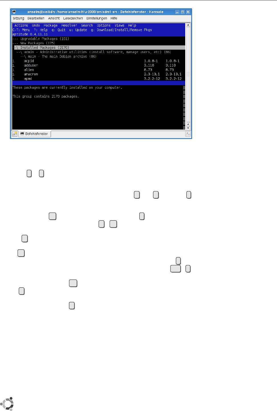
26.3 Debian Package Management: The Next Generation 411
Figure 26.1: The
aptitude
program
used to “open” the next level of such a subtree. (You can open all of the subtree
by typing ].) /gives you a window that lets you enter a search term (or reg-
ular expression) for a package name. When scrolling through the package lists,
explanations for the packages encountered are displayed in the lower part of the
screen, and you can scroll these up or down using the aand zkeys. The ikey
lets you change from the explanatory text to a representation of the dependencies.
If the cursor bar sits on a package’s line, you can select it for installation or
updating using the +key, or mark it for deletion using -. If you want to remove
it completely (as in “
dpkg --purge
”), use _.=sets a package’s status to “hold”,
which means that it will no longer be automatically upgraded.
With u, you can update the package lists (like “
apt-get update
”) and then check
the “Updated Packages” subtree to nd which packages
aptitude
would update.
Using U, you can mark all of these packages for actual updating. The “New
Packages” subtree displays those packages added since the last update; fempties
this list and places these packages among the “normal” lists. The Ctrl +tkey
combination opens the menu bar, in which you can move using the arrow keys
and select a function using ↩.
The gcommand starts the actual installation, update, or package removal. At
rst it shows an overview of the planned actions, which you may revise using the
usual commands. Another gstarts the actual work: First all required new pack-
ages are fetched, then
aptitude
calls
dpkg
to atually install or remove the desired
packages.
BContrary to popular perception,
aptitude
is not really a front-end to
apt-get
,
but does by itself whatever
apt-get
would otherwise do.
If conicts occur,
aptitude
oers solution strategies by way of suitable proposals solution strategies
for installations, updates, or package removals, from which you can pick the one
that is most appropriate.
BIn its default conguration,
aptitude
automatically installs even those pack-
ages that a package marks
Recommended:
. This is not always what is wanted
and can be switched o from the “Options” menu.
You can install and use
aptitude
on Ubuntu, but it is not the recommended
program. For this reason, it does not agree 100% with the graphical tools

412 26 Software Package Management Using Debian Tools
proposed for package management by Ubuntu—so you should either do
everything like Ubuntu recommends, or else do everything using
aptitude
.
26.4 Debian Package Integrity
The
debsums
program is used to check the integrity of the les in a single package
(Section 26.2.6). This is nice but does not ensure that an attacker has not manip-
ulated both the les in the package and the
.md5sums
le containing the original
checksums. The question remains: How does the Debian project ensure the in-integrity of complete packages
tegrity of complete packages (and, based on this, the integrity of the whole distri-
bution)? This works as follows:
• Every Debian package is cryptographically signed by a Debian developer.
This means that the receipient of the package can use the developer’s public
key to verify that they received the package in the state it was in when the
developer released it.
BThe Debian developer who signed the package must not necessar-
ily have been the person who assembled it. In principle, every De-
bian developer may sign and release any package in Debian (a “non-
maintainer upload”), and this is being done in practice for timely
updates xing critical security holes and to adopt “orphaned” pack-
ages. Furthermore, there are numerous people who help with Debian
GNU/Linux and, even though they are not formally Debian develop-
ers (or whose applications for developer status are pending), maintain
packages. These people cannot by themselves release packages, but
must do this via a “sponsor” who must be a Debian developer. The
sponsor assumes the responsibility that the package is reasonable.
AYou should not overestimate the security gained through digital sig-
natures: A developer’s signature does not guarantee that there is no
malicious code in a package, but only that the developer signed the
package. Theoretically it is possible for a cracker to pass the Debian
developer accreditation procedure and be able to release ocial pack-
ages into the distribution—whose control scripts most users will exe-
cute uncritically as
root
. Most other Linux distributions share the same
weaknesses.
• The Debian infrastructure only accepts packages for publication that have
been signed by a Debian developer.
• On the Debian server (and all servers mirroring Debian GNU/Linux) there
is a le (or several) called
Packages.gz
for each current Debian distribution.
This le contains the MD5 checksums of all packages in the distribution, as
they are on the server; since the server only accepts packages from accred-
ited developers, these are authentic.
• For each current Debian distribution on the server there is a le called
Release
, which contains the MD5 checksums of the
Packages.gz
le(s) in-
volved. This le is cryptographically signed (the signature is in a le called
Release.gpg
).
With this chain of checksums and signatures, the integrity of packages in the dis-
tribution can be checked:
• A new package is downloaded and its MD5 checksum is determined.
• We check whether the signature of the
Release
le is correct, and, if so, read
the MD5 checksum of
Packages.gz
from that le.

26.5 The debconf Infrastructure 413
• With that checksum, we verify the integrity of the actual
Packages.gz
le.
• The MD5 checksum of the package given in
Packages.gz
must match that of
the downloaded le.
If the MD5 checksum of the downloaded le does not match the “nominal value”
from
Packages.gz
, the administrator is made aware of this fact and the package is
not installed (just yet, anyway).
BIt is possible to congure a Debian system such that it only installs packages
that can be veried in this way. (Usually all you get is warnings which can be
overridden manually.) With this, you can construct an infrastructure where
only packages from a considered-safe-and-sensible “subdistribution” can
be installed. These packages may be from Debian GNU/Linux or else have
been made available locally.
BThe APT infrastructure only trusts package sources for which a public
GnuPG key has been placed in the
/etc/apt/trusted.gpg
. The
apt-key
pro-
gram is used to maintain this le.
BThe current public keys for Debian package sources are contained in the
debian-archive-keyring
package and can be renewed by updating this le.
(Debian rotates the keys on a yearly basis).
You can nd out more about managing signed packages in Debian in [F+07,
chapter 7]. We explain GnuPG in the Linup Front training manual Linux Admin-
istration II.
26.5 The debconf Infrastructure
Sometimes questions come up during the installation of software packages. For
example, if you are installing a mail server package, it is important to know, in or-
der to generate an appropriate conguration le, whether the computer in ques-
tion is connected directly to the Internet, whether it is part of a LAN with its own
dedicated mail server, or whether it uses a dial-up connection to access the net. It
is also necessary to know the domain the computer is to use for its messages and
so on.
The debconf mechanism is designed to collect this information and to store
it for future use. It is basically a database for system-wide conguration set-
tings, which can, for example, be accessed by the installation scripts of a package.
To manipulate the database, debconf supports modular user interfaces covering
all tastes from very simple textual prompts to text-oriented dialogs and various
graphical desktop applications such as KDE and GNOME. There are also inter-
faces to popular programming languages like Python.
You can redo the initial debconf-based conguration of a software package at
any time by giving a command like
#dpkg-reconfigure my-package
dpkg-reconfigure
repeats the questions asked during the original installation pro-
cess of the package, using the pre-set user interface.
BYou can select another user interface on an ad-hoc basis by means of the
--frontend
(or
-f
) option. The possible names are given in
debconf
(7) if you
have installed the
debconf-doc
package. The default is
dialog
.
BTo change the user interface temporarily if you are not calling
dpkg-reconfigure
directly, use the
DEBCONF_FRONTEND
environment variable:
#DEBCONF_FRONTEND=noninteractive aptitude upgrade

414 26 Software Package Management Using Debian Tools
With
dpkg-reconfigure
, you can also control the level of detail of the questions
you will be asked. Use the
--priority
(or
-p
) option followed by a priority. The
possible priorities are (in descending order):
critical
Questions you absolutely must answer lest terrible things happen.
high
Questions without a sensible default—your opinion counts.
medium
Questions with a sensible default.
low
Trivial questions with a default that works most of the time.
If you say something like
#dpkg-reconfigure --priority=medium my-package
you will be asked all priority
critical
,
high
, and
medium
questions; any priority
low
questions will be skipped.
BFor ad-hoc changes if debconf is called indirectly, there is also the
DEBCONF_PRIORITY
environment variable.
The debconf infrastructure is fairly complex but useful. For example, it is pos-
sible to put the answers into an LDAP database that is accessible to all computers
on a network. You can thus install a large number of machines without manual
intervention. To explain this in detail would, however, be beyond the scope of this
manual.
Exercises
C26.11 [1] How can you change the pre-set user interface for debconf on a
permanent basis?
26.6
alien
: Software From Different Worlds
Many software packages are only available in the popular RPM format. Commer-
cial packages in particular are more likely to be oered for the Red Hat or SUSE
distributions, even though nothing would prevent anyone from trying the soft-
ware on Debian GNU/Linux (serious use may be precluded by the loss of man-
ufacturer support if a non-approved platform is used). You cannot install RPM
packages on a Debian system directly, but the
alien
program makes it possible
to convert the package formats of various Linux distributions—besides RPM also
the Stampede and Slackware formats (not that these are desperately required)—to
the Debian package format (and vice-versa).
Important: While
alien
will let you convert packages from one format to another,
there is no guarantee whatsoever that the resulting package will be useful in any
way. On the one hand, the programs in the package may depend on libraries
that are not available (or not available in the appropriate version) in the target
distribution—since
alien
does not deal with dependencies, you must sort out any
problems of this type manually. On the other hand, it is quite possible that the
package integrates itself into the source distribution in a way that is impossible or
dicult to replicate on the target distribution.
As a matter of principle, the farther “down” a package sits in the system the
smaller the probability that
alien
will do what you want. With packages that con-
sist of a few executable programs without bizarre library dependencies, the cor-
responding manual pages, and a few example les, chances are good for
alien
to do the Right Thing. With system services that must integrate into the system
boot sequence, things may well look dierent. And you should not even think of
replacing
libc
…

26.6 Bibliography 415
B
alien
is used, in particular, to convert LSB-compliant software packages for
installation on a Debian GNU/Linux system—LSB species RPM as the
software distribution package format.
After these introductory remarks, we’ll show you quickly how to use
alien
to
convert a RPM package to a Debian package:
#alien --to-deb paket.rpm
(Where
--to-deb
represents the default case and may be left out.) The reverse is
possible using
#alien --to-rpm paket.deb
To assemble and disassemble RPM les, the
rpm
program must be installed (which
is available as a package for Debian GNU/Linux); to assemble
deb
packages you
need a fewpertinent Debian packageswhich are listed in
alien
(1p). (As mentioned
in Section 26.2, you can take
deb
packages to bits on almost all Linux systems using
“on-board tools” such as
tar
,
gzip
, and
ar
.)
Commands in this Chapter
alien
Converts various software packaging formats
alien
(1) 414
apt-get
Powerful command-line tool for Debian GNU/Linux package manage-
ment
apt-get
(8) 407
aptitude
Convenient package installation and maintenance tool (Debian)
aptitude
(8) 410
dpkg
Debian GNU/Linux package management tool
dpkg
(8) 400
dpkg-reconfigure
Recongures an already-installed Debian package
dpkg-reconfigure
(8) 413
Bibliography
F+07 Javier Fernández-Sanguino Peña, et al. “Securing Debian Manual”, 2007.
http://www.debian.org/doc/manuals/securing-debian-howto/

$ echo tux
tux
$ ls
hallo.c
hallo.o
$ /bin/su -
Password:
27
Package Management with RPM
and YUM
Contents
27.1 Introduction. . . . . . . . . . . . . . . . . . . . . . 418
27.2 Package Management Using
rpm
...............419
27.2.1 Installation and Update . . . . . . . . . . . . . . . 419
27.2.2 Deinstalling Packages . . . . . . . . . . . . . . . . 419
27.2.3 Database and Package Queries . . . . . . . . . . . . . 420
27.2.4 Package Verication . . . . . . . . . . . . . . . . . 422
27.2.5 The
rpm2cpio
Program . . . . . . . . . . . . . . . . 422
27.3YUM........................423
27.3.1 Overview . . . . . . . . . . . . . . . . . . . . 423
27.3.2 Package Repositories . . . . . . . . . . . . . . . . 423
27.3.3 Installing and Removing Packages Using YUM . . . . . . . 424
27.3.4 Information About Packages. . . . . . . . . . . . . . 426
27.3.5 Downloading Packages. . . . . . . . . . . . . . . . 428
Goals
• Knowing the basics of RPM and related tools
• Being able to use
rpm
for package management
• Being able to use YUM
Prerequisites
• Knowledge of Linux system administration
• Experience with an RPM-based Linux distribution is helpful
adm1-rpm.tex
(
33e55eeadba676a3
)

418 27 Package Management with RPM and YUM
27.1 Introduction
The “Red Hat Package Manager” (RPM, for short) is a tool for managing software
packages. It supports the straightforward installation and deinstallation of pack-
ages while ensuring that dierent packages do not conict and that dependencies
between the packages are taken into account. In addition, RPM allows you to
specify package queries and to ensure the integrity of packages.
RPM’s core is a database. Software packages add themselves when they are
installed and remove themselves again when they are deinstalled. To allow this,
software packages must be provided in a specic format, i. e., as RPM packages.
The RPM package format is used used by many distributions (including those
by Red Hat, Novell/SUSE, TurboLinux, and Mandriva). An arbitrary RPM pack-
age, though, cannot generally be installed on any RPM-based distribution without
forethought: Since the RPM package contains compiled software, it must t the
processor architecture in use; since le system structure, the type of service con-
trol (init scripts, etc.), and the internal description of dependencies dier between
distributions or even between dierent versions of the same distribution, careless
installation across distribution may cause problems.
BRPM was originally developed by Red Hat and was accordingly called “Red
Hat Package Manager” at rst. Since various other distributions have taken
to using the program, it has been renamed to “RPM Package Manager”.
BAt the moment there is a certain controversy as to who is in charge of further
development of this critical piece of infrastructure. After a long hiatus, dur-
ing which nobody really bothered to put out a canonical version, some Fe-
dora developers tried in 2006/7 to restart RPM development as an ocially
distribution-neutral project (this project is now led by Panu Matilainen of
Red Hat, with developers aliated with some other RPM-using distribu-
tions in support). Independently, Je Johnson, the last ocial RPM devel-
oper at Red Hat (who is no longer with the company), is putting work into
RPM and claims that his code represents “the ocial code base”—although
no Linux distribution seems to pay attention.
An RPM package has a compound le name, for examplefile name
openssh-3.5p1-107.i586.rpm
which usually consists of the package name (
openssh-3.5p1-107
), the architecture
(
i586
) and the
.rpm
sux. The package name is used to identify the package inter-
nally once it has been installed. It contains the name of the software (
openssh
) and
the software version as assigned by its original developers (
3.5p1
) followed by a
release number (
107
) assigned by the package builder (the distributor).
The “RPM Package Manager” is invoked using the
rpm
command, followed by
a basic mode. The most important modes will be discussed presently, exceptingbasic mode
the modes for initialising the RPM database and constructing and signing RPM
packages, which are outside the scope of this course.
There is a number of global options as well as supplementary, mode-specicoptions
options. Since some modes and supplementary options are identical, the mode
must (unlike with
tar
) be specied rst.
Global options include
-v
and
-vv
, which increase the “verbosity” of RPM’s
output.
BRPM’s conguration is stored within the
/usr/lib/rpm
directory; local or in-
dividual customisations are made within the
/etc/rpmrc
or
~/.rpmrc
les, but
should not be necessary for normal operations.

27.2 Package Management Using
rpm
419
27.2 Package Management Using
rpm
27.2.1 Installation and Update
An RPM package is installed in
-i
mode, followed by the package le’s path name,
such as
#rpm -i /tmp/openssh-3.5p1-107.i586.rpm
You may also specify the path as an HTTP or FTP URL in order to install package
les that reside on remote serers. It is permissible to specify several packages at
once, as in “
rpm -i /tmp/*.rpm
”.
Additionally, there are the two related modes
-U
(“upgrade”) and
-F
(“freshen”).
The former removes any older versions of a package as well as installing the new
one, while the latter installs the package only if an earlier version is already
installed (which is subsequently removed).
All three modes support a number of options, which must absolutely be men-
tioned after the mode. Besides
-h
(“hash mark”, for a progress bar) there is
--test
,
which prevents the actual installation and only checks for possible conicts.
When a conict occurs, the package in question is not installed. Conicts arise
if
• an already-installed package is to be installed again,
• a package is to be installed even though it is already installed in a dierent
version (mode
-i
) or a more current version (mode
-U
),
• the installation would overwrite a le belonging to a dierent package,
• a package requires a dierent package which is not already installed or
about to be installed.
If the installation fails for any of these reasons, you can force it to be performed
through options. For example, the
--nodeps
option disables the dependency check.
Further options can inuence the installation itself (rather than just the security
checks). For example, you can move packages to dierent directories on installa-
tion. This is the only way to install, e. g., Apache 1.3 and Apache 2.0 at the same
time, since usually both of them would claim
/sbin/http
for themselves: one of the
two must move to
/usr/local
.
27.2.2 Deinstalling Packages
Packages can be deinstalled using
-e
(“erase”) mode, e. g.,
#rpm -e openssh-3.5p1-107
Note that you need to specify the internal package name rather than the package
le path, since RPM does not remember the latter. (The next section will tell you
how to nd out the package name.) You can also abbreviate the package name as
long as it stays unique. If there is no other
openssh
package, you might also remove
it by
#rpm -e openssh
Again, RPM takes care not to remove packages that other packages depend upon.
The
--test
and
--nodeps
options have the same meaning as upon installation;
they must also appear after the mode.
When deinstalling, all of the package’s installed les will be removed unless
they are conguration les that you have changed. These will not be removed but configuration files
merely renamed by appending the
.rpmsave
sux. (The RPM package determines
which of its les will be considered conguration les.)

420 27 Package Management with RPM and YUM
27.2.3 Database and Package Queries
The “RPM Package Manager” becomes even more useful if you do not just con-
sider it a package installation and removal tool, but also an information source.
The mode for this is
-q
(“query”), and you can specify in more detail what kind of
information you would like to obtain and from which package.
Specifying the Package Without further options,
rpm
expects an internal package
name, which may be abbreviated, and it outputs the full package name:
$rpm -q openssh
openssh-3.5p1-107
This makes it easy to determine how current your system is. You can also nd the
package claiming a le, using the
-f
option:
$rpm -qf /usr/bin/ssh
openssh-3.5p1-107
This lets you relate unknown les to a package. As a third possibility, you can
obtain a list of all installed packages with the
-a
option:
$rpm -qa
This list may of course be processed further, as in the following example:1
$rpm -qa | grep cups
cups-client-1.1.18-82
cups-libs-1.1.18-82
kdelibs3-cups-3.1.1-13
cups-drivers-1.1.18-34
cups-drivers-stp-1.1.18-34
cups-1.1.18-82
Finally, RPM allows you to query a non-installed package. Use
-p
followed by
the package le’s name:
$rpm -qp /tmp/openssh-3.5p1-107.i586.rpm
openssh-3.5p1-107
This does not look too spectacular, since the internal package name was already
part of the package le name. But the le name might have been changed until it
no longer had anything to do with the actual package name, and secondly, there
are other questions that you might want to ask.
Specifying the Query If you are not just interested in the package name, you can
extend your query. Every extension may be combined with every way of specify-
ing a packet. Via
$rpm -qi openssh
you can obtain detailed information (
-i
) about the package; while
-l
provides a
list of all les belonging to the package, together with
-v
it forms an equivalent to
the
ls -l
command:
1The naming and arrangement of packages is the package preparer’s concern; dierences may occur
depending on the distribution and version.

27.2 Package Management Using
rpm
421
$rpm -qlf /bin/bash
/bin/bash
/bin/sh
$rpm -qlvf /bin/bash
-rwxr-xr-x root root 491992 Mar 14 2003 /bin/bash
lrwxrwxrwx root root 4 Mar 14 2003 /bin/sh -> bash
It is important to note that the les listed for a package are only those that show
up in the RPM database, namely those that a package brought along when it was
installed. This does not include les that were generated during installation (by
the package’s installation scripts) or during system operation (log les, etc.).
We have already seen that RPM treats conguration les specially (when de-
installing). The second class of special les are documentation les; these can be
omitted from installation. The
-c
and
-d
options of query mode behave like
-l
, but
they conne themselves to conguration and documentation les, respectively.
Advanced Queries The following details are not relevant for LPIC-1, but they
will improve your understanding of RPM’s concepts and database structure.
Dependencies between packages can belong to various types. For example, a dependencies
package may simply require a shell, i.e.,
/bin/sh
. By means of
$rpm -qf /bin/sh
bash-2.05b-105
it is straightforward to nd out that this le is provided by the
bash
package (the
same can be done for non-installed packages).
Things are dierent, e. g., for the SAINT package, a security analysis tool which
requires a web browser. Every specic dependency on a particular web browser
would be unduly limiting. For this reason, RPM lets packages provide or depend
upon “capabilities”. In our example, SAINT requires the abstract capability “web
browser”. The les and capabilities that a package requires can be queried using
the
--requires
option:2
$rpm -q --requires saint
web_browser
/bin/rm
/bin/sh
/usr/bin/perl
The packages providing these capabilities can be found using the
--whatprovides
option:
$rpm -q --whatprovides web_browser
w3m-0.3.2.2-53
mozilla-1.2.1-65
lynx-2.8.4-391
For SAINT, you need just one of these packages.
In the same manner, the
--provides
and
--whatrequires
options allow you to
query the services (or les, with the
-l
option) that a package oers, and a ser-
vice’s consumers.
2Here, again, the assignment and naming of capabilities is up to the package preparer; it may thus
dier between distributions and versions.

422 27 Package Management with RPM and YUM
27.2.4 Package Verification
Pre-Installation Checks Two things may happen to a package which might pre-
clude its installation: It may have been damaged during the download, i. e., the
package is erroneous. Or the package is not what it pretends to be, i. e., it has
been falsied—for example, because some malicious person tries to pass a “Tro-
jan” package o as the original.
RPM safeguards you against both scenarios: with
$rpm --checksig /tmp/openssh-3.5p1-107.i586.rpm
/tmp/openssh-3.5p1-107.i586.rpm: md5 gpg OK
an MD5 checksum of the package is compared to the checksum contained within
itself, which guarantees the proper transmission of the package. In addition, the
signature within the package, which was created using the private PGP or GPG
key of the package preparer, is checked using the package preparer’s public key.
This guarantees that the correct package has arrived.
Should the MD5 checksum be correct but not the signature, the output looks
correspondingly dierent:
$rpm --checksig /tmp/openssh-3.5p1-107.i586.rpm
/tmp/openssh-3.5p1-107.i586.rpm: md5 GPG NOT OK
Of course your distributor’s public key must be available on your system for
the signature checks.
Post-Installation Verification RPM lets you compare certain values within the
RPM database to the le system. This is done by means of the
-V
(“verify”) mode;
instead of one or more internal package names, this mode can use all specica-
tions made available for the query mode.
#rpm -V openssh
.......T c /etc/init.d/sshd
S.5....T c /etc/pam.d/sshd
S.5....T c /etc/ssh/ssh_config
SM5....T c /etc/ssh/sshd_config
.M...... /usr/bin/ssh
This output contains all les for which at least one “required” value from the
database diers from the “actual” value within the le system: a “
.
” signies
agreement, while a letter indicates a deviation. The following checks are per-
formed: access mode and le type (
M
), owner and group (
U
,
G
); for symbolic links,
the path of the referenced le (
L
); for device les, major and minor device num-
bers (
D
); for plain les the size (
S
), modication time (
T
), and content (
5
). Since
conguration les are unlikely to remain in their original state, they are labeled
with a
c
.
Even though the verication of installed packages using RPM cannot replace
an “intrusion detection system” (why should an intruder not modify the RPM
database as well?), it can be useful to limit the damage, e. g., after a hard disk
crash.
27.2.5 The
rpm2cpio
Program
RPM packages are essentially
cpio
archives with a prepended “header”. You can
use this fact to extract individual les from an RPM package without having to
install the package rst. Simply convert the RPM package to a
cpio
archive using
the
rpm2cpio
program, and feed the archive into
cpio
. Since
rpm2cpio
works as a lter,
you can easily connect the two programs using a pipe:

27.3 YUM 423
$rpm2cpio hello-2.4-1.fc10.i386.rpm \
>| cpio -idv ./usr/share/man/man1/hello.1.gz
./usr/share/man/man1/hello.1.gz
387 blocks
$zcat usr/share/man/man1/hello.1.gz | head
.\" DO NOT MODIFY THIS FILE! It was generated by help2man 1.35.
.TH HELLO "1" "December 2008" "hello 2.4" "User Commands"
.SH NAME
hello \- friendly greeting program
Exercises
C27.1 [2] Use
rpm2cpio
and
cpio
to display the list of les contained in an RPM
package.
27.3 YUM
27.3.1 Overview
The
rpm
program is useful but does have its limits. As a basic tool it can install pack-
ages that are available as les or URLs, but, for example, does not help with lo-
cating appropriate, possibly installable packages. Many RPM-based distributions
use YUM (short for “Yellow Dog Updater, Modied”, after the distribution for
which the program was originally developed) to enable access to package sources package sources
(repositories) available on the Internet or on CD-ROM.
BIn RPM-based distributions, YUM takes up approximately the same “eco-
logical niche” occupied by
apt-get
in Debian GNU/Linux and its deriva-
tives.
BYUM is usually controlled via the command line, but the “
yum shell
” com-
mand starts a “YUM shell” where you can enter multiple YUM commands
interactively.
27.3.2 Package Repositories
YUM introduces the concept of package repositories. A package repository is a set of
RPM packages that is available via the network and allows the installation of pack-
ages with YUM. The “
yum repolist
” command outputs a list of congured package
repositories:
$yum repolist
Loaded plugins: refresh-packagekit
repo id repo name status
fedora Fedora 10 - i386 enabled: 11416
updates Fedora 10 - i386 - Updates enabled: 3324
repolist: 14740
“
yum repolist disabled
” yields a list of known but disabled repositories:
$yum repolist disabled
Loaded plugins: refresh-packagekit
repo id repo name status
fedora-debuginfo Fedora 10 - i386 - Debug disabled
fedora-source Fedora 10 - Source disabled

424 27 Package Management with RPM and YUM
rawhide Fedora - Rawhide - Development disabled
To enable a repository, you need to give the
--enablerepo=
option, followed by the
“repo ID” from the list. This only works in connection with a “genuine”
yum
com-
mand;
repolist
is fairly innocuos:
$yum --enablerepo=rawhide repolist
Loaded plugins: refresh-packagekit
rawhide | 3.4 kB 00:00
rawhide/primary_db | 7.2 MB 00:14
repo id repo name status
fedora Fedora 10 - i386 enabled: 11416
rawhide Fedora - Rawhide - Development enabled: 12410
updates Fedora 10 - i386 - Updates enabled: 3324
repolist: 27150
You can disable a repository using the
--disablerepo
option.
BRepositories are most conveniently made known to YUM by means of con-
guration les in the
/etc/yum.repos.d
directory. (You could also enter them
into
/etc/yum.conf
directly, but this is more inconvenient to manage.)
BYUM keeps itself current as far as the content of repositories is concerned.
There is no equivalent to the Debian tools’ “
apt-get update
”.
27.3.3 Installing and Removing Packages Using YUM
To install a new package using YUM, you merely need to know its name. YUM
checks whether the active repositories contain an appropriately-named package,
resolves any dependencies the package may have, downloads the package and
possibly other packages that it depends upon, and installs all of them:
#yum install hello
Setting up Install Process
Parsing package install arguments
Resolving Dependencies
--> Running transaction check
---> Package hello.i386 0:2.4-1.fc10 set to be updated
--> Finished Dependency Resolution
Dependencies Resolved
=============================================================
Package Arch Version Repository Size
=============================================================
Installing:
hello i386 2.4-1.fc10 updates 68 k
Transaction Sum
=============================================================
Install 1 Package(s)
Update 0 Package(s)
Remove 0 Package(s)
Total download size: 68 k
Is this ok [y/N]: y
Downloading Packages:
hello-2.4-1.fc10.i386.rpm | 68 kB 00:00

27.3 YUM 425
====================== Entering rpm code =======================
Running rpm_check_debug
Running Transaction Test
Finished Transaction Test
Transaction Test Succeeded
Running Transaction
Installing : hello 1/1
====================== Leaving rpm code ========================
Installed:
hello.i386 0:2.4-1.fc10
Complete!
BYUM accepts not just simple package names, but also package names with
architecture specications, version numbers, and release numbers. Check
yum
(8) to nd the allowable formats.
Removing packages is just as simple:
#yum remove hello
This will also remove packages that this package depends upon—as long as these
are not required by another installed package, anyway.
BInstead of “
yum remove
” you can also say “
yum erase
”—the two are equivalent.
You can update packages using “
yum update
”:
#yum update hello
checks whether a newer version of the package is available and installs that if
this is the case. YUM takes care that all dependencies are resolved. “
yum update
”
without a package name attempts to update all installed packages.
BWhen the
--obsoletes
is specied (the default case),
yum
tries to handle the
case where one package has been replaced by another (of a dierent name).
This makes full upgrades of the whole distribution easier to perform.
B“
yum upgrade
” is the same as “
yum update --obsoletes
”—but saves some typing
in the case that you have switched o the
obsoletes
option in the congura-
tion.
BYUM supports the idea of “package groups”, i. e., packages that together
are useful for a certain task. The available package groups can be displayed
using “
yum grouplist
”:
$yum grouplist
Loaded plugins: refresh-packagekit
Setting up Group Process
Installed Groups:
Administration Tools
Authoring and Publishing
Base
Dial-up Networking Support
Editors
BIf you want to know which packages a group consists of, use “
yum groupinfo
”:

426 27 Package Management with RPM and YUM
$yum groupinfo 'Printing Support'
Loaded plugins: refresh-packagekit
Setting up Group Process
Group: Printing Support
Description: Install these tools to enable the system to
print or act as a print server.
Mandatory Packages:
cups
ghostscript
Default Packages:
a2ps
bluez-cups
enscript
A group is considered “installed” if all its “mandatory” packages are in-
stalled. Besides these there are “default packages” and “optional packages”.
B“
yum groupinstall
” lets you install the packages of a group. The conguration
option
group_package_types
determines which class package will actually be
installed—usually the “mandatory” and the “default packages”.
B“
yum groupremove
” removes all packages of a group, without taking into ac-
count package classes (
group_package_types
is ignored). Note that packages
can belong to more than one group at the same time, so they may be miss-
ing from group 𝑋after having been removed along with group 𝑌.
27.3.4 Information About Packages
The “
yum list
” command is available to nd out which packages exist:
$yum list gcc
Loaded plugins: refresh-packagekit
Installed Packages
gcc.i386 4.3.2-7 installed
You can also give a search pattern (it is best to put it inside quotes so the shell will
not mess with it):
$yum list "gcc*"
Loaded plugins: refresh-packagekit
Installed Packages
gcc.i386 4.3.2-7 installed
gcc-c++.i386 4.3.2-7 installed
Availabe Packages
gcc-gfortran.i386 4.3.2-7 fedora
gcc-gnat.i386 4.3.2-7 fedora
The “installed packages” are installed on the local system, while the “available
packages” can be fetched from repositories. The repository oering the package
is displayed on the far right.
To restrict the search to locally installed, or uninstalled but available, packages,
you can use “
yum list installed
” or “
yum list available
”:
$yum list installed "gcc*"
Loaded plugins: refresh-packagekit

27.3 YUM 427
Installed Packages
gcc.i386 4.3.2-7 installed
gcc-c++.i386 4.3.2-7 installed
$yum list available "gcc*"
Loaded plugins: refresh-packagekit
Available Packages
gcc-gfortran.i386 4.3.2-7 fedora
gcc-gnat.i386 4.3.2-7 fedora
B“
yum list updates
” lists the packages that are installed and for which updates
are available, while “
yum list recent
” lists the packages that have “recently”
arrived in a repository. “
yum list extras
” points out packages that are in-
stalled locally but are not available from any repository.
To nd out more about a package, use “
yum info
”:
$yum info hello
Loaded plugins: refresh-packagekit
Installed Packages
Name : hello
Arch : i386
Version : 2.4
Release : 1.fc10
Size : 186 k
Repo : installed
Summary : Prints a Familiar, Friendly Greeting
URL : http://www.gnu.org/software/hello/
License : GPLv3+ and GFDL and BSD and Public Domain
Description: Hello prints a friendly greeting. It also serves as a
: sample GNU package, showing practices that may be
: useful for GNU projects.
The advantage over “
rpm -qi
” is that “
yum info
” also works for packages that are not
installed locally but are available from a repository.
BYou con otherwise use “
yum info
” like “
yum
list”—“
yum info installed
”, for ex-
ample, displays detailed information about all installed packages.
Using “
yum search
”, you can search for all packages in whose name or descrip-
tion a given string occurs:
$yum search mysql
Loaded plugins: refresh-packagekit
============================ Matched: mysql ========================
dovecot-mysql.i386 : MySQL backend for dovecot
koffice-kexi-driver-mysql.i386 : Mysql-driver for kexi
libgda-mysql.i386 : MySQL provider for libgda
Unfortunately, the resulting list is unsorted and a little dicult to read.
yum
uses
boldface to emphasise the places where the search string occurs.
BYou can examine a package’s dependencies using “
yum deplist
”:
$yum deplist gcc
Loaded plugins: refresh-packagekit
Finding dependencies:
package: gcc.i386 4.3.2-7

428 27 Package Management with RPM and YUM
dependency: binutils >= 2.17.50.0.17-3
provider: binutils.i386 2.18.50.0.9-7.fc10
dependency: libc.so.6(GLIBC_2.3)
provider: glibc.i386 2.9-2
27.3.5 Downloading Packages
If you want to download a package from a repository but do not want to install it
outright, you can use the
yumdownloader
program. A command like
$yumdownloader --destdir /tmp hello
searches the repositories for the
hello
package just like YUM would and down-
loads the corresponding le to the
/tmp
directory.
The
--resolve
option causes dependencies to be resolved and any other missing
packages to be downloaded as well—but only those that are not installed on the
local system.
BWith the
--urls
option, nothing is downloaded at all, but
yumdownloader
out-
puts the URLs of the packages it would otherwise have downloaded.
BWith the
--source
option,
yumdownloader
downloads source RPMs instead of
binary RPMs.
Commands in this Chapter
cpio
File archive manager
cpio
(1) 422
rpm
Package management tool used by various Linux distributions (Red Hat,
SUSE, …)
rpm
(8) 418
rpm2cpio
Converts RPM packages to
cpio
archives
rpm2cpio
(1) 422
vimtutor
Interactive introduction to
vim vimtutor
(1) 430
yum
Convenient RPM package maintenance tool
yum
(8) 423
Summary
• RPM is a system for Linux software package management which is used by
various distributions such as those by Red Hat and Novell/SUSE.
• YUM is a front-end for
rpm
that gives access to package repositories over the
network.

$ echo tux
tux
$ ls
hallo.c
hallo.o
$ /bin/su -
Password:
A
Sample Solutions
This appendix contains sample solutions for selected exercises.
1.2 There is a copy of
linux-0.01.tar.gz
on
ftp.kernel.org
.
1.3
1. False. GPL software may be sold for arbitrary amounts of money, as long as
the buyer receives the source code (etc.) and the GPL rights.
2. False. Companies are encouraged to develop products based on GPL code,
but these products must also be distributed under the GPL. Of course a
company is not required to give away their product to the world at large—it
only needs to make the source code available to its direct customers who
bought the executables, but these may make full use of their rights to the
software under the GPL.
3. True.
4. False. You may use a program freely without having accepted the GPL (it
is not a contract). The GPL governs just the redistribution of the software,
and you can peruse the GPL before doing that. (Interactive programs are
supposed to call your attention to the GPL.) The observation is true that
only those conditions can be valid that the software recipient could know
before the purchase of the product; since the GPL gives to the recipient rights
that he would otherwise not have had at all—such as the right to distribute
original or modied code—this is not a problem: One may ignore the GPL
completely and still do all with the software that copyright allows for. This
is a marked dierence to the EULAs of proprietary programs; these try to es-
tablish a contract relationship in which the buyer explicitly gives away rights
that he would otherwise have been entitled to by copyright law (such as the
right to inspect the program to nd out its structure). This of course only
works before the purchase (if at all).
1.5 This exercise can of course not be answered correctly in printed courseware.
Look around—on
ftp.kernel.org
or in the weekly edition of
http://lwn.net/
.
2.2 In both cases, the message “
Login incorrect
” appears, but only after the pass-
word has been prompted for and entered. This is supposed to make it dicult
to guess valid user names (those that do not elicit an error message right away).
The way the system is set up, a “cracker” cannot tell whether the user name was

430 A Sample Solutions
invalid already, or whether the password was wrong, which makes breaking into
the system a lot more dicult.
2.5 Decency forbids us from printing a sample program here. It is reasonably
simple using the (deprecated) C function
getpass
(3).
3.2 In the login shell, the output is “
-bash
”, whereas in the “subshell” it is “
bash
”.
The minus sign at the beginning tells the shell to behave as a login shell rather
than a “normal” shell, which pertains to the initialisation.
3.3
alias
is an internal command (does not work otherwise).
rm
is an external
command. Within bash,
echo
and
test
are internal commands but are also avail-
able as external commands (executable program les), since other shells do not
implement them internally. In bash’s case, they are internal mostly for reasons of
eciency.
4.2 Try “
apropos process
” or “
man -k process
”.
4.5 The format and tools for info les were written in the mid-1980s. HTML
wasn’t even invented then.
5.1 In theory, you could start every program on the system and check whether
it behaves like a text editor … but that might take more time than this exercise
is worth. You could, for example, begin with a command like “
apropos edit
” and
see which of the man pages in the output correspond with an actual text editor
(rather than an editor for graphics, icons, X resources or some such). Text editors
from graphical desktop environments such as KDE or GNOME frequently do not
actually have man pages, but are documented within the desktop environment, so
it can be useful to check the desktop’s menus for a submenu such as “Editors” or
“Oce”. The third possibility is to use a package management command—such
as “
rpm -qa
” or “
dpkg -l
”—to obtain a list of installed software packages and check
for text editors there.
5.2 The program is called
vimtutor
.
6.1 In Linux, the current directory is a process attribute, i. e., every process has
its own current directory (with DOS, the current directory is a feature of the drive,
which of course is inappropriate in a multi-user system). Therefore
cd
must be
an internal command. If it was an external command, it would be executed in a
new process, change that process’s current directory and quit, while the invoking
shell’s current directory would remain unchanged throughout the process.
6.4 If a le name is passed to
ls
, it outputs information about that le only. With
a directory name, it outputs information about all the les in that directory.
6.5 The
-d
option to
ls
does exactly that.
6.6 This could look approximately like so:
$mkdir -p grd1-test/dir1 grd1-test/dir2 grd1-test/dir3
$cd grd1-test/dir1
$vi hello
$cd
$vi grd1-test/dir2/howdy
$ls grd1-test/dir1/hallo grd1-test/dir2/howdy
grd1-test/dir1/hello

A Sample Solutions 431
grd1-test/dir2/howdy
$rmdir grd1-test/dir3
$rmdir grd1-test/dir2
rmdir: grd1-test/dir2: Directory not empty
To remove a directory using
rmdir
, it must be empty (except for the entries “
.
” and
“
..
”, which cannot be removed).
6.7 The matching names are, respectively
(a)
prog.c
,
prog1.c
,
prog2.c
,
progabc.c
(b)
prog1.c
,
prog2.c
(c)
p1.txt
,
p2.txt
,
p21.txt
,
p22.txt
(d)
p1.txt
,
p21.txt
,
p22.txt
,
p22.dat
(e) all names
(f) all names except
prog
(does not contain a period)
6.8 “
ls
” without arguments lists the content of the current directory. Directories
in the current directory are only mentioned by name. “
ls
” with arguments, on the
other hand (and in particular “
ls *
”—
ls
does not get to see the search pattern, after
all) lists information about the given arguments. For directories this means that
the content of the directories is listed as well.
6.9 The “
- l
” le (visible in the output of the rst command) is interpreted as an
option by the
ls
command. Thus it does not show up in the output of the second
command, since
ls
with path name arguments only outputs information about
the les specied as arguments.
6.10 If the asterisk matched le names starting with a dot, the recursive dele-
tion command “
rm -r *
” would also apply to the “
..
” entry of a directory. This
would delete not just subdirectories of the current directory, but also the enclosing
directory and so on.
6.11 Here are the commands:
$cd
$cp /etc/services myservices
$mv myservices src.dat
$cp src.dat /tmp
$rm src.dat /tmp/src.dat
6.12 When you rename a directory, all its les and subdirectories will automat-
ically be “moved” so as to be within the directory with its new name. An
-R
to
mv
is therefore completely unnecessary.
6.13 The simple-minded approach—something like “
rm -file
”—fails because
rm
misinterprets the le name as a sequence of options. The same goes for commands
like “
rm "-file"
” or “
rm '-file'
”. The following methods work better:
1. With “
rm ./-file
”, the dash is no longer at the start of the parameter and
thus no longer introduces an option.
2. With “
rm -- -file
”, you tell
rm
that there are denitely no options after the
“
--
” but only path names. This also works with many other programs.

432 A Sample Solutions
6.14 During the replacement of the “
*
”, the “
- i
” le is picked up as well. Since
the le names are inserted into the command line in ASCII order,
rm
sees a param-
eter list like
-i a.txt b.jpg c.dat
or whatever
and considers the “
- i
” the option
-i
, which makes it remove les only with conr-
mation. We hope that this is sucient to get you to think things over.
6.15 If you edit the le via one link, the new content should also be visible via
the other link. However, there are “clever” editors which do not overwrite your
le when saving, but save a new le and rename it afterwards. In this case you
will have two dierent les again.
6.16 If the target of a symbolic link does not exist (any longer), accessing that
“dangling” link will lead to an error message.
6.17 To itself. You can recognise the le system root directory by this.
6.18 On this system, the
/home
directory is on a separate partition and has inode
number 2on that partition, while the
/
directory is inode number 2on its own
le system. Since inode numbers are only unique within the same physical le
system, the same number can show up for dierent les in “
ls -i
” output; this is
no cause for concern.
6.19 Hard links are indistinguishable, equivalent names for the same le (or,
hypothetically, directory). But every directory has a “link” called “
..
” referring to
the directory “above”. There can be just one such link per directory, which does
not agree with the idea of several equivalent names for that directory. Another
argument against hard links on directories is that for every name in the le system
tree there must be a unique path leading to the root directory (
/
) in a nite number
of steps. If hard links to directories were allowed, a command sequence such as
$mkdir -p a/b
$cd a/b
$ln .. c
could lead to a loop.
6.20 The reference counter for the subdirectory has the value 2(one link results
from the name of the subdirectory in
~
, one from the “
.
” link in the subdirectory
itself). If there were additional subdirectories within the directory, their “
..
” links
would increment the reference counter beyond its minimum value of 2.
6.21 The chain of symbolic links will be followed until you reach something that
is not a symbolic link. However, the maximum length of such chains is usually
bounded (see Exercise 6.22).
6.22 Examining this question becomes easier if you can use shell loops (see Sec-
tion 8.6). Something like
$touch d
$ln -s d L1
$i=1
$while ls -lH L$i >/dev/null
>do
>ln -s L$i L$((i+1))

A Sample Solutions 433
>i=$((i+1))
>done
creates a “chain” of symbolic links where every link points to the previous one.
This is continued until the “
ls -lH
” command fails. The error message will tell
you which length is still allowed. (On the author’s computer, the result is “40”,
which in real life should not unduly cramp anybody’s style.)
6.23 Hard links need hardly any space, since they are only additional directory
entries. Symbolic links are separate les and need one inode at least (every le
has its own inode). Also, some space is required to store the name of the target
le. In theory, disk space is assigned to les in units of the le system’s block
size (1 KiB or more, usually 4 KiB), but there is a special exception in the
ext
le
systems for “short” symbolic links (smaller than approximately 60 bytes), which
can be stored within the inode itself and do not require a full data block. Other
le systems such as the Reiser le system can handle short les of any type very
eciently, thus the space required for symbolic links ought to be negligible.
6.24 One possible command could be “
find / -size +1024k -print
”.
6.25 The basic approach is something like
find . -maxdepth 1
⟨tests⟩
-ok rm '{}' \;
The ⟨tests⟩should match the le as closely as possible. The “
-maxdepth 1
” option
restricts the search to the current directory (no subdirectories). In the simplest
case, use “
ls -i
” to determine the le’s inode number (e.g., 4711) and then use
find . -maxdepth 1 -inum 4711 -exec rm -f '{}' \;
to delete the le.
6.26 Add a line like
find /tmp -user $LOGNAME -type f -exec rm '{}' \;
or—more eciently—
find /tmp -user $LOGNAME -type f -print0 \
| xargs -0 -r rm -f
to the le
.bash_logout
in your home directory. (The
LOGNAME
environment variable
contains the current user name.)
6.27 Use a command like “
locate '*/README'
”. Of course, something like “
find
/
-name README
” would also do the trick, but it will take a lot longer.
6.28 Immediately after its creation the new le does not occur in the database
and thus cannot be found (you need to run
updatedb
rst). The database also
doesn’t notice that you have deleted the le until you invoke
updatedb
again.—It
is best not to invoke
updatedb
directly but by means of the shell script that your
distribution uses (e. g.,
/etc/cron.daily/find
on Debian GNU/Linux). This ensures
that
updatedb
uses the same parameters as always.
6.29
slocate
should only return le names that the invoking user may access.
The
/etc/shadow
le, which contains the users’ encrypted passwords, is restricted
to the system administrator (see Linux Administration I).

434 A Sample Solutions
7.1 A (probable) explanation is that the
ls
program works roughly like this:
Read directory information to list 𝑙
;
if (
option
-U
not specied
) {
Sort the entries of 𝑙
;
}
Write 𝑙to standard output
;
That is, everything is being read, then sorted (or not), and then output.
The other explanation is that, at the time the
filelist
entry is being read, there
has not in fact been anything written to the le to begin with. For eciency, most
le-writing programs buer their output internally and only call upon the oper-
ating system to write to the le if a substantial amount of data has been collected
(e. g. 8192 bytes). This can be observed with commands that produce very much
output relatively slowly; the output le will grow by 8192 bytes at a time.
7.2 When
ls
writes to the screen (or, generally, a “screen-like” device), it formats
the output dierently from when it writes to a “real” le: It tries to display several
le names on the same line if the le names’ length permits, and can also colour
the le names according to their type. When output is redirected to a “real” le,
just the names will be output one per line, with no formatting.
At rst glance this seems to contradict the claim that programs do not know
whether their output goes to the screen or elsewhere. This claim is correct in the
normal case, but if a program is seriously interested in whether its output goes
to a screen-like device (a “terminal”) it can ask the system. In the case of
ls
, the
reasoning behind this is that terminal output is usually looked at by people who
deserve as much information as possible. Redirected output, on the other hand, is
processed by other programs and should therefore be simple; hence the limitation
to one le name per line and the omission of colors, which must be set up using
terminal control characters which would “pollute” the output.
7.3 The shell arranges for the output redirection before the command is invoked.
Therefore the command sees only an empty input le, which usually does not lead
to the desired result.
7.4 The le is read from the beginning, and all that is read is appended to the
le at the same time, so that it grows until it takes up all the free space on the disk.
7.5 You need to redirect standard output to standard error output:
echo Error >&2
7.6 There is nothing wrong in principle with
… | tee foo | tee bar | …
However, it is easier to write
… | tee foo bar | …
See also
tee
’s documentation (man page or info page).
7.7 Pipe the list of le names through “
cat -b
”.
7.8 One method would be “
head -n 13 | tail -n 1
”.
7.10
tail
notices it, emits a warning, and continues from the new end of le.

A Sample Solutions 435
7.11 The
tail
window displays
Hello
orld
The rst line results from the rst
echo
; the second
echo
overwrites the complete
le, but “
tail -f
” knows that it has already written the rst six characters of the
le (“
Hello
” and a newline character)—it just waits for the le to become longer,
and then outputs whatever is new, in particular, “
orld
” (and a newline character).
7.12 With “
a
”, invisible characters are displayed using their symbolic names like
“
cr
” or “
lf
”, with “
c
” using backslash sequences such as “
\r
” or “
\n
”. With “
a
”,
the space character appears as “
sp
”.
7.13 The desired range of values (0 … 65535 = 216 − 1) corresponds exactly to the
range of values that can be stored in two bytes. Thus we must read two bytes from
/dev/random
and output them as a decimal number:
$r=`od -An -N2 -tu2 /dev/random`
$echo $r
4711
The
-N2
option reads two bytes, and
-tu2
formats them as an unsigned 2-byte dec-
imal number.
-An
suppresses the position oset (see Table 7.4).
7.14 Try
$echo "ALEA IACTA EST" | tr A-Z D-ZA-C
DOHD LDFWD HVW
$echo "DOHD LDFWD HVW" | tr A-Z X-ZA-W
ALEA IACTA EST
Similar to Caesar’s cipher is the “ROT13” method used, e. g., to publish potentially-
oensive jokes on USENET while preventing sensitive persons from accidentally
seeing them (the method leaves something to be desired as far as “real” encryp-
tion of private content is concerned). ROT13 can be described by the command
“
tr A-Za-z N-ZA-Mn-za-m
”; the advantage of this method is that you get the original
text again if you apply it twice over. The ROT13 routine in a news reader can thus
be used for decryption as well as encryption, which simplies the code.
7.15 The easy way is of course “
tr AEIOU AAAAA
”. To save typing, “
tr AEIOU A
” will
also do.
7.16 One way to do this is
$tr -cs '[:alpha:]' '\n'
The “
-c [:alpha:] \n
” converts all non-letters to newline characters, the
-s
option
causes runs of these newline characters to be replace by a single newline. It is
advisable to put the parameters in single quotes to keep the brackets from being
processed by the shell. (If you want to do this for German-language text, you
should set the
LANG
environment to
de_DE
(or some such) to ensure that umlauts
and “ß” are considered letters.)
7.17 To make this work, the “
-
” character must occur at the end of ⟨s1⟩—if it oc-
curs at the beginning, “
-az
” will look like a command option (which
tr
does not
understand), if it occurs in the middle, “
a-z
” looks like a character range. Alterna-
tively, with more typing, you could circumscribe the “
-
” character by “
[=-=]
” (see
Table 7.6), which may occur anywhere in the string.

436 A Sample Solutions
7.18 Use something like “
cat -T
” (see the documentation) or “
od -tc
”.
7.19 The command to do this is “
nl -v 100 -l 2 frog.txt
”.
7.20 The
tac
command is your friend:
$tac frog.txt | cat -n | tac
(“
nl -ba
” would have been ne instead of “
cat -n
”).
7.21 With the rst command,
wc
considers all input les separately and outputs
a line of totals in addition to the results for the individual les. With the second
command,
wc
considers its standard input, where the fact that this consists of three
separate les is no longer evident. Therefore, with the second command, there is
just one line of output instead of four.
7.24 The line containing the name “de Leaping” is sorted wrongly, since on that
line the second eld isn’t really the rst name but the word “Leaping”. If you look
closely at the examples you will note that the sorted output is always correct—
regarding “Leaping”, not “Gwen”. This is a strong argument for the second type
of input le, the one with the colon as the separator character.
7.25 You can sort the lines by year using “
sort -k 1.4,1.8
”. If two lines are equal
according to the sort key,
sort
makes an “emergency comparison” considering the
whole line, which in this case leads to the months getting sorted correctly within
every year. If you want to be sure and very explicit, you could also write “
sorkt -k
1.4,1.8 -k 1.1,1.2
”.
7.26 With the solution of Exercise 7.16, the matter is straightforward:
$tr -cs '[:alpha:]' '\n' | sort -uf
The
-u
option to
sort
ensures that from a sequence of equal words, only the rst
word will be output. The
-f
option treats uppercase and lowercase letters as iden-
tical (“
LC_COLLATE=en_GB
” would do that as well).
7.30 Use something like
cut -d: -f 4 /etc/passwd | sort -u | wc -l
The
cut
command isolates the group number in each line of the user database.
“
sort -u
” (see also Exercise 7.26) constructs a sorted list of all group numbers con-
taining each group number exactly once. Finally, “
wc -l
” counts the number of
lines in that list. The result is the number of dierent primary groups in use on
the system.
8.1 For example:
1.
%d-%m-%Y
2.
%y-%j (WK%V)
3.
%Hh%Mm%Ss
8.2 We don’t know either, but try something like “
TZ=America/Los_Angeles date
”.

A Sample Solutions 437
8.4 If you change an environment variable in the child process, its value in the
parent process remains unmodied. There are ways and means to pass informa-
tion back to the parent process but the environment is not one.
8.5 Start a new shell and remove the
PATH
variable from the environment (with-
out deleting the variable itself). Try starting external programs.—If
PATH
does not
exist at all, the shell will not start external programs.
8.6 Unfortunately we cannot oer a system-independent sample solution; you
need to see for yourself (using
which
).
8.7 Using
whereis
, you should be able to locate two les called
/usr/share/man/man1/
crontab.1.gz
and
/usr/share/man/man5/crontab.5.gz
. The former contains the docu-
mentation for the actual
crontab
command, the latter the documentation for the
format of the les that
crontab
creates. (The details are irrelevant for this exercise;
see Advanced Linux.)
8.8
bash
uses character sequences of the form “
!
⟨character⟩” to access previous
commands (an alternative to keyboard functions such as Ctrl +rwhich have mi-
grated from the C shell to
bash
). The “
!"
” character sequence, however, counts as
a syntax error.
8.9 None.
8.10 If the le name is passed as a parameter,
wc
insists on outputting it together
with the number of lines. If
wc
reads its standard input, it only outputs the line
count.
8.11 Try something like
#!/bin/bash
pattern=$1
shift
for f
do
grep $pattern "$f" && cp "$f" backup
done
After the
shift
, the regular expression is no longer the rst parameter, and that
must be taken into account for “
for f
”.
8.12 If the
-f
le test is applied to a symbolic link, it always applies to the le (or
directory, or whatever) that the link refers to. Hence it also succeeds if the name
in question is really just a symbolic link. (Why does this problem not apply to
filetest2
?)
8.14 With the rst command line, you need to wait 10 seconds for a new shell
command prompt. With the second, the waiting time amounts to 5 seconds,
after which the second
sleep
is started in the background. With the third line,
the new command prompt appears immediately, after two background processes
have been created.

438 A Sample Solutions
9.2 You can nd out about this using something like
ls /bin /sbin /usr/bin /usr/sbin | wc -l
Alternatively, you can hit Tab twice at a shell prompt—the shell will answer
something like
Display all 2371 possibilities? (y or n)
and that is—depending on
PATH
—your answer. (If you are logged in as a normal—
non-privileged—user, the les in
/sbin
and
/usr/sbin
will not normally be included
in the total.)
9.3 Use “
grep
⟨pattern⟩
*.txt /dev/null
” instead of “
grep
⟨pattern⟩
*.txt
”. Thus
grep
always has at least two le name parameters, but
/dev/null
does not otherwise
change the output.—The GNU implementation of
grep
, which is commonly found
on Linux, supports an
-H
option which does the same thing but in a non-portable
manner.
9.4 With
cp
to an existing le, the le is opened for writing and truncated to
length 0, before the source data is written to it. For
/dev/null
, this makes the data
disappear. With
mv
to an existing le, the target le is rst removed—and that is
a directory operation which, disregarding the special nature of
/dev/null
, simply
removes the name
null
from the directory
/dev
and creates a new le called
null
with the content of
foo.txt
in its place.
9.6 It is inadvisable because rstly it doesn’t work right, secondly the data in
question isn’t worth backing up anyway since it is changing constantly (you would
be wasting lots of space on backup media and time for copying), and thirdly be-
cause such a backup could never be restored. Uncontrolled write operations to,
say,
/proc/kcore
will with great certainty lead to a system crash.
10.1 Access control applies to normal users but not the administrator.
root
may
do anything! The
root
account should only be used to execute commands that
really require
root
’s privileges, e. g., to partition the disk, to create le systems,
to add user accounts, or to change system conguration les. All other actions
should be performed from an unprivileged account. This includes invoking ad-
ministration commands to gather information (where possible) and unpacking
tar
archives.
10.2 As
root
you may do anything, therefore it is very easy to damage the system,
e. g., through inadvertently mistyped commands.
10.3 This question aims at a comparison to other operating systems. Depend-
ing on the system in question, there are no access controls at all (DOS, Win-
dows 95/98) or dierent methods for access control (Windows NT/2000/XP or
Windows Vista). Accordingly, the former do not support administrator access (as
opposed to normal user access), while the latter even allow the creation of several
administrator accounts.
10.4 Basically you can log in as
root
, or create a UID 0shell using
su
. The latter
method is better, e. g., because the change including the former UID is logged.
10.5 The shell prompt often looks dierent. In addition, the
id
command may
help.

A Sample Solutions 439
10.6 You can either log in directly or
su
. For frequent changes, it is a good idea
to log in on two consoles at the same time, and obtain a
root
shell using
su
on one.
Alternatively, you could open several terminal windows on a GUI.
10.7 You will generally nd the log entry in
/var/log/messages
.
10.10 The obvious advantage is that administration is possible from anywhere,
if necessary by using an internet-enabled cell phone on the beach, and without
having to have access to specialised hardware or software. The obvious disad-
vantage is that you need to secure access to the administration tool very carefully,
in order to prevent unbidden guests to “miscongure” your system (or worse).
This may imply that (the obvious advantage notwithstanding) you may be able
to provide the administration tool only from within the local network, or that
you should secure access to it using strong cryptography (e. g., SSL with client
certicates). If you consider deploying Webmin in your company, you should dis-
cuss the possibility of external access very carefully with the appropriate decision
makers and/or corporate data protection ocers in order to avoid extremely dire
consequences that could hit you if problems appear. Consider yourself warned.
11.1 By their respective numerical UIDs and GIDs.
11.2 This works but is not necessarily a good idea. As far as the system is con-
cerned, the two are a single user, i. e., all les and processes with that UID belong
to both user names.
11.3 A pseudo-user’s UID is used by programs in order to obtain particular well-
dened access rights.
11.4 Whoever is in group
disk
has block-level read and write permission to the
system’s disks. With knowledge of the le system structure it is easy to make a
copy of
/bin/sh
into a SUID
root
shell (Section 12.5) by changing the le system
metadata directly on disk. Thus, group
disk
membership is tantamount to
root
privileges; you should put nobody into the
disk
group whom you would not want
to tell the
root
password outright.
11.5 You will usually nd an “
x
”. This is a hint that the password that would
usually be stored there is indeed stored in another le, namely
/etc/shadow
, which
unlike the former le is readable only for
root
.
11.6 There are basically two possibilities:
1. Nothing. In this case the system should turn you away after you entered
your password, since no user account corresponds to the all-uppercase user
name.
2. From now on, the system talks to you in uppercase letters only. In this case
your Linux system assumes that you are sitting in front of an absolutely
antediluvial terminal (1970s vintage or so) that does not support lowercase
letters, and kindly switches its processing of input and output data such that
uppercase letters in the input are interpreted as lowercase, and lowercase
letters in the output are displayed as uppercase. Today this is of limited
benet (except if you work in a computer museum), and you should log out
as quickly again as possible before your head explodes. Since this behaviour
is so atavistic, not every Linux distribution goes along with it, though.
11.7 Use
getent
,
cut
, and
sort
to generate lists of user names for the databases,
and
comm
to compare the two lists.

440 A Sample Solutions
11.8 Use the
passwd
command if you’re logged in as user
joe
, or “
passwd joe
” as
root
. In
joe
’s entry in the
/etc/shadow
le there should be a dierent value in the
second eld, and the date of the last password change (eld 3) should show the
current date (in what unit?)
11.9 As
root
, you set a new password for him using “
passwd dumbo
”, as you cannot
retrieve his old one even though you are the administrator.
11.10 Use the command “
passwd -n 7 -x 14 -w 2 joe
”. You can verify the settings
using “
passwd -S joe
”.
11.11 Use the
useradd
command to create the user, “
usermod -u
” to modify the
UID. Instead of a user name, the les should display a UID as their owner, since
no user name is known for that UID …
11.12 For each of the three user accounts there should be one line in
/etc/passwd
and one in
/etc/shadow
. To work with the accounts, you do not necessarily need a
password (you can use
su
as
root
), but if you want to login you do. You can create
a le without a home directory by placing it in
/tmp
(in case you forgot—a home
directory for a new user would however be a good thing).
11.13 Use the
userdel
command to delete the account. To remove the les, use
the “
find / -uid
⟨UID⟩
-delete
” command.
11.14 If you use “
usermod -u
”, you must reassign the user’s le to the new UID,
for example by means of “
find / -uid
⟨UID⟩
-exec chown test1 {} \;
” or (more e-
ciently) “
chown -R --from=
⟨UID⟩
test1 /
”. In each case, ⟨UID⟩is the (numerical) for-
mer UID.
11.15 You can either edit
/etc/passwd
using
vipw
or else call
usermod
.
11.16 Groups make it possible to give specic privileges to groups [sic!] of users.
You could, for example, add all HR employees to a single group and assign that
group a working directory on a le server. Besides, groups can help organise
access rights to certain peripherals (e. g., by means of the groups
disk
,
audio
, or
video
).
11.17 Use the “
mkdir
⟨directory⟩” command to create the directory and “
chgrp
⟨groupname⟩ ⟨directory⟩” to assign that directory to the group. You should also
set the SGID bit to ensure that newly created les belong to the group as well.
11.18 Use the following commands:
#groupadd test
#gpasswd -a test1 test
Adding user test1 to group test
#gpasswd -a test2 test
Adding user test2 to group test
#gpasswd test
Changing the password for group test
New Password:x9q.Rt/y
Re-enter new password:x9q.Rt/y
To change groups, use the “
newgrp test
” command. You will be asked for the pass-
word only if you are not a member of the group in question.

A Sample Solutions 441
12.1 A new le is assigned to your current primary group. You can’t assign a
le to a group that you are not a member of—unless you are
root
.
12.3 077 and ”‘
u=rwx,go=
”’, respectively.
12.5 This is the SUID or SGID bit. The bits cause a process to assume the
UID/GID of the executable le rather than that of the executing user. You can
see the bits using “
ls -l
”. Of course you may change all the permissions on your
own les. However, at least the SUID bit only makes sense on binary executable
les, not shell scripts and the like.
12.6 One of the two following (equivalent) commands will serve:
$umask 007
$umask -S u=rwx,g=rwx
You may perhaps ask yourself why this umask contains
x
bits. They are indeed
irrelevant for les, as les are not created executable by default. However it might
be the case that subdirectories are desired in the project directory, and it makes
sense to endow these with permissions that allow them to be used reasonably.
12.7 The so-called “sticky bit” on a directory implies that only the owner of a
le (or the owner of the directory) may delete or rename it. You will nd it, e. g.,
on the
/tmp
directory.
12.9 This doesn’t work with the
bash
shell (at least not without further trickery).
We can’t speak for other shells here.
12.11 You cannot do this with
chattr
alone, since various attributes can be dis-
played with
lsattr
but not set with
chattr
. Read up on the details in
chattr
(1).—In
addition, some attributes are only dened for “plain” les while others are only
dened for directories; you will, for example, nd it dicult to make the
D
and
E
attributes visible for the same “le system object” at the same time. (The
E
at-
tribute is to do with transparent compression, which cannot be used on directo-
ries, while
D
only applies to directories—write operations to such directories will
be performed synchronously.)
13.1 In the directory of a process below
/proc
there is a le called
environ
which
contains the environment variables of that process. You can output this le using
cat
. The only blemish is that the variables in this le are separated using zero
bytes, which looks messy on the screen; for convenience, you might use something
like “
tr "\0" "\n" </proc/4711/environ
” to display the environment.
13.2 Funnily enough, the limit is not documented in any obvious placees. In
/usr/include/linux/threads.h
on a Linux 2.6 kernel, the constant
PID_MAX_LIMIT
is de-
ned with a value of 32768; this is the lowest value that will by default not be
assigned to processes. You can query the actual value in
/proc/sys/kernel/pid_max
(or even change it—the maximum for 32-bit platforms is actually 32768, while on
64-bit systems you may set an arbitrary value of up to 222, which is approximately
4 million).
The PIDs assigned to processes rise monotonically at rst. When the above-
mentioned limit is reached, assignment starts again with lower PIDs, where PIDs
that are still being used by processes are of course not given again to others. Many
low PIDs are assigned to long-running daemons during the boot process, and for
this reason after the limit has been reached, the search for unused PIDs starts again
not at PID 1but at PID 300. (The details are in the
kernel/pid_namespace.c
le within
the Linux source code.)

442 A Sample Solutions
13.4 As we said, zombies arise when the parent process does not pick up the
return code of a child process. Thus, to create a zombie you must start a child
process and then prevent the parent process from picking up its return code, for
example by stopping it by means of a signal. Try something like
$sh
$echo $$
In the subshell
12345
$sleep 20
In a dierent window:
$kill -STOP 12345
Wait
$ps u | grep sleep
joe 12346 0.0 0.0 3612 456 pts/2 Z 18:19 0:00 sleep 20
13.5 Consult
ps
(1).
13.6 Try
$ps -o pid,ppid,state,cmd
13.7 Usually
SIGCHLD
(“child process nished”—sometimes called
SIGCLD
),
SIGURG
(urgent data was received on a network connection) and
SIGWINCH
(the size of the
window for a text-based program was changed). These three events are so inane
that the process should not be terminated on their account.
13.8 Something like
$pgrep -u hugo
should suce.
13.10 Use, e. g., the “
renice -10
⟨PID⟩” command. You can only specify negative
nice values as
root
.
14.2
sda1
,
sda2
,
sda5
,
sda6
, and
sdb1
,
sdb5
,
sdb6
,
sdb7
.
15.2 Use
tune2fs
with the
-c
,
-u
and
-m
options.
15.3
mkreiserfs /dev/sdb5
15.6
/etc/fstab
contains all frequently-used le systems and their mount points,
while
/etc/mtab
contains those le systems that are actually mounted at the mo-
ment.
16.1 The boot loader can be placed inside the MBR, in another (partition) boot
sector, or a le on disk. In the two latter cases, you will need another boot loader
that can “chain load” the Linux boot loader. Be that as it may, for a Linux system
you absolutely need a boot loader that can boot a Linux kernel, such as GRUB
(there are others).
16.3 Assign a password preventing the unauthorised entry of kernel parame-
ters. With GRUB Legacy, e. g., using
password --md5
⟨encrypted keyword⟩
lock
helps with the password request for a specic operating system.

A Sample Solutions 443
17.3 You can display the previous and current runlevel using
runlevel
. If the
previous runlevel is “
N
” that means “none”—the system started into the current
runlevel. To change, say “
init 2
”, then “
runlevel
” again to check.
17.4 A possible entry for the
inittab
le might be
aa:A:ondemand:/bin/date >/tmp/runlevel-a.txt
This entry should write the current time to the mentioned le if you activate it
using “
telinit A
”. Don’t forget the “
telinit q
” to make
init
reread its conguration
le.
17.5 Call the
syslog
init script with the
restart
or
reload
parameters.
17.6 For example, by using “
chkconfig -l
” (on a SUSE or Red Hat system).
17.7 It is tempting just to remove the symbolic links from the runlevel directory
in question. However, depending on the distribution, they may reappear after the
next automated change. So if your distribution uses a tool like
chkconfig
or
insserv
you had better use that.
17.8 You should be prepared for the system asking for the
root
password.
17.10 Use the
#shutdown -h +15 'This is just a test'
command; everything that you pass to
shutdown
after the delay will be sent to your
users as a broadcast message. To cancel the shutdown, you can either interrupt
the program using the Ctrl +ckey combination (if you started
shutdown
in the
foreground), or give the “
shutdown -c
” command.
17.10 The le name will be sent as the message.
18.4 The unit le does not need to be modied in order to express dependencies.
This makes the automatic installation and, in particular, deinstallation of units
as part of software packages easier (e. g., in the context of a distribution-specic
package management tool) and allows the seamless updating of unit les by a
distribution.
18.10 There is no exact equivalent because systemd does not use the runlevel
concept. You can, however, display all currently active targets:
#systemctl list-units -t target
18.11 “
systemctl kill
” guarantees that the signal will only be sent to processes
belonging to the unit in question. The other two commands send the signal to all
processes whose name happens to be
example
.
18.13 You can’t (“
systemctl mask
” outputs an error message). You must deactivate
the service and then remove, move, or rename the unit le.
19.1 (a) On 1 March, 5 P. M.; (b) On 2 March, 2 P. M.; (c) On 2 March, 4 P. M.; (d)
On 2 March, 1 A.M.

444 A Sample Solutions
19.2 Use, e. g., “
at now + 3 minutes
”.
19.4 One possibility might be “
atq | sort -bk 2
”.
19.6 Your task list itself is owned by you, but you do not have permission to write
to the
crontabs
directory. Debian GNU/Linux, for example, uses the following
permission bits:
$ls -ld /var/spool/cron/crontabs
drwx-wx--T 2 root crontab 4096 Aug 31 01:03 /var/spool/cron/crontabs
As usual,
root
has full access to the le (in fact regardless of the permission bits)
und members of the
crontab
group can write to les in the directory. Note that
members of that group have to know the le names in advance, because the di-
rectory is not searchable by them (
ls
will not work). The
crontab
utility is a set-GID
program owned by the
crontab
group:
$ls -l $(which crontab)
-rwxr-sr-x 1 root crontab 27724 Sep 28 11:33 /usr/bin/crontab
So it is executed with the access permissions of the
crontab
group, no matter which
users invokes the program. (The set-GID mechanism is explained in detail in the
document Linux System Administration I.)
19.7 Register the job for the 13th of every month and check within the script
(e. g., by inspecting the result of “
date +%u
”) if the current day is a Friday.
19.8 The details depend on the distribution.
19.9 Use something like
* * * * logger -p local0.info "cron test"
To write the date to the le every other minute, you could use the following line:
0,2,4,
,56,58 * * * * /bin/date >>/tmp/date.log
But this one is more convenient:
*/2 * * * * /bin/date >>/tmp/date.log
19.10 The commands to accomplish this are »
crontab -l
« and »
crontab -r
«.
19.11 You should add
hugo
to the
/etc/cron.deny
le (on SUSE distributions,
/var/
spool/cron/deny
) or delete him from
/etc/cron.allow
.
19.13
/etc/cron.daily
contains a script called
0anacron
which is executed as the
rst job. This script invokes “
anacron -u
”; this option causes
anacron
to update the
time stamps without actually executing jobs (which is the next thing that
cron
will
do). When the system is restarted, this will prevent
anacron
from running jobs
unnecessarily, at least if the re-boot occurs after
cron
has done its thing.
20.1 Such events are customarily logged by
syslogd
to the
/var/log/messages
le.
You can solve the problem most elegantly like
#grep 'su: (to root)' /var/log/messages

A Sample Solutions 445
20.2 Insert a line
*.* -/var/log/test
anywhere in
/etc/syslog.conf
. Then tell
syslogd
using “
kill -HUP …
” to re-read its
conguration le. If you check
/var/log
afterwards, the new le should already be
there and contain some entries (which ones?).
20.3 On the receiving system,
syslogd
must be started using the
-r
parameter (see
p. 304). The sending system needs a conguration line of the form
local0.* @blue.example.com
(if the receiving system is called “
blue.example.com
”).
20.4 The only safe method consists of putting the log out of the attacker’s reach.
Therefore you must send the messages to another host. If you don’t want the
attacker to be able to compromise that host, too, then you should connect the log-
ging host to the one storing the log by means of a serial interface, and congure
syslogd
such that it sends the messages to the corresponding device (
/dev/ttyS0
or
something). On the storing host, a simple program can accept the messages on the
serial interface and store them or process them further. Alternatively, you could
of course also use an (old-fashioned) dot-matrix printer with fan-fold paper.
20.5 You can, among other things, expect information about the amount and us-
age of RAM, available CPUs, disks and other mass storage devices (IDE and SCSI),
USB devices and network cards. Of course the details depend on your system and
your Linux installation.
20.10 Versuchen Sie etwas wie
# We assume a suitable source definition.
filter login_hugo {
facility(authpriv)
and (match("session opened") or match("session closed"))
and match("user hugo");
};
destination d_root { usertty("root"); };
log { source(...);
filter(login_hugo);
destination(d_root);
};
20.14 In
/etc/logrotate.d
, create an arbitrarily-named le containing the lines
/var/log/test {
compress
dateext
rotate 10
size 100
create
}

446 A Sample Solutions
21.1 Text les are, in principle, amenable to the standard Unix tools (
grep
etc.)
and, as such, ideologically purer. They can be inspected without specialised soft-
ware. In addition, the concept is very well understood and there are gazillions of
tools that help evaluate the traditional log les. Disadvantages include the fact
that text les are dicult to search, and any sort of targeted evaluation is either
extremely tedious or else requires additional (non-standardised) software. There
is no type of cryptographic protection against the manipulation of log entries, and
the amount of information that can be written to the log is limited.
22.2 ISO/OSI layer 2 describes the interaction between two nodes that are con-
nected directly (e.g., via Ethernet). Layer 3 describes the interaction among
nodes that are not networked directly, and thus includes routing and media-
independent addressing (e. g., IP over Ethernet or Token-Ring or …).
22.3 You can look to the
/etc/services
and (possibly)
/etc/protocols
les for inspi-
ration. You will have to assign the protocols to layers by yourself. Hint: Practically
everything mentioned in
/etc/services
belongs to the application layer.
22.4 It is, of course, impossible to give a specic answer, but usually a TTL of
30–40 should be more than sucient. (The default value is 64.) You can determine
the minimal TTL by means of sending successive packets with increasing TTL
(starting at TTL 1) to the desired target. If you receive an ICMP error message
from some router telling you that the packet was discarded, the TTL is still too
low. (The
traceroute
program automates this procedure.) This “minimal” TTL
is naturally not a constant, since IP does not guarantee a unique path for packet
delivery.
22.5
1. The
127.55.10.3
address cannot be used as a host address since it is that net-
work’s broadcast address.
2. The
138.44.33.12
address can be used as a host address.
3. The
10.84.13.160
address is the network address of the network in question
and is thus unavailable as a host address.
22.6 For example, to implement certain network topologies or assign parts of
the address range to computers in dierent providers.
22.7 There are 16 subnets altogether (which is obvious from the fact that the
subnet mask has four more bits set than the original netmask). Further subnets are
145.2.0.0
,
145.2.16.0
,
145.2.48.0
,
145.2.80.0
,
145.2.96.0 145.2.112.0
,
145.2.144.0
,
145.2.
176.0
,
145.2.208.0
,
145.2.224.0
, and
145.2.240.0
. The node with the IP address
145.2.
195.13
is part of the
145.2.192.0
subnet.
23.1
lsmod
displays all loaded modules. “
rmmod
⟨module name⟩” tries to unload a
module, which will fail when the module is still in use.
23.2 This is done most easily with
ifconfig
.
23.3 Use “
ifconfig
⟨interface⟩ ⟨IP address⟩”. To check whether other computers
can be reached, use the
ping
command.
24.1 The former should be on the order of tens of microseconds, the latter—
depending on the networking infrastructure—in the vicinity of milliseconds.

A Sample Solutions 447
24.2 Try something like
#ping -f -c 1000000 localhost
The total running time is at the end of the penultimate line of output from
ping
.
(On the author’s system it takes approximately 13 seconds.)
24.3 For example:
$ping6 ff02::2%eth0
PING ff02::2%eth0(ff02::2) 56 data bytes
64 bytes from fe80::224:feff:fee4:1aa1: icmp_seq=1 ttl=64 time=12.4 ms
64 bytes from fe80::224:feff:fee4:1aa1: icmp_seq=2 ttl=64 time=5.27 ms
64 bytes from fe80::224:feff:fee4:1aa1: icmp_seq=3 ttl=64 time=4.53 ms
Ctrl
+
c
--- ff02::2%eth0 ping statistics ---
3 packets transmitted, 3 received, 0% packet loss, time 2003ms
rtt min/avg/max/mdev = 4.531/7.425/12.471/3.581 ms
25.1 During the rst login procedure,
ssh
should ask you to conrm the remote
host’s public server key. During the second login procedure, the public server key
is already stored in the
~/.ssh/known_hosts
le and does not need to be reconrmed.
25.2 In the rst case, the connection is refused, since no public server key for the
remote host is available from
~/.ssh/known_hosts
. In the second case, the connection
is established without a query.
25.3 The le contains public keys only and thus does not need to be kept secret.
25.6 Use something like
$ssh-keygen -l -f ~/.ssh/id_rsa.pub
(Does it make a dierence whether you specify
id_rsa.pub
or
id_rsa
?)
25.7 Noninteractive programs that need to use an SSH connection are often un-
able to enter a passphrase. In restricted cases like these, it is conceivable to use
a private key without a passphrase. You should then make use of the possibility
to make a public key on the remote host useable for specic commands only (in
particular the ones that the noninteractive program needs to invoke). Details may
be found in
sshd
(8).
25.8 Try “
ssh -X root@localhost
”.
25.9 One possible command line might be
#ssh -L 4711:localhost:7 user@remote.example.com
Do consider that
localhost
is evaluated from the perspective of the
remote
host.
Unfortunately,
ssh
does not allow symbolic names of well-known ports (as per
/etc/services
).
26.11 Try
#dpkg-reconfigure debconf

448 A Sample Solutions
27.1 This is most easily done using something like
$rpm2cpio
⟨package⟩
| cpio -t

$ echo tux
tux
$ ls
hallo.c
hallo.o
$ /bin/su -
Password:
B
Example Files
In various places, the fairy tale The Frog King, more exactly The Frog King, or Iron
Henry, from German Children’s and Domestic Fairy Tales by the brothers Grimm, is
used as an example. The fairy tale is presented here in its entirety to allow for
comparisons with the examples.
The Frog King, or Iron Henry
In olden times when wishing still helped one, there lived a king whose
daughters were all beautiful, but the youngest was so beautiful that
the sun itself, which has seen so much, was astonished whenever it
shone in her face.
Close by the king's castle lay a great dark forest, and under an old
lime-tree in the forest was a well, and when the day was very warm,
the king's child went out into the forest and sat down by the side of
the cool fountain, and when she was bored she took a golden ball, and
threw it up on high and caught it, and this ball was her favorite
plaything.
Now it so happened that on one occasion the princess's golden ball did
not fall into the little hand which she was holding up for it, but on
to the ground beyond, and rolled straight into the water. The king's
daughter followed it with her eyes, but it vanished, and the well was
deep, so deep that the bottom could not be seen. At this she began to
cry, and cried louder and louder, and could not be comforted.
And as she thus lamented someone said to her, »What ails you, king's
daughter? You weep so that even a stone would show pity.«
She looked round to the side from whence the voice came, and saw a
frog stretching forth its big, ugly head from the water. »Ah, old
water-splasher, is it you,« she said, »I am weeping for my golden
ball, which has fallen into the well.«
»Be quiet, and do not weep,« answered the frog, »I can help you, but
what will you give me if I bring your plaything up again?«
»Whatever you will have, dear frog,« said she, »My clothes, my pearls
and jewels, and even the golden crown which I am wearing.«
grd1-beispiele.tex
(
be27bba8095b329b
)

450 B Example Files
The frog answered, »I do not care for your clothes, your pearls and
jewels, nor for your golden crown, but if you will love me and let me
be your companion and play-fellow, and sit by you at your little
table, and eat off your little golden plate, and drink out of your
little cup, and sleep in your little bed - if you will promise me this
I will go down below, and bring you your golden ball up again.«
»Oh yes,« said she, »I promise you all you wish, if you will but bring
me my ball back again.« But she thought, »How the silly frog does
talk. All he does is to sit in the water with the other frogs, and
croak. He can be no companion to any human being.«
But the frog when he had received this promise, put his head into the
water and sank down; and in a short while came swimming up again with
the ball in his mouth, and threw it on the grass. The king's daughter
was delighted to see her pretty plaything once more, and picked it up,
and ran away with it.
»Wait, wait,« said the frog. »Take me with you. I can't run as you
can.« But what did it avail him to scream his croak, croak, after her,
as loudly as he could. She did not listen to it, but ran home and soon
forgot the poor frog, who was forced to go back into his well again.
The next day when she had seated herself at table with the king and
all the courtiers, and was eating from her little golden plate,
something came creeping splish splash, splish splash, up the marble
staircase, and when it had got to the top, it knocked at the door and
cried, »Princess, youngest princess, open the door for me.«
She ran to see who was outside, but when she opened the door, there
sat the frog in front of it. Then she slammed the door to, in great
haste, sat down to dinner again, and was quite frightened.
The king saw plainly that her heart was beating violently, and said,
»My child, what are you so afraid of? Is there perchance a giant
outside who wants to carry you away?«
»Ah, no,« replied she. »It is no giant but a disgusting frog.«
»What does that frog want from you?«
»Yesterday as I was in the forest sitting by the well, playing, my
golden ball fell into the water. And because I cried so, the frog
brought it out again for me, and because he so insisted, I promised
him he should be my companion, but I never thought he would be able to
come out of his water. And now he is outside there, and wants to come
in to me.«
In the meantime it knocked a second time, and cried, »Princess,
youngest princess, open the door for me, do you not know what you said
to me yesterday by the cool waters of the well. Princess, youngest
princess, open the door for me.«
Then said the king, »That which you have promised must you perform.
Go and let him in.«
She went and opened the door, and the frog hopped in and followed her,
step by step, to her chair. There he sat and cried, »Lift me up beside

B Example Files 451
you.« She delayed, until at last the king commanded her to do it. Once
the frog was on the chair he wanted to be on the table, and when he
was on the table he said, »Now, push your little golden plate nearer
to me that we may eat together.« The frog enjoyed what he ate, but
almost every mouthful she took choked her.
At length he said, »I have eaten and am satisfied, now I am tired,
carry me into your little room and make your little silken bed ready,
and we will both lie down and go to sleep.« The king's daughter began
to cry, for she was afraid of the cold frog which she did not like to
touch, and which was now to sleep in her pretty, clean little bed.
But the king grew angry and said, »He who helped you when you were in
trouble ought not afterwards to be despised by you.«
So she took hold of the frog with two fingers, carried him upstairs,
and put him in a corner, but when she was in bed he crept to her and
said, »I am tired, I want to sleep as well as you, lift me up or I
will tell your father.«
At this she was terribly angry, and took him up and threw him with all
her might against the wall. »Now, will you be quiet, odious frog,«
said she. But when he fell down he was no frog but a king's son with
kind and beautiful eyes. He by her father's will was now her dear
companion and husband. Then he told her how he had been bewitched by a
wicked witch, and how no one could have delivered him from the well
but herself, and that to-morrow they would go together into his
kingdom.
And indeed, the next morning a carriage came driving up with eight
white horses, which had white ostrich feathers on their heads, and
were harnessed with golden chains, and behind stood the young king's
servant Faithful Henry.
Faithful Henry had been so unhappy when his master was changed into a
frog, that he had caused three iron bands to be laid round his heart,
lest it should burst with grief and sadness. The carriage was to
conduct the young king into his kingdom. Faithful Henry helped them
both in, and placed himself behind again, and was full of joy because
of this deliverance.
And when they had driven a part of the way the king's son heard a
cracking behind him as if something had broken. So he turned round and
cried, »Henry, the carriage is breaking.« »No, master, it is not the
carriage. It is a band from my heart, which was put there in my great
pain when you were a frog and imprisoned in the well.«
Again and once again while they were on their way something cracked,
and each time the king's son thought the carriage was breaking, but it
was only the bands which were springing from the heart of Faithful
Henry because his master was set free and was happy.
(Linup Front GmbH would like to point out that the authors strongly disap-
prove of any cruelty to animals.)

$ echo tux
tux
$ ls
hallo.c
hallo.o
$ /bin/su -
Password:
C
LPIC-1 Certification
C.1 Overview
The Linux Professional Institute (LPI) is a vendor-independent non-prot organi-
zation dedicated to furthering the professional use of Linux. One aspect of the
LPI’s work concerns the creation and delivery of distribution-independent certi-
cation exams, for example for Linux professionals. These exams are available
world-wide and enjoy considerable respect among Linux professionals and em-
ployers.
Through LPIC-1 certication you can demonstrate basic Linux skills, as re-
quired, e. g., for system administrators, developers, consultants, or user support
professionals. The certication is targeted towards Linux users with 1 to 3 years
of experience and consists of two exams, LPI-101 and LPI-102. These are oered
as computer-based multiple-choice and ll-in-the-blanks tests in all Pearson VUE
and Thomson Prometric test centres. On its web pages at
http://www.lpi.org/
, the
LPI publishes objectives outlining the content of the exams. objectives
This training manual is part of Linup Front GmbH’s curriculum for preparation
of the LPI-101 exam and covers part of the ocial examination objectives. Refer
to the tables below for details. An important observation in this context is that
the LPIC-1 objectives are not suitable or intended to serve as a didactic outline for
an introductory course for Linux. For this reason, our curriculum is not strictly
geared towards the exams or objectives as in “Take classes 𝑥and 𝑦, sit exam 𝑝,
then take classes 𝑎and 𝑏and sit exam 𝑞.” This approach leads many prospective
students to the assumption that, being complete Linux novices, they could book
𝑛days of training and then be prepared for the LPIC-1 exams. Experience shows
that this does not work in practice, since the LPI exams are deviously constructed
such that intensive courses and exam-centred “swotting” do not really help.
Accordingly, our curriculum is meant to give you a solid basic knowledge of
Linux by means of a didactically reasonable course structure, and to enable you as
a participant to work independently with the system. LPIC-1 certication is not a
primary goal or a goal in itself, but a natural consequence of your newly-obtained
knowledge and experience.
C.2 Exam LPI-101
The following table displays the objectives for the LPI-101 exam and the materials
from the “Concise Linux” series covering these objectives. The numbers in the
columns for the individual manuals refer to the chapters containing the material
in question.
lxk1-objs-101.tex
(
807d647231c25323
)

454 C LPIC-1 Certification
No Wt Title LXK1
101.1 2 Determine and congure hardware settings 14
101.2 3 Boot the system 16–18
101.3 3 Change runlevels/boot targets and shutdown or reboot system 17–18
102.1 2 Design hard disk layout 14
102.2 2 Install a boot manager 16
102.3 1 Manage shared libraries –
102.4 3 Use Debian package management 26
102.5 3 Use RPM and YUM package management 27
103.1 4 Work on the command line 3–4
103.2 3 Process text streams using lters 7
103.3 4 Perform basic le management 6, 15.3
103.4 4 Use streams, pipes and redirects 7
103.5 4 Create, monitor and kill processes 13
103.6 2 Modify process execution priorities 13
103.7 2 Search text les using regular expressions 7
103.8 3 Perform basic le editing operations using vi 5
104.1 2 Create partitions and lesystems 14–15
104.2 2 Maintain the integrity of lesystems 15
104.3 3 Control mounting and unmounting of lesystems 15
104.4 1 Manage disk quotas –
104.5 3 Manage le permissions and ownership 12
104.6 2 Create and change hard and symbolic links 6
104.7 2 Find system les and place les in the correct location 6, 9
C.3 Exam LPI-102
The following table displays the objectives for the LPI-102 exam and the materials
from the “Concise Linux” series covering these objectives. The numbers in the
columns for the individual manuals refer to the chapters containing the material
in question.
No Wt Title LXK1
105.1 4 Customize and use the shell environment –
105.2 4 Customize or write simple scripts –
105.3 2 SQL data management –
106.1 2 Install and congure X11 –
106.2 1 Setup a display manager –
106.3 1 Accessibility –
107.1 5 Manage user and group accounts and related system les 11
107.2 4 Automate system administration tasks by scheduling jobs 19
107.3 3 Localisation and internationalisation –
108.1 3 Maintain system time –
108.2 3 System logging 20–21
108.3 3 Mail Transfer Agent (MTA) basics –
108.4 2 Manage printers and printing –
109.1 4 Fundamentals of internet protocols 22–23
109.2 4 Basic network conguration 23–24
109.3 4 Basic network troubleshooting 23–24
109.4 2 Congure client side DNS 23
110.1 3 Perform security administration tasks 11, 23–24
110.2 3 Setup host security 11, 23
110.3 3 Securing data with encryption 25

C LPIC-1 Certification 455
C.4 LPI Objectives In This Manual
101.1 Determine and configure hardware settings
Weight 2
Description Candidates should be able to determine and congure fundamen-
tal system hardware.
Key Knowledge Areas
• Enable and disable integrated peripherals
• Congure systems with or without external peripherals such as keyboards
• Dierentiate between the various types of mass storage devices
• Know the dierences between coldplug and hotplug devices
• Determine hardware resources for devices
• Tools and utilities to list various hardware information (e.g.
lsusb
,
lspci
, etc.)
• Tools and utilities to manipulate USB devices
• Conceptual understanding of sysfs, udev, dbus
The following is a partial list of the used les, terms and utilities:
•
/sys/
•
/proc/
•
/dev/
•
modprobe
•
lsmod
•
lspci
•
lsusb
101.2 Boot the system
Weight 3
Description Candidates should be able to guide the system through the booting
process.
Key Knowledge Areas
• Provide common commands to the boot loader and options to the kernel at
boot time
• Demonstrate knowledge of the boot sequence from BIOS to boot completion
• Understanding of SysVinit and systemd
• Awareness of Upstart
• Check boot events in the log les
The following is a partial list of the used les, terms and utilities:
•
dmesg
• BIOS
• bootloader
• kernel
• initramfs
•
init
• SysVinit
• systemd
101.3 Change runlevels/boot targets and shutdown or reboot sys-
tem
Weight 3

456 C LPIC-1 Certification
Description Candidates should be able to manage the SysVinit runlevel or sys-
temd boot target of the system. This objective includes changing to single user
mode, shutdown or rebooting the system. Candidates should be able to alert users
before switching runlevels/boot targets and properly terminate processes. This
objective also includes setting the default SysVinit runlevel or systemd boot target.
It also includes awareness of Upstart as an alternative to SysVinit or systemd.
Key Knowledge Areas
• Set the default runlevel or boot target
• Change between runlevels/boot targets including single user mode
• Shutdown and reboot from the command line
• Alert users before switching runlevels/boot targets or other major system
events
• Properly terminate processes
The following is a partial list of the used les, terms and utilities:
•
/etc/inittab
•
shutdown
•
init
•
/etc/init.d/
•
telinit
• systemd
•
systemctl
•
/etc/systemd/
•
/usr/lib/systemd/
•
wall
102.1 Design hard disk layout
Weight 2
Description Candidates should be able to design a disk partitioning scheme for
a Linux system.
Key Knowledge Areas
• Allocate lesystems and swap space to separate partitions or disks
• Tailor the design to the intended use of the system
• Ensure the
/boot
partition conforms to the hardware architecture require-
ments for booting
• Knowledge of basic features of LVM
The following is a partial list of the used les, terms and utilities:
•
/
(root) lesystem
•
/var
lesystem
•
/home
lesystem
•
/boot
lesystem
• swap space
• mount points
• partitions
102.2 Install a boot manager
Weight 2
Description Candidates should be able to select, install and congure a boot
manager.
Key Knowledge Areas
• Providing alternative boot locations and backup boot options

C LPIC-1 Certification 457
• Install and congure a boot loader such as GRUB Legacy
• Perform basic conguration changes for GRUB 2
• Interact with the boot loader
The following is a partial list of the used les, terms and utilities:
•
menu.lst
,
grub.cfg
and
grub.conf
•
grub-install
•
grub-mkconfig
• MBR
102.4 Use Debian package management
Weight 3
Description Candidates should be able to perform package management using
the Debian package tools.
Key Knowledge Areas
• Install, upgrade and uninstall Debian binary packages
• Find packages containing specic les or libraries which may or may not be
installed
• Obtain package information like version, content, dependencies, package
integrity and installation status (whether or not the package is installed)
The following is a partial list of the used les, terms and utilities:
•
/etc/apt/sources.list
•
dpkg
•
dpkg-reconfigure
•
apt-get
•
apt-cache
•
aptitude
102.5 Use RPM and YUM package management
Weight 3
Description Candidates should be able to perform package management using
RPM and YUM tools.
Key Knowledge Areas
• Install, re-install, upgrade and remove packages using RPM and YUM
• Obtain information on RPM packages such as version, status, dependencies,
integrity and signatures
• Determine what les a package provides, as well as nd which package a
specic le comes from
The following is a partial list of the used les, terms and utilities:
•
rpm
•
rpm2cpio
•
/etc/yum.conf
•
/etc/yum.repos.d/
•
yum
•
yumdownloader
103.1 Work on the command line
Weight 4

458 C LPIC-1 Certification
Description Candidates should be able to interact with shells and commands
using the command line. The objective assumes the Bash shell.
Key Knowledge Areas
• Use single shell commands and one line command sequences to perform
basic tasks on the command line
• Use and modify the shell environment including dening, referencing and
exporting environment variables
• Use and edit command history
• Invoke commands inside and outside the dened path
The following is a partial list of the used les, terms and utilities:
•
bash
•
echo
•
env
•
export
•
pwd
•
set
•
unset
•
man
•
uname
•
history
•
.bash_history
103.2 Process text streams using filters
Weight 3
Description Candidates should should be able to apply lters to text streams.
Key Knowledge Areas
• Send text les and output streams through text utility lters to modify the
output using standard UNIX commands found in the GNU textutils pack-
age
The following is a partial list of the used les, terms and utilities:
•
cat
•
cut
•
expand
•
fmt
•
head
•
join
•
less
•
nl
•
od
•
paste
•
pr
•
sed
•
sort
•
split
•
tail
•
tr
•
unexpand
•
uniq
•
wc
103.3 Perform basic file management
Weight 4

C LPIC-1 Certification 459
Description Candidates should be able to use the basic Linux commands to
manage les and directories.
Key Knowledge Areas
• Copy, move and remove les and directories individually
• Copy multiple les and directories recursively
• Remove les and directories recursively
• Use simple and advanced wildcard specications in commands
• Using nd to locate and act on les based on type, size, or time
• Usage of tar, cpio and dd
The following is a partial list of the used les, terms and utilities:
•
cp
•
find
•
mkdir
•
mv
•
ls
•
rm
•
rmdir
•
touch
•
tar
•
cpio
•
dd
•
file
•
gzip
•
gunzip
•
bzip2
•
xz
• le globbing
103.4 Use streams, pipes and redirects
Weight 4
Description Candidates should be able to redirect streams and connect them in
order to eciently process textual data. Tasks include redirecting standard input,
standard output and standard error, piping the output of one command to the
input of another command, using the output of one command as arguments to
another command and sending output to both stdout and a le.
Key Knowledge Areas
• Redirecting standard input, standard output and standard error
• Pipe the output of one command to the input of another command
• Use the output of one command as arguments to another command
• Send output to both stdout and a le
The following is a partial list of the used les, terms and utilities:
•
tee
•
xargs
103.5 Create, monitor and kill processes
Weight 4
Description Candidates should be able to perform basic process management.
Key Knowledge Areas
• Run jobs in the foreground and background

460 C LPIC-1 Certification
• Signal a program to continue running after logout
• Monitor active processes
• Select and sort processes for display
• Send signals to processes
The following is a partial list of the used les, terms and utilities:
•
&
•
bg
•
fg
•
jobs
•
kill
•
nohup
•
ps
•
top
•
free
•
uptime
•
pgrep
•
pkill
•
killall
•
screen
103.6 Modify process execution priorities
Weight 2
Description Candidates should be able to manage process execution priorities.
Key Knowledge Areas
• Know the default priority of a job that is created
• Run a program with higher or lower priority than the default
• Change the priority of a running process
The following is a partial list of the used les, terms and utilities:
•
nice
•
ps
•
renice
•
top
103.7 Search text files using regular expressions
Weight 2
Description Candidates should be able to manipulate les and text data using
regular expressions. This objective includes creating simple regular expressions
containing several notational elements. It also includes using regular expression
tools to perform searches through a lesystem or le content.
Key Knowledge Areas
• Create simple regular expressions containing several notational elements
• Use regular expression tools to perform searches through a lesystem or le
content
The following is a partial list of the used les, terms and utilities:
•
grep
•
egrep
•
fgrep
•
sed
•
regex
(7)

C LPIC-1 Certification 461
103.8 Perform basic file editing operations using vi
Weight 3
Description Candidates should be able to edit text les using
vi
. This objective
includes
vi
navigation, basic
vi
modes, inserting, editing, deleting, copying and
nding text.
Key Knowledge Areas
• Navigate a document using
vi
• Use basic
vi
modes
• Insert, edit, delete, copy and nd text
The following is a partial list of the used les, terms and utilities:
•
vi
•
/
,
?
•
h
,
j
,
k
,
l
•
i
,
o
,
a
•
c
,
d
,
p
,
y
,
dd
,
yy
•
ZZ
,
:w!
,
:q!
,
:e!
104.1 Create partitions and filesystems
Weight 2
Description Candidates should be able to congure disk partitions and then
create lesystems on media such as hard disks. This includes the handling of
swap partitions.
Key Knowledge Areas
• Manage MBR partition tables
• Use various mkfs commands to create various lesystems such as:
–ext2/ext3/ext4
–XFS
–VFAT
• Awareness of ReiserFS and Btrfs
• Basic knowledge of gdisk and parted with GPT
The following is a partial list of the used les, terms and utilities:
•
fdisk
•
gdisk
•
parted
•
mkfs
•
mkswap
104.2 Maintain the integrity of filesystems
Weight 2
Description Candidates should be able to maintain a standard lesystem, as
well as the extra data associated with a journaling lesystem.
Key Knowledge Areas
• Verify the integrity of lesystems
• Monitor free space and inodes
• Repair simple lesystem problems
The following is a partial list of the used les, terms and utilities:

462 C LPIC-1 Certification
•
du
•
df
•
fsck
•
e2fsck
•
mke2fs
•
debugfs
•
dumpe2fs
•
tune2fs
• XFS tools (such as
xfs_metadump
and
xfs_info
)
104.3 Control mounting and unmounting of filesystems
Weight 3
Description Candidates should be able to congure the mounting of a lesys-
tem.
Key Knowledge Areas
• Manually mount and unmount lesystems
• Congure lesystem mounting on bootup
• Congure user mountable removable lesystems
The following is a partial list of the used les, terms and utilities:
•
/etc/fstab
•
/media/
•
mount
•
umount
104.5 Manage file permissions and ownership
Weight 3
Description Candidates should be able to control le access through the proper
use of permissions and ownerships.
Key Knowledge Areas
• Manage access permissions on regular and special les as well as directories
• Use access modes such as suid, sgid and the sticky bit to maintain security
• Know how to change the le creation mask
• Use the group eld to grant le access to group members
The following is a partial list of the used les, terms and utilities:
•
chmod
•
umask
•
chown
•
chgrp
104.6 Create and change hard and symbolic links
Weight 2
Description Candidates should be able to create and manage hard and symbolic
links to a le.
Key Knowledge Areas
• Create links
• Identify hard and/or soft links
• Copying versus linking les

C LPIC-1 Certification 463
• Use links to support system administration tasks
The following is a partial list of the used les, terms and utilities:
•
ln
•
ls
104.7 Find system files and place files in the correct location
Weight 2
Description Candidates should be thoroughly familiar with the Filesystem Hi-
erarchy Standard (FHS), including typical le locations and directory classica-
tions.
Key Knowledge Areas
• Understand the correct locations of les under the FHS
• Find les and commands on a Linux system
• Know the location and purpose of important le and directories as dened
in the FHS
The following is a partial list of the used les, terms and utilities:
•
find
•
locate
•
updatedb
•
whereis
•
which
•
type
•
/etc/updatedb.conf
107.1 Manage user and group accounts and related system files
Weight 5
Description Candidates should be able to add, remove, suspend and change
user accounts.
Key Knowledge Areas
• Add, modify and remove users and groups
• Manage user/group info in password/group databases
• Create and manage special purpose and limited accounts
The following is a partial list of the used les, terms and utilities:
•
/etc/passwd
•
/etc/shadow
•
/etc/group
•
/etc/skel/
•
chage
•
getent
•
groupadd
•
groupdel
•
groupmod
•
passwd
•
useradd
•
userdel
•
usermod

464 C LPIC-1 Certification
107.2 Automate system administration tasks by scheduling jobs
Weight 4
Description Candidates should be able to use
cron
or
anacron
to run jobs at reg-
ular intervals and to use
at
to run jobs at a specic time.
Key Knowledge Areas
• Manage
cron
and
at
jobs
• Congure user access to
cron
and
at
services
• Congure
anacron
The following is a partial list of the used les, terms and utilities:
•
/etc/cron.{d
,
daily
,
hourly
,
monthly
,
weekly}/
•
/etc/at.deny
•
/etc/at.allow
•
/etc/crontab
•
/etc/cron.allow
•
/etc/cron.deny
•
/var/spool/cron/
•
crontab
•
at
•
atq
•
atrm
•
anacron
•
/etc/anacrontab
108.2 System logging
Weight 3
Description Candidates should be able to congure the syslog daemon. This
objective also includes conguring the logging daemon to send log output to a
central log server or accept log output as a central log server. Use of the systemd
journal subsystem is covered. Also, awareness of rsyslog and syslog-ng as alter-
native logging systems is included.
Key Knowledge Areas
• Conguration of the syslog daemon
• Understanding of standard facilities, priorities and actions
• Conguration of
logrotate
• Awareness of rsyslog and syslog-ng
The following is a partial list of the used les, terms and utilities:
•
syslog.conf
•
syslogd
•
klogd
•
/var/log/
•
logger
•
logrotate
•
/etc/logrotate.conf
•
/etc/logrotate.d/
•
journalctl
•
/etc/systemd/journald.conf
•
/var/log/journal/
109.1 Fundamentals of internet protocols
Weight 4

C LPIC-1 Certification 465
Description Candidates should demonstrate a proper understanding of TCP/IP
network fundamentals.
Key Knowledge Areas
• Demonstrate an understanding of network masks and CIDR notation
• Knowledge of the dierences between private and public »dotted quad« IP
addresses
• Knowledge about common TCP and UDP ports and services (20, 21, 22, 23,
25, 53, 80, 110, 123, 139, 143, 161, 162, 389, 443, 465, 514, 636, 993, 995)
• Knowledge about the dierences and major features of UDP, TCP and ICMP
• Knowledge of the major dierences between IPv4 and IPv6
• Knowledge of the basic features of IPv6
The following is a partial list of the used les, terms and utilities:
•
/etc/services
• IPv4, IPv6
• Subnetting
• TCP, UDP, ICMP
109.2 Basic network configuration
Weight 4
Description Candidates should be able to view, change and verify conguration
settings on client hosts.
Key Knowledge Areas
• Manually and automatically congure network interfaces
• Basic TCP/IP host conguration
• Setting a default route
The following is a partial list of the used les, terms and utilities:
•
/etc/hostname
•
/etc/hosts
•
/etc/nsswitch.conf
•
ifconfig
•
ifup
•
ifdown
•
ip
•
route
•
ping
109.3 Basic network troubleshooting
Weight 4
Description Candidates should be able to troubleshoot networking issues on
client hosts.
Key Knowledge Areas
• Manually and automatically congure network interfaces and routing ta-
bles to include adding, starting, stopping, restarting, deleting or recong-
uring network interfaces
• Change, view, or congure the routing table and correct an improperly set
default route manually
• Debug problems associated with the network conguration
The following is a partial list of the used les, terms and utilities:

466 C LPIC-1 Certification
•
ifconfig
•
ip
•
ifup
•
ifdown
•
route
•
host
•
hostname
•
dig
•
netstat
•
ping
•
ping6
•
traceroute
•
traceroute6
•
tracepath
•
tracepath6
•
netcat
109.4 Configure client side DNS
Weight 2
Description Candidates should be able to congure DNS on a client host.
Key Knowledge Areas
• Query remote DNS servers
• Congure local name resolution and use remote DNS servers
• Modify the order in which name resolution is done
The following is a partial list of the used les, terms and utilities:
•
/etc/hosts
•
/etc/resolv.conf
•
/etc/nsswitch.conf
•
host
•
dig
•
getent
110.1 Perform security administration tasks
Weight 3
Description Candidates should know how to review system conguration to
ensure host security in accordance with local security policies.
Key Knowledge Areas
• Audit a system to nd les with the suid/sgid bit set
• Set or change user passwords and password aging information
• Being able to use nmap and netstat to discover open ports on a system
• Set up limits on user logins, processes and memory usage
• Determine which users have logged in to the system or are currently logged
in
• Basic sudo conguration and usage
The following is a partial list of the used les, terms and utilities:
•
find
•
passwd
•
fuser
•
lsof
•
nmap

C LPIC-1 Certification 467
•
chage
•
netstat
•
sudo
•
/etc/sudoers
•
su
•
usermod
•
ulimit
•
who
,
w
,
last
110.2 Setup host security
Weight 3
Description Candidates should know how to set up a basic level of host security.
Key Knowledge Areas
• Awareness of shadow passwords and how they work
• Turn o network services not in use
• Understand the role of TCP wrappers
The following is a partial list of the used les, terms and utilities:
•
/etc/nologin
•
/etc/passwd
•
/etc/shadow
•
/etc/xinetd.d/
•
/etc/xinetd.conf
•
/etc/inetd.d/
•
/etc/inetd.conf
•
/etc/inittab
•
/etc/init.d/
•
/etc/hosts.allow
•
/etc/hosts.deny
110.3 Securing data with encryption
Weight 3
Description The candidate should be able to use public key techniques to secure
data and communication.
Key Knowledge Areas
• Perform basic OpenSSH 2 client conguration and usage
• Understand the role of OpenSSH 2 server host keys
• Perform basic GnuPG conguration, usage and revocation
• Understand SSH port tunnels (including X11 tunnels)
The following is a partial list of the used les, terms and utilities:
•
ssh
•
ssh-keygen
•
ssh-agent
•
ssh-add
•
~/.ssh/id_rsa
and
id_rsa.pub
•
~/.ssh/id_dsa
and
id_dsa.pub
•
/etc/ssh/ssh_host_rsa_key
and
ssh_host_rsa_key.pub
•
/etc/ssh/ssh_host_dsa_key
and
ssh_host_dsa_key.pub
•
~/.ssh/authorized_keys
•
ssh_known_hosts
•
gpg
•
~/.gnupg/

$ echo tux
tux
$ ls
hallo.c
hallo.o
$ /bin/su -
Password:
D
Command Index
This appendix summarises all commands explained in the manual and points to
their documentation as well as the places in the text where the commands have
been introduced.
.
Reads a le containing shell commands as if they had been entered on
the command line
bash
(1) 128
adduser
Convenient command to create new user accounts (Debian)
adduser
(8) 172
alien
Converts various software packaging formats
alien
(1) 414
anacron
Executes periodic job even if the computer does not run all the time
anacron
(8) 298
apropos
Shows all manual pages whose NAME sections contain a given keyword
apropos
(1) 49
apt-get
Powerful command-line tool for Debian GNU/Linux package manage-
ment
apt-get
(8) 407
aptitude
Convenient package installation and maintenance tool (Debian)
aptitude
(8) 410
arp
Allows access to the ARP cache (maps IP to MAC adresses)
arp
(8) 338
at
Registers commands for execution at a future point in time
at
(1) 292
atd
Daemon to execute commands in the future using
at atd
(8) 294
atq
Queries the queue of commands to be executed in the future
atq
(1) 293
atrm
Cancels commands to be executed in the future
atrm
(1) 294
bash
The “Bourne-Again-Shell”, an interactive command interpreter
bash
(1) 38, 39
batch
Executes commands as soon as the system load permits
batch
(1) 293
bg
Continues a (stopped) process in the background
bash
(1) 134
blkid
Locates and prints block device attributes
blkid
(8) 242
cat
Concatenates les (among other things)
cat
(1) 94
cd
Changes a shell’s current working directory
bash
(1) 67
cfdisk
Character-screen based disk partitioner
cfdisk
(8) 217
chattr
Sets le attributes for
ext2
and
ext3
le systems
chattr
(1) 189
chfn
Allows users to change the GECOS eld in the user database
chfn
(1) 165
chgrp
Sets the assigned group of a le or directory
chgrp
(1) 182
chkconfig
Starts or shuts down system services (SUSE, Red Hat)
chkconfig
(8) 267
chmod
Sets access modes for les and directories
chmod
(1) 181
chown
Sets the owner and/or assigned group of a le or directory
chown
(1) 182

470 D Command Index
convmv
Converts le names between character encodings
convmv
(1) 64
cp
Copies les
cp
(1) 74
cpio
File archive manager
cpio
(1) 422
crontab
Manages commands to be executed at regular intervals
crontab
(1) 297
csh
The “C-Shell”, an interactive command interpreter
csh
(1) 39
cut
Extracts elds or columns from its input
cut
(1) 112
date
Displays the date and time
date
(1) 120, 41
dd
“Copy and convert”, copies les or le systems block by block and does
simple conversions
dd
(1) 244
debugfs
File system debugger for xing badly damaged le systems. For gurus
only!
debugfs
(8) 232
dmesg
Outputs the content of the kernel message buer
dmesg
(8) 145, 257
dnsmasq
A lightweight DHCP and caching DNS server for small installations
dnsmasq
(8) 367
dpkg
Debian GNU/Linux package management tool
dpkg
(8) 400
dpkg-reconfigure
Recongures an already-installed Debian package
dpkg-reconfigure
(8) 413
dumpe2fs
Displays internal management data of the
ext2
le system. For gurus
only!
dumpe2fs
(8) 232
dumpreiserfs
Displays internal management data of the Reiser le system. For
gurus only!
dumpreiserfs
(8) 235
e2fsck
Checks
ext2
and
ext3
le systems for consistency
e2fsck
(8) 231
e2label
Changes the label on an ext2/3 le system
e2label
(8) 242
echo
Writes all its parameters to standard output, separated by spaces
bash
(1),
echo
(1) 41
ed
Primitive (but useful) line-oriented text editor
ed
(1) 55
elvis
Popular “clone” of the
vi
editor
elvis
(1) 54
env
Outputs the process environment, or starts programs with an adjusted
environment
env
(1) 122
ex
Powerful line-oriented text editor (really
vi
)
vi
(1) 54
exit
Quits a shell
bash
(1) 34
expand
Replaces tab characters in its input by an equivalent number of spaces
expand
(1) 102
export
Denes and manages environment variables
bash
(1) 121
fg
Fetches a background process back to the foreground
bash
(1) 134
file
Guesses the type of a le’s content, according to rules
file
(1) 138
find
Searches les matching certain given criteria
find
(1), Info:
find
81
fmt
Wraps the lines of its input to a given width
fmt
(1) 103
free
Displays main memory and swap space usage
free
(1) 144
fsck
Organises le system consistency checks
fsck
(8) 225
gdisk
Partitioning tool for GPT disks
gdisk
(8) 216
gears
Displays turning gears on X11
gears
(1) 135
getent
Gets entries from administrative databases
getent
(1) 170, 382
getfacl
Displays ACL data
getfacl
(1) 185
gpasswd
Allows a group administrator to change a group’s membership and up-
date the group password
gpasswd
(1) 176
groff
Sophisticated typesetting program
groff
(1) 47, 49
groupadd
Adds user groups to the system group database
groupadd
(8) 175
groupdel
Deletes groups from the system group database
groupdel
(8) 176
groupmod
Changes group entries in the system group database
groupmod
(8) 175
groups
Displays the groups that a user is a member of
groups
(1) 162
grub-md5-crypt
Determines MD5-encrypted passwords for GRUB Legacy
grub-md5-crypt
(8) 255
halt
Halts the system
halt
(8) 271
hash
Shows and manages ”‘seen”’ commands in
bash bash
(1) 123
hd
Abbreviation for
hexdump hexdump
(1) 98
head
Displays the beginning of a le
head
(1) 96
help
Displays on-line help for
bash
commands
bash
(1) 41, 46

D Command Index 471
hexdump
Displays le contents in hexadecimal (octal, …) form
hexdump
(1) 98
history
Displays recently used
bash
command lines
bash
(1) 125
host
Searches for information in the DNS
host
(1) 381
id
Displays a user’s UID and GIDs
id
(1) 162
ifconfig
Congures network interfaces
ifconfig
(8) 356
ifdown
Shuts down a network interface (Debian)
ifdown
(8) 362
ifup
Starts up a network interface (Debian)
ifup
(8) 362
inetd
Internet superserver, supervises ports and starts services
inetd
(8) 342
info
Displays GNU Info pages on a character-based terminal
info
(1) 49
initctl
Supervisory tool for Upstart
initctl
(8) 270
insserv
Activates or deactivates init scripts (SUSE)
insserv
(8) 267
ip
Manages network interfaces and routing
ip
(8) 360
ipv6calc
Utility for IPv6 address calculations
ipv6calc
(8) 351
jobs
Reports on background jobs
bash
(1) 134
join
Joins the lines of two les according to relational algebra
join
(1) 114
kdesu
Starts a program as a dierent user on KDE KDE:
help:/kdesu
35
kill
Terminates a background process
bash
(1),
kill
(1) 135, 196
killall
Sends a signal to all processes matching the given name
killall
(1) 197
klogd
Accepts kernel log messages
klogd
(8) 145, 302, 306
kpartx
Creates block device maps from partition tables
kpartx
(8) 218
ksh
The ”‘Korn shell”’, an interactive command interpreter
ksh
(1) 39
last
List recently-logged-in users
last
(1) 162
less
Displays texts (such as manual pages) by page
less
(1) 48, 80
ln
Creates (“hard” or symbolic) links
ln
(1) 76
locate
Finds les by name in a le name database
locate
(1) 84
logger
Adds entries to the system log les
logger
(1) 304
logout
Terminates a shell session
bash
(1) 33
logrotate
Manages, truncates and “rotates” log les
logrotate
(8) 314
logsurfer
Searches the system log les for important events
www.cert.dfn.de/eng/logsurf/
305
losetup
Creates and maintains loop devices
losetup
(8) 218
ls
Lists le information or directory contents
ls
(1) 67
lsattr
Displays le attributes on
ext2
and
ext3
le systems
lsattr
(1) 189
lsblk
Lists available block devices
lsblk
(8) 243
man
Displays system manual pages
man
(1) 46
manpath
Determines the search path for system manual pages
manpath
(1) 47
mkdir
Creates new directories
mkdir
(1) 69
mkdosfs
Creates FAT-formatted le systems
mkfs.vfat
(8) 238
mke2fs
Creates
ext2
or
ext3
le systems
mke2fs
(8) 229
mkfifo
Creates FIFOs (named pipes)
mkfifo
(1) 139
mkfs
Manages le system creation
mkfs
(8) 224
mkfs.vfat
Creates FAT-formatted le systems
mkfs.vfat
(8) 238
mkfs.xfs
Creates XFS-formatted le systems
mkfs.xfs
(8) 235
mknod
Creates device les
mknod
(1) 139
mkreiserfs
Creates Reiser le systems
mkreiserfs
(8) 235
mkswap
Initialises a swap partition or le
mkswap
(8) 239
more
Displays text data by page
more
(1) 80
mount
Includes a le system in the directory tree
mount
(8),
mount
(2) 240
mv
Moves les to dierent directories or renames them
mv
(1) 75
nice
Starts programs with a dierent nice value
nice
(1) 199
nmap
Network port scanner, analyses open ports on hosts
nmap
(1) 379
nohup
Starts a program such that it is immune to
SIGHUP
signals
nohup
(1) 199
od
Displays binary data in decimal, octal, hexadecimal, … formats
od
(1) 97
paste
Joins lines from dierent input les
paste
(1) 114
pgrep
Searches processes according to their name or other criteria
pgrep
(1) 197

472 D Command Index
ping
Checks basic network connectivity using ICMP
ping
(8) 372
ping6
Checks basic network connectivity (for IPv6)
ping
(8) 373
pkill
Signals to processes according to their name or other criteria
pkill
(1) 198
pr
Prepares its input for printing—with headers, footers, etc.
pr
(1) 104
ps
Outputs process status information
ps
(1) 194
pstree
Outputs the process tree
pstree
(1) 195
pwd
Displays the name of the current working directory
pwd
(1),
bash
(1) 67
reboot
Restarts the computer
reboot
(8) 271
reiserfsck
Checks a Reiser le system for consistency
reiserfsck
(8) 235
renice
Changes the nice value of running processes
renice
(8) 199
reset
Resets a terminal’s character set to a “reasonable” value
tset
(1) 95
resize_reiserfs
Changes the size of a Reiser le system
resize_reiserfs
(8) 235
rm
Removes les or directories
rm
(1) 75
rmdir
Removes (empty) directories
rmdir
(1) 70
route
Manages the Linux kernel’s static routing table
route
(8) 358
rpm
Package management tool used by various Linux distributions (Red Hat,
SUSE, …)
rpm
(8) 418
rpm2cpio
Converts RPM packages to
cpio
archives
rpm2cpio
(1) 422
runlevel
Displays the previous and current run level
runlevel
(8) 265
scp
Secure le copy program based on SSH
scp
(1) 391
sed
Stream-oriented editor, copies its input to its output making changes in
the process
sed
(1) 55
set
Manages shell variables and options
bash
(1) 122
setfacl
Enables ACL manipulation
setfacl
(1) 185
sfdisk
Non-interactive hard disk partitioner
sfdisk
(8) 217
sftp
Secure FTP-like program based on SSH
sftp
(1) 391
sgdisk
Non-interactive hard disk partitioning tool for GPT disks
sgdisk
(8) 217
sh
The “Bourne shell”, an interactive command interpreter
sh
(1) 39
shutdown
Shuts the system down or reboots it, with a delay and warnings for
logged-in users
shutdown
(8) 271
slocate
Searches le by name in a le name database, taking le permissions into
account
slocate
(1) 85
sort
Sorts its input by line
sort
(1) 107
source
Reads a le containing shell commands as if they had been entered on
the command line
bash
(1) 128
ssh
”‘Secure shell”’, creates secure interactive sessions on remote hosts
ssh
(1) 388
ssh-add
Adds private SSH keys to
ssh-agent ssh-add
(1) 394
ssh-agent
Manages private keys and pass phrases for SSH
ssh-agent
(1) 394
ssh-copy-id
Copies public SSH keys to other hosts
ssh-copy-id
(1) 393
ssh-keygen
Generates and manages keys for SSH
ssh-keygen
(1) 392
sshd
Server for the SSH protocol (secure interactive remote access)
sshd
(8) 388
star
POSIX-compatible tape archive with ACL support
star
(1) 185
su
Starts a shell using a dierent user’s identity
su
(1) 154, 34
sudo
Allows normal users to execute certain commands with administrator
privileges
sudo
(8) 152, 35
swapoff
Deactivates a swap partition or le
swapoff
(8) 239
swapon
Activates a swap partition or le
swapon
(8) 239
syslogd
Handles system log messages
syslogd
(8) 145, 302
systemctl
Main control utility for systemd
systemctl
(1) 277, 286
tac
Displays a le back to front
tac
(1) 95
tail
Displays a le’s end
tail
(1) 305, 96
tcpdump
Network snier, reads and analyzes network trac
tcpdump
(1) 385
tcsh
The “Tenex C shell”, an interactive command interpreter
tcsh
(1) 39

D Command Index 473
telnet
Opens connections to arbitrary TCP services, in particular TELNET (re-
mote access)
telnet
(1) 383
test
Evaluates logical expressions on the command line
test
(1),
bash
(1) 130
top
Screen-oriented tool for process monitoring and control
top
(1) 199
tr
Substitutes or deletes characters on its standard input
tr
(1) 100
tracepath
Traces path to a network host, including path MTU discovery
tracepath
(8) 377
tracepath6
Equivalent to
tracepath
, but for IPv6
tracepath
(8) 378
traceroute
Analyses TCP/IP routing to a dierent host
traceroute
(8) 375
tune2fs
Adjusts
ext2
and
ext3
le system parameters
tunefs
(8) 232, 243
type
Determines the type of command (internal, external, alias)
bash
(1) 41
unexpand
“Optimises” tabs and spaces in its input lines
unexpand
(1) 102
uniq
Replaces sequences of identical lines in its input by single specimens
uniq
(1) 111
unset
Deletes shell or environment variables
bash
(1) 122
update-rc.d
Installs and removes System-V style init script links (Debian)
update-rc.d
(8) 267
updatedb
Creates the le name database for
locate updatedb
(1) 85
uptime
Outputs the time since the last system boot as well as the system load
averages
uptime
(1) 144
useradd
Adds new user accounts
useradd
(8) 171
userdel
Removes user accounts
userdel
(8) 174
usermod
Modies the user database
usermod
(8) 174
vi
Screen-oriented text editor
vi
(1) 54
vigr
Allows editing
/etc/group
or
/etc/gshadow
with “le locking”, to avoid con-
icts
vipw
(8) 176
vim
Popular “clone” of the
vi
editor
vim
(1) 54
vimtutor
Interactive introduction to
vim vimtutor
(1) 430
vol_id
Determines le system types and reads labels and UUIDs
vol_id
(8) 242
wc
Counts the characters, words and lines of its input
wc
(1) 107
whatis
Locates manual pages with a given keyword in its description
whatis
(1) 49
whereis
Searches executable programs, manual pages, and source code for given
programs
whereis
(1) 123
which
Searches programs along
PATH which
(1) 123
xargs
Constructs command lines from its standard input
xargs
(1), Info:
find
83
xclock
Displays a graphical clock
xclock
(1x) 135
xconsole
Displays system log messages in an X window
xconsole
(1) 302
xfs_mdrestore
Restores an XFS metadata dump to a lesystem image
xfs_mdrestore
(8) 236
xfs_metadump
Produces metadata dumps from XFS le systems
xfs_metadump
(8) 236
xinetd
Improved Internet super server, supervises ports and starts services
xinetd
(8) 342
xlogmaster
X11-based system monitoring program
xlogmaster
(1),
www.gnu.org/software/xlogmaster/
305
yum
Convenient RPM package maintenance tool
yum
(8) 423

$ echo tux
tux
$ ls
hallo.c
hallo.o
$ /bin/su -
Password:
Index
This index points to the most important key words in this document. Particu-
larly important places for the individual key words are emphasised by bold type.
Sorting takes place according to letters only; “
~/.bashrc
” is therefore placed under
“B”.
.
, 66
.
, 128
..
, 66
/
, 147, 210
_
(environment variable), 293
access mode, 180
adduser
, 172
administration tools, 152
alias
, 42, 430
alien
, 399, 414–415
--to-deb
(option), 415
anacron
, 298–299, 444
-s
(option), 299
-u
(option), 444
apropos
, 49
apt
, 400, 408
apt-cache
, 399, 408–410
apt-get
, 399, 402, 407–408, 410–411,
423–424
dist-upgrade
(option), 407–408
install
(option), 408
remove
(option), 408
source
(option), 408
upgrade
(option), 408
apt-key
, 413
aptitude
, 399–401, 410–411
ar
, 400–401, 415
arp
, 338
at
, 282, 292–295, 297
-c
(option), 294
-f
(option), 293
-q
(option), 294
ATA, 202
atd
, 294–295
-b
(option), 294
-d
(option), 294
-l
(option), 294
atq
, 293–294
-q
(option), 294
atrm
, 294
awk
, 99, 113
bash
, 38–39, 42, 46, 51, 67, 89–90, 99,
121–123, 126, 128, 130,
135–136, 188, 194, 394, 437,
441, 470–471
-c
(option), 127
~/.bash_history
, 125
batch
, 293–295
Bell Laboratories, 16
Berkeley, 16
Bernstein, Daniel J., 389
bg
, 134–135, 192
/bin
, 41, 140–141, 143
/bin/ls
, 123
/bin/sh
, 439
/bin/sh
, 296
/bin/true
, 165
blkid
, 242–243
block devices, 141
/boot
, 139–140, 254
boot manager, 248
boot script, 264
boot sector, 248
/boot/grub
, 253
/boot/grub/custom.cfg
, 254
/boot/grub/grub.cfg
, 254
/boot/grub/menu.lst
, 252
Bottomley, James, 250
Bourne, Stephen L., 38
broadcast address, 344
BSD, 16
BSD license, 20
btrfs
, 238
btrfs check
--repair
(option), 238
buers, 55
C, 16
Cameron, Jamie, 156
Canonical Ltd., 28
Card, Rémy, 226–227

476 Index
cat
, 91, 94–95, 97, 138, 169, 441
cc
, 244
cd
, 41, 66–67, 86, 180, 391, 430
cfdisk
, 217
chage
, 173
character devices, 141
chattr
, 189, 441
-R
(option), 189
chfn
, 165
chgrp
, 176, 182–183, 187
-R
(option), 183
child process, 132
chkconfig
, 267, 443
chmod
, 82, 128, 153, 181, 184, 186–187,
189
-R
(option), 182
--reference=
⟨name⟩(option), 182
chown
, 174, 182–183
-R
(option), 183
chsh
, 165
comm
, 439
command substitution, 90
connectionless protocol, 336
convmv
, 64
cp
, 74–77, 79, 240, 391, 438
-a
(option), 79
-i
(option), 74
-L
(option), 79
-l
(option), 77, 79
-P
(option), 79
-s
(option), 79
cpio
, 250, 252, 422–423, 428, 472
cron
, 85, 267, 282, 292, 295–299, 314,
393, 395, 444
crontab
, 124, 295–297, 437, 444
-e
(option), 297
-l
(option), 297, 444
-r
(option), 297, 444
-u
(option), 297
csh
, 39
cut
, 112–114, 436, 439
-c
(option), 112–113
-d
(option), 113
-f
(option), 113
--output-delimiter
(option), 113
-s
(option), 114
datagrams, 336
date
, 41, 120–121, 444
dd
, 142, 212, 217–218, 234, 236, 240,
244–245, 258
DEBCONF_FRONTEND
(environment
variable), 413
DEBCONF_PRIORITY
(environment
variable), 414
Debian Free Software Guidelines, 21
Debian project, 27
debsums
, 406, 412
debugfs
, 232
-w
(option), 232
denitions, 14
demand paging, 188
/dev
, 141, 356, 438
/dev/block
, 209
/dev/fd0
, 139
/dev/klog
, 325
/dev/log
, 302, 311, 320
/dev/mapper
, 218
/dev/null
, 141, 146, 290, 438
/dev/random
, 100, 142, 435
/dev/scd0
, 231
/dev/sda
, 208, 212
/dev/tty
, 89
/dev/ttyS0
, 154
/dev/urandom
, 142
/dev/xconsole
, 304
/dev/zero
, 98, 142, 230
diff
, 403
dig
, 380–381, 383
-x
(option), 382
Dijkstra, Edsger, 256
dirs
, 67
disk
, 216
disk cache, 224
DISPLAY
(environment variable), 293,
394–395
dmesg
, 145, 257, 306
-c
(option), 306
-n
(option), 306
dnsmasq
, 367
domain
(
/etc/resolv.conf
), 366
dpkg
, 399–402, 404–407, 409, 411
-a
(option), 401
--configure
(option), 401
--force-depends
(option), 401
--force-overwrite
(option), 401
-i
(option), 401
--install
(option), 401
-L
(option), 405
-l
(option), 403
--list
(option), 403
--listfiles
(option), 405
-P
(option), 402
--purge
(option), 411
-r
(option), 402
-s
(option), 404, 406
--search
(option), 406
--status
(option), 404–405, 409
--unpack
(option), 401
dpkg-reconfigure
, 413
-f
(option), 413
--frontend
(option), 413
-p
(option), 413
--priority
(option), 413
dpkg-source
, 403
dselect
, 407, 410
dump
, 188

Index 477
dumpe2fs
, 232
dumpreiserfs
, 235
e2fsck
, 231–232, 235
-B
(option), 231
-b
(option), 231–232
-c
(option), 231
-f
(option), 231
-l
(option), 231
-p
(option), 231
-v
(option), 231
e2label
, 242
e4defrag
, 233
echo
, 41–42, 71, 95, 97, 120, 360, 430, 435
-n
(option), 120
ed
, 55
EDITOR
(environment variable), 175, 297
egrep
, 198
elvis
, 54
env
, 122
environment variable
_
, 293
DEBCONF_FRONTEND
, 413
DEBCONF_PRIORITY
, 414
DISPLAY
, 293, 394–395
EDITOR
, 175, 297
HOME
, 296
LANG
, 108, 435
LC_ALL
, 108
LC_COLLATE
, 108, 436
LOGNAME
, 296, 433
MAILTO
, 296
MANPATH
, 47
PAGER
, 322
PATH
, 66, 122–124, 128, 135, 436,
438, 473
SHELL
, 296
SYSTEMD_LESS
, 322
SYSTEMD_PAGER
, 322
TERM
, 80, 293
TZ
, 120
VISUAL
, 175, 297
environment variables, 121
/etc
, 142, 155, 240
/etc/anacrontab
, 298
/etc/apt/apt.conf
, 408
/etc/apt/sources.list
, 407
/etc/apt/trusted.gpg
, 413
/etc/at.allow
, 294
/etc/at.deny
, 294
/etc/at.deny
, 294
/etc/cron.allow
, 297, 444
/etc/cron.d
, 296
/etc/cron.daily
, 85, 296–297
/etc/cron.deny
, 297, 444
/etc/cron.hourly
, 296–297
/etc/crontab
, 296–297
/etc/dpkg/dpkg.cfg
, 401
/etc/filesystems
, 241–242
/etc/fstab
, 142, 147–149, 209, 212,
225–226, 233, 240–241, 243,
245, 264, 277, 442
/etc/group
, 163, 165, 168–169, 171,
174–176
/etc/grub.d
, 254
/etc/grub.d/40_custom
, 254
/etc/grub.inst
, 253
/etc/gshadow
, 169, 175–177, 473
/etc/hosts
, 142, 367–368, 383
/etc/inetd.conf
, 277
/etc/init
, 269
/etc/init.d/*
, 142
/etc/init.d/network
, 362
/etc/init.d/networking
, 362
/etc/inittab
, 142, 262, 264–266, 271, 277,
280, 284–285
/etc/issue
, 142
/etc/logrotate.conf
, 314–315
/etc/logrotate.d
, 314, 445
/etc/machine-id
, 325
/etc/magic
, 138
/etc/modules.conf
, 356
/etc/motd
, 142
/etc/mtab
, 142, 144, 244, 442
/etc/network/interfaces
, 361, 364, 377
/etc/network/options
, 360
/etc/nologin
, 271
/etc/nsswitch.conf
, 170, 368, 383
/etc/passwd
, 93, 116, 142, 149, 163–166,
168–172, 174–175, 296, 383,
391, 440
/etc/protocols
, 446
/etc/rc.d/init.d
, 142
/etc/resolv.conf
, 366
domain
, 366
nameserver
, 366
options
, 367
search
, 366
sortlist
, 367
/etc/rpmrc
, 418
/etc/rsyslog.conf
, 302, 307, 309
/etc/securetty
, 154
/etc/services
, 342, 383, 446–447
/etc/shadow
, 86, 142, 164, 166–167,
169–171, 173–175, 177, 186,
391, 433, 439–440
/etc/shells
, 39, 165
/etc/skel
, 171
/etc/ssh
, 389
/etc/ssh/ssh_config
, 394
/etc/ssh/sshd_config
, 393–394
/etc/sysconfig
, 156, 362–363
/etc/sysconfig/locate
, 85
/etc/sysconfig/network
, 362
/etc/sysconfig/network-scripts
, 363
/etc/sysconfig/network-scripts/ifcg-eth0
,
363

478 Index
/etc/sysconfig/network/config
, 362
/etc/sysconfig/network/routes
, 363
/etc/sysconfig/static-routes
, 363
/etc/sysconfig/sysctl
, 360
/etc/sysctl.conf
, 360, 366
/etc/syslog-ng/syslog-ng.conf
, 310
/etc/syslog.conf
, 302, 304, 307, 313, 445
/etc/systemd/journald.conf
, 321–323
/etc/udev/rules.d
, 356
/etc/udev/rules.d/70-persistent-
net.rules
, 372
/etc/updatedb.conf
, 85
/etc/yum.conf
, 424
/etc/yum.repos.d
, 424
ethereal
, 386
ethernet, 330
ex
, 54, 57, 59
exit
, 34, 39, 41, 127
expand
, 102
-i
(option), 102
-t
(option), 102
export
, 121–122
-n
(option), 122
fdisk
, 212–217
-l
(option), 213
-u
(option), 213
fg
, 134, 192, 384
fgrep
, 124
FHS, 139
file
, 138
le attributes, 188
find
, 81–84, 433
-exec
(option), 83
-maxdepth
(option), 433
-name
(option), 433
-ok
(option), 83
-print
(option), 81, 83
-print0
(option), 83
finger
, 165
ags, 340
fmt
, 103, 105
-c
(option), 103–104
-w
(option), 103
Fox, Brian, 38
fragmentation, 337
free
, 144
Free Software Foundation, 17
freeware, 19
fsck
, 225–226, 231–233, 236, 259
-A
(option), 226
-a
(option), 226
-f
(option), 226
-N
(option), 226
-p
(option), 226
-R
(option), 226
-s
(option), 226
-t
(option), 225, 236
-V
(option), 226
-v
(option), 226
fsck.ext2
, 231
fsck.xfs
, 236
FSF, 17
Garrett, Matthew, 250
gated
, 358
gcc
, 64
gdisk
, 216–217, 245
gears
, 135
gedit
, 59
Gerhards, Rainer, 306
getent
, 169–170, 382–383, 439
getfacl
, 185
getmail_fetch
, 396
getty
, 284
GNOME, 59, 413
GNU, 17
gpasswd
, 176
-A
(option), 176
-a
(option), 176
-d
(option), 176
GPL, 17
grep
, 47, 88, 91, 94–95, 112, 140, 146,
169–170, 195, 197, 438, 445
-H
(option), 438
groff
, 47, 49, 54
group, 161
administrative, 169
administrator, 176
password, 169, 176
groupadd
, 175
-g
(option), 175
groupdel
, 175–176
groupmod
, 174–175
-g
(option), 176
-n
(option), 176
groups, 153
groups
, 162
GRUB, 248
boot problems, 258
grub
, 253
--device-map
(option), 253
lock
(option), 442
password
(option), 255
grub-install
, 253
grub-md5-crypt
, 255
grub-mkconfig
, 254–255
gzip
, 316, 415
-6
(option), 316
Hakim, Pascal, 298
halt
, 271
hard disks
SCSI, 203
hash
, 123
-r
(option), 123
hd
, 98
head
, 96–97

Index 479
-c
(option), 96
-n
(option), 96
-
𝑛(option), 96
hello
, 400, 403
help
, 41, 46, 123, 126
hexdump
, 98–99, 116, 470
history
, 125–126
-c
(option), 126
HOME
(environment variable), 296
/home
, 80, 145–146, 165–166, 210
home directory, 161
/home/opt
, 210
Homme, Kjetil Torgrim, 197
host
, 380–381, 383
-a
(option), 381
-l
(option), 381
-t
(option), 381
- i
, 432
IANA, 341
id
, 36, 162, 164, 188, 438
-G
(option), 162
-g
(option), 162
-Gn
(option), 162
-n
(option), 162
-u
(option), 162
id_ed25519
, 393
id_ed25519.pub
, 393
id_rsa
, 393
id_rsa.pub
, 393
ifconfig
, 356–357, 359, 361, 366, 372, 446
-a
(option), 372
ifdown
, 362–363, 378
-a
(option), 362
ifup
, 362–363, 378
-a
(option), 362
inetd
, 342
info
, 49
init
, 142, 225, 255, 257, 264–266, 443
init scripts, 266, 272
parameters, 266
initctl
, 270
initctl start
, 270
initctl status
, 270
initctl stop
, 270
inode numbers, 76
insserv
, 267, 443
ip
, 360–361, 366, 375
addr
(option), 360
addr add
(option), 361
brd +
(option), 361
help
(option), 360
link
(option), 360
local
(option), 361
route
(option), 360
IP forwarding, 360
ipv6calc
, 351
ISOLINUX
, 248
jobs
, 134–135, 192
Johnson, Je, 418
join
, 114–115
journalctl
, 321–327
-b
(option), 324–325
-f
(option), 324
-k
(option), 324
--list-boots
(option), 325
-n
(option), 324
--no-pager
(option), 322
--output=verbose
(option), 325
-p
(option), 324
--since
(option), 324
-u
(option), 324
--until
(option), 324
journald
, 327
Journaling, 227
Joy, Bill, 54
kate
, 59
KDE, 59, 413
kdesu
, 35
kernel modules, 141
kill
, 135, 196–198, 267
killall
, 196–198
-i
(option), 197
-l
(option), 197
-w
(option), 197
klogd
, 145, 302, 306, 310–311
Knoppix, 28
Kok, Auke, 268
konsole
, 165
Korn, David, 38
kpartx
, 217–218, 220
-v
(option), 218
Krat, Martin F., 27
ksh
, 39
label, 242
LANG
(environment variable), 108, 435
last
, 162–163
LC_ALL
(environment variable), 108
LC_COLLATE
(environment variable), 108,
436
less
, 48, 80–81, 89, 92, 169, 305, 322
/lib
, 141
/lib/modules
, 141
linux-*.tar.gz
, 17
linux-0.01.tar.gz
, 429
ln
, 76–79, 139
-b
(option), 79
-f
(option), 79
-i
(option), 79
-s
(option), 78–79, 139
-v
(option), 79
Local area networks, 332
locate
, 84–86, 433, 473
-e
(option), 85
logger
, 293, 304, 310, 314, 323

480 Index
login
, 154, 165, 271
LOGNAME
(environment variable), 296, 433
logout
, 33
logrotate
, 314–317, 323
-f
(option), 314
--force
(option), 314
logsurfer
, 305
losetup
, 218
-a
(option), 218
-f
(option), 218
lost+found
, 146, 232
lpr
, 104
ls
, 49, 67–69, 71, 73, 76, 79, 90, 92–93,
107, 112, 123, 140, 164,
180–181, 189, 430–431,
433–434
-a
(option), 68
-d
(option), 69, 430
-F
(option), 68
-H
(option), 79
-i
(option), 76
-L
(option), 79
-l
(option), 68–69, 79, 164, 181, 189
-p
(option), 68
-U
(option), 92
lsattr
, 189, 441
-a
(option), 189
-d
(option), 189
-R
(option), 189
LSB, 400
lsblk
, 243
lsmod
, 372, 446
lspci
, 372
-k
(option), 372
mail
, 165
MAILTO
(environment variable), 296
man
, 46–49, 72, 81, 144
-a
(option), 48
-f
(option), 49
-k
(option), 49
MANPATH
(environment variable), 47
manpath
, 47
Mason, Chris, 224
master boot record, 248
Matilainen, Panu, 418
/media
, 145
/media/cdrom
, 145
/media/dvd
, 145
/media/floppy
, 145
mesg
, 272
Minix, 16, 226
minsize
, 316
mkdir
, 69–70, 138–140
-p
(option), 69
mkdosfs
, 238–239
mke2fs
, 224, 229–230, 233
-F
(option), 230
mkfifo
, 139
mkfs
, 224–225, 229–230, 237–238, 249
-t
(option), 224, 229–230, 238
mkfs.btrfs
-d
(option), 237
-L
(option), 243
mkfs.vfat
, 238
mkfs.xfs
, 235–236
-l
(option), 236
mknod
, 139
mkreiserfs
, 235
mkswap
, 239–240, 243
/mnt
, 145, 230
more
, 80
-l
(option), 80
-n
⟨number⟩(option), 80
-s
(option), 80
Morton, Andrew, 22
mount
, 124, 140, 212, 233, 240–242
-t
(option), 241
mount point, 240
Multics, 16
Murdock, Ian, 27
mv
, 75–77, 240, 431, 438
-b
(option), 75
-f
(option), 75
-i
(option), 75
-R
(option), 76, 431
-u
(option), 75
-v
(option), 75
nameserver
(
/etc/resolv.conf
), 366
NAT, 348
nc
, 384
netcat
, 384
netstat
, 378–379
-l
(option), 378–379
-t
(option), 378–379
-u
(option), 378–379
network address, 344
network classes, 346
network mask, 344
newgrp
, 169
nice
, 199, 294
nl
, 105–106
-b
(option), 106
-i
(option), 106
-n
(option), 106
-w
(option), 106
nmap
, 378–380, 385
-A
(option), 380
nobody
, 85
nohup
, 199
nohup.out
, 199
Novell, 26
NSA, 389
nslookup
, 381
objectives, 453
od
, 97–98, 100, 435

Index 481
-A
(option), 435
-N
(option), 98, 435
-t
(option), 97–98, 435
-v
(option), 98
Open Source, 17
OpenSSH, 388
/opt
, 142–143, 146, 210
options
(
/etc/resolv.conf
), 367
Packages.gz
, 412–413
PAGER
(environment variable), 322
parted
, 214–216
passwd
, 164, 172–173, 175–176, 185–186,
439
-l
(option), 173
-S
(option), 173
-u
(option), 173
passwd -n
, 173
passwd -w
, 173
passwd -x
, 173
passwords, 161, 164, 166
changing, 172
group —, 169, 176
GRUB, 255
setting up, 172
shadow –, 164
shadow —, 166
paste
, 113–115
-d
(option), 114
-s
(option), 114
PATH
(environment variable), 66,
122–124, 128, 135, 436, 438,
473
PDP-11, 16
perl
, 113
pgrep
, 197–198
-a
(option), 197
-d
(option), 197
-f
(option), 198
-G
(option), 198
-l
(option), 197
-n
(option), 198
-o
(option), 198
-P
(option), 198
-t
(option), 198
-u
(option), 198
ping
, 338, 372–373, 375–376, 446–447
-a
(option), 373
-b
(option), 373
-c
(option), 373
-f
(option), 373
-I
(option), 373
-i
(option), 373
-n
(option), 373
-s
(option), 373
ping6
, 373, 375
pipeline, 92
pipes, 92
pkill
, 197–198, 288
--signal
(option), 198
Poettering, Lennart, 262, 276
popd
, 67
port numbers, 339
port scanner, 379
ports, 341
pppd
, 363
pr
, 104–105
pre-emptive multitasking, 193
primary group, 164
printf
, 99
priority, 198
/proc
, 143–144, 147, 192, 194, 441
/proc/cpuinfo
, 143
/proc/devices
, 143
/proc/dma
, 143
/proc/filesystems
, 241–242
/proc/interrupts
, 143–144
/proc/ioports
, 144
/proc/kcore
, 144, 438
/proc/kmsg
, 306
/proc/loadavg
, 144
/proc/meminfo
, 144
/proc/mounts
, 144
/proc/scsi
, 144
/proc/swaps
, 239–240
/proc/sys/kernel/pid_max
, 441
process state, 193
ps
, 144, 185, 194–198
a
(option), 194–195
ax
(option), 195
-C
(option), 195
--forest
(option), 194, 196
--help
(option), 194
-l
(option), 194
-o
(option), 195
p
(option), 198
r
(option), 194
T
(option), 194
U
(option), 194
-u
(option), 185
x
(option), 194–195
pseudo devices, 141
pseudo-users, 163
pstree
, 195–196
-G
(option), 196
-p
(option), 196
-u
(option), 196
“public-domain” software, 19
pushd
, 67
pwconv
, 170
pwd
, 67, 86
Python, 413
Qt, 21
Ramey, Chet, 38
rcnetwork
, 362
reboot
, 271

482 Index
Red Hat, 22
reference counter, 76
registered ports, 341
Reiser, Hans, 234
reiserfsck
, 235
Release
, 412
Release.gpg
, 412
Remnant, Scott James, 262, 268
renice
, 199
reset
, 95
resize_reiserfs
, 235
restart
, 443
return code, 193
return value, 126
Ritchie, Dennis, 16, 186
rm
, 42, 75–76, 79, 83, 180, 306, 430–431
-f
(option), 76
-i
(option), 75–76, 432
-r
(option), 76
-v
(option), 76
rmdir
, 70, 431
-p
(option), 70
rmmod
, 446
/root
, 139, 146
root
, 380
root directory, 139
route
, 358–359, 361, 363, 375
-host
(option), 359
-net
(option), 359
netmask
⟨netmask⟩(option), 359
routed
, 358
Routing, 339
rpm
, 400, 415, 418, 420, 423, 427
-a
(option), 420
-c
(option), 421
-d
(option), 421
-e
(option), 419
-F
(option), 419
-f
(option), 420
-h
(option), 419
-i
(option), 418–420
-l
(option), 420–421
--nodeps
(option), 419
-p
(option), 420
--provides
(option), 421
-q
(option), 419
-qi
(option), 427
--requires
(option), 421
--test
(option), 419
-U
(option), 419
-V
(option), 422
-v
(option), 418, 420
-vv
(option), 418
--whatprovides
(option), 421
--whatrequires
(option), 421
rpm2cpio
, 422–423
~/.rpmrc
, 418
/run/log/journal
, 321
runlevel, 271–272
changing —, 265
runlevel
, 265, 288, 442
runlevels, 262
conguring —, 267
meaning, 265
/sbin
, 141, 143
/sbin/init
, 262
Scheidler, Balazs, 310
scp
, 391, 393–394
-r
(option), 391
search
(
/etc/resolv.conf
), 366
sed
, 55
SELinux, 152
set
, 122
setfacl
, 185
sfdisk
, 217, 245, 258
sftp
, 391, 394
sgdisk
, 217
sh
, 39
SHELL
(environment variable), 296
shell script, 128
shell variables, 121
shutdown
, 153, 264, 271–272, 285–286
-c
(option), 443
-r
(option), 271
Shuttleworth, Mark, 28
Sievers, Kay, 262, 276
signals, 196
single-user mode, 267
SkoleLinux, 28
sleep
, 198, 396, 437
slocate
, 85–86, 433
Snowden, Edward, 389
sort
, 93–94, 107–109, 111–112, 117, 124,
130, 145, 340, 436, 439
-b
(option), 109–110
-f
(option), 436
-k
(option), 108
-n
(option), 111
-r
(option), 110
-t
(option), 110
-u
(option), 436, 482
-u
, 112
sortlist
(
/etc/resolv.conf
), 367
source
, 128
/srv
, 145, 211
~/.ssh
, 393
ssh
, 162, 340, 383, 388–397, 447
-f
(option), 396
-KR
(option), 396
-L
(option), 395–396
-N
(option), 395
-R
(option), 395–396
-X
(option), 394
ssh-add
, 394
-D
(option), 394
ssh-agent
, 393–394

Index 483
ssh-copy-id
, 393
ssh-keygen
, 389, 392–394
-l
(option), 389
-t ed25519
(option), 393
~/.ssh/authorized_keys
, 393
~/.ssh/config
, 390
~/.ssh/known_hosts
, 390–391, 447
~/.ssh/ssh_config
, 391
~/.ssh_config
, 394
sshd
, 197, 383, 388, 394
Stallman, Richard M., 17
standard channels, 88
star
, 185
su
, 34, 36, 154–155, 163, 293, 297, 304,
438, 440
subnetting
, 346
sudo
, 35, 152, 155
super user, 152
superblock, 224
SUSE, 22
SuSEconfig
, 156, 362
swap partition, 239
swapoff
, 239
swapon
, 239–240
symbolic links, 78
/sys
, 144
/sys/bus/scsi/devices
, 209
sysctl
, 366
syslog
, 267, 443
Syslog-NG, 310
syslog-ng
, 310
syslog.conf
, 305
syslogd
, 144–145, 257, 267, 294, 296, 302,
304–308, 310–315, 323,
444–445
-r
(option), 304, 311, 445
system load, 293
systemctl
, 277, 285–290, 320, 443
--full
(option), 287
--kill-who
(option), 287
-l
(option), 287, 320
--lines
(option), 287
-n
(option), 287
--now
(option), 289
-s
(option), 287
--signal
(option), 287
-t
(option), 286–287
systemd
, 288
systemd-escape
, 282
-p
(option), 282
-u
(option), 282
systemd-journald
, 321–323
SYSTEMD_LESS
(environment variable),
322
SYSTEMD_PAGER
(environment variable),
322
tac
, 95, 97, 436
-b
(option), 95
-s
(option), 95
tail
, 96–97, 305, 323–324, 434
-c
(option), 96
-f
(option), 96, 305, 323
-n
(option), 96
-
𝑛(option), 96
Tanenbaum, Andrew S., 16
tar
, 185, 250, 401, 415, 418, 438
tcpdump
, 385, 397
tcsh
, 39
tee
, 93, 434
-a
(option), 93
telinit
, 264–266, 268
q
(option), 264
telnet
, 383–384
TERM
(environment variable), 80, 293
termination, 204
test
, 42, 130, 430
-f
(option), 437
Thawte, 28
Thompson, Ken, 16
/tmp
, 145, 147, 175, 187, 211, 440
top
, 199
Torvalds, Linus, 16, 19, 22
touch
, 175
tr
, 100–102, 435
-c
(option), 100, 435
-s
(option), 101, 435
tracepath
, 375, 377–378
tracepath6
, 378
traceroute
, 375–378, 446
-6
(option), 376
-I
(option), 376
-M tcp
(option), 376
-p
(option), 376
-T
(option), 376
traceroute6
, 376, 378
Ts’o, Theodore, 228
tune2fs
, 231–233, 243, 442
-c
(option), 442
-L
(option), 243
-l
(option), 231
-m
(option), 442
-u
(option), 442
Tweedie, Stephen, 227
type
, 41, 123
TZ
(environment variable), 120
Tzur, Itai, 298
Ubuntu, 28
UID, 161
umask
, 184, 188
-S
(option), 184
umount
, 148, 240
uname
, 162
-r
(option), 162
unexpand
, 102
-a
(option), 102
uniq
, 111

484 Index
Unix, 16
unset
, 122
update-grub
, 254
update-rc.d
, 267
updatedb
, 85, 433
uptime
, 144
user accounts, 160
user database, 163, 166
stored elsewhere, 166
user name, 161
useradd
, 171–172, 174–175, 440
userdel
, 174–175
-r
(option), 174
usermod
, 174–175, 440
/usr
, 139, 143
/usr/bin
, 41, 139, 143
/usr/lib
, 143
/usr/lib/rpm
, 418
/usr/local
, 143, 145, 210, 419
/usr/local/bin
, 139
/usr/sbin
, 143
/usr/share
, 143
/usr/share/doc
, 143
/usr/share/file
, 138
/usr/share/file/magic
, 138
/usr/share/info
, 143
/usr/share/man
, 47, 143
/usr/share/zoneinfo
, 120
/usr/src
, 143
UUID, 243
van de Ven, Arjan, 268
/var
, 144–145, 147, 211
/var/lib/dpkg/info
, 406
/var/log
, 144, 305, 320, 327
/var/log/journal
, 321
/var/log/messages
, 155, 257, 322, 439, 444
/var/log/syslog
, 257
/var/mail
, 78, 144, 174
/var/spool
, 147
/var/spool/atjobs
, 294
/var/spool/atspool
, 294
/var/spool/cron
, 144
/var/spool/cron/allow
, 297
/var/spool/cron/crontabs
, 295–296
/var/spool/cron/deny
, 297, 444
/var/spool/cups
, 144
/var/tmp
, 145, 147
Verisign, 28
vi
, 54–60, 78, 157, 175, 297
vigr
, 175–176
-s
(option), 176
vim
, 54, 59, 428, 473
vimtutor
, 430
vipw
, 175–176, 440
-s
(option), 175
VISUAL
(environment variable), 175, 297
vmlinuz
, 140
vol_id
, 242
Volkerding, Patrick, 26
w
, 216
wall
, 272–274
-n
(option), 273
--nobanner
(option), 273
wc
, 91, 107, 117, 130, 436–437
-l
(option), 130
Webmin, 156
well-known ports, 341
whatis
, 49
whereis
, 123, 437
which
, 123, 437
wide area networks, 332
wireshark
, 385–386, 397
write
, 273
Xandros, 28
xargs
, 83
-0
(option), 83
-r
(option), 83
xclock
, 135, 194
-update 1
(option), 135
xconsole
, 302
xfs_copy
, 236
xfs_info
, 236
xfs_mdrestore
, 236
xfs_metadump
, 236
xfs_repair
, 236
-n
(option), 236
xfsdump
, 236
xfsrestore
, 236
xinetd
, 342
xlogmaster
, 305
xterm
, 124, 165
YUM, 423
yum
, 423, 425–427
--disablerepo
(option), 424
--enablerepo=
(option), 423
--obsoletes
(option), 425
yumdownloader
, 428
--resolve
(option), 428
--source
(option), 428
--urls
(option), 428
zombies, 193
zsh
, 172
