REDUCE User's Manual, Free Version March 9, 2019 Manual
User Manual:
Open the PDF directly: View PDF ![]() .
.
Page Count: 1035 [warning: Documents this large are best viewed by clicking the View PDF Link!]
- Contents
- Abstract
- 1 Introductory Information
- 2 Structure of Programs
- 3 Expressions
- 4 Lists
- 5 Statements
- 6 Commands and Declarations
- 7 Built-in Prefix Operators
- 7.1 Numerical Operators
- 7.2 Mathematical Functions
- 7.3 Bernoulli Numbers and Euler Numbers
- 7.4 Fibonacci Numbers and Fibonacci Polynomials
- 7.5 Motzkin numbers
- 7.6 CHANGEVAR operator
- 7.7 CONTINUED_FRACTION Operator
- 7.8 DF Operator
- 7.9 INT Operator
- 7.10 LENGTH Operator
- 7.11 MAP Operator
- 7.12 MKID Operator
- 7.13 The Pochhammer Notation
- 7.14 PF Operator
- 7.15 SELECT Operator
- 7.16 SOLVE Operator
- 7.17 Even and Odd Operators
- 7.18 Linear Operators
- 7.19 Non-Commuting Operators
- 7.20 Symmetric and Antisymmetric Operators
- 7.21 Declaring New Prefix Operators
- 7.22 Declaring New Infix Operators
- 7.23 Creating/Removing Variable Dependency
- 8 Display and Structuring of Expressions
- 9 Polynomials and Rationals
- 9.1 Controlling the Expansion of Expressions
- 9.2 Factorization of Polynomials
- 9.3 Cancellation of Common Factors
- 9.4 Working with Least Common Multiples
- 9.5 Controlling Use of Common Denominators
- 9.6 divide and mod / remainder Operators
- 9.7 Polynomial Pseudo-Division
- 9.8 RESULTANT Operator
- 9.9 DECOMPOSE Operator
- 9.10 INTERPOL operator
- 9.11 Obtaining Parts of Polynomials and Rationals
- 9.12 Polynomial Coefficient Arithmetic
- 9.13 ROOT_VAL Operator
- 10 Assigning and Testing Algebraic Properties
- 11 Substitution Commands
- 12 File Handling Commands
- 13 Commands for Interactive Use
- 14 Matrix Calculations
- 15 Procedures
- 16 User Contributed Packages
- 16.1 ALGINT: Integration of square roots
- 16.2 APPLYSYM: Infinitesimal symmetries of differential equations
- 16.3 ARNUM: An algebraic number package
- 16.4 ASSERT: Dynamic Verification of Assertions on Function Types
- 16.5 ASSIST: Useful utilities for various applications
- 16.5.1 Introduction
- 16.5.2 Survey of the Available New Facilities
- 16.5.3 Control of Switches
- 16.5.4 Manipulation of the List Structure
- 16.5.5 The Bag Structure and its Associated Functions
- 16.5.6 Sets and their Manipulation Functions
- 16.5.7 General Purpose Utility Functions
- 16.5.8 Properties and Flags
- 16.5.9 Control Functions
- 16.5.10 Handling of Polynomials
- 16.5.11 Handling of Transcendental Functions
- 16.5.12 Handling of n–dimensional Vectors
- 16.5.13 Handling of Grassmann Operators
- 16.5.14 Handling of Matrices
- 16.6 AVECTOR: A vector algebra and calculus package
- 16.7 BIBASIS: A Package for Calculating Boolean Involutive Bases
- 16.8 BOOLEAN: A package for boolean algebra
- 16.9 CALI: A package for computational commutative algebra
- 16.10 CAMAL: Calculations in celestial mechanics
- 16.11 CANTENS: A Package for Manipulations and Simplifications of Indexed Objects
- 16.12 CDE: A package for integrability of PDEs
- 16.12.1 Introduction: why CDE?
- 16.12.2 Jet space of even and odd variables, and total derivatives
- 16.12.3 Differential equations in even and odd variables
- 16.12.4 Calculus of variations
- 16.12.5 C-differential operators
- 16.12.6 C-differential operators as superfunctions
- 16.12.7 The Schouten bracket
- 16.12.8 Computing linearization and its adjoint
- 16.12.9 Higher symmetries
- 16.12.10 Setting up the jet space and the differential equation.
- 16.12.11 Solving the problem via dimensional analysis.
- 16.12.12 Solving the problem using CRACK
- 16.12.13 Local conservation laws
- 16.12.14 Local Hamiltonian operators
- 16.12.15 Korteweg–de Vries equation
- 16.12.16 Boussinesq equation
- 16.12.17 Kadomtsev–Petviashvili equation
- 16.12.18 Examples of Schouten bracket of local Hamiltonian operators
- 16.12.19 Bi-Hamiltonian structure of the KdV equation
- 16.12.20 Bi-Hamiltonian structure of the WDVV equation
- 16.12.21 Schouten bracket of multidimensional operators
- 16.12.22 Non-local operators
- 16.12.23 Non-local Hamiltonian operators for the Korteweg–de Vries equation
- 16.12.24 Non-local recursion operator for the Korteweg–de Vries equation
- 16.12.25 Non-local Hamiltonian-recursion operators for Plebanski equation
- 16.12.26 Appendix: old versions of CDE
- Bibliography
- 16.13 CDIFF: A package for computations in geometry of Differential Equations
- 16.14 CGB: Computing Comprehensive Gröbner Bases
- 16.15 COMPACT: Package for compacting expressions
- 16.16 CRACK: Solving overdetermined systems of PDEs or ODEs
- 16.17 CVIT: Fast calculation of Dirac gamma matrix traces
- 16.18 DEFINT: A definite integration interface
- 16.18.1 Introduction
- 16.18.2 Integration between zero and infinity
- 16.18.3 Integration over other ranges
- 16.18.4 Using the definite integration package
- 16.18.5 Integral Transforms
- 16.18.6 Additional Meijer G-function Definitions
- 16.18.7 The print_conditions function
- 16.18.8 Tracing
- 16.18.9 Acknowledgements
- Bibliography
- 16.19 DESIR: Differential linear homogeneous equation solutions in the neighborhood of irregular and regular singular points
- 16.20 DFPART: Derivatives of generic functions
- 16.21 DUMMY: Canonical form of expressions with dummy variables
- 16.22 EXCALC: A differential geometry package
- 16.22.1 Introduction
- 16.22.2 Declarations
- 16.22.3 Exterior Multiplication
- 16.22.4 Partial Differentiation
- 16.22.5 Exterior Differentiation
- 16.22.6 Inner Product
- 16.22.7 Lie Derivative
- 16.22.8 Hodge-* Duality Operator
- 16.22.9 Variational Derivative
- 16.22.10 Handling of Indices
- 16.22.11 Metric Structures
- 16.22.12 Riemannian Connections
- 16.22.13 Killing Vectors
- 16.22.14 Ordering and Structuring
- 16.22.15 Summary of Operators and Commands
- 16.22.16 Examples
- 16.23 FIDE: Finite difference method for partial differential equations
- 16.24 FPS: Automatic calculation of formal power series
- 16.25 GCREF: A Graph Cross Referencer
- 16.26 GENTRAN: A code generation package
- 16.27 GNUPLOT: Display of functions and surfaces
- 16.28 GROEBNER: A Gröbner basis package
- 16.29 GUARDIAN: Guarded Expressions in Practice
- 16.30 IDEALS: Arithmetic for polynomial ideals
- 16.31 INEQ: Support for solving inequalities
- 16.32 INVBASE: A package for computing involutive bases
- 16.33 LALR: A parser generator
- 16.34 LAPLACE: Laplace transforms
- 16.35 LIE: Functions for the classification of real n-dimensional Lie algebras
- 16.36 LIMITS: A package for finding limits
- 16.37 LINALG: Linear algebra package
- 16.38 LISTVECOPS: Vector operations on lists
- 16.39 LPDO: Linear Partial Differential Operators
- 16.40 MODSR: Modular solve and roots
- 16.41 MRVLIMIT: A new exp-log limits package
- 16.42 NCPOLY: Non–commutative polynomial ideals
- 16.43 NORMFORM: Computation of matrix normal forms
- 16.44 NUMERIC: Solving numerical problems
- 16.45 ODESOLVE: Ordinary differential equations solver
- 16.46 ORTHOVEC: Manipulation of scalars and vectors
- 16.47 PHYSOP: Operator calculus in quantum theory
- 16.48 PM: A REDUCE pattern matcher
- 16.49 QSUM: Indefinite and Definite Summation of q-hypergeometric Terms
- 16.50 RANDPOLY: A random polynomial generator
- 16.51 RATAPRX: Rational Approximations Package for REDUCE
- 16.52 RATINT: Integrate Rational Functions using the Minimal Algebraic Extension to the Constant Field
- 16.53 REACTEQN: Support for chemical reaction equation systems
- 16.54 REDLOG: Extend REDUCE to a computer logic system
- 16.55 RESET: Code to reset REDUCE to its initial state
- 16.56 RESIDUE: A residue package
- 16.57 RLFI: REDUCE LaTeX formula interface
- 16.58 ROOTS: A REDUCE root finding package
- 16.59 RSOLVE: Rational/integer polynomial solvers
- 16.60 RTRACE: Tracing in REDUCE
- 16.61 SCOPE: REDUCE source code optimization package
- 16.62 SETS: A basic set theory package
- 16.63 SPARSE: Sparse Matrix Calculations
- 16.64 SPDE: Finding symmetry groups of PDE's
- 16.65 SPECFN: Package for special functions
- 16.66 SPECFN2: Package for special special functions
- 16.67 SSTOOLS: Computations with supersymmetric algebraic and differential expressions
- 16.68 SUM: A package for series summation
- 16.69 SYMMETRY: Operations on symmetric matrices
- 16.70 TAYLOR: Manipulation of Taylor series
- 16.71 TPS: A truncated power series package
- 16.71.1 Introduction
- 16.71.2 PS Operator
- 16.71.3 PSEXPLIM Operator
- 16.71.4 PSPRINTORDER Switch
- 16.71.5 PSORDLIM Operator
- 16.71.6 PSTERM Operator
- 16.71.7 PSORDER Operator
- 16.71.8 PSSETORDER Operator
- 16.71.9 PSDEPVAR Operator
- 16.71.10 PSEXPANSIONPT operator
- 16.71.11 PSFUNCTION Operator
- 16.71.12 PSCHANGEVAR Operator
- 16.71.13 PSREVERSE Operator
- 16.71.14 PSCOMPOSE Operator
- 16.71.15 PSSUM Operator
- 16.71.16 PSTAYLOR Operator
- 16.71.17 PSCOPY Operator
- 16.71.18 PSTRUNCATE Operator
- 16.71.19 Arithmetic Operations
- 16.71.20 Differentiation
- 16.71.21 Restrictions and Known Bugs
- 16.72 TRI: TeX REDUCE interface
- 16.73 TRIGINT: Weierstrass substitution in REDUCE
- 16.74 TRIGSIMP: Simplification and factorization of trigonometric and hyperbolic functions
- 16.75 TURTLE: Turtle Graphics Interface for REDUCE
- 16.76 WU: Wu algorithm for polynomial systems
- 16.77 XCOLOR: Color factor in some field theories
- 16.78 XIDEAL: Gröbner Bases for exterior algebra
- 16.79 ZEILBERG: Indefinite and definite summation
- 16.79.1 Introduction
- 16.79.2 Gosper Algorithm
- 16.79.3 Zeilberger Algorithm
- 16.79.4 REDUCE operator GOSPER
- 16.79.5 REDUCE operator EXTENDED_GOSPER
- 16.79.6 REDUCE operator SUMRECURSION
- 16.79.7 REDUCE operator EXTENDED_SUMRECURSION
- 16.79.8 REDUCE operator HYPERRECURSION
- 16.79.9 REDUCE operator HYPERSUM
- 16.79.10 REDUCE operator SUMTOHYPER
- 16.79.11 Simplification Operators
- 16.79.12 Tracing
- 16.79.13 Global Variables and Switches
- 16.79.14 Messages
- Bibliography
- 16.80 ZTRANS: Z-transform package
- 17 Symbolic Mode
- 18 Calculations in High Energy Physics
- 19 REDUCE and Rlisp Utilities
- 20 Maintaining REDUCE
- A Reserved Identifiers
- B Bibliography
- C Changes since Version 3.8
- Index
Copyright c
2004–2019 Anthony C. Hearn, Rainer Schöpf and contributors to the
Reduce project. All rights reserved.
Reproduction of this manual is allowed, provided that the source of the material is
clearly acknowledged, and the copyright notice is retained.
Contents
Abstract 27
1 Introductory Information 31
2 Structure of Programs 35
2.1 The REDUCE Standard Character Set ............... 35
2.2 Numbers ............................... 36
2.3 Identifiers .............................. 37
2.4 Variables .............................. 38
2.5 Strings ................................ 39
2.6 Comments .............................. 40
2.7 Operators .............................. 40
3 Expressions 45
3.1 Scalar Expressions ......................... 45
3.2 Integer Expressions ......................... 46
3.3 Boolean Expressions ........................ 47
3.4 Equations .............................. 48
3.5 Proper Statements as Expressions ................. 49
4 Lists 51
4.1 Operations on Lists ......................... 51
4.1.1 LIST ............................ 52
4.1.2 FIRST ............................ 52
1
2CONTENTS
4.1.3 SECOND .......................... 52
4.1.4 THIRD ........................... 52
4.1.5 REST ............................ 52
4.1.6 .(Cons) Operator ...................... 52
4.1.7 APPEND .......................... 52
4.1.8 REVERSE ......................... 53
4.1.9 List Arguments of Other Operators ............ 53
4.1.10 Caveats and Examples ................... 53
5 Statements 55
5.1 Assignment Statements ....................... 56
5.1.1 Set and Unset Statements .................. 56
5.2 Group Statements .......................... 57
5.3 Conditional Statements ....................... 57
5.4 FOR Statements ........................... 59
5.5 WHILE . . . DO ........................... 60
5.6 REPEAT . . . UNTIL ......................... 61
5.7 Compound Statements ....................... 62
5.7.1 Compound Statements with GO TO ............ 63
5.7.2 Labels and GO TO Statements ............... 64
5.7.3 RETURN Statements .................... 64
6 Commands and Declarations 67
6.1 Array Declarations ......................... 67
6.2 Mode Handling Declarations .................... 68
6.3 END ................................. 69
6.4 BYE Command ........................... 69
6.5 SHOWTIME Command ...................... 69
6.6 DEFINE Command ......................... 69
7 Built-in Prefix Operators 71
7.1 Numerical Operators ........................ 71
CONTENTS 3
7.1.1 ABS ............................. 71
7.1.2 CEILING .......................... 72
7.1.3 CONJ ............................ 72
7.1.4 FACTORIAL ........................ 73
7.1.5 FIX ............................. 73
7.1.6 FLOOR ........................... 73
7.1.7 IMPART .......................... 73
7.1.8 MAX/MIN ......................... 74
7.1.9 NEXTPRIME ........................ 74
7.1.10 RANDOM ......................... 74
7.1.11 RANDOM_NEW_SEED .................. 74
7.1.12 REPART .......................... 75
7.1.13 ROUND .......................... 75
7.1.14 SIGN ............................ 75
7.2 Mathematical Functions ....................... 76
7.3 Bernoulli Numbers and Euler Numbers .............. 80
7.4 Fibonacci Numbers and Fibonacci Polynomials .......... 80
7.5 Motzkin numbers .......................... 81
7.6 CHANGEVAR operator ...................... 81
7.6.1 CHANGEVAR example: The 2-dim. Laplace Equation . . . 83
7.6.2 Another CHANGEVAR example: An Euler Equation . . . . 83
7.7 CONTINUED_FRACTION Operator ............... 84
7.8 DF Operator ............................. 85
7.8.1 Switches influencing differentiation ............ 85
7.8.2 Adding Differentiation Rules ................ 87
7.9 INT Operator ............................ 88
7.9.1 Options ........................... 89
7.9.2 Advanced Use ....................... 89
7.9.3 References ......................... 90
7.10 LENGTH Operator ......................... 90
4CONTENTS
7.11 MAP Operator ........................... 90
7.12 MKID Operator ........................... 91
7.13 The Pochhammer Notation ..................... 92
7.14 PF Operator ............................. 92
7.15 SELECT Operator ......................... 93
7.16 SOLVE Operator .......................... 95
7.16.1 Handling of Undetermined Solutions ........... 96
7.16.2 Solutions of Equations Involving Cubics and Quartics . . 97
7.16.3 Other Options ........................ 99
7.16.4 Parameters and Variable Dependency ........... 100
7.17 Even and Odd Operators ...................... 102
7.18 Linear Operators .......................... 103
7.19 Non-Commuting Operators ..................... 104
7.20 Symmetric and Antisymmetric Operators ............. 104
7.21 Declaring New Prefix Operators .................. 105
7.22 Declaring New Infix Operators ................... 106
7.23 Creating/Removing Variable Dependency ............. 106
8 Display and Structuring of Expressions 109
8.1 Kernels ............................... 109
8.2 The Expression Workspace ..................... 110
8.3 Output of Expressions ........................ 111
8.3.1 LINELENGTH Operator .................. 112
8.3.2 Output Declarations .................... 112
8.3.3 Output Control Switches .................. 113
8.3.4 WRITE Command ..................... 116
8.3.5 Suppression of Zeros .................... 119
8.3.6 FORTRAN Style Output Of Expressions ......... 119
8.3.7 Saving Expressions for Later Use as Input ......... 121
8.3.8 Displaying Expression Structure .............. 122
8.4 Changing the Internal Order of Variables .............. 123
CONTENTS 5
8.5 Obtaining Parts of Algebraic Expressions ............. 124
8.5.1 COEFF Operator ...................... 124
8.5.2 COEFFN Operator ..................... 125
8.5.3 PART Operator ....................... 125
8.5.4 Substituting for Parts of Expressions ............ 126
9 Polynomials and Rationals 129
9.1 Controlling the Expansion of Expressions ............. 130
9.2 Factorization of Polynomials .................... 130
9.3 Cancellation of Common Factors .................. 132
9.3.1 Determining the GCD of Two Polynomials ........ 133
9.4 Working with Least Common Multiples .............. 134
9.5 Controlling Use of Common Denominators ............ 134
9.6 divide and mod /remainder Operators ............ 135
9.7 Polynomial Pseudo-Division .................... 136
9.8 RESULTANT Operator ....................... 139
9.9 DECOMPOSE Operator ...................... 140
9.10 INTERPOL operator ........................ 141
9.11 Obtaining Parts of Polynomials and Rationals ........... 141
9.11.1 DEG Operator ....................... 141
9.11.2 DEN Operator ....................... 142
9.11.3 LCOF Operator ....................... 142
9.11.4 LPOWER Operator ..................... 142
9.11.5 LTERM Operator ...................... 143
9.11.6 MAINVAR Operator .................... 143
9.11.7 NUM Operator ....................... 143
9.11.8 REDUCT Operator ..................... 144
9.11.9 TOTALDEG Operator ................... 144
9.12 Polynomial Coefficient Arithmetic ................. 145
9.12.1 Rational Coefficients in Polynomials ............ 145
9.12.2 Real Coefficients in Polynomials .............. 145
6CONTENTS
9.12.3 Modular Number Coefficients in Polynomials ....... 147
9.12.4 Complex Number Coefficients in Polynomials ...... 147
9.13 ROOT_VAL Operator ........................ 148
10 Assigning and Testing Algebraic Properties 149
10.1 REALVALUED Declaration and Check .............. 149
10.2 SELFCONJUGATE Declaration .................. 150
10.3 Declaring Expressions Positive or Negative ............ 151
11 Substitution Commands 153
11.1 SUB Operator ............................ 153
11.2 LET Rules .............................. 154
11.2.1 FOR ALL . . . LET ..................... 156
11.2.2 FOR ALL . . . SUCH THAT . . . LET ........... 157
11.2.3 Removing Assignments and Substitution Rules ...... 157
11.2.4 Overlapping LET Rules .................. 158
11.2.5 Substitutions for General Expressions ........... 159
11.3 Rule Lists .............................. 161
11.4 Asymptotic Commands ....................... 167
12 File Handling Commands 169
12.1 IN Command ............................ 169
12.2 OUT Command ........................... 170
12.3 SHUT Command .......................... 170
12.4 REDUCE startup file ........................ 171
13 Commands for Interactive Use 173
13.1 Referencing Previous Results .................... 173
13.2 Interactive Editing .......................... 174
13.3 Interactive File Control ....................... 175
14 Matrix Calculations 177
14.1 MAT Operator ............................ 177
CONTENTS 7
14.2 Matrix Variables ........................... 177
14.3 Matrix Expressions ......................... 178
14.4 Operators with Matrix Arguments ................. 179
14.4.1 DET Operator ........................ 179
14.4.2 MATEIGEN Operator ................... 180
14.4.3 TP Operator ......................... 181
14.4.4 Trace Operator ....................... 181
14.4.5 Matrix Cofactors ...................... 181
14.4.6 NULLSPACE Operator ................... 181
14.4.7 RANK Operator ...................... 182
14.5 Matrix Assignments ......................... 183
14.6 Evaluating Matrix Elements .................... 183
15 Procedures 185
15.1 Procedure Heading ......................... 186
15.2 Procedure Body ........................... 187
15.3 Matrix-valued Procedures ...................... 188
15.4 Using LET Inside Procedures .................... 189
15.5 LET Rules as Procedures ...................... 190
15.6 REMEMBER Statement ...................... 191
16 User Contributed Packages 193
16.1 ALGINT: Integration of square roots ................ 194
16.2 APPLYSYM: Infinitesimal symmetries of differential equations . 195
16.2.1 Introduction and overview of the symmetry method . . . . 195
16.2.2 Applying symmetries with APPLYSYM .......... 201
16.2.3 Solving quasilinear PDEs ................. 210
16.2.4 Transformation of DEs ................... 213
Bibliography ............................ 215
16.3 ARNUM: An algebraic number package .............. 218
Bibliography ............................ 223
8CONTENTS
16.4 ASSERT: Dynamic Verification of Assertions on Function Types . 224
16.4.1 Loading and Using ..................... 224
16.4.2 Type Definitions ...................... 224
16.4.3 Assertions .......................... 225
16.4.4 Dynamic Checking of Assertions ............. 225
16.4.5 Switches .......................... 227
16.4.6 Efficiency .......................... 227
16.4.7 Possible Extensions ..................... 229
16.5 ASSIST: Useful utilities for various applications .......... 230
16.5.1 Introduction ......................... 230
16.5.2 Survey of the Available New Facilities .......... 230
16.5.3 Control of Switches .................... 232
16.5.4 Manipulation of the List Structure ............. 233
16.5.5 The Bag Structure and its Associated Functions . . . . . 238
16.5.6 Sets and their Manipulation Functions ........... 240
16.5.7 General Purpose Utility Functions ............. 241
16.5.8 Properties and Flags .................... 248
16.5.9 Control Functions ..................... 249
16.5.10 Handling of Polynomials .................. 252
16.5.11 Handling of Transcendental Functions ........... 253
16.5.12 Handling of n–dimensional Vectors ............ 255
16.5.13 Handling of Grassmann Operators ............. 255
16.5.14 Handling of Matrices .................... 256
16.6 AVECTOR: A vector algebra and calculus package ........ 260
16.6.1 Introduction ......................... 260
16.6.2 Vector declaration and initialisation ............ 260
16.6.3 Vector algebra ....................... 261
16.6.4 Vector calculus ....................... 262
16.6.5 Volume and Line Integration ................ 264
16.6.6 Defining new functions and procedures .......... 266
CONTENTS 9
16.6.7 Acknowledgements ..................... 266
16.7 BIBASIS: A Package for Calculating Boolean Involutive Bases . . 267
16.7.1 Introduction ......................... 267
16.7.2 Boolean Ring ........................ 267
16.7.3 Pommaret Involutive Algorithm .............. 268
16.7.4 BIBASIS Package ..................... 269
16.7.5 Examples .......................... 270
Bibliography ............................ 273
16.8 BOOLEAN: A package for boolean algebra ............ 274
16.8.1 Introduction ......................... 274
16.8.2 Entering boolean expressions ............... 274
16.8.3 Normal forms ........................ 275
16.8.4 Evaluation of a boolean expression ............ 276
16.9 CALI: A package for computational commutative algebra . . . . . 278
16.10CAMAL: Calculations in celestial mechanics ........... 279
16.10.1 Introduction ......................... 279
16.10.2 How CAMAL Worked ................... 280
16.10.3 Towards a CAMAL Module ................ 283
16.10.4 Integration with REDUCE ................. 285
16.10.5 The Simple Experiments .................. 286
16.10.6 A Medium-Sized Problem ................. 287
16.10.7 Conclusion ......................... 289
Bibliography ............................ 292
16.11CANTENS: A Package for Manipulations and Simplifications of
Indexed Objects ........................... 293
16.11.1 Introduction ......................... 293
16.11.2 Handling of space(s) .................... 294
16.11.3 Generic tensors and their manipulation .......... 298
16.11.4 Specific tensors ....................... 312
16.11.5 The simplification function CANONICAL ......... 328
16.12CDE: A package for integrability of PDEs ............. 347
10 CONTENTS
16.12.1 Introduction: why CDE? .................. 347
16.12.2 Jet space of even and odd variables, and total derivatives . 348
16.12.3 Differential equations in even and odd variables ...... 352
16.12.4 Calculus of variations ................... 354
16.12.5 C-differential operators ................... 354
16.12.6 C-differential operators as superfunctions ......... 357
16.12.7 The Schouten bracket .................... 358
16.12.8 Computing linearization and its adjoint .......... 359
16.12.9 Higher symmetries ..................... 362
16.12.10Setting up the jet space and the differential equation. . . . 363
16.12.11Solving the problem via dimensional analysis. ...... 363
16.12.12Solving the problem using CRACK ............ 367
16.12.13Local conservation laws .................. 368
16.12.14Local Hamiltonian operators ................ 369
16.12.15Korteweg–de Vries equation ................ 370
16.12.16Boussinesq equation .................... 373
16.12.17Kadomtsev–Petviashvili equation ............. 374
16.12.18Examples of Schouten bracket of local Hamiltonian operators375
16.12.19Bi-Hamiltonian structure of the KdV equation ....... 376
16.12.20Bi-Hamiltonian structure of the WDVV equation . . . . . 377
16.12.21Schouten bracket of multidimensional operators ...... 381
16.12.22Non-local operators ..................... 383
16.12.23Non-local Hamiltonian operators for the Korteweg–de Vries
equation ........................... 383
16.12.24Non-local recursion operator for the Korteweg–de Vries
equation ........................... 386
16.12.25Non-local Hamiltonian-recursion operators for Plebanski
equation ........................... 386
16.12.26Appendix: old versions of CDE .............. 388
Bibliography ............................ 389
16.13CDIFF: A package for computations in geometry of Differential
Equations .............................. 392
CONTENTS 11
16.13.1 Introduction ......................... 392
16.13.2 Computing with CDIFF .................. 393
Bibliography ............................ 416
16.14CGB: Computing Comprehensive Gröbner Bases ......... 417
16.14.1 Introduction ......................... 417
16.14.2 Using the REDLOG Package ................ 417
16.14.3 Term Ordering Mode .................... 418
16.14.4 CGB: Comprehensive Gröbner Basis ........... 418
16.14.5 GSYS: Gröbner System .................. 418
16.14.6 GSYS2CGB: Gröbner System to CGB .......... 420
16.14.7 Switch CGBREAL: Computing over the Real Numbers . . 420
16.14.8 Switches .......................... 421
Bibliography ............................ 421
16.15COMPACT: Package for compacting expressions ......... 422
16.16CRACK: Solving overdetermined systems of PDEs or ODEs . . . 423
16.17CVIT: Fast calculation of Dirac gamma matrix traces ....... 424
16.18DEFINT: A definite integration interface .............. 433
16.18.1 Introduction ......................... 433
16.18.2 Integration between zero and infinity ........... 433
16.18.3 Integration over other ranges ................ 434
16.18.4 Using the definite integration package ........... 435
16.18.5 Integral Transforms ..................... 437
16.18.6 Additional Meijer G-function Definitions ......... 439
16.18.7 The print_conditions function ............... 440
16.18.8 Tracing ........................... 441
16.18.9 Acknowledgements ..................... 441
Bibliography ............................ 441
16.19DESIR: Differential linear homogeneous equation solutions in the
neighborhood of irregular and regular singular points ....... 443
16.19.1 INTRODUCTION ..................... 443
16.19.2 FORMS OF SOLUTIONS ................. 444
12 CONTENTS
16.19.3 INTERACTIVE USE .................... 445
16.19.4 DIRECT USE ....................... 445
16.19.5 USEFUL FUNCTIONS .................. 446
16.19.6 LIMITATIONS ....................... 449
16.20DFPART: Derivatives of generic functions ............. 450
16.20.1 Generic Functions ..................... 450
16.20.2 Partial Derivatives ..................... 451
16.20.3 Substitutions ........................ 453
16.21DUMMY: Canonical form of expressions with dummy variables . 455
16.21.1 Introduction ......................... 455
16.21.2 Dummy variables and dummy summations ........ 456
16.21.3 The Operators and their Properties ............. 458
16.21.4 The Function CANONICAL ................ 459
16.21.5 Bibliography ........................ 460
16.22EXCALC: A differential geometry package ............ 462
16.22.1 Introduction ......................... 462
16.22.2 Declarations ........................ 463
16.22.3 Exterior Multiplication ................... 464
16.22.4 Partial Differentiation ................... 465
16.22.5 Exterior Differentiation ................... 466
16.22.6 Inner Product ........................ 468
16.22.7 Lie Derivative ........................ 469
16.22.8 Hodge-* Duality Operator ................. 469
16.22.9 Variational Derivative ................... 470
16.22.10Handling of Indices ..................... 471
16.22.11Metric Structures ...................... 474
16.22.12Riemannian Connections .................. 478
16.22.13Killing Vectors ....................... 479
16.22.14Ordering and Structuring .................. 480
16.22.15Summary of Operators and Commands .......... 482
CONTENTS 13
16.22.16Examples .......................... 483
16.23FIDE: Finite difference method for partial differential equations . 494
16.23.1 Abstract ........................... 494
16.23.2 EXPRES .......................... 495
16.23.3 IIMET ........................... 498
16.23.4 APPROX .......................... 511
16.23.5 CHARPOL ......................... 514
16.23.6 HURWP .......................... 517
16.23.7 LINBAND ......................... 518
16.24FPS: Automatic calculation of formal power series ........ 522
16.24.1 Introduction ......................... 522
16.24.2 REDUCE operator FPS .................. 522
16.24.3 REDUCE operator SimpleDE .............. 524
16.24.4 Problems in the current version .............. 524
Bibliography ............................ 524
16.25GCREF: A Graph Cross Referencer ................ 526
16.25.1 Basic Usage ......................... 526
16.25.2 Shell Script "gcref" ..................... 526
16.25.3 Redering with yED ..................... 526
16.26GENTRAN: A code generation package .............. 528
16.27GNUPLOT: Display of functions and surfaces ........... 529
16.27.1 Introduction ......................... 529
16.27.2 Command plot ...................... 529
16.27.3 Paper output ........................ 533
16.27.4 Mesh generation for implicit curves ............ 533
16.27.5 Mesh generation for surfaces ................ 534
16.27.6 GNUPLOT operation .................... 534
16.27.7 Saving GNUPLOT command sequences .......... 534
16.27.8 Direct Call of GNUPLOT .................. 535
16.27.9 Examples .......................... 535
14 CONTENTS
16.28GROEBNER: A Gröbner basis package .............. 540
16.28.1 Background ......................... 540
16.28.2 Loading of the Package ................... 543
16.28.3 The Basic Operators .................... 543
16.28.4 Ideal Decomposition & Equation System Solving . . . . . 563
16.28.5 Calculations “by Hand” .................. 567
Bibliography ............................ 570
16.29GUARDIAN: Guarded Expressions in Practice .......... 572
16.29.1 Introduction ......................... 572
16.29.2 An outline of our method .................. 573
16.29.3 Examples .......................... 582
16.29.4 Outlook ........................... 584
16.29.5 Conclusions ......................... 587
Bibliography ............................ 587
16.30IDEALS: Arithmetic for polynomial ideals ............ 589
16.30.1 Introduction ......................... 589
16.30.2 Initialization ........................ 589
16.30.3 Bases ............................ 589
16.30.4 Algorithms ......................... 590
16.30.5 Examples .......................... 591
16.31INEQ: Support for solving inequalities ............... 592
16.32INVBASE: A package for computing involutive bases ....... 594
16.32.1 Introduction ......................... 594
16.32.2 The Basic Operators .................... 595
Bibliography ............................ 597
16.33LALR: A parser generator ..................... 598
16.33.1 Limitations ......................... 599
16.33.2 An example ......................... 600
16.34LAPLACE: Laplace transforms ................... 601
16.35LIE: Functions for the classification of real n-dimensional Lie al-
gebras ................................ 603
CONTENTS 15
Bibliography ............................ 606
16.36LIMITS: A package for finding limits ............... 607
16.36.1 Normal entry points .................... 607
16.36.2 Direction-dependent limits ................. 607
16.37LINALG: Linear algebra package ................. 608
16.37.1 Introduction ......................... 608
16.37.2 Getting started ....................... 609
16.37.3 What’s available ...................... 610
16.37.4 Fast Linear Algebra ..................... 634
16.37.5 Acknowledgments ..................... 635
Bibliography ............................ 635
16.38LISTVECOPS: Vector operations on lists ............. 636
16.39LPDO: Linear Partial Differential Operators ............ 639
16.39.1 Introduction ......................... 639
16.39.2 Operators .......................... 640
16.39.3 Shapes of F-elements .................... 641
16.39.4 Commands ......................... 642
16.40MODSR: Modular solve and roots ................. 649
16.41MRVLIMIT: A new exp-log limits package ............ 650
16.41.1 The Exp-Log Limits package ................ 650
16.41.2 The Algorithm ....................... 651
16.41.3 The tracing facility ..................... 653
Bibliography ............................ 656
16.42NCPOLY: Non–commutative polynomial ideals .......... 656
16.42.1 Introduction ......................... 656
16.42.2 Setup, Cleanup ....................... 656
16.42.3 Left and right ideals .................... 658
16.42.4 Gröbner bases ........................ 658
16.42.5 Left or right polynomial division .............. 659
16.42.6 Left or right polynomial reduction ............. 660
16 CONTENTS
16.42.7 Factorization ........................ 660
16.42.8 Output of expressions ................... 661
16.43NORMFORM: Computation of matrix normal forms ....... 663
16.43.1 Introduction ......................... 663
16.43.2 Smith normal form ..................... 664
16.43.3 smithex_int ......................... 665
16.43.4 frobenius .......................... 666
16.43.5 ratjordan .......................... 667
16.43.6 jordansymbolic ....................... 668
16.43.7 jordan ............................ 670
16.43.8 Algebraic extensions: Using the ARNUM package . . . . . 671
16.43.9 Modular arithmetic ..................... 672
Bibliography ............................ 673
16.44NUMERIC: Solving numerical problems ............. 674
16.44.1 Syntax ........................... 674
16.44.2 Minima ........................... 675
16.44.3 Roots of Functions/ Solutions of Equations ........ 676
16.44.4 Integrals ........................... 677
16.44.5 Ordinary Differential Equations .............. 678
16.44.6 Bounds of a Function .................... 680
16.44.7 Chebyshev Curve Fitting .................. 681
16.44.8 General Curve Fitting ................... 682
16.44.9 Function Bases ....................... 683
16.45ODESOLVE: Ordinary differential equations solver ........ 685
16.45.1 Introduction ......................... 685
16.45.2 Installation ......................... 686
16.45.3 User interface ........................ 687
16.45.4 Output syntax ........................ 693
16.45.5 Solution techniques ..................... 693
16.45.6 Extension interface ..................... 698
CONTENTS 17
16.45.7 Change log ......................... 701
16.45.8 Planned developments ................... 701
Bibliography ............................ 702
16.46ORTHOVEC: Manipulation of scalars and vectors ......... 704
16.46.1 Introduction ......................... 704
16.46.2 Initialisation ........................ 705
16.46.3 Input-Output ........................ 705
16.46.4 Algebraic Operations .................... 706
16.46.5 Differential Operations ................... 708
16.46.6 Integral Operations ..................... 710
16.46.7 Test Cases .......................... 710
Bibliography ............................ 713
16.47PHYSOP: Operator calculus in quantum theory .......... 714
16.47.1 Introduction ......................... 714
16.47.2 The NONCOM2 Package ................. 714
16.47.3 The PHYSOP package ................... 715
16.47.4 Known problems in the current release of PHYSOP . . . . 723
16.47.5 Final remarks ........................ 723
16.47.6 Appendix: List of error and warning messages ...... 724
16.48PM: A REDUCE pattern matcher .................. 726
16.48.1 M(exp,temp) ...................... 727
16.48.2 temp _= logical_exp .................... 728
16.48.3 S(exp,{temp1 -> sub1, temp2 -> sub2, .. . }, rept, depth) . 729
16.48.4 temp :- exp and temp ::- exp ................ 730
16.48.5 Arep({rep1,rep2,. . . }) ................... 731
16.48.6 Drep({rep1,rep2,..}) .................... 731
16.48.7 Switches .......................... 731
16.49QSUM: Indefinite and Definite Summation of q-hypergeometric
Terms ................................ 733
16.49.1 Introduction ......................... 733
16.49.2 Elementary q-Functions .................. 733
18 CONTENTS
16.49.3 q-Gosper Algorithm .................... 734
16.49.4 q-Zeilberger Algorithm ................... 735
16.49.5 REDUCE operator QGOSPER ............... 736
16.49.6 REDUCE operator QSUMRECURSION .......... 738
16.49.7 Simplification Operators .................. 743
16.49.8 Global Variables and Switches ............... 744
16.49.9 Messages .......................... 745
Bibliography ............................ 746
16.50RANDPOLY: A random polynomial generator ........... 748
16.50.1 Introduction ......................... 748
16.50.2 Basic use of randpoly .................. 749
16.50.3 Advanced use of randpoly ................ 750
16.50.4 Subsidiary functions: rand, proc, random ......... 751
16.50.5 Examples .......................... 753
16.50.6 Appendix: Algorithmic background ............ 754
16.51RATAPRX: Rational Approximations Package for REDUCE . . . 758
16.51.1 Periodic Decimal Representation .............. 758
16.51.2 Continued Fractions .................... 760
16.51.3 Padé Approximation .................... 766
Bibliography ............................ 769
16.52RATINT: Integrate Rational Functions using the Minimal Alge-
braic Extension to the Constant Field ................ 770
16.52.1 Rational Integration .................... 770
16.52.2 The Algorithm ....................... 772
16.52.3 The log_sum operator ................... 774
16.52.4 Options ........................... 775
16.52.5 Hermite’s method ...................... 778
16.52.6 Tracing the ratint program ................ 779
16.52.7 Bugs, suggestions and comments ............. 780
Bibliography ............................ 780
16.53REACTEQN: Support for chemical reaction equation systems . . 780
CONTENTS 19
16.54REDLOG: Extend REDUCE to a computer logic system . . . . . 785
16.55RESET: Code to reset REDUCE to its initial state ......... 785
16.56RESIDUE: A residue package ................... 786
16.57RLFI: REDUCE L
A
T
EX formula interface .............. 790
16.57.1 APPENDIX: Summary and syntax ............. 792
Bibliography ............................ 794
16.58ROOTS: A REDUCE root finding package ............. 796
16.58.1 Introduction ......................... 796
16.58.2 Root Finding Strategies ................... 796
16.58.3 Top Level Functions .................... 797
16.58.4 Switches Used in Input ................... 800
16.58.5 Internal and Output Use of Switches ............ 801
16.58.6 Root Package Switches ................... 801
16.58.7 Operational Parameters and Parameter Setting. ...... 802
16.58.8 Avoiding truncation of polynomials on input ....... 803
16.59RSOLVE: Rational/integer polynomial solvers ........... 804
16.59.1 Introduction ......................... 804
16.59.2 The user interface ...................... 804
16.59.3 Examples .......................... 805
16.59.4 Tracing ........................... 806
16.60RTRACE: Tracing in REDUCE .................. 807
16.60.1 Introduction ......................... 807
16.60.2 RTrace versus RDebug ................... 807
16.60.3 Procedure tracing: RTR, UNRTR ............. 808
16.60.4 Assignment tracing: RTRST, UNRTRST ......... 810
16.60.5 Tracing active rules: TRRL, UNTRRL .......... 812
16.60.6 Tracing inactive rules: TRRLID, UNTRRLID ....... 813
16.60.7 Output control: RTROUT ................. 814
16.61SCOPE: REDUCE source code optimization package ....... 815
16.62SETS: A basic set theory package ................. 816
20 CONTENTS
16.62.1 Introduction ......................... 816
16.62.2 Infix operator precedence .................. 817
16.62.3 Explicit set representation and mkset ........... 817
16.62.4 Union and intersection ................... 818
16.62.5 Symbolic set expressions .................. 818
16.62.6 Set difference ........................ 819
16.62.7 Predicates on sets ...................... 820
16.62.8 Possible future developments ................ 824
16.63SPARSE: Sparse Matrix Calculations ............... 825
16.63.1 Introduction ......................... 825
16.63.2 Sparse Matrix Calculations ................. 825
16.63.3 Sparse Matrix Expressions ................. 826
16.63.4 Operators with Sparse Matrix Arguments ......... 826
16.63.5 The Linear Algebra Package for Sparse Matrices . . . . . 828
16.63.6 Available Functions ..................... 829
16.63.7 Fast Linear Algebra ..................... 851
16.63.8 Acknowledgments ..................... 851
Bibliography ............................ 851
16.64SPDE: Finding symmetry groups of PDE’s ............. 852
16.64.1 Description of the System Functions and Variables . . . . 852
16.64.2 How to Use the Package .................. 855
16.64.3 Test File ........................... 861
16.65SPECFN: Package for special functions .............. 864
16.66SPECFN2: Package for special special functions ......... 865
16.66.1 REDUCE operator HYPERGEOMETRIC ......... 866
16.66.2 Extending the HYPERGEOMETRIC operator ...... 866
16.66.3 REDUCE operator meijerg ............... 867
Bibliography ............................ 867
16.67SSTOOLS: Computations with supersymmetric algebraic and dif-
ferential expressions ........................ 869
16.67.1 Overview .......................... 869
CONTENTS 21
Bibliography ............................ 870
16.68SUM: A package for series summation ............... 871
16.69SYMMETRY: Operations on symmetric matrices ......... 873
16.69.1 Introduction ......................... 873
16.69.2 Operators for linear representations ............ 873
16.69.3 Display Operators ..................... 875
16.69.4 Storing a new group .................... 875
Bibliography ............................ 877
16.70TAYLOR: Manipulation of Taylor series .............. 878
16.70.1 Basic Use .......................... 878
16.70.2 Caveats ........................... 882
16.70.3 Warning messages ..................... 883
16.70.4 Error messages ....................... 883
16.70.5 Comparison to other packages ............... 885
16.71TPS: A truncated power series package .............. 887
16.71.1 Introduction ......................... 887
16.71.2 PS Operator ......................... 887
16.71.3 PSEXPLIM Operator .................... 889
16.71.4 PSPRINTORDER Switch ................. 889
16.71.5 PSORDLIM Operator ................... 889
16.71.6 PSTERM Operator ..................... 890
16.71.7 PSORDER Operator .................... 890
16.71.8 PSSETORDER Operator .................. 890
16.71.9 PSDEPVAR Operator ................... 891
16.71.10PSEXPANSIONPT operator ................ 891
16.71.11PSFUNCTION Operator .................. 891
16.71.12PSCHANGEVAR Operator ................ 892
16.71.13PSREVERSE Operator ................... 892
16.71.14PSCOMPOSE Operator .................. 893
16.71.15PSSUM Operator ...................... 894
22 CONTENTS
16.71.16PSTAYLOR Operator ................... 895
16.71.17PSCOPY Operator ..................... 895
16.71.18PSTRUNCATE Operator .................. 896
16.71.19Arithmetic Operations ................... 896
16.71.20Differentiation ....................... 897
16.71.21Restrictions and Known Bugs ............... 897
16.72TRI: TeX REDUCE interface .................... 899
16.73TRIGINT: Weierstrass substitution in REDUCE .......... 900
16.73.1 Introduction ......................... 900
16.73.2 Statement of the Algorithm ................. 901
16.73.3 REDUCE implementation ................. 901
16.73.4 Definite Integration ..................... 903
16.73.5 Tracing the trigint function ................ 904
16.73.6 Bugs, comments, suggestions ............... 904
Bibliography ............................ 905
16.74TRIGSIMP: Simplification and factorization of trigonometric and
hyperbolic functions ........................ 905
16.74.1 Introduction ......................... 905
16.74.2 Simplifying trigonometric expressions ........... 905
16.74.3 Factorizing trigonometric expressions ........... 909
16.74.4 GCDs of trigonometric expressions ............ 910
16.74.5 Further Examples ...................... 910
Bibliography ............................ 914
16.75TURTLE: Turtle Graphics Interface for REDUCE ......... 915
16.75.1 Turtle Graphics ....................... 915
16.75.2 Implementation ....................... 915
16.75.3 Turtle Functions ...................... 916
16.75.4 Examples .......................... 921
16.75.5 References ......................... 927
16.76WU: Wu algorithm for polynomial systems ............ 929
16.77XCOLOR: Color factor in some field theories ........... 931
CONTENTS 23
16.78XIDEAL: Gröbner Bases for exterior algebra ........... 933
16.78.1 Description ......................... 933
16.78.2 Declarations ........................ 934
16.78.3 Operators .......................... 935
16.78.4 Switches .......................... 937
16.78.5 Examples .......................... 937
Bibliography ............................ 940
16.79ZEILBERG: Indefinite and definite summation .......... 941
16.79.1 Introduction ......................... 941
16.79.2 Gosper Algorithm ..................... 941
16.79.3 Zeilberger Algorithm .................... 942
16.79.4 REDUCE operator GOSPER ................ 943
16.79.5 REDUCE operator EXTENDED_GOSPER ......... 946
16.79.6 REDUCE operator SUMRECURSION ........... 946
16.79.7 REDUCE operator EXTENDED_SUMRECURSION . . . . 949
16.79.8 REDUCE operator HYPERRECURSION .......... 950
16.79.9 REDUCE operator HYPERSUM .............. 952
16.79.10REDUCE operator SUMTOHYPER ............. 954
16.79.11Simplification Operators .................. 954
16.79.12Tracing ........................... 956
16.79.13Global Variables and Switches ............... 958
16.79.14Messages .......................... 959
Bibliography ............................ 960
16.80ZTRANS: Z-transform package .................. 962
16.80.1 Z-Transform ........................ 962
16.80.2 Inverse Z-Transform .................... 962
16.80.3 Input for the Z-Transform ................. 962
16.80.4 Input for the Inverse Z-Transform ............. 963
16.80.5 Application of the Z-Transform .............. 964
16.80.6 EXAMPLES ........................ 964
24 CONTENTS
Bibliography ............................ 970
17 Symbolic Mode 971
17.1 Symbolic Infix Operators ...................... 973
17.2 Symbolic Expressions ........................ 973
17.3 Quoted Expressions ......................... 973
17.4 Lambda Expressions ........................ 973
17.5 Symbolic Assignment Statements ................. 974
17.6 FOR EACH Statement ....................... 975
17.7 Symbolic Procedures ........................ 975
17.8 Standard Lisp Equivalent of Reduce Input ............. 976
17.9 Communicating with Algebraic Mode ............... 976
17.9.1 Passing Algebraic Mode Values to Symbolic Mode . . . . 977
17.9.2 Passing Symbolic Mode Values to Algebraic Mode . . . . 980
17.9.3 Complete Example ..................... 980
17.9.4 Defining Procedures for Intermode Communication . . . . 981
17.10Rlisp ’88 ............................... 982
17.11References .............................. 982
18 Calculations in High Energy Physics 983
18.1 High Energy Physics Operators ................... 983
18.1.1 . (Cons) Operator ...................... 983
18.1.2 G Operator for Gamma Matrices .............. 984
18.1.3 EPS Operator ........................ 985
18.2 Vector Variables ........................... 985
18.3 Additional Expression Types .................... 986
18.3.1 Vector Expressions ..................... 986
18.3.2 Dirac Expressions ..................... 986
18.4 Trace Calculations ......................... 987
18.5 Mass Declarations .......................... 987
18.6 Example ............................... 988
CONTENTS 25
18.7 Extensions to More Than Four Dimensions ............ 989
19 REDUCE and Rlisp Utilities 991
19.1 The Standard Lisp Compiler .................... 991
19.2 Fast Loading Code Generation Program .............. 992
19.3 The Standard Lisp Cross Reference Program ............ 993
19.3.1 Restrictions ......................... 994
19.3.2 Usage ............................ 994
19.3.3 Options ........................... 994
19.4 Prettyprinting REDUCE Expressions ................ 994
19.5 Prettyprinting Standard Lisp S-Expressions ............ 995
20 Maintaining REDUCE 997
A Reserved Identifiers 1001
B Bibliography 1005
C Changes since Version 3.8 1007
26 CONTENTS
Abstract
This document provides the user with a description of the algebraic programming
system REDUCE. The capabilities of this system include:
1. expansion and ordering of polynomials and rational functions,
2. substitutions and pattern matching in a wide variety of forms,
3. automatic and user controlled simplification of expressions,
4. calculations with symbolic matrices,
5. arbitrary precision integer and real arithmetic,
6. facilities for defining new functions and extending program syntax,
7. analytic differentiation and integration,
8. factorization of polynomials,
9. facilities for the solution of a variety of algebraic equations,
10. facilities for the output of expressions in a variety of formats,
11. facilities for generating numerical programs from symbolic input,
12. Dirac matrix calculations of interest to high energy physicists.
27
28 CONTENTS
Acknowledgment
The production of this version of the manual has been the result of the contribu-
tions of a large number of individuals who have taken the time and effort to suggest
improvements to previous versions, and to draft new sections. Particular thanks
are due to Gerry Rayna, who provided a draft rewrite of most of the first half of
the manual. Other people who have made significant contributions have included
John Fitch, Martin Griss, Stan Kameny, Jed Marti, Herbert Melenk, Don Morri-
son, Arthur Norman, Eberhard Schrüfer, Larry Seward and Walter Tietze. Finally,
Richard Hitt produced a T
EX version of the REDUCE 3.3 manual, which has been
a useful guide for the production of the L
A
T
EX version of this manual.
29
30 CONTENTS
Chapter 1
Introductory Information
REDUCE is a system for carrying out algebraic operations accurately, no matter
how complicated the expressions become. It can manipulate polynomials in a va-
riety of forms, both expanding and factoring them, and extract various parts of
them as required. REDUCE can also do differentiation and integration, but we
shall only show trivial examples of this in this introduction. Other topics not con-
sidered include the use of arrays, the definition of procedures and operators, the
specific routines for high energy physics calculations, the use of files to eliminate
repetitious typing and for saving results, and the editing of the input text.
Also not considered in any detail in this introduction are the many options that
are available for varying computational procedures, output forms, number systems
used, and so on.
REDUCE is designed to be an interactive system, so that the user can input an al-
gebraic expression and see its value before moving on to the next calculation. For
those systems that do not support interactive use, or for those calculations, espe-
cially long ones, for which a standard script can be defined, REDUCE can also be
used in batch mode. In this case, a sequence of commands can be given to RE-
DUCE and results obtained without any user interaction during the computation.
In this introduction, we shall limit ourselves to the interactive use of REDUCE,
since this illustrates most completely the capabilities of the system. When RE-
DUCE is called, it begins by printing a banner message like:
Reduce (Free CSL version), 25-Oct-14 ...
where the version number and the system release date will change from time to
time. It proceeds to execute the commands in user’s startup (reducerc) file, if
such a file is present, then prompts the user for input by:
1:
31

32 CHAPTER 1. INTRODUCTORY INFORMATION
You can now type a REDUCE statement, terminated by a semicolon to indicate the
end of the expression, for example:
(x+y+z)^2;
This expression would normally be followed by another character (a Return on
an ASCII keyboard) to “wake up” the system, which would then input the expres-
sion, evaluate it, and return the result:
2 2 2
X + 2*X*Y+2*X*Z+Y +2*Y*Z+Z
Let us review this simple example to learn a little more about the way that RE-
DUCE works. First, we note that REDUCE deals with variables, and constants
like other computer languages, but that in evaluating the former, a variable can
stand for itself. Expression evaluation normally follows the rules of high school
algebra, so the only surprise in the above example might be that the expression was
expanded. REDUCE normally expands expressions where possible, collecting like
terms and ordering the variables in a specific manner. However, expansion, order-
ing of variables, format of output and so on is under control of the user, and various
declarations are available to manipulate these.
Another characteristic of the above example is the use of lower case on input and
upper case on output. In fact, input may be in either mode, but output is usually in
lower case. To make the difference between input and output more distinct in this
manual, all expressions intended for input will be shown in lower case and output
in upper case. However, for stylistic reasons, we represent all single identifiers in
the text in upper case.
Finally, the numerical prompt can be used to reference the result in a later compu-
tation.
As a further illustration of the system features, the user should try:
for i:= 1:40 product i;
The result in this case is the value of 40!,
815915283247897734345611269596115894272000000000
You can also get the same result by saying
factorial 40;
Since we want exact results in algebraic calculations, it is essential that integer
arithmetic be performed to arbitrary precision, as in the above example. Further-
33
more, the FOR statement in the above is illustrative of a whole range of combining
forms that REDUCE supports for the convenience of the user.
Among the many options in REDUCE is the use of other number systems, such as
multiple precision floating point with any specified number of digits — of use if
roundoff in, say, the 100th digit is all that can be tolerated.
In many cases, it is necessary to use the results of one calculation in succeeding
calculations. One way to do this is via an assignment for a variable, such as
u := (x+y+z)^2;
If we now use Uin later calculations, the value of the right-hand side of the above
will be used.
The results of a given calculation are also saved in the variable WS (for WorkSpace),
so this can be used in the next calculation for further processing.
For example, the expression
df(ws,x);
following the previous evaluation will calculate the derivative of (x+y+z)^2 with
respect to X. Alternatively,
int(ws,y);
would calculate the integral of the same expression with respect to y.
REDUCE is also capable of handling symbolic matrices. For example,
matrix m(2,2);
declares mto be a two by two matrix, and
m := mat((a,b),(c,d));
gives its elements values. Expressions that include Mand make algebraic sense
may now be evaluated, such as 1/m to give the inverse, 2*m-u*m^2 to give us
another matrix and det(m) to give us the determinant of M.
REDUCE has a wide range of substitution capabilities. The system knows about
elementary functions, but does not automatically invoke many of their well-known
properties. For example, products of trigonometrical functions are not converted
automatically into multiple angle expressions, but if the user wants this, he can say,
for example:
(sin(a+b)+cos(a+b))*(sin(a-b)-cos(a-b))
34 CHAPTER 1. INTRODUCTORY INFORMATION
where cos(~x)*cos(~y) = (cos(x+y)+cos(x-y))/2,
cos(~x)*sin(~y) = (sin(x+y)-sin(x-y))/2,
sin(~x)*sin(~y) = (cos(x-y)-cos(x+y))/2;
where the tilde in front of the variables Xand Yindicates that the rules apply for
all values of those variables. The result of this calculation is
-(COS(2*A) + SIN(2*B))
See also the user-contributed packages ASSIST (chapter 16.5), CAMAL (chap-
ter 16.10) and TRIGSIMP (chapter 16.74).
Another very commonly used capability of the system, and an illustration of one of
the many output modes of REDUCE, is the ability to output results in a FORTRAN
compatible form. Such results can then be used in a FORTRAN based numerical
calculation. This is particularly useful as a way of generating algebraic formulas
to be used as the basis of extensive numerical calculations.
For example, the statements
on fort;
df(log(x)*(sin(x)+cos(x))/sqrt(x),x,2);
will result in the output
ANS=(-4.*LOG(X)*COS(X)*X**2-4.*LOG(X)*COS(X)*X+3.*
. LOG(X)*COS(X)-4.*LOG(X)*SIN(X)*X**2+4.*LOG(X)*
. SIN(X)*X+3.*LOG(X)*SIN(X)+8.*COS(X)*X-8.*COS(X)-8.
.*SIN(X)*X-8.*SIN(X))/(4.*SQRT(X)*X**2)
These algebraic manipulations illustrate the algebraic mode of REDUCE. RE-
DUCE is based on Standard Lisp. A symbolic mode is also available for executing
Lisp statements. These statements follow the syntax of Lisp, e.g.
symbolic car ’(a);
Communication between the two modes is possible.
With this simple introduction, you are now in a position to study the material in the
full REDUCE manual in order to learn just how extensive the range of facilities
really is. If further tutorial material is desired, the seven REDUCE Interactive
Lessons by David R. Stoutemyer are recommended. These are normally distributed
with the system.
Chapter 2
Structure of Programs
A REDUCE program consists of a set of functional commands which are evaluated
sequentially by the computer. These commands are built up from declarations,
statements and expressions. Such entities are composed of sequences of numbers,
variables, operators, strings, reserved words and delimiters (such as commas and
parentheses), which in turn are sequences of basic characters.
2.1 The REDUCE Standard Character Set
The basic characters which are used to build REDUCE symbols are the following:
1. The 26 letters athrough z
2. The 10 decimal digits 0through 9
3. The special characters _!"$%’()*+,-./:;<
>={}hblanki
With the exception of strings and characters preceded by an exclamation mark, the
case of characters is ignored: depending of the underlying LISP they will all be
converted internally into lower case or upper case: ALPHA,Alpha and alpha
represent the same symbol. Most implementations allow you to switch this con-
version off. The operating instructions for a particular implementation should be
consulted on this point. For portability, we shall limit ourselves to the standard
character set in this exposition.
35
36 CHAPTER 2. STRUCTURE OF PROGRAMS
2.2 Numbers
There are several different types of numbers available in REDUCE. Integers consist
of a signed or unsigned sequence of decimal digits written without a decimal point,
for example:
-2, 5396, +32
In principle, there is no practical limit on the number of digits permitted as exact
arithmetic is used in most implementations. (You should however check the spe-
cific instructions for your particular system implementation to make sure that this
is true.) For example, if you ask for the value of 22000 you get it displayed as a
number of 603 decimal digits, taking up several lines of output on an interactive
display. It should be borne in mind of course that computations with such long
numbers can be quite slow.
Numbers that aren’t integers are usually represented as the quotient of two integers,
in lowest terms: that is, as rational numbers.
In essentially all versions of REDUCE it is also possible (but not always desirable!)
to ask REDUCE to work with floating point approximations to numbers again, to
any precision. Such numbers are called real. They can be input in two ways:
1. as a signed or unsigned sequence of any number of decimal digits with an
embedded or trailing decimal point.
2. as in 1. followed by a decimal exponent which is written as the letter E
followed by a signed or unsigned integer.
e.g. 32. +32.0 0.32E2 and 320.E-1 are all representations of 32.
The declaration SCIENTIFIC_NOTATION controls the output format of float-
ing point numbers. At the default settings, any number with five or less dig-
its before the decimal point is printed in a fixed-point notation, e.g., 12345.6.
Numbers with more than five digits are printed in scientific notation, e.g.,
1.234567E+5. Similarly, by default, any number with eleven or more zeros
after the decimal point is printed in scientific notation. To change these defaults,
SCIENTIFIC_NOTATION can be used in one of two ways.
SCIENTIFIC_NOTATION m;
where mis a positive integer, sets the printing format so that a number with more
than mdigits before the decimal point, or mor more zeros after the decimal point,
is printed in scientific notation.
SCIENTIFIC_NOTATION{m,n},
with mand nboth positive integers, sets the format so that a number with more
2.3. IDENTIFIERS 37
than mdigits before the decimal point, or nor more zeros after the decimal point
is printed in scientific notation.
CAUTION: The unsigned part of any number may not begin with a decimal point,
as this causes confusion with the CONS (.) operator, i.e., NOT ALLOWED ARE:
.5 -.23 +.12; use 0.5 -0.23 +0.12 instead.
2.3 Identifiers
Identifiers in REDUCE consist of one or more alphanumeric characters (i.e. alpha-
betic letters or decimal digits) the first of which must be alphabetic. The maximum
number of characters allowed is implementation dependent, although twenty-four
is permitted in most implementations. In addition, the underscore character (_) is
considered a letter if it is within an identifier. For example,
a az p1 q23p a_very_long_variable
are all identifiers, whereas
_a
is not.
A sequence of alphanumeric characters in which the first is a digit is interpreted as
a product. For example, 2ab3c is interpreted as 2*ab3c. There is one exception
to this: If the first letter after a digit is E, the system will try to interpret that part of
the sequence as a real number, which may fail in some cases. For example, 2E12
is the real number 2.0∗1012,2e3c is 2000.0*C, and 2ebc gives an error.
Special characters, such as -,*, and blank, may be used in identifiers too, even as
the first character, but each must be preceded by an exclamation mark in input. For
example:
light!-years d!*!*n good! morning
!$sign !5goldrings
CAUTION: Many system identifiers have such special characters in their names
(especially * and =). If the user accidentally picks the name of one of them for his
own purposes it may have catastrophic consequences for his REDUCE run. Users
are therefore advised to avoid such names.
Identifiers are used as variables, labels and to name arrays, operators and proce-
dures.

38 CHAPTER 2. STRUCTURE OF PROGRAMS
Restrictions
The reserved words listed in section (Amay not be used as identifiers. No spaces
may appear within an identifier, and an identifier may not extend over a line of text.
2.4 Variables
Every variable is named by an identifier, and is given a specific type. The type is
of no concern to the ordinary user. Most variables are allowed to have the default
type, called scalar. These can receive, as values, the representation of any ordinary
algebraic expression. In the absence of such a value, they stand for themselves.
Reserved Variables
Several variables in REDUCE have particular properties which should not be
changed by the user. These variables include:
CATALAN Catalan’s constant, defined as
∞
X
n=0
(−1)n
(2n+ 1)2.
EIntended to represent the base of the natural logarithms. log(e),
if it occurs in an expression, is automatically replaced by 1. If
ROUNDED is on, Eis replaced by the value of E to the current degree
of floating point precision.
EULER_GAMMA Euler’s constant, also available as −ψ(1).
GOLDEN_RATIO The number 1+√5
2.
IIntended to represent the square
root of −1.i^2 is replaced by −1, and appropriately for higher
powers of I. This applies only to the symbol Iused on the top level,
not as a formal parameter in a procedure, a local variable, nor in the
context for i:= ....
INFINITY Intended to represent ∞
in limit and power series calculations for example, as well as in def-
inite integration. Note however that the current system does not do
proper arithmetic on ∞. For example, infinity + infinity
is 2*infinity.

2.5. STRINGS 39
KHINCHIN Khinchin’s constant, defined as
∞
Y
n=1 1 + 1
n(n+ 2)log2n
.
NEGATIVE Used in the Roots package.
NIL In REDUCE (algebraic mode only) taken as a synonym for zero.
Therefore NIL cannot be used as a variable.
PI Intended to represent the circular constant. With ROUNDED on, it
is replaced by the value of πto the current degree of floating point
precision.
POSITIVE Used in the Roots package.
TMust not be used as a formal parameter or local variable in proce-
dures, since conflict arises with the symbolic mode meaning of T as
true.
Other reserved variables, such as LOW_POW, described in other sections, are listed
in Appendix A.
Using these reserved variables inappropriately will lead to errors.
There are also internal variables used by REDUCE that have similar restrictions.
These usually have an asterisk in their names, so it is unlikely a casual user would
use one. An example of such a variable is K!*used in the asymptotic command
package.
Certain words are reserved in REDUCE. They may only be used in the manner
intended. A list of these is given in the section “Reserved Identifiers”. There are,
of course, an impossibly large number of such names to keep in mind. The reader
may therefore want to make himself a copy of the list, deleting the names he doesn’t
think he is likely to use by mistake.
2.5 Strings
Strings are used in WRITE statements, in other output statements (such as error
messages), and to name files. A string consists of any number of characters en-
closed in double quotes. For example:
"A String".
40 CHAPTER 2. STRUCTURE OF PROGRAMS
Lower case characters within a string are not converted to upper case.
The string "" represents the empty string. A double quote may be included in a
string by preceding it by another double quote. Thus "a""b" is the string a"b,
and """" is the string consisting of the single character ".
2.6 Comments
Text can be included in program listings for the convenience of human readers, in
such a way that REDUCE pays no attention to it. There are two ways to do this:
1. Everything from the word COMMENT to the next statement terminator, nor-
mally ; or $, is ignored. Such comments can be placed anywhere a blank
could properly appear. (Note that END and >> are not treated as COMMENT
delimiters!)
2. Everything from the symbol %to the end of the line on which it appears is
ignored. Such comments can be placed as the last part of any line. Statement
terminators have no special meaning in such comments. Remember to put
a semicolon before the %if the earlier part of the line is intended to be so
terminated. Remember also to begin each line of a multi-line %comment
with a %sign.
2.7 Operators
Operators in REDUCE are specified by name and type. There are two types, in-
fix and prefix. Operators can be purely abstract, just symbols with no properties;
they can have values assigned (using := or simple LET declarations) for specific
arguments; they can have properties declared for some collection of arguments
(using more general LET declarations); or they can be fully defined (usually by a
procedure declaration).
Infix operators have a definite precedence with respect to one another, and normally
occur between their arguments. For example:
a+b-c (spaces optional)
x<y and y=z (spaces required where shown)
Spaces can be freely inserted between operators and variables or operators and
operators. They are required only where operator names are spelled out with let-
ters (such as the AND in the example) and must be unambiguously separated from
another such or from a variable (like Y). Wherever one space can be used, so can
any larger number.
2.7. OPERATORS 41
Prefix operators occur to the left of their arguments, which are written as a list
enclosed in parentheses and separated by commas, as with normal mathematical
functions, e.g.,
cos(u)
df(x^2,x)
q(v+w)
Unmatched parentheses, incorrect groupings of infix operators and the like, natu-
rally lead to syntax errors. The parentheses can be omitted (replaced by a space
following the operator name) if the operator is unary and the argument is a single
symbol or begins with a prefix operator name:
cos y means cos(y)
cos (-y) – parentheses necessary
log cos y means log(cos(y))
log cos (a+b) means log(cos(a+b))
but
cos a*bmeans (cos a)*b
cos -y is erroneous (treated as a variable
“cos” minus the variable y)
A unary prefix operator has a precedence higher than any infix operator, including
unary infix operators. In other words, REDUCE will always interpret cos y +
3as (cos y) + 3 rather than as cos(y + 3).
Infix operators may also be used in a prefix format on input, e.g., +(a,b,c). On
output, however, such expressions will always be printed in infix form (i.e., a +
b+cfor this example).
A number of prefix operators are built into the system with predefined properties.
Users may also add new operators and define their rules for simplification. The
built in operators are described in another section.
Built-In Infix Operators
The following infix operators are built into the system. They are all defined inter-
nally as procedures.
hinfix operatori −→ where |:= |or |and |member |memq |
=|neq |eq |>= |>|<= |<|
+|-|*|/|^|** |.
42 CHAPTER 2. STRUCTURE OF PROGRAMS
These operators may be further divided into the following subclasses:
hassignment operatori −→ :=
hlogical operatori −→ or |and |member |memq
hrelational operatori −→ =|neq |eq |>= |>|<= |<
hsubstitution operatori −→ where
harithmetic operatori −→ +|-|*|/|^|**
hconstruction operatori −→ .
MEMQ and EQ are not used in the algebraic mode of REDUCE. They are explained
in the section on symbolic mode. WHERE is described in the section on substitu-
tions.
In previous versions of REDUCE, not was also defined as an infix operator. In the
present version it is a regular prefix operator, and interchangeable with null.
For compatibility with the intermediate language used by REDUCE, each special
character infix operator has an alternative alphanumeric identifier associated with
it. These identifiers may be used interchangeably with the corresponding special
character names on input. This correspondence is as follows:
:= setq (the assignment operator)
= equal
>= geq
> greaterp
<= leq
< lessp
+ plus
- difference (if unary, minus)
*times
/ quotient (if unary, recip)
^ or ** expt (raising to a power)
. cons
Note: NEQ is used to mean not equal. There is no special symbol provided for it.
The above operators are binary, except NOT which is unary and +and *which
are nary (i.e., taking an arbitrary number of arguments). In addition, -and /may
be used as unary operators, e.g., /2 means the same as 1/2. Any other operator is
parsed as a binary operator using a left association rule. Thus a/b/c is interpreted
as (a/b)/c. There are two exceptions to this rule: := and .are right associa-
tive. Example: a:=b:=c is interpreted as a:=(b:=c). Unlike ALGOL and
PASCAL, ^is left associative. In other words, a^b^c is interpreted as (a^b)^c.
The operators <,<=,>,>= can only be used for making comparisons between
numbers. No meaning is currently assigned to this kind of comparison between
general expressions.
2.7. OPERATORS 43
Parentheses may be used to specify the order of combination. If parentheses are
omitted then this order is by the ordering of the precedence list defined by the
right-hand side of the hinfix operatoritable at the beginning of this section, from
lowest to highest. In other words, WHERE has the lowest precedence, and .(the
dot operator) the highest.
44 CHAPTER 2. STRUCTURE OF PROGRAMS
Chapter 3
Expressions
REDUCE expressions may be of several types and consist of sequences of num-
bers, variables, operators, left and right parentheses and commas. The most com-
mon types are as follows:
3.1 Scalar Expressions
Using the arithmetic operations + - */ ^ (power) and parentheses, scalar
expressions are composed from numbers, ordinary “scalar” variables (identifiers),
array names with subscripts, operator or procedure names with arguments and
statement expressions.
Examples:
x
x^3 - 2*y/(2*z^2 - df(x,z))
(p^2 + m^2)^(1/2)*log (y/m)
a(5) + b(i,q)
The symbol ** may be used as an alternative to the caret symbol (^) for forming
powers, particularly in those systems that do not support a caret symbol.
Statement expressions, usually in parentheses, can also form part of a scalar ex-
pression, as in the example
w + (c:=x+y) + z .
When the algebraic value of an expression is needed, REDUCE determines it, start-
ing with the algebraic values of the parts, roughly as follows:
Variables and operator symbols with an argument list have the algebraic values
45
46 CHAPTER 3. EXPRESSIONS
they were last assigned, or if never assigned stand for themselves. However, array
elements have the algebraic values they were last assigned, or, if never assigned,
are taken to be 0.
Procedures are evaluated with the values of their actual parameters.
In evaluating expressions, the standard rules of algebra are applied. Unfortunately,
this algebraic evaluation of an expression is not as unambiguous as is numerical
evaluation. This process is generally referred to as “simplification” in the sense that
the evaluation usually but not always produces a simplified form for the expression.
There are many options available to the user for carrying out such simplification.
If the user doesn’t specify any method, the default method is used. The default
evaluation of an expression involves expansion of the expression and collection
of like terms, ordering of the terms, evaluation of derivatives and other functions
and substitution for any expressions which have values assigned or declared (see
assignments and LET statements). In many cases, this is all that the user needs.
The declarations by which the user can exercise some control over the way in which
the evaluation is performed are explained in other sections. For example, if a real
(floating point) number is encountered during evaluation, the system will normally
convert it into a ratio of two integers. If the user wants to use real arithmetic,
he can effect this by the command on rounded;. Other modes for coefficient
arithmetic are described elsewhere.
If an illegal action occurs during evaluation (such as division by zero) or functions
are called with the wrong number of arguments, and so on, an appropriate error
message is generated.
3.2 Integer Expressions
These are expressions which, because of the values of the constants and variables
in them, evaluate to whole numbers.
Examples:
2, 37 *999, (x + 3)^2 - x^2 - 6*x
are obviously integer expressions.
j+k-2*j^2
is an integer expression when Jand Khave values that are integers, or if not integers
are such that “the variables and fractions cancel out”, as in
k-7/3-j+2/3+2*j^2.
3.3. BOOLEAN EXPRESSIONS 47
3.3 Boolean Expressions
A boolean expression returns a truth value. In the algebraic mode of REDUCE,
boolean expressions have the syntactical form:
hexpressionihrelational operatorihexpressioni
or
hboolean operatori(hargumentsi)
or
hboolean expressionihlogical operatorihboolean expressioni.
Parentheses can also be used to control the precedence of expressions.
In addition to the logical and relational operators defined earlier as infix operators,
the following boolean operators are also defined:
EVENP(U) determines if the number Uis even or not;
FIXP(U) determines if the expression Uis integer or not;
FREEOF(U,V) determines if the expression Udoes not contain the kernel
Vanywhere in its structure;
NUMBERP(U) determines if Uis a number or not;
ORDP(U,V) determines if Uis ordered ahead of Vby some canonical
ordering (based on the expression structure and an internal
ordering of identifiers);
PRIMEP(U) true if Uis a prime object, i.e., any object other than 0 and
plus or minus 1 which is only exactly divisible by itself or
a unit.
Examples:
j<1
x>0 or x=-2
numberp x
fixp x and evenp x
numberp x and x neq 0
48 CHAPTER 3. EXPRESSIONS
Boolean expressions can only appear directly within IF,FOR,WHILE, and UNTIL
statements, as described in other sections. Such expressions cannot be used in place
of ordinary algebraic expressions, or assigned to a variable.
NB: For those familiar with symbolic mode, the meaning of some of these oper-
ators is different in that mode. For example, NUMBERP is true only for integers and
reals in symbolic mode.
When two or more boolean expressions are combined with AND, they are evaluated
one by one until a false expression is found. The rest are not evaluated. Thus
numberp x and numberp y and x>y
does not attempt to make the x>y comparison unless Xand Yare both verified to
be numbers.
Similarly, evaluation of a sequence of boolean expressions connected by OR stops
as soon as a true expression is found.
NB: In a boolean expression, and in a place where a boolean expression is expected,
the algebraic value 0 is interpreted as false, while all other algebraic values are
converted to true. So in algebraic mode a procedure can be written for direct usage
in boolean expressions, returning say 1 or 0 as its value as in
procedure polynomialp(u,x);
if den(u)=1 and deg(u,x)>=1 then 1 else 0;
One can then use this in a boolean construct, such as
if polynomialp(q,z) and not polynomialp(q,y) then ...
In addition, any procedure that does not have a defined return value (for example,
a block without a RETURN statement in it) has the boolean value false.
3.4 Equations
Equations are a particular type of expression with the syntax
hexpressioni=hexpressioni.
In addition to their role as boolean expressions, they can also be used as arguments
to several operators (e.g., SOLVE), and can be returned as values.
Under normal circumstances, the right-hand-side of the equation is evaluated but
not the left-hand-side. This also applies to any substitutions made by the SUB
3.5. PROPER STATEMENTS AS EXPRESSIONS 49
operator. If both sides are to be evaluated, the switch EVALLHSEQP should be
turned on.
To facilitate the handling of equations, two selectors, LHS and RHS, which re-
turn the left- and right-hand sides of an equation respectively, are provided. For
example,
lhs(a+b=c) -> a+b
and
rhs(a+b=c) -> c.
3.5 Proper Statements as Expressions
Several kinds of proper statements deliver an algebraic or numerical result of some
kind, which can in turn be used as an expression or part of an expression. For
example, an assignment statement itself has a value, namely the value assigned. So
2*(x := a+b)
is equal to 2*(a+b), as well as having the “side-effect” of assigning the value
a+b to X. In context,
y := 2 *(x := a+b);
sets Xto a+b and Yto 2*(a+b).
The sections on the various proper statement types indicate which of these state-
ments are also useful as expressions.
50 CHAPTER 3. EXPRESSIONS
Chapter 4
Lists
A list is an object consisting of a sequence of other objects (including lists them-
selves), separated by commas and surrounded by braces. Examples of lists are:
{a,b,c}
{1,a-b,c=d}
{{a},{{b,c},d},e}.
The empty list is represented as
{}.
4.1 Operations on Lists
Several operators in the system return their results as lists, and a user can create
new lists using braces and commas. Alternatively, one can use the operator LIST
to construct a list. An important class of operations on lists are MAP and SELECT
operations. For details, please refer to the chapters on MAP, SELECT and the FOR
command. See also the documentation on the ASSIST (chapter 16.5) package.
To facilitate the use of lists, a number of operators are also available for manip-
ulating them. PART(hlisti,n) for example will return the nth element of a
list. LENGTH will return the length of a list. Several operators are also defined
uniquely for lists. For those familiar with them, these operators in fact mirror the
operations defined for Lisp lists. These operators are as follows:
51
52 CHAPTER 4. LISTS
4.1.1 LIST
The operator LIST is an alternative to the usage of curly brackets. LIST accepts an
arbitrary number of arguments and returns a list of its arguments. This operator is
useful in cases where operators have to be passed as arguments. E.g.,
list(a,list(list(b,c),d),e); -> {{a},{{b,c},d},e}
4.1.2 FIRST
This operator returns the first member of a list. An error occurs if the argument is
not a list, or the list is empty.
4.1.3 SECOND
SECOND returns the second member of a list. An error occurs if the argument is
not a list or has no second element.
4.1.4 THIRD
This operator returns the third member of a list. An error occurs if the argument is
not a list or has no third element.
4.1.5 REST
REST returns its argument with the first element removed. An error occurs if the
argument is not a list, or is empty.
4.1.6 . (Cons) Operator
This operator adds (“conses”) an expression to the front of a list. For example:
a . {b,c} -> {a,b,c}.
4.1.7 APPEND
This operator appends its first argument to its second to form a new list. Examples:
append({a,b},{c,d}) -> {a,b,c,d}
append({{a,b}},{c,d}) -> {{a,b},c,d}.
4.1. OPERATIONS ON LISTS 53
4.1.8 REVERSE
The operator REVERSE returns its argument with the elements in the reverse or-
der. It only applies to the top level list, not any lower level lists that may occur.
Examples are:
reverse({a,b,c}) -> {c,b,a}
reverse({{a,b,c},d}) -> {d,{a,b,c}}.
4.1.9 List Arguments of Other Operators
If an operator other than those specifically defined for lists is given a single argu-
ment that is a list, then the result of this operation will be a list in which that
operator is applied to each element of the list. For example, the result of evaluating
log{a,b,c} is the expression {LOG(A),LOG(B),LOG(C)}.
There are two ways to inhibit this operator distribution. Firstly, the switch
LISTARGS, if on, will globally inhibit such distribution. Secondly, one can in-
hibit this distribution for a specific operator by the declaration LISTARGP. For
example, with the declaration listargp log,log{a,b,c} would evaluate to
LOG({A,B,C}).
If an operator has more than one argument, no such distribution occurs.
4.1.10 Caveats and Examples
Some of the natural list operations such as member or delete are available only
after loading the package ASSIST (chapter 16.5).
Please note that a non-list as second argument to CONS (a "dotted pair" in LISP
terms) is not allowed and causes an "invalid as list" error.
a := 17 . 4;
***** 17 4 invalid as list
Also, the initialization of a scalar variable is not the empty list – one has to set list
type variables explicitly, as in the following example:
load_package assist;
procedure lotto (n,m);
begin scalar list_1_n, luckies, hit;
list_1_n := {};
54 CHAPTER 4. LISTS
luckies := {};
for k:=1:n do list_1_n := k . list_1_n;
for k:=1:m do
<< hit := part(list_1_n,random(n-k+1) + 1);
list_1_n := delete(hit,list_1_n);
luckies := hit . luckies >>;
return luckies;
end;
% In Germany, try lotto (49,6);
Another example: Find all coefficients of a multivariate polynomial with respect to
a list of variables:
procedure allcoeffs(q,lis);
% q : polynomial, lis: list of vars
allcoeffs1 (list q,lis);
procedure allcoeffs1(q,lis);
if lis={} then q else
allcoeffs1(foreach qq in q join coeff(qq,first lis),
rest lis);

Chapter 5
Statements
A statement is any combination of reserved words and expressions, and has the
syntax
hstatementi −→ hexpressioni | hproper statementi
A REDUCE program consists of a series of commands which are statements fol-
lowed by a terminator:
hterminatori −→ ;|$
The division of the program into lines is arbitrary. Several statements can be on
one line, or one statement can be freely broken onto several lines. If the program
is run interactively, statements ending with ; or $ are not processed until an end-of-
line character is encountered. This character can vary from system to system, but
is normally the Return key on an ASCII terminal. Specific systems may also use
additional keys as statement terminators.
If a statement is a proper statement, the appropriate action takes place.
Depending on the nature of the proper statement some result or response may or
may not be printed out, and the response may or may not depend on the terminator
used.
If a statement is an expression, it is evaluated. If the terminator is a semicolon, the
result is printed. If the terminator is a dollar sign, the result is not printed. Because
it is not usually possible to know in advance how large an expression will be, no
explicit format statements are offered to the user. However, a variety of output
declarations are available so that the output can be produced in different forms.
These output declarations are explained in Section 8.3.3.
The following sub-sections describe the types of proper statements in REDUCE.
55
56 CHAPTER 5. STATEMENTS
5.1 Assignment Statements
These statements have the syntax
hassignment statementi −→ hexpressioni:=hexpressioni
The hexpressionion the left side is normally the name of a variable, an operator
symbol with its list of arguments filled in, or an array name with the proper number
of integer subscript values within the array bounds. For example:
a1:=b+c
h(l,m) := x-2*y(where his an operator)
k(3,5) := x-2*y(where kis a 2-dim. array)
More general assignments such as a+b := c are also allowed. The effect of these
is explained in Section 11.2.5.
An assignment statement causes the expression on the right-hand-side to be evalu-
ated. If the left-hand-side is a variable, the value of the right-hand-side is assigned
to that unevaluated variable. If the left-hand-side is an operator or array expression,
the arguments of that operator or array are evaluated, but no other simplification
done. The evaluated right-hand-side is then assigned to the resulting expression.
For example, if ais a single-dimensional array, a(1+1) := b assigns the value
bto the array element a(2).
If a semicolon is used as the terminator when an assignment is issued as a command
(i.e. not as a part of a group statement or procedure or other similar construct), the
left-hand side symbol of the assignment statement is printed out, followed by a
“:=”, followed by the value of the expression on the right.
It is also possible to write a multiple assignment statement:
hexpressioni:= . . . :=hexpressioni:=hexpressioni
In this form, each hexpressionibut the last is set to the value of the last hexpressioni.
If a semicolon is used as a terminator, each expression except the last is printed
followed by a “:=” ending with the value of the last expression.
5.1.1 Set and Unset Statements
In some cases, it is desirable to perform an assignment in which both the left- and
right-hand sides of an assignment are evaluated. In this case, the SET statement
can be used with the syntax:
SET(hexpressioni,hexpressioni);
5.2. GROUP STATEMENTS 57
For example, the statements
j := 23;
set(mkid(a,j),x);
assigns the value Xto A23.
To remove a value from such a variable, the UNSET statement can be used with the
syntax:
UNSET(hexpressioni);
For example, the statement
j := 23;
unset(mkid(a,j));
clears the value of A23.
5.2 Group Statements
The group statement is a construct used where REDUCE expects a single state-
ment, but a series of actions needs to be performed. It is formed by enclosing one
or more statements (of any kind) between the symbols << and >>, separated by
semicolons or dollar signs – it doesn’t matter which. The statements are executed
one after another.
Examples will be given in the sections on IF and other types of statements in which
the << ...>> construct is useful.
If the last statement in the enclosed group has a value, then that is also the value
of the group statement. Care must be taken not to have a semicolon or dollar sign
after the last grouped statement, if the value of the group is relevant: such an extra
terminator causes the group to have the value NIL or zero.
5.3 Conditional Statements
The conditional statement has the following syntax:
hconditional statementi −→ IF hboolean expressioniTHEN hstatementi
[ELSE hstatementi]
The boolean expression is evaluated. If this is true, the first hstatementiis executed.
If it is false, the second is.
58 CHAPTER 5. STATEMENTS
Examples:
if x=5 then a:=b+c else d:=e+f
if x=5 and numberp y
then <<ff:=q1; a:=b+c>>
else <<ff:=q2; d:=e+f>>
Note the use of the group statement.
Conditional statements associate to the right; i.e.,
IF <a> THEN <b> ELSE IF <c> THEN <d> ELSE <e>
is equivalent to:
IF <a> THEN <b> ELSE (IF <c> THEN <d> ELSE <e>)
In addition, the construction
IF <a> THEN IF <b> THEN <c> ELSE <d>
parses as
IF <a> THEN (IF <b> THEN <c> ELSE <d>).
If the value of the conditional statement is of primary interest, it is often called a
conditional expression instead. Its value is the value of whichever statement was
executed. (If the executed statement has no value, the conditional expression has
no value or the value 0, depending on how it is used.)
Examples:
a:=if x<5 then 123 else 456;
b:=u + v^(if numberp z then 10*z else 1) + w;
If the value is of no concern, the ELSE clause may be omitted if no action is
required in the false case.
if x=5 then a:=b+c;
Note: As explained in Section 3.3, if a scalar or numerical expression is used in
place of the boolean expression – for example, a variable is written there – the true
alternative is followed unless the expression has the value 0.
5.4. FOR STATEMENTS 59
5.4 FOR Statements
The FOR statement is used to define a variety of program loops. Its general syntax
is as follows:
FOR
hvari:= hnumberiSTEP hnumberiUNTIL
:hnumberi
EACH hvariIN
ONhlisti
hactioni hexprni
where
hactioni −→ do |product |sum |collect |join.
The assignment form of the FOR statement defines an iteration over the indicated
numerical range. If expressions that do not evaluate to numbers are used in the
designated places, an error will result.
The FOR EACH form of the FOR statement is designed to iterate down a list.
Again, an error will occur if a list is not used.
The action DO means that hexprniis simply evaluated and no value kept; the state-
ment returning 0 in this case (or no value at the top level). COLLECT means that
the results of evaluating hexprnieach time are linked together to make a list, and
JOIN means that the values of hexprniare themselves lists that are joined to make
one list (similar to CONC in Lisp). Finally, PRODUCT and SUM form the respective
combined value out of the values of hexprni.
In all cases, hexprniis evaluated algebraically within the scope of the current value
of hvari. If hactioniis DO, then nothing else happens. In other cases, hactioniis
a binary operator that causes a result to be built up and returned by FOR. In those
cases, the loop is initialized to a default value (0for SUM,1for PRODUCT, and an
empty list for the other actions). The test for the end condition is made before any
action is taken. As in Pascal, if the variable is out of range in the assignment case,
or the hlistiis empty in the FOR EACH case, hexprniis not evaluated at all.
Examples:
1. If A,Bhave been declared to be arrays, the following stores 52through 102
in A(5) through A(10), and at the same time stores the cubes in the B
array:
for i := 5 step 1 until 10 do
<<a(i):=i^2; b(i):=i^3>>
2. As a convenience, the common construction
step 1 until
60 CHAPTER 5. STATEMENTS
may be abbreviated to a colon. Thus, instead of the above we could write:
for i := 5:10 do <<a(i):=i^2; b(i):=i^3>>
3. The following sets Cto the sum of the squares of 1,3,5,7,9; and Dto the
expression x*(x+1)*(x+2)*(x+3)*(x+4):
c := for j:=1 step 2 until 9 sum j^2;
d := for k:=0 step 1 until 4 product (x+k);
4. The following forms a list of the squares of the elements of the list
{a,b,c}:
for each x in {a,b,c} collect x^2;
5. The following forms a list of the listed squares of the elements of the list
{a,b,c} (i.e., {{A^2},{B^2},{C^2}}):
for each x in {a,b,c} collect {x^2};
6. The following also forms a list of the squares of the elements of the list
{a,b,c}, since the JOIN operation joins the individual lists into one list:
for each x in {a,b,c} join {x^2};
The control variable used in the FOR statement is actually a new variable, not
related to the variable of the same name outside the FOR statement. In other words,
executing a statement for i:= . . . doesn’t change the system’s assumption that
i2=−1. Furthermore, in algebraic mode, the value of the control variable is
substituted in hexprnionly if it occurs explicitly in that expression. It will not
replace a variable of the same name in the value of that expression. For example:
b := a; for a := 1:2 do write b;
prints Atwice, not 1 followed by 2.
5.5 WHILE . . . DO
The FOR ... DO feature allows easy coding of a repeated operation in which the
number of repetitions is known in advance. If the criterion for repetition is more
complicated, WHILE ... DO can often be used. Its syntax is:
WHILE hboolean expressioniDO hstatementi
5.6. REPEAT . . . UNTIL 61
The WHILE ... DO controls the single statement following DO. If several state-
ments are to be repeated, as is almost always the case, they must be grouped using
the << ... >> or BEGIN ... END as in the example below.
The WHILE condition is tested each time before the action following the DO is
attempted. If the condition is false to begin with, the action is not performed at all.
Make sure that what is to be tested has an appropriate value initially.
Example:
Suppose we want to add up a series of terms, generated one by one, until we reach
a term which is less than 1/1000 in value. For our simple example, let us suppose
the first term equals 1 and each term is obtained from the one before by taking one
third of it and adding one third its square. We would write:
ex:=0; term:=1;
while num(term - 1/1000) >= 0 do
<<ex := ex+term; term:=(term + term^2)/3>>;
ex;
As long as TERM is greater than or equal to (>=) 1/1000 it will be added to EX and
the next TERM calculated. As soon as TERM becomes less than 1/1000 the WHILE
test fails and the TERM will not be added.
5.6 REPEAT . . . UNTIL
REPEAT ... UNTIL is very similar in purpose to WHILE ... DO. Its syntax is:
REPEAT hstatementiUNTIL hboolean expressioni
(PASCAL users note: Only a single statement – usually a group statement – is
allowed between the REPEAT and the UNTIL.)
There are two essential differences:
1. The test is performed after the controlled statement (or group of statements)
is executed, so the controlled statement is always executed at least once.
2. The test is a test for when to stop rather than when to continue, so its “polar-
ity” is the opposite of that in WHILE ... DO.
62 CHAPTER 5. STATEMENTS
As an example, we rewrite the example from the WHILE ...DO section:
ex:=0; term:=1;
repeat <<ex := ex+term; term := (term + term^2)/3>>
until num(term - 1/1000) < 0;
ex;
In this case, the answer will be the same as before, because in neither case is a term
added to EX which is less than 1/1000.
5.7 Compound Statements
Often the desired process can best (or only) be described as a series of steps to be
carried out one after the other. In many cases, this can be achieved by use of the
group statement. However, each step often provides some intermediate result, until
at the end we have the final result wanted. Alternatively, iterations on the steps are
needed that are not possible with constructs such as WHILE or REPEAT statements.
In such cases the steps of the process must be enclosed between the words BEGIN
and END forming what is technically called a block or compound statement. Such a
compound statement can in fact be used wherever a group statement appears. The
converse is not true: BEGIN ...END can be used in ways that << ... >> cannot.
If intermediate results must be formed, local variables must be provided in which
to store them. Local means that their values are deleted as soon as the block’s
operations are complete, and there is no conflict with variables outside the block
that happen to have the same name. Local variables are created by a SCALAR
declaration immediately after the BEGIN:
scalar a,b,c,z;
If more convenient, several SCALAR declarations can be given one after another:
scalar a,b,c;
scalar z;
In place of SCALAR one can also use the declarations INTEGER or REAL. In the
present version of REDUCE variables declared INTEGER are expected to have
only integer values, and are initialized to 0. REAL variables on the other hand are
currently treated as algebraic mode SCALARs.
CAUTION: INTEGER,REAL and SCALAR declarations can only be given imme-
diately after a BEGIN. An error will result if they are used after other statements
in a block (including ARRAY and OPERATOR declarations, which are global in
scope), or outside the top-most block (e.g., at the top level). All variables declared
5.7. COMPOUND STATEMENTS 63
SCALAR are automatically initialized to zero in algebraic mode (NIL in symbolic
mode).
Any symbols not declared as local variables in a block refer to the variables of
the same name in the current calling environment. In particular, if they are not so
declared at a higher level (e.g., in a surrounding block or as parameters in a calling
procedure), their values can be permanently changed.
Following the SCALAR declaration(s), if any, write the statements to be executed,
one after the other, separated by delimiters (e.g., ;or $) (it doesn’t matter which).
However, from a stylistic point of view, ;is preferred.
The last statement in the body, just before END, need not have a terminator (since
the BEGIN ... END are in a sense brackets confining the block statements). The
last statement must also be the command RETURN followed by the variable or
expression whose value is to be the value returned by the procedure. If the RETURN
is omitted (or nothing is written after the word RETURN) the procedure will have
no value or the value zero, depending on how it is used (and NIL in symbolic
mode). Remember to put a terminator after the END.
Example:
Given a previously assigned integer value for N, the following block will compute
the Legendre polynomial of degree Nin the variable X:
begin scalar seed,deriv,top,fact;
seed:=1/(y^2 - 2*x*y +1)^(1/2);
deriv:=df(seed,y,n);
top:=sub(y=0,deriv);
fact:=for i:=1:n product i;
return top/fact
end;
5.7.1 Compound Statements with GO TO
It is possible to have more complicated structures inside the BEGIN ... END brack-
ets than indicated in the previous example. That the individual lines of the program
need not be assignment statements, but could be almost any other kind of state-
ment or command, needs no explanation. For example, conditional statements,
and WHILE and REPEAT constructions, have an obvious role in defining more
intricate blocks.
If these structured constructs don’t suffice, it is possible to use labels and GO TOs
within a compound statement, and also to use RETURN in places within the block
other than just before the END. The following subsections discuss these matters in
detail. For many readers the following example, presenting one possible definition
64 CHAPTER 5. STATEMENTS
of a process to calculate the factorial of Nfor preassigned Nwill suffice:
Example:
begin scalar m;
m:=1;
l: if n=0 then return m;
m:=m*n;
n:=n-1;
go to l
end;
5.7.2 Labels and GO TO Statements
Within a BEGIN ...END compound statement it is possible to label statements,
and transfer to them out of sequence using GO TO statements. Only statements on
the top level inside compound statements can be labeled, not ones inside subsidiary
constructions like << ...>>,IF ...THEN ...,WHILE ...DO . . . , etc.
Labels and GO TO statements have the syntax:
hgo to statementi −→ GO TO hlabeli | GOTO hlabeli
hlabeli −→ hidentifieri
hlabeled statementi −→ hlabeli:hstatementi
Note that statement names cannot be used as labels.
While GO TO is an unconditional transfer, it is frequently used in conditional state-
ments such as
if x>5 then go to abcd;
giving the effect of a conditional transfer.
Transfers using GO TOs can only occur within the block in which the GO TO is
used. In other words, you cannot transfer from an inner block to an outer block us-
ing a GO TO. However, if a group statement occurs within a compound statement,
it is possible to jump out of that group statement to a point within the compound
statement using a GO TO.
5.7.3 RETURN Statements
The value corresponding to a BEGIN ... END compound statement, such as a
procedure body, is normally 0 (NIL in symbolic mode). By executing a RETURN
statement in the compound statement a different value can be returned. After a
5.7. COMPOUND STATEMENTS 65
RETURN statement is executed, no further statements within the compound state-
ment are executed.
Examples:
return x+y;
return m;
return;
Note that parentheses are not required around the x+y, although they are permitted.
The last example is equivalent to return 0 or return nil, depending on
whether the block is used as part of an expression or not.
Since RETURN actually moves up only one block level, in a sense the casual user
is not expected to understand, we tabulate some cautions concerning its use.
1. RETURN can be used on the top level inside the compound statement, i.e. as
one of the statements bracketed together by the BEGIN ... END
2. RETURN can be used within a top level << ... >> construction within the
compound statement. In this case, the RETURN transfers control out of both
the group statement and the compound statement.
3. RETURN can be used within an IF ... THEN ... ELSE . . . on the top level
within the compound statement.
NOTE: At present, there is no construct provided to permit early termination of
aFOR,WHILE, or REPEAT statement. In particular, the use of RETURN in such
cases results in a syntax error. For example,
begin scalar y;
y := for i:=0:99 do if a(i)=x then return b(i);
...
will lead to an error.
66 CHAPTER 5. STATEMENTS
Chapter 6
Commands and Declarations
A command is an order to the system to do something. Some commands cause
visible results (such as calling for input or output); others, usually called declara-
tions, set options, define properties of variables, or define procedures. Commands
are formally defined as a statement followed by a terminator
hcommandi −→ hstatementihterminatori
hterminatori −→ ;|$
Some REDUCE commands and declarations are described in the following sub-
sections.
6.1 Array Declarations
Array declarations in REDUCE are similar to FORTRAN dimension statements.
For example:
array a(10),b(2,3,4);
Array indices each range from 0 to the value declared. An element of an array is
referred to in standard FORTRAN notation, e.g. A(2).
We can also use an expression for defining an array bound, provided the value of
the expression is a positive integer. For example, if Xhas the value 10 and Ythe
value 7 then array c(5*x+y) is the same as array c(57).
If an array is referenced by an index outside its range, an error occurs. If the array
is to be one-dimensional, and the bound a number or a variable (not a more general
expression) the parentheses may be omitted:
array a 10, c 57;
67

68 CHAPTER 6. COMMANDS AND DECLARATIONS
The operator LENGTH applied to an array name returns a list of its dimensions.
All array elements are initialized to 0 at declaration time. In other words, an array
element has an instant evaluation property and cannot stand for itself. If this is
required, then an operator should be used instead.
Array declarations can appear anywhere in a program. Once a symbol is declared
to name an array, it can not also be used as a variable, or to name an operator or
a procedure. It can however be re-declared to be an array, and its size may be
changed at that time. An array name can also continue to be used as a parameter in
a procedure, or a local variable in a compound statement, although this use is not
recommended, since it can lead to user confusion over the type of the variable.
Arrays once declared are global in scope, and so can then be referenced anywhere
in the program. In other words, unlike arrays in most other languages, a declara-
tion within a block (or a procedure) does not limit the scope of the array to that
block, nor does the array go away on exiting the block (use CLEAR instead for this
purpose).
6.2 Mode Handling Declarations
The ON and OFF declarations are available to the user for controlling various sys-
tem options. Each option is represented by a switch name. ON and OFF take a list
of switch names as argument and turn them on and off respectively, e.g.,
on time;
causes the system to print a message after each command giving the elapsed CPU
time since the last command, or since TIME was last turned off, or the session be-
gan. Another useful switch with interactive use is DEMO, which causes the system
to pause after each command in a file (with the exception of comments) until a
Return is typed on the terminal. This enables a user to set up a demonstration
file and step through it command by command.
As with most declarations, arguments to ON and OFF may be strung together sep-
arated by commas. For example,
off time,demo;
will turn off both the time messages and the demonstration switch.
We note here that while most ON and OFF commands are obeyed almost instanta-
neously, some trigger time-consuming actions such as reading in necessary mod-
ules from secondary storage.
A diagnostic message is printed if ON or OFF are used with a switch that is not
6.3. END 69
known to the system. For example, if you misspell DEMO and type
on demq;
you will get the message
***** DEMQ not defined as switch.
6.3 END
The identifier END has two separate uses.
1) Its use in a BEGIN ... END bracket has been discussed in connection with
compound statements.
2) Files to be read using IN should end with an extra END; command. The reason
for this is explained in the section on the IN command. This use of END does not
allow an immediately preceding END (such as the END of a procedure definition),
so we advise using ;END; there.
6.4 BYE Command
The command BYE; (or alternatively QUIT;) stops the execution of REDUCE,
closes all open output files, and returns you to the calling program (usually the
operating system). Your REDUCE session is normally destroyed.
6.5 SHOWTIME Command
SHOWTIME; prints the elapsed time since the last call of this command or, on its
first call, since the current REDUCE session began. The time is normally given
in milliseconds and gives the time as measured by a system clock. The operations
covered by this measure are system dependent.
6.6 DEFINE Command
The command DEFINE allows a user to supply a new name for any identifier or
replace it by any well-formed expression. Its argument is a list of expressions of
the form
70 CHAPTER 6. COMMANDS AND DECLARATIONS
hidentifieri=hnumberi | hidentifieri | hoperatori |
hreserved wordi | hexpressioni
Example:
define be==,x=y+z;
means that BE will be interpreted as an equal sign, and Xas the expression y+z
from then on. This renaming is done at parse time, and therefore takes precedence
over any other replacement declared for the same identifier. It stays in effect until
the end of the REDUCE run.
The identifiers ALGEBRAIC and SYMBOLIC have properties which prevent
DEFINE from being used on them. To define ALG to be a synonym for
ALGEBRAIC, use the more complicated construction
put(’alg,’newnam,’algebraic);
Chapter 7
Built-in Prefix Operators
In the following subsections are descriptions of the most useful prefix operators
built into REDUCE that are not defined in other sections (such as substitution
operators). Some are fully defined internally as procedures; others are more nearly
abstract operators, with only some of their properties known to the system.
In many cases, an operator is described by a prototypical header line as follows.
Each formal parameter is given a name and followed by its allowed type. The
names of classes referred to in the definition are printed in lower case, and param-
eter names in upper case. If a parameter type is not commonly used, it may be
a specific set enclosed in brackets {... }. Operators that accept formal param-
eter lists of arbitrary length have the parameter and type class enclosed in square
brackets indicating that zero or more occurrences of that argument are permitted.
Optional parameters and their type classes are enclosed in angle brackets.
7.1 Numerical Operators
REDUCE includes a number of functions that are analogs of those found in most
numerical systems. With numerical arguments, such functions return the expected
result. However, they may also be called with non-numerical arguments. In such
cases, except where noted, the system attempts to simplify the expression as far as
it can. In such cases, a residual expression involving the original operator usually
remains. These operators are as follows:
7.1.1 ABS
ABS returns the absolute value of its single argument, if that argument has a nu-
merical value. A non-numerical argument is returned as an absolute value, with an
71
72 CHAPTER 7. BUILT-IN PREFIX OPERATORS
overall numerical coefficient taken outside the absolute value operator. For exam-
ple:
abs(-3/4) -> 3/4
abs(2a) -> 2*ABS(A)
abs(i) -> 1
abs(-x) -> ABS(X)
7.1.2 CEILING
This operator returns the ceiling (i.e., the least integer greater than the given argu-
ment) if its single argument has a numerical value. A non-numerical argument is
returned as an expression in the original operator. For example:
ceiling(-5/4) -> -1
ceiling(-a) -> CEILING(-A)
7.1.3 CONJ
This returns the complex conjugate of an expression, if that argument has a nu-
merical value. By default the complex conjugate of a non-numerical argument is
returned as an expression in the operators REPART and IMPART. For example:
conj(1+i) -> 1-I
conj(a+i*b) -> REPART(A) - REPART(B)*I
- IMPART(A)*I - IMPART(B)
However, if rules have been previously defined for the complex conjugate(s) of one
or more non-numerical terms appearing in the argument, these rules are applied and
the expansion in terms of the operators REPART and IMPART is suppressed.
For example:
realvalued a,b;
conj(a+i*b) -> a-b*i
let conj z => z!*, conj c => c!*;
conj(a+b*z*z!*+z*c!*) -> a+b*z*z*+ c*z*
conj atan z -> atan(z*)
Note that in defining the rule conj z => z!*, the rule conj z!*=> z
is (in effect) automatically defined. Note also that the standard elementary
functions and their inverses (where appropriate) are automatically defined to be
SELFCONJUGATE so that conj(f(z)) => f(conj(z)).
7.1. NUMERICAL OPERATORS 73
7.1.4 FACTORIAL
If the single argument of FACTORIAL evaluates to a non-negative integer, its fac-
torial is returned. Otherwise an expression involving FACTORIAL is returned. For
example:
factorial(5) -> 120
factorial(a) -> FACTORIAL(A)
7.1.5 FIX
This operator returns the fixed value (i.e., the integer part of the given argument) if
its single argument has a numerical value. A non-numerical argument is returned
as an expression in the original operator. For example:
fix(-5/4) -> -1
fix(a) -> FIX(A)
7.1.6 FLOOR
This operator returns the floor (i.e., the greatest integer less than the given argu-
ment) if its single argument has a numerical value. A non-numerical argument is
returned as an expression in the original operator. For example:
floor(-5/4) -> -2
floor(a) -> FLOOR(A)
7.1.7 IMPART
This operator returns the imaginary part of an expression, if that argument has an
numerical value. A non-numerical argument is returned as an expression in the
operators REPART and IMPART. For example:
impart(1+i) -> 1
impart(sin(3+4*i)) -> cos(3)*sinh(4)
impart(log(2+i)) -> atan(1/2)
impart(asin(1+i)) -> acosh(sqrt(5)+2)/2
impart(a+i*b) -> impart(a) + repart(b)
74 CHAPTER 7. BUILT-IN PREFIX OPERATORS
7.1.8 MAX/MIN
MAX and MIN can take an arbitrary number of expressions as their arguments.
If all arguments evaluate to numerical values, the maximum or minimum of the
argument list is returned. If any argument is non-numeric, an appropriately reduced
expression is returned. For example:
max(2,-3,4,5) -> 5
min(2,-2) -> -2.
max(a,2,3) -> MAX(A,3)
min(x) -> X
MAX or MIN of an empty list returns 0.
7.1.9 NEXTPRIME
NEXTPRIME returns the next prime greater than its integer argument, using a prob-
abilistic algorithm. A type error occurs if the value of the argument is not an inte-
ger. For example:
nextprime(5) -> 7
nextprime(-2) -> 2
nextprime(-7) -> -5
nextprime 1000000 -> 1000003
whereas nextprime(a) gives a type error.
7.1.10 RANDOM
random(n)returns a random number rin the range 0≤r < n. A type error
occurs if the value of the argument is not a positive integer in algebraic mode, or
positive number in symbolic mode. For example:
random(5) -> 3
random(1000) -> 191
whereas random(a) gives a type error.
7.1.11 RANDOM_NEW_SEED
random_new_seed(n)reseeds the random number generator to a sequence
determined by the integer argument n. It can be used to ensure that a repeat-
7.1. NUMERICAL OPERATORS 75
able pseudo-random sequence will be delivered regardless of any previous use of
RANDOM, or can be called early in a run with an argument derived from something
variable (such as the time of day) to arrange that different runs of a REDUCE pro-
gram will use different random sequences. When a fresh copy of REDUCE is first
created it is as if random_new_seed(1) has been obeyed.
A type error occurs if the value of the argument is not a positive integer.
7.1.12 REPART
This returns the real part of an expression, if that argument has an numerical value.
A non-numerical argument is returned as an expression in the operators REPART
and IMPART. For example:
repart(1+i) -> 1
repart(sin(3+4*i)) -> cosh(4)*sin(3)
repart(log(2+i)) -> log(5)/2
repart(asin(1+i)) -> acos(sqrt(5)-2)/2
repart(a+i*b) -> - impart(b) + repart(a)
7.1.13 ROUND
This operator returns the rounded value (i.e, the nearest integer) of its single argu-
ment if that argument has a numerical value. A non-numeric argument is returned
as an expression in the original operator. For example:
round(-5/4) -> -1
round(a) -> ROUND(A)
7.1.14 SIGN
SIGN tries to evaluate the sign of its argument. If this is possible SIGN returns
one of 1, 0 or -1. Otherwise, the result is the original form or a simplified variant.
For example:
sign(-5) -> -1
sign(-a^2*b) -> -SIGN(B)
Note that even powers of formal expressions are assumed to be positive only as
long as the switch COMPLEX is off.
76 CHAPTER 7. BUILT-IN PREFIX OPERATORS
7.2 Mathematical Functions
REDUCE knows that the following represent mathematical functions that can take
arbitrary scalar expressions as their argument(s):
ACOS ACOSH ACOT ACOTH ACSC ACSCH ASEC ASECH ASIN
ASINH ATAN ATANH ATAN2 BETA CI COS COSH COT COTH CSC
CSCH DILOG EI EXP GAMMA HYPOT IBETA IGAMMA LOG
LOGB LOG10 SEC SECH SI SIN SINH SQRT TAN TANH
AIRY_AI AIRY_AIPRIME AIRY_BI AIRY_BIPRIME
BESSELI BESSELJ BESSELK BESSELY
HANKEL1 HANKEL2 KUMMERM KUMMERU LOMMEL1 LOMMEL2
STRUVEH STRUVEL WHITTAKERM WHITTAKERU
POLYGAMMA PSI ZETA
SOLIDHARMONICY SPHERICALHARMONICY
where LOG is the natural logarithm, and LOGB has two arguments of which the
second is the logarithmic base.
The derivatives of all these functions are also known to the system.
REDUCE knows various elementary identities and properties of these functions.
For example:
cos(-x) = cos(x) sin(-x) = - sin (x)
cos(n*pi) = (-1)^n sin(n*pi) = 0
log(e) = 1 e^(i*pi/2) = i
log(1) = 0 e^(i*pi) = -1
log(e^x) = x e^(3*i*pi/2) = -i
Beside these identities, there are a lot of simplifications for elementary funct-
ions defined in the REDUCE system as rulelists. In order to view these, the
SHOWRULES operator can be used, e.g.
SHOWRULES tan;
{tan(~n*arbint(~i)*pi + ~~x) => tan(x) when fixp(n),
tan(~x) => trigquot(sin(x),cos(x)) when knowledge_about(sin,x,tan),
~x + ~~k*pi x k k 1
tan(-------------) => - cot(--- + i*pi*impart(---)) when abs(repart(---))=---,
~~d d d d 2
7.2. MATHEMATICAL FUNCTIONS 77
~~w + ~~k*pi w k k
tan(--------------) => tan(--- + (--- - fix(repart(---)))*pi)
~~d d d d
k
when ((ratnump(rp) and abs(rp)>=1) where rp => repart(---)),
d
tan(atan(~x)) => x,
2
df(tan(~x),~x) => 1 + tan(x) }
For further simplification, especially of expressions involving trigonometric funct-
ions, see the TRIGSIMP package (chapter 16.74) documentation.
Functions not listed above may be defined in the special functions package
SPECFN.
The user can add further rules for the reduction of expressions involving these
operators by using the LET command.
In many cases it is desirable to expand product arguments of logarithms, or collect
a sum of logarithms into a single logarithm. Since these are inverse operations, it
is not possible to provide rules for doing both at the same time and preserve the
REDUCE concept of idempotent evaluation. As an alternative, REDUCE provides
two switches EXPANDLOGS and COMBINELOGS to carry out these operations.
Both are off by default, and are subject to the value of the switch PRECISE. This
switch is on by default and prevents modifications that may be false in a complex
domain. Thus to expand LOG(3*Y) into a sum of logs, one can say
ON EXPANDLOGS; LOG(3*Y);
whereas to expand LOG(X*Y) into a sum of logs, one needs to say
OFF PRECISE; ON EXPANDLOGS; LOG(X*Y);
To combine this sum into a single log:
OFF PRECISE; ON COMBINELOGS; LOG(X) + LOG(Y);
These switches affect the logarithmic functions LOG10 (base 10) and LOGB (ar-
bitrary base) as well.
At the present time, it is possible to have both switches on at once, which could
78 CHAPTER 7. BUILT-IN PREFIX OPERATORS
lead to infinite recursion. However, an expression is switched from one form to the
other in this case. Users should not rely on this behavior, since it may change in
the next release.
The current version of REDUCE does a poor job of simplifying surds. In particular,
expressions involving the product of variables raised to non-integer powers do not
usually have their powers combined internally, even though they are printed as if
those powers were combined. For example, the expression
x^(1/3)*x^(1/6);
will print as
SQRT(X)
but will have an internal form containing the two exponentiated terms. If you
now subtract sqrt(x) from this expression, you will not get zero. Instead, the
confusing form
SQRT(X) - SQRT(X)
will result. To combine such exponentiated terms, the switch COMBINEEXPT
should be turned on.
The square root function can be input using the name SQRT, or the power opera-
tion ^(1/2). On output, unsimplified square roots are normally represented by
the operator SQRT rather than a fractional power. With the default system switch
settings, the argument of a square root is first simplified, and any divisors of the
expression that are perfect squares taken outside the square root argument. The
remaining expression is left under the square root. Thus the expression
sqrt(-8a^2*b)
becomes
2*a*sqrt(-2*b).
Note that such simplifications can cause trouble if Ais eventually given a value
that is a negative number. If it is important that the positive property of the square
root and higher even roots always be preserved, the switch PRECISE should be
set on (the default value). This causes any non-numerical factors taken out of surds
to be represented by their absolute value form. With PRECISE on then, the above
example would become

7.2. MATHEMATICAL FUNCTIONS 79
2*abs(a)*sqrt(-2*b).
However, this is incorrect in the complex domain, where the √x2is not identical
to |x|. To avoid the above simplification, the switch PRECISE_COMPLEX should
be set on (default is off). For example:
on precise_complex; sqrt(-8a^2*b);
yields the output
2
2*sqrt( - 2*a*b)
The statement that REDUCE knows very little about these functions applies only
in the mathematically exact off rounded mode. If ROUNDED is on, any of the
functions
ACOS ACOSH ACOT ACOTH ACSC ACSCH ASEC ASECH ASIN
ASINH ATAN ATANH ATAN2 COS COSH COT COTH CSC CSCH
EXP HYPOT IBETA IGAMMA LN LOG LOGB LOG10 PSI SEC
SECH SIN SINH SQRT TAN TANH
when given a numerical argument has its value calculated to the current degree of
floating point precision. In addition, real (non-integer valued) powers of numbers
will also be evaluated.
If the COMPLEX switch is turned on in addition to ROUNDED, these funct-
ions will also calculate a real or complex result, again to the current degree of
floating point precision, if given complex arguments. For example, with on
rounded,complex;
2.3^(5.6i) -> -0.0480793490914 - 0.998843519372*I
cos(2+3i) -> -4.18962569097 - 9.10922789376*I
For log and the inverse trig. and hyperbolic functions which are multi-valued,
the principal value is returned. The branch cuts chosen (except for acot) are now
those recommended by W. Kahan (Branch Cuts for Complex Elementary Funct-
ions, or Much Ado About Nothing’s Sign Bit, in The State of the Art in Numerical
Analysis, A. Iserles, M.J.D. Powell Eds., Clarendon Press, Oxford, 1987).
The exception for acot is necessary as elsewhere in Reduce acot(−z)is taken to
be π−acot(z)rather than −acot(z). The branch cuts are:
80 CHAPTER 7. BUILT-IN PREFIX OPERATORS
log:{r|r∈R∧r < 0}
asin,acos:{r|r∈R∧(r > 1∨r < −1)}
acsc,asec:{r|r∈R∧r6= 0 ∧r > −1∧r < 1}
atan,acot:{r∗i|r∈R∧(r > 1∨r < −1)}
asinh:{r∗i|r∈R∧(r≥1∨r≤ −1)}
acsch:{r∗i|r∈R∧r6= 0 ∧r≥ −1∧r≤1}
acosh:{r|r∈R∧r < 1}
asech:{r|r∈R∧(r > 1∨r < 0)}
atanh:{r|r∈R∧(r > 1∨r < −1)}
acoth:{r|r∈R∧r > −1∧r < 1}
7.3 Bernoulli Numbers and Euler Numbers
The unary operator Bernoulli provides notation and computation for Bernoulli
numbers. Bernoulli(n) evaluates to the nth Bernoulli number; all of the odd
Bernoulli numbers, except Bernoulli(1), are zero.
The algorithms are based upon those by Herbert Wilf, presented by Sandra
Fillebrown.[?]. If the ROUNDED switch is off, the algorithms are exactly those;
if it is on, some further rounding may be done to prevent computation of redundant
digits. Hence, these functions are particularly fast when used to approximate the
Bernoulli numbers in rounded mode.
Euler numbers are computed by the unary operator Euler, which return the nth Eu-
ler number. The computation is derived directly from Pascal’s triangle of binomial
coefficients.
7.4 Fibonacci Numbers and Fibonacci Polynomials
The unary operator Fibonacci provides notation and computation for Fibonacci
numbers. Fibonacci(n) evaluates to the nth Fibonacci number. If n is a posi-
tive or negative integer, it will be evaluated following the definition:
F0= 0; F1= 1; Fn=Fn−1+Fn−2
Fibonacci Polynomials are computed by the binary operator FibonacciP. Fibonac-
ciP(n,x) returns the nth Fibonaccip polynomial in the variable x. If n is a positive
or negative integer, it will be evaluated following the definition:
F0(x) = 0; F1(x) = 1; Fn(x) = xFn−1(x) + Fn−2(x)

7.5. MOTZKIN NUMBERS 81
7.5 Motzkin numbers
A Motzkin number Mn(named after Theodore Motzkin) is the number of different
ways of drawing non-intersecting chords on a circle between n points. For a non-
negative integer n, the operator Motzkin(n) returns the nth Motzkin number,
according to the recursion formula
M0= 1 ; M1= 1 ; Mn+1 =2n+ 3
n+ 3 Mn+3n
n+ 3Mn−1.
7.6 CHANGEVAR operator
Author: G. Üçoluk.
The operator CHANGEVAR does a variable transformation in a set of differential
equations. Syntax:
changevar(hdepvarsi,hnewvarsi,heqlisti,hdiffeqi)
hdiffeqiis either a single differential equation or a list of differential equat-
ions, hdepvarsiare the dependent variables to be substituted, hnewvarsiare the
new depend variables, and heqlistiis a list of equations of the form hdepvari=
hexpressioniwhere hexpressioniis some function in the new dependent variables.
The three lists hdepvarsi,hnewvarsi, and heqlistimust be of the same length. If
there is only one variable to be substituted, then it can be given instead of the
list. The same applies to the list of differential equations, i.e., the following two
commands are equivalent
changevar(u,y,x=e^y,df(u(x),x) - log(x));
changevar({u},{y},{x=e^y},{df(u(x),x) - log(x)});
except for one difference: the first command returns the transformed differential
equation, the second one a list with a single element.
The switch DISPJACOBIAN governs the display the entries of the inverse Jaco-
bian, it is OFF per default.
The mathematics behind the change of independent variable(s) in differential
equations is quite straightforward. It is basically the application of the chain rule.
If the dependent variable of the differential equation is F, the independent vari-
ables are xiand the new independent variables are ui(where i=1...n) then the first
derivatives are: ∂F
∂xi
=∂F
∂uj
∂uj
∂xi

82 CHAPTER 7. BUILT-IN PREFIX OPERATORS
We assumed Einstein’s summation convention. Here the problem is to calculate
the ∂uj/∂xiterms if the change of variables is given by
xi=fi(u1, . . . , un)
The first thought might be solving the above given equations for ujand then dif-
ferentiating them with respect to xi, then again making use of the equations above,
substituting new variables for the old ones in the calculated derivatives. This is
not always a preferable way to proceed. Mainly because the functions fimay not
always be easily invertible. Another approach that makes use of the Jacobian is
better. Consider the above given equations which relate the old variables to the
new ones. Let us differentiate them:
∂xj
∂xi
=∂fj
∂xi
δij =∂fj
∂uk
∂uk
∂xi
The first derivative is nothing but the (j, k)th entry of the Jacobian matrix.
So if we speak in matrix language
1=J·D
where we defined the Jacobian
Jij 4
=∂fi
∂uj
and the matrix of the derivatives we wanted to obtain as
Dij 4
=∂ui
∂xj
.
If the Jacobian has a non-vanishing determinant then it is invertible and we are able
to write from the matrix equation above:
D=J−1
so finally we have what we want
∂ui
∂xj
=J−1ij
The higher derivatives are obtained by the successive application of the chain rule
and using the definitions of the old variables in terms of the new ones. It can be
easily verified that the only derivatives that are needed to be calculated are the first
order ones which are obtained above.

7.6. CHANGEVAR OPERATOR 83
7.6.1 CHANGEVAR example: The 2-dim. Laplace Equation
The 2-dimensional Laplace equation in cartesian coordinates is:
∂2u
∂x2+∂2u
∂y2= 0
Now assume we want to obtain the polar coordinate form of Laplace equation. The
change of variables is:
x=rcos θ, y =rsin θ
The solution using CHANGEVAR is as follows
changevar({u},{r,theta},{x=r*cos theta,y=r*sin theta},
{df(u(x,y),x,2)+df(u(x,y),y,2)} );
Here we could omit the curly braces in the first and last arguments (because those
lists have only one member) and the curly braces in the third argument (because
they are optional), but you cannot leave off the curly braces in the second argument.
So one could equivalently write
changevar(u,{r,theta},x=r*cos theta,y=r*sin theta,
df(u(x,y),x,2)+df(u(x,y),y,2) );
If you have tried out the above example, you will notice that the denominator con-
tains a cos2θ+ sin2θwhich is actually equal to 1. This has of course nothing to
do with CHANGEVAR. One has to be overcome these pattern matching problems
by the conventional methods REDUCE provides (a rule, for example, will fix it).
Secondly you will notice that your u(x,y) operator has changed to u(r,theta)
in the result. Nothing magical about this. That is just what we do with pencil and
paper. u(r,theta) represents the the transformed dependent variable.
7.6.2 Another CHANGEVAR example: An Euler Equation
Consider a differential equation which is of Euler type, for instance:
x3y000 −3x2y00 + 6xy0−6y= 0
where prime denotes differentiation with respect to x. As is well known, Euler
type of equations are solved by a change of variable:
x=eu
So our call to CHANGEVAR reads as follows:
84 CHAPTER 7. BUILT-IN PREFIX OPERATORS
changevar(y, u, x=e**u, x**3*df(y(x),x,3)-
3*x**2*df(y(x),x,2)+6*x*df(y(x),x)-6*y(x));
and returns the result
df(y(u),u,3) - 6*df(y(u),u,2) + 11*df(y(u),u) - 6*y(u)
7.7 CONTINUED_FRACTION Operator
The operator CONTINUED_FRACTION generates the continued fraction expan-
sion of a rational number argument. For irrational or rounded arguments it approx-
imates the real number as a rational number (to the current system precision) and
generates the continued fraction expansion. CONTINUED_FRACTION has one or
two arguments, the number to be converted and an optional precision:
continued_fraction(hnumi)
or
continued_fraction(hnumi,hsizei)
The result is a list of two elements: the first is the rational value of the approxi-
mation (final convergent) and the second is the list of terms of the continued frac-
tion which represents the same value according to the definition t0 +1/(t1 +
1/(t2 + ...)). Precision: the second optional parameter hsizeiis an upper
bound for the absolute value of the result denominator. If omitted, the expansion
performed is exact for rational number arguments and for irrational or rounded
arguments it is up to the current system precision.
Examples:
continued_fraction pi;
->
1146408
{---------,{3,7,15,1,292,1,1,1,2,1}}
364913
continued_fraction(pi,100);
->
7.8. DF OPERATOR 85
22
{----,{3,7}}
7
7.8 DF Operator
The operator DF is used to represent partial differentiation with respect to one or
more variables. It is used with the syntax:
DF(hEXPRN:algebraici[,hVAR:kerneli<, hNUM:integeri>]) : algebraic.
The first argument is the expression to be differentiated. The remaining arguments
specify the differentiation variables and the number of times they are applied.
The number NUM may be omitted if it is 1. For example,
df(y,x) =∂y/∂x
df(y,x,2) =∂2y/∂x2
df(y,x1,2,x2,x3,2) =∂5y/∂x2
1∂x2∂x2
3.
The evaluation of df(y,x) proceeds as follows: first, the values of Yand Xare
found. Let us assume that Xhas no assigned value, so its value is X. Each term
or other part of the value of Ythat contains the variable Xis differentiated by the
standard rules. If Zis another variable, not Xitself, then its derivative with respect
to Xis taken to be 0, unless Zhas previously been declared to DEPEND on X, in
which case the derivative is reported as the symbol df(z,x).
7.8.1 Switches influencing differentiation
Consider df(u,x,y,z), assuming udepends on each of x,y,z in some way.
If none of x,y,z is equal to uthen the order of differentiation is commuted into a
canonical form, unless the switch NOCOMMUTEDF is turned on (default is off). If at
least one of x,y,z is equal to uthen the order of differentiation is not fully com-
muted and the derivative is not simplified to zero, unless the switch COMMUTEDF
is turned on. It is off by default.
If COMMUTEDF is off and the switch SIMPNONCOMDF is on then simplify as fol-
lows:
DF(U,X,U) -> DF(U,X,2) / DF(U,X)
DF(U,X,N,U) -> DF(U,X,N+1) / DF(U,X)
86 CHAPTER 7. BUILT-IN PREFIX OPERATORS
provided Udepends only on the one variable X. This simplification removes the
non-commutative aspect of the derivative.
If the switch EXPANDDF is turned on then REDUCE uses the chain rule to expand
symbolic derivatives of indirectly dependent variables provided the result is unam-
biguous, i.e. provided there is no direct dependence. It is off by default. Thus, for
example, given
7.8. DF OPERATOR 87
DEPEND F,U,V; DEPEND {U,V},X;
ON EXPANDDF;
DF(F,X) -> DF(F,U)*DF(U,X) + DF(F,V)*DF(V,X)
whereas after
DEPEND F,X;
DF(F,X) does not expand at all (since the result would be ambiguous and the
algorithm would loop).
Turning on the switch ALLOWDFINT allows “differentiation under the integral
sign”, i.e.
DF(INT(Y, X), V) -> INT(DF(Y, V), X)
if this results in a simplification. If the switch DFINT is also turned on then this
happens regardless of whether the result simplifies. Both switches are off by de-
fault.
7.8.2 Adding Differentiation Rules
The LET statement can be used to introduce rules for differentiation of user-defined
operators. Its general form is
FOR ALL hvar1i,. . . ,hvarni
LET DF(hoperatorihvarlisti,hvarii)=hexpressioni
where
hvarlisti −→ (hvar1i,...,hvarni),
and hvar1i,...,hvarniare the dummy variable arguments of hoperatori.
An analogous form applies to infix operators.
Examples:
for all x let df(tan x,x)= 1 + tan(x)^2;
(This is how the tan differentiation rule appears in the REDUCE source.)
for all x,y let df(f(x,y),x)=2*f(x,y),
df(f(x,y),y)=x*f(x,y);
88 CHAPTER 7. BUILT-IN PREFIX OPERATORS
Notice that all dummy arguments of the relevant operator must be declared arbi-
trary by the FOR ALL command, and that rules may be supplied for operators with
any number of arguments. If no differentiation rule appears for an argument in an
operator, the differentiation routines will return as result an expression in terms
of DF. For example, if the rule for the differentiation with respect to the second
argument of Fis not supplied, the evaluation of df(f(x,z),z) would leave this
expression unchanged. (No DEPEND declaration is needed here, since f(x,z)
obviously “depends on” Z.)
Once such a rule has been defined for a given operator, any future differentiation
rules for that operator must be defined with the same number of arguments for that
operator, otherwise we get the error message
Incompatible DF rule argument length for <operator>
7.9 INT Operator
INT is an operator in REDUCE for indefinite integration using a combination of
the Risch-Norman algorithm and pattern matching. It is used with the syntax:
INT(hEXPRN:algebraici,hVAR:kerneli):algebraic.
This will return correctly the indefinite integral for expressions comprising poly-
nomials, log functions, exponential functions and tan and atan. The arbitrary con-
stant is not represented. If the integral cannot be done in closed terms, it returns a
formal integral for the answer in one of two ways:
1. It returns the input, INT(...,...) unchanged.
2. It returns an expression involving INTs of some other functions (sometimes
more complicated than the original one, unfortunately).
Rational functions can be integrated when the denominator is factorizable by the
program. In addition it will attempt to integrate expressions involving error funct-
ions, dilogarithms and other trigonometric expressions. In these cases it might not
always succeed in finding the solution, even if one exists.
Examples:
int(log(x),x) -> X*(LOG(X) - 1),
int(e^x,x) -> E**X.
The program checks that the second argument is a variable and gives an error if it
is not.
7.9. INT OPERATOR 89
Note: If the int operator is called with 4 arguments, REDUCE will implicitly call
the definite integration package (DEFINT) and this package will interpret the third
and fourth arguments as the lower and upper limit of integration, respectively. For
details, consult the documentation on the DEFINT package.
7.9.1 Options
The switch TRINT when on will trace the operation of the algorithm. It produces
a great deal of output in a somewhat illegible form, and is not of much interest to
the general user. It is normally off.
The switch TRINTSUBST when on will trace the heuristic attempts to solve the
integral by substitution. It is normally off.
If the switch FAILHARD is on the algorithm will terminate with an error if the
integral cannot be done in closed terms, rather than return a formal integration
form. FAILHARD is normally off.
The switch NOLNR suppresses the use of the linear properties of integration in
cases when the integral cannot be found in closed terms. It is normally off.
The switch NOINTSUBST disables the heuristic attempts to solve the integral by
substitution. It is normally off.
7.9.2 Advanced Use
If a function appears in the integrand that is not one of the functions EXP, ERF,
TAN, ATAN, LOG, DILOG then the algorithm will make an attempt to inte-
grate the argument if it can, differentiate it and reach a known function. However
the answer cannot be guaranteed in this case. If a function is known to be alge-
braically independent of this set it can be flagged transcendental by
flag(’(trilog),’transcendental);
in which case this function will be added to the permitted field descriptors for a
genuine decision procedure. If this is done the user is responsible for the mathe-
matical correctness of his actions.
The standard version does not deal with algebraic extensions. Thus integration
of expressions involving square roots and other like things can lead to trouble. A
contributed package that supports integration of functions involving square roots is
available, however (ALGINT, chapter 16.1). In addition there is a definite integra-
tion package, DEFINT( chapter 16.18).
90 CHAPTER 7. BUILT-IN PREFIX OPERATORS
7.9.3 References
A. C. Norman & P. M. A. Moore, “Implementing the New Risch Algorithm”,
Proc. 4th International Symposium on Advanced Comp. Methods in Theor. Phys.,
CNRS, Marseilles, 1977.
S. J. Harrington, “A New Symbolic Integration System in Reduce”, Comp. Journ.
22 (1979) 2.
A. C. Norman & J. H. Davenport, “Symbolic Integration — The Dust Settles?”,
Proc. EUROSAM 79, Lecture Notes in Computer Science 72, Springer-Verlag,
Berlin Heidelberg New York (1979) 398-407.
7.10 LENGTH Operator
LENGTH is a generic operator for finding the length of various objects in the sys-
tem. The meaning depends on the type of the object. In particular, the length
of an algebraic expression is the number of additive top-level terms its expanded
representation.
Examples:
length(a+b) -> 2
length(2) -> 1.
Other objects that support a length operator include arrays, lists and matrices. The
explicit meaning in these cases is included in the description of these objects.
7.11 MAP Operator
The MAP operator applies a uniform evaluation pattern to all members of a com-
posite structure: a matrix, a list, or the arguments of an operator expression. The
evaluation pattern can be a unary procedure, an operator, or an algebraic expression
with one free variable.
It is used with the syntax:
MAP(FNC:function,OBJ:object)
Here OBJ is a list, a matrix or an operator expression. FNC can be one of the
following:
1. the name of an operator with a single argument: the operator is evaluated
once with each element of OBJ as its single argument;
7.12. MKID OPERATOR 91
2. an algebraic expression with exactly one free variable, i.e. a variable pre-
ceded by the tilde symbol. The expression is evaluated for each element of
OBJ, with the element substituted for the free variable;
3. a replacement rule of the form var => rep where var is a variable (a
kernel without a subscript) and rep is an expression that contains var. The
replacement expression rep is evaluated for each element of OBJ with the
element substituted for var. The variable var may be optionally preceded
by a tilde.
The rule form for FNC is needed when more than one free variable occurs.
Examples:
map(abs,{1,-2,a,-a}) -> {1,2,ABS(A),ABS(A)}
map(int(~w,x), mat((x^2,x^5),(x^4,x^5))) ->
[ 3 6 ]
[ x x ]
[---- ----]
[ 3 6 ]
[ ]
[ 5 6 ]
[ x x ]
[---- ----]
[ 5 6 ]
map(~w*6, x^2/3 = y^3/2 -1) -> 2*X^2=3*(Y^3-2)
You can use MAP in nested expressions. However, you cannot apply MAP to a
non-composite object, e.g. an identifier or a number.
7.12 MKID Operator
In many applications, it is useful to create a set of identifiers for naming objects in
a consistent manner. In most cases, it is sufficient to create such names from two
components. The operator MKID is provided for this purpose. Its syntax is:
MKID(U:id,V:id|non-negative integer):id
for example
mkid(a,3) -> A3
mkid(apple,s) -> APPLES

92 CHAPTER 7. BUILT-IN PREFIX OPERATORS
while mkid(a+b,2) gives an error.
The SET statement can be used to give a value to the identifiers created by MKID,
for example
set(mkid(a,3),3);
will give A3 the value 2. Similarly, the UNSET statement can be used to remove
the value from these identifiers, for example
unset(mkid(a,3));
7.13 The Pochhammer Notation
The Pochhammer notation (a)k(also called Pochhammer’s symbol) is supported
by the binary operator POCHHAMMER(A,K). For a non-negative integer k, it is
defined as (http://dlmf.nist.gov/5.2.iii)
(a)0= 1,
(a)k=a(a+ 1)(a+ 2) ···(a+k−1).
For a6= 0,±1,±2, . . . , this is equivalent to
(a)k=Γ(a+k)
Γ(a)
With ROUNDED off, this expression is evaluated numerically if aand kare both
integral, and otherwise may be simplified where appropriate. The simplification
rules are based upon algorithms supplied by Wolfram Koepf.
7.14 PF Operator
PF(hexpi,hvari)transforms the expression hexpiinto a list of partial fractions
with respect to the main variable, hvari.PF does a complete partial fraction decom-
position, and as the algorithms used are fairly unsophisticated (factorization and the
extended Euclidean algorithm), the code may be unacceptably slow in complicated
cases.
7.15. SELECT OPERATOR 93
Example: Given 2/((x+1)^2*(x+2)) in the workspace, pf(ws,x); gives
the result
2 - 2 2
{-------,-------,--------------} .
X+2 X+1 2
X + 2*X+1
If you want the denominators in factored form, use off exp;. Thus, with
2/((x+1)^2*(x+2)) in the workspace, the commands off exp; pf(ws,x);
give the result
2 - 2 2
{-------,-------,----------} .
X+2 X+1 2
(X + 1)
To recombine the terms, FOR EACH ... SUM can be used. So with the above list
in the workspace, for each j in ws sum j; returns the result
2
------------------
2
(X + 2)*(X + 1)
Alternatively, one can use the operations on lists to extract any desired term.
7.15 SELECT Operator
The SELECT operator extracts from a list, or from the arguments of an n–ary
operator, elements corresponding to a boolean predicate. It is used with the syntax:
SELECT(hFNC:functioni,hLST:listi)
FNC can be one of the following forms:
1. the name of an operator with a single argument: the operator is evaluated
once on each element of LST;
2. an algebraic expression with exactly one free variable, i.e. a variable pre-
ceded by the tilde symbol. The expression is evaluated for each element of
hLSTi, with the element substituted for the free variable;
94 CHAPTER 7. BUILT-IN PREFIX OPERATORS
3. a replacement rule of the form hvari=> hrepiwhere hvariis a variable (a
kernel without subscript) and hrepiis an expression that contains hvari.hrepi
is evaluated for each element of LST with the element substituted for hvari.
hvarimay be optionally preceded by a tilde.
The rule form for FNC is needed when more than one free variable occurs.
The result of evaluating FNC is interpreted as a boolean value corresponding to the
conventions of REDUCE. These values are composed with the leading operator of
the input expression.
Examples:
select( ~w>0 , {1,-1,2,-3,3}) -> {1,2,3}
select(evenp deg(~w,y),part((x+y)^5,0):=list)
-> {X^5 ,10*X^3*Y^2 ,5*X*Y^4}
select(evenp deg(~w,x),2x^2+3x^3+4x^4) -> 4X^4 + 2X^2
7.16. SOLVE OPERATOR 95
7.16 SOLVE Operator
SOLVE is an operator for solving one or more simultaneous algebraic equations.
It is used with the syntax:
SOLVE(hEXPRN:algebraici[,hVAR:kerneli |,hVARLIST:list of kernelsi]) : list.
EXPRN is of the form hexpressionior {hexpression1i,hexpression2i, . . . }. Each
expression is an algebraic equation, or is the difference of the two sides of the
equation. The second argument is either a kernel or a list of kernels representing
the unknowns in the system. This argument may be omitted if the number of
distinct, non-constant, top-level kernels equals the number of unknowns, in which
case these kernels are presumed to be the unknowns.
For one equation, SOLVE recursively uses factorization and decomposition, to-
gether with the known inverses of LOG,SIN,COS,^,ACOS,ASIN, and linear,
quadratic, cubic, quartic, or binomial factors. Solutions of equations built with
exponentials or logarithms are often expressed in terms of Lambert’s Wfunction.
This function is (partially) implemented in the special functions package.
Linear equations are solved by the multi-step elimination method due to Bareiss,
unless the switch CRAMER is on, in which case Cramer’s method is used. The
Bareiss method is usually more efficient unless the system is large and dense.
Non-linear equations are solved using the Groebner basis package (chapter 16.28).
Users should note that this can be quite a time consuming process.
Examples:
solve(log(sin(x+3))^5 = 8,x);
solve(a*log(sin(x+3))^5 - b, sin(x+3));
solve({a*x+y=3,y=-2},{x,y});
SOLVE returns a list of solutions. If there is one unknown, each solution is an
equation for the unknown. If a complete solution was found, the unknown will
appear by itself on the left-hand side of the equation. On the other hand, if the
solve package could not find a solution, the “solution” will be an equation for the
unknown in terms of the operator ROOT_OF. If there are several unknowns, each
solution will be a list of equations for the unknowns. For example,
solve(x^2=1,x); -> {X=-1,X=1}
solve(x^7-x^6+x^2=1,x)
6
-> {X=ROOT_OF(X_ + X_ + 1,X_,TAG_1),X=1}
96 CHAPTER 7. BUILT-IN PREFIX OPERATORS
solve({x+3y=7,y-x=1},{x,y}) -> {{X=1,Y=2}}.
The TAG argument is used to uniquely identify those particular solutions. Solution
multiplicities are stored in the global variable ROOT_MULTIPLICITIES rather
than the solution list. The value of this variable is a list of the multiplicities of the
solutions for the last call of SOLVE. For example,
solve(x^2=2x-1,x); root_multiplicities;
gives the results
{X=1}
{2}
If you want the multiplicities explicitly displayed, the switch MULTIPLICITIES
can be turned on. For example
on multiplicities; solve(x^2=2x-1,x);
yields the result
{X=1,X=1}
7.16.1 Handling of Undetermined Solutions
When SOLVE cannot find a solution to an equation, it normally returns an equation
for the relevant indeterminates in terms of the operator ROOT_OF. For example, the
expression
solve(cos(x) + log(x),x);
returns the result
{X=ROOT_OF(COS(X_) + LOG(X_),X_,TAG_1)} .
An expression with a top-level ROOT_OF operator is implicitly a list with an un-
known number of elements (since we don’t always know how many solutions an
equation has). If a substitution is made into such an expression, closed form solu-
tions can emerge. If this occurs, the ROOT_OF construct is replaced by an operator
ONE_OF. At this point it is of course possible to transform the result of the original
SOLVE operator expression into a standard SOLVE solution. To effect this, the
operator EXPAND_CASES can be used.
7.16. SOLVE OPERATOR 97
The following example shows the use of these facilities:
solve(-a*x^3+a*x^2+x^4-x^3-4*x^2+4,x);
2 3
{X=ROOT_OF(A*X_ - X_ + 4*X_ + 4,X_,TAG_2),X=1}
sub(a=-1,ws);
{X=ONE_OF({2,-1,-2},TAG_2),X=1}
expand_cases ws;
{X=2,X=-1,X=-2,X=1}
7.16.2 Solutions of Equations Involving Cubics and Quartics
Since roots of cubics and quartics can often be very messy, a switch FULLROOTS
is available, that, when off (the default), will prevent the production of a result in
closed form. The ROOT_OF construct will be used in this case instead.
In constructing the solutions of cubics and quartics, trigonometrical forms are used
where appropriate. This option is under the control of a switch TRIGFORM, which
is normally on.
The following example illustrates the use of these facilities:
let xx = solve(x^3+x+1,x);
xx;
3
{X=ROOT_OF(X_ + X_ + 1,X_)}
on fullroots;
xx;
- SQRT(31)*I
ATAN(---------------)
3*SQRT(3)
{X=(I*(SQRT(3)*SIN(-----------------------)
3
98 CHAPTER 7. BUILT-IN PREFIX OPERATORS
- SQRT(31)*I
ATAN(---------------)
3*SQRT(3)
- COS(-----------------------)))/SQRT(3),
3
- SQRT(31)*I
ATAN(---------------)
3*SQRT(3)
X=( - I*(SQRT(3)*SIN(-----------------------)
3
- SQRT(31)*I
ATAN(---------------)
3*SQRT(3)
+ COS(-----------------------)))/SQRT(
3
3),
- SQRT(31)*I
ATAN(---------------)
3*SQRT(3)
2*COS(-----------------------)*I
3
X=----------------------------------}
SQRT(3)
off trigform;
xx;
2/3
{X=( - (SQRT(31) - 3*SQRT(3)) *SQRT(3)*I
2/3 2/3
- (SQRT(31) - 3*SQRT(3)) - 2 *SQRT(3)*I
2/3 1/3 1/3
+ 2 )/(2*(SQRT(31) - 3*SQRT(3)) *6
1/6
*3 ),
2/3
7.16. SOLVE OPERATOR 99
X=((SQRT(31) - 3*SQRT(3)) *SQRT(3)*I
2/3 2/3
- (SQRT(31) - 3*SQRT(3)) + 2 *SQRT(3)*I
2/3 1/3 1/3
+ 2 )/(2*(SQRT(31) - 3*SQRT(3)) *6
1/6
*3 ),
2/3 2/3
(SQRT(31) - 3*SQRT(3)) - 2
X=-------------------------------------}
1/3 1/3 1/6
(SQRT(31) - 3*SQRT(3)) *6*3
7.16.3 Other Options
If SOLVESINGULAR is on (the default setting), degenerate systems such as
x+y=0,2x+2y=0 will be solved by introducing appropriate arbitrary constants.
The consistent singular equation 0=0 or equations involving functions with multi-
ple inverses may introduce unique new indeterminant kernels ARBCOMPLEX(j),
or ARBINT(j), (j=1,2,...), representing arbitrary complex or integer numbers re-
spectively. To automatically select the principal branches, do off allbranch;
.ALLBRANCH To avoid the introduction of new indeterminant kernels do OFF
ARBVARS – then no equations are generated for the free variables and their original
names are used to express the solution forms. To suppress solutions of consistent
singular equations do OFF SOLVESINGULAR.
To incorporate additional inverse functions do, for example:
put(’sinh,’inverse,’asinh);
put(’asinh,’inverse,’sinh);
together with any desired simplification rules such as
for all x let sinh(asinh(x))=x, asinh(sinh(x))=x;
For completeness, functions with non-unique inverses should be treated as ^,SIN,
and COS are in the SOLVE module source.
Arguments of ASIN and ACOS are not checked to ensure that the absolute value
of the real part does not exceed 1; and arguments of LOG are not checked to ensure

100 CHAPTER 7. BUILT-IN PREFIX OPERATORS
that the absolute value of the imaginary part does not exceed π; but checks (perhaps
involving user response for non-numerical arguments) could be introduced using
LET statements for these operators.
7.16.4 Parameters and Variable Dependency
The proper design of a variable sequence supplied as a second argument to SOLVE
is important for the structure of the solution of an equation system. Any unknown
in the system not in this list is considered totally free. E.g. the call
solve({x=2*z,z=2*y},{z});
produces an empty list as a result because there is no function z=z(x, y)which
fulfills both equations for arbitrary xand yvalues. In such a case the share variable
REQUIREMENTS displays a set of restrictions for the parameters of the system:
requirements;
{x - 4*y}
The non-existence of a formal solution is caused by a contradiction which disap-
pears only if the parameters of the initial system are set such that all members of
the requirements list take the value zero. For a linear system the set is complete:
a solution of the requirements list makes the initial system solvable. E.g. in the
above case a substitution x= 4ymakes the equation set consistent. For a non-
linear system only one inconsistency is detected. If such a system has more than
one inconsistency, you must reduce them one after the other. 1The set shows you
also the dependency among the parameters: here one of xand yis free and a formal
solution of the system can be computed by adding it to the variable list of solve.
The requirement set is not unique – there may be other such sets.
A system with parameters may have a formal solution, e.g.
solve({x=a*z+1,0=b*z-y},{z,x});
y a*y+b
{{z=---,x=---------}}
b b
which is not valid for all possible values of the parameters. The variable
1The difference between linear and non–linear inconsistent systems is based on the algorithms
which produce this information as a side effect when attempting to find a formal solution; example:
solve({x=a, x =b, y =c, y =d},{x, y}gives a set {a−b, c −d}while solve({x2=a, x2=
b, y2=c, y2=d},{x, y}leads to {a−b}.
7.16. SOLVE OPERATOR 101
ASSUMPTIONS contains then a list of restrictions: the solutions are valid only
as long as none of these expressions vanishes. Any zero of one of them represents
a special case that is not covered by the formal solution. In the above case the value
is
assumptions;
{b}
which excludes formally the case b= 0; obviously this special parameter value
makes the system singular. The set of assumptions is complete for both, linear and
non–linear systems.
SOLVE rearranges the variable sequence to reduce the (expected) computing time.
This behavior is controlled by the switch VAROPT, which is on by default. If it is
turned off, the supplied variable sequence is used or the system kernel ordering is
taken if the variable list is omitted. The effect is demonstrated by an example:
s:= {y^3+3x=0,x^2+y^2=1};
solve(s,{y,x});
6 2
{{y=root_of(y_ + 9*y_ - 9,y_),
3
- y
x=-------}}
3
off varopt; solve(s,{y,x});
6 4 2
{{x=root_of(x_ - 3*x_ + 12*x_ - 1,x_),
4 2
x*(-x +2*x - 10)
y=-----------------------}}
3
In the first case, solve forms the solution as a set of pairs (yi, x(yi)) because the
degree of xis higher – such a rearrangement makes the internal computation of the
Gröbner basis generally faster. For the second case the explicitly given variable
102 CHAPTER 7. BUILT-IN PREFIX OPERATORS
sequence is used such that the solution has now the form (xi, y(xi)). Controlling
the variable sequence is especially important if the system has one or more free
variables. As an alternative to turning off varopt, a partial dependency among
the variables can be declared using the depend statement: solve then rearranges
the variable sequence but keeps any variable ahead of those on which it depends.
on varopt;
s:={a^3+b,b^2+c}$
solve(s,{a,b,c});
3 6
{{a=arbcomplex(1),b= - a ,c= - a }}
depend a,c; depend b,c; solve(s,{a,b,c});
{{c=arbcomplex(2),
6
a=root_of(a_ + c,a_),
3
b= - a }}
Here solve is forced to put cafter aand after b, but there is no obstacle to inter-
changing aand b.
7.17 Even and Odd Operators
An operator can be declared to be even or odd in its first argument by the declara-
tions EVEN and ODD respectively. Expressions involving an operator declared in
this manner are transformed if the first argument contains a minus sign. Any other
arguments are not affected. In addition, if say Fis declared odd, then f(0) is
replaced by zero unless Fis also declared non zero by the declaration NONZERO.
For example, the declarations
even f1; odd f2;
mean that
f1(-a) -> F1(A)
f2(-a) -> -F2(A)
f1(-a,-b) -> F1(A,-B)
f2(0) -> 0.
7.18. LINEAR OPERATORS 103
To inhibit the last transformation, say nonzero f2;.
7.18 Linear Operators
An operator can be declared to be linear in its first argument over powers of its
second argument. If an operator Fis so declared, Fof any sum is broken up into
sums of Fs, and any factors that are not powers of the variable are taken outside.
This means that Fmust have (at least) two arguments. In addition, the second
argument must be an identifier (or more generally a kernel), not an expression.
Example:
If Fwere declared linear, then
5
f(a*x^5+b*x+c,x) -> F(X ,X)*A + F(X,X)*B + F(1,X)*C
More precisely, not only will the variable and its powers remain within the scope
of the Foperator, but so will any variable and its powers that had been declared
to DEPEND on the prescribed variable; and so would any expression that contains
that variable or a dependent variable on any level, e.g. cos(sin(x)).
To declare operators Fand Gto be linear operators, use:
linear f,g;
The analysis is done of the first argument with respect to the second; any other
arguments are ignored. It uses the following rules of evaluation:
f(0) -> 0
f(-y,x) -> -F(Y,X)
f(y+z,x) -> F(Y,X)+F(Z,X)
f(y*z,x) -> Z*F(Y,X) if Z does not depend on X
f(y/z,x) -> F(Y,X)/Z if Z does not depend on X
To summarize, Y“depends” on the indeterminate Xin the above if either of the
following hold:
1. Yis an expression that contains Xat any level as a variable, e.g.: cos(sin(x))
2. Any variable in the expression Yhas been declared dependent on Xby use
of the declaration DEPEND.
The use of such linear operators can be seen in the paper Fox, J.A. and A. C. Hearn,
“Analytic Computation of Some Integrals in Fourth Order Quantum Electrodynam-
ics” Journ. Comp. Phys. 14 (1974) 301-317, which contains a complete listing of
104 CHAPTER 7. BUILT-IN PREFIX OPERATORS
a program for definite integration of some expressions that arise in fourth order
quantum electrodynamics.
7.19 Non-Commuting Operators
An operator can be declared to be non-commutative under multiplication by the
declaration NONCOM.
Example:
After the declaration
noncom u,v;
the expressions u(x)*u(y)-u(y)*u(x) and u(x)*v(y)-v(y)*u(x) will
remain unchanged on simplification, and in particular will not simplify to zero.
Note that it is the operator (Uand Vin the above example) and not the variable that
has the non-commutative property.
The LET statement may be used to introduce rules of evaluation for such operators.
In particular, the boolean operator ORDP is useful for introducing an ordering on
such expressions.
Example:
The rule
for all x,y such that x neq y and ordp(x,y)
let u(x)*u(y)= u(y)*u(x)+comm(x,y);
would introduce the commutator of u(x) and u(y) for all Xand Y. Note that
since ordp(x,x) is true, the equality check is necessary in the degenerate case
to avoid a circular loop in the rule.
7.20 Symmetric and Antisymmetric Operators
An operator can be declared to be symmetric with respect to its arguments by the
declaration SYMMETRIC. For example
symmetric u,v;
means that any expression involving the top level operators Uor Vwill have its
arguments reordered to conform to the internal order used by REDUCE. The user
can change this order for kernels by the command KORDER.
7.21. DECLARING NEW PREFIX OPERATORS 105
For example, u(x,v(1,2)) would become u(v(2,1),x), since numbers are
ordered in decreasing order, and expressions are ordered in decreasing order of
complexity.
Similarly the declaration ANTISYMMETRIC declares an operator antisymmetric.
For example,
antisymmetric l,m;
means that any expression involving the top level operators Lor Mwill have its
arguments reordered to conform to the internal order of the system, and the sign
of the expression changed if there are an odd number of argument interchanges
necessary to bring about the new order.
For example, l(x,m(1,2)) would become -l(-m(2,1),x) since one inter-
change occurs with each operator. An expression like l(x,x) would also be
replaced by 0.
7.21 Declaring New Prefix Operators
The user may add new prefix operators to the system by using the declaration
OPERATOR. For example:
operator h,g1,arctan;
adds the prefix operators H,G1 and ARCTAN to the system.
This allows symbols like h(w), h(x,y,z), g1(p+q), arctan(u/v) to
be used in expressions, but no meaning or properties of the operator are implied.
The same operator symbol can be used equally well as a 0-, 1-, 2-, 3-, etc.-place
operator.
To give a meaning to an operator symbol, or express some of its properties, LET
statements can be used, or the operator can be given a definition as a procedure.
If the user forgets to declare an identifier as an operator, the system will prompt the
user to do so in interactive mode, or do it automatically in non-interactive mode.
A diagnostic message will also be printed if an identifier is declared OPERATOR
more than once.
Operators once declared are global in scope, and so can then be referenced any-
where in the program. In other words, a declaration within a block (or a procedure)
does not limit the scope of the operator to that block, nor does the operator go away
on exiting the block (use CLEAR instead for this purpose).
106 CHAPTER 7. BUILT-IN PREFIX OPERATORS
7.22 Declaring New Infix Operators
Users can add new infix operators by using the declarations INFIX and PRECEDENCE.
For example,
infix mm;
precedence mm,-;
The declaration infix mm; would allow one to use the symbol MM as an infix
operator:
a mm b instead of mm(a,b).
The declaration precedence mm,-; says that MM should be inserted into the
infix operator precedence list just after the −operator. This gives it higher prece-
dence than −and lower precedence than * . Thus
a-bmmc-d means a-(bmmc)-d,
while
a*b mm c *dmeans (a *b) mm (c *d).
Both infix and prefix operators have no transformation properties unless LET state-
ments or procedure declarations are used to assign a meaning.
We should note here that infix operators so defined are always binary:
ammbmmc means (a mm b) mm c.
7.23 Creating/Removing Variable Dependency
There are several facilities in REDUCE, such as the differentiation operator and
the linear operator facility, that can utilize knowledge of the dependency between
various variables, or kernels. Such dependency may be expressed by the command
DEPEND. This takes an arbitrary number of arguments and sets up a dependency
of the first argument on the remaining arguments. For example,
depend x,y,z;
says that Xis dependent on both Yand Z.
depend z,cos(x),y;
7.23. CREATING/REMOVING VARIABLE DEPENDENCY 107
says that Zis dependent on COS(X) and Y.
Dependencies introduced by DEPEND can be removed by NODEPEND. The argu-
ments of this are the same as for DEPEND. For example, given the above depen-
dencies,
nodepend z,cos(x);
says that Zis no longer dependent on COS(X), although it remains dependent on
Y.
As a convenience, one or more dependent variables can be specified together in a
list for both the DEPEND and NODEPEND commands, i.e.
(no)depend {y1,y2,. . .}, x1,x2,. . .
is equivalent to
(no)depend y1,x1,x2,. . .; (no)depend y2,x1,x2,. . .;. . .
Both commands also accept a sequence of “dependence sequences”, where the
beginning of each new dependence sequence is indicated by a list of one or more
dependent variables. For example,
depend {x,y,z},u,v,{theta},time;
is equivalent to
depend x,u,v;
depend y,u,v;
depend z,u,v;
depend theta,time;
108 CHAPTER 7. BUILT-IN PREFIX OPERATORS
Chapter 8
Display and Structuring of
Expressions
In this section, we consider a variety of commands and operators that permit the
user to obtain various parts of algebraic expressions and also display their structure
in a variety of forms. Also presented are some additional concepts in the REDUCE
design that help the user gain a better understanding of the structure of the system.
8.1 Kernels
REDUCE is designed so that each operator in the system has an evaluation (or
simplification) function associated with it that transforms the expression into an
internal canonical form. This form, which bears little resemblance to the original
expression, is described in detail in Hearn, A. C., “REDUCE 2: A System and Lan-
guage for Algebraic Manipulation,” Proc. of the Second Symposium on Symbolic
and Algebraic Manipulation, ACM, New York (1971) 128-133.
The evaluation function may transform its arguments in one of two alternative
ways. First, it may convert the expression into other operators in the system, leav-
ing no functions of the original operator for further manipulation. This is in a sense
true of the evaluation functions associated with the operators +,*and /, for ex-
ample, because the canonical form does not include these operators explicitly. It
is also true of an operator such as the determinant operator DET because the rel-
evant evaluation function calculates the appropriate determinant, and the operator
DET no longer appears. On the other hand, the evaluation process may leave some
residual functions of the relevant operator. For example, with the operator COS,
a residual expression like COS(X) may remain after evaluation unless a rule for
the reduction of cosines into exponentials, for example, were introduced. These
residual functions of an operator are termed kernels and are stored uniquely like
109
110 CHAPTER 8. DISPLAY AND STRUCTURING OF EXPRESSIONS
variables. Subsequently, the kernel is carried through the calculation as a variable
unless transformations are introduced for the operator at a later stage.
In those cases where the evaluation process leaves an operator expression with
non-trivial arguments, the form of the argument can vary depending on the state
of the system at the point of evaluation. Such arguments are normally produced in
expanded form with no terms factored or grouped in any way. For example, the
expression cos(2*x+2*y) will normally be returned in the same form. If the
argument 2*x+2*ywere evaluated at the top level, however, it would be printed
as 2*(X+Y). If it is desirable to have the arguments themselves in a similar form,
the switch INTSTR (for “internal structure”), if on, will cause this to happen.
In cases where the arguments of the kernel operators may be reordered, the sys-
tem puts them in a canonical order, based on an internal intrinsic ordering of the
variables. However, some commands allow arguments in the form of kernels, and
the user has no way of telling what internal order the system will assign to these
arguments. To resolve this difficulty, we introduce the notion of a kernel form as
an expression that transforms to a kernel on evaluation.
Examples of kernel forms are:
a
cos(x*y)
log(sin(x))
whereas
a*b
(a+b)^4
are not.
We see that kernel forms can usually be used as generalized variables, and most
algebraic properties associated with variables may also be associated with kernels.
8.2 The Expression Workspace
Several mechanisms are available for saving and retrieving previously evaluated
expressions. The simplest of these refers to the last algebraic expression simpli-
fied. When an assignment of an algebraic expression is made, or an expression is
evaluated at the top level, (i.e., not inside a compound statement or procedure) the
results of the evaluation are automatically saved in a variable WS that we shall refer
to as the workspace. (More precisely, the expression is assigned to the variable WS
that is then available for further manipulation.)
8.3. OUTPUT OF EXPRESSIONS 111
Example:
If we evaluate the expression (x+y)^2 at the top level and next wish to differen-
tiate it with respect to Y, we can simply say
df(ws,y);
to get the desired answer.
If the user wishes to assign the workspace to a variable or expression for later use,
the SAVEAS statement can be used. It has the syntax
SAVEAS hexpressioni
For example, after the differentiation in the last example, the workspace holds the
expression 2*x+2*y. If we wish to assign this to the variable Zwe can now say
saveas z;
If the user wishes to save the expression in a form that allows him to use some of
its variables as arbitrary parameters, the FOR ALL command can be used.
Example:
for all x saveas h(x);
with the above expression would mean that h(z) evaluates to 2*Y+2*Z.
A further method for referencing more than the last expression is described in
chapter 13 on interactive use of REDUCE.
8.3 Output of Expressions
A considerable degree of flexibility is available in REDUCE in the printing of
expressions generated during calculations. No explicit format statements are sup-
plied, as these are in most cases of little use in algebraic calculations, where the size
of output or its composition is not generally known in advance. Instead, REDUCE
provides a series of mode options to the user that should enable him to produce his
output in a comprehensible and possibly pleasing form.
The most extreme option offered is to suppress the output entirely from any top
level evaluation. This is accomplished by turning off the switch OUTPUT which is
normally on. It is useful for limiting output when loading large files or producing
“clean” output from the prettyprint programs.
In most circumstances, however, we wish to view the output, so we need to know
how to format it appropriately. As we mentioned earlier, an algebraic expression
112 CHAPTER 8. DISPLAY AND STRUCTURING OF EXPRESSIONS
is normally printed in an expanded form, filling the whole output line with terms.
Certain output declarations, however, can be used to affect this format. To begin
with, we look at an operator for changing the length of the output line.
8.3.1 LINELENGTH Operator
This operator is used with the syntax
LINELENGTH(NUM:integer):integer
and sets the output line length to the integer NUM. It returns the previous output line
length (so that it can be stored for later resetting of the output line if needed).
8.3.2 Output Declarations
We now describe a number of switches and declarations that are available for con-
trolling output formats. It should be noted, however, that the transformation of
large expressions to produce these varied output formats can take a lot of comput-
ing time and space. If a user wishes to speed up the printing of the output in such
cases, he can turn off the switch PRI. If this is done, then output is produced in
one fixed format, which basically reflects the internal form of the expression, and
none of the options below apply. PRI is normally on.
With PRI on, the output declarations and switches available are as follows:
ORDER Declaration
The declaration ORDER may be used to order variables on output. The syntax is:
order v1,...vn;
where the vi are kernels. Thus,
order x,y,z;
orders Xahead of Y,Yahead of Zand all three ahead of other variables not given
an order. order nil; resets the output order to the system default. The order
of variables may be changed by further calls of ORDER, but then the reordered
variables would have an order lower than those in earlier ORDER calls. Thus,
order x,y,z;
order y,x;
8.3. OUTPUT OF EXPRESSIONS 113
would order Zahead of Yand X. The default ordering is usually alphabetic.
FACTOR Declaration
This declaration takes a list of identifiers or kernels as argument. FACTOR is not
a factoring command (use FACTORIZE or the FACTOR switch for this purpose);
rather it is a separation command. All terms involving fixed powers of the declared
expressions are printed as a product of the fixed powers and a sum of the rest of the
terms.
For example, after the declaration
factor x;
the polynomial (x+y+ 1)2will be printed as
2 2
X + 2*X*(Y+1)+Y +2*Y+1
All expressions involving a given prefix operator may also be factored by putting
the operator name in the list of factored identifiers. For example:
factor x,cos,sin(x);
causes all powers of Xand SIN(X) and all functions of COS to be factored.
Note that FACTOR does not affect the order of its arguments. You should also use
ORDER if this is important.
The declaration remfac v1,...,vn; removes the factoring flag from the ex-
pressions v1 through vn.
8.3.3 Output Control Switches
In addition to these declarations, the form of the output can be modified by switch-
ing various output control switches using the declarations ON and OFF. We shall
illustrate the use of these switches by an example, namely the printing of the ex-
pression
x^2*(y^2+2*y)+x*(y^2+z)/(2*a) .
The relevant switches are as follows:
114 CHAPTER 8. DISPLAY AND STRUCTURING OF EXPRESSIONS
ALLFAC Switch
This switch will cause the system to search the whole expression, or any sub-
expression enclosed in parentheses, for simple multiplicative factors and print them
outside the parentheses. Thus our expression with ALLFAC off will print as
2 2 2 2
(2*X*Y*A+4*X*Y*A+X*Y + X*Z)/(2*A)
and with ALLFAC on as
2 2
X*(2*X*Y*A+4*X*Y*A + Y + Z)/(2*A) .
ALLFAC is normally on, and is on in the following examples, except where other-
wise stated.
DIV Switch
This switch makes the system search the denominator of an expression for simple
factors that it divides into the numerator, so that rational fractions and negative
powers appear in the output. With DIV on, our expression would print as
2 2 (-1) (-1)
X*(X*Y + 2*X*Y + 1/2*Y*A + 1/2*A*Z) .
DIV is normally off.
HORNER Switch
This switch causes the system to print polynomials according to Horner’s rule.
With HORNER on, our expression prints as
2
X*(Y + Z + 2*(Y + 2)*A*X*Y)/(2*A) .
HORNER is normally off.
LIST Switch
This switch causes the system to print each term in any sum on a separate line.
With LIST on, our expression prints as
8.3. OUTPUT OF EXPRESSIONS 115
2
X*(2*X*Y*A
+ 4*X*Y*A
2
+ Y
+ Z)/(2*A) .
LIST is normally off.
NOSPLIT Switch
Under normal circumstances, the printing routines try to break an expression across
lines at a natural point. This is a fairly expensive process. If you are not overly
concerned about where the end-of-line breaks come, you can speed up the printing
of expressions by turning off the switch NOSPLIT. This switch is normally on.
RAT Switch
This switch is only useful with expressions in which variables are factored with
FACTOR. With this mode, the overall denominator of the expression is printed
with each factored sub-expression. We assume a prior declaration factor x; in
the following output. We first print the expression with RAT set to off:
2 2
(2*X*Y*A*(Y+2)+X*(Y + Z))/(2*A) .
With RAT on the output becomes:
2 2
X*Y*(Y+2)+X*(Y + Z)/(2*A) .
RAT is normally off.
Next, if we leave Xfactored, and turn on both DIV and RAT, the result becomes
2 (-1) 2
X*Y*(Y + 2) + 1/2*X*A*(Y + Z) .
Finally, with Xfactored, RAT on and ALLFAC off we retrieve the original structure
116 CHAPTER 8. DISPLAY AND STRUCTURING OF EXPRESSIONS
2 2 2
X*(Y + 2*Y) + X*(Y + Z)/(2*A) .
RATPRI Switch
If the numerator and denominator of an expression can each be printed in one line,
the output routines will print them in a two dimensional notation, with numerator
and denominator on separate lines and a line of dashes in between. For example,
(a+b)/2 will print as
A+B
-----
2
Turning this switch off causes such expressions to be output in a linear form.
REVPRI Switch
The normal ordering of terms in output is from highest to lowest power. In some
situations (e.g., when a power series is output), the opposite ordering is more con-
venient. The switch REVPRI if on causes such a reverse ordering of terms. For
example, the expression y*(x+1)^2+(y+3)^2 will normally print as
2 2
X*Y+2*X*Y+Y +7*Y+9
whereas with REVPRI on, it will print as
2 2
9+7*Y+Y +2*X*Y+X*Y.
8.3.4 WRITE Command
In simple cases no explicit output command is necessary in REDUCE, since the
value of any expression is automatically printed if a semicolon is used as a delim-
iter. There are, however, several situations in which such a command is useful.
In a FOR,WHILE, or REPEAT statement it may be desired to output something
each time the statement within the loop construct is repeated.
It may be desired for a procedure to output intermediate results or other information
while it is running. It may be desired to have results labeled in special ways,
especially if the output is directed to a file or device other than the terminal.
8.3. OUTPUT OF EXPRESSIONS 117
The WRITE command consists of the word WRITE followed by one or more items
separated by commas, and followed by a terminator. There are three kinds of items
that can be used:
1. Expressions (including variables and constants). The expression is evalu-
ated, and the result is printed out.
2. Assignments. The expression on the right side of the := operator is evalu-
ated, and is assigned to the variable on the left; then the symbol on the left is
printed, followed by a “:=”, followed by the value of the expression on the
right – almost exactly the way an assignment followed by a semicolon prints
out normally. (The difference is that if the WRITE is in a FOR statement and
the left-hand side of the assignment is an array position or something similar
containing the variable of the FOR iteration, then the value of that variable is
inserted in the printout.)
3. Arbitrary strings of characters, preceded and followed by double-quote
marks (e.g., "string").
The items specified by a single WRITE statement print side by side on one line.
(The line is broken automatically if it is too long.) Strings print exactly as quoted.
The WRITE command itself however does not return a value.
The print line is closed at the end of a WRITE command evaluation. Therefore the
command WRITE ""; (specifying nothing to be printed except the empty string)
causes a line to be skipped.
Examples:
1. If Ais X+5,Bis itself, Cis 123, Mis an array, and Q=3, then
write m(q):=a," ",b/c," THANK YOU";
will set M(3) to x+5 and print
M(Q) := X + 5 B/123 THANK YOU
The blanks between the 5and B, and the 3and T, come from the blanks in
the quoted strings.
2. To print a table of the squares of the integers from 1 to 20:
for i:=1:20 do write i," ",i^2;
3. To print a table of the squares of the integers from 1 to 20, and at the same
time store them in positions 1 to 20 of an array A:
118 CHAPTER 8. DISPLAY AND STRUCTURING OF EXPRESSIONS
for i:=1:20 do <<a(i):=i^2; write i," ",a(i)>>;
This will give us two columns of numbers. If we had used
for i:=1:20 do write i," ",a(i):=i^2;
we would also get A(i) := repeated on each line.
4. The following more complete example calculates the famous f and g se-
ries, first reported in Sconzo, P., LeSchack, A. R., and Tobey, R., “Symbolic
Computation of f and g Series by Computer”, Astronomical Journal 70 (May
1965).
x1:= -sig*(mu+2*eps)$
x2:= eps - 2*sig^2$
x3:= -3*mu*sig$
f:= 1$
g:= 0$
for i:= 1 step 1 until 10 do begin
f1:= -mu*g+x1*df(f,eps)+x2*df(f,sig)+x3*df(f,mu);
write "f(",i,") := ",f1;
g1:= f+x1*df(g,eps)+x2*df(g,sig)+x3*df(g,mu);
write "g(",i,") := ",g1;
f:=f1$
g:=g1$
end;
A portion of the output, to illustrate the printout from the WRITE command,
is as follows:
... <prior output> ...
2
F(4) := MU*(3*EPS - 15*SIG + MU)
G(4) := 6*SIG*MU
2
F(5) := 15*SIG*MU*(-3*EPS + 7*SIG - MU)
2
G(5) := MU*(9*EPS - 45*SIG + MU)
... <more output> ...
8.3. OUTPUT OF EXPRESSIONS 119
8.3.5 Suppression of Zeros
It is sometimes annoying to have zero assignments (i.e. assignments of the form
<expression> := 0) printed, especially in printing large arrays with many
zero elements. The output from such assignments can be suppressed by turning on
the switch NERO.
8.3.6 FORTRAN Style Output Of Expressions
It is naturally possible to evaluate expressions numerically in REDUCE by giving
all variables and sub-expressions numerical values. However, as we pointed out
elsewhere the user must declare real arithmetical operation by turning on the switch
ROUNDED. However, it should be remembered that arithmetic in REDUCE is not
particularly fast, since results are interpreted rather than evaluated in a compiled
form. The user with a large amount of numerical computation after all necessary
algebraic manipulations have been performed is therefore well advised to perform
these calculations in a FORTRAN or similar system. For this purpose, REDUCE
offers facilities for users to produce FORTRAN compatible files for numerical pro-
cessing.
First, when the switch FORT is on, the system will print expressions in a FOR-
TRAN notation. Expressions begin in column seven. If an expression extends over
one line, a continuation mark (.) followed by a blank appears on subsequent cards.
After a certain number of lines have been produced (according to the value of the
variable CARD_NO), a new expression is started. If the expression printed arises
from an assignment to a variable, the variable is printed as the name of the expres-
sion. Otherwise the expression is given the default name ANS. An error occurs if
identifiers or numbers are outside the bounds permitted by FORTRAN.
A second option is to use the WRITE command to produce other programs.
Example:
The following REDUCE statements
on fort;
out "forfil";
write "C this is a fortran program";
write " 1 format(e13.5)";
write " u=1.23";
write " v=2.17";
write " w=5.2";
x:=(u+v+w)^11;
write "C it was foolish to expand this expression";
write " print 1,x";
120 CHAPTER 8. DISPLAY AND STRUCTURING OF EXPRESSIONS
write " end";
shut "forfil";
off fort;
will generate a file forfil that contains:
c this is a fortran program
1 format(e13.5)
u=1.23
v=2.17
w=5.2
ans1=1320.*u**3*v*w**7+165.*u**3*w**8+55.*u**2*v**9+495.*u
.**2*v**8*w+1980.*u**2*v**7*w**2+4620.*u**2*v**6*w**3+
. 6930.*u**2*v**5*w**4+6930.*u**2*v**4*w**5+4620.*u**2*v**3*
. w**6+1980.*u**2*v**2*w**7+495.*u**2*v*w**8+55.*u**2*w**9+
. 11.*u*v**10+110.*u*v**9*w+495.*u*v**8*w**2+1320.*u*v**7*w
.**3+2310.*u*v**6*w**4+2772.*u*v**5*w**5+2310.*u*v**4*w**6
. +1320.*u*v**3*w**7+495.*u*v**2*w**8+110.*u*v*w**9+11.*u*w
.**10+v**11+11.*v**10*w+55.*v**9*w**2+165.*v**8*w**3+330.*
. v**7*w**4+462.*v**6*w**5+462.*v**5*w**6+330.*v**4*w**7+
. 165.*v**3*w**8+55.*v**2*w**9+11.*v*w**10+w**11
x=u**11+11.*u**10*v+11.*u**10*w+55.*u**9*v**2+110.*u**9*v*
. w+55.*u**9*w**2+165.*u**8*v**3+495.*u**8*v**2*w+495.*u**8
.*v*w**2+165.*u**8*w**3+330.*u**7*v**4+1320.*u**7*v**3*w+
. 1980.*u**7*v**2*w**2+1320.*u**7*v*w**3+330.*u**7*w**4+462.
.*u**6*v**5+2310.*u**6*v**4*w+4620.*u**6*v**3*w**2+4620.*u
.**6*v**2*w**3+2310.*u**6*v*w**4+462.*u**6*w**5+462.*u**5*
. v**6+2772.*u**5*v**5*w+6930.*u**5*v**4*w**2+9240.*u**5*v
.**3*w**3+6930.*u**5*v**2*w**4+2772.*u**5*v*w**5+462.*u**5
.*w**6+330.*u**4*v**7+2310.*u**4*v**6*w+6930.*u**4*v**5*w
.**2+11550.*u**4*v**4*w**3+11550.*u**4*v**3*w**4+6930.*u**
. 4*v**2*w**5+2310.*u**4*v*w**6+330.*u**4*w**7+165.*u**3*v
.**8+1320.*u**3*v**7*w+4620.*u**3*v**6*w**2+9240.*u**3*v**
. 5*w**3+11550.*u**3*v**4*w**4+9240.*u**3*v**3*w**5+4620.*u
.**3*v**2*w**6+ans1
c it was foolish to expand this expression
print 1,x
end
If the arguments of a WRITE statement include an expression that requires con-
tinuation records, the output will need editing, since the output routine prints the
arguments of WRITE sequentially, and the continuation mechanism therefore gen-
erates its auxiliary variables after the preceding expression has been printed.
Finally, since there is no direct analog of list in FORTRAN, a comment line of the
form
c***** invalid fortran construct (list) not printed
8.3. OUTPUT OF EXPRESSIONS 121
will be printed if you try to print a list with FORT on.
FORTRAN Output Options
There are a number of methods available to change the default format of the FOR-
TRAN output.
The breakup of the expression into subparts is such that the number of continuation
lines produced is less than a given number. This number can be modified by the
assignment
card_no := hnumberi;
where hnumberiis the total number of cards allowed in a statement. The default
value of CARD_NO is 20.
The width of the output expression is also adjustable by the assignment
fort_width := hintegeri;
FORT_WIDTH which sets the total width of a given line to hintegeri. The initial
FORTRAN output width is 70.
REDUCE automatically inserts a decimal point after each isolated integer coeffi-
cient in a FORTRAN expression (so that, for example, 4 becomes 4. ). To prevent
this, set the PERIOD mode switch to OFF.
FORTRAN output is normally produced in lower case. If upper case is desired, the
switch FORTUPPER should be turned on.
Finally, the default name ANS assigned to an unnamed expression and its subparts
can be changed by the operator VARNAME. This takes a single identifier as argu-
ment, which then replaces ANS as the expression name. The value of VARNAME is
its argument.
Further facilities for the production of FORTRAN and other language output are
provided by the SCOPE and GENTRAN packagesdescribed in chapters 16.26 and
16.61.
8.3.7 Saving Expressions for Later Use as Input
It is often useful to save an expression on an external file for use later as input
in further calculations. The commands for opening and closing output files are
explained elsewhere. However, we see in the examples on output of expressions
that the standard “natural” method of printing expressions is not compatible with
the input syntax. So to print the expression in an input compatible form we must
122 CHAPTER 8. DISPLAY AND STRUCTURING OF EXPRESSIONS
inhibit this natural style by turning off the switch NAT. If this is done, a dollar sign
will also be printed at the end of the expression.
Example:
The following sequence of commands
off nat; out "out"; x := (y+z)^2; write "end";
shut "out"; on nat;
will generate a file out that contains
X := Y**2+2*Y*Z+Z**2$
END$
8.3.8 Displaying Expression Structure
In those cases where the final result has a complicated form, it is often convenient
to display the skeletal structure of the answer. The operator STRUCTR, that takes
a single expression as argument, will do this for you. Its syntax is:
STRUCTR(EXPRN:algebraic[,ID1:identifier[,ID2:identifier]]);
The structure is printed effectively as a tree, in which the subparts are laid out with
auxiliary names. If the optional ID1 is absent, the auxiliary names are prefixed by
the root ANS. This root may be changed by the operator VARNAME. If the optional
ID1 is present, and is an array name, the subparts are named as elements of that
array, otherwise ID1 is used as the root prefix. (The second optional argument
ID2 is explained later.)
The EXPRN can be either a scalar or a matrix expression. Use of any other will
result in an error.
Example:
Let us suppose that the workspace contains ((A+B)^2+C)^3+D. Then the input
STRUCTR WS; will (with EXP off) result in the output:
ANS3
where
3
ANS3 := ANS2 + D
2
8.4. CHANGING THE INTERNAL ORDER OF VARIABLES 123
ANS2 := ANS1 + C
ANS1 := A + B
The workspace remains unchanged after this operation, since STRUCTR in the de-
fault situation returns no value (if STRUCTR is used as a sub-expression, its value
is taken to be 0). In addition, the sub-expressions are normally only displayed and
not retained. If you wish to access the sub-expressions with their displayed names,
the switch SAVESTRUCTR should be turned on. In this case, STRUCTR returns a
list whose first element is a representation for the expression, and subsequent ele-
ments are the sub-expression relations. Thus, with SAVESTRUCTR on, STRUCTR
WS in the above example would return
3 2
{ANS3,ANS3=ANS2 + D,ANS2=ANS1 + C,ANS1=A + B}
The PART operator can be used to retrieve the required parts of the expression. For
example, to get the value of ANS2 in the above, one could say:
part(ws,3,2);
If FORT is on, then the results are printed in the reverse order; the algorithm in fact
guaranteeing that no sub-expression will be referenced before it is defined. The
second optional argument ID2 may also be used in this case to name the actual
expression (or expressions in the case of a matrix argument).
Example:
Let us suppose that M, a 2 by 1 matrix, contains the elements ((a+b)^2 + c)^3
+ d and (a + b)*(c + d) respectively, and that Vhas been declared to be an
array. With EXP off and FORT on, the statement structr(2*m,v,k); will
result in the output
V(1)=A+B
V(2)=V(1)**2+C
V(3)=V(2)**3+D
V(4)=C+D
K(1,1)=2.*V(3)
K(2,1)=2.*V(1)*V(4)
8.4 Changing the Internal Order of Variables
The internal ordering of variables (more specifically kernels) can have a significant
effect on the space and time associated with a calculation. In its default state, RE-
124 CHAPTER 8. DISPLAY AND STRUCTURING OF EXPRESSIONS
DUCE uses a specific order for this which may vary between sessions. However,
it is possible for the user to change this internal order by means of the declaration
KORDER. The syntax for this is:
korder v1,...,vn;
where the Vi are kernels. With this declaration, the Vi are ordered internally ahead
of any other kernels in the system. V1 has the highest order, V2 the next highest,
and so on. A further call of KORDER replaces a previous one. KORDER NIL;
resets the internal order to the system default.
Unlike the ORDER declaration, that has a purely cosmetic effect on the way results
are printed, the use of KORDER can have a significant effect on computation time.
In critical cases then, the user can experiment with the ordering of the variables
used to determine the optimum set for a given problem.
8.5 Obtaining Parts of Algebraic Expressions
There are many occasions where it is desirable to obtain a specific part of an ex-
pression, or even change such a part to another expression. A number of operators
are available in REDUCE for this purpose, and will be described in this section. In
addition, operators for obtaining specific parts of polynomials and rational funct-
ions (such as a denominator) are described in another section.
8.5.1 COEFF Operator
Syntax:
COEFF(EXPRN:polynomial,VAR:kernel)
COEFF is an operator that partitions EXPRN into its various coefficients with re-
spect to VAR and returns them as a list, with the coefficient independent of VAR
first.
Under normal circumstances, an error results if EXPRN is not a polynomial in VAR,
although the coefficients themselves can be rational as long as they do not depend
on VAR. However, if the switch RATARG is on, denominators are not checked for
dependence on VAR, and are taken to be part of the coefficients.
Example:
coeff((y^2+z)^3/z,y);
returns the result
8.5. OBTAINING PARTS OF ALGEBRAIC EXPRESSIONS 125
2
{Z ,0,3*Z,0,3,0,1/Z}.
whereas
coeff((y^2+z)^3/y,y);
gives an error if RATARG is off, and the result
3 2
{Z /Y,0,3*Z /Y,0,3*Z/Y,0,1/Y}
if RATARG is on.
The length of the result of COEFF is the highest power of VAR encountered plus
1. In the above examples it is 7. In addition, the variable HIGH_POW is set to
the highest non-zero power found in EXPRN during the evaluation, and LOW_POW
to the lowest non-zero power, or zero if there is a constant term. If EXPRN is a
constant, then HIGH_POW and LOW_POW are both set to zero.
8.5.2 COEFFN Operator
The COEFFN operator is designed to give the user a particular coefficient of a vari-
able in a polynomial, as opposed to COEFF that returns all coefficients. COEFFN
is used with the syntax
COEFFN(EXPRN:polynomial,VAR:kernel,N:integer)
It returns the nth coefficient of VAR in the polynomial EXPRN.
8.5.3 PART Operator
Syntax:
PART(EXPRN:algebraic[,INTEXP:integer])
This operator works on the form of the expression as printed or as it would have
been printed at that point in the calculation bearing in mind all the relevant switch
settings at that point. The reader therefore needs some familiarity with the way
that expressions are represented in prefix form in REDUCE to use these operators
effectively. Furthermore, it is assumed that PRI is ON at that point in the calcula-
tion. The reason for this is that with PRI off, an expression is printed by walking
the tree representing the expression internally. To save space, it is never actually
126 CHAPTER 8. DISPLAY AND STRUCTURING OF EXPRESSIONS
transformed into the equivalent prefix expression as occurs when PRI is on. How-
ever, the operations on polynomials described elsewhere can be equally well used
in this case to obtain the relevant parts.
The evaluation proceeds recursively down the integer expression list. In other
words,
PART(hexpressioni,hinteger1i,hinteger2i)
→PART(PART(hexpressioni,hinteger1i),hinteger2i)
and so on, and
PART(hexpressioni)→ hexpressioni.
INTEXP can be any expression that evaluates to an integer. If the integer is pos-
itive, then that term of the expression is found. If the integer is 0, the operator
is returned. Finally, if the integer is negative, the counting is from the tail of the
expression rather than the head.
For example, if the expression a+b is printed as A+B (i.e., the ordering of the
variables is alphabetical), then
part(a+b,2) -> B
part(a+b,-1) -> B
and
part(a+b,0) -> PLUS
An operator ARGLENGTH is available to determine the number of arguments of the
top level operator in an expression. If the expression does not contain a top level
operator, then −1is returned. For example,
arglength(a+b+c) -> 3
arglength(f()) -> 0
arglength(a) -> -1
8.5.4 Substituting for Parts of Expressions
PART may also be used to substitute for a given part of an expression. In this case,
the PART construct appears on the left-hand side of an assignment statement, and
the expression to replace the given part on the right-hand side.
For example, with the normal settings of the REDUCE switches:
xx := a+b;
part(xx,2) := c; -> A+C
part(c+d,0) := -; -> C-D
8.5. OBTAINING PARTS OF ALGEBRAIC EXPRESSIONS 127
Note that xx in the above is not changed by this substitution. In addition, un-
like expressions such as array and matrix elements that have an instant evaluation
property, the values of part(xx,2) and part(c+d,0) are also not changed.
128 CHAPTER 8. DISPLAY AND STRUCTURING OF EXPRESSIONS
Chapter 9
Polynomials and Rationals
Many operations in computer algebra are concerned with polynomials and rational
functions. In this section, we review some of the switches and operators available
for this purpose. These are in addition to those that work on general expressions
(such as DF and INT) described elsewhere. In the case of operators, the arguments
are first simplified before the operations are applied. In addition, they operate
only on arguments of prescribed types, and produce a type mismatch error if given
arguments which cannot be interpreted in the required mode with the current switch
settings. For example, if an argument is required to be a kernel and a/2 is used
(with no other rules for A), an error
A/2 invalid as kernel
will result.
With the exception of those that select various parts of a polynomial or rational
function, these operations have potentially significant effects on the space and time
associated with a given calculation. The user should therefore experiment with
their use in a given calculation in order to determine the optimum set for a given
problem.
One such operation provided by the system is an operator LENGTH which returns
the number of top level terms in the numerator of its argument. For example,
length ((a+b+c)^3/(c+d));
has the value 10. To get the number of terms in the denominator, one would first
select the denominator by the operator DEN and then call LENGTH, as in
length den ((a+b+c)^3/(c+d));
Other operations currently supported, the relevant switches and operators, and the
129
130 CHAPTER 9. POLYNOMIALS AND RATIONALS
required argument and value modes of the latter, follow.
9.1 Controlling the Expansion of Expressions
The switch EXP controls the expansion of expressions. If it is off, no expansion of
powers or products of expressions occurs. Users should note however that in this
case results come out in a normal but not necessarily canonical form. This means
that zero expressions simplify to zero, but that two equivalent expressions need not
necessarily simplify to the same form.
Example: With EXP on, the two expressions
(a+b)*(a+2*b)
and
a^2+3*a*b+2*b^2
will both simplify to the latter form. With EXP off, they would remain unchanged,
unless the complete factoring (ALLFAC) option were in force. EXP is normally on.
Several operators that expect a polynomial as an argument behave differently when
EXP is off, since there is often only one term at the top level. For example, with
EXP off
length((a+b+c)^3/(c+d));
returns the value 1.
9.2 Factorization of Polynomials
REDUCE is capable of factorizing univariate and multivariate polynomials that
have integer coefficients, finding all factors that also have integer coefficients. The
package for doing this was written by Dr. Arthur C. Norman and Ms. P. Mary Ann
Moore at The University of Cambridge. It is described in P. M. A. Moore and A.
C. Norman, “Implementing a Polynomial Factorization and GCD Package”, Proc.
SYMSAC ’81, ACM (New York) (1981), 109-116.
The easiest way to use this facility is to turn on the switch FACTOR, which causes
all expressions to be output in a factored form. For example, with FACTOR on, the
expression A^2-B^2 is returned as (A+B)*(A-B).
It is also possible to factorize a given expression explicitly. The operator
FACTORIZE that invokes this facility is used with the syntax
9.2. FACTORIZATION OF POLYNOMIALS 131
FACTORIZE(EXPRN:polynomial[,INTEXP:prime integer]):list,
the optional argument of which will be described later. Thus to find and display all
factors of the cyclotomic polynomial x105 −1, one could write:
factorize(x^105-1);
The result is a list of factor,exponent pairs. In the above example, there is no overall
numerical factor in the result, so the results will consist only of polynomials in x.
The number of such polynomials can be found by using the operator LENGTH. If
there is a numerical factor, as in factorizing 12x2−12, that factor will appear as
the first member of the result. It will however not be factored further. Prime factors
of such numbers can be found, using a probabilistic algorithm, by turning on the
switch IFACTOR. For example,
on ifactor; factorize(12x^2-12);
would result in the output
{{2,2},{3,1},{X + 1,1},{X - 1,1}}.
If the first argument of FACTORIZE is an integer, it will be decomposed into its
prime components, whether or not IFACTOR is on.
Note that the IFACTOR switch only affects the result of FACTORIZE. It has no
effect if the FACTOR switch is also on.
The order in which the factors occur in the result (with the exception of a possi-
ble overall numerical coefficient which comes first) can be system dependent and
should not be relied on. Similarly it should be noted that any pair of individ-
ual factors can be negated without altering their product, and that REDUCE may
sometimes do that.
The factorizer works by first reducing multivariate problems to univariate ones and
then solving the univariate ones modulo small primes. It normally selects both
evaluation points and primes using a random number generator that should lead
to different detailed behavior each time any particular problem is tackled. If, for
some reason, it is known that a certain (probably univariate) factorization can be
performed effectively with a known prime, Psay, this value of Pcan be handed to
FACTORIZE as a second argument. An error will occur if a non-prime is provided
to FACTORIZE in this manner. It is also an error to specify a prime that divides
the discriminant of the polynomial being factored, but users should note that this
condition is not checked by the program, so this capability should be used with
care.
Factorization can be performed over a number of polynomial coefficient domains
132 CHAPTER 9. POLYNOMIALS AND RATIONALS
in addition to integers. The particular description of the relevant domain should
be consulted to see if factorization is supported. For example, the following state-
ments will factorize x4+ 1 modulo 7:
setmod 7;
on modular;
factorize(x^4+1);
The factorization module is provided with a trace facility that may be useful as a
way of monitoring progress on large problems, and of satisfying curiosity about the
internal workings of the package. The most simple use of this is enabled by issuing
the REDUCE command on trfac; . Following this, all calls to the factorizer
will generate informative messages reporting on such things as the reduction of
multivariate to univariate cases, the choice of a prime and the reconstruction of
full factors from their images. Further levels of detail in the trace are intended
mainly for system tuners and for the investigation of suspected bugs. For example,
TRALLFAC gives tracing information at all levels of detail. The switch that can
be set by on timings; makes it possible for one who is familiar with the algo-
rithms used to determine what part of the factorization code is consuming the most
resources. on overview; reduces the amount of detail presented in other forms
of trace. Other forms of trace output are enabled by directives of the form
symbolic set!-trace!-factor(<number>,<filename>);
where useful numbers are 1, 2, 3 and 100, 101, ... . This facility is intended to make
it possible to discover in fairly great detail what just some small part of the code has
been doing — the numbers refer mainly to depths of recursion when the factorizer
calls itself, and to the split between its work forming and factorizing images and
reconstructing full factors from these. If NIL is used in place of a filename the
trace output requested is directed to the standard output stream. After use of this
trace facility the generated trace files should be closed by calling
symbolic close!-trace!-files();
NOTE: Using the factorizer with MCD off will result in an error.
9.3 Cancellation of Common Factors
Facilities are available in REDUCE for cancelling common factors in the numer-
ators and denominators of expressions, at the option of the user. The system will
perform this greatest common divisor computation if the switch GCD is on. (GCD
is normally off.)
9.3. CANCELLATION OF COMMON FACTORS 133
A check is automatically made, however, for common variable and numerical prod-
ucts in the numerators and denominators of expressions, and the appropriate can-
cellations made.
When GCD is on, and EXP is off, a check is made for square free factors in an
expression. This includes separating out and independently checking the content
of a given polynomial where appropriate. (For an explanation of these terms, see
Anthony C. Hearn, “Non-Modular Computation of Polynomial GCDs Using Trial
Division”, Proc. EUROSAM 79, published as Lecture Notes on Comp. Science,
Springer-Verlag, Berlin, No 72 (1979) 227-239.)
Example: With EXP off and GCD on, the polynomial a*c+a*d+b*c+b*dwould
be returned as (A+B)*(C+D).
Under normal circumstances, GCDs are computed using an algorithm described in
the above paper. It is also possible in REDUCE to compute GCDs using an al-
ternative algorithm, called the EZGCD Algorithm, which uses modular arithmetic.
The switch EZGCD, if on in addition to GCD, makes this happen.
In non-trivial cases, the EZGCD algorithm is almost always better than the basic
algorithm, often by orders of magnitude. We therefore strongly advise users to
use the EZGCD switch where they have the resources available for supporting the
package.
For a description of the EZGCD algorithm, see J. Moses and D.Y.Y. Yun, “The EZ
GCD Algorithm”, Proc. ACM 1973, ACM, New York (1973) 159-166.
NOTE: This package shares code with the factorizer, so a certain amount of trace
information can be produced using the factorizer trace switches.
An implementation of the heuristic GCD algorithm, first introduced by B.W. Char,
K.O. Geddes and G.H. Gonnet, as described in J.H. Davenport and J. Padget,
“HEUGCD: How Elementary Upperbounds Generate Cheaper Data”, Proc. of EU-
ROCAL ’85, Vol 2, 18-28, published as Lecture Notes on Comp. Science, No. 204,
Springer-Verlag, Berlin, 1985, is also available on an experimental basis. To use
this algorithm, the switch HEUGCD should be on in addition to GCD. Note that if
both EZGCD and HEUGCD are on, the former takes precedence.
9.3.1 Determining the GCD of Two Polynomials
This operator, used with the syntax
GCD(EXPRN1:polynomial,EXPRN2:polynomial):polynomial,
returns the greatest common divisor of the two polynomials EXPRN1 and EXPRN2.
Examples:
134 CHAPTER 9. POLYNOMIALS AND RATIONALS
gcd(x^2+2*x+1,x^2+3*x+2) -> X+1
gcd(2*x^2-2*y^2,4*x+4*y) -> 2*X+2*Y
gcd(x^2+y^2,x-y) -> 1.
9.4 Working with Least Common Multiples
Greatest common divisor calculations can often become expensive if extensive
work with large rational expressions is required. However, in many cases, the only
significant cancellations arise from the fact that there are often common factors
in the various denominators which are combined when two rationals are added.
Since these denominators tend to be smaller and more regular in structure than the
numerators, considerable savings in both time and space can occur if a full GCD
check is made when the denominators are combined and only a partial check when
numerators are constructed. In other words, the true least common multiple of
the denominators is computed at each step. The switch LCM is available for this
purpose, and is normally on.
In addition, the operator LCM, used with the syntax
LCM(EXPRN1:polynomial,EXPRN2:polynomial):polynomial,
returns the least common multiple of the two polynomials EXPRN1 and EXPRN2.
Examples:
lcm(x^2+2*x+1,x^2+3*x+2) -> X**3+4*X**2+5*X+2
lcm(2*x^2-2*y^2,4*x+4*y) -> 4*(X**2-Y**2)
9.5 Controlling Use of Common Denominators
When two rational functions are added, REDUCE normally produces an expression
over a common denominator. However, if the user does not want denominators
combined, he or she can turn off the switch MCD which controls this process. The
latter switch is particularly useful if no greatest common divisor calculations are
desired, or excessive differentiation of rational functions is required.
CAUTION: With MCD off, results are not guaranteed to come out in either normal
or canonical form. In other words, an expression equivalent to zero may in fact not
be simplified to zero. This option is therefore most useful for avoiding expression
swell during intermediate parts of a calculation.
MCD is normally on.
9.6. DIVIDE AND MOD /REMAINDER OPERATORS 135
9.6 divide and mod /remainder Operators
The operators divide and mod /remainder implement Euclidean division of
polynomials. The remainder operator is used with the syntax
remainder(EXPRN1:polynomial,EXPRN2:polynomial):polynomial.
It returns the remainder when EXPRN1 is divided by EXPRN2. This is the true
remainder based on the internal ordering of the variables, and not the pseudo-
remainder.
Examples:
remainder((x+y)*(x+2*y),x+3*y) -> 2*Y**2
remainder(2*x+y,2) -> Y.
CAUTION: In the default case, remainders are calculated over the integers. If you
need the remainder with respect to another domain, it must be declared explicitly.
Example:
remainder(x^2-2,x+sqrt(2)); -> X^2 - 2
load_package arnum;
defpoly sqrt2**2-2;
remainder(x^2-2,x+sqrt2); -> 0
The infix operator is an alias for remainder, e.g.
(x^2 + y^2) mod (x - y);
2
2*y
The Euclidean division operator divide is used with the syntax
divide(EXPRN1:polynomial,EXPRN2:polynomial):
list(polynomial,polynomial).
and returns both the quotient and the remainder together as the first and second
elements of a list, e.g.
divide(x^2 + y^2, x - y);
2
{x + y,2*y }
136 CHAPTER 9. POLYNOMIALS AND RATIONALS
It can also be used as an infix operator:
(x^2 + y^2) divide (x - y);
2
{x + y,2*y }
All Euclidean division operators (when used in prefix form, and including the
standard remainder operator) accept an optional third argument, which spec-
ifies the main variable to be used during the division. The default is the leading
kernel in the current global ordering. Specifying the main variable does not change
the ordering of any other variables involved, nor does it change the global environ-
ment. For example
remainder(x^2 + y^2, x - y, y);
2
2*x
divide(x^2 + y^2, x - y, y);
2
{ - (x + y),2*x }
Specifying xas main variable gives the same behaviour as the default shown ear-
lier, i.e.
divide(x^2 + y^2, x - y, x);
2
{x + y,2*y }
remainder(x^2 + y^2, x - y, x);
2
2*y
9.7 Polynomial Pseudo-Division
The polynomial division discussed above is normally most useful for a univariate
polynomial over a field, otherwise the division is likely to fail giving trivially a zero
quotient and a remainder equal to the dividend. (A ring of univariate polynomials
is a Euclidean domain only if the coefficient ring is a field.) For example, over the
9.7. POLYNOMIAL PSEUDO-DIVISION 137
integers:
divide(x^2 + y^2, 2(x - y));
2 2
{0,x + y }
The division of a polynomial u(x)of degree mby a polynomial v(x)of de-
gree n≤mcan be performed over any commutative ring with identity (such
as the integers, or any polynomial ring) if the polynomial u(x)is first multi-
plied by lc(v, x)m−n+1 (where lc denotes the leading coefficient). This is called
pseudo-division. The polynomial pseudo-division operators pseudo_divide,
pseudo_quotient (or pseudo_div) and pseudo_remainder are imple-
mented as prefix operators (only). When multivariate polynomials are pseudo-
divided it is important which variable is taken as the main variable, because the
leading coefficient of the divisor is computed with respect to this variable. There-
fore, if this is allowed to default and there is any ambiguity, i.e. the polynomials are
multivariate or contain more than one kernel, the pseudo-division operators output
a warning message to indicate which kernel has been selected as the main variable
– it is the first kernel found in the internal forms of the dividend and divisor. (As
usual, the warning can be turned off by setting the switch msg to off.) For example
pseudo_divide(x^2 + y^2, x - y);
*** Main division variable selected is x
2
{x + y,2*y }
pseudo_divide(x^2 + y^2, x - y, x);
2
{x + y,2*y }
pseudo_divide(x^2 + y^2, x - y, y);
2
{ - (x + y),2*x }
If the leading coefficient of the divisor is a unit (invertible element) of the coeffi-
cient ring then division and pseudo-division should be identical, otherwise they are
not, e.g.
divide(x^2 + y^2, 2(x - y));
138 CHAPTER 9. POLYNOMIALS AND RATIONALS
2 2
{0,x + y }
pseudo_divide(x^2 + y^2, 2(x - y));
*** Main division variable selected is x
2
{2*(x + y),8*y }
The pseudo-division gives essentially the same result as would division over the
field of fractions of the coefficient ring (apart from the overall factors [contents] of
the quotient and remainder), e.g.
on rational;
divide(x^2 + y^2, 2(x - y));
1 2
{---*(x + y),2*y }
2
pseudo_divide(x^2 + y^2, 2(x - y));
*** Main division variable selected is x
2
{2*(x + y),8*y }
Polynomial division and pseudo-division can only be applied to what REDUCE
regards as polynomials, i.e. rational expressions with denominator 1, e.g.
off rational;
pseudo_divide((x^2 + y^2)/2, x - y);
2 2
x + y
***** --------- invalid as polynomial
2
Pseudo-division is implemented in the polydiv package using an algorithm (D.
E. Knuth 1981, Seminumerical Algorithms, Algorithm R, page 407) that does not

9.8. RESULTANT OPERATOR 139
perform any actual division at all (which proves that it applies over a ring). It is
more efficient than the naive algorithm, and it also has the advantage that it works
over coefficient domains in which REDUCE may not be able to perform in prac-
tice divisions that are possible mathematically. An example of this is coefficient
domains involving algebraic numbers, such as the integers extended by √2, as
illustrated in the file polydiv.tst.
The implementation attempts to be reasonably efficient, except that it always com-
putes the quotient internally even when only the remainder is required (as does the
standard remainder operator).
9.8 RESULTANT Operator
This is used with the syntax
RESULTANT(EXPRN1:polynomial,EXPRN2:polynomial,VAR:kernel):
polynomial.
It computes the resultant of the two given polynomials with respect to the given
variable, the coefficients of the polynomials can be taken from any domain. The
result can be identified as the determinant of a Sylvester matrix, but can often
also be thought of informally as the result obtained when the given variable is
eliminated between the two input polynomials. If the two input polynomials have
a non-trivial GCD their resultant vanishes.
The switch BEZOUT controls the computation of the resultants. It is off by default.
In this case a subresultant algorithm is used. If the switch Bezout is turned on,
the resultant is computed via the Bezout Matrix. However, in the latter case, only
polynomial coefficients are permitted.
The sign conventions used by the resultant function follow those in R. Loos, “Com-
puting in Algebraic Extensions” in “Computer Algebra — Symbolic and Algebraic
Computation”, Second Ed., Edited by B. Buchberger, G.E. Collins and R. Loos,
Springer-Verlag, 1983. Namely, with Aand Bnot dependent on X:
deg(p)*deg(q)
resultant(p(x),q(x),x)= (-1) *resultant(q,p,x)
deg(p)
resultant(a,p(x),x) = a
resultant(a,b,x) = 1
140 CHAPTER 9. POLYNOMIALS AND RATIONALS
Examples:
2
resultant(x/r*u+y,u*y,u) -> - y
calculation in an algebraic extension:
load arnum;
defpoly sqrt2**2 - 2;
resultant(x + sqrt2,sqrt2 *x +1,x) -> -1
or in a modular domain:
setmod 17;
on modular;
resultant(2x+1,3x+4,x) -> 5
9.9 DECOMPOSE Operator
The DECOMPOSE operator takes a multivariate polynomial as argument, and re-
turns an expression and a list of equations from which the original polynomial can
be found by composition. Its syntax is:
DECOMPOSE(EXPRN:polynomial):list.
For example:
decompose(x^8-88*x^7+2924*x^6-43912*x^5+263431*x^4-
218900*x^3+65690*x^2-7700*x+234)
2 2 2
-> {U + 35*U + 234, U=V + 10*V, V=X - 22*X}
2
decompose(u^2+v^2+2u*v+1) -> {W + 1, W=U + V}
Users should note however that, unlike factorization, this decomposition is not
unique.
9.10. INTERPOL OPERATOR 141
9.10 INTERPOL operator
Syntax:
INTERPOL(hvaluesi,hvariablei,metapoints);
where hvaluesiand hpointsiare lists of equal length and <variable> is an alge-
braic expression (preferably a kernel).
INTERPOL generates an interpolation polynomial fin the given variable of degree
length(hvaluesi)-1. The unique polynomial fis defined by the property that for
corresponding elements vof hvaluesiand pof hpointsithe relation f(p) = vholds.
The Aitken-Neville interpolation algorithm is used which guarantees a stable result
even with rounded numbers and an ill-conditioned problem.
9.11 Obtaining Parts of Polynomials and Rationals
These operators select various parts of a polynomial or rational function structure.
Except for the cost of rearrangement of the structure, these operations take very
little time to perform.
For those operators in this section that take a kernel VAR as their second argument,
an error results if the first expression is not a polynomial in VAR, although the coef-
ficients themselves can be rational as long as they do not depend on VAR. However,
if the switch RATARG is on, denominators are not checked for dependence on VAR,
and are taken to be part of the coefficients.
9.11.1 DEG Operator
This operator is used with the syntax
DEG(EXPRN:polynomial,VAR:kernel):integer.
It returns the leading degree of the polynomial EXPRN in the variable VAR. If VAR
does not occur as a variable in EXPRN, 0 is returned.
Examples:
deg((a+b)*(c+2*d)^2,a) -> 1
deg((a+b)*(c+2*d)^2,d) -> 2
deg((a+b)*(c+2*d)^2,e) -> 0.
Note also that if RATARG is on,
142 CHAPTER 9. POLYNOMIALS AND RATIONALS
deg((a+b)^3/a,a) -> 3
since in this case, the denominator Ais considered part of the coefficients of the
numerator in A. With RATARG off, however, an error would result in this case.
9.11.2 DEN Operator
This is used with the syntax:
DEN(EXPRN:rational):polynomial.
It returns the denominator of the rational expression EXPRN. If EXPRN is a poly-
nomial, 1 is returned.
Examples:
den(x/y^2) -> Y**2
den(100/6) -> 3
[since 100/6 is first simplified to 50/3]
den(a/4+b/6) -> 12
den(a+b) -> 1
9.11.3 LCOF Operator
LCOF is used with the syntax
LCOF(EXPRN:polynomial,VAR:kernel):polynomial.
It returns the leading coefficient of the polynomial EXPRN in the variable VAR. If
VAR does not occur as a variable in EXPRN,EXPRN is returned. Examples:
lcof((a+b)*(c+2*d)^2,a) -> C**2+4*C*D+4*D**2
lcof((a+b)*(c+2*d)^2,d) -> 4*(A+B)
lcof((a+b)*(c+2*d),e) -> A*C+2*A*D+B*C+2*B*D
9.11.4 LPOWER Operator
Syntax:
LPOWER(EXPRN:polynomial,VAR:kernel):polynomial.
LPOWER returns the leading power of EXPRN with respect to VAR. If EXPRN
does not depend on VAR, 1 is returned.
9.11. OBTAINING PARTS OF POLYNOMIALS AND RATIONALS 143
Examples:
lpower((a+b)*(c+2*d)^2,a) -> A
lpower((a+b)*(c+2*d)^2,d) -> D**2
lpower((a+b)*(c+2*d),e) -> 1
9.11.5 LTERM Operator
Syntax:
LTERM(EXPRN:polynomial,VAR:kernel):polynomial.
LTERM returns the leading term of EXPRN with respect to VAR. If EXPRN does
not depend on VAR,EXPRN is returned.
Examples:
lterm((a+b)*(c+2*d)^2,a) -> A*(C**2+4*C*D+4*D**2)
lterm((a+b)*(c+2*d)^2,d) -> 4*D**2*(A+B)
lterm((a+b)*(c+2*d),e) -> A*C+2*A*D+B*C+2*B*D
Compatibility Note: In some earlier versions of REDUCE, LTERM returned 0if
the EXPRN did not depend on VAR. In the present version, EXPRN is always equal
to LTERM(EXPRN,VAR) + REDUCT(EXPRN,VAR).
9.11.6 MAINVAR Operator
Syntax:
MAINVAR(EXPRN:polynomial):expression.
Returns the main variable (based on the internal polynomial representation) of
EXPRN. If EXPRN is a domain element, 0 is returned.
Examples:
Assuming Ahas higher kernel order than B,C, or D:
mainvar((a+b)*(c+2*d)^2) -> A
mainvar(2) -> 0
9.11.7 NUM Operator
Syntax:
144 CHAPTER 9. POLYNOMIALS AND RATIONALS
NUM(EXPRN:rational):polynomial.
Returns the numerator of the rational expression EXPRN. If EXPRN is a polyno-
mial, that polynomial is returned.
Examples:
num(x/y^2) -> X
num(100/6) -> 50
num(a/4+b/6) -> 3*A+2*B
num(a+b) -> A+B
9.11.8 REDUCT Operator
Syntax:
REDUCT(EXPRN:polynomial,VAR:kernel):polynomial.
Returns the reductum of EXPRN with respect to VAR (i.e., the part of EXPRN left
after the leading term is removed). If EXPRN does not depend on the variable VAR,
0 is returned.
Examples:
reduct((a+b)*(c+2*d),a) -> B*(C + 2*D)
reduct((a+b)*(c+2*d),d) -> C*(A + B)
reduct((a+b)*(c+2*d),e) -> 0
Compatibility Note: In some earlier versions of REDUCE, REDUCT returned
EXPRN if it did not depend on VAR. In the present version, EXPRN is always equal
to LTERM(EXPRN,VAR) + REDUCT(EXPRN,VAR).
9.11.9 TOTALDEG Operator
Syntax:
totaldeg(a*x^2+b*x+c, x) => 2
totaldeg(a*x^2+b*x+c, {a,b,c}) => 1
totaldeg(a*x^2+b*x+c, {x, a}) => 3
totaldeg(a*x^2+b*x+c, {x,b}) => 2
totaldeg(a*x^2+b*x+c, {p,q,r}) => 0
totaldeg(u, kernlist) finds the total degree of the polynomial uin the
variables in kernlist. If kernlist is not a list it is treated as a simple single
9.12. POLYNOMIAL COEFFICIENT ARITHMETIC 145
variable. The denominator of uis ignored, and "degree" here does not pay attention
to fractional powers. Mentions of a kernel within the argument to any operator or
function (eg sin, cos, log, sqrt) are ignored. Really uis expected to be just a
polynomial.
9.12 Polynomial Coefficient Arithmetic
REDUCE allows for a variety of numerical domains for the numerical coefficients
of polynomials used in calculations. The default mode is integer arithmetic, al-
though the possibility of using real coefficients has been discussed elsewhere. Ra-
tional coefficients have also been available by using integer coefficients in both the
numerator and denominator of an expression, using the ON DIV option to print the
coefficients as rationals. However, REDUCE includes several other coefficient opt-
ions in its basic version which we shall describe in this section. All such coefficient
modes are supported in a table-driven manner so that it is straightforward to extend
the range of possibilities. A description of how to do this is given in R.J. Brad-
ford, A.C. Hearn, J.A. Padget and E. Schrüfer, “Enlarging the REDUCE Domain
of Computation,” Proc. of SYMSAC ’86, ACM, New York (1986), 100–106.
9.12.1 Rational Coefficients in Polynomials
Instead of treating rational numbers as the numerator and denominator of a rational
expression, it is also possible to use them as polynomial coefficients directly. This
is accomplished by turning on the switch RATIONAL.
Example: With RATIONAL off, the input expression a/2 would be converted
into a rational expression, whose numerator was Aand denominator 2. With
RATIONAL on, the same input would become a rational expression with numerator
1/2*Aand denominator 1. Thus the latter can be used in operations that require
polynomial input whereas the former could not.
9.12.2 Real Coefficients in Polynomials
The switch ROUNDED permits the use of arbitrary sized real coefficients in poly-
nomial expressions. The actual precision of these coefficients can be set by the
operator PRECISION. For example, precision 50; sets the precision to fifty
decimal digits. The default precision is system dependent and can be found by
precision 0;. In this mode, denominators are automatically made monic, and
an appropriate adjustment is made to the numerator.
Example: With ROUNDED on, the input expression a/2 would be converted into a
rational expression whose numerator is 0.5*Aand denominator 1.
146 CHAPTER 9. POLYNOMIALS AND RATIONALS
Internally, REDUCE uses floating point numbers up to the precision supported by
the underlying machine hardware, and so-called bigfloats for higher precision or
whenever necessary to represent numbers whose value cannot be represented in
floating point. The internal precision is two decimal digits greater than the external
precision to guard against roundoff inaccuracies. Bigfloats represent the fraction
and exponent parts of a floating-point number by means of (arbitrary precision)
integers, which is a more precise representation in many cases than the machine
floating point arithmetic, but not as efficient. If a case arises where use of the
machine arithmetic leads to problems, a user can force REDUCE to use the bigfloat
representation at all precisions by turning on the switch ROUNDBF. In rare cases,
this switch is turned on by the system, and the user informed by the message
ROUNDBF turned on to increase accuracy
Rounded numbers are normally printed to the specified precision. However, if the
user wishes to print such numbers with less precision, the printing precision can be
set by the command PRINT_PRECISION. For example, print_precision
5; will cause such numbers to be printed with five digits maximum.
Under normal circumstances when ROUNDED is on, REDUCE converts the number
1.0 to the integer 1. If this is not desired, the switch NOCONVERT can be turned
on.
Numbers that are stored internally as bigfloats are normally printed with a space
between every five digits to improve readability. If this feature is not required, it
can be suppressed by turning off the switch BFSPACE.
Further information on the bigfloat arithmetic may be found in T. Sasaki, “Man-
ual for Arbitrary Precision Real Arithmetic System in REDUCE”, Department of
Computer Science, University of Utah, Technical Note No. TR-8 (1979).
When a real number is input, it is normally truncated to the precision in effect
at the time the number is read. If it is desired to keep the full precision of all
numbers input, the switch ADJPREC (for adjust precision) can be turned on. While
on, ADJPREC will automatically increase the precision, when necessary, to match
that of any integer or real input, and a message printed to inform the user of the
precision increase.
When ROUNDED is on, rational numbers are normally converted to rounded rep-
resentation. However, if a user wishes to keep such numbers in a rational form
until used in an operation that returns a real number, the switch ROUNDALL can be
turned off. This switch is normally on.
Results from rounded calculations are returned in rounded form with two excep-
tions: if the result is recognized as 0or 1to the current precision, the integer result
is returned.
9.12. POLYNOMIAL COEFFICIENT ARITHMETIC 147
9.12.3 Modular Number Coefficients in Polynomials
REDUCE includes facilities for manipulating polynomials whose coefficients are
computed modulo a given base. To use this option, two commands must be used;
SETMOD hintegeri, to set the prime modulus, and ON MODULAR to cause the
actual modular calculations to occur. For example, with setmod 3; and on
modular;, the polynomial (a+2*b)^3 would become A^3+2*B^3.
The argument of SETMOD is evaluated algebraically, except that non-modular (in-
teger) arithmetic is used. Thus the sequence
setmod 3; on modular; setmod 7;
will correctly set the modulus to 7.
Modular numbers are by default represented by integers in the interval [0,p-1]
where p is the current modulus. Sometimes it is more convenient to use an equiv-
alent symmetric representation in the interval [-p/2+1,p/2], or more precisely [-
floor((p-1)/2), ceiling((p-1)/2)], especially if the modular numbers map objects that
include negative quantities. The switch BALANCED_MOD allows you to select the
symmetric representation for output.
Users should note that the modular calculations are on the polynomial coefficients
only. It is not currently possible to reduce the exponents since no check for a prime
modulus is made (which would allow xp−1to be reduced to 1 mod p). Note also
that any division by a number not co-prime with the modulus will result in the error
“Invalid modular division”.
9.12.4 Complex Number Coefficients in Polynomials
Although REDUCE routinely treats the square of the variable ias equivalent to −1,
this is not sufficient to reduce expressions involving ito lowest terms, or to factor
such expressions over the complex numbers. For example, in the default case,
factorize(a^2+1);
gives the result
{{A**2+1,1}}
and
(a^2+b^2)/(a+i*b)
is not reduced further. However, if the switch COMPLEX is turned on, full complex
148 CHAPTER 9. POLYNOMIALS AND RATIONALS
arithmetic is then carried out. In other words, the above factorization will give the
result
{{A + I,1},{A - I,1}}
and the quotient will be reduced to A-I*B.
The switch COMPLEX may be combined with ROUNDED to give complex real num-
bers; the appropriate arithmetic is performed in this case.
Complex conjugation is used to remove complex numbers from denominators
of expressions. To do this if COMPLEX is off, you must turn the switch
RATIONALIZE on.
9.13 ROOT_VAL Operator
The ROOT_VAL operator takes a single univariate polynomial as argument, and
returns a list of root values at system precision (or greater if required to separate
roots). It is used with the syntax
ROOT_VAL(EXPRN:univariate polynomial):list.
For example, the sequence
on rounded; root_val(x^3-x-1);
gives the result
{0.562279512062*I - 0.662358978622, - 0.562279512062*I
- 0.662358978622,1.32471795724}
Chapter 10
Assigning and Testing Algebraic
Properties
Sometimes algebraic expressions can be further simplified if there is additional
information about the value ranges of its components. The following section de-
scribes how to inform REDUCE of such assumptions.
10.1 REALVALUED Declaration and Check
The declaration REALVALUED may be used to restrict variables to the real num-
bers. The syntax is:
realvalued v1,...vn;
For such variables the operator IMPART gives the result zero. Thus, with
realvalued x,y;
the expression impart(x+sin(y)) is evaluated as zero. You may also declare
an operator as real valued with the meaning, that this operator maps real arguments
always to real values. Example:
operator h; realvalued h,x;
impart h(x);
0
impart h(w);
149
150 CHAPTER 10. ASSIGNING AND TESTING ALGEBRAIC PROPERTIES
impart(h(w))
Such declarations are not needed for the standard elementary functions.
To remove the propery from a variable or an operator use the declaration
NOTREALVALUED with the syntax:
notrealvalued v1,...vn;
The boolean operator REALVALUEDP allows you to check if a variable, an opera-
tor, or an operator expression is known as real valued. Thus,
realvalued x;
write if realvaluedp(sin x) then "yes" else "no";
write if realvaluedp(sin z) then "yes" else "no";
would print first yes and then no. For general expressions test the impart for
checking the value range:
realvalued x,y; w:=(x+i*y); w1:=conj w;
impart(w*w1);
0
impart(w*w);
2*x*y
10.2 SELFCONJUGATE Declaration
The declaration SELFCONJUGATE may be used to declare an operator to be self-
conjuate in the sense that conj(f(z)) = f(conj(z)). The syntax is:
selfconjugate f1,...fn;
Such declarations are not needed for the standard elementary functions nor for
the inverses atan, acot, asinh, acsch. The remaining inverse functions
log, asin, acos, atanh, acosh etc. and sqrt fail to be self-conjugate
on their branch cuts (which are all subsets of the real axis).
10.3. DECLARING EXPRESSIONS POSITIVE OR NEGATIVE 151
10.3 Declaring Expressions Positive or Negative
Detailed knowlege about the sign of expressions allows REDUCE to simplify ex-
pressions involving exponentials or ABS. You can express assumptions about the
positivity or negativity of expressions by rules for the operator SIGN. Examples:
abs(a*b*c);
abs(a*b*c);
let sign(a)=>1,sign(b)=>1; abs(a*b*c);
abs(c)*a*b
on precise; sqrt(x^2-2x+1);
abs(x - 1)
ws where sign(x-1)=>1;
x-1
Here factors with known sign are factored out of an ABS expression.
on precise; on factor;
(q*x-2q)^w;
w
((x - 2)*q)
ws where sign(x-2)=>1;
w w
q*(x - 2)
In this case the factor (x−2)wmay be extracted from the base of the exponential
because it is known to be positive.
Note that REDUCE knows a lot about sign propagation. For example, with xand y
also x+y,x+y+πand (x+e)/y2are known as positive. Nevertheless, it is often
necessary to declare additionally the sign of a combined expression. E.g. at present
a positivity declaration of x−2does not automatically lead to sign evaluation for
152 CHAPTER 10. ASSIGNING AND TESTING ALGEBRAIC PROPERTIES
x−1or for x.
Chapter 11
Substitution Commands
An important class of commands in REDUCE define substitutions for variables and
expressions to be made during the evaluation of expressions. Such substitutions use
the prefix operator SUB, various forms of the command LET, and rule sets.
11.1 SUB Operator
Syntax:
SUB(hsubstitution_listi,hEXPRN1:algebraici):algebraic
where hsubstitution_listiis a list of one or more equations of the form
hVAR:kerneli=hEXPRN:algebraici
or a kernel that evaluates to such a list.
The SUB operator gives the algebraic result of replacing every occurrence of the
variable VAR in the expression EXPRN1 by the expression EXPRN. Specifically,
EXPRN1 is first evaluated using all available rules. Next the substitutions are made,
and finally the substituted expression is reevaluated. When more than one variable
occurs in the substitution list, the substitution is performed by recursively walking
down the tree representing EXPRN1, and replacing every VAR found by the ap-
propriate EXPRN. The EXPRN are not themselves searched for any occurrences of
the various VARs. The trivial case SUB(EXPRN1) returns the algebraic value of
EXPRN1.
Examples:
2 2
sub({x=a+y,y=y+1},x^2+y^2) -> A + 2*A*Y+2*Y + 2*Y+1
153
154 CHAPTER 11. SUBSTITUTION COMMANDS
and with s := {x=a+y,y=y+1},
2 2
sub(s,x^2+y^2) -> A + 2*A*Y+2*Y + 2*Y+1
Note that the global assignments x:=a+y, etc., do not take place.
EXPRN1 can be any valid algebraic expression whose type is such that a substi-
tution process is defined for it (e.g., scalar expressions, lists and matrices). An
error will occur if an expression of an invalid type for substitution occurs either in
EXPRN or EXPRN1.
The braces around the substitution list may also be omitted, as in:
2 2
sub(x=a+y,y=y+1,x^2+y^2) -> A + 2*A*Y+2*Y + 2*Y+1
11.2 LET Rules
Unlike substitutions introduced via SUB,LET rules are global in scope and stay in
effect until replaced or CLEARed.
The simplest use of the LET statement is in the form
LET hsubstitution listi
where hsubstitution listiis a list of rules separated by commas, each of the form:
hvariablei=hexpressioni
or
hprefix operatori(hargumenti,...,hargumenti) = hexpressioni
or
hargumentihinfix operatori,...,hargumenti=hexpressioni
For example,
let {x => y^2,
h(u,v) => u - v,
cos(pi/3) => 1/2,
a*b => c,

11.2. LET RULES 155
l+m => n,
w^3 => 2*z - 3,
z^10 => 0}
The list brackets can be left out if preferred. The above rules could also have been
entered as seven separate LET statements.
After such LET rules have been input, Xwill always be evaluated as the square of
Y, and so on. This is so even if at the time the LET rule was input, the variable Y
had a value other than Y. (In contrast, the assignment x:=y^2 will set Xequal to
the square of the current value of Y, which could be quite different.)
The rule let a*b=c means that whenever Aand Bare both factors in an ex-
pression their product will be replaced by C. For example, a^5*b^7*wwould be
replaced by c^5*b^2*w.
The rule for l+m will not only replace all occurrences of l+m by N, but will also
normally replace Lby n-m, but not Mby n-l. A more complete description of this
case is given in Section 11.2.5.
The rule pertaining to w^3 will apply to any power of Wgreater than or equal to
the third.
Note especially the last example, let z^10=0. This declaration means, in effect:
ignore the tenth or any higher power of Z. Such declarations, when appropriate,
often speed up a computation to a considerable degree. (See Section 11.4 for more
details.)
Any new operators occurring in such LET rules will be automatically declared
OPERATOR by the system, if the rules are being read from a file. If they are being
entered interactively, the system will ask DECLARE ... OPERATOR? . Answer Y
or Nand hit Return .
In each of these examples, substitutions are only made for the explicit expressions
given; i.e., none of the variables may be considered arbitrary in any sense. For
example, the command
let h(u,v) = u - v;
will cause h(u,v) to evaluate to U-V, but will not affect h(u,z) or Hwith
any arguments other than precisely the symbols U,V.
These simple LET rules are on the same logical level as assignments made with
the := operator. An assignment x := p+q cancels a rule let x = y^2 made
earlier, and vice versa.
CAUTION: A recursive rule such as
letx=x+1;
156 CHAPTER 11. SUBSTITUTION COMMANDS
is erroneous, since any subsequent evaluation of Xwould lead to a non-terminating
chain of substitutions:
x->x+1->(x+1)+1->((x+1)+1)+1->...
Similarly, coupled substitutions such as
letl=m+n,n=l+r;
would lead to the same error. As a result, if you try to evaluate an X,Lor Ndefined
as above, you will get an error such as
X improperly defined in terms of itself
Array and matrix elements can appear on the left-hand side of a LET statement.
However, because of their instant evaluation property, it is the value of the element
that is substituted for, rather than the element itself. E.g.,
array a(5);
a(2) := b;
let a(2) = c;
results in Bbeing substituted by C; the assignment for a(2) does not change.
Finally, if an error occurs in any equation in a LET statement (including generalized
statements involving FOR ALL and SUCH THAT), the remaining rules are not
evaluated.
11.2.1 FOR ALL . . . LET
If a substitution for all possible values of a given argument of an operator is re-
quired, the declaration FOR ALL may be used. The syntax of such a command
is
FOR ALL hvariablei,...,hvariablei
hLET statementihterminatori
e.g.,
for all x,y let h(x,y) = x-y;
for all x let k(x,y) = x^y;
The first of these declarations would cause h(a,b) to be evaluated as A-B,
h(u+v,u+w) to be V-W, etc. If the operator symbol His used with more or
11.2. LET RULES 157
fewer argument places, not two, the LET would have no effect, and no error would
result.
The second declaration would cause k(a,y) to be evaluated as a^y, but would
have no effect on k(a,z) since the rule didn’t say FOR ALL Y ....
Where we used Xand Yin the examples, any variables could have been used. This
use of a variable doesn’t affect the value it may have outside the LET statement.
However, you should remember what variables you actually used. If you want
to delete the rule subsequently, you must use the same variables in the CLEAR
command.
It is possible to use more complicated expressions as a template for a LET state-
ment, as explained in the section on substitutions for general expressions. In nearly
all cases, the rule will be accepted, and a consistent application made by the sys-
tem. However, if there is a sole constant or a sole free variable on the left-hand side
of a rule (e.g., let 2=3 or for all x let x=2), then the system is unable
to handle the rule, and the error message
Substitution for ... not allowed
will be issued. Any variable listed in the FOR ALL part will have its symbol
preceded by an equal sign: Xin the above example will appear as =X. An error will
also occur if a variable in the FOR ALL part is not properly matched on both sides
of the LET equation.
11.2.2 FOR ALL . . . SUCH THAT . . . LET
If a substitution is desired for more than a single value of a variable in an operator
or other expression, but not all values, a conditional form of the FOR ALL ...
LET declaration can be used.
Example:
for all x such that numberp x and x<0 let h(x)=0;
will cause h(-5) to be evaluated as 0, but Hof a positive integer, or of an argument
that is not an integer at all, would not be affected. Any boolean expression can
follow the SUCH THAT keywords.
11.2.3 Removing Assignments and Substitution Rules
The user may remove all assignments and substitution rules from any expression
by the command CLEAR, in the form
158 CHAPTER 11. SUBSTITUTION COMMANDS
CLEAR hexpressioni,...,hexpressioni=hterminatori
e.g.
clear x, h(x,y);
Because of their instant evaluation property, array and matrix elements cannot be
cleared with CLEAR. For example, if Ais an array, you must say
a(3) := 0;
rather than
clear a(3);
to “clear” element a(3).
On the other hand, a whole array (or matrix) Acan be cleared by the command
clear a; This means much more than resetting to 0 all the elements of A. The
fact that Ais an array, and what its dimensions are, are forgotten, so Acan be
redefined as another type of object, for example an operator.
If you need to clear a variable whose name must be computed, see the UNSET
statement.
The more general types of LET declarations can also be deleted by using CLEAR.
Simply repeat the LET rule to be deleted, using CLEAR in place of LET, and omit-
ting the equal sign and right-hand part. The same dummy variables must be used
in the FOR ALL part, and the boolean expression in the SUCH THAT part must be
written the same way. (The placing of blanks doesn’t have to be identical.)
Example: The LET rule
for all x such that numberp x and x<0 let h(x)=0;
can be erased by the command
for all x such that numberp x and x<0 clear h(x);
11.2.4 Overlapping LET Rules
CLEAR is not the only way to delete a LET rule. A new LET rule identical to
the first, but with a different expression after the equal sign, replaces the first.
Replacements are also made in other cases where the existing rule would be in
conflict with the new rule. For example, a rule for x^4 would replace a rule for
x^5. The user should however be cautioned against having several LET rules in
11.2. LET RULES 159
effect that relate to the same expression. No guarantee can be given as to which
rules will be applied by REDUCE or in what order. It is best to CLEAR an old rule
before entering a new related LET rule.
11.2.5 Substitutions for General Expressions
The examples of substitutions discussed in other sections have involved very sim-
ple rules. However, the substitution mechanism used in REDUCE is very general,
and can handle arbitrarily complicated rules without difficulty.
The general substitution mechanism used in REDUCE is discussed in Hearn, A.
C., “REDUCE, A User-Oriented Interactive System for Algebraic Simplification,”
Interactive Systems for Experimental Applied Mathematics, (edited by M. Klerer
and J. Reinfelds), Academic Press, New York (1968), 79-90, and Hearn. A. C.,
“The Problem of Substitution,” Proc. 1968 Summer Institute on Symbolic Mathe-
matical Computation, IBM Programming Laboratory Report FSC 69-0312 (1969).
For the reasons given in these references, REDUCE does not attempt to imple-
ment a general pattern matching algorithm. However, the present system uses far
more sophisticated techniques than those discussed in the above papers. It is now
possible for the rules appearing in arguments of LET to have the form
hsubstitution expressioni=hexpressioni
where any rule to which a sensible meaning can be assigned is permitted. How-
ever, this meaning can vary according to the form of hsubstitution expressioni. The
semantic rules associated with the application of the substitution are completely
consistent, but somewhat complicated by the pragmatic need to perform such sub-
stitutions as efficiently as possible. The following rules explain how the majority
of the cases are handled.
To begin with, the hsubstitution expressioniis first partly simplified by collecting
like terms and putting identifiers (and kernels) in the system order. However, no
substitutions are performed on any part of the expression with the exception of
expressions with the instant evaluation property, such as array and matrix elements,
whose actual values are used. It should also be noted that the system order used is
not changeable by the user, even with the KORDER command. Specific cases are
then handled as follows:
1. If the resulting simplified rule has a left-hand side that is an identifier, an
expression with a top-level algebraic operator or a power, then the rule is
added without further change to the appropriate table.
2. If the operator *appears at the top level of the simplified left-hand side, then
any constant arguments in that expression are moved to the right-hand side
160 CHAPTER 11. SUBSTITUTION COMMANDS
of the rule. The remaining left-hand side is then added to the appropriate
table. For example,
let 2*x*y=3
becomes
let x*y=3/2
so that x*yis added to the product substitution table, and when this rule is
applied, the expression x*ybecomes 3/2, but Xor Yby themselves are not
replaced.
3. If the operators +,-or /appear at the top level of the simplified left-hand
side, all but the first term is moved to the right-hand side of the rule. Thus
the rules
let l+m=n, x/2=y, a-b=c
become
let l=n-m, x=2*y, a=c+b.
One problem that can occur in this case is that if a quantified expression is moved
to the right-hand side, a given free variable might no longer appear on the left-hand
side, resulting in an error because of the unmatched free variable. E.g.,
for all x,y let f(x)+f(y)=x*y
would become
for all x,y let f(x)=x*y-f(y)
which no longer has Yon both sides.
The fact that array and matrix elements are evaluated in the left-hand side of rules
can lead to confusion at times. Consider for example the statements
array a(5); let x+a(2)=3; let a(3)=4;
The left-hand side of the first rule will become X, and the second 0. Thus the first
rule will be instantiated as a substitution for X, and the second will result in an
error.
The order in which a list of rules is applied is not easily understandable without
a detailed knowledge of the system simplification protocol. It is also possible for
11.3. RULE LISTS 161
this order to change from release to release, as improved substitution techniques
are implemented. Users should therefore assume that the order of application of
rules is arbitrary, and program accordingly.
After a substitution has been made, the expression being evaluated is reexamined
in case a new allowed substitution has been generated. This process is continued
until no more substitutions can be made.
As mentioned elsewhere, when a substitution expression appears in a product, the
substitution is made if that expression divides the product. For example, the rule
let a^2*c=3*z;
would cause a^2*c*xto be replaced by 3*Z*Xand a^2*c^2 by 3*Z*C. If the
substitution is desired only when the substitution expression appears in a product
with the explicit powers supplied in the rule, the command MATCH should be used
instead.
For example,
match a^2*c=3*z;
would cause a^2*c*xto be replaced by 3*Z*X, but a^2*c^2 would not be
replaced. MATCH can also be used with the FOR ALL constructions described
above.
To remove substitution rules of the type discussed in this section, the CLEAR com-
mand can be used, combined, if necessary, with the same FOR ALL clause with
which the rule was defined, for example:
for all x clear log(e^x),e^log(x),cos(w*t+theta(x));
Note, however, that the arbitrary variable names in this case must be the same as
those used in defining the substitution.
11.3 Rule Lists
Rule lists offer an alternative approach to defining substitutions that is different
from either SUB or LET. In fact, they provide the best features of both, since they
have all the capabilities of LET, but the rules can also be applied locally as is pos-
sible with SUB. In time, they will be used more and more in REDUCE. However,
since they are relatively new, much of the REDUCE code you see uses the older
constructs.
A rule list is a list of rules that have the syntax
162 CHAPTER 11. SUBSTITUTION COMMANDS
<expression> => <expression> (WHEN <boolean expression>)
For example,
{cos(~x)*cos(~y) => (cos(x+y)+cos(x-y))/2,
cos(~n*pi) => (-1)^n when remainder(n,2)=0}
The tilde preceding a variable marks that variable as free for that rule, much as a
variable in a FOR ALL clause in a LET statement. The first occurrence of that
variable in each relevant rule must be so marked on input, otherwise inconsistent
results can occur. For example, the rule list
{cos(~x)*cos(~y) => (cos(x+y)+cos(x-y))/2,
cos(x)^2 => (1+cos(2x))/2}
designed to replace products of cosines, would not be correct, since the second
rule would only apply to the explicit argument X. Later occurrences in the same
rule may also be marked, but this is optional (internally, all such rules are stored
with each relevant variable explicitly marked). The optional WHEN clause allows
constraints to be placed on the application of the rule, much as the SUCH THAT
clause in a LET statement.
A rule list may be named, for example
trig1 := {cos(~x)*cos(~y) => (cos(x+y)+cos(x-y))/2,
cos(~x)*sin(~y) => (sin(x+y)-sin(x-y))/2,
sin(~x)*sin(~y) => (cos(x-y)-cos(x+y))/2,
cos(~x)^2 => (1+cos(2*x))/2,
sin(~x)^2 => (1-cos(2*x))/2};
Such named rule lists may be inspected as needed. E.g., the command trig1;
would cause the above list to be printed.
Rule lists may be used in two ways. They can be globally instantiated by means of
the command LET. For example,
let trig1;
would cause the above list of rules to be globally active from then on until cancelled
by the command CLEARRULES, as in
clearrules trig1;
CLEARRULES has the syntax
11.3. RULE LISTS 163
CLEARRULES <rule list>|<name of rule list>(,...) .
The second way to use rule lists is to invoke them locally by means of a WHERE
clause. For example
cos(a)*cos(b+c)
where {cos(~x)*cos(~y) => (cos(x+y)+cos(x-y))/2};
or
cos(a)*sin(b) where trigrules;
The syntax of an expression with a WHERE clause is:
<expression>
WHERE <rule>|<rule list>(,<rule>|<rule list> ...)
so the first example above could also be written
cos(a)*cos(b+c)
where cos(~x)*cos(~y) => (cos(x+y)+cos(x-y))/2;
The effect of this construct is that the rule list(s) in the WHERE clause only apply to
the expression on the left of WHERE. They have no effect outside the expression. In
particular, they do not affect previously defined WHERE clauses or LET statements.
For example, the sequence
let a=2;
a where a=>4;
a;
would result in the output
4
2
Although WHERE has a precedence less than any other infix operator, it still binds
higher than keywords such as ELSE,THEN,DO,REPEAT and so on. Thus the
expression
if a=2 then 3 else a+2 where a=3
will parse as
164 CHAPTER 11. SUBSTITUTION COMMANDS
if a=2 then 3 else (a+2 where a=3)
WHERE may be used to introduce auxiliary variables in symbolic mode expres-
sions, as described in Section 17.4. However, the symbolic mode use has different
semantics, so expressions do not carry from one mode to the other.
Compatibility Note: In order to provide compatibility with older versions of rule
lists released through the Network Library, it is currently possible to use an equal
sign interchangeably with the replacement sign => in rules and LET statements.
However, since this will change in future versions, the replacement sign is prefer-
able in rules and the equal sign in non-rule-based LET statements.
Advanced Use of Rule Lists
Some advanced features of the rule list mechanism make it possible to write more
complicated rules than those discussed so far, and in many cases to write more
compact rule lists. These features are:
•Free operators
•Double slash operator
•Double tilde variables.
Afree operator in the left hand side of a pattern will match any operator with the
same number of arguments. The free operator is written in the same style as a
variable. For example, the implementation of the product rule of differentiation
can be written as:
operator diff, !~f, !~g;
prule := {diff(~f(~x) *~g(~x),x) =>
diff(f(x),x) *g(x) + diff(g(x),x) *f(x)};
let prule;
diff(sin(z)*cos(z),z);
cos(z)*diff(sin(z),z) + diff(cos(z),z)*sin(z)
The double slash operator may be used as an alternative to a single slash (quotient)
in order to match quotients properly. E.g., in the example of the Gamma function
above, one can use:
11.3. RULE LISTS 165
gammarule :=
{gamma(~z)//(~c*gamma(~zz)) => gamma(z)/(c*gamma(zz-1)*zz)
when fixp(zz -z) and (zz -z) >0,
gamma(~z)//gamma(~zz) => gamma(z)/(gamma(zz-1)*zz)
when fixp(zz -z) and (zz -z) >0};
let gammarule;
gamma(z)/gamma(z+3);
1
----------------------
3 2
z + 6*z + 11*z+6
The above example suffers from the fact that two rules had to be written in order
to perform the required operation. This can be simplified by the use of double tilde
variables. E.g. the rule list
GGrule := {
gamma(~z)//(~~c*gamma(~zz)) => gamma(z)/(c*gamma(zz-1)*zz)
when fixp(zz -z) and (zz -z) >0};
will implement the same operation in a much more compact way. In general, dou-
ble tilde variables are bound to the neutral element with respect to the operation in
which they are used.
Pattern given Argument used Binding
~z + ~~y x z=x; y=0
~z + ~~y x+3 z=x; y=3 or z=3; y=x
~z * ~~y x z=x; y=1
~z * ~~y x*3 z=x; y=3 or z=3; y=x
~z / ~~y x z=x; y=1
~z / ~~y x/3 z=x; y=3
Remarks: A double tilde variable as the numerator of a pattern is not allowed.
Also, using double tilde variables may lead to recursion errors when the zero case
is not handled properly.
let f(~~a *~x,x) => a *f(x,x) when freeof (a,x);
166 CHAPTER 11. SUBSTITUTION COMMANDS
f(z,z);
***** f(z,z) improperly defined in terms of itself
% BUT:
let ff(~~a *~x,x)
=> a *ff(x,x) when freeof (a,x) and a neq 1;
ff(z,z);
ff(z,z)
ff(3*z,z);
3*ff(z,z)
Displaying Rules Associated with an Operator
The operator SHOWRULES takes a single identifier as argument, and returns in
rule-list form the operator rules associated with that argument. For example:
showrules log;
{LOG(E) => 1,
LOG(1) => 0,
~X
LOG(E ) => ~X,
1
DF(LOG(~X),~X) => ----}
~X
Such rules can then be manipulated further as with any list. For example rhs
first ws; has the value 1. Note that an operator may have other properties that
cannot be displayed in such a form, such as the fact it is an odd function, or has a
definition defined as a procedure.
Order of Application of Rules
If rules have overlapping domains, their order of application is important. In gen-
eral, it is very difficult to specify this order precisely, so that it is best to assume
11.4. ASYMPTOTIC COMMANDS 167
that the order is arbitrary. However, if only one operator is involved, the order of
application of the rules for this operator can be determined from the following:
1. Rules containing at least one free variable apply before all rules without free
variables.
2. Rules activated in the most recent LET command are applied first.
3. LET with several entries generate the same order of application as a corre-
sponding sequence of commands with one rule or rule set each.
4. Within a rule set, the rules containing at least one free variable are applied in
their given order. In other words, the first member of the list is applied first.
5. Consistent with the first item, any rule in a rule list that contains no free
variables is applied after all rules containing free variables.
Example: The following rule set enables the computation of exact values of the
Gamma function:
operator gamma,gamma_error;
gamma_rules :=
{gamma(~x)=>sqrt(pi)/2 when x=1/2,
gamma(~n)=>factorial(n-1) when fixp n and n>0,
gamma(~n)=>gamma_error(n) when fixp n,
gamma(~x)=>(x-1)*gamma(x-1) when fixp(2*x) and x>1,
gamma(~x)=>gamma(x+1)/x when fixp(2*x)};
Here, rule by rule, cases of known or definitely uncomputable values are sorted out;
e.g. the rule leading to the error expression will be applied for negative integers
only, since the positive integers are caught by the preceding rule, and the last rule
will apply for negative odd multiples of 1/2only. Alternatively the first rule could
have been written as
gamma(1/2) => sqrt(pi)/2,
but then the case x= 1/2should be excluded in the WHEN part of the last rule
explicitly because a rule without free variables cannot take precedence over the
other rules.
11.4 Asymptotic Commands
In expansions of polynomials involving variables that are known to be small, it is
often desirable to throw away all powers of these variables beyond a certain point
168 CHAPTER 11. SUBSTITUTION COMMANDS
to avoid unnecessary computation. The command LET may be used to do this. For
example, if only powers of Xup to x^7 are needed, the command
let x^8 = 0;
will cause the system to delete all powers of Xhigher than 7.
CAUTION: This particular simplification works differently from most substitu-
tion mechanisms in REDUCE in that it is applied during polynomial manipulation
rather than to the whole evaluated expression. Thus, with the above rule in effect,
x^10/x^5 would give the result zero, since the numerator would simplify to zero.
Similarly x^20/x^10 would give a Zero divisor error message, since both
numerator and denominator would first simplify to zero.
The method just described is not adequate when expressions involve several vari-
ables having different degrees of smallness. In this case, it is necessary to supply
an asymptotic weight to each variable and count up the total weight of each product
in an expanded expression before deciding whether to keep the term or not. There
are two associated commands in the system to permit this type of asymptotic con-
straint. The command WEIGHT takes a list of equations of the form
hkernel formi=hnumberi
where hnumberimust be a positive integer (not just evaluate to a positive integer).
This command assigns the weight hnumberito the relevant kernel form. A check
is then made in all algebraic evaluations to see if the total weight of the term is
greater than the weight level assigned to the calculation. If it is, the term is deleted.
To compute the total weight of a product, the individual weights of each kernel
form are multiplied by their corresponding powers and then added.
The weight level of the system is initially set to 1. The user may change this setting
by the command
wtlevel <number>;
which sets hnumberias the new weight level of the system. meta must evaluate to
a positive integer. WTLEVEL will also allow NIL as an argument, in which case
the current weight level is returned.
Chapter 12
File Handling Commands
In many applications, it is desirable to load previously prepared REDUCE files
into the system, or to write output on other files. REDUCE offers four commands
for this purpose, namely, IN,OUT,SHUT,LOAD, and LOAD_PACKAGE. The first
three operators are described here; LOAD and LOAD_PACKAGE are discussed in
Section 19.2.
12.1 IN Command
This command takes a list of file names as argument and directs the system to
input each file (that should contain REDUCE statements and commands) into the
system. File names can either be an identifier or a string. The explicit format of
these will be system dependent and, in many cases, site dependent. The explicit
instructions for the implementation being used should therefore be consulted for
further details. For example:
in f1,"ggg.rr.s";
will first load file f1, then ggg.rr.s. When a semicolon is used as the terminator
of the IN statement, the statements in the file are echoed on the terminal or written
on the current output file. If $is used as the terminator, the input is not shown.
Echoing of all or part of the input file can be prevented, even if a semicolon was
used, by placing an off echo; command in the input file.
Files to be read using IN should end with ;END;. Note the two semicolons! First
of all, this is protection against obscure difficulties the user will have if there are,
by mistake, more BEGINs than ENDs on the file. Secondly, it triggers some file
control book-keeping which may improve system efficiency. If END is omitted, an
error message "End-of-file read" will occur.
169
170 CHAPTER 12. FILE HANDLING COMMANDS
While a file is being loaded, the special identifier !__LINE__ is replaced by the
number of the current line in the file currently being read. Similarly, !__FILE__
is replaced by the name of the file currently being read.
12.2 OUT Command
This command takes a single file name as argument, and directs output to that
file from then on, until another OUT changes the output file, or SHUT closes it.
Output can go to only one file at a time, although many can be open. If the file
has previously been used for output during the current job, and not SHUT, the new
output is appended to the end of the file. Any existing file is erased before its first
use for output in a job, or if it had been SHUT before the new OUT.
To output on the terminal without closing the output file, the reserved file name T
(for terminal) may be used. For example, out ofile; will direct output to the
file OFILE and out t; will direct output to the user’s terminal.
The output sent to the file will be in the same form that it would have on the
terminal. In particular x^2 would appear on two lines, an Xon the lower line and
a 2 on the line above. If the purpose of the output file is to save results to be read
in later, this is not an appropriate form. We first must turn off the NAT switch that
specifies that output should be in standard mathematical notation.
Example: To create a file ABCD from which it will be possible to read – using IN
– the value of the expression XYZ:
off echo$ % needed if your input is from a file.
off nat$ % output in IN-readable form. Each expression
% printed will end with a $ .
out abcd$ % output to new file
linelength 72$ % for systems with fixed input line length.
xyz:=xyz; % will output "XYZ := " followed by the value
% of XYZ
write ";end"$ % standard for ending files for IN
shut abcd$ % save ABCD, return to terminal output
on nat$ % restore usual output form
12.3 SHUT Command
This command takes a list of names of files that have been previously opened via
an OUT statement and closes them. Most systems require this action by the user
before he ends the REDUCE job (if not sooner), otherwise the output may be lost.
If a file is shut and a further OUT command issued for the same file, the file is

12.4. REDUCE STARTUP FILE 171
erased before the new output is written.
If it is the current output file that is shut, output will switch to the terminal. At-
tempts to shut files that have not been opened by OUT, or an input file, will lead to
errors.
12.4 REDUCE startup file
At the start of a REDUCE session, the system checks for the existence of a user’s
startup file, and executes the REDUCE statements in it. This is equivalent to in-
putting the file with the IN command.
To find the directory/folder where the file resides, the system checks the existence
of the following environment variables:
1. HOME,
2. HOMEDRIVE and HOMEPATH together (Windows).
If none of these are set, the current directory is used. The file itself must be named
either .reducerc or reduce.rc1.
1If none of these exist, the system checks for a file called reduce.INI in the current directory.
This is historical and may be removed in future.
172 CHAPTER 12. FILE HANDLING COMMANDS
Chapter 13
Commands for Interactive Use
REDUCE is designed as an interactive system, but naturally it can also operate in
a batch processing or background mode by taking its input command by command
from the relevant input stream. There is a basic difference, however, between in-
teractive and batch use of the system. In the former case, whenever the system
discovers an ambiguity at some point in a calculation, such as a forgotten type
assignment for instance, it asks the user for the correct interpretation. In batch
operation, it is not practical to terminate the calculation at such points and require
resubmission of the job, so the system makes the most obvious guess of the user’s
intentions and continues the calculation.
There is also a difference in the handling of errors. In the former case, the computa-
tion can continue since the user has the opportunity to correct the mistake. In batch
mode, the error may lead to consequent erroneous (and possibly time consuming)
computations. So in the default case, no further evaluation occurs, although the
remainder of the input is checked for syntax errors. A message "Continuing
with parsing only" informs the user that this is happening. On the other
hand, the switch ERRCONT, if on, will cause the system to continue evaluating
expressions after such errors occur.
When a syntactical error occurs, the place where the system detected the error is
marked with three dollar signs ($$$). In interactive mode, the user can then use ED
to correct the error, or retype the command. When a non-syntactical error occurs in
interactive mode, the command being evaluated at the time the last error occurred
is saved, and may later be reevaluated by the command RETRY.
13.1 Referencing Previous Results
It is often useful to be able to reference results of previous computations during a
REDUCE session. For this purpose, REDUCE maintains a history of all interactive
173
174 CHAPTER 13. COMMANDS FOR INTERACTIVE USE
inputs and the results of all interactive computations during a given session. These
results are referenced by the command number that REDUCE prints automatically
in interactive mode. To use an input expression in a new computation, one writes
input(n), where nis the command number. To use an output expression, one
writes WS(n).WS references the previous command. E.g., if command number 1
was INT(X-1,X); and the result of command number 7 was X-1, then
2*input(1)-ws(7)^2;
would give the result -1, whereas
2*ws(1)-ws(7)^2;
would yield the same result, but without a recomputation of the integral.
The operator DISPLAY is available to display previous inputs. If its argument
is a positive integer, nsay, then the previous n inputs are displayed. If its argu-
ment is ALL (or in fact any non-numerical expression), then all previous inputs are
displayed.
13.2 Interactive Editing
It is possible when working interactively to edit any REDUCE input that comes
from the user’s terminal, and also some user-defined procedure definitions. At the
top level, one can access any previous command string by the command ed(n),
where n is the desired command number as prompted by the system in interactive
mode. ED; (i.e. no argument) accesses the previous command.
After ED has been called, you can now edit the displayed string using a string editor
with the following commands:
Bmove pointer to beginning
Chcharacterireplace next character by hcharacteri
Ddelete next character
Eend editing and reread text
Fhcharacterimove pointer to next occurrence of
hcharacteri
Ihstringihescapeiinsert hstringiin front of pointer
Khcharacteridelete all characters until hcharacteri
Pprint string from current pointer
Qgive up with error exit
Shstringihescapeisearch for first occurrence of hstringi, po-
sitioning pointer just before it
space or Xmove pointer right one character.
13.3. INTERACTIVE FILE CONTROL 175
The above table can be displayed online by typing a question mark followed by a
carriage return to the editor. The editor prompts with an angle bracket. Commands
can be combined on a single line, and all command sequences must be followed by
a carriage return to become effective.
Thus, to change the command x := a+1; to x := a+2; and cause it to be
executed, the following edit command sequence could be used:
f1c2e<return>.
The interactive editor may also be used to edit a user-defined procedure that has
not been compiled. To do this, one says:
editdef hidi;
where hidiis the name of the procedure. The procedure definition will then be
displayed in editing mode, and may then be edited and redefined on exiting from
the editor.
Some versions of REDUCE now include input editing that uses the capabilities of
modern window systems. Please consult your system dependent documentation to
see if this is possible. Such editing techniques are usually much easier to use then
ED or EDITDEF.
13.3 Interactive File Control
If input is coming from an external file, the system treats it as a batch processed
calculation. If the user desires interactive response in this case, he can include the
command ON INT; in the file. Likewise, he can issue the command off int;
in the main program if he does not desire continual questioning from the system.
Regardless of the setting of INT, input commands from a file are not kept in the
system, and so cannot be edited using ED. However, many implementations of RE-
DUCE provide a link to an external system editor that can be used for such editing.
The specific instructions for the particular implementation should be consulted for
information on this.
Two commands are available in REDUCE for interactive use of files. PAUSE; may
be inserted at any point in an input file. When this command is encountered on
input, the system prints the message CONT? on the user’s terminal and halts. If the
user responds Y(for yes), the calculation continues from that point in the file. If the
user responds N(for no), control is returned to the terminal, and the user can input
further statements and commands. Later on he can use the command cont; to
transfer control back to the point in the file following the last PAUSE encountered.
A top-level pause; from the user’s terminal has no effect.
176 CHAPTER 13. COMMANDS FOR INTERACTIVE USE
Chapter 14
Matrix Calculations
A very powerful feature of REDUCE is the ease with which matrix calculations
can be performed. To extend our syntax to this class of calculations we need to
add another prefix operator, MAT, and a further variable and expression type as
follows:
14.1 MAT Operator
This prefix operator is used to represent n×mmatrices. MAT has narguments
interpreted as rows of the matrix, each of which is a list of mexpressions repre-
senting elements in that row. For example, the matrix
a b c
d e f
would be written as mat((a,b,c),(d,e,f)).
Note that the single column matrix
x
y
becomes mat((x),(y)). The inside parentheses are required to distinguish it
from the single row matrix
x y
that would be written as mat((x,y)).
14.2 Matrix Variables
An identifier may be declared a matrix variable by the declaration MATRIX. The
size of the matrix may be declared explicitly in the matrix declaration, or by default
177
178 CHAPTER 14. MATRIX CALCULATIONS
in assigning such a variable to a matrix expression. For example,
matrix x(2,1),y(3,4),z;
declares Xto be a 2 x 1 (column) matrix, Yto be a 3 x 4 matrix and Za matrix
whose size is to be declared later.
Matrix declarations can appear anywhere in a program. Once a symbol is declared
to name a matrix, it can not also be used to name an array, operator or a procedure,
or used as an ordinary variable. It can however be redeclared to be a matrix, and
its size may be changed at that time. Note however that matrices once declared
are global in scope, and so can then be referenced anywhere in the program. In
other words, a declaration within a block (or a procedure) does not limit the scope
of the matrix to that block, nor does the matrix go away on exiting the block (use
CLEAR instead for this purpose). An element of a matrix is referred to in the
expected manner; thus x(1,1) gives the first element of the matrix Xdefined
above. References to elements of a matrix whose size has not yet been declared
leads to an error. All elements of a matrix whose size is declared are initialized to
0. As a result, a matrix element has an instant evaluation property and cannot stand
for itself. If this is required, then an operator should be used to name the matrix
elements as in:
matrix m; operator x; m := mat((x(1,1),x(1,2));
14.3 Matrix Expressions
These follow the normal rules of matrix algebra as defined by the following syntax:
hmatrix expressioni −→ MAThmatrix descriptioni | hmatrix variablei |
hscalar expressioni*hmatrix expressioni |
hmatrix expressioni*hmatrix expressioni |
hmatrix expressioni+hmatrix expressioni |
hmatrix expressioni^hintegeri |
hmatrix expressioni/hmatrix expressioni
Sums and products of matrix expressions must be of compatible size; otherwise an
error will result during their evaluation. Similarly, only square matrices may be
raised to a power. A negative power is computed as the inverse of the matrix raised
to the corresponding positive power. a/b is interpreted as a*b^(-1).
Examples:
Assuming Xand Yhave been declared as matrices, the following are matrix ex-
pressions
14.4. OPERATORS WITH MATRIX ARGUMENTS 179
y
y^2*x-3*y^(-2)*x
y + mat((1,a),(b,c))/2
The computation of the quotient of two matrices normally uses a two-step elimina-
tion method due to Bareiss. An alternative method using Cramer’s method is also
available. This is usually less efficient than the Bareiss method unless the matrices
are large and dense, although we have no solid statistics on this as yet. To use
Cramer’s method instead, the switch CRAMER should be turned on.
14.4 Operators with Matrix Arguments
The operator LENGTH applied to a matrix returns a list of the number of rows and
columns in the matrix. Other operators useful in matrix calculations are defined in
the following subsections. Attention is also drawn to the LINALG (section 16.37)
and NORMFORM (section 16.43) packages.
14.4.1 DET Operator
Syntax:
DET(EXPRN:matrix_expression):algebraic.
The operator DET is used to represent the determinant of a square matrix expres-
sion. E.g.,
det(y^2)
is a scalar expression whose value is the determinant of the square of the matrix Y,
and
det mat((a,b,c),(d,e,f),(g,h,j));
is a scalar expression whose value is the determinant of the matrix
a b c
d e f
g h j
Determinant expressions have the instant evaluation property. In other words, the
statement
let det mat((a,b),(c,d)) = 2;
180 CHAPTER 14. MATRIX CALCULATIONS
sets the value of the determinant to 2, and does not set up a rule for the determinant
itself.
14.4.2 MATEIGEN Operator
Syntax:
MATEIGEN(EXPRN:matrix_expression,ID):list.
MATEIGEN calculates the eigenvalue equation and the corresponding eigenvectors
of a matrix, using the variable ID to denote the eigenvalue. A square free decom-
position of the characteristic polynomial is carried out. The result is a list of lists
of 3 elements, where the first element is a square free factor of the characteristic
polynomial, the second its multiplicity and the third the corresponding eigenvector
(as an nby 1 matrix). If the square free decomposition was successful, the product
of the first elements in the lists is the minimal polynomial. In the case of degener-
acy, several eigenvectors can exist for the same eigenvalue, which manifests itself
in the appearance of more than one arbitrary variable in the eigenvector. To extract
the various parts of the result use the operations defined on lists.
Example: The command
mateigen(mat((2,-1,1),(0,1,1),(-1,1,1)),eta);
gives the output
{{ETA - 1,2,
[ARBCOMPLEX(1)]
[ ]
[ARBCOMPLEX(1)]
[ ]
[0]
},
{ETA - 2,1,
[0]
[ ]
[ARBCOMPLEX(2)]
[ ]
[ARBCOMPLEX(2)]
14.4. OPERATORS WITH MATRIX ARGUMENTS 181
}}
14.4.3 TP Operator
Syntax:
TP(EXPRN:matrix_expression):matrix.
This operator takes a single matrix argument and returns its transpose.
14.4.4 Trace Operator
Syntax:
TRACE(EXPRN:matrix_expression):algebraic.
The operator TRACE is used to represent the trace of a square matrix.
14.4.5 Matrix Cofactors
Syntax:
COFACTOR(EXPRN:matrix_expression,ROW:integer,COLUMN:integer):
algebraic
The operator COFACTOR returns the cofactor of the element in row ROW and col-
umn COLUMN of the matrix MATRIX. Errors occur if ROW or COLUMN do not
simplify to integer expressions or if MATRIX is not square.
14.4.6 NULLSPACE Operator
Syntax:
NULLSPACE(EXPRN:matrix_expression):list
NULLSPACE calculates for a matrix Aa list of linear independent vectors (a basis)
whose linear combinations satisfy the equation Ax = 0. The basis is provided in a
form such that as many upper components as possible are isolated.
Note that with b := nullspace a the expression length b is the nullity of
A, and that second length a - length b calculates the rank of A. The
182 CHAPTER 14. MATRIX CALCULATIONS
rank of a matrix expression can also be found more directly by the RANK operator
described below.
Example: The command
nullspace mat((1,2,3,4),(5,6,7,8));
gives the output
{
[ 1 ]
[ ]
[ 0 ]
[ ]
[ - 3]
[ ]
[ 2 ]
,
[ 0 ]
[ ]
[ 1 ]
[ ]
[ - 2]
[ ]
[ 1 ]
}
In addition to the REDUCE matrix form, NULLSPACE accepts as input a matrix
given as a list of lists, that is interpreted as a row matrix. If that form of input
is chosen, the vectors in the result will be represented by lists as well. This addi-
tional input syntax facilitates the use of NULLSPACE in applications different from
classical linear algebra.
14.4.7 RANK Operator
Syntax:
RANK(EXPRN:matrix_expression):integer
RANK calculates the rank of its argument, that, like NULLSPACE can either be a
standard matrix expression, or a list of lists, that can be interpreted either as a row
matrix or a set of equations.
Example:
14.5. MATRIX ASSIGNMENTS 183
rank mat((a,b,c),(d,e,f));
returns the value 2.
14.5 Matrix Assignments
Matrix expressions may appear in the right-hand side of assignment statements. If
the left-hand side of the assignment, which must be a variable, has not already been
declared a matrix, it is declared by default to the size of the right-hand side. The
variable is then set to the value of the right-hand side.
Such an assignment may be used very conveniently to find the solution of a set of
linear equations. For example, to find the solution of the following set of equations
a11*x(1) + a12*x(2) = y1
a21*x(1) + a22*x(2) = y2
we simply write
x := 1/mat((a11,a12),(a21,a22))*mat((y1),(y2));
14.6 Evaluating Matrix Elements
Once an element of a matrix has been assigned, it may be referred to in standard
array element notation. Thus y(2,1) refers to the element in the second row and
first column of the matrix Y.
184 CHAPTER 14. MATRIX CALCULATIONS
Chapter 15
Procedures
It is often useful to name a statement for repeated use in calculations with varying
parameters, or to define a complete evaluation procedure for an operator. REDUCE
offers a procedural declaration for this purpose. Its general syntax is:
[hprocedural typei]PROCEDURE hnamei[hvarlisti];hstatementi;
where
hvarlisti −→ (hvariablei,. . . ,hvariablei)
This will be explained more fully in the following sections.
In the algebraic mode of REDUCE the hprocedural typeican be omitted, since the
default is ALGEBRAIC. Procedures of type INTEGER or REAL may also be used.
In the former case, the system checks that the value of the procedure is an integer.
At present, such checking is not done for a real procedure, although this will change
in the future when a more complete type checking mechanism is installed. Users
should therefore only use these types when appropriate. An empty variable list
may also be omitted.
All user-defined procedures are automatically declared to be operators.
In order to allow users relatively easy access to the whole REDUCE source pro-
gram, system procedures are not protected against user redefinition. If a procedure
is redefined, a message
*** <procedure name> REDEFINED
is printed. If this occurs, and the user is not redefining his own procedure, he is
well advised to rename it, and possibly start over (because he has already redefined
some internal procedure whose correct functioning may be required for his job!)
185
186 CHAPTER 15. PROCEDURES
All required procedures should be defined at the top level, since they have global
scope throughout a program. In particular, an attempt to define a procedure within
a procedure will cause an error to occur.
15.1 Procedure Heading
Each procedure has a heading consisting of the word PROCEDURE (optionally
preceded by the word ALGEBRAIC), followed by the name of the procedure to be
defined, and followed by its formal parameters – the symbols that will be used in
the body of the definition to illustrate what is to be done. There are three cases:
1. No parameters. Simply follow the procedure name with a terminator (semi-
colon or dollar sign).
procedure abc;
When such a procedure is used in an expression or command, abc(), with
empty parentheses, must be written.
2. One parameter. Enclose it in parentheses or just leave at least one space,
then follow with a terminator.
procedure abc(x);
or
procedure abc x;
3. More than one parameter. Enclose them in parentheses, separated by com-
mas, then follow with a terminator.
procedure abc(x,y,z);
Referring to the last example, if later in some expression being evaluated the sym-
bols abc(u,p*q,123) appear, the operations of the procedure body will be
carried out as if Xhad the same value as Udoes, Ythe same value as p*qdoes,
and Zthe value 123. The values of X,Y,Z, after the procedure body operations are
completed are unchanged. So, normally, are the values of U,P,Q, and (of course)
123. (This is technically referred to as call by value.)
The reader will have noted the word normally a few lines earlier. The call by value
protections can be bypassed if necessary, as described elsewhere.

15.2. PROCEDURE BODY 187
15.2 Procedure Body
Following the delimiter that ends the procedure heading must be a single statement
defining the action to be performed or the value to be delivered. A terminator must
follow the statement. If it is a semicolon, the name of the procedure just defined is
printed. It is not printed if a dollar sign is used.
If the result wanted is given by a formula of some kind, the body is just that for-
mula, using the variables in the procedure heading.
Simple Example:
If f(x) is to mean (x+5)*(x+6)/(x+7), the entire procedure definition could
read
procedure f x; (x+5)*(x+6)/(x+7);
Then f(10) would evaluate to 240/17, f(a-6) to A*(A-1)/(A+1), and so
on.
More Complicated Example:
Suppose we need a function p(n,x) that, for any positive integer N, is the Legen-
dre polynomial of order n. We can define this operator using the textbook formula
defining these functions:
pn(x) = 1
n!
dn
dyn
1
(y2−2xy + 1)1
2y=0
Put into words, the Legendre polynomial pn(x)is the result of substituting y= 0
in the nth partial derivative with respect to yof a certain fraction involving xand
y, then dividing that by n!.
This verbal formula can easily be written in REDUCE:
procedure p(n,x);
sub(y=0,df(1/(y^2-2*x*y+1)^(1/2),y,n))
/(for i:=1:n product i);
Having input this definition, the expression evaluation
2p(2,w);
would result in the output
2
3*W - 1 .
188 CHAPTER 15. PROCEDURES
If the desired process is best described as a series of steps, then a group or com-
pound statement can be used.
Example:
The above Legendre polynomial example can be rewritten as a series of steps in-
stead of a single formula as follows:
procedure p(n,x);
begin scalar seed,deriv,top,fact;
seed:=1/(y^2 - 2*x*y +1)^(1/2);
deriv:=df(seed,y,n);
top:=sub(y=0,deriv);
fact:=for i:=1:n product i;
return top/fact
end;
Procedures may also be defined recursively. In other words, the procedure body can
include references to the procedure name itself, or to other procedures that them-
selves reference the given procedure. As an example, we can define the Legendre
polynomial through its standard recurrence relation:
procedure p(n,x);
if n<0 then rederr "Invalid argument to P(N,X)"
else if n=0 then 1
else if n=1 then x
else ((2*n-1)*x*p(n-1,x)-(n-1)*p(n-2,x))/n;
The operator REDERR in the above example provides for a simple error exit from
an algebraic procedure (and also a block). It can take a string as argument.
It should be noted however that all the above definitions of p(n,x) are quite
inefficient if extensive use is to be made of such polynomials, since each call ef-
fectively recomputes all lower order polynomials. It would be better to store these
expressions in an array, and then use say the recurrence relation to compute only
those polynomials that have not already been derived. We leave it as an exercise
for the reader to write such a definition.
15.3 Matrix-valued Procedures
Normally, procedures can only return scalar values. In order for a procedure to
return a matrix, it has to be declared of type MATRIXPROC:
matrixproc SkewSym1 (w);
15.4. USING LET INSIDE PROCEDURES 189
mat((0,-w(3,1),w(2,1)),
(w(3,1),0,-w(1,1)),
(-w(2,1), w(1,1), 0));
Following this declaration, the call to SkewSym1 can be used as a matrix, e.g.
X := SkewSym1(mat((qx),(qy),(qz)));
[ 0 - qz qy ]
[ ]
x := [ qz 0 - qx]
[ ]
[ - qy qx 0 ]
X*mat((rx),(ry),(rz));
[ qy*rz - qz*ry ]
[ ]
[ - qx*rz + qz*rx]
[ ]
[ qx*ry - qy*rx ]
15.4 Using LET Inside Procedures
By using LET instead of an assignment in the procedure body it is possible to
bypass the call-by-value protection. If Xis a formal parameter or local variable
of the procedure (i.e. is in the heading or in a local declaration), and LET is used
instead of := to make an assignment to X, e.g.
let x = 123;
then it is the variable that is the value of Xthat is changed. This effect also occurs
with local variables defined in a block. If the value of Xis not a variable, but a
more general expression, then it is that expression that is used on the left-hand side
of the LET statement. For example, if Xhad the value p*q, it is as if let p*q =
123 had been executed.
190 CHAPTER 15. PROCEDURES
15.5 LET Rules as Procedures
The LET statement offers an alternative syntax and semantics for procedure defi-
nition.
In place of
procedure abc(x,y,z); <procedure body>;
one can write
for all x,y,z let abc(x,y,z) = <procedure body>;
There are several differences to note.
If the procedure body contains an assignment to one of the formal parameters, e.g.
x := 123;
in the PROCEDURE case it is a variable holding a copy of the first actual argument
that is changed. The actual argument is not changed.
In the LET case, the actual argument is changed. Thus, if ABC is defined using
LET, and abc(u,v,w) is evaluated, the value of Uchanges to 123. That is, the
LET form of definition allows the user to bypass the protections that are enforced
by the call by value conventions of standard PROCEDURE definitions.
Example: We take our earlier FACTORIAL procedure and write it as a LET state-
ment.
for all n let factorial n =
begin scalar m,s;
m:=1; s:=n;
l1: if s=0 then return m;
m:=m*s;
s:=s-1;
go to l1
end;
The reader will notice that we introduced a new local variable, S, and set it equal
to N. The original form of the procedure contained the statement n:=n-1;. If the
user asked for the value of factorial(5) then Nwould correspond to, not just
have the value of, 5, and REDUCE would object to trying to execute the statement
5 := 5−1.
If PQR is a procedure with no parameters,
15.6. REMEMBER STATEMENT 191
procedure pqr;
<procedure body>;
it can be written as a LET statement quite simply:
let pqr = <procedure body>;
To call procedure PQR, if defined in the latter form, the empty parentheses would
not be used: use PQR not PQR() where a call on the procedure is needed.
The two notations for a procedure with no arguments can be combined. PQR can
be defined in the standard PROCEDURE form. Then a LET statement
let pqr = pqr();
would allow a user to use PQR instead of PQR() in calling the procedure.
A feature available with LET-defined procedures and not with procedures defined
in the standard way is the possibility of defining partial functions.
for all x such that numberp x let uvw(x)=<procedure body>;
Now UVW of an integer would be calculated as prescribed by the procedure body,
while UVW of a general argument, such as Zor p+q (assuming these evaluate to
themselves) would simply stay uvw(z) or uvw(p+q) as the case may be.
15.6 REMEMBER Statement
Setting the remember option for an algebraic procedure by
REMEMBER (PROCNAME:procedure);
saves all intermediate results of such procedure evaluations, including recursive
calls. Subsequent calls to the procedure can then be determined from the saved
results, and thus the number of evaluations (or the complexity) can be reduced.
This mode of evalation costs extra memory, of course. In addition, the procedure
must be free of side–effects.
The following examples show the effect of the remember statement on two well–
192 CHAPTER 15. PROCEDURES
known examples.
procedure H(n); % Hofstadter’s function
if numberp n then
<< cnn := cnn +1; % counts the calls
if n < 3 then 1 else H(n-H(n-1))+H(n-H(n-2))>>;
remember h;
<< cnn := 0; H(100); cnn>>;
100
% H has been called 100 times only.
procedure A(m,n); % Ackermann function
if m=0 then n+1 else
if n=0 then A(m-1,1) else
A(m-1,A(m,n-1));
remember a;
A(3,3);
Chapter 16
User Contributed Packages
The complete REDUCE system includes a number of packages contributed by
users that are provided as a service to the user community. Questions regarding
these packages should be directed to their individual authors.
All such packages have been precompiled as part of the installation process. How-
ever, many must be specifically loaded before they can be used. (Those that are
loaded automatically are so noted in their description.) You should also consult the
user notes for your particular implementation for further information on whether
this is necessary. If it is, the relevant command is LOAD_PACKAGE, which takes a
list of one or more package names as argument, for example:
load_package algint;
although this syntax may vary from implementation to implementation.
Nearly all these packages come with separate documentation and test files (except
those noted here that have no additional documentation), which is included, along
with the source of the package, in the REDUCE system distribution. These items
should be studied for any additional details on the use of a particular package.
The packages available in the current release of REDUCE are as follows:
193
194 CHAPTER 16. USER CONTRIBUTED PACKAGES
16.1 ALGINT: Integration of square roots
This package, which is an extension of the basic integration package distributed
with REDUCE, will analytically integrate a wide range of expressions involving
square roots where the answer exists in that class of functions. It is an implemen-
tation of the work described in J.H. Davenport, “On the Integration of Algebraic
Functions", LNCS 102, Springer Verlag, 1981. Both this and the source code
should be consulted for a more detailed description of this work.
The ALGINT package is loaded automatically when the switch ALGINT is turned
on. One enters an expression for integration, as with the regular integrator, for
example:
int(sqrt(x+sqrt(x**2+1))/x,x);
If one later wishes to integrate expressions without using the facilities of this pack-
age, the switch ALGINT should be turned off.
The switches supported by the standard integrator (e.g., TRINT) are also sup-
ported by this package. In addition, the switch TRA, if on, will give further tracing
information about the specific functioning of the algebraic integrator.
There is no additional documentation for this package.
Author: James H. Davenport.
195
16.2 APPLYSYM: Infinitesimal symmetries of differen-
tial equations
This package provides programs APPLYSYM, QUASILINPDE and DETRAFO
for applying infinitesimal symmetries of differential equations, the generalization
of special solutions and the calculation of symmetry and similarity variables.
Author: Thomas Wolf.
In this paper the programs APPLYSYM,QUASILINPDE and DETRAFO are de-
scribed which aim at the utilization of infinitesimal symmetries of differential
equations. The purpose of QUASILINPDE is the general solution of quasilinear
PDEs. This procedure is used by APPLYSYM for the application of point symme-
tries for either
•calculating similarity variables to perform a point transformation which low-
ers the order of an ODE or effectively reduces the number of explicitly oc-
curing independent variables in a PDE(-system) or for
•generalizing given special solutions of ODEs / PDEs with new constant pa-
rameters.
The program DETRAFO performs arbitrary point- and contact transformations of
ODEs / PDEs and is applied if similarity and symmetry variables have been found.
The program APPLYSYM is used in connection with the program LIEPDE for
formulating and solving the conditions for point- and contact symmetries which is
described in [4]. The actual problem solving is done in all these programs through
a call to the package CRACK for solving overdetermined PDE-systems.
16.2.1 Introduction and overview of the symmetry method
The investigation of infinitesimal symmetries of differential equations (DEs) with
computer algebra programs attrackted considerable attention over the last years.
Corresponding programs are available in all major computer algebra systems. In
a review article by W. Hereman [1] about 200 references are given, many of them
describing related software.
One reason for the popularity of the symmetry method is the fact that Sophus Lie’s
method [2],[3] is the most widely used method for computing exact solutions of
non-linear DEs. Another reason is that the first step in this method, the formulation
of the determining equation for the generators of the symmetries, can already be
very cumbersome, especially in the case of PDEs of higher order and/or in case of
many dependent and independent variables. Also, the formulation of the conditions
is a straight forward task involving only differentiations and basic algebra - an ideal
task for computer algebra systems. Less straight forward is the automatic solution

196 CHAPTER 16. USER CONTRIBUTED PACKAGES
of the symmetry conditions which is the strength of the program LIEPDE (for a
comparison with another program see [4]).
The novelty described in this paper are programs aiming at the final third step:
Applying symmetries for
•calculating similarity variables to perform a point transformation which low-
ers the order of an ODE or effectively reduces the number of explicitly oc-
curing independent variables of a PDE(-system) or for
•generalizing given special solutions of ODEs/PDEs with new constant pa-
rameters.
Programs which run on their own but also allow interactive user control are indis-
pensible for these calculations. On one hand the calculations can become quite
lengthy, like variable transformations of PDEs (of higher order, with many vari-
ables). On the other hand the freedom of choosing the right linear combination
of symmetries and choosing the optimal new symmetry- and similarity variables
makes it necessary to ‘play’ with the problem interactively.
The focus in this paper is directed on questions of implementation and efficiency,
no principally new mathematics is presented.
In the following subsections a review of the first two steps of the symmetry method
is given as well as the third, i.e. the application step is outlined. Each of the re-
maining sections is devoted to one procedure.
The first step: Formulating the symmetry conditions
To obey classical Lie-symmetries, differential equations
HA= 0 (16.1)
for unknown functions yα,1≤α≤pof independent variables xi,1≤i≤q
must be forminvariant against infinitesimal transformations
˜xi=xi+εξi,˜yα=yα+εηα(16.2)
in first order of ε. To transform the equations (16.1) by (16.2), derivatives of yα
must be transformed, i.e. the part linear in εmust be determined. The correspond-
ing formulas are (see e.g. [10], [20])
˜yα
j1...jk=yα
j1...jk+εηα
j1...jk+O(ε2)
ηα
j1...jk−1jk=Dηα
j1...jk−1
Dxk−yα
ij1...jk−1
Dξi
Dxk(16.3)

197
where D/Dxkmeans total differentiation w.r.t. xkand from now on lower latin
indices of functions yα,(and later uα) denote partial differentiation w.r.t. the inde-
pendent variables xi,(and later vi). The complete symmetry condition then takes
the form
XHA= 0 mod HA= 0 (16.4)
X=ξi∂
∂xi+ηα∂
∂yα+ηα
m
∂
∂yα
m
+ηα
mn
∂
∂yα
mn
+. . . +ηα
mn...p
∂
∂yα
mn...p
.(16.5)
where mod HA= 0 means that the original PDE-system is used to replace some
partial derivatives of yαto reduce the number of independent variables, because
the symmetry condition (16.4) must be fulfilled identically in xi, yαand all partial
derivatives of yα.
For point symmetries, ξi, ηαare functions of xj, yβand for contact symmetries
they depend on xj, yβand yβ
k.We restrict ourself to point symmetries as those are
the only ones that can be applied by the current version of the program APPLYSYM
(see below). For literature about generalized symmetries see [1].
Though the formulation of the symmetry conditions (16.4), (16.5), (16.3) is
straightforward and handled in principle by all related programs [1], the computa-
tional effort to formulate the conditions (16.4) may cause problems if the number
of xiand yαis high. This can partially be avoided if at first only a few condi-
tions are formulated and solved such that the remaining ones are much shorter and
quicker to formulate.
A first step in this direction is to investigate one PDE HA= 0 after another, as done
in [22]. Two methods to partition the conditions for a single PDE are described by
Bocharov/Bronstein [9] and Stephani [20].
In the first method only those terms of the symmetry condition XHA= 0 are
calculated which contain at least a derivative of yαof a minimal order m. Setting
coefficients of these u-derivatives to zero provides symmetry conditions. Lowering
the minimal order msuccessively then gradually provides all symmetry conditions.
The second method is even more selective. If HAis of order nthen only terms of
the symmetry condition XHA= 0 are generated which contain n0th order deriva-
tives of yα.Furthermore these derivatives must not occur in HAitself. They can
therefore occur in the symmetry condition (16.4) only in ηα
j1...jn,i.e. in the terms
ηα
j1...jn
∂HA
∂yα
j1...jn
.
If only coefficients of n0th order derivatives of yαneed to be accurate to formulate
preliminary conditions then from the total derivatives to be taken in (16.3) only
that part is performed which differentiates w.r.t. the highest yα-derivatives. This
means, for example, to form only yα
mnk∂/∂yα
mn if the expression, which is to be
differentiated totally w.r.t. xk, contains at most second order derivatives of yα.
198 CHAPTER 16. USER CONTRIBUTED PACKAGES
The second method is applied in LIEPDE. Already the formulation of the remain-
ing conditions is speeded up considerably through this iteration process. These
methods can be applied if systems of DEs or single PDEs of at least second order
are investigated concerning symmetries.
The second step: Solving the symmetry conditions
The second step in applying the whole method consists in solving the determining
conditions (16.4), (16.5), (16.3) which are linear homogeneous PDEs for ξi, ηα.
The complete solution of this system is not algorithmic any more because the so-
lution of a general linear PDE-system is as difficult as the solution of its non-linear
characteristic ODE-system which is not covered by algorithms so far.
Still algorithms are used successfully to simplify the PDE-system by calculating
its standard normal form and by integrating exact PDEs if they turn up in this sim-
plification process [4]. One problem in this respect, for example, concerns the
optimization of the symbiosis of both algorithms. By that we mean the ranking of
priorities between integrating, adding integrability conditions and doing simplifi-
cations by substitutions - all depending on the length of expressions and the overall
structure of the PDE-system. Also the extension of the class of PDEs which can be
integrated exactly is a problem to be pursuit further.
The program LIEPDE which formulates the symmetry conditions calls the pro-
gram CRACK to solve them. This is done in a number of successive calls in order
to formulate and solve some first order PDEs of the overdetermined system first and
use their solution to formulate and solve the next subset of conditions as described
in the previous subsection. Also, LIEPDE can work on DEs that contain paramet-
ric constants and parametric functions. An ansatz for the symmetry generators can
be formulated. For more details see [4] or [17].
The procedure LIEPDE is called through
LIEPDE(problem,symtype,flist,inequ);
All parameters are lists.
The first parameter specifies the DEs to be investigated:
problem has the form {equations, ulist, xlist} where
equations is a list of equations, each has the form df(ui,..)=... where
the LHS (left hand side) df(ui,..) is selected such that
- The RHS (right h.s.) of an equations must not include
the derivative on the LHS nor a derivative of it.
- Neither the LHS nor any derivative of it of any equation
may occur in any other equation.
- Each of the unknown functions occurs on the LHS of
exactly one equation.
199
ulist is a list of function names, which can be chosen freely
xlist is a list of variable names, which can be chosen freely
Equations can be given as a list of single differential expressions and then the
program will try to bring them into the ‘solved form’ df(ui,..)=... auto-
matically. If equations are given in the solved form then the above conditions are
checked and execution is stopped it they are not satisfied. An easy way to get the
equations in the desired form is to use
FIRST SOLVE({eq1,eq2,...},{one highest derivative for each function
u})
(see the example of the Karpman equations in LIEPDE.TST). The example of the
Burgers equation in LIEPDE.TST demonstrates that the number of symmetries
for a given maximal order of the infinitesimal generators depends on the derivative
chosen for the LHS.
The second parameter symtype of LIEPDE is a list { } that specifies the symmetry
to be calculated. symtype can have the following values and meanings:
{"point"} Point symmetries with ξi=ξi(xj, uβ), ηα=ηα(xj, uβ)are
determined.
{"contact"} Contact symmetries with ξi= 0, η =η(xj, u, uk)are
determined (uk=∂u/∂xk), which is only applicable if a
single equation (16.1) with an order >1for a single function
uis to be investigated. (The symtype {"contact"}
is equivalent to {"general",1} (see below) apart from
the additional checks done for {"contact"}.)
{"general",order}where order is an integer >0. Generalized symmetries ξi= 0,
ηα=ηα(xj, uβ, . . . , uβ
K)of a specified order are determined
(where Kis a multiple index representing order many indices.)
NOTE: Characteristic functions of generalized symmetries
(=ηαif ξi= 0) are equivalent if they are equal on
the solution manifold. Therefore, all dependences of
characteristic functions on the substituted derivatives
and their derivatives are dropped. For example, if the heat
equation is given as ut=uxx (i.e. utis substituted by uxx)
then {"general",2} would not include characteristic
functions depending on utx or uxxx.
THEREFORE:
If you want to find all symmetries up to a given order then either
- avoid using HA= 0 to substitute lower order
derivatives by expressions involving higher derivatives, or
- increase the order specified in symtype.
For an illustration of this effect see the two symmetry
determinations of the Burgers equation in the file

200 CHAPTER 16. USER CONTRIBUTED PACKAGES
LIEPDE.TST.
{xi!_x1 =...,...,
eta!_u1=...,...} It is possible to specify an ansatz for the symmetry. Such
an ansatz must specify all ξifor all independent variables and
all ηαfor all dependent variables in terms of differential
expressions which may involve unknown functions/constants.
The dependences of the unknown functions have to be declared
in advance by using the DEPEND command. For example,
DEPEND f, t, x, u$
specifies fto be a function of t, x, u. If one wants to have fas
a function of derivatives of u(t, x), say fdepending on utxx,
then one cannot write
DEPEND f, df(u,t,x,2)$
but instead must write
DEPEND f, u!‘1!‘2!‘2$
assuming xlist has been specified as {t,x}. Because tis the
first variable and xis the second variable in xlist and uis
differentiated oncs wrt. tand twice wrt. xwe therefore
use u!‘1!‘2!‘2. The character !is the escape character
to allow special characters like ‘ to occur in an identifier.
For generalized symmetries one usually sets all ξi= 0.
Then the ηαare equal to the characteristic functions.
The third parameter flist of LIEPDE is a list { } that includes
•all parameters and functions in the equations which are to be determined
such that symmetries exist (if any such parameters/functions are specified in
flist then the symmetry conditions formulated in LIEPDE become non-linear
conditions which may be much harder for CRACK to solve with many cases
and subcases to be considered.)
•all unknown functions and constants in the ansatz xi!_.. and eta!_..
if that has been specified in symtype.
The fourth parameter inequ of LIEPDE is a list { } that includes all non-vanishing
expressions which represent inequalities for the functions in flist.
The result of LIEPDE is a list with 3 elements, each of which is a list:
{{con1,con2, . . .},{xi_... =...,...,eta_... =...,...},{flist }}.
The first list contains remaining unsolved symmetry conditions coni. It is the empty
list {} if all conditions have been solved. The second list gives the symmetry
generators, i.e. expressions for ξiand ηj. The last list contains all free constants
and functions occuring in the first and second list.
201
The third step: Application of infinitesimal symmetries
If infinitesimal symmetries have been found then the program APPLYSYM can use
them for the following purposes:
1. Calculation of one symmetry variable and further similarity variables. After
transforming the DE(-system) to these variables, the symmetry variable will
not occur explicitly any more. For ODEs this has the consequence that their
order has effectively been reduced.
2. Generalization of a special solution by one or more constants of integration.
Both methods are described in the following section.
16.2.2 Applying symmetries with APPLYSYM
The first mode: Calculation of similarity and symmetry variables
In the following we assume that a symmetry generator X, given in (16.5), is known
such that ODE(s)/PDE(s) HA= 0 satisfy the symmetry condition (16.4). The aim
is to find new dependent functions uα=uα(xj, yβ)and new independent variables
vi=vi(xj, yβ),1≤α, β ≤p, 1≤i, j ≤qsuch that the symmetry generator
X=ξi(xj, yβ)∂xi+ηα(xj, yβ)∂yαtransforms to
X=∂v1.(16.6)
Inverting the above transformation to xi=xi(vj, uβ), yα=yα(vj, uβ)and setting
HA(xi(vj, uβ), yα(vj, uβ), . . .) = hA(vj, uβ, . . .)this means that
0 = XHA(xi, yα, yβ
j, . . .)mod HA= 0
=XhA(vi, uα, uβ
j, . . .)mod hA= 0
=∂v1hA(vi, uα, uβ
j, . . .)mod hA= 0.
Consequently, the variable v1does not occur explicitly in hA. In the case of
an ODE(-system) (v1=v)the new equations 0 = hA(v, uα, duβ/dv, . . .)are
then of lower total order after the transformation z=z(u1) = du1/dv with now
z, u2,...upas unknown functions and u1as independent variable.
The new form (16.6) of Xleads directly to conditions for the symmetry variable
v1and the similarity variables vi|i6=1, uα(all functions of xk, yγ):
Xv1= 1 = ξi(xk, yγ)∂xiv1+ηα(xk, yγ)∂yαv1(16.7)
Xvj|j6=1 =Xuβ= 0 = ξi(xk, yγ)∂xiuβ+ηα(xk, yγ)∂yαuβ(16.8)
202 CHAPTER 16. USER CONTRIBUTED PACKAGES
The general solutions of (16.7), (16.8) involve free functions of p+q−1arguments.
From the general solution of equation (16.8), p+q−1functionally independent
special solutions have to be selected (v2, . . . , vpand u1, . . . , uq), whereas from
(16.7) only one solution v1is needed. Together, the expressions for the symmetry
and similarity variables must define a non-singular transformation x, y →u, v.
Different special solutions selected at this stage will result in different resulting
DEs which are equivalent under point transformations but may look quite differ-
ently. A transformation that is more difficult than another one will in general only
complicate the new DE(s) compared with the simpler transformation. We therefore
seek the simplest possible special solutions of (16.7), (16.8). They also have to be
simple because the transformation has to be inverted to solve for the old variables
in order to do the transformations.
The following steps are performed in the corresponding mode of the program
APPLYSYM:
•The user is asked to specify a symmetry by selecting one symmetry from all
the known symmetries or by specifying a linear combination of them.
•Through a call of the procedure QUASILINPDE (described in a later sec-
tion) the two linear first order PDEs (16.7), (16.8) are investigated and, if
possible, solved.
•From the general solution of (16.7) 1 special solution is selected and from
(16.8)p+q−1special solutions are selected which should be as simple as
possible.
•The user is asked whether the symmetry variable should be one of the inde-
pendent variables (as it has been assumed so far) or one of the new functions
(then only derivatives of this function and not the function itself turn up in
the new DE(s)).
•Through a call of the procedure DETRAFO the transformation xi, yα→
vj, uβof the DE(s) HA= 0 is finally done.
•The program returns to the starting menu.
The second mode: Generalization of special solutions
A second application of infinitesimal symmetries is the generalization of a known
special solution given in implicit form through 0 = F(xi, yα). If one knows a
symmetry variable v1and similarity variables vr, uα,2≤r≤pthen v1can
be shifted by a constant cbecause of ∂v1HA= 0 and therefore the DEs 0 =
HA(vr, uα, uβ
j, . . .)are unaffected by the shift. Hence from
0 = F(xi, yα) = F(xi(vj, uβ), yα(vj, uβ)) = ¯
F(vj, uβ)

203
follows that
0 = ¯
F(v1+c, vr, uβ) = ¯
F(v1(xi, yα) + c, vr(xi, yα), uβ(xi, yα))
defines implicitly a generalized solution yα=yα(xi, c).
This generalization works only if ∂v1¯
F6= 0 and if ¯
Fdoes not already have a
constant additive to v1.
The method above needs to know xi=xi(uβ, vj), yα=yα(uβ, vj)and uα=
uα(xj, yβ), vα=vα(xj, yβ)which may be practically impossible. Better is, to
integrate xi, yαalong X:
d¯xi
dε =ξi(¯xj(ε),¯yβ(ε)),d¯yα
dε =ηα(¯xj(ε),¯yβ(ε)) (16.9)
with initial values ¯xi=xi,¯yα=yαfor ε= 0.(This ODE-system is the character-
istic system of (16.8).)
Knowing only the finite transformations
¯xi= ¯xi(xj, yβ, ε),¯yα= ¯yα(xj, yβ, ε)(16.10)
gives immediately the inverse transformation ¯xi= ¯xi(xj, yβ, ε),¯yα=
¯yα(xj, yβ, ε)just by ε→ −εand renaming xi, yα↔¯xi,¯yα.
The special solution 0 = F(xi, yα)is generalized by the new constant εthrough
0 = F(xi, yα) = F(xi(¯xj,¯yβ, ε), yα(¯xj,¯yβ, ε))
after dropping the¯.
The steps performed in the corresponding mode of the program APPLYSYM show
features of both techniques:
•The user is asked to specify a symmetry by selecting one symmetry from all
the known symmetries or by specifying a linear combination of them.
•The special solution to be generalized and the name of the new constant have
to be put in.
•Through a call of the procedure QUASILINPDE, the PDE (16.7) is solved
which amounts to a solution of its characteristic ODE system (16.9) where
v1=ε.
•QUASILINPDE returns a list of constant expressions
ci=ci(xk, yβ, ε),1≤i≤p+q(16.11)
which are solved for xj=xj(ci, ε), yα=yα(ci, ε)to obtain the general-
ized solution through
0 = F(xj, yα) = F(xj(ci(xk, yβ,0), ε), yα(ci(xk, yβ,0), ε)).
204 CHAPTER 16. USER CONTRIBUTED PACKAGES
•The new solution is availabe for further generalizations w.r.t. other symme-
tries.
If one would like to generalize a given special solution with mnew constants be-
cause msymmetries are known, then one could run the whole program mtimes,
each time with a different symmetry or one could run the program once with a lin-
ear combination of msymmetry generators which again is a symmetry generator.
Running the program once adds one constant but we have in addition m−1arbi-
trary constants in the linear combination of the symmetries, so mnew constants are
added. Usually one will generalize the solution gradually to make solving (16.9)
gradually more difficult.
Syntax
The call of APPLYSYM is APPLYSYM({de,fun,var}, {sym,cons});
•de is a single DE or a list of DEs in the form of a vanishing expression or in
the form . . . =. . . .
•fun is the single function or the list of functions occuring in de.
•var is the single variable or the list of variables in de.
•sym is a linear combination of all symmetries, each with a different constant
coefficient, in form of a list of the ξiand ηα: {xi_...=...,...,eta_...=...,...},
where the indices after ‘xi_’ are the variable names and after ‘eta_’ the func-
tion names.
•cons is the list of constants in sym, one constant for each symmetry.
The list that is the first argument of APPLYSYM is the same as the first argument of
LIEPDE and the second argument is the list that LIEPDE returns without its first
element (the unsolved conditions). An example is given below.
What APPLYSYM returns depends on the last performed modus. After modus 1
the return is
{{newde,newfun,newvar}, trafo}
where
•newde lists the transformed equation(s)
•newfun lists the new function name(s)
•newvar lists the new variable name(s)
•trafo lists the transformations xi=xi(vj, uβ), yα=yα(vj, uβ)
After modus 2, APPLYSYM returns the generalized special solution.
205
Example: A second order ODE
Weyl’s class of solutions of Einsteins field equations consists of axialsymmetric
time independent metrics of the form
ds2=e−2Uhe2kdρ2+ dz2+ρ2dϕ2i−e2Udt2,(16.12)
where Uand kare functions of ρand z. If one is interested in generalizing these
solutions to have a time dependence then the resulting DEs can be transformed such
that one longer third order ODE for Uresults which contains only ρderivatives
[23]. Because Uappears not alone but only as derivative, a substitution
g=dU/dρ (16.13)
lowers the order and the introduction of a function
h=ρg −1(16.14)
simplifies the ODE to
0=3ρ2h h00 −5ρ2h02+ 5ρ h h0−20ρ h3h0−20 h4+ 16 h6+ 4 h2.(16.15)
where 0=d/dρ. Calling LIEPDE through
depend h,r;
prob:={{-20*h**4+16*h**6+3*r**2*h*df(h,r,2)+5*r*h*df(h,r)
-20*h**3*r*df(h,r)+4*h**2-5*r**2*df(h,r)**2},
{h}, {r}};
sym:=liepde(prob, {"point"},{},{});
end;
gives
3 2
sym := {{}, {xi_r= - c10*r - c11*r, eta_h=c10*h*r }, {c10,c11}}.
All conditions have been solved because the first element of sym is {}. The two
existing symmetries are therefore
−ρ3∂ρ+hρ2∂hand ρ∂ρ.(16.16)
Corresponding finite transformations can be calculated with APPLYSYM through
newde:=applysym(prob,rest sym);
The interactive session is given below with the user input following the prompt
‘Input:3:’ or following ‘?’. (Empty lines have been deleted.)
206 CHAPTER 16. USER CONTRIBUTED PACKAGES
Do you want to find similarity and symmetry variables (enter ‘1;’)
or generalize a special solution with new parameters (enter ‘2;’)
or exit the program (enter ‘;’)
Input:3: 1;
We enter ‘1;’ because we want to reduce dependencies by finding similarity vari-
ables and one symmetry variable and then doing the transformation such that the
symmetry variable does not explicitly occur in the DE.
---------------------- The 1. symmetry is:
3
xi_r= - r
2
eta_h=h*r
---------------------- The 2. symmetry is:
xi_r= - r
----------------------
Which single symmetry or linear combination of symmetries
do you want to apply?
Enter an expression with ‘sy_(i)’ for the i’th symmetry.
sy_(1);
We could have entered ‘sy_(2);’ or a combination of both as well with the calcula-
tion running then differently.
The symmetry to be applied in the following is
3 2
{xi_r= - r ,eta_h=h*r }
Enter the name of the new dependent variables:
Input:3: u;
Enter the name of the new independent variables:
Input:3: v;
This was the input part, now the real calculation starts.
The ODE/PDE (-system) under investigation is :
2 2 2 3
0=3*df(h,r,2)*h*r - 5*df(h,r) *r - 20*df(h,r)*h*r
6 4 2
+ 5*df(h,r)*h*r + 16*h - 20*h + 4*h
for the function(s) : h.
It will be looked for a new dependent variable u
and an independent variable v such that the transformed
de(-system) does not depend on u or v.
1. Determination of the similarity variable
2
The quasilinear PDE: 0 = r *(df(u_,h)*h - df(u_,r)*r).
The equivalent characteristic system:
3
207
0= - df(u_,r)*r
2
0= - r *(df(h,r)*r + h)
for the functions: h(r) u_(r).
The PDE is equation (16.8).
The general solution of the PDE is given through
0 = ff(u_,h*r)
with arbitrary function ff(..).
A suggestion for this function ff provides:
0 = - h*r + u_
Do you like this choice? (Y or N)
?y
For the following calculation only a single special solution of the PDE is neces-
sary and this has to be specified from the general solution by choosing a special
function ff. (This function is called ff to prevent a clash with names of user
variables/functions.) In principle any choice of ff would work, if it defines a non-
singular coordinate transformation, i.e. here rmust be a function of u_. If we have
qindependent variables and pfunctions of them then ff has p+qarguments.
Because of the condition 0 =ff one has essentially the freedom of choosing a
function of p+q−1arguments freely. This freedom is also necessary to select
p+q−1different functions ff and to find as many functionally independent so-
lutions u_ which all become the new similarity variables. qof them become the
new functions uαand p−1of them the new variables v2, . . . , vp. Here we have
p=q= 1 (one single ODE).
Though the program could have done that alone, once the general solution ff(..)
is known, the user can interfere here to enter a simpler solution, if possible.
2. Determination of the symmetry variable
2 3
The quasilinear PDE: 0 = df(u_,h)*h*r - df(u_,r)*r - 1.
The equivalent characteristic system:
3
0=df(r,u_) + r
2
0=df(h,u_) - h*r
for the functions: r(u_) h(u_) .
New attempt with a different independent variable
The equivalent characteristic system:
2
0=df(u_,h)*h*r - 1
2
0=r *(df(r,h)*h + r)
for the functions: r(h) u_(h) .
The general solution of the PDE is given through
208 CHAPTER 16. USER CONTRIBUTED PACKAGES
2 2 2
- 2*h*r*u_ + h
0 = ff(h*r,--------------------)
2
with arbitrary function ff(..).
A suggestion for this function ff(..) yields:
2 2
h*(-2*r*u_ + 1)
0 = ---------------------
2
Do you like this choice? (Y or N)
?y
Similar to above.
The suggested solution of the algebraic system which will
do the transformation is:
sqrt(v)*sqrt(2)
{h=sqrt(v)*sqrt(2)*u,r=-----------------}
2*v
Is the solution ok? (Y or N)
?y
In the intended transformation shown above the dependent
variable is u and the independent variable is v.
The symmetry variable is v, i.e. the transformed expression
will be free of v.
Is this selection of dependent and independent variables ok? (Y or N)
?n
We so far assumed that the symmetry variable is one of the new variables, but,
of course we also could choose it to be one of the new functions. If it is one
of the functions then only derivatives of this function occur in the new DE, not
the function itself. If it is one of the variables then this variable will not occur
explicitly.
In our case we prefer (without strong reason) to have the function as symmetry vari-
able. We therefore answered with ‘no’. As a consequence, uand vwill exchange
names such that still all new functions have the name uand the new variables have
name v:
Please enter a list of substitutions. For example, to
make the variable, which is so far call u1, to an
independent variable v2 and the variable, which is
so far called v2, to an dependent variable u1,
enter: ‘{u1=v2, v2=u1};’
Input:3: {u=v,v=u};
The transformed equation which should be free of u:
3 6 2 3

209
0=3*df(u,v,2)*v - 16*df(u,v) *v - 20*df(u,v) *v + 5*df(u,v)
Do you want to find similarity and symmetry variables (enter ‘1;’)
or generalize a special solution with new parameters (enter ‘2;’)
or exit the program (enter ‘;’)
Input:3: ;
We stop here. The following is returned from our APPLYSYM call:
3 6 2 3
{{{3*df(u,v,2)*v - 16*df(u,v) *v - 20*df(u,v) *v+5*df(u,v)},
{u},
{v}},
sqrt(u)*sqrt(2)
{r=-----------------, h=sqrt(u)*sqrt(2)*v }}
2*u
The use of APPLYSYM effectively provided us the finite transformation
ρ= (2 u)−1/2, h = (2 u)1/2v. (16.17)
and the new ODE
0=3u00 v−16u03v6−20u02v3+ 5u0(16.18)
where u=u(v)and 0=d/dv. Using one symmetry we reduced the 2. order ODE (16.15)
to a first order ODE (16.18) for u0plus one integration. The second symmetry can be used
to reduce the remaining ODE to an integration too by introducing a variable wthrough
v3d/dv =d/dw, i.e. w=−1/(2v2). With
p=du/dw (16.19)
the remaining ODE is
0=3wdp
dw + 2 p(p+ 1)(4 p+ 1)
with solution
˜cw−2/4 = ˜cv4=p3(p+ 1)
(4 p+ 1)4,˜c=const.
Writing (16.19) as p=v3(du/dp)/(dv/dp)we get uby integration and with (16.17)
further a parametric solution for ρ, h:
ρ=3c2
1(2p−1)
p1/2(p+ 1)1/2+c2−1/2
(16.20)
h=(c2p1/2(p+ 1)1/2+ 6c2
1p−3c2
1)1/2p1/2
c1(4p+ 1) (16.21)
where c1, c2=const. and c1= ˜c1/4.Finally, the metric function U(p)is obtained as an
integral from (16.13),(16.14).

210 CHAPTER 16. USER CONTRIBUTED PACKAGES
Limitations of APPLYSYM
Restrictions of the applicability of the program APPLYSYM result from limitations of the
program QUASILINPDE described in a section below. Essentially this means that sym-
metry generators may only be polynomially non-linear in xi, yα. Though even then the
solvability can not be guaranteed, the generators of Lie-symmetries are mostly very simple
such that the resulting PDE (16.22) and the corresponding characteristic ODE-system have
good chances to be solvable.
Apart from these limitations implied through the solution of differential equations with
CRACK and algebraic equations with SOLVE the program APPLYSYM itself is free
of restrictions, i.e. if once new versions of CRACK, SOLVE would be available then
APPLYSYM would not have to be changed.
Currently, whenever a computational step could not be performed the user is informed and
has the possibility of entering interactively the solution of the unsolved algebraic system
or the unsolved linear PDE.
16.2.3 Solving quasilinear PDEs
The content of QUASILINPDE
The generalization of special solutions of DEs as well as the computation of similarity
and symmetry variables involve the general solution of single first order linear PDEs. The
procedure QUASILINPDE is a general procedure aiming at the general solution of PDEs
a1(wi, φ)φw1+a2(wi, φ)φw2+. . . +an(wi, φ)φwn=b(wi, φ)(16.22)
in nindependent variables wi, i = 1 . . . n for one unknown function φ=φ(wi).
1. The first step in solving a quasilinear PDE (16.22) is the formulation of the corre-
sponding characteristic ODE-system
dwi
dε =ai(wj, φ)(16.23)
dφ
dε =b(wj, φ)(16.24)
for φ, wiregarded now as functions of one variable ε.
Because the aiand bdo not depend explicitly on ε, one of the equations
(16.23),(16.24) with non-vanishing right hand side can be used to divide all others
through it and by that having a system with one less ODE to solve. If the equation
to divide through is one of (16.23) then the remaining system would be
dwi
dwk
=ai
ak
, i = 1,2,...k−1, k + 1,...n (16.25)
dφ
dwk
=b
ak
(16.26)
with the independent variable wkinstead of ε. If instead we divide through equation
(16.24) then the remaining system would be
dwi
dφ =ai
b, i = 1,2,...n (16.27)
211
with the independent variable φinstead of ε.
The equation to divide through is chosen by a subroutine with a heuristic to find the
“simplest” non-zero right hand side (akor b), i.e. one which
•is constant or
•depends only on one variable or
•is a product of factors, each of which depends only on one variable.
One purpose of this division is to reduce the number of ODEs by one. Secondly,
the general solution of (16.23), (16.24) involves an additive constant to εwhich is
not relevant and would have to be set to zero. By dividing through one ODE we
eliminate εand lose the problem of identifying this constant in the general solution
before we would have to set it to zero.
2. To solve the system (16.25), (16.26) or (16.27), the procedure CRACK is called. Al-
though being designed primarily for the solution of overdetermined PDE-systems,
CRACK can also be used to solve simple not overdetermined ODE-systems. This
solution process is not completely algorithmic. Improved versions of CRACK could
be used, without making any changes of QUASILINPDE necessary.
If the characteristic ODE-system can not be solved in the form (16.25), (16.26) or
(16.27) then successively all other ODEs of (16.23), (16.24) with non-vanishing
right hand side are used for division until one is found such that the resulting
ODE-system can be solved completely. Otherwise the PDE can not be solved by
QUASILINPDE.
3. If the characteristic ODE-system (16.23), (16.24) has been integrated completely
and in full generality to the implicit solution
0 = Gi(φ, wj, ck, ε), i, k = 1, . . . , n + 1, j = 1, . . . , n (16.28)
then according to the general theory for solving first order PDEs, εhas to be elim-
inated from one of the equations and to be substituted in the others to have left n
equations. Also the constant that turns up additively to εis to be set to zero. Both
tasks are automatically fulfilled, if, as described above, εis already eliminated from
the beginning by dividing all equations of (16.23), (16.24) through one of them.
On either way one ends up with nequations
0 = gi(φ, wj, ck), i, j, k = 1 . . . n (16.29)
involving nconstants ck.
The final step is to solve (16.29) for the cito obtain
ci=ci(φ, w1, . . . , wn)i= 1, . . . n. (16.30)
The final solution φ=φ(wi)of the PDE (16.22) is then given implicitly through
0 = F(c1(φ, wi), c2(φ, wi), . . . , cn(φ, wi))
where Fis an arbitrary function with narguments.
212 CHAPTER 16. USER CONTRIBUTED PACKAGES
Syntax
The call of QUASILINPDE is
QUASILINPDE(de,fun,varlist);
•de is the differential expression which vanishes due to the PDE de = 0 or, de may
be the differential equation itself in the form . . . =. . . .
•fun is the unknown function.
•varlist is the list of variables of fun.
The result of QUASILINPDE is a list of general solutions
{sol1,sol 2, . . .}.
If QUASILINPDE can not solve the PDE then it returns {}. Each solution soliis a list of
expressions
{ex 1,ex 2, . . .}
such that the dependent function (φin (16.22)) is determined implicitly through an arbitrary
function Fand the algebraic equation
0 = F(ex 1,ex 2, . . .).
Examples
Example 1:
To solve the quasilinear first order PDE
1 = xu,x+uu,y−zu,z
for the function u=u(x, y, z),the input would be
depend u,x,y,z;
de:=x*df(u,x)+u*df(u,y)-z*df(u,z) - 1;
varlist:={x,y,z};
QUASILINPDE(de,u,varlist);
In this example the procedure returns
{{x/eu, zeu, u2−2y}},
i.e. there is one general solution (because the outer list has only one element which
itself is a list) and uis given implicitly through the algebraic equation
0 = F(x/eu, zeu, u2−2y)
with arbitrary function F.
Example 2:
For the linear inhomogeneous PDE
0 = yz,x+xz,y−1,for z=z(x, y)

213
QUASILINPDE returns the result that for an arbitrary function F, the equation
0 = Fx+y
ez, ez(x−y)
defines the general solution for z.
Example 3:
For the linear inhomogeneous PDE (3.8) from [15]
0 = xw,x+(y+z)(w,y−w,z),for w=w(x, y, z)
QUASILINPDE returns the result that for an arbitrary function F, the equation
0 = F(w, y +z, ln(x)(y+z)−y)
defines the general solution for w, i.e. for any function f
w=f(y+z, ln(x)(y+z)−y)
solves the PDE.
Limitations of QUASILINPDE
One restriction on the applicability of QUASILINPDE results from the program
CRACK which tries to solve the characteristic ODE-system of the PDE. So far
CRACK can be applied only to polynomially non-linear DE’s, i.e. the characteristic
ODE-system (16.25),(16.26) or (16.27) may only be polynomially non-linear, i.e.
in the PDE (16.22) the expressions aiand bmay only be rational in wj, φ.
The task of CRACK is simplified as (16.28) does not have to be solved for wj, φ. On
the other hand (16.28) has to be solved for the ci. This gives a second restriction
coming from the REDUCE function SOLVE. Though SOLVE can be applied to
polynomial and transzendential equations, again no guarantee for solvability can
be given.
16.2.4 Transformation of DEs
The content of DETRAFO
Finally, after having found the finite transformations, the program APPLYSYM calls
the procedure DETRAFO to perform the transformations. DETRAFO can also be
used alone to do point- or higher order transformations which involve a consid-
erable computational effort if the differential order of the expression to be trans-
formed is high and if many dependent and independent variables are involved. This
might be especially useful if one wants to experiment and try out different coordi-
nate transformations interactively, using DETRAFO as standalone procedure.

214 CHAPTER 16. USER CONTRIBUTED PACKAGES
To run DETRAFO, the old functions yαand old variables ximust be known explic-
itly in terms of algebraic or differential expressions of the new functions uβand
new variables vj. Then for point transformations the identity
dyα=yα,vi+yα,uβuβ,vidvi(16.31)
=yα,xjdxj(16.32)
=yα,xjxj,vi+xj,uβuβ,vidvi(16.33)
provides the transformation
yα,xj=dyα
dvi·dxj
dvi−1
(16.34)
with detdxj/dvi6= 0 because of the regularity of the transformation which is
checked by DETRAFO. Non-regular transformations are not performed.
DETRAFO is not restricted to point transformations. In the case of contact- or
higher order transformations, the total derivatives dyα/dviand dxj/dvithen only
include all vi−derivatives of uβwhich occur in
yα=yα(vi, uβ, uβ,vj, . . .)
xk=xk(vi, uβ, uβ,vj, . . .).
Syntax
The call of DETRAFO is
DETRAFO({ex1,ex2,...,exm},
{ofun1=fex1,ofun2=fex2,...,ofunp=fexp},
{ovar1=vex1,ovar2=vex2,...,ovarq=vexq},
{nfun1,nfun2,...,nfunp},
{nvar1,nvar2,...,nvarq});
where m, p, q are arbitrary.
•The exiare differential expressions to be transformed.
•The second list is the list of old functions ofun expressed as expressions fex
in terms of new functions nfun and new independent variables nvar.
•Similarly the third list expresses the old independent variables ovar as ex-
pressions vex in terms of new functions nfun and new independent variables
nvar.
215
•The last two lists include the new functions nfun and new independent vari-
ables nvar.
Names for ofun, ovar, nfun and nvar can be arbitrarily chosen.
As the result DETRAFO returns the first argument of its input, i.e. the list
{ex 1,ex 2,...,ex m}
where all ex iare transformed.
Limitations of DETRAFO
The only requirement is that the old independent variables xiand old functions
yαmust be given explicitly in terms of new variables vjand new functions uβ
as indicated in the syntax. Then all calculations involve only differentiations and
basic algebra.
Bibliography
[1] W. Hereman, Chapter 13 in vol 3 of the CRC Handbook of Lie Group Anal-
ysis of Differential Equations, Ed.: N.H. Ibragimov, CRC Press, Boca Raton,
Florida (1995). Systems described in this paper are among others:
DELiA (Alexei Bocharov et.al.) Pascal
DIFFGROB2 (Liz Mansfield) Maple
DIMSYM (James Sherring and Geoff Prince) REDUCE
HSYM (Vladimir Gerdt) Reduce
LIE (V. Eliseev, R.N. Fedorova and V.V. Kornyak) Reduce
LIE (Alan Head) muMath
Lie (Gerd Baumann) Mathematica
LIEDF/INFSYM (Peter Gragert and Paul Kersten) Reduce
Liesymm (John Carminati, John Devitt and Greg Fee) Maple
MathSym (Scott Herod) Mathematica
NUSY (Clara Nucci) Reduce
PDELIE (Peter Vafeades) Macsyma
SPDE (Fritz Schwarz) Reduce and Axiom
SYM_DE (Stanly Steinberg) Macsyma
Symmgroup.c (Dominique Berube and Marc de Montigny) Mathematica
STANDARD FORM (Gregory Reid and Alan Wittkopf) Maple
SYMCAL (Gregory Reid) Macsyma and Maple
SYMMGRP.MAX (Benoit Champagne, Willy Hereman and Pavel Winter-
nitz) Macsyma
LIE package (Khai Vu) Maple
216 CHAPTER 16. USER CONTRIBUTED PACKAGES
Toolbox for symmetries (Mark Hickman) Maple
Lie symmetries (Jeffrey Ondich and Nick Coult) Mathematica.
[2] S. Lie, Sophus Lie’s 1880 Transformation Group Paper, Translated by M.
Ackerman, comments by R. Hermann, Mathematical Sciences Press, Brook-
line, (1975).
[3] S. Lie, Differentialgleichungen, Chelsea Publishing Company, New York,
(1967).
[4] T. Wolf, An efficiency improved program LIEPDE for determining Lie - sym-
metries of PDEs, Proceedings of the workshop on Modern group theory meth-
ods in Acireale (Sicily) Nov. (1992)
[5] C. Riquier, Les systèmes d’équations aux dérivées partielles, Gauthier–
Villars, Paris (1910).
[6] J. Thomas, Differential Systems, AMS, Colloquium publications, v. 21,
N.Y. (1937).
[7] M. Janet, Leçons sur les systèmes d’équations aux dérivées, Gauthier–Villars,
Paris (1929).
[8] V.L. Topunov, Reducing Systems of Linear Differential Equations to a Passive
Form, Acta Appl. Math. 16 (1989) 191–206.
[9] A.V. Bocharov and M.L. Bronstein, Efficiently Implementing Two Methods
of the Geometrical Theory of Differential Equations: An Experience in Al-
gorithm and Software Design, Acta. Appl. Math. 16 (1989) 143–166.
[10] P.J. Olver, Applications of Lie Groups to Differential Equations, Springer-
Verlag New York (1986).
[11] G.J. Reid, A triangularization algorithm which determines the Lie symmetry
algebra of any system of PDEs, J.Phys. A: Math. Gen. 23 (1990) L853-L859.
[12] F. Schwarz, Automatically Determining Symmetries of Partial Differential
Equations, Computing 34, (1985) 91-106.
[13] W.I. Fushchich and V.V. Kornyak, Computer Algebra Application for De-
termining Lie and Lie–Bäcklund Symmetries of Differential Equations,
J. Symb. Comp. 7 (1989) 611–619.
[14] E. Kamke, Differentialgleichungen, Lösungsmethoden und Lösungen, Band
1, Gewöhnliche Differentialgleichungen, Chelsea Publishing Company, New
York, 1959.
[15] E. Kamke, Differentialgleichungen, Lösungsmethoden und Lösungen, Band
2, Partielle Differentialgleichungen, 6.Aufl., Teubner, Stuttgart:Teubner,
1979.
217
[16] T. Wolf, An Analytic Algorithm for Decoupling and Integrating systems of
Nonlinear Partial Differential Equations, J. Comp. Phys., no. 3, 60 (1985)
437-446 and, Zur analytischen Untersuchung und exakten Lösung von Dif-
ferentialgleichungen mit Computeralgebrasystemen, Dissertation B, Jena
(1989).
[17] T. Wolf, A. Brand, The Computer Algebra Package CRACK for Investigating
PDEs, Manual for the package CRACK in the REDUCE network library and
in Proceedings of ERCIM School on Partial Differential Equations and Group
Theory, April 1992 in Bonn, GMD Bonn.
[18] M.A.H. MacCallum, F.J. Wright, Algebraic Computing with REDUCE,
Clarendon Press, Oxford (1991).
[19] M.A.H. MacCallum, An Ordinary Differential Equation Solver for RE-
DUCE, Proc. ISAAC’88, Springer Lect. Notes in Comp Sci. 358, 196–205.
[20] H. Stephani, Differential equations, Their solution using symmetries, Cam-
bridge University Press (1989).
[21] V.I. Karpman, Phys. Lett. A 136, 216 (1989)
[22] B. Champagne, W. Hereman and P. Winternitz, The computer calcula-
tion of Lie point symmetries of large systems of differential equations,
Comp. Phys. Comm. 66, 319-340 (1991)
[23] M. Kubitza, private communication

218 CHAPTER 16. USER CONTRIBUTED PACKAGES
16.3 ARNUM: An algebraic number package
This package provides facilities for handling algebraic numbers as polynomial co-
efficients in REDUCE calculations. It includes facilities for introducing indetermi-
nates to represent algebraic numbers, for calculating splitting fields, and for factor-
ing and finding greatest common divisors in such domains.
Author: Eberhard Schrüfer.
Algebraic numbers are the solutions of an irreducible polynomial over some
ground domain. The algebraic number i(imaginary unit), for example, would
be defined by the polynomial i2+ 1. The arithmetic of algebraic number scan be
viewed as a polynomial arithmetic modulo the defining polynomial.
Given a defining polynomial for an algebraic number a
an+pn−1an−1+... +p0
All algebraic numbers which can be built up from aare then of the form:
rn−1an−1+rn−2an−2+... +r0
where the rj’s are rational numbers.
The operation of addition is defined by
(rn−1an−1+rn−2an−2+...)+(sn−1an−1+sn−2an−2+...) =
(rn−1+sn−1)an−1+ (rn−2+sn−2)an−2+...
Multiplication of two algebraic numbers can be performed by normal polynomial
multiplication followed by a reduction of the result with the help of the defining
polynomial.
(rn−1an−1+rn−2an−2+...)×(sn−1an−1+sn−2an−2+...) =
rn−1sn−1a2n−2+... modulo an+pn−1an−1+... +p0
=qn−1an−1+qn−2an−2+...
Division of two algebraic numbers r and s yields another algebraic number q.
r
s=qor r=qs.
The last equation written out explicitly reads
(rn−1an−1+rn−2an−2+. . .)
= (qn−1an−1+qn−2an−2+. . .)×(sn−1an−1+sn−2an−2+. . .)
modulo(an+pn−1an−1+. . .)
= (tn−1an−1+tn−2an−2+. . .)
219
The tiare linear in the qj. Equating equal powers of ayields a linear system for
the quotient coefficients qj.
With this, all field operations for the algebraic numbers are available. The transla-
tion into algorithms is straightforward. For an implementation we have to decide
on a data structure for an algebraic number. We have chosen the representation
REDUCE normally uses for polynomials, the so-called standard form. Since our
polynomials have in general rational coefficients, we must allow for a rational num-
ber domain inside the algebraic number.
<algebraic number >::=
:ar: .<univariate polynomial over the rationals >
<univariate polynomial over the rationals >::=
<variable >.** <ldeg >.* <rational >.+ <reductum >
<ldeg >::= integer
<rational >::=
:rn: .<integer numerator >.<integer denominator >: integer
<reductum >::= <univariate polynomial >:<rational >: nil
This representation allows us to use the REDUCE functions for adding and multi-
plying polynomials on the tail of the tagged algebraic number. Also, the routines
for solving linear equations can easily be used for the calculation of quotients.
We are still left with the problem of introducing a particular algebraic number. In
the current version this is done by giving the defining polynomial to the statement
defpoly. The algebraic number sqrt(2), for example, can be introduced by
defpoly sqrt2**2 - 2;
This statement associates a simplification function for the translation of the vari-
able in the defining polynomial into its tagged internal form and also generates a
power reduction rule used by the operations times and quotient for the reduction
of their result modulo the defining polynomial. A basis for the representation of
an algebraic number is also set up by the statement. In the working version, the
basis is a list of powers of the indeterminate of the defining polynomial up to one
less then its degree. Experiments with integral bases, however, have been very
encouraging, and these bases might be available in a later version. If the defining
polynomial is not monic, it will be made so by an appropriate substitution.
Example 1
defpoly sqrt2**2-2;
220 CHAPTER 16. USER CONTRIBUTED PACKAGES
1/(sqrt2+1);
sqrt2 - 1
(x**2+2*sqrt2*x+2)/(x+sqrt2);
x + sqrt2
on gcd;
(x**3+(sqrt2-2)*x**2-(2*sqrt2+3)*x-3*sqrt2)/(x**2-2);
2
(x - 2*x - 3)/(x - sqrt2)
off gcd;
sqrt(x**2-2*sqrt2*x*y+2*y**2);
abs(x - sqrt2*y)
Until now we have dealt with only a single algebraic number. In practice this is not
sufficient as very often several algebraic numbers appear in an expression. There
are two possibilities for handling this: one can use multivariate extensions [2] or
one can construct a defining polynomial that contains all specified extensions. This
package implements the latter case (the so called primitive representation). The
algorithm we use for the construction of the primitive element is the same as given
by Trager [3]. In the implementation, multiple extensions can be given as a list
of equations to the statement defpoly, which, among other things, adds the new
extension to the previously defined one. All algebraic numbers are then expressed
in terms of the primitive element.
Example 2
defpoly sqrt2**2-2,cbrt5**3-5;
*** defining polynomial for primitive element:
6 4 3 2
a1 - 6*a1 - 10*a1 + 12*a1 - 60*a1 + 17
sqrt2;
5 4 3 2
221
48/1187*a1 + 45/1187*a1 - 320/1187*a1 - 780/1187*a1 +
735/1187*a1 - 1820/1187
sqrt2**2;
2
222 CHAPTER 16. USER CONTRIBUTED PACKAGES
We can provide factorization of polynomials over the algebraic number domain by
using Trager’s algorithm. The polynomial to be factored is first mapped to a poly-
nomial over the integers by computing the norm of the polynomial, which is the
resultant with respect to the primitive element of the polynomial and the defining
polynomial. After factoring over the integers, the factors over the algebraic number
field are recovered by GCD calculations.
Example 3
defpoly a**2-5;
on factor;
x**2+x-1;
(x + (1/2*a + 1/2))*(x - (1/2*a - 1/2))
We have also incorporated a function split_field for the calculation of a primitive
element of minimal degree for which a given polynomial splits into linear factors.
The algorithm as described in Trager’s article is essentially a repeated primitive
element calculation.
Example 4
split_field(x**3-3*x+7);
*** Splitting field is generated by:
642
a2 - 18*a2 + 81*a2 + 1215
4 2
{1/126*a2 - 5/42*a2 - 1/2*a2 + 2/7,
4 2
- (1/63*a2 - 5/21*a2 + 4/7),
4 2
1/126*a2 - 5/42*a2 + 1/2*a2 + 2/7}
223
for each j in ws product (x-j);
3
x - 3*x+7
A more complete description can be found in [1].
Bibliography
[1] R. J. Bradford, A. C. Hearn, J. A. Padget, and E. Schrüfer. Enlarging the
REDUCE domain of computation. In Proceedings of SYMSAC ’86, pages
100–106, 1986.
[2] James Harold Davenport. On the integration of algebraic functions. In Lecture
Notes in Computer Science, volume 102. Springer Verlag, 1981.
[3] B. M. Trager. Algebraic factoring and rational function integration. In Pro-
ceedings of SYMSAC ’76, pages 196–208, 1976.
224 CHAPTER 16. USER CONTRIBUTED PACKAGES
16.4 ASSERT: Dynamic Verification of Assertions on Func-
tion Types
ASSERT admits to add to symbolic mode RLISP code assertions (partly) specify-
ing types of the arguments and results of RLISP expr procedures. These types can
be associated with functions testing the validity of the respective arguments during
runtime.
Author: Thomas Sturm.
16.4.1 Loading and Using
The package is loaded using load_package or load!-package in algebraic
or symbolic mode, resp. There is a central switch assert, which is off by default.
With assert off, all type definitions and assertions described in the sequel are
ignored and have the status of comments. For verification of the assertions it most
be turned on (dynamically) before the first relevant type definition or assertion.
ASSERT aims at the dynamic analysis of RLISP expr procedure in symbolic mode.
All uses of typedef and assert discussed in the following have to take place
in symbolic mode. There is, in contrast, a final print routine assert_analyze
that is available in both symbolic and algebraic mode.
16.4.2 Type Definitions
Here are some examples for definitions of types:
typedef any;
typedef number checked by numberp;
typedef sf checked by sfpx;
typedef sq checked by sqp;
The first one defines a type any, which is not possibly checked by any function.
This is useful, e.g., for functions which admit any argument at one position but at
others rely on certain types or guarantee certain result types, e.g.,
procedure cellcnt(a);
% a is any, returns a number.
if not pairp a then 0 else cellcnt car a + cellcnt cdr a + 1;
The other ones define a type number, which can be checked by the RLISP func-
tion numberp, a type sf for standard forms, which can be checked by the function
sfpx provided by ASSERT, and similarly a type for standard quotients.

225
All type checking functions take one argument and return extended Boolean, i.e.,
non-nil iff their argument is of the corresponding type.
16.4.3 Assertions
Having defined types, we can formulate assertions on expr procedures in terms of
these types:
assert cellcnt: (any) -> number;
assert addsq: (sq,sq) -> sq;
Note that on the argument side parenthesis are mandatory also with only one argu-
ment. This notation is inspired by Haskell but avoids the intuition of currying.1
Assertions can be dynamically checked only for expr procedures. When making
assertions for other types of procedures, a warning is issued and the assertion has
the status of a comment.
It is important that assertions via assert come after the definitions of the used types
via typedef and also after the definition of the procedures they make assertions
on.
A natural order for adding type definitions and assertions to the source code files
would be to have all typedefs at the beginning of a module and assertions immedi-
ately after the respective functions. Fig. 16.1 illustrates this. Note that for dynamic
checking of the assertions the switch assert has to be on during the translation
of the module; i.e., either when reading it with in or during compilation. For com-
pilation this can be achieved by commenting in the on assert at the beginning
or by parameterizing the Lisp-specific compilation scripts in a suitable way.
An alternative option is to have type definitions and assertions for specific packages
right after load_package in batch files as illustrated in Fig. 16.2.
16.4.4 Dynamic Checking of Assertions
Recall that with the switch assert off at translation time, all type definitions and
assertions have the status of comments. We are now going to discuss how these
statements are processed with assert on.
typedef marks the type identifier as a valid type and possibly associates the given
typechecking function with it. Technically, the property list of the type identifier is
used for both purposes.
assert encapsulates the procedure that it asserts on into another one, which
1This notation has benn suggested by C. Zengler
226 CHAPTER 16. USER CONTRIBUTED PACKAGES
module sizetools;
load!-package ’assert;
% on assert;
typedef any;
typedef number checked by number;
procedure cellcnt(a);
% a is any, returns a number.
if not pairp a then 0 else cellcnt car a + cellcnt cdr a + 1;
assert cellcnt: (any) -> number;
% ...
endmodule;
end; % of file
Figure 16.1: Assertions in the source code.
load_package sizetools;
load_package assert;
on assert;
lisp <<
typedef any;
typedef number checked by numberp;
assert cellcnt: (any) -> number
>>;
% ... computations ...
assert_analyze();
end; % of file
Figure 16.2: Assertions in a batch file.
227
checks the types of the arguments and of the result to the extent that there are
typechecking functions given. Whenever some argument does not pass the test by
the typechecking function, there is a warning message issued. Furthermore, the
following numbers are counted for each asserted function:
1. The number of overall calls,
2. the number of calls with at least one assertion violation,
3. the number of assertion violations.
These numbers can be printed anytime in either symbolic or algebraic mode using
the command assert_analyze(). This command at the same time resets all
the counters.
Fig. 16.3 shows an interactive sample session.
16.4.5 Switches
As discussed above, the switch assert controls at translation time whether or not
assertions are dynamically checked.
There is a switch assertbreak, which is off by default. When on, there are not
only warnings issued for assertion violations but the computations is interrupted
with a corresponding error.
The statistical counting of procedure calls and assertion violations is toggled by
the switch assertstatistics, which is on by default.
16.4.6 Efficiency
The encapsulating functions introduced with assertions are automatically com-
piled.
We have experimentally checked assertions on the standard quotient arithmetic
addsq,multsq,quotsq,invsq,negsq for the test file taylor.tst of the
TAYLOR package. For CSL we observe a slowdown of factor 3.2, and for PSL
we observe a slowdown of factor 1.8 in this particular example, where there are
323 750 function calls checked altogether.
The ASSERT package is considered an analysis and debugging tool. Production
system should as a rule not run with dynamic assertion checking. For critical ap-
plications, however, the slowdown might be even acceptable.
228 CHAPTER 16. USER CONTRIBUTED PACKAGES
1: symbolic$
2*load_package assert$
3*on assert$
4*typedef sq checked by sqp;
sqp
5*assert negsq: (sq) -> sq;
+++ negsq compiled, 13 + 20 bytes
(negsq)
6*assert addsq: (sq,sq) -> sq;
+++ addsq compiled, 14 + 20 bytes
(addsq)
7*addsq(simp ’x,negsq simp ’y);
((((x . 1) . 1) ((y . 1) . -1)) . 1)
8*addsq(simp ’x,negsq numr simp ’y);
*** assertion negsq: (sq) -> sq violated by arg1 (((y . 1) . 1))
*** assertion negsq: (sq) -> sq violated by result (((y . -1) . -1))
*** assertion addsq: (sq,sq) -> sq violated by arg2 (((y . -1) . -1))
*** assertion addsq: (sq,sq) -> sq violated by result (((y . -1) . -1))
(((y . -1) . -1))
9*assert_analyze()$
------------------------------------------------------------------------
function #calls #bad calls #assertion violations
------------------------------------------------------------------------
addsq 2 1 2
negsq 2 1 2
------------------------------------------------------------------------
sum 4 2 4
------------------------------------------------------------------------
Figure 16.3: An interactive sample session.
229
16.4.7 Possible Extensions
Our assertions could be used also for a static type analysis of source code. In
that case, the type checking functions become irrelevant. On the other hand, the
introduction of variouse unchecked types becomes meaningful.
In a model, where the source code is systematically annotated with assertions, it
is technically no problem to generalize the specification of procedure definitions
such that assertions become implicit. For instance, one could optionally admit
procedure definitions like the following:
procedure cellcnt(a:any):number;
if not pairp a then 0 else cellcnt car a + cellcnt cdr a + 1;
230 CHAPTER 16. USER CONTRIBUTED PACKAGES
16.5 ASSIST: Useful utilities for various applications
ASSIST contains a large number of additional general purpose functions that allow
a user to better adapt REDUCE to various calculational strategies and to make the
programming task more straightforward and more efficient.
Author: Hubert Caprasse.
16.5.1 Introduction
The package ASSIST contains an appreciable number of additional general pur-
pose functions which allow one to better adapt REDUCE to various calculational
strategies, to make the programming task more straightforward and, sometimes,
more efficient.
In contrast with all other packages, ASSIST does not aim to provide either a new
facility to compute a definite class of mathematical objects or to extend the base of
mathematical knowledge of REDUCE . The functions it contains should be useful
independently of the nature of the application which is considered. They were ini-
tially written while applying REDUCE to specific problems in theoretical physics.
Most of them were designed in such a way that their applicability range is broad.
Though it was not the primary goal, efficiency has been sought whenever possible.
The source code in ASSIST contains many comments concerning the meaning
and use of the supplementary functions available in the algebraic mode. These
comments, hopefully, make the code transparent and allow a thorough exploitation
of the package. The present documentation contains a non–technical description
of it and describes the various new facilities it provides.
16.5.2 Survey of the Available New Facilities
An elementary help facility is available both within the MS-DOS and Windows
environments. It is independent of the help facility of REDUCE itself. It includes
two functions:
ASSIST is a function which takes no argument. If entered, it returns the informa-
tions required for a proper use of ASSISTHELP.
ASSISTHELP takes one argument.
i. If the argument is the identifier assist, the function returns the information
necessary to retrieve the names of all the available functions.
ii. If the argument is an integer equal to one of the section numbers of the
present documentation. The names of the functions described in that section
are obtained.
231
There is, presently, no possibility to retrieve the number and the type of the
arguments of a given function.
The package contains several modules. Their content reflects closely the various
categories of facilities listed below. Some functions do already exist inside the
KERNEL of REDUCE. However, their range of applicability is extended.
•Control of Switches:
SWITCHES SWITCHORG
•Operations on Lists and Bags:
MKLIST KERNLIST ALGNLIST LENGTH
POSITION FREQUENCY SEQUENCES SPLIT
INSERT INSERT_KEEP_ORDER MERGE_LIST
FIRST SECOND THIRD REST REVERSE LAST
BELAST CONS ( . ) APPEND APPENDN
REMOVE DELETE DELETE_ALL DELPAIR
MEMBER ELMULT PAIR DEPTH MKDEPTH_ONE
REPFIRST REPREST ASFIRST ASLAST ASREST
ASFLIST ASSLIST RESTASLIST SUBSTITUTE
BAGPROP PUTBAG CLEARBAG BAGP BAGLISTP
ALISTP ABAGLISTP LISTBAG
•Operations on Sets:
MKSET SETP UNION INTERSECT DIFFSET SYMDIFF
•General Purpose Utility Functions:
LIST_TO_IDS MKIDN MKIDNEW DELLASTDIGIT DETIDNUM
ODDP FOLLOWLINE == RANDOMLIST MKRANDTABL
PERMUTATIONS CYCLICPERMLIST PERM_TO_NUM NUM_TO_PERM
COMBNUM COMBINATIONS SYMMETRIZE REMSYM
SORTNUMLIST SORTLIST ALGSORT EXTREMUM GCDNL
DEPATOM FUNCVAR IMPLICIT EXPLICIT REMNONCOM
KORDERLIST SIMPLIFY CHECKPROPLIST EXTRACTLIST
•Properties and Flags:
PUTFLAG PUTPROP DISPLAYPROP DISPLAYFLAG
CLEARFLAG CLEARPROP
•Control Statements, Control of Environment:
NORDP DEPVARP ALATOMP ALKERNP PRECP
SHOW SUPPRESS CLEAROP CLEARFUNCTIONS
232 CHAPTER 16. USER CONTRIBUTED PACKAGES
•Handling of Polynomials:
ALG_TO_SYMB SYMB_TO_ALG
DISTRIBUTE LEADTERM REDEXPR MONOM
LOWESTDEG DIVPOL SPLITTERMS SPLITPLUSMINUS
•Handling of Transcendental Functions:
TRIGEXPAND HYPEXPAND TRIGREDUCE HYPREDUCE
•Coercion from Lists to Arrays and converse:
LIST_TO_ARRAY ARRAY_TO_LIST
•Handling of n-dimensional Vectors:
SUMVECT MINVECT SCALVECT CROSSVECT MPVECT
•Handling of Grassmann Operators:
PUTGRASS REMGRASS GRASSP GRASSPARITY GHOSTFACTOR
•Handling of Matrices:
UNITMAT MKIDM BAGLMAT COERCEMAT
SUBMAT MATSUBR MATSUBC RMATEXTR RMATEXTC
HCONCMAT VCONCMAT TPMAT HERMAT
SETELTMAT GETELTMAT
•Control of the HEPHYS package:
REMVECTOR REMINDEX MKGAM
In the following all these functions are described.
16.5.3 Control of Switches
The two available functions i.e. SWITCHES, SWITCHORG have no argument
and are called as if they were mere identifiers.
SWITCHES displays the actual status of the most frequently used switches when
manipulating rational functions. The chosen switches are
EXP, ALLFAC, EZGCD, GCD, MCD, LCM, DIV, RAT,
INTSTR, RATIONAL, PRECISE, REDUCED, RATIONALIZE,
COMBINEEXPT, COMPLEX, REVPRI, DISTRIBUTE.
233
The selection is somewhat arbitrary but it may be changed in a trivial fashion by
the user.
The new switch DISTRIBUTE allows one to put polynomials in a distributed form
(see the description below of the new functions for manipulating them. ).
Most of the symbolic variables !*EXP, !*DIV, . . . which have either the value
T or the value NIL are made available in the algebraic mode so that it becomes
possible to write conditional statements of the kind
IF !*EXP THEN DO ......
IF !*GCD THEN OFF GCD;
SWITCHORG resets the switches enumerated above to the status they had when
starting REDUCE .
16.5.4 Manipulation of the List Structure
Additional functions for list manipulations are provided and some already defined
functions in the kernel of REDUCE are modified to properly generalize them to
the available new structure BAG.
i. Generation of a list of length n with all its elements initialized to 0 and
possibility to append to a list la certain number of zero’s to make it of length
n:
MKLIST n ; n is an INTEGER
MKLIST(l,n); l is List-like, n is an INTEGER
ii. Generation of a list of sublists of length n containing p elements equal to 0
and q elements equal to 1 such that
p+q=n.
The function SEQUENCES works both in algebraic and symbolic modes.
Here is an example in the algebraic mode:
SEQUENCES 2 ; ==> {{0,0},{0,1},{1,0},{1,1}}
234 CHAPTER 16. USER CONTRIBUTED PACKAGES
An arbitrary splitting of a list can be done. The function SPLIT generates a
list which contains the splitted parts of the original list.
SPLIT({a,b,c,d},{1,1,2}) ==> {{a},{b},{c,d}}
The function ALGNLIST constructs a list which contains n copies of a list
bound to its first argument.
ALGNLIST({a,b,c,d},2); ==> {{a,b,c,d},{a,b,c,d}}
The function KERNLIST transforms any prefix of a kernel into the list
prefix. The output list is a copy:
KERNLIST (<kernel>); ==> {<kernel arguments>}
Four functions to delete elements are DELETE, REMOVE, DELETE_ALL
and DELPAIR. The first two act as in symbolic mode, and the third elimi-
nates from a given list all elements equal to its first argument. The fourth
acts on a list of pairs and eliminates from it the first pair whose first element
is equal to its first argument :
DELETE(x,{a,b,x,f,x}); ==> {a,b,f,x}
REMOVE({a,b,x,f,x},3); ==> {a,b,f,x}
DELETE_ALL(x,{a,b,x,f,x}); ==> {a,b,f}
DELPAIR(a,{{a,1},{b,2},{c,3}}; ==> {{b,2},{c,3}}
iv. The function ELMULT returns an integer which is the multiplicity of its
first argument inside the list which is its second argument. The function
FREQUENCY gives a list of pairs whose second element indicates the num-
ber of times the first element appears inside the original list:
ELMULT(x,{a,b,x,f,x}) ==> 2
FREQUENCY({a,b,c,a}); ==> {{a,2},{b,1},{c,1}}
235
v. The function INSERT allows one to insert a given object into a list at the
desired position.
The functions INSERT_KEEP_ORDER and MERGE_LIST allow one to
keep a given ordering when inserting one element inside a list or when merg-
ing two lists. Both have 3 arguments. The last one is the name of a binary
boolean ordering function:
ll:={1,2,3}$
INSERT(x,ll,3); ==> {1,2,x,3}
INSERT_KEEP_ORDER(5,ll,lessp); ==> {1,2,3,5}
MERGE_LIST(ll,ll,lessp); ==> {1,1,2,2,3,3}
Notice that MERGE_LIST will act correctly only if the two lists are well
ordered themselves.
vi. Algebraic lists can be read from right to left or left to right. They look sym-
metrical. One would like to dispose of manipulation functions which reflect
this. So, to the already defined functions FIRST and REST are added the
functions LAST and BELAST.LAST gives the last element of the list while
BELAST gives the list without its last element.
Various additional functions are provided. They are:
. (“dot”), POSITION, DEPTH, MKDEPTH_ONE,
PAIR, APPENDN, REPFIRST, REPREST
The token “dot” needs a special comment. It corresponds to several different
operations.
1. If one applies it on the left of a list, it acts as the CONS function. Note
however that blank spaces are required around the dot:
4 . {a,b}; ==> {4,a,b}
2. If one applies it on the right of a list, it has the same effect as the PART
operator:
{a,b,c}.2; ==> b
236 CHAPTER 16. USER CONTRIBUTED PACKAGES
3. If one applies it to a 4–dimensional vectors, it acts as in the HEPHYS
package.
POSITION returns the POSITION of the first occurrence of x in a list or a
message if x is not present in it.
DEPTH returns an integer equal to the number of levels where a list is found
if and only if this number is the same for each element of the list otherwise
it returns a message telling the user that the list is of unequal depth. The
function MKDEPTH_ONE allows to transform any list into a list of depth
equal to 1.
PAIR has two arguments which must be lists. It returns a list whose ele-
ments are lists of two elements. The nth sublist contains the nth element of
the first list and the nth element of the second list. These types of lists are
called association lists or ALISTS in the following. To test for these type of
lists a boolean function ABAGLISTP is provided. It will be discussed below.
APPENDN has any fixed number of lists as arguments. It generalizes the al-
ready existing function APPEND which accepts only two lists as arguments.
It may also be used for arbitrary kernels but, in that case, it is important to
notice that the concatenated object is always a list.
REPFIRST has two arguments. The first one is any object, the second one
is a list. It replaces the first element of the list by the object. It works like the
symbolic function REPLACA except that the original list is not destroyed.
REPREST has also two arguments. It replaces the rest of the list by its first
argument and returns the new list without destroying the original list. It is
analogous to the symbolic function REPLACD. Here are examples:
ll:={{a,b}}$
ll1:=ll.1; ==> {a,b}
ll.0; ==> list
0 . ll; ==> {0,{a,b}}
DEPTH ll; ==> 2
PAIR(ll1,ll1); ==> {{a,a},{b,b}}
REPFIRST{new,ll); ==> {new}
ll3:=APPENDN(ll1,ll1,ll1); ==> {a,b,a,b,a,b}
POSITION(b,ll3); ==> 2
REPREST(new,ll3); ==> {a,new}
237
vii. The functions ASFIRST, ASLAST, ASREST, ASFLIST, ASSLIST,
RESTASLIST act on ALISTS or on lists of lists of well defined depths and
have two arguments. The first is the key object which one seeks to associate
in some way with an element of the association list which is the second argu-
ment.
ASFIRST returns the pair whose first element is equal to the first argument.
ASLAST returns the pair whose last element is equal to the first argument.
ASREST needs a list as its first argument. The function seeks the first sublist
of a list of lists (which is its second argument) equal to its first argument and
returns it.
RESTASLIST has a list of keys as its first argument. It returns the collection
of pairs which meet the criterium of ASREST.
ASFLIST returns a list containing all pairs which satisfy the criteria of the
function ASFIRST. So the output is also an association list.
ASSLIST returns a list which contains all pairs which have their second
element equal to the first argument.
Here are a few examples:
lp:={{a,1},{b,2},{c,3}}$
ASFIRST(a,lp); ==> {a,1}
ASLAST(1,lp); ==> {a,1}
ASREST({1},lp); ==> {a,1}
RESTASLIST({a,b},lp); ==> {{1},{2}}
lpp:=APPEND(lp,lp)$
ASFLIST(a,lpp); ==> {{a,1},{a,1}}
ASSLIST(1,lpp); ==> {{a,1},{a,1}}
vii. The function SUBSTITUTE has three arguments. The first is the object to
be substituted, the second is the object which must be replaced by the first,
and the third is the list in which the substitution must be made. Substitution
is made to all levels. It is a more elementary function than SUB but its
capabilities are less. When dealing with algebraic quantities, it is important
to make sure that all objects involved in the function have either the prefix
lisp or the standard quotient representation otherwise it will not properly
work.

238 CHAPTER 16. USER CONTRIBUTED PACKAGES
16.5.5 The Bag Structure and its Associated Functions
The LIST structure of REDUCE is very convenient for manipulating groups of ob-
jects which are, a priori, unknown. This structure is endowed with other properties
such as “mapping” i.e. the fact that if OP is an operator one gets, by default,
OP({x,y}); ==> {OP(x),OP(y)}
It is not permitted to submit lists to the operations valid on rings so that, for exam-
ple, lists cannot be indeterminates of polynomials.
Very frequently too, procedure arguments cannot be lists. At the other extreme,
so to say, one has the KERNEL structure associated with the algebraic declaration
operator . This structure behaves as an “unbreakable” one and, for that reason,
behaves like an ordinary identifier. It may generally be bound to all non-numeric
procedure parameters and it may appear as an ordinary indeterminate inside poly-
nomials.
The BAG structure is intermediate between a list and an operator. From the operator
it borrows the property of being a KERNEL and, therefore, may be an indetermi-
nate of a polynomial. From the list structure it borrows the property of being a
composite object.
Definition:
A bag is an object endowed with the following properties:
1. It is a KERNEL i.e. it is composed of an atomic prefix (its envelope) and its
content (miscellaneous objects).
2. Its content may be handled in an analogous way as the content of a list. The
important difference is that during these manipulations the name of the bag
is kept.
3. Properties may be given to the envelope. For instance, one may declare it
NONCOM or SYMMETRIC etc. . . .
Available Functions:
i. A default bag envelope BAG is defined. It is a reserved identifier. An iden-
tifier other than LIST or one which is already associated with a boolean
function may be defined as a bag envelope through the command PUTBAG.
In particular, any operator may also be declared to be a bag. When and only
when the identifier is not an already defined function does PUTBAG put on
it the property of an OPERATOR PREFIX. The command:
239
PUTBAG id1,id2,....idn;
declares id1,.....,idn as bag envelopes. Analogously, the command
CLEARBAG id1,...idn;
eliminates the bag property on id1,...,idn.
ii. The boolean function BAGP detects the bag property. Here is an example:
aa:=bag(x,y,z)$
if BAGP aa then "ok"; ==> ok
iii. The functions listed below may act both on lists or bags. Moreover, functions
subsequently defined for SETS also work for a bag when its content is a set.
Here is a list of the main ones:
FIRST, SECOND, LAST, REST, BELAST, DEPTH, LENGTH,
REVERSE,
MEMBER, APPEND, . (“dot”), REPFIRST, REPREST
. . .
However, since they keep track of the envelope, they act somewhat differ-
ently. Remember that
the NAME of the ENVELOPE is KEPT by the functions
FIRST, SECOND and LAST.
Here are a few examples (more examples are given inside the test file):
PUTBAG op; ==> T
aa:=op(x,y,z)$
FIRST op(x,y,z); ==> op(x)
240 CHAPTER 16. USER CONTRIBUTED PACKAGES
REST op(x,y,z); ==> op(y,z)
BELAST op(x,y,z); ==> op(x,y)
APPEND(aa,aa); ==> op(x,y,z,x,y,z)
APPENDN(aa,aa,aa); ==> {x,y,z,x,y,z,x,y,z}
LENGTH aa; ==> 3
DEPTH aa; ==> 1
MEMBER(y,aa); ==> op(y,z)
When “appending” two bags with different envelopes, the resulting bag
gets the name of the one bound to the first parameter of APPEND. When
APPENDN is used, the output is always a list.
The function LENGTH gives the number of objects contained in the bag.
iv. The connection between the list and the bag structures is made easy thanks
to KERNLIST which transforms a bag into a list and thanks to the coercion
function LISTBAG which transforms a list into a bag. This function has 2
arguments and is used as follows:
LISTBAG(<list>,<id>); ==> <id>(<arg_list>)
The identifier <id>, if allowed, is automatically declared as a bag envelope
or an error message is generated.
Finally, two boolean functions which work both for bags and lists are pro-
vided. They are BAGLISTP and ABAGLISTP. They return t or nil (in a
conditional statement) if their argument is a bag or a list for the first one, or
if their argument is a list of sublists or a bag containing bags for the second
one.
16.5.6 Sets and their Manipulation Functions
Functions for sets exist at the level of symbolic mode. The package makes them
available in algebraic mode but also generalizes them so that they can be applied
to bag-like objects as well.
241
i. The constructor MKSET transforms a list or bag into a set by eliminating
duplicates.
MKSET({1,a,a}); ==> {1,a}
MKSET bag(1,a,1,a); ==> bag(1,a)
SETP is a boolean function which recognizes set–like objects.
if SETP {1,2,3} then ... ;
ii. The available functions are
UNION, INTERSECT, DIFFSET, SYMDIFF.
They have two arguments which must be sets otherwise an error message
is issued. Their meaning is transparent from their name. They respectively
give the union, the intersection, the difference and the symmetric difference
of two sets.
16.5.7 General Purpose Utility Functions
Functions in this sections have various purposes. They have all been used many
times in applications in some form or another. The form given to them in this
package is adjusted to maximize their range of applications.
i. The functions MKIDNEW DELLASTDIGIT DETIDNUM LIST_TO_IDS
handle identifiers.
MKIDNEW has either 0 or 1 argument. It generates an identifier which has
not yet been used before.
MKIDNEW(); ==> g0001
MKIDNEW(a); ==> ag0002
DELLASTDIGIT takes an integer as argument and strips it from its last digit.
DELLASTDIGIT 45; ==> 4
242 CHAPTER 16. USER CONTRIBUTED PACKAGES
DETIDNUM deletes the last digit from an identifier. It is a very convenient
function when one wants to make a do loop starting from a set of indices
a1, . . . , an.
DETIDNUM a23; ==> 23
LIST_to_IDS generalizes the function MKID to a list of atoms. It creates
and intern an identifier from the concatenation of the atoms. The first atom
cannot be an integer.
LIST_TO_IDS {a,1,id,10}; ==> a1id10
The function ODDP detects odd integers.
The function FOLLOWLINE is convenient when using the function PRIN2.
It allows one to format output text in a much more flexible way than with the
function WRITE.
Try the following examples :
<<prin2 2; prin2 5>>$ ==> ?
<<prin2 2; followline(5); prin2 5;>>; ==> ?
The function == is a short and convenient notation for the SET function. In
fact it is a generalization of it to allow one to deal also with KERNELS:
operator op;
op(x):=abs(x)$
op(x) == x; ==> x
op(x); ==> x
abs(x); ==> x
243
The function RANDOMLIST generates a list of random numbers. It takes two
arguments which are both integers. The first one indicates the range inside
which the random numbers are chosen. The second one indicates how many
numbers are to be generated. Its output is the list of generated numbers.
RANDOMLIST(10,5); ==> {2,1,3,9,6}
MKRANDTABL generates a table of random numbers. This table is either a
one or two dimensional array. The base of random numbers may be either an
integer or a decimal number. In this last case, to work properly, the switch
rounded must be ON. It has three arguments. The first is either a one
integer or a two integer list. The second is the base chosen to generate the
random numbers. The third is the chosen name for the generated array. In
the example below a two-dimensional table of random integers is generated
as array elements of the identifier ar.
MKRANDTABL({3,4},10,ar); ==>
*** array ar redefined
{3,4}
The output is the dimension of the constructed array.
PERMUTATIONS gives the list of permutations of nobjects. Each permuta-
tion is itself a list. CYCLICPERMLIST gives the list of cyclic permutations.
For both functions, the argument may also be a bag.
PERMUTATIONS {1,2} ==> {{1,2},{2,1}}
CYCLICPERMLIST {1,2,3} ==>
{{1,2,3},{2,3,1},{3,1,2}}
PERM_TO_NUM and NUM_TO_PERM allow to associate to a given permu-
tation of n numbers or identifiers a number between 0and n!−1. The first
function has the two permutated lists as its arguments and it returns an in-
teger. The second one has an integer as its first argument and a list as its
second argument. It returns the list of permutated objects.
244 CHAPTER 16. USER CONTRIBUTED PACKAGES
PERM_TO_NUM({4,3,2,1},{1,2,3,4}) ==> 23
NUM_TO_PERM(23,{1,2,3,4}); ==> {4,3,2,1}
COMBNUM gives the number of combinations of nobjects taken pat a time.
It has the two integer arguments nand p.
COMBINATIONS gives a list of combinations on nobjects taken pat a time.
It has two arguments. The first one is a list (or a bag) and the second one is
the integer p.
COMBINATIONS({1,2,3},2) ==> {{2,3},{1,3},{1,2}}
REMSYM is a command that suppresses the effect of the REDUCE com-
mands symmetric or antisymmetric .
SYMMETRIZE is a powerful function which generates a symmetric expres-
sion. It has 3 arguments. The first is a list (or a list of lists) containing the
expressions which will appear as variables for a kernel. The second argu-
ment is the kernel-name and the third is a permutation function which exists
either in algebraic or symbolic mode. This function may be constructed
by the user. Within this package the two functions PERMUTATIONS and
CYCLICPERMLIST may be used. Examples:
ll:={a,b,c}$
SYMMETRIZE(ll,op,cyclicpermlist); ==>
OP(A,B,C) + OP(B,C,A) + OP(C,A,B)
SYMMETRIZE(list ll,op,cyclicpermlist); ==>
OP({A,B,C}) + OP({B,C,A}) + OP({C,A,B})
Notice that, taking for the first argument a list of lists gives rise to an ex-
pression where each kernel has a list as argument. Another peculiarity of
this function is the fact that, unless a pattern matching is made on the oper-
ator OP, it needs to be reevaluated. This peculiarity is convenient when OP
is an abstract operator if one wants to control the subsequent simplification
process. Here is an illustration:
245
op(a,b,c):=a*b*c$
SYMMETRIZE(ll,op,cyclicpermlist); ==>
OP(A,B,C) + OP(B,C,A) + OP(C,A,B)
REVAL ws; ==>
OP(B,C,A) + OP(C,A,B) + A*B*C
for all x let op(x,a,b)=sin(x*a*b);
SYMMETRIZE(ll,op,cyclicpermlist); ==>
OP(B,C,A) + SIN(A*B*C) + OP(A,B,C)
The functions SORTNUMLIST and SORTLIST are functions which sort
lists. They use the bubblesort and the quicksort algorithms.
SORTNUMLIST takes as argument a list of numbers. It sorts it in increasing
order.
SORTLIST is a generalization of the above function. It sorts the list accord-
ing to any well defined ordering. Its first argument is the list and its second
argument is the ordering function. The content of the list need not necessar-
ily be numbers but must be such that the ordering function has a meaning.
ALGSORT exploits the PSL SORT function. It is intended to replace the two
functions above.
l:={1,3,4,0}$ SORTNUMLIST l; ==> {0,1,3,4}
ll:={1,a,tt,z}$ SORTLIST(ll,ordp); ==> {a,z,tt,1}
l:={-1,3,4,0}$ ALGSORT(l,>); ==> {4,3,0,-1}
It is important to realise that using these functions for kernels or bags may
be dangerous since they are destructive. If it is necessary, it is recommended
to first apply KERNLIST to them to act on a copy.
The function EXTREMUM is a generalization of the already defined functions
MIN, MAX to include general orderings. It is a 2 argument function. The
first is the list and the second is the ordering function. With the list ll
defined in the last example, one gets
246 CHAPTER 16. USER CONTRIBUTED PACKAGES
EXTREMUM(ll,ordp); ==> 1
GCDNL takes a list of integers as argument and returns their gcd.
iii. There are four functions to identify dependencies. FUNCVAR takes any ex-
pression as argument and returns the set of variables on which it depends.
Constants are eliminated.
FUNCVAR(e+pi+sin(log(y)); ==> {y}
DEPATOM has an atom as argument. It returns it if it is a number or if no
dependency has previously been declared. Otherwise, it returns the list of
variables which the prevoius DEPEND declarations imply.
depend a,x,y;
DEPATOM a; ==> {x,y}
The functions EXPLICIT and IMPLICIT make explicit or implicit the de-
pendencies. This example shows how they work:
depend a,x; depend x,y,z;
EXPLICIT a; ==> a(x(y,z))
IMPLICIT ws; ==> a
These are useful when one wants to trace the names of the independent vari-
ables and (or) the nature of the dependencies.
KORDERLIST is a zero argument function which displays the actual order-
ing.
korder x,y,z;
KORDERLIST; ==> (x,y,z)
247
iv. A command REMNONCOM to remove the non-commutativity of operators
previously declared non-commutative is available. Its use is like the one of
the command NONCOM.
v. Filtering functions for lists.
CHECKPROPLIST is a boolean function which checks if the elements of a
list have a definite property. Its first argument is the list, its second argument
is a boolean function (FIXP NUMBERP . . .) or an ordering function (as
ORDP).
EXTRACTLIST extracts from the list given as its first argument the elements
which satisfy the boolean function given as its second argument. For exam-
ple:
if CHECKPROPLIST({1,2},fixp) then "ok"; ==> ok
l:={1,a,b,"st")$
EXTRACTLIST(l,fixp); ==> {1}
EXTRACTLIST(l,stringp); ==> {st}
vi. Coercion.
Since lists and arrays have quite distinct behaviour and storage properties,
it is interesting to coerce lists into arrays and vice-versa in order to fully
exploit the advantages of both datatypes. The functions ARRAY_TO_LIST
and LIST_TO_ARRAY are provided to do that easily. The first function has
the array identifier as its unique argument. The second function has three
arguments. The first is the list, the second is the dimension of the array
and the third is the identifier which defines it. If the chosen dimension is
not compatible with the the list depth, an error message is issued. As an
illustration suppose that ar is an array whose components are 1,2,3,4. then
ARRAY_TO_LIST ar; ==> {1,2,3,4}
LIST_TO_ARRAY({1,2,3,4},1,arr}; ==>
generates the array arr with the components 1,2,3,4.
vii. Control of the HEPHYS package.
248 CHAPTER 16. USER CONTRIBUTED PACKAGES
The commands REMVECTOR and REMINDEX remove the property of being
a 4-vector or a 4-index respectively.
The function MKGAM allows to assign to any identifier the property of a Dirac
gamma matrix and, eventually, to suppress it. Its interest lies in the fact that,
during a calculation, it is often useful to transform a gamma matrix into an
abstract operator and vice-versa. Moreover, in many applications in basic
physics, it is interesting to use the identifier gfor other purposes. It takes
two arguments. The first is the identifier. The second must be chosen equal
to tif one wants to transform it into a gamma matrix. Any other binding for
this second argument suppresses the property of being a gamma matrix the
identifier is supposed to have.
16.5.8 Properties and Flags
In spite of the fact that many facets of the handling of property lists is easily acces-
sible in algebraic mode, it is useful to provide analogous functions genuine to the
algebraic mode. The reason is that, altering property lists of objects, may easily
destroy the integrity of the system. The functions, which are here described, do
ignore the property list and flags already defined by the system itself. They gen-
erate and track the addtional properties and flags that the user issues using them.
They offer him the possibility to work on property lists so that he can design a
programming style of the “conceptual” type.
i. We first consider “flags”.
To a given identifier, one may associate another one linked to it “in
the background”. The three functions PUTFLAG, DISPLAYFLAG and
CLEARFLAG handle them.
PUTFLAG has 3 arguments. The first one is the identifier or a list of iden-
tifiers, the second one is the name of the flag, and the third one is T (true)
or 0 (zero). When the third argument is T, it creates the flag, when it is 0 it
destroys it. In this last case, the function does return nil (not seen inside the
algebraic mode).
PUTFLAG(z1,flag_name,t); ==> flag_name
PUTFLAG({z1,z2},flag1_name,t); ==> t
PUTFLAG(z2,flag1_name,0) ==>
DISPLAYFLAG allows one to extract flags. The previous actions give:
249
DISPLAYFLAG z1; ==>{flag_name,flag1_name}
DISPLAYFLAG z2 ; ==> {}
CLEARFLAG is a command which clears all flags associated with the iden-
tifiers id1, . . . , idn.
ii. Properties are handled by similar functions. PUTPROP has four arguments.
The second argument is, here, the indicator of the property. The third argu-
ment may be any valid expression. The fourth one is also T or 0.
PUTPROP(z1,property,x^2,t); ==> z1
In general, one enters
PUTPROP(LIST(idp1,idp2,..),<propname>,<value>,T);
To display a specific property, one uses DISPLAYPROP which takes two
arguments. The first is the name of the identifier, the second is the indicator
of the property.
2
DISPLAYPROP(z1,property); ==> {property,x }
Finally, CLEARPROP is a nary commmand which clears all properties of the
identifiers which appear as arguments.
16.5.9 Control Functions
Here we describe additional functions which improve user control on the environ-
ment.
i. The first set of functions is composed of unary and binary boolean functions.
They are:
250 CHAPTER 16. USER CONTRIBUTED PACKAGES
ALATOMP x; x is anything.
ALKERNP x; x is anything.
DEPVARP(x,v); x is anything.
(v is an atom or a kernel)
ALATOMP has the value T iff x is an integer or an identifier after it has been
evaluated down to the bottom.
ALKERNP has the value T iff x is a kernel after it has been evaluated down
to the bottom.
DEPVARP returns T iff the expression x depends on v at any level.
The above functions together with PRECP have been declared operator func-
tions to ease the verification of their value.
NORDP is equal to NOT ORDP.
ii. The next functions allow one to analyze and to clean the environment of
REDUCE created by the user while working interactively. Two functions
are provided:
SHOW allows the user to get the various identifiers already assigned and to
see their type. SUPPRESS selectively clears the used identifiers or clears
them all. It is to be stressed that identifiers assigned from the input of files
are ignored. Both functions have one argument and the same options for this
argument:
SHOW (SUPPRESS) all
SHOW (SUPPRESS) scalars
SHOW (SUPPRESS) lists
SHOW (SUPPRESS) saveids (for saved expressions)
SHOW (SUPPRESS) matrices
SHOW (SUPPRESS) arrays
SHOW (SUPPRESS) vectors
(contains vector, index and tvector)
SHOW (SUPPRESS) forms
The option all is the most convenient for SHOW but, with it, it may takes
some time to get the answer after one has worked several hours. When en-
tering REDUCE the option all for SHOW gives:
251
SHOW all; ==>
scalars are: NIL
arrays are: NIL
lists are: NIL
matrices are: NIL
vectors are: NIL
forms are: NIL
It is a convenient way to remind the various options. Here is an example
which is valid when one starts from a fresh environment:
a:=b:=1$
SHOW scalars; ==> scalars are: (A B)
SUPPRESS scalars; ==> t
SHOW scalars; ==> scalars are: NIL
iii. The CLEAR function of the system does not do a complete cleaning of
OPERATORS and FUNCTIONS . The following two functions do a more
complete cleaning and, also, automatically takes into account the user flag
and properties that the functions PUTFLAG and PUTPROP may have intro-
duced.
Their names are CLEAROP and CLEARFUNCTIONS.CLEAROP takes one
operator as its argument.
CLEARFUNCTIONS is a nary command. If one issues
CLEARFUNCTIONS a1,a2, ... , an $
The functions with names a1,a2, ... ,an are cleared. One should
be careful when using this facility since the only functions which cannot be
erased are those which are protected with the lose flag.
252 CHAPTER 16. USER CONTRIBUTED PACKAGES
16.5.10 Handling of Polynomials
The module contains some utility functions to handle standard quotients and sev-
eral new facilities to manipulate polynomials.
i. Two functions ALG_TO_SYMB and SYMB_TO_ALG allow one to change
an expression which is in the algebraic standard quotient form into a prefix
lisp form and vice-versa. This is done in such a way that the symbol list
which appears in the algebraic mode disappears in the symbolic form (there
it becomes a parenthesis “()” ) and it is reintroduced in the translation from
a symbolic prefix lisp expression to an algebraic one. Here, is an exam-
ple, showing how the wellknown lisp function FLATTENS can be trivially
transposed inside the algebraic mode:
algebraic procedure ecrase x;
lisp symb_to_alg flattens1 alg_to_symb algebraic x;
symbolic procedure flattens1 x;
% ll; ==> ((A B) ((C D) E))
% flattens1 ll; (A B C D E)
if atom x then list x else
if cdr x then
append(flattens1 car x, flattens1 cdr x)
else flattens1 car x;
gives, for instance,
ll:={a,{b,{c},d,e},{{{z}}}}$
ECRASE ll; ==> {A, B, C, D, E, Z}
The function MKDEPTH_ONE described above implements that functional-
ity.
ii. LEADTERM and REDEXPR are the algebraic equivalent of the symbolic
functions LT and RED. They give, respectively, the leading term and the
reductum of a polynomial. They also work for rational functions. Their in-
terest lies in the fact that they do not require one to extract the main variable.
They work according to the current ordering of the system:
253
pol:=x++y+z$
LEADTERM pol; ==> x
korder y,x,z;
LEADTERM pol; ==> y
REDEXPR pol; ==> x + z
By default, the representation of multivariate polynomials is recursive. It
is justified since it is the one which takes the least memory. With such a
representation, the function LEADTERM does not necessarily extract a true
monom. It extracts a monom in the leading indeterminate multiplied by a
polynomial in the other indeterminates. However, very often, one needs to
handle true monoms separately. In that case, one needs a polynomial in dis-
tributive form. Such a form is provided by the package GROEBNER (H.
Melenk et al.). The facility there is, however, much too involved in many
applications and the necessity to load the package makes it interesting to
construct an elementary facility to handle the distributive representation of
polynomials. A new switch has been created for that purpose. It is called
DISTRIBUTE and a new function DISTRIBUTE puts a polynomial in dis-
tributive form. With that switch set to on,LEADTERM gives true monoms.
MONOM transforms a polynomial into a list of monoms. It works whatever
the position of the switch DISTRIBUTE.
SPLITTERMS is analoguous to MONOM except that it gives a list of two lists.
The first sublist contains the positive terms while the second sublist contains
the negative terms.
SPLITPLUSMINUS gives a list whose first element is the positive part of
the polynomial and its second element is its negative part.
iii. Two complementary functions LOWESTDEG and DIVPOL are provided. The
first takes a polynomial as its first argument and the name of an indeterminate
as its second argument. It returns the lowest degree in that indeterminate.
The second function takes two polynomials and returns both the quotient
and its remainder.
16.5.11 Handling of Transcendental Functions
The functions TRIGREDUCE and TRIGEXPAND and the equivalent ones for hy-
perbolic functions HYPREDUCE and HYPEXPAND make the transformations to
254 CHAPTER 16. USER CONTRIBUTED PACKAGES
multiple arguments and from multiple arguments to elementary arguments. Here
is a simple example:
aa:=sin(x+y)$
TRIGEXPAND aa; ==> SIN(X)*COS(Y) + SIN(Y)*COS(X)
TRIGREDUCE ws; ==> SIN(Y + X)
When a trigonometric or hyperbolic expression is symmetric with respect to the in-
terchange of SIN (SINH) and COS (COSH), the application of
TRIG(HYP)-REDUCE may often lead to great simplifications. However, if it is
highly asymmetric, the repeated application of TRIG(HYP)-REDUCE followed
by the use of TRIG(HYP)-EXPAND will lead to more complicated but more sym-
metric expressions:
aa:=(sin(x)^2+cos(x)^2)^3$
TRIGREDUCE aa; ==> 1
bb:=1+sin(x)^3$
TRIGREDUCE bb; ==>
- SIN(3*X) + 3*SIN(X) + 4
---------------------------
4
TRIGEXPAND ws; ==>
3 2
SIN(X) - 3*SIN(X)*COS(X) + 3*SIN(X) + 4
-------------------------------------------
4
255
16.5.12 Handling of n–dimensional Vectors
Explicit vectors in EUCLIDEAN space may be represented by list-like or bag-like
objects of depth 1. The components may be bags but may not be lists. Funct-
ions are provided to do the sum, the difference and the scalar product. When the
space-dimension is three there are also functions for the cross and mixed prod-
ucts. SUMVECT, MINVECT, SCALVECT, CROSSVECT have two arguments.
MPVECT has three arguments. The following example is sufficient to explain how
they work:
l:={1,2,3}$
ll:=list(a,b,c)$
SUMVECT(l,ll); ==> {A + 1,B + 2,C + 3}
MINVECT(l,ll); ==> { - A + 1, - B + 2, - C + 3}
SCALVECT(l,ll); ==> A + 2*B+3*C
CROSSVECT(l,ll); ==> { - 3*B+2*C,3*A-C,-2*A + B}
MPVECT(l,ll,l); ==> 0
16.5.13 Handling of Grassmann Operators
Grassman variables are often used in physics. For them the multiplication oper-
ation is associative, distributive but anticommutative. The KERNEL of REDUCE
does not provide it. However, implementing it in full generality would almost cer-
tainly decrease the overall efficiency of the system. This small module together
with the declaration of antisymmetry for operators is enough to deal with most cal-
culations. The reason is, that a product of similar anticommuting kernels can easily
be transformed into an antisymmetric operator with as many indices as the number
of these kernels. Moreover, one may also issue pattern matching rules to imple-
ment the anticommutativity of the product. The functions in this module represent
the minimum functionality required to identify them and to handle their specific
features.
PUTGRASS is a (nary) command which give identifiers the property of being the
names of Grassmann kernels. REMGRASS removes this property.
GRASSP is a boolean function which detects grassmann kernels.
256 CHAPTER 16. USER CONTRIBUTED PACKAGES
GRASSPARITY takes a monom as argument and gives its parity. If the monom is
a simple grassmann kernel it returns 1.
GHOSTFACTOR has two arguments. Each one is a monom. It is equal to
(-1)**(GRASSPARITY u *GRASSPARITY v)
Here is an illustration to show how the above functions work:
PUTGRASS eta; ==> t
if GRASSP eta(1) then "grassmann kernel"; ==>
grassmann kernel
aa:=eta(1)*eta(2)-eta(2)*eta(1); ==>
AA := - ETA(2)*ETA(1) + ETA(1)*ETA(2)
GRASSPARITY eta(1); ==> 1
GRASSPARITY (eta(1)*eta(2)); ==> 0
GHOSTFACTOR(eta(1),eta(2)); ==> -1
grasskernel:=
{eta(~x)*eta(~y) => -eta y *eta x when nordp(x,y),
(~x)*(~x) => 0 when grassp x};
exp:=eta(1)^2$
exp where grasskernel; ==> 0
aa where grasskernel; ==> - 2*ETA(2)*ETA(1)
16.5.14 Handling of Matrices
This module provides functions for handling matrices more comfortably.
i. Often, one needs to construct some UNIT matrix of a given dimension. This
257
construction is done by the system thanks to the function UNITMAT. It is a
nary function. The command is
UNITMAT M1(n1), M2(n2), .....Mi(ni) ;
where M1,...Mi are names of matrices and n1, n2, ..., ni are
integers .
MKIDM is a generalization of MKID. It allows one to connect two or several
matrices. If uand u1 are two matrices, one can go from one to the other:
matrix u(2,2);$ unitmat u1(2)$
u1; ==>
[1 0]
[ ]
[0 1]
mkidm(u,1); ==>
[1 0]
[ ]
[0 1]
This function allows one to make loops on matrices like in the following
illustration. If U, U1, U2,.., U5 are matrices:
FOR I:=1:5 DO U:=U-MKIDM(U,I);
can be issued.
ii. The next functions map matrices on bag-like or list-like objects and con-
versely they generate matrices from bags or lists.
COERCEMAT transforms the matrix Uinto a list of lists. The entry is
COERCEMAT(U,id)
258 CHAPTER 16. USER CONTRIBUTED PACKAGES
where id is equal to list othewise it transforms it into a bag of bags whose
envelope is equal to id.
BAGLMAT does the opposite job. The first argument is the bag-like or list-
like object while the second argument is the matrix identifier. The entry is
BAGLMAT(bgl,U)
bgl becomes the matrix U. The transformation is not done if Uis already
the name of a previously defined matrix. This is to avoid ACCIDENTAL
redefinition of that matrix.
ii. The functions SUBMAT, MATEXTR, MATEXTC take parts of a given ma-
trix.
SUBMAT has three arguments. The entry is
SUBMAT(U,nr,nc)
The first is the matrix name, and the other two are the row and column num-
bers. It gives the submatrix obtained from Uby deleting the row nr and the
column nc. When one of them is equal to zero only column nc or row nr
is deleted.
MATEXTR and MATEXTC extract a row or a column and place it into a list-
like or bag-like object. The entries are
MATEXTR(U,VN,nr)
MATEXTC(U,VN,nc)
where Uis the matrix, VN is the “vector name”, nr and nc are integers. If
VN is equal to list the vector is given as a list otherwise it is given as a
bag.
iii. Functions which manipulate matrices. They are MATSUBR, MATSUBC,
HCONCMAT, VCONCMAT, TPMAT, HERMAT
MATSUBR MATSUBC substitute rows and columns. They have three argu-
ments. Entries are:
259
MATSUBR(U,bgl,nr)
MATSUBC(U,bgl,nc)
The meaning of the variables U, nr, nc is the same as above while bgl
is a list-like or bag-like vector. Its length should be compatible with the
dimensions of the matrix.
HCONCMAT VCONCMAT concatenate two matrices. The entries are
HCONCMAT(U,V)
VCONCMAT(U,V)
The first function concatenates horizontally, the second one concatenates
vertically. The dimensions must match.
TPMAT makes the tensor product of two matrices. It is also an infix function.
The entry is
TPMAT(U,V) or U TPMAT V
HERMAT takes the hermitian conjuguate of a matrix The entry is
HERMAT(U,HU)
where HU is the identifier for the hermitian matrix of U. It should be unas-
signed for this function to work successfully. This is done on purpose to
prevent accidental redefinition of an already used identifier .
iv. SETELMAT GETELMAT are functions of two integers. The first one resets
the element (i,j) while the second one extracts an element identified by
(i,j). They may be useful when dealing with matrices inside procedures.

260 CHAPTER 16. USER CONTRIBUTED PACKAGES
16.6 AVECTOR: A vector algebra and calculus package
This package provides REDUCE with the ability to perform vector algebra using
the same notation as scalar algebra. The basic algebraic operations are supported,
as are differentiation and integration of vectors with respect to scalar variables,
cross product and dot product, component manipulation and application of scalar
functions (e.g. cosine) to a vector to yield a vector result.
Author: David Harper.
16.6.1 Introduction
This package 2is written in RLISP (the LISP meta-language) and is intended for
use with REDUCE 3.4. It provides REDUCE with the ability to perform vector
algebra using the same notation as scalar algebra. The basic algebraic operations
are supported, as are differentiation and integration of vectors with respect to scalar
variables, cross product and dot product, component manipulation and application
of scalar functions (e.g. cosine) to a vector to yield a vector result.
A set of vector calculus operators are provided for use with any orthogonal curvi-
linear coordinate system. These operators are gradient, divergence, curl and del-
squared (Laplacian). The Laplacian operator can take scalar or vector arguments.
Several important coordinate systems are pre-defined and can be invoked by name.
It is also possible to create new coordinate systems by specifying the names of the
coordinates and the values of the scale factors.
16.6.2 Vector declaration and initialisation
Any name may be declared to be a vector, provided that it has not previously been
declared as a matrix or an array. To declare a list of names to be vectors use the
VEC command:
VEC A,B,C;
declares the variables A,Band Cto be vectors. If they have already been assigned
(scalar) values, these will be lost.
When a vector is declared using the VEC command, it does not have an initial
value.
If a vector value is assigned to a scalar variable, then that variable will automati-
cally be declared as a vector and the user will be notified that this has happened.
2Reference: Computer Physics Communications, 54, 295-305 (1989)
261
A vector may be initialised using the AVEC function which takes three scalar argu-
ments and returns a vector made up from those scalars. For example
A := AVEC(A1, A2, A3);
sets the components of the vector Ato A1,A2 and A3.
16.6.3 Vector algebra
(In the examples which follow, V,V1,V2 etc are assumed to be vectors while S,
S1,S2 etc are scalars.)
The scalar algebra operators +,-,* and / may be used with vector operands accord-
ing to the rules of vector algebra. Thus multiplication and division of a vector by
a scalar are both allowed, but it is an error to multiply or divide one vector by
another.
V := V1 + V2 - V3; Addition and subtraction
V := S1*3*V1; Scalar multiplication
V := V1/S; Scalar division
V := -V1; Negation
Vector multiplication is carried out using the infix operators DOT and CROSS.
These are defined to have higher precedence than scalar multiplication and divi-
sion.
V := V1 CROSS V2; Cross product
S := V1 DOT V2; Dot product
V := V1 CROSS V2 + V3;
V := (V1 CROSS V2) + V3;
The last two expressions are equivalent due to the precedence of the CROSS oper-
ator.
The modulus of a vector may be calculated using the VMOD operator.
S := VMOD V;
A unit vector may be generated from any vector using the VMOD operator.
V1 := V/(VMOD V);
Components may be extracted from any vector using index notation in the same
way as an array.
262 CHAPTER 16. USER CONTRIBUTED PACKAGES
V := AVEC(AX, AY, AZ);
V(0); yields AX
V(1); yields AY
V(2); yields AZ
It is also possible to set values of individual components. Following from above:
V(1) := B;
The vector Vnow has components AX,B,AZ.
Vectors may be used as arguments in the differentiation and integration routines in
place of the dependent expression.
V := AVEC(X**2, SIN(X), Y);
DF(V,X); yields (2*X, COS(X), 0)
INT(V,X); yields (X**3/3, -COS(X), Y*X)
Vectors may be given as arguments to monomial functions such as SIN,LOG and
TAN. The result is a vector obtained by applying the function component-wise to
the argument vector.
V := AVEC(A1, A2, A3);
SIN(V); yields (SIN(A1), SIN(A2), SIN(A3))
16.6.4 Vector calculus
The vector calculus operators div, grad and curl are recognised. The Laplacian
operator is also available and may be applied to scalar and vector arguments.
V := GRAD S; Gradient of a scalar field
S := DIV V; Divergence of a vector field
V := CURL V1; Curl of a vector field
S := DELSQ S1; Laplacian of a scalar field
V := DELSQ V1; Laplacian of a vector field
These operators may be used in any orthogonal curvilinear coordinate system. The
user may alter the names of the coordinates and the values of the scale factors.
Initially the coordinates are X,Yand Zand the scale factors are all unity.
There are two special vectors : COORDS contains the names of the coordinates in
the current system and HFACTORS contains the values of the scale factors.
The coordinate names may be changed using the COORDINATES operator.
COORDINATES R,THETA,PHI;
This command changes the coordinate names to R,THETA and PHI.
263
The scale factors may be altered using the SCALEFACTORS operator.
SCALEFACTORS(1,R,R*SIN(THETA));
This command changes the scale factors to 1,Rand R SIN(THETA).
Note that the arguments of SCALEFACTORS must be enclosed in parentheses.
This is not necessary with COORDINATES.
When vector differential operators are applied to an expression, the current set of
coordinates are used as the independent variables and the scale factors are em-
ployed in the calculation. (See, for example, Batchelor G.K. ’An Introduction to
Fluid Mechanics’, Appendix 2.)
Several coordinate systems are pre-defined and may be invoked by name. To see a
list of valid names enter
SYMBOLIC !*CSYSTEMS;
and REDUCE will respond with something like
(CARTESIAN SPHERICAL CYLINDRICAL)
To choose a coordinate system by name, use the command GETCSYSTEM.
To choose the Cartesian coordinate system :
GETCSYSTEM ’CARTESIAN;
Note the quote which prefixes the name of the coordinate system. This is required
because GETCSYSTEM (and its complement PUTCSYSTEM) is a SYMBOLIC pro-
cedure which requires a literal argument.
REDUCE responds by typing a list of the coordinate names in that coordinate
system. The example above would produce the response
(X Y Z)
whilst
GETCSYSTEM ’SPHERICAL;
would produce
(R THETA PHI)
Note that any attempt to invoke a coordinate system is subject to the same restric-
264 CHAPTER 16. USER CONTRIBUTED PACKAGES
tions as the implied calls to COORDINATES and SCALEFACTORS. In particular,
GETCSYSTEM fails if any of the coordinate names has been assigned a value and
the previous coordinate system remains in effect.
A user-defined coordinate system can be assigned a name using the command
PUTCSYSTEM. It may then be re-invoked at a later stage using GETCSYSTEM.
Example 5
We define a general coordinate system with coordinate names X,Y,Zand scale fac-
tors H1,H2,H3 :
COORDINATES X,Y,Z;
SCALEFACTORS(H1,H2,H3);
PUTCSYSTEM ’GENERAL;
This system may later be invoked by entering
GETCSYSTEM ’GENERAL;
16.6.5 Volume and Line Integration
Several functions are provided to perform volume and line integrals. These operate
in any orthogonal curvilinear coordinate system and make use of the scale factors
described in the previous section.
Definite integrals of scalar and vector expressions may be calculated using the
DEFINT function.
Example 6
To calculate the definite integral of sin(x)2between 0 and 2πwe enter
DEFINT(SIN(X)**2,X,0,2*PI);
This function is a simple extension of the INT function taking two extra arguments,
the lower and upper bounds of integration respectively.
Definite volume integrals may be calculated using the VOLINTEGRAL function
whose syntax is as follows :
VOLINTEGRAL(integrand, vector lower-bound, vector upper-bound);
Example 7
In spherical polar coordinates we may calculate the volume of a sphere by integrat-
ing unity over the range r=0 to RR,θ=0 to PI,φ=0 to 2*πas follows :
265
VLB := AVEC(0,0,0); Lower bound
VUB := AVEC(RR,PI,2*PI); Upper bound in r, θ, φ respectively
VOLINTORDER := (0,1,2); The order of integration
VOLINTEGRAL(1,VLB,VUB);
Note the use of the special vector VOLINTORDER which controls the order in
which the integrations are carried out. This vector should be set to contain the
number 0, 1 and 2 in the required order. The first component of VOLINTORDER
contains the index of the first integration variable, the second component is the
index of the second integration variable and the third component is the index of the
third integration variable.
Example 8
Suppose we wish to calculate the volume of a right circular cone. This is equivalent
to integrating unity over a conical region with the bounds:
z = 0 to H (H = the height of the cone)
r = 0 to pZ (p = ratio of base diameter to height)
phi = 0 to 2*PI
We evaluate the volume by integrating a series of infinitesimally thin circular disks
of constant z-value. The integration is thus performed in the order : d(φ) from 0 to
2π, dr from 0 to p*Z, dz from 0 to H. The order of the indices is thus 2, 0, 1.
VOLINTORDER := AVEC(2,0,1);
VLB := AVEC(0,0,0);
VUB := AVEC(P*Z,H,2*PI);
VOLINTEGRAL(1,VLB,VUB);
(At this stage, we replace P*Hby RR, the base radius of the cone, to obtain the
result in its more familiar form.)
Line integrals may be calculated using the LINEINT and DEFLINEINT funct-
ions. Their general syntax is
LINEINT(vector-function,vector-curve,variable);
DEFLINENINT(vector-function,vector-curve,variable,lower-bound,
upper-bound);
where
vector-function is any vector-valued expression;
vector-curve is a vector expression which describes the path of integration in
terms of the independent variable;
variable is the independent variable;
lower-bound
266 CHAPTER 16. USER CONTRIBUTED PACKAGES
upper-bound are the bounds of integration in terms of the independent variable.
Example 9
In spherical polar coordinates, we may integrate round a line of constant theta
(‘latitude’) to find the length of such a line. The vector function is thus the tangent
to the ‘line of latitude’, (0,0,1) and the path is (0,LAT,PHI) where PHI is the
independent variable. We show how to obtain the definite integral i.e. from φ= 0
to 2π:
DEFLINEINT(AVEC(0,0,1),AVEC(0,LAT,PHI),PHI,0,2*PI);
16.6.6 Defining new functions and procedures
Most of the procedures in this package are defined in symbolic mode and are in-
voked by the REDUCE expression-evaluator when a vector expression is encoun-
tered. It is not generally possible to define procedures which accept or return vector
values in algebraic mode. This is a consequence of the way in which the REDUCE
interpreter operates and it affects other non-scalar data types as well : arrays cannot
be passed as algebraic procedure arguments, for example.
16.6.7 Acknowledgements
This package was written whilst the author was the U.K. Computer Algebra Sup-
port Officer at the University of Liverpool Computer Laboratory.
267
16.7 BIBASIS: A Package for Calculating Boolean Invo-
lutive Bases
Authors: Yuri A. Blinkov and Mikhail V. Zinin
16.7.1 Introduction
Involutive polynomial bases are redundant Gröbner bases of special structure with
some additional useful features in comparison with reduced Gröbner bases [1].
Apart from numerous applications of involutive bases [2] the involutive algo-
rithms [3] provide an efficient method for computing reduced Gröbner bases. A
reduced Gröbner basis is a well-determined subset of an involutive basis and can
be easily extracted from the latter without any extra reductions. All this takes place
not only in rings of commutative polynomials but also in Boolean rings.
Boolean Gröbner basis already have already revealed their value and usability in
practice. The first impressive demonstration of practicability of Boolean Gröbner
bases was breaking the first HFE (Hidden Fields Equations) challenge in the public
key cryptography done in [4] by computing a Boolean Gröbner basis for the system
of quadratic polynomials in 80 variables. Since that time the Boolean Gröbner
bases application area has widen drastically and nowadays there is also a number
of quite successful examples of using Gröbner bases for solving SAT problems.
During our research we had developed [5,6,7] Boolean involutive algorithms
based on Janet and Pommaret divisions and applied them to computation of
Boolean Gröbner bases. Our implementation of both divisions has experimentally
demonstrated computational superiority of the Pommaret division implementation.
This package BIBASIS is the result of our thorough research in the field of Boolean
Gröbner bases. BIBASIS implements the involutive algorithm based on Pommaret
division in a multivariate Boolean ring.
In section 2 the Boolean ring and its peculiarities are shortly introduced. In section
3 we briefly argue why the involutive algorithm and Pommaret division are good
for Boolean ring while the Buhberger’s algorithm is not. And finally in section 4
we give the full description of BIBASIS package capabilities and illustrate it by
examples.
16.7.2 Boolean Ring
Boolean ring perfectly goes with its name, it is a ring of Boolean functions of n
variables, i.e mappings from {0,1}nto {0,1}n. Considering these variables are
X:= {x1, . . . , xn}and F2is the finite field of two elements {0,1}, Boolean ring
268 CHAPTER 16. USER CONTRIBUTED PACKAGES
can be regarded as the quotient ring
B[X] := F2[X]/ < x2
1+x1, . . . , x2
n+xn> .
Multiplication in B[X]is idempotent and addition is nilpotent
∀b∈B[X] : b2=b , b +b= 0.
Elements in B[X]are Boolean polynomials and can be represented as finite sums
X
jY
x∈Ωj⊆X
x
of Boolean monomials. Each monomial is a conjunction. If set Ωis empty, then
the corresponding monomial is the unity Boolean function 1. The sum of zero
monomials corresponds to zero polynomial, i.e. is zero Boolean function 0.
16.7.3 Pommaret Involutive Algorithm
Detailed description of involutive algorithm can found in [3]. Here we note that
result of both involutive and Buhberger’s algorithms depend on chosen monomial
ordering. At that the ordering must be admissible, i.e.
m6= 1 ⇐⇒ m1, m1m2⇐⇒ m1mm2m∀m, m1, m2.
But as one can easily check the second condition of admissibility does not hold for
any monomial ordering in Boolean ring:
x1x2∗x1
−−−−→ x1∗x1x2∗x2−−→ x1≺x1x2
Though B[X]is a principal ideal ring, boolean singleton {p}is not necessarily a
Gröbner basis of ideal <p>, for example:
x1, x2∈< x1x2+x1+x2>⊂B[x1, x2].
That the reason why one cannot apply the Buhberger’s algorithm directly in a
Boolean ring, using instead a ring F2[X]and the field binomials x2
1+x1, . . . , x2
n+
xn.
The involutive algorithm based on Janet division has the same disadvantage unlike
the Pommaret division algorithm as shown in [5]. The Pommaret division algo-
rithm can be applied directly in a Boolean ring and admits effective data structures
for monomial representation.
269
16.7.4 BIBASIS Package
The package BIBASIS implements the Pommaret division algorithm in a Boolean
ring. The first step to using the package is to load it:
1: load_package bibasis;
The current version of the BIBASIS user interface consists only of 2 functions:
bibasis and bibasis_print_statistics.
The bibasis is the function that performs all the computation and has the fol-
lowing syntax:
bibasis(initial_polynomial_list, variables_list,
monomial_ordering, reduce_to_groebner);
Input:
•initial_polynomial_list is the list of polynomials containing the
known basis of initial Boolean ideal. All given polynomials are treated mod-
ulo 2. See Example 1.
•variables_list is the list of independent variables in decreasing order.
•monomial_ordering is a chosen monomial ordering and the supported
ones are:
lex – pure lexicographical ordering;
deglex – degree lexicographic ordering;
degrevlex – degree reverse lexicographic.
See Examples 2—4 to check that Gröbner (as well as involutive) basis de-
pends on monomial ordering.
•reduce_to_groebner is a Boolean value, if it is tthe output is the
reduced Boolean Gröbner basis, if nil, then the reduced Boolean Pommaret
basis. Examples 5,6 show distinctions between these two outputs.
Output:
•The list of polynomials which constitute the reduced Boolean Gröbner or
Pommaret basis.
The syntax of bibasis_print_statistics is simple:
bibasis_print_statistics();
270 CHAPTER 16. USER CONTRIBUTED PACKAGES
This function prints out a brief statistics for the last invocation of bibasis func-
tion. See Example 7.
16.7.5 Examples
Example 1:
1: load_package bibasis;
2: bibasis({x+2*y}, {x,y}, lex, t);
{x}
Example 2:
1: load_package bibasis;
2: variables :={x0,x1,x2,x3,x4}$
3: polynomials := {x0*x3+x1*x2,x2*x4+x0}$
4: bibasis(polynomials, variables, lex, t);
{x0 + x2*x4,x2*(x1 + x3*x4)}
Example 3:
1: load_package bibasis;
2: variables :={x0,x1,x2,x3,x4}$
3: polynomials := {x0*x3+x1*x2,x2*x4+x0}$
4: bibasis(polynomials, variables, deglex, t);
{x1*x2*(x3 + 1),
x1*(x0 + x2),
x0*(x2 + 1),
x0*x3 + x1*x2,
x0*(x4 + 1),
x2*x4 + x0}
Example 4:
1: load_package bibasis;
2: variables :={x0,x1,x2,x3,x4}$
3: polynomials := {x0*x3+x1*x2,x2*x4+x0}$
4: bibasis(polynomials, variables, degrevlex, t);
{x0*(x1 + x3),
x0*(x2 + 1),
271
x1*x2 + x0*x3,
x0*(x4 + 1),
x2*x4 + x0}
272 CHAPTER 16. USER CONTRIBUTED PACKAGES
Example 5:
1: load_package bibasis;
2: variables :={x,y,z}$
3: polinomials := {x, z}$
4: bibasis(polinomials, variables, degrevlex, t);
{x,z}
Example 6:
1: load_package bibasis;
2: variables :={x,y,z}$
3: polinomials := {x, z}$
4: bibasis(polinomials, variables, degrevlex, nil);
{x,z,y*z}
Example 7:
1: load_package bibasis;
2: variables :={u0,u1,u2,u3,u4,u5,u6,u7,u8,u9}$
3: polinomials := {u0*u1+u1*u2+u1+u2*u3+u3*u4+u4*u5+u5*u6+u6*u7+u7*u8+u8*u9,
3: u0*u2+u1+u1*u3+u2*u4+u2+u3*u5+u4*u6+u5*u7+u6*u8+u7*u9,
3: u0*u3+u1*u2+u1*u4+u2*u5+u3*u6+u3+u4*u7+u5*u8+u6*u9,
3: u0*u4+u1*u3+u1*u5+u2+u2*u6+u3*u7+u4*u8+u4+u5*u9,
3: u0*u5+u1*u4+u1*u6+u2*u3+u2*u7+u3*u8+u4*u9+u5,
3: u0*u6+u1*u5+u1*u7+u2*u4+u2*u8+u3+u3*u9+u6,
3: u0*u7+u1*u6+u1*u8+u2*u5+u2*u9+u3*u4+u7,
3: u0*u8+u1*u7+u1*u9+u2*u6+u3*u5+u4+u8,
3: u0+u1+u2+u3+u4+u5+u6+u7+u8+u9+1}$
4: bibasis(polinomials, variables, degrevlex, t);
{u3*u6,
u3*u7,
u7*(u6 + 1),
u3*u8,
u6*u8 + u6 + u7,
u7*u8,
u3*(u9 + 1),
u6*u9 + u7,
u7*(u9 + 1),
u8*u9 + u6 + u7 + u8,
u0+u3+u6+u9+1,
u1 + u7,
273
u2 + u7 + u8,
u4 + u6 + u8,
u5 + u6 + u7 + u8}
5: bibasis_print_statistics();
Variables order = u0 > u1 > u2 > u3 > u4 > u5 > u6 > u7 > u8 > u9
Normal forms calculated = 216
Non-zero normal forms = 85
Reductions made = 4488
Time: 270 ms
GC time: 0 ms
Bibliography
[1] V.P.Gerdt and Yu.A.Blinkov. Involutive Bases of Polynomial Ideals. Mathe-
matics and Computers in Simulation, 45, 519–542, 1998; Minimal Involutive
Bases, ibid. 543–560.
[2] W.M.Seiler. Involution: The Formal Theory of Differential Equations and its
Applications in Computer Algebra. Algorithms and Computation in Mathe-
matics, 24, Springer, 2010. arXiv:math.AC/0501111
[3] Vladimir P. Gerdt. Involutive Algorithms for Computing Gröbner Bases.
Computational Commutative and Non-Commutative Algebraic Geometry.
IOS Press, Amsterdam, 2005, pp.199–225.
[4] J.-C.Faugère and A.Joux. Algebraic Cryptanalysis of Hidden Field Equations
(HFE) Using Gröbner Bases. LNCS 2729, Springer-Verlag, 2003, pp.44–60.
[5] V.P.Gerdt and M.V.Zinin. A Pommaret Division Algorithm for Computing
Gröbner Bases in Boolean Rings. Proceedings of ISSAC 2008, ACM Press,
2008, pp.95–102.
[6] V.P.Gerdt and M.V.Zinin. Involutive Method for Computing Gröbner Bases
over F2.Programming and Computer Software, Vol.34, No. 4, 2008, 191–
203.
[7] Vladimir Gerdt, Mikhail Zinin and Yuri Blinkov. On computation of Boolean
involutive bases, Proceedings of International Conference Polynomial Com-
puter Algebra 2009, pp. 17-24 (International Euler Institute, April 7-12, 2009,
St. Peterburg, Russia)
274 CHAPTER 16. USER CONTRIBUTED PACKAGES
16.8 BOOLEAN: A package for boolean algebra
This package supports the computation with boolean expressions in the proposi-
tional calculus. The data objects are composed from algebraic expressions con-
nected by the infix boolean operators and,or,implies,equiv, and the unary prefix
operator not.Boolean allows you to simplify expressions built from these oper-
ators, and to test properties like equivalence, subset property etc.
Author: Herbert Melenk.
16.8.1 Introduction
The package Boolean supports the computation with boolean expressions in the
propositional calculus. The data objects are composed from algebraic expressions
(“atomic parts”, “leafs”) connected by the infix boolean operators and,or,im-
plies,equiv, and the unary prefix operator not.Boolean allows you to simplify
expressions built from these operators, and to test properties like equivalence, sub-
set property etc. Also the reduction of a boolean expression by a partial evaluation
and combination of its atomic parts is supported.
16.8.2 Entering boolean expressions
In order to distinguish boolean data expressions from boolean expressions in the
REDUCE programming language (e.g. in an if statement), each expression must
be tagged explicitly by an operator boolean. Otherwise the boolean operators
are not accepted in the REDUCE algebraic mode input. The first argument of
boolean can be any boolean expression, which may contain references to other
boolean values.
boolean (a and b or c);
q := boolean(a and b implies c);
boolean(q or not c);
Brackets are used to override the operator precedence as usual. The leafs or atoms
of a boolean expression are those parts which do not contain a leading boolean
operator. These are considered as constants during the boolean evaluation. There
are two pre-defined values:
•true,tor 1
•false,nil or 0
These represent the boolean constants. In a result form they are used only as 1and
0.
275
By default, a boolean expression is converted to a disjunctive normal form, that is
a form where terms are connected by or on the top level and each term is set of
leaf expressions, eventually preceded by not and connected by and. An operators
or or and is omitted if it would have only one single operand. The result of the
transformation is again an expression with leading operator boolean such that the
boolean expressions remain separated from other algebraic data. Only the boolean
constants 0and 1are returned untagged.
On output, the operators and and or are represented as /\ and \/, respectively.
boolean(true and false); -> 0
boolean(a or not(b and c)); -> boolean(not(b) \/ not(c) \/ a)
boolean(a equiv not c); -> boolean(not(a)/\c \/ a/\not(c))
16.8.3 Normal forms
The disjunctive normal form is used by default. It represents the “natural” view
and allows us to represent any form free or parentheses. Alternatively a conjunc-
tive normal form can be selected as simplification target, which is a form with
leading operator and. To produce that form add the keyword and as an additional
argument to a call of boolean.
boolean (a or b implies c);
->
boolean(not(a)/\not(b) \/ c)
boolean (a or b implies c, and);
->
boolean((not(a) \/ c)/\(not(b) \/ c))
Usually the result is a fully reduced disjunctive or conjuntive normal form, where
all redundant elements have been eliminated following the rules
a∧b∨ ¬a∧b←→ b
a∨b∧ ¬a∨b←→ b
Internally the full normal forms are computed as intermediate result; in these forms
each term contains all leaf expressions, each one exactly once. This unreduced
form is returned when you set the additional keyword full:
boolean (a or b implies c, full);
->
boolean(a/\b/\c \/ a/\not(b)/\c \/ not(a)/\b/\c \/ not(a)/\not(b)/\c
276 CHAPTER 16. USER CONTRIBUTED PACKAGES
\/ not(a)/\not(b)/\not(c))
The keywords full and and may be combined.
16.8.4 Evaluation of a boolean expression
If the leafs of the boolean expression are algebraic expressions which may eval-
uate to logical values because the environment has changed (e.g. variables have
been bound), you can re–investigate the expression using the operator testbool
with the boolean expression as argument. This operator tries to evaluate all leaf
expressions in REDUCE boolean style. As many terms as possible are replaced
by their boolean values; the others remain unchanged. The resulting expression is
contracted to a minimal form. The result 1(= true) or 0(=false) signals that the
complete expression could be evaluated.
In the following example the leafs are built as numeric greater test. For using >in
the expressions the greater sign must be declared operator first. The error messages
are meaningless.
operator >;
fm:=boolean(x>v or not (u>v));
->
fm := boolean(not(u>v) \/ x>v)
v:=10$
testbool fm;
***** u - 10 invalid as number
***** x - 10 invalid as number
->
boolean(not(u>10) \/ x>10)
x:=3$
testbool fm;
***** u - 10 invalid as number
->
boolean(not(u>10))
x:=17$
277
testbool fm;
***** u - 10 invalid as number
->
1
278 CHAPTER 16. USER CONTRIBUTED PACKAGES
16.9 CALI: A package for computational commutative
algebra
This package contains algorithms for computations in commutative algebra closely
related to the Gröbner algorithm for ideals and modules. Its heart is a new imple-
mentation of the Gröbner algorithm that also allows for the computation of syzy-
gies. This implementation is also applicable to submodules of free modules with
generators represented as rows of a matrix.
Author: Hans-Gert Gräbe.
279
16.10 CAMAL: Calculations in celestial mechanics
This packages implements in REDUCE the Fourier transform procedures of the
CAMAL package for celestial mechanics.
Author: John P. Fitch.
It is generally accepted that special purpose algebraic systems are more efficient
than general purpose ones, but as machines get faster this does not matter. An
experiment has been performed to see if using the ideas of the special purpose
algebra system CAMAL(F) it is possible to make the general purpose system RE-
DUCE perform calculations in celestial mechanics as efficiently as CAMAL did
twenty years ago. To this end a prototype Fourier module is created for REDUCE,
and it is tested on some small and medium-sized problems taken from the CAMAL
test suite. The largest calculation is the determination of the Lunar Disturbing
Function to the sixth order. An assessment is made as to the progress, or lack of
it, which computer algebra has made, and how efficiently we are using modern
hardware.
16.10.1 Introduction
A number of years ago there emerged the divide between general-purpose algebra
systems and special purpose one. Here we investigate how far the improvements
in software and more predominantly hardware have enabled the general systems
to perform as well as the earlier special ones. It is similar in some respects to the
Possion program for MACSYMA [8] which was written in response to a similar
challenge.
The particular subject for investigation is the Fourier series manipulator which had
its origins in the Cambridge University Institute for Theoretical Astronomy, and
later became the F subsystem of CAMAL [3,10]. In the late 1960s this system
was used for both the Delaunay Lunar Theory [7,2] and the Hill Lunar Theory
[5], as well as other related calculations. Its particular area of application had a
number of peculiar operations on which the general speed depended. These are
outlined below in the section describing how CAMAL worked. There have been a
number of subsequent special systems for celestial mechanics, but these tend to be
restricted to the group of the originator.
The main body of the paper describes an experiment to create within the REDUCE
system a sub-system for the efficient manipulation of Fourier series. This prototype
program is then assessed against both the normal (general) REDUCE and the extant
CAMAL results. The tests are run on a number of small problems typical of those
for which CAMAL was used, and one medium-sized problem, the calculation of
the Lunar Disturbing Function. The mathematical background to this problem is
also presented for completeness. It is important as a problem as it is the first stage
280 CHAPTER 16. USER CONTRIBUTED PACKAGES
in the development of a Delaunay Lunar Theory.
The paper ends with an assessment of how close the performance of a modern
REDUCE on modern equipment is to the (almost) defunct CAMAL of eighteen
years ago.
16.10.2 How CAMAL Worked
The Cambridge Algebra System was initially written in assembler for the Titan
computer, but later was rewritten a number of times, and matured in BCPL, a ver-
sion which was ported to IBM mainframes and a number of microcomputers. In
this section a brief review of the main data structures and special algorithms is
presented.
CAMAL Data Structures
CAMAL is a hierarchical system, with the representation of polynomials being
completely independent of the representations of the angular parts.
The angular part had to represent a polynomial coefficient, either a sine or cosine
function and a linear sum of angles. In the problems for which CAMAL was
designed there are 6 angles only, and so the design restricted the number, initially
to six on the 24 bit-halfword TITAN, and later to eight angles on the 32-bit IBM
370, each with fixed names (usually u through z). All that is needed is to remember
the coefficients of the linear sum. As typical problems are perturbations, it was
reasonable to restrict the coefficients to small integers, as could be represented in a
byte with a guard bit. This allowed the representation to pack everything into four
words.
[ NextTerm, Coefficient, Angles0-3, Angles4-7 ]
The function was coded by a single bit in the Coefficient field. This gives a
particularly compact representation. For example the Fourier term sin(u−2v+
w−3x)would be represented as
[ NULL, "1"|0x1, 0x017e017d, 0x00000000 ]
or
[ NULL, "1"|0x1, 1:-2:1:-3, 0:0:0:0 ]
where "1" is a pointer to the representation of the polynomial 1. In all this rep-
resentation of the term took 48 bytes. As the complexity of a term increased the
store requirements to no grow much; the expression (7/4)ae3f5cos(u−2v+3w−
4x+ 5y+ 6z)also takes 48 bytes. There is a canonicalisation operation to ensure
that the leading angle is positive, and sin(0) gets removed. It should be noted that
281
cos(0) is a valid and necessary representation.
The polynomial part was similarly represented, as a chain of terms with packed
exponents for a fixed number of variables. There is no particular significance in this
except that the terms were held in increasing total order, rather than the decreasing
order which is normal in general purpose systems. This had a number of important
effects on the efficiency of polynomial multiplication in the presence of a truncation
to a certain order. We will return to this point later. Full details of the representation
can be found in [9].
The space administration system was based on explicit return rather than garbage
collection. This meant that the system was sometimes harder to write, but it did
mean that much attention was focussed on efficient reuse of space. It was possible
for the user to assist in this by marking when an expression was needed no longer,
and the compiler then arranged to recycle the space as part of the actual opera-
tion. This degree of control was another assistance in running of large problems on
relatively small machines.
Automatic Linearisation
In order to maintain Fourier series in a canonical form it is necessary to apply the
transformations for linearising products of sine and cosines. These will be familiar
to readers of the REDUCE test program as
cos θcos φ⇒(cos(θ+φ) + cos(θ−φ))/2,(16.35)
cos θsin φ⇒(sin(θ+φ)−sin(θ−φ))/2,(16.36)
sin θsin φ⇒(cos(θ−φ)−cos(θ+φ))/2,(16.37)
cos2θ⇒(1 + cos(2θ))/2,(16.38)
sin2θ⇒(1 −cos(2θ))/2.(16.39)
In CAMAL these transformations are coded directly into the multiplication rou-
tines, and no action is necessary on the part of the user to invoke them. Of course
they cannot be turned off either.
Differentiation and Integration
The differentiation of a Fourier series with respect to an angle is particularly sim-
ple. The integration of a Fourier series is a little more interesting. The terms like
cos(nu +. . .)are easily integrated with respect to u, but the treatment of terms
independent of the angle would normally introduce a secular term. By convention
in Fourier series these secular terms are ignored, and the constant of integration is
taken as just the terms independent of the angle in the integrand. This is equivalent
282 CHAPTER 16. USER CONTRIBUTED PACKAGES
to the substitution rules
sin(nθ)⇒ −(1/n) cos(nθ)
cos(nθ)⇒(1/n) sin(nθ)
In CAMAL these operations were coded directly, and independently of the differ-
entiation and integration of the polynomial coefficients.
Harmonic Substitution
An operation which is of great importance in Fourier operations is the harmonic
substitution. This is the substitution of the sum of some angles and a general ex-
pression for an angle. In order to preserve the format, the mechanism uses the
translations
sin(θ+A)⇒sin(θ) cos(A) + cos(θ) sin(A)
cos(θ+A)⇒cos(θ) cos(A)−sin(θ) sin(A)
and then assuming that the value Ais small it can be replaced by its expansion:
sin(θ+A)⇒sin(θ){1−A2/2! + A4/4! . . .}+
cos(θ){A−A3/3! + A5/5! . . .}
cos(θ+A)⇒cos(θ){1−A2/2! + A4/4! . . .} −
sin(θ){A−A3/3! + A5/5! . . .}
If a truncation is set for large powers of the polynomial variables then the series
will terminate. In CAMAL the HSUB operation took five arguments; the original
expression, the angle for which there is a substitution, the new angular part, the
expression part (Ain the above), and the number of terms required.
The actual coding of the operation was not as expressed above, but by the use of
Taylor’s theorem. As has been noted above the differentiation of a harmonic series
is particularly easy.
Truncation of Series
The main use of Fourier series systems is in generating perturbation expansions,
and this implies that the calculations are performed to some degree of the small
quantities. In the original CAMAL all variables were assumed to be equally small
(a restriction removed in later versions). By maintaining polynomials in increasing
283
maximum order it is possible to truncate the multiplication of two polynomials.
Assume that we are multiplying the two polynomials
A=a0+a1+a2+. . .
B=b0+b1+b2+. . .
If we are generating the partial answer
ai(b0+b1+b2+. . .)
then if for some jthe product aibjvanishes, then so will all products aibkfor
k > j. This means that the later terms need not be generated. In the product of
1 + x+x2+x3+. . . +x10 and 1 + y+y2+y3+. . . +y10to a total order of 10
instead of generating 100 term products only 55 are needed. The ordering can also
make the merging of the new terms into the answer easier.
16.10.3 Towards a CAMAL Module
For the purposes of this work it was necessary to reproduce as many of the ideas
of CAMAL as feasible within the REDUCE framework and philosophy. It was not
intended at this stage to produce a complete product, and so for simplicity a number
of compromises were made with the “no restrictions” principle in REDUCE and
the space and time efficiency of CAMAL. This section describes the basic design
decisions.
Data Structures
In a fashion similar to CAMAL a two level data representation is used. The coef-
ficients are the standard quotients of REDUCE, and their representation need not
concern us further. The angular part is similar to that of CAMAL, but the ability to
pack angle multipliers and use a single bit for the function are not readily available
in Standard LISP, so instead a longer vector is used. Two versions were written.
One used a balanced tree rather than a linear list for the Fourier terms, this being a
feature of CAMAL which was considered but never coded. The other uses a simple
linear representation for sums. The angle multipliers are held in a separate vector
in order to allow for future flexibility. This leads to a representation as a vector of
length 6 or 4;
Version1: [ BalanceBits, Coeff, Function, Angles, LeftTree, RightTree ]
Version2: [ Coeff, Function, Angles, Next ]
where the Angles field is a vector of length 8, for the multipliers. It was decided
to forego packing as for portability we do not know how many to pack into a small
284 CHAPTER 16. USER CONTRIBUTED PACKAGES
integer. The tree system used is AVL, which needs 2 bits to maintain balance infor-
mation, but these are coded as a complete integer field in the vector. We can expect
the improvements implicit in a binary tree to be advantageous for large expressions,
but the additional overhead may reduce its utility for smaller expressions.
A separate vector is kept relating the position of an angle to its print name, and
on the property list of each angle the allocation of its position is kept. So long as
the user declares which variables are to be treated as angles this mechanism gives
flexibility which was lacking in CAMAL.
Linearisation
As in the CAMAL system the linearisation of products of sines and cosines is done
not by pattern matching but by direct calculation at the heart of the product func-
tion, where the transformations (1) through (3) are made in the product of terms
function. A side effect of this is that there are no simple relations which can be used
from within the Fourier multiplication, and so a full addition of partial products is
required. There is no need to apply linearisations elsewhere as a special case. Ad-
dition, differentiation and integration cannot generate such products, and where
they can occur in substitution the natural algorithm uses the internal multiplication
function anyway.
Substitution
Substitution is the main operation of Fourier series. It is useful to consider three
different cases of substitutions.
1. Angle Expression for Angle:
2. Angle Expression + Fourier Expression for Angle:
3. Fourier Expression for Polynomial Variable.
The first of these is straightforward, and does not require any further comment.
The second substitution requires a little more care, but is not significantly difficult
to implement. The method follows the algorithm used in CAMAL, using TAYLOR
series. Indeed this is the main special case for substitution.
The problem is the last case. Typically many variables used in a Fourier series
program have had a WEIGHT assigned to them. This means that substitution must
take account of any possible WEIGHTs for variables. The standard code in RE-
DUCE does this in effect by translating the expression to prefix form, and recal-
culating the value. A Fourier series has a large number of coefficients, and so this
operations are repeated rather too often. At present this is the largest problem area
285
with the internal code, as will be seen in the discussion of the Disturbing Function
calculation.
16.10.4 Integration with REDUCE
The Fourier module needs to be seen as part of REDUCE rather than as a separate
language. This can be seen as having internal and external parts.
Internal Interface
The Fourier expressions need to co-exist with the normal REDUCE syntax and
semantics. The prototype version does this by (ab)using the module method, based
in part on the TPS code [1]. Of course Fourier series are not constant, and so are
not really domain elements. However by asserting that Fourier series form a ring
of constants REDUCE can arrange to direct basic operations to the Fourier code
for addition, subtraction, multiplication and the like.
The main interface which needs to be provided is a simplification function for
Fourier expressions. This needs to provide compilation for linear sums of angles,
as well as constructing sine and cosine functions, and creating canonical forms.
User Interface
The creation of HDIFF and HINT functions for differentiation disguises this. An
unsatisfactory aspect of the interface is that the tokens SIN and COS are already in
use. The prototype uses the operator form
fourier sin(u)
to introduce harmonically represented sine functions. An alternative of using the
tokens F_SIN and F_COS is also available.
It is necessary to declare the names of the angles, which is achieved with the dec-
laration
harmonic theta, phi;
At present there is no protection against using a variable as both an angle and a
polynomial varaible. This will nooed to be done in a user-oriented version.
286 CHAPTER 16. USER CONTRIBUTED PACKAGES
16.10.5 The Simple Experiments
The REDUCE test file contains a simple example of a Fourier calculation, deter-
mining the value of (a1cos(wt) + a3cos(3wt) + b1sin(wt) + b3sin(3wt))3. For
the purposes of this system this is too trivial to do more than confirm the correct
answers.
The simplest non-trivial calculation for a Fourier series manipulator is to solve
Kepler’s equation for the eccentric anomoly E in terms of the mean anomoly u,
and the eccentricity of an orbit e, considered as a small quantity
E=u+esin E
The solution procedes by repeated approximation. Clearly the initial approxima-
tion is E0=u. The nth approximation can be written as u+An, and so Ancan
be calculated by
Ak=esin(u+Ak−1)
This is of course precisely the case for which the HSUB operation is designed, and
so in order to calculate En−uall one requires is the code
bige := fourier 0;
for k:=1:n do <<
wtlevel k;
bige:=fourier e *hsub(fourier(sin u), u, u, bige, k);
>>;
write "Kepler Eqn solution:", bige$
It is possible to create a regular REDUCE program to simulate this (as is done
for example in Barton and Fitch[4], page 254). Comparing these two programs
indicates substantial advantages to the Fourier module, as could be expected.

287
Solving Kepler’s Equation
Order REDUCE Fourier Module
5 9.16 2.48
6 17.40 4.56
7 33.48 8.06
8 62.76 13.54
9 116.06 21.84
10 212.12 34.54
11 381.78 53.94
12 692.56 82.96
13 1247.54 125.86
14 2298.08 187.20
15 4176.04 275.60
16 7504.80 398.62
17 13459.80 569.26
18 *** 800.00
19 *** 1116.92
20 *** 1536.40
These results were with the linear representation of Fourier series. The tree rep-
resentation was slightly slower. The ten-fold speed-up for the 13th order is most
satisfactory.
16.10.6 A Medium-Sized Problem
Fourier series manipulators are primarily designed for large-scale calculations, but
for the demonstration purposes of this project a medium problem is considered.
The first stage in calculating the orbit of the Moon using the Delaunay theory (of
perturbed elliptic motion for the restricted 3-body problem) is to calculate the en-
ergy of the Moon’s motion about the Earth — the Hamiltonian of the system. This
is the calculation we use for comparisons.
Mathematical Background
The full calculation is described in detail in [6], but a brief description is given here
for completeness, and to grasp the extent of the calculation.

288 CHAPTER 16. USER CONTRIBUTED PACKAGES
Referring to the figure 1 which gives the cordinate system, the basic equations are
S= (1 −γ2) cos(f+g+h−f0−g0−h0) + γ2cos(f+g−h+f0+g0+h0)(16.40)
r=a(1 −ecos E)(16.41)
l=E−esin E(16.42)
a=rdE
dl(16.43)
r2df
dl=a2(1 −e2)1
2(16.44)
R=m0a2
a03
a0
r0(r
a2a0
r02
P2(S) + a
a0r
a3a0
r03
P3(S) + . . .)(16.45)
There are similar equations to (7) to (10) for the quantities r0,a0,e0,l0,E0and f0
which refer to the position of the Sun rather than the Moon. The problem is to
calculate the expression Ras an expansion in terms of the quantities e,e0,γ,a/a0,
l,g,h,l0,g0and h0. The first three quantities are small quantities of the first order,
and a/a0is of second order.
The steps required are
1. Solve the Kepler equation (8)
2. Substiture into (7) to give r/a in terms of eand l.
3. Calculate a/r from (9) and ffrom (10)
4. Substitute for fand f0into Susing (6)
5. Calculate Rfrom S,a0/r0and r/a
The program is given in the Appendix.
Results
The Lunar Disturbing function was calculated by a direct coding of the previous
sections’ mathematics. The program was taken from Barton and Fitch [4] with
just small changes to generalise it for any order, and to make it acceptable for
Reduce3.4. The Fourier program followed the same pattern, but obviously used
the HSUB operation as appropriate and the harmonic integration. It is very similar
to the CAMAL program in [4].
The disturbing function was calculated to orders 2, 4 and 6 using Cambridge LISP
on an HLH Orion 1/05 (Intergraph Clipper), with the three programs α) Reduce3.4,
β) Reduce3.4 + Camal Linear Module and γ) Reduce3.4 + Camal AVL Module.

289
The timings for CPU seconds (excluding garbage collection time) are summarised
the following table:
Order of DDF Reduce Camal Linear Camal Tree
2 23.68 11.22 12.9
4 429.44 213.56 260.64
6>7500 3084.62 3445.54
If these numbers are normalised so REDUCE calculating the DDF is 100 units for
each order the table becomes
Order of DDF Reduce Camal Linear Camal Tree
2 100 47.38 54.48
4 100 49.73 60.69
6 100 <41.13 <45.94
From this we conclude that a doubling of speed is about correct, and although the
balanced tree system is slower as the problem size increases the gap between it and
the simpler linear system is narrowing.
It is disappointing that the ratio is not better, nor the absolute time less. It is worth
noting in this context that Jefferys claimed that the sixth order DDF took 30s on a
CDC6600 with TRIGMAN in 1970 [11], and Barton and Fitch took about 1s for
the second order DDF on TITAN with CAMAL [4]. A closer look at the relative
times for individual sections of the program shows that the substitution case of
replacing a polynomial variable by a Fourier series is only marginally faster than
the simple REDUCE program. In the DDF program this operation is only used
once in a major form, substituting into the Legendre polynomials, which have been
previously calculated by Rodrigues formula. This suggests that we replace this
with the recurrence relationship.
Making this change actually slows down the normal REDUCE by a small amount
but makes a significant change to the Fourier module; it reduces the run time for
the 6th order DDF from 3084.62s to 2002.02s. This gives some indication of the
problems with benchmarks. What is clear is that the current implementation of
substitution of a Fourier series for a polynomial variable is inadequate.
16.10.7 Conclusion
The Fourier module is far from complete. The operations necessary for the solution
of Duffing’s and Hill’s equations are not yet written, although they should not
cause much problem. The main defficiency is the treatment of series truncation;
at present it relies on the REDUCE WTLEVEL mechanism, and this seems too
290 CHAPTER 16. USER CONTRIBUTED PACKAGES
coarse for efficient truncation. It would be possible to re-write the polynomial
manipulator as well, while retaining the REDUCE syntax, but that seems rather
more than one would hope.
The real failure so far is the large time lag between the REDUCE-based system on a
modern workstation against a mainframe of 25 years ago running a special system.
The CAMAL Disturbing function program could calculate the tenth order with a
maximum of 32K words (about 192Kbytes) whereas this system failed to calculate
the eigth order in 4Mbytes (taking 2000s before failing). I have in my archives
the output from the standard CAMAL test suite, which includes a sixth order DDF
on an IBM 370/165 run on 2 June 1978, taking 22.50s and using a maximum of
15459 words of memory for heap — or about 62Kbytes. A rough estimate is that
the Orion 1/05 is comparable in speed to the 360/165, but with more real memory
and virtual memory.
However, a simple Fourier manipulator has been created for REDUCE which per-
forms between twice and three times the speed of REDUCE using pattern match-
ing. It has been shown that this system is capable of performing the calculations of
celestial mechanics, but it still seriously lags behind the efficiency of the specialist
systems of twenty years before. It is perhaps fortunate that it was not been possible
to compare it with a modern specialist system.
There is still work to do to provide a convenient user interface, but it is intended to
develop the system in this direction. It would be pleasant to have again a system of
the efficiency of CAMAL(F).
I would like to thank Codemist Ltd for the provision of computing resources for
this project, and David Barton who taught be so much about Fourier series and
celstial mechanics. Thank are also due to the National Health Service, without
whom this work and paper could not have been produced.
Appendix: The DDF Function
array p(n/2+2);
harmonic u,v,w,x,y,z;
weight e=1, b=1, d=1, a=1;
%% Generate Legendre Polynomials to sufficient order
for i:=2:n/2+2 do <<
p(i):=(h*h-1)^i;
for j:=1:i do p(i):=df(p(i),h)/(2j)
>>;
%%%%%%%%%%%%%%%% Step1: Solve Kepler equation
bige := fourier 0;
291
for k:=1:n do <<
wtlevel k;
bige:=fourier e *hsub(fourier(sin u), u, u, bige, k);
>>;
%% Ensure we do not calculate things of too high an order
wtlevel n;
%%%%%%%%%%%%%%%% Step 2: Calculate r/a in terms of e and l
dd:=-e*e; hh:=3/2; j:=1; cc := 1;
for i:=1:n/2 do <<
j:=i*j; hh:=hh-1; cc:=cc+hh*(dd^i)/j
>>;
bb:=hsub(fourier(1-e*cos u), u, u, bige, n);
aa:=fourier 1+hdiff(bige,u); ff:=hint(aa*aa*fourier cc,u);
%%%%%%%%%%%%%%%% Step 3: a/r and f
uu := hsub(bb,u,v); uu:=hsub(uu,e,b);
vv := hsub(aa,u,v); vv:=hsub(vv,e,b);
ww := hsub(ff,u,v); ww:=hsub(ww,e,b);
%%%%%%%%%%%%%%%% Step 4: Substitute f and f’ into S
yy:=ff-ww; zz:=ff+ww;
xx:=hsub(fourier((1-d*d)*cos(u)),u,u-v+w-x-y+z,yy,n)+
hsub(fourier(d*d*cos(v)),v,u+v+w+x+y-z,zz,n);
%%%%%%%%%%%%%%%% Step 5: Calculate R
zz:=bb*vv; yy:=zz*zz*vv;
on fourier;
for i := 2:n/2+2 do <<
wtlevel n+4-2i; p(i) := hsub(p(i), h, xx) >>;
wtlevel n;
for i:=n/2+2 step -1 until 3 do
p(n/2+2):=fourier(a*a)*zz*p(n/2+2)+p(i-1);
yy*p(n/2+2);
292 CHAPTER 16. USER CONTRIBUTED PACKAGES
Bibliography
[1] A. Barnes and J. A. Padget. Univariate power series expansions in Reduce. In
S. Watanabe and M. Nagata, editors, Proceedings of ISSAC’90, pages 82–7.
ACM, Addison-Wesley, 1990.
[2] D. Barton. Astronomical Journal, 72:1281–7, 1967.
[3] D. Barton. A scheme for manipulative algebra on a computer. Computer
Journal, 9:340–4, 1967.
[4] D. Barton and J. P. Fitch. The application of symbolic algebra system to
physics. Reports on Progress in Physics, 35:235–314, 1972.
[5] Stephen R. Bourne. Literal expressions for the co-ordinates of the moon. I.
the first degree terms. Celestial Mechanics, 6:167–186, 1972.
[6] E. W. Brown. An Introductory Treatise on the Lunar Theory. Cambridge
University Press, 1896.
[7] C. Delaunay. Théorie du Mouvement de la Lune. (Extraits des Mém. Acad.
Sci.). Mallet-Bachelier, Paris, 1860.
[8] Richard J. Fateman. On the multiplication of poisson series. Celestial Me-
chanics, 10(2):243–249, October 1974.
[9] J. P. Fitch. Syllabus for algebraic manipulation lectures in cambridge.
SIGSAM Bulletin, 32:15, 1975.
[10] J. P. Fitch. CAMAL User’s Manual. University of Cambridge Computer
Laboratory, 2nd edition, 1983.
[11] W. H. Jeffereys. Celestial Mechanics, 2:474–80, 1970.
293
16.11 CANTENS: A Package for Manipulations and Sim-
plifications of Indexed Objects
This package creates an environment which allows the user to manipulate and sim-
plify expressions containing various indexed objects like tensors, spinors, fields
and quantum fields.
Author: Hubert Caprasse.
16.11.1 Introduction
CANTENS is a package that creates an environment inside REDUCE which allows
the user to manipulate and simplify expressions containing various indexed objects
like tensors, spinors, fields and quantum fields. Briefly said, it allows him
- to define generic indexed quantities which can eventually depend implicitly
or explicitly on any number of variables;
- to define one or several affine or metric (sub-)spaces, and to work within
them without difficulty;
- to handle dummy indices and simplify adequatly expressions which contain
them.
Beside the above features, it offers the user:
1. Several invariant elementary tensors which are always used in the applica-
tions involving the use of indexed objects like delta, epsilon, eta
and the generalized delta function.
2. The possibility to define any metric and to make it bloc-diagonal if he wishes
to.
3. The capability to symmetrize or antisymmetrize any expression.
4. The possibility to introduce any kind of symmetry (even partial symmetries)
for the indexed objects.
5. The choice to work with commutative, non-commutative or anticommutative
indexed objects.
In this package, one cannot find algorithms or even specific objects (i.e. like the
covariant derivative or the SU(3) group structure constants) which are of used either
in nuclear and particle physics. The objective of the package is simply to allow the
user to easily formulate his algorithms in the notations he likes most. The package
294 CHAPTER 16. USER CONTRIBUTED PACKAGES
is also conceived so as to minimize the number of new commands. However, the
large number of new capabilities inherently implies that quite a substantial number
of new functions and commands must be used. On the other hand, in order to
avoid too many error or warning messages the package assumes, in many cases,
that the user is reponsible of the consistency of its inputs. The author is aware that
the package is still perfectible and he will be grateful to all people who shall spare
some time to communicate bugs or suggest improvements.
The documentation below is separated into four sections. In the first one, the
space(s) properties and definitions are described.
In the second one, the commands to geberate and handle generic indexed quantities
(called abusively tensors) are illustrated. The manipulation and control of free and
dummy indices is discussed.
In the third one, the special tensors are introduced and their properties discussed
especially with respect to their ability to work simultaneously within several sub-
spaces.
The last section, which is also the most important, is devoted entirely to the simpli-
fication function CANONICAL. This function originates from the package DUMMY
and has been substantially extended . It takes account of all symmetries, make
dummy summations and seeks a “canonical” form for any tensorial expression.
Without it, the present package would be much less useful.
Finally, an index has been created. It contains numerous references to the text.
Different typings have been adopted to make a clear distinction between them.
The conventions are the following:
•Procedure keywords are typed in capital roman letters.
•Package keywords are typed in typewriter capital letters.
•Cantens package keywords are in small typewriter letters.
•All other keywords are typed in small roman letters.
When CANTENS is loaded, the packages ASSIST and DUMMY are also loaded.
16.11.2 Handling of space(s)
One can work either in a single space environment or in a multiple space environ-
ment. After the package is loaded, the single space environment is set and a unique
space is defined. It is euclidian, and has a symbolic dimension equal to dim. The
single space environment is determined by the switch ONESPACE which is turned
on. One can verify the above assertions as follows :
295
onespace ?; => yes
wholespace_dim ?; => dim
signature ?; => 0
One can introduce a pseudoeuclidian metric for the above space by the command
SIGNATURE and verify that the signature is indeed 1:
signature 1;
signature ?; => 1
In principle the signature may be set to any positive integer. However, presently,
the package cannot handle signatures larger than 1. One gets the Minkowski-like
space metric
1 0 0 0
0−1 0 0
0 0 −1 0
0 0 0 −1
which corresponds to the convention of high energy physicists. It is possible to
change it into the astrophysicists convention using the command GLOBAL_SIGN:
global_sign ?; => 1
global_sign (-1);
global_sign ?; => -1
This means that the actual metric is now (−1,1,1,1). The space dimension may,
of course, be assigned at will using the function WHOLESPACE_DIM. Below, it is
assigned to 4:
wholespace_dim 4; ==> 4
When the switch ONESPACE is turned off, the system assumes that this default
space is non-existent and, therefore, that the user is going to define the space(s) in
which he wants to work. Unexpected error messages will occur if it is not done.
Once the switch is turned off many more functions become active. A few of them
are available in the algebraic mode to allow the user to properly conctruct and
control the properties of the various (sub-)spaces he is going to define and, also, to
assign symbolic indices to some of them.
DEFINE_SPACES is the space constructor and wholespace is a reserved identi-
296 CHAPTER 16. USER CONTRIBUTED PACKAGES
fier which is meant to be the name of the global space if subspaces are introduced.
Suppose we want to define a unique space, we can choose for its any name but
choosing wholespace will be more efficient. On the other hand, it leaves open
the possibility to introduce subspaces in a more transparent way. So one writes, for
instance,:
define_spaces wholespace=
{6,signature=1,indexrange=0 .. 5}; ==>t
The arguments inside the list, assign respectively the dimension, the signature and
the range of the numeric indices which is allowed. Notice that the range starts from
0 and not from 1. This is made to conform with the usual convention for spaces of
signature equal to 1. However, this is not compulsory. Notice that the declaration
of the indexrange may be omitted if this is the only defined space. There are two
other options which may replace the signature option, namely euclidian and
affine. They have both an obvious significance.
In the subsequent example, an eleven dimension global space is defined and two
subspaces of this space are specified. Notice that no indexrange has been declared
for the entire space. However, the indexrange declaration is compulsory for sub-
spaces otherwise the package will improperly work when dealing with numeric
indices.
define_spaces wholespace={11,signature=1}; ==> t
define_spaces mink=
{4,signature=1,indexrange=0 .. 3}; ==> t
define_spaces eucl=
{6,euclidian,indexrange=4 .. 9}; ==> t
To remind ones the space context in which one is working, the use of the func-
tion SHOW_SPACES is required. Its output is an algebraic value from which the
user can retrieve all the informations displayed. After the declarations above, this
function gives:
show_spaces(); ==>
{{wholespace,11,signature=1}
{mink,4,signature=1,indexrange=0..3},
297
{eucl,6,euclidian,indexrange=4..9}}
If an input error is made or if one wants to change the space framework, one cannot
directly redefine the relevant space(s). For instance, the input
define_spaces eucl=
{7,euclidian,indexrange=4 .. 9}; ==>
*** Warning: eucl cannot be (or is already)
defined as space identifier
t
whih aims to fill all dimensions present in wholespace tells that the space eucl
cannot be redefined. To redefine it effectively, one is to remove the existing defini-
tion first using the function REM_SPACES which takes any number of space-names
as its argument. Here is the illustration:
rem_spaces eucl; ==> t
show_spaces(); ==>
{{wholespace,11,signature=1},
{mink,4,signature=1,indexrange=0..3}}
define_spaces eucl=
{7,euclidian,indexrange=4 .. 10}; ==> t
show_spaces(); ==>
{{wholespace,11,signature=1},
{mink,4,signature=1,indexrange=0..3},
{eucl,7,euclidian,indexrange=4..10}}
Here, the user is entirely responsible of the coherence of his construction. The
system does NOT verify it but will incorrectly run if there is a mistake at this level.
When two spaces are direct product of each other (as the color and Minkowski
298 CHAPTER 16. USER CONTRIBUTED PACKAGES
spaces in quantum chromodynamics), it is not necessary to introduce the global
space wholespace.
“Tensors” and symbolic indices can be declared to belong to a specific space or
subspace. It is in fact an essential ingredient of the package and make it able
to handle expressions which involve quantities belonging to several (sub-)spaces
or to handle bloc-diagonal “tensors”. This will be discussed in the next section.
Here, we just mention how to declare that some set of symbolic indices belong to
a specific (sub-)space or how to declare them to belong to any space. The relevant
command is MK_IDS_BELONG_SPACE whose syntax is
mk_ids_belong_space(<list of indices>,
<space | subspace identifier>)
For example, within the above declared spaces one could write:
mk_ids_belong_space({a0,a1,a2,a3},mink); ==> t
mk_ids_belong_space({x,y,z,u,v},eucl); ==> t
The command MK_IDS_BELONG_ANYSPACE allows to remake them usable ei-
ther in wholespace if it is defined or in anyone among the defined spaces. For
instance, the declaration:
mk_ids_belong_anyspace a1,a2; ==> t
tells that a1 and a2 belong either to mink or to eucl or to wholespace.
16.11.3 Generic tensors and their manipulation
Definition
The generic tensors handled by CANTENS are objects much more general than
usual tensors. The reason is that they are not supposed to obey well defined trans-
formation properties under a change of coordinates. They are only indexed quan-
tities. The indices are either contravariantly (upper indices) or covariantly (lower
indices) placed. They can be symbolic or numeric. When a given index is found
both in one upper and in one lower place, it is supposed to be summed over all
space-coordinates it belongs to viz. it is a dummy index and automatically recog-
nized as such. So they are supposed to obey the summation rules of tensor calcu-
lus. This why and only why they are called tensors. Moreover, aside from indices
they may also depend implicitly or explicitly on any number of variables. Within
this definition, tensors may also be spinors, they can be non-commutative or anti-
commutative, they may also be algebra generators and represent fields or quantum
299
fields.
Implications of TENSOR declaration
The procedure TENSOR which takes an arbitrary number of identifiers as argument
defines them as operator-like objects which admit an arbitrary number of indices.
Each component has a formal character and may or may not belong to a specific
(sub-)space. Numeric indices are also allowed. The way to distinguish upper and
lower indices is the same as the one in the package EXCALC e.g. −ais a lower
index and ais an upper index. A special printing function has been created so as
to mimic as much as possible the way of writing such objects on a sheet of paper.
Let us illustrate the use of TENSOR:
tensor te; ==> t
te(3,a,-4,b,-c,7); ==>
3 a b 7
te
4 c
te(3,a,{x,y},-4,b,-c,7); ==>
3 a b 7
te (x,y)
4 c
te(3,a,-4,b,{u,v},-c,7); ==>
3 a b 7
te (u,v)
4 c
te({x,y}); ==> te(x,y)
Notice that the system distinguishes indices from variables on input solely on the
basis that the user puts variables inside a list.
The dependence can also be declared implicit through the REDUCE command
DEPEND which is generalized so as to allow to declare a tensor to depend on

300 CHAPTER 16. USER CONTRIBUTED PACKAGES
another tensor irrespective of its components. It means that only one declaration
is enough to express the dependence with respect to all its components. A simple
example:
tensor te,x;
depend te,x;
df(te(a,-b),x(c)); ==>
a c
df(te ,x )
b
Therefore, when all objects are tensors, the dependence declaration is valid for all
indices.
One can also avoid the trouble to place the explicit variables inside a list if one de-
clare them as variables through the command MAKE_VARIABLES. This property
can also be removed3using REMOVE_VARIABLES:
make_variables x,y; ==> t
te(x,y); ==> te(x,y)
te(x,y,a); ==>
a
te (x,y)
remove_variables x; ==> t
te(x,y,a); ==>
x a
te (y)
If one does that one must be careful not to substitute a number to such declared
3One important feature of this package is its reversibility viz. it gives the user the means to erase
its previous operations at any time. So, most functions described below do possess “removing” action
companions.
301
variables because this number would be considered as an index and no longer as a
variable. So it is only useful for formal variables.
A tensor can be easily eliminated using the function REM_TENSOR. It has the
syntax
rem_tensor t1,t2,t3 ....;
Dummy indices recognition For all individual tensors met by the evaluator, the
system will analyse the written indices and will detect those which must be con-
sidered dummy according to the usual rules of tensor calculus. Those indices
will be given the dummy property and will no longer be allowed to play the role
of free indices unless the user removes this dummy property. In that way, the
system checks immediately the consistency of an input. Three functions are at
the disposal of the user to control dummy indices. They are DUMMY_INDICES,
REM_DUMMY_INDICES and REM_DUMMY_IDS. The following illustrates their
use as well as the behaviour of the system:
dummy_indices(); ==> {} % In a fresh environment
te(a,b,-c,-a); ==>
a b
te
c a
dummy_indices(); ==> {a}
te(a,b,-c,a); ==>
***** ((c)(a b a)) are inconsistent lists of indices
% a cannot be found twice as an upper index
te(a,b,-b,-a); ==>
a b
te
b a
dummy_indices(); ==> {b,a}
te(d,-d,d); ==>
302 CHAPTER 16. USER CONTRIBUTED PACKAGES
***** ((d)(d d)) are inconsistent lists of indices
dummy_indices(); ==> {d,b,a}
rem_dummy_ids d; ==> t
dummy_indices(); ==> {b,a}
te(d,d); ==>
d d
te % This is allowed again.
dummy_indices(); ==> {b,a}
rem_dummy_indices(); ==> t
dummy_indices(); ==> {}
Other verifications of coherence are made when space specifications are introduced
both in the ON and OFF onespace environment. We shall discuss them later.
Substitutions, assignements and rewriting rules The user must be able to ma-
nipulate and give specific characteristics to the generic tensors he has introduced.
Since tensors are essentially REDUCE operators, the usual commands of the sys-
tem are available. However, some limitations are implied by the fact that indices
and, especially numeric indices, must always be properly recognized before any
substitution or manipulation is done. We have gathered below a set of examples
which illustrate all the “delicate” points. First, the substitutions:
sub(a=-c,te(a,b)); ==>
b
te
c
sub(a=-1,te(a,b)); ==>
b
te
1
sub(a=-0,te(a,b)); ==>

303
0 b
te % sub has replaced -0 by 0. wrong!
sub(a=-!0,te(a,b)); ==>
b
te % right
0
The substitution of an index by -0 is the only one case where there is a problem.
The function SUB replaces -0 by 0 because it does not recognize 0 as an index of
course. Such a recognition is context dependent and implies a modification of SUB
for this single exceptional case. Therefore,we have opted, not do do so and to use
the index 0 which is simply !0 instead of 0.
Second, the assignments. Here, we advise the user to rely on the operator==4
instead of the operator :=. Again, the reason is to avoid the problem raised above
in the case of substitutions. := does not evaluate its left hand side so that -0 is not
recognized as an index and simplified to 0 while the == operator evaluates both
its left and right hand sides and does recognize it. The disadvantage of == is that
it demands that a second assignement on a given component be made only after
having suppressed explicitly the first assignement. This is done by the function
REM_VALUE_TENS which can be applied on any component. We stress, however,
that if one is willing to use -!0 instead of -0 as the lower 0 index, the use of := is
perfectly legitimate:
te({x,y},a,-0)==x*y*te(a,-0); ==>
a
te *x*y
0
te({x,y},a,-0); ==>
a
te *x*y
0
te({x,y},a,0); ==>
4See the ASSIST documentation for its description.
304 CHAPTER 16. USER CONTRIBUTED PACKAGES
a 0
te (x,y)
te({x,y},a,-0)==x*y*te(a,-0); ==>
a
***** te *x*y invalid as setvalue kernel
0
rem_value_tens te({x,y},a,-0);
te({x,y},a,-0); ==>
a
te (x,y)
0
te({x,y},a,-0)==(x+y)*te(a,-0); ==>
a
te *(x + y)
0
In the elementary application below, the use of a tensor avoids the introduction of
two different operators and makes the calculation more readable.
te(1)==sin th *cos phi; ==> cos(phi)*sin(th)
te(-1)==sin th *cos phi; ==> cos(phi)*sin(th)
te(2)==sin th *sin phi; ==> sin(phi)*sin(th)
te(-2)==sin th *sin phi; ==> sin(phi)*sin(th)
te(3)==cos th ; ==> cos(th)
te(-3)==cos th ; ==> cos(th)
for i:=1:3 sum te(i)*te(-i); ==>
2 2 2 2 2
cos(phi) *sin(th) + cos(th) + sin(phi) *sin(th)
305
rem_value_tens te;
te(2); ==>
2
te
There is no difference in the manipulation of numeric indices and numeric tensor
indices. The function REM_VALUE_TENS when applied to a tensor prefix sup-
presses the value of all its components. Finally, there is no “interference” with i as
a dummy index and i as a numeric index in a loop.
Third, rewriting rules. They are either global or local and can be used as in RE-
DUCE. Again, here, the -0 index problem exists each time a substitution by the
index -0 must be made in a template.
% LET:
let te({x,y},-0)=x*y;
te({x,y},-0); ==> x*y
te({x,y},+0); ==>
0
te (x,y)
te({x,u},-0); ==>
te (x,u)
0
% FOR ALL .. LET:
for all x,a let te({x},a,-b)=x*te(a,-b);
te({u},1,-b); ==>
1
te *u
b
te({u},c,-b); ==>
306 CHAPTER 16. USER CONTRIBUTED PACKAGES
c
te *u
b
te({u},b,-b); ==>
b
te *u
b
te({u},a,-a); ==>
a
te (u)
a
for all x,a clear te({x},a,-b);
te({u},c,-b); ==>
c
te (u)
b
for all a,b let te({x},a,-b)=x*te(a,-b);
te({x},c,-b); ==>
c
te *x
b
te({x},a,-a); ==>
a
te *x
a
% The index -0 problem:
te({x},a,-0); ==> % -0 becomes +0 in the template
a
307
te (x) % the rule does not apply.
0
te({x},0,-!0); ==>
0
te *x % here it applies.
0
% WHERE:
rul:={te(~a) => sin a}; ==>
a
rul := {te => sin(a)}
te(1) where rul; ==> sin(1)
te(1); ==>
1
te
% with variables:
rul1:={te(~a,{~x,~y}) => x*y*sin(a)}; ==>
~a
rul1 := {te (~x,~y) => x*y*sin(a)}
te(a,{x,y}) where rul1; ==> sin(a)*x*y
te({x,y},a) where rul1; ==> sin(a)*x*y
rul2:={te(-~a,{~x,~y}) => x*y*sin(-a)};
308 CHAPTER 16. USER CONTRIBUTED PACKAGES
rul2 := {te (~x,~y) => x*y*sin(-a)}
~a
te(-a,{x,y}) where rul2; ==> -sin(a)*x*y
te({x,y},-a) where rul2; ==> -sin(a)*x*y
Notice that the position of the list of variables inside the rule may be chosen at will.
It is an irrelevant feature of the template. This may be confusing, so, we advise to
write the rules not as above but placing the list of variables in front of all indices
since it is in that canonical form which it is written by the simplification function
of individual tensors.
Behaviour under space specifications
The characteristics and the behaviour of generic tensors described up to now are
independent of all space specifications. They are complete as long as we confine
to the default space which is active when starting CANTENS. However, as soon as
some space specification is introduced, it has some consequences one the generic
tensor properties. This is true both when ONESPACE is switched ON or OFF. Here
we shall describe how to deal with these features.
When onespace is ON, if the space dimension is set to an integer, numeric in-
dices of any generic tensors are forced to be less or equal that integer if the sig-
nature is 0 or less than that integer if the signature is equal to 1. The following
illustrates what happens.
on onespace;
wholespace_dim 4; ==> 4
signature 0; ==> 0
te(3,a,-b,7); ==> ***** numeric indices out of range
te(3,a,-b,3); ==>
3 a 3
te
b
309
te(4,a,-b,4); ==>
4 a 4
te
b
sub(a=5,te(3,a,-b,3));
==> ***** numeric indices out of range
signature 1; ==> 1
% Now indices range from 0 to 3:
te(4,a,-b,4);
==> ***** numeric indices out of range
te(0,a,-b,3); ==>
0 a 3
te
b
When onespace is OFF, many more possibilities to control the input or to give
specific properties to tensors are open. For instance, it is possible to declare that
a tensor belongs to one of them. It is also possible to declare that some indices
belongs to one of them. It is even possible to do that for numeric indices thanks
to the declaration indexrange included optionally in the space definition generated
by DEFINE_SPACES. First, when onespace is OFF, the run equivalent to the
previous one is like the following:
off onespace;
define_spaces wholespace={6,signature=1); ==> t
show_spaces(); ==> {{wholespace,6,signature=1}}
make_tensor_belong_space(te,wholespace);
310 CHAPTER 16. USER CONTRIBUTED PACKAGES
==> wholespace
te(4,a,-b,6); ==>
***** numeric indices out of range
te(4,a,-b,5); ==>
4 a 5
te
b
rem_spaces wholespace;
define_spaces wholespace={4,euclidean}; ==> t
te(a,5,-b); ==> ***** numeric indices out of range
te(a,4,-b); ==>
a 4
te
b
define_spaces eucl={1,signature=0}; ==> t
show_spaces(); ==>
{{wholespace,5,signature=1},
{eucl,1,signature=0}}
make_tensor_belong_space(te,eucl); ==> eucl
te(1); ==>
1
te
te(2); ==> ***** numeric indices out of range
311
te(0); ==>
0
te
In the run, the new function MAKE_TENSOR_BELONG_SPACE has been used.
One may be surprised that te(0) is allowed in the end of the previous run and,
indeed, it is incorrect that the system allows two different components to te. This
is due to an incomplete definition of the space. When one deals with spaces of inte-
ger dimensions, if one wants to control numeric indices correctly when onespace
is switched off one must also give the indexrange. So the previous run must be cor-
rected to
define_spaces eucl=
{1,signature=0,indexrange=1 .. 1}; ==> t
make_tensor_belong_space(te,eucl); ==> eucl
te(0); ==>
***** numeric indices do not belong to (sub)-space
te(1); ==>
1
te
te(2); ==>
***** numeric indices do not belong to (sub)-space
Notice that the error message has also changed accordingly. So, now one can even
constrain the 0 component to belong to an euclidian space.
Let us go back to symbolic indices. By default, any symbolic index belongs
to the global space or to all defined partial spaces. In many cases, this is, of
course, not consistent. So, the possibility exists to declare that one or several
indices belong to a specific (sub-)space. To this end, one is to use the function
MK_IDS_BELONG_SPACE. Its syntax is
mk_ids_belong_space(<list of indices>,
<(sub-)space identifier>)
312 CHAPTER 16. USER CONTRIBUTED PACKAGES
The function MK_IDS_BELONG_ANYSPACE whose syntax is the same do the
reverse operation.
Combined with the declaration MAKE_TENSOR_BELONG_SPACE, it allows to
express all problems which involve tensors belonging to different spaces and do
the dummy summations correctly. One can also define a tensor which has a “bloc-
diagonal” structure. All these features are illustrated in the next sections which
describe specific tensors and the properties of the extended function CANONICAL.
16.11.4 Specific tensors
The means provided in the two previous subsection to handle generic tensors al-
ready allow to construct any specific tensor we may need. That the package con-
tains a certain number of them is already justified on the level of conviviality. How-
ever, a more important justification is that some basic tensors are so universaly and
frequently used that a careful programming of these improves considerably the ro-
bustness and the efficiency of most calculations. The choice of the set of specific
tensors is not clearcut. We have tried to keep their number to a minimum but, ex-
perience, may lead us extend it without dificulty. So, up to now, the list of specific
tensors is:
-delta tensor,
-eta Minkowski tensor,
-epsilon tensor,
-del generalised delta tensor,
-metric generic tensor metric.
It is important to realize that the typewriter font names in the list are keywords for
the corresponding tensors and do not necessarily correspond to their actual names.
Indeed, the choice of the names of particular tensors is left to the user. When
startting CANTENS specific tensors are NOT available. They must be activated by
the user using the function MAKE_PARTIC_TENS whose syntax is:
make_partic_tens(<tensor name> , <keyword>);
The name chosen may be the same as the keyword. As we shall see, it is never
needed to define more than one delta tensor but it is often needed to define
several epsilon tensors. Hereunder, we describe each of the above tensors espe-
cially their behaviour in a multi-space environment.
313
DELTA tensor
It is the simplest example of a bloc-diagonal tensor we mentioned in the previous
section. It can also work in a space which is a direct product of two spaces. There-
fore, one never needs to introduce more than one such tensor. If one is working
in a graphic environment, it is advantageous to choose the keyword as its name.
Here we choose DELT. We illustrate how it works when the switch onespace is
successively switched ON and OFF.
on onespace;
make_partic_tens(delt,delta); ==> t
delt(a,b); ==>
***** bad choice of indices for DELTA tensor
% order of upper and lower indices irrelevant:
delt(a,-b); ==>
a
delt
b
delt(-b,a); ==>
a
delt
b
delt(-a,b); ==>
b
delt
a
wholespace_dim ?; ==> dim
delt(1,-5); ==> 0
% dummy summation done:
314 CHAPTER 16. USER CONTRIBUTED PACKAGES
delt(-a,a); ==> dim
wholespace_dim 4; ==> 4
delt(1,-5); ==> ***** numeric indices out of range
wholespace_dim 3; ==> 3
delt(-a,a); ==> 3
There is a peculiarity of this tensor, viz. it can serve to represent the Dirac delta
function when it has no indices and an explicit variable dependency as hereunder
delt({x-y}) ==> delt(x-y)
Next we work in the context of several spaces:
off onespace;
define_spaces wholespace={5,signature=1}; ==> t
% we need to assign delta to wholespace when it exists:
make_tensor_belong_space(delt,wholespace);
delt(a,-a); ==> 5
delt(0,-0); ==>1
rem_spaces wholespace; ==> t
define_spaces wholespace={5,signature=0}; ==> t
delt(a,-a); ==> 5
delt(0,-a); ==>
***** bad value of indices for DELTA tensor
The checking of consistency of chosen indices is made in the same way as for
generic tensor. In fact, all the previous functions which act on generic tensors may
315
also affect, in the same way, a specific tensor. For instance, it was compulsory to
explicitly tell that we want DELT to belong to the wholespace overwise, DELT
would remain defined on the default space. In the next sample run, we display the
bloc-diagonal property of the delta tensor.
onespace ?; ==> no
rem_spaces wholespace; ==> t
define_spaces wholespace={10,signature=1}$
define_spaces d1={5,euclidian}$
define_spaces d2={2,euclidian}$
mk_ids_belong_space({a},d1); ==> t
mk_ids_belong_space({b},d2); ==> t
% c belongs to wholespace so:
delt(c,-b); ==>
c
delt
b
delt(c,-c); ==> 10
delt(b,-b); ==> 2
delt(a,-a); ==> 5
% this is especially important:
delt(a,-b); ==> 0
The bloc-diagonal property of delt is made active under two conditions. The first
is that the system knows to which space it belongs, the second is that indices must
be declared to belong to a specific space. To enforce the same property on a generic
tensor, we have to make the MAKE_BLOC_DIAGONAL declaration:
316 CHAPTER 16. USER CONTRIBUTED PACKAGES
make_bloc_diagonal t1,t2, ...;
and to make it active, one proceeds as in the above run. Starting from a fresh
environment, the following sample run is illustrative:
off onespace;
define_spaces wholespace={6,signature=1}$
define_spaces mink={4,signature=1,indexrange=0 .. 3}$
define_spaces eucl={3,euclidian,indexrange=4 .. 6}$
tensor te;
make_tensor_belong_space(te,eucl); ==> eucl
% the key declaration:
make_bloc_diagonal te; ==> t
% bloc-diagonal property activation:
mk_ids_belong_space({a,b,c},eucl); ==> t
mk_ids_belong_space({m1,m2},mink); ==> t
te(a,b,m1); ==> 0
te(a,b,m2); ==> 0
% bloc-diagonal property suppression:
mk_ids_belong_anyspace a,b,c,m1,m2; ==> t
te(a,b,m2); ==>
a b m2
te
317
ETA Minkowski tensor
The use of MAKE_PARTIC_TENS with the keyword eta allows to create a
Minkowski diagonal metric tensor in a one or multi-space context either with the
convention of high energy physicists or in the convention of astrophysicists. Any
eta-like tensor is assumed to work within a space of signature 1. Therefore, if the
space whose metric, it is supposed to describe has a signature 0, an error message
follows if one is working in an ON onespace context and a warning when in an
OFF onespace context. Illustration:
on onespace;
make_partic_tens(et,eta); ==> t
signature 0; ==> 0;
et(-b,-a); ==>
***** signature must be equal to 1 for ETA tensor
off onespace;
et(a,b); ==>
*** ETA tensor not properly assigned to a space
% it is then evaluated to zero:
0
on onespace;
signature 1; ==> 1
et(-b,-a); ==>
et
a b
Since et(a,-a) is evaluated to the corresponding delta tensor, one cannot
define properly an eta tensor without a simultaneous introduction of a delta
tensor. Otherwise one gets the following message:
318 CHAPTER 16. USER CONTRIBUTED PACKAGES
et(a,-a); ==> ***** no name found for (delta)
So we need to issue, for instance,
make_partic_tens(delta,delta); ==> t
The value of its diagonal elements depends on the chosen global sign. The next
run illustrates this:
global_sign ?; ==> 1
et(0,0); ==> 1
et(3,3); ==> - 1
global_sign(-1); ==> -1
et(0,0); ==> - 1
et(3,3); ==> 1
The tensor is of course symmetric . Its indices are checked in the same way as for
a generic tensor. In a multi_space context, the eta tensor must belong to a well
defined space of signature 1:
off onespace;
define_spaces wholespace={4,signature=1}$
make_tensor_belong_space(et,wholespace)$
et(a,-a); ==> 4
If the space to which et belongs to is a subspace, one must also take care to give
a space-identity to dummy indices which may appear inside it. In the following
run, the index abelongs to wholespace if it is not told to the system that it is a
dummy index of the space mink:
make_tensor_belong_anyspace et; ==> t
rem_spaces wholespace; ==> t
define_spaces wholespace={8,signature=1}; ==> t
319
define_spaces mink={5,signature=1}; ==> t
make_tensor_belong_space(et,mink); ==> mink
% a sits in wholespace:
et(a,-a); ==> 8
mk_ids_belong_space({a},mink); ==> t
% a sits in mink:
et(a,-a); ==> 5
EPSILON tensors
It is an antisymmetric tensor which is the invariant tensor for the unitary group
transformations in n-dimensional complex space which are continuously connected
to the identity transformation. The number of their indices are always stricty equal
to the number of space dimensions. So, to each specific space is associated a
specific epsilon tensor. Its properties are also dependent on the signature of the
space. We describe how to define and manipulate it in the context of a unique space
and, next, in a multi-space context.
ONESPACE is ON The use of MAKE_PARTIC_TENS places it, by default, in
an euclidian space if the signature is 0 and in a Minkowski-type space if the sig-
nature is 1. For higher signatures it is not constructed. For a space of symbolic
dimension, the number of its indices is not constrained. When it appears inside
an expression, its indices are all currently upper or lower indices. However, the
system allows for mixed positions of the indices. In that case, the output of the
system is changed compared to the input only to place all contravariant indices to
the left of the covariant ones.
make_partic_tens(eps,epsilon); ==> t
eps(a,d,b,-g,e,-f); ==>
adbe
- eps
g f
eps(a,d,b,-f,e,-f); ==> 0
320 CHAPTER 16. USER CONTRIBUTED PACKAGES
% indices have all the same variance:
eps(-b,-a); ==>
- eps
a b
signature ?; ==> 0
eps(1,2,3,4); ==> 1
eps(-1,-2,-3,-4); ==> 1
wholespace_dim 3; ==> 3
eps(-1,-2,-3); ==> 1
eps(-1,-2,-3,-4); ==>
***** numeric indices out of range
eps(-1,-2,-3,-3); ==>
***** bad number of indices for (eps) tensor
eps(a,b); ==>
***** bad number of indices for (eps) tensor
eps(a,b,c); ==>
abc
eps
eps(a,b,b); ==> 0
When the signature is equal to 1, it is known that there exists two conventions
which are linked to the chosen value 1 or -1 of the (0,1, . . . , n)component. So,
the sytem does evaluate all components in terms of the (0,1, . . . , n)upper index
component. It is left to the user to assign it to 1 or -1.
321
signature 1; ==> 1
eps(0,1,2); ==>
012
eps
eps(-0,-1,-2); ==>
012
eps
wholespace_dim 4; ==> 4
eps(0,1,2,3); ==>
0123
eps
eps(-0,-1,-2,-3); ==>
0123
- eps
% change of the global_sign convention:
global_sign(-1);
wholespace_dim 3; ==> 3
% compare with second input:
eps(-0,-1,-2); ==>
012
- eps
ONESPACE is OFF As already said, several epsilon tensors may be defined.
They must be assigned to a well defined (sub-)space otherwise the simplify-
ing function CANONICAL will not properly work. The set of epsilon ten-
sors defined associated to their space-name may be retrieved using the function
SHOW_EPSILONS. An important word of caution here. The output of this function
322 CHAPTER 16. USER CONTRIBUTED PACKAGES
does NOT show the epsilon tensor one may have defined in the ON onespace
context. This is so because the default space has NO name. Starting from a fresh
environment, the following run illustrates this point:
show_epsilons(); ==> {}
onespace ?; ==> yes
make_partic_tens(eps,epsilon); ==> t
show_epsilons(); ==> {}
To make the epsilon tensor defined in the single space environment visible in
the multi-space environment, one needs to associate it to a space. For example:
off onespace;
define_spaces wholespace={7,signature=1}; ==> t
show_epsilons(); ==> {} % still invisible
make_tensor_belong_space(eps,wholespace); ==>
wholespace
show_epsilons(); ==> {{eps,wholespace}}
Next, let us define an additional epsilon-type tensor:
define_spaces eucl={3,euclidian}; ==> t
make_partic_tens(ep,epsilon); ==>
*** Warning: ep MUST belong to a space
t
make_tensor_belong_space(ep,eucl); ==> eucl
show_epsilons(); ==> {{ep,eucl},{eps,wholespace}}
% We show that it is indeed working inside eucl:
ep(-1,-2,-3); ==> 1
323
ep(1,2,3); ==> 1
ep(a,b,c,d); ==>
***** bad number of indices for (ep) tensor
ep(1,2,4); ==>
***** numeric indices out of range
As previously, the discrimation between symbolic indices may be introduced by
assigning them to one or another space :
rem_spaces wholespace;
define_spaces wholespace={dim,signature=1}; ==> t
mk_ids_belong_space({e1,e2,e3},eucl); ==> t
mk_ids_belong_space({a,b,c},wholespace); ==> t
ep(e1,e2,e3); ==>
e1 e2 e3
ep % accepted
ep(e1,e2,z); ==>
e1 e2 z
ep % accepted because z
% not attached to a space.
ep(e1,e2,a);==>
***** some indices are not in the space of ep
eps(a,b,c); ==>
abc
eps % accepted because *symbolic*
% space dimension.
324 CHAPTER 16. USER CONTRIBUTED PACKAGES
epsilon-like tensors can also be defined on disjoint spaces. The subsequent
sample run starts from the environment of the previous one. It suppresses the space
wholespace as well as the space-assignment of the indices a,b,c. It defines
the new space mink. Next, the previously defined eps tensor is attached to this
space. ep remains unchanged and e1,e2,e3 still belong to the space eucl.
rem_spaces wholespace; ==> t
make_tensor_belong_anyspace eps; ==> t
show_epsilons(); ==> {{ep,eucl}}
show_spaces(); ==> {{eucl,3,signature=0}}
mk_ids_belong_anyspace a,b,c; ==> t
define_spaces mink={4,signature=1}; ==> t
show_spaces(); ==>
{{eucl,3,signature=0},
{mink,4,signature=1}}
make_tensor_belong_space(eps,mink); ==> mink
show_epsilons(); ==> {{eps,mink},{ep,eucl}}
eps(a,b,c,d); ==>
abcd
eps
eps(e1,b,c,d); ==>
***** some indices are not in the space of eps
ep(e1,b,c,d); ==>
***** bad number of indices for (ep) tensor
ep(e1,b,c); ==>
b c e1
325
ep
ep(e1,e2,e3); ==>
e1 e2 e3
ep
DEL generalized delta tensor
The generalized delta function comes from the contraction of two epsilons. It is
totally antisymmetric. Suppose its name has been chosen to be gd, that the space
to which it is attached has dimension n while the name of the chosen delta tensor
is δ, then one can define it as follows:
gda1,a2,...,an
b1,b2,...,bn=
δa1
b1δa1
b2. . . δa1
bn
δa2
b1δa2
b2. . . δa2
bn
.
.
..
.
.....
.
.
δan
b1δan
b1. . . δan
b1
It is, in general uneconomical to explicitly write that determinant except for par-
ticular numeric values of the indices or when almost all upper and lower indices
are recognized as dummy indices. In the sample run below, gd is defined as the
generalized delta function in the default space. The main automatic evaluations are
illustrated. The indices which are summed over are always simplified:
onespace ? ==> yes
make_partic_tens(delta,delta); ==> t
make_partic_tens(gd,del); ==> t
% immediate simplifications:
gd(1,2,-3,-4); ==> 0
gd(1,2,-1,-2); ==> 1
gd(1,2,-2,-1); ==> -1 % antisymmetric
gd(a,b,-a,-b);
==> dim*(dim - 1) % summed over dummy indices
326 CHAPTER 16. USER CONTRIBUTED PACKAGES
gd(a,b,c,-a,-d,-e); ==>
b c
gd *(dim - 2)
d e
gd(a,b,c,-a,-d,-c); ==>
b 2
delta *(dim - 3*dim + 2)
d
% no simplification:
gd(a,b,c,-d,-e,-f); ==>
abc
gd
def
One can force evaluation in terms of the determinant in all cases. To this end, the
switch EXDELT is provided. It is initially OFF. Switching it ON will most often
give inconveniently large outputs:
on exdelt;
gd(a,b,c,-d,-e,-f); ==>
abc abc
delta *delta *delta - delta *delta *delta
def dfe
abc abc
- delta *delta *delta + delta *delta *delta
edf efd
abc abc
+ delta *delta *delta - delta *delta *delta
fde fed
In a multi-space environment, it is never necessary to define several such tensor.
The reason is that CANONICAL uses it always from the contraction of a pair of
epsilon-like tensors. Therefore the control of indices is already done, the space-
dimension in which del is working is also well defined.
327
METRIC tensors
Very often, one has to define a specific metric. The metric-type of tensors in-
clude all generic properties. The first one is their symmetry, the second one is
their equality to the delta tensor when they get mixed indices, the third one is
their optional bloc-diagonality. So, a metric (generic) tensor is generated by the
declaration
make_partic_tens(<tensor-name>,metric);
By default, when one is working in a multi-space environment, it is defined in
wholespace One uses the usual means of REDUCE to give it specific values. In
particular, the metric ’delta’ tensor of the euclidian space can be defined that way.
Implicit or explicit dependences on variables are allowed. Here is an illustration in
the single space environment:
make_partic_tens(g,metric); ==> t
make_partic_tens(delt,delta); ==> t
onespace ?; ==> yes
g(a,b); ==>
a b
g
g(b,a); ==>
a b
g
g(a,b,c); ==>
***** bad choice of indices for a METRIC tensor
g(a,b,{x,y}); ==>
a b
g (x,y)
g(a,-b,{x,z}); ==>
328 CHAPTER 16. USER CONTRIBUTED PACKAGES
a
delt
b
let g({x,y},1,1)=1/2(x+y);
g({x,y},1,1); ==>
x+y
-------
2
rem_value_tens g({x,y},1,1);
g({x,y},1,1); ==>
1 1
g (x,y)
16.11.5 The simplification function CANONICAL
Tensor expressions
Up to now, we have described the behaviour of individual tensors and how they
simplify themselves whenever possible. However, this is far from being sufficient.
In general, one is to deal with objects which involve several tensors together with
various dummy summations between them. We define a tensor expression as an
arbitrary multivariate polynomial. The indeterminates of such a polynomial may
be either an indexed object, an operator, a variable or a rational number. A tensor-
type indeterminate cannot appear to a degree larger than one except if it is a trace.
The following is a tensor expression:
aa:= delt({x - y})*delt(a, - g)*delt(d, - g)*delt(g, -r)
*eps( - d, - e, - f)*eps(a,b,c)*op(x,y) + 1; ==>
adg
329
aa := delt(x - y)*delt *delt *delt *eps
g g r d e f
abc
*eps *op(x,y) + 1
In the above expression, delt and eps are, respectively, the delta and the
epsilon tensors, op is an operator. and delt(x-y) is the Dirac delta func-
tion. Notice that the above expression is not cohérent since the first term has a
variance while the second term is a scalar. Moreover, the dummy index gappears
three times in the first term. In fact, on input, each factor is simplified and each fac-
tor is checked for coherence not more. Therefore, if a dummy summation appears
inside one factor, it will be done whenever possible. Hereunder delt(a,-a) is
summed over:
sub(g=a,aa); ==>
a d a b c
delt(x - y)*delt *delt *eps *eps
r a d e f
*op(x,y)*dim + 1
The use of CANONICAL
CANONICAL is an offspring of the function with the same name of the package
DUMMY. It applies to tensor expressions as defined above. When it acts, this funct-
ions has several features which are worth to realise:
1. It tracks the free indices in each term and checks their identity. It identifies
and verify the coherence of the various dummy index summations.
2. Dummy indices summations are done on tensor products whenever possible
since it recognises the particular tensors defined above or defined by the user.
3. It seeks a canonical form for the various simplified terms, makes the compar-
ison between them. In that way it maximises simplifications and generates a
canonical form for the output polynomial.
Its capabilities have been extended in four directions:
•It is able to work within several spaces.

330 CHAPTER 16. USER CONTRIBUTED PACKAGES
•It manages correctly expressions where formal tensor derivatives are present5.
•It takes into account all symmetries even if partial.
•As its parent function, it can deal with non-commutative and anticommuta-
tive indexed objects. So, Indexed objects may be spinors or quantum fields.
We describe most of these features in the rest of this documentation.
Check of tensor indices
Dummy indices for individual tensors are kept in the memory of the system. If
they are badly distributed over several tensors, it is CANONICAL which gives an
error message:
tensor te,tf; ==> t
bb:=te(a,b,b)*te(-b); ==>
abb
bb := te *te
b
canonical bb; ==>
***** ((b)(a b b)) are inconsistent lists of indices
aa:=te(b,-c)*tf(b,-c); ==>
b b
aa := te *tf % b and c are free.
c c
canonical aa; ==>
b b
te *tf
c c
bb:=te(a,c,b)*te(-b)*tf(a)$
5In DUMMY it does not take them into account
331
canonical bb; ==>
a c b a
te *te *tf
b
delt(a,-a); ==> dim % a is now a dummy index
canonical bb; ==>
***** wrong use of indices (a)
The message of canonical is clear, the first sublist contains the list of all lower in-
dices, and the second one the list of all upper indices. The index bis repeated three
times. In the second example, band care considered as free indices, so they may
be repeated. The last example shows the interference between the check on indi-
vidual tensors and the one of canonical. The use of aas dummy index inside delt
does no longer allow ato be used as a free index in expression bb. To be usable,
one must explicitly remove it as dummy index using REM_DUMMY_INDICES.
Dans le quatrième cas, il n’y a pas de problème puisque bet csont tous les deux
des indices libres.CANONICAL checks that in a tensor polynomial all do possess
the same variance:
aa:=te(a,c)+x^2; ==>
a c 2
aa := te + x
canonical aa; ==>
***** scalar added with tensor(s)
aa:=te(a,b)+tf(a,c); ==>
a b a c
aa := te + tf
canonical aa; ==>
***** mismatch in free indices : ((a c) (a b))

332 CHAPTER 16. USER CONTRIBUTED PACKAGES
In the message the first two lists of incompatible indices are explicitly indicated.
So, it is not an exhaustive message and a more complete correction may be needed.
Of course, no message of that kind appears if the indices are inside ordinary oper-
ators6
dummy_names b; ==> t
cc:=op(b)*op(a,b,b); ==> cc := op(a,b,b)*op(b)
canonical cc; ==> op(a,b,b)*op(b)
clear_dummy_names; ==> t
Position and renaming of dummy indices
For a specific tensor, contravariant dummy indices are place in front of covariant
ones. This already leads to some useful simplifications. For instance:
pp:=te(a,-a)+te(-a,a)+1; ==>
a a
pp := te + te + 1
a a
canonical pp; ==>
a
2*te + 1
a
pp:=te(a,-a)+te(-b,b); ==>
b a
pp := te + te
b a
canonical pp; ==>
a
2*te
a
6This is the case inside the DUMMY package.
333
pp:=te(r,a,c,d,-a,f)+te(r,-b,c,d,b,f); ==>
r cdbf racd f
pp := te + te
b a
canonical pp; ==>
racd f
2*te
a
In the second and third example, there is also a renaming of the dummy variable
bwhih becomes a. There is a loophole at this point. For some expressions one
will never reach a stable expression. This is the case for the following very simple
monom:
tensor nt; ==> t
a1:=nt(-a,d)*nt(-c,a); ==>
d a
nt *nt
a c
canonical a1; ==>
a d
nt *nt
c a
a12:=a1-canonical a1; ==>
d a a d
a12 := nt *nt - nt *nt
a c c a
canonical a12; ==>
334 CHAPTER 16. USER CONTRIBUTED PACKAGES
d a a d
- nt *nt + nt *nt % changes sign.
a c c a
In the above example, no canonical form can be reached. When applied twice on
the tensor monom a1 it gives back a1!
No change of dummy index position is allowed if a tensor belongs to an AFFINE
space. With the tensor polynomial pp introduced above one has:
off onespace;
define_spaces aff={dd,affine}; ==> t
make_tensor_belong_space(te,aff); ==> aff
mk_ids_belong_space({a,b},aff); ==> t
canonical pp; ==>
r cdaf racd f
te + te
a a
The renaming of bhas been made however.
Contractions and summations with particular tensors
This is a central part of the extension of CANONICAL. The required contractions
and summations can be done in a multi-space environment as well in a single space
environment.
The case of DELTA
Dummy indices are recognized contracted and summed over whenever possible:
aa:=delt(a,-b)*delt(b,-c)*delt(c,-a) + 1; ==>
abc
aa := delt *delt *delt + 1
bca
335
canonical aa; ==> dim + 1
aa:=delt(a,-b)*delt(b,-c)*delt(c,-d)*te(d,e)$
canonical aa; ==>
a e
te
CANONICAL will not attempt to make contraction with dummy indices included
inside ordinary operators:
operator op;
aa:=delt(a,-b)*op(b,b)$
canonical aa; ==>
a
delt *op(b,b)
b
dummy_names b; ==> t
canonical aa; ==>
a
delta *op(b,b)
b
The case of ETA
First, we introduce ETA:
make_partic_tens(eta,eta); ==> t
signature 1; ==> 1 % necessary
aa:=delta(a,-b)*eta(b,c); ==>
a b c
aa := delt *eta
336 CHAPTER 16. USER CONTRIBUTED PACKAGES
b
canonical aa; ==>
a c
eta
canonical(eta(a,b)*eta(-b,c)); ==>
a c
eta
canonical(eta(a,b)*eta(-b,-c)); ==>
a
delt
c
canonical(eta(a,b)*eta(-b,-a)); ==> dim
canonical (eta(-a,-b)*te(d,-e,f,b)); ==>
d f
te
e a
aa:=eta(a,b)*eta(-b,-c)*te(-a,c)+1; ==>
a b c
aa := eta *eta *te + 1
b c a
canonical aa; ==>
a
te + 1
a
aa:=eta(a,b)*eta(-b,-c)*delta(-a,c)+
1+eta(a,b)*eta(-b,-c)*te(-a,c)$
337
canonical aa; ==>
a
te + dim + 1
a
Let us add a generic metric tensor:
aa:=g(a,b)*g(-b,-d); ==>
a b
aa := g *g
b d
canonical aa; ==>
a
delt
d
aa:=g(a,b)*g(c,d)*eta(-c,-e)*eta(e,f)*te(-f,g); ==>
e f a b c d g
aa := eta *eta *g*g*te
c e f
canonical aa; ==>
a b d g
g*te
The case of EPSILON
The epsilon tensor plays an important role in many contexts. CANONICAL realises
the contraction of two epsilons if and only if they belong to the same space. The
proper use of CANONICAL on expressions which contains it requires a prelimi-
nary definition of the tensor DEL. When the signature is 0; the contraction of two
epsilons gives a DEL-like tensor. When the signature is equal to 1, it is equal to
minus aDEL-like tensor. Here we choose 1 for the signature and we work in a
single space. We define the DEL tensor:

338 CHAPTER 16. USER CONTRIBUTED PACKAGES
on onespace;
wholespace_dim dim; ==> dim
make_partic_tens(gd,del); ==> t
signature 1; ==> 1
We define the EPSILON tensor and show how CANONICAL contracts expression
containing two7of them:
aa:=eps(a,b)*eps(-c,-d); ==>
a b
aa := eps *eps
c d
canonical aa; ==>
a b
- gd
c d
aa:=eps(a,b)*eps(-a,-b); ==>
a b
aa := eps *eps
a b
canonical aa; ==> dim*( - dim + 1)
on exdelt;
gd(-a,-b,a,b); ==> dim*(dim - 1)
aa:=eps(a,b,c)*eps(-b,-d,-e)$
canonical aa; ==>
a c a c
7No contractions are done on expressions containing three or more epsilons which sit in the same
space. We are not sure whether it is useful to be more general than we are presently.
339
delt *delt *dim - 2*delt *delt -
d e d e
a c a c
- delt *delt *dim + 2*delt *delt
e d e d
Several expressions which contain the epsilon tensor together with other special
tensors are given below as examples to treat with CANONICAL:
aa:=eps( - b, - c)*eta(a,b)*eta(a,c); ==>
a b a c
eps *eta *eta
b c
canonical aa; ==> 0
aa:=eps(a,b,c)*te(-a)*te(-b); ==> % te is generic.
abc
aa := eps *te *te
a b
canonical aa; ==> 0
tensor tf,tg;
aa:=eps(a,b,c)*te(-a)*tf(-b)*tg(-c)
+ eps(d,e,f)*te(-d)*tf(-e)*tg(-f); ==>
canonical aa; ==>
abc
2*eps *te *tf *tg
abc
aa:=eps(a,b,c)*te(-a)*tf(-c)*tg(-b)
+ eps(d,e,f)*te(-d)*tf(-e)*tg(-f)$
canonical aa; ==> 0
340 CHAPTER 16. USER CONTRIBUTED PACKAGES
Since CANONICAL is able to work inside several spaces, we can introduce also
several epsilons and make the relevant simplifications on each (sub)-spaces. This
is the goal of the next illustration.
off onespace;
define_spaces wholespace=
{dim,signature=1}; ==> t
define_spaces subspace=
{3,signature=0}; ==> t
show_spaces(); ==>
{{wholespace,dim,signature=1},
{subspace,3,signature=0}}
make_partic_tens(eps,epsilon); ==> t
make_partic_tens(kap,epsilon); ==> t
make_tensor_belong_space(eps,wholespace);
==> wholespace
make_tensor_belong_space(kap,subspace);
==> subspace
show_epsilons(); ==>
{{eps,wholespace},{kap,subspace}}
off exdelt;
aa:=kap(a,b,c)*kap(-d,-e,-f)*eps(i,j)*eps(-k,-l)$
canonical aa; ==>
abc ij
- gd *gd
341
def kl
If there are no index summation, as in the expression above, one can develop both
terms into the delta tensor with EXDELT switched ON. In fact, the previous calcu-
lation is correct only if there are no dummy index inside the two gd’s. If some of
the indices are dummy, then we must take care of the respective spaces in which
the two gd tensors are considered. Since, the tensor themselves do not belong to
a given space, the space identification can only be made through the indices. This
is enough since the DELTA-like tensor is bloc-diagonal. With aa the result of the
above illustration, one gets, for example,:
mk_ids_belong_space({a,b,c,d,e,f},wholespace)$
mk_ids_belong_space({i,j,k,l},subspace)$
sub(d=a,e=b,k=i,aa); ==>
c j 2
2*delt *delt *( - dim + 3*dim - 2)
f l
sub(k=i,l=j,aa); ==>
abc
- 6*gd
def
CANONICAL and symmetries
Most of the time, indexed objects have some symmetry property. When this prop-
erty is either full symmetry or antisymmetry, there is no difficulty to implement it
using the declarations SYMMETRIC or ANTISYMMETRIC of REDUCE. However,
most often, indexed objects are neither fully symmetric nor fully antisymmetric:
they have partial or mixed symmetries . In the DUMMY package, the declaration
SYMTREE allows to impose such type of symmetries on operators. This command
has been improved and extended to apply to tensors. In order to illustrate it, we
shall take the example of the wellknown Riemann tensor in general relativity. Let
us remind the reader that this tensor has four indices. It is separately antisymmet-
ric with respect to the interchange of the first two indices and with respect to the
interchange of the last two indices. It is symmetric with respect to the interchange
of the first two and the last two indices. In the illustration below, we show how to
express this and how CANONICAL is able to recognize mixed symmetries:
342 CHAPTER 16. USER CONTRIBUTED PACKAGES
tensor r; ==> t
symtree(r,{!+,{!-,1,2},{!-,3,4}});
rem_dummy_indices a,b,c,d; % free indices
ra:=r(b,a,c,d); ==>
bacd
ra := r
canonical ra; ==>
abcd
- r
ra:=r(c,d,a,b); ==>
cdab
ra := r
canonical ra; ==>
abcd
r
canonical r(-c,-d,a,b); ==>
a b
r
c d
r(-c,-c,a,b); ==> 0
ra:=r(-c,-d,c,b); ==>
c b
ra := r
c d
canonical ra; ==>
b c
343
- r
c d
In the last illustration, contravariant indices are placed in front of covariant indices
and the contravariant indices are transposed. The superposition of the two partial
symmetries gives a minus sign.
There exists an important (though natural) restriction on the use of SYMTREE
which is linked to the algorithm itself: Integer used to localize indices must start
from 1, be contiguous and monotoneously increasing. For instance, one is not
allow to introduce
symtree(r,{!*,{!+,1,3},{!*,2,4}});
symtree(r,{!*,{!+,1,2},{!*,4,5}};
symtree(r,{!*,{!-,1,3},{!*,2}});
but the subsequent declarations are allowed:
symtree(r,{!*,{!+,1,2},{!*,3,4}});
symtree(r,{!*,{!+,1,2},{!*,3,4,5}});
symtree(r,{!*,{!-,1,2},{!*,3}});
The first declaration endows rwith a partial symmetry with respect to the first two
indices.
A side effect of SYMTREE is to restrict the number of indices of a generic tensor.
For instance, the second declaration in the above illustrations makes rdepend on
5 indices as illustrated below:
symtree(r,{!*,{!+,1,2},{!*,3,4,5}});
canonical r(-b,-a,d,c); ==>
***** Index ‘5’ out of range for
((minus b) (minus a) d c) in nth
canonical r(-b,-a,d,c,e); ==>
dce
r % correct
344 CHAPTER 16. USER CONTRIBUTED PACKAGES
a b
canonical r(-b,-a,d,c,e,g); ==>
dce
r % The sixth index is forgotten!
a b
Finally, the function REMSYM applied on any tensor identifier removes all symme-
try properties.
Another related question is the frequent need to symmetrize a tensor polynomial.
To fulfill it, the function SYMMETRIZE of the package ASSIST has been im-
proved and generalised. For any kernel (which may be either an operator or a
tensor) that function generates
- the sum over the cyclic permutations of indices,
- the symetric or antisymetric sums over all permutations of the indices.
Moreover, if it is given a list of indices, it generates a new list which contains
sublists wich contain the relevant permutations of these indices
symmetrize(te(x,y,z,{v}),te,cyclicpermlist); ==>
xyz yzx zxy
te (v) + te (v) + te (v)
symmetrize(te(x,y),te,permutations); ==>
x y y x
te + te
symmetrize(te(x,y),te,permutations,perm_sign); ==>
x y y x
te - te
symmetrize(te(y,x),te,permutations,perm_sign); ==>
x y y x
- te + te
If one wants to symmetrise an expression which is not a kernel, one can also use
345
SYMMETRIZE to obtain the desired result as the next example shows:
ex:=te(a,-b,c)*te1(-a,-d,-e); ==>
a c
ex := te *te1
b a d e
ll:=list(b,c,d,e)$ % the chosen relevant indices
lls:=symmetrize(ll,list,cyclicpermlist); ==>
lls := {{b,c,d,e},{c,d,e,b},{d,e,b,c},{e,b,c,d}}
% The sum over the cyclic permutations is:
excyc:=for each i in lls sum
sub(b=i.1,c=i.2,d=i.3,e=i.4,ex); ==>
a c a d
excyc := te *te1 + te *te1
b a d e c a e b
a e a b
+ te *te1 + te *te1
d a b c e a c d
CANONICAL and tensor derivatives
Only ordinary (partial) derivatives are fully correctly handled by CANONICAL.
This is enough, to explicitly construct covariant derivatives. We recognize here
that extensions should still be made. The subsequent illustrations show how
CANONICAL does indeed manage to find the canonical form and simplify ex-
pressions which contain derivatives. Notice, the use of the (modified) DEPEND
declaration.
on onespace;
tensor te,x; ==> t
346 CHAPTER 16. USER CONTRIBUTED PACKAGES
depend te,x;
aa:=df(te(a,-b),x(-b))-df(te(a,-c),x(-c))$
canonical aa; ==> 0
make_partic_tens(eta,eta); ==> t
signature 1;
aa:=df(te(a,-b),x(-b))$
aa:=aa*eta(-a,-d);
a
aa := df(te ,x )*eta
b b a d
canonical aa; ==>
a a
df(te ,x )
d
In the last example, after contraction, the covariant dummy index bhas been
changed into the contravariant dummy index a. This is allowed since the space
is metric.
347
16.12 CDE: A package for integrability of PDEs
Author: Raffaele Vitolo
We describe CDE, a REDUCE package devoted to differential-geometric compu-
tations on Differential Equations (DEs, for short).
We will give concrete recipes for computations in the geometry of differential
equations: higher symmetries, conservation laws, Hamiltonian operators and their
Schouten bracket, recursion operators. All programs discussed here are shipped
together with the CDE sources, inside the REDUCE sources. The mathematical
theory on which computations are based can be found in refs. [2,12]. We invite
the interested reader to have a look at the website [1] which contains useful re-
seources in the above mathematical area. A book on integrable systems and CDE
is currently being written [17] with more examples and more detailed explanations
about the mathematical part.
16.12.1 Introduction: why CDE?
CDE is a REDUCE package for differential-geometric computations for DEs. The
package aims at defining differential operators in total derivatives and computing
with them. Such operators are called C-differential operators (see [2]).
CDE depends on the REDUCE package CDIFF for constructing total derivatives.
CDIFF was developed by Gragert and Kersten for symmetry computations in DEs,
and later extended by Roelofs and Post.
There are many software packages that can compute symmetries and conservation
laws; many of them run on Mathematica or Maple. Those who run on REDUCE
were written by M.C. Nucci [22,23], F. Oliveri (RELIE, [24]), F. Schwartz (SPDE,
REDUCE official distribution) T. Wolf (APPLYSYM and CONLAW in the official
REDUCE distribution, [28,29,30,31]).
The development of CDE started from the idea that a computer algebra tool for
the investigation of integrability-related structures of PDEs still does not exist in
the public domain. We are only aware of a Mathematica package that may find
recursion operators under quite restrictive hypotheses [3].
CDE is especially designed for computations of integrability-related structures
(such as Hamiltonian, symplectic and recursion operators) for systems of differ-
ential equations with an arbitrary number of independent or dependent variables.
On the other hand CDE is also capable of (generalized) symmetry and conservation
laws computations. The aim of this guide is to introduce the reader to computations
of integrability related structures using CDE.
The current version of CDE, 2.0, has the following features:
348 CHAPTER 16. USER CONTRIBUTED PACKAGES
1. It is able to do standard computations in integrable systems like determining
systems for generalized symmetries and conservation laws. However, CDE
has not been programmed with this purpose in mind.
2. CDE is able to compute linear overdetermined systems of partial differential
equations whose solutions are Hamiltonian, symplectic or recursion oper-
ators. Such equations may be solved by different techniques; one of the pos-
sibilities is to use CRACK, a REDUCE package for solving overdetermined
systems of PDEs [32].
3. CDE can compute linearization (or Fréchet derivatives) of vector functions
and adjoints of differential operators.
4. CDE is able to compute Schouten brackets between multivectors. This can
be used eg to check Hamiltonianity of an operator or to check their compat-
ibility.
At the moment the papers [8,9,14,16,26,27] have been written using CDE, and
more research by CDE on integrable systems is in progress.
The readers are warmly invited to send questions, comments, etc., both on the
computations and on the technical aspects of installation and configuration of RE-
DUCE, to the author of this document.
Acknowledgements. I’d like to thank Paul H.M. Kersten, who explained to me
how to use the original CDIFF package for several computations of interest in the
Geometry of Differential Equations. When I started writing CDE I was substan-
tially helped by A.C. Norman in understanding many features of Reduce which
were deeply hidden in the source code and not well documented. This also led to
writing a manual of Reduce’s internals for programmers [21]. Moreover, I’d like
to thank the developers of the REDUCE mailing list for their prompt replies with
solutions to my problems. On the mathematical side, I would like to thank J.S.
Krasil’shchik and A.M. Verbovetsky for constant support and stimulating discus-
sions which led me to write the software. Thanks are also due to B.A. Dubrovin,
M. Casati, E.V. Ferapontov, P. Lorenzoni, M. Marvan, V. Novikov, A. Savoldi, A.
Sergyeyev, M.V. Pavlov for many interesting discussions.
16.12.2 Jet space of even and odd variables, and total derivatives
The mathematical theory for jets of even (ie standard) variables and total deriva-
tives can be found in [2,25].
Let us consider the space Rn×Rm, with coordinates (xλ, ui),1≤λ≤n,1≤i≤
m. We say xλto be independent variables and uito be dependent variables. Let
us introduce the jet space Jr(n, m). This is the space with coordinates (xλ, ui
σ),

349
where ui
σis defined as follows. If s:Rn→Rmis a differentiable function, then
ui
σ◦s(x) = ∂|σ|(ui◦s)
(∂x1)σ1···(∂xn)σn.
Here σ= (σ1, . . . , σn)∈Nnis a multiindex. We set |σ|=σ1+··· +σn. If
σ= (0,...,0) we set ui
σ=ui.
CDE is first of all a program which is able to create a finite order jet space inside
REDUCE. To this aim, issue the command
load_package cde;
Then, CDE needs to know the variables and the maximal order of derivatives. The
input can be organized as in the following example:
indep_var:={x,t}$
dep_var:={u,v}$
total_order:=10$
Here
•indep_var is the list of independent variables;
•dep_var is the list of dependent variables;
•total_order is the maximal order of derivatives.
Two more parameters can be set for convenience:
statename:="jetuv_state.red"$
resname:="jetuv_res.red"$
These are the name of the output file for recording the internal state of the program
cde.red (and for debugging purposes), and the name of the file containing results
of the computation.
The main routine in cde.red is called as follows:
cde({indep_var,dep_var,{},total_order},{})$
Here the two empty lists are placeholders; they are of interest for computations with
odd variables/differential equations. The function cde defines derivative symbols
of the type:
u_x,v_t,u_2xt,v_xt,v_2x3t,...

350 CHAPTER 16. USER CONTRIBUTED PACKAGES
Note that the symbol v_tx does not exist in the jet space. Indeed, introducing
all possible permutations of independent variables in indices would increase the
complexity and slow down every computation.
Two lists generated by CDE can be useful: all_der_id and all_odd_id,
which are, respectively, the lists of identifiers of all even and odd variables.
Other lists are generated by CDE, but they are accessible in REDUCE symbolic
mode only. Please check the file global.txt to know the names of the lists.
It can be useful to inspect the output generated by the function cde and the above
lists in particular. All that data can be saved by the function:
save_cde_state(statename)$
CDE has a few procedures involving the jet space, namely:
•jet_fiber_dim(jorder) returns the number of derivative coordinates
ui
σwith |σ|equal to jorder;
•jet_dim(jorder) returns the number of derivative coordinates ui
σwith
0≤ |σ|and |σ|equal to jorder;
•selectvars(par,orderofder,depvars,vars) returns all deriva-
tive coordinates (even if par=0, odd if par=1) of order orderofder of
the list of dependent variables depvars which belong to the set of deriva-
tive coordinates vars.
The function cde defines total derivatives truncated at the order total_order.
Their coordinate expressions are of the form
Dλ=∂
∂xλ+ui
σλ
∂
∂ui
σ
,(16.46)
where σis a multiindex.
The total derivative of an argument ϕis invoked as follows:
td(phi,x,2);
td(phi,x,t,3);
the syntax closely follows REDUCE’s syntax for standard derivatives df; the
above expression translates to DxDxϕ, or D{2,0}ϕin multiindex notation.
When in total derivatives there is a coefficient of order higher than maximal this is
replaced by the identifier letop, which is a function that depends on independent
variables. If such a function (or its derivatives) appears during computations it is
likely that we went too close to the highest order variables that we defined in the

351
file. All results of computations are scanned for the presence of such variables by
default, and if the presence of letop is detected the computation is stopped with
an error message. This usually means that we need to extend the order of the jet
space, just by increasing the number total_order.
Note that in the folder containing all examples there is also a shell script, rrr.sh
(works only under bash, a GNU/Linux command interpreter) which can be used
to run reduce on a given CDE program. When an error message about letop is
issued the script reruns the computation with a new value of total_order one
unity higher than the previous one.
The function that checks an expression for the presence of letop is check_letop.
If you wish to switch off this kind of check in order to increase the speed, the switch
checkord must be set off:
off checkord;
The computation of total derivatives of a huge expression can be extremely time
and resources consuming. In some cases it is a good idea to disable the expansion
of the total derivative and leave an expression of the type Dσϕas indicated. This
is achieved by the command
noexpand_td();
If you wish to restore the default behaviour, do
expand_td();
CDE can also compute on jets of supermanifolds. The theory can be found in
[11,12,15]. The input can be organized as follows:
indep_var:={x,t}$
dep_var:={u,v}$
odd_var:={p,q}
total_order:=10$
Here odd_var is the list of odd variables. The call
cde({indep_var,dep_var,odd_var,total_order},{})$
will create the jet space of the supermanifold described by the independent vari-
ables and the even and odd dependent variables, up to the order total_order.
Total derivatives truncated at the order total_order will also include odd
derivatives:
Dλ=∂
∂xλ+ui
σλ
∂
∂ui
σ
+pi
σλ
∂
∂pi
σ
,(16.47)

352 CHAPTER 16. USER CONTRIBUTED PACKAGES
where σis a multiindex. The considerations on expansion and letop apply in
this case too.
Odd variables can appear in anticommuting products; this is represented as
ext(p,p_2xt),ext(p_x,q_t,q_x2t),...
where ext(p_2xt,p) = - ext(p,p_2xt) and the variables are arranged
in a unique way terms of an internal ordering. Indeed, the internal representation
of odd variables and their products (not intended for normal users!) is
ext(3,23),ext(1,3,5),...
as all odd variables and their derivatives are indexed by integers. Note that p
and ext(p) are just the same. The odd product of two expressions ϕand ψis
achieved by the CDIFF function
super_product(phi,psi);
The derivative of an expression ϕwith respect to an odd variable pis achieved by
df_odd(phi,p);
16.12.3 Differential equations in even and odd variables
We now give the equation in the form of one or more derivatives equated to right-
hand side expressions. The left-hand side derivatives are called principal, and the
remaining derivatives are called parametric8. Parametric coordinates are coordi-
nates on the equation manifold and its differential consequences, and principal
coordinates are determined by the differential equation and its differential conse-
quences. For scalar evolutionary equations with two independent variables para-
metric derivatives are of the type (u, ux, uxx, . . .). Note that the system must be
in passive orthonomic form; this also means that there will be no nontrivial inte-
grability conditions between parametric derivatives. (Lines beginning with %are
comments for REDUCE.) The input is formed as follows (Burger’s equation).
% left-hand side of the differential equation
principal_der:={u_t}$
% right-hand side of the differential equation
de:={u_2x+2*u*u_x}$
Systems of PDEs are input in the same way: of course, the above two lists must
have the same length. See 16.12.16 for an example.
8This terminology dates back to Riquier, see [19]

353
The main routine in cde.red is called as follows:
cde({indep_var,dep_var,{},total_order},
{principal_der,de,{},{}})$
Here the three empty lists are placeholders; they are important for computations
with odd variables. The function cde computes principal and parametric deriva-
tives of even and odd variables, they are stored in the lists all_parametric_der,
all_principal_der, all_parametric_odd, all_principal_odd.
The function cde also defines total derivatives truncated at the order total_order
and restricted on the (even and odd) equation; this means that total derivatives are
tangent to the equation manifold. Their coordinate expressions are of the form
Dλ=∂
∂xλ+X
ui
σparametric
ui
σλ
∂
∂ui
σ
+X
pi
σparametric
pi
σλ
∂
∂pi
σ
,(16.48)
where σis a multiindex. It can happen that ui
σλ(or pi
σλ) is principal and must be
replaced with differential consequences of the equation. Such differential conse-
quences are called primary differential consequences, and are computed; in general
they will depend on other, possibly new, differential consequences, and so on. Such
newly appearing differential consequences are called secondary differential conse-
quences. If the equation is in passive orthonomic form, the system of all differential
consequences (up to the maximal order total_order) must be solvable in terms
of parametric derivatives only. The function cde automatically computes all neces-
sary and sufficient differential consequences which are needed to solve the system.
The solved system is available in the form of REDUCE let-rules in the variables
repprincparam_der and repprincparam_odd.
The syntax and properties (expansion and letop) of total derivatives remain the
same. For exmaple:
td(u,t);
returns
u_2x+2*u*u_x;
It is possible to deal with mixed systems on eve and odd variables. For example,
in the case of Burgers equation we can input the linearized equation as a PDE on
a new odd variable as follows (of course, in addition to what has been defined
before):
odd_var:={q}$
principal_odd:={q_t}$
de_odd:={q_2x + 2*u_x*q+2*u*q_x}$

354 CHAPTER 16. USER CONTRIBUTED PACKAGES
The main routine in cde.red is called as follows:
cde({indep_var,dep_var,odd_var,total_order},
{principal_der,de,principal_odd,de_odd})$
16.12.4 Calculus of variations
CDE can compute variational derivatives of any function (usually a Lagrangian
density) or superfunction L. We have the following coordinate expression
δL
δui= (−1)|σ|Dσ
∂L
∂ui
σ
,δL
δpi= (−1)|σ|Dσ
∂L
∂pi
σ
(16.49)
which translates into the CDE commands
pvar_df(0,lagrangian_dens,ui);
pvar_df(1,lagrangian_dens,pi);
where
•the first argument can be 0or 1and is the parity of the variable ui or pi;
•lagrangian_dens is L;
•ui or pi are the given dependent variables.
The Euler operator computes variational derivatives with respect to all even and
odd variables in the jet space, and arranges them in a list of two lists, the list of even
variational derivatives and the list of odd variational derivatives. The command is
euler_df(lagrangian_dens);
All the above is used in the definition of Schouten brackets, as we will see in
Subsection 16.12.6.
16.12.5 C-differential operators
Linearizing (or taking the Fréchet derivative) of a vector function that defines a dif-
ferential equation yields a differential operator in total derivatives. This operator
can be restricted to the differential equation, which may be regarded as a differen-
tial constraint; the kernel of the restricted operator is the space of all symmetries
(including higher or generalized symmetries) [2,25].
The formal adjoint of the linearization operator yields by restriction to the cor-
responding differential equation a differential operator whose kernel contains all
characteristic vectors or generating functions of conservation laws [2,25].
355
Such operators are examples of C-differential operators. The (still incomplete)
REDUCE implementation of the calculus of C-differential operators is the subject
of this section.
C-differential operators
Let us consider the spaces
P={ϕ:Jr(n, m)→Rk}, Q ={ψ:Jr(n, m)→Rs}.
AC-differential operator ∆: P→Qis defined to be a map of the type
∆(ϕ) = (X
σ,i
aσj
iDσϕi),(16.50)
where aσj
iare differentiable functions on Jr(n, m),1≤i≤k,1≤j≤s. The
order of δis the highest length of σin the above formula.
We may consider a generalization to k-C-differential operators of the type
∆: P1× ··· × Ph→Q
∆(ϕ1, . . . , ϕh) = ( X
σ1,...,σh,i1,...,ih
aσ1,...,σh, j
i1···ihDσ1ϕi1
1···Dσhϕih
h),(16.51)
where the enclosing parentheses mean that the value of the operator is a vector
function in Q.
AC-differential operator in CDE must be declared as follows:
mk_cdiffop(opname,num_arg,length_arg,length_target)
where
•opname is the name of the operator;
•num_arg is the number of arguments eg kin (16.51);
•length_arg is the list of lengths of the arguments: eg the length of the
single argument of ∆(16.50) is k, and the corresponding list is {k}, while in
(16.51) one needs a list of kitems {k_1,...,k_h}, each corresponding
to number of components of the vector functions to which the operator is
applied;
•length_target is the numer of components of the image vector function.
The syntax for one component of the operator opname is

356 CHAPTER 16. USER CONTRIBUTED PACKAGES
opname(j,i1,...,ih,phi1,...,phih)
The above operator will compute
∆(ϕ1, . . . , ϕh) = X
σ1,...,σh
aσ1,...,σh, j
i1···ihDσ1ϕi1
1···Dσhϕih
h,(16.52)
for fixed integer indices i1,...,ihand j.
There are several operations which involve differential operators. Obviously they
can be summed and multiplied by scalars.
An important example of C-differential operator is that of linearization, or Fréchet
derivative, of a vector function
F:Jr(n, m)→Rk.
This is the operator
`F:κ→P, ϕ 7→ X
σ,i
∂F k
∂ui
σ
Dσϕi,
where κ={ϕ:Jr(n, m)→Rm}is the space of generalized vector fields on jets
[2,25].
Linearization can be extended to an operation that, starting from a k-C-differential
operator, generates a k+ 1-C-differential operator as follows:
`∆(p1, . . . , pk, ϕ)=( X
σ,σ1,...,σk,i,i1,...,ik
∂aσ1,...,σk, j
i1···ik
∂ui
σ
DσϕiDσ1pi1
1···Dσkpik
k)
(The above operation is also denoted by `∆,p1,...,pk(ϕ).)
At the moment, CDE is only able to compute the linearization of a vector function
(Section 16.12.8).
Given a C-differential operator ∆like in (16.50) we can define its adjoint as
∆∗((qj)) = (X
σ,i
(−1)|σ|Dσ(aσj
iqj)).(16.53)
Note that the matrix of coefficients is transposed. Again, the coefficients of the
adjoint operator can be found by computing ∆∗(xσej)for every basis vector ejand
every count xσ, where |σ| ≤ r, and ris the order of the operator. This operation
can be generalized to C-differential operators with harguments.
At the moment, CDE can compute the adjoint of an operator with one argument
(Section 16.12.8).
357
Now, consider two operators ∆: P→Qand ∇:Q→R. Then the composition
∇ ◦ ∆is again a C-differential operator. In particular, if
∆(p)=(X
σ,i
aσj
iDσpi),∇(q)=(X
τ,j
bτk
jDτqj),
then
∇ ◦ ∆(p)=(X
τ,j
bτk
jDτ(X
σ,i
aσj
iDσpi))
This operation can be generalized to C-differential operators with harguments.
There is another important operation between C-differential operators with har-
guments: the Schouten bracket [2]. We will discuss it in next Subsection, in the
context of another formalism, where it takes an easier form [12].
16.12.6 C-differential operators as superfunctions
In the papers [11,12] (and independently in [10]) a scheme for dealing with (skew-
adjoint) variational multivectors was devised. The idea was that operators of the
type (16.51) could be represented by homogeneous vector superfunctions on a
supermanifold, where odd coordinates qi
σwould correspond to total derivatives
Dσϕi.
The isomorphism between the two languages is given by
X
σ1,...,σh,i1,...,ih
aσ1,...,σh, j
i1···ihDσ1ϕi1
1···Dσhϕih
h
−→ X
σ1,...,σh,i1,...,ih
aσ1,...,σh, j
i1···ihqi1
σ1···qih
σh(16.54)
where qi
σis the derivative of an odd dependent variable (and an odd variable itself).
A superfunction in CDE must be declared as follows:
mk_superfun(sfname,num_arg,length_arg,length_target)
where
•sfname is the name of the superfunction;
•num_arg is the degree of the superfunction eg hin (16.54);
•length_arg is the list of lengths of the arguments: eg the length of the
single argument of ∆(16.50) is k, and the corresponding list is {k}, while in
(16.51) one needs a list of kitems {k_1,...,k_h}, each corresponding
to number of components of the vector functions to which the operator is
applied;

358 CHAPTER 16. USER CONTRIBUTED PACKAGES
•length_target is the numer of components of the image vector function.
The above parameters of the operator opname are stored in the property list9of
the identifier opname. This means that if one would like to know how many
arguments has the operator opname the answer will be the output of the command
get(’cdnarg,cdiff_op);
and the same for the other parameters.
The syntax for one component of the superfunction sfname is
sfname(j)
CDE is able to deal with C-differential operators in both formalisms, and provides
conversion utilities:
•conv_cdiff2superfun(cdop,superfun)
•conv_superfun2cdiff(superfun,cdop)
where in the first case a C-differential operator cdop is converted into a vector
superfunction superfun with the same properties, and conversely.
16.12.7 The Schouten bracket
We are interested in the operation of Schouten bracket between variational multi-
vectors [11]. These are differential operators with harguments in κwith values in
densities, and whose image is defined up to total divergencies:
∆: κ× ··· × κ→
{Jr(n, m)→λnT∗Rn}/¯
d({Jr(n, m)→λn−1T∗Rn})(16.55)
It is known [10,12] that the Schouten bracket between two variational multivec-
tors A1,A2can be computed in terms of their corresponding superfunction by the
formula
[A1, A2] = hδA1
δuj
δA2
δpj
+δA2
δuj
δA1
δpji(16.56)
where δ/δui,δ/δpjare the variational derivatives and the square brackets at the
right-hand side should be understood as the equivalence class up to total divergen-
cies.
9The property list is a lisp concept, see [21] for details.

359
If the operators A1,A2are compatible, ie [A1, A2]=0, the expression (16.56)
must be a total derivative. This means that:
[A1, A2] = 0 ⇔ E δA1
δuj
δA2
δpj
+δA2
δuj
δA1
δpj= 0.(16.57)
If A1is an h-vector and A2is a k-vector the formula (16.56) produces a (h+k−1)-
vector, or a C-differential operator with h+k−1arguments. If we would like to
check that this multivector is indeed a total divergence, we should apply the Euler
operator, and check that it is zero. This procedure is considerably simpler than the
analogue formula with operators (see for example [12]). All this is computed by
CDE:
schouten_bracket(biv1,biv2,tv12),
where biv1 and biv2 are bivectors, or C-differential operators with 2arguments,
and tv12 is the result of the computation, which is a three-vector (it is automat-
ically declared to be a superfunction). Examples of this computation are given in
Section 16.12.18.
16.12.8 Computing linearization and its adjoint
Currently, CDE supports linearization of a vector function, or a C-differential op-
erator with 0arguments. The computation is performed in odd coordinates.
Suppose that we would like to linearize the vector function that defines the (disper-
sionless) Boussinesq equation [13]:
ut−uxv−uvx−σvxxx = 0
vt−ux−vvx= 0 (16.58)
where σis a constant. Then a jet space with independent variables x,t, dependent
variables u,v and odd variables in the same number as dependent variables p,q
must be created:
indep_var:={x,t}$
dep_var:={u,v}$
odd_var:={p,q}$
total_order:=8$
cde({indep_var,dep_var,odd_var,total_order},{})$
360 CHAPTER 16. USER CONTRIBUTED PACKAGES
The linearization of the above system and its adjoint are, respectively
`Bou =Dt−vDx−vx−ux−uDx−σDxxx
−DxDt−vx−vDx,
`∗
Bou =−Dt+vDxDx
uDx+σDxxx −Dt+vDx
Let us introduces the vector function whose zeros are the Boussinesq equation:
f_bou:={u_t - (u_x*v+u*v_x + sig*v_3x),
v_t - (u_x + v*v_x)};
The following command assigns to the identifier lbou the linearization C-
differential operator `Bou of the vector function f_bou
ell_function(f_bou,lbou);
moreover, a superfunction lbou_sf is also defined as the vector superfunction
corresponding to `Bou. Indeed, the following sequence of commands:
2: lbou_sf(1);
- p*v_x + p_t - p_x*v-q*u_x - q_3x*sig - q_x*u
3: lbou_sf(2);
- p_x - q*v_x + q_t - q_x*v
shows the vector superfunction corresponding to `Bou. To compute the value of the
(1,1) component of the matrix `Bou applied to an argument psi do
lbou(1,1,psi);
In order to check that the result is correct one could define the linearization as a
C-differential operator and then check that the corresponding superfunctions are
the same:
mk_cdiffop(lbou2,1,{2},2);
for all phi let lbou2(1,1,phi)
= td(phi,t) - v*td(phi,x) - v_x*phi;
for all phi let lbou2(1,2,phi)
= - u_x*phi - u*td(phi,x) - sig*td(phi,x,3);
for all phi let lbou2(2,1,phi)
= - td(phi,x);
for all phi let lbou2(2,2,phi)
361
= td(phi,t) - v*td(phi,x) - v_x*phi;
conv_cdiff2superfun(lbou2,lbou2_sf);
lbou2_sf(1) - lbou_sf(1);
lbou2_sf(2) - lbou_sf(2);
the result of the two last commands must be zero.
The formal adjoint of lbou can be computed and assigned to the identifier
lbou_star by the command
adjoint_cdiffop(lbou,lbou_star);
Again, the associated vector superfunction lbou_star_sf is computed, with
values
4: lbou_star_sf(1);
- p_t + p_x*v + q_x
5: lbou_star_sf(2);
p_3x*sig + p_x*u - q_t + q_x*v
Again, the above operator can be checked for correctness.
Once the linearization and its ajdoint are computed, in order to do computations
with symmetries and conservation laws such operator must be restricted to the
corresponding equation. This can be achieved with the following steps:
1. compute linearization of a PDE of the form F= 0 and its adjoint, and save
them in the form of a vector superfunction;
2. start a new computation with the given even PDE as a constraint on the (even)
jet space;
3. load the superfunctions of item 1;
4. restrict them to the even PDE.
Only the last step needs to be explained. If we are considering, eg the Boussinesq
equation, then utand its differential consequences (ie the principal derivatives) are
not automatically expanded to the right-hand side of the equation and its differen-
tial consequences. At the moment this step is not fully automatic. More precisely,
only principal derivatives which appear as coefficients in total derivatives can be
replaced by their expression. The lists of such derivatives with the corresponding
362 CHAPTER 16. USER CONTRIBUTED PACKAGES
expressions are repprincparam_der and repprincparam_odd (see Sec-
tion 16.12.3). They are in the format of REDUCE’s replacement list and can be
used in let-rules. If the linearization or its adjoint happen to depend on another
principal derivative this must be computed separately. A forthcoming release of
REDUCE will automatize this procedure.
However, note that for evolutionary equations this step is trivial, as the restriction
of linearization and its adjoint on the given PDE will only affect total derivatives
which are restricted by CDE to the PDE.
16.12.9 Higher symmetries
In this section we show the computation of (some) higher [2] (or generalized, [25])
symmetries of Burgers’equation B=ut−uxx + 2uux= 0.
We provide two ways to solve the equations for higher symmetries. The first pos-
sibility is to use dimensional analysis. The idea is that one can use the scale sym-
metries of Burgers’equation to assign “gradings” to each variable appearing in the
equation (in other words, one can use dimensional analisys). As a consequence,
one could try different ansatz for symmetries with polynomial generating funct-
ions. For example, it is possible to require that they are sum of monomials of given
degrees. This ansatz yields a simplification of the equations for symmetries, be-
cause it is possible to solve them in a “graded” way, i.e., it is possible to split them
into several equations made by the homogeneous components of the equation for
symmetries with respect to gradings.
In particular, Burgers’equation translates into the following dimensional equation:
[ut] = [uxx],[uxx] = [2uux].
By the rules [uz]=[u]−[z]and [uv]=[u] + [v], and choosing [x] = −1, we
have [u] = 1 and [t] = −2. This will be used to generate the list of homogeneous
monomials of given grading to be used in the ansatz about the structure of the
generating function of the symmetries.
The file for the above computation is bur_hsy1.red and the results of the com-
putation are in results/bur_hsy1_res.red.
Another possibility to solve the equation for higher symmetries is to use a PDE
solver that is especially devoted to overdetermined systems, which is the distin-
guishing feature of systems coming from the symmetry analysis of PDEs. This ap-
proach is described below. The file for the above computation is bur_hsy2.red
and the results of the computation are in results/bur_hsy2_res.red.
363
16.12.10 Setting up the jet space and the differential equation.
After loading CDE:
indep_var:={x,t}$
dep_var:={u}$
deg_indep_var:={-1,-2}$
deg_dep_var:={1}$
total_order:=10$
Here the new lists are scale degrees:
•deg_indep_var is the list of scale degrees of the independent variables;
•deg_dep_var is the list of scale degrees of the dependent variables;
We now give the equation and call CDE:
principal_der:={u_t}$
de:={u_2x+2*u*u_x}$
cde({indep_var,dep_var,{},total_order},
{principal_der,de,{},{}})$
16.12.11 Solving the problem via dimensional analysis.
Higher symmetries of the given equation are functions sym depending on paramet-
ric coordinates up to some jet space order. We assume that they are graded poly-
nomials of all parametric derivatives. In practice, we generate a linear combination
of graded monomials with arbitrary coefficients, then we plug it in the equation of
the problem and find conditions on the coefficients that fulfill the equation. To con-
struct a good ansatz, it is required to make several attempts with different gradings,
possibly including independent variables, etc.. For this reason, ansatz-constructing
functions are especially verbose. In order to use such functions they must be ini-
tialized with the following command:
cde_grading(deg_indep_var,deg_dep_var,{})$
Note the empty list at the end; it playe a role only for computations involving odd
variables.
We need one operator equ whose components will be the equation of higher sym-
metries and its consequences. Moreover, we need an operator cwhich will play
the role of a vector of constants, indexed by a counter ctel:
ctel:=0;
364 CHAPTER 16. USER CONTRIBUTED PACKAGES
operator c,equ;
We prepare a list of variables ordered by scale degree:
l_grad_var:=der_deg_ordering(0,all_parametric_der)$
The function der_deg_ordering is defined in cde.red. It produces the
given list using the list all_parametric_der of all parametric derivatives of
the given equation up to the order total_order. The first two parameters can
assume the values 0or 1and say that we are considering even variables and that
the variables are of parametric type.
Then, due to the fact that all parametric variables have positive scale degree then
we prepare the list ansatz of all graded monomials of scale degree from 0to 5
gradmon:=graded_mon(1,5,l_grad_var)$
gradmon:={1} . gradmon$
ansatz:=for each el in gradmon join el$
More precisely, the command graded_mon produces a list of monomials of de-
grees from ito j, formed from the list of graded variables l_grad_var; the
second command adds the zero-degree monomial; and the last command produces
a single list of all monomials.
Finally, we assume that the higher symmetry is a graded polynomial obtained from
the above monomials (so, it is independent of xand t!)
sym:=(for each el in ansatz sum (c(ctel:=ctel+1)*el))$
Next, we define the equation `B(sym) = 0. Here, `Bstands for the linearization
(Section 16.12.8). A function sym that fulfills the above equation, on account of
B= 0, is an higher symmetry.
We cannot define the linearization as a C-differential operator in this way:
bur:={u_t - (2*u*u_x+u_2x)};
ell_function(bur,lbur);
as the linearization is performed with respect to parametric derivatives only! This
means that the linearization has to be computed beforehand in a free jet space, then
it may be used here.
So, the right way to go is
mk_cdiffop(lbur,1,{1},1);
for all phi let lbur(1,1,phi)
365
= td(phi,t)-td(phi,x,2)-2*u*td(phi,x)-2*u_x*phi;
Note that for evolutionary equations the restriction of the linearization to the equat-
ion is equivalent to just restricting total derivatives, which is automatic in CDE.
The equation becomes
equ 1:=lbur(1,1,sym);
At this point we initialize the equation solver. This is a part of the CDIFF pack-
age called integrator.red (see the original documentation inside the folder
packages/cdiff in REDUCE’s source code). In our case the above package
will solve a large sparse linear system of algebraic equations on the coefficients of
sym.
The list of variables, to be passed to the equation solver:
vars:=append(indep_var,all_parametric_der);
The number of initial equation(s):
tel:=1;
Next command initializes the equation solver. It passes
•the equation vector equ togeher with its length tel (i.e., the total number
of equations);
•the list of variables with respect to which the system must not split the equat-
ions, i.e., variables with respect to which the unknowns are not polynomial.
In this case this list is just {};
•the constants’vector c, its length ctel, and the number of negative indexes
if any; just 0in our example;
•the vector of free functions fthat may appear in computations. Note that in
{f,0,0 }the second 0stands for the length of the vector of free functions.
In this example there are no free functions, but the command needs the pres-
ence of at least a dummy argument, fin this case. There is also a last zero
which is the negative length of the vector f, just as for constants.
initialize_equations(equ,tel,{},{c,ctel,0},{f,0,0});
Run the procedure splitvars_opequ on the first component of equ in order
to obtain equations on coefficiens of each monomial.
366 CHAPTER 16. USER CONTRIBUTED PACKAGES
tel:=splitvars_opequ(equ,1,1,vars);
Note that splitvars_opequ needs to know the indices of the first and the last
equation in equ, and here we have only one equation as equ(1). The output
tel is the final number of splitted equations, starting just after the initial equation
equ(1).
Next command tells the solver the total number of equations obtained after running
splitvars.
put_equations_used tel;
This command solves the equations for the coefficients. Note that we have to skip
the initial equations!
for i:=2:tel do integrate_equation i;
The output is written in the result file by the commands
off echo$
off nat$
out <<resname>>;
sym:=sym;
write ";end;";
shut <<resname>>;
on nat$
on echo$
The command off nat turns off writing in natural notation; results in this form
are better only for visualization, not for writing or for input into another computa-
tion. The command «resname» forces the evaluation of the variable resname
to its string value. The commands out and shut are for file opening and closing.
The command sym:=sym is evaluated only on the right-hand side.
One more example file is available; it concerns higher symmetries of the KdV
equation. In order to deal with symmetries explicitely depending on xand t
it is possible to use REDUCE and CDE commands in order to have sym =
x*(something of degree 3) + t*(something of degree 5) + (something of degree
2); this yields scale symmetries. Or we could use sym = x*(something of degree
1) + t*(something of degree 3) + (something of degree 0); this yields Galilean
boosts.
367
16.12.12 Solving the problem using CRACK
CRACK is a PDE solver which is devoted mostly to the solution of overdeter-
mined PDE systems [30,32]. Several mathematical problems have been solved by
the help of CRACK, like finding symmetries [29,31] and conservation laws [28].
The aim of CDE is to provide a tool for computations with total derivatives, but it
can be used to compute symmetries too. In this subsection we show how to inter-
face CDE with CRACK in order to find higher (or generalized) symmetries for the
Burgers’equation. To do that, after loading CDE and introducing the equation, we
define the linearization of the equation lbur.
We introduce the new unknown function ‘ansatz’. We assume that the function
depends on parametric variables of order not higher than 3. The variables are
selected by the function selectvars of CDE as follows:
even_vars:=for i:=0:3 join
selectvars(0,i,dep_var,all_parametric_der)$
In the arguments of selectvars,0means that we want even variables, i
stands for the order of variables, dep_var stands for the dependent vari-
ables to be selected by the command (here we use all dependent variables),
all_parametric_der is the set of variables where the function will extract
the variables with the required properties. In the current example we wish to get
all higher symmetries depending on parametric variables of order not higher than
3.
The dependency of ansatz from the variables is given with the standard RE-
DUCE command depend:
for each el in even_vars do depend(ansatz,el)$
The equation to be solved is the equation lbur(ansatz)=0, hence we give the
command
total_eq:=lbur(1,1,ansatz)$
The above command will issue an error if the list {total_eq} depends on the
flag variable letop. In this case the computation has to be redone within a jet
space of higher order.
The equation ell_b(ansatz)=0 is polynomial with respect to the variables of
order higher than those appearing in ansatz. For this reason, its coefficients can
be put to zero independently. This is the reason why the PDEs that determine
symmetries are overdetermined. To tell this to CRACK, we issue the command
split_vars:=diffset(all_parametric_der,even_vars)$
368 CHAPTER 16. USER CONTRIBUTED PACKAGES
The list split_vars contains variables which are in the current CDE jet space
but not in even_vars.
Then, we load the package CRACK and get results.
load_package crack;
crack_results:=crack(total_eq,{},{ansatz},split_vars);
The results are in the variable crack_results:
{{{},
{ansatz=(2*c_12*u_x + 2*c_13*u*u_x + c_13*u_2x
+ 6*c_8*u**2*u_x + 6*c_8*u*u_2x + 2*c_8*u_3x
+ 6*c_8*u_x**2)/2},{c_8,c_13,c_12},
{}}}$
So, we have three symmetries; of course the generalized symmetry corresponds
to c_8. Remember to check always the output of CRACK to see if any of the
symbols c_n is indeed a free function depending on some of the variables, and not
just a constant.
16.12.13 Local conservation laws
In this section we will find (some) local conservation laws for the KdV equation
F=ut−uxxx +uux= 0. Concretely, we have to find non-trivial 1-forms
f=fxdx+ftdt on F= 0 such that ¯
df = 0 on F= 0. “Triviality” of conservation
laws is a delicate matter, for which we invite the reader to have a look in [2].
The files containing this example are kdv_lcl1,kdv_lcl2 and the correspond-
ing results and debug files.
We suppose that the conservation law has the form ω=fxdx +ftdt. Using the
same ansatz as in the previous example we assume
fx:=(for each el in ansatz sum (c(ctel:=ctel+1)*el))$
ft:=(for each el in ansatz sum (c(ctel:=ctel+1)*el))$
Next we define the equation ¯
d(ω) = 0, where ¯
dis the total exterior derivative
restricted to the equation.
equ 1:=td(fx,t)-td(ft,x)$
After solving the equation as in the above example we get
fx := c(3)*u_x + c(2)*u + c(1)$
369
ft := (2*c(8) + 2*c(3)*u*u_x + 2*c(3)*u_3x + c(2)*u**2 +
2*c(2)*u_2x)/2$
Unfortunately it is clear that the conservation law corresponding to c(3) is trivial,
because it is just the KdV equation. Here this fact is evident; how to get rid of less
evident trivialities by an ‘automatic’ mechanism? We considered this problem in
the file kdv_lcl2, where we solved the equation
equ 1:=fx-td(f0,x);
equ 2:=ft-td(f0,t);
after having loaded the values fx and ft found by the previous program. In order
to do that we have to introduce two new counters:
operator cc,equ;
cctel:=0;
We make the following ansatz on f0:
f0:=(for each el in ansatz sum (cc(cctel:=cctel+1)*el))$
After solving the system, issuing the commands
fxnontriv := fx-td(f0,x);
ftnontriv := ft-td(f0,t);
we obtain
fxnontriv := c(2)*u$
ftnontriv := (c(2)*(u**2+2*u_2x))/2$
This mechanism can be easily generalized to situations in which the conservation
laws which are found by the program are difficult to treat by pen and paper. How-
ever, we will present another approach to the computation of conservation laws in
subsection 16.12.25.
16.12.14 Local Hamiltonian operators
In this section we will show how to compute local Hamiltonian operators for
Korteweg–de Vries, Boussinesq and Kadomtsev–Petviashvili equations. It is inter-
esting to note that we will adopt the same computational scheme for all equations,
even if the latter is not in evolutionary form and it has more than two independent
variables. This comes from a new mathematical theory which started in [12] for
evolution equations and was later extended to general differential equations in [14].
370 CHAPTER 16. USER CONTRIBUTED PACKAGES
16.12.15 Korteweg–de Vries equation
Here we will find local Hamiltonian operators for the KdV equation ut=uxxx +
uux. A necessary condition for an operator to be Hamiltonian is that it sends
generating functions (or characteristics, according with [25]) of conservation laws
to higher (or generalized) symmetries. As it is proved in [12], this amounts at
solving ¯
`KdV (phi) = 0 over the equation
ut=uxxx +uux
pt=pxxx +upx
or, in geometric terminology, find the shadows of symmetries on the `∗-covering
of the KdV equation, with the further condition that the shadows must be linear in
the p-variables. Note that the second equation (in odd variables!) is just the adjoint
of the linearization of the KdV equation applied to an odd variable.
The file containing this example is kdv_lho1.
We stress that the linearization ¯
`KdV (phi) = 0 is the equation
td(phi,t)-u*td(phi,x)-u_x*phi-td(phi,x,3)=0
but the total derivatives are lifted to the `∗covering, hence they contain also deriva-
tives with respect to p’s. We can define a linearization operator lkdv as usual.
In order to produce an ansatz which is a superfunction of one odd variable (or a
linear function in odd variables) we produce two lists: the list l_grad_var of all
even variables collected by their gradings and a similar list l_grad_odd for odd
variables:
l_grad_var:=der_deg_ordering(0,all_parametric_der)$
l_grad_odd:={1} . der_deg_ordering(1,all_parametric_odd)$
gradmon:=graded_mon(1,10,l_grad_var)$
gradmon:={1} . gradmon$
We need a list of graded monomials which are linear in odd variables. The func-
tion mkalllinodd produces all monomials which are linear with respect to the
variables from l_grad_odd, have (monomial) coefficients from the variables in
l_grad_var, and have total scale degrees from 1to 6. Such monomials are then
converted to the internal representation of odd variables.
linodd:=mkalllinodd(gradmon,l_grad_odd,1,6)$
Note that all odd variables have positive scale degrees thanks to our initial choice
deg_odd_var:=1;. Finally, the ansatz for local Hamiltonian operators:
sym:=(for each el in linext sum (c(ctel:=ctel+1)*el))$

371
After having set
equ 1:=lkdv(1,1,sym);
and having initialized the equation solver as before, we do splitext
tel:=splitext_opequ(equ,1,1);
in order to split the polynomial equation with respect to the ext variables, then
splitvars
tel2:=splitvars_opequ(equ,2,tel,vars);
in order to split the resulting polynomial equation in a list of equations on the
coefficients of all monomials.
Now we are ready to solve all equations:
put_equations_used tel;
for i:=2:tel do integrate_equation i;
end;
Note that we want all equations to be solved!
The results are the two well-known Hamiltonian operators for the KdV. After inte-
gration the function sym becomes
sym := (c(5)*p*u_x + 2*c(5)*p_x*u +
3*c(5)*p_3x + 3*c(2)*p_x)/3$
Of course, the results correspond to the operators
px→Dx,
1
3(3p3x+ 2upx+uxp)→1
3(3Dxxx + 2uDx+ux)
Note that each operator is multiplied by one arbitrary real constant, c(5) and
c(2).
The same problem can be approached using CRACK, as follows (file kdv_lho2.red).
An ansatz is constructed by the following instructions:
even_vars:=for i:=0:3 join
selectvars(0,i,dep_var,all_parametric_der)$
odd_vars:=for i:=0:3 join
selectvars(1,i,odd_var,all_parametric_odd)$
ext_vars:=replace_oddext(odd_vars)$
372 CHAPTER 16. USER CONTRIBUTED PACKAGES
ctemp:=0$
ansatz:=for each el in ext_vars sum
mkid(s,ctemp:=ctemp+1)*el$
Note that we have
ansatz := p*s1 + p_2x*s3 + p_3x*s4 + p_x*s2$
Indeed, we are looking for a third-order operator whose coefficients depend on
variables of order not higher than 3. This last property has to be introduced by
unk:=for i:=1:ctemp collect mkid(s,i)$
for each ell in unk do
for each el in even_vars do depend ell,el$
Then, we introduce the linearization (lifted on the cotangent covering)
operator ell_f$
for all sym let ell_f(sym)=
td(sym,t) - u*td(sym,x) - u_x*sym - td(sym,x,3)$
and the equation to be solved, together with the usual test that checks for the nedd
to enlarge the jet space:
total_eq:=ell_f(ansatz)$
Finally, we split the above equation by collecting all coefficients of odd variables:
system_eq:=splitext_list({total_eq})$
and we feed CRACK with the equations that consist in asking to the above coeffi-
cients to be zero:
load_package crack;
crack_results:=crack(system_eq,{},unk,
diffset(all_parametric_der,even_vars));
The results are the same as in the previous section:
crack_results := {{{},
{s4=(3*c_17)/2,s3=0,s2=c_16 + c_17*u,s1=(c_17*u_x)/2},
{c_17,c_16},
{}}}$
373
16.12.16 Boussinesq equation
There is no conceptual difference when computing for systems of PDEs with re-
spect to the previous computations for scalar equations. We will look for Hamilto-
nian structures for the dispersionless Boussinesq equation (16.58).
We will proceed by dimensional analysis. Gradings can be taken as
[t] = −2,[x] = −1,[v]=1,[u] = 2,[p]=1,[q] = 2
where p,qare the two odd coordinates. We have the `∗
Bou covering equation
−pt+vpx+qx= 0
upx+σpxxx −qt+vqx= 0
ut−uxv−uvx−σvxxx = 0
vt−ux−vvx= 0
We have to find Hamiltonian operators as shadows of symmetries on the above
covering. At the level of source file (bou_lho1) the input data is:
indep_var:={x,t}$
dep_var:={u,v}$
odd_var:={p,q}$
deg_indep_var:={-1,-2}$
deg_dep_var:={2,1}$
deg_odd_var:={1,2}$
total_order:=8$
principal_der:={u_t,v_t}$
de:={u_x*v+u*v_x+sig*v_3x,u_x+v*v_x}$
principal_odd:={p_t,q_t}$
de_odd:={v*p_x+q_x,u*p_x+sig*p_3x+v*q_x}$
The ansatz for the components of the Hamiltonian operator, of scale degree be-
tween 1and 6, is
linodd:=mkalllinodd(gradmon,l_grad_odd,1,6)$
phi1:=(for each el in linodd sum (c(ctel:=ctel+1)*el))$
phi2:=(for each el in linodd sum (c(ctel:=ctel+1)*el))$
and the equation for shadows of symmetries is (lbou2 is taken from Sec-
tion 16.12.8)
equ 1:=lbou2(1,1,phi1) + lbou2(1,2,phi2);
equ 2:=lbou2(2,1,phi1) + lbou2(2,2,phi2);

374 CHAPTER 16. USER CONTRIBUTED PACKAGES
After the usual procedures for decomposing polynomials we obtain three local
Hamiltonian operators:
phi1_odd := (2*c(31)*p*sig*v_3x + 2*c(31)*p*u*v_x
+ 2*c(31)*p*u_x*v+6*c(31)*p_2x*sig*v_x
+ 4*c(31)*p_3x*sig*v+6*c(31)*p_x*sig*v_2x
+ 4*c(31)*p_x*u*v+2*c(31)*q*u_x + 4*c(31)*q_3x*sig
+ 4*c(31)*q_x*u + c(31)*q_x*v**2+2*c(16)*p*u_x
+ 4*c(16)*p_3x*sig + 4*c(16)*p_x*u
+ 2*c(16)*q_x*v+2*c(10)*q_x)/2$
phi2_odd := (2*c(31)*p*u_x + 2*c(31)*p*v*v_x
+ 4*c(31)*p_3x*sig + 4*c(31)*p_x*u
+ c(31)*p_x*v**2+2*c(31)*q*v_x + 4*c(31)*q_x*v
+ 2*c(16)*p*v_x + 2*c(16)*p_x*v
+ 4*c(16)*q_x + 2*c(10)*p_x)/2$
There is a whole hierarchy of nonlocal Hamiltonian operators [12].
16.12.17 Kadomtsev–Petviashvili equation
There is no conceptual difference in symbolic computations of Hamiltonian oper-
ators for PDEs in 2independent variables and in more than 2independent variables,
regardless of the fact that the equation at hand is written in evolutionary form. As
a model example, we consider the KP equation
uyy =utx −u2
x−uuxx −1
12uxxxx.(16.59)
Proceeding as in the above examples we input the following data:
indep_var:={t,x,y}$
dep_var:={u}$
odd_var:={p}$
deg_indep_var:={-3,-2,-1}$
deg_dep_var:={2}$
deg_odd_var:={1}$
total_order:=6$
principal_der:={u_2y}$
de:={u_tx-u_x**2-u*u_2x-(1/12)*u_4x}$
principal_odd:={p_2y}$
de_odd:={p_tx-u*p_2x-(1/12)*p_4x}$
and look for Hamiltonian operators of scale degree between 1and 5:
linodd:=mkalllinodd(gradmon,l_grad_odd,1,5)$
375
phi:=(for each el in linodd sum (c(ctel:=ctel+1)*el))$
After solving the equation for shadows of symmetries in the cotangent covering
equ 1:=td(phi,y,2) - td(phi,x,t) + 2*u_x*td(phi,x)
+ u_2x*phi + u*td(phi,x,2) + (1/12)*td(phi,x,4);
we get the only local Hamiltonian operator
phi := c(13)*p_2x$
As far as we know there are no further local Hamiltonian operators.
Remark: the above Hamiltonian operator is already known in an evolutionary pre-
sentation of the KP equation [18]. Our mathematical theory of Hamiltonian oper-
ators for general differential equations [14] allows us to formulate and solve the
problem for any presentation of the KP equation. Change of coordinate formulae
could also be provided.
16.12.18 Examples of Schouten bracket of local Hamiltonian oper-
ators
Let F= 0 be a system of PDEs. Here F∈P, where Pis the module (in the
algebraic sense) of vector functions P={Jr(n, m)→Rk}.
The Hamiltonian operators which have been computed in the previous Section are
differential operators sending generating functions of conservation laws into gen-
erating functions of symmetries for the above system of PDEs:
H:ˆ
P→κ(16.60)
•ˆ
P={Jr(n, m)→(Rk)∗⊗ ∧nT∗Rn}is the space of covector-valued den-
sities,
•κ={Jr(n, m)→Rm}is the space of generalized vector fields on jets;
generating functions of higher symmetries of the system of PDEs are ele-
ments of this space.
As the operators are mainly used to define a bracket operation and a Lie alge-
bra structure on conservation laws, two properties are required: skew-adjointness
H∗=−H(corresponding with skew-symmetry of the bracket) and [H, H] = 0
(corresponding with the Jacobi property of the bracket).
In order to compute the two properties we proceed as follows. Skew-adjointness
is checked by computing the adjoint and verifying that the sum with the initial
operator is zero.
376 CHAPTER 16. USER CONTRIBUTED PACKAGES
In the case of evolutionary equations, P=κ, and Hamiltonian operators (16.60)
can also be interpreted as variational bivectors, ie
ˆ
H: ˆκ׈κ→ ∧nT∗Rn(16.61)
where the correspondence is given by
H(ψ)=(aijσDσψj)→ˆ
H(ψ1, ψ2) = (aijσ Dσψ1jψ2i)(16.62)
In terms of the corresponding superfunctions:
H=aik σpk σ →ˆ
H=aik σpk σpi.
Note that the product pk σpiis anticommutative since p’s are odd variables.
After that a C-differential operator of the type of Hhas been converted into a
bivector it is possible to apply the formulae (16.56) and (16.57) in order to compute
the Schouten bracket. This is what we will see in next section.
16.12.19 Bi-Hamiltonian structure of the KdV equation
We can do the above computations using KdV equation as a test case (see the file
kdv_lho3.red).
Let us load the above operators:
operator ham1;
for all psi1 let ham1(psi1)=td(psi1,x);
operator ham2;
for all psi2 let ham2(psi2)=
(1/3)*u_x*psi2 + td(psi2,x,3) + (2/3)*u*td(psi2,x);
We may convert the two operators into the corresponding superfunctions
conv_cdiff2superfun(ham1,sym1);
conv_cdiff2superfun(ham2,sym2);
The result of the conversion is
sym1(1) := {p_x};
sym2(2) := {(1/3)*p*u_x + p_3x + (2/3)*p_x*u};
Skew-adjointness is checked at once:
adjoint_cdiffop(ham1,ham1_star);
adjoint_cdiffop(ham2,ham2_star);
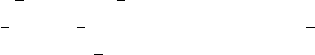
377
ham1_star_sf(1)+sym1(1);
ham2_star_sf(1)+sym2(1);
and the result of the last two commands is zero.
Then we shall convert the two superfunctions into bivectors:
conv_genfun2biv(sym1_odd,biv1);
conv_genfun2biv(sym2_odd,biv2);
The output is:
biv1(1) := - ext(p,p_x);
biv2(1) := - (1/3)*(-3*ext(p,p_3x) - 2*ext(p,p_x)*u);
Finally, the three Schouten brackets [ˆ
Hi,ˆ
Hj]are computed, with i, j = 1,2:
schouten_bracket(biv1,biv1,sb11);
schouten_bracket(biv1,biv2,sb12);
schouten_bracket(biv2,biv2,sb22);
the result are well-known lists of zeros.
16.12.20 Bi-Hamiltonian structure of the WDVV equation
This subsection refers to the the example file wdvv_biham1.red. The simplest
nontrivial case of the WDVV equations is the third-order Monge–Ampère equat-
ion, fttt =f2
xxt −fxxxfxtt [4]. This PDE can be transformed into hydrodynamic
form,
at=bx, bt=cx, ct= (b2−ac)x,
via the change of variables a=fxxx,b=fxxt,c=fxtt. This system possesses
two Hamiltonian formulations [7]:
a
b
c
t
=Ai
δHi/δa
δHi/δb
δHi/δc
, i = 1,2
with the homogeneous first-order Hamiltonian operator
ˆ
A1=
−3
2Dx1
2Dxa Dxb
1
2aDx1
2(Dxb+bDx)3
2cDx+cx
bDx3
2Dxc−cx(b2−ac)Dx+Dx(b2−ac)

378 CHAPTER 16. USER CONTRIBUTED PACKAGES
with the Hamiltonian H1=Rc dx, and the homogeneous third-order Hamiltonian
operator
A2=Dx
0 0 Dx
0Dx−Dxa
Dx−aDxDxb+bDx+aDxa
Dx,
with the nonlocal Hamiltonian
H2=−Z1
2aDx−1b2+Dx−1bDx−1cdx.
Both operators are of Dubrovin–Novikov type [5,6]. This means that the operators
are homogeneous with respect to the grading |Dx|= 1. It follows that the operators
are form-invariant under point transformations of the dependent variables, ui=
ui(˜uj). Here and in what follows we will use the letters uito denote the dependent
variables (a, b, c). Under such transformations, the coefficients of the operators
transform as differential-geometric objects.
The operator A1has the general structure
A1=gij
1Dx+ Γij
kuk
x
where the covariant metric g1ij is flat, Γij
k=gis
1Γj
sk (here gij
1is the inverse matrix
that represent the contravariant metric induced by g1ij ), and Γj
sk are the usual
Christoffel symbols of g1ij.
The operator A2has the general structure
A2=Dxgij
2Dx+cij
kuk
xDx,(16.63)
where the inverse g2ij of the leading term transforms as a covariant pseudo-
Riemannian metric. From now on we drop the subscript 2for the metric of A2.
It was proved in [8] that, if we set cijk =giqgjpcpq
k, then
cijk =1
3(gik,j −gij,k)
and the metric fulfills the following identity:
gmk,n +gkn,m +gmn,k = 0.(16.64)
This means that the metric is a Monge metric [8]. In particular, its coefficients are
quadratic in the variables ui. It is easy to input the two operators in CDE. Let us
start by A1: we may define its entries one by one as follows
operator a1;
for all psi let a1(1,1,psi) = - (3/2)*td(psi,x);
for all psi let a1(1,2,psi) = (1/2)*td(a*psi,x);
...

379
We could also use one specialized Reduce package for the computation of
the Christoffel symbols, like RedTen or GRG. Assuming that the operators
gamma_hi(i,j,k) have been defined equal to Γij
kand computed in the sys-
tem using the inverse matrix gij of the leading coefficient contravariant metric10
gij =
−3
2
1
2a b
1
2a b 3
2c
b3
2c2(b2−ac)
then, provided we defined a list dep_var of the dependent variables, we could set
operator gamma_hi_con;
for all i,j let gamma_hi_con(i,j) =
(
for k:=1:3 sum gamma_hi(i,j,k)*mkid(part(dep_var,k),!_x)
)$
and
operator a1$
for all i,j,psi let a1(i,j,psi) =
gu1(i,j)*td(psi,x)+(for k:=1:3 sum gamma_hi_con(i,j)*psi
)$
The third order operator can be reconstructed as follows. Observe that the leading
contravariant metric is
gij =
0 0 1
0 1 −a
1−a2b+a2
Introduce the above matrix in REDUCE as gu3. Then set
gu3:=gl3**(-1)$
and define cijk as
operator c_lo$
for i:=1:3 do
for j:=1:3 do
for k:=1:3 do
<<
c_lo(i,j,k):=
10Indeed in the example file wdvv_biham1.red there are procedures for computing all those
quantities.
380 CHAPTER 16. USER CONTRIBUTED PACKAGES
(1/3)*(df(gl3(k,i),part(dep_var,j))
- df(gl3(j,i),part(dep_var,k)))$
>>$
Then define cij
k
templist:={}$
operator c_hi$
for i:=1:ncomp do
for j:=1:ncomp do
for k:=1:ncomp do
c_hi(i,j,k):=
<<
templist:=
for m:=1:ncomp join
for n:=1:ncomp collect
gu3(n,i)*gu3(m,j)*c_lo(m,n,k)$
templist:=part(templist,0):=plus
>>$
Introduce the contracted operator
operator c_hi_con$
for i:=1:ncomp do
for j:=1:ncomp do
c_hi_con(i,j):=
<<
templist:=for k:=1:ncomp collect
c_hi(i,j,k)*mkid(part(dep_var,k),!_x)$
templist:=part(templist,0):=plus
>>$
Finally, define the operator A2
operator aa2$
for all i,j,psi let aa2(i,j,psi) =
td(
gu3(i,j)*td(psi,x,2)+c_hi_con(i,j)*td(psi,x)
,x)$
Now, we can test the Hamiltonian property of A1,A2and their compatibility:
conv_cdiff2genfun(aa1,sym1)$
conv_cdiff2genfun(aa2,sym2)$

381
conv_genfun2biv(sym1,biv1)$
conv_genfun2biv(sym2,biv2)$
schouten_bracket(biv1,biv1,sb11);
schouten_bracket(biv1,biv2,sb12);
schouten_bracket(biv2,biv2,sb22);
Needless to say, the result of the last three command is a list of zeroes.
We observe that the same software can be used to prove the bi-Hamiltonianity of a
6-component WDVV system [26].
16.12.21 Schouten bracket of multidimensional operators
The formulae (16.56), (16.57) hold also in the case of multidimensional operators,
ie operators with total derivatives in more than one independent variables. Here
we give one Hamiltonian operator Hand we give two more variational bivectors
P1,P2; all operators are of Dubrovin–Novikov type (homogeneous). We check the
compatibility by computing [H, P1]and [H, P2]. Such computations are standard
for the problem of computing the Hamiltonian cohomology of H.
This example has been provided by M. Casati. The file of the computation is
dn2d_sb1.red. The dependent variables are p1,p2.
Let us set
H=Dx0
0Dy(16.65)
P1=P11
1P12
1
P21
1P22
1(16.66)
where
P11
1=2 ∂g
∂p1p2
yDx+∂g
∂p1p2
xy +∂g
∂p1∂p2p2
xp2
y+∂g
∂2p1p1
xp2
y
P21
1=−fD2
x+gD2
y+∂g
∂p2p2
yDy−(∂f
∂p1p1
x+ 2 ∂f
∂p2p2
x)Dx
−∂f
∂2p2p2
xp2
x−∂f
∂p1∂p2p1
xp2
x−∂f
∂p2p2
2x;
P12
1=fD2
x−gD2
y+∂f
∂p1p1
xDx−∂g
∂p2p2
y+ 2 ∂g
∂p1p1
yDy
−∂g
∂2p1p1
yp1
y−∂g
∂p1∂p2p1
yp2
y−∂g
∂p1p1
2y;
P22
1=2 ∂f
∂p2p1
xDy+∂f
∂p2p1
xy+∂f
∂p1∂p2p1
xp1
y+∂f
∂2p2p1
xp2
y;
382 CHAPTER 16. USER CONTRIBUTED PACKAGES
and let P2=PT
1. This is implemented as follows:
mk_cdiffop(aa2,1,{2},2)$
for all psi let aa2(1,1,psi) =
2*df(g,p1)*p2_y*td(psi,x) + df(g,p1)*p2_xy*psi
+ df(g,p1,p2)*p2_x*p2_y*psi + df(g,p1,2)*p1_x*p2_y*psi;
for all psi let aa2(1,2,psi) =
f*td(psi,x,2) - g*td(psi,y,2) + df(f,p1)*p1_x*td(psi,x)
- (df(g,p2)*p2_y + 2*df(g,p1)*p1_y)*td(psi,y)
- df(g,p1,2)*p1_y*p1_y*psi - df(g,p1,p2)*p1_y*p2_y*psi
- df(g,p1)*p1_2y*psi;
for all psi let aa2(2,1,psi) =
- f*td(psi,x,2) + g*td(psi,y,2)
+ df(g,p2)*p2_y*td(psi,y)
- (df(f,p1)*p1_x+2*df(f,p2)*p2_x)*td(psi,x)
- df(f,p2,2)*p2_x*p2_x*psi - df(f,p1,p2)*p1_x*p2_x*psi
- df(f,p2)*p2_2x*psi;
for all psi let aa2(2,2,psi) =
2*df(f,p2)*p1_x*td(psi,y)
+ df(f,p2)*p1_xy*psi + df(f,p1,p2)*p1_x*p1_y*psi
+ df(f,p2,2)*p1_x*p2_y*psi;
mk_cdiffop(aa3,1,{2},2)$
for all psi let aa3(1,1,psi) = aa2(1,1,psi);
for all psi let aa3(1,2,psi) = aa2(2,1,psi);
for all psi let aa3(2,1,psi) = aa2(1,2,psi);
for all psi let aa3(2,2,psi) = aa2(2,2,psi);
Let us check the skew-adjointness of the above bivectors:
conv_cdiff2superfun(aa1,sym1)$
conv_cdiff2superfun(aa2,sym2)$
conv_cdiff2superfun(aa3,sym3)$
adjoint_cdiffop(aa1,aa1_star);
adjoint_cdiffop(aa2,aa2_star);
adjoint_cdiffop(aa3,aa3_star);
for i:=1:2 do write sym1(i) + aa1_star_sf(i);
for i:=1:2 do write sym2(i) + aa2_star_sf(i);
for i:=1:2 do write sym3(i) + aa3_star_sf(i);
383
Of course the last three commands produce two zeros each.
Let us compute Schouten brackets.
conv_cdiff2superfun(aa1,sym1)$
conv_cdiff2superfun(aa2,sym2)$
conv_cdiff2superfun(aa3,sym3)$
conv_genfun2biv(sym1,biv1)$
conv_genfun2biv(sym2,biv2)$
conv_genfun2biv(sym3,biv3)$
schouten_bracket(biv1,biv1,sb11);
schouten_bracket(biv1,biv2,sb12);
schouten_bracket(biv1,biv3,sb13);
sb11(1) is trivially a list of zeros, while sb12(1) is nonzero and sb13(1) is
again zero.
More formulae are currently being implemented in the system, like symplecticity
and Nijenhuis condition for recursion operators [13]. Interested readers are warmly
invited to contact R. Vitolo for questions/feature requests.
16.12.22 Non-local operators
In this section we will show an experimental way to find nonlocal operators. The
word ‘experimental’ comes from the lack of a comprehensive mathematical theory
of nonlocal operators; in particular, it is still missing a theoretical framework for
Schouten brackets of nonlocal opeartors in the odd variable language.
In any case we will achieve the results by means of a covering of the cotangent
covering. Indeed, it can be proved that there is a 1−1correspondence between
(higher) symmetries of the initial equation and conservation laws on the cotangent
covering. Such conservation laws provide new potential variables, hence a cover-
ing (see [2] for theoretical details on coverings).
In Section 16.12.25 we will also discuss a procedure for finding conservation laws
from their generating functions that is of independent interest.
16.12.23 Non-local Hamiltonian operators for the Korteweg–de Vries
equation
Here we will compute some nonlocal Hamiltonian operators for the KdV equation.
The result of the computation (without the details below) has been published in
384 CHAPTER 16. USER CONTRIBUTED PACKAGES
[12].
We have to solve equations of the type ddx(ct)-ddt(cx) as in 16.12.13. The
main difference is that we will attempt a solution on the `∗-covering (see Subsec-
tion 16.12.14). For this reason, first of all we have to determine covering variables
with the usual mechanism of introducing them through conservation laws, this time
on the `∗-covering.
As a first step, let us compute conservation laws on the `∗-covering whose compo-
nents are linear in the p’s. This computation can be found in the file kdv_nlcl1
and related results and debug files.
The conservation laws that we are looking for are in 1−1correspondence with
symmetries of the initial equation [12]. We will look for conservatoin laws which
correspond to Galilean boost, x-translation, t-translation at the same time. In the
case of 2 independent variables and 1 dependent variable, one could prove that one
component of such conservation laws can always be written as sym*pas follows:
c1x:=(t*u_x+1)*p$ % degree 1
c2x:=u_x*p$ % degree 4
c3x:=(u*u_x+u_3x)*p$ % degree 6
The second component must be found by solving an equation. To this aim we
produce the ansatz
c1t:=f1*p+f2*p_x+f3*p_2x$
% degree 6
c2t:=(for each el in linodd6 sum (c(ctel:=ctel+1)*el))$
% degree 8
c3t:=(for each el in linodd8 sum (c(ctel:=ctel+1)*el))$
where we already introduced the sets linodd6 and linodd8 of 6-th and 8-th
degree monomials which are linear in odd variables (see the source code). For the
first conservation law solutions of the equation
equ 1:=td(c1t,x) - td(c1x,t);
are found by hand due to the presence of ‘t’ in the symmetry:
f3:=t*u_x+1$
f2:=-td(f3,x)$
f1:=u*f3+td(f3,x,2)$
We also have the equations
equ 2:=td(c2t,x)-td(c2x,t);
385
equ 3:=td(c3t,x)-td(c3x,t);
They are solved in the usual way (see the source code of the example and the results
file kdv_nlcl1_res).
Now, we solve the equation for shadows of nonlocal symmetries in a covering of
the `∗-covering (source file kdv_nlho1). We can produce such a covering by
introducing three new nonlocal (potential) variables ra,rb,rc. We are going to
look for non-local Hamiltonian operators depending linearly on one of these vari-
ables. To this aim we modify the odd part of the equation to include the components
of the above conservation laws as the derivatives of the new non-local variables r1,
r2,r3:
principal_odd:={p_t,r1_x,r1_t,r2_x,r2_t,r3_x,r3_t}$
de_odd:={u*p_x+p_3x,
p*(t*u_x + 1),
p*t*u*u_x + p*t*u_3x + p*u + p_2x*t*u_x + p_2x
- p_x*t*u_2x,
p*u_x,
p*u*u_x + p*u_3x + p_2x*u_x - p_x*u_2x,
p*(u*u_x + u_3x),
p*u**2*u_x + 2*p*u*u_3x + 3*p*u_2x*u_x + p*u_5x
+ p_2x*u*u_x + p_2x*u_3x - p_x*u*u_2x
- p_x*u_4x - p_x*u_x**2}$
The scale degree analysis of the local Hamiltonian operators of the KdV equation
leads to the formulation of the ansatz
phi:=(for each el in linodd sum (c(ctel:=ctel+1)*el))$
where linext is the list of graded mononials which are linear in odd variables
and have degree 7(see the source file). The equation for shadows of nonlocal
symmetries in `∗-covering
equ 1:=td(phi,t)-u*td(phi,x)-u_x*phi-td(phi,x,3);
is solved in the usual way, obtaining (in odd variables notation):
phi := (c(5)*(4*p*u*u_x + 3*p*u_3x + 18*p_2x*u_x
+ 12*p_3x*u+9*p_5x + 4*p_x*u**2
+ 12*p_x*u_2x - r2*u_x))/4$
Higher non-local Hamiltonian operators could also be found [12]. The CRACK
approach also holds for non-local computations.
386 CHAPTER 16. USER CONTRIBUTED PACKAGES
16.12.24 Non-local recursion operator for the Korteweg–de Vries
equation
Following the ideas in [12], a differential operator that sends symmetries into sym-
metries can be found as a shadow of symmetry on the `-covering of the KdV equat-
ion, with the further condition that the shadows must be linear in the covering
q-variables. The tangent covering of the KdV equation is
ut=uxxx +uux
qt=uxq+uqx+qxxx
and we have to solve the equation ¯
`KdV (phi) = 0, where ¯
`KdV means that the
linearization of the KdV equation is lifted over the tangent covering.
The file containing this example is kdv_ro1.red. The example closely follows
the computational scheme presented in [16].
Usually, recursion operators are non-local: operators of the form D−1
xappear in
their expression. Geometrically we interpret this kind of operator as follows. We
introduce a conservation law on the cotangent covering of the form
ω=rt dx +rx dt
where rt =uq +qxx and rx =q. It has the remarkable feature of being linear
with respect to q-variables. A non-local variable rcan be introduced as a potential
of ω, as rx=rx,rt=rt. A computation of shadows of symmetries on the system
of PDEs
ut=uxxx +uux
qt=uxq+uqx+qxxx
rt=uq +qxx
rx=q
yields, analogously to the previous computations,
2*c(5)*q*u+3*c(5)*q_2x + c(5)*r*u_x + c(2)*q.
The operator qstands for the identity operator, which is (and must be!) always a
solution; the other solution corresponds to the Lenard–Magri operator
3Dxx + 2u+uxD−1
x.
16.12.25 Non-local Hamiltonian-recursion operators for Plebanski
equation
The Plebanski (or second Heavenly) equation
F=uttuxx −u2
tx +uxz +uty = 0 (16.67)
387
is Lagrangian. This means that its linearization is self-adjoint: `F=`∗
F, so that
the tangent and cotangent covering coincide, its odd equation being
`F(p) = pxz +pty −2utxptx +u2xp2t+u2tp2x= 0.(16.68)
It is not difficult to realize that the above equation can be written in explicit con-
servative form as
pxz +pty +uttpxx +uxxptt −2utxptx
=Dx(pz+uttpx−utxpt) + Dt(py+uxxpt−utxpx)=0,
thus the corresponding conservation law is
υ(1) = (py+uxxpt−utxpx)dx∧dy∧dz+(utxpt−pz−uttpx)dt∧dy∧dz. (16.69)
We can introduce a potential rfor the above 2-component conservation law.
Namely, we can assume that
rx=py+uxxpt−utxpx, rt=utxpt−pz−uttpx.(16.70)
This is a new nonlocal variable for the (co)tangent covering of the Plebanski equat-
ion. We can load the Plebanski equation together with its nonlocal variable ras
follows:
indep_var:={t,x,y,z}$
dep_var:={u}$
odd_var:={p,r}$
deg_indep_var:={-1,-1,-4,-4}$
deg_dep_var:={1}$
deg_odd_var:={1,4}$
total_order:=6$
principal_der:={u_xz}$
de:={-u_ty+u_tx**2-u_2t*u_2x}$
% rhs of the equations that define the nonlocal variable
rt:= - p_z - u_2t*p_x + u_tx*p_t$
rx:= p_y + u_2x*p_t - u_tx*p_x$
% We add conservation laws as new nonlocal odd variables;
principal_odd:={p_xz,r_x,r_t}$
%
de_odd:={-p_ty+2*u_tx*p_tx-u_2x*p_2t-u_2t*p_2x,rx,rt}$
We can easily verify that the integrability condition for the new nonlocal variable
holds:
td(r,t,x) - td(r,x,t);
388 CHAPTER 16. USER CONTRIBUTED PACKAGES
the result is 0.
Now, we look for nonlocal recursion operators in the tangent covering using the
new nonlocal odd variable r. We can load the equation exactly as before. We look
for recursion operators which depend on r(which has scale degree 4); we produce
the following ansatz for phi:
linodd:=mkalllinodd(gradmon,l_grad_odd,1,4)$
phi:=(for each el in linodd sum (c(ctel:=ctel+1)*el))$
then we solve the equation of shadows of symmetries:
equ 1:=td(phi,x,z)+td(phi,t,y)-2*u_tx*td(phi,t,x)
+u_2x*td(phi,t,2)+u_2t*td(phi,x,2)$
The solution is
phi := c(28)*r + c(1)*p
hence we obtain the identity operator pand the new nonlocal operator r. It can be
proved that changing coordinates to the evolutionary presentation yields the local
operator (which has a much more complex expression than the identity operator)
and one of the nonlocal operators of [?]. More details on this computation can be
found in [?].
16.12.26 Appendix: old versions of CDE
A short version history is provided here.
CDE 1.0 This version was published in October 2014. It was programmed in
REDUCE’s algebraic mode, so its capabilities were limited, and its speed was
severely affected by the systematic use of the package assist for manipulating
algebraic lists. Its features were:
1. CDE 1.0 is able to do standard computations in integrable systems like de-
termining systems for generalized symmetries and conservation laws.
2. CDE 1.0 is able to compute linear overdetermined systems of partial differ-
ential equations whose solutions are Hamiltonian operators.
3. CDE is able to compute Schouten brackets between bivectors. This can be
used eg to check Hamiltonianity of an operator, or the compatibility of two
operators.
389
CDE 1.0 has never ben included in the official REDUCE distribution, and it is still
available at [1].
Bibliography
[1] Geometry of Differential Equations web site: http://gdeq.org.
[2] A. V. BOCHAROV, V. N. CHETVERIKOV, S. V. DUZHIN, N. G.
KHOR0KOVA, I. S. KRASIL0SHCHIK, A. V. SAMOKHIN, YU. N. TORKHOV,
A. M. VERBOVETSKY AND A. M. VINOGRADOV: Symmetries and Con-
servation Laws for Differential Equations of Mathematical Physics, I. S.
Krasil0shchik and A. M. Vinogradov eds., Translations of Math. Monographs
182, Amer. Math. Soc. (1999).
[3] D. BALDWIN, W. HEREMAN,A symbolic algorithm for computing recursion
operators of nonlinear partial differential equations, International Journal of
Computer Mathematics, vol. 87 (5), pp. 1094-1119 (2010).
[4] B.A. DUBROVIN, Geometry of 2D topological field theories, Lecture Notes
in Math. 1620, Springer-Verlag (1996) 120–348.
[5] B.A. DUBROVIN AND S.P. NOVIKOV, Hamiltonian formalism of one-
dimensional systems of hydrodynamic type and the Bogolyubov-Whitham
averaging method, Soviet Math. Dokl. 27 No. 3 (1983) 665–669.
[6] B.A. DUBROVIN AND S.P. NOVIKOV, Poisson brackets of hydrodynamic
type, Soviet Math. Dokl. 30 No. 3 (1984), 651–2654.
[7] E.V. FERAPONTOV, C.A.P. GALVAO, O. MOKHOV, Y. NUTKU, Bi-
Hamiltonian structure of equations of associativity in 2-d topological field
theory, Comm. Math. Phys. 186 (1997) 649-669.
[8] E.V. FERAPONTOV, M.V. PAVLOV, R.F. VITOLO,Projective-geometric as-
pects of homogeneous third-order Hamiltonian operators, J. Geom. Phys. 85
(2014) 16-28, DOI: 10.1016/j.geomphys.2014.05.027.
[9] E.V. FERAPONTOV, M.V. PAVLOV, R.F. VITOLO,Towards the classifica-
tion of homogeneous third-order Hamiltonian operators,http://arxiv.
org/abs/1508.02752
[10] E. Getzler, A Darboux theorem for Hamiltonian operators in the formal cal-
culus of variations, Duke J. Math. 111 (2002), 535-560.
[11] S. IGONIN, A. VERBOVETSKY, R. VITOLO:Variational Multivectors and
Brackets in the Geometry of Jet Spaces, V Int. Conf. on on Symmetry in Non-
linear Mathematical Physics, Kyiv 2003; Part 3 of Volume 50 of Proceedings
of Institute of Mathematics of NAS of Ukraine, Editors A.G. Nikitin, V.M.
390 CHAPTER 16. USER CONTRIBUTED PACKAGES
Boyko, R.O. Popovych and I.A. Yehorchenko (2004), 1335–1342; http://
www.imath.kiev.ua/~snmp2003/Proceedings/vitolo.pdf.
[12] P.H.M. KERSTEN, I.S. KRASIL’SHCHIK, A.M. VERBOVETSKY,Hamilto-
nian operators and `∗-covering, Journal of Geometry and Physics 50 (2004),
273–302.
[13] P.H.M. KERSTEN, I.S. KRASIL’SHCHIK, A.M. VERBOVETSKY,A geomet-
ric study of the dispersionless Boussinesq equation, Acta Appl. Math. 90
(2006), 143–178.
[14] P. KERSTEN, I. KRASIL0SHCHIK, A. VERBOVETSKY,AND R. VITOLO,
Hamiltonian structures for general PDEs, Differential equations: Geome-
try, Symmetries and Integrability. The Abel Symposium 2008 (B. Kruglikov,
V. V. Lychagin, and E. Straume, eds.), Springer-Verlag, 2009, pp. 187–198,
arXiv:0812.4895.
[15] I. KRASIL0SHCHIK AND A. VERBOVETSKY,Geometry of
jet spaces and integrable systems, J. Geom. Phys. (2011)
doi:10.1016/j.geomphys.2010.10.012, arXiv:1002.0077.
[16] I. KRASIL0SHCHIK, A. VERBOVETSKY, R. VITOLO,A unified approach to
computation of integrable structures, Acta Appl. Math. (2012).
[17] I. KRASIL0SHCHIK, A. VERBOVETSKY, R. VITOLO,The symbolic compu-
tation of integrability structures for partial differential equations, book, to
appear in the Springer series “Texts and monographs in symbolic computa-
tions” (2017).
[18] B. KUPERSCHMIDT:Geometric Hamiltonian forms for the Kadomtsev–
Petviashvili and Zabolotskaya–Khokhlov equations, in Geometry in Partial
Differential Equations, A. Prastaro, Th.M. Rassias eds., World Scientific
(1994), 155–172.
[19] M. MARVAN,Sufficient set of integrability conditions of an orthonomic sys-
tem. Foundations of Computational Mathematics 9(2009), 651–674.
[20] F. NEYZI, Y. NUTKU,AND M.B. SHEFTEL,Multi-Hamiltonian structure
of Plebanski’s second heavenly equation J. Phys. A: Math. Gen. 38 (2005),
8473. arXiv:nlin/0505030v2.
[21] A.C. NORMAN, R. VITOLO,Inside Reduce, part of the official REDUCE
documentation included in the source code, see below.
[22] M.C. NUCCI,Interactive REDUCE programs for calculating classical, non-
classical, and approximate symmetries of differential equations, in Compu-
tational and Applied Mathematics II. Differential Equations, W.F. Ames, and
P.J. Van der Houwen, Eds., Elsevier, Amsterdam (1992) pp. 345–350.
391
[23] M.C. NUCCI,Interactive REDUCE programs for calculating Lie point, non-
classical, Lie-Bäcklund, and approximate symmetries of differential equat-
ions: manual and floppy disk, in CRC Handbook of Lie Group Analysis of
Differential Equations. Vol. 3 N.H. Ibragimov, Ed., CRC Press, Boca Raton
(1996) pp. 415–481.
[24] F. OLIVERI, RELIE, REDUCE software and user guide, http://
mat521.unime.it/oliveri/.
[25] P. OLVER, Applications of Lie Groups to Partial Differential Equations, 2nd
ed, GTM Springer, 1992.
[26] M.V. PAVLOV, R.F. VITOLO:On the bi-Hamiltonian geometry of the WDVV
equations,http://arxiv.org/abs/1409.7647
[27] G. SACCOMANDI, R. VITOLO:On the Mathematical and Geometrical
Structure of the Determining Equations for Shear Waves in Nonlinear
Isotropic Incompressible Elastodynamics, J. Math. Phys. 55 (2014), 081502.
[28] T. WOLF,A comparison of four approaches to the calculation of conservation
laws, Euro. Jnl of Applied Mathematics 13 part 2 (2002) 129-152.
[29] T. WOLF,APPLYSYM - a package for the application of Lie-symmetries,
software distributed together with the computer algebra system REDUCE,
(1995).
[30] T. WOLF, A. BRAND,Investigating DEs with CRACK and Related Pro-
grams, SIGSAM Bulletin, Special Issue, (June 1995), p 1-8.
[31] T. WOLF,An efficiency improved program LIEPDE for determining Lie-
symmetries of PDEs, Proc.of Modern Group Analysis: advanced analytical
and computational methods in mathematical physics, Catania, Italy Oct.1992,
Kluwer Acad.Publ. (1993) 377-385.
[32] T. WOLF, A. BRAND: CRACK, user guide, examples and documenta-
tion http://lie.math.brocku.ca/Crack_demo.html. For appli-
cations, see also the publications of T. Wolf.
392 CHAPTER 16. USER CONTRIBUTED PACKAGES
16.13 CDIFF: A package for computations in geometry of
Differential Equations
Authors: P. Gragert, P.H.M. Kersten, G. Post and G. Roelofs.
Author of this Section: R. Vitolo.
We describe CDIFF, a Reduce package for computations in geometry of Differen-
tial Equations (DEs, for short) developed by P. Gragert, P.H.M. Kersten, G. Post
and G. Roelofs from the University of Twente, The Netherlands.
The package is part of the official REDUCE distribution at Sourceforge [1], but
it is also distributed on the Geometry of Differential Equations web site http:
//gdeq.org (GDEQ for short).
We start from an installation guide for Linux and Windows. Then we focus on con-
crete usage recipes for the computation of higher symmetries, conservation laws,
Hamiltonian and recursion operators for polynomial differential equations. All
programs discussed here are shipped together with this manual and can be found
at the GDEQ website. The mathematical theory on which computations are based
can be found in refs. [11,12].
NOTE: The new REDUCE package CDE [14], also distributed on http://
gdeq.org, simplifies the use of CDIFF and extends its capabilities. Interested
users may read the manual of CDE where the same computations described here
for CDIFF are done in a simpler way, and further capabilities allow CDE to solve
a greater variety of problems.
16.13.1 Introduction
This brief guide refers to using CDIFF, a set of symbolic computation programs
devoted to computations in geometry of DEs and developed by P. Gragert, P.H.M.
Kersten, G. Post and G. Roelofs at the University of Twente, The Netherlands.
Initially, the development of the CDIFF packages was started by Gragert and Ker-
sten for symmetry computations in DEs, then they have been partly rewritten and
extended by Roelofs and Post. The CDIFF packages consist of 3 program files plus
a utility file; only the main three files are documented [7,8,9]. The CDIFF pack-
ages, as well as a copy of the documentation (including this manual) and several
example programs, can be found both at Sourceforge in the sources of REDUCE
[1] and in the Geometry of Differential Equations (GDEQ for short) web site [2].
The name of the packages, CDIFF, comes from the fact that the package is aimed
at defining differential operators in total derivatives and do computations involving
them. Such operators are called C-differential operators (see [11]).
The main motivation for writing this manual was that REDUCE 3.8 recently be-
393
came free software, and can be downloaded here [1]. For this reason, we are able
to make our computations accessible to a wider public, also thanks to the inclusion
of CDIFF in the official REDUCE distribution. The readers are warmly invited
to send questions, comments, etc., both on the computations and on the technical
aspects of installation and configuration of REDUCE, to the author of the present
manual.
Acknowledgements. My warmest thanks are for Paul H.M. Kersten, who ex-
plained to me how to use the CDIFF packages for several computations of in-
terest in the Geometry of Differential Equations. I also would like to thank I.S.
Krasil’shchik and A.M. Verbovetsky for constant support and stimulating discus-
sions which led me to write this text.
16.13.2 Computing with CDIFF
In order to use CDIFF it is necessary to load the package by the command
load_package(cdiff);
All programs that we will discuss in this manual can be found inside the subfolder
examples in the folder which contains this manual. In order to run them just do
in "filename.red";
at the REDUCE command prompt.
There are some conventions that I adopted on writing programs which use CDIFF.
•Program files have the extension .red. This will load automatically the
reduce-ide mode in emacs (provided you made the installation steps de-
scribed in the reduce-ide guides).
•Program files have the following names:
equationname_typeofcomputation_version.red
where equationname stands for the shortened name of the equation (e.g.
Korteweg–de Vries is always indicated by KdV), typeofcomputation
stands for the type of geometric object which is computed with the given file,
for example symmetries, Hamiltonian operators, etc., version is a version
number.
•More specific information, like the date and more details on the computation
done in each version, are included as comment lines at the very beginning of
each file.
394 CHAPTER 16. USER CONTRIBUTED PACKAGES
Now we describe some examples of computations with CDIFF. The parts of exam-
ples which are shared between all examples are described only once. We stress that
all computations presented in this document are included in the official REDUCE
distribution and can be also downloaded at the GDEQ website [2]. The examples
can be run with REDUCE by typing in "program.red"; at the REDUCE
prompt, as explained above.
Remark. The mathematical theories on which the computations are based can be
found in [11,12].
Higher symmetries
In this section we show the computation of (some) higher symmetries of Burgers’
equation B=ut−uxx+2uux= 0. The corresponding file is Burg_hsym_1.red
and the results of the computation are in Burg_hsym_1_res.red.
The idea underlying this computation is that one can use the scale symmetries of
Burgers’ equation to assign “gradings” to each variable appearing in the equation.
As a consequence, one could try different ansatz for symmetries with polynomial
generating function. For example, it is possible to require that they are sum of
monomials of given degrees. This ansatz yields a simplification of the equations
for symmetries, because it is possible to solve them in a “graded” way, i.e., it is
possible to split them into several equations made by the homogeneous components
of the equation for symmetries with respect to gradings.
In particular, Burgers’ equation translates into the following dimensional equation:
[ut] = [uxx],[uxx = 2uux].
By the rules [uz]=[u]−[z]and [uv]=[u] + [v], and choosing [x] = −1, we
have [u] = 1 and [t] = −2. This will be used to generate the list of homogeneous
monomials of given grading to be used in the ansatz about the structure of the
generating function of the symmetries.
The following instructions initialize the total derivatives. The first string is the
name of the vector field, the second item is the list of even variables (note that
u1,u2, ... are ux,uxx, . . . ), the third item is the list of odd (non-commuting)
variables (‘ext’ stands for ‘external’ like in external (wedge) product). Note that in
this example odd variables are not strictly needed, but it is better to insert some of
them for syntax reasons.
super_vectorfield(ddx,{x,t,u,u1,u2,u3,u4,u5,u6,u7,
u8,u9,u10,u11,u12,u13,u14,u15,u16,u17},
{ext 1,ext 2,ext 3,ext 4,ext 5,ext 6,ext 7,ext 8,ext 9,
ext 10,ext 11,ext 12,ext 13,ext 14,ext 15,ext 16,ext 17,
ext 18,ext 19,ext 20,ext 21,ext 22,ext 23,ext 24,ext 25,
395
ext 26,ext 27,ext 28,ext 29,ext 30,ext 31,ext 32,ext 33,
ext 34,ext 35,ext 36,ext 37,ext 38,ext 39,ext 40,ext 41,
ext 42,ext 43,ext 44,ext 45,ext 46,ext 47,ext 48,ext 49,
ext 50,ext 51,ext 52,ext 53,ext 54,ext 55,ext 56,ext 57,
ext 58,ext 59,ext 60,ext 61,ext 62,ext 63,ext 64,ext 65,
ext 66,ext 67,ext 68,ext 69,ext 70,ext 71,ext 72,ext 73,
ext 74,ext 75,ext 76,ext 77,ext 78,ext 79,ext 80
});
super_vectorfield(ddt,{x,t,u,u1,u2,u3,u4,u5,u6,u7,
u8,u9,u10,u11,u12,u13,u14,u15,u16,u17},
{ext 1,ext 2,ext 3,ext 4,ext 5,ext 6,ext 7,ext 8,ext 9,
ext 10,ext 11,ext 12,ext 13,ext 14,ext 15,ext 16,ext 17,
ext 18,ext 19,ext 20,ext 21,ext 22,ext 23,ext 24,ext 25,
ext 26,ext 27,ext 28,ext 29,ext 30,ext 31,ext 32,ext 33,
ext 34,ext 35,ext 36,ext 37,ext 38,ext 39,ext 40,ext 41,
ext 42,ext 43,ext 44,ext 45,ext 46,ext 47,ext 48,ext 49,
ext 50,ext 51,ext 52,ext 53,ext 54,ext 55,ext 56,ext 57,
ext 58,ext 59,ext 60,ext 61,ext 62,ext 63,ext 64,ext 65,
ext 66,ext 67,ext 68,ext 69,ext 70,ext 71,ext 72,ext 73,
ext 74,ext 75,ext 76,ext 77,ext 78,ext 79,ext 80
});
Specification of the vectorfield ddx. The meaning of the first index is the par-
ity of variables. In particular here we have just even variables. The second in-
dex parametrizes the second item (list) in the super_vectorfield declara-
tion. More precisely, ddx(0,1) stands for ∂/∂x,ddx(0,2) stands for ∂/∂t,
ddx(0,3) stands for ∂/∂u,ddx(0,4) stands for ∂/∂ux, . . . , and all coordi-
nates x,t,ux, . . . , are treated as even coordinates. Note that ‘$’ suppresses the
output.
ddx(0,1):=1$
ddx(0,2):=0$
ddx(0,3):=u1$
ddx(0,4):=u2$
ddx(0,5):=u3$
ddx(0,6):=u4$
ddx(0,7):=u5$
ddx(0,8):=u6$
ddx(0,9):=u7$
ddx(0,10):=u8$
ddx(0,11):=u9$
ddx(0,12):=u10$

396 CHAPTER 16. USER CONTRIBUTED PACKAGES
ddx(0,13):=u11$
ddx(0,14):=u12$
ddx(0,15):=u13$
ddx(0,16):=u14$
ddx(0,17):=u15$
ddx(0,18):=u16$
ddx(0,19):=u17$
ddx(0,20):=letop$
The string letop is treated as a variable; if it appears during computations it is
likely that we went too close to the highest order variables that we defined in the
file. This could mean that we need to extend the operators and variable list. In
case of large output, one can search in it the string letop to check whether errors
occurred.
Specification of the vectorfield ddt. In the evolutionary case we never have more
than one time derivative, other derivatives are utxxx···.
ddt(0,1):=0$
ddt(0,2):=1$
ddt(0,3):=ut$
ddt(0,4):=ut1$
ddt(0,5):=ut2$
ddt(0,6):=ut3$
ddt(0,7):=ut4$
ddt(0,8):=ut5$
ddt(0,9):=ut6$
ddt(0,10):=ut7$
ddt(0,11):=ut8$
ddt(0,12):=ut9$
ddt(0,13):=ut10$
ddt(0,14):=ut11$
ddt(0,15):=ut12$
ddt(0,16):=ut13$
ddt(0,17):=ut14$
ddt(0,18):=letop$
ddt(0,19):=letop$
sddt(0,20):=letop$
We now give the equation in the form one of the derivatives equated to a right-hand
side expression. The left-hand side derivative is called principal, and the remaining
derivatives are called parametric11. For scalar evolutionary equations with two
independent variables internal variables are of the type (t, x, u, ux, uxx, . . .).
11This terminology dates back to Riquier, see [13]
397
ut:=u2+2*u*u1;
ut1:=ddx ut;
ut2:=ddx ut1;
ut3:=ddx ut2;
ut4:=ddx ut3;
ut5:=ddx ut4;
ut6:=ddx ut5;
ut7:=ddx ut6;
ut8:=ddx ut7;
ut9:=ddx ut8;
ut10:=ddx ut9;
ut11:=ddx ut10;
ut12:=ddx ut11;
ut13:=ddx ut12;
ut14:=ddx ut13;
Test for verifying the commutation of total derivatives. Highest order defined terms
may yield some letop.
operator ev;
for i:=1:17 do write ev(0,i):=ddt(ddx(0,i))-ddx(ddt(0,i));
This is the list of variables with respect to their grading, starting from degree one.
all_graded_der:={{u},{u1},{u2},{u3},{u4},{u5},
{u6},{u7},{u8},{u9},{u10},{u11},{u12},{u13},{u14},{u15},
{u16},{u17}};
This is the list of all monomials of degree 0,1,2, . . . which can be constructed from
the above list of elementary variables with their grading.
grd0:={1};
grd1:= mkvarlist1(1,1)$
grd2:= mkvarlist1(2,2)$
grd3:= mkvarlist1(3,3)$
grd4:= mkvarlist1(4,4)$
grd5:= mkvarlist1(5,5)$
grd6:= mkvarlist1(6,6)$
grd7:= mkvarlist1(7,7)$
grd8:= mkvarlist1(8,8)$
grd9:= mkvarlist1(9,9)$
grd10:= mkvarlist1(10,10)$
398 CHAPTER 16. USER CONTRIBUTED PACKAGES
grd11:= mkvarlist1(11,11)$
grd12:= mkvarlist1(12,12)$
grd13:= mkvarlist1(13,13)$
grd14:= mkvarlist1(14,14)$
grd15:= mkvarlist1(15,15)$
grd16:= mkvarlist1(16,16)$
Initialize a counter ctel for arbitrary constants c; initialize equations:
operator c,equ;
ctel:=0;
We assume a generating function sym,independent of xand t, of degree ≤5.
sym:=
(for each el in grd0 sum (c(ctel:=ctel+1)*el))+
(for each el in grd1 sum (c(ctel:=ctel+1)*el))+
(for each el in grd2 sum (c(ctel:=ctel+1)*el))+
(for each el in grd3 sum (c(ctel:=ctel+1)*el))+
(for each el in grd4 sum (c(ctel:=ctel+1)*el))+
(for each el in grd5 sum (c(ctel:=ctel+1)*el))$
This is the equation ¯
`B(sym)=0, where B= 0 is Burgers’ equation and sym is
the generating function. From now on all equations are arranged in a single vector
whose name is equ.
equ 1:=ddt(sym)-ddx(ddx(sym))-2*u*ddx(sym)-2*u1*sym ;
This is the list of variables, to be passed to the equation solver.
vars:={x,t,u,u1,u2,u3,u4,u5,u6,u7,u8,u9,u10,u11,
u12,u13,u14,u15,u16,u17};
This is the number of initial equation(s)
tel:=1;
The following procedure uses multi_coeff (from the package tools). It gets
all coefficients of monomials appearing in the initial equation(s). The coefficients
are put into the vector equ after the initial equations.
procedure splitvars i;
begin;
399
ll:=multi_coeff(equ i,vars);
equ(tel:=tel+1):=first ll;
ll:=rest ll;
for each el in ll do equ(tel:=tel+1):=second el;
end;
This command initializes the equation solver. It passes
•the equation vector equ togeher with its length tel (i.e., the total number
of equations);
•the list of variables with respect to which the system must not split the equat-
ions, i.e., variables with respect to which the unknowns are not polynomial.
In this case this list is just {};
•the constants’vector c, its length ctel, and the number of negative indexes
if any; just 0in our example;
•the vector of free functions fthat may appear in computations. Note that in
{f,0,0 }the second 0stands for the length of the vector of free functions.
In this example there are no free functions, but the command needs the pres-
ence of at least a dummy argument, fin this case. There is also a last zero
which is the negative length of the vector f, just as for constants.
initialize_equations(equ,tel,{},{c,ctel,0},{f,0,0});
Run the procedure splitvars in order to obtain equations on coefficiens of each
monomial.
splitvars 1;
Next command tells the solver the total number of equations obtained after running
splitvars.
put_equations_used tel;
It is worth to write down the equations for the coefficients.
for i:=2:tel do write equ i;
This command solves the equations for the coefficients. Note that we have to skip
the initial equations!
for i:=2:tel do integrate_equation i;
;end;
400 CHAPTER 16. USER CONTRIBUTED PACKAGES
In the folder computations/NewTests/Higher_symmetries it is possi-
ble to find the following files:
Burg_hsym_1.red The above file, together with its results file.
KdV_hsym_1.red Higher symmetries of KdV, with the ansatz: deg(sym) ≤5.
KdV_hsym_2.red Higher symmetries of KdV, with the ansatz:
sym = x*(something of degree 3) + t*(something of degree 5)
+ (something of degree 2).
This yields scale symmetries.
KdV_hsym_3.red Higher symmetries of KdV, with the ansatz:
sym = x*(something of degree 1) + t*(something of degree 3)
+ (something of degree 0).
This yields Galilean boosts.
Local conservation laws
In this section we will find (some) local conservation laws for the KdV equation
F=ut−uxxx +uux= 0. Concretely, we have to find non-trivial 1-forms
f=fxdx+ftdt on F= 0 such that ¯
df = 0 on F= 0. “Triviality” of conservation
laws is a delicate matter, for which we invite the reader to have a look in [11].
The files containing this example is KdV_loc-cl_1.red, KdV_loc-cl_2.red
and the corresponding results files.
We make use of ddx and ddt, which in the even part are the same as in the previ-
ous example (subsection 16.13.2). After defining the total derivatives we prepare
the list of graded variables (recall that in KdV uis of degree 2):
all_graded_der:={{},{u},{u1},{u2},{u3},{u4},{u5},
{u6},{u7},{u8},{u9},{u10},{u11},{u12},{u13},{u14},
{u15},{u16},{u17}};
We make the ansatz
fx:=
(for each el in grd0 sum (c(ctel:=ctel+1)*el))+
(for each el in grd1 sum (c(ctel:=ctel+1)*el))+
(for each el in grd2 sum (c(ctel:=ctel+1)*el))+
(for each el in grd3 sum (c(ctel:=ctel+1)*el))$
401
ft:=
(for each el in grd2 sum (c(ctel:=ctel+1)*el))+
(for each el in grd3 sum (c(ctel:=ctel+1)*el))+
(for each el in grd4 sum (c(ctel:=ctel+1)*el))+
(for each el in grd5 sum (c(ctel:=ctel+1)*el))$
for the components of the conservation law. We have to solve the equation
equ 1:=ddt(fx)-ddx(ft);
the fact that ddx and ddt are expressed in internal coordinates on the equation
means that the objects that we consider are already restricted to the equation.
We shall split the equation in its graded summands with the procedure splitvars,
then solve it
initialize_equations(equ,tel,{},{c,ctel,0},{f,0,0});
splitvars 1;
pte tel;
for i:=2:tel do es i;
end;
As a result we get
fx := c(3)*u1 + c(2)*u + c(1)$
ft := (2*c(3)*u*u1 + 2*c(3)*u3 + c(2)*u**2+2*c(2)*u2)/2$
Unfortunately it is clear that the conservation law corresponding to c(3) is trivial,
because it is the total x-derivative of F; its restriction on the infinite prolonga-
tion of the KdV is zero. Here this fact is evident; how to get rid of less evident
trivialities by an ‘automatic’ mechanism? We considered this problem in the file
KdV_loc-cl_2.red, where we solved the equation
equ 1:=fx-ddx(f0);
equ 2:=ft-ddt(f0);
after having loaded the values fx and ft found by the previous program. We make
the following ansatz on f0:
f0:=
(for each el in grd0 sum (cc(cctel:=cctel+1)*el))+
(for each el in grd1 sum (cc(cctel:=cctel+1)*el))+
(for each el in grd2 sum (cc(cctel:=cctel+1)*el))+
(for each el in grd3 sum (cc(cctel:=cctel+1)*el))$
402 CHAPTER 16. USER CONTRIBUTED PACKAGES
Note that this gives a grading which is compatible with the gradings of fx and ft.
After solving the system
initialize_equations(equ,tel,{},{cc,cctel,0},{f,0,0});
for i:=1:2 do begin splitvars i;end;
pte tel;
for i:=3:tel do es i;
end;
issuing the commands
fxnontriv := fx-ddx(f0);
ftnontriv := ft-ddt(f0);
we obtain
fxnontriv := c(2)*u + c(1)$
ftnontriv := (c(2)*(u**2+2*u2))/2$
This mechanism can be easily generalized to situations in which the conservation
laws which are found by the program are difficult to treat by pen and paper.
Local Hamiltonian operators
In this section we will find local Hamiltonian operators for the KdV equation ut=
uxxx +uux. Concretely, we have to solve ¯
`KdV (phi)=0over the equation
ut=uxxx +uux
pt=pxxx +upx
or, in geometric terminology, find the shadows of symmetries on the `∗-covering
of the KdV equation. The reference paper for this type of computations is [12].
The file containing this example is KdV_Ham_1.red.
We make use of ddx and ddt, which in the even part are the same as in the previ-
ous example (subsection 16.13.2). We stress that the linearization ¯
`KdV (phi) = 0
is the equation
ddt(phi)-u*ddx(phi)-u1*phi-ddx(ddx(ddx(phi)))=0
but the total derivatives are lifted to the `∗covering, hence they must contain also
derivatives with respect to p’s. This will be achieved by treating pvariables as odd
and introducing the odd parts of ddx and ddt,
ddx(1,1):=0$
403
ddx(1,2):=0$
ddx(1,3):=ext 4$
ddx(1,4):=ext 5$
ddx(1,5):=ext 6$
ddx(1,6):=ext 7$
ddx(1,7):=ext 8$
ddx(1,8):=ext 9$
ddx(1,9):=ext 10$
ddx(1,10):=ext 11$
ddx(1,11):=ext 12$
ddx(1,12):=ext 13$
ddx(1,13):=ext 14$
ddx(1,14):=ext 15$
ddx(1,15):=ext 16$
ddx(1,16):=ext 17$
ddx(1,17):=ext 18$
ddx(1,18):=ext 19$
ddx(1,19):=ext 20$
ddx(1,20):=letop$
In the above definition the first index ‘1’ says that we are dealing with odd vari-
ables, ext indicates anticommuting variables. Here, ext 3 is p0,ext 4 is px,
ext 5 is pxx, . . . so ddx(1,3):=ext 4 indicates px∂/∂p, etc..
Now, remembering that the additional equation is again evolutionary, we can get
rid of ptby letting it be equal to ext 6 + u*ext 4, as follows:
ddt(1,1):=0$
ddt(1,2):=0$
ddt(1,3):=ext 6 + u*ext 4$
ddt(1,4):=ddx(ddt(1,3))$
ddt(1,5):=ddx(ddt(1,4))$
ddt(1,6):=ddx(ddt(1,5))$
ddt(1,7):=ddx(ddt(1,6))$
ddt(1,8):=ddx(ddt(1,7))$
ddt(1,9):=ddx(ddt(1,8))$
ddt(1,10):=ddx(ddt(1,9))$
ddt(1,11):=ddx(ddt(1,10))$
ddt(1,12):=ddx(ddt(1,11))$
ddt(1,13):=ddx(ddt(1,12))$
ddt(1,14):=ddx(ddt(1,13))$
ddt(1,15):=ddx(ddt(1,14))$
ddt(1,16):=ddx(ddt(1,15))$
ddt(1,17):=ddx(ddt(1,16))$
404 CHAPTER 16. USER CONTRIBUTED PACKAGES
ddt(1,18):=letop$
ddt(1,19):=letop$
ddt(1,20):=letop$
Let us make the following ansatz about the Hamiltonian operators:
phi:=
(for each el in grd0 sum (c(ctel:=ctel+1)*el))*ext 3+
(for each el in grd1 sum (c(ctel:=ctel+1)*el))*ext 3+
(for each el in grd2 sum (c(ctel:=ctel+1)*el))*ext 3+
(for each el in grd3 sum (c(ctel:=ctel+1)*el))*ext 3+
(for each el in grd0 sum (c(ctel:=ctel+1)*el))*ext 4+
(for each el in grd1 sum (c(ctel:=ctel+1)*el))*ext 4+
(for each el in grd2 sum (c(ctel:=ctel+1)*el))*ext 4+
(for each el in grd0 sum (c(ctel:=ctel+1)*el))*ext 5+
(for each el in grd1 sum (c(ctel:=ctel+1)*el))*ext 5+
(for each el in grd0 sum (c(ctel:=ctel+1)*el))*ext 6
$
Note that we are looking for generating functions of shadows which are linear
with respect to p’s. Moreover, having set [p] = −2we will look for solutions of
maximal possible degree +1.
After having set
equ 1:=ddt(phi)-u*ddx(phi)-u1*phi-ddx(ddx(ddx(phi)));
vars:={x,t,u,u1,u2,u3,u4,u5,u6,u7,u8,u9,u10,u11,u12,
u13,u14,u15,u16,u17};
tel:=1;
we define the procedures splitvars as in subsection 16.13.2 and splitext
as follows:
procedure splitext i;
begin;
ll:=operator_coeff(equ i,ext);
equ(tel:=tel+1):=first ll;
ll:=rest ll;
for each el in ll do equ(tel:=tel+1):=second el;
end;
405
Then we initialize the equations:
initialize_equations(equ,tel,{},{c,ctel,0},{f,0,0});
do splitext
splitext 1;
then splitvars
tel1:=tel;
for i:=2:tel1 do begin splitvars i;equ i:=0;end;
Now we are ready to solve all equations:
put_equations_used tel;
for i:=2:tel do write equ i:=equ i;
pause;
for i:=2:tel do integrate_equation i;
end;
Note that we want all equations to be solved!
The results are the two well-known Hamiltonian operators for the KdV:
phi := c(4)*ext(4) + 3*c(3)*ext(6) + 2*c(3)*ext(4)*u
+ c(3)*ext(3)*u1$
Of course, the results correspond to the operators
ext(4) →Dx,
3*c(3)*ext(6) + 2*c(3)*ext(4)*u + c(3)*ext(3)*u1 →
3Dxxx + 2uDx+ux
Note that each operator is multiplied by one arbitrary real constant, c(4) and
c(3).
Non-local Hamiltonian operators
In this section we will show an experimental way to find nonlocal Hamiltonian
operators for the KdV equation. The word ‘experimental’ comes from the lack of a
consistent mathematical theory. The result of the computation (without the details
below) has been published in [12].
We have to solve equations of the type ddx(ft)-ddt(fx) as in 16.13.2. The
406 CHAPTER 16. USER CONTRIBUTED PACKAGES
main difference is that we will attempt a solution on the `∗-covering (see Subsec-
tion 16.13.2). For this reason, first of all we have to determine covering variables
with the usual mechanism of introducing them through conservation laws, this time
on the `∗-covering.
As a first step, let us compute conservation laws on the `∗-covering whose
components are linear in the p’s. This computation can be found in the file
KdV_nloc-cl_1.red and related results file. When specifying odd variables
in ddx and ddt, we have something like
ddx(1,1):=0$
ddx(1,2):=0$
ddx(1,3):=ext 4$
ddx(1,4):=ext 5$
ddx(1,5):=ext 6$
ddx(1,6):=ext 7$
ddx(1,7):=ext 8$
ddx(1,8):=ext 9$
ddx(1,9):=ext 10$
ddx(1,10):=ext 11$
ddx(1,11):=ext 12$
ddx(1,12):=ext 13$
ddx(1,13):=ext 14$
ddx(1,14):=ext 15$
ddx(1,15):=ext 16$
ddx(1,16):=ext 17$
ddx(1,17):=ext 18$
ddx(1,18):=ext 19$
ddx(1,19):=ext 20$
ddx(1,20):=letop$
ddx(1,50):=(t*u1+1)*ext 3$ % degree -2
ddx(1,51):=u1*ext 3$ % degree +1
ddx(1,52):=(u*u1+u3)*ext 3$ % degree +3
and
ddt(1,1):=0$
ddt(1,2):=0$
ddt(1,3):=ext 6 + u*ext 4$
ddt(1,4):=ddx(ddt(1,3))$
ddt(1,5):=ddx(ddt(1,4))$
ddt(1,6):=ddx(ddt(1,5))$
ddt(1,7):=ddx(ddt(1,6))$
ddt(1,8):=ddx(ddt(1,7))$
407
ddt(1,9):=ddx(ddt(1,8))$
ddt(1,10):=ddx(ddt(1,9))$
ddt(1,11):=ddx(ddt(1,10))$
ddt(1,12):=ddx(ddt(1,11))$
ddt(1,13):=ddx(ddt(1,12))$
ddt(1,14):=ddx(ddt(1,13))$
ddt(1,15):=ddx(ddt(1,14))$
ddt(1,16):=ddx(ddt(1,15))$
ddt(1,17):=ddx(ddt(1,16))$
ddt(1,18):=letop$
ddt(1,19):=letop$
ddt(1,20):=letop$
ddt(1,50):=f1*ext 3+f2*ext 4+f3*ext 5$
ddt(1,51):=f4*ext 3+f5*ext 4+f6*ext 5$
ddt(1,52):=f7*ext 3+f8*ext 4+f9*ext 5$
The variables corresponding to the numbers 50,51,52 here play a dummy role,
the coefficients of the corresponding vector are the unknown generating functions
of conservation laws on the `∗-covering. More precisely, we look for conservation
laws of the form
fx= phi*ext 3
ft= f1*ext3+f2*ext4+f3*ext5
The ansatz is chosen because, first of all, ext 4 and ext 5 can be removed from
fx by adding a suitable total divergence (trivial conservation law); moreover it can
be proved that phi is a symmetry of KdV. We can write down the equations
equ 1:=ddx(ddt(1,50))-ddt(ddx(1,50));
equ 2:=ddx(ddt(1,51))-ddt(ddx(1,51));
equ 3:=ddx(ddt(1,52))-ddt(ddx(1,52));
However, the above choices make use of a symmetry which contains ‘t’ in the
generator. This would make automatic computations more tricky, but still possible.
In this case the solution of equ 1 has been found by hand and passed to the
program:
f3:=t*u1+1$
f1:=u*f3+ddx(ddx(f3))$
f2:=-ddx(f3)$
together with the ansatz on the coefficients for the other equations
f4:=(for each el in grd5 sum (c(ctel:=ctel+1)*el))$
408 CHAPTER 16. USER CONTRIBUTED PACKAGES
f5:=(for each el in grd4 sum (c(ctel:=ctel+1)*el))$
f6:=(for each el in grd3 sum (c(ctel:=ctel+1)*el))$
f7:=(for each el in grd7 sum (c(ctel:=ctel+1)*el))$
f8:=(for each el in grd6 sum (c(ctel:=ctel+1)*el))$
f9:=(for each el in grd5 sum (c(ctel:=ctel+1)*el))$
The previous ansatz keep into account the grading of the starting symmetry in
phi*ext 3. The resulting equations are solved in the usual way (see the example
file).
Now, we solve the equation for shadows of nonlocal symmetries in a covering of
the `∗-covering. We can choose between three new nonlocal variables ra,rb,rc.
We are going to look for non-local Hamiltonian operators depending linearly on
one of these variables. Higher non-local Hamiltonian operators could be found by
introducing total derivatives of the r’s. As usual, the new variables are specified
through the components of the previously found conservation laws according with
the rule
ra_x=fx, ra_t=ft,
and analogously for the others. We define
ddx(1,50):=(t*u1+1)*ext 3$ % degree -2
ddx(1,51):=u1*ext 3$ % degree +1
ddx(1,52):=(u*u1+u3)*ext 3$ % degree +3
and
ddt(1,50) := ext(5)*t*u1 + ext(5) - ext(4)*t*u2
+ ext(3)*t*u*u1 + ext(3)*t*u3 + ext(3)*u$
ddt(1,51) := ext(5)*u1 - ext(4)*u2 + ext(3)*u*u1
+ ext(3)*u3$
ddt(1,52) := ext(5)*u*u1 + ext(5)*u3 - ext(4)*u*u2
- ext(4)*u1**2 - ext(4)*u4 + ext(3)*u**2*u1
+ 2*ext(3)*u*u3 + 3*ext(3)*u1*u2 + ext(3)*u5$
as it results from the computation of the conservation laws. The following ansatz
for the nonlocal Hamiltonian operator comes from the fact that local Hamiltonian
operators have gradings −1and +1 when written in terms of p’s. So we are looking
for a nonlocal Hamiltonian operator of degree 3.
phi:=
(for each el in grd6 sum (c(ctel:=ctel+1)*el))*ext 50+
(for each el in grd3 sum (c(ctel:=ctel+1)*el))*ext 51+

409
(for each el in grd1 sum (c(ctel:=ctel+1)*el))*ext 52+
(for each el in grd5 sum (c(ctel:=ctel+1)*el))*ext 3+
(for each el in grd4 sum (c(ctel:=ctel+1)*el))*ext 4+
(for each el in grd3 sum (c(ctel:=ctel+1)*el))*ext 5+
(for each el in grd2 sum (c(ctel:=ctel+1)*el))*ext 6+
(for each el in grd1 sum (c(ctel:=ctel+1)*el))*ext 7+
(for each el in grd0 sum (c(ctel:=ctel+1)*el))*ext 8
$
As a solution, we obtain
phi := c(1)*(ext(51)*u1 - 9*ext(8) - 12*ext(6)*u
- 18*ext(5)*u1 - 4*ext(4)*u**2 - 12*ext(4)*u2
- 4*ext(3)*u*u1 - 3*ext(3)*u3)$
where ext51 stands for the nonlocal variable rb fulfilling
rb_x:=u1*ext 3$
rb_t:=ext(5)*u1 - ext(4)*u2 + ext(3)*u*u1 + ext(3)*u3$
Remark. In the file KdV_nloc-Ham_2.red it is possible to find another ansatz
for a non-local Hamiltonian operator of degree +5.
Computations for systems of PDEs
There is no conceptual difference when computing for systems of PDEs. We will
look for Hamiltonian structures for the following Boussinesq equation:
ut−uxv−uvx−σvxxx = 0
vt−ux−vvx= 0 (16.71)
where σis a constant. This example also shows how to deal with jet spaces with
more than one dependent variable. Here gradings can be taken as
[t] = −2,[x] = −1,[v] = 1,[u] = 2,[p]=[∂
∂u] = −2,[q]=[∂
∂v ] = −1
where p,qare the two coordinates in the space of generating functions of conser-
vation laws.
The linearization of the above system and its adjoint are, respectively
`Bou =Dt−vDx−vx−ux−uDx−σDxxx
−DxDt−vx−vDx, `∗
Bou =−Dt+vDxDx
uDx+σDxxx −Dt+vDx
410 CHAPTER 16. USER CONTRIBUTED PACKAGES
and lead to the `∗
Bou covering equation
−pt+vpx+qx= 0
upx+σpxxx −qt+vqx= 0
ut−uxv−uvx−σvxxx = 0
vt−ux−vvx= 0
We have to find shadows of symmetries on the above covering. Total derivatives
must be defined as follows:
super_vectorfield(ddx,{x,t,u,v,u1,v1,u2,v2,u3,v3,u4,v4,
u5,v5,u6,v6,u7,v7,u8,v8,u9,v9,u10,v10,u11,v11,u12,v12,
u13,v13,u14,v14,u15,v15,u16,v16,u17,v17},
{ext 1,ext 2,ext 3,ext 4,ext 5,ext 6,ext 7,ext 8,ext 9,
ext 10,ext 11,ext 12,ext 13,ext 14,ext 15,ext 16,ext 17,
ext 18,ext 19,ext 20,ext 21,ext 22,ext 23,ext 24,ext 25,
ext 26,ext 27,ext 28,ext 29,ext 30,ext 31,ext 32,ext 33,
ext 34,ext 35,ext 36,ext 37,ext 38,ext 39,ext 40,ext 41,
ext 42,ext 43,ext 44,ext 45,ext 46,ext 47,ext 48,ext 49,
ext 50,ext 51,ext 52,ext 53,ext 54,ext 55,ext 56,ext 57,
ext 58,ext 59,ext 60,ext 61,ext 62,ext 63,ext 64,ext 65,
ext 66,ext 67,ext 68,ext 69,ext 70,ext 71,ext 72,ext 73,
ext 74,ext 75,ext 76,ext 77,ext 78,ext 79,ext 80
});
super_vectorfield(ddt,{x,t,u,v,u1,v1,u2,v2,u3,v3,u4,v4,
u5,v5,u6,v6,u7,v7,u8,v8,u9,v9,u10,v10,u11,v11,u12,v12,
u13,v13,u14,v14,u15,v15,u16,v16,u17,v17},
{ext 1,ext 2,ext 3,ext 4,ext 5,ext 6,ext 7,ext 8,ext 9,
ext 10,ext 11,ext 12,ext 13,ext 14,ext 15,ext 16,ext 17,
ext 18,ext 19,ext 20,ext 21,ext 22,ext 23,ext 24,ext 25,
ext 26,ext 27,ext 28,ext 29,ext 30,ext 31,ext 32,ext 33,
ext 34,ext 35,ext 36,ext 37,ext 38,ext 39,ext 40,ext 41,
ext 42,ext 43,ext 44,ext 45,ext 46,ext 47,ext 48,ext 49,
ext 50,ext 51,ext 52,ext 53,ext 54,ext 55,ext 56,ext 57,
ext 58,ext 59,ext 60,ext 61,ext 62,ext 63,ext 64,ext 65,
ext 66,ext 67,ext 68,ext 69,ext 70,ext 71,ext 72,ext 73,
ext 74,ext 75,ext 76,ext 77,ext 78,ext 79,ext 80
});
In the list of coordinates we alternate derivatives of uand derivatives of v. The
same must be done for coefficients; for example,
ddx(0,1):=1$
ddx(0,2):=0$
411
ddx(0,3):=u1$
ddx(0,4):=v1$
ddx(0,5):=u2$
ddx(0,6):=v2$
...
After specifying the equation
ut:=u1*v+u*v1+sig*v3;
vt:=u1+v*v1;
we define the (already introduced) time derivatives:
ut1:=ddx ut;
ut2:=ddx ut1;
ut3:=ddx ut2;
...
vt1:=ddx vt;
vt2:=ddx vt1;
vt3:=ddx vt2;
...
up to the required order (here the order can be stopped at 15). Odd variables pand q
must be specified with an appropriate length (here it is OK to stop at ddx(1,36)).
Recall to replace pt,qtwith the internal coordinates of the covering:
ddt(1,1):=0$
ddt(1,2):=0$
ddt(1,3):=+v*ext 5+ext 6$
ddt(1,4):=u*ext 5+sig*ext 9+v*ext 6$
ddt(1,5):=ddx(ddt(1,3))$
...
The list of graded variables:
all_graded_der:={{v},{u,v1},{u1,v2},{u2,v3},{u3,v4},{u4,v5},
{u5,v6},{u6,v7},{u7,v8},{u8,v9},{u9,v10},{u10,v11},
{u11,v12},{u12,v13},{u13,v14},{u14,v15},{u15,v16},
{u16,v17},{u17}};
The ansatz for the components of the Hamiltonian operator is
phi1:=
(for each el in grd2 sum (c(ctel:=ctel+1)*el))*ext 3+
412 CHAPTER 16. USER CONTRIBUTED PACKAGES
(for each el in grd1 sum (c(ctel:=ctel+1)*el))*ext 5+
(for each el in grd1 sum (c(ctel:=ctel+1)*el))*ext 4+
(for each el in grd0 sum (c(ctel:=ctel+1)*el))*ext 6
$
phi2:=
(for each el in grd1 sum (c(ctel:=ctel+1)*el))*ext 3+
(for each el in grd0 sum (c(ctel:=ctel+1)*el))*ext 5+
(for each el in grd0 sum (c(ctel:=ctel+1)*el))*ext 4
$
and the equation for shadows of symmetries is
equ 1:=ddt(phi1)-v*ddx(phi1)-v1*phi1-u1*phi2-u*ddx(phi2)
-sig*ddx(ddx(ddx(phi2)));
equ 2:=-ddx(phi1)-v*ddx(phi2)-v1*phi2+ddt(phi2);
After the usual procedures for decomposing polynomials we obtain the following
result:
phi1 := c(6)*ext(6)$
phi2 := c(6)*ext(5)$
which corresponds to the vector (Dx, Dx). Extending the ansatz to
phi1:=
(for each el in grd3 sum (c(ctel:=ctel+1)*el))*ext 3+
(for each el in grd2 sum (c(ctel:=ctel+1)*el))*ext 5+
(for each el in grd1 sum (c(ctel:=ctel+1)*el))*ext 7+
(for each el in grd0 sum (c(ctel:=ctel+1)*el))*ext 9+
(for each el in grd2 sum (c(ctel:=ctel+1)*el))*ext 4+
(for each el in grd1 sum (c(ctel:=ctel+1)*el))*ext 6+
(for each el in grd0 sum (c(ctel:=ctel+1)*el))*ext 8
$
phi2:=
(for each el in grd2 sum (c(ctel:=ctel+1)*el))*ext 3+
(for each el in grd1 sum (c(ctel:=ctel+1)*el))*ext 5+
(for each el in grd0 sum (c(ctel:=ctel+1)*el))*ext 7+
(for each el in grd1 sum (c(ctel:=ctel+1)*el))*ext 4+
(for each el in grd0 sum (c(ctel:=ctel+1)*el))*ext 6
$
allows us to find a second (local) Hamiltonian operator
413
phi1 := (c(3)*(2*ext(9)*sig + ext(6)*v+2*ext(5)*u
+ ext(3)*u1))/2$
phi2 := (c(3)*(2*ext(6) + ext(5)*v + ext(3)*v1))/2$
There is one more higher local Hamiltonian operator, and a whole hierarchy of
nonlocal Hamiltonian operators [12].
Explosion of denominators and how to avoid it
Here we propose the computation of the repeated total derivative of a denominator.
This computation fills up the whole memory after some time, and can be used as a
kind of speed test for the system. The file is KdV_denom_1.red.
After having defined total derivatives on the KdV equation, run the following iter-
ation:
phi:=1/(u3+u*u1)$
for i:=1:100 do begin
phi:=ddx(phi)$
write i;
end;
The program shows the iteration number. At the 18th iteration the program uses
about 600MB of RAM, as shown by top run from another shell, and 100% of one
processor.
There is a simple way to avoid denominator explosion. The file is KdV_denom_2.red.
After having defined total derivatives with respect to x(on the KdV equation, for
example) consider in the same ddx a component with a sufficently high index
immediately after ‘letop’ (otherwise super_vectorfield does not work!),
say ddx(0,21), and think of it as being the coefficient to a vector of the type
aa21:=1/(u3+u*u1);
In this case, its coefficient must be
ddx(0,21):=-aa21**2*(u4+u1**2+u*u2)$
More particularly, here follows the detailed definition of ddx
ddx(0,1):=1$
ddx(0,2):=0$
ddx(0,3):=u1$
ddx(0,4):=u2$
414 CHAPTER 16. USER CONTRIBUTED PACKAGES
ddx(0,5):=u3$
ddx(0,6):=u4$
ddx(0,7):=u5$
ddx(0,8):=u6$
ddx(0,9):=u7$
ddx(0,10):=u8$
ddx(0,11):=u9$
ddx(0,12):=u10$
ddx(0,13):=u11$
ddx(0,14):=u12$
ddx(0,15):=u13$
ddx(0,16):=u14$
ddx(0,17):=u15$
ddx(0,18):=u16$
ddx(0,19):=u17$
ddx(0,20):=letop$
ddx(0,21):=-aa21**2*(u4+u1**2+u*u2)$
Now, suppose that we want to compute the 5th total derivative of phi. Write the
following code:
phi:=aa30;
for i:=1:5 do begin
phi:=ddx(phi)$
write i;
end;
The result is then a polynomial in the additional ‘denominator’ variable
phi := aa21**2*( - 120*aa21**4*u**5*u2**5
- 600*aa21**4*u**4*u1**2*u2**4 - 600*aa21**4*u**4*u2**4*u4
- 1200*aa21**4*u**3*u1**4*u2**3 - 2400*aa21**4*u**3*u1**2*u2**3*u4
- 1200*aa21**4*u**3*u2**3*u4**2 - 1200*aa21**4*u**2*u1**6*u2**2
- 3600*aa21**4*u**2*u1**4*u2**2*u4 - 3600*aa21**4*u**2*u1**2*u2**2*u4**2
- 1200*aa21**4*u**2*u2**2*u4**3 - 600*aa21**4*u*u1**8*u2
- 2400*aa21**4*u*u1**6*u2*u4 - 3600*aa21**4*u*u1**4*u2*u4**2
- 2400*aa21**4*u*u1**2*u2*u4**3 - 600*aa21**4*u*u2*u4**4
- 120*aa21**4*u1**10 - 600*aa21**4*u1**8*u4
- 1200*aa21**4*u1**6*u4**2 - 1200*aa21**4*u1**4*u4**3
- 600*aa21**4*u1**2*u4**4 - 120*aa21**4*u4**5
+ 240*aa21**3*u**4*u2**3*u3
+ 720*aa21**3*u**3*u1**2*u2**2*u3 + 720*aa21**3*u**3*u1*u2**4
+ 240*aa21**3*u**3*u2**3*u5 + 720*aa21**3*u**3*u2**2*u3*u4
+ 720*aa21**3*u**2*u1**4*u2*u3 + 2160*aa21**3*u**2*u1**3*u2**3
415
+ 720*aa21**3*u**2*u1**2*u2**2*u5 + 1440*aa21**3*u**2*u1**2*u2*u3*u4
+ 2160*aa21**3*u**2*u1*u2**3*u4 + 720*aa21**3*u**2*u2**2*u4*u5
+ 720*aa21**3*u**2*u2*u3*u4**2 + 240*aa21**3*u*u1**6*u3
+ 2160*aa21**3*u*u1**5*u2**2 + 720*aa21**3*u*u1**4*u2*u5
+ 720*aa21**3*u*u1**4*u3*u4 + 4320*aa21**3*u*u1**3*u2**2*u4
+ 1440*aa21**3*u*u1**2*u2*u4*u5 + 720*aa21**3*u*u1**2*u3*u4**2
+ 2160*aa21**3*u*u1*u2**2*u4**2 + 720*aa21**3*u*u2*u4**2*u5
+ 240*aa21**3*u*u3*u4**3 + 720*aa21**3*u1**7*u2
+ 240*aa21**3*u1**6*u5
+ 2160*aa21**3*u1**5*u2*u4 + 720*aa21**3*u1**4*u4*u5
+ 2160*aa21**3*u1**3*u2*u4**2 + 720*aa21**3*u1**2*u4**2*u5
+ 720*aa21**3*u1*u2*u4**3 + 240*aa21**3*u4**3*u5
- 60*aa21**2*u**3*u2**2*u4 - 90*aa21**2*u**3*u2*u3**2
- 120*aa21**2*u**2*u1**2*u2*u4 - 90*aa21**2*u**2*u1**2*u3**2
- 780*aa21**2*u**2*u1*u2**2*u3 - 180*aa21**2*u**2*u2**4
- 60*aa21**2*u**2*u2**2*u6 - 180*aa21**2*u**2*u2*u3*u5
- 120*aa21**2*u**2*u2*u4**2 - 90*aa21**2*u**2*u3**2*u4
- 60*aa21**2*u*u1**4*u4 - 1020*aa21**2*u*u1**3*u2*u3
- 1170*aa21**2*u*u1**2*u2**3 - 120*aa21**2*u*u1**2*u2*u6
- 180*aa21**2*u*u1**2*u3*u5 - 120*aa21**2*u*u1**2*u4**2
- 540*aa21**2*u*u1*u2**2*u5 - 1020*aa21**2*u*u1*u2*u3*u4
- 360*aa21**2*u*u2**3*u4 - 120*aa21**2*u*u2*u4*u6
- 90*aa21**2*u*u2*u5**2 - 180*aa21**2*u*u3*u4*u5
- 60*aa21**2*u*u4**3 - 240*aa21**2*u1**5*u3
- 990*aa21**2*u1**4*u2**2 - 60*aa21**2*u1**4*u6
- 540*aa21**2*u1**3*u2*u5 - 480*aa21**2*u1**3*u3*u4
- 1170*aa21**2*u1**2*u2**2*u4 - 120*aa21**2*u1**2*u4*u6
- 90*aa21**2*u1**2*u5**2 - 540*aa21**2*u1*u2*u4*u5
- 240*aa21**2*u1*u3*u4**2 - 180*aa21**2*u2**2*u4**2
- 60*aa21**2*u4**2*u6 - 90*aa21**2*u4*u5**2
+ 10*aa21*u**2*u2*u5 + 20*aa21*u**2*u3*u4 + 10*aa21*u*u1**2*u5
+ 110*aa21*u*u1*u2*u4 + 80*aa21*u*u1*u3**2 + 160*aa21*u*u2**2*u3
+ 10*aa21*u*u2*u7 + 20*aa21*u*u3*u6 + 30*aa21*u*u4*u5
+ 50*aa21*u1**3*u4 + 340*aa21*u1**2*u2*u3 + 10*aa21*u1**2*u7
+ 180*aa21*u1*u2**3 + 60*aa21*u1*u2*u6 + 80*aa21*u1*u3*u5
+ 50*aa21*u1*u4**2 + 60*aa21*u2**2*u5 + 100*aa21*u2*u3*u4
+ 10*aa21*u4*u7 + 20*aa21*u5*u6 - u*u6 - 6*u1*u5 - 15*u2*u4
- 10*u3**2 - u8)$
where the value of aa21 can be replaced back in the expression.
416 CHAPTER 16. USER CONTRIBUTED PACKAGES
Bibliography
[1] Obtaining REDUCE: http://reduce-algebra.sourceforge.
net/.
[2] Geometry of Differential Equations web site: http://gdeq.org.
[3] notepad++:http://notepad-plus.sourceforge.net/
[4] List of text editors: http://en.wikipedia.org/wiki/List_of_
text_editors
[5] How to install emacs in Windows: http://www.cmc.
edu/math/alee/emacs/emacs.html. See also http:
//www.gnu.org/software/emacs/windows/ntemacs.html
[6] How to install REDUCE in Windows: http://reduce-algebra.
sourceforge.net/windows.html
[7] G.H.M. ROELOFS, The SUPER VECTORFIELD package for REDUCE.
Version 1.0, Memorandum 1099, Dept. Appl. Math., University of Twente,
1992. Available at http://gdeq.org.
[8] G.H.M. ROELOFS, The INTEGRATOR package for REDUCE. Version 1.0,
Memorandum 1100, Dept. Appl. Math., University of Twente, 1992. Avail-
able at http://gdeq.org.
[9] G.F. POST, A manual for the package TOOLS 2.1, Memorandum 1331, Dept.
Appl. Math., University of Twente, 1996. Available at http://gdeq.org.
[10] REDUCE IDE for emacs:http://centaur.maths.qmul.ac.uk/
Emacs/REDUCE_IDE/
[11] A. V. BOCHAROV, V. N. CHETVERIKOV, S. V. DUZHIN, N. G.
KHOR0KOVA, I. S. KRASIL0SHCHIK, A. V. SAMOKHIN, YU. N. TORKHOV,
A. M. VERBOVETSKY AND A. M. VINOGRADOV: Symmetries and Con-
servation Laws for Differential Equations of Mathematical Physics, I. S.
Krasil0shchik and A. M. Vinogradov eds., Translations of Math. Monographs
182, Amer. Math. Soc. (1999).
[12] P.H.M. KERSTEN, I.S. KRASIL’SHCHIK, A.M. VERBOVETSKY,Hamilto-
nian operators and `∗-covering, Journal of Geometry and Physics 50 (2004),
273–302.
[13] M. MARVAN,Sufficient set of integrability conditions of an orthonomic sys-
tem. Foundations of Computational Mathematics 9(2009) 651–674.
[14] R. VITOLO,CDE: a reduce package for computations in geometry of Differ-
ential Equations. Available at http://gdeq.org.

417
16.14 CGB: Computing Comprehensive Gröbner Bases
Authors: Andreas Dolzmann, Thomas Sturm, and Winfried Neun
16.14.1 Introduction
Consider the ideal basis F={ax, x +y}. Treating aas a parameter, the calling
sequence
torder({x,y},lex)$
groebner{a*x,x+y};
{x,y}
yields {x, y}as reduced Gröbner basis. This is, however, not correct under the spe-
cialization a= 0. The reduced Gröbner basis would then be {x+y}. Taking these
results together, we obtain C={x+y, ax, ay}, which is correct wrt. all special-
izations for aincluding zero specializations. We call this set Cacomprehensive
Gröbner basis (CGB).
The notion of a CGB and a corresponding algorithm has been introduced bei
Weispfenning [Wei92]. This algorithm works by performing case distinctions
wrt. parametric coefficient polynomials in order to find out what the head monomi-
als are under all possible specializations. It does thus not only determine a CGB, but
even classifies the contained polynomials wrt. the specializations they are relevant
for. If we keep the Gröbner bases for all cases separate and associate information
on the respective specializations with them, we obtain a Gröbner system. For our
example, the Gröbner system is the following;
a6= 0 {x+y, ax, ay}
a= 0 {x+y}.
ACGB is obtained as the union of the single Gröbner bases in a Gröbner system.
It has also been shown that, on the other hand, a Gröbner system can easily be
reconstructed from a given CGB [Wei92].
The CGB package provides functions for computing both CGB’s and Gröbner sys-
tems, and for turning Gröbner systems into CGB’s.
16.14.2 Using the REDLOG Package
For managing the conditions occurring with the CGB computations, the CGB
package uses the package REDLOG implementing first-order formulas, [DS97a,
DS99], which is also part of the REDUCE distribution.
418 CHAPTER 16. USER CONTRIBUTED PACKAGES
16.14.3 Term Ordering Mode
The CGB package uses the settings made with the function torder of the
GROEBNER package. This includes in particular the choice of the main vari-
ables. All variables not mentioned in the variable list argument of torder are
parameters. The only term ordering modes recognized by CGB are lex and
revgradlex.
16.14.4 CGB: Comprehensive Gröbner Basis
The function cgb expects a list Fof expressions. It returns a CGB of Fwrt. the
current torder setting.
Example
torder({x,y},lex)$
cgb{a*x+y,x+b*y};
{x + b*y,a*x + y,(a*b - 1)*y}
ws;
{b*y + x,
a*x + y,
y*(a*b - 1)}
Note that the basis returned by the cgb call has not undergone the standard eval-
uation process: The returned polynomials are ordered wrt. the chosen term order.
Reevaluation changes this as can be seen with the output of ws.
16.14.5 GSYS: Gröbner System
The function gsys follows the same calling conventions as cgb. It returns the
complete Gröbner system represented as a nested list
c1,{g11, . . . , g1n1},...,cm,{gm1, . . . , g1nm}.
The ciare conditions in the parameters represented as quantifier-free REDLOG
formulas. Each choice of parameters will obey at least one of the ci. Whenever a
419
choice of parameters obeys some ci, the corresponding {gi1, . . . , gini}is a Gröbner
basis for this choice.
Example
torder({x,y},lex)$
gsys {a*x+y,x+b*y};
{{a*b-1<>0anda<>0,
{a*x+y,x+b*y,(a*b - 1)*y}},
{a <> 0 and a*b-1=0,
{a*x+y,x+b*y}},
{a = 0,{a*x+y,x+b*y}}}
As with the function cgb, the contained polynomials remain unevaluated.
Computing a Gröbner system is not harder than computing a CGB. In fact, cgb
also computes a Gröbner system and then turns it into a CGB.
Switch CGBGEN: Only the Generic Case
If the switch cgbgen is turned on, both gsys and cgb will assume all parametric
coefficients to be non-zero ignoring the other cases. For cgb this means that the re-
sult equals—up to auto-reduction—that of groebner. A call to gsys will return
this result as a single case including the assumptions made during the computation:
Example
torder({x,y},lex)$
on cgbgen;
gsys{a*x+y,x+b*y};
{{a*b-1<>0anda<>0,
{a*x+y,x+b*y,(a*b - 1)*y}}}
off cgbgen;
420 CHAPTER 16. USER CONTRIBUTED PACKAGES
16.14.6 GSYS2CGB: Gröbner System to CGB
The call gsys2cgb turns a given Gröbner system into a CGB by constructing the
union of the Gröbner bases of the single cases.
Example
torder({x,y},lex)$
gsys{a*x+y,x+b*y}$
gsys2cgb ws;
{x + b*y,a*x + y,(a*b - 1)*y}
16.14.7 Switch CGBREAL: Computing over the Real Numbers
All computations considered so far have taken place over the complex numbers,
more precisely, over algebraically closed fields. Over the real numbers, certain
branches of the CGB computation can become inconsitent though they are not in-
consistent over the complex numbers. Consider, e.g., a condition a2+ 1 = 0.
When turning on the switch cgbreal, all simplifications of conditions are per-
formed over the real numbers. The methods used for this are described in [DS97b].
Example
torder({x,y},lex)$
off cgbreal;
gsys {a*x+y,x-a*y};
2
{{a + 1 <> 0 and a <> 0,
2
{a*x+y,x-a*y,(a + 1)*y}},
2
{a <> 0 and a + 1 = 0,{a*x+y,x-a*y}},
{a = 0,{a*x+y,x-a*y}}}
on cgbreal;
gsys({a*x+y,x-a*y});
421
{{a <> 0,
2
{a*x+y,x-a*y,(a + 1)*y}},
{a = 0,{a*x+y,x-a*y}}}
16.14.8 Switches
cgbreal Compute over the real numbers. See Section 16.14.7 for details.
cgbgs Gröbner simplification of the condition. The switch cgbgs can be turned
on for applying advanced algebraic simplification techniques to the condi-
tions. This will, in general, slow down the computation, but lead to a simpler
Gröbner system.
cgbstat Statistics of the CGB run. The switch cgbstat toggles the creation and
output of statistical information on the CGB run. The statistical information
is printed at the end of the run.
cgbfullred Full reduction. By default, the CGB functions perform full reductions
in contrast to pure top reductions. By turning off the switch cgbfullred,
reduction can be restricted to top reductions.
Bibliography
[DS97a] Andreas Dolzmann and Thomas Sturm. Redlog: Computer algebra
meets computer logic. ACM SIGSAM Bulletin, 31(2):2–9, June 1997.
[DS97b] Andreas Dolzmann and Thomas Sturm. Simplification of quantifier-
free formulae over ordered fields. Journal of Symbolic Computation,
24(2):209–231, August 1997.
[DS99] Andreas Dolzmann and Thomas Sturm. Redlog User Manual. FMI,
Universität Passau, D-94030 Passau, Germany, April 1999. Edition 2.0
for Version 2.0.
[Wei92] Volker Weispfenning. Comprehensive Gröbner bases. Journal of Symb-
olic Computation, 14:1–29, July 1992.
422 CHAPTER 16. USER CONTRIBUTED PACKAGES
16.15 COMPACT: Package for compacting expressions
COMPACT is a package of functions for the reduction of a polynomial in the pres-
ence of side relations. COMPACT applies the side relations to the polynomial so
that an equivalent expression results with as few terms as possible. For example,
the evaluation of
compact(s*(1-sin x^2)+c*(1-cos x^2)+sin x^2+cos x^2,
{cos x^2+sin x^2=1});
yields the result
2 2
SIN(X) *C + COS(X) *S+1.
The switch TRCOMPACT can be used to trace the operation.
Author: Anthony C. Hearn.
423
16.16 CRACK: Solving overdetermined systems of PDEs
or ODEs
CRACK is a package for solving overdetermined systems of partial or ordinary
differential equations (PDEs, ODEs). Examples of programs which make use
of CRACK (finding symmetries of ODEs/PDEs, first integrals, an equivalent La-
grangian or a "differential factorization" of ODEs) are included. The application
of symmetries is also possible by using the APPLYSYM package.
Authors: Andreas Brand, Thomas Wolf.
424 CHAPTER 16. USER CONTRIBUTED PACKAGES
16.17 CVIT: Fast calculation of Dirac gamma matrix
traces
This package provides an alternative method for computing traces of Dirac gamma
matrices, based on an algorithm by Cvitanovich that treats gamma matrices as 3-j
symbols.
Authors: V.Ilyin, A.Kryukov, A.Rodionov, A.Taranov.
Abstract
In modern high energy physics the calculation of Feynman diagrams are still very
important. One of the difficulties of these calculations are trace calculations. So
the calculation of traces of Dirac’s γ-matrices were one of first task of computer al-
gebra systems. All available algorithms are based on the fact that gamma-matrices
constitute a basis of a Clifford algebra:
{Gm,Gn} = 2gmn.
We present the implementation of an alternative algorithm based on treating of
gamma-matrices as 3-j symbols (details may be found in [1,2]).
The program consists of 5 modules described below.
425
MODULES CROSS REFERENCES
+--------+
| REDUCE |
|________| |ISIMP1
ISIMP2| +-----------------------+
+--->-----| RED_TO_CVIT_INTERFACE |
|_______________________|
CALC_SPUR| |REPLACE_BY_VECTOR
| |REPLACE_BY_VECTORP
| |GAMMA5P
^ V
+--------------+
| CVITMAPPING |
|______________|
^
|PRE-CALC-MAP
|CALC_MAP_TAR
|CALC_DENTAR
|
+-------------+
| INTERFIERZ |
|_____________|
| |MK-NUMR
| |STRAND-ALG-TOP
| ^
MAP-TO-STRAND| +------------+
INCIDENT1| | EVAL-MAPS |
| |____________|
^ |DELETEZ1
| |CONTRACT-STRAND
+----------------+ |COLOR-STRAND
| MAP-TO-STRAND |---->---+
|________________|
Requires of REDUCE version: 3.2, 3.3.
Module RED_TO_CVIT_INTERFACE
Author: A.P.Kryukov
Purpose:interface REDUCE and CVIT package
426 CHAPTER 16. USER CONTRIBUTED PACKAGES
RED_TO_CVIT_INTERFACE module is intended for connection of REDUCE
with main module of CVIT package. The main idea is to preserve standard RE-
DUCE syntax for high energy calculations. For realization of this we redefine
SYMBOLIC PROCEDURE ISIMP1 from HEPhys module of REDUCE system.
After loading CVIT package user may use switch CVIT which is ON by default.
If switch CVIT is OFF then calculations of Diracs matrices traces are performed
using standard REDUCE facilities. If CVIT switch is ON then CVIT package will
be active.
RED_TO_CVIT_INTERFACE module performs some primitive simplification
and control input data independently. For example it remove GmGm, check parity
of the number of Dirac matrices in each trace etc. There is one principal restriction
concerning G5-matrix. There are no closed form for trace in non-integer dimension
case when trace include G5-matrix. The next restriction is that if the space-time
dimension is integer then it must be even (2,4,6,...). If these and other restrictions
are violated then the user get corresponding error message. List of messages is
included.
LIST OF IMPORTED FUNCTIONS
-------------------------------------------------
Function From module
-------------------------------------------------
ISIMP2 HEPhys
CALC_SPUR CVITMAPPING
-------------------------------------------------
LIST OF EXPORTED FUNCTION
-------------------------------------------------
Function To module
-------------------------------------------------
ISIMP1 HEPhys (redefine)
REPLACE_BY_VECTOR EVAL_MAP
REPLACE_BY_VECTORP EVAL__MAP
GAMMA5P CVITMAPPING, EVAL_MAP
-------------------------------------------------
Module CVITMAPPING
Author: A.Ya.Rodionov
Purpose: graphs reduction
CVITMAPPING module is intended for diagrams calculation according to Cvi-
tanovic - Kennedy algorithm. The top function of this module CALC_SPUR
427
is called from RED_TO_CVIT_INTERFACE interface module. The main idea
of the algorithm consists in diagram simplification according to rules (1.9’) and
(1.14) from [1]. The input data - trace of Diracs gamma matrices (G-matrices)
has a form of a list of identifiers lists with cyclic order. Some of identifiers may
be identical. In this case we assume summation over dummy indices. So trace
Sp(GbGr).Sp(GwGbGcGwGcGr) is represented as list ((b r) (w b c w c r)).
The first step is to transform the input data to “map” structure and then to reduce
the map to a “simple” one. This transformation is made by function TRANS-
FORM_MAP_ (top function). Transformation is made in three steps. At the first
step the input data are transformed to the internal form - a map (by function PRE-
PARE_MAP_). At the second step a map is subjected to Fierz transformations
(1.14) (function MK_SIMPLE_MAP_). At this step of optimization can be maid
(if switch CVITOP is on) by function MK_FIRZ_OP. In this case Fierzing starts
with linked vertices with minimal distance (number of vertices) between them. Af-
ter Fierz transformations map is further reduced by vertex simplification routine
MK_SIMPLE_VERTEX using (1.9’). Vertices reduced to primitive ones, that is to
vertices with three or less edges. This is the last (third) step in transformation from
input to internal data.
The next step is optional. If switch CVITBTR is on factorisation of bubble (func-
tion FIND_BUBBLES1) and triangle (function FIND_TRIANGLES1) submaps
is made. This factorisation is very efficient for “wheel” diagrams and unneces-
sary for “lattice” diagrams. Factorisation is made recursively by substituting com-
posed edges for bubbles and composed vertices for triangles. So check (function
SORT_ATLAS) must be done to test possibility of future marking procedure. If the
check fails then a new attempt to reorganize atlas (so we call complicated struc-
ture witch consists of MAP, COEFFicient and DENOMinator) is made. This cause
backtracking (but very seldom). Backtracking can be traced by turning on switch
CVITRACE. FIND_BUBLTR is the top function of this program’s branch.
Then atlases must be prepared (top function WORLD_FROM_ATLAS) for final
algebraic calculations. The resulted object called “world” consists of edges names
list (EDGELIST), their marking variants (VARIANTS) and WORLD1 structure.
WORLD1 structure differs from WORLD structure in one point. It contains MAP2
structure instead of MAP structure. MAP2 is very complicated structure and con-
sist of VARIANTS, marking plan and GSTRAND. (GSTRAND constructed by
PRE!-CALC!-MAP_ from INTERFIERZ module.) By marking we understand
marking of edges with numbers according to Cvitanovic - Kennedy algorithm.
The last step is performed by function CALC_WORLD. At this step algebraic
calculations are done. Two functions CALC_MAP_TAR and CALC_DENTAR
from INTERFIERZ module make algebraic expressions in the prefix form. This
expressions are further simplified by function REVAL. This is the REDUCE system
general function for algebraic expressions simplification. REVAL and SIMP!*are
the only REDUCE functions used in this module.
428 CHAPTER 16. USER CONTRIBUTED PACKAGES
There are also some functions for printing several internal structures: PRINT_ATLAS,
PRINT_VERTEX, PRINT_EDGE, PRINT_COEFF, PRINT_DENOM. This func-
tions can be used for debugging.
If an error occur in module CVITMAPPING the error message “ERROR IN
MAP CREATING ROUTINES” is displayed. Error has number 55. The switch
CVITERROR allows to give full information about error: name of function where
error occurs and names and values of function’s arguments. If CVITERROR switch
is on and backtracking fails message about error in SORT_ATLAS function is
printed. The result of computation however will be correct because in this case
factorized structure is not used. This happens extremely seldom.
List of imported function
-------------------------------------------------
function from module
-------------------------------------------------
REVAL REDUCE
SIMP!*REDUCE
CALC_MAP_TAR INTERFIERZ
CALC_DENTAR INTERFIERZ
PRE!-CALC!-MAP_ INTERFIERZ
GAMMA5P RED_TO_CVIT_INTERFACE
-------------------------------------------------
List of exported function
-------------------------------------------------
function to module
-------------------------------------------------
CALC_SPUR REDUCE - CVIT interface
-------------------------------------------------
Data structure
WORLD ::= (EDGELIST,VARIANTS,WORLD1)
WORLD1 ::= (MAP2,COEFF,DENOM)
MAP2 ::= (MAPS,VARIANTS,PLAN)
MAPS ::= (EDGEPAIR . GSTRAND)
MAP1 ::= (EDGEPAIR . MAP)
MAP ::= list of VERTICES (unordered)
EDGEPAIR ::= (OLDEDGELIST . NEWEDGELIST)
COEFF ::= list of WORLDS (unordered)
ATLAS ::= (MAP,COEFF,DENOM)
GSTRAND ::= (STRAND*,MAP,TADPOLES,DELTAS)
VERTEX ::= list of EDGEs (with cyclic order)
EDGE ::= (NAME,PROPERTY,TYPE)
429
NAME ::= ATOM
PROPERTY ::= (FIRSTPAIR . SECONDPAIR)
TYPE ::= T or NIL
------------------------------------------------
*Define in module MAP!-TO!-STRAND.
Modules INTERFIERZ, EVAL_MAPS, AND MAP-TO-STRAND.
Author: A.Taranov
Purpose: evaluate single Map
Module INTERFIERZ exports to module CVITMAPPING three functions: PRE-
CALC-MAP_, CALC-MAP_TAR, CALC-DENTAR.
Function PRE-CALC-MAP_ is used for preliminary processing of a map. It returns
a list of the form (STRAND NEWMAP TADEPOLES DELTAS) where STRAND
is strand structure described in MAP-TO-STRAND module. NEWMAP is a map
structure without “tadepoles” and “deltas”. “Tadepole” is a loop connected with
map with only one line (edge). “Delta” is a single line disconnected from a map.
TADEPOLES is a list of “tadepole” submaps. DELTAS is a list (CONS E1 E2)
where E1 and E2 are
Function CALC_MAP_TAR takes a list of the same form as returned by PRE-
CALC-MAP_, a-list, of the form (... edge . weight ... ) and returns a prefix form
of algebraic expression corresponding to the map numerator.
Function CALC-DENTAR returns a prefix form of algebraic expression corre-
sponding to the map denominator.
Module EVAL-MAP exports to module INTERFIERZ functions MK-NUMR and
STRAND-ALG-TOP.
Function MK-NUMR returns a prefix form for some combinatorial coefficient (Po-
hgammer symbol).
Function STRAND-ALG-TOP performs an actual computation of a prefix form
of algebraic expression corresponding to the map numerator. This computation is
based on a “strand” structure constructed from the “map” structure.
Module MAP-TO-STRAND exports functions MAP-TO-STRAND, INCIDENT1
to module INTERFIERZ and functions DELETEZ1, CONTRACT-STRAND,
COLOR-STRAND to module EVAL-MAPS.
Function INCIDENT1 is a selector in “strand” structure. DELETEZ1 performs
auxiliary optimization of “strand”. MAP-TO-STRAND transforms “map” to
“strand” structure. The latter is describe in program module.
430 CHAPTER 16. USER CONTRIBUTED PACKAGES
CONTRACT-STRAND do strand vertex simplifications of “strand” and COLOR-
STRAND finishes strand generation.
Description of STRAND data structure.
STRAND ::=<LIST OF VERTEX>
VERTEX ::=<NAME> . (<LIST OF ROAD> <LIST OF ROAD>)
ROAD ::=<ID> . NUMBER
NAME ::=NUMBER
LIST OF MESSAGES
•CALC_SPUR: <vecdim>IS NOT EVEN SPACE-TIME DIMENSION The
dimension of space-time <vecdimis integer but not even. Only even numeric
dimensions are allowed.
•NOSPUR NOT YET IMPLEMENTED Attempt to calculate trace when
NOSPUR switch is on. This facility is not implemented now.
•G5 INVALID FOR VECDIM NEQ 4 Attempt to calculate trace with
gamma5-matrix for space-time dimension not equal to 4.
•CALC_SPUR: <expr>HAS NON-UNIT DENOMINATOR The <expr>
has non-unit denominator.
•THREE INDICES HAVE NAME <name>There are three indices with
equal names in evaluated expression.
List of switches
------------------------------------------------------------
switch default comment
------------------------------------------------------------
CVIT ON If it is on then use Kennedy-
Cvitanovic algorithm else use
standard facilities.
CVITOP OFF Fierz optimization switch
CVITBTR ON Bubbles and triangles
factorisation switch
CVITRACE OFF Backtracking tracing switch
------------------------------------------------------------
Functions cross references*.
CALC_SPUR
431
|
+-->SIMP!*(REDUCE)
|
+-->CALC_SPUR0
|
|--->TRANSFORM_MAP_
| |
| |--->MK_SIMPLE_VERTEX
| +--->MK_SIMPLE_MAP_
| |
| +--->MK_SIMPLE_MAP_1
| |
| +--->MK_FIERS_OP
|
|--->WORLD_FROM_ATLAS
| |
| +--->CONSTR_WORLDS
| |
| +---->MK_WORLD1
| |
| +--->MAP_2_FROM_MAP_1
| |
| |--->MARK_EDGES
| +--->MAP_1_TO_STRAND
| |
| +-->PRE!-CALC!-MAP_
| (INTERFIRZ)
|
|--->CALC_WORLD
| |
| |--->CALC!-MAP_TAR (INTERFIRZ)
| |--->CALC!-DENTAR (INTERFIRZ)
| +--->REVAL (REDUCE)
|
+--->FIND_BUBLTR
|
+--->FIND_BUBLTR0
|
|--->SORT_ATLAS
+--->FIND_BUBLTR1
|
|--->FIND_BUBLES1
+--->FIND_TRIANGLES1
*Unmarked functions are from CVITMPPING module.
432 CHAPTER 16. USER CONTRIBUTED PACKAGES
References
•1. Ilyin V.A., Kryukov A.P., Rodionov A.Ya., Taranov A.Yu. Fast algorithm
for calculation of Diracs gamma-matrices traces. SIGSAM Bull., 1989, v.23,
no.4, pp.15-24.
•2. Kennedy A.D. Phys.Rev., 1982, D26, p.1936.
Keywords
REDUCE, GAMMA-MATRIX, TRACE, SPACE-TIME DIMENSION, HIGH
ENERGY PHYSICS.

433
16.18 DEFINT: A definite integration interface
This package finds the definite integral of an expression in a stated interval. It
uses several techniques, including an innovative approach based on the Meijer G-
function, and contour integration.
Authors: Kerry Gaskell, Stanley M. Kameny, Winfried Neun.
16.18.1 Introduction
This documentation describes part of REDUCE’s definite integration package that
is able to calculate the definite integrals of many functions, including several spe-
cial functions. There are other parts of this package, such as Stan Kameny’s code
for contour integration, that are not included here. The integration process de-
scribed here is not the more normal approach of initially calculating the indefinite
integral, but is instead the rather unusual idea of representing each function as a
Meijer G-function (a formal definition of the Meijer G-function can be found in
[1]), and then calculating the integral by using the following Meijer G integration
formula.
Z∞
0
xα−1Gst
uv σx
(cu)
(dv)!Gmn
pq ωxl/k
(ap)
(bq)!dx =kGij
kl ξ
(gk)
(hl)!
(16.72)
The resulting Meijer G-function is then retransformed, either directly or via a
hypergeometric function simplification, to give the answer. A more detailed ac-
count of this theory can be found in [2].
16.18.2 Integration between zero and infinity
As an example, if one wishes to calculate the following integral
Z∞
0
x−1e−xsin(x)dx
then initially the correct Meijer G-functions are found, via a pattern matching pro-
cess, and are substituted into eq. 16.72 to give
√πZ∞
0
x−1G10
01 x
.
0!G10
02 x2
4
. .
1
20!dx

434 CHAPTER 16. USER CONTRIBUTED PACKAGES
The cases for validity of the integral are then checked. If these are found to be
satisfactory then the formula is calculated and we obtain the following Meijer G-
function
G12
22 1
1
21
1
20!
This is reduced to the following hypergeometric function
2F1(1
2,1; 3
2;−1)
which is then calculated to give the correct answer of
π
4
The above formula (1) is also true for the integration of a single Meijer G-function
by replacing the second Meijer G-function with a trivial Meijer G-function.
A list of numerous particular Meijer G-functions is available in [1].
16.18.3 Integration over other ranges
Although the description so far has been limited to the computation of definite inte-
grals between 0 and infinity, it can also be extended to calculate integrals between
0 and some specific upper bound, and by further extension, integrals between any
two bounds. One approach is to use the Heaviside function, i.e.
Z∞
0
x2e−xH(1 −x)dx =Z1
0
x2e−xdx
Another approach, again not involving the normal indefinite integration process,
again uses Meijer G-functions, this time by means of the following formula
Zy
0
xα−1Gmn
pq σx
(au)
(bv)!dx =yαGm n+1
p+1 q+1 σy
(a1..an,1−α, an+1..ap)
(b1..bm,−α, bm+1..bq)!
(16.73)
For a more detailed look at the theory behind this see [2].
For example, if one wishes to calculate the following integral
Zy
0
sin(2√x)dx

435
then initially the correct Meijer G-function is found, by a pattern matching process,
and is substituted into eq. 16.73 to give
Zy
0
G10
02 x
. .
1
20!dx
which then in turn gives
y G11
13 y
0
1
2−1 0!dx
and returns the result
√π J3/2(2 √y)y
y1/4
16.18.4 Using the definite integration package
To use this package, you must first load it by the command
load_package defint;
Definite integration is then possible using the int command with the syntax:
INT(EXPRN:algebraic,VAR:kernel,LOW:algebraic,UP:algebraic)
:algebraic.
where LOW and UP are the lower and upper bounds respectively for the definite
integration of EXPRN with respect to VAR.
Examples
Z∞
0
e−xdx
int(e^(-x),x,0,infinity);
1
Z∞
0
xsin(1/x)dx
436 CHAPTER 16. USER CONTRIBUTED PACKAGES
int(x*sin(1/x),x,0,infinity);
1
INT(X*SIN(---),X,0,INFINITY)
X
Z∞
0
x2cos(x)e−2xdx
int(x^2*cos(x)*e^(-2*x),x,0,infinity);
4
-----
125
Z∞
0
xe−1/2xH(1 −x)dx =Z1
0
xe−1/2xdx
int(x*e^(-1/2x)*Heaviside(1-x),x,0,infinity);
2*(2*SQRT(E) - 3)
-------------------
SQRT(E)
Z1
0
x log(1 + x)dx
int(x*log(1+x),x,0,1);
1
---
4
Zy
0
cos(2x)dx
int(cos(2x),x,y,2y);
SIN(4*Y) - SIN(2*Y)
---------------------
2

437
16.18.5 Integral Transforms
A useful application of the definite integration package is in the calculation of
various integral transforms. The transforms available are as follows:
•Laplace transform
•Hankel transform
•Y-transform
•K-transform
•StruveH transform
•Fourier sine transform
•Fourier cosine transform
Laplace transform
The Laplace transform
f(s) = L{F(t)} = R∞
0e−stF(t)dt
can be calculated by using the laplace_transform command.
This requires as parameters
•the function to be integrated
•the integration variable.
For example
L {e−at}
is entered as
laplace_transform(e^(-a*x),x);
and returns the result
1
s+a

438 CHAPTER 16. USER CONTRIBUTED PACKAGES
Hankel transform
The Hankel transform
f(ω) = Z∞
0
F(t)Jν(2√ωt)dt
can be calculated by using the hankel_transform command e.g.
hankel_transform(f(x),x);
This is used in the same way as the laplace_transform command.
Y-transform
The Y-transform
f(ω) = Z∞
0
F(t)Yν(2√ωt)dt
can be calculated by using the Y_transform command e.g.
Y_transform(f(x),x);
This is used in the same way as the laplace_transform command.
K-transform
The K-transform
f(ω) = Z∞
0
F(t)Kν(2√ωt)dt
can be calculated by using the K_transform command e.g.
K_transform(f(x),x);
This is used in the same way as the laplace_transform command.
StruveH transform
The StruveH transform

439
f(ω) = Z∞
0
F(t)StruveH(ν, 2√ωt)dt
can be calculated by using the struveh_transform command e.g.
struveh_transform(f(x),x);
This is used in the same way as the laplace_transform command.
Fourier sine transform
The Fourier sine transform
f(s) = Z∞
0
F(t)sin(st)dt
can be calculated by using the fourier_sin command e.g.
fourier_sin(f(x),x);
This is used in the same way as the laplace_transform command.
Fourier cosine transform
The Fourier cosine transform
f(s) = Z∞
0
F(t)cos(st)dt
can be calculated by using the fourier_cos command e.g.
fourier_cos(f(x),x);
This is used in the same way as the laplace_transform command.
16.18.6 Additional Meijer G-function Definitions
The relevant Meijer G representation for any function is found by a pattern-
matching process which is carried out on a list of Meijer G-function definitions.
This list, although extensive, can never hope to be complete and therefore the user
may wish to add more definitions. Definitions can be added by adding the follow-
ing lines:

440 CHAPTER 16. USER CONTRIBUTED PACKAGES
defint_choose(f(~x),~var => f1(n,x);
symbolic putv(mellin!-transforms!*,n,’
(() (m n p q) (ai) (bj) (C) (var)));
where f(x) is the new function, i = 1..p, j=1..q, C = a constant, var = variable, n =
an indexing number.
For example when considering cos(x)we have
Meijer G representation -
√π G10
02 x2
4
. .
01
2!dx
Internal definite integration package representation -
defint_choose(cos(~x),~var) => f1(3,x);
where 3 is the indexing number corresponding to the 3 in the following formula
symbolic putv(mellin!-transforms!*,3,’
(() (1 0 0 2) () (nil (quotient 1 2))
(sqrt pi) (quotient (expt x 2) 4)));
or the more interesting example of Jn(x):
Meijer G representation -
G10
02 x2
4
. .
n
2−n
2!dx
Internal definite integration package representation -
defint_choose(besselj(~n,~x),~var) => f1(50,x,n);
symbolic putv(mellin!-transforms!*,50,’
((n) (1 0 0 2) () ((quotient n 2)
(minus quotient n 2)) 1
(quotient (expt x 2) 4)));
16.18.7 The print_conditions function
The required conditions for the validity of the transform integrals can be viewed
using the following command:

441
print_conditions().
For example after calculating the following laplace transform
laplace_transform(x^k,x);
using the print_conditions command would produce
repart(sum(ai) - sum(bj)) + 1/2 (q + 1 - p)>(q - p) repart(s)
and ( - min(repart(bj))<repart(s))<1 - max(repart(ai))
or mod(arg(eta))=pi*delta
or ( - min(repart(bj))<repart(s))<1 - max(repart(ai))
or mod(arg(eta))<pi*delta
where
delta =s+t−u−v
2
eta = 1 −α(v−u)−µ−ρ
µ=Pq
j=1 bj−Pp
i=1 ai+p−q
2+ 1
ρ=Pv
j=1 dj −Pu
i=1 ci+u−v
2+ 1
s, t, u, v, p, q, α as in (1)
16.18.8 Tracing
A new switch TRDEFINT can be set to ON to print information about intermediate
steps of the calculation.
16.18.9 Acknowledgements
I would like to thank Victor Adamchik whose implementation of the definite inte-
gration package for REDUCE is vital to this interface.
Bibliography
[1] A.P. Prudnikov, Yu.A. Brychkov and O.I. Marichev, Integrals and Series, Vol-
ume 3: More Special Functions Gordon and Breach Science Publishers (1990)
442 CHAPTER 16. USER CONTRIBUTED PACKAGES
[2] V.S. Adamchik and O.I. Marichev, The Algorithm for Calculating Integrals
of Hypergeometric Type Functions and its Realization in Reduce System from
ISSAC 90:Symbolic and Algebraic Computation Addison-Wesley Publishing
Company (1990)
[3] Yudell L. Luke, The Special Functions and their Approximations, Volume 1
Academic Press (1969).
443
16.19 DESIR: Differential linear homogeneous equation
solutions in the neighborhood of irregular and reg-
ular singular points
This package enables the basis of formal solutions to be computed for an ordinary
homogeneous differential equation with polynomial coefficients over Q of any or-
der, in the neighborhood of zero (regular or irregular singular point, or ordinary
point).
Authors: C. Dicrescenzo, F. Richard-Jung, E. Tournier.
Differential linear homogenous Equation Solutions in the
neighbourhood of Irregular and Regular singular points
Version 3.1 - Septembre 89
Groupe de Calcul Formel de Grenoble
laboratoire TIM3
(C. Dicrescenzo, F. Richard-Jung, E. Tournier)
E-mail: dicresc@afp.imag.fr
16.19.1 INTRODUCTION
This software enables the basis of formal solutions to be computed for an ordinary
homogeneous differential equation with polynomial coefficients over Q of any or-
der, in the neighbourhood of zero ( regular or irregular singular point, or ordinary
point ).
Tools have been added to deal with equations with a polynomial right-hand side,
parameters and a singular point not to be found at zero.
This software can be used in two ways :
•direct ( DELIRE procedure )
•interactive ( DESIR procedure)
The basic procedure is the DELIRE procedure which enables the solutions of a
444 CHAPTER 16. USER CONTRIBUTED PACKAGES
linear homogeneous differential equation to be computed in the neigh- bourhood
of zero.
The DESIR procedure is a procedure without argument whereby DELIRE can be
called without preliminary treatment to the data, that is to say, in an interactive au-
tonomous way. This procedure also proposes some transfor- mations on the initial
equation. This allows one to start comfortably with an equation which has a non
zero singular point, a polynomial right-hand side and parameters.
This document is a succint user manual. For more details on the underlying math-
ematics and the algorithms used, the reader can refer to :
E. Tournier : Solutions formelles d’equations differentielles - Le logiciel de cal-
cul formel DESIR.
These d’Etat de l’Universite Joseph Fourier (Grenoble - avril 87).
He will find more precision on use of parameters in :
F. Richard-Jung : Representation graphique de solutions d’equations differen-
tielles dans le champ complexe.
These de l’Universite Louis Pasteur (Strasbourg - septembre 88).
16.19.2 FORMS OF SOLUTIONS
We have tried to represent solutions in the simplest form possible. For that, we
have had to choose different forms according to the complexity of the equation
(parameters) and the later use we shall have of these solutions.
"general solution" = {......, { split_sol , cond },....}
cond = list of conditions or empty list (if there is no condition)
that parameters have to verify such that split_sol is in the
basis of solutions. In fact, if there are parameters, basis of
solutions can have different expressions according to the
values of parameters. ( Note : if cond={}, the list "general
solution" has one element only.)
split_sol = { q, ram, polysol, r }
( " split solution " enables precise information on the solu-
tion to be obtained immediately )
The variable in the differential operator being x, solutions are expressed in respect
to a new variable xt, which is a fractional power of x, in the following way :
445
q: polynomial in 1/xt with complex coefficients
ram :xt =xram (1/ram is an integer)
polysol :polynomial in log(xt)with formal series in xt coefficients
r: root of a complex coefficient polynomial ("indicial equation").
"standard solution" = eqxxr∗rampolysolx
qx and polysolx are qand polysol expressions in which xt has been replaced by
xram
N.B. : the form of these solutions is simplified according to the nature of the point
zero.
- if 0 is a regular singular point : the series appearing in polysol are conver-
gent, ram = 1 and q= 0.
- if 0 is a regular point, we also have : polysol is constant in log(xt)(no
logarithmic terms).
16.19.3 INTERACTIVE USE
To call the procedure : desir();
solution:=desir();
The DESIR procedure computes formal solutions of a linear homogeneous differ-
ential equation in an interactive way.
In this equation the variable must be x.
The procedure requires the order and the coefficients of the equation, the names of
parameters if there are any, then if the user wants to transform this equation and
how ( for example to bring back a singular point to zero see procedures changehom,
changevar, changefonc - ).
This procedure DISPLAYS the solutions and RETURNS a list of general term {
lcoeff, {....,{ general_solution },....}}. The number of elements in this list is linked
to the number of transformations requested :
* lcoeff : list of coefficients of the differential equation
* general_solution : solution written in the general form
16.19.4 DIRECT USE
procedure delire(x, k, grille, lcoef f, param);
This procedure computes formal solutions of a linear homogeneous differential
equation with polynomial coefficients over Q and of any order, in the neighbor-
hood of zero, regular or irregular singular point. In fact it initializes the call of
446 CHAPTER 16. USER CONTRIBUTED PACKAGES
the NEWTON procedure that is a recursive procedure (algorithm of NEWTON-
RAMIS-MALGRANGE)
x: variable
k: "number of desired terms".
For each formal series in xt appearing in polysol,
a0+a1xt +a2xt2+... +anxtn+. . ., we compute the k+ 1 first
coefficients a0, a1, . . . , ak.
grille : the coefficients of the differential operator are polynomial in xgrille (in
general grille = 1)
lcoef f : list of coefficients of the differential operator (in increasing order of
differentiation)
param : list of parameters
This procedure RETURNS the list of general solutions.
16.19.5 USEFUL FUNCTIONS
Reading of equation coefficients
procedure lectabcoef( );
This procedure is called by DESIR to read the coefficients of an equation, in in-
creasing order of differentiation, but can be used independently.
reading of n : order of the equation.
reading of parameters (only if a variable other than xappears in the coefficients)
this procedure returns the list { lcoef f, param } made up of the list of coefficients
and the list of parameters (which can be empty).
Verification of results
procedure solvalide(solutions, solk, k);
This procedure enables the validity of the solution number solk in the list "solu-
tions" to be verified.
solutions = {lcoeff,{....,{general_solution},....}} is any element of the list re-
turned by DESIR or is {lcoef f, sol} where sol is the list returned by DELIRE.
If we carry over the solution eqxxr∗rampolysolx in the equation, the result has the
form eqxxr∗ramreste, where reste is a polynomial in log(xt), with polynomial
coefficients in xt. This procedure computes the minimal valuation V of reste as
polynomial in xt, using k"number of desired terms" asked for at the call of DESIR
or DELIRE, and DISPLAYS the "theoretical" size order of the regular part of the
result : xram∗(r+v).
447
On the other hand, this procedure carries over the solution in the equation and
DISPLAYS the significative term of the result. This is of the form :
eqxxapolynomial(log(xt)),with a >=ram ∗(r+v).
Finally this procedure RETURNS the complete result of the carry over of the solu-
tion in the equation.
This procedure cannot be used if the solution number solk is linked to a condition.
Writing of different forms of results
procedure standsol(solutions);
This procedure enables the simplified form of each solution to be obtained from
the list "solutions", {lcoef f ,{...,{general_solution},....}} which is one of the el-
ements of the list returned by DESIR, or {lcoef f, sol} where sol is the list returned
by DELIRE.
This procedure RETURNS a list of 3 elements : { lcoef f, solstand, solcond }
lcoef = list of differential equation coefficients
solstand = list of solutions written in standard form
solcond = list of conditional solutions that have not been written in
standard form. This solutions remain in general form.
This procedure has no meaning for "conditional" solutions. In case, a value has
to be given to the parameters, that can be done either by calling the procedure
SORPARAM that displays and returns these solutions in the standard form, either
by calling the procedure SOLPARAM which returns these solutions in general
form.
procedure sorsol(sol);
This procedure is called by DESIR to write the solution sol, given in general form,
in standard form with enumeration of different conditions (if there are any).
It can be used independently.
Writing of solutions after the choice of parameters
procedure sorparam(solutions, param);
This is an interactive procedure which displays the solutions evaluated : the value
of parameters is requested.
solutions : {lcoeff,{....,{general_solution},....}}
param : list of parameters.
It returns the list formed of 2 elements :
448 CHAPTER 16. USER CONTRIBUTED PACKAGES
•list of evaluated coefficients of the equation
•list of standard solutions evaluated for the value of parameters.
procedure solparam(solutions, param, valparam);
This procedure evaluates the general solutions for the value of parameters given by
valparam and returns these solutions in general form.
solutions : {lcoeff,{....,{general_solution},....}}
param : list of parameters
valparam : list of parameters values
It returns the list formed of 2 elements :
•list of evaluated coefficients of the equation
•list of solutions in general form, evaluated for the value of parameters.
Transformations
procedure changehom(lcoef f, x, secmember, id);
Differentiation of an equation with right-hand side.
lcoef f : list of coefficients of the equation
x: variable
secmember : right-hand side
id : order of the differentiation.
It returns the list of coefficients of the differentiated equation. It enables an equat-
ion with polynomial right-hand side to be transformed into a homogeneous equat-
ion by differentiating id times, id = degre(secmember) + 1.
procedure changevar(lcoeff, x, v, fct);
Changing of variable in the homogeneous equation defined by the list,lcoeff of its
coefficients : the old variable xand the new variable vare linked by the relation
x=fct(v).
It returns the list of coefficients in respect to the variable vof the new equation.
examples of use :
- translation enabling a rational singularity to be brought back to zero.
-x= 1/v brings the infinity to 0.
procedure changefonc(lcoeff, x, q, fct);
Changing of unknown function in the homogeneous equation defined by the list
lcoeff of its coefficients :
449
lcoef f : list of coefficients of the initial equation
x: variable
q: new unknown function
fct :ybeing the unknown function y=fct(q)
It returns the list of coefficients of the new equation.
Example of use :
this procedure enables the computation,in the neighbourhood of an irregular sin-
gularity, of the "reduced" equation associated to one of the slopes (the Newton
polygon having a null slope of no null length). This equation gives much informa-
tions on the associated divergent series.
Optional writing of intermediary results
switch trdesir : when it is ON, at each step of the Newton algorithm, a description
of the Newton polygon is displayed (it is possible to follow the break of slopes), and
at each call of the FROBENIUS procedure ( case of a null slope ) the corresponding
indicial equation is displayed.
By default, this switch is OFF.
16.19.6 LIMITATIONS
1. This DESIR version is limited to differential equations leading to indicial
equations of degree <=3. To pass beyond this limit, a further version writ-
ten in the D5 environment of the computation with algebraic numbers has to
be used.
2. The computation of a basis of solutions for an equation depending on pa-
rameters is assured only when the indicial equations are of degree <=2.

450 CHAPTER 16. USER CONTRIBUTED PACKAGES
16.20 DFPART: Derivatives of generic functions
This package supports computations with total and partial derivatives of formal
function objects. Such computations can be useful in the context of differential
equations or power series expansions.
Author: Herbert Melenk.
The package DFPART supports computations with total and partial derivatives of
formal function objects. Such computations can be useful in the context of differ-
ential equations or power series expansions.
16.20.1 Generic Functions
A generic function is a symbol which represents a mathematical function. The
minimal information about a generic function function is the number of its argu-
ments. In order to facilitate the programming and for a better readable output this
package assumes that the arguments of a generic function have default names such
as f(x, y),q(rho, phi). A generic function is declared by prototype form in a state-
ment
GENERIC_FUNCTION hfnamei(harg1i,harg2i···hargni);
where fname is the (new) name of a function and argiare symbols for its for-
mal arguments. In the following fname is referred to as “generic function",
arg1, arg2···argnas “generic arguments" and fname(arg1, arg2···argn)as
“generic form". Examples:
generic_function f(x,y);
generic_function g(z);
After this declaration REDUCE knows that
•there are formal partial derivatives ∂f
∂x ,∂f
∂y
∂g
∂z and higher ones, while partial
derivatives of fand gwith respect to other variables are assumed as zero,
•expressions of the type f(),g() are abbreviations for f(x, y),g(z),
•expressions of the type f(u, v)are abbreviations for
sub(x=u, y =v, f(x, y))
•a total derivative df(u,v)
dw has to be computed as ∂f
∂x
du
dw +∂f
∂y
dv
dw

451
16.20.2 Partial Derivatives
The operator DFP represents a partial derivative:
DFP(hexpri,hdfarg1i,hdfarg2i···hdfargni);
where expr is a function expression and dfargiare the differentiation variables.
Examples:
dfp(f(),{x,y});
means ∂2f
∂x∂y and
dfp(f(u,v),{x,y});
stands for ∂2f
∂x∂y (u, v). For compatibility with the DF operator the differentiation
variables need not be entered in list form; instead the syntax of DF can be used,
where the function expression is followed by the differentiation variables, eventu-
ally with repetition numbers. Such forms are interenally converted to the above
form with a list as second parameter.
The expression expr can be a generic function with or without arguments, or an
arithmetic expression built from generic functions and other algebraic parts. In the
second case the standard differentiation rules are applied in order to reduce each
derivative expressions to a minimal form.
When the switch NAT is on partial derivatives of generic functions are printed in
standard index notation, that is fxy for ∂2f
∂x∂y and fxy(u, v)for ∂2f
∂x∂y (u, v). There-
fore single characters should be used for the arguments whenever possible. Exam-
ples:
generic_function f(x,y);
generic_function g(y);
dfp(f(),x,2);
F
XX
dfp(f()*g(),x,2);
F*G()
XX
dfp(f()*g(),x,y);

452 CHAPTER 16. USER CONTRIBUTED PACKAGES
F*G() + F *G
XY X Y
The difference between partial and total derivatives is illustrated by the following
example:
generic_function h(x);
dfp(f(x,h(x))*g(h(x)),x);
F (X,H(X))*G(H(X))
X
df(f(x,h(x))*g(h(x)),x);
F (X,H(X))*G(H(X)) + F (X,H(X))*H (X)*G(H(X))
X Y X
+ G (H(X))*H (X)*F(X,H(X))
Y X
Cooperation of partial derivatives and Taylor series under a differential side relation
dq
dx =f(x, q):
load_package taylor;
operator q;
let df(q(~x),x) => f(x,q(x));
taylor(q(x0+h),h,0,3);
F (X0,Q(X0)) + F (X0,Q(X0))*F(X0,Q(X0))
X Y 2
Q(X0) + F(X0,Q(X0))*H + -----------------------------------------*H
2
+ (F (X0,Q(X0)) + F (X0,Q(X0))*F(X0,Q(X0))
XX XY
+ F (X0,Q(X0))*F (X0,Q(X0)) + F (X0,Q(X0))*F(X0,Q(X0))
X Y YX
2 2 3
+ F (X0,Q(X0))*F(X0,Q(X0)) + F (X0,Q(X0)) *F(X0,Q(X0)))/6*H
453
YY Y
4
+ O(H )
Normally partial differentials are assumed as non-commutative
dfp(f(),x,y)-dfp(f(),y,x);
F - F
XY YX
However, a generic function can be declared to have globally interchangeable par-
tial derivatives using the declaration DFP_COMMUTE which takes the name of a
generic function or a generic function form as argument. For such a function dif-
ferentiation variables are rearranged corresponding to the sequence of the generic
variables.
generic_function q(x,y);
dfp_commute q(x,y);
dfp(q(),{x,y,y}) + dfp(q(),{y,x,y}) + dfp(q(),{y,y,x});
3*Q
XYY
If only a part of the derivatives commute, this has to be declared using the standard
REDUCE rule mechanism. Please note that then the derivative variables must be
written as list.
16.20.3 Substitutions
When a generic form or a DFP expression takes part in a substitution the following
steps are performed:
1. The substitutions are performed for the arguments. If the argument list is
empty the substitution is applied to the generic arguments of the function; if
these change, the resulting forms are used as new actual arguments. If the
generic function itself is not affected by the substitution, the process stops
here.
2. If the function name or the generic function form occurs as a left hand side
in the substitution list, it is replaced by the corresponding right hand side.
454 CHAPTER 16. USER CONTRIBUTED PACKAGES
3. The new form is partially differentiated according to the list of partial deriva-
tive variables.
4. The (eventually modified) actual parameters are substituted into the form for
their corresponding generic variables. This substitution is done by name.
Examples:
generic_function f(x,y);
sub(y=10,f());
F(X,10)
sub(y=10,dfp(f(),x,2));
F (X,10)
XX
sub(y=10,dfp(f(y,y),x,2));
F (10,10)
XX
sub(f=x**3*y**3,dfp(f(),x,2));
3
6*X*Y
generic_function ff(y,z);
sub(f=ff,f(a,b));
FF(B,Z)
The dataset dfpart.tst contains more examples, including a complete applica-
tion for computing the coefficient equations for Runge-Kutta ODE solvers.
455
16.21 DUMMY: Canonical form of expressions with dummy
variables
This package allows a user to find the canonical form of expressions involving
dummy variables. In that way, the simplification of polynomial expressions can be
fully done. The indeterminates are general operator objects endowed with as few
properties as possible. In that way the package may be used in a large spectrum of
applications.
Author: Alain Dresse.
16.21.1 Introduction
The possibility to handle dummy variables and to manipulate dummy summations
are important features in many applications. In particular, in theoretical physics,
the possibility to represent complicated expressions concisely and to realize sim-
plifications efficiently depend on both capabilities. However, when dummy vari-
ables are used, there are many more ways to express a given mathematical objects
since the names of dummy variables may be chosen almost arbitrarily. Therefore,
from the point of view of computer algebra the simplification problem is much
more difficult. Given a definite ordering, one is, at least, to find a representation
which is independent of the names chosen for the dummy variables otherwise,
simplifications are impossible. The package does handle any number of dummy
variables and summations present in expressions which are arbitrary multivariate
polynomials and which have operator objects eventually dependent on one (or sev-
eral) dummy variable(s) as some of their indeterminates. These operators have the
same generality as the one existing in REDUCE. They can be noncommutative,
anticommutative or commutative. They can have any kind of symmetry property.
Such polynomials will be called in the following dummy polynomials. Any mono-
mial of this kind will be called dummy monomial. For any such object, the package
allows to find a well defined normal form in one-to-one correspondance with it.
In section 2, the convention for writing dummy summations is explained and the
available declarations to introduce or suppress dummy variables are given.
In section 3, the commands allowing to give various algebraic properties to the
operators are described.
In section 4, the use of the function CANONICAL is explained and illustrated.
In section 5, a fairly complete set of references is given.
The use of DUMMY requires that the package ASSIST version 2.2 be available.
This is the case when REDUCE 3.6 is used. When loaded, ASSIST is automati-
cally loaded.
456 CHAPTER 16. USER CONTRIBUTED PACKAGES
16.21.2 Dummy variables and dummy summations
A dummy variable (let us name it dv) is an identifier which runs from the integer
i1to another integer i2. To the extent that no definite space is defined, i1and i2are
assumed to be some integers which are the same for all dummy variables.
If fis any REDUCE operator, then the simplest dummy summation associated to
dv is the sum i2
X
dv=i1
f(dv)
and is simply written as
f(dv).
No other rules govern the implicit summations. dv can appear as many times we
want since the operator fmay depend on an arbitrary number of variables. So, the
package is potentially applicable to many contexts. For instance, it is possible to
add rules of the kind one encounters in tensor calculus.
Obviously, there are as many ways we want to express the same quantity. If the
name of another dummy variable is dum then the previous expression is written as
i2
X
dum=i1
f(dum)
and the computer algebra system should be able to find that the expression
f(dv)−f(dum);
is equal to 0. A very special case which is allowed is when fis the identity operator.
So, a generic dummy polynomial will be a sum of dummy monomials of the kind
Y
i
ci∗fi(dv1, . . . , dvki, fr1, . . . , frli)
where dv1,...,are dummy variables while fr1,...,are ordinary or free variables.
To declare dummy variables, two commands are available:
•i.
dummy_base <idp>;
where idp is the name of any unassigned identifier.
•ii.
dummy_names <d>,<dp>,<dpp> ....;
457
The first one declares idp1, . . . , idpnas dummy variables i.e. all variables of
the form idpxxx where xxx is a number will be dummy variables, such as
idp1, idp2, . . . , idp23. The second one gives special names for dummy variables.
All other identifiers which may appear are assumed to be free. However, there is a
restriction: named and base dummy variables cannot be declared simultaneously.
The above declarations are mutually exclusive. Here is an example showing that:
dummy_base dv; ==> dv
% dummy indices are dv1, dv2, dv3, ...
dummy_names i,j,k; ==>
***** The created dummy base dv must be cleared
When this is done, an expression like
op(dv1)*sin(dv2)*abs(i)*op(dv2)$
means a sum over dv1, dv2. To clear the dummy base, and to create the dummy
names i, j, k one is to do
clear_dummy_base; ==> t
dummy_names i,j,k; ==> t
% dummy indices are i,j,k.
When this is done, an expression like
op(dv1)*sin(dv2)*abs(x)*op(i)^3*op(dv2)$
means a sum over i. One should keep in mind that every application of the above
commands erases the previous ones. It is also possible to display the declared
dummy names using SHOW_DUMMY_NAMES:
show_dummy_names(); ==> {i,j,k}
To suppress all dummy variables one can enter
clear_dummy_names; clear_dummy_base;
458 CHAPTER 16. USER CONTRIBUTED PACKAGES
16.21.3 The Operators and their Properties
All dummy variables should appear at first level as arguments of operators. For
instance, if iand jare dummy variables, the expression
rr:= op(i,j)-op(j,j)
is allowed but the expression
op(i,op(j)) - op(j,op(j))
is not allowed. This is because dummy variables are not detected if they appear
at a level larger than 1. Apart from that there is no restrictions. Operators may
be commutative, noncommutative or even anticommutative. Therefore they may
be elements of an algebra, they may be tensors, spinors, grassman variables, etc.
. . . By default they are assumed to be commutative and without symmetry proper-
ties. The REDUCE command NONCOM is taken into account and, in addition, the
command
anticom at1, at2;
makes the operators at1and at2anticommutative.
One can also give symmetry properties to them. The usual declarations SYMMETRIC
and ANTISYMMETRIC are taken into account. Moreover and most important
they can be endowed with a partial symmetry through the command SYMTREE.
Here are three illustrative examples for the roperator:
symtree (r,{!+, 1, 2, 3, 4});
symtree (r,{!*, 1, {!-, 2, 3, 4}});
symtree (r, {!+, {!-, 1, 2}, {!-, 3, 4}});
The first one makes the operator (fully) symmetric. The second one declares it
antisymmetric with respect to the three last indices. The symbols !*, !+ and !- at
the beginning of each list mean that the operator has no symmetry, is symmetric or
is antisymmetric with respect to the indices inside the list. Notice that the indices
are not denoted by their names but merely by their natural order of appearance. 1
means the first written argument of r, 2 its second argument etc. The first command
is equivalent to the declaration symmetric except that the number of indices of
ris restricted to 4 i.e. to the number declared in SYMTREE. In the second example
ris stated to have no symmetry with respect to the first index and is declared to
be antisymmetric with respect to the three last indices. In the third example, ris
made symmetric with respect to the interchange of the pairs of indices 1,2 and 3,4
respectively and is made antisymmetric separately within the pairs (1,2) and (3,4).
It is the symmetry of the Riemann tensor. The anticommutation property and the
459
various symmetry properties may be suppressed by the commands REMANTICOM
and REMSYM. To eliminate partial symmetry properties one can also use SYMTREE
itself. For example, assuming that rhas the Riemann symmetry, to eliminate it do
symtree (r,{!*, 1, 2, 3, 4});
However, notice that the number of indices remains fixed and equal to 4 while with
REMSYM it becomes again arbitrary.
16.21.4 The Function CANONICAL
CANONICAL is the most important functionality of the package. It can be applied
on any polynomial whether it is a dummy polynommial or not. It returns a normal
form uniquely determined from the current ordering of the system. If the poly-
nomial does not contain any dummy index, it is rewriten taking into account the
various operator properties or symmetries described above. For instance,
symtree (r, {!+, {!-, 1, 2}, {!-, 3, 4}});
aa:=r(x3,x4,x2,x1)$
canonical aa; ==> - r(x1,x2,x3,x4).
If it contains dummy indices, CANONICAL takes also into account the various
dummy summations, makes the relevant simplifications, eventually rename the
dummy indices and returns the resulting normal form. Here is a simple example:
operator at1,at2;
anticom at1,at2;
dummy_names i,j,k; ==> t
show_dummy_names(); ==> {i,j,k}
rr:=at1(i)*at2(k) -at2(k)*at1(i)$
canonical rr; => 2*at1(i)*at2(j)
It is important to notice, in the above example, that in addition to the summa-
tions over indices iand k, and of the anticommutativity property of the operators,
canonical has replaced the index kby the index j. This substitution is essen-
tial to get full simplification. Several other examples are given in the test file and,
460 CHAPTER 16. USER CONTRIBUTED PACKAGES
there, the output of CANONICAL is explained.
As stated in the previous section, the dependence of operators on dummy indices
is limited to first level. An erroneous result will be generated if it is not the case as
the subsequent example illustrates:
operator op;
dummy_names i,j;
rr:=op(i,op(j))-op(j,op(j))$
canonical rr; ==> 0
Zero is obtained because, in the second term, CANONICAL has replaced jby i
but has left op(j)unchanged because it does not see the index jwhich is inside.
This fact has also the consequence that it is unable to simplify correctly (or at
all) expressions which contain some derivatives. For instance (iand jare dummy
indices):
aa:=df(op(x,i),x) -df(op(x,j),x)$
canonical aa; ==> df(op(x,i),x) - df(op(x,j),x)
instead of zero. A second limitation is that CANONICAL does not add anything
to the problem of simplifications when side relations (like Bianchi identities) are
present.
16.21.5 Bibliography
-Butler, G. and Lam, C. W. H., “A general backtrack algorithm for the
isomorphism problem of combinatorial objects", J. Symb. Comput. vol.1,
(1985) p.363-381.
-Butler, G. and Cannon, J. J., “Computing in Permutation and Matrix
Groups I: Normal Closure, Commutator Subgroups, Series", Math. Comp.
vol.39, number 60, (1982), p. 663-670.
-Butler, G., “Computing in Permutation and Matrix Groups II: Backtrack
Algorithm", Math. Comp. vol.39, number 160, (1982), p.671-680.
-Leon, J.S., “On an Algorithm for Finding a Base and a Strong Generating
Setfor a Group Given by Generating Permutations”, Math. Comp. vol.35,
(1980), p941-974.
-Leon, J. S., “Computing Automorphism Groups of Combinatorial Objects”,
Proc. LMS Symp. on Computational Group Theory, Durham, England,
editor: Atkinson, M. D., Academic Press, London, (1984).
461
-Leon, J. S., “Permutation Group Algorithms Based on Partitions, I: Theory
and Algorithms”, J.Symb. Comput.vol.12, (1991) p. 533-583.
-Linton, Stephen Q., “Double Coset Enumeration”, J. Symb. Comput.,
vol.12, (1991) p. 415-426.
-McKay, B. D., “Computing Automorphism Groups and Canonical La-
bellings of Graphs”, Proc. Internat. Conf. on Combinatorial Theory, Lecture
Notes in Mathematics“ vol. 686, (1977), p.223-232, Springer-Verlag, Berlin.
-Rodionov, A. Ya. and Taranov, A. Yu., “Combinatorial Aspects of Simpli-
fication of Algebraic Expression”, Proceedings of Eurocal 87, Lecture Notes
in Comp. Sci., vol. 378, (1989), p. 192.
-Sims, C. C., “Determining the Conjugacy Classes of a Permutation Group”,
Computers in Algebra and Number Theory, SIAM-AMS Proceedings, vol.
4, (1971), p. 191-195, editor G. Birckhoff and M. Hall Jr., Amer. Math.
Soc..
-Sims, C. C., “Computation with Permutation Groups”, Proc. of the Second
Symposium on Symbolic and Algebraic Manipulation, (1971), p. 23-28,
editor S. R. Petrick, Assoc. Comput. Mach., New York.
-Burnel A., Caprasse H., Dresse A., “ Computing the BRST operator used
in Quantization of Gauge Theories” IJMPC vol. 3, (1993) p.321-35.
-Caprasse H., “BRST charge and Poisson Algebras”, Discrete Mathematics
and Theoretical Computer Science, Special Issue: Lie Computations papers,
http://dmtcs.thomsonscience.com, (1997).
462 CHAPTER 16. USER CONTRIBUTED PACKAGES
16.22 EXCALC: A differential geometry package
EXCALC is designed for easy use by all who are familiar with the calculus of Mod-
ern Differential Geometry. The program is currently able to handle scalar-valued
exterior forms, vectors and operations between them, as well as non-scalar valued
forms (indexed forms). It is thus an ideal tool for studying differential equations,
doing calculations in general relativity and field theories, or doing simple things
such as calculating the Laplacian of a tensor field for an arbitrary given frame.
Author: Eberhard Schrüfer.
Acknowledgments
This program was developed over several years. I would like to express my deep
gratitude to Dr. Anthony Hearn for his continuous interest in this work, and es-
pecially for his hospitality and support during a visit in 1984/85 at the RAND
Corporation, where substantial progress on this package could be achieved. The
Heinrich Hertz-Stiftung supported this visit. Many thanks are also due to Drs.
F.W. Hehl, University of Cologne, and J.D. McCrea, University College Dublin,
for their suggestions and work on testing this program.
16.22.1 Introduction
EXCALC is designed for easy use by all who are familiar with the calculus of
Modern Differential Geometry. Its syntax is kept as close as possible to standard
textbook notations. Therefore, no great experience in writing computer algebra
programs is required. It is almost possible to input to the computer the same as what
would have been written down for a hand-calculation. For example, the statement
f*x^y + u _| (y^z^x)
would be recognized by the program as a formula involving exterior products and
an inner product. The program is currently able to handle scalar-valued exterior
forms, vectors and operations between them, as well as non-scalar valued forms
(indexed forms). With this, it should be an ideal tool for studying differential
equations, doing calculations in general relativity and field theories, or doing such
simple things as calculating the Laplacian of a tensor field for an arbitrary given
frame. With the increasing popularity of this calculus, this program should have an
application in almost any field of physics and mathematics.
Since the program is completely embedded in REDUCE, all features and facilities
of REDUCE are available in a calculation. Even for those who are not quite com-
fortable in this calculus, there is a good chance of learning it by just playing with
463
the program.
This is the last release of version 2. A much extended differential geometry pack-
age (which includes complete symbolic index simplification, tensors, mappings,
bundles and others) is under development.
Complaints and comments are appreciated and should be send to the author. If the
use of this program leads to a publication, this document should be cited, and a
copy of the article to the above address would be welcome.
16.22.2 Declarations
Geometrical objects like exterior forms or vectors are introduced to the system by
declaration commands. The declarations can appear anywhere in a program, but
must, of course, be made prior to the use of the object. Everything that has no
declaration is treated as a constant; therefore zero-forms must also be declared.
An exterior form is introduced by
PFORM <declaration1>,<declaration2>,...;
where
<declaration >::= <name >|<list of names >=<number >|<identifier >|
<expression >
<name >::= <identifier >|<identifier >(<arguments >)
For example
pform u=k,v=4,f=0,w=dim-1;
declares Uto be an exterior form of degree K,Vto be a form of degree 4, Fto be a
form of degree 0 (a function), and Wto be a form of degree DIM-1.
If the exterior form should have indices, the declaration would be
pform curv(a,b)=2,chris(a,b)=1;
The names of the indices are arbitrary.
Exterior forms of the same degree can be grouped into lists to save typing.
pform {x,y,z}=0,{rho(k,l),u,v(k)}=1;
The declaration of vectors is similar. The command TVECTOR takes a list of
names.
TVECTOR <name1>,<name2>,...;
464 CHAPTER 16. USER CONTRIBUTED PACKAGES
For example, to declare Xas a vector and COMM as a vector with two indices, one
would say
tvector x,comm(a,b);
If a declaration of an already existing name is made, the old declaration is removed,
and the new one is taken.
The exterior degree of a symbol or a general expression can be obtained with the
function
EXDEGREE <expression >;
Example:
exdegree(u + 3*chris(k,-k));
1
16.22.3 Exterior Multiplication
Exterior multiplication between exterior forms is carried out with the nary infix op-
erator ˆ (wedge). Factors are ordered according to the usual ordering in REDUCE
using the commutation rule for exterior products.
Example 10
pform u=1,v=1,w=k;
u^v;
U^V
v^u;
- U^V
u^u;
0
w^u^v;
K
( - 1) *U^V^W
465
(3*u-a*w)^(w+5*v)^u;
A*(5*U^V^W - U^W^W)
It is possible to declare the dimension of the underlying space by
SPACEDIM <number >|<identifier >;
If an exterior product has a degree higher than the dimension of the space, it is
replaced by 0:
spacedim 4;
pform u=2,v=3;
u^v;
0
16.22.4 Partial Differentiation
Partial differentiation is denoted by the operator @. Its capability is the same as the
REDUCE DF operator.
Example 11
@(sin x,x);
COS(X)
@(f,x);
0
An identifier can be declared to be a function of certain variables. This is done
with the command FDOMAIN. The following would tell the partial differentiation
operator that Fis a function of the variables Xand Yand that His a function of X.
fdomain f=f(x,y),h=h(x);
Applying @to Fand Hwould result in
@(x*f,x);
466 CHAPTER 16. USER CONTRIBUTED PACKAGES
F+X*@ F
X
@(h,y);
0
The partial derivative symbol can also be an operator with a single argument. It
then represents a natural base element of a tangent vector.
Example 12
a*@x+b*@ y;
A*@ + B*@
X Y
16.22.5 Exterior Differentiation
Exterior differentiation of exterior forms is carried out by the operator d. Products
are normally differentiated out, i.e.
pform x=0,y=k,z=m;
d(x *y);
X*dY+dX^Y
d(r*y);
R*d Y
d(x*y^z);
K
( - 1) *X*Y^d Z + X*d Y^Z + d X^Y^Z
This expansion can be suppressed by the command NOXPND D.
noxpnd d;
d(y^z);
467
d(Y^Z)
To obtain a canonical form for an exterior product when the expansion is switched
off, the operator Dis shifted to the right if it appears in the leftmost place.
dy^z;
K
-(-1)*Y^d Z + d(Y^Z)
Expansion is performed again when the command XPND D is executed.
Functions which are implicitly defined by the FDOMAIN command are expanded
into partial derivatives:
pform x=0,y=0,z=0,f=0;
fdomain f=f(x,y);
d f;
@ F*dX+@ F*d Y
X Y
If an argument of an implicitly defined function has further dependencies the chain
rule will be applied e.g.
fdomain y=y(z);
d f;
@ F*dX+@ F*@ Y*d Z
X Y Z
Expansion into partial derivatives can be inhibited by NOXPND @ and enabled
again by XPND @.
The operator is of course aware of the rules that a repeated application always leads
to zero and that there is no exterior form of higher degree than the dimension of
the space.
d d x;
468 CHAPTER 16. USER CONTRIBUTED PACKAGES
0
pform u=k;
spacedim k;
d u;
0
16.22.6 Inner Product
The inner product between a vector and an exterior form is represented by the
diphthong _| (underscore or-bar), which is the notation of many textbooks. If the
exterior form is an exterior product, the inner product is carried through any factor.
Example 13
pform x=0,y=k,z=m;
tvector u,v;
u _| (x*y^z);
K
X*(( - 1) *Y^U _| Z + U _| Y^Z)
In repeated applications of the inner product to the same exterior form the vector
arguments are ordered e.g.
(u+x*v) _| (u _| (3*z));
- 3*U_|V_|Z
The duality of natural base elements is also known by the system, i.e.
pform {x,y}=0;
(a*@ x+b*@(y)) _| (3*d x-d y);
3*A-B
469
16.22.7 Lie Derivative
The Lie derivative can be taken between a vector and an exterior form or between
two vectors. It is represented by the infix operator |_ . In the case of Lie differen-
tiating, an exterior form by a vector, the Lie derivative is expressed through inner
products and exterior differentiations, i.e.
pform z=k;
tvector u;
u |_ z;
U_|dZ+d(U_|Z)
If the arguments of the Lie derivative are vectors, the vectors are ordered using the
anticommutivity property, and functions (zero forms) are differentiated out.
Example 14
tvector u,v;
v |_ u;
-U|_V
pform x=0,y=0;
(x*u) |_ (y*v);
- U*Y*V_|dX+V*X*U_|dY+X*Y*U |_ V
16.22.8 Hodge-* Duality Operator
The Hodge-* duality operator maps an exterior form of degree Kto an exterior form
of degree N-K, where Nis the dimension of the space. The double application
of the operator must lead back to the original exterior form up to a factor. The
following example shows how the factor is chosen here
spacedim n;
pform x=k;
# # x;
470 CHAPTER 16. USER CONTRIBUTED PACKAGES
2
(K + K*N)
( - 1) *X*SGN
The indeterminate SGN in the above example denotes the sign of the determinant
of the metric. It can be assigned a value or will be automatically set if more of
the metric structure is specified (via COFRAME), i.e. it is then set to g/|g|, where
gis the determinant of the metric. If the Hodge-* operator appears in an exterior
product of maximal degree as the leftmost factor, the Hodge-* is shifted to the right
according to
pform {x,y}=k;
#x^y;
2
(K + K*N)
( - 1) *X^# Y
More simplifications are performed if a coframe is defined.
16.22.9 Variational Derivative
The function VARDF returns as its value the variation of a given Lagrangian n-form
with respect to a specified exterior form (a field of the Lagrangian). In the shared
variable BNDEQ!*, the expression is stored that has to yield zero if integrated over
the boundary.
Syntax:
VARDF(<Lagrangian n-form >,<exterior form >)
Example 15
spacedim 4;
pform l=4,a=1,j=3;
l:=-1/2*d a ^ # d a - a^# j$ %Lagrangian of the e.m. field
vardf(l,a);
- (# J + d # d A) %Maxwell’s equations
471
bndeq!*;
- ’A^# d A %Equation at the boundary
Restrictions:
In the current implementation, the Lagrangian must be built up by the fields and
the operations d,#, and @. Variation with respect to indexed quantities is currently
not allowed.
For the calculation of the conserved currents induced by symmetry operators (vec-
tor fields), the function NOETHER is provided. It has the syntax:
NOETHER(<Lagrangian n-form >,<field >,<symmetry generator >)
Example 16
pform l=4,a=1,f=2;
spacedim 4;
l := -1/2*d a^#d a; %Free Maxwell field;
tvector x; %An unspecified generator;
noether(l,a,x);
- 2*d(x_|a)^#da+da^x_|#da-x_|da^#da
--------------------------------------------------------
2
The above expression would be the canonical energy momentum 3-forms of the
Maxwell field, if X is interpreted as a translation;
16.22.10 Handling of Indices
Exterior forms and vectors may have indices. On input, the indices are given as
arguments of the object. A positive argument denotes a superscript and a negative
argument a subscript. On output, the indexed quantity is displayed two dimension-
ally if NAT is on. Indices may be identifiers or numbers.
Example 17
472 CHAPTER 16. USER CONTRIBUTED PACKAGES
pform om(k,l)=m,e(k)=1;
e(k)^e(-l);
K
E ^E
L
om(4,-2);
4
OM
2
In the current release, full simplification is performed only if an index range is
specified. It is hoped that this restriction can be removed soon. If the index range
(the values that the indices can obtain) is specified, the given expression is evalu-
ated for all possible index values, and the summation convention is understood.
Example 18
indexrange t,r,ph,z;
pform e(k)=1,s(k,l)=2;
w := e(k)*e(-k);
T R PH Z
W := E *E + E *E + E *E + E *E
T R PH Z
s(k,l):=e(k)^e(l);
T T
S := 0
R T T R
S := - E ^E
PH T T PH
S := - E ^E
.
473
.
.
If the expression to be evaluated is not an assignment, the values of the expression
are displayed as an assignment to an indexed variable with name NS. This is done
only on output, i.e. no actual binding to the variable NS occurs.
e(k)^e(l);
T T
NS := 0
R T T R
NS := - E ^E
.
.
.
It should be noted, however, that the index positions on the variable NS can some-
times not be uniquely determined by the system (because of possible reorderings in
the expression). Generally it is advisable to use assignments to display complicated
expressions.
A range can also be assigned to individual index-names. For example, the declara-
tion
indexrange {k,l}={x,y,z},{u,v,w}={1,2};
would assign to the index identifiers k,l the range values x,y,z and to the index
identifiers u,v,w the range values 1,2. The use of an index identifier not listed in
previous indexrange statements has the range of the union of all given index ranges.
With the above example of an indexrange statement, the following index evalua-
tions would take place
pform w n=0;
w(k)*w(-k);
XYZ
W*W + W *W + W *W
XYZ
474 CHAPTER 16. USER CONTRIBUTED PACKAGES
w(u)*w(-u);
1 2
W*W + W *W
1 2
w(r)*w(-r);
12XYZ
W*W + W *W + W *W + W *W + W *W
12XYZ
In certain cases, one would like to inhibit the summation over specified index
names, or at all. For this the command
NOSUM <indexname1>,...;
and the switch NOSUM are available. The command NOSUM has the effect that
summation is not performed over those indices which had been listed. The com-
mand RENOSUM enables summation again. The switch NOSUM, if on, inhibits any
summation.
It is possible to declare symmetry properties for an indexed quantity by the com-
mand INDEX_SYMMETRIES. A prototypical example is as follows
index_symmetries u(k,l,m,n): symmetric in {k,l},{m,n}
antisymmetric in {{k,l},{m,n}},
g(k,l),h(k,l): symmetric;
It declares the object usymmetric in the first two and last two indices and anti-
symmetric with respect to commutation of the given index pairs. If an object is
completely symmetric or antisymmetric, the indices need not to be given after the
corresponding keyword as shown above for gand h.
If applicable, this command should be issued, since great savings in memory and
execution time result. Only strict components are printed.
The commands symmetric and antisymmetric of earlier releases have no effect.
16.22.11 Metric Structures
A metric structure is defined in EXCALC by specifying a set of basis one-forms
(the coframe) together with the metric.
475
Syntax:
COFRAME <identifier >< (index1)>=<expression1>,
<identifier >< (index2)>=<expression2>,
.
.
.
<identifier >< (indexn)>=<expressionn>
WITH METRIC <name >=<expression >;
This statement automatically sets the dimension of the space and the index range.
The clause WITH METRIC can be omitted if the metric is Euclidean and the short-
hand WITH SIGNATURE <diagonal elements >can be used in the case
of a pseudo-Euclidean metric. The splitting of a metric structure in its metric ten-
sor coefficients and basis one-forms is completely arbitrary including the extremes
of an orthonormal frame and a coordinate frame.
Example 19
coframe e r=d r, e(ph)=r*d ph
with metric g=e(r)*e(r)+e(ph)*e(ph); %Polar coframe
coframe e(r)=d r,e(ph)=r*d(ph); %Same as before
coframe o(t)=d t, o x=d x
with signature -1,1; %A Lorentz coframe
coframe b(xi)=d xi, b(eta)=d eta %A lightcone coframe
with metric w=-1/2*(b(xi)*b(eta)+b(eta)*b(xi));
coframe e r=d r, e ph=d ph %Polar coordinate
with metric g=e r*e r+r**2*e ph*e ph; %basis
Individual elements of the metric can be accessed just by calling them with the
desired indices. The value of the determinant of the covariant metric is stored in
the variable DETM!*. The metric is not needed for lowering or raising of indices
as the system performs this automatically, i.e. no matter in what index position
values were assigned to an indexed quantity, the values can be retrieved for any
index position just by writing the indexed quantity with the desired indices.
Example 20
476 CHAPTER 16. USER CONTRIBUTED PACKAGES
coframe e t=d t,e x=d x,e y=d y
with signature -1,1,1;
pform f(k,l)=0;
index_symmetries f(k,l): antisymmetric;
f(k,l) := 0$
f(-t,-x):=ex$ f(-x,-y):=b$
on nero;
f(k,-l);
X
NS := - EX
T
T
NS := - EX
X
Y
NS := - B
X
X
NS := B
Y
Any expression containing differentials of the coordinate functions will be trans-
formed into an expression of the basis one-forms.The system also knows how to
take the exterior derivative of the basis one-forms.
Example 21(Spherical coordinates)
coframe e(r)=d(r), e(th)=r*d(th), e(ph)=r*sin(th)*d(ph);
d r^d th;
R TH
(E ^E )/R
d(e(th));
477
R TH
(E ^E )/R
pform f=0;
fdomain f=f(r,th,ph);
factor e;
on rat;
d f; %The "gradient" of F in spherical coordinates;
R TH PH
E*@ F + (E *@ F)/R + (E *@ F)/(R*SIN(TH))
R TH PH
The frame dual to the frame defined by the COFRAME command can be introduced
by FRAME command.
FRAME <identifier >;
This command causes the dual property to be recognized, and the tangent vectors
of the coordinate functions are replaced by the frame basis vectors.
Example 22
coframe b r=d r,b ph=r*d ph,e z=d z; %Cylindrical coframe;
frame x;
on nero;
x(-k) _| b(l);
R
NS := 1
R
PH
NS := 1
PH
Z
478 CHAPTER 16. USER CONTRIBUTED PACKAGES
NS := 1
Z
x(-k) |_ x(-l); %The commutator of the dual frame;
NS := X /R
PH R PH
NS := ( - X )/R %i.e. it is not a coordinate base;
R PH PH
As a convenience, the frames can be displayed at any point in a program by the
command DISPLAYFRAME;.
The Hodge-* duality operator returns the explicitly constructed dual element if
applied to coframe base elements. The metric is properly taken into account.
The total antisymmetric Levi-Cevita tensor EPS is also available. The value of
EPS with an even permutation of the indices in a covariant position is taken to be
+1.
16.22.12 Riemannian Connections
The command RIEMANNCONX is provided for calculating the connection 1 forms.
The values are stored on the name given to RIEMANNCONX. This command is far
more efficient than calculating the connection from the differential of the basis
one-forms and using inner products.
Example 23(Calculate the connection 1-form and curvature 2-form on S(2))
coframe e th=r*d th,e ph=r*sin(th)*d ph;
riemannconx om;
om(k,-l); %Display the connection forms;
TH
NS := 0
TH
PH PH
479
NS := (E *COS(TH))/(SIN(TH)*R)
TH
TH PH
NS := ( - E *COS(TH))/(SIN(TH)*R)
PH
PH
NS := 0
PH
pform curv(k,l)=2;
curv(k,-l):=d om(k,-l) + om(k,-m)^om(m-l);
%The curvature forms
TH
CURV := 0
TH
PH TH PH 2
CURV := ( - E ^E )/R
TH %Of course it was a sphere with
%radius R.
TH TH PH 2
CURV := (E ^E )/R
PH
PH
CURV := 0
PH
16.22.13 Killing Vectors
The command KILLING_VECTOR is provided for calculating the determining
system of partial differential equations of Killing vectors for a given metric struc-
ture provided by the coframe statement. The result is a list where the first entry is
a vector constructed from the identifier given to the command and the second entry
consists of a list of partial differential equations for the coefficients of this vector.
Example 24(Calculate the determining pde’s for a Killing vector of S(2))
480 CHAPTER 16. USER CONTRIBUTED PACKAGES
coframe e th = d th,e ph = sin th*d ph;
killing_vector u;
ph th
{@ *u + @ *u ,
ph th
th
{@ (u ),
th
ph 2 th
@ (u )*sin(th) + @ (u ),
th ph
th ph
cos(th)*u + @ (u )*sin(th)}}
ph
16.22.14 Ordering and Structuring
The ordering of an exterior form or vector can be changed by the command
FORDER. In an expression, the first identifier or kernel in the arguments of
FORDER is ordered ahead of the second, and so on, and ordered ahead of all not
appearing as arguments. This ordering is done on the internal level and not only on
output. The execution of this statement can therefore have tremendous effects on
computation time and memory requirements. REMFORDER brings back standard
ordering for those elements that are listed as arguments.
An expression can be put in a more structured form by renaming a subexpression.
This is done with the command KEEP which has the syntax
KEEP <name1>=<expression1>,<name2>=<expression2>, . . .
The effect is that rules are set up for simplifying <name >without introducing its
definition in an expression. In an expression the system also tries by reordering to
generate as many instances of <name >as possible.
Example 25
pform x=0,y=0,z=0,f=0,j=3;
481
keep j=d x^d y^d z;
j;
J
d j;
0
j^d x;
0
fdomain f=f(x);
d f^d y^d z;
@ F*J
X
The capabilities of KEEP are currently very limited. Only exterior products should
occur as righthand sides in KEEP.
482 CHAPTER 16. USER CONTRIBUTED PACKAGES
16.22.15 Summary of Operators and Commands
Table 16.1 summarizes EXCALC commands and the page number they are defined
on.
ˆExterior Multiplication 464
@Partial Differentiation 465
@Tangent Vector 466
#Hodge-* Operator 469
_| Inner Product 468
|_ Lie Derivative 469
COFRAME Declaration of a coframe 475
dExterior differentiation 466
DISPLAYFRAME Displays the frame 478
EPS Levi-Civita tensor 478
EXDEGREE Calculates the exterior degree of an expression 464
FDOMAIN Declaration of implicit dependencies 465
FORDER Ordering command 480
FRAME Declares the frame dual to the coframe 477
INDEXRANGE Declaration of indices 472
INDEX_SYMMETRIES Declares arbitrary index symmetry properties 474
KEEP Structuring command 480
KILLING_VECTOR Structuring command 479
METRIC Clause of COFRAME to specify a metric 475
NOETHER Calculates the Noether current 471
NOSUM Inhibits summation convention 474
NOXPND d Inhibits the use of product rule for d 466
NOXPND @ Inhibits expansion into partial derivatives 467
PFORM Declaration of exterior forms 463
REMFORDER Clears ordering 480
RENOSUM Enables summation convention 474
RIEMANNCONX Calculation of a Riemannian Connection 478
SIGNATURE Clause of COFRAME to specify a pseudo- 475
Euclidean metric
SPACEDIM Command to set the dimension of a space 465
TVECTOR Declaration of vectors 463
VARDF Variational derivative 470
XPND d Enables the use of product rule for d 467
(default)
XPND @ Enables expansion into partial derivatives 467
(default)
Table 16.1: EXCALC Command Summary
483
16.22.16 Examples
The following examples should illustrate the use of EXCALC. It is not intended
to show the most efficient or most elegant way of stating the problems; rather the
variety of syntactic constructs are exemplified. The examples are on a test file
distributed with EXCALC.
% Problem: Calculate the PDE’s for the isovector of the heat equation.
% --------
% (c.f. B.K. Harrison, f.B. Estabrook, "Geometric Approach...",
% J. Math. Phys. 12, 653, 1971)
% The heat equation @ psi = @ psi is equivalent to the set of exterior
% xx t
% equations (with u=@ psi, y=@ psi):
% T x
pform {psi,u,x,y,t}=0,a=1,{da,b}=2;
a:=dpsi-u*dt-y*d x;
da:=-du^dt-dy^dx;
b := u*d x^d t - d y^d t;
% Now calculate the PDE’s for the isovector.
tvector v;
pform {vpsi,vt,vu,vx,vy}=0;
fdomain vpsi=vpsi(psi,t,u,x,y),vt=vt(psi,t,u,x,y),vu=vu(psi,t,u,x,y),
vx=vx(psi,t,u,x,y),vy=vy(psi,t,u,x,y);
v := vpsi*@ psi + vt*@t+vu*@u+vx*@x+vy*@ y;
factor d;
on rat;
i1:=v|_a-l*a;
pform o=1;
o := ot*dt+ox*dx+ou*du+oy*d y;
484 CHAPTER 16. USER CONTRIBUTED PACKAGES
fdomain f=f(psi,t,u,x,y);
i11:=v_|da-l*a+df;
let vx=-@(f,y),vt=-@(f,u),vu=@(f,t)+u*@(f,psi),vy=@(f,x)+y*@(f,psi),
vpsi=f-u*@(f,u)-y*@(f,y);
factor ^;
i2:=v|_b-xi*b - o^a + zeta*da;
let ou=0,oy=@(f,u,psi),ox=-u*@(f,u,psi),
ot=@(f,x,psi)+u*@(f,y,psi)+y*@(f,psi,psi);
i2;
let zeta=-@(f,u,x)-@(f,u,y)*u-@(f,u,psi)*y;
i2;
let xi=-@(f,t,u)-u*@(f,u,psi)+@(f,x,y)+u*@(f,y,y)+y*@(f,y,psi)+@(f,psi);
i2;
let @(f,u,u)=0;
i2; % These PDE’s have to be solved.
clear a,da,b,v,i1,i11,o,i2,xi,t;
remfdomain f,vpsi,vt,vu,vx,vy;
clear @(f,u,u);
% Problem:
% --------
% Calculate the integrability conditions for the system of PDE’s:
% (c.f. B.F. Schutz, "Geometrical Methods of Mathematical Physics"
% Cambridge University Press, 1984, p. 156)
%@z/@x+a1*z + b1*z = c1
% 1 1 2
%@z/@y+a2*z + b2*z = c2
% 1 1 2
%@z/@x+f1*z + g1*z = h1
% 2 1 2
485
%@z/@y+f2*z + g2*z = h2
% 2 1 2 ;
pform w(k)=1,integ(k)=4,{z(k),x,y}=0,{a,b,c,f,g,h}=1,
{a1,a2,b1,b2,c1,c2,f1,f2,g1,g2,h1,h2}=0;
fdomain a1=a1(x,y),a2=a2(x,y),b1=b1(x,y),b2=b2(x,y),
c1=c1(x,y),c2=c2(x,y),f1=f1(x,y),f2=f2(x,y),
g1=g1(x,y),g2=g2(x,y),h1=h1(x,y),h2=h2(x,y);
a:=a1*d x+a2*d y$
b:=b1*d x+b2*d y$
c:=c1*d x+c2*d y$
f:=f1*d x+f2*d y$
g:=g1*d x+g2*d y$
h:=h1*d x+h2*d y$
% The equivalent exterior system:
factor d;
w(1) := d z(-1) + z(-1)*a + z(-2)*b - c;
w(2) := d z(-2) + z(-1)*f + z(-2)*g - h;
indexrange 1,2;
factor z;
% The integrability conditions:
integ(k) := d w(k) ^ w(1) ^ w(2);
clear a,b,c,f,g,h,x,y,w(k),integ(k),z(k);
remfdomain a1,a2,b1,c1,c2,f1,f2,g1,g2,h1,h2;
% Problem:
% --------
% Calculate the PDE’s for the generators of the d-theta symmetries of
% the Lagrangian system of the planar Kepler problem.
% c.f. W.Sarlet, F.Cantrijn, Siam Review 23, 467, 1981
% Verify that time translation is a d-theta symmetry and calculate the
% corresponding integral.
pform {t,q(k),v(k),lam(k),tau,xi(k),eta(k)}=0,theta=1,f=0,
{l,glq(k),glv(k),glt}=0;
tvector gam,y;
indexrange 1,2;
fdomain tau=tau(t,q(k),v(k)),xi=xi(t,q(k),v(k)),f=f(t,q(k),v(k));
486 CHAPTER 16. USER CONTRIBUTED PACKAGES
l := 1/2*(v(1)**2 + v(2)**2) + m/r$ % The Lagrangian.
pform r=0;
fdomain r=r(q(k));
let @(r,q 1)=q(1)/r,@(r,q 2)=q(2)/r,q(1)**2+q(2)**2=r**2;
lam(k) := -m*q(k)/r; % The force.
gam := @ t + v(k)*@(q(k)) + lam(k)*@(v(k))$
eta(k) := gam _| d xi(k) - v(k)*gam _| d tau$
y := tau*@ t + xi(k)*@(q(k)) + eta(k)*@(v(k))$ % Symmetry generator.
theta := l*d t + @(l,v(k))*(d q(k) - v(k)*d t)$
factor @;
s := y |_ theta - d f$
glq(k) := @(q k) _| s;
glv(k) := @(v k) _| s;
glt := @(t) _| s;
% Translation in time must generate a symmetry.
xi(k) := 0;
tau := 1;
glq k := glq k;
glv k := glv k;
glt;
% The corresponding integral is of course the energy.
integ := - y _| theta;
clear l,lam k,gam,eta k,y,theta,s,glq k,glv k,glt,t,q k,v k,tau,xi k;
remfdomain r,f,tau,xi;
% Problem:
% --------
% Calculate the "gradient" and "Laplacian" of a function and the "curl"
% and "divergence" of a one-form in elliptic coordinates.
coframe e u = sqrt(cosh(v)**2 - sin(u)**2)*d u,
e v = sqrt(cosh(v)**2 - sin(u)**2)*d v,
e phi = cos u*sinh v*d phi;
487
pform f=0;
fdomain f=f(u,v,phi);
factor e,^;
on rat,gcd;
order cosh v, sin u;
% The gradient:
d f;
factor @;
% The Laplacian:
#d#df;
% Another way of calculating the Laplacian:
-#vardf(1/2*d f^#d f,f);
remfac @;
% Now calculate the "curl" and the "divergence" of a one-form.
pform w=1,a(k)=0;
fdomain a=a(u,v,phi);
w := a(-k)*e k;
% The curl:
x:=#dw;
factor @;
% The divergence:
y:=#d#w;
remfac @;
clear x,y,w,u,v,phi,e k,a k;
remfdomain a,f;
% Problem:
% --------
% Calculate in a spherical coordinate system the Navier Stokes equations.
coframe e r=d r, e theta =r*d theta, e phi = r*sin theta *d phi;
frame x;
fdomain v=v(t,r,theta,phi),p=p(r,theta,phi);
488 CHAPTER 16. USER CONTRIBUTED PACKAGES
pform v(k)=0,p=0,w=1;
% We first calculate the convective derivative.
w := v(-k)*e(k)$
factor e; on rat;
cdv := @(w,t) + (v(k)*x(-k)) |_ w - 1/2*d(v(k)*v(-k));
%next we calculate the viscous terms;
visc := nu*(d#d# w - #d#d w) + mu*d#d# w;
% Finally we add the pressure term and print the components of the
% whole equation.
pform nasteq=1,nast(k)=0;
nasteq := cdv - visc + 1/rho*d p$
factor @;
nast(-k) := x(-k) _| nasteq;
remfac @,e;
clear v k,x k,nast k,cdv,visc,p,w,nasteq,e k;
remfdomain p,v;
% Problem:
% --------
% Calculate from the Lagrangian of a vibrating rod the equation of
% motion and show that the invariance under time translation leads
% to a conserved current.
pform {y,x,t,q,j}=0,lagr=2;
fdomain y=y(x,t),q=q(x),j=j(x);
factor ^;
lagr := 1/2*(rho*q*@(y,t)**2-e*j*@(y,x,x)**2)*d x^d t;
vardf(lagr,y);
% The Lagrangian does not explicitly depend on time; therefore the
% vector field @ t generates a symmetry. The conserved current is
489
pform c=1;
factor d;
c := noether(lagr,y,@ t);
% The exterior derivative of this must be zero or a multiple of the
% equation of motion (weak conservation law) to be a conserved current.
remfac d;
d c;
% i.e. it is a multiple of the equation of motion.
clear lagr,c,j,y,q;
remfdomain y,q,j;
% Problem:
% --------
% Show that the metric structure given by Eguchi and Hanson induces a
% self-dual curvature.
% c.f. T. Eguchi, P.B. Gilkey, A.J. Hanson, "Gravitation, Gauge Theories
% and Differential Geometry", Physics Reports 66, 213, 1980
for all x let cos(x)**2=1-sin(x)**2;
pform f=0,g=0;
fdomain f=f(r), g=g(r);
coframe o(r) = f*d r,
o(theta) = (r/2)*(sin(psi)*d theta - sin(theta)*cos(psi)*d phi),
o(phi) = (r/2)*(-cos(psi)*d theta - sin(theta)*sin(psi)*d phi),
o(psi) = (r/2)*g*(d psi + cos(theta)*d phi);
frame e;
pform gamma(a,b)=1,curv2(a,b)=2;
index_symmetries gamma(a,b),curv2(a,b): antisymmetric;
factor o;
gamma(-a,-b) := -(1/2)*( e(-a) _| (e(-c) _| (d o(-b)))
-e(-b) _| (e(-a) _| (d o(-c)))
+e(-c) _| (e(-b) _| (d o(-a))) )*o(c)$
curv2(-a,b) := d gamma(-a,b) + gamma(-c,b)^gamma(-a,c)$
490 CHAPTER 16. USER CONTRIBUTED PACKAGES
let f=1/g,g=sqrt(1-(a/r)**4);
pform chck(k,l)=2;
index_symmetries chck(k,l): antisymmetric;
% The following has to be zero for a self-dual curvature.
chck(k,l) := 1/2*eps(k,l,m,n)*curv2(-m,-n) + curv2(k,l);
clear gamma(a,b),curv2(a,b),f,g,chck(a,b),o(k),e(k),r,phi,psi;
remfdomain f,g;
% Example: 6-dimensional FRW model with quadratic curvature terms in
% -------
% the Lagrangian (Lanczos and Gauss-Bonnet terms).
% cf. Henriques, Nuclear Physics, B277, 621 (1986)
for all x let cos(x)**2+sin(x)**2=1;
pform {r,s}=0;
fdomain r=r(t),s=s(t);
coframe o(t) = d t,
o(1) = r*d u/(1 + k*(u**2)/4),
o(2) = r*u*d theta/(1 + k*(u**2)/4),
o(3) = r*u*sin(theta)*d phi/(1 + k*(u**2)/4),
o(4) = s*d v1,
o(5) = s*sin(v1)*d v2
with metric g =-o(t)*o(t)+o(1)*o(1)+o(2)*o(2)+o(3)*o(3)
+o(4)*o(4)+o(5)*o(5);
frame e;
on nero; factor o,^;
riemannconx om;
pform curv(k,l)=2,{riemann(a,b,c,d),ricci(a,b),riccisc}=0;
index_symmetries curv(k,l): antisymmetric,
riemann(k,l,m,n): antisymmetric in {k,l},{m,n}
symmetric in {{k,l},{m,n}},
ricci(k,l): symmetric;
curv(k,l) := d om(k,l) + om(k,-m)^om(m,l);
riemann(a,b,c,d) := e(d) _| (e (c) _| curv(a,b));
491
% The rest is done in the Ricci calculus language,
ricci(-a,-b) := riemann(c,-a,-d,-b)*g(-c,d);
riccisc := ricci(-a,-b)*g(a,b);
pform {laglanc,inv1,inv2} = 0;
index_symmetries riemc3(k,l),riemri(k,l),
hlang(k,l),einst(k,l): symmetric;
pform {riemc3(i,j),riemri(i,j)}=0;
riemc3(-i,-j) := riemann(-i,-k,-l,-m)*riemann(-j,k,l,m)$
inv1 := riemc3(-i,-j)*g(i,j);
riemri(-i,-j) := 2*riemann(-i,-k,-j,-l)*ricci(k,l)$
inv2 := ricci(-a,-b)*ricci(a,b);
laglanc := (1/2)*(inv1 - 4*inv2 + riccisc**2);
pform {einst(a,b),hlang(a,b)}=0;
hlang(-i,-j) := 2*(riemc3(-i,-j) - riemri(-i,-j) -
2*ricci(-i,-k)*ricci(-j,K) +
riccisc*ricci(-i,-j) - (1/2)*laglanc*g(-i,-j));
% The complete Einstein tensor:
einst(-i,-j) := (ricci(-i,-j) - (1/2)*riccisc*g(-i,-j))*alp1 +
hlang(-i,-j)*alp2$
alp1 := 1$
factor alp2;
einst(-i,-j) := einst(-i,-j);
clear o(k),e(k),riemc3(i,j),riemri(i,j),curv(k,l),riemann(a,b,c,d),
ricci(a,b),riccisc,t,u,v1,v2,theta,phi,r,om(k,l),einst(a,b),
hlang(a,b);
remfdomain r,s;
% Problem:
% --------
% Calculate for a given coframe and given torsion the Riemannian part and
% the torsion induced part of the connection. Calculate the curvature.
% For a more elaborate example see E.Schruefer, F.W. Hehl, J.D. McCrea,
% "Application of the REDUCE package EXCALC to the Poincare gauge field
492 CHAPTER 16. USER CONTRIBUTED PACKAGES
% theory of gravity", GRG Journal, vol. 19, (1988) 197--218
pform {ff, gg}=0;
fdomain ff=ff(r), gg=gg(r);
coframe o(4) = d u + 2*b0*cos(theta)*d phi,
o(1) = ff*(du+2*b0*cos(theta)*d phi) + d r,
o(2) = gg*d theta,
o(3) = gg*sin(theta)*d phi
with metric g = -o(4)*o(1)-o(4)*o(1)+o(2)*o(2)+o(3)*o(3);
frame e;
pform {tor(a),gwt(a)}=2,gamma(a,b)=1,
{u1,u3,u5}=0;
index_symmetries gamma(a,b): antisymmetric;
fdomain u1=u1(r),u3=u3(r),u5=u5(r);
tor(4) := 0$
tor(1) := -u5*o(4)^o(1) - 2*u3*o(2)^o(3)$
tor(2) := u1*o(4)^o(2) + u3*o(4)^o(3)$
tor(3) := u1*o(4)^o(3) - u3*o(4)^o(2)$
gwt(-a) := d o(-a) - tor(-a)$
% The following is the combined connection.
% The Riemannian part could have equally well been calculated by the
% RIEMANNCONX statement.
gamma(-a,-b) := (1/2)*( e(-b) _| (e(-c) _| gwt(-a))
+e(-c) _| (e(-a) _| gwt(-b))
-e(-a) _| (e(-b) _| gwt(-c)) )*o(c);
pform curv(a,b)=2;
index_symmetries curv(a,b): antisymmetric;
factor ^;
curv(-a,b) := d gamma(-a,b) + gamma(-c,b)^gamma(-a,c);
clear o(k),e(k),curv(a,b),gamma(a,b),theta,phi,x,y,z,r,s,t,u,v,p,q,c,cs;
remfdomain u1,u3,u5,ff,gg;
showtime;
493
end;
494 CHAPTER 16. USER CONTRIBUTED PACKAGES
16.23 FIDE: Finite difference method for partial differ-
ential equations
This package performs automation of the process of numerically solving partial
differential equations systems (PDES) by means of computer algebra. For PDES
solving, the finite difference method is applied. The computer algebra system RE-
DUCE and the numerical programming language FORTRAN are used in the pre-
sented methodology. The main aim of this methodology is to speed up the process
of preparing numerical programs for solving PDES. This process is quite often,
especially for complicated systems, a tedious and time consuming task.
Documentation for this package is in plain text.
Author: Richard Liska.
16.23.1 Abstract
The FIDE package performs automation of the process of numerical solving par-
tial differential equations systems (PDES) by means of computer algebra. For
PDES solving finite difference method is applied. The computer algebra system
REDUCE and the numerical programming language FORTRAN are used in the
presented methodology. The main aim of this methodology is to speed up the
process of preparing numerical programs for solving PDES. This process is quite
often, especially for complicated systems, a tedious and time consuming task. In
the process one can find several stages in which computer algebra can be used
for performing routine analytical calculations, namely: transforming differential
equations into different coordinate systems, discretization of differential equations,
analysis of difference schemes and generation of numerical programs. The FIDE
package consists of the following modules:
EXPRES for transforming PDES into any orthogonal coordinate system.
IIMET for discretization of PDES by integro-interpolation method.
APPROX for determining the order of approximation of difference scheme.
CHARPOL for calculation of amplification matrix and characteristic polynomial
of difference scheme, which are needed in Fourier stability analysis.
HURWP for polynomial roots locating necessary in verifying the von Neumann
stability condition.
LINBAND for generating the block of FORTRAN code, which solves a system
of linear algebraic equations with band matrix appearing quite often in dif-
ference schemes.
495
Version 1.1 of the FIDE package is the result of porting FIDE package to RE-
DUCE 3.4. In comparison with Version 1.0 some features has been changed in the
LINBAND module (possibility to interface several numerical libraries).
References ———-
[1] R. Liska, L. Drska: FIDE: A REDUCE package for automation of FInite dif-
ference method for solving pDE. In ISSAC ’90, Proceedings of the International
Symposium on Symbolic and Algebraic Computation, Ed. S. Watanabe, M. Na-
gata. p. 169-176, ACM Press, Addison Wesley, New York 1990.
16.23.2 EXPRES
A Module for Transforming Differential Operators and Equations into an Arbitrary
Orthogonal Coordinate System
This module makes it possible to express various scalar, vector, and tensor differ-
ential equations in any orthogonal coordinate system. All transformations needed
are executed automatically according to the coordinate system given by the user.
The module was implemented according to the similar MACSYMA module from
[1].
The specification of the coordinate system
The coordinate system is specified using the following statement:
SCALEFACTORS <d>,<tr 1>,...,<tr d>,<cor 1>,...,<cor d>;
<d> ::= 2 | 3 coordinate system dimension
<tr i> ::= "algebraic expression" the expression of the i-th
Cartesian coordinate in new
coordinates
<cor i> ::= "identifier" the i-th new coordinate
All evaluated quantities are transformed into the coordinate system set by the last
SCALEFACTORS statement. By default, if this statement is not applied, the three-
dimensional Cartesian coordinate system is employed. During the evaluation of
SCALEFACTORS statement the metric coefficients, i.e. scale factors SF(i), of a
defined coordinate system are computed and printed. If the WRCHRI switch is
ON, then the nonzero Christoffel symbols of the coordinate system are printed too.
By default the WRCHRI switch is OFF.
496 CHAPTER 16. USER CONTRIBUTED PACKAGES
The declaration of tensor quantities
Tensor quantities are represented by identifiers. The VECTORS declaration de-
clares the identifiers as vectors, the DYADS declaration declares the identifiers as
dyads. i.e. two-dimensional tensors, and the TENSOR declaration declares the
identifiers as tensor variables. The declarations have the following syntax:
<declaration> <id 1>,<id 2>,...,<id n>;
<declaration> ::= VECTORS | DYADS | TENSOR
<id i> ::= "identifier"
The value of the identifier V declared as vector in the two-dimensional coordinate
system is (V(1), V(2)), where V(i) are the components of vector V. The value of
the identifier T declared as a dyad is ((T(1,1), T(1,2)), (T(2,1), T(2,2))). The value
of the tensor variable can be any tensor (see below). Tensor variables can be used
only for a single coordinate system, after the coordinate system redefining by a
new SCALEFACTORS statement, the tensor variables have to be re-defined using
the assigning statement.
New infix operators
For four different products between the tensor quantities, new infix operators have
been introduced (in the explaining examples, a two-dimensional coordinate system,
vectors U, V, and dyads T, W are considered):
. - scalar product U.V = U(1)*V(1)+U(2)*V(2)
? - vector product U?V = U(1)*V(2)-U(2)*V(1)
& - outer product U&V = ((U(1)*V(1),U(1)*V(2)),
(U(2)*V(1),U(2)*V(2)))
# - double scalar product T#W = T(1,1)*W(1,1)+T(1,2)*W(1,2)+
T(2,1)*W(2,1)+T(2,2)*W(2,2)
The other usual arithmetic infix operators +, -, *, ** can be used in all situations
that have sense (e.g. vector addition, a multiplication of a tensor by a scalar, etc.).
New prefix operators
New prefix operators have been introduced to express tensor quantities in its com-
ponents and the differential operators over the tensor quantities:
VECT - the explicit expression of a vector in its components
DYAD - the explicit expression of a dyad in its components
497
GRAD - differential operator of gradient
DIV - differential operator of divergence
LAPL - Laplace’s differential operator
CURL - differential operator of curl
DIRDF - differential operator of the derivative in direction (1st argument is the
directional vector)
The results of the differential operators are written using the DIFF operator.
DIFF(<scalar>,<cor i>) expresses the derivative of <scalar> with respect to the
coordinate <cor i>. This operator is not further simplified. If the user wants to
make it simpler as common derivatives, he performs the following declaration:
FOR ALL X,Y LET DIFF(X,Y) = DF(X,Y); .
Then, however, we must realize that if the scalars or tensor quantities do not di-
rectly explicitly depend on the coordinates, their dependencies have to be declared
using the DEPEND statements, otherwise the derivative will be evaluated to zero.
The dependence of all vector or dyadic components (as dependence of the name of
vector or dyad) has to appear before VECTORS or DYADS declarations, otherwise
after these declarations one has to declare the dependencies of all components. For
formulating the explicit derivatives of tensor expressions, the differentiation oper-
ator DF can be used (e.g. the differentiation of a vector in its components).
Tensor expressions
Tensor expressions are the input into the EXPRES module and can have a variety
of forms. The output is then the formulation of the given tensor expression in
the specified coordinate system. The most general form of a tensor expression
<tensor> is described as follows (the conditions (d=i) represent the limitation on
the dimension of the coordinate system equalling i):
<tensor> ::= <scalar> | <vector> | <dyad>
<scalar> ::= "algebraic expression, can contain <scalars>" |
"tensor variable with scalar value" |
<vector 1>.<vector 2> | <dyad 1>#<dyad 2> |
(d=2)<vector 1>?<vector 2> | DIV <vector> |
LAPL <scalar> | (d=2) ROT <vector> |
DIRDF(<vector>,<scalar>)
<vector> ::= "identifier declared by VECTORS statement" |
"tensor variable with vector value" |
VECT(<scalar 1>,...,<scalar d>) | -<vector> |
498 CHAPTER 16. USER CONTRIBUTED PACKAGES
<vector 1>+<vector 2> | <vector 1>-<vector 2> |
<scalar>*<vector> | <vector>/<scalar> |
<dyad>.<vector> | <vector>.<dyad> | (d=3)
<vector 1>?<vector 2> | (d=2) <vector>?<dyad> |
(d=2) <dyad>?<vector> | GRAD <scalar> |
DIV <dyad> | LAPL <vector> | (d=3) ROT <vector> |
DIRDF(<vector 1>,<vector 2>) | DF(<vector>,"usual
further arguments")
<dyad> ::= "identifier declared by DYADS statement" |
"tensor variable with dyadic value" |
DYAD((<scalar 11>,...,<scalar 1d>),...,(<scalar d1>,
...,<scalar dd>)) | -<dyad> | <dyad 1>+<dyad 2> |
<dyad 1>-<dyad 2> | <scalar>*<dyad> | <dyad>/<scalar>
| <dyad 1>.<dyad 2> | <vector 1>&<vector 2> |
(d=3) <vector>?<dyad> | (d=3) <dyad>?<vector> |
GRAD <vector> | DF(<dyad>,"usual further arguments")
Assigning statement
The assigning statement for tensor variables has a usual syntax, namely:
<tensor variable> := <tensor>
<tensor variable> ::= "identifier declared TENSOR" .
The assigning statement assigns the tensor variable the value of the given tensor
expression, formulated in the given coordinate system. After a change of the coor-
dinate system, the tensor variables have to be redefined.
References ———-
[1] M. C. Wirth, On the Automation of Computational Physics. PhDr Thesis. Re-
port UCRL-52996, Lawrence Livermore National Laboratory, Livermore, 1980.
16.23.3 IIMET
A Module for Discretizing the Systems of Partial Differential Equations
This program module makes it possible to discretize the specified system of par-
tial differential equations using the integro-interpolation method, minimizing the
number of the used interpolations in each independent variable. It can be used
for non-linear systems and vector or tensor variables as well. The user specifies
the way of discretizing individual terms of differential equations, controls the dis-
cretization and obtains various difference schemes according to his own wish.
499
Specification of the coordinates and the indices corresponding to them
The independent variables of differential equations will be called coordinates. The
names of the coordinates and the indices that will correspond to the particular coor-
dinates in the difference scheme are defined using the COORDINATES statement:
COORDINATES <coordinate 1>{,<coordinate i>} [ INTO
<index 1>{,<index i>}];
<coordinate i> ::= "identifier" - the name of the coordinate
<index i> ::= "identifier" - the name of the index
This statement specifies that the <coordinate i> will correspond to the <index i>.
A new COORDINATES statement cancels the definitions given by the preceding
COORDINATES statement. If the part [ INTO ... ] is not included in the statement,
the statement assigns the coordinates the indices I, J, K, L, M, N, respectively. If
it is included, the number of coordinates and the number of indices should be the
same.
2.2 Difference grids
In the discretization, orthogonal difference grids are employed. In addition to the
basic grid, called the integer one, there is another, the half-integer grid in each co-
ordinate, whose cellular boundary points lie in the centers of the cells of the integer
grid. The designation of the cellular separating points and centers is determined by
the CENTERGRID switch: if it is ON and the index in the given coordinate is I,
the centers of the grid cells are designated by indices I, I + 1,..., and the boundary
points of the cells by indices I + 1/2,..., if, on the contrary, the switch is OFF, the
cellular centers are designated by indices I + 1/2,..., and the boundary points by
indices I, I + 1,... (see Fig. 2.1).
ON CENTERGRID
I-1/2 I I+1/2 I+1 I+3/2
---|--------|--------|--------------|--------------|----
I I+1/2 I+1 I+3/2 I+2
OFF CENTERGRID
Figure 2.1 Types of grid
In the case of ON CENTERGRID, the indices i,i+1,i-1... thus designate the centers
of the cells of the integer grid and the boundary points of the cells of the half-integer
grid, and, similarly, in the case of OFF CENTERGRID, the boundaries of the cells
of the integer grid and the central points of the half-integer grid. The meaning
of the integer and half-integer grids depends on the CENTERGRID switch in the
500 CHAPTER 16. USER CONTRIBUTED PACKAGES
described way. After the package is loaded, the CENTERGRID is ON. Obviously,
this switch is significant only for non-uniform grids with a variable size of each
cell. The grids can be uniform, i.e. with a constant cell size - the step of the grid.
The following statement:
GRID UNIFORM,<coordinate>{,<coordinate>};
defines uniform grids in all coordinates occurring in it. Those coordinates that do
not occur in the GRID UNIFORM statement are supposed to have non-uniform
grids. In the outputs, the grid step is designated by the identifier that is made by
putting the character H before the name of the coordinate. For a uniform grid,
this identifier (e.g. for the coordinate X the grid step HX) has the meaning of a
step of an integer or half-integer grids that are identical. For a non-uniform grid,
this identifier is an operator and has the meaning of a step of an integer grid, i.e.
the length of a cell whose center (in the case of ON CENTERGRID) or beginning
(in the case of OFF CENTERGRID) is designated by a single argument of this
operator. For each coordinate s designated by the identifier i, this step of the integer
non-uniform grid is defined as follows:
Hs(i+j) = s(i+j+1/2) - s(i+j-1/2) at ON CENTERGRID
Hs(i+j) = s(i+j+1) - s(i+j) at OFF CENTERGRID
for all integers j (s(k) designates the value of the coordinate s in the cellular bound-
ary point subscripted with the index k). The steps of the half-integer non-uniform
grid are not applied in outputs.
Declaring the dependence of functions on coordinates
In the system of partial differential equations, two types of functions, in other
words dependent variables can occur: namely, the given functions, whose values
are known before the given system is solved, and the sought functions, whose val-
ues are not available until the system of equations is solved. The functions can be
scalar, vector, or tensor, for vector or tensor functions the EXPRES module has to
be applied at the same time. The names of the functions employed in the given
system and their dependence on the coordinates are specified using the DEPEN-
DENCE statement.
DEPENDENCE <dependence>{,<dependence>};
<dependence> ::= <function>([<order>],<coordinate>{,
<coordinate>})
<function> ::= "identifier" - the name of the function
<order> ::= 1|2 tensor order of the function (the value of
the function is 1 - vector, 2 - dyad (two-
501
dimensional tensor))
Every <dependence> in the statement determines on which <coordinates> the
<function> depends. If the tensor <order> of the function occurs in the <de-
pendence>, the <function> is declared as a vector or a dyad. If, however, the
<function> has been declared by the VECTORS and DYADS statements of the
EXPRES module, the user need not present the tensor <order>. By default, a func-
tion without any declaration is regarded as scalar. In the discretization, all scalar
components of tensor functions are replaced by identifiers that arise by putting suc-
cessively the function name and the individual indices of the given component (e.g.
the tensor component T(1,2), written in the EXPRES module as T(1,2), is repre-
sented by the identifier T12). Before the DEPENDENCE statement is executed,
the coordinates have to be defined using the COORDINATES statement. There
may be several DEPENDENCE statements. The DEPENDENCE statement can-
cels all preceding determinations of which grids are to be used for differentiating
the function or the equation for this function. These determinations can be either
defined by the ISGRID or GRIDEQ statements, or computed in the evaluation of
the IIM statement. The GIVEN statement:
GIVEN <function>{,<function>};
declares all functions included in it as given functions whose values are known to
the user or can be computed. The CLEARGIVEN statement:
CLEARGIVEN;
cancels all preceding GIVEN declarations. If the TWOGRID switch is ON, the
given functions can be differentiated both on the integer and the half-integer grids.
If the TWOGRID switch is OFF, any given function can be differentiated only on
one grid. After the package is loaded, the TWOGRID is ON.
Functions and difference grids
Every scalar function or scalar component of a vector or a dyadic function occur-
ring in the discretized system can be discretized in any of the coordinates either
on the integer or half-integer grid. One of the tasks of the IIMET module is to
find the optimum distribution of each of these dependent variables of the system
on the integer and half-integer grids in all variables so that the number of the per-
formed interpolations in the integro-interpolation method will be minimal. Using
the statement
SAME <function>{,<function>};
502 CHAPTER 16. USER CONTRIBUTED PACKAGES
all functions given in one of these declarations will be discretized on the same
grids in all coordinates. In each SAME statement, at least one of these functions
in one SAME statement must be the sought one. If the given function occurs in
the SAME statement, it will be discretized only on one grid, regardless of the state
of the TWOGRID switch. If a vector or a dyadic function occurs in the SAME
statement, what has been said above relates to all its scalar components. There
are several SAME statements that can be presented. All SAME statements can be
canceled by the following statement:
CLEARSAME;
The SAME statement can be successfully used, for example, when the given func-
tion depends on the function sought in a complicated manner that cannot be in-
cluded either in the differential equation or in the difference scheme explicitly, and
when both the functions are desired to be discretized in the same points so that
the user will not be forced to execute the interpolation during the evaluation of the
given function. In some cases, it is convenient too to specify directly which vari-
able on which grid is to be discretized, for which case the ISGRID statement is
applied:
ISGRID <s-function>{,<s-function>};
<s-function> ::= <function>([<component>,]<s-grid>{,<s-grid>})
<s-grid> ::= <coordinate> .. <grid>,
<grid> ::= ONE | HALF designation of the integer
(ONE) and half-integer (HALF)
grids
<component> ::= <i-dim> | for the vector <function>
<i-dim>,<i-dim> for the dyadic <function>
it is not presented for the
scalar <function>
<i-dim> ::= *| "natural number from 1 to the space dimension
the space dimension is specified in the EXPRES
module by the SCALEFACTORS statement, *means all
components
The statement defines that the given functions or their components will be dis-
cretized in the specified coordinates on the specified grids, so that, for example,
the statement ISGRID U (X..ONE,Y..HALF), V(1,Z..ONE), T(*,1,X..HALF); de-
fines that scalar U will be discretized on the integer grid in the coordinate X, and
on the half-integer one in the coordinate Y, the first component of vector V will
be on the integer grid in the coordinate Z, and the first column of tensor T will be
on the half-integer grid in the coordinate X. The ISGRID statement can be applied
more times. The functions used in this statement have to be declared before by the
DEPENDENCE statement.
503
Equations and difference grids
Every equation of the system of partial differential equations is an equation for
some sought function (specified in the IIM statement). The correspondence be-
tween the sought functions and the equations is mutually unambiguous. The
GRIDEQ statement makes it possible to determine on which grid an individual
equation will be discretized in some or all coordinates
GRIDEQ <g-function>{,<g-function>};
<g-function> ::= <function>(<s-grid>{,<s-grid>})
Every equation can be discretized in any coordinate either on the integer or half-
integer grid. This statement determines the discretization of the equations given by
the functions included in it in given coordinates, on given grids. The meaning of
the fact that an equation is discretized on a certain grid is as follows: index I used
in the DIFMATCH statements (discussed in the following section), specifying the
discretization of the basic terms, will be located in the center of the cell of this
grid, and indices I+1/2, I-1/2 from the DIFMATCH statement on the boundaries
of the cell of this grid. The actual name of the index in the given coordinate is
determined using the COORDINATES statement, and its location on the grid is set
by the CENTERGRID switch.
Discretization of basic terms
The discretization of a system of partial differential equations is executed succes-
sively in individual coordinates. In the discretization of an equation in one coor-
dinate, the equation is linearized into its basic terms first that will be discretized
independently then. If D is the designation for the discretization operator in the
coordinate x, this linearization obeys the following rules:
1. D(a+b) = D(a)+D(b)
2. D(-a) = -D(a)
3. D(p.a) = p.D(a) (p does not depend on the coordinate x)
4. D(a/p) = D(a)/p
The linearization lasts as long as some of these rules can be applied. The basic
terms that must be discretized after the linearization have then the forms of the
following quantities:
1. The actual coordinate in which the discretization is performed.
2. The sought function.
3. The given function.
504 CHAPTER 16. USER CONTRIBUTED PACKAGES
4. The product of the quantities 1 - 7.
5. The quotient of the quantities 1 - 7.
6. The natural power of the quantities 1 - 7.
7. The derivative of the quantities 1 - 7 with respect to the actual coordinate.
The way of discretizing these basic terms, while the functions are on integer and
half-integer grids, is determined using the DIFMATCH statement:
DIFMATCH <coordinate>,<pattern term>,{{<grid specification>,}
<number of interpolations>, <discretized term>};
<coordinate> ::= ALL | "identifier" - the coordinate name from
the COORDINATES statement
<pattern term> ::= <pattern coordinate>|
<pattern sought function>|
<pattern given function>|<pattern term> *
<pattern term>|<pattern term> / <pattern term>|
<pattern term> ** <exponent>|
DIFF(<pattern term>,<pattern coordinate>[,<order
of derivative>])|
<declared operator>(<pattern term>{,<pattern term>})
<pattern coordinate> ::= X
<pattern sought function> ::= U | V | W
<pattern given function> ::= F | G
<exponent> ::= N | "integer greater than 1"
<order of derivative> ::= "integer greater than 2"
<grid specification> ::= <pattern function>=<grid>
<pattern function> ::= <pattern sought function>|
<pattern given function>
<number of interpolations> ::= "non-negative integer"
<discretized term> ::= <pattern operator>(<index expression>)|
"natural number"|DI|DIM1|DIP1|DIM2|DIP2|
<declared term> | - <discretized term> |
<discretized term> + <discretized term> |
<discretized term> *<discretized term> |
<discretized term> / <discretized term> |
(<discretized term>) |
<discretized term> **<exponent>
<pattern operator> ::= X | U | V | W | F | G
<index expression> ::= <pattern index> |
<pattern index> + <increment> |
<pattern index> - <increment>
<pattern index> ::= I
505
<increment> = "rational number"
DIFCONST <declared term>{,<declared term>};
<declared term> ::= "identifier" - the constant parameter of
the difference scheme.
DIFFUNC <declared operator>{,<declared operator>};
<declared operator> ::= "identifier" - prefix operator, that can
appear in discretized equations (e.g. SIN).
The first parameter of the DIFMATCH statement determines the coordinate for
which the discretization defined in it is valid. If ALL is used, the discretization
will be valid for all coordinates, and this discretization is accepted when it has
been checked whether there has been no other discretization defined for the given
coordinate and the given pattern term. Each pattern sought function, occurring in
the pattern term, must be included in the specification of the grids. The pattern
given functions from the pattern term can occur in the grid specification, but in
some cases (see below) need not. In the grid specification the maximum number
of 3 pattern functions may occur. The discretization of each pattern term has to
be specified in all combinations of the pattern functions occurring in the grid spec-
ification, on the integer and half-integer grids, that is 2**n variants for the grid
specification with n pattern functions (n=0,1,2,3). The discretized term is the dis-
cretization of the pattern term in the pattern coordinate X in the point X(I) on the
pattern grid (see Fig. 2.2), and the pattern functions occurring in the grid specifi-
cation are in the discretized term on the respective grids from this specification (to
the discretized term corresponds the grid specification preceding it).
integer grid
X(I-1) X(I) X(I+1)
| DIM1 | DIP1 |
---|------|------|-------------|-------------|-----|-----|---
| DIM2 | DI | DIP2 |
X(I-3/2) X(I-1/2) X(I+1/2) X(I+3/2)
half-integer grid
Figure 2.2 Pattern grid
The pattern grid steps defined as
DIM2 = X(I - 1/2) - X(I - 3/2)
DIM1 = X(I) - X(I - 1)
DI = X(I + 1/2) - X(I - 1/2)
DIP1 = X(I + 1) - X(I)
DIP2 = X(I + 3/2) - X(I + 1/2)
can occur in the discretized term. In the integro-interpolation method, the dis-
506 CHAPTER 16. USER CONTRIBUTED PACKAGES
cretized term is specified by the integral
<discretized term>=1/(X(I+1/2)-X(I-1/2))*DINT(X(I-1/2),X(I+1/2),
<pattern term>,X),
where DINT is operator of definite integration DINT(from, to, function, variable).
The number of interpolations determines how many interpolations were needed for
calculating this integral in the given discrete form (the function on the integer or
half-integer grid). If the integro-interpolation method is not used, the more conve-
nient is the distribution of the functions on the half-integer and integer grids, the
smaller number is chosen by the user. The parameters of the difference scheme
defined by the DIFCONST statement can occur in the discretized expression too
(for example, the implicit-explicit scheme on the implicit layer multiplied by the
constant C and on the explicit one by (1-C)). As a matter of fact, all DIFMATCH
statements create a base of pattern terms with the rules of how to discretize these
terms in individual coordinates under the assumption that the functions occurring
in the pattern terms are on the grids determined in the grid specification (all combi-
nations must be included). The DIFMATCH statement does not check whether the
discretized term is actually the discretization of the pattern term or whether in the
discretized term occur the functions from the grid specification on the grids given
by this specification. An example can be the following definition of the discretiza-
tion of the first and second derivatives of the sought function in the coordinate R
on a uniform grid:
DIFMATCH R,DIFF(U,X),U=ONE,2,(U(I+1)-U(I-1))/(2*DI);
U=HALF,0,(U(I+1/2)-U(I-1/2))/DI;
DIFMATCH R,DIFF(U,X,2),U=ONE,0,(U(I+1)-2*U(I)+U(I-1))/DI**2,
U=HALF,2,(U(I+3/2)-U(I+1/2)-U(I-1/2)+U(I-3/2))/(2*DI**2);
All DIFMATCH statements can be cleared by the statement
CLEARDIFMATCH;
After this statement user has to supply its own DIFMATCH statements. But now
back to the discretizing of the basic terms obtained by the linearization of the par-
tial differential equation, as mentioned at the beginning of this section. Using the
method of pattern matching, for each basic term a term representing its pattern is
found in the base of pattern terms (specified by the DIFMATCH statements). The
pattern matching obeys the following rules:
1. The pattern for the coordinate in which the discretization is executed is the
pattern coordinate X.
2. The pattern for the sought function is some pattern sought function, and this
507
correspondence is mutually unambiguous.
3. The pattern for the given function is some pattern given function, or, in case
the EQFU switch is ON, some pattern sought function, and, again, the cor-
respondence of the pattern with the given function is mutually unambiguous
(after loading the EQFU switch is ON).
4. The pattern for the products of quantities is the product of the patterns of
these quantities, irrespective of their sequence.
5. The pattern for the quotient of quantities is the quotient of the patterns of
these quantities.
6. The pattern for the natural power of a quantity is the same power of the
pattern of this quantity or the power of this quantity with the pattern exponent
N.
7. The pattern for the derivative of a quantity with respect to the coordinate in
which the discretization is executed is the derivative of the pattern of this
quantity with respect to the pattern coordinate X of the same order of differ-
entiation.
8. The pattern for the sum of the quantities that have the same pattern with the
identical correspondence of functions and pattern functions is this common
pattern (so that it will not be necessary to multiply the parentheses during
discretizing the products in the second and further coordinates).
When matching the pattern of one basic term, the program finds the pattern term
and the functions corresponding to the pattern functions, maybe also the exponent
corresponding to the pattern exponent N. After determining on which grids the in-
dividual functions and the individual equations will be discretized, which will be
discussed in the next section, the program finds in the pattern term base the dis-
cretized term either with pattern functions on the same grids as are the functions
from the basic term corresponding to them in case that the given equation is differ-
entiated on the integer grid, or with pattern functions on inverse grids (an inverse
integer grid is a half-integer grid, and vice versa) compared with those used for
the functions from the basic term corresponding to them in case the given equation
is differentiated on the half-integer grid (the discretized term in the DIFMATCH
statement is expressed in the point X(I), i.e. on the integer grid, and holds for the
discretizing of the equation on the integer grid; with regard to the substitutions for
the pattern index I mentioned later, it is possible to proceed in this way and not nec-
essary to define the discretization in the points X(I+1/2) too, i.e. on the half-integer
grid). The program replaces in the thus obtained discretized term:
1. The pattern coordinate X with the particular coordinate s in which the dis-
cretization is actually performed.
508 CHAPTER 16. USER CONTRIBUTED PACKAGES
2. The pattern index I and the grid steps DIM2, DIM1, DI, DIP1, DIP2 with
the expression given in table 2.1 according to the state of the CENTERGRID
switch and to the fact whether the given equation is discretized on the integer
or half-integer grid (i is the index corresponding to the coordinate s according
to the COORDINATES statement, the grid steps were defined in section 2.2)
3. The pattern functions with the corresponding functions from the basic term
and, possibly, the pattern exponent with the corresponding exponent from
the basic term.
--------------------------------------------------------------------
| the equation discretized on |
| the integer grid | the half-integer grid |
| CENTERGRID |CENTERGRID|CENTERGRID| CENTERGRID |
| OFF | ON | OFF | ON |
|------------------------------------------------------------------|
| I | i | i+1/2 |
|----|-------------------------------------------------------------|
|DIM2|(Hs(i-2)+Hs(i-1))/2| Hs(i-1) |(Hs(i-1)+Hs(i))/2 |
|DIM1| Hs(i-1) | (Hs(i-1)+Hs(i))/2 | Hs(i) |
|DI |(Hs(i-1)+Hs(i))/2 | Hs(i) |(Hs(i)+Hs(i+1))/2 |
|DIP1| Hs(i) | (Hs(i)+Hs(i+1))/2 | Hs(i+1) |
|DIP2|(Hs(i)+Hs(i+1))/2 | Hs(i+1) |(Hs(i+1)+Hs(i+2))/2|
--------------------------------------------------------------------
Table 2.1 Values of the pattern index and
the pattern grid steps.
More details will be given now to the discretization of the given functions and its
specification. The given function may occur in the SAME statement, which makes
it bound with some sought function, in other words it can be discretized only on one
grid. This means that all basic terms, in which this function occurs, must have their
pattern terms in whose discretization definitions by the DIFMATCH statement the
pattern function corresponding to the mentioned given function has to occur in the
grid specification. If the given function does not occur in the SAME statement and
the TWOGRID switch is OFF, i.e. it can be discretized only on one grid again,
the same holds true. If, however, the given function does not occur in the SAME
statement and the TWOGRID switch is ON, i.e. it can be discretized simultane-
ously on the integer and the half-integer grids, then the basic terms of the equations
including this function have their pattern terms in whose discretization definitions
the pattern function corresponding to the mentioned given function need not occur
in the grid specification. If, however, in spite of all, this pattern function in the dis-
cretization definition does occur in the grid specification, it is the alternative with
a smaller number of interpolations occurring in the DIFMATCH statement that
509
is selected for each particular basic term with a corresponding pattern (the given
function can be on the integer or half-integer grid). Before the discretization is exe-
cuted, it is necessary to define using the DIFMATCH statements the discretization
of all pattern terms that are the patterns of all basic terms of all equations appearing
in the discretized system in all coordinates. The fact that the pattern terms of the
basic terms of partial equations occur repeatedly in individual systems has made
it possible to create a library of the discretizations of the basic types of pattern
terms using the integro-interpolation method. This library is a component part of
the IIMET module (in its end) and makes work easier for those users who find
the pattern matching mechanism described here too difficult. New DIFMATCH
statements have to be created by those whose equations will contain a basic term
having no pattern in this library, or those who need another method to perform
the discretization. The described implemented algorithm of discretizing the basic
terms is sufficiently general to enable the use of a nearly arbitrary discretization on
orthogonal grids.
Discretization of a system of equations
All statements influencing the run of the discretization that one want use in this
run have to be executed before the discretization is initiated. The COORDI-
NATES, DEPENDENCE, and DIFMATCH statements have to occur in all appli-
cations. Further, if necessary, the GRID UNIFORM, GIVEN, ISGRID, GRIDEQ,
SAME, and DIFCONST statements can be used, or some of the CENTREGRID,
TWOGRID, EQFU, and FULLEQ switches can be set. Only then the discretization
of a system of partial differential equations can be started using the IIM statement:
IIM <array>{,<sought function>,<equation>};
<array> ::= "identifier" - the name of the array for storing
the result
<sought function> ::= "identifier" - the name of the function
whose behavior is described by the
equation
<equation> ::= <left side> = <right side>
<left side> ::= "algebraic expression" , the derivatives are
designated by the DIFF operator
<right side> ::= "algebraic expression"
Hence, in the IIM statement the name of the array in which the resulting difference
schemes will be stored, and the pair sought function - equation, which describes
this function, are specified. The meaning of the relation between the sought func-
tion and its equation during the discretization lies in the fact that the sought function
is preferred in its equation so that the interpolation is not, if possible, used in dis-
cretizing the terms of this equation that contain it. In the equations, the functions
510 CHAPTER 16. USER CONTRIBUTED PACKAGES
and the coordinates appear as identifiers. The identifiers that have not been de-
clared as functions by the DEPENDENCE statement or as coordinates by the CO-
ORDINATES statement are considered constants independent of the coordinates.
The partial derivatives are expressed by the DIFF operator that has the same syntax
as the standard differentiation operator DF. The functions and the equations can
also have the vector or tensor character. If these non-scalar quantities are applied,
the EXPRES module has to be used together with the IIMET module, and also
non-scalar differential operators such as GRAD, DIV, etc. can be employed. The
sequence performed by the program in the discretization can be briefly summed up
in the following items:
1. If there are non-scalar functions or equations in a system of equations, they
are automatically converted into scalar quantities by means of the EXPRES
module.
2. In each equation, the terms containing derivatives are transferred to the left
side, and the other terms to the right side of the equation.
3. For each coordinate, with respect to the sequence in which they occur in the
COORDINATES statement, the following is executed:
a) It is determined on which grids all functions and all equations in the actual
coordinate will be discretized, and simultaneously the limits are kept result-
ing from the ISGRID, GRIDEQ, and SAME statements if they were used.
Such a distribution of functions and equations on the grids is selected among
all possible variants that ensures the minimum sum of all numbers of the
interpolations of the basic terms (specified by the DIFMATCH statement) of
all equations if the FULLEQ switch is ON, or of all left sides of the equat-
ions if the FULLEQ switch is OFF (after the loading the FULLEQ switch is
ON).
b) The discretization itself is executed, as specified by the DIFMATCH state-
ments.
4. If the array name is A, then if there is only one scalar equation in the IIM
statement, the discretized left side of this equation is stored in A(0) and the
discretized right side in A(1) (after the transfer mentioned in item 2), if there
are more scalar equations than one in the IIM statement, the discretization of
the left side of the i-th scalar equation is stored in A(i,0) and the discretiza-
tion of the right side in A(i,1).
The IIM statement can be used more times during one program run, and between its
calls, the discretizing process can be altered using other statements of this module.
511
Error messages
The IIMET module provides error messages in the case of the user’s errors. Sim-
ilarly as in the REDUCE system, the error reporting is marked with five stars :
"*****" on the line start. Some error messages are identical with those of the
REDUCE system. Here are given some other error messages that require a more
detailed explanation:
***** Matching of X term not found
- the discretization of the pattern term that is the pattern of
the basic term printed on the place X has not been
defined (using the DIFMATCH statement)
***** Variable of type F not defined on grids in DIFMATCH
- in the definition of the discretizing of the pattern term
the given functions were not used in the grid
specification and are needed now
***** X Free vars not yet implemented
- in the grid specification in the DIFMATCH statement
more than 3 pattern functions were used
***** All grids not given for term X
- in the definition of the discretization of the pattern of
the basic term printed on the place X not all
necessary combinations of the grid specification
of the pattern functions were presented
16.23.4 APPROX
A Module for Determining the Precision Order of the Difference Scheme
This module makes it possible to determine the differential equation that is solved
by the given difference scheme, and to determine the order of accuracy of the
solution of this scheme in the grid steps in individual coordinates. The discrete
function values are expanded into the Taylor series in the specified point.
Specification of the coordinates and the indices corresponding to them
The COORDINATES statement, described in the IIMET module manual, speci-
fying the coordinates and the indices corresponding to them is the same for this
program module as well. It has the same meaning and syntax. The present module
version assumes a uniform grid in all coordinates. The grid step in the input dif-
ference schemes has to be designated by an identifier consisting of the character H
and the name of the coordinate, e.g. the step of the coordinate X is HX.
512 CHAPTER 16. USER CONTRIBUTED PACKAGES
Specification of the Taylor expansion
In the determining of the approximation order, all discrete values of the functions
are expanded into the Taylor series in all coordinates. In order to determine the
Taylor expansion, the program needs to know the point in which it performs this
expansion, and the number of terms in the Taylor series in individual coordinates.
The center of the Taylor expansion is specified by the CENTER statement and the
number of terms in the Taylor series in individual coordinates by the MAXORDER
statement:
CENTER <center>{,<center>};
<center> ::= <coordinate> = <increment>
<increment> ::= "rational number"
MAXORDER <order>{,<order>};
<order> ::= <coordinate> = <number of terms>
<number of terms> ::= "natural number"
The increment in the CENTER statement determines that the center of the Taylor
expansion in the given coordinate will be in the point specified by the index I +
<increment>, where I is the index corresponding to this coordinate, defined using
the COORDINATES statement, e.g. the following example
COORDINATE T,X INTO N,J;
CENTER T = 1/2, X = 1;
MAXORDER T = 2, X = 3;
specifies that the center of the Taylor expansion will be in the point (t(n+1/2),x(j+1))
and that until the second derivatives with respect to t (second powers of ht) and un-
til the third derivatives with respect to x (third powers of hx) the expansion will
be performed. The CENTER and MAXORDER statements can be placed only
after the COORDINATES statement. If the center of the Taylor expansion is not
defined in some coordinate, it is supposed to be in the point given by the index
of this coordinate (i.e. zero increment). If the number of the terms of the Taylor
expansion is not defined in some coordinate, the expansion is performed until the
third derivatives with respect to this coordinate.
Function declaration
All functions whose discrete values are to be expanded into the Taylor series must
be declared using the FUNCTIONS statement:
FUNCTIONS <name of function>{,<name of function>};
<name of function> ::= "identifier"
513
In the specification of the difference scheme, the functions are used as operators
with one or more arguments, designating the discrete values of the functions. Each
argument is the sum of the coordinate index (from the COORDINATES statement)
and a rational number. If some index is omitted in the arguments of a function, this
functional value is supposed to lie in the point in which the Taylor expansion is
performed, as specified by the CENTER statement. In other words, if the COOR-
DINATES and CENTER statements, shown in the example in the previous section,
are valid, then it holds that U(N+1) = U(N+1,J+1) and U(J-1) = U(N+1/2,J-1). The
FUNCTIONS statement can declare both the sought and the known functions for
the expansion.
Order of accuracy determination
The order of accuracy of the difference scheme is determined by the APPROX
statement:
APPROX (<diff. scheme>);
<diff. scheme> ::= <l. side> = <r. side>
<l. (r.) side> ::= "algebraic expression"
In the difference scheme occur the functions in the form described in the preceding
section, the coordinate indices and the grid steps described in section 3.1, and the
other symbolic parameters of the difference scheme. The APPROX statement ex-
pands all discrete values of the functions declared in the FUNCTIONS statement
into the Taylor series in all coordinates (the point in which the Taylor expansion
is performed is specified by the CENTER statement, and the number of the ex-
pansion terms by the MAXORDER statement), substitutes the expansions into the
difference scheme, which gives a modified differential equation. The modified dif-
ferential equation, containing the grid steps too, is an equation that is really solved
by the difference scheme (into the given orders in the grid steps). The partial
differential equation, whose solution is approximated by the difference scheme, is
determined by replacing the grid steps by zeros and is displayed after the following
message:
"Difference scheme approximates differential equation"
Then the following message is displayed:
"with orders of approximation:"
and the lowest powers (except for zero) of the grid steps in all coordinates, occur-
ring in the modified differential equation are written. If the PRAPPROX switch
is ON, then the rest of the modified differential equation is printed. If this rest is
added to the left hand side of the approximated differential equation, one obtain
modified equation. By default the PRAPPROX switch is OFF. If the grid steps are
514 CHAPTER 16. USER CONTRIBUTED PACKAGES
found in some denominator in the modified equation, i.e. with a negative exponent,
the following message is written, preceding the approximated differential equation:
"Reformulate difference scheme, grid steps remain in denominator"
and the approximated differential equation is not correctly determined (one of its
sides is zero). Generally, this message means that there is a term in the difference
scheme that is not a difference replacement of the derivative, i.e. the ratio of the
differences of the discrete function values and the discrete values of the coordinates
(the steps of the difference grid). The user, however, must realize that in some cases
such a term occurs purposefully in the difference scheme (e.g. on the grid boundary
to keep the scheme conservative).
16.23.5 CHARPOL
A Module for Calculating the Amplification Matrix and the Characteristic Polyno-
mial of the Difference Scheme
This program module is used for the first step of the stability analysis of the differ-
ence scheme using the Fourier method. It substitutes the Fourier components into
the difference scheme, calculates the amplification matrix of the scheme for tran-
sition from one time layer to another, and computes the characteristic polynomial
of this matrix.
Commands common with the IIMET module
The COORDINATES and GRID UNIFORM statements, described in the IIMET
module manual, are applied in this module as well, having the same meaning and
syntax. The time coordinate is assumed to be designated by the identifier T. The
present module version requires all coordinates to have uniform grids, i.e. to be
declared in the GRID UNIFORM statement. The grid step in the input difference
schemes has to be designated by the identifier consisting of the character H and the
name of the coordinate, e.g. the step of the time coordinate T is HT.
Function declaration
The UNFUNC statement declares the names of the sought functions used in the
difference scheme:
UNFUNC <function>{,<function>}
<function> ::= "identifier" - the name of the sought function
The functions are used in the difference schemes as operators with one or more
arguments for designating the discrete function values. Each argument is the sum
515
of the index (from the COORDINATES statement) and a rational number. If some
index is omitted in the function arguments, this function value is supposed to lie in
the point specified only by this index, which means that, with the indices N and J
and the function U, it holds that U(N+1) = U(N+1,J) and U(J-1) = U(N,J-1). As
two-step (in time) difference schemes may be used only, the time index may occur
either completely alone in the arguments, or in the sum with a one.
Amplification matrix
The AMPMAT matrix operator computes the amplification matrix of a two-step
difference scheme. Its argument is an one column matrix of the dimension (1,k),
where k is the number of the equations of the difference scheme, that contains the
difference equations of this scheme as algebraic expressions equal to the difference
of the right and left sides of the difference equations. The value of the AMPMAT
matrix operator is the square amplification matrix of the dimension (k,k). During
the computation of the amplification matrix, two new identifiers are created for
each spatial coordinate. The identifier made up of the character K and the name
of the coordinate represents the wave number in this coordinate, and the identi-
fier made up of the character A and the name of the coordinate represents the
product of this wave number and the grid step in this coordinate divided by the
least common multiple of all denominators occurring in the scheme in the function
argument containing the index of this coordinate. On the output an equation is dis-
played defining the latter identifier. For example, if in the case of function U and
index J in the coordinate X the expression U(J+1/2) has been used in the scheme
(and, simultaneously, no denominator higher than 2 has occurred in the arguments
with J), the following equation is displayed: AX: = (KX*HX)/2. The definition
of these quantities As allows to express every sum occurring in the argument of
the exponentials as the sum of these quantities multiplied by integers, so that after
a transformation, the amplification matrix will contain only sin(As) and cos(As)
(for all spatial coordinates s). The AMPMAT operator performs these transforma-
tions automatically. If the PRFOURMAT switch is ON (after the loading it is ON),
the matrices H0 and H1 (the amplification matrix is equal to -H1**(-1)*H0) are
displayed during the evaluation of the AMPMAT operator. These matrices can be
used for finding a suitable substitution for the goniometric functions in the next
run for a greater simplification. The TCON matrix operator transforms the square
matrix into a Hermit-conjugate matrix, i.e. a transposed and complex conjugate
one. Its argument is the square matrix and its value is Hermit-conjugate matrix of
the argument. The Hermit-conjugate matrix is used for testing the normality and
unitarity of the amplification matrix in the determining of the sufficient stability
condition.
516 CHAPTER 16. USER CONTRIBUTED PACKAGES
Characteristic polynomial
The CHARPOL operator calculates the characteristic polynomial of the given
square matrix. The variable of the characteristic polynomial is designated by the
LAM identifier. The operator has one argument, the square matrix, and its value is
its characteristic polynomial in LAM.
Automatic denotation
Several statements and procedures are designed for automatic denotation of some
parts of algebraic expressions by identifiers. This denotation is namely useful when
we obtain very large expressions, which cannot fit into the available memory. We
can denote subparts of an expression from the previous step of calculation by iden-
tifiers, replace these subparts by these identifiers and continue the analytic calcu-
lation only with these identifiers. Every time we use this technique we have to
explicitly survive in processed expressions those algebraic quantities which will be
necessary in the following steps of calculation. The process of denotation and re-
placement is performed automatically and the algebraic values which are denoted
by these new identifiers can be written out at any time. We describe how this au-
tomatic denotation can be used. The statement DENOTID defines the beginning
letters of newly created identifiers. Its syntax is
DENOTID <id>;
<id> ::= "identifier"
After this statement the new identifiers created by the operators DENOTEPOL and
DENOTEMAT will begin with the letters of the identifier <id> used in this state-
ment. Without using any DENOTID statement all new identifiers will begin with
one letter A. We suggest to use this statement every time before using operators
DENOTEPOL or DENOTEMAT with some new identifier and to choose identi-
fiers used in this statement in such a way that the newly created identifiers are not
equal to any identifiers used in the expressions you are working with. The operator
DENOTEPOL has one argument, a polynomial in LAM, and denotes the real and
imaginary part of its coefficients by new identifiers. The real part of the j-th LAM
power coefficient is denoted by the identifier <id>R0j and the imaginary part by
<id>I0j, where <id> is the identifier used in the last DENOTID statement. The
denotation is done only for non-numeric coefficients. The value of this operator
is the polynomial in LAM with coefficients constructed from the new identifiers.
The algebraic expressions which are denoted by these identifiers are stored as LISP
data structure standard quotient in the LISP variable DENOTATION!* (assoc. list).
The operator DENOTEMAT has one argument, a matrix, and denotes the real and
imaginary parts of its elements. The real part of the (j,k) matrix element is denoted
by the identifier <id>Rjk and the imaginary part by <id>Ijk. The returned value of
517
the operator is the original matrix with non-numeric elements replaced by <id>Rjk
+ I*<id>Ijk. Other matters are the same as for the DENOTEPOL operator. The
statement PRDENOT has the syntax
PRDENOT;
and writes from the variable DENOTATION!* the definitions of all new identifiers
introduced by the DENOTEPOL and DENOTEMAT operators since the last call of
CLEARDENOT statement (or program start) in the format defined by the present
setting of output control declarations and switches. The definitions are written in
the same order as they have been entered, so that the definitions of the first DE-
NOTEPOL or DENOTEMAT operators are written first. This order guarantees
that this statement can be utilized directly to generate a semantically correct nu-
merical program (the identifiers from the first denotation can appear in the second
one, etc.). The statement CLEARDENOT with the syntax
CLEARDENOT;
clears the variable DENOTATION!*, so that all denotations saved earlier by the
DENOTEPOL and DENOTEMAT operators in this variable are lost. The PRDE-
NOT statement succeeding this statement writes nothing.
16.23.6 HURWP
A Module for Polynomial Roots Locating
This module is used for verifying the stability of a polynomial, i.e. for verifying
if all roots of a polynomial lie in a unit circle with its center in the origin. By
investigating the characteristic polynomial of the difference scheme, the user can
determine the conditions of the stability of this scheme.
Conformal mapping
The HURW operator transforms a polynomial using the conformal mapping
LAM=(z+1)/(z-1). Its argument is a polynomial in LAM and its value is a trans-
formed polynomial in LAM (LAM=z). If P is a polynomial in LAM, then it holds:
all roots LAM1i of the polynomial P are in their absolute values smaller than one,
i.e. |LAM1i|<1, iff the real parts of all roots LAM2i of the HURW(P) polynomial
are negative, i.e. Re (LAM2i)<0. The elimination of the unit polynomial roots
(LAM=1), which has to occur before the conformal transformation is performed,
is made by the TROOT1 operator. The argument of this operator is a polynomial
in LAM and its value is a polynomial in LAM not having its root equal to one any
more. Mostly, the investigated polynomial has some more parameters. For some
518 CHAPTER 16. USER CONTRIBUTED PACKAGES
special values of those parameters, the polynomial may have a unit root. During
the evaluation of the TROOT1 operator, the condition concerning the polynomial
parameters is displayed, and if it is fulfilled, the resulting polynomial has a unit
root.
Investigation of polynomial roots
The HURWITZP operator checks whether a polynomial is the Hurwitz polynomial,
i.e. whether all its roots have negative real parts. The argument of the HURWITZP
operator is a polynomial in LAM with real or complex coefficients, and its value
is YES if the argument is the Hurwitz polynomial. It is NO if the argument is
not the Hurwitz polynomial, and COND if it is the Hurwitz polynomial when the
conditions displayed by the HURWITZP operator during its analysis are fulfilled.
These conditions have the form of inequalities and contain algebraic expressions
made up of the polynomial coefficients. The conditions have to be valid either si-
multaneously, or they are designated and a proposition is created from them by the
AND and OR logic operators that has to be fulfilled (it is the condition concerning
the parameters occurring in the polynomial coefficient) by a polynomial to be the
Hurwitz one. This proposition is the sufficient condition, the necessary condition
is the fulfillment of all the inequalities displayed. If the HURWITZP operator is
called interactively, the user is directly asked if the inequalities are or are not valid.
The user responds "Y" if the displayed inequality is valid, "N" if it is not, and "?"
if he does not know whether the inequality is true or not.
16.23.7 LINBAND
A Module for Generating the Numeric Program for Solving a System of Linear
Algebraic Equations with Band Matrix
The LINBAND module generates the numeric program in the FORTRAN lan-
guage, which solves a system of linear algebraic equations with band matrix us-
ing the routine from the LINPACK, NAG ,IMSL or ESSL program library. As
input data only the system of equations is given to the program. Automatically, the
statements of the FORTRAN language are generated that fill the band matrix of
the system in the corresponding memory mode of chosen library, call the solving
routine, and assign the chosen variables to the solution of the system. The module
can be used for solving linear difference schemes often having the band matrix.
Program generation
The program in the FORTRAN language is generated by the GENLINBANDSOL
statement (the braces in this syntax definition occur directly in the program and do
519
not have the usual meaning of the possibility of repetition, they designate REDUCE
lists):
GENLINBANDSOL (<n-lower>,<n-upper>,{<system>});
<n-lower> ::= "natural number"
<n-upper> ::= "natural number"
<system> ::= <part of system> | <part of system>,<system>
<part of system>::= {<variable>,<equation>} | <loop>
<variable> ::= "kernel"
<equation> ::= <left side> = <right side>
<left side> ::= "algebraic expression"
<right side> ::= "algebraic expression"
<loop> ::= {DO,{<parameter>,<from>,<to>,<step>},<c-system>}
<parameter> ::= "identifier"
<from> ::= <i-expression>
<to> ::= <i-expression>
<step> ::= <i-expression>
<i-expression> ::= "algebraic expression" with natural value
(evaluated in FORTRAN)
<c-system> ::= <part of c-system> | <part of c-system>,<c-
system>
<part of c-system> ::= {<variable>,<equation>}
The first and second argument of the GENLINBANDSOL statement specifies the
number of the lower (below the main diagonal) and the upper diagonals of the
band matrix of the system. The system of linear algebraic equations is specified
by means of lists expressed by braces in the REDUCE system. The variables of
the equation system can be identifiers, but most probably they are operators with an
argument or with arguments that are analogous to array in FORTRAN. The left side
of each equation has to be a linear combination of the system variables, the right
side, on the contrary, is not allowed to contain any variables of the system. The
sequence of the band matrix lines is given by the sequence of the equations, and
the sequence of the columns by the sequence of the variables in the list describing
the equation system. The meaning of the loop in the system list is similar to that of
the DO loop of the FORTRAN language. The individual variables and equations
described by the loop are obtained as follows:
1. <parameter> = <from>. 2. The <parameter> value is substituted into the vari-
ables and equations of the <c-system> loop, by which further variables and equat-
ions of the system are obtained. 3. <parameter> is increased by <step>. 4. If
<parameter> is less or equal <to>, then go to step 2, else all variables and equat-
ions described by the loop have already been obtained.
The variables and equations of the system included in the loop usually contain the
loop parameter, which mostly occur in the operator arguments in the REDUCE
520 CHAPTER 16. USER CONTRIBUTED PACKAGES
language, or in the array indices in the FORTRAN language. If NL = <n-lower>,
NU = <n-upper>, and for some loop F = <from>, T = <to>, S = <step> and N is
the number of the equations in the loop <c-system>, it has to be true that
UP(NL/N) + UP(NU/N) < DOWN((T-F)/S)
where UP represents the rounding-off to a higher natural number, and DOWN the
rounding-off to a lower natural number. With regard to the fact that, for example,
the last variable before the loop is not required to equal the last variable from the
loop system, into which the loop parameter equal to F-S is substituted, when the
band matrix is being constructed, from the FORTRAN loop that corresponds to the
loop from the specification of the equation system, at least the first NL variables-
equations have to be moved to precede the FORTRAN loop, and at least the last
NU variables-equations have to be moved to follow this loop in order that the cor-
respondence of the system variables in this loop with the system variables before
and after this loop will be secured. And this move requires the above mentioned
condition to be fulfilled. As, in most cases, NL/N and NU/N are small with respect
to (T-F)/S, this condition does not represent any considerable constrain. The loop
parameters <from>, <to>, and <step> can be natural numbers or expressions that
must have natural values in the run of the FORTRAN program.
Choosing the numerical library
The user can choose the routines of which numerical library will be used in the
generated FORTRAN code. The supported numerical libraries are: LINPACK,
NAG, IMSL and ESSL (IBM Engineering and Scientific Subroutine Library) .
The routines DGBFA, DGBSL (band solver) and DGTSL (tridiagonal solver) are
used from the LINPACK library, the routines F01LBF, F04LDF (band solver) and
F01LEF, F04LEF (tridiagonal solver) are used from the NAG library, the routine
LEQT1B is used from the IMSL library and the routines DGBF, DGBS (band
solver) and DGTF, DGTS (tridiagonal solver) are used from the ESSL library. By
default the LINPACK library routines are used. The using of other libraries is con-
trolled by the switches NAG,IMSL and ESSL. All these switches are by default
OFF. If the switch IMSL is ON then the IMSL library routine is used. If the switch
IMSL is OFF and the switch NAG is ON then NAG library routines are used. If
the switches IMSL and NAG are OFF and the switch ESSL is ON then the ESSL
library is used. During generating the code using LINPACK, NAG or ESSL li-
braries the special routines are use for systems with tridiagonal matrices, because
tridiagonal solvers are faster than the band matrix solvers.
521
Completion of the generated code
The GENLINBANDSOL statement generates a block of FORTRAN code ( a block
of statements of the FORTRAN language) that performs the solution of the given
system of linear algebraic equations. In order to be used, this block of code has to
be completed with some declarations and statements, thus getting a certain enve-
lope that enables it to be integrated into the main program. In order to be able to
work, the generated block of code has to be preceded by:
1. The declaration of arrays as described by the comments generated into the
FORTRAN code (near the calling of library routines)
2. The assigning the values to the integer variables describing the real dimen-
sions of used arrays (again as described in generated FORTRAN comments)
3. The filling of the variables that can occur in the loop parameters.
4. The filling or declaration of all variables and arrays occurring in the system
equations, except for the variables of the system of linear equations.
5. The definition of subroutine ERROUT the call to which is generated after
some routines found that the matrix is algorithmically singular
The mentioned envelope for the generated block can be created manually, or di-
rectly using the GENTRAN program package for generating numeric programs.
The LINBAND module itself uses the GENTRAN package, and the GENLIN-
BANDSOL statement can be applied directly in the input files of the GENTRAN
package (template processing). The GENTRAN package has to be loaded prior to
loading of the LINBAND module. The generated block of FORTRAN code has to
be linked with the routines from chosen numerical library.
References ———-
[1] R. Liska: Numerical Code Generation for Finite Difference Schemes Solving.
In IMACS World Congress on Computation and Applied Mathematics. Dublin,
July 22-26, 1991, Dublin,(In press).
522 CHAPTER 16. USER CONTRIBUTED PACKAGES
16.24 FPS: Automatic calculation of formal power series
This package can expand a specific class of functions into their corresponding
Laurent-Puiseux series.
Authors: Wolfram Koepf and Winfried Neun.
16.24.1 Introduction
This package can expand functions of certain type into their corresponding
Laurent-Puiseux series as a sum of terms of the form
∞
X
k=0
ak(x−x0)mk/n+s
where mis the ‘symmetry number’, sis the ‘shift number’, nis the ‘Puiseux
number’, and x0is the ‘point of development’. The following types are supported:
•functions of ‘rational type’, which are either rational or have a rational
derivative of some order;
•functions of ‘hypergeometric type’ where a(k+m)/a(k)is a rational func-
tion for some integer m;
•functions of ‘explike type’ which satisfy a linear homogeneous differential
equation with constant coefficients.
The FPS package is an implementation of the method presented in [2]. The imple-
mentations of this package for MAPLE (by D. Gruntz) and MATHEMATICA (by W.
Koepf) served as guidelines for this one.
Numerous examples can be found in [3]–[4], most of which are contained in the test
file fps.tst. Many more examples can be found in the extensive bibliography
of Hansen [1].
16.24.2 REDUCE operator FPS
FPS(f,x,x0) tries to find a formal power series expansion for fwith respect
to the variable xat the point of development x0. It also works for formal Lau-
rent (negative exponents) and Puiseux series (fractional exponents). If the third
argument is omitted, then x0:=0 is assumed.
Examples: FPS(asin(x)^2,x) results in
523
2*k 2*k 2 2
x*2*factorial(k) *x
infsum(----------------------------,k,0,infinity)
factorial(2*k + 1)*(k + 1)
FPS(sin x,x,pi) gives
2*k k
(-pi+x) *( - 1) *(-pi+x)
infsum(------------------------------------,k,0,infinity)
factorial(2*k + 1)
and FPS(sqrt(2-x^2),x) yields
2*k
- x *sqrt(2)*factorial(2*k)
infsum(--------------------------------,k,0,infinity)
k 2
8*factorial(k) *(2*k - 1)
Note: The result contains one or more infsum terms such that it does not interfere
with the REDUCE operator sum. In graphical oriented REDUCE interfaces this
operator results in the usual Pnotation.
If possible, the output is given using factorials. In some cases, the use of the
Pochhammer symbol pochhammer(a,k):= a(a+1) ···(a+k−1) is necessary.
The operator FPS uses the operator SimpleDE of the next section.
If an error message of type
Could not find the limit of:
occurs, you can set the corresponding limit yourself and try a recalculation. In the
computation of FPS(atan(cot(x)),x,0), REDUCE is not able to find the
value for the limit limit(atan(cot(x)),x,0) since the atan function is
multi-valued. One can choose the branch of atan such that this limit equals π/2
so that we may set
let limit(atan(cot(~x)),x,0)=>pi/2;
and a recalculation of FPS(atan(cot(x)),x,0) yields the output pi -
2*xwhich is the correct local series representation.
524 CHAPTER 16. USER CONTRIBUTED PACKAGES
16.24.3 REDUCE operator SimpleDE
SimpleDE(f,x) tries to find a homogeneous linear differential equation with
polynomial coefficients for fwith respect to x. Make sure that yis not a used
variable. The setting factor df; is recommended to receive a nicer output
form.
Examples: SimpleDE(asin(x)^2,x) then results in
2
df(y,x,3)*(x - 1) + 3*df(y,x,2)*x + df(y,x)
SimpleDE(exp(x^(1/3)),x) gives
2
27*df(y,x,3)*x + 54*df(y,x,2)*x+6*df(y,x) - y
and SimpleDE(sqrt(2-x^2),x) yields
2
df(y,x)*(x - 2) - x*y
The depth for the search of a differential equation for fis controlled by the vari-
able fps_search_depth; higher values for fps_search_depth will in-
crease the chance to find the solution, but increases the complexity as well. The
default value for fps_search_depth is 5. For FPS(sin(x^(1/3)),x), or
SimpleDE(sin(x^(1/3)),x) e. g., a setting fps_search_depth:=6 is
necessary.
The output of the FPS package can be influenced by the switch tracefps. Set-
ting on tracefps causes various prints of intermediate results.
16.24.4 Problems in the current version
The handling of logarithmic singularities is not yet implemented.
The rational type implementation is not yet complete.
The support of special functions [5] will be part of the next version.
Bibliography
[1] E. R. Hansen, A table of series and products. Prentice-Hall, Englewood Cliffs,
NJ, 1975.
525
[2] Wolfram Koepf, Power Series in Computer Algebra, J. Symbolic Computation
13 (1992)
[3] Wolfram Koepf, Examples for the Algorithmic Calculation of Formal Puiseux,
Laurent and Power series, SIGSAM Bulletin 27, 1993, 20-32.
[4] Wolfram Koepf, Algorithmic development of power series. In: Artificial in-
telligence and symbolic mathematical computing, ed. by J. Calmet and J. A.
Campbell, International Conference AISMC-1, Karlsruhe, Germany, August
1992, Proceedings, Lecture Notes in Computer Science 737, Springer-Verlag,
Berlin–Heidelberg, 1993, 195–213.
[5] Wolfram Koepf, Algorithmic work with orthogonal polynomials and special
functions. Konrad-Zuse-Zentrum Berlin (ZIB), Preprint SC 94-5, 1994.
526 CHAPTER 16. USER CONTRIBUTED PACKAGES
16.25 GCREF: A Graph Cross Referencer
This package reuses the code of the RCREF package to create a graph displaying
the interdependency of procedures in a Reduce source code file.
Authors: A. Dolzmann, T. Sturm.
16.25.1 Basic Usage
Similarly to the Reduce cross referencer, it is used via switches as follows:
load_package gcref;
on gcref;
in "<filename>.red";
off gcref;
At off gcref; the graph is printed to the screen in TGF format. To redirect this
output to a file, use the following:
load_package gcref;
on gcref;
in "<filename>.red";
out "<filename>.tgf";
off gcref;
shut "<filename>.tgf";
16.25.2 Shell Script "gcref"
There is a shell script "gcref" in this directory automizing this like
./gcref filename.red
"gcref" is configured to use CSL Reduce. To use PSL Reduce instead, set $RE-
DUCE in the environment. To use PSL by default, define
REDUCE=redpsl
in line 3 of "gcref".
16.25.3 Redering with yED
The obtained TGF file can be viewed with a graph editor. I recommend using the
free software yED, which is written in Java and available for many platforms.
527
http://www.yworks.com/en/products_yed_about.html
Note that TGF is not suitable for storing rendering information. After opening the
TGF file with yED, the graph has to be rendered explicitly as follows:
* From menu "Layout" choose "Hierarchical Layout".
To resize the nodes to the procedure names
* from menu "Tools" choose "Fit Node to Label".
Feel free to experiment with yED and use other layout and layout options, which
might be suitable for your particular software.
For saving your particular layout at the end, use the GRAPHML format instead of
TGF.
528 CHAPTER 16. USER CONTRIBUTED PACKAGES
16.26 GENTRAN: A code generation package
GENTRAN is an automatic code GENerator and TRANslator. It constructs com-
plete numerical programs based on sets of algorithmic specifications and symbolic
expressions. Formatted FORTRAN, RATFOR, PASCAL or C code can be gener-
ated through a series of interactive commands or under the control of a template
processing routine. Large expressions can be automatically segmented into subex-
pressions of manageable size, and a special file-handling mechanism maintains
stacks of open I/O channels to allow output to be sent to any number of files si-
multaneously and to facilitate recursive invocation of the whole code generation
process.
Author: Barbara L. Gates.
529
16.27 GNUPLOT: Display of functions and surfaces
This package is an interface to the popular GNUPLOT package. It allows you to
display functions in 2D and surfaces in 3D on a variety of output devices including
X terminals, PC monitors, and postscript and Latex printer files.
NOTE: The GNUPLOT package may not be included in all versions of REDUCE.
Author: Herbert Melenk.
16.27.1 Introduction
The GNUPLOT system provides easy to use graphics output for curves or surfaces
which are defined by formulas and/or data sets. GNUPLOT supports a variety of
output devices such as VGA screen,postscript,picT
EX, MS Windows.
The REDUCE GNUPLOT package lets one use the GNUPLOT graphical output
directly from inside REDUCE, either for the interactive display of curves/surfaces
or for the production of pictures on paper.
16.27.2 Command plot
Under REDUCE GNUPLOT is used as graphical output server, invoked by the com-
mand plot(...). This command can have a variable number of parameters:
•A function to plot; a function can be
–an expression with one unknown, e.g. u*sin(u)ˆ2.
–a list of expressions with one (identical) unknown, e.g. {sin(u),
cos(u)}.
–an expression with two unknowns, e.g. u*sin(u)ˆ2+sqrt(v).
–a list of expressions with two (identical) unknowns, e.g.
{x^2+y^2,x^2-y^2}.
–a parametic expression of the form point(<u>,<v>) or point(<u>,
<v>,<w>) where u,v,w are expressions which depend of one or two
parameters; if there is one parameter, the object describes a curve in the
plane (only uand v) or in 3D space; if there are two parameters, the
object describes a surface in 3D. The parameters are treated as inde-
pendent variables. Example: point(sin t,cos t,t/10).
–an equation with a symbol on the left-hand side and an expression
with one or two unknowns on the right-hand side, e.g. dome=
1/(xˆ2+yˆ2).
530 CHAPTER 16. USER CONTRIBUTED PACKAGES
–an equation with an expression on the left-hand side and a zero on
right-hand side describing implicitly a one dimensional variety in the
plane (implicitly given curve), e.g. xˆ3 + x*yˆ2-9x = 0, or a
two-dimensional surface in 3-dimensional Euclidean space,
–an equation with an expression in two variables on the left-hand side
and a list of numbers on the right-hand side; the contour lines corre-
sponding to the given values are drawn, e.g.
xˆ3 - yˆ2 + x*y = {-2,-1,0,1,2}.
–a list of points in 2 or 3 dimensions, e.g. {{0,0},{0,1},{1,1}}
representing a curve,
–a list of lists of points in 2 or 3 dimensions e.g. {{{0,0},{0,1},{1,1}},
{{0,0},{0,1},{1,1}}} representing a family of curves.
•A range for a variable; this has the form variable=(lower_bound,..,
upper_bound) where lower_bound and upper_bound must be ex-
pressions which evaluate to numbers. If no range is specified the de-
fault ranges for independent variables are (−10 .. 10) and the range for
the dependent variable is set to maximum number of the GNUPLOT ex-
ecutable (using double floats on most IEEE machines). Additionally the
number of interval subdivisions can be assigned as a formal quotient
variable=(lower_bound .. upper_bound)/<it> where it is a
positive integer. E.g. (1 .. 5)/30 means the interval from 1to 5sub-
divided into 30 pieces of equal size. A subdivision parameter overrides the
value of the variable points for this variable.
•A plot option, either as fixed keyword, e.g. hidden3d or as equation e.g.
term=pictex; free texts such as titles and labels should be enclosed in
string quotes.
Please note that a blank has to be inserted between a number and a dot, otherwise
the REDUCE translator will be misled.
If a function is given as an equation the left-hand side is mainly used as a label for
the axis of the dependent variable.
In two dimensions, plot can be called with more than one explicit function; all
curves are drawn in one picture. However, all these must use the same independent
variable name. One of the functions can be a point set or a point set list. Normally
all functions and point sets are plotted by lines. A point set is drawn by points only
if functions and the point set are drawn in one picture.
The same applies to three dimensions with explicit functions. However, an implic-
itly given curve must be the sole object for one picture.
The functional expressions are evaluated in rounded mode. This is done auto-
matically, it is not necessary to turn on rounded mode explicitly.
531
Examples:
plot(cos x);
plot(s=sin phi, phi=(-3 .. 3));
plot(sin phi, cos phi, phi=(-3 .. 3));
plot (cos sqrt(x^2 + y^2), x=(-3 .. 3), y=(-3 .. 3), hidden3d);
plot {{0,0},{0,1},{1,1},{0,0},{1,0},{0,1},{0.5,1.5},{1,1},{1,0}};
% parametric: screw
on rounded;
w := for j := 1:200 collect {1/j*sin j, 1/j*cos j, j/200}$
plot w;
% parametric: globe
dd := pi/15$
w := for u := dd step dd until pi-dd collect
for v := 0 step dd until 2pi collect
{sin(u)*cos(v), sin(u)*sin(v), cos(u)}$
plot w;
% implicit: superposition of polynomials
plot((x^2+y^2-9)*x*y = 0);
Piecewise-defined functions
A composed graph can be defined by a rule-based operator. In that case each rule
must contain a clause which restricts the rule application to numeric arguments,
e.g.
operator my_step1;
let {my_step1(~x) => -1 when numberp x and x<-pi/2,
my_step1(~x) => 1 when numberp x and x>pi/2,
my_step1(~x) => sin x
when numberp x and -pi/2<=x and x<=pi/2};
plot(my_step2(x));
Of course, such a rule may call a procedure:
procedure my_step3(x);
if x<-1 then -1 else if x>1 then 1 else x;
operator my_step2;
let my_step2(~x) => my_step3(x) when numberp x;
532 CHAPTER 16. USER CONTRIBUTED PACKAGES
plot(my_step2(x));
The direct use of a produre with a numeric if clause is impossible.
Plot options
The following plot options are supported in the plot command:
•points=<integer>: the number of unconditionally computed data
points; for a grid pointsˆ2 grid points are used. The default value is
20. The value of points is used only for variables for which no individual
interval subdivision has been specified in the range specification.
•refine=<integer>: the maximum depth of adaptive interval intersec-
tions. The default is 8. A value 0 switches any refinement off. Note that a
high value may increase the computing time significantly.
Additional options
The following additional GNUPLOT options are supported in the plot command:
•title=name: the title (string) is put at the top of the picture.
•axes labels: xlabel="text1", ylabel="text2", and for surfaces
zlabel="text3". If omitted the axes are labeled by the independent
and dependent variable names from the expression. Note that xlabel,
ylabel, and zlabel here are used in the usual sense, xfor the horizontal
and yfor the vertical axis in 2-d and zfor the perpendicular axis under 3-d
– these names do not refer to the variable names used in the expressions.
plot(1,x,(4*x^2-1)/2,(x*(12*x^2-5))/3, x=(-1 .. 1),
ylabel="L(x,n)", title="Legendre Polynomials");
•terminal=name: prepare output for device type name. Every instal-
lation uses a default terminal as output device; some installations support
additional devices such as printers; consult the original GNUPLOT docu-
mentation or the GNUPLOT Help for details.
•output="filename": redirect the output to a file.
•size="s_x,s_y": rescale the graph (not the window) where sxand sy
are scaling factors for the x- and y-sizes. Defaults are sx= 1, xz= 1. Note
that scaling factors greater than 1 will often cause the picture to be too big
for the window.
533
plot(1/(x^2+y^2), x=(0.1 .. 5), y=(0.1 .. 5), size="0.7,1");
•view="r_x,r_z": set the viewpoint in 3 dimensions by turning the object
around the xor zaxis; the values are degrees (integers). Defaults are rx=
60, rz= 30.
plot(1/(x^2+y^2), x=(0.1 .. 5), y=(0.1 .. 5), view="30,130");
•contour resp. nocontour: in 3 dimensions an additional contour map
is drawn (default: nocontour). Note that contour is an option which is
executed by GNUPLOT by interpolating the precomputed function values. If
you want to draw contour lines of a delicate formula, you had better use the
contour form of the REDUCE plot command.
•surface resp. nosurface: in 3 dimensions the surface is drawn, resp.
suppressed (default: surface).
•hidden3d: hidden line removal in 3 dimensions.
16.27.3 Paper output
The following example works for a PostScript printer. If your printer uses a differ-
ent communication, please find the correct setting for the terminal variable in
the GNUPLOT documentation.
For a PostScript printer, add the options terminal=postscript and output="filename"
to your plot command, e.g.
plot(sin x, x=(0 .. 10), terminal=postscript, output="sin.ps");
16.27.4 Mesh generation for implicit curves
The basic mesh for finding an implicitly-given curve, the x, y plane is subdivided
into an initial set of triangles. Those triangles which have an explicit zero point or
which have two points with different signs are refined by subdivision. A further re-
finement is performed for triangles which do not have exactly two zero neighbours
because such places may represent crossings, bifurcations, turning points or other
difficulties. The initial subdivision and the refinements are controlled by the option
points which is initially set to 20: the initial grid is refined unconditionally until
approximately points *points equally-distributed points in the x, y plane
have been generated.
The final mesh can be visualized in the picture by setting
on show_grid;
534 CHAPTER 16. USER CONTRIBUTED PACKAGES
16.27.5 Mesh generation for surfaces
By default the functions are computed at predefined mesh points: the ranges are
divided by the number associated with the option points in both directions.
For two dimensions the given mesh is adaptively smoothed when the curves are
too coarse, especially if singularities are present. On the other hand refinement can
be rather time-consuming if used with complicated expressions. You can control it
with the option refine. At singularities the graph is interrupted.
In three dimensions no refinement is possible as GNUPLOT supports surfaces only
with a fixed regular grid. In the case of a singularity the near neighborhood is
tested; if a point there allows a function evaluation, its clipped value is used instead,
otherwise a zero is inserted.
When plotting surfaces in three dimensions you have the option of hidden line
removal. Because of an error in Gnuplot 3.2 the axes cannot be labeled correctly
when hidden3d is used ; therefore they aren’t labelled at all. Hidden line removal
is not available with point lists.
16.27.6 GNUPLOT operation
The command plotreset; deletes the current GNUPLOT output window. The
next call to plot will then open a new one.
If GNUPLOT is invoked directly by an output pipe (UNIX and Windows), an even-
tual error in the GNUPLOT data transmission might cause GNUPLOT to quit. As
REDUCE is unable to detect the broken pipe, you have to reset the plot system by
calling the command plotreset; explicitly. Afterwards new graphics output
can be produced.
Under Windows 3.1 and Windows NT, GNUPLOT has a text and a graph window.
If you don’t want to see the text window, iconify it and activate the option update
wgnuplot.ini from the graph window system menu - then the present screen
layout (including the graph window size) will be saved and the text windows will
come up iconified in future. You can also select some more features there and so
tailor the graphic output. Before you terminate REDUCE you should terminate
the graphic window by calling plotreset;. If you terminate REDUCE without
deleting the GNUPLOT windows, use the command button from the GNUPLOT text
window - it offers an exit function.
16.27.7 Saving GNUPLOT command sequences
GNUPLOT If you want to use the internal GNUPLOT command sequence more
than once (e.g. for producing a picture for a publication), you may set
535
on trplot, plotkeep;
trplot causes all GNUPLOT commands to be written additionally to the actual
REDUCE output. Normally the data files are erased after calling GNUPLOT, how-
ever with plotkeep on the files are not erased.
16.27.8 Direct Call of GNUPLOT
GNUPLOT has a lot of facilities which are not accessed by the operators and pa-
rameters described above. Therefore genuine GNUPLOT commands can be sent by
REDUCE. Please consult the GNUPLOT manual for the available commands and
parameters. The general syntax for a GNUPLOT call inside REDUCE is
gnuplot(<cmd>,<p_1>,<p_2> ...)
where cmd is a command name and p1, p2, . . . are the parameters, inside REDUCE
separated by commas. The parameters are evaluated by REDUCE and then trans-
mitted to GNUPLOT in GNUPLOT syntax. Usually a drawing is built by a sequence
of commands which are buffered by REDUCE or the operating system. For termi-
nating and activating them use the REDUCE command plotshow. Example:
gnuplot(set,polar);
gnuplot(set,noparametric);
gnuplot(plot, x*sin x);
plotshow;
In this example the function expression is transferred literally to GNUPLOT, while
REDUCE is responsible for computing the function values when plot is called.
Note that GNUPLOT restrictions with respect to variable and function names have
to be taken into account when using this type of operation. Important: String
quotes are not transferred to the GNUPLOT executable; if the GNUPLOT syntax
needs string quotes, you must add doubled stringquotes inside the argument string,
e.g.
gnuplot(plot, """mydata""", "using 2:1");
16.27.9 Examples
The following are taken from a collection of sample plots (gnuplot.tst) and
a set of tests for plotting special functions. The pictures are made using the qt
GNUPLOT device and using the menu of the graphics window to export to PDF or
PNG.
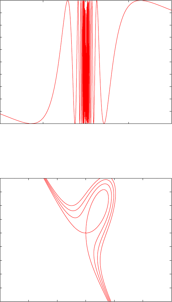
536 CHAPTER 16. USER CONTRIBUTED PACKAGES
A simple plot for sin(1/x):
plot(sin(1/x), x=(-1 .. 1), y=(-3 .. 3));
-1
-0.8
-0.6
-0.4
-0.2
0
0.2
0.4
0.6
0.8
1
-1
-0.5
0
0.5
1
y
x
REDUCE Plot
Some implicitly-defined curves:
plot(x^3 + y^3 - 3*x*y = {0,1,2,3}, x=(-2.5 .. 2), y=(-5 .. 5));
-2.5
-2
-1.5
-1
-0.5
0
0.5
1
1.5
2
-6
-4
-2
0
2
4
6
x
y
REDUCE Plot
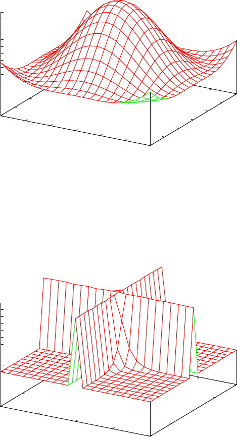
537
A test for hidden surfaces:
plot(cos sqrt(x^2 + y^2), x=(-3 .. 3), y=(-3 .. 3), hidden3d);
REDUCE Plot
-3
-2
-1
0
1
2
3
y
-3
-2
-1
0
1
2
3
x
-1
-0.8
-0.6
-0.4
-0.2
0
0.2
0.4
0.6
0.8
1
z
This may be slow on some machines because of a delicate evaluation context:
plot(sinh(x*y)/sinh(2*x*y), hidden3d);
REDUCE Plot
-10
-5
0
5
10
y
-10
-5
0
5
10
x
0
0.05
0.1
0.15
0.2
0.25
0.3
0.35
0.4
0.45
0.5
z
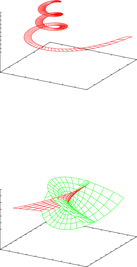
538 CHAPTER 16. USER CONTRIBUTED PACKAGES
on rounded;
w:= {for j:=1 step 0.1 until 20 collect {1/j*sin j, 1/j*cos j, j},
for j:=1 step 0.1 until 20 collect
{(0.1+1/j)*sin j, (0.1+1/j)*cos j, j} }$
plot w;
-0.4
-0.2
0
0.2
0.4
0.6
0.8
1
-0.6
-0.4
-0.2
0
0.2
0.4
0.6
0
2
4
6
8
10
12
14
16
18
20
z
REDUCE Plot
x
y
z
An example taken from: Cox, Little, O’Shea, Ideals, Varieties and Algorithms:
plot(point(3u+3u*v^2-u^3, 3v+3u^2*v-v^3, 3u^2-3v^2), hidden3d,
title="Enneper Surface");
Enneper Surface
-2500
-2000
-1500
-1000
-500
0
500
1000
1500
2000
2500
x
-2500
-2000
-1500
-1000
-500
0
500
1000
1500
2000
2500
y
-300
-200
-100
0
100
200
300
z
539
The following examples use the specfn package to draw a collection of Cheby-
shev T polynomials and Bessel Y functions. The special function package has to
be loaded explicitely to make the operator ChebyshevT and BesselY available.
load_package specfn;
plot(chebyshevt(1,x), chebyshevt(2,x), chebyshevt(3,x),
chebyshevt(4,x), chebyshevt(5,x),
x=(-1 .. 1), title="Chebyshev t Polynomials");
-1
-0.5
0
0.5
1
-1
-0.5
0
0.5
1
y
x
Chebyshev t Polynomials
plot(bessely(0,x), bessely(1,x), bessely(2,x), x=(0.1 .. 10),
y=(-1 .. 1), title="Bessel functions of 2nd kind");
-1
-0.8
-0.6
-0.4
-0.2
0
0.2
0.4
0.6
0
1
2
3
4
5
6
7
8
9
10
y
x
Bessel functions of 2nd kind
540 CHAPTER 16. USER CONTRIBUTED PACKAGES
16.28 GROEBNER: A Gröbner basis package
GROEBNER is a package for the computation of Gröbner Bases using the Buch-
berger algorithm and related methods for polynomial ideals and modules. It can be
used over a variety of different coefficient domains, and for different variable and
term orderings.
Gröbner Bases can be used for various purposes in commutative algebra, e.g. for
elimination of variables, converting surd expressions to implicit polynomial form,
computation of dimensions, solution of polynomial equation systems etc. The
package is also used internally by the SOLVE operator.
Authors: Herbert Melenk, H.M. Möller and Winfried Neun.
Gröbner bases are a valuable tool for solving problems in connection with multi-
variate polynomials, such as solving systems of algebraic equations and analyzing
polynomial ideals. For a definition of Gröbner bases, a survey of possible applica-
tions and further references, see [6]. Examples are given in [5], in [7] and also in
the test file for this package.
The groebner package calculates Gröbner bases using the Buchberger algorithm.
It can be used over a variety of different coefficient domains, and for different
variable and term orderings.
The current version of the package uses parts of a previous version, written by R.
Gebauer, A.C. Hearn, H. Kredel and H. M. Möller. The algorithms implemented
in the current version are documented in [10], [11], [15] and [12]. The operator
saturation has been implemented in July 2000 (Herbert Melenk).
16.28.1 Background
Variables, Domains and Polynomials
The various functions of the groebner package manipulate equations and/or poly-
nomials; equations are internally transformed into polynomials by forming the dif-
ference of left-hand side and right-hand side, if equations are given.
All manipulations take place in a ring of polynomials in some variables x1, . . . , xn
over a coefficient domain d:
d[x1, . . . , xn],
where dis a field or at least a ring without zero divisors. The set of variables
x1, . . . , xn can be given explicitly by the user or it is extracted automatically from
the input expressions.
All REDUCE kernels can play the role of “variables” in this context; examples are
541
x y z22 sin(alpha) cos(alpha) c(1,2,3) c(1,3,2) farina4711
The domain dis the current REDUCE domain with those kernels adjoined that are
not members of the list of variables. So the elements of dmay be complicated
polynomials themselves over kernels not in the list of variables; if, however, the
variables are extracted automatically from the input expressions, dis identical with
the current REDUCE domain. It is useful to regard kernels not being members of
the list of variables as “parameters”, e.g.
a∗x+ (a−b)∗y∗ ∗2with “variables” {x, y}
and “parameters” aand b .
The exponents of groebner variables must be positive integers.
Agroebner variable may not occur as a parameter (or part of a parameter) of
a coefficient function. This condition is tested in the beginning of the groebner
calculation; if it is violated, an error message occurs (with the variable name), and
the calculation is aborted. When the groebner package is called by solve, the test
is switched off internally.
The current version of the Buchberger algorithm has two internal modes, a field
mode and a ring mode. In the starting phase the algorithm analyzes the domain
type; if it recognizes das being a ring it uses the ring mode, otherwise the field
mode is needed. Normally field calculations occur only if all coefficients are num-
bers and if the current REDUCE domain is a field (e.g. rational numbers, modular
numbers modulo a prime). In general, the ring mode is faster. When no specific
REDUCE domain is selected, the ring mode is used, even if the input formulas
contain fractional coefficients: they are multiplied by their common denominators
so that they become integer polynomials. Zeroes of the denominators are included
in the result list.
Term Ordering
In the theory of Gröbner bases, the terms of polynomials are considered as or-
dered. Several order modes are available in the current package, including the
basic modes:
lex,gradlex,revgradlex
All orderings are based on an ordering among the variables. For each pair of vari-
ables (a, b)an order relation must be defined, e.g. “ab”. The greater sign
does not represent a numerical relation among the variables; it can be interpreted
only in terms of formula representation: “a” will be placed in front of “b” or “a” is
more complicated than “b”.
542 CHAPTER 16. USER CONTRIBUTED PACKAGES
The sequence of variables constitutes this order base. So the notion of
{x1, x2, x3}
as a list of variables at the same time means
x1x2x3
with respect to the term order.
If terms (products of powers of variables) are compared with lex, that term is cho-
sen which has a greater variable or a higher degree if the greatest variable is the
first in both. With gradlex the sum of all exponents (the total degree) is compared
first, and if that does not lead to a decision, the lex method is taken for the final de-
cision. The revgradlex method also compares the total degree first, but afterward
it uses the lex method in the reverse direction; this is the method originally used
by Buchberger.
Example 26 with {x, y, z}:
lex:
x∗y∗ ∗3y∗ ∗48 (heavier variable)
x∗ ∗4∗y∗ ∗2x∗ ∗3∗y∗ ∗10 (higher degree in 1st variable)
gradlex:
y∗ ∗3∗z∗ ∗4x∗ ∗3∗y∗ ∗3(higher total degree)
x∗zy∗ ∗2(equal total degree)
revgradlex:
y∗ ∗3∗z∗ ∗4x∗ ∗3∗y∗ ∗3(higher total degree)
x∗zy∗ ∗2(equal total degree,
so reverse order of lex)
The formal description of the term order modes is similar to [14]; this description
regards only the exponents of a term, which are written as vectors of integers with
0for exponents of a variable which does not occur:
(e)=(e1, . . . , en)representing x1∗ ∗e1x2∗ ∗e2···xn ∗ ∗en.
deg(e)is the sum over all elements of (e)
(e)(l)⇐⇒ (e)−(l)(0) = (0,...,0)
lex:
(e)> lex > (0) =⇒ek>0and ej= 0 for j= 1, . . . , k −1
gradlex:
(e)> gl > (0) =⇒deg(e)>0or (e)> lex > (0)
revgradlex:
(e)> rgl > (0) =⇒deg(e)>0or (e)< lex < (0)
543
Note that the lex ordering is identical to the standard REDUCE kernel ordering,
when korder is set explicitly to the sequence of variables.
lex is the default term order mode in the groebner package.
It is beyond the scope of this manual to discuss the functionality of the term order
modes. See [7].
The list of variables is declared as an optional parameter of the torder statement
(see below). If this declaration is missing or if the empty list has been used, the
variables are extracted from the expressions automatically and the REDUCE sys-
tem order defines their sequence; this can be influenced by setting an explicit order
via the korder statement.
The result of a Gröbner calculation is algebraically correct only with respect to the
term order mode and the variable sequence which was in effect during the calcu-
lation. This is important if several calls to the groebner package are done with
the result of the first being the input of the second call. Therefore we recommend
that you declare the variable list and the order mode explicitly. Once declared it re-
mains valid until you enter a new torder statement. The operator gvars helps you
extract the variables from a given set of polynomials, if an automatic reordering
has been selected.
The Buchberger Algorithm
The Buchberger algorithm of the package is based on GEBAUER/MÖLLER [11].
Extensions are documented in [16] and [12].
16.28.2 Loading of the Package
The following command loads the package into REDUCE (this syntax may vary
according to the implementation):
load_package groebner;
The package contains various operators, and switches for control over the reduction
process. These are discussed in the following.
16.28.3 The Basic Operators
Term Ordering Mode
torder (vl,m,[p1, p2, . . .]);
544 CHAPTER 16. USER CONTRIBUTED PACKAGES
where vl is a variable list (or the empty list if no variables are declared ex-
plicitly), mis the name of a term ordering mode lex,gradlex,revgradlex
(or another implemented mode) and [p1, p2, . . .]are additional parameters
for the term ordering mode (not needed for the basic modes).
torder sets variable set and the term ordering mode. The default mode is lex.
The previous description is returned as a list with corresponding elements.
Such a list can alternatively be passed as sole argument to torder.
If the variable list is empty or if the torder declaration is omitted, the auto-
matic variable extraction is activated.
gvars ({exp1, exp2,. . ., expn});
where {exp1, exp2, . . . , expn}is a list of expressions or equations.
gvars extracts from the expressions {exp1, exp2, . . . , expn}the kernels,
which can play the role of variables for a Gröbner calculation. This can be
used e.g. in a torder declaration.
groebner: Calculation of a Gröbner Basis
groebner {exp1, exp2, . . . , expm};
where {exp1, exp2, . . . , expm}is a list of expressions or equations.
groebner calculates the Gröbner basis of the given set of expressions with
respect to the current torder setting.
The Gröbner basis {1}means that the ideal generated by the input polynom-
ials is the whole polynomial ring, or equivalently, that the input polynomials
have no zeroes in common.
As a side effect, the sequence of variables is stored as a REDUCE list in the
shared variable
gvarslast.
This is important if the variables are reordered because of optimization: you
must set them afterwards explicitly as the current variable sequence if you
want to use the Gröbner basis in the sequel, e.g. for a preduce call. A
basis has the property “Gröbner” only with respect to the variable sequences
which had been active during its computation.
Example 27
torder({},lex)$
groebner{3*x**2*y+2*x*y+y+9*x**2+5*x - 3,
2*x**3*y-x*y-y+6*x**3-2*x**2-3*x + 3,
545
x**3*y+x**2*y+3*x**3+2*x**2 };
2
{8*x-2*y + 5*y + 3,
3 2
2*y - 3*y - 16*y + 21}
This example used the default system variable ordering, which was {x, y}. With
the other variable ordering, a different basis results:
torder({y,x},lex)$
groebner{3*x**2*y+2*x*y+y+9*x**2+5*x - 3,
2*x**3*y-x*y-y+6*x**3-2*x**2-3*x + 3,
x**3*y+x**2*y+3*x**3+2*x**2 };
2
{2*y+2*x - 3*x - 6,
3 2
2*x - 5*x - 5*x}
Another basis yet again results with a different term ordering:
torder({x,y},revgradlex)$
groebner{3*x**2*y+2*x*y+y+9*x**2+5*x - 3,
2*x**3*y-x*y-y+6*x**3-2*x**2-3*x + 3,
x**3*y+x**2*y+3*x**3+2*x**2 };
2
{2*y - 5*y-8*x - 3,
y*x-y+x+3,
2
2*x + 2*y-3*x - 6}
The operation of groebner can be controlled by the following switches:
groebopt – If set on, the sequence of variables is optimized with respect to execu-
tion speed; the algorithm involved is described in [5]; note that the final list
of variables is available in gvarslast.
An explicitly declared dependency supersedes the variable optimization. For
546 CHAPTER 16. USER CONTRIBUTED PACKAGES
example
depend a,x,y;
guarantees that awill be placed in front of xand y. So groebopt can be used
even in cases where elimination of variables is desired.
By default groebopt is off, conserving the original variable sequence.
groebf ullreduction – If set off, the reduction steps during the
groebner operation are limited to the pure head term reduction; subsequent
terms are reduced otherwise.
By default groebfullreduction is on.
gltbasis – If set on, the leading terms of the result basis are extracted. They are
collected in a basis of monomials, which is available as value of the global
variable with the name gltb.
glterms – If {exp1, . . . , expm}contain parameters (symbols which are not mem-
ber of the variable list), the share variable glterms contains a list of expres-
sion which during the calculation were assumed to be nonzero. A Gröbner
basis is valid only under the assumption that all these expressions do not
vanish.
The following switches control the print output of groebner; by default all these
switches are set off and nothing is printed.
groebstat – A summary of the computation is printed including the computing
time, the number of intermediate h–polynomials and the counters for the
hits of the criteria.
trgroeb – Includes groebstat and the printing of the intermediate h-polynomials.
trgroebs – Includes trgroeb and the printing of intermediate s–polynomials.
trgroeb1– The internal pairlist is printed when modified.
Gzerodim?: Test of dim = 0
gzerodim!? bas
where bas is a Gröbner basis in the current setting. The result is nil, if bas is
the basis of an ideal of polynomials with more than finitely many common
zeros. If the ideal is zero dimensional, i. e. the polynomials of the ideal have
only finitely many zeros in common, the result is an integer kwhich is the
number of these common zeros (counted with multiplicities).
547
gdimension,gindependent_sets: compute dimension and independent vari-
ables
The following operators can be used to compute the dimension and the independent
variable sets of an ideal which has the Gröbner basis bas with arbitrary term order:
gdimension bas
gindependent_sets bas gindependent_sets computes the maximal left indepen-
dent variable sets of the ideal, that are the variable sets which play the role
of free parameters in the current ideal basis. Each set is a list which is a
subset of the variable list. The result is a list of these sets. For an ideal with
dimension zero the list is empty. gdimension computes the dimension of the
ideal, which is the maximum length of the independent sets.
The switch groebopt plays no role in the algorithms gdimension and gindependent_sets.
It is set off during the processing even if it is set on before. Its state is saved during
the processing.
The “Kredel-Weispfenning" algorithm is used (see [15], extended to general order-
ing in [4].
Conversion of a Gröbner Basis
glexconvert: Conversion of an Arbitrary Gröbner Basis of a Zero Dimen-
sional Ideal into a Lexical One
glexconvert ({exp, . . . , expm}[,{var1. . . , varn}] [, maxdeg =mx]
[, newvars ={nv1, . . . , nvk}])
where {exp1, . . . , expm}is a Gröbner basis with {var1, . . . , varn}as vari-
ables in the current term order mode, mx is an integer, and {nv1, . . . , nvk}
is a subset of the basis variables. For this operator the source and target
variable sets must be specified explicitly.
glexconvert converts a basis of a zero-dimensional ideal (finite number of isolated
solutions) from arbitrary ordering into a basis under lex ordering. During the call
of glexconvert the original ordering of the input basis must be still active!
newvars defines the new variable sequence. If omitted, the original variable se-
quence is used. If only a subset of variables is specified here, the partial ideal basis
is evaluated. For the calculation of a univariate polynomial, newvars should be a
list with one element.
maxdeg is an upper limit for the degrees. The algorithm stops with an error mes-
sage, if this limit is reached.
548 CHAPTER 16. USER CONTRIBUTED PACKAGES
A warning occurs if the ideal is not zero dimensional.
glexconvert is an implementation of the FLGM algorithm by
FAUGÈRE, GIANNI, LAZARD and MORA [10]. Often, the calculation of a Gröb-
ner basis with a graded ordering and subsequent conversion to lex is faster than a
direct lex calculation. Additionally, glexconvert can be used to transform a lex
basis into one with different variable sequence, and it supports the calculation of
a univariate polynomial. If the latter exists, the algorithm is even applicable in the
non zero-dimensional case, if such a polynomial exists. If the polynomial does not
exist, the algorithm computes until maxdeg has been reached.
torder({{w,p,z,t,s,b},gradlex)
g := groebner { f1 := 45*p + 35*s -165*b -36,
35*p + 40*z + 25*t - 27*s, 15*w + 25*p*s +30*z -18*t
-165*b**2, -9*w + 15*p*t + 20*z*s,
w*p+2*z*t - 11*b**3, 99*w - 11*s*b +3*b**2,
b**2 + 33/50*b + 2673/10000};
g := {60000*w + 9500*b + 3969,
1800*p - 3100*b - 1377,
18000*z + 24500*b + 10287,
750*t - 1850*b + 81,
200*s - 500*b - 9,
2
10000*b + 6600*b + 2673}
glexconvert(g,{w,p,z,t,s,b},maxdeg=5,newvars={w});
2
100000000*w + 2780000*w + 416421
glexconvert(g,{w,p,z,t,s,b},maxdeg=5,newvars={p});
2
6000*p - 2360*p + 3051
groebner_walk: Conversion of a (General) Total Degree Basis into a Lex One
The algorithm groebner_walk convertes from an arbitrary polynomial system a
549
graduated basis of the given variable sequence to a lex one of the same sequence.
The job is done by computing a sequence of Gröbner bases of correspondig mono-
mial ideals, lifting the original system each time. The algorithm has been described
(more generally) by [2],[3],[1] and [8]. groebner_walk should be only called, if
the direct calculation of a lex Gröbner base does not work. The computation of
groebner_walk includes some overhead (e. g. the computation divides poly-
nomials). Normally torder must be called before to define the variables and the
variable sorting. The reordering of variables makes no sense with groebner_walk;
so do not call groebner_walk with groebopt on!
groebner_walk g
where gis a polynomial ideal basis computed under gradlex or under
weighted with a one–element, non zero weight vector with only one ele-
ment, repeated for each variable. The result is a corresponding lex basis (if
that is computable), independet of the degree of the ideal (even for non zero
degree ideals). The variabe gvarslast is not set.
groebnerf : Factorizing Gröbner Bases
Background If Gröbner bases are computed in order to solve systems of equat-
ions or to find the common roots of systems of polynomials, the factorizing version
of the Buchberger algorithm can be used. The theoretical background is simple: if
a polynomial pcan be represented as a product of two (or more) polynomials, e.g.
h=f∗g, then hvanishes if and only if one of the factors vanishes. So if during the
calculation of a Gröbner basis hof the above form is detected, the whole problem
can be split into two (or more) disjoint branches. Each of the branches is simpler
than the complete problem; this saves computing time and space. The result of
this type of computation is a list of (partial) Gröbner bases; the solution set of the
original problem is the union of the solutions of the partial problems, ignoring the
multiplicity of an individual solution. If a branch results in a basis {1}, then there
is no common zero, i.e. no additional solution for the original problem, contributed
by this branch.
groebnerf Call The syntax of groebnerf is the same as for groebner.
groebnerf({exp1, exp2, . . . , expm}[,{},{nz1, . . . nzk});
where {exp1, exp2, . . . , expm}is a given list of expressions or equations, and
{nz1, . . . nzk}is an optional list of polynomials known to be non-zero.
groebnerf tries to separate polynomials into individual factors and to branch the
computation in a recursive manner (factorization tree). The result is a list of partial
Gröbner bases. If no factorization can be found or if all branches but one lead to
550 CHAPTER 16. USER CONTRIBUTED PACKAGES
the trivial basis {1}, the result has only one basis; nevertheless it is a list of lists
of polynomials. If no solution is found, the result will be {{1}}. Multiplicities
(one factor with a higher power, the same partial basis twice) are deleted as early
as possible in order to speed up the calculation. The factorizing is controlled by
some switches.
As a side effect, the sequence of variables is stored as a REDUCE list in the shared
variable
gvarslast .
If gltbasis is on, a corresponding list of leading term bases is also produced and is
available in the variable gltb.
The third parameter of groebnerf allows one to declare some polynomials
nonzero. If any of these is found in a branch of the calculation the branch is can-
celled. This can be used to save a substantial amount of computing time. The
second parameter must be included as an empty list if the third parameter is to be
used.
torder({x,y},lex)$
groebnerf { 3*x**2*y+2*x*y+y+9*x**2+5*x = 3,
2*x**3*y-x*y-y+6*x**3-2*x**2-3*x = -3,
x**3*y+x**2*y+3*x**3+2*x**2 \};
{{y - 3,x},
2
{2*y+2*x - 1,2*x - 5*x - 5}}
It is obvious here that the solutions of the equations can be read off immediately.
All switches from groebner are valid for groebnerf as well:
groebopt
gltbasis
groebf ullreduction
groebstat
trgroeb
trgroebs
rgroeb1
Additional switches for groebnerf:
551
trgroebr – All intermediate partial basis are printed when detected.
By default trgroebr is off.
groebmonfac groebresmax groebrestriction
These variables are described in the following paragraphs.
Suppression of Monomial Factors The factorization in groebnerf is controlled
by the following switches and variables. The variable groebmonfac is connected
to the handling of “monomial factors”. A monomial factor is a product of variable
powers occurring as a factor, e.g. x∗ ∗2∗yin x∗ ∗3∗y−2∗x∗ ∗2∗y∗ ∗2. A
monomial factor represents a solution of the type “x= 0 or y= 0” with a certain
multiplicity. With groebnerf the multiplicity of monomial factors is lowered to
the value of the shared variable
groebmonf ac
which by default is 1 (= monomial factors remain present, but their multiplicity is
brought down). With
groebmonf ac := 0
the monomial factors are suppressed completely.
Limitation on the Number of Results The shared variable
groebresmax
controls the number of partial results. Its default value is 300. If groebresmax
partial results are calculated, the calculation is terminated. groebresmax counts
all branches, including those which are terminated (have been computed already),
give no contribution to the result (partial basis 1), or which are unified in the result
with other (partial) bases. So the resulting number may be much smaller. When
the limit of groeresmax is reached, a warning
GROEBRESMAX limit reached
is issued; this warning in any case has to be taken as a serious one. For "nor-
mal" calculations the groebresmax limit is not reached. groebresmax is a shared
variable (with an integer value); it can be set in the algebraic mode to a different
(positive integer) value.
Restriction of the Solution Space In some applications only a subset of the
complete solution set of a given set of equations is relevant, e.g. only nonnegative
552 CHAPTER 16. USER CONTRIBUTED PACKAGES
values or positive definite values for the variables. A significant amount of com-
puting time can be saved if nonrelevant computation branches can be terminated
early.
Positivity: If a polynomial has no (strictly) positive zero, then every system con-
taining it has no nonnegative or strictly positive solution. Therefore, the Buch-
berger algorithm tests the coefficients of the polynomials for equal sign if re-
quested. For example, in 13 ∗x+ 15 ∗y∗zcan be zero with real nonnegative
values for x, y and zonly if x= 0 and y= 0 or z= 0; this is a sort of “factoriza-
tion by restriction”. A polynomial 13 ∗x+ 15 ∗y∗z+ 20 never can vanish with
nonnegative real variable values.
Zero point: If any polynomial in an ideal has an absolute term, the ideal cannot
have the origin point as a common solution.
By setting the shared variable
groebrestriction
groebnerf is informed of the type of restriction the user wants to impose on the
solutions:
groebrestiction:=nonnegative;
only nonnegative real solutions are of interest
groebrestriction:=positive;
only nonnegative and nonzero solutions are of interest
groebrestriction:=zeropoint;
only solution sets which contain the point {0,0,...,0}are or interest.
If groebnerf detects a polynomial which formally conflicts with the restriction, it
either splits the calculation into separate branches, or, if a violation of the restric-
tion is determined, it cancels the actual calculation branch.
greduce,preduce: Reduction of Polynomials
Background Reduction of a polynomial “p” modulo a given sets of polynomials
“b” is done by the reduction algorithm incorporated in the Buchberger algorithm.
Informally it can be described for polynomials over a field as follows:
553
loop1: % head term elimination
if there is one polynomial bin Bsuch that the leading
term of pis a multiple of the leading term of Pdo
p:= p−lt(p)/lt(b)∗b(the leading term vanishes)
do this loop as long as possible;
loop2: % elimination of subsequent terms
for each term sin pdo
if there is one polynomial bin Bsuch that sis a
multiple of the leading term of pdo
p:= p−s/lt(b)∗b(the term svanishes)
do this loop as long as possible;
If the coefficients are taken from a ring without zero divisors we cannot divide by
each possible number like in the field case. But using that in the field case, c∗pis
reduced to c∗q, if pis reduced to q, for arbitrary numbers c, the reduction for the
ring case uses the least cwhich makes the (field) reduction for c∗pinteger. The
result of this reduction is returned as (ring) reduction of peventually after removing
the content, i.e. the greatest common divisor of the coefficients. The result of this
type of reduction is also called a pseudo reduction of p.
Reduction via Gröbner Basis Calculation
greduce(exp, {exp1, exp2, . . . , expm}]);
where exp is an expression, and {exp1, exp2, . . . , expm}is a list of any number
of expressions or equations.
greduce first converts the list of expressions {exp1, . . . , expn}to a Gröbner basis,
and then reduces the given expression modulo that basis. An error results if the list
of expressions is inconsistent. The returned value is an expression representing the
reduced polynomial. As a side effect, greduce sets the variable gvarslast in the
same manner as groebner does.
Reduction with Respect to Arbitrary Polynomials
preduce(exp, {exp1, exp2, . . . , expm});
where expm is an expression, and {exp1, exp2, . . . , expm}is a list of any number
of expressions or equations.
preduce reduces the given expression modulo the set {exp1, . . . , expm}. If this
set is a Gröbner basis, the obtained reduced expression is uniquely determined.
If not, then it depends on the subsequence of the single reduction steps (see 27).
preduce does not check whether {exp1, exp2, . . . , expm}is a Gröbner basis in
the actual order. Therefore, if the expressions are a Gröbner basis calculated earlier
554 CHAPTER 16. USER CONTRIBUTED PACKAGES
with a variable sequence given explicitly or modified by optimization, the proper
variable sequence and term order must be activated first.
Example 28(preduce called with a Gröbner basis):
torder({x,y},lex);
gb:=groebner{3*x**2*y+2*x*y+y+9*x**2+5*x - 3,
2*x**3*y-x*y-y+6*x**3-2*x**2-3*x + 3,
x**3*y+x**2*y+3*x**3+2*x**2}$
preduce (5*y**2+2*x**2*y + 5/2*x*y + 3/2*y
+ 8*x**2 + 3/2*x - 9/2, gb);
2
y
greduce_orders: Reduction with several term orders The shortest poly-
nomial with different polynomial term orders is computed with the operator
greduce_orders:
greduce_orders (exp, {exp1,exp2,...,expm} [,{v1,v2...vn}]);
where exp is an expression and {exp1, exp2, . . . , expm}is a list of any num-
ber of expressions or equations. The list of variables v1, v2. . . vnmay be
omitted; if set, the variables must be a list.
The expression exp is reduced by greduce with the orders in the shared variable
gorders, which must be a list of term orders (if set). By default it is set to
{revgradlex, gradlex, lex}
The shortest polynomial is the result. The order with the shortest polynomial is
set to the shared variable gorder. A Gröbner basis of the system {exp1,exp2,...,
expm} is computed for each element of orders. With the default setting gorder in
most cases will be set to revgradlex. If the variable set is given, these variables are
taken; otherwise all variables of the system {exp1,exp2,...,expm} are extracted.
The Gröbner basis computations can take some time; if interrupted, the interme-
diate result of the reduction is set to the shared variable greduce_result, if one is
done already. However, this is not nesessarily the minimal form.
If the variable gorders should be set to orders with a parameter, the term oder has
to be replaced by a list; the first element is the term oder selected, followed by its
parameter(s), e.g.
orders := {{gradlexgradlex, 2},{lexgradlex, 2}}
555
Reduction Tree In some case not only are the results produced by greduce and
preduce of interest, but the reduction process is of some value too. If the switch
groebprot
is set on, groebner,greduce and preduce produce as a side effect a trace of their
work as a REDUCE list of equations in the shared variable
groebprotf ile.
Its value is a list of equations with a variable “candidate” playing the role of the
object to be reduced. The polynomials are cited as “poly1”, “poly2”, . . . . If read as
assignments, these equations form a program which leads from the reduction input
to its result. Note that, due to the pseudo reduction with a ring as the coefficient
domain, the input coefficients may be changed by global factors.
556 CHAPTER 16. USER CONTRIBUTED PACKAGES
Example 29
on groebprot $
preduce (5 ∗y∗ ∗2+2∗x∗ ∗2∗y+ 5/2∗x∗y+ 3/2∗y+ 8 ∗x∗ ∗2
+3/2∗x−9/2, gb);
2
y
groebprotfile;
2 2 2
{candidate=4*x*y + 16*x + 5*x*y+3*x + 10*y + 3*y - 9,
2
poly1=8*x-2*y + 5*y + 3,
3 2
poly2=2*y - 3*y - 16*y + 21,
candidate=2*candidate,
candidate= - x*y*poly1 + candidate,
candidate= - 4*x*poly1 + candidate,
candidate=4*candidate,
3
candidate= - y *poly1 + candidate,
candidate=2*candidate,
2
candidate= - 3*y*poly1 + candidate,
candidate=13*y*poly1 + candidate,
candidate=candidate + 6*poly1,
2
candidate= - 2*y*poly2 + candidate,
candidate= - y*poly2 + candidate,
candidate=candidate + 6*poly2}

557
This means
16(5y2+ 2x2y+5
2xy +3
2y+ 8x2+3
2x−9
2) =
(−8xy −32x−2y3−3y2+ 13y+ 6)poly1
+(−2y2−2y+ 6)poly2 +y2.
Tracing with groebnert and preducet
Given a set of polynomials {f1, . . . , fk}and their Gröbner basis {g1, . . . , gl}, it is
well known that there are matrices of polynomials Cij and Dji such that
fi=X
j
Cijgjand gj=X
i
Djifi
and these relations are needed explicitly sometimes. In BUCHBERGER [6], such
cases are described in the context of linear polynomial equations. The standard
technique for computing the above formulae is to perform Gröbner reductions,
keeping track of the computation in terms of the input data. In the current package
such calculations are performed with (an internally hidden) cofactor technique:
the user has to assign unique names to the input expressions and the arithmetic
combinations are done with the expressions and with their names simultaneously.
So the result is accompanied by an expression which relates it algebraically to the
input values.
There are two complementary operators with this feature: groebnert and preducet;
functionally they correspond to groebner and preduce. However, the sets of ex-
pressions here must be equations with unique single identifiers on their left side
and the lhs are interpreted as names of the expressions. Their results are sets of
equations (groebnert) or equations (preducet), where a lhs is the computed value,
while the rhs is its equivalent in terms of the input names.
Example 30
We calculate the Gröbner basis for an ellipse (named “p1” ) and a line (named
“p2” ); p2is member of the basis immediately and so the corresponding first result
element is of a very simple form; the second member is a combination of p1and
p2as shown on the rhs of this equation:
gb1:=groebnert {p1=2*x**2+4*y**2-100,p2=2*x-y+1};
gb1 := {2*x - y + 1=p2,
2
9*y - 2*y - 199= - 2*x*p2 - y*p2 + 2*p1 + p2}
Example 31

558 CHAPTER 16. USER CONTRIBUTED PACKAGES
We want to reduce the polynomial x**2wrt the above Gröbner basis and need
knowledge about the reduction formula. We therefore extract the basis polynomials
from gb1, assign unique names to them (here g1,g2) and call preducet. The
polynomial to be reduced here is introduced with the name Q, which then appears
on the rhs of the result. If the name for the polynomial is omitted, its formal value
is used on the right side too.
gb2 := for k := 1:length gb1 collect
mkid(g,k) = lhs part(gb1,k)$
preducet (q=x**2,gb2);
- 16*y + 208= - 18*x*g1 - 9*y*g1 + 36*q+9*g1 - g2
This output means
x2= (1
2x+1
4y−1
4)g1 + 1
36g2+(−4
9y+52
9).
Example 32
If we reduce a polynomial which is member of the ideal, we consequently get a
result with lhs zero:
preducet(q=2*x**2+4*y**2-100,gb2);
0= - 2*x*g1 - y*g1 + 2*q+g1-g2
This means
q= (x+1
2y−1
2)g1 + 1
2g2.
With these operators the matrices Cij and Dji are available implicitly, Dji as side
effect of groebnertT, cij by calls of preducet of fiwrt {gj}. The latter by defini-
tion will have the lhs zero and a rhs with linear fi.
If {1}is the Gröbner basis, the groebnert calculation gives a “proof”, showing,
how 1can be computed as combination of the input polynomials.
Remark: Compared to the non-tracing algorithms, these operators are much
more time consuming. So they are applicable only on small sized problems.
Gröbner Bases for Modules
Given a polynomial ring, e.g. r=z[x1···xk]and an integer n > 1: the vectors
with nelements of rform a module under vector addition (= componentwise
559
addition) and multiplication with elements of r. For a submodule given by a finite
basis a Gröbner basis can be computed, and the facilities of the groebner package
can be used except the operators groebnerf and groesolve.
The vectors are encoded using auxiliary variables which represent the unit vectors
in the module. E.g. using v1, v2, v3the module element [x2
1,0, x1−x2]is repre-
sented as x2
1v1+x1v3−x2v3. The use of v1, v2, v3as unit vectors is set up by
assigning the set of auxiliary variables to the share variable gmodule, e.g.
gmodule := {v1,v2,v3};
After this declaration all monomials built from these variables are considered as an
algebraically independent basis of a vector space. However, you had best use them
only linearly. Once gmodule has been set, the auxiliary variables automatically
will be added to the end of each variable list (if they are not yet member there).
Example:
torder({x,y,v1,v2,v3},lex)$
gmodule := {v1,v2,v3}$
g:=groebner{x^2*v1 + y*v2,x*y*v1 - v3,2y*v1 + y*v3};
2
g := {x *v1 + y*v2,
2
x*v3 + y *v2,
3
y*v2 - 2*v3,
2*y*v1 + y*v3}
preduce((x+y)^3*v1,g);
1 3 2
- x*y*v2 - ---*y*v3 - 3*y*v2 + 3*y*v3
2
In many cases a total degree oriented term order will be adequate for computations
in modules, e.g. for all cases where the submodule membership is investigated.
However, arranging the auxiliary variables in an elimination oriented term order
can give interesting results. E.g.
560 CHAPTER 16. USER CONTRIBUTED PACKAGES
p1:=(x-1)*(x^2-x+3)$ p2:=(x-1)*(x^2+x-5)$
gmodule := {v1,v2,v3};
torder({v1,x,v2,v3},lex)$
gb:=groebner {p1*v1+v2,p2*v1+v3};
gb := {30*v1*x - 30*v1 + x*v2 - x*v3 + 5*v2 - 3*v3,
2 2
x*v2 - x *v3 + x*v2 + x*v3 - 5*v2 - 3*v3}
g:=coeffn(first gb,v1,1);
g := 30*(x - 1)
c1:=coeffn(first gb,v2,1);
c1:=x+5
c2:=coeffn(first gb,v3,1);
c2 := - x - 3
c1*p1 + c2*p2;
30*(x - 1)
Here two polynomials are entered as vectors [p1,1,0] and [p2,0,1]. Using a term
ordering such that the first dimension ranges highest and the other components low-
est, a classical cofactor computation is executed just as in the extended Euclidean
algorithm. Consequently the leading polynomial in the resulting basis shows the
greatest common divisor of p1and p2, found as a coefficient of v1while the coef-
ficients of v2and v3are the cofactors c1and c2of the polynomials p1and p2with
the relation gcd(p1, p2) = c1p1+c2p2.
Additional Orderings
Besides the basic orderings, there are ordering options that are used for special
purposes.
Separating the Variables into Groups It is often desirable to separate variables
and formal parameters in a system of polynomials. This can be done with a lex
561
Gröbner basis. That however may be hard to compute as it does more separation
than necessary. The following orderings group the variables into two (or more)
sets, where inside each set a classical ordering acts, while the sets are handled via
their total degrees, which are compared in elimination style. So the Gröbner basis
will eliminate the members of the first set, if algebraically possible. torder here
gets an additional parameter which describe the grouping
torder (vl,gradlexgradlex,n)
torder (vl,gradlexrevgradlex,n)
torder (vl,lexgradlex,n)
torder (vl,lexrevgradlex,n)
Here the integer nis the number of variables in the first group and the names
combine the local ordering for the first and second group, e.g.
lexgradlex, 3 for {x1, x2, x3, x4, x5}:
xi1
1. . . xi5
5xj1
1. . . xj5
5
if (i1, i2, i3)lex (j1, j2, j3)
or (i1, i2, i3) = (j1, j2, j3)
and (i4, i5)gradlex (j4, j5)
Note that in the second place there is no lex ordering available; that would not make
sense.
Weighted Ordering The statement
torder (vl,weighted, {n1, n2, n3. . .}) ;
establishes a graduated ordering, where the exponents are first multiplied by the
given weights. If there are less weight values than variables, the weight 1 is added
automatically. If the weighted degree calculation is not decidable, a lex compari-
son follows.
Graded Ordering The statement
torder (vl,graded, {n1, n2, n3. . .},order2) ;
establishes a graduated ordering, where the exponents are first multiplied by the
given weights. If there are less weight values than variables, the weight 1 is added
automatically. If the weighted degree calculation is not decidable, the term order
order2specified in the following argument(s) is used. The ordering graded is
designed primarily for use with the operator dd_groebner.
562 CHAPTER 16. USER CONTRIBUTED PACKAGES
Matrix Ordering The statement
torder (vl,matrix, m) ;
where mis a matrix with integer elements and row length which corresponds to the
variable number. The exponents of each monomial form a vector; two monomials
are compared by multiplying their exponent vectors first with mand comparing
the resulting vector lexicographically. E.g. the unit matrix establishes the classical
lex term order mode, a matrix with a first row of ones followed by the rows of a
unit matrix corresponds to the gradlex ordering.
The matrix mmust have at least as many rows as columns; a non–square matrix
contains redundant rows. The matrix must have full rank, and the top non–zero
element of each column must be positive.
The generality of the matrix based term order has its price: the computing time
spent in the term sorting is significantly higher than with the specialized term or-
ders. To overcome this problem, you can compile a matrix term order ; the com-
pilation reduces the computing time overhead significantly. If you set the switch
comp on, any new order matrix is compiled when any operator of the groebner
package accesses it for the first time. Alternatively you can compile a matrix ex-
plicitly
torder_compile(<n>,<m>);
where <n>is a name (an identifier) and <m>is a term order matrix.
torder_compile transforms the matrix into a LISP program, which is compiled
by the LISP compiler when comp is on or when you generate a fast loadable mod-
ule. Later you can activate the new term order by using the name < n > in a
torder statement as term ordering mode.
Gröbner Bases for Graded Homogeneous Systems
For a homogeneous system of polynomials under a term order graded,gradlex,
revgradlex or weighted a Gröbner Base can be computed with limiting the grade of
the intermediate s–polynomials:
dd_groebner (d1,d2,{p1, p2, . . .});
where d1is a non–negative integer and d2is an integer > d1or “infinity". A pair
of polynomials is considered only if the grade of the lcm of their head terms is
between d1and d2. See [4] for the mathematical background. For the term orders
graded or weighted the (first) weight vector is used for the grade computation.
Otherwise the total degree of a term is used.
563
16.28.4 Ideal Decomposition & Equation System Solving
Based on the elementary Gröbner operations, the groebner package offers ad-
ditional operators, which allow the decomposition of an ideal or of a system of
equations down to the individual solutions.
Solutions Based on Lex Type Gröbner Bases
groesolve: Solution of a Set of Polynomial Equations The groesolve operator
incorporates a macro algorithm; lexical Gröbner bases are computed by groebnerf
and decomposed into simpler ones by ideal decomposition techniques; if alge-
braically possible, the problem is reduced to univariate polynomials which are
solved by solve; if rounded is on, numerical approximations are computed for
the roots of the univariate polynomials.
groesolve({exp1, exp2, . . . , expm}[,{var1, var2, . . . , varn}]);
where {exp1, exp2, . . . , expm}is a list of any number of expressions or equations,
{var1, var2, . . . , varn}is an optional list of variables.
The result is a set of subsets. The subsets contain the solutions of the polynomial
equations. If there are only finitely many solutions, then each subset is a set of
expressions of triangular type {exp1, exp2, . . . , expn},where exp1depends only
on var1, exp2depends only on var1and var2etc. until expn which depends
on var1, . . . , varn. This allows a successive determination of the solution com-
ponents. If there are infinitely many solutions, some subsets consist in less than
nexpressions. By considering some of the variables as “free parameters”, these
subsets are usually again of triangular type.
Example 33(Intersubsections of a line with a circle):
groesolve({x∗ ∗2−y∗ ∗2−a, p ∗x+q∗y+s},{x, y});
2 2 2 2 2
{{x=(sqrt( - a*p + a*q + s )*q-p*s)/(p - q ),
2 2 2 2 2
y= - (sqrt( - a*p + a*q + s )*p-q*s)/(p - q )},
2 2 2 2 2
{x= - (sqrt( - a*p + a*q + s )*q+p*s)/(p - q ),
2 2 2 2 2
y=(sqrt( - a*p + a*q + s )*p+q*s)/(p - q )}}
If the system is zero–dimensional (has a number of isolated solutions), the algo-
rithm described in [13] is used, if the decomposition leaves a polynomial with
564 CHAPTER 16. USER CONTRIBUTED PACKAGES
mixed leading term. Hillebrand has written the article and Möller was the tutor of
this job.
The reordering of the groesolve variables is controlled by the REDUCE switch
varopt. If varopt is on (which is the default of varopt), the variable sequence
is optimized (the variables are reordered). If varopt is off, the given variable
sequence is taken (if no variables are given, the order of the REDUCE system
is taken instead). In general, the reordering of the variables makes the Gröbner
basis computation significantly faster. A variable dependency, declare by one (or
several) depend statements, is regarded (if varopt is on). The switch groebopt has
no meaning for groesolve; it is stored during its processing.
groepostproc: Postprocessing of a Gröbner Basis In many cases, it is difficult
to do the general Gröbner processing. If a Gröbner basis with a lex ordering is
calculated already (e.g., by very individual parameter settings), the solutions can
be derived from it by a call to groepostproc.groesolve is functionally equivalent
to a call to groebnerf and subsequent calls to groepostproc for each partial basis.
groepostproc({exp1, exp2, . . . , expm}[,{var1, var2, . . . , varn}]);
where {exp1, exp2, . . . , expm}is a list of any number of expressions,
{var1, var2, . . . , varn}is an optional list of variables. The expressions must
be a lex Gröbner basis with the given variables; the ordering must be still active.
The result is the same as with groesolve.
groepostproc({x3**2+x3+x2-1,
x2*x3 + x1*x3 + x3 + x1*x2 + x1 + 2,
x2**2+2*x2 - 1,
x1**2 - 2},{x3,x2,x1});
{{x3= - sqrt(2),
x2=sqrt(2) - 1,
x1=sqrt(2)},
{x3=sqrt(2),
x2= - (sqrt(2) + 1),
x1= - sqrt(2)},
sqrt(4*sqrt(2) + 9) - 1
{x3=-------------------------,
565
2
x2= - (sqrt(2) + 1),
x1=sqrt(2)},
- (sqrt(4*sqrt(2) + 9) + 1)
{x3=------------------------------,
2
x2= - (sqrt(2) + 1),
x1=sqrt(2)},
sqrt( - 4*sqrt(2) + 9) - 1
{x3=----------------------------,
2
x2=sqrt(2) - 1,
x1= - sqrt(2)},
- (sqrt( - 4*sqrt(2) + 9) + 1)
{x3=---------------------------------,
2
x2=sqrt(2) - 1,
x1= - sqrt(2)}}
Idealquotient: Quotient of an Ideal and an Expression Let ibe an ideal and f
be a polynomial in the same variables. Then the algebraic quotient is defined by
i:f={p|p∗fmember of i}.
The ideal quotient i:fcontains iand is obviously part of the whole polynomial
ring, i.e. contained in {1}. The case i:f={1}is equivalent to fbeing a
member of i. The other extremal case, i:f=i, occurs, when fdoes not vanish
at any general zero of i. The explanation of the notion “general zero” introduced
by van der Waerden, however, is beyond the aim of this manual. The operation of
groesolve/groepostproc is based on nested ideal quotient calculations.
If iis given by a basis and fis given as an expression, the quotient can be calculated
by
idealquotient({exp1, . . . , expm}, exp);
566 CHAPTER 16. USER CONTRIBUTED PACKAGES
where {exp1, exp2, . . . , expm}is a list of any number of expressions or equations,
exp is a single expression or equation.
idealquotient calculates the algebraic quotient of the ideal iwith the basis
{exp1, exp2, . . . , expm}and exp with respect to the variables given or extracted.
{exp1, exp2, . . . , expm}is not necessarily a Gröbner basis. The result is the Gröb-
ner basis of the quotient.
Saturation: Saturation of an Ideal and an Expression The saturation op-
erator computes the quotient on an ideal and an arbitrary power of an expression
exp ∗ ∗nwith arbitrary n. The call is
saturation({exp1, . . . , expm}, exp);
where {exp1, exp2, . . . , expm}is a list of any number of expressions or equations,
exp is a single expression or equation.
saturation calls idealquotient several times, until the result is stable, and returns
it.
Operators for Gröbner Bases in all Term Orderings
In some cases where no Gröbner basis with lexical ordering can be calculated, a
calculation with a total degree ordering is still possible. Then the Hilbert polyno-
mial gives information about the dimension of the solutions space and for finite sets
of solutions univariate polynomials can be calculated. The solutions of the equat-
ion system then is contained in the cross product of all solutions of all univariate
polynomials.
Hilbertpolynomial: Hilbert Polynomial of an Ideal This algorithm was con-
tributed by JOACHIM HOLLMAN, Royal Institute of Technology, Stockholm (pri-
vate communication).
hilbertpolynomial({exp1, . . . , expm}) ;
where {exp1, . . . , expm}is a list of any number of expressions or equations.
hilertpolynomial calculates the Hilbert polynomial of the ideal with basis
{exp1, . . . , expm}with respect to the variables given or extracted provided
the given term ordering is compatible with the degree, such as the gradlex-
or revgradlex-ordering. The term ordering of the basis must be active and
{exp1, . . .,expm}should be a Gröbner basis with respect to this ordering. The
Hilbert polynomial gives information about the cardinality of solutions of the sys-
tem {exp1, . . . , expm}: if the Hilbert polynomial is an integer, the system has
567
only a discrete set of solutions and the polynomial is identical with the number
of solutions counted with their multiplicities. Otherwise the degree of the Hilbert
polynomial is the dimension of the solution space.
If the Hilbert polynomial is not a constant, it is constructed with the variable “x”
regardless of whether xis member of {var1, . . . , varn}or not. The value of this
polynomial at sufficiently large numbers “x” is the difference of the dimension of
the linear vector space of all polynomials of degree ≤xminus the dimension of
the subspace of all polynomials of degree ≤xwhich belong also to the ideal.
xmust be an undefined variable or the value of xmust be an undefined variable;
otherwise a warning is given and a new (generated) variable is taken instead.
Remark: The number of zeros in an ideal and the Hilbert polynomial depend
only on the leading terms of the Gröbner basis. So if a subsequent Hilbert calcu-
lation is planned, the Gröbner calculation should be performed with on gltbasis
and the value of gltb (or its elements in a groebnerf context) should be given to
hilbertpolynomial. In this manner, a lot of computing time can be saved in the
case of long calculations.
16.28.5 Calculations “by Hand”
The following operators support explicit calculations with polynomials in a dis-
tributive representation at the REDUCE top level. So they allow one to do Gröbner
type evaluations stepwise by separate calls. Note that the normal REDUCE arith-
metic can be used for arithmetic combinations of monomials and polynomials.
Representing Polynomials in Distributive Form
gsortp;
where pis a polynomial or a list of polynomials.
If pis a single polynomial, the result is a reordered version of pin the distributive
representation according to the variables and the current term order mode; if p
is a list, its members are converted into distributive representation and the result
is the list sorted by the term ordering of the leading terms; zero polynomials are
eliminated from the result.
torder({alpha,beta,gamma},lex);
dip := gsort(gamma*(alpha-1)**2*(beta+1)**2);
568 CHAPTER 16. USER CONTRIBUTED PACKAGES
2 2 2
dip := alpha *beta *gamma + 2*alpha *beta*gamma
2 2
+ alpha *gamma - 2*alpha*beta *gamma - 4*alpha*beta*gamma
2
- 2*alpha*gamma + beta *gamma + 2*beta*gamma + gamma
Splitting of a Polynomial into Leading Term and Reductum
gsplitp;
where pis a polynomial.
gsplit converts the polynomial pinto distributive representation and splits it into
leading monomial and reductum. The result is a list with two elements, the leading
monomial and the reductum.
gslit dip;
2 2
{alpha *beta *gamma,
2 2 2
2*alpha *beta*gamma + alpha *gamma - 2*alpha*beta *gamma
2
- 4*alpha*beta*gamma - 2*alpha*gamma + beta *gamma
+ 2*beta*gamma + gamma}
Calculation of Buchberger’s S-polynomial
gspoly(p1, p2);
where p1and p2are polynomials.
gspoly calculates the s-polynomial from p1and p2;
569
Example for a complete calculation (taken from DAVENPORT ET AL. [9]):
torder({x,y,z},lex)$
g1 := x**3*y*z-x*z**2;
g2 := x*y**2*z-x*y*z;
g3 := x**2*y**2 - z;$
% first S-polynomial
g4 := gspoly(g2,g3);$
2 2
g4 := x *y*z-z
% next S-polynomial
p := gspoly(g2,g4); $
2 2
p := x *y*z-y*z
% and reducing, here only by g4
g5 := preduce(p,{g4});
2 2
g5 := - y*z + z
% last S-polynomial}
g6 := gspoly(g4,g5);
2 2 3
g6 := x *z - z
% and the final basis sorted descending
gsort{g2,g3,g4,g5,g6};
2 2
{x *y - z,
2 2
x*y*z-z,
570 CHAPTER 16. USER CONTRIBUTED PACKAGES
2 2 3
x*z - z ,
2
x*y*z-x*y*z,
2 2
- y*z + z }
Bibliography
[1] Beatrice Amrhein and Oliver Gloor. The fractal walk. In Bruno Buchberger
an Franz Winkler, editor, Gröbner Bases and Applications, volume 251 of
LMS, pages 305 –322. Cambridge University Press, February 1998.
[2] Beatrice Amrhein, Oliver Gloor, and Wolfgang Kuechlin. How fast does
the walk run? In Alain Carriere and Louis Remy Oudin, editors, 5th Rhine
Workshop on Computer Algebra, volume PR 801/96, pages 8.1 – 8.9. Institut
Franco–Allemand de Recherches de Saint–Louis, January 1996.
[3] Beatrice Amrhein, Oliver Gloor, and Wolfgang Kuechlin. Walking faster. In
J. Calmet and C. Limongelli, editors, Design and Implementation of Symbolic
Computation Systems, volume 1128 of Lecture Notes in Computer Science,
pages 150 –161. Springer, 1996.
[4] Thomas Becker and Volker Weispfenning. Gröbner Bases. Springer, 1993.
[5] W. Boege, R. Gebauer, and H. Kredel. Some examples for solving systems of
algebraic equations by calculating Gröbner bases. J. Symbolic Computation,
2(1):83–98, March 1986.
[6] Bruno Buchberger. Gröbner bases: An algorithmic method in polynomial
ideal theory. In N. K. Bose, editor, Progress, directions and open problems in
multidimensional systems theory, pages 184–232. Dordrecht: Reidel, 1985.
[7] Bruno Buchberger. Applications of Gröbner bases in non-linear computa-
tional geometry. In R. Janssen, editor, Trends in Computer Algebra, pages
52–80. Berlin, Heidelberg, 1988.
[8] S. Collart, M. Kalkbrener, and D. Mall. Converting bases with the Gröbner
walk. J. Symbolic Computation, 24:465 – 469, 1997.
[9] James H. Davenport, Yves Siret, and Evelyne Tournier. Computer Algebra,
Systems and Algorithms for Algebraic Computation. Academic Press, 1989.
571
[10] J. C. Faugère, P. Gianni, D. Lazard, and T. Mora. Efficient computation of
zero-dimensional Gröbner bases by change of ordering. Technical report,
1989.
[11] Rüdiger Gebauer and H. Michael Möller. On an installation of Buchberger’s
algorithm. J. Symbolic Computation, 6(2 and 3):275–286, 1988.
[12] A. Giovini, T. Mora, G. Niesi, L. Robbiano, and C. Traverso. One sugar cube,
please or selection strategies in the Buchberger algorithm. In Proc. of ISSAC
’91, pages 49–55, 1991.
[13] Dietmar Hillebrand. Triangulierung nulldimensionaler Ideale - Implemen-
tierung und Vergleich zweier Algorithmen - in German . Diplomarbeit im
Studiengang Mathematik der Universität Dortmund. Betreuer: Prof. Dr. H.
M. Möller. Technical report, 1999.
[14] Heinz Kredel. Admissible termorderings used in computer algebra systems.
SIGSAM Bulletin, 22(1):28–31, January 1988.
[15] Heinz Kredel and Volker Weispfenning. Computing dimension and inde-
pendent sets for polynomial ideals. J. Symbolic Computation, 6(1):231–247,
November 1988.
[16] Herbert Melenk, H. Michael Möller, and Winfried Neun. On Gröbner bases
computation on a supercomputer using REDUCE. Preprint SC 88-2, Konrad-
Zuse-Zentrum für Informationstechnik Berlin, January 1988.

572 CHAPTER 16. USER CONTRIBUTED PACKAGES
16.29 GUARDIAN: Guarded Expressions in Practice
Computer algebra systems typically drop some degenerate cases when evaluating
expressions, e.g., x/x becomes 1dropping the case x= 0. We claim that it is feasi-
ble in practice to compute also the degenerate cases yielding guarded expressions.
We work over real closed fields but our ideas about handling guarded expression
can be easily transferred to other situations. Using formulas as guards provides
a powerful tool for heuristically reducing the combinatorial explosion of cases:
equivalent, redundant, tautological, and contradictive cases can be detected by sim-
plification and quantifier elimination. Our approach allows to simplify the expres-
sions on the basis of simplification knowledge on the logical side. The method
described in this paper is implemented in the REDUCE package GUARDIAN.
Authors: Andreas Dolzmann and Thomas Sturm.
16.29.1 Introduction
It is meanwhile a well-known fact that evaluations obtained with the interactive use
of computer algebra systems (CAS) are not entirely correct in general. Typically,
some degenerate cases are dropped. Consider for instance the evaluation
x2
x=x,
which is correct only if x6= 0. The problem here is that CAS consider variables
to be transcendental elements. The user, in contrast, has in mind variables in the
sense of logic. In other words: The user does not think of rational functions but of
terms.
Next consider the valid expression
√x+√−x
x.
It is meaningless over the reals. CAS often offer no choice than to interprete surds
over the complex numbers even if they distinguish between a real and a complex
mode.
Corless and Jeffrey [4] have examined the behavior of a number of CAS with such
input data. They come to the conclusion that simultaneous computation of all
cases is exemplary but not feasible due to the combinatorial explosion of cases
to be considered. Therefore, they suggest to ignore the degenerate cases but to
provide the assumptions to the user on request. We claim, in contrast, that it is in
fact feasible to compute all possible cases.
Our setting is as follows: Expressions are evaluated to guarded expressions con-
sisting of possibly several conventional expressions guarded by quantifier-free for-

573
mulas. For the above examples, we would obtain
x6= 0 x,hF√x+√−x
xi.
As the second example illustrates, we are working in ordered fields, more precisely
in real closed fields. The handling of guarded expressions as described in this paper
can, however, be easily transferred to other situations.
Our approach can also deal with redundant guarded expressions, such as
T|x| − x
x≥0 0
x < 0−2x
which leads to algebraic simplification techniques based on logical simplification
as proposed by Davenport and Faure [5].
We use formulas over the language of ordered rings as guards. This provides pow-
erful tools for heuristically reducing the combinatorial explosion of cases: equiv-
alent, redundant, tautological, and contradictive cases can be detected by simplifi-
cation [6] and quantifier elimination [17,3,18,15,21,20]. In certain situations,
we will allow the formulas also to contain extra functions such as √·or |·|. Then
we take care that there is no quantifier elimination applied.
Simultaneous computation of several cases concerning certain expressions being
zero or not has been extensively investigated as dynamic evaluation [12,10,11,2].
It has also been extended to real closed fields [9]. The idea behind the development
of these methods is of a more theoretical nature than to overcome the problems with
the interactive usage of CAS sketched above: one wishes to compute in algebraic
(or real) extension fields of the rationals. Guarded expressions occur naturally
when solving problems parametrically. Consider, e.g., the Gröbner systems used
during the computation of comprehensive Gröbner bases [19].
The algorithms described in this paper are implemented in the REDUCE package
GUARDIAN. It is based on the REDUCE [13,16] package REDLOG [7,8] imple-
menting a formula data type with corresponding algorithms, in particular including
simplification and quantifier elimination.
16.29.2 An outline of our method
Guarded expressions
Aguarded expression is a scheme
γ0t0
γ1t1
.
.
..
.
.
γntn

574 CHAPTER 16. USER CONTRIBUTED PACKAGES
where each γiis a quantifier-free formula, the guard, and each tiis an associated
conventional expression. The idea is that some tiis a valid interpretation iff γi
holds. Each pair (γi, ti)is called a case.
The first case (γ0, t0)is the generic case: t0is the expression the system would
compute without our package, and γ0is the corresponding guard.
The guards γineed neither exclude one another, nor do we require that they form
a complete case distinction. We shall, however, assume that all cases covered by a
guarded expression are already covered by the generic case; in other words:
n
^
i=1
(γi−→ γ0).(16.74)
Consider the following evaluation of |x|to a guarded expression:
T|x|
x≥0x
x < 0−x
.
Here the non-generic cases already cover the whole domain. The generic case is
in some way redundant. It is just present for keeping track of the system’s default
behavior. Formally we have
n
_
i=1
γi←→ γ0.(16.75)
As an example for a non-redundant, i.e., necessary generic case we have the eval-
uation of the reciprocal 1
x:
x6= 0 1
x.
In every guarded expression, the generic case is explicitly marked as either neces-
sary or redundant. The corresponding tag is inherited during the evaluation process.
Unfortunately it can happen that guarded expressions satisfy (16.75) without being
tagged redundant, e.g., specialization of
T sin x
x= 0 0
to x= 0 if the system cannot evaluate sin(0). This does not happen if one claims
for necessary generic cases to have, as the reciprocal above, no alternative cases at
all. Else, in the sequel “redundant generic case” has to be read as “tagged redun-
dant.”
With guarded expressions, the evaluation splits into two independent parts: Al-
gebraic evaluation and a subsequent simplification of the guarded expression ob-
tained.

575
Guarding schemes
In the introduction we have seen that certain operators introduce case distinctions.
For this, with each operator fthere is a guarding scheme associated providing
information on how to map f(t1, . . . , tm)to a guarded expression provided that
one does not have to care for the argument expressions t1, ..., tm. In the easiest
case, this is a rewrite rule
f(a1, . . . , am)→G(a1, . . . , am).
The actual terms t1, ..., tmare simply substituted for the formal symbols a1,
..., aminto the generic guarded expression G(a1, . . . , am). We give some ex-
amples:
a1
a2→ha26= 0 a1
a2i
√a1→a1≥0√a1
sign(a1)→
T sign(a1)
a1>0 1
a1= 0 0
a1<0−1
|a1| →
T|a1|
a1≥0a1
a1<0−a1
(16.76)
For functions of arbitrary arity, e.g., min or max, we formally assume infinitely
many operators of the same name. Technically, we associate a procedure parame-
terized with the number of arguments mthat generates the corresponding rewrite
rule. As min_scheme(2)we obtain, e.g.,
min(a1, a2)→
T min(a1, a2)
a1≤a2a1
a2≤a1a2
,(16.77)
while for higher arities there are more case distinctions necessary.
For later complexity analysis, we state the concept of a guarding scheme formally:
a guarding scheme for an m-ary operator fis a map
gschemef: Em→GE
where Eis the set of expressions, and GE is the set of guarded expressions. This al-
lows to split f(t1, . . . , tm)in dependence on the form of the parameter expressions
t1,...,tm.

576 CHAPTER 16. USER CONTRIBUTED PACKAGES
Algebraic evaluation
Evaluating conventional expressions The evaluation of conventional expres-
sions into guarded expressions is performed recursively: Constants cevaluate to
Tc.
For the evaluation of f(e1, . . . , em)the argument expressions e1, ..., emare re-
cursively evaluated to guarded expressions
e0
i=
γi0ti0
γi1ti1
.
.
..
.
.
γinitini
for 1≤i≤m. (16.78)
Then the operator fis “moved inside” the e0
iby combining all cases, technically a
simultaneous Cartesian product computation of both the sets of guards and the sets
of terms:
Γ =
m
Y
i=1{γi0, . . . , γini}, T =
m
Y
i=1{ti0, . . . , tini}.(16.79)
This leads to the intermediate result
γ10 ∧ ··· ∧ γm0f(t10, . . . , tm0)
.
.
..
.
.
γ1n1∧ ··· ∧ γm0f(t1n1, . . . , tm0)
.
.
..
.
.
γ1n1∧ ··· ∧ γmnmf(t1n1, . . . , tmnm)
.(16.80)
The new generic case is exactly the combination of the generic cases of the e0
i. It
is redundant if at least one of these combined cases is redundant.
Next, all non-generic cases containing at least one redundant generic constituent
γi0in their guard are deleted. The reason for this is that generic cases are only
used to keep track of the system default behavior. All other cases get the status of a
non-generic case even if they contain necessary generic constituents in their guard.
At this point, we apply the guarding scheme of fto all remaining expressions
f(t1i1, . . . , tmim)in the form (16.80) yielding a nested guarded expression
Γ0
δ00 u00
.
.
..
.
.
δ0k0u0k0
.
.
..
.
.
ΓN
δN0uN0
.
.
..
.
.
δNkNuNkN
,(16.81)

577
which can be straightforwardly resolved to a guarded expression
Γ0∧δ00 u00
.
.
..
.
.
Γ0∧δ0k0u0k0
.
.
..
.
.
ΓN∧δN0uN0
.
.
..
.
.
ΓN∧δNkNuNkN
.
This form is treated analogously to the form (16.80): The new generic case
(Γ0∧δ00, u00)is redundant if at least one of Γ0, f (t10, . . . , tm0)and (δ00, u00)
is redundant. Among the non-generic cases all those containing redundant generic
constituents in their guard are deleted, and all those containing necessary generic
constituents in their guard get the status of an ordinary non-generic case.
Finally the standard evaluator of the system—reval in the case of REDUCE—
is applied to all contained expressions, which completes the algebraic part of the
evaluation.
Evaluating guarded expressions The previous section was concerned with the
evaluation of pure conventional expressions into guarded expressions. Our system
currently combines both conventional and guarded expressions. We are thus faced
with the problem of treating guarded subexpressions during evaluation.
When there is a guarded subexpression eidetected during evaluation, all contained
expressions are recursively evaluated to guarded expressions yielding a nested
guarded expression of the form (16.81). This is resolved as described above yield-
ing the evaluation subresult e0
i.
As a special case, this explains how guarded expressions are (re)evaluated to
guarded expressions.
Example
We describe the evaluation of the expression min(x, |x|). The first argument e1=
xevaluates recursively to
e0
1=Tx(16.82)
with a necessary generic case. The nested xinside e2=|x|evaluates to the same
form (16.82). For obtaining e0
2, we apply the guarding scheme (16.76) of the abso-
lute value to the only term of (16.82) yielding
T
T|x|
x≥0x
x < 0−x
,

578 CHAPTER 16. USER CONTRIBUTED PACKAGES
where the inner generic case is redundant. This form is resolved to
e0
2=
T∧T|x|
T∧x≥0x
T∧x < 0−x
with a redundant generic case. The next step is the combination of cases by Carte-
sian product computation. We obtain
T∧(T ∧T) min(x, |x|)
T∧(T ∧x≥0) min(x, x)
T∧(T ∧x < 0) min(x, −x)
,
which corresponds to (16.80) above. For the outer min, we apply the guarding
scheme (16.77) to all terms yielding the nested guarded expression
T∧(T ∧T)
T min(x, |x|)
x≤ |x|x
|x| ≤ x|x|
T∧(T ∧x≥0)
T min(x, x)
x≤x x
x≤x x
T∧(T ∧x < 0)
T min(x, −x)
x≤ −x x
−x≤x−x
,
which is in turn resolved to
(T ∧(T ∧T)) ∧T min(x, |x|)
(T ∧(T ∧T)) ∧x≤ |x|x
(T ∧(T ∧T)) ∧ |x| ≤ x|x|
(T ∧(T ∧x≥0)) ∧T min(x, x)
(T ∧(T ∧x≥0)) ∧x≤x x
(T ∧(T ∧x≥0)) ∧x≤x x
(T ∧(T ∧x < 0)) ∧T min(x, −x)
(T ∧(T ∧x < 0)) ∧x≤ −x x
(T ∧(T ∧x < 0)) ∧ −x≤x−x
.
From this, we delete the two non-generic cases obtained by combination with the
redundant generic case of the min. The final result of the algebraic evaluation step
is the following:
(T ∧(T ∧T)) ∧T min(x, |x|)
(T ∧(T ∧T)) ∧x≤ |x|x
(T ∧(T ∧T)) ∧ |x| ≤ x|x|
(T ∧(T ∧x≥0)) ∧x≤x x
(T ∧(T ∧x≥0)) ∧x≤x x
(T ∧(T ∧x < 0)) ∧x≤ −x x
(T ∧(T ∧x < 0)) ∧ −x≤x−x
.(16.83)

579
Worst-case complexity
Our measure of complexity |G|for guarded expressions Gis the number of con-
tained cases:
γ0t0
γ1t1
.
.
..
.
.
γntn
=n+ 1.
As in Section 16.29.2, consider an m-ary operator f, guarded expression argu-
ments e0
1,..., e0
mas in equation (16.78), and the Cartesian product Tas in equat-
ion (16.79). Then
|f(e0
1, . . . , e0
m)| ≤ X
(t1,...,tm)∈T|gschemef(t1, . . . , tm)|
≤max
(t1,...,tm)∈T|gschemef(t1, . . . , tm)| · #T
= max
(t1,...,tm)∈T|gschemef(t1, . . . , tm)| ·
m
Y
j=1 |e0
j|
≤max
(t1,...,tm)∈T|gschemef(t1, . . . , tm)| · max
1≤j≤m|e0
j|m.
In the important special case that the guarding scheme of fis a rewrite rule
f(a1, . . . , am)→G, the above complexity estimation simplifies to
|f(e0
1, . . . , e0
m)|≤|G| ·
m
Y
j=1 |e0
j|≤|G| · max
1≤j≤m|e0
j|m.
In other words: |G|plays the role of a factor, which, however, depends on f, and
|f(e0
1, . . . , e0
m)|is polynomial in the size of the eibut exponential in the arity of f.
Simplification
In view of the increasing size of the guarded expressions coming into existence
with subsequent computations, it is indispensable to apply simplification strate-
gies. There are two different algorithms involved in the simplification of guarded
expressions:
1. A formula simplifier mapping quantifier-free formulas to equivalent simpler
ones.
2. Effective quantifier elimination for real closed fields over the language of
ordered rings.

580 CHAPTER 16. USER CONTRIBUTED PACKAGES
It is not relevant, which simplifier and which quantifier elimination procedure is ac-
tually used. We use the formula simplifier described in [6]. Our quantifier elimina-
tion uses test point methods developed by Weispfenning [18,15,21]. It is restricted
to formulas obeying certain degree restrictions wrt. the quantified variables. As an
alternative, REDLOG provides an interface to Hong’s QEPCAD quantifier elimina-
tion package [14]. Compared to the simplification, the quantifier elimination is
more time consuming. It can be turned off by a switch.
The following simplification steps are applied in the given order:
Contraction of cases This is restricted to the non-generic cases of the considered
guarded expression. We contract different cases containing the same terms:
γ0t0
.
.
..
.
.
γiti
.
.
..
.
.
γjti
.
.
..
.
.
becomes
γ0t0
.
.
..
.
.
γi∨γjti
.
.
..
.
.
.
Simplification of the guards The simplifier is applied to all guards replacing
them by simplified equivalents. Since our simplifier maps γ∨γto γ, this together
with the contraction of cases takes care for the deletion of duplicate cases.
Keep one tautological case If the guard of some non-generic case becomes “T,”
we delete all other non-generic cases. Else, if quantifier elimination is turned on,
we try to detect a tautology by eliminating the universal closures ∀γof the guards
γ. This quantifier elimination is also applied to the guards of generic cases. These
are, in case of success, simply replaced by “T” without deleting the case.
Remove contradictive cases A non-generic case is deleted if its guard has be-
come “F.” If quantifier elimination is turned on, we try to detect further contradic-
tive cases by eliminating the existential closure ∃γfor each guard γ. This quantifier
elimination is also applied to generic cases. In case of success they are not deleted
but their guards are replaced by “F.” Our assumption (16.74) allows then to delete
all non-generic cases.

581
Example revisited
We turn back to the form (16.83) of our example min(x, |x|). Contraction of cases
with subsequent simplification automatically yields
T min(x, |x|)
Tx
|x| − x≤0|x|
F−x
,
of which only the tautological non-generic case survives:
T min(x, |x|)
Tx.(16.84)
Output modes
An output mode determines which part of the information contained in the guarded
expressions is provided to the user. GUARDIAN knows the following output modes:
Matrix Output matrices in the style used throughout this paper. We have already
seen that these can become very large in general.
Generic case Output only the generic case.
Generic term Output only the generic term. Thus the output is exactly the same
as without the guardian package. If the condition of the generic case becomes “F,”
awarning “contradictive situation” is given. The computation can,
however, be continued.
Note that output modes are restrictions concerning only the output; internally the
system still computes with the complete guarded expressions.
A smart mode
Consider the evaluation result (16.84) of min(x, |x|). The generic term output
mode would output min(x, |x|), although more precise information could be given,
namely x. The problem is caused by the fact that generic cases are used to keep
track of the system’s default behavior. In this section we will describe an optional
smart mode with a different notion of generic case. To begin with, we show why
the problem can not be overcome by a “smart output mode.”

582 CHAPTER 16. USER CONTRIBUTED PACKAGES
Assume that there is an output mode which outputs xfor (16.84). As the next
computation involving (16.84) consider division by y. This would result in
"y6= 0 min(x,|x|)
y
y6= 0 x
y#.
Again, there are identic conditions for the generic case and some non-generic case,
and, again, the term belonging to the latter is simpler. Our mode would output x
y.
Next, we apply the absolute value once more yielding
y6= 0 |min(x,|x|)|
|y|
xy ≥0∧y6= 0 x
y
xy < 0∧y6= 0 −x
y
.
Here, the condition of the generic case differs from all other conditions. We thus
have to output the generic term. For the user, the evaluation of |x
y|results in
|min(x,|x|)|
|y|.
The smart mode can turn a non-generic case into a necessary generic one dropping
the original generic case and all other non-generic cases. Consider, e.g., (16.84),
where the conditions are equal, and the non-generic term is “simpler.”
In fact, the relevant relationship between the conditions is that the generic condition
implies the non-generic one. In other words: Some non-generic condition is not
more restrictive than the generic condition, and thus covers the whole domain of the
guarded expression. Note that from the implication and (16.74) we may conclude
that the cases are even equivalent.
Implication is heuristically checked by simplification. If this fails, quantifier elim-
ination provides a decision procedure. Note that our test point methods are in-
complete in this regard due to the degree restrictions. Also it cannot be applied
straightforwardly to guards containing operators that do not belong to the language
of ordered rings.
Whenever we happen to detect a relevant implication, we actually turn the cor-
responding non-generic case into the generic one. From our motivation of non-
generic cases, we may expect that non-generic expressions are generally more con-
venient than generic ones.
16.29.3 Examples
We give the results for the following computations as they are printed in the output
mode matrix providing the full information on the computation result. The reader
can derive himself what the output in the mode generic case or generic term would
be.

583
•Smart mode or not:
1
x2+ 2x+ 1 =hx+ 1 6= 0 1
x2+2x+1 i.
The simplifier recognizes that the denominator is a square.
•Smart mode or not:
1
x2+ 2x+ 2 =hT1
x2+2x+2 i.
Quantifier elimination recognizes the positive definiteness of the denomina-
tor.
•Smart mode:
|x| − √x=x≥0−√x+x.
The square root allows to forget about the negative branch of the absolute
value.
•Smart mode:
|x2+ 2x+ 1|=Tx2+ 2x+ 1 .
The simplifier recognizes the positive semidefiniteness of the argument. RE-
DUCE itself recognizes squares within absolute values only in very special
cases such as |x2|.
•Smart mode:
minx, max(x, y)=Tx.
Note that REDUCE does not know any rules about nested minima and max-
ima.
•Smart mode:
minsign(x),−1=T−1.
•Smart mode or not:
|x| − x=
T|x| − x
x≥0 0
x < 0−2x
.
This example is taken from [5].
•Smart mode or not:
p1 + x2y2(x2+y2−3) = hTpx4y2+x2y4−3x2y2+ 1 i
The Motzkin polynomial is recognized to be positive semidefinite by quanti-
fier elimination.
The evaluation time for the last example is 119 ms on a SUN SPARC-4. This illus-
trates that efficiency is no problem with such interactive examples.

584 CHAPTER 16. USER CONTRIBUTED PACKAGES
16.29.4 Outlook
This section describes possible extensions of the GUARDIAN. The extensions pro-
posed in Section 16.29.4 on simplification of terms and Section 16.29.4 on a back-
ground theory are clear from a theoretical point of view but not yet implemented.
Section 16.29.4 collects some ideas on the application of our ideas to the REDUCE
integrator. In this field, there is some more theoretical work necessary.
Simplification of terms
Consider the expression sign(x)x− |x|. It evaluates to the following guarded
expression:
T−|x|+ sign(x)x
x6= 0 0
x= 0 −x
.
This suggests to substitute −xby 0in the third case, which would in turn allow to
contract the two non-generic cases yielding
T−|x|+ sign(x)x
T 0 .
In smart mode second case would then become the only generic case.
Generally, one would proceed as follows: If the guard is a conjunction containing
as toplevel equations
t1= 0, . . . , tk= 0,
reduce the corresponding expression modulo the set of univariate linear polynom-
ials among t1,...,tk.
A more general approach would reduce the expression modulo a Gröbner basis of
all the t1,...,tk. This leads, however, to larger expressions in general.
One can also imagine to make use of non-conjunctive guards in the following way:
1. Compute a DNF of the guard.
2. Split the case into several cases corresponding to the conjunctions in the
DNF.
3. Simplify the terms.
4. Apply the standard simplification procedure to the resulting guarded expres-
sion. Note that it includes contraction of cases.
According to experiences with similar ideas in the “Gröbner simplifier” described
in [6], this should work well.

585
Background theory
In practice one often computes with quantities guaranteed to lie in a certain range.
For instance, when computing an electrical resistance, one knows in advance that it
will not be negative. For such cases one would like to have some facility to provide
external information to the system. This can then be used to reduce the complexity
of the guarded expressions.
One would provide a function assert(ϕ), which asserts the formula ϕto hold.
Successive applications of assert establish a background theory, which is a set of
formulas considered conjunctively. The information contained in the background
theory can be used with the guarded expression computation. The user must, how-
ever, not rely on all the background information to be actually used.
Technically, denote by Φthe (conjunctive) background theory. For the simplifica-
tion of the guards, we can make use of the fact that our simplifier is designed to
simplify wrt. a theory, cf. [6]. For proving that some guard γis tautological, we
try to prove
∀(Φ −→ γ)
instead of ∀γ. Similarly, for proving that γis contradictive, we try to disprove
∃(Φ ∧γ).
Instead of proving ∀(γ1−→ γ2)in smart mode, we try to prove
∀(Φ ∧γ1)−→ γ2.
Independently, one can imagine to use a background theory for reducing the output
with the matrix output mode. For this, one simplifies each guard wrt. the theory
at the output stage treating contradictions and tautologies appropriately. Using the
theory for replacing all cases by one at output stage in a smart mode manner leads
once more to the problem of expressions or even guarded expressions “mysteri-
ously” getting more complicated. Applying the theory only at the output stage
makes it possible to implement a procedure unassert(ϕ)in a reasonable way.
Integration
CAS integrators make “mistakes” similar to those we have examined. Consider,
e.g., the typical result
Zxadx =1
a+ 1xa+1.
It does not cover the case a=−1, for which one wishes to obtain
Zx−1dx = ln x.

586 CHAPTER 16. USER CONTRIBUTED PACKAGES
This problem can also be solved by using guarded expressions for integration re-
sults.
Within the framework of this paper, we would have to associate a guarding scheme
to the integrator int. It is not hard to see that this cannot be done in a reasonable
way without putting as much knowledge into the scheme as into the integrator
itself. Thus for treating integration, one has to modify the integrator to provide
guarded expressions.
Next, we have to clarify what the guarded expression for the above integral would
look like. Since we know that the integral is defined for all interpretations of the
variables, our assumption (16.74) implies that the generic condition be “T.” We
obtain the guarded expression
TRxadx
a6=−11
a+1 xa+1
a=−1 ln x
.
Note that the redundant generic case does not model the system’s current behavior.
Combining algebra with logic
Our method, in the described form, uses an already implemented algebraic evalu-
ator. In the previous section, we have seen that this point of view is not sufficient
for treating integration appropriately.
Also our approach runs into trouble with built-in knowledge such as
√x2=|x|,(16.85)
sign(|x|)=1.(16.86)
Equation (16.85) introduces an absolute value operator within a non-generic term
without making a case distinction. Equation (16.86) is wrong when not considering
xtranscendental. In contrast to the situation with reciprocals, our technique cannot
be used to avoid this “mistake.” We obtain
sign(|x|) =
T 1
x6= 0 1
x= 0 0
yielding two different answers for x= 0.
We have already seen in the example Section 16.29.3 that the implementation of
knowledge such as (16.85) and (16.86) is usually quite ad hoc, and can be mostly
covered by using guarded expressions. This obesrvation gives rise to the following
question: When designing a new CAS based on guarded expressions, how should
the knowledge be distributed between the algebraic side and the logic side?
587
16.29.5 Conclusions
Guarded expressions can be used to overcome well-known problems with interpret-
ing expressions as terms. We have explained in detail how to compute with guarded
expressions including several simplification techniques. Moreover we gain alge-
braic simplification power from the logical simplifications. Numerous examples
illustrate the power of our simplification methods. The largest part of our ideas
is efficiently implemented, and the software is published. The outlook on back-
ground theories and on the treatment of integration by guarded expressions points
on interesting future extensions.
Bibliography
[1] Bradford, R. Algebraic simplification of multiple valued functions. In Design
and Implementation of Symbolic Computation Systems (1992), J. Fitch, Ed.,
vol. 721 of Lecture Notes in Computer Science, Springer-Verlag, pp. 13–21.
Proceedings of the DISCO 92.
[2] Broadberry, P., Gómez-Díaz, T., and Watt, S. On the implementation of dy-
namic evaluation. In Proceedings of the International Symposium on Symb-
olic and Algebraic Manipulation (ISSAC 95) (New York, N.Y., 1995), A. Lev-
elt, Ed., ACM Press, pp. 77–89.
[3] Collins, G. E. Quantifier elimination for the elementary theory of real closed
fields by cylindrical algebraic decomposition. In Automata Theory and For-
mal Languages. 2nd GI Conference (Berlin, Heidelberg, New York, May
1975), H. Brakhage, Ed., vol. 33 of Lecture Notes in Computer Science,
Gesellschaft für Informatik, Springer-Verlag, pp. 134–183.
[4] Corless, R. M., and Jeffrey, D. J. Well . . . it isn’t quite that simple. ACM
SIGSAM Bulletin 26, 3 (Aug. 1992), 2–6. Feature.
[5] Davenport, J. H., and Faure, C. The “unknown” in computer algebra. Pro-
grammirovanie 1, 1 (1994).
[6] Dolzmann, A., and Sturm, T. Simplification of quantifier-free formulas over
ordered fields. Technical Report MIP-9517, FMI, Universität Passau, D-
94030 Passau, Germany, Oct. 1995. To appear in the Journal of Symbolic
Computation.
[7] Dolzmann, A., and Sturm, T. Redlog—computer algebra meets computer
logic. Technical Report MIP-9603, FMI, Universität Passau, D-94030 Passau,
Germany, Feb. 1996.
588 CHAPTER 16. USER CONTRIBUTED PACKAGES
[8] Dolzmann, A., and Sturm, T. Redlog user manual. Technical Report MIP-
9616, FMI, Universität Passau, D-94030 Passau, Germany, Oct. 1996. Edi-
tion 1.0 for Version 1.0.
[9] Duval, D., and Gonzáles-Vega, L. Dynamic evaluation and real closure. In
Proceedings of the IMACS Symposium on Symbolic Computation (1993).
[10] Duval, D., and Reynaud, J.-C. Sketches and computation I: Basic definitions
and static evaluation. Mathematical Structures in Computer Science 4, 2
(1994), 185–238.
[11] Duval, D., and Reynaud, J.-C. Sketches and computation II: Dynamic eval-
uation and applications. Mathematical Structures in Computer Science 4, 2
(1994), 239–271.
[12] Gómez-Díaz, T. Examples of using dynamic constructible closure. In Pro-
ceedings of the IMACS Symposium on Symbolic Computation (1993).
[13] Hearn, A. C., and Fitch, J. P. Reduce User’s Manual for Version 3.6. RAND,
Santa Monica, CA 90407-2138, July 1995. RAND Publication CP78.
[14] Hong, H., Collins, G. E., Johnson, J. R., and Encarnacion, M. J. QEPCAD
interactive version 12. Kindly communicated to us by Hoon Hong, Sept.
1993.
[15] Loos, R., and Weispfenning, V. Applying linear quantifier elimination. The
Computer Journal 36, 5 (1993), 450–462. Special issue on computational
quantifier elimination.
[16] Melenk, H. Reduce symbolic mode primer. In REDUCE 3.6 User’s Guide
for UNIX. Konrad-Zuse-Institut, Berlin, 1995.
[17] Tarski, A. A decision method for elementary algebra and geometry. Tech.
rep., University of California, 1948. Second edn., rev. 1951.
[18] Weispfenning, V. The complexity of linear problems in fields. Journal of
Symbolic Computation 5, 1 (Feb. 1988), 3–27.
[19] Weispfenning, V. Comprehensive Gröbner bases. Journal of Symbolic Com-
putation 14 (July 1992), 1–29.
[20] Weispfenning, V. Quantifier elimination for real algebra—the cubic case.
In Proceedings of the International Symposium on Symbolic and Algebraic
Computation in Oxford (New York, July 1994), ACM Press, pp. 258–263.
[21] Weispfenning, V. Quantifier elimination for real algebra—the quadratic case
and beyond. To appear in AAECC.
589
16.30 IDEALS: Arithmetic for polynomial ideals
This package implements the basic arithmetic for polynomial ideals by exploiting
the Gröbner bases package of REDUCE. In order to save computing time all inter-
mediate Gröbner bases are stored internally such that time consuming repetitions
are inhibited.
Author: Herbert Melenk.
16.30.1 Introduction
This package implements the basic arithmetic for polynomial ideals by exploiting
the Gröbner bases package of REDUCE. In order to save computing time all inter-
mediate Gröbner bases are stored internally such that time consuming repetitions
are inhibited. A uniform setting facilitates the access.
16.30.2 Initialization
Prior to any computation the set of variables has to be declared by calling the
operator I_setting . E.g. in order to initiate computations in the polynomial ring
Q[x, y, z]call
I_setting(x,y,z);
A subsequent call to I_setting allows one to select another set of variables; at the
same time the internal data structures are cleared in order to free memory resources.
16.30.3 Bases
An ideal is represented by a basis (set of polynomials) tagged with the symbol I,
e.g.
u := I(x*z-y**2, x**3-y*z);
Alternatively a list of polynomials can be used as input basis; however, all arith-
metic results will be presented in the above form. The operator ideal2list allows
one to convert an ideal basis into a conventional REDUCE list.
Operators
Because of syntactical restrictions in REDUCE, special operators have to be used
for ideal arithmetic:
590 CHAPTER 16. USER CONTRIBUTED PACKAGES
.+ ideal sum (infix)
.*ideal product (infix)
.: ideal quotient (infix)
./ ideal quotient (infix)
.= ideal equality test (infix)
subset ideal inclusion test (infix)
intersection ideal intersection (prefix,binary)
member test for membership in an ideal
(infix: polynomial and ideal)
gb Groebner basis of an ideal (prefix, unary)
ideal2list convert ideal basis to polynomial list
(prefix,unary)
Example:
I(x+y,x^2) .*I(x-z);
2 2 2
I(X + X*Y-X*Z-Y*Z,X*Y - Y *Z)
The test operators return the values 1 (=true) or 0 (=false) such that they can be
used in REDUCE if −then −else statements directly.
The results of sum, product, quotient, intersction are ideals represented by their
Gröbner basis in the current setting and term order. The term order can be modified
using the operator torder from the Gröbner package. Note that ideal equality
cannot be tested with the REDUCE equal sign:
I(x,y) = I(y,x) is false
I(x,y) .= I(y,x) is true
16.30.4 Algorithms
The operators groebner,preduce and idealquotient of the REDUCE Gröbner
package support the basic algorithms:
GB(Iu1, u2...)→groebner({u1, u2...},{x, ...})
p∈I1→p= 0 mod I1
I1:I(p)→(I1TI(p))/p elementwise
On top of these the Ideals package implements the following operations:
591
I(u1, u2...) + I(v1, v2...)→GB(I(u1, u2..., v1, v2...))
I(u1, u2...)∗I(v1, v2...)→GB(I(u1∗v1, u1∗v2, ..., u2∗v1, u2∗v2...))
I1TI2→Q[x, ...]TGBlex(t∗I1+ (1 −t)∗I2,{t, x, ..})
I1:I(p1, p2, ...)→I1:I(p1)TI1:I(p2)T...
I1=I2→GB(I1) = GB(I2)
I1⊆I2→ui∈I2∀ui∈I1=I(u1, u2...)
16.30.5 Examples
Please consult the file ideals.tst.

592 CHAPTER 16. USER CONTRIBUTED PACKAGES
16.31 INEQ: Support for solving inequalities
This package supports the operator ineq_solve that tries to solves single in-
equalities and sets of coupled inequalities.
Author: Herbert Melenk.
The following types of systems are supported :
•only numeric coefficients (no parametric system),
•a linear system of mixed equations and <=–>=inequalities, applying the
method of Fourier and Motzkin 12,
•a univariate inequality with <=,>=,>or <operator and polynomial or
rational left–hand and right–hand sides, or a system of such inequalities with
only one variable.
For linear optimization problems please use the operator simplex of the LINALG
package (cf. section 16.37).
Syntax:
INEQ_SOLVE(hexpri[,hvli])
where <expr>is an inequality or a list of coupled inequalities and equations, and
the optional argument <vl>is a single variable (kernel) or a list of variables (ker-
nels). If not specified, they are extracted automatically from <expr>. For mul-
tivariate input an explicit variable list specifies the elimination sequence: the last
member is the most specific one.
An error message occurs if the input cannot be processed by the currently imple-
mented algorithms.
The result is a list. It is empty if the system has no feasible solution. Otherwise
the result presents the admissible ranges as set of equations where each variable
is equated to one expression or to an interval. The most specific variable is the
first one in the result list and each form contains only preceding variables (resolved
form). The interval limits can be formal max or min expressions. Algebraic num-
bers are encoded as rounded number approximations.
Examples:
ineq_solve({(2*x^2+x-1)/(x-1) >= (x+1/2)^2, x>0});
{x=(0 .. 0.326583),x=(1 .. 2.56777)}
12described by G.B. Dantzig in Linear Programming and Extensions.
593
reg:=
{a + b - c>=0, a - b + c>=0, - a + b + c>=0, 0>=0, 2>=0,
2*c-2>=0,a-b+c>=0,a+b-c>=0,-a+b+c-2>=0,
2>=0, 0>=0, 2*b - 2>=0, k + 1>=0, - a - b - c + k>=0,
-a-b-c+k+2>=0,-2*b + k>=0,
- 2*c + k>=0, a + b + c - k>=0,
2*b+2*c-k-2>=0,a+b+c-k>=0}$
ineq_solve (reg,{k,a,b,c});
{c=(1 .. infinity),
b=(1 .. infinity),
a=(max( - b + c,b - c) .. b + c - 2),
k=a + b + c}

594 CHAPTER 16. USER CONTRIBUTED PACKAGES
16.32 INVBASE: A package for computing involutive
bases
Involutive bases are a new tool for solving problems in connection with multivari-
ate polynomials, such as solving systems of polynomial equations and analyzing
polynomial ideals. An involutive basis of polynomial ideal is nothing but a special
form of a redundant Gröbner basis. The construction of involutive bases reduces
the problem of solving polynomial systems to simple linear algebra.
Authors: A.Yu. Zharkov and Yu.A. Blinkov.
16.32.1 Introduction
Involutive bases are a new tool for solving problems in connection with multivari-
ate polynomials, such as solving systems of polynomial equations and analyzing
polynomial ideals, see [1]. An involutive basis of polynomial ideal is nothing but
a special form of a redundant Gröbner basis. The construction of involutive bases
reduces the problem of solving polynomial systems to simple linear algebra.
The INVBASE package 13 calculates involutive bases of polynomial ideals using
an algorithm described in [1] which may be considered as an alternative to the
well-known Buchberger algorithm [2]. The package can be used over a variety of
different coefficient domains, and for different variable and term orderings.
The algorithm implemented in the INVBASE package is proved to be valid for
any zero-dimensional ideal (finite number of solutions) as well as for positive-
dimensional ideals in generic form. However, the algorithm does not terminate
for “sparse” positive-dimensional systems. In order to stop the process we use
the maximum degree bound for the Gröbner bases of generic ideals in the total-
degree term ordering established in [3]. In this case, it is reasonable to call the
GROEBNER package with the answer of INVBASE as input information in order
to compute the reduced Gröbner basis under the same variable and term ordering.
Though the INVBASE package supports computing involutive bases in any admis-
sible term ordering, it is reasonable to compute them only for the total-degree term
orderings. The package includes a special algorithm for conversion of total-degree
involutive bases into the triangular bases in the lexicographical term ordering that is
desirable for finding solutions. Normally the sum of timings for these two compu-
tations is much less than the timing for direct computation of the lexicographical
involutive bases. As a rule, the result of the conversion algorithm is a reduced
Gröbner basis in the lexicographical term ordering. However, because of some
gaps in the current version of the algorithm, there may be rare situations when
the resulting triangular set does not possess the formal property of Gröbner bases.
Anyway, we recommend using the GROEBNER package with the result of the
13The REDUCE implementation has been supported by the Konrad-Zuse-Zentrum Berlin
595
conversion algorithm as input in order either to check the Gröbner bases property
or to transform the result into a lexicographical Gröbner basis.
16.32.2 The Basic Operators
Term Ordering
The following term order modes are available:
REV GRADLEX, GRADLEX, LEX
These modes have the same meaning as for the GROEBNER package.
All orderings are based on an ordering among the variables. For each pair of vari-
ables an order relation >must be defined, e.g. x>y. The term ordering mode as
well as the order of variables are set by the operator
INV T ORDER < mode >, {x1, ..., xn}
where < mode > is one of the term order modes listed above. The notion of
{x1, ..., xn}as a list of variables at the same time means x1> ... > xn.
Example 1.
INV T ORDER REV GRADLEX, {x, y, z}
sets the reverse graduated term ordering based on the variable order x>y>z.
The operator INV T ORDER may be omitted. The default term order mode is
REV GRADLEX and the default decreasing variable order is alphabetical (or,
more generally, the default REDUCE kernel order). Furthermore, the list of vari-
ables in the INV T ORDER may be omitted. In this case the default variable
order is used.
Computing Involutive Bases
To compute the involutive basis of ideal generated by the set of polynomials
{p1, ..., pm}one should type the command
INV BASE {p1, ..., pm}
where piare polynomials in variables listed in the INV T ORDER operator. If
some kernels in piwere not listed previously in the INV T ORDER operator they
are considered as parameters, i.e. they are considered part of the coefficients of
polynomials. If IN V T ORDER was omitted, all the kernels in piare considered
as variables with the default REDUCE kernel order.
The coefficients of polynomials pimay be integers as well as rational numbers (or,
596 CHAPTER 16. USER CONTRIBUTED PACKAGES
accordingly, polynomials and rational functions in the parametric case). The com-
putations modulo prime numbers are also available. For this purpose one should
type the REDUCE commands
ON MODULAR;SET M OD p;
where pis a prime number.
The value of the INV BASE function is a list of integer polynomials {g1, ..., gn}
representing an involutive basis of a given ideal.
Example 2.
INV T ORDER REV GRADLEX, {x, y, z};
g:= INV BASE {4∗x∗ ∗2 + x∗y∗ ∗2−z+ 1/4,2∗x+y∗ ∗2∗z+ 1/2,
x∗ ∗2∗z−1/2∗x−y∗ ∗2};
The resulting involutive basis in the reverse graduate ordering is
g:= {8∗x∗y∗z3−2∗x∗y∗z2+ 4 ∗y3−
4∗y∗z2+ 16 ∗x∗y+ 17 ∗y∗z−4∗y,
8∗y4−8∗x∗z2−256 ∗y2+ 2 ∗x∗z+ 64 ∗z2−96 ∗x+ 20 ∗z−9,
2∗y3∗z+ 4 ∗x∗y+y,
8∗x∗z3−2∗x∗z2+ 4 ∗y2−4∗z2+ 16 ∗x+ 17 ∗z−4,
−4∗y∗z3−8∗y3+ 6 ∗x∗y∗z+y∗z2−36 ∗x∗y−8∗y,
4∗x∗y2+ 32 ∗y2−8∗z2+ 12 ∗x−2∗z+ 1,
2∗y2∗z+ 4 ∗x+ 1,
−4∗z3−8∗y2+ 6 ∗x∗z+z2−36 ∗x−8,
8∗x2−16 ∗y2+ 4 ∗z2−6∗x−z}
To convert it into a lexicographical Gröbner basis one should type
h:= INV LEX g;
The result is
h:= {3976 ∗x+ 37104 ∗z6−600 ∗z5+ 2111 ∗z4+
122062 ∗z3+ 232833 ∗z2−680336 ∗z+ 288814,
1988 ∗y2−76752 ∗z6+ 1272 ∗z5−4197 ∗z4−
251555 ∗z3−481837 ∗z2+ 1407741 ∗z−595666,
16 ∗z7−8∗z6+z5+ 52 ∗z4+ 75 ∗z3−342 ∗z2+ 266 ∗z−60 }
In the case of “sparse” positive-dimensioned system when the involutive basis in
the sense of [1] does not exist, you get the error message
∗∗∗∗∗MAXIMUM DEGREE BOU N D EXCEEDED
597
The resulting list of polynomials which is not an involutive basis is stored in the
share variable INVTEMPBASIS. In this case it is reasonable to call the GROEB-
NER package with the value of INVTEMPBASIS as input under the same variable
and term ordering.
Bibliography
[1] Zharkov A.Yu., Blinkov Yu.A. Involution Approach to Solving Systems of
Algebraic Equations. Proceedings of the IMACS ’93, 1993, 11-16.
[2] Buchberger B. Gröbner bases: an Algorithmic Method in Polynomial Ideal
Theory. In: (Bose N.K., ed.) Recent Trends in Multidimensional System The-
ory, Reidel, 1985.
[3] Lazard D. Gröbner Bases, Gaussian Elimination and Resolution of Systems
of Algebraic Equations. Proceedings of EUROCAL ’83. Lecture Notes in
Computer Science 162, Springer 1983, 146-157.
598 CHAPTER 16. USER CONTRIBUTED PACKAGES
16.33 LALR: A parser generator
Author: Arthur Norman
This package provides a parser-generator, somewhat styled after yacc or the many
programs available for use with other languages. You present it with a phrase
structure grammar and it generates a set of tables that can then be used by the
function yyparse to read in material in the syntax that you specified. Internally
it uses a very well established technique known “LALR” which takes the grammar
are derives the description of a stack automaton that can accept it. Details of the
procedure can be found in standard books on compiler construction, such as the
one by Aho, Ullman Lam and Sethi.
At the time of writing this explanation the code is not in its final form, so this will
describe the current state and include a few notes on what might chaneg in the
future.
Building a parser is done in Reduce symbolic mode, so say "symbolic;" or
"lisp;" before starting your work.
To use the code here you use a function lalr_create_parser, giving it two
arguments. The first indicates precedence information and will be described later:
for now just pass the value nil. The second argument is a list of productions, and
the first one of these is taken to be the top-level target for the whole grammar.
Each production is in the form
(LHS ((rhs1.1 rhs1.2 ...) a1.1 a1.2 ...)
((rhs2.1 rhs2.1 ...) a2.1 a2.2 ...)
...)
which in regular publication style for grammars might be interpreted as meaning
LHS ⇒rhs1,1rhs1,2. . . {a1,1a1,2. . .}
|rhs2,1rhs2,2. . . {a2,1a2,2. . .}
. . .
;
The various lines specify different options for what the left hand side (non-terminal
symbol) might correspond to, while the items within the braces are sematic actions
that get obeyed or evaluated when the production ruls is used.
Each LHS is treated as a non-terminal symbol and is specified as a simple name.
Note that by default the Reduce parser will be folding characters within names
to lower case and so it will be best to choose names for non-terminals that are
unambiguous even when case-folded, but I would like to establish a convention
that in source code they are written in capitals.
599
The RHS items may be either non-terminals (identified because they are present
in the left hand side of some production) or terminals. Terminal symbols can be
specified in two different ways.
The lexer has built-in recipes that decode certain sequences of characters and return
the special markers for !:symbol, !:number, !:string, !:list for commonly used cases.
In these cases the variable yylval gets left set to associated data, so for instance in
the case of !:symbol it gets set to the particular symbol concerned. The token type
:list is used for Lisp or rlisp-like notation where the input contains ’expression or
‘expression so for instance the input ‘(a b c) leads to the lexer returning !:list and
yylvel being set to (backquote (a b c)). This treatment is specialised for handling
rlisp-like syntax.
Other terminals are indicated by writing a string. That may either consist of char-
acters that would otherwise form a symbol (ie a letter followed by letters, digits
and underscores) or a sequence of non-alphanumeric characters. In the latter case
if a sequence of three or more punctuation marks make up a terminal then all the
shorter prefixes of it will also be grouped to form single entities. So if "<–>" is a
terminal then ’<’, ’<-’ and ’<–’ will each by parsed as single tokens, and any of
them that are not used as terminals will be classified as !:symbol.
As well as terminals and non-terminals (which are writtent as symbols or strings)
it is possible to write one of
(OPT s1 s2 . . . ) 0 or 1 instances of the sequence s1, . . .
(STAR s1 s2 . . . ) 0, 1, 2, . . . instances.
(PLUS s1 s2 . . . ) 1, 2, 3, . . . instances.
(LIST sep s1 s2 . . . ) like (STAR s1 s2 . . . ) but with the single item
sep between each instance.
(LISTPLUS sep s1 . . . ) like (PLUS s2 . . . ) but with sep interleaved.
(OR s1 s2 . . . ) one or other of the tokens shown.
When the lexer processes input it will return a numeric code that identifies the type
of the item seen, so in a production one might write (!:symbol ":=" EXPRESSION)
and as it recognises the first two tokens the lexer will return a numeric code for
!:symbol (and set yylval to the actual symbol as seen) and then a numeric code
that it allocates for ":=". In the latter case it will also set yylval to the symbol
!:!= in case that is useful. Precedence can be set using lalr_precedence. See
examples below.
16.33.1 Limitations
1. Grammar rules and semantic actions are specified in fairly raw Lisp.
2. The lexer is hand-written and can not readily be reconfigured for use with
languages other than rlisp. For instance it has use of "!" as a character escape
built into it.
600 CHAPTER 16. USER CONTRIBUTED PACKAGES
16.33.2 An example
% Here I set up a sample grammar
% S’ -> S
% S -> C C { }
% C -> "c" C { }
% | "d" { }
% This is example 4.42 from Aho, Sethi and Ullman’s Red Dragon book.
% It is example 4.54 in the more recent Purple book.
%
%
grammar := ’(
(s ((cc cc) ) % Use default semantic action here
)
(cc (("c" cc) (list ’c !$2)) % First production for C
(("d") ’d ) % Second production for C
))$
parsertables := lalr_create_parser(nil, grammar)$
<< lex_init();
yyparse() >>;
cccdcd;
601
16.34 LAPLACE: Laplace transforms
This package can calculate ordinary and inverse Laplace transforms of expressions.
Documentation is in plain text.
Authors: C. Kazasov, M. Spiridonova, V. Tomov.
Reference: Christomir Kazasov, Laplace Transformations in REDUCE 3,
Proc. Eurocal ’87, Lecture Notes in Comp. Sci., Springer-Verlag
(1987) 132-133.
Some hints on how to use to use this package:
Syntax:
LAPLACE(< exp >, < var −s >, < var −t > )
INVLAP(< exp >, < var −s >, < var −t >)
where < exp > is the expression to be transformed, < var −s > is the source
variable (in most cases < exp > depends explicitly of this variable) and < var −
t > is the target variable. If < var −t > is omitted, the package uses an internal
variable lp!& or il!&, respectively.
The following switches can be used to control the transformations:
lmon: If on, sin, cos, sinh and cosh are converted by LAPLACE into
exponentials,
lhyp: If on, expressions e
˜xare converted by INVLAP into hyperbolic
functions sinh and cosh,
ltrig: If on, expressions e
˜xare converted by INVLAP into trigonometric
functions sin and cos.
The system can be extended by adding Laplace transformation rules for single
functions by rules or rule sets. In such a rule the source variable MUST be free,
the target variable MUST be il!& for LAPLACE and lp!& for INVLAP and the
third parameter should be omitted. Also rules for transforming derivatives are en-
tered in such a form.
602 CHAPTER 16. USER CONTRIBUTED PACKAGES
Examples:
let {laplace(log(~x),x) => -log(gam *il!&)/il!&,
invlap(log(gam *~x)/x,x) => -log(lp!&)};
operator f;
let{
laplace(df(f(~x),x),x) => il!&*laplace(f(x),x) - sub(x=0,f(x)),
laplace(df(f(~x),x,~n),x) => il!&**n*laplace(f(x),x) -
for i:=n-1 step -1 until 0 sum
sub(x=0, df(f(x),x,n-1-i)) *il!&**i
when fixp n,
laplace(f(~x),x) = f(il!&)
};
Remarks about some functions:
The DELTA and GAMMA functions are known.
ONE is the name of the unit step function.
INTL is a parametrized integral function
intl(< expr >, < var >, 0, < obj.var >)
which means "Integral of < expr > wrt. < var > taken from 0 to < obj.var >",
e.g. intl(2∗y2, y, 0, x)which is formally a function in x.
We recommend reading the file LAPLACE.TST for a further introduction.
603
16.35 LIE: Functions for the classification of real n-dimensional
Lie algebras
LIE is a package of functions for the classification of real n-dimensional Lie al-
gebras. It consists of two modules: liendmc1 and lie1234. With the help of the
functions in the liendmcl module, real n-dimensional Lie algebras Lwith a derived
algebra L(1) of dimension 1 can be classified.
Authors: Carsten and Franziska Schöbel.
LIE is a package of functions for the classification of real n-dimensional Lie alge-
bras. It consists of two modules: liendmc1 and lie1234.
liendmc1
With the help of the functions in this module real n-dimensional Lie algebras L
with a derived algebra L(1) of dimension 1 can be classified. Lhas to be defined
by its structure constants ck
ij in the basis {X1, . . . , Xn}with [Xi, Xj] = ck
ijXk.
The user must define an ARRAY LIENSTRUCIN(n, n, n) with n being the dimen-
sion of the Lie algebra L. The structure constants LIENSTRUCIN(i, j, k):=ck
ij for
i < j should be given. Then the procedure LIENDIMCOM1 can be called. Its
syntax is:
LIENDIMCOM1(<number>).
<number> corresponds to the dimension n. The procedure simplifies the structure
of Lperforming real linear transformations. The returned value is a list of the form
(i) {LIE_ALGEBRA(2),COMMUTATIVE(n-2)} or
(ii) {HEISENBERG(k),COMMUTATIVE(n-k)}
with 3≤k≤n,kodd.
The concepts correspond to the following theorem (LIE_ALGEBRA(2) →L2,
HEISENBERG(k) →Hkand COMMUTATIVE(n-k) →Cn−k):
Theorem. Every real n-dimensional Lie algebra Lwith a 1-dimensional derived
algebra can be decomposed into one of the following forms:
(i) C(L)∩L(1) ={0}:L2⊕Cn−2or
(ii) C(L)∩L(1) =L(1) :Hk⊕Cn−k(k= 2r−1, r ≥2), with
604 CHAPTER 16. USER CONTRIBUTED PACKAGES
1. C(L) = Cj⊕(L(1) ∩C(L)) and dim Cj=j,
2. L2is generated by Y1, Y2with [Y1, Y2] = Y1,
3. Hkis generated by {Y1, . . . , Yk}with
[Y2, Y3] = ··· = [Yk−1, Yk] = Y1.
(cf. [2])
The returned list is also stored as LIE_LIST. The matrix LIENTRANS gives
the transformation from the given basis {X1, . . . , Xn}into the standard basis
{Y1, . . . , Yn}:Yj= (LIENTRANS)k
jXk.
A more detailed output can be obtained by turning on the switch TR_LIE:
ON TR_LIE;
before the procedure LIENDIMCOM1 is called.
The returned list could be an input for a data bank in which mathematical relevant
properties of the obtained Lie algebras are stored.
lie1234
This part of the package classifies real low-dimensional Lie algebras Lof the di-
mension n:=dim L= 1,2,3,4.Lis also given by its structure constants ck
ij in
the basis {X1, . . . , Xn}with [Xi, Xj] = ck
ijXk. An ARRAY LIESTRIN(n, n, n)
has to be defined and LIESTRIN(i, j, k):=ck
ij for i<jshould be given. Then the
procedure LIECLASS can be performed whose syntax is:
LIECLASS(<number>).
<number> should be the dimension of the Lie algebra L. The procedure stepwise
simplifies the commutator relations of Lusing properties of invariance like the
dimension of the centre, of the derived algebra, unimodularity etc. The returned
value has the form:
{LIEALG(n),COMTAB(m)},
where mcorresponds to the number of the standard form (basis: {Y1, . . . , Yn}) in
an enumeration scheme. The corresponding enumeration schemes are listed below
(cf. [3],[1]). In case that the standard form in the enumeration scheme depends on
one (or two) parameter(s) p1(and p2) the list is expanded to:
{LIEALG(n),COMTAB(m),p1,p2}.
This returned value is also stored as LIE_CLASS. The linear transformation from
the basis {X1, . . . , Xn}into the basis of the standard form {Y1, . . . , Yn}is given
by the matrix LIEMAT: Yj= (LIEMAT)k
jXk.

605
By turning on the switch TR_LIE:
ON TR_LIE;
before the procedure LIECLASS is called the output contains not only the list
LIE_CLASS but also the non-vanishing commutator relations in the standard form.
By the value mand the parameters further examinations of the Lie algebra are pos-
sible, especially if in a data bank mathematical relevant properties of the enumer-
ated standard forms are stored.
Enumeration schemes for lie1234
returned list LIE_CLASS the corresponding commutator relations
LIEALG(1),COMTAB(0) commutative case
LIEALG(2),COMTAB(0) commutative case
LIEALG(2),COMTAB(1) [Y1, Y2] = Y2
LIEALG(3),COMTAB(0) commutative case
LIEALG(3),COMTAB(1) [Y1, Y2] = Y3
LIEALG(3),COMTAB(2) [Y1, Y3] = Y3
LIEALG(3),COMTAB(3) [Y1, Y3] = Y1,[Y2, Y3] = Y2
LIEALG(3),COMTAB(4) [Y1, Y3] = Y2,[Y2, Y3] = Y1
LIEALG(3),COMTAB(5) [Y1, Y3] = −Y2,[Y2, Y3] = Y1
LIEALG(3),COMTAB(6) [Y1, Y3] = −Y1+p1Y2,[Y2, Y3] = Y1, p16= 0
LIEALG(3),COMTAB(7) [Y1, Y2] = Y3,[Y1, Y3] = −Y2,[Y2, Y3] = Y1
LIEALG(3),COMTAB(8) [Y1, Y2] = Y3,[Y1, Y3] = Y2,[Y2, Y3] = Y1
LIEALG(4),COMTAB(0) commutative case
LIEALG(4),COMTAB(1) [Y1, Y4] = Y1
LIEALG(4),COMTAB(2) [Y2, Y4] = Y1
LIEALG(4),COMTAB(3) [Y1, Y3] = Y1,[Y2, Y4] = Y2
LIEALG(4),COMTAB(4) [Y1, Y3] = −Y2,[Y2, Y4] = Y2,
[Y1, Y4]=[Y2, Y3] = Y1
LIEALG(4),COMTAB(5) [Y2, Y4] = Y2,[Y1, Y4]=[Y2, Y3] = Y1
LIEALG(4),COMTAB(6) [Y2, Y4] = Y1,[Y3, Y4] = Y2
LIEALG(4),COMTAB(7) [Y2, Y4] = Y2,[Y3, Y4] = Y1
LIEALG(4),COMTAB(8) [Y1, Y4] = −Y2,[Y2, Y4] = Y1
LIEALG(4),COMTAB(9) [Y1, Y4] = −Y1+p1Y2,[Y2, Y4] = Y1, p16= 0
LIEALG(4),COMTAB(10) [Y1, Y4] = Y1,[Y2, Y4] = Y2
LIEALG(4),COMTAB(11) [Y1, Y4] = Y2,[Y2, Y4] = Y1

606 CHAPTER 16. USER CONTRIBUTED PACKAGES
returned list LIE_CLASS the corresponding commutator relations
LIEALG(4),COMTAB(12) [Y1, Y4] = Y1+Y2,[Y2, Y4] = Y2+Y3,
[Y3, Y4] = Y3
LIEALG(4),COMTAB(13) [Y1, Y4] = Y1,[Y2, Y4] = p1Y2,[Y3, Y4] = p2Y3,
p1, p26= 0
LIEALG(4),COMTAB(14) [Y1, Y4] = p1Y1+Y2,[Y2, Y4] = −Y1+p1Y2,
[Y3, Y4] = p2Y3, p26= 0
LIEALG(4),COMTAB(15) [Y1, Y4] = p1Y1+Y2,[Y2, Y4] = p1Y2,
[Y3, Y4] = Y3, p16= 0
LIEALG(4),COMTAB(16) [Y1, Y4] = 2Y1,[Y2, Y3] = Y1,
[Y2, Y4] = (1 + p1)Y2,[Y3, Y4] = (1 −p1)Y3,
p1≥0
LIEALG(4),COMTAB(17) [Y1, Y4] = 2Y1,[Y2, Y3] = Y1,
[Y2, Y4] = Y2−p1Y3,[Y3, Y4] = p1Y2+Y3,
p16= 0
LIEALG(4),COMTAB(18) [Y1, Y4] = 2Y1,[Y2, Y3] = Y1,
[Y2, Y4] = Y2+Y3,[Y3, Y4] = Y3
LIEALG(4),COMTAB(19) [Y2, Y3] = Y1,[Y2, Y4] = Y3,[Y3, Y4] = Y2
LIEALG(4),COMTAB(20) [Y2, Y3] = Y1,[Y2, Y4] = −Y3,[Y3, Y4] = Y2
LIEALG(4),COMTAB(21) [Y1, Y2] = Y3,[Y1, Y3] = −Y2,[Y2, Y3] = Y1
LIEALG(4),COMTAB(22) [Y1, Y2] = Y3,[Y1, Y3] = Y2,[Y2, Y3] = Y1
Bibliography
[1] M.A.H. MacCallum. On the classification of the real four-dimensional lie al-
gebras. 1979.
[2] C. Schoebel. Classification of real n-dimensional lie algebras with a low-
dimensional derived algebra. In Proc. Symposium on Mathematical Physics
’92, 1993.
[3] F. Schoebel. The symbolic classification of real four-dimensional lie algebras.
1992.
607
16.36 LIMITS: A package for finding limits
This package loads automatically.
Author: Stanley L. Kameny.
LIMITS is a fast limit package for REDUCE for functions which are continuous
except for computable poles and singularities, based on some earlier work by Ian
Cohen and John P. Fitch. The Truncated Power Series package is used for non-
critical points, at which the value of the function is the constant term in the expan-
sion around that point. l’Hôpital’s rule is used in critical cases, with preprocessing
of ∞ − ∞ forms and reformatting of product forms in order to apply l’Hôpital’s
rule. A limited amount of bounded arithmetic is also employed where applicable.
16.36.1 Normal entry points
LIMIT(hEXPRN:algebraici,hVAR:kerneli,hLIMPOINT:algebraici) : algebraic
This is the standard way of calling limit, applying all of the methods. The result is
the limit of EXPRN as VAR approaches LIMPOINT.
16.36.2 Direction-dependent limits
LIMIT!+(hEXPRN:algebraici,hVAR:kerneli,hLIMPOINT:algebraici):algebraic
LIMIT!-(hEXPRN:algebraici,hVAR:kerneli,hLIMPOINT:algebraici):algebraic
If the limit depends upon the direction of approach to the LIMPOINT, the functions
LIMIT!+ and LIMIT!- may be used. They are defined by:
LIMIT!+ (LIMIT!-) (EXP,VAR,LIMPOINT) →LIMIT(EXP*,,0),
EXP*=sub(VAR=VAR+(-)2,EXP)
608 CHAPTER 16. USER CONTRIBUTED PACKAGES
16.37 LINALG: Linear algebra package
This package provides a selection of functions that are useful in the world of linear
algebra.
Author: Matt Rebbeck.
16.37.1 Introduction
This package provides a selection of functions that are useful in the world of linear
algebra. These functions are described alphabetically in subsection 16.37.3 and are
labelled 16.37.3.1 to 16.37.3.53. They can be classified into four sections(n.b: the
numbers after the dots signify the function label in section 16.37.3).
Contributions to this package have been made by Walter Tietze (ZIB).
16.37.1.1 Basic matrix handling
add_columns . . . 16.37.3.1 add_rows . . . 16.37.3.2
add_to_columns . . . 16.37.3.3 add_to_rows . . . 16.37.3.4
augment_columns . . . 16.37.3.5 char_poly . . . 16.37.3.9
column_dim . . . 16.37.3.12 copy_into . . . 16.37.3.14
diagonal . . . 16.37.3.15 extend ldots 16.37.3.16
find_companion . . . 16.37.3.17 get_columns . . . 16.37.3.18
get_rows . . . 16.37.3.19 hermitian_tp . . . 16.37.3.21
matrix_augment . . . 16.37.3.28 matrix_stack . . . 16.37.3.30
minor . . . 16.37.3.31 mult_columns . . . 16.37.3.32
mult_rows . . . 16.37.3.33 pivot . . . 16.37.3.34
remove_columns . . . 16.37.3.37 remove_rows . . . 16.37.3.38
row_dim . . . 16.37.3.39 rows_pivot . . . 16.37.3.40
stack_rows . . . 16.37.3.43 sub_matrix . . . 16.37.3.44
swap_columns . . . 16.37.3.46 swap_entries . . . 16.37.3.47
swap_rows . . . 16.37.3.48
16.37.1.2 Constructors
Functions that create matrices.
609
band_matrix . . . 16.37.3.6 block_matrix . . . 16.37.3.7
char_matrix . . . 16.37.3.8 coeff_matrix . . . 16.37.3.11
companion . . . 16.37.3.13 hessian . . . 16.37.3.22
hilbert . . . 16.37.3.23 mat_jacobian . . . 16.37.3.24
jordan_block . . . 16.37.3.25 make_identity . . . 16.37.3.27
random_matrix . . . 16.37.3.36 toeplitz . . . 16.37.3.50
Vandermonde . . . 16.37.3.52 Kronecker_Product . . . 16.37.3.53
16.37.1.3 High level algorithms
char_poly . . . 16.37.3.9 cholesky . . . 16.37.3.10
gram_schmidt . . . 16.37.3.20 lu_decom . . . 16.37.3.26
pseudo_inverse . . . 16.37.3.35 simplex . . . 16.37.3.41
svd . . . 16.37.3.45 triang_adjoint . . . 16.37.3.51
There is a separate NORMFORM[1] package for computing the following matrix
normal forms in REDUCE:
smithex, smithex_int, frobenius, ratjordan, jordansymbolic, jordan.
16.37.1.4 Predicates
matrixp . . . 16.37.3.29 squarep . . . 16.37.3.42
symmetricp . . . 16.37.3.49
Note on examples:
In the examples the matrix Awill be
A=
123
456
789
Notation
Throughout Iis used to indicate the identity matrix and ATto indicate the trans-
pose of the matrix A.
16.37.2 Getting started
If you have not used matrices within REDUCE before then the following may be
helpful.
610 CHAPTER 16. USER CONTRIBUTED PACKAGES
Creating matrices
Initialisation of matrices takes the following syntax:
mat1 := mat((a,b,c),(d,e,f),(g,h,i));
will produce
mat1 :=
a b c
d e f
g h i
Getting at the entries
The (i, j)th entry can be accessed by:
mat1(i,j);
Loading the linear_algebra package
The package is loaded by:
load_package linalg;
16.37.3 What’s available
16.37.3.1 add_columns, add_rows
Syntax:
add_columns(A,c1,c2,expr);
A:- a matrix.
c1, c2:- positive integers.
expr :- a scalar expression.
Synopsis:
add_columns replaces column c2 of Aby
expr ∗column(A,c1) +column(A,c2).
add_rows performs the equivalent task on the rows of A.
611
Examples:
add_columns(A,1,2, x) =
1x+ 2 3
4 4 ∗x+ 5 6
7 7 ∗x+ 8 9
add_rows(A,2,3,5) =
123
456
27 33 39
Related functions:
add_to_columns,add_to_rows,mult_columns,mult_rows.
16.37.3.2 add_rows
See: add_columns.
16.37.3.3 add_to_columns, add_to_rows
Syntax:
add_to_columns(A,column_list,expr);
A:- a matrix.
column_list :- a positive integer or a list of positive integers.
expr :- a scalar expression.
Synopsis:
add_to_columns adds expr to each column specified in column_list of
A.
add_to_rows performs the equivalent task on the rows of A.
Examples:
add_to_columns(A,{1,2},10) =
11 12 3
14 15 6
17 18 9
add_to_rows(A,2,−x) =
123
−x+ 4 −x+ 5 −x+ 6
7 8 9
Related functions:
add_columns,add_rows,mult_rows,mult_columns.
612 CHAPTER 16. USER CONTRIBUTED PACKAGES
16.37.3.4 add_to_rows
See: add_to_columns.
16.37.3.5 augment_columns, stack_rows
Syntax:
augment_columns(A,column_list);
A:- a matrix.
column_list :- either a positive integer or a list of positive integers.
Synopsis:
augment_columns gets hold of the columns of Aspecified in col-
umn_list and sticks them together.
stack_rows performs the same task on rows of A.
Examples:
augment_columns(A,{1,2}) =
cc1 2
4 5
7 8
stack_rows(A,{1,3}) = 123
789
Related functions:
get_columns,get_rows,sub_matrix.
16.37.3.6 band_matrix
Syntax:
band_matrix(expr_list,square_size);
expr_list :- either a single scalar expression or a list of an odd num-
ber of scalar expressions.
square_size :- a positive integer.
Synopsis:
band_matrix creates a square matrix of dimension square_size. The
diagonal consists of the middle expr of the expr_list. The expressions to
the left of this fill the required number of sub-diagonals and the expressions
to the right the super-diagonals.
613
Examples: band_matrix({x, y, z},6) =
y z 0 0 0 0
x y z 0 0 0
0x y z 0 0
0 0 x y z 0
000x y z
0 0 0 0 x y
Related functions:
diagonal.
16.37.3.7 block_matrix
Syntax:
block_matrix(r,c,matrix_list);
r, c :- positive integers.
matrix_list :- a list of matrices.
Synopsis:
block_matrix creates a matrix that consists of r×cmatrices filled from
the matrix_list row-wise.
Examples:
B=1 0
0 1,C=5
5,D=22 33
44 55
block_matrix(2,3,{B,C,D,D,C,B}) =
1 0 5 22 33
0 1 5 44 55
22 33 5 1 0
44 55 5 0 1
16.37.3.8 char_matrix
Syntax:
char_matrix(A, λ);
A:- a square matrix.
λ:- a symbol or algebraic expression.
Synopsis:
char_matrix creates the characteristic matrix Cof A. This is C=λI −
A.
Examples: char_matrix(A, x) =
x−1−2−3
−4x−5−6
−7−8x−9
614 CHAPTER 16. USER CONTRIBUTED PACKAGES
Related functions:
char_poly.
16.37.3.9 char_poly
Syntax:
char_poly(A, λ);
A:- a square matrix.
λ:- a symbol or algebraic expression.
Synopsis:
char_poly finds the characteristic polynomial of A.
This is the determinant of λI − A.
Examples:
char_poly(A, x)=x3−15 ∗x2−18 ∗x
Related functions:
char_matrix.
16.37.3.10 cholesky
Syntax:
cholesky(A);
A:- a positive definite matrix containing numeric entries.
Synopsis:
cholesky computes the cholesky decomposition of A.
It returns {L,U} where Lis a lower matrix, Uis an upper matrix,
A=LU, and U=LT.
Examples:
F=
1 1 0
1 3 1
0 1 1
cholesky(F) =
1 0 0
1√2 0
01
√2
1
√2
,
1 1 0
0√21
√2
0 0 1
√2
Related functions:
lu_decom.

615
16.37.3.11 coeff_matrix
Syntax:
coeff_matrix({lin_eqn1,lin_eqn2, ...,lin_eqnn}); 14
lin_eqn1,lin_eqn2, . . . ,lin_eqnn:- linear equations. Can be of the
form equation =number or just
equation which is equivalent to
equation =0.
Synopsis:
coeff_matrix creates the coefficient matrix Cof the linear equations. It
returns {C,X,B} such that CX =B.
Examples:
coeff_matrix({x+y+ 4 ∗z= 10, y +x−z= 20, x +y+ 4}) =
4 1 1
−111
0 1 1
,
z
y
x
,
10
20
−4
16.37.3.12 column_dim, row_dim
Syntax:
column_dim(A);
A:- a matrix.
Synopsis:
column_dim finds the column dimension of A.
row_dim finds the row dimension of A.
Examples:
column_dim(A)=3
16.37.3.13 companion
Syntax:
companion(poly,x);
poly :- a monic univariate polynomial in x.
x:- the variable.
14If you’re feeling lazy then the {}’s can be omitted.

616 CHAPTER 16. USER CONTRIBUTED PACKAGES
Synopsis:
companion creates the companion matrix Cof poly.
This is the square matrix of dimension n, where nis the degree of poly
w.r.t. x. The entries of Care: C(i, n) = −coeffn(poly, x, i −1) for
i= 1, . . . , n,C(i, i −1) = 1 for i= 2, . . . , n and the rest are 0.
Examples: companion(x4+ 17 ∗x3−9∗x2+ 11, x) =
000−11
1 0 0 0
0 1 0 9
001−17
Related functions:
find_companion.
16.37.3.14 copy_into
Syntax:
copy_into(A,B,r,c);
A,B:- matrices.
r, c :- positive integers.
Synopsis:
copy_into copies matrix Ainto Bwith A(1,1) at B(r, c).
Examples:
G=
0 0 0 0
0 0 0 0
0 0 0 0
0 0 0 0
copy_into(A,G,1,2) =
0 1 2 3
0 4 5 6
0 7 8 9
0 0 0 0
Related functions:
augment_columns,extend,matrix_augment,matrix_stack,
stack_rows,sub_matrix.
16.37.3.15 diagonal
Syntax:
diagonal({mat1,mat2, ...,matn});15
15If you’re feeling lazy then the {}’s can be omitted.
617
mat1,mat2, . . . ,matn:- each can be either a scalar expr or a square
matrix.
Synopsis:
diagonal creates a matrix that contains the input on the diagonal.
Examples:
H=66 77
88 99
diagonal({A, x, H}) =
1 2 3 0 0 0
4 5 6 0 0 0
7 8 9 0 0 0
000x0 0
0 0 0 0 66 77
0 0 0 0 88 99
Related functions:
jordan_block.
16.37.3.16 extend
Syntax:
extend(A,r,c,expr);
A:- a matrix.
r, c :- positive integers.
expr :- algebraic expression or symbol.
Synopsis:
extend returns a copy of Athat has been extended by rrows and c
columns. The new entries are made equal to expr.
Examples: extend(A,1,2, x) =
123x x
456x x
789x x
xxxxx
Related functions:
copy_into,matrix_augment,matrix_stack,remove_columns,
remove_rows.
16.37.3.17 find_companion
Syntax:
find_companion(A,x);
618 CHAPTER 16. USER CONTRIBUTED PACKAGES
A:- a matrix.
x:- the variable.
Synopsis:
Given a companion matrix, find_companion finds the polynomial from
which it was made.
Examples:
C=
0 0 0 −11
1 0 0 0
0 1 0 9
0 0 1 −17
find_companion(C, x) = x4+ 17 ∗x3−9∗x2+ 11
Related functions:
companion.
16.37.3.18 get_columns, get_rows
Syntax:
get_columns(A,column_list);
A:- a matrix.
c:- either a positive integer or a list of positive integers.
Synopsis:
get_columns removes the columns of Aspecified in column_list and
returns them as a list of column matrices.
get_rows performs the same task on the rows of A.
Examples:
get_columns(A,{1,3}) =
1
4
7
,
3
6
9
get_rows(A,2) = 4 5 6
Related functions:
augment_columns,stack_rows,sub_matrix.
16.37.3.19 get_rows
See: get_columns.

619
16.37.3.20 gram_schmidt
Syntax:
gram_schmidt({vec1,vec2, ...,vecn}); 16
vec1,vec2, . . . ,vecn:- linearly-independent vectors. Each vector must
be written as a list, eg:{1,0,0}.
Synopsis:
gram_schmidt performs the Gram-Schmidt orthonormalisation on the in-
put vectors. It returns a list of orthogonal normalised vectors.
Examples:
gram_schmidt({{1,0,0},{1,1,0},{1,1,1}}) = {{1,0,0},{0,1,0},{0,0,1}}
gram_schmidt({{1,2},{3,4}}) ={{ 1
√5,2
√5},{2∗√5
5,−√5
5}}
16.37.3.21 hermitian_tp
Syntax:
hermitian_tp(A);
A:- a matrix.
Synopsis:
hermitian_tp computes the hermitian transpose of A.
This is a matrix in which the (i, j)th entry is the conjugate of the (j, i)th
entry of A.
Examples:
J=
i+ 1 i+ 2 i+ 3
452
1i0
hermitian_tp(J) =
−i+ 1 4 1
−i+ 2 5 −i
−i+ 3 2 0
Related functions:
tp17.
16If you’re feeling lazy then the {}’s can be omitted.
17standard reduce call for the transpose of a matrix - see section 14.4.

620 CHAPTER 16. USER CONTRIBUTED PACKAGES
16.37.3.22 hessian
Syntax:
hessian(expr,variable_list);
expr :- a scalar expression.
variable_list :- either a single variable or a list of variables.
Synopsis:
hessian computes the hessian matrix of expr w.r.t. the varibles in
variable_list.
This is an n×nmatrix where nis the number of variables and the (i, j)th
entry is df(expr,variable_list(i),variable_list(j)).
Examples: hessian(x∗y∗z+x2,{w, x, y, z}) =
0 0 0 0
0 2 z y
0z0x
0y x 0
Related functions:
df18.
16.37.3.23 hilbert
Syntax:
hilbert(square_size,expr);
square_size :- a positive integer.
expr :- an algebraic expression.
Synopsis:
hilbert computes the square hilbert matrix of dimension square_size.
This is the symmetric matrix in which the (i, j)th entry is 1/(i+j−expr).
Examples: hilbert(3, y +x) =
−1
x+y−2−1
x+y−3−1
x+y−4
−1
x+y−3−1
x+y−4−1
x+y−5
−1
x+y−4−1
x+y−5−1
x+y−6
16.37.3.24 jacobian
Syntax:
mat_jacobian(expr_list,variable_list);
18standard reduce call for differentiation - see section 7.8.

621
expr_list :- either a single algebraic expression or a list of algebraic
expressions.
variable_list :- either a single variable or a list of variables.
Synopsis:
mat_jacobian computes the jacobian matrix of expr_list w.r.t.
variable_list.
This is a matrix whose (i, j)th entry is df(expr_list(i),variable_list(j)).
The matrix is n×mwhere nis the number of variables and mthe number
of expressions.
Examples:
mat_jacobian({x4, x ∗y2, x ∗y∗z3},{w, x, y, z}) =
0 4 ∗x30 0
0y22∗x∗y0
0y∗z3x∗z33∗x∗y∗z2
Related functions:
hessian,df19.
NOTE: The function mat_jacobian used to be called just "jacobian"
however us of that name was in conflict with another Reduce package.
16.37.3.25 jordan_block
Syntax:
jordan_block(expr,square_size);
expr :- an algebraic expression or symbol.
square_size :- a positive integer.
Synopsis:
jordan_block computes the square jordan block matrix Jof dimension
square_size.
The entries of Jare: J(i, i) = expr for i= 1, . . . , n,J(i, i + 1) = 1 for
i= 1, . . . , n −1, and all other entries are 0.
Examples: jordan_block(x,5) =
x1 0 0 0
0x100
0 0 x1 0
000x1
0 0 0 0 x
Related functions:
diagonal,companion.
19standard reduce call for differentiation - see REDUCE User’s Manual[2].
622 CHAPTER 16. USER CONTRIBUTED PACKAGES
16.37.3.26 lu_decom
Syntax:
lu_decom(A);
A:- a matrix containing either numeric entries or imaginary entries
with numeric coefficients.
Synopsis:
lu_decom performs LU decomposition on A, ie: it returns {L,U} where
Lis a lower diagonal matrix, Uan upper diagonal matrix and A=LU.
Caution: The algorithm used can swap the rows of Aduring the calculation.
This means that LU does not equal Abut a row equivalent of it. Due to this,
lu_decom returns {L,U,vec}. The call convert(A,vec) will return
the matrix that has been decomposed, ie: LU =convert(A,vec).
Examples: K=
1 3 5
−437
8 6 4
lu := lu_decom(K) =
8 0 0
−4 6 0
1 2.25 1.1251
,
1 0.75 0.5
011.5
0 0 1
,[323]
first lu *second lu =
8 6 4
−437
1 3 5
convert(K,third lu) =
8 6 4
−437
1 3 5
P=
i+ 1 i+ 2 i+ 3
452
1i0
lu := lu_decom(P) =
1 0 0
4−4∗i+ 5 0
i+ 1 3 0.41463 ∗i+ 2.26829
,
1i0
010.19512 ∗i+ 0.24390
0 0 1
,[323]

623
first lu *second lu =
1i0
452
i+ 1 i+ 2 i+ 3
convert(P,thirdlu) =
1i0
452
i+ 1 i+ 2 i+ 3
Related functions:
cholesky.
16.37.3.27 make_identity
Syntax:
make_identity(square_size);
square_size :- a positive integer.
Synopsis:
make_identity creates the identity matrix of dimension square_size.
Examples: make_identity(4) =
1 0 0 0
0 1 0 0
0 0 1 0
0 0 0 1
Related functions:
diagonal.
16.37.3.28 matrix_augment, matrix_stack
Syntax:
matrix_augment({mat1,mat2, ...,matn});20
mat1,mat2, . . . ,matn:- matrices.
Synopsis:
matrix_augment sticks the matrices in matrix_list together hori-
zontally.
matrix_stack sticks the matrices in matrix_list together vertically.
20If you’re feeling lazy then the {}’s can be omitted.
624 CHAPTER 16. USER CONTRIBUTED PACKAGES
Examples:
matrix_augment({A,A}) =
123123
446456
789789
matrix_stack({A,A}) =
123
456
789
123
456
789
Related functions:
augment_columns,stack_rows,sub_matrix.
16.37.3.29 matrixp
Syntax:
matrixp(test_input);
test_input :- anything you like.
Synopsis:
matrixp is a boolean function that returns t if the input is a matrix and nil
otherwise.
Examples:
matrixp(A)=t
matrixp(doodlesackbanana) = nil
Related functions:
squarep,symmetricp.
16.37.3.30 matrix_stack
See: matrix_augment.
16.37.3.31 minor
Syntax:
minor(A,r,c);
A:- a matrix.
r, c :- positive integers.
625
Synopsis:
minor computes the (r, c)th minor of A.
This is created by removing the rth row and the cth column from A.
Examples: minor(A,1,3) = 4 5
7 8
Related functions:
remove_columns,remove_rows.
16.37.3.32 mult_columns, mult_rows
Syntax:
mult_columns(A,column_list,expr);
A:- a matrix.
column_list :- a positive integer or a list of positive integers.
expr :- an algebraic expression.
Synopsis:
mult_columns returns a copy of Ain which the columns specified in
column_list have been multiplied by expr.
mult_rows performs the same task on the rows of A.
Examples:
mult_columns(A,{1,3}, x) =
x2 3 ∗x
4∗x5 6 ∗x
7∗x8 9 ∗x
mult_rows(A,2,10) =
123
40 50 60
789
Related functions:
add_to_columns,add_to_rows.
16.37.3.33 mult_rows
See: mult_columns.
16.37.3.34 pivot
Syntax:
pivot(A,r,c);
626 CHAPTER 16. USER CONTRIBUTED PACKAGES
A:- a matrix.
r, c :- positive integers such that A(r, c)6= 0.
Synopsis:
pivot pivots Aabout its (r, c)th entry.
To do this, multiples of the r’th row are added to every other row in the
matrix.
This means that the c’th column will be 0 except for the (r,c)’th entry.
Examples: pivot(A,2,3) =
−1−0.5 0
4 5 6
1 0.5 0
Related functions:
rows_pivot.
16.37.3.35 pseudo_inverse
Syntax:
pseudo_inverse(A);
A:- a matrix containing only real numeric entries.
Synopsis:
pseudo_inverse, also known as the Moore-Penrose inverse, computes
the pseudo inverse of A.
Given the singular value decomposition of A, i.e: A=UΣVT, then the
pseudo inverse A†is defined by A†=VΣ†UT. For the diagonal matrix
Σ, the pseudoinverse Σ†is computed by taking the reciprocal of only the
nonzero diagonal elements.
If Ais square and non-singular, then A†=A. In general, however,
AA†A=A, and A†AA†=A†.
Perhaps more importantly, A†solves the following least-squares problem:
given a rectangular matrix Aand a vector b, find the xminimizing kAx−bk2,
and which, in addition, has minimum `2(euclidean) Norm, kxk2. This xis
A†b.
Examples:
R=1 2 3 4
9 8 7 6,pseudo_inverse(R) =
−0.2 0.1
−0.05 0.05
0.1 0
0.25 −0.05
Related functions:
svd.
627
16.37.3.36 random_matrix
Syntax:
random_matrix(r,c,limit);
r, c, limit :- positive integers.
Synopsis:
random_matrix creates an r×cmatrix with random entries in the range
−limit <entry <limit.
Switches:
imaginary :- if on, then matrix entries are x+iy where −limit <
x, y < limit.
not_negative :- if on then 0<entry <limit. In the imaginary case
we have 0< x, y < limit.
only_integer :- if on then each entry is an integer. In the imaginary
case x, y are integers.
symmetric :- if on then the matrix is symmetric.
upper_matrix :- if on then the matrix is upper triangular.
lower_matrix :- if on then the matrix is lower triangular.
Examples:
random_matrix(3,3,10) =
−4.729721 6.987047 7.521383
−5.224177 5.797709 −4.321952
−9.418455 −9.94318 −0.730980
on only_integer, not_negative, upper_matrix, imaginary;
random_matrix(4,4,10) =
2∗i+ 5 3 ∗i+ 7 7 ∗i+ 3 6
0 2 ∗i+ 5 5 ∗i+ 1 2 ∗i+ 1
0 0 8 i
0 0 0 5 ∗i+ 9
16.37.3.37 remove_columns, remove_rows
Syntax:
remove_columns(A,column_list);
A:- a matrix.
column_list :- either a positive integer or a list of positive integers.
Synopsis:
remove_columns removes the columns specified in column_list from A.
remove_rows performs the same task on the rows of A.
628 CHAPTER 16. USER CONTRIBUTED PACKAGES
Examples:
remove_columns(A,2) =
1 3
4 6
7 9
remove_rows(A,{1,3}) = 456
Related functions:
minor.
16.37.3.38 remove_rows
See: remove_columns.
16.37.3.39 row_dim
See: column_dim.
16.37.3.40 rows_pivot
Syntax:
rows_pivot(A,r,c,{row_list});
A:- a matrix.
r,c :- positive integers such that A(r,c) neq 0.
row_list :- positive integer or a list of positive integers.
Synopsis:
rows_pivot performs the same task as pivot but applies the pivot only
to the rows specified in row_list.
Examples:
N=
1 2 3
4 5 6
7 8 9
1 2 3
4 5 6
rows_pivot(N,2,3,{4,5}) =
1 2 3
4 5 6
7 8 9
−0.75 0 0.75
−0.375 0 0.375
629
Related functions:
pivot.
16.37.3.41 simplex
Syntax:
simplex(max/min,objective function,{linear inequalities},[{bounds}]);
max/min :- either max or min (signifying maximise and
minimise).
objective function :- the function you are maximising or minimising.
linear inequalities :- the constraint inequalities. Each one must be of
the form sum of variables (<=,=, >=) num-
ber.
bounds :- bounds on the variables as specified for the LP
file format. Each bound is of one of the forms
l≤v,v≤u, or l≤v≤u, where vis a
variable and l,uare numbers or infinity or
-infinity
Synopsis:
simplex applies the revised simplex algorithm to find the optimal(either
maximum or minimum) value of the objective function under the linear in-
equality constraints.
It returns {optimal value,{ values of variables at this optimal}}.
The {bounds} argument is optional and admissible only when the switch
fastsimplex is on, which is the default.
Without a {bounds} argument, the algorithm implies that all the variables
are non-negative.
Examples: simplex(max,x+y,{x>=10,y>=20,x+y<=25});
***** Error in simplex: Problem has no feasible solution.
simplex(max,10x+5y+5.5z,{5x+3z<=200,x+0.1y+0.5z<=12,
0.1x+0.2y+0.3z<=9, 30x+10y+50z<=1500});
{525.0,{x=40.0,y=25.0,z=0}}
16.37.3.42 squarep
Syntax:
squarep(A);
630 CHAPTER 16. USER CONTRIBUTED PACKAGES
A:- a matrix.
Synopsis:
squarep is a boolean function that returns t if the matrix is square and nil
otherwise.
Examples:
L=135
squarep(A) = t
squarep(L) = nil
Related functions:
matrixp,symmetricp.
16.37.3.43 stack_rows
See: augment_columns.
16.37.3.44 sub_matrix
Syntax:
sub_matrix(A,row_list,column_list);
A:- a matrix.
row_list, column_list :- either a positive integer or a list of positive in-
tegers.
Synopsis:
sub_matrix produces the matrix consisting of the intersection of the rows
specified in row_list and the columns specified in column_list.
Examples: sub_matrix(A,{1,3},{2,3}) = 2 3
8 9
Related functions:
augment_columns,stack_rows.
16.37.3.45 svd (singular value decomposition)
Syntax:
svd(A);
A:- a matrix containing only real numeric entries.
631
Synopsis:
svd computes the singular value decomposition of A. If Ais an m×nreal
matrix of (column) rank r,svd returns the 3-element list {U,Σ,V} where
A=UΣVT.
Let k= min(m, n). Then Uis m×k,Vis n×k, and and Σ =
diag(σ1, . . . , σk), where σi≥0are the singular values of A; only rof
these are non-zero. The singular values are the non-negative square roots of
the eigenvalues of ATA.
Uand Vare such that UUT=VVT=VTV=Ik.
Note: there are a number of different definitions of SVD in the literature, in
some of which Σis square and Uand Vrectangular, as here, but in others U
and Vare square, and Σis rectangular.
Examples:
Q=
1 3
−4 3
3 6
svd(Q) =
0.0236042 0.419897
−0.969049 0.232684
0.245739 0.877237
,4.83288 0
0 7.52618,
0.959473 0.281799
−0.281799 0.959473
svd(TP(Q)) = 0.959473 0.281799
−0.281799 0.959473,4.83288 0
0 7.52618,
0.0236042 0.419897
−0.969049 0.232684
0.245739 0.877237
16.37.3.46 swap_columns, swap_rows
Syntax:
swap_columns(A,c1,c2);
A:- a matrix.
c1,c1 :- positive integers.
Synopsis:
swap_columns swaps column c1 of Awith column c2.
swap_rows performs the same task on 2 rows of A.
632 CHAPTER 16. USER CONTRIBUTED PACKAGES
Examples: swap_columns(A,2,3) =
132
465
798
Related functions:
swap_entries.
16.37.3.47 swap_entries
Syntax:
swap_entries(A,{r1,c1},{r2,c2});
A:- a matrix.
r1,c1,r2,c2 :- positive integers.
Synopsis:
swap_entries swaps A(r1,c1) with A(r2,c2).
Examples: swap_entries(A,{1,1},{3,3}) =
9 2 3
4 5 6
7 8 1
Related functions:
swap_columns,swap_rows.
16.37.3.48 swap_rows
See: swap_columns.
16.37.3.49 symmetricp
Syntax:
symmetricp(A);
A:- a matrix.
Synopsis:
symmetricp is a boolean function that returns t if the matrix is symmetric
and nil otherwise.
Examples:
M=1 2
2 1
symmetricp(A) = nil
symmetricp(M) = t

633
Related functions:
matrixp,squarep.
16.37.3.50 toeplitz
Syntax:
toeplitz({expr1,expr2, ...,exprn}); 21
expr1,expr2, . . . ,exprn:- algebraic expressions.
Synopsis:
toeplitz creates the toeplitz matrix from the expression list.
This is a square symmetric matrix in which the first expression is placed on
the diagonal and the i’th expression is placed on the (i-1)’th sub and super
diagonals.
It has dimension n where n is the number of expressions.
Examples: toeplitz({w, x, y, z}) =
w x y z
x w x y
y x w x
z y x w
16.37.3.51 triang_adjoint
Syntax:
triang_adjoint(A);
A:- a matrix.
Synopsis: triang_adjoint computes the triangularizing adjoint Fof matrix
Adue to the algorithm of Arne Storjohann. Fis lower triangular matrix and
the resulting matrix Tof F ∗ A =Tis upper triangular with the property
that the i-th entry in the diagonal of Tis the determinant of the principal i-th
submatrix of the matrix A.
Examples:
triang_adjoint(A) =
100
−4 1 0
−3 6 −3
F ∗ A =
1 2 3
0−3−6
0 0 0
21If you’re feeling lazy then the {}’s can be omitted.

634 CHAPTER 16. USER CONTRIBUTED PACKAGES
16.37.3.52 Vandermonde
Syntax:
vandermonde({expr1,expr2, . . . ,exprn}); 22
expr1,expr2, . . . ,exprn:- algebraic expressions.
Synopsis:
Vandermonde creates the Vandermonde matrix from the expression list.
This is the square matrix in which the (i, j)th entry is expr(j−1)
i. It has
dimension n, where nis the number of expressions.
Examples: vandermonde({x, 2∗y, 3∗z}) =
1x x2
1 2 ∗y4∗y2
1 3 ∗z9∗z2
16.37.3.53 kronecker_product
Syntax:
kronecker_product(M1, M2)
M1, M2:- Matrices
Synopsis:
kronecker_product creates a matrix containing the Kronecker product
(also called direct product or tensor product) of its arguments.
Examples: a1 := mat((1,2),(3,4),(5,6))$
a2 := mat((1,1,1),(2,z,2),(3,3,3))$
kronecker_product(a1,a2);
111222
2z2 4 2 ∗z4
333666
333444
6 3 ∗z6 8 4 ∗z8
9 9 9 12 12 12
555666
10 5 ∗z10 12 6 ∗z12
15 15 15 18 18 18
16.37.4 Fast Linear Algebra
By turning the fast_la switch on, the speed of the following functions will be
increased:
22If you’re feeling lazy then the {}’s can be omitted.
635
add_columns add_rows augment_columns column_dim
copy_into make_identity matrix_augment matrix_stack
minor mult_column mult_row pivot
remove_columns remove_rows rows_pivot squarep
stack_rows sub_matrix swap_columns swap_entries
swap_rows symmetricp
The increase in speed will be insignificant unless you are making a significant num-
ber(i.e: thousands) of calls. When using this switch, error checking is minimised.
This means that illegal input may give strange error messages. Beware.
16.37.5 Acknowledgments
Many of the ideas for this package came from the Maple[3] Linalg package [4].
The algorithms for cholesky,lu_decom, and svd are taken from the book
Linear Algebra - J.H. Wilkinson & C. Reinsch[5].
The gram_schmidt code comes from Karin Gatermann’s Symmetry package[6]
for REDUCE.
Bibliography
[1] Matt Rebbeck: NORMFORM: A REDUCE package for the computation of
various matrix normal forms. ZIB, Berlin. (1993)
[2] Anthony C. Hearn: REDUCE User’s Manual 3.6. RAND (1995)
[3] Bruce W. Char. . . [et al.]: Maple (Computer Program). Springer-Verlag (1991)
[4] Linalg - a linear algebra package for Maple[3].
[5] J. H. Wilkinson & C. Reinsch: Linear Algebra (volume II). Springer-Verlag
(1971)
[6] Karin Gatermann: Symmetry: A REDUCE package for the computation of
linear representations of groups. ZIB, Berlin. (1992)
636 CHAPTER 16. USER CONTRIBUTED PACKAGES
16.38 LISTVECOPS: Vector operations on lists
Author: Eberhard Schrüfer
This package implements vector operations on lists.. Addition, multiplication, di-
vision, and exponentiation work elementwise. For example, after
A := {a1,a2,a3,a4};
B := {b1,b2,b3,b4};
c*Awill simplify to {c*a1,..,c*a4},A+Bto {a1+b1,...,a4+b4},
and A*Bto {a1*b1,...,a4*b4}. Linear operations work as expected:
c1*A + c2*B;
{a1*c1 + b1*c2,
a2*c1 + b2*c2,
a3*c1 + b3*c2,
a4*c1 + b4*c2}
A division and an exponentation example:
{a,b,c}/{3,g,5};
abc
{---,---,---}
3g5
ws^3;
333
abc
{----,----,-----}
27 3 125
g
The new operator *.(ldot) implements the dot product:
{a,b,c,d} *. {5,7,9,11/d};
5*a+7*b+9*c + 11
637
For accessing list elements, the new operator _(lnth) can be used instead of the
PART operator:
l := {1,{2,3},4}$
lnth(l,3);
4
l _2*3;
{6,9}
l _2 _2;
3
It can also be used to modify a list (unlike PART, which returns a modified list):
part(l,2,2):=three;
{1,{2,three},4}
l;
{1,{2,3},4}
l _ 2 _2 :=three;
three
l;
{1,{2,three},4}
Operators are distributed over lists:
a*. log b;
log(b1)*a1 + log(b2)*a2 + log(b3)*a3 + log(b4)*a4
df({sin x*y,x^3*cos y},x,2,y);
{ - sin(x), - 6*sin(y)*x}
638 CHAPTER 16. USER CONTRIBUTED PACKAGES
int({sin x,cos x},x);
{ - cos(x),sin(x)}
By using the keyword listproc, an algebraic procedure can be declared to return a
list:
listproc spat3(u,v,w);
begin scalar x,y;
x := u *. w;
y := u *. v;
return v*x-w*y
end;
639
16.39 LPDO: Linear Partial Differential Operators
Author: Thomas Sturm
16.39.1 Introduction
Consider the field F=Q(x1, . . . , xn)of rational functions and a set ∆ =
{∂x1,...,∂xn}of commuting derivations acting on F. That is, for all ∂xi,∂xj∈∆
and all f,g∈Fthe following properties are satisfied:
∂xi(f+g) = ∂xi(f) + ∂xi(g),
∂xi(f·g) = f·∂xi(g) + ∂xi(f)·g, (16.87)
∂xi(∂xj(f)) = ∂xj(∂xi(f)).(16.88)
Consider now the set F[∂x1, . . . , ∂xn], where the derivations are used as variables.
This set forms a non-commutative linear partial differential operator ring with
pointwise addition, and multiplication defined as follows: For f∈Fand ∂xi,
∂xj∈∆we have for any g∈Fthat
(f∂xi)(g) = f·∂xi(g),
(∂xif)(g) = ∂xi(f·g),(16.89)
(∂xi∂xj)(g) = ∂xi(∂xj(g)).(16.90)
Here “ ·” denotes the multiplication in F. From (16.90) and (16.88) it follows that
∂xi∂xj=∂xj∂xi, and using (16.89) and (16.87) the following commutator can be
proved:
∂xif=f∂xi+∂xi(f).
Alinear partial differential operator (LPDO) of order kis an element
D=X
|j|≤k
aj∂j∈F[∂x1, . . . , ∂xn]
in canonical form. Here the expression |j| ≤ kspecifies the set of all tuples of the
form j= (j1, . . . , jn)∈Nnwith Pn
i=1 ji≤k, and we define ∂j=∂j1
x1···∂jn
xn.
Afactorization of Dis a non-trivial decomposition
D=D1···Dr∈F[∂x1, . . . , ∂xn]
into multiplicative factors, each of which is an LPDO Diof order greater than 0and
less than k. If such a factorization exists, then Dis called reducible or factorable,
else irreducible.
640 CHAPTER 16. USER CONTRIBUTED PACKAGES
For the purpose of factorization it is helpful to temporarily consider as regular
commutative polynomials certain summands of the LPDO under consideration.
Consider a commutative polynomial ring over Fin new indeterminates y1,...,yn.
Adopting the notational conventions above, for m≤kthe symbol of Dof order m
is defined as
Symm(D) = X
|j|=m
ajyj∈F[y1, . . . , yn].
For m=kwe obtain as a special case the symbol Sym(D)of D.
16.39.2 Operators
16.39.2.1 partial
There is a unary operator partial(·)denoting ∂.
hpartial-termi → partial ( hidi)
16.39.2.2 ***
There is a binary operator *** for the non-commutative multiplication involving
partials ∂x. All expressions involving *** are implicitly transformed into LPDOs,
i.e., into the following normal form:
hnormalized-lpdoi → hnormalized-moni[+hnormalized-lpdoi]
hnormalized-moni → hF-elementi[*** hpartial-termprodi]
hpartial-termprodi → hpartial-termi[*** hpartial-termprodi]
The summands of the normalized-lpdo are ordered in some canonical way. As an
example consider
input: a()***partial(y)***b()***partial(x);
(a()*b()) *** partial(x) *** partial(y) + (a()*diff(b(),y,1)) *** partial(x)
Here the F-elements are polynomials, where the unknowns are of the type constant-
operator denoting functions from F:
hconstant-operatori → hidi( )
We do not admit division of such constant operators since we cannot exclude that
such a constant operator denotes 0.
641
The operator notation on the one hand emphasizes the fact that the denoted el-
ements are functions. On the other hand it distinguishes a() from the variable
aof a rational function, which specifically denotes the corresponding projection.
Consider e.g.
input: (x+y)***partial(y)***(x-y)***partial(x);
2 2
(x - y ) *** partial(x) *** partial(y) + ( - x - y) *** partial(x)
Here we use as F-elements specific elements from F=Q(x, y).
16.39.2.3 diff
In our example with constant operators, the transformation into normal form in-
troduces a formal derivative operation diff(·,·,·), which cannot be evaluated.
Notice that we do not use the Reduce operator df(·,·,·)here, which for technical
reasons cannot smoothly handle our constant operators.
In our second example with rational functions as F-elements, derivative occurring
with commutation can be computed such that diff does not occur in the output.
16.39.3 Shapes of F-elements
Besides the generic computations with constant operators, we provide a mechanism
to globally fix a certain shape for F-elements and to expand constant operators
according to that shape.
16.39.3.1 lpdoset
We give an example for a shape that fixes all constant operators to denote generic
bivariate affine linear functions:
input: d := (a()+b())***partial(x1)***partial(x2)**2;
2
d := (a() + b()) *** partial(x1) *** partial(x2)
input: lpdoset {!#10*x1+!#01*x2+!#00,x1,x2};
{-1}
input: d;
2
642 CHAPTER 16. USER CONTRIBUTED PACKAGES
(a00 + a01*x2 + a10*x1 + b00 + b01*x2 + b10*x1) *** partial(x1) *** partial(x2)
Notice that the placeholder #must be escaped with !, which is a general conven-
tion for Rlisp/Reduce. Notice that lpdoset returns the old shape and that {-1}
denotes the default state that there is no shape selected.
16.39.3.2 lpdoweyl
The command lpdoweyl {n,x1,x2,...} creates a shape for generic poly-
nomials of total degree nin variables x1,x2,....
input: lpdoweyl(2,x1,x2);
2 2
{#_00_ + #_01_*x2 + #_02_*x2 + #_10_*x1 + #_11_*x1*x2 + #_20_*x1 ,x1,x2}
input: lpdoset ws;
{#10*x1 + #01*x2 + #00,x1,x2}
input: d;
2 2
(a_00_ + a_01_*x2 + a_02_*x2 + a_10_*x1 + a_11_*x1*x2 + a_20_*x1 + b_00_
2 2
+ b_01_*x2 + b_02_*x2 + b_10_*x1 + b_11_*x1*x2 + b_20_*x1 ) *** partial(x1)
2
*** partial(x2)
16.39.4 Commands
16.39.4.1 General
lpdoord The order of an lpdo:
input: lpdoord((a()+b())***partial(x1)***partial(x2)**2+3***partial(x1));
3
lpdoptl Returns the list of derivations (partials) occurring in its argument
LPDO d.
input: lpdoptl(a()***partial(x1)***partial(x2)+partial(x4)+diff(a(),x3,1));
{partial(x1),partial(x2),partial(x4)}
643
That is the smallest set {...,∂xi, . . . }such that dis defined in F[...,∂xi, . . . ].
Notice that formal derivatives are not derivations in that sense.
lpdogp Given a starting symbol a, a list of variables l, and a degree n,
lpdogp(a,l,n)generates a generic (commutative) polynomial of degree nin
variables lwith coefficients generated from the starting symbol a:
input: lpdogp(a,{x1,x2},2);
2 2
a_00_ + a_01_*x2 + a_02_*x2 + a_10_*x1 + a_11_*x1*x2 + a_20_*x1
lpdogdp Given a starting symbol a, a list of variables l, and a degree n,
lpdogp(a,l,n)generates a generic differential polynomial of degree nin vari-
ables lwith coefficients generated from the starting symbol a:
input: lpdogdp(a,{x1,x2},2);
2 2
a_20_ *** partial(x1) + a_02_ *** partial(x2)
+ a_11_ *** partial(x1) *** partial(x2) + a_10_ *** partial(x1)
+ a_01_ *** partial(x2) + a_00_
16.39.4.2 Symbols
lpdosym The symbol of an lpdo. That is the differential monomial of highest
order with the partials replaced by corresponding commutative variables:
input: lpdosym((a()+b())***partial(x1)***partial(x2)**2+3***partial(x1));
2
y_x1_*y_x2_ *(a() + b())
More generally, one can use a second optional arguments to specify a the order of
a different differential monomial to form the symbol of:
input: lpdosym((a()+b())***partial(x1)***partial(x2)**2+3***partial(x1),1);
3*y_x1_
Finally, a third optional argument can be used to specify an alternative starting sym-
bol for the commutative variable, which is yby default. Altogether, the optional
arguments default like lpdosym(·)=lpdosym(·,lpdoord(·),y).
644 CHAPTER 16. USER CONTRIBUTED PACKAGES
lpdosym2dp This converts a symbol obtained via lpdosym back into an
LPDO resulting in the corresponding differential monomial of the original LPDO.
input: d := a()***partial(x1)***partial(x2)+partial(x3)$
input: s := lpdosym d;
s := a()*y_x1_*y_x2_
input: lpdosym2dp s;
a() *** partial(x1) *** partial(x2)
In analogy to lpdosym there is an optional argument for specifying an alternative
starting symbol for the commutative variable, which is yby default.
lpdos Given LPDOs p,qand m∈Nthe function lpdos(p,q,m)computes
the commutative polynomial
Sm=X
|j|=m
|j|<k
n
X
i=1
pi∂i(qj) + p0qj!yj.
This is useful for the factorization of LPDOs.
input: p := a()***partial(x1)+b()$
input: q := c()***partial(x1)+d()***partial(x2)$
input: lpdos(p,q,1);
a()*diff(c(),x1,1)*y_x1_ + a()*diff(d(),x1,1)*y_x2_ + b()*c()*y_x1_
+ b()*d()*y_x2_
16.39.4.3 Factorization
lpdofactorize Factorize the argument LPDO d. The ground field Fmust
be fixed via lpdoset. The result is a list of lists {. . . , (Ai, Li), . . . }.Aiis is
genrally the identifiers true, which indicates reducibility. The respective Liis a
list of two differential polynomial factors, the first of which has order 1.
input: bk := (partial(x)+partial(y)+(a10-a01)/2) ***
(partial(x)-partial(y)+(a10+a01)/2);
2 2
bk := partial(x) - partial(y) + a10 *** partial(x) + a01 *** partial(y)
645
2 2
- a01 + a10
+ ----------------
4
input: lpdoset lpdoweyl(1,x,y);
{#_00_ + #_01_*y + #_10_*x,x,y}
input: lpdofactorize bk;
{{true,
a01 - a10
{ - partial(x) - partial(y) + -----------,
2
- a01 - a10
- partial(x) + partial(y) + --------------}}}
2
If the result is the empty list, then this guarantees that there is no approximate fac-
torization possible. In general it is possible to obtain several sample factorizations.
Note, however, that the result does not provide a complete list of possible factor-
izations with a left factor of order 1 but only at least one such sample factorization
in case of reducibility.
Furthermore, the procedure might fail due to polynomial degrees exceeding cer-
tain bounds for the extended quantifier elimination by virtual substitution used in-
ternally. In this case there is the identifier failed returned. This must not be
confused with the empty list indicating irreducibility as described above.
Besides
1. the LPDO d,
lpdofactorizex accepts several optional arguments:
2. An LPDO of order 1, which serves as a template for the left (linear) factor.
The default is a generic linear LPDO with generic coefficient functions ac-
cording from the ground field specified via lpdoset. The principle idea is
to support the factorization by guessing that certain differential monomials
are not present.
3. An LPDO of order ord(d)−1, which serves as a template for the right factor.
Similarly to the previous argument the default is fully generic.
646 CHAPTER 16. USER CONTRIBUTED PACKAGES
lpdofac This is a low-level entry point to the factorization lpdofactorize.
It accepts the same arguments as lpdofactorize. It generates factorization
conditions as a quite large first-order formula over the reals. This can be passed to
extended quantifier elimination. For example, consider bk as in the example for
lpdofactorize above:
input: faccond := lpdofac bk$
input: rlqea faccond;
{{true,
a01 - a10
{p_00_00_ = -----------,
2
p_00_01_ = 0, p_00_10_ = 0, p_01_00_ = -1, p_01_01_ = 0, p_01_10_ = 0,
p_10_00_ = -1, p_10_01_ = 0, p_10_10_ = 0,
- a01 - a10
q_00_00_ = --------------,
2
q_00_01_ = 0, q_00_10_ = 0, q_01_00_ = 1, q_01_01_ = 0, q_01_10_ = 0,
q_10_00_ = -1, q_10_01_ = 0, q_10_10_ = 0}}}
The result of the extended quantifier elimination provides coefficient values for
generic factor polynomials pand q. These are automatically interpreted and con-
verted into differential polynomials by lpdofactorize.
16.39.4.4 Approximate Factorization
lpdofactorizex Approximately factorize the argument LPDO d. The
ground field Fmust be fixed via lpdoset. The result is a list of lists
{. . . , (Ai, Li), . . . }. Each Aiis quantifier-free formula possibly containing a vari-
able epsilon, which describes the precision of corresponding factorization Li.
Liis a list containing two factors, the first of which is linear.
input: off lpdocoeffnorm$
input: lpdoset lpdoweyl(0,x1,x2)$
input: f2 := partial(x1)***partial(x2) + 1$
input: lpdofactorizex f2;
647
{{epsilon - 1 >= 0,{partial(x1),partial(x2)}},
{epsilon - 1 >= 0,{partial(x2),partial(x1)}}}
If the result is the empty list, then this guarantees that there is no approximate
factorization possible. In our example we happen to obtain two possible factor-
izations. Note, however, that the result in general does not provide a complete
list of factorizations with a left factor of order 1 but only at least one such sample
factorization.
Furthermore, the procedure might fail due to polynomial degrees exceeding certain
bounds for the extended quantifier elimination by virtual substitution used inter-
nally. If this happens, the corresponding Aiwill contain existential quantifiers ex,
and Liwill be meaningless.
Da sollte besser ein failed kommen ...
The first of the two subresults above has the semantics that ∂x1∂x2is an approxi-
mate factorization of f2for all ε≥1. Formally, ||f2−∂x1∂x2|| ≤ εfor all ε≥1,
which is equivalent to ||f2−∂x1∂x2|| ≤ 1. That is, 1is an upper bound for the ap-
proximation error over R2. Where there are two possible choices for the seminorm
|| · ||:
1. ...
2. ...
explain switch lpdocoeffnorm ...
Besides
1. the LPDO d,
lpdofactorizex accepts several optional arguments:
2. A Boolean combination ψof equations, negated equations, and (possibly
strict) ordering constraints. This ψdescribes a (semialgebraic) region over
which to factorize approximately. The default is true specifying the entire
Rn. It is possible to choose ψparametrically. Then the parameters will in
general occur in the conditions Aiin the result.
3., 4. An LPDO of order 1, which serves as a template for the left (linear) factor,
and an LPDO of order ord(d)−1, which serves as a template for the right
factor. See the documentation of lpdofactorize for defaults and details.
5. A bound εfor describing the desired precision for approximate factoriza-
tion. The default is the symbol epsilon, i.e., a symbolic choice such that
648 CHAPTER 16. USER CONTRIBUTED PACKAGES
the optimal choice (with respect to parameters in ψ) is obtained during fac-
torization. It is possible to fix ε∈Q. This does, however, not considerably
simplify the factorization process in most cases.
input: f3 := partial(x1) *** partial(x2) + x1$
input: psi1 := 0<=x1<=1 and 0<=x2<=1$
input: lpdofactorizex(f3,psi1,a()***partial(x1),b()***partial(x2));
{{epsilon - 1 >= 0,{partial(x1),partial(x2)}}}
lpdofacx This is a low-level entry point to the factorization lpdofactorizex.
It is analogous to lpdofac for lpdofactorize; see the documentation there
for details.
lpdohrect
lpdohcirc

649
16.40 MODSR: Modular solve and roots
This package supports solve (M_SOLVE) and roots (M_ROOTS) operators for
modular polynomials and modular polynomial systems. The moduli need not be
primes. M_SOLVE requires a modulus to be set. M_ROOTS takes the modulus as
a second argument. For example:
on modular; setmod 8;
m_solve(2x=4); -> {{X=2},{X=6}}
m_solve({x^2-y^3=3});
-> {{X=0,Y=5}, {X=2,Y=1}, {X=4,Y=5}, {X=6,Y=1}}
m_solve({x=2,x^2-y^3=3}); -> {{X=2,Y=1}}
off modular;
m_roots(x^2-1,8); -> {1,3,5,7}
m_roots(x^3-x,7); -> {0,1,6}
The operator legendre_symbol(a,p) denotes the Legendre symbol
a
p≡ap−1
2(mod p)
which, by its very definition can only have one of the values {−1,0,1}.
There is no further documentation for this package.
Author: Herbert Melenk.

650 CHAPTER 16. USER CONTRIBUTED PACKAGES
16.41 MRVLIMIT: A new exp-log limits package
Author: Neil Langmead
This package was written when the author was a placement student at ZIB Berlin.
16.41.1 The Exp-Log Limits package
This package arises from the PhD thesis of Dominik Gruntz, of the ETH Zürich.
He developed a new algorithm to compute limits of "exp-log" functions. Many of
the examples he gave were unable to be computed by the present limits package in
REDUCE, the simplest example being the following, whose limit is obviously 0:
load limits;
limit(x^7/e^x,x,infinity);
7
x
limit(----,x,infinity)
x
e
This particular problem arises, because L’Hopital’s rule for the computation of
indefinite forms (such as 0/0, or ∞
∞) can only be applied in a CAS a finite num-
ber of times, and in REDUCE, this number is 3. Applied 7 times to the above
problem would have yielded the correct answer 0. The new algorithm solves this
particular problem, and enables the computation of many more limit calculations
in REDUCE. We first define the domain in which we work, and then give a state-
ment of the main algorithm that is used in this package.
Definition:
Let <[x]be the ring of polynomials in xwith real coefficients, and let fbe an
element in this ring. The field which is obtained from <[x]by closing it under the
operations f→exp(f)and f→log |f|is called the L- field (or logarithmico-
exponential field, or field of exp-log functions for short).
Hardy proved that every Lfunction is ultimately continuous, of constant sign,
monotonic, and tends to ±∞ or to a finite real constant as x→+∞.
Here are some examples of exp-log functions, which the package is able to deal

651
with:
f(x) = ex∗log(log(x))
f(x) = log(log(x+e−x))
ex2+ log(log(x))
f(x) = log(x)log(x)
f(x) = ex∗log(x)
16.41.2 The Algorithm
A complete statement of the algorithm now follows: Let fbe a log-exp function in
x, whose limit we wish to compute as x→x0.The main steps of the algorithm to
do this are as follows:
•Determine the set Ωof the most rapidly varying subexpressions of f(x).
Limits may have to be computed recursively at this stage.
•Choose an expression ωsuch that ω > 0,limx→∞ ω= 0 and ωis in the same
comparability class as any element of Ω. Rewrite the other expressions in Ω
as A(x)ωc, where A(x)only contains subexpressions in lower comparability
classes than Ω.
•Let f(ω)be the function obtained from f(x)by replacing all elements of Ω
by their representation in terms of ω. Consider all expressions independent
of ωas constants and compute the leading term of the power series of f(ω)
around ω= 0+
•If the leading exponent e0>0, then the limit is 0, and we stop. If the leading
exponent e0<0then the limit is ±∞. The sign is defined by the sign of the
leading coefficient c0. If the leading exponent e0= 0 then the limit is the
limit of the leading coeficient c0. If c06∈ C, where C=Const(L), the set of
exp-log constants, we apply the same algorithm recursively on c0.
The algorithm to compute the most rapidly varying subset (the mrv set) of a func-
tion f is given below:
procedure mrv(f)
if (not (depend(f,x))) →return ({})
else if f=x→return({x})
else if f=gh →return(max(mrv(g),mrv(h)))
else if f=g+h→return(max(mrv(g),mrv(h)))
else if f=gcand c ∈C→return(mrv(g))
652 CHAPTER 16. USER CONTRIBUTED PACKAGES
else if f=log(g)→return(mrv(g))
else if f=eg→
if limx→∞ g=±∞ →
return(max({eg}, mrv(g)))
else →return mrv(g)
end
The function max() computes the maximum of the two sets of expressions. Max()
compares two elements of its argument sets and returns the set which is in the
higher comparability class or the union of both if they have the same order of vari-
ation.
For further details, proofs and explanations of the algorithm, please consult [Grn96].
For example, we have
mrv(ex) = {ex}
mrv(log(log(log(x+x2+x3)))) = {x}
mrv(x) = {x}
mrv(ex+e−x+x2+xlog(x)) = {ex, e−x}
mrv(ee−x) = {e−x}
16.41.2.1 Mrv_limit Examples
Consider the following in REDUCE:
mrv_limit(e^x,x,infinity);
infinity
mrv_limit(1/log(x),x,infinity);
0
b:=e^x*(e^(1/x-e^-x)-e^(1/x));
-1 - x
x+x -e
b := e *(e - 1)
mrv_limit(b,x,infinity);
653
-1
-1
ex:= - log(log(log(log(x))) + log(x)) *log(x)
*(log(log(x)) - log(log(log(x)) + log(x)));
- log(x)*(log(log(x)) - log(log(log(x)) + log(x)))
ex:= -----------------------------------------------------
log(log(log(log(x))) + log(x))
off mcd;
mrv_limit(ex,x,infinity);
1
(log(x+e^-x)+log(1/x))/(log(x)*e^x);
- x -1 -1 - x
e*log(x) *(log(x ) + log(e + x));
mrv_limit(ws,x,infinity);
0
mrv_limit((log(x)*e^-x)/e^(log(x)+e^(x^2)),x,infinity);
0
16.41.3 The tracing facility
The package provides a means of tracing the mrv_limit function at its main steps,
and is intended to help the user if he encounters problems. Messages are displayed
informing the user which Taylor expansion is being computed, all recursive calls
are listed, and the value returned by the mrv function is given. This information
is displayed when a switch tracelimit is on. This is off by default, but can be
654 CHAPTER 16. USER CONTRIBUTED PACKAGES
switched on with the command
on tracelimit;
For a more complete examination of the workings of the algorithm, the user could
also try the command
tr mrv_limit;
This is not recommended, as the amount of information returned is often huge and
difficult to wade through. Here is a simple example in REDUCE:
Loading image file: /silo/cons/reduce35/Alpha/binary/redu37a.img
REDUCE Development Version, 4-Nov-96 ...
1: load mrvlimit;
2: on tracelimit;
3: mrv_limit(e^x,x,infinity);
mrv_f is {x}
x
After move_up, f is e
-1
performing taylor on: ww
-1
series expansion is ww
-1
series is ww
exponent list is {expt,-1}
leading exponent e0 is {expt,-1}
x
mrv_f is {e }
h is x
655
mrv_f is {x}
x
After move_up, f is e
-1
performing taylor on: ww
-1
series expansion is ww
-1
series is ww
exponent list is {expt,-1}
leading exponent e0 is {expt,-1}
- x
small has been changed to e
-1
After substitution to ww, f is ww
-1
performing taylor on: ww
-1
series expansion is ww
-1
series is ww
exponent list is {expt,-1}
leading exponent e0 is {expt,-1}
infinity
Note that, due to the recursiveness of the functions mrv and mrv_limit, many
656 CHAPTER 16. USER CONTRIBUTED PACKAGES
calls to each function are made, and information is given on all calls when the
tracelimit switch is on.
Bibliography
[Grn96] Gruntz, Dominik, On Computing Limits in a Symbolik Manipulation Sys-
tem,
PhD Thesis, ETH Zürich
[Red36] Hearn, Anthony C. and Fitch, John F. REDUCE User’s Manual 3.6,
RAND Corporation, 1995
16.42 NCPOLY: Non–commutative polynomial ideals
This package allows the user to set up automatically a consistent environment for
computing in an algebra where the non–commutativity is defined by Lie-bracket
commutators. The package uses the REDUCE noncom mechanism for elementary
polynomial arithmetic; the commutator rules are automatically computed from the
Lie brackets.
Authors: Herbert Melenk and Joachim Apel.
16.42.1 Introduction
REDUCE supports a very general mechanism for computing with objects under a
non–commutative multiplication, where commutator relations must be introduced
explicitly by rule sets when needed. The package NCPOLY allows you to set
up automatically a consistent environment for computing in an algebra where the
non–commutativity is defined by Lie-bracket commutators. The package uses the
REDUCE noncom mechanism for elementary polynomial arithmetic; the commu-
tator rules are automatically computed from the Lie brackets. You can perform
polynomial arithmetic directly, including division and factorization. Additionally
NCPOLY supports computations in a one sided ideal (left or right), especially one
sided Gröbner bases and polynomial reduction.
16.42.2 Setup, Cleanup
Before the computations can start the environment for a non–commutative compu-
tation must be defined by a call to nc_setup:
nc_setup(<vars>[,<comms>][,<dir>]);
657
where
< vars > is a list of variables; these must include the non–commutative quantities.
< comms > is a list of equations <u>*<v> - <v>*<u>=<rh> where < u >
and < v > are members of < vars >, and < rh > is a polynomial.
< dir > is either left or right selecting a left or a right one sided ideal. The initial
direction is lef t.
nc_setup generates from < comms > the necessary rules to support an algebra
where all monomials are ordered corresponding to the given variable sequence.
All pairs of variables which are not explicitly covered in the commutator set are
considered as commutative and the corresponding rules are also activated.
The second parameter in nc_setup may be omitted if the operator is called for
the second time, e.g. with a reordered variable sequence. In such a case the last
commutator set is used again.
Remarks:
•The variables need not be declared noncom -nc_setup performs all neces-
sary declarations.
•The variables need not be formal operator expressions; nc_setup encapsu-
lates a variable xinternally as nc!*(!_x) expressions anyway where the
operator nc!∗keeps the noncom property.
•The commands order and korder should be avoided because nc_setup sets
these such that the computation results are printed in the correct term order.
Example:
nc_setup({KK,NN,k,n},
{NN*n-n*NN= NN, KK*k-k*KK= KK});
NN*n; -> NN*n
n*NN; -> NN*n - NN
nc_setup({k,n,KK,NN});
NN*n - NN -> n*NN;
Here KK, NN, k, n are non–commutative variables where the commutators are
described as [NN, n] = NN,[KK, k] = KK.
The current term order must be compatible with the commutators: the product
<u>∗< v > must precede all terms on the right hand side < rh > under the
current term order. Consequently
658 CHAPTER 16. USER CONTRIBUTED PACKAGES
•the maximal degree of <u>or < v > in < rh > is 1,
•in a total degree ordering the total degree of < rh > may be not higher than
1,
•in an elimination degree order (e.g. lex) all variables in < rh > must be
below the minimum of < u > and < v >.
•If < rh > does not contain any variables or has at most <u>or < v >,
any term order can be selected.
If you want to use the non–commutative variables or results from non–commutative
computations later in commutative operations it might be necessary to switch off
the non–commutative evaluation mode because not all operators in REDUCE are
prepared for that environment. In such a case use the command
nc_cleanup;
without parameters. It removes all internal rules and definitions which nc_setup
had introduced. To reactive non–commutative call nc_setup again.
16.42.3 Left and right ideals
A (polynomial) left ideal Lis defined by the axioms
u∈L, v ∈L=⇒u+v∈L
u∈L=⇒k∗u∈Lfor an arbitrary polynomial k
where “*” is the non–commutative multiplication. Correspondingly, a right ideal
Ris defined by
u∈R, v ∈R=⇒u+v∈R
u∈R=⇒u∗k∈Rfor an arbitrary polynomial k
16.42.4 Gröbner bases
When a non–commutative environment has been set up by nc_setup, a basis for
a left or right polynomial ideal can be transformed into a Gröbner basis by the
operator nc_groebner:
nc_groebner(<plist>);
Note that the variable set and variable sequence must be defined before in the
nc_setup call. The term order for the Gröbner calculation can be set by using the
torder declaration. The internal steps of the Gröbner calculation can be watched

659
by setting the switches trgroeb (=list all internal basis polynomials) or trgroebs
(=list additionally the S-polynomials) 23.
For details about torder,trgroeb and trgroebs see the REDUCE GROEBNER
manual.
2: nc_setup({k,n,NN,KK},{NN*n-n*NN=NN,KK*k-k*KK=KK},left);
3: p1 := (n-k+1)*NN - (n+1);
p1 := - k*nn + n*nn-n+nn-1
4: p2 := (k+1)*KK -(n-k);
p2 := k*kk+k-n+kk
5: nc_groebner ({p1,p2});
{k*nn - n*nn+n-nn+1,
k*kk+k-n+kk,
n*nn*kk - n*kk-n+nn*kk - kk - 1}
Important: Do not use the operators of the GROEBNER package directly as they
would not consider the non–commutative multiplication.
16.42.5 Left or right polynomial division
The operator nc_divide computes the one sided quotient and remainder of two
polynomials:
nc_divide(<p1>,<p2>);
The result is a list with quotient and remainder. The division is performed as a
pseudo–division, multiplying < p1>by coefficients if necessary. The result {<
q >, < r >}is defined by the relation
< c > ∗< p1>=< q > ∗< p2>+< r > for direction lef t and
< c > ∗< p1>=< p2>∗< q > +< r > for direction right,
23The command lisp(!*trgroebfull:=t); causes additionally all elementary polynomial
operations to be printed.
660 CHAPTER 16. USER CONTRIBUTED PACKAGES
where <c>is an expression that does not contain any of the ideal variables, and
the leading term of < r > is lower than the leading term of < p2>according to
the actual term order.
16.42.6 Left or right polynomial reduction
For the computation of the one sided remainder of a polynomial modulo a given
set of other polynomials the operator nc_preduce may be used:
nc_preduce(<polynomial>,<plist>);
The result of the reduction is unique (canonical) if and only if < plist > is a one
sided Gröbner basis. Then the computation is at the same time an ideal membership
test: if the result is zero, the polynomial is member of the ideal, otherwise not.
16.42.7 Factorization
16.42.7.1 Technique
Polynomials in a non–commutative ring cannot be factored using the ordinary fac-
torize command of REDUCE. Instead one of the operators of this section must be
used:
nc_factorize(<polynomial>);
The result is a list of factors of < polynomial >. A list with the input expression
is returned if it is irreducible.
As non–commutative factorization is not unique, there is an additional operator
which computes all possible factorizations
nc_factorize_all(<polynomial>);
The result is a list of factor decompositions of < polynomial >. If there are no
factors at all the result list has only one member which is a list containing the input
polynomial.
16.42.7.2 Control of the factorization
In contrast to factoring in commutative polynomial rings, the non–commutative
factorization is rather time consuming. Therefore two additional operators allow
you to reduce the amount of computing time when you look only for isolated fac-
661
tors in special context, e.g. factors with a limited degree or factors which contain
only explicitly specified variables:
left_factor(<polynomial>[,<deg>[,<vars>]])
right_factor(<polynomial>[,<deg>[,<vars>]])
left_factors(<polynomial>[,<deg>[,<vars>]])
right_factors(<polynomial>[,<deg>[,<vars>]])
where < polynomial > is the form under investigation, < vars > is an optional
list of variables which must appear in the factor, and < deg > is an optional
integer degree bound for the total degree of the factor, a zero for an unbounded
search, or a monomial (product of powers of the variables) where each exponent is
an individual degree bound for its base variable; unmentioned variables are allowed
in arbitrary degree. The operators ∗_factor stop when they have found one factor,
while the operators ∗_factors select all one–sided factors within the given range.
If there is no factor of the desired type, an empty list is returned by ∗_factors
while the routines ∗_factor return the input polynomial.
16.42.7.3 Time of the factorization
The share variable nc_factor_time sets an upper limit for the time to be spent
for a call to the non–commutative factorizer. If the value is a positive integer,
a factorization is terminated with an error message as soon as the time limit is
reached. The time units are milliseconds.
16.42.7.4 Usage of SOLVE
The factorizer internally uses solve, which is controlled by the REDUCE switch
varopt. This switch (which per default is set on) allows, to reorder the variable
sequence, which is favourable for the normal system. It should be avoided to set
varopt of f, when using the non–commutative factorizer, unless very small poly-
nomials are used.
16.42.8 Output of expressions
It is often desirable to have the commutative parts (coefficients) in a non–
commutative operation condensed by factorization. The operator
nc_compact(<polynomial>)
collects the coefficients to the powers of the lowest possible non-commutative vari-
able.
662 CHAPTER 16. USER CONTRIBUTED PACKAGES
load ncpoly;
nc_setup({n,NN},{NN*n-n*NN=NN})$
p1 := n**4+n**2*nn + 4*n**2+4*n*nn + 4*nn + 4;
4 2 2
p1 := n + n *nn + 4*n + 4*n*nn + 4*nn + 4
nc_compact p1;
2 2 2
(n + 2) + (n + 2) *nn
663
16.43 NORMFORM: Computation of matrix normal forms
This package contains routines for computing the following normal forms of ma-
trices:
•smithex_int
•smithex
•frobenius
•ratjordan
•jordansymbolic
•jordan.
Author: Matt Rebbeck.
16.43.1 Introduction
When are two given matrices similar? Similar matrices have the same trace, deter-
minant, characteristic polynomial, and eigenvalues, but the matrices
U=0 1
0 0and V=0 0
0 0
are the same in all four of the above but are not similar. Otherwise there could exist
a nonsingular N∈M2(the set of all 2×2matrices) such that U=NVN−1=
N0N−1=0, which is a contradiction since U 6=0.
Two matrices can look very different but still be similar. One approach to deter-
mining whether two given matrices are similar is to compute the normal form of
them. If both matrices reduce to the same normal form they must be similar.
NORMFORM is a package for computing the following normal forms of matrices:
- smithex
- smithex_int
- frobenius
- ratjordan
- jordansymbolic
- jordan
The package is loaded by load_package normform;

664 CHAPTER 16. USER CONTRIBUTED PACKAGES
By default all calculations are carried out in Q(the rational numbers). For
smithex,frobenius,ratjordan,jordansymbolic, and jordan, this
field can be extended. Details are given in the respective sections.
The frobenius,ratjordan, and jordansymbolic normal forms can also
be computed in a modular base. Again, details are given in the respective sections.
The algorithms for each routine are contained in the source code.
NORMFORM has been converted from the normform and Normform packages
written by T.M.L. Mulders and A.H.M. Levelt. These have been implemented
in Maple [4].
16.43.2 Smith normal form
Function
smithex(A, x) computes the Smith normal form Sof the matrix A.
It returns {S,P,P−1} where S,P, and P−1are such that PSP−1=A.
Ais a rectangular matrix of univariate polynomials in x.
xis the variable name.
Field extensions
Calculations are performed in Q. To extend this field the ARNUM package
can be used. For details see subsection 16.43.8.
Synopsis: •The Smith normal form Sof an n by m matrix Awith univariate
polynomial entries in xover a field Fis computed. That is, the poly-
nomials are then regarded as elements of the Euclidean domain F(x).
•The Smith normal form is a diagonal matrix Swhere:
–rank(A)= number of nonzero rows (columns) of S.
–S(i, i)is a monic polynomial for 0< i ≤rank(A).
–S(i, i)divides S(i+ 1, i + 1) for 0<i<rank(A).
–S(i, i)is the greatest common divisor of all iby iminors of A.
Hence, if we have the case that n=m, as well as rank(A) = n, then
n
Y
i=1 S(i, i) = det(A)
lcoeff(det(A), x).
•The Smith normal form is obtained by doing elementary row and col-
umn operations. This includes interchanging rows (columns), multi-
plying through a row (column) by −1, and adding integral multiples of
one row (column) to another.
665
•Although the rank and determinant can be easily obtained from S, this
is not an efficient method for computing these quantities except that this
may yield a partial factorization of det(A)without doing any explicit
factorizations.
Example:
load_package normform;
A=x x + 1
0 3 ∗x2
smithex(A, x) = 1 0
0x3,1 0
3∗x21,x x + 1
−3−3
16.43.3 smithex_int
Function
Given an nby mrectangular matrix Athat contains only integer entries,
smithex_int(A) computes the Smith normal form Sof A.
It returns {S,P,P−1}where S,P, and P−1are such that PSP−1=A.
Synopsis •The Smith normal form Sof an nby mmatrix Awith integer
entries is computed.
•The Smith normal form is a diagonal matrix Swhere:
–rank(A)= number of nonzero rows (columns) of S.
–sign(S(i, i)) = 1 for 0< i ≤rank(A).
–S(i, i)divides S(i+ 1, i + 1) for 0<i<rank(A).
–S(i, i)is the greatest common divisor of all iby iminors of A.
Hence, if we have the case that n=m, as well as rank(A)=n, then
|det(A)|=
n
Y
i=1 S(i, i).
•The Smith normal form is obtained by doing elementary row and col-
umn operations. This includes interchanging rows (columns), multi-
plying through a row (column) by −1, and adding integral multiples of
one row (column) to another.
Example
666 CHAPTER 16. USER CONTRIBUTED PACKAGES
load_package normform;
A=
9−36 30
−36 192 −180
30 −180 180
smithex_int(A) =
3 0 0
0 12 0
0 0 60
,
−17 −5−4
64 19 15
−50 −15 −12
,
1−24 30
−1 25 −30
0−1 1
16.43.4 frobenius
Function
frobenius(A)computes the Frobenius normal form Fof the matrix A.
It returns {F,P,P−1}where F,P, and P−1are such that PFP−1=A.
Ais a square matrix.
Field extensions
Calculations are performed in Q. To extend this field the ARNUM package
can be used. For details see subsection 16.43.8
Modular arithmetic
frobenius can be calculated in a modular base. For details see subsection
16.43.9.
Synopsis • F has the following structure:
F=
Cp1
Cp2...
Cpk
where the C(pi)’s are companion matrices associated with polynomials
p1, p2, . . . , pk, with the property that pidivides pi+1 for i= 1 . . . k −1.
All unmarked entries are zero.
•The Frobenius normal form defined in this way is unique (ie: if we
require that pidivides pi+1 as above).
Example

667
load_package normform;
A= −x2+y2+y
y−x2+x+y2−y
y
−x2−x+y2+y
y−x2+x+y2−y
y!
frobenius(A) =
( 0x∗(x2−x−y2+y)
y
1−2∗x2+x+2∗y2
y!, 1−x2+y2+y
y
0−x2−x+y2+y
y!, 1−x2+y2+y
x2+x−y2−y
0−y
x2+x−y2−y!)
16.43.5 ratjordan
Function
ratjordan(A) computes the rational Jordan normal form Rof the matrix
A.
It returns {R,P,P−1}where R,P, and P−1are such that PRP−1=A.
Ais a square matrix.
Field extensions
Calculations are performed in Q. To extend this field the ARNUM package
can be used. For details see subsection 16.43.8.
Modular arithmetic
ratjordan can be calculated in a modular base. For details see subsection
16.43.9.
Synopsis • R has the following structure:
R=
r11
r12 ...
r21
r22 ...
The rij’s have the following shape:
rij =
C(p)I
C(p)I
......
C(p)I
C(p)

668 CHAPTER 16. USER CONTRIBUTED PACKAGES
where there are eij times C(p)blocks along the diagonal and C(p)is
the companion matrix associated with the irreducible polynomial p. All
unmarked entries are zero.
Example
load_package normform;
A=x+y5
y x2
ratjordan(A) =
( 0−x3−x2∗y+ 5 ∗y
1x2+x+y!, 1x+y
0y!, 1−(x+y)
y
01
y!)
16.43.6 jordansymbolic
Function
jordansymbolic(A)computes the Jordan normal form Jof the matrix
A.
It returns {J,L,P,P−1}, where J,P, and P−1are such that PJP−1=
A.L={ll, ξ}, where ξis a name and ll is a list of irreducible factors of
p(ξ).
Ais a square matrix.
Field extensions
Calculations are performed in Q. To extend this field the ARNUM package
can be used. For details see subsection 16.43.8.
Modular arithmetic
jordansymbolic can be calculated in a modular base. For details see
subsection 16.43.9.
Extras
If using xr, the X interface for REDUCE, the appearance of the output can
be improved by setting the switch looking_good to on. This converts
all lambda to ξand improves the indexing, e.g., lambda12 ⇒ξ12. The
example below shows the output when this switch is on.
Synopsis •AJordan block k(λ)is a kby kupper triangular matrix of the
form:
k(λ) =
λ1
λ1
......
λ1
λ

669
There are k−1terms “+1” in the superdiagonal; the scalar λappears
ktimes on the main diagonal. All other matrix entries are zero, and
1(λ)=(λ).
•A Jordan matrix J ∈ Mn(the set of all nby nmatrices) is a direct
sum of jordan blocks
J=
n1(λ1)
n2(λ2)...
nk(λk)
, n1+n2+··· +nk=n
in which the orders nimay not be distinct and the values λineed not
be distinct.
•Here λis a zero of the characteristic polynomial pof A. If pdoes
not split completely, symbolic names are chosen for the missing zeroes
of p. If, by some means, one knows such missing zeroes, they can
be substituted for the symbolic names. For this, jordansymbolic
actually returns {J,L,P,P−1}.Jis the Jordan normal form of A
(using symbolic names if necessary). L={ll , ξ}, where ξis a name
and ll is a list of irreducible factors of p(ξ). If symbolic names are used
then ξij is a zero of lli.Pand P−1are as above.
Example
load_package normform;
on looking_good;
A=1y
y23
jordansymbolic(A) =
ξ11 0
0ξ12,−y3+ξ2−4∗ξ+ 3, ξ,
ξ11 −3ξ12 −3
y2y2!, ξ11−2
2∗(y3−1)
ξ11+y3−1
2∗y2∗(y3+1)
ξ12−2
2∗(y3−1)
ξ12+y3−1
2∗y2∗(y3+1) !)
solve(-yˆ3+xiˆ2-4*xi+3,xi);
{ξ=py3+ 1 + 2, ξ =−py3+ 1 + 2}
J = sub({xi(1,1)=sqrt(yˆ3+1)+2, xi(1,2)=-sqrt(yˆ3+1)+2},
first jordansymbolic (A))
J= py3+ 1 + 2 0
0−py3+ 1 + 2!
For a similar example ot this in standard REDUCE (ie: not using xr), see
the normform.rlg file.
670 CHAPTER 16. USER CONTRIBUTED PACKAGES
16.43.7 jordan
Function
jordan(A) computes the Jordan normal form Jof the matrix A.
It returns {J,P,P−1}, where J,P, and P−1are such that PJP−1=A.
Ais a square matrix.
Field extensions
Calculations are performed in Q. To extend this field the ARNUM package
can be used. For details see subsection 16.43.8.
Note
In certain polynomial cases the switch fullroots is turned on to compute
the zeroes. This can lead to the calculation taking a long time, as well as the
output being very large. In this case a message
***** WARNING: fullroots turned on. May take a while.
will be printed. It may be better to kill the calculation and compute
jordansymbolic instead.
Synopsis •The Jordan normal form Jwith entries in an algebraic extension
of Qis computed.
•AJordan block k(λ)is a kby kupper triangular matrix of the form:
k(λ) =
λ1
λ1
......
λ1
λ
There are k−1terms “+1” in the superdiagonal; the scalar λappears
ktimes on the main diagonal. All other matrix entries are zero, and
1(λ)=(λ).
•A Jordan matrix J ∈ Mn(the set of all nby nmatrices) is a direct
sum of jordan blocks.
J=
n1(λ1)
n2(λ2)...
nk(λk)
, n1+n2+··· +nk=n
in which the orders nimay not be distinct and the values λineed not
be distinct.
•Here λis a zero of the characteristic polynomial pof A. The zeroes of
the characteristic polynomial are computed exactly, if possible. Other-
wise they are approximated by floating point numbers.

671
Example
load_package normform;
A=
−9−21 −15 4 2 0
−10 21 −14 4 2 0
−8 16 −11 4 2 0
−6 12 −9 3 3 0
−4 8 −6 0 5 0
−2 4 −3 0 1 3
J = first jordan(A);
J=
3 0 0 0 0 0
0 3 0 0 0 0
0 0 1 1 0 0
0 0 0 1 0 0
0 0 0 0 i+ 2 0
0 0 0 0 0 −i+ 2
16.43.8 Algebraic extensions: Using the ARNUM package
The package is loaded by the command load_package arnum;. The alge-
braic field Qcan now be extended. For example, defpoly sqrt2**2-2; will
extend it to include √2(defined here by sqrt2). The ARNUM package was writ-
ten by Eberhard Schrüfer and is described in section 16.3.
16.43.8.1 Example
load_package normform;
load_package arnum;
defpoly sqrt2**2-2;

672 CHAPTER 16. USER CONTRIBUTED PACKAGES
(sqrt2 now changed to √2for looks!)
A=
4∗√2−6−4∗√2+7 −3∗√2+6
3∗√2−6−3∗√2+7 −3∗√2+6
3∗√2 1 −3∗√2−2∗√2
ratjordan(A) =
√2 0 0
0√2 0
0 0 −3∗√2+1
,
7∗√2−62∗√2−49
31 −21∗√2+18
31
3∗√2−621∗√2−18
31 −21∗√2+18
31
3∗√2+1 −3∗√2+24
31
3∗√2−24
31
,
0√2 + 1 1
−1 4 ∗√2 + 9 4 ∗√2
−1−1
6∗√2 + 1 1
16.43.9 Modular arithmetic
Calculations can be performed in a modular base by setting the switch modular
to on. The base can then be set by setmod p; (p a prime). The normal form will
then have entries in Z/pZ.
By also switching on balanced_mod the output will be shown using a symmetric
modular representation.
Information on this modular manipulation can be found in chapter 9.
16.43.9.1 Example
load_package normform;
on modular;
setmod 23;
A=10 18
17 20
jordansymbolic(A) =
18 0
0 12,{{λ+ 5, λ + 11}, λ},15 9
22 1,1 14
1 15
673
on balanced_mod;
jordansymbolic(A) =
−5 0
0−11,{{λ+ 5, λ + 11}, λ},−8 9
−1 1,1−9
1−8
Bibliography
[1] T.M.L.Mulders and A.H.M. Levelt: The Maple normform and Normform pack-
ages. (1993)
[2] T.M.L.Mulders: Algoritmen in De Algebra, A Seminar on Algebraic Algo-
rithms, Nigmegen. (1993)
[3] Roger A. Horn and Charles A. Johnson: Matrix Analysis. Cambridge Univer-
sity Press (1990)
[4] Bruce W. Chat. . . [et al.]: Maple (Computer Program). Springer-Verlag (1991)
[5] Anthony C. Hearn: REDUCE User’s Manual 3.6. RAND (1995)
674 CHAPTER 16. USER CONTRIBUTED PACKAGES
16.44 NUMERIC: Solving numerical problems
This package implements basic algorithms of numerical analysis. These include:
•solution of algebraic equations by Newton’s method
num_solve({sin x=cos y, x + y = 1},{x=1,y=2})
•solution of ordinary differential equations
num_odesolve(df(y,x)=y,y=1,x=(0 .. 1), iterations=5)
•bounds of a function over an interval
bounds(sin x+x,x=(1 .. 2));
•minimizing a function (Fletcher Reeves steepest descent)
num_min(sin(x)+x/5, x);
•Chebyshev curve fitting
chebyshev_fit(sin x/x,x=(1 .. 3),5);
•numerical quadrature
num_int(sin x,x=(0 .. pi));
Author: Herbert Melenk.
The NUMERIC package implements some numerical (approximative) algorithms
for REDUCE, based on the REDUCE rounded mode arithmetic. These algorithms
are implemented for standard cases. They should not be called for ill-conditioned
problems; please use standard mathematical libraries for these.
16.44.1 Syntax
16.44.1.1 Intervals, Starting Points
Intervals are generally coded as lower bound and upper bound connected by the
operator ‘..’, usually associated to a variable in an equation. E.g.
x= (2.5 .. 3.5)
675
means that the variable x is taken in the range from 2.5 up to 3.5. Note, that the
bounds can be algebraic expressions, which, however, must evaluate to numeric
results. In cases where an interval is returned as the result, the lower and upper
bounds can be extracted by the PART operator as the first and second part respec-
tively. A starting point is specified by an equation with a numeric righthand side,
e.g.
x=3.0
If for multivariate applications several coordinates must be specified by intervals or
as a starting point, these specifications can be collected in one parameter (which is
then a list) or they can be given as separate parameters alternatively. The list form is
more appropriate when the parameters are built from other REDUCE calculations
in an automatic style, while the flat form is more convenient for direct interactive
input.
16.44.1.2 Accuracy Control
The keyword parameters accuracy =aand iterations =i, where aand imust be
positive integer numbers, control the iterative algorithms: the iteration is continued
until the local error is below 10−a; if that is impossible within isteps, the iteration
is terminated with an error message. The values reached so far are then returned as
the result.
16.44.1.3 tracing
Normally the algorithms produce only a minimum of printed output during their
operation. In cases of an unsuccessful or unexpected long operation a trace of the
iteration can be printed by setting
on trnumeric;
16.44.2 Minima
The Fletcher Reeves version of the steepest descent algorithms is used to find
the minimum of a function of one or more variables. The function must have
continuous partial derivatives with respect to all variables. The starting point of
the search can be specified; if not, random values are taken instead. The steepest
descent algorithms in general find only local minima.
Syntax:
NUM_MIN (exp, var1[= val1][, var2[= val2]. . .]
676 CHAPTER 16. USER CONTRIBUTED PACKAGES
[, accuracy =a][, iterations =i])
or
NUM_MIN (exp, {var1[= val1][, var2[= val2]. . .]}
[, accuracy =a][, iterations =i])
where exp is a function expression,
var1, var2, . . . are the variables in exp and val1, val2, . . . are the (optional)
start values.
NUM_MIN tries to find the next local minimum along the descending path
starting at the given point. The result is a list with the minimum function
value as first element followed by a list of equations, where the variables are
equated to the coordinates of the result point.
Examples:
num_min(sin(x)+x/5, x);
{4.9489585606,{X=29.643767785}}
num_min(sin(x)+x/5, x=0);
{ - 1.3342267466,{X= - 1.7721582671}}
% Rosenbrock function (well known as hard to minimize).
fktn := 100*(x1**2-x2)**2 + (1-x1)**2;
num_min(fktn, x1=-1.2, x2=1, iterations=200);
{0.00000021870228295,{X1=0.99953284494,X2=0.99906807238}}
16.44.3 Roots of Functions/ Solutions of Equations
An adaptively damped Newton iteration is used to find an approximative zero of
a function, a function vector or the solution of an equation or an equation sys-
tem. Equations are internally converted to a difference of lhs and rhs such that
the Newton method (=zero detection) can be applied. The expressions must have
continuous derivatives for all variables. A starting point for the iteration can be
given. If not given, random values are taken instead. If the number of forms is not
equal to the number of variables, the Newton method cannot be applied. Then the
minimum of the sum of absolute squares is located instead.
With ON COMPLEX solutions with imaginary parts can be found, if either the
expression(s) or the starting point contain a nonzero imaginary part.
677
Syntax:
NUM_SOLVE (exp1, var1[= val1][, accuracy =a][, iterations =i])
or
NUM_SOLVE ({exp1, . . . , expn}, var1[= val1], . . . , varn[= valn]
[, accuracy =a][, iterations =i])
or
NUM_SOLVE ({exp1, . . . , expn},{var1[= val1], . . . , varn[= valn]}
[, accuracy =a][, iterations =i])
where exp1, . . . , expnare function expressions,
var1, . . . , varnare the variables,
val1, . . . , valnare optional start values.
NUM_SOLVE tries to find a zero/solution of the expression(s). Result is a
list of equations, where the variables are equated to the coordinates of the
result point.
The Jacobian matrix is stored as a side effect in the shared variable JACO-
BIAN.
Example:
num_solve({sin x=cos y, x + y = 1},{x=1,y=2});
{X= - 1.8561957251,Y=2.856195584}
jacobian;
[COS(X) SIN(Y)]
[ ]
[ 1 1 ]
16.44.4 Integrals
For the numerical evaluation of univariate integrals over a finite interval the fol-
lowing strategy is used:
1. If the function has an antiderivative in close form which is bounded in the
integration interval, this is used.
678 CHAPTER 16. USER CONTRIBUTED PACKAGES
2. Otherwise a Chebyshev approximation is computed, starting with order 20,
eventually up to order 80. If that is recognized as sufficiently convergent
it is used for computing the integral by directly integrating the coefficient
sequence.
3. If none of these methods is successful, an adaptive multilevel quadrature
algorithm is used.
For multivariate integrals only the adaptive quadrature is used. This algorithm tol-
erates isolated singularities. The value iterations here limits the number of local
interval intersection levels. Accuracy is a measure for the relative total discretiza-
tion error (comparison of order 1 and order 2 approximations).
Syntax:
NUM_INT (exp, var1= (l1..u1)[, var2= (l2..u2). . .]
[, accuracy =a][, iterations =i])
where exp is the function to be integrated,
var1, var2, . . . are the integration variables,
l1, l2, . . . are the lower bounds,
u1, u2, . . . are the upper bounds.
Result is the value of the integral.
Example:
num_int(sin x,x=(0 .. pi));
2.0000010334
16.44.5 Ordinary Differential Equations
A Runge-Kutta method of order 3 finds an approximate graph for the solution of a
ordinary differential equation real initial value problem.
Syntax:
NUM_ODESOLVE (exp,depvar =dv,indepvar=(from..to)
[, accuracy =a][, iterations =i])
where
exp is the differential expression/equation,
679
depvar is an identifier representing the dependent variable (function to be
found),
indepvar is an identifier representing the independent variable,
exp is an equation (or an expression implicitly set to zero) which contains
the first derivative of depvar wrt indepvar,
from is the starting point of integration,
to is the endpoint of integration (allowed to be below from),
dv is the initial value of depvar in the point indepvar =from.
The ODE exp is converted into an explicit form, which then is used for a
Runge Kutta iteration over the given range. The number of steps is controlled
by the value of i(default: 20). If the steps are too coarse to reach the desired
accuracy in the neighborhood of the starting point, the number is increased
automatically.
Result is a list of pairs, each representing a point of the approximate solution
of the ODE problem.
Example:
num_odesolve(df(y,x)=y,y=1,x=(0 .. 1), iterations=5);
{{0.0,1.0},{0.2,1.2214},{0.4,1.49181796},{0.6,1.8221064563},
{0.8,2.2255208258},{1.0,2.7182511366}}
Remarks:
– If in exp the differential is not isolated on the lefthand side, please ensure
that the dependent variable is explicitly declared using a DEPEND statement,
e.g.
depend y,x;
otherwise the formal derivative will be computed to zero by REDUCE.
– The REDUCE package SOLVE is used to convert the form into an explicit
ODE. If that process fails or has no unique result, the evaluation is stopped
with an error message.
680 CHAPTER 16. USER CONTRIBUTED PACKAGES
16.44.6 Bounds of a Function
Upper and lower bounds of a real valued function over an interval or a rectangu-
lar multivariate domain are computed by the operator BOUNDS. The algorithmic
basis is the computation with inequalities: starting from the interval(s) of the vari-
ables, the bounds are propagated in the expression using the rules for inequality
computation. Some knowledge about the behavior of special functions like ABS,
SIN, COS, EXP, LOG, fractional exponentials etc. is integrated and can be eval-
uated if the operator BOUNDS is called with rounded mode on (otherwise only
algebraic evaluation rules are available).
If BOUNDS finds a singularity within an interval, the evaluation is stopped with
an error message indicating the problem part of the expression.
Syntax:
BOUNDS (exp, var1= (l1..u1)[, var2= (l2..u2). . .])
BOUNDS (exp, {var1= (l1..u1)[, var2= (l2..u2). . .]})
where exp is the function to be investigated,
var1, var2, . . . are the variables of exp,
l1, l2, . . . and u1, u2, . . . specify the area (intervals).
BOUNDS computes upper and lower bounds for the expression in the
given area. An interval is returned.
Example:
bounds(sin x,x=(1 .. 2));
{-1,1}
on rounded;
bounds(sin x,x=(1 .. 2));
0.84147098481 .. 1
bounds(x**2+x,x=(-0.5 .. 0.5));
- 0.25 .. 0.75
681
16.44.7 Chebyshev Curve Fitting
The operator family Chebyshev_. . . implements approximation and evaluation of
functions by the Chebyshev method. Let T(a,b)
n(x)be the Chebyshev polynomial
of order ntransformed to the interval (a, b). Then a function f(x)can be approxi-
mated in (a, b)by a series
f(x)≈PN
i=0 ciT(a,b)
i(x)
The operator Chebyshev_f it computes this approximation and returns a list,
which has as first element the sum expressed as a polynomial and as second element
the sequence of Chebyshev coefficients ci.Chebyshev_df and Chebyshev_int
transform a Chebyshev coefficient list into the coefficients of the corresponding
derivative or integral respectively. For evaluating a Chebyshev approximation at a
given point in the basic interval the operator Chebyshev_eval can be used. Note
that Chebyshev_eval is based on a recurrence relation which is in general more
stable than a direct evaluation of the complete polynomial.
CHEBYSHEV_FIT (fcn, var = (lo..hi), n)
CHEBYSHEV_EVAL (coef f s, var = (lo..hi), var =pt)
CHEBYSHEV_DF (coeffs, var = (lo..hi))
CHEBYSHEV_INT (coeffs, var = (lo..hi))
where fcn is an algebraic expression (the function to be fitted), var is the
variable of fcn,lo and hi are numerical real values which describe an in-
terval (lo < hi), nis the approximation order,an integer >0, set to 20 if
missing, pt is a numerical value in the interval and coeffs is a series of
Chebyshev coefficients, computed by one of CHEBY SHEV _COEF F ,
_DF or _INT .
Example:
on rounded;
w:=chebyshev_fit(sin x/x,x=(1 .. 3),5);
3 2
w := {0.03824*x - 0.2398*x + 0.06514*x + 0.9778,
{0.8991,-0.4066,-0.005198,0.009464,-0.00009511}}
chebyshev_eval(second w, x=(1 .. 3), x=2.1);
682 CHAPTER 16. USER CONTRIBUTED PACKAGES
0.4111
16.44.8 General Curve Fitting
The operator NUM_F IT finds for a set of points the linear combination of a
given set of functions (function basis) which approximates the points best under
the objective of the least squares criterion (minimum of the sum of the squares of
the deviation). The solution is found as zero of the gradient vector of the sum of
squared errors.
Syntax:
NUM_FIT (vals, basis, var =pts)
where vals is a list of numeric values,
var is a variable used for the approximation,
pts is a list of coordinate values which correspond to var,
basis is a set of functions varying in var which is used for the approxima-
tion.
The result is a list containing as first element the function which approximates the
given values, and as second element a list of coefficients which were used to build
this function from the basis.
Example:
% approximate a set of factorials by a polynomial
pts:=for i:=1 step 1 until 5 collect i$
vals:=for i:=1 step 1 until 5 collect
for j:=1:i product j$
num_fit(vals,{1,x,x**2},x=pts);
2
{14.571428571*X - 61.428571429*X + 54.6,{54.6,
- 61.428571429,14.571428571}}
num_fit(vals,{1,x,x**2,x**3,x**4},x=pts);
683
4 3
{2.2083333234*X - 20.249999879*X
2
+ 67.791666154*X - 93.749999133*X
+ 44.999999525,
{44.999999525, - 93.749999133,67.791666154,
- 20.249999879,2.2083333234}}
16.44.9 Function Bases
The following procedures compute sets of functions e.g. to be used for approxima-
tion. All procedures have two parameters, the expression to be used as variable
(an identifier in most cases) and the order of the desired system. The functions are
not scaled to a specific interval, but the variable can be accompanied by a scale
factor and/or a translation in order to map the generic interval of orthogonality to
another (e.g. (x−1/2) ∗2pi). The result is a function list with ascending order,
such that the first element is the function of order zero and (for the polynomial
systems) the function of order nis the n+ 1-th element.
monomial_base(x,n) {1,x,...,x**n}
trigonometric_base(x,n) {1,sin x,cos x,sin(2x),cos(2x)...}
Bernstein_base(x,n) Bernstein polynomials
Legendre_base(x,n) Legendre polynomials
Laguerre_base(x,n) Laguerre polynomials
Hermite_base(x,n) Hermite polynomials
Chebyshev_base_T(x,n) Chebyshev polynomials first kind
Chebyshev_base_U(x,n) Chebyshev polynomials second kind
Example:
Bernstein_base(x,5);
5 4 3 2
{-X +5*X - 10*X + 10*X - 5*X + 1,
684 CHAPTER 16. USER CONTRIBUTED PACKAGES
432
5*X*(X - 4*X + 6*X - 4*X + 1),
232
10*X*(-X +3*X - 3*X + 1),
3 2
10*X*(X - 2*X + 1),
4
5*X*(-X+1),
5
X }
685
16.45 ODESOLVE:
Ordinary differential equations solver
The ODESOLVE package is a solver for ordinary differential equations. At the
present time it has very limited capabilities. It can handle only a single scalar
equation presented as an algebraic expression or equation, and it can solve only
first-order equations of simple types, linear equations with constant coefficients and
Euler equations. These solvable types are exactly those for which Lie symmetry
techniques give no useful information. For example, the evaluation of
depend(y,x);
odesolve(df(y,x)=x**2+e**x,y,x);
yields the result
X 3
3*E + 3*ARBCONST(1) + X
{Y=---------------------------}
3
Main Author: Malcolm A.H. MacCallum.
Other contributors: Francis Wright, Alan Barnes.
16.45.1 Introduction
ODESolve 1+ is an experimental project to update and enhance the ordinary dif-
ferential equation (ODE) solver (odesolve) that has been distributed as a stand-
ard component of REDUCE [2,4,3] for about 10 years. ODESolve 1+ is intended
to provide a strict superset of the facilities provided by odesolve. This document
describes a substantial re-implementation of previous versions of ODESolve 1+
that now includes almost none of the original odesolve code. This version is
targeted at REDUCE 3.7 or later, and will not run in earlier versions. This project
is being conducted partly under the auspices of the European CATHODE project
[1]. Various test files, including three versions based on a published review of ODE
solvers [7], are included in the ODESolve 1+ distribution. For further background
see [10], which describes version 1.03. See also [11].
ODESolve 1+ is intended to implement some solution techniques itself (i.e. most
of the simple and well known techniques [12]) and to provide an automatic inter-
face to other more sophisticated solvers, such as PSODE [5,6,8] and CRACK [9],
to handle cases where simple techniques fail. It is also intended to provide a uni-
fied interface to other special solvers, such as Laplace transforms, series solutions
and numerical methods, under user request. Although none of these extensions
686 CHAPTER 16. USER CONTRIBUTED PACKAGES
is explicitly implemented yet, a general extension interface is implemented (see
§16.45.6).
The main motivation behind ODESolve 1+ is pragmatic. It is intended to meet
user expectations, to have an easy user interface that normally does the right thing
automatically, and to return solutions in the form that the user wants and ex-
pects. Quite a lot of development effort has been directed toward this aim. Hence,
ODESolve 1+ solves common text-book special cases in preference to esoteric
pathological special cases, and it endeavours to simplify solutions into convenient
forms.
16.45.2 Installation
The file odesolve.in inputs the full set of source files that are required to im-
plement ODESolve 1+ assuming that the current directory is the ODESolve 1+
source directory. Hence, ODESolve 1+ can be run without compiling it in any im-
plementation of REDUCE 3.7 by starting REDUCE in the ODESolve 1+ source
directory and entering the statement
1: in "odesolve.in"$
However, the recommended procedure is to compile it by starting REDUCE in the
ODESolve 1+ source directory and entering the statements
1: faslout odesolve;
2: in "odesolve.in"$
3: faslend;
In CSL-REDUCE, this will work only if you have write access to the REDUCE
image file (reduce.img), so you may need to set up a private copy first. In
PSL-REDUCE, you may need to move the compiled image file odesolve.b to
a directory in your PSL load path, such as the main fasl directory. Please refer
to the documentation for your implementation of REDUCE for details. Once a
compiled version of ODESolve 1+ has been correctly installed, it can be loaded
by entering the REDUCE statement
1: load_package odesolve;
A string describing the current version of ODESolve 1+ is assigned to the
algebraic-mode variable odesolve_version, which can be evaluated to check
what version is actually in use.
In versions of REDUCE derived from the development source after 22 September
2000, use of the normal algebraic-mode odesolve operator causes the package to
687
autoload. However, the ODESolve 1+ global switches are not declared, and the
symbolic mode interface provided for backward compatibility with the previous
version is not defined, until after the package has loaded. The former is not a huge
problem because all ODESolve switches can be accessed as optional arguments,
and the backward compatibility interface should probably not be used in new code
anyway.
16.45.3 User interface
The principal interface is via the operator odesolve. (It also has a synonym
called dsolve to make porting of examples from Maple easier, but it does not
accept general Maple syntax!) For purposes of description I will refer to the de-
pendent variable as “y” and the independent variable as “x”, but of course the
names are arbitrary. The general input syntax is
odesolve(ode, y, x, conditions, options);
All arguments except the first are optional. This is possible because, if necessary,
ODESolve 1+ attempts to deduce the dependent and independent variables used
and to make any necessary DEPEND declarations. Messages are output to indicate
any assumptions or dependence declarations that are made. Here is an example of
what is probably the shortest possible valid input:
odesolve(df(y,x));
*** Dependent var(s) assumed to be y
*** Independent var assumed to be x
*** depend y , x
{y=arbconst(1)}
Output of ODESolve 1+ messages is controlled by the standard REDUCE switch
msg.
16.45.3.1 Specifying the ODE and its variables
The first argument (ode) is required, and must be either an ODE or a variable (or
expression) that evaluates to an ODE. Automatic dependence declaration works
only when the ODE is input directly as an argument to the odesolve operator.
Here, “ODE” means an equation or expression containing one or more derivatives
of ywith respect to x. Derivatives of ywith respect to other variables are not
688 CHAPTER 16. USER CONTRIBUTED PACKAGES
allowed because ODESolve 1+ does not solve partial differential equations, and
symbolic derivatives of variables other than yare treated as symbolic constants.
An expression is implicitly equated to zero, as is usual in equation solvers.
The independent variable may be either an operator that explicitly depends on the
independent variable, e.g. y(x)(as required in Maple), or a simple variable that is
declared (by the user or automatically by ODESolve 1+) to depend on the inde-
pendent variable. If the independent variable is an operator then it may depend on
parameters as well as the independent variable. Variables may be simple identifiers
or, more generally, REDUCE “kernels”, e.g.
operator x, y;
odesolve(df(y(x(a),b),x(a)) = 0);
*** Dependent var(s) assumed to be y(x(a),b)
*** Independent var assumed to be x(a)
{y(x(a),b)=arbconst(1)}
The order in which arguments are given must be preserved, but arguments may
be omitted, except that if xis specified then ymust also be specified, although an
empty list {} can be used as a “place-holder” to represent “no specified argument”.
Variables are distinguished from options by requiring that if a variable is specified
then it must appear in the ODE, otherwise it is assumed to be an option.
Generally in REDUCE it is not recommended to use the identifier tas a variable,
since it is reserved in Lisp. However, it is very common practice in applied mathe-
matics to use it as a variable to represent time, and for that reason ODESolve 1+
provides special support to allow it as either the independent or a dependent vari-
able. But, of course, its use may still cause trouble in other parts of REDUCE!
16.45.3.2 Specifying conditions
If specified, the “conditions” argument must take the form of an (unordered) list of
(unordered lists of) equations with either y,x, or a derivative of yon the left. A
single list of conditions need not be contained within an outer list. Combinations
of conditions are allowed. Conditions within one (inner) list all relate to the same
xvalue. For example:
Boundary conditions:
{{y=y0, x=x0}, {y=y1, x=x1}, ...}
Initial conditions:
{x=x0, y=y0, df(y,x)=dy0, ...}
689
Combined conditions:
{{y=y0, x=x0}, {df(y,x)=dy1, x=x1}, {df(y,x)=dy2, y=y2, x=x2}, ...}
Here is an example of boundary conditions:
odesolve(df(y,x,2) = y, y, x, {{x = 0, y = A}, {x = 1, y = B}});
2*x 2*x 2
- e *a+e *b*e+a*e - b*e
{y=-----------------------------------}
x 2 x
e*e - e
Here is an example of initial conditions:
odesolve(df(y,x,2) = y, y, x, {x = 0, y = A, df(y,x) = B});
2*x 2*x
e*a+e *b+a-b
{y=-------------------------}
x
2*e
Here is an example of combined conditions:
odesolve(df(y,x,2) = y, y, x, {{x=0, y=A}, {x=1, df(y,x)=B}});
2*x 2*x 2
e*a+e *b*e+a*e - b*e
{y=--------------------------------}
x 2 x
e*e + e
Boundary conditions on the values of yat various values of xmay also be speci-
fied by replacing the variables by equations with single values or matching lists of
values on the right, of the form
y=y0,x=x0
or
y = {y0, y1, ...}, x = {x0, x2, ...}
For example

690 CHAPTER 16. USER CONTRIBUTED PACKAGES
odesolve(df(y,x) = y, y = A, x = 0);
x
{y=e *a}
odesolve(df(y,x,2) = y, y = {A, B}, x = {0, 1});
2*x 2*x 2
- e *a+e *b*e+a*e - b*e
{y=-----------------------------------}
x 2 x
e*e - e
16.45.3.3 Specifying options and defaults
The final arguments may be one or more of the option identifiers listed in the table
below, which take precedence over the default settings. All options can also be
specified on the right of equations with the identifier “output” on the left, e.g. “out-
put = basis”. This facility if provided mainly for compatibility with other systems
such as Maple, although it also allows options to be distinguished from variables
in case of ambiguity. Some options can be specified on the left of equations that
assign special values to the option. Currently, only “trode” and its synonyms can
be assigned the value 1 to give an increased level of tracing.
The following switches set default options – they are all off by default. Options set
locally using option arguments override the defaults set by switches.
Switch Option Effect on solution
odesolve_explicit explicit fully explicit
odesolve_expand expand expand roots of unity
odesolve_full full fully explicit and expanded
odesolve_implicit implicit implicit instead of parametric
algint turn on algint
odesolve_noint noint turn off selected integrations
odesolve_verbose verbose display ODE and conditions
odesolve_basis basis output basis solution for linear ODE
trode
trode trace turn on algorithm tracing
tracing
odesolve_fast fast turn off heuristics
odesolve_check check turn on solution checking
An “explicit” solution is an equation with yisolated on the left whereas an “im-
plicit” solution is an equation that determines yas one or more of its solutions. A
691
“parametric” solution expresses both xand yin terms of some additional param-
eter. Some solution techniques naturally produce an explicit solution, but some
produce either an implicit or a parametric solution. The “explicit” option causes
ODESolve 1+ to attempt to convert solutions to explicit form, whereas the “im-
plicit” option causes ODESolve 1+ to attempt to convert parametric solutions
(only) to implicit form (by eliminating the parameter). These solution conversions
may be slow or may fail in complicated cases.
ODESolve 1+ introduces two operators used in solutions: root_of_unity
and plus_or_minus, the latter being a special case of the former, i.e. a sec-
ond root of unity. These operators carry a tag that associates the same root of unity
when it appears in more than one place in a solution (cf. the standard root_of
operator). The “expand” option expands a single solution expressed in terms of
these operators into a set of solutions that do not involve them. ODESolve 1+
also introduces two operators expand_roots_of_unity [which should per-
haps be named expand_root_of_unity] and expand_plus_or_minus,
that are used internally to perform the expansion described above, and can be used
explicitly.
The “algint” option turns on “algebraic integration” locally only within ODESolve 1+.
It also loads the algint package if necessary. Algint allows ODESolve 1+ to
solve some ODEs for which the standard REDUCE integrator hangs (i.e. takes an
extremely long time to return). If the resulting solution contains unevaluated inte-
grals then the algint switch should be turned on outside ODESolve 1+ before the
solution is re-evaluated, otherwise the standard integrator may well hang again!
For some ODEs, the algint option leads to better solutions than the standard RE-
DUCE integrator.
Alternatively, the “noint” option prevents REDUCE from attempting to evaluate
the integrals that arise in some solution techniques. If ODESolve 1+ takes too
long to return a result then you might try adding this option to see if it helps
solve this particular ODE, as illustrated in the test files. This option is provided
to speed up the computation of solutions that contain integrals that cannot be eval-
uated, because in some cases REDUCE can spend a long time trying to evaluate
such integrals before returning them unevaluated. This only affects integrals eval-
uated within the ODESolve 1+ operator. If a solution containing an unevaluated
integral that was returned using the “noint” option is re-evaluated, it may again
take REDUCE a very long time to fail to evaluate the integral, so considerable
caution is recommended! (A global switch called “noint” is also installed when
ODESolve 1+ is loaded, and can be turned on to prevent REDUCE from attempt-
ing to evaluate any integrals. But this effect may be very confusing, so this switch
should be used only with extreme care. If you turn it on and then forget, you may
wonder why REDUCE seems unable to evaluate even trivial integrals!)
The “verbose” option causes ODESolve 1+ to display the ODE, variables and
conditions as it sees them internally, after pre-processing. This is intended for use
692 CHAPTER 16. USER CONTRIBUTED PACKAGES
in demonstrations and possibly for debugging, and not really for general users.
The “basis” option causes ODESolve 1+ to output the general solutions of linear
ODEs in basis format (explained below). Special solutions (of ODEs with condi-
tions) and solutions of nonlinear ODEs are not affected.
The “trode” (or “trace” or “tracing”) option turns on tracing of the algorithms used
by ODESolve 1+. It reports its classification of the ODE and any intermediate
results that it computes, such as a chain of progressively simpler (in some sense)
ODEs that finally leads to a solution. Tracing can produce a lot of output, e.g. see
the test log file “zimmer.rlg”. The option “trode = 1” or the global assign-
ment “!*trode := 1” causes ODESolve 1+ to report every test that it tries
in its classification process, producing even more tracing output. This is probably
most useful for debugging, but it may give the curious user further insight into the
operation of ODESolve 1+.
The “fast” option disables all non-deterministic solution techniques (including
most of those for nonlinear ODEs of order >1). It may be most useful if
ODESolve 1+ is used as a subroutine, including calling it recursively in a hook.
It makes ODESolve 1+ behave like the odesolve distributed with REDUCE
versions up to and including 3.7, and so does not affect the odesolve.tst file.
The “fast” option causes ODESolve 1+ to return no solution fast in cases where,
by default, if would return either a solution or no solution (perhaps much) more
slowly. Solution of sufficiently simple “deterministically-solvable” ODEs is unaf-
fected.
The “check” option turns on checking of the solution. This checking is performed
by code that is largely independent of the solver, so as to perform a genuinely
independent check. It is not turned on by default so as to avoid the computa-
tional overhead, which is currently of the order of 30%. A check is made that
each component solution satisfies the ODE and that a general solution contains
at least enough arbitrary constants, or equivalently that a basis solution contains
enough basis functions. Otherwise, warning messages are output. It is possible
that ODESolve 1+ may fail to verify a solution because the automatic simplifica-
tion fails, which indicates a failure in the checker rather than in the solver. This
option is not yet well tested; please report any checking failures to me (FJW).
In some cases, in particular when an implicit solution contains an unevaluated in-
tegral, the checker may need to differentiate an integral with respect to a variable
other than the integration variable. In order to do this, it turns on the differentiator
switch “allowdfint” globally. [I hope that this setting will eventually become the
default.] In some cases, in particular in symbolic solutions of Clairaut ODEs, the
checker may need to differentiate a composition of operators using the chain rule.
In order to do this, it turns on the differentiator switch “expanddf” locally only.
Although the code to support both these differentiator facilities has been in RE-
DUCE for a while, they both require patches that are currently only applied when
693
ODESolve 1+ is loaded. [I hope that these patches will eventually become part of
REDUCE itself.]
16.45.4 Output syntax
If ODESolve 1+ is successful it outputs a list of sub-solutions that together rep-
resent the solution of the input ODE. Each sub-solution is either an equation that
defines a branch of the solution, explicitly or implicitly, or it is a list of equations
that define a branch of the solution parametrically in the form {y=G(p), x =
F(p), p}. Here pis the parameter, which is actually represented in terms of an
operator called arbparam which has an integer argument to distinguish it from
other unrelated parameters, as usual for arbitrary values in REDUCE.
A general solution will contain a number of arbitrary constants represented by an
operator called arbconst with an integer argument to distinguish it from other
unrelated arbitrary constants. A special solution resulting from applying conditions
will contain fewer (usually no) arbitrary constants.
The general solution of a linear ODE in basis format is a list consisting of a list of
basis functions for the solution space of the reduced ODE followed by a particular
solution if the input ODE had a y-independent “driver” term, i.e. was not reduced
(which is sometimes ambiguously called “homogeneous”). The particular solution
is normally omitted if it is zero. The dependent variable ydoes not appear in a
basis solution. The linear solver uses basis solutions internally.
Currently, there are cases where ODESolve 1+ cannot solve a linear ODE using
its linear solution techniques, in which case it will try nonlinear techniques. These
may generate a solution that is not (obviously) a linear combination of basis so-
lutions. In this case, if a basis solution has been requested, ODESolve 1+ will
report that it cannot separate the nonlinear combination, which it will return as the
default linear combination solution.
If ODESolve 1+ fails to solve the ODE then it will return a list containing the in-
put ODE (always in the form of a differential expression equated to 0). At present,
ODESolve 1+ does not return partial solutions. If it fails to solve any part of the
problem then it regards this as complete failure. (You can probably see if this has
happened by turning on algorithm tracing.)
16.45.5 Solution techniques
The ODESolve 1+ interface module pre-processes the problem and applies any
conditions to the solution. The other modules deal with the actual solution.
ODESolve 1+ first classifies the input ODE according to whether it is linear or
nonlinear and calls the appropriate solver. An ODE that consists of a product of
694 CHAPTER 16. USER CONTRIBUTED PACKAGES
linear factors is regarded as nonlinear. The second main classification is based on
whether the input ODE is of first or higher degree.
Solution proceeds essentially by trying to reduce nonlinear ODEs to linear ones,
and to reduce higher order ODEs to first order ODEs. Only simple linear ODEs and
simple first-order nonlinear ODEs can be solved directly. This approach involves
considerable recursion within ODESolve 1+.
If all solution techniques fail then ODESolve 1+ attempts to factorize the deriva-
tive of the whole ODE, which sometimes leads to a solution.
16.45.5.1 Linear solution techniques
ODESolve 1+ splits every linear ODE into a “reduced ODE” and a “driver” term.
The driver is the component of the ODE that is independent of y, the reduced ODE
is the component of the ODE that depends on y, and the sign convention is such
that the ODE can be written in the form “reduced ODE = driver”. The reduced
ODE is then split into a list of “ODE coefficients”.
The linear solver now determines the order of the ODE. If it is 1 then the ODE
is immediately solved using an integrating factor (if necessary). For a higher or-
der linear ODE, ODESolve 1+ considers a sequence of progressively more com-
plicated solution techniques. For most purposes, the ODE is made “monic” by
dividing through by the coefficient of the highest order derivative. This puts the
ODE into a standard form and effectively deals with arbitrary overall algebraic
factors that would otherwise confuse the solution process. (Hence, there is no need
to perform explicit algebraic factorization on linear ODEs.) The only situation in
which the original non-monic form of the ODE is considered is when checking for
exactness, which may depend critically on otherwise irrelevant overall factors.
If the ODE has constant coefficients then it can (in principle) be solved using ele-
mentary “D-operator” techniques in terms of exponentials via an auxiliary equat-
ion. However, this works only if the polynomial auxiliary equation can be solved.
Assuming that it can and there is a driver term, ODESolve 1+ tries to use a
method based on inverse “D-operator” techniques that involves repeated integra-
tion of products of the solutions of the reduced ODE with the driver. Experience
(by Malcolm MacCallum) suggests that this normally gives the most satisfactory
form of solution if the integrals can be evaluated. If any integral fails to evaluate,
the more general method of “variation of parameters”, based on the Wronskian of
the solution set of the reduced ODE, is used instead. This involves only a single
integral and so can never lead to nested unevaluated integrals.
If the ODE has non-constant coefficients then it may be of Euler (sometimes am-
biguously called “homogeneous”) type, which can be trivially reduced to an ODE
with constant coefficients. A shift in xis accommodated in this process. Next it
is tested for exactness, which leads to a first integral that is an ODE of order one
695
lower. After that it is tested for the explicit absence of yand low order derivatives,
which allows trivial order reduction. Then the monic ODE is tested for exactness,
and if that fails and the original ODE was non-monic then the original form is
tested for exactness.
Finally, pattern matching is used to seek a solution involving special functions,
such as Bessel functions. Currently, this is implemented only for second-order
ODEs satisfied by Bessel and Airy-integral functions. It could easily be extended
to other orders and other special functions. Shifts in xcould also be accommodated
in the pattern matching. [Work to enhance this component of ODESolve 1+ is
currently in progress.]
If all linear techniques fail then ODESolve 1+ currently calls the variable inter-
change routine (described below), which takes it into the nonlinear solver. Occa-
sionally, this is successful in producing some, although not necessarily the best,
solution of a linear ODE.
16.45.5.2 Nonlinear solution techniques
In order to handle trivial nonlinearity, ODESolve 1+ first factorizes the ODE al-
gebraically, solves each factor that depends on yand then merges the resulting
solutions. Other factors are ignored, but a warning is output unless they are purely
numerical.
If all attempts at solution fail then ODESolve 1+ checks whether the original (un-
factored) ODE was exact, because factorization could destroy exactness. Currently,
ODESolve 1+ handles only first and second order nonlinear exact ODEs.
A version of the main solver applied to each algebraic factor branches depending
on whether the ODE factor is linear or nonlinear, and the nonlinear solver branches
depending on whether the order is 1 or higher and calls one of the solvers described
in the next two sections. If that solver fails, ODESolve 1+ checks for exactness (of
the factor). If that fails, it checks whether only a single order derivative is involved
and tries to solve algebraically for that. If successful, this decomposes the ODE
into components that are, in some sense, simpler and may be solvable. (However,
in some cases these components are algebraically very complicated examples of
simple types of ODE that the integrator cannot in practice handle, and it can take a
very long time before returning an unevaluated integral.)
If all else fails, ODESolve 1+ interchanges the dependent and independent vari-
ables and calls the top-level solver recursively. It keeps a list of all ODEs that have
entered the top-level solver in order to break infinite loops that could arise if the
solution of the variable-interchanged ODE fails.

696 CHAPTER 16. USER CONTRIBUTED PACKAGES
First-order nonlinear solution techniques If the ODE is a first-degree poly-
nomial in the derivative then ODESolve 1+ represents it in terms of the “gra-
dient”, which is a function of xand ysuch that the ODE can be written as
“dy/dx =gradient”. It then checks in sequence for the following special types
of ODE, each of which it can (in principle) solve:
Separable The gradient has the form f(x)g(y), leading immediately to a solution
by quadrature, i.e. the solution can be immediately written in terms of indef-
inite integrals. (This is considered to be a solution of the ODE, regardless of
whether the integrals can be evaluated.) The solver recognises both explicit
and implicit dependence when detecting separable form.
Quasi-separable The gradient has the form f(y+kx), which is (trivially) sepa-
rable after a linear transformation. It arises as a special case of the “quasi-
homogeneous” case below, but is better treated earlier as a case in its own
right.
Homogeneous The gradient has the form f(y/x), which is algebraically homoge-
neous. A substitution of the form “y=vx” leads to a first-order linear ODE
that is (in principle) immediately solvable.
Quasi-homogeneous The gradient has the form f(a1x+b1y+c1
a2x+b2y+c2), which is homo-
geneous after a linear transformation.
Bernoulli The gradient has the form P(x)y+Q(x)yn, in which case the ODE is
a first-order linear ODE for y1−n.
Riccati The gradient has the form a(x)y2+b(x)y+c(x), in which case the ODE
can be transformed into a linear second-order ODE that may be solvable.
If the ODE is not first-degree then it may be linear in either xor y. Solving by
taking advantage of this leads to a parametric solution of the original ODE, in
which the parameter corresponds to y0. It may then be possible to eliminate the
parameter to give either an implicit or explicit solution.
An ODE is “solvable for y” if it can be put into the form y=f(x, y0). Differenti-
ating with respect to xleads to a first-order ODE for y0(x), which may be easier to
solve than the original ODE. The special case that y=xF (y0) + G(y0)is called a
Lagrange (or d’Alembert) ODE. Differentiating with respect to xleads to a first-
order linear ODE for x(y0). The even more special case that y=xy0+G(y0),
which may arise in the equivalent implicit form F(xy0−y) = G(y0), is called a
Clairaut ODE. The general solution is given by replacing y0by an arbitrary con-
stant, and it may be possible to obtain a singular solution by differentiating and
solving the resulting factors simultaneously with the original ODE.
An ODE is “solvable for x” if it can be put into the form x=f(y, y0). Differenti-
ating with respect to yleads to a first-order ODE for y0(y), which may be easier to
solve than the original ODE.
697
Currently, ODESolve 1+ recognises the above forms only if the ODE manifestly
has the specified form and does not try very hard to actually solve for xor y, which
perhaps it should!
Higher-order nonlinear solution techniques The techniques used here are all
special cases of Lie symmetry analysis, which is not yet applied in any general
way.
Higher-order nonlinear ODEs are passed through a number of “simplifier” filters
that are applied in succession, regardless of whether the previous filter simplifies
the ODE or not. Currently, the first filter tests for the explicit absence of yand
low order derivatives, which allows trivial order reduction. The second filter tests
whether the ODE manifestly depends on x+kfor some constant k, in which case
it shifts xto remove k.
After that, ODESolve 1+ tests for each of the following special forms in sequence.
The sequence used here is important, because the classification is not unique, so it
is important to try the most useful classification first.
Autonomous An ODE is autonomous if it does not depend explicitly on x, in
which case it can be reduced to an ODE in y0of order one lower.
Scale invariant or equidimensional in xAn ODE is scale invariant if it is invari-
ant under the transformation x→ax, y →apy, where ais an arbitrary
indeterminate and pis a constant to be determined. It can be reduced to an
autonomous ODE, and thence to an ODE of order one lower. The special
case p= 0 is called equidimensional in x. It is the nonlinear generalization
of the (reduced) linear Euler ODE.
Equidimensional in yAn ODE is equidimensional in yif it is invariant under the
transformation y→ay. An exponential transformation of yleads to an
ODE of the same order that may be “more linear” and so easier to solve,
but there is no guarantee of this. All (reduced) linear ODEs are trivially
equidimensional in y.
The recursive nature of ODESolve 1+, especially the thread described in this sec-
tion, can lead to complicated “arbitrary constant expressions”. Arbitrary constants
must be included at the point where an ODE is solved by quadrature. Further
processing of such a solution, as may happen when a recursive solution stack is
unwound, can lead to arbitrary constant expressions that should be re-written as
simple arbitrary constants. There is some simple code included to perform this
arbitrary constant simplification, but it is rudimentary and not entirely successful.
698 CHAPTER 16. USER CONTRIBUTED PACKAGES
16.45.6 Extension interface
The idea is that the ODESolve extension interface allows any user to add solution
techniques without needing to edit and recompile the main source code, and (in
principle) without needing to be intimately familiar with the internal operation of
ODESolve 1+.
The extension interface consists of a number of “hooks” at various critical places
within ODESolve 1+. These hooks are modelled in part on the hook mechanism
used to extend and customize the Emacs editor, which is a large Lisp-based system
with a structure similar to that of REDUCE . Each ODESolve 1+ hook is an
identifier which can be defined to be a function (i.e. a procedure), or have assigned
to it (in symbolic mode) a function name or a (symbolic mode) list of function
names. The function should be written to accept the arguments specified for the
particular hook, and it should return either a solution to the specified class of ODE
in the specified form or nil.
If a hook returns a non-nil value then that value is used by ODESolve 1+ as the
solution of the ODE at that stage of the solution process. [If the ODE being solved
was generated internally by ODESolve 1+ or conditions are imposed then the so-
lution will be re-processed before being finally returned by ODESolve 1+.] If a
hook returns nil then it is ignored and ODESolve 1+ proceeds as if the hook func-
tion had not been called at all. This is the same mechanism that it used internally by
ODESolve 1+ to run sub-solvers. If a hook evaluates to a list of function names
then they are applied in turn to the hook arguments until a non-nil value is returned
and this is the value of the hook; otherwise the hook returns nil. The same code
is used to run all hooks and it checks that an identifier is the name of a function
before it tries to apply it; otherwise the identifier is ignored. However, the hook
code does not perform any other checks, so errors within functions run by hooks
will probably terminate ODESolve 1+ and errors in the return value will probably
cause fatal errors later in ODESolve 1+. Such errors are user errors rather than
ODESolve 1+ errors!
Hooks are defined in pairs which are inserted before and after critical stages of the
solver, which currently means the general ODE solver, the nonlinear ODE solver,
and the solver for linear ODEs of order greater than one (on the grounds that solv-
ing first order linear ODEs is trivial and the standard ODESolve 1+ code should
always suffice). The precise interface definition is as follows.
A reference to an “algebraic expression” implies that the REDUCE representation
is a prefix or pseudo-prefix form. A reference to a “variable” means an identifier
(and never a more general kernel). The “order” of an ODE is always an explicit
positive integer. The return value of a hook function must always be either nil or
an algebraic-mode list (which must be represented as a prefix form). Since the
input and output of hook functions uses prefix forms (and never standard quotient
forms), hook functions can equally well be written in either algebraic or symbolic

699
mode, and in fact ODESolve 1+ uses a mixture internally. (An algebraic-mode
procedure can return nil by returning nothing. The integer zero is not equivalent to
nil in the context of ODESolve 1+ hooks.)
Hook names: ODESolve_Before_Hook,ODESolve_After_Hook.
Run before and after: The general ODE solver.
Arguments: 3
1. The ODE in the form of an algebraic expression with no denominator
that must be made identically zero by the solution.
2. The dependent variable.
3. The independent variable.
Return value: A list of equations exactly as returned by ODESolve 1+ itself.
Hook names: ODESolve_Before_Non_Hook,ODESolve_After_Non_Hook.
Run before and after: The nonlinear ODE solver.
Arguments: 4
1. The ODE in the form of an algebraic expression with no denominator
that must be made identically zero by the solution.
2. The dependent variable.
3. The independent variable.
4. The order of the ODE.
Return value: A list of equations exactly as returned by ODESolve 1+ itself.

700 CHAPTER 16. USER CONTRIBUTED PACKAGES
Hook names: ODESolve_Before_Lin_Hook,ODESolve_After_Lin_Hook.
Run before and after: The general linear ODE solver.
Arguments: 6
1. A list of the coefficient functions of the “reduced ODE”, i.e. the co-
efficients of the different orders (including zero) of derivatives of the
dependent variable, each in the form of an algebraic expression, in low
to high derivative order. [In general the ODE will not be “monic” so
the leading (i.e. last) coefficient function will not be 1. Hence, the ODE
may contain an essentially irrelevant overall algebraic factor.]
2. The “driver” term, i.e. the term involving only the independent variable,
in the form of an algebraic expression. The sign convention is such that
“reduced ODE = driver”.
3. The dependent variable.
4. The independent variable.
5. The (maximum) order (>1) of the ODE.
6. The minimum order derivative present.
Return value: A list consisting of a basis for the solution space of the reduced
ODE and optionally a particular integral of the full ODE. This list does not
contain any equations, and the dependent variable never appears in it. The
particular integral may be omitted if it is zero. The basis is itself a list of
algebraic expressions in the independent variable. (Hence the return value is
always a list and its first element is also always a list.)
Hook names: ODESolve_Before_Non1Grad_Hook,
ODESolve_After_Non1Grad_Hook.
Run before and after: The solver for first-order first-degree nonlinear (“gradi-
ent”) ODEs, which can be expressed in the form dy/dx = gradient(y, x).
Arguments: 3
1. The “gradient”, which is an algebraic expression involving (in general)
the dependent and independent variables, to which the ODE equates
the derivative.
2. The dependent variable.
3. The independent variable.
Return value: A list of equations exactly as returned by ODESolve 1+ itself. (In
this case the list should normally contain precisely one equation.)

701
The file extend.tst contains a very simple test and demonstration of the oper-
ation of the first three classes of hook.
This extension interface is experimental and subject to change. Please check the
version of this document (or the source code) for the version of ODESolve 1+
you are actually running.
16.45.7 Change log
27 February 1999 Version 1.06 frozen.
13 July 2000 Version 1.061 added an extension interface.
8 August 2000 Version 1.062 added the “fast” option.
21 September 2000 Version 1.063 added the “trace”, “check” and “algint” opt-
ions, the “Non1Grad” hooks, handling of implicit dependence in separable
ODEs, and handling of the general class of quasi-homogeneous ODEs.
28 September 2000 Version 1.064 added support for using ‘t’ as a variable and re-
placed the version identification output by the odesolve_version vari-
able.
14 August 2001 Version 1.065 fixed obscure bugs in the first-order nonlinear ODE
handler and the arbitrary constant simplifier, and revised some tracing mes-
sages slightly.
16.45.8 Planned developments
•Extend special-function solutions and allow shifts in x.
•Improve solution of linear ODEs, by (a) using linearity more generally to
solve as “CF + PI”, (b) finding at least polynomial solutions of ODEs with
polynomial coefficients, (c) implementing non-trivial reduction of order.
•Improve recognition of exact ODEs, and add some support for more general
use of integrating factors.
•Add a “classify” option, that turns on trode but avoids any actual solution, to
report all possible (?) top-level classifications.
•Improve arbconst and arbparam simplification.
•Add more standard elementary techniques and more general techniques such
as Lie symmetry, Prelle-Singer, etc.
702 CHAPTER 16. USER CONTRIBUTED PACKAGES
•Improve integration support, preferably to remove the need for the “noint”
option.
•Solve systems of ODEs, including under- and over-determined ODEs and
systems. Link to CRACK (Wolf) and/or DiffGrob2 (Mansfield)?
•Move more of the implementation to symbolic-mode code.
Bibliography
[1] CATHODE (Computer Algebra Tools for Handling Ordinary Dif-
ferential Equations) http://www-lmc.imag.fr/CATHODE/,
http://www-lmc.imag.fr/CATHODE2/.
[2] A. C. Hearn and J. P. Fitch (ed.), REDUCE User’s Manual 3.6, RAND Pub-
lication CP78 (Rev. 7/95), RAND, Santa Monica, CA 90407-2138, USA
(1995).
[3] M. A. H. MacCallum, An Ordinary Differential Equation Solver for RE-
DUCE, Proc. ISSAC ’88, ed. P. Gianni, Lecture Notes in Computer Science
358, Springer-Verlag (1989), 196–205.
[4] M. A. H. MacCallum, ODESOLVE, L
A
T
EX file
reduce/doc/odesolve.tex distributed with REDUCE 3.6.
The first part of this document is included in the printed REDUCE User’s
Manual 3.6 [2], 345–346.
[5] Y.-K. Man, Algorithmic Solution of ODEs and Symbolic Summation using
Computer Algebra, PhD Thesis, School of Mathematical Sciences, Queen
Mary and Westfield College, University of London (July 1994).
[6] Y.-K. Man and M. A. H. MacCallum, A Rational Approach to the Prelle-
Singer Algorithm, J. Symbolic Computation,24 (1997), 31–43.
[7] F. Postel and P. Zimmermann, A Review of the ODE Solvers of AX-
IOM, DERIVE, MAPLE, MATHEMATICA, MACSYMA, MUPAD and RE-
DUCE,Proceedings of the 5th Rhine Workshop on Computer Alge-
bra, April 1-3, 1996, Saint-Louis, France. Specific references are to
the version dated April 11, 1996. The latest version of this review,
together with log files for each of the systems, is available from
http://www.loria.fr/~zimmerma/ComputerAlgebra/.
[8] M. J. Prelle and M. F. Singer, Elementary First Integrals of Differential Equat-
ions, Trans. AMS 279 (1983), 215–229.
703
[9] T. Wolf and A. Brand, The Computer Algebra Package CRACK for Investi-
gating PDEs, L
A
T
EX file reduce/doc/crack.tex distributed with RE-
DUCE 3.6. A shorter document is included in the printed REDUCE User’s
Manual 3.6 [2], 241–244.
[10] F. J. Wright, An Enhanced ODE Solver for REDUCE. Programmirovanie No
3 (1997), 5–22, in Russian, and Programming and Computer Software No 3
(1997), in English.
[11] F. J. Wright, Design and Implementation of ODESolve 1+ : An Enhanced
REDUCE ODE Solver. CATHODE Workshop Report, Marseilles, May 1999,
CATHODE (1999).
http://centaur.maths.qmw.ac.uk/Papers/Marseilles/.
[12] D. Zwillinger, Handbook of Differential Equations, Academic Press. (Second
edition 1992.)
704 CHAPTER 16. USER CONTRIBUTED PACKAGES
16.46 ORTHOVEC: Manipulation of scalars and vectors
ORTHOVEC is a collection of REDUCE procedures and operations which provide
a simple-to-use environment for the manipulation of scalars and vectors. Opera-
tions include addition, subtraction, dot and cross products, division, modulus, div,
grad, curl, laplacian, differentiation, integration, and Taylor expansion.
Author: James W. Eastwood.
Version 2 is summarized in [2]. It differs from the original ([1]) in revised notation
and extended capabilities.
16.46.1 Introduction
The revised version of ORTHOVEC[2] is, like the original[1], a collection of RE-
DUCE procedures and operators designed to simplify the machine aided manip-
ulation of vectors and vector expansions frequently met in many areas of applied
mathematics. The revisions have been introduced for two reasons: firstly, to add
extra capabilities missing from the original and secondly, to tidy up input and out-
put to make the package easier to use.
The changes from Version 1 include:
1. merging of scalar and vector unary and binary operators, +,−,∗, /
2. extensions of the definitions of division and exponentiation to vectors
3. new vector dependency procedures
4. application of l’Hôpital’s rule in limits and Taylor expansions
5. a new component selector operator
6. algebraic mode output of LISP vector components
The LISP vector primitives are again used to store vectors, although with the in-
troduction of LIST types in algebraic mode in REDUCE 3.4, the implementation
may have been more simply achieved using lists to store vector components.
The philosophy used in Version 2 follows that used in the original: namely, alge-
braic mode is used wherever possible. The view is taken that some computational
inefficiencies are acceptable if it allows coding to be intelligible to (and thence
adaptable by) users other than LISP experts familiar with the internal workings of
REDUCE.
Procedures and operators in ORTHOVEC fall into the five classes: initialisation,
input-output, algebraic operations, differential operations and integral operations.
705
Definitions are given in the following sections, and a summary of the procedure
names and their meanings are give in Table 1. The final section discusses test
examples.
16.46.2 Initialisation
The procedure VSTART initialises ORTHOVEC. It may be called after OR-
THOVEC has been INputted (or LOADed if a fast load version has been made)
to reset coordinates. VSTART provides a menu of standard coordinate systems:-
1. cartesian (x, y, z) = (x, y, z)
2. cylindrical (r, θ, z) = (r, th, z)
3. spherical (r, θ, φ) = (r, th, ph)
4. general (u1, u2, u3) = (u1, u2, u3)
5. others
which the user selects by number. Selecting options (1)-(4) automatically sets up
the coordinates and scale factors. Selection option (5) shows the user how to select
another coordinate system. If VSTART is not called, then the default cartesian co-
ordinates are used. ORTHOVEC may be re-initialised to a new coordinate system
at any time during a given REDUCE session by typing
VSTART $.
16.46.3 Input-Output
ORTHOVEC assumes all quantities are either scalars or 3 component vectors. To
define a vector awith components (c1, c2, c3)use the procedure SVEC as follows
a := svec(c1, c2, c3);
The standard REDUCE output for vectors when using the terminator “;” is to list
the three components inside square brackets [···], with each component in prefix
form. A replacement for the standard REDUCE procedure MAPRIN is included in
the package to change the output of LISP vector components to algebraic notation.
The procedure VOUT (which returns the value of its argument) can be used to give
labelled output of components in algebraic form: e.g.,
b := svec (sin(x)**2, y**2, z)$
vout(b)$
706 CHAPTER 16. USER CONTRIBUTED PACKAGES
The operator _can be used to select a particular component (1, 2 or 3) for output
e.g.
b_1 ;
16.46.4 Algebraic Operations
Six infix operators, sum, difference, quotient, times, exponentiation and cross prod-
uct, and four prefix operators, plus, minus, reciprocal and modulus are defined in
ORTHOVEC. These operators can take suitable combinations of scalar and vector
arguments, and in the case of scalar arguments reduce to the usual definitions of
+,−,∗, /, etc.
The operators are represented by symbols
+, -, /, *, ^, ><
The composite >< is an attempt to represent the cross product symbol ×in ASCII
characters. If we let vbe a vector and sbe a scalar, then valid combinations
of arguments of the procedures and operators and the type of the result are as
summarised below. The notation used is
result :=procedure(left argument, right argument) or
result :=(left operand) operator (right operand) .

707
Vector Addition
v:= VECTORPLUS(v) or v:= + v
s := VECTORPLUS(s) or s := + s
v:= VECTORADD(v,v) or v:= v+v
s := VECTORADD(s,s) or s := s + s
Vector Subtraction
v:= VECTORMINUS(v) or v:= - v
s := VECTORMINUS(s) or s := - s
v:= VECTORDIFFERENCE(v,v) or v:= v-v
s := VECTORDIFFERENCE(s,s) or s := s - s
Vector Division
v:= VECTORRECIP(v) or v:= / v
s := VECTORRECIP(s) or s := / s
v:= VECTORQUOTIENT(v,v) or v:= v/v
v:= VECTORQUOTIENT(v, s ) or v:= v/ s
v:= VECTORQUOTIENT( s ,v) or v:= s / v
s := VECTORQUOTIENT(s,s) or s := s / s
Vector Multiplication
v:= VECTORTIMES( s ,v) or v:= s * v
v:= VECTORTIMES(v, s ) or v:= v* s
s := VECTORTIMES(v,v) or s := v*v
s := VECTORTIMES( s , s ) or s := s * s
Vector Cross Product
v:= VECTORCROSS(v,v) or v:= v×v
Vector Exponentiation
s := VECTOREXPT (v, s ) or s := vˆ s
s := VECTOREXPT ( s , s ) or s := s ˆ s
Vector Modulus
s := VMOD (s)
s := VMOD (v)
All other combinations of operands for these operators lead to error messages being
issued. The first two instances of vector multiplication are scalar multiplication of
vectors, the third is the product of two scalars and the last is the inner (dot)
product. The unary operators +, -, / can take either scalar or vector arguments
and return results of the same type as their arguments. VMOD returns a scalar.
In compound expressions, parentheses may be used to specify the order of combi-
nation. If parentheses are omitted the ordering of the operators, in increasing order
of precedence is
+ | - | dotgrad | *|><|^|_

708 CHAPTER 16. USER CONTRIBUTED PACKAGES
s := div (v)
v:= grad(s)
v:= curl(v)
v:= delsq(v)
s := delsq(s)
v:= vdotgrad v
s := vdotgrad s
Table 16.2: ORTHOVEC valid combinations of operator and argument
and these are placed in the precedence list defined in REDUCE after <. The differ-
ential operator DOTGRAD is defined in the following section, and the component
selector _was introduced in section 3.
Vector divisions are defined as follows: If aand bare vectors and cis a scalar, then
a/b=a·b
|b|2
c/a=ca
|a|2
Both scalar multiplication and dot products are given by the same symbol, braces
are advisable to ensure the correct precedences in expressions such as (a·b)(c·d).
Vector exponentiation is defined as the power of the modulus:
an≡VMOD(a)n=|a|n
16.46.5 Differential Operations
Differential operators provided are div, grad, curl, delsq, and dotgrad. All
but the last of these are prefix operators having a single vector or scalar argument
as appropriate. Valid combinations of operator and argument, and the type of the
result are shown in table 16.2.
All other combinations of operator and argument type cause error messages to be
issued. The differential operators have their usual meanings [3]. The coordinate
system used by these operators is set by invoking VSTART (cf. Sec. 16.46.2). The
names h1,h2 and h3 are reserved for the scale factors, and u1,u2 and u3 are
used for the coordinates.
A vector extension, VDF, of the REDUCE procedure DF allows the differentiation
of a vector (scalar) with respect to a scalar to be performed. Allowed forms are
VDF(v, s) →vand VDF(s, s) →s , where, for example
vdf(B,x)≡∂B
∂x
709
VEX VX VPT VORDER
v v v v
v v v s
vs s s
sv v v
sv v s
s s s s
Table 16.3: ORTHOVEC valid combination of argument types.
The standard REDUCE procedures DEPEND and NODEPEND have been rede-
fined to allow dependences of vectors to be compactly defined. For example
a := svec(a1,a2,a3)$;
depend a,x,y;
causes all three components a1,a2 and a3 of ato be treated as functions of xand
y. Individual component dependences can still be defined if desired.
depend a3,z;
The procedure VTAYLOR gives truncated Taylor series expansions of scalar or
vector functions:-
vtaylor(vex,vx,vpt,vorder);
returns the series expansion of the expression VEX with respect to variable VX
about point VPT to order VORDER. Valid combinations of argument types are
shown in table 16.3.
Any other combinations cause error messages to be issued. Elements of VORDER
must be non-negative integers, otherwise error messages are issued. If scalar
VORDER is given for a vector expansion, expansions in each component are trun-
cated at the same order, VORDER.
The new version of Taylor expansion applies l’Hôpital’s rule in evaluating coef-
ficients, so handle cases such as sin(x)/(x), etc. which the original version of
ORTHOVEC could not. The procedure used for this is LIMIT, which can be used
directly to find the limit of a scalar function ex of variable xat point pt:-
ans := limit(ex,x,pt);

710 CHAPTER 16. USER CONTRIBUTED PACKAGES
16.46.6 Integral Operations
Definite and indefinite vector, volume and scalar line integration procedures are
included in ORTHOVEC. They are defined as follows:
VINT(v, x) = Zv(x)dx
DVINT(v, x, a, b) = Zb
a
v(x)dx
VOLINT(v) = Zvh1h2h3du1du2du3
DVOLINT(v,l,u, n) = Zu
l
vh1h2h3du1du2du3
LINEINT(v, ω, t) = Zv·dr ≡Zvihi
∂ωi
∂t dt
DLINEINT(v, ωt, a, b) = Zb
a
vihi
∂ωi
∂t dt
In the vector and volume integrals, vare vector or scalar, a, b, x and nare scalar.
Vectors land ucontain expressions for lower and upper bounds to the integrals.
The integer index ndefines the order in which the integrals over u1, u2and u3are
performed in order to allow for functional dependencies in the integral bounds:
n order
1u1u2u3
2u3u1u2
3u2u3u1
4u1u3u2
5u2u1u3
otherwise u3u2u1
The vector ωin the line integral’s arguments contain explicit paramterisation of the
coordinates u1, u2, u3of the line u(t)along which the integral is taken.
16.46.7 Test Cases
To use the REDUCE source version of ORTHOVEC, initiate a REDUCE session
and then IN the file orthovec.red containing ORTHOVEC. However, it is recom-
mended that for efficiency a compiled fast loading version be made and LOADed
when required (see Sec. 18 of the REDUCE manual). If coordinate dependent dif-
ferential and integral operators other than cartesian are needed, then VSTART must
be used to reset coordinates and scale factors.

711
Procedures Description
VSTART select coordinate system
SVEC set up a vector
VOUT output a vector
VECTORCOMPONENT _ extract a vector component (1-3)
VECTORADD + add two vectors or scalars
VECTORPLUS + unary vector or scalar plus
VECTORMINUS - unary vector or scalar minus
VECTORDIFFERENCE - subtract two vectors or scalars
VECTORQUOTIENT / vector divided by scalar
VECTORRECIP / unary vector or scalar division
(reciprocal)
VECTORTIMES * multiply vector or scalar by
vector/scalar
VECTORCROSS >< cross product of two vectors
VECTOREXPT ˆ exponentiate vector modulus or scalar
VMOD length of vector or scalar
Table 16.4: Procedures names and operators used in ORTHOVEC (part 1)
Six simple examples are given in the Test Run Output file orthovectest.log to il-
lustrate the working of ORTHOVEC. The input lines were taken from the file
orthovectest.red (the Test Run Input), but could equally well be typed in at the
Terminal.
Example 34
Show that
(a×b)·(c×d)−(a·c)(b·d)+(a·d)(b·c)≡0
Example 35
Write the equation of motion
∂v
∂t +v· ∇v+∇p−curl(B)×B
in cylindrical coordinates.
Example 36
Taylor expand
•sin(x) cos(y) + ezabout the point (0,0,0) to third order in x, fourth order
in yand fifth order in z.

712 CHAPTER 16. USER CONTRIBUTED PACKAGES
Procedures Description
DIV divergence of vector
GRAD gradient of scalar
CURL curl of vector
DELSQ laplacian of scalar or vector
DOTGRAD (vector).grad(scalar or vector)
VTAYLOR vector or scalar Taylor series of vector or scalar
VPTAYLOR vector or scalar Taylor series of scalar
TAYLOR scalar Taylor series of scalar
LIMIT limit of quotient using l’Hôpital’s rule
VINT vector integral
DVINT definite vector integral
VOLINT volume integral
DVOLINT definite volume integral
LINEINT line integral
DLINEINT definite line integral
MAPRIN vector extension of REDUCE MAPRIN
DEPEND vector extension of REDUCE DEPEND
NODEPEND vector extension of REDUCE NODEPEND
Table 16.5: Procedures names and operators used in ORTHOVEC (part 2)

713
•sin(x)/x about xto fifth order.
•vabout x= (x, y, z)to fifth order, where v= (x/ sin(x),(ey−1)/y, (1 +
z)10).
Example 37
Obtain the second component of the equation of motion in example 35, and the
first component of the final vector Taylor series in example 36.
Example 38
Evaluate the line integral
Zr2
r1
A·dr
from point r1= (1,1,1) to point r2= (2,4,8) along the path (x, y, z) =
(s, s2, s3)where
A= (3x2+ 5y)i−12xyj+ 2xyz2k
and (i,j,k)are unit vectors in the (x, y, z) directions.
Example 39
Find the volume Vcommon to the intersecting cylinders x2+y2=r2and x2+
z2=r2i.e. evaluate
V= 8 Zr
0
dx Zub
0
dy Zub
0
dz
where ub =√r2−x2
Bibliography
[1] James W. Eastwood. Orthovec: A REDUCE program for 3-D vector analysis
in orthogonal curvilinear coordinates. Comp. Phys. Commun., 47(1):139–147,
October 1987.
[2] James W. Eastwood. ORTHOVEC: version 2 of the REDUCE program for 3-D
vector analysis in orthogonal curvilinear coordinates. Comp. Phys. Commun.,
64(1):121–122, April 1991.
[3] M . Speigel. Vector Analysis. Scheum Publishing Co., 1959.
714 CHAPTER 16. USER CONTRIBUTED PACKAGES
16.47 PHYSOP: Operator calculus in quantum theory
This package has been designed to meet the requirements of theoretical physicists
looking for a computer algebra tool to perform complicated calculations in quan-
tum theory with expressions containing operators. These operations consist mainly
of the calculation of commutators between operator expressions and in the evalua-
tions of operator matrix elements in some abstract space.
Author: Mathias Warns.
16.47.1 Introduction
The package PHYSOP has been designed to meet the requirements of theoretical
physicists looking for a computer algebra tool to perform complicated calculations
in quantum theory with expressions containing operators. These operations consist
mainly in the calculation of commutators between operator expressions and in the
evaluations of operator matrix elements in some abstract space. Since the capabil-
ities of the current REDUCE release to deal with complex expressions containing
noncommutative operators are rather restricted, the first step was to enhance these
possibilities in order to achieve a better usability of REDUCE for these kind of
calculations. This has led to the development of a first package called NONCOM2
which is described in section 2. For more complicated expressions involving both
scalar quantities and operators the need for an additional data type has emerged
in order to make a clear separation between the various objects present in the cal-
culation. The implementation of this new REDUCE data type is realized by the
PHYSOP (for PHYSical OPerator) package described in section 3.
16.47.2 The NONCOM2 Package
The package NONCOM2 redefines some standard REDUCE routines in order to
modify the way noncommutative operators are handled by the system. In standard
REDUCE declaring an operator to be noncommutative using the NONCOM state-
ment puts a global flag on the operator. This flag is checked when the system has
to decide whether or not two operators commute during the manipulation of an
expression.
The NONCOM2 package redefines the NONCOM statement in a way more suitable
for calculations in physics. Operators have now to be declared noncommutative
pairwise, i.e. coding:
NONCOM A,B;
declares the operators Aand Bto be noncommutative but allows them to commute

715
with any other (noncommutative or not) operator present in the expression. In a
similar way if one wants e.g. A(X) and A(Y) not to commute, one has now to
code:
NONCOM A,A;
Each operator gets a new property list containing the operators with which it does
not commute. A final example should make the use of the redefined NONCOM
statement clear:
NONCOM A,B,C;
declares Ato be noncommutative with Band C,Bto be noncommutative with A
and Cand Cto be noncommutative with Aand B. Note that after these declaration
e.g. A(X) and A(Y) are still commuting kernels.
Finally to keep the compatibility with standard REDUCE declaring a single iden-
tifier using the NONCOM statement has the same effect as in standard REDUCE
i.e., the identifier is flagged with the NONCOM tag.
From the user’s point of view there are no other new commands implemented by
the package. Commutation relations have to be declared in the standard way as
described in the manual i.e. using LET statements. The package itself consists
of several redefined standard REDUCE routines to handle the new definition of
noncommutativity in multiplications and pattern matching processes.
CAVEAT: Due to its nature, the package is highly version dependent. The current
version has been designed for the 3.3 and 3.4 releases of REDUCE and may not
work with previous versions. Some different (but still correct) results may occur
by using this package in conjunction with LET statements since part of the pattern
matching routines have been redesigned. The package has been designed to bridge
a deficiency of the current REDUCE version concerning the notion of noncommu-
tativity and it is the author’s hope that it will be made obsolete by a future release
of REDUCE.
16.47.3 The PHYSOP package
The package PHYSOP implements a new REDUCE data type to perform calcula-
tions with physical operators. The noncommutativity of operators is implemented
using the NONCOM2 package so this file should be loaded prior to the use of
PHYSOP24. In the following the new commands implemented by the package are
24To build a fast loading version of PHYSOP the NONCOM2 source code should be read in prior
to the PHYSOP code

716 CHAPTER 16. USER CONTRIBUTED PACKAGES
described. Beside these additional commands, the full set of standard REDUCE
instructions remains available for performing any other calculation.
16.47.3.1 Type declaration commands
The new REDUCE data type PHYSOP implemented by the package allows the
definition of a new kind of operators (i.e. kernels carrying an arbitrary number
of arguments). Throughout this manual, the name “operator” will refer, unless
explicitly stated otherwise, to this new data type. This data type is in turn divided
into 5 subtypes. For each of this subtype, a declaration command has been defined:
SCALOP A; declares Ato be a scalar operator. This operator may carry an ar-
bitrary number of arguments i.e. after the declaration: SCALOP A; all
kernels of the form e.g. A(J), A(1,N), A(N,L,M) are recognized by
the system as being scalar operators.
VECOP V; declares Vto be a vector operator. As for scalar operators, the vector
operators may carry an arbitrary number of arguments. For example V(3)
can be used to represent the vector operator ~
V3. Note that the dimension of
space in which this operator lives is arbitrary. One can however address a
specific component of the vector operator by using a special index declared
as PHYSINDEX (see below). This index must then be the first in the argu-
ment list of the vector operator.
TENSOP C(3); declares Cto be a tensor operator of rank 3. Tensor operators of
any fixed integer rank larger than 1 can be declared. Again this operator may
carry an arbitrary number of arguments and the space dimension is not fixed.
The tensor components can be addressed by using special PHYSINDEX in-
dices (see below) which have to be placed in front of all other arguments in
the argument list.
STATE U; declares Uto be a state, i.e. an object on which operators have a
certain action. The state U can also carry an arbitrary number of arguments.
PHYSINDEX X; declares Xto be a special index which will be used to address
components of vector and tensor operators.
It is very important to understand precisely the way how the type declaration com-
mands work in order to avoid type mismatch errors when using the PHYSOP pack-
age. The following examples should illustrate the way the program interprets type
declarations. Assume that the declarations listed above have been typed in by the
user, then:
•A,A(1,N),A(N,M,K) are SCALAR operators.

717
•V,V(3),V(N,M) are VECTOR operators.
•C, C(5),C(Y,Z) are TENSOR operators of rank 3.
•U,U(P),U(N,L,M) are STATES.
BUT: V(X),V(X,3),V(X,N,M) are all scalar operators since the special index
Xaddresses a specific component of the vector operator (which is a scalar
operator). Accordingly, C(X,X,X) is also a scalar operator because the di-
agonal component Cxxx of the tensor operator Cis meant here (C has rank 3
so 3 special indices must be used for the components).
In view of these examples, every time the following text refers to scalar operators,
it should be understood that this means not only operators defined by the SCALOP
statement but also components of vector and tensor operators. Depending on the
situation, in some case when dealing only with the components of vector or tensor
operators it may be preferable to use an operator declared with SCALOP rather than
addressing the components using several special indices (throughout the manual,
indices declared with the PHYSINDEX command are referred to as special indices).
Another important feature of the system is that for each operator declared using
the statements described above, the system generates 2 additional operators of the
same type: the adjoint and the inverse operator. These operators are accessible to
the user for subsequent calculations without any new declaration. The syntax is as
following:
If Ahas been declared to be an operator (scalar, vector or tensor) the adjoint oper-
ator is denoted A!+ and the inverse operator is denoted A!-1 (an inverse adjoint
operator A!+!-1 is also generated). The exclamation marks do not appear when
these operators are printed out by REDUCE (except when the switch NAT is set to
off) but have to be typed in when these operators are used in an input expression.
An adjoint (but no inverse) state is also generated for every state defined by the
user. One may consider these generated operators as ”placeholders” which means
that these operators are considered by default as being completely independent of
the original operator. Especially if some value is assigned to the original operator,
this value is not automatically assigned to the generated operators. The user must
code additional assignement statements in order to get the corresponding values.
Exceptions from these rules are (i) that inverse operators are always ordered at
the same place as the original operators and (ii) that the expressions A!-1*Aand
A*A!-1 are replaced25 by the unit operator UNIT . This operator is defined as a
scalar operator during the initialization of the PHYSOP package. It should be used
to indicate the type of an operator expression whenever no other PHYSOP occur
in it. For example, the following sequence:
25This may not always occur in intermediate steps of a calculation due to efficiency reasons.

718 CHAPTER 16. USER CONTRIBUTED PACKAGES
SCALOP A;
A:= 5;
leads to a type mismatch error and should be replaced by:
SCALOP A;
A:=5*UNIT;
The operator UNIT is a reserved variable of the system and should not be used for
other purposes.
All other kernels (including standard REDUCE operators) occurring in expressions
are treated as ordinary scalar variables without any PHYSOP type (referred to as
scalars in the following). Assignement statements are checked to ensure correct
operator type assignement on both sides leading to an error if a type mismatch
occurs. However an assignement statement of the form A:= 0 or LET A = 0 is
always valid regardless of the type of A.
Finally a command CLEARPHYSOP has been defined to remove the PHYSOP type
from an identifier in order to use it for subsequent calculations (e.g. as an ordinary
REDUCE operator). However it should be remembered that no substitution rule
is cleared by this function. It is therefore left to the user’s responsibility to clear
previously all substitution rules involving the identifier from which the PHYSOP
type is removed.
Users should be very careful when defining procedures or statements of the type
FOR ALL ... LET ... that the PHYSOP type of all identifiers occurring
in such expressions is unambigously fixed. The type analysing procedure is rather
restrictive and will print out a ”PHYSOP type conflict” error message if such am-
biguities occur.
16.47.3.2 Ordering of operators in an expression
The ordering of kernels in an expression is performed according to the following
rules:
1. Scalars are always ordered ahead of PHYSOP operators in an expression. The
REDUCE statement KORDER can be used to control the ordering of scalars but
has no effect on the ordering of operators.
2. The default ordering of operators follows the order in which they have been
declared (and not the alphabetical one). This ordering scheme can be changed
using the command OPORDER. Its syntax is similar to the KORDER statement,
i.e. coding: OPORDER A,V,F; means that all occurrences of the operator Aare
ordered ahead of those of Vetc. It is also possible to include operators carrying
indices (both normal and special ones) in the argument list of OPORDER. However

719
including objects not defined as operators (i.e. scalars or indices) in the argument
list of the OPORDER command leads to an error.
3. Adjoint operators are placed by the declaration commands just after the original
operators on the OPORDER list. Changing the place of an operator on this list
means not that the adjoint operator is moved accordingly. This adjoint operator can
be moved freely by including it in the argument list of the OPORDER command.
16.47.3.3 Arithmetic operations on operators
The following arithmetic operations are possible with operator expressions:
1. Multiplication or division of an operator by a scalar.
2. Addition and subtraction of operators of the same type.
3. Multiplication of operators is only defined between two scalar operators.
4. The scalar product of two VECTOR operators is implemented with a new func-
tion DOT . The system expands the product of two vector operators into an ordinary
product of the components of these operators by inserting a special index generated
by the program. To give an example, if one codes:
VECOP V,W;
V DOT W;
the system will transform the product into:
V(IDX1) *W(IDX1)
where IDX1 is a PHYSINDEX generated by the system (called a DUMMY INDEX
in the following) to express the summation over the components. The identifiers
IDXn (nis a nonzero integer) are reserved variables for this purpose and should
not be used for other applications. The arithmetic operator DOT can be used both
in infix and prefix form with two arguments.
5. Operators (but not states) can only be raised to an integer power. The sys-
tem expands this power expression into a product of the corresponding number of
terms inserting dummy indices if necessary. The following examples explain the
transformations occurring on power expressions (system output is indicated with
an ->):
SCALOP A; A**2;
- --> A*A
VECOP V; V**4;
- --> V(IDX1)*V(IDX1)*V(IDX2)*V(IDX2)

720 CHAPTER 16. USER CONTRIBUTED PACKAGES
TENSOP C(2); C**2;
- --> C(IDX3,IDX4)*C(IDX3,IDX4)
Note in particular the way how the system interprets powers of tensor operators
which is different from the notation used in matrix algebra.
6. Quotients of operators are only defined between scalar operator expressions.
The system transforms the quotient of 2 scalar operators into the product of the
first operator times the inverse of the second one. Example26:
SCALOP A,B; A / B;
-1
--> (B )*A
7. Combining the last 2 rules explains the way how the system handles negative
powers of operators:
SCALOP B;
B**(-3);
-1 -1 -1
--> (B )*(B )*(B )
The method of inserting dummy indices and expanding powers of operators has
been chosen to facilitate the handling of complicated operator expressions and par-
ticularly their application on states (see section 3.4.3). However it may be use-
ful to get rid of these dummy indices in order to enhance the readability of the
system’s final output. For this purpose the switch CONTRACT has to be turned
on (CONTRACT is normally set to OFF). The system in this case contracts over
dummy indices reinserting the DOT operator and reassembling the expanded pow-
ers. However due to the predefined operator ordering the system may not remove
all the dummy indices introduced previously.
16.47.3.4 Special functions
Commutation relations If 2 PHYSOPs have been declared noncommutative us-
ing the (redefined) NONCOM statement, it is possible to introduce in the environ-
ment elementary (anti-) commutation relations between them. For this purpose, 2
scalar operators COMM and ANTICOMM are available. These operators are used in
conjunction with LET statements. Example:
SCALOP A,B,C,D;
LET COMM(A,B)=C;
26This shows how inverse operators are printed out when the switch NAT is on

721
FOR ALL N,M LET ANTICOMM(A(N),B(M))=D;
VECOP U,V,W; PHYSINDEX X,Y,Z;
FOR ALL X,Y LET COMM(V(X),W(Y))=U(Z);
Note that if special indices are used as dummy variables in FOR ALL ...
LET constructs then these indices should have been declared previously using the
PHYSINDEX command.
Every time the system encounters a product term involving 2 noncommutative
operators which have to be reordered on account of the given operator ordering,
the list of available (anti-) commutators is checked in the following way: First the
system looks for a commutation relation which matches the product term. If it fails
then the defined anticommutation relations are checked. If there is no successful
match the product term A*Bis replaced by:
A*B;
--> COMM(A,B) + B*A
so that the user may introduce the commutation relation later on.
The user may want to force the system to look for anticommutators only; for this
purpose a switch ANTICOM is defined which has to be turned on (ANTICOM is
normally set to OFF). In this case, the above example is replaced by:
ON ANTICOM;
A*B;
--> ANTICOMM(A,B) - B*A
Once the operator ordering has been fixed (in the example above Bhas to be or-
dered ahead of A), there is no way to prevent the system from introducing (anti-
)commutators every time it encounters a product whose terms are not in the right
order. On the other hand, simply by changing the OPORDER statement and reeval-
uating the expression one can change the operator ordering without the need to
introduce new commutation relations. Consider the following example:
SCALOP A,B,C; NONCOM A,B; OPORDER B,A;
LET COMM(A,B)=C;
A*B;
- --> B*A + C;
OPORDER A,B;
B*A;
- --> A*B - C;
The functions COMM and ANTICOMM should only be used to define elemen-

722 CHAPTER 16. USER CONTRIBUTED PACKAGES
tary (anti-) commutation relations between single operators. For the calcula-
tion of (anti-) commutators between complex operator expressions, the functions
COMMUTE and ANTICOMMUTE have been defined. Example (is included as ex-
ample 1 in the test file):
VECOP P,A,K;
PHYSINDEX X,Y;
FOR ALL X,Y LET COMM(P(X),A(Y))=K(X)*A(Y);
COMMUTE(P**2,P DOT A);
Adjoint expressions As has been already mentioned, for each operator and state
defined using the declaration commands quoted in section 3.1, the system generates
automatically the corresponding adjoint operator. For the calculation of the adjoint
representation of a complicated operator expression, a function ADJ has been
defined. Example27:
SCALOP A,B;
ADJ(A*B);
+ +
--> (B )*(A )
Application of operators on states For this purpose, a function OPAPPLY has
been defined. It has 2 arguments and is used in the following combinations:
(i) LET OPAPPLY(operator, state) = state; This is to define a elementary action
of an operator on a state in analogy to the way elementary commutation relations
are introduced to the system. Example:
SCALOP A; STATE U;
FOR ALL N,P LET OPAPPLY((A(N),U(P))= EXP(I*N*P)*U(P);
(ii) LET OPAPPLY(state, state) = scalar exp.; This form is to define scalar prod-
ucts between states and normalization conditions. Example:
STATE U;
FOR ALL N,M LET OPAPPLY(U(N),U(M)) = IF N=M THEN 1 ELSE 0;
(iii) state := OPAPPLY(operator expression, state); In this way, the action of
an operator expression on a given state is calculated using elementary relations
defined as explained in (i). The result may be assigned to a different state vector.
27This shows how adjoint operators are printed out when the switch NAT is on

723
(iv) OPAPPLY(state, OPAPPLY(operator expression, state)); This is the way
how to calculate matrix elements of operator expressions. The system proceeds in
the following way: first the rightmost operator is applied on the right state, which
means that the system tries to find an elementary relation which match the appli-
cation of the operator on the state. If it fails the system tries to apply the leftmost
operator of the expression on the left state using the adjoint representations. If
this fails also, the system prints out a warning message and stops the evaluation.
Otherwise the next operator occuring in the expression is taken and so on until the
complete expression is applied. Then the system looks for a relation expressing the
scalar product of the two resulting states and prints out the final result. An example
of such a calculation is given in the test file.
The infix version of the OPAPPLY function is the vertical bar |. It is right asso-
ciative and placed in the precedence list just above the minus (−) operator. Some
of the REDUCE implementation may not work with this character, the prefix form
should then be used instead28.
16.47.4 Known problems in the current release of PHYSOP
(i) Some spurious negative powers of operators may appear in the result of a cal-
culation using the PHYSOP package. This is a purely ”cosmetic” effect which is
due to an additional factorization of the expression in the output printing routines
of REDUCE. Setting off the REDUCE switch ALLFAC (ALLFAC is normally on)
should make these terms disappear and print out the correct result (see example 1
in the test file).
(ii) The current release of the PHYSOP package is not optimized w.r.t. computa-
tion speed. Users should be aware that the evaluation of complicated expressions
involving a lot of commutation relations requires a significant amount of CPU time
and memory. Therefore the use of PHYSOP on small machines is rather limited.
A minimal hardware configuration should include at least 4 MB of memory and a
reasonably fast CPU (type Intel 80386 or equiv.).
(iii) Slightly different ordering of operators (especially with multiple occurrences
of the same operator with different indices) may appear in some calculations due
to the internal ordering of atoms in the underlying LISP system (see last example
in the test file). This cannot be entirely avoided by the package but does not affect
the correctness of the results.
16.47.5 Final remarks
The package PHYSOP has been presented by the author at the IV inter. Conference
on Computer Algebra in Physical Research, Dubna (USSR) 1990 (see M. Warns,
28The source code can also be modified to choose another special character for the function
724 CHAPTER 16. USER CONTRIBUTED PACKAGES
Software Extensions of REDUCE for Operator Calculus in Quantum Theory, Proc.
of the IV inter. Conf. on Computer Algebra in Physical Research, Dubna 1990,
to appear). It has been developed with the aim in mind to perform calculations
of the type exemplified in the test file included in the distribution of this package.
However it should also be useful in some other domains like e.g. the calculations of
complicated Feynman diagrams in QCD which could not be performed using the
HEPHYS package. The author is therefore grateful for any suggestion to improve
or extend the usability of the package. Users should not hesitate to contact the
author for additional help and explanations on how to use this package. Some bugs
may also appear which have not been discovered during the tests performed prior
to the release of this version. Please send in this case to the author a short input
and output listing displaying the encountered problem.
Acknowledgements
The main ideas for the implementation of a new data type in the REDUCE envi-
ronnement have been taken from the VECTOR package developed by Dr. David
Harper (D. Harper, Comp. Phys. Comm. 54 (1989) 295). Useful discussions with
Dr. Eberhard Schrüfer and Prof. John Fitch are also gratefully acknowledged.
16.47.6 Appendix: List of error and warning messages
In the following the error (E) and warning (W) messages specific to the PHYSOP
package are listed.
cannot declare xas data type (W): An attempt has been made to declare
an object xwhich cannot be used as a PHYSOP operator of the required type.
The declaration command is ignored.
xalready defined as data type (W): The object xhas already been de-
clared using a REDUCE type declaration command and can therefore not
be used as a PHYSOP operator. The declaration command is ignored.
xalready declared as data type (W): The object xhas already been de-
clared with a PHYSOP declaration command. The declaration command is
ignored.
xis not a PHYSOP (E): An invalid argument has been included in an OPORDER
command. Check the arguments.
invalid argument(s) to function (E): A function implemented by the
PHYSOP package has been called with an invalid argument. Check type
of arguments.
725
Type conflict in operation (E): A PHYSOP type conflict has occured
during an arithmetic operation. Check the arguments.
invalid call of function with args: arguments (E): A function of the
PHYSOP package has been declared with invalid argument(s). Check the
argument list.
type mismatch in expression (E): A type mismatch has been detected in an
expression. Check the corresponding expression.
type mismatch in assignement (E): A type mismatch has been detected in
an assignment or in a LET statement. Check the listed statement.
PHYSOP type conflict in expr (E): A ambiguity has been detected dur-
ing the type analysis of the expression. Check the expression.
operators in exponent cannot be handled (E): An operator has
occurred in the exponent of an expression.
cannot raise a state to a power (E): states cannot be exponentiated
by the system.
invalid quotient (E): An invalid denominator has occurred in a quotient.
Check the expression.
physops of different types cannot be commuted (E): An invalid
operator has occurred in a call of the COMMUTE/ANTICOMMUTE function.
commutators only implemented between scalar operators (E):
An invalid operator has occurred in the call of the COMMUTE/ANTICOMMUTE
function.
evaluation incomplete due to missing elementary relations
(W):
The system has not found all the elementary commutators or application re-
lations necessary to calculate or reorder the input expression. The result may
however be used for further calculations.
726 CHAPTER 16. USER CONTRIBUTED PACKAGES
16.48 PM: A REDUCE pattern matcher
PM is a general pattern matcher similar in style to those found in systems such
as SMP and Mathematica, and is based on the pattern matcher described in Kevin
McIsaac, “Pattern Matching Algebraic Identities”, SIGSAM Bulletin, 19 (1985),
4-13.
Author: Kevin McIsaac.
PM is a general pattern matcher similar in style to those found in systems such
as SMP and Mathematica, and is based on the pattern matcher described in Kevin
McIsaac, “Pattern Matching Algebraic Identities”, SIGSAM Bulletin, 19 (1985),
4-13. The following is a description of its structure.
Atemplate is any expression composed of literal elements, e.g. 5,a, or a+1, and
specially-denoted pattern variables, e.g. ?a or ??b. Atoms beginning with ?are
called generic variables and match any expression.
Atoms beginning with ?? are called multi-generic variables and match any ex-
pression or any sequence of expressions including the null or empty sequence. A
sequence is an expression of the form [a1,a2,...]. When placed in a func-
tion argument list the brackets are removed, i.e. f([a,1]) -> f(a,1) and
f(a,[1,2],b) -> f(a,1,2,b).
A template is said to match an expression if the template is literally equal to the ex-
pression, or if by replacing any of the generic or multi-generic symbols occurring in
the template, the template can be made to be literally equal to the expression. These
replacements are called the bindings for the generic variables. A replacement is
an expression of the form exp1 -> exp2, which means exp1 is replaced by
exp2, or exp1 -> exp2, which is the same except exp2 is not simplified until
after the substitution for exp1 is made. If the expression has any of the properties
associativity, commutativity, or an identity element, they are used to determine if
the expressions match. If an attempt to match the template to the expression fails
the matcher backtracks, unbinding generic variables, until it reaches a place where
it can make a different choice. It then proceeds along the new branch.
The current matcher proceeds from left to right in a depth-first search of the tem-
plate expression tree. Rearrangements of the expression are generated when the
match fails and the matcher backtracks.
The matcher also supports semantic matching. Briefly, if a subtemplate does not
match the corresponding subexpression because they have different structures, then
the two are equated and the matcher continues matching the rest of the expression
until all the generic variables in the subexpression are bound. The equality is then
checked. This is controlled by the switch semantic. By default it is on.
727
16.48.1 M(exp,temp)
The template temp is matched against the expression exp. If the template is
literally equal to the expression Tis returned. If the template is literally equal to
the expression after replacing the generic variables by their bindings then the set of
bindings is returned as a set of replacements. Otherwise 0(nil) is returned.
Examples:
A “literal” template:
m(f(a), f(a));
t
Not literally equal:
m(f(a), f(b));
0
Nested operators:
m(f(a,h(b)), f(a,h(b)));
t
“Generic” templates:
m(f(a,b), f(a,?a));
{?a -> b}
m(f(a,b), f(?a,?b));
{?b -> b, ?a -> a}
The multi-generic symbol ??a matches the “rest” of the arguments:
m(f(a,b), f(??a));
{??a -> {[a, b]}
but the generic symbol ?a does not:
m(f(a,b), f(?a));
0
Flag has “associative”:
flag(’(h), ’assoc);
728 CHAPTER 16. USER CONTRIBUTED PACKAGES
Associativity is used to group terms together:
m(h(a,b,d,e), h(?a,d,?b));
{?b -> e, ?a -> h(a,b)}
“plus” is a symmetric function:
m(a+b+c, c+?a+?b);
{?b -> a, ?a -> b}
and it is also associative
m(a+b+c, b+?a);
{?a -> c + a}
Note that the effect of using a multi-generic symbol is different:
m(a+b+c,b+??c);
{??c -> [c,a]}
16.48.2 temp _= logical_exp
A template may be qualified by the use of the conditional operator _=,such!-that.
When a such-that condition is encountered in a template, it is held until all
generic variables appearing in logical_exp are bound.
On the binding of the last generic variable, logical_exp is simplified and if
the result is not Tthe condition fails and the pattern matcher backtracks. When
the template has been fully parsed any remaining held such-that conditions are
evaluated and compared to T.
Examples:
m(f(a,b), f(?a,?b\_=(?a=?b)));
0
m(f(a,a), f(?a,?b\_=(?a=?b)));
{?b -> a, ?a -> a}
Note that f(?a,?b_=(?a=?b)) is the same as f(?a,?a).
729
16.48.3 S(exp,{temp1 →sub1, temp2 →sub2, . . . }, rept, depth)
Substitute the set of replacements into exp, re-substituting a maximum of rept
times and to a maximum depth depth.rept and depth have the default values
of 1 and ∞respectively. Essentially, Sis a breadth-first search-and-replace. (There
is also a depth-first version, Sd(...).) Each template is matched against exp
until a successful match occurs.
Any replacements for generic variables are applied to the r.h.s. of that replacement
and exp is replaced by the r.h.s. The substitution process is restarted on the new
expression starting with the first replacement. If none of the templates match exp
then the first replacement is tried against each sub-expression of exp. If a matching
template is found then the sub-expression is replaced and process continues with
the next sub-expression.
When all sub-expressions have been examined, if a match was found, the expres-
sion is evaluated and the process is restarted on the sub-expressions of the resulting
expression, starting with the first replacement. When all sub-expressions have been
examined and no match found the sub-expressions are reexamined using the next
replacement. Finally when this has been done for all replacements and no match
found then the process recures on each sub-expression. The process is terminated
after rept replacements or when the expression no longer changes.
The command
Si(exp, {temp1 -> sub1, temp2 -> sub2, ...}, depth)
means “substitute infinitely many times until expression stops changing”. It is
short-hand for S(exp,{temp1 -> sub1, temp2 -> sub2,...},Inf,
depth).
Examples:
s(f(a,b), f(a,?b) -> ?b\^{}2);
2
b
s(a+b, a+b -> a{*}b);
b*a
“Associativity” is used to group a+b+cto (a+b) + c:
s(a+b+c, a+b -> a*b);
b*a+c
The next three examples use a rule set that defines the factorial function. Substitute
730 CHAPTER 16. USER CONTRIBUTED PACKAGES
once:
s(nfac(3), {nfac(0) -> 1, nfac(?x) -> ?x*nfac(?x-1)});
3*nfac(2)
Substitute twice:
s(nfac(3), {nfac(0) -> 1, nfac(?x) -> ?x*nfac(?x-1)}, 2);
6*nfac(1)
Substitute until expression stops changing:
si(nfac(3), {nfac(0) -> 1, nfac(?x) -> ?x{*}nfac(?x-1)});
6
Only substitute at the top level:
s(a+b+f(a+b), a+b -> a*b, inf, 0);
f(b+a) + b*a
16.48.4 temp :- exp and temp ::- exp
If during simplification of an expression, temp matches some sub-expression, then
that sub-expression is replaced by exp. If there is a choice of templates to apply,
the least general is used.
If an old rule exists with the same template, then the old rule is replaced by the new
rule. If exp is nil the rule is retracted.
temp ::- exp is the same as temp :- exp, but the l.h.s. is not simplified
until the replacement is made.
Examples:
Define the factorial function of a natural number as a recursive function and a
termination condition. For all other values write it as a gamma function. Note that
the order of definition is not important, as the rules are re-ordered so that the most
specific rule is tried first. Note the use of ::- instead of :- to stop simplification
of the l.h.s. hold stops its arguments from being simplified.
fac(?x \_= Natp(?x)) ::- ?x*fac(?x-1);
hold(fac(?X-1)*?X)
fac(0) :- 1;
1
731
fac(?x) :- Gamma(?x+1);
gamma(?X + 1)
fac(3);
6
fac(3/2);
gamma(5/2)
16.48.5 Arep({rep1,rep2,. . . })
In future simplifications automatically apply replacements rep1, rep2, ...
until the rules are retracted. In effect, this replaces the operator -> by :- in the set
of replacements {rep1, rep2, ...}.
16.48.6 Drep({rep1,rep2,..})
Delete the rules rep1, rep2, ....
As we said earlier, the matcher has been constructed along the lines of the pat-
tern matcher described in McIsaac with the addition of such-that conditions and
“semantic matching” as described in Grief. To make a template efficient, some
consideration should be given to the structure of the template and the position of
such-that statements. In general the template should be constructed so that fail-
ure to match is recognized as early as possible. The multi-generic symbol should
be used whenever appropriate, particularly with symmetric functions. For further
details see McIsaac.
Examples:
f(?a,?a,?b) is better than f(?a,?b,?c_=(?a=?b)).?a+??b is better
than ?a+?b+?c....
The template f(?a+?b,?a,?b), matched against f(3,2,1) is matched as
f(?e_=(?e=?a+?b),?a,?b) when semantic matching is allowed.
16.48.7 Switches
TRPM Produces a trace of the rules applied during a substitution. This is useful to
see how the pattern matcher works, or to understand an unexpected result.
In general usage the following switches need not be considered:
SEMANTIC Allow semantic matches, e.g. f(?a+?b,?a,?b) will match
f(3,2,1), even though the matcher works from left to right.
732 CHAPTER 16. USER CONTRIBUTED PACKAGES
SYM!-ASSOC Limits the search space of symmetric associative functions when
the template contains multi-generic symbols so that generic symbols will not
function. For example (a+b+c,?a+??b) will return
{?a -> a, ??b -> [b,c]} or
{?a -> b, ??b -> [a,c]} or
{?a -> c, ??b -> [a,b]}
but not {?a -> a+b, ??b -> c}, etc. No sane template should require
these types of matches. However they can be made available by turning the
switch off.

733
16.49 QSUM: Indefinite and Definite Summation of q-
hypergeometric Terms
Authors: Harald Böing and Wolfram Koepf
16.49.1 Introduction
This package is an implementation of the q-analogues of Gosper’s and Zeil-
berger’s29 algorithm for indefinite, and definite summation of q-hypergeometric
terms, respectively.
An expression akis called a q-hypergeometric term, if ak/ak−1is a rational func-
tion with respect to qk. Most q-terms are based on the q-shifted factorial or
qpochhammer. Other typical q-hypergeometric terms are ratios of products of pow-
ers, q-factorials, q-binomial coefficients, and q-shifted factorials that are integer-
linear in their arguments.
16.49.2 Elementary q-Functions
Our package supports the input of the following elementary q-functions:
•qpochhammer(a,q,infinity)@
(a;q)∞:= ∞
Y
j=0 1−a qj
•qpochhammer(a,q,k)
(a;q)k:=
Qk−1
j=0 1−a qjif k > 0
1if k= 0
Qk
j=1 1−a q−j−1if k < 0
•qbrackets(k,q)
[q, k] := qk−1
q−1
•qfactorial(k,q)
[k]q! := (q;q)k
(1 −q)k
29The ZEILBERG package (see [7]) contains the hypergeometric versions. Those algorithms are
described in [4],[11],[12] and [6].

734 CHAPTER 16. USER CONTRIBUTED PACKAGES
•qbinomial(n,k,q)
n
kq
:= (q;q)n
(q;q)k·(q;q)n−k
Furthermore it is possible to use an abbreviation for the generalized q-hypergeometric
series (basic generalized hypergeometric series, see e. g. [3], Chapter 1) which is
defined as:
rφsa1, a2, . . . , ar
b1, b2, . . . , bs
q, z:=
∞
X
k=0
(a1, a2, . . . , ar;q)k
(b1, b2, . . . , bs;q)k
zk
(q;q)kh(−1)kq(k
2)i1+s−r
where (a1, a2, . . . , ar;q)kis a short form to write the product Qr
j=1 (aj;q)k. An
rφsseries terminates if one of its numerator parameters is of the form q−nwith
n∈N. The additional factor h(−1)kq(k
2)i1+s−r(which does not occur in the
corresponding definition of the generalized hypergeometric function) is due to a
confluence process. With this factor one gets the simple formula:
lim
ar→∞ rφsa1, a2, . . . , ar
b1, b2, . . . , bs
q, z=r−1φsa1, a2, . . . , ar−1
b1, b2, . . . , bs
q, z.
Another variation is the bilateral basic hypergeometric series (see e. g. [3], Chapter
5) that is defined as
rψsa1, a2, . . . , ar
b1, b2, . . . , bs
q, z:= ∞
X
k=−∞
(a1, a2, . . . , ar;q)k
(b1, b2, . . . , bs;q)k
zkh(−1)kq(k
2)is−r.
The summands of those generalized q-hypergeometric series may be entered by
•qphihyperterm(a1,a2,...,a3,b1,b2,...,b3,q,z,k) and
•qpsihyperterm(a1,a2,...,a3,b1,b2,...,b3,q,z,k)
respectively.
16.49.3 q-Gosper Algorithm
The q-Gosper algorithm[8] is a decision procedure, that decides by algebraic cal-
culations whether or not a given q-hypergeometric term akhas a q-hypergeometric
term antidifference gk, i. e. ak=gk−gk−1with gk/gk−1rational in qk. The ratio
gk/akis also rational in qk— an important fact which makes the rational certifi-
cation (see § 16.49.4) of Zeilberger’s algorithm possible. If the procedure is suc-
cessful it returns gk, in which case we call akq-Gosper-summable. Otherwise no
735
q-hypergeometric antidifference exists. Therefore if the q-Gosper algorithm does
not return a q-hypergeometric antidifference, it has proved that no such solution
exists, an information that may be quite useful and important.
Any antidifference is uniquely determined up to a constant, and is denoted by
gk=Xakδk.
Finding gkgiven akis called indefinite summation. The antidifference operator Σ
is the inverse of the downward difference operator ∇ak=ak−ak−1. There is
an analogous summation theory corresponding to the upward difference operator
∆ak=ak+1 −ak.
In case, an antidifference gkof akis known, any sum Pn
k=makcan be easily
calculated by an evaluation of gat the boundary points like in the integration case:
n
X
k=m
ak=gn−gm−1
16.49.4 q-Zeilberger Algorithm
The q-Zeilberger algorithm [8] deals with the definite summation of q-hypergeo-
metric terms f(n, k)wrt. nand k:
s(n) := ∞
X
k=−∞
f(n, k)
Zeilberger’s idea is to use Gosper’s algorithm to find an inhomogeneous recurrence
equation with polynomial coefficients for f(n, k)of the form
J
X
j=0
σj(n)·f(n+j, k) = g(k)−g(k−1),(16.91)
where g(k)/f(k)is rational in qkand qn. Assuming finite support of f(n, k)wrt.
k(i. e. f(n, k)=0for any nand all sufficiently large k) we can sum equation
(16.91) over all k∈Z. Thus we receive a homogeneous recurrence equation with
polynomial coefficients (called holonomic equation) for s(n):
J
X
j=0
σj(n)·s(n+j)=0 (16.92)
At this stage the implementation assumes that the summation bounds are infinite
and the input term has finite support wrt. k. If those input requirements are not
fulfilled the resulting recursion is probably not valid. Thus we strongly advise the
user to check those requirements.
736 CHAPTER 16. USER CONTRIBUTED PACKAGES
Despite this restriction you may still be able to get valuable information by the
program: On request it returns the left hand side of the recurrence equation (16.92)
and the antidifference g(k)of equation (16.91).
Once you have the certificate g(k)it is trivial (at least theoretically) to prove equat-
ion (16.92) as long as the input requirements are fulfilled. Let’s assume somone
gives us equation (16.91). If we divide it by f(n, k)we get a rational identity (in
qnand qk) —due to the fact that g(k)/f(n, k)is rational in qnand qk. Once we
confirmed this identity we sum equation (16.91) over k∈Z:
X
k∈Z
J
X
j=0
σj(n)·f(n+j, k) = X
k∈Z
(g(k)−g(k−1)),(16.93)
Again we exploit the fact that g(k)is a rational multiple of f(n, k)and thus g(k)
has finite support which makes the telescoping sum on the right hand side vanish.
If we exchange the order of summation we get equation (16.92) which finishes the
proof.
Note that we may relax the requirements for f(n, k): An infinite support is possible
as long as lim
k→∞ g(k)=0. (This is certainly true if lim
k→∞ p(k) f(k)=0for all
polynomials p(k).)
For a quite general class of q-hypergeometric terms (proper q-hypergeometric
terms) the q-Zeilberger algorithm always finds a recurrence equation, not necessar-
ily of lowest order though. Unlike Zeilberger’s original algorithm its q-analogue
more often fails to determine the recursion of lowest possible order, however (see
[10]).
If the resulting recurrence equation is of first order
a(n) s(n−1) + b(n) s(n)=0,
s(n)turns out to be a q-hypergeometric term (as a and b are polynomials in qn),
and a q-hypergeometric solution can be easily established using a suitable initial
value.
If the resulting recurrence equation has order larger than one, this information can
be used for identification purposes: Any other expression satisfying the same re-
currence equation, and the same initial values, represents the same function.
Our implementation is mainly based on [8] and on the hypergeometric analogue
described in [6]. More examples can be found in [3], [2], some of which are
contained in the test file qsum.tst.
16.49.5 REDUCE operator QGOSPER
The QSUM package must be loaded by:
737
1: load qsum;
The qgosper operator is an implementation of the q-Gosper algorithm.
•qgosper(a,q,k) determines a q-hypergeometric antidifference. (By de-
fault it returns a downward antidifference, which may be changed by the
switch qgosper_down; see also § 16.49.8.) If it does not return a q-
hypergeometric antidifference, then such an antidifference does not exist.
•qgosper(a,q,k,m,n) determines a closed formula for the definite sum
n
P
k=m
akusing the q-analogue of Gosper’s algorithm. This is only successful
if q-Gosper’s algorithm applies.
Examples: The following two examples can be found in [3] ((II.3) and (2.3.4)).
2: qgosper(qpochhammer(a,q,k)*q^k/qpochhammer(q,q,k),q,k);
k
(q *a - 1)*qpochhammer(a,q,k)
-------------------------------
(a - 1)*qpochhammer(q,q,k)
3: qgosper(qpochhammer(a,q,k)*qpochhammer(a*q^2,q^2,k)*
qpochhammer(q^(-n),q,k)*q^(n*k)/(qpochhammer(a,q^2,k)*
qpochhammer(a*q^(n+1),q,k)*qpochhammer(q,q,k)),q,k);
k*n k k n 1
(-q *(q *a - 1)*(q - q )*qpochhammer(----,q,k)
n
q
2 2 2*k n
*qpochhammer(a*q ,q ,k)*qpochhammer(a,q,k))/((q *a - 1)*(q - 1)
n 2
*qpochhammer(q *a*q,q,k)*qpochhammer(a,q ,k)*qpochhammer(q,q,k))
Here are some other simple examples:
4: qgosper(qpochhammer(q^(-n),q,k)*z^k/qpochhammer(q,q,k),q,k);
***** No q-hypergeometric antidifference exists.
5: off qgosper_down;
6: qgosper(q^k*qbrackets(k,q),q,k);
738 CHAPTER 16. USER CONTRIBUTED PACKAGES
k k
- q *(q+1-q)*qbrackets(k,q)
-----------------------------------
k
(q - 1)*(q + 1)*(q - 1)
7: on qgosper_down;
8: qgosper(q^k,q,k,0,n);
n
q*q-1
----------
q-1
16.49.6 REDUCE operator QSUMRECURSION
The qsumrecursion operator is an implementation of the q-Zeilberger algo-
rithm. It tries to determine a homogeneous recurrence equation for summ(n)wrt.
nwith polynomial coefficients (in n), where
summ(n) := ∞
X
k=−∞
f(n, k).
If successful the left hand side of the recurrence equation (16.92) is returned.
There are three different ways to pass a summand f(n, k)to qsumrecursion:
•qsumrecursion(f,q,k,n), where fis a q-hypergeometric term wrt.
kand n,kis the summation variable and nthe recursion variable, qis a
symbol.
•qsumrecursion(upper,lower,q,z,n) is a shortcut for
qsumrecursion(qphihyperterm(upper,lower,q,z,k),q,k,n)
•qsumrecursion(f,upper,lower,q,z,n) is a similar shortcut for
qsumrecursion(f*qphihyperterm(upper,lower,q,z,k),q,k,n),
i. e. upper and lower are lists of upper and lower parameters of the generalized
q-hypergeometric function. The third form is handy if you have any additional
factors.
For all three instances the following variations are allowed:

739
•If for some reason the recursion order is known in advance you can spec-
ify it as an additional (optional ) argument at the very end of the parame-
ter sequence. There are two ways. If you just specify a positive integer,
qsumrecursion looks only for a recurrence equation of this order. You
can also specify a range by a list of two positive integers, i. e. the first one
specifying the lowest and the second one the highest order.
By default qsumrecursion will search for recurrences of order from 1
to 5. (The global variable qsumrecursion_recrange!*controls this
behavior, see § 16.49.8.)
•Usually qsumrecursion uses summ as a name for the summ-function
defined above. If you want to use another operator, say e. g. s, then the
following syntax applies: qsumrecursion(f,q,k,s(n))
As a first example we want to consider the q-binomial theorem:
∞
X
k=0
(a;q)k
(q;q)k
zk=(a z;q)∞
(z;q)∞
,
provided that |z|,|q|<1. It is the q-analogue of the binomial theorem in the sense
that
lim
q→1−
∞
X
k=0
(qa;q)k
(q;q)k
zk=∞
X
k=0
(a)k
k!zk= (1 −z)−a.
For a:= q−nwith n∈Nour implementation gets:
9: qsumrecursion(qpochhammer(q^(-n),q,k)*z^k/
qpochhammer(q,q,k),q,k,n);
n n
- ((q - z)*summ(n - 1) - q *summ(n))
Notice that the input requirements are fulfilled. For n∈Nthe summand is zero
for all k > n as (q−n;q)k= 0 and the (q;q)k-term in the denominator makes the
summand vanish for all k < 0.
With the switch qsumrecursion_certificate it is possible to get the an-
tidifference gkdescribed above. When switched on, qsumrecursion returns a
list with five entries, see § 16.49.8. For the last example we get:
10: on qsumrecursion_certificate;
11: proof:= qsumrecursion(qpochhammer(q^(-n),q,k)*z^k/
qpochhammer(q,q,k),q,k,n);
n n
proof := - ((q - z)*summ(n - 1) - q *summ(n)),
740 CHAPTER 16. USER CONTRIBUTED PACKAGES
k n
- (q - q )*z
----------------,
n
q - 1
k 1
z*qpochhammer(----,q,k)
n
q
--------------------------,
qpochhammer(q,q,k)
k,
downward_antidifference
12: off qsumrecursion_certificate;
Let’s define the list entries as {rec,cert,f,k,dir}. If you substitute
summ(n+j)by f(n+j, k)in rec then you obtain the left hand side of equation
(16.91), where fis the input summand. The function g(k) := f*cert is the cor-
responding antidifference, where dir states which sort of antidifference was cal-
culated downward_antidifference or upward_antidifference, see
also § 16.49.8. Those informations enable you to prove the recurrence equation for
the sum or supply you with the necessary informations to determine an inhomoge-
neous recurrence equation for a sum with nonnatural bounds.
For our last example we can now calculate both sides of equation (16.91):
13: lhside:= qsimpcomb(sub(summ(n)=part(proof,3),
summ(n-1)=sub(n=n-1,part(proof,3)),part(proof,1)));
k k n n 1
z*(q *(q - z) + q *(z - 1))*qpochhammer(----,q,k)
n
q
lhside := -----------------------------------------------------
n
(q - 1)*qpochhammer(q,q,k)
14: rhside:= qsimpcomb((part(proof,2)*part(proof,3)-
sub(k=k-1,part(proof,2)*part(proof,3))));
k k n n k 1
- z *((q - q )*z-q*(q - 1))*qpochhammer(----,q,k)
n
741
q
rhside := ---------------------------------------------------------
n
(q - 1)*qpochhammer(q,q,k)
15: qsimpcomb((rhside-lhside)/part(proof,3));
0
Thus we have proved the validity of the recurrence equation.
As some other examples we want to consider some generalizations of orthogo-
nal polynomials from the Askey–Wilson–scheme [9]: The q-Laguerre (3.21), q-
Charlier (3.23) and the continuous q-Jacobi (3.10) polynomials.
16: operator qlaguerre,qcharlier;
17: qsumrecursion(qpochhammer(q^(alpha+1),q,n)/qpochhammer(q,q,n),
{q^(-n)}, {q^(alpha+1)}, q, -x*q^(n+alpha+1), qlaguerre(n));
n alpha + n n
((q+1-q)*q-q *(q *x + q))*qlaguerre(n - 1)
alpha + n n
+ ((q - q)*qlaguerre(n - 2) + (q - 1)*qlaguerre(n))*q
18: qsumrecursion({q^(-n),q^(-x)},{0},q,-q^(n+1)/a,qcharlier(n));
x n n 2*n
- ((q *((q+1-q)*a+q)*q - q )*qcharlier(n - 1)
x n n
+ q *((q + a*q)*(q - q)*qcharlier(n - 2) - qcharlier(n)*a*q))
19: on qsum_nullspace;
20: term:= qpochhammer(q^(alpha+1),q,n)/qpochhammer(q,q,n)*
qphihyperterm({q^(-n),q^(n+alpha+beta+1),
q^(alpha/2+1/4)*exp(I*theta), q^(alpha/2+1/4)*exp(-I*theta)},
{q^(alpha+1), -q^((alpha+beta+1)/2), -q^((alpha+beta+2)/2)},
q,q,k)$
21: qsumrecursion(term,q,k,n,2);
n i*theta alpha beta n
- ((q *e*(q *(q *(q *(q+1)-q)-q
alpha + beta + n n beta + n
+ q *(q+1-q -q ))-
742 CHAPTER 16. USER CONTRIBUTED PACKAGES
(alpha + beta)/2 alpha n beta + n n
q*(q *(q *(q+1)-q+q *(q+1-q))
2*alpha + beta + 2*n
- (q + q)))*(sqrt(q) + q) +
(2*alpha + 1)/4 2*i*theta alpha + beta + 2*n 2
q*(e + 1)*(q - q )
alpha + beta + 2*n alpha + beta + 2*n
*(q - 1))*(q - q)*summ(n - 1) -
i*theta (alpha + beta + 2*n)/2 (alpha + beta + 2*n)/2
e*((q *(q + q)
(alpha + beta + 2*n)/2
*(q - q)*(sqrt(q) + q) +
(2*alpha + 2*beta + 4*n + 1)/2
(q + q)

743
alpha + beta + 2*n 2 alpha + beta + n
*(q - q ))*(q - 1)
n alpha alpha + beta + 2*n
*(q - 1)*summ(n) + (q *(sqrt(q)*q + q )
(3*alpha + beta + 2*n)/2
+ q *(sqrt(q) + q))
alpha + beta + 2*n alpha + n beta + n
*(q - 1)*(q - q)*(q - q)
*summ(n - 2)))
22: off qsum_nullspace;
The setting of qsum_nullspace (see [10] and § 16.49.8) results in a faster
calculation of the recurrence equation for this example.
16.49.7 Simplification Operators
An essential step in the algorithms introduced above is to decide whether a term ak
is q-hypergeometric, i. e. if the ratio ak/ak−1is rational in qk.
The procedure qsimpcomb provides this facility. It tries to simplify all expo-
nential expressions in the given term and applies some transformation rules to the
known elementary q-functions as qpochhammer,qbrackets,qbinomial
and qfactorial. Note that the procedure may fail to completely simplify some
expressions. This is due to the fact that the procedure was designed to simplify
ratios of q-hypergeometric terms in the form f(k)/f(k−1) and not arbitrary q-
hypergeometric terms.
E. g. an expression like (a;q)−n·(a/qn;q)nis not recognized as 1, despite the
transformation formula
(a;q)−n=1
(a/qn;q)n
,
which is valid for n∈N.
Note that due to necessary simplification of powers, the switch precise is (lo-
cally) turned off in qsimpcomb. This might produce wrong results if the input
term contains e. g. complex variables.
The following synomyms may be used:
•up_qratio(f,k) or qratio(f,k) for qsimpcomb(sub(k=k+1,f)/f)
and
•down_qratio(f,k) for qsimpcomp(f/sub(k=k-1,f)).
744 CHAPTER 16. USER CONTRIBUTED PACKAGES
16.49.8 Global Variables and Switches
The following switches can be used in connection with the QSUM package:
•qsum_trace, default setting is off. If it is turned on some intermediate
results are printed.
•qgosper_down, default setting is on. It determines whether qgosper
returns a downward or an upward antidifference gkfor the input term ak,
i. e. ak=gk−gk−1or ak=gk+1 −gkrespectively.
•qsumrecursion_down, default setting is on. If it is switched on a down-
ward recurrence equation will be returned by qsumrecursion. Switching
it off leads to an upward recurrence equation.
•qsum_nullspace, default setting is off. The antidifference g(k)is al-
ways a rational multiple (in qk) of the input term f(k).qgosper and
qsumrecursion determine this certificate, which requires solving a set
of linear equations. If the switch qsum_nullspace is turned on a modi-
fied nullspace-algorithm will be used for solving those equations. In general
this method is slower. However if the resulting recurrence equation is quite
complicated it might help to switch on qsum_nullspace. See also [5]
and [10].
•qgosper_specialsol, default setting is on. The antidifference g(k)
which is determined by qgosper might not be unique. If this switch is
turned on, just one special solution is returned. If you want to see all solu-
tions, you should turn the switch off.
•qsumrecursion_exp, default setting is off. This switch determines if the
coefficients of the resulting recurrence equation should be factored. Turning
it off might speed up the calculation (if factoring is complicated). Note that
when turning on qsum_nullspace usually no speedup occurs by switch-
ing qsumrecursion_exp on.
•qsumrecursion_certificate, default off. As Zeilberger’s algorithm
delivers a recurrence equation for a q-hypergeometric term f(n, k), see equat-
ion (16.91), this switch is used to get all necessary informations for proving
this recurrence equation.
If it is set on, instead of simply returning the resulting recurrence equation
(for the sum)—if one exists—qsumrecursion returns a list {rec,cert,f,k,dir}
with five items: The first entry contains the recurrence equation, while the
other items enable you to prove the recurrence a posteriori by rational arith-
metic.
745
If we denote by rthe recurrence rec where we substituted the summ-
function by the input term f(with the corresponding shifts in n) then the
following equation is valid:
r = cert*f - sub(k=k-1,cert*f)
or
r = sub(k=k+1,cert*f) - cert*f
if dir=downward_antidifference or dir=upward_antidifference
respectively.
The global variable qsumrecursion_recrange!*controls for which recur-
sion orders the procedure qsumrecursion looks. It has to be a list with two
entries, the first one representing the lowest and the second one the highest order
of a recursion to search for. By default it is set to {1,5}.
16.49.9 Messages
The following messages may occur:
•If your call to qgosper or qsumrecursion reveals some incorrect syn-
tax, e. g. wrong number of arguments or wrong type you may receive the
following messages:
***** Wrong number of arguments.
or
***** Wrong type of arguments.
•If you call qgosper with a summand term that is free of the summation
variable you get
WARNING: Summand is independent of summation variable.
***** No q-hypergeometric antidifference exists.
•If qgosper finds no antidifference it returns:
***** No q-hypergeometric antidifference exists.
•If qsumrecursion finds no recursion in the specified range it returns:
***** Found no recursion. Use higher order.
746 CHAPTER 16. USER CONTRIBUTED PACKAGES
(If you do not pass a range as an argument to qsumrecursion the default
range in qsumrecursion_recrange!*will be used.)
•If the input term passed to qgosper (qsumrecursion) is not q-hyper-
geometric wrt. the summation variable — say k— (and the recursion vari-
able) then you get
***** Input term is probably not q-hypergeometric.
With all the examples we tested, our procedures decided properly whether
the input term was q-hypergeometric or not. However, we cannot guarantee
in general that qsimpcomb always returns an expression that looks rational
in qkif it actually is.
•If the global variable qsumrecursion_recrange!*was assigned an
invalid value:
Global variable qsumrecursion_recrange!*must be a list
of two positive integers: {lo,hi} with lo<=hi.
***** Invalid value of qsumrecursion_recrange!*
Bibliography
[1] Askey R. and Wilson, J.: Some Basic Hypergeometric Orthogonal Polynom-
ials that Generalize Jacobi Polynomials. Memoirs Amer. Math. Soc. 319,
Providence, RI, 1985.
[2] Gasper, G.: Lecture Notes for an Introductory Minicourse on
q-Series. 1995. To obtain from ftp://unvie6.un.or.at/siam/opsf_new/
00index_by_author.html.
[3] Gasper, G. and Rahman, M.: Basic Hypergeometric Series, Encyclopedia of
Mathematics and its Applications, 35, (G.-C. Rota, ed.), Cambridge Univer-
sity Press, London and New York, 1990.
[4] Gosper Jr., R. W.: Decision procedure for indefinite hypergeometric summa-
tion. Proc. Natl. Acad. Sci. USA 75, 1978, 40–42.
[5] Knuth, D. E.: The Art of Computer Programming, Seminumerical Algo-
rithms. 2nd ed., 1981, Addison-Wesley Publishing Company.
[6] Koepf, W.: Algorithms for m-fold hypergeometric summation. Journal of
Symbolic Computation 20, 1995, 399–417.
[7] Koepf, W.: REDUCE package for indefinite and definite summation.
SIGSAM Bulletin 29, 1995, 14–30.
747
[8] Koornwinder, T. H.: On Zeilberger’s algorithm and its q-analogue: a rigorous
description. J. of Comput. and Appl. Math. 48, 1993, 91–111.
[9] Koekoek, R. und Swarttouw, R.F.: The Askey-scheme of Hypergeometric Or-
thogonal Polynomials and its q-analogue. Report 94–05, Technische Univer-
siteit Delft, Faculty of Technical Mathematics and Informatics, Delft, 1994.
[10] Paule, P. und Riese, A.: A Mathematica q-analogue of Zeilberger’s
algorithm based on an algebraically motivated approach to q-hypergeometric
telescoping. Fields Proceedings of the Workshop ‘Special Functions, q-
Series and Related Topics’, organized by the Fields Institute for Research
in Mathematical Sciences at Univerisity College, 12-23 June 1995, Toronto,
Ontario,179–210.
[11] Zeilberger, D.: A fast algorithm for proving terminating hypergeometric iden-
tities. Discrete Math. 80, 1990, 207–211.
[12] Zeilberger, D.: The method of creative telescoping. J. Symbolic Computation
11, 1991, 195–204.
748 CHAPTER 16. USER CONTRIBUTED PACKAGES
16.50 RANDPOLY: A random polynomial generator
This package is based on a port of the Maple random polynomial generator together
with some support facilities for the generation of random numbers and anonymous
procedures.
Author: Francis J. Wright.
This package is based on a port of the Maple random polynomial generator together
with some support facilities for the generation of random numbers and anonymous
procedures.
16.50.1 Introduction
The operator randpoly is based on a port of the Maple random polynomial gen-
erator. In fact, although by default it generates a univariate or multivariate poly-
nomial, in its most general form it generates a sum of products of arbitrary integer
powers of the variables multiplied by arbitrary coefficient expressions, in which the
variable powers and coefficient expressions are the results of calling user-supplied
functions (with no arguments). Moreover, the “variables” can be arbitrary expres-
sions, which are composed with the underlying polynomial-like function.
The user interface, code structure and algorithms used are essentially identical to
those in the Maple version. The package also provides an analogue of the Maple
rand random-number-generator generator, primarily for use by randpoly.
There are principally two reasons for translating these facilities rather than de-
signing comparable facilites anew: (1) the Maple design seems satisfactory and
has already been “proven” within Maple, so there is no good reason to repeat the
design effort; (2) the main use for these facilities is in testing the performance of
other algebraic code, and there is an advantage in having essentially the same test
data generator implemented in both Maple and REDUCE. Moreover, it is interest-
ing to see the extent to which a facility can be translated without change between
two systems. (This aspect will be described elsewhere.)
Sections 16.50.2 and 16.50.3 describe respectively basic and more advanced use of
randpoly; §16.50.4 describes subsidiary functions provided to support advanced
use of randpoly; §16.50.5 gives examples; an appendix gives some details of the
only non-trivial algorithm, that used to compute random sparse polynomials. Ad-
ditional examples of the use of randpoly are given in the test and demonstration
file randpoly.tst.

749
16.50.2 Basic use of randpoly
The operator randpoly requires at least one argument corresponding to the poly-
nomial variable or variables, which must be either a single expression or a list of
expressions.30 In effect, randpoly replaces each input expression by an internal
variable and then substitutes the input expression for the internal variable in the
generated polynomial (and by default expands the result as usual), although in fact
if the input expression is a REDUCE kernel then it is used directly. The rest of
this document uses the term “variable” to refer to a general input expression or the
internal variable used to represent it, and all references to the polynomial structure,
such as its degree, are with respect to these internal variables. The actual degree of
a generated polynomial might be different from its degree in the internal variables.
By default, the polynomial generated has degree 5 and contains 6 terms. Therefore,
if it is univariate it is dense whereas if it is multivariate it is sparse.
16.50.2.1 Optional arguments
Other arguments can optionally be specified, in any order, after the first compulsory
variable argument. All arguments receive full algebraic evaluation, subject to the
current switch settings etc. The arguments are processed in the order given, so that
if more than one argument relates to the same property then the last one specified
takes effect. Optional arguments are either keywords or equations with keywords
on the left.
In general, the polynomial is sparse by default, unless the keyword dense is spec-
ified as an optional argument. (The keyword sparse is also accepted, but is the
default.) The default degree can be changed by specifying an optional argument of
the form
degree = natural number.
In the multivariate case this is the total degree, i.e. the sum of the degrees with
respect to the individual variables. The keywords deg and maxdeg can also be
used in place of degree. More complicated monomial degree bounds can be
constructed by using the coefficient function described below to return a monomial
or polynomial coefficient expression. Moreover, randpoly respects internally
the REDUCE “asymptotic” commands let,weight etc. described in §10.4 of
the REDUCE 3.6 manual, which can be used to exercise additional control over
the polynomial generated.
30If it is a single expression then the univariate code is invoked; if it is a list then the multivariate
code is invoked, and in the special case of a list of one element the multivariate code is invoked to
generate a univariate polynomial, but the result should be indistinguishable from that resulting from
specifying a single expression not in a list.
750 CHAPTER 16. USER CONTRIBUTED PACKAGES
In the sparse case (only), the default maximum number of terms generated can be
changed by specifying an optional argument of the form
terms = natural number.
The actual number of terms generated will be the minimum of the value of terms
and the number of terms in a dense polynomial of the specified degree, number of
variables, etc.
16.50.3 Advanced use of randpoly
The default order (or minimum or trailing degree) can be changed by specifying an
optional argument of the form
ord = natural number.
The keyword is ord rather than order because order is a reserved command
name in REDUCE. The keyword mindeg can also be used in place of ord. In the
multivariate case this is the total degree, i.e. the sum of the degrees with respect to
the individual variables. The order normally defaults to 0.
However, the input expressions to randpoly can also be equations, in which case
the order defaults to 1 rather than 0. Input equations are converted to the difference
of their two sides before being substituted into the generated polynomial. The
purpose of this facility is to easily generate polynomials with a specified zero – for
example
randpoly(x = a);
generates a polynomial that is guaranteed to vanish at x=a, but is otherwise
random.
Order specification and equation input are extensions of the current Maple version
of randpoly.
The operator randpoly accepts two further optional arguments in the form of
equations with the keywords coeffs and expons on the left. The right sides of
each of these equations must evaluate to objects that can be applied as functions of
no variables. These functions should be normal algebraic procedures (or something
equivalent); the coeffs procedure may return any algebraic expression, but the
expons procedure must return an integer (otherwise randpoly reports an error).
The values returned by the functions should normally be random, because it is the
randomness of the coefficients and, in the sparse case, of the exponents that makes
the constructed polynomial random.
A convenient special case is to use the function rand on the right of one or both of
751
these equations; when called with a single argument rand returns an anonymous
function of no variables that generates a random integer. The single argument of
rand should normally be an integer range in the form a .. b, where a,bare integers
such that a<b. The spaces around (or at least before) the infix operator “..” are
necessary in some cases in REDUCE and generally recommended. For example,
the expons argument might take the form
expons = rand(0 .. n)
where nwill be the maximum degree with respect to each variable independently.
In the case of coeffs the lower limit will often be the negative of the upper limit
to give a balanced coefficient range, so that the coeffs argument might take the
form
coeffs = rand(-n .. n)
which will generate random integer coefficients in the range [−n, n].
16.50.4 Subsidiary functions: rand, proc, random
16.50.4.1 Rand: a random-number-generator generator
The first argument of rand must be either an integer range in the form a .. b, where
a,bare integers such that a<b, or a positive integer nwhich is equivalent to the
range 0.. n −1. The operator rand constructs a function of no arguments that
calls the REDUCE random number generator function random to return a random
integer in the range specified; in the case that the first argument of rand is a single
positive integer nthe function constructed just calls random(n), otherwise the
call of random is scaled and shifted.
As an additional convenience, if rand is called with a second argument that is an
identifier then the call of rand acts exactly like a procedure definition with the
identifier as the procedure name. The procedure generated can then be called with
an empty argument list by the algebraic processor.
[Note that rand() with no argument is an error in REDUCE and does not return
directly a random number in a default range as it does in Maple – use instead the
REDUCE function random (see below).]
16.50.4.2 Proc: an anonymous procedure generator
The operator proc provides a generalization of rand, and is primarily intended to
be used with expressions involving the random function (see below). Essentially,
it provides a mechanism to prevent functions such as random being evaluated

752 CHAPTER 16. USER CONTRIBUTED PACKAGES
when the arguments to randpoly are evaluated, which is too early. Proc accepts
a single argument which is converted into the body of an anonymous procedure,
which is returned as the value of proc. (If a named procedure is required then the
normal REDUCE procedure statement should be used instead.) Examples are
given in the following sections, and in the file randpoly.tst.
16.50.4.3 Random: a generalized interface
As an additional convenience, this package extends the interface to the standard
REDUCE random function so that it will directly accept either a natural number
or an integer range as its argument, exactly as for the first argument of rand.
Hence effectively
rand(X) = proc random(X)
although rand is marginally more efficient. However, proc and the generalized
random interface allow expressions such as the following anonymous random
fraction generator to be easily constructed:
proc(random(-99 .. 99)/random(1 .. 99))
16.50.4.4 Further support for procs
Rand is a special case of proc, and (for either) if the switch comp is on (and the
compiler is available) then the generated procedure body is compiled.
Rand with a single argument and proc both return as their values anonymous
procedures, which if they are not compiled are Lisp lambda expressions. However,
if compilation is in effect then they return only an identifier that has no external
significance31 but which can be applied as a function in the same way as a lambda
expression.
It is primarily intended that such “proc expressions” will be used immediately as
input to randpoly. The algebraic processor is not intended to handle lambda ex-
pressions. However, they can be output or assigned to variables in algebraic mode,
although the output form looks a little strange and is probably best not displayed.
But beware that lambda expressions cannot be evaluated by the algebraic processor
(at least, not without declaring some internal Lisp functions to be algebraic oper-
ators). Therefore, for testing purposes or curious users, this package provides the
operators showproc and evalproc respectively to display and evaluate “proc
expressions” output by rand or proc (or in fact any lambda expression), in the
case of showproc provided they are not compiled.
31It is not interned on the oblist.
753
16.50.5 Examples
The file randpoly.tst gives a set of test and demonstration examples.
The following additional examples were taken from the Maple randpoly help
file and converted to REDUCE syntax by replacing [ ] by { } and making the other
changes shown explicitly:
randpoly(x);
5432
- 54*x - 92*x - 30*x + 73*x - 69*x - 67
randpoly({x, y}, terms = 20);
5 4 4 3 2 3 3
31*x - 17*x*y - 48*x - 15*x*y + 80*x*y + 92*x
2322432
+ 86*x*y + 2*x*y - 44*x + 83*x*y + 85*x*y + 55*x*y
5 4 3 2
- 27*x*y + 33*x - 98*y + 51*y - 2*y + 70*y - 60*y - 10
randpoly({x, sin(x), cos(x)});
4 3 3
sin(x)*(-4*cos(x) - 85*cos(x) *x + 50*sin(x)
2
- 20*sin(x) *x + 76*sin(x)*x + 96*sin(x))
% randpoly(z, expons = rand(-5..5)); % Maple
% A generalized random "polynomial"!
% Note that spaces are needed around .. in REDUCE.
on div; off allfac;
randpoly(z, expons = rand(-5 .. 5));
4 3 -3 -4 -5
- 39*z + 14*z - 77*z - 37*z - 8*z
754 CHAPTER 16. USER CONTRIBUTED PACKAGES
off div; on allfac;
% randpoly([x], coeffs = proc() randpoly(y) end); % Maple
randpoly({x}, coeffs = proc randpoly(y));
5 5 5 4 5 3 5 2 5 5
95*x*y - 53*x*y - 78*x*y + 69*x*y + 58*x*y - 58*x
4 5 4 4 4 3 4 2 4
+ 64*x*y + 93*x*y - 21*x*y + 24*x*y - 13*x*y
4 3 5 3 4 3 3 3 2
- 28*x - 57*x*y - 78*x*y - 44*x*y + 37*x*y
3 3 2 5 2 4 2 3 2 2
- 64*x*y - 95*x - 71*x*y - 69*x*y - x *y - 49*x*y
225432
+ 77*x*y + 48*x + 38*x*y + 93*x*y - 65*x*y - 83*x*y
5432
+ 25*x*y + 51*x + 35*y - 18*y - 59*y + 73*y - y + 31
% A more conventional alternative is ...
% procedure r; randpoly(y)$ randpoly({x}, coeffs = r);
% or, in fact, equivalently ...
% randpoly({x}, coeffs = procedure r; randpoly(y));
randpoly({x, y}, dense);
5 4 4 3 2 3 3
85*x + 43*x*y + 68*x + 87*x*y - 93*x*y - 20*x
2 2 2 2 4 3 2
- 74*x*y - 29*x*y+7*x + 10*x*y + 62*x*y - 86*x*y
5432
+ 15*x*y - 97*x - 53*y + 71*y - 46*y - 28*y + 79*y + 44
16.50.6 Appendix: Algorithmic background
The only part of this package that involves any mathematics that is not completely
trivial is the procedure to generate a sparse set of monomials of specified maximum
755
and minimum total degrees in a specified set of variables. This involves some com-
binatorics, and the Maple implementation calls some procedures from the Maple
Combinatorial Functions Package combinat (of which I have implemented re-
stricted versions in REDUCE).
Given the maximum possible number Nof terms (in a dense polynomial), the re-
quired number of terms (in the sparse polynomial) is selected as a random subset of
the natural numbers up to N, where each number indexes a term. In the univariate
case these indices are used directly as monomial exponents, but in the multivari-
ate case they are converted to monomial exponent vectors using a lexicographic
ordering.
16.50.6.1 Numbers of polynomial terms
By explicitly enumerating cases with 1, 2, etc. variables, as indicated by the induc-
tive proof below, one deduces that:
Proposition 1. In nvariables, the number of distinct monomials having total de-
gree precisely ris r+n−1Cn−1, and the maximum number of distinct monomials in
a polynomial of maximum total degree dis d+nCn.
Proof Suppose the first part of the proposition is true, namely that there are at most
Nh(n, r) = r+n−1Cn−1
distinct monomials in an n-variable homogeneous polynomial of total degree r.
Then there are at most
N(d, r) =
d
X
r=0
r+n−1Cn−1=d+nCn
distinct monomials in an n-variable polynomial of maximum total degree d.
The sum follows from the fact that
r+nCn=(r+n)n
n!
where xn=x(x−1)(x−2) ···(x−n+ 1) denotes a falling factorial, and
X
a≤x<b
xn=xn+1
n+ 1
b
a
.
(See, for example, D. H. Greene & D. E. Knuth, Mathematics for the Analysis of
Algorithms, Birkhäuser, Second Edn. 1982, equation (1.37)). Hence the second
part of the proposition follows from the first.
756 CHAPTER 16. USER CONTRIBUTED PACKAGES
The proposition holds for 1 variable (n= 1), because there is clearly 1 distinct
monomial of each degree precisely rand hence at most d+ 1 distinct monomials
in a polynomial of maximum degree d.
Suppose that the proposition holds for nvariables, which are represented by the
vector X. Then a homogeneous polynomial of degree rin the n+ 1 variables X
together with the single variable xhas the form
xrP0(X) + xr−1P1(X) + ··· +x0Pr(X)
where Ps(X)represents a polynomial of maximum total degree sin the nvariables
X, which therefore contains at most s+nCndistinct monomials. The homogeneous
polynomial of degree rin n+ 1 terms therefore contains at most
r
X
s=0
s+nCn=r+n+1Cn+1
distinct monomials. Hence the proposition holds for n+ 1 variables, and therefore
by induction it holds for all n.
16.50.6.2 Mapping indices to exponent vectors
The previous proposition is also the basis of the algorithm to map term indices
m∈Nto exponent vectors v∈Nn, where nis the number of variables.
Define a norm k · k on exponent vectors by kvk=Pn
i=1 vi, which corresponds
to the total degree of the monomial. Then, from the previous proposition, the
number of exponent vectors of length nwith norm kvk ≤ dis N(n, d) = d+nCn.
The elements of the mth exponent vector are constructed recursively by applying
the algorithm to successive tail vectors, so let a subscript denote the length of the
vector to which a symbol refers.
The aim is to compute the vector of length nwith index m=mn. If this vector
has norm dnthen the index and norm must satisfy
N(n, dn−1) ≤mn< N(n, dn),
which can be used (as explained below) to compute dngiven nand mn. Since
there are N(n, dn−1) vectors with norm less than dn, the index of the (n−1)-
element tail vector must be given by mn−1=mn−N(n, dn−1), which can be
used recursively to compute the norm dn−1of the tail vector. From this, the first
element of the exponent vector is given by v1=dn−dn−1.
The algorithm therefore has a natural recursive structure that computes the norm of
each tail subvector as the recursion stack is built up, but can only compute the first
term of each tail subvector as the recursion stack is unwound. Hence, it constructs
the exponent vector from right to left, whilst being applied to the elements from

757
left to right. The recursion is terminated by the observation that v1=d1=m1for
an exponent vector of length n= 1.
The main sub-procedure, given the required length nand index mnof an exponent
vector, must return its norm dnand the index of its tail subvector of length n−
1. Within this procedure, N(n, d)can be efficiently computed for values of d
increasing from 0, for which N(n, 0) = nCn= 1, until N(n, d)> m by using the
observation that
N(n, d) = d+nCn=(d+n)(d−1 + n)···(1 + n)
d!.

758 CHAPTER 16. USER CONTRIBUTED PACKAGES
16.51 RATAPRX: Rational Approximations Package for
REDUCE
Authors: Lisa Temme and Wolfram Koepf
16.51.1 Periodic Decimal Representation
The division of one integer by another often results in a period in the decimal
part. The rational2periodic function in this package can recognise and
represent such an answer in a periodic representation. The inverse function,
periodic2rational, can also convert a periodic representation back to a ra-
tional number.
Periodic Representation of a Rational Number
SYNTAX: rational2periodic(n);
INPUT: nis a rational number
RESULT: periodic({a,b} , {c1,...,cn})
where a/b is the non-periodic part
and c1,...,cn are the digits of the periodic part.
EXAMPLE: 59/70 written as 0.8428571
1: rational2periodic(59/70);
periodic({8,10},{4,2,8,5,7,1})
Rational Number of a Periodic Representation
SYNTAX: periodic2rational(periodic({a,b},{c1,...,cn}))
periodic2rational({a,b},{c1,...,cn})
INPUT: ais an integer
bis 1,−1or an integer multiple of 10
c1,...,cn is a list of positive digits
RESULT: A rational number.
EXAMPLE: 0.8428571 written as 59/70
2: periodic2rational(periodic({8,10},{4,2,8,5,7,1}));
759
59
---
70
3: periodic2rational({8,10},{4,2,8,5,7,1});
59
---
70
Note that if ais zero, bwill indicate how many places after the decimal point that
the period occurs. Note also that if the answer is negative then this will be indicated
by the sign of a(unless ais zero in which case it is indicated by the sign of b).
ERROR MESSAGE
***** operator to be used in off rounded mode
The periodicity of a function can only be recognised in the off rounded mode.
This is also true for the inverse procedure.
EXAMPLES
4: rational2periodic(1/3);
periodic({0,1},{3})
5: periodic2rational(ws);
1
---
3
6: periodic2rational({0,1},{3});
1
---
3
7: rational2periodic(-1/6);
periodic({-1,10},{6})
8: periodic2rational(ws);
760 CHAPTER 16. USER CONTRIBUTED PACKAGES
- 1
------
6
9: rational2periodic(6/17);
periodic({0,1},{3,5,2,9,4,1,1,7,6,4,7,0,5,8,8,2})
10: periodic2rational(ws);
6
----
17
11: rational2periodic(352673/3124);
periodic({11289,100},{1,4,8,5,2,7,5,2,8,8,0,9,2,1,8,9,5,0,0,6,
4,0,2,0,4,8,6,5,5,5,6,9,7,8,2,3,3,0,3,4,
5,7,1,0,6,2,7,4,0,0,7,6,8,2,4,5,8,3,8,6,
6,8,3,7,3,8,7,9,6,4})
12: periodic2rational(ws);
352673
--------
3124
16.51.2 Continued Fractions
A continued fraction (see [1] §4.2) has the general form
b0+a1
b1+a2
b2+a3
b3+...
.
A more compact way of writing this is as
b0+a1|
|b1
+a2|
|b2
+a3|
|b3
+. . . .
This is represented in REDUCE as
contfrac(Rational approximant,{b0,{a1,b1},{a2,b2}, .....})
761
SYNTAX: cfrac(number);
cfrac(number,length);
cfrac(f, var);
cfrac(f, var, length);
INPUT: number is any real number
fis a function
var is the function variable
Optional Argument: length
The length argument is optional. For a NON-RATIONAL function input the
length argument specifies the number of ordered pairs, {ai, bi}, to be returned.
Its default value is five. For RATIONAL function input the length argument
can only truncate the answer, it cannot return additional pairs even if the precision
is increased. The default for rational function input is the complete continued
fraction.
For numerical input the default value is exact for rational number arguments whilst
for irrational or rounded input it is dependent on the precision of the session. The
length argument will only take effect if it has a smaller value than that of the
number of ordered pairs which the default value would return.
If the number of pairs in the list of coefficients returned does not exceed twelve, the
result will usually be pretty-printed as a two element list consisting of the conver-
gent followed by a rendering of the traditional continued fraction expansion. For
a larger number of pairs the output is of the second element is printed as a list of
pairs.
Thus, usually the operator contfrac is not seen in the output.
EXAMPLES
2: cfrac(23.696);
2962 1
{------,23 + ---------------------------}
125 1
1 + ---------------------
1
2 + ---------------
1
762 CHAPTER 16. USER CONTRIBUTED PACKAGES
3 + ---------
1
2 + ---
5
3: cfrac(23.696,3);
237 1
{-----,23 + ---------------}
10 1
1 + ---------
1
2 + ---
3
4: cfrac(pi,3);
355 1
{-----,3 + ----------------}
113 1
7 + ----------
1
15 + ---
1
5: cfrac(pi*e*sqrt(2),4);
10978 1
{-------,12 + -----------------------}
909 1
12 + ----------------
1
1 + ----------
1
68 + ---
1
6: cfrac((x+2/3)^2/(6*x-5),x,1);
2
9*x + 12*x+4
763
{-----------------,
54*x - 45
6*x + 13 1
---------- + -------------}
36 24*x - 20
-----------
9
7: cfrac((x+2/3)^2/(6*x-5),x,10);
2
9*x + 12*x+4
{-----------------,
54*x - 45
6*x + 13 1
---------- + -------------}
36 24*x - 20
-----------
9
8: cfrac(e^x,x);
3 2
x + 9*x + 36*x + 60
{-----------------------,
2
3*x - 24*x + 60
x
1 + ---------------------------}
- x
1 + ---------------------
x
2 + ---------------
- x
3 + ---------
x
2 + ---
5
764 CHAPTER 16. USER CONTRIBUTED PACKAGES
9: cfrac(x^2/(x-1)*e^x,x);
6 4 2
x + 3*x + x
{----------------,
4 2
3*x - x - 1
2
- x
----------------------------}
2
- 2*x
1 + ----------------------
2
x
1 + ----------------
2
x
1 + ----------
2
x
1 + ----
1
To facilitate pretty-printing of a continued fraction expansion produced by
the operator CONTINUED_FRACTION a new operator CF has been intro-
duced.
cf(hnumi)
or
cf(hnumi,hsizei)
The meaning of the arguments is the same as for the operator CONTINUED_FRACTION.
The output is similar to that of CONTINUED_FRACTION, but has an extra
element, namely the originating expression of the continued fraction and
everything is wrapped inside the operator CONFRAC1.
Thus in REDUCE it is represented as
confrac1(Originating expression, Rational approximant,{b0,b1,b2, .....})
765
Normally output of CF is pretty-printed so the operator confrac1 will not
be seen.
The operators CF_EXPRESSION ,CF_CONVERGENT ,CF_COEFLIST
and CF_CONVLIST allow the various parts of a continued fraction object
as returned by the operator CF to be extracted. These return respectively
the originating expression of the continued fraction object, the last conver-
gent of the continued fraction, a list of the coefficients in the expansion and
finally a list of all the convergents of the expansion. For example
cf_coeflist(hcf_objecti)
With the exception of CF_EXPRESSION they may also be used on the
value returned by calls to CFRAC and CONTINUED_FRACTION.
EXAMPLES
2: cf(6/11);
6 6 1
{----,----,---------------}
11 11 1
1 + ---------
1
1 + ---
5
3: a := cf(pi,1000);
355 1
a := {pi,-----,3 + ----------------}
113 1
7 + ----------
1
15 + ---
1
4: cf_convlist a;
22 333 355
{3,----,-----,-----}
7 106 113
5: cf_coeflist a;

766 CHAPTER 16. USER CONTRIBUTED PACKAGES
{3,7,15,1}
6: precision 20;
12
7: cf pi;
21053343141
{pi,-------------,{3,7,15,1,292,1,1,1,2,1,3,1,14,2,1,1,2,2,2,2,1}}
6701487259
16.51.3 Padé Approximation
The Padé approximant represents a function by the ratio of two polynom-
ials. The coefficients of the powers occuring in the polynomials are deter-
mined by the coefficients in the Taylor series expansion of the function (see
[1]). Given a power series
f(x) = c0+c1(x−h) + c2(x−h)2. . .
and the degree of numerator, n, and of the denominator, d, the pade func-
tion finds the unique coefficients ai, biin the Padé approximant
a0+a1x+··· +anxn
b0+b1x+··· +bdxd.
SYNTAX: pade(f, x, h, n, d);
INPUT: fis the funtion to be approximated
xis the function variable
his the point at which the approximation is
evaluated
nis the (specified) degree of the numerator
dis the (specified) degree of the denominator
RESULT: Padé Approximant, ie. a rational function.
767
ERROR MESSAGES
***** not yet implemented
The Taylor series expansion for the function, f, has not yet been imple-
mented in the REDUCE Taylor Package.
***** no Pade Approximation exists
A Padé Approximant of this function does not exist.
***** Pade Approximation of this order does not exist
A Padé Approximant of this order (ie. the specified numerator and denom-
inator orders) does not exist but one of a different order may exist.
EXAMPLES
23: pade(sin(x),x,0,3,3);
2
x*(-7*x + 60)
------------------
2
3*(x + 20)
24: pade(tanh(x),x,0,5,5);
4 2
x*(x + 105*x + 945)
-----------------------
4 2
15*(x + 28*x + 63)
25: pade(atan(x),x,0,5,5);
4 2
x*(64*x + 735*x + 945)
--------------------------
4 2
15*(15*x + 70*x + 63)
26: pade(exp(1/x),x,0,5,5);
***** no Pade Approximation exists
768 CHAPTER 16. USER CONTRIBUTED PACKAGES
27: pade(factorial(x),x,1,3,3);
***** not yet implemented
28: pade(asech(x),x,0,3,3);
2 2 2
- 3*log(x)*x + 8*log(x) + 3*log(2)*x - 8*log(2) + 2*x
--------------------------------------------------------
2
3*x - 8
29: taylor(ws-asech(x),x,0,10);
11
log(x)*(0 + O(x ))
13 6 43 8 1611 10 11
+ (-----*x + ------*x + -------*x + O(x ))
768 2048 81920
30: pade(sin(x)/x^2,x,0,10,0);
***** Pade Approximation of this order does not exist
31: pade(sin(x)/x^2,x,0,10,2);
10 8 6 4 2
( - x + 110*x - 7920*x + 332640*x - 6652800*x
+ 39916800)/(39916800*x)
32: pade(exp(x),x,0,10,10);
10 9 8 7 6
(x + 110*x + 5940*x + 205920*x + 5045040*x
5 4 3
+ 90810720*x + 1210809600*x + 11762150400*x
769
2
+ 79394515200*x + 335221286400*x + 670442572800)/
10 9 8 7 6
(x - 110*x + 5940*x - 205920*x + 5045040*x
5 4
- 90810720*x + 1210809600*x
3 2
- 11762150400*x + 79394515200*x
- 335221286400*x + 670442572800)
33: pade(sin(sqrt(x)),x,0,3,3);
(sqrt(x)*
3 2
(56447*x - 4851504*x + 132113520*x - 885487680))\
3 2
(7*(179*x - 7200*x - 2209680*x - 126498240))
Bibliography
[1] Baker(Jr.), George A. and Graves-Morris, Peter:
Padé Approximants, Part I: Basic Theory, (Encyclopedia of mathe-
matics and its applications, Vol 13, Section: Mathematics of physics),
Addison-Wesley Publishing Company, Reading, Massachusetts, 1981.

770 CHAPTER 16. USER CONTRIBUTED PACKAGES
16.52 RATINT: Integrate Rational Functions using the
Minimal Algebraic Extension to the Constant Field
Author: Neil Langmead
This package was written when the author was a placement student at ZIB
Berlin.
16.52.1 Rational Integration
This package implements the Horowitz/ Rothstein/ Trager algorithms
[Ged92] for the integration of rational functions in REDUCE. We work
within a field Kof characteristic 0and functions p, q ∈K[x].Kis nor-
mally the field Qof rational numbers, but not always. These procedures
return Rp
qdx. The aim is to be able to integrate any function of the form
p/q in x, where pand qare polynomials in the field Q. The algorithms
used avoid algebraic number extensions wherever possible, and in general,
express the integral using the minimal algebraic extension field.
16.52.1.1 Syntax of ratint
This function has the following syntax:
ratint(p,q,var)
where p/q is a rational function in var. The output of ratint is a list of two
elements: the first is the polynomial part of the integral, the second is the
logarithmic part. The integral is the sum of these parts.
16.52.1.2 Examples
consider the following examples in REDUCE:
ratint(1,x^2-2,x);
sqrt(2)*x-2 sqrt(2)*x+2
log(-------------) - log(-------------)
sqrt(2) sqrt(2)
{ 0, --------------------------------------- }
2*sqrt(2)
771
p:=441*x^7+780*x^6-2861*x^5+4085*x^4+7695*x^3+3713*x^2-43253*x
+24500;
q:=9*x^6+6*x^5-65*x^4+20*x^3+135*x^2-154*x+49;
ratint(p,q,x);
49 6 226 5 268 4 1332 3 2809 2 752 256
---*(x + ---*x - ---*x + ----*x - ----*x - ---*x + ---)
2 147 49 49 147 21 9
{----------------------------------------------------------- , 0 }
4 2 3 2 7
x - ---*x - 4*x + 6*x - ---
3 3
k:=36*x^6+126*x^5+183*x^4+(13807/6)*x^3-407*x^2-(3242/5)*x+(3044/15);
l:=(x^2+(7/6)*x+(1/3))^2*(x-(2/5))^3;
ratint(k,l,x);
5271 3 39547 2 31018 7142
------*(x + -------*x - -------*x + -------)
5 52710 26355 26355
{------------------------------------------------,
4 11 3 11 2 2 4
x + ----*x - ----*x - ----*x + ----
30 25 25 75
37451 2 91125 2 128000 1
-------*(log(x - ---) + -------*log(x + ---) - --------*log(x + ---))}
16 5 37451 3 37451 2
ratint(1,x^2+1,x);
2 1
772 CHAPTER 16. USER CONTRIBUTED PACKAGES
{0,log_sum(beta,beta + ---,0,log(2*beta*x - 1)*beta)}
4
The meaning of the log_sum function will be explained later.
16.52.2 The Algorithm
The following main algorithm is used:
procedure ratint(p, q, x);
solution_list ←HorowitzReduction(p, q, x)
c/d ←part(solution_list,1)
poly_part ←part(solution_list,2)
rat_part ←part(solution_list,3)
rat_part ←LogarithmicP artIntegral(rat_part, x)
return(rat_part +c/d +poly_part)
end
The algorithm contains two subroutines, HorowitzReduction and rt.
HorowitzReduction is an implementation of Horowitz’ method to reduce
a given rational function into a polynomial part and a logarithmic part. The
integration of the polynomial part is a trivial task, and is done by the int
operator in REDUCE. The integration of the logarithmic part is done by the
routine rt, which is an impementation of the Rothstein and Trager method.
These two answers are outputed in a list, the complete answer being the
sum of these two parts.
These two algorithms are as follows:
procedure how(p, q, x)
for a given rational function p/q in x, this algorithm calculates the reduction
of R(p/q)into a polynomial part and logarithmic part.
poly_part ←quo(p, q); p←rem(p, q);
d←GCD(q, q0);b←quo(q, d);m←deg(b);
n←deg(d);
a←Pm−1
i=1 aixi;c←Pn−1
i=1 cixi;
r←b∗c0−quo(b∗d0, d) + d∗a;
for ifrom 0to m+n−1do
773
{
eqns(i)←coeff(p, i) = coeff(r, i);
};
solve(eqns, {a(0), ...., a(m−1), c(0), ...., c(n−1)});
return(c/d +Rpoly_part +Ra/b);
end;
procedure RothsteinTrager(a, b, x)
% Given a rational function a/b in xwith deg(a)< deg(b), with b monic
and square free, we calculate R(a/b)
R(z)←residue(a−zb0, b)
(r1(z)...rk(z)) ←factors(R(z))
integral ←0
for ifrom 1to kdo
{
d←degree(ri(z))
if d= 1 then
{
c←solve(ri(z) = 0, z)
v←GCD(a−cb0, b)
v←v/lcoeff(v)
integral ←integral +c∗log(v)
}
else {
% we need to do a GCD over algebraic number field
v←GCD(a−α∗b0, b)
v←v/lcoff(v), where α=roof_of(ri(z))
if d=2 then {
% give answer in terms of radicals
c←solve(ri(z)=0, z)
for j from 1 to 2 do {
v[j]←substitute(α=c[j], v)
integral ←integral +c[j]∗log(v[j])
}
else {
% Need answer in terms of root_of notation
for j from 1 to d do {
v[j] ←substitute(α=c[j], v)
integral ←integral +c[j]∗log(v[j])

774 CHAPTER 16. USER CONTRIBUTED PACKAGES
% where c[j] = root_of(ri(z)) }
}
}
}
return(integral)
end
16.52.3 The log_sum operator
The algorithms above returns a sum of terms of the form
X
α|R(α)=0
log(S(α, x)),
where R∈K[z]is square free, and S∈K[z, x]. In the cases where the
degree of R(α)is less than two, this is merely a sum of logarithms. For
cases where the degree is two or more, I have chosen to adopt this notation
as the answer to the original problem of integrating the rational function.
For example, consider the integral
Za
b=Z2x5−19x4+ 60x3−159 + x2+ 50x+ 11
x6−13x5+ 58x4−85x3−66x2−17x+ 1 dx
Calculating the resultant R(z) = resx(a−zb0, b)and factorising gives
R(z) = −190107645728000(z3−z2+z+ 1)2
Making the result monic, we have
R2(z) = z3−z2+z+ 1
which does not split over the constant field Q. Continuting with the Roth-
stein Trager algorithm, we now calculate
gcd(a−α b0, b) = z2+ (2 ∗α−5) ∗z+α2,
where αis a root of R2(z).
Thus we can write
Za
b=X
α|α3−α2+α+1=0
α∗log(x2+ 2αx −5x+α2),
and this is the answer now returned by REDUCE, via a function called
log_sum. This has the following syntax:

775
log_sum(α, eqn(α),0, sum_term, var)
where αsatisfies eqn = 0, and sum_term is the term of the summation in
the variable var. Thus in the above example, we have
Za
bdx =log_sum(α, α3−α2+α+ 1,0, α ∗log(x2+ 2αx −5x+α2), x)
Many rational functions that could not be integrated by REDUCE previ-
ously can now be integrated with this package. The above is one example;
some more are given on the next page.
16.52.3.1 More examples
Z1
x5+ 1 dx =1
5log(x+ 1)
+ 5log_sum(β, β4+1
5β3+1
25β2+1
125β+1
625,0,log(5 ∗β+x)∗β)
which should be read as
Z1
x5+ 1 dx =1
5log(x+ 1) + X
β|β4+1
5β3+1
25 β2+1
125 β+1
625 =0
log(5 ∗β+x)β
Z7x13 + 10x8+ 4x7−7x6−4x3−4x2+ 3x+ 3
x14 −2x8−2x7−2x4−4x3−x2+ 2x+ 1 dx =
log_sum(α, α2−α−1
4,0, log(−2αx2−2αx +x7+x2−1) ∗α, x),
Z1
x3+x+ 1 dx =log_sum(β, β3−3
31β2−1
31,0, β log(−62
9β2+31
9β+x+4
9)).
16.52.4 Options
There are several alternative forms that the answer to the integration prob-
lem can take. One output is the log_sum form shown in the examples
above. There is an option with this package to convert this to a "normal"
sum of logarithms in the case when the degree of eqn in αis two, and αcan
be expressed in surds. To do this, use the function convert, which has the
following syntax:
776 CHAPTER 16. USER CONTRIBUTED PACKAGES
convert(exp)
If exp is free of log_sum terms, then exp itself is returned. If exp con-
tains log_sum terms, then αis represented as surds, and substituted into
the log_sum expression. For example, using the last example, we have in
REDUCE:
2: ratint(a,b,x);
{0,
2 1
log_sum(alpha,alpha - alpha - ---,0,
4
2 7 2
log( - 2*alpha*x - 2*alpha*x + x + x - 1)*alpha,x)}
3: convert(ws);
1 2 7
---*(sqrt(2)*log( - sqrt(2)*x - sqrt(2)*x+x -x-1)
2
2 7
- sqrt(2)*log(sqrt(2)*x + sqrt(2)*x+x -x-1)
2 7
+ log( - sqrt(2)*x - sqrt(2)*x+x -x-1)
2 7
+ log(sqrt(2)*x + sqrt(2)*x+x -x-1))

777
16.52.4.1 LogtoAtan function
The user could then combine these to form a more elegant answer, using the
switch combinelogs if one so wished. Another option is to convert complex
logarithms to real arctangents [Bron97], which is recommended if definite
integration is the goal. This is implemented in REDUCE via a function
convert_log, which has the following syntax:
convert_log(exp),
where exp is any log_sum expression.
The procedure to convert complex logarithms to real arctangents is based
on an algorithm by Rioboo. Here is what it does:
Given a field Kof characteristic 0 such that p(−1) 6∈ Kand A, B ∈K[x]
with B6= 0, return a sum fof arctangents of polynomials in K[x]such that
df
dx =d
dxilog(A+iB
A−iB )
Example:
Zx4−3∗x2+ 6
x6−5∗x4+ 5 ∗x2+ 4 dx =X
α|4α+1=0
αlog(x3+ 2αx2−3x−4α)
Substituting α=i/2and α=−i/2gives the result
i
2log((x3−3x) + i(x2−2)
(x3−3x)−i(x2−2))
Applying logtoAtan now with A=x3−3x, and B=x2−2we obtain
Zx4−3∗x2+ 6
x6−5∗x4+ 5 ∗x2+ 4 dx = arctan(x5−3x3+x
2)+arctan(x3)+arctan(x),
and this is the formula which should be used for definite integration.
Another example in REDUCE is given below:
1: ratint(1,x^2+1,x);
778 CHAPTER 16. USER CONTRIBUTED PACKAGES
*** Domain mode rational changed to arnum
2 1
{0,log_sum(beta,beta + ---,0,log(2*beta*x - 1)*beta)}
4
13: part(ws,2);
2 1
log_sum(beta,beta + ---,0,log(2*beta*x - 1)*beta)
4
14: on combinelogs;
15: convertlog(ws);
1 - i*x+1
---*log(------------)*i
2 i*x+1
logtoAtan(-x,1,x);
2*atan(x)
16.52.5 Hermite’s method
The package also implements Hermite’s method to reduce the integral into
its polynomial and logarithmic parts, but occasionally, REDUCE returns the
incorrect answer when this algorithm is used. This is due to the REDUCE
operator pf, which performs a complete partial fraction expansion when
given a rational function as input. Work is presently being done to give the
pf operator a facility which tells it that the input is already factored. This
would then enable REDUCE to perform a partial fraction decomposition
with respect to a square free denominator, which may not necessarily be
fully factored over Q.
For a complete explanation of this and the other algorithms used in this
package, including the theoretical justification and proofs, please consult
[Ged92].
779
16.52.6 Tracing the ratint program
The package includes a facility to trace in some detail the inner workings of
the ratint program. Messages are given at the key stages of the algorithm,
together with the results obtained. These messages are displayed when the
switch traceratint is on, which is done in REDUCE with the command
on traceratint;
This switch is off by default. Here is an example of the output obtained
with this switch on:
Loading image file: /silo/tony/red/lisp/psl/solaris/red/reduce.img
REDUCE Development Version, 21-May-97 ...
1: load_package ratint;
2: on traceratint;
3: ratint(1+x,x^2-2*x+1,x);
x+1
performing Howoritz reduction on --------------
2
x - 2*x+1
- 2 1
Howoritz gives: {-------,0,-------}
x-1 x-1
1
computing Rothstein Trager on -------
x-1
integral in Rothstein T is log(x - 1)
- 2
{-------,log(x - 1)}
x-1
780 CHAPTER 16. USER CONTRIBUTED PACKAGES
16.52.7 Bugs, suggestions and comments
This package was written when the author was working as a placement stu-
dent at ZIB Berlin. All comments should therefore be reported to Winfried
Neun, ZIB, Takustrasse 7, D 14195 Berlin Dahlem, Germany
(email: neun@zib.de).
Bibliography
[Bron97] Bronstein, Manuel, Symbolic Integration I: Transendental Functions,
Springer-Verlag, Heidelberg, 1997.
[Dav88] Davenport, James H. et al, Computer Algebra- Systems and Algorithms
for Algebraic Computation, Academic Press, 1988.
[Ged92] Geddes, K.O. et al, Algorithms for Computer Algebra, Klewer Aca-
demic Publishers, 1992.
[Red36] Hearn, Anthony C. and Fitch, John F. REDUCE User’s Manual 3.6,
RAND Corporation, 1995
16.53 REACTEQN: Support for chemical reaction equat-
ion systems
This package allows a user to transform chemical reaction systems into or-
dinary differential equation systems (ODE) corresponding to the laws of
pure mass action.
Author: Herbert Melenk.
A single reaction equation is an expression of the form
hn1ihs1i+hn2ihs2i+ . . . -> hn3ihs3i+hn4ihs4i+ . . .
or
hn1ihs1i+hn2ihs2i+ . . . <> hn3ihs3i+hn4ihs4i+ . . .
where the hsiiare arbitrary names of species (REDUCE symbols) and the
hniiare positive integer numbers. The number 1 can be omitted. The con-
nector -> describes a one way reaction, while <> describes a forward and
backward reaction.
781
A reaction system is a list of reaction equations, each of them optionally
followed by one or two expressions for the rate constants. A rate constant
can a number, a symbol or an arbitrary REDUCE expression. If a rate
constant is missing, an automatic constant of the form RATE(n) (where n
is an integer counter) is generated. For double reactions the first constant is
used for the forward direction, the second one for the backward direction.
The names of the species are collected in a list bound to the REDUCE
variable SPECIES. This list is automatically filled during the processing
of a reaction system. The species enter in an order corresponding to their
appearance in the reaction system and the resulting ode’s will be ordered in
the same manner.
If a list of species is preassigned to the variable SPECIES either explicitly
or from previous operations, the given order will be maintained and will
dominate the formatting process. So the ordering of the result can be easily
influenced by the user.
Syntax:
reac2ode { hreactioni[,hratei[,hratei]] [,hreactioni[,hratei[,hratei]]] ....
};
where two rates are applicable only for <> reactions.
Result is a system of explicit ordinary differential equations with polyno-
mial righthand sides. As side effect the following variables are set:
lists:
rates: list of the rates in the system
species: list of the species in the system
matrices:
inputmat: matrix of the input coefficients
outputmat: matrix of the output coefficients
In the matrices the row number corresponds to the input reaction number,
while the column number corresponds to the species index. Note: if the
rates are numerical values, it will be in most cases appropriate to switch on
REDUCE rounded mode for floating point numbers. That is
on rounded;
Inputmat and outputmat can be used for linear algebra type investigations
of the reaction system. The classical reaction matrix is the difference of
these matrices; however, the two matrices contain more information than
their differences because the appearance of a species on both sides is not
782 CHAPTER 16. USER CONTRIBUTED PACKAGES
reflected by the reaction matrix.
EXAMPLES: This input
% Example taken from Feinberg (Chemical Engineering):
species := {A1,A2,A3,A4,A5};
reac2ode { A1 + A4 <> 2A1, rho, beta,
A1 + A2 <> A3, gamma, epsilon,
A3 <> A2 + A5, theta, mue};
gives the output
2
{DF(A1,T)=RHO*A1*A4 - BETA*A1 - GAMMA*A1*A2 + EPSILON*A3,
DF(A2,T)= - GAMMA*A1*A2 + EPSILON*A3 + THETA*A3 - MUE*A2*A5,
DF(A3,T)=GAMMA*A1*A2 - EPSILON*A3 - THETA*A3 + MUE*A2*A5,
2
DF(A4,T)= - RHO*A1*A4 + BETA*A1 ,
DF(A5,T)=THETA*A3 - MUE*A2*A5}
The corresponding matrices are
inputmat;
[10010]
[ ]
[11000]
[ ]
[00100]
outputmat;
[20000]
[ ]
[00100]
[ ]
[01001]
783
% computation of the classical reaction matrix as difference
% of output and input matrix:
reactmat := outputmat-inputmat;
[ 1 0 0 -1 0 ]
[ ]
REACTMAT := [ -1 -1 1 0 0 ]
[ ]
[ 0 1 -1 0 1 ]
% Example with automatic generation of rate constants
% and automatic extraction of species
species := {};
reac2ode { A1 + A4 <> 2A1,
A1 + A2 <> A3,
a3 <> A2 + A5};
new species: A1
new species: A4
new species: A3
new species: A2
new species: A5
2
{DF(A1,T)= - A1 *RATE(2) + A1*A4*RATE(1) - A1*A2*RATE(3) +
A3*RATE(4),
2
DF(A4,T)=A1 *RATE(2) - A1*A4*RATE(1),
DF(A2,T)= - A1*A2*RATE(3) - A2*A5*RATE(6) + A3*RATE(5) + A3*RATE(4),
DF(A3,T)=A1*A2*RATE(3) + A2*A5*RATE(6) - A3*RATE(5) - A3*RATE(4),
DF(A5,T)= - A2*A5*RATE(6) + A3*RATE(5)\}
784 CHAPTER 16. USER CONTRIBUTED PACKAGES
% Example with rates computed from numerical expressions
species := {};
reac2ode { A1 + A4 <> 2A1, 17.3*22.4^1.5,
0.04*22.4^1.5 };
new species: A1
new species: A4
2
{DF(A1,T)= - 4.24065*A1 + 1834.08*A1*A4,
2
DF(A4,T)=4.24065*A1 - 1834.08*A1*A4}
785
16.54 REDLOG: Extend REDUCE to a computer logic
system
The name REDLOG stand for REDuce LOGic system. Redlog implements
symbolic algorithms on first-order formulas with respect to user-chosen
first-order languages and theories. The available domains include real num-
bers, integers, complex numbers, p-adic numbers, quantified propositional
calculus, term algebras.
Documentation for this package can be found online.
Authors: Andreas Dolzmann and Thomas Sturm
16.55 RESET: Code to reset REDUCE to its initial state
This package defines a command RESETREDUCE that works through the
history of previous commands, and clears any values which have been as-
signed, plus any rules, arrays and the like. It also sets the various switches
to their initial values. It is not complete, but does work for most things
that cause a gradual loss of space. It would be relatively easy to make it
interactive, so allowing for selective resetting.
There is no further documentation on this package.
Author: John Fitch.

786 CHAPTER 16. USER CONTRIBUTED PACKAGES
16.56 RESIDUE: A residue package
This package supports the calculation of residues of arbitrary expressions.
Author: Wolfram Koepf.
The residue Res
z=af(z)of a function f(z)at the point a∈Cis defined as
Res
z=af(z) = 1
2πi If(z)dz ,
with integration along a closed curve around z=awith winding number 1.
If f(z)is given by a Laurent series development at z=a
f(z) = ∞
X
k=−∞
ak(z−a)k,
then
Res
z=af(z) = a−1.(16.94)
If a=∞, one defines on the other hand
Res
z=∞f(z) = −a−1(16.95)
for given Laurent representation
f(z) = ∞
X
k=−∞
ak
1
zk.
The package is loaded by the statement
1: load residue;
It contains two REDUCE operators:
•residue(f,z,a) determines the residue of fat the point z=aif
fis meromorphic at z=a. The calculation of residues at essential
singularities of fis not supported.
•poleorder(f,z,a) determines the pole order of fat the point
z=aif fis meromorphic at z=a.
Note that both functions use the taylor package in connection with rep-
resentations (16.94)–(16.95).
Here are some examples:
787
2: residue(x/(x^2-2),x,sqrt(2));
1
---
2
3: poleorder(x/(x^2-2),x,sqrt(2));
1
4: residue(sin(x)/(x^2-2),x,sqrt(2));
sqrt(2)*sin(sqrt(2))
----------------------
4
5: poleorder(sin(x)/(x^2-2),x,sqrt(2));
1
6: residue(1/(x-1)^m/(x-2)^2,x,2);
- m
7: poleorder(1/(x-1)/(x-2)^2,x,2);
2
8: residue(sin(x)/x^2,x,0);
1
9: poleorder(sin(x)/x^2,x,0);
1
10: residue((1+x^2)/(1-x^2),x,1);
-1
11: poleorder((1+x^2)/(1-x^2),x,1);
788 CHAPTER 16. USER CONTRIBUTED PACKAGES
1
12: residue((1+x^2)/(1-x^2),x,-1);
1
13: poleorder((1+x^2)/(1-x^2),x,-1);
1
14: residue(tan(x),x,pi/2);
-1
15: poleorder(tan(x),x,pi/2);
1
16: residue((x^n-y^n)/(x-y),x,y);
0
17: poleorder((x^n-y^n)/(x-y),x,y);
0
18: residue((x^n-y^n)/(x-y)^2,x,y);
n
y*n
------
y
19: poleorder((x^n-y^n)/(x-y)^2,x,y);
1
20: residue(tan(x)/sec(x-pi/2)+1/cos(x),x,pi/2);
-2
21: poleorder(tan(x)/sec(x-pi/2)+1/cos(x),x,pi/2);
789
1
22: for k:=1:2 sum residue((a+b*x+c*x^2)/(d+e*x+f*x^2),x,
part(part(solve(d+e*x+f*x^2,x),k),2));
b*f-c*e
-----------
2
f
23: residue(x^3/sin(1/x)^2,x,infinity);
- 1
------
15
24: residue(x^3*sin(1/x)^2,x,infinity);
-1
Note that the residues of factorial and Γfunction terms are not yet sup-
ported.
790 CHAPTER 16. USER CONTRIBUTED PACKAGES
16.57 RLFI: REDUCE L
A
T
E
X formula interface
This package adds L
A
T
EX syntax to REDUCE. Text generated by REDUCE
in this mode can be directly used in L
A
T
EX source documents. Various math-
ematical constructions are supported by the interface including subscripts,
superscripts, font changing, Greek letters, divide-bars, integral and sum
signs, derivatives, and so on.
Author: Richard Liska.
High quality typesetting of mathematical formulas is a quite tedious task.
One of the most sophisticated typesetting programs for mathematical text
T
EX [5], together with its widely used macro package L
A
T
EX [6], has a
strange syntax of mathematical formulas, especially of the complicated
type. This is the main reason which lead us to designing the formula in-
terface between the computer algebra system REDUCE and the document
preparation system L
A
T
EX. The other reason is that all available syntaxes
of the REDUCE formula output are line oriented and thus not suitable for
typesetting in mathematical text. The idea of interfacing a computer algebra
system to a typesetting program has already been used, eg. in [3] presenting
the T
EX output of the MACSYMA computer algebra system.
The formula interface presented here adds to REDUCE the new syntax of
formula output, namely L
A
T
EX syntax, and can also be named REDUCE -
L
A
T
EX translator. Text generated by REDUCE in this syntax can be directly
used in L
A
T
EX source documents. Various mathematical constructions are
supported by the interface including subscripts, superscripts, font changing,
Greek letters, divide-bars, integral and sum signs, derivatives etc.
The interface can be used in two ways:
•for typesetting of results of REDUCE algebraic calculations.
•for typesetting of users formulas.
The latter can even be used by users unfamiliar with the REDUCE system,
because the REDUCE input syntax of formulas is almost the same as the
syntax of the majority of programming languages. We aimed at speeding
up the process of formula typesetting, because we are convinced, that the
writing of correct complicated formulas in the REDUCE syntax is a much
more simpler task than writing them in the L
A
T
EX syntax full of keywords
and special characters \, {, ^ etc. It is clear, that not every formula
produced by the interface is typeset in the best format from an aesthetic
point of view. When a user is not satisfied with the result, he can add some
L
A
T
EX commands to the REDUCE output - L
A
T
EX input.
791
The interface is connected to REDUCE by three new switches and sev-
eral statements. To activate the L
A
T
EX output mode the switch latex must
be set on. this switch, similar to the switch fort producing FORTRAN
output, being on causes all outputs to be written in the L
A
T
EX syntax of for-
mulas. The switch VERBATIM is used for input printing control. If it is on
input to REDUCE system is typeset in L
A
T
EX verbatim environment after
the line containing the string REDUCE Input:.
The switch lasimp controls the algebraic evaluation of input formulas. If
it is on every formula is evaluated, simplified and written in the form given
by ordinary REDUCE statements and switches such as factor,order,
rat etc. In the case when the lasimp switch is off evaluation, simplifi-
cation or reordering of formulas is not performed and REDUCE acts only
as a formula parser and the form of the formula output is exactly the same
as that of the input, the only difference remains in the syntax. The mode
off lasimp is designed especially for typesetting of formulas for which
the user needs preservation of their structure. This switch has no meaning
if the switch Latex is off and thus is working only for L
A
T
EX output.
For every identifier used in the typeset REDUCE formula the following
properties can be defined by the statement defid:
•its printing symbol (Greek letters can be used).
•the font in which the symbol will be typeset.
•accent which will be typeset above the symbol.
Symbols with indexes are treated in REDUCE as operators. Each index
corresponds to an argument of the operator. The meaning of operator ar-
guments (where one wants to typeset them) is declared by the statement
defindex. This statement causes the arguments to be typeset as sub-
scripts or superscripts (on left or right-hand side of the operator) or as argu-
ments of the operator.
The statement mathstyle defines the style of formula typesetting. The
variable laline!*defines the length of output lines.
The fractions with horizontal divide bars are typeset by using the new RE-
DUCE infix operator //. This operator is not algebraically simplified. Dur-
ing typesetting of powers the checking on the form of the power base and
exponent is performed to determine the form of the typeset expression (eg.
sqrt symbol, using parentheses).
Some special forms can be typeset by using REDUCE prefix operators.
These are as follows:
792 CHAPTER 16. USER CONTRIBUTED PACKAGES
•int - integral of an expression.
•dint - definite integral of an expression.
•df - derivative of an expression.
•pdf - partial derivative of an expression.
•sum - sum of expressions.
•product - product of expressions.
•sqrt - square root of expression.
There are still some problems unsolved in the present version of the inter-
face as follows:
•breaking the formulas which do not fit on one line.
•automatic decision where to use divide bars in fractions.
•distinction of two- or more-character identifiers from the product of
one-character symbols.
•typesetting of matrices.
Remark
After finishing presented interface, we have found another work [1], which
solves the same problem. The RLFI package has been described in [2] too.
16.57.1 APPENDIX: Summary and syntax
Warning
The RLFI package can be used only on systems supporting lower case let-
ters with off raise statement. The package distinquishes the upper and
lower case letters, so be carefull in typing them. In REDUCE 3.6 the RE-
DUCE commands have to be typed in lower-case while the switch latex
is on, in previous versions the commands had to be typed in upper-case.
Switches
latex - If on output is in L
A
T
EX format. It turns off the raise switch
if it is set on and on the raise switch if it is set off. By default is
off.
793
lasimp - If on formulas are evaluated (simplified), REDUCE works as
usually. If off no evaluation is performed and the structure of for-
mulas is preserved. By default is on.
verbatim - If on the REDUCE input, while latex switch being on, is
printed in L
A
T
EX verbatim environment. The acutal REDUCE input is
printed after the line containing the string "REDUCE Input:". It
turns on resp. off the echo switch when turned on resp. off. by
default is off.
Operators
infix -//
prefix -int,dint,df,pdf,sum,product,sqrt and all REDUCE
prefix operators defined in the REDUCE kernel and the SOLVE mod-
ule.
<alg. expression> // <alg. expression>
int(<function>,<variable>)
dint(<from>,<to>,<function>,<variable>)
df(<function>,<variables>)
<variables> ::= <o-variable>|<o-variable>,<variables>
<o-variable> ::= <variable>|<variable>,<order>
<variable> ::= <kernel>
<order> ::= <integer>
<function> ::= <alg. expression>
<from> ::= <alg. expression>
<to> ::= <alg. expression>
pdf(<function>,<variables>)
sum(<from>,<to>,<function>)
product(<from>,<to>,<function>)
sqrt(<alg. expression>)
<alg. expression> is any algebraic expression. Where appropriate,
it can include also relational operators (e.g. argument <from> of sum or
product operators is usually equation). <kernel> is identifier or prefix
operator with arguments as described in [4]. Interface supports typesetting
lists of algebraic expressions.
Statements
mathstyle <m-style>;
794 CHAPTER 16. USER CONTRIBUTED PACKAGES
<m-style> ::= math | displaymath | equation
defid <identifier>,<d-equations>;
<d-equations> ::= <d-equation> | <d-equation>,<d-equations>
<d-equation> ::= <d-print symbol> | <d-font>|<d-accent>
<d-print symbol> ::= name = <print symbol>
<d-font> ::= font = <font>
<d-accent> ::= accent = <accent>
<print symbol> ::= <character> | <special symbol>
<special symbol> ::= alpha|beta|gamma|delta|epsilon|
varepsilon|zeta|eta|theta|vartheta|iota|kappa|lambda|
mu|nu|xi|pi|varpi|rho|varrho|sigma|varsigma|tau|
upsilon|phi|varphi|chi|psi|omega|Gamma|Delta|Theta|
Lambda|Xi|Pi|Sigma|Upsilon|Phi|Psi|Omega|infty|hbar
<font> ::= bold|roman
<accent> ::=hat|check|breve|acute|grave|tilde|bar|vec|
dot|ddot
For special symbols and accents see [6], p. 43, 45, 51.
defindex <d-operators>;
<d-operators> ::= <d-operator> | <d-operator>,<d-operators>
<d-operator> ::= <prefix operator>(<descriptions>)
<prefix operator> ::= <identifier>
<descriptions> ::= <description> | <description>,
<descriptions>
<description> ::= arg | up | down | leftup | leftdown
The meaning of the statements is briefly described in the preceding text.
Bibliography
[1] Werner Antweiler, Andreas Strotmann, and Volker Winkelmann. A
T
EX-reduce-interface. SIGSAM Bulletin, 23:26–33, February 1989.
[2] Ladislav Drska, Richard Liska, and Milan Sinor. Two practical pack-
ages for computational physics - GCPM, RLFI. Comp. Phys. Comm.,
61:225–230, 1990.
[3] Richard J. Fateman. T
EX output from macsyma-like systems. ACM
SIGSAM Bulletin, 21(4):1–5, 1987. Issue #82.
[4] Anthony C. Hearn. REDUCE user’s manual, version 3.6. Technical Re-
port CP 78 (Rev. 7/95), The RAND Corporation, Santa Monica, 1995.
795
[5] Donald E. Knuth. The T
E
X book. Addison-Wesley, Reading, 1984.
[6] Leslie Lamport. L
A
T
E
X - A Document Preparation System. Addison-
Wesley, Reading, 1986.
796 CHAPTER 16. USER CONTRIBUTED PACKAGES
16.58 ROOTS: A REDUCE root finding package
This root finding package can be used to find some or all of the roots of
a univariate polynomial with real or complex coefficients, to the accuracy
specified by the user.
It is designed so that it can be used as an independent package, or it may be
called from SOLVE if ROUNDED is on. For example, the evaluation of
on rounded,complex;
solve(x**3+x+5,x);
yields the result
{X= - 1.51598,X=0.75799 + 1.65035*I,X=0.75799 - 1.65035*I}
This package loads automatically.
Author: Stanley L. Kameny.
16.58.1 Introduction
The root finding package is designed so that it can be used as an independent
package, or it can be integrated with and called by SOLVE. This document
describes the package in its independent use. It can be used to find some or
all of the roots of univariate polynomials with real or complex coefficients,
to the accuracy specified by the user.
16.58.2 Root Finding Strategies
For all polynomials handled by the root finding package, strategies of fac-
toring are employed where possible to reduce the amount of required work.
These include square-free factoring and separation of complex polynomials
into a product of a polynomial with real coefficients and one with complex
coefficients. Whenever these succeed, the resulting smaller polynomials
are solved separately, except that the root accuracy takes into account the
possibility of close roots on different branches. One other strategy used
where applicable is the powergcd method of reducing the powers of the ini-
tial polynomial by a common factor, and deriving the roots in two stages, as
roots of the reduced power polynomial. Again here, the possibility of close
roots on different branches is taken into account.
797
16.58.3 Top Level Functions
The top level functions can be called either as symbolic operators from
algebraic mode, or they can be called directly from symbolic mode with
symbolic mode arguments. Outputs are expressed in forms that print out
correctly in algebraic mode.
16.58.3.1 Functions that refer to real roots only
Three top level functions refer only to real roots. Each of these functions
can receive 1, 2 or 3 arguments.
The first argument is the polynomial p, that can be complex and can have
multiple or zero roots. If arg2 and arg3 are not present, all real roots are
found. If the additional arguments are present, they restrict the region of
consideration.
•If arguments are (p,arg2) then Arg2 must be POSITIVE or NEGATIVE.
If arg2=NEGATIVE then only negative roots of p are included; if
arg2=POSITIVE then only positive roots of p are included. Zero
roots are excluded.
•If arguments are (p,arg2,arg3) then Arg2 and Arg3 must be r (a
real number) or EXCLUDE r, or a member of the list POSITIVE,
NEGATIVE,INFINITY,-INFINITY.EXCLUDE r causes the value
r to be excluded from the region. The order of the sequence arg2, arg3
is unimportant. Assuming that arg2 ≤arg3 when both are numeric,
then
{-INFINITY,INFINITY} is equivalent to {} represents all roots;
{arg2,NEGATIVE} represents −∞ < r < arg2;
{arg2,POSITIVE} represents arg2< r < ∞;
In each of the following, replacing an arg with EXCLUDE arg converts
the corresponding inclusive ≤to the exclusive <
{arg2,-INFINITY} represents −∞ < r ≤arg2;
{arg2,INFINITY} represents arg2≤r < ∞;
{arg2,arg3} represents arg2≤r≤arg3;
•If zero is in the interval the zero root is included.
REALROOTS This function finds the real roots of the polynomial p, using
the REALROOT package to isolate real roots by the method of Sturm
sequences, then polishing the root to the desired accuracy. Precision
798 CHAPTER 16. USER CONTRIBUTED PACKAGES
of computation is guaranteed to be sufficient to separate all real roots
in the specified region. (cf. MULTIROOT for treatment of multiple
roots.)
ISOLATER This function produces a list of rational intervals, each con-
taining a single real root of the polynomial p, within the specified
region, but does not find the roots.
RLROOTNO This function computes the number of real roots of p in the
specified region, but does not find the roots.
16.58.3.2 Functions that return both real and complex roots
ROOTS p; This is the main top level function of the roots package. It will
find all roots, real and complex, of the polynomial p to an accuracy
that is sufficient to separate them and which is a minimum of 6 deci-
mal places. The value returned by ROOTS is a list of equations for all
roots. In addition, ROOTS stores separate lists of real roots and com-
plex roots in the global variables ROOTSREAL and ROOTSCOMPLEX.
The order of root discovery by ROOTS is highly variable from system
to system, depending upon very subtle arithmetic differences during
the computation. In order to make it easier to compare results obtained
on different computers, the output of ROOTS is sorted into a standard
order: a root with smaller real part precedes a root with larger real
part; roots with identical real parts are sorted so that larger imaginary
part precedes smaller imaginary part. (This is done so that for com-
plex pairs, the positive imaginary part is seen first.)
However, when a polynomial has been factored (by square-free fac-
toring or by separation into real and complex factors) then the root
sorting is applied to each factor separately. This makes the final re-
sulting order less obvious. However it is consistent from system to
system.
ROOTS_AT_PREC p; Same as ROOTS except that roots values are re-
turned to a minimum of the number of decimal places equal to the
current system precision.
ROOT_VAL p; Same as ROOTS_AT_PREC, except that instead of return-
ing a list of equations for the roots, a list of the root value is returned.
This is the function that SOLVE calls.
799
NEARESTROOT(p,s); This top level function uses an iterative method
to find the root to which the method converges given the initial start-
ing origin s, which can be complex. If there are several roots in the
vicinity of s and s is not significantly closer to one root than it is to
all others, the convergence could arrive at a root that is not truly the
nearest root. This function should therefore be used only when the
user is certain that there is only one root in the immediate vicinity of
the starting point s.
FIRSTROOT p; ROOTS is called, but only the first root determined by
ROOTS is computed. Note that this is not in general the first root that
would be listed in ROOTS output, since the ROOTS outputs are sorted
into a canonical order. Also, in some difficult root finding cases, the
first root computed might be incorrect.
16.58.3.3 Other top level functions
GETROOT(n,rr); If rr has the form of the output of ROOTS, REAL-
ROOTS, or NEARESTROOTS; GETROOT returns the rational, real,
or complex value of the root equation. An error occurs if n < 1or
n > the number of roots in rr.
MKPOLY rr; This function can be used to reconstruct a polynomial
whose root equation list is rr and whose denominator is 1. Thus one
can verify that if rr := ROOT S p, and rr1 := ROOT S MKP OLY rr,
then rr1 = rr. (This will be true if MULTIROOT and RATROOT are
ON, and ROUNDED is off.) However, MKP OLY rr −NUM p = 0
will be true if and only if all roots of p have been computed exactly.
16.58.3.4 Functions available for diagnostic or instructional use only
GFNEWT(p,r,cpx); This function will do a single pass through the func-
tion GFNEWTON for polynomial p and root r. If cpx=T, then any com-
plex part of the root will be kept, no matter how small.
GFROOT(p,r,cpx); This function will do a single pass through the func-
tion GFROOTFIND for polynomial p and root r. If cpx=T, then any
complex part of the root will be kept, no matter how small.
800 CHAPTER 16. USER CONTRIBUTED PACKAGES
16.58.4 Switches Used in Input
The input of polynomials in algebraic mode is sensitive to the switches
COMPLEX,ROUNDED, and ADJPREC. The correct choice of input method
is important since incorrect choices will result in undesirable truncation or
rounding of the input coefficients.
Truncation or rounding may occur if ROUNDED is on and one of the follow-
ing is true:
1. a coefficient is entered in floating point form or rational form.
2. COMPLEX is on and a coefficient is imaginary or complex.
Therefore, to avoid undesirable truncation or rounding, then:
1. ROUNDED should be off and input should be in integer or rational
form; or
2. ROUNDED can be on if it is acceptable to truncate or round input to the
current value of system precision; or both ROUNDED and ADJPREC
can be on, in which case system precision will be adjusted to accom-
modate the largest coefficient which is input; or
3. if the input contains complex coefficients with very different mag-
nitude for the real and imaginary parts, then all three switches
ROUNDED,ADJPREC and COMPLEX must be on.
integer and complex modes (off ROUNDED) any real polynomial can be
input using integer coefficients of any size; integer or rational coef-
ficients can be used to input any real or complex polynomial, inde-
pendent of the setting of the switch COMPLEX. These are the most
versatile input modes, since any real or complex polynomial can be
input exactly.
modes rounded and complex-rounded (on ROUNDED) polynomials can
be input using integer coefficients of any size. Floating point coef-
ficients will be truncated or rounded, to a size dependent upon the
system. If complex is on, real coefficients can be input to any preci-
sion using integer form, but coefficients of imaginary parts of complex
coefficients will be rounded or truncated.
801
16.58.5 Internal and Output Use of Switches
The REDUCE arithmetic mode switches ROUNDED and COMPLEX control
the behavior of the root finding package. These switches are returned in the
same state in which they were set initially, (barring catastrophic error).
COMPLEX The root finding package controls the switch COMPLEX inter-
nally, turning the switch on if it is processing a complex polynomial.
For a polynomial with real coefficients, the starting point argument
for NEARESTROOT can be given in algebraic mode in complex form
as rl + im * I and will be handled correctly, independent of the set-
ting of the switch COMPLEX. Complex roots will be computed and
printed correctly regardless of the setting of the switch COMPLEX.
However, if COMPLEX is off, the imaginary part will print out ahead
of the real part, while the reverse order will be obtained if COMPLEX
is on.
ROUNDED The root finding package performs computations using the
arithmetic mode that is required at the time, which may be integer,
Gaussian integer, rounded, or complex rounded. The switch BFTAG is
used internally to govern the mode of computation and precision is ad-
justed whenever necessary. The initial position of switches ROUNDED
and COMPLEX are ignored. At output, these switches will emerge in
their initial positions.
16.58.6 Root Package Switches
Note: switches AUTOMODE,ISOROOT and ACCROOT, present in earlier
versions, have been eliminated.
RATROOT (Default OFF) If RATROOT is on all root equations are out-
put in rational form. Assuming that the mode is COMPLEX (i.e.
ROUNDED is off,) the root equations are guaranteed to be able to be
input into REDUCE without truncation or rounding errors. (Cf. the
function MKPOLY described above.)
MULTIROOT (Default ON) Whenever the polynomial has complex coef-
ficients or has real coefficients and has multiple roots, as determined
by the Sturm function, the function SQFRF is called automatically to
factor the polynomial into square-free factors. If MULTIROOT is on,
the multiplicity of the roots will be indicated in the output of ROOTS
or REALROOTS by printing the root output repeatedly, according to
802 CHAPTER 16. USER CONTRIBUTED PACKAGES
its multiplicity. If MULTIROOT is off, each root will be printed once,
and all roots should be normally be distinct. (Two identical roots
should not appear. If the initial precision of the computation or the
accuracy of the output was insufficient to separate two closely-spaced
roots, the program attempts to increase accuracy and/or precision if
it detects equal roots. If, however, the initial accuracy specified was
too low, and it was not possible to separate the roots, the program will
abort.)
TRROOT (Default OFF) If switch TRROOT is on, trace messages are
printed out during the course of root determination, to show the
progress of solution.
ROOTMSG (Default OFF) If switch ROOTMSG is on in addition to switch
TRROOT, additional messages are printed out to aid in following the
progress of Laguerre and Newton complex iteration. These messages
are intended for debugging use primarily.
16.58.7 Operational Parameters and Parameter Setting.
ROOTACC# (Default 6) This parameter can be set using the function
ROOTACC n; which causes ROOTACC!# to be set to MAX(n,6). If
ACCROOT is on, roots will be determined to a minimum of ROOT-
ACC!# significant places. (If roots are closely spaced, a higher num-
ber of significant places is computed where needed.)
system precision The roots package, during its operation, will change the
value of system precision but will restore the original value of system
precision at termination except that the value of system precision is
increased if necessary to allow the full roots output to be printed.
PRECISION n; If the user sets system precision, using the command
PRECISION n; then the effect is to increase the system precision to n,
and to have the same effect on ROOTS as ROOTACC n; ie. roots will
now be printed with minimum accuracy n. The original conditions
can then be restored by using the command PRECISION RESET; or
PRECISION NIL;.
ROOTPREC n; The roots package normally sets the computation mode
and precision automatically. However, if ROOTPREC n; is called and
nis greater than the initial system precision then all root computation
will be done initially using a minimum system precision n. Automatic
operation can be restored by input of ROOTPREC 0;.
803
16.58.8 Avoiding truncation of polynomials on input
The roots package will not internally truncate polynomials. However, it is
possible that a polynomial can be truncated by input reading functions of
the embedding lisp system, particularly when input is given in floating point
(rounded) format.
To avoid any difficulties, input can be done in integer or Gaussian integer
format, or mixed, with integers or rationals used to represent quantities of
high precision. There are many examples of this in the test package. It
is usually best to let the roots package determine the precision needed to
compute roots.
The number of digits that can be safely represented in floating point in the
lisp system are contained in the global variable !!NFPD. Similarly, the
maximum number of significant figures in floating point output are con-
tained in the global variable !!FLIM. The roots package computes these
values, which are needed to control the logic of the program.
The values of intermediate root iterations (that are printed when TRROOT is
on) are given in bigfloat format even when the actual values are computed
in floating point. This avoids intrusive rounding of root printout.
804 CHAPTER 16. USER CONTRIBUTED PACKAGES
16.59 RSOLVE:
Rational/integer polynomial solvers
This package provides operators that compute the exact rational zeros of a
single univariate polynomial using fast modular methods. The algorithm
used is that described by R. Loos (1983): Computing rational zeros of inte-
gral polynomials by p-adic expansion, SIAM J. Computing,12, 286–293.
Author: Francis J. Wright.
This package provides the operators r/i_solve that compute respec-
tively the exact rational or integer zeros of a single univariate polynomial
using fast modular methods.
16.59.1 Introduction
This package provides operators that compute the exact rational zeros of a
single univariate polynomial using fast modular methods. The algorithm
used is that described by R. Loos (1983): Computing rational zeros of in-
tegral polynomials by p-adic expansion, SIAM J. Computing,12, 286–293.
The operator r_solve computes all rational zeros whereas the operator
i_solve computes only integer zeros in a way that is slightly more ef-
ficient than extracting them from the rational zeros. The r_solve and
i_solve interfaces are almost identical, and are intended to be completely
compatible with that of the general solve operator, although r_solve
and i_solve give more convenient output when only rational or integer
zeros respectively are required. The current implementation appears to be
faster than solve by a factor that depends on the example, but is typically
up to about 2.
I plan to extend this package to compute Gaussian integer and rational zeros
and zeros of polynomial systems.
16.59.2 The user interface
The first argument is required and must simplify to either a univariate poly-
nomial expression or equation with integer, rational or rounded coefficients.
Symbolic coefficients are not allowed (and currently complex coefficients
are not allowed either.) The argument is simplified to a quotient of integer
polynomials and the denominator is silently ignored.
Subsequent arguments are optional. If the polynomial variable is to be spec-
ified then it must be the first optional argument, and if the first optional

805
argument is not a valid option (see below) then it is (mis-)interpreted as
the polynomial variable. However, since the variable in a non-constant uni-
variate polynomial can be deduced from the polynomial it is unnecessary
to specify it separately, except in the degenerate case that the first argu-
ment simplifies to either 0 or 0=0. In this case the result is returned by
i_solve in terms of the operator arbint and by r_solve in terms of
the (new) analogous operator arbrat. The operator i_solve will gen-
erally run slightly faster than r_solve.
The (rational or integer) zeros of the first argument are returned as a
list and the default output format is the same as that used by solve.
Each distinct zero is returned in the form of an equation with the vari-
able on the left and the multiplicities of the zeros are assigned to the
variable root_multiplicities as a list. However, if the switch
multiplicities is turned on then each zero is explicitly included in the
solution list the appropriate number of times (and root_multiplicities
has no value).
Optional keyword arguments acting as local switches allow other output
formats. They have the following meanings:
separate:assign the multiplicity list to the global variable
root_multiplicities (the default);
expand or multiplicities:expand the solution list to include mul-
tiple zeros multiple times (the default if the |multiplicities| switch is
on);
together:return each solution as a list whose second element is the mul-
tiplicity;
nomul:do not compute multiplicities (thereby saving some time);
noeqs:do not return univariate zeros as equations but just as values.
16.59.3 Examples
r_solve((9x^2 - 16)*(x^2 - 9), x);
x=−4
3, x = 3, x =−3, x =4
3
i_solve((9x^2 - 16)*(x^2 - 9), x);
806 CHAPTER 16. USER CONTRIBUTED PACKAGES
{x= 3, x =−3}
See the test/demonstration file rsolve.tst for more examples.
16.59.4 Tracing
The switch trsolve turns on tracing of the algorithm. It is off by default.
807
16.60 RTRACE: Tracing in REDUCE
Authors: Herbert Melenk and Francis J. Wright
16.60.1 Introduction
The package rtrace provides portable tracing facilities for REDUCE pro-
gramming. These include
•entry-exit tracing of procedures,
•assignment tracing of procedures,
•tracing of rules when they fire.
In contrast to conventional Lisp-level tracing, values are printed in algebraic
style whenever possible if the switch rtrace is on, which it is by default.
The output has been specially tailored for the needs of algebraic-mode pro-
gramming. Most features can be applied without explicitly modifying the
target program, and they can be turned on and off dynamically at run time.
If the switch rtrace is turned off then values are printed in conventional
Lisp style, and the result should be similar to the tracing provided by the
underlying Lisp system.
To make the facilities available, load the package using the command
load_package rtrace;
Alternatively, the package can be set up to auto load by putting appropriate
code in your REDUCE initialisation file. An example is provided in the file
reduce.rc in the rtrace source directory.
16.60.2 RTrace versus RDebug
The rtrace package is a modification (by FJW) of the rdebug package
(written by HM, and included in the rtrace source directory). The mod-
ifications are as follows. The procedure-tracing facilities in rdebug rely
upon the low-level tracing facilities in PSL; in rtrace these low-level fa-
cilities have been (partly) re-implemented portably. The names of the trac-
ing commands that have been re-implemented portably have been changed
to avoid conflicting with those provided by the underlying Lisp system by
preceding them with the letter “r”, and they provide a generalized interface
808 CHAPTER 16. USER CONTRIBUTED PACKAGES
that supports algebraic mode better. An additional set of rule tracing facili-
ties for inactive rules has been provided. Beware that the rtrace package
is still experimental!
This package is intended to be portable, and has been tested with both
CSL- and PSL-based REDUCE. However, it is intended not as a replace-
ment for rdebug but as a partial re-implementation of rdebug that works
with CSL-REDUCE, and it is assumed that PSL users will continue to use
rdebug. It should, in principle, be possible to use both. Any rtrace
functions with the same names as rdebug functions should either be iden-
tical or compatible; rtrace should be loaded after rdebug in order to
retain any enhancements provided by rtrace. Perhaps at some future
time the two packages should be merged. However, note that rtrace cur-
rently provides only tracing (hence the name) and does not support break
points. (The current version also does not support conditional tracing.)
16.60.3 Procedure tracing: RTR, UNRTR
Tracing of one or more procedures is initiated by the command rtr:
rtr <proc1>, <proc2>, ..., <procn>;
and cancelled by the command unrtr:
unrtr <proc1>, <proc2>, ..., <procn>;
Every time a traced procedure is executed, a message is printed when the
procedure is entered or exited. The entry message displays the actual pro-
cedure arguments equated to the dummy parameter names, and the exit
message displays the value returned by the procedure. Recursive calls are
marked by a level number. Here is a (simplistic) example, using first the
default algebraic display and second conventional Lisp display:
algebraic procedure power(x, n);
if n = 0 then 1 else x*power(x, n-1)$
rtr power;
(power)
power(x+1, 2);
Enter (1) power
809
x: x + 1$
n: 2$
Enter (2) power
x: x + 1$
n: 1$
Enter (3) power
x: x + 1$
n: 0$
Leave (3) power = 1$
Leave (2) power = x + 1$
Leave (1) power = x**2+2*x + 1$
2
x + 2*x+1
off rtrace;
power(x+1, 2);
Enter (1) power
x: (plus x 1)
n: 2
Enter (2) power
x: (plus x 1)
n: 1
Enter (3) power
x: (plus x 1)
n: 0
Leave (3) power = 1
Leave (2) power = (!*sq ((((x . 1) . 1) . 1) . 1) t)
Leave (1) power = (!*sq ((((x . 2) . 1) ((x . 1) . 2) . 1) . 1) t)
2
x + 2*x+1
on rtrace;
unrtr power;
(power)
Many algebraic-mode operators are implemented as internal procedures
810 CHAPTER 16. USER CONTRIBUTED PACKAGES
with different names. If an internal procedure with the specified name does
not exist then rtrace tracing automatically applies to the appropriate in-
ternal procedure and returns a list of the names of the internal procedures,
e.g.
rtr int;
(simpint)
This facility is an extension of the rdebug package.
Tracing of compiled procedures by the rtrace package is not completely
reliable, in that recursive calls may not be traced. This is essentially because
tracing works only when the procedure is called by name and not when it
is called directly via an internal compiled pointer. It may not be possible to
avoid this restriction in a portable way. Also, arguments of compiled proce-
dures are not displayed using the names given to them in the source code,
because these names are no longer available. Instead, they are displayed
using the names Arg1,Arg2, etc.
16.60.4 Assignment tracing: RTRST, UNRTRST
One often needs information about the internal behaviour of a procedure,
especially if it is a longer piece of code. For an interpreted procedure de-
clared in an rtrst command:
rtrst <proc1>, <proc2>, ..., <procn>;
all explicit assignments executed (as either the symbolic-mode setq or the
algebraic-mode setk) inside these procedures are displayed during pro-
cedure execution. All procedure tracing (assignment and entry-exit) is re-
moved by the command unrtrst (or unrtr, for which it is just a syn-
onym):
unrtrst <proc1>, <proc2>, ..., <procn>;
Assignment tracing is not possible if a procedure is compiled, either be-
cause it was loaded from a “fasl” file or image, or because it was compiled
as it was read in as source code. This is because assignment tracing works
by modifying the interpreted code of the procedure, which must therefore
be available.
Applying rtr to a procedure that has been declared in an rtrst com-
811
mand, or vice versa, toggles the type of tracing applied (and displays an
explanatory message).
Note that when a program contains a for loop, REDUCE translates this to
a sequence of Lisp instructions. When using rtrst, the printout is driven
by the “unfolded” code. When the code contains a for each ... in
statement, the name of the control variable is internally used to keep the
remainder of the list during the loop, and you will see the corresponding
assignments in the trace rather than the individual values in the loop steps,
e.g.
procedure fold u;
for each x in u sum x$
rtrst fold;
(fold)
fold {z, z*y, y};
produces the following output (using CSL-REDUCE):
Enter (1) fold
u: {z,y*z,y}$
x := [z,y*z,y]$
G0 := 0$
G0 := z$
x := [y*z,y]$
G0 := z*(y + 1)$
x := [y]$
G0 := y*z+y+z$
x := []$
Leave (1) fold = y*z+y+z$
y*z+y+z
unrtrst fold;
(fold)
In this example, the printed assignments for xshow the various stages of
the loop. The variable G0 is an internally generated place-holder for the
sum, and may have a slightly different name depending on the underlying
812 CHAPTER 16. USER CONTRIBUTED PACKAGES
Lisp systems.
16.60.5 Tracing active rules: TRRL, UNTRRL
The command trrl initiates tracing when they fire of individual rules or
rule lists that have been activated using let.
trrl <rl1>, <rl2>, ..., <rln>;
where each of the < rli>is:
•a rule or rule list;
•the name of a rule or rule list (that is, a non-indexed variable which is
bound to a rule or rule list);
•an operator name, representing the rules assigned to this operator.
The specified rules are (re-) activated in REDUCE such that each of them
prints a report every time it fires. The report is composed of the name of
the rule or the name of the rule list together with the number of the rule in
the list, the form matching the left side (“input”) and the resulting right side
(“output”). For an explicitly given rule or rule list, trrl assigns a unique
generated name.
Note, however, that trrl does not trace rules with constant expressions on
the left, on the assumption that they are not particularly interesting. [This
behaviour may be made user-controllable in a future version.]
The command untrrl removes the tracing from rules:
untrrl <rl1>, <rl2>, ..., <rln>;
where each of the < rli>is:
•a rule or rule list;
•the name of a rule or rule list (that is, a non-indexed variable which is
bound to a rule or rule list or a unique name generated by trrl);
•an operator name, representing the rules assigned to this operator.
The rules are reactivated in their original form. Alternatively you can use
the command clearrules to remove the rules totally from the system.
813
Please do not modify the rules between trrl and untrrl – the result may
be unpredictable.
Here are two simple examples that show tracing via the rule name and via
the operator name:
trigrules := {sin(~x)^2 => 1 - cos(x)^2};
2 2
trigrules := {sin(~x) => 1 - cos(x) }
let trigrules;
trrl trigrules;
1 - sin(x)^2;
Rule trigrules.1: sin(x)**2 => 1 - cos(x)**2$
2
cos(x)
untrrl trigrules;
trrl sin;
1 - sin(x)^2;
Rule sin.23: sin(x)**2 => 1 - cos(x)**2$
2
cos(x)
untrrl sin;
clearrules trigrules;
16.60.6 Tracing inactive rules: TRRLID, UNTRRLID
The command trrlid initiates tracing of individual rule lists that have
been assigned to variables, but have not been activated using let:
trrlid <rlid1>, <rlid2>, ..., <rlidn>;
where each of the < rlidi>is an identifier of a rule list (that is, a non-
814 CHAPTER 16. USER CONTRIBUTED PACKAGES
indexed variable which is bound to a rule list). It is assumed that they
will be activated later, either via a let command or by using the where
operator. When they are activated and fire, tracing output will be as if they
had been traced using trrl. The command untrrlid clears the tracing.
This facility is an extension of the rdebug package.
Here is a simple example that continues the example above:
trrlid trigrules;
1 - sin(x)^2 where trigrules;
Rule trigrules.1: sin(x)**2 => 1 - cos(x)**2$
2
cos(x)
untrrlid trigrules;
16.60.7 Output control: RTROUT
The trace output (only) can be redirected to a separate file by using the
command rtrout, followed by a file name in string quotes. A second call
of rtrout closes any current output file and opens a new one. The file
name NIL (without string quotes) closes any current output file and causes
the trace output to be redirected to the standard output device.
The rdebug variables trlimit and trprinter!*are not imple-
mented in rtrace. If you want to select Lisp-style tracing then turn off
the switch rtrace:
off rtrace;
after loading the rtrace package. Note that the rtrace switch controls
the display format of both procedure and rule tracing.
815
16.61 SCOPE: REDUCE source code optimization pack-
age
SCOPE is a package for the production of an optimized form of a set of
expressions. It applies an heuristic search for common (sub)expressions to
almost any set of proper REDUCE assignment statements. The output is
obtained as a sequence of assignment statements. GENTRAN is used to
facilitate expression output.
Author: J.A. van Hulzen.
816 CHAPTER 16. USER CONTRIBUTED PACKAGES
16.62 SETS: A basic set theory package
Author: Francis J. Wright.
The SETS package for REDUCE 3.5 and later versions provides algebraic-
mode support for set operations on lists regarded as sets (or representing
explicit sets) and on implicit sets represented by identifiers. It provides
the set-valued infix operators (with synonyms) union,intersection
(intersect) and setdiff (\,minus) and the Boolean-valued infix
operators (predicates) member,subset_eq,subset,set_eq. The
union and intersection operators are n-ary and the rest are binary. A list can
be explicitly converted to the canonical set representation by applying the
operator mkset. (The package also provides an operator not specifically
related to set theory called evalb that allows the value of any Boolean-
valued expression to be displayed in algebraic mode.)
16.62.1 Introduction
REDUCE has no specific representation for a set, neither in algebraic mode
nor internally, and any object that is mathematically a set is represented in
REDUCE as a list. The difference between a set and a list is that in a set
the ordering of elements is not significant and duplicate elements are not
allowed (or are ignored). Hence a list provides a perfectly natural and satis-
factory representation for a set (but not vice versa). Some languages, such
as Maple, provide different internal representations for sets and lists, which
may allow sets to be processed more efficiently, but this is not necessary.
This package supports set theoretic operations on lists and represents the
results as normal algebraic-mode lists, so that all other REDUCE facilities
that apply to lists can still be applied to lists that have been constructed
by explicit set operations. The algebraic-mode set operations provided by
this package have all been available in symbolic mode for a long time, and
indeed are used internally by the rest of REDUCE, so in that sense set theory
facilities in REDUCE are far from new. What this package does is make
them available in algebraic mode, generalize their operation by extending
the arity of union and intersection, and allow their arguments to be implicit
sets represented by unbound identifiers. It performs some simplifications
on such symbolic set-valued expressions, but this is currently rather ad hoc
and is probably incomplete.
For examples of the operation of the SETS package see (or run) the test
file sets.tst. This package is experimental and developments are under
consideration; if you have suggestions for improvements (or corrections)
817
then please send them to me (FJW), preferably by email. The package is
intended to be run under REDUCE 3.5 and later versions; it may well run
correctly under earlier versions although I cannot provide support for such
use.
16.62.2 Infix operator precedence
The set operators are currently inserted into the standard REDUCE prece-
dence list (see page 28, §2.7, of the REDUCE 3.6 manual) as follows:
or and not member memq = set_eq neq eq >= > <= < subset_eq
subset freeof + - setdiff union intersection */^.
16.62.3 Explicit set representation and mkset
Explicit sets are represented by lists, and this package does not require any
restrictions at all on the forms of lists that are regarded as sets. Nevertheless,
duplicate elements in a set correspond by definition to the same element and
it is conventional and convenient to represent them by a single element, i.e.
to remove any duplicate elements. I will call this a normal representation.
Since the order of elements in a set is irrelevant it is also conventional and
may be convenient to sort them into some standard order, and an appro-
priate ordering of a normal representation gives a canonical representation.
This means that two identical sets have identical representations, and there-
fore the standard REDUCE equality predicate (=) correctly determines set
equality; without a canonical representation this is not the case.
Pre-processing of explicit set-valued arguments of the set-valued operators
to remove duplicates is always done because of the obvious efficiency ad-
vantage if there were any duplicates, and hence explicit sets appearing in the
values of such operators will never contain any duplicate elements. Such
sets are also currently sorted, mainly because the result looks better. The
ordering used satisfies the ordp predicate used for most sorting within RE-
DUCE, except that explicit integers are sorted into increasing numerical
order rather than the decreasing order that satisfies ordp.
Hence explicit sets appearing in the result of any set operator are currently
returned in a canonical form. Any explicit set can also be put into this form
by applying the operator mkset to the list representing it. For example
mkset {1,2,y,x*y,x+y};
818 CHAPTER 16. USER CONTRIBUTED PACKAGES
{x + y,x*y,y,1,2}
The empty set is represented by the empty list {}.
16.62.4 Union and intersection
The operator intersection (the name used internally) has the shorter
synonym intersect. These operators will probably most commonly be
used as binary infix operators applied to explicit sets, e.g.
{1,2,3} union {2,3,4};
{1,2,3,4}
{1,2,3} intersect {2,3,4};
{2,3}
They can also be used as n-ary operators with any number of arguments, in
which case it saves typing to use them as prefix operators (which is possible
with all REDUCE infix operators), e.g.
{1,2,3} union {2,3,4} union {3,4,5};
{1,2,3,4,5}
intersect({1,2,3}, {2,3,4}, {3,4,5});
{3}
For completeness, they can currently also be used as unary operators, in
which case they just return their arguments (in canonical form), and so act
as slightly less efficient versions of mkset (but this may change), e.g.
union {1,5,3,5,1};
{1,3,5}
16.62.5 Symbolic set expressions
If one or more of the arguments evaluates to an unbound identifier then it is
regarded as representing a symbolic implicit set, and the union or intersec-
819
tion will evaluate to an expression that still contains the union or intersection
operator. These two operators are symmetric, and so if they remain symb-
olic their arguments will be sorted as for any symmetric operator. Such
symbolic set expressions are simplified, but the simplification may not be
complete in non-trivial cases. For example:
a union b union {} union b union {7,3};
{3,7} union a union b
a intersect {};
{}
In implementations of REDUCE that provide fancy display using mathe-
matical notation, the empty set, union, intersection and set difference are all
displayed using their conventional mathematical symbols, namely ∅,∪,∩,
\.
A symbolic set expression is a valid argument for any other set operator,
e.g.
a union (b intersect c);
b intersection c union a
Intersection distributes over union, which is not applied by default but is im-
plemented as a rule list assigned to the variable set_distribution_rule,
e.g.
a intersect (b union c);
(b union c) intersection a
a intersect (b union c) where set_distribution_rule;
a intersection b union a intersection c
16.62.6 Set difference
The set difference operator is represented by the symbol \and is always
output using this symbol, although it can also be input using either of the
two names setdiff (the name used internally) or minus (as used in
820 CHAPTER 16. USER CONTRIBUTED PACKAGES
Maple). It is a binary operator, its operands may be any combination of
explicit or implicit sets, and it may be used in an argument of any other set
operator. Here are some examples:
{1,2,3} \ {2,4};
{1,3}
{1,2,3} \ {};
{1,2,3}
a \ {1,2};
a\{1,2}
a \ a;
{}
a \ {};
a
{} \ a;
{}
16.62.7 Predicates on sets
These are all binary infix operators. Currently, like all REDUCE predicates,
they can only be used within conditional statements (if,while,repeat)
or within the argument of the evalb operator provided by this package,
and they cannot remain symbolic – a predicate that cannot be evaluated to
a Boolean value causes a normal REDUCE error.
The evalb operator provides a convenient shorthand for an if statement
designed purely to display the value of any Boolean expression (not only
predicates defined in this package). It has some similarity with the evalb
function in Maple, except that the values returned by evalb in REDUCE
(the identifiers true and false) have no significance to REDUCE itself.
Hence, in REDUCE, use of evalb is never necessary.
821
if a = a then true else false;
true
evalb(a = a);
true
if a = b then true else false;
false
evalb(a = b);
false
evalb 1;
true
evalb 0;
false
I will use the evalb operator in preference to an explicit if statement for
purposes of illustration.
16.62.7.1 Set membership
Set membership is tested by the predicate member. Its left operand is re-
garded as a potential set element and its right operand must evaluate to an
explicit set. There is currently no sense in which the right operand could
be an implicit set; this would require a mechanism for declaring implicit set
membership (akin to implicit variable dependence) which is currently not
implemented. Set membership testing works like this:
evalb(1 member {1,2,3});
true
evalb(2 member {1,2} intersect {2,3});
822 CHAPTER 16. USER CONTRIBUTED PACKAGES
true
evalb(a member b);
***** b invalid as list
16.62.7.2 Set inclusion
Set inclusion is tested by the predicate subset_eq where a subset_eq
bis true if the set ais either a subset of or equal to the set b; strict inclusion
is tested by the predicate subset where a subset b is true if the set a
is strictly a subset of the set band is false is ais equal to b. These predicates
provide some support for symbolic set expressions, but this is not yet correct
as indicated below. Here are some examples:
evalb({1,2} subset_eq {1,2,3});
true
evalb({1,2} subset_eq {1,2});
true
evalb({1,2} subset {1,2});
false
evalb(a subset a union b);
true
evalb(a\b subset a);
true
evalb(a intersect b subset a union b); %%% BUG
false
An undecidable predicate causes a normal REDUCE error, e.g.
823
evalb(a subset_eq {b});
***** Cannot evaluate a subset_eq {b} as Boolean-valued set
expression
evalb(a subset_eq b); %%% BUG
false
16.62.7.3 Set equality
As explained above, equality of two sets in canonical form can be reliably
tested by the standard REDUCE equality predicate (=). This package also
provides the predicate set_eq to test equality of two sets not represented
canonically. The two predicates behave identically for operands that are
symbolic set expressions because these are always evaluated to canonical
form (although currently this is probably strictly true only in simple cases).
Here are some examples:
evalb({1,2,3} = {1,2,3});
true
evalb({2,1,3} = {1,3,2});
false
evalb(mkset{2,1,3} = mkset{1,3,2});
true
evalb({2,1,3} set_eq {1,3,2});
true
evalb(a union a = a\{});
true
824 CHAPTER 16. USER CONTRIBUTED PACKAGES
16.62.8 Possible future developments
•Unary union/intersection to implement repeated union/intersection on
a set of sets.
•More symbolic set algebra, canonical forms for set expressions, more
complete simplification.
•Better support for Boolean variables via a version (evalb10?) of
evalb that returns 1/0 instead of true/false, or predicates that
return 1/0 directly.
825
16.63 SPARSE: Sparse Matrix Calculations
Author: Stephen Scowcroft
16.63.1 Introduction
A very powerful feature of REDUCE is the ease with which matrix calcula-
tions can be performed. This package extends the available matrix feature
to enable calculations with sparse matrices. This package also provides a
selection of functions that are useful in the world of linear algebra with
respect to sparse matrices.
Loading the Package
The package is loaded by: load_package sparse;
16.63.2 Sparse Matrix Calculations
To extend the the syntax to this class of calculations we need to add an
expression type sparse.
16.63.2.1 Sparse Variables
An identifier may be declared a sparse variable by the declaration SPARSE.
The size of the sparse matrix must be declared explicitly in the matrix dec-
laration. For example,
sparse aa(10,1),bb(200,200);
declares AA to be a 10 x 1 (column) sparse matrix and Yto be a 200 x
200 sparse matrix. The declaration SPARSE is similar to the declaration
MATRIX. Once a symbol is declared to name a sparse matrix, it can not
also be used to name an array, operator, procedure, or used as an ordinary
variable. For more information see the Matrix Variables section (14.2).
16.63.2.2 Assigning Sparse Matrix Elements
Once a matix has been declared a sparse matrix all elements of the matrix
are initialized to 0. Thus when a sparse matrix is initially referred to the
826 CHAPTER 16. USER CONTRIBUTED PACKAGES
message
"The matrix is dense, contains only zeros"
is returned. When printing out a matrix only the non-zero elements are
printed. This is due to the fact that only the non-zero elements of the matrix
are stored. To assign the elements of the declared matrix we use the follow-
ing syntax. Assuming AA and BB have been declared as spasre matrices, we
simply write,
aa(1,1):=10;
bb(100,150):=a;
etc. This then sets the element in the first row and first column to 10, or the
element in the 100th row and 150th column to a.
16.63.2.3 Evaluating Sparse Matrix Elements
Once an element of a sparse matrix has been assingned, it may be referred
to in standard array element notation. Thus aa(2,1) refers to the element
in the second row and first column of the sparse matrix AA.
16.63.3 Sparse Matrix Expressions
These follow the normal rules of matrix algebra. Sums and products must
be of compatible size; otherwise an error will result during evaluation. Sim-
ilarly, only square matrices may be raised to a power. A negative power is
computed as the inverse of the matrix raised to the corresponding positive
power. For more information and the syntax for matrix algebra see the Ma-
trix Expressions section (14.3).
16.63.4 Operators with Sparse Matrix Arguments
The operators in the Sparse Matix Package are the same as those in the Ma-
trix Packge with the exception that the NULLSPACE operator is not defined.
See section Operators with Matrix Arguments (14.4) for more details.
16.63.4.1 Examples
In the examples the matrix AA will be
827
AA =
1 0 0 0
0 3 0 0
0 0 5 0
0 0 0 9
det ppp;
135
trace ppp;
18
rank ppp;
4
spmateigen(ppp,eta);
{{eta - 1,1,
spm(1,1) := arbcomplex(4)$
},
{eta - 3,1,
spm(2,1) := arbcomplex(5)$
},
{eta - 5,1,
spm(3,1) := arbcomplex(6)$
},
{eta - 9,1,
spm(4,1) := arbcomplex(7)$
}}
828 CHAPTER 16. USER CONTRIBUTED PACKAGES
16.63.5 The Linear Algebra Package for Sparse Matrices
This package is an extension of the Linear Algebra Package for REDUCE
described in section 16.37. These functions are described alphabetically in
section 16.63.6. They can be classified into four sections(n.b: the numbers
after the dots signify the function label in section 6).
16.63.5.1 Basic matrix handling
spadd_columns . . . 16.63.6.1 spadd_rows . . . 16.63.6.2
spadd_to_columns . . . 16.63.6.3 spadd_to_rows . . . 16.63.6.4
spaugment_columns . . . 16.63.6.5 spchar_poly . . . 16.63.6.9
spcol_dim . . . 16.63.6.12 spcopy_into . . . 16.63.6.14
spdiagonal . . . 16.63.6.15 spextend . . . 16.63.6.16
spfind_companion . . . 16.63.6.17 spget_columns . . . 16.63.6.18
spget_rows . . . 16.63.6.19 sphermitian_tp . . . 16.63.6.21
spmatrix_augment . . . 16.63.6.27 spmatrix_stack . . . 16.63.6.29
spminor . . . 16.63.6.30 spmult_columns . . . 16.63.6.31
spmult_rows . . . 16.63.6.32 sppivot . . . 16.63.6.33
spremove_columns . . . 16.63.6.35 spremove_rows . . . 16.63.6.36
sprow_dim . . . 16.63.6.37 sprows_pivot . . . 16.63.6.38
spstack_rows . . . 16.63.6.41 spsub_matrix . . . 16.63.6.42
spswap_columns . . . 16.63.6.44 spswap_entries . . . 16.63.6.45
spswap_rows . . . 16.63.6.46
16.63.5.2 Constructors
Functions that create sparse matrices.
spband_matrix . . . 16.63.6.6 spblock_matrix . . . 16.63.6.7
spchar_matrix . . . 16.63.6.11 spcoeff_matrix . . . 16.63.6.11
spcompanion . . . 16.63.6.13 sphessian . . . 16.63.6.22
spjacobian . . . 16.63.6.23 spjordan_block . . . 16.63.6.24
spmake_identity . . . 16.63.6.26
16.63.5.3 High level algorithms
spchar_poly . . . 16.63.6.9 spcholesky . . . 16.63.6.10
spgram_schmidt . . . 16.63.6.20 splu_decom . . . 16.63.6.25
sppseudo_inverse . . . 16.63.6.34 spsvd . . . 16.63.6.43
829
16.63.5.4 Predicates
matrixp . . . 16.63.6.28 sparsematp . . . 16.63.6.39
squarep . . . 16.63.6.40 symmetricp . . . 16.63.6.47
Note on examples:
In the examples the matrix Awill be
A=
1 0 0
0 5 0
0 0 9
Unfortunately, due to restrictions of size, it is not practical to use “large”
sparse matrices in the examples. As a result the examples shown may ap-
pear trivial, but they give an idea of how the functions work.
Notation
Throughout Iis used to indicate the identity matrix and ATto indicate the
transpose of the matrix A.
16.63.6 Available Functions
16.63.6.1 spadd_columns, spadd_rows
Syntax:
spadd_columns(A,c1,c2,expr);
A:- a sparse matrix.
c1, c2:- positive integers.
expr :- a scalar expression.
Synopsis:
spadd_columns replaces column c2of Aby
expr ∗column(A,c1) +column(A,c2).
add_rows performs the equivalent task on the rows of A.
830 CHAPTER 16. USER CONTRIBUTED PACKAGES
Examples:
spadd_columns(A,1,2, x) =
1x0
0 5 0
0 0 9
spadd_rows(A,2,3,5) =
100
050
0 25 9
Related functions:
spadd_to_columns,spadd_to_rows,spmult_columns,
spmult_rows.
16.63.6.2 spadd_rows
See: spadd_columns.
16.63.6.3 spadd_to_columns, spadd_to_rows
Syntax:
spadd_to_columns(A,column_list,expr);
A:- a sparse matrix.
column_list :- a positive integer or a list of positive integers.
expr :- a scalar expression.
Synopsis:
spadd_to_columns adds expr to each column specified in col-
umn_list of A.
spadd_to_rows performs the equivalent task on the rows of A.
Examples:
spadd_to_columns(A,{1,2},10) =
11 10 0
10 15 0
10 10 9
spadd_to_rows(A,2,−x) =
1 0 0
−x−x+ 5 −x
0 0 9
Related functions:
spadd_columns,spadd_rows,spmult_rows,spmult_columns.
831
16.63.6.4 spadd_to_rows
See: spadd_to_columns.
16.63.6.5 spaugment_columns, spstack_rows
Syntax:
spaugment_columns(A,column_list);
A:- a sparse matrix.
column_list :- either a positive integer or a list of positive integers.
Synopsis:
spaugment_columns gets hold of the columns of Aspecified in
column_list and sticks them together.
spstack_rows performs the same task on rows of A.
Examples:
spaugment_columns(A,{1,2}) =
1 0
0 5
0 0
spstack_rows(A,{1,3}) = 1 0 0
0 0 9
Related functions:
spget_columns,spget_rows,spsub_matrix.
16.63.6.6 spband_matrix
Syntax:
spband_matrix(expr_list,square_size);
expr_list :- either a single scalar expression or a list of an odd
number of scalar expressions.
square_size :- a positive integer.
Synopsis:
spband_matrix creates a sparse square matrix of dimension
square_size.
832 CHAPTER 16. USER CONTRIBUTED PACKAGES
Examples: spband_matrix({x, y, z},6) =
y z 0 0 0 0
x y z 0 0 0
0x y z 0 0
0 0 x y z 0
000x y z
0000x y
Related functions:
spdiagonal.
16.63.6.7 spblock_matrix
Syntax:
spblock_matrix(r,c,matrix_list);
r,c :- positive integers.
matrix_list :- a list of matrices of either sparse or matrix type.
Synopsis:
spblock_matrix creates a sparse matrix that consists of r by c
matrices filled from the matrix_list row wise.
Examples:
B=1 0
0 1,C=5
0,D=22 0
0 0
spblock_matrix(2,3,{B,C,D,D,C,B}) =
1 0 5 22 0
0 1 0 0 0
22 0 5 1 0
0 0 0 0 1
16.63.6.8 spchar_matrix
Syntax:
spchar_matrix(A, λ);
A:- a square sparse matrix.
λ:- a symbol or algebraic expression.
Synopsis:
spchar_matrix creates the characteristic matrix Cof A.
This is C=λ∗ I − A.
833
Examples: spchar_matrix(A, x) =
x−1 0 0
0x−5 0
0 0 x−9
Related functions:
spchar_poly.
16.63.6.9 spchar_poly
Syntax:
spchar_poly(A, λ);
A:- a sparse square matrix.
λ:- a symbol or algebraic expression.
Synopsis:
spchar_poly finds the characteristic polynomial of A.
This is the determinant of λ∗ I − A.
Examples:
spchar_poly(A,x)=x3−15 ∗x2−59 ∗x−45
Related functions:
spchar_matrix.
16.63.6.10 spcholesky
Syntax:
spcholesky(A);
A:- a positive definite sparse matrix containing numeric entries.
Synopsis:
spcholesky computes the cholesky decomposition of A.
It returns {L,U} where Lis a lower matrix, Uis an upper matrix,
A=LU, and U=LT.

834 CHAPTER 16. USER CONTRIBUTED PACKAGES
Examples:
F=
1 0 0
0 5 0
0 0 9
cholesky(F) =
100
0√5 0
003
,
100
0√5 0
003
Related functions:
splu_decom.
16.63.6.11 spcoeff_matrix
Syntax:
spcoeff_matrix({lin_eqn1,lin_eqn2, ...,lin_eqnn});
lin_eqn1,lin_eqn2, . . . ,lin_eqnn:- linear equations. Can be of the
form equation =number or
just equation which is equiv-
alent to equation =0.
Synopsis:
spcoeff_matrix creates the coefficient matrix Cof the linear
equations.
It returns {C,X,B} such that CX =B.
Examples:
spcoeff_matrix({y−20 ∗w= 10, y −z= 20, y + 4 + 3 ∗z, w +x+ 50}) =
1−20 0 0
1 0 −1 0
1 0 3 0
0 1 0 1
,
y
w
z
x
,
10
20
−4
50
16.63.6.12 spcol_dim, sprow_dim
Syntax:
column_dim(A);
A:- a sparse matrix.
835
Synopsis:
spcol_dim finds the column dimension of A.
sprow_dim finds the row dimension of A.
Examples:
spcol_dim(A)=3
16.63.6.13 spcompanion
Syntax:
spcompanion(poly,x);
poly :- a monic univariate polynomial in x.
x :- the variable.
Synopsis:
spcompanion creates the companion matrix Cof poly.
This is the square matrix of dimension n, where nis the degree of poly
w.r.t. x. The entries of Care: C(i, n) = −coeffn(poly, x, i −1)
for i= 1 . . . n,C(i, i −1) = 1 for i= 2 . . . n and the rest are 0.
Examples:
spcompanion(x4+ 17 ∗x3−9∗x2+ 11, x) =
0 0 0 −11
1 0 0 0
0 1 0 9
0 0 1 −17
Related functions:
spfind_companion.
16.63.6.14 spcopy_into
Syntax:
spcopy_into(A,B,r,c);
A,B:- matrices of type sparse or matrix.
r,c :- positive integers.
Synopsis:
spcopy_into copies matrix Ainto Bwith A(1,1) at B(r,c).

836 CHAPTER 16. USER CONTRIBUTED PACKAGES
Examples:
G=
0 0 0 0
0 0 0 0
0 0 0 0
0 0 0 0
spcopy_into(A,G,1,2) =
0 1 0 0
0 0 5 0
0 0 0 9
0 0 0 0
Related functions:
spaugment_columns,spextend,spmatrix_augment,spmatrix_stack,
spstack_rows,spsub_matrix.
16.63.6.15 spdiagonal
Syntax:
spdiagonal({mat1,mat2, ...,matn});32
mat1,mat2, . . . ,matn:- each can be either a scalar expr or a
square matrix of sparse or matrix type.
Synopsis:
spdiagonal creates a sparse matrix that contains the input on the
diagonal.
Examples:
H=66 77
88 99
spdiagonal({A, x, H}) =
1 0 0 0 0 0
0 5 0 0 0 0
0 0 9 0 0 0
0 0 0 x0 0
0 0 0 0 66 77
0 0 0 0 88 99
Related functions:
spjordan_block.
32The {}’s can be omitted.
837
16.63.6.16 spextend
Syntax:
spextend(A,r,c,expr);
A:- a sparse matrix.
r,c :- positive integers.
expr :- algebraic expression or symbol.
Synopsis:
spextend returns a copy of Athat has been extended by r rows and
c columns. The new entries are made equal to expr.
Examples: spextend(A,1,2,0) =
10000
05000
00900
00000
Related functions:
spcopy_into,spmatrix_augment,spmatrix_stack,spremove_columns,
spremove_rows.
16.63.6.17 spfind_companion
Syntax:
spfind_companion(A,x);
A:- a sparse matrix.
x :- the variable.
Synopsis:
Given a sparse companion matrix, spfind_companion finds the
polynomial from which it was made.
Examples:
C=
0 0 0 −11
1 0 0 0
0 1 0 9
0 0 1 −17
spfind_companion(C, x) = x4+ 17 ∗x3−9∗x2+ 11
Related functions:
spcompanion.
838 CHAPTER 16. USER CONTRIBUTED PACKAGES
16.63.6.18 spget_columns, spget_rows
Syntax:
spget_columns(A,column_list);
A:- a sparse matrix.
c :- either a positive integer or a list of positive integers.
Synopsis:
spget_columns removes the columns of Aspecified in col-
umn_list and returns them as a list of column matrices.
spget_rows performs the same task on the rows of A.
Examples:
spget_columns(A,{1,3}) =
1
0
0
,
0
0
9
spget_rows(A,2) = 0 5 0
Related functions:
spaugment_columns,spstack_rows,spsub_matrix.
16.63.6.19 spget_rows
See: spget_columns.
16.63.6.20 spgram_schmidt
Syntax:
spgram_schmidt({vec1,vec2, ...,vecn});
vec1,vec2, . . . ,vecn:- linearly independent vectors. Each vec-
tor must be written as a list of prede-
fined sparse (column) matrices, eg: sparse
a(4,1);, a(1,1):=1;
Synopsis:
spgram_schmidt performs the gram_schmidt orthonormalisation
on the input vectors.
It returns a list of orthogonal normalised vectors.

839
Examples:
Suppose a,b,c,d correspond to sparse matrices representing the fol-
lowing lists: {{1,0,0,0},{1,1,0,0},{1,1,1,0},{1,1,1,1}}.
spgram_schmidt({{a},{b},{c},{d}}) =
{{1,0,0,0},{0,1,0,0},{0,0,1,0},{0,0,0,1}}
16.63.6.21 sphermitian_tp
Syntax:
sphermitian_tp(A);
A:- a sparse matrix.
Synopsis:
sphermitian_tp computes the hermitian transpose of A.
Examples:
J=
i+ 1 i+ 2 i+ 3
0 0 0
0i0
sphermitian_tp(J) =
−i+ 1 0 0
−i+ 2 0 −i
−i+ 3 0 0
Related functions:
tp33.
16.63.6.22 sphessian
Syntax:
sphessian(expr,variable_list);
expr :- a scalar expression.
variable_list :- either a single variable or a list of variables.
Synopsis:
sphessian computes the hessian matrix of expr w.r.t. the variables
in variable_list.
33standard reduce call for the transpose of a matrix - see section 14.4.

840 CHAPTER 16. USER CONTRIBUTED PACKAGES
Examples: sphessian(x∗y∗z+x2,{w, x, y, z}) =
0 0 0 0
0 2 z y
0z0x
0y x 0
16.63.6.23 spjacobian
Syntax:
spjacobian(expr_list,variable_list);
expr_list :- either a single algebraic expression or a list of al-
gebraic expressions.
variable_list :- either a single variable or a list of variables.
Synopsis:
spjacobian computes the jacobian matrix of expr_list w.r.t. vari-
able_list.
Examples:
spjacobian({x4, x ∗y2, x ∗y∗z3},{w, x, y, z}) =
0 4 ∗x30 0
0y22∗x∗y0
0y∗z3x∗z33∗x∗y∗z2
Related functions:
sphessian,df34.
16.63.6.24 spjordan_block
Syntax:
spjordan_block(expr,square_size);
expr :- an algebraic expression or symbol.
square_size :- a positive integer.
Synopsis:
spjordan_block computes the square jordan block matrix Jof
dimension square_size.
34standard reduce call for differentiation - see 7.8.
841
Examples: spjordan_block(x,5) =
x1000
0x100
0 0 x1 0
000x1
0000x
Related functions:
spdiagonal,spcompanion.
16.63.6.25 splu_decom
Syntax:
splu_decom(A);
A:- a sparse matrix containing either numeric entries or imagi-
nary entries with numeric coefficients.
Synopsis:
splu_decom performs LU decomposition on A, ie: it returns
{L,U} where Lis a lower diagonal matrix, Uan upper diagonal ma-
trix and A=LU.
Caution: The algorithm used can swap the rows of Aduring the cal-
culation. This means that LU does not equal Abut a row equiva-
lent of it. Due to this, splu_decom returns {L,U,vec}. The call
spconvert(A,vec) will return the sparse matrix that has been
decomposed, ie: LU =spconvert(A,vec).
Examples: K=
1 0 0
0 5 0
0 0 9
lu := splu_decom(K) =
1 0 0
0 5 0
0 0 9
,
1 0 0
0 1 0
0 0 1
,[123]
first lu *second lu =
1 0 0
0 5 0
0 0 9
convert(K,third lu) =
1 0 0
0 5 0
0 0 9

842 CHAPTER 16. USER CONTRIBUTED PACKAGES
Related functions:
spcholesky.
16.63.6.26 spmake_identity
Syntax:
spmake_identity(square_size);
square_size :- a positive integer.
Synopsis:
spmake_identity creates the identity matrix of dimension square_size.
Examples: spmake_identity(4) =
1 0 0 0
0 1 0 0
0 0 1 0
0 0 0 1
Related functions:
spdiagonal.
16.63.6.27 spmatrix_augment, spmatrix_stack
Syntax:
spmatrix_augment({mat1,mat2, ...,matn});35
mat1,mat2, . . . ,matn:- matrices.
Synopsis:
spmatrix_augment joins the matrices in matrix_list together hor-
izontally.
spmatrix_stack joins the matrices in matrix_list together verti-
cally.
35The {}’s can be omitted.
843
Examples:
spmatrix_augment({A,A}) =
1 0 0 1 0 0
0 5 0 0 5 0
0 0 9 0 0 9
spmatrix_stack({A,A}) =
1 0 0
0 5 0
0 0 9
1 0 0
0 5 0
0 0 9
Related functions:
spaugment_columns,spstack_rows,spsub_matrix.
16.63.6.28 matrixp
Syntax:
matrixp(test_input);
test_input :- anything you like.
Synopsis:
matrixp is a boolean function that returns t if the input is a matrix
of type sparse or matrix and nil otherwise.
Examples:
matrixp(A)=t
matrixp(doodlesackbanana) = nil
Related functions:
squarep,symmetricp,sparsematp.
16.63.6.29 spmatrix_stack
See: spmatrix_augment.
16.63.6.30 spminor
Syntax:
spminor(A,r,c);
844 CHAPTER 16. USER CONTRIBUTED PACKAGES
A:- a sparse matrix.
r,c :- positive integers.
Synopsis:
spminor computes the (r,c)’th minor of A.
Examples: spminor(A,1,3) = 0 5
0 0
Related functions:
spremove_columns,spremove_rows.
16.63.6.31 spmult_columns, spmult_rows
Syntax:
spmult_columns(A,column_list,expr);
A:- a sparse matrix.
column_list :- a positive integer or a list of positive integers.
expr :- an algebraic expression.
Synopsis:
spmult_columns returns a copy of Ain which the columns spec-
ified in column_list have been multiplied by expr.
spmult_rows performs the same task on the rows of A.
Examples:
spmult_columns(A,{1,3}, x) =
x0 0
0 5 0
0 0 9 ∗x
spmult_rows(A,2,10) =
100
0 50 0
009
Related functions:
spadd_to_columns,spadd_to_rows.
16.63.6.32 spmult_rows
See: spmult_columns.
845
16.63.6.33 sppivot
Syntax:
sppivot(A,r,c);
A:- a sparse matrix.
r,c :- positive integers such that A(r,c) neq 0.
Synopsis:
sppivot pivots Aabout it’s (r,c)’th entry.
To do this, multiples of the r’th row are added to every other row in
the matrix.
This means that the c’th column will be 0 except for the (r,c)’th entry.
Related functions:
sprows_pivot.
16.63.6.34 sppseudo_inverse
Syntax:
sppseudo_inverse(A);
A:- a sparse matrix containing only real numeric entries.
Synopsis:
sppseudo_inverse, also known as the Moore-Penrose inverse,
computes the pseudo inverse of A.
Given the singular value decomposition of A, i.e: A=UΣVT, then
the pseudo inverse A†is defined by A†=VΣ†UT. For the diagonal
matrix Σ, the pseudoinverse Σ†is computed by taking the reciprocal
of only the nonzero diagonal elements.
If Ais square and non-singular, then A†=A. In general, however,
AA†A=A, and A†AA†=A†.
Perhaps more importantly, A†solves the following least-squares prob-
lem: given a rectangular matrix Aand a vector b, find the xminimiz-
ing kAx−bk2, and which, in addition, has minimum `2(euclidean)
Norm, kxk2. This xis A†b.
846 CHAPTER 16. USER CONTRIBUTED PACKAGES
Examples:
R=0 0 3 0
9 0 7 0
sppseudo_inverse(R) =
−0.26 0.11
0 0
0.33 0
0.25 −0.05
Related functions:
spsvd.
16.63.6.35 spremove_columns, spremove_rows
Syntax:
spremove_columns(A,column_list);
A:- a sparse matrix.
column_list :- either a positive integer or a list of positive integers.
Synopsis:
spremove_columns removes the columns specified in column_list
from A.
spremove_rows performs the same task on the rows of A.
Examples:
spremove_columns(A,2) =
1 0
0 0
0 9
spremove_rows(A,{1,3}) = 0 5 0
Related functions:
spminor.
16.63.6.36 spremove_rows
See: spremove_columns.
16.63.6.37 sprow_dim
See: spcolumn_dim.
847
16.63.6.38 sprows_pivot
Syntax:
sprows_pivot(A,r,c,{row_list});
A:- a sparse matrix.
r,c :- positive integers such that A(r,c) neq 0.
row_list :- positive integer or a list of positive integers.
Synopsis:
sprows_pivot performs the same task as sppivot but applies
the pivot only to the rows specified in row_list.
Related functions:
sppivot.
16.63.6.39 sparsematp
Syntax:
sparsematp(A);
A:- a matrix.
Synopsis:
sparsematp is a boolean function that returns t if the matrix is de-
clared sparse and nil otherwise.
Examples:
L:= mat((1,2,3),(4,5,6),(7,8,9));
sparsematp(A) = t
sparsematp(L) = nil
Related functions:
matrixp,symmetricp,squarep.
16.63.6.40 squarep
Syntax:
squarep(A);
A:- a matrix.
848 CHAPTER 16. USER CONTRIBUTED PACKAGES
Synopsis:
squarep is a boolean function that returns t if the matrix is square
and nil otherwise.
Examples:
L=1 3 5
squarep(A) = t
squarep(L) = nil
Related functions:
matrixp,symmetricp,sparsematp.
16.63.6.41 spstack_rows
See: spaugment_columns.
16.63.6.42 spsub_matrix
Syntax:
spsub_matrix(A,row_list,column_list);
A:- a sparse matrix.
row_list, column_list :- either a positive integer or a list of positive
integers.
Synopsis:
spsub_matrix produces the matrix consisting of the intersection
of the rows specified in row_list and the columns specified in col-
umn_list.
Examples: spsub_matrix(A,{1,3},{2,3}) = 5 0
0 9
Related functions:
spaugment_columns,spstack_rows.
16.63.6.43 spsvd (singular value decomposition)
Syntax:
spsvd(A);
A:- a sparse matrix containing only real numeric entries.
849
Synopsis:
spsvd computes the singular value decomposition of A.
If Ais an m×nreal matrix of (column) rank r,svd returns the
3-element list {U,Σ,V} where A=UΣVT.
Let k= min(m, n). Then Uis m×k,Vis n×k, and and Σ =
diag(σ1, . . . , σk), where σi≥0are the singular values of A; only rof
these are non-zero. The singular values are the non-negative square
roots of the eigenvalues of ATA.
Uand Vare such that UUT=VVT=VTV=Ik.
Note: there are a number of different definitions of SVD in the litera-
ture, in some of which Σis square and Uand Vrectangular, as here,
but in others Uand Vare square, and Σis rectangular.
Examples:
Q=1 0
0 3
svd(Q) = −1 0
0 0,1.0 0
0 5.0,
−1 0
0−1
16.63.6.44 spswap_columns, spswap_rows
Syntax:
spswap_columns(A,c1,c2);
A:- a sparse matrix.
c1,c1 :- positive integers.
Synopsis:
spswap_columns swaps column c1 of Awith column c2.
spswap_rows performs the same task on 2 rows of A.
Examples: spswap_columns(A,2,3) =
1 0 0
0 0 5
0 9 0
Related functions:
spswap_entries.
850 CHAPTER 16. USER CONTRIBUTED PACKAGES
16.63.6.45 swap_entries
Syntax:
spswap_entries(A,{r1,c1},{r2,c2});
A:- a sparse matrix.
r1,c1,r2,c2 :- positive integers.
Synopsis:
spswap_entries swaps A(r1,c1) with A(r2,c2).
Examples: spswap_entries(A,{1,1},{3,3}) =
9 0 0
0 5 0
0 0 1
Related functions:
spswap_columns,spswap_rows.
16.63.6.46 spswap_rows
See: spswap_columns.
16.63.6.47 symmetricp
Syntax:
symmetricp(A);
A:- a matrix.
Synopsis:
symmetricp is a boolean function that returns t if the matrix is sym-
metric and nil otherwise.
Examples:
M=1 2
2 1
symmetricp(A) = nil
symmetricp(M) = t
Related functions:
matrixp,squarep,sparsematp.
851
16.63.7 Fast Linear Algebra
By turning the fast_la switch on, the speed of the following functions
will be increased:
spadd_columns spadd_rows spaugment_columns spcol_dim
spcopy_into spmake_identity spmatrix_augment spmatrix_stack
spminor spmult_column spmult_row sppivot
spremove_columns spremove_rows sprows_pivot squarep
spstack_rows spsub_matrix spswap_columns spswap_entries
spswap_rows symmetricp
The increase in speed will be insignificant unless you are making a signifi-
cant number(i.e: thousands) of calls. When using this switch, error check-
ing is minimised. This means that illegal input may give strange error mes-
sages. Beware.
16.63.8 Acknowledgments
This package is an extention of the code from the Linear Algebra Package
for REDUCE by Matt Rebbeck (cf. section 16.37).
The algorithms for spcholesky,splu_decom, and spsvd are taken
from the book Linear Algebra - J.H. Wilkinson & C. Reinsch[3].
The spgram_schmidt code comes from Karin Gatermann’s Symmetry
package[4] for REDUCE.
Bibliography
[1] Matt Rebbeck: A Linear Algebra Package for REDUCE, ZIB , Berlin.
(1994)
[2] Anthony C. Hearn: REDUCE User’s Manual 3.6. RAND (1995)
[3] J. H. Wilkinson & C. Reinsch: Linear Algebra (volume II). Springer-
Verlag (1971)
[4] Karin Gatermann: Symmetry: A REDUCE package for the computa-
tion of linear representations of groups. ZIB, Berlin. (1992)
852 CHAPTER 16. USER CONTRIBUTED PACKAGES
16.64 SPDE: Finding symmetry groups of PDE’s
The package SPDE provides a set of functions which may be used to de-
termine the symmetry group of Lie- or point-symmetries of a given system
of partial differential equations. In many cases the determining system is
solved completely automatically. In other cases the user has to provide ad-
ditional input information for the solution algorithm to terminate.
Author: Fritz Schwarz.
The package SPDE provides a set of functions which may be applied to
determine the symmetry group of Lie- or point-symmetries of a given sys-
tem of partial differential equations. Preferably it is used interactively on a
computer terminal. In many cases the determining system is solved com-
pletely automatically. In some other cases the user has to provide some
additional input information for the solution algorithm to terminate. The
package should only be used in compiled form.
For all theoretical questions, a description of the algorithm and numerous
examples the following articles should be consulted: “Automatically De-
termining Symmetries of Partial Differential Equations”, Computing vol.
34, page 91-106(1985) and vol. 36, page 279-280(1986), “Symmetries of
Differential Equations: From Sophus Lie to Computer Algebra”, SIAM Re-
view, to appear, and Chapter 2 of the Lecture Notes “Computer Algebra and
Differential Equations of Mathematical Physics”, to appear.
16.64.1 Description of the System Functions and Variables
The symmetry analysis of partial differential equations logically falls into
three parts. Accordingly the most important functions provided by the pack-
age are:
Function name Operation
CRESYS(<arguments >) Constructs determining system
SIMPSYS() Solves determining system
RESULT() Prints infinitesimal generators
and commutator table
Table 16.6: SPDE Functions
Some other useful functions for obtaining various kinds of output are:

853
Function name Operation
PRSYS() Prints determining system
PRGEN() Prints infinitesimal generators
COMM(U,V) Prints commutator of generators U and V
Table 16.7: SPDE Useful Output Functions
There are several global variables defined by the system which should not
be used for any other purpose than that given in Table 16.8 and 16.9. The
three globals of the type integer are:
Variable name Meaning
NN Number of independent variables
MM Number of dependent variables
PCLASS=0, 1 or 2 Controls amount of output
Table 16.8: SPDE Integer valued globals
In addition there are the following global variables of type operator:
Variable name Meaning
X(I) Independent variable xi
U(ALFA) Dependent variable ualfa
U(ALFA,I) Derivative of ualfa w.r.t. xi
DEQ(I) i-th differential equation
SDER(I) Derivative w.r.t. which DEQ(I) is resolved
GL(I) i-th equation of determining system
GEN(I) i-th infinitesimal generator
XI(I), ETA(ALFA) See definition given in the
ZETA(ALFA,I) references quoted in the introduction.
C(I) i-th function used for substitution
Table 16.9: SPDE Operator type global variables
The differential equations of the system at issue have to be assigned as
values to the operator deq i applying the notation which is defined in Ta-
ble 16.9. The entries in the third and the last line of that Table have obvious
extensions to higher derivatives.
The derivative w.r.t. which the i-th differential equation deq i is resolved has
to be assigned to sder i. Exception: If there is a single differential equation
and no assignment has been made by the user, the highest derivative is taken
by default.
When the appropriate assignments are made to the variable deq, the values
854 CHAPTER 16. USER CONTRIBUTED PACKAGES
of NN and MM (Table 16.7) are determined automatically, i.e. they have
not to be assigned by the user.
The function CRESYS may be called with any number of arguments, i.e.
CRESYS(); or CRESYS(deq 1,deq 2,... );
are legal calls. If it is called without any argument, all current assignments
to deq are taken into account. Example: If deq 1, deq 2 and deq 3 have been
assigned a differential equation and the symmetry group of the full system
comprising all three equations is desired, equivalent calls are
CRESYS(); or CRESYS(deq 1,deq 2,deq 3);
The first alternative saves some typing. If later in the session the symmetry
group of deq 1 alone has to be determined, the correct call is
CRESYS deq 1;
After the determining system has bee created, SIMPSYS which has no ar-
guments may be called for solving it. The amount of intermediate output
produced by SIMPSYS is controlled by the global variable PCLASS with
the default value 0. With PCLASS equal to 0, no intermediate steps are
shown. With PCLASS equal to 1, all intermediate steps are displayed so
that the solution algorithm may be followed through in detail. Each time
the algorithm passes through the top of the main solution loop the message
Entering main loop
is written. PCLASS equal 2 produces a lot of LISP output and is of no
interest for the normal user.
If with PCLASS=0 the procedure SIMPSYS terminates without any re-
sponse, the determining system is completely solved. In some cases SIMP-
SYS does not solve the determining system completely in a single run. In
general this is true if there are only genuine differential equations left which
the algorithm cannot handle at present. If a case like this occurs, SIMPSYS
returns the remaining equations of the determining system. To proceed with
the solution algorithm, appropriate assignments have to be transmitted by
the user, e.g. the explicit solution for one of the returned differential equat-
ions. Any new functions which are introduced thereby must be operators
of the form c(k) with the correct dependencies generated by a depend state-
ment (see the “REDUCE User’s Guide”). Its enumeration has to be chosen
855
in agreement with the current number of functions which have alreday been
introduced. This value is returned by SIMPSYS too.
After the determining system has been solved, the procedure RESULT,
which has no arguments, may be called. It displays the infinitesimal gener-
ators and its non-vanishing commutators.
16.64.2 How to Use the Package
In this Section it is explained by way of several examples how the pack-
age SPDE is used interactively to determine the symmetry group of partial
differential equations. Consider first the diffusion equation which in the
notation given above may be written as
deq 1:=u(1,1)+u(1,2,2);
It has been assigned as the value of deq 1 by this statement. There is no
need to assign a value to sder 1 here because the system comprises only a
single equation.
The determining system is constructed by calling
CRESYS(); or CRESYS deq 1;
The latter call is compulsory if there are other assignments to the operator
deq i than for i=1.
The error message
***** Differential equations not defined
appears if there are no differential equations assigned to any deq.
If the user wants the determining system displayed for inspection before
starting the solution algorithm he may call
PRSYS();
and gets the answer
GL(1):=2*DF(ETA(1),U(1),X(2)) - DF(XI(2),X(2),2) -
DF(XI(2),X(1))
856 CHAPTER 16. USER CONTRIBUTED PACKAGES
GL(2):=DF(ETA(1),U(1),2) - 2*DF(XI(2),U(1),X(2))
GL(3):=DF(ETA(1),X(2),2) + DF(ETA(1),X(1))
GL(4):=DF(XI(2),U(1),2)
GL(5):=DF(XI(2),U(1)) - DF(XI(1),U(1),X(2))
GL(6):=2*DF(XI(2),X(2)) - DF(XI(1),X(2),2) - DF(XI(1),X(1))
GL(7):=DF(XI(1),U(1),2)
GL(8):=DF(XI(1),U(1))
GL(9):=DF(XI(1),X(2))
The remaining dependencies
XI(2) depends on U(1),X(2),X(1)
XI(1) depends on U(1),X(2),X(1)
ETA(1) depends on U(1),X(2),X(1)
The last message means that all three functions XI(1), XI(2) and ETA(1)
depend on X(1), X(2) and U(1). Without this information the nine equations
GL(1) to GL(9) forming the determining system are meaningless. Now the
solution algorithm may be activated by calling
SIMPSYS();
If the print flag PCLASS has its default value which is 0 no intermediate
output is produced and the answer is
Determining system is not completely solved
The remaining equations are
GL(1):=DF(C(1),X(2),2) + DF(C(1),X(1))
Number of functions is 16
857
The remaining dependencies
C(1) depends on X(2),X(1)
With PCLASS equal to 1 about 6 pages of intermediate output are obtained.
It allows the user to follow through each step of the solution algorithm.
In this example the algorithm did not solve the determining system com-
pletely as it is shown by the last message. This was to be expected because
the diffusion equation is linear and therefore the symmetry group contains
a generator depending on a function which solves the original differential
equation. In cases like this the user has to provide some additional infor-
mation to the system so that the solution algorithm may continue. In the
example under consideration the appropriate input is
DF(C(1),X(1)) := - DF(C(1),X(2),2);
If now the solution algorithm is activated again by
SIMPSYS();
the solution algorithm terminates without any further message, i.e. there
are no equations of the determining system left unsolved. To obtain the
symmetry generators one has to say finally
RESULT();
and obtains the answer
The differential equation
DEQ(1):=U(1,2,2) + U(1,1)
The symmetry generators are
GEN(1):= DX(1)
GEN(2):= DX(2)
GEN(3):= 2*DX(2)*X(1) + DU(1)*U(1)*X(2)
858 CHAPTER 16. USER CONTRIBUTED PACKAGES
GEN(4):= DU(1)*U(1)
GEN(5):= 2*DX(1)*X(1) + DX(2)*X(2)
2
GEN(6):= 4*DX(1)*X(1)
+ 4*DX(2)*X(2)*X(1)
2
+ DU(1)*U(1)*(X(2) - 2*X(1))
GEN(7):= DU(1)*C(1)
The remaining dependencies
C(1) depends on X(2),X(1)
Constraints
DF(C(1),X(1)):= - DF(C(1),X(2),2)
The non-vanishing commutators of the finite subgroup
COMM(1,3):= 2*DX(2)
COMM(1,5):= 2*DX(1)
COMM(1,6):= 8*DX(1)*X(1) + 4*DX(2)*X(2) - 2*DU(1)*U(1)
COMM(2,3):= DU(1)*U(1)
COMM(2,5):= DX(2)
COMM(2,6):= 4*DX(2)*X(1) + 2*DU(1)*U(1)*X(2)
COMM(3,5):= - (2*DX(2)*X(1) + DU(1)*U(1)*X(2))
2
859
COMM(5,6):= 8*DX(1)*X(1)
+ 8*DX(2)*X(2)*X(1)
2
+ 2*DU(1)*U(1)*(X(2) - 2*X(1))
The message “Constraints” which appears after the symmetry generators
are displayed means that the function c(1) depends on x(1) and x(2) and
satisfies the diffusion equation.
More examples which may used for test runs are given in the final section.
If the user wants to test a certain ansatz of a symmetry generator for given
differential equations, the correct proceeding is as follows. Create the deter-
mining system as described above. Make the appropriate assignments for
the generator and call PRSYS() after that. The determining system with this
ansatz substituted is returned. Example: Assume again that the determining
system for the diffusion equation has been created. To check the correct-
ness for example of generator GEN 3 which has been obtained above, the
assignments
XI(1):=0; XI(2):=2*X(1); ETA(1):=X(2)*U(1);
have to be made. If now PRSYS() is called all GL(K) are zero proving the
correctness of this generator.
Sometimes a user only wants to know some of the functions ZETA for for
various values of its possible arguments and given values of MM and NN.
In these cases the user has to assign the desired values of MM and NN and
may call the ZETAs after that. Example:
MM:=1; NN:=2;
FACTOR U(1,2),U(1,1),U(1,1,2),U(1,1,1);
ON LIST;
ZETA(1,1);
-U(1,2)*U(1,1)*DF(XI(2),U(1))
-U(1,2)*DF(XI(2),X(1))
860 CHAPTER 16. USER CONTRIBUTED PACKAGES
2
-U(1,1) *DF(XI(1),U(1))
+U(1,1)*(DF(ETA(1),U(1)) -DF(XI(1),X(1)))
+DF(ETA(1),X(1))
ZETA(1,1,1);
-2*U(1,1,2)*U(1,1)*DF(XI(2),U(1))
-2*U(1,1,2)*DF(XI(2),X(1))
-U(1,1,1)*U(1,2)*DF(XI(2),U(1))
-3*U(1,1,1)*U(1,1)*DF(XI(1),U(1))
+U(1,1,1)*(DF(ETA(1),U(1)) -2*DF(XI(1),X(1)))
2
-U(1,2)*U(1,1) *DF(XI(2),U(1),2)
-2*U(1,2)*U(1,1)*DF(XI(2),U(1),X(1))
-U(1,2)*DF(XI(2),X(1),2)
3
-U(1,1) *DF(XI(1),U(1),2)
2
+U(1,1) *(DF(ETA(1),U(1),2) -2*DF(XI(1),U(1),X(1)))
+U(1,1)*(2*DF(ETA(1),U(1),X(1)) -DF(XI(1),X(1),2))
+DF(ETA(1),X(1),2)
If by error no values to MM or NN and have been assigned the message
***** Number of variables not defined
is returned. Often the functions ZETA are desired for special values of its
861
arguments ETA(ALFA) and XI(K). To this end they have to be assigned
first to some other variable. After that they may be evaluated for the special
arguments. In the previous example this may be achieved by
Z11:=ZETA(1,1)$ Z111:=ZETA(1,1,1)$
Now assign the following values to XI 1, XI 2 and ETA 1:
XI 1:=4*X(1)**2; XI 2:=4*X(2)*X(1);
ETA 1:=U(1)*(X(2)**2 - 2*X(1));
They correspond to the generator GEN 6 of the diffusion equation which has
been obtained above. Now the desired expressions are obtained by calling
Z11;
2
- (4*U(1,2)*X(2) - U(1,1)*X(2) + 10*U(1,1)*X(1) + 2*U(1))
Z111;
2
- (8*U(1,1,2)*X(2) - U(1,1,1)*X(2) + 18*U(1,1,1)*X(1) +
12*U(1,1))
16.64.3 Test File
This appendix is a test file. The symmetry groups for various equations or
systems of equations are determined. The variable PCLASS has the default
value 0 and may be changed by the user before running it. The output may
be compared with the results which are given in the references.
%The Burgers equations
deq 1:=u(1,1)+u 1*u(1,2)+u(1,2,2)$
cresys deq 1$ simpsys()$ result()$
%The Kadomtsev-Petviashvili equation
862 CHAPTER 16. USER CONTRIBUTED PACKAGES
deq 1:=3*u(1,3,3)+u(1,2,2,2,2)+6*u(1,2,2)*u 1
+6*u(1,2)**2+4*u(1,1,2)$
cresys deq 1$ simpsys()$ result()$
%The modified Kadomtsev-Petviashvili equation
deq 1:=u(1,1,2)-u(1,2,2,2,2)-3*u(1,3,3)
+6*u(1,2)**2*u(1,2,2)+6*u(1,3)*u(1,2,2)$
cresys deq 1$ simpsys()$ result()$
%The real- and the imaginary part of the nonlinear
%Schroedinger equation
deq 1:= u(1,1)+u(2,2,2)+2*u 1**2*u 2+2*u 2**3$
deq 2:=-u(2,1)+u(1,2,2)+2*u 1*u 2**2+2*u 1**3$
%Because this is not a single equation the two assignments
sder 1:=u(2,2,2)$ sder 2:=u(1,2,2)$
%are necessary.
cresys()$ simpsys()$ result()$
%The symmetries of the system comprising the four equations
deq 1:=u(1,1)+u 1*u(1,2)+u(1,2,2)$
deq 2:=u(2,1)+u(2,2,2)$
deq 3:=u 1*u 2-2*u(2,2)$
deq 4:=4*u(2,1)+u 2*(u 1**2+2*u(1,2))$
sder 1:=u(1,2,2)$ sder 2:=u(2,2,2)$ sder 3:=u(2,2)$
sder 4:=u(2,1)$
863
%is obtained by calling
cresys()$ simpsys()$
df(c 5,x 1):=-df(c 5,x 2,2)$
df(c 5,x 2,x 1):=-df(c 5,x 2,3)$
simpsys()$ result()$
% The symmetries of the subsystem comprising equation 1
% and 3 are obtained by
cresys(deq 1,deq 3)$ simpsys()$ result()$
% The result for all possible subsystems is discussed in
% detail in ‘‘Symmetries and Involution Systems: Some
% Experiments in Computer Algebra’’, contribution to the
% Proceedings of the Oberwolfach Meeting on Nonlinear
% Evolution Equations, Summer 1986, to appear.
864 CHAPTER 16. USER CONTRIBUTED PACKAGES
16.65 SPECFN: Package for special functions
This special function package is separated into two portions to make it eas-
ier to handle. The packages are called SPECFN and SPECFN2. The first
one is more general in nature, whereas the second is devoted to special spe-
cial functions. Documentation for the first package can be found in the
file specfn.tex in the “doc” directory, and examples in specfn.tst and specf-
mor.tst in the examples directory.
The package SPECFN is designed to provide algebraic and numerical ma-
nipulations of several common special functions, namely:
•Bernoulli Numbers and Euler Numbers;
•Stirling Numbers;
•Binomial Coefficients;
•Pochhammer notation;
•The Gamma function;
•The Psi function and its derivatives;
•The Riemann Zeta function;
•The Bessel functions J and Y of the first and second kind;
•The modified Bessel functions I and K;
•The Hankel functions H1 and H2;
•The Kummer hypergeometric functions M and U;
•The Beta function, and Struve, Lommel and Whittaker functions;
•The Airy functions;
•The Exponential Integral, the Sine and Cosine Integrals;
•The Hyperbolic Sine and Cosine Integrals;
•The Fresnel Integrals and the Error function;
•The Dilog function;
•Hermite Polynomials;
•Jacobi Polynomials;

865
•Legendre Polynomials;
•Spherical and Solid Harmonics;
•Laguerre Polynomials;
•Chebyshev Polynomials;
•Gegenbauer Polynomials;
•Euler Polynomials;
•Bernoulli Polynomials.
•Jacobi Elliptic Functions and Integrals;
•3j symbols, 6j symbols and Clebsch Gordan coefficients;
Author: Chris Cannam, with contributions from Winfried Neun, Herbert
Melenk, Victor Adamchik, Francis Wright and several others.
16.66 SPECFN2: Package for special special functions
This package provides algebraic manipulations of generalized hypergeometric
functions and Meijer’s G function. Generalized hypergeometric functions
are simplified towards special functions and Meijer’s G function is simpli-
fied towards special functions or generalized hypergeometric functions.
Author: Victor Adamchik, with major updates by Winfried Neun.
The (generalised) hypergeometric functions
pFq a1, . . . , ap
b1, . . . , bq
z!
are defined in textbooks on special functions as
pFq a1, . . . , ap
b1, . . . , bq
z!=∞
X
n=0
(a1)n. . . (ap)n
(b1)n. . . (bq)n
zn
n!
w where (a)nis the Pochhammer symbol
(a)n=
n−1
Y
k=0
(a+k)
866 CHAPTER 16. USER CONTRIBUTED PACKAGES
The function
Gmn
pq z
(ap)
(bq)!
has been studied by C. S. Meijer beginning in 1936 and has been called
Meijer’s G function later on. The complete definition of Meijer’s G func-
tion can be found in [1]. Many well-known functions can be written as
G functions, e.g. exponentials, logarithms, trigonometric functions, Bessel
functions and hypergeometric functions.
Several hundreds of particular values can be found in [1].
16.66.1 REDUCE operator HYPERGEOMETRIC
The operator hypergeometric expects 3 arguments, namely the list of
upper parameters (which may be empty), the list of lower parameters (which
may be empty too), and the argument, e.g the input:
hypergeometric ({},{},z);
yields the output
z
e
and the input
hypergeometric ({1/2,1},{3/2},-x^2);
gives
atan(abs(x))
--------------
abs(x)
16.66.2 Extending the HYPERGEOMETRIC operator
Since hundreds of particular cases for the generalised hypergeometric func-
tions can be found in the literature, one cannot expect that all cases are
known to the hypergeometric operator. Nevertheless the set of special
cases can be augmented by adding rules to the REDUCE system, e.g.
let {hypergeometric({1/2,1/2},{3/2},-(~x)^2) => asinh(x)/x};

867
16.66.3 REDUCE operator meijerg
The operator meijerg expects 3 arguments, namely the list of upper pa-
rameters (which may be empty), the list of lower parameters (which may be
empty too), and the argument.
The first element of the lists has to be the list of the first n or m respective
parameters, e.g. to describe
G10
11 x
1
0!
one has to write
MeijerG({{},1},{{0}},x); % and the result is:
sign( - x + 1) + sign(x + 1)
------------------------------
2
and for
G10
02 x2
41 + 1
4,1−1
4!
MeijerG({{}},{{1+1/4},1-1/4},(x^2)/4) *sqrt pi;
2 2
sqrt(pi)*sqrt(-----------)*sin(abs(x))*x
abs(x)*pi
-------------------------------------------
4
Bibliography
[1] A. P. Prudnikov, Yu. A. Brychkov, O. I. Marichev, Integrals and Se-
ries, Volume 3: More special functions, Gordon and Breach Science
Publishers (1990).
868 CHAPTER 16. USER CONTRIBUTED PACKAGES
[2] R. L. Graham, D. E. Knuth, O. Patashnik, Concrete Mathematics,
Addison-Wesley Publishing Company (1989).
869
16.67 SSTOOLS: Computations with supersymmetric al-
gebraic and differential expressions
Authors: Thomas Wolf and Eberhard Schruefer
16.67.1 Overview
A detailed description is available through the online tutorial
https://lie.ac.brocku.ca/crack/susy/. An essentially equiv-
alent description is available after loading SSTOOLS and issuing the com-
mand sshelp()$. The correct functioning of all procedures is tested
through reading in and running sstools.tst. This test also illustrates
the commutator rules for products of the different fields and their derivatives
with respect to besonic and fermionic variables.
The topics in the tutorial and in sshelp()$ are:
Purpose
Interactive Session
Loading Files
Notation
Initializations
The command coeffn
The procedure SSym
The procedure SSConL
The procedure FindSSWeights
The procedure Linearize
The procedure GenSSPoly
The procedure ToCoo
The procedure ToField
Discovery of recursion operators
Verification of symmetries
870 CHAPTER 16. USER CONTRIBUTED PACKAGES
Bibliography
[1] Hussin, V., Kiselev, A.V., Krutov, A.O., Wolf, T.: N=2 Supersymmet-
ric a=4 - Korteweg-de Vries hierarchy derived via Gardner’s deforma-
tion of Kaup-Bousinesq equation, J. Math. Phys. 51, 083507 (2010);
doi:10.1063/1.3447731 (19 pages) link, pdf file
[2] Kiselev, A. and Wolf, T.: Supersymmetric Representations and In-
tegrable Super-Extensions of the Burgers and Bussinesq Equations,
SIGMA, Vol. 2 (2006), Paper 030, 19 pages (arXiv math-ph/0511071).
ps file, pdf file
[3] Kiselev, A. and Wolf, T.: On weakly non-local, nilpotent, and super-
recursion operators for N=1 homogeneous super-equations, Proc. Int.
Workshop “Supersymmetries and Quantum Symmetries” (SQS’05),
Dubna, July 24–31, 2005, JINR, p. 231–237. (arXiv nlin.SI/0511056)
http://theor.jinr.ru/ sqs05/SQS05.pdf dvi file, ps file,
[4] Kiselev, A. and Wolf, T.: Classification of integrable super-equations
by the SsTools environment, Comp Phys Comm, Vol. 177, no. 3
(2007) p 315-328 (and on arXiv: nlin.SI/0609065). dvi file, ps file,
pdf file
[5] I. S. Krasil’shchik, P. H. M. Kersten, Symmetries and recursion oper-
ators for classical and supersymmetric differential equations, Kluwer
Acad. Publ., Dordrecht etc, (2000)

871
16.68 SUM: A package for series summation
This package implements the Gosper algorithm for the summation of series.
It defines operators SUM and PROD. The operator SUM returns the indefinite
or definite summation of a given expression, and PROD returns the product
of the given expression.
This package loads automatically.
Author: Fujio Kako.
This package implements the Gosper algorithm for the summation of series.
It defines operators SUM and PROD. The operator SUM returns the indef-
inite or definite summation of a given expression, and the operator PROD
returns the product of the given expression. These are used with the syntax:
SUM(EXPR:expression, K:kernel, [LOLIM:expression [, UPLIM:expression]])
PROD(EXPR:expression, K:kernel, [LOLIM:expression [, UPLIM:expression]])
If there is no closed form solution, these operators return the input un-
changed. UPLIM and LOLIM are optional parameters specifying the lower
limit and upper limit of the summation (or product), respectively. If UPLIM
is not supplied, the upper limit is taken as K (the summation variable itself).
For example:
sum(n**3,n);
sum(a+k*r,k,0,n-1);
sum(1/((p+(k-1)*q)*(p+k*q)),k,1,n+1);
prod(k/(k-2),k);
Gosper’s algorithm succeeds whenever the ratio
Pn
k=n0f(k)
Pn−1
k=n0f(k)
is a rational function of n. The function SUM!-SQ handles basic functions
such as polynomials, rational functions and exponentials.
The trigonometric functions sin, cos, etc. are converted to exponentials and
then Gosper’s algorithm is applied. The result is converted back into sin,
cos, sinh and cosh.
872 CHAPTER 16. USER CONTRIBUTED PACKAGES
Summations of logarithms or products of exponentials are treated by the
formula:
n
X
k=n0
log f(k) = log
n
Y
k=n0
f(k)
n
Y
k=n0
exp f(k) = exp
n
X
k=n0
f(k)
Other functions, as shown in the test file for the case of binomials and for-
mal products, can be summed by providing LET rules which must relate the
functions evaluated at kand k−1(kbeing the summation variable).
There is a switch TRSUM (default OFF). If this switch is on, trace messages
are printed out during the course of Gosper’s algorithm.
873
16.69 SYMMETRY: Operations on symmetric matrices
This package computes symmetry-adapted bases and block diagonal forms
of matrices which have the symmetry of a group. The package is the im-
plementation of the theory of linear representations for small finite groups
such as the dihedral groups.
Author: Karin Gatermann.
16.69.1 Introduction
The exploitation of symmetry is a very important principle in mathematics,
physics and engineering sciences. The aim of the SYMMETRY package is
to give an easy access to the underlying theory of linear representations for
small groups. For example the dihedral groups D3, D4, D5, D6are included.
For an introduction to the theory see SERRE [3] or STIEFEL and FÄSSLER
[4]. For a given orthogonal (or unitarian) linear representation
ϑ:G−→ GL(Kn), K =R, C.
the character ψ→K, the canonical decomposition or the bases of the
isotypic components are computed. A matrix Ahaving the symmetry of a
linear representation,e.g.
ϑtA=Aϑt∀t∈G,
is transformed to block diagonal form by a coordinate transformation. The
dependence of the algorithm on the field of real or complex numbers is
controled by the switch complex. An example for this is given in the
testfile symmetry.tst.
As the algorithm needs information concerning the irreducible representa-
tions this information is stored for some groups (see the operators in Section
3). It is assumed that only orthogonal (unitar) representations are given.
The package is loaded by
load symmetry;
16.69.2 Operators for linear representations
First the data structure for a linear representation has to be explained. rep-
resentation is a list consisting of the group identifier and equations which
assign matrices to the generators of the group.
Example:
874 CHAPTER 16. USER CONTRIBUTED PACKAGES
rr:=mat((0,1,0,0),
(0,0,1,0),
(0,0,0,1),
(1,0,0,0));
sp:=mat((0,1,0,0),
(1,0,0,0),
(0,0,0,1),
(0,0,1,0));
representation:={D4,rD4=rr,sD4=sp};
For orthogonal (unitarian) representations the following operators are avail-
able.
canonicaldecomposition(representation);
returns an equation giving the canonical decomposition of the linear repre-
sentation.
character(representation);
computes the character of the linear representation. The result is a list of
the group identifier and of lists consisting of a list of group elements in one
equivalence class and a real or complex number.
symmetrybasis(representation,nr);
computes the basis of the isotypic component corresponding to the irre-
ducible representation of type nr. If the nr-th irreducible representation is
multidimensional, the basis is symmetry adapted. The output is a matrix.
symmetrybasispart(representation,nr);
is similar as symmetrybasis, but for multidimensional irreducible rep-
resentations only the first part of the symmetry adapted basis is computed.
allsymmetrybases(representation);
is similar as symmetrybasis and symmetrybasispart, but the
bases of all isotypic components are computed and thus a complete co-
ordinate transformation is returned.
diagonalize(matrix,representation);
returns the block diagonal form of matrix which has the symmetry of the
given linear representation. Otherwise an error message occurs.
on complex;
875
Of course the property of irreducibility depends on the field Kof real or
complex numbers. This is why the algorithm depends on K. The type of
computation is set by the switch complex.
16.69.3 Display Operators
In this section the operators are described which give access to the stored
information for a group. First the operators for the abstract groups are given.
Then it is described how to get the irreducible representations for a group.
availablegroups();
returns the list of all groups for which the information such as irreducible
representations is stored. In the following group is always one of these
group identifiers.
printgroup(group);
returns the list of all group elements;
generators(group);
returns a list of group elements which generates the group. For the definition
of a linear representation matrices for these generators have to be defined.
charactertable(group);
returns a list of the characters corresponding to the irreducible representa-
tions of this group.
charactern(group,nr);
returns the character corresponding to the nr-th irreducible representation
of this group as a list (see also character).
irreduciblereptable(group);
returns the list of irreducible representations of the group.
irreduciblerepnr(group,nr);
returns an irreducible representation of the group. The output is a list of
the group identifier and equations assigning the representation matrices to
group elements.
16.69.4 Storing a new group
If the user wants to do computations for a group for which information is
not predefined, the package SYMMETRY offers the possibility to supply
876 CHAPTER 16. USER CONTRIBUTED PACKAGES
information for this group.
For this the following data structures are used.
elemlist = list of identifiers.
relationlist = list of equations with identifiers and operators @and ∗∗.
grouptable = matrix with the (1,1)-entry grouptable.
filename = "myfilename.new".
The following operators have to be used in this order.
setgenerators(group,elemlist,relationlist);
Example:
setgenerators(K4,{s1K4,s2K4},
{s1K4^2=id,s2K4^2=id,s1K4@s2K4=s2K4@s1K4});
setelements(group,relationlist);
The group elements except the neutral element are given as product of the
defined generators. The neutral element is always called id.
Example:
setelements(K4,
{s1K4=s1K4,s2K4=s2K4,rK4=s1K4@s2K4});
setgrouptable(group,grouptable);
installs the group table.
Example:
tab:=
mat((grouptable, id, s1K4, s2K4, rK4),
(id , id, s1K4, s2K4, rK4),
(s1K4 , s1K4, id, rK4,s2K4),
(s2K4 , s2K4, rK4, id,s1K4),
(rK4 , rK4, s2K4, s1K4, id));
setgrouptable(K4,tab);
877
Rsetrepresentation(representation,type);
is used to define the real irreducible representations of the group. The vari-
able type is either realtype or complextype which indicates the type of the
real irreducible representation.
Example:
eins:=mat((1));
mineins:=mat((-1));
rep3:={K4,s1K4=eins,s2K4=mineins};
Rsetrepresentation(rep3,realtype);
Csetrepresentation(representation);
This defines the complex irreducible representations.
setavailable(group);
terminates the installation of the group203. It checks some properties of the
irreducible representations and makes the group available for the operators
in Sections 2 and 3.
storegroup(group,filename);
writes the information concerning the group to the file with name filename.
loadgroups(filename);
loads a user defined group from the file filename into the system.
Bibliography
[1] G. James, A. Kerber: Representation Theory of the Symmetric Group.
Addison, Wesley (1981).
[2] W. Ludwig, C. Falter: Symmetries in Physics. Springer, Berlin, Heidel-
berg, New York (1988).
[3] J.–P. Serre, Linear Representations of Finite Groups. Springer,
New York (1977).
[4] E. Stiefel, A. Fässler, Gruppentheoretische Methoden und ihre An-
wendung. Teubner, Stuttgart (1979). (English translation to appear by
Birkhäuser (1992)).
878 CHAPTER 16. USER CONTRIBUTED PACKAGES
16.70 TAYLOR: Manipulation of Taylor series
This package carries out the Taylor expansion of an expression in one or
more variables and efficient manipulation of the resulting Taylor series. Ca-
pabilities include basic operations (addition, subtraction, multiplication and
division) and also application of certain algebraic and transcendental func-
tions.
Author: Rainer Schöpf.
16.70.1 Basic Use
The most important operator is ‘TAYLOR’. It is used as follows:
TAYLOR(EXP:algebraic,
VAR:kernel,VAR0:algebraic,ORDER:integer[,...])
:algebraic.
where EXP is the expression to be expanded. It can be any REDUCE object,
even an expression containing other Taylor kernels. VAR is the kernel with
respect to which EXP is to be expanded. VAR0 denotes the point about
which and ORDER the order up to which expansion is to take place. If more
than one (VAR, VAR0, ORDER) triple is specified TAYLOR will expand
its first argument independently with respect to each variable in turn. For
example,
taylor(e^(x^2+y^2),x,0,2,y,0,2);
will calculate the Taylor expansion up to order X2∗Y2:
2 2 2 2 3 3
1+y +x +y*x + O(x ,y )
Note that once the expansion has been done it is not possible to calculate
higher orders. Instead of a kernel, VAR may also be a list of kernels. In this
case expansion will take place in a way so that the sum of the degrees of the
kernels does not exceed ORDER. If VAR0 evaluates to the special identifier
INFINITY, expansion is done in a series in 1/VAR instead of VAR.
The expansion is performed variable per variable, i.e. in the example above
by first expanding exp(x2+y2)with respect to xand then expanding every
coefficient with respect to y.
There are two extra operators to compute the Taylor expansions of implicit
879
and inverse functions:
IMPLICIT_TAYLOR(F:algebraic,
VAR:kernel,DEPVAR:kernel,
VAR0:algebraic,DEPVAR0:algebraic,
ORDER:integer)
:algebraic
takes a function F depending on two variables VAR and DEPVAR and com-
putes the Taylor series of the implicit function DEPVAR(VAR) given by the
equation F(VAR,DEPVAR) = 0, around the point VAR0. (Violation of the
necessary condition F(VAR0,DEPVAR0)=0 causes an error.) For example,
implicit_taylor(x^2 + y^2 - 1,x,y,0,1,5);
gives the output
1 2 1 4 6
1 - ---*x - ---*x + O(x )
2 8
The operator
INVERSE_TAYLOR(F:algebraic,VAR:kernel,DEPVAR:kernel,
VAR0:algebraic,ORDER:integer)
: algebraic
takes a function F depending on VAR1 and computes the Taylor series of
the inverse of F with respect to VAR2. For example,
inverse_taylor(exp(x)-1,x,y,0,8);
yields
1 2 1 3 1 4 1 5 9
y - ---*y + ---*y - ---*y + ---*y + (3 terms) + O(y )
2345
When a Taylor kernel is printed, only a certain number of (non-zero) coeffi-
cients are shown. If there are more, an expression of the form (nterms)
is printed to indicate how many non-zero terms have been suppressed. The
number of terms printed is given by the value of the shared algebraic vari-
able TAYLORPRINTTERMS. Allowed values are integers and the special
880 CHAPTER 16. USER CONTRIBUTED PACKAGES
identifier ALL. The latter setting specifies that all terms are to be printed.
The default setting is 5.
The PART operator can be used to extract subexpressions of a Taylor expan-
sion in the usual way. All terms can be accessed, irregardless of the value
of the variable TAYLORPRINTTERMS.
If the switch TAYLORKEEPORIGINAL is set to ON the original expression
EXP is kept for later reference. It can be recovered by means of the operator
TAYLORORIGINAL(EXP:exprn):exprn
An error is signalled if EXP is not a Taylor kernel or if the original ex-
pression was not kept, i.e. if TAYLORKEEPORIGINAL was OFF during
expansion. The template of a Taylor kernel, i.e. the list of all variables with
respect to which expansion took place together with expansion point and
order can be extracted using .
TAYLORTEMPLATE(EXP:exprn):list
This returns a list of lists with the three elements (VAR,VAR0,ORDER).
As with TAYLORORIGINAL, an error is signalled if EXP is not a Taylor
kernel.
The operator
TAYLORTOSTANDARD(EXP:exprn):exprn
converts all Taylor kernels in EXP into standard form and resimplifies the
result.
The boolean operator
TAYLORSERIESP(EXP:exprn):boolean
may be used to determine if EXP is a Taylor kernel. (Note that this operator
is subject to the same restrictions as, e.g., ORDP or NUMBERP, i.e. it may
only be used in boolean expressions in IF or LET statements.
Finally there is
TAYLORCOMBINE(EXP:exprn):exprn
which tries to combine all Taylor kernels found in EXP into one. Opera-
tions currently possible are:
•Addition, subtraction, multiplication, and division.
•Roots, exponentials, and logarithms.
•Trigonometric and hyperbolic functions and their inverses.
Application of unary operators like LOG and ATAN will nearly always suc-
881
ceed. For binary operations their arguments have to be Taylor kernels with
the same template. This means that the expansion variable and the expan-
sion point must match. Expansion order is not so important, different order
usually means that one of them is truncated before doing the operation.
If TAYLORKEEPORIGINAL is set to ON and if all Taylor kernels in exp
have their original expressions kept TAYLORCOMBINE will also combine
these and store the result as the original expression of the resulting Taylor
kernel. There is also the switch TAYLORAUTOEXPAND (see below).
There are a few restrictions to avoid mathematically undefined expressions:
it is not possible to take the logarithm of a Taylor kernel which has no terms
(i.e. is zero), or to divide by such a beast. There are some provisions made
to detect singularities during expansion: poles that arise because the denom-
inator has zeros at the expansion point are detected and properly treated, i.e.
the Taylor kernel will start with a negative power. (This is accomplished by
expanding numerator and denominator separately and combining the re-
sults.) Essential singularities of the known functions (see above) are han-
dled correctly.
Differentiation of a Taylor expression is possible. If you differentiate with
respect to one of the Taylor variables the order will decrease by one.
Substitution is a bit restricted: Taylor variables can only be replaced by
other kernels. There is one exception to this rule: you can always substi-
tute a Taylor variable by an expression that evaluates to a constant. Note
that REDUCE will not always be able to determine that an expression is
constant.
Only simple taylor kernels can be integrated. More complicated expressions
that contain Taylor kernels as parts of themselves are automatically con-
verted into a standard representation by means of the TAYLORTOSTANDARD
operator. In this case a suitable warning is printed.
It is possible to revert a Taylor series of a function f, i.e., to compute the
first terms of the expansion of the inverse of ffrom the expansion of f.
This is done by the operator
TAYLORREVERT(EXP:exprn,OLDVAR:kernel, NEWVAR:kernel):exprn
EXP must evaluate to a Taylor kernel with OLDVAR being one of its ex-
pansion variables. Example:
taylor (u - u**2, u, 0, 5)$
taylorrevert (ws, u, x);
gives
882 CHAPTER 16. USER CONTRIBUTED PACKAGES
234 56
x+x +2*x + 5*x + 14*x + O(x )
This package introduces a number of new switches:
TAYLORAUTOCOMBINE causes Taylor expressions to be automatically
combined during the simplification process. This is equivalent to ap-
plying TAYLORCOMBINE to every expression that contains Taylor
kernels. Default is ON.
TAYLORAUTOEXPAND makes Taylor expressions “contagious” in the sense
that TAYLORCOMBINE tries to Taylor expand all non-Taylor subex-
pressions and to combine the result with the rest. Default is OFF.
TAYLORKEEPORIGINAL forces the package to keep the original expres-
sion, i.e. the expression that was Taylor expanded. All operations per-
formed on the Taylor kernels are also applied to this expression which
can be recovered using the operator TAYLORORIGINAL. Default is
OFF.
TAYLORPRINTORDER causes the remainder to be printed in big-Onota-
tion. Otherwise, three dots are printed. Default is ON.
VERBOSELOAD will cause REDUCE to print some information when the
Taylor package is loaded. This switch is already present in PSL sys-
tems. Default is OFF.
16.70.2 Caveats
TAYLOR should always detect non-analytical expressions in its first argu-
ment. As an example, consider the function xy/(x+y)that is not analytical
in the neighborhood of (x, y) = (0,0): Trying to calculate
taylor(x*y/(x+y),x,0,2,y,0,2);
causes an error
***** Not a unit in argument to QUOTTAYLOR
Note that it is not generally possible to apply the standard REDUCE oper-
ators to a Taylor kernel. For example, PART,COEFF, or COEFFN cannot
be used. Instead, the expression at hand has to be converted to standard
form first using the TAYLORTOSTANDARD operator.
883
16.70.3 Warning messages
*** Cannot expand further... truncation done
You will get this warning if you try to expand a Taylor kernel to a
higher order.
*** Converting Taylor kernels to standard representation
This warning appears if you try to integrate an expression containing
Taylor kernels.
16.70.4 Error messages
***** Branch point detected in ...
This occurs if you take a rational power of a Taylor kernel and raising
the lowest order term of the kernel to this power yields a non analytical
term (i.e. a fractional power).
***** Cannot replace part ... in Taylor kernel
The PART operator can only be used to either replace the template
of a Taylor kernel (part 2) or the original expression that is kept for
reference (part 3).
***** Computation loops (recursive definition?): ...
Most probably the expression to be expanded contains an operator
whose derivative involves the operator itself.
***** Error during expansion (possible singularity)
The expression you are trying to expand caused an error. As far as
I know this can only happen if it contains a function with a pole or
an essential singularity at the expansion point. (But one can never be
sure.)
***** Essential singularity in ...
An essential singularity was detected while applying a special func-
tion to a Taylor kernel.
***** Expansion point lies on branch cut in ...
The only functions with branch cuts this package knows of are (natu-
ral) logarithm, inverse circular and hyperbolic tangent and cotangent.
The branch cut of the logarithm is assumed to lie on the negative real
884 CHAPTER 16. USER CONTRIBUTED PACKAGES
axis. Those of the arc tangent and arc cotangent functions are cho-
sen to be compatible with this: both have essential singularities at the
points ±i. The branch cut of arc tangent is the straight line along the
imaginary axis connecting +1 to −1going through ∞whereas that of
arc cotangent goes through the origin. Consequently, the branch cut
of the inverse hyperbolic tangent resp. cotangent lies on the real axis
and goes from −1to +1, that of the latter across 0, the other across
∞.
The error message can currently only appear when you try to calculate
the inverse tangent or cotangent of a Taylor kernel that starts with a
negative degree. The case of a logarithm of a Taylor kernel whose
constant term is a negative real number is not caught since it is difficult
to detect this in general.
***** Input expression non-zero at given point
Violation of the necessary condition F(VAR0,DEPVAR0)=0 for the
arguments of IMPLICIT_TAYLOR.
***** Invalid substitution in Taylor kernel: ...
You tried to substitute a variable that is already present in the Taylor
kernel or on which one of the Taylor variables depend.
***** Not a unit in ...
This will happen if you try to divide by or take the logarithm of a
Taylor series whose constant term vanishes.
***** Not implemented yet (...)
Sorry, but I haven’t had the time to implement this feature. Tell me if
you really need it, maybe I have already an improved version of the
package.
***** Reversion of Taylor series not possible: ...
You tried to call the TAYLORREVERT operator with inappropriate
arguments. The second half of this error message tells you why this
operation is not possible.
***** Taylor kernel doesn’t have an original part
The Taylor kernel upon which you try to use TAYLORORIGINAL
was created with the switch TAYLORKEEPORIGINAL set to OFF and
does therefore not keep the original expression.
***** Wrong number of arguments to TAYLOR
You try to use the operator TAYLOR with a wrong number of argu-
ments.
885
***** Zero divisor in TAYLOREXPAND
A zero divisor was found while an expression was being expanded.
This should not normally occur.
***** Zero divisor in Taylor substitution
That’s exactly what the message says. As an example consider the
case of a Taylor kernel containing the term 1/x and you try to substi-
tute xby 0.
***** ... invalid as kernel
You tried to expand with respect to an expression that is not a kernel.
***** ... invalid as order of Taylor expansion
The order parameter you gave to TAYLOR is not an integer.
***** ... invalid as Taylor kernel
You tried to apply TAYLORORIGINAL or TAYLORTEMPLATE to
an expression that is not a Taylor kernel.
***** ... invalid as Taylor Template element
You tried to substitute the TAYLORTEMPLATE part of a Taylor kernel
with a list a incorrect form. For the correct form see the description
of the TAYLORTEMPLATE operator.
***** ... invalid as Taylor variable
You tried to substitute a Taylor variable by an expression that is not a
kernel.
***** ... invalid as value of TaylorPrintTerms
You have assigned an invalid value to TAYLORPRINTTERMS. Al-
lowed values are: an integer or the special identifier ALL.
TAYLOR PACKAGE (...): this can’t happen ...
This message shows that an internal inconsistency was detected. This
is not your fault, at least as long as you did not try to work with the
internal data structures of REDUCE. Send input and output to me,
together with the version information that is printed out.
16.70.5 Comparison to other packages
At the moment there is only one REDUCE package that I know of: the
truncated power series package by Alan Barnes and Julian Padget. In my
opinion there are two major differences:
886 CHAPTER 16. USER CONTRIBUTED PACKAGES
•The interface. They use the domain mechanism for their power series,
I decided to invent a special kind of kernel. Both approaches have
advantages and disadvantages: with domain modes, it is easier to do
certain things automatically, e.g., conversions.
•The concept of a truncated series. Their idea is to remember the orig-
inal expression and to compute more coefficients when more of them
are needed. My approach is to truncate at a certain order and forget
how the unexpanded expression looked like. I think that their method
is more widely usable, whereas mine is more efficient when you know
in advance exactly how many terms you need.
887
16.71 TPS: A truncated power series package
This package implements formal Laurent series expansions in one variable
using the domain mechanism of REDUCE. This means that power series
objects can be added, multiplied, differentiated etc., like other first class
objects in the system. A lazy evaluation scheme is used and thus terms of
the series are not evaluated until they are required for printing or for use
in calculating terms in other power series. The series are extendible giving
the user the impression that the full infinite series is being manipulated. The
errors that can sometimes occur using series that are truncated at some fixed
depth (for example when a term in the required series depends on terms of
an intermediate series beyond the truncation depth) are thus avoided.
Authors: Alan Barnes and Julian Padget.
16.71.1 Introduction
This package implements formal power series expansions in one variable
using the domain mechanism of REDUCE. This means that power series
objects can be added, multiplied, differentiated etc. like other first class
objects in the system. A lazy evaluation scheme is used in the package
and thus terms of the series are not evaluated until they are required for
printing or for use in calculating terms in other power series. The series
are extendible giving the user the impression that the full infinite series is
being manipulated. The errors that can sometimes occur using series that
are truncated at some fixed depth (for example when a term in the required
series depends on terms of an intermediate series beyond the truncation
depth) are thus avoided.
Below we give a brief description of the operators available in the power
series package together with some examples of their use.
16.71.2 PS Operator
Syntax:
PS(EXPRN:algebraic,DEPVAR:kernel, ABOUT:algebraic):ps object
The PS operator returns a power series object (a tagged domain element)
representing the univariate formal power series expansion of EXPRN with
respect to the dependent variable DEPVAR about the expansion point
ABOUT. EXPRN may itself contain power series objects.
The algebraic expression ABOUT should simplify to an expression which
888 CHAPTER 16. USER CONTRIBUTED PACKAGES
is independent of the dependent variable DEPVAR, otherwise an error will
result. If ABOUT is the identifier INFINITY then the power series expan-
sion about DEPVAR = ∞is obtained in ascending powers of 1/DEPVAR.
If the command is terminated by a semi-colon, a power series object rep-
resenting EXPRN is compiled and then a number of terms of the power
series expansion are evaluated and printed. The expansion is carried out
as far as the value specified by PSEXPLIM. If, subsequently, the value of
PSEXPLIM is increased, sufficient information is stored in the power series
object to enable the additional terms to be calculated without recalculating
the terms already obtained.
If the command is terminated by a dollar symbol, a power series object is
compiled, but at most one term is calculated at this stage.
If the function has a pole at the expansion point then the correct Laurent
series expansion will be produced.
The following examples are valid uses of PS:
psexplim 6;
ps(log x,x,1);
ps(e**(sin x),x,0);
ps(x/(1+x),x,infinity);
ps(sin x/(1-cos x),x,0);
New user-defined functions may be expanded provided the user provides
LET rules giving
1. the value of the function at the expansion point
2. a differentiation rule for the new function.
For example
operator sech;
forall x let df(sech x,x)= - sech x *tanh x;
let sech 0 = 1;
ps(sech(x**2),x,0);
The power series expansion of an integral may also be obtained (even if
REDUCE cannot evaluate the integral in closed form). An example of this
is
ps(int(e**x/x,x),x,1);
889
Note that if the integration variable is the same as the expansion variable
then REDUCE’s integration package is not called; if on the other hand the
two variables are different then the integrator is called to integrate each of
the coefficients in the power series expansion of the integrand. The constant
of integration is zero by default.
16.71.3 PSEXPLIM Operator
Syntax:
PSEXPLIM(UPTO:integer):integer
or
PSEXPLIM():integer
Calling this operator sets an internal variable of the TPS package to the
value of UPTO (which should evaluate to an integer).
This internal variable controls how many terms of a power series are printed.
The value returned by PSEXPLIM is the previous value of this variable. The
default value is six.
If PSEXPLIM is called with no argument, the current value for the expan-
sion limit is returned.
16.71.4 PSPRINTORDER Switch
Syntax:
ON PSPRINTORDER
or
OFF PSPRINTORDER
When ON this switch causes the remainder of the power series to be printed
in big-O notation. Otherwise, three dots are printed. The default is ON.
16.71.5 PSORDLIM Operator
Syntax:
PSORDLIM(UPTO:integer):integer
or
PSORDLIM():integer
890 CHAPTER 16. USER CONTRIBUTED PACKAGES
An internal variable is set to the value of UPTO (which should evaluate to
an integer). The value returned is the previous value of the variable. The
default value is 15.
If PSORDLIM is called with no argument, the current value is returned.
The significance of this control is that the system attempts to find the order
of the power series required, that is the order is the degree of the first non-
zero term in the power series. If the order is greater than the value of this
variable an error message is given and the computation aborts. This prevents
infinite loops in examples such as
ps(1 - (sin x)**2 - (cos x)**2,x,0);
where the expression being expanded is identically zero, but is not recog-
nized as such by REDUCE.
16.71.6 PSTERM Operator
Syntax:
PSTERM(TPS:power series object, NTH:integer):algebraic
The operator PSTERM returns the NTH term of the existing power series
object TPS. If NTH does not evaluate to an integer or TPS to a power series
object an error results. It should be noted that an integer is treated as a
power series.
16.71.7 PSORDER Operator
Syntax:
PSORDER(TPS:power series object):integer
The operator PSORDER returns the order, that is the degree of the first non-
zero term, of the power series object TPS. TPS should evaluate to a power
series object or an error results. If TPS is zero, the identifier UNDEFINED
is returned.
16.71.8 PSSETORDER Operator
Syntax:
PSSETORDER(TPS:power series object, ORD:integer):integer
891
The operator PSSETORDER sets the order of the power series TPS to the
value ORD, which should evaluate to an integer. If TPS does not evaluate
to a power series object, then an error occurs. The value returned by this
operator is the previous order of TPS, or 0 if the order of TPS was undefined.
This operator is useful for setting the order of the power series of a function
defined by a differential equation in cases where the power series package
is inadequate to determine the order automatically.
16.71.9 PSDEPVAR Operator
Syntax:
PSDEPVAR(TPS:power series object) :identifier
The operator PSDEPVAR returns the expansion variable of the power series
object TPS. TPS should evaluate to a power series object or an integer,
otherwise an error results. If TPS is an integer, the identifier UNDEFINED
is returned.
16.71.10 PSEXPANSIONPT operator
Syntax:
PSEXPANSIONPT(TPS:power series object):algebraic
The operator PSEXPANSIONPT returns the expansion point of the power
series object TPS. TPS should evaluate to a power series object or an inte-
ger, otherwise an error results. If TPS is integer, the identifier UNDEFINED
is returned. If the expansion is about infinity, the identifier INFINITY is
returned.
16.71.11 PSFUNCTION Operator
Syntax:
PSFUNCTION(TPS:power series object):algebraic
The operator PSFUNCTION returns the function whose expansion gave rise
to the power series object TPS. TPS should evaluate to a power series object
or an integer, otherwise an error results.
892 CHAPTER 16. USER CONTRIBUTED PACKAGES
16.71.12 PSCHANGEVAR Operator
Syntax:
PSCHANGEVAR(TPS:power series object, X:kernel):power series ob-
ject
The operator PSCHANGEVAR changes the dependent variable of the power
series object TPS to the variable X. TPS should evaluate to a power series
object and X to a kernel, otherwise an error results. Also X should not
appear as a parameter in TPS. The power series with the new dependent
variable is returned.
16.71.13 PSREVERSE Operator
Syntax:
PSREVERSE(TPS:power series object):power series
Power series reversion. The power series TPS is functionally inverted. Four
cases arise:
1. If the order of the series is 1, then the expansion point of the inverted
series is 0.
2. If the order is 0 and if the first order term in TPS is non-zero, then the
expansion point of the inverted series is taken to be the coefficient of
the zeroth order term in TPS.
3. If the order is -1 the expansion point of the inverted series is the point
at infinity. In all other cases a REDUCE error is reported because the
series cannot be inverted as a power series. Puiseux expansion would
be required to handle these cases.
4. If the expansion point of TPS is finite it becomes the zeroth order term
in the inverted series. For expansion about 0 or the point at infinity
the order of the inverted series is one.
If TPS is not a power series object after evaluation an error results.
Here are some examples:
ps(sin x,x,0);
psreverse(ws); % produces series for asin x about x=0.
ps(exp x,x,0);
893
psreverse ws; % produces series for log x about x=1.
ps(sin(1/x),x,infinity);
psreverse(ws); % series for 1/asin(x) about x=0.
16.71.14 PSCOMPOSE Operator
Syntax:
PSCOMPOSE(TPS1:power series, TPS2:power series):power series
PSCOMPOSE performs power series composition. The power series TPS1
and TPS2 are functionally composed. That is to say that TPS2 is substituted
for the expansion variable in TPS1 and the result expressed as a power se-
ries. The dependent variable and expansion point of the result coincide with
those of TPS2. The following conditions apply to power series composition:
1. If the expansion point of TPS1 is 0 then the order of the TPS2 must
be at least 1.
2. If the expansion point of TPS1 is finite, it should coincide with the
coefficient of the zeroth order term in TPS2. The order of TPS2 should
also be non-negative in this case.
3. If the expansion point of TPS1 is the point at infinity then the order of
TPS2 must be less than or equal to -1.
If these conditions do not hold the series cannot be composed (with the
current algorithm terms of the inverted series would involve infinite sums)
and a REDUCE error occurs.
Examples of power series composition include the following.
a:=ps(exp y,y,0); b:=ps(sin x,x,0);
pscompose(a,b);
% Produces the power series expansion of exp(sin x)
% about x=0.
a:=ps(exp z,z,1); b:=ps(cos x,x,0);
pscompose(a,b);
% Produces the power series expansion of exp(cos x)
% about x=0.
a:=ps(cos(1/x),x,infinity); b:=ps(1/sin x,x,0);
pscompose(a,b);
894 CHAPTER 16. USER CONTRIBUTED PACKAGES
% Produces the power series expansion of cos(sin x)
% about x=0.
16.71.15 PSSUM Operator
Syntax:
PSSUM(J:kernel = LOWLIM:integer, COEFF:algebraic, X:kernel,
ABOUT:algebraic, POWER:algebraic):power series
The formal power series sum for J from LOWLIM to INFINITY of
COEFF*(X-ABOUT)**POWER
or if ABOUT is given as INFINITY
COEFF*(1/X)**POWER
is constructed and returned. This enables power series whose general term
is known to be constructed and manipulated using the other procedures of
the power series package.
J and X should be distinct simple kernels. The algebraics ABOUT, COEFF
and POWER should not depend on the expansion variable X, similarly the
algebraic ABOUT should not depend on the summation variable J. The
algebraic POWER should be a strictly increasing integer valued function
of J for J in the range LOWLIM to INFINITY.
pssum(n=0,1,x,0,n*n);
% Produces the power series summation for n=0 to
% infinity of x**(n*n).
pssum(m=1,(-1)**(m-1)/(2m-1),y,1,2m-1);
% Produces the power series expansion of atan(y-1)
% about y=1.
pssum(j=1,-1/j,x,infinity,j);
% Produces the power series expansion of log(1-1/x)
% about the point at infinity.
pssum(n=0,1,x,0,2n**2+3n) + pssum(n=1,1,x,0,2n**2-3n);
% Produces the power series summation for n=-infinity
895
% to +infinity of x**(2n**2+3n).
16.71.16 PSTAYLOR Operator
Syntax:
PSTAYLOR(EXPRN:algebraic,DEPVAR:kernel, ABOUT:algebraic):ps ob-
ject
The PSTAYLOR operator returns a power series object (a tagged domain
element) representing the univariate formal Taylor series expansion of EX-
PRN with respect to the dependent variable DEPVAR about the expansion
point ABOUT. Unlike the operator PS it directly evaluates the nth deriva-
tive of the expression EXPRN wrt the variable DEPVAR at the expansion
point ABOUT to find the nth term of the series. Poles (and other singulari-
ties) at the expansion point will cause an error – PS and TAYLOR are more
robust in this respect. The PSTAYLOR operator may be useful in contexts
where PS fails to build a suitable recurrence relation automatically and re-
ports too deep a recursion in ps!:unknown!-crule. A typical example
is the expansion of the Γfunction about an expansion point which is not a
non-positive integer.
The algebraic expression ABOUT should simplify to an expression which
is independent of the dependent variable DEPVAR, otherwise an error will
result.
If ABOUT is the identifier INFINITY then the power series expansion
about DEPVAR = ∞is obtained in ascending powers of 1/DEPVAR.
16.71.17 PSCOPY Operator
Syntax:
PSCOPY(TPS:power series):power series
This procedure returns a copy of the power series TPS. The copy has no
shared sub-structures in common with the original series. This enables sub-
stitutions to be performed on the series without side-effects on previously
computed objects. For example:
clear a;
b := ps(sin(a*x)), x, 0);
b where a => 1;
896 CHAPTER 16. USER CONTRIBUTED PACKAGES
will result in abeing set to 1 in each of the terms of the power series and
the resulting expressions being simplified. Owing to the way power series
objects are implemented using Lisp vectors, this has the side-effect that the
value of bis changed. This may be avoided by copying the series with
PSCOPY before applying the substitution, thus:
b := ps(sin(a*x)), x, 0);
pscopy b where a => 1;
16.71.18 PSTRUNCATE Operator
Syntax:
PSTRUNCATE(TPS:power series POWER: integer) :algebraic
This procedure truncates the power series TPS discarding terms of order
higher than POWER. The series is extended automtically if the value of
POWER is greater than the order of last term calculated to date.
b := ps(sin x, x, 0);
a := pstruncate(b, 11);
will result in abeing set to the eleventh order polynomial resulting in trun-
cating the series for sinx after the term involving x11.
If POWER is less than the order of the series then 0is returned. If POWER
does not simplify to an integer or if TPS is not a power series object then
Reduce errors result.
16.71.19 Arithmetic Operations
As power series objects are domain elements they may be combined to-
gether in algebraic expressions in algebraic mode of REDUCE in the nor-
mal way.
For example if A and B are power series objects then the commands such
as:
a*b;
a/b;
a**2+b**2;
will produce power series objects representing the product,quotient and the
897
sum of the squares of the power series objects A and B respectively.
16.71.20 Differentiation
If A is a power series object depending on X then the input df(a, x);
will produce the power series expansion of the derivative of A with respect
to X.
Note however that currently the input int(a, x); will not work as in-
tended; instead one must input ps(int(a, x),x,0); in order to obtain
the power series expansion of the integral of a.
16.71.21 Restrictions and Known Bugs
If A is a power series object and X is a variable which evaluates to itself then
currently expressions such as a*xdo not evaluate to a single power series
object (although the result is formally valid). Instead use ps(a*x,x,0)
etc..
Similarly expressions such as sin(A) where Ais a PS object currently will
not be expanded. For example:
a:=ps(1/(1+x),x,0);
b:=sin a;
will not expand sin(1/(1+x)) as a power series. In fact
SIN(1 - X + X**2-X**3 + .....)
will be returned. However,
b:=ps(sin(a),x,0);
or
b:=ps(sin(1/(1+x)),x,0);
should work as intended.
The handling of functions with essential singularities is currently erratic:
usually an error message
***** Essential Singularity
898 CHAPTER 16. USER CONTRIBUTED PACKAGES
or
***** Logarithmic Singularity
occurs but occasionally a division by zero error or some drastic error like
(for PSL) binding stack overflow may occur.
There is no simple way to write the results of power series calculation to a
file and read them back into REDUCE at a later stage.
899
16.72 TRI: TeX REDUCE interface
This package provides facilities written in REDUCE-Lisp for typesetting
REDUCE formulas using T
EX. The T
EX-REDUCE-Interface incorporates
three levels of T
EXoutput: without line breaking, with line breaking, and
with line breaking plus indentation.
Author: Werner Antweiler.

900 CHAPTER 16. USER CONTRIBUTED PACKAGES
16.73 TRIGINT: Weierstrass substitution in REDUCE
Author: Neil Langmead
This package was written when the author was a placement student at ZIB
Berlin.
16.73.1 Introduction
This package is an implementation of a new algorithm proposed by D.J. Jef-
frey and A.D. Rich [Jeff] to remove "spurious" discontinuities from inte-
grals. Their paper focuses on the Weirstrass substitution, u= tan(x/2),
currently used in conjunction with the Risch algorithm in most computer
algebra systems to evaluate trigonometric integrals. Expressions obtained
using this substitution sometimes contain discontinuities, which limit the
domain over which the expression is correct. The algorithm presented finds
a better expression, in the sense that it is continous on wider intervals whilst
still being an anti derivative of the integrand.
16.73.1.1 Example
Consider the following problem:
Z3
5−4 cos(x)dx
REDUCE computes an anti derivative to the given function using the Weirstrass
substitution u=tan(x
2), and then the Risch algorithm is used, returning:
2 arctan(3 tan(x
2))
3,
which is discontinuous at all odd multiples of π. Yet our original function is contin-
uous everywhere on the real line, and so by the Fundamental Theorem of Calculus,
any anti-derivative should also be everywhere continuous. The problem arises from
the substitution used to transform the given trigonometric function to a rational
function: often, the substituted function is discontinuous, and spurious discontinu-
ities are introduced as a result.
Jeffery and Richs’ algorithm returns the following to the given problem:
Z3
5−4 cos(x)dx = 2 arctan(3 tan(x
2)) + 2πbx−π
2πc
which differs from (2) by the constant 2π, and this is the correct way of removing
the discontinuity.
901
16.73.2 Statement of the Algorithm
We define a Weierstrass substitution to be one that uses a function u= Φ(x)ap-
pearing in the following table:
Functions u= Φ used in the Weirstrass Alg. and their corresponding substitutions
Choice Φ(x) sin(x) cos(x)dx b p
(a) tan(x/2) 2u
1+u21−u2
1+u22du
1+u2π2π
(b) tan(x
2+π
4)u2−1
u2+1
2u
u2+1
2du
1+u2π
22π
(c) cot(x/2) 2u
1+u2u2−1
1+u2−2du
1+u20 2π
(d) tan(x)u
√1+u2
1
√1+u2
du
1+u2π
2π
There are of course, other trigonometric substitutions, used by REDUCE, such as
sin and cos, but since these are never singular, they cannot lead to problems with
discontinuities.
Given an integrable function f(sin x, cos x)whose indefinite integral is required,
select one of the substitutions listed in the table. The choice is based on the fol-
lowing heuristics: choice (a) is used for integrands not containing sin x, choice (b)
for integrands not containing cos x; (c) is useful in cases when (a) gives an integral
that cannot be evaluated by REDUCE,and (d) is good for conditions described in
Gradshteyn and Ryzhik (1979, sect 2.50). The integral is then transformed using
the entries in the table,; for example, with choice (c), we have:
Zf(sin x, cos x)dx =Zf(2u
1 + u2,u2−1
1 + u2)−2du
1 + u2.
The integral in uis now evaluated using the standard routines of the system, then
uis substituted for. Call the result ˆg(x). Next we calculate
K= lim
x→b−
ˆg(x)−lim
x→b+ˆg(x),
where the point bis given in the table. the corrected integral is then
g(x) = Zf(sin x, cos x)dx = ˆg(x) + Kbx−b
pc,
where the period pis taken from the table, and bxcis the floor function.
16.73.3 REDUCE implementation
The name of the function used in REDUCE to implement these ideas is trigint,
which has the following syntax:
trigint(exp,var),
902 CHAPTER 16. USER CONTRIBUTED PACKAGES
where exp is the expression to be integrated, and var is the variable of integration.
If trigint is used to calculate the integrals of trigonometric functions for which no
substitution is necessary, then non standard results may occur. For example, if we
calculate
trigint(cos(x),x),
we obtain 2 tan x
2
tan x
2
2+ 1
which, by using simple trigonometric identities, simplifies to:
2 tan x
2
tan x
2
2+ 1 →2 tan x
2
sec2x
2→2 sin x
2cos x
2→sin 2x
2→sin x,
which is the answer we would normally expect. In the absence of a normal form
for trigonometric functions though, both answers are equally valid, although most
would prefer the simpler answer sin x. Thus, some interesting trigonometric iden-
tities could be derived from the program if one so wished.
16.73.3.1 Examples
Using our example in (1), we compute the corrected result, and show a few other
examples as well:
REDUCE Development Version, 4-Nov-96 ...
1: trigint(3/(5-4*cos(x)),x);
x - pi + x
2*(atan(3*tan(---)) + floor(-----------)*pi)
2 2*pi
2: trigint(3/(5+4*sin(x)),x);
2
pi + 2*x - pi + 2*pi*x
2*(atan(3*tan(----------)) + floor(-----------------)*pi
4 4

903
-pi+2*x
+ floor(-------------)*pi)
4*pi
3: trigint(15/(cos(x)*(5-4*cos(x))),x);
x - pi + x x
8*atan(3*tan(---)) + 8*floor(-----------)*pi - 3*log(tan(---) - 1)
2 2*pi 2
x
+ 3*log(tan(---) + 1)
2
16.73.4 Definite Integration
The corrected expressions can now be used to calculate some definite integrals,
provided the region of integration lies between adjacent singularities. For example,
using our earlier function, we can use the corrected primitive to calculate
Z4π
0
1
2 + cos xdx (16.96)
trigint returns the answer below to give an indefinite integral, F(x):
x
tan(---)
2 - pi + x
2*sqrt(3)*(atan(----------) + floor(-----------)*pi)
sqrt(3) 2*pi
------------------------------------------------------ (*)
3
And now, we can apply the Fundamental Theorem of Calculus to give
Z4π
0
1
2 + cos xdx =F(4π)−F(0) (16.97)
904 CHAPTER 16. USER CONTRIBUTED PACKAGES
sub(x=4*pi,F)-sub(x=0,F);
4*sqrt(3)*pi
-----------------
3
and this is the correct value of the definite integral. Note that although the expres-
sion in (*) is continuous, the functions value at the points x=π, 3πetc. must
be intepreted as a limit, and these values cannot substituted directly into the for-
mula given in (*). Hence care should be taken to ensure that the definite integral
is well defined, and that singularities are dealt with appropriately. For more details
of this in REDUCE,please see the documentation for the cwi addition to the defint
package.
16.73.5 Tracing the trigint function
The package includes a facility to trace in some detail the inner workings of the
ratint program. Messages are given at key points of the algorithm, together with
the results obtained. These messages are displayed whenever the switch tracetrig
is on, which is done in REDUCE with the following command:
on tracetrig;
This switch is off by default. In particular, the messages inform the user which
substitution is being tried, and the result of that substitution. The error message
cannot integrate after subs
means that REDUCE has tried all four of the Weierstraß substitutions, and the
system’s standard integrator is unable to integrate after the substitution has been
completed.
16.73.6 Bugs, comments, suggestions
This program was written whilst the author was a placement student at ZIB Berlin.
Please refer all suggestions, comments or bugs therefore to Winfried Neun, Symbo-
lik, ZIB, Takustrasse 7, D- 14195 Berlin Dahlem, Germany (e-mail neun@zib.de).
905
Bibliography
[Jeff] Jeffery, D.J. and Rich, A.D. The Evaluation of Trigonometric Integrals
avoiding Spurious Discontinuities , ACM Trans. Math Software 20, 1,
1994, pages 124–135, DOI: 10.1145/174603.174409.
16.74 TRIGSIMP: Simplification and factorization of trigono-
metric and hyperbolic functions
Author: Wolfram Koepf.
16.74.1 Introduction
The REDUCE package TRIGSIMP is a useful tool for all kinds of problems re-
lated to trigonometric and hyperbolic simplification and factorization. There are
three operators included in TRIGSIMP: trigsimp, trigfactorize and triggcd. The
first is for simplifying trigonometric or hyperbolic expressions and has many opt-
ions, the second is for factorizing them and the third is for finding the greatest
common divisor of two trigonometric or hyperbolic polynomials. This package is
automatically loaded when one of these operators is used.
16.74.2 Simplifying trigonometric expressions
As there is no normal form for trigonometric and hyperbolic expressions, the same
function can convert in many different directions, e.g. sin(2x)↔2 sin(x) cos(x).
The user has the possibility to give several parameters to the operator trigsimp
in order to influence the transformations. It is possible to decide whether or not a
rational expression involving trigonometric and hyperbolic functions vanishes.
To simplify an expression f, one uses trigsimp(f[,options]). For exam-
ple:
trigsimp(sin(x)^2+cos(x)^2);
1
The possible options (where ∗denotes the default) are:
1. sin∗or cos;
2. sinh∗or cosh;
906 CHAPTER 16. USER CONTRIBUTED PACKAGES
3. expand∗,combine or compact;
4. hyp,trig or expon;
5. keepalltrig;
6. tan and/or tanh;
7. target arguments of the form variable /positive integer.
From each of the first four groups one can use at most one option, otherwise an
error message will occur. Options can be given in any order.
The first group fixes the preference used while transforming a trigonometric ex-
pression:
trigsimp(sin(x)^2);
2
sin(x)
trigsimp(sin(x)^2, cos);
2
- cos(x) + 1
The second group is the equivalent for the hyperbolic functions.
The third group determines the type of transformation. With the default, expand,
an expression is transformed to use only simple variables as arguments:
trigsimp(sin(2x+y));
2
2*cos(x)*cos(y)*sin(x) - 2*sin(x) *sin(y) + sin(y)
With combine, products of trigonometric functions are transformed to trig-
onometric functions involving sums of variables:
trigsimp(sin(x)*cos(y), combine);
sin(x - y) + sin(x + y)
-------------------------
2
With compact, the REDUCE operator compact [2] is applied to f. This often
leads to a simple form, but in contrast to expand one does not get a normal form.
907
For example:
trigsimp((1-sin(x)^2)^20*(1-cos(x)^2)^20, compact);
40 40
cos(x) *sin(x)
With an option from the fourth group, the input expression is transformed to
trigonometric, hyperbolic or exponential form respectively:
trigsimp(sin(x), hyp);
- sinh(i*x)*i
trigsimp(sinh(x), expon);
2*x
e - 1
----------
x
2*e
trigsimp(e^x, trig);
cos(i*x) - sin(i*x)*i
Usually, tan,cot,sec,csc are expressed in terms of sin and cos. It can
sometimes be useful to avoid this, which is handled by the option keepalltrig:
trigsimp(tan(x+y), keepalltrig);
- (tan(x) + tan(y))
----------------------
tan(x)*tan(y) - 1
Alternatively, the options tan and/or tanh can be given to convert the output to
the specified form as far as possible:
trigsimp(tan(x+y), tan);
- (tan(x) + tan(y))
----------------------
tan(x)*tan(y) - 1
908 CHAPTER 16. USER CONTRIBUTED PACKAGES
By default, the other functions used will be cos and/or cosh, unless the other
desired functions are also specified in which case this choice will be respected.
The final possibility is to specify additional target arguments for the trigonometric
or hyperbolic functions, each of which should have the form of a variable divided
by a positive integer. These additional arguments are treated as if they had oc-
curred within the expression to be simplified, and their denominators are used in
determining the overall denominator to use for each variable in the simplified form:
trigsimp(csc x - cot x + csc y - cot y, x/2, y/2, tan);
x y
tan(---) + tan(---)
2 2
It is possible to use the options of different groups simultaneously:
trigsimp(sin(x)^4, cos, combine);
cos(4*x) - 4*cos(2*x) + 3
---------------------------
8
Sometimes, it is necessary to handle an expression in separate steps:
trigsimp((sinh(x)+cosh(x))^n+(cosh(x)-sinh(x))^n, expon);
1 n n*x
(----) + e
x
e
trigsimp(ws, hyp);
2*cosh(n*x)
trigsimp((cosh(a*n)*sinh(a)*sinh(p)+cosh(a)*sinh(a*n)*sinh(p)+
sinh(a - p)*sinh(a*n))/sinh(a));
cosh(a*n)*sinh(p) + cosh(p)*sinh(a*n)
trigsimp(ws, combine);
sinh(a*n + p)
909
The trigsimp operator can be applied to equations, lists and matrices (and com-
positions thereof) as well as scalar expressions, and automatically maps itself re-
cursively over such non-scalar data structures:
trigsimp( { sin(2x) = cos(2x) } );
2
{2*cos(x)*sin(x)= - 2*sin(x) + 1}
16.74.3 Factorizing trigonometric expressions
With trigfactorize(p,x) one can factorize the trigonometric or hyperbolic
polynomial pin terms of trigonometric functions of the argument x. The output
has the same format as that from the standard REDUCE operator factorize.
For example:
trigfactorize(sin(x), x/2);
x x
{{2,1},{sin(---),1},{cos(---),1}}
2 2
If the polynomial is not coordinated or balanced [1], the output will equal the input.
In this case, changing the value for xcan help to find a factorization, e.g.
trigfactorize(1+cos(x), x);
{{cos(x) + 1,1}}
trigfactorize(1+cos(x), x/2);
x
{{2,1},{cos(---),2}}
2
The polynomial can consist of both trigonometric and hyperbolic functions:
trigfactorize(sin(2x)*sinh(2x), x);
{{4,1}, {sinh(x),1}, {cosh(x),1}, {sin(x),1}, {cos(x),1}}
The trigfactorize operator respects the standard REDUCE factorize
switch nopowers – see the REDUCE manual for details. Turning it on gives
910 CHAPTER 16. USER CONTRIBUTED PACKAGES
the behaviour that was standard before REDUCE 3.7:
on nopowers;
trigfactorize(1+cos(x), x/2);
x x
{2,cos(---),cos(---)}
2 2
16.74.4 GCDs of trigonometric expressions
The operator triggcd is essentially an application of the algorithm behind
trigfactorize. With its help the user can find the greatest common divi-
sor of two trigonometric or hyperbolic polynomials. It uses the method described
in [1]. The syntax is triggcd(p,q,x), where pand qare the trigonometric
polynomials and xis the argument to use. For example:
triggcd(sin(x), 1+cos(x), x/2);
x
cos(---)
2
triggcd(sin(x), 1+cos(x), x);
1
The polynomials pand qcan consist of both trigonometric and hyperbolic funct-
ions:
triggcd(sin(2x)*sinh(2x), (1-cos(2x))*(1+cosh(2x)), x);
cosh(x)*sin(x)
16.74.5 Further Examples
With the help of this package the user can create identities:
trigsimp(tan(x)*tan(y));
sin(x)*sin(y)
---------------
911
cos(x)*cos(y)
trigsimp(ws, combine);
cos(x - y) - cos(x + y)
-------------------------
cos(x - y) + cos(x + y)
trigsimp((sin(x-a)+sin(x+a))/(cos(x-a)+cos(x+a)));
sin(x)
--------
cos(x)
trigsimp(cosh(n*acosh(x))-cos(n*acos(x)), trig);
0
trigsimp(sec(a-b), keepalltrig);
csc(a)*csc(b)*sec(a)*sec(b)
-------------------------------
csc(a)*csc(b) + sec(a)*sec(b)
trigsimp(tan(a+b), keepalltrig);
- (tan(a) + tan(b))
----------------------
tan(a)*tan(b) - 1
trigsimp(ws, keepalltrig, combine);
tan(a + b)
Some difficult expressions can be simplified:
df(sqrt(1+cos(x)), x, 4);
5 4 3 2 3
(-4*cos(x) - 4*cos(x) - 20*cos(x) *sin(x) + 12*cos(x)
2 2 2 4
- 24*cos(x) *sin(x) + 20*cos(x) - 15*cos(x)*sin(x)
912 CHAPTER 16. USER CONTRIBUTED PACKAGES
2 4 2
+ 12*cos(x)*sin(x) + 8*cos(x) - 15*sin(x) + 16*sin(x) )/
(16*sqrt(cos(x) + 1)
432
*(cos(x) + 4*cos(x) + 6*cos(x) + 4*cos(x) + 1))
on rationalize;
trigsimp(ws);
sqrt(cos(x) + 1)
------------------
16
off rationalize;
load_package taylor;
taylor(sin(x+a)*cos(x+b), x, 0, 4);
cos(b)*sin(a) + (cos(a)*cos(b) - sin(a)*sin(b))*x
2
- (cos(a)*sin(b) + cos(b)*sin(a))*x
2*( - cos(a)*cos(b) + sin(a)*sin(b)) 3
+ --------------------------------------*x
3
cos(a)*sin(b) + cos(b)*sin(a) 4 5
+ -------------------------------*x + O(x )
3
trigsimp(ws, combine);
sin(a - b) + sin(a + b) 2
------------------------- + cos(a + b)*x - sin(a + b)*x
2
2*cos(a + b) 3 sin(a + b) 4 5
- --------------*x + ------------*x + O(x )
3 3
913
Certain integrals whose evaluation was not possible in REDUCE (without prepro-
cessing) are now computable:
int(trigsimp(sin(x+y)*cos(x-y)*tan(x)), x);
2
(cos(x) *x - cos(x)*sin(x) - 2*cos(y)*log(cos(x))*sin(y)
2
+ sin(x) *x)/2
int(trigsimp(sin(x+y)*cos(x-y)/tan(x)), x);
x 2
(cos(x)*sin(x) - 2*cos(y)*log(tan(---) + 1)*sin(y)
2
x
+ 2*cos(y)*log(tan(---))*sin(y) + x)/2
2
Without the package, the integration fails, and in the second case one does not
receive an answer for many hours.
trigfactorize(sin(2x)*cos(y)^2, y/2);
{{2*cos(x)*sin(x),1},
y y
{cos(---) - sin(---),2},
2 2
y y
{cos(---) + sin(---),2}}
2 2
trigfactorize(sin(y)^4-x^2, y);
2 2
{{sin(y) + x,1},{sin(y) - x,1}}
trigfactorize(sin(x)*sinh(x), x/2);
914 CHAPTER 16. USER CONTRIBUTED PACKAGES
{{4,1},
x
{sinh(---),1},
2
x
{cosh(---),1},
2
x
{sin(---),1},
2
x
{cos(---),1}}
2
triggcd(-5+cos(2x)-6sin(x), -7+cos(2x)-8sin(x), x/2);
x x
2*cos(---)*sin(---) + 1
2 2
triggcd(1-2cosh(x)+cosh(2x), 1+2cosh(x)+cosh(2x), x/2);
x 2
2*sinh(---) + 1
2
Bibliography
[1] Roach, Kelly: Difficulties with Trigonometrics. Notes of a talk.
[2] Hearn, A.C.: COMPACT User Manual.
915
16.75 TURTLE: Turtle Graphics Interface for REDUCE
Author: Caroline Cotter
This package is a simple implementation of the “Turtle Graphics” style of drawing
graphs in REDUCE. The background and ideas of “Turtle Graphics” are outlined
below.
16.75.1 Turtle Graphics
Turtle Graphics was originally developed in the 1960’s as part of the LOGO sys-
tem, and used in the classroom as an introduction to graphics and using computers
to help with mathematics.
The LOGO language was created as part of an experiment to test the idea that
programming may be used as an educational discipline to teach children. It was
first intended to be used for problem solving, for illustrating mathematical concepts
usually difficult to grasp, and for creation of experiments with abstract ideas.
At first LOGO had no graphics capabilities, but fast development enabled the in-
corporation of graphics, known as “Turtle Graphics” into the language. “Turtle
Graphics” is regarded by many as the main use of LOGO.
Main Idea: To use simple commands directing a turtle, such as forward, back,
turnleft, in order to construct pictures as opposed to drawing lines connecting carte-
sian coordinate points.
The ‘turtle’ is at all times determined by its state {x,y,a,p}- where x,ydetermine its
position in the (x,y)-plane, adetermines the angle (which describes the direction
the turtle is facing) and psignals whether the pen is up or down (i. e. whether or
not it is drawing on the paper).
16.75.2 Implementation
Some alterations to the original “Turtle Graphics” commands have been made in
this implementation due to the design of the graphics package gnuplot used in
REDUCE.
•It is not possible to draw lines individually and to see each seperate line as
it is added to the graph since gnuplot automatically replaces the last graph
each time it calls on the plot function.
Thus the whole sequence of commands must be input together if the com-
plete picture is to be seen.
916 CHAPTER 16. USER CONTRIBUTED PACKAGES
•This implementation does not make use of the standard turtle commands
‘pen-up’ or ‘pen-down’ . Instead, ‘set’ commands are included which allow
the turtle to move without drawing a line.
•No facility is provided here to change the pen-colour, but gnuplot does have
the capability to handle a few different colours (which could be included
later).
•Many of the commands are long and difficult to type out repeatedly, there-
fore all the commands included under ‘Turtle Functions’ (below) are listed
alongside an equivalent abbreviated form.
•The user has no control over the range of output that can be seen on the
screen since the gnuplot program automatically adjusts the picture to fit the
window. Hence the size of each specified ‘step’ the turtle takes in any direc-
tion is not a fixed unit of length, rather it is relative to the scale chosen by
gnuplot.
16.75.3 Turtle Functions
As previously mentioned, the turtle is determined at all times by its state {x,y,a}:
its position on the (x,y)-plane and its angle(a) - its heading - which determines
the direction the turtle is facing, in degrees, relative anticlockwise to the positive
x-axis.
16.75.3.1 User Setting Functions
setheading Takes a number as its argument and resets the heading to this number.
If the number entered is negative or greater than or equal to 360 then it is
automatically checked to lie between 0 and 360.
Returns the turtle position {x,y}
SYNTAX: setheading(θ)
Abbreviated form: sh(θ)
leftturn The turtle is turned anticlockwise through the stated number of degrees.
Takes a number as its argument and resets the heading by adding this number
to the previous heading setting.
Returns the turtle position {x,y}
SYNTAX: leftturn(α)
Abbreviated form: slt(α)
917
rightturn Similar to leftturn, but the turtle is turned clockwise through the
stated number of degrees. Takes a number as its argument and resets the
heading by subtracting this number from the previous heading setting.
Returns the turtle position {x,y}
SYNTAX: rightturn(β)
Abbreviated form: srt(β)
setx Relocates the turtle in the x direction. Takes a number as its argument and
repositions the state of the turtle by changing its x-coordinate.
Returns {}
SYNTAX: setx(x)
Abbreviated form: sx(x)
sety Relocates the turtle in the y direction. Takes a number as its argument and
repositions the state of the turtle by changing its y-coordinate.
Returns {}
SYNTAX: sety(y)
Abbreviated form: sy(y)
setposition Relocates the turtle from its current position to the new cartesian co-
ordinate position described. Takes a pair of numbers as its arguments and
repositions the state of the turtle by changing the x and y coordinates.
Returns {}
SYNTAX: setposition(x,y)
Abbreviated form: spn(x,y)
setheadingtowards Resets the heading so that the turtle is facing towards the
given point, with respect to its current position on the coordinate axes. Takes
a pair of numbers as its arguments and changes the heading, but the turtle
stays in the same place.
Returns the turtle position {x,y}
SYNTAX: setheadingtowards(x,y)
Abbreviated form: shto(x,y)
setforward Relocates the turtle from its current position by moving forward (in
the direction of its heading) the number of steps given. Takes a number as
its argument and repositions the state of the turtle by changing the x and y
coordinates.
Returns {}
SYNTAX: setforward(n)
Abbreviated form: sfwd(n)

918 CHAPTER 16. USER CONTRIBUTED PACKAGES
setback As with setforward, but moves back (in the opposite direction of its
heading) the number of steps given.
Returns {}
SYNTAX: setback(n)
Abbreviated form: sbk(n)
16.75.3.2 Line-Drawing Functions
forward Moves the turtle forward (in the direction its heading) the number of
steps given. Takes a number as its argument and draws a line from its current
position to a new position on the coordinate plane. The x and y coordinates
are reset to the new values.
Returns the list of points { {old x,old y}, {new x,new y} }
SYNTAX: forward(s)
Abbreviated form: fwd(s)
back As with forward except the turtle moves back (in the opposite direction to
its heading) the number of steps given.
Returns the list of points { {old x,old y}, {new x,new y} }
SYNTAX: back(s)
Abbreviated form: bk(s)
move Moves the turtle to a specified point on the coordinate plane. Takes a pair
of numbers as its arguments and draws a line from its current position to the
position described. The x and y coordinates are set to these new values.
Returns the list of points { {old x,old y}, {new x,new y} }
SYNTAX: move(x,y)
Abbreviated form: mv(x,y)
16.75.3.3 Plotting Functions
draw This is the function the user calls within REDUCE to draw the list of turtle
commands given into a picture. Takes a list as its argument, with each seper-
ate command being seperated by a comma, and returns the graph drawn by
following the commands.
SYNTAX: draw{command(command_args),...,command(command_args)}
Note: all commands may be entered in either long or shorthand form, and
with a space before the arguments instead of parentheses only if just one
argument is needed. Commands taking more than one argument must be
written in parentheses and arguments seperated by a comma.

919
fdraw This function is also called in REDUCE by the user and outputs the same as
the draw command, but it takes a filename as its argument. The file which
is called upon by fdraw must contain only the turtle commands and other
functions defined by the user for turtle graphics. (This is intended to make it
easier for the user to make small changes without constantly typing out long
series of commands.)
SYNTAX: fdraw{"filename"} Note: commands may be entered in
long or shorthand form but each command must be written on a separate
line of the file. Also, arguments are to be written without parentheses and
separated with a space, not a comma, regardless of the number of arguments
given to the function.
16.75.3.4 Other Important Functions
info This function is called on its own in REDUCE to tell user the current state of
the turtle. Takes no arguments but returns a list containing the current values
of the x and y coordinates and the heading variable.
Returns the list {x_coord,y_coord,heading}
SYNTAX: info() or simply info
clearscreen This is also called on its own in REDUCE to get rid of the last gnuplot
window, displaying the last turtle graphics picture, and to reset all the vari-
ables to 0. Takes no arguments and returns no printed output to the screen
but the graphics window is simply cleared.
SYNTAX: clearscreen() or simply clearscreen
Abbreviated form: cls() or cls
home This is a command which can be called within a plot function as well as out-
side of one. Takes no arguments, and simply resets the x and y coordinates
and the heading variable to 0. When used in a series of turtle commands, it
moves the turtle from its current position to the origin and sets the direction
of the turtle along the x-axis, without drawing a line.
Returns {0,0}
SYNTAX: home() or simply home
16.75.3.5 Defining Functions
It is possible to use conditional statements (if . . . then . . . else . . . ) and ‘for’ state-
ments (for i:=. . . collect{. . . }) in calls to draw. However, care must be taken - when
using conditional statements the final else statement must return a point or at least
920 CHAPTER 16. USER CONTRIBUTED PACKAGES
{x_coord,y_coord} if the picture is to be continued at that point. Also, ‘for’ state-
ments must include ‘collect’ followed by a list of turtle commands (in addition, the
variable must begin counting from 0 if it is to be joined to the previous list of turtle
commands at that point exactly, e. g. for i:=0:10 collect {. . . }).
SYNTAX: {(For user-defined Turtle functions)}
procedure func_name(func_args);
begin [scalar additional variables];
.
.
.
(the procedure body containing some turtle commands)
.
.
.
return (a list, or label to a list, of turtle commands
as accepted by draw)
end;
For convenience, it is recommended that all user defined functions, such as
those involving if...then...else... or for i:=...collect{...}
are defined together in a separate file, then called into REDUCE using the in
"filename"command.
921
16.75.4 Examples
The following examples are taken from the tur.tst file. Examples 1,2,5 & 6 are
simple calls to draw. Examples 3 & 4 show how more complicated commands can
be built (which can take their own set of arguments) using procedures. Examples 7
& 8 show the difference between the draw and fdraw commands.
% (1) Draw 36 rays of length 100
draw {for i:=1:36 collect{setheading(i*10), forward 100, back 100} };
-100
-50
0
50
100
-100 -50 0 50 100
points
x
REDUCE Plot
% (2) Draw 12 regular polygons with 12 sides of length 40,each polygon
%forming an angle of 360/n degrees with the previous one.
draw {for i:=1:12 collect
{leftturn(30), for j:=1:12 collect
{forward 40, leftturn(30)}} };
922 CHAPTER 16. USER CONTRIBUTED PACKAGES
-150
-100
-50
0
50
100
150
-150 -100 -50 0 50 100 150
points
x
REDUCE Plot
% (3) A "peak" pattern - an example of a recursive procedure.
procedure peak(r);
begin;
return for i:=0:r collect
{move(x_coord+5,y_coord-10), move(x_coord+10,y_coord+60),
move(x_coord+10,y_coord-60),move(x_coord+5,y_coord+10)};
end;
draw {home(), peak(3)};
923
-10
0
10
20
30
40
50
0 20 40 60 80 100 120
points
x
REDUCE Plot
%This procedure can then be part of a longer chain of commands:
draw {home(), move(5,50), peak(3), move(x_coord+10,-100),
peak(2), move(x_coord+10,0)};
-150
-100
-50
0
50
100
0 50 100 150 200 250
points
x
REDUCE Plot
% (4) Write a recursive procedure which draws "trees" such that every
%branch is half the length of the previous branch.
924 CHAPTER 16. USER CONTRIBUTED PACKAGES
procedure tree(a,b); %Here: a is the start length, b is the
%number of levels
begin;
return if fixpb and b>0 %checking b is a positive integer
then {leftturn(45), forward a, tree(a/2,b-1),
back a, rightturn(90), forward a, tree(a/2,b-1),
back a, leftturn(45)}
else {x_coord,y_coord}; %default: Turtle stays still
end;
draw {home(), tree(130,7)};
-250
-200
-150
-100
-50
0
50
100
150
200
250
0 50 100 150 200 250
points
x
REDUCE Plot
% (5) A 36-point star.
draw {home(), for i:=1:36 collect
{leftturn(10), forward 100, leftturn(10), back 100} };
925
0
20
40
60
80
100
-60 -40 -20 0 20 40 60
points
x
REDUCE Plot
% (6) Draw 100 equilateral triangles with the leading points
%equally spaced on a circular path.
draw {home(), for i:=1:100 collect
{forward 150, rightturn(60), back(150),
rightturn(60), forward 150, setheading(i*3.6)} };
-150
-100
-50
0
50
100
150
-150 -100 -50 0 50 100 150
points
x
REDUCE Plot
926 CHAPTER 16. USER CONTRIBUTED PACKAGES
% (7) Two or more graphs can be drawn together (this is easier
%if the graphs are named). Here we show graphs 2 and 6 on top of one
%another:
gr2:={home(), for i:=1:12 collect
{leftturn(30), for j:=1:12 collect
{forward 40, leftturn(30)}} }$
gr6:={home(), for i:=1:100 collect
{forward 150, rightturn(60), back(150),
rightturn(60), forward 150, setheading(i*3.6)} }$
draw {gr2, gr6};
-150
-100
-50
0
50
100
150
-150 -100 -50 0 50 100 150
points
x
REDUCE Plot
% (8) Example 7 could have been tackled another way, which makes use of
%the fdraw command.
%By inputting gr2 and gr6 as procedures into reduce, they can then be
%used at any time in the same reduce session in a call to draw and even
%fdraw.
%First save the procedures in a file, say fxp (fdraw example procedures):
procedure gr2;
begin;
return {home, for i:=1:12 collect
927
{leftturn(30), for j:=1:12 collect
{forward 40, leftturn(30)}} };
end;
procedure gr6;
begin;
return {home(), for i:=1:100 collect
{forward 150, rightturn(60), back(150),
rightturn(60), forward 150, setheading(i*3.6)} };
end;
%Then create another file where the functions may be called to fdraw,
%e.g. fx:
gr2
gr6
%Now in reduce, after loading the turtle package just type the following:
in "fxp";
fdraw ’"fx";
%..and the graphs will appear.
%This method is useful if the user wants to define many of their own
%functions, and, using fdraw, subtle changes can be made quickly without
%having to type out the whole string of commands to plot each time. It
%is particularly useful if there are several pictures to plot at once and
%it is an easy way to build pictures so that the difference an extra
%command makes to the overall picture can be clearly seen.
%(In the above example, the file called to fdraw was only 2 lines long,
%so this method did not have any advantage over the normal draw command.
%However, when the list of commands is longer it is clearly advantageous
%to use fdraw)
16.75.5 References
1. An Implementation of Turtle Graphics for Teaching Purposes
Zoran I. Putnik & Zoram d.Budimac
2. Mapletech - Maple in Mathematics and the Sciences,
Special Issue 1994
928 CHAPTER 16. USER CONTRIBUTED PACKAGES
An Implementation of “Turtle Graphics” in Maple V
Eugenio Roanes Lozano & Eugenio Roanes Macias
929
16.76 WU: Wu algorithm for polynomial systems
This is a simple implementation of the Wu algorithm implemented in REDUCE
working directly from “A Zero Structure Theorem for Polynomial-Equations-
Solving,” Wu Wen-tsun, Institute of Systems Science, Academia Sinica, Beijing.
Author: Russell Bradford.
Its purpose was to aid my understanding of the algorithm, so the code is simple,
and has a lot of tracing included. This is a working implementation, but there is
magnificent scope for improvement and optimisation. Things like using intelligent
sorts on polynomial lists, and avoiding the re-computation of various data spring
easily to mind. Also, an attempt at factorization of the input polynomials at each
pass might have beneficial results. Of course, exploitation of the natural parallel
structure is a must!
All bug fixes and improvements are welcomed.
The interface:
wu( {x^2+y^2+z^2-r^2, x*y+z^2-1, x*y*z-x^2-y^2-z+1}, {x,y,z});
calls wu with the named polynomials, and with the variable ordering x>y>z.
In this example, ris a parameter.
The result is
232
{{{r + z - z - 1,
2 2 2 2 4 2 2 2
r*y + r *z+r -y -y*z + z - z - 2,
2
x*y + z - 1},
y},
6 4 6 2 6 4 7 4 6 4 5 4 4
{{r *z - 2*r*z + r + 3*r*z - 3*r*z - 6*r*z + 3*r*z + 3*
4 3 4 2 4 2 10 2 9 2 8 2 7
r*z + 3*r*z - 3*r + 3*r*z - 6*r*z - 3*r*z + 6*r*z +
2 6 2 5 2 4 2 3 2 13 12 11
3*r*z + 6*r*z - 6*r*z - 6*r*z + 3*r + z - 3*z + z
930 CHAPTER 16. USER CONTRIBUTED PACKAGES
10 9 8 7 6 4 3 2
+ 2*z + z + 2*z - 6*z - z + 2*z + 3*z - z - 1,
2 2 3 2
y*(r + z - z - 1),
2
x*y + z - 1},
232
y*(r + z - z - 1)}}
namely, a list of pairs of characteristic sets and initials for the characteristic sets.
Thus, the first pair above has the characteristic set
r2+z3−z2−1, r2y2+r2z+r2−y4−y2z2+z2−z−2, xy +z2−1
and initial y.
According to Wu’s theorem, the set of roots of the original polynomials is the
union of the sets of roots of the characteristic sets, with the additional constraints
that the corresponding initial is non-zero. Thus, for the first pair above, we find
the roots of {r2+z3−z2−1, . . . }under the constraint that y6= 0. These
roots, together with the roots of the other characteristic set (under the constraint of
y(r2+z3−z2−1) 6= 0), comprise all the roots of the original set.
Additional information about the working of the algorithm can be gained by
on trwu;
This prints out details of the choice of basic sets, and the computation of charac-
teristic sets.
The second argument (the list of variables) may be omitted, when all the variables
in the input polynomials are implied with some random ordering.
931
16.77 XCOLOR: Color factor in some field theories
This package calculates the color factor in non-abelian gauge field theories using
an algorithm due to Cvitanovich.
Documentation for this package is in plain text.
Author: A. Kryukov.
Program "xCOLOR" is intended for calculation the colour factor in non-abelian
gauge field theories. It is realized Cvitanovich algorithm [1]. In comparision with
"COLOR" program [2] it was made many improvements. The package was writen
by symbolic mode. This version is faster then [2] more then 10 times.
After load the program by the following command load xcolor;
user can be able to use the next additional commands and operators.
Command SUdim.
Format: SUdim <any expression>;
Set the order of SU group.
The default value is 3, i.e. SU(3).
Command SpTT.
Format: SpTT <any expression>;
Set the normalization coefficient A: Sp(TiTj) = A*Delta(i,j). Default value is 1/2.
Operator QG.
Format: QG(inQuark,outQuark,Gluon)
Describe the quark-gluon vertex. Parameters may be any identifiers. First and
second of then must be in- and out- quarks correspondently. Third one is a gluon.
Operator G3.
Format: G3(Gluon1,Gluon2,Gluon3)
Describe the three-gluon vertex. Parameters may be any identifiers. The order of
gluons must be clock.
In terms of QG and G3 operators you input diagram in "color" space as a product
of these operators. For example.

932 CHAPTER 16. USER CONTRIBUTED PACKAGES
Diagram: REDUCE expression:
e1
---->---
/ \
| e2 |
v1*..........*v2 <===> QG(e3,e1,e2)*QG(e1,e3,e2)
| |
\ e3 /
----<---
Here: --->--- quark
....... gluon
More detail see [2].
References.
[1] P.Cvitanovic, Phys. Rev. D14(1976), p.1536.
[2] A.Kryukov & A.Rodionov, Comp. Phys. Comm., 48(1988), pp.327-334.
Please send any remarks to my address above!
Good luck!
933
16.78 XIDEAL: Gröbner Bases for exterior algebra
XIDEAL constructs Gröbner bases for solving the left ideal membership problem:
Gröbner left ideal bases or GLIBs. For graded ideals, where each form is homo-
geneous in degree, the distinction between left and right ideals vanishes. Further-
more, if the generating forms are all homogeneous, then the Gröbner bases for the
non-graded and graded ideals are identical. In this case, XIDEAL is able to save
time by truncating the Gröbner basis at some maximum degree if desired.
Author: David Hartley.
16.78.1 Description
The method of Gröbner bases in commutative polynomial rings introduced by
Buchberger (e.g. [1]) is a well-known and very important tool in polynomial ideal
theory, for example in solving the ideal membership problem. XIDEAL extends
the method to exterior algebras using algorithms from [2] and [3].
There are two main departures from the commutative polynomial case. First, ow-
ing to the non-commutative product in exterior algebras, ideals are no longer auto-
matically two-sided, and it is necessary to distinguish between left and right ide-
als. Secondly, because there are zero divisors, confluent reduction relations are no
longer sufficient to solve the ideal membership problem: a unique normal form for
every polynomial does not guarantee that all elements in the ideal reduce to zero.
This leads to two possible definitions of Gröbner bases as pointed out by Stokes
[4].
XIDEAL constructs Gröbner bases for solving the left ideal membership problem:
Gröbner left ideal bases or GLIBs. For graded ideals, where each form is homo-
geneous in degree, the distinction between left and right ideals vanishes. Further-
more, if the generating forms are all homogeneous, then the Gröbner bases for the
non-graded and graded ideals are identical. In this case, XIDEAL is able to save
time by truncating the Gröbner basis at some maximum degree if desired.
XIDEAL uses the exterior calculus package EXCALC of E. Schrüfer [5] to provide
the exterior algebra definitions. EXCALC is loaded automatically with XIDEAL.
The exterior variables may be specified explicitly, or extracted automatically from
the input polynomials. All distinct exterior variables in the input are assumed
to be linearly independent – if a dimension has been fixed (using the EXCALC
spacedim or coframe statements), then input containing distinct exterior vari-
ables with degrees totaling more than this number will generate an error.
934 CHAPTER 16. USER CONTRIBUTED PACKAGES
16.78.2 Declarations
xorder
xorder sets the term ordering for all other calculations. The syntax is
xorder k
where kis one of lex,gradlex or deglex. The lexicographical ordering lex
is based on the prevailing EXCALC kernel ordering for the exterior variables.
The EXCALC kernel ordering can be changed with the REDUCE korder or
EXCALC forder declarations. The graded lexicographical ordering gradlex
puts terms with more factors first (irrespective of their exterior degrees) and sorts
terms of the same grading lexicographically. The degree lexicographical ordering
deglex takes account of the exterior degree of the variables, putting highest de-
gree first and then sorting terms of the same degree lexicographically. The default
ordering is deglex.
xvars
It is possible to consider scalar and 0-form variables in exterior polynomials in
two ways: as variables or as coefficient parameters. This difference is crucial
for Gröbner basis calculations. By default, all scalar variables which have been
declared as 0-forms are treated as exterior variables, along with any EXCALC
kernels of degree 0. This division can be changed with the xvars declaration.
The syntax is
xvars U,V,W,...
where the arguments are either kernels or lists of kernels. All variables specified
in the xvars declaration are treated as exterior variables in subsequent XIDEAL
calculations with exterior polynomials, and any other scalars are treated as param-
eters. This is true whether or not the variables have been declared as 0-forms. The
declaration
xvars {}
causes all degree 0 variables to be treated as parameters, and
xvars nil
restores the default. Of course, p-form kernels with p6= 0 are always considered
as exterior variables. The order of the variables in an xvars declaration has no
935
effect on the REDUCE kernel ordering or XIDEAL term ordering.
16.78.3 Operators
xideal
xideal calculates a Gröbner left ideal basis in an exterior algebra. The syntax is
xideal(S:list of forms[,V:list of kernels][,R:integer])
:list of forms.
xideal calculates a Gröbner basis for the left ideal generated by Susing the
current term ordering. The resulting list can be used for subsequent reductions
with xmod as long as the term ordering is not changed. Which 0-form variables
are to be regarded as exterior variables can be specified in an optional argument V
(just like an xvars declaration). The order of variables in Vhas no effect on the
term ordering. If the set of generators Sis graded, an optional parameter Rcan be
given, and xideal produces a truncated basis suitable for reducing exterior forms
of degree less than or equal to Rin the left ideal. This can save time and space with
large problems, but the result cannot be used for exterior forms of degree greater
than R. The forms returned by xideal are sorted in increasing order. See also the
switches trxideal and xfullreduction.
xmodideal
xmodideal reduces exterior forms to their (unique) normal forms modulo a left
ideal. The syntax is
xmodideal(F:form, S:list of forms):form
or
xmodideal(F:list of forms, S:list of forms)
:list of forms.
An alternative infix syntax is also available:
F xmodideal S.
xmodideal(F,S) first calculates a Gröbner basis for the left ideal generated by
S, and then reduces F.Fmay be either a single exterior form, or a list of forms,
and Sis a list of forms. If Fis a list of forms, each element is reduced, and any
which vanish are deleted from the result. If the set of generators Sis graded, then a
936 CHAPTER 16. USER CONTRIBUTED PACKAGES
truncated Gröbner basis is calculated using the degree of F(or the maximal degree
in F). See also trxmod.
xmod
xmod reduces exterior forms to their (not necessarily unique) normal forms mod-
ulo a set of exterior polynomials. The syntax is
xmod(F:form, S:list of forms):form
or
xmod(F:list of forms, S:list of forms):list of forms.
An alternative infix syntax is also available:
F xmod S.
xmod(F,S) reduces Fwith respect to the set of exterior polynomials S, which is
not necessarily a Gröbner basis. Fmay be either a single exterior form, or a list
of forms, and Sis a list of forms. This operator can be used in conjunction with
xideal to produce the same effect as xmodideal: for a single homogeneous
form Fand a set of exterior forms S,F xmodideal S is equivalent to F xmod
xideal(S,exdegree F). See also trxmod.
xauto
xauto autoreduces a set of exterior forms. The syntax is
xauto(S:list of forms):list of forms.
xauto S returns a set of exterior polynomials which generate the same left ideal,
but which are in normal form with respect to each other. For linear expressions,
this is equivalent to finding the reduced row echelon form of the coefficient matrix.
excoeffs
The operator excoeffs, with syntax
excoeffs(F:form):list of expressions
returns the coefficients from an exterior form as a list. The coefficients are always
937
scalars, but which degree 0 variables count as coefficient parameters is controlled
by the command xvars.
exvars
The operator exvars, with syntax
exvars(F:form):list of kernels
returns the exterior powers from an exterior form as a list. All non-scalar vari-
ables are returned, but which degree 0 variables count as coefficient parameters is
controlled by the command xvars.
16.78.4 Switches
xfullreduce
on xfullreduce allows xideal and xmodideal to calculate reduced,
monic Gröbner bases, which speeds up subsequent reductions, and guarantees a
unique form for the Gröbner basis. off xfullreduce turns of this feature,
which may speed up calculation of some Gröbner basis. xfullreduce is on by
default.
trxideal
on trxideal produces a trace of the calculations done by xideal and
xmodideal, showing the basis polynomials and the results of the critical ele-
ment calculations. This can generate profuse amounts of output. trxideal is
off by default.
trxmod
on trxmod produces a trace of reductions to normal form during calculations by
XIDEAL operators. trxmod is off by default.
16.78.5 Examples
Suppose XIDEAL has been loaded, the switches are at their default settings, and
the following exterior variables have been declared:
pform x=0,y=0,z=0,t=0,f(i)=1,h=0,hx=0,ht=0;
938 CHAPTER 16. USER CONTRIBUTED PACKAGES
In a commutative polynomial ring, a single polynomial is its own Gröbner basis.
This is no longer true for exterior algebras because of the presence of zero divisors,
and can lead to some surprising reductions:
xideal {d x^d y - d z^d t};
{d t^d z + d x^d y,
d x^d y^d z,
d t^d x^d y}
f(3)^f(4)^f(5)^f(6)
xmodideal {f(1)^f(2) + f(3)^f(4) + f(5)^f(6)};
0
The heat equation, hxx =htcan be represented by the following exterior differen-
tial system.
S:={dh-ht*dt-hx*d x,
d ht^d t + d hx^d x,
d hx^d t - ht*d x^d t};
xmodideal can be used to check that the exterior differential system is closed
under exterior differentiation.
d S xmodideal S;
{}
xvars, or a second argument to xideal can be used to change the division
between exterior variables of degree 0 and parameters.
xideal {a*d x+y*d y};
d x*a+dy*y
{---------------}
a
xvars {a};
xideal {a*d x+y*d y};
{d x*a+dy*y,d x^d y}
939
xideal({a*d x+y*d y},{a,y});
{d x*a+dy*y,
d x^d y*y}
xvars {}; % all 0-forms are coefficients
excoeffs(d u - (a*p - q)*d y);
{1, - a*p + q}
exvars(d u - (a*p - q)*d y);
{d u,d y}
xvars {p,q}; % p,q are no longer coefficients
excoeffs(d u - (a*p - q)*d y);
{ - a,1,1}
exvars(d u - (a*p - q)*d y);
{d y*p,d y*q,d u}
xvars nil;
Non-graded left and right ideals are no longer the same:
d t^(d z+d x^d y) xmodideal {d z+d x^d y};
0
(d z+d x^d y)^d t xmodideal {d z+d x^d y};
- 2*d t^d z
Any form containing a 0-form term generates the whole ideal:
xideal {1 + f(1) + f(1)^f(2) + f(2)^f(3)^f(4)};
{1}
940 CHAPTER 16. USER CONTRIBUTED PACKAGES
Bibliography
[1] B. Buchberger, Gröbner Bases: an algorithmic method in polynomial ideal
theory, in Multidimensional Systems Theory ed. N.K. Bose (Reidel, Dor-
drecht, 1985) chapter 6.
[2] D. Hartley and P.A. Tuckey, A Direct Characterisation of Gröbner Bases in
Clifford and Grassmann Algebras, Preprint MPI-Ph/93–96 (1993).
[3] J. Apel, A relationship between Gröbner bases of ideals and vector modules
of G-algebras, Contemporary Math. 131(1992)195–204.
[4] T. Stokes, Gröbner bases in exterior algebra, J. Automated Reasoning
6(1990)233–250.
[5] E. Schrüfer, EXCALC, a system for doing calculations in the calculus of mod-
ern differential geometry, User’s manual, (The Rand Corporation, Santa Mon-
ica, 1986).

941
16.79 ZEILBERG: Indefinite and definite summation
This package is a careful implementation of the Gosper and Zeilberger algorithms
for indefinite and definite summation of hypergeometric terms, respectively. Ex-
tensions of these algorithms are also included that are valid for ratios of products
of powers, factorials, Γfunction terms, binomial coefficients, and shifted factorials
that are rational-linear in their arguments.
Authors: Gregor Stölting and Wolfram Koepf.
16.79.1 Introduction
This package is a careful implementation of the Gosper36 and Zeilberger algo-
rithms for indefinite, and definite summation of hypergeometric terms, respec-
tively. Further, extensions of these algorithms given by the first author are covered.
An expression akis called a hypergeometric term (or closed form), if ak/ak−1is
a rational function with respect to k. Typical hypergeometric terms are ratios of
products of powers, factorials, Γfunction terms, binomial coefficients, and shifted
factorials (Pochhammer symbols) that are integer-linear in their arguments.
The extensions of Gosper’s and Zeilberger’s algorithm mentioned in particular are
valid for ratios of products of powers, factorials, Γfunction terms, binomial coef-
ficients, and shifted factorials that are rational-linear in their arguments.
16.79.2 Gosper Algorithm
The Gosper algorithm [1] is a decision procedure, that decides by algebraic calcu-
lations whether or not a given hypergeometric term akhas a hypergeometric term
antidifference gk, i. e. gk−gk−1=akwith rational gk/gk−1, and returns gkif the
procedure is successful, in which case we call akGosper-summable. Otherwise
no hypergeometric term antidifference exists. Therefore if the Gosper algorithm
does not return a closed form solution, it has proved that no such solution exists,
an information that may be quite useful and important. The Gosper algorithm is
the discrete analogue of the Risch algorithm for integration in terms of elementary
functions.
Any antidifference is uniquely determined up to a constant, and is denoted by
gk=Xkak.
Finding gkgiven akis called indefinite summation. The antidifference operator Σ
is the inverse of the downward difference operator ∇ak=ak−ak−1. There is
36The sum package contains also a partial implementation of the Gosper algorithm.
942 CHAPTER 16. USER CONTRIBUTED PACKAGES
an analogous summation theory corresponding to the upward difference operator
∆ak=ak+1 −ak.
In case, an antidifference gkof akis known, any sum
n
X
k=m
ak=gn−gm−1
can be easily calculated by an evaluation of gat the boundary points like in the
integration case. Note, however, that the sum
n
X
k=0 n
k(16.98)
e. g. is not of this type since the summand n
kdepends on the upper boundary
point nexplicitly. This is an example of a definite sum that we consider in the next
section.
Our package supports the input of powers (a^k), factorials (factorial(k)), Γ
function terms (gamma(a)), binomial coefficients (binomial(n,k)), shifted
factorials (pochhammer(a,k)=a(a+ 1) ···(a+k−1) = Γ(a+k)/Γ(a)),
and partially products (prod(f,k,k1,k2)). It takes care of the necessary sim-
plifications, and therefore provides you with the solution of the decision problem
as long as the memory or time requirements are not too high for the computer used.
16.79.3 Zeilberger Algorithm
The (fast) Zeilberger algorithm [10]–[11] deals with the definite summation of
hypergeometric terms. Zeilberger’s paradigm is to find (and return) a linear ho-
mogeneous recurrence equation with polynomial coefficients (called holonomic
equation) for an infinite sum
s(n) = ∞
X
k=−∞
f(n, k),
the summation to be understood over all integers k, if f(n, k)is a hypergeometric
term with respect to both kand n. The existence of a holonomic recurrence equat-
ion for s(n)is then generally guaranteed.
If one is lucky, and the resulting recurrence equation is of first order
p(n)s(n−1) + q(n)s(n) = 0 (p, q polynomials),
s(n)turns out to be a hypergeometric term, and a closed form solution can be
easily established using a suitable initial value, and is represented by a ratio of
Pochhammer or Γfunction terms if the polynomials p, and qcan be factored.
943
Zeilberger’s algorithm does not guarantee to find the holonomic equation of lowest
order, but often it does.
If the resulting recurrence equation has order larger than one, this information can
be used for identification purposes: Any other expression satisfying the same re-
currence equation, and the same initial values, represents the same function.
Note that a definite sum
m2
P
k=m1
f(n, k)is an infinite sum if f(n, k)=0for
k < m1and k > m2. This is often the case, an example of which is the
sum (16.98) considered above, for which the hypergeometric recurrence equation
2s(n−1) −s(n) = 0 is generated by Zeilberger’s algorithm, leading to the closed
form solution s(n)=2n.
Definite summation is trivial if the corresponding indefinite sum is Gosper-
summable analogously to the fact that definite integration is trivial as soon as an el-
ementary antiderivative is known. If this is not the case, the situation is much more
difficult, and it is therefore quite remarkable and non-obvious that Zeilberger’s
method is just a clever application of Gosper’s algorithm.
Our implementation is mainly based on [3] and [2]. More examples can be found in
[5], [7], [8], and [9] many of which are contained in the test file zeilberg.tst.
16.79.4 REDUCE operator GOSPER
The ZEILBERG package must be loaded by:
1: load zeilberg;
The gosper operator is an implementation of the Gosper algorithm.
•gosper(a,k) determines a closed form antidifference. If it does not re-
turn a closed form solution, then a closed form solution does not exist.
•gosper(a,k,m,n) determines
n
X
k=m
ak
using Gosper’s algorithm. This is only successful if Gosper’s algorithm ap-
plies.
Example:
2: gosper((-1)^(k+1)*(4*k+1)*factorial(2*k)/
(factorial(k)*4^k*(2*k-1)*factorial(k+1)),k);

944 CHAPTER 16. USER CONTRIBUTED PACKAGES
k
-(-1)*factorial(2*k)
------------------------------------
2*k
2*factorial(k + 1)*factorial(k)
This solves a problem given in SIAM Review ([6], Problem 94–2) where it was
asked to determine the infinite sum
S= lim
n→∞ Sn, Sn=
n
X
k=1
(−1)k+1(4k+ 1)(2k−1)!!
2k(2k−1)(k+ 1)! ,
((2k−1)!! = 1 ·3···(2k−1) = (2k)!
2kk!). The above calculation shows that the
summand is Gosper-summable, and the limit S= 1 is easily established using
Stirling’s formula.
The implementation solves further deep and difficult problems some examples of
which are:
3: gosper(sub(n=n+1,binomial(n,k)^2/binomial(2*n,n))-
binomial(n,k)^2/binomial(2*n,n),k);
2
((binomial(n + 1,k) *binomial(2*n,n)
2
- binomial(2*(n + 1),n + 1)*binomial(n,k) )*(2*k-3*n - 1)
2 3 2
*(k - n - 1) )/((2*(2*(n + 1) - k)*(2*n + 1)*k-3*n - 7*n - 5*n
- 1)*binomial(2*(n + 1),n + 1)*binomial(2*n,n))
4: gosper(binomial(k,n),k);
(k + 1)*binomial(k,n)
-----------------------
n+1
5: gosper((-25+15*k+18*k^2-2*k^3-k^4)/
(-23+479*k+613*k^2+137*k^3+53*k^4+5*k^5+k^6),k);
2
- (2*k - 15*k + 8)*k
----------------------------
3 2
23*(k + 4*k + 27*k + 23)

945
The Gosper algorithm is not capable to give antidifferences depending on the har-
monic numbers
Hk:=
k
X
j=1
1
j,
e. g. PkHk= (k+ 1)(Hk+1 −1), but, is able to give a proof, instead, for the fact
that Hkdoes not possess a closed form evaluation:
6: gosper(1/k,k);
***** Gosper algorithm: no closed form solution exists
The following code gives the solution to a summation problem proposed in
Gosper’s original paper [1]. Let
fk=
k
Y
j=1
(a+b j +c j2)and gk=
k
Y
j=1
(e+b j +c j2).
Then a closed form solution for
Xk
fk−1
gk
is found by the definitions
7: operator ff,gg$
8: let {ff(~k+~m) => ff(k+m-1)*(c*(k+m)^2+b*(k+m)+a)
when (fixp(m) and m>0),
ff(~k+~m) => ff(k+m+1)/(c*(k+m+1)^2+b*(k+m+1)+a)
when (fixp(m) and m<0)}$
9: let {gg(~k+~m) => gg(k+m-1)*(c*(k+m)^2+b*(k+m)+e)
when (fixp(m) and m>0),
gg(~k+~m) => gg(k+m+1)/(c*(k+m+1)^2+b*(k+m+1)+e)
when (fixp(m) and m<0)}$
and the calculation
10: gosper(ff(k-1)/gg(k),k);
ff(k)
---------------
(a - e)*gg(k)
11: clear ff,gg$

946 CHAPTER 16. USER CONTRIBUTED PACKAGES
Similarly closed form solutions of Pk
fk−m
gkfor positive integers mcan be ob-
tained, as well as of Pk
fk−1
gkfor
fk=
k
Y
j=1
(a+b j +c j2+d j3)and gk=
k
Y
j=1
(e+b j +c j2+d j3)
and for analogous expressions of higher degree polynomials.
16.79.5 REDUCE operator EXTENDED_GOSPER
The extended_gosper operator is an implementation of an extended version
of Gosper’s algorithm given by Koepf [2].
•extended_gosper(a,k) determines an antidifference gkof akwhen-
ever there is a number msuch that hk−hk−m=ak, and hkis an m-fold
hypergeometric term, i. e.
hk/hk−mis a rational function with respect to k.
If it does not return a solution, then such a solution does not exist.
•extended_gosper(a,k,m) determines an m-fold antidifference hkof
ak, i. e. hk−hk−m=ak, if it is an m-fold hypergeometric term.
Examples:
12: extended_gosper(binomial(k/2,n),k);
k k - 1
(k + 2)*binomial(---,n) + (k + 1)*binomial(-------,n)
2 2
-------------------------------------------------------
2*(n + 1)
13: extended_gosper(k*factorial(k/7),k,7);
k
(k + 7)*factorial(---)
7
16.79.6 REDUCE operator SUMRECURSION
The sumrecursion operator is an implementation of the (fast) Zeilberger algo-
rithm.

947
•sumrecursion(f,k,n) determines a holonomic recurrence equation
for
sum(n) = ∞
X
k=−∞
f(n, k)
with respect to n, applying extended_sumrecursion if necessary, see
§16.79.7. The resulting expression equals zero.
•sumrecursion(f,k,n,j) searches for a holonomic recurrence equat-
ion of order j. This operator does not use extended_sumrecursion
automatically. Note that if jis too large, the recurrence equation may not be
unique, and only one particular solution is returned.
A simple example deals with Equation (16.98)37
14: sumrecursion(binomial(n,k),k,n);
2*sum(n - 1) - sum(n)
The whole hypergeometric database of the Vandermonde, Gauß, Kummer, Saalschütz,
Dixon, Clausen and Dougall identities (see [9]), and many more identities (see e.
g. [2]), can be obtained using sumrecursion. As examples, we consider the
difficult cases of Clausen and Dougall:
15: summand:=factorial(a+k-1)*factorial(b+k-1)/(factorial(k)*
factorial(-1/2+a+b+k))*factorial(a+n-k-1)*factorial(b+n-k-1)/
(factorial(n-k)*factorial(-1/2+a+b+n-k))$
16: sumrecursion(summand,k,n);
(2*a+2*b+2*n - 1)*(2*a+2*b+n-1)*sum(n)*n
- 2*(2*a+n-1)*(a+b+n-1)*(2*b+n-1)*sum(n - 1)
17: summand:=pochhammer(d,k)*pochhammer(1+d/2,k)*pochhammer(d+b-a,k)*
pochhammer(d+c-a,k)*pochhammer(1+a-b-c,k)*pochhammer(n+a,k)*
pochhammer(-n,k)/(factorial(k)*pochhammer(d/2,k)*
pochhammer(1+a-b,k)*pochhammer(1+a-c,k)*pochhammer(b+c+d-a,k)*
pochhammer(1+d-a-n,k)*pochhammer(1+d+n,k))$
18: sumrecursion(summand,k,n);
(2*a-b-c-d+n)*(b+n-1)*(c+n-1)*(d + n)*sum(n - 1) +
37Note that with REDUCE Version 3.5 we use the global operator summ instead of sum to denote
the sum.

948 CHAPTER 16. USER CONTRIBUTED PACKAGES
(a-b-c-d-n+1)*(a-b+n)*(a-c+n)*(a-d+n-1)
*sum(n)
corresponding to the statements
4F3 a , b , 1/2−a−b−n , −n
1/2 + a+b , 1−a−n , 1−b−n
1!=(2a)n(a+b)n(2b)n
(2a+ 2b)n(a)n(b)n
and
7F6 d , 1 + d/2, d +b−a , d +c−a , 1 + a−b−c , n +a , −n
d/2,1 + a−b , 1 + a−c , b +c+d−a , 1 + d−a−n , 1 + d+n
1!
=(d+ 1)n(b)n(c)n(1 + 2 a−b−c−d)n
(a−d)n(1 + a−b)n(1 + a−c)n(b+c+d−a)n
(compare next section), respectively.
Other applications of the Zeilberger algorithm are connected with the verification
of identities. To prove the identity
n
X
k=0 n
k3
=
n
X
k=0 n
k22k
n,
e. g., we may prove that both sums satisfy the same recurrence equation
19: sumrecursion(binomial(n,k)^3,k,n);
2 2 2
(7*n - 7*n + 2)*sum(n - 1) + 8*(n - 1) *sum(n - 2) - sum(n)*n
20: sumrecursion(binomial(n,k)^2*binomial(2*k,n),k,n);
2 2 2
(7*n - 7*n + 2)*sum(n - 1) + 8*(n - 1) *sum(n - 2) - sum(n)*n
and finally check the initial conditions:
21: sub(n=0,k=0,binomial(n,k)^3);
1
22: sub(n=0,k=0,binomial(n,k)^2*binomial(2*k,n));
1

949
23: sub(n=1,k=0,binomial(n,k)^3)+sub(n=1,k=1,binomial(n,k)^3);
2
24: sub(n=1,k=0,binomial(n,k)^2*binomial(2*k,n))+
sub(n=1,k=1,binomial(n,k)^2*binomial(2*k,n));
2
16.79.7 REDUCE operator EXTENDED_SUMRECURSION
The extended_sumrecursion operator is an implementation of an extension
of the (fast) Zeilberger algorithm given by Koepf [2].
•extended_sumrecursion(f,k,n,m,l) determines a holonomic re-
currence equation for sum(n) = ∞
P
k=−∞
f(n, k)with respect to nif f(n, k)is
an (m, l)-fold hypergeometric term with respect to (n, k), i. e.
F(n, k)
F(n−m, k)and F(n, k)
F(n, k −l)
are rational functions with respect to both nand k. The resulting expression
equals zero.
•sumrecursion(f,k,n) invokes extended_sumrecursion(f,k,n,m,l)
with suitable values mand l, and covers therefore the extended algorithm
completely.
Examples:
25: extended_sumrecursion(binomial(n,k)*binomial(k/2,n),k,n,1,2);
sum(n - 1) + 2*sum(n)
which can be obtained automatically by
26: sumrecursion(binomial(n,k)*binomial(k/2,n),k,n);
sum(n - 1) + 2*sum(n)
Similarly, we get
27: extended_sumrecursion(binomial(n/2,k),k,n,2,1);

950 CHAPTER 16. USER CONTRIBUTED PACKAGES
2*sum(n - 2) - sum(n)
28: sumrecursion(binomial(n/2,k),k,n);
2*sum(n - 2) - sum(n)
29: sumrecursion(hyperterm({a,b,a+1/2-b,1+2*a/3,-n},
{2*a+1-2*b,2*b,2/3*a,1+a+n/2},4,k)/(factorial(n)*2^(-n)/
factorial(n/2))/hyperterm({a+1,1},{a-b+1,b+1/2},1,n/2),k,n);
sum(n - 2) - sum(n)
In the last example, the progam chooses m= 2, and l= 1 to derive the resulting
recurrence equation (see [2], Table 3, (1.3)).
16.79.8 REDUCE operator HYPERRECURSION
Sums to which the Zeilberger algorithm applies, in general are special cases of the
generalized hypergeometric function
pFqa1, a2,··· , ap
b1, b2,··· , bq
x:= ∞
X
k=0
(a1)k·(a2)k···(ap)k
(b1)k·(b2)k···(bq)kk!xk
with upper parameters {a1, a2, . . . , ap}, and lower parameters {b1, b2, . . . , bq}. If
a recursion for a generalized hypergeometric function is to be established, you can
use the following REDUCE operator:
•hyperrecursion(upper,lower,x,n) determines a holonomic re-
currence equation with respect to nfor pFqa1, a2,··· , ap
b1, b2,··· , bq
x,
where upper={a1, a2, . . . , ap}is the list of upper parameters, and
lower={b1, b2, . . . , bq}is the list of lower parameters depending on n.
If Zeilberger’s algorithm does not apply, extended_sumrecursion of
§16.79.7 is used.
•hyperrecursion(upper,lower,x,n,j) (j∈N)searches only for
a holonomic recurrence equation of order j. This operator does not use
extended_sumrecursion automatically.
Therefore
30: hyperrecursion({-n,b},{c},1,n);
(b-c-n+1)*sum(n - 1) + (c + n - 1)*sum(n)

951
establishes the Vandermonde identity
2F1 −n , b
c
1!=(c−b)n
(c)n
,
whereas
31: hyperrecursion({d,1+d/2,d+b-a,d+c-a,1+a-b-c,n+a,-n},
{d/2,1+a-b,1+a-c,b+c+d-a,1+d-a-n,1+d+n},1,n);
(2*a-b-c-d+n)*(b+n-1)*(c+n-1)*(d + n)*sum(n - 1) +
(a-b-c-d-n+1)*(a-b+n)*(a-c+n)*(a-d+n-1)
*sum(n)
proves Dougall’s identity, again.
If a hypergeometric expression is given in hypergeometric notation, then the use of
hyperrecursion is more natural than the use of sumrecursion.
Moreover you may use the REDUCE operator
•hyperterm(upper,lower,x,k) that yields the hypergeometric term
(a1)k·(a2)k···(ap)k
(b1)k·(b2)k···(bq)kk!xk
with upper parameters upper={a1, a2, . . . , ap}, and lower parameters
lower={b1, b2, . . . , bq}
in connection with hypergeometric terms.
The operator sumrecursion can also be used to obtain three-term recurrence
equations for systems of orthogonal polynomials with the aid of known hyper-
geometric representations. By ([4], (2.7.11a)), the discrete Krawtchouk polynom-
ials k(p)
n(x, N)have the hypergeometric representation
k(p)
n(x, N) = (−1)npnN
n2F1 −n , −x
−N
1
p!,
and therefore we declare
32: krawtchoukterm:=
(-1)^n*p^n*binomial(NN,n)*hyperterm({-n,-x},{-NN},1/p,k)$
and get the three three-term recurrence equations
952 CHAPTER 16. USER CONTRIBUTED PACKAGES
33: sumrecursion(krawtchoukterm,k,n);
((2*p - 1)*n - nn*p-2*p+x+1)*sum(n - 1)
-(n-nn-2)*(p - 1)*sum(n - 2)*p - sum(n)*n
34: sumrecursion(krawtchoukterm,k,x);
(2*(x - 1)*p+n-nn*p-x+1)*sum(x - 1)
- ((x - 1) - nn)*sum(x)*p-(p-1)*(x - 1)*sum(x - 2)
35: sumrecursion(krawtchoukterm,k,NN);
((p - 2)*nn+n+x+1)*sum(nn - 1) + (n - nn)*(p - 1)*sum(nn)
+(nn-x-1)*sum(nn - 2)
with respect to the parameters n,x, and Nrespectively.
16.79.9 REDUCE operator HYPERSUM
With the operator hypersum, hypergeometric sums are directly evaluated in
closed form whenever the extended Zeilberger algorithm leads to a recurrence
equation containing only two terms:
•hypersum(upper,lower,x,n) determines a closed form representa-
tion for pFqa1, a2,··· , ap
b1, b2,··· , bq
x, where upper={a1, a2, . . . , ap}
is the list of upper parameters, and lower={b1, b2, . . . , bq}is the list of
lower parameters depending on n. The result is given as a hypergeometric
term with respect to n.
If the result is a list of length m, we call it m-fold symmetric, which is to be
interpreted as follows: Its jth part is the solution valid for all nof the form
n=mk +j−1 (k∈N0). In particular, if the resulting list contains two
terms, then the first part is the solution for even n, and the second part is the
solution for odd n.
Examples [2]:
36: hypersum({a,1+a/2,c,d,-n},{a/2,1+a-c,1+a-d,1+a+n},1,n);
pochhammer(a - c - d + 1,n)*pochhammer(a + 1,n)
-------------------------------------------------
pochhammer(a - c + 1,n)*pochhammer(a - d + 1,n)

953
37: hypersum({a,1+a/2,d,-n},{a/2,1+a-d,1+a+n},-1,n);
pochhammer(a + 1,n)
-------------------------
pochhammer(a - d + 1,n)
Note that the operator togamma converts expressions given in factorial-Γ-
binomial-Pochhammer notation into a pure Γfunction representation:
38: togamma(ws);
gamma(a - d + 1)*gamma(a + n + 1)
-----------------------------------
gamma(a - d + n + 1)*gamma(a + 1)
Here are some m-fold symmetric results:
39: hypersum({-n,-n,-n},{1,1},1,n);
n/2 2 n 1 n
( - 27) *pochhammer(---,---)*pochhammer(---,---)
3 2 3 2
{----------------------------------------------------,
n 2
factorial(---)
2
0}
40: hypersum({-n,n+3*a,a},{3*a/2,(3*a+1)/2},3/4,n);
2 n 1 n
pochhammer(---,---)*pochhammer(---,---)
3 3 3 3
{-----------------------------------------------------,
3*a + 2 n 3*a + 1 n
pochhammer(---------,---)*pochhammer(---------,---)
3 3 3 3
0,
0}
These results correspond to the formulas (compare [2])
3F2 −n , −n , −n
1,1
1!=
0if nodd
(1/3)n/2(2/3)n/2
(n/2)!2(−27)n/2otherwise

954 CHAPTER 16. USER CONTRIBUTED PACKAGES
and
3F2 −n , n + 3a , a
3a/2,(3a+ 1)/2
3
4!=
0if n6= 0 (mod 3)
(1/3)n/3(2/3)n/3
(a+ 1/3)n/3(a+ 2/3)n/3
otherwise .
16.79.10 REDUCE operator SUMTOHYPER
With the operator sumtohyper, sums given in factorial-Γ-binomial-Pochhammer
notation are converted into hypergeometric notation.
sumtohyper(f,k) determines the hypergeometric representation of ∞
P
k=−∞
fk,
i. e. its output is c*hypergeometric(upper,lower,x), corresponding to
the representation
∞
X
k=−∞
fk=c·pFqa1, a2,··· , ap
b1, b2,··· , bq
x,
where upper={a1, a2, . . . , ap}and lower={b1, b2, . . . , bq}are the lists of
upper and lower parameters.
Examples:
41: sumtohyper(binomial(n,k)^3,k);
hypergeometric({ - n, - n, - n},{1,1},-1)
42: sumtohyper(binomial(n,k)/2^n-sub(n=n-1,binomial(n,k)/2^n),k);
-n+2 -n
- hypergeometric({----------, - n,1},{1,------},-1)
2 2
------------------------------------------------------
n
2
16.79.11 Simplification Operators
For the decision that an expression akis a hypergeometric term, it is necessary to
find out whether or not ak/ak−1is a rational function with respect to k. For the pur-
pose to decide whether or not an expression involving powers, factorials, Γfunction
terms, binomial coefficients, and Pochhammer symbols is a hypergeometric term,
the following simplification operators can be used:
•simplify_gamma(f) simplifies an expression finvolving only ratio-
nal, powers and Γfunction terms according to a recursive application of the
955
simplification rule Γ (a+ 1) = aΓ (a)to the expression tree. Since all
Γarguments with integer difference are transformed, this gives a decision
procedure for rationality for integer-linear Γterm product ratios.
•simplify_combinatorial(f) simplifies an expression finvolving
powers, factorials, Γfunction terms, binomial coefficients, and Pochhammer
symbols by converting factorials, binomial coefficients, and Pochhammer
symbols into Γfunction terms, and applying simplify_gamma to its re-
sult. If the output is not rational, it is given in terms of Γfunctions. If you
prefer factorials you may use
•gammatofactorial (rule) converting Γfunction terms into factorials us-
ing Γ (x)→(x−1)!.
•simplify_gamma2(f) uses the duplication formula of the Γfunction to
simplify f.
•simplify_gamman(f,n) uses the multiplication formula of the Γfunc-
tion to simplify f.
The use of simplify_combinatorial(f) is a safe way to decide the ratio-
nality for any ratio of products of powers, factorials, Γfunction terms, binomial
coefficients, and Pochhammer symbols.
Example:
43: simplify_combinatorial(sub(k=k+1,krawtchoukterm)/krawtchoukterm);
(k - n)*(k - x)
--------------------
(k - nn)*(k + 1)*p
From this calculation, we see again that the upper parameters of the hypergeometric
representation of the Krawtchouk polynomials are given by {−n, −x}, its lower
parameter is {−N}, and the argument of the hypergeometric function is 1/p.
Other examples are
44: simplify_combinatorial(binomial(n,k)/binomial(2*n,k-1));
gamma( - (k - 2*n - 2))*gamma(n + 1)
----------------------------------------
gamma( - (k - n - 1))*gamma(2*n + 1)*k
45: ws where gammatofactorial;
factorial( - k + 2*n + 1)*factorial(n)
----------------------------------------
956 CHAPTER 16. USER CONTRIBUTED PACKAGES
factorial( - k + n)*factorial(2*n)*k
46: simplify_gamma2(gamma(2*n)/gamma(n));
2*n 2*n+1
2*gamma(---------)
2
-----------------------
2*sqrt(pi)
47: simplify_gamman(gamma(3*n)/gamma(n),3);
3*n 3*n + 2 3*n+1
3*gamma(---------)*gamma(---------)
3 3
----------------------------------------
2*sqrt(3)*pi
16.79.12 Tracing
If you set
48: on zb_trace;
tracing is enabled, and you get intermediate results, see [2].
Example for the Gosper algorithm:
49: gosper(pochhammer(k-n,n),k);
k-1
a(k)/a(k-1):= -----------
k-n-1
Gosper algorithm applicable
p:= 1
q:= k - 1
r:=k-n-1
degreebound := 0
1
f:= -------
n+1
957
Gosper algorithm successful
pochhammer(k - n,n)*k
-----------------------
n+1
Example for the Zeilberger algorithm:
50: sumrecursion(binomial(n,k)^2,k,n);
2
n
F(n,k)/F(n-1,k):= ----------
2
(k - n)
2
(k-n-1)
F(n,k)/F(n,k-1):= --------------
2
k
Zeilberger algorithm applicable
applying Zeilberger algorithm for order:= 1
2 2 2
p:= zb_sigma(1)*k - 2*zb_sigma(1)*k*n + zb_sigma(1)*n + n
2 2
q:= k - 2*k*n-2*k+n +2*n+1
2
r:= k
degreebound := 1
2*k-3*n+2
f:= ---------------
n
2 2 2 3 2
- 4*k*n+2*k + 8*k*n - 4*k*n-3*n + 2*n
p:= -------------------------------------------------
n
Zeilberger algorithm successful

958 CHAPTER 16. USER CONTRIBUTED PACKAGES
4*sum(n - 1)*n-2*sum(n - 1) - sum(n)*n
51: off zb_trace;
16.79.13 Global Variables and Switches
The following global variables and switches can be used in connection with the
ZEILBERG package:
•zb_trace, switch; default setting off. Turns tracing on and off.
•zb_direction, variable; settings: down,up; default setting down.
In the case of the Gosper algorithm, either a downward or a forward antidif-
ference is calculated, i. e., gosper finds gkwith either
ak=gk−gk−1or ak=gk+1 −gk,
respectively.
In the case of the Zeilberger algorithm, either a downward or an upward
recurrence equation is returned. Example:
52: zb_direction:=up$
53: sumrecursion(binomial(n,k)^2,k,n);
sum(n + 1)*n + sum(n + 1) - 4*sum(n)*n-2*sum(n)
54: zb_direction:=down$
•zb_order, variable; settings: any nonnegative integer; default setting 5.
Gives the maximal order for the recurrence equation that sumrecursion
searches for.
•zb_factor, switch; default setting on. If off, the factorization of the
output usually producing nicer results is suppressed.
•zb_proof, switch; default setting off. If on, then several intermediate
results are stored in global variables:
•gosper_representation, variable; default setting nil.
If a gosper command is issued, and if the Gosper algorithm is applicable,
then the variable gosper_representation is set to the list of polynom-
ials (with respect to k){p,q,r,f} corresponding to the representation
ak
ak−1
=pk
pk−1
qk
rk
, gk=qk+1
pk
fkak,
see [1]. Examples:
959
55: on zb_proof;
56: gosper(k*factorial(k),k);
(k + 1)*factorial(k)
57: gosper_representation;
{k,k,1,1}
58: gosper(
1/(k+1)*binomial(2*k,k)/(n-k+1)*binomial(2*n-2*k,n-k),k);
((2*k-n+1)*(2*k + 1)*binomial( - 2*(k - n), - (k - n))
*binomial(2*k,k))/((k + 1)*(n + 2)*(n + 1))
59: gosper_representation;
{1,
(2*k - 1)*(k - n - 2),
(2*k-2*n - 1)*(k + 1),
- (2*k-n+1)
------------------}
(n + 2)*(n + 1)
•zeilberger_representation, variable; default setting nil.
If a sumrecursion command is issued, and if the Zeilberger algorithm is
successful, then the variable zeilberger_representation is set to
the final Gosper representation used, see [3].
16.79.14 Messages
The following messages may occur:
•***** Gosper algorithm: no closed form solution exists
Example input:
gosper(factorial(k),k).
•***** Gosper algorithm not applicable
Example input:
gosper(factorial(k/2),k).
960 CHAPTER 16. USER CONTRIBUTED PACKAGES
The term ratio ak/ak−1is not rational.
•***** illegal number of arguments
Example input:
gosper(k).
•***** Zeilberger algorithm fails. Enlarge zb_order
Example input:
sumrecursion(binomial(n,k)*binomial(6*k,n),k,n)
For this example a setting zb_order:=6 is needed.
•***** Zeilberger algorithm not applicable
Example input:
sumrecursion(binomial(n/2,k),k,n)
One of the term ratios f(n, k)/f(n−1, k)or f(n, k)/f (n, k −1) is not
rational.
•***** SOLVE given inconsistent equations
You can ignore this message that occurs with Version 3.5.
Bibliography
[1] Gosper Jr., R. W.: Decision procedure for indefinite hypergeometric summa-
tion. Proc. Natl. Acad. Sci. USA 75, 1978, 40–42.
[2] Koepf, W.: Algorithms for the indefinite and definite summation. Konrad-
Zuse-Zentrum Berlin (ZIB), Preprint SC 94-33, 1994.
[3] Koornwinder, T. H.: On Zeilberger’s algorithm and its q-analogue: a rigorous
description. J. of Comput. and Appl. Math. 48, 1993, 91–111.
[4] Nikiforov, A. F., Suslov, S. K, and Uvarov, V. B.: Classical orthogonal
polynomials of a discrete variable. Springer-Verlag, Berlin–Heidelberg–New
York, 1991.
[5] Paule, P. and Schorn, M.: A MATHEMATICA version of Zeilberger’s algo-
rithm for proving binomial coefficient identities. J. Symbolic Computation,
1994, to appear.
[6] Problem 94–2, SIAM Review 36, March 1994.
[7] Strehl, V.: Binomial sums and identities. Maple Technical Newsletter 10,
1993, 37–49.
961
[8] Wilf, H. S.: Generatingfunctionology. Academic Press, Boston, 1990.
[9] Wilf, H. S.: Identities and their computer proofs. “SPICE” Lec-
ture Notes, August 31–September 2, 1993. Anonymous ftp file
pub/wilf/lecnotes.ps on the server ftp.cis.upenn.edu.
[10] Zeilberger, D.: A fast algorithm for proving terminating hypergeometric iden-
tities. Discrete Math. 80, 1990, 207–211.
[11] Zeilberger, D.: The method of creative telescoping. J. Symbolic Computation
11, 1991, 195–204.

962 CHAPTER 16. USER CONTRIBUTED PACKAGES
16.80 ZTRANS: Z-transform package
This package is an implementation of the Z-transform of a sequence. This is the
discrete analogue of the Laplace Transform.
Authors: Wolfram Koepf and Lisa Temme.
16.80.1 Z-Transform
The Z-Transform of a sequence {fn}is the discrete analogue of the Laplace Trans-
form, and
Z{fn}=F(z) = ∞
X
n=0
fnz−n.
This series converges in the region outside the circle |z|=|z0|= lim sup
n→∞
n
p|fn|.
SYNTAX: ztrans(fn, n, z) where fnis an expression, and n,z
are identifiers.
16.80.2 Inverse Z-Transform
The calculation of the Laurent coefficients of a regular function results in the fol-
lowing inverse formula for the Z-Transform:
If F(z)is a regular function in the region |z|> ρ then ∃a sequence {fn} with
Z{fn}=F(z)given by
fn=1
2πi IF(z)zn−1dz
SYNTAX: invztrans(F(z), z, n) where F(z)is an expression,
and z,nare identifiers.
16.80.3 Input for the Z-Transform
This package can compute the Z-Transforms of the following list of fn, and
certain combinations thereof.
1eαn 1
(n+k)
1
n!
1
(2n)!
1
(2n+1)!

963
sin(βn)
n!sin(αn +φ)eαn sin(βn)
cos(βn)
n!cos(αn +φ)eαn cos(βn)
sin(β(n+1))
n+1 sinh(αn +φ)cos(β(n+1))
n+1
cosh(αn +φ)n+k
m
Other Combinations
Linearity Z{afn+bgn}=aZ{fn}+bZ{gn}
Multiplication by nZ{nk·fn}=−zd
dz Z{nk−1·fn, n, z}
Multiplication by λnZ{λn·fn}=Fz
λ
Shift Equation Z{fn+k}=zk F(z)−k−1
P
j=0
fjz−j!
Symbolic Sums Zn
P
k=0
fk=z
z−1· Z{fn}
Z(n+q
P
k=p
fk)combination of the above
where k,λ∈N−{0}; and a,bare variables or fractions; and p,q∈Zor
are functions of n; and α,β&φare angles in radians.
16.80.4 Input for the Inverse Z-Transform
This package can compute the Inverse Z-Transforms of any rational function,
whose denominator can be factored over Q, in addition to the following list
of F(z).
sin sin(β)
zecos(β)
zcos sin(β)
zecos(β)
z
pz
Asin pz
Acos pz
A
pz
Asinh pz
Acosh pz
A

964 CHAPTER 16. USER CONTRIBUTED PACKAGES
zlog z
√z2−Az+Bzlog √z2+Az+B
z
arctan sin(β)
z+cos(β)
where k,λ∈N−{0}and A,Bare fractions or variables (B > 0) and α,β, & φare
angles in radians.
16.80.5 Application of the Z-Transform
Solution of difference equations
In the same way that a Laplace Transform can be used to solve differential equat-
ions, so Z-Transforms can be used to solve difference equations.
Given a linear difference equation of k-th order
fn+k+a1fn+k−1+. . . +akfn=gn(16.99)
with initial conditions f0=h0,f1=h1,. . .,fk−1=hk−1(where hjare given),
it is possible to solve it in the following way. If the coefficients a1, . . . , akare con-
stants, then the Z-Transform of (16.99) can be calculated using the shift equation,
and results in a solvable linear equation for Z{fn}. Application of the Inverse Z-
Transform then results in the solution of (16.99).
If the coefficients a1, . . . , akare polynomials in nthen the Z-Transform of (16.99)
constitutes a differential equation for Z{fn}. If this differential equation can be
solved then the Inverse Z-Transform once again yields the solution of (16.99).
Some examples of these methods of solution can be found in §16.80.6.
16.80.6 EXAMPLES
Here are some examples for the Z-Transform
1: ztrans((-1)^n*n^2,n,z);
z*(-z+1)
---------------------
3 2
z + 3*z + 3*z+1
2: ztrans(cos(n*omega*t),n,z);
z*(cos(omega*t) - z)

965
---------------------------
2
2*cos(omega*t)*z-z -1
3: ztrans(cos(b*(n+2))/(n+2),n,z);
z
z*( - cos(b) + log(------------------------------)*z)
2
sqrt( - 2*cos(b)*z + z + 1)
4: ztrans(n*cos(b*n)/factorial(n),n,z);
cos(b)/z sin(b) sin(b)
e*(cos(--------)*cos(b) - sin(--------)*sin(b))
z z
---------------------------------------------------------
z
5: ztrans(sum(1/factorial(k),k,0,n),n,z);
1/z
e*z
--------
z-1
6: operator f$
7: ztrans((1+n)^2*f(n),n,z);
2
df(ztrans(f(n),n,z),z,2)*z - df(ztrans(f(n),n,z),z)*z
+ ztrans(f(n),n,z)
Here are some examples for the Inverse Z-Transform
8: invztrans((z^2-2*z)/(z^2-4*z+1),z,n);
n n n
(sqrt(3) - 2) *( - 1) + (sqrt(3) + 2)
-----------------------------------------
2

966 CHAPTER 16. USER CONTRIBUTED PACKAGES
9: invztrans(z/((z-a)*(z-b)),z,n);
n n
a - b
---------
a-b
10: invztrans(z/((z-a)*(z-b)*(z-c)),z,n);
nnnnnn
a*b-a*c-b*a+b*c+c*a-c*b
-----------------------------------------
2 2 2 2 2 2
a*b-a*c-a*b + a*c + b *c-b*c
11: invztrans(z*log(z/(z-a)),z,n);
n
a*a
-------
n+1
12: invztrans(e^(1/(a*z)),z,n);
1
-----------------
n
a*factorial(n)
13: invztrans(z*(z-cosh(a))/(z^2-2*z*cosh(a)+1),z,n);
cosh(a*n)
Examples: Solutions of Difference Equations
I(See [1], p. 651, Example 1).
Consider the homogeneous linear difference equation
fn+5 −2fn+3 + 2fn+2 −3fn+1 + 2fn= 0
with initial conditions f0= 0,f1= 0,f2= 9,f3=−2,f4= 23. The
Z-Transform of the left hand side can be written as F(z) = P(z)/Q(z)

967
where P(z) = 9z3−2z2+ 5zand Q(z) = z5−2z3+ 2z2−3z+ 2 =
(z−1)2(z+ 2)(z2+ 1), which can be inverted to give
fn= 2n+ (−2)n−cos π
2n .
The following REDUCE session shows how the present package can
be used to solve the above problem.
14: operator f$ f(0):=0$ f(1):=0$ f(2):=9$ f(3):=-2$ f(4):=23$
20: equation:=ztrans(f(n+5)-2*f(n+3)+2*f(n+2)-3*f(n+1)+2*f(n),n,z);
5 3
equation := ztrans(f(n),n,z)*z - 2*ztrans(f(n),n,z)*z
2
+ 2*ztrans(f(n),n,z)*z - 3*ztrans(f(n),n,z)*z
3 2
+ 2*ztrans(f(n),n,z) - 9*z + 2*z - 5*z
21: ztransresult:=solve(equation,ztrans(f(n),n,z));
2
z*(9*z - 2*z + 5)
ztransresult := {ztrans(f(n),n,z)=----------------------------}
532
z - 2*z + 2*z - 3*z+2
22: result:=invztrans(part(first(ztransresult),2),z,n);
n n n n
2*( - 2) - i *( - 1) - i + 4*n
result := -----------------------------------
2
II (See [1], p. 651, Example 2).
Consider the inhomogeneous difference equation:

968 CHAPTER 16. USER CONTRIBUTED PACKAGES
fn+2 −4fn+1 + 3fn= 1
with initial conditions f0= 0,f1= 1. Giving
F(z) = Z{1}1
z2−4z+3 +z
z2−4z+3
=z
z−11
z2−4z+3 +z
z2−4z+3 .
The Inverse Z-Transform results in the solution
fn=1
23n+1−1
2−(n+ 1).
The following REDUCE session shows how the present package can
be used to solve the above problem.
23: clear(f)$ operator f$ f(0):=0$ f(1):=1$
27: equation:=ztrans(f(n+2)-4*f(n+1)+3*f(n)-1,n,z);
3 2
equation := (ztrans(f(n),n,z)*z - 5*ztrans(f(n),n,z)*z
2
+ 7*ztrans(f(n),n,z)*z-3*ztrans(f(n),n,z) - z )/(z - 1)
28: ztransresult:=solve(equation,ztrans(f(n),n,z));
2
z
result := {ztrans(f(n),n,z)=---------------------}
3 2
z - 5*z + 7*z-3
29: result:=invztrans(part(first(ztransresult),2),z,n);
n
3*3 - 2*n-3
result := ----------------
4
969
III Consider the following difference equation, which has a differential
equation for Z{fn}.
(n+ 1) ·fn+1 −fn= 0
with initial conditions f0= 1,f1= 1. It can be solved in REDUCE
using the present package in the following way.
30: clear(f)$ operator f$ f(0):=1$ f(1):=1$
34: equation:=ztrans((n+1)*f(n+1)-f(n),n,z);
2
equation := - (df(ztrans(f(n),n,z),z)*z + ztrans(f(n),n,z))
35: operator tmp;
36: equation:=sub(ztrans(f(n),n,z)=tmp(z),equation);
2
equation := - (df(tmp(z),z)*z + tmp(z))
37: load(odesolve);
38: ztransresult:=odesolve(equation,tmp(z),z);
1/z
ztransresult := {tmp(z)=e *arbconst(1)}
39: preresult:=invztrans(part(first(ztransresult),2),z,n);
arbconst(1)
preresult := --------------
factorial(n)
40: solve({sub(n=0,preresult)=f(0),sub(n=1,preresult)=f(1)},
arbconst(1));
{arbconst(1)=1}
970 CHAPTER 16. USER CONTRIBUTED PACKAGES
41: result:=preresult where ws;
1
result := --------------
factorial(n)
Bibliography
[1] Bronstein, I.N. and Semedjajew, K.A., Taschenbuch der Mathematik, Verlag
Harri Deutsch, Thun und Frankfurt(Main), 1981.
ISBN 3 87144 492 8.
Chapter 17
Symbolic Mode
At the system level, REDUCE is based on a version of the programming language
Lisp known as Standard Lisp which is described in J. Marti, Hearn, A. C., Griss,
M. L. and Griss, C., “Standard LISP Report" SIGPLAN Notices, ACM, New York,
14, No 10 (1979) 48-68. We shall assume in this section that the reader is familiar
with the material in that paper. This also assumes implicitly that the reader has
a reasonable knowledge about Lisp in general, say at the level of the LISP 1.5
Programmer’s Manual (McCarthy, J., Abrahams, P. W., Edwards, D. J., Hart, T.
P. and Levin, M. I., “LISP 1.5 Programmer’s Manual”, M.I.T. Press, 1965) or any
of the books mentioned at the end of this section. Persons unfamiliar with this
material will have some difficulty understanding this section.
Although REDUCE is designed primarily for algebraic calculations, its source lan-
guage is general enough to allow for a full range of Lisp-like symbolic calculations.
To achieve this generality, however, it is necessary to provide the user with two
modes of evaluation, namely an algebraic mode and a symbolic mode. To enter
symbolic mode, the user types symbolic; (or lisp;) and to return to algebraic
mode one types algebraic;. Evaluations proceed differently in each mode so
the user is advised to check what mode he is in if a puzzling error arises. He can
find his mode by typing
eval_mode;
The current mode will then be printed as ALGEBRAIC or SYMBOLIC.
Expression evaluation may proceed in either mode at any level of a calculation,
provided the results are passed from mode to mode in a compatible manner. One
simply prefixes the relevant expression by the appropriate mode. If the mode name
prefixes an expression at the top level, it will then be handled as if the global system
mode had been changed for the scope of that particular calculation.
For example, if the current mode is ALGEBRAIC, then the commands
971
972 CHAPTER 17. SYMBOLIC MODE
symbolic car ’(a);
x+y;
will cause the first expression to be evaluated and printed in symbolic mode and
the second in algebraic mode. Only the second evaluation will thus affect the
expression workspace. On the other hand, the statement
x + symbolic car ’(12);
will result in the algebraic value X+12.
The use of SYMBOLIC (and equivalently ALGEBRAIC) in this manner is the same
as any operator. That means that parentheses could be omitted in the above ex-
amples since the meaning is obvious. In other cases, parentheses must be used, as
in
symbolic(x := ’a);
Omitting the parentheses, as in
symbolic x := a;
would be wrong, since it would parse as
symbolic(x) := a;
For convenience, it is assumed that any operator whose first argument is quoted is
being evaluated in symbolic mode, regardless of the mode in effect at that time.
Thus, the first example above could be equally well written:
car ’(a);
Except where explicit limitations have been made, most REDUCE algebraic con-
structions carry over into symbolic mode. However, there are some differences.
First, expression evaluation now becomes Lisp evaluation. Secondly, assignment
statements are handled differently, as we shall discuss shortly. Thirdly, local vari-
ables and array elements are initialized to NIL rather than 0. (In fact, any variables
not explicitly declared INTEGER are also initialized to NIL in algebraic mode, but
the algebraic evaluator recognizes NIL as 0.) Finally, function definitions follow
the conventions of Standard Lisp.
To begin with, we mention a few extensions to our basic syntax which are designed
primarily if not exclusively for symbolic mode.
17.1. SYMBOLIC INFIX OPERATORS 973
17.1 Symbolic Infix Operators
There are three binary infix operators in REDUCE intended for use in symbolic
mode, namely .(CONS), EQ and MEMQ. The precedence of these operators was
given in another section.
17.2 Symbolic Expressions
These consist of scalar variables and operators and follow the normal rules of the
Lisp meta language.
Examples:
x
car u . reverse v
simp (u+v^2)
17.3 Quoted Expressions
Because symbolic evaluation requires that each variable or expression has a value,
it is necessary to add to REDUCE the concept of a quoted expression by analogy
with the Lisp QUOTE function. This is provided by the single quote mark ’. For
example,
’a represents the Lisp S-expression (quote a)
’(a b c) represents the Lisp S-expression (quote (a b c))
Note, however, that strings are constants and therefore evaluate to themselves in
symbolic mode. Thus, to print the string "A String", one would write
prin2 "A String";
Within a quoted expression, identifier syntax rules are those of REDUCE. Thus
(A !. B) is the list consisting of the three elements A,., and B, whereas (A
. B) is the dotted pair of Aand B.
17.4 Lambda Expressions
LAMBDA expressions provide the means for constructing Lisp LAMBDA expres-
sions in symbolic mode. They may not be used in algebraic mode.
974 CHAPTER 17. SYMBOLIC MODE
Syntax:
hLAMBDA expressioni −→
LAMBDA hvarlistihterminatorihstatementi
where
hvarlisti −→ (hvariablei,. . . ,hvariablei)
e.g.,
lambda (x,y); car x . cdr y;
is equivalent to the Lisp LAMBDA expression
(lambda (x y) (cons (car x) (cdr y)))
The parentheses may be omitted in specifying the variable list if desired.
LAMBDA expressions may be used in symbolic mode in place of prefix operators,
or as an argument of the reserved word FUNCTION.
In those cases where a LAMBDA expression is used to introduce local variables
to avoid recomputation, a WHERE statement can also be used. For example, the
expression
(lambda (x,y); list(car x,cdr x,car y,cdr y))
(reverse u,reverse v)
can also be written
{car x,cdr x,car y,cdr y} where x=reverse u,y=reverse v
Where possible, WHERE syntax is preferred to LAMBDA syntax, since it is more
natural.
17.5 Symbolic Assignment Statements
In symbolic mode, if the left side of an assignment statement is a variable, a SETQ
of the right-hand side to that variable occurs. If the left-hand side is an expression,
it must be of the form of an array element, otherwise an error will result. For exam-
ple, x:=y translates into (SETQ X Y) whereas a(3) := 3 will be valid if A
has been previously declared a single dimensioned array of at least four elements.
17.6. FOR EACH STATEMENT 975
17.6 FOR EACH Statement
The FOR EACH form of the FOR statement, designed for iteration down a list, is
more general in symbolic mode. Its syntax is:
FOR EACH ID:identifier {IN|ON} LST:list
{DO|COLLECT|JOIN|PRODUCT|SUM} EXPRN:S-expr
As in algebraic mode, if the keyword IN is used, iteration is on each element of the
list. With ON, iteration is on the whole list remaining at each point in the iteration.
As a result, we have the following equivalence between each form of FOR EACH
and the various mapping functions in Lisp:
DO COLLECT JOIN
IN MAPC MAPCAR MAPCAN
ON MAP MAPLIST MAPCON
Example: To list each element of the list (a b c):
for each x in ’(a b c) collect list x;
17.7 Symbolic Procedures
All the functions described in the Standard Lisp Report are available to users in
symbolic mode. Additional functions may also be defined as symbolic procedures.
For example, to define the Lisp function ASSOC, the following could be used:
symbolic procedure assoc(u,v);
if null v then nil
else if u = caar v then car v
else assoc(u, cdr v);
If the default mode were symbolic, then SYMBOLIC could be omitted in the above
definition. MACROs may be defined by prefixing the keyword PROCEDURE by the
word MACRO. (In fact, ordinary functions may be defined with the keyword EXPR
prefixing PROCEDURE as was used in the Standard Lisp Report.) For example,
we could define a MACRO CONSCONS by
symbolic macro procedure conscons l;
expand(cdr l,’cons);
Another form of macro, the SMACRO is also available. These are described in the
976 CHAPTER 17. SYMBOLIC MODE
Standard Lisp Report. The Report also defines a function type FEXPR. However,
its use is discouraged since it is hard to implement efficiently, and most uses can be
replaced by macros. At the present time, there are no FEXPRs in the core REDUCE
system.
17.8 Standard Lisp Equivalent of Reduce Input
A user can obtain the Standard Lisp equivalent of his REDUCE input by turning
on the switch DEFN (for definition). The system then prints the Lisp translation
of his input but does not evaluate it. Normal operation is resumed when DEFN is
turned off.
17.9 Communicating with Algebraic Mode
One of the principal motivations for a user of the algebraic facilities of REDUCE to
learn about symbolic mode is that it gives one access to a wider range of techniques
than is possible in algebraic mode alone. For example, if a user wishes to use parts
of the system defined in the basic system source code, or refine their algebraic
code definitions to make them more efficient, then it is necessary to understand the
source language in fairly complete detail. Moreover, it is also necessary to know a
little more about the way REDUCE operates internally. Basically, REDUCE con-
siders expressions in two forms: prefix form, which follow the normal Lisp rules
of function composition, and so-called canonical form, which uses a completely
different syntax.
Once these details are understood, the most critical problem faced by a user is how
to make expressions and procedures communicate between symbolic and algebraic
mode. The purpose of this section is to teach a user the basic principles for this.
If one wants to evaluate an expression in algebraic mode, and then use that ex-
pression in symbolic mode calculations, or vice versa, the easiest way to do this
is to assign a variable to that expression whose value is easily obtainable in both
modes. To facilitate this, a declaration SHARE is available. SHARE takes a list of
identifiers as argument, and marks these variables as having recognizable values in
both modes. The declaration may be used in either mode.
E.g.,
share x,y;
says that Xand Ywill receive values to be used in both modes.
If a SHARE declaration is made for a variable with a previously assigned algebraic
17.9. COMMUNICATING WITH ALGEBRAIC MODE 977
value, that value is also made available in symbolic mode.
17.9.1 Passing Algebraic Mode Values to Symbolic Mode
If one wishes to work with parts of an algebraic mode expression in symbolic
mode, one simply makes an assignment of a shared variable to the relevant expres-
sion in algebraic mode. For example, if one wishes to work with (a+b)^2, one
would say, in algebraic mode:
x := (a+b)^2;
assuming that Xwas declared shared as above. If we now change to symbolic mode
and say
x;
its value will be printed as a prefix form with the syntax:
(*SQ <standard quotient> T)
This particular format reflects the fact that the algebraic mode processor currently
likes to transfer prefix forms from command to command, but doesn’t like to re-
convert standard forms (which represent polynomials) and standard quotients back
to a true Lisp prefix form for the expression (which would result in excessive com-
putation). So *SQ is used to tell the algebraic processor that it is dealing with a
prefix form which is really a standard quotient and the second argument (Tor NIL)
tells it whether it needs further processing (essentially, an already simplified flag).
So to get the true standard quotient form in symbolic mode, one needs CADR of the
variable. E.g.,
z := cadr x;
would store in Zthe standard quotient form for (a+b)^2.
Once you have this expression, you can now manipulate it as you wish. To facilitate
this, a standard set of selectors and constructors are available for getting at parts of
the form. Those presently defined are as follows:
REDUCE Selectors
978 CHAPTER 17. SYMBOLIC MODE
DENR denominator of standard quotient
LC leading coefficient of polynomial
LDEG leading degree of polynomial
LPOW leading power of polynomial
LT leading term of polynomial
MVAR main variable of polynomial
NUMR numerator (of standard quotient)
PDEG degree of a power
RED reductum of polynomial
TC coefficient of a term
TDEG degree of a term
TPOW power of a term
17.9. COMMUNICATING WITH ALGEBRAIC MODE 979
REDUCE Constructors
.+ add a term to a polynomial
./ divide (two polynomials to get quotient)
.*multiply power by coefficient to produce term
.^ raise a variable to a power
For example, to find the numerator of the standard quotient above, one could say:
numr z;
or to find the leading term of the numerator:
lt numr z;
Conversion between various data structures is facilitated by the use of a set of
functions defined for this purpose. Those currently implemented include:
!*A2F convert an algebraic expression to a standard form. If result is
rational, an error results;
!*A2K converts an algebraic expression to a kernel. If this is not possible,
an error results;
!*F2A converts a standard form to an algebraic expression;
!*F2Q convert a standard form to a standard quotient;
!*K2F convert a kernel to a standard form;
!*K2Q convert a kernel to a standard quotient;
!*P2F convert a standard power to a standard form;
!*P2Q convert a standard power to a standard quotient;
!*Q2F convert a standard quotient to a standard form. If the quotient de-
nominator is not 1, an error results;
!*Q2K convert a standard quotient to a kernel. If this is not possible, an
error results;
!*T2F convert a standard term to a standard form
!*T2Q convert a standard term to a standard quotient.
980 CHAPTER 17. SYMBOLIC MODE
17.9.2 Passing Symbolic Mode Values to Algebraic Mode
In order to pass the value of a shared variable from symbolic mode to algebraic
mode, the only thing to do is make sure that the value in symbolic mode is a
prefix expression. E.g., one uses (expt (plus a b) 2) for (a+b)^2, or
the format (*sq hstandard quotientit) as described above. However, if
you have been working with parts of a standard form they will probably not be in
this form. In that case, you can do the following:
1. If it is a standard quotient, call PREPSQ on it. This takes a standard quo-
tient as argument, and returns a prefix expression. Alternatively, you can call
MK!*SQ on it, which returns a prefix form like (*SQ hstandard quotienti
T) and avoids translation of the expression into a true prefix form.
2. If it is a standard form, call PREPF on it. This takes a standard form as
argument, and returns the equivalent prefix expression. Alternatively, you
can convert it to a standard quotient and then call MK!*SQ.
3. If it is a part of a standard form, you must usually first build up a standard
form out of it, and then go to step 2. The conversion functions described
earlier may be used for this purpose. For example,
(a) If Zis an expression which is a term, !*T2F Z is a standard form.
(b) If Zis a standard power, !*P2F Z is a standard form.
(c) If Zis a variable, you can pass it direct to algebraic mode.
For example, to pass the leading term of (a+b)^2 back to algebraic mode, one
could say:
y:= mk!*sq !*t2q lt numr z;
where Yhas been declared shared as above. If you now go back to algebraic mode,
you can work with Yin the usual way.
17.9.3 Complete Example
The following is the complete code for doing the above steps. The end result will
be that the square of the leading term of (a+b)2is calculated.
share x,y; % declare X and Y as shared
x := (a+b)^2; % store (a+b)^2 in X
symbolic; % transfer to symbolic mode
z := cadr x; % store a true standard quotient
% in Z
17.9. COMMUNICATING WITH ALGEBRAIC MODE 981
lt numr z; % print the leading term of the
% numerataor of Z
y := mk!*sq !*t2q lt numr z; % store the prefix form of this
% leading term in Y
algebraic; % return to algebraic mode
y^2; % evaluate square of the
% leading term of (a+b)^2
17.9.4 Defining Procedures for Intermode Communication
If one wishes to define a procedure in symbolic mode for use as an operator in alge-
braic mode, it is necessary to declare this fact to the system by using the declaration
OPERATOR in symbolic mode. Thus
symbolic operator leadterm;
would declare the procedure LEADTERM as an algebraic operator. This declaration
must be made in symbolic mode as the effect in algebraic mode is different. The
value of such a procedure must be a prefix form.
The algebraic processor will pass arguments to such procedures in prefix form.
Therefore if you want to work with the arguments as standard quotients you must
first convert them to that form by using the function SIMP!*. This function takes
a prefix form as argument and returns the evaluated standard quotient.
For example, if you want to define a procedure LEADTERM which gives the leading
term of an algebraic expression, one could do this as follows:
symbolic operator leadterm; % Declare LEADTERM as a symbolic
% mode procedure to be used in
% algebraic mode.
symbolic procedure leadterm u; % Define LEADTERM.
mk!*sq !*t2q lt numr simp!*u;
Note that this operator has a different effect than the operator LTERM . In the latter
case, the calculation is done with respect to the second argument of the operator. In
the example here, we simply extract the leading term with respect to the system’s
choice of main variable.
Finally, if you wish to use the algebraic evaluator on an argument in a symbolic
mode definition, the function REVAL can be used. The one argument of REVAL
must be the prefix form of an expression. REVAL returns the evaluated expression
as a true Lisp prefix form.
982 CHAPTER 17. SYMBOLIC MODE
17.10 Rlisp ’88
Rlisp ’88 is a superset of the Rlisp that has been traditionally used for the support
of REDUCE. It is fully documented in the book Marti, J.B., “RLISP ’88: An Evo-
lutionary Approach to Program Design and Reuse”, World Scientific, Singapore
(1993). Rlisp ’88 adds to the traditional Rlisp the following facilities:
1. more general versions of the looping constructs for,repeat and while;
2. support for a backquote construct;
3. support for active comments;
4. support for vectors of the form name[index];
5. support for simple structures;
6. support for records.
In addition, “-” is a letter in Rlisp ’88. In other words, A-B is an identifier, not
the difference of the identifiers Aand B. If the latter construct is required, it is
necessary to put spaces around the - character. For compatibility between the two
versions of Rlisp, we recommend this convention be used in all symbolic mode
programs.
To use Rlisp ’88, type on rlisp88;. This switches to symbolic mode with the
Rlisp ’88 syntax and extensions. While in this environment, it is impossible to
switch to algebraic mode, or prefix expressions by “algebraic”. However, symb-
olic mode programs written in Rlisp ’88 may be run in algebraic mode provided the
rlisp88 package has been loaded. We also expect that many of the extensions de-
fined in Rlisp ’88 will migrate to the basic Rlisp over time. To return to traditional
Rlisp or to switch to algebraic mode, say “off rlisp88;”.
17.11 References
There are a number of useful books which can give you further information about
LISP. Here is a selection:
Allen, J.R., “The Anatomy of LISP”, McGraw Hill, New York, 1978.
McCarthy J., P.W. Abrahams, J. Edwards, T.P. Hart and M.I. Levin, “LISP 1.5
Programmer’s Manual”, M.I.T. Press, 1965.
Touretzky, D.S, “LISP: A Gentle Introduction to Symbolic Computation”, Harper
& Row, New York, 1984.
Winston, P.H. and Horn, B.K.P., “LISP”, Addison-Wesley, 1981.
Chapter 18
Calculations in High Energy
Physics
A set of REDUCE commands is provided for users interested in symbolic calcula-
tions in high energy physics. Several extensions to our basic syntax are necessary,
however, to allow for the different data structures encountered.
18.1 High Energy Physics Operators
We begin by introducing three new operators required in these calculations.
18.1.1 . (Cons) Operator
Syntax:
(EXPRN1:vector_expression)
. (EXPRN2:vector_expression):algebraic.
The binary .operator, which is normally used to denote the addition of an element
to the front of a list, can also be used in algebraic mode to denote the scalar product
of two Lorentz four-vectors. For this to happen, the second argument must be
recognizable as a vector expression at the time of evaluation. With this meaning,
this operator is often referred to as the dot operator. In the present system, the index
handling routines all assume that Lorentz four-vectors are used, but these routines
could be rewritten to handle other cases.
Components of vectors can be represented by including representations of unit vec-
tors in the system. Thus if EO represents the unit vector (1,0,0,0),(p.eo)
represents the zeroth component of the four-vector P. Our metric and notation fol-
983
984 CHAPTER 18. CALCULATIONS IN HIGH ENERGY PHYSICS
lows Bjorken and Drell “Relativistic Quantum Mechanics” (McGraw-Hill, New
York, 1965). Similarly, an arbitrary component Pmay be represented by (p.u).
If contraction over components of vectors is required, then the declaration INDEX
must be used. Thus
index u;
declares Uas an index, and the simplification of
p.u *q.u
would result in
P.Q
The metric tensor gµν may be represented by (u.v). If contraction over Uand V
is required, then they should be declared as indices.
Errors occur if indices are not properly matched in expressions.
If a user later wishes to remove the index property from specific vectors, he can do
it with the declaration REMIND. Thus remind v1,...,vn; removes the index
flags from the variables V1 through Vn. However, these variables remain vectors
in the system.
18.1.2 G Operator for Gamma Matrices
Syntax:
G(ID:identifier[,EXPRN:vector_expression])
:gamma_matrix_expression.
Gis an n-ary operator used to denote a product of γmatrices contracted with
Lorentz four-vectors. Gamma matrices are associated with fermion lines in a Feyn-
man diagram. If more than one such line occurs, then a different set of γmatrices
(operating in independent spin spaces) is required to represent each line. To facil-
itate this, the first argument of Gis a line identification identifier (not a number)
used to distinguish different lines.
Thus
g(l1,p) *g(l2,q)
denotes the product of γ.p associated with a fermion line identified as L1, and
γ.q associated with another line identified as L2 and where pand qare Lorentz
18.2. VECTOR VARIABLES 985
four-vectors. A product of γmatrices associated with the same line may be written
in a contracted form.
Thus
g(l1,p1,p2,...,p3) = g(l1,p1)*g(l1,p2)*...*g(l1,p3) .
The vector Ais reserved in arguments of G to denote the special γmatrix γ5. Thus
g(l,a) =γ5associated with the line L
g(l,p,a) =γ·p×γ5associated with the line L.
γµ(associated with the line L) may be written as g(l,u), with Uflagged as an
index if contraction over Uis required.
The notation of Bjorken and Drell is assumed in all operations involving γmatri-
ces.
18.1.3 EPS Operator
Syntax:
EPS(EXPRN1:vector_expression,...,EXPRN4:vector_exp)
:vector_exp.
The operator EPS has four arguments, and is used only to denote the completely
antisymmetric tensor of order 4 and its contraction with Lorentz four-vectors. Thus
ijkl =
+1 if i, j, k, l is an even permutation of 0,1,2,3
−1if i, j, k, l is an odd permutation of 0,1,2,3
0otherwise
A contraction of the form ijµν pµqνmay be written as eps(i,j,p,q), with I
and Jflagged as indices, and so on.
18.2 Vector Variables
Apart from the line identification identifier in the Goperator, all other arguments
of the operators in this section are vectors. Variables used as such must be declared
so by the type declaration VECTOR, for example:
vector p1,p2;
986 CHAPTER 18. CALCULATIONS IN HIGH ENERGY PHYSICS
declares P1 and P2 to be vectors. Variables declared as indices or given a mass are
automatically declared vector by these declarations.
18.3 Additional Expression Types
Two additional expression types are necessary for high energy calculations, namely
18.3.1 Vector Expressions
These follow the normal rules of vector combination. Thus the product of a scalar
or numerical expression and a vector expression is a vector, as are the sum and
difference of vector expressions. If these rules are not followed, error messages are
printed. Furthermore, if the system finds an undeclared variable where it expects
a vector variable, it will ask the user in interactive mode whether to make that
variable a vector or not. In batch mode, the declaration will be made automatically
and the user informed of this by a message.
Examples:
Assuming Pand Qhave been declared vectors, the following are vector expressions
p
2*q/3
2*x*y*p - p.q*q/(3*q.q)
whereas p*qand p/q are not.
18.3.2 Dirac Expressions
These denote those expressions which involve γmatrices. A γmatrix is im-
plicitly a 4 ×4 matrix, and so the product, sum and difference of such expres-
sions, or the product of a scalar and Dirac expression is again a Dirac expres-
sion. There are no Dirac variables in the system, so whenever a scalar variable ap-
pears in a Dirac expression without an associated γmatrix expression, an implicit
unit 4 by 4 matrix is assumed. For example, g(l,p) + m denotes g(l,p) +
m*hunit 4 by 4 matrixi. Multiplication of Dirac expressions, as for matrix
expressions, is of course non-commutative.
18.4. TRACE CALCULATIONS 987
18.4 Trace Calculations
When a Dirac expression is evaluated, the system computes one quarter of the trace
of each γmatrix product in the expansion of the expression. One quarter of each
trace is taken in order to avoid confusion between the trace of the scalar M, say,
and Mrepresenting M*hunit 4 by 4 matrixi. Contraction over indices
occurring in such expressions is also performed. If an unmatched index is found in
such an expression, an error occurs.
The algorithms used for trace calculations are the best available at the time this
system was produced. For example, in addition to the algorithm developed by
Chisholm for contracting indices in products of traces, REDUCE uses the elegant
algorithm of Kahane for contracting indices in γmatrix products. These algorithms
are described in Chisholm, J. S. R., Il Nuovo Cimento X, 30, 426 (1963) and
Kahane, J., Journal Math. Phys. 9, 1732 (1968).
It is possible to prevent the trace calculation over any line identifier by the declara-
tion NOSPUR. For example,
nospur l1,l2;
will mean that no traces are taken of γmatrix terms involving the line numbers L1
and L2. However, in some calculations involving more than one line, a catastrophic
error
This NOSPUR option not implemented
can occur (for the reason stated!) If you encounter this error, please let us know!
A trace of a γmatrix expression involving a line identifier which has been declared
NOSPUR may be later taken by making the declaration SPUR.
See also the CVIT package for an alternative mechanism (chapter 16.17).
18.5 Mass Declarations
It is often necessary to put a particle “on the mass shell” in a calculation. This can,
of course, be accomplished with a LET command such as
let p.p= m^2;
but an alternative method is provided by two commands MASS and MSHELL.MASS
takes a list of equations of the form:
hvector variablei=hscalar variablei

988 CHAPTER 18. CALCULATIONS IN HIGH ENERGY PHYSICS
for example,
mass p1=m, q1=mu;
The only effect of this command is to associate the relevant scalar variable as a
mass with the corresponding vector. If we now say
mshell hvector variablei,. . . ,hvector variableihterminatori
and a mass has been associated with these arguments, a substitution of the form
hvector variablei.hvector variablei=hmassi^2
is set up. An error results if the variable has no preassigned mass.
18.6 Example
We give here as an example of a simple calculation in high energy physics the
computation of the Compton scattering cross-section as given in Bjorken and Drell
Eqs. (7.72) through (7.74). We wish to compute the trace of
α2
2k0
k2γ·pf+m
2mγ·e0γ·eγ ·ki
2k.pi
+γ·eγ ·e0γ·kf
2k0·pi
γ·pi+m
2mγ·kiγ·eγ ·e0
2k.pi
+γ·kfγ·e0γ·e
2k0·pi
where kiand kfare the four-momenta of incoming and outgoing photons (with
polarization vectors eand e0and laboratory energies kand k0respectively) and pi,
pfare incident and final electron four-momenta.
Omitting therefore an overall factor α2
2m2k0
k2
we need to find one quarter of
the trace of
(γ·pf+m)γ·e0γ·eγ ·ki
2k.pi
+γ·eγ ·e0γ·kf
2k0.pi×
(γ·pi+m)γ·kiγ·eγ ·e0
2k.pi
+γ·kfγ·e0γ·e
2k0.pi
A straightforward REDUCE program for this, with appropriate substitutions (using
P1 for pi,PF for pf,KI for kiand KF for kf) is
18.7. EXTENSIONS TO MORE THAN FOUR DIMENSIONS 989
on div; % this gives output in same form as Bjorken and Drell.
mass ki= 0, kf= 0, p1= m, pf= m; vector e,ep;
% if e is used as a vector, it loses its scalar identity
% as the base of natural logarithms.
mshell ki,kf,p1,pf;
let p1.e= 0, p1.ep= 0, p1.pf= m^2+ki.kf, p1.ki= m*k,p1.kf=
m*kp, pf.e= -kf.e, pf.ep= ki.ep, pf.ki= m*kp, pf.kf=
m*k, ki.e= 0, ki.kf= m*(k-kp), kf.ep= 0, e.e= -1,
ep.ep=-1;
operator gp;
for all p let gp(p)= g(l,p)+m;
comment this is just to save us a lot of writing;
gp(pf)*(g(l,ep,e,ki)/(2*ki.p1) + g(l,e,ep,kf)/(2*kf.p1))
*gp(p1)*(g(l,ki,e,ep)/(2*ki.p1) + g(l,kf,ep,e)/
(2*kf.p1))$
write "The Compton cxn is ",ws;
(We use P1 instead of PI in the above to avoid confusion with the reserved variable
PI).
This program will print the following result
2 1 -1 1 -1
The Compton cxn is 2*E.EP + ---*K*KP + ---*K*KP - 1
2 2
18.7 Extensions to More Than Four Dimensions
In our discussion so far, we have assumed that we are working in the normal four
dimensions of QED calculations. However, in most cases, the programs will also
work in an arbitrary number of dimensions. The command
vecdim hexpressionihterminatori
sets the appropriate dimension. The dimension can be symbolic as well as numer-
ical. Users should note however, that the EPS operator and the γ5symbol (A) are
not properly defined in other than four dimensions and will lead to an error if used.
990 CHAPTER 18. CALCULATIONS IN HIGH ENERGY PHYSICS
Chapter 19
REDUCE and Rlisp Utilities
REDUCE and its associated support language system Rlisp include a number of
utilities which have proved useful for program development over the years. The
following are supported in most of the implementations of REDUCE currently
available.
19.1 The Standard Lisp Compiler
Many versions of REDUCE include a Standard Lisp compiler that is automatically
loaded on demand. You should check your system specific user guide to make sure
you have such a compiler. To make the compiler active, the switch COMP should be
turned on. Any further definitions input after this will be compiled automatically. If
the compiler used is a derivative version of the original Griss-Hearn compiler, (M.
L. Griss and A. C. Hearn, “A Portable LISP Compiler", SOFTWARE — Practice
and Experience 11 (1981) 541-605), there are other switches that might also be
used in this regard. However, these additional switches are not supported in all
compilers. They are as follows:
PLAP If ON, causes the printing of the portable macros produced by the compiler;
PGWD If ON, causes the printing of the actual assembly language instructions gen-
erated from the macros;
PWRDS If ON, causes a statistic message of the form
hfunctioniCOMPILED, hwordsiWORDS, hwordsiLEFT
to be printed. The first number is the number of words of binary program
space the compiled function took, and the second number the number of
words left unused in binary program space.
991
992 CHAPTER 19. REDUCE AND RLISP UTILITIES
19.2 Fast Loading Code Generation Program
In most versions of REDUCE, it is possible to take any set of Lisp, Rlisp or RE-
DUCE commands and build a fast loading version of them. In Rlisp or REDUCE,
one does the following:
faslout <filename>;
<commands or IN statements>
faslend;
To load such a file, one uses the command LOAD, e.g. load foo; or load
foo,bah;
This process produces a fast-loading version of the original file. In some imple-
mentations, this means another file is created with the same name but a different
extension. For example, in PSL-based systems, the extension is b(for binary). In
CSL-based systems, however, this process adds the fast-loading code to a single
file in which all such code is stored. Particular functions are provided by CSL for
managing this file, and described in the CSL user documentation.
In doing this build, as with the production of a Standard Lisp form of such state-
ments, it is important to remember that some of the commands must be instantiated
during the building process. For example, macros must be expanded, and some
property list operations must happen. The REDUCE sources should be consulted
for further details on this.
To avoid excessive printout, input statements should be followed by a $instead of
the semicolon. With LOAD however, the input doesn’t print out regardless of which
terminator is used with the command.
If you subsequently change the source files used in producing a fast loading file,
don’t forget to repeat the above process in order to update the fast loading file
correspondingly. Remember also that the text which is read in during the creation
of the fast load file, in the compiling process described above, is not stored in your
REDUCE environment, but only translated and output. If you want to use the file
just created, you must then use LOAD to load the output of the fast-loading file
generation program.
When the file to be loaded contains a complete package for a given application,
LOAD_PACKAGE rather than LOAD should be used. The syntax is the same. How-
ever, LOAD_PACKAGE does some additional bookkeeping such as recording that
this package has now been loaded, that is required for the correct operation of the
system.
19.3. THE STANDARD LISP CROSS REFERENCE PROGRAM 993
19.3 The Standard Lisp Cross Reference Program
CREF is a Standard Lisp program for processing a set of Standard LISP function
definitions to produce:
1. A “summary” showing:
(a) A list of files processed;
(b) A list of “entry points” (functions which are not called or are only
called by themselves);
(c) A list of undefined functions (functions called but not defined in this
set of functions);
(d) A list of variables that were used non-locally but not declared GLOBAL
or FLUID before their use;
(e) A list of variables that were declared GLOBAL but not used as FLUIDs,
i.e., bound in a function;
(f) A list of FLUID variables that were not bound in a function so that one
might consider declaring them GLOBALs;
(g) A list of all GLOBAL variables present;
(h) A list of all FLUID variables present;
(i) A list of all functions present.
2. A “global variable usage” table, showing for each non-local variable:
(a) Functions in which it is used as a declared FLUID or GLOBAL;
(b) Functions in which it is used but not declared;
(c) Functions in which it is bound;
(d) Functions in which it is changed by SETQ.
3. A “function usage” table showing for each function:
(a) Where it is defined;
(b) Functions which call this function;
(c) Functions called by it;
(d) Non-local variables used.
The program will also check that functions are called with the correct number of
arguments, and print a diagnostic message otherwise.
The output is alphabetized on the first seven characters of each function name.
994 CHAPTER 19. REDUCE AND RLISP UTILITIES
19.3.1 Restrictions
Algebraic procedures in REDUCE are treated as if they were symbolic, so that
algebraic constructs will actually appear as calls to symbolic functions, such as
AEVAL.
19.3.2 Usage
To invoke the cross reference program, the switch CREF is used. on cref causes
the cref program to load and the cross-referencing process to begin. After all the
required definitions are loaded, off cref will cause the cross-reference listing
to be produced. For example, if you wish to cross-reference all functions in the
file tst.red, and produce the cross-reference listing in the file tst.crf, the
following sequence can be used:
out "tst.crf";
on cref;
in "tst.red"$
off cref;
shut "tst.crf";
To process more than one file, more IN statements may be added before the call of
off cref, or the IN statement changed to include a list of files.
19.3.3 Options
Functions with the flag NOLIST will not be examined or output. Initially, all
Standard Lisp functions are so flagged. (In fact, they are kept on a list NOLIST!*,
so if you wish to see references to all functions, then CREF should be first loaded
with the command load cref, and this variable then set to NIL).
It should also be remembered that any macros with the property list flag EXPAND,
or, if the switch FORCE is on, without the property list flag NOEXPAND, will be
expanded before the definition is seen by the cross-reference program, so this flag
can also be used to select those macros you require expanded and those you do not.
19.4 Prettyprinting REDUCE Expressions
REDUCE includes a module for printing REDUCE syntax in a standard format.
This module is activated by the switch PRET, which is normally off.
Since the system converts algebraic input into an equivalent symbolic form, the
19.5. PRETTYPRINTING STANDARD LISP S-EXPRESSIONS 995
printing program tries to interpret this as an algebraic expression before printing
it. In most cases, this can be done successfully. However, there will be occasional
instances where results are printed in symbolic mode form that bears little resem-
blance to the original input, even though it is formally equivalent.
If you want to prettyprint a whole file, say off output,msg; and (hopefully)
only clean output will result. Unlike DEFN, input is also evaluated with PRET on.
19.5 Prettyprinting Standard Lisp S-Expressions
REDUCE includes a module for printing S-expressions in a standard format. The
Standard Lisp function for this purpose is PRETTYPRINT which takes a Lisp ex-
pression and prints the formatted equivalent.
Users can also have their REDUCE input printed in this form by use of the switch
DEFN. This is in fact a convenient way to convert REDUCE (or Rlisp) syntax into
Lisp. off msg; will prevent warning messages from being printed.
NOTE: When DEFN is on, input is not evaluated.
996 CHAPTER 19. REDUCE AND RLISP UTILITIES
Chapter 20
Maintaining REDUCE
Since January 1, 2009 REDUCE is Open Source Software. It is hosted at
http://reduce-algebra.sourceforge.net/
We mention here three ways in which REDUCE is maintained. The first is the
collection of queries, observations and bug-reports. All users are encouraged to
subscribe to the mailing list that Sourceforge.net provides so that they will re-
ceive information about updates and concerns. Also on SourceForge there is a bug
tracker and a forum. The expectation is that the maintainers and keen users of RE-
DUCE will monitor those and try to respond to issues. However these resources
are not there to seek answers to Maths homework problems - they are intended
specifically for issues to do with the use and support of REDUCE.
The second level of support is provided by the fact that all the sources of REDUCE
are available, so any user who is having difficulty either with a bug or understand-
ing system behaviour can consult the code to see if (for instance) comments in it
clarify something that was unclear from the regular documentation.
The source files for REDUCE are available on SourceForge in the Subversion
repository. Check the "code/SVN" tab on the SourceForge page to find instruc-
tions for using a Subversion client to fetch the most up to date copy of everything.
From time to time there may be one-file archives of a snapshot of the sources placed
in the download area on SourceForge, and eventually some of these mat be marked
as “stable” releases, but at present it is recommended that developers use a copy
from the Subversion repository.
The files fetched there come with a directory called “trunk” that holds the main
current REDUCE, and one called “branches” that is reserved for future experimen-
tal versions. All the files that we have for creating help files and manuals should
also be present in the files you fetch.
The packages that make up the source for the algebraic capabilities of REDUCE
997
998 CHAPTER 20. MAINTAINING REDUCE
are in the “packages” sub-directory, and often there are test files for a package
present there and especially for contributed packages there will be documentation
in the form of a L
A
T
EX file. Although REDUCE is coded in its own language many
people in the past have found that it does not take too long to start to get used to it.
In various cases even fairly “ordinary end users” may wish to fetch the source ver-
sion of REDUCE and compile it all for themselves. This may either be because
they need the benefit of a bug-fix only recently checked into the subversion repos-
itory or because no pre-compiled binary is available for the particular computer
and operating system they use. This latter is to some extent unavoidable since RE-
DUCE can run on both 32 and 64-bit Windows, the various MacOSX options (eg
Intel and Powerpc), many different distributions of Linux, some BSD variants and
Solaris (at least). It is not practically feasible for us to provide a constant stream of
up to date ready-built binaries for all these.
There are instructions for compiling REDUCE present at the top of the trunk source
tree. Usually the hardest issue seems to be encuring that your computer has an
adequate set of development tools and libraries installled before you start, but once
that is sorted out the hope is that the compilation of REDUCE should proceed
uneventfully if sometimes tediously.
In a typical Open Source way the hope is that some of those who build REDUCE
from source or explore the source (out of general interest or to pursue an under-
standing of some bug or detail) will transform themselves into contributors or de-
velopers which moves on to the third level of support.
At this third level any user can contribute proposals for bug fixes or extensions to
REDUCE or its documentation. It might be valuable to collect a library of addi-
tional user-contributed examples illustrating the use of the system too. To do this
first ensure that you have a fully up to date copy of the sources from Subversion,
and then depending on just what sort of change is being proposed provide the up-
dates to the developers via the SourceForge bug tracker or other route. In time we
may give more concrete guidance about the format of changes that will be easiest to
handle. It is obviously important that proposed changes have been properly tested
and that they are accompanied with a clear explanation of why they are of benefit.
A specific concern here is that in the past fixes to a bug in one part of REDUCE
have had bad effects on some other applications and packages, so some degree of
caution is called for. Anybody who develops a significant whole new package for
REDUCE is encouraged to make the developers aware so that it can be considered
for inclusion.
So the short form explanation about Support and Maintenance is that it is mainly
focussed around the SourceForge system. That if discussions about bugs, require-
ments or issues are conducted there then all users and potential users of REDUCE
will be able to benefit from reviewing them, and the Sourceforge mailing lists,
tracker, forums and wiki will grow to be both a static repository of answers to
999
common questions, an active set of locations to to get new issues looked at and a
focus for guiding future development.
1000 CHAPTER 20. MAINTAINING REDUCE
Appendix A
Reserved Identifiers
We list here all identifiers that are normally reserved in REDUCE including names
of commands, operators and switches initially in the system. Excluded are words
that are reserved in specific implementations of the system.
Commands ALGEBRAIC ANTISYMMETRIC ARRAY BYE CLEAR
CLEARRULES COMMENT CONT DECOMPOSE
DEFINE DEPEND DISPLAY ED EDITDEF END
EVEN FACTOR FOR FORALL FOREACH GO GOTO
IF IN INDEX INFIX INPUT INTEGER KORDER
LET LINEAR LISP LISTARGP LOAD
LOAD_PACKAGE MASS MATCH MATRIX
MATRIXPROC MSHELL NODEPEND NONCOM
NONZERO NOSPUR NOTREALVALUED ODD OFF ON
OPERATOR ORDER OUT PAUSE PRECEDENCE
PRINT_PRECISION PROCEDURE QUIT REAL
REALVALUED REMEMBER REMFAC REMIND RETRY
RETURN SAVEAS SCALAR SELFCONJUGATE
SETMOD SHARE SHOWTIME SHUT SPUR SYMBOLIC
SYMMETRIC UNSET VECDIM VECTOR WEIGHT
WRITE WTLEVEL
Boolean Operators EVENP FIXP FREEOF NUMBERP ORDP PRIMEP
REALVALUEDP
Infix Operators :==>=><=<=>+-*/ // ^ ** . ..
WHERE SETQ OR AND CONS DIFFERENCE divide
EQ EQUAL EXPT GEQ GREATERP LEQ LESSP
MEMBER MEMQ MINUS mod NEQ PLUS QUOTIENT
RECIP TIMES
1001
1002 APPENDIX A. RESERVED IDENTIFIERS
Numerical Operators ABS ACOS ACOSH ACOT ACOTH ACSC ACSCH
AIRY_AI AIRY_AIPRIME AIRY_BI
AIRY_BIPRIME ASEC ASECH ASIN ASINH ATAN
ATANH ATAN2 BERNOULLI BESSELI BESSELJ
BESSELK BESSELY BETA COS COSH COT COTH
CSC CSCH CSCH EXP FACTORIAL FIX FLOOR
GAMMA HANKEL1 HANKEL2 HYPOT IBETA IGAMMA
KUMMERM KUMMERU LERCH_PHI LN LOG LOGB
LOG10 LOMMEL1 LOMMEL2 NEXTPRIME
POCHHAMMER POLYGAMMA PSI ROUND SEC SECH
SIN SINH SQRT STRUVEH STRUVEL TAN TANH
WHITTAKERM WHITTAKERU ZETA
Prefix Operators APPEND ARBCOMPLEX ARBINT ARGLENGTH
CEILING CI COEFF COEFFN COFACTOR CONJ
CONTINUED_FRACTION DEG DEN DET DF DILOG
EI EPS ERF EXPAND_CASES FACTORIZE
FIBONACCI FIBONACCIP FIRST GCD G
HYPERGEOMETRIC IMPART INT INTERPOL LCM
LCOF LENGTH LHS LINELENGTH LIST LPOWER
LTERM MAINVAR MAP MAT MATEIGEN MAX
MEIJERG MIN MKID MOTZKIN NULLSPACE NUM
ONE_OF PART PF PRECISION PROD pseudo_div
pseudo_divide pseudo_quotient
pseudo_remainder RANDOM RANDOM_NEW_SEED
RANK REDERR REDUCT remainder REPART REST
RESULTANT REVERSE RHS ROOT_OF ROOT_VAL
SECOND SELECT SET SHOWRULES SI SIGN
SOLVE SOLIDHARMONICY SPHERICALHARMONICY
STRUCTR SUB SUM THIRD TOTALDEG TP TRACE
VARNAME
Reserved Variables !__FILE__ !__LINE__ ASSUMPTIONS CARD_NO
CATALAN E EULER_GAMMA EVAL_MODE
FORT_WIDTH GOLDEN_RATIO HIGH_POW I
INFINITY K!*KHINCHIN LOW_POW NEGATIVE
NIL PI POSITIVE REQUIREMENTS
ROOT_MULTIPLICITIES T
Switches ADJPREC ALGINT ALLBRANCH ALLFAC
ALLOWDFINT ANTICOM ARBVARS ASSERT
ASSERTBREAK ASSERTSTATISTICS
BALANCE_MOD BEZOUT BFSPACE CHECKORD
COMBINEEXPT COMBINELOGS COMMUTEDF COMP
COMPLEX CONTRACT CRAMER CREF DEFN DEMO
1003
DFINT DISPJACOBIAN DISTRIBUTE DIV ECHO
ERRCONT EVALLHSEQP EXP EXPANDDF
EXPANDLOGS EZGCD FACTOR FAILHARD FORT
FORTUPPER FULLROOTS GCD HORNER IFACTOR
IMAGINARY INT INTSTR LCM LIST LISTARGS
LHYP LMON LOOKING_GOOD LOWER_MATRIX
LTRIG MCD MODULAR MSG MULTIPLICITIES NAT
NERO NOCOMMUTEDF NOCONVERT NOLNR
NOSPLIT NOT_NEGATIVE ONLY_INTEGER
OUTPUT PERIOD PLOTKEEP PRECISE
PRECISE_COMPLEX PRET PRI RAT RATARG
RATIONAL RATIONALIZE RATPRI REVPRI
RLISP88 ROUNDALL ROUNDBF ROUNDED
SAVESTRUCTR SIMPNONCOMDF SOLVESINGULAR
SYMMETRIC TIME TRA TRDEFINT TRFAC
TRIGFORM TRINT TRPLOT UPPER_MATRIX
VAROPT
Other Reserved Ids BEGIN DO THEN EXPR FEXPR INPUT LAMBDA
LISP MACRO PRODUCT REPEAT SMACRO SUM
THEN UNTIL WHEN WHILE WS
1004 APPENDIX A. RESERVED IDENTIFIERS
Appendix B
Bibliography
[1] Sandra Fillebrown. Faster computation of bernoulli numbers. Journal of Al-
gorithms, 13:431–445, 1992.
[2] Wolfram Koepf, Power Series in Computer Algebra, J. Symbolic Computation
13 (1992)
1005
1006 APPENDIX B. BIBLIOGRAPHY
Appendix C
Changes since Version 3.8
New packages assert bibasis breduce cde cdiff clprl gcref guardian lalr lessons
libreduce listvecops lpdo redfront reduce4 sstools utf8
Core package rlisp Support for namespaces (::)
Default value in switch statement
Support for utf8 characters
Core package poly Improvements for differentiation: new switches expanddf,
allowdfint etc (from odesolve)
Core package alg New switch precise_complex
Improvements for switch combineexpt (exptchk.red)
New command unset
New operators continued_fraction,totaldeg
Operators now defined in the REDUCE core:
changevar,divide,pseudo_divide,pseudo_div,pseudo_quotient,
pseudo_remainder,si,ci,gamma,igamma,psi,polygamma,beta,
ibeta,euler,bernoulli,pochhammer,lerch_phi,polylog,zeta,
besselj,bessely,besseli,besselk,hankel1,hankel2,kummerM,
kummerU,struveh,struvel,lommel1,lommel2,whittakerm,whittakerw,
Airy_Ai,Airy_Bi,Airy_AiPrime,Airy_biprime,binomial,solidharmonic,
sphericalharmonic,fibonacci,fibonaccip,motzkin,hypergeometric,
MeijerG.
Constants now part of the core:
1007
1008 APPENDIX C. CHANGES SINCE VERSION 3.8
now known as part of the core, as well as constants catalan,euler_gamma,
golden_ratio,khinchin.
Consistent branch cuts for complex numerical functions.
Improvements to the conj operator, added selfconjugate declaration.
Core Package mathpr New switch unicode_in_off_nat to have unicode
characters displayed as such when nat is off.
Core Package solve New boolean operator polyp(p,var), to determine whether
p is a pure polynomial in var, ie. the coefficients of p do not contain var.
Core Package matrix New keyword matrixproc for declaration of matrix-
valued procedures.
Package specfn psi (digamma) function can now be calculated numerically for
complex arguments.
Package defint Added tracing output printing of which is controlled by the
switch trdefint.
TeXmacs interface Print prompt numbers by setting the switch promptnumbers
to on by default.
Index
!!FLIM global variable, 803
!!NFPD global variable, 803
!*CSYSTEMS global (AVECTOR), 263
!__FILE__ (special identifier), 170
!__LINE__ (special identifier), 170
*operator, 45
3-D vectors, 706
algebraic numbers, 218
lists, 636
power series, 896
vectors, 261
** operator, 45
lists, 636
power series, 896
*.(ldot) operator, 636
+operator, 45
3-D vectors, 706
algebraic numbers, 218
lists, 636
power series, 896
vectors, 261
-operator, 45
3-D vectors, 706
lists, 636
power series, 896
vectors, 261
. (CONS) operator, 52
.. operator, 674
/operator, 45
3-D vectors, 706
algebraic numbers, 218
lists, 636
power series, 896
vectors, 261
// operator, 164
:= (assignment) operator, 117,303
;(statement terminator), 55
<operator, 42
<< (begin group), 57
<= operator, 42
== operator (CANTENS)PACKAGE), 303
>operator, 42
>< (cross product) operator
3-D vectors, 706
>= operator, 42
>> (end group), 57
@operator, 465
partial differentiation, 482
tangent vector, 482
#(Hodge-*) operator, 469,482
$(statement terminator), 55
%(Percent sign), 40
\operator (SETDIFF), 819
ˆoperator, 45
3-D vectors, 706
exterior multiplication, 464,482
lists, 636
_(lnth) operator for lists, 637
_| (inner product) operator, 468,482
|_ (Lie derivative) operator, 469,482
3j and 6j symbols, 864
ABS,71,151
ACOS,76,79
ACOSH,76,79
ACOT,76,79
ACOTH,76,79
ACSC,76,79
ACSCH,76,79
ADD_TO_COLUMNS operator, 611
ADD_TO_ROWS operator, 612
ADD_COLUMNS operator, 610
1009
1010 INDEX
ADD_ROWS operator, 611
ADJ,722
ADJOINT_CDIFFOP operator (CDE),
361
ADJPREC switch, 146
affine,296
Affine space
CANTENS package, 334
Airy functions, 864
Airy_Ai,76,864
Airy_Aiprime,76,864
Airy_Bi,76,864
Airy_Biprime,76,864
ALGEBRAIC,971
Algebraic mode, 971,976,977
Algebraic number fields, 218
Algebraic numbers, 218
ALGINT package, 89,194
ALGINT switch, 194
ALL_PARAMETRIC_DER shared global
variable (CDE), 353
ALL_PARAMETRIC_ODD shared global
variable (CDE), 353
ALL_PARAMTERIC_DER shared global
variable (CDE), 367
ALL_PRINCIPAL_DER shared global
variable (CDE), 353
ALL_PRINCIPAL_ODD shared global
variable (CDE), 353
ALLBRANCH switch, 99
ALLFAC switch, 114,115
ALLOWDFINT switch, 87
ALLSYMMETRYBASES,873
AND logical operator, 48
ansatz of symmetry generator, 859
ANTICOM switch, 721
ANTICOMM operator, 720
Anticommutative
CANTENS package, 330
ANTICOMMUTE,722
Antisymmetric
CANTENS package, 319
ANTISYMMETRIC declaration, 105,341
Antisymmetric operator, 104
APPEND operator, 52
APPLYSYM,204
APPLYSYM package
example, 205
APPLYSYM package, 195
approximation, 84
ARBCOMPLEX,99
ARBINT,99
ARBVARS switch, 99
ARGLENGTH operator, 126
ARNUM package, 218
ARNUM package
example, 219,220,222
ARRAY,67
Array declaration, 67
ASEC,76,79
ASECH,76,79
ASIN,76,79
ASINH,76,79
ASSERT package, 224
Assignment, 56,59,63,974,977
Assignment statement, 56
multiple, 56
ASSIST,294,344
ASSIST package, 230
ASSUMPTIONS variable, 101
Asymptotic command, 155,167
ATAN,76,79,89
ATAN2,76,79
ATANH,76,79
AUGMENT_COLUMNS operator, 612
AVAILABLEGROUPS,875
AVEC function, 260
AVECTOR package, 260
example, 264–266
AVECTOR package, 260
BALANCED_MOD switch, 147,672
BAND_MATRIX operator, 612
Barnes, Alan, 887
BEGIN ... END,62–65
BERNOULLI,864
Bernoulli,80
Bernoulli numbers, 80,864
INDEX 1011
BERNSTEIN_BASE,683
Bessel functions, 864
BesselI,76,864
BesselJ,76,864
BesselK,76,864
BesselY,76,864
BETA,76,864
Beta function, 864
BEZOUT switch, 139
BFSPACE switch, 146
BIBASIS,269
BIBASIS package, 267
bibasis_print_statistics,269
Binomial,864
Binomial coefficients, 864
bloc-diagonal, 312,313,315
Block, 62,65
BLOCK_MATRIX operator, 613
BNDEQ!*shared variable, 470
Boolean expression, 47
BOOLEAN operator, 274
BOOLEAN package, 274
BOUNDS,674,680
Buchberger’s Algorithm, 540,543
BYE command, 69
C(I),853
CALI package, 278
Call by value, 186,189
CAMAL package, 279
CANONICAL,459
Canonical form, 109
CANONICAL operator, 294,312,321,
326,328,329,331,340
CANONICALDECOMPOSITION,873
CANTENS package, 293
CANTENS package
== operator, 303
affine space, 334
anticommutative indexed objects, 330
antisymmetric tensor, 319
DEPEND,299
dummy indices, 332
epsilon tensor, 319
FOR ALL,305
indices, 330,341
indices, dummy, 332
indices, numeric, 325
indices, symbolic, 323
LET,302
loading, 294
metric tensor, 337
mixed symmetry, 341
numeric indices, 325
partial symmetry, 341
rewriting rules, 302
Riemann tensor, 341
signature, 318–320,337
spaces, 323,329,337
spinor, 330
SUB,302,329
subspaces, 318
symbolic indices, 311,323
symmetries, 341
tensor contractions, 334
tensor derivatives, 345
tensor polynomial, 328
trace, 328
variables, 298,301,307
CARD_NO shared global variable, 119
Cartesian coordinates, 705
CATALAN reserved variable, 38
Caveats
TAYLOR package, 882
CDE operator, 349
CDE package, 347
CDE_GRADING operator (CDE), 363
CDIFF package, 392
CEILING,72
CF operator, 764
CF_COEFLIST operator, 765
CF_CONVERGENT operator, 765
CF_CONVLIST operator, 765
CF_EXPRESSION operator, 765
CFRAC operator, 760
CGB operator, 418
CGB package, 417
CGBFULLRED switch, 421
1012 INDEX
CGBGEN switch, 419
CGBGS switch, 421
CGBREAL switch, 420
CGBSTAT switch, 421
Chain rule, 467
CHANGEVAR operator, 81
CHAR_MATRIX operator, 613
CHAR_POLY operator, 614
CHARACTER,873
Character set, 35
CHARACTERN,875
Chebyshev fit, 674
Chebyshev polynomials, 864
CHEBYSHEV_BASE_T,683
CHEBYSHEV_BASE_U,683
CHEBYSHEV_DF,681
CHEBYSHEV_EVAL,681
CHEBYSHEV_FIT,681
CHEBYSHEV_INT,681
ChebyshevT,864
ChebyshevU,864
CHECKORD switch, 351
CHOLESKY operator, 614
CI,76
CLEAR,157,161
CLEAR_DUMMY_BASE,457
CLEARPHYSOP,718
CLEARRULES,162
Clebsch Gordan coefficients, 864
Clebsch_Gordan,864
COEFF operator, 124
COEFF_MATRIX operator, 615
Coefficient, 145,147
COEFFN operator, 125
COFACTOR,181
COFRAME
WITH METRIC, 475
WITH SIGNATURE, 475
Coframe, 470,474
COFRAME command, 482
COLLECT keyword, 59
COLUMN_DIM operator, 615
COMBINEEXPT switch, 78
COMBINELOGS switch, 77
COMM,853
COMM operator, 720
Command, 67
BYE,69
CONT,175
DEFINE,69
PAUSE,175
SHOWTIME,69
Command terminator
IN command, 169
COMMENT keyword, 40
COMMUTE,722
COMMUTEDF switch, 85
COMP switch, 991
COMPACT operator, 422
COMPACT package, 422
COMPANION operator, 615
Compiler, 991
COMPLEX,801
Complex coefficient, 147
COMPLEX switch, 79,147
Compound statement, 62,63
Computations with supersymmetric al-
gebraic and differential expres-
sions, 869
Conditional statement, 57,58
CONFRAC1 operator, 764
CONJ,72
Constructor, 977
CONT COMMAND, 175
CONTFRAC operator, 760
Continued fractions, 760
CONTINUED_FRACTION operator, 84,
764
CONTRACT,720
CONV_CDIFF2SUPERFUN operator (CDE),
358
CONV_SUPERFUN2CDIFF operator (CDE),
358
Coordinates
cartesian, 705
cylindrical, 705
coordinates
spherical, 705
INDEX 1013
COORDINATES operator, 262
COORDS vector, 262
COPY_INTO operator, 616
COS,76,79
COSH,76,79
COT,76,79
COTH,76,79
CRACK package, 423
crack, running in CDE package, 368
CRAMER switch, 95,179
CREF,993
CREF switch, 994
CRESYS,852,854
CROSS
vector, 261
Cross product, 261,707
Cross reference, 993
CSC,76,79
CSCH,76,79
CSETREPRESENTATION,875
Curl
vector field, 262
CURL
operator, 262
CURL operator, 708
CVIT package, 424
Cylindrical coordinates, 705
d
exterior differentiation, 482
dd_groebner,562
Declaration, 67
array, 67
KORDER, 124
mode handling, 68
DECOMPOSE,140
decomposition
partial fraction, 92
Default
term order, 543
Defaults
TAYLOR package, 882
DEFINE command, 69
DEFINE_SPACES,295,309
Definite integration (simple), 264
DEFINT function, 264
DEFINT package, 89,433
DEFINT package, 89
DEFLINEINT function, 265
DEFN switch, 976,995
DEFPOLY statement, 219
DEG,141
Degree, 141
del,312,325,337
DELSQ
operator, 262
DELSQ operator, 708
delta,312,313,315,327,329,334
delta function,314,329
DEMO,68
DEN,129,142
DEP_VAR global variable (CDE), 349
DEPEND,102
DEPEND
CANTENS package, 299
DEPEND command, 106
DEPEND declaration, 345
DEPEND statement, 709
DEQ(I),853
DER_DEG_ORDERING operator (CDE),
364
Derivative
variational, 470
derivatives, 450
DESIR package, 443
DET,179
DET operator, 109
Determinant
in DETM!*, 475
DETM!*variable, 475
DETRAFO,213
DF, 300
DF operator, 85,88
DF_ODD operator (CDE), 352
DFINT switch, 87
DFP,451
DFPART package, 450
DIAGONAL operator, 616
1014 INDEX
DIAGONALIZE,873
Differential geometry, 462
Differentiation, 85,88,106
partial, 465
vector, 262
Digamma,864
Digamma function, 864
DILOG,76,89,864
Dilogarithm function, 864
Dimension, 465
Dirac γmatrix, 984
DISPJACOBIAN switch, 81
DISPLAY,174
Display, 109
DISPLAYFRAME command, 478,482
Displaying structure, 122
DIV
operator, 262
DIV operator, 708
DIV switch, 114,145
Divergence
vector field, 262
divide operator, 135
DLINEINT,710
DO,59,60
DO keyword, 59
Dollar sign, 55
DOT,719
DOT
vector, 261
Dot product, 261,707,983
DOTGRAD operator, 708
Double slash operator
in rules, 164
Double tilde variables
in rules, 165
DOWN_QRATIO operator, 743
DOWNWARD_ANTIDIFFERENCE,744
DUMMY,294,329,330,332,341
dummy, 298,301
Dummy indices
CANTENS package, 332
dummy indices, 329
DUMMY package, 455
DUMMY_BASE,456
DUMMY_INDICES,301
DUMMY_NAME,456
DVINT,710
DVOLINT,710
Ereserved variable, 38
ECHO switch, 169
ED,173,174
EDITDEF,175
Ei,76
ELL_FUNCTION operator (CDE), 360
EllipticE,864
EllipticF,864
EllipticTheta,864
END,69
EPS,478,985
EPS
Levi-Civita tensor, 482
epsilon,312,329,337
Epsilon tensor
CANTENS package, 319
Equation, 48,49
ERF,89
ERRCONT switch, 173
Errors
TAYLOR package, 883
eta,312,317,335
ETA(ALFA),853
Euclidean metric, 475
euclidian,296
EULER,864
Euler,80
Euler numbers, 80,864
Euler polynomials, 864
EULER_DF operator (CDE), 354
EULER_GAMMA reserved variable, 38
EulerP,864
EVAL_MODE shared global variable, 971
EVALB,820
EVALLHSEQP switch, 49
EVEN declaration, 102
Even operator, 102
EVENP boolean operator, 47
INDEX 1015
EXCALC,299
EXCALC package
example, 464–466,468–472,475–
478,480,483
tracing, 478
EXCALC package, 462
EXCALC package
example, 479
Exclamation mark, 35
EXCLUDE,797
EXCOEFFS,936
EXDEGREE,482
EXDEGREE command, 464
EXDELT,326,341
EXP,76,79,89,133
EXP switch, 130
EXPAND_CASES operator, 96
EXPAND_TD command, 351
EXPANDDF switch, 86
EXPANDLOGS switch, 77
EXPR,975
Expression, 45
boolean, 47
EXT operator (CDE), 352
EXTEND operator, 617
EXTENDED_GOSPER,946
EXTENDED_SUMRECURSION,949
Exterior calculus, 462
Exterior differentiation, 466
Exterior form
declaration, 463
ordering, 480
vector, 463
with indices, 463,471
Exterior product, 464,481
EXVARS,937
EZGCD switch, 133
FACTOR declaration, 113
FACTOR switch, 130,131
FACTORIAL,73,190
Factorization, 130
FACTORIZE,130,131
FAILHARD switch, 89
Fast loading of code, 992
FAST_LA switch, 634,851
FASTSIMPLEX switch, 629
FDOMAIN command, 465,482
FEXPR reserved identifier, 976
Fibonacci,80
Fibonacci numbers, 80
Fibonacci Polynomials, 80
FibonacciP,80
FIDE package, 494
File handling, 169
File, startup, 171
FIND_COMPANION operator, 617
FIRST operator, 52
FIRSTROOT,799
FIX,73
FIXP boolean operator, 47
FLOOR,73
FOR,65
FOR ALL,156,157
FOR ALL
CANTENS package, 305
FOR EACH,59,60
FOR EACH statement, 975
FOR statement, 59
FORDER command, 480,482
FORT,119
FORT switch, 119
FORTRAN, 119,121
FORTUPPER switch, 121
FPS,522
FPS package, 522
FRAME command, 477,482
Free operators
in rules, 164
FREEOF boolean operator, 47
FROBENIUS operator, 666
FULLROOTS switch, 97,670
Function, 191
G,984
GAMMA,76,864
Gamma function, 864
GAMMATOFACTORIAL,954
1016 INDEX
GCD,133
GCD switch, 132
GCREF package, 526
gdimension,547
Gegenbauer polynomials, 864
GegenbauerP,864
GEN(I),853
Generalized Hypergeometric functions,
865
GENERATORS,875
generic function, 450
generic tensor, 298
GENERIC_FUNCTION,450
GENTRAN package, 528
GET_COLUMNS operator, 618
GET_ROWS operator, 618
GETCSYSTEM command, 263
GETROOT,799
GFNEWT,799
GFROOT,799
gindependent_sets,547
GL(I),853
glexconvert,547
GLOBAL_SIGN,295,318,320
GLTBASIS switch, 546,550
GNUPLOT command, 535
GNUPLOT package, 529
GNUPLOT package, 529
GO TO,63,64
GO TO statement, 63
GOLDEN_RATIO reserved variable, 38
GOSPER,943
Gosper’s Algorithm, 871
GOSPER_REPRESENTATION variable,
958
Gröbner Bases, 540
GRAD
operator, 262
GRAD operator, 708
Graded ordering, 561
Gradient
vector field, 262
gradlex
term order, 541
GRAM_SCHMIDT operator, 619
greduce,553
greduce_orders,554
GROEBFULLREDUCTION switch, 546,
550
groebmonfac,551
groebner,544
Groebner Bases, 656
GROEBNER package, 540
Groebner package, 540
example, 542,544,556–558,563
ordering
graded, 561
grouped, 560
matrix, 561
weighted, 561
term order
default, 543
gradlex, 541
lex, 541
revgradlex, 541
GROEBNER package, 95
groebner_walk,549
groebnerf,549,551,563
groebnert,557
GROEBOPT switch, 545,547,550
GROEBPROT switch, 555
groebprotfile,555
groebresmax,551
groebrestriction,552
GROEBSTAT switch, 546,550
groepostproc,564
groesolve,563
Group statement, 57,58,62
Grouped ordering, 560
gsort,567
gsplit,568
gspoly,568
GSYS operator, 418
GSYS2CGB operator, 420
GUARDIAN package, 572
gvars,544
gvarslast,544,545
gzerodim?,546
INDEX 1017
Hankel functions, 864
Hankel1,76,864
Hankel2,76,864
Hermite polynomials, 864
HERMITE_BASE,683
HermiteP,864
HERMITIAN_TP operator, 619
HESSIAN operator, 620
HEUGCD switch, 133
HFACTORS scale factors, 262
High energy trace, 987
High energy vector expression, 983,986
HIGH_POW,125
HILBERT operator, 620
Hilbert polynomial, 566
Hilbertpolynomial,566
History, 173
Hodge-* duality operator, 469,478
HORNER,114
HORNER switch, 114
HYPERRECURSION,950
HYPERSUM,952
HYPERTERM,950
HYPOT,76,79
i, 218
Ireserved variable, 38
I_SOLVE,804
IBETA,76
ideal dimension,547
Ideal quotient, 565
idealquotient,565
IDEALS package, 589
Identifier, 37
IF,57,58
IFACTOR switch, 131
IGAMMA,76
IMAGINARY switch, 627
imaginary unit, 218
IMPART,72,73,75,149
IMPLICIT_TAYLOR operator, 878
IN command, 169
IN keyword, 59
Indefinite integration, 88
INDEP_VAR global variable (CDE), 349
independent sets,547
INDEX,984
INDEX_SYMMETRIES command, 474,
482
indexrange,296,309,311
INDEXRANGE command, 482
Indices
CANTENS package, 330,341
INEQ package, 592
INEQ_SOLVE operator, 592
INFINITY,797
INFINITY reserved variable, 38
INFIX declaration, 106
Infix operator, 40–43
INITIALIZE_EQUATIONS operator (CDE),
365
Inner product, 707
exterior form, 468
INPUT,174
Input, 169
Instant evaluation, 68,127,156,178,
179
INT,88,175
INTEGER,62
Integer, 46
INTEGRATE_EQUATION operator (CDE),
366
Integration, 88,104
definite (simple), 264
line, 265
volume, 264
Interactive use, 173,175
INTERPOL,141
INTERSECTION,818
Introduction, 31
INTSTR switch, 110
INVBASE package, 594
INVZTRANS,962
IRREDUCIBLEREPNR,875
IRREDUCIBLEREPTABLE,875
ISOLATER,798
Jacobi Elliptic Functions and Integrals,
1018 INDEX
864
Jacobi’s polynomials, 864
Jacobiamplitude,864
JACOBIAN operator, 620
Jacobicn,864
Jacobidn,864
JacobiP,864
Jacobisn,864
JacobiZeta,864
JET_FIBER_DIM operator, 350
JET_DIM operator, 350
JOIN keyword, 59
JORDAN operator, 670
JORDAN_BLOCK operator, 621
JORDANSYMBOLIC operator, 668
KEEP command, 480,482
Kernel, 109,113,124
CANTENS package, 344
kernel form, 110
KHINCHIN reserved variable, 39
Killing Vectors, 479
KILLING_VECTOR command, 479,482
KORDER,718
KORDER declaration, 124
KRONECKER_PRODUCT operator, 634
Kummer functions, 864
KummerM,76,864
KummerU,76,864
l’Hôpital’s rule, 607,709
Label, 63,64
Laguerre polynomials, 864
LAGUERRE_BASE,683
LaguerreP,864
LALR package, 598
LAMBDA reserved word, 973
Lambert’s W, 95
LAPLACE package, 601
Laplacian
vector field, 262
Laurent series, 878
LCM,134
LCOF,142
LDOT operator, 636
Leading coefficient, 142
Legendre polynomials, 187,864
LEGENDRE_BASE,683
LEGENDRE_SYMBOL,649
LegendreP,864
LENGTH,68,90,129,131,179
LENGTH operator, 51
use on lists, 51
LET,77,87,100,104–106,154,162,
189,190
Levi-Cevita tensor, 478
LEX,418
lex
term order, 541
LHS operator, 49
LHYP switch, 601
Lie Derivative, 469
LIE package, 603
LIEPDE,198
LIMIT,607,709
LIMIT+,607
LIMIT-,607
LIMITS package, 607
LIMITS package, 607
LINALG package, 608
Line integrals, 265
LINEAR,103
Linear Algebra package, 608,825
LINEAR declaration, 103
Linear operator, 103,106
LINEINT,710
LINEINT function, 265
LINELENGTH operator, 112
LISP,971
Lisp, 971
LIST,114
List, 51
vector operations, 636
list,93
List operation, 51,53
LIST switch, 114
LISTARGP declaration, 53
LISTARGS switch, 53
INDEX 1019
LISTPROC keyword, 638
LISTVECOPS package, 636
LMON switch, 601
LN,79
LNTH operator, 637
LOAD,992
LOAD_PACKAGE,193,992
LOADGROUPS,875
LOG,76,79,89
LOG10,76,79
LOGB,76,79
Lommel functions, 864
Lommel1,76,864
Lommel2,76,864
LOOKING_GOOD switch, 668
Loop, 59
LOW_POW,125
LOWER_MATRIX switch, 627
LPDO package, 639
LPOWER,142
LTERM,143,981
LTRIG switch, 601
LU_DECOM operator, 622
M_ROOTS operator, 649
M_SOLVE operator, 649
MACRO,975
MAINVAR,143
MAKE_BLOC_DIAGONAL,315,316
MAKE_PARTIC_TENS,312,317,319,
327
MAKE_TENSOR_BELONG_SPACE,309,
315
MAKE_TENSOR_BELONG_SPACE dec-
laration, 312
MAKE_TENSOR_BELONG_SPACE op-
erator, 311
MAKE_IDENTITY operator, 623
MAKE_VARIABLES,300
MAP,90
map,93
MASS,986,987
MAT,177,178
MATCH,161
MATEIGEN,180
Mathematical function, 76
MATRIX,177
Matrix assignment, 183
Matrix calculations, 177
Matrix ordering, 561
MATRIX_AUGMENT operator, 623
MATRIX_STACK operator, 624
MATRIXP,624,843
MATRIXPROC,188
MAX,74
MCD,134
MCD switch, 132,134
Meijer’s G function, 865
MEMBER,821
metric,312,327
METRIC command, 482
Metric structure, 474
Metric tensor
CANTENS package, 337
MIN,74
Minimum, 674
Minkowski, 295,312,317
MINOR operator, 624
Mixed symmetry
CANTENS package, 341
MK_IDS_BELONG_ANYSPACE, 298
MK_IDS_BELONG_SPACE, 298
MK_IDS_BELONG_ANYSPACE opera-
tor, 312
MK_IDS_BELONG_SPACE,341
MK_IDS_BELONG_SPACE operator, 311
MK_CDIFFOP operator (CDE), 355
MK_SUPERFUN operator (CDE), 357
MKALLLINODD operator (CDE), 370
MKID,91
MKPOLY,799
MKSET,817
MM,853
mod operator, 135
Mode, 68
algebraic, 976
symbolic, 976
Mode communication, 976
1020 INDEX
Mode handling declarations, 68
MODSR package, 649
Modular coefficient, 147
MODULAR switch, 131,147,672
MONOMIAL_BASE,683
Motzkin,81
Motzkin number, 81
MRV_LIMIT operator, 652
MRVLIMIT package, 650
MSG switch, 995
MSHELL,987
MULT_COLUMNS operator, 625
MULT_ROWS operator, 625
Multiple assignment statement, 56
MULTIPLICITIES switch, 96
MULTIROOT switch, 801
NAT switch, 122,471
NCPOLY package, 656
NEARESTROOT,798,801
NEARESTROOTS,799
NEGATIVE,797
NEGATIVE reserved variable, 39
negativity, 151
NERO switch, 119
Newton’s method, 674
NEXTPRIME,74
NIL reserved variable, 39
NN,853
NOCOMMUTEDF switch, 85
NOCONVERT switch, 146
NODEPEND command, 107
NODEPEND statement, 709
NOETHER function, 471,482
NOEXPAND_TD command, 351
NOINTSUBST switch, 89
NOLNR switch, 89
Non-commuting operator, 104
NONCOM,714
NONCOM declaration, 104
NONZERO declaration, 102
NORMFORM package, 663
NORMFORM package, 663
NOSPLIT,115
NOSPLIT switch, 115
NOSPUR,987
NOSUM command, 474,482
NOSUM switch, 474
NOT_NEGATIVE switch, 627
NOTREALVALUED declaration, 150
NOXPND
@, 467
D, 466
NOXPND @ command, 482
NOXPND command, 482
NS dummy variable, 473
NULLSPACE,181
NUM,143
NUM_FIT,682
NUM_INT,674,677
NUM_MIN,674,675
NUM_ODESOLVE,674,678
NUM_SOLVE,674,676
Number, 36,37
NUMBERP boolean operator, 47
Numeric indices
CANTENS package, 325
NUMERIC package, 674
NUMERIC package, 674
Numerical operator, 71
Numerical precision, 38
ODD declaration, 102
Odd operator, 102
ODD_VAR global variable (CDE), 351
ODESOLVE package, 685
OFF,68
ON,68
ON keyword, 59
ONE_OF operator, 96
ONESPACE switch, 294,308,313
Off, 302,309,314,317,318,321,
334,340
On, 302,308,313,317,319,337,
345
ONLY_INTEGER switch, 627
OPAPPLY,722
OPERATOR,981
INDEX 1021
Operator, 40–42
antisymmetric, 104
CANTENS package, 329
double slash, 164
even, 102
infix, 41
linear, 103
non-commuting, 104
numerical, 71
odd, 102
precedence, 41,43
symmetric, 104
unary prefix, 41
OPERATOR declaration, 105
CANTENS package, 335
Operators
free, in rules, 164
OPORDER,718
OR logical operator, 48
ORDER declaration, 112,124
Ordering
exterior form, 480
ORDP boolean operator, 47,104
Orthogonal polynomials, 864
ORTHOVEC package, 704
ORTHOVEC package
example, 711,713
OUT command, 170
Output, 116,121
Output declaration, 112
OUTPUT switch, 111
Packages
ALGINT,89,194
APPLYSYM,195
ARNUM,218
ASSERT,224
ASSIST,230
AVECTOR,260
BIBASIS,267
BOOLEAN,274
CALI,278
CAMAL,279
CANTENS,293
CDE,347
CDIFF,392
CGB,417
COMPACT,422
CRACK,423
CVIT,424
DEFINT,89,433
DEFINT,89
DESIR,443
DFPART,450
DUMMY,455
EXCALC,462
FIDE,494
FPS,522
GCREF,526
GENTRAN,528
GNUPLOT,529
GROEBNER,540
GROEBNER,95
GUARDIAN,572
IDEALS,589
INEQ,592
INVBASE,594
LALR,598
LAPLACE,601
LIE,603
LIMITS,607
LINALG,608
LISTVECOPS,636
LPDO,639
MODSR,649
MRVLIMIT,650
NCPOLY,656
NORMFORM,663
NUMERIC,674
ODESOLVE,685
ORTHOVEC,704
PHYSOP,714
PLOT,529
PM,726
QSUM,733
RANDPOLY,748
RATAPRX,758
RATINT,770
1022 INDEX
REACTEQN,780
REDLOG,785
RESET,785
RESIDUE,786
RLFI,790
ROOTS,796
RSOLVE,804
RTRACE,807
SCOPE,815
SETS,816
SPARSE,825
SPDE,852
SPECFN,864
SPECFN2, 865
SSTOOLS,869
SUM,871
SYMMETRY,873
TAYLOR,878
TPS,887
TRI,899
TRIGINT,900
TRIGSIMP,77,905
TURTLE,915
WU,929
XCOLOR,931
XIDEAL,933
ZEILBERG,941
ZTRANS,962
Padé Approximation, 766
PADE operator, 766
Padget, Julian, 887
PART operator, 123,125
use on lists, 51
use on Taylor kernel, 880,883
partial derivatives, 450
Partial differentiation, 465
partial fraction, 92
partial fraction decomposition, 92
Partial symmetry
CANTENS package, 341
PAUSE command, 175
PCLASS,853,854,856
Percent sign, 40
PERIOD switch, 121
Periodic decimal representation, 758
PERIODIC operator, 758
PERIODIC2RATIONAL operator, 758
PF operator, 92
PFORM command, 482
PFORM statement, 463
PHYSINDEX,716
PHYSOP package, 714
PI reserved variable, 39
PIVOT operator, 625
PLOT,529
PLOT package, 529
PLOTKEEP switch, 534
PLOTRESET,534
PMpackage, 726
POCHHAMMER,76,864
Pochhammer,92
Pochhammer notation, 92
Pochhammer’s symbol, 92,864
POLYGAMMA,76,864
Polygamma functions, 864
Polynomial, 129
Polynomial equations, 540
Polynomial Pseudo-Division, 136
POSITIVE,797
POSITIVE reserved variable, 39
positivity, 151
Power series, 887
arithmetic, 896
composition, 893
differentiation, 897
of integral, 888
of user defined function, 888
Power series expansions, 887
PRECEDENCE declaration, 106
PRECISE switch, 77,78
PRECISE_COMPLEX switch, 79
PRECISION operator, 145
in ROOTS package, 802
preduce,553
preducet,557
Prefix, 71,106
Prefix operator, 40
declaring new one, 105
INDEX 1023
Prefix operator, unary, 41
PRET switch, 994,995
PRETTYPRINT,995
Prettyprinting, 994,995
PRGEN,853
PRI switch, 112
PRIMEP boolean operator, 47
PRINCIPAL_DER global variable (CDE),
352
PRINT_PRECISION command, 146
PRINTGROUP,875
Procedure
body, 187,188
heading, 186
list-valued, 638
matrix-valued, 188
using LET inside body, 189
PROCEDURE command, 185
PROD operator, 871
PRODUCT,59
PRODUCT keyword, 59
Program, 40
Program structure, 35
Proper statement, 49,55
PRSYS,853,855
PS,887
PS operator, 887
PSCHANGEVAR operator, 892
PSCOMPOSE operator, 893
PSCOPY operator, 895
PSDEPVAR operator, 891
Pseudo-Division, 136
pseudo_div operator, 137
pseudo_divide operator, 137
PSEUDO_INVERSE operator, 626
pseudo_quotient operator, 137
pseudo_remainder operator, 137
PSEXPANSIONPT operator, 891
PSEXPLIM Operator, 889
PSEXPLIM operator, 888
PSFUNCTION operator, 891
PSI,76,79,864
Psi function, 864
PSORDER operator, 890
PSORDLIM operator, 889
PSPRINTORDER switch, 889
PSREVERSE operator, 892
PSSETORDER operator, 890
PSSUM operator, 894
PSTAYLOR operator, 895
PSTERM operator, 890
PSTRUNCATE operator, 896
Puiseux expansion, 892
Puiseux series, 878
PUT_EQUATIONS_USED operator (CDE),
366
PUTCSYSTEM command, 263
PVAR_DF operator (CDE), 354
QBINOMIAL operator, 733
QBRACKETS operator, 733
QFACTORIAL operator, 733
QGOSPER operator, 736
QGOSPER_DOWN switch, 737,744
QGOSPER_SPECIALSOL switch, 744
QPHIHYPERTERM operator, 734
QPOCHHAMMER operator, 733
QPSIHYPERTERM operator, 734
QRATIO operator, 743
QSIMPCOMB operator, 740,743
QSUM package, 733
QSUM_NULLSPACE switch, 743,744
QSUM_TRACE switch, 744
QSUMRECURSION operator, 738
QSUMRECURSION_CERTIFICATE switch,
739,744
QSUMRECURSION_DOWN switch, 744
QSUMRECURSION_EXP switch, 744
Quadrature, 674
QUASILINPDE,210
QUIT,69
QUOTE,973
R_SOLVE,804
RANDOM,74
RANDOM_NEW_SEED,74
RANDOM_MATRIX operator, 627
RANDPOLY package, 748
1024 INDEX
RANK,182
RAT,115
RAT switch, 115
RATAPRX package, 758
RATARG switch, 124,141
RATINT package, 770
Rational coefficient, 145
Rational function, 129
rational number, 84
RATIONAL switch, 145
RATIONAL2PERIODIC operator, 758
RATIONALIZE switch, 148
RATJORDAN operator, 667
RATPRI,116
RATPRI switch, 116
RATROOT switch, 801
REACTEQN package, 780
REAL,62
Real coefficient, 145
Real number, 36,37
REALROOTS,797,799
REALVALUED declaration, 149
REALVALUEDP,150
REDERR,188
REDLOG package, 785
REDUCE,302
reducerc file, 31,171
REDUCT,144
REM_SPACES, 297
REM_DUMMY_IDS,301
REM_DUMMY_INDICES,301,331
REM_VALUE_TENS,303,305
REM_SPACES,309
REM_TENSOR,301
remainder operator, 135
REMANTICOM,459
REMEMBER,191
REMFAC,113
REMFORDER command, 480,482
REMIND,984
REMOVE_COLUMNS operator, 627,846
REMOVE_ROWS operator, 628
REMOVE_VARIABLES,300
REMSYM,344,459
RENOSUM command, 474,482
REPART,72,73,75
REPEAT,61–63,65
REPEAT statement, 61
REPPRINCPARAM_DER shared global
variable (CDE), 353
REPPRINCPARAM_ODD shared global
variable (CDE), 353
REQUIREMENTS shared variable, 100
Reserved variable, 38,39
Reserved variable
HIGH_POW,125
LOW_POW,125
CATALAN,38
EULER_GAMMA,38
GOLDEN_RATIO,38
I,38
INFINITY,38
KHINCHIN,39
NEGATIVE,39
NIL,39
PI,39
POSITIVE,39
T,39
RESET package, 785
RESIDUE package, 786
REST operator, 52
RESULT,852
RESULTANT,139
RETRY,173
RETURN,63–65
RETURN statement, 64
REVERSE operator, 53
REVGRADLEX,418
revgradlex
term order, 541
REVPRI,116
REVPRI switch, 116
Rewriting rules
CANTENS package, 302
RHS operator, 49
Riemann tensor
CANTENS package, 341
RIEMANNCONX command, 478,482
INDEX 1025
Riemannian Connections, 478
RLFI package, 790
Rlisp, 991
RLISP88,982
RLROOTNO,798
root finding, 796
ROOT_MULTIPLICITIES global vari-
able, 96
ROOT_OF operator, 95,96
ROOT_VAL,148,798
ROOTACC operator (ROOTS package),
802
ROOTACC!# global variable (ROOTS
package), 802
ROOTMSG switch, 802
ROOTPREC operator (ROOTS package),
802
ROOTS,798,799
ROOTS package, 796
ROOTS package, 796
ROOTS_AT_PREC,798
ROOTSCOMPLEX,798
ROOTSREAL,798
ROUND,75
ROUNDALL switch, 146
ROUNDBF switch, 146
ROUNDED,119,801
ROUNDED switch, 38,39,46,79,145
ROW_DIM operator, 628
ROWS_PIVOT operator, 628
RSETREPRESENTATION,875
RSOLVE package, 804
RTR command, 808
RTRACE package, 807
RTRACE switch, 807,814
RTROUT command, 814
RTRST command, 810
Rule lists, 161
Rules
Double slash operators, 164
Double tilde variables, 165
Free operators, 164
saturation,566
SAVE_CDE_STATE operator, 350
SAVEAS statement, 111
SAVESTRUCTR switch, 123
Saving an expression, 121
SCALAR,62,63
Scalar, 45
Scalar variable, 38
SCALEFACTORS operator, 262
SCALOP,716
SCHOUTEN_BRACKET operator (CDE),
359
SCIENTIFIC_NOTATION declaration,
36
SCOPE package, 815
SDER(I),853
SEC,76,79
SECH,76,79
SECOND operator, 52
SELECT,93
Selector, 977
SELECTVARS operator, 350
SELFCONJUGATE declaration, 72,150
Semicolon, 55
SET statement, 56,92
Set Statement, 56
SET_EQ,823
SETAVAILABLE,875
SETDIFF,819
SETELEMENTS,875
SETGENERATORS,875
SETGROUPTABLE,875
SETMOD,147
SETS package, 816
SGN
indeterminate sign, 470
SHARE declaration, 976
SHOW_DUMMY_NAMES,457
SHOW_EPSILONS,321,324,340
SHOW_SPACES,296,309,324
SHOWRULES,166
SHOWTIME command, 69
SHUT command, 170
SI,76
Side effect, 49
1026 INDEX
SIGN,75,151
SIGNATURE,317
Signature
CANTENS package, 318–320,337
signature,295,296,337
SIGNATURE command, 482
SIMPLEDE,524
SIMPLEX operator, 629
Simplification, 46,109
simplify_combinatorial,954
SIMPLIFY_GAMMA,954
simplify_gamma2,954
simplify_gamman,954
SIMPNONCOMDF switch, 85
SIMPSYS,852,854,856
SIN,76,79
SINH,76,79
SixjSymbol,864
SMACRO reserved identifier, 975
SMITHEX operator, 664
SMITHEX_INT operator, 665
SolidHarmonicY,864
SOLVE operator, 95,96
ASSUMPTIONS variable, 101
REQUIREMENTS shared variable,
100
ROOT_MULTIPLICITIES global
variable, 96
use of GROEBNER package, 540
SOLVE package
with ROOTS package, 796
SOLVESINGULAR switch, 99
space, 294
SPACEDIM command, 465,482
Spaces
CANTENS package, 323,329,337
spaces, 298,308,315,318
SPADD_TO_COLUMNS operator, 830
SPADD_TO_ROWS operator, 831
SPADD_COLUMNS operator, 829
SPADD_ROWS operator, 830
SPARSE declaration, 825
SPARSE package, 825
SPARSEMATP predicate, 847
SPAUGMENT_COLUMNS operator, 831
SPBAND_MATRIX operator, 831
SPBLOCK_MATRIX operator, 832
SPCHAR_MATRIX operator, 832
SPCHAR_POLY operator, 833
SPCHOLESKY operator, 833
SPCOEFF_MATRIX operator, 834
SPCOL_DIM operator, 834
SPCOMPANION operator, 835
SPCOPY_INTO operator, 835
SPDE package, 852
SPDIAGONAL operator, 836
SPECFN,77
SPECFN package, 864
SPECFN2 package, 865
SPEXTEND operator, 837
SPFIND_COMPANION operator, 837
SPGET_COLUMNS operator, 838
SPGET_ROWS operator, 838
SPGRAM_SCHMIDT operator, 838
Spherical and Solid Harmonics, 864
Spherical coordinates, 476,705
SphericalHarmonicY,864
SPHERMITIAN_TP operator, 839
SPHESSIAN operator, 839
Spinor
CANTENS package, 330
SPJACOBIAN operator, 840
SPJORDAN_BLOCK operator, 840
SPLIT_FIELD function, 222
SPLITEXT_LIST operator (CDE), 372
SPLITEXT_OPEQU operator (CDE), 371
SPLITVARS_OPEQU operator (CDE),
365
SPLU_DECOM operator, 841
SPMAKE_IDENTITY operator, 842
SPMATRIX_AUGMENT operator, 842
SPMATRIX_STACK operator, 843
SPMINOR operator, 843
SPMULT_COLUMNS operator, 844
SPMULT_ROWS operator, 844
SPPIVOT operator, 845
SPPSEUDO_INVERSE operator, 845
SPREMOVE_ROWS operator, 846
INDEX 1027
SPROW_DIM operator, 846
SPROWS_PIVOT operator, 847
SPSUB_MATRIX operator, 848
SPSVD operator, 848
SPSWAP_COLUMNS operator, 849
SPSWAP_ENTRIES operator, 850
SPSWAP_ROWS operator, 850
SPUR,987
SQFRF,801
SQRT,76,79
SQUAREP predicate, 629,847
SSTOOLS package, 869
STACK_ROWS operator, 630,848
Standard form, 977
Standard quotient, 977
Startup file, 171
STATE,716
Statement, 55
assignment, 56
compound, 62
conditional, 57
FOR,59
FOR EACH,975
GO TO, 63
Group, 57
REPEAT, 61
RETURN, 64
SAVEAS,111
Set, 56
Unset, 56
WHILE, 60
Statement terminator, 55
Stirling numbers, 864
Stirling1,864
Stirling2,864
STOREGROUP,875
String, 39
STRUCTR,122,123
Structuring, 109
Struve functions, 864
StruveH,76,864
StruveL,76,864
Sturm Sequences, 797
SUB,153
SUB operator, 48
SUB_MATRIX operator, 630
SUBSET_EQ,822
Subspaces
CANTENS package, 318
subspaces, 298
Substitution, 153
SUCH THAT,157
SUM,59
SUM keyword, 59
SUM operator, 871
SUM package, 871
SUM!-SQ operator, 871
SUMRECURSION,946
SUMTOHYPER,954
SUPER_PRODUCT operator (CDE), 352
SVD operator, 630
SVEC,705
SWAP_COLUMNS operator, 631
SWAP_ENTRIES operator, 632
SWAP_ROWS operator, 632
Switch, 68,69
ADJPREC,146
ALGINT,194
ALLBRANCH,99
ALLFAC,114,115
ALLOWDFINT,87
ANTICOM,721
ARBVARS,99
BALANCED_MOD,147,672
BEZOUT,139
BFSPACE,146
CHECKORD,351
COMBINEEXPT,78
COMBINELOGS,77
COMMUTEDF,85
COMP,991
COMPLEX,79,147
CRAMER,95,179
CREF,994
DEFN,976,995
DFINT,87
DISPJACOBIAN,81
DIV,114,145
1028 INDEX
ECHO,169
ERRCONT,173
EVALLHSEQP,49
EXP,130
EXPANDDF,86
EXPANDLOGS,77
EZGCD,133
FACTOR,130,131
FAILHARD,89
FAST_LA,634,851
FASTSIMPLEX,629
FORT,119
FORTUPPER,121
FULLROOTS,97
GCD,132
GLTBASIS,546,550
GROEBFULLREDUCTION,546,550
GROEBOPT,545,547,550
GROEBPROT,555
GROEBSTAT,546,550
HEUGCD,133
HORNER,114
IFACTOR,131
IMAGINARY,627
INTSTR,110
LHYP,601
LIST,114
LISTARGS,53
LMON,601
LOOKING_GOOD,668
LOWER_MATRIX,627
LTRIG,601
MCD,132,134
MODULAR,131,147,672
MSG,995
MULTIPLICITIES,96
MULTIROOT,801
NAT,122,471
NERO,119
NOCOMMUTEDF,85
NOCONVERT,146
NOINTSUBST,89
NOLNR,89
NOSPLIT,115
NOSUM,474
NOT_NEGATIVE,627
ONESPACE,294,308,313
ONLY_INTEGER,627
OUTPUT,111
PERIOD,121
PLOTKEEP,534
PRECISE,77,78
PRECISE_COMPLEX,79
PRET,994,995
PRI,112
PSPRINTORDER,889
QGOSPER_DOWN,737,744
QGOSPER_SPECIALSOL,744
QSUM_NULLSPACE,743,744
QSUM_TRACE,744
QSUMRECURSION_CERTIFICATE,
739,744
QSUMRECURSION_DOWN,744
QSUMRECURSION_EXP,744
RAT,115
RATARG,124,141
RATIONAL,145
RATIONALIZE,148
RATPRI,116
RATROOT,801
REVPRI,116
ROOTMSG,802
ROUNDALL,146
ROUNDBF,146
ROUNDED,38,39,46,79,145
RTRACE,807,814
SAVESTRUCTR,123
SIMPNONCOMDF,85
SOLVESINGULAR,99
SYMMETRIC,627
TAYLORAUTOCOMBINE,882
TAYLORAUTOEXPAND,881,882
TAYLORKEEPORIGINAL,880–882,
884
TAYLORPRINTORDER,882
TR_LIE,604
TRA,194
TRCOMPACT,422
INDEX 1029
TRFAC,132
TRGROEB,546,550
TRGROEB1,546,550
TRGROEBR,550
TRGROEBS,546,550
TRIGFORM,97
TRINT,89,194
TRINTSUBST,89
TRNUMERIC,675
TRPLOT,534
TRROOT,802
TRSOLVE,806
TRSUM,872
TRWU,930
UPPER_MATRIX,627
VAROPT,101
VERBOSELOAD,882
ZB_FACTOR,958
ZB_PROOF,958
ZB_TRACE,956,958
switch ASSERT, 227
switch ASSERTBREAK, 227
switch ASSERTSTATISTICS, 227
Switches by package
REDUCE Core
ADJPREC,146
ALLBRANCH,99
ALLFAC,114,115
ALLOWDFINT,87
ARBVARS,99
BALANCED_MOD,147,672
BEZOUT,139
BFSPACE,146
COMBINEEXPT,78
COMBINELOGS,77
COMMUTEDF,85
COMP,991
COMPLEX,79,147
CRAMER,95,179
CREF,994
DEFN,976,995
DFINT,87
DISPJACOBIAN,81
DIV,114,145
ECHO,169
ERRCONT,173
EVALLHSEQP,49
EXP,130
EXPANDDF,86
EXPANDLOGS,77
EZGCD,133
FACTOR,130,131
FAILHARD,89
FORT,119
FORTUPPER,121
FULLROOTS,97
GCD,132
HEUGCD,133
HORNER,114
IFACTOR,131
INTSTR,110
LIST,114
LISTARGS,53
MCD,132,134
MODULAR,131,147,672
MSG,995
MULTIPLICITIES,96
NAT,122,471
NERO,119
NOCOMMUTEDF,85
NOCONVERT,146
NOINTSUBST,89
NOLNR,89
NOSPLIT,115
OUTPUT,111
PERIOD,121
PLOTKEEP,534
PRECISE,77,78
PRECISE_COMPLEX,79
PRET,994,995
PRI,112
RAT,115
RATARG,124,141
RATIONAL,145
RATIONALIZE,148
RATPRI,116
REVPRI,116
ROUNDALL,146
1030 INDEX
ROUNDBF,146
ROUNDED,38,39,46,79,145
SAVESTRUCTR,123
SIMPNONCOMDF,85
SOLVESINGULAR,99
TRFAC,132
TRIGFORM,97
TRINT,89
TRINTSUBST,89
VAROPT,101
ALGINT package
ALGINT,194
TRA,194
TRINT,194
CANTENS package
ONESPACE,294,308,313
CDE package
CHECKORD,351
COMPACT package
TRCOMPACT,422
EXCALC package
NOSUM,474
GNUPLOT package
TRPLOT,534
GROEBNER package
GLTBASIS,546,550
GROEBFULLREDUCTION,546,
550
GROEBOPT,545,547,550
GROEBPROT,555
GROEBSTAT,546,550
TRGROEB,546,550
TRGROEB1,546,550
TRGROEBR,550
TRGROEBS,546,550
LAPLACE package
LHYP,601
LMON,601
LTRIG,601
LIE package
TR_LIE,604
LINALG package
FAST_LA,634
FASTSIMPLEX,629
IMAGINARY,627
LOWER_MATRIX,627
NOT_NEGATIVE,627
ONLY_INTEGER,627
SYMMETRIC,627
UPPER_MATRIX,627
NORMFORM package
LOOKING_GOOD,668
NUMERIC package
TRNUMERIC,675
PHYSOP package
ANTICOM,721
QSUM package
QGOSPER_DOWN,737,744
QGOSPER_SPECIALSOL,744
QSUM_NULLSPACE,743,744
QSUM_TRACE,744
QSUMRECURSION_CERTIFICATE,
739,744
QSUMRECURSION_DOWN,744
QSUMRECURSION_EXP,744
ROOTS package
MULTIROOT,801
RATROOT,801
ROOTMSG,802
TRROOT,802
RSOLVE package
TRSOLVE,806
RTRACE package
RTRACE,807,814
SPARSE package
FAST_LA,851
SUM package
TRSUM,872
TAYLOR package
TAYLORAUTOCOMBINE,882
TAYLORAUTOEXPAND,881,882
TAYLORKEEPORIGINAL,880–
882,884
TAYLORPRINTORDER,882
VERBOSELOAD,882
TPS package
PSPRINTORDER,889
WUpackage
INDEX 1031
TRWU,930
ZEILBERG package
ZB_FACTOR,958
ZB_PROOF,958
ZB_TRACE,956,958
SYMBOLIC,971
Symbolic indices
CANTENS package, 323
Symbolic mode, 971,972,976,977
Symbolic procedure, 975
symmetric
tensor, 318
SYMMETRIC declaration, 104,341
Symmetric operator, 104
SYMMETRIC switch, 627
SYMMETRICP predicate, 632,850
Symmetries
CANTENS package, 341
SYMMETRIZE,344
SYMMETRY package, 873
SYMMETRY package, 873
SYMMETRYBASIS,873
SYMMETRYBASISPART,873
SYMTREE,458
SYMTREE declaration, 341
system precision,802
Treserved variable, 39
TAN,76,79,89
Tangent vector, 466
TANH,76,79
TAYLOR operator, 878
TAYLOR package, 878
Taylor series, 878
arithmetic, 880
differentiation, 881
integration, 881
reversion, 881
substitution, 881
TAYLORAUTOCOMBINE switch, 882
TAYLORAUTOEXPAND switch, 881,882
TAYLORCOMBINE operator, 880,881
TAYLORKEEPORIGINAL switch, 880–
882,884
TAYLORORIGINAL operator, 884,885
TAYLORPRINTORDER switch, 882
TAYLORPRINTTERMS variable, 879,
885
TAYLORREVERT operator, 881,884
TAYLORSERIESP operator, 880
TAYLORTEMPLATE operator, 880,885
TAYLORTOSTANDARD operator, 880
TENSOP,716
TENSOR,299
Tensor contractions
CANTENS package, 334
Tensor derivatives
CANTENS package, 345
Tensor polynomial
CANTENS package, 328
Terminator, statement, 55
THIRD operator, 52
ThreejSymbol,864
TIME,68
TOEPLITZ operator, 633
torder,543,561
TORDER operator, 418
TOTAL_ORDER global variable (CDE),
349
TOTALDEG,144
TP,181
TPS package, 887
TR_LIE switch, 604
TRA switch, 194
TRACE,181
Trace
CANTENS package, 328
Tracing
EXCALC package, 478
GNUPLOT package, 534
ROOTS package, 802
SPDE package, 854
SUM package, 872
TRCOMPACT switch, 422
TRFAC switch, 132
TRGROEB switch, 546,550
TRGROEB1 switch, 546,550
TRGROEBR switch, 550
1032 INDEX
TRGROEBS switch, 546,550
TRI package, 899
TRIANG_ADJOINT operator, 633
TRIGFORM switch, 97
TRIGINT package, 900
TRIGONOMETRIC_BASE,683
TRIGSIMP,905
TRIGSIMP package, 77,905
TRINT switch, 89,194
TRINTSUBST switch, 89
TRNUMERIC switch, 675
TRPLOT switch, 534
TRRL command, 812
TRRLID command, 813
TRROOT switch, 802
TRSOLVE switch, 806
TRSUM switch, 872
truncated power series, 887
TRWU switch, 930
TRXIDEAL switch, 937
TRXMOD switch, 937
TURTLE package, 915
TURTLE package, 915
TVECTOR command, 463,482
U(ALFA),853
U(ALFA,I),853
Unary prefix operator, 41
UNION,818
UNIT,717
UNRTR command, 808
UNRTRST command, 810
UNSET statement, 57,92
Unset Statement, 56
UNTIL,59
UNTRRL command, 812
UNTRRLID command, 813
UP_QRATIO operator, 743
UPPER_MATRIX switch, 627
UPWARD_ANTIDIFFERENCE,744
User packages, 193
VANDERMONDE operator, 634
VARDF,482
VARDF (variational derivative) opera-
tor), 470
Variable, 38
double tilde, 165
Variable elimination, 540
Variational derivative, 470
VARNAME,121,122
VAROPT switch, 101
VDF,708
VEC command, 260
VECDIM,989
VECOP,716
VECTOR,985
Vector
addition, 707
cross product, 707
differentiation, 262
division, 707
dot product, 707
exponentiation, 707
inner product, 707
integration, 262
modulus, 707
multiplication, 707
subtraction, 707
Vector algebra, 260
VECTORADD,707
VECTORCROSS,707
VECTORDIFFERENCE,707
VECTOREXPT,707
VECTORMINUS,707
VECTORPLUS,707
VECTORQUOTIENT,707
VECTORRECIP,707
VECTORTIMES,707
VERBOSELOAD switch, 882
VINT,710
VMOD,707
VMOD operator, 261
VOLINT,710
VOLINTEGRAL function, 264
VOLINTORDER vector, 265
VORDER,709
VOUT,705
INDEX 1033
VSTART,705
VTAYLOR,709
Warnings
TAYLOR package, 883
Wedge, 482
WEIGHT,168
Weighted ordering, 561
WHEN,162
WHERE,163
WHILE,60,62,63,65
WHILE statement, 60
Whittaker functions, 864
WhittakerM,76,864
WhittakerU,76
WhittakerW,864
wholespace,295,298,318,324,327
WHOLESPACE_DIM,294,295
Workspace, 110
WRITE,116
WS,33,174
WTLEVEL,168
WUpackage, 929
X(I),853
XAUTO,936
XCOLOR package, 931
XFULLREDUCE switch, 937
XI(I),853
XIDEAL,935
XIDEAL package, 933
XMOD,936
XMODIDEAL,935
XORDER,934
XPND
XPND
@,482
XPND
@, 467
D,467
XPND command, 482
XVARS,934
ZB_DIRECTION variable, 958
ZB_FACTOR switch, 958
ZB_ORDER variable, 958
ZB_PROOF switch, 958
ZB_TRACE switch, 956,958
ZEILBERG package, 941
ZEILBERGER_REPRESENTATION vari-
able, 958
ZETA,76,864
Zeta function (Riemann’s), 864
ZETA(ALFA,I),853
ZTRANS,962
ZTRANS package, 962
