Manual
manual
manual
manual
User Manual:
Open the PDF directly: View PDF ![]() .
.
Page Count: 310 [warning: Documents this large are best viewed by clicking the View PDF Link!]
- Introduction
- ec.Evolve and Utility Classes
- ec.EvolutionState and the ECJ Evolutionary Process
- Basic Evolutionary Processes
- Representations
- Vector and List Representations (The ec.vector Package)
- Genetic Programming (The ec.gp Package)
- GPNodes, GPTrees, and GPIndividuals
- Basic Setup
- Defining the Representation, Problem, and Statistics
- Initialization
- Breeding
- A Complete Example
- GPNodes in Depth
- GPTrees and GPIndividuals in Depth
- Ephemeral Random Constants
- Automatically Defined Functions and Macros
- Strongly Typed Genetic Programming
- Parsimony Pressure (The ec.parsimony Package)
- Grammatical Evolution (The ec.gp.ge Package)
- Push (The ec.gp.push Package)
- NEAT (The ec.neat Package)
- Rulesets and Collections (The ec.rule Package)
- Parallel Processes
- Additional Evolutionary Algorithms
- Coevolution (The ec.coevolve Package)
- Spatially Embedded Evolutionary Algorithms (The ec.spatial Package)
- Particle Swarm Optimization (The ec.pso Package)
- Differential Evolution (The ec.de Package)
- Multiobjective Optimization (The ec.multiobjective Package)
- Estimation of Distribution Algorithms
- Meta-Evolutionary Algorithms
- Resets (The ec.evolve Package)
The ECJ Owner’s Manual
A User Manual for the ECJ Evolutionary Computation Library
Sean Luke
Department of Computer Science
George Mason University
Manual Version 26
July 5, 2018
Where to Obtain ECJ
http://cs.gmu.edu/∼eclab/projects/ecj/
Copyright 2010–2017 by Sean Luke.
Thanks to Carlotta Domeniconi.
Get the latest version of this document or suggest improvements here:
http://cs.gmu.edu/∼eclab/projects/ecj/
This document is licensed
under the
Creative Commons Attribution-No Derivative Works 3.0 United
States License,
except for those portions of the work licensed differently as described in the next section. To view a copy
of this license, visit http://creativecommons.org/licenses/by-nd/3.0/us/ or send a letter to Creative Commons, 171
Second Street, Suite 300, San Francisco, California, 94105, USA. A quick license summary:
• You are free to redistribute this document.
•You may not modify, transform, translate, or build upon the document except for personal use.
• You must maintain the author’s attribution with the document at all times.
• You may not use the attribution to imply that the author endorses you or your document use.
This summary is just informational: if there is any conflict in interpretation between the summary and the actual license,
the actual license always takes precedence.
This document is was produced
in part through funding from grants 0916870 and 1317813 from the
National Science Foundation.
0
Contents
1 Introduction 7
1.1 AboutECJ ................................................ 7
1.2 Overview................................................. 9
1.3 Unpacking ECJ and Using the Tutorials . . . . . . . . . . . . . . . . . . . . . . . . . . . . . . . 14
1.3.1 The ec Directory, the CLASSPATH, and jar files . . . . . . . . . . . . . . . . . . . . . . . 15
1.3.1.1 The ec/display Directory:ECJ’sGUI........................ 15
1.3.1.2 The ec/app Directory: Demo Applications . . . . . . . . . . . . . . . . . . . . 15
1.3.2 The docs Directory ....................................... 15
1.3.2.1 Tutorials........................................ 16
2ec.Evolve and Utility Classes 17
2.1 TheParameterDatabase ........................................ 18
2.1.1 Inheritance............................................ 19
2.1.2 KindsofParameters ...................................... 20
2.1.3 Namespace Hierarchies and Parameter Bases . . . . . . . . . . . . . . . . . . . . . . . . 22
2.1.4 Parameter Files in Jar Files . . . . . . . . . . . . . . . . . . . . . . . . . . . . . . . . . . . 24
2.1.5 AccessingParameters ..................................... 25
2.1.6 ParameterMacros ....................................... 27
2.1.6.1 TheAliasMacro ................................... 27
2.1.7 Debugging Your Parameters . . . . . . . . . . . . . . . . . . . . . . . . . . . . . . . . . 29
2.1.8 Building a Parameter Database from Scratch . . . . . . . . . . . . . . . . . . . . . . . . 30
2.2 Output .................................................. 32
2.2.1 Creating and Writing to Logs . . . . . . . . . . . . . . . . . . . . . . . . . . . . . . . . . 32
2.2.2 QuietingtheProgram ..................................... 34
2.2.3 The ec.util.Code Class...................................... 34
2.2.3.1 Decoding the Hard Way . . . . . . . . . . . . . . . . . . . . . . . . . . . . . . 35
2.2.3.2 Decoding the Easy Way . . . . . . . . . . . . . . . . . . . . . . . . . . . . . . . 36
2.3 Checkpointing.............................................. 37
2.3.1 Implementing Checkpointable Code . . . . . . . . . . . . . . . . . . . . . . . . . . . . . 39
2.4 Threads and Random Number Generation . . . . . . . . . . . . . . . . . . . . . . . . . . . . . 40
2.4.1 RandomNumbers ....................................... 40
2.4.2 Selecting Randomly from Distributions . . . . . . . . . . . . . . . . . . . . . . . . . . . 43
2.4.3 Thread-LocalStorage...................................... 45
2.4.4 MultithreadingSupport .................................... 45
2.5 Jobs.................................................... 46
2.6 The ec.Evolve Top-level......................................... 47
2.7 Integrating ECJ with other Applications or Libraries . . . . . . . . . . . . . . . . . . . . . . . . 49
2.7.1 ControlbyECJ ......................................... 49
2.7.2 Control by another Application or Library . . . . . . . . . . . . . . . . . . . . . . . . . 53
1
3ec.EvolutionState and the ECJ Evolutionary Process 55
3.1 CommonPatterns............................................ 57
3.1.1 Setup............................................... 57
3.1.2 SingletonsandCliques..................................... 57
3.1.3 Prototypes............................................ 57
3.1.4 TheFlyweightPattern ..................................... 58
3.1.5 Groups.............................................. 58
3.2 Populations, Subpopulations, Species, Individuals, and Fitnesses . . . . . . . . . . . . . . . . 59
3.2.1 Making Large Numbers of Subpopulations . . . . . . . . . . . . . . . . . . . . . . . . . 61
3.2.2 How Species Make Individuals . . . . . . . . . . . . . . . . . . . . . . . . . . . . . . . . 62
3.2.3 Reading and Writing Populations and Subpopulations . . . . . . . . . . . . . . . . . . 62
3.2.4 AboutIndividuals ....................................... 64
3.2.4.1 Implementing an Individual . . . . . . . . . . . . . . . . . . . . . . . . . . . . 64
3.2.5 AboutFitnesses......................................... 66
3.3 InitializersandFinishers........................................ 68
3.3.1 Population Files and Subpopulation Files . . . . . . . . . . . . . . . . . . . . . . . . . . 70
3.4 EvaluatorsandProblems........................................ 71
3.4.1 Problems............................................. 72
3.4.2 ImplementingaProblem ................................... 73
3.5 Breeders ................................................. 75
3.5.1 Breeding Pipelines and BreedingSources . . . . . . . . . . . . . . . . . . . . . . . . . . 78
3.5.1.1 AuxiliaryData.................................... 79
3.5.2 SelectionMethods........................................ 79
3.5.2.1 Implementing a Simple SelectionMethod . . . . . . . . . . . . . . . . . . . . . 80
3.5.2.2 StandardClasses................................... 81
3.5.3 BreedingPipelines ....................................... 84
3.5.3.1 Implementing a Simple BreedingPipeline . . . . . . . . . . . . . . . . . . . . 86
3.5.3.2 Standard Utility Pipelines . . . . . . . . . . . . . . . . . . . . . . . . . . . . . 87
3.5.4 SettingupaPipeline...................................... 91
3.5.4.1 A Genetic Algorithm Pipeline . . . . . . . . . . . . . . . . . . . . . . . . . . . 91
3.5.4.2 A Genetic Programming Pipeline . . . . . . . . . . . . . . . . . . . . . . . . . 92
3.6 Exchangers................................................ 93
3.7 Statistics ................................................. 93
3.7.1 Creating a Statistics Chain . . . . . . . . . . . . . . . . . . . . . . . . . . . . . . . . . . . 96
3.7.2 TabularStatistics ........................................ 96
3.7.3 QuietingtheStatistics ..................................... 99
3.7.4 Implementing a Statistics Object . . . . . . . . . . . . . . . . . . . . . . . . . . . . . . . 99
3.8 Debugging an Evolutionary Process . . . . . . . . . . . . . . . . . . . . . . . . . . . . . . . . . 101
4 Basic Evolutionary Processes 107
4.1 GenerationalEvolution......................................... 107
4.1.1 The Genetic Algorithm (The ec.simple Package)....................... 109
4.1.2 Evolution Strategies (The ec.es Package)........................... 111
4.2 Steady-State Evolution (The ec.steadystate Package) ........................ 115
4.2.1 SteadyStateStatistics ..................................... 118
4.2.2 Producing More than One Individual at a Time . . . . . . . . . . . . . . . . . . . . . . 118
4.3 Single-State Methods (The ec.singlestate Package).......................... 120
4.3.1 Simple Hill-Climbing and (1+1) . . . . . . . . . . . . . . . . . . . . . . . . . . . . . . . . 120
4.3.2 Steepest Ascent Hill-Climbing and (1+λ) .......................... 121
4.3.3 Steepest Ascent Hill-Climbing With Replacement and (1, λ) ............... 122
4.3.4 SimulatedAnnealing...................................... 123
2
5 Representations 125
5.1 Vector and List Representations (The ec.vector Package)...................... 125
5.1.1 Vectors.............................................. 126
5.1.1.1 Initialization ..................................... 127
5.1.1.2 Crossover....................................... 128
5.1.1.3 Multi-Vector Crossover . . . . . . . . . . . . . . . . . . . . . . . . . . . . . . . 131
5.1.1.4 Mutation ....................................... 131
5.1.1.5 Heterogeneous Vector Individuals . . . . . . . . . . . . . . . . . . . . . . . . . 137
5.1.2 Lists ............................................... 139
5.1.2.1 UtilityMethods ................................... 139
5.1.2.2 Initialization ..................................... 140
5.1.2.3 Crossover....................................... 140
5.1.2.4 Mutation ....................................... 141
5.1.3 Arbitrary Genes: ec.vector.Gene ................................ 142
5.2 Genetic Programming (The ec.gp Package).............................. 144
5.2.1 GPNodes, GPTrees, and GPIndividuals . . . . . . . . . . . . . . . . . . . . . . . . . . . 146
5.2.1.1 GPNodes ....................................... 147
5.2.1.2 GPTrees........................................ 147
5.2.1.3 GPIndividual..................................... 148
5.2.1.4 GPNodeConstraints................................. 148
5.2.1.5 GPTreeConstraints.................................. 148
5.2.1.6 GPFunctionSet.................................... 148
5.2.2 BasicSetup ........................................... 149
5.2.2.1 DefiningGPNodes.................................. 150
5.2.3 Defining the Representation, Problem, and Statistics . . . . . . . . . . . . . . . . . . . . 151
5.2.3.1 GPData ........................................ 152
5.2.3.2 KozaFitness...................................... 153
5.2.3.3 GPProblem...................................... 154
5.2.3.4 GPNodeSubclasses ................................. 155
5.2.3.5 Statistics........................................ 157
5.2.4 Initialization........................................... 158
5.2.5 Breeding............................................. 162
5.2.6 ACompleteExample...................................... 169
5.2.7 GPNodesinDepth....................................... 172
5.2.8 GPTrees and GPIndividuals in Depth . . . . . . . . . . . . . . . . . . . . . . . . . . . . 176
5.2.8.1 Pretty-Printing Trees . . . . . . . . . . . . . . . . . . . . . . . . . . . . . . . . 177
5.2.8.2 GPIndividuals .................................... 180
5.2.9 Ephemeral Random Constants . . . . . . . . . . . . . . . . . . . . . . . . . . . . . . . . 180
5.2.10 Automatically Defined Functions and Macros . . . . . . . . . . . . . . . . . . . . . . . 183
5.2.10.1 AboutADFStacks.................................. 186
5.2.11 Strongly Typed Genetic Programming . . . . . . . . . . . . . . . . . . . . . . . . . . . . 189
5.2.11.1 InsideGPTypes ................................... 194
5.2.12 Parsimony Pressure (The ec.parsimony Package) ...................... 195
5.3 Grammatical Evolution (The ec.gp.ge Package) ........................... 197
5.3.1 GEIndividuals, GESpecies, and Grammars . . . . . . . . . . . . . . . . . . . . . . . . . 198
5.3.1.1 StrongTyping .................................... 199
5.3.1.2 ADFsandERCs ................................... 200
5.3.2 Translation and Evaluation . . . . . . . . . . . . . . . . . . . . . . . . . . . . . . . . . . 200
5.3.3 Printing ............................................. 202
5.3.4 Initialization and Breeding . . . . . . . . . . . . . . . . . . . . . . . . . . . . . . . . . . 203
5.3.5 DealingwithGP ........................................ 204
5.3.6 ACompleteExample...................................... 204
3
5.3.6.1 GrammarFiles.................................... 206
5.3.7 HowParsingisDone...................................... 206
5.4 Push (The ec.gp.push Package)..................................... 207
5.4.1 PushandGP .......................................... 209
5.4.2 Defining the Push Instruction Set . . . . . . . . . . . . . . . . . . . . . . . . . . . . . . . 210
5.4.3 CreatingaPushProblem ................................... 211
5.4.4 Building a Custom Instruction . . . . . . . . . . . . . . . . . . . . . . . . . . . . . . . . 212
5.5 NEAT (The ec.neat Package)...................................... 213
5.5.1 Building a NEAT Application . . . . . . . . . . . . . . . . . . . . . . . . . . . . . . . . . 214
5.5.1.1 Breeding ....................................... 214
5.5.1.2 Evaluation ...................................... 217
5.6 Rulesets and Collections (The ec.rule Package) ........................... 220
5.6.1 RuleIndividuals and RuleSpecies . . . . . . . . . . . . . . . . . . . . . . . . . . . . . . . 220
5.6.2 RuleSets and RuleSetConstraints . . . . . . . . . . . . . . . . . . . . . . . . . . . . . . . 221
5.6.3 Rules and RuleConstraints . . . . . . . . . . . . . . . . . . . . . . . . . . . . . . . . . . 224
5.6.4 Initialization........................................... 226
5.6.5 Mutation............................................. 226
5.6.6 Crossover ............................................ 227
6 Parallel Processes 229
6.1 Distributed Evaluation (The ec.eval Package) ............................ 229
6.1.1 TheMaster............................................ 230
6.1.2 Slaves .............................................. 231
6.1.3 OpportunisticEvolution.................................... 233
6.1.4 AsynchronousEvolution ................................... 235
6.1.5 TheMasterProblem....................................... 236
6.1.6 Noisy Distributed Problems . . . . . . . . . . . . . . . . . . . . . . . . . . . . . . . . . . 238
6.2 Island Models (The ec.exchange Package) .............................. 239
6.2.1 Islands.............................................. 239
6.2.2 TheServer............................................ 241
6.2.2.1 Synchronicity..................................... 242
6.2.3 InternalIslandModels..................................... 243
6.2.4 TheExchanger ......................................... 244
7 Additional Evolutionary Algorithms 247
7.1 Coevolution (The ec.coevolve Package)................................ 247
7.1.1 CoevolutionaryFitness .................................... 247
7.1.2 GroupedProblems....................................... 248
7.1.3 One-Population Competitive Coevolution . . . . . . . . . . . . . . . . . . . . . . . . . 250
7.1.4 Multi-Population Coevolution . . . . . . . . . . . . . . . . . . . . . . . . . . . . . . . . 252
7.1.4.1 Parallel and Sequential Coevolution . . . . . . . . . . . . . . . . . . . . . . . 254
7.1.4.2 Maintaining Context . . . . . . . . . . . . . . . . . . . . . . . . . . . . . . . . 255
7.1.5 Performing Distributed Evaluation with Coevolution . . . . . . . . . . . . . . . . . . . 256
7.2 Spatially Embedded Evolutionary Algorithms (The ec.spatial Package) . . . . . . . . . . . . . 257
7.2.1 ImplementingaSpace ..................................... 258
7.2.2 SpatialBreeding ........................................ 259
7.2.3 Coevolutionary Spatial Evaluation . . . . . . . . . . . . . . . . . . . . . . . . . . . . . . 260
7.3 Particle Swarm Optimization (The ec.pso Package)......................... 261
7.4 Differential Evolution (The ec.de Package).............................. 265
7.4.1 Evaluation............................................ 265
7.4.2 Breeding............................................. 265
7.4.2.1 The DE/rand/1/bin Operator . . . . . . . . . . . . . . . . . . . . . . . . . . . 267
4
7.4.2.2 The DE/best/1/bin Operator . . . . . . . . . . . . . . . . . . . . . . . . . . . 267
7.4.2.3 The DE/rand/1/either-or Operator . . . . . . . . . . . . . . . . . . . . . . . . 268
7.5 Multiobjective Optimization (The ec.multiobjective Package) ................... 269
7.5.0.1 The MultiObjectiveFitness class . . . . . . . . . . . . . . . . . . . . . . . . . . 269
7.5.0.2 The MultiObjectiveStatistics class . . . . . . . . . . . . . . . . . . . . . . . . . 271
7.5.0.3 The HypervolumeStatistics class . . . . . . . . . . . . . . . . . . . . . . . . . . 272
7.5.1 Selecting with Multiple Objectives . . . . . . . . . . . . . . . . . . . . . . . . . . . . . . 272
7.5.1.1 ParetoRanking.................................... 273
7.5.1.2 Archives ....................................... 274
7.5.2 NSGA-II/III (ec.multiobjective.nsga2 and ec.multiobjective.nsga3 Packages) . . . . . . . 274
7.5.3 SPEA2 (The ec.multiobjective.spea2 Package) ........................ 275
7.6 Estimation of Distribution Algorithms . . . . . . . . . . . . . . . . . . . . . . . . . . . . . . . . 276
7.6.1 PBIL ............................................... 276
7.6.2 CMA-ES............................................. 278
7.6.2.1 Parameters ...................................... 279
7.6.3 iAMaLGaM IDEA ....................................... 281
7.6.4 DOvS............................................... 283
7.7 Meta-Evolutionary Algorithms . . . . . . . . . . . . . . . . . . . . . . . . . . . . . . . . . . . . 285
7.7.1 TheTwoParameterFiles.................................... 286
7.7.2 DefiningtheParameters.................................... 288
7.7.3 StatisticsandMessages .................................... 290
7.7.4 Populations Versus Generations . . . . . . . . . . . . . . . . . . . . . . . . . . . . . . . 291
7.7.5 Using Meta-Evolution with Distributed Evaluation . . . . . . . . . . . . . . . . . . . . 292
7.7.6 Customization ......................................... 293
7.8 Resets (The ec.evolve Package)..................................... 295
5
6
Chapter 1
Introduction
The purpose of this manual is to describe practically every feature of ECJ, an evolutionary computation
toolkit. It’s not a good choice of reading material if your goal is to learn the system from scratch. It’s very
terse, boring, and long, and not organized as a tutorial but rather as an encyclopedia. Instead, I refer you to
ECJ’s four tutorials and various other documentation that comes with the system. But when you need to
know about some particular gizmo that ECJ has available, this manual is where to look.
1.1 About ECJ
ECJ is an evolutionary computation framework written in Java. The system was designed for large, heavy-
weight experimental needs and provides tools which provide many popular EC algorithms and conventions
of EC algorithms, but with a particular emphasis towards genetic programming. ECJ is free open-source
with a BSD-style academic license (AFL 3.0).
ECJ is now well over fifteen years old and is a mature, stable framework which has (fortunately) exhibited
relatively few serious bugs over the years. Its design has readily accommodated many later additions, includ-
ing multiobjective optimization algorithms, island models, master/slave evaluation facilities, coevolution,
steady-state and evolution strategies methods, parsimony pressure techniques, and various new individual
representations (for example, rule-sets). The system is widely used in the genetic programming community
and is reasonably popular in the EC community at large. I myself have used it in over thirty or forty
publications.
A toolkit such as this is not for everyone. ECJ was designed for big projects and to provide many facilities,
and this comes with a relatively steep learning curve. We provide tutorials and many example applications,
but this only partly mitigates ECJ’s imposing nature. Further, while ECJ is extremely “hackable”, the initial
development overhead for starting a new project is relatively large. As a result, while I feel ECJ is an excellent
tool for many projects, other tools might be more apropos for quick-and-dirty experimental work.
Why ECJ was Made
ECJ’s primary inspiration comes from lil-gp [
18
], to which it owes much. Homage to
lil-gp may be found in ECJ’s command-line facility, how it prints out messages, and how it stores statistics.
Work on ECJ commenced in Fall 1998 after experiences with lil-gp in evolving simulated soccer robot teams
[6]. This project involved heavily modifying lil-gp to perform parallel evaluations, a simple coevolutionary
procedure, multiple threading, and strong typing. Such modifications made it clear that lil-gp could not be
further extended without considerable effort, and that it would be worthwhile developing an “industrial-
grade” evolutionary computation framework in which GP was one of a number of orthogonal features. I
intended ECJ to provide at least ten years of useful life, and I believe it has performed well so far.
7

Evaluator
Pre-Evaluation Statistics
Post-Evaluation Statistics
Pre-Breeding
Exchange
Pre-Pre-Breeding Exchange Statistics
Post-Pre-Breeding Exchange Statistics
Breeding
Pre-Breeding Statistics
Post-Breeding Statistics
Post-Breeding
Exchange
Pre-Post-Breeding Exchange Statistics
Post-Post-Breeding Exchange Statistics
Initializer
Pre-Initialization Statistics
Post-Initialization Statistics
Initialize Exchanger, Evaluator
Finisher
Pre-Finishing Statistics
Shut Down Exchanger, Evaluator
Out of time or
want to quit?
Recover
from
Checkpoint
Reinitialize Exchanger, Evaluator
Optionally
Checkpoint
Optional Post-Checkpoint Statistics
Optional Pre-Checkpoint Statistics
Increment Generation
Want to quit?
NO
NO
YES
YES
Figure 1.1 Top-Level Loop of ECJ’s SimpleEvolutionState class, used for basic generational EC algorithms. Various sub-operations are
shown occurring before or after the primary operations. The full population is revised each iteration.
8
1.2 Overview
ECJ is a general-purpose evolutionary computation framework which attempts to permit as many valid
combinations as possible of individual representation and breeding method, fitness and selection procedure,
evolutionary algorithm, and parallelism.
Top-level Loop
ECJ hangs the entire state of the evolutionary run off of a single instance of a subclass of
EvolutionState. This enables ECJ to serialize out the entire state of the system to a checkpoint file and to
recover it from the same. The EvolutionState subclass chosen defines the kind of top-level evolutionary loop
used in the ECJ process. We provide two such loops: a simple generational loop with optional elitism, and a
steady-state loop.
Figure 1.1 shows the top-level loop of the simple generational EvolutionState. The loop iterates between
breeding and evaluation, with an optional “exchange” period after each. Statistics hooks are called before
and after each period of breeding, evaluation, and exchanging, as well as before and after initialization of
the population and “finishing” (cleaning up prior to quitting the program).
Breeding and evaluation are handled by singleton objects known as the Breeder and Evaluator respectively.
Likewise, population initialization is handled by an Initializer singleton, and finishing is done by a Finisher.
Exchanges after breeding and after evaluation are handled by an Exchanger. The particular versions of these
singleton objects are determined by the experimenter, though we provide versions which perform common
tasks. For example, we provide a traditional-EA SimpleEvaluator, a steady-state EA SteadyStateEvaluator, a
“single-population coevolution” CompetitiveEvaluator, and a multi-population coevolution MultiPopCoevolu-
tionaryEvaluator, among others. There are likewise custom breeders and initializers for different functions.
The Exchanger provides an opportunity for other hooks, notably internal and external island models. For ex-
ample, post-breeding exchange might allow external immigrants to enter the population, while emmigrants
might leave the population during post-evaluation exchange. These singleton operators comprise most of
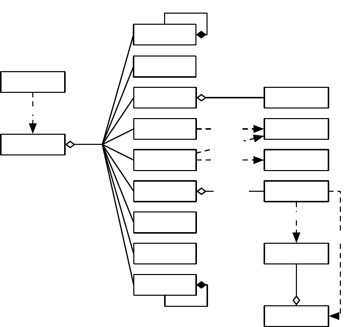
the high-level “verbs” in the ECJ system, as shown in Figure 1.2.
Parameterized Construction
ECJ is unusually heavily parameterized: practically every feature of the
system is determined at runtime from a parameter. Parameters define the classes of objects, the specific
subobjects they hold, and all of their initial runtime values. ECJ does this through a bootstrap class called
Evolve, which loads a ParameterDatabase from runtime parameter files at startup. Using this database, Evolve
constructs the top-level EvolutionState and tells it to “setup” itself. EvolutionState in turn calls subsidiary
classes (such as Evaluator) and tells them to “setup” themselves from the database. This procedure continues
down the chain until the entire system is constructed.
State Objects
In addition to “verbs”, EvolutionState also holds “nouns” — the state objects representing
the things being evolved. Specifically, EvolutionState holds exactly one Population, which contains some
N
(typically 1) Subpopulations. Multiple Subpopulations permit experiments in coevolution, internal island
models, etc. Each Subpopulation holds some number of Individuals and the Species to which the Individuals
belong. Species is a flyweight object for Individual: it provides a central repository for things common to many
Individuals so they don’t have to each contain them in their own instances.
While running, numerous state objects must be created, destroyed, and recreated. As ECJ only learns the
specific classes of these objects from the user-defined parameter file at runtime, it cannot simply construct
them using Java’s new operator. Instead such objects are created by constructing a prototype object at startup
time, and then using this object to stamp out copies of itself as often as necessary. For example, Species
contains a prototypical Individual. When new Individuals must be created for a given Subpopulation, they are
copied from the Subpopulation’s Species and then customized. This allows different Subpopulations to use
different Individual representations.
In keeping with its philosophy of orthogonality, ECJ defines Fitnesses separate from Individuals (represen-
tations), and provides both single-objective and multi-objective Fitness subclasses. In addition to holding a
prototypical Individual, Species also hold the prototypical Fitness to be used with that kid of Individual.
9
EvolutionState
Initializer
Breeder
Evaluator
Finisher
Statistics
Exchanger
Problem
Mersenne Twister
RNG
Output
Parameter
Database
11
11
makes Population
Breeding Pipelineapplies
Evolve
makes
updates
Fitness
updates
Individual
evaluates
1
n
1
1
0..n
1
prototype
Log
n1
0..n
1
Figure 1.2 Top-Level operators and utility facilities in EvolutionState, and their relationship to certain state objects.
Breeding
ASpecies holds a prototypical breeding pipeline which is cloned by the Breeder and used per-thread
to breed individuals and form the next-generation population. Breeding pipelines are tree structures where
a node in the tree filters incoming Individuals from its child nodes and hands them to its parents. The leaf
nodes in the tree are SelectionMethods which simply choose Individuals from the old subpopulation and
hand them off. There exist SelectionMethods which perform tournament selection, fitness proportional
selection, truncation selection, etc. Nonleaf nodes in the tree are BreedingPipelines, many of which copy and
modify their received Individuals before handing them to their parent nodes. Some BreedingPipelines are
representation-independent: for example, MultiBreedingPipeline asks for Individuals from one of its children at
random according to some probability distribution. But most BreedingPipelines act to mutate or cross over
Individuals in a representation-dependent way. For example, the GP CrossoverPipeline asks for one Individual
of each of its two children, which must be genetic programming Individuals, performs subtree crossover on
those Individuals, then hands them to its parent.
A tree-structured breeding pipeline allows for a rich assortment of experimenter-defined selection and
breeding proceses. Further, ECJ’s pipeline is copy-forward:BreedingPipelines must ensure that they copy
Individuals before modifying them or handing them forward, if they have not been already copied. This
guarantees that new Individuals are copies of old ones in the population, and furthermore that multiple
pipelines may operate on the same Subpopulation in different threads without the need for locking. ECJ may
apply multiple threads to parallelize the breeding process without the use of Java synchronization at all.
10
EvolutionState
Population
Subpopulation
Individual
1
1
1..n
1
1..n
1
Species
Fitness
1
1
prototype
1
1
prototype
1 1
Breeding Pipeline
prototype
1
1
flyweight
1..n 1
Selection Method
child of
0..n
1
child of
0..n
1
uses
uses
1
1
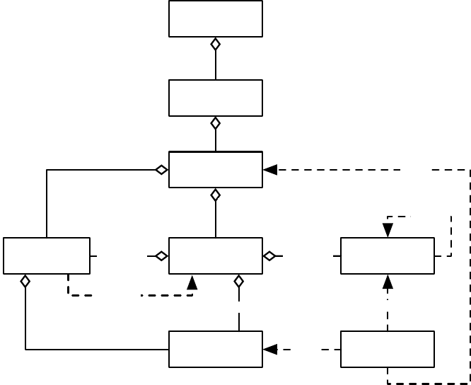
Figure 1.3 Top-Level data objects used in evolution.
Evaluation
The Evaluator performs evaluation of a population by passing one or (for coevolutionary
evaluation) several Individuals to a Problem subclass which the Evaluator has cloned off of its prototype.
Evaluation may too be done in multithreaded fashion with no locking, using one Problem per thread.
Individuals may also undergo repeated evaluation in coevolutionary Evaluators of different sorts.
In most projects using ECJ, the primary task is to construct an appropriate Problem subclass. The task
of the Problem is to assess the fitness of the Individual(s) and set its Fitness accordingly. Problem classes also
report if the ideal Individual has been discovered.
Utilities
In addition to its ParameterDatabase, ECJ also uses a checkpointable Output convenience facility
which maintains various streams, repairing them after checkpoint. Output also provides for message logging,
retaining in memory all messages during the run, so that on checkpoint recovery the messages are printed
out again as before. Other utilities include population distribution selectors, searching and sorting tools, etc.
The quality of a random number generator is important for a stochastic optimization system. As such,
ECJ’s random number generator was the very first class written in the system: it is a Java implementation
of the highly respected Mersenne Twister algorithm [
12
] and is the fastest such implementation available.
Since ECJ’s release, the ECJ MersenneTwister and MersenneTwisterFast classes have found their way in a
number of unrelated public-domain systems, including the popular NetLogo multiagent simulator [
26
].
MersenneTwisterFast is also shared in ECJ’s sister software, the MASON multiagent simulation toolkit [8].
Representations and Genetic Programming
ECJ allows you to specify any genome representation you
like. Standard representation packages in ECJ provide functionality for vectors of all Java data types;
arbitrary-length lists; trees; and collections of objects (such as rulesets).
ECJ is perhaps best known for its support of “Koza”-style tree-structured genetic programming repre-
sentations. ECJ represents these individuals as forests of parse-trees, each tree equivalent to a single Lisp
11
ir
2.3
*
if
and
on-
wall tick>
20 3
bool
bool
bool
bool
bool
bool
int
int
int
int
int, float
float
6
int, float
int
int, float
float
int, float
float
tree
int, float
float
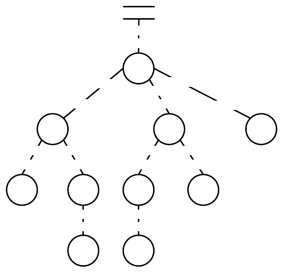
Figure 1.4 A typed genetic programming parse tree.
s-expression. Figure 1.4 shows a parse-tree for a simple robot program, equivalent to the Lisp s-expression
(if (and on-wall (tick>20) (∗(ir 3) 6) 2.3).
In C this might look like
(onWall && tick >20) ? ir(3) * 6 : 2.3.
This notionally says “If I’m on the wall and my tick-count is greater than 20, then return the value of my
third infrared sensor times six, else return 2.3”. Such parse-trees are typically evaluated by executing their
programs in a test environment, and modified via subtree crossover (swapping subtrees among individuals)
or various kinds of mutation (replacing a subtree with a randomly-generated one, perhaps).
ECJ allows multiple subtrees for various experimental needs: Automatically Defined Functions (ADFs —
a mechanism for evolving subroutine calls [
4
]), or parallel program execution, or evolving teams of programs.
Along with ADFs, ECJ provides built-in support for Automatically Defined Macros (ADMs) [
20
] and
Ephemeral Random Constants (ERCs [3], such as the numbers 20, 3, 6, and 2.3 in Figure 1.4).
Genetic programming trees are constructed out of a “primorial soup” of function templates (such as
on-wall or 2.3. Early forms of genetic programming were typeless: though such templates had a predefined
arity (number of arguments), any node could be connected to any other. Many genetic programming needs
require more constraints than this. For example, the node if might expect a boolean value in its first argument,
and integers or floats in the second and third arguments, and return a float when evaluated. Similarly and
might take two booleans as arguments and return a boolean, while
∗
would take ints or floats as arguments
and return a float.
Such types are often associated with the kinds of data passed from node to node, but they do not have
to be. Typing might be used to constrain certain nodes to be evaluated in groups or in a certain order: for
example, a function type-block might insist that its first argument be of type foo and its second argument be
of type ar to make certain that a foo node be executed before a ar node.
ECJ permits a simple static typing mechanism called set-based typing, which is suitable for many such
tasks. In set-based typing, the return type and argument types of each node are each defined to be sets of
type symbols (for example,
{ool}
or
{
foo, bar, baz
}
, or
{
int, float
}
. The desired return type for the tree’s root is
12

similarly defined. A child node is permitted to fit into the argument slot of a parent node if the child node’s
return type and type of the that argument slot in the parent are compatible. We define types to be compatible
if their set intersection is nonempty (that is, they share at least one type symbol).
Set-based typing is sufficient for the typing requirements found in many programming languages,
including ones with type hierarchies. It allows, among other things, for nodes such as
∗
to accept either
integers or floats. However there are considerable restrictions on the power of set-based typing. It’s often
useful for the return type of a node to change based on the particular nodes which have plugged into it as
arguments. For example,
∗
might be defined as returning a float if at least one of its arguments returns floats,
but returning an integer if both of its arguments return integers. if might be similarly defined not to return a
particular type, but to simply require that its return type and the second and third argument types must all
match. Such “polymorphic” typing is particularly useful in situations such as matrix multiplication, where
the operator must place constraints on the width and height of its arguments and the final returned matrix.
In this example, it’s also useful to have an infinite number of types (perhaps to represent matrices of varying
widths or heights).
ECJ does not support polymorphic typing out of the box simply because it is difficult to implement
many if not most common tree modification and generation algorithms using polymorphic typing: instead,
set-based typing is offered to handle as many common needs as can be easily done.
Out of the Box Capabilities ECJ provides support out-of-the-box for a bunch of algorithm options:
•
Generational algorithms:
(µ
,
λ)
and
(µ+λ)
Evolution Strategies, the Genetic Algorithm, Genetic
Programming variants, Grammatical Evolution, PushGP, and Differential Evolution
• Steady-State evolution
• Parsimony pressure algorithms
• Spatially-embeded evolutionary algorithms
• Random restarts
• Multiobjective optimization, including the NSGA-II and SPEA2 algorithms.
• Cooperative, 1-Population Competitive, and 2-Population Competitive coevolution.
• Multithreaded evaluation and breeding.
• Parallel synchronous and asynchronous Island Models spread over a grid of computers.
• Internal synchronous Island Models internally in a single ECJ process.
• Massive parallel generational fitness evaluation of individuals on remote slave machines.
•
Asynchronous Evolution, a version of steady-state evolution with massive parallel fitness evaluation
on remote slave machines.
•
Opportunistic Evolution, where remote slave machines run their own mini-evolutionary processes for
a while before sending individuals back to the master process.
• Internal synchronous Island Models internally in a single ECJ process.
• Meta-Evolution
• A large number of selection and breeding operators
ECJ also has a GUI, though in truth I nearly universally use the command-line.
Idiosyncracies
ECJ was developed near the introduction of Java and so has a lot of historical idiosyncra-
cies.
1
Some of them exist to this day because of conservatism: refactoring is disruptive. If you code with ECJ,
1It used to have a lot more — I’ve been weeding out ones that I think are unnecessary nowadays!
13
you’ll definitely have to get used to one or more of the following:
•
No generics at all, few iterators or enumerators, no Java features beyond 1.4 (including annotations),
and little use of the Java Collections library. This is part historical, and part my own dislike of Java’s
byzantine generics implementation, but it’s mostly efficiency. Generics are very slow when used with
basic data types, as they require boxing and unboxing. The Java Collections library is unusually badly
written in many places internally: and anyway, for speed we tend to work directly with arrays.
•
Hand-rolled socket code. With one exception (optional compression), ECJ’s parallel facility doesn’t
rely on other libraries.
•
ECJ loads nearly every object from its parameter database. This means that you’ll rarely see the new
keyword in ECJ, nor any constructors. Instead ECJ’s usual “constructor” method is a method called
setup(...), which sets up an object from the database.
•
A proprietary logging facility. ECJ was developed before the existence of java.util.logging. Partly out of
conservatism, I am hesitant to rip up all the pervasive logging just to use Sun’s implementation (which
isn’t very good anyway).
•
A parameter database derived from Java’s old java.util.Properties list rather than XML. This is historical
of course. But seriously, do I need a justification to avoid XML?
•
Mersenne Twister random number generator. java.lang.Random is grotesquely bad, and systems which
use it should be shunned.
• A Makefile. ECJ was developed before Ant and I’ve personally never needed it.
1.3 Unpacking ECJ and Using the Tutorials
ECJ is designed to be built either with
maven
or with
make
. If you build ECJ with maven, then it will
package all of ECJ into a single
jar file
. If you build with
make
, you have the option of packaging into a
single
jar file
or into a
directory of class files and resources
. Building to a directory is how ECJ classically
was constructed, but nowadays a jar file is more useful. However even if you build to a jar file, it’s still useful
to have the resources and java files on-hand so you know what various ECJ applications can do and how to
run them.
After unpacking ECJ, you’re left with one directory called ecj where you will find several items:
• A top-level README.md file, which should be self-explanatory in its importance.
• ECJ’s LICENSE file, which describes the primary license (AFL 3.0, a BSD-style academic license).
• A CHANGES log, which lists all past changes to all versions (including the latest).
• A Makefile for building via make.
• A pom.xml for building via Maven.
• The docs directory. This contains most of the ECJ documentation.
•
The start directory. This contains various scripts for starting up ECJ: though in truth we rarely use
them.
•
The lib directory. This contains any additional libraries that maven (not make) will need to build ECJ
(to build with make, you’ll use a different mechanism).
•
The classes directory. This contains the class files, and possibly other resources (see next bullet), for ECJ
after it has been built.
14
•
The src directory, which contains the main Java code and the internal library test code. Of particular
interest to you will be the directories
src/main/java/ec/
, which is the top-level package for ECJ, and
src/main/java/resources/ec/. The src/main/java/ec/ directory holds the top-level package for ECJ,
ec. The src/main/java/resources/ec directory is an identical-structured directory containing various
resources (notably parameter files). If you build with
make
, then these resources will get merged into
the classes directory.
1.3.1 The ec Directory, the CLASSPATH, and jar files
The ec (ecj/src/main/java/ec/) directory is ECJ’s top-level package. Every subdirectory is a subpackage,
and most of them are headed by helpful README files which describe the contents of the directory. Most
packages contain not only Java files and class files but also parameter files and occasional data files: ECJ
was designed originally for the class files to be compiled and stored right alongside the Java files in these
directories, though it can be used with the separate-build-area approach taken by IDEs like Eclipse.
Because ec is the top-level package, you can compile ECJ, more or less, by just sticking its parent directory
(the ecj directory), in your CLASSPATH. You will also need to add certain
jar files
in order to compile ECJ’s
distributed evaluation and island model facilities, and its GUI. You can get these jar files from the ECJ
main website (http://cs.gmu.edu/
∼
eclab/projects/ecj/). Note that none of these libraries is required. For
example, if the libraries for the distributed evaluator and island model are missing, ECJ will compile but will
complain if you try to run those packages with compression turned on (a feature of the packages). The GUI
library is optional to ECJ, so if you don’t install its libraries, you can still compile ECJ by just deleting the
ec/display directory.
1.3.1.1 The ec/display Directory: ECJ’s GUI
This directory contains ECJ’s GUI. It’s in a state of disrepair and I suggest you do not use it. ECJ is really best
as a command line program. In fact, as mentioned above, you can simply delete the directory and ECJ will
compile just fine.
1.3.1.2 The ec/app Directory: Demo Applications
This directory contains all the demo applications. We have quite a number of demo applications, many
sharing the same subdirectories. Read the provided README file for some guidance.
1.3.2 The docs Directory
This directory contains all top-level documentation of ECJ except for the various README files scattered
throughout the package. The index.html file provides the top-level entry point to the documentation.
The documentation includes:
• Introduction to parameters in ECJ
• Class documentation
•
ECJ’s four tutorials and post-tutorial discussion. The actual tutorial code is located in the ec/app
directory.
• An (old) overview of ECJ
• An (old) discussion of ECJ’s warts
• Some (old) graph diagrams of ECJ’s structure
• This manual
15
1.3.2.1 Tutorials
ECJ has four tutorials which introduce you to the basics of coding on the system.
I strongly suggest you go
through them before continuing through the rest of this manual. They are roughly:
1. A simple GA to solve the MaxOnes problem with a boolean representation.
2. A GA to solve an integer problem, with a custom mutation pipeline.
3.
An evolution strategy to solve a floating-point problem, with a custom statistics object and reading
and writing populations.
4. A genetic programming problem, plus some elitism.
As should be obvious from the rest of this manual, this
barely scratches the surface
of ECJ. No mention
is given of parallelism, differential evolution, coevolution, multiobjective optimization, list and ruleset
representations, grammatical encoding, spatial embedding, etc. But it’ll get you up to speed.
16
Chapter 2
ec.Evolve and Utility Classes
ECJ is big. Let us begin.
ECJ’s entry point is the class ec.Evolve. This class is little more than bootstrapping code to set up the ECJ
system, construct basic datatypes, and get things going.
To run an ECJ process, you fire up ec.Evolve with certain runtime arguments.
java ec.Evolve -file myParameterFile.params -p param=value -p param=value (etc.)
ECJ sets itself up entirely using a
parameter file
. To this you can add additional
command-line parame-
ters
which override those found in the parameter file. More on the parameter file will be discussed starting
in Section 2.1.
For example, if you were presently in the ecj directory, you could do this:
java ec.Evolve -file ec/app/ecsuite/ecsuite.params
This all assumes that the parameter file is a free-standing file in your filesystem. But it might not be:
you might want to start up from a parameter file stored within a Jar file (for example if your ECJ library is
bundled up into a Jar file like ecj.jar). To do this you can specify the parameter file as a file resource relative
to the .class file of a class (a-la Java’s Class.getResource(...) method):
java ec.Evolve -from myParameterFile.params -at relative.to.Classname -p param=value
(etc.)
... for example:
java ec.Evolve -from ecsuite.params -at ec.app.ecsuite.ECSuite
You can also say:
java ec.Evolve -from myParameterFile.params -p param=value (etc.)
In which case ECJ will assume that the class is ec.Evolve. In this situation, you’d probably need to specify
the parameter file as a path away from ec.Evolve (which is in the ec directory), for example:
java ec.Evolve -from app/ecsuite/ecsuite.params
(Note the missing ec/...). See Section 2.1 for more discussion about all this.
17
ECJ can also restart from a checkpoint file it created in a previous run:
java ec.Evolve -checkpoint myCheckpointFile.gz
Checkpointing will be discussed in Section 2.3.
Last but not least, if you forget this stuff, you can always type this to get some reminders:
java ec.Evolve -help
The purpose of ec.Evolve is to construct an ec.EvolutionState instance, or load one from a checkpoint file;
then get it running; and finally clean up. The ec.EvolutionState class actually performs the evolutionary
process. Most of the stuff ec.EvolutionState holds is associated with evolutionary algorithms or other
stochastic optimization procedures. However there are certain important utility objects or data which are
created by ec.Evolve prior to creating the ec.EvolutionState, and are then stored into ec.EvolutionState after it
has been constructed. These objects are:
•
The
Parameter Database
, which holds all the parameters ec.EvolutionState uses to build and run the
process.
• The Output, which handles logging and writing to files.
• The Checkpointing Facility to create checkpoint files as the process continues.
• The Number of Threads to use, and the Random Number Generators, one per thread.
• A simple declaration of the Number of Jobs to run in the process.
The remainder Section 2 discusses each of these items. It’s not the most exciting of topics: but it’s
important in order to understand the rest of the ECJ process.
2.1 The Parameter Database
To build and run an experiment in ECJ, you typically write three things:
• (In Java) A problem which evaluates individuals and assigns fitness values to them.
•
(In Java) Depending on the kind of experiment, various
components
from which individuals can be
constructed — for example, for a genetic programming experiment, you’ll need to define the kinds of
nodes which can be used to make up the individual’s tree.
•
(In one or more Parameter Files) Various
parameters
which define the kind of algorithm you are using,
the nature of the experiment, and the makeup of your populations and processes.
Let’s begin with the third item. Parameters are the lifeblood of ECJ: practically everything in the system
is defined by them. This makes ECJ highly flexible; but it also adds complexity to the system.
ECJ loads parameter files and stores them into the ec.util.ParameterDatabase object, which is available
to nearly everything. Parameter files are an extension of the files used by Java’s old
java.util.PropertyList
object. Parameter files usually end in
".params"
, and contain parameters one to a line. Parameter files may
also contain blank (all whitespace) lines, which are ignored, and also lines which start with
"#"
, which are
considered comments and also ignored. An example comment:
# This is a comment
The parameter lines in a parameter file typically look like this:
parameter.name =parameter value
18

A
parameter name
is a string of non-whitespace characters except for
"="
. After this comes some optional
whitespace, then an
"="
, then some more optional whitespace.
1
A
parameter value
is a string of characters,
including whitespace, except that all whitespace is trimmed from the front and end of the string. Notice the
use of a period the parameter name. It’s quite a common convention to use periods in various parameter
names in ECJ. We’ll get to why in a second.
Here are some legal parameter lines:
generations = 400
pop.subpop.0.size =1000
pop.subpop= ec.Subpopulation
Here are some illegal parameter lines:
generations
= 1000
pop subpop = ec.Subpopulation
2.1.1 Inheritance
Parameter files may be set up to
derive from
one or more other parameter files. Let’s say you have two
parameter files, a.params and b.params. Both are located in the same directory. You can set up a.params to
derive from b.params by adding the following line as the very first line in the a.params file:
parent.0 = b.params
This says, in effect: “include in me all the parameters found in the b.params file, but any parameters I
myself declare will override any parameters of the same name in the b.params file.” Note that b.params may
itself derive from some other file (say, c.params). In this case, a.params receives parameters from both (and
parameters in b.params will likewise override ones of the same name in c.params).
Let’s say that b.params is located inside a subdirectory called foo. Then the line will look like this:
parent.0 = foo/b.params
Notice the forward slash: ECJ was designed on UNIX systems. Likewise, imagine if b.params was stored
in a sibling directory called bar: then we might say:
parent.0 = ../bar/b.params
You can also define absolute paths, UNIX-style:
parent.0 = /tmp/myproject/foo.params
Long story short: parameter files are declared using traditional UNIX path syntax.
A parameter file can also derive from multiple parent parameter files, by including each at the beginning
of the file, with consecutive numbers, like this:
parent.0 = b.params
parent.1 = yo/d.params
parent.2 = ../z.params
This says in effect: “first look in a.params for the parameter. If you can’t find it there, look in b.params and,
ultimately, all the files b.params derives from. If you can’t find it in any of them, look in d.params and all the
1Actually, you can omit the "=", but it’s considered bad style.
19
files it derives from. If you can’t find it in any of them, look in z.params and all the files it derives from. If
you’ve still not found the parameter, give up.”
This is essentially a depth-first search through a tree or DAG, with parents overriding their children
(the files they derive from) and earlier siblings overriding later siblings. Note that this multiple inheritance
scheme is not the same as C++ or Lisp/CLOS, which use a distance measure!
Parent parameter files can be explicit files on your file system (as shown above) or they can be files located
in JAR files etc. But how do you refer to a file inside a JAR file? It’s easy: refer to it using a
class relative
path
(see the next Section, 2.1.2), which defines the path relative to the class file of some class. For example,
suppose you’re creating a parameter file whose parent is ec/app/ant/ant.params. But you’re not using ECJ in
its unpacked form, but rather bundled up into a JAR file. Thus ec/app/ant/ant.params is archived in that JAR
file. Since this file is right next to ec/app/ant/Ant.class — the class file for the ec.app.ant.Ant class– you can
refer to it as:
parent.0 = @ec.app.ant.Ant ant.params
If your parameter file is already in a JAR file, and it uses ordinary relative path names to refer to its
parents (like ../z.params), these will be interpreted as other files in the archived file system inside that JAR
file. To escape the JAR file you have to use an absolute path name, such as
parent.0 = /tmp/foo.params
It’s pretty rare to need that though, and hardly good style. The whole point of JAR files is to encapsulate
functionality into one package.
Overriding the Parameter File
When you fire up ECJ, you point it at a single parameter file, and you can
provide additional parameters at the command-line, like this:
java ec.Evolve -file parameterFile.params -p command-line-parameter=value \
-p command-line-parameter=value ...
Furthermore, your program itself can submit parameters to the parameter database, though it’s very
unusual to do so. When a parameter is requested from the parameter database, here’s how it’s looked up:
1. If the parameter was declared by the program itself, this value is returned.
2. Else if the parameter was provided on the command line, this value is returned.
3.
Else the parameter is looked up in the provided parameter file and all derived files using the inheritance
ordering described earlier.
4. Else the database signals failure.
2.1.2 Kinds of Parameters
ECJ supports the following kinds of parameters:
•Numbers. Either long integers or double floating-point values. Examples:
generations = 500
tournament.size = 3.25
minimum-fitness = -23.45e15
•Arbitrary Strings trimmed of whitespace. Example:
crossover-type = two-point
20

•Booleans
. Any value except for
"false"
(case-insensitive) is considered to be true. It’s best style to use
lower-case "true" and "false". The first two of these examples are false and the second two are true:
print-params = false
die-a-painful-death = fAlSe
pop.subpop.0.perform-injections = true
quit-on-run-complete = whatever
•Class Names
. Class names are defined as the full class name of the class, including the package.
Example:
pop.subpop.0.species = ec.gp.GPSpecies
•File or Resource Path Names. Paths can be of four types.
– Absolute paths
, which (in UNIX) begin with a
"/"
, stipulate a precise location in the file system.
– Relative paths
, which do not begin with a
"/"
, are defined relative to the parameter file in which
the parameter was located. If the parameter file was an actual file in the filesystem, the relative
path will also be considered to point to a file. If the parameter file was in a jar file, then the relative
path will be considered to point to a resource inside the same jar file relative to the parameter file
location. You’ve seen relative paths already used for derived parameter files.
– Execution relative paths
are defined relative to the directory in which the ECJ process was
launched. Execution relative paths look exactly like relative paths except that they begin with the
special character "$".
– Class relative paths
define a path relative to the class file of a class. They have two parts: the
class in question, and then the path to the resource relative to it. If the class is stored in a Jar file,
then the path to the resource will also be within that Jar file. Otherwise the path will point to an
actual file. Class relative paths begin with
"@"
, followed by the full class name, then spaces or
tabs, then the relative path.
Examples of all four kinds of paths:
stat.file = $out.stat
eval.prob.map-file = ../dungeon.map
temporary-output-file = /tmp/output.txt
image = @ec.app.myapp.MyClass images/picture.png
If the parameter is for a file meant to be opened
read-only
, any of the four approaches above will
work fine. But if the parameter is for a
writable file
, then you have an issue. As discussed in Section
2.1.4, the parameter in question could refer to a file in your operating system, or it could refer to a file
bundled inside a Java jar file. In this second case, the file cannot be written to.
The only kinds of paths which can refer to things inside jar files are relative paths and class-relative
paths. Thus if you stick with absolute paths or execution-relative paths, you know you’ll be referring
to a writable file. For this reason we recommend:
– Read-only Files
should use class-relative paths or relative paths, and should only be accessed
using getResource(...) (see Section 2.1.5).
– Read-Write Files
should use absolute paths or (in most cases) execution-relative paths, and
should only be accessed using getFile(...) (see Section 2.1.5).
•Arrays. ECJ supports loading arrays of doubles,2but does not have direct support for loading arrays
of other types. However it has a convention you should be made aware of. It’s common for arrays to
2See the various “getDoubles” methods in Section 2.1.5.
21
be loaded by first stipulating the number of elements in the array, then stipulating each array element
in turn, starting with 0. The parameter used for the number of elements differs from case to case. Note
the use of periods prior to each number in the following example:
gp.fs.0.size = 6
gp.fs.0.func.0 = ec.app.ant.func.Left
gp.fs.0.func.1 = ec.app.ant.func.Right
gp.fs.0.func.2 = ec.app.ant.func.Move
gp.fs.0.func.3 = ec.app.ant.func.IfFoodAhead
gp.fs.0.func.4 = ec.app.ant.func.Progn2
gp.fs.0.func.5 = ec.app.ant.func.Progn3
The particulars vary. Here’s another, slightly different, example:
exch.num-islands = 8
exch.island.0.id = SurvivorIsland
exch.island.1.id = GilligansIsland
exch.island.2.id = FantasyIsland
exch.island.3.id = TemptationIsland
exch.island.4.id = RhodeIsland
exch.island.5.id = EllisIsland
exch.island.6.id = ConeyIsland
exch.island.7.id = TreasureIsland
Anyway, you get the idea.
2.1.3 Namespace Hierarchies and Parameter Bases
ECJ has lots of parameters, and by convention organizes them in a namespace hierarchy to maintain some
sense of order. The delimiter for paths in this hierarchy is — you guessed it — the period.
The vast majority of parameters are used by one Java object or another to set itself up immediately after it
has been instantiated for the first time. ECJ has an important convention which uses the namespace hierarchy
to do just this: the
parameter base
. A parameter base is essentially a path (or namespace, what have you) in
which an object expects to find all of its parameters. The prefix for this path is typically the parameter name
by which the object itself was loaded.
For example, let us consider the process of defining the class to be used for the global population. This
class is found in the following parameter:
pop = ec.Population
ECJ looks for this parameter, expects a class (in this case, ec.Population), loads the class, and creates one
instance. It then calls a special method (setup(...), we’ll discuss it later) on this class so it can set itself up
from various parameters. In this case, ec.Population needs to know how many subpopulations it will have.
This is defined by the following parameter:
pop.subpops = 2
ec.Population didn’t know that it was supposed to look in
pop.subpops
for this value. Instead, it only
knew that it needed to look in a parameter called
subpops
. The rest (in this case,
pop
) was provided
to ec.Population as its parameter base: the text to be prepended — plus a period — to all parameters that
ec.Population needed to set itself up. It’s not a coincidence that the parameter base also happened to be the
very parameter which defined ec.Population in the first place. This is by convention.
Armed with the fact that it needs to create an array of two subpopulations, ec.Population is ready to load
the classes for those two subpopulations. Let’s say that for our experiment we want them to be of different
classes. Here they are:
22
pop.subpop.0 = ec.Subpopulation
pop.subpop.1 = ec.app.myapp.MySpecialSubpopulation
The two classes are loaded and one instance is created of each of them. Then setup(...) is called on each of
them. Each subpopulation looks for a parameter called
size
to tell it how may individuals will be in that
subpopulation. Since each of them is provided with a different parameter base, they can have different sizes:
pop.subpop.0.size = 100
pop.subpop.1.size = 512
Likewise, each of these subpopulations needs a “species”. Presuming that the species are different classes,
we might have:
pop.subpop.0.species = ec.vector.VectorSpecies
pop.subpop.1.species = ec.gp.GPSpecies
These species objects themselves need to be set up, and when they do, their parameter bases will be
pop.subpop.0.species and pop.subpop.1.species respectively. And so on.
Now imagine that we have ten subpopulations, all of the same class (ec.Subpopulation), and all but the first
one has the exact same size. We’d wind up having to write silly stuff like this:
pop.subpop.0.size = 1000
pop.subpop.1.size = 500
pop.subpop.2.size = 500
pop.subpop.3.size = 500
pop.subpop.4.size = 500
pop.subpop.5.size = 500
pop.subpop.6.size = 500
pop.subpop.7.size = 500
pop.subpop.8.size = 500
pop.subpop.9.size = 500
That’s a lot of typing. Though I am saddened to report that ECJ’s parameter files do require a lot of typing,
at least the parameter database facility offers an option to save our fingers somewhat in this case. Specifically,
when the ec.Subpopulation class sets itself up each time, it actually looks in not one but two path locations for
the
size
parameter: first it tacks on its current base (as above), and if there’s no parameter at that location,
then it tries tacking on a
default base
defined for its class. In this case, the default base for ec.Subpopulation
is the prefix ec.subpop. Armed with this we could simply write:
ec.subpop.size = 500
pop.subpop.0.size = 1000
When ECJ looks for subpopulation 0’s size, it’ll find it as normal (1000). But when it looks for subpopula-
tion 1 (etc.), it won’t find a size parameter in the normal location, so it’ll look in the default location, and use
what it finds there (500). Only if there’s no parameter to be found in either location will ECJ signal an error.
It’s important to note that if a class is loaded from a default parameter, this doesn’t mean that the default
parameter will become its parameter base: rather, the original expected location will continue to be the base.
For example, imagine if both of our Species objects were the same class, and we had defined them using the
default base. That is, instead of
pop.subpop.0.species = ec.vector.VectorSpecies
pop.subpop.1.species = ec.vector.VectorSpecies
...we simply said
23
ec.subpop.species = ec.vector.VectorSpecies
When the species for subpopulation 0 is loaded, its parameter base is not going to be
ec.subpop.species
.
Instead, it will still be
pop.subpop.0.species
. Likewise, the parameter base for the species of subpopulation
1 will still be pop.subpop.1.species.
Keep in mind that all of this is just a convention. You can use periods for whatever you like ultimately.
And there exist a few global parameters without any base at all. For example, the number of generations is
defined as
generations = 200
...and the seed for the random number generator the fourth thread is
seed.3 = 12303421
...even though there is no object set up with the
seed
parameter, and hence no object has
seed
as its parameter
base. Random number generators are one of the few rare objects in ECJ which are not specified from the
parameter file.
2.1.4 Parameter Files in Jar Files
Parameter files don’t have to be just in your file system: they can be bundled up in jar files. If a parameter
file is being read from a jar file, its parents will be generally assumed to be from the same jar file as well if
they’re relative paths (they don’t start with "’/’" in UNIX).
So how do you point to a parameter file in a jar file to get things rolling? You can run ECJ like this:
java ec.Evolve -from parameterFile.params -at relative.class.Name ...
This instructs ECJ to look for the .class file of the class relative.class.Name, be it in the file system or in a Jar
file. Once ECJ has found it, it looks for the path parameterFile.params relative to this file. You can omit the
classname, which causes ECJ to assume that the class in question is ec.Evolve. For example, to run the Ant
demo from ECJ (in a Jar file or unpacked into the file system), you could say:
java ec.Evolve -from app/ant/ant.params
Notice it does not say ec/app/ant/ant.params, which is probably what you’d expect if you used
"-file"
rather than
"-from"
. This is because ECJ goes to the ec/Evolve.class file, then from there it searches for the
parameter file. The path of the parameter file relative to the ec/Evolve.class file is app/ant/ant.params.
There are similar rules regarding file references (such as parent references) within a parameter file. Let’s
say that your parameter file is inside a jar file. If you say something like:
parent.0 = ../path/to/the/parent.params
... then ECJ will look around inside the same Jar file for this file, rather than externally in the operating
system’s file system or in some other Jar file.
You can escape this however. For example, once your parameter file is inside a Jar file, you can still define
a parent in another Jar file, or in the file system, if you know a another class file it’s located relative to. You
just need to specify another class for ECJ to start at, and a path relative to it, like this:
parent.0 = @ec.foo.AnotherClass relative/path/to/the/parent.params
See the next section for more explanation of that text format.
Last but not least, once your parameter file is in a Jar file, you can refer to a parent in the file system if
you use an absolute path (that is, one which (in UNIX anyway) starts with "’/’"). For example:
24

parent.0 = /Users/sean/myexperiment/other.params
Absolute path names aren’t very portable and aren’t recommended.
2.1.5 Accessing Parameters
Parameters are looked up in the ec.util.ParameterDatabase class, and parameter names are specified using
the ec.Parameter class. The latter is little more than a cover for Java strings. To create the parameter
pop.subpop.0.size, we say:
Parameter param = new Parameter("pop.subpop.0.size");
Of course, usually we don’t want to just make a direct parameter, but rather want to construct one from a
parameter base and the remainder. Let’s say our base (
pop.subpop.0
) is stored in the variable base, and we
want to look for size. We do this as:
Parameter param = base.push("size");
Here are some common ec.util.ParameterDatabase methods. Note that all of them look in two places to
find a parameter value. This is what we use to handle “standard” and “default” bases. Typically you’d pass
in the parameter in its standard location, and also (in the “default parameter”) parameter with its default
base configuration. You can pass in null for either, and it’ll get ignored.
ec.util.ParameterDatabase Methods
public boolean exists(Parameter parameter, Parameter default)
If either parameter exists in the database, return true. Either parameter may be null.
public String getString(Parameter parameter, Parameter default)
Look first in parameter, then failing that, in default parameter, and return the result as a String, else null if not found.
Either parameter may be null.
public File getFile(Parameter parameter, Parameter default)
Look first in parameter, then failing that, in default parameter, and return the result as a File, else null if not found.
Either parameter may be null.
Important Note.
You should generally only use this method if you are writing to a
file. Otherwise it’s best if you used getResource(...).
public InputStream getResource(Parameter parameter, Parameter default)
Look first in parameter, then failing that, in default parameter, and open an InputStream to the result, else null if not
found. Either parameter may be null.
Important Note.
This is distinguished from getFile(...) in that the object
doesn’t have to be a file in the file system: it can for example be a location in a jar file. If the parameter specifies an
absolute path or an execution relative path, then a file in the file system will be opened. If the parameter specifies
a relative path, and the parameter database was itself loaded as a file rather than a resource (in a jar file say), then
a file will be opened, else a resource will be opened in the same jar file as the parameter file. You can also specify a
resource path directly.
public Object getInstanceForParameterEq(Parameter parameter, Parameter default, Class superclass)
Look first in parameter, then failing that, in default parameter, to find a class. The class must have superclass as a
superclass, or can be the superclass itself. Instantiate one instance of the class using the default (no-argument)
constructor, and return the instance. Throws an ec.util.ParamClassLoadException if no class is found.
public Object getInstanceForParameter(Parameter parameter, Parameter default, Class superclass)
Look first in parameter, then failing that, in default parameter, to find a class. The class must have superclass as a
superclass, but may not be superclass itself. Instantiate one instance of the class using the default (no-argument)
constructor, and return the instance. Throws an ec.util.ParamClassLoadException if no class is found.
25
public int getBoolean(Parameter parameter, Parameter default, double defaultValue)
Look first in parameter, then failing that, in default parameter, and return the result as a boolean, else defaultValue if
not found or not a boolean. Either parameter may be null.
public int getIntWithDefault(Parameter parameter, Parameter default, int defaultValue)
Look first in parameter, then failing that, in default parameter, and return the result as an int, else defaultValue if not
found or not an int. Either parameter may be null.
public int getInt(Parameter parameter, Parameter default, int minValue)
Look first in parameter, then failing that, in default parameter, and return the result as an int, else minValue
−
1 if not
found, not an int, or <minValue. Either parameter may be null.
public int getIntWithMax(Parameter parameter, Parameter default, int minValue, int maxValue)
Look first in parameter, then failing that, in default parameter, and return the result as an int, else minValue
−
1 if not
found, not an int, <minValue, or >maxValue. Either parameter may be null.
public long getLongWithDefault(Parameter parameter, Parameter default, long defaultValue)
Look first in parameter, then failing that, in default parameter, and return the result as a long, else defaultValue if not
found or not a long. Either parameter may be null.
public long getLong(Parameter parameter, Parameter default, long minValue)
Look first in parameter, then failing that, in default parameter, and return the result as a long, else minValue
−
1 if not
found, not a long, or <minValue. Either parameter may be null.
public long getLongWithMax(Parameter parameter, Parameter default, long minValue, long maxValue)
Look first in parameter, then failing that, in default parameter, and return the result as a long, else minValue
−
1 if not
found, not a long, <minValue, or >maxValue. Either parameter may be null.
public float getFloatWithDefault(Parameter parameter, Parameter default, float defaultValue)
Look first in parameter, then failing that, in default parameter, and return the result as a float, else defaultValue if not
found or not a float. Either parameter may be null.
public float getFloat(Parameter parameter, Parameter default, float minValue)
Look first in parameter, then failing that, in default parameter, and return the result as a float, else minValue
−
1 if not
found, not a float, or <minValue. Either parameter may be null.
public float getFloatWithMax(Parameter parameter, Parameter default, float minValue, float maxValue)
Look first in parameter, then failing that, in default parameter, and return the result as a float, else minValue
−
1 if not
found, not a float, <minValue, or >maxValue. Either parameter may be null.
public double getDoubleWithDefault(Parameter parameter, Parameter default, double defaultValue)
Look first in parameter, then failing that, in default parameter, and return the result as a double, else defaultValue if
not found or not a double. Either parameter may be null.
public double getDouble(Parameter parameter, Parameter default, double minValue)
Look first in parameter, then failing that, in default parameter, and return the result as a double, else minValue
−
1 if
not found, not a double, or <minValue. Either parameter may be null.
public double getDoubleWithMax(Parameter parameter, Parameter default, double minValue, double maxValue)
Look first in parameter, then failing that, in default parameter, and return the result as a double, else minValue
−
1 if
not found, not a double, <minValue, or >maxValue. Either parameter may be null.
public double getDoubles(Parameter parameter, Parameter default, double minValue)
Look first in parameter, then failing that, in default parameter, for a space- or tab-delimited list of double values, and
return the result as an array of doubles, else null if they are improperly formatted or if any of them is
<
minValue,
or if the list is zero in length, or if it has garbage at the end of it. Either parameter may be null.
public double getDoubles(Parameter parameter, Parameter default, double minValue, int expectedLength)
Look first in parameter, then failing that, in default parameter, for a space- or tab-delimited list of double values, and
return the result as an array of doubles, else null if they are improperly formatted or if any of them is
<
minValue,
or if the list is not expectedLength (>0)long, or if it has garbage at the end of it. Either parameter may be null.
26

public double getDoublesWithMax(Parameter parameter, Parameter default, double minValue, double maxValue)
Look first in parameter, then failing that, in default parameter, for a space- or tab-delimited list of double values, and
return the result as an array of doubles, else null if they are improperly formatted or if any of them is
<
minValue,
or >maxValue, or if the list is zero in length, or if it has garbage at the end of it. Either parameter may be null.
public double getDoublesWithMax(Parameter parameter, Parameter default, double minValue, double maxValue,
int expectedLength)
Look first in parameter, then failing that, in default parameter, for a space- or tab-delimited list of double values, and
return the result as an array of doubles, else null if they are improperly formatted or if any of them is
<
minValue,
or
>
maxValue, or if the list is not expectedLength
(>
0
)
long, or if it has garbage at the end of it. Either parameter
may be null.
public double getDoublesUnconstrained(Parameter parameter, Parameter default)
Look first in parameter, then failing that, in default parameter, for a space- or tab-delimited list of double values, and
return the result as an array of doubles, else null if they are improperly formatted, or if the list is zero in length, or
if it has garbage at the end of it. Either parameter may be null.
public double getDoublesUnconstrained(Parameter parameter, Parameter default, int expectedLength)
Look first in parameter, then failing that, in default parameter, for a space- or tab-delimited list of double values,
and return the result as an array of doubles, else null if they are improperly formatted, or if the list is not
expectedLength (>0)long, or if it has garbage at the end of it. Either parameter may be null.
2.1.6 Parameter Macros
The get() method can also handle special macro parameters. Macro parameter names will end in
alias
, which
means you cannot have any parameter names which end with this word. The idea behind a macro parameter
is that it can substitute one substring for another among your parameter names, making your parameters
potentially much simpler. Macros work along period boundaries.
2.1.6.1 The Alias Macro
The alias parameter macro works as follows. Let’s say that you have:
hello.there.alias = foo
This means to replace
hello.there
with
foo
and continue looking up the parameter. For example, when
When query for the parameter
hello.there.mom.how.are.you
it is converted to the parameter
foo.mom.how.are.you
which is then looked up in the database. Furthermore
hello.there.partner
is converted to the parameter
foo.partner
and
hello.there
27
is converted to just the parameter
foo
Which are then looked up in the database. Conflicting rules are handled in order of specificity. For example,
if you had
hello.there.alias = foo
hello.there.mom.alias = bar
hello.there.mom.how.are.you = whoa
hello.there.brother = hey
Now let’s say we queried
hello.there.dad
This would get converted to
foo.dad
which would then get looked up. But if we queried
hello.there.mom.42
Then our second rule would take precedence, because it’s more specific, and instead of converting to
foo.mom.42 we would instead convert to
bar.42
which would then get looked up. Finally, if we queried
hello.there.mom.how.are.you
Then this would take precedence and the system would immediately return
whoa
. Furthermore, if we
queried
hello.there.brother
This would immediately return hey, because exact parameters take precedence over macros.
Additionally note that the substitution is delimited by the periods. So querying
hello.therewhoa
will not get translated. And furthermore the substitution must start at the start of the parameter name, so
querying
my.hello.there.mom
will also not get translated.
Beware of cycles! For example, if you have
a.b.alias = foo
foo.alias = a.b
... and you query
a.b.yo
28
... you should get an error reported and null returned.
2.1.7 Debugging Your Parameters
Your ECJ experiment is loading and running, but how do you know you didn’t make a mistake in your
parameters? How do you know ECJ is using the parameters you stated rather than some default values? If
you include the following parameter in your collection:
print-params = true
...then ECJ will print out all the parameters which were used or tested for existence. For example, you might
get things like this printed out:
!P: pop.subpop.0.file
P: pop.subpop.0.species = ec.gp.GPSpecies
<P: ec.subpop.species
P: pop.subpop.0.species.pipe = ec.breed.MultiBreedingPipeline
<P: gp.species.pipe
!E: pop.subpop.0.species.pipe.prob
P: pop.subpop.0.species.pipe.num-sources = 2
<P: breed.multibreed.num-sources
P: pop.subpop.0.species.pipe.source.0 = ec.gp.koza.CrossoverPipeline
<P: breed.multibreed.source.0
E: pop.subpop.0.species.pipe.source.0.prob = 0.9
<E: gp.koza.xover.prob
A
P
means that a parameter value was accessed (or attempted to). An
E
means that a parameter was
tested for existence. An
!
means that the parameter did not exist. A
<
means that the parameter existed in
the default base as well as the primary base, but the value of the primary base was the one used. In this last
case, the primary base is printed out on the line immediately prior.
There are a few other debugging parameters of less value. At the end of a run, ECJ can dump all the
parameters in the database; all the parameters accessed (retrieved or tested for existence); all the parameters
used (retrieved); all the parameters not accessed; and all the parameters not used. Pick your poison. Here are
the relevant parameters:
print-all-params = true
print-accessed-params = true
print-used-params = true
print-unaccessed-params = true
print-unused-params = true
Typically you’d only want to set one of these to true. The most useful one is
print-unaccessed-params
,
since by examining the results you can see if a parameter you set was used or not: if not, probably because it
wasn’t typed right. It also tells you about old, disused parameters. In fact, as I was writing this manual and
needed
print-unaccessed-params
examples, I ran the Lawnmower problem (in ec/app/lawnmower) and
got the following:
29

Unaccessed Parameters
===================== (Ignore parent.x references)
gp.fs.2.info = ec.gp.GPFuncInfo
gp.koza.grow.min-depth = 5
gp.tc.0.init.max = 6
gp.koza.mutate.build.0 = ec.gp.koza.GrowBuilder
gp.tc.1.init.max = 6
parent.0 = ../../gp/koza/koza.params
gp.koza.grow.max-depth = 5
gp.tc.2.init.max = 6
gp.koza.mutate.ns.0 = ec.gp.koza.KozaNodeSelector
gp.fs.0.info = ec.gp.GPFuncInfo
gp.koza.half.growp = 0.5
gp.tc.0.init.min = 2
gp.koza.mutate.source.0 = ec.select.TournamentSelection
gp.koza.mutate.tries = 1
gp.tc.1.init.min = 2
gp.fs.1.info = ec.gp.GPFuncInfo
gp.tc.2.init.min = 2
gp.koza.mutate.maxdepth = 17
Most of these unaccessed parameters are perfectly fine; standard boilerplate stuff for genetic pro-
gramming that didn’t happen to be used by this application. But then there’s the first parameter:
gp.fs.2.info = ec.gp.GPFuncInfo
, and two others like it later. I had deleted the GPFuncInfo class from
the ECJ distribution well over a year ago. But apparently I forgot to remove a vestigial parameter which
referred to it. Oops!
By the way, note the request to ignore “parent.x references” — this means to ignore the stuff like
parent.0 = ../../gp/koza/koza.params that gets printed out with everything else.
For more on debugging ECJ, see Section 3.8.
2.1.8 Building a Parameter Database from Scratch
This is starting to get inside-baseball, so you may wish to skip it for now. Normally ParameterDatabase is
constructed from the Evolve class on your behalf. But in some unusual situations you may need to build
one yourself. Most notably, if you’re attaching ECJ as a sub-module under some application or toolkit (see
Section 2.7), you may need to make a custom ParameterDatabase with which to run ECJ.
A typical ParameterDatabase is constructed from a file or a resource relative to a class. When this is done,
what you receive is an empty ParameterDatabase which points to another ParameterDatabase, The empty
ParameterDatabase is free for you to modify. For example, if you call...
File file = ...
String[] commandLineArguments = ...
ParameterDatabase db = new ParameterDatabase(file, commandLineArguments);
... you will get back an empty ParameterDatabase whose parent is a ParameterDatabase holding the
commands-line arguments, whose parent is a ParameterDatabase constructed from the file. That final
ParameterDatabase may have further parents as specified in the file itself.
Other ParameterDatabase constructors, particularly ones which do not concern themselves with specific
files, will not have this feature.
The particular chain, if there is one at all, varies depending on the constructor you call. The one in the
example above is the most common constructor.
ec.util.ParameterDatabase Constructor Methods
30

public ParameterDatabase()
Creates a simple empty parameter database with no parents. The database hierarchy is simply: empty
public ParameterDatabase(Dictionary map)
Creates a parameter database with the given Dictionary. Both the keys and values will be run through toString()
before adding to the database. Keys are parameters. Values are the values of the parameters. If parents are defined
in the map’s parameters, they will be attempted to be loaded: only parents which are absolute path names are
permitted. Beware that a ParameterDatabase is itself a Dictionary; but if you pass one in here you will only get the
lowest-level elements. The database hierarchy is :
map → · · ·
Note that unlike other methods, this method
does not create an empty base parameter database. If you want a hierarchy like
empty →map → · · ·
you can
achieve this with new ParameterDatabase().addParent(new ParameterDatabase(myMap))
public ParameterDatabase(InputStream stream)
Creates a parameter database by reading parameters from the provided stream. If parents are defined among
the parameters, they will be attempted to be loaded: only parents which are absolute path names are permitted.
Beware that a ParameterDatabase is itself a Dictionary; but if you pass one in here you will only get the lowest-level
elements. The database hierarchy is :
stream → · · ·
Note that unlike other methods, this method does not create
an empty base parameter database. If you want a hierarchy like
empty →stream → · · ·
you can achieve this
with new ParameterDatabase().addParent(new ParameterDatabase(myStream))
public ParameterDatabase(File file)
Creates a new parameter database from the given file (and possibly parent files). The database hierarchy is:
empty →file → · · ·
public ParameterDatabase(File file, String[] args)
Creates a new parameter database from the given file (and possibly parent files). The database hierarchy is:
empty →args →file → · · ·
public ParameterDatabase(String pathNameRelativeToClassFile, Class cls)
Creates a new parameter database from the given file (and possibly parent files). The file is located a path
name relative to object (.class) file of the provided class. For example, if the class were Foo, and its object file
was located at /a/b/Foo.class, and the path name relative to the class file was ../c/bar.params, then the file
would be expected to be located at /a/c/bar.params. This also works inside jar files. The database hierarchy is:
empty →pathNameRelativeToClassFile → · · ·
public ParameterDatabase(String pathNameRelativeToClassFile, Class cls, String[] args)
Creates a new parameter database from the given file (and possibly parent files). The file is located a path
name relative to object (.class) file of the provided class. For example, if the class were Foo, and its object file
was located at /a/b/Foo.class, and the path name relative to the class file was ../c/bar.params, then the file
would be expected to be located at /a/c/bar.params. This also works inside jar files. The database hierarchy is:
empty →args →pathNameRelativeToClassFile → · · ·
Once you have created a ParameterDatabase, you can attach parent ParameterDatabases to it. You can
also set values in the ParameterDatabase, and remove values (though you cannot remove values from its
parents without accessing the parents themselves), among other operations.
ec.util.ParameterDatabase Methods
public void addParent(ParameterDatabase database)
Adds a parent database to the parameter database.
31

public void set(Parameter parameter, String value)
Sets a parameter in the immediate parameter database. This overrides settings in parents. The value is first
trimmed of whitespace.
public void remove(Parameter parameter)
Removes a parameter from an immediate parameter database (but not from its parents in the hierarchy).
public ParameterDatabase getLocation(Parameter parameter)
Returns the parameter database in the parent hierarchy which defined the currently-used value for the given
parameter.
public String getLabel()
Returns a string describing the location of the ParameterfDatabase (such as the file name from which it was
loaded), or the empty string if there is nothing appropriate.
2.2 Output
ECJ has its own idiosyncratic logging and output facility called ec.util.Output. This is largely historical: ECJ
predates any standard logging facilities available in Java. The facility is in part inspired by a similar facility
that existed in the
lil-gp
C-based genetic programming system. The system has generally worked out well
so we’ve not seen fit to replace it.
The primary reason for the central logging and output facility is to survive checkpointing and restarting
from checkpoints (see Section 2.3). Except for the occasional debugging statement which we’ve forgotten to
remove, all output in ECJ goes through ec.util.Output.
The output facility has four basic features:
•Logs
, attached to Files or to Writers, which output text of all kinds. Logs can be restarted, meaning that
they can be reopened when ECJ is restarted from a checkpoint.
• Two dedicated Logs, the Message Logs, which write text out to stdout and stderr respectively.
• The ability to print arbitrary text to any Log.
•
Short
Announcements
of different kinds. Announcements are different from arbitrary text in that they
are not only written out to Logs (usually the stderr message Log) but are also stored in memory. This
allows them to be checkpointed and automatically reposted after ECJ has started up again from a
checkpoint.
The least important announcements are simple
messages
. One special kind of message is the
system
message
generated by ECJ itself. Next in importance are
warnings
. One special kind of warning, the
once-only-warning
, will be written only once to a Log even if it’s posted multiple times. Next are
basic
errors
. Things can be configured such that after a bunch of errors, ECJ will quit. Finally,
fatal
errors will cause ECJ to quit immediately rather than wait for more errors to accumulate.
2.2.1 Creating and Writing to Logs
There are many methods in ec.util.Output for creating or accessing Logs. Here are some common ones:
ec.util.Output Methods
public int addLog(File file, boolean appendOnRestart)
Add a log on a given file. If ECJ is restarted from a checkpoint, and appendOnRestart is true, then the log will be
appended to the current file contents. Else they will be replaced. The Log is registered with ec.util.Output and its
log number is returned.
32

public int addLog(File file, boolean appendOnRestart, boolean gzip)
Add a log on a given file. If ECJ is restarted from a checkpoint, and appendOnRestart is true, then the log will be
appended to the current file contents. Else they will be replaced. If gzip is true, then the log will be gzipped. You
cannot have both appendOnRestart and gzip true at the same time. The Log is registered with ec.util.Output and its
log number is returned.
public Log getLog(int index)
Returns the log indexed at the given location.
public int numLogs()
Returns the total number of logs.
Two logs are always made for you automatically: a log to
stdout
(log index 0); and another log to
stderr
(log index 1). The stderr log prints all announcements, but the stdout log does not.
Logs have various instance variables, but few are important, except for this one:
public boolean silent = false;
If you set this flag to true, the log will not print anything at all. See section 2.2.2 for more information on
how to do this.
To write arbitrary text to a log, here are the most common methods:
ec.util.Output Methods
public void print(String text, int log number)
Prints a string to a log.
public void println(String text, int log number)
Prints a string to a log, plus a newline.
Besides stdout (0) and stderr (1), there are two other special log numbers you should be aware of:
public int ALL MESSAGE LOGS;
public int NO LOGS;
NO LOGS is a special log value meaning “don’t bother printing this”. It’s sometimes used to turn off
printing to certain logs temporarily. ALL MESSAGE LOGS will cause printing to be sent to all logs for which
message logging is turned on. By default that’s just stderr (1). This is not commonly used. To post a message
or generate a warning or error (all of which ordinarily go to the stderr log, and are also stored in memory):
ec.util.Output Methods
public void message(String text)
Posts a message.
public void warning(String text)
Posts a warning.
public void warning(String text, Parameter parameter, Parameter default)
Posts a warning, and indicates the parameters which caused the warning. Typically used for cautioning the user
about the parameters he chose.
public void warnOnce(String text)
Posts a warning which will not appear a second time.
public void warnOnce(String text, Parameter parameter, Parameter default)
Posts a warning which will not appear a second time, and indicates the parameters which caused the warning.
Typically used for cautioning the user about the parameters he chose.
33

public void error(String text)
Posts an error message. The contract implied in using this method is that at some point in the near future you will
call exitIfErrors().
public void error(String text, Parameter parameter, Parameter default)
Posts an error message, and indicates the parameters which caused the warning. Typically used for cautioning the
user about the parameters he chose. The contract implied in using this method is that at some point in the near
future you will call exitIfErrors().
public void exitIfErrors()
Exits immediately if an error has been posted.
public void fatal(String text)
Posts an error message and exits immediately.
public void fatal(String text, Parameter parameter, Parameter default)
Posts an error message, indicates the parameters which caused the warning, and exits immediately. Typically
used for cautioning the user about the parameters he chose.
2.2.2 Quieting the Program
ECJ prints a lot of stuff to the screen (both stdout and stderr) when doing its work. Perhaps you’d like to
shut ECJ up. It’s easy. If you set the following parameter:
silent = true
... then ECJ will eliminate both of its stdout and stderr logs, so nothing will be printed to the screen.
This parameter doesn’t prevent ECJ statistics objects from writing to various file logs. However many
statistics objects have similar options to quiet them. See Sections 3.7.3 and 7.5.0.2.
2.2.3 The ec.util.Code Class
ECJ Individuals, Fitnesses, and various other components sometimes need to write themselves to a file in a
way which can both be read by humans and be read back into Java resulting in perfect copies of the original.
This means that neither printing text nor writing raw data binary is adequate.
ECJ provides a utility facility to make doing this task a little simpler. The ec.util.Code class encodes and
decodes basic Java data types (booleans, bytes, shorts, ints, longs, floats, chars, Strings) into Strings which
can be emitted as text. They all have the same pattern:
ec.util.Code Methods
public static String encode(boolean val)
Encodes val into a String and returns it.
public static String encode(byte val )
Encodes val into a String and returns it.
public static String encode(short val )
Encodes val into a String and returns it.
public static String encode(int val)
Encodes val into a String and returns it.
public static String encode(long val)
Encodes val into a String and returns it.
34

public static String encode(float val)
Encodes val into a String and returns it.
public static String encode(double val)
Encodes val into a String and returns it.
public static String encode(char val )
Encodes val into a String and returns it.
public static String encode(String val)
Encodes val into a String and returns it. Obviously encoding a String into a String sounds goofy, but go with us
here.
These methods encode their data in an idiosyncratic way. Here’s a table describing it:
Data Type Encoding Example
boolean Tor F T
byte bvalueAsDecimalNumber|b59|
short svalueAsDecimalNumber|s-321|
int ivalueAsDecimalNumber|i42391|
long lvalueAsDecimalNumber|l-342341232|
float fvalueEncodedAsInteger|valuePrintedForHumans|f-665866527|-9.1340002E14|
double dvalueEncodedAsLong|valuePrintedForHumans|d4614256656552045848|3.141592653589793|
char ’characterWithEscapes’ ’w’ or ’ ’ or ’\n’ or ’\’’ or ’\u2FD3’
String "stringWithEscapes" "Dragon in Chinese is:\n\u2FD3"
These are of course idiosyncratic,
3
but lacking a Java standard for doing the same task, they do an
adequate job. You’re more than welcome to go your own way.
2.2.3.1 Decoding the Hard Way
To decode a sequence of values from a String, you begin by creating an ec.util.DecodeReturn object wrapped
around the String:
DecodeReturn decodeReturn = new DecodeReturn(string);
To decode the next item out of the string, you call:
Code.decode(decodeReturn);
The type of the decoded data is stored here:
int type = decodeReturn.type;
... and is one of the following ec.util.DecodeReturn constants:
3
The eccentricities in this class stem from it being developed well before Java had any standard way to do such things itself — indeed
Java still doesn’t have a standard way to do most of this. I might improve it in the future, at the very least, by not requiring type
symbols (like b
|
) in front of integer types. And including methods named things like DecodeReturn.getFloat() which throws exceptions
rather than requiring one to look up type information.
35

public static final byte DecodeReturn. T ERROR = -1;
public static final byte DecodeReturn. T BOOLEAN = 0;
public static final byte DecodeReturn. T BYTE = 1;
public static final byte DecodeReturn. T CHAR = 2;
public static final byte DecodeReturn. T SHORT = 3;
public static final byte DecodeReturn. T INT = 4;
public static final byte DecodeReturn. T LONG = 5;
public static final byte DecodeReturn. T FLOAT = 6;
public static final byte DecodeReturn. T DOUBLE = 7;
public static final byte DecodeReturn. T STRING = 8;
If the type is a boolean (false =0, true =1), byte, char, short, int, or long, the result is stored here:
long result = decodeReturn.l;
If the type is a double or float, the result is stored here:
double result = decodeReturn.d;
If the type is a String, the result is stored here:
String result = decodeReturn.s;
To decode the next element out of the String, just call Code.decode(decodeReturn) again. Continue doing
this until you’re satisfied or reach a type of T ERROR.
2.2.3.2 Decoding the Easy Way
One of the most common decoding tasks is reading a decoded number or boolean from a single line, often
preceded with a preamble, such as:
Evaluated: T
... or ...
Size of Genome: i13|
The Code class has some convenience methods for decoding these lines without having to muck about
with a DecodeReturn:
ec.util.Code Methods
public static float readFloatWithPreamble(String preamble, EvolutionState state, LineNumberReader reader)
Decodes and returns an encoded single floating-point value from the reader, first skipping past an expected
preamble. If the preamble does not exist, or the value does not exist, an error is issued.
public static float readDoubleWithPreamble(String preamble, EvolutionState state, LineNumberReader reader)
Decodes and returns an encoded double floating-point value from the reader, first skipping past an expected
preamble. If the preamble does not exist, or the value does not exist, an error is issued.
public static float readBooleanWithPreamble(String preamble, EvolutionState state, LineNumberReader reader )
Decodes and returns an encoded boolean value from the reader, first skipping past an expected preamble. If the
preamble does not exist, or the value does not exist, an error is issued.
public static byte readByteWithPreamble(String preamble, EvolutionState state, LineNumberReader reader )
Decodes and returns an encoded byte from the reader, first skipping past an expected preamble. If the preamble
does not exist, or the value does not exist, an error is issued.
36

public static short readShortWithPreamble(String preamble, EvolutionState state, LineNumberReader reader)
Decodes and returns an encoded short from the reader, first skipping past an expected preamble. If the preamble
does not exist, or the value does not exist, an error is issued.
public static float readIntegerWithPreamble(String preamble, EvolutionState state, LineNumberReader reader)
Decodes and returns an encoded integer from the reader, first skipping past an expected preamble. If the preamble
does not exist, or the value does not exist, an error is issued.
public static long readLongWithPreamble(String preamble, EvolutionState state, LineNumberReader reader)
Decodes and returns an encoded long from the reader, first skipping past an expected preamble. If the preamble
does not exist, or the value does not exist, an error is issued.
public static char readCharacterWithPreamble(String preamble, EvolutionState state, LineNumberReader reader)
Decodes and returns an encoded character from the reader, first skipping past an expected preamble. If the
preamble does not exist, or the value does not exist, an error is issued.
public static char readStringWithPreamble(String preamble, EvolutionState state, LineNumberReader reader )
Decodes and returns an encoded string from the reader, first skipping past an expected preamble. If the preamble
does not exist, or the value does not exist, an error is issued.
2.3 Checkpointing
ECJ supports
checkpointing
, meaning the ability to save the state of the stochastic optimization process to a
file at any point in time, and later start a new ECJ process resuming at that exact state. Checkpointing is
particularly useful when doing long processes on shared servers or other environments where the process
may be killed at any time. ECJ’s checkpointing procedure largely consists of applying Java’s serialization
mechanism to the ec.EvolutionState object, which in turn serializes the entire object graph of the current
system.
Turn on checkpointing like this:
checkpoint = true
ECJ typically writes out checkpoint files every
n
generations (or, in the steady-state evolution situation,
every ngenerations’ worth of evaluations of individuals). To set n=4, you’d say:
checkpoint-modulo = 4
ECJ writes to checkpoint files named ec.generation.gz, where generation is the current generation number.
If you don’t like the ec prefix for some reason, change it to, say, curmudgeon like this:
checkpoint-prefix = curmudgeon
By default ECJ writes checkpoints to the directory in which you had run Java. But you can set a parameter
to specify a directory to which checkpoints should be written, such as /tmp/:
checkpoint-directory = /tmp/
This directory can be an absolute, relative, execution relative, or class relative path (see Section 2.1.2 for a
refresher). But it must be a directory, not a file.
Whenever a checkpoint is written, this fact is also added as an announcement. Here’s the output of a
typical run with checkpointing every two generations.
| ECJ
| An evolutionary computation system (version 19)
37
| By Sean Luke
| Contributors: L. Panait, G. Balan, S. Paus, Z. Skolicki, R. Kicinger, E. Popovici,
| K. Sullivan, J. Harrison, J. Bassett, R. Hubley, A. Desai, A. Chircop,
| J. Compton, W. Haddon, S. Donnelly, B. Jamil, and J. O’Beirne
| URL: http://cs.gmu.edu/~eclab/projects/ecj/
| Mail: ecj-help@cs.gmu.edu
| (better: join ECJ-INTEREST at URL above)
| Date: July 10, 2009
| Current Java: 1.5.0_20 / Java HotSpot(TM) Client VM-1.5.0_20-141
| Required Minimum Java: 1.4
Threads: breed/1 eval/1
Seed: -530434079
Job: 0
Setting up
Initializing Generation 0
Subpop 0 best fitness of generation: Fitness: -1542.1932
Generation 1
Subpop 0 best fitness of generation: Fitness: -1499.354
Checkpointing
Wrote out checkpoint file ec.2.gz
Generation 2
Subpop 0 best fitness of generation: Fitness: -1497.0482
Generation 3
Subpop 0 best fitness of generation: Fitness: -1481.9377
Checkpointing
Wrote out checkpoint file ec.4.gz
Generation 4
Subpop 0 best fitness of generation: Fitness: -1426.816
...
Imagine that at this point the power failed and we lost the process. We’d like to start again from the
checkpoint file ec.4.gz. We can do that by typing:
java ec.Evolve -checkpoint ec.4.gz
Notice that we don’t provide a parameter file or optional command-line parameters. That’s because
the parameter database has already been built and stored inside the checkpoint file. When ECJ starts up
from a checkpoint file, it starts right where it left off, but first spits out all the announcements that had been
produced up to that point, with one exception. See if you can catch it:
Restoring from Checkpoint ec.4.gz
| ECJ
| An evolutionary computation system (version 19)
| By Sean Luke
| Contributors: L. Panait, G. Balan, S. Paus, Z. Skolicki, R. Kicinger, E. Popovici,
| K. Sullivan, J. Harrison, J. Bassett, R. Hubley, A. Desai, A. Chircop,
| J. Compton, W. Haddon, S. Donnelly, B. Jamil, and J. O’Beirne
| URL: http://cs.gmu.edu/~eclab/projects/ecj/
| Mail: ecj-help@cs.gmu.edu
| (better: join ECJ-INTEREST at URL above)
| Date: July 10, 2009
| Current Java: 1.5.0_20 / Java HotSpot(TM) Client VM-1.5.0_20-141
| Required Minimum Java: 1.4
38
Threads: breed/1 eval/1
Seed: -530434079
Job: 0
Setting up
Initializing Generation 0
Subpop 0 best fitness of generation: Fitness: -1542.1932
Generation 1
Subpop 0 best fitness of generation: Fitness: -1499.354
Checkpointing
Wrote out checkpoint file ec.2.gz
Generation 2
Subpop 0 best fitness of generation: Fitness: -1497.0482
Generation 3
Subpop 0 best fitness of generation: Fitness: -1481.9377
Checkpointing
Generation 4
Subpop 0 best fitness of generation: Fitness: -1426.816
Generation 5
Subpop 0 best fitness of generation: Fitness: -1336.0835
Checkpointing
Wrote out checkpoint file ec.6.gz
Generation 6
Subpop 0 best fitness of generation: Fitness: -1302.0063
...
2.3.1 Implementing Checkpointable Code
ECJ’s checkpoint facility relies on Java’s serialization package. When ECJ checkpoints, it serializes the
EvolutionState. Since everything in an ECJ run is hanging off of the EvolutionState somewhere, the entire ECJ
run is serialized out to disk.
Checkpointing is fragile. When you write your code, here are some good practices you should follow:
• Add to each of your classes the following instance variable:
private static final long serialVersionUID = 1;
•
Try to avoid non-static inner classes. But if you must have one, it should also have the aforementioned
instance variable in its variables as well.
•
All static variables should be final and should be simple types, such as Strings, ints, floats, etc. If
you need to store global information, it should be stored as an instance variable in your subclass of
EvolutionState.
• Don’t allocate your own threads or locks.
•
If you make a special object, it must be java.io.Serializable. Most ECJ classes are already serializable, so
you inherit this by just subclassing from them.
Checkpointing is normally done after breeding has occurred, and the generation number has been
incremented. Three things typically happen:
1. The preCheckpointStatistics(...) method is called on the statistics object.
2.
The setCheckpoint(...) method is called on the checkpoint object. This causes the checkpoint object to
serialize out the current EvolutionState to a gzipped checkpoint file.
39
3. The postCheckpointStatistics(...) method is called on the statistics object.
When the system is restored from a checkpoint, the following happens:
1.
The restoreFromCheckpoint(...) method is called on the Checkpoint class. This method does the
following:
(a) It first unserializes the EvolutionState from the checkpoint file.
(b)
It then calls resetFromCheckpoint(...) on the EvolutionState. The resetFromCheckpoint method
normally does two things:
i. restart(...) is called on the Output. This allows it to set up output logs again.
ii.
reinitializeContacts(...) is called on the Exchanger, then on the Evaluator, to allow them to
reestablish network connections for distributed evaluation and for island models.
2. Evolution is resumed by calling the run(...) method on the unserialized EvolutionState.
3.
startFromCheckpoint(...) is then called on the EvolutionState. This is a simple hook method you can use
to set up things before evolution starts again.
At this point, evolution continues.
In general you have two hooks available to you to set up after resuming from a checkpoint. First, you
can override the method EvolutionState.resetFromCheckpoint(). This method is called before Evolution-
State.run(...) is called to resume running. You would override this method to reopen files or sockets (it
optionally throws an IOException).
Second, you could override the method EvolutionState.startFromCheckpoint(). This method is called
during EvolutionState.run(...), typically immediately before the run resumes. You would typically override
this method to do internal setup that doesn’t involve external communication.
In either case, be sure to call the supermethod first.
2.4 Threads and Random Number Generation
In many cases ECJ supports multiple threads at two stages of the evolutionary process: during breeding and
during evaluation. You can specify the number of threads for each of these processes like this:
breedthreads = 4
evalthreads = 4
Typically, but not always, you’d want to set these numbers to match the number of cores or processors on
your computer. And usually these two numbers should be the same. If you don’t know the number of cores,
you can let ECJ try to figure it out for you by saying:
breedthreads = auto
evalthreads = auto
ECJ is still capable of producing replicable results even when threading is turned on: you’ll get the
same results if you use the same number of evaluation and breeding threads and the same random number
generator seeds. Which brings us to...
2.4.1 Random Numbers
As befitting its name, stochastic optimization is stochastic, meaning involving randomness. This means
that a random number generator is central to the algorithms in ECJ, and it’s crucial to have a fairly good
generator. Unfortunately, Java’s default random number generator, java.util.Random, is notoriously bad. It
40

creates highly nonrandom sequences, so much so that websites have been developed to show off how awful
it is.4Never, ever, use java.util.Random in your ECJ code.
ECJ comes with a high quality random number generator ready for you to use: ec.util.MersenneTwisterFast.
This is a fast implementation of a famous random number generator, the Mersenne Twister.
5
The Mersenne
Twister has a very high period and good statistical randomness qualities.
If you’re comfortable with java.util.Random, you’ll be fine. ec.util.MersenneTwisterFast has all the methods
that java.util.Random has, plus one or two more.
In ECJ, Mersenne Twister is seeded with a single 32-bit integer other than zero (actually, it’s a long, but
only the first 32 bits are used).6You specify this seed with the following parameter:
seed.0 = -492341
Setting the seed this way gives you control over ECJ’s results: if you set the seed to the same value, ECJ
will produce the exact same results again. But if you like you can also let ECJ set the seed to the current wall
clock time in milliseconds, which is almost always different for different runs:
seed.0 = time
One reason ECJ’s Mersenne Twister implementation is fairly fast is that it’s not threadsafe. Thus ECJ
maintains one random number generator for each thread used by the program. This means that if you have
more than one thread, you’ll have more than one random number generator, and each one of them will need
a seed. Let’s say you’ve settled on two threads. You can set both random number generator seeds like this:
evalthreads = 2
breedthreads = 2
seed.0 = -492341
seed.1 = 93123
You can also use wall clock time. Specifically, if you instead do the following:
evalthreads = 2
breedthreads = 2
seed.0 = time
seed.1 = time
...ECJ will guarantee that the two seeds differ. Last, if you set your threads automatically:
evalthreads = auto
breedthreads = auto
...then ECJ will automatically set all the seeds using wall clock time, except the ones you specify by hand.
After all, you don’t know how many seeds you’ll get!
The Mersenne Twister random number generators are stored in an array, located in a variable called
random in the ec.EvolutionState object. The size of the array is the maximum of the number of breed and
evaluation threads being used. How do you know which random number generator you should use? Many
methods in ECJ are passed a
thread number
. This number is the index into the random number generator
array for the thread in which this method is being called. For example, to get a random double, you typically
see things along these lines:
double d = state.random[threadnum].nextDouble();
If you’re in a single-threaded portion of the program, you can just use generator number 0.
4See for example http://alife.co.uk/nonrandom/
5http://www.math.sci.hiroshima-u.ac.jp/∼m-mat/MT/emt.html
6
Actually, Mersenne Twister can be seeded with its full internal state: an array of over 600 integers. But it’s pretty rare to need this,
and you’d have to do it programmatically in the random number generator rather than as an ECJ parameter.
41

Any gotchas?
Yes. The standard MT199937 seeding algorithm uses one of Donald Knuth’s plain-jane linear
congruential generators to fill the Mersenne Twister’s arrays. This means that for a short while the algorithm
will initially be outputting a (very slightly) lower quality random number stream until it warms up. After
about 625 calls to the generator, it’ll be warmed up sufficiently. You probably will never notice or care, but if
you wanted to be extra extra paranoid, you could call nextInt() 1300 times or so when your model is initially
started. Perhaps in the future we’ll do that for you.
MersenneTwisterFast (which ECJ uses) and its sibling MersenneTwisterFast have identical methods to
java.util.Random, plus one or two more for good measure. They should look familiar to you:
ec.util.MersenneTwisterFast Constructor Methods
public MersenneTwisterFast(long seed)
Seeds the random number generator. Note that only the first 32 bits of the seed are used.
public MersenneTwisterFast()
Seeds the random number generator using the current time in milliseconds.
public MersenneTwisterFast(int[] vals)
Seeds the random number generator using the given array. Only the first 624 integers in the array are used. If the
array is shorter than 624, then the integers are repeatedly used in a wrap-around fashion (not recommended). The
integers can be anything, but you should avoid too many zeros. MASON does not call this method.
ec.util.MersenneTwisterFast Methods
public void setSeed(long seed)
Seeds the random number generator. Note that only the first 32 bits of the seed are used.
public void setSeed(int[] vals)
Seeds the random number generator using the given array. Only the first 624 integers in the array are used. If the
array is shorter than 624, then the integers are repeatedly used in a wrap-around fashion (not recommended). The
integers can be anything, but you should avoid too many zeros.
public double nextDouble()
Returns a random double drawn in the half-open interval from [0.0, 1.0). That is, 0.0 may be drawn but 1.0 will
never be drawn.
public double nextDouble(boolean includeZero, boolean includeOne)
Returns a random double drawn in interval from 0.0 to 1.0, possibly including 0.0 or 1.0 or both, as specified in the
arguments.
public float nextFloat()
Returns a random float drawn in the half-open interval from [0.0f, 1.0f). That is, 0.0f may be drawn but 1.0f will
never be drawn.
public float nextFloat(boolean includeZero, boolean includeOne)
Returns a random float drawn in interval from 0.0f to 1.0f, possibly including 0.0f or 1.0f or both, as specified in
the arguments.
public double nextGaussian()
Returns a random double drawn from the standard normal Gaussian distribution (that is, a Gaussian distribution
with a mean of 0 and a standard deviation of 1).
public long nextLong()
Returns a random long.
public long nextLong(long n)
Returns a random long drawn from between 0 to n−1 inclusive.
42

public int nextInt()
Returns a random integer.
public int nextInt(int n)
Returns a random integer drawn from between 0 to n−1 inclusive.
public short nextShort()
Returns a random short.
public char nextChar()
Returns a random character.
public byte nextByte()
Returns a random byte.
public void nextBytes(byte[] bytes)
Fills the given array with random bytes.
public boolean nextBoolean()
Returns a random boolean.
public boolean nextBoolean(float probability)
Returns a random boolean which is true with the given probability, else false. Note that you must carefully pass in
afloat here, else it’ll use the double version below (which is twice as slow).
public boolean nextBoolean(double probability)
Returns a random boolean which is true with the given probability, else false.
public Object clone()
Clones the generator.
public boolean stateEquals(Object o)
Returns true if the given Object is a MersenneTwisterFast and if its internal state is identical to this one.
public void writeState(DataOutputStream stream)
Writes the state to a stream.
public void readState(DataInputStream stream)
Reads the state from a stream as written by writeState(...).
public static void main(String[] args)
Performs a test of the code.
2.4.2 Selecting Randomly from Distributions
Selecting from distributions is a common task in stochastic optimization.
7
ECJ has a utility class,
ec.util.RandomChoice, which makes it easy to set up and select from histogram-style (arbitrary) distributions,
such as selecting randomly from a Population by Fitness.
The distributions in question come in the form of arrays of floats, doubles, or special objects which can
provide their own float or double values. The values in these arrays are expected to form a probability
density function (PDF). The objective is to select indexes in this array proportional to their value. To begin,
you call one of the following methods on your array to have RandomChoice convert it into a Cumulative
Density Function (CDF) to make selection easier:
ec.util.RandomChoice Methods
7
These are just histogram distributions. If what you need is to pick random numbers under some mathematical distribution (Poisson,
say), ECJ doesn’t have support for that. However ECJ’s sister package, MASON, has support for it in its utilities. See MASON’s
sim.util.distribution package. You can remove this package from MASON and just use it with ECJ with no problems: it comes with
MASON but is independent of it. See http://cs.gmu.edu/∼eclab/projects/mason/
43

public static void organizeDistribution(float[ ] probabilities, boolean allowAllZeros)
If the array is all zeros, then if allowAllZeroes is false, then an ArithmeticException is thrown, else the array is
converted to all ones. Then the array is converted to a CDF. If the array has negative numbers or is of zero length,
an Arithmetic Exception is thrown.
public static void organizeDistribution(float[ ] probabilities)
If the array is all zeros, then if allowAllZeroes is false, then an ArithmeticException is thrown. If not, then the array
is converted to a CDF. If the array has negative numbers or is of zero length, an Arithmetic Exception is thrown.
public static void organizeDistribution(double[ ] probabilities, boolean allowAllZeros)
If the array is all zeros, then if allowAllZeroes is false, then an ArithmeticException is thrown, else the array is
converted to all ones. Then the array is converted to a CDF. If the array has negative numbers or is of zero length,
an Arithmetic Exception is thrown.
public static void organizeDistribution(double[ ] probabilities)
If the array is all zeros, then if allowAllZeroes is false, then an ArithmeticException is thrown. If not, then the array
is converted to a CDF. If the array has negative numbers or is of zero length, an Arithmetic Exception is thrown.
public static void organizeDistribution(Object[ ] objs, RandomChoiceChooser chooser, boolean allowAllZeros)
The objects in objs ae passed to chooser to provide their floating-point values (and to set them if needed). If the array
is all zeros, then if allowAllZeroes is false, then an ArithmeticException is thrown, else the array is converted to all
ones. Then the array is converted to a CDF. If the array has negative numbers or is of zero length, an Arithmetic
Exception is thrown.
public static void organizeDistribution(Object[ ] objs, RandomChoiceChooser chooser )
The objects in objs ae passed to chooser to provide their floating-point values (and to set them if needed). If the
array is all zeros, then if allowAllZeroes is false, then an ArithmeticException is thrown. Then the array is converted
to a CDF. If the array has negative numbers or is of zero length, an Arithmetic Exception is thrown.
public static void organizeDistribution(Object[ ] objs, RandomChoiceChooserD chooser, boolean allowAllZeros)
The objects in objs ae passed to chooser to provide their double-floating-point values (and to set them if needed).
If the array is all zeros, then if allowAllZeroes is false, then an ArithmeticException is thrown, else the array is
converted to all ones. Then the array is converted to a CDF. If the array has negative numbers or is of zero length,
an Arithmetic Exception is thrown.
public static void organizeDistribution(Object[ ] objs, RandomChoiceChooserD chooser )
The objects in objs ae passed to chooser to provide their double-floating-point values (and to set them if needed).
If the array is all zeros, then if allowAllZeroes is false, then an ArithmeticException is thrown. Then the array is
converted to a CDF. If the array has negative numbers or is of zero length, an Arithmetic Exception is thrown.
These methods rely on two special interfaces,
RandomChoiceChooser
(ec.util.RandomChoiceChooser) and
RandomChoiceChooserD
(ec.util.RandomChoiceChooserD). RandomChoiceChooser requires two method
which map between Objects and floating-point values.
public float getProbability(Object obj);
public void setProbability(Object obj, float probability);
RandomChoiceChooserD is the same, except that it’s used for double values:
public double getProbability(Object obj);
public void setProbability(Object obj, double probability);
Once the array has been modified, you can then select random indexes from it. This is done by first
generating a random floating-point number from 0...1, then passing that number into one of the following
methods.
ec.util.RandomChoice Methods
44

public static int pickFromDistribution(float[ ] probabilities, float probability)
Selects and returns an index in the given array which contains the given probability.
public static int pickFromDistribution(double[ ] probabilities, double probability)
Selects and returns an index in the given array which contains the given probability.
public static int pickFromDistribution(Object[ ] objs, RandomChoiceChooser chooser, float probability)
Selects and returns an index in the given array which contains the given probability. The chooser will provide the
floating-point values of each element in the array.
public static int pickFromDistribution(Object[ ] objs, RandomChoiceChooserD chooser, double probability)
Selects and returns an index in the given array which contains the given probability. The chooser will provide the
floating-point values of each element in the array.
2.4.3 Thread-Local Storage
In certain rare cases you might need your threads to be able to stash away temporary information on a
per-thread basis. To do this, ECJ has an array of hash tables, one per thread number (indexed just like the
random number generators are). You can use these as you like, though we suggest you use them to store
information you need hashed under a unique string name special to your task. The hash tables are located in
EvolutionState and are called:
public HashMap[] data; // one hash table per thread number
These serve roughly the same purpose as Java’s ThreadLocal variables, but we can use an array here
instead of a ThreadLocal because we know beforehand how many threads we have.
2.4.4 Multithreading Support
ECJ not only can evaluate and breed individuals in a multithreaded fashion, but it also uses multiple threads
in other areas, such as handling island models or distributed parallel evaluation on remote machines. Many
of these ECJ modules take advantage of a thread pool, essentially a cache of hot threads, so they don’t have to
create new ones on-the-fly all the time. This could have been done with Java’s concurrency package; but ECJ
has its own lightweight thread pool called ec.util.ThreadPool.
You can hand the ThreadPool a java.lang.Runnable, and it will fire off this Runnable in a separate thread,
either drawn from the ThreadPool or (if none are available) created new. ThreadPool returns to you a
ec.util.ThreadPool.Worker which represents that thread. When your Runnable has completed its task, the
Worker will return to the ThreadPool to be used later. You can also wait for a specific Worker to complete its
Runnable (a task known as joining); or wait for all currently running Workers to complete their Runnables.
You can also kill Workers not presently running a Runnable, or join all Workers and then kill everyone.
Overall it’s a very simple, lightweight API.
ec.util.ThreadPool Methods
public Worker start(Runnable run)
Starts a Worker’s thread on a given Runnable and returns that Worker. This Worker and its thread are drawn from
the pool, or if there is no available Worker, it is created new (with a new thread).
public Worker start(Runnable run, String name)
Starts a Worker’s thread on a given Runnable and returns that Worker. The thread will be named with the given
name so it is easily recognized in a debugger. This Worker and its thread are drawn from the pool, or if there is no
available Worker, it is created new (with a new thread).
public int getTotalWorkers()
Returns the total number of workers either waiting in the pool or presently working on some Runnable.
45

public int getPooledWorkers()
Returns the total number of workers waiting in the pool (not working on some Runnable).
public boolean join(Worker thread, Runnable run)
Blocks until the given Worker has completed running the given Runnable, then returns true. If the Worker is not
running this Runnable, returns false immediately.
public boolean join(Worker thread)
Blocks until the given Worker has completed running any current Runnable, then returns true. If the Worker is not
any Runnable, returns false immediately.
public void joinAll()
Blocks until all Workers have completed running any current Runnables.
public void killPooled()
Destroys all currently pooled Workers (that is, ones which are not running a Runnable).
public void killAll()
Blocks until all Workers have completed running any current Runnables. Then destroys all Workers.
A Worker encapsulates a running thread, and is intentionally very opaque. However you can send an
interrupt to the underlying thread if you need to (a rare need):
ec.util.ThreadPool.Worker Methods
public void interrupt()
Calls interrupt() on the Worker’s underlying thread.
2.5 Jobs
Perhaps you need to run ECJ 50 times and collect statistics from all 50 runs. ECJ’s ec.Evolve class provides a
rudimentary but extensible jobs facility to do this. You specify the number of jobs as follows:
jobs = 50
Each job will automatically use a different set of random number generator seeds. Additionally, if there
is more than one job, ECJ will prepend each statistics file with job.jobnumber.For example, if we ran with
just a single job (the default) we’d probably create an output statistics file called out.stat. But if we ran with
multiple jobs, during the fourth job we’d create the output statistics file as job.3.out.stat (jobs start with 0).
Jobs are restarted properly from checkpoints: when you resume from a checkpoint, you’ll start up right
in that job and continue from there. This is accomplished by storing the job parameter, and the runtime
arguments, in the ec.EvolutionState object. See extended comments in the ec.Evolve source code for more
information.
But what if you need more job complexity? For example, what if you want to run ECJ with 10 different
parameter settings and 50 runs per setting? You’ll need to do some coding.
For example, let’s say we want to run 50 jobs, and each job changes the generation length. The first job has
20 generations, the second job has 21 generations, etc. Here’s the trick. After ECJ creates the ec.EvolutionState
object, it calls the startFresh() method on this object. The default implementation calls setup(...) on this
object, then starts running the evolutionary loop. There’s your chance. Let’s say you’re using the common
EvolutionState ec.simple.SimpleEvolutionState subclass as your EvolutionState. Override the startFresh(...)
method in a custom subclass of SimpleEvolutionState along these lines:
46
public class ec.app.myexample.MySimpleEvolutionState extends ec.simple.SimpleEvolutionState
{
public void startFresh()
{
// setup() hasn’t been called yet, so very few instance variables are valid at this point.
// Here’s what you can access: parameters, random, output, evalthreads, breedthreads,
// randomSeedOffset, job, runtimeArguments, checkpointPrefix,
// checkpointDirectory
// Let’s modify the ’generations’ parameter based on the job number
int jobNum = ((Integer)(job[0])).intValue();
parameters.set(new ec.util.Parameter("generations"), "" + (jobNum + 20));
// call super.startFresh() here at the end. It’ll call setup() from the parameters
super.startFresh();
}
}
Now we need to stipulate that this is our EvolutionState, by changing the state parameter:
state = ec.app.myexample.MySimpleEvolutionState
jobs = 50
In truth though, in all my experiments, I have personally always handled different parameter settings in a
completely different way: on the command line using a UNIX script. It’s much simpler than mucking with
Java code. For example, to run ten runs each of five different population sizes, perhaps you could do this (in
the tcsh shell language):
@ seed = 92341
foreach size (2 4 8 16 32)
foreach job (1 2 3 4 5 6 7 8 9 10)
@ seed = ${seed} + 17
java ec.Evolve -file ant.params \
-p seed.0=${seed} \
-p pop.subpop.0.size=${size} \
-p stat.file=out.${size}.${job}.stat
end
end
2.6 The ec.Evolve Top-level
ECJ’s Evolve.java class looks complex but that’s just because it has various gizmos to do jobs, checkpoint
handling, etc. But in in fact, the top-level loop for ECJ can be quite small. Here’s all you need to do:
1. Try to load an ec.EvolutionState from a checkpoint file.
2. If it loads call run(...) on it.
3. Otherwise...
(a) Load a parameter database.
(b) Create a new ec.EvolutionState from the parameter database.
(c) Call run(...) on it.
4. Call cleanup(...) and exit.
47

Here’s the basic code. As you can see, it’s not very complex.
public static void main(String[] args)
{
EvolutionState state = Evolve.possiblyRestoreFromCheckpoint(args);
if (state!=null) // loaded from checkpoint
state.run(EvolutionState.C_STARTED_FROM_CHECKPOINT);
else
{
ParameterDatabase parameters = Evolve.loadParameterDatabase(args);
state = Evolve.initialize(parameters, 0);
state.run(EvolutionState.C_STARTED_FRESH);
}
Evolve.cleanup(state);
System.exit(0);
}
The source code for ec.Evolve is very heavily commented with examples and ideas for customization.
Check it out!
The ec.Evolve class is the most common way to start up ECJ but it’s just a bootstrapping mechanism and
can be completely replaced with code of your own. However there are a number of useful utility methods in
the class which you might want to take advantage of even if you decide to roll your own bootstrapper.
ec.Evolve Methods
public static void main(String[ ] args)
The top-level. Starts up ECJ either from a checkpoint file (by calling possiblyRestoreFromCheckpoint(...)) or from
scratch (by calling initialize(...), runs the EC process, then finally calls cleanup(...).
public static EvolutionState possiblyRestoreFromCheckpoint(String[ ] args)
If the command-line arguments indicate that ECJ should load an EvolutionState from a checkpoint file, this method
does so and returns it. Else it returns null.
public static ParameterDatabase loadParameterDatabase(String[ ] args)
Loads a ParameterDatabase from the file or resource indicated on the command line.
public static EvolutionState initialize(ParameterDatabase parameters, int randomSeedOffset)
Builds a new EvolutionState and initializes it, using the provided random seed offset. This method simply calls
buildOutput(), then calls initialize(parameters, randomSeedOffset, output).
public static Output buildOutput()
Builds a new Output and returns it.
public static EvolutionState initialize(ParameterDatabase parameters, int randomSeedOffset, Output output)
Builds a new EvolutionState and initializes it, using the provided Output and random seed offset. The random
seed is determined by first drawing it from the command line, then adding the random seed offset multiplied by
the number of random number generators (e.g., threads). Thus the randomSeedOffset can be used to indicate a
job number. For example, if there are two random number generators and the base seed was 1234, and there are
three jobs, then the first (zeroth) job will have generators 1234 and 1235, the second job will have generators 1236
and 1237, and the third job will have 1238 and 1239. If you’re not doing jobs, just pass in 0 for the offset.
public static int determineThreads(Output output, ParameterDatabase parameters, Parameter threadParameter)
Looks up the given thread parameter and, using it, determines the number of threads to use.
public static int determineSeed(Output output, ParameterDatabase parameters, Parameter seedParameter,
long currentTime, int offset, boolean auto)
Computes a random number generator seed. The seed is computed by first looking up seedParameter and using
this as the base seed. If the seed parameter is “time”, or auto is true, then the provided current time is used as a
base seed (you might wish to change the time each time you call this method). Otherwise, the base seed is the
number value stored in the seed parameter. Then the base seed plus the offset is returned as the final seed.
48

public static MersenneTwisterFast primeGenerator(MersenneTwisterFast generator )
Mersenne Twister’s first 624 or so random numbers are not as good as its later numbers because they were
constructed using a Knuth LCS generator to initialize Mersenne Twister from a seed. They’re acceptable to use but
just to be careful, this method “primes the pump” by calling nextInt() 1048 times, then returns the same generator.
public static void cleanup(EvolutionState state)
Flushes and closes output buffers and writes out used, accessed, unused, and unaccessed parameters as requested.
2.7 Integrating ECJ with other Applications or Libraries
When integrating ECJ with other applications or libraries, you have to decide who’s going to be in the
driver’s seat — that is, in control of main(...). There are two common situations:
•ECJ is in control.
The most common scenario here is ECJ using an external library, such as a simulation
toolkit, to assess the fitness of an Individual.
•The other application or library is in control.
This might arise if you have some external application
which wishes to use ECJ as a sub-procedure to do some optimization.
You can of course do both: have Application A control ECJ, which in turn controls Simulation Library B.
2.7.1 Control by ECJ
When ECJ is in control, usually the subordinate library is being used to assess the quality of an Individual,
perhaps as a simulation library. To do this, you’ll probably need a place to set up your library, prepare a
simulation to test a string of Individuals, reset the simulation for each Individual, and eventually destroy the
library. Note that if you use checkpointing, your library must be serializable.
Let’s do the simplest case: it may well be the case that all you need to do is create a simulation, run it,
and destroy it each time an individual is evaluated. in this case, you just do this inside the evaluate() method
in your Problem, along these lines:
public void evaluate(EvolutionState state, Individual ind, int subpopulation, int threadnum)
{
if (!ind.evaluated) // don’t bother reevaluating
{
// Build the simulation
Simulation mySimulation = new Simulation(state.random[threadnum], threadnum, ...);
// use the simulation, then get rid of it
// then set the fitness of the individual
}
}
Notice that in this example, to construct our simulation, we’re passing in the random number generator
for the thread, which would be the best practice. We’re also passing in the thread number, which is a unique
integer from 0 ... state.evalthreads), which might be useful for the simulation to distinguish itself from others
(for example, so it can write out some kind of statistics file as ”foo.threadnumber.out” or whatever so none of
the simulations overwrite each other).
You need to be careful about random number generators. The best thing to do would be to use ECJ’s
generator. But here’s the order of options, from best to least good.
49
1.
The best would be for simulator #thread to use state.random[thread] as its only random number genera-
tor.
2.
If this is not possible, next best would be for each simulator to use a unique random number generator
object. This may not result in replicable results.
3.
If this is not possible, next best would be for each simulator to use a shared random number generator
object which is synchronized for multithreading. This will definitely not result in replicable results, and
may also not be properly serializable.
4.
If your simulator is using java.util.Random or (heaven forbid) Math.random(...), then it’s time for a
rewrite of your simulator.
Note also that if you use distributed evaluation, this code will be run on remote machines, so you’d want
to do this stuff on the slave, not on the master.
Finally, remember that if you run multithreaded, you’ll have multiple simulations running in parallel,
and you’ll want to make sure that these simulations don’t share any global (static) data in common that
would create race conditions.
This approach is plausible but it’s a bit inflexible and inefficient. You are given no opportunity to globally
set up the simulation system, and furthermore you’re constructing and destroying an entire simulation each
time — perhaps it would be better to:
1. Load and set up the simulation library once
2. Use this to construct some Nsimulations, one per thread, once, or perhaps once per generation
3.
Reuse these simulations multiple times by resetting them (rather than destroying and recreating them)
when new individuals need to be assessed
4. Clean up before quitting
Here are some plausible locations for these tasks:
Set up the library
I would create a custom EvolutionState, and override setup() to create a blank array of
simulations, one per evaluation thread. This would also be the spot to set up the library as appropriate. Note
that setup() is called even on the master when you’re doing distributed evaluation, but in that case you’d not
want to set up since you’re not doing any simulations on the master. So the code below checks for that.
public class MyEvolutionState extends ec.simple.SimpleEvolutionState // or whatever...
{
public Simulation[] simulations;
public void setup(EvolutionState state, Parameter base)
{
super.setup(state, base); // state is obviously the MyEvolutionState itself
// there are two cases where we’d want to set this up:
// 1. I am running ECJ in a single process, and am NOT running with
// distributed (master/slave) evaluation
// 2. I am running with distributed evaluation, and I am a slave (not the master).
// So we check for those cases here:
// the code below verifies that I’m running on a slave, not the master
ec.util.Parameter param = new ec.util.Parameter("eval.i-am-slave");
boolean amASlave = state.parameters.getBoolean(param, null, false);
50
// the code below verifies that I’m doing distributed evaluation
boolean doingDistributedEvaluation = (Evaluator.masterProblem == null);
// okay here we go
if (!doingDistributedEvaluation || amASlave)
{
simulations = new Simulation[state.evalthreads];
// do your library setup here
// now create the simulation array
}
}
}
You’d then set this parameter:
state = MyEvolutionState
You could of course override the setup(...) method of certain other classes, such as ec.Initializer (see
Section 3.3).
It’s possible that you might need to differentiate between setting up from a fresh run and setting up
due to recovering from checkpoint. In this case, you might instead override the methods startFresh() and
startFromCheckpoint(). See Section 3.
Prepare the simulation and evaluate an individual
Whenever evaluate(...) is called, you can now grab
your simulation, reset it as appropriate, and test your individual. Alternatively you could just delete your
existing simulation and create a new fresh one:
public void evaluate(EvolutionState state, Individual ind, int subpopulation, int thread)
{
if (simulations[thread] == null) // simulator doesn’t exist
simulations[thread] = new Simulation(state.random[thread], thread, ...);
else simulations[thread].reset(); // reset your simulator somehow
// run the simulation with your individual and assess the individual
// now set its fitness here
}
Alternatively of course you could always just make a new simulation if that’s not terribly inefficient.
Now you’d set up the simulation with your ECJ individual, pulse it multiple times until you’re finished,
and then determine the Individual’s Fitness and return.
Alternatively if your Problem implements the coevolutionary ec.coevolve.GroupedProblemForm (see
Section 7.1.2), you might write this:
public void evaluate(EvolutionState state, Individual[] ind, boolean[] updateFitness,
boolean countVictoriesOnly, int[] subpops, int thread)
{
if (simulations[thread] == null) // simulator doesn’t exist
simulations[thread] = new Simulation(state.random[thread], thread, ...);
else simulations[thread].reset(); // reset your simulator somehow
// run the simulation with all individuals in ind[] and assess them
51
// now set their fitnesses here
}
At the end of a run, ECJ may call the describe() method on your Problem (see Section 3.4.1). I’d do things
similarly:
public void describe(EvolutionState state, Individual ind, int subpopulation, int thread, int log)
{
if (simulations[thread] == null) // simulator doesn’t exist
simulations[thread] = new Simulation(state.random[thread], thread, ...);
else simulations[thread].reset(); // reset your simulator somehow
// run the simulation with your individual and write out to the log interesting facts
}
At present there is no describe(...) method for GroupedProblemForm.
Optionally Delete the Simulation each Generation
It’s possible that you might want to clean delete your
simulation or clean it up somehow after a generation has transpired. This is an unusual need: I wouldn’t do
this. But if you must, you could do this in your Problem class:
public void finishEvaluating(EvolutionState state, int thread)
{
super.finishEvaluating(state, thread);
// do your cleanup here of simulations[thread], then...
simulations[thread] = null;
}
See again Section 3.4.1.
Clean up the Library
Finally at the end of an ECJ run you can clean up the library if you need to: perhaps
to flush out logs or close sockets. A reasonable place to do this is to create a custom ec.Finisher subclass (see
Section 3.3):
public class MyFinisher extends SimpleFinisher // or whatever
{
public void finishPopulation(EvolutionState state, int result)
{
super.finishPopulation(state, result);
// clean up the simulations
for(int simID = 0; simID < state.evalthreads; simID++)
{
if (simulations[simID] != null)
{
// clean up simulations[simID] as you wish, then...
simulations[simID] == null;
}
// finally clean up the whole library here
}
}
52

2.7.2 Control by another Application or Library
To set up and run ECJ from an external application or library, you need to get a parameter database, initialize
ECJ on it, and start it running. Most likely you’ll be running ECJ multiple times, so it makes sense to
construct a single ParameterDatabase, then clone it repeatedly for each time ECJ does an optimization run.
You could create your initial ParameterDatabase by pointing it at a file:
File parameterFile = ...
ParameterDatabase dbase = new ParameterDatabase(parameterFile,
new String[] { "-file", parameterFile.getCanonicalPath() });
There are other options besides loading from files of course: see Section 2.1.8. Once you have created
your ParameterDatabase, you’ll likely want to make copies of it over and over again so you can customize
some of its parameters differently each time you run ECJ from the application or library. You could do this
in two ways. You could just make a ParameterDatabase which uses the original database as its parent:
ParameterDatabase child = new ParameterDatabase();
child.addParent(dbase);
I instead prefer to first copy the original so as to keep a completely separate version in case there
are multithreading issues. Here we use ec.util.DataPipe to copy the ParameterDatabase, because it’s not
Cloneable:8
ParameterDatabase copy = (ParameterDatabase)(DataPipe.copy(dbase));
ParameterDatabase child = new ParameterDatabase();
child.addParent(dbase);
Once you have your ParameterDatabase ready, it’s time to add some custom parameters. Perhaps each
time you’re setting up ECJ from your application you want it to run in a slightly different way. Notably you
may want to customize the random number seed. You can do it like this:
child.set(...);
child.set(...);
child.set(...);
// ... etc...
(and so on). Now you set up the Output class. At this point you may wish to quiet stdout and stderr if you
don’t want ECJ polluting them:
Output out = Evolve.buildOutput();
// this stuff is optional
out.getLog(0).silent = true; // stdout
out.getLog(1).silent = true; // stderr
You can shut up the Statistics log with this parameter:
stat.file = /dev/null
Now you initialize ECJ and start it running:
EvolutionState evaluatedState = Evolve.initialize(child, 0, out);
evaluatedState.run(EvolutionState.C_STARTED_FRESH);
8
This isn’t ECJ’s fault. It’s because ParameterDatabase is a subclass of java.util.Properties, which is Cloneable only in the most recent
versions of Java.
53
This runs the whole thing from start to end, then returns. Alternatively to pulse ECJ every generation
(maybe so you can test stuff per-generation) you could say:
EvolutionState evaluatedState = Evolve.initialize(child, 0, out);
evaluatedState.startFresh();
int result = EvolutionState.R_NOTDONE;
while( result == EvolutionState.R_NOTDONE )
result = evaluatedState.evolve();
At this point you might wish to check the Statistics to see what the results were. Let’s say it’s a
SimpleStatistics. You could then say:
// inds is an array, one per subpopulation
Individual[] inds = ((SimpleStatistics)(evaluatedState.statistics)).getBestSoFar();
// ... grab the Fitness from these Individuals, etc. ...
Finally, you clean up.
Evolve.cleanup(evaluatedState);
And you can forget about evaluatedState at this point.
54
Chapter 3
ec.EvolutionState and the ECJ
Evolutionary Process
As discussed in Section 2, the purpose of the ec.Evolve class is simply to set up an ec.EvolutionState and get it
going. ec.EvolutionState is the central object in all of ECJ.
An ECJ process has only one ec.EvolutionState instance. Practically everything in ECJ, except for ec.Evolve
itself, is pointed to somehow from ec.EvolutionState, so if you checkpoint ec.EvolutionState, the entire ECJ
process is written to disk. Various subclasses of ec.EvolutionState define the stochastic optimization process.
And a great many methods are handed the ec.EvolutionState instance, and so have essentially global access
to the system.
If you peek inside ec.EvolutionState, you will find a number of objects, as shown in Figure 3.1:
•
Some familiar objects, placed there by ec.Evolve after it created the ec.EvolutionState: the
Parameter
Database, Output,
and array of
Random Number Generators
. Additionally, the number of
breeding
threads and evaluation threads (and various checkpoint and job stuff, not shown below):
public ec.util.ParameterDatabase parameters;
public ec.util.MersenneTwisterFast[] random;
public ec.util.Output output;
public int breedthreads;
public int evalthreads;
•
A
Population
, which holds the individuals in the evolutionary process; plus the current
generation
(iteration) of the evolutionary process and the total
number of generations
to run, or alternatively the
total
number of evaluations
to run. How or whether these last three variables are used depends on
the evolutionary process in question.
public ec.Population population;
public int generation;
public int numGenerations = UNDEFINED;
public int numEvaluations = UNDEFINED;
Some notes. The default setting for numEvaluations and numGenerations is EvolutionState.UNDEFINED
(0). One of these two variables will be set at parameter-loading time. The other will stay, initially, at
UNDEFINED. If numEvaluations was set, and generational evolution is being used, then numGenerations
will eventually be set to a real value after the initial population has been created but before it has been
evaluated. We’ll get to how these are set later, in the Generational and Steady-State sections (Sections
4.1 and 4.2).
55

EvolutionState
Initializer
Breeder
Evaluator
Finisher
Statistics
Exchanger
Problem
Mersenne Twister
RNG
Output
Parameter
Database
11
11
makes Population
Breeding Pipelineapplies
Evolve
makes
updates
Fitness
updates
Individual
evaluates
1
n
1
1
0..n
1
prototype
Log
n1
0..n
1
Figure 3.1 Top-Level operators and utility facilities in EvolutionState, and their relationship to certain state objects. A repeat of Figure
1.2. Compare to Figure 4.2.
•
An
Initializer
, whose job is to create the initial ec.Population at the beginning of the run, and a
Finalizer
,
whose job is to clean up at the very end of the run.
public ec.Initializer initializer;
public ec.Finalizer finalizer;
•
An
Evaluator
, whose job is assign quality assessments (fitnesses) to each member of the Population,
and a
Breeder
, whose job is to produce a new Population from the previous-generation’s Population
through some collection of selection and modification operators.
public ec.Evaluator evaluator;
public ec.Breeder breeder;
•
An
Exchanger
, which optionally exports Population members to other ECJ processes, or imports ones
to add to the Population. And finally, a
Statistics
object, whose methods are called at many points in
the run to output statistics on the current run performance.
public ec.Exchanger exchanger;
public ec.Statistics statistics;
56

3.1 Common Patterns
Most of ECJ’s classes follow certain patterns which you’ll see many times, so it’s useful to review them here.
3.1.1 Setup
Nearly all classes adhere to the ec.Setup interface. This interface is java.io.Serializable (which is why ECJ can
serialize all its objects) and defines a single method:
ec.Setup Methods
public void setup(EvolutionState state, Parameter base)
Constructs the Setup object from the Parameter Database using base as the primary parameter base. Nearly all ECJ
classes implement this method.
ECJ objects are born from ECJ’s Parameter Database, which constructs them with the default (no-
argument) constructor. Then they have setup(...) called on them, and are expected to construct themselves
by loading parameters as necessary from the Parameter Database (state.parameters), using the provided
Parameter base.
Thus the setup(...) method is, for all intents and purposes, the constructor for nearly all
ECJ objects.
When implementing setup(...) always call super.setup(...) if a superclass exists.
3.1.2 Singletons and Cliques
Singletons (ec.Singleton) are Setups which create a single instance per evolutionary run, and that’s it. For
example, ec.EvolutionState is a Singleton, as are ec.Initializer,ec.Finalizer,ec.Evaluator,ec.Breeder,ec.Exchanger,
and ec.Statistics. Singletons are generally meant to be globally accessible.
Though Singleton are single objects, Cliques (ec.Clique) are objects for which only a small number (but
usually more than 1) are created. Cliques are also generally meant to be globally accessible. Most Cliques
have a globally accessible registry of some sort in which all Clique members can be found.
Because they are global, Prototypes and Singletons usually are set up from a single parameter base (the
one provided by setup(...)).
3.1.3 Prototypes
Prototypes (ec.Prototype) are by far the most common objects in ECJ. Prototypes are Setups which follow the
following design pattern: only one instance is loaded from the Parameter Database and set up; this object
is the prototype. Then many objects are created by deep cloning the prototype. One example of a Prototype
is an Individual (ec.Individual): a single prototypical Individual is created when ECJ starts up; and further
Individuals are deep cloned from this prototype to fill Populations.
Because they can be deep cloned, Prototypes implement the java.lang.Cloneable interface, so you must
implement the method:
ec.Prototype Methods
public Object clone()
Deep-clones the object. Implemented by all Prototypes. Must call super.clone(), possibly catching a thrown
CloneNotSupportedException.
Unlike Singletons and Cliques, Prototypes also usually have two parameter bases: the primary base
provided by setup(...), and a default base. As a result, Prototypes must implement a method which can be
called to provide this default base:
57

ec.Prototype Methods
public ec.util.Parameter defaultBase()
Returns the default base for the Prototype.
The standard way to implement this method is to consult a special
defaults class
in the Parameter’s
Java package. For example, in the ec.simple package the defaults class is ec.simple.SimpleDefaults. Here’s the
entirety of this class:
public final class SimpleDefaults implements ec.DefaultsForm
{
public static final String P_SIMPLE = "simple";
public static final Parameter base() { return new Parameter(P_SIMPLE); }
}
The Parameter returned by base() here provides
package default base
for the ec.simple package. Now
consider ec.simple.SimpleFitness, a Prototype in this package. This class implements the defaultBase() method
like this:
public static final String P_FITNESS = "fitness";
public Parameter defaultBase()
{
return SimpleDefaults.base().push(P_FITNESS);
}
Thus, as a result the default parameter base for ec.simple.SimpleFitness is simple.fitness.
3.1.4 The Flyweight Pattern
Many Prototypes follow what is commonly known as the
flyweight pattern
. Prototypes are often great in
number and Java is a memory hog: so it’s helpful for groups of Prototypes to place shared information
common to them in a single central location rather than keep copies of their own. For various reasons
(particularly because it’s hard to do serialization) ECJ doesn’t use static variables to store this common
information. Instead groups of Prototypes often all point to a special object which contains information
common to all of them. For example, instances of ec.Individual, in groups, typically share a common ec.Species
which contains information common to them. At any particular time there may be several such groups of
Individuals, each with a different Species.
3.1.5 Groups
Groups are similar to Prototypes in that a single object is loaded from the Parameter Database and further
objects are created by a cloning procedure. Groups are likewise java.lang.Cloneable. However, Groups are
different in that there is no prototype per se: the object loaded from the Parameter Database isn’t held in
reserve but is actively used. It must not just clone another object, but actually create a new, fresh, clean object
ready to be used. This is done by implementing the method:
ec.Group Methods
public ec.util.Parameter emptyClone()
Returns a pristine, new clone of the Group which has been emptied of members.
This method is normally implemented by cloning the object, cleaning out the clone, and returning it
in the same pristine state that it would be if it had been created directly from the Parameter Database. At
58
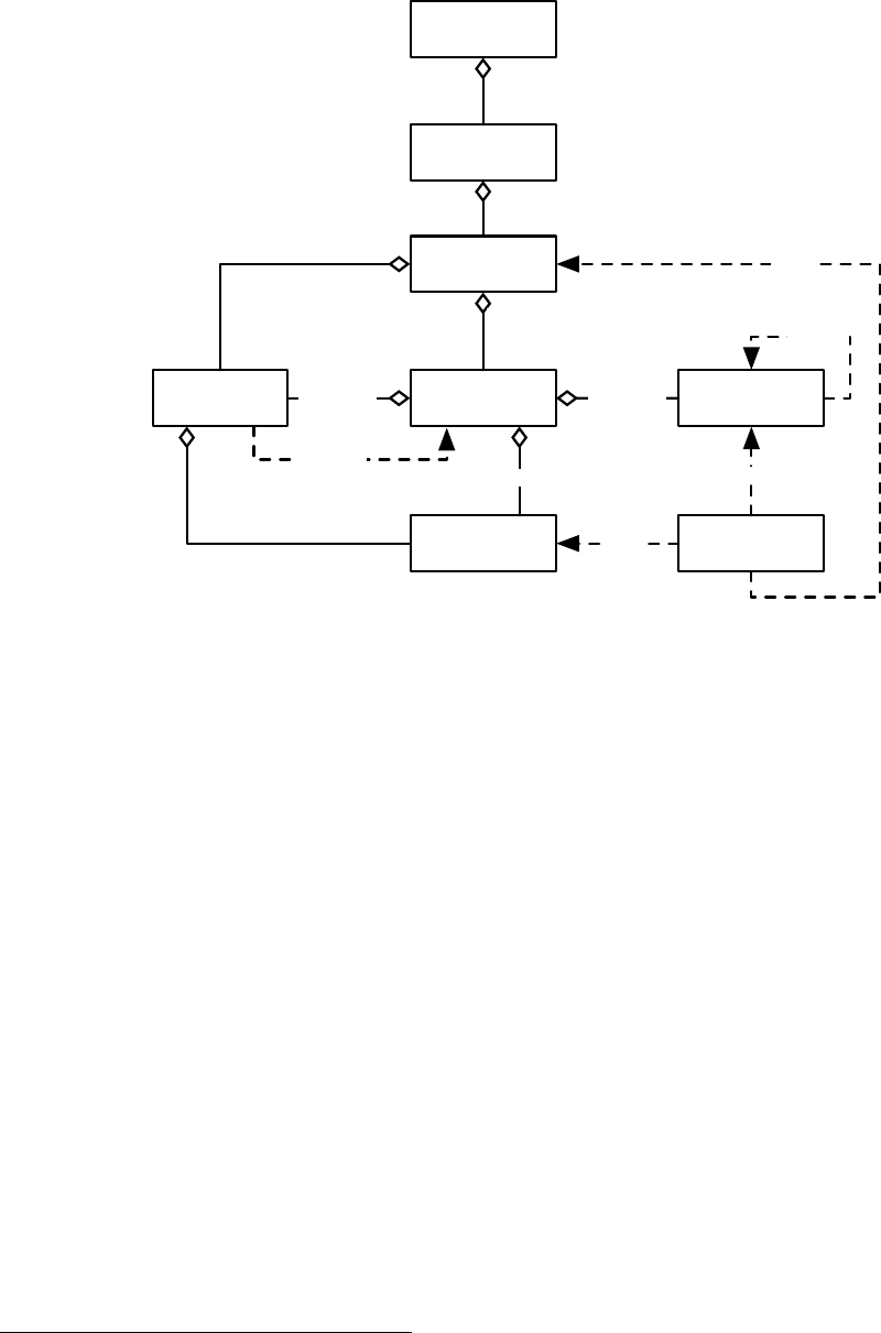
EvolutionState
Population
Subpopulation
Individual
1
1
1..n
1
1..n
1
Species
Fitness
1
1
prototype
1
1
prototype
1 1
Breeding Pipeline
prototype
1
1
flyweight
1..n 1
Selection Method
child of
0..n
1
child of
0..n
1
uses
uses
1
1
Figure 3.2 Top-Level data objects used in evolution. A repeat of Figure 1.3.
present there are only a few ECJ objects which implement Group: namely, ec.Population,ec.Subpopulation, and
certain specialized subclasses of ec.Subpopulation.
3.2 Populations, Subpopulations, Species, Individuals, and Fitnesses
Populations, Subpopulations, and Individuals are the “nouns” of an evolutionary system, and Fitnesses
are the “adjectives”. They’re pretty central to the operation of any evolutionary or sample-based stochastic
search algorithm.
In ECJ, an
individual
is a candidate solution to a problem. Some
M
Individuals are grouped together
into a sample of solutions known as a
subpopulation
. Some
N
subpopulations are grouped together into
the system’s
population
. There’s only one population per evolutionary process. The most common scenario
is for ECJ to have
M
individuals grouped into a single subpopulation, which then is the sole member of
ECJ’s population. However, coevolutionary algorithms (Section 7.1) typically have
N>
1 subpopulations:
as does a special and little-used internal island model scheme (see Section 6.2).1
Usually ECJ’s population is an instance of the class ec.Population and its subpopulations are instances of
the class ec.Subpopulation. Both of these are Groups. Let’s say that there’s a single subpopulation, which
must contain 100 individuals. We can express this as follows:
pop = ec.Population
pop.subpops = 1
pop.subpop.0 = ec.Subpopulation
pop.subpop.0.size = 100
1Because these two techniques use the subpopulations in different ways, they cannot be used together (a rare situation in ECJ).
59

Obviously further subpopulations would be
pop.subpop.1
,
pop.subpop.2
, etc. The population is found
in an instance variable in the EvolutionState:
public Population population;
The Population is little more than an array of Subpopulations. To get Subpopulation 0, with the Evolu-
tionState being state, you’d say:
Subpopulation theSubpop = state.population.subpops.get(0);
Subpopulations themselves contain arrays of individuals. To get Individual 15 of Subpopulation 0, you’d
say:
Individual theIndividual = state.population.subpops.get(0).individuals.get(15);
In addition to an array of individuals, each subpopulation contains a
species
which defines the indi-
viduals used to fill the subpopulation, as well as their fitness and the means by which they are modified.
Subpopulations also contain some basic parameters for creating initial individuals, though the procedure is
largely handled by Species.2We’ll get to creation and modification later.
Species have an odd relationship to Individuals and to Subpopulations. First recall the Flyweight pattern
in Section 3.1.4. Individuals are related to a common Species using the Flyweight pattern: they use Species
to store a lot of common information (how to modify themselves, for example). Ordinarily you’d think that
the Subpopulation would be a good place for this storage. However different Subpopulations can share the
same Species. This allows you to, for example, have one Species guide an entire evolutionary run that might
have twenty Subpoulations in it.3The species of Subpopulation 0 may be found here:
Species theSpecies = state.population.subpops.get(0).species;
A Species contains three major elements: first, the
prototypical Individual
for Subpopulations which use
that Species. Recall that Individuals are Prototypes and new ones are formed by cloning from a prototypical
individual held in reserve. This “queen bee” individual, so to speak, is found here:
Individual theProto = state.population.subpops.get(0).species.i_prototype;
A Species also contains a
prototypical Fitness
object. In ECJ fitnesses are separate from individuals.
Individuals define the candidate solution, and Fitnesses define how well it has performed. Like Individuals,
Fitnesses are also Prototypes. The prototypical Fitness for Subpopulation 0 may be found here:
Fitness theProtoFitness = state.population.subpops.get(0).species.f_prototype;
The Species class you pick is usually determined by the kind of Individual you pick, that is, by the kind of
representation of your solution. You define the class of the Species for Subpopulation 0, and its prototypical
Fitness and prototypical Individual, as follows. For example, let’s make Individuals which are arrays of
integers, and a simple Fitness common to many evolutionary algorithms:
pop.subpop.0.species = ec.vector.IntegerVectorSpecies
pop.subpop.0.species.ind = ec.vector.IntegerVectorIndividual
pop.subpop.0.species.fitness = ec.simple.SimpleFitness
By way of explanation, IntegerVectorIndividual, along with various other “integer” vector individuals like
LongVectorIndividual,ShortVectorIndividual, and ByteVectorIndividual, requires an IntegerVectorSpecies. And
ec.simple.SimpleFitness is widely used for problems such as Genetic Algorithms or Evolution Strategies. The
2
You might be asking: if Species are responsible for making individuals, why are Subpopulations involved at all? A very good
question indeed.
3Granted, this isn’t very common.
60
prototypical Individual is never assigned a Fitness (it’s null). But once assembled in a Subpopulation, each
Individual has its very own Fitness. To get the Fitness of individual 15 in Subpopulation 0, you’d say:
Fitness theFitness = state.population.subpops.get(0).individuals.get(15).fitness;
Last, a Species contains a
prototypical Breeding Pipeline
to modify individuals. We’ll get to that in
Section 3.5.
Since they’re Prototypes, Individuals, Fitnesses, and Species all have default bases. We’ll talk about the
different kinds of Individuals, Fitnesses, and Species later, plus various default bases for them.
3.2.1 Making Large Numbers of Subpopulations
Let’s say you’re doing an evolutionary experiment (perhaps coevolution, see Section 7.1) which involves 100
Subpopulations. It’s going to get very tiresome to repeat...
pop = ec.Population
pop.subpops = 100
pop.subpop.0 = ec.Subpopulation
pop.subpop.0.size = 100
pop.subpop.0.species = ec.vector.IntegerVectorSpecies
pop.subpop.0.species.ind = ec.vector.IntegerVectorIndividual
pop.subpop.0.species.fitness = ec.simple.SimpleFitness
....
pop.subpop.1 = ec.Subpopulation
pop.subpop.1.size = 100
pop.subpop.1.species = ec.vector.IntegerVectorSpecies
pop.subpop.1.species.ind = ec.vector.IntegerVectorIndividual
pop.subpop.1.species.fitness = ec.simple.SimpleFitness
....
pop.subpop.2 = ec.Subpopulation
pop.subpop.2.size = 100
pop.subpop.2.species = ec.vector.IntegerVectorSpecies
pop.subpop.2.species.ind = ec.vector.IntegerVectorIndividual
pop.subpop.2.species.fitness = ec.simple.SimpleFitness
....
... and so on some 100 times. Even with the help of ECJ’s default parameters, you’ll still be typing an awful
lot. Population has a simple mechanism to make this easier on you: the parameter...
pop.default-subpop = 0
This says that if you do not specify a Subpopulation in parameters, ECJ will assume its parameters are
identical for those of Subpopulation 0. Thus you could simply say:
pop = ec.Population
pop.subpops = 100
pop.default-subpop = 0
pop.subpop.0 = ec.Subpopulation
pop.subpop.0.size = 100
pop.subpop.0.species = ec.vector.IntegerVectorSpecies
pop.subpop.0.species.ind = ec.vector.IntegerVectorIndividual
pop.subpop.0.species.fitness = ec.simple.SimpleFitness
...
61

... and be done with it. Note that you can always specify a Subpopulation specially. For example, suppose all
of your Subpopulations were exactly like Subpopulation 0 except for Subpopulation 19. You can say:
pop = ec.Population
pop.subpops = 100
pop.default-subpop = 0
pop.subpop.0 = ec.Subpopulation
pop.subpop.0.size = 100
pop.subpop.0.species = ec.vector.IntegerVectorSpecies
pop.subpop.0.species.ind = ec.vector.IntegerVectorIndividual
pop.subpop.0.species.fitness = ec.simple.SimpleFitness
...
pop.subpop.19 = ec.Subpopulation
pop.subpop.19.size = 25
pop.subpop.19.species = ec.vector.FloatVectorSpecies
pop.subpop.19.species.ind = ec.vector.DoubleVectorIndividual
pop.subpop.19.species.fitness = ec.simple.SimpleFitness
...
Note that even though Subpopulation 19 shared the same fitness type as the others, we still had to specify
it. It’s an all-or-nothing proposition: either you say nothing about that particular Subpopulation, or you say
everything.
3.2.2 How Species Make Individuals
Species have two ways to create new individuals: from scratch, or reading from a stream. To generate an
individual from scratch, you can call (in ec.Species):
ec.Species Methods
public Individual newIndividual(EvolutionState state, int thread)
Returns a brand new, randomized Individual.
The default implementation of this method simply clones an Individual from the prototype and returns it.
Subclasses of Species override this to randomize the Individual in a fashion appropriate to its representation.
Another way to create an individual is to read it from a binary or text stream. ec.Species provides two
methods for this:
ec.Species Methods
public Individual newIndividual(EvolutionState state, LineNumberReader reader) throws IOException
Produces a new individual read from the stream.
public Individual newIndividual(EvolutionState state, DataInput input) throws IOException
Produces a new individual read from the given DataInput.
These methods create Individuals by cloning the prototype, then calling the equivalent readIndividual(...)
method in ec.Individual. See Section 3.2.4 for more information on those methods.
3.2.3 Reading and Writing Populations and Subpopulations
Populations and Subpopulations have certain predefined methods for reading and writing, which you
should know how to use. If you subclass Population or Subpopulation (relatively rare) you may need to
reimplement these methods. Population’s methods are:
62
public void printPopulationForHumans(EvolutionState state, int log);
public void printPopulation(EvolutionState state, int log);
public void printPopulation(EvolutionState state, PrintWriter writer);
public void readPopulation(EvolutionState state, LineNumberReader reader)
throws IOException;
public void writePopulation(EvolutionState state, DataOutput output)
throws IOException;
public void readPopulation(EvolutionState state, DataInput input)
throws IOException;
Subpopulation’s methods are nearly identical:
In Subpopulation:
public void printSubopulationForHumans(EvolutionState state, int log);
public void printSubopulation(EvolutionState state, int log);
public void printSubopulation(EvolutionState state, PrintWriter writer);
public void readSubopulation(EvolutionState state, LineNumberReader reader)
throws IOException;
public void writeSubopulation(EvolutionState state, DataOutput output)
throws IOException;
public void readSubopulation(EvolutionState state, DataInput input)
throws IOException;
These methods employ similar methods in ec.Individual to print out, or read, Individuals. Those methods
are discussed next in Section 3.2.4.
The first Population method, printPopulationForHumans(...), prints an entire population to a log in a
form pleasing to the human eye. It begins by printing out the number of subpopulations, then prints each
Subpopulation index and calls printSubpopulationForHumans(...) on each Subpopulation in turn. printPopula-
tionForHumans(...) then prints out the number of individuals, then for each Individual it prints the Individual
index, then calls printIndividualForHumans to print the Individual. Overall, it looks along these lines:
Number of Subpopulations: 1
Subpopulation Number: 0
Number of Individuals: 1000
Individual Number: 0
Evaluated: T
Fitness: 0.234
-4.97551104730313 -1.7220830524609632 1.7908415218297096
2.3277606156190496 3.5616099573877404 -3.8002895023118617
Individual Number: 1
Evaluated: T
Fitness: 4.91235
3.1033182498148575 -3.613847679151146 -0.562978505270439
-2.860926011046968 1.9007479097991151 -3.051348823625001
...
The next two Population methods, both named printPopulation(...), print an entire population to a log
in a form that can be (barely) read by humans but can also be read back in perfectly by ECJ, resulting in
identical Populations These operate similarly to printPopulationForHumans(...), except that various data types
are emitted using ec.util.Code (Section 2.2.3).
63

Number of Subpopulations: i1|
Subpopulation Number: i0|
Number of Individuals: i1000|
Individual Number: i0|
Evaluated: F
Fitness: f0|0.0|
i6|d4600627607395240880|0.3861348728170766|d4616510324226321041|4.284844300646584|
d4614576621171274054|3.2836854885228233|d4616394543356495435|4.182010230653371|
Individual Number: i1|
Evaluated: F
Fitness: f0|0.0|
i6|d4603775819114015296|0.6217914592919627|d4612464338011645914|2.345643329183969|
d-4606767824441912859|-4.368233761797886|d4616007477858046134|3.919113503960115|
...
The Population method readPopulation(..., LineNumberReader) can read in this mess to produce a Popula-
tion. It in turn does its magic by calling the equivalent method in Subpopulation.
The last two methods, writePopulation(...) and readPopulation(..., DataInput), read and write Populations
(or Subpopulations) to binary files.
3.2.4 About Individuals
Individuals have four basic parts:
• The Individual’s fitness.
public Fitness fitness;
• The Individual’s species.
public Species species;
• Whether the individual has been evaluated and had its Fitness set to a legal value yet.4
public boolean evaluated;
•
The representation of the Individual. This could be anything from an array to a tree structure —
representations of course vary and are defined by subclasses. We’ll talk about them later.
3.2.4.1 Implementing an Individual
For many purposes you can just use one of the standard “off-the-rack” individuals — vector individuals,
genetic programming tree individuals, ruleset individuals — but if you need to implement one yourself,
here are some methods you need to be aware of. First off, Individuals are Prototypes and must override
the clone() method to deep-clone themselves, including deep-cloning their representation and their Fitness,
but not their Species (which is just pointer-copied). Individuals must also implement the setup(...), and
defaultBase() methods. Additionally, Individuals have a number of methods which either should or must be
overridden. Let’s start with the “must override” ones:
public abstract int hashCode();
public abstract boolean equals(Object individual);
4Why isn’t this in the Fitness object? Another excellent question.
64

These two standard Java methods enable hashing by value, which allows Subpopulations to remove
duplicate Individuals. hashCode() must return a hashcode for an individual based on value of its representa-
tion. equals(...) must return true if the Individual is identical to the other object (which in ECJ will always be
another Individual).
The next two methods are optional and may not be appropriate depending on your representation:
public long size();
public double distanceTo(Individual other);
size() returns an estimate of the size of the individual. The only hard-and-fast rule is that 0 is the smallest
possible size (and the default returned by the method). Size information is largely used by the ec.parsimony
package (Section 5.2.12) to apply one of several parsimony pressure techniques.
distanceTo(...) returns an estimate of the distance, in some metric space, of the Individual to some other
Individual of the same type. In the future this method may be used for various crowding or niching methods.
At present no package uses it, though all vector individuals implement it. The default implementation
returns 0 if the other Individual is identical, else Double.POSITIVE INFINITY.
Last come a host of functions whose purpose is to read and write individuals. You’ve seen this pattern
before in Section 3.2.3. Some of these are important to implement; others can wait if you’re in a hurry to get
your custom Individual up and running.
public void printIndividualForHumans(EvolutionState state, int log);
public void printIndividual(EvolutionState state, int log);
public void printIndividual(EvolutionState state, PrintWriter writer);
public void readIndividual(EvolutionState state, LineNumberReader reader)
throws IOException;
public void writeIndividual(EvolutionState state, DataOutput output)
throws IOException;
public void readIndividual(EvolutionState state, DataInput input)
throws IOException;
These six methods only need to be overridden in certain situations, and in each case there’s another
method which is typically overridden instead. Here’s what they do:
•
printIndividualForHumans(...) prints an individual, whether it’s been evaluated, and its fitness, out a
log in a way that’s pleasing and useful for real people to read. Rather than override this method, you
probably should instead override this method:
public String genotypeToStringForHumans();
... which should return the representation of the individual in a human-pleasing fashion. Or, since
genotypeToStringForHumans() by default just calls toString(), you can just override:
public String toString();
Overriding one or both of these methods is pretty important: otherwise Statistics objects will largely be
printing your individuals as gibberish. Here’s a typical output of these methods:
Evaluated: T
Fitness: 0.234
-4.97551104730313 -1.7220830524609632 1.7908415218297096
2.3277606156190496 3.5616099573877404 -3.8002895023118617
•
Both printIndividual(...) methods print an individual, and its fitness, out in a way that can be perfectly
65
read back in again with readIndividual(...), but which can also be parsed by humans with some effort.
Rather than override this method, you probably should instead override this method:
public String genotypeToString();
This method is important to implement only if you intend to write individuals out to files in such a way
that you can load them back in later. If you don’t implement it, toString() will be used, which probably
won’t be as helpful. This returns a String which can be parsed in again in the next method. Note
that you need to write an individual out so that it can perfectly be read back in again as an identical
individual. How do you do this? ECJ’s classes by default all use the aging and idiosyncratic package
ec.util.Code package developed long ago for this purpose, but which still works well. See Section 2.2.3.
Here’s a typical output of these methods (note the use of ec.util.Code):
Evaluated: F
Fitness: f0|0.0|
i6|d4600627607395240880|0.3861348728170766|d4616510324226321041|4.284844300646584|
d4614576621171274054|3.2836854885228233|d4616394543356495435|4.182010230653371|
•
readIndividual(..., LineNumberReader) reads an individual, and its fitness, in from a LineNumberReader.
The stream of text being read is assumed to have been generated by printIndividual(.... Rather than
override this method, you probably should instead override this method:
protected void parseGenotype(EvolutionState state, LineNumberReader reader)
throws IOException;
This modifies the existing Individual’s genotype to match the genotype read in from the reader. The
genotype will have been written out using printIndividual(...). You only need to override this method if
you plan on reading individuals in from files (by default the method just throws an error).
•
The last two methods (writeIndividual(...) and readIndividual(..., DataInput)) read and write an individual,
including its representation, fitness and evaluated flag, in a purely binary fashion to a stream. Don’t
write the Species. It’s probably best instead to override the following methods to just read and write
the genotype:
public void writeGenotype(EvolutionState state, DataOutput output)
throws IOException;
public void readGenotype(EvolutionState state, DataInput input)
throws IOException;
These methods are probably only important to implement if you plan on using ECJ’s distributed
facilities (distributed evaluator, island models). The default implementations of these methods simply
throw exceptions.
3.2.5 About Fitnesses
Fitnesses are separate from Individuals, and various Fitnesses can be used depending on the demands of
the evolutionary algorithm. The most common Fitness is ec.simple.SimpleFitness, which represents fitness
as a single number from negative infinity to positive infinity, where larger values are “fitter”. Certain
selection methods (notably fitness proportionate selection) require that the fitness be non-negative; and
ideally between 0 and 1 inclusive.
66

There are other Fitness objects. For example, there are various multiobjective fitnesses (see Section 7.5), in
which the fitness value is not one but some
N
numbers, and either higher or lower may be better depending
on the algorithm. Other Fitnesses, like the one used in genetic programming (Section 5.2), maintain a primary
Fitness statistic and certain auxiliary ones.
You probably won’t need to implement a Fitness object. But you may need to use some of the meth-
ods below. Fitnesses are Prototypes and so must implement the clone() (as a deep-clone), setup(...), and
defaultBase() methods. Fitness has four additional required methods:
public abstract double fitness();
public abstract boolean isIdealFitness();
public abstract boolean equivalentTo(Fitness other);
public abstract boolean betterThan(Fitness other);
The first method, fitness(), should return the fitness cast into a value from negative infinity to positive
infinity, where higher values are better. This is used largely for fitness-proportionate and similar selection
methods. If there is no appropriate mechanism for this, you’ll need to fake it. For example, multiobjective
fitnesses might return the maximum or sum over their various objectives.
The second method, isIdealFitness(), returns true if the fitness in question is the best possible. This is
largely used to determine if it’s okay to quit. It’s fine for this method to always return false if you so desire.
The third and fourth methods compare against another fitness object, of the same type. The first returns
true if the two Fitnesses are in the same equivalence class: that is, neither is fitter than the other. For simple
fitnesses, this is just equality. For multiobjective fitnesses this is Pareto-nondomination of one another. The
second method returns true if the Fitness is superior to the one provided in the method. For simple fitnesses,
this just means fitter. For multiobjective fitnesses this implies Pareto domination.
Fitnesses also have similar printing facilities to Individuals:5
public void printFitnessForHumans(EvolutionState state, int log);
public void printFitness(EvolutionState state, int log);
public void printFitness(EvolutionState state, PrintWriter writer);
public void readFitness(EvolutionState state, LineNumberReader reader)
throws IOException;
public void writeFitness(EvolutionState state, DataOutput output)
throws IOException;
public void readFitness(EvolutionState state, DataInput input)
throws IOException;
As usual: the first method, printFitnessForHumans(...), prints a Fitness in a way pleasing for humans to
read. It simply prints out the result of the following method (which you should override instead if you ever
need to):
public String fitnessToStringForHumans();
The default implementation of fitnessToString() simply calls:
public String toString();
The next two methods, both named printFitness(...), prints a Fitness in a way that can be (barely) read by
humans, and can be read by ECJ to produce an identical Fitness to the original. These methods just print out
the result of the following method (which you should override instead if you ever need to):
public String fitnessToString();
5Starting to get redundant? Sorry about that.
67

The default implementation of this method calls toString(), which is almost certainly wrong. But all the
standard Fitness subclasses implement it appropriately using the ec.util.Code tools (Section 2.2.3).
The method readFitness(..., LineNumberReader) reads into ECJ a Fitness written by these last two printers.
Finally, the last two methods, writeFitness(...) and readFitness(..., DataInput), read and write the Fitness in a
binary fashion. The default implementation of these methods throws an error, but all standard subclasses of
Fitness implement them properly.
Fitnesses have two auxiliary variables:
public ArrayList trials = null;
public Individual[] context = null;
These variables are used by coevolutionary processes (see Section 7.1) to keep track of the number of
trials (in the form of java.lang.Double used to compute the Fitness value, and to maintain the context (other
collaborating Individuals) which produced the best result represented by he Fitness. Outside of coevolution
they’re presently unused: leave them null and they won’t be printed.
Fitnesses have three hooks which can be used to merge multiple Fitness values into one, if appropriate
(for example, this doesn’t make much sense for multiobjective fitnesses). Though this could be used to
assemble a Fitness over multiple trials, Coevolution uses the different mechanism above to achieve this
which preserves contextual information (see Section 7.1). One method setToMeanOf(...), is unimplemented
in the Fitness class proper, though it’s been implemented in common subclasses in ECJ. If you make your
own Fitness object you might ultimately want to implement this method if appropriate, but it’s not necessary
in most cases. The other two methods call setToMeanOf(...) internally.
ec.util.Fitness Methods
public void setToMeanOf(EvolutionState state, Fitness[] fitnesses)
Sets the fitness to the mean of the provided fitness values. By default this method is unimplemented and generates
an error. Common subclasses (like SimpleFitness and KozaFitness) override this method and implement it. Other
classes, such as MultiobjectiveFitness and its subclasses,, do not, since there is no notion of a “mean” in that context.
You do not have to implement this utility method in most situations.
public void setToMedianOf(EvolutionState state, Fitness[] fitnesses)
Sets the fitness to the median of the provided fitness values. This method calls setToMeanOf(...) in its implementa-
tion.
public void setToBestOf(EvolutionState state, Fitness[] fitnesses)
Sets the fitness to the best of the provided fitness values. This method calls setToMeanOf(...) in its implementation.
3.3 Initializers and Finishers
The
Initializer
is called at the beginning of an evolutionary run to create the initial population. The
Finisher
is called at the end of a run to clean up. In fact, it’s very rare to use any Finisher other than ec.simple.Finisher,
which does nothing at all. So nearly always you’ll have this:
finish = ec.simple.SimpleFinisher
Initializers vary largely based on representation, but not for the reason you think. Initializers generally
don’t need to know anything about the representation of an individual in order to construct it. Instead,
certain representations require a lot of pieces which need to be in a central repository (they’re Cliques). For
example, the genetic programming facility (Section 5.2) has various types,function sets,tree constraints,node
constraints, etc. It’s not in ECJ’s style to store these things as static variables because of the difficulty it presents
for serialization. Instead ECJ needed a global object to hold them, and Initializers were chosen for that task.
68

It’s probably not been the smartest of decisions: Finishers (which have historically had little purpose) could
have been recruited to the job, or some generic type repository perhaps. As it stands, Initializers aren’t an
optimal location, but there it is.6
Unless you’re doing genetic programming (ec.gp) or using the ec.rule package, you’ll probably use a
ec.simple.SimpleInitializer:
init = ec.simple.SimpleInitializer
ECJ’s generational7initialization procedure goes like this:
1. The EvolutionState asks the Initializer to build a Population by calling:
population = state.initializer.initialPopulation(state, 0);
The 0 is thread index 0: this portion of the code is single-threaded.
2.
The Initializer then creates and sets up a Population by calling the following on itself. It then tells the
Population to populate itself with individuals:
Population pop = setupPopulation(state, 0);
pop.populate(state, 0);
Why break this out? Because there are a few EvolutionState subclasses which don’t want to populate
the population immediately or at all — they just want to set it up. For example, steady state evolution
sets up a Population but may only gradually fill it with initial population members. In this case, the
steady state system will just call setupPopulation(...) directly, bypassing initialPopulation(...).
3.
The Population’s default populate(...) method is usually straightforward: it calls populate(...) in turn on
each Subpoulation in the Population’s subpopulation array.
Alternatively, the Population can read an entire population from a file. This is determined by (as usual)
a parameter! If the Population should be read in from the file /tmp/population.in, the parameter setting
would be:
pop.file = /tmp/population.in
The Population will read Subpopulations, and ultimately Individuals, from this file by calling its
readPopulation(..., LineNumberReader) method.
4.
If the Population is not reading from a file, it will call populate(...) on each of its Subpopulations. A
Subpopulation’s populate(...) method usually works like this. First, it determines if it should create
new individuals from scratch or if it should fill its array by reading Individuals from a file. If the
individuals are to be generated from scratch (the most common case by far), Subpopulation generates
new individuals using the standard newIndividual(...) method in ec.Species (see Section 3.2.2). ECJ
can also check to make sure that the Subpopulation does not produce duplicate individuals while
generating from scratch, if you set the following parameter (in this case, in Subpopulation 0):
pop.subpop.0.duplicate-retries = 100
The default value is no retries. This says that if the Subpopulation creates a duplicate individual, it will
try up to 100 times to replace it with a new, original individual. After that it will give up and use the
duplicate individual.
6
This makes it problematic to have both a “rule” representation and a genetic programming representation in the same run without
a little hacking, since both require their own Initializer. Perhaps this might be remedied in the future.
7ECJ’s Steady State evolution mechanism has a different initialization procedure. See Section 4.2 for more information.
69
You can also read Subpopulations directly from files, in a procedure similar to how it’s done for
Population. If Subpopulation 0 should be read in from the file /tmp/subpopulation.in, the parameter
setting would be:
pop.subpop.0.file = /tmp/subpopulation.in
Subpopulations will try to read individuals from files using readSubpopulation(..., LineNumberReader).
If the number of individuals in the file is greater than the size of the Subpopulation, then the Subpopu-
lation will be resized to match the file. If the number of individuals is in the file is less than the size of
the Subpopulation, then the Subpopulation will try to do on of three things:
•
Truncate the Subpopulation to the size of the file. This the default when reading from a file, but if
you want to be explicit, it’s specified like so:
pop.subpop.0.extra-behavior = truncate
•
Wrap copies of the file’s individuals repeatedly into the Subpopulation. For example, if the file
had individuals A, B, and C, and the Subpopulation was of size 8, then it’d be filled with A, B, C,
A B, C, A, B. This is particularly useful if you want to fill a file with copies of a single individual.
This is specified like so:
pop.subpop.0.extra-behavior = wrap
•
Fill the remainder of the Subpopulation with random individuals (see below). This is specified
like so:
pop.subpop.0.extra-behavior = fill
These options aren’t available if you’re reading the whole Population from a file: it always truncates
its Subpopulations appropriately. Note that if you’re reading the Population from a file, you can’t
simultaneously read one of its Subpopulations from a file — that wouldn’t make any sense.
3.3.1 Population Files and Subpopulation Files
If you write out a population using printPopulation(...), the resulting file or print-out typically starts with a
declaration of the number of subpopulations, followed by a declaration of a subpopulation number, then
the number of individuals in that subpopulation, then the individuals one by one. After this come the
declaration of the next subpopulation number, and the number of individuals in that subpopulation, then
those individuals. And so on. It looks like this:
Number of Subpopulations: i3|
Subpopulation Number: i0|
Number of Individuals: i1024|
... [the individuals] ...
Subpopulation Number: i1|
Number of Individuals: i512|
... [the individuals] ...
Subpopulation Number: i2|
Number of Individuals: i2048|
... [the individuals] ...
But ECJ doesn’t read in entire populations on initialization. Instead if you want to initialize your
population from a file, you do so on a per-subpopulation basis, as in the parameters:
pop.subpop.0.file = myfile.in
A subpopulation file like this usually just has the the number of individuals for the subpopulation,
followed by the individuals:
70

Number of Individuals: i512|
... [the individuals] ...
You can typically edit a subpopulation file out of a population file with some judicious typing: the
relevant text is between the relevant “subpopulation Number:” lines.
In the example above, there are three subpopulations, because of the line
Number of Subpopulations: i3|
This “i3
|
” oddity is due to use of ECJ’s Code package (Section 2.2.3). The “i” means “integer”, the “3” is
the value, and the “|” is a separator. Likewise subpopulation 0 starts with “i0|”.
3.4 Evaluators and Problems
ECJ evaluates (assesses the fitness of) Individuals in a Population by passing it to an ec.Evaluator. Various
evolutionary algorithms and other stochastic search algorithms have their own special kinds of Evaluators.
Evaluators perform this fitness assessment by cloning one or more
Problems
, discussed in the next Section,
and asking these Problems to evaluate the individuals on their behalf. Evaluators hold the prototypical
Problem here:
public Problem p problem;
This problem is loaded from parameters. For example, to specify that we will use the Artificial Ant
Problem to test our genetic programming Individuals, we’d say:
eval.problem = ec.app.ant.Ant
The basic Evaluator is ec.simple.SimpleEvaluator. This class evaluates a Population first by determining
how many threads to use. To use four threads (for example), we say:
evalthreads = 4
The default value is a single thread.
Recall from Section 2.4 that his will require at least four random number generator seeds, for example:
seed.0 = 1234
seed.1 = -503812
seed.2 = 992341
seed.3 = -16723
When evaluating a Population, ec.simple.SimpleEvaluator will construct
N
Problems cloned from the
Problem prototype, and assign one to each thread. Then, for each Subpopulation, the Evaluator will use
these threads to evaluate the individuals in the Subpopulation. By default SimpleEvaluator simply breaks
each Subpopulation into
N
even chunks and assigns each chunk to a different thread and its Problem. This
enables the Population to be evaluated in parallel.
The problem with this approach to parallelism is that it’s not fine-grained: and so if some individuals
take much longer to evaluate, then some threads will sit around waiting for a thread to finish its chunk. You
can fix this by specifying the chunk size, all the way own to chunks of a single individual each. When an
individual has finished its chunk, it will request another chunk to work on, and if it has exhausted on all
the chunks in a Subpopulation, it’ll grab chunks from the next Subpopulation. For example, the extreme of
fine-grained parallelism would be:
eval.chunk-size=1
71
The disadvantage of a small chunk size is that it involves a lot of locking to get each chunk. This is a small
but significant overhead: so we suggest using the default (large automatic chunks) unless your evaluations
are costly and of high variance in evaluation time.
Another disadvantage of a nonstandard chunk size is that threads run at different speeds and are no
longer asynchronous: as a result, different runs with the same seeds could produce different results if
evaluation is stochastic.
Of course, you probably most often don’t do parallelism at all: you’ll just have a single thread (that is,
N=
1). In this case you have one further option: to avoid cloning the Problem each time, by setting the
following parameter to false:
eval.clone-problem = false
If false, then the same Problem instance (the Prototype, in fact) will be used again and again. Ob-
viously, this only is allowed if there’s a single evaluation thread. And steady-state evolution (via
ec.simple.SteadyStateEvaluator) does not support it.
The idea of not cloning the population and pipeline is due to Brian Olsen, a GMU PhD Student.
Certain Evaluator methods are required. The primary method an Evaluator must implement is
public abstract void evaluatePopulation(EvolutionState state);
This method must take the Population (that is, state.population) and evaluate all the individuals in it in
the fashion expected by the stochastic search algorithm being employed. Additionally, an Evaluator must
implement the method
public abstract String runComplete(EvolutionState state);
... which returns a non-null String if the Evaluator believes the process has reached a terminating state.
Typically this is done by scanning through the Population and determining if any of the Individuals have
ideal fitnesses. The String provides a message for the user as to why the run terminated early (typically
because the ideal individual was discovered). If you don’t want to be bothered, it’s fine to have this method
always return null.
If you would like to terminate the run early for some other reason — perhaps you have run out of
resources or got stuck somehow — you can call the following method to request that ECJ terminate its run
at its earliest convenience. You provide a String which tells the user why you’ve decided to quit.
public void setRunComplete(String message);
3.4.1 Problems
Evaluators assess the fitness of individuals typically by creating one or more Problems and handing them
chunks of Subpopulations to evaluate. There are two ways that an Evaluator can ask a Problem to perform
evaluation:
•
For each Individual, the Evaluator can call the Problem’s evaluation method. This method varies
depending on the kind of Problem. Problems which adhere to ec.simple.SimpleProblemForm — by far
the most common situation — use the following method:
public void evaluate(EvolutionState state, Individual ind,
int subpopulation, int threadnum);
When this approach is taken, the Problem must assign a fitness immediately during the evaluate(...)
method. In practice, ECJ doesn’t do this all that much.
72

•
The more common approach allows a Problem to perform fitness evaluation in bulk. In this approach,
the Evaluator will first call the following method once:
public void prepareToEvaluate(EvolutionState state, int thread);
This signals to the Problem that it must prepare itself to begin evaluating a series of Individuals, and
then afterwards assign fitness to all of them. Next the Evaluator calls the Problem’s evaluation method
for each Individual, typically using the method evaluate(...) as before. Finally, the Evaluator calls this
method:
public void finishEvaluating(EvolutionState state, int thread);
Using this approach, the Problem is permitted to delay assigning fitness to Individuals until finishEvalu-
ating(...) is called.
When ECJ is preparing to exit various Statistics objects sometimes construct a Problem in order to
re-evaluate the fittest Individual of the run, solely to have such evaluation print out useful information to
tell the user how the Individual operates. This special version of evaluation is done with the following
ec.simple.SimpleProblemForm method:
public void describe(EvolutionState state, Individual ind, int subpopulation,
int threadnum, int log);
Note that ECJ will not call prepareToEvaluate(...) before describe(...), nor call finishEvaluating(...)
after it.
When this method is called, the expectation is that the individual will be evaluated for the purpose
of writing out interesting descriptive information to the log. For example, a fit Artificial Ant agent might
show the map of the trail it produces as it wanders about eating pellets of food. If you prefer you don’t
have to implement this method: and in fact many Problems don’t. The default version (in ec.Problem) does
nothing at all.
Problem is a Prototype, and so it must implement the clone() (as a deep-clone), setup(...), and defaultBase()
methods: although in truth the default base is rarely used. Problem’s “default” default base is
problem
,
which is very rarely used.
3.4.2 Implementing a Problem
Commonly the only method a Problem needs to implement is the evaluate(...) method. For example, let’s
imagine that our Individuals are of the class ec.vector.IntegerVectorIndidual, discussed in Section 5.1. The
genotype for IntegerVectorIndividual is little more than an array of integers. Let us presume that the fitness
of these individuals is defined as the product of their integers.
The example below does five basic things:
1.
If the individual has already been evaluated, we don’t bother evaluating it again. It’s possible you’d
might want to evaluate it anyway (perhaps if you had a dynamically changing fitness function, for
example).
2. We do a sanity check: if the individual is of the wrong type, we issue an error.
3. We compute product of the values in the genome.
4.
We set the fitness to that product, and test to see if the fitness is optimal (in this case, if it’s equal to
Double.POSITIVE INFINITY.
5. We set the individual’s evaluated flag.
73
The implementation is pretty straightforward:
package ec.app.myapp;
import ec.*;
import ec.simple.*;
import ec.vector.*;
public class MyProblem extends Problem implements SimpleProblemForm
{
public void evaluate(EvolutionState state, Individual ind,
int subpopulation, int thread)
{
if (ind.evaluated) return;
if (!(ind instanceof IntegerVectorIndividual))
state.output.fatal("Whoa! It’s not an IntegerVectorIndividual!!!");
int[] genome = ((IntegerVectorIndividual)ind).genome;
double product = 1.0;
for(int x=0; x<genome.length; x++)
product = product * genome[x];
((SimpleFitness)ind.fitness).setFitness(state, product,
product == Double.POSITIVE_INFINITY);
ind.evaluated = true;
}
}
If you’re doing ec.simple.SimpleProblemForm may wish to also implement the describe(...) method. This
method will be called a single time at the end of the run, and will be passed the fittest individual discovered.
It gives you a chance to write out interesting statistics about the individual, typically to the statistics log. For
example, the ec/app/ant/Ant.java file implements the describe(...) method to print out the winning path that
the ant took to achieve its high fitness. Here is a silly example of implementing describe(...) to give you the
general idea.
74
public void describe(EvolutionState state, Individual ind,
int subpopulation, int thread, int log)
{
if (!(ind instanceof IntegerVectorIndividual))
state.output.fatal("Whoa! It’s not an IntegerVectorIndividual!!!");
int[] genome = ((IntegerVectorIndividual)ind).genome;
double product = 1.0;
double min = Double.POSITIVE_INFINITY;
for(int x=0; x<genome.length; x++)
{
product = product * genome[x];
min = Math.min(genome[x], min);
}
state.output.println("Best Individual’s total: " + product, log);
state.output.println("Best Individual’s minimum genome: " + min, log);
if (product == Double.POSITIVE_INFINITY)
state.output.println("Best Individual is OPTIMAL!", log);
else
state.output.println("Best Individual is not optimal.", log);
}
Notice that describe(...) basically looks the same as evaluate(...), except that you always do evaluation
(why wouldn’t you?), and don’t set the fitness (why would you?).
3.5 Breeders
Individuals are selected bred to create new Individuals using a subclass of ec.Breeder. Because this is so
central to the differences among various evolutionary algorithms, many such algorithms implement their
own Breeder subclasses. A Breeder consists of a single method:
public abstract Population breedPopulation(EvolutionState state);
This method is required to take the current Population, found here...
state.population
... and return a Population to be used for the next generation, consisting of individuals selected and bred
from the previous Population in a manner appropriate for the algorithm being used. The Population returned
can be the original Population, or it can be an entirely new Population cloned from the original (Population
is a Group, recall — see Section 3.1.5).
The most common Breeder is ec.simple.SimpleBreeder, which implements a basic form of generational
breeding common to the Genetic Algorithm and to Genetic Programming, among others. SimpleBreeder has
facilities for multithreaded breeding and a simple form of elitism, and works as follows:
1. For each Subpopulation in the Population,
(a) Determine the Nfittest Individuals in the Subpopulation.
(b) Create a new Subpopulation.
(c)
Load these
N
individuals (the “elites”) into first slots of the new Subpopulation’s individuals array.
(d)
Break the remaining unfilled region of this individuals array into
M
chunks, one chunk per thread.
75
(e) For each of the Mthreads (in parallel),
i. Construct a new Breeding Pipeline.
ii. Use this Breeding Pipeline to populate the thread’s chunk with newly-bred Individuals.
2. Assemble all the new Subpopulations into a new Population and return it.
The number of elites (
N
) in each Subpopulation is a parameter. To set 10 elites for Subpopulation 0 (for
example), you’d say:
breed.elite.0 = 10
Alternatively you can define the number of elites as a proportion of the Subpouplation:.
breed.elite-fraction.0 = 0.25
You can’t do both, but you can do neither: rhe default value is no elites.
You don’t have to specify the elitism on a per-Subpopulation basis. If you specified a default subpopula-
tion using the parameter
pop.default-subpop
(see Section 3.2.1), SimpleBreeder will try this instead when
it can’t find an elitism parameter, and will issue a warning letting you know it’s doing so. For example, if
you declared:
pop.default-subpop = 0
breed.elite.0 = 10
... then when SimpleBreeder must determine elitism for (say) Subpopulation 4, and that parameter doesn’t
exist, it’ll use 10 instead (the value for Subpopulation 0).
Ordinarily elites never have their fitness reevaluated. But if you have a dynamic fitness function, you
may wish to reevaluate their fitness each generation to see if it’s still the same. To do this for Subpopulation
0, you say:
breed.reevaluate-elites.0 = true
The default value is false.
Again, you don’t have to specify the elitism on a per-Subpopulation basis, if you specified a default
subpopulation using the parameter
pop.default-subpop
. SimpleBreeder will use the default value and
issue a warning.
The number of threads (M) is also a parameter. To set it to 4, you’d say:
breedthreads = 4
The default value is a single thread.
As was the case for the
evalthreads
parameter (for Evaluator), recall from Section 2.4 that his will
require at least four random number generator seeds, one per thread. For example:
seed.0 = 1234
seed.1 = -503812
seed.2 = 992341
seed.3 = -16723
Certain Breeders allow you to change the subpopulation breeding order to a sequential one. Let’s say you
have 3 subpopulations. If you turn on the following parameter:
breed.sequential = true
... then SimpleBreeder will only breed subpopulation 0 the first generation, then only subpopulation 1 the
second generation, then only subpopulation 2 the second generation, then only subpopulation 0 the third
76
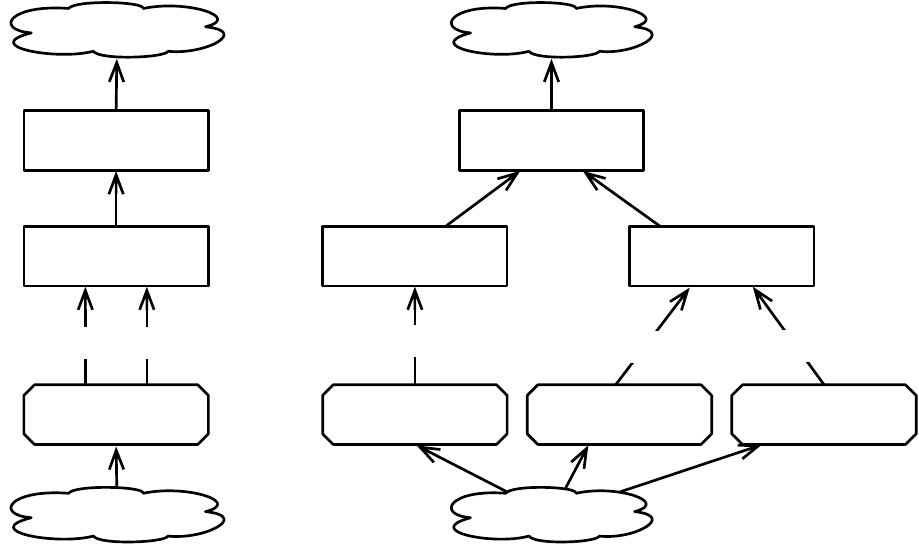
Vector Crossover
Pipeline
Vector Mutation
Pipeline
Reproduction
Pipeline
Multi-Breeding
Pipeline
Tournament
Selection
(GP) Crossover Pipeline
Tournament
Selection
Fitness Proportionate
Selection
Sigma Scaling
Selection
New Subpopulation
Old SubpopulationOld Subpopulation
New Subpopulation
Copy Copy
Copy
Copy
Copy
Figure 3.3 Two example Breeding Pipelines.
generation, and so on. Obviously if you only have one subpopulation, this parameter has no effect. Why
would you want this? ECJ only uses it for a common kind of coevolution, discussed later in Section 7.1.4.1.
Otherwise you should keep this set to
false
. The only reason it’s mentioned here is so that if you make
a Breeder subclass, you can check for this parameter and signal an error if it is
true
, indicating that your
Breeder subclass doesn’t support it.
All that remains is the breeding procedure itself, for which SimpleBreeder (and many Breeders) constructs
aBreeding Pipeline.
Last but not least, if you breed with only one thread (
M=
1), you have an additional option: to avoid
cloning the Population and Pipeline each time. Instead, the same Pipeline will be used each generation; and
the breeder will swap back and forth between two Populations each time rather than create new ones. This
primarily exists to be a little more efficient in some situations, primarily with small populations. This is done
by setting this parameter to false:
eval.clone-pipeline-and-population = false
Obviously, this only is allowed if there’s a single evaluation thread. And this option is not supported by
a number of subclasses, namely:
•ec.spatial.SpatialBreeder
•ec.multiobjective.nsga2.NSGA2Breeder
•ec.multiobjective.spea2.SPEA2Breeder
•ec.steadystate.SteadyStateBreeder
The idea of not cloning the population and pipeline is due to Brian Olsen, a GMU PhD Student.
77
3.5.1 Breeding Pipelines and BreedingSources
A Breeding Pipeline is a chain of selection and breeding operators whose function is to draw from Individuals
in an old Subpopulation to produce individuals in a new Subpopulation.
Breeding Pipelines consist of two kinds of objects. First there are
Selection Methods
, which select
Individuals from the old Subpopulation and return copies of them. Then there are
Breeding Pipelines
(what
would have better been called
Breeding Operators
), which take Individuals from Selection Methods or from
other Breeding Pipelines, modify them in some way, and return them.
The Breeding Pipeline structure isn’t actually a pipeline: it’s really a tree (or in some situations, a directed
acyclic graph). The leaf nodes in the graph tree are the Selection Methods (subclasses of ec.SelectionMethod,
and the nonleaf nodes are the Breeding Pipeline objects (subclasses of ec.BreedingPipeline).
Each BreedingPipeline object can have some
Nsources
(children) from which it draws Individuals. Both
ec.SelectionMethod and ec.BreedingPipeline are subclasses of the abstract superclass ec.BreedingSource, and
so can function as sources for BreedingPipelines. SelectionMethods do not have sources: rather, they draw
Individuals directly from the old Subpopulation.
Breeding Pipelines implement a
copy-forward
protocol: the leaf nodes (SelectionMethods) build clones
of individuals selected from the original population, and the non-leaf BreedingPipeline objects modify those
clones. This way every Breeding Pipeline has its own copies of individuals from which it generates children,
and so no locks are required on the original population when doing multithreaded breeding.
BreedingSources (and BreedingPipeline, and SelectionMethods) are Prototypes, and so must implement
the clone(),defaultBase(), and setup(...) methods. BreedingSources also implement three special methods
which perform the actual selection and breeding, which we describe here. When a Breeder wishes to produce
a series of new Individuals from an old Subpopulation, it begins by calling the method
public abstract void prepareToProduce(EvolutionState state, int subpopulation,
int thread);
This instructs the BreedingSource to prepare for a number of requests for Individuals drawn from
subpopulation number subpopulation. During this method the BreedingSource will, at a minimum, call
prepareToProduce(...) on each of its sources.
Next, the Breeder calls the following zero or more times to actually produce the Individuals:
public abstract int produce(int min, int max, int subpopulation,
java.util.ArrayList<Individual> inds, EvolutionState state,
int thread, java.util.HashMap<String, Object> misc);
This instructs the BreedingSource to produce between min and max Individuals drawn from subpop-
ulation number subpopulation. The Individuals are to added to the end of the ArrayList inds. Auxiliary
information may be found (or placed in) the HashMap misc: see Section 3.5.1.1. Finally the method returns
the actual number of Individuals produced.
Last, the Breeder calls the following method to give the BreedingSource an opportunity to clean up. The
BreedingSource in turn, at a minimum, will call the same method on each of its sources.
public abstract void finishProducing(EvolutionState state, int subpopulation,
int thread);
Additionally, BreedingSources implement three other methods. The first:
public abstract int typicalIndsProduced();
This method returns the number of individuals a BreedingSource would produce by default if not
constrained by min and max. The method can return any number >0.
The next method:
78

public abstract boolean produces(EvolutionState state, Population newpop,
int subpopulation, int thread);
... returns true if the BreedingSource believes it can validly produce Individuals of the type described by the
given Species, that is, by newpop.subpops.get(subpopulation).species. This is basically a sanity check. At the
minimum, the BreedingSource should call this method on each of its sources and return false if any of them
return false.
Last, we have the hook...
public void preparePipeline(Object hook);
You don’t have to implement this at all. ECJ does not call this method nor implement it in any of its
BreedingSources beyond the default implementation (which in BreedingPipeline calls the method in turn on
each of its sources). This method simply exists in the case that you need a way to communicate with all the
methods of a BreedingPipeline at some unusual time.
3.5.1.1 Auxiliary Data
In addition to Individuals, Breeding Sources can also return various
auxiliary data
associated with them.
This is an elaborate hook which lets you do much more sophisticated things with Breeding Sources are your
needs may require. This data is stored in the misc variable passed into the produce(...) method of a Breeding
Source.
A Breeder may set misc to null, in which case Breeding Sources should simply ignore it. Otherwise misc
holds a HashMap which maps
keyword strings
to
custom objects
, and is created immediately before any
call to produce(...) by calling the following method in ec.Species:
public HashMap<String, Object> buildMisc(EvolutionState state, int subpopIndex,
int thread);
By default this method just builds an empty HashMap.
You can put whatever you want in this HashMap. But ECJ currently reserves exactly one keyword string,
defined in SelectionMethod.java:
public static final String KEY PARENTS = "parents";
Associated with this string in the HashMap is an array of ec.util.IntBag objects. An IntBag is very much
like an ArrayList but it holds ordinary integers, not objects.
8
. For a given individual number
x
returned in
the ArrayList, the IntBag number
x
in the parents array holds indexes to all the parents of that Individual in
the old Subpopulation.
3.5.2 SelectionMethods
Selection Methods by default implement the typicalIndsProduced() method to return Selection-
Method.INDS PRODUCED (that is, 1).
Furthermore, the default implementation of the produces method,
public abstract boolean produces(EvolutionState state, Population newpop,
int subpopulation, int thread);
...just returns true. But you may wish to use this method to check to make sure that your Selection-
Method knows how to work with the kind of Fitnesses found in the given subpopulation, that is,
state.population.subpops.get(subpopulation).f prototype.
8IntBag comes from ECJ’s sister project, MASON https://cs.gmu.edu/∼eclab/projects/mason
79
The default implementations of prepareToProduce(...) and finishProducing(...) do nothing at all; though
some kinds of SelectionMethods, such as Fitness Proportionate Selection (ec.select.FitProportionateSelection),
use prepareToProduce(...) to prepare probability distributions based on the Subpopulation in order to select
properly.
SelectionMethods are sometimes called upon not to produce a cloned Individual but to provide an index
into a subpopulation where the Individual is located — perhaps to kill that Individual and place another
Individual in its stead. To this end, SelectionMethods have an alternative form of the produce(...) method:
public abstract int produce(int subpopulation, EvolutionState state, int thread);
This method must return the index of the selected individual in the Subpopulation given by:
state.population.subpops.get(subpopulation).individuals;
Furthermore, SelectionMethods have a special version of produce(...) called produceWithoutCloning(...),
which selects individuals (using the alternative form of produce(...) as described earlier) and sticks them
directly into the ArrayList without cloning them.
public int produceWithoutCloning(int min, int max, int subpopulation,
java.util.ArrayList<Individual> inds, EvolutionState state,
int thread, java.util.HashMap<String, Object> misc);
At present, produceWithoutCloning() does exactly one thing with the misc variable: it creates a
parents
bag for each produced child, and places in it the index of the original individual in the old subpopulation.
The default implementation of the full produce(...) method just calls producewithoutCloning(...), then
replaces with clones each of the individuals placed in the ArrayList. All this means that
you don’t have
to implement the full produce(...) method
. You typically just implement the alternative form (which you
have to implement anyway).
3.5.2.1 Implementing a Simple SelectionMethod
Implementing a SelectionMethod can be as simple as overriding the “alternative” form of the produce(...)
method. You don’t have to implement the “standard” form of produce(...) because its default implementation
calls the alternative form and handles the rest of the work for you.
To select an individual at random from a Subpopulation, you could simply implement the “alternative”
form to return a random number between 0 and the size of the subpopulation in question:
public int produce(int subpopulation, EvolutionState state, int thread)
{
return state.random[thread.next(
state.population.subpops.get(subpopulation).individuals.size())];
}
You’ll want to always implement the alternative form of produce(...). But in some cases you may wish to
also reimplement the “standard” form of produce(...) for some reason (you’ll still have to implement the
alternative form) —, perhaps you want to play with the misc variable, for example. In this case it’s best to
implement the produceWithoutCloning(...) version. We start by determining how many individuals we’ll
produce, defaulting with 1:
public int produceWithoutCloning(int min, int max, int subpopulation, java.util.ArrayList<Individual> inds,
EvolutionState state, int thread, java.util.HashMap<String, Object> misc)
{
int start = inds.size();
int n = 1;
80
if (n>max) n = max;
if (n<min) n = min;
Next we select
n
individuals from the old subpopulation and place them into slots inds[start] ...
inds[start+n-1]. Here we’re do it randomly:
for(int q = 0; q < n; q++)
{
int index = produce(subpopulation,state,thread);
inds.add(state.population.subpops.get(subpopulation).individuals.get(index));
// here we will create a parents IntBag for each selected individual, and place
// the index of that selected individual directly in this IntBag. An array of
// IntBags are stored associated with KEY_PARENTS.
// Note that misc could be null, that’s perfectly legitimate.
if (misc!=null && misc.get(KEY_PARENTS)!=null)
{
ec.util.IntBag bag = new ec.util.IntBag(1);
bag.add(index);
((IntBag[])misc.get(KEY_PARENTS))[start+q] = bag;
}
// Here is where you could play around some more with the misc variable,
// for example...
}
return n;
}
3.5.2.2 Standard Classes
There are a number of standard SelectionMethods available in ECJ, all found in the ec.select package.
•
ec.select.FirstSelection always returns the first individual in the Subpopulation. This is largely used for
testing purposes.
•
ec.select.RandomSelection returns an Individual chosen uniformly at random. Basically it does the same
thing as the example given above.
•
ec.select.TopSelection always returns the very best individual in the Subpopulation, breaking ties
randomly. You can optionally cache this individual so TopSelection doesn’t hunt for him every time it’s
called. To do this, you set:
base.cache = true
The default value is false. Note that if multiple individuals are tied for best, only one will be selected
for the cache, and the others will never be returned. The cache is reset when the method prepareToPro-
duce(...) is called. Warning: in steady-state evolution, this method is only called once, at the beginning
of the run. In generational evolution, the method is called at the start of every generation.
•ec.select.AnnealedSelection is used for doing Simulated Annealing. It works as follows. If there is only
one individual in the population, it is selected. Otherwise we choose a random individual that is not
the first individual. If that random individual is fitter than the first individual, it is selected. Otherwise
if that random individual is as fit as (has a fitness equivalent to) the first individual, one of the two is
selected at random. Otherwise if the random individual is not as fit as the first individual, it is selected
81

with a probability
P=eFitness(the random individual)−Fitness(the first individual)
t
, where
t
is a temperature. Otherwise the
first individual is selected.
The temperature starts at a high value
0, and is slowly cut down by multiplying it by a cutdown
value every generation. When the temperature reaches 0, then the first individual is always selected.
The initial temperature and cutdown are set like this:
base.temperature = 10000
base.cutdown = 0.95
(You don’t have to provide a cutdown, in which case its default is 0.95.)
Like TopSelection, AnnealedSelection also has a caching option. The selected individual can be cached
so the same individual is returned repeatedly without being recomputed. This cache is cleared after a
call to prepareToProduce(...). Again, note that this option is not appropriate for Steady State Evolution,
which only calls prepareToProduce(...) once. To do this, you set:
base.cache = true
The default value is false.
•
ec.select.FitProportionateSelection
9
uses
Fitness-Proportionate Selection
, sometimes called
Roulette
Selection, to pick individuals. Thus ec.select.BestSelection requires that all fitnesses be non-negative.
•
ec.select.SUSSelection selects individuals using
Stochastic Universal Sampling
, a low-variance version
of Fitness-Proportionate selection in which highly fit individuals are unlikely to never be chosen. Every
new generation, and
M
selection events thereafter, it shuffles the Subpopulation, then computes the
next
M
individuals to be selected in the future. ECJ assumes that
M
is the size of the Subpopulation.
Fitnesses must be non-negative. You have the option of whether or not to shuffle the Subpopulation
first:
base.shuffle = true
The default value is false.
•
ec.select.SigmaScalingSelection (written by Jack Compton, a former undergraduate at GMU) is another
low-variance version of Fitness-Proportionate Selection, in which modified versions of the Individuals’
fitnesses are used to reduce the variance among them. This is done by first computing the mean
µ
and standard deviation
σ
among the fitnesses. If
σ=
0 no change is made. Otherwise each modified
fitness
g
is then treated as
g←
1
+f−µ
2σ
. This can result in negative modified fitnesses, so we introduce
a fitness floor: modified fitnesses are bounded to be no less than the floor. Original fitnesses must be
non-negative To set this floor to 0.1 (a common value), you’d say:
base.scaled-fitness-floor = 0.1
0.1 is the default value already, so this is redundant.
SigmaScalingSelection default base is select.sigma-scaling.
•
ec.select.BoltzmanSelection (also written by Jack Compton) works like Fitness-Proportionate Selection,
but uses modified fitness values according to a Boltzman (Simulated-Annealing-style) cooling schedule.
Initially BoltzmanSelection has a high temperature
T
, and for each successive generation it decreases
T
by a cooling rate
R
as
T←T∗R
. Each modified fitness
g
is computed as
g←ef/T
, where
f
is the
original fitness. Fitnesses must be non-negative. When the temperature reaches 1.0, BoltzmanSelection
9
It’s called FitProportionateSelection rather than FitnessProportionateSelection for a historical reason: MacOS 9 didn’t allow
filenames longer than 32 characters, and FitnessProportionateSelection.class is 35 characters long.
82
reverts to FitnessProportionateSelection. To set the initial temperature to 1000 and the cooling rate to
0.99, you’d say:
base.starting-temperature = 1000
base.cooling-rate = 0.99
The default temperature is 1.0; and the default cooling rate is 0.0, which causes BoltzmanSelection to
behave exactly like FitProportionateSelection.
BoltzmanSelection’s default base is select.boltzman.
•
ec.select.GreedyOverselection is a variation of Fitness-Proportionate Selection which was common in
the early genetic programming community (see Section 5.2), but no longer. The Individuals are sorted
and divided into the “fitter” and “less fit” groups. With a certain probability the “fitter” individuals
will be selected (using Fitness-Proportionate Selection), else the “less fit” individuals will be selected
(also using Fitness-Proportionate Selection). Fitnesses must be non-negative. To specify that the “fitter”
group is 25% of the Subpopulation, and that individuals are chosen from it 40% of the time, you’d say:
base.top = 0.25
base.gets = 0.40
GreedyOverselection’s default base is select.greedy.
•
ec.select.TournamentSelection first chooses
T
individuals entirely at random with replacement (thus the
same Individual may be chosen more than once). These individuals are known as the tournament, and
T
is the tournament size. Then from among those
T
it returns the fittest (or least fit, a parameter setting)
Individual, breaking ties randomly.
T
is often an integer but in fact it doesn’t have to be: it can be any
real-valued number
N>
0. If
T
isn’t an integer, it’s interpreted as follows: with probability
T− bTc
we choose
dTe
individuals at random, else we choose
bTc
individuals at random. Fitnesses must be
non-negative. The most common setting for
T
is 2. To use 2, and return the fittest individual rather
than the least-fit one, say:
base.size = 2
base.pick-worst = false
By default, pick-worst is false, so the second parameter is redundant here.
TournamentSelection’s default base is select.tournament.
•
ec.select.BestSelection gathers the best or worst
N
individuals in the population. It then uses a tourna-
ment selection of size
T
to select, restricted to just those
N
. The tournament selection procedure works
just like ec.select.TournamentSelection. If the
N
worst individuals were gathered, then the tournament
will pick the worst in the tournament.
This could be used in various ways. Continuing the example above, to use a value of
T=
2, selecting
among the best 15 individuals in the population (say), we could say:
base.n = 15
base.size = 2
base.pick-worst = false
We could also use this to always pick the single worst individual in the population:
base.n = 1
base.size = 1
base.pick-worst = true
83

Or we could also use this to pick randomly among the best 100 individuals in the population, in a kind
of poor-man’s (µ,λ)Evolution Strategy (see Section 4.1.2):
base.n = 100
base.size = 1
base.pick-worst = false
Speaking of Evolution Strategies, you could also do a kind of poor-man’s
(µ+λ)
as well by including
those top 100 individuals as elites:
base.n = 100
base.size = 1
base.pick-worst = false
breed.elite.0 = 100
If you don’t like specifying
n
as a fixed value, you also have the option of specifying it as a fraction of
the population:
base.n-fraction = 0.1
You can still use this to do a poor-man’s (µ+λ)because elitism can likewise be defined this way:
base.n-fraction = 0.1
base.size = 1
base.pick-worst = false
breed.elite.0 = 0.1
•
Finally, ec.select.MultiSelection is a special version of a SelectionMethod with
N
other SelectionMethods
as sources. Each time it must produce an individual, it picks one of these SelectionMethods at random
(using certain probabilities) and has it produce the Individual instead. To set up MultiSelection with
two sources, TournamentSelection (chosen 60% of the time) and FitnessProportionateSelection (chosen
40% of the time), you’d say:
base.num-selects = 2
base.select.0 = ec.select.TournamentSelection
base.select.0.prob = 0.60
base.select.1 = ec.select.FitnessProportionateSelection
base.select.1.prob = 0.40
MultiSelection’s default base is select.multiselect.
3.5.3 BreedingPipelines
BreedingPipelines (ec.BreedingPipeline) take Individuals from sources, typically modify them in some way,
and hand them off. Some BreedingPipelines are mutation or crossover operators; others are more mundane
utility pipelines. BreedingPipelines specify the required number of sources they use with the following
method:
public abstract int numSources();
This method must return a value
>=
0, or it can return the value BreedingPipeline.DYNAMIC SOURCES,
which indicates that the BreedingPipeline can vary its number of sources, and that the user must specify the
number of sources with the parameter like this:
base.num-sources = 3
84

Note: if you use BreedingPipeline.DYNAMIC SOURCES, in the BreedingPipeline’s setup(...) method, you
probably will want to check that the number of sources specified by the user is acceptable. You can do this
by checking the size of sources.length. For example, the user can specify 0 as a number of sources, which for
most pipelines will make little sense.
At any rate, the user specifies each source with a parameter. For example, to stipulate sources 0, 1, and 2,
you might say:
base.source.0 = ec.select.TournamentSelection
base.source.1 = ec.select.TournamentSelection
base.source.2 = ec.select.GreedyOverselection
A diversion. One trick available to you is to state that a source is the same source as a previous one
using a special value called
same
. For example, in the example above two TournamentSelection operators are
created. But if you said the following instead:
base.source.0 = ec.select.TournamentSelection
base.source.1 = same
base.source.2 = ec.select.GreedyOverselection
...then sources 0 and 1 will be the exact same object. This allows you to create a (very simple) Directed
Acyclic Graph, or DAG, rather than a tree. There is an even more sophisticated facility for creating DAGs
called StubPipeline in Section 3.5.3.2. We will not talk about it further here except to say that there is an
additional option available to say:
base.source.0 = ec.select.TournamentSelection
base.source.1 = stub
base.source.2 = ec.select.GreedyOverselection
... and StubPipeline will fill the stub in with a pointer to a different pipeline. Note that if you see
stub
, it
must be the case that StubPipeline is somewhere in the ancestors of that parameter’s BreedingPipeline.
Getting back on track now. At any rate, the sources are then stored in the following instance variable:
public BreedingSource[] sources;
Some BreedingPipelines, like crossover pipelines, have a very specific number of children they produce
by default (the value returned by typicalIndsProduced()). However many others (mutation operators, etc.)
simply return whatever Individuals they receive from their sources. For these, BreedingPipeline has a
default implementation of typicalIndsProduced() which should work fine: it simply calls typicalIndsProduced()
on all of its sources, and returns the minimum. This computation is done via a simple utility function,
minChildProduction(), one of two such methods which might be useful to you:
public int minChildProduction();
public int maxChildProduction();
BreedingPipeline has default implementations of the produces(...),prepareToProduce(...),finishProduc-
ing(...), and preparePipeline(...) methods, all of which call the same methods on the BreedingPipeline’s
children.
One final option common to most BreedingPipelines which make modifications (mutation, crossover):
you can specify the probability that the pipeline will operate at all, or if Individuals will simply be passed
through. For example, let’s say you’re using a crossover pipeline of some sort, which creates two children
from its sources, then crosses them over and returns them. If you state:
base.likelihood = 0.8
85

...then with an 0.8 probability crossover will occur as normal. But with a 0.2 probability two Individuals
from the sources will be simply copied and returned, with no crossover occurring.
3.5.3.1 Implementing a Simple BreedingPipeline
To implement a BreedingPipeline, at a minimum, you’ll need to override two methods: numSources() and
produce(...).numSources() is easy. Just return the number of sources your BreedingPipeline requires, or
BreedingPipeline.DYNAMIC SOURCES if the number can be any size specified by the user (0 and greater). For
example, to make a mutation pipeline, we probably want a single source, which we’ll extract Individuals
from and mutate:
public int numSources() { return 1;}
If you have chosen to return BreedingPipeline.DYNAMIC SOURCES, you probably want to double-check
that the number of sources the user has specified in his parameter file is valid for your pipeline. You can do
this in setup(...). For example, the example below verifies that the value is not zero:
public void setup(final EvolutionState state, final Parameter base)
{
super.setup(state,base);
Parameter def = defaultBase();
if (sources.length == 0) // uh oh
state.output.fatal("num-sources must be > 0 for MyPipeline",
base.push(P_NUMSOURCES), def.push(P_NUMSOURCES));
...
}
Similarly if you have certain unusual constraints on the nature of your sources (that they are certain
classes, for example), you can double-check that in setup(...) too.
Now we need to implement the produce(...) method. Most mutation procedures ask their sources to
produce some number of Individuals for them (however many the source prefers), and then mutate those
Indviduals and return them. We can ask our source to produce sources like this:
public int produce(int min, int max, int subpopulation, ArrayList<Individual> inds,
EvolutionState state, int thread, HashMap<String, Object> misc)
{
int start = inds.size(); // this tells us where we started adding individuals
int n = sources[0].produce(min,max,subpopulation,inds,state,thread,misc);
The source has taken the liberty of adding some
n
individuals to the inds ArrayList. Next we need to
decide whether to bother mutating at all, based on the
likelihood
parameter. We do a coin-flip to determine
this:
// should we bother mutating at all?
if (!state.random[thread].nextBoolean(likelihood))
return n;
At this point we’re committed to mutating the
n
Individuals. How mutation occurs depends on the
representation of the Individual of course, so we’ll fake it with a comment:
for(int q=start;q<n+start;q++)
{
// modify Individual inds.get(q) somehow
// we probably now want to turn off its evaluated flag now since he’s not like his parent
inds.get(q).evaluated = false;
}
return n;
}
86
3.5.3.2 Standard Utility Pipelines
Most BreedingPipelines are custom for your representation: vectors and trees etc. all have their own special
ways of being crossed over or mutated. However there are some utility BreedingPipelines you should be
aware of, all stored in the ec.breed package:
•
ec.breed.ReproductionPipeline is by far the most common utility BreedingPipeline. In response to a
request for
N
individuals, ReproductionPipeline requests the same number from its single source,
then simply returns them (copying if necessary). ReproductionPipeline has one rarely-used parameter,
which indicates if it must copy the individuals even if it’s not required to maintain the copy-forward
protocol:
base.must-clone = true
By default, must-clone is false.
•
Also common is ec.breed.MultiBreedingPipeline, which takes some
M
sources — determined by the
user — and when asked to produce Individuals, chooses randomly among its sources to produce the
Individuals for it. It then returns those Individuals. This is a common BreedingPipeline used in genetic
programming (Section 5.2). Recall that to stipulate the number of sources, you say:
base.num-sources = 2
Each source can be accompanied with a probability that this source will be chosen. For example, to
state that the first Source is a ReproductionPipeline, chosen 10% of the time, and that the second is a
VectorCrossoverPipeline, chosen 90% of the time, we’d say something like:
base.source.0 = ec.vector.breed.VectorCrossoverPipeline
base.source.0.prob = 0.90
base.source.1 = ec.breed.ReproductionPipeline
base.source.1.prob = 0.10
You can also state that the number of Individuals returned by any source must be exactly the same —
specifically, the maximum that any one of them would return in response to a given request. For
example, if you had a Crossover pipeline (which normally returns 2 Individuals) and a Reproduction
pipeline (which normally returns 1 Individual), you could force both of them to return 2 Individuals if
called on. This is done by saying:
base.generate-max = true
By default,
generate-max
is true, so this is redundant. Note that in Genetic Programming it is common
to have a single Crossover pipeline returning 2 Individuals and a Reproduction pipeline returning a
single individual, so in the Genetic Programming parameter files, generate-max is set to false.
•
ec.breed.InitializationPipeline takes no sources at all: instead it simply generates new random individuals
and returns them. It always generates the maximum number requested by its parent. This pipeline is
useful for doing random search, for example.
•
ec.breed.BufferedBreedingPipeline buffers up Individual requests and then hands them out one by one.
When you first call produce() on a BufferedBreedingPipeline, regardless of the number of Individuals
requested, it will in turn demand some
N
children from its single source. It then stores them in a buffer
and hands them to this and later produce() requests until they are depleted, at which time it requests
N
more, and so on. This value of Nis set like this:
base.num-inds = 10
87
Why would you want to do this? Primarily tricks like the following. Let’s say you want to create a
crossover operator which produces two children, which are then fed into another different crossover
operator and thus are crossed over again. Ordinarily you’d think you could do it along these lines:
pop.subpop.0.pipe.0 = ec.app.myCrossover
pop.subpop.0.pipe.0.source.0 = ec.app.myOtherCrossover
pop.subpop.0.pipe.0.source.1 = same
Looks good, right? Not so fast. The myCrossover class will request exactly one individual from each of
its sources. First it’ll request from source 0, which will cross over two children, return one, and throw
away the other. Then it’ll request from source 1, which will again produce two children, return one, and
throw away the other. As a result you’re not crossing over two individuals twice. You’re crossing over
different individuals which are the result of separate earlier crossovers.
But if you did it instead like this:
pop.subpop.0.pipe.0 = ec.app.myCrossover
pop.subpop.0.pipe.0.source.0 = ec.breed.BufferedBreedingPipeline
pop.subpop.0.pipe.0.source.1 = same
pop.subpop.0.pipe.0.source.0.num-inds = 2
pop.subpop.0.pipe.0.source.0.source.0 = ec.app.myOtherCrossover
pop.subpop.0.pipe.0.source.0.source.1 = same
Now myCrossover requests one child from BufferedBreedingPipeline, which in turn demands two
children from myOtherCrossover, which crosses over two Individuals and returns them. Buffered-
BreedingPipeline returns one of the Individuals. Then myOtherCrossover requests the second child,
and BufferedBreedingPipeline returns the other Individual out of its buffer. Problem solved.
•
ec.breed.RepeatPipeline takes a single source. After the method prepareToProduce(...) has been called, it
will request a single individual from its source. It will then provide only copies of that individual in
response to produce(...) requests. This is useful for selecting a single individual and then (for example)
mutating him many times to form children, as is often done in hill-climbing techniques. Warning:
in steady-state evolution, prepareToProduce(...) is only called once, at the beginning of the run. In
generational evolution, the method is called at the start of every generation.
•
ec.breed.ForceBreedingPipeline takes a single source and a parameter num-inds. In response for a request
for at least
N
individuals (minimum), ForceBreedingPipeline will return
N
individuals, or num-inds
individuals, whichever is larger. If num-inds is equal to or larger than
N
, ForceBreedingPipeline will
demand exactly num-inds children from its breeding source, then copy (if necessary) and return them.
If
N
is larger, ForceBreedingPipeline will repeatedly request num-inds children, or (for the final request)
fewer than num-inds, in order to satisfy the request for
N
. For example, if
N=
15 and num-inds
=
4,
then ForceBreedingPipeline will request 4, then 4, then 4, then 3 Individuals, then return them all. The
parameter of interest is set to some value like:
base.num-inds = 5
This pipeline gives you a way of either forcing the child pipeline to provide an exact number of
individuals at a time. This trick is sort of the counterpart to BufferedBreedingPipeline: it gives you a
way of demanding a certain number of individuals from a pipeline (like a CrossoverPipeline) which
doesn’t normally return that number.
•
ec.breed.CheckingPipeline takes two sources, and some
N
times to produce “valid” individuals from
source 0. To verify validity, it calls the method allValid(...), which you override. If it fails after
N
attempts, it instead produces individuals from source 1 and returns them. The value of
N
is determined
with the parameter:
88

base.num-times = 20
The allValid(...) method is defined as:
ec.breed.CheckingPipeline Methods
public boolean allValid(Individual[] inds, int numInds, int subpopulation, EvolutionState state, int thread)
Returns whether all of the individuals in inds[0] ... inds[numInds - 1] are valid. Override this to customize
how CheckingBreedingPipeline checks individuals. By default, this method simply returns true.
It may be the case that you wish to produce some
N
individuals which are checked for validity inde-
pendently of one another. Probably the easiest way to do this is to set the CheckingBreedingPipeline as
a child of ForceBreedingPipeline whose
num-inds
parameter has been set to 1. For example, you might
do something like:
pop.subpop.0.pipe.0 = ec.app.myMutation
pop.subpop.0.pipe.0.source.0 = ec.breed.ForceBreedingPipeline
pop.subpop.0.pipe.0.source.0.num-inds = 1
pop.subpop.0.pipe.0.source.0.source.0 = ec.app.myCheckingBreedingPipeline
pop.subpop.0.pipe.0.source.0.source.0.num-times = 20
pop.subpop.0.pipe.0.source.0.source.0.source.0 = ...
•
ec.breed.UniquePipeline tries hard to guarantee that all individuals it produces are different from
individual in the past generation’s subpopulation. It does this each generation by building a set of
individuals in the previous generation’s subpopulation, then checks newly generated individuals
against this set. If they match, it discards them and tries again.
UniquePipeline will try
N
times to fill a certain requested number of individuals. If it fails after
N
attempts, it will fill the remainder with non-unique generated individuals. The value of
N
is
determined with the parameter:
base.duplicate-retries = 20
How may individuals must be generated for UniquePipeline to be satisfied? If the following parameter
is
true
, then UniquePipeline will always fill to the maximum number permitted; else it will fill to at
least the minimum number, or whatever its subsidiary pipeline provides it. The default is false:
base.generate-max = true
•
ec.breed.GenerationSwitchPipeline takes two sources. In response to a request for individuals, for
generations 1 through
N−
1 GenerationSwitchPipeline will request Indivduals from source 0. For
generations
N
and on, GenerationSwitchPipeline will request Individuals from source 1. You specify
the switch-generation Nas:
base.switch-at = 15
Like ReproductionPipeline, GenerationSwitchPipeline can guarantee that both of its sources always
return the same number of individuals (the maximum of the two) with:
base.generate-max = true
By default, generate-max is true, so this example is redundant.
89
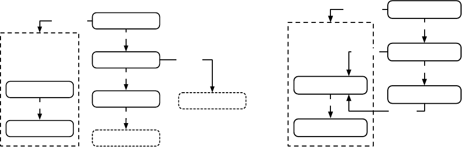
StubPipeline
ReproductionPipeline
TournamentSelection
VectorCrossoverPipeline
VectorMutationPipeline
source.0
source.0
source.0
stub-pipeline
stub
stub
source.0
source.1
StubPipeline
ReproductionPipeline
TournamentSelection
VectorCrossoverPipeline
VectorMutationPipeline
source.0
source.0
source.0
stub-pipeline
source.1
source.0
Figure 3.4 Stub Pipeline before (as specified in the parameter file) and after (as constructed). See text.
•
ec.breed.FirstCopyPipeline is a version of ReproductionPipeline but has two sources. Whenever pre-
pareToProduce(...) is called, FirstCopyPipeline is reset. the immediate next time produce(...) is called,
FirstCopyPipeline will use source #0 to fulfill the very first child produced. Thereafter it use source
#1 for all future children (and all future produce(...) calls. prepareToProduce(...) resets it again. This is
useful for performing a simple elitism in a pipeline rather than doing it at the Breeder level.
•
Last, ec.breed.StubPipeline is a version of ReproductionPipeline but includes a special subsidiary
pipeline called a stub pipeline. If some BreedingPipeline which feeds into StubPipeline’s source #0
itself contains a source simply called
stub
, then that source location is filled with that StubPipeline’s
stub pipeline. Each breeding thread gets its own copy of the stub pipeline, but within a thread stub
pipelines are not copied. Using StubPipeline you can construct elaborate Directed Acyclic Graphs in
your Pipeline.
For example, if we had:
pop.subpop.0.pipe.0 = ec.breed.StubPipeline
# Here’s the stub:
pop.subpop.0.pipe.0.stub-source = ec.breed.ReproductionPipeline
pop.subpop.0.pipe.0.stub-source.source.0 = ec.select.TournamentSelection
pop.subpop.0.pipe.0.source.0 = ec.vector.VectorCrossoverPipeline
pop.subpop.0.pipe.0.source.0.source.0 = stub
pop.subpop.0.pipe.0.source.0.source.1 = ec.vector.VectorMutationPipeline
pop.subpop.0.pipe.0.source.0.source.1.source.0 = stub
... then the ECJ would fill the two stubs such that the stub lines would be more or less like this:
# First stub pop.subpop.0.pipe.0.source.0.source.0 = ec.breed.ReproductionPipeline
pop.subpop.0.pipe.0.source.0.source.0.source.0 = ec.select.TournamentSelection
# Second stub -- note that these are the EXACT SAME OBJECTS as in the first stub!
pop.subpop.0.pipe.0.source.0.source.1.source.0 = ec.breed.ReproductionPipeline
pop.subpop.0.pipe.0.source.0.source.1.source.0.source.0 = ec.select.TournamentSelection
Figure 3.4 shows the process of building this pipeline from the stub declarations. The critical feature is
that the two stubs are replaced with the same object, not copies, and thus it’s a Directed Acyclic Graph.
The procedure is as follows. During setup(...) sources declared as a “stub” are not filled: they’re set
to null. Then after a pipeline has been cloned and handed to a thread to begin breeding, but before
produce(...) commences, the method BreedingSource.fillStubs(...) is called. This recursively traverses
90

Vector Crossover
Pipeline
Vector Mutation
Pipeline
Reproduction
Pipeline
Multi-Breeding
Pipeline
Tournament
Selection
(GP) Crossover Pipeline
Tournament
Selection
Fitness Proportionate
Selection
Sigma Scaling
Selection
New Subpopulation
Old SubpopulationOld Subpopulation
New Subpopulation
Copy Copy
Copy
Copy
Copy
Figure 3.5 Two example Breeding Pipelines (Repeat of Figure 3.3).
through the tree: whenever a StubPipeline receives this method, it fills all the null references in its
children with its stub pipeline.
StubPipelines replace all the stubs down to the next StubPipeline (which gets to replace stubs of its
own subtree). Additionally it’s possible that a stub-pipeline itself contains stubs. In this case, if a
StubPipeline A contains a child or descendent StubPipeline B whose stub-pipeline contains stubs, they
are filled with StubPipeline A’s stub-pipeline before control is handed off to StubPipeline B to start
filling.
3.5.4 Setting up a Pipeline
Setting up a pipeline using parameters sometimes isn’t entirely obvious. Let’s do the two examples shown
in Figure 3.5, in both cases setting up a pipeline for Subpopulation 0.
3.5.4.1 A Genetic Algorithm Pipeline
The left figure is a Breeding Pipeline common to the Genetic Algorithm: two Individuals are selected from
the old Subpopulation, then copied and crossed over, and the two children are then mutated and added to
the new Subpopulation. To build the pipeline, we work our way backwards: first defining the mutator as the
top element, then the crossover as its source, then the selector as the crossover’s two sources.
First the mutator. We’ll use ec.vector.VectorMutationPipeline, a common mutator for vector individuals.
Subpopulation 0’s species holds the prototypical pipeline:
pop.subpop.0.species.pipe = ec.vector.VectorMutationPipeline
91
Next we define its sole source: the crossover operator (ec.vector.VectorCrossoverPipeline)
pop.subpop.0.species.pipe.source.0 = ec.vector.VectorCrossoverPipeline
Back to building the Pipeline. Crossover has two sources. We’d like them to both be the Tournament
Selector (they could be different Tournament Selectors; it doesn’t really matter):
pop.subpop.0.species.pipe.source.0.source.0 = ec.select.TournamentSelection
pop.subpop.0.species.pipe.source.0.source.1 = same
Tournament Selection has a tournament size operator. Since we’re using the same selector for both
sources, we only need to set it once:
pop.subpop.0.species.pipe.source.0.source.0.size = 2
We could also just set the default parameter for all tournament selectors:
select.tournament.size = 2
Perhaps we’d like the second source to use a tournament size of 4. To do this we’d need to use a separate
selector, so we could do this:
pop.subpop.0.species.pipe.source.0.source.1 = ec.select.TournamentSelection
pop.subpop.0.species.pipe.source.0.source.1.size = 4
This would also override the default we just set, so it’d work whether or not we used the default-setting
approach for source 0.
VectorCrossoverPipeline and VectorMutationPipeline, discussed later, have various parameters; to
simplify the pipeline-building procedure, the ec.vector package (Section 5.1) puts these parameters in the
Species, not the pipeline. For completeness sakes, let’s include some of them here:
pop.subpop.0.species = ec.vector.FloatVectorSpecies
pop.subpop.0.species.crossover-type = one
pop.subpop.0.species.mutation-prob = 1.0
pop.subpop.0.species.mutation-type = gauss
pop.subpop.0.species.mutation-stdev = 0.01
3.5.4.2 A Genetic Programming Pipeline
The right figure is a typical Genetic Programming pipeline (see Section 5.2). We begin with the root:
pop.subpop.0.species.pipe = ec.breed.MultiBreedingPipeline
As discussed earlier, MultiBreedingPipeline can take any number of sources, so we have to specify it (to 2
here). We also need to state the sources and the probabilities for each source. We’ll do 10% Reproduction for
the first source and 90% Genetic Programming Crossover for the second. We won’t require the two sources
to produce the same number of individuals:
pop.subpop.0.species.pipe.num-sources = 2
pop.subpop.0.species.pipe.generate-max = false
pop.subpop.0.species.pipe.source.0 = ec.breed.ReproductionPipeline
pop.subpop.0.species.pipe.source.0.prob = 0.10
pop.subpop.0.species.pipe.source.1 = ec.gp.koza.CrossoverPipeline
pop.subpop.0.species.pipe.source.1.prob = 0.90
92
In Genetic Programming nearly always we’d use Tournament Selection for all selectors. But we’ll do
various selectors as shown in the Figure. First the Fitness Proportionate Selection source for the Reproduc-
tionPipeline:
pop.subpop.0.species.pipe.source.0.source.0 = ec.select.FitProportionateSelection
Next TournamentSelection (tournament size 7) as Crossover’s first source:
pop.subpop.0.species.pipe.source.1.source.0 = ec.select.TournamentSelection
pop.subpop.0.species.pipe.source.1.source.0.size = 7
Last, Sigma Scaling Selection as Crossover’s second source:
pop.subpop.0.species.pipe.source.1.source.1 = ec.select.SigmaScalingSelection
pop.subpop.0.species.pipe.source.1.source.1.scaled-fitness-floor = 0.1
(The default setting for
pop.subpop.0.species.pipe.source.1.source.1.scaled-fitness-floor
is
already 0.1, so it doesn’t really need to be set.)
3.6 Exchangers
An Exchanger is a subclass of ec.Exchanger, and is called both before and after breeding. Exchangers form
the basis of Island Models in ECJ and will be discussed in-depth in Section 6.2.
Besides setup(...), Exchangers have three basic functions, called at different times in the evolutionary
cycle:
public abstract Population preBreedingExchangePopulation(EvolutionState state);
public abstract Population postBreedingExchangePopulation(EvolutionState state);
public abstract String runComplete(EvolutionState state);
The first method is called prior to breeding a population. It’s largely available for Island Models to ship
off members of the Population to remote ECJ processes. The second method is called immediately after
breeding a Population, and enables Island Models to import members from remote ECJ processes, possibly
displacing newly-bred individuals. The third method is called after preBreedingExchangePopulation(...) to
determine whether or not the Exchanger thinks ECJ should shut down its process because some other process
has found the optimal individual. To cause ECJ to shutdown, return a String with a shutdown message of
some sort (which will get printed out); otherwise return null.
Unless you’re doing Island Models, almost certainly you’ll use a default Exchanger called
ec.simple.SimpleExchanger which does nothing to the Population at all. To wit:
exch = ec.simple.SimpleExchanger
3.7 Statistics
ECJ provides a large number of
statistics hooks
, places where ECJ will call arbitrary methods on a Statistics
object throughout the process. These hooks give you a chance to examine the current process at all sorts of
stages and output useful logging information as you see fit. Statistics objects are subclasses of ec.Statistics
and often follow one or more
statistics forms
which provide different alternative Statistics hooks. For
example, ec.steadystate.SteadyStateStatisticsForm, discussed later in Section 4.2, stipulates hooks for Statistics
in steady-state evolution. The Statistics class ec.simple.SimpleStatistics and has hooks for both regular
generational evolution (defined in ec.Statistics) and SteadyStateStatisticsForm. Another basic Statistics class,
93
ec.simple.SimpleShortStatistics, has hooks only for generational evolution. Other Statistics classes exist, such
as those found in Genetic Programming (Section 5.2).
You can have as many Statistics objects as you want, but one Statistics object (usually arbitrarily chosen)
must be the statistics root. To define an ec.simple.SimpleStatistics as the root, you say:
stat = ec.simple.SimpleStatistics
Statistics objects usually, but not always, have a
file
which they log their statistics results out to. It’s
common to stipulate that file as:
stat.file = $out.stat
This tells SimpleStatistics to write to a file called out.stat, located right where the user launched ECJ (for a
reminder on the meaning of the “
$
”, see Section 2.1.2). If you are running with multiple jobs (Section 2.5),
ECJ will automatically append the prefix ”jobs.n.” to this filename, where
n
is the job number. Thus the
statistics file for job number 5 will be ”jobs.5.out.stat”. If no file is provided, SimpleStatistics will simply
print out to the screen.
If ECJ is restarted from a checkpoint, SimpleStatistics will append to existing files rather than overwriting
them. SimpleStatistics also has an option to compress the file using GZIP (and thus add a ”.gz” suffix at the
very end, as in ”jobs.5.out.stat.gz”. Note that if this option is used, SimpleStatistics will simply overwrite the
file if restarted from a checkpoint. The parameter is:
stat.gzip = true
For each generation, the SimpleStatistics object prints out the best Individual of the generation using the
printIndividualForHumans(...) method. For example, generation 0 might have:
Generation: 0
Best Individual:
Subpopulation 0:
Evaluated: T
Fitness: -1503.8322
2.4502202187677815 0.9879236448665667 0.7631586426217085 0.6854305126240172
If you would like to prevent this per-generational statistics from being written out to the log, you can say:
stat.do-generation = false
At the end of the run, the SimpleStatistics object prints out the best Individual of the run:
Best Individual of Run:
Subpopulation 0:
Evaluated: T
Fitness: -185.78166
-1.0393115193403102 -2.006026366200021 -0.03642166362331428 -1.1196984643947918
If you would like to prevent this information from being written to the log, say:
stat.do-final = false
At the end of the run, the SimpleStatistics object finally calls the describe(...) method on the Evaluator to
get it to write out a phenotypical description of the performance of the best individual of the run (see Section
3.4.1). Only some problems implement the describe(...) method: for example the Artificial Ant problem will
use it to print out a map of the food trail by the best discovered ant algorithm, such as:
94
Best Individual’s Map
=====================
acdgf.......f............m......
...h........g............l......
...i........h...........+k##++..
...j........i.yzabqdefghij...#..
...k........j.x...pon...#....#..
...lmnopqrstkvw....tmrqp+....+..
............l......ul..o.....#..
............mbazyxwvk..n.....+..
............n.......j..m.....+..
............o.......i..l.....#..
............p.......h..k.....+..
............q.......g..j.....+..
............r.......f..i.....#..
............s.......e..h.....+..
............t.......d..g++###+..
............u...+zabc..f........
............v...vy.....e........
............w...ux.....d........
............x...t......c#+++....
............y...s......b...#....
............z...r......a...+....
............a...q......z...+....
............b...p......y++#+....
...........tc...o......x........
.wvuts+####ud...n......w........
.x...r.....ve...m......v........
.y...qpo...wf...l......u........
.z.....n###xghijk......t........
.a.....m...y...........s........
.b.....l...z...........r........
.cdehijk..bcd..........q........
...fg.......e..........pon......
If you don’t want to see stuff like this at the end of your statistics file, say:
stat.do-description = false
SimpleStatistics can also call describe(...) to print out stuff like this every generation, for the best individual
of that generation. For backwards-compatibility reasons by default it’s turned off. To turn it on, say:
stat.do-per-generation-description = true
Finally, SimpleStatistics will also write out a message (see Section 2.2) to stdout, which prints to the
screen some short statistical information about each generation. For example:
Initializing Generation 0
Subpop 0 best fitness of generation Fitness: Standardized=63.0 Adjusted=0.015625 Hits=26
Generation 1
Subpop 0 best fitness of generation Fitness: Standardized=57.0 Adjusted=0.01724138 Hits=32
Generation 2
Subpop 0 best fitness of generation Fitness: Standardized=48.0 Adjusted=0.020408163 Hits=41
Generation 3
Subpop 0 best fitness of generation Fitness: Standardized=48.0 Adjusted=0.020408163 Hits=41
Generation 4
Subpop 0 best fitness of generation Fitness: Standardized=40.0 Adjusted=0.024390243 Hits=49
Generation 5
Subpop 0 best fitness of generation Fitness: Standardized=38.0 Adjusted=0.025641026 Hits=51
...
95
If you would prefer not to see this information, just say:
stat.do-message = false
... and what you’ll get on the screen will be:
Initializing Generation 0
Generation 1
Generation 2
Generation 3
Generation 4
Generation 5
...
3.7.1 Creating a Statistics Chain
So how do you add additional Statistics objects? As children of the root, or of one another. Any Statistics
object can have some
n
children. Children are called the same hooks as their parents are. To add another
Statistics object (say, ec.simple.SimpleShortStatistics, we might add a child to the root:
stat.num-children = 1
stat.child.0 = ec.simple.SimpleShortStatistics
stat.child.0.file = $out2.stat
Notice that the file has changed: you don’t want both Statistics objects writing to the same file! If we
wanted to add a third Statistics object (say, another ec.simple.SimpleShortStatistics), we could do it this way:
stat.num-children = 2
stat.child.0 = ec.simple.SimpleShortStatistics
stat.child.0.file = $out2.stat
stat.child.1 = ec.simple.SimpleShortStatistics
stat.child.1.file = $out3.stat
...or we could do it this way:
stat.num-children = 1
stat.child.0 = ec.simple.SimpleShortStatistics
stat.child.0.file = $out2.stat
stat.child.0.num-children = 1
stat.child.0.child.0 = ec.simple.SimpleShortStatistics
stat.child.0.child.0.file = $out3.stat
The point is, you can hang a Statistics object as a child of any other Statistics object. Pick your poison.
3.7.2 Tabular Statistics
SimpleShortStatistics writes out a different kind of statistics from SimpleStatistics In its basic form, for each
generation it writes out a line of the following values, each separated by a space.
1. The generation number
2. The mean fitness of the entire population for this generation
3. The best fitness of the entire population for this generation
4. The best fitness of the entire population so far in the run
96
For example, we might have values like this...
0 -1851.9916400146485 -1559.68 -1559.68
1 -1801.2400487060547 -1557.7627 -1557.7627
2 -1758.2322434082032 -1513.4955 -1513.4955
3 -1715.5276463623047 -1420.0074 -1420.0074
4 -1675.379030883789 -1459.842 -1420.0074
5 -1637.332774291992 -1426.798 -1420.0074
...
You can add sizing information as well. If you set:
stat.child.0.do-size = true
... you’ll get
1. The generation number
2. (If do-size is true) The average size of an individual this generation
3. (If do-size is true) The average size of an individual so far in the run
4. (If do-size is true) The size of the best individual this generation
5. (If do-size is true) The size of the best individual so far in the run
6. The mean fitness of the entire population for this generation
7. The best fitness of the entire population for this generation
8. The best fitness of the entire population so far in the run
You can also turn on timing information. If you set:
stat.child.0.do-size = true
stat.child.0.do-time = true
You’ll additionally get:
1. The generation number
2.
(If
do-time
is true) How long initialization took in milliseconds, or how long the previous generation
took to breed to form this generation
3. (If do-time is true) How long evaluation took in milliseconds this generation
4. (If do-size is true) The average size of an individual this generation
5. (If do-size is true) The average size of an individual so far in the run
6. (If do-size is true) The size of the best individual this generation
7. (If do-size is true) The size of the best individual so far in the run
8. The mean fitness of the entire population for this generation
9. The best fitness of the entire population for this generation
10. The best fitness of the entire population so far in the run
97
Finally, you can add in per-subpopulation information. If you set:
stat.child.0.do-size = true
stat.child.0.do-time = true
stat.child.0.do-subpops = true
you get the whole shebang:
1. The generation number
2.
(If
do-time
is true) How long initialization took in milliseconds, or how long the previous generation
took to breed to form this generation
3. (If do-time is true) How long evaluation took in milliseconds this generation
4. Once for each subpopulation...
(a) (If do-size is true) The average size of an individual this generation for this subpopulation
(b) (If do-size is true) The average size of an individual so far in the run for this subpopulation
(c) (If do-size is true) The size of the best individual this generation for this subpopulation
(d) (If do-size is true) The size of the best individual so far in the run for this subpopulation
(e) The mean fitness of the subpopulation for this generation
(f) The best fitness of the subpopulation for this generation
(g) The best fitness of the subpopulation so far in the run
5. (If do-size is true) The average size of an individual this generation
6. (If do-size is true) The average size of an individual so far in the run
7. (If do-size is true) The size of the best individual this generation
8. (If do-size is true) The size of the best individual so far in the run
9. The mean fitness of the entire population for this generation
10. The best fitness of the entire population for this generation
11. The best fitness of the entire population so far in the run
Restricting Rows with a Modulus
If you’ve got a lot of subpopulations, or very long runs, there’s another
way you can reduce the size of your file: only output results ever
n
generations. For example, if we had set
stat.child.0.modulus = 2
.. then the aforementioned statistics would look like this:
0 -1851.9916400146485 -1559.68 -1559.68
2 -1758.2322434082032 -1513.4955 -1513.4955
4 -1675.379030883789 -1459.842 -1420.0074
...
An important thing to keep in mind. Let’s say you want to run for 1000 generations and gather the
last. Thus your generations are 0 through 999. If you did a modulus of 100 (say), your reported results
would be for generations 0, 100, 200, 300, 400, 500, 600, 700, 800, and 900. That is, you’d have lost the last 99
generations, including the final generation. How might you fix this? The easiest way is to simply run for
1001 generations. Then your last reported generation will be 1000.
98
3.7.3 Quieting the Statistics
Many statistics objects have options to prevent them from either writing to the screen, or creating statistics
logs, or both. Because statistics classes vary in the kinds of files they write, the options they have for quieting
them vary from class to class.
Basic subclasses of SimpleStatistics (such as ec.simple.SimpleStatistics,ec.simple.SimpleShortStatistics, and
ec.gp.koza.KozaShortStatistics) allow you to do any of the following:
• Not print to the screen
• Not create statistics logs or print to them
• Both of the above
To do any of these with the first Statistics object in the Statistics chain, you’d say:
# Pick one of these:
# Turn off printing to the screen
stat.silent.print = true
# Do not create statistics logs (don’t even open them)
stat.silent.file = true
# Do both of the above
stat.silent = true
Obviously for other Statistics objects in your chain, it’s slightly different. For example, to do the same to
the first child object in the chain, you might say:
# Pick one of these:
# Turn off printing to the screen
stat.child.0.silent.print = true
# Do not create statistics logs (don’t even open them)
stat.child.0.silent.file = true
# Do both of the above
stat.child.0.silent = true
You should be made aware of the important difference between these parameters and the “do-...” param-
eters discussed earlier in Sections 5.2.3.5 and 3.7.2. The “do-...” parameters control what kinds of messages
will be written out to logs or to the screen. Whereas the “silent” parameters are much cruder: they control
whether anything will be written at all. Note that the “do-...” parameters don’t prevent statistics files from
being opened or created, even if nothing is written to them. However the “silent” parameters will stop the
files from even being opened or created in the first place.
Also note the relationship between these “silent” parameters and the
silent
parameter from Section
2.2.2. That second parameter cuts off the stderr and stdout streams entirely, preventing anything from being
written to the screen; it takes precedence over the settings of the “silent” parameters in this section.
3.7.4 Implementing a Statistics Object
A basic Statistics object implements one or more of the following hooks:
99

public void preInitializationStatistics(EvolutionState state);
public void postInitializationStatistics(EvolutionState state); // Generational
public void preCheckpointStatistics(EvolutionState state);
public void postCheckpointStatistics(EvolutionState state);
public void preEvaluationStatistics(EvolutionState state); // Generational
public void postEvaluationStatistics(EvolutionState state); // Generational
public void prePreBreedingExchangeStatistics(EvolutionState state);
public void postPreBreedingExchangeStatistics(EvolutionState state);
public void preBreedingStatistics(EvolutionState state); // Generational
public void postBreedingStatistics(EvolutionState state); // Generational
public void prePostBreedingExchangeStatistics(EvolutionState state);
public void postPostBreedingExchangeStatistics(EvolutionState state);
public void finalStatistics(EvolutionState state, int result);
When these statistics hooks are called should be self-explanatory from the method name. Note that
the methods marked Generational are only called by generational EvolutionState objects — notably the
ec.simple.SimpleEvolutionState object. There are also some additional hooks called by the ec.steadystate
package for steady-state evolution (see Section 4.2.1).
The finalStatistics(...) method, called at the end of an evolutionary run, contains one additional argument,
result. This argument will be either ec.EvolutionState.R SUCCESS or ec.EvolutionState.R FAILURE. Success
simply means that the optimal individual was discovered, and nothing more.
Whenever you override one of these methods, make certain to call super(...) first. Let’s say that we’d like
to know what the size is of the very first individual created after initialization. We might create a Statistics
subclass which overrides this to print this size out to the screen:
public void postInitializationStatistics(EvolutionState state)
{
super.postInitializationStatistics(state); // always call this
state.output.println(state.population.subpops.get(0).individuals.get(0).size(), 0); // stdout
}
We could also write to a file, but to do so we’d need to determine the file name. We could do it in a
manner similar to SimpleStatistics (ignoring the compression):
public static final String P_STATISTICS_FILE = "file";
public int log = 0; // 0 by default means stdout
public void setup(final EvolutionState state, final Parameter base)
{
super.setup(state, base);
File statisticsFile = state.parameters.getFile(base.push(P_STATISTICS_FILE),null);
if (statisticsFile!=null) try
{
log = state.output.addLog(statisticsFile, true, false, null, false);
}
catch (IOException i)
{
state.output.fatal("An IOException occurred trying to create the log "
+ statisticsFile + ":\n" + i);
}
// else we’ll just keep the log at 0, which is stdout
}
Now we can write out to the log:
100

public void postInitializationStatistics(EvolutionState state)
{
super.postInitializationStatistics(state); // always call this
state.output.println(state.population.subpops.get(0).individuals.get(0).size(), log);
}
3.8 Debugging an Evolutionary Process
A hint. One helpful way to debug ECJ is via BeanShell (http://www.beanshell.org). This tool is essentially a
command-line for Java. Using it, we can create an ECJ process and get it going quite easily. Let’s say that the
parameter file is called ”foo.params”. We can type the following into BeanShell:
show();
import ec.*;
args = new String[] { "-file", "foo.params" };
database = Evolve.loadParameterDatabase(args);
state = Evolve.initialize(database, 0);
state.run(EvolutionState.C_STARTED_FRESH);
Evolve.cleanup(state);
This is basically a variation of the main code found in Section 2.5. When state.run(...) is executed, ECJ will
go through the entire evolutionary run. It turns out that state.run(...) is really just a cover for three methods
(at least, if we’re starting from scratch rather than from a checkpoint). They are: first calling state.startFresh(),
then repeatedly calling state.evolve(), and when it returns something other than state.R NOTDONE, finally
calling state.finish(...), passing in what was returned. In other words:
show();
import ec.*;
args = new String[] { "-file", "foo.params" };
database = Evolve.loadParameterDatabase(args);
state = Evolve.initialize(database, 0);
state.startFresh();
result = EvolutionState.R_NOTDONE;
while( result == EvolutionState.R_NOTDONE )
{
result = state.evolve();
}
state.finish(result);
Evolve.cleanup(state);
So how can we use this for debugging? Well, BeanShell gives us full access to Java. Let’s try it on the
ecsuite.params file. We begin with the preliminaries:
show();
import ec.*;
args = new String[] { "-file", "ecsuite.params" };
BeanShell responds with:
<[Ljava.lang.String;@39617189>
This is the String array. We continue with:
101
database = Evolve.loadParameterDatabase(args);
BeanShell responds with the ParameterDatabase:
<{} : ({} : ({eval=ec.simple.SimpleEvaluator, pop.subpop.0=ec.Subpopulation,
quit-on-run-complete=true, generations=1000,
pop.subpop.0.species.pipe.source.0=ec.vector.breed.VectorCrossoverPipeline,
pop.subpop.0.species.min-gene=-5.12, eval.problem=ec.app.ecsuite.ECSuite,
state=ec.simple.SimpleEvolutionState, pop.subpop.0.species.mutation-type=gauss,
pop=ec.Population, pop.subpop.0.duplicate-retries=2, select.tournament.size=2,
pop.subpops=1, pop.subpop.0.species.mutation-stdev=0.01,
pop.subpop.0.species.pipe=ec.vector.breed.VectorMutationPipeline,
pop.subpop.0.species.max-gene=5.12, pop.subpop.0.species.pipe.source.0.source.1=same,
pop.subpop.0.species.pipe.source.0.source.0=ec.select.TournamentSelection,
pop.subpop.0.species=ec.vector.FloatVectorSpecies, breed=ec.simple.SimpleBreeder,
pop.subpop.0.species.mutation-prob=1.0, pop.subpop.0.species.genome-size=100,
pop.subpop.0.species.crossover-type=one, finish=ec.simple.SimpleFinisher,
parent.0=../../ec.params, init=ec.simple.SimpleInitializer,
pop.subpop.0.species.ind=ec.vector.DoubleVectorIndividual,
pop.subpop.0.species.fitness=ec.simple.SimpleFitness, pop.subpop.0.size=1000,
eval.problem.type=rastrigin, stat=ec.simple.SimpleStatistics,
exch=ec.simple.SimpleExchanger, stat.file=$out.stat} : ({checkpoint-modulo=1,
evalthreads=1, checkpoint=false, breedthreads=1, checkpoint-prefix=ec, seed.0=time})))>
Now we initialize the EvolutionState from the database:
state = Evolve.initialize(database, 0);
This causes ECJ to start printing to the screen something along these lines:
| ECJ
| An evolutionary computation system (version 19)
| By Sean Luke
| Contributors: L. Panait, G. Balan, S. Paus, Z. Skolicki, R. Kicinger, E. Popovici,
| K. Sullivan, J. Harrison, J. Bassett, R. Hubley, A. Desai, A. Chircop,
| J. Compton, W. Haddon, S. Donnelly, B. Jamil, and J. O’Beirne
| URL: http://cs.gmu.edu/~eclab/projects/ecj/
| Mail: ecj-help@cs.gmu.edu
| (better: join ECJ-INTEREST at URL above)
| Date: July 10, 2009
| Current Java: 1.6.0_20 / Java HotSpot(TM) 64-Bit Server VM-16.3-b01-279
| Required Minimum Java: 1.4
Threads: breed/1 eval/1
Seed: 1853290822
<ec.simple.SimpleEvolutionState@1f5b0afd>
Notice the last line — BeanShell is returning the EvolutionState. Now we fire up the EvolutionState to
initialize the first population:
state.startFresh();
... and get back:
102
Setting up
Initializing Generation 0
The first population has been created. Let’s look at the first Individual:
state.population.subpops.get(0).individuals.get(0);
This produces:
<ec.vector.DoubleVectorIndividual@87740549{699618236}>
Not very helpful. Instead, let’s have it printed:
state.population.subpops.get(0).individuals.get(0).printIndividualForHumans(state, 0);
This produces something more useful:
Evaluated: F
Fitness: 0.0
-4.3846934361930945 4.051323475292111 2.750742781209575 -2.1599970035296088
3.5139838195638236 -4.326431483145531 -1.5799722524229094 -4.64489169381555
-4.809825694271426 -0.6969239813124668 -4.322411553562226 4.8723307904232565
2.8978088843319947 -4.311437772193992 -1.556903048013028 2.876699531303326
-1.5461627480422133 -3.406470106152458 0.3510231690045371 -1.26870148662141
-2.9943682283832675 -1.1321325429409796 -4.780798908878881 -2.789054768098288
2.7957975471728034 -2.4529277934521363 0.06864524959557006 -2.807030901927618
-3.817734647565329 3.0018199187738803 3.893346256074625 -4.1700250768556355
-3.3035366716916714 -1.5300889532287534 -1.2924365390313826 2.6878356877535623
4.344108056131552 1.0732802812225044 1.804809997034555 0.6627493849916508
1.6556742582736854 -3.8324177646471913 0.2901815515514814 -0.5045301890375606
-2.755111883054377 -4.057309896490254 -2.097059222061862 -2.062611078568839
3.676980437590175 3.4010063830636517 5.001876654997903 2.3637174851440808
-2.3242430228722846 -0.2027490501614988 4.948796285958214 3.645393286308912
-0.9981883696957627 -2.4911201811073296 2.281601570422807 -3.0028177298996583
-0.6949487749058276 2.4115725052273005 2.2705630820859133 3.8198793397976756
3.927188087275849 3.5439728479577974 4.195897069928313 4.064291914283307
-1.6071055662352376 -0.45138576561254506 0.5382601925283925 2.2824947546503687
-0.0837300863613164 -2.4997930740673895 0.06696037058102089 1.782243737261787
-3.390249634178219 4.669336185081783 2.371290190775591 1.8743739255868377
0.13349732700681827 2.808175830805574 -4.2297879656940705 -0.5781599273148448
3.4174595199606577 2.5509508748123793 0.9574470878471297 1.181916131827328
3.3128918249657184 3.5085201808925843 -0.8921840350705308 -4.016933626993176
2.5591127486976983 1.580181276449899 -0.6102226049991097 1.0644092417475743
0.5897983455130262 2.5504671849586904 -2.230897886457403 1.8133759722806326
Now we’re getting somewhere. You could print out all the individuals like this:
for(int i = 0; i < state.population.subpops.get(0).individuals.size(); i++ )
state.population.subpops.get(0).individuals.get(i).printIndividualForHumans(state, 0);
... but I won’t torture you with what comes out. Instead, notice that the Individual has not been evaluated
yet — just initialized with the Population. We go through one evolutionary loop — evaluating the individuals
and breeding a new Population — by calling
state.evolve();
103

This produces:
Subpop 0 best fitness of generation: Fitness: -1493.534
<2>
The first line was printed to the screen. The second line indicates what state.evolve() returned. 2 is the
value of EvolutionState.R NOTDONE, indicating that the process needs to be evolved more.
Let’s look at that first individual again:
state.population.subpops.get(0).individuals.get(0).printIndividualForHumans(state, 0);
...yielding...
Evaluated: F
Fitness: -1806.1432
-1.5595820609909528 -2.9941135630034292 -3.188550961391961 0.8673223056511647
2.4308132097811472 -3.6298006589453533 -4.62193495641744 1.7381186900517611
-3.2707539202577953 -2.8517369832386144 -4.701099579700639 1.1683479248633841
0.10118833856168477 2.7982137159130787 -1.3673458253800685 -4.548719487000453
-1.7852252742508177 -1.662999422245311 -4.891889992368657 2.0689413066938824
4.64815452362056 4.03620579726471 -2.6065781548997413 2.8384398494616585
-1.6231723965539844 -0.19641152832494305 -0.8025430015631594 -4.337733534634894
-4.259188069209607 0.0974585410674078 4.878006291864429 4.187577755641656
3.9507153065207605 -3.3456633008586922 3.7163666200189596 -0.7581028665673978
4.28299933455259 1.8522464455693997 4.4324032846812935 -1.3209545115697914
4.239911043319335 -2.7741200087506352 -3.181419981396656 -0.4574562816089688
3.9209870275697982 0.31049605413333237 -0.46868091240064014 -4.570530964131764
-0.9126484738704782 3.6348709305820153 -1.800821491837854 -0.8548399118205554
-1.6874962921883667 2.628667604603462 0.060377157894385663 3.194354857448187
1.2106237734207714 -3.477534436566739 1.919326547065771 -3.74880517912247
4.076653684533312 -2.9153006121227034 -2.4460232838375973 0.6128610868842217
0.7785108819209824 -1.213371979065718 3.2441049504290587 -1.352037820951835
1.151316091162472 0.3915293759690397 -0.15229424767569708 1.8192706794904545
-3.057866603248519 -3.2217378304635926 3.7963181147558447 1.9609441782591566
2.1365399986514815 -0.7608502832241196 -1.2202190662246202 -3.2592371482282956
-2.612971504172355 3.1496849987738167 -5.083084415090031 -4.243405086300351
3.8516939433487387 -4.87008846122508 1.012854792831603 3.77728764346906
2.843506550933032 4.705462097924235 1.4291349248648448 3.8398215224809875
1.1776568359195472 -4.784524531392207 2.765230136436807 -2.6521295800350555
-2.271480494878218 -2.018481022639772 -2.2536397207045686 -1.5048357519436404
It’s a different Individual: the next generation one to be exact. Notice that although it has a “fitness”, in
fact it’s not been evaluated: the “fitness” is just nonsense cloned from a previous Individual.
So how do you see a population with fitness-evaluated Individuals? Generational ECJ EvolutionState
processes assess the fitness of a Population, then create a new Population and throw away the old one. You
can hold onto the old Population pretty easily. Just do this:
p = state.population;
state.evolve();
Now pholds the old Population, filled with now-evaluated Individuals, and state.population holds the
next-generation Population, which hasn’t been evaluated yet. For example, if you say:
p.subpops[0].individuals.get(0).printIndividualForHumans(state, 0);
... you will get back something like this:
104
Evaluated: T
Fitness: -1779.4391
-1.5595820609909528 -2.9941135630034292 -3.188550961391961 0.8673223056511647
2.4308132097811472 -3.6298006589453533 -4.62193495641744 1.7381186900517611
-3.2707539202577953 -2.8517369832386144 -4.701099579700639 1.1683479248633841
0.10118833856168477 2.7982137159130787 -1.3673458253800685 -4.548719487000453
-1.7852252742508177 -1.662999422245311 -4.891889992368657 2.0689413066938824
4.64815452362056 4.03620579726471 -2.6065781548997413 2.8384398494616585
-1.6231723965539844 -0.19641152832494305 -0.8025430015631594 -4.337733534634894
-4.259188069209607 0.0974585410674078 4.878006291864429 4.187577755641656
3.9507153065207605 -3.3456633008586922 3.7163666200189596 -0.7581028665673978
4.28299933455259 1.8522464455693997 4.4324032846812935 -1.3209545115697914
4.239911043319335 -2.7741200087506352 -3.181419981396656 -0.4574562816089688
3.9209870275697982 0.31049605413333237 -0.46868091240064014 -4.570530964131764
-0.9126484738704782 3.6348709305820153 -1.800821491837854 -0.8548399118205554
-1.6874962921883667 2.628667604603462 0.060377157894385663 3.194354857448187
1.2106237734207714 -3.477534436566739 1.919326547065771 -3.74880517912247
4.076653684533312 -2.9153006121227034 -2.4460232838375973 0.6128610868842217
0.7785108819209824 -1.213371979065718 3.2441049504290587 -1.352037820951835
1.151316091162472 0.3915293759690397 -0.15229424767569708 1.8192706794904545
-3.057866603248519 -3.2217378304635926 3.7963181147558447 1.9609441782591566
2.1365399986514815 -0.7608502832241196 -1.2202190662246202 -3.2592371482282956
-2.612971504172355 3.1496849987738167 -5.083084415090031 -4.243405086300351
3.8516939433487387 -4.87008846122508 1.012854792831603 3.77728764346906
2.843506550933032 4.705462097924235 1.4291349248648448 3.8398215224809875
1.1776568359195472 -4.784524531392207 2.765230136436807 -2.6521295800350555
-2.271480494878218 -2.018481022639772 -2.2536397207045686 -1.5048357519436404
Notice that this Individual has been evaluated. Its Fitness is valid.
For more on debugging ECJ, see Section 2.1.7.
105
106
Chapter 4
Basic Evolutionary Processes
4.1 Generational Evolution
ECJ is most commonly used for generational evolution: where a whole Population is evaluated, then updated,
at a time. There are a number of packages which use generational evolution, but the two most common are
the ec.simple package, which does Genetic Algorithm style generational evolution, and the ec.es package
which does Evolution Strategies.
Generations and Evaluations
Generational Evolution, of course, has generations. A generation is one
iteration of the top-level evolutionary loop. It also has evaluations, which is the number of times an individual
has been (potentially) assigned a fitness. By potentially we mean that if an individual could have been tested,
but the Problem chose not to because the individual had already been assessed (its evaluated flag was raised),
this still counts as an evaluation.
When the population does not change in size (which is often the case), the number of generations
transpired is equal to the number of evaluations times the total size of the population. But when the
population size changes, this relationship is no longer necessarily true.
The generational facility will run until one of two events has happened:
• The maximum number of generations has been exceeded.
•
The maximum number of evaluations has been exceeded. ECJ will then continue evaluating individuals
until it hits the next generation boundary, at which point it quits. For example, let’s say that your
system is supposed to run for seven evaluations, but in fact you a total population size of four, so your
generation boundary is every four individuals. When seven evaluations has been reached, there’s still
one more individual left in the population to be evaluated before the next generation boundary. ECJ
will thus evaluate eight individuals.
You specify the maximum number of generations as:
generations = 100
ECJ will set the SimpleEvolutionState.numGenerations variable to be set to this value (100).
You specify the maximum number of evaluations as:
evaluations = 10000
ECJ will set the SimpleEvolutionState.numEvaluations variable to this value (10000).
You must specify one or the other of these. If you specify both of them, then you will get a warning that
either event could occur and ECJ can’t predict which one will happen first.
107
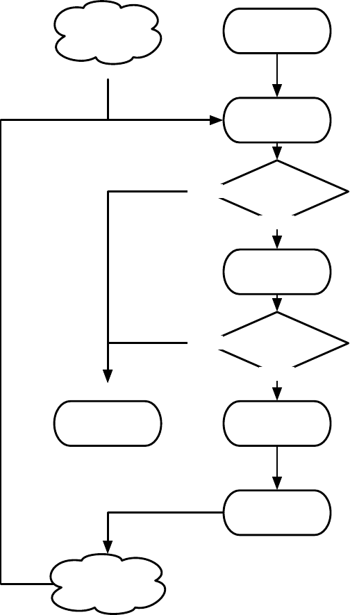
Evaluator
Pre-Evaluation Statistics
Post-Evaluation Statistics
Pre-Breeding
Exchange
Pre-Pre-Breeding Exchange Statistics
Post-Pre-Breeding Exchange Statistics
Breeding
Pre-Breeding Statistics
Post-Breeding Statistics
Post-Breeding
Exchange
Pre-Post-Breeding Exchange Statistics
Post-Post-Breeding Exchange Statistics
Initializer
Pre-Initialization Statistics
Post-Initialization Statistics
Initialize Exchanger, Evaluator
Finisher
Pre-Finishing Statistics
Shut Down Exchanger, Evaluator
Out of time or
want to quit?
Recover
from
Checkpoint
Reinitialize Exchanger, Evaluator
Optionally
Checkpoint
Optional Post-Checkpoint Statistics
Optional Pre-Checkpoint Statistics
Increment Generation
Want to quit?
NO
NO
YES
YES
Figure 4.1 Top-Level Loop of ECJ’s SimpleEvolutionState class, used for basic generational EC algorithms. Various sub-operations are
shown occurring before or after the primary operations. The full population is revised each iteration. A repeat of Figure 1.1.
108
The current generation is stored in the variable EvolutionState.generation, and is updated on a generation
boundary. The current number of evaluations is stored in the variable EvolutionState.evaluation, and is
updated . Note that these variables will only be updated on a generation boundary.
4.1.1 The Genetic Algorithm (The ec.simple Package)
We’ve pretty much covered everything in the ec.simple package throughout Section 3. But just a quick
reminder:
•
ec.simple.SimpleEvolutionState subclasses ec.EvolutionState to provide the generational top-level loop
shown in Figure 4.1. Each generation the entire Population is handed to the Evaluator, then the Breeder.
The class adds no new parameters beyond those defined in EvolutionState.
•
ec.simple.SimpleBreeder subclasses ec.Breeder to provide multithreaded breeding and elitism. Simple-
Breeder was discussed at length in Section 3.5.
•
ec.simple.SimpleEvaluator subclasses ec.Evaluator to provide multithreaded evaluation. SimpleEvaluator
adds no new parameters beyond those defined in Evaluator, and was discussed at length in Section 3.4.
•
ec.simple.SimpleFitness subclasses ec.Fitness to provide a simple fitness consisting of a double floating-
point number, where higher fitness values are preferred. SimpleFitness also holds a boolean flag
indicating whether the fitness assigned is the optimal fitness. SimpleFitness adds no new parameters
beyond those defined in Fitness, and was discussed at length in Section 3.2.5.
•
ec.simple.SimpleProblemForm defines the kind of methods which must be implemented by Problems
used by a SimpleEvaluator, and was discussed at length in Section 3.4.1. As a reminder, the two
methods defined by SimpleProblemForm are evaluate(...), which evaluates an individual and sets its
fitness; and describe(...), which evaluates an individual solely for the purpose of writing a detailed
description about the individual’s performance out to a stream. They look like this:
public void evaluate(EvolutionState state, Individual ind,
int subpopulation, int threadnum);
public void describe(EvolutionState state, Individual ind,
int subpopulation, int threadnum, int log);
•
ec.simple.SimpleInitializer subclasses ec.Initializer to provide multithreaded breeding and elitism. Sim-
pleInitializer adds no new parameters beyond those defined in Initializer, and was discussed at length
in Section 3.3.
•
ec.simple.SimpleFinisher subclasses ec.Finisher and does nothing at all. SimpleFinisher was discussed at
length (so to speak) in Section 3.3.
•
ec.simple.SimpleExchanger subclasses ec.Exchanger and does nothing at all. SimpleExchanger was
mentioned in Section 3.6.
•
ec.simple.SimpleStatistics subclasses ec.Statistics and outputs the best-of-generation individual each
generation, plus the best-of-run individual at the end. SimpleStatistics was discussed at length in
Section 5.2.3.5.
•
ec.simple.SimpleShortStatistics subclasses ec.Statistics and gives numerical statistics about the progress
of the generation. SimpleStatistics was also discussed at length in Section 5.2.3.5.
•
ec.simple.SimpleDefaults implements ec.DefaultsForm and provides the package default parameter base.
109
An Example
Let’s put these together to do a simple genetic algorithm. We start with the basic parameters:
# Threads and Seeds
evalthreads = 1
breedthreads = 1
seed.0 = time
# Checkpointing
checkpoint = false
checkpoint-modulo = 1
checkpoint-prefix = ec
Next a basic generational setup:
# The basic setup
state = ec.simple.SimpleEvolutionState
init = ec.simple.SimpleInitializer
finish = ec.simple.SimpleFinisher
exch = ec.simple.SimpleExchanger
breed = ec.simple.SimpleBreeder
eval = ec.simple.SimpleEvaluator
stat = ec.simple.SimpleStatistics
pop = ec.Population
# Basic parameters
generations = 200
quit-on-run-complete = true
pop.subpops = 1
pop.subpops.0 = ec.Subpopulation
pop.subpop.0.size = 1000
pop.subpop.0.duplicate-retries = 0
breed.elite.0 = 0
stat.file = $out.stat
We’ll use Individuals of the form ec.vector.IntegerVectorIndividual, discussed later in Section 5.1. This is
not much more than a cover for a one-dimensional array of integers:
# Representation
pop.subpops.0.species = ec.vector.IntegerVectorSpecies
pop.subpop.0.species.ind = ec.vector.IntegerVectorIndividual
pop.subpop.0.species.genome-size = 100
For fitness, we’ll use SimpleFitness:
# Fitness
pop.subpop.0.species.fitness = ec.simple.SimpleFitness
In Section 3.5.4 we laid out a simple Genetic Algorithm Pipeline:
# Pipeline
pop.subpop.0.species.pipe = ec.vector.VectorMutationPipeline
pop.subpop.0.species.pipe.source.0 = ec.vector.VectorCrossoverPipeline
pop.subpop.0.species.pipe.source.0.source.0 = ec.select.TournamentSelection
pop.subpop.0.species.pipe.source.0.source.1 = same
select.tournament.size = 2
Because they are so common, Vector pipelines are unusual in that they define certain probabilities in
110
Species rather than in the Pipeline, mostly for simplicity. We haven’t discussed these yet (we’ll get to them in
Section 5.1), but here’s one possibility:
pop.subpop.0.species.crossover-type = one
pop.subpop.0.species.mutation-prob = 0.01
In Section 3.4.2 we defined a simple Problem in which the fitness of an IntegerVectorIndividual was the
product of the integers in its genome. Let’s use it here.
package ec.app.myapp;
import ec.*;
import ec.simple.*;
import ec.vector.*;
public class MyProblem extends Problem implements SimpleProblemForm
{
public void evaluate(EvolutionState state, Individual ind,
int subpopulation, int thread)
{
if (ind.evaluated) return;
if (!(ind instanceof IntegerVectorIndividual))
state.output.fatal("Whoa! It’s not an IntegerVectorIndividual!!!");
int[] genome = ((IntegerVectorIndividual)ind).genome;
double product = 1.0;
for(int x=0; x<genome.length; x++)
product = product * genome[x];
((SimpleFitness)ind.fitness).setFitness(state, product,
product == Double.POSITIVE_INFINITY);
ind.evaluated = true;
}
}
Now we state that we’re using this class:
eval.problem = myapp.MyProblem
... and we’re ready to go! Save out as the file ga.params, we then run ECJ as:
java ec.Evolve -file ga.params
4.1.2 Evolution Strategies (The ec.es Package)
The ec.es package implements basic versions of the
(µ
,
λ)
and
(µ+λ)
algorithms. Since it’s also generational,
it largely depends on and extends the ec.simple package. The way these algorithms are done is via special
Breeders: the aptly named ec.es.MuCommaLambdaBreeder and ec.es.MuPlusLambdaBreeder. These work in
conjunction with a specially formulated Selection operator called ec.es.ESSelection.
Evolution Strategies differs from the Genetic Algorithm mostly in that it does
truncation selection
: an
entire segment of the Population (all but the best
µ
) is simply lopped off, and breeding occurs among the
remainder. ECJ does this by having ESSelection only select among the best
µ
Individuals in the Population. In
truncation selection, each remaining Individual gets the same number of opportunities to breed. ESSelection
works with the two Breeders to guarantee this: each time the BreedingPipeline is pulsed for an individual,
111

the parent has been pre-determined by the Breeder, and ESSelection simply returns that parent.
ESSelection doesn’t have to be the only selection operator in your BreedingPipeline: you can have various
other ones. But you should have at least one ESSelection operator in your pipeline, else it just isn’t Evolution
Strategies any more. Also note that ESSelection always returns the Individual pre-determined by the Breeder:
thus if you have multiple ESSelection operators in your pipeline, they will all return that same Individual.
1
(µ,λ)
This evolution strategy is implemented by the MuCommaLambdaBreeder. The
µ
variable stipulates
the number of parents left after truncation selection has lopped off the population. The
λ
variable stipulates
how many children are generated by the
µ
parents in total. Each Indivdiual in the
µ
gets to produce exactly
λ
µ
children. Obviously
µ
must divide evenly into
λ
. Often
λ
is also the initial population size: but this doesn’t
have to be the case. If not, it will be the population size of the second and later generations.
This MuCommaLambdaBreeder has two parameters, which, not surprisingly, specify the values of
µ
and
λ
in a given Subpopulation. For Subpopulation 0, this will provide
µ=
1 and
λ=
10, to make a
(
10, 100
)
Evolution Strategy.
breed = ec.es.MuCommaLambdaBreeder
es.mu.0 = 10
es.lambda.0 = 100
You have the option of not specifying
λ
. If you do so, then
λ
will be set to the subpopulation size.
Furthermore, if
µ>λ
2
(the largest possible value of
µ
) then you will receive a warning and
µ
will be set to
λ
2
.
If you don’t like defining µthis way, alternatively you can define µas a fraction of λ:
es.mu-fraction = 0.25
(µ+λ)
This algorithm differs from
(µ
,
λ)
in that, after creating the children, the
µ
parents join the
λ
children to form the next generation Population. Thus the next generation is
µ+λ
in size. Again, the
initial population can be any size (traditionally I think it’s
µ+λ
). The MuPlusLambdaBreeder subclasses
MuCommaLambdaBreeder and adds no new parameters, though you’d change the Breeder of course:
breed = ec.es.MuPlusLambdaBreeder
(µ+λ)
has different maximum values of
µ
than
(µ
,
λ)
does. As a result, in
(µ+λ)
, if
µ>λ
(the largest
possible value of µ) then you will receive a warning and µwill be set to λ.
It’s common in Evolution Strategies to use a mutation-only pipeline. Here’s one:
pop.subpop.0.pipe = ec.vector.VectorMutation
pop.subpop.0.pipe.source.0 = ec.es.ESSelection
Last but not least, ec.es.ESDefaults provides the package default parameter base.
Example We build off of the example shown in Section 4.1.1, so let’s use that file:
parent.0 = ga.params
Next, let’s override some parameters to use Evolution Strategies:
1For fun, note the relationships between these techniques and the options provided in ec.select.BestSelection (Section 3.5.2.2).
112
breed = ec.es.MuCommaLambdaBreeder
es.mu.0 = 10
es.lambda.0 = 100
pop.subpop.0.pipe = ec.vector.VectorMutation
pop.subpop.0.pipe.source.0 = ec.es.ESSelection
Evolution Strategies also often uses a floating-point array representation. The Genetic Algorithm example
in Section 4.1.1 used an integer array representation. We could change it to an array of Doubles like this:
pop.subpop.0.species = ec.vector.FloatVectorSpecies
pop.subpop.0.species.ind = ec.vector.DoubleVectorIndividual
IntegerVectorIndividual has a simple default mutator: randomizing the integers. This is why the
mutation-prob
is set low (to 0.01). Since we’re using floating-point values, let’s change the mutation type to
gaussian mutation with a standard deviation of 0.01, happening 100% of the time:
pop.subpop.0.species.mutation-type = gauss
pop.subpop.0.species.mutation-stdev = 0.01
pop.subpop.0.species.mutation-prob = 1.0
Since we’re using a different representation, we need to change our Problem a bit:
package ec.app.myapp;
import ec.*;
import ec.simple.*;
import ec.vector.*;
public class MySecondProblem extends Problem implements SimpleProblemForm
{
public void evaluate(EvolutionState state, Individual ind,
int subpopulation, int thread)
{
if (ind.evaluated) return;
if (!(ind instanceof DoubleVectorIndividual))
state.output.fatal("Whoa! It’s not an DoubleVectorIndividual!!!");
double[] genome = ((DoubleVectorIndividual)ind).genome;
double product = 1.0;
for(int x=0; x<genome.length; x++)
product = product * genome[x];
((SimpleFitness)ind.fitness).setFitness(state, product,
product == Double.POSITIVE_INFINITY);
ind.evaluated = true;
}
}
Finally, we set the problem:
eval.problem = ec.app.myapp.MySecondProblem
... and we’re ready to go! Save out the file as es.params, and then run ECJ as:
java ec.Evolve -file es.params
113

Evaluator
(Begin evaluation
of Individual)
Initializer
(Set up popuation,
but don't populate)
Pre-Initialization Statistics
Post-Initialization Statistics
Initialize Exchanger, Evaluator
Recover from
Checkpoint
Optionally
Checkpoint
Entering-Initial-Population Statistics
If first iteration:
Entering-Steady-State Statistics
Individuals-Bred Statistics
Is an Evaluated
Indivdiual Ready?
YES
Is the
Subpopulation
Full?
YES
NO
Choose a
Subpopulation
(Round-robin)
Evaluator Ready
for an Indivdiual?
YES
Is the
Subpopulation
Full?
YES
NO
Make an
Indivdiual
Breeder
(Breed an
Individual)
Add Individual to
Subpopulation
Breeder
(Pick Individual
to replace)
Possibly Replace
Individual in the
Population with
Evaluated
Individual
Generation
Boundary?
NO
YES
Indivdiuals-Evaluated Statistics
Pre-Breeding
Exchange
Post-Breeding
Exchange
Want to quit? YES
NO
Finisher
Shut Down Exchanger, Evaluator
NO
Out of time or
want to quit?
NO
YES
NO
Pre-Pre-Breeding Exchange Statistics
Post-Pre-Breeding Exchange Statistics
Increment Generation
Generation
Boundary? NO
YES
Generation Boundary Statistics
Generation
Boundary? NO
YES
Pre-Evaluation Statistics
Post-Evaluation Statistics
Generation
Boundary? NO
YES
Post-Evaluation Statistics
Generation
Boundary?
NO
YES
Increment Generation
Post-Post-Breeding Exchange Statistics
Pre-Post-Breeding Exchange Statistics
Reinitialize Exchanger, Evaluator
Optional Post-Checkpoint Statistics
Optional Pre-Checkpoint Statistics
Pre-Finishing Statistics
Figure 4.2 Top-Level Loop of ECJ’s SteadyStateEvolutionState class, used for simple steady-state EC and Asynchronous Evolution
algorithms. “First?” means to perform the Statistics whenever the Subpopulation in question is picking an Individual to displace for the
very first time. (Each Subpopulation will do it once, but possibly at different times).
114
4.2 Steady-State Evolution (The ec.steadystate Package)
In Steady-state Evolution, each iteration some
n
individuals are breed from the existing Population, have
their fitnesses assessed, and then are stuck back in the Population, displacing
n
others. ECJ’s implementation
of Steady-State Evolution sets n=1, which is the most common case.
To implement Steady-State Evolution ECJ requires special versions of: an EvolutionState, a Breeder, and
an Evaluator:
state = ec.steadystate.SteadyStateEvolutionState
breed = ec.steadystate.SteadyStateBreeder
eval = ec.steadystate.SteadyStateEvaluator
Additionally Breeding Sources must adhere to certain rules, as must Exchangers and Statistics.
ECJ’s top-level Steady-State Evolution loop, implemented in the class
ec.steadystate.SteadyStateEvolutionState, is shown in Figure 4.2. Compare to Figure 4.1, which shows a
generational loop. At this abstract level, the two are very similar: the primary differences lie in the Statistics
methods called. But inside the Breeder and Evaluator there are some significant differences. One important
detail: Steady-State Evolution must at present be single-threaded:
evalthreads = 1
breedthreads = 1
SteadyStateEvolutionState can either run until some
n
evaluations have been processed, or until some
m
“generations” have been processed, like this:
generations = 100
What does a “generation” mean in this context? ECJ sums up the sizes of all of the subpopulations to
form the total population size p. Whenever pindividuals have been evaluated, that’s a new generation.
Normally SteadyStateEvolutionState uses generations. If you’d prefer to work in evaluations, you can
say something like this:
evaluations = 10000
ECJ will still treat a “generation” as
p
worth of individuals being evaluated. Note that, unlike was
the case for generational evolution, the number of evaluations does not have to be a multiple of
p
: when
evaluations
number of individuals have been evaluated, the process terminates. However,
evaluations
, if
you set it, does have to be at least as big as the total initial population size.
Steady-State evolution in ECJ works in two stages:
•Stage 1: Initialization
. The Subpopulation begins completely empty. One-by-one, individuals are
created at random and then sent off to be evaluated. In Steady-State evolution, this evaluation happens
immediately and each individual is returned immediately. However in a distributed version called
Asynchronous Evolution (discussed in Section 6.1), individuals are shipped off to remote sites and
may not come back for a while. In this case evolution does not wait for them, but continues generating
new individuals.
When an individual returns with its fitness assessed, it then is added to the Subpopulation until the
Subpopulation is full, at which time the system advances to...
•Stage 2: The Steady State. One-by-one, individuals are bred and then sent off to be evaluated. Again,
in Steady-State evolution, this evaluation happens immediately and each individual is returned
immediately. However in Asynchronous Evolution individuals are shipped off to remote sites and
may not come back for a while. In this case evolution does not wait for them, but continues breeding
new individuals.
115
When an individual returns with its fitness assessed, an existing Subpopulation member is marked for
death. With a certain probability the marked-for-death individual is directly replaced with the new
individual; else it is replaced by the new individual only if the new individual’s fitness is superior.
Note that if using Asynchronous Evolution, some of these new individuals may be stragglers created
during Initialization.
These stages aren’t immediately obvious from Figure 4.2: they’re distinguished by both “Is the Subpopu-
lation Full?” branches.
The Evaluator in question is ec.steadystate.SteadyStateEvaluator, which has no special parameters.
The Breeder in question is ec.steadystate.SteadyStateBreeder. It contains the SelectionMethod which
is used to select individuals for death. Typically this SelectionMethod is set up to select unfit or random
individuals rather than fit ones (which wouldn’t make much sense). To pick an unfit individual using
Tournament Selection for Subpopulation 0, for example, we might say:
steady.deselector.0 = ec.select.TournamentSelection
steady.deselector.0.size = 2
steady.deselector.0.pick-worst = true
To pick a random individual, you could change this to
steady.deselector.0.size = 1
...or you could just use...
steady.deselector.0 = ec.select.RandomSelection
Once an individual has been selected for death, we determine to what degree the new incoming individual
must compete with it for its spot in the population. This is done with an EvolutionState parameter. Let’s say
we want the incoming individual to always have to compete with the existing individual for the existing
individual’s spot in the population. We’d do:
% No direct replacement -- must always compete
steady.replacement-probability = 0.0
Alternatively we could just dump in the new individual every time, displacing the individual marked
for death:
% No competition. Always directly replace
steady.replacement-probability = 1.0
This is
the default
if you don’t provide a parameter setting, and it’s reasonable for ordinary Steady-State
Evolution: but it’s probably not smart if you’re doing Asynchronous Evolution (See Section 6.1) with a large
number of processors relative to the population size. And of course you could have any probability value
in-between:
% With 0.15 probability, directly replace, and with 0.85, require competition
steady.replacement-probability = 0.15
All BreedingSources in your breeding pipeline, and in particular SelectionMethods, must implement
ec.steadystate.SteadyStateBSourceForm. This interface contains a method called to update the BreedingSource
that a new individual has entered into the population, displacing an old one. This is important because some
SelectionMethods, such as FitProportionateSelection, rely on precomputed statistics which will be no longer
correct. This method is:
116
public void individualReplaced(SteadyStateEvolutionState state,
int subpopulation, int thread, int individual);
At the very least, a BreedingSource must implement this method to call the same method on its sources.
This means that they must be of SteadyStateBSourceForm as well. To guarantee this, the following check
method must be implemented:
public void sourcesAreProperForm(SteadyStateEvolutionState state);
This method should likewise call its namesake on all sources. If the sources are not of SteadyStateB-
SourceForm, it should then issue an ordinary Output “error” (not a fatal error) indicating this problem.
SteadyStateBSourceForm is implemented by all BreedingPipelines. Further, it is implemented by the
following SelectionMethods:
ec.select.RandomSelection Random Selection (Section 3.5.2.2)
ec.select.TournamentSelection Tournament Selection (Section 3.5.2.2)
ec.select.FirstSelection First Selection (Section 3.5.2.2)
ec.parsimony.BucketTournamentSelection Bucket Tournament Selection (Section 5.2.12)
ec.parsimony.DoubleTournamentSelection Double Tournament Selection (Section 5.2.12)
ec.parsimony.RatioTournamentSelection Ratio Tournament Selection (Section 5.2.12)
You can implement SteadyStateBSourceForm for other SelectionMethods, such as FitProportionateSe-
lection and its ilk, but it’s not implemented by default because they’d be so inefficient. I strongly suggest
sticking with TournamentSelection.
Exchangers are called every generation worth of evaluations. Since Exchangers also modify individuals in
the population, they also need to update the BreedingSources of this fact. This is done by having them call
the following method in the Breeder, which lets all the relevant BreedingSources know:
public void individualReplaced(SteadyStateEvolutionState state,
int subpopulation, int thread, int individual);
(Yes, it’s the same name). If an Exchanger makes this promise, it gets to implement the
ec.steadystate.SteadyStateExchangerForm interface as a badge of honor.
Last but not least, ec.steady.SteadyStateDefaults provides the package default parameter base.
Example
We again build off of the example shown in Section 4.1.1, and continue to use generation
boundaries rather than evaluations to keep things simple. So let’s use that file:
parent.0 = ga.params
Steady-State evolution doesn’t allow multiple threads:
evalthreads = 1
breedthreads = 1
Next, let’s override some parameters to use Steady-State Evolution:
state = ec.steadystate.SteadyStateEvolutionState
breed = ec.steadystate.SteadyStateBreeder
eval = ec.steadystate.SteadyStateEvaluator
Traditionally, steady-state evolutionary algorithms try hard not to produce duplicates during initializa-
tion:
117
steady.duplicate-retries = 100
We’ll need to specify a deselector for each supopulation too. Let’s do random selection:
steady.deselector.0 = ec.select.ec.select.RandomSelection
...and we’re done! We don’t bother changing the Statistics object. SimpleStatistics will do in a pinch when
we’re observing generation boundaries. But if you’d like to create a Statistics subclass which is a bit more
useful in the steady-state case, we come to....
4.2.1 Steady State Statistics
The steady state nature of evolution requires a different set of Statistics hooks. These hooks are defined in the
interface ec.steadystate.SteadyStateStatisticsForm. Note that no ECJ Statistics class presently implements these
hooks; but SteadyStateEvolutionState can handle non-SteadyStateStatisticsForm Statistics objects gracefully.
Several hooks you’ve already seen in Section 5.2.3.5:
public void preCheckpointStatistics(EvolutionState state);
public void postCheckpointStatistics(EvolutionState state);
public void prePreBreedingExchangeStatistics(EvolutionState state);
public void postPreBreedingExchangeStatistics(EvolutionState state);
public void prePostBreedingExchangeStatistics(EvolutionState state);
public void postPostBreedingExchangeStatistics(EvolutionState state);
public void finalStatistics(EvolutionState state, int result);
Other hooks are special to steady-state evolution. First, we have:
public void enteringInitialPopulationStatistics(SteadyStateEvolutionState state);
public void enteringSteadyStateStatistics(int subpop, SteadyStateEvolutionState state);
public void generationBoundaryStatistics(EvolutionState state);
The first method is called immediately after the Population has been constructed but before any Individ-
uals have been created. The second method is called when a Subpopulation enters its “steady state”, that is,
it has been filled with Indivdiuals. The third method is called whenever a generation boundary is reached,
that is, when a Population’s worth of individuals has been evaluated.
Last, we have two hooks which are called whenever an individual is bred or evaluated:
public void individualsBredStatistics(SteadyStateEvolutionState state,
Individual[] individuals);
public void individualsEvaluatedStatistics(SteaPodyStateEvolutionState state,
Individual[] newIndividuals, Individual[] oldIndividuals,
int[] subpopulations, int[] indices);
The first method is called when one or more Individuals has just been bred (at present only one individual
will be bred at a time). The second method is called when one or more Individuals have just been evaluated
and inserted into the Population, dispersing other Individuals (at present, it’ll only be one individual
evaluated). The Subpopulations and Individual indices in the Subpopulations where the event occurred are
provided as well.
4.2.2 Producing More than One Individual at a Time
The Steady-State system is at present designed to breed, evaluate, and replace one individual at a time. This
is the typical scenario, and it also makes perfect sense if you’re doing Asynchronous Evolution (Section 6.1).
118
But let’s say you’re using some form of crossover to breed this individual. Crossover makes two children,
and you’re throwing one away. What if you want to insert both kids into the population? How can you do
this?
One way is to use ec.breed.BufferedBreedingPipeline (see Section 3.5.3.2). The idea here is that the breeding
pipeline will still be asked to produce only one individual at a time; but it will in fact produce two individuals,
return one of them, and store the other. When asked again for another single individual, it’ll return the
stored individual. It’ll repeat this process as necessary.
For example, consider the following pipeline:
pop.subpop.0.species.pipe = ec.vector.breed.VectorMutationPipeline
pop.subpop.0.species.pipe.likelihood = 1.0
pop.subpop.0.species.pipe.source.0 = ec.vector.breed.VectorCrossoverPipeline
pop.subpop.0.species.pipe.source.0.likelihood = 0.9
pop.subpop.0.species.pipe.source.0.source.0 = ec.select.TournamentSelection
pop.subpop.0.species.pipe.source.0.source.1 = same
If we used this pipeline in Steady-State evolution, the pipeline would be forced to generate only a single
individual at a time, even though by default it’d make two individuals (due to the crossover) and return
them. The other individual would simply be discarded.
We can change this to retain that second individual like this:
pop.subpop.0.species.pipe = ec.breed.BufferedBreedingPipeline
pop.subpop.0.species.pipe.num-inds = 2
pop.subpop.0.species.pipe.likelihood = 1.0
pop.subpop.0.species.pipe.source.0 = ec.vector.breed.VectorMutationPipeline
pop.subpop.0.species.pipe.source.0.likelihood = 1.0
pop.subpop.0.species.pipe.source.0.source.0 = ec.vector.breed.VectorCrossoverPipeline
pop.subpop.0.species.pipe.source.0.source.0.likelihood = 0.9
pop.subpop.0.species.pipe.source.0.source.0.source.0 = ec.select.TournamentSelection
pop.subpop.0.species.pipe.source.0.source.0.source.1 = same
This pipeline would only return one individual at a time, but in the process it would build two individuals
(from crossover), and put one aside, returning the other. When asked again for another individual, it’d
return the stored individual, then repeat.
All fine and good, but there’s a catch. Recall that steady-state evolution first breeds one individual (storing
it in abeyance); then it evaluates that one individual and inserts it into the population. This means that using
this revised pipeline, things would go like this (two iterations):
1. The pipeline would be requested to return an individual.
2. Two individuals A and B would be generated. B would be stored and A would be returned.
3. A would be evaluated, and replace some individual in the population.
4. The pipeline would be again requested to return an individual.
5. B would be immediately returned.
6. B would be evaluated, and replace some individual in the population. That individual might be A.
It’s a small probability: 1/subpopsize. But it can happen. If you don’t like this, we’d need to significantly
modify Steady-State evolution. We can do it but it’s not high on the list. If you need it higher on the list,
send us mail.
It’s worth noting that this is all possible because, unlike generational evolution, steady-state evolution
only generates one breeding pipeline and continues to use it throughout the run. Were we to try this trick
with generational evolution, the BufferedBreedingPipeline would be destroyed each generation, including
any kids presently in its buffer.
119
4.3 Single-State Methods (The ec.singlestate Package)
In contrast to evolutionary methods, which maintain a Population of Individuals at a time, Single-State
methods typically maintain just one or two individuals. Though they may spawn many individuals at a
time, they’ll whittle them back down to just one or two. Examples of single-state methods include variations
on Hill-Climbing and Simulated Annealing.
You can of course implement single-state methods in a population context, and so you could just use
SimpleEvolutionState and be done with it. However, SimpleEvolutionState has a lot of overhead per iteration.
The goal in the SingleState package is to reduce this overhead considerably because iterations are numerous.
To implement a Single-State method you will need a special EvolutionState and a special Breeder. You
can have multithreaded evaluation (if you use SteadyStateEvaluator for example) but you can only have
single-threaded breeding.
state = ec.singlestate.SingleStateEvolutionState
breed = ec.singlestate.SingleStateBreeder
breedthreads = 1
In a SingleState method you’d most commonly use generations as your measure of progress, though
you could also use evaluations. One chief difference is that, like checkpoints, statistics and exchanges are
also only performed once every
n
generations. Additionally, this modulo value for the exchanges and
checkpoints should be a multiple of the value for the statistics. For example, if you have statistics performed
every 5 generations, exchanges must be done every 10, 15, or 20 generations (etc.) but not 7 or 3. Typically
you’d set these to pretty high values:
stats-modulo = 1000
checkpoint-modulo = 10000
exchange-modulo = 10000
A number of single-state methods have an elitism of 1: the original best individual is propagated
forward. SingleStateBreeder supports elitism but only for 1, not for larger numbers. To turn on elitism in
subpopulation 0 you’d say:
breed.elite.0 = true
Additionally, some single-state methods begin with an initial subpopulation of a given size, then change
it to a different size for future generations. SingleStateBreeder supports this. For example, if you had a single
subpopulation initially of size 1 but then changing to size 2, you could do this
pop.subpop.0.size = 1
breed.expanded-subpop-size.0 = 2
SingleStateBreeder also supports the same
default subpopulation
mechanism as SimpleBreeder; and
both of these parameters will be looked up in the default subpopulation if they do not appear for a given
subpopulation.
4.3.1 Simple Hill-Climbing and (1+1)
Hill-climbing works as follows:
1. Build a subpopulation of size 1
2. Loop gtimes:
(a) Test all individuals in the subpopulation
(b) Create the next subpopulation, of size 2
120
(c) Select the best individual in the old subpopulation, and add to the next subpopulation
(d) Fill the remaining slot with an individual copied and mutated from the best individual
The Evolution Strategies method
(
1
+
1
)
is the same, with the caveat that the mutation is global: it must
in theory be able to produce any child from any parent.
Note that this method (1) starts with a subpopulation of size 1 but changes it to 2 later (2) has elitism and
(3) breeds a child from the elitist individual. We will do these things as follows. First, we handle the change
of subpopulation size:
pop.subpop.0.size = 1
breed.expanded-subpop-size.0 = 2
Next we add elitism:
breed.elite.0 = true
Finally, to grab the best individual from the previous subpopulation efficiently, we use
ec.select.TopSelection, for example, something like:
pop.subpop.0.species.pipe = ec.vector.breed.VectorMutationPipeline
pop.subpop.0.species.pipe.source.0 = ec.select.TopSelection
We’ll make the modulos big and run for, say, 100000 generations:
generations = 100000
checkpoint-modulo = 10000
stats-modulo = 10000
exchange-modulo = 10000
For a complete example, try the file ec/app/ecsuite/hc.params
4.3.2 Steepest Ascent Hill-Climbing and (1+λ)
Steepest Ascent Hill-Climbing is similar to Simple Hill-Climbing, except that some
λ
children are generated
at one time; they’re then whittled down to 1 again (or more specifically, only the best is selected from them).
We can do it this way:
1. Build a subpopulation of size 1
2. Loop gtimes:
(a) Test all individuals in the subpopulation
(b) Create the next subpopulation, of size 1 +λ
(c) Select the best individual in the old subpopulation, and add to the next subpopulation
(d) Fill the remaining λslots with individuals copied and mutated from the best individual
The Evolution Strategies method
(
1
+λ)
is the same, with the caveat that the mutation is global: it must
in theory be able to produce any child from any parent.
Note again that this method (1) starts with a subpopulation of size 1 but changes it to 1
+λ
later (2) has
elitism and (3) breeds children only from the elitist individual. We will do these things as follows. First, we
handle the change of subpopulation size:
pop.subpop.0.size = 1
# let’s say lambda is 10
breed.expanded-subpop-size.0 = 11
121
Next we add elitism:
breed.elite.0 = true
Finally, to grab the best individual from the previous subpopulation efficiently, we use
ec.select.TopSelection, for example, something like:
pop.subpop.0.species.pipe = ec.vector.breed.VectorMutationPipeline
pop.subpop.0.species.pipe.source.0 = ec.select.TopSelection
Because our population is 10x larger than our simple hillclimbing example, we’ll run for 1/10 the
generations, and adjust the modulos accordingly:
generations = 10000
checkpoint-modulo = 1000
stats-modulo = 1000
exchange-modulo = 1000
For a complete example, try the file ec/app/ecsuite/hcsteep.params
4.3.3 Steepest Ascent Hill-Climbing With Replacement and (1, λ)
Steepest Ascent Hill-Climbing With Replacement is similar to Simple Hill-Climbing, except that there is no
elitism: the parent is not propagated forward into the next generation, so there are only
λ
children in the
next subpopulation. We can do it like this:
1. Build a subpopulation of size 1
2. Loop gtimes:
(a) Test all individuals in the subpopulation
(b) Create the next subpopulation, of size λ
(c)
Fill the
λ
slots with individuals copied and mutated from the best individual in the old population
The Evolution Strategies method
(
1,
λ)
is the same, with the caveat that the mutation is global: it must in
theory be able to produce any child from any parent.
Note that this method (1) starts with a subpopulation of size 1 but changes it to
λ
later (2) does not have
elitism and (3) breeds children only from the best individual. We will do these things as follows. First, we
handle the change of subpopulation size:
pop.subpop.0.size = 1
# let’s say lambda is 10
breed.expanded-subpop-size.0 = 10
No elitism:
breed.elite.0 = false
Finally, to grab the best individual from the previous subpopulation efficiently, we use
ec.select.TopSelection, for example, something like:
pop.subpop.0.species.pipe = ec.vector.breed.VectorMutationPipeline
pop.subpop.0.species.pipe.source.0 = ec.select.TopSelection
Because our population is 10x larger than our simple hillclimbing example, we’ll run for 1/10 the
generations, and adjust the modulos accordingly:
122

generations = 10000
checkpoint-modulo = 1000
stats-modulo = 1000
exchange-modulo = 1000
For a complete example, try the file ec/app/ecsuite/hcsteepwr.params
4.3.4 Simulated Annealing
Simulated Annealing is a bit tricky for ECJ because Simulated Annealing is sometimes doing elitism on the
best individual, and sometimes doing it on some other individual. This means we can’t use our standard
elitism trick but have to handle it though elaborate manipulation of the Breeding Pipelines. Here’s the
general algorithm we’ll be using:
1. Build a subpopulation of size 1
2. Loop gtimes:
(a) Test all individuals in the subpopulation
(b) Create the next subpopulation, of size λ(normally 2)
(c)
We need to choose a parent: If there’s only one individual in the old subpopulation, it’s the parent.
Otherwise we select a random individual other than the first individual as a candidate and...
i. If the candidate is fitter than the first individual, it becomes the parent.
ii.
Else the candidate is as fit as the first individual, one of them becomes the parent (chosen at
random).
iii.
Else if the candidate is less fit than the first individual, the candidate becomes the parent with
probability P=eFitness(candidate)−Fitness(the first individual)
t
iv. Else the first individual becomes the parent.
(d) Copy the parent to the first slot of the next subpopulation.
(e) Fill the remaining λ−1 slots of the next subpopulation with mutated copies of the parent.
(f) Decrease t, staying ≥0.
Notice that elitism is on the “parent”, and the parent can be the best individual or it can be some other
individual, so we’ll handle this through special Breeding Pipelines as follows. We select the parent using
ec.select.AnnealedSelection. We’ll turn its caching on so it always returns the same parent in a given generation.
This parent is passed through ec.vector.breed.VectorMutationPipeline to make mutated children, and both
are also hooked up to a ec.breed.FirstCopyPipeline. The FirstCopyPipeline will start by reproducing directly
from the AnnealedSelection for the first individual, then calling the VectorMutationPipeline to fill out the
remaining individuals.
To pull this off, we need AnnealedSelection to serve as a source both to FirstCopyPipeline and to
VectorMutationPipeline. This is done using stubs (so the top-level pipeline is an ec.breed.StubPipeline.
We begin with the population sizes:
pop.subpop.0.size = 1
# Lambda is 2 here breed.expanded-subpop-size.0 = 2
No elitism, basic checkpoint mechanisms
breed.elite.0 = false
checkpoint-modulo = 10000
stats-modulo = 10000
exchange-modulo = 10000
123
Now we define the pipeline structure:
pop.subpop.0.species.pipe = ec.breed.StubPipeline
pop.subpop.0.species.pipe.stub-source = ec.select.AnnealedSelection
pop.subpop.0.species.pipe.source.0 = ec.breed.FirstCopyPipeline
pop.subpop.0.species.pipe.source.0.source.0 = stub
pop.subpop.0.species.pipe.source.0.source.1 = ec.vector.breed.VectorMutationPipeline
pop.subpop.0.species.pipe.source.0.source.1.source.0 = stub
Finally, we define the caching, annealed temperature, and cutdown for the AnnealedSelection:
pop.subpop.0.species.pipe.stub-source.cache = true
pop.subpop.0.species.pipe.stub-source.temperature = 3000.0
pop.subpop.0.species.pipe.stub-source.cutdown = 0.995
For a complete example, try the file ec/app/ecsuite/sa.params
124

Chapter 5
Representations
5.1 Vector and List Representations (The ec.vector Package)
The ec.vector package defines one of the most common representations used in evolutionary algorithms:
one-dimensional arrays of numbers or objects. In Genetic Algorithms such things have often been referred
to as chromosomes. ECJ supports Individuals consisting of a single vector of the following types:
Array Type Individual Species
boolean ec.vector.BitVectorIndividual ec.vector.VectorSpecies
byte ec.vector.ByteVectorIndividual ec.vector.IntegerVectorSpecies
short ec.vector.ShortVectorIndividual ec.vector.IntegerVectorSpecies
int ec.vector.IntegerVectorIndividual ec.vector.IntegerVectorSpecies
long ec.vector.LongVectorIndividual ec.vector.IntegerVectorSpecies
float ec.vector.DoubleVectorIndividual ec.vector.FloatVectorSpecies
double ec.vector.DoubleVectorIndividual ec.vector.FloatVectorSpecies
Subclasses of ec.vector.Gene ec.vector.GeneVectorIndividual ec.vector.GeneVectorSpecies
Note that all the integer-type Individuals (byte, short, int, long) share the same species:
ec.vector.IntegerVectorSpecies. Likewise, all the float-type Individuals (float, double) share
ec.vector.FloatVectorSpecies. Last, GeneVectorIndividual holds an array of subclasses of the abstract
class ec.vector.Gene, which you can subclass to do or hold any data type. All these Individuals are subclasses
of the abstract class ec.vector.VectorIndividual; and all Species are subclasses of ec.vector.VectorSpecies.
Each of these Individuals has the same crossover operators and support for vector manipulation. They
differ in the default initialization and mutation mechanisms available to them: obviously Gaussian mutation
makes little sense on integers, for example.
To make matters simple, ECJ has a single set of BreedingPipelines for all of these data types. To do this,
the BreedingPipelines call crossover or mutation functions in the Individuals themselves (or more properly,
in their Species). This is different from other representations and results in some breeding parameters
(crossover type, mutation probability) being found in the Species and not in the BreedingPipeline in question.
But as it makes the package much smaller and simpler, so be it.
ECJ does not use generics in this package: each of the data types above has an Individual subclass all its
own. The reason for this is straightforward: generics would be exceptionally slow. These are arrays of basic
data types, and Java’s generics would box and unbox them. So no generics it is.
Every vector or list has a single array which holds the genes proper. This array is:
public type[] genome;
125

... where type is the array type of the Vector (review the table above). You are welcome to read this array
as you like, and modify it if you need to (don’t replace it or change its length unless you’re doing a List, and
even then you should use the cover functions discussed in Section 5.1.2).
Many Vector genomes have minimum and maximum acceptable gene values. These values may be
defined for the whole genome, for certain sections of it, or on a per-gene basis. For this reason, the easiest
way to get this information is with the minGene() and maxGene() methods defined in the Vector’s Species:
ec.vector.IntegerVectorSpecies Methods
public long minGene(int gene)
Returns the minimum valid gene value for this gene index.
public long maxGene(int gene)
Returns the maximum valid gene value for this gene index.
public boolean inNumericalTypeRange(long geneVal)
Returns true if the given gene value is within the numerical type range of the prototypical Individual for this
Species. Note that just because the gene value lies within the type range does not mean that it’s a valid value —
you should use minGene(...) and maxGene(...) to determine this instead.
ec.vector.FloatVectorSpecies Methods
public double minGene(int gene)
Returns the minimum valid gene value for this gene index.
public double maxGene(int gene)
Returns the maximum valid gene value for this gene index.
public boolean inNumericalTypeRange(double geneVal)
Returns true if the given gene value is within the numerical type range of the prototypical Individual for this
Species. Note that just because the gene value lies within the type range does not mean that it’s a valid value —
you should use minGene(...) and maxGene(...) to determine this instead.
5.1.1 Vectors
The default use of this representation is as fixed-length vectors which can be crossed over and mutated. The
size of the vectors is specified in the Species. For example, to define Individuals of the form of 100 bytes in
Subpopulation 0, we might do this:
pop.subpop.0.species = ec.vector.IntegerVectorSpecies
pop.subpop.0.species.ind = ec.vector.ByteVectorIndividual
pop.subpop.0.species.genome-size = 100
The package ec.vector.breed contains BreedingPipelines which know how to manipulate all such vectors.
Specifically:
•
ec.vector.breed.VectorMutationPipeline takes a single source and mutates Individuals from that source
by calling the mutate(...) method on them (discussed later).
•
ec.vector.breed.VectorCrossoverPipeline takes a two sources and draws one Individuals at a time each
from these sources, then crosses them over by calling the crossover(...) method on one of them
(discussed later).
126

•
ec.vector.breed.MultipleVectorCrossoverPipeline, by Beenish Jamil, a former undergraduate at GMU,
takes Individuals from a variable number of sources, then performs uniform crossover between
all of them. For example, imagine if there were three Individuals,
A
,
B
, and
C
. For each index
i
,
MultipleVectorCrossoverPipeline randomly shuffles the values among
Ai
,
Bi
, and
Ci
with a certain
crossoverProbability, described next.
5.1.1.1 Initialization
VectorIndividuals are initialized by being cloned from the prototypical Individual, and then having the
following method called on them:
public void reset(EvolutionState state, int thread);
You can override this as you see fit, but how VectorIndividuals implement this method by default
depends on their type:
•Boolean: each gene is set to a random value.
•Integer
(byte, short, int, long): each gene is set to a random value between its legal minimum and
maximum values, inclusive.
•Floating Point
(float, double): each gene is set to a random value between its legal minimum and
maximum values, inclusive.
Note:
in some special cases (which you won’t normally see) floating point
individuals will have their genes set to integer values only. Section 5.1.1.5 (Heterogeneous Individuals)
explains when that can happen.
•Gene: each gene is randomized by calling the following method on its ec.vector.Gene:
public void reset(EvolutionState state, int thread);
Floating Point and Integer individuals need minimum and maximum values for their genes. These values
can be set in any combination of three ways:
• Global settings for the entire Individual. For example:
pop.subpop.0.species.min-gene = -14
pop.subpop.0.species.max-gene = 92
• Settings for segments along the Individual. The number of segments is:
pop.subpop.0.species.num-segments = 4
Segments may be either specified by stating the start indices of each segment:
pop.subpop.0.species.segment-type = start
pop.subpop.0.species.segment.0.start = 0
pop.subpop.0.species.segment.1.start = 15
pop.subpop.0.species.segment.2.start = 50
pop.subpop.0.species.segment.3.start = 80
... or they may be specified by stating the end indices of each segment.1
1Why do this? It’s a long story, with no good excuses.
127
pop.subpop.0.species.segment-type = end
pop.subpop.0.species.segment.0.end = 14
pop.subpop.0.species.segment.1.end = 49
pop.subpop.0.species.segment.2.end = 79
pop.subpop.0.species.segment.3.end = 100
Then we specify the min and max gene values for all genes in each segment:
pop.subpop.0.species.segment.0.min-gene = -14
pop.subpop.0.species.segment.0.max-gene = 92
pop.subpop.0.species.segment.1.min-gene = 0
pop.subpop.0.species.segment.1.max-gene = 100
pop.subpop.0.species.segment.2.min-gene = 0
pop.subpop.0.species.segment.2.max-gene = 50
pop.subpop.0.species.segment.3.min-gene = -0
pop.subpop.0.species.segment.3.max-gene = 1
The code for segments was provided by Rafal Kicinger, then a PhD student at GMU.
•
Last, settings for individual genes may be stated. Not all genes have to be stated this way, just the ones
you want. For example:
pop.subpop.0.species.min-gene.59 = 2
pop.subpop.0.species.max-gene.59 = 26
pop.subpop.0.species.min-gene.72 = 3
pop.subpop.0.species.max-gene.59 = 19
The rule is: individual gene settings override segment settings, which in turn override global settings.
5.1.1.2 Crossover
The class ec.vector.breed.VectorCrossoverPipeline works by calling the following method on one of the Individ-
uals, passing in the other:
public void defaultCrossover(EvolutionState state, int thread, VectorIndividual ind);
The two Individuals must be of the same type. You could override this method in a custom VectorIndivd-
ual of some sort to do your own crossover type.
All VectorIndividuals have default implementations of this method, which follow parameters specified
in their Species. The first thing to know about crossover in vectors is that most forms (one-point, two-point,
uniform) only occur along
chunk boundaries
. By default chunks are the size of a single gene; but you can
make them larger. For example, you could specify that crossover can only occur every seven bytes in our
ByteVectorIndivdiual:
pop.subpop.0.species.chunk-size = 7
Why would you do this? Mostly because you have encoded genes such that groups of seven genes
together constitute a unit of some sort which shouldn’t be broken up arbitrarily via crossover.
ECJ’s ec.vector.breed.VectorCrossoverPipeline supports five typoes of crossover. The crossover type is
specified like this:
pop.subpop.0.species.crossover-type = one-point
The types are:
128
•one-point
performs standard One-Point crossover, where we select a value 0
≤c<l
(
l
is the vector
length), then swap elements whose indices
i
are
i<c
. Notice that the top element in the vector is never
swapped (which is fine) and that if c=0 then nothing is crossed over.
•one-point-nonempty
performs standard One-Point crossover as above, but with the restriction that
c6=
0, thus the crossover cannot be empty (or a “no-op”). This allows you to control the occurrence of
“no-op” crossovers in some other way, such as through an ec.breed.MultiBreedingPipeline.
•two-point
performs standard Two-Point crossover, where we select two values 0
≤a≤b<l
(
l
is the
vector length), then swap elements whose indices
i
are
a≤i<b
. Notice that if
a=b
then nothing is
crossed over.
•two-point-nonempty
performs standard Two-Point crossover as above, but with the restriction that
a6=b
, thus the crossover cannot be empty (or a “no-op”). This allows you to control the occurrence of
“no-op” crossovers in some other way, such as through an ec.breed.MultiBreedingPipeline.
•uniform
performs parameterized Uniform crossover, where every gene is crossed over independently
with a certain probability. ec.vector.breed.MultipleVectorCrossoverPipeline also uses this probability. The
probability is stated like this:
pop.subpop.0.species.crossover-prob = 0.25
(It doesn’t make sense to use a probability over 0.5). It’s important to note that the
crossover-probability
parameter is the the per-gene crossover probability, not the probability that
the entire individual will be crossed over. For that, see the likelihood parameter in Section 3.5.
•line
performs Line Recombination. The two individuals are treated as points in space. A straight line
is drawn through both points, and two children are created along this line. If the individuals are
~
x
and
~
y
, we draw two random values
α
and
β
, each between
−p
and 1
+p
inclusive. Then the two children
are defined as
α~
x+ (
1
−α)~
y
and
β~
y+ (
1
−β)~
x
respectively. For Integer vector individuals, the values
of each index are then rounded to the nearest integer. The most common setting of
p
is 0.25, which
allows children to be somewhat outside the hypercube formed with the parents at corners. To set the
value of p, we state:
pop.subpop.0.species.line-extension = 0.25
Line Recombination cannot be performed on BitVectorIndividuals or GeneVectorIndividuals. And
LongVectorIndividuals cannot perform LineRecombination with values outside of
[−
2
53
, 2
53]
(or
[−
9007199254740992, 9007199254740992
]
). This is because the floating-point math in Line Recombi-
nation involves doubles, whose total integer precision is 53 bits (a long’s integer precision is 63 bits).
ECJ’s implementation of Line Recombination is due to William Haddon, a former student at GMU.
•intermediate
performs Intermediate Recombination. This is very similar to Line Recombination. The
two individuals are again treated as points in space. Children are created somewhere in the vicinity
of the hypercube formed with the two individuals as corners. If the individuals are
~
x
and
~
y
,for every
index
i
we draw two independent random values
αi
and
βi
, each between
−p
and 1
+p
inclusive.
Then genes at index value
i
of the two children are defined as
αixi+ (
1
−αi)yi
and
βiyi+ (
1
−βi)xi
respectively. For Integer vector individuals, the values of each index are then rounded to the nearest
integer. Again, the most common setting of
p
is 0.25, which allows children to be somewhat outside
the hypercube formed with the parents at corners. Again, to set the value of p, we state:
pop.subpop.0.species.line-extension = 0.25
Intermediate Recombination cannot be performed on BitVectorIndivdiuals or GeneVectorIndividuals.
And LongVectorIndividuals cannot perform Intermediate Recombination with values outside of
129

[−
2
53
, 2
53]
(or
[−
9007199254740992, 9007199254740992
]
). This is because the floating-point math in
Intermediate Recombination involves doubles, whose total integer precision is 53 bits (a long’s integer
precision is 63 bits). ECJ’s implementation of Intermediate Recombination is also due to William
Haddon.
•sbx
performs Simulated Binary Crossover. This crossover, by Kalyanmoy Deb, attempts to simulate
the effect of binary crossover on doubles and floats as if they were encoded as bits. It relies on the
Polynomial Distribution and as such has a parameter called the crossover distribution index which
specifies the kind of distribution. The standard accepted value for this index is 20 (but it’s not the ECJ
default: you must set it):
pop.subpop.0.species.crossover-distribution-index = 20
You can use any integer
≥
0. There are probably several different versions of SBX out there. The
implementation in ECJ is a faithful reproduction of the one which appears in the NSGA-II C code
found here: http://www.iitk.ac.in/kangal/codes/nsga/nsgaorig.tar
VectorCrossoverPipeline can be set to return both crossed-over children or just one of them. This
parameter isn’t in the Species but is actually in the Pipeline proper. Let’s say that VectorCrossoverPipeline
was the root Pipeline for Subpopulation 0. To set it to return just one child, you’d say:
pop.subpop.0.species.pipe = ec.vector.breed.VectorCrossoverPipeline
pop.subpop.0.species.pipe.toss = true
Alternatively you could use the default base:
vector.xover.toss = true
The default value is false.
Customizing Crossover
Assuming you’re using VectorCrossoverPipeline, crossover is handled by the
method defaultCrossover(...):
ec.vector.VectorIndividual Methods
public void defaultCrossover(EvolutionState state, int thread, VectorIndividual ind)
Crosses over this individual with ind, modifying both genomes.
Simply override this method to set the genome array as you like.
Integer and floating-point VectorIndividual subclasses also have minimum and maximum gene bounds.
When you initialize your individual, it’s probably wise to keep the gene values inside those bounds. These
are accessed via methods found in the VectorIndividual’s species. For example, FloatVectorIndividual can
get the maximum gene bound for gene 5 like this:
double val = ((FloatVectorSpecies)species).minGene(5);
ec.vector.FloatVectorSpecies Methods
public double maxGene(int gene)
Returns the maximum bound on the given gene’s value (inclusive) as stipulated by the user.
public double minGene(int gene)
Returns the minimum bound on the given gene’s value (inclusive) as stipulated by the user.
130

public boolean inNumericalTypeRange(double geneVal)
Returns whether the given gene value is the numerical type range of the VectorIndividual (or more specifically,
the VectorSpecies’ protoypical VectorIndividual). This range should always be at least as large as the minimum
and maximum gene bound.
ec.vector.IntegerVectorSpecies Methods
public long maxGene(int gene)
Returns the maximum bound on the given gene’s value (inclusive) as stipulated by the user.
public long minGene(int gene)
Returns the minimum bound on the given gene’s value (inclusive) as stipulated by the user.
public boolean inNumericalTypeRange(double geneVal)
Returns whether the given gene value is the numerical type range of the VectorIndividual (or more specifically,
the VectorSpecies’ protoypical VectorIndividual). This range should always be at least as large as the minimum
and maximum gene bound.
5.1.1.3 Multi-Vector Crossover
The class ec.vector.breed.MultipleVectorCrossoverPipeline performs uniform crossover among the Indivdiuals
in question as described earlier. It ignores the
crossover-type
parameter, but it does respect, and indeed
require, the parameter:
pop.subpop.0.species.crossover-prob = 0.25
This is the probability that a given gene index will be shuffled among the various Individuals. As before,
it doesn’t make much sense for this to be set to any value over 0.5.
5.1.1.4 Mutation
Similarly, the BreedingPipeline ec.vector.breed.VectorMutationPipeline does its work by calling the following
method on the Individual in question:
public void defaultMutate(EvolutionState state, int thread);
You could override this method in a custom VectorIndivdual of some sort to do your own custom kind of
mutation.
Every VectorIndivdiual has a default implementation of this method. Mutation parameters are also
specified in the Species of each Individual. At present the default mutation procedures do not respect
chunk boundaries, unlike Crossover. However, each gene is only mutated with a certain probability. This
probability is defined as:
pop.subpop.0.species.mutation-probability = 0.1
Additionally, you can specify how many times ECJ should try to guarantee that the mutation performed
produces a different gene than the original value:
pop.subpop.0.species.duplicate-retries = 5
The default value for this is 0, meaning that ECJ doesn’t bother checking.
131
Like min- and max-gene settings (see Section 5.1.1.1), the mutation probability and duplicate retries can
be set on a per-segment and/or per-gene basis. Thus if you have specified gene segments, you can do stuff
like:
# segements...
pop.subpop.0.species.segment.0.mutation-probability = 0.3
pop.subpop.0.species.segment.0.duplicate-retries = 4
pop.subpop.0.species.segment.1.mutation-probability = 1.0
...
# genes...
pop.subpop.0.species.mutation-probability.59 = 0.5
pop.subpop.0.species.mutation-probability.72 = 0.0
pop.subpop.0.species.duplicate-retries.14 = 2
...
Per-gene settings override per-segment settings, which override global settings.
Kinds of Mutations Different representations have different kinds of mutations. Specifically:
•Gene
: the default mutation operator for ec.vector.GeneVectorIndividual, with the given mutation proba-
bility, calls the following Gene method:
public void mutate(EvolutionState state, int thread);
You are responsible for implementing this method. The default version of the method calls:
public void reset(EvolutionState state, int thread);
...on the Gene.
•Boolean (boolean): allows bit-flip mutation or uniform gene randomization:
Bit-Flip Mutation This mutation simply flips the bit. To use it, you say
pop.subpop.0.species.mutation-type = flip
You don’t really need to say this: it’s the default.
Uniform Mutation
This mutation randomizes the bit: it may be reset to its previous value of course.
To use it, you say
pop.subpop.0.species.mutation-type = reset
If you set the duplicate-retries to a high value, then this is more or less equivalent to bit-flip mutation:
pop.subpop.0.species.mutation-type = reset
pop.subpop.0.species.duplicate-retries = 100000
... but of course why bother doing this? It’s resetting over and over again until it successfully flips the
bit. In actuality the usefulness of uniform mutation for boolean vectors is questionable. It’s mostly
here to be consistent with the integer and float versions.
132
Mixtures
You can specify the mutation method and on a per-segment and/or per-gene basis. Thus if
you have specified gene segments, you can do stuff like:
# segements...
pop.subpop.0.species.segment.0.mutation-type = reset
pop.subpop.0.species.segment.1.mutation-type = flip
...
# genes...
pop.subpop.0.species.mutation-type.59 = flip
pop.subpop.0.species.mutation-type.72 = reset
...
Per-gene settings override per-segment settings, which override global settings. Again, not sure why
you’d do it though.
•Integer
(byte, short, int, long): allows uniform gene randomization (
reset
) and random walk mutation
(random-walk).
Uniform Mutation
Uniform gene randomization simply sets the gene to a random value between its
minimum and maximum legal values. To use it, you say:
pop.subpop.0.species.mutation-type = reset
Random Walk Mutation
Random walk mutation performs a random walk starting at the current
gene value. Each step in the random walk it sets a variable
n
to either 1 or
−
1. Then it tries adding
n
to
the current value as long as this does not exceed the minimum and maximum legal values. If the values
were exceeded, it instead tries subtracting
n
from the current value as long as this toes not exceed
the minimum and maximum values. Then with a probability value of
random-walk-probability
it
iterates another step, else it immediately quits the walk. At the end of the walk, the gene is set to the
current value, as modified during the walk. You will need to specify this probability along with the
mutation type, for example:
pop.subpop.0.species.mutation-type = random-walk
# This is the probability that we will continue the random walk;
# hence larger probabilities yield longer walks.
pop.subpop.0.species.random-walk-probability = 0.9
You have the option of lifting the bounds entirely and letting Random Walk Mutation freely exceed
the min/max gene bounds. If you do this, be certain that the particular problem you’re testing works
properly with values outside the stated initial bounds. To lift the bounds in this way, you say:
pop.subpop.0.species.mutation-bounded = false
Once again, this does not affect the use of gene bounds in determining initialization values.
Mixtures
Like min- and max-gene settings (see Section 5.1.1.1), the mutation method and associated
parameters can be set on a per-segment and/or per-gene basis. Thus if you have specified gene
segments, you can do stuff like:
133
# segements...
pop.subpop.0.species.segment.0.mutation-type = reset
pop.subpop.0.species.segment.1.mutation-type = random-walk
pop.subpop.0.species.segment.1.random-walk-probability = 0.7
pop.subpop.0.species.segment.1.mutation-bounded = true
...
# genes...
pop.subpop.0.species.mutation-type.59 = reset
pop.subpop.0.species.mutation-type.72 = random-walk
pop.subpop.0.species.random-walk-probability.72 = 0.34
pop.subpop.0.species.mutation-bounded.72 = false
...
Per-gene settings override per-segment settings, which override global settings.
•Floating Point
(float, double): allows uniform gene randomization (
reset
), Gaussian mutation (
gauss
),
or Polynomial mutation(polynomial).
Uniform Mutation
Uniform gene randomization simply sets the gene to a random value between its
minimum and maximum legal values. To use it, you say:
pop.subpop.0.species.mutation-type = reset
Gaussian Mutation
Gaussian mutation adds Gaussian noise to the current value. If the result is
outside the bounds of minimum and maximum legal values, another Gaussian noise is tried instead,
and so on, until a legal value is found. You will need to specify a standard deviation for the Gaussian
random noise and also the number of times ECJ should attempt to apply Gaussian noise within the
minimum and maximum bounds before giving up and simply keeping the original value. For example:
pop.subpop.0.species.mutation-type = gauss
pop.subpop.0.species.mutation-stdev = 0.1
pop.subpop.0.species.out-of-bounds-retries = 20
Note that if
out-of-bounds-retries
is 0, then ECJ behaves specially: it never stops retrying. The
default value is 100.
Alternatively you can add Gaussian noise to the current values and simply allow the results to freely
exceed the min/max gene bounds. No retries are attempted (and
out-of-bounds-retries
is ignored):
noise is simply added and that’s it. If you do this, be certain that the particular problem you’re testing
works properly with values outside the stated initial bounds. To lift the bounds in this way, you say:
pop.subpop.0.species.mutation-bounded = false
This does not affect the use of gene bounds in determining initialization values. Even if you declare
the mutation to be bounded, you’ll still need to provide
out-of-bounds-retries
(though it won’t be
used).
Polynomial Mutation
Finally, Polynomial mutation is by Kalyanmoy Deb, and uses a distribution
chosen from the Polynomial distribution series rather than a Gaussian distribution. All Polyno-
mial distributions have a min and max value ranging in [-1, 1], and Polynomial mutation adjusts
this to reflect the min and max gene ranges. The Polynomial distribution used is defined by the
distribution index and by far the most common setting (but not the ECJ default) is 20. There are
at least four different versions of Polynomial mutation in the literature or various common code.
134

We have implemented two versions: the
standard
version, which can produce values outside the
min/max range,
2
and an
alternative
version found in the NSGA-II C code among certain other places
(http://www.iitk.ac.in/kangal/codes/nsga/nsgaorig.tar), which modifies the distribution to always
mutate values within the min/max range. Note that we’ve found the alternative version superior for
multiobjective optimization problems. In ECJ, the alternative version is the default.
To use the alternative version, you’ll need to state something like this.
pop.subpop.0.species.mutation-type = polynomial
pop.subpop.0.species.mutation-distribution-index = 20
pop.subpop.0.species.alternative-polynomial-version = true
pop.subpop.0.species.out-of-bounds-retries = 20
You can use any integer
≥
0 for the distribution index. Note that even though the alternative version
doesn’t actually need
out-of-bounds-retries
, ECJ requires it anyway, so just put something arbitrary
there.
To use the standard version, you’ll need to state something along these lines.
pop.subpop.0.species.mutation-type = polynomial
pop.subpop.0.species.mutation-distribution-index = 20
pop.subpop.0.species.alternative-polynomial-version = false
pop.subpop.0.species.out-of-bounds-retries = 20
Here you’ll need to provide a rational value for out-of-bounds-retries.
Just as was the case for Gaussian noise, you have the option of lifting the bounds entirely and letting
Polynomial Mutation freely exceed the min/max gene bounds. In this case, no retries are attempted
(and
out-of-bounds-retries
is ignored): noise is simply added and that’s it. Again, if you do this, be
certain that the particular problem you’re testing works properly with values outside the stated initial
bounds. To lift the bounds in this way, you say:
pop.subpop.0.species.mutation-bounded = false
Once again, this does not affect the use of gene bounds in determining initialization values. And
even if you declare the mutation to be bounded, you’ll still need to provide
out-of-bounds-retries
(though it won’t be used).
Mixtures
Like min- and max-gene settings (see Section 5.1.1.1), the mutation method and associated
parameters can be set on a per-segment and/or per-gene basis, except for
out-of-bounds-retries
,
which is global only. Thus if you have specified gene segments, you can do stuff like:
2
If you have bounded the mutation, don’t worry. If it goes outside the min/max range, we’ll just keep trying again and again until
we get a valid mutation within the values, up to
out-of-bounds-retries
times. If we’ve still failed after that, the original gene value
is retained.
135
# segements...
pop.subpop.0.species.segment.0.mutation-type = gauss
pop.subpop.0.species.segment.0.mutation-stddev = 0.2
pop.subpop.0.species.segment.0.bounded = true
pop.subpop.0.species.segment.1.mutation-type = polynomial
pop.subpop..0.species.segment.1.bounded = false
pop.subpop.0.species.segment.1.mutation-distribution-index = 10
pop.subpop.0.species.segment.1.alternative-polynomial-version = false
...
# genes...
pop.subpop.0.species.mutation-type.59 = reset
pop.subpop.0.species.mutation-type.72 = gaus
pop.subpop.0.mutation-stddev.72 = 0.0012
pop.subpop.0.bounded.72 = true
...
Per-gene settings override per-segment settings, which override global settings.
Numeric representations (integer, floating-point) provide two utility methods which may be useful to
you in creating or debugging a custom mutator:
public boolean isInRange();
public void clamp();
The first method returns true if all the genes in the representation are within their minimum and
maximum per-gene bounds. The second method insures that this is the case: if a gene is larger than its
maximum, it is set to the maximum; and if it is smaller than the minimum, it is set to the minimum.
Example
In the Genetic Algorithms section (Section 4.1.1), we provided an example for a pipeline for
crossing over and mutating VectorIndividuals:
pop.subpop.0.species.pipe = ec.vector.breed.VectorMutationPipeline
pop.subpop.0.species.pipe.source.0 = ec.vector.breed.VectorCrossoverPipeline
pop.subpop.0.species.pipe.source.0.source.0 = ec.select.TournamentSelection
pop.subpop.0.species.pipe.source.0.source.1 = same
select.tournament.size = 2
The example used IntegerVectorIndividuals. Let’s change it to DoubleVectorIndividuals, and also specify
some constraints.
pop.subpops.0.species = ec.vector.FloatVectorSpecies
pop.subpop.0.species.ind = ec.vector.DoubleVectorIndividual
pop.subpop.0.species.genome-size = 100
Let’s also add some minimum and maximum gene information, both globally and for the first gene:
pop.subpops.0.species.min-gene = 0.0
pop.subpops.0.species.max-gene = 1.0
pop.subpops.0.species.min-gene.0 = 0.0
pop.subpops.0.species.max-gene.0 = 2.0
We’ll do gaussian mutation with 100% likelihood, and some uniform crossover:
136
pop.subpop.0.species.crossover-type = uniform
pop.subpop.0.species.crossover-prob = 0.25
pop.subpop.0.species.mutation-prob = 1.0
pop.subpop.0.species.mutation-type = gauss
pop.subpop.0.species.mutation-stdev = 0.1
Another Example
Bit vectors used to be very common. Let’s change our Individual to one. Note that it
uses ec.vector.VectorSpecies as its Species:
pop.subpops.0.species = ec.vector.VectorSpecies
pop.subpop.0.species.ind = ec.vector.BooleanVectorIndividual
pop.subpop.0.species.genome-size = 128
Perhaps our encoding uses each 32 bits to represent some important concept, so we’d like to prevent
crossover from occurring anywhere except on 32-bit boundaries:
pop.subpops.0.species.chunk-size = 32
Booleans only have one mutation parameter: probability of bit-flip. Let’s also include two-point crossover
on the chunk boundaries:
pop.subpop.0.species.crossover-type = one
pop.subpop.0.species.mutation-prob = 0.01
5.1.1.5 Heterogeneous Vector Individuals
One common need is individuals which are a mixture of different data types. Of course, since you have Gene
and GeneVectorIndividual and GeneVectorSpecies available to you, you can do whatever crazy individuals
you like. More on that in Section 5.1.3. But it’s more common to need individuals which are a mixture of
floating-point, integer, and perhaps boolean genes.
ECJ handles this with two extensions to its DoubleVectorIndivdual and FloatVectorIndividual classes and
their associated species FloatVectorSpecies. Specifically: these representations can restrict certain individual
genes to just integer values, and mutate them like integers rather than floats. This is done by including two
additional mutation methods:
•Uniform Mutation Restricted to Integer Values
This simply sets the gene to a random integer
value between its minimum and maximum legal values. For obvious reasons, this will nearly always
be done on a per-gene or per-segment basis:
# segements...
pop.subpop.0.species.segment.0.mutation-type = reset
pop.subpop.0.species.segment.4.mutation-type = reset
...
# genes...
pop.subpop.0.species.mutation-type.59 = reset
pop.subpop.0.species.mutation-type.72 = reset
...
But if you want the default to be integer uniform mutation, you can do that.
pop.subpop.0.species.mutation-type = integer-reset
Remember that per-gene values override per-segment settings which in turn override global settings.
137
You should take care to make sure that the min-gene and max-gene values are integers.
Use of this
mutation method will also change how initialization is done: this gene will be initialized to only
an integer value.
•Random Walk Mutation
This method works just like Random Walk Mutation for integers, and
has similar parameters. It only does random walks through integer values in the floating point space.
Again, for obvious reasons, this will nearly always be done on a per-gene or per-segment basis:
# segements...
pop.subpop.0.species.segment.2.mutation-type = integer-random-walk
pop.subpop.0.species.segment.2.random-walk-probability = 0.9
pop.subpop.0.species.segment.2.bounded = true
pop.subpop.0.species.segment.9.mutation-type = integer-random-walk
pop.subpop.0.species.segment.9.random-walk-probability = 0.7
pop.subpop.0.species.segment.9.bounded = false
...
# genes...
pop.subpop.0.species.mutation-type.41 = integer-random-walk
pop.subpop.0.random-walk-probability.42 = 0.9
pop.subpop.0.random-walk-probability.bounded.42 = false
pop.subpop.0.species.mutation-type.22 = integer-random-walk
pop.subpop.0.random-walk-probability.22 = 0.95
pop.subpop.0.random-walk-probability.bounded.22 = true
...
But if you want the default to be integer random mutation, you can do that.
pop.subpop.0.species.mutation-type = integer-random-walk
pop.subpop.0.species.random-walk-probability = 0.9
Remember that per-gene values override per-segment settings which in turn override global settings.
Again, you should take care to make sure that the min-gene and max-gene values are integers.
Use
of this mutation method will also change how initialization is done: this gene will be initialized
to only an integer value.
What You Can Do
Using the above mutation methods and their associated automatic initialization proce-
dures, you can create genes which are:
•Floats Just mutate the gene using a normal floating-point mutation method.
•Integers
Specify one of the two above integer mutation methods and appropriate parameters if
not specified as defaults. Specify a min-gene and max-gene which are integer values. In your Probem,
interpret this gene value (which will always be an integer) as an integer.
•Members of a Fixed Size Set
Let’s say the set holds
n
elements. Specify min-gene to be 0 and
max-gene to be
n−
1. Choose integer uniform (reset) mutation. In your Problem, interpret this gene
value (which will always be an integer) as a particular set element.
•Booleans
This is just like Members of a Fixed Size Set, except that
n=
2. In your Problem, interpret
a gene value of 0.0 as false and a gene value of 1.0 as true.
If you need more complex mixtures (vectors of trees and sets and graphs and Strings, or whatever), you’ll
need to use GeneVectorIndividual and customize it as you see fit.
138
5.1.2 Lists
While vectors are arrays of fixed length, Lists are arrays of arbitrary and possibly changing length. List
representations are much less common in evolutionary algorithms. Since they are of arbitrary length,
you should not use per-gene or per-segment parameter specification with lists.
It’s global parameters or
nothing.
With a few changes, the classes in ECJ’s ec.vector package may be used for lists as well as for vectors. ECJ
supports list representations in four ways:
• Useful utility methods for manipulating lists.
• List-oriented initialization
• List-oriented crossover procedures. Default vector crossover also can work for lists.
• List-oriented mutation procedures. Default vector mutation also works fine for lists.
Let’s cover each in turn. But first read the previous section on Vectors (Section 5.1.1). And note that lists
completely ignore the chunk facility: it’s to complex.
5.1.2.1 Utility Methods
VectorIndividual provides methods for manipulating the genome without knowing the type of the object in
question. First, the genome (the array) may be retrieved and set:
public Object getGenome();
public void setGenome(Object genome);
Second, the genome length can be changed. If the length is shortened, the array will be truncated. If the
length is lengthened, the extra area will be set as follows: boolean array slots will be set to false. Numeric
array slots will be set to 0. Gene array slots will be set to a blank Gene cloned from the prototype. The
methods for checking or changing the length are:
public int size();
public int genomeLength();
public void setGenomeLength(int length);
public void reset(EvolutionState state, int thread, int newSize);
The first two methods are synonymous. The last method resizes the individual, then resets it entirely
(randomizes its values).
Third, VectorIndividual supplies methods for cutting a splicing genome arrays, which is quite useful for
manipulating variable-length lists. For example, you can
split
a genome into some
n
pieces. To do this you
provide
n−
1 split points. The first piece will start at index 0 and run up to, but not including, the first split
point; the second piece will start with the first spit point and run up to, but not including, the second split
point; and so on. The final piece will run to the end of the genome. The
n
pieces are placed into the provided
Object array.
public void split(int[] points, Object[] pieces);
Note that each of the pieces is an array of the proper type. For example, in DoubleVectorIndividual, each
piece is a double[].
VectorIndividual can also
join
certain pieces — concatenate them — to form the genome, replacing the
original genome.
public void join(Object[] pieces);
139
Last, VectorIndividual can clone all the genes in a given piece, setting that piece to the cloned values.
This is useful for concatenating genes to an Individual for example. Obviously, genomes consisting of arrays
of numbers or booleans don’t need to be “cloned” — but the Genes found in GeneVectorIndividual need to be
copied or else the concatenated gene slots will share pointers with the original genes, which you perhaps
didn’t want. Note that the pieces array is modified in place.
public void cloneGenes(Object piece);
5.1.2.2 Initialization
The initial size of the genome can be hard-coded in parameters (just like it was for vectors), or you can
specify one of two algorithms for picking a size. To hard-code the size, just do it like a vector:
pop.subpop.0.species.genome-size = 100
Alternatively you can ask ECJ to pick the genome size uniformly from between a minimum and maximum
size inclusive:
pop.subpop.0.species.genome-size = uniform
pop.subpop.0.species.min-initial-size = 10
pop.subpop.0.species.max-initial-size = 80
Last, you can ask ECJ to pick the genome size from the geometric distribution. Here ECJ will start at the
minimum size, then flip a coin of a given probability. If the coin comes up heads (true), ECJ will increase the
size by one, then flip the coin again, and so on, until the coin comes up tails (false). That’ll be the resulting
size. For this you need to provide the probability and the minimum size:
pop.subpop.0.species.genome-size = geometric
pop.subpop.0.species.min-initial-size = 10
pop.subpop.0.species.geometric-prob = 0.95
5.1.2.3 Crossover
The standard vector crossover procedures will work fine for lists: but they will only perform crossover in the
first
n
indices of the lists, where
n
is the minimum length of either list. For example, one-point crossover
will pick a crossover point
p<n
, then swap elements 0 through
p−
1, leaving the rest of the lists alone.
Additionally, a warning will be issued letting you know when this happens.
There are more options. In the ec.vector.breed package is one special pipeline made for crossing over lists,
called, not surprisingly, ec.vector.breed.ListCrossoverPipeline. This class was developed by Stephen Donnelly,
then an undergraduate at GMU.
ListCrossoverPipeline performs either one-point or two-point list crossover. In one-point list crossover,
we pick random indexes
i
and
j
in each of two individuals
A
and
B
(which may have different lengths).
We then swap the string of genes
Ai
, ...,
Aend
and
Bj
, ...,
Bend
. It’s possible for these strings to be all of the
Individual, or entirely empty.
In two-point list crossover, for each individual we pick two random indexes:
i≤j
for Individual
A
and
k≤l
for Individual
B
. We then swap the string of genes
Ai
, ...,
Aj
with
Bk
, ...,
Bl
. Again, it’s possible for these
strings to be all of the Individual, or entirely empty.
You specify the form of crossover like you do with Vectors: in the Species.
pop.subpop.0.species.crossover-type = one-point
(or two-point, if you prefer).
140
ListCrossoverPipeline’s crossover can be constrained in several ways. First, you can stipulate that the
children are no less than a certain size. Let’s say that ListCrossoverPipeline was the root Pipeline for
Subpopulation 0. To set it to never return children less than 5 in length, you might say:
pop.subpop.0.species.pipe = ec.vector.breed.ListCrossoverPipeline
pop.subpop.0.species.pipe.min-child-size = 5
The default is 0.
To set it to never remove more than a certain percentage, and no less than another percentage, of material
from a parent, you could say:
pop.subpop.0.species.pipe.min-crossover-percent = 0.25
pop.subpop.0.species.pipe.max-crossover-percent = 0.50
The defaults are 0.0 and 1.0 respectively.
ListCrossoverPipeline will try repeatedly to find crossover points which met these constraints. If it fails,
it will simply return the two parents. You set the number of times it will try like this:
pop.subpop.0.species.pipe.tries = 100
The default is 1.
Like VectorCrossoverPipeline, ListCrossoverPipeline can be set to return both crossed-over children or
just one of them. To set it to return just one child, you’d say:
pop.subpop.0.species.pipe.toss = true
The default value is false.
Alternatively you could use the default base for any or all of these:
vector.list-xover.min-child-size = 5
vector.list-xover.min-crossover-percent = 0.25
vector.list-xover.max-crossover-percent = 0.50
vector.list-xover.tries = 100
vector.list-xover.toss = true
5.1.2.4 Mutation
The standard vector mutation operator will work fine in list mode: it doesn’t care what the length of the
array is.
ECJ at present has a single mutation operator special to lists: ec.vector.breed.GeneDuplicationPipeline.
This pipeline replicates a particular mutation operation common in Grammatical Evolution (Section 5.3).
Specifically: we select two indices in the list at random such that they are not equal to one another. Then we
copy the region between the two indices, and concatenate it to the end of the list. And that’s it!
Example Let’s modify the Vector example given previously. First, we’ll change the crossover procedure:
pop.subpop.0.species.pipe = ec.vector.VectorMutationPipeline
pop.subpop.0.species.pipe.source.0 = ec.vector.ListCrossoverPipeline
pop.subpop.0.species.pipe.source.0.source.0 = ec.select.TournamentSelection
pop.subpop.0.species.pipe.source.0.source.1 = same
select.tournament.size = 2
Let’s stipulate that crossed-over individuals must be at least two genes in length if possible:
141
pop.subpop.0.species.pipe.source.0.min-child-size = 2
Finally, let’s change the procedure for determining the initial size of an Individual:
pop.subpop.0.species.genome-size = geometric
pop.subpop.0.species.min-initial-size = 10
pop.subpop.0.species.geometric-prob = 0.95
5.1.3 Arbitrary Genes: ec.vector.Gene
Last, some discussion should be reserved regarding vectors of “arbitrary genes”. The idea behind this is to
provide you with maximum flexibility as to what you can create vectors out of. Before we start, note that
if your goal is just to do some heterogeneity within the standard classes (a vector consisting of a boolean,
an int, and ten floats, say) you’d be better off with ECJ’s heterogeneous gene facility (see Section 5.1.1.5),
which will require much less coding. But if you need something completely arbitrary, such as vectors of trees
or vectors of finite-state automata, you’ve come to the right place.
So. The classes involved here are:
•ec.vector.Gene, the abstract superclass of objects which can fill gene positions.
•ec.vector.GeneVectorIndividual, the VectorIndividual which contains nothing but Genes.
•ec.vector.GeneVectorSpecies, the Species for GeneVectorIndividuals.
To use these classes, you’ll not only need to specify the use of GeneVectorIndividual and GeneVector-
Species, but you’ll also need to state which subclass of Gene will be used to fill the GeneVectorIndividual.
These three things are done as follows:
pop.subpop.0.species = ec.vector.GeneVectorSpecies
pop.subpop.0.species.ind = ec.vector.GeneVectorIndividual
pop.subpop.0.species.gene = ec.app.MySubclassOfGene
As mentioned earlier, GeneVectorIndividual’s reset(...) method, used to initialize the Individual, in turn
calls this method on your Gene subclass:
public abstract void reset(EvolutionState state, int thread);
Furthermore, mutation on GeneVectorIndividuals call this method on each Gene (with the mutation
probability):
public abstract void mutate(EvolutionState state, int thread);
The default form of this method just calls reset(...). You’d probably want to make a better mutation
function than this.
Gene is a Prototype, and so requires setup(...),clone(...), and defaultBase(). Default implementations are
already provided for you. Except for clone(...) you’re unlikely to need to override them.
You do need to provide two additional Gene methods:
public abstract int hashCode();
public abstract boolean equals(Object other);
The first method should provide an intelligent hash code based on the value of the Gene contents. The
second method should test this Gene against another for equality and return true if they contain the same
thing.
142
Technically that’s all you need to provide. But in reality Gene is not going to be very useful unless you at
least provide a way to describe the gene when it’s printed to a log. The easiest way to do this is to override
this method:
public String printGeneToStringForHumans();
The default version of this method simply calls toString() (which you could override too if you wanted).
This method is in turn called by
public void printGeneForHumans(EvolutionState state, int verbosity, int log);
If you’re writing Individuals with the intent that they be read back in again later, you’ll probably want to
override this method:
public String printGeneToString();
This method is called in turn by the following two methods:
public void printGene(EvolutionState state, int verbosity, int log);
public void printGene(EvolutionState state, PrintWriter writer);
The default form simply calls toString(), which is definitely wrong. You’ll also want to override the
method which reads in the gene again:
public void readGeneFromString(String string, EvolutionState state);
To write out the gene in a computer-readable fashion, I suggest using ECJ’s Code package (Section 2.2.3),
but it’s up to you. This method is called by
public void readGene(EvolutionState state, LineNumberReader reader) throws IOException;
Finally if you’re intending to send your Individual over the network, either for distributed evaluation or
island models, you’ll need to implement these methods:
public void writeGene(EvolutionState state, DataOutput output) throws IOException;
public void readGene(EvolutionState state, DataInput input) throws IOException;
Example
The following Gene contains two doubles and mutates them by performing a random affine
rotation on them (why not?). We’ll implement it fully here, though keep in mind that this isn’t entirely
necessary. For fun, we’ll use an elaborate hash code which XORs all four 32-bit segments of the two doubles
together (I hope I wrote that right!).
First the parameters:
pop.subpop.0.species = ec.vector.GeneVectorSpecies
pop.subpop.0.species.ind = ec.vector.GeneVectorIndividual
pop.subpop.0.species.gene = ec.app.trig.TrigGene
Now the implementation:
143
package ec.app.trig;
import ec.util.*;
public class TrigGene extends Gene {
double x;
double y;
public void reset(EvolutionState state, int thread) {
double alpha = state.random[thread].nextDouble() * Math.PI * 2;
x = Math.cos(alpha); y = Math.sin(alpha);
}
public void mutate(EvolutionState state, int thread) {
double alpha = Math.atan2(y,x);
double dalpha = (state.random[thread].nextDouble() - 0.5) * Math.PI * 2 / 100.0;
x = Math.cos(alpha + dalpha); y = Math.sin(alpha + dalpha);
}
public int hashCode() {
long a = Double.doubleToRawLongBits(x); long b = Double.doubleToRawLongBits(y);
return (int) ((a & (int)-1) ^ (a >> 32) (b & (int)-1) ^ (b >> 32));
}
public boolean equals(Object other) {
return (other != null && other instanceof TrigGene &&
((TrigGene)other).x == x && ((TrigGene)other).y == y);
}
public String printGeneToStringForHumans() { return ">" + x + " " + y ; }
public String printGeneToString() {
return ">" + Code.Encode(x) + " " + Code.Encode(x);
}
public void readGeneFromString(String string, EvolutionState state) {
string = string.trim().substring(0); // get rid of the ">"
DecodeReturn dr = new DecodeReturn(string);
Code.decode(dr); x = dr.d; // no error checking
Code.decode(dr); y = dr.d;
}
public void writeGene(EvolutionState state, DataOutput out) throws IOException {
out.writeDouble(x); out.writeDouble(y);
}
public void readGene(EvolutionState state, DataOutput in) throws IOException {
x = in.readDouble(); y = in.readDouble();
}
}
5.2 Genetic Programming (The ec.gp Package)
The ec.gp package is far and away the most developed and tested package in ECJ. ECJ was largely developed
in order to support this package, and much of our existing literature is based on it.
ECJ’s genetic programming package uses “Koza-style” tree structures [
3
,
4
] which represent the parse
trees of Lisp s-expressions. For an introduction to genetic programming, see [
16
]. Much of ECJ’s approach
144
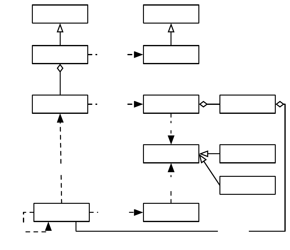
GPIndividual
GPTree
1
1..n
Individual
GPNode
1
1
root of
1
0..n
child of
GPTree
Constraints
GPNode
Constraints
GPSpecies
Species
GPFunctionSet
GPType GPAtomicType
GPSetType
1..n 1
1..n
n
argument and
return types
1
1..n
root type
11..n
flyweight
11..n
flyweight
11..n
flyweight
1..n
0..n
prototype
Figure 5.1 Data objects common to tree-based “Koza-style” genetic programming Individuals.
145
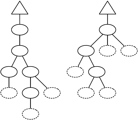
sin
+
cos –
sqrt x
x
x
if-food-
ahead
left progn2
move right
move left
progn3
GP
Tree
GP
Tree
Root Root
Figure 5.2 Two example genetic programming parse trees. At top is a single ec.gp.GPTree instance, which holds onto a single
ec.gp.GPNode designated the root of the tree. GPNodes form the tree itself, and so have a parent and zero or more children. The parent
of the root is the GPTree object itself. Leaf nodes, denoted with dotted ovals, are traditionally called terminals, and non-leaf nodes,
including the root, are traditionally called nonterminals. Normally GPNodes have fixed arity. That is, all if-food-ahead GPNodes will
always have two children, and all cos nodes will always have one child, etc.
to GP is inspired by lil-gp [
18
], an earlier C-based GP system. However lil-gp and many other GP systems
pack the parse trees into arrays to save memory. ECJ does not: the parse trees are stored as tree structures in
memory. This is much more wasteful of memory but it is faster to evaluate and far easier to manipulate.
GP’s top-level class is an Individual called ec.gp.GPIndividual. GPIndividual holds an array of GP trees,
held by ec.gp.GPTree objects. Each GP tree is a tree of ec.gp.GPNode objects. One GPNode, the root of the
tree, is held by the GPTree.
GPIndividual, GPTree, and GPNode are all Prototypes, and furthermore they all adhere to the fly-
weight pattern (Section 3.1.4). GPIndividual’s flyweight relationship is with a Species (of course), called
ec.gp.GPSpecies. GPTrees have a flyweight relationship with subclasses of ec.gp.GPTreeConstraints. GPNodes
have a flyweight relationship with subclasses of ec.gp.GPNodeConstraints.
GP’s tree nodes are
typed
, meaning that they can have certain constraints which specify which nodes
may serve as children of other nodes. These types are defined by an abstract class called ec.gp.GPType, of
which there are two concrete subclasses, ec.gp.GPAtomicType and ec.gp.GPSetType.
The primary function of GPSpecies is to build new GPIndividuals properly. The primary function of
GPTreeConstraints is to hold onto the
function set
(ec.gp.GPFunctionSet) for a given tree. This is a set of
prototypical GPNodes, copies of which are used to construct the tree in question. GPTreeConstraints also
contains typing information for the tree root. The primary purpose of GPNodeConstraints is to provide
typing and arity information for various GPNode.
5.2.1 GPNodes, GPTrees, and GPIndividuals
Figure 5.2 shows two example trees of GPNodes (shown as ovals). The top of each tree is a GPTree, and
directly under it is the root GPNode. As can be seen from the figure, each GPNode has both a parent and
146

zero or more children; and each GPTree has exactly one child. Both GPNodes and GPTrees implement
ec.gp.GPNodeParent, and can serve as parents of other GPNodes (the root has the GPTree as its parent).
5.2.1.1 GPNodes
A basic GPNode consists of four items:
public GPNodeParent parent;
public GPNode children[];
public byte argposition;
public byte constraints;
The parent should be self-explanatory. The children[] is an array holding the children to the GPNode. Leaf
nodes in a GP tree (traditionally called
terminals
) are permitted to either have a zero-length array or a null
value for children[].
The argposition is the position of the node in its parent’s children[] array. The root’s argposition is 0. Last,
the constraints is a tag which refers to the GPNode’s GPNodeConstraints object. It’s a byte rather than a
full pointer to save a bit of space: GPNodes make up by far the bulk of memory in a genetic programming
experiment. You can get the GPNodeConstraints by calling the following GPNode method:
public final GPNodeConstraints constraints(GPInitializer initializer);
Why the GPInitializer? Because GPNodeConstraints, GPTreeConstraints, GPTypes, and GPFunctionSets
are all accessible via the Initializer, which must be a GPInitializer.
3
More on that later. Assuming you have
access to the EvolutionState (probably called state) can call this function like this:
GPNodeConstraints constraints = myGPNode.constraints((GPInitializer)(state.initializer));
You will make various subclasses of GPNode to define the kinds of functions which may appear in your
genetic programming tree.
5.2.1.2 GPTrees
Unlike GPNode, which is liberally subclassed, you’ll rarely subclass GPTree. The ec.gp.GPTree class holds
onto the root GPNode here:
public GPNode child;
Each GPTree also has a backpointer to the GPIndividual which holds it:
public GPIndividual owner;
GPTree also has a pointer to its GPTreeConstraints object. Like GPNode, GPTree uses a byte rather than a
full pointer.4
public byte constraints;
Just like GPNode, you can access GPTree’s constraints using this function:
public final GPTreeConstraints constraints(GPInitializer initializer);
...which is typically called like this:
3It wasn’t a good decision to use the Initializer in this fashion, and one day we may change it to something else.
4
This is mostly historic: GPTree doesn’t fill nearly as much memory as GPNode and so doesn’t really need this tight reference
approach.
147
GPTreeConstraints constraints = myGPTree.constraints((GPInitializer)(state.initializer));
5.2.1.3 GPIndividual
The GPIndividual contains an array of GPTrees. In most cases, this array has a single GPTree in it:
public GPTree[] trees;
5.2.1.4 GPNodeConstraints
The GPNodeConstraints contains several data elements shared by various GPNodes:
public byte constraintNumber;
public GPType returntype;
public GPType[] childtypes;
public String name;
public double probabilityOfSelection;
public GPNode zeroChildren[] = new GPNode[0];
The first element is obvious: it’s number of the constraints which the GPNode objects point to. The next
two items hold the return type and children types of the node: more on that later. Specifically, the return
type of a child in slot 0 must be compatible with the child type declared for slot 0. For now what matters is
that you can determine the expected number of children to a GPNode by the length of the childtypes array.
The name variable holds the name of the GPNodeConstraints (not the GPNodes which refer to them):
we’ll define some in the next section. The probabilityOfSelection variable holds an auxiliary variable used by
certain tree-building operators. Last, zeroChildren[] holds a blank, zero-length GPNode which terminals are
free to use in lieu of null for their children.
5.2.1.5 GPTreeConstraints
The GPTreeConstraints contains data elements shared by GPTrees:
public byte constraintNumber;
public GPType treetype;
public String name;
public GPNodeBuilder init;
public GPFunctionSet functionset;
The first element is again obvious. The treetype variable declares the GPType for the tree as a whole:
the return type of the root must be compatible with this type. The name works similarly to the one in
GPNodeConstraints.
The last two variables are critical. The init variable holds the algorithm used to generate trees or subtrees
for this GPTree. We will discuss tree builders later. Last, the functionset variable holds the function set for
this tree: all GPNodes appearing in this GPTree must be cloned from this function set.
5.2.1.6 GPFunctionSet
The GPFunctionSet contains a name (like GPNodeConstraints and GPTreeConstraints) and a set of GPNodes,
clones of which may appear in the GPTree. This set is stored in various hash tables and arrays to make
lookup easy for different common queries (such as “give me all terminals”) or (“give me all nodes whose
return type is foo”). Usually you don’t need to access this class directly: instead, we’ll set up the function set
using parameters.
148
5.2.2 Basic Setup
Now let’s work towards setting a GP problem. We begin by defining the GPIndividual and GPSpecies.
Usually, we’ll just use those classes directly:
pop.subpop.0.species = ec.gp.GPSpecies
pop.subpop.0.species.ind = ec.gp.GPIndividual
Let’s presume for now that we just want a single tree per GPIndividual. This is the usual case. Typically
this class is defined by GPTree unless we’re doing something odd. We say:
pop.subpop.0.species.ind.numtrees = 1
pop.subpop.0.species.ind.tree.0 = ec.gp.GPTree
Different trees can have different GPTreeConstraints objects, or share them. This is done by defining a set
of GPTreeConstraints (which is a Clique, Section 3.1.2) and giving each member of the set a unique identifier.
Then GPTrees identify with a given GPTreeConstraints by using that identifier.
Since we have only one tree, we really only need to create one GPTreeConstraints. We’ll call it “tc0”.
gp.tc.size = 1
gp.tc.0 = ec.gp.GPTreeConstraints
gp.tc.0.name = tc0
Note that as a Clique, GPTreeConstraints objects all have a global parameter base of
gp.tc
. Now we
assign it to the tree:
pop.subpop.0.species.ind.tree.0.tc = tc0
A GPTreeConstraints object in turn holds onto the GPFunctionSet used to construct trees which identify
with it. GPFunctionSet is also a clique. We’ll call the function set “f0”:
gp.fs.size = 1
gp.fs.0 = ec.gp.GPFunctionSet
gp.fs.0.name = f0
Note that as a Clique, GPFunctionSet objects all have a global parameter base of
gp.fs
. We now assign
this function set to our tree constraints:
gp.tc.0.fset = f0
As to types: we’ll discuss typed GP later on. For now we’ll assume that there is a single atomic type
which is used universally by everyone — that is, everything can connect with everything (it’s “typeless”).
This is the classic GP scenario. GPTypes are also a clique: and they have a global parameter base of
gp.type
.
We define zero GPSetTypes and one GPAtomicType (which we will name, for lack of a better word, “
nil
”)
like this:
gp.type.a.size = 1
gp.type.a.0.name = nil
gp.type.s.size = 0
Our GPTreeConstraints object needs to define the GPType of the tree as a whole (the “root type”). To set
it to our nil type, we’d say:
gp.tc.0.returns = nil
This means that the root GPNode of the tree must have its return type compatible with nil.
149
Last, we need to define some GPNodeConstraints. A GPNodeConstraint object describes three things
about the GPNodes related to them via the Flyweight pattern:
• The number of children of the GPNode.
• The GPTypes that the children of the GPNode must be consistent with.
• The GPType of that the parent of the GPNode must be consistent with.
More on types later. But for now we’ll define a few GPNodeConstraints for nodes with zero, one, and
two children. Since we only have one type, the types of all the children and the return type are all going to
be nil. We’ll call these GPNodeConstraints nc0,nc1, and nc2.
gp.nc.size = 3
gp.nc.0 = ec.gp.GPNodeConstraints
gp.nc.0.name = nc0
gp.nc.0.returns = nil
gp.nc.0.size = 0
gp.nc.1 = ec.gp.GPNodeConstraints
gp.nc.1.name = nc1
gp.nc.1.returns = nil
gp.nc.1.size = 1
gp.nc.1.child.0 = nil
gp.nc.2 = ec.gp.GPNodeConstraints
gp.nc.2.name = nc2
gp.nc.2.returns = nil
gp.nc.2.size = 2
gp.nc.2.child.0 = nil
gp.nc.2.child.1 = nil
5.2.2.1 Defining GPNodes
Let’s imagine that we’re trying to create trees that consist of the following tree nodes (which we’ll create
later): ec.app.myapp.X, ec.app.myapp.Y, ec.app.myapp.Mul, ec.app.myapp.Sub, ec.app.myapp.Sin. These nodes
take 0, 0, 2, 2, and 1 children respectively and have no special types (we’ll use nil). We could add them to the
function set like this:
gp.fs.0 = ec.gp.GPFunctionSet
gp.fs.0.size = 5
gp.fs.0.func.0 = ec.app.myapp.X
gp.fs.0.func.0.nc = nc0
gp.fs.0.func.1 = ec.app.myapp.Y
gp.fs.0.func.1.nc = nc0
gp.fs.0.func.2 = ec.app.myapp.Mul
gp.fs.0.func.2.nc = nc2
gp.fs.0.func.3 = ec.app.myapp.Sub
gp.fs.0.func.3.nc = nc2
gp.fs.0.func.4 = ec.app.myapp.Sin
gp.fs.0.func.4.nc = nc1
Notice that we don’t state the number of children or the types explicitly: instead we state them implicitly
by assigning the appropriate GPNodeConstraints object.
150
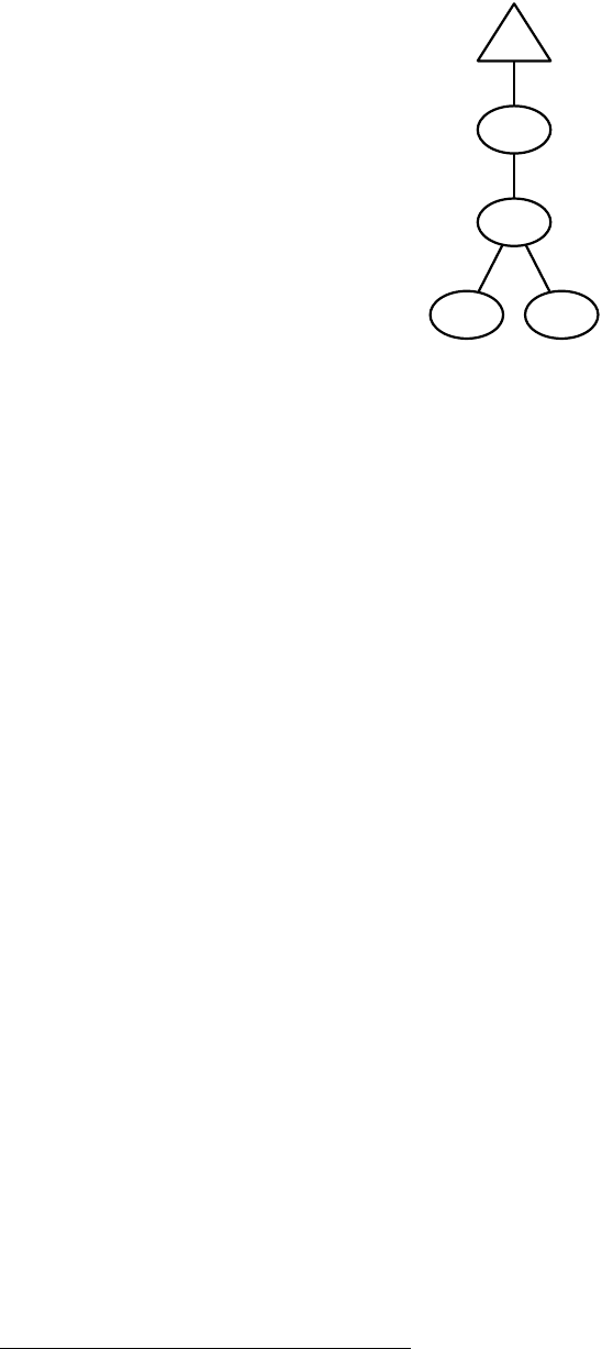
sin
–
GP
Tree
x y
Figure 5.3 A simple GP tree representing the mathematical expression sin(x−y).
5.2.3 Defining the Representation, Problem, and Statistics
GP is more complex than most other optimization procedures because of its representation. When you create
a GP problem, you have two primary tasks:
• Create the GPNodes with which a GPIndividual may be constructed
• Create a Problem which tests the GPIndividual
Let’s start with the first one. As an example, we’ll build a simple Symbolic Regression example on two
variables, X and Y. The GP tree can have GPNodes which subtract, multiply, and perform sine, just as was
done earlier.
5
This means we’ll need two terminals (X and Y), and three nonterminals (subtract and multiply,
each of arity 2 — two children each — and cosine, with arity 1).
Recall from Section 5.2.2 that our function set would look like this:
gp.fs.0 = ec.gp.GPFunctionSet
gp.fs.0.size = 5
gp.fs.0.func.0 = ec.app.myapp.X
gp.fs.0.func.0.nc = nc0
gp.fs.0.func.1 = ec.app.myapp.Y
gp.fs.0.func.1.nc = nc0
gp.fs.0.func.2 = ec.app.myapp.Mul
gp.fs.0.func.2.nc = nc2
gp.fs.0.func.3 = ec.app.myapp.Sub
gp.fs.0.func.3.nc = nc2
gp.fs.0.func.4 = ec.app.myapp.Sin
gp.fs.0.func.4.nc = nc1
We need to make each of these classes. Each of these are GPNodes with a single crucial method
overridden:
public abstract void eval(EvolutionState state, int thread, GPData input,
ADFStack stack, GPIndividual individual, Problem problem);
This method is called when the GPNode is being executed in the course of executing the tree. Execution
proceeds depth-first like the evaluation of a standard parse tree. For example, in order to compute the
expression
sin(x−y)
(shown in GP form in Figure 5.3) we will call eval(...) on the Sin object, which will in
5Ridiculously limited, but what did you expect? This is a demonstration example!
151
turn call eval(...) on the Sub object. This will then call eval(...) on the X object, then on the Y object. X and Y
will return their values. The Sub object will then subtract them and return the result, and finally Sin will
return the sine of that.
Execution doesn’t have to be just in terms of calling eval(...) on children, processing the results, and
returning a final value. In fact, for some problems the return value may not matter at all, but simply which
nodes are executed. In this case, likely the nodes themselves are doing things via side effects: moving a
robot around, for example. Execution could also be tentative: an “if” node might evaluate one or another of
its children and leave it at that. Execution could also be repetitive: you might make a “while” node which
repeatedly evaluates a child until some test is true. Basically you can execute these nodes any way that might
appear in a regular programming language.
5.2.3.1 GPData
The eval(...) method has several arguments, only two of which should be nonobvious: ec.gp.ADFStack and
ec.gp.GPData. We will discuss ADFStack later in Section 5.2.10. The GPData object is a simple data object
passed around amongst your GPNodes when they execute one another. It’s your opportunity to pass data
from node to node. In the example above, it’s how the values are passed from the children to their parents:
for example, it’s how the Sub node returns its value to the Sin node. It’s also possible that the parent needs
to pass data to its child: and the GPData object can be used like that as well.
Typically a single GPData object is created and handed to the GPNodes, and then they hand it to one
another during execution, reusing it. This avoids making lots of clones of a GPData object during execution.
Your prototypical GPData instance normally managed by the GPProblem (Section
??
, coming up). We’ll see
how to specify it in the parameters then.
In the simplest case, your nodes don’t need to pass any data to each other at all. For example, in the
Artificial Ant problem, the nodes are simply executed in a certain order and don’t pass or return any data. In
this case, you can simply use GPData itself: there is no need to specify a subclass.
More often, our GPData object needs to hold the return value from a child. If you are holding a simple
piece of data (like a double or an int) also just need to implement a single method, copyTo(...), which copies
the data from your GPData object into another, then returns it:
public GPData copyTo(GPData other);
In this case, it’s simple:
package ec.app.myapp;
import ec.gp.*;
public class MyData extends GPData
{
public double val;
public void copyTo(GPData other)
{ ((MyData)other).val = val; return other; }
}
Now it might be the case that you need to hold more complex data. For example, what if you had an
array of doubles? In this case you’d need to either clone or copy the data during the copyTo(...) operation.
Additionally, GPData is a Prototype and so it needs to implement the clone() method as a deep clone. The
default implementation just does a light clone. But with your array of doubles, you’d need to clone that.
Altogether you might have something like this:
152

package ec.app.myapp;
import ec.gp.*;
public class MyData extends GPData
{
public double[15] val = new double[15];
public void copyTo(GPData other)
{
System.arraycopy(val, 0, ((MyData)other).val, 0, val.length);
return other;
}
public Object clone()
{
MyData other = (MyData)(super.clone());
other.val = (double[])(val.clone());
return other;
}
}
The important thing to note is that when you perform copyTo(...) or clone(), the resulting other object
should not be sharing any data in common with you except constant (immutable, read-only) data. Why
the two methods? Certainly most things copyTo(...) performs could be done with clone(). The reason for
copyTo(...) is entirely for efficiency when using Automatically Defined Functions (Section 5.2.10). Perhaps in
the future we might obviate the need for its use.
Now that you’ve defined the GPData object, you’ll need to specify its use. This is done as follows:
eval.problem.data = ec.app.myapp.MyData
5.2.3.2 KozaFitness
You can use any fitness you like for GP. But it’s common to use a particular fitness function popularized
by John Koza [
3
]. This fitness object contains a standardized fitness in which 0 is the ideal result and Infinity
is worse than the worst possible result. Note that this isn’t yet the correct fitness according the ec.Fitness.
Instead, when asked for fitness, the function converts this to an adjusted fitness in which 1 is the ideal result
and 0 is worse than the worst possible result, using the function
adjusted =1
1+standardized
. The adjusted
fitness makes this a valid Fitness subclass. The GP fitness also has an auxiliary variable, hits, which originally
was meant to indicate how many optimal subsolutions were discovered: it’s printed out in the statistics and
used for nothing else; use it as you like. This fitness is set as:
pop.subpop.0.species.fitness = ec.gp.koza.KozaFitness
The standard fitness-setting function for this class is:
public final void setStandardizedFitness(EvolutionState state, double value);
You can get (or set) the hits as:
int hits = myKozaFitness.hits;
Note that though the adjusted fitness is returned by the fitness() method, and is thus used by selection
methods such as ec.select.FitProportionateSelection, the standardized fitness is what’s used in the comparison
methods betterThan() and equivalentTo(), as well as isIdealFitness(). This is because it’s possible to convert
different standardized fitness values into the adjusted fitness and have them come out equal due to floating
153
point inaccuracy in division.
5.2.3.3 GPProblem
GPProblem is the subclass of Problem which you will define for evaluating candidate GP solutions. GPProb-
lems contain two variables:
public ADFStack stack;
public GPData input;
The ec.gp.ADFStack— is the mechanism used to handle Automatically Defined Functions (or ADFs, see
Section 5.2.10). You’ll usually not bother with this variable, it’s handled automatically for you.
However, the second variable, input, will be of considerable interest to you: it’s the GPData object for
you to pass among your GPNodes. It’s automatically loaded via this parameter, as mentioned earlier in
Section 5.2.3.1 (GPData):
eval.problem.data = ec.app.myapp.MyData
Your primary task, done during setup(...), will be to verify that the GPData object is of the subclass you’ll
be using, along these lines:
// verify that our GPData is of the right class (or subclasses from it)
if (!input instanceof MyData))
state.output.fatal("GPData class must subclass from " + MyData.class,
base.push(P_DATA), null);
Then during evaluation (evaluate(...) or describe(...)) of a GPIndividual, you’ll use your copy of the input
prototype and hand it to your top-level GPNode to evaluate.
With all that out of our hair, let’s construct the Problem. Let’s attempt to create a GP tree which closely
matches a set of data we’ve created: we’ll generate the data from the function
z=sin(x×y)−sin(x)−x×y
,
in the range
[
0, 1
)
for both
x
and
y
. What we’ll do is define
nhx
,
yi
data points up front, then evaluate our
individuals. For each data point, we’ll set some global variables accessible by the X and Y GPNodes. The
individual will return a value, which we’ll compare against the expected
z
result. The fitness will be the sum
of squared differences.
package ec.app.myapp;
import ec.gp.*;
import ec.simple.*;
import ec.*;
import ec.gp.koza.*;
public class MyProblem extends GPProblem implements SimpleProblemForm {
final static int N = 20;
int current;
double[] Xs = new double[N]; // will be pointer-copied in clone(), which is okay
double[] Ys = new double[N]; // likewise
double[] Zs = new double[N]; // likewise
public void setup(EvolutionState state, Parameter base) {
super.setup(state, base);
// verify that our GPData is of the right class (or subclasses from it)
if (!input instanceof MyData))
state.output.fatal("GPData class must subclass from " + MyData.class,
base.push(P_DATA), null);
// generate N random <x, y, z = f(x,y)> tuples
154
for(int i = 0; i < N; i++) {
double x, y;
Xs[i] = x = state.random[0].nextDouble();
Ys[i] = y = state.random[0].nextDouble();
Zs[i] = Math.sin(x * y) - Math.sin(x) - x * y;
}
}
public void evaluate(final EvolutionState state, Individual ind,
int subpopulation, int threadnum) {
if (!ind.evaluated) { // don’t bother reevaluating
MyData input = (MyData)(this.input);
double sum = 0.0;
// for each tuple, evaluate the individual. For good measure reset
// the GPData first, though in this example it’s not necessary
input.val = 0;
for(current = 0; current < N; current++) // note: an instance variable
((GPIndividual)ind).trees[0].child.eval(
state, threadnum, input, stack, ((GPIndividual)ind),this);
sum += (input.val * input.val);
// set the fitness and the evaluated flag
KozaFitness f = (KozaFitness)(ind.fitness);
f.setStandardizedFitness(state, sum);
f.hits = 0; // don’t bother using this
ind.evaluated = true;
}
}
}
5.2.3.4 GPNode Subclasses
Now let’s implement our five GPNode subclasses. Each will implement toString() to print out the node
name, and also eval(...) discussed earlier. It’s also common to implement the method checkConstraints() to
do a final sanity-check on the node (whether it has the right number of children, etc.) but it’s not necessary,
and we’ll omit it here. Instead we implement the simpler expectedChildren() method, which is called by
the default checkConstraints() implementation. expectedChildren() simply returns the expected number of
children to the node, or a negative number, which means “the number of children could be anything”. The
value returned by expectedChildren() is checked against the type constraints of this node as a sanity check.
First the terminals:
155
package ec.app.myapp;
import ec.*;
import ec.gp.*;
public class X extends GPNode {
public String toString() { return "x" };
public int expectedChildren() { return 0; }
public void eval(EvolutionState state, int thread, GPData input,
ADFStack stack, GPIndividual indivdiual, GPProblem problem) {
MyData data = (MyData) input;
MyProblem prob = (MyProblem) problem;
data.val = problem.Xs[problem.current]; // return current X value to parent
}
}
... and...
package ec.app.myapp;
import ec.*;
import ec.gp.*;
public class Y extends GPNode {
public String toString() { return "y" };
public int expectedChildren() { return 0; }
public void eval(EvolutionState state, int thread, GPData input,
ADFStack stack, GPIndividual indivdiual, GPProblem problem) {
MyData data = (MyData) input;
MyProblem prob = (MyProblem) problem;
data.val = problem.Ys[problem.current]; // return current Y value to parent
}
}
Next the Sine:
package ec.app.myapp;
import ec.*;
import ec.gp.*;
public class Sin extends GPNode {
public String toString() { return "sin" };
public int expectedChildren() { return 1; }
public void eval(EvolutionState state, int thread, GPData input,
ADFStack stack, GPIndividual indivdiual, GPProblem problem) {
MyData data = (MyData) input;
MyProblem prob = (MyProblem) problem;
children[0].eval(state, thread, data, stack, individual, prob);
data.val = Math.sin(data.val);
}
}
Next the Multiply and Subtract:
156
package ec.app.myapp;
import ec.*;
import ec.gp.*;
public class Mul extends GPNode {
public String toString() { return "*" };
public int expectedChildren() { return 2; }
public void eval(EvolutionState state, int thread, GPData input,
ADFStack stack, GPIndividual indivdiual, GPProblem problem) {
MyData data = (MyData) input;
MyProblem prob = (MyProblem) problem;
children[0].eval(state, thread, data, stack, individual, prob);
double val1 = data.val;
children[1].eval(state, thread, data, stack, individual, prob);
data.val = val1 * data.val;
}
}
package ec.app.myapp;
import ec.*;
import ec.gp.*;
public class Sub extends GPNode {
public String toString() { return "-" };
public int expectedChildren() { return 2; }
public void eval(EvolutionState state, int thread, GPData input,
ADFStack stack, GPIndividual indivdiual, GPProblem problem) {
MyData data = (MyData) input;
MyProblem prob = (MyProblem) problem;
children[0].eval(state, thread, data, stack, individual, prob);
double val1 = data.val;
children[1].eval(state, thread, data, stack, individual, prob);
data.val = val1 - data.val;
}
}
5.2.3.5 Statistics
The default statistics class for GP is SimpleStatistics. However, the GP package has a Statistics subclass
designed for doing the same basic stuff as SimpleShortStatistics (Section 3.7.2), but with some extra GP-
specific tree statistics. You can turn it on like this:
stat = ec.gp.koza.KozaShortStatistics
This statistics object has all the basic features of SimpleShortStatistics, including the
do-time
,
do-size
,
do-subpops
, and
modulus
parameters. Additionally it adds a new parameter which you can turn on like
this:
stat.child.0.do-depth = true
This parameter enables tree depth information.
Beyond depth options, the full form of output differs from SimpleShortStatistics in that it reports per-tree
157
information as well, like this:
1. The generation number
2.
(If
do-time
is true) How long initialization took in milliseconds, or how long the previous generation
took to breed to form this generation
3. (If do-time is true) How long evaluation took in milliseconds this generation
4. Once for each subpopulation...
(a)
(If
do-depth
is true) Output of the form
[a b c ...]
, representing the average depth of each tree
a, b, c, etc. of an individual this generation for this subpopulation
(b)
(If
do-size
is true) Output of the form
[a b c ...]
, representing the average size of each tree a,
b, c, etc. of an individual this generation for this subpopulation
(c) (If do-size is true) The average size of an individual this generation for this subpopulation
(d) (If do-size is true) The average size of an individual so far in the run for this subpopulation
(e) (If do-size is true) The size of the best individual this generation for this subpopulation
(f) (If do-size is true) The size of the best individual so far in the run for this subpopulation
(g) The mean fitness of the subpopulation for this generation
(h) The best fitness of the subpopulation for this generation
(i) The best fitness of the subpopulation so far in the run
5.
(If
do-depth
is true) Output of the form
[a b c ...]
, representing the average depth of each tree a, b,
c, etc. of an individual this generation
6.
(If
do-size
is true) Output of the form
[a b c ...]
, representing the average size of each tree a, b, c,
etc. of an individual this generation
7. (If do-size is true) The average size of an individual this generation
8. (If do-size is true) The average size of an individual so far in the run
9. (If do-size is true) The size of the best individual this generation
10. (If do-size is true) The size of the best individual so far in the run
11. The mean fitness of the entire population for this generation
12. The best fitness of the entire population for this generation
13. The best fitness of the entire population so far in the run
5.2.4 Initialization
To use GP we’ll need to define the initializer as a subclass of ec.gp.GPInitializer:
init = ec.gp.GPInitializer
ECJ has traditionally followed the lil-gp default for disallowing duplicates in the initial Population: if a
duplicate is created, ECJ will try 100 times to create another non-duplicate Individual in its stead. If this fails,
the last duplicate created will be allowed. We say this in the standard way:
pop.subpop.0.duplicate-retries = 100
158
To create trees. ECJ relies on a tree-creation algorithm in the form of an ec.gp.GPNodeBuilder, part of the
GPTreeConstraints object. The GPNodeBuilder for GPTreeConstraints 0 is specified like this:
gp.tc.0.init = ec.gp.koza.HalfBuilder
ECJ provides quite a number of node builders in the ec.gp.koza and ec.gp.build packages. You request a
tree with the following function:
public abstract GPNode newRootedTree(EvolutionState state, GPType type,
int thread, GPNodeParent parent, GPFunctionSet set,
int argposition, int requestedSize);
This method builds a tree of GPNodes whose root return type is compatible with type, attached to the
given GPNodeParent, at position argposition, and built from clones of GPNodes in the function set set. The
root node is returned. Several GPNodeBuilders also produce the tree of the requestedSize: others ignore this
function. You can also ask the GPNodeBuilder to pick its own tree size from a distribution specified by the
user in parameters, by passing ec.gp.GPNodeBuilder.NOSIZEGIVEN for the size (this is the usual thing done
by most initialization procedures).
If you are using a GPNodeBuilder which generates trees of a certain size, and
ec.gp.GPNodeBuilder.NOSIZEGIVEN is used (as usual), then you can specify a distribution of sizes
in two ways. First, you can have the GPNodeBuilder pick a size uniformly from among a minimum and
maximum size, for example:
gp.tc.0.init.min-size = 10
gp.tc.0.init.max-size = 20
Alternatively you can specify the distribution of sizes manually. To stipulate probabilities sizes for 1, 2, 3,
4, and 5, you’d say:
gp.tc.0.init.num-sizes = 5
gp.tc.0.init.size.0 = 0.2
gp.tc.0.init.size.1 = 0.1
gp.tc.0.init.size.2 = 0.2
gp.tc.0.init.size.3 = 0.25
gp.tc.0.init.size.4 = 0.25
ECJ has a whole bunch of GPNodeBuilder algorithms available to you. I wrote a shoot-out paper
describing and comparing nearly all of these algorithms [9]. Here is the run-down:
•
ec.gp.koza.FullBuilder generates full trees using Koza’s FULL algorithm. You cannot request a size. It
requires a minimum and maximum depth, for example:
gp.tc.0.init = ec.gp.koza.FullBuilder
gp.tc.0.init.min-depth = 2
gp.tc.0.init.max-depth = 6
Alternatively:
gp.koza.full.min-depth = 2
gp.koza.full.max-depth = 6
•
ec.gp.koza.GrowBuilder generates arbitrary trees depth-first using Koza’s GROW algorithm. You cannot
request a size. It requires a minimum and maximum depth, for example:
159
gp.tc.0.init = ec.gp.koza.GrowBuilder
gp.tc.0.init.min-depth = 2
gp.tc.0.init.max-depth = 6
Alternatively:
gp.koza.grow.min-depth = 2
gp.koza.grow.max-depth = 6
•
ec.gp.koza.HalfBuilder generates arbitrary trees depth-first using Koza’s RAMPED HALF-AND-HALF
algorithm. You cannot request a size. This is nothing more than flipping a coin of probability
growp
to decide whether to use GROW or FULL. HalfBuilder is the default builder for creating GP trees in
ECJ, but it’s not particularly good. It requires a minimum and maximum depth, and the probability of
doing GROW, for example:
gp.tc.0.init = ec.gp.koza.HalfBuilder
gp.tc.0.init.min-depth = 2
gp.tc.0.init.max-depth = 6
gp.tc.0.init.growp = 0.5
Alternatively:
gp.koza.half.min-depth = 2
gp.koza.half.max-depth = 6
gp.koza.half.growp = 0.5
•
ec.gp.build.PTC1 is a modification of GROW which guarantees that trees will be generated with a
given mean. You cannot request a size. Additionally, each terminal and nonterminal can specify
its probability of being chosen from the function set as PTC1 constructs the tree. PTC1 requires an
expected size and a maximum depth:
gp.tc.0.init = ec.gp.build.PTC1
gp.tc.0.init.expected-size = 10
gp.tc.0.init.max-depth = 6
Alternatively:
gp.build.ptc1.expected-size = 10
gp.build.ptc1.max-depth = 6
PTC1 requires that its function sets adhere to the interface ec.gp.build.PTCFunctionSetForm. This
interface contains three tables of probabilities for your GPNodes to be selected:
public [] terminalProbabilities(int type);
public double[] nonterminalProbabilities(int type);
public double[] nonterminalSelectionProbabilities(int expectedTreeSize);
The first function returns, for a given GPType number, a distribution of desired selection probabil-
ities for terminals of that type. The order of the terminals is the same as the following array in
GPFunctionSet:
public GPNode[type][] terminals;
The second function returns, for a given GPType number, a distribution of desired selection probabilities
for nonterminals of that type. The order of the nonterminals is the same as the following array in
160
GPFunctionSet:
public GPNode[type][] nonterminals;
The final function returns, for a given desired tree size, the probability that a nonterminal (of a given
GPType return type) should be selected over a terminal of the same GPType. This is only used by
PTC1, not PTC2 below.
You don’t need to implement this interface: the ec.gp.build.PTCFunctionSet class does it for you:
gp.fs.size = 1
gp.fs.0 = ec.gp.build.PTCFunctionSet
gp.fs.0.name = f0
This function set computes all the above probabilities from user-specified probabilities as parameters.
The probabilities are specified by each GPNodeConstraints object. Following the example we started
in Section 5.2.2, we might state that the terminals X and Y (node constraints 0) should be picked with
0.5 probability each, and the nonterminals Mul, Sub (node constraints 2) and Cos (node constraints 1)
should be picked with 0.3, 0.3, and 0.4 probability:
gp.nc.0.prob = 0.5
gp.nc.1.prob = 0.3
gp.nc.2.prob = 0.4
What if you wanted Mul and Sub to have different probabilities? You’d need to create different
GPNodeConstraints. For example, we could create a new, separate GPNodeConstraints for Sub:
gp.nc.size = 4
gp.nc.3 = ec.gp.GPNodeConstraints
gp.nc.3.name = nc3
gp.nc.3.returns = nil
gp.nc.3.size = 2
gp.nc.3.child.0 = nil
gp.nc.3.child.1 = nil
Now we assign it to Sub:
gp.fs.0.func.3 = ec.app.myapp.Sub
gp.fs.0.func.3.nc = nc3
...and last change the probabilities of Sub and Mul to be different:
gp.nc.0.prob = 0.5
gp.nc.1.prob = 0.3
gp.nc.2.prob = 0.25
gp.nc.3.prob = 0.35
•
ec.gp.build.PTC2 generates trees near to a desired size (which you request) by picking randomly from
the current outer edge in the tree and adding a node. When the tree is large enough, all the remaining
edge slots are filled with terminals. Additionally, each terminal and nonterminal can specify its
probability of being chosen from the function set as PTC2 constructs the tree. PTC2 requires a desired
size and a maximum depth:
gp.tc.0.init = ec.gp.build.PTC2
gp.tc.0.init.expected-size = 10
gp.tc.0.init.max-depth = 6
161

Alternatively:
gp.build.ptc2.expected-size = 10
gp.build.ptc2.max-depth = 6
Like PTC1, PTC2 requires that function sets adhere to the PTCFunctionSetForm interface. Just use
PTCFunctionSet.
•
ec.gp.build.RandomBranch generates trees near to a desired size (which you request) using the RAN-
DOMBRANCH algorithm. Beyond the size distributions, this algorithm has no additional parameters.
•
ec.gp.build.Uniform generates trees near to a desired size (which you request) using the UNIFORM
algorithm, which selects trees of any tree size. You can select sizes either using the user distribution, or
according to the natural distribution of tree sizes. To do the second, you’d say:
gp.tc.0.init = ec.gp.build.Uniform
gp.tc.0.init.true-dist = true
Alternatively:
gp.breed.uniform.true-dist = true
WARNING:
This algorithm is complex and I fear it may be suffering from bit-rot. I have been told it’s
not working properly any more but have not debugged it yet.
•
ec.gp.build.RandTree (by Alexander Chircop) generates trees near to a desired size (which you request)
using the RAND TREE algorithm, which selects trees distributed uniformly using Dyck words. No
extra parameters are needed beyond the tree size selection.
WARNING:
I suspect this algorithm may
have some bugs.
5.2.5 Breeding
ECJ has a large number of breeding pipeline operators for GP trees. This includes the most common operators
used in GP (ec.gp.koza.Crossover,ec.gp.koza.Mutation), and several more found in the ec.gp.breed package.
Pipelines generally pick a single GPTree in a given GPindividual in which to do mutation or crossover.
In most cases you can lock down the specific GPTree, or let the pipeline choose it at random.
Once they’ve picked a GPTree, GP breeding operators often need to choose GPNodes in the tree in which
to perform crossover, mutation, etc. To do this, they make use of a ec.gp.GPNodeSelector. A GPNodeSelector
is a simple interface for picking nodes, consisting of the following methods:
public abstract void reset();
public abstract GPNode pickNode(EvolutionState s, int subpopulation,
int thread, GPIndividual ind, GPTree tree);
When a breeding pipeline needs to pick a node in a particular GPTree of a particular GPIndividual, it
first will call the reset() to get the GPNodeSelector to ready itself, then it will call pickNode(...) to select a
node. If the breeding pipeline needs another node in the same tree, it can call pickNode(...) again as many
times as necessary.
The standard GPNodeSelector is
ec.gp.koza.KozaNodeSelector
, which picks certain kinds of nodes
with different probabilities. The kinds of nodes you can state probabilities for are: the root, nonterminals,
terminals, and all nodes. The most common settings are (here as default parameters):
gp.koza.ns.terminals = 0.1
gp.koza.ns.nonterminals = 0.9
gp.koza.ns.root = 0.0
162
This says to pick terminals 10% of the time, nonterminals 90% of the time, the root (specifically) 0% of the
time and any arbitrary node 0% of the time. The arbitrary-node percentage is whatever is left over from the
other three percentages. (The root could still be picked, since it’s a nonterminal or a terminal — but it won’t
be specially picked).
Why might the breeding pipeline need to call pickNode(...) repeatedly? Most likely because the chosen
GPNode has type constraint problems. For example, in order to do crossover between the subtrees rooted by
two GPNodes, the nodes need to be type-compatible with one another’s parent nodes: otherwise the tree
locations wouldn’t be valid. Pipelines with these issues will try some
n
times to pick compatible nodes; if
they fail all ntimes, the parents are returned rather than the generated children.
Here are the breeding pipelines that come with ECJ. In each case, let’s presume that we’re placing the
pipeline as the root pipeline of Subpopulation 0, parameter-wise:
•
ec.gp.koza.CrossoverPipeline performs standard subtree crossover: it requests a GPIndividual from
each of its two sources; then a tree is selected from each GPndividual, then a node is selected in each
tree, and finally the two subtrees rooted by those nodes are swapped. CrossoverPipeline has several
parameters. The first four:
pop.subpop.0.species.pipe.tries = 1
pop.subpop.0.species.pipe.maxdepth = 17
pop.subpop.0.species.pipe.toss = false
% This one is undefined initially but you can define it:
% pop.subpop.0.species.pipe.maxsize = ...
This tells CrossoverPipeline that children may not have a depth which exceeds 17 (the common value).
The pipeline will to try just one times to find type-valid and depth-legal crossover points before giving
up and just returning the parents instead. This is the most common setting in Genetic Programming. If
toss=true
then only one child is returned — the other is thrown away. The default value for
toss
is
false.
The CrossoverPipeline also can be set, via the
maxsize
parameter, to not generate children which
exceed some number of nodes in any one tree. Initially this is unset, meaning that there is no maximum
size.
pop.subpop.0.species.pipe.tree.0 = 0
pop.subpop.0.species.pipe.tree.1 = 0
This tells CrossoverPipeline that it should pick GPNodes in GPTree 0 of each individual. If either of
these parameters is missing entirely, then CrossoverPipeline will pick that tree at random. At any rate,
the GPTrees chosen must have the same GPTreeConstraints. Finally we have:
pop.subpop.0.species.pipe.ns.0 = ec.gp.koza.KozaNodeSelector
pop.subpop.0.species.pipe.ns.1 = same
This states that the GPNodeSelector for both GPIndividuals should be a KozaNodeSelector. You can
state them independently or node selector 1 can be same.
The default parameter base versions for all of these would be:
gp.koza.xover.tries = 1
gp.koza.xover.maxdepth = 17
gp.koza.xover.toss = false
gp.koza.xover.tree.0
gp.koza.xover.tree.1
gp.koza.xover.ns = ec.gp.koza.KozaNodeSelector
163
Important note:
the default version of the parameter for node selectors is just
ns
. There’s no
ns.0
or
ns.1.
•
ec.gp.koza.MutationPipeline performs standard subtree mutation: it requests a GPIndividual from a
single source; then a tree is selected; then a node is selected in that tree; and finally the subtree rooted
by that node is replaced in its entirety by a randomly-generated tree.
MutationPipeline has many parameters similar to CrossoverPipeline:
pop.subpop.0.species.pipe.tries = 1
pop.subpop.0.species.pipe.maxdepth = 17
pop.subpop.0.species.pipe.tree.0 = 0
pop.subpop.0.species.pipe.ns = ec.gp.koza.KozaNodeSelector
% This one is undefined initially but you can define it:
% pop.subpop.0.species.pipe.maxsize = ...
Note that the node selector is just ns, not ns.0.
The replacing subtree is generated using a GPNodeBuilder. The standard GPNodeBuilder is a Grow-
Builder with the following default values:
gp.koza.grow.min-depth = 5
gp.koza.grow.max-depth = 5
These are strange default values, but that’s common GP original settings. You stipulate the GPNode-
Builder as:
pop.subpop.0.species.pipe.build.0 = ec.gp.koza.GrowBuilder
Though GrowBuilder ignores size demands, if you replaced with another builder such as PTC2, you
can also optionally stipulate that the replacing subtree must be about the same size as the original
subtree. Here’s the parameter:
pop.subpop.0.species.pipe.equal = true
The default setting is false.
The default parameter base versions for all of these would be:
gp.koza.mutate.tries = 1
gp.koza.mutate.maxdepth = 17
gp.koza.mutate.tree.0 = 0
gp.koza.mutate.pipe.ns = ec.gp.koza.KozaNodeSelector
gp.koza.mutate.build.0 = ec.gp.koza.GrowBuilder
gp.koza.mutate.equal = true
•
ec.gp.breed.InternalCrossoverPipeline selects two GPNodes in the same GPIndividual, such that neither
GPNode is in the subtree rooted by the other. The GPNodes may be in different GPTrees, or they may
be in the same GPTree. It then swaps the two subtrees.
InternalCrossoverPipeline’s parameters are essentially identical to those in CrossoverPipeline, except
for a missing maxsize parameter. For example:
164
pop.subpop.0.species.pipe.tries = 1
pop.subpop.0.species.pipe.maxdepth = 17
pop.subpop.0.species.pipe.tree.0 = 0
pop.subpop.0.species.pipe.tree.1 = 0
pop.subpop.0.species.pipe.ns.0 = ec.gp.koza.KozaNodeSelector
pop.subpop.0.species.pipe.ns.1 = same
The default parameter base versions for all of these would be:
gp.breed.internal-xover.tries = 1
gp.breed.internal-xover.maxdepth = 17
gp.breed.internal-xover.toss = false
gp.breed.internal-xover.tree.0
gp.breed.internal-xover.tree.1
gp.breed.internal-xover.ns = ec.gp.koza.KozaNodeSelector
Important note:
just as is the case for CrossoverPipeline, the default version of the parameter for node
selectors is just ns. There’s no ns.0 or ns.1.
•
ec.gp.breed.MutatePromotePipeline selects a GPNode, other than the root, and replaces its parent (and
its parent’s subtree) with the GPNode and its subtree. This was called the PromoteNode algorithm in [
1
]
and is similar to the Deletion algorithm in [13].
MutatePromotePipeline’s parameters are pretty simple. Because its constraints are tighter, it doesn’t use
a GPNodeSelector: instead it searches among all nodes in the tree to find one which is type-compatable
with its parent. thus its parameters are simply the number of times it tries before giving up, and
returning the original tree. Like previous methods, if the tree parameter doesn’t exist, a tree is picked
at random (which is usually what’d you’d want anyway).
pop.subpop.0.species.pipe.tries = 1
pop.subpop.0.species.pipe.tree.0 = 0
The default parameter base versions:
gp.breed.mutate-promote.tries = 1
gp.breed.mutate-promote.tree.0
•
ec.gp.breed.MutateDemotePipeline selects a GPNode, then replaces the node with a new nonterminal.
The old Node becomes a child of the new node at a random argument location, and the remaining
child slots are filled with terminals. This was called the DemoteNode algorithm in [
1
] and is similar to
the Insertion algorithm in [13].
MutatePromotePipeline is similar to MutatePromotePipeline: it doesn’t use a GPNodeSelector, and
tries a certain number of times to find valid node points before giving up and returning the tree.
parameters are pretty simple. Because its constraints are tighter, it doesn’t use a NodeSelector: instead
it searches among all nodes in the tree to find one which is type-compatable with its parent, and
which wouldn’t create a tree deeper than a maximum legal value. Like previous methods, if the tree
parameter doesn’t exist, a tree is picked at random (which is usually what’d you’d want anyway).
pop.subpop.0.species.pipe.tries = 1
pop.subpop.0.species.pipe.maxdepth = 17
pop.subpop.0.species.pipe.tree.0 = 0
The default parameter base versions:
165
gp.breed.mutate-demote.tries = 1
gp.breed.mutate-demote.maxdepth = 17
gp.breed.mutate-demote.tree.0 = 0
•
ec.gp.breed.MutateSwapPipeline selects a GPNode with at least two children, then selects two children
of that node such that each is type-compatable with the other. Then it swaps the two subtrees rooted
by those children.
MutateSwap’s parameters are simple because it doesn’t use a GPNodeSelector (the constraints are
too complex). You simply specify the tree (or have one picked at random if none is specified) and the
number of tries:
pop.subpop.0.species.pipe.tries = 1
pop.subpop.0.species.pipe.tree.0 = 0
The default parameter base versions for all of these would be:
gp.breed.mutate-swap.tries = 1
gp.breed.mutate-swap.tree.0
•
ec.gp.breed.MutateOneNodePipeline selects a GPNode, then replaces that node with a different node of
the same arity and type constraints. This was called the OneNode algorithm in [1].
MutateOneNodePipeline uses a GPNodeSelector to pick the node. You also specify the tree number: or
if you don’t specify anything, one will be picked at random (which is usually what’d you’d want).
pop.subpop.0.species.pipe.ns.0 = ec.gp.koza.KozaNodeSelector
pop.subpop.0.species.pipe.tree.0 = 0
The default parameter base versions:
gp.breed.mutate-one-node.ns.0 = ec.gp.koza.KozaNodeSelector
gp.breed.mutate-one-node.tree.0 = 0
•
ec.gp.breed.MutateAllNodesPipeline selects a GPNode, then for every node in the subtree rooted by the
GPnode, it replaces each node with a different node of the same arity and type constraints. This highly
destructive operator was called the AllNodes algorithm in [1].
MutateAllNodesPipeline uses a GPNodeSelector to pick the GPNode. You also specify the tree number:
or if you don’t specify anything, one will be picked at random (which is usually what’d you’d want).
pop.subpop.0.species.pipe.ns.0 = ec.gp.koza.KozaNodeSelector
pop.subpop.0.species.pipe.tree.0 = 0
The default parameter base versions:
gp.breed.mutate-one-node.ns.0 = ec.gp.koza.KozaNodeSelector
gp.breed.mutate-one-node.tree.0 = 0
•
ec.gp.breed.RehangPipeline is an oddball mutator of my own design mean to be highly destructive.
It selects a nonterminal other than the root, and designates it the “new root”. It then picks a child
subtree of this new root, which is disconnected from its parent. The new root becomes the root of the
tree. The original parent of the new root becomes the new root’s child, filling the spot vacated by the
disconnected subtree. The grandparent then fills the spot vacated by the parent, and so on, clear up to
the root. Then finally the disconnected subtree fills remaining spot. Figure 5.4 shows this procedure.
There are two parameters, as usual:
166
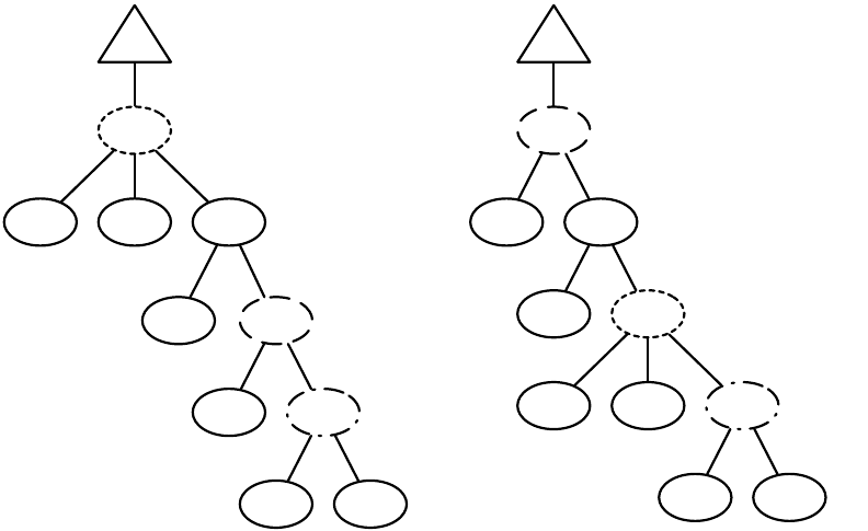
if-food-
ahead
left
GP
Tree
if-food-
ahead
left progn2
move right
move left
progn3
GP
Tree
New
Root
New Root
Subtree
Old
Root
New
Root
progn2
move
progn2
move
move left
progn3
progn2
move right
New Root
Subtree
Old
Root
Figure 5.4 Rehanging a tree. A new root is chosen at random from among the nonterminals except for the original root. Then a subtree
of that new root is chosen at random and disconnected. The tree is then rehung as shown: the parent of the new root becomes its child;
the grandparent becomes the parent’s child, and so on up to the root. The disconnected subtree then fills the remaining spot.
pop.subpop.0.species.pipe.tries = 1
pop.subpop.0.species.pipe.tree.0 = 0
The default parameter base versions for all of these would be:
gp.breed.rehang.tries = 1
gp.breed.rehang.tree.0
Warning:
Because of the complexity of its rehanging process, RehangPipeline ignores all typing
information.
•
ec.gp.breed.MutateERCPipeline works similarly to the Gaussian algorithm in [
1
]. The algorithm picks
a random node in a random tree in the GPIndividual, then for every Ephemeral Random Constant
(ERC) in the subtree rooted by that node, it calls mutateERC() on that ERC. ERCs are discussed later in
Section 5.2.9. As usual, the two common parameters:
pop.subpop.0.species.pipe.tries = 1
pop.subpop.0.species.pipe.tree.0 = 0
The default parameter base versions for all of these would be:
gp.breed.mutate-erc.tries = 1
gp.breed.mutate-erc.tree.0
If you wished to mutate the ERCs in the entire tree, you could set the node selector parameters like this:
167

gp.breed.mutate-erc.ns.0 = ec.gp.koza.KozaNodeSelector
gp.breed.mutate-erc.ns.0.terminals = 0.0
gp.breed.mutate-erc.ns.0.nonterminals = 0.0
gp.breed.mutate-erc.ns.0.root = 1.0
•
ec.gp.breed.SizeFairCrossoverPipeline implements the size fair and homologous crossover methods de-
scribed in [
5
]. SizeFairCrossoverPipeline has many parameters in common with CrossoverPipeline,
which should look familiar, something like:
pop.subpop.0.species.pipe.tries = 1
pop.subpop.0.species.pipe.maxdepth = 17
pop.subpop.0.species.pipe.toss = false
pop.subpop.0.species.pipe.ns.0 = ec.gp.koza.KozaNodeSelector
pop.subpop.0.species.pipe.ns.1 = same
% These are unset by default but you can set them to lock down
% the trees being crossed over
% pop.subpop.0.species.pipe.tree.0 = 0
% pop.subpop.0.species.pipe.tree.1 = 0
The default parameter base versions for all of these would be:
gp.breed.size-fair.tries = 1
gp.breed.size-fair.maxdepth = 17
gp.breed.size-fair.toss = false
gp.breed.size-fair.ns = ec.gp.koza.KozaNodeSelector
% These are unset by default but you can set them to lock down
% the trees being crossed over
% gp.breed.size-fair.tree.0 = ...
% gp.breed.size-fair.tree.1 = ...
By default SizeFairCrossoverPipeline will perform
size-fair crossover,
defined as follows. First, it
finds a crossover point in the first parent in a fashion identical to CrossoverPipeline. But to find the
crossover point in the second parent, it first computes the size
s1
of the subtree in the first parent. It
then calculates the size of every subtree in the second parent, and discards from consideration any
subtrees whose size
s2
is
s2>
1
+
2
s1
. From the remainder, it then counts the number of subtrees
smaller, equal to, and larger than
s1
(call these
n<
,
n=
and
n>
), and likewise the means of the smaller
and larger subtrees (call these mu<and mu>).
If
n<=
0 or if
n>=
0, then a random subtree is selected from among the subtrees exactly the same
size as
s1
. Thus terminals are always crossed over with terminals. Otherwise, we decide on selecting
an equal, smaller, or larger subtree with the following probabilities:
p==1
s1
p>=1−p=
n>×(1+µ>
µ<)
p<=1−(p=+p>)
The idea is to select bigger or smaller subtrees randomly such that the mean stays the same. Once we
have decided on bigger or smaller or equal subtrees, we then select a size uniformly from among the
sizes of subtrees appearing in that set. If there is more than one subtree of the selected size, we select
uniformly from among them.
168
Alternatively we can perform a kind of
homologous crossover
, if we turn on the following parameter:
pop.subpop.0.species.pipe.homologous = true
(or the default...)
gp.breed.size-fair.homologous = true
Homologous crossover is identical to size-fair crossover except for the final detail. Instead of selecting
uniformly from among all subtrees of a chosen size, we instead select the one whose root is “closest” to
the selected crossover point in the first parent. Here, distance between crossover points is defined as
the depth at which their paths to the root begin to deviate from one another.
Size-fair and homologous crossover is due to Uday Kamath, a PhD student at GMU.
5.2.6 A Complete Example
Much of these initial parameters could have been entered simply by including the parameter file
ec/gp/koza/koza.params. But we’ll go through it in detail. First some basic generational parameters:
# Threads and Seeds
evalthreads = 1
breedthreads = 1
seed.0 = time
# Checkpointing
checkpoint = false
checkpoint-modulo = 1
checkpoint-prefix = ec
# The basic setup
state = ec.simple.SimpleEvolutionState
finish = ec.simple.SimpleFinisher
exch = ec.simple.SimpleExchanger
breed = ec.simple.SimpleBreeder
eval = ec.simple.SimpleEvaluator
stat = ec.simple.SimpleStatistics
pop = ec.Population
pop.subpops = 1
pop.subpops.0 = ec.Subpopulation
pop.subpop.0.duplicate-retries = 0
pop.subpop.0.size = 1024
breed.elite.0 = 0
stat.file = $out.stat
quit-on-run-complete = true
Genetic programming typically doesn’t run very long, and (for the time being) require their own Initializer.
We’ll also use KozaFitness. Following the lil-gp example, we’ll set the duplicate retries to 100:
init = ec.gp.GPInitializer
generations = 51
pop.subpop.0.species.fitness = ec.gp.koza.KozaFitness
pop.subpop.0.duplicate-retries = 100
For good measure, let’s attach KozaShortStatistics to the statistics chain. This isn’t standard in the
koza.params file, but what the heck.
169
stat.num-children = 1
stat.child.0 = ec.gp.koza.KozaShortStatistics
stat.child.0.gather-full = true
stat.child.0.file = $out2.stat
Our initializer will work by using HalfBuilder to build trees. We define its parameters here:
# HalfBuilder
gp.koza.half.min-depth = 2
gp.koza.half.max-depth = 6
gp.koza.half.growp = 0.5
We begin by defining the tree constraints, node constraints, types, and function sets for the problem:
# Types
gp.type.a.size = 1
gp.type.a.0.name = nil
gp.type.s.size = 0
# Basic Function Set Parameters (more later)
gp.fs.size = 1
gp.fs.0 = ec.gp.GPFunctionSet
gp.fs.0.name = f0
# Tree Constraints
gp.tc.size = 1
gp.tc.0 = ec.gp.GPTreeConstraints
gp.tc.0.name = tc0
gp.tc.0.fset = f0
gp.tc.0.returns = nil
gp.tc.0.init = ec.gp.koza.HalfBuilder
# Node Constraints
gp.nc.size = 3
gp.nc.0 = ec.gp.GPNodeConstraints
gp.nc.0.name = nc0
gp.nc.0.returns = nil
gp.nc.0.size = 0
gp.nc.1 = ec.gp.GPNodeConstraints
gp.nc.1.name = nc1
gp.nc.1.returns = nil
gp.nc.1.size = 1
gp.nc.1.child.0 = nil
gp.nc.2 = ec.gp.GPNodeConstraints
gp.nc.2.name = nc2
gp.nc.2.returns = nil
gp.nc.2.size = 2
gp.nc.2.child.0 = nil
gp.nc.2.child.1 = nil
Now we define the GP elements of the Species and the Individual:
170
# Representation
pop.subpop.0.species = ec.gp.GPSpecies
pop.subpop.0.species.ind = ec.gp.GPIndividual
pop.subpop.0.species.ind.numtrees = 1
pop.subpop.0.species.ind.tree.0 = ec.gp.GPTree
pop.subpop.0.species.ind.tree.0.tc = tc0
Here’s a basic GP breeding pipeline:
# Pipeline
pop.subpop.0.species.pipe = ec.breed.MultiBreedingPipeline
pop.subpop.0.species.pipe.generate-max = false
pop.subpop.0.species.pipe.num-sources = 2
pop.subpop.0.species.pipe.source.0 = ec.gp.koza.CrossoverPipeline
pop.subpop.0.species.pipe.source.0.prob = 0.9
pop.subpop.0.species.pipe.source.1 = ec.breed.ReproductionPipeline
pop.subpop.0.species.pipe.source.1.prob = 0.1
For no good reason, we’ll define the selection methods, and various other parameters using the default
parameter bases for CrossoverPipeline and ReproductionPipeline:
# Reproduction
breed.reproduce.source.0 = ec.select.TournamentSelection
# Crossover
gp.koza.xover.source.0 = ec.select.TournamentSelection
gp.koza.xover.source.1 = same
gp.koza.xover.ns.0 = ec.gp.koza.KozaNodeSelector
gp.koza.xover.ns.1 = same
gp.koza.xover.maxdepth = 17
gp.koza.xover.tries = 1
# Selection
select.tournament.size = 7
Since Crossover is using a node selector, let’s define some parameters for that:
# Node Selectors
gp.koza.ns.terminals = 0.1
gp.koza.ns.nonterminals = 0.9
gp.koza.ns.root = 0.0
Let’s presume that we have created the X,Y,Sin,Mul, and Sub methods described in Section 5.2.3. We’ll
now hook them up.
171
# Our Function Set
gp.fs.0 = ec.gp.GPFunctionSet
gp.fs.0.size = 5
gp.fs.0.func.0 = ec.app.myapp.X
gp.fs.0.func.0.nc = nc0
gp.fs.0.func.1 = ec.app.myapp.Y
gp.fs.0.func.1.nc = nc0
gp.fs.0.func.2 = ec.app.myapp.Mul
gp.fs.0.func.2.nc = nc2
gp.fs.0.func.3 = ec.app.myapp.Sub
gp.fs.0.func.3.nc = nc2
gp.fs.0.func.4 = ec.app.myapp.Sin
gp.fs.0.func.4.nc = nc1
Also we’re using the MyProblem and MyData classes defined in Section 5.2.3 as our Problem. Even though
we’re not using ADFs (see Section 5.2.10), we need to define a few items here as well.
# Our Problem eval.problem = ec.app.myapp.MyProblem
eval.problem.data = ec.app.myapp.MyData
gp.problem.stack = ec.gp.ADFStack
gp.adf-stack.context = ec.gp.ADFContext
Phew! That was a lot of parameters. Thankfully nearly all of them are already defined for you in
ec/gp/koza/koza.params.
5.2.7 GPNodes in Depth
GPNode has a gazillion utility methods to assist various crossover, mutation, statistics, and tree-building
operators in their tasks of making, breaking, printing, reading, writing and examining trees of GPNodes.
Let’s look at some of them here, and divvy up the rest in later sections where they’re more appropriate.
First, the two abstract methods which you must override:
public String toString();
public abstract void eval(EvolutionState state, int thread, GPData input,
ADFStack stack, GPIndividual individual, Problem problem);
The first method prints out the node in a human-readable fashion, with no whitspace. Except for rare
cases such as Ephemeral Random Constants (Section 5.2.9), this should be a single simple symbol like “cos”
or “if-food-ahead”. The second method we introduced in Section 5.2.3, of course.
Sanity Checking
ECJ can double-check to make sure that the number of children to a given node, as
claimed in the parameter file, is in fact proper. Other sanity checks might include that the children and
parent are of the right GPType, and so on. The general method for doing this sanity check, which you can
override if you like, is;
public void checkConstraints(EvolutionState state, int tree,
GPIndividual typicalIndividual, Parameter individualBase);
This method is called after the prototypical GPNode is loaded into a function set, and throws an error
if the sanity check fails. The primary purpose of this method is to allow Automatically Defined Functions
(Section 5.2.10) a chance to make sure that everything is working. But you can override this method to do
some checking of your own as well. If you do so, be sure to call super(...).
The default implementation of checkConstraints(...) just calls a simpler method which I suggest you
implement instead. This method is:
172

public int expectedChildren();
You can override this method to return the expected number of children to this kind of node, as the
most commonly-needed sanity check. If you override it and provide this value, checkConstraints(...) will
by default call this method, then double-check for you that the number of children attached is indeed the
expected number. By default, expectedChildren() returns:
public static final int CHILDREN UNKNOWN;
This indicates to checkConstraints(...) that expectedChildren() is unimplemented and so checkConstraints(...)
won’t do anything at all by default. So you have three options here to help ECJ sanity-check that everything’s
okay:
•
Override expectedChildren() to return the expected number of children to the node. The default
implementation of checkConstraints(...) will compare this result against the actual number of children.
• Override checkConstraints() to do your own more sophisticated sanity-checking.
•
Do nothing. ECJ will do no sanity checking and will rely on the correctness of your parameter file (this
is often perfectly fine).
Next come some methods which are usually overridden by Ephemeral Random Constants but rarely by
any other kind of GPNode (the default implementation suffices):
ec.gp.GPNode Methods
public String name()
Returns the name of the GPNode. By default, this calls toString().
public int nodeHashCode()
Returns a hash code appropriate to your GPNode (hash by value, not by address).
public boolean nodeEquals(GPNode node)
Returns true if this method is identical to the given node.
public boolean nodeEquivalentTo(GPNode node)
Returns true if the two nodes are the same “kind” of node — usually meaning they could have been cloned from
the same prototype node. The default form of this function returns true if the two nodes are the same class, have
the same length child array, and have the same constraints. Often nodeEquals(...) and nodeEquivalentTo(...) may
return the same thing, but in Ephemeral Random Constants, they often return different values. For example, two
ERCs that are the same class, and have the same constraints, may hold different values (2.34 vs. 3.14 say). These
ERCs would be equivalent to one another but not equal to one another. You’d rarely need to override this method.
public String toStringForHumans()
Writes the node to a String in a fashion readable by humans. The default version simply calls toString.
public void resetNode(EvolutionState state, int thread)
Randomizes the node. Ephemeral Random Constants randomize their internal values; other GPNodes typically
do nothing.
Next, some test functions:
ec.gp.GPNode Methods
public int atDepth()
Returns the depth of the node (the root is at depth 0).
173

public int depth()
Returns the depth of the subtree rooted by the node (terminals have a subtree depth of 1).
public GPNodeParent rootParent()
Returns the parent of the root of the tree in which the GPNode resides. Though the method returns a GPNodePar-
ent, this returned object should always be some kind of GPTree.
public boolean contains(GPNode subnode)
Returns true subnode exists somewhere within the subtree rooted by the GPNode.
public pathLength(int nodesearch)
Returns the sum of all paths from all nodes in the GPNode’s subtree to the GPNode itself. The nodesearch parameter
allows us to restrict which nodes have paths included in the sum: only leaf nodes (terminals), non-leaf nodes
(nonterminal), or all nodes:
public static final int GPNode. NODESEARCH ALL;
public static final int GPNode. NODESEARCH TERMINALS;
public static final int GPNode. NODESEARCH NONTERMINALS;
public int numNodes(int nodesearch)
Returns the number of nodes in the subtree rooted by GPNode. The nodesearch parameter allows us to restrict
which nodes are included in the total, using the constants above.
public int meanDepth(int nodesearch)
Returns the path length divided by the number of nodes.The nodesearch parameter allows us to restrict which
nodes are included in the total, using the constants above.
public GPNode nodeInPosition(int p, int nodesearch)
Returns the
p
th node in the subtree rooted by the GPNode, using left-to-right depth-first search, and only
considering those nodes specified by nodesearch, which can be one of:
public static final int GPNode. NODESEARCH ALL;
public static final int GPNode. NODESEARCH TERMINALS;
public static final int GPNode. NODESEARCH NONTERMINALS;
public java.util.Iterator iterator(int nodesearch)
Returns a depth-first, left-to-right Iterator over all the nodes rooted by the GPNode. The nodesearch parameter
allows us to restrict which nodes are iterated over, and may be one of:
public static final int GPNode. NODESEARCH ALL;
public static final int GPNode. NODESEARCH TERMINALS;
public static final int GPNode. NODESEARCH NONTERMINALS;
public java.util.Iterator iterator()
Returns a depth-first, left-to-right Iterator over all the nodes rooted by the GPNode. Equivalent to itera-
tor(GPNode.NODESEARCH ALL).
Three methods permit even more flexibility in filtering exactly which GPNodes you want to consider, by
using a ec.gp.GPNodeGatherer object. This object contains a single method, which you should override, and a
single instance variable:
GPNode node; // used internally only
public abstract boolean test(GPNode thisNode);
You can ignore the variable: it’s used by GPNode’s recursion. As far as you are concerned, GPNode-
Gatherer provides a filter: override the test(...) method to specify whether certain GPNodes fit your needs.
Armed with a GPNodeGatherer you’ve constructed, you can then call one of the two GPNode methods:
174

ec.gp.GPNode Methods
public int numNodes(GPNodeGatherer gatherer)
Returns the number of nodes (filtered by the GPNodeGatherer) in the subtree rooted by the GPNode.
public GPNode nodeInPosition(int p, GPNodeGatherer gatherer)
Returns the
p
th node in the subtree rooted by the GPNode, using left-to-right depth-first search, and only
considering those nodes filtered by the provided GPNodeGatherer.
public java.util.Iterator iterator(GPNodeGatherer gatherer )
Returns a depth-first, left-to-right Iterator over all the nodes rooted by the GPNode, filtered by the GPNodeGath-
erer.
And now we come to rigamarole which should look familiar to you if you’ve trudged through the Vector
chapter.
ec.gp.GPNode Methods
public int printNodeForHumans(EvolutionState state, int log )
Prints a node to a log in a fashion readable by humans. You don’t want to override this method: it calls
toStringForHumans() by default — override that instead.
public int printNode(EvolutionState state, int log)
Prints a node to a log in a fashion readable by humans and also parsable by readNode(...). You don’t want to
override this method: it calls toString() by default — override that instead.
public int printNode(EvolutionState state, PrintWriter writer)
Prints a node to a writer in a fashion readable by humans and also parsable by readNode(...). You don’t want to
override this method: it calls toString() by default — override that instead.
public String toStringForError()
Writes a node to a string in a fashion useful for error messages. The default writes out the name and the tree the
node is in, which works fine.
public GPNode readNode(DecodeReturn dret)
Generates a GPNode from the DecodeReturn via a light clone: children and parents are not produced. The default
version clones the the node, then reads a string from the DecodeReturn. This string should match toString() exactly.
If not, returns null to indicate an error. Otherwise returns the GPNode. This default implementation should be
fine in most cases: though Ephemeral Random Constants (Section 5.2.9) require a different procedure.
public void writeNode(EvolutionState state, DataOutput output) throws IOException
Writes the node, but not any of its children or parents, out to output.
public void readNode(EvolutionState state, DataInput input) throws IOException
Reads a node from input. Children and parents are not produced.
Last are a host of different ways of cloning a GPNode or tree. In most cases the default implementations
work just fine:
ec.gp.GPNode Methods
public GPNode lightClone()
Light-clones a GPNode, including its children array, but not any children or parents.
public Object clone()
Deep-clones a GPNode, except for its parent. All children are cloned as well.
175

public final GPNode cloneReplacing(GPNode newSubtree, GPNode oldSubtree)
Deep-clones a GPNode, except that, if found within its cloned subtree, oldSubtree is replaced with a deep-cloned
version of newSubtree.
public final GPNode cloneReplacing(GPNode[] newSubtrees, GPNode[] oldSubtrees)
Deep-clones a GPNode, except that, if found within its cloned subtree, each of the oldSubtrees is replaced with a
clone of the corresponding member of newSubtrees.
public final GPNode cloneReplacingNoSubclone(GPNode newSubtree, GPNode oldSubtree)
Deep-clones a GPNode, except that, if found within its cloned subtree, oldSubtree is replaced with newSubtree (not
a clone of newSubtree).
public final GPNode cloneReplacingAtomic(GPNode newNode, GPNode oldNode)
Deep-clones a GPNode, except that, if found within its cloned subtree, oldNode is replaced with newNode (not a
clone of newNode).
public final GPNode cloneReplacingAtomic(GPNode[] newNodes, GPNode[] oldNodes)
Deep-clones a GPNode, except that, if found within its cloned subtree, each of the oldNodes is replaced with the
corresponding member of newNodes (not a clone).
public final void replaceWith(GPNode newNode)
Replaces the GPnode with newNode right where it lives in its GPTree.
These are the primary public methods. There are plenty of other public methods, but they’re largely used
internally and you’ll rarely need them.
5.2.8 GPTrees and GPIndividuals in Depth
Unlike GPNode, there’s nothing in a GPTree that you have to override or modify. It’s pretty rare to subclass
GPTree, though it’s perfectly reasonable to do so. But there are a number of methods you should be aware
of, many of which are probably very familiar by now. First, let’s cover the three non-familiar ones:
ec.gp.GPTree Methods
public int treeNumber()
Returns the position of the GPTree in its GPIndividual’s trees[] array. This is an
O(n)
operation — it works by
scanning through the array until it finds the GPTree. If the tree is not found (which would indicate an error), then
GPTree.NO TREENUM is returned.
public final void verify(EvolutionState state)
An auxillary debugging method which verifies many features of the structure of the GPTree and all of its GPNodes.
This method isn’t called by ECJ but has proven useful in determining errors in GPTree construction by various
tree building or breeding algorithms.
public void buildTree(EvolutionState state, int thread)
Builds a tree and attaches it to the GPTree, displacing the original, using the tree-generation algorithm defined for
its GPTreeConstraints. No specific tree size is requested.
Next come cloning and tests for removing duplicates:
ec.gp.GPTree Methods
public boolean treeEquals(GPTree tree)
Returns true if the GPNodes which make up the GPTree are structured the same and equal in value to one another.
Override this to provide more equality if necessary.
176

public int treeHashCode()
Returns a hash code generated for the structure and makeup of the GPNodes in the GPTree. Override this to add
additional hash information.
public GPTree lightClone()
Performs a light clone on the GPTree: the GPNodes are not cloned but are instead the pointer to the root is simply
copied.
public Object clone()
Performs a deep clone on the GPTree, including all of its GPNodes but not its parent GPIndividual.
Last, the standard methods for printing and reading:
ec.gp.GPTree Methods
public void printTreeForHumans(EvolutionState state, int log)
Prints the tree in a human-readable fashion to log.
public void printTree(EvolutionState state, int log)
Prints to log the tree in a fashion readable both by humans and also by readTree(..., LineNumberReader). By default
this uses the Code package (Section 2.2.3).
public void printTree(EvolutionState state, PrintWriter writer )
Prints to writer the tree in a fashion readable both by humans and also by readTree(..., LineNumberReader). By
default this uses the Code package.
public void readTree(EvolutionState state, LineNumberReader reader ) throws IOException
Reads a tree produced by printTree(...). By default, this uses the Code package (Section 2.2.3).
public void writeTree(EvolutionState state, DataOutput output) throws IOException
Writes a tree to output in binary fashion such that it can be read by readTree(..., DataInput).
public void readTree(EvolutionState state, DataInput input) throws IOException
Reads a tree from input in binary fashion that had been written by writeTree(...).
5.2.8.1 Pretty-Printing Trees
GPTrees have a particular gizmo that’s not well known but is quite nice: you can print out GPTrees in one of
(at present) four styles:
• Lisp (the default):
(* (+ x (- (% x x) (cos x))) (exp x))
• A style easily converted to C, C++, Java, or C#:
(x + ((x % x) - cos(x))) * exp(x)
To print out trees this way you’d use a parameter along these lines (notice the lower-case “c”):
pop.subpop.0.species.ind.tree.0.print-style = c
...or using the default parameter base:
gp.tree.print-style = c
177
Printing in C-style has two options. First, by default ECJ prints out two-child GPNodes as if they were
operators
"b a c"
rather than as
"a(b, c)"
. This is what’s being done above. But if you’re not using
mathematical operators and would prefer to see 2-child GPNodes as functions, you can do it like this:
pop.subpop.0.species.ind.tree.0.c-operators = false
...or using the default parameter base:
gp.tree.c-operators = false
This results in the following:
*(+(x, -(%(x, x), cos(x))), exp(x))
This doesn’t seem useful for the example here (Symbolic Regression) but for other problems it’s
probably the right thing to do, particularly if all the GPNodes aren’t operators.
Second, by default ECJ prints out zero-child GPNodes as constants, as in
"a"
, rather than as zero-
argument functions, as in "a()". If you’d prefer zero-argument functions, you might say:
pop.subpop.0.species.ind.tree.0.c-variables = false
...or using the default parameter base:
gp.tree.c-variables = false
This results in the following:
x() + ((x() % x()) - cos(x()))) * exp(x())
Again, whether this will be useful to you is based on exactly what kind of problem you’re emitting.
ECJ does not at present have support for converting if-statements (such as the
"if-food-ahead"
node
in Artificial Ant) into a brace format appropriate to C. But hopefully these options will help you get
most of the ugly parsing work out the way.
•
.dot format: used by dot/GraphViz to produce high-quality trees and graphs. The code below produces
the tree shown at left in Figure 5.5:
digraph g {
node [shape=rectangle];
n[label = "*"];
n0[label = "+"];
n00[label = "x"];
n0 -> n00;
n01[label = "-"];
n010[label = "%"];
n0100[label = "x"];
n010 -> n0100;
n0101[label = "x"];
n010 -> n0101;
n01 -> n010;
n011[label = "cos"];
n0110[label = "x"];
n011 -> n0110;
n01 -> n011;
n0 -> n01;
n -> n0;
178
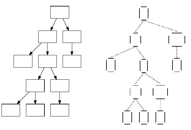
*
+ exp
x -
% cos
xxx
x
!"#$
x
!"#$
x!"#$
x
%
&'
(
%
!"#$
x
%
&'
(
cos
!"#$
-
%
&'
(
+
!"#$
x
%
&'
(
exp
!"#$
*
1
Figure 5.5 Auto-generated trees: in “.dot” format (left) and in L
A
T
EX format (right)
n1[label = "exp"];
n10[label = "x"];
n1 -> n10;
n -> n1;
}
To generate trees in .dot format, you’d say:
pop.subpop.0.species.ind.tree.0.print-style = dot
...or using the default parameter base:
gp.tree.print-style = dot
• L
A
T
EXformat, which emits the following code:
\begin{bundle}{\gpbox{*}}\chunk{\begin{bundle}{\gpbox{+}}\chunk{\gpbox{x}}
\chunk{\begin{bundle}{\gpbox{-}}\chunk{\begin{bundle}{\gpbox{%}}
\chunk{\gpbox{x}}\chunk{\gpbox{x}}\end{bundle}}\chunk{\begin{bundle}
{\gpbox{cos}}\chunk{\gpbox{x}}\end{bundle}}\end{bundle}}\end{bundle}}
\chunk{\begin{bundle}{\gpbox{exp}}\chunk{\gpbox{x}}\end{bundle}}\end{bundle}
To generate trees in L
A
T
EX format, you’d say:
pop.subpop.0.species.ind.tree.0.print-style = latex
...or using the default parameter base:
gp.tree.print-style = latex
179

This code works with the L
A
T
E
X ecltree and fancybox packages to produce a tree. Note that you’ll have
to replace the “
%
” with “
\%
” to make it legal L
A
T
E
X. The code works with the following boilerplate to
produce the tree shown at right in Figure 5.5.
\documentclass[]{article}
\usepackage{epic} % required by ecltree and fancybox packages
\usepackage{ecltree} % to draw the GP trees
\usepackage{fancybox} % required by \Ovalbox
\begin{document}
% minimum distance between nodes on the same line
\setlength{\GapWidth}{1em}
% draw with a thick dashed line, very nice looking
\thicklines \drawwith{\dottedline{2}}
% draw an oval and center it with the rule. You may want to fool with the
% rule values, though these seem to work quite well for me. If you make the
% rule smaller than the text height, then the GP nodes may not line up with
% each other horizontally quite right, so watch out.
\newcommand{\gpbox}[1]{\Ovalbox{#1\rule[-.7ex]{0ex}{2.7ex}}}
% And now the code. Note that % has been replaced with \%
\begin{bundle}{\gpbox{*}}\chunk{\begin{bundle}{\gpbox{+}}\chunk{\gpbox{x}}
\chunk{\begin{bundle}{\gpbox{-}}\chunk{\begin{bundle}{\gpbox{\%}}
\chunk{\gpbox{x}}\chunk{\gpbox{x}}\end{bundle}}\chunk{\begin{bundle}
{\gpbox{cos}}\chunk{\gpbox{x}}\end{bundle}}\end{bundle}}\end{bundle}}
\chunk{\begin{bundle}{\gpbox{exp}}\chunk{\gpbox{x}}\end{bundle}}\end{bundle}
% Finally end the document
\end{document}
5.2.8.2 GPIndividuals
Okay, there’s not much in-depth here. GPIndividual implements all the standard Individual methods
discussed in Section 3.2. Note that the distanceTo(...) method is not implemented. Two methods you might
want to be aware of:
ec.gp.GPIndividual Methods
public final void verify(EvolutionState state)
An auxillary debugging method which verifies many features of the structure of the GPIndividual and ll of its
GPTrees (and their GPNodes). This method isn’t called by ECJ but has proven useful in determining errors in
GPTree construction by various tree building or breeding algorithms.
public long size()
By default, returns the number of nodes in all the trees held by the GPIndividual.
5.2.9 Ephemeral Random Constants
An
Ephemeral Random Constant
or
ERC
[
3
] is a special GPNode, usually a terminal, which represents
a constant such as 3.14159 or true or 724 or complex: 3.24
+
5i or “aegu”. Usually ERCs are used to add
constants to programs which rely on math (such as Symbolic Regression).
An ERC needs to be able to do three things:
180
• Set itself to a random value when first created.
• Mutate to a new value when asked to do so.
• Stay fixed at that value all other times (as a constant).
In ECJ, ERCs are usually subclasses of ec.gp.ERC, an abstract superclass which provides basic functionality.
For example, if we were building a subclass of ERC which represents a floating point numerical constant, we
might add a single instance variable to hold its value:
package ec.app.myapp;
import ec.gp.*;
public class MyERC extends ERC {
public double value;
// other methods go here...
}
We’ll also probably need to implement some or most of the following methods to modify, read, write, or
compare the ERC.
public String name();
public boolean nodeEquals(GPNode node);
public int nodeHashCode();
public void resetNode(EvolutionState state, int thread);
public void mutateERC(EvolutionState state, int thread);
public String toStringForHumans();
public String encode();
public boolean decode(DecodeReturn ret);
public void readNode(EvolutionState state, DataInput input) throws IOException
public void writeNode(EvolutionState state, DataOutput output) throws IOException
public abstract void eval(EvolutionState state, int thread, GPData input,
ADFStack stack, GPIndividual individual, Problem problem);
Let’s go through these in turn:
public String name();
This is not the default GPNode implementation. When an ERC prints itself out in various ways, it writes
its name, then its value. By default the name is simply “ERC”, and if you have only one ERC type, you don’t
have to override it. For example, an ERC printed out might be ERC[3.14159]. However if you have more than
one class of ERCs, holding different kinds of values, you’ll want to distinguish them both for humans and
for ECJ to read back in again. To do this, override name() to return a unique symbol for each kind of ERC.
For example, you might just return “ERC1” versus “ERC2”, resulting in ERC1[3.14159] versus ERC2[921].
public boolean nodeEquals(GPNode node);
public int nodeHashCode();
Override the first method to test for equality with the second node: it’s the same kind of ERC, the same
class, has the same values, etc. Override the second method to provide a hash code for the ERC based on
its type and the values it contains. By default you can avoid implementing this second method, and just
implement the encode() method, discussed later. The default version of nodeHashCode() calls encode() and
then hashes the String.
public void resetNode(EvolutionState state, int thread);
public void mutateERC(EvolutionState state, int thread);
181
Override the first method to entirely randomize the value of the ERC. Override the second method to
mutate the value of the ERC when called to do so by the MutateERCPipeline. By default, mutateERC(...) just
calls resetNode(...), which is probably not what you want. Instead the mutation will likely need to be a small
deviation from the current value.
public String toStringForHumans();
public String encode();
public boolean decode(DecodeReturn ret);
public void readNode(EvolutionState state, DataInput input) throws IOException
public void writeNode(EvolutionState state, DataOutput output) throws IOException
As usual, override toStringForHumans() to provide a pretty version of the ERC for human consumption,
used by GPNode’s printer functions. The default version just calls toString(). You probably want to write
something prettier. The encode() and decode(...) methods are supposed to use the Code package (Section 2.2.3)
to encode and decode the ERC in a reasonable fashion.
Finally, the readNode(...) and writeNode(...) methods, as usual, read and write the ERC in binary fashion.
You only need to implement these methods if you’re planning on writing over the network (such as using
distributed evaluation or island models). But they’re easy so why not? And of course, there’s the method to
actually execute the ERC as code. This typically returns the ERC’s internal value (it’s a constant after all):
public abstract void eval(EvolutionState state, int thread, GPData input,
ADFStack stack, GPIndividual individual, Problem problem);
Note that ERCs by default override the expectedChildren() method to return 0 (they are usually terminals).
If for some reason your ERC is not a terminal, you’ll want to override this method to return the right number
of children.
Example
Let’s create an ERC and add it to our existing example from Section 5.2.6. We’ll make an ERC
which represents constants between 0.0 and 1.0, not including 1.0. Our mutator will add a little Gaussian
noise to the node. Here’s a full class:
package ec.app.myapp;
import ec.gp.*;
public class MyERC extends ERC {
public double value;
public String toStringForHumans() { return "" + value; }
public String encode() { return Code.encode(value); }
public boolean decode(DecodeReturn ret) {
int pos = dret.pos;
String data = dret.data;
Code.decode(dret);
if (dret.type != DecodeReturn.T_DOUBLE) // uh oh! Restore and signal error.
{ dret.data = data; dret.pos = pos; return false; }
value = dret.d
return true;
}
public boolean nodeEquals(GPNode node)
{ return (node.getClass() == this.getClass() && ((MyERC)node).value == value); }
public void readNode(EvolutionState state, DataInput input) throws IOException
{ value = dataInput.readDouble(); }
public void writeNode(EvolutionState state, DataOutput output) throws IOException
182
{ dataOutput.writeDouble(value); }
public void resetNode(EvolutionState state, int thread)
{ val = state.random[thread].nextDouble(); }
public void mutateNode(EvolutionState state, int thread) {
double v;
do v = value + state.random[thread].nextGaussian() * 0.01;
while( v < 0.0 || v >= 1.0 );
value = v;
}
public void eval(EvolutionState state, int thread, GPData input, ADFStack stack,
GPIndividual individual, Problem Problem)
{ ((MyData)data).val = value; }
}
Now let’s set up the parameters to use it. We’ll change the function set. Our ERC is a terminal so it takes
no arguments: we’ll use nc0 as its constraints.
# Our Function Set
gp.fs.0 = ec.gp.GPFunctionSet
gp.fs.0.size = 6
gp.fs.0.func.0 = ec.app.myapp.X
gp.fs.0.func.0.nc = nc0
gp.fs.0.func.1 = ec.app.myapp.Y
gp.fs.0.func.1.nc = nc0
gp.fs.0.func.2 = ec.app.myapp.Mul
gp.fs.0.func.2.nc = nc2
gp.fs.0.func.3 = ec.app.myapp.Sub
gp.fs.0.func.3.nc = nc2
gp.fs.0.func.4 = ec.app.myapp.Sin
gp.fs.0.func.4.nc = nc1
gp.fs.0.func.5 = ec.app.myapp.MyERC
gp.fs.0.func.5.nc = nc0
... and we’re done.
5.2.10 Automatically Defined Functions and Macros
Automatically Defined Functions
(ADFs) [
4
] are a standard way of creating some modularism in Genetic
Programming. They define multiple trees in the GPIndividual and essentially define a function calling
structure where certain trees can call other trees as subfunctions. ADFs are the primary reason why
GPIndividual has multiple GPTrees.
The simplest kind of ADF is found in Figure 5.6. Here each ADF function is a terminal, and when it is
evaluated, it simply evaluates the corresponding ADF tree, then returns the tree’s return value. The ADF
function is a GPNode, an instance of ec.gp.ADF. It’s very rare to further specialize this class. Notice that
calling is nested — an ADF can call another ADF and so on. However it’s not very common to have recursive
calls because you’ll need to construct some kind of stopping base-case criterion to avoid infinite recursive
loops.
ADFs add a two more parameters to the standard GPNode suite. Let’s say we’re adding a zero-argument
ADF. Beyond the node constraints, we also need to specify which tree will be called when the ADF is
executed; and also a simple name for the ADF to distinguish it from other ADFs and GPNodes. Ideally this
name should only have lowercase letters, numbers, and hyphens (that is, “Lisp-style”):
183
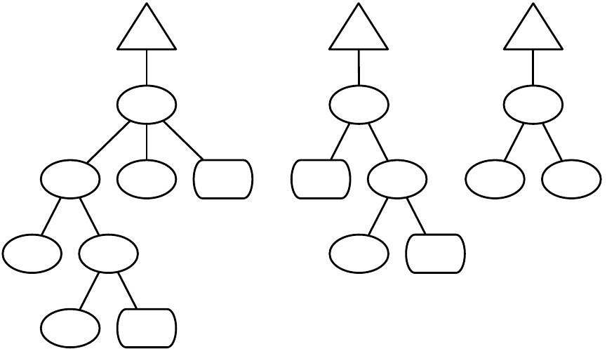
if-food-
ahead
left progn2
move ADF 1
move ADF 0
progn3
GP
Tree
Root if-food-
ahead
ADF 1 progn2
move ADF 1
ADF
0
Root progn2
move left
ADF
1
Root
Figure 5.6 A GPIndividual with two no-argument (terminal) ADFs. The primary GP Tree has functions in its function set that can call
the other two trees; in turn the ADF 1 tree has a function in its function set that can call the ADF 2 tree. The return values of the various
ADF trees become the return values of their respective calling functions.
gp.fs.0.func.5 = ec.gp.ADF
gp.fs.0.func.5.nc = nc0
gp.fs.0.func.5.tree = 1
gp.fs.0.func.5.name = ADF0
It’s traditional that the first tree be called ADF0, the second ADF1, and so on.
Since typically the first
GP Tree in the array is the “main” tree, and the second tree is ADF0, this means that ADF0’s associated tree
number is usually 1, and ADF1’s associated tree number is usually 2. If you don’t specify a name, ECJ will
maintain this tradition by setting the name to “ADF”
+
(tree number
−
1), which is usually right anyway.
It’ll also issue a warning.
The name of the ADF (in this case “ADF1”) and its associated GP tree (in this case, tree 1) are stored in
the ec.gp.ADF class like this:
public int associatedTree;
public String name;
The name() method returns the value of the name variable.
ADFArguments override the checkConstraints(...) method to do a lot of custom advanced checking. If
you override this, be sure to call super().
We’ll show how to set up the ADF tree itself in the Example below.
ADFs can also have arguments to the functions. In Figure 5.7, we have an ADF with two arguments. The
way this works is as follows: when an ADF function is called, we first evaluate its children, then hold their
return values in storage. We then call the corresponding ADF tree. In that tree there may be one or more
special terminal GPNodes, two different kinds of instances of ec.gp.ADFArgument. One group of instances,
when evaluated, will return the value of the first child. The second group return the value of the second
child. This enables the ADF tree to use arguments in its “function call” so to speak.
184
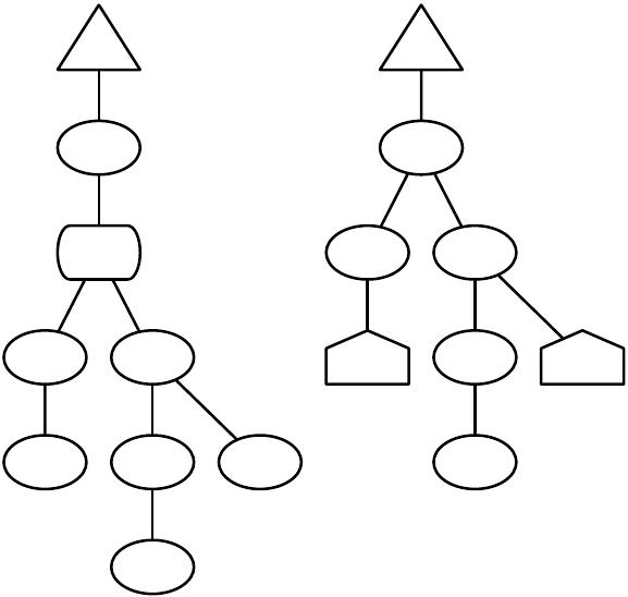
sin
ADF 0
cos –
sqrt x
x
x
GP
Tree
Root +
sin –
sin ARG 2
x
ARG 1
ADF
0
Root
Figure 5.7 A GPIndividual with one 2-argument ADF. The primary GP Tree has a function in its function set that can call the ADF tree.
This function first evaluates its children, then executes the ADF tree. In the ADF tree there are two terminal functions (ARG 1 and ARG
2) which, when evaluated, return the values of the two children respectively. The return value of the ADF tree becomes the return value
of the ADF function.
ADFArguments add one additional parameter: the child number associated with the argument. For
example:
gp.fs.1.func.6 = ec.gp.ADFArgument
gp.fs.1.func.6.nc = nc0
gp.fs.1.func.6.arg = 0
gp.fs.1.func.6.name = ARG0
If you don’t specify a name, ECJ will set the name to “ARG”
+
arg number, which is usually right anyway.
It’ll also issue a warning.
The ADFArgument’s name and argument number are stored in the ec.gp.ADFArgument class as:
public int argument;
public String name;
Again, the name() method returns the value of the name variable.
ADFArguments are always terminals, and so they override the expectedChildren() method to return 0.
ECJ also supports
Automatically-Defined Macros
(or ADMs), described in [
20
]. These differ from ADFs
only in when the children are evaluated. When an ADM node is evaluated, its children are not evaluated
first; rather the ADM immediately calls its associated tree. When an argument node in that tree (again, a
terminal) is evaluated, we teleport back to the associated child and evaluate it right then and there, then
return its value. Note that this means that children may never be evaluated; or can be evaluated multiple
times, as shown in Figure 5.8.
ADMs are just like ADFs in their parameters:
185
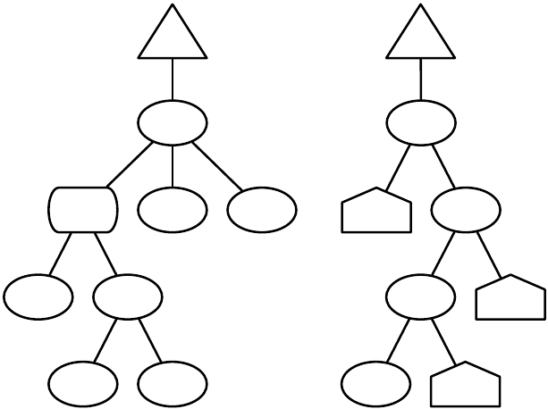
ADM 0
left progn2
move right
move left
progn3
GP
Tree
Root progn2
ARG 1
if-food-
ahead
ARG 1
ADM
0
Root
progn2
move ARG 2
Figure 5.8 A GPIndividual with one 2-argument ADM. The primary GP Tree has a function in its function set that can call the ADM
tree. This function delays the evaluation of its its children, and immediately executes the ADM tree. In the ADM tree there are two
terminal functions (ARG 1 and ARG 2) which, when evaluated, evaluate (or, as necessary, re-evaluate) the original children to the ADM
function and then return their values. Notice that in this example child # 1 may be evaluated twice, and child #2, depending on whether
there’s food ahead, may be never evaluated.
gp.fs.0.func.6 = ec.gp.ADM
gp.fs.0.func.6.nc = nc2
gp.fs.0.func.6.tree = 1
# This will be called "ADM1"
gp.fs.0.func.6.name = ADM1
If an ADF or ADM tree has arguments, it probably will require its own separate GPTreeConstraints,
because it needs to have its own GPFunctionSet with those arguments defined. See the Example below.
5.2.10.1 About ADF Stacks
ADFs and ADMs are a bit complex. To do their magic, they need a special object called an ec.gp.ADFStack.
This is actually two stacks of ec.gp.ADFContext objects which store the location and current return values of
various children. These classes are almost never overridden: here’s the standard (default) parameters for
them:
gp.problem.stack = ec.gp.ADFStack
gp.adf-stack.context = ec.gp.ADFContext
You could have defined it this way...
eval.problem.stack = ec.gp.ADFStack
eval.problem.stack.context = ec.gp.ADFContext
... but there are advantages in using the default parameters, particularly when getting to Grammatical
Evolution (Section 5.3).
186
Example
ADFs and ADMs are fairly straightforward to implement but they can require a fair number of
parameters. Continuing with the example in started in Section 5.2.6 and extended in Section 5.2.9, let’s add a
2-argument ADF to the individual. This will require adding a second GPTree and its own GPTreeConstraints.
Let’s begin by modifying the GPFunctionSet of the original tree to include this ADF:
# Our Function Set
gp.fs.0 = ec.gp.GPFunctionSet
gp.fs.0.size = 7
gp.fs.0.func.0 = ec.app.myapp.X
gp.fs.0.func.0.nc = nc0
gp.fs.0.func.1 = ec.app.myapp.Y
gp.fs.0.func.1.nc = nc0
gp.fs.0.func.2 = ec.app.myapp.Mul
gp.fs.0.func.2.nc = nc2
gp.fs.0.func.3 = ec.app.myapp.Sub
gp.fs.0.func.3.nc = nc2
gp.fs.0.func.4 = ec.app.myapp.Sin
gp.fs.0.func.4.nc = nc1
gp.fs.0.func.5 = ec.app.myapp.MyERC
gp.fs.0.func.5.nc = nc0
gp.fs.0.func.6 = ec.gp.ADF
gp.fs.0.func.6.nc = nc2
gp.fs.0.func.6.tree = 1
gp.fs.0.func.6.name = ADF1
Let’s create a second function set for our second (ADF) tree. This set will have all the same functions as
the main tree, except for the ADF function (we don’t want to call ourselves recursively!) Instead we’ll add
two ADFArgument nodes to represent the two children.
187
gp.fs.size = 2
# Our Second Function Set
gp.fs.1 = ec.gp.GPFunctionSet
gp.fs.1.name = f1
gp.fs.1.size = 8
gp.fs.1.func.0 = ec.app.myapp.X
gp.fs.1.func.0.nc = nc0
gp.fs.1.func.1 = ec.app.myapp.Y
gp.fs.1.func.1.nc = nc0
gp.fs.1.func.2 = ec.app.myapp.Mul
gp.fs.1.func.2.nc = nc2
gp.fs.1.func.3 = ec.app.myapp.Sub
gp.fs.1.func.3.nc = nc2
gp.fs.1.func.4 = ec.app.myapp.Sin
gp.fs.1.func.4.nc = nc1
gp.fs.1.func.5 = ec.app.myapp.MyERC
gp.fs.1.func.5.nc = nc0
gp.fs.1.func.6 = ec.gp.ADFArgument
gp.fs.1.func.6.nc = nc0
gp.fs.1.func.6.arg = 0
gp.fs.1.func.6.name = ARG0
gp.fs.1.func.7 = ec.gp.ADFArgument
gp.fs.1.func.7.nc = nc0
gp.fs.1.func.7.arg = 1
gp.fs.1.func.7.name = ARG1
Now we create a new GPTreeConstraints which uses this function set:
gp.tc.size = 2
# Our Second Tree Constraints
gp.tc.1 = ec.gp.GPTreeConstraints
gp.tc.1.name = tc1
gp.tc.1.fset = f1
gp.tc.1.returns = nil
gp.tc.1.init = ec.gp.koza.HalfBuilder
Next we add the second tree to the GPIndividual:
pop.subpop.0.species.ind.numtrees = 2
pop.subpop.0.species.ind.tree.1 = ec.gp.GPTree
pop.subpop.0.species.ind.tree.1.tc = tc1
The ADF stack and ADF context were already defined in the previous examples, but we’ll do it again
here for clarity:
gp.problem.stack = ec.gp.ADFStack
gp.adf-stack.context = ec.gp.ADFContext
...and we’re done!
An important note: because the main GP Tree and the ADF have different function sets and thus different
GPTreeConstraints, standard GP Crossover (see Section 5.2.5) won’t cross over the ADF tree with a main
tree of some other individual or vice versa. But if, for example, your GPIndividual had two ADF trees that
188

had the same GPTreeConstraints, they could get crossed over with arbitrary other ADF trees in another
GPIndividuals.
5.2.11 Strongly Typed Genetic Programming
Sometimes it’s useful to constrain which GPNodes may serve as children of other GPNodes, or the root of
the GPTree. For example, consider a GPNode called (if test then else). This node evaluates test, and based
on its result (true or false) it either evaluates and returns then or else. Let’s presume that then and else (and
if) return doubles. On the other hand, test is intended to return a boolean. So you’ll need to have some
GPNodes in your function set which return doubles and others which return booleans; the (if ...) node itself
returns a double.
The problem is not that you have nodes which return different values — this is easily handled by hacking
your GPData object. The problem is that you now have constraints on valid tree structures: you can’t plug
a node which returns a double (say, (sin ...)) into the test slot of your (if ...) node, which is expecting a
boolean.6This is where strong typing comes in.
ECJ’s typing system is simple but sufficient for many common uses. It’s not as sophisticated as a full
polymorphic typing system but it also doesn’t have the hair-raising complexity that such a system requires.
ECJ is complex enough as it is thank you very much!
ECJ’s system is based on
type objects
, subclasses of the abstract superclass ec.gp.GPType, and nodes are
allowed to connect as parent and child if their corresponding type objects are
type compatible
. ECJ’s type
objects of two kinds: atomic types and set types. An atomic type is just a single object (in fact, it’s theoretically
just a symbol, or in some sense, an integer). A set type is a set of atomic types. Type compatibility is as
follows:
• Two atomic types are compatible if they are the same.
• A set type is compatible with an atomic type if it contains the atomic type in its set.
• Two set types are compatible if their intersection is nonempty.
Every GPNode is assigned a type object to represent the “return type” of the GPNode. Furthermore
every nonterminal GPNode is assigned a type object for each of its children: this is called the “child type” or
“argument type” or that particular child slot. Last, the GPTree itself is assigned “root type”: a type for the
root of the tree. Each GPTree in a GPIndividual can have a different root type. Here’s what must be true
about any given GPTree.
•
For any parent and child in a tree, with the child in slot C, the return type of the child must be
compatible with the child type of the parent for slot C.
•
The return type of the root GPNode must be compatible with the GPTree’s root type. This ensures that
the tree is returning
You can see an example of a GPTree with type constraints listed in Figure 5.9.
Every GPNodeBuilder and GP Breeding Pipeline must maintain the constraints guaranteed by typing.
The issue is guaranteeing that if you replace one GPNode with another, that the second GPNode will be
legal. This is done primarily with the following two utility functions:
ec.gp.GPNode Methods
public GPType parentType(GPInitializer initializer)
If the GPNode’s parent is another GPNode, this returns the type of the parent’s child slot presently filled by the
GPNode. If the GPNode’s parent is a GPTree, this returns the type of the tree’s root.
6
Well, you could if you assumed that 0.0 was false and anything else was true. But this is a hack. The right way to do it is to constrain
things properly
189
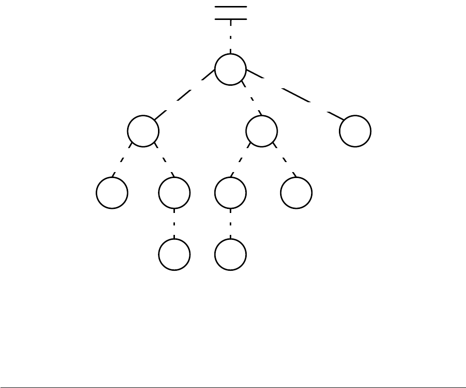
ir
2.3
*
if
and
on-
wall tick>
20 3
bool
bool
bool
bool
bool
bool
int
int
int
int
int, float
float
6
int, float
int
int, float
float
int, float
float
tree
int, float
float
Figure 5.9 A typed genetic programming parse tree. Each edge is labeled with two types. The “lower” type is the return type of the
child node. The “upper” type is the type of the argument slot of the parent. For the child to fit into that particular argument slot, the
types must be compatible. Types of the form “int, float” are set types. All others are atomic types. Note that the root of the tree plugs
into a particular slot of the “tree” object (ec.gp.GPTree) , which itself has a slot type. A repeat of Figure 1.4.
public final boolean swapCompatibleWith(GPInitializer initializer, GPNode node)
Returns true swapping the GPNode into the slot presently occupied by node is acceptable, type-wise.
Before you can assign types, you’ll need to define them. Each type is given a unique symbol. As an
example, let’s begin by creating two atomic types, called (uninterestingly) “boolean” and “nil” (we say “nil”
instead of “double” so we don’t have to redefine the GPTreeConstraints and GPNodeConstraints we defined
earlier, which all use “nil” as their types). We’d say:
gp.type.a.size = 2
gp.type.a.0.name = boolean
gp.type.a.1.name = nil
We might also define a set type or two. For fun, let’s create a set type which contains both booleans and
doubles. We’ll also have to stipulate the atomic types encompassed by the set type:
gp.type.s.size = 1
gp.type.s.0.name = boolean-or-nil
gp.type.s.0.size = 2
gp.type.s.0.member.0 = boolean
gp.type.s.0.member.1 = nil
What’s the point of set types, you might ask. Why not just atomic types? Set types are particularly useful
for describing situations where a given GPNode can adapt to several different kinds of children in a given
190
slot. This is particularly useful for simulating notions of subtyping or subclassing. For example, a GPNode
like (sin ... ) might declare that its child can either be an “integer” or a “double”, by having its child type
defined as a set type of “number” which encapsulates both integers and doubles.
What this typing facility cannot do is dynamically change types as necessary. For example, you cannot
say that a GPNode like (+ ... ...) returns a double if either of its children is of type double, but if both of its
children are of type integer, then it returns an integer.
You are also restricted to a finite number of types. For example, consider a GPNode called (matrix-multiply
... ...) which takes two children which return matrices. You cannot say that if the left child is an
MxN
matrix,
and your right child is an
NxP
matrix, that the return type will be an
MxP
matrix. This is partly because you
can’t define dynamic typing, but it’s also because
M
,
N
, and
P
can be any of an infinite number of numbers,
resulting in an infinite number of types: specifying an infinite number of types would be hard on your
fingers. There exist polymorphic typing systems for genetic programming but they’re fairly bleeding-edge.
If you need things like this, I suggest instead to look at Grammatical Evolution (Section 5.3).
Example
Let’s add some typing to the example we started in Section 5.2.6 and continued in Sections 5.2.9
and 5.2.10. We’ll add a boolean type as before, and a few functions which rely on it.
First the boolean type:
gp.type.a.size = 2
gp.type.a.0.name = boolean
gp.type.a.1.name = nil
gp.type.s.size = 1
gp.type.s.0.name = boolean-or-nil
gp.type.s.0.size = 2
gp.type.s.0.member.0 = boolean
gp.type.s.0.member.1 = nil
Next we need to say what kinds of nodes are permitted as the root of the tree. We do this by specifying
the tree’s return type. For a node to be permitted as the root of the tree, it must have a return type compatible
with this tree return type. Let’s say that we want our tree to only have root nodes which have a return type
of nil (no boolean allowed):
gp.tc.size = 1
gp.tc.0 = ec.gp.GPTreeConstraints
gp.tc.0.name = tc0
gp.tc.0.fset = f0
# Here we define the return type of this GPTreeConstraints
gp.tc.0.returns = nil
As it so happens, this is what we already have by default, so putting it all here is a bit redundant.
Next we’ll need to modify the node constraints for each GPNode, so we specify the return type of each of
our nodes and also the expected child types of their child slots. For the node constraints, let’s add three new
GPNodeConstraints:
•
A function which returns a double (nil), has three children, and the first child needs to be a boolean.
The other two children are nil. This would be for things like the (if ... ... ...) node.
•
A function which takes two booleans and returns a boolean. This would be for functions like (nand ...
...).
•
A function which takes two doubles and returns a boolean. This would be for functions like (
>
... ...).
These three new GPNodeConstraints would be:
191
gp.nc.size = 6
# ... first come the original node constraints, then these:
# Example: (if ... ... ...)
gp.nc.3 = ec.gp.GPNodeConstraints
gp.nc.3.name = nc3
gp.nc.3.returns = nil
gp.nc.3.size = 3
gp.nc.3.child.0 = boolean
gp.nc.3.child.1 = nil
gp.nc.3.child.2 = nil
# Example: (nand ... ...)
gp.nc.4 = ec.gp.GPNodeConstraints
gp.nc.4.name = nc2
gp.nc.4.returns = boolean
gp.nc.4.size = 2
gp.nc.4.child.0 = boolean
gp.nc.4.child.1 = boolean
# Example: (>... ...)
gp.nc.5 = ec.gp.GPNodeConstraints
gp.nc.5.name = nc2
gp.nc.5.returns = boolean
gp.nc.5.size = 2
gp.nc.5.child.0 = nil
gp.nc.5.child.1 = nil
Recall that our GPData looks like this:
package ec.app.myapp;
import ec.gp.*;
public class MyData extends GPData
{
public double val;
public GPData copyTo(GPData other)
{ ((MyData)other).val = val; return other; }
}
We could modify this to include a boolean data type as well, but we’ll just use the val variable to store
both boolean and real-valued data. Before you go about that, re-read Section 5.2.3.1 (on GPData) and its
discussion about clone() and copyTo(...).
Now let’s define our three new GPNodes. First our If-statement:
192
package ec.app.myapp;
import ec.*;
import ec.gp.*;
public class If extends GPNode {
public String toString() { return "if" };
public void eval(EvolutionState state, int thread, GPData input,
ADFStack stack, GPIndividual indivdiual, GPProblem problem) {
MyData data = (MyData) input;
children[0].eval(state, thread, data, stack, individual, prob);
if (data.val != 0.0) // true
children[1].eval(state, thread, data, stack, individual, prob);
else
children[2].eval(state, thread, data, stack, individual, prob);
// the result be stored in data
}
}
Next, the nand node:
package ec.app.myapp;
import ec.*;
import ec.gp.*;
public class Nand extends GPNode {
public String toString() { return "nand" };
public void eval(EvolutionState state, int thread, GPData input,
ADFStack stack, GPIndividual indivdiual, GPProblem problem) {
MyData data = (MyData) input;
children[0].eval(state, thread, data, stack, individual, prob);
boolean left = (data.val != 0.0);
children[1].eval(state, thread, data, stack, individual, prob);
boolean right = (data.val != 0.0);
data.val = !(left && right) ? 1.0 : 0.0;
}
}
Next, the >node:
package ec.app.myapp;
import ec.*;
import ec.gp.*;
public class GreaterThan extends GPNode {
public String toString() { return ">" };
public void eval(EvolutionState state, int thread, GPData input,
ADFStack stack, GPIndividual indivdiual, GPProblem problem) {
MyData data = (MyData) input;
children[0].eval(state, thread, data, stack, individual, prob);
double left = data.val;
children[1].eval(state, thread, data, stack, individual, prob);
double right = data.val;
data.val = (left > right) ? 1.0 : 0.0;
}
}
Notice that these functions hijack the double value to store boolean information. This is okay because
we know that the recipient of this information will understand it. How do we know? Because the typing
constraints have made it impossible to be otherwise.
193

So let’s add these functions to the function set of our main GP Tree:
# Our Main Tree Function Set
gp.fs.0 = ec.gp.GPFunctionSet
gp.fs.0.size = 10
gp.fs.0.func.0 = ec.app.myapp.X
gp.fs.0.func.0.nc = nc0
gp.fs.0.func.1 = ec.app.myapp.Y
gp.fs.0.func.1.nc = nc0
gp.fs.0.func.2 = ec.app.myapp.Mul
gp.fs.0.func.2.nc = nc2
gp.fs.0.func.3 = ec.app.myapp.Sub
gp.fs.0.func.3.nc = nc2
gp.fs.0.func.4 = ec.app.myapp.Sin
gp.fs.0.func.4.nc = nc1
gp.fs.0.func.5 = ec.app.myapp.MyERC
gp.fs.0.func.5.nc = nc0
gp.fs.0.func.6 = ec.gp.ADF
gp.fs.0.func.6.nc = nc2
gp.fs.0.func.6.tree = 1
gp.fs.0.func.6.name = ADF1
gp.fs.0.func.7 = ec.app.myapp.If
gp.fs.0.func.7.nc = nc3
gp.fs.0.func.8 = ec.app.myapp.Nand
gp.fs.0.func.8.nc = nc4
gp.fs.0.func.9 = ec.app.myapp.GreaterThan
gp.fs.0.func.9.nc = nc5
...and we’re done!
Mixing ADF and ADMs and Typed GP
A quick note. The return type of an ADF node must match the
root type of its corresponding ADF tree. Additionally, the child type of a certain slot in an ADF node must
match the return type of the corresponding ADFArgument.
5.2.11.1 Inside GPTypes
If you want to create a GPNodeBuilder or a GP Breeding Pipeline, you ought to go in more detail about
GPTypes.
ec.gp.GPType is an abstract superclass of ec.gp.GPAtomicType and ec.gp.GPSetType, which define the
atomic and set types respectively. The two basic data elements in a GPType are:
public String name;
public int type;
The first variable, like GPFunctionSet, GPTreeConstraints, and GPNodeConstraints, holds the name of
the type (as defined in the parameters). The second variable holds a uniquely-assigned integer for this type.
The important feature for types is to determine whether they are
type-compatible
with one another. The
compatibility function is this:
ec.gp.GPType Methods
public boolean compatibleWith(GPInitializer initializer, GPType type)
Returns true if the return type of this GPNode is type-compatible with the given type.
194

GPAtomicTypes are simple: they are compatible with one another if their type integer is the same. A
GPSetType instead is a set of GPAtomicTypes, stored in different ways for query convenience:
public Hashtable types h;
public int[] types packed;
public boolean[] types sparse;
The first is the GPAtomicTypes in the set stored in a Hashtable. The second is an array of the GPAtomic-
Types. And the third is an array of booleans, one for each GPAtomicType number, which is true if that
GPAtomicType is a member of the set.
A GPSetType is compatible with a GPAtomicType if the GPSetType contains the GPAtomicType as an
element. Two GPSetTypes are compatible with one another if their intersection is nonempty.
5.2.12 Parsimony Pressure (The ec.parsimony Package)
Genetic programming has a serious bloat problem: as evolution progresses, the size of the trees inside
the population tend to grow without bound. This is a problem that exists for various arbitrary-length
representations (lists, graphs, rulsests, etc.) but genetic programming has studied it the most.
The most common simple way of keeping trees down is to make it illegal to produce a tree larger than a
certain depth. For example, Koza’s standard rules, adhered to by the basic parameters in ECJ, stipulate that
crossover and mutation operators may not produce a child which is deeper than 17 nodes [3], for example:
gp.koza.xover.tries = 1
gp.koza.xover.maxdepth = 17
Here if the crossover operation produces a child greater than 17, it is not forwarded on; but rather its
(presumably smaller) parent is forwarded on in its stead. This is a fairly crude approach, but it’s fairly
effective. Another approach — which can be done at the same time — is to modify the selection operator to
favor smaller individuals. This notion is called parsimony pressure.
In the ec.parsimony package, ECJ has several SelectionMethods which select both based on fitness and on
size (smaller size being preferred). These methods compute size based on GPNode’s size() function. Many of
these selection methods were compared and discussed at length in [10]. Here they are:
•
ec,parsimony.LexicographicTournamentSelection is a straightforward TournamentSelection operator, ex-
cept that the fitter Individual is preferred (as usual), but when both Individuals are the same fitness,
the smaller Individual is preferred. Parameters for this operator are basically the same as for Tourna-
mentSelection.
Let us presume that the SelectionMethod is the first source of the pipeline of Subpopulation 0. Then
the basic parameters are the same as in TournamentSelection:
pop.subpop.0.species.pipe.source.0 = ec.parsimony.LexicographicTournamentSelection
pop.subpop.0.species.pipe.source.0.size = 7
pop.subpop.0.species.pipe.source.0.pick-worst = false
Or using the default parameters:
pop.subpop.0.species.pipe.source.0 = ec.parsimony.LexicographicTournamentSelection
select.lexicographic-tournament.size = 7
select.lexicographic-tournament.pick-worst = false
The problem with this method is that bloat control only comes into effect for problems where lots of
fitness ties occur. This problem lead us to two modifications of the basic idea:
•
ec,parsimony.BucketTournamentSelection is like LexicographicTournamentSelection, except that first
individuals are placed into
N
classes (“buckets”) based on fitness. The subpopulation is first sorted by
195

fitness. Then the bottom
subpopulation size
N
individuals are placed in the worst bucket, plus any individuals
remaining in the subpopulation with the same fitness as the best individual in that bucket. Next the
bottom remaining
subpopulation size
N
are placed in the second worst bucket, plus any individuals remaining
in the population with the same fitness as the best individual in that bucket. This continues until
all the individuals are exhausted. BucketTournamentSelection then works like LexicographicTourna-
mentSelection except that instead of comparing based on fitness, it compares based on the bucket the
individual is in. The number of buckets is defined by num-buckets:
pop.subpop.0.species.pipe.source.0 = ec.parsimony.BucketTournamentSelection
pop.subpop.0.species.pipe.source.0.size = 7
pop.subpop.0.species.pipe.source.0.pick-worst = false
pop.subpop.0.species.pipe.source.0.num-buckets = 10
Or using the default parameters:
pop.subpop.0.species.pipe.source.0 = ec.parsimony.BucketTournamentSelection
select.bucket-tournament.size = 7
select.bucket-tournament.pick-worst = false
select.bucket-tournament.num-buckets = 10
•
ec,parsimony.ProportionalTournamentSelection is like TournamentSelection, except that it either selects
based on fitness or selects based on size. It determines which one to do by flipping a coin of a certain
probability that fitness will be used. The parameters are:
pop.subpop.0.species.pipe.source.0 = ec.parsimony.ProportionalTournamentSelection
pop.subpop.0.species.pipe.source.0.size = 7
pop.subpop.0.species.pipe.source.0.pick-worst = false
pop.subpop.0.species.pipe.source.0.fitness-prob = 0.9
Or using the default parameters:
pop.subpop.0.species.pipe.source.0 = ec.parsimony.ProportionalTournamentSelection
select.bucket-tournament.size = 7
select.bucket-tournament.pick-worst = false
select.bucket-tournament.fitness-prob = 0.9
•
ec,parsimony.DoubleTournamentSelection is actually two TournamentSelections in a row. In short, we
do a TournamentSelection of tournament size
N
based on fitness: but the entrants to that tournament
are not chosen uniformly at random from the subpopulation, but rather are the winners of
N
other
tournament selections, each performed based on size. Alternatively, we can first do tournament
selections on fitness, then have a final tournament on size.
Thus there are roughly twice as many parameters: ones describing the final tournament, and ones
describing the initial (“qualifying”) tournaments
196
pop.subpop.0.species.pipe.source.0 = ec.parsimony.DoubleTournamentSelection
# Final tournament
pop.subpop.0.species.pipe.source.0.size = 2
pop.subpop.0.species.pipe.source.0.pick-worst = false
# Qualifying tournaments
pop.subpop.0.species.pipe.source.0.size2 = 2
pop.subpop.0.species.pipe.source.0.pick-worst2 = false
# Make the qualifying tournament based on size
pop.subpop.0.species.pipe.source.0.do-length-first = true
Or using the default parameters:
pop.subpop.0.species.pipe.source.0 = ec.parsimony.DoubleTournamentSelection
# Final tournament
select.double-tournament.size = 7
select.double-tournament.pick-worst = false
# Qualifying tournaments
select.double-tournament.size2 = 7
select.double-tournament.pick-worst2 = false
# Make the qualifying tournament based on size
select.double-tournament.do-length-first = true
•
ec,parsimony.TarpeianStatistics implements the “Tarpiean” parsimony pressure method [
15
]. This
method identifies the individuals in the subpopulation with above-average size. Notice that this may
not be half the subpopulation: it could be a very small number if they are very large and the others are
very small. Then a certain proportion of these individuals, picked randomly, are assigned a very bad
fitness, and their evaluated flags are set. This happens before evaluation, so the evaluation procedure
doesn’t bother to evaluate those individuals further.
The Tarpiean method isn’t a selection procedure: it’s a fitness assignment procedure. As such it’s not
implemented as a SelectionMethod but rather as a Statistics subclass which hooks into the evolutionary
loop prior to evaluation.
Let’s say that TarpieanStatistics is the only child of our primary Statistics object. The parameters would
look like this:
stat.num-children = 1
stat.child.0 = ec.parsimony.TarpeianStatistics
stat.child.0.kill-proportion = 0.2
5.3 Grammatical Evolution (The ec.gp.ge Package)
Grammatical Evolution (GE) [
19
] is an approach to building genetic programming trees using a grammar
interpreted by a list representation. The trees are then evaluated and tested. In ECJ the procedure for
evaluating Individuals in GE works roughly like this.
•
The representation is an arbitrarily long list of ints (See Section 5.1.2), implemented as a special subclass
of IntegerVectorIndividual called ec.gp.ge.GEIndividual.
197
• The Fitness is typically a KozaFitness.
• The GEIndividual’s species is a ec.gp.ge.GESpecies.
•
The GESpecies holds a
grammar
, loaded from a file and produced via an ec.gp.ge.GrammarParser, which
we will interpret according to the ints in the Individual.
•
To assess the fitness of a GEIndividual, we hand it to the GESpecies which interprets it according to the
grammar, producing a GPIndividual.
• The GPIndividual is then evaluated in the normal ECJ fashion and its Fitness is set.
• We then transfer the Fitness to the GEIndividual.
We’d like to use plain-old GP test problems to make this as easy as possible. To pull this off we have to
do a few minor hacks. First, we must insert the GE conversion process in-between the Evaluator and the
GPProblem that the user wrote. To do this we have a special Problem class called ec.gp.ge.GEProblem, which
is assigned as the Evaluator’s problem. The GPProblem is then set up as a subsidiary of the GEProblem.
When the Evaluator wishes to evaluate an IntegerVectorIndividual, it calls the GEProblem, which converts it
to a GPIndividual and then hands the GPIndividual to the GPProblem to evaluate. This is done as follows:
eval.problem = ec.gp.ge.GEProblem
eval.problem.problem = ec.app.myproblem.MyGProblem
Note that GPProblems usually require auxiliary parameters (not the least of which is their GPData), so
we’ll need to also say things like...
eval.problem.problem.data = ec.app.myproblem.MyGPData
... etc. You don’t need to define the ADFStack or ADFContext specially because the default parameters
for them suffice:
gp.problem.stack = ec.gp.ADFStack
gp.adf-stack.context = ec.gp.ADFContext
5.3.1 GEIndividuals, GESpecies, and Grammars
The reason we use GEIndividual instead of just IntegerVectorIndividual is simple: when we print out the
GEIndividual we wish to print out the equivalent GPIndividual as well. That’s the only thing GEIndividual
does beyond being just a IntegerVectorIndividual.
The GEProblem doesn’t actually do the translation from list to tree. Instead, it calls on the GESpecies to
do this dirty work. First, let’s set the GESpecies, GEIndividual, GrammarParser, and Fitness of Species 0:
pop.subpop.0.species = ec.gp.ge.GESpecies
pop.subpop.0.species.parser = ec.gp.ge.GrammarParser
pop.subpop.0.species.ind = ec.gp.ge.GEIndividual
pop.subpop.0.species.fitness = ec.gp.koza.KozaFitness
GESpecies requires a
grammar file
for each tree in the GPIndividual. If your GPIndividual has two trees
(say), you’ll need two grammar files, which are specified like this:
pop.subpop.0.species.file.0 = foo.grammar
pop.subpop.0.species.file.1 = bar.grammar
Alternatively you can use the default parameter base:
198

ge.species.file.0 = foo.grammar
ge.species.file.1 = bar.grammar
Grammar files are text files consisting of lines. Each line can be blank whitespace (which is ignored), a
comment (which starts with a #, just like parameter files), or a
grammar rule
. A grammar rule has a
head
,
followed by whitespace, followed by the string
"::="
, then more whitespace, and finally a
body
. Here is an
example rule:
<foo> ::= (hello <bar>) | (yo) | (whoa <bar> <baz>)
In this example,
<
foo
>
is the head, and (hello
<
bar
>
)
|
(yo)
|
(whoa
<
bar
> <
baz
>
)is the body. The
head is always a simple, usually lower-case, symbol surrounded in angle brackets. The body is a collection
of
clauses
separated by the pipe symbol (
|
). Each clause is a single GP node in Lisp s-expression form.
7
For example, (hello <bar>)defines a GP node named hello, which has a single child defined by the symbol
<bar>.
Terminal (leaf-node) GPNodes are defined as S-expressions with no children. For example, (yo) is a termi-
nal GPNode whose name is yo. And a GPNode can have more than one child, such as
(whoa <bar> <baz>)
.
For each symbol that appears in the body of a rule in angle brackets, there must be at least one such
symbol in a head of a rule. However you can have multiple such heads:
<foo> ::= (hello <bar>)
<foo> ::= (yo) | (whoa <bar> <baz>)
This says the exact same thing as the previous rule example. You are free to use pipe symbols or create
separate rules with the same head, or mix and match the two. You can also have plain angle-bracket symbols
in the body like this:
<foo> ::= (blah <bar>) | <okay>
This says that
<
foo
>
can expand to either the GPNode blah or it can expand to whatever
<
okay
>
expands
to. You’d probably want to watch out for recursive definitions. For example, these wouldn’t be great rules:
<foo> ::= (blah <bar>) | <okay>
<okay> ::= <foo> | (yuck)
The
head of the first rule in the file
is the entry point of the grammar and represents the root node of the
GPTree. In all of our examples we have called it
<
start
>
, but it doesn’t have to be that. For example, here is
a complete grammar for a very simple tree which produces the same kinds of GPIndividuals as described in
the example in Section 5.2.3:
<start> ::= <op>
<op> ::= (x) | (y)
<op> ::= (sin <op>) | (* <op> <op>) | (- <op> <op>)
5.3.1.1 Strong Typing
At this point we don’t see a lot of power. But Grammatical Evolution can define all sorts of typing require-
ments by specifying which symbols appear where in rules. For example, we could extend this grammar to
handle the Strongly-Typed Genetic Programming example shown in Section 5.2.11:
7
Traditionally, Gramamtical Evolution does not restrict the language for which the grammar is designed: you could plausibly have
the system output a C program, for example. However to maintain compatibility with ECJ’s GP package, and thus greatly simplify the
complexity of the system, ECJ’s GE system only outputs in the pseudo-lisp form typical of GP. There’s no loss of generality however.
199

<start> ::= <op>
<op> ::= (x) | (y) | (sin <op>) | (* <op> <op>) | (- <op> <op>)
<op> ::= (if <bool> <op> <op>)
<bool> ::= (nand <bool> <bool>)
<bool> ::= (> <op> <op>)
If you have a grammar like this, you’d imagine it would need to be accompanied by GPNodes that
have been appropriately typed in a strongly typed context. But it’s not true. Recall that strong typing is
intended to provide constraints for building trees, mutating them, and crossing them over using traditional
GP methods. But since Grammatical Evolution is doing all of this based on a list of ints, GPTypes serve no
function.
As a result, you should just have a single GPType even in a “strongly typed” example such as the one
above. You can have more if you like, but it serves no purpose and may trip you up.
5.3.1.2 ADFs and ERCs
Each GPNode in the grammar is looked up according to its name. Thus if you have a grammar element
called
(sin
...
)
, you’ll need to have a GPNode whose name() method returns sin. This goes for ERCs and ADFs
as well. Typically the name() of an ERC is simply ERC, the name() of an ADF is something like ADF1, and the
name() of an ADFArgument is often something like ARG0. Thus you might have a grammar that looks like:
<start> ::= <op>
<op> ::= (x) | (y) | (sin <op>) | (* <op> <op>) | (- <op> <op>)
<op> ::= (ERC)
<op> ::= (ADF1 <op> <op>)
Then a second grammar file for ADF1 might have something like:
<start> ::= <op>
<op> ::= (x) | (y) | (cos <op>) | (+ <op> <op>)
<op> := (ARG0) | (ARG1)
5.3.2 Translation and Evaluation
Translation is done as follows. GESpecies is handed a GEIndividual, which is little more than an arbitrary-
length IntegerVectorIndividual. You should set this GEIndividual to have maximal min-gene and max-gene
values, so it can have any of all 256 possible settings per gene:
pop.subpop.0.species.min-gene = -128
pop.subpop.0.species.max-gene = 127
GESpecies starts working through the int array and the grammar, depth-first. Each time GESpecies comes
across a point in the grammar where multiple expansions are possible, it consults the next int in the int array.
Let’s say there are four possible expansions of the head
<
foo
>
, and the next int says 145. We compute 145
mod 4 =1 and so pick expansion 1 (the second expansion — the first one is expansion 0).
This continues until one of two things happens. Either the tree (or tree forest) is completed, or we run
out of ints. In the first case, the tree is finished. In the second case, processing continues again at the first
int (so-called
wrapping
). If after some number of wrapping iterations the tree is still not completed, the
translation process is halted and the fitness is simply set to the worst possible Koza Standardized Fitness
(Double.MAX VALUE).
You specify the number of wrappings using the following parameter:
200

pop.subpop.0.species.passes = 4
or alternatively
ge.species.passes = 4
This tells ECJ that it may pass through the genome no more than 4 times (including the original pass).
At present this value must be a
power of two
, and should be less than MAXIMUM PASSES, presently set to
1024. In fact you should make it much smaller than this, perhaps 8 or 16, because with large genomes, if you
have many passes, the recursion stack depth of the tree generator can be easily exceeded, which will throw
an error internally and eventually result in (once again) the fitness being set to Double.MAX Value.
This scheme allows ECJ to do both of the common GE approaches to handling over-size genomes: either
killing them immediately or wrapping around some Nnumber of times. I prefer the first approach, and so
by default have passes set to 1.
At any rate, once a tree or tree forest is completed, we record the position in the int array where we
had stopped. If there are more trees yet to produce for the GPIndividual (for ADFs for example), we build
the next one starting at that position, and so on, until the GPIndividual is completed. Then we send the
GPIndividual to the GPProblem to be evaluated, and after evaluation the GEIndividual’s fitness is set to the
GPIndividual’s fitness, the GEIndividal’s evaluated flag is set to the GPIndividual’s flag, and evaluation of
the GEIndividual is now done.
To do the translation, GESpecies relies on certain methods that may be useful to you:
ec.gp.ge.GESpecies Methods
public int makeTree(EvolutionState state, int[] genome, GPTree tree, int position, int treeNum, int threadnum,
HashMap ERCmap)
Builds a GPTree from the genome of a GEIndividual. The tree is stored in tree. The tree number (and thus the
particular grammar to be used) is defined by treeNum. Ints are read from the GEIndivdidual’s genome starting at
position. When the tree has been generated, the first unread int position is returned. If the tree could not be built
because there were not enough ints, then ec.gp.ge.GESpecies.BIG TREE ERROR is returned instead. If ERCmap is
non-null, then as the tree is being built, any ERCs appearing the tree are registered in the ERCmap as the key-value
pair
hGene Value −→ ERCi
where Gene Value is the gene value used (an int), and ERC is the a ec.gp.ERC object
which has the same value as the actual ERC object used. You should treat this map as read-only. If you don’t care
about any of this, just pass in null.
public int makeTrees(EvolutionState state, int[] genome, GPTree[] trees, int threadnum, HashMap ERCmap)
Builds an entire array of GPTrees, sufficient to create an entire GPIndividual, from the genome of a GEIndividual.
The trees are stored in trees. Ints are read from the GEIndivdidual’s genome starting at position 0. When the
tree has been generated, the first unread int position is returned. If the trees could not be built because there
were not enough ints, then ec.gp.ge.GESpecies.BIG TREE ERROR is returned instead. If ERCmap is non-null,
then as the tree is being built, any ERCs appearing the tree are registered in the ERCmap as the key-value pair
hGene Value −→ ERCi
where Gene Value is the gene value used (an int), and ERC is the a ec.gp.ERC object which
has the same value as the actual ERC object used. You should treat this map as read-only. If you don’t care about
any of this, just pass in null.
public int makeTrees(EvolutionState state, GEIndividual ind, GPTree[] trees, int threadnum, HashMap ERCmap)
Builds an entire array of GPTrees, sufficient to create an entire GPIndividual, from a GEIndividual, possibly
performing wrapping. The trees are stored in trees. Ints are read from the GEIndivdidual starting at posi-
tion 0. When the tree has been generated, the first unread int position is returned.
If we have run out
of ints and the trees are not completed, then processing continues at position 0 again. This is done some
passes −1 times (specified in the individual’s species). If the trees have still not been completely built, then
ec.gp.ge.GESpecies.BIG TREE ERROR is returned instead.
If ERCmap is non-null, then as the tree is being
built, any ERCs appearing the tree are registered in the ERCmap as the key-value pair
hGene Value −→ ERCi
where Gene Value is the gene value used (an int), and ERC is the a ec.gp.ERC object which has the same value as
the actual ERC object used. You should treat this map as read-only. If you don’t care about any of this, just pass in
null.
201

public int consumed(EvolutionState state, GEIndividual ind, int threadnum)
Computes and returns the number of ints that would be consumed to produce a GPIndividual from the given
GEIndividual, including wrapping as discussed in the previous method. This is done by actually building an
individual, then throwing it away. If the GPIndividual could not be built because there were not enough ints, then
ec.gp.ge.GESpecies.BIG TREE ERROR is returned instead.
Handling ERCs
When the GESpecies needs to produce an ERC from the grammar, it consults the next int
in the array. If the int is 27, it looks up 27 in a special hash table stored in GESpecies. If it finds that 27 has
hashed to an existing ERC, it clones this ERC and uses the clone. Else, it creates a new ERC, calls reset() on it,
stores it in the hash table with 27, clones it, and uses the clone. This way all ERCs whose int is 27 are the
same value.
Handling ADFs and Multiple Trees
Recall that the GESpecies maintains a separate grammar for each
tree in the GPIndividual (and thus for each separate ADF). However there’s only a single int array in the
GEIndividual. This is handled straightforwardly the array is used to build the first tree; then the unused
remainder of the array is used to build the second tree; and so on. If not all trees were able to be built,
evaluation of the GPIndividual is bypassed and the fitness is set to the (Double.MAX VALUE).
Grammatical Evolution Does Not Support GroupedProblemForm
GroupedProblemForm (Section 7.1.2)
evaluates several Individuals together. What if at least one of them is a GEIndividual, and the GEIndividual
cannot generate a valid GPIndividual? This creates a number of hassles. For example, if we’re doing
cooperative coevolution, and one Individual can’t be generated, what’s the fitness of the group? Is it fair to
penalize the group thusly? Likewise if we’re doing competitive coevolution, and one of the competitors can’t
be generated, what’s the resulting fitness of the other? For this reason, at present Grammatical Evolution
does not support GroupedProblemForm.
5.3.3 Printing
GEIndividual prints itself (via printIndividualForHumans(...)) by first printing itself in the standard way, then
translating and printing the GPTrees from equivalent GPIndividual, then finally printing the ERC mappings
used by this GEIndividual in the GESpecies ERC hash table. For example, consider the GEIndividual below:
Evaluated: T
Fitness: Standardized=1.0308193 Adjusted=0.49241206 Hits=5
-96 122 -92 -96 -50 -96 122 122 -96 122 -92 -50 -50 -50 -50 111 -50 111 111 -50 -50 111 -50 111
Equivalent GP Individual:
Tree 0:
(* (+ (exp (* x (* (+ (+ (* (+ (exp x) x)
x) x) 0.4099041340133447) 0.25448855944201476)))
x) x)
ERCs: 111 -> 0.25448855944201476 -50 -> 0.4099041340133447
In this individual, two ERCs were used, 0.25448855944201476 and 0.4099041340133447, and they were
associated with gene values 111 and -50 respectively. Note that in both cases the genome has these genes
appearing multiple times: but not all these elements were used as ERCs: some were used as choice points or
functions in the grammar, and others (near the end of the string) were ignored.
Individuals don’t have to have any ERCs at all of course. Here is a perfect Symbolic Regression individual:
202
Evaluated: T
Fitness: Standardized=0.0 Adjusted=1.0 Hits=20
112 80 -126 -40 112 80 -126 -40 112 80 -126 -40 -40 21 112
Equivalent GP Individual:
Tree 0:
(+ x (* x (+ x (* x (+ x (* x x))))))
ERCs:
5.3.4 Initialization and Breeding
Since we’re doing lists, we’ll need to define the parameters for creating new lists in the first place. The
default parameters in ge.params do geometric size distribution as follows:
pop.subpop.0.species.genome-size = geometric
pop.subpop.0.species.geometric-prob = 0.85
pop.subpop.0.species.min-initial-size = 5
Change this to your heart’s content.
While we could use things like ListCrossoverPipeline, GE has two idiosyncratic list breeding operators:
•
ec.vector.breed.GeneDuplicationPipeline picks two random indices in the list, copies the int sequence
between them, then tacks the copy to the end of the list. Because this doesn’t rely on anything special
to GE, it’s located in ec.breed.vector.
•
ec.gp.ge.breed.GETruncationPipeline determines how many ints were consumed in the production of the
GPTree. It then truncates the list to remove the unused ints.
The default pipeline in ge.params is a MultiBreedingPipeline which with 0.9 probability performs GETrun-
cation, followed by crossover; and with 0.05 probability performs GETruncation followed by GeneDuplica-
tion; and 0.05 probability simply does plain VectorMutation. In all cases we use Tournament Selection with
size of 7.
pop.subpop.0.species.pipe = ec.breed.MultiBreedingPipeline
pop.subpop.0.species.pipe.num-sources = 3
pop.subpop.0.species.pipe.source.0 = ec.vector.breed.ListCrossoverPipeline
pop.subpop.0.species.pipe.source.0.source.0 = ec.gp.ge.breed.GETruncationPipeline
pop.subpop.0.species.pipe.source.0.source.0.source.0 = ec.select.TournamentSelection
pop.subpop.0.species.pipe.source.0.source.1 = same
pop.subpop.0.species.pipe.source.0.prob = 0.9
pop.subpop.0.species.pipe.source.1 = ec.vector.breed.GeneDuplicationPipeline
pop.subpop.0.species.pipe.source.1.source.0 = ec.gp.ge.breed.GETruncationPipeline
pop.subpop.0.species.pipe.source.1.source.0.source.0 = ec.select.TournamentSelection
pop.subpop.0.species.pipe.source.1.prob = 0.05
pop.subpop.0.species.pipe.source.2 = ec.vector.breed.VectorMutationPipeline
pop.subpop.0.species.pipe.source.2.source.0 = ec.select.TournamentSelection
pop.subpop.0.species.pipe.source.2.prob = 0.05
select.tournament.size = 7
You are of course welcome to change this any way you like.
The default pipeline also defines the mutation probability for VectorMutationPipeline, and includes a
crossover type even though it’s unused (to quiet complaints from ECJ):
203
pop.subpop.0.species.mutation-prob = 0.01
# This isn’t used at all but we include it here to quiet a warning from ECJ
pop.subpop.0.species.crossover-type = one
5.3.5 Dealing with GP
Once you’ve created your grammar and set up your GEIndividual and GESpecies, you’ll still need to define
all the same GPNodes, GPFunctionSets, GPNodeConstraints, GPTreeConstraints, etc. as usual. All GE is
doing is giving you a new way to breed and create trees: but the tree information must still remain intact.
However, certain items must be redefined because the GPSpecies is no longer in the normal parameter
base (
pop.subpop.0.species
) but rather is the subsidiary to GESpecies, and thus at the parameter base
(
pop.subpop.0.species.gp-species
). The simplest way to do this is to include ec/gp/koza/koza.params to
define all the basic GP stuff, then create all of your GPNodes etc., and then override certain GP parameters,
namely:
# We define a dummy KozaFitness here, and set the number of trees to 1.
# If you’re doing ADFs, you’ll need to add some more trees.
pop.subpop.0.species.gp-species = ec.gp.GPSpecies
pop.subpop.0.species.gp-species.fitness = ec.gp.koza.KozaFitness
pop.subpop.0.species.gp-species.ind = ec.gp.GPIndividual
pop.subpop.0.species.gp-species.ind.numtrees = 1
pop.subpop.0.species.gp-species.ind.tree.0 = ec.gp.GPTree
pop.subpop.0.species.gp-species.ind.tree.0.tc = tc0
# We also need a simple dummy breeding pipeline for GP, which will never
# be used, but if it’s not here GP will complain. We’ll just use Reproduction.
pop.subpop.0.species.gp-species.pipe = ec.breed.ReproductionPipeline
pop.subpop.0.species.gp-species.pipe.num-sources = 1
pop.subpop.0.species.gp-species.pipe.source.0 = ec.select.TournamentSelection
This is enough to convince the GP system to go along with our bizarre plans.
One Last Note
There are some unusual and very rare cases where you may need to run GPIndividuals and
GEIndividuals using the same problem class. To assist in this, GEProblem can recognize that GPIndividuals
are being passed to it rather than GEIndividuals, in which case it simply evaluates them directly in the
subsidiary GPProblem. You will receive a once-only warning if this happens. No other kinds of Individuals
can be given to GEProblem: it’ll issue an error.
5.3.6 A Complete Example
We will continue the example given in Section 5.2.11. We don’t include the parameters and Java files specified
so far in that example, but you’ll of course need them.
That example showed how to do a strongly-typed Individual with various functions, plus an ADF
and an ERC. The ADF points to a tree that contains the same basic functions, plus another ERC and two
ADFArguments. Keep in mind that strong typing just gets in our way, but in this example, it’s fairly harmless.
We use all the existing parameters, but change a few. First, let’s do the most of the ones we’ve discussed so
far:
204
# Basic parameters that we redefine
eval.problem = ec.gp.ge.GEProblem
pop.subpop.0.species = ec.gp.ge.GESpecies
pop.subpop.0.species.parser = ec.gp.ge.GrammarParser
pop.subpop.0.species.gp-species = ec.gp.GPSpecies
pop.subpop.0.species.fitness = ec.gp.koza.KozaFitness
pop.subpop.0.species.ind = ec.gp.ge.GEIndividual
pop.subpop.0.species.min-gene = -128
pop.subpop.0.species.max-gene = 127
pop.subpop.0.species.mutation-prob = 0.01
pop.subpop.0.species.crossover-type = one
pop.subpop.0.species.genome-size = geometric
pop.subpop.0.species.geometric-prob = 0.85
pop.subpop.0.species.min-initial-size = 5
# The pipeline
pop.subpop.0.species.pipe = ec.breed.MultiBreedingPipeline
pop.subpop.0.species.pipe.num-sources = 3
pop.subpop.0.species.pipe.source.0 = ec.vector.breed.ListCrossoverPipeline
pop.subpop.0.species.pipe.source.0.source.0 = ec.gp.ge.breed.GETruncationPipeline
pop.subpop.0.species.pipe.source.0.source.0.source.0 = ec.select.TournamentSelection
pop.subpop.0.species.pipe.source.0.source.1 = same
pop.subpop.0.species.pipe.source.0.prob = 0.9
pop.subpop.0.species.pipe.source.1 = ec.vector.breed.GeneDuplicationPipeline
pop.subpop.0.species.pipe.source.1.source.0 = ec.gp.ge.breed.GETruncationPipeline
pop.subpop.0.species.pipe.source.1.source.0.source.0 = ec.select.TournamentSelection
pop.subpop.0.species.pipe.source.1.prob = 0.05
pop.subpop.0.species.pipe.source.2 = ec.vector.breed.VectorMutationPipeline
pop.subpop.0.species.pipe.source.2.source.0 = ec.select.TournamentSelection
pop.subpop.0.species.pipe.source.2.prob = 0.05
select.tournament.size = 7
# GP hacks
pop.subpop.0.species.gp-species.fitness = ec.gp.koza.KozaFitness
pop.subpop.0.species.gp-species.ind = ec.gp.GPIndividual
pop.subpop.0.species.gp-species.pipe = ec.breed.ReproductionPipeline
pop.subpop.0.species.gp-species.pipe.num-sources = 1
pop.subpop.0.species.gp-species.pipe.source.0 = ec.select.TournamentSelection
You don’t have to specify all this: just include ge.params as a parent of your parameter file.
Since we’re doing ADFs, we’ll need
two trees
rather than just one. ge.params by default defines a single
tree. We do two here:
# More GP hacks to handle an ADF
pop.subpop.0.species.gp-species.ind.numtrees = 2
pop.subpop.0.species.gp-species.ind.tree.0 = ec.gp.GPTree
pop.subpop.0.species.gp-species.ind.tree.0.tc = tc0
pop.subpop.0.species.gp-species.ind.tree.1 = ec.gp.GPTree
pop.subpop.0.species.gp-species.ind.tree.1.tc = tc1
Next let’s hook up the Problem, which was originally called ec.app.myapp.MyProblem:
205
# The problem
eval.problem.problem = ec.app.myapp.MyProblem
eval.problem.problem.data = ec.app.myapp.MyData
Now for each tree (the main tree and the ADF) we need to define the grammar files:
# The grammars
ge.species.file.0 = myproblem.grammar
ge.species.file.1 = adf0.grammar
5.3.6.1 Grammar Files
The myproblem.grammar file defines our basic functions (both boolean and real-valued) and also our ADF
and ERC.
# This is the grammar file for the main tree
<start> ::= <op>
<op> ::= (x) | (y) | (sin <op>) | (* <op> <op>) | (- <op> <op>)
<op> ::= (ERC)
<op> ::= (ADF <op> <op>)
<op> ::= (if <bool> <op> <op>)
<bool> ::= (nand <bool> <bool>)
<bool> ::= (> <op> <op>)
The adf0.grammar file uses just the real-valued functions, plus an ERC and two ADFArguments:
# This is the grammar file for ADF0, which requires two arguments
<start> ::= <op>
<op> ::= (x) | (y) | (sin <op>) | (* <op> <op>) | (- <op> <op>)
<op> ::= (ERC)
<op> ::= (ARG0) | (ARG1)
5.3.7 How Parsing is Done
GESpecies parses the grammar files by running them through an ec.gp.ge.GrammarParser, a special
class which converts the files into parse graphs. The parse graphs consist of two kinds of nodes:
aec.gp.ge.GrammarFunctionNode and a ec.gp.ge.GrammarRuleNode, both subclasses of the abstract class
ec.gp.ge.GrammarNode. You can replace ec.gp.ge.GrammarParser with your own subclass if you like, via:
pop.subpop.0.species.parser = ec.app.MySpecialGrammarParser
The parse graph produced by a GrammarParser is rooted with a GrammarRuleNode which indicates the
initial rule. For example, reconsider the grammar below.
<start> ::= <op>
<op> ::= (x) | (y) | (sin <op>) | (* <op> <op>) | (- <op> <op>)
<op> ::= (if <bool> <op> <op>)
<bool> ::= (nand <bool> <bool>)
<bool> ::= (> <op> <op>)
The parse graph for this grammar is shown in Figure 5.10. Once the parse graph has been generated, the
GESpecies wanders through this graph as follows:
206
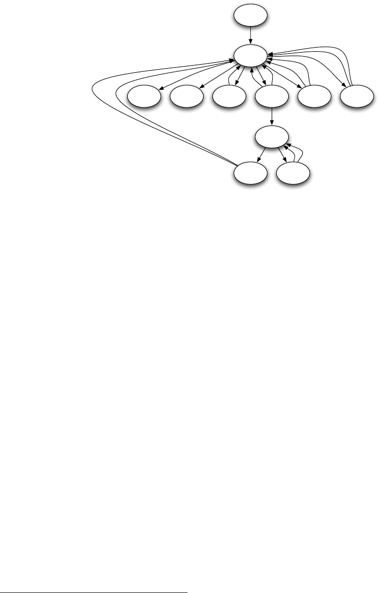
<start>
<op>
<bool>
x y sin if
nand>
*–
Figure 5.10 Parse graph (orderings among children not shown). The entry point is
<start>
. GrammarRuleNodes are shown with
angle brackets. GrammarFunctionNodes are shown without brackets.
•
If on a GrammarRuleNode, the GESpecies selects exactly one child to traverse, using the next number
in the GEIndividual array.
•
If on a GrammarFunctionNode, the GESpecies traverses each and every child of the node in order.
These become children to the GrammarFunctionNode’s GPNode.
GrammarFunctionNodes hold GPNode prototypes and represent them. Their children are arguments to
the node in question. GrammarRuleNodes hold choice points in the rule, and their children are the choices
(only one choice will be made).
5.4 Push (The ec.gp.push Package)
Push is a stack-based programming language developed by Lee Spector [
22
,
21
]. The language is designed
to allow the evolution of self-modifying programs, and this allows all manner of experimentation. ECJ has
an experimental simple implementation of Push which uses a Push interpreter called Psh.8
The Push interpreter has several stacks on which data of different types can be pushed, popped, or
otherwise manipulated. Built-in Push instructions designed to manipulate certain stacks usually have the
name of the stack at the beginning of the instruction name, for convenience. For example, float.+ is an
instruction which adds floating-point numbers found on the float stack. The Psh interpreter has a large
number of built-in instructions: but you can also create your own instructions in ECJ to do whatever you
like, and add them to Psh’s vocabulary.
Push programs take the form of Lisp lists of arbitrary size and nesting. For example, here is an uninter-
esting Push program consisting entirely of instructions which use the float stack:
((float.swap ((float.swap float.dup))) float.dup float.* (float.+ float.-) float.dup)
Parentheses define blocks of code, but if you don’t have any code-manipulation instructions then
parentheses don’t mean much. This code does the following:
8
https://github.com/jonklein/Psh/ Note that ECJ uses a modified version of Psh which comes with the ECJ distribution: don’t
use the GitHub version.
207

1. Swap the top two elements of the float stack
2. Swap the top two elements of the float stack
3. Duplicate the top item of the float stack and push it on the float stack
4. Duplicate the top item of the float stack and push it on the float stack
5. Multiply the top two items of the float stack and push the result on the float stack
6. Add the top two items of the float stack and push the result on the float stack
7. Subtract the top two items of the float stack and push the result on the float stack
8. Duplicate the top item of the float stack and push it on the float stack
Like I said, an uninteresting program.
Note that unlike in Lisp or GP tradition, the first element in each list in Psh isn’t special: it doesn’t define
a function. Indeed it could just be another list. All lists do is set apart blocks of code, which might be useful
in manipulation by special code-modifying instructions.
Because Push lists don’t start with a function symbol, their parse trees are different from GP program
trees, and so while ECJ uses the GPNode and GPTree classes to encode Push trees, it does so in an unusual
way. All the symbols in the Push program are leaf nodes in the tree. Dummy nonleaf nodes define the list
and sublist structure of the tree. Furthermote, nonleaf nodes can have arbitrary arity, which is something not
normally done in ECJ’s GP trees. For example, the previous Push program looks like this in tree form:
2
2
float.swap 2
2
float.swap float.dup
float.dup float.∗2
float.+float.−
float.dup
Thus ECJ creates Push programs using its GPTree facility with only two kinds of nodes: dummy nontermi-
nals (the class ec.gp.push.Nonterminal) and instructions (the class ec.gp.push.Terminal, which is a special ECJ
ERC that handles leaf nodes in the tree). The dummy nonterminals are shown in the figure above with the
symbol 2.
Evaluation
Push trees are evaluated by submitting them to an interpreter, in this case the Psh interpreter.
But there’s a problem. Psh, like every other Push interpreter out there, has its own notions of the objects
used to construct a Push tree. It’s obviously not compatible with ECJ’s GPNode, GPTree, and GPIndividual
objects. As a result, ECJ evaluates its Push trees by first writing them out to strings in Lisp form. It then sets
up an interpreter, gives it the string program, and lets it parse the program into its own internal structure
and evaluate it. This is circuitous but doesn’t really slow things down very much as it turns out.
Some Caveats
Much of the modern Push work is being done on a Clojure-based interpreter (Clojush) rather
than Psh, and perhaps in the future we may move to that instead. Long story short, this is an experimental
package.
Also, much of the Push literature involves individuals which modify themselves and then pass these
modifications onto successive generations. At present ECJ does not do this: once an individual is entered into
208
the interpreter, it stays there. Any changes made in the interpreter are ignored when the fitness evaluation is
complete. We may change that in the future.
5.4.1 Push and GP
ECJ’s Push package only uses two GPNode classes, ec.gp.push.Nonterminal (for dummy nonleaf nodes) and
ec.gp.push.Terminal (to define all possible leaf nodes). This means that, for all intents and purposes, the GP
function set, from ECJ’s perspective, is hard-coded. But of course you still have the Push “function set” to set
up: these are the actual instructions that ec.gp.push.Terminal can be set to (it’s an ERC which displays Strings)
and that can be submitted to the Psh interpreter. Setting these instructions up is discussed in Section 5.4.2
coming next; for now, keep in mind that the Push “function set” is not the same thing as the GP function set.
This “hard-coded” GP function set is defined as follows in the ec/gp/push/push.params file:
gp.fs.size = 1
gp.fs.0.name = f0
gp.fs.0.size = 2
gp.fs.0.func.0 = ec.gp.push.Nonterminal
gp.fs.0.func.0.nc = nc1
gp.fs.0.func.1 = ec.gp.push.Terminal
gp.fs.0.func.1.nc = nc0
Note that Nonterminal is listed as having an arity of 1 even though it has an arbitrary arity. Because
ec.gp.push.Nonterminal can have variable number of children, Push uses its own special tree builder to allow
this. The class is called ec.gp.push.PushBuilder. PushBuilder follows the following algorithm:
1: function Build-Tree (int size)
2: if size = 1 then
3: return a terminal (of the class ec.gp.push.Terminal)
4: else
5: p←a nonterminal (of the class ec.gp.push.Nonterminal)
6: while size >0do
7: a←a random number from 1 to size inclusive
8: size ←size −a
9: c←Build-Tree(a)
10: Add cas a child of p
11: Randomly shuffle the order of children of p
12: return p
PushBuilder must choose a size, and this is done in the usual GPNodeBuilder way. To set up PushBuilder
as the default initialization builder, and define it to pick sizes uniformly between 4 and 10 inclusive, you’d
say:
gp.tc.0.init = ec.gp.push.PushBuilder
gp.tc.0.init.min-size = 4
gp.tc.0.init.max-size = 10
You can of course define the size distribution directly too, to describe a more complicated distribution:
209
gp.tc.0.init = ec.gp.push.PushBuilder
gp.tc.0.init.num-sizes = 10
gp.tc.0.init.size.0 = 0.0
gp.tc.0.init.size.1 = 0.0
gp.tc.0.init.size.2 = 0.0
gp.tc.0.init.size.3 = 0.0
gp.tc.0.init.size.4 = 0.5
gp.tc.0.init.size.5 = 0.25
gp.tc.0.init.size.6 = 0.125
gp.tc.0.init.size.7 = 0.0625
gp.tc.0.init.size.8 = 0.03125
gp.tc.0.init.size.9 = 0.015625
gp.tc.0.init.size.10 = 0.015625
Because ECJ’s Push package only uses two GPNode classes, you can basically use any GP crossover or
mutation method you like, as long as it doesn’t rely on a fixed arity (ec.gp.push.Nonterminal has a variable
number of children). None of the built-in ECJ GP breeding pipelines will cause any problem. However if
you’re using a breeding pipeline which creates random subtrees (such as ec.gp.koza.MutationPipeline) you
will want to make sure it uses the ec.gp.push.PushBuilder tree builder to generate those subtrees.
5.4.2 Defining the Push Instruction Set
Though the GP function set used by ECJ’s GP facility is hard-coded for Push, you still of course have to
specify the instructions which can form a Push program. This is done via the ec.gp.push.Terminal.
Let’s say you wanted to do a symbolic regression problem and had settled on the following seven Push
instructions: float.* float.+ float.% float.- float.dup float.swap float.pop. You”d set it up like this:
# The Instruction Set
push.in.size = 7
push.in.0 = float.*
push.in.1 = float.+
push.in.2 = float.%
push.in.3 = float.-
push.in.4 = float.dup
push.in.5 = float.swap
push.in.6 = float.pop
This is, in effect, the Push equivalent of a GP Function Set. Psh also supports a limited number of
Ephemeral Random Constants, or ERCs. Keep in mind that these are not GP ERCs, though they operate
similarly inside the Push interpreter. ECJ defines these with the names float.erc and int.erc, one for Push’s
float stack and one for the integer stack. So if you’d like to add an ERC to your instruction set, you might say:
push.in.size = 8
push.in.0 = float.*
push.in.1 = float.+
push.in.2 = float.%
push.in.3 = float.-
push.in.4 = float.dup
push.in.5 = float.swap
push.in.6 = float.pop
push.in.7 = float.erc
If you use an ERC, you should also set its minimum and maximum values. ECJ defines the following
defaults in the push.params file:
210
push.erc.float.min = -10.0
push.erc.float.max = 10.0
push.erc.int.min = -10
push.erc.int.max = 10
The following instructions are built into the Psh interpreter.
integer.+
integer.-
integer./
integer.%
integer.*
integer.pow
integer.log
integer.=
integer.>
integer.<
integer.min
integer.max
integer.abs
integer.neg
integer.ln
integer.fromfloat
integer.fromboolean
integer.rand
float.+
float.-
float./
float.%
float.*
float.pow
float.log
float.=
float.>
float.<
float.min
float.max
float.sin
float.cos
float.tan
float.exp
float.abs
float.neg
float.ln
float.frominteger
float.fromboolean
float.rand
boolean.=
boolean.not
boolean.and
boolean.or
boolean.xor
boolean.frominteger
boolean.fromfloat
boolean.rand
true
false
code.quote
code.fromboolean
code.frominteger
code.fromfloat
code.noop
code.do*times
code.do*count
code.do*range
code.=
code.if
code.rand
exec.k
exec.s
exec.y
exec.noop
exec.do*times
exec.do*count
exec.do*range
exec.=
exec.if
exec.rand
input.index
input.inall
input.inallrev
input.stackdepth
frame.push
frame.pop
5.4.3 Creating a Push Problem
Push Problems are created by subclassing from ec.gp.push.PushProblem. Building a Push Problem is more
complex than other ECJ Problems because you may have to interact with the Psh interpreter. We have
provided some cover functions to enable you to keep your hands relatively clean.
One common way a Push program is evaluated (such as in Symbolic Regression) is along these lines:
1. A Push Program is created from the GPIndividual.
2. An Interpreter is created or reset.
3. Certain stacks in the interpreter are loaded with some data
4. The program is run on the interpreter
5.
The tops of certain stacks in the interpreter are inspected to determine the return value, and thus the
fitness.
6. The GPIndividual’s fitness is set to this fitness.
To create a Push Program, you’d call getProgram(...), passing in the individual in question. This will
return a Program object (this is a class used in Psh).
To create an interpreter, you’d call getInterpreter(...), again passing in the individual in question. This
will return an Interpreter object (another class used in Psh). You can also call resetInterpreter(...) to reset the
interpreter to a pristine state so you can reuse it.
211

Let’s say your approach is to push a number on the float stack of the interpreter, run the program, and
then examine what’s left on the float stack to determine fitness. PushProblem has utility methods for pushing,
and examining the float and integer stacks. If you want to do more sophisticated stuff than this, you’re
welcome to but will have to consult Psh directly.
Finally, to run the program on the interpreter, you can call executeProgram(...).
ec.gp.push.PushProblem Methods
public org.spiderland.Psh.Program getProgram(EvolutionState state, GPIndividual ind)
Builds and returns a new Program object from the provided individual.
public org.spiderland.Psh.Interpreter getInterpreter(EvolutionState state, GPIndividual ind, int thread)
Builds and returns a new, empty Interpreter object.
public void resetInterpreter(org.spiderland.Psh.Interpreter interpreter)
Resets the interpreter’s stack so it can execute a new program.
public void executeProgram(org.spiderland.Psh.Program program, org.spiderland.Psh.Interpreter interpreter, int maxSteps)
Runs the provided program on the given interpreter for up to maxSteps steps.
public void pushOntoFloatStack(org.spiderland.Psh.Interpreter interpreter, float val)
Pushes the given value onto the interpreter’s float stack.
public void pushOntoIntStack(org.spiderland.Psh.Interpreter interpreter, int val)
Pushes the given value onto the interpreter’s integer stack.
public boolean isFloatStackEmpty(org.spiderland.Psh.Interpreter interpreter)
Returns whether the interpreter’s float stack is emtpy.
public boolean isIntStackEmpty(org.spiderland.Psh.Interpreter interpreter)
Returns whether the interpreter’s integer stack is emtpy.
public float topOfFloatStack(org.spiderland.Psh.Interpreter interpreter)
Returns the top element on the interpreter’s float stack. You ought to check to see if the stack is empty first.
public int topOfIntStack(org.spiderland.Psh.Interpreter interpreter)
Returns the top element on the interpreter’s stack. You ought to check to see if the stack is empty first.
You will define your PushProblem in the usual ECJ fashion. Furthermore, since Push uses the GP facility,
you also need to provide a GPData object, though it’ll never be used:
eval.problem = ec.app.myapp.MyPushProblem
eval.problem.data = ec.gp.GPData
5.4.4 Building a Custom Instruction
It’s often the case that Psh’s built-in instructions aren’t enough for you. Perhaps you want an instruction
which prints the top of the float stack. Perhaps you want an instruction which does more interesting math,
or which reads from a file, or moves an ant. To do this you need to be able to create a class which you can
submit as an instruction. This is what ec.gp.push.PushInstruction does for you.
PushInstruction is a org.spiderland.Psh.Instruction subclass which also implements ECJ’s ec.Prototype
interface and so is properly cloneable and serializable. Since it’s a Prototype, it has a setup(...) method which
you can take advantage of to get things ready, and a clone() method you might need to override. But critically
it has an Execute(...) method which the interpreter uses to run the instruction. Note the unusual spelling:
this is a Psh method name.
212

To implement a PushInstruction you’ll need to know how Psh works so you can manipulate its stacks
according to the needs of the instruction. Two examples (Atan and Print) are provided in the ec/app/push
application example.
ec.gp.push.PushInstruction Methods
public void Execute(org.spiderland.Psh.Interpreter interpreter)
Executes the given instruction.
Once you have constructed your custom instruction, you need to add it to your instruction set. To do this
you give it a name and also specify the PushInstruction class which defines the instruction. The presence of
this class specification informs ECJ that this isn’t a built-in Psh instruction. For example, we might add to
the end of our existing instruction set like so:
push.in.size = 9
push.in.0 = float.*
push.in.1 = float.+
push.in.2 = float.%
push.in.3 = float.-
push.in.4 = float.dup
push.in.5 = float.swap
push.in.6 = float.pop
push.in.7 = float.erc
push.in.8 = my.instruction.name
push.in.8.func = ec.app.myapp.MyInstruction
5.5 NEAT (The ec.neat Package)
NEAT [
24
] is a direct-encoding
9
representation for neural networks and related graph structures. ECJ’s
NEAT implementation tries to stay fairly faithful to the original. ECJ does not at support NEAT extensions,
such as HyperNEAT. Note that NEAT is not a simple representation, and this manual is not a place to learn
about how NEAT works. You would do well to read up on NEAT first to get your head wrapped around the
stuff discussed here.
A NEAT individual consists of two vectors: a vector of genes and a vector of nodes. ECJ represents
NEAT individuals with the class ec.neat.NEATIndivdiual, which is a subclass of ec.vector.GeneVectorIndividual.
Neat’s genes are stored in the genome inherited from GeneVectorIndividual, and the nodes are stored in a
separate ArrayList called nodes. All NEATIndividuals belong to the species ec.neat.NEATSpecies. Genes are
represented by the class ec.neat.NEATGene, which naturally extends ec.vector.Gene. Nodes are represented
by the class ec.neat.NEATNode.
NEAT uses the term
species
to refer to individuals tagged to belong to a special subgroup. This obviously
conflicts with ECJ’s usage of the term. To refer to a NEAT species, ECJ uses the term
subspecies
, represented
by the class ec.neat.NEATSubspecies.
The phenotype of a NEAT individual is a graph structure which represents the individual’s neural
network. It is represented by ec.neat.NEATNetwork and is built up out of NEATNodes.
One of NEAT’s, um, innovations, is its use of the innovation number. This is a unique birthday number
which distinguishes and orders NeatGenes. Innovation numbers are particularly prevalent (and com-
plex) among links between nodes, and ECJ represents those innovation values with a special class called
ec.neat.NEATInnovation.
9
This means that the genome explicitly contains every single node and edge. As opposed to indirect encoding, where the genome
contains a set of (possibly very compact) rules for how to “grow” a complex neural network.
213
Finally, NEAT has a custom breeding procedure and so has its own ec.neat.NEATBreeder, as well as a
custom ec.neat.NEATInitializer.
A Warning on NEAT Breeding
NEAT has a custom breeding procedure. For the time being ECJ is hard-
coding that breeding procedure in NEATBreeder (no BreedingPipelines) to make sure that it’s 100% faithful
to the original NEAT code. But after we have verified this, eventually ECJ will carefully break this out into a
Breeding Pipeline model, and NEATBreeder will go away. Stay tuned.
5.5.1 Building a NEAT Application
We’ll use the simple package as our default, and begin by specifying all of the above classes:
parent.0 = ../simple/simple.params
init = ec.neat.NEATInitializer
breed = ec.neat.NEATBreeder
pop.subpop.0.species = ec.neat.NEATSpecies
pop.subpop.0.species.fitness = ec.simple.SimpleFitness
pop.subpop.0.species.ind = ec.neat.NEATIndividual
pop.subpop.0.species.network = ec.neat.NEATNetwork
pop.subpop.0.species.gene = ec.neat.NEATGene
pop.subpop.0.species.node = ec.neat.NEATNode
pop.subpop.0.species.subspecies = ec.neat.NEATSubspecies
pop.subpop.0.species.innovation = ec.neat.NEATInnovation
Note that NEATIndividual is a subset of VectorIndividual, though it does some things differently. This
means we’ll need a few dummy parameters that VectorIndividual is expecting, even though we won’t use
them. Notably:
• NEAT builds genomes from templates loaded from a file, so the genome-size parameter isn’t used.
•
NEAT has its own mutation and crossover mechanisms, so
crossover-type
and
mutation-prob
aren’t
used (for now).
• ECJ’s NEAT package doesn’t use a pipeline for the time being, so we need to stub that out.
So here we go:
# Dummy parameters to satisfy VectorSpecies
pop.subpop.0.species.genome-size = 20
pop.subpop.0.species.crossover-type = one
pop.subpop.0.species.mutation-prob = 0.01
pop.subpop.0.species.pipe = ec.breed.InitializationPipeline
5.5.1.1 Breeding
Next we’ll go through all the NEAT breeding parameters.
NEAT Breeding is an elaborate process involving fitness-sharing within subspecies, “innovation numbers”
(birthdays) aging, population stagnation checks, “champions”, “stolen babies” (we kid you not), and other
stuff. But in short: each subspecies compete to produce some number of individuals based on various factors.
Within a subspecies, individuals are selected for breeding using various fitness-sharing metrics. Breeding
can involve mutation or crossover or both. Newly-generated individuals are assigned a species which is
most genome-compatible with themselves. Finally, empty subspecies are deleted and the remainder are
aged.
214
NEAT Genome Compatibility and Speciation
NEAT uses three factors which determine the degree to
which individual are genetically compatible: the amount of disjoint genes, the amount of excess genes, and
the mutational difference within matching genes. Here are the relative weights of those factors:
neat.species.disjoint-coeff = 1.0
neat.species.excess-coeff = 1.0
neat.species.mutdiff-coeff = 0.4
An individual must meet a “compatibility threshold” in order to join a subspecies:
neat.species.compat-thresh = 3.0
Individuals within a subspecies are fitness-penalized for being too old once they reach a certain age:
neat.species.dropoff-age = 15
Finally, species can take offspring from other species (“steal their babies”) when this parameter is
>
0
(the default is 0):
neat.species.babies-stolen = 0
Survival, Mutation, and Crossover
Once NEAT has determined which individuals will be permitted to
breed, breeding commences. Here are the default probabilities:
# Percentage of subspecies that is permitted to reproduce into the next generation
neat.species.survival-thresh = 0.20
# Probability that mutation will occur only, no crossover
neat.species.mutate-only-prob = 0.25
# Probability that crossover will occur only, no mutation (if mutate-only-prob fails)
neat.species.mate-only-prob = 0.2
The probabilities for mutation and crossover are a bit screwy. The general procedure is as follows:
1. With probability mutate-only-prob, mutate
2. Else
(a) cross over
(b) With probability (1−mate-only-prob), mutate
Obviously, this means that
mate-only-probability
doesn’t really mean “mate-only probability”. It
means “mate-only probability assuming you’re not just doing mutating”.
Crossover can be with members of your own species, or with other species. There are three kinds of
crossover available in NEAT:
# Probability of mating with another subspecies
neat.species.interspecies-mate-prob = 0.001
# Various probabilities of crossover types
neat.species.mate-multipoint-prob = 0.6
neat.species.mate-multipoint-avg-prob = 0.4
# Don’t change this one -- it’s usually unused neat.species.mate-singlepoint-prob = 0.0
215
Crossover yields a single child and works as follows. In mate-multipoint, every gene up to the length of
the more fit parent is matched with its corresponding gene in the less fit parent. For each pair of genes, with
50% probability we select the gene in the fitter parent, else the other. When one parent is longer than the
other, the excess genes are included only if from the fitter parent. Mate-multipoint-average is similar, except
that the gene weights of the two genes in the pair are averaged to form the gene weight in the final gene.
Mate-singlepoint is somewhat like traditional single-point crossover: we pick a gene locus. Genes less than
that locus come from one parent and genes greater than the locus come from the other parent. However in
NEAT the locus falls on a gene: that gene has an averaging performed on it like mate-multipoint-average.
Excess is always included as well.
MateSinglePoint is generally left unused.
Mutation can involve changing the values of
links
(the genes) in the genome, enabling or disabling them,
or adding new links. Newly added links can be feed-forward or recurrent in the network.
## MUTATING LINK WEIGHTS
# Probability of mutating each and every one of the weights of the links in the genome
neat.species.mutate-link-weight-prob = 0.9
# Factor which influences how much a link is mutated
neat.species.weight-mut-power = 2.5
## ENABLING AND DISABLING LINKS
# Probability of randomly enabling or disabling a single gene (link) in the genome
neat.species.mutate-toggle-enable-prob = 0.0
# Probability of reenabling a gene (link)
neat.species.mutate-gene-reenable-prob = 0.0
## ADDING NEW LINKS
# Probability of adding a single new gene (link)
neat.species.mutate-add-link-prob = 0.05
# Probability that this link will be recurrent rather than feed-forward.
# If recurrent, 50% of the time it will be a self-link, and 50% of the
# time it will be a reversed link
neat.species.recur-only-prob = 0.0
# How many times we’re willing to try adding a valid new link before giving up
neat.species.new-link-tries = 20
Mutation can also involve adding a new random
node
in the genome. Adding a node involves splitting
an existing link into two links and putting the node in-between them. The choice of link is biased in certain
ways when the genome is small; otherwise it is a randomly-selected link:
# Probability of adding a single new node
neat.species.mutate-add-node-prob = 0.03
# How many times we’re willing to try adding a new node before giving up
neat.species.new-node-tries = 20
# In genomes this size or greater, mutateAddNode will do a pure random split
neat.species.add-node-max-genome-length = 15
216

5.5.1.2 Evaluation
NEAT works by interpreting its two genomes (the Node array and the Gene (Link) array) to build a neural
network or other graph structure. This network is a NEATNetwork. You then evaluate NEATNetwork to see
how it performs, and set the NEATIndividual’s fitness appropriately.
To build a network from an existing individual, you call:
ec.neat.NEATIndividual Methods
public NEATNetwork createNetwork()
Returns a NEATNetwork generated from the current genome of the individual.
Like many neural networks, a NEATNetwork consists of
input nodes
(some of which may be hard-coded
bias units
,
output nodes
, and
hidden nodes
. The general procedure is to load the non-bias unit input nodes
with values, then pulse the network until information has flowed to the output nodes, then read the result
off of the output nodes and compare with the desired output. Finally, we’ll
flush
the network to clear it and
reuse it.
You’ll need to pulse the network at least as many times as the
depth
of the network so the information
can flow all the way through. To do all these things, we’ll need a few methods:
ec.neat.NEATNetwork Methods
public int maxDepth()
Returns the maximum depth of the network.
public void loadSensors(double[] values)
Given nsensor (input) nodes, sets each to emit a corresponding value.
public void activate(EvolutionState state)
Pulses the network once, flowing information forward one step.
public double[] getOutputResults()
Returns an array of activation values, one per output node.
public void flush()
Clears the network and prepares it for reuse.
Example
Let’s take the XOR example as shown in the package ec.app.xor. We first create the file XOR.java
which contains the class XOR. In the evaluate(...) method we’ll start with the usual pleasantries:
public class XOR extends Problem implements SimpleProblemForm
{
public void evaluate(EvolutionState state, Individual ind, int subpopulation, int threadnum)
{
if (ind.evaluated) return;
if (!(ind instanceof NEATIndividual))
state.output.fatal("Whoa! It’s not a NEATIndividual!!!", null);
NEATIndividual neatInd = (NEATIndividual)ind;
if (!(neatInd.fitness instanceof SimpleFitness))
state.output.fatal("Whoa! It’s not a SimpleFitness!!!", null);
217
At this point we’re ready to do evaluation. Our NEAT neural network takes three inputs (the first input
is a bias unit) in one of four combinations and produces one of four outputs, for each combination, following
the standard XOR rule. The inputs and outputs are:
// The four possible input combinations to xor
// The first number is for biasing
double[][] in=
{
{1.0, 0.0, 0.0}, // output 0
{1.0, 0.0, 1.0}, // 1
{1.0, 1.0, 0.0}, // 1
{1.0, 1.0, 1.0} // 0
};
// we’ll put the results here
double[] out = new double[4];
// here’s what we WANT the results to be:
double[] expectedOut = new double[] { 0.0, 1.0, 1.0, 0.0 };
Now we build our network.
NEATNetwork net = neatInd.createNetwork();
int netDepth = net.maxDepth();
At this point we’re ready to test it. We’ll go through all combinations and see what the network produces:
// Load and activate the network on each input
for(int i = 0; i < in.length ;i++)
{
net.loadSensors(in[i]);
for(int relax = 0; relax < netDepth; relax++)
{
net.activate(state);
}
// we only have one output, at position 0, so let’s get it
out[i] = net.getOutputResults()[0];
net.flush();
}
Finally we need to calculate the fitness. The NEAT XOR example actually has several different fitness-
calculation methods. For our purposes we’ll use sum squared error. And an ideal individual will be
considered one in which all four of the results is less than 0.5 error.
double errorSum = 0;
for(int i = 0; i < out.length; i++)
errorSum += (out[i] - expectedOut[i]) * (out[i] - expectedOut[i]);
double fitness = 4.0 - errorSum;
boolean ideal = true;
for(int i = 0; i < out.length; i++)
if (Math.abs(out[i] - expectedOut[i]) > 0.5)
{ ideal = false; break; }
218
((SimpleFitness)neatInd.fitness).setFitness(state, fitness, ideal);
neatInd.evaluated = true;
}
}
Note that in this example, the measurement for the ideal individual is not the same as the measurement
for fitness. This means that ideal individuals may vary in fitness. It also means that if we quit when we find
an ideal individual, the end of run fitness may vary, which could really screw up statistical results if you’re
doing an experiment. You might add the parameter:
quit-on-run-complete = false
... to run until generations are terminated rather than when an ideal individual is discovered.
Next we need to specify a seed individual: recall that NEAT individuals are typically loaded from a seed.
We do this as:
1. Whether the individual is evaluated: the boolean false (F)
2. The fitness for the individual: a double 0.0 (d0|0.0|)
3. The size of the link (gene) genome: an integer 3 (i3|)
4. Three link genes. Each gene contains:
(a) An input node ID as an integer, 1, 2, or 3 (i1|i2|i3|)
(b) An output node id as an integer: 4 (i4|)
(c) A weight as a double: 0.0 (d0|0.0|)
(d) Whether the link is recurrent: false (F)
(e) An innovation number as an integer, 1, 2, or 3 (i1|i2|i3|)
(f) A mutation number as a double: 0.0 (d0|0.0|)
(g) Whether the link is enabled: true (T)
5. Four node genes. Each gene contains:
(a) A node ID as an integer:
(b) A node type as an integer. Node types can be NEURON=0 or SENSOR=1 (i0|i1|)
(c)
A node place as an integer. Node places can be HIDDEN = 0, INPUT = 1, OUTPUT=2, or BIAS=3
(i0|i1|i2|i3|)
Our default individual is stored as a subpopulation of size 1 and looks like this, stored in the file
start.neatind. See if you can understand it:
Number of Individuals: i1|
Individual Number: i0|
Evaluated: F
Fitness: d0|0.0|
i3|
i1|i4|d0|0.0|Fi1|d0|0.0|T
i2|i4|d0|0.0|Fi2|d0|0.0|T
i3|i4|d0|0.0|Fi3|d0|0.0|T
i4|
i1|i1|i1|
i2|i1|i1|
i3|i1|i3|
i4|i0|i2|
219

Now we finish out with a parameter file. The file ec/neat/neat.params contains all the parameters we’ve
discussed so far: we’ll have that as our parent. So we make the file ec/app/xor.params like this as follows:
parent.0 = ../../neat/neat.params
pop.subpop.0.species.genome-size = 3
pop.subpop.0.file = start.neatind
pop.subpop.0.extra-behavior = wrap
eval.problem = ec.app.xor.XOR
pop.subpop.0.size = 150
generations = 100
Two parameters need explanation. To load the NEAT template (seed) individual, ECJ does this by
loading the subpopulation. The subpopulation file, as discussed earlier, contains a single individual: but the
subpopulation is 150 in size! This is handled by turning on the
wrap
option, which causes the individual
in the file to be copied to the whole subpopulation. Thereafter NEAT will mutate that individual a bit, so
they’re all different.
5.6 Rulesets and Collections (The ec.rule Package)
Let’s get one thing out of the way right now. Though we had rulesets in mind when we developed it, the
ec.rule package isn’t really for rulesets. Not only can the package be used for things other than rules, but it’s
not even sets: it’s collections (or “bags” or “multisets”) of arbitrary objects.
The representation defined by this package is fairly straightforward: an ec.rule.RuleIndividual contains one
or more ec.ruleRuleSets, each of which contain zero or more ec.rule.Rules. A Rule is an abstract superclass
which can contain anything you want. And that’s about it.
Problem domains for which the ec.rule package is appropriate are often also good candidates for the
variable-length lists found in the ec.vector package. You’ll need to think about which is a better choice for
you. Also beware that of the various representation packages in ECJ, ec.rule is definitely the least used and
least tested. So its facilities are somewhat cruder than the others and it’s possible you may see bugs.
Each level of the ec.rule package (individual, ruleset, rule) is a Prototype and has a Flyweight relationship
with a central object special to that level (for a reminder on Flyweights, see Section 3.1.4). Specifically:
Object In Flyweight Relationship With
ec.rule.RuleIndividual ec.rule.RuleSpecies
ec.rule.RuleSet ec.rule.RuleSetConstraints
ec.rule.Rule ec.rule.RuleConstraints
The ec.rule package follows the same approach as the ec.vector package does when it comes
to breeding: two basic breeding operators are provided (ec.rule.breed.RuleCrossoverPipeline and
ec.rule.breed.RuleMutationPipeline) which simply call default mutation and crossover functions in the Indi-
viduals themselves. Thus to do more sophisticated breeding you have the choice of either overriding these
functions or creating new breeding pipelines which perform more detailed operations on their own.
5.6.1 RuleIndividuals and RuleSpecies
RuleIndividuals and RuleSpecies are specified in parameters in the standard way:
pop.subpop.0.species = ec.rule.RuleSpecies
pop.subpop.0.species.ind = ec.rule.RuleIndividual
A RuleIndividual is a subclass of Individual which simply consists of an array of RuleSets:
220

public RuleSet[] rulesets;
Each RuleSet can be a different class. You’d think that the number and class of RuleSets was specified in
the RuleSpecies (like in ec.vector). But for no good reason it’s not the case: you specify them in the parameters
for the prototypical individual, along these lines:
pop.subpop.0.species.ind.num-rulesets = 2
pop.subpop.0.species.ind.ruleset.0 = ec.rule.Ruleset
pop.subpop.0.species.ind.ruleset.1 = ec.app.myapp.MyRuleset
Alternatively, you can use the RuleIndividual’s default parameter base:
rule.individual.num-rulesets = 2
rule.individual.ruleset.0 = ec.rule.Ruleset
rule.individual.ruleset.1 = ec.app.myapp.MyRuleset
Though for many applications you will probably just have a single RuleSet, and it’ll probably just be an
ec.rule.Ruleset:
pop.subpop.0.species.ind.num-rulesets = 1
pop.subpop.0.species.ind.ruleset.0 = ec.rule.Ruleset
5.6.2 RuleSets and RuleSetConstraints
A RuleSet contains an arbitrary number of Rules (ec.rule.Rule), anywhere between zero and up. It’s largely
your job to customize the breeding and initialization procedures appropriate to your problem to constraint
the number and type of rules. They’re defined here:
public Rule[] rules;
public int numRules;
Notice that the number of rules in the array may be less than the array size, that is, numRules
≤
rules.length.
The rules themselves run from rules[0] ... rules[numRules
−
1]. This is done because, like ArrayList etc., rules
is variable in size and an grow and shrink. RuleSet contains a number of utility methods for manipulating
the order and number of these rules:
ec.rule.RuleSet Methods
public int numRules()
Returns the number of rules in the RuleSet.
public void randomizeRulesOrder(EvolutionState state, int thread)
An auxillary debugging method which verifies many features of the structure of the GPTree and all of its GPNodes.
This method isn’t called by ECJ but has proven useful in determining errors in GPTree construction by various
tree building or breeding algorithms.
public void addRule(Rule rule)
Adds the rule to the end of the ruleset, increasing the length of the RuleSet array as necessary.
public void addRandomRule(EvolutionState state, int thread)
Produces a new randomly-generated rule and adds it to the RuleSet. The Rule is created by cloning the prototypical
Rule from the RuleSet’s RuleSetConstraints, then calling reset(...) on it.
public Rule removeRule(int index)
Removes a rule located at the given index from the RuleSet and returns it. All rules are shifted down to fill the
void.
221

public Rule removeRandomRule(EvolutionState state, int thread)
Removes a random rule returns it. All rules are shifted down to fill the void.
public RuleSet[] split(int[] points, RuleSet[] sets)
Breaks the RuleSet into
n
disjoint groups, then clones the rules in those groups and adds them to the respective
sets, which must be provided in the given array. The first group of rules starts at 0 and ends below points[0]: this
goes into sets[0]. Intermediate groups, which go into sets[i], start at points[i] and end below points[i+1]. The final
group, which goes into sets[points.length], starts at points[points.length
−
1] and continues to the end of the rule
array. If points.length = 0, then all rules simply get put into sets[0]. Note that the size of sets must be one more
than the size of points. The sets are returned.
public RuleSet[] split(EvolutionState state, int thread, RuleSet[] sets)
For each rule in the RuleSet, clones the rule and adds the clone to a randomly chosen RuleSet from sets. Returns
sets.
public RuleSet[] splitIntoTwo(EvolutionState state, int thread, RuleSet[] sets, double probability)
For each rule in the RuleSet, clones the rule and, with the given probability, adds the clone to sets[0], else sets[1].
Note that sets must be two in length.
public void join(RuleSet other)
Copies the rules in the other RuleSet, then adds them to the end of this RuleSet.
public void copyNoClone(RuleSet other )
Deletes all the rules in the RuleSet. Then places all the rules from the other RuleSet into this RuleSet. No cloning is
done: both RuleSets now have pointers to the same rules.
Groups of RuleSets have a flyweight relationship with a RuleSetConstraints object. RuleSetConstraints is
a Clique. You specify the number and class of RuleSetConstraints and assign each a unique name. Let’s say
you need two RuleSetConstraints objects, both instances of RuleSetConstraints itself. You’d write this:
rule.rsc.size = 2
rule.rsc.0 = ec.rule.RuleSetConstraints
rule.rsc.0.name = rsc1
rule.rsc.1 = ec.rule.RuleSetConstraints
rule.rsc.1.name = rsc2
RuleSetConstraints specify a number of constraints which guide the initialization and mutation of
RuleSets, specifically:
•
A distribution for choosing the number of Rules an initial RuleSet will have. This guides how the
RuleSet’s reset(...) method operates. The distribution can either be uniform with a minimum and
maximum, or you can specify a histogram of possible size probabilities. We’ll do the first case for
Ruleset 0 and the second case for Ruleset 1 below:
# RuleSetConstraints 0 will have between 5 and 10 rules inclusive
rule.rsc.0.reset-min-size = 5
rule.rsc.0.reset-max-size = 10
# RuleSetConstraints 1 will have 0 to 4 rules with these probabilities...
rule.rsc.1.reset-num-sizes = 5
rule.rsc.1.size.0 = 0.1
rule.rsc.1.size.1 = 0.2
rule.rsc.1.size.2 = 0.2
rule.rsc.1.size.3 = 0.3
rule.rsc.1.size.4 = 0.4
222

•
The probability of adding, deleting, and rearranging rules, when the RuleSet’s mutate(...) method
is called, typically by the BreedingPipeline ec.rule.RuleMutationPipeline. When this method is called,
the Ruleset first mutates all of its rules by calling mutate(...) on them. Then it repeatedly flips a coin
of a given probability: each time the coin comes up true, or until the number of rules is equal to the
minimum number of initial rules as specified above, one rule is deleted. Afterwards it repeatedly flips
a coin of another probability: each time the coin comes up true, or until the number of rules is equal
to the maximum number of initial rules, one new rule is added at random. Finally, with a certain
probability the rule ordering is shuffled. Here’s some examples of specifying these probabilities:
rule.rsc.0.p-add = 0.1
rule.rsc.0.p-del = 0.1
rule.rsc.0.rand-order = 0.25
rule.rsc.1.p-add = 0.5
rule.rsc.1.p-del = 0.6
rule.rsc.1.rand-order = 0.0
Once you’ve specified a RuleSetConstraints, you then attach one to each RuleSet. For example:
pop.subpop.0.species.ind.ruleset.0.constraints = rsc2
pop.subpop.0.species.ind.ruleset.1.constraints = rsc1
... or alternatively use the default parameter base...
rule.individual.constraints = rsc2
Once set, you can access the constraints with the following method:
ec.rule.RuleSet Methods
public final RuleSetConstraints ruleSetConstraints(RuleInitializer initializer)
Returns the RuleSet’s RuleSetConstraints
RuleSetConstraints one method for choosing random initial values under the constraints above:
ec.rule.RuleSetConstraints Methods
public int numRulesForReset(RuleSet ruleset, EvolutionState state, int thread)
Returns a random value from the initial (reset(...)) distribution, to use as the number of rules to initialize or reset
the RuleSet.
Additionally, the various addition, deletion, and randomization probabilities can be accessed like this:
RuleSetConstraints rsc = myRuleSet.ruleSetConstraints((RuleInitializer)(state.init));
double addition = rsc.p add;
double deletion = rsc.p del;
double shuffling = rsc.p randorder;
RuleSets also contain all the standard reading and writing methods, none of which you’ll need to override
unless you’re making a custom RuleSet.
ec.rule.RuleSet Methods
public void printRuleSetForHumans(EvolutionState state, int log)
Writes a RuleSet to a log in a fashion easy for humans to read.
223

public void printRuleSet(EvolutionState state, int log)
Writes a RuleSet to a log in a fashion that can be read back in via readRule(...), typically by using the Code package.
public void printRuleSet(EvolutionState state, PrintWriter writer)
Writes a RuleSet to a Writer in a fashion that can be read back in via readRule(...), typically by using the code
package.
public void readRuleSet(EvolutionState state, LineNumberReader reader) throws IOException
Reads a RuleSet written by printRuleSet(...) or printRuleSetToString(...), typically using the Code package.
public void writeRuleSet(EvolutionState state, DataOutput output) throws IOException
Writes a RuleSet in binary fashion to the given output.
public void readRuleSet(EvolutionState state, DataInput input) throws IOException
Reads a RuleSet in binary fashion from the given input.
5.6.3 Rules and RuleConstraints
RuleSetConstraints also contain the
prototypical Rule
for RuleSets adhering to a given constraints. RuleSets
will clone this Rule to create Rules to fill themselves with. ec.rule.Rule is an abstract superclass which doesn’t
do anything by itself: you’re required to subclass it to make the Rule into the kind of thing you want to
create a collection of in your Ruleset.
The prototypical Rule is specified like this:
pop.subpop.0.species.ind.ruleset.0.rule = ec.app.MyRule
pop.subpop.0.species.ind.ruleset.1.rule = ec.app.MyOtherRule
You can get the prototypical rule like this:
RuleSetConstraints rsc = myRuleSet.ruleSetConstraints((RuleInitializer)(state.init));
Rule prototype = rsc.rulePrototype;
Each Rule has a flyweight-related RuleConstraints object, which is defined similarly to RuleSetConstraints
(it’s also a Clique). For example, to create a single RuleConstraints in the clique, you might say:
rule.rc.size = 1
rule.rc.0 = ec.rule.RuleConstraints
rule.rc.0.name = rc1
RuleConstraints are essentially blank: they define no special parameters or variables. You can use them
however you see fit. If you don’t really care, you can just make a single RuleConstraints object as above and
assign it to your prototypical rules, such as:
pop.subpop.0.species.ind.ruleset.0.rule.constraints = rc1
pop.subpop.0.species.ind.ruleset.1.rule.constraints = rc1
...or use the default parameter base:
rule.rule.constraints = rc1
A Rule is abstract, and so has certain abstract methods which must be overridden, as well as others which
ought to be overridden. First the required ones:
ec.rule.Rule Methods
224

public abstract int hashCode()
Returns a hash code for the rule, based on value, suitable for weeding out duplicates.
public abstract int compareTo(Object other)
Returns 0 if this Rule is identical in value to other (which will also be a Rule), -1 if this Rule is “less” than the other
rule in sorting order, and 1 if the Rule is “greater” than the other rule in sorting order.
public abstract void reset(EvolutionState state, int thread)
Randomizes the value of the rule.
Rules are Prototypes and so implement the clone(),setup(...), and defaultBase() methods. You’ll most
likely need to override the clone() and setup(...) methods as usual. Additionally, you may want to override:
ec.rule.Rule Methods
public void mutate(EvolutionState state, int thread)
Mutates the Rule in some way and with some probability. The default implementation simply calls reset(...),
which is probably much too harsh.
public abstract int compareTo(Object other)
Returns 0 if this Rule is identical in value to other (which will also be a Rule), -1 if this Rule is “less” than the other
rule in sorting order, and 1 if the Rule is “greater” than the other rule in sorting order.
public abstract void reset(EvolutionState state, int thread)
Randomizes the value of the rule.
Then there are the standard printing and reading methods. You’ll need to override at least printRule-
ToStringForHumans(), and probably will want to override toString(). The others you can optionally override
depending on the kind of experiments you’re doing.
ec.rule.Rule Methods
public String toString()
Writes the Rule to a String, typically in a fashion that can be read back in via readRule(...). You’ll want to override
this method or printRuleToString(). You probably want to use the Code package to write the rule out. You only
really need to implement this method if you expect to write Individuals to files that will be read back in later.
public String printRuleToStringForHumans()
Writes the Rule to a String in a fashion easy for humans to read. The default implementation of this method simply
calls toString(). You’ll probably want to override this method.
public void printRuleForHumans(EvolutionState state, int log)
Writes a Rule to a log in a fashion easy for humans to read. The default implementation of this method calls
printRuleToStringForHumans(), which you should probably override instead.
public String printRuleToString()
Writes the Rule to a String, typically in a fashion that can be read back in via readRule(...). The default implemen-
tation of this method simply calls toString(). You’ll want to override this method or toString(). You probably want
to use the Code package to write the rule out. You only need to implement this method if you expect to write
Individuals to files that will be read back in later.
public void printRule(EvolutionState state, int log)
Writes a Rule to a log in a fashion that can be read back in via readRule(...). The default implementation of this
method calls printRuleToString(), which you should probably override instead.
public void printRule(EvolutionState state, PrintWriter writer)
Writes a Rule to a Writer in a fashion that can be read back in via readRule(...). The default implementation of this
method calls printRuleToString(), which you should probably override instead.
225

public void readRule(EvolutionState state, LineNumberReader reader) throws IOException
Reads a Rule written by printRule(...) or printRuleToString(...), typically using the Code package. The default does
nothing. You only need to implement this method if you expect to read Individuals from files.
public void writeRule(EvolutionState state, DataOutput output) throws IOException
Writes a Rule in binary fashion to the given output. The default does nothing. You only need to implement this
method if you expect to read and write Rules over a network (such as the distributed evaluation or island models).
public void readRule(EvolutionState state, DataInput input) throws IOException
Reads a Rule in binary fashion from the given input. The default signals an error. You only need to implement this
method if you expect to read and write Rules over a network (such as the distributed evaluation or island models).
5.6.4 Initialization
Basic Initialization works as follows:
1.
The RuleSpecies method newIndividual(EvolutionState, int) produces a RuleIndividual by calling su-
per.newIndividual(...) — cloning a RuleIndividual prototype
˙
-– and then calling reset(...) on the resultant
RuleIndividual.
2. The RuleIndividual’s reset(...) by default just calls reset(...) on each of the RuleSets.
3.
A RuleSet’s reset(...) method calls numRulesForReset(...) on the RuleSetConstraints to pick a random
number of rules to generate (see Section 5.6.2). It then produces an array of that size and fills it with
rules cloned from the RuleSetConstraint’s prototypical Rule. Then it calls reset(...) on each of the Rules.
4. You are responsible for implementing a Rule’s reset(...) method.
You can of course intervene and modify any of these methods as you see fit.
5.6.5 Mutation
As in the case in the ec.vector package, the ec.rule.breed.RuleMutationPipeline class doesn’t mutate rules
directly, but rather calls a method on them to ask them to mutate themselves. The procedure is as follows:
1. The RuleMutationPipeline calls preprocessIndividual(...) on the RuleIndividual.
2. The RuleIndividual’s preprocessIndividual(...) method calls preprocessRules(...) on each of the RuleSets.
3. The RuleSet’s preprocessRules(...) method by default does nothing: override it as you like.
4. The RuleMutationPipeline then calls mutate(...) on the RuleIndividual.
5. The RuleIndividual’s mutate(...) method by default just calls mutate(...) on each of its RuleSets.
6. The RuleSet’s mutate(...) method does several modifications to the rules in the RuleSet, in this order:
(a) All the Rules in the RuleSet have mutate(...) called on them.
(b)
A coin of is repeatedly flipped of a certain probability (p del), and each time it comes up true, a
rule is deleted at random using removeRandomRule(...). The indivdiual will not shrink smaller
than its specified minimum size.
(c)
A coin of is repeatedly flipped of a certain probability (p add), and each time it comes up true,
a rule is added at random using addRandomRule(...). That method clones a new Rule from the
prototypical Rule, then calls reset(...) on it. The indivdiual will not grow larger than its specified
maximum size.
226

(d)
With a certain probability (p randorder), the order of the rules is shuffled using randomizeRulesOr-
der(...).
The three probabilities (p del,p add, and p randorder), and the minimum and maximum rule sizes, are
discussed in Section 5.6.2, and are determined by RuleSetConstraints parameters, also discussed in
that Section.
7.
A Rule’s mutate(...) method by default simply calls reset(...), which is probably not what you want.
You’ll probably want a much more subtle mutation if any, and so will need to override this method.
8. You are responsible for implementing a Rule’s reset(...) method.
9. Finally, the RuleMutationPipeline calls postprocessIndividual(...) on the RuleIndividual.
10.
The RuleIndividual’s postprocessIndividual(...) method calls postprocessRules(...) on each of the RuleSets.
11. The RuleSet’s postprocessRules(...) method by default does nothing: override it as you like.
Often rules need to be in a carefully-constructed dance of constraints to be valid in an Individual. The
intent of the preprocessIndividual(...),postprocessIndividual(...),preprocessRules(...), and postProcessRules(...)
methods is to give your RuleIndividual a chance to fix RuleSets that have been broken by crossover or
mutation. The default implementation of these methods doesn’t do much:
ec.rule.RuleSet Methods
public void preprocessRules(EvolutionState state, int thread)
A hook called prior to mutation or crossover to prepare for possible breakage of Rules due to the mutation or
crossover event. The default implementation does nothing.
public void postprocessRules(EvolutionState state, int thread)
A hook called after to mutation or crossover to fix possible breakage of Rules due to the mutation or crossover
event. The default implementation does nothing.
ec.rule.RuleIndividual Methods
public void preprocessIndividual(EvolutionState state, int thread)
Calls preprocessRules(...) on each RuleSet in the Individual.
public void postprocessIndividual(EvolutionState state, int thread)
Calls postprocessRules(...) on each RuleSet in the Individual.
5.6.6 Crossover
Unlike RuleMutationPipeline, the ec.rule.breed.RuleCrossoverPipeline performs direct crossover on two RuleIn-
dividuals. Here is the procedure:
1. The RuleCrossoverPipeline calls preprocessIndividual(...) on each RuleIndividual.
2. The RuleIndividual’s preprocessIndividual(...) method calls preprocessRules(...) on each of the RuleSets.
3. The RuleSet’s preprocessRules(...) method by default does nothing: override it as you like.
4. For each pair of RuleSets, one per RuleIndividual...
(a)
Each RuleSet
A
and
B
is split into two pieces,
A1
and
A2
(and
B1
and
B2
) by calling splitIntoTwo(...)
227
(b)
A new RuleSet
A0
is formed from the union of
A1
and
B1
, and likewise, a new RuleSet
B0
is formed
from the union of A2and B2.
(c) If A0and B0do not minimum and maximum size constraints (see Section 5.6.2), go to (a) and try
again.
(d) Else A0and B0replace Aand Brespectively in each RuleIndivdiual.
5. Finally, the RuleCrossoverPipeline calls postprocessIndividual(...) on each RuleIndividual.
6.
The RuleIndividual’s postprocessIndividual(...) method calls postprocessRules(...) on each of the RuleSets.
7. The RuleSet’s postprocessRules(...) method by default does nothing: override it as you like.
RuleCrossoverPipeline has a few parameters which guide its operation. First, any given Rule will migrate
from one Individual’s RuleSet to the other only with a certain probability. Second, the CrossoverPipeline can
be set up to return only one child (tossing the second) rather than returning two. By default it returns both
children. To set both of these parameters, let’s say that the RuleCrossoverPipeline is the root pipeline for the
species. We’d say:
pop.subpop.0.species.pipe = ec.rule.breed.RuleCrossoverPipeline
pop.subpop.0.species.pipe.crossover-prob = 0.1
pop.subpop.0.species.pipe.toss = true
It doesn’t make any sense to have a rule crossover probability higher than 0.5. As usual, you could use
the default parameter base as well:
rule.xover.crossover-prob = 0.1
rule.xover.toss = true
228

Chapter 6
Parallel Processes
ECJ has various built-in methods for parallelism, and they can be used in combination with one another:
• Multiple breeding and evaluation threads, already discussed in Section 2.4.
•Distributed evaluation
: sending chunks of Individuals to remote computers to be evaluated. This is
typically done in a generational fashion, but a variation of this is
asynchronous evolution
, in which
Individuals are sent to multiple remote computers in a steady-state fashion. Additionally, remote
computers can (given time) engage in a little evolutionary optimization of their own on the chunks
they’ve received before sending them back. This is known as opportunistic evolution.1
•Island models
: multiple parallel evolutionary processes occasionally send fit individuals to one
another.2
Warning
ECJ’s distributed evaluation and island models facilities use unencrypted network sockets to
transfer individuals over a network. The individuals are not serialized, but individual pieces of them (ints,
etc.) are written in binary format. Thus ECJ theoretically vulnerable to injection hacks, and so if you plan to
use this facility in more distributed form than a local cluster, you might consider adding an encrypted socket
or using a VPN facility to be safe.
6.1 Distributed Evaluation (The ec.eval Package)
Distributed Evaluation is connects one
master
ECJ process with some
Nslave
ECJ processes. The master
handles the evolutionary loop, but when Individuals are evaluated, they are shipped off to the remote slaves
to do this task. This way evaluation can be parallelized.
Distributed Evaluation is only useful if the amount of time you save by parallelizing evaluation exceeds
the amount of time lost by shipping Individuals over the network (and sending at least Fitnesses back).
Generally this means that evaluation needs to take a fair bit of time per Individual: perhaps several seconds.
There are two kinds of EvolutionState objects which can work with Distributed Evaluation:
• SimpleEvolutionState, which sends entire Populations off to be evaluated in parallel.
•
SteadyStateEvolutionState, which sends individuals off to be evaluated one at a time, in a fashion
called asynchronous evolution (discussed later).
1
ECJ’s built-in distributed evaluation is meant for clusters. However, Parabon Inc. has developed a grid-computing version, called
Origin, which runs on hundreds of thousands or even millions of machines. See the ECJ main website for more information.
2
ECJ’s built-in island models are meant for clusters. However, a version of ECJ was ported to run on top of the DR-EA-M system,
a peer-to-peer evolutionary computation network facility developed from a grant in Europe. See the ECJ main website for more
information.
229
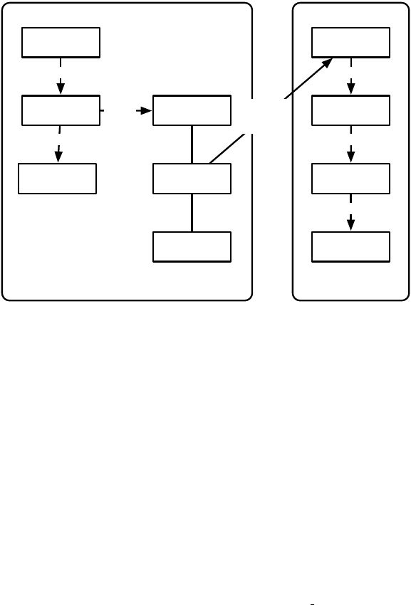
Slave ComputerMaster Computer
Master
Problem
Evaluator
problem
Your Problem
"actual" problem
Slave
Monitor
Slave
Connection
Slave
Job
1
*
1
*
Posts
Jobs to
Works with
and Sends
Jobs to
Evolution State
Your Problem
Evaluator
problem
evaluator
manages
Figure 6.1 Layout of the Distributed Evaluation package.
6.1.1 The Master
To set up Distributed Evaluation, you first need to set up the Master. This is done just like a regular
evolutionary computation process: but there are some additional parameters which must be defined. First,
we must define the
master problem
, nearly always as ec.eval.MasterProblem. The presence of the master
problem turns on distributed evaluation:
eval.masterproblem = ec.eval.MasterProblem
The MasterProblem is the interface that connects the distributed evaluation system to a regular evolu-
tionary computation loop. When it is defined, ECJ replaces the Problem prototype with a MasterProblem
prototype. The original Problem doesn’t go away — it’s rehung as a variable in the MasterProblem. Specifi-
cally, you can get to it like this:
Problem originalProblem = ((MasterProblem)(state.evaluator.p problem)).problem;
When your evolutionary computation process wishes to evaluate one or more individuals, it hands them
to the MasterProblem, which it thinks is the Problem for the application. But the MasterProblem doesn’t
send them to a clone of your underlying Problem but rather routes them to a Slave.
Slaves register themselves over the network with an object in the Master process called a
ec.eval.SlaveMonitor, which maintains one ec.eval.SlaveConnection per Slave to communicate with the remote
Slave. The SlaveMonitor listens in on a specific socket port for incoming Slaves to register themselves. You’ll
need to define this port (to something over 2000). Here’s what’s standard:
eval.master.port = 15000
Your MasterProblem will submit Individuals to the SlaveMonitor, which will in turn direct them to one
of the SlaveConnections. SlaveConnections don’t just ship off single Individuals to Slaves — that would be
far too inefficient a use of network bandwidth. Instead, they often batch them up into
jobs
for the Slave to
perform. Here’s how you define the size of a job:
230

eval.masterproblem.job-size = 10
The default is 1, which is safe but maximally inefficient. The idea is to make the job large enough to pack
Individuals into a network packet without wasting space. If your Individuals are large, then a large job size
won’t have any efficiency benefit. If they’re very small, the job size will have a huge benefit.
You also need to keep the Slaves humming along, ideally by keeping the TCP/IP streams filled with
waiting jobs queued up. Increasing this number can have a significant effect on performance. Here’s a
reasonable minumum:
eval.masterproblem.max-jobs-per-slave = 3
Again, the default is 1, which is safe but inefficient.
Warning!
If you set these two parameters wrong, you may wind up sending all your individuals to just
a few slaves, while the others sit by idly. Let’s say that the value
N
is equal to the floor of the number of
individuals in a subpopulation divided by the number of slaves. For example, if you have 100 individuals
and 45 slaves, then
N=
2. In general, you never want your
job-size
to be greater than
N
. Furthermore, if
your
job-size
is set to some value
M
, you never want your
max-jobs-per-slave
to be greater than
bN/Mc
.
The safe (but potentially network-inefficient) settings are always 1 and 1 respectively.
ECJ would prefer to compress the network streams to make them more efficient. But it can’t do
it without the jzlib/ZLIB library, which you must install separately
3
(see the ECJ main webpage or
http://www.jcraft.com/jzlib). Once it’s installed, you can turn it on like this:
eval.compression = true
Another warning!
If you turn on compression in your master but not your slave (or vice versa), the slave
will connect but then nothing will happen. You will not get any warning about your error.
Keep Your Master Single-Threaded
Multi-threaded breeding is fine. But evaluation should be kept
single-threaded, that is,
evalthreads = 1
Multi-threaded evaluation will probably work fine: but I’m not absolutely positive of it, and there’s no use
to multithreading when all you’re doing is shipping jobs off-site. Play it safe.
6.1.2 Slaves
Slaves are started up on separate CPUs, often in different machines from the Master. You can have as many
Slaves as you like: the more the merrier. The Slave class replaces ec.Evolve to handle its own startup, so you
don’t start up a Slave using the standard ec.Evolve procedure. Instead you’d type:
java ec.eval.Slave -file slave.params -p param=value ... (etc.)
The slave parameters must include all the evolutionary parameters and also all the master parameters (in
fact, you might as well say something like...)
parent.0 = master.params
3
Sure, Java has built-in compression routines. Unfortunately they’re entirely broken for network streams: they don’t support “partial
flush”, a critical item for sending stuff across networks. They’re only really useful for compressing files on disks. It’s a long-standing
Java bug, and unlikely to get fixed in the foreseeable future.
231
Slaves set themselves up with their own nearly complete EvolutionState and Evaluator objects — enough
to evaluate Individuals and also perform evolution if necessary. A slave distinguishes itself by setting
a special internal parameter:
eval.i-am-slave = true
. You don’t need to set this parameter — it’s set
programmatically by ec.eval.Slave when it’s fired up. But you should be aware of it: it’s used by ec.Evaluator
to determine whether to replace the Problem with the MasterProblem (it needs to know if the process
is a Master or a Slave, and since your Slave probably included the Master parameters — including the
eval.masterproblem
parameter — it looks confusingly like a Master). You could also use it yourself to
determine if your code is presently being run on a Slave or not. This is occasionally useful:
ec.util.Parameter param = new ec.util.Parameter("eval.i-am-slave");
boolean amASlave = state.parameters.getBoolean(param, null, false);
The first thing a Slave needs to know is where the Master is so it can set itself up. This is done with
something like this:
eval.master.host = 129.8.2.4
Remember that you’ll also need the port (among other Master parameters!)
Next the Slave needs to know whether it should return entire Individuals or just the Fitnesses of those
Individuals. Individuals are generally much bigger than Fitnesses, and if you only return Fitnesses you
can cut your network traffic almost in half. The problem is that in some custom experiments your fitness
evaluation procedure might modify the Individual (it depends on the nature of your experiment), and so
you’d need to return it in that case. You’ll need to state whether to return entire Individuals or not:
eval.return-inds = false
Slaves can come and go at any time dynamically. If new slaves show up, the Master will immediately
start taking advantage of them. If a Slave disappears, the Individuals it was responsible for will be reassigned
to another Slave.
Slaves can be multithreaded: they can process multiple individuals in parallel in the background as they
come in. This is done with the standard parameter:
evalthreads = 4
This will create four threads on the Slave process to evaluate Individuals. Note that it makes no sense for
this parameter to exceed the Master’s
eval.masterproblem.job-size
parameter. Also, if you exceed the
actual number of CPUs or cores allocated to your Slave process, it doesn’t make much sense either. Last,
Slaves are not multithreaded when evaluating Individuals with GroupedProblemForm (such as coevolved
evaluation, see Section 7.1.2).
When you fire up a Slave, it will repeatedly try to connect to a Master process until it succeeds. This
means you can start Slaves before you start the Master; or you can start them after you start the Master,
it doesn’t matter. Ordinarily when the Master dies (it finishes the EC process, or it bombs, or whatever)
the Slaves will all terminate. But you can also set up Slaves to run in a
daemon mode
: when the Master
terminates the Slave resets itself and waits for another Master to come online. Slaves in daemon mode
also reset themselves if an error occurs on the Slave: perhaps a Java error in the user’s fitness evaluation
procedure, say, or if the virtual machine runs out of memory. In the case of out-of-memory errors, the Slave
will make a good-faith attempt to reset itself, but if it cannot, it will quit.
By default slaves do not run in daemon mode: they are one-shot. To run in daemon mode, say:
eval.slave.one-shot = false
The default is “true” (that is, not daemon mode).
232
Warning!
If you make your slave multithreaded, and run it in daemon mode, and an exception occurs
while the slave is doing multithreaded evaluation, then the slave may reset without cleaning up the other
threads: they may continue in the background.
You can give your slave a name which it and the master will use when printing out connection information.
It’s not at all necessary: you don’t have to, in which case it’ll make up a name consisting of its IP address
and a unique number . To assign a name, you say:
eval.slave.name = MyName
If you would like to prevent the slave from writing anything to the screen, except in the case of a fatal
error or exception, you can say:
eval.slave.silent = true
The default is “false”.
6.1.3 Opportunistic Evolution
Slaves have the option of doing some evolutionary computation of their own, a procedure known as
opportunistic evolution [25]. The procedure works like this:
1. The Master sends the Slave a large Job.
2. The Slave evaluates the Individuals in the Job.
3.
The Slave has a maximum allotted time to evaluate the Individuals. If it has not yet exceeded this time,
it treats the Job as a Population and does some evolution on the Individuals in the Population.
4.
When the time is up, the Slave returns the most recent Individuals in the Population in lieu of the
original Individuals. The new Individuals replace the old ones in the Master’s evolutionary process.
This means that the Slave cannot just return Fitnesses, but must return whole Individuals.
This procedure is turned on with:
eval.slave.run-evolve = true
You’ll also need to specify the amount of time (in milliseconds) allotted to the Slave. Here’s how you’d
set it to six seconds:
eval.slave.runtime = 6000
Last, if you’re doing opportunistic evolution, you
must
return whole Individuals, not just Fitnesses. After
all, you could have entirely different individuals after running on the Slave. Thus you’ll need to set:
eval.return-inds = true
The procedure for evolution is entirely specified by the Slave’s parameters just as if it were specified in a
regular ECJ process, including breeding and evaluation threads, etc. There’s absolutely no reason the Slave
can’t have its own evolutionary algorithm that’s different from the Master’s evolutionary algorithm — just
specify it differently in the Slave’s parameters. The only thing that’d be required is that the Slave and the
Master have exactly the same kinds of Individuals, Fitnesses, and Species in their Subpopulations.
Note that Opportunistic Evolution won’t work with coevolution or other procedures which require
GroupedProblemForm (Section 7.1.2). Additionally, although Steady-State Evolution (via Asynchronous
Evolution, see Section 6.1.4) can work with Opportunistic Evolution in theory, it’d be quite odd to do so.
233
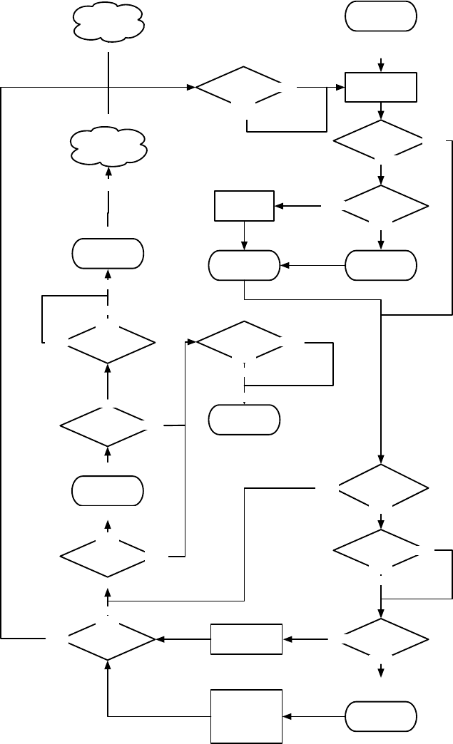
Evaluator
(Begin evaluation
of Individual)
Initializer
(Set up popuation,
but don't populate)
Pre-Initialization Statistics
Post-Initialization Statistics
Initialize Exchanger, Evaluator
Recover from
Checkpoint
Optionally
Checkpoint
Entering-Initial-Population Statistics
If first iteration:
Entering-Steady-State Statistics
Individuals-Bred Statistics
Is an Evaluated
Indivdiual Ready?
YES
Is the
Subpopulation
Full?
YES
NO
Choose a
Subpopulation
(Round-robin)
Evaluator Ready
for an Indivdiual?
YES
Is the
Subpopulation
Full?
YES
NO
Make an
Indivdiual
Breeder
(Breed an
Individual)
Add Individual to
Subpopulation
Breeder
(Pick Individual
to replace)
Possibly Replace
Individual in the
Population with
Evaluated
Individual
Generation
Boundary?
NO
YES
Indivdiuals-Evaluated Statistics
Pre-Breeding
Exchange
Post-Breeding
Exchange
Want to quit? YES
NO
Finisher
Shut Down Exchanger, Evaluator
NO
Out of time or
want to quit?
NO
YES
NO
Pre-Pre-Breeding Exchange Statistics
Post-Pre-Breeding Exchange Statistics
Increment Generation
Generation
Boundary? NO
YES
Generation Boundary Statistics
Generation
Boundary? NO
YES
Pre-Evaluation Statistics
Post-Evaluation Statistics
Generation
Boundary? NO
YES
Post-Evaluation Statistics
Generation
Boundary?
NO
YES
Increment Generation
Post-Post-Breeding Exchange Statistics
Pre-Post-Breeding Exchange Statistics
Reinitialize Exchanger, Evaluator
Optional Post-Checkpoint Statistics
Optional Pre-Checkpoint Statistics
Pre-Finishing Statistics
Figure 6.2 Top-Level Loop of ECJ’s SteadyStateEvolutionState class, used for simple steady-state EC and Asynchronous Evolution
algorithms. “First?” means to perform the Statistics whenever the Subpopulation in question is picking an Individual to displace for the
very first time. (Each Subpopulation will do it once, but possibly at different times). A repeat of Figure 4.2.
234
6.1.4 Asynchronous Evolution
ECJ’s distributed evaluation procedure works intuitively with generational methods (such
as ec.simple.SimpleEvolutionState) but it also works nicely with Steady-State evolution
(ec.simple.SteadyStateEvolutionState). This procedure is called
asynchronous evolution
. See [
25
] for
more information.
The procedure is similar to Steady State Evolution, as discussed in Section 4.2. The Population starts
initially empty. Then the algorithm starts creating randomly-generated Individuals and shipping them off to
remote Slaves to be evaluated. If a Slave is available, the algorithm will generate an Individual for it to work
on. When a Slave has finished evaluating an Individual and has returned it (or its Fitness), the Individual is
then placed into the Population.
At some point the Population will fill up. At this point the algorithm shifts to “steady state” mode. When
a Slave returns an Individual, and there’s no space in the Population, the algorithm makes room by marking
an existing Individual for death and possibly replacing it with the newcomer, just like it’s done in Steady
State Evolution (see Section 4.2 for details). And when a Slave becomes available, an Individual will no
longer be created at random to give to it: rather, the Individual will be bred from the existing Population.
This procedure requires some careful consideration. First, note that at the point that the algorithm shifts
to “steady state” mode, there are probably a large number of Individuals being evaluated on Slaves which
were not bred from the Population but were created at random. Until those Individuals have made their
way into the Population, we won’t be in a true “steady state”.
Second, Steady-State Evolution assumes the production of one Individual at a time: but distributed
evaluation allows more than one individual per Job. This is reconciled as follows. when Steady-State
Evolution starts up, it calls prepareToEvaluate(...) on the Problem (the MasterProblem) once. Thereafter
whenever an individual is sent to the Problem to be evaluated, it calls evaluate(...). Recall from Section 3.4.1
that this process does not require the Problem to immediately assign Fitness — it can bulk up Individuals for
evaluation and is only required to provide a Fitness on or prior to a call to finishEvaluating(...). However,
Steady-State Evolution never calls finishEvaluating(...). As a result, the distributed evaluator is free to assess
Individuals in any order and any way it likes, and to take as long as it likes to assign them a Fitness.
The distributed evaluator will wait for up to
job-size
worth of calls to evaluate(...), then pack those
Individuals together in one Job and ship them out to a remote Slave for evaluation. In “steady-state”
mode, when the Individuals come back, they are placed in the Population, killing and replacing other
individuals already there. Depending on the selection process for marking Individuals for death, it’s entirely
possible that an Individual newly placed into the Population may be immediately marked for death and
replaced with another Individual from the same Job! You can get around this by setting the
job-size
and
max-jobs-per-slave to as low as 1:
eval.masterproblem.job-size = 1
eval.masterproblem.max-jobs-per-slave = 1
...but of course this will make the network utilization poor.
Rescheduling Lost Jobs
If you’re doing generational evolution, then if a slave disappears you need the
SlaveMonitor to reschedule the lost jobs, or else your population won’t be fully evaluated. But that’s not
necessarily the case for Asynchronous Evolution. Here, if slave disappears along with its jobs, well, that’s
life. No big loss. Indeed, this is probably the desired behavior.
By default the SlaveMonitor reschedules its lost jobs. But you can turn off this behavior, so lost jobs just
disappear into the ether, with:
eval.masterproblem.reschedule-lost-jobs = false
An Example For an example Asynchronous Evolution in action, see the files
ec/app/regression/asyncmaster.params and ec/app/regression/asyncslave.params
235

6.1.5 The MasterProblem
The MasterProblem is where much of the magic lies in the interface between ECJ and the distributed
evaluator, so it’s worth mentioning some of its details.
Checkpointing and Synchronization
To start, let’s discuss how MasterProblem handles checkpointing.
Evaluators have three methods which we didn’t discuss in Section 3.4:
public void initializeContacts(EvolutionState state);
public void reinitializeContacts(EvolutionState state);
public void closeContacts(EvolutionState state, int result);
These methods are meant to assist in checkpointing with remote slaves. They in turn call similar methods
in the prototypical Problem:
public void initializeContacts(EvolutionState state);
public void reinitializeContacts(EvolutionState state);
public void closeContacts(EvolutionState state, int result);
result will be one of EvolutionState.R FAILURE (the most common case) or EvolutionState.R SUCCESS
(which only happens if the Evaluator in this process or some external process found the ideal individual).
The default implementation of these Problem methods does nothing at all. But in MasterProblem these
methods are used to handle reconnection of Slaves after a checkpoint recovery. The first two methods create
both a new SlaveMonitor. The final method shuts down the monitor cleanly.
Asynchronous Evolution
MasterProblem also has special methods used only by Steady-State Evolution
(and thus Asynchronous Evolution:
ec.eval.MasterProblem Methods
public boolean canEvaluate()
Returns true if a Slave is available to take an Individual.
public boolean evaluatedIndividualAvailable()
Returns true if a Slave has a completed Individual waiting to be introduced to the Population.
public QueueIndividual getNextEvaluatedIndividual()
Blocks until an Individual is available from a Slave. Then returns it as an ec.steadystate.QueueIndividual. A
QueueIndividual is a very simple class which just contains the Individual and the Subpopulation that the
Individual should be introduced into. It has the following instance variables:
public Individual ind;
public int subpop;
Batching up Jobs
MasterProblem implements all the methods defined in SimpleProblemForm and
GroupedProblemForm (Section 7.1.2). Additionally, MasterProblem overrides common Problem meth-
ods and handles them specially:
ec.eval.MasterProblem Methods
public void prepareToEvaluate(EvolutionState state, int threadnum)
Creates a new queue of Individuals who are out waiting to be sent to be processed.
236

public void finishEvaluating(EvolutionState state, int threadnum)
Sends all Individuals presently in the queue out in one or more Jobs. Then waits for all slaves to complete
evaluation of all Individuals.
Most Evaluators instruct Problems to evaluate a sequence of Individuals by first calling prepareToEvalu-
ate(...), then repeatedly calling evaluate(...), then finally calling finishEvaluating(...). MasterProblem takes
advantage of this as follows. When prepareToEvaluate(...) is called, MasterProblem creates a list in which to
put Individuals. evaluate(...) does not actually evaluate individuals: instead, individuals are simply added
to the list. When enough individuals have been added to the queue to form one Job, the Job is queued up to
be submitted to the next available Slave. When finishEvaluating(...) is called, any remaining individuals in
the list are bundled together in a final Job and sent to a Slave. Then finishEvaluating(...) waits until all the
Jobs have been completed before it returns.
When the GroupedProblemForm form of evaluate(...) is called (such as from a coevolutionary evaluator),
the Individuals passed to that call are treated as a single Job and shipped off immediately —˙
that is, there is
no queue. However, evaluate(...) again does not wait for results to come back. The waiting again happens
when finishEvaluating(...) is called.
There are certain Evaluators which do call prepareToEvaluate(...) or finishEvaluating(...), but instead just
repeatedly call evaluate(...). This is meant for processes which cannot delay the evaluation of individuals in an
evaluate(...) before the next evaluate(...) is called. For example, certain competitive coevolutionary processes
may require a serial evaluation of this kinds. In this case, a call to evaluate(...) will cause MasterProblem to
simply ship off the Individual or Individuals to evaluate as a single job, wait for the result, and return it.
Perhaps this isn’t the best use of massive parallelism!
Sending Initialization Data from the Master to the Slaves
MasterProblem has one additional feature:
three methods you can override such that, whenever a Slave is started up, you are given the chance to send
one-time data from the Master to the Slave, perhaps to initialize some variables you need your Slave to know.
Note that this facility is untested and may be somewhat fragile: we suggest that before you use this facility
you consider instead placing the data in a file that each Slave can read.
Here’s how it works. You begin by declaring a special subclass of MasterProblem — let’s call it
ec.app.myapp.MyMasterProblem. Then you must tell ECJ that you’re using it (on both sides, master and slave)
with something like this:
eval.masterproblem = ec.app.myapp.MyMasterProblem
An instance of this MasterProblem subclass is used by the Master. When a Slave shows up, the Master
will call the method sendAdditionalData(...) on that instance to give you the chance to send data down
the stream to the Slave before any evaluation occurs. The Slave receives this data by calling the method
receiveAdditionalData(...) on a dummy instance of this same subclass. This dummy instance will not be used
for any purpose except to handle the data reception. That method must store away the transferred data,
typically as instance variable in your subclass which you have created for this purpose. Finally, each time
the Slave creates a new EvolutionState (and it may do so many times), it calls transferAdditionalData(...) on
that dummy instance to give it a chance to modify and set up EvolutionState appropriately to reflect the data
it had received from the Master.
sendAdditionalData(...) will be called once on the Master for each Slave that shows up. receiveAdditional-
Data(...) will only be called once on the Slave side. transferAdditionalData(...) may be called multiple times
on the Slave side, every time a new EvolutionState is loaded and set up. It is entirely up to you to handle the
protocol for sending and receiving this data: if you mess up (write more data than you read on the other
side, say), it’s undefined what’ll happen. Probably something bad.
ec.eval.MasterProblem Methods
public void sendAdditionalData(EvolutionState state, DataOutputStream dataOut)
237

Called from the SlaveMonitor’s accept() method to optionally send additional data to the Slave via the dataOut
stream. By default it does nothing.
public void receiveAdditionalData(EvolutionState state, DataInputStream dataIn)
Called on a dummy MasterProblem by the Slave. You should use this method to store away received data via the
dataIn stream for later transferring to the current EvolutionState via the transferAdditionalData(...) method. You
should NOT expect this MasterProblem to be used for by the Slave for evolution (though it might). By default
this method does nothing, which is the usual situation. The EvolutionState is provided solely for you to be able
to output warnings and errors: do not rely on it for any other purpose (including access of the random number
generator or storing any data).
public void transferAdditionalData(EvolutionState state)
Called on a dummy MasterProblem by the Slave to transfer data previously loaded via receiveAdditionalData(...)
to a running EvolutionState at the beginning of evolution. This method may be called multiple times if multiple
EvolutionStates are created. By default this method does nothing, which is the usual situation. Unlike in
receiveAdditionalData(...), the provided EvolutionState is “live” and you can set it up however you like.
6.1.6 Noisy Distributed Problems
Sometimes your fitness function is noisy: the same individual will get different fitness values depending on
some degree of randomness. An easy way to deal with this is to run the same individual for some
N
trials
inside your Problem instance and to take the median or mean or whatnot, and use that as your fitness.
This works fine in a single-CPU setting, but in a parallel setting there’s a gotcha. Let’s say you have 100
parallel machines available to you but you have a population size of 20. You’d like to do 5 trials for each
individual, and trials are not cheap. If you farmed out individuals using the distributed evaluator and a
Problem subclass which did 5 trials internally, only 20 machines would be used, and they’d be expected
to run 5 trials each. What you want to do is run one trial on each of the machines. But because of the way
MasterProblem is set up, this won’t work.
ECJ has a hack that you can use in this situation. SimpleEvaluator has the parameters:
eval.num-tests = 5
% Other options are: median, best
eval.merge = mean
This tells the SimpleEvaluator to test each individual 5 times and set its fitness value to their mean. How
does it do this? By temporarily modifying the Subpopulation.
If your Subpopulation presently has 20 individuals in it, and you want to test each 5 times, SimpleEval-
uator will replace this Subpopulation with a copy which has 100 individuals in it. These 100 individuals
are 5 clones each of the original 20. Then SimpleEvaluator evaluates this new population (which causes the
distributed evaluation system to farm them out to potentially 100 machines).
After all the fitnesses have come back, SimpleEvaluator merges the fitnesses of the 5 clones together to
form a single fitness and sets the original individual’s fitness to that merged value. The legal merge settings
are mean,median, and best. Finally, SimpleEvaluator restores the original Subpopulation.
This means that if you have a custom Subpopulation subclass, it needs to deal gracefully with being
copied and having its individuals array extended. In general this is probably the case but you should be
warned.
Also, in this situation, the number of individuals being evaluated is smaller than the number of machines
available. Thus you will need to turn off ECJ features which bulk up multiple individuals per job, and
multiple jobs per slave. Set these to 1:
eval.masterproblem.job-size = 1
eval.masterproblem.max-jobs-per-slave = 1
238
A note about merging and multiobjective optimization. Multiobjective Fitness classes can do merging,
but only using
mean
. The
median
and
best
options will throw exceptions. When a multiobjective fitness
undergoes merging, it’s essentially forming the centroid of the merged fitnesses. Merging is okay for
subclasses like SPEA2 or NSGA-II’s fitness classes because it’d done before their auxiliary fitness information
is computed.
There’s no equivalent to this hack in Asynchronous Evolution: you’ll just have to ask a machine to test
the individual 5 times.
6.2 Island Models (The ec.exchange Package)
In addition to Distributed Evaluation, ECJ supports Island Models: separate ECJ processes (“islands”) which
connect over the network and occasionally hand highly-fit Individuals to one another. This facility is handled
by an Exchanger called ec.exchange.IslandExchange which ships individuals off to other islands immediately
before breeding, and immediately after breeding brings in new individuals provided it by other islands.
You’ll run your separate islands as ordinary processes.
Most of the issues in Island models surround the particular topology being chosen. Which islands
will send Individuals to which other islands? How many at a time? How often? Are Individuals sent
synchronously or asynchronously? Etc. ECJ manages all topology and connection parameters via a special
ECJ process called the
island model server
. Each island will connect to and register itself with the server.
When the islands have all connected, the server will tell them which islands need to hook up to which other
islands and how. After the islands have hooked up, they’re given the go-ahead to start their evolutionary
processes. If the islands are acting synchronously, each generation will wait for the server to give them the
go-ahead to continue to the next generation; this go-ahead only occurs after all islands have finished the
previous generation. Finally, when an island discovers an optimal individual, it will signal the server to let
the other islands know (so they can shut down).
As you can see, the server really does little more than tell the islands how to connect and acts as a referee.
Thus it’s actually a very lightweight process. You can run the server either as its own process like this:
java ec.exchange.IslandExchange -file server.params -p param=value ... (etc.)
...or an ECJ island can also do double-duty, serving as the server as well. All islands, whether ordinary
islands or double-duty island-server combos, are fired up in the same standard ECJ fashion:
java ec.Evolve -file island.params -p param=value -p param=value ... (etc.)
...or (as usual):
java ec.Evolve -checkpoint myCheckpointFile.gz
A double-duty island-server combo would differ from a plain island solely in the parameters it defines:
it’d need server parameters in addition to client parameters.
Mixing Island Models, Threading, and Distributed Evaluation
There’s absolutely no reason you can’t
create an unholy union of Island Models and Distributed Evaluation. For example, it’s perfectly reasonable
to have an Island Model where each island maintains its own pool of Slaves to do distributed evaluation. It’d
be a lot of parameter files though! Island Models also work perfectly fine in a multithreaded environment.
6.2.1 Islands
You set up an ECJ process as an island by defining a special Exchange object for it:
239

exch = ec.exchange.IslandExchange
IslandExchange maintains the island’s
mailbox
. Prior to breeding, the IslandExchange procedure will
send some fit individuals off to mailboxes of remote islands. The procedure for selecting Individuals is
defined along these lines:
exch.select = ec.select.TournamentSelection
Obviously this selection procedure may require its own parameters, such as (in this example):
exch.select.size = 2
After breeding, the IslandExchange will empty its own mailbox and introduce into the Population all of
the Individuals contained therein. These Individuals will displace some of the recently-bred Individuals,
which never get a chance to be selected.
4
The selection method for picking the Individuals to die and be
displaced is defined as:
exch.select-to-die = ec.select.RandomSelection
If this parameter isn’t defined, individuals are picked at random. Again, as this is a selection operator, it
may have its own parameters.
An Island needs to know where the Server is so it can register itself, and the socket port on which the
server is listening, for example:
exch.server-addr = 128.2.30.4
exch.server-port = 8999
When an Island registers itself with the Server, it’ll tell it two things. First, it’ll tell the Server the island’s
name
, a String which uniquely identifies the island (and by which the Server looks up topology information
for the island). Second, it’ll tell the Server the socket port on which it’ll receive incoming Individuals from
other islands. Let’s say that you’re creating an island called StatenIsland. You might specify the following:
exch.id = StatenIsland
exch.client-port = 9002
Note that the client socket port should be (1) higher than 2000 and (2) different from other client ports,
and the server port, if they’re running on the same machine or in the same process. You’ll also probably
want to have compressed network streams. Like was the case in Distributed Evaluation, this can’t be
done without the jzlib/ZLIB library, which you must install separately (see the ECJ main webpage or
http://www.jcraft.com/jzlib). This is because Java’s compression facilities are broken. Once this library
installed, you can turn it on like this:
exch.compression = true
Be certain to give your island a unique random number seed different from other islands! Don’t set the
seed to
time
, since it’s possible that two islands will have the same seed because they were launched within
the one millisecond of one another. I’d hard-set the seed on a per-island basis.
seed.0 = 5921623
If your islands share the same file system, you’ll want to make sure they don’t overwrite each other’s
statistics files etc. To do this, for example, StatenIsland might change its statistics file name to:
4Life’s not fair.
240
stat.file = $statenisland.stat
If you have multiple Statistics files you’ll need to change all of them; the same goes for other files being
written out. Also, if you are checkpointing, and your islands might overwrite each others’ checkpoint files,
you need to change the checkpoint prefix on a per-island basis. For example:
checkpoint-prefix = statenisland
... or alternatively change the directory in which checkpoint files are written on a per-island basis:
checkpoint-directory = /tmp/statenisland/
Last, you can cut down on the verbosity of the islands by setting...
exch.chatty = false
6.2.2 The Server
The Server holds all the parameters for setting up the island topology. But first we must clue your ECJ
process into realizing that it is a Server in the first place. This is done with:
exch.i-am-server = true
Next we need to state how many islands are in the island model graph:
exch.num-islands = 3
As discussed in Section 6.2.1, each island has a unique name (id). Here you will state which island in
your graph has which id:
exch.island.0.id = StatenIsland
exch.island.1.id = ConeyIsland
exch.island.2.id = EllisIsland
Each island has some number of connections to other islands (the islands it’ll send Individuals, or migrants,
to). In this example, we’ll say that StatenIsland sends migrants to ConeyIsland, which sends migrants to
EllisIsland, which sends migrants to both StatenIsland and ConeyIsland:
exch.island.0.num-mig = 1
exch.island.0.mig.0 = ConeyIsland
exch.island.1.num-mig = 1
exch.island.1.mig.0 = EllisIsland
exch.island.2.num-mig = 2
exch.island.2.mig.0 = StatenIsland
exch.island.2.mig.1 = ConeyIsland
StatenIsland and ConeyIsland send 10 migrants to each of the islands they’re connected to. But we want
EllisIsland to send 50 migrants to each of the (two) islands it’s connected to:
exch.island.0.size = 10
exch.island.1.size = 10
exch.island.2.size = 50
Altenatively you can use a default parameter base of sorts:
241
exch.size = 10
Each island has a maximum mailbox capacity: if there is no room, further immigrants will be dropped
and disappear into the ether. You should make your mailbox big enough to accept immigrants at a reasonable
rate, but not so large that in theory they could entirely overwhelm your population! I suggest a mailbox
three or four times the size of the expected immigrants. How about 100 or 200?
exch.island.0.mailbox-capacity = 200
exch.island.1.mailbox-capacity = 200
exch.island.2.mailbox-capacity = 200
Altenatively you can use a default parameter base of sorts:
exch.mailbox-capacity = 200
Last you’ll need to stipulate two additional parameters on a per-island basis: the
start-generation
(in
which generation the island will start sending Individuals out) and
modulus
(how many generations the
island will wait before it sends out another batch of Individuals). These are mostly set to maximize network
utilization: perhaps you may wish the islands to send out individuals at different times so as not to clog
your network, for example. Here we’ll tell each island to send out individuals every three generations, but
to start at different initial generations so to be somewhat staggered:
exch.island.0.mod = 3
exch.island.1.mod = 3
exch.island.2.mod = 3
exch.island.0.start = 1
exch.island.1.start = 2
exch.island.2.start = 3
Altenatively you can use a default parameter base of sorts:
exch.mod = 3
exch.start = 2
6.2.2.1 Synchronicity
Island models can be either
synchronous
or
asynchronous
. In a synchronous island model, islands wait until
they all have reached the next generation before sending immigrants to one another. In the asynchronous
island model, islands go at their own pace and send immigrants whenever they feel like it. This means
that one evolutionary process on one computer may run much faster than another one (good, because it
doesn’t waste resources waiting for the other one to catch up) but it may overwhelm the other process with
multiple generations of immigrants before the other process can get around to processing them (usually
bad). Generally speaking asynchronicity is preferred — and is the default setting.
If for some reason you want to turn on synchronicity, you do this:
exch.sync = true
Note that the modulo and start-generation of islands results in a predictable behavior for synchronous
island models: but since asynchronous islands can go at their own pace, the modulo and start-generation
happen when they happen for each island.
Note too that because asynchronous island models go at their own pace, and are subject to the whims of
the speed of the operating system and the CPU time allotted to the process, there’s no way to guarantee
replicability.
242
6.2.3 Internal Island Models
ECJ’s Internal Island Model facility simulates islands using separate Subpopulations: each Subpopulation is
an island, and occasionally highly fit Individuals migrate from Subpopulation to Subpopulation. Like any
other Exchanger, the Internal Island Model facility takes Individuals from other Subpopulations immediately
before Breeding, stores them, and then introduces them into their destination Subpopulations immediately
after Breeding.
There are four important things to note about this facility:
• Obviously each Subpopulation must have identical Species and Individual and Fitness prototypes.
• Internal Island Models are always synchronous.
•
Because they use the Subpopulation facility, Internal Island Models are incompatible with any other
ECJ procedure which relies on Subpopulations: notably coevolution.
•
Because they define an Exchanger, Internal Island Models are incompatible with any other ECJ
procedure which uses an Exchanger: in particular, you can’t mix Internal Island Models with regular
Island Models!
Why would you use Internal Island Models? I think mostly for academic purposes: to study and simulate
synchronous Island Models without having to rope together a bunch of machines. You could also use
Internal Island Models to run
N
evolutionary processes in parallel — just set the number of immigrants to
zero.
Internal Island Models depend solely on a specific Exchanger, ec.exchange.InterPopulationExchange. To
build an Internal Island Model, you first define three subpopulations and their species, individuals, breeding
pipelines, the whole works, using a standard generational algorithm. Then you define the exchanger:
exch = ec.exchange.InterPopulationExchange
Let’s say you have four Subpopulations acting as islands. You’ll first need to stipulate the Selection
Method used to select individuals to migrate to other Subpopulations and the Selection Method used to kill
Individuals to make way for incoming immigrants:
exch.subpop.0.select = ec.select.TournamentSelection
exch.subpop.1.select = ec.select.TournamentSelection
exch.subpop.2.select = ec.select.TournamentSelection
exch.subpop.3.select = ec.select.TournamentSelection
exch.subpop.0.select-to-die = ec.select.RandomSelection
exch.subpop.1.select-to-die = ec.select.RandomSelection
exch.subpop.2.select-to-die = ec.select.RandomSelection
exch.subpop.3.select-to-die = ec.select.RandomSelection
If you don’t define a selection method for death, ECJ will assume you mean to select individuals randomly.
Alternatively you can use the default parameter base:
exch.select = ec.select.TournamentSelection
exch.select-to-die = ec.select.RandomSelection
Remember that these selection operators may have their own parameters. For example, we may wish to
say (for some reason):
exch.subpop.0.select.size = 2
exch.subpop.1.select.size = 2
exch.subpop.2.select.size = 7
exch.subpop.3.select.size = 7
243
Otherwise the selection operators will rely on their default parameters.
Note
: recall that these default pa-
rameters are not based on the Exchanger’s default parameter base. That is, they’re
select.tournament.size
and not exch.select.size. I strongly suggest using non-default paramters.
Next you need to state the number of immigrants sent at a time; the first generation in which they’ll
be sent; and the modulus (the interval, in terms of generations, between successive migrations). These are
basically the same as the standard Island Model. The parameters might look like this:
exch.subpop.0.size = 5
exch.subpop.1.size = 5
exch.subpop.2.size = 5
exch.subpop.3.size = 15
exch.subpop.0.start = 1
exch.subpop.1.start = 2
exch.subpop.2.start = 3
exch.subpop.3.start = 4
exch.subpop.0.mod = 8
exch.subpop.1.mod = 8
exch.subpop.2.mod = 8
exch.subpop.3.mod = 8
It’s here where you could convert these to separate independent evolutionary processes: just set the
size
parameter to 0 for all subpopulations. Anyway, you can also use default parameter bases for these:
exch.size = 5
exch.start = 1
exch.mod = 8
Now we need to define the topology. For each island we’ll define the number of Subpopulations it sends
migrants to, and then which ones. Imagine if Subpopulation 2 sent migrants to everyone else, but the other
Subpopulations just sent migrants to Subpopulation 2. We would define it like this:
exch.subpop.0.num-dest = 1
exch.subpop.0.dest.0 = 2
exch.subpop.1.num-dest = 1
exch.subpop.1.dest.0 = 2
exch.subpop.2.num-dest = 3
exch.subpop.2.dest.0 = 0
exch.subpop.2.dest.1= 1
exch.subpop.2.dest.2 = 3
exch.subpop.3.num-dest = 1
exch.subpop.3.dest.0 = 2
Last, Internal Island Models tend to be verbose. To make them less chatty, you can say:
exch.chatty = false;
Reminder
It’s laborious to write a zillion parameters if you have large numbers of subpopulations in your
internal island model experiments. You can greatly simplify this process using the
pop.default-subpop
parameter (see Section 3.2.1).
6.2.4 The Exchanger
In Section 3.6 we talked about various basic Exchanger methods. But three were not discussed, mostly
because they’re only used for Island Models (not even Internal Island Models). They are:
244

public void initializeContacts(EvolutionState state);
public void reinitializeContacts(EvolutionState state);
public void closeContacts(EvolutionState state, int result);
If these look similar to the methods in Section 6.1.5, it’s with good reason. Their function is to set up net-
working connections, re-establish networking connections after restarting from a checkpoint, and shut down
networking connections in a clean way. IslandExchange implements them but not InterPopulationExchange.
Additionally, prior to migrating an Individual to another island, Exchangers typically call a hook you can
override to modify that Individual or replace it with some other Individual:
protected Individual process(EvolutionState state, int thread, String island,
int subpop, Individual ind);
There are various reasons you might do this: perhaps the islands have different representations for their
individuals or fitness classes, for example, requiring a conversion before you send migrants off.
This method has two parameters which require explanation. The island is the id of the island that will re-
ceive the Individual, or null if there is no such island (as is the case for InterPopulationExchange). The subpop
is the destination subpopulation of the Individual (particularly important in InterPopulationExchange).
To assist you in your processing, IslandExchange provides an additional method which is useful to call
inside the process method:
public int getIslandIndex(EvolutionState state, String island);
This method returns the index in the parameter database of the island referred to by id, or IslandEx-
change.ISLAND INDEX LOOKUP FAILED.
The purpose of this method is to allow islands to look up information, typically stored in a parameter
database, about the islands they’re about to send migrants to, so as to convert individuals in a way ap-
propriate to those islands, perhaps. To take advantage of this method, you’d need to make sure that the
server’s island exchange parameters are also in each client’s database. For example, let’s say that your id is
“GilligansIsland”, and in the parameter database (which again the client must have) we have the following
parameters in the server database file:
exch.num-islands = 8
...
exch.island.1.id = GilligansIsland
exch.island.1.num-mig = 3
exch.island.1.mig.0 = SurvivorIsland
exch.island.1.mig.1 = EllisIsland
exch.island.1.mig.2 = FantasyIsland
exch.island.1.size = 4
exch.island.1.mod = 4
exch.island.1.start = 2
exch.island.1.mailbox-capacity = 20
# this is just made up
exch.island.1.is-gp-island = true
...
(Note the last nonstandard parameter, which I made up for purposes of this example.) We begin by
also including these parameters in each island’s database file. We are about to send some migrants to
GilligansIsland (the name passed into process(...). To look up information about this island, we can use
getIslandIndex(...) to discover that GilligansIsland is island number 1 in our parameter database. This makes
it easy for us to look up other information we’ve stashed there to tell us how we should process our island:
protected Individual process(EvolutionState state, int thread, String island, int subpop, Individual ind)
245
{
int index = getIslandIndex(state, island);
if (index == ISLAND_INDEX_LOOKUP_FAILED) // uh oh
state.output.fatal("Missing island index for " + island);
Parameter param = new Parameter("exch.island." + index + ".is-gp-island");
if (!state.parameters.exists(param)) // uh oh
state.output.fatal("Missing parameter for island!", param, null);
boolean isGPIsland = getBoolean(param, null, false);
if (isGPIsland)
{
// process the individual in some way because it’s going to a "GP Island" or whatever
}
}
This method isn’t necessary (nor provided) for InterPopulationExchange since it doesn’t really do “islands”
per se so much as exchanges between subpopulations. In this case, the process(...) method has told us what
subpopulation we’ll be sending the individual to and we have direct access to it. For example, we might do
this:
protected Individual process(EvolutionState state, int thread, String island, int subpop, Individual ind)
{
if (state.population.subpops.get(subpop).species instanceof ec.gp.GPSpecies)
{
// convert to a GP individual, or whatever
}
}
246
Chapter 7
Additional Evolutionary Algorithms
7.1 Coevolution (The ec.coevolve Package)
The coevolution package is meant to provide support for three kinds of Coevolution:
• One-Population Competitive Coevolution
• Two-Population Competitive Coevolution
•N-Population Cooperative Coevolution
Coevolution differs from evolutionary methods largely in how evaluation is handled (and of course, by
the fact that there are often multiple subpopulations). Thus the classes in this package are basically Problems
and Evaluators. The first form of Coevolution is provided by the ec.coevolve.CompetitiveEvaluator class. The
second two are made possible by the ec.coevolve.MultiPopCoevolutionaryEvaluator class.
7.1.1 Coevolutionary Fitness
Coevolution is distinguished by its evaluation of Individuals not separately but in groups, where the Fitness
of an Individual depends on its performance in the
context
of other Individuals (either competing with them
or working with them towards a common goal). For this reason, coevolution typically involves evaluating
an Individual multiple times, each time with a different set of other Individuals, and then computing the
Fitness based on these multiple trials.
To assist in this procedure, the ec.Fitness class has two auxiliary variables:
public ArrayList trials = null;
public Individual[] context = null;
The first variable (trials) is available for you to maintain the results of each trial performed. Later on you
will be asked to compute the final fitness of an individual, and at this point you can use this variable to do
the final calculation. The variable is initially null, and after fitness is assessed it will be reset to null again. You
are free to use this variable as you like (or ignore it entirely), Most commonly you’d store each trial in the
trials variable as a java.lang.Double, with higher values being considered better. You’re free to do something
else, but if you do, be sure to read Section 7.1.5 first.
Even if your trials are not java.lang.Double, they must
be immutable: their internals cannot be modified, so they can be pointer-copied and not just cloned.
The second variable (context) is available for you to maintain the context of the best trial discovered for
the Individual. It’s typically only useful when you’re doing Cooperative Coevolution, where it’s important
to retain not only the performance of the Individual (his Fitness), but which collaborating Individuals made
it possible for him to achieve that Fitness. Again, this is an optional variable though often useful. If context is
247

used, it’s assumed that the slots of context hold each collaborator, except for the Individual himself, whose
slot is set to null. Section 7.1.4.2 discusses the issue of context in more detail.
7.1.2 Grouped Problems
Since Coevolution involves evaluating multiple Individuals at once, it will require a new kind of Problem
which takes multiple Individuals at a time. This Problem Form is defined by ec.coevolve.GroupedProblemForm.
Evaluation in coevolution involves multiple trials, along these lines:
1. Performance scores of Individuals are cleared.
2.
Individuals are tested against each other in various matches (or with one another in various collabo-
rative problems). These trials cause trial performance scores of the Individuals to accumulate. If the
trials are cooperative, the best trial found for a given Individual (its context) is maintained.
3. The final Fitnesses of the Individuals are set based on the performance scores over all the trials.
It’s up to you to store the trial results and eventually form them into final Fitness values, as discussed
later. It’s also up to you to maintain the best context if you find this useful, as discussed later as well (in
Section 7.1.4.2). GroupedProblemForm will help you by defining three methods to do these various portions
of the evaluation process. You’ll need to implement all three methods:
ec.coevolve.GroupedProblemForm Methods
public abstract void preprocessPopulation(EvolutionState state, int thread, boolean[] prepareForAssessment,
boolean countVictoriesOnly)
Called prior to the evaluation of a Population, mostly to clear the trials of Individuals. Only clear the trials for
Individuals in Subpopulations for which prepareForAssessment is true. Note that although this method is not static,
you should not assume that this method will be called on the same Problem as is used later for evaluate(...). Thus
don’t use this method to set any instance variables in the Problem for later use. If countVictoriesOnly is true, the
method being used is SingleEliminationTournament. Commonly you’ll use this method to create a brand-new
trials ArrayList for every Fitness of every Individual in every Subpopulation.
void evaluate(EvolutionState state, Individual[] individuals, boolean[] updateFitness, boolean countVictoriesOnly,
int[] subpops, int thread)
Evaluates the individuals in a single trial, setting their performance scores for that trial. Each individual will be
from a certain subpopulation, specified in subpops. In some versions of coevolution, only certain individuals
are supposed to have their performance scores updated (the others are acting as foils). In this case, the relevant
individuals will be indicated in the updateFitness array. Typically you’ll update fitness by adding trial results to the
trials ArrayList. For any individual for whom you’re updating trials, also set the Fitness value to reflect that one
trial: this allows Single Elimination Tournament to compare Individuals based on this notional Fitness value. In
doing so, do not set the evaluated flag for Individuals.
If you’re doing cooperative coevolution, in this method you’ll also probably want to maintain the context of the
trial (the collaborating Individuals) if it’s produced the best results so far. More on that in Section 7.1.4.2.
public abstract void postprocessPopulation(EvolutionState state, int thread, boolean[] assessFitness,
boolean countVictoriesOnly)
Called after evaluation of a Population to form final Fitness scores for the individuals based on the various
performance scores they accumulated during trials; and then to set their evaluated flags to true. Only assess the
Fitness and set the evaluated flags for Individuals in Subpopulations for which assessFitness is true. Note that
although this method is not static, you should not assume that this method will be called on the same Problem as
was used earlier for evaluate(...). You’ll probably want to set the trials variable to null to let it garbage collect.
Do not assume that Individuals will have the same number of trials: in several versions of Coevolution
this will not be the case.
248
You’re going to have to do some work to make sure that your Fitnesses are properly updated, and this
depends on the kind of Coevolution you choose to do. So how do you keep track of trials? If you’re just
accumulating scores or wins, then you could use SimpleFitness and just increment it with each new win.
But since different Individuals may have different numbers of trials, it’s possible that you may need to keep
track of the number of trials, or keep track of each trial result separately. Probably the best approach is to use
the auxiliary variable trials found in ec.Fitness to store all your trials in an ArrayList. Thus you typically use
GroupedProblemForm like this:
1. In preprocessPopulation(...), set the Fitness’s trials to a new ArrayList for all Individuals.
2.
In evaluate(...), add to trials the results of this trial for each Individual for whom updateFitness is set.
Then set the Fitness to reflect just the immediate results of the trial (particularly if countVictoriesOnly is
set). This allows Single Elimination Tournament — if you’re using that — to determine who should
advance to the next round. Make certain that whatever you add to trials is java.io.Serializable.
If you’re doing cooperative coevolution, determine if the new trial is superior to all the existing trials
previously found in the trials array. If it is, set the context of this trial using Fitness.setContext(...).
3.
In postprocessPopulation(...), set the Fitness to the final result. For example, you might set it to the
average or the maximum of the various trials. Finally, set the Fitness’s trials to null to let it GC.
Notice that unlike in SimpleProblemForm (Section 3.4.1) there’s no describe(...) method. This is because
to describe an Individual, you’d need to do so in the context of other Individuals. So we left it out.
Example
Assume we’ve replaced the Fitness with our MyCoevolutionaryFitness class. Let’s create a
Problem similar to the example in Section 4.1.1. In our Problem we take two Individuals, and the trial
performance of an Individual is his vector values’ product minus that of his opponent. Obviously this is a
stupid example since Individuals are in a total ordering Fitness-wise: so it hardly illustrates the issues in
Coevolution. But it’ll suffice for the demonstration here. What we’ll do is set an Individual’s fitness to his
average score over the trials performed.
package ec.app.myapp;
import ec.*;
import ec.simple.*;
import ec.vector.*;
import ec.coevolve.*;
public class MyCoevolutionaryProblem extends Problem implements GroupedProblemForm {
public void preprocessPopulation(EvolutionState state, Population pop,
boolean[] prepareForAssessment, boolean countVictoriesOnly) {
for(int i = 0; i < pop.subpops.size(); i++)
if (prepareForAssessment[i])
for(int j = 0; j < pop.subpops.get(i).individuals.size(); j++) {
SimpleFitness fit = (SimpleFitness)(pop.subpops.get(i).individuals.get(j).fitness);
fit.trials = new ArrayList();
}
}
public void evaluate(EvolutionState state, Individual[] ind, boolean[] updateFitness,
boolean countVictoriesOnly, int[] subpops, int threadnum) {
int[] genome1 = ((IntegerVectorIndividual)ind[0]).genome;
int[] genome2 = ((IntegerVectorIndividual)ind[1]).genome;
double product1 = 1.0;
double product2 = 1.0;
for(int x=0; x<genome1.length; x++) product1 = product1 * genome1[x];
249
for(int x=0; x<genome2.length; x++) product2 = product2 * genome2[x];
MyCoevolutionaryFitness fit1 = (MyCoevolutionaryFitness)(ind[0].fitness);
MyCoevolutionaryFitness fit2 = (MyCoevolutionaryFitness)(ind[1].fitness);
if (updateFitness[0]) {
fit1.trials.add(new Double(product1 - product2));
// set the fitness in case we’re using Single Elimination Tournament
fit1.setFitness(state, fit1.fitness() + product1 - product2, false);
}
if (updateFitness[1]) {
fit2.trials.add(new Double(product2 - product1));
// set the fitness in case we’re using Single Elimination Tournament
fit2.setFitness(state, fit2.fitness() + product2 - product1, false);
}
}
public void postprocessPopulation(EvolutionState state, Population pop,
boolean[] assessFitness, boolean countVictoriesOnly) {
for(int i = 0; i < pop.subpops.size(); i++)
if (assessFitness[i])
for(int j = 0; j < pop.subpops.get(i).individuals.size(); j++) {
SimpleFitness fit = (SimpleFitness)(pop.subpops.get(i).individuals.get(j).fitness);
// Let’s set the fitness to the average of the trials
int len = fit.trials.size();
double sum = 0;
for(int l = 0; l < len; l++)
sum += ((Double)(fit.trials.get(l))).doubleValue();
// Alternatively if we were interested in how *many* times we won rather
// than by how much, we might set the fitness to, say, how often the doubleValue()
// was positive.
fit.setFitness(state, sum / len, false);
pop.subpops.get(i).individuals.get(j).evaluated = true;
}
}
}
Now we hook it up as so:
eval.problem = ec.myapp.MyCoevolutionaryProblem
It’s important to note that the trials variable doesn’t have to store an ArrayList of numbers — it can store
any object reflecting the outcome of a trial that you’d like to invent. It’s available for you to use.
Generally the trials variable should never need to be cloned — it’ll be set up, used during Evaluation,
and then destroyed. The default implementation of the Fitness.cloneTrials() method, called by Fitness.clone(),
simply throws an exception if trials is null.
7.1.3 One-Population Competitive Coevolution
In One-Population Competitive Coevolution, the whole population (or in ECJ parlance, a whole Subpopula-
tion) competes in various games. The outcomes of those games determines the fitness of Individuals in the
Subpopulation. Thus the Fitness of an Individual depends on which other Individuals it plays against.
250

ECJ does One-Population Competitive Coevolution with a special Evaluator called
ec.coevolve.CompetitiveEvaluator, meant to be used in generational evolutionary methods. Building
on the genetic algorithm example in Section 4.1.1, we’ll replace the Evaluator:
eval = ec.coevolve.CompetitiveEvaluator
The main issue in One-Population Competitive Coevolution is the layout of the trials (competitions)
between various Individuals. CompetitiveEvaluator provides the following options:1
•
Round Robin. Every Individual of the Subpopulation is paired up and evaluated with every other
Individual, not including the Individual itself. The Fitness of both Individuals is updated. This is
stipulated as:
eval.style = round-robin
•
K-Random-Opponents (One-Way). Every Individual of the Subpopulation is paired up with
K
random
opponents other than himself, picked at random with replacement. Only the Individual’s fitness is
updated, not his opponents’. This is stipulated, plus the size of K, as:
eval.style = rand-1-way
eval.group-size = 8
Our experiments have tended to suggest that
K=
6 to 8 are good values. Remember that larger group
sizes result in many more evaluations.
•
K-Random-Opponents (Two-Way). Every Individual of the Subpopulation is paired up with at least
K
random opponents other than himself, picked at random with replacement. Both Individuals’ fitnesses
are updated; thus being selected as an “opponent” allows an Individual to need fewer “regular” tests
in order to fill his own
K
quota. Overall this results in about half the total number of tests as One-Way.
eval.style = rand-2-way
eval.group-size = 8
A few individuals would be expected to be tested more than
K
times. If your fitness procedure simply
cannot permit this, you can have the algorithm turn off fitness updating for those Individuals with:
eval.over-eval = false
•
Single Elimination Tournament. All Individuals in the Subpopulation are paired up and evaluated. In
each pair, the “winner” is the individual which winds up with the superior performance. If neither
Individual is superior, then the “winner” is chosen at random. The winners advance to the next level:
they’re paired up and evaluated, and so on, just like in a single-elimination tournament.
Important
note:
It is important that the Subpopulation size be a power of two for a proper Single-Elimination
Tournament.
You stipulate Single-Elimination Tournament with:
eval.style = single-elim-tournament
After a single trial, you need to increment the Fitness of the winning Individual: this will tell Single-
Elimination Tournament who to advance to the next round.
2
After all the trials have completed, we
1
Note that we used to have a number of other options at one point, many of which are still in the CompetitiveEvaluator source code
of various ECJ versions, such as double-elimination tournament, world cup style, etc. But these have fallen by the wayside.
2
Keep in mind that two Individuals compete with one another only because they’ve advanced to the same level, and so have the
same Fitness initially.
251

will treat the Fitness of an Individual simply to be the number of trials it won, and so not modify the
Fitness during postprocessPopulation. You can tell Single-Elimination Tournament is being used because
countVictoriesOnly is true in the GroupedProblemForm methods.
One-Population Competitive Coevolution can be prohibitively expensive. So if you can use it, we suggest
you not use Round Robin. Here’s why. Round Robin is
O(n2)
. K-Random-Opponents (One-Way) is
O(kn)
.
K-Random-Opponents (Two-Way) is roughly
O(k
2n)
. But Single-Elimination Tournament is
O(n)
. When
cast in terms of performance by number of evaluations, sometimes Single-Elimination Tournament performs
best, though often K-Random-Opponents performs best with
K
set to somewhere between 6 and 8. We did a
comparison paper on the two [14].
ec.coevolve.CompetitiveEvaluator is multithreaded and responds to the evalthreads parameter.
7.1.4 Multi-Population Coevolution
There are two common kinds of multi-population coevolution: 2-Population Competitive Coevolution and
N
-Population Cooperative Coevolution. Both are handled by the ec.coevolve.MultiPopCoevolutionaryEvaluator
class:
eval = ec.coevolve.MultiPopCoevolutionaryEvaluator
In 2-Population Competitive Coevolution Individuals in each of two Subpopulations are tested by pitting
them against Individuals in the opposing Subpopulation. The Fitness of an Individual is based on several
such tests. Typically one Subpopulation is of interest; the other largely acts as a foil to challenge it.
In
N
-Population Cooperative Coevolution, a problem is broken into
N
subparts, and solutions for each
subpart are optimized in separate Subpopulations. An Individual in a Subpopulation is tested by combining
it with one member from each of the other Subpopulations to form a joint solution, which is then evaluated.
Again, the Fitness of an Individual is based on several such tests.
When ec.coevolve.MultiPopCoevolutionaryEvaluator tests Individuals together, it typically selects one
Individual from each Subpopulation and passes them to the evaluate(...) method: the order of the array of
Individuals passed in should correspond to the order of the Subpopulations. Pay attention to the passed-in
updateFitness array: only these individuals should be assessed based on a given test.
ec.coevolve.MultiPopCoevolutionaryEvaluator tests a given Individual in a Subpopulation in combination
with Individuals selected from the other Subpopulations in various ways. The number of trials of each type
that an Individual receives is determined by several associated parameters.
•
Individuals selected at random, with replacement, from the current generation. The number of trials of
this type is:
eval.num-current = 4
Since Individuals do not yet have their Fitnesses set, the selection procedure should be one which
does not consider Fitness.
3
You need to specify the selection procedure for each subpopulation. For
example, if we had two Subpopulations, we could say:
eval.subpop.0.select-current = ec.select.RandomSelection
eval.subpop.1.select-current = ec.select.RandomSelection
RandomSelection is strongly recommended. Alternatively you could use the default parameter base:
eval.select-current = ec.select.RandomSelection
3
What’s the point then? Why bother with a SelectionMethod at all? Why not just pick Individuals at Random? The answer
is simple: the ec.spatial package (Section 7.2) has a variation of Multi-Population Coevolution which uses its special version of
TournamentSelection.
252

•
Individuals selected at random, with replacement, from the previous generation. You provide the
selection method for them; unlike before, this one can be based on Fitness if you like. For generation 0,
Individuals are picked from the current generation and at random. For example, to specify the number
of individuals of this type, and to use TournamentSelection, we might do:
eval.num-prev = 6
eval.subpop.0.select = ec.select.TournamentSelection
eval.subpop.0.select.size = 2
Again, you could use the default parameter base, though be warned that (in this example) it’ll share
parameters with all TournamentSelection uses.
eval.num-prev = 6
eval.select-prev = ec.select.TournamentSelection
select.tournament.size = 2
•
The very fittest Individuals from the previous generation (or randomly chosen if we’re at the generation
0). The number of fittest Individuals stored is the same as the number of trials (they’re called “gurus”):
4
eval.subpop.0.num-gurus = 5
•
Individuals in the current Population are paired up using random shuffling. For each trial, all the
Subpopulations are randomly shuffled
5
. Then each Individual #0 of each Subpopulation is paired
together for a trial; likewise each Individual #1 of each Subpopulation, each Individual #2, and so
on. This produces one trial for every Individual. For the next trial, all Subpopulations are randomly
shuffled again, and so on.
Note that this procedure makes it possible to guarantee
N
trials per Individual with many fewer
total trials: you can then use your saved Evaluations towards other things, such as more trials, larger
Subpopulation sizes, or longer generations. To do 4 shuffled trials per Individual, you’d say:
eval.num-shuffled = 4
For competitive coevolution, you can use the same example as in Section 7.1.2 (GroupedProblemForm).
For Cooperative Coevolution it’s typical to base Fitness instead on the maximum of tests with
N
other
collaborators. For example, let’s revise the postprocessPopulation(...) method to assess trial performance as
the sum of all the products of the genomes in the various Individuals:
4They used to be called “elites”, but that was easily confused with elitism.
5Not actually shuffled — just shuffled internal index arrays to them: the effect is the same.
253

public void postprocessPopulation(EvolutionState state, Population pop,
boolean[] assessFitness, boolean countVictoriesOnly) {
for(int i = 0; i < pop.subpops.size(); i++)
if (assessFitness[i])
for(int j = 0; j < pop.subpops.get(i).individuals.size(); j++)
if (!pop.subpops.get(i).individuals.get(j).evaluated) {
SimpleFitness fit = (SimpleFitness)(pop.subpops.get(i).individuals.get(j).fitness);
// Let’s set the fitness to the maximum of the trials
int len = fit.trials.size();
double max = Double.NEGATIVE_INFINITY;
for(int l = 0; l < len; l++)
max = Math.max(max, ((Double)(fit.trials.get(l))).doubleValue());
fit.setFitness(state, max, false);
pop.subpops.get(i).individuals.get(j).evaluated = true;
}
}
ec.coevolve.MultiPopCoevolutionaryEvaluator is not at present multithreaded. It does not respond to the
evalthreads parameter.
Reminder
It’s laborious to write a zillion parameters if you have large numbers of subpopulations in your
coevolution experiments. You can greatly simplify this process using the
pop.default-subpop
parameter
(see Section 3.2.1).
7.1.4.1 Parallel and Sequential Coevolution
Note that the options above enable the “Parallel” and “Parallel Previous” coevolutionary techniques [
7
], but
not the “Serial” (or “Sequential”) technique whereby each Subpopulation is evaluated in turn. For Sequential
coevolution, there’s an additional parameter option in ec.simple.SimpleBreeder:
breed.sequential = true
Ordinarily SimpleBreeder breeds every Subpopulation every generation. But if this parameter is set, then
SimpleBreeder will instead breed only one Subpopulation each generation. The chosen Subpopulation’s
index will be the generation number, modulo the number of Subpopulations.6
This parameter is very rarely used outside of sequential cooperative coevolution. MultiPopCoevolu-
tionaryEvaluator responds to SimpleBreeder’s parameter as well to match the sequential breeding with
sequential evaluation. That is, MultiPopCoevolutionaryEvaluator will only evaluate a single Subpopulation
at a time (the same one that’s later bred by SimpleBreeder).
Even though the evaluator and breeder are only updating one Subpopulation a generation, the Statis-
tics classes are still doing statistics on every Subpopulation. However two basic Statistics subclasses
(ec.simple.SimpleStatistics and ec.gp.koza.KozaShortStatistics, have some tweaks in them to print out the
proper information. Specifically, when these Statistics classes print to screen the Fitnesses of the best individ-
uals of each Subpopulation, they only do so if the individuals in question have their “evaluated” flags set.
Otherwise it’ll say “not evaluated”. Recall that in ec.coevolve.GroupedProblemForm this only happens in post-
processPopulation, and only to individuals for whom the assessFitness[] slot is set. In sequential cooperative
coevolution, that slot is set only for the subpopulation which is being updated that generation.
Okay fine, but what about the Statistics’ logs? They’ll still have nonsensical “best of generation” Individ-
uals right? Yes, but you can tell which ones are valid simply by looking at their evaluated flags. Only the
6Note that though SimpleBreeder implements this, a number of subclasses of SimpleBreeder explicitly do not.
254

best individual of the currently-being-updated Subpopulation will have its evaluated flag set to true.
7.1.4.2 Maintaining Context
When you do Cooperative Coevolution, you’ll probably want to retain information not only on how the
Individual performed, but which collaborating Individuals helped him do his best. It’s up to you to maintain
this information, but ECJ’s Fitness object provides a variable which can help:
public Individual[] context;
You can use this variable to store each collaborator, one per Subpopulation, plus one slot set to null to
represent the Individual himself. The Fitness object will detect if this variable exists (by default it’s null)
and print out the context information when printFitnessForHumans(...) is called. Fitness will also handle
cloning this array (it calls newFitness.setContext(oldFitness.getContext(context))) when the Fitness is cloned,
etc. Fitness has some methods you can use rather than playing with the context directly:
ec.Fitness Methods
public void setContext(Individual[] cont, int index)
Sets the Fitness’s context according to the information provided. The context is set to the clones of the individuals
provided, except that context[index] is set to null. The cont array is not stored: rather, a new array is created for
context.
public void setContext(Individual[] cont)
Sets the Fitness’s context according to the information provided. The context is set to the clones of the individuals
provided. The Fitness’s individual must be set to null in the cont array. The cont array is not stored: rather, a new
array is created for context. Alternatively, if cont is null, then the Fitness’s context is eliminated and set to null.
public Individual[] getContext()
Returns the context, which may be null.
You’ll want to update the context during the evaluate(...) method. Here’s an example Cooperative
Coevolution evaluation method:
public void evaluate(EvolutionState state, Individudual[] ind, boolean[] updateFitness,
boolean countVictoriesOnly, int[] subpops, int threadnum)
{
// First compute the value of this trial. For example, imagine if each Individual was a
// DoubleVectorIndividual, and the fitness function was simply their sum.
double sum = 0;
for(int i = 0; i < ind.length; i++)
{
DoubleVectorIndividual dind = (DoubleVectorIndividual)(ind[i]);
for(int j = 0; j < dind.genome.length; j++)
sum += dind.genome[j];
}
// next update each Individual to reflect this trial result
for(int i = 0; i < ind.length; i++)
{
if (updateFitness[i]) // need to include this trial for this Individual
{
// We presume that the best trial found so far has been stored at
// position 0 of the trials array. This makes it O(1) to determine if
// we’re the new "best trial". Heeeere we go!
255
ArrayList tr = ind[i].fitness.trials;
if (tr.size() == 0) // we’re the first trial to be performed so far
{
tr.add(new Double(sum)); // just dump us in
ind[i].fitness.setContext(ind, i); // set the context to us
}
else if (((Double)(tr.get(0))).doubleValue < sum) // we’re the new best
{
// swap us to the 0th position
Double t = (Double)(tr.get(0));
tr.set(0, new Double(sum)); // I’m at 0
tr.add(t); // move the old guy to the end of the line
ind[i].fitness.setContext(ind, i); // set the context to us
}
// don’t bother setting the fitness here
}
}
}
Warning
Maintaining context in this way is expensive. If you have
N
individuals involved in a trial, you’ll
likely be updating the context on all
N
of them, and each context array is
N
size, so you’re looking at an
O(N2)
operation for every trial! If you’re doing coevolution with 1000 subpopulations, that’s a million array
slots for each trial of each individual. Furthermore, if you are using ec.simple.SimpleStatistics, large contexts
will be printed to disk.
In this situation, you probably want to simply avoid setting context: it’s just too expensive.
7.1.5 Performing Distributed Evaluation with Coevolution
Coevolution introduces its own wrinkle to Distributed Evaluation, because it has multiple trials, and each of
those trials is a separate job potentially processed on a separate machine. We need a way to merge all those
trials together to compute the final fitness. Furthermore we may need a way to determine which context (see
Section 7.1.4.2) among those merged trials should be retained. If your trial results are java.lang.Double, with
higher values considered better, you probably don’t need to do anything. Otherwise you’ll need to make a
tweak. Here’s some details on how the mechanism works.
When ECJ sends off a group of Individuals to a remote site to be evaluated using a
ec.coevolve.GroupedProblemForm, the first thing it does (in ec.eval.Job) is make clones of them, then strip the
clones of both trials and context. When the Individuals come back, they need to have their trials and context
reintegrated with the original Individuals. This is done by calling the merge(...) method on the Individuals.
The Individual.merge(...) method isn’t particularly efficient but it gets the job done. First, it calls Fit-
ness.merge(...) to handle merging trials and context (actual fitness value isn’t bothered with — at this point it
doesn’t matter). However this merging isn’t in the direction you think: the old Fitness is merged into the
new Fitness. Then it copies the entire new Individual, including the merged Fitness, into the old Individual,
displacing it. This way the merged Fitness retains the new fitness value, plus merged trials and context.
How are trials and context merged? Keep in mind that when the Individual was cloned and sent to the
remote site to be evaluated, the clone’s trials and context were stripped. When the cloned Individual returns
and must be merged with the original Individual, the cloned Individual will have a new context and one or
more new trials. Fitness.merge(...) retains the trials group with the best trial result: accordingly, this is the
context that is retained. Then the new trials are appended to the original trials.
The crucial item.
To determine which group of trials contains a superior trial, Fitness.merge(...) calls a
method called Fitness.contextIsBetterThan(Fitness other). This method returns true if the given Fitness’s
trials are superior to the “other” Fitness’s trials.
This method assumes that trials are java.lang.Double.
256

If they are not, you’ll need to override this method and replace it. Recall again that
even if your trials
are not java.lang.Double, they must be immutable: their internals cannot be modified, so they can be
pointer-copied and not just cloned.
Here are the relevant methods of interest:
ec.Individual Methods
public void merge(EvolutionState state, Individual other)
Merges the other Individual into the original Individual, including Fitnesses. After the merge, (1) the Individual
should be a copy of other (2) the Fitness’s value should be a copy of other (3) the Fitness’s trials should be a merger
of the original trials and those of other (4) the higher-quality context of the two Individuals should be retained. By
default this method does this by calling other.fitness.merge(fitness) (note the backwards merge), then copying back
the entirety of other into the original Individual.7You’ll rarely need to override this method.
ec.Fitness Methods
public void merge(EvolutionState state, Fitness other)
Merges the other Fitness into the original Fitness. The only thing that needs to be merged is trials and context.
If other has better trials than the original Individual, its context replaces the original context. Then the trials are
concatenated together. Calls contextIsBetterThan(...) to determine which Fitness has the superior trials, and thus
context. You’ll not often need to override this method, but may need to override contextIsBetterThan(...).
public boolean contextIsBetterThan(Fitness other)
Returns true if my context is better than the other Fitness’s context. This is computed by comparing our trials: if I
have trials and the other does not, or if one of my trials is superior to all of the other’s trials, then this method
returns true. This method assumes that trials are java.lang.Double, and that higher values are better. If this is not
the case, you’ll need to override this method to customize it.
7.2 Spatially Embedded Evolutionary Algorithms (The ec.spatial Pack-
age)
The ec.spatial package helps in designing evolutionary algorithms in which the Individuals in a Subpopula-
tion are embedded in a metric space of some kind, and their decisions about breeding and/or selection are
based on their location in that space and their relationship with other Individals. For example, an Individual
chosen to breed might be restricted to only do so with Individuals near to himself.
In order for a Subpopulation to be used in a spatially-embedded way, it must implement the
ec.spatial.Space interface. This interface enables the Breeder to set an index for a
target
Individual in the
Space, then later request a neighbor, chosen at random, within a given distance in the Space of that target
Individual.
ec.spatial.Space Methods
public void setIndex(int thread, int index)
Set the index for a certain target Individual in the Space. (Each thread can have its own index).
public int getIndex(int thread)
Return the index for the current targert Individual in the Space. (Each thread can have its own index).
7
How is this magic copying done? By use of a ec.util.DataPipe: we first call other.writeIndividual(...) into the pipe, then call
readIndividual(...) from the pipe. It’s a hack but it works, and avoids the need for a custom version of Individual.merge for every possible
genotype.
257

public int getIndexRandomNeighbor(EvolutionState state, int thread, int distance)
Return the index of a neighbor in the embedded space, chosen at random, and who is no more than distance away
from the current target individual.
This seems convoluted. Why store indices? Why you might ask, can’t we just pass in the index into the
getIndexRandomNeighbor method? The answer is: because at the time this method is called (usually during a
TournamentSelection method call), the index isn’t available. Another option would be to store the index not
in the Space but in a Breeder,
8
but it turns out that Spaces can be used not only for breeding but also for
Evaluation. So we’re storing the indices in the only logical location left: the Space itself.
7.2.1 Implementing a Space
ECJ has one common space implemented for you already: a toroidal 1D ring. For fun, let’s implement
another space: a 2D non-toroidal 10x10 space.
9
We’ll start with the easy part: storing the per-thread index
array.
public class 2DSubpopulation extends Subpopulation implements Space {
int[] indices;
public void setup(EvolutionState state, Parameter base) {
super.setup(state, base);
indices = new int[state.breedthreads];
}
public Group emptyClone() {
2DSubpopulation other = (2DSubpopulation)(super.emptyClone());
other.indices = new int[indices.length];
return other;
}
public void setIndex(int thread, int index) { indices[thread] = index; }
public int getIndex(int thread) { return indices[thread]; }
Now we need to implement the getIndexRandomNeighbor method. We’ll define a random neighbor as one
which is within the rectangular box up to distance away from the target index.
public int getIndexRandomNeighbor(EvolutionState state, int thread, int distance) {
if (individuals.size() != 100)
state.output.fatal("This ridiculous example requires that the Subpopulation" +
"be exactly 100 in size.")
int target = getIndex(thread);
int targetX = target / 10; // integer division
int minX = targetX - distance < 0 ? 0 : targetX - distance;
int maxX = targetX + distance > 9 ? 9 : targetX + distance;
int targetY = target % 10;
int minY = targetY - distance < 0 ? 0 : targetY - distance;
int maxY = targetY + distance > 9 ? 9 : targetY + distance;
8
This is what’s done in MuCommaLambdaBreeder (Section 4.1.2) to enable the magic of ESSelection always picking a certain
individual.
9I didn’t say it’d be useful: just an easy demonstration!
258
int x = minX + state.random(thread).nextInt(maxX - minX + 1);
int y = minY + state.random(thread).nextInt(maxY - minY + 1);
return x * 10 + y;
}
}
7.2.2 Spatial Breeding
To breed, you can use the Space ECJ has already done for you: a 1D Space. ec.spatial.Spatial1DSubpopulation
can be set up to be either toroidal (the default) or non-toroidal. To use it as toroidal, you might say:
pop.subpop.0 = ec.spatial.Spatial1DSubpopulation
pop.subpop.0.toroidal = true
You’ll also need a selection procedure which understands how to pick using Spaces. ECJ provides one
such procedure: ec.spatial.SpatialTournamentSelection. This selection operator picks its tournament members
randomly from the Subpopulation but constrained so that they’re within distance of the target index. That is:
it uses getIndexRandomNeighbor(...) to pick them.
SpatialTournamentSelection has three parameter options above and beyond the standard TournamentSe-
lection operators. Let’s say that SpatialTournamentSelection is our pipeline’s first source:
pop.subpop.0.species.pipe.source.0 = ec.spatial.SpatialTournamentSelection
pop.subpop.0.species.pipe.source.0.size = 2
pop.subpop.0.species.pipe.source.0.pick-worst = false
pop.subpop.0.species.pipe.source.0.neighborhood-size = 3
pop.subpop.0.species.pipe.source.0.ind-competes = false
pop.subpop.0.species.pipe.source.0.type = uniform
The
size
parameter should be obvious: it’s TournamentSelection’s tournament size. Likewise the
pick-worst
parameter determines whether we’re picking the fittest or the least fit of the tournament. The
remaining three parameters are as follows.
neighborhood-size
defines the distance from the target in-
dex. If
ind-competes
is true, then at least one member of the tournament is guaranteed to be the target
Individual itself. Last, if
type
is
uniform
, then an individual is picked simply using getIndexRandomNeigh-
bor(...). However you also have the option of doing a
random walk
through the space. The walk will
be
neighborhood-size
steps and each step will move to a neighbor immediately bordering your current
position (that is, one chosen when you pass in 1 as the distance to getIndexRandomNeighbor. Random walks
of this kind approximate a Gaussian distibution centered on the target Individual. You can choose to do a
random walk rather than uniform selection with:
pop.subpop.0.species.pipe.source.0.type = random-walk
You can of course use the default parameters for this kind of stuff. Note that since the default parameter
base is different, you need to specify all the standard Tournament Selection stuff under this default base, not
under Tournament Selection’s own default base (select.tournament):
spatial.tournament.size = 2
spatial.tournament.pick-worst = flase
spatial.tournament.neighborhood-size = 3
spatial.tournament.ind-competes = false
spatial.tournament.type = uniform
In order for SpatialTournamentSelection to work, you’ll have to have the target Individual set. This is the
job of ec.spatial.SpatialBreeder, a simple extension of SimpleBreeder. The procedure works like this. For each
Individual iin the new Subpopulation to fill:
259

1. SpatialBreeder sets the target index to i.
2. SpatialBreeder requests one Individual from its Pipeline
3.
SpatialTournamentSelection methods in that Pipeline use this index to compute distances and pick
Individuals
Warning:
Note that although SpatialBreeder is enumerating over the new Subpopulation, the SpatialTour-
namentSelection operator is using the target index to pick Individuals from the old Subpopulation. This means
that Subpopulations must not change in size from generation to generation.
SpatialBreeder is very simple: there are no parameters to set up at all.
7.2.3 Coevolutionary Spatial Evaluation
The spatial package also enables one of many
10
possible approaches to doing coevolution in a spatially
embedded Subpopulation. Recall from Section 7.1.4 that the ec.coevolve.MultiPopCoevolutionEvaluator class
performs multi-population coevolution: each Individual is tested
N
times, each time by grouping it with
one Individual from each of the other Subpopulations. These other Individuals are called
collaborators
.
Theec.spatial.SpatialMultiPopCoevolutionaryEvaluator extends this by allowing you to pick those collaborators
in a spatial manner: their locations in their respective Subpopulations are near to the position of the target
Individual in his Subpopulation:
eval = ec.spatial.SpatialMultiPopCoevolutionaryEvaluator
The way this is done is by using the SpatialTournamentSelection class to pick collaborators, based on
the target Individual’s index. Two kinds of collaborators can be picked with a Selection Method in Multi-
PopCoevolutionEvaluator: members of the current Population, and members of the previous generation’s
Population. You need to be careful with the first situation, since the members don’t have their Fitnesses
set, and so you can’t use a Selection Method which is based on Fitness. In the examples in Section 7.1.4, we
used RandomSelection. But for spatial coevolution, we can do a “random” selection which simply picks a
collaborator based on the neighborhood from the target Individual. We do this by setting the
size
parameter
in SpatialTournamentSelection — the tournament size — to 1:
eval.subpop.0.select-current = ec.spatial.SpatialTournamentSelection
# It’s important that the size be 1 ---
# this causes ’random’ selection, so Fitness is not considered
eval.subpop.0.select-current.size = 1
eval.subpop.0.select-current.pick-worst = false
eval.subpop.0.select-current.neighborhood-size = 3
# It’s also important that this value be false ---
# otherwise the target index will always be selected
eval.subpop.0.select-current.ind-competes = false
eval.subpop.0.select-current.type = uniform
eval.subpop.1.select-current = ec.spatial.SpatialTournamentSelection
eval.subpop.1.select-current size = 1
eval.subpop.1.select-current pick-worst = false
eval.subpop.1.select-current neighborhood-size = 3
eval.subpop.1.select-current ind-competes = false
eval.subpop.1.select-current type = random-walk
10
The other obvious approach would be a variant of ec.coevolve.CompetitiveEvaluator where competitors to test Individuals in a
population are selected based on nearness to the Individual. Perhaps we might put this together one day.
260
You can also select collaborators from the previous generation based on spatial distance. In this case, you
can have the Selection Method pick based on Fitness too (though you don’t have to if you don’t want to).
For example:
eval.subpop.0.select-prev = ec.spatial.SpatialTournamentSelection
eval.subpop.0.select-prev.size = 2
eval.subpop.0.select-prev.pick-worst = false
eval.subpop.0.select-prev.neighborhood-size = 3
eval.subpop.0.select-prev.ind-competes = false
eval.subpop.0.select-prev.type = uniform
eval.subpop.1.select-prev = ec.spatial.SpatialTournamentSelection
eval.subpop.1.select-prev.size = 7
eval.subpop.1.select-prev.pick-worst = false
eval.subpop.1.select-prev.neighborhood-size = 4
eval.subpop.1.select-prev.ind-competes = true
eval.subpop.1.select-prev.type = random-walk
The remaining parameters are basically just like those in MultiPopCoevolutionaryEvaluator (see Sec-
tion 7.1.4), for example:
eval.num-current = 4
eval.num-prev = 6
eval.subpop.0.num-gurus = 5
Warning:
Just like was the case for Spatial Breeding, Spatial Multi-Population Coevolution requires that
Subpopulations not change in size from generation to generation.
7.3 Particle Swarm Optimization (The ec.pso Package)
The ec.pso package provides a basic framework for Particle Swarm Optimization (PSO).
PSO differs from most other population-based optimization methods in that the individuals never die,
never are selected, and never breed. Instead they just undergo a directed mutation influenced by personal
best results, neighborhood (“informant”) best results, and global best results.
ECJ’s PSO algorithm works like this. Each individual is an instance of the class ec.pso.Particle, which is
itself a subclass of ec.vector.DoubleVectorIndividual. Because it’s a DoubleVectorIndividual, you should use
the associated species ec.vector.FloatVectorspecies.
Particles hold various information:
• The particle’s (real-valued) genome (or, in PSO parlance, its “location”).
•
The particle’s velocity. This is equal to the Particle’s present genome, minus the genome it had last
generation.
• The best genome the particle has ever had (its personal best)
• The fitness the particle had when it held its personal best genome.
• The best genome ever discovered from among the neighbors or informants of the particle.
• The fitness assigned to the best-of-neighbors genome
•
The indexes into the subpopulation array of the members of the subpopulation comprising the neigh-
bors (or informants) of the particle.
The genome is stored in the DoubleVectorIndividual superclass. Other items are stored like this:
261
// my velocity
public double[] velocity ;
// the individuals in my neighborhood
public int[] neighborhood = null ;
// the best genome and fitness members of my neighborhood ever achieved
public double[] neighborhoodBestGenome = null;
public Fitness neighborhoodBestFitness = null;
// the best genome and fitness *I* personally ever achieved
public double[] personalBestGenome = null;
public Fitness personalBestFitness = null;
Notice that some values are initially null, and will be set when the particle discovers proper values for
them. The velocity is at present initially all zero.
PSO has a special breeder called ec.pso.PSOBreeder. This breeder holds the global best genome ever
discovered by the subpopulation, and its associated fitness:
public double[][] globalBest = null ; // one for each subpopulation
public Fitness[] globalBestFitness = null;
Note that PSOBreeder is single-threaded for now, though that may change in the future.
Reading and Writing
Particles have a lot of data, and this impacts on their ability to read and write to files,
streams, etc. Some notes:
•
If you are writing a Particle for human consumption (using printIndividualForHumans()), it will write
out just like a DoubleVectorIndividual: velocity information, neighborhood information, personal
information, etc.
•
If you are writing a Particle meant to be read by a computer (using printIndividual() or writeIndividual()),
it will write out the DoubleVectorIndividual information, followed by all the auxiliary information
except for global best information, which is stored in PSOBreeder and not Particle.
Updating
Each timestep, all particles simultaneously compute three vectors: the difference between the
particle’s personal best and the particle’s genome (that is, a vector towards the personal best), the difference
between the particle’s neighborhood best and the particle’s genome, and finally the difference between the
global best and the particle’s genome. These vectors essentially act to move the particle towards the personal
best, neighborhood best, and global best.
Then the particle updates its velocity as the weighted sum of its old velocity and these three vectors. The
four weights are global values and are defined in PSOBreeder as:
public double velCoeff; // coefficient for the velocity
public double personalCoeff; // coefficient for self
public double informantCoeff; // coefficient for informants/neighbors
public double globalCoeff; // coefficient for global best
Finally, each particle updates its location (genome) as the sum of the old genome and the new velocity,
effectively moving the particle “towards” these respective values.
These coefficients are specified fairly straightforwardly.
262
breed.velocity-coefficient = 0.7
breed.personal-coefficient = 0.4
breed.informant-coefficient = 0.4
breed.global-coefficient = 0.0
Notice that the global-coefficient is set to 0 in the example above: we’ve found it’s not very good and best
left out. And we’re not alone — a lot of current PSO practice does this as well.
PSO determines the neighbors or informants of a particle in one of three ways. Both require that you specify
aneighborhood size (the number of informants to the individual), for example:
# We strongly suggest this be an even number if you’re doing toroidal (see below)
breed.neighborhood-size = 10
Then you can either have ECJ:
•
Select informants at random without replacement for each particle at the beginning of the run (not
including the particle itself).
•
Select informants at random without replacement for each particle, not including the particle itself. This is
done every single generation.
•
Select the
bN/
2
c
informants immediately below the of the particle’s position in the population, and
the
dN/
2
e
informants immediately above the particle’s position. This is toroidal (wrap-around), is
done at the beginning of the run, and does not include the particle itself.
These three options are random,random-each-time, and toroidal respectively:
breed.neighborhood-style = random
#breed.neighborhood-style = random-each-time
#breed.neighborhood-style = toroidal
(Note that the 2007 PSO C standard suggests that it’s using random-each-time, but we’ve informally
found random or toroidal to perform better.) To this collection of informants, you can also add the particle
itself with:
breed.include-self = true
The default is false in ECJ, but in historical forms of PSO this was set to true.
Finally, you’ll also need to specify the breeder and individual:
breed = ec.pso.PSOBreeder
pop.subpop.0.species = ec.vector.FloatVectorSpecies
pop.subpop.0.species.ind = ec.pso.Particle
The rest of the parameters are fairly standard, though since we’re using FloatVectorSpecies, we’ll need to
specify a pipeline and various mutation and crossover methods even though we don’t use them. We can
pick dummy stuff for this. Here’s an example of a full working PSO parameter file:
263
state = ec.simple.SimpleEvolutionState
init = ec.simple.SimpleInitializer
finish = ec.simple.SimpleFinisher
exch = ec.simple.SimpleExchanger
breed = ec.pso.PSOBreeder
eval = ec.simple.SimpleEvaluator
stat = ec.simple.SimpleStatistics
stat.file $out.stat
breedthreads = auto
evalthreads = auto
checkpoint = false
checkpoint-modulo = 1
checkpoint-prefix = ec
generations = 1000
quit-on-run-complete = true
pop = ec.Population
pop.subpops = 1
pop.subpop.0 = ec.Subpopulation
pop.subpop.0.size = 1000
pop.subpop.0.duplicate-retries = 2
pop.subpop.0.species = ec.vector.FloatVectorSpecies
pop.subpop.0.species.ind = ec.pso.Particle
pop.subpop.0.species.fitness = ec.simple.SimpleFitness
# You have to specify some kind of dummy pipeline even though we won’t use it
pop.subpop.0.species.pipe = ec.vector.breed.VectorMutationPipeline
pop.subpop.0.species.pipe.source.0 = ec.select.TournamentSelection
select.tournament.size = 2
# You also have to specify a few dummy mutation parameters we won’t use either
pop.subpop.0.species.mutation-prob = 0.01
pop.subpop.0.species.mutation-stdev = 0.05
pop.subpop.0.species.mutation-type = gauss
pop.subpop.0.species.crossover-type = one
# Here you specify your individual in the usual way
pop.subpop.0.species.genome-size = 100
pop.subpop.0.species.min-gene = -5.12
pop.subpop.0.species.max-gene = 5.12
# Problem. Here we’re using ECSuite’s rastrigin function
eval.problem = ec.app.ecsuite.ECSuite
eval.problem.type = rastrigin
# PSO parameters
breed.velocity-coefficient = 0.7
breed.personal-coefficient = 0.4
breed.informant-coefficient = 0.4
breed.global-coefficient = 0.0
breed.neighborhood-size = 10
breed.neighborhood-style = random
breed.include-self = false
264
7.4 Differential Evolution (The ec.de Package)
The ec.de package provides a Differential Evolution framework and some basic DE breeding operators.
Differential Evolution is notable for its wide range of operator options: ECJ only has a few of them defined,
but others are not hard to create yourself.
Differential Evolution does not have a traditional selection mechanism: instead, children are created
entirely at random but then must compete with their parents for survival. Additionally, Differential Evolution
breeding operators are somewhat opaque and not particularly amenable to mixing and matching. Because of
this, we have eschewed the Breeding Pipeline approach for doing breeding. Instead, Differential Evolution
simply has different Breeders for each of its breeding operator approaches. Differential Evolution operators
are defined by creating a subclass of ec.de.DEBreeder. We have three such operators implemented, including
the default in ec.de.DEBreeder itself: more on them in a moment.
7.4.1 Evaluation
We implement DE’s unusual selection procedure through a custom SimpleEvaluator called ec.de.DEEvaluator.
It turns out this code could have been done in ec.de.DEBreeder (making the package simpler) but then various
Statistics objects wouldn’t report the right values. So we made a simple Evaluator to do the job. DEEvaluator
is very simple subclass of SimpleEvaluator and works just like it, including multithreaded evaluation. You
specify it as follows:
eval = ec.de.DEEvaluator
7.4.2 Breeding
Before we start, note that Differential Evolution does not use ECJ’s breeding pipelines. However, ECJ species
still expect some kind of pipeline even though it won’t be used. So you might define a default pipeline for a
species like this:
# This pipeline won’t be used, it’s just a dummy, pick some simple
stuff pop.subpop.0.species.pipe = ec.breed.ReproductionPipeline
pop.subpop.0.species.pipe.source.0 = ec.select.FirstSelection
If you’re using DoubleVectorIndividual (and you probably are), you’ll need some default mutation and
crossover stuff too, though it again won’t be used. Some of this stuff are required (but unused parameters),
others are here just to quiet warnngs:
pop.subpop.0.species.mutation-prob = 1.0 pop.subpop.0.species.mutation-type = reset
pop.subpop.0.species.crossover-type = one
Okay back to breeding. DEBreeder serves both as the superclass of all DE breeding operators, and also
implements the basic “classic” Differential Evolution breeding operator, known as DE/rand/1/bin. We
begin by talking about the top-level elements of DEBreeder, then we discuss DEBreeder’s specific default
operator, followed by other operators.
Most Differential Evolution breeding operators work as follows. For each Individual
~
a
in the Population
(recall that in Differential Evolution all Individuals are DoubleVectorIndividuals, so we’ll treat them as
vectors), we will create a single child
~
c
. After this is done, we replace each parent with its child if the child is
as good or better than the parent (this last part is done in DEEvaluator).
Children are usually, but not always created by first generating a child
~
d
through a combination, of sorts,
of Individuals than
~
a
. We then perform a crossover between
d
and
a
, essentially replacing parts of
d
with
a
,
which results in the final child
c
. Thus there are often two parts to creating children: first building
d
, then
crossing over dwith a.
265

The whole creation process is handled by a single method:
ec.de.DEBreeder Methods
public DoubleVectorIndividual createIndividual(EvolutionState state, int subpop, int index, int thread)
Creates and returns a new Individual derived from the parent Individual found in
state.population.subpops.get(subpop).individuals.get(index), using other individuals chosen from
state.population.subpops.get(subpop) as necessary.
The default implementation performs the DE/rand/1/bin operation, discussed later. If you want to
create a whole new breeding operator, you’ll largely need to override this individual-creation method.
Because crossover is a common operation, ECJ has broken it out into a separate method. You can override
just this method, if you like, to customize how crossover is done.
ec.de.DEBreeder Methods
public DoubleVectorIndividual crossover(EvolutionState state, DoubleVectorIndividual target,
DoubleVectorIndividual child, int thread)
Crosses over child (earlier referred to as
~
d
) with target (earlier referred to as
~
a
), modifying child.child is then
returned.
The default implementation performs uniform crossover: for each gene, with independent probability Cr,
the child’s gene will be replaced with the target’s gene. One child gene, chosen at random, is guaranteed to
not be replaced.
The Cr value, which must be between 0.0 and 1.0, is set by a parameter:
breed.cr = 0.5
And it’s stored in the following DEBreeder instance variable:
public double Cr;
You can leave this parameter unspecified: as mentioned before, some DEBreeder subclasses do no
crossover and so don’t need it. But if crossover is performed and the parameter is unspecified (it’s set to the
value ec.DEBreeder.CR UNSPECIFIED), it’ll be assumed to be 0.5 (probably not a good choice) and a warning
will be issued.
The combination of various Individuals to form
~
d
in the first place is usually a mathematical vector
operation involving certain variables. The most common variable, used by all the operators in this package,
is a scaling factor F, which ranges from 0.0 to 1.0. We define Flike this:
breed.f = 0.6
The Fparameter is then stored in the following DEBreeder instance variable:
public double F;
Unlike Cr,Fis required as a parameter.
Some DE breeding operators need to know the fittest Individual in the Subpopualtion. Thus prior to
constructing individuals, DEBreeder first computes this whether it’s used or not. The location of the fittest
Individuals, indexed by Subpopulation, are stored in the following DEBreeder variable:
public int[] bestSoFarIndex;
For example, you can get the fittest Individual in Subpopulation 0 as:
266
DoubleVectorIndividual bestForSubpopZero = (DoubleVectorIndividual)
(state.population.subpops.get(0).individuals.get(bestSoFarIndex[0]));
Last but not least, DEBreeder must store away the old Population before it is overwritten by the new
child Individuals. This is because in DEEvaluator the original parents in the old Population get a chance to
displace the children if the children are not sufficiently fit. So we need to keep the parents around until then.
The parents are stored in DEBreeder as:
public Population previousPopulation;
This value is initially null, since there are no parents in the first generation. But in successive generations
it’s set to the parents.
A final note: though evaluation is multithreaded, breeding at present is not. The
breedthreads
parameter
has no effect.
7.4.2.1 The DE/rand/1/bin Operator
The “classic” DE breeding operator, DE/rand/1/bin, is the default operator implemented by DEBreeder
itself. The implementation follows that found on page 140 of the text Differential Evolution [
17
]. It works as
follows. For each Individual
~
a
in the Subpopulation, we select three other Individuals at random. These
Individuals must be different from one another and from
~
a
. We’ll call them
~
r0
,
~
r1
, and
~
r2
. We create a child
~
d
whose values are defined as:
di=r0i+F×(r1i−r2i)
We then cross over
d
with
a
, producing a final child
c
, which is then placed in the new Subpopulation.
Note the use of the Fparameter.
To use this operator, you’ll need to specify DEBreeder as the breeder, and of course also set the
F
and Cr
parameters as well. For example:
breed = ec.de.DEBreeder
breed.f = 0.6
breed.cr = 0.5
This operator can produce values which are outside the min/max gene range. You’ll need to specify
whether or not you wish to force the operator to only produce values bounded to within that range. For
example, to turn of bounding and allow values to be anything, you would say (on a per-Species basis):
pop.subpop.0.species.mutation-bounded = false
Otherwise you’d say:
pop.subpop.0.species.mutation-bounded = true
If you bound the operator, then it will try repeatedly with new values of
~
r0
,
~
r1
, and
~
r2
, until it produces a
valid individual di.
7.4.2.2 The DE/best/1/bin Operator
The class ec.de.Best1BinDEBreeder, a subclass of DEBreeder, implements the DE/best/1/bin operator, plus
“random jitter”, as found on page 140 of the text Differential Evolution [
17
]. It works as follows. For each
Individual
~
a
in the Subpopulation, we first identify the fittest Individual
~
b
in the Subpopulation, and also
select two other Individuals at random. These Individuals must be different from one another, from
~
b
, and
from~
a. We’ll call them ~
r1 and ~
r2. We create a child ~
dwhose values are defined as:
267

di=~
b+jittter() ×(r1i−r2i)
We then cross over
d
with
a
, producing a final child
c
, which is then placed in the new Population. jitter()
produces different random numbers for each i. It’s define as:
jitter() =F+FNOISE ×(random(0, 1)−0.5)
The random(0,1) function returns a random number between 0.0 and 1.0 inclusive. Again, note the use of
the
F
parameter. The FNOISE constant is typically 0.001. It’s defined by the parameter
breed.f-noise
and
is stored in the Best1BinDEBreeder instance variable:
public double F NOISE;
To use this breeding operator, you’ll need to specify the breeder and the various parameters:
breed = ec.de.Best1BinDEBreeder
breed.f = 0.6
breed.cr = 0.5
breed.f-noise = 0.001
This operator can produce values which are outside the min/max gene range. You’ll need to specify
whether or not you wish to force the operator to only produce values bounded to within that range. For
example, to turn of bounding and allow values to be anything, you would say (on a per-Species basis):
pop.subpop.0.species.mutation-bounded = false
Otherwise you’d say:
pop.subpop.0.species.mutation-bounded = true
If you bound the operator, then it will try repeatedly with new values of
~
r1
and
~
r2
, until it produces a
valid individual di.
7.4.2.3 The DE/rand/1/either-or Operator
The class ec.de.Rand1EitherOrDEBreeder, again a subclass of DEBreeder, implements the DE/rand/1/either-or
operator, as found on page 141 of the text Differential Evolution [
17
]. It works as follows. For each Individual
~
a
in the Subpopulation, we select three other Individuals at random. These Individuals must be different
from one another and from
~
a
. We’ll call them
~
r0
,
~
r1
, and
~
r2
. Then with probability PF, we create a child
~
d
defined in the same way as the DE/rand/1/bin operator:
di=r0i+F×(r1i−r2i)
... else we create the child like this:
di=r0i+0.5 ×(F+1)×(r1i+r2i−2×r0i)
We do not cross over dwith a: we simply return das the child.
The PF probability value, which must be between 0.0 and 1.0, is defined by the parameter
breed.pf
and
is stored in the Rand1EitherOrDEBreeder instance variable:
public double PF;
To use this breeding operator, you’ll need to specify the breeder and the various parameters:
268
breed = ec.de.Rand1EitherOrDEBreeder
breed.f = 0.6
breed.pf = 0.5
Note that the Cr parameter is not used, since no crossover is performed.
This operator can produce values which are outside the min/max gene range. You’ll need to specify
whether or not you wish to force the operator to only produce values bounded to within that range. For
example, to turn of bounding and allow values to be anything, you would say (on a per-Species basis):
pop.subpop.0.species.mutation-bounded = false
Otherwise you’d say:
pop.subpop.0.species.mutation-bounded = true
If you bound the operator, then it will try repeatedly with new values of
~
r0
,
~
r1
, and
~
r2
, until it produces a
valid individual di.
7.5 Multiobjective Optimization (The ec.multiobjective Package)
ECJ has three packages which handle multiobjective optimization: the ec.multiobjective package, and two
concrete implementations (SPEA2 and NSGA-II): the ec.multiobjective.spea2 and ec.multiobjective.nsga2
packages respectively.
7.5.0.1 The MultiObjectiveFitness class
The ec.multiobjective package contains a single new kind of Fitness. Multiobjective optimization differs from
other optimization algorithms in that the Fitness of an Individual is not a single value but rather consists
of some
Nobjectives
, separate values describing the quality of the Individual on various aspects of the
Problem. Thus the primary class overridden by multiobjective algorithms is a special version of Fitness
called ec.multiobjective.MultiObjectiveFitness. Internally in this class the objective results are stored in an array
of doubles:
public double[] objectives;
The number of objectives is the length of this array.
You create a MultiObjectiveFitness and define its objectives along these lines:
pop.subpop.0.species.fitness = ec.multiobjective.MultiObjectiveFitness
pop.subpop.0.species.fitness.num-objectives = 3
Though ECJ tends to assume that higher Fitness values are better, many multiobjective algorithms assume
the opposite. Thus MultiObjectiveFitness has the option of doing either case. ECJ assumes lower objective
values are better when you state:
pop.subpop.0.species.fitness.maximize = false
You can also state maximization (versus minimization) on a per-objective basis, for example:
pop.subpop.0.species.fitness.maximize.0 = false
pop.subpop.0.species.fitness.maximize.1 = true
Per-objective settings override global settings.
In any event, true is the default setting. Maximization settings are stored in the variable:
269

public boolean[] maximize;
Similarly, you can also set the minimum and maximum objective values on a per-objective basis:
pop.subpop.0.species.fitness.min.0 = 0.0
pop.subpop.0.species.fitness.max.0 = 2.0
pop.subpop.0.species.fitness.min.1 = 1.0
pop.subpop.0.species.fitness.max.1 = 3.5
pop.subpop.0.species.fitness.min.2 = -10
pop.subpop.0.species.fitness.max.2 = 0
The default minimum is 0.0 and the default maximum is 1.0. If you like you can set global minimum and
maximum values instead:
pop.subpop.0.species.fitness.min = 0.0
pop.subpop.0.species.fitness.max = 2.0
Local min/max values, if set, override the global values. The resulting minimum and maximum values
are stored in the following arrays:
public double[] minObjectives;
public double[] maxObjectives;
Note that these min/max arrays are shared
11
among all Fitness objects cloned from the same Prototype.
So you should treat them as read-only.
You can get and set objectives via functions, which have the added benefit of double-checking their
min/max validity:
ec.multiobjective.MultiObjectiveFitness Methods
public int getNumObjectives()
Returns the number of objectives.
public double[] getObjectives()
Returns all the current objective values.
public double getObjective(int index)
Returns a given objective value.
public void setObjectives(EvolutionState state, double[] objectives)
Sets the objective values to the ones provided, double-checking that they are within valid minimum and maximum
ranges (discussed in a moment)
public double sumSquaredObjectiveDistance(MultiObjectiveFitness other)
Returns the sum squared distance in objective space between this Fitness and the other. That is, if for a given
objective i, this fitness has value Aiand the other has value Bi, this function will return ∑i(Ai−Bi)2.
public double manhattanObjectiveDistance(MultiObjectiveFitness other)
Returns the Manhattan distance in objective space between this Fitness and the other. That is, if for a given
objective i, this fitness has value Aiand the other has value Bi, this function will return ∑i||(Ai−Bi)||.
Since MultiObjectiveFitness is a Prototype, of course you can define these parameters using a default
parameter base. For example:
11
Why doesn’t Fitness store them in the Species or something? Because Fitness, for historical and not particularly good reasons, does
not have a Flyweight relationship with any object.
270

pop.subpop.0.species.fitness = ec.multiobjective.MultiObjectiveFitness
multi.fitness.num-objectives = 3
multi.fitness.maximize = false
# Global objectives
multi.fitness.min = 0.0
multi.fitness.max = 2.0
# Local Overrides (heck, why not?)
multi.fitness.min.1 = 1.0
multi.fitness.max.1 = 3.5
multi.fitness.min.2 = -10
multi.fitness.max.2 = 0
7.5.0.2 The MultiObjectiveStatistics class
To help output useful statistics about the Pareto Front, ECJ has an optional but strongly encouraged Statistics
class, ec.multiobjective.MultiObjectiveStatistics. This class largely overrides the finalStatistics method to do the
following:
• All the individuals forming the Front are printed to the statistics log file.
•
If a separate “front log file” is specified, a whitespace-delimited table of the objective values of each
member of the Front, one per line, is written to this log. If the log is not specified, they’re printed to the
screen instead.
If the Front is 2-objective, and the file is called, say, front.stat, you can easily view the Front results by
firing up GNUPLOT and entering:
plot front.stat
The MultiObjectiveStatistics class is used, and the Front file defined, as follows:
stat = ec.multiobjective.MultiObjectiveStatistics
stat.front = $front.stat
Keep in mind that none of this happens of the
do-final
parameter has been set to
false
. In addition to
standard statistics-quieting features (see Section 3.7.3), you can also quiet the front-log writing. This is done
with:
stat.silent.front = true
Various multiobjective optimization algorithms subclass from MultiObjectiveFitness to add auxiliary
fitness values. We’d like those values to be included as columns in the Front summary when it is outputted
to the screen by MultiObjectiveStatistics. To do this, MultiObjectiveFitness has two special methods which
are overridden by subclasses:
ec.multiobjective.MultiObjectiveFitness Methods
public String[] getAuxilliaryFitnessNames()
Returns an array of names, one per auxiliary fitness element. These will appear as headers to their respective
columns.
public double[] getAuxilliaryFitnessValues()
Returns an array of doubles, one per auxiliary fitness element, of the current values of those elements.
271
7.5.0.3 The HypervolumeStatistics class
Because multiobjective algorithms work with several competing objectives at once, their performance can be
tricky to quantify as a scalar value. One popular way of expressing the quality of a Pareto front is compute
the hypervolume of the portion of the objective space that is dominated by the current population. In general,
the larger the hypervolume, the better the Pareto front. The ec.multiobjective package offers a statistics class
for recording such a hypervolume over the course of a run: ec.multiobjective.HypervolumeStatistics.
We envision HypervolumeStatistics will typically be used as a complement to the
ec.multiobjective.MultiobjectiveStatistics class. Thus you’d probably want to set things up like this:
stat = ec.multiobjective.MultiobjectiveStatistics
### ... followed by various MultiobjectiveStatistics parameter settings, and then...
stat.num-children = 1
stat.child.0 = ec.multiobjective.HypervolumeStatistics
HypervolumeStatistics requires an output file in which to dump its statistics:
stat.child.0.file = $hypervolume.out
Hypervolume is always measured relative to a
reference point
in the multiobjective space, which we
must specify in advance. If our method is minimizing then the reference point serves as a
lower bound
on
possible objective values in the Pareto front space; and if our method is maximizing then the reference point
serves as an
upper bound
. As long as the Pareto front dominates the reference point, we get a positive (and,
we hope, increasing!) hypervolume.
If you know the worst fitness that is possible for each objective, then that can serve as a nice choice of an
absolute reference point. If you’re maximizing, then in the simplest case, a natural choice of reference point
might be the origin (shown here for three objectives):
stat.child.0.reference-point = 0.0 0.0 0.0
If you don’t know the actual worst possible fitnesses, you can just choose an arbitrary reference point with
very poor objective values. HypervolumeStatistics will generate a fatal error if it encounters a Pareto front
with negative hypervolume, so make sure your reference point is bad enough that it will never dominate the
population.
Warning
Note that hypervolume can be a
notoriously expensive calculation
to perform for large popula-
tions and/or large numbers of objectives! ECJ uses a hypervolume algorithm that aims at efficiency, but in
some applications you may want to avoid calculating hypervolume at every generation. One simple way to
do this is to simply comment out the num-children line:
### We don’t want hypervolume for now.
# stat.num-children = 1
7.5.1 Selecting with Multiple Objectives
ECJ’s primary multiobjective algorithms don’t use MultiObjectiveFitness directly, but rather subclass it to
add per-algorithm gizmos. But if you’re not using these algorithms, you can still use MultiObjectiveFitness
in a more “traditional” generational algorithm. This requires some thought: at the end of the day, ECJ needs
to select based on this Fitness mechanism. But if there is more than one objective value, how is this done?
You could just sum the objectives to form a final “fitness” value of course. If your SelectionMethod
uses the raw fitness() value (for example, FitProportionateSelection from Section 3.5.2) this is exactly what
MultiObjectiveFitness returns.
272

But the most common approach is instead to use some form of
Pareto domination
. Pareto domination
works like this. Individual
A
Pareto dominates Individual
B
if and only if
A
is at least as good as
B
in all
objectives, and is superior to
B
in at least one objective. Notice that there are three cases where
A
might
not
Pareto-dominate B:
•BPareto-dominates A
•Aand Bhave exactly the same objective values for all objectives.
•Ais superior to Bin some objectives, but Bis superior to Ain other objectives.
MultiObjectiveFitness implements the betterThan and equivalentTo
12
methods to return pareto domination
results: betterThan is true if the Individual Pareto-dominates the one passed in. equivalentTo returns true if
neither Pareto-dominates the other (either of the last two cases above).
If your SelectionMethod relies entirely on the betterThan and equivalentTo methods (such as Tourna-
mentSelection), it’ll use Pareto domination to sort Individuals.
Various subclasses of MultiObjectiveFitness for different kinds of algorithms override the betterThan and
equivalentTo methods to measure fitness differently. However you can still determine Pareto Domination
with the following method:
ec.multiobjective.MultiObjectiveFitness Methods
public boolean paretoDominates(MultiObjectiveFitness other)
Returns true if this fitness Pareto-dominates other.
7.5.1.1 Pareto Ranking
An alternative method, widely used in multiobjective algorithms but not implemented in MultiObjectiv-
eFitness proper, is to perform
Pareto ranking
(sometimes called non-dominated sorting [
23
], which works
as follows. The
Pareto non-dominated front
(or simply
Pareto front
) is the set of Individuals in a Sub-
population who are dominated by no one else, including one another. All members of a Pareto front of a
Subpopulation receive a ranking of 0. We then remove those members from consideration in the Subpop-
ulation and form the Pareto front among the remaining members. These members receive a ranking of 1.
We then remove those members from consideration as well and repeat. Ultimately every member of the
Subpopulation receives a ranking. These rankings become fitness values, where lower rankings are preferred
to higher rankings. Pareto ranking plays a major part in the NSGA-II algorithm (Section 7.5.2).
Here are methods for extracting the Pareto Front and various Pareto Front Ranks:
ec.multiobjective.MultiObjectiveFitness Methods
public static ArrayList partitionIntoParetoFront(Individual[] inds, ArrayList front, ArrayList nonFront)
Partitions inds into the front and the non-front Individuals. If front is provided, the front Individuals are placed
there and returned. If front is not provided, a new ArrayList is created, the front is placed there, and it is returned.
If nonFront is provided, the non-front Individuals are placed in it, else they are discarded.
public static ArrayList partitionIntoRanks(Individual[] inds)
Partitions inds into Pareto Front ranks. Each rank is an ArrayList of Individuals. The ranks are then placed into an
ArrayList in increasing order (worsening rank) starting with rank zero. This ArrayList is returned.
public static int[] getRankings(Individual[] inds)
For each individual, returns the Pareto Front ranking of that individual, starting at 0 (the best ranking) and
increasing with worse Pareto Front ranks. Note that though this function is O(n), it has a high constant overhead
because it does some boxing and hashing.
12Perhaps now it might make sense why the method is called equivalentTo and not equalTo.
273
7.5.1.2 Archives
The most common — and often most effective — multiobjective optimization algorithms are very strongly
elitist, essentially versions of the
(µ+λ)
evolution strategy (Section 4.1.2). Specifically, they split the
Population into two groups: the primary Population, and an
archive
consisting largely of the Pareto front of
nondominated Individuals discovered so far. Any time a new Individual is discovered which dominates
members of this front, those members are removed from the elitist archive and the Individual is introduced
to it. ECJ has two Pareto archive multiobjective algorithms: NSGA-II and SPEA2. We discuss them next.
7.5.2 NSGA-II/III (ec.multiobjective.nsga2 and ec.multiobjective.nsga3 Packages)
The Non-dominated Sorting Genetic Algorithm Version II (or NSGA-II) [
2
] is essentially a version of the
(µ+µ)
evolution strategy using non-dominated sorting. It maintains and updates an archive (half the
population) of the current best individuals (essentially the current estimate of the Pareto Front), and breeds
the remaining population from the archive.
NSGA-II requires a Breeder, ec.mutiobjective.nsga2.NSGA2Breeder, to maintain the archive and handle the
algorithm’s custom breeding; it also computes the non-dominated sorting on the fly. The non-dominated
sorting information is included in the fitness, and so NSGA-II uses a subclass of MultiObjectiveFitness called
ec.mutiobjective.nsga2.NSGA2MultiObjectiveFitness. To output the Pareto Front for the user, we also include a
special Statistics subclass called ec.mutiobjective.nsga2.NSGA2Statistics.
Simply replace MultiObjectiveFitness with this class:
pop.subpop.0.species.fitness = ec.multiobjective.nsga2.NSGA2MultiObjectiveFitness
You’ll need to set the number of objectives, and min/max objectives, etc., as usual, something like:
multi.fitness.num-objectives = 3
multi.fitness.min = 0.0
multi.fitness.max = 2.0
multi.fitness.min.1 = 1.0
multi.fitness.max.1 = 3.5
multi.fitness.min.2 = -10
multi.fitness.max.2 = 0
This class contains two special fitness measures: the
rank
and
sparsity
of the Individual. The rank is
computed as the Pareto Rank of the individual. The sparsity is a measure of distance of the individual
to others on the same rank. We like sparse individuals because we don’t want individuals all clustered
in one area of the front. The fitness is simple: an Individual is superior to another if its rank is lower
(better). If the same, an Individual is superior if its sparsity is higher. These two measures are stored in
NSGA2MultiObjectiveFitness as the instance variables:
public int rank;
public double sparsity;
The NSGA2Breeder performs breeding using the archive. Again, defined in the obvious way:
breed = ec.multiobjective.nsga2.NSGA2Breeder
You’re responsible for setting up breeding pipelines like you see fit.
Note that although NSGA2Breeder is a subclass of SimpleBreeder, it cannot be used with elitism and will
complain if you attempt to do so.
When breeding, NSGA-II assumes you’re using TournamentSelection. You can do what you like selection-
wise, but if you pick something other than TournamentSelection, it won’t be “standard” NSGA-II.
274
NSGA-III
NSGA-III is run in largely the same way as NSGA-II except that it is found in the
ec.multiobjective.nsga3 package. Thus you would instead change the relevant parameters to:
pop.subpop.0.species.fitness = ec.multiobjective.nsga3.NSGA3MultiObjectiveFitness
multi.fitness.num-objectives = 3
multi.fitness.min = 0.0
multi.fitness.max = 2.0
multi.fitness.min.1 = 1.0
multi.fitness.max.1 = 3.5
multi.fitness.min.2 = -10
multi.fitness.max.2 = 0
breed = ec.multiobjective.nsga3.NSGA3Breeder
The big difference between NSGA-II and NSGA-III is that NSGA-III does not use sparsity. Instead it uses
a special niching mechanism meant to try to distribute individuals consistently through the pareto front
(so-called reference points). This means that NSGA-III does not have NSGA-II’s sparsity variable.
Like NSGA-II, when breeding, NSGA-III assumes you’re using TournamentSelection. You can do what
you like selection-wise, but if you pick something other than TournamentSelection, it won’t be “standard”
NSGA-III.
Where to get examples
The package ec.app.moosuite has NSGA-II implementations of a number of famous
multiobjective test problems. Be sure to read the moosuite.params file, where you can specify that you want
to use NSGA-II or NSGA-III for the problems.
The NSGA-III code is due to Ben Brumbac, a GMU graduate student.
7.5.3 SPEA2 (The ec.multiobjective.spea2 Package)
The Strength Pareto Evolutionary Algorithm 2 (SPEA2) [
29
] splits the Subpopulation in two two parts: the
archive and the “regular” Subpopulation. Unlike the NSGA-II algorithm, this archive can vary in size. The
size of the archive is a parameter in ec.multiobjective.spea2.SPEA2Subpopulation:
pop.subpop.0 = ec.multiobjective.spea2.SPEA2Subpopulation
pop.subpop.0.size = 100
pop.subpop.0.archive-size = 50
Each iteration SPEA2 updates the archive to include the Pareto front, plus (if there is room) additional
fit individuals using a special domination-based fitness measure called strength. If there are too many
Individuals to fit in the archive, the archive is trimmed by removing Individuals which are too close to one
another. It then uses its special fitness measure to breed individuals from the Archive and place them into
the “regular” Subpopulation.
To do this, SPEA2 needs to augment the MultiObjectiveFitness with a few additional values:
public double strength;
public double kthNNDistance;
public double fitness;
The first measure is the strength of an Individual, defined as the number of Individuals whom it dominates.
The second measure (“distance”) is an inverted measure of how far the Individual is from other Individuals
in the population. The final measure (the actual fitness) is the sum of the so-called SPEA2 “raw fitness” and
the distance measure: higher fitness values are worse.
This version of MultObjectiveFitness is called ec.multiobjective.spea2.SPEA2MultiObjectiveFitness, and we
include it as well, for example,
275

pop.subpop.0.species.fitness = ec.multiobjective.spea2.SPEA2MultiObjectiveFitness
multi.fitness.num-objectives = 2
multi.fitness.min.0 = 1.0
multi.fitness.max.0 = 3.5
multi.fitness.min.1 = -10
multi.fitness.max.1 = 0
SPEA2 also requires a special Breeder:
breed = ec.multiobjective.spea2.SPEA2Breeder
When breeding, SPEA2 assumes you’re using TournamentSelection. You can do what you like selection-
wise, but if you pick something other than TournamentSelection, it won’t be “standard” SPEA2.
Where to get examples
The package ec.app.moosuite has SPEA2 implementations of a number of famous
multiobjective test problems. Be sure to read the moosuite.params file, where you can specify that you want
to use SPEA2 for the problems.
7.6 Estimation of Distribution Algorithms
An estimation of distribution algorithm is similar to an evolutionary algorithm in that it periodically pro-
duces individuals and assesses their fitness. However, the manner in which individuals are generated is
quite different. Rather than producing individuals from a previous generation of individuals, an estimation
of distribution algorithm typically maintains some kind of
distribution
from which individuals are sam-
pled. After individuals have their fitnesses assessed, the distribution is revised to reflect the better quality
individuals, and then the next generation is sampled from this revised distribution, and so on.
ECJ’s estimation of distribution package is ec.eda. In it there are presently three estimation of distribution
algorithms:
• PBIL
• CMA-ES
• DOvS
7.6.1 PBIL
Population-based Incremental Learning (or PBIL) is a univariate estimation of distribution method.
13
It
assumes that individuals are vectors of integers (thus ec.vector.IntegerVectorIndividual and maintains one
distribution for each gene. A gene’s distribution is simply an array of probabilities, one for each possible
value that that gene could take on. To build a new individual, PBIL selects randomly from each distribution
to determine the gene value for that particular gene. The distributions are updated by performing truncation
selection on the population, then revising each distribution somewhat to reflect the distribution of values of
its gene in the truncated population. PBIL is single-threaded in its breeding. PBIL does not have a lot of
parameters:
## Standard ECJ Stuff
evalthreads = auto
breedthreads = auto
checkpoint-prefix = ec
checkpoint-modulo = 1
13A basic introduction to the algorithm can be found in [7].
276
state = ec.simple.SimpleEvolutionState
init = ec.simple.SimpleInitializer
finish = ec.simple.SimpleFinisher
eval = ec.simple.SimpleEvaluator
stat = ec.simple.SimpleStatistics
stat.file = $out.stat
exch = ec.simple.SimpleExchanger
pop = ec.Population
pop.default-subpop = 0
pop.subpop.0 = ec.Subpopulation
## PBIL Specific Stuff
breed = ec.eda.pbil.PBILBreeder
pop.subpop.0.species = ec.eda.pbil.PBILSpecies
pop.subpop.0.species.ind = ec.vector.DoubleVectorIndividual
## This gunk must be set even though we don’t use it.
pop.subpop.0.species.mutation-prob = 0
pop.subpop.0.species.pipe = ec.breed.InitializationPipeline
pop.subpop.0.species.mutation-type = reset
pop.subpop.0.species.crossover-type = one
# PBIL will probably not generate duplicate individuals
pop.subpop.0.duplicate-retries = 0
Now we need to specify the size of the population as well as the truncation selection size (similar to
λ
and
µ
in evolution strategies). And we need to specify to what degree the distribution will be updated to reflect
the genes in the truncated population each time. These parameters are:
pop.subpop.0.size = 100
# how many individuals survive truncation?
pop.subpop.0.species.b = 50
# To what degree (0.0 ... 1.0) is the distribution updated? This should be fairly small.
pop.subpop.0.species.alpha = 0.05
We’ll also need to provide some generations, genome information, fitnesses, and an evaluation problem,
for example:
pop.subpop.0.species.genome-size = 10
pop.subpop.0.species.min-gene = 0
pop.subpop.0.species.max-gene = 100
pop.subpop.0.species.fitness = ec.simple.SimpleFitness
generations = 1000
eval.problem = ec.app.sum.Sum
There is an example application for PBIL in ec/app/sum/pbil.params. The PBIL code is due to Sunil Kumar
Rajendran, a GMU graduate student.
277

7.6.2 CMA-ES
The
(µ/µW
,
λ)
Covariance Adaptation Evolution Strategy, or CMA-ES, maintains a distribution in the
form of a multivariate Gaussian distribution.
14
The CMA-ES facility in ECJ consists of three classes:
ec.eda.cmaes.CMAESSpecies,ec.eda.cmaes.CMAESBreeder, and ec.eda.cmaes.CMAESInitializer. The critical
class is ec.eda.cmaes.CMAESSpecies, which does all the hard work. The other two largely call it to initialize
the initial population (and set up the CMA-ES distribution), and to resample a subpopulation for the next
generation.
As such, ec.eda.cmaes.CMAESSpecies has two methods of note: newIndividual(...) and updateDistribution(...).
The first samples a random individual from the distribution. The second updates the distribution to reflect
the fitness values among individuals in a given subpopulation. The other big method is setup(...), which
does a lot of work because CMA-ES, unusually for a metaheuristic algorithm, has default values for many of
its parameters determined not by constant numbers but by equations.
CMA-ES is single-threaded only.
CMA-ES only uses real-valued vector individuals, and so is restricted to using
ec.vector.DoubleVectorIndividual. Furthermore, it does not use the population size parameter at all,
preferring instead to use a (possibly computed) lambda parameter similar to other ES algorithms. You’ll still
have to provide a population size as it’s required by ECJ: but CMA-ES will entirely ignore it. There are a few
other required parameters that will be ignored as well, so we have:
## Standard ECJ Stuff
evalthreads = auto
breedthreads = auto
checkpoint-prefix = ec
checkpoint-modulo = 1
state = ec.simple.SimpleEvolutionState
finish = ec.simple.SimpleFinisher
eval = ec.simple.SimpleEvaluator
stat = ec.simple.SimpleStatistics
stat.file = $out.stat
exch = ec.simple.SimpleExchanger
pop = ec.Population
pop.default-subpop = 0
pop.subpop.0 = ec.Subpopulation
## CMA-ES Specific Stuff
init = ec.eda.cmaes.CMAESInitializer
breed = ec.eda.cmaes.CMAESBreeder
pop.subpop.0.species = ec.eda.cmaes.CMAESSpecies
pop.subpop.0.species.ind = ec.vector.DoubleVectorIndividual
## This gunk must be set even though we don’t use it. We set the population
## size to 1 (we gotta set it to something) even though it’ll be ignored.
pop.subpop.0.size = 1
pop.subpop.0.species.mutation-prob = 0
pop.subpop.0.species.pipe = ec.breed.InitializationPipeline
pop.subpop.0.species.mutation-type = reset
pop.subpop.0.species.crossover-type = one
# CMA-ES will almost certainly not generate duplicate individuals
14
There is significant standardized source code available for CMA-ES (see https://www.lri.fr/
∼
hansen/cmaes inmatlab.html), and
although it is a clean rewrite, ECJ’s implementation tries to be fairly faithful to that code.
278
pop.subpop.0.duplicate-retries = 0
In order to get CMA-ES running, we also will need to provide at least an initial mean for our distribution.
ECJ provides a few options for this. First, you can set the mean to the center of the space (defined by the min
and max gene values of your genome). Second, you could set the mean to the origin (
~
0
) of the space. Third,
you could set the mean to a random position somewhere within the space bounded by the min and max gene
values:
pop.subpop.0.species.mean = center
# other options: zero random
Alternatively, you can specify the precise initial mean position like this:
pop.subpop.0.species.mean.0 = 0.762
pop.subpop.0.species.mean.1 = -0.932
pop.subpop.0.species.mean.2 = 1.234
# ... etc.
Warning
Beware of
random
: if you have a high-dimensional individual, it’s likely to pick a mean fairly
close to several edges in the space. This in turn will cause CMA-ES to, at least initially, generate a high
number of invalid individuals, which it must reject and resample. This in turn will cause ECJ to sit and wait
for quite a while before starting evolution.
To finish things, we need to provide some generations, genome information, fitnesses, and an evaluation
problem, for example:
pop.subpop.0.species.genome-size = 11
pop.subpop.0.species.min-gene = -2.048
pop.subpop.0.species.max-gene = 2.048
pop.subpop.0.species.fitness = ec.simple.SimpleFitness
generations = 1000
eval.problem = ec.app.ecsuite.ECSuite
eval.problem.type = rosenbrock
You can use whatever fitness method you wish, but it must be comparable and sortable. Generally
speaking, this means, don’t use a multiobjective fitness.
7.6.2.1 Parameters
CMA-ES has a large number of parameters: but nearly all of them are set to default values. More importantly,
and unusually, nearly all of these default values are computed at runtime based on your genome size and
other choices. This means that you may not know what values are being used internally when running
CMA-ES: so it will print out these parameters when it runs so you know what you’re getting into.
Let’s start with parameters you may wish to play with. First, there’s the sigma, which defines the value
of
σ
, a standard CMA-ES parameter which specifies the scaling of the covariance matrix. By default this is
set to 1.0, but you can change it as shown below.
pop.subpop.0.species.sigma = 0.5
Second, ECJ provides a bit more control over the initial shape of the covariance matrix. Normally it’s
set to the identity matrix. However if you have genes with unusual min/max values this might not be a
good choice, because most initial individuals will be out-of-bounds, resulting in some severe wait-times to
279

get a valid individual. Alternatively, you can scale the covariance matrix so that its standard deviations are
equal to the various min/max ranges per-gene. You might still want to reduce sigma as well (perhaps to
0.5?). Anyway, to do this, you say:
% The default is: identity
pop.subpop.0.species.covariance = scaled
Third, there’s the question of how CMA-ES should terminate. Normally ECJ terminates when it has
run out of generations or evaluations, or when it has found the ideal individual. But CMA-ES has a new
wrinkle: when the eigenvalues of its covariance matrix get too small, floating-point errors can cause them
to go negative, at which point the whole thing goes up in smoke. ECJ will terminate when that happens
and let you know. You can alternatively terminate early when the eigenvalues get very small, by setting
alternative-termination to true, for example:
pop.subpop.0.species.alternative-termination = true
Fourth, there’s the issue of how CMA-ES should generate an individual. Ordinarily it builds an individual
in the normal way, by generating one under the CMA-ES distribution. However this individual might
violate min/max gene constraints, particularly early on and when the individual has many genes. This
causes CMA-ES to regenerate the individual. If the probability of generating an invalid individual is high,
this could effectively be an infinite loop; ECJ will eventually warn you that this might be happening. You
would normally deal with this by reducing the value of sigma, or perhaps using scaled covariance matrix
initialization. But another way to handle it is as follows: if, after some
altGeneratorTries
CMA-ES has
failed to generate a given individual, it will instead generate the individual in the normal way, but whenever
a gene violates min/max constraints, its value is just randomized uniformly to a value between the min and
max values. This alternative approach would be specified as:
pop.subpop.0.species.alternative-generator = true
% The default here is 100
pop.subpop.0.species.alternative-generator-tries = 100
Next, we have
lambda
and
mu
. These define the
λ
and
µ
parameters, just as in a standard evolution
strategy. However in CMA-ES, they are normally computed automatically if you don’t specify them.
λ
is by
default set to 4
+b3 ln nc
, where
n
is the genome size. And
µ
is by default set to
bλ
2c
. Note that this means
that
λ
doesn’t have to be a multiple of
µ
. We also have various
weights w0
...
wµ−1
. These are values used
instead of the fitness values for the (sorted) best
µ
individuals in the subpopulation, and affect the resulting
distribution. The default settings for each weight are ∀i:wi←lnλ+1
2(i+1)
∑µ−1
j=0lnλ+1
2(j+1).
If you don’t specify weights, ECJ will use the equation above. Otherwise you have to specify every single
weight. Furthermore, ECJ will then renormalize your weights to guarantee that they sum to 1. Using the
weights, ECJ will compute a value called
µeff =1
∑µ−1
i=0w2
i
, which is used in internal computation and also in
the default values of additional parameters. Those include:
•cmu
: or
cµ≤
1
−c1
. This is the so-called rank-
µ
update learning rate, and is by default set to
min 1−c1, 2 µeff −2+1/µeff
(n+2)2+µeff .
•c1
: or
c1≤
1
−cµ
. This is the so-called rank-1 update learning rate, and is by default set to
2
(n+1.3)2+µeff
.
•cc
: or
cc≤
1. This is the so-called rank-1 evolution path cumulation learning rate, and is by default set
to 4+µeff /n
n+4+2µeff /n.
280

•cs: or cσ≤1. This is the so-called step-size control cumulation, and is by default set to µeff +2
n+µeff +5.
•damps
: or
dσ≤
1. This is the so-called update dampening of the step-size control, and is by default set to
cσ+2 max 1, qµeff −1
n+1−1.
Normally you wouldn’t play with any of these parameters, but if you wanted to set them, you can as:
# pop.subpop.0.species.lambda =
# pop.subpop.0.species.mu =
# pop.subpop.0.species.cc =
# pop.subpop.0.species.cs =
# pop.subpop.0.species.c1 =
# pop.subpop.0.species.cmu =
# pop.subpop.0.species.damps =
# pop.subpop.0.species.weight.0 =
# pop.subpop.0.species.weight.1 =
# ... and so on ...
There is an example parameter file, ec/app/ecsuite/cmaes.params, located in the ecsuite application, which
you can try. The CMA-ES code is due to Sam McKay, a GMU undergraduate student.
7.6.3 iAMaLGaM IDEA
The Adapted Maximum-Likelihood Gaussian Model Iterated Density-Estimation Evolutionary Algorithm
(iAMaLGaM ID
E
A ) is an EDA in the same vein as CMA-ES, and likewise ECJ’s implementation of it is set
up in a manner very similar to how ECJ does CMA-ES. Like CMA-ES, iAMaLGaM ID
E
A has its on breeder
and species; but unlike CMA-ES, iAMaLGaM IDEA does not have its one specialized initializer.
The critical class is ec.eda.amalgam.AMALGAMSpecies, which does the heavy lifting. Like the CMA-ES
version, this one has two primary methods, newIndividual(...) and updateDistribution(...). The first samples a
random individual from the distribution. The second updates the distribution to reflect the fitness values
among individuals in a given subpopulation. iAMaLGaM ID
E
A is single-threaded only. iAMaLGaM ID
E
A
only uses real-valued vector individuals, and so is restricted to using ec.vector.DoubleVectorIndividual. Thus
we might start with something like this:
## Standard ECJ Stuff
evalthreads = auto
breedthreads = auto
seed.0 = time
quit-on-run-complete = true
checkpoint-prefix = ec
checkpoint-modulo = 1
state = ec.simple.SimpleEvolutionState
init = ec.simple.SimpleInitializer
finish = ec.simple.SimpleFinisher
eval = ec.simple.SimpleEvaluator
stat = ec.simple.SimpleStatistics
stat.file = $out.stat
exch = ec.simple.SimpleExchanger
pop = ec.Population
pop.default-subpop = 0
pop.subpops = 1
281

pop.subpop.0 = ec.Subpopulation
pop.subpop.0.duplicate-retries = 0
pop.subpop.0.size = 30
generations = 1000
pop.subpop.0.species.ind = ec.vector.DoubleVectorIndividual
pop.subpop.0.species.fitness = ec.simple.SimpleFitness
## Sample Problem Parameters, just like an ECJ vector problem
pop.subpop.0.species.genome-size = 10
pop.subpop.0.species.max-gene = 2.048
pop.subpop.0.species.min-gene = -2.048
## AMaLGaM-IDEA Specific Stuff
breed = ec.eda.amalgam.AMALGAMBreeder
pop.subpop.0.species = ec.eda.amalgam.AMALGAMSpecies
iAMaLGaM ID
E
A does its own breeding, and doesn’t use pipelines at all. Furthermore it doesn’t use
ECJ’s mutation or breeding. So we’ll use the following unused defaults because ECJ needs something:
pop.subpop.0.species.pipe = ec.breed.InitializationPipeline
pop.subpop.0.species.mutation-prob = 0
pop.subpop.0.species.mutation-type = reset
pop.subpop.0.species.crossover-type = one
iAMaLGaM ID
E
A has several custom parameters which have standard defaults, and several other
parameters whose values can be set but are normally computed from the custom parameters. Specifically:
Item Default Description
τ0.35 Proportion of elite individuals
Variance Tolerance 0.0
iAMaLGaM ID
E
A terminates if the variance is less
than this amount
δAMS 2.0 Controls how much selected individuals are shifted
ηDEC 0.9
Degree to which the distribution multiplier is de-
creased in certain conditions
θSDR 1.0 Threshold for the standard deviation ratio
NISMAX 25 +genome size
Number of generations with no improvement beyond
which the distribution multiplier begins to decrease
αAMS τ
2×subpopulation size
subpopulation size−1
Proportion of individuals to be shifted in the direction
of the anticipated mean shift
ηShift 1−e
−1.2×bτ×subpopulation sizec0.31
genome size0.5 Proportion of elite individuals
ηΣ1−e
−1.1×bτ×subpopulation sizec1.20
genome size1.6 Learning rate of the covariance matrix
The parameters for these, which if unset use the defaults above, are:
### Standard customizable parameters with defaults if you don’t set them
amalgam.species.tau = ...
amalgam.species.variance-tolerance = ...
amalgam.species.delta-ams = ...
amalgam.species.eta-dec = ...
amalgam.species.theta-sdr = ...
282
### Additional parameters. These are computed automatically from the above parameters
### if you don’t set them
amalgam.species.nis-max = ...
amalgam.species.alpha-ams = ...
amalgam.species.eta-shift = ...
amalgam.species.eta-sigma = ...
All nine of the above parameters can of course also be defined as:
### Standard customizable parameters with defaults if you don’t set them
pop.subpop.0.species.tau = ...
pop.subpop.0.species.variance-tolerance = ...
pop.subpop.0.species.delta-ams = ...
pop.subpop.0.species.eta-dec = ...
pop.subpop.0.species.theta-sdr = ...
### Additional parameters. These are computed automatically from the above parameters
### if you don’t set them
pop.subpop.0.species.nis-max = ...
pop.subpop.0.species.alpha-ams = ...
pop.subpop.0.species.eta-shift = ...
pop.subpop.0.species.eta-sigma = ...
Last, iAMaLGaM ID
E
A has a few custom termination conditions which ECJ can apply beyond the
traditional ones (number of generations exceeded, ideal fitness discovered). You already saw one: variance-
tolerance. To turn on use of these termination conditions, you say:
amalgam.species.alternative-termination = true
There is an example parameter file, ec/app/ecsuite/amalgam.params, located in the ecsuite application,
which you can try. The iAMaLGaM IDEA code is due to Sam McKay, a GMU undergraduate student.
7.6.4 DOvS
WARNING: EJC’s DOvS code is in early preview and is not ready for serious use yet.
Discrete Optimization via Simulation, or DOvS [
27
,
28
], increasingly divides up the space into smaller
and smaller regions in the search for regions with high-performing samples. Obviously this implies that the
original space is bounded (and DOvS assumes it’s closed and convex).
DOvS is designed for scenarios with high degrees of noise in fitness assessment, and thus where
individuals must be tested many times to obtain an accurate reading. The question is which individuals are
worth assessing more times than others. Additionally, DOvS is meant for discrete vector spaces, rather than
continuous ones, where the gradient is not likely to be assessable. Finally, DOvS assumes a constrained space,
where each individual ~
xmust meet the constraint A~
x≤~
bfor some matrix Aand vector~
b.
The DOvS family is conceptually simple and closely related to an EDA: it maintains most promising area
(MPA) subset of the search space, as well as an active set consisting of those individuals tested in the past
which happen to fall within the MPA, including the best known individual. The algorithm works as follows.
We start with an initial user-provided individual as a starting point: this individual is assessed and forms
both the best known individual the active set. We build an MPA around this individual (perhaps infinite
in size). We then repeat as follows. From within the MPA we sample a new population of individuals. We
then assess the population as well as members of the active set. This may produce a new best individual.
From the current results of the active set and population we build a new MPA. We then update the active set
according to this new MPA, and repeat.
283
There are several DOvS methods for building the MPA: the one ECJ implements is the Adaptive Hyperbox
algorithm. Here the MPA is a hyperbox built as follows. For each dimension
d
, let
xd
be the value of
dimension
d
in individual
x
. Also let the best individual be
x∗
. The lower bound for
d
is the maximum value
of
d
over all individuals
x
in the active set or population, except for
x∗
. If this value is equal to or greater
than
x∗
d
, it is revised to
−∞
. Similarly, the upper bound for
d
is the minimum value of
d
over all individuals
x
in the active set or population, except for
x∗
. If this value is equal to or less than
x∗
d
, it is revised to
+∞
.
Collectively these bounds form the edges of a hyperbox surrounding
x∗
, but not touching it. This hyperbox
is the new MPA. We sample uniformly from within it to form the next-generation population.
Adaptive Hyperbox is extremely aggressive in its exploitation — it would be hard to call it a global search
algorithm — and so is probably best used after searching globally using another method.
To use DOvs, you’d include the file ec/eda/dovs/dovs.params. This parameter file defines many of the
basic elements for you. Let’s go through them. First off, we define certain special evolutionary objects:
init = ec.eda.dovs.DOVSInitializer
breed = ec.eda.dovs.DOVSBreeder
eval = ec.eda.dovs.DOVSEvaluator
pop.subpop.0.species = ec.eda.dovs.HyperboxSpecies
pop.subpop.0.species.ind = ec.vector.IntegerVectorIndividual
pop.subpop.0.species.fitness = ec.eda.dovs.DOVSFitness
Your species must be some subset of ec.eda.dovs.DOVSSpecies: at present ec.eda.dovs.HyperboxSpecies is
the only option.
Now we need to set up some basic parameters. First we need to specify the minimum number of
evaluations an individual will receive in order to get a basic idea of fitness. Good individuals which stay
within the MPA will receive more evaluations that this.
pop.subpop.0.species.initial-reps = 1
Next we state whether the fitness assessments are stochastic. By default we’ll assume not:
pop.subpop.0.species.stochastic = false
The following parameter specifies how often the best individual is mutated and resampled as part of
breeding. It is essentially part of λfrom an Evolution Strategies perspective:
pop.subpop.0.species.warmup = 10
Now we need to specify the constraints for our problem. For example, in the ec/app/highdimension
example, there are ten constraints on a genome of size 5, which looks like this:
pop.subpop.0.species.constraints-size = 10
pop.subpop.0.species.constraints-A.0 = 1 0 0 0 0
pop.subpop.0.species.constraints-A.1 = -1 0 0 0 0
pop.subpop.0.species.constraints-A.2 = 0 1 0 0 0
pop.subpop.0.species.constraints-A.3 = 0 -1 0 0 0
pop.subpop.0.species.constraints-A.4 = 0 0 1 0 0
pop.subpop.0.species.constraints-A.5 = 0 0 -1 0 0
pop.subpop.0.species.constraints-A.6 = 0 0 0 1 0
pop.subpop.0.species.constraints-A.7 = 0 0 0 -1 0
pop.subpop.0.species.constraints-A.8 = 0 0 0 0 1
pop.subpop.0.species.constraints-A.9 = 0 0 0 0 -1
pop.subpop.0.species.constraints-b = -5000 -5000 -5000 -5000 -5000 -5000 -5000 -5000
-5000 -5000
Last, we’ll need to specify the initial individual(s) with which to populate the population. In the
ec/app/highdimension example this individual looks like this:
284

Number of Individuals: i1|
Individual Number: i0|
Evaluated: F
Fitness: d0|0.0|
i5|i25|i25|i25|i25|i25|
We include this individual (assuming he’s in a file called start.in) as:
pop.subpop.0.file = start.in
We include a few more parameters and we’re ready to go, perhaps:
pop.subpop.0.species.genome-size = 5
pop.subpop.0.species.min-gene = 0
pop.subpop.0.species.max-gene = 100
pop.subpop.0.size = 10
generations = 500
eval.problem = ec.app.OurTestProblem
Evaluating Evaluating an individual is straightforward, but with two differences. First, we never use the
evaluated flag to prematurely terminate evaluation: we always evaluate the individuals (because they’re
often stochastic).
Second, instead of setting the fitness, we’ll record an observation like this:
// g is our evaluated value, higher values are better: ((DOVSFitness)
ind.fitness).recordObservation(state, g);
Two examples using DOvS are ec/app/singular and ec/app/highdimension
7.7 Meta-Evolutionary Algorithms
A Meta-Evolutionary Algorithm (or Meta-EA) is an evolutionary algorithm used to optimize the parameters
of a second evolutionary algorithm. Meta-EAs were originally called “Meta-GAs” (for obvious reasons),
and are closely related to the concept of hyperheuristics. ECJ implements Meta-EAs in a surprisingly clean
fashion, using a single subclass of Problem called ec.eval.MetaProblem. Interestingly, that is the only class
in the Meta-EA facility! The Meta-EA package was developed through collaboration with Khaled Ahsan
Talukder, a GMU graduate student.
In ECJ, a Meta-EA works like this. We create an ordinary evolutionary process which evolves individuals
in the form of DoubleVectorIndividuals. These individuals’ genomes notionally contain parameter values
for a second ECJ system. To test an individual, we hand it to MetaProblem, which fires up another ECJ
system (in the same Java process) using those parameter values and runs it. This happens some
N
times, and
the mean best fitness over those
N
runs becomes the fitness of the DoubleVectorIndividual holding those
parameter values.
Note that there are at least two levels of evolution.
15
First there is the evolutionary process which
is optimizing the parameters. We will refer to this process as the
meta-level process
. Then there is the
evolutionary process whose being run with these parameters. We will refer to this process as the
base-level
process.
Within certain constraints, you can use pretty much any EA at the meta-level or at the base level. But
there are some rules. First off, the meta-level individual must be a DoubleVectorIndividual. We will treat this
15
You can of course have an EA which optimizes the parameters for an EA which optimizes the parameters for an EA, and so on.
MetaProblem can handle this without much issue. But it’s a pretty rare need! So we’ll go with “two” for purposes of this discussion.
285
individual as a
heterogeneous individual
(see Section 5.1.1.5), which allows the Meta-EA system to use
genes of different types: integers, floats, booleans, and the like. Second the meta-level fitness must be one
which can respond to setToMeanOf(...), and typically should be of the same kind of fitness as the base-level
fitness. Generally this means: no multiobjective fitness at either level; and coevolutionary fitness might be a
bit tricky. SimpleFitness is fine, as is KozaFitness.
Meta-EAs work very well in combination with ECJ’s distributed evaluator, which is good news because
it’s the natural setting for using them! The idea here is to have the meta-level process as a master process,
distributing meta-level individuals out to slaves, where each is tested by firing up a base-level ECJ process
to assess it. And Meta-EAs also work nicely in multiple threads. This magic all works because ECJ is
self-contained: ECJ processes do not interact with other ECJ processes even within the same thread.
7.7.1 The Two Parameter Files
Generally speaking, you’ll create two parameter files: a base-level parameter file and a meta-level parameter
file. The base-level parameter file tells ECJ what the default parameters are for the base-level EA process
(some of these parameters will be modified to reflect the meta-level individual being tested). The meta-level
parameter file defines the meta-level EA process.
The first step in constructing a Meta-EA is to get the base level working on its own without any parameter
optimization. This is straightforward: it’s just a standard ECJ process.
Generally you want an ordinary EA at the base level. You’ll probably want to stay away from multi-
objective optimization at the base level (how do you define “best individual of run”, and its fitness, in a
multiobjective setting?). You can use coevolution in some cases, but note that the best individual of run,
whose fitness is extracted, will be only the best individual of Subpopulation 0. This means that cooperative
coevolution doesn’t make much sense, though 2-population competitive coevolution might make sense
assuming that the primary (non-foil) subpopulation is 0.
So for example, we might have a base-level EA like this:
#### BASE-LEVEL FILE
evalthreads = 1
breedthreads = 1
seed.0 = time
checkpoint = false
checkpoint-modulo = 1
checkpoint-prefix = ec
state = ec.simple.SimpleEvolutionState
init = ec.simple.SimpleInitializer
finish = ec.simple.SimpleFinisher
exch = ec.simple.SimpleExchanger
breed = ec.simple.SimpleBreeder
eval = ec.simple.SimpleEvaluator
eval.problem = MyTestProblem
stat = ec.simple.SimpleStatistics
stat.file $out.stat
generations = 1000
quit-on-run-complete = true
pop = ec.Population
pop.subpops = 1
pop.subpop.0 = ec.Subpopulation
pop.subpop.0.size = 1000
pop.subpop.0.duplicate-retries = 2
pop.subpop.0.species = ec.vector.FloatVectorSpecies
pop.subpop.0.species.pipe = ec.vector.breed.VectorMutationPipeline
286
pop.subpop.0.species.pipe.source.0 = ec.vector.breed.VectorCrossoverPipeline
pop.subpop.0.species.pipe.source.0.source.0 = ec.select.TournamentSelection
pop.subpop.0.species.pipe.source.0.source.1 = same
pop.subpop.0.species.fitness = ec.simple.SimpleFitness
pop.subpop.0.species.ind = ec.vector.DoubleVectorIndividual
pop.subpop.0.species.mutation-bounded = true
pop.subpop.0.species.min-gene = -5.12
pop.subpop.0.species.max-gene = 5.12
pop.subpop.0.species.genome-size = 100
pop.subpop.0.species.mutation-prob = 1.0
pop.subpop.0.species.crossover-type = one
pop.subpop.0.species.mutation-type = gauss
pop.subpop.0.species.mutation-stdev = 0.01
select.tournament.size = 2
Let’s call this file
base.params
. It’s nothing special. Assuming you have a Problem subclass called
MyTestProblem, ECJ should run this file all by itself (independent of any meta stuff) without incident.
Next you need to create the meta-level file, where we set up evolution of a DoubleVectorIndividual. Let’s
call this file meta.params. Here’s one possibility. We’ll start with certain basic items (it won’t run yet):
#### META-LEVEL FILE
evalthreads = 1
breedthreads = 1
seed.0 = time
checkpoint = false
checkpoint-modulo = 1
checkpoint-prefix = ec
state = ec.simple.SimpleEvolutionState
init = ec.simple.SimpleInitializer
finish = ec.simple.SimpleFinisher
exch = ec.simple.SimpleExchanger
breed = ec.simple.SimpleBreeder
eval = ec.simple.SimpleEvaluator
stat = ec.simple.SimpleStatistics
generations = 50
quit-on-run-complete = true
pop = ec.Population
pop.subpops = 1
pop.subpop.0 = ec.Subpopulation
pop.subpop.0.size = 50
pop.subpop.0.duplicate-retries = 2
pop.subpop.0.species = ec.vector.FloatVectorSpecies
pop.subpop.0.species.ind = ec.vector.DoubleVectorIndividual
# Stuff special to meta-evolution
eval.problem = ec.eval.MetaProblem
eval.problem.file = base.params
eval.problem.set-random = true
eval.problem.reevaluate = true
eval.problem.runs = 1
stat.file $meta.stat
287

Notice that we have set apart six parameters (so far) special to meta-evolution:
• The Problem must be an ec.eval.MetaProblem.
•
MetaProblem has a
file
parameter which points to the base.params file (wherever it is). This is how
the MetaProblem identifies what file to use to set up base-level evolutionary processes.
•
The
reevaluate
parameter, typically set to
true
. This tells MetaProblem to reevaluate individuals even
if their evaluated flag has been set. This is because meta-level evolution of individuals is stochastic — it
involves firing up an ECJ process underneath — and so every time an individual is evaluated its fitness
is likely to be different.
•
The
set-random
parameter, typically set to
true
. This tells MetaProblem to override the random
number seeds of the base ECJ processes it constructs and instead seed them with random numbers.
16
Alternatively, you could tell the base process to seed itself using the wall clock time. This is slightly
less safe as it runs the (very small) risk of having multiple parallel base processes having the same seed.
To do this second option, instead of setting set-random to true, you’d say:
### In the Base Parameter File
seed.0 = time
I don’t suggest it though.
•
The
runs
parameter is set to the number of times you want to run a base-level ECJ process to test a
certain meta-level individual. Because base-level processes are stochastic, the fitness at the meta-level
is potentially very noisy. If you set this to 1, then only a single test is done: the meta-level individual’s
fitness is set to the best fitness of run of the base process which was run using its parameters. Otherwise
multiple tests are done and the fitness of the meta-level individual is set to the mean best fitness of
run of all the multiple runs performed using those parameters.
Based on our experiments [11], we
suggest using a single test.
•
The
stat.file
file is set to
$meta.stat
, not
$out.stat
as usual. This is because the base-level process
has
$out.stat
as its statistics file, and even if the base-level process is instructed not to write anything
out to it, it’d probably be best if the two ECJ processes not write to the same file! So we renamed it to
another filename.
7.7.2 Defining the Parameters
Next you’ll need to specify the parameters whose values we will evolve at the meta-level. In ECJ’s Meta-EA
facility, every parameter value is stored as a double in a heterogeneous (Section 5.1.1.5) DoubleVectorIndi-
vidual. However there are a variety of ways these doubles are interpreted:
•Type: float As a double (of course) between some min value and max value inclusive.
•Type: integer As an integer between some min value and max value inclusive.
•
Type: boolean As a boolean (either the string
true
or
false
), represented in the genome by the values
0 and 1.
•(no type name) As one of Mstrings, represented in the genome by the values 0 ... M−1.
16
Seeding a random number generator using random numbers from another number generator can be perilous, particularly for
random number generators with simple internal seeds. But it’s probably fine in this case, because the way MersenneTwister uses
its seed is to build an array of 624 random numbers from that seed using a Knuth generator; we then pulse the MersenneTwister
624 ×2+1 times to prime it, at which point these numbers have been throughly converted and cleaned out.
288
A great many, though not all, ECJ parameters can be represented by one of the above options. To represent
a parameter, you’ll need to specify its gene form for the heterogeneous DoubleVectorIndividual, and you’ll
also need to specify the parameter name and other information about how the parameter is to be interpreted.
Let’s say that you have chosen to evolve the following parameters:
•pop.subpop.0.species.mutation-prob
A double-valued number ranging from 0.0 to 1.0 inclusive.
•pop.subpop.0.species.mutation-type One of the following strings: reset gauss polynomial
•pop.subpop.0.species.mutation-stdev
A double-valued number ranging from (let’s say) 0.0 to
1.0 inclusive.
•pop.subpop.0.species.mutation-distribution-index An integer ranging from 0 to 10 inclusive.
•pop.subpop.0.species.alternative-polynomial-version
A boolean value, that is, one of the
strings true false
Let’s start by setting up some some default mutation and crossover information for our meta-level
individuals:
### In the Meta Parameter File
pop.subpop.0.species.min-gene = 0.0
pop.subpop.0.species.max-gene = 1.0
pop.subpop.0.species.mutation-prob = 0.25
pop.subpop.0.species.mutation-type = gauss
pop.subpop.0.species.mutation-stdev = 0.1
pop.subpop.0.species.mutation-bounded = true
pop.subpop.0.species.out-of-bounds-retries = 100
pop.subpop.0.species.crossover-type = one
Now we need to define information about each of the parameters. Note that in each case we define
the name of the parameter, and the type of the parameter. We also define some mutation features; different
parameter types should be mutated in the appropriate way.
We start with the number of parameters and the genome size (which will be the same thing, namely 5):
### In the Meta Parameter File
pop.subpop.0.species.genome-size = 5
eval.problem.num-params = 5
Now the first parameter. It’s a double, so its type is
float
(for “floating-point type”). We’ll use the
default mutation settings (gaussian, 0.25 probability, 0.1 standard deviation, bounded to 0...1) for this gene,
so we don’t specify anything special.
### In the Meta Parameter File
eval.problem.param.0 = pop.subpop.0.species.mutation-prob
eval.problem.param.0.type = float
Next the mutation-type parameter is one of 3 possible strings, represented in the genome as the integers
0 ... 2. For this kind of parameter we don’t declare a type, but instead declare the number of values it can
take on and what those values (as strings) are. Additionally, since it’s represented as an integer internally,
we define the maximum gene to be 2 (the minimum gene was already declared in the defaults as 0). And we
use integer-reset mutation, which is the appropriate mutation for genes of this type.
289
### In the Meta Parameter File
eval.problem.param.1 = pop.subpop.0.species.mutation-type
eval.problem.param.1.num-vals = 3
eval.problem.param.1.val.0 = reset
eval.problem.param.1.val.1 = gauss
eval.problem.param.1.val.2 = polynomial
pop.subpop.0.species.max-gene.1 = 2
pop.subpop.0.species.mutation-type.1 = integer-reset
The standard deviation parameter is also floating-point, ranging from 0...1, like the first parameter was.
### In the Meta Parameter File
eval.problem.param.2 = pop.subpop.0.species.mutation-stdev
eval.problem.param.2.type = float
The mutation distribution index parameter is an integer which can range from 0 to 10 inclusive, hence
our max gene value below (remember that the min gene value was declared in the defaults already to be 0).
Unlike the mutation-type parameter, which has three unrelated strings, here the integers have an explicit
ordering: 5 is closer to 6 than it is to 9. For integer values of this kind it’s probably more appropriate to use
something like integer-random-walk mutation than integer-reset mutation.
### In the Meta Parameter File
eval.problem.param.3 = pop.subpop.0.species.mutation-distribution-index
eval.problem.param.3.type = integer
pop.subpop.0.species.max-gene.3 = 10
pop.subpop.0.species.mutation-type.3 = integer-random-walk
pop.subpop.0.species.random-walk-probability.3 = 0.8
Finally, the alternative polynomial version parameter is a boolean value (a string of the form
true
or
false
). Booleans will be represented internally as integers (0 or 1), and integer-reset is the most appropriate
form. Since the default min and max values are already 0.0 and 1.0, there’s no need to define them.
### In the Meta Parameter File
eval.problem.param.4 = pop.subpop.0.species.alternative-polynomial-version
eval.problem.param.4.type = boolean
pop.subpop.0.species.mutation-type.4 = integer-reset
Note that
integer-reset
randomizes the value. This isn’t very efficient if you only have boolean values
(just 0 or 1): there’s a 50% chance that
integer-reset
does nothing at all, right? Nope. Recall that we set
pop.subpop.0.species.out-of-bounds-retries = 100
. This means that if we’re presently a 0, then ECJ
will try resetting the gene up to 100 times until it sets it to a 1. So in this case
integer-reset
is more or less
bit-flip mutation.
In every case,
note that we define both parameters (
eval.problem.n....
) and corresponding gene
information (
pop.subpop.0.species...n
). You need to make sure that the right kind of parameter types
match up with the right kinds of gene types.
7.7.3 Statistics and Messages
Meta-EAs can be chatty: you’re running lots of base-level ECJ processes and they’re writing out all sorts of
messages to the screen. Furthermore, these processes are probably writing statistics files that are unnecessary
and significantly slow them down. Once you’ve got things debugged and working well, it’s probably best to
shut the base-level ECJ processes up before doing your big run.
Let’s start with eliminating the base-level ECJ statistics file. If you’re using SimpleStatistics, it normally
creates a file and starts writing it. Buf if you say:
290
### In the Base Parameter File
stat.silent = true
... this will prevent this behavior even if the file name was defined in the base-level parameters.
Next, your base-level ECJ process will write all sorts of things to the screen. The aforementioned
stat.silent
parameter will quiet some of them but not all of them. To completely shut the base-level
ECJ process up, you can set up things so that the stdout and stderr logs of the base-level ECJ process are
completely silenced. This is defined at the base-level again
### In the Base Parameter File
silent = true
In addition to the best fitnesses of
N
runs, used to determine the fitness of a meta-level individual, the
Meta-EA system also keeps track of the best base-level individual discovered in any run each meta-level
generation, and ultimately the best base-level individual ever discovered.
The best base-level individual is printed out via the MetaProblem’s describe(...) method. Ordinarily such
individuals are only printed out to the statistics file at the very end of the run; but you also have the option
of printing them out once every generation (which we suggest you do) with:
### In the Meta Parameter File
stat.do-per-generation-description = true
See Section 5.2.3.5 for more information on this parameter.
7.7.4 Populations Versus Generations
One very common parameter setting you may wish to evolve with a Meta-EA is how big you’d like your
Population to be, where the number of generations shrinks as the Population grows so as to maintain a
constant number of evaluations. Unfortunately by default ECJ treats the population size (or more properly,
subpopulation sizes) and the number of generations as separate parameters.
But there’s an easy way around that. All you do is define your evolution in terms of number of evaluations
rather than generations. Let’s say that you have a fixed budget of 64K (65536) evaluations. You can set
various population sizes and let ECJ modify the generations appropriately like this:
### In the Base Parameter File
evaluations = 65536
### In the Meta Parameter File
eval.problem.param.3 = pop.subpop.0.size
eval.problem.param.3.num-vals = 5
eval.problem.param.3.val.0 = 16
eval.problem.param.3.val.1 = 32
eval.problem.param.3.val.2 = 64
eval.problem.param.3.val.3 = 128
eval.problem.param.3.val.4 = 256
pop.subpop.0.species.mutation-type.3 = integer-random-walk
pop.subpop.0.species.random-walk-probability.3 = 0.5
Because we’ve fixed the
evaluations
parameter, and are varying the
pop.subpop.0.size
parameter, the
generations parameter is automatically inferred from the other two.
Note that we’ve set the population sizes to numbers which divide evenly into the desired number of
evaluations (in this case, powers of 2). This is important so that when the number of generations is chosen,
the total number of evaluations stays constant (ECJ rounds the evaluations down if it can’t divide the
population size evenly into them). Also note that even though the parameters are strings, we’ve chosen to
still use integer-random-walk, with a low probability, rather than reset mutation. You might ponder why.
291
7.7.5 Using Meta-Evolution with Distributed Evaluation
Because of its high cost, almost certainly the most common usage of a Meta-EA is in a massively parallel
setting. The general idea is to farm out the base-level processes to remote slaves. To do this, we take
advantage of ECJ’s master-slave evaluator. Before we go further, you should familiarize yourself with the
master-slave distributed evaluator, in Section 6.1.
The meta-level evolution will take place on the master. The master will then ship meta-level individuals
to slaves, which will then hand them to the MetaProblem to fire up a base-level process to test them:
### In the Meta Parameter File
eval.masterproblem = ec.eval.MasterProblem
eval.master.port = 5000
eval.masterproblem.job-size = 1
eval.masterproblem.max-jobs-per-slave = 1
eval.compression = true
eval.master.host = my.machine.ip.address
Some notes. First note that you must replace
my.machine.ip.address
in
eval.master.host
with the
IP address of your master computer. Second, notice the job size and maximum number of jobs per slave
are both set to 1. You almost certainly want this because the evaluation time is so long on the slaves: it’s
an entire evolutionary process. You probably don’t want to bulk up multiple jobs per slave, though you
theoretically could if your evolutionary processes were very short.
Your slave’s parameter file is a new file called, let’s say,
slave.params
. Note that it points to
meta.params
in order to grab some of the master’s parameters.
### In the Slave Parameter File
# This file is run like this:
# java ec.eval.Slave -file slave.params
parent.0 = meta.params
Not complicated! However, in addition to various muzzling parameters (
stat.silent
,
eval.problem.silent
, etc) you probably had added to your meta parameter file, you might also want
to add the following to your slave parameter file:
### In the Slave Parameter File
eval.slave.silent = true
This tells the slave to be completely silent when starting up and printing slave information. It’s often a
good idea. Once again, you’d do this only when you’ve got everything debugged.
There is one important gotcha involved with combining meta-EAs with distributed evaluation, and that
is the matter of tests. The meta-EA does some
N
tests of a single meta-level individual in order to assess its
fitness, and each test is a base-level evolutionary run. The problem is that these tests are performed by the
MetaProblem.
Here’s the issue. Let’s say you have 1000 machines at your disposal. You want to distribute an entire
generation to these 1000 machines, and so you have decided to do 10 tests per meta-level individual, and
to have a population of 100. So in the meta parameter file, we’ve set
eval.problem.runs = 10
to turn on
those tests.
Sounds great, right? Not so fast. The master-slave evaluator will distribute your 100 individuals out to
100 machines. Because the MetaProblem resides on the slave machines, each of those 100 machines will do 10
tests, while the other 900 machines stand by idle.
The problem is that ECJ is distributing the tests happens after the distribution out to the slaves. We need
a way to break up the tests before slave distribution. The simplest way to do this is to use a different way of
doing tests: SimpleEvaluator’s
num-tests
mechanism. We turn off tests in the MetaProblem (set it to 1) and
instead turn on tests in the SimpleEvaluator. SimpleEvaluator also gives us options about how to merge
those tests: we’ll stick with averaging like before:
292
### In the Meta Parameter File
eval.problem.runs = 1
eval.num-tests = 10
eval.merge = mean
What’s going on here exactly? When the SimpleEvaluator is told to evaluate its population, what it will
do in this case is create a new population that is ten times the size of the old one. It then clones all the old
population members ten times each and inserts them in the new population. Then it evaluates this new
population. Finally, it gathers each of the ten clones and merges their fitnesses and reinserts the resulting
fitness back into the original individual.
This hack helps us because when SimpleEvaluator has already made ten copies of each individual before
it starts evaluating them. Thus each copy will get shipped off to a separate slave machine. Problem solved!
If you aren’t using SimpleEvaluator at the meta-level, you’re out of luck with this approach. But it’s not
hard to code a similar procedure in your own Evaluator subclass. For hints, see SimpleEvaluator’s private
expand(...) and contract(...) methods.
7.7.6 Customization
It may be the case that the four parameter types aren’t sufficient for your purposes. Never fear! You can
override certain protected methods in MetaProblem to customize how parameters are mapped from the
genome to parameter strings in the base-level database.
For each parameter, MetaProblem needs to store the name of the parameter and the kinds of values
which the parameter may be to set to. MetaProblem performs mapping as follows. During setup(...), it calls
a protected method called loadDomain(...), which reads the parameters and stores the type of the values for
of each parameter, storing them all in a instance variable:
public Object[] domain;
Once built, this array does not change, and is shared among all instances of MetaProblem cloned from
the same prototype. The array contains, for each parameter (and hence each gene in the genome), an object
which indicates the parameter’s value type:
•double[0] Double floating-point values.
•int[0] Integer values.
•boolean[0] Boolean values (mapped to 0 and 1 for false and true)
•
String[...] An array of strings which are valid parameter values. These are mapped to the integers
0 ... String.length −1
The first three cases simply identify the type as being a double, an int, or a boolean. The last case actually
identifies all the valid strings the parameter may take on. In the case of a double or an int, we also need to
know the minimum and maximum values. The minimum and maximum values for parameter number
i
are
determined by the minGene(...) and maxGene(...) values called on the Species of the corresponding genome,
passing in i.
During setup(...), the MetaProblem also loads a ParameterDatabase from the base parameter file. To
evaluate a meta-level individual, it will copy this ParameterDatabase and then modify some of its parameters
to reflect the settings in the meta-level individual. The modification procedure is done via the method
modifyParameters(...), which is passed the individual and the database to modify.
To modify the database, modifyParameters(...), must first map this individual into the proper parameter
value strings. It does this by repeatedly calling the method map(...), passing in the EvolutionState, the
genome, the index of the gene of interest, and the Species (a FloatVectorSpecies). The Species is passed in to
enable map(...) to call minGene(...) and maxGene(...) if necessary. map(...) will also certainly use the domain
293

instance variable, of course. This method returns a String which holds the parameter value corresponding to
the gene’s numerical value.
modifyParameters(...) also must identify the parameter names: it does this by consulting the meta-level
ParameterDatabase to identify the parameter names. To do this, modifyParameters(...) must know the
parameter base underlying the parameter names. This is stored in the variable:
public Parameter base;
(Forgive the overriding of the terms “base” and “parameter” here). For example, the name of base
parameter 1 is:
base.push(P_PARAM).push("1")
All of these are opportunities for you to customize the parameter loading facility. For example, if you
need another kind of parameter type, you’d override loadDomain(...) to load new kinds of information into
the domain array, and then override map(...) to map genes using this new kind of parameter to appropriate
strings.
Finally, modifyParameters(...) gives you nearly full control over the mapping process. But note that if
you override modifyParameters(...), you’ll also need to override describe(...) in a similar fashion. See the
source code for MetaProblem to work through this, including certain locks. describe(...) normally prints out
the parameters and values corresponding to the given Individual, then also prints out the best underlying
(base-level) individual discovered, which is stored in the array...
public Individual bestUnderlyingIndividual[]; // per subpopulation
One last method you might be interested in overriding: combine(...). This method is responsible for
taking multiple fitness results and combining them into a final fitness for a meta-level individual. The default
form calls fitness.setToMeanOf(...) to combine them using their average. But you can change this if you like.
ec.eval.MetaProblem Methods
protected void loadDomain(EvolutionState state, Parameter ase)
Constucts the domain array from the given parameter database.
public void modifyParameters(EvolutionState state, ParameterDatabase database, int run, Individual metaIndividual)
Given a ParameterDatabase to modify, and an Individual, extracts the parameters from the individual and sets
them in the database. The Individual is normally a DoubleVectorIndividual.
public void describe(EvolutionState state, Individual ind, int subpopulation, int threadnum, int log)
Given an Individual, extracts the parameters from the individual and prints them and their values to the log.
Then prints the best “underlying individual” so far (the fittest base-level Individual discovered). The Individual is
normally a DoubleVectorIndividual.
protected String map(EvolutionState state, double[] genome, FloatVectorSpecies species, int index)
Given a genome and gene index, maps the gene into a String value corresponding to a base-level parameter and
returns it.
public void combine(EvolutionState state, Fitness[] runs, Fitness finalFitness)
Combines multiple fitness values into a single final fitness, typically by setting it to their mean.
294
7.8 Resets (The ec.evolve Package)
The ec.evolve package presently contains a single class, ec.evolve.RandomRestarts. This is a subclass of Statistics
which performs random or timed restarts. RandomRestarts reinitializes your entire Population either once
every fixed
N
generations or once every
M
generations where
M
is a random integer between 1 and
N
inclusive. The value of Mis randomized each reset.
To use RandomRestarts, include it as part of your Statistics chain. For example, if you have a single
Statistics object at present, you could say:
stat.num-children = 1
stat.child.0 = ec.evolve.RandomRestarts
Next you need to specify N. Here we set it to 20.
stat.child.0.restart-upper-bound = 20
You’ll also need to state whether we reset exactly every
N
generations in some random number of
generations between 1 and
N
inclusive (this random value changes every reset). The options are
fixed
and
random. Here we set the reset type to fixed:
stat.child.0.restart-type = fixed
Last, you’ll need to state the generation in which resetting begins. By default, this is generation 1 (after all,
in generation 0 either the population was randomly generated to start with, or you specifically had loaded it
from a file). But you can set it to any value >=0. To set it to generation 4, you’d say:
stat.child.0.start = 4
Resetting occurs just before evaluation. Thus a new generation may be bred, then entirely thrown away
and replaced with a reset population.
One common use for resets is to randomize the population every single generation so as to do random
search. You can do it like this:
stat.child.0.restart-upper-bound = 1
stat.child.0.restart-type = fixed
# This is the default anyway so it’s not necessary to state this:
stat.child.0.start = 1
Random Restarts is due to James O’Beirne, a student at GMU.
295
296
Bibliography
[1]
Kumar Chellapilla. A preliminary investigation into evolving modular programs without subtree
crossover. In John R. Koza, Wolfgang Banzhaf, Kumar Chellapilla, Kalyanmoy Deb, Marco Dorigo,
David B. Fogel, Max H. Garzon, David E. Goldberg, Hitoshi Iba, and Rick Riolo, editors, Genetic
Programming 1998: Proceedings of the Third Annual Conference, pages 23–31, University of Wisconsin,
Madison, Wisconsin, USA, 22-25 July 1998. Morgan Kaufmann.
[2]
Kalyanmoy Deb, Amrit Pratap, Sameer Agarwal, and T. Meyarivan. A fast elitist non-dominated
sorting genetic algorithm for multi-objective optimization: NSGA-II. In Marc Schoenauer, Kalyanmoy
Deb, G
¨
unther Rudolph, Xin Yao, Evelyne Lutton, Juan Julian Merelo, and Hans-Paul Schwefel, editors,
Parallel Problem Solving from Nature (PPSN VI), pages 849–858. Springer, 2000.
[3]
John R. Koza. Genetic Programming: On the Programming of Computers by Means of Natural Selection. MIT
Press, 1992.
[4] John R. Koza. Genetic Programming II: Automatic Discovery of Reusable Programs. MIT Press, 1994.
[5]
W. B. Langdon. Size fair and homologous tree genetic programming crossovers. In Wolfgang Banzhaf,
Jason Daida, Agoston E. Eiben, Max H. Garzon, Vasant Honavar, Mark Jakiela, and Robert E. Smith,
editors, Proceedings of the Genetic and Evolutionary Computation Conference, volume 2, pages 1092–1097,
Orlando, Florida, USA, 13-17 July 1999. Morgan Kaufmann.
[6]
Sean Luke. Genetic programming produced competitive soccer softbot teams for robocup97. In John R.
Koza, Wolfgang Banzhaf, Kumar Chellapilla, Kalyanmoy Deb, Marco Dorigo, David B. Fogel, Max H.
Garzon, David E. Goldberg, Hitoshi Iba, and Rick Riolo, editors, Genetic Programming 1998: Proceedings
of the Third Annual Conference, pages 214–222, University of Wisconsin, Madison, Wisconsin, USA, 1998.
Morgan Kaufmann.
[7]
Sean Luke. Essentials of Metaheuristics. 2009. Available at
http://cs.gmu.edu/∼sean/book/metaheuristics/.
[8]
Sean Luke, Cladio Cioffi-Revilla, Liviu Panait, Keith Sullivan, and Gabriel Balan. MASON: A multiagent
simulation environment. Simulation, 81(7):517–527, July 2005.
[9]
Sean Luke and Liviu Panait. A survey and comparison of tree generation algorithms. In Lee Spector,
Erik D. Goodman, Annie Wu, W. B. Langdon, Hans-Michael Voigt, Mitsuo Gen, Sandip Sen, Marco
Dorigo, Shahram Pezeshk, Max H. Garzon, and Edmund Burke, editors, Proceedings of the Genetic and
Evolutionary Computation Conference (GECCO-2001), pages 81–88, San Francisco, California, USA, 7–11
July 2001. Morgan Kaufmann.
[10]
Sean Luke and Liviu Panait. A comparison of bloat control methods for genetic programming. Evolu-
tionary Computation, 14(3):309–344, Fall 2006.
[11]
Sean Luke and A. K. M. Khaled Ahsan Talukder. Is the meta-ea a viable optimization method? In
Proceedings of the 15th Annual Conference on Genetic and Evolutionary Computation (GECCO 2013), 2013.
297
[12]
Makato Matsumoto and Takuji Nishimura. Mersenne twister: a 623-dimensionally equidistributed
uniform pseudo-random number generator. ACM Transactions on Modeling and Computer Simulation,
8(1):3–30, 1998.
[13]
Una-May O’Reilly. An Analysis of Genetic Programming. PhD thesis, Carleton University, Ottawa-Carleton
Institute for Computer Science, Ottawa, Ontario, Canada, 22 September 1995.
[14]
Liviu Panait. A comparison of two competitive fitness functions. In GECCO 2002: Proceedings of the
Genetic and Evolutionary Computation Conference, pages 503–511. Morgan Kaufmann Publishers, 2002.
[15]
Ricardo Poli. A simple but theoretically-motivated method to control bloat in genetic programming. In
Genetic Programming, Proceedings of EuroGP’2003, pages 204–217. Springer, 14-16 April 2003.
[16]
Riccardo Poli, William B. Langdon, and Nicholas Freitag McPhee. A Field Guide to Genetic Programming.
Available in print from lulu.com, 2008.
[17]
Kenneth Price, Rainer Storn, and Journi Lampinen. Differential Evolution: A Practical Approach to Global
Optimization. Springer, 2005.
[18]
Bill Punch and Douglas Zongker. lil-gp 1.1. A genetic programming system. Available at
http://garage.cse.msu.edu/software/lil-gp/, 1998.
[19]
Conor Ryan, J. J. Collins, and Michael O’Neill. Grammatical evolution: Evolving programs for an
arbitrary language. In EuroGP 1998, pages 83–96, 1998.
[20]
Lee Spector. Simultaneous evolution of programs and their control structures. In Peter J. Angeline and
K. E. Kinnear, Jr., editors, Advances in Genetic Programming 2, chapter 7, pages 137–154. MIT Press, 1996.
[21]
Lee Spector, Jon Klein, and Martin Keijzer. The Push3 execution stack and the evolution of control. In
Proceedings of the Genetic and Evolutionary Conference (GECCO 2005), pages 1689–1696. Springer, 2005.
[22]
Lee Spector and Alan Robinson. Genetic programming and autoconstructive evolution with the push
programming language. Genetic Programming and Evolvable Machines, 3(1):7–40, 2002.
[23]
N. Srinivas and Kalyanmoy Deb. Multiobjective optimization using nondominated sorting in genetic
algorithms. Evolutionary Computation, 2:221–248, 1994.
[24]
Kenneth O. Stanley and Risto Miikkulainen. Evolving neural networks through augmenting topologies.
Evolutionary Computation, 10(2):99–127, 2002.
[25]
Keith Sullivan, Sean Luke, Curt Larock, Sean Cier, and Steven Armentrout. Opportunistic evolution:
efficient evolutionary computation on large-scale computational grids. In GECCO ’08: Proceedings of the
2008 GECCO conference companion on Genetic and evolutionary computation, pages 2227–2232, New York,
NY, USA, 2008. ACM.
[26]
Seth Tisue and Uri Wilensky. Netlogo: A simple environment for modeling complexity. In International
Conference on Complex Systems, pages 16–21, 2004.
[27]
Jie Xu, Barry L. Nelson, and L. Jeff Hong. Industrial strength COMPASS: A comprehensive algorithm
and software for optimization via simulation. ACM Transactions on Modeling and Computer Simulation,
20(1):1–43, 2010.
[28]
Jie Xu, Barry L. Nelson, and L. Jeff Hong. An adaptive hyperbox algorithm for high-dimensional
discrete optimization via simulation problems. INFORMS Journal on Computing, 25(1):133–146, 2013.
[29]
Eckart Zitzler, Marco Laumanns, and Lothar Thiele. SPEA2: Improving the strength pareto evolutionary
algorithm for multiobjective optimization. In K. Giannakoglou, D. Tshalis, J. Periaux, K. Papailiou, and
T. Fogarty, editors, Evolutionary Methods for Design, Optimization, and Control, pages 19–26, 2002.
298

Index
(+ ... ...), 187
(if ...), 185
(if test then else), 185
(matrix-multiply ... ...), 187
(sin ... ), 187
(sin ...), 185
-50, 198
../c/bar.params, 27
../z.params, 16
.class, 13, 20, 27
.dot, 174, 175
.gz—hyperpage, 90
/a/b/Foo.class, 27
/a/c/bar.params, 27
/tmp/, 33
/tmp/population.in, 65
/tmp/subpopulation.in, 66
$meta.stat, 284
$out.stat, 284
0.1, 89
0.25448855944201476, 198
0.4099041340133447, 198
2.34, 169
3.14, 169
111, 198
a.params, 15
accept(), 234
addRandomRule(...), 222
adf0.grammar, 202
ADF1, 196
ALL MESSAGE LOGS, 29
allValid(...), 84, 85
alternative-termination, 276
altGeneratorTries, 276
app/ant/ant.params, 20
ARG0, 196
argposition, 143, 155
assessFitness[], 250
Atan, 209
auto, 44
b.params, 15
bar, 15
base, 21
base(), 54
base.params, 284
best, 234, 235
betterThan, 269
betterThan(), 149
blah, 195
boolean, 121, 128
boolean[0], 289
breed.f-noise, 264
breed.pf, 264
Breeder, 5, 6
BreedingPipeline, 6
BreedingPipeline.DYNAMIC SOURCES, 80–82
BreedingSource.fillStubs(...), 86
breedthreads, 263
buildOutput(), 44
byte, 121
byte, short, int, long, 123, 129
ByteVectorIndividual, 56
c.params, 15
c1, 276
cc, 276
CHANGES, 10
checkConstraints(), 151, 169
checkConstraints(...), 168, 169, 180
children[], 143
childtypes, 144
Class.getResource(...), 13
classes, 10, 11
cleanup(...), 43, 44
clone(), 60, 63, 69, 74, 148, 149, 188, 208, 221
clone(...), 138
Cloneable, 49
CloneNotSupportedException, 53
cmu, 276
Code, 32
Code.decode(decodeReturn), 32
combine(...), 290
CompetitiveEvaluator, 5
constraints, 143
299

cont, 251
context, 243, 244, 251
context[index], 251
contextIsBetterThan(...), 253
contract(...), 289
copyTo(...), 148, 149, 188
cos, 142
countVictoriesOnly, 245, 248
crossover(...), 122
crossover-probability, 125
crossover-type, 127, 210
CrossoverPipeline, 6
cs, 277
curmudgeon, 33
d.params, 15
damps, 277
decode(...), 178
DecodeReturn.getFloat(), 31
defaultBase(), 54, 60, 63, 69, 74, 138, 221
defaultCrossover(...), 126
describe(), 48
describe(...), 48, 69–71, 90, 91, 105, 150, 245, 287, 290
distanceTo(...), 61, 176
do-depth, 154
do-final, 267
do-size, 93, 94, 153, 154
do-subpops, 153
do-time, 93, 94, 153, 154
docs, 10, 11
domain, 289, 290
double, 121
Double.MAX VALUE, 196, 198
Double.MAX Value, 197
Double.POSITIVE INFINITY, 61, 69
double[0], 289
double[], 135
DoubleVectorIndivdual, 133
DoubleVectorIndividual, 281
ec, 11, 13, 33
ec,parsimony.BucketTournamentSelection, 191
ec,parsimony.DoubleTournamentSelection, 192
ec,parsimony.LexicographicTournamentSelection,
191
ec,parsimony.ProportionalTournamentSelection, 192
ec,parsimony.TarpeianStatistics, 193
ec.4.gz, 34
ec.generation.gz, 33
ec.app.ant.Ant, 16
ec.app.moosuite, 271, 272
ec.app.myapp.MyMasterProblem, 233
ec.app.myapp.MyProblem, 201
ec.app.myapp.X, ec.app.myapp.Y,
ec.app.myapp.Mul, ec.app.myapp.Sub,
ec.app.myapp.Sin, 146
ec.app.xor, 213
ec.breed, 83
ec.breed.BufferedBreedingPipeline, 83, 115
ec.breed.CheckingPipeline, 84
ec.breed.FirstCopyPipeline, 86, 119
ec.breed.ForceBreedingPipeline, 84
ec.breed.GenerationSwitchPipeline, 85
ec.breed.InitializationPipeline, 83
ec.breed.MultiBreedingPipeline, 83, 125
ec.breed.RepeatPipeline, 84
ec.breed.ReproductionPipeline, 83
ec.breed.StubPipeline, 86, 119
ec.breed.UniquePipeline, 85
ec.breed.vector, 199
ec.Breeder, 53, 71, 105
ec.BreedingPipeline, 74, 80
ec.BreedingSource, 74
ec.Clique, 53
ec.coevolve, 243
ec.coevolve.CompetitiveEvaluator, 243, 247, 248, 256
ec.coevolve.GroupedProblemForm, 47, 244, 250, 252
ec.coevolve.MultiPopCoevolutionaryEvaluator, 243,
248, 250
ec.coevolve.MultiPopCoevolutionEvaluator, 256
ec.de, 261
ec.de.Best1BinDEBreeder, 263
ec.de.DEBreeder, 261
ec.de.DEEvaluator, 261
ec.de.Rand1EitherOrDEBreeder, 264
ec.DEBreeder.CR UNSPECIFIED, 262
ec.DefaultsForm, 105
ec.eda, 272
ec.eda.amalgam.AMALGAMSpecies, 277
ec.eda.cmaes.CMAESBreeder, 274
ec.eda.cmaes.CMAESInitializer, 274
ec.eda.cmaes.CMAESSpecies, 274
ec.eda.dovs.DOVSSpecies, 280
ec.eda.dovs.HyperboxSpecies, 280
ec.es, 103, 107
ec.es.ESDefaults, 108
ec.es.ESSelection, 107
ec.es.MuCommaLambdaBreeder, 107
ec.es.MuPlusLambdaBreeder, 107
ec.eval, 225
ec.eval.Job, 252
ec.eval.MasterProblem, 226
ec.eval.MetaProblem, 281, 284
ec.eval.Slave, 228
300

ec.eval.SlaveConnection, 226
ec.eval.SlaveMonitor, 226
ec.Evaluator, 53, 67, 105, 228
ec.EvolutionState, 14, 33, 37, 42, 43, 51, 53, 105
ec.EvolutionState.R FAILURE, 96
ec.EvolutionState.R SUCCESS, 96
ec.Evolve, 13, 14, 20, 42–44, 51, 227
ec.evolve, 291
ec.evolve.RandomRestarts, 291
ec.exchange, 235
ec.exchange.InterPopulationExchange, 239
ec.exchange.IslandExchange, 235
ec.Exchanger, 53, 89, 105
ec.Finalizer, 53
ec.Finisher, 48, 105
ec.Fitness, 105, 149, 243, 245
ec.gp, 65, 140
ec.gp.ADF, 179, 180
ec.gp.ADFArgument, 180, 181
ec.gp.ADFContext, 182
ec.gp.ADFStack, 148, 150, 182
ec.gp.breed, 158
ec.gp.breed.InternalCrossoverPipeline, 160
ec.gp.breed.MutateAllNodesPipeline, 162
ec.gp.breed.MutateDemotePipeline, 161
ec.gp.breed.MutateERCPipeline, 163
ec.gp.breed.MutateOneNodePipeline, 162
ec.gp.breed.MutatePromotePipeline, 161
ec.gp.breed.MutateSwapPipeline, 162
ec.gp.breed.RehangPipeline, 162
ec.gp.breed.SizeFairCrossoverPipeline, 164
ec.gp.build, 155
ec.gp.build.PTC1, 156
ec.gp.build.PTC2, 157
ec.gp.build.PTCFunctionSet, 157
ec.gp.build.PTCFunctionSetForm, 156
ec.gp.build.RandomBranch, 158
ec.gp.build.RandTree, 158
ec.gp.build.Uniform, 158
ec.gp.ERC, 177, 197
ec.gp.ge, 193
ec.gp.ge.breed.GETruncationPipeline, 199
ec.gp.ge.GEIndividual, 193
ec.gp.ge.GEProblem, 194
ec.gp.ge.GESpecies, 194
ec.gp.ge.GESpecies.BIG TREE ERROR, 197, 198
ec.gp.ge.GrammarFunctionNode, 202
ec.gp.ge.GrammarNode, 202
ec.gp.ge.GrammarParser, 194, 202
ec.gp.ge.GrammarRuleNode, 202
ec.gp.GPAtomicType, 142, 190
ec.gp.GPData, 148
ec.gp.GPFunctionSet, 142
ec.gp.GPIndividual, 142
ec.gp.GPInitializer, 154
ec.gp.GPNode, 142
ec.gp.GPNodeBuilder, 155
ec.gp.GPNodeBuilder.NOSIZEGIVEN, 155
ec.gp.GPNodeConstraints, 142
ec.gp.GPNodeGatherer, 170
ec.gp.GPNodeParent, 143
ec.gp.GPNodeSelector, 158
ec.gp.GPSetType, 142, 190
ec.gp.GPSpecies, 142
ec.gp.GPTree, 142, 143, 186
ec.gp.GPTreeConstraints, 142
ec.gp.GPType, 142, 185, 190
ec.gp.koza, 155
ec.gp.koza.Crossover, 158
ec.gp.koza.CrossoverPipeline, 159
ec.gp.koza.FullBuilder, 155
ec.gp.koza.GrowBuilder, 155
ec.gp.koza.HalfBuilder, 156
ec.gp.koza.KozaNodeSelector, 158
ec.gp.koza.KozaShortStatistics, 95, 250
ec.gp.koza.Mutation, 158
ec.gp.koza.MutationPipeline, 160, 206
ec.gp.push, 203
ec.gp.push.Nonterminal, 204–206
ec.gp.push.PushBuilder, 205, 206
ec.gp.push.PushInstruction, 208
ec.gp.push.PushProblem, 207
ec.gp.push.Terminal, 204–206
ec.Individual, 53, 54, 58, 59
ec.Initializer, 47, 53, 105
ec.multiobjective, 265, 268
ec.multiobjective.HypervolumeStatistics, 268
ec.multiobjective.MultiObjectiveFitness, 265
ec.multiobjective.MultiObjectiveStatistics, 267
ec.multiobjective.MultiobjectiveStatistics, 268
ec.multiobjective.nsga2, 265, 270
ec.multiobjective.nsga2.NSGA2Breeder, 73
ec.multiobjective.nsga3, 270, 271
ec.multiobjective.spea2, 265, 271
ec.multiobjective.spea2.SPEA2Breeder, 73
ec.multiobjective.spea2.SPEA2MultiObjectiveFitness,
271
ec.multiobjective.spea2.SPEA2Subpopulation, 271
ec.mutiobjective.nsga2.NSGA2Breeder, 270
ec.mutiobjective.nsga2.NSGA2MultiObjectiveFitness,
270
ec.mutiobjective.nsga2.NSGA2Statistics, 270
ec.neat, 209
ec.neat.NEATBreeder, 210
301
ec.neat.NEATGene, 209
ec.neat.NEATIndivdiual, 209
ec.neat.NEATInitializer, 210
ec.neat.NEATInnovation, 209
ec.neat.NEATNetwork, 209
ec.neat.NEATNode, 209
ec.neat.NEATSpecies, 209
ec.neat.NEATSubspecies, 209
ec.Parameter, 21
ec.parsimony, 61, 191
ec.Population, 18, 52, 55
ec.Problem, 69
ec.Prototype, 53, 208
ec.pso, 257
ec.pso.Particle, 257
ec.pso.PSOBreeder, 258
ec.rule, 65, 216
ec.rule.breed.RuleCrossoverPipeline, 216, 223
ec.rule.breed.RuleMutationPipeline, 216, 222
ec.rule.Rule, 216, 217, 220
ec.rule.RuleConstraints, 216
ec.rule.RuleIndividual, 216
ec.rule.RuleMutationPipeline, 219
ec.rule.RuleSet, 216
ec.rule.Ruleset, 217
ec.rule.RuleSetConstraints, 216
ec.rule.RuleSpecies, 216
ec.ruleRuleSet, 216
ec.select, 77
ec.select.AnnealedSelection, 77, 119
ec.select.BestSelection, 78, 79, 108
ec.select.BoltzmanSelection, 78
ec.select.FirstSelection, 77
ec.select.FitProportionateSelection, 76, 78, 149
ec.select.GreedyOverselection, 79
ec.select.MultiSelection, 80
ec.select.RandomSelection, 77
ec.select.SigmaScalingSelection, 78
ec.select.SUSSelection, 78
ec.select.TopSelection, 77, 117, 118
ec.select.TournamentSelection, 79
ec.SelectionMethod, 74
ec.Setup, 53
ec.simple, 54, 103, 105, 107
ec.simple.Finisher, 64
ec.simple.SimpleBreeder, 71, 105, 250
ec.simple.SimpleDefaults, 54, 105
ec.simple.SimpleEvaluator, 67, 105
ec.simple.SimpleEvolutionState, 42, 96, 105, 231
ec.simple.SimpleExchanger, 89, 105
ec.simple.SimpleFinisher, 105
ec.simple.SimpleFitness, 54, 56, 62, 105
ec.simple.SimpleInitializer, 65, 105
ec.simple.SimpleProblemForm, 68–70, 105
ec.simple.SimpleShortStatistics, 90, 92, 95, 105
ec.simple.SimpleStatistics, 89, 90, 95, 105, 250, 252
ec.simple.SteadyStateEvaluator, 68
ec.simple.SteadyStateEvolutionState, 231
ec.singlestate, 116
ec.Singleton, 53
ec.spatial, 248, 253
ec.spatial.Space, 253
ec.spatial.Spatial1DSubpopulation, 255
ec.spatial.SpatialBreeder, 73, 255
ec.spatial.SpatialMultiPopCoevolutionaryEvaluator,
256
ec.spatial.SpatialTournamentSelection, 255
ec.Species, 54, 58, 65, 75
ec.Statistics, 53, 89, 105
ec.steady.SteadyStateDefaults, 113
ec.steadystate, 96, 111
ec.steadystate.QueueIndividual, 232
ec.steadystate.SteadyStateBreeder, 73, 112
ec.steadystate.SteadyStateBSourceForm, 112
ec.steadystate.SteadyStateEvaluator, 112
ec.steadystate.SteadyStateEvolutionState, 111
ec.steadystate.SteadyStateExchangerForm, 113
ec.steadystate.SteadyStateStatisticsForm, 89, 114
ec.subpop, 19
ec.subpop.species, 20
ec.Subpopulation, 19, 55
ec.util.Code, 30, 59, 62, 64
ec.util.DataPipe, 49, 253
ec.util.DecodeReturn, 31
ec.util.IntBag, 75
ec.util.MersenneTwisterFast, 37, 38
ec.util.Output, 28, 29
ec.util.ParamClassLoadException, 21
ec.util.ParameterDatabase, 14, 21
ec.util.RandomChoice, 39
ec.util.RandomChoiceChooser, 40
ec.util.RandomChoiceChooserD, 40
ec.util.ThreadPool, 41
ec.util.ThreadPool.Worker, 41
ec.vector, 88, 121, 135, 216, 217, 222
ec.vector.BitVectorIndividual, 121
ec.vector.breed, 122, 136
ec.vector.breed.GeneDuplicationPipeline, 137, 199
ec.vector.breed.ListCrossoverPipeline, 136
ec.vector.breed.MultipleVectorCrossoverPipeline,
123, 125, 127
ec.vector.breed.VectorCrossoverPipeline, 122, 124
ec.vector.breed.VectorMutationPipeline, 119, 122, 127
ec.vector.ByteVectorIndividual, 121
302

ec.vector.DoubleVectorIndividual, 121, 257, 274, 277
ec.vector.FloatVectorSpecies, 121
ec.vector.FloatVectorspecies, 257
ec.vector.Gene, 121, 123, 138, 209
ec.vector.GeneVectorIndividual, 121, 128, 138, 209
ec.vector.GeneVectorSpecies, 121, 138
ec.vector.IntegerVectorIndidual, 69
ec.vector.IntegerVectorIndividual, 106, 121, 272
ec.vector.IntegerVectorSpecies, 121
ec.vector.LongVectorIndividual, 121
ec.vector.ShortVectorIndividual, 121
ec.vector.VectorCrossoverPipeline, 88
ec.vector.VectorIndividual, 121
ec.vector.VectorMutationPipeline, 87
ec.vector.VectorSpecies, 121, 133
ec/..., 13
ec/app, 11
ec/app/ant/Ant.class, 16
ec/app/ant/Ant.java, 70
ec/app/ant/ant.params, 16
ec/app/ecsuite/amalgam.params, 279
ec/app/ecsuite/cmaes.params, 277
ec/app/ecsuite/hc.params, 117
ec/app/ecsuite/hcsteep.params, 118
ec/app/ecsuite/hcsteepwr.params, 119
ec/app/ecsuite/sa.params, 120
ec/app/highdimension, 280, 281
ec/app/lawnmower, 25
ec/app/push, 209
ec/app/regression/asyncmaster.params, 231
ec/app/regression/asyncslave.params, 231
ec/app/singular, 281
ec/app/sum/pbil.params, 273
ec/app/xor.params, 216
ec/display, 11
ec/eda/dovs/dovs.params, 280
ec/Evolve.class, 20
ec/gp/koza/koza.params, 165, 168, 200
ec/gp/push/push.params, 205
ec/neat/neat.params, 216
ecj, 10, 11, 13
ecj.jar, 13
ecj/src/main/java/ec/, 11
ecsuite, 277, 279
ecsuite.params, 97
encode(), 177, 178
equals(...), 61
equalTo, 269
equivalentTo, 269
equivalentTo(), 149
ERC, 196
ERC1[3.14159], 177
ERC2[921], 177
ERC[3.14159], 177
es.params, 109
eval(...), 147, 148, 151
eval.i-am-slave = true, 228
eval.master.host, 288
eval.masterproblem, 228
eval.masterproblem.job-size, 228
eval.problem.n...., 286
eval.problem.runs = 10, 288
eval.problem.silent, 288
evalthreads, 72, 248, 250
evaluate(), 45
evaluate(...), 47, 68, 69, 71, 105, 150, 213, 231, 233, 244,
245, 248, 251
evaluated, 69, 103, 193, 197, 281, 284
evaluatedState, 50
evaluations, 111, 287
Evaluator, 5, 7, 90
EvolutionState, 5, 41
EvolutionState.evaluation, 105
EvolutionState.generation, 105
EvolutionState.R FAILURE, 232
EvolutionState.R NOTDONE, 100
EvolutionState.R SUCCESS, 232
EvolutionState.UNDEFINED, 51
Evolve, 5
exch.select.size, 240
Exchanger, 5
Execute(...), 208
executeProgram(...), 208
exitIfErrors(), 30
expand(...), 289
expectedChildren(), 151, 169, 178, 181
f0, 145
false, 73, 75, 83, 85, 135, 267, 284–286
file, 284
finalStatistics, 267
finalStatistics(...), 96
Finisher, 5
finishEvaluating(...), 69, 231, 233
finishProducing(...), 76, 81
Fitness, 5, 7, 64
fitness(), 63, 149, 268
Fitness.clone(), 246
Fitness.cloneTrials(), 246
Fitness.contextIsBetterThan(Fitness other), 252
Fitness.merge(...), 252
Fitness.setContext(...), 245
fitness.setToMeanOf(...), 290
fitnessToString(), 63
303

fixed, 291
float, 121, 203, 285
float, double, 123, 130
float.* float.+ float.% float.- float.dup float.swap
float.pop, 206
float.+, 203
float.erc, 206
FloatVectorIndividual, 133
FloatVectorSpecies, 133
Foo, 27
foo, 15, 23
foo.mom.42, 24
foo.threadnumber.out—hyperpage, 45
front.stat, 267
functionset, 144
ga.params, 107
gauss, 130, 285
ge.params, 199, 201
Gene, 133, 136
generate-max, 83, 85
Generational, 96
generations, 287
GeneVectorIndividual, 121, 133, 134, 136
GeneVectorSpecies, 133
genome, 126
genome-size, 210
genotypeToStringForHumans(), 61
getFile(...), 17, 21
getIndexRandomNeighbor, 254, 255
getIndexRandomNeighbor(...), 255
getInterpreter(...), 207
getIslandIndex(...), 241
getProgram(...), 207
getResource(...), 17, 21
gp.fs, 145
gp.fs.2.info = ec.gp.GPFuncInfo, 26
gp.tc, 145
gp.type, 145
GPNodeParent, 155
GPTree.NO TREENUM, 172
GPType, 168
Group, 55
growp, 156
hashCode(), 61
hello.there, 23
hey, 24
hits, 149
id, 241
if-food-ahead, 142
ind-competes, 255
index.html, 11
Individual, 5–7
Individual.merge, 253
Individual.merge(...), 252
Individuals, 5
individuals, 71
inds, 74, 82
inds[start] ... inds[start+n-1], 77
init, 144
initialize(...), 44
initialize(parameters, randomSeedOffset, output), 44
Initializer, 5
initialPopulation(...), 65
input, 150
int, 121
int.erc, 206
int[0], 289
integer-reset, 286
IntegerVectorIndividual, 56
IntegerVectorSpecies, 56
intermediate, 125
InterPopulationExchange, 242
Interpreter, 207
interrupt(), 42
isIdealFitness(), 63, 149
island, 241
IslandExchange.ISLAND INDEX LOOKUP FAILED,
241
iterator(GPNode.NODESEARCH ALL), 170
jar, 27
java.io.Serializable, 35, 53, 245
java.lang.Cloneable, 53, 54
java.lang.Double, 64, 243, 252, 253
java.lang.Random, 10
java.lang.Runnable, 41
java.util.logging, 10
java.util.Properties, 10, 49
java.util.Random, 36–38, 46
job-size, 227, 231
job.3.out.stat, 42
job.jobnumber., 42
jobs.5.out.stat.gz—hyperpage, 90
jobs.5.out.stat—hyperpage, 90
jobs.n.—hyperpage, 90
koza.params, 165
KozaFitness, 64
lambda, 276
lib, 10
LICENSE, 10
likelihood, 82, 125
304

line, 125
loadDomain(...), 289, 290
long, 121
LongVectorIndividual, 56
main, 97
main(...), 45
Makefile, 10
map(...), 289, 290
mate-only-prob, 211
mate-only-probability, 211
Math.random(...), 46
max, 74
max-jobs-per-slave, 227, 231
maxGene(), 122
maxGene(...), 289
MAXIMUM PASSES, 197
maxsize, 159, 160
mean, 234, 235
median, 234, 235
merge(...), 252
MersenneTwister, 7
MersenneTwisterFast, 7
min, 74
minChildProduction(), 81
minGene(), 122
minGene(...), 289
misc, 74–76
modifyParameters(...), 289, 290
modulus, 153
moosuite.params, 271, 272
mu, 276
Mul, 167
MultiBreedingPipeline, 6
MultiobjectiveFitness, 64
MultiPopCoevolutionaryEvaluator, 5
must-clone, 83
mutate(...), 122, 219, 222, 223
mutate-only-prob, 211
mutateERC(), 163
mutateERC(...), 178
mutation-prob, 109, 210
my.machine.ip.address, 288
MyData, 168
MyProblem, 168
myproblem.grammar, 202
MyTestProblem, 283
name, 144, 180, 181
name(), 177, 180, 181, 196
nc0, 146, 179
nc1, 146
nc2, 146
neighborhood-size, 255
new, 5, 10
newFitness.setContext(oldFitness.getContext(context)),
251
newIndividual(...), 65, 274, 277
newIndividual(EvolutionState, int), 222
newpop.subpops.get(subpopulation).species, 75
nextInt(), 38, 45
nil, 145, 146
NO LOGS, 29
nodeEquals(...), 169
nodeEquivalentTo(...), 169
nodeHashCode(), 177
nodes, 209
ns, 160, 161
ns.0, 160, 161
ns.1, 160, 161
null, 21, 25, 44, 68, 75, 86, 87, 241, 243, 251, 263
num-buckets, 192
num-children, 268
num-inds, 84, 85
num-tests, 288
numEvaluations, 51
numGenerations, 51
numRules ≤rules.length, 217
numRulesForReset(...), 222
numSources(), 82
one-point, 125
one-point-nonempty, 125
org.spiderland.Psh.Instruction, 208
other, 253
other.fitness.merge(fitness), 253
other.writeIndividual(...), 253
out-of-bounds-retries, 130, 131
out.stat, 42, 90
Output, 7, 49
p, 100
p add, 222, 223
p del, 222, 223
p randorder, 223
ParameterDatabase, 5, 7
parent, 143
parent.0 = ../../gp/koza/koza.params, 26
passes, 197
pick-worst, 79, 255
pickNode(...), 158, 159
pieces, 136
points, 218
points.length = 0, 218
305
points[0], 218
points[i+1], 218
points[i], 218
points[points.length −1], 218
polynomial, 130, 285
pom.xml, 10
pop, 18
pop.default-subpop, 72, 240, 250
pop.subpop.0, 21
pop.subpop.0.size, 21, 287
pop.subpop.0.species, 19, 20, 200
pop.subpop.0.species...n, 286
pop.subpop.0.species.alternative-polynomial-
version, 285
pop.subpop.0.species.gp-species, 200
pop.subpop.0.species.mutation-distribution-index,
285
pop.subpop.0.species.mutation-prob, 285
pop.subpop.0.species.mutation-stdev, 285
pop.subpop.0.species.mutation-type, 285
pop.subpop.0.species.out-of-bounds-retries = 100,
286
pop.subpop.0.species.pipe.source.1.source.1.scaled-
fitness-floor, 89
pop.subpop.1, 56
pop.subpop.1.species, 19, 20
pop.subpop.2, 56
pop.subpops, 18
populate(...), 65
Population, 5
possiblyRestoreFromCheckpoint(...), 44
postCheckpointStatistics(...), 36
postprocessIndividual(...), 223, 224
postprocessPopulation, 248, 250
postprocessPopulation(...), 245, 249
postProcessRules(...), 223
postprocessRules(...), 223, 224
preBreedingExchangePopulation(...), 89
preCheckpointStatistics(...), 35
preparePipeline(...), 81
prepareToEvaluate(...), 69, 231, 233
prepareToProduce(...), 74, 76–78, 81, 84, 86
preprocessIndividual(...), 222, 223
preprocessPopulation(...), 245
preprocessRules(...), 222, 223
Print, 209
print-unaccessed-params, 25
printFitness(...), 63
printFitnessForHumans(...), 63, 251
printIndividual() or writeIndividual(), 258
printIndividual(..., 62
printIndividual(...), 61, 62
printIndividualForHumans, 59
printIndividualForHumans(), 258
printIndividualForHumans(...), 61, 90, 198
printPopulation(...), 59, 66
printPopulationForHumans(...), 59
printRule(...), 222
printRuleSet(...), 220
printRuleSetToString(...), 220
printRuleToString(), 221
printRuleToString(...), 222
printRuleToStringForHumans(), 221
printSubpopulationForHumans(...), 59
printTree(...), 173
probabilityOfSelection, 144
Problem, 7, 45, 48
problem, 69
process, 241
process(...), 241, 242
produce(), 83
produce(...), 75, 76, 82, 84, 86
produces, 75
produces(...), 81
produceWithoutCloning(), 76
produceWithoutCloning(...), 76
producewithoutCloning(...), 76
Program, 207
push.params, 206
random, 37, 259, 275, 291
random-each-time, 259
random-walk, 129
random-walk-probability, 129
randomizeRulesOrder(...), 223
readFitness(..., DataInput), 64
readFitness(..., LineNumberReader), 64
readIndividual(...), 58, 62, 253
readIndividual(..., DataInput), 62
readIndividual(..., LineNumberReader), 62
README.md, 10
readNode(...), 171, 178
readPopulation(..., DataInput), 60
readPopulation(..., LineNumberReader), 60, 65
readSubpopulation(..., LineNumberReader), 66
readTree(..., DataInput), 173
readTree(..., LineNumberReader), 173
receiveAdditionalData(...), 233, 234
reevaluate, 284
reinitializeContacts(...), 36
removeRandomRule(...), 222
requestedSize, 155
reset, 129, 130, 285
reset(), 158, 198
306

reset(...), 138, 218, 219, 221–223
resetFromCheckpoint(...), 36
resetInterpreter(...), 207
resetNode(...), 178
restart(...), 36
restoreFromCheckpoint(...), 36
result, 96, 232
rules, 217
rules[0] ... rules[numRules −1], 217
run(...), 36, 43
runs, 284
same, 81, 159
sbx, 126
seed, 20
select.boltzman, 79
select.greedy, 79
select.multiselect, 80
select.sigma-scaling, 78
select.tournament, 79, 255
select.tournament.size, 240
SelectionMethod, 6
SelectionMethod.INDS PRODUCED, 75
SelectionMethod.java, 75
sendAdditionalData(...), 233
set, 155
set-random, 284
setCheckpoint(...), 35
sets, 218
sets[0], 218
sets[1], 218
sets[i], 218
sets[points.length], 218
setToMeanOf(...), 64, 282
setup(), 46
setup(...), 10, 18, 19, 42, 47, 53, 60, 63, 69, 74, 81, 82, 86,
89, 138, 150, 208, 221, 274, 289
setupPopulation(...), 65
short, 121
ShortVectorIndividual, 56
sigma, 275
silent, 95
sim.util.distribution, 39
simple, 210
simple.fitness, 54
SimpleEvaluator, 5
SimpleEvolutionState, 4, 104
SimpleEvolutionState.numEvaluations, 103
SimpleEvolutionState.numGenerations, 103
SimpleFitness, 64
SimpleStatistics, 50
Sin, 167
sin, 196
size, 19, 21, 240, 255, 256
size(), 61, 191
sources.length, 81
sparsity, 271
Species, 5, 6
splitIntoTwo(...), 223
src, 11
src/main/java/ec/, 11
src/main/java/resources/ec, 11
src/main/java/resources/ec/, 11
start, 10
start.in, 281
start.neatind, 215
startFresh(), 42, 47
startFresh(...), 42
startFromCheckpoint(), 47
startFromCheckpoint(...), 36
stat.file, 284
stat.silent, 287, 288
state, 43, 56, 143
state.evalthreads, 45
state.evolve(), 97, 100
state.finish(...), 97
state.parameters, 53
state.population, 68, 100
state.population.subpops.get(subpop), 262
state.population.subpops.get(subpop).individuals.get(index),
262
state.population.subpops.get(subpopulation).f prototype,
75
state.R NOTDONE, 97
state.random[thread], 46
state.run(...), 97
state.startFresh(), 97
StatenIsland, 236
Statistics, 5
stderr, 49
stdout, 49
SteadyStateEvaluator, 5
SteadyStateEvolutionState, 110, 230
String[...], 289
stub, 81, 86
Sub, 167
subpop, 241
subpops, 18
Subpopulation, 5, 6
subpopulation, 74
super(), 180
super(...), 96, 168
super.newIndividual(...), 222
super.setup(...), 53
307

T ERROR, 32
tc0, 145
tcsh, 43
test(...), 170
thread, 46
ThreadLocal, 41
time, 236
toroidal, 259
toss, 159
toss=true, 159
toString, 169
toString(), 27, 61, 62, 64, 139, 151, 171, 178, 221
toString()., 169
toStringForHumans(), 171, 178
transferAdditionalData(...), 233, 234
trees[], 172
treetype, 144
trials, 243, 245, 246, 252
true, 29, 73, 75, 85, 265, 284–286
two-point, 125, 136
two-point-nonempty, 125
type, 155, 255
typicalIndsProduced(), 75, 81
UNDEFINED, 51
uniform, 125, 255
updateDistribution(...), 274, 277
updateFitness, 245, 248
val, 188
whoa, 24
wrap, 216
writeFitness(...), 64
writeIndividual(...), 62
writeNode(...), 178
writePopulation(...), 60
writeState(...), 39
writeTree(...), 173
X, 167
XOR, 213
XOR.java, 213
Y, 167
z.params, 16
zeroChildren[], 144
308
