Manual
User Manual:
Open the PDF directly: View PDF ![]() .
.
Page Count: 55
- Introduction
- The physical equations of Fluid Dynamics
- The building blocks of the Finite Element Method
- Solving the Stokes equations with the FEM
- Solving the elastic equations with the FEM
- Additional techniques
- Picard and Newton
- The SUPG formulation for the energy equation
- Tracking materials and/or interfaces
- Dealing with a free surface
- Convergence criterion for nonlinear iterations
- Static condensation
- The method of manufactured solutions
- Assigning values to quadrature points
- Matrix (Sparse) storage
- Mesh generation
- Visco-Plasticity
- Pressure smoothing
- Pressure scaling
- Pressure normalisation
- The choice of solvers
- The GMRES approach
- The consistent boundary flux (CBF)
The Finite Element Method in Geodynamics
C. Thieulot
January 25, 2019
Contents
1 Introduction 3
1.1 Philosophy ............................................ 3
1.2 Acknowledgments......................................... 3
1.3 Essentialliterature........................................ 3
1.4 Installation ............................................ 3
2 The physical equations of Fluid Dynamics 4
2.1 The heat transport equation - energy conservation equation . . . . . . . . . . . . . . . . . 4
2.2 The momentum conservation equations . . . . . . . . . . . . . . . . . . . . . . . . . . . . 5
2.3 The mass conservation equations . . . . . . . . . . . . . . . . . . . . . . . . . . . . . . . . 5
2.4 The equations in ASPECT manual . . . . . . . . . . . . . . . . . . . . . . . . . . . . . . . 5
2.5 the Boussinesq approximation: an Incompressible flow . . . . . . . . . . . . . . . . . . . . 7
3 The building blocks of the Finite Element Method 8
3.1 Numericalintegration ...................................... 8
3.1.1 in1D-theory ...................................... 8
3.1.2 in1D-examples..................................... 10
3.1.3 in2D/3D-theory .................................... 11
3.2 Themesh ............................................. 11
3.3 AbitofFEterminology..................................... 11
3.4 Elements and basis functions in 1D . . . . . . . . . . . . . . . . . . . . . . . . . . . . . . . 12
3.4.1 Linear basis functions (Q1) ............................... 12
3.4.2 Quadratic basis functions (Q2) ............................. 12
3.4.3 Cubic basis functions (Q3) ............................... 13
3.5 Elements and basis functions in 2D . . . . . . . . . . . . . . . . . . . . . . . . . . . . . . . 15
3.5.1 Bilinear basis functions in 2D (Q1)........................... 16
3.5.2 Biquadratic basis functions in 2D (Q2)......................... 18
3.5.3 Bicubic basis functions in 2D (Q3) ........................... 19
4 Solving the Stokes equations with the FEM 21
4.1 strongandweakforms...................................... 21
4.2 Thepenaltyapproach ...................................... 21
4.3 ThemixedFEM ......................................... 24
5 Solving the elastic equations with the FEM 25
6 Additional techniques 26
6.1 PicardandNewton........................................ 26
6.2 The SUPG formulation for the energy equation . . . . . . . . . . . . . . . . . . . . . . . . 26
6.3 Tracking materials and/or interfaces . . . . . . . . . . . . . . . . . . . . . . . . . . . . . . 26
6.4 Dealingwithafreesurface.................................... 26
6.5 Convergence criterion for nonlinear iterations . . . . . . . . . . . . . . . . . . . . . . . . . 26
6.6 Staticcondensation........................................ 26
1
6.7 The method of manufactured solutions . . . . . . . . . . . . . . . . . . . . . . . . . . . . . 27
6.7.1 AnalyticalbenchmarkI ................................. 27
6.7.2 Analytical benchmark II . . . . . . . . . . . . . . . . . . . . . . . . . . . . . . . . 27
6.8 Assigning values to quadrature points . . . . . . . . . . . . . . . . . . . . . . . . . . . . . 28
6.9 Matrix(Sparse)storage ..................................... 31
6.9.1 2D domain - One degree of freedom per node . . . . . . . . . . . . . . . . . . . . . 31
6.9.2 2D domain - Two degrees of freedom per node . . . . . . . . . . . . . . . . . . . . 32
6.9.3 infieldstone........................................ 33
6.10Meshgeneration ......................................... 34
6.11Visco-Plasticity.......................................... 37
6.11.1 Tensorinvariants..................................... 37
6.11.2 Scalarviscoplasticity................................... 38
6.11.3 about the yield stress value Y.............................. 38
6.12Pressuresmoothing........................................ 39
6.13Pressurescaling.......................................... 41
6.14Pressurenormalisation...................................... 42
6.15Thechoiceofsolvers....................................... 43
6.15.1 The Schur complement approach . . . . . . . . . . . . . . . . . . . . . . . . . . . . 43
6.16TheGMRESapproach...................................... 47
6.17 The consistent boundary flux (CBF) . . . . . . . . . . . . . . . . . . . . . . . . . . . . . . 48
6.17.1 applied to the Stokes equation . . . . . . . . . . . . . . . . . . . . . . . . . . . . . 48
6.17.2 applied to the heat equation . . . . . . . . . . . . . . . . . . . . . . . . . . . . . . . 48
2

WARNING: this is work in progress
1 Introduction
1.1 Philosophy
This document was writing with my students in mind, i.e. 3rd and 4th year Geology/Geophysics stu-
dents at Utrecht University. I have chosen to use jargon as little as possible unless it is a term that is
commonly found in the geodynamics literature (methods paper as well as application papers). There is
no mathematical proof of any theorem or statement I make. These are to be found in generic Numerical
Analysic, Finite Element and Linear Algebra books.
The codes I provide here are by no means optimised as I value code readability over code efficiency. I
have also chosen to avoid resorting to multiple code files or even functions to favour a sequential reading of
the codes. These codes are not designed to form the basis of a real life application: Existing open source
highly optimised codes shoud be preferred, such as ASPECT, CITCOM, LAMEM, PTATIN, PYLITH,
...
All kinds of feedback is welcome on the text (grammar, typos, ...) or on the code(s). You will have
my eternal gratitude if you wish to contribute an example, a benchmark, a cookbook.
All the python scripts and this document are freely available at
https://github.com/cedrict/fieldstone
1.2 Acknowledgments
I have benefitted from many discussions, lectures, tutorials, coffee machine discussions, debugging ses-
sions, conference poster sessions, etc ... over the years. I wish to name these instrumental people in
particular and in alphabetic order: Wolfgang Bangerth, Jean Braun, Philippe Fullsack, Menno Fraters,
Anne Glerum, Timo Heister, Robert Myhill, John Naliboff, Lukas van de Wiel, Arie van den Berg, and
the whole ASPECT family/team.
I wish to acknowledge many BSc and MSc students for their questions and feedback. and wish to
mention Job Mos in particular who wrote the very first version of fieldstone as part of his MSc thesis.
and Tom Weir for his contributions to the compressible formulations.
1.3 Essential literature
1.4 Installation
python3.6 -m pip install --user numpy scipy matplotlib
3

2 The physical equations of Fluid Dynamics
Symbol meaning unit
tTime s
x, y, z Cartesian coordinates m
vvelocity vector m·s−1
ρmass density kg/m3
ηdynamic viscosity Pa·s
λpenalty parameter Pa·s
Ttemperature K
∇gradient operator m−1
∇·divergence operator m−1
ppressure Pa
˙
ε(v) strain rate tensor s−1
αthermal expansion coefficient K−1
kthermal conductivity W/(m ·K)
CpHeat capacity J/K
Hintrinsic specific heat production W/kg
βTisothermal compressibility Pa−1
τdeviatoric stress tensor Pa
σfull stress tensor Pa
2.1 The heat transport equation - energy conservation equation
Let us start from the heat transport equation as shown in Schubert, Turcotte and Olson [?]:
ρCp
DT
Dt −αT Dp
Dt =∇·k∇T+Φ+ρH
with D/Dt being the total derivatives so that
DT
Dt =∂T
∂t +v·∇TDp
Dt =∂p
∂t +v·∇p
Solving for temperature, this equation is often rewritten as follows:
ρCp
DT
Dt −∇·k∇T=αT Dp
Dt +Φ+ρH
A note on the shear heating term Φ: In many publications, Φ is given by Φ = τij ∂jui=τ:∇v.
Φ = τij ∂jui
= 2η˙εd
ij ∂jui
= 2η1
2˙εd
ij ∂jui+ ˙εd
ji∂iuj
= 2η1
2˙εd
ij ∂jui+ ˙εd
ij ∂iuj
= 2η˙εd
ij
1
2(∂jui+∂iuj)
= 2η˙εd
ij ˙εij
= 2η˙
εd:˙
ε
= 2η˙
εd:˙
εd+1
3(∇·v)1
= 2η˙
εd:˙
εd+ 2η˙
εd:1(∇·v)
= 2η˙
εd:˙
εd(1)
Finally
Φ = τ:∇v= 2η˙
εd:˙
εd= 2η( ˙εd
xx)2+ ( ˙εd
yy)2+ 2( ˙εd
xy)2
4

2.2 The momentum conservation equations
Because the Prandlt number is virtually zero in Earth science applications the Navier Stokes equations
reduce to the Stokes equation:
∇·σ+ρg= 0
Since
σ=−p1+τ
it also writes
−∇p+∇·τ+ρg= 0
Using the relationship τ= 2η˙
εdwe arrive at
−∇p+∇·(2η˙
εd) + ρg= 0
2.3 The mass conservation equations
The mass conservation equation is given by
Dρ
Dt +ρ∇·v= 0
or,
∂ρ
∂t +∇·(ρv)=0
In the case of an incompressible flow, then ∂ρ/∂t = 0 and ∇ρ= 0, i.e. Dρ/Dt = 0 and the remaining
equation is simply:
∇·v= 0
2.4 The equations in ASPECT manual
The following is lifted off the ASPECT manual. We focus on the system of equations in a d= 2- or
d= 3-dimensional domain Ω that describes the motion of a highly viscous fluid driven by differences in
the gravitational force due to a density that depends on the temperature. In the following, we largely
follow the exposition of this material in Schubert, Turcotte and Olson [?].
Specifically, we consider the following set of equations for velocity u, pressure pand temperature T:
−∇ · 2η˙ε(v)−1
3(∇ · v)1+∇p=ρgin Ω,(2)
∇ · (ρv) = 0 in Ω,(3)
ρCp∂T
∂t +v· ∇T−∇·k∇T=ρH
+ 2η˙ε(v)−1
3(∇ · v)1:˙ε(v)−1
3(∇ · v)1(4)
+αT (v· ∇p)
in Ω,
where ˙
ε(u) = 1
2(∇u+∇uT) is the symmetric gradient of the velocity (often called the strain rate).
In this set of equations, (5) and (6) represent the compressible Stokes equations in which v=v(x, t)
is the velocity field and p=p(x, t) the pressure field. Both fields depend on space xand time t. Fluid
flow is driven by the gravity force that acts on the fluid and that is proportional to both the density of
the fluid and the strength of the gravitational pull.
Coupled to this Stokes system is equation (7) for the temperature field T=T(x, t) that contains
heat conduction terms as well as advection with the flow velocity v. The right hand side terms of this
equation correspond to
5

•internal heat production for example due to radioactive decay;
•friction (shear) heating;
•adiabatic compression of material;
In order to arrive at the set of equations that ASPECT solves, we need to
•neglect the ∂p/∂t.WHY?
•neglect the ∂ρ/∂t .WHY?
from equations above.
—————————————-
Also, their definition of the shear heating term Φ is:
Φ = kB(∇·v)2+ 2η˙
εd:˙
εd
For many fluids the bulk viscosity kBis very small and is often taken to be zero, an assumption known
as the Stokes assumption: kB=λ+ 2η/3 = 0. Note that ηis the dynamic viscosity and λthe second
viscosity. Also,
τ= 2η˙
ε+λ(∇·v)1
but since kB=λ+ 2η/3 = 0, then λ=−2η/3 so
τ= 2η˙
ε−2
3η(∇·v)1= 2η˙
εd
6

2.5 the Boussinesq approximation: an Incompressible flow
[from aspect manual] The Boussinesq approximation assumes that the density can be considered constant
in all occurrences in the equations with the exception of the buoyancy term on the right hand side of (5).
The primary result of this assumption is that the continuity equation (6) will now read
∇·v= 0
This implies that the strain rate tensor is deviatoric. Under the Boussinesq approximation, the equations
are much simplified:
−∇ · [2η˙
ε(v)] + ∇p=ρgin Ω,(5)
∇ · (ρv) = 0 in Ω,(6)
ρ0Cp∂T
∂t +v· ∇T−∇·k∇T=ρH in Ω (7)
Note that all terms on the rhs of the temperature equations have disappeared, with the exception of the
source term.
7

3 The building blocks of the Finite Element Method
3.1 Numerical integration
As we will see later, using the Finite Element method to solve problems involves computing integrals
which are more often than not too complex to be computed analytically/exactly. We will then need to
compute them numerically.
[wiki] In essence, the basic problem in numerical integration is to compute an approximate solution
to a definite integral Zb
a
f(x)dx
to a given degree of accuracy. This problem has been widely studied [?] and we know that if f(x) is a
smooth function, and the domain of integration is bounded, there are many methods for approximating
the integral to the desired precision.
There are several reasons for carrying out numerical integration.
•The integrand f(x) may be known only at certain points, such as obtained by sampling. Some
embedded systems and other computer applications may need numerical integration for this reason.
•A formula for the integrand may be known, but it may be difficult or impossible to find an an-
tiderivative that is an elementary function. An example of such an integrand is f(x) = exp(−x2),
the antiderivative of which (the error function, times a constant) cannot be written in elementary
form.
•It may be possible to find an antiderivative symbolically, but it may be easier to compute a numerical
approximation than to compute the antiderivative. That may be the case if the antiderivative is
given as an infinite series or product, or if its evaluation requires a special function that is not
available.
3.1.1 in 1D - theory
The simplest method of this type is to let the interpolating function be a constant function (a polynomial
of degree zero) that passes through the point ((a+b)/2, f((a+b)/2)).
This is called the midpoint rule or rectangle rule.
Zb
a
f(x)dx '(b−a)f(a+b
2)
insert here figure
The interpolating function may be a straight line (an affine function, i.e. a polynomial of degree 1)
passing through the points (a, f(a)) and (b, f(b)).
This is called the trapezoidal rule.
Zb
a
f(x)dx '(b−a)f(a) + f(b)
2
insert here figure
For either one of these rules, we can make a more accurate approximation by breaking up the interval
[a, b] into some number n of subintervals, computing an approximation for each subinterval, then adding
up all the results. This is called a composite rule, extended rule, or iterated rule. For example, the
composite trapezoidal rule can be stated as
Zb
a
f(x)dx 'b−a
n f(a)
2+
n−1
X
k=1
f(a+kb−a
n) + f(b)
2!
where the subintervals have the form [kh, (k+ 1)h], with h= (b−a)/n and k= 0,1,2, . . . , n −1.
8
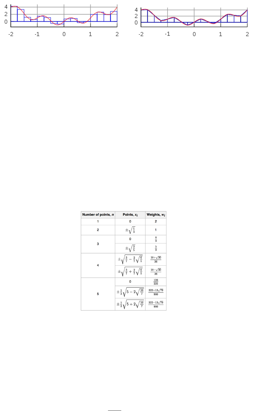
a) b)
The interval [−2,2] is broken into 16 sub-intervals. The blue lines correspond to the approximation of
the red curve by means of a) the midpoint rule, b) the trapezoidal rule.
There are several algorithms for numerical integration (also commonly called ’numerical quadrature’,
or simply ’quadrature’) . Interpolation with polynomials evaluated at equally spaced points in [a, b] yields
the NewtonCotes formulas, of which the rectangle rule and the trapezoidal rule are examples. If we allow
the intervals between interpolation points to vary, we find another group of quadrature formulas, such
as the Gauss(ian) quadrature formulas. A Gaussian quadrature rule is typically more accurate than a
NewtonCotes rule, which requires the same number of function evaluations, if the integrand is smooth
(i.e., if it is sufficiently differentiable).
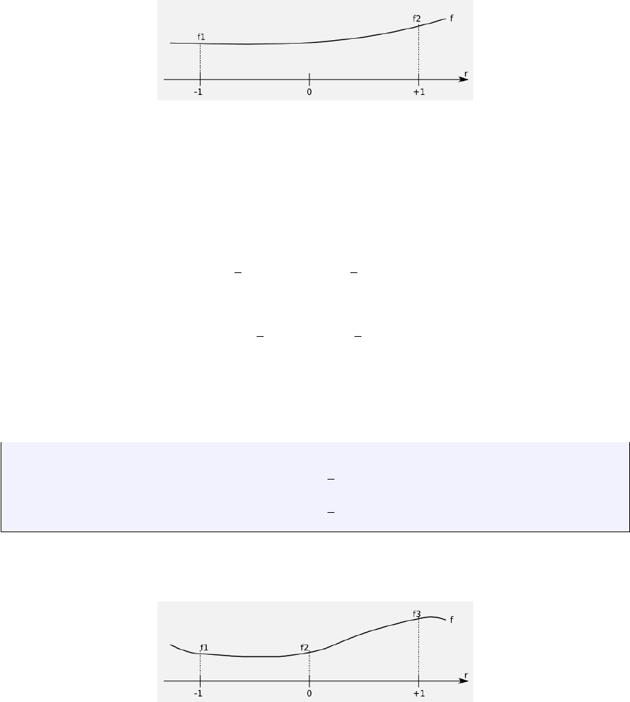
An n−point Gaussian quadrature rule, named after Carl Friedrich Gauss, is a quadrature rule con-
structed to yield an exact result for polynomials of degree 2n−1 or less by a suitable choice of the points
xiand weights wifor i= 1, . . . , n.
The domain of integration for such a rule is conventionally taken as [−1,1], so the rule is stated as
Z+1
−1
f(x)dx =
n
X
iq=1
wiqf(xiq)
In this formula the xiqcoordinate is the i-th root of the Legendre polynomial Pn(x).
It is important to note that a Gaussian quadrature will only produce good results if the function f(x)
is well approximated by a polynomial function within the range [−1,1]. As a consequence, the method
is not, for example, suitable for functions with singularities.
Gauss-Legendre points and their weights.
As shown in the above table, it can be shown that the weight values must fulfill the following condition:
X
iq
wiq= 2 (8)
and it is worth noting that all quadrature point coordinates are symmetrical around the origin.
Since most quadrature formula are only valid on a specific interval, we now must address the problem
of their use outside of such intervals. The solution turns out to be quite simple: one must carry out a
change of variables from the interval [a, b] to [−1,1].
We then consider the reduced coordinate r∈[−1,1] such that
r=2
b−a(x−a)−1
9

This relationship can be reversed such that when ris known, its equivalent coordinate x∈[a, b] can be
computed:
x=b−a
2(1 + r) + a
From this it follows that
dx =b−a
2dr
and then Zb
a
f(x)dx =b−a
2Z+1
−1
f(r)dr 'b−a
2
n
X
iq=1
wiqf(riq)
3.1.2 in 1D - examples
example 1 Since we know how to carry out any required change of variables, we choose for simplicity
a=−1, b= +1. Let us take for example f(x) = π. Then we can compute the integral of this function
over the interval [a, b] exactly:
I=Z+1
−1
f(x)dx =πZ+1
−1
dx = 2π
We can now use a Gauss-Legendre formula to compute this same integral:
Igq =Z+1
−1
f(x)dx =
nq
X
iq=1
wiqf(xiq) =
nq
X
iq=1
wiqπ=π
nq
X
iq=1
wiq
| {z }
=2
= 2π
where we have used the property of the weight values of Eq.(8). Since the actual number of points was
never specified, this result is valid for all quadrature rules.
example 2 Let us now take f(x) = mx +pand repeat the same exercise:
I=Z+1
−1
f(x)dx =Z+1
−1
(mx +p)dx = [1
2mx2+px]+1
−1= 2p
Igq =Z+1
−1
f(x)dx=
nq
X
iq=1
wiqf(xiq)=
nq
X
iq=1
wiq(mxiq+p)= m
nq
X
iq=1
wiqxiq
| {z }
=0
+p
nq
X
iq=1
wiq
| {z }
=2
= 2p
since the quadrature points are symmetric w.r.t. to zero on the x-axis. Once again the quadrature is able
to compute the exact value of this integral: this makes sense since an n-point rule exactly integrates a
2n−1 order polynomial such that a 1 point quadrature exactly integrates a first order polynomial like
the one above.
example 3 Let us now take f(x) = x2. We have
I=Z+1
−1
f(x)dx =Z+1
−1
x2dx = [1
3x3]+1
−1=2
3
and
Igq =Z+1
−1
f(x)dx=
nq
X
iq=1
wiqf(xiq)=
nq
X
iq=1
wiqx2
iq
•nq= 1: x(1)
iq = 0, wiq= 2. Igq = 0
•nq= 2: x(1)
q=−1/√3, x(2)
q= 1/√3, w(1)
q=w(2)
q= 1. Igq =2
3
•It also works ∀nq>2 !
10
3.1.3 in 2D/3D - theory
Let us now turn to a two-dimensional integral of the form
I=Z+1
−1Z+1
−1
f(x, y)dxdy
The equivalent Gaussian quadrature writes:
Igq '
nq
X
iq=1
nq
X
jq
f(xiq, yjq)wiqwjq
3.2 The mesh
3.3 A bit of FE terminology
We introduce here some terminology for efficient element descriptions [?]:
•For triangles/tetrahedra, the designation Pm×Pnmeans that each component of the velocity is
approximated by continuous piecewise complete Polynomials of degree mand pressure by continuous
piecewise complete Polynomials of degree n. For example P2×P1means
u∼a1+a2x+a3y+a4xy +a5x2+a6y2
with similar approximations for v, and
p∼b1+b2x+b3y
Both velocity and pressure are continuous across element boundaries, and each triangular element
contains 6 velocity nodes and three pressure nodes.
•For the same families, Pm×P−nis as above, except that pressure is approximated via piecewise
discontinuous polynomials of degree n. For instance, P2×P−1is the same as P2P1except that
pressure is now an independent linear function in each element and therefore discontinuous at
element boundaries.
•For quadrilaterals/hexahedra, the designation Qm×Qnmeans that each component of the velocity
is approximated by a continuous piecewise polynomial of degree min each direction on the quadri-
lateral and likewise for pressure, except that the polynomial is of degree n. For instance, Q2×Q1
means
u∼a1+a2x+a3y+a4xy +a5x2+a6y2+a7x2y+a8xy2+a9x2y2
and
p∼b1+b2x+b3y+b4xy
•For these same families, Qm×Q−nis as above, except that the pressure approximation is not
continuous at element boundaries.
•Again for the same families, Qm×P−nindicates the same velocity approximation with a pressure
approximation that is a discontinuous complete piecewise polynomial of degree n(not of degree n
in each direction !)
•The designation P+
mor Q+
mmeans that some sort of bubble function was added to the polynomial
approximation for the velocity. You may also find the term ’enriched element’ in the literature.
•Finally, for n= 0, we have piecewise-constant pressure, and we omit the minus sign for simplicity.
Another point which needs to be clarified is the use of so-called ’conforming elements’ (or ’non-
conforming elements’). Following again [?], conforming velocity elements are those for which the basis
functions for a subset of H1for the continuous problem (the first derivatives and their squares are
integrable in Ω). For instance, the rotated Q1×P0element of Rannacher and Turek (see section ??) is
such that the velocity is discontinous across element edges, so that the derivative does not exist there.
Another typical example of non-conforming element is the Crouzeix-Raviart element [?].
11
3.4 Elements and basis functions in 1D
3.4.1 Linear basis functions (Q1)
Let f(r) be a C1function on the interval [−1 : 1] with f(−1) = f1and f(1) = f2.
Let us assume that the function f(r) is to be approximated on [−1,1] by the first order polynomial
f(r) = a+br (9)
Then it must fulfill
f(r=−1) = a−b=f1
f(r= +1) = a+b=f2
This leads to
a=1
2(f1+f2)b=1
2(−f1+f2)
and then replacing a, b in Eq. (9) by the above values on gets
f(r) = 1
2(1 −r)f1+1
2(1 + r)f2
or
f(r) =
2
X
i=1
Ni(r)f1
with
N1(r) = 1
2(1 −r)
N2(r) = 1
2(1 + r) (10)
3.4.2 Quadratic basis functions (Q2)
Let f(r) be a C1function on the interval [−1 : 1] with f(−1) = f1,f(0) = f2and f(1) = f3.
Let us assume that the function f(r) is to be approximated on [−1,1] by the second order polynomial
f(r) = a+br +cr2(11)
Then it must fulfill
f(r=−1) = a−b+c=f1
f(r= 0) = a=f2
f(r= +1) = a+b+c=f3
12
This leads to
a=f2b=1
2(−f1 + f3) c=1
2(f1+f3−2f2)
and then replacing a, b, c in Eq. (11) by the above values on gets
f(r) = 1
2r(r−1)f1+ (1 −r2)f2+1
2r(r+ 1)f3
or,
f(r) =
3
X
i=1
Ni(r)fi
with
N1(r) = 1
2r(r−1)
N2(r) = (1 −r2)
N3(r) = 1
2r(r+ 1) (12)
3.4.3 Cubic basis functions (Q3)
The 1D basis polynomial is given by
f(r) = a+br +cr2+dr3
with the nodes at position -1,-1/3, +1/3 and +1.
f(−1) = a−b+c−d=f1
f(−1/3) = a−b
3+c
9−d
27 =f2
f(+1/3) = a−b
3+c
9−d
27 =f3
f(+1) = a+b+c+d=f4
Adding the first and fourth equation and the second and third, one arrives at
f1+f4= 2a+ 2c f2+f3= 2a+2c
9
and finally:
a=1
16 (−f1+ 9f2+ 9f3−f4)
c=9
16 (f1−f2−f3+f4)
Combining the original 4 equations in a different way yields
2b+ 2d=f4−f1
2b
3+2d
27 =f3−f2
so that
b=1
16 (f1−27f2+ 27f3−f4)
d=9
16 (−f1+ 3f2−3f3+f4)
Finally,
13
f(r) = a+b+cr2+dr3
=1
16(−1 + r+ 9r2−9r3)f1
+1
16(9 −27r−9r2+ 27r3)f2
+1
16(9 + 27r−9r2−27r3)f3
+1
16(−1−r+ 9r2+ 9r3)f4
=
4
X
i=1
Ni(r)fi
where
N1=1
16(−1 + r+ 9r2−9r3)
N2=1
16(9 −27r−9r2+ 27r3)
N3=1
16(9 + 27r−9r2−27r3)
N4=1
16(−1−r+ 9r2+ 9r3)
Verification:
•Let us assume f(r) = C, then
ˆ
f(r) = XNi(r)fi=X
i
NiC=CX
i
Ni=C
so that a constant function is exactly reproduced, as expected.
•Let us assume f(r) = r, then f1=−1, f2=−1/3, f3= 1/3 and f4= +1. We then have
ˆ
f(r) = XNi(r)fi
=−N1(r)−1
3N2(r) + 1
3N3(r) + N4(r)
= [−(−1 + r+ 9r2−9r3)
−1
3(9 −27r−9r2−27r3)
+1
3(9 + 27r−9r2+ 27r3)
+(−1−r+ 9r2+ 9r3)]/16
= [−r+ 9r+ 9r−r]/16 + ...0...
=r(13)
The basis functions derivative are given by
14
∂N1
∂r =1
16(1 + 18r−27r2)
∂N2
∂r =1
16(−27 −18r+ 81r2)
∂N3
∂r =1
16(+27 −18r−81r2)
∂N4
∂r =1
16(−1 + 18r+ 27r2)
Verification:
•Let us assume f(r) = C, then
∂ˆ
f
∂r =X
i
∂Ni
∂r fi
=CX
i
∂Ni
∂r
=C
16[(1 + 18r−27r2)
+(−27 −18r+ 81r2)
+(+27 −18r−81r2)
+(−1 + 18r+ 27r2)]
= 0
•Let us assume f(r) = r, then f1=−1, f2=−1/3, f3= 1/3 and f4= +1. We then have
∂ˆ
f
∂r =X
i
∂Ni
∂r fi
=1
16[−(1 + 18r−27r2)
−1
3(−27 −18r+ 81r2)
+1
3(+27 −18r−81r2)
+(−1 + 18r+ 27r2)]
=1
16[−2 + 18 + 54r2−54r2]
= 1
3.5 Elements and basis functions in 2D
Let us for a moment consider a single quadrilateral element in the xy-plane, as shown on the following
figure:
15

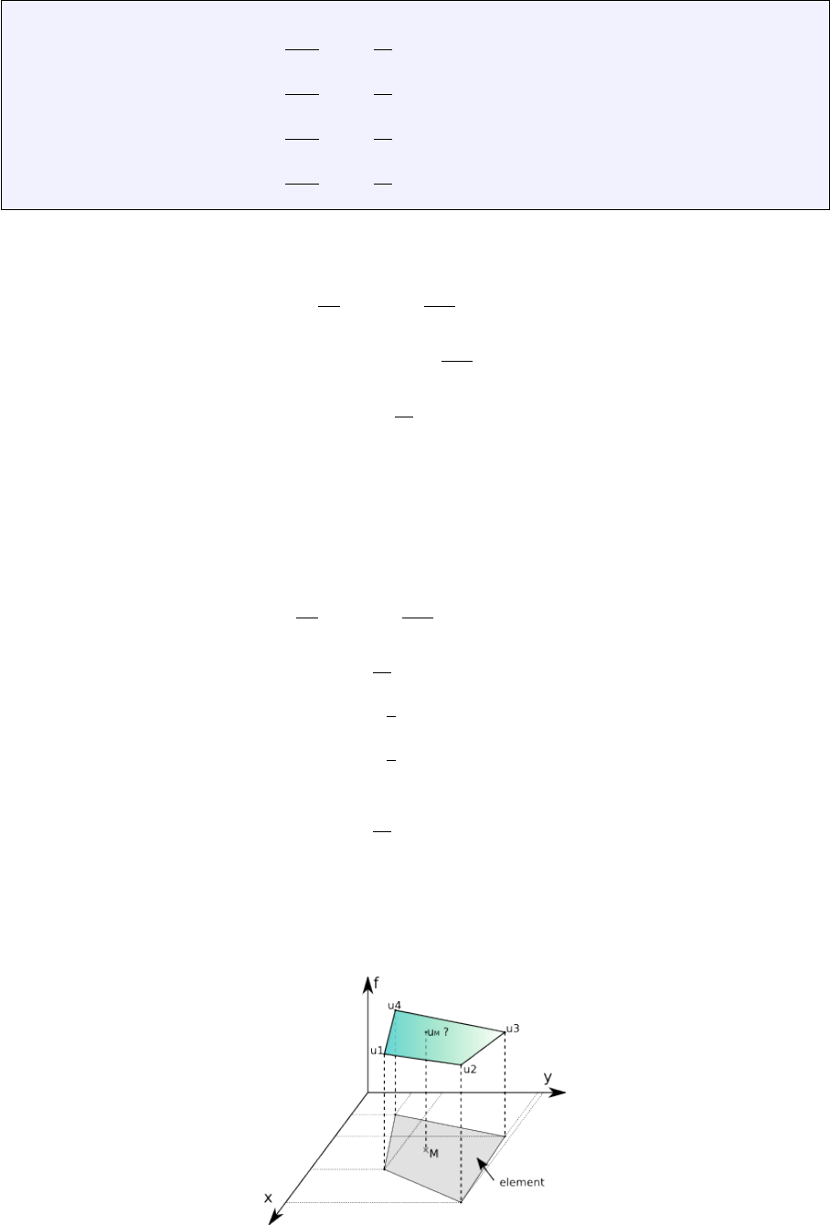
Let us assume that we know the values of a given field uat the vertices. For a given point Minside
the element in the plane, what is the value of the field uat this point? It makes sense to postulate that
uM=u(xM, yM) will be given by
uM=φ(u1, u2, u3, u4, xM, yM)
where φis a function to be determined. Although φis not unique, we can decide to express the value
uMas a weighed sum of the values at the vertices ui. One option could be to assign all four vertices the
same weight, say 1/4 so that uM= (u1+u2+u3+u4)/4, i.e. uMis simply given by the arithmetic mean
of the vertices values. This approach suffers from a major drawback as it does not use the location of
point Minside the element. For instance, when (xM, yM)→(x2, y2) we expect uM→u2.
In light of this, we could now assume that the weights would depend on the position of Min a
continuous fashion:
u(xM, yM) =
4
X
i=1
Ni(xM, yM)ui
where the Niare continous (”well behaved”) functions which have the property:
Ni(xj, yj) = δij
or, in other words:
N3(x1, y1) = 0 (14)
N3(x2, y2) = 0 (15)
N3(x3, y3) = 1 (16)
N3(x4, y4) = 0 (17)
The functions Niare commonly called basis functions.
Omitting the Msubscripts for any point inside the element, the velocity components uand vare
given by:
ˆu(x, y) =
4
X
i=1
Ni(x, y)ui(18)
ˆv(x, y) =
4
X
i=1
Ni(x, y)vi(19)
Rather interestingly, one can now easily compute velocity gradients (and therefore the strain rate tensor)
since we have assumed the basis functions to be ”well behaved” (in this case differentiable):
˙xx(x, y) = ∂u
∂x =
4
X
i=1
∂Ni
∂x ui(20)
˙yy(x, y) = ∂v
∂y =
4
X
i=1
∂Ni
∂y vi(21)
˙xy(x, y) = 1
2
∂u
∂y +1
2
∂v
∂x =1
2
4
X
i=1
∂Ni
∂y ui+1
2
4
X
i=1
∂Ni
∂x vi(22)
How we actually obtain the exact form of the basis functions is explained in the coming section.
3.5.1 Bilinear basis functions in 2D (Q1)
In this section, we place ourselves in the most favorables case, i.e. the element is a square defined by
−1< r < 1, −1< s < 1 in the Cartesian coordinates system (r, s):
16

3===========2
| | (r_0,s_0)=(-1,-1)
| | (r_1,s_1)=(+1,-1)
| | (r_2,s_2)=(+1,+1)
| | (r_3,s_3)=(-1,+1)
| |
0===========1
This element is commonly called the reference element. How we go from the (x, y) coordinate system
to the (r, s) once and vice versa will be dealt later on. For now, the basis functions in the above reference
element and in the reduced coordinates system (r, s) are given by:
N1(r, s)=0.25(1 −r)(1 −s)
N2(r, s)=0.25(1 + r)(1 −s)
N3(r, s)=0.25(1 + r)(1 + s)
N4(r, s)=0.25(1 −r)(1 + s)
The partial derivatives of these functions with respect to rans sautomatically follow:
∂N1
∂r (r, s) = −0.25(1 −s)∂N1
∂s (r, s) = −0.25(1 −r)
∂N2
∂r (r, s) = +0.25(1 −s)∂N2
∂s (r, s) = −0.25(1 + r)
∂N3
∂r (r, s) = +0.25(1 + s)∂N3
∂s (r, s) = +0.25(1 + r)
∂N4
∂r (r, s) = −0.25(1 + s)∂N4
∂s (r, s) = +0.25(1 −r)
Let us go back to Eq.(19). And let us assume that the function v(r, s) = Cso that vi=Cfor
i= 1,2,3,4. It then follows that
ˆv(r, s) =
4
X
i=1
Ni(r, s)vi=C
4
X
i=1
Ni(r, s) = C[N1(r, s) + N2(r, s) + N3(r, s) + N4(r, s)] = C
This is a very important property: if the vfunction used to assign values at the vertices is constant, then
the value of ˆvanywhere in the element is exactly C. If we now turn to the derivatives of vwith respect
to rand s:
∂ˆv
∂r (r, s) =
4
X
i=1
∂Ni
∂r (r, s)vi=C
4
X
i=1
∂Ni
∂r (r, s) = C[−0.25(1 −s)+0.25(1 −s)+0.25(1 + s)−0.25(1 + s)] = 0
∂ˆv
∂s (r, s) =
4
X
i=1
∂Ni
∂s (r, s)vi=C
4
X
i=1
∂Ni
∂s (r, s) = C[−0.25(1 −r)−0.25(1 + r)+0.25(1 + r)+0.25(1 −r)] = 0
We reassuringly find that the derivative of a constant field anywhere in the element is exactly zero.
17

If we now choose v(r, s) = ar +bs with aand btwo constant scalars, we find:
ˆv(r, s) =
4
X
i=1
Ni(r, s)vi(23)
=
4
X
i=1
Ni(r, s)(ari+bsi) (24)
=a
4
X
i=1
Ni(r, s)ri
| {z }
r
+b
4
X
i=1
Ni(r, s)si
| {z }
s
(25)
=a[0.25(1 −r)(1 −s)(−1) + 0.25(1 + r)(1 −s)(+1) + 0.25(1 + r)(1 + s)(+1) + 0.25(1 −r)(1 + s)(−1)]
+b[0.25(1 −r)(1 −s)(−1) + 0.25(1 + r)(1 −s)(−1) + 0.25(1 + r)(1 + s)(+1) + 0.25(1 −r)(1 + s)(+1)]
=a[−0.25(1 −r)(1 −s)+0.25(1 + r)(1 −s)+0.25(1 + r)(1 + s)−0.25(1 −r)(1 + s)]
+b[−0.25(1 −r)(1 −s)−0.25(1 + r)(1 −s)+0.25(1 + r)(1 + s)+0.25(1 −r)(1 + s)]
=ar +bs (26)
verify above eq. This set of bilinear shape functions is therefore capable of exactly representing a bilinear
field. The derivatives are:
∂ˆv
∂r (r, s) =
4
X
i=1
∂Ni
∂r (r, s)vi(27)
=a
4
X
i=1
∂Ni
∂r (r, s)ri+b
4
X
i=1
∂Ni
∂r (r, s)si(28)
=a[−0.25(1 −s)(−1) + 0.25(1 −s)(+1) + 0.25(1 + s)(+1) −0.25(1 + s)(−1)]
+b[−0.25(1 −s)(−1) + 0.25(1 −s)(−1) + 0.25(1 + s)(+1) −0.25(1 + s)(+1)]
=a
4[(1 −s) + (1 −s) + (1 + s) + (1 + s)]
+b
4[(1 −s)−(1 −s) + (1 + s)−(1 + s)]
=a(29)
Here again, we find that the derivative of the bilinear field inside the element is exact: ∂ˆv
∂r =∂v
∂r .
However, following the same methodology as above, one can easily prove that this is no more true
for polynomials of degree strivtly higher than 1. This fact has serious consequences: if the solution to
the problem at hand is for instance a parabola, the Q1shape functions cannot represent the solution
properly, but only by approximating the parabola in each element by a line. As we will see later, Q2
basis functions can remedy this problem by containing themselves quadratic terms.
3.5.2 Biquadratic basis functions in 2D (Q2)
Inside an element the local numbering of the nodes is as follows:
3=====6=====2
| | | (r_0,s_0)=(-1,-1) (r_4,s_4)=( 0,-1)
| | | (r_1,s_1)=(+1,-1) (r_5,s_5)=(+1, 0)
7=====8=====5 (r_2,s_2)=(+1,+1) (r_6,s_6)=( 0,+1)
| | | (r_3,s_3)=(-1,+1) (r_7,s_7)=(-1, 0)
| | | (r_8,s_8)=( 0, 0)
0=====4=====1
The velocity shape functions are then given by:
18
N0(r, s) = 1
2r(r−1)1
2s(s−1)
N1(r, s) = 1
2r(r+ 1)1
2s(s−1)
N2(r, s) = 1
2r(r+ 1)1
2s(s+ 1)
N3(r, s) = 1
2r(r−1)1
2s(s+ 1)
N4(r, s) = (1 −r2)1
2s(s−1)
N5(r, s) = 1
2r(r+ 1)(1 −s2)
N6(r, s) = (1 −r2)1
2s(s+ 1)
N7(r, s) = 1
2r(r−1)(1 −s2)
N8(r, s) = (1 −r2)(1 −s2)
and their derivatives by:
∂N0
∂r =1
2(2r−1)1
2s(s−1) ∂N0
∂s =1
2r(r−1)1
2(2s−1)
∂N1
∂r =1
2(2r+ 1)1
2s(s−1) ∂N1
∂s =1
2r(r+ 1)1
2(2s−1)
∂N2
∂r =1
2(2r+ 1)1
2s(s+ 1) ∂N2
∂s =1
2r(r+ 1)1
2(2s+ 1)
∂N3
∂r =1
2(2r−1)1
2s(s+ 1) ∂N3
∂s =1
2r(r−1)1
2(2s+ 1)
∂N4
∂r = (−2r)1
2s(s−1) ∂N4
∂s = (1 −r2)1
2(2s−1)
∂N5
∂r =1
2(2r+ 1)(1 −s2)∂N5
∂s =1
2r(r+ 1)(−2s)
∂N6
∂r = (−2r)1
2s(s+ 1) ∂N6
∂s = (1 −r2)1
2(2s+ 1)
∂N7
∂r =1
2(2r−1)(1 −s2)∂N7
∂s =1
2r(r−1)(−2s)
∂N8
∂r = (−2r)(1 −s2)∂N8
∂s = (1 −r2)(−2s)
3.5.3 Bicubic basis functions in 2D (Q3)
Inside an element the local numbering of the nodes is as follows:
12===13===14===15 (r,s)_{00}=(-1,-1) (r,s)_{08}=(-1,+1/3)
|| || || || (r,s)_{01}=(-1/3,-1) (r,s)_{09}=(-1/3,+1/3)
08===09===10===11 (r,s)_{02}=(+1/3,-1) (r,s)_{10}=(+1/3,+1/3)
|| || || || (r,s)_{03}=(+1,-1) (r,s)_{11}=(+1,+1/3)
04===05===06===07 (r,s)_{04}=(-1,-1/3) (r,s)_{12}=(-1,+1)
|| || || || (r,s)_{05}=(-1/3,-1/3) (r,s)_{13}=(-1/3,+1)
00===01===02===03 (r,s)_{06}=(+1/3,-1/3) (r,s)_{14}=(+1/3,+1)
(r,s)_{07}=(+1,-1/3) (r,s)_{15}=(+1,+1)
19

The velocity shape functions are given by:
N1(r)=(−1 + r+ 9r2−9r3)/16 N1(t)=(−1 + t+ 9t2−9t3)/16
N2(r) = (+9 −27r−9r2+ 27r3)/16 N2(t) = (+9 −27t−9t2+ 27t3)/16
N3(r) = (+9 + 27r−9r2−27r3)/16 N3(t) = (+9 + 27t−9t2−27t3)/16
N4(r)=(−1−r+ 9r2+ 9r3)/16 N4(t)=(−1−t+ 9t2+ 9t3)/16
N01(r, s) = N1(r)N1(s)=(−1 + r+ 9r2−9r3)/16 ∗(−1 + t+ 9s2−9s3)/16
N02(r, s) = N2(r)N1(s) = (+9 −27r−9r2+ 27r3)/16 ∗(−1 + t+ 9s2−9s3)/16
N03(r, s) = N3(r)N1(s) = (+9 + 27r−9r2−27r3)/16 ∗(−1 + t+ 9s2−9s3)/16
N04(r, s) = N4(r)N1(s)=(−1−r+ 9r2+ 9r3)/16 ∗(−1 + t+ 9s2−9s3)/16
N05(r, s) = N1(r)N2(s) = (−1 + r+ 9r2−9r3)/16 ∗(9 −27s−9s2+ 27s3)/16
N06(r, s) = N2(r)N2(s) = (+9 −27r−9r2+ 27r3)/16 ∗(9 −27s−9s2+ 27s3)/16
N07(r, s) = N3(r)N2(s) = (+9 + 27r−9r2−27r3)/16 ∗(9 −27s−9s2+ 27s3)/16
N08(r, s) = N4(r)N2(s)=(−1−r+ 9r2+ 9r3)/16 ∗(9 −27s−9s2+ 27s3)/16
N09(r, s) = N1(r)N3(s) = (30)
N10(r, s) = N2(r)N3(s) = (31)
N11(r, s) = N3(r)N3(s) = (32)
N12(r, s) = N4(r)N3(s) = (33)
N13(r, s) = N1(r)N4(s) = (34)
N14(r, s) = N2(r)N4(s) = (35)
N15(r, s) = N3(r)N4(s) = (36)
N16(r, s) = N4(r)N4(s) = (37)
20

4 Solving the Stokes equations with the FEM
In the case of an incompressible flow, we have seen that the continuity (mass conservation) equation takes
the simple form ∇·v= 0. In other word flow takes place under the constraint that the divergence of its
velocity field is exactly zero eveywhere (solenoidal constraint), i.e. it is divergence free.
We see that the pressure in the momentum equation is then a degree of freedom which is needed to
satisfy the incompressibilty constraint (and it is not related to any constitutive equation) [?]. In other
words the pressure is acting as a Lagrange multiplier of the incompressibility constraint.
Various approaches have been proposed in the literature to deal with the incompressibility constraint
but we will only focus on the penalty method (section 4.2) and the so-called mixed finite element method
4.3.
4.1 strong and weak forms
The strong form consists of the governing equation and the boundary conditions, i.e. the mass, momentum
and energy conservation equations supplemented with Dirichlet and/or Neumann boundary conditions
on (parts of) the boundary.
To develop the finite element formulation, the partial differential equations must be restated in an
integral form called the weak form. In essence the PDEs are first multiplied by an arbitrary function and
integrated over the domain.
4.2 The penalty approach
In order to impose the incompressibility constraint, two widely used procedures are available, namely
the Lagrange multiplier method and the penalty method [?,?]. The latter is implemented in elefant,
which allows for the elimination of the pressure variable from the momentum equation (resulting in a
reduction of the matrix size).
Mathematical details on the origin and validity of the penalty approach applied to the Stokes problem
can for instance be found in [?], [?] or [?].
The penalty formulation of the mass conservation equation is based on a relaxation of the incompress-
ibility constraint and writes
∇·v+p
λ= 0 (38)
where λis the penalty parameter, that can be interpreted (and has the same dimension) as a bulk
viscosity. It is equivalent to say that the material is weakly compressible. It can be shown that if one
chooses λto be a sufficiently large number, the continuity equation ∇·v= 0 will be approximately
satisfied in the finite element solution. The value of λis often recommended to be 6 to 7 orders of
magnitude larger than the shear viscosity [?,?].
Equation (38) can be used to eliminate the pressure in Eq. (??) so that the mass and momentum
conservation equations fuse to become :
∇·(2η˙ε(v)) + λ∇(∇·v) = ρg= 0 (39)
[?] have established the equivalence for incompressible problems between the reduced integration of
the penalty term and a mixed Finite Element approach if the pressure nodes coincide with the integration
points of the reduced rule.
In the end, the elimination of the pressure unknown in the Stokes equations replaces the original
saddle-point Stokes problem [?] by an elliptical problem, which leads to a symmetric positive definite
(SPD) FEM matrix. This is the major benefit of the penalized approach over the full indefinite solver
with the velocity-pressure variables. Indeed, the SPD character of the matrix lends itself to efficient
solving stragegies and is less memory-demanding since it is sufficient to store only the upper half of the
matrix including the diagonal [?] . list codes which
use this ap-
proach
list codes which
use this ap-
proach
The stress tensor σis symmetric (i.e. σij =σji). For simplicity I will now focus on a Stokes flow in
two dimensions.
21

Since the penalty formulation is only valid for incompressible flows, then ˙
=˙
dso that the dsuper-
script is ommitted in what follows. The stress tensor can also be cast in vector format:
σxx
σyy
σxy
=
−p
−p
0
+ 2η
˙xx
˙yy
˙xy
=λ
˙xx + ˙yy
˙xx + ˙yy
0
+ 2η
˙xx
˙yy
˙xy
=
λ
110
110
000
| {z }
K
+η
200
020
001
| {z }
C
·
∂u
∂x
∂v
∂y
∂u
∂y +∂v
∂x
Remember that
∂u
∂x =
4
X
i=1
∂Ni
∂x ui
∂v
∂y =
4
X
i=1
∂Ni
∂y vi
∂u
∂y +∂v
∂x =
4
X
i=1
∂Ni
∂y ui+
4
X
i=1
∂Ni
∂x vi
so that
∂u
∂x
∂v
∂y
∂u
∂y +∂v
∂x
=
∂N1
∂x 0∂N2
∂x 0∂N3
∂x 0∂N4
∂x 0
0∂N1
∂y 0∂N2
∂y 0∂N3
∂y 0∂N4
∂y
∂N1
∂y
∂N1
∂x
∂N2
∂y
∂N2
∂x
∂N3
∂y
∂N3
∂x
∂N3
∂y
∂N4
∂x
| {z }
B
·
u1
v1
u2
v2
u3
v3
u4
v4
| {z }
V
Finally,
σ =
σxx
σyy
σxy
= (λK+ηC)·B·V
We will now establish the weak form of the momentum conservation equation. We start again from
∇·σ+b=0
For the Ni’s ’regular enough’, we can write:
ZΩe
Ni∇·σdΩ + ZΩe
NibdΩ=0
We can integrate by parts and drop the surface term1:
ZΩe
∇Ni·σdΩ = ZΩe
NibdΩ
or,
ZΩe
∂Ni
∂x 0∂Ni
∂y
0∂Ni
∂y
∂Ni
∂x
·
σxx
σyy
σxy
dΩ = ZΩe
NibdΩ
1We will come back to this at a later stage
22
Let i= 1,2,3,4 and stack the resulting four equations on top of one another.
ZΩe
∂N1
∂x 0∂N1
∂y
0∂N1
∂y
∂N1
∂x
·
σxx
σyy
σxy
dΩ = ZΩe
N1bx
bydΩ (40)
ZΩe
∂N2
∂x 0∂N2
∂y
0∂N2
∂y
∂N2
∂x
·
σxx
σyy
σxy
dΩ = ZΩe
Nibx
bydΩ (41)
ZΩe
∂N3
∂x 0∂N3
∂y
0∂N3
∂y
∂N3
∂x
·
σxx
σyy
σxy
dΩ = ZΩe
N3bx
bydΩ (42)
ZΩe
∂N4
∂x 0∂N4
∂y
0∂N4
∂y
∂N4
∂x
·
σxx
σyy
σxy
dΩ = ZΩe
N4bx
bydΩ (43)
We easily recognize BTinside the integrals! Let us define
NT
b= (N1bx, N1by, ...N4bx, N4by)
then we can write
ZΩe
BT·
σxx
σyy
σxy
dΩ = ZΩe
NbdΩ
and finally: ZΩe
BT·[λK+ηC]·B·VdΩ = ZΩe
NbdΩ
Since Vcontains the velocities at the corners, it does not depend on the xor ycoordinates so it can be
taking outside of the integral:
ZΩe
BT·[λK+ηC]·BdΩ
| {z }
Ael(8×8)
·V
|{z}
(8x1)
=ZΩe
NbdΩ
| {z }
Bel(8×1)
or,
ZΩe
λBT·K·BdΩ
| {z }
Aλ
el(8×8)
+ZΩe
ηBT·C·BdΩ
| {z }
Aη
el(8×8)
·V
|{z}
(8x1)
=ZΩe
NbdΩ
| {z }
Bel(8×1)
INTEGRATION - MAPPING
reduced integration [?]
1. partition domain Ω into elements Ωe,e= 1, ...nel.
2. loop over elements and for each element compute Ael,Bel
3. a node belongs to several elements
→need to assemble Ael and Bel in A,B
4. apply boundary conditions
5. solve system: x=A−1·B
6. visualise/analyse x
23
4.3 The mixed FEM
24
5 Solving the elastic equations with the FEM
25
6 Additional techniques
6.1 Picard and Newton
6.2 The SUPG formulation for the energy equation
6.3 Tracking materials and/or interfaces
6.4 Dealing with a free surface
6.5 Convergence criterion for nonlinear iterations
6.6 Static condensation
26

6.7 The method of manufactured solutions
The method of manufactured solutions is a relatively simple way of carrying out code verification. In
essence, one postulates a solution for the PDE at hand (as well as the proper boundary conditions),
inserts it in the PDE and computes the corresponding source term. The same source term and boundary
conditions will then be used in a numerical simulation so that the computed solution can be compared
with the (postulated) true analytical solution.
Examples of this approach are to be found in [?,?,?].
python codes/fieldstone
python codes/fieldstone saddlepoint
python codes/fieldstone saddlepoint q2q1
python codes/fieldstone saddlepoint q3q2
python codes/fieldstone burstedde
6.7.1 Analytical benchmark I
Taken from [?].
u(x, y) = x2(1 −x)2(2y−6y2+ 4y3)
v(x, y) = −y2(1 −y)2(2x−6x2+ 4x3)
p(x, y) = x(1 −x)−1/6
Note that the pressure obeys RΩp dΩ=0
The corresponding components of the body force bare prescribed as
bx= (12 −24y)x4+ (−24 + 48y)x3+ (−48y+ 72y2−48y3+ 12)x2
+(−2 + 24y−72y2+ 48y3)x+ 1 −4y+ 12y2−8y3
by= (8 −48y+ 48y2)x3+ (−12 + 72y−72y2)x2
+(4 −24y+ 48y2−48y3+ 24y4)x−12y2+ 24y3−12y4
With this prescribed body force, the exact solution is
6.7.2 Analytical benchmark II
Taken from [?]
u(x, y) = x+x2−2xy +x3−3xy2+x2y(44)
v(x, y) = −y−2xy +y2−3x2y+y3−xy2(45)
p(x, y) = xy +x+y+x3y2−4/3 (46)
Note that the pressure obeys RΩp dΩ=0
bx=−(1 + y−3x2y2) (47)
by=−(1 −3x−2x3y) (48)
27

6.8 Assigning values to quadrature points
As we have seen in Section ??, the building of the elemental matrix and rhs requires (at least) to assign
a density and viscosity value to each quadrature point inside the element. Depending on the type of
modelling, this task can prove more complex than one might expect and have large consequences on the
solution accuracy.
Here are several options:
•The simplest way (which is often used for benchmarks) consists in computing the ’real’ coordinates
(xq, yq, zq) of a given quadrature point based on its reduced coordinates (rq, sq, tq), and passing these
coordinates to a function which returns density and/or viscosity at this location. For instance, for
the Stokes sphere:
def rho(x,y):
if (x-.5)**2+(y-0.5)**2<0.123**2:
val=2.
else:
val=1.
return val
def mu(x,y):
if (x-.5)**2+(y-0.5)**2<0.123**2:
val=1.e2
else:
val=1.
return val
This is very simple, but it has been shown to potentially be problematic. In essence, it can introduce
very large contrasts inside a single element and perturb the quadrature. Please read section 3.3
of [?] and/or have a look at the section titled ”Averaging material properties” in the ASPECT
manual.
•another similar approach consists in assigning a density and viscosity value to the nodes of the FE
mesh first, and then using these nodal values to assign values to the quadrature points. Very often
,and quite logically, the shape functions are used to this effect. Indeed we have seen before that for
any point (r, s, t) inside an element we have
fh(r, s, t) =
m
X
i
fiNi(r, s, t)
where the fiare the nodal values and the Nithe corresponding basis functions.
In the case of linear elements (Q1basis functions), this is straightforward. In fact, the basis functions
Nican be seen as moving weights: the closer the point is to a node, the higher the weight (basis
function value).
However, this is quite another story for quadratic elements (Q2basis functions). In order to
illustrate the problem, let us consider a 1D problem. The basis functions are
N1(r) = 1
2r(r−1) N2(r)=1−r2N3(r) = 1
2r(r+ 1)
Let us further assign: ρ1=ρ2= 0 and ρ3= 1. Then
ρh(r) =
m
X
i
ρiNi(r) = N3(r)
There lies the core of the problem: the N3(r) basis function is negative for r∈[−1,0]. This means
that the quadrature point in this interval will be assigned a negative density, which is nonsensical
and numerically problematic!
use 2X Q1. write about it !
28

The above methods work fine as long as the domain contains a single material. As soon as there are
multiple fluids in the domain a special technique is needed to track either the fluids themselves or their
interfaces. Let us start with markers. We are then confronted to the infernal trio (a menage a trois?)
which is present for each element, composed of its nodes, its markers and its quadrature points.
Each marker carries the material information (density and viscosity). This information must ul-
timately be projected onto the quadrature points. Two main options are possible: an algorithm is
designed and projects the marker-based fields onto the quadrature points directly or the marker fields
are first projected onto the FE nodes and then onto the quadrature points using the techniques above.
————————–
At a given time, every element econtains nemarkers. During the FE matrix building process, viscosity
and density values are needed at the quadrature points. One therefore needs to project the values carried
by the markers at these locations. Several approaches are currently in use in the community and the
topic has been investigated by [?] and [?] for instance.
elefant adopts a simple approach: viscosity and density are considered to be elemental values, i.e.
all the markers within a given element contribute to assign a unique constant density and viscosity value
to the element by means of an averaging scheme.
While it is common in the literature to treat the so-called arithmetic, geometric and harmonic means
as separate averagings, I hereby wish to introduce the notion of generalised mean, which is a family of
functions for aggregating sets of numbers that include as special cases the arithmetic, geometric and
harmonic means.
If pis a non-zero real number, we can define the generalised mean (or power mean) with exponent p
of the positive real numbers a1, ... anas:
Mp(a1, ...an) = 1
n
n
X
i=1
ap
i!1/p
(49)
and it is trivial to verify that we then have the special cases:
M−∞ = lim
p→−∞ Mp= min(a1, ...an) (minimum) (50)
M−1=n
1
a1+1
a2+··· +1
an
(harm.avrg.) (51)
M0= lim
p→0Mp=n
Y
i=1
ai1/n
(geom.avrg.) (52)
M+1 =1
n
n
X
i=1
ai(arithm.avrg.) (53)
M+2 =v
u
u
t1
n
n
X
i=1
a2
i(root mean square) (54)
M+∞= lim
p→+∞Mp= max(a1, ...an) (maximum) (55)
Note that the proofs of the limit convergence are given in [?].
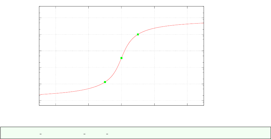
An interesting property of the generalised mean is as follows: for two real values pand q, if p < q
then Mp≤Mq. This property has for instance been illustrated in Fig. 20 of [?].
One can then for instance look at the generalised mean of a randomly generated set of 1000 viscosity
values within 1018P a.s and 1023P a.s for −5≤p≤5. Results are shown in the figure hereunder and the
arithmetic, geometric and harmonic values are indicated too. The function Mpassumes an arctangent-
like shape: very low values of p will ultimately yield the minimum viscosity in the array while very high
values will yield its maximum. In between, the transition is smooth and occurs essentially for |p| ≤ 5.
29
1e+18
1e+19
1e+20
1e+21
1e+22
1e+23
-4 -2 0 2 4
M(p)
p
geom.
arithm.
harm.
python codes/fieldstone markers avrg
30
6.9 Matrix (Sparse) storage
The FE matrix is the result of the assembly process of all elemental matrices. Its size can become quite
large when the resolution is being increased (from thousands of lines/columns to tens of millions).
One important property of the matrix is its sparsity. Typically less than 1% of the matrix terms is
not zero and this means that the matrix storage can and should be optimised. Clever storage formats
were designed early on since the amount of RAM memory in computers was the limiting factor 3 or 4
decades ago. [?]
There are several standard formats:
•compressed sparse row (CSR) format
•compressed sparse column format (CSC)
•the Coordinate Format (COO)
•Skyline Storage Format
•...
I focus on the CSR format in what follows.
6.9.1 2D domain - One degree of freedom per node
Let us consider again the 3 ×2 element grid which counts 12 nodes.
8=======9======10======11
||||
| (3) | (4) | (5) |
||||
4=======5=======6=======7
||||
| (0) | (1) | (2) |
||||
0=======1=======2=======3
In the case there is only a single degree of freedom per node, the assembled FEM matrix will look
like this:
X X X X
X X X X X X
X X X X X X
X X X X
X X X X X X
X X X X X X X X X
X X X X X X X X X
X X X X X X
X X X X
X X X X X X
X X X X X X
X X X X
where the Xstand for non-zero terms. This matrix structure stems from the fact that
•node 0 sees nodes 0,1,4,5
•node 1 sees nodes 0,1,2,4,5,6
•node 2 sees nodes 1,2,3,5,6,7
•...
31

•node 5 sees nodes 0,1,2,4,5,6,8,9,10
•...
•node 10 sees nodes 5,6,7,9,10,11
•node 11 sees nodes 6,7,10,11
In light thereof, we have
•4 corner nodes which have 4 neighbours (counting themselves)
•2(nnx-2) nodes which have 6 neighbours
•2(nny-2) nodes which have 6 neighbours
•(nnx-2)×(nny-2) nodes which have 9 neighbours
In total, the number of non-zero terms in the matrix is then:
NZ = 4 ×4+4×6+2×6+2×9 = 70
In general, we would then have:
NZ = 4 ×4 + [2(nnx −2) + 2(nny −2)] ×6+(nnx −2)(nny −2) ×9
Let us temporarily assume nnx =nny =n. Then the matrix size (total number of unknowns) is
N=n2and
NZ = 16 + 24(n−2) + 9(n−2)2
A full matrix array would contain N2=n4terms. The ratio of NZ (the actual number of reals to store)
to the full matrix size (the number of reals a full matrix contains) is then
R=16 + 24(n−2) + 9(n−2)2
n4
It is then obvious that when nis large enough R∼1/n2.
CSR stores the nonzeros of the matrix row by row, in a single indexed array A of double precision
numbers. Another array COLIND contains the column index of each corresponding entry in the A array.
A third integer array RWPTR contains pointers to the beginning of each row, which an additional pointer
to the first index following the nonzeros of the matrix A. A and COLIND have length NZ and RWPTR
has length N+1.
In the case of the here-above matrix, the arrays COLIND and RWPTR will look like:
COLIND = (0,1,4,5,0,1,2,4,5,6,1,2,3,5,6,7, ..., 6,7,10,11)
RW P T R = (0,4,10,16, ...)
6.9.2 2D domain - Two degrees of freedom per node
When there are now two degrees of freedom per node, such as in the case of the Stokes equation in
two-dimensions, the size of the Kmatrix is given by
NfemV=nnp∗ndofV
In the case of the small grid above, we have NfemV=24. Elemental matrices are now 8 ×8 in size.
We still have
•4 corner nodes which have 4 ,neighbours,
•2(nnx-2) nodes which have 6 neighbours
•2(nny-2) nodes which have 6 neighbours
32

•(nnx-2)x(nny-2) nodes which have 9 neighbours,
but now each degree of freedom from a node sees the other two degrees of freedom of another node too.
In that case, the number of nonzeros has been multiplied by four and the assembled FEM matrix looks
like:
X X X X X X X X
X X X X X X X X
X X X X X X X X X X X X
X X X X X X X X X X X X
X X X X X X X X X X X X
X X X X X X X X X X X X
X X X X X X X X
X X X X X X X X
X X X X X X X X X X X X
X X X X X X X X X X X X
X X X X X X X X X X X X X X X X X X
X X X X X X X X X X X X X X X X X X
X X X X X X X X X X X X X X X X X X
X X X X X X X X X X X X X X X X X X
X X X X X X X X X X X X
X X X X X X X X X X X X
X X X X X X X X
X X X X X X X X
X X X X X X X X X X X X
X X X X X X X X X X X X
X X X X X X X X X X X X
X X X X X X X X X X X X
X X X X X X X X
X X X X X X X X
Note that the degrees of freedom are organised as follows:
(u0, v0, u1, v1, u2, v2, ...u11, v11)
In general, we would then have:
NZ = 4 [4 ×4 + [2(nnx −2) + 2(nny −2)] ×6+(nnx −2)(nny −2) ×9]
and in the case of the small grid, the number of non-zero terms in the matrix is then:
NZ = 4 [4 ×4+4×6+2×6+2×9] = 280
In the case of the here-above matrix, the arrays COLIND and RWPTR will look like:
COLIND = (0,1,2,3,8,9,10,11,0,1,2,3,8,9,10,11, ...)
RW P T R = (0,8,16,28, ...)
6.9.3 in fieldstone
The majority of the codes have the FE matrix being a full array
a mat = np . z e r os ( ( Nfem , Nfem) , dtype=np . f l o a t 6 4 )
and it is converted to CSR format on the fly in the solve phase:
s o l = s p s . l i n a l g . s p s o l v e ( s ps . c s r m a t r i x ( a mat ) , r hs )
Note that linked list storages can be used (lil matrix). Substantial memory savings but much longer
compute times.
33
6.10 Mesh generation
Before basis functions can be defined and PDEs can be discretised and solved we must first tesselate the
domain with polygons, e.g. triangles and quadrilaterals in 2D, tetrahedra, prisms and hexahedra in 3D.
When the domain is itself simple (e.g. a rectangle, a sphere, ...) the mesh (or grid) can be (more or
less) easily produced and the connectivity array filled with straightforward algorithms [?]. However, real
life applications can involve etremely complex geometries (e.g. a bridge, a human spine, a car chassis and
body, etc ...) and dedicated algorithms/softwares must be used (see [?,?,?]).
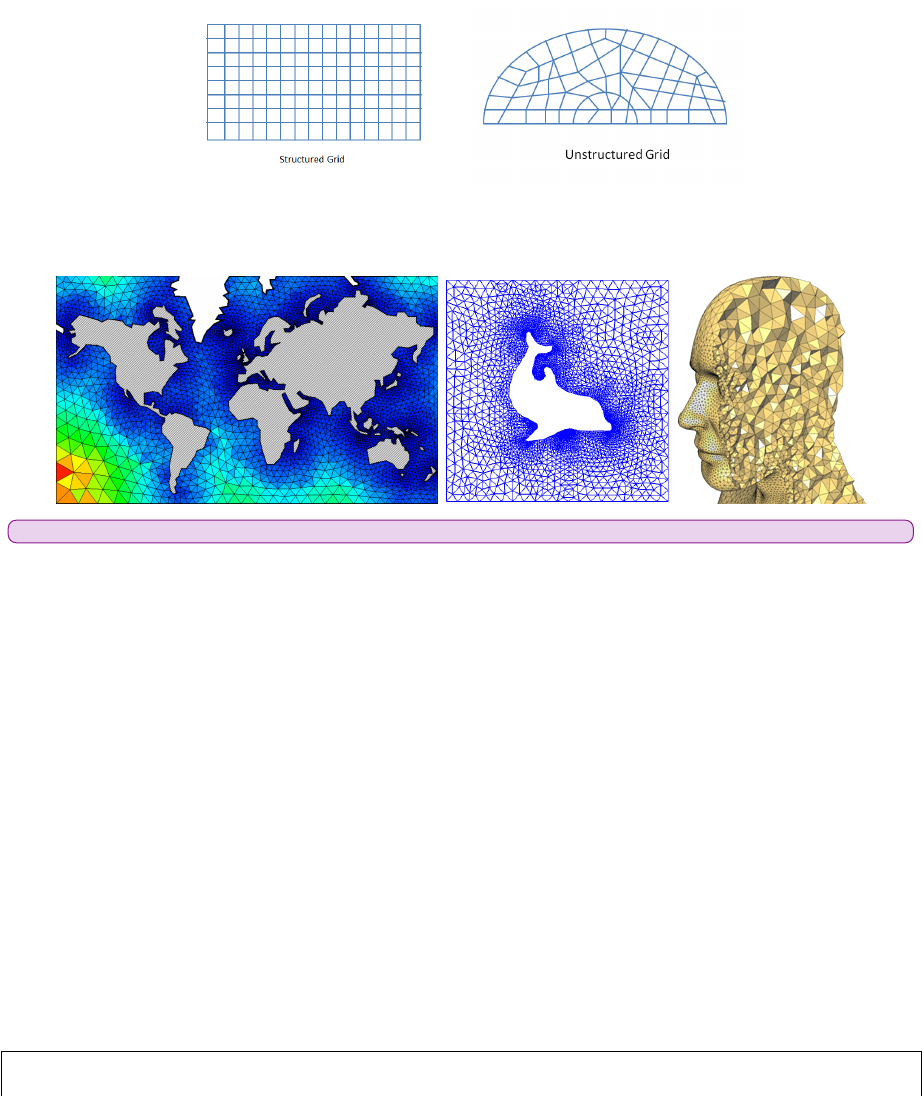
We usually distinguish between two broad classes of grids: structured grids (with a regular connec-
tivity) and unstructured grids (with an irregular connectivity).
On the following figure are shown various triangle- tetrahedron-based meshes. These are obviously
better suited for simulations of complex geometries:
add more examples coming from geo
Let us now focus on the case of a rectangular computational domain of size Lx ×Ly with a regular
mesh composed of nelx×nely=nel quadrilaterals. There are then nnx×nny=nnp grid points. The
elements are of size hx×hy with hx=Lx/nelx.
We have no reason to come up with an irregular/ilogical node numbering so we can number nodes
row by row or column by column as shown on the example hereunder of a 3×2 grid:
8=======9======10======11 2=======5=======8======11
||||||||
| (3) | (4) | (5) | | (1) | (3) | (5) |
||||||||
4=======5=======6=======7 1=======4=======7======10
||||||||
| (0) | (1) | (2) | | (0) | (2) | (4) |
||||||||
0=======1=======2=======3 0=======3=======6=======9
"row by row" "column by column"
The numbering of the elements themselves could be done in a somewhat chaotic way but we follow
the numbering of the nodes for simplicity. The row by row option is the adopted one in fieldstoneand
the coordinates of the points are computed as follows:
x = np . empty (nnp , dtype=np . f l o a t 6 4 )
y = np . empty (nnp , dtype=np . f l o a t 6 4 )
34

co u nt er = 0
f o r jin range ( 0 , nny ) :
f o r ii n r an ge ( 0 , nnx ) :
x [ c ou nt er ]= i ∗hx
y [ c ou nt er ]= j ∗hy
co u nt er += 1
The inner loop has iranging from 0to nnx-1 first for j=0, 1, ... up to nny-1 which indeed corresponds
to the row by row numbering.
We now turn to the connectivity. As mentioned before, this is a structured mesh so that the so-called
connectivity array, named icon in our case, can be filled easily. For each element we need to store the
node identities of its vertices. Since there are nel elements and m=4 corners, this is a m×nel array. The
algorithm goes as follows:
i c o n =np . z e r o s ( (m, n e l ) , d type=np . i n t 1 6 )
co u nt er = 0
f o r jin range ( 0 , n e l y ) :
f o r ii n r an ge ( 0 , n e l x ) :
i c o n [ 0 , c o u n t er ] = i + j ∗nnx
i c o n [ 1 , c o u n t er ] = i + 1 + j ∗nnx
i c o n [ 2 , c o u n t er ] = i + 1 + ( j + 1 ) ∗nnx
i c o n [ 3 , c o u n t er ] = i + ( j + 1 ) ∗nnx
co u nt er += 1
In the case of the 3×2 mesh, the icon is filled as follows:
element id→0 1 2 3 4 5
node id↓
0 0 1 2 4 5 6
1 1 2 3 5 6 7
2 56791011
3 4 5 6 8 9 10
It is to be understood as follows: element #4 is composed of nodes 5, 6, 10 and 9. Note that nodes are
always stored in a counter clockwise manner, starting at the bottom left. This is very important since
the corresponding basis functions and their derivatives will be labelled accordingly.
In three dimensions things are very similar. The mesh now counts nelx×nely×nelz=nel elements
which represent a cuboid of size Lx×Ly×Lz. The position of the nodes is obtained as follows:
x = np . empty (nnp , dtype=np . f l o a t 6 4 )
y = np . empty (nnp , dtype=np . f l o a t 6 4 )
z = np . empty (nnp , dtype=np . f l o a t 6 4 )
co u nt er=0
f o r iin range ( 0 , nnx ) :
f o r jin range ( 0 , nny ) :
f o r kin range ( 0 , nnz ) :
x [ c ou nt er ]= i ∗hx
y [ c ou nt er ]= j ∗hy
z [ c ou nt e r ]=k∗hz
co u nt er += 1
The connectivity array is now of size m×nel with m=8:
i c o n =np . z e r o s ( (m, n e l ) , d type=np . i n t 1 6 )
co u nt er = 0
f o r iin range ( 0 , n e l x ) :
f o r jin range ( 0 , n e l y ) :
f o r kin range ( 0 , n e l z ) :
i c o n [ 0 , c o u n t er ]= nny ∗nnz∗( i )+nnz ∗( j )+k
i c o n [ 1 , c o u n t er ]= nny ∗nnz∗( i +1)+nnz ∗( j )+k
i c o n [ 2 , c o u n t er ]= nny ∗nnz∗( i +1)+nnz ∗( j +1)+k
i c o n [ 3 , c o u n t er ]= nny ∗nnz∗( i )+nnz ∗( j +1)+k
i c o n [ 4 , c o u n t er ]= nny ∗nnz∗( i )+nnz ∗( j )+k+1
i c o n [ 5 , c o u n t er ]= nny ∗nnz∗( i +1)+nnz ∗( j )+k+1
i c o n [ 6 , c o u n t er ]= nny ∗nnz∗( i +1)+nnz ∗( j +1)+k+1
i c o n [ 7 , c o u n t er ]= nny ∗nnz∗( i )+nnz ∗( j +1)+k+1
co u nt er += 1
35

produce drawing of node numbering
36
6.11 Visco-Plasticity
6.11.1 Tensor invariants
Before we dive into the world of nonlinear rheologies it is necessary to introduce the concept of tensor
invariants since they are needed further on. Unfortunately there are many different notations used in the
literature and these can prove to be confusing.
Given a tensor T, one can compute its (moment) invariants as follows:
•first invariant :
TI|2D=T r[T] = Txx +Tyy
TI|3D=T r[T] = Txx +Tyy +Tzz
•second invariant :
TII |2D=1
2T r[T2] = 1
2X
ij
Tij Tji =1
2(T2
xx +T2
yy) + T2
xy
TII |3D=1
2T r[T2] = 1
2X
ij
Tij Tji =1
2(T2
xx +T2
yy +T2
yy) + T2
xy +T2
xz +T2
yz
•third invariant :
TIII =1
3T r[T3] = 1
3X
ijk
Tij TjkTki
The implementation of the plasticity criterions relies essentially on the second invariants of the (de-
viatoric) stress τand the (deviatoric) strainrate tensors ˙
ε:
τII |2D=1
2(τ2
xx +τ2
yy) + τ2
xy
=1
4(σxx −σyy)2+σ2
xy
=1
4(σ1−σ2)2
τII |3D=1
2(τ2
xx +τ2
yy +τ2
zz) + τ2
xy +τ2
xz +τ2
yz
=1
6(σxx −σyy )2+ (σyy −σzz)2+ (σxx −σzz)2+σ2
xy +σ2
xz +σ2
yz
=1
6(σ1−σ2)2+ (σ2−σ3)2+ (σ1−σ3)2
εII |2D=1
2( ˙εd
xx)2+ ( ˙εd
yy)2+ ( ˙εd
xy)2
=1
21
4( ˙εxx −˙εyy)2+1
4( ˙εyy −˙εxx)2+ ˙ε2
xy
=1
4( ˙εxx −˙εyy)2+ ˙ε2
xy
εII |3D=1
2( ˙εd
xx)2+ ( ˙εd
yy)2+ ( ˙εd
zz)2+ ( ˙εd
xy)2+ ( ˙εd
xz)2+ ( ˙εd
yz)2
=1
6(˙xx −˙yy)2+ ( ˙yy −˙zz)2+ ( ˙xx −˙zz)2+ ˙2
xy + ˙2
xz + ˙2
yz
Note that these (second) invariants are almost always used under a square root so we define:
37

τII =√τII ˙εII =p˙εII
Note that these quantities have the same dimensions as their tensor counterparts, i.e. Pa for stresses and
s−1for strain rates.
6.11.2 Scalar viscoplasticity
This formulation is quite easy to implement. It is widely used, e.g. [?,?,?], and relies on the assumption
that a scalar quantity ηp(the ’effective plastic viscosity’) exists such that the deviatoric stress tensor
τ= 2ηp˙
ε(56)
is bounded by some yield stress value Y. From Eq. (56) it follows that τII = 2ηp˙εII =Ywhich yields
ηp=Y
2˙εII
This approach has also been coined the Viscosity Rescaling Method (VRM) [?].
insert here the rederivation 2.1.1 of spmw16
It is at this stage important to realise that (i) in areas where the strainrate is low, the resulting effective
viscosity will be large, and (ii) in areas where the strainrate is high, the resulting effective viscosity will be
low. This is not without consequences since (effective) viscosity contrasts up to 8-10 orders of magnitude
have been observed/obtained with this formulation and it makes the FE matrix very stiff, leading to
(iterative) solver convergence issues. In order to contain these viscosity contrasts one usually resorts to
viscosity limiters ηmin and ηmax such that
ηmin ≤ηp≤ηmax
Caution must be taken when choosing both values as they may influence the final results.
python codes/fieldstone indentor
6.11.3 about the yield stress value Y
In geodynamics the yield stress value is often given as a simple function. It can be constant (in space
and time) and in this case we are dealing with a von Mises plasticity yield criterion. . We simply assume
YvM =Cwhere Cis a constant cohesion independent of pressure, strainrate, deformation history, etc ...
Another model is often used: the Drucker-Prager plasticity model. A friction angle φis then intro-
duced and the yield value Ytakes the form
YDP =psin φ+Ccos φ
and therefore depends on the pressure p. Because φis with the range [0◦,45◦], Yis found to increase
with depth (since the lithostatic pressure often dominates the overpressure).
Note that a slightly modified verion of this plasticity model has been used: the total pressure pis
then replaced by the lithostatic pressure plith.
38
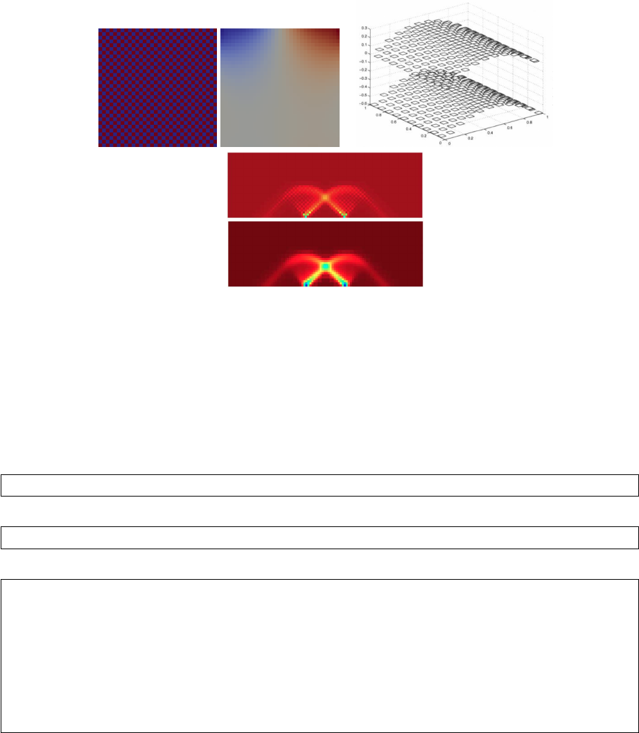
6.12 Pressure smoothing
It has been widely documented that the use of the Q1×P0element is not without problems. Aside from
the consequences it has on the FE matrix properties, we will here focus on another unavoidable side
effect: the spurious pressure checkerboard modes.
These modes have been thoroughly analysed [?,?,?,?]. They can be filtered out [?] or simply
smoothed [?].
On the following figure (a,b), pressure fields for the lid driven cavity experiment are presented for
both an even and un-even number of elements. We see that the amplitude of the modes can sometimes
be so large that the ’real’ pressure is not visible and that something as simple as the number of elements
in the domain can trigger those or not at all.
a) b)
c)
a) element pressure for a 32x32 grid and for a 33x33 grid;
b) image from [?, p307] for a manufactured solution;
c) elemental pressure and smoothed pressure for the punch experiment [?]
The easiest post-processing step that can be used (especially when a regular grid is used) is explained
in [?]: ”The element-to-node interpolation is performed by averaging the elemental values from elements
common to each node; the node-to-element interpolation is performed by averaging the nodal values
element-by-element. This method is not only very efficient but produces a smoothing of the pressure that
is adapted to the local density of the octree. Note that these two steps can be repeated until a satisfying
level of smoothness (and diffusion) of the pres- sure field is attained.”
In the codes which rely on the Q1×P0element, the (elemental) pressure is simply defined as
p=np . z e r o s ( ne l , dtype=np . f l o a t 6 4 )
while the nodal pressure is then defined as
q=np . z e r o s ( nnp , dtype=np . f l o a t 6 4 )
The element-to-node algorithm is then simply (in 2D):
cou nt=np . z e r o s ( nnp , dtype=np . i n t 1 6 )
f o r i e l in range ( 0 , n e l ) :
q [ i c o n [ 0 , i e l ]]+=p [ i e l ]
q [ i c o n [ 1 , i e l ]]+=p [ i e l ]
q [ i c o n [ 2 , i e l ]]+=p [ i e l ]
q [ i c o n [ 3 , i e l ]]+=p [ i e l ]
co un t [ i c o n [ 0 , i e l ]]+=1
co un t [ i c o n [ 1 , i e l ]]+=1
co un t [ i c o n [ 2 , i e l ]]+=1
co un t [ i c o n [ 3 , i e l ]]+=1
q=q/ count
39

Pressure smoothing is further discussed in [?].
produce figure to explain this
link to proto paper
link to least square and nodal derivatives
40

6.13 Pressure scaling
As perfectly explained in the step 32 of deal.ii2, we often need to scale the Gterm since it is many orders
of magnitude smaller than K, which introduces large inaccuracies in the solving process to the point that
the solution is nonsensical. This scaling coefficient is η/L. We start from
K G
GT0·V
P=f
h
and introduce the scaling coefficient as follows (which in fact does not alter the solution at all):
Kη
LG
η
LGT0·V
L
ηP=f
η
Lh
We then end up with the modified Stokes system:
K G
GT0·V
P=f
h
where
G=η
LGP=L
ηPh=η
Lh
After the solve phase, we recover the real pressure with P=η
LP0.
2https://www.dealii.org/9.0.0/doxygen/deal.II/step 32.html
41

6.14 Pressure normalisation
When Dirichlet boundary conditions are imposed everywhere on the boundary, pressure is only present
by its gradient in the equations. It is thus determined up to an arbitrary constant. In such a case, one
commonly impose the average of the pressure over the whole domain or on a subsect of the boundary to
be have a zero average, i.e. ZΩ
pdV = 0
Another possibility is to impose the pressure value at a single node.
Let us assume that we are using Q1×P0elements. Then the pressure is constant inside each element.
The integral above becomes:
ZΩ
pdV =X
eZΩe
pdV =X
e
peZΩe
dV =X
e
peAe=
where the sum runs over all elements eof area Ae. This can be rewritten
LTP= 0
and it is a constraint on the pressure. As we have seen before ??, we can associate to it a Lagrange
multiplier λso that we must solve the modified Stokes system:
K G 0
GT0L
0LT0
·
V
P
λ
=
f
h
0
When higher order spaces are used for pressure (continuous or discontinuous) one must then carry out
the above integration numerically by means of (usually) a Gauss-Legendre quadrature.
python codes/fieldstone stokes sphere 3D saddlepoint/
python codes/fieldstone burstedde/
python codes/fieldstone busse/
python codes/fieldstone RTinstability1/
python codes/fieldstone saddlepoint q2q1/
python codes/fieldstone compressible2/
python codes/fieldstone compressible1/
python codes/fieldstone saddlepoint q3q2/
42

6.15 The choice of solvers
Let us first look at the penalty formulation. In this case we are only solving for velocity since pressure is
recovered in a post-processing step. We also know that the penalty factor is many orders of magnitude
higher than the viscosity and in combination with the use of the Q1×P0element the resulting matrix
condition number is very high so that the use of iterative solvers in precluded. Indeed codes such as
SOPALE [?], DOUAR [?], or FANTOM [?] relying on the penalty formulation all use direct solvers
(BLKFCT, MUMPS, WSMP).
The main advantage of direct solvers is used in this case: They can solve ill-conditioned matrices.
However memory requirements for the storage of number of nonzeros in the Cholesky matrix grow very
fast as the number of equations/grid size increases, especially in 3D, to the point that even modern
computers with tens of Gb of RAM cannot deal with a 1003element mesh. This explains why direct
solvers are often used for 2D problems and rarely in 3D with noticeable exceptions [?,?,?,?,?,?,?,?,?].
In light of all this, let us start again from the (full) Stokes system:
K G
GT0·V
P=f
h
We need to solve this system in order to obtain the solution, i.e. the Vand Pvectors. But how?
Unfortunately, this question is not simple to answer and the ’right’ depends on many parameters.
How big is the matrix ? what is the condition number of the matrix K? Is it symmetric ? (i.e. how are
compressible terms handled?).
6.15.1 The Schur complement approach
Let us write the above system as two equations:
KV+GP=f(57)
GTV=h(58)
The first line can be re-written V=K−1(f−GP) and can be inserted in the second:
GTV=GT[K−1(f−GP)] = h
or,
GTK−1GP=GTK−1f−h
The matrix S=GTK−1Gis called the Schur complement. It is Symmetric (since Kis symmetric) and
Postive-Definite3(SPD) if Ker(G) = 0. look in donea-huerta book for details Having solved this equation
(we have obtained P), the velocity can be recovered by solving KV=f−GP. For now, let us assume
that we have built the Smatrix and the right hand side ˜
f=GTK−1f−h. We must solve SP=˜
f.
Since Sis SPD, the Conjugate Gradient (CG) method is very appropriate to solve this system. Indeed,
looking at the definition of Wikipedia: In mathematics, the conjugate gradient method is an algorithm for
the numerical solution of particular systems of linear equations, namely those whose matrix is symmetric
and positive-definite. The conjugate gradient method is often implemented as an iterative algorithm,
applicable to sparse systems that are too large to be handled by a direct implementation or other direct
methods such as the Cholesky decomposition. Large sparse systems often arise when numerically solving
partial differential equations or optimization problems.
The Conjugate Gradient algorithm is as follows:
3Mpositive definite ⇐⇒ xTM x > 0∀x∈Rn\0
43
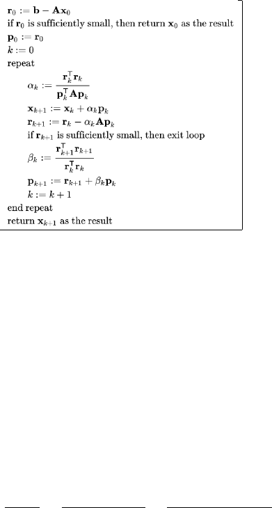
Algorithm obtained from https://en.wikipedia.org/wiki/Conjugate_gradient_method
Let us look at this algorithm up close. The parts which may prove to be somewhat tricky are those
involving the matrix (in our case the Schur complement). We start the iterations with a guess pressure
P0( and an initial guess velocity which could be obtained by solving KV0=f−GP0).
r0=˜
f−SP0(59)
=GTK−1f−h−(GTK−1G)P0(60)
=GTK−1(f−GP0)−h(61)
=GTK−1KV0−h(62)
=GTV0−h(63)
(64)
We now turn to the αkcoefficient:
αk=rT
krk
pkSpk
=rT
krk
pkGTK−1Gpk
=rT
krk
(Gpk)TK−1(Gpk)
We then define ˜pk=Gpk, so that αkcan be computed as follows:
1. compute ˜pk=Gpk
2. solve Kdk= ˜pk
3. compute αk= (rT
krk)/(˜pT
kdk)
Then we need to look at the term Spk:
Spk=GTK−1Gpk=GTK−1˜pk=GTdk
We can then rewrite the CG algorithm as follows [?]:
•r0=GTV0−h
•if r0is sufficiently small, then return (V0,P0) as the result
•p0=r0
•k= 0
•repeat
–compute ˜pk=Gpk
–solve Kdk= ˜pk
–compute αk= (rT
krk)/(˜pT
kdk)
44

–Pk+1 =Pk+αkpk
–rk+1 =rk−αkGTdk
–if rk+1 is sufficiently small, then exit loop
–βk= (rT
k+1rk+1)/(rT
krk)
–pk+1 =rk+1 +βkpk
–k=k+ 1
•return Pk+1 as result
We see that we have managed to solve the Schur complement equation with the Conjugate Gradient
method without ever building the matrix S. Having obtained the pressure solution, we can easily recover
the corresponding velocity with KVk+1 =f−GPk+1. However, this is rather unfortunate because it
requires yet another solve with the Kmatrix. As it turns out, we can slightly alter the above algorithm
to have it update the velocity as well so that this last solve is unnecessary.
We have
Vk+1 =K−1(f−GPp+1) = K−1(f−G(Pk+αkpk)) = K−1(f−GPk)−αkK−1Gpk=V−αkK−1˜pk=Vk−αkdk
and we can insert this minor extra calculation inside the algorithm and get the velocity solution nearly
for free. The final CG algorithm is then
solver cg:
•compute V0=K−1(f−GP0)
•r0=GTV0−h
•if r0is sufficiently small, then return (V0,P0) as the result
•p0=r0
•k= 0
•repeat
–compute ˜pk=Gpk
–solve Kdk= ˜pk
–compute αk= (rT
krk)/(˜pT
kdk)
–Pk+1 =Pk+αkpk
–Vk+1 =Vk−αkdk
–rk+1 =rk−αkGTdk
–if rk+1 is sufficiently small (|rk+1|2/|r0|2< tol), then exit loop
–βk= (rT
k+1rk+1)/(rT
krk)
–pk+1 =rk+1 +βkpk
–k=k+ 1
•return Pk+1 as result
This iterative algorithm will converge to the solution with a rate which depends on the condition
number of the Smatrix, which is not easily obtainable since Sis never built. Also, we know that large
viscosity contrasts in the domain will influence this too. Finally, we notice that this algorithm requires
one solve with matrix Kper iteration but says nothing about the method employed to do so.
One thing we know improves the convergence of any iterative solver is the use of a preconditioner
matrix and therefore use the Preconditioned Conjugate Gradient method:
45

Algorithm obtained from https://en.wikipedia.org/wiki/Conjugate_gradient_method
In the algorithm above the preconditioner matrix Mhas to be symmetric positive-definite and fixed,
i.e., cannot change from iteration to iteration.
We see that this algorithm introduces an additional vector zand a solve with the matrix Mat each
iteration, which means that Mmust be such that solving Mx =fwhere fis a given rhs vector must be
cheap. Ultimately, the PCG algorithm applied to the Schur complement equation takes the form:
solver pcg:
•compute V0=K−1(f−GP0)
•r0=GTV0−h
•if r0is sufficiently small, then return (V0,P0) as the result
•z0=M−1r0
•p0=z0
•k= 0
•repeat
–compute ˜pk=Gpk
–solve Kdk= ˜pk
–compute αk= (rT
kzk)/(˜pT
kdk)
–Pk+1 =Pk+αkpk
–Vk+1 =Vk−αkdk
–rk+1 =rk−αkGTdk
–if rk+1 is sufficiently small (|rk+1|2/|r0|2< tol), then exit loop
–zk+1 =M−1rk+1
–βk= (zT
k+1rk+1)/(zT
krk)
–pk+1 =zk+1 +βkpk
–k=k+ 1
•return Pk+1 as result
46

how to compute Mfor the Schur complement ?
6.16 The GMRES approach
47

6.17 The consistent boundary flux (CBF)
The Consistent Boundary Flux technique was devised to alleviate the problem of the accuracy of primary
variables derivatives (mainly velocity and temperature) on boundaries, where basis function (nodal)
derivatives do not exist. These derivatives are important since they are needed to compute the heat flux
(and therefore the NUsselt number) or dynamic topography and geoid.
The idea was first introduced in [?] and later used in geodynamics [?]. It was finally implemented in
the CitcomS code [?] and more recently in the ASPECT code (dynamic topography postprocessor). Note
that the CBF should be seen as a post-processor step as it does not alter the primary variables values.
The CBF method is implemented and used in ??.
6.17.1 applied to the Stokes equation
We start from the strong form:
∇·σ=b
and then write the weak form: ZΩ
N∇·σdV =ZΩ
NbdV
where Nis any test function. We then use the two equations:
∇·(Nσ) = N∇·σ+∇N·σ(chain rule)
ZΩ
(∇·f)dV =ZΓ
f·ndS (divergence theorem)
Integrating the first equation over Ω and using the second, we can write:
ZΓ
Nσ·ndS −ZΩ∇N·σdV =ZΩ
NbdV
On Γ, the traction vector is given by t=σ·n:
ZΓ
NtdS =ZΩ∇N·σdV +ZΩ
NbdV
Considering the traction vector as an unknown living on the nodes on the boundary, we can expand (for
Q1elements)
tx=
2
X
i=1
tx|iNity=
2
X
i=1
ty|iNi
on the boundary so that the left hand term yields a mass matrix M0. Finally, using our previous experience
of discretising the weak form, we can write:
M0· T =−KV − GP+f
where Tis the vector of assembled tractions which we want to compute and Vand Tare the solutions
of the Stokes problem. Note that the assembly only takes place on the elements along the boundary.
Note that the assembled mass matrix is tri-diagonal can be easily solved with a Conjugate Gradient
method. With a trapezoidal integration rule (i.e. Gauss-Lobatto) the matrix can even be diagonalised
and the resulting matrix is simply diagonal, which results in a very cheap solve [?].
6.17.2 applied to the heat equation
We start from the strong form of the heat transfer equation (without the source terms for simplicity):
ρcp∂T
∂t +v·∇T=∇·k∇T
The weak form then writes:
ZΩ
Nρcp
∂T
∂t dV +ρcpZΩ
Nv·∇T dV =ZΩ
N∇·k∇T dV
48

Using once again integration by parts and divergence theorem:
ZΩ
Nρcp
∂T
∂t dV +ρcpZΩ
Nv·∇T dV =ZΓ
Nk∇T·ndΓ−ZΩ
∇N·k∇T dV
On the boundary we are interested in the heat flux q=−k∇T
ZΩ
Nρcp
∂T
∂t dV +ρcpZΩ
Nv·∇T dV =−ZΓ
Nq·ndΓ−ZΩ
∇N·k∇T dV
or, ZΓ
Nq·ndΓ = −ZΩ
Nρcp
∂T
∂t dV −ρcpZΩ
Nv·∇T dV −ZΩ
∇N·k∇T dV
Considering the normal heat flux qn=q·nas an unknown living on the nodes on the boundary,
qn=
2
X
i=1
qn|iNi
so that the left hand term becomes a mass matrix for the shape functions living on the boundary. We
have already covered the right hand side terms when building the FE system to solve the heat transport
equation, so that in the end
M0· Qn=−M·∂T
∂t −Ka·T−Kd·T
where Qnis the assembled vector of normal heat flux components. Note that in all terms the assembly
only takes place over the elements along the boundary.
49

What follows only applies to the reference element.
N
3-----2
| |
W| |E
| |
0-----1
S
We start from
ZΓ
NitdS =ZΓ0−1
NitdS +ZΓ1−2
NitdS +ZΓ2−3
NitdS +ZΓ3−0
NitdS (65)
for i= 0,3. Let us start with N0, then
ZΓ
N0tdS =ZΓ0−1
N0tdS +ZΓ1−2
N0tdS +ZΓ2−3
N0tdS +ZΓ3−0
N0tdS
=ZΓ0−1
N0(NΓ
0t0+NΓ
1t1)dS
+ZΓ1−2
N0(NΓ
1t1+NΓ
2t2)dS
+ZΓ2−3
N0(NΓ
2t2+NΓ
3t3)dS
+ZΓ3−0
N0(NΓ
3t3+NΓ
0t0)dS
= ZΓ0−1
N0NΓ
0dS!t0+ ZΓ0−1
N0NΓ
1dS!t1
+ ZΓ1−2
N0NΓ
1dS!t1+ ZΓ1−2
N0NΓ
2dS!t2
+ ZΓ2−3
N0NΓ
2dS!t2+ ZΓ2−3
N0NΓ
3dS!t3
+ ZΓ3−0
N0NΓ
3dS!t3+ ZΓ3−0
N0NΓ
0dS!t0
In what follows we will make use of
Z+1
−1
1
4(1 −x)(1 −x)dx = 2/3
Z+1
−1
1
4(1 + x)(1 + x)dx = 2/3
Z+1
−1
1
4(1 + x)(1 −x)dx = 1/3
50
ZΓ0−1
N0(r, s =−1)NΓ
0(r)dS =Z+1
−1
1
2(1 −r)·1
2(1 −r)dr = 2/3
ZΓ0−1
N0(r, s =−1)NΓ
1(r)dS =Z+1
−1
1
2(1 −r)·1
2(1 + r)dr = 1/3
ZΓ1−2
N0(r= +1, s)NΓ
1(s)dS =Z+1
−1
1
4(0)(1 −s)·1
2(1 −s)ds = 0
ZΓ1−2
N0(r= +1, s)NΓ
2(s)dS =Z+1
−1
1
4(0)(1 −s)·1
2(1 + s)ds = 0
ZΓ2−3
N0(r, s = +1)NΓ
2(r)dS =−Z+1
−1
1
4(1 −r)(0) ·1
2(1 + r)dr = 0
ZΓ2−3
N0(r, s = +1)NΓ
3(r)dS =−Z+1
−1
1
4(1 −r)(0) ·1
2(1 −r)dr = 0
ZΓ3−0
N0(r=−1, s)NΓ
3(s)dS =−Z+1
−1
1
2(1 −s)·1
2(1 + s)ds =−1/3
ZΓ3−0
N0(r=−1, s)NΓ
0(s)dS =−Z+1
−1
1
2(1 −s)·1
2(1 −s)ds =−2/3
ZΓ0−1
N1(r, s =−1)NΓ
0(r)dS =Z+1
−1
1
2(1 + r)·1
2(1 −r)dr = 1/3
ZΓ0−1
N1(r, s =−1)NΓ
1(r)dS =Z+1
−1
1
2(1 + r)·1
2(1 + r)dr = 2/3
ZΓ1−2
N1(r= +1, s)NΓ
1(s)dS =Z+1
−1
1
2(1 −s)·1
2(1 −s)ds = 2/3
ZΓ1−2
N1(r= +1, s)NΓ
2(s)dS =Z+1
−1
1
2(1 −s)·1
2(1 + s)ds = 1/3
ZΓ2−3
N1(r, s = +1)NΓ
2(r)dS =−Z+1
−1
1
4(1 + r)(0) ·1
2(1 + r)dr = 0
ZΓ2−3
N1(r, s = +1)NΓ
3(r)dS =−Z+1
−1
1
4(1 + r)(0) ·1
2(1 −r)dr = 0
ZΓ3−0
N1(r=−1, s)NΓ
3(s)dS =−Z+1
−1
1
4(0)(1 −s)·1
2(1 + s)ds = 0
ZΓ3−0
N1(r=−1, s)NΓ
0(s)dS =−Z+1
−1
1
4(0)(1 −s)·1
2(1 −s)ds = 0
51
ZΓ0−1
N2(r, s =−1)NΓ
0(r)dS =Z+1
−1
1
4(1 + r)(0) ·1
2(1 −r)dr = 0
ZΓ0−1
N2(r, s =−1)NΓ
1(r)dS =Z+1
−1
1
4(1 + r)(0) ·1
2(1 + r)dr = 0
ZΓ1−2
N2(r= +1, s)NΓ
1(s)dS =Z+1
−1
1
2(1 + s)·1
2(1 −s)ds = 1/3
ZΓ1−2
N2(r= +1, s)NΓ
2(s)dS =Z+1
−1
1
2(1 + s)·1
2(1 + s)ds = 2/3
ZΓ2−3
N2(r, s = +1)NΓ
2(r)dS =−Z+1
−1
1
2(1 + r)·1
2(1 + r)dr =−2/3
ZΓ2−3
N2(r, s = +1)NΓ
3(r)dS =−Z+1
−1
1
2(1 + r)·1
2(1 −r)dr =−1/3
ZΓ3−0
N2(r=−1, s)NΓ
3(s)dS =−Z+1
−1
1
4(0)(1 + s)·1
2(1 + s)ds = 0
ZΓ3−0
N2(r=−1, s)NΓ
0(s)dS =−Z+1
−1
1
4(0)(1 + s)·1
2(1 −s)ds = 0
ZΓ0−1
N3(r, s =−1)NΓ
0(r)dS =Z+1
−1
1
4(1 −r)(0) ·1
2(1 −r)dr = 0
ZΓ0−1
N3(r, s =−1)NΓ
1(r)dS =Z+1
−1
1
4(1 −r)(0) ·1
2(1 + r)dr = 0
ZΓ1−2
N3(r= +1, s)NΓ
1(s)dS =Z+1
−1
1
4(0)(1 + s)·1
2(1 −s)ds = 0
ZΓ1−2
N3(r= +1, s)NΓ
2(s)dS =Z+1
−1
1
4(0)(1 + s)·1
2(1 + s)ds = 0
ZΓ2−3
N3(r, s = +1)NΓ
2(r)dS =−Z+1
−1
1
2(1 −r)·1
2(1 + r)dr =−1/3
ZΓ2−3
N3(r, s = +1)NΓ
3(r)dS =−Z+1
−1
1
2(1 −r)·1
2(1 −r)dr =−2/3
ZΓ3−0
N3(r=−1, s)NΓ
3(s)dS =−Z+1
−1
1
2(1 + s)·1
2(1 + s)ds =−2/3
ZΓ3−0
N3(r=−1, s)NΓ
0(s)dS =−Z+1
−1
1
2(1 + s)·1
2(1 −s)ds =−1/3
52

so finally
ZΓ
N0tdS =1
3t1−1
3t3
ZΓ
N1tdS =1
3t0+4
3t1+1
3t2
ZΓ
N2tdS =1
3t1−1
3t3
ZΓ
N3tdS =−1
3t0−1
3t2−4
3t3
1
3
. . 1. . . −1.
. . . 1...−1
1.4.1...
.1.4.1. .
. . 1. . . −1.
. . . 1...−1
−1. . . −1.−4.
.−1. . . −1.−4
·
tx,0
ty,0
tx,1
ty,1
tx,2
ty,2
tx,3
ty,3
=
rhs
Note that the resulting matrix is symmetric.
53

Let us start with a small example, a 3x2 element FE grid:
8=======9======10======11
||||
| (3) | (4) | (5) |
||||
4=======5=======6=======7
||||
| (0) | (1) | (2) |
||||
0=======1=======2=======3
Element 0: ZΓ
NitdS =ZΓ0−1
NitdS +ZΓ1−5
NitdS +ZΓ5−4
NitdS +ZΓ4−0
NitdS (66)
Element 1: ZΓ
NitdS =ZΓ1−2
NitdS +ZΓ2−6
NitdS +ZΓ6−5
NitdS +ZΓ5−1
NitdS (67)
Element 2: ZΓ
NitdS =ZΓ2−3
NitdS +ZΓ3−7
NitdS +ZΓ7−6
NitdS +ZΓ6−2
NitdS (68)
Element 3: ZΓ
NitdS =ZΓ4−5
NitdS +ZΓ5−9
NitdS +ZΓ9−8
NitdS +ZΓ8−4
NitdS (69)
Element 4: ZΓ
NitdS =ZΓ5−6
NitdS +ZΓ6−10
NitdS +ZΓ10−9
NitdS +ZΓ9−5
NitdS (70)
Element 5: ZΓ
NitdS =ZΓ6−7
NitdS +ZΓ7−11
NitdS +ZΓ11−10
NitdS +ZΓ10−6
NitdS (71)
We see that the integral RΓ1−5NitdS of element 0 is exactly the opposite4of the the integral RΓ5−1NitdS
of element 1, so that their contributions to the assembled matrix would actually cancel out. Likewise,
any edge common to two elements will see in the expressions above two integrals of opposite sign, shich
ultimately will not contribute to the assembled matrix.
Let us then remove the integrals over edges 1-5, 2-6, 4-5, 5-6, 6-7, 5-9 and 6-10 off the equations
above:
4these are line integrals, one is going from node 1 to 5, the other from 5 to 1
54
Element 0: ZΓ
NitdS =ZΓ0−1
NitdS +ZΓ4−0
NitdS (72)
=ZΓ0−1
Ni(N0t0+N1t1)dS +ZΓ4−0
Ni(N0t0+N4t4)dS (73)
=ZΓ0−1
NiN0dS t0+ZΓ0−1
NiN1dS t1+ZΓ4−0
NiN0dS t0+ZΓ4−0
NiN4dS t4
Element 1: ZΓ
NitdS =ZΓ1−2
NitdS (74)
=ZΓ1−2
Ni(N1t1+N2t2)dS (75)
Element 2: ZΓ
NitdS =ZΓ2−3
NitdS +ZΓ3−7
NitdS (76)
Element 3: ZΓ
NitdS =ZΓ9−8
NitdS +ZΓ8−4
NitdS (77)
Element 4: ZΓ
NitdS =ZΓ10−9
NitdS (78)
=ZΓ10−9
Ni(N10t10 +N9t9)dS (79)
Element 5: ZΓ
NitdS =ZΓ7−11
NitdS +ZΓ11−10
NitdS (80)
We see that the
55
