Manual
User Manual:
Open the PDF directly: View PDF ![]() .
.
Page Count: 77
- Introduction
- The physical equations of Fluid Dynamics
- The Finite Element Method
- Additional techniques
- fieldstone: simple analytical solution
- fieldstone: Stokes sphere
- fieldstone: Convection in a 2D box
- fieldstone: solcx benchmark
- fieldstone: solkz benchmark
- fieldstone: solvi benchmark
- fieldstone: the indentor benchmark
- fieldstone: the annulus benchmark
- fieldstone: stokes sphere (3D) - penalty
- fieldstone: stokes sphere (3D) - mixed formulation
- fieldstone: consistent pressure recovery
- fieldstone: the Particle in Cell technique (1) - the effect of averaging
- fieldstone: solving the full saddle point problem
- fieldstone: solving the full saddle point problem in 3D
- fieldstone: solving the full saddle point problem with Q2Q1 elements
- fieldstone: The non-conforming Q1 P0 element
- fieldstone: The stabilised Q1 Q1 element
- fieldstone: compressible flow (1)
- fieldstone: compressible flow (2)
- The main codes in computational geodynamics
- fieldstone.py
- fieldstone_stokes_sphere.py
- fieldstone_convection_box.py
- fieldstone_solcx.py
- fieldstone_indentor.py
- fieldstone_saddlepoint.py
The Finite Element Method in Geodynamics
C. Thieulot
December 31, 2018
Contents
1 Introduction 4
1.1 Acknowledgments................................................ 4
1.2 Essentialliterature............................................... 4
1.3 Installation ................................................... 4
2 The physical equations of Fluid Dynamics 5
2.1 the Boussinesq approximation: an Incompressible flow . . . . . . . . . . . . . . . . . . . . . . . . . . . 8
3 The Finite Element Method 9
3.1 Numericalintegration ............................................. 9
3.1.1 in1D-theory ............................................. 9
3.1.2 in1D-examples............................................ 11
3.1.3 in2D/3D-theory ........................................... 11
3.2 Themesh .................................................... 12
3.3 Elements and basis functions in 1D . . . . . . . . . . . . . . . . . . . . . . . . . . . . . . . . . . . . . . 12
3.4 Elements and basis functions in 2D . . . . . . . . . . . . . . . . . . . . . . . . . . . . . . . . . . . . . . 12
3.4.1 The Q1basisin2D........................................... 13
3.4.2 The Q2basisin2D........................................... 14
3.5 Thepenaltyapproach ............................................. 14
4 Additional techniques 18
4.1 The method of manufactured solutions . . . . . . . . . . . . . . . . . . . . . . . . . . . . . . . . . . . . 18
4.2 Sparsestorage.................................................. 18
4.3 Meshgeneration ................................................ 18
4.4 Thevalueofthetimestep ........................................... 18
4.5 Trackingmaterials ............................................... 18
4.6 Visco-Plasticity................................................. 18
4.7 PicardandNewton............................................... 18
4.8 Thechoiceofsolvers.............................................. 18
4.9 The SUPG formulation for the energy equation . . . . . . . . . . . . . . . . . . . . . . . . . . . . . . . 18
4.10 Tracking materials and/or interfaces . . . . . . . . . . . . . . . . . . . . . . . . . . . . . . . . . . . . . 18
4.11Dealingwithafreesurface........................................... 18
4.12Pressurenormalisation............................................. 18
5fieldstone: simple analytical solution 20
6fieldstone: Stokes sphere 23
7fieldstone: Convection in a 2D box 24
8fieldstone: solcx benchmark 26
9fieldstone: solkz benchmark 28
10 fieldstone: solvi benchmark 29
11 fieldstone: the indentor benchmark 31
12 fieldstone: the annulus benchmark 33
1
13 fieldstone: stokes sphere (3D) - penalty 35
14 fieldstone: stokes sphere (3D) - mixed formulation 36
15 fieldstone: consistent pressure recovery 37
16 fieldstone: the Particle in Cell technique (1) - the effect of averaging 38
17 fieldstone: solving the full saddle point problem 41
18 fieldstone: solving the full saddle point problem in 3D 43
18.0.1 Constantviscosity ........................................... 44
18.0.2 Variableviscosity............................................ 45
19 fieldstone: solving the full saddle point problem with Q2×Q1elements 47
20 fieldstone: The non-conforming Q1×P0element 50
21 fieldstone: The stabilised Q1×Q1element 51
22 fieldstone: compressible flow (1) 52
23 fieldstone: compressible flow (2) 54
23.1Thephysics ................................................... 54
23.2Thenumerics .................................................. 54
23.3Theexperimentalsetup ............................................ 55
23.4Scaling...................................................... 56
23.5Conservationofenergy1............................................ 56
23.5.1 under BA and EBA approximations . . . . . . . . . . . . . . . . . . . . . . . . . . . . . . . . . 56
23.5.2 under no approximation at all . . . . . . . . . . . . . . . . . . . . . . . . . . . . . . . . . . . . . 57
23.6Conservationofenergy2............................................ 57
23.7 The problem of the onset of convection . . . . . . . . . . . . . . . . . . . . . . . . . . . . . . . . . . . . 58
23.8 results - BA - Ra = 104............................................ 60
23.9 results - BA - Ra = 105............................................ 62
23.10results - BA - Ra = 106............................................ 63
23.11results - EBA - Ra = 104........................................... 64
23.12results - EBA - Ra = 105........................................... 66
23.13Onsetofconvection............................................... 67
A The main codes in computational geodynamics 68
A.1 ADELI...................................................... 68
A.2 ASPECT .................................................... 68
A.3 CITCOMSandCITCOMCU ......................................... 68
A.4 DOUAR..................................................... 68
A.5 GAIA ...................................................... 68
A.6 GALE...................................................... 68
A.7 GTECTON................................................... 68
A.8 ELVIS...................................................... 68
A.9 ELEFANT.................................................... 68
A.10ELLIPSIS.................................................... 68
A.11FANTOM.................................................... 68
A.12FLUIDITY ................................................... 68
A.13LAMEM..................................................... 68
A.14MILAMIN.................................................... 68
A.15PARAVOZ/FLAMAR ............................................. 68
A.16PTATIN..................................................... 68
A.17RHEA...................................................... 68
A.18SEPRAN .................................................... 68
A.19SOPALE .................................................... 68
A.20STAGYY .................................................... 68
A.21SULEC ..................................................... 68
A.22TERRA..................................................... 68
2

1 Introduction
WARNING: this is work in progress
practical hands-on approach
as little as possible jargon
no mathematical proof
no optimised codes (readability over efficiency). avoiding as much as possible to have to look elsewhere. very
sequential, so unavoidable repetitions (jacobian, shape functions)
FE is one of several methods.
All the python scripts and this document are freely available at https://github.com/cedrict/fieldstone.
1.1 Acknowledgments
Jean Braun, Philippe Fullsack, Arie van den Berg. Lukas van de Wiel. Robert Myhill. Menno, Anne Too many BSc
and MSc students to name indivisually, although Job Mos did produce the very first version of fieldstone as part of
his MSc thesis. The ASPECT team in general and Wolfgang Bangerth and Timo Heister in particular.
1.2 Essential literature
a) b) c) d) e)
1.3 Installation
python3.6 -m pip install --user numpy scipy matplotlib
4

2 The physical equations of Fluid Dynamics
Symbol meaning unit
tTime s
x, y, z Cartesian coordinates m
vvelocity vector m·s−1
ρmass density kg/m3
ηdynamic viscosity Pa·s
λpenalty parameter Pa·s
Ttemperature K
∇gradient operator m−1
∇·divergence operator m−1
ppressure Pa
˙
ε(v) strain rate tensor s−1
αthermal expansion coefficient K−1
kthermal conductivity W/(m ·K)
CpHeat capacity J/K
Hintrinsic specific heat production W/kg
βTisothermal compressibility Pa−1
Let us start from the heat transport equation as shown in Schubert, Turcotte and Olson [47]:
ρCp
DT
Dt −αT Dp
Dt =∇·k∇T+Φ+ρH
with DT
Dt =∂T
∂t +v·∇TDp
Dt =∂p
∂t +v·∇p
In order to arrive at the set of equations that ASPECT solves, we need to neglect the ∂p/∂t.WHY? Also, their
definition of the shear heating term Φ is:
Φ = kB(∇·v)2+ 2η˙
εd:˙
εd
For many fluids the bulk viscosity kBis very small and is often taken to be zero, an assumption known as the Stokes
assumption: kB=λ+ 2η/3 = 0. Note that ηis the dynamic viscosity and λthe second viscosity. Also,
τ= 2η˙
ε+λ(∇·v)1
but since kB=λ+ 2η/3 = 0, then λ=−2η/3 so
τ= 2η˙
ε−2
3η(∇·v)1= 2η˙
εd
[from aspect manual] We focus on the system of equations in a d= 2- or d= 3-dimensional domain Ω that describes
the motion of a highly viscous fluid driven by differences in the gravitational force due to a density that depends on
the temperature. In the following, we largely follow the exposition of this material in Schubert, Turcotte and Olson
[47].
Specifically, we consider the following set of equations for velocity u, pressure pand temperature T:
−∇ · 2η˙ε(v)−1
3(∇ · v)1+∇p=ρgin Ω,(1)
∇ · (ρv) = 0 in Ω,(2)
ρCp∂T
∂t +v· ∇T−∇·k∇T=ρH
+ 2η˙ε(v)−1
3(∇ · v)1:˙ε(v)−1
3(∇ · v)1(3)
+αT (v· ∇p)
+ρT ∆S∂X
∂t +v· ∇Xin Ω,
where ˙
ε(u) = 1
2(∇u+∇uT) is the symmetric gradient of the velocity (often called the strain rate).
5
In this set of equations, (82) and (83) represent the compressible Stokes equations in which v=v(x, t) is the
velocity field and p=p(x, t) the pressure field. Both fields depend on space xand time t. Fluid flow is driven by the
gravity force that acts on the fluid and that is proportional to both the density of the fluid and the strength of the
gravitational pull.
Coupled to this Stokes system is equation (84) for the temperature field T=T(x, t) that contains heat conduction
terms as well as advection with the flow velocity v. The right hand side terms of this equation correspond to
•internal heat production for example due to radioactive decay;
•friction (shear) heating;
•adiabatic compression of material;
•phase change.
The last term of the temperature equation corresponds to the latent heat generated or consumed in the process of
phase change of material. In what follows we will not assume that no phase change takes place so that we disregard
this term altogether.
6

A note on the shear heating term Φ: In many publications, Φ is given by Φ = τij ∂jui=τ:∇v.
Φ = τij ∂jui(4)
= 2η˙εd
ij ∂jui(5)
= 2η1
2˙εd
ij ∂jui+ ˙εd
ji∂iuj(6)
= 2η1
2˙εd
ij ∂jui+ ˙εd
ij ∂iuj(7)
= 2η˙εd
ij
1
2(∂jui+∂iuj) (8)
= 2η˙εd
ij ˙εij (9)
= 2η˙
εd:˙
ε(10)
= 2η˙
εd:˙
εd+1
3(∇·v)1(11)
= 2η˙
εd:˙
εd+ 2η˙
εd:1(∇·v) (12)
= 2η˙
εd:˙
εd(13)
Finally
Φ = τ:∇v= 2η˙
εd:˙
εd= 2η( ˙εd
xx)2+ ( ˙εd
yy)2+ 2( ˙εd
xy)2
7

2.1 the Boussinesq approximation: an Incompressible flow
[from aspect manual] The Boussinesq approximation assumes that the density can be considered constant in all
occurrences in the equations with the exception of the buoyancy term on the right hand side of (82). The primary
result of this assumption is that the continuity equation (83) will now read
∇·v= 0
This implies that the strain rate tensor is deviatoric. Under the Boussinesq approximation, the equations are much
simplified:
−∇ · [2η˙
ε(v)] + ∇p=ρgin Ω,(14)
∇ · (ρv) = 0 in Ω,(15)
ρ0Cp∂T
∂t +v· ∇T−∇·k∇T=ρH in Ω (16)
Note that all terms on the rhs of the temperature equations have disappeared, with the exception of the source term.
8
3 The Finite Element Method
3.1 Numerical integration
As we will see later, using the Finite Element method to solve problems involves computing integrals which are more
often than not too complex to be computed analytically/exactly. We will then need to compute them numerically.
[wiki] In essence, the basic problem in numerical integration is to compute an approximate solution to a definite
integral Zb
a
f(x)dx
to a given degree of accuracy. This problem has been widely studied [?] and we know that if f(x) is a smooth function,
and the domain of integration is bounded, there are many methods for approximating the integral to the desired
precision.
There are several reasons for carrying out numerical integration.
•The integrand f(x) may be known only at certain points, such as obtained by sampling. Some embedded systems
and other computer applications may need numerical integration for this reason.
•A formula for the integrand may be known, but it may be difficult or impossible to find an antiderivative that is
an elementary function. An example of such an integrand is f(x) = exp(−x2), the antiderivative of which (the
error function, times a constant) cannot be written in elementary form.
•It may be possible to find an antiderivative symbolically, but it may be easier to compute a numerical approx-
imation than to compute the antiderivative. That may be the case if the antiderivative is given as an infinite
series or product, or if its evaluation requires a special function that is not available.
3.1.1 in 1D - theory
The simplest method of this type is to let the interpolating function be a constant function (a polynomial of degree
zero) that passes through the point ((a+b)/2, f((a+b)/2)).
This is called the midpoint rule or rectangle rule.
Zb
a
f(x)dx '(b−a)f(a+b
2)
insert here figure
The interpolating function may be a straight line (an affine function, i.e. a polynomial of degree 1) passing through
the points (a, f(a)) and (b, f(b)).
This is called the trapezoidal rule. Zb
a
f(x)dx '(b−a)f(a) + f(b)
2
insert here figure
For either one of these rules, we can make a more accurate approximation by breaking up the interval [a, b] into
some number n of subintervals, computing an approximation for each subinterval, then adding up all the results. This
is called a composite rule, extended rule, or iterated rule. For example, the composite trapezoidal rule can be stated
as
Zb
a
f(x)dx 'b−a
n f(a)
2+
n−1
X
k=1
f(a+kb−a
n) + f(b)
2!
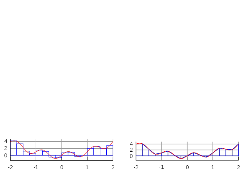
where the subintervals have the form [kh, (k+ 1)h], with h= (b−a)/n and k= 0,1,2, . . . , n −1.
a) b)
The interval [−2,2] is broken into 16 sub-intervals. The blue lines correspond to the approximation of the red curve
by means of a) the midpoint rule, b) the trapezoidal rule.
9
There are several algorithms for numerical integration (also commonly called ’numerical quadrature’, or simply
’quadrature’) . Interpolation with polynomials evaluated at equally spaced points in [a, b] yields the NewtonCotes
formulas, of which the rectangle rule and the trapezoidal rule are examples. If we allow the intervals between inter-
polation points to vary, we find another group of quadrature formulas, such as the Gauss(ian) quadrature formulas.
A Gaussian quadrature rule is typically more accurate than a NewtonCotes rule, which requires the same number of
function evaluations, if the integrand is smooth (i.e., if it is sufficiently differentiable).
An n−point Gaussian quadrature rule, named after Carl Friedrich Gauss, is a quadrature rule constructed to
yield an exact result for polynomials of degree 2n−1 or less by a suitable choice of the points xiand weights wifor
i= 1, . . . , n.
The domain of integration for such a rule is conventionally taken as [−1,1], so the rule is stated as
Z+1
−1
f(x)dx =
n
X
iq=1
wiqf(xiq)
In this formula the xiqcoordinate is the i-th root of the Legendre polynomial Pn(x).
It is important to note that a Gaussian quadrature will only produce good results if the function f(x) is well
approximated by a polynomial function within the range [−1,1]. As a consequence, the method is not, for example,
suitable for functions with singularities.
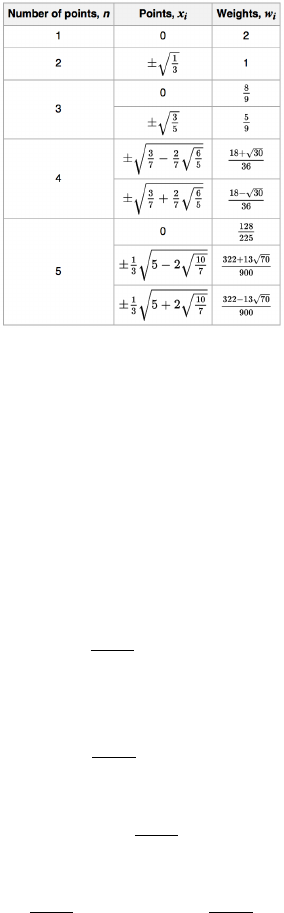
Gauss-Legendre points and their weights.
As shown in the above table, it can be shown that the weight values must fulfill the following condition:
X
iq
wiq= 2 (17)
and it is worth noting that all quadrature point coordinates are symmetrical around the origin.
Since most quadrature formula are only valid on a specific interval, we now must address the problem of their use
outside of such intervals. The solution turns out to be quite simple: one must carry out a change of variables from
the interval [a, b] to [−1,1].
We then consider the reduced coordinate r∈[−1,1] such that
r=2
b−a(x−a)−1
This relationship can be reversed such that when ris known, its equivalent coordinate x∈[a, b] can be computed:
x=b−a
2(1 + r) + a
From this it follows that
dx =b−a
2dr
and then Zb
a
f(x)dx =b−a
2Z+1
−1
f(r)dr 'b−a
2
n
X
iq=1
wiqf(riq)
10

3.1.2 in 1D - examples
example 1 Since we know how to carry out any required change of variables, we choose for simplicity a=−1,
b= +1. Let us take for example f(x)=π. Then we can compute the integral of this function over the interval [a, b]
exactly:
I=Z+1
−1
f(x)dx =πZ+1
−1
dx = 2π
We can now use a Gauss-Legendre formula to compute this same integral:
Igq =Z+1
−1
f(x)dx =
nq
X
iq=1
wiqf(xiq) =
nq
X
iq=1
wiqπ=π
nq
X
iq=1
wiq
| {z }
=2
= 2π
where we have used the property of the weight values of Eq.(17). Since the actual number of points was never specified,
this result is valid for all quadrature rules.
example 2 Let us now take f(x) = mx +pand repeat the same exercise:
I=Z+1
−1
f(x)dx =Z+1
−1
(mx +p)dx = [1
2mx2+px]+1
−1= 2p
Igq =Z+1
−1
f(x)dx=
nq
X
iq=1
wiqf(xiq)=
nq
X
iq=1
wiq(mxiq+p)= m
nq
X
iq=1
wiqxiq
| {z }
=0
+p
nq
X
iq=1
wiq
| {z }
=2
= 2p
since the quadrature points are symmetric w.r.t. to zero on the x-axis. Once again the quadrature is able to compute
the exact value of this integral: this makes sense since an n-point rule exactly integrates a 2n−1 order polynomial
such that a 1 point quadrature exactly integrates a first order polynomial like the one above.
example 3 Let us now take f(x) = x2. We have
I=Z+1
−1
f(x)dx =Z+1
−1
x2dx = [1
3x3]+1
−1=2
3
and
Igq =Z+1
−1
f(x)dx=
nq
X
iq=1
wiqf(xiq)=
nq
X
iq=1
wiqx2
iq
•nq= 1: x(1)
iq = 0, wiq= 2. Igq = 0
•nq= 2: x(1)
q=−1/√3, x(2)
q= 1/√3, w(1)
q=w(2)
q= 1. Igq =2
3
•It also works ∀nq>2 !
3.1.3 in 2D/3D - theory
Let us now turn to a two-dimensional integral of the form
I=Z+1
−1Z+1
−1
f(x, y)dxdy
The equivalent Gaussian quadrature writes:
Igq '
nq
X
iq=1
nq
X
jq
f(xiq, yjq)wiqwjq
11
3.2 The mesh
3.3 Elements and basis functions in 1D
3.4 Elements and basis functions in 2D
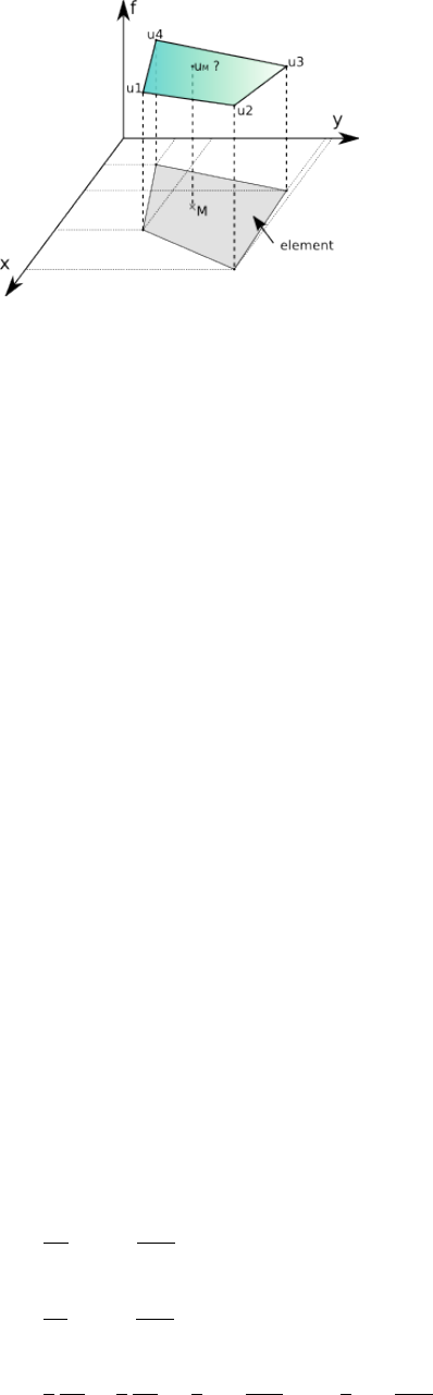
Let us for a moment consider a single quadrilateral element in the xy-plane, as shown on the following figure:
Let us assume that we know the values of a given field uat the vertices. For a given point Minside the element in
the plane, what is the value of the field uat this point? It makes sense to postulate that uM=u(xM, yM) will be
given by
uM=φ(u1, u2, u3, u4, xM, yM)
where φis a function to be determined. Although φis not unique, we can decide to express the value uMas a weighed
sum of the values at the vertices ui. One option could be to assign all four vertices the same weight, say 1/4 so that
uM= (u1+u2+u3+u4)/4, i.e. uMis simply given by the arithmetic mean of the vertices values. This approach
suffers from a major drawback as it does not use the location of point Minside the element. For instance, when
(xM, yM)→(x2, y2) we expect uM→u2.
In light of this, we could now assume that the weights would depend on the position of Min a continuous fashion:
u(xM, yM) =
4
X
i=1
Ni(xM, yM)ui
where the Niare continous (”well behaved”) functions which have the property:
Ni(xj, yj) = δij
or, in other words:
N3(x1, y1) = 0 (18)
N3(x2, y2) = 0 (19)
N3(x3, y3) = 1 (20)
N3(x4, y4) = 0 (21)
The functions Niare commonly called basis functions.
Omitting the Msubscripts for any point inside the element, the velocity components uand vare given by:
ˆu(x, y) =
4
X
i=1
Ni(x, y)ui(22)
ˆv(x, y) =
4
X
i=1
Ni(x, y)vi(23)
Rather interestingly, one can now easily compute velocity gradients (and therefore the strain rate tensor) since we
have assumed the basis functions to be ”well behaved” (in this case differentiable):
˙xx(x, y) = ∂u
∂x =
4
X
i=1
∂Ni
∂x ui(24)
˙yy(x, y) = ∂v
∂y =
4
X
i=1
∂Ni
∂y vi(25)
˙xy(x, y) = 1
2
∂u
∂y +1
2
∂v
∂x =1
2
4
X
i=1
∂Ni
∂y ui+1
2
4
X
i=1
∂Ni
∂x vi(26)
12
How we actually obtain the exact form of the basis functions is explained in the coming section.
3.4.1 The Q1basis in 2D
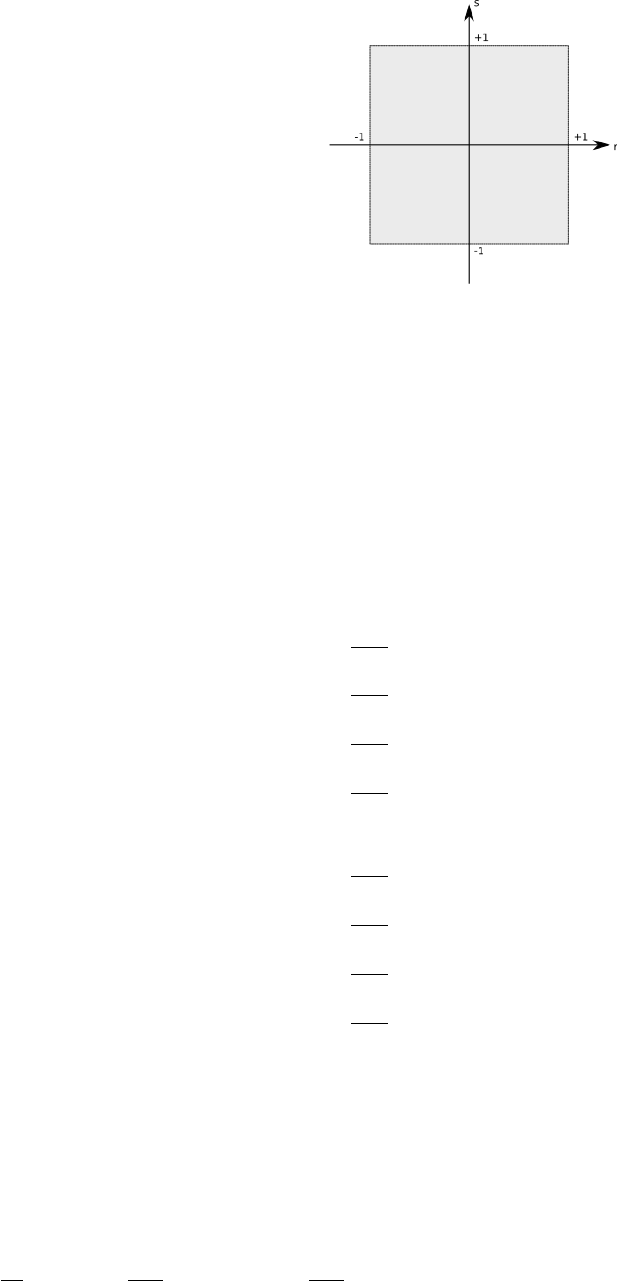
In this section, we place ourselves in the most favorables case, i.e. the element is a square defined by −1< r < 1,
−1< s < 1 in the Cartesian coordinates system (r, s):
add corner numbering
This element is commonly called the reference element. How we go from the (x, y) coordinate system to the (r, s)
once and vice versa will be dealt later on. For now, the basis functions in the above reference element and in the
reduced coordinates system (r, s) are given by:
N1(r, s)=0.25(1 −r)(1 −s)
N2(r, s)=0.25(1 + r)(1 −s)
N3(r, s)=0.25(1 + r)(1 + s)
N4(r, s)=0.25(1 −r)(1 + s)
The partial derivatives of these functions with respect to rans sautomatically follow:
∂N1
∂r (r, s) = −0.25(1 −s)
∂N2
∂r (r, s) = +0.25(1 −s)
∂N3
∂r (r, s) = +0.25(1 + s)
∂N4
∂r (r, s) = −0.25(1 + s)
∂N1
∂s (r, s) = −0.25(1 −r)
∂N2
∂s (r, s) = −0.25(1 + r)
∂N3
∂s (r, s) = +0.25(1 + r)
∂N4
∂s (r, s) = +0.25(1 −r)
Let us go back to Eq.(23). And let us assume that the function v(r, s) = Cso that vi=Cfor i= 1,2,3,4. It then
follows that
ˆv(r, s) =
4
X
i=1
Ni(r, s)vi=C
4
X
i=1
Ni(r, s) = C[N1(r, s) + N2(r, s) + N3(r, s) + N4(r, s)] = C
This is a very important property: if the vfunction used to assign values at the vertices is constant, then the value of
ˆvanywhere in the element is exactly C. If we now turn to the derivatives of vwith respect to rand s:
∂ˆv
∂r (r, s) =
4
X
i=1
∂Ni
∂r (r, s)vi=C
4
X
i=1
∂Ni
∂r (r, s) = C[−0.25(1 −s)+0.25(1 −s)+0.25(1 + s)−0.25(1 + s)] = 0
13

∂ˆv
∂s (r, s) =
4
X
i=1
∂Ni
∂s (r, s)vi=C
4
X
i=1
∂Ni
∂s (r, s) = C[−0.25(1 −r)−0.25(1 + r)+0.25(1 + r)+0.25(1 −r)] = 0
We reassuringly find that the derivative of a constant field anywhere in the element is exactly zero.
If we now choose v(r, s) = ar +bs with aand btwo constant scalars, we find:
ˆv(r, s) =
4
X
i=1
Ni(r, s)vi(27)
=
4
X
i=1
Ni(r, s)(ari+bsi) (28)
=a
4
X
i=1
Ni(r, s)ri
| {z }
r
+b
4
X
i=1
Ni(r, s)si
| {z }
s
(29)
=a[0.25(1 −r)(1 −s)(−1) + 0.25(1 + r)(1 −s)(+1) + 0.25(1 + r)(1 + s)(+1) + 0.25(1 −r)(1 + s)(−1)]
+b[0.25(1 −r)(1 −s)(−1) + 0.25(1 + r)(1 −s)(−1) + 0.25(1 + r)(1 + s)(+1) + 0.25(1 −r)(1 + s)(+1)]
=a[−0.25(1 −r)(1 −s)+0.25(1 + r)(1 −s)+0.25(1 + r)(1 + s)−0.25(1 −r)(1 + s)]
+b[−0.25(1 −r)(1 −s)−0.25(1 + r)(1 −s)+0.25(1 + r)(1 + s)+0.25(1 −r)(1 + s)]
=ar +bs (30)
verify above eq. This set of bilinear shape functions is therefore capable of exactly representing a bilinear field. The
derivatives are:
∂ˆv
∂r (r, s) =
4
X
i=1
∂Ni
∂r (r, s)vi(31)
=a
4
X
i=1
∂Ni
∂r (r, s)ri+b
4
X
i=1
∂Ni
∂r (r, s)si(32)
=a[−0.25(1 −s)(−1) + 0.25(1 −s)(+1) + 0.25(1 + s)(+1) −0.25(1 + s)(−1)]
+b[−0.25(1 −s)(−1) + 0.25(1 −s)(−1) + 0.25(1 + s)(+1) −0.25(1 + s)(+1)]
=a
4[(1 −s) + (1 −s) + (1 + s) + (1 + s)]
+b
4[(1 −s)−(1 −s) + (1 + s)−(1 + s)]
=a(33)
Here again, we find that the derivative of the bilinear field inside the element is exact: ∂ˆv
∂r =∂v
∂r .
However, following the same methodology as above, one can easily prove that this is no more true for polynomials
of degree strivtly higher than 1. This fact has serious consequences: if the solution to the problem at hand is for
instance a parabola, the Q1shape functions cannot represent the solution properly, but only by approximating the
parabola in each element by a line. As we will see later, Q2basis functions can remedy this problem by containing
themselves quadratic terms.
3.4.2 The Q2basis in 2D
3.5 The penalty approach
In order to impose the incompressibility constraint, two widely used procedures are available, namely the Lagrange
multiplier method and the penalty method [2, 25]. The latter is implemented in elefant, which allows for the
elimination of the pressure variable from the momentum equation (resulting in a reduction of the matrix size).
Mathematical details on the origin and validity of the penalty approach applied to the Stokes problem can for
instance be found in [10], [43] or [23].
The penalty formulation of the mass conservation equation is based on a relaxation of the incompressibility con-
straint and writes
∇·v+p
λ= 0 (34)
where λis the penalty parameter, that can be interpreted (and has the same dimension) as a bulk viscosity. It is
equivalent to say that the material is weakly compressible. It can be shown that if one chooses λto be a sufficiently
14
large number, the continuity equation ∇·v= 0 will be approximately satisfied in the finite element solution. The
value of λis often recommended to be 6 to 7 orders of magnitude larger than the shear viscosity [17, 26].
Equation (34) can be used to eliminate the pressure in Eq. (??) so that the mass and momentum conservation
equations fuse to become :
∇·(2η˙ε(v)) + λ∇(∇·v) = ρg= 0 (35)
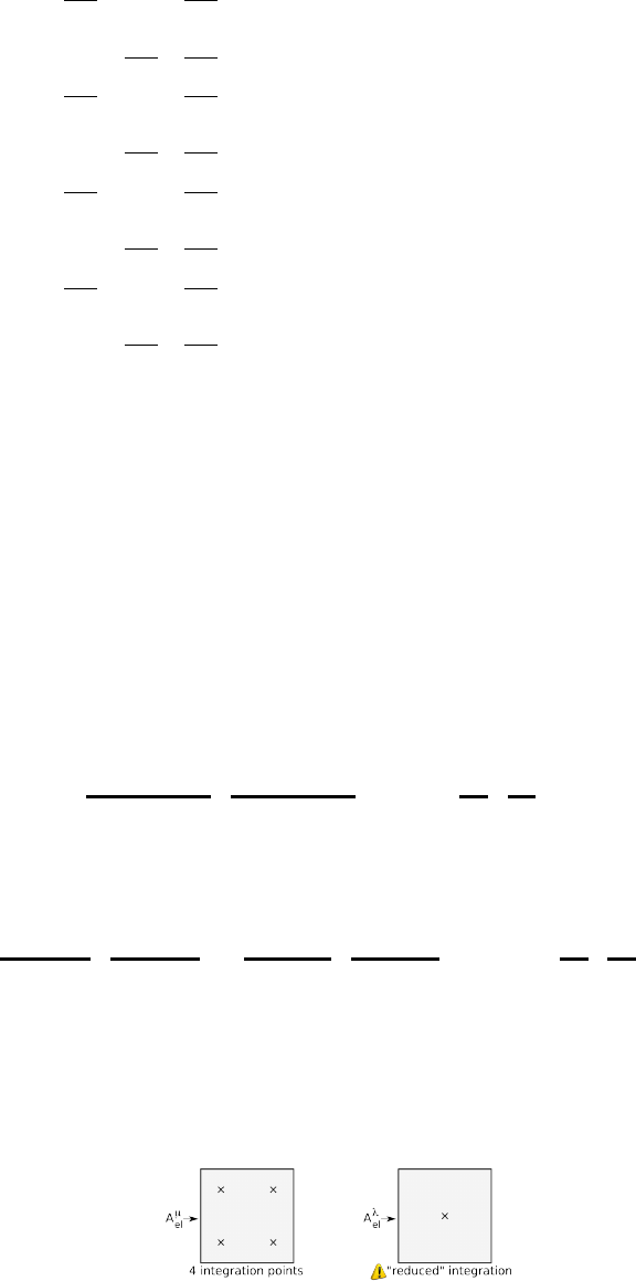
[36] have established the equivalence for incompressible problems between the reduced integration of the penalty
term and a mixed Finite Element approach if the pressure nodes coincide with the integration points of the reduced
rule.
In the end, the elimination of the pressure unknown in the Stokes equations replaces the original saddle-point
Stokes problem [3] by an elliptical problem, which leads to a symmetric positive definite (SPD) FEM matrix. This is
the major benefit of the penalized approach over the full indefinite solver with the velocity-pressure variables. Indeed,
the SPD character of the matrix lends itself to efficient solving stragegies and is less memory-demanding since it is
sufficient to store only the upper half of the matrix including the diagonal [22] . ToDo: list codes which use this
approach.
15

The stress tensor σis symmetric (i.e. σij =σji). For simplicity I will now focus on a Stokes flow in two dimensions.
Since the penalty formulation is only valid for incompressible flows, then ˙
=˙
dso that the dsuperscript is
ommitted in what follows. The stress tensor can also be cast in vector format:
σxx
σyy
σxy
=
−p
−p
0
+ 2η
˙xx
˙yy
˙xy
=λ
˙xx + ˙yy
˙xx + ˙yy
0
+ 2η
˙xx
˙yy
˙xy
=
λ
110
110
000
| {z }
K
+η
200
020
001
| {z }
C
·
∂u
∂x
∂v
∂y
∂u
∂y +∂v
∂x
Remember that
∂u
∂x =
4
X
i=1
∂Ni
∂x ui
∂v
∂y =
4
X
i=1
∂Ni
∂y vi
∂u
∂y +∂v
∂x =
4
X
i=1
∂Ni
∂y ui+
4
X
i=1
∂Ni
∂x vi
so that
∂u
∂x
∂v
∂y
∂u
∂y +∂v
∂x
=
∂N1
∂x 0∂N2
∂x 0∂N3
∂x 0∂N4
∂x 0
0∂N1
∂y 0∂N2
∂y 0∂N3
∂y 0∂N4
∂y
∂N1
∂y
∂N1
∂x
∂N2
∂y
∂N2
∂x
∂N3
∂y
∂N3
∂x
∂N3
∂y
∂N4
∂x
| {z }
B
·
u1
v1
u2
v2
u3
v3
u4
v4
| {z }
V
Finally,
~σ =
σxx
σyy
σxy
= (λK+ηC)·B·V
We will now establish the weak form of the momentum conservation equation. We start again from
∇·σ+b=0
For the Ni’s ’regular enough’, we can write:
ZΩe
Ni∇·σdΩ + ZΩe
NibdΩ=0
We can integrate by parts and drop the surface term1:
ZΩe
∇Ni·σdΩ = ZΩe
NibdΩ
or,
ZΩe
∂Ni
∂x 0∂Ni
∂y
0∂Ni
∂y
∂Ni
∂x
·
σxx
σyy
σxy
dΩ = ZΩe
NibdΩ
1We will come back to this at a later stage
16
Let i= 1,2,3,4 and stack the resulting four equations on top of one another.
ZΩe
∂N1
∂x 0∂N1
∂y
0∂N1
∂y
∂N1
∂x
·
σxx
σyy
σxy
dΩ = ZΩe
N1bx
bydΩ (36)
ZΩe
∂N2
∂x 0∂N2
∂y
0∂N2
∂y
∂N2
∂x
·
σxx
σyy
σxy
dΩ = ZΩe
Nibx
bydΩ (37)
ZΩe
∂N3
∂x 0∂N3
∂y
0∂N3
∂y
∂N3
∂x
·
σxx
σyy
σxy
dΩ = ZΩe
N3bx
bydΩ (38)
ZΩe
∂N4
∂x 0∂N4
∂y
0∂N4
∂y
∂N4
∂x
·
σxx
σyy
σxy
dΩ = ZΩe
N4bx
bydΩ (39)
We easily recognize BTinside the integrals! Let us define
NT
b= (N1bx, N1by, ...N4bx, N4by)
then we can write
ZΩe
BT·
σxx
σyy
σxy
dΩ = ZΩe
NbdΩ
and finally: ZΩe
BT·[λK+ηC]·B·VdΩ = ZΩe
NbdΩ
Since Vcontains the velocities at the corners, it does not depend on the xor ycoordinates so it can be taking outside
of the integral: ZΩe
BT·[λK+ηC]·BdΩ
| {z }
Ael(8×8)
·V
|{z}
(8x1)
=ZΩe
NbdΩ
| {z }
Bel(8×1)
or,
ZΩe
λBT·K·BdΩ
| {z }
Aλ
el(8×8)
+ZΩe
ηBT·C·BdΩ
| {z }
Aη
el(8×8)
·V
|{z}
(8x1)
=ZΩe
NbdΩ
| {z }
Bel(8×1)
INTEGRATION - MAPPING
1. partition domain Ω into elements Ωe,e= 1, ...nel.
2. loop over elements and for each element compute Ael,Bel
3. a node belongs to several elements
→need to assemble Ael and Bel in A,B
4. apply boundary conditions
5. solve system: x=A−1·B
6. visualise/analyse x
17
4 Additional techniques
4.1 The method of manufactured solutions
4.2 Sparse storage
4.3 Mesh generation
4.4 The value of the timestep
4.5 Tracking materials
4.6 Visco-Plasticity
4.7 Picard and Newton
4.8 The choice of solvers
4.9 The SUPG formulation for the energy equation
4.10 Tracking materials and/or interfaces
4.11 Dealing with a free surface
4.12 Pressure normalisation
18
so much to do ...
write about impose bc on el matrix
Q3Q2
full compressible
total energy calculations
constraints
compositions, marker chain
van keken initial value with deformed mesh
free-slip bc on annulus and sphere . See for example p540 Gresho and Sani book.
non-linear rheologies (two layer brick spmw16, tosn15)
Picard vs Newton
markers
Schur complement approach
periodic boundary conditions
open boundary conditions
free surface
SUPG
produce fastest version possible for convection box
zaleski disk advection
all kinds of interesting benchmarks
Busse convection pb, compare with aspect
cvi !!!
pure elastic
including phase changes (w. R. Myhill)
derivatives on nodes
Nusselt
discontinuous galerkin
formatting of code style
navier-stokes ? (LUKAS)
pressure smoothing
compute strainrate in middle of element or at quad point for punch?
GEO1442 code
GEO1442 indenter setup in plane ?
in/out flow on sides for lith modelling
Problems to solve:
colorscale
better yet simple matrix storage ?
19

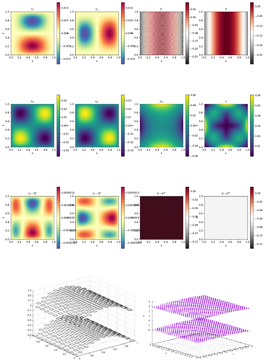
5fieldstone: simple analytical solution
From [15]. In order to illustrate the behavior of selected mixed finite elements in the solution of stationary Stokes
flow, we consider a two-dimensional problem in the square domain Ω = [0,1] ×[0,1], which possesses a closed-form
analytical solution. The problem consists of determining the velocity field v= (u, v) and the pressure psuch that
−ν∆v+∇p=bin Ω
∇·v= 0 in Ω
v=0on Γ
where the fluid viscosity is taken as ν= 1. The components of the body force bare prescribed as
bx= (12 −24y)x4+ (−24 + 48y)x3+ (−48y+ 72y2−48y3+ 12)x2
+(−2 + 24y−72y2+ 48y3)x+ 1 −4y+ 12y2−8y3
by= (8 −48y+ 48y2)x3+ (−12 + 72y−72y2)x2
+(4 −24y+ 48y2−48y3+ 24y4)x−12y2+ 24y3−12y4
With this prescribed body force, the exact solution is
u(x, y) = x2(1 −x)2(2y−6y2+ 4y3)
v(x, y) = −y2(1 −y)2(2x−6x2+ 4x3)
p(x, y) = x(1 −x)−1/6
Note that the pressure obeys RΩp dΩ=0
features
•Q1×P0element
•incompressible flow
•penalty formulation
•Dirichlet boundary conditions (no-slip)
•direct solver
•isothermal
•isoviscous
•analytical solution
20

0.000001
0.000010
0.000100
0.001000
0.010000
0.100000
0.01 0.1
error
h
velocity
pressure
x2
x1
Quadratic convergence for velocity error, linear convergence for pressure error, as expected.
ToDo:
pressure normalisation?
different cmat, a la schmalholz
To go further:
21
1. make your own analytical solution
22
6fieldstone: Stokes sphere
Viscosity and density directly computed at the quadrature points.
features
•Q1×P0element
•incompressible flow
•penalty formulation
•Dirichlet boundary conditions (free-slip)
•direct solver
•isothermal
•non-isoviscous
•buoyancy-driven flow
23

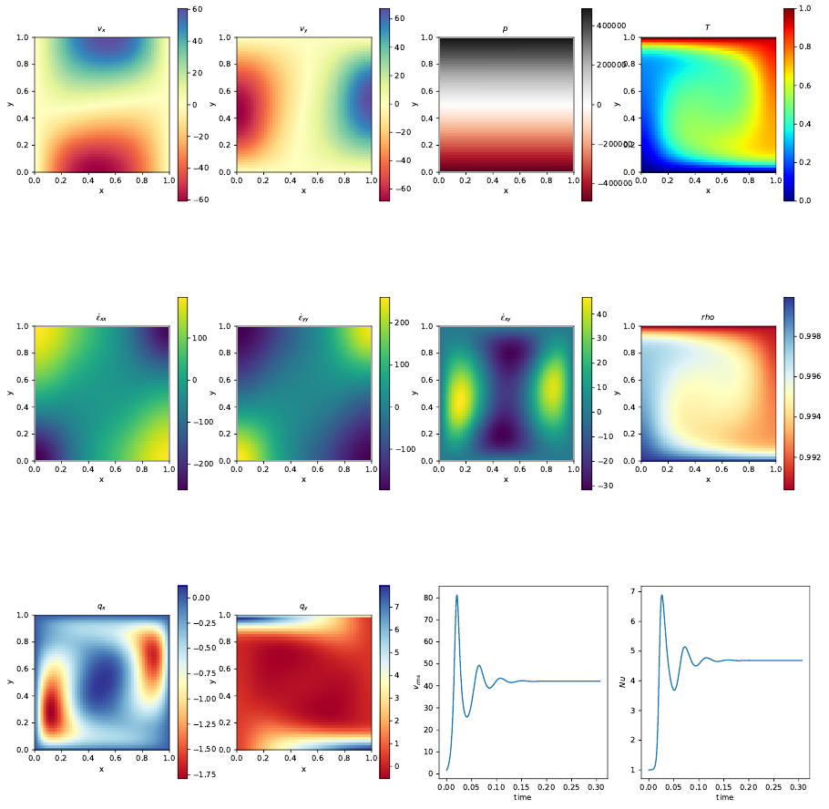
7fieldstone: Convection in a 2D box
This benchmark deals with the 2-D thermal convection of a fluid of infinite Prandtl number in a rectangular closed
cell. In what follows, I carry out the case 1a, 1b, and 1c experiments as shown in [5]: steady convection with constant
viscosity in a square box.
The temperature is fixed to zero on top and to ∆Tat the bottom, with reflecting symmetry at the sidewalls (i.e.
∂xT= 0) and there are no internal heat sources. Free-slip conditions are implemented on all boundaries.
The Rayleigh number is given by
Ra =αgy∆T h3
κν =αgy∆T h3ρ2cp
kµ (40)
In what follows, I use the following parameter values: Lx=Ly= 1,ρ0=cP=k=µ= 1, T0= 0, α= 10−2,
g= 102Ra and I run the model with Ra = 104,105and 106.
The initial temperature field is given by
T(x, y) = (1 −y)−0.01 cos(πx) sin(πy) (41)
The perturbation in the initial temperature fields leads to a perturbation of the density field and sets the fluid in
motion.
Depending on the initial Rayleigh number, the system ultimately reaches a steady state after some time.
The Nusselt number (i.e. the mean surface temperature gradient over mean bottom temperature) is computed as
follows [5]:
Nu =LyR∂T
∂y (y=Ly)dx
RT(y= 0)dx (42)
Note that in our case the denominator is equal to 1 since Lx= 1 and the temperature at the bottom is prescribed to
be 1.
Finally, the steady state root mean square velocity and Nusselt number measurements are indicated in Table ??
alongside those of [5] and [49]. (Note that this benchmark was also carried out and published in other publications
[54, 1, 20, 11, 34] but since they did not provide a complete set of measurement values, they are not included in the
table.)
Blankenbach et al Tackley [49]
Ra = 104Vrms 42.864947 ±0.000020 42.775
Nu 4.884409 ±0.000010 4.878
Ra = 105Vrms 193.21454 ±0.00010 193.11
Nu 10.534095 ±0.000010 10.531
Ra = 106Vrms 833.98977 ±0.00020 833.55
Nu 21.972465 ±0.000020 21.998
Steady state Nusselt number N u and Vrms measurements as reported in the literature.
features
•Q1×P0element
•incompressible flow
•penalty formulation
•Dirichlet boundary conditions (free-slip)
•Boussinesq approximation
•direct solver
•non-isothermal
•buoyancy-driven flow
•isoviscous
•CFL-condition
24
ToDo:
implement steady state criterion
reach steady state
do Ra=1e4, 1e5, 1e6
plot against blankenbach paper and aspect
look at critical Ra number
25

8fieldstone: solcx benchmark
The SolCx benchmark is intended to test the accuracy of the solution to a problem that has a large jump in the
viscosity along a line through the domain. Such situations are common in geophysics: for example, the viscosity in a
cold, subducting slab is much larger than in the surrounding, relatively hot mantle material.
The SolCx benchmark computes the Stokes flow field of a fluid driven by spatial density variations, subject to a
spatially variable viscosity. Specifically, the domain is Ω = [0,1]2, gravity is g= (0,−1)Tand the density is given by
ρ(x, y) = sin(πy) cos(πx) (43)
Boundary conditions are free slip on all of the sides of the domain and the temperature plays no role in this benchmark.
The viscosity is prescribed as follows:
µ(x, y) = 1for x < 0.5
106for x > 0.5(44)
Note the strongly discontinuous viscosity field yields a stagnant flow in the right half of the domain and thereby yields
a pressure discontinuity along the interface.
The SolCx benchmark was previously used in [18] (references to earlier uses of the benchmark are available there)
and its analytic solution is given in [57]. It has been carried out in [32] and [21]. Note that the source code which
evaluates the velocity and pressure fields for both SolCx and SolKz is distributed as part of the open source package
Underworld ([39], http://underworldproject.org).
In this particular example, the viscosity is computed analytically at the quadrature points (i.e. tracers are not
used to attribute a viscosity to the element). If the number of elements is even in any direction, all elements (and
their associated quadrature points) have a constant viscosity(1 or 106). If it is odd, then the elements situated at the
viscosity jump have half their integration points with µ= 1 and half with µ= 106(which is a pathological case since
the used quadrature rule inside elements cannot represent accurately such a jump).
features
•Q1×P0element
•incompressible flow
•penalty formulation
•Dirichlet boundary conditions (free-slip)
•direct solver
•isothermal
•non-isoviscous
•analytical solution
26
What we learn from this
27
9fieldstone: solkz benchmark
The SolKz benchmark [44] is similar to the SolCx benchmark. but the viscosity is now a function of the space
coordinates:
µ(y) = exp(By) with B= 13.8155 (45)
It is however not a discontinuous function but grows exponentially with the vertical coordinate so that its overall
variation is again 106. The forcing is again chosen by imposing a spatially variable density variation as follows:
ρ(x, y) = sin(2y) cos(3πx) (46)
Free slip boundary conditions are imposed on all sides of the domain. This benchmark is presented in [57] as well and
is studied in [18] and [21].
0.00000001
0.00000010
0.00000100
0.00001000
0.00010000
0.00100000
0.01000000
0.10000000
0.01 0.1
error
h
velocity
pressure
x2
x1
28

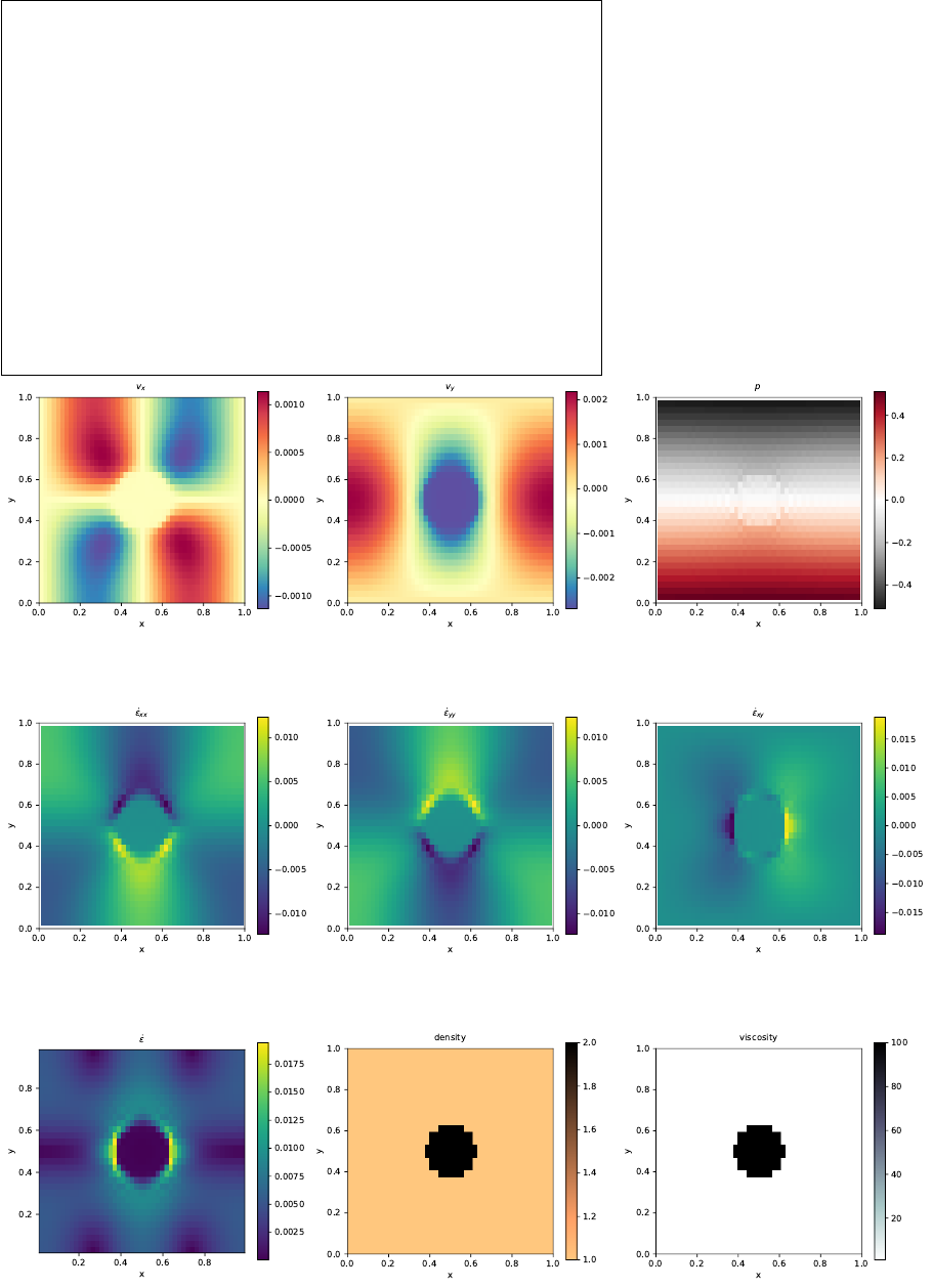
10 fieldstone: solvi benchmark
Following SolCx and SolKz, the SolVi inclusion benchmark solves a problem with a discontinuous viscosity field, but
in this case the viscosity field is chosen in such a way that the discontinuity is along a circle. Given the regular nature
of the grid used by a majority of codes and the present one, this ensures that the discontinuity in the viscosity never
aligns to cell boundaries. This in turns leads to almost discontinuous pressures along the interface which are difficult to
represent accurately. [46] derived a simple analytic solution for the pressure and velocity fields for a circular inclusion
under simple shear and it was used in [13], [48], [18], [32] and [21].
Because of the symmetry of the problem, we only have to solve over the top right quarter of the domain (see Fig.
??a).
The analytical solution requires a strain rate boundary condition (e.g., pure shear) to be applied far away from the
inclusion. In order to avoid using very large domains and/or dealing with this type of boundary condition altogether,
the analytical solution is evaluated and imposed on the boundaries of the domain. By doing so, the truncation error
introduced while discretizing the strain rate boundary condition is removed.
A characteristic of the analytic solution is that the pressure is zero inside the inclusion, while outside it follows the
relation
pm= 4˙µm(µi−µm)
µi+µm
r2
i
r2cos(2θ) (47)
where µi= 103is the viscosity of the inclusion and µm= 1 is the viscosity of the background media, θ= tan−1(y/x),
and ˙= 1 is the applied strain rate.
[13] thoroughly investigated this problem with various numerical methods (FEM, FDM), with and without tracers,
and conclusively showed how various averagings lead to different results. [18] obtained a first order convergence for
both pressure and velocity, while [32] and [21] showed that the use of adaptive mesh refinement in respectively the
FEM and FDM yields convergence rates which depend on refinement strategies.
29

0.00000001
0.00000010
0.00000100
0.00001000
0.00010000
0.00100000
0.01000000
0.10000000
1.00000000
10.00000000
0.01 0.1
error
h
velocity
pressure
x2
x1
30
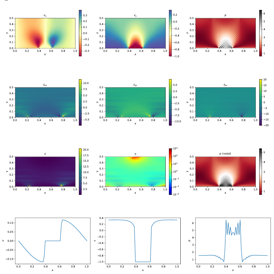
11 fieldstone: the indentor benchmark
The punch benchmark is one of the few boundary value problems involving plastic solids for which there exists an
exact solution. Such solutions are usually either for highly simplified geometries (spherical or axial symmetry, for
instance) or simplified material models (such as rigid plastic solids) [30].
In this experiment, a rigid punch indents a rigid plastic half space; the slip line field theory gives exact solutions
as shown in Fig. ??a. The plane strain formulation of the equations and the detailed solution to the problem were
derived in the Appendix of [53] and are also presented in [19].
The two dimensional punch problem has been extensively studied numerically for the past 40 years [60, 59, 9, 8, 27,
56, 6, 42] and has been used to draw a parallel with the tectonics of eastern China in the context of the India-Eurasia
collision [51, 38]. It is also worth noting that it has been carried out in one form or another in series of analogue
modelling articles concerning the same region, with a rigid indenter colliding with a rheologically stratified lithosphere
[40, 12, 29].
Numerically, the one-time step punch experiment is performed on a two-dimensional domain of purely plastic
von Mises material. Given that the von Mises rheology yield criterion does not depend on pressure, the density of
the material and/or the gravity vector is set to zero. Sides are set to free slip boundary conditions, the bottom to
no slip, while a vertical velocity (0,−vp) is prescribed at the top boundary for nodes whose xcoordinate is within
[Lx/2−δ/2, Lx/2 + δ/2].
The following parameters are used: Lx= 1, Ly= 0.5, µmin = 10−3,µmax = 103,vp= 1, δ= 0.123456789 and the
yield value of the material is set to k= 1.
The analytical solution predicts that the angle of the shear bands stemming from the sides of the punch is π/4,
that the pressure right under the punch is 1 + π, and that the velocity of the rigid blocks on each side of the punch is
vp/√2 (this is simply explained by invoking conservation of mass).
31

ToDo: smooth punch
features
•Q1×P0element
•incompressible flow
•penalty formulation
•Dirichlet boundary conditions (no-slip)
•isothermal
•non-isoviscous
•nonlinear rheology
32

12 fieldstone: the annulus benchmark
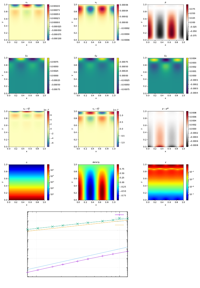
This benchmark is based on Thieulot & Puckett [Subm.] in which an analytical solution to the isoviscous incompressible
Stokes equations is derived in an annulus geometry. The velocity and pressure fields are as follows:
vr(r, θ) = g(r)ksin(kθ),(48)
vθ(r, θ) = f(r) cos(kθ),(49)
p(r, θ) = kh(r) sin(kθ),(50)
ρ(r, θ) = ℵ(r)ksin(kθ),(51)
with
f(r) = Ar +B/r, (52)
g(r) = A
2r+B
rln r+C
r,(53)
h(r) = 2g(r)−f(r)
r,(54)
ℵ(r) = g00 −g0
r−g
r2(k2−1) + f
r2+f0
r,(55)
A=−C2(ln R1−ln R2)
R2
2ln R1−R2
1ln R2
,(56)
B=−CR2
2−R2
1
R2
2ln R1−R2
1ln R2
.(57)
The parameters Aand Bare chosen so that vr(R1) = vr(R2) = 0, i.e. the velocity is tangential to both inner
and outer surfaces. The gravity vector is radial and of unit length. In the present case, we set R1= 1, R2= 2 and
C=−1.
features
•Q1×P0element
•incompressible flow
•penalty formulation
•Dirichlet boundary conditions
•direct solver
•isothermal
•isoviscous
•analytical solution
•annulus geometry
•elemental boundary conditions
33

0.0001
0.001
0.01
0.1
1
10
0.01
error
h
velocity
pressure
x2
x1
34
13 fieldstone: stokes sphere (3D) - penalty
features
•Q1×P0element
•incompressible flow
•penalty formulation
•Dirichlet boundary conditions (free-slip)
•direct solver
•isothermal
•non-isoviscous
•3D
•elemental b.c.
•buoyancy driven
resolution is 24x24x24
35


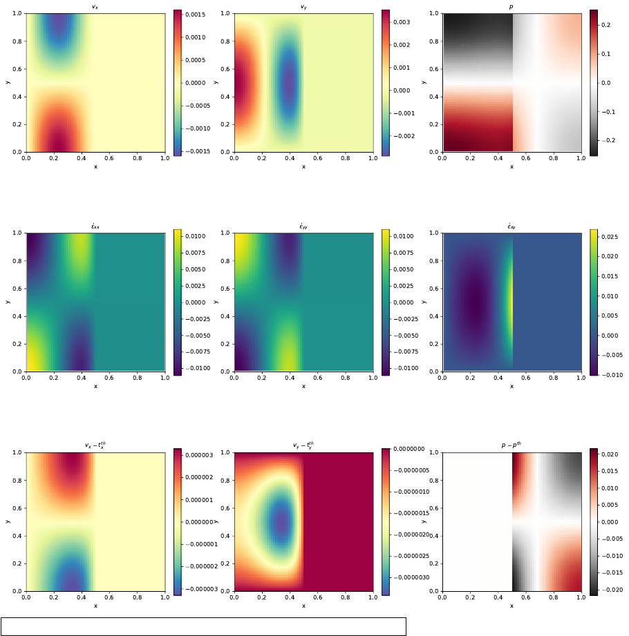
15 fieldstone: consistent pressure recovery
p=−λ∇·v
q1is smoothed pressure obtained with the center-to-node approach.
q2is recovered pressure obtained with [58].
All three fulfill the zero average condition: RpdΩ = 0.
0.000001
0.000010
0.000100
0.001000
0.010000
0.100000
0.01 0.1
error
h
velocity
pressure (el)
pressure (q1)
pressure (q2)
x2
x1
In terms of pressure error, q2is better than q1which is better than elemental.
QUESTION: why are the averages exactly zero ?!
TODO:
•add randomness to internal node positions.
•look at elefant algorithms
37
16 fieldstone: the Particle in Cell technique (1) - the effect of averaging
features
•Q1×P0element
•incompressible flow
•penalty formulation
•Dirichlet boundary conditions (no-slip)
•isothermal
•non-isoviscous
•particle-in-cell
After the initial setup of the grid, markers can then be generated and placed in the domain. One could simply
randomly generate the marker positions in the whole domain but unless a very large number of markers is used, the
chance that an element does not contain any marker exists and this will prove problematic. In order to get a better
control over the markers spatial distribution, one usually generates the marker per element, so that the total number
of markers in the domain is the product of the number of elements times the user-chosen initial number of markers
per element.
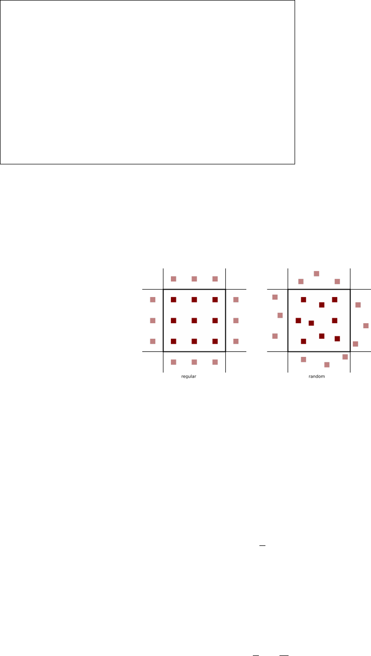
Our next concern is how to actually place the markers inside an element. Two methods come to mind: on a regular
grid, or in a random manner, as shown on the following figure:
In both cases we make use of the basis shape functions: we generate the positions of the markers (random or
regular) in the reference element first (rim, sim), and then map those out to the real element as follows:
xim =
m
X
i
Ni(rim, sim)xiyim =
m
X
i
Ni(rim, sim)yi
where xi, yiare the coordinates of the vertices of the element.
When using active markers, one is faced with the problem of transferring the properties they carry to the mesh on
which the PDEs are to be solved. As we have seen, building the FE matrix involves a loop over all elements, so one
simple approach consists of assigning each element a single property computed as the average of the values carried by
the markers in that element. Often in colloquial language ”average” refers to the arithmetic mean:
hφiam =1
n
n
X
k
φi
where <φ>am is the arithmetic average of the nnumbers φi. However, in mathematics other means are commonly
used, such as the geometric mean:
hφigm = n
Y
i
φi!
and the harmonic mean:
hφihm = 1
n
n
X
i
1
φi!−1
Furthermore, there is a well known inequality for any set of positive numbers,
hφiam ≥ hφigm ≥ hφihm
38
which will prove to be important later on.
Let us now turn to a simple concrete example: the 2D Stokes sphere. There are two materials in the domain, so
that markers carry the label ”mat=1” or ”mat=2”. For each element an average density and viscosity need to be
computed. The majority of elements contains markers with a single material label so that the choice of averaging does
not matter (it is trivial to verify that if φi=φ0then hφiam =hφigm =hφihm =φ0. Remain the elements crossed by
the interface between the two materials: they contain markers of both materials and the average density and viscosity
inside those depends on 1) the total number of markers inside the element, 2) the ratio of markers 1 to markers 2, 3)
the type of averaging.
This averaging problem has been studied and documented in the literature [45, 13, 52, 41]
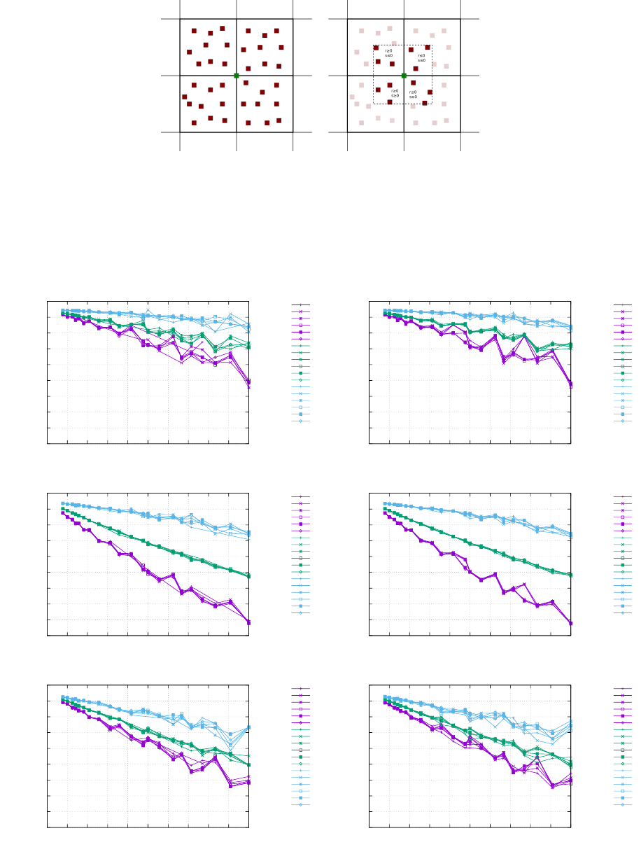
Nodal projection. Left: all markers inside elements to which the green node belongs to are taken into account.
Right: only the markers closest to the green node count.
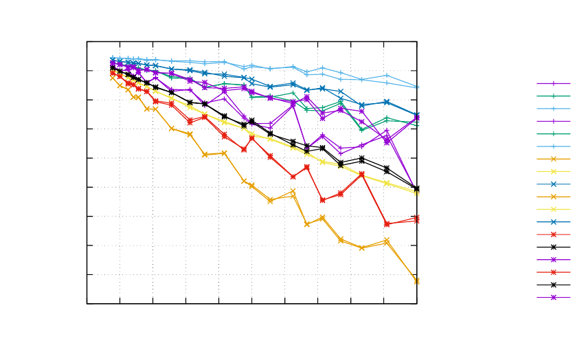
The setup is identical as the Stokes sphere experiment. The bash script runall runs the code for many resolutions,
both initial marker distribution and all three averaging types. The viscosity of the sphere has been set to 103while
the viscosity of the surrounding fluid is 1. The average density is always computed with an arithmetic mean. Root
mean square velocity results are shown hereunder:
0.001
0.002
0.003
0.004
0.005
0.006
0.007
0.008
0.009
0.01
0 0.01 0.02 0.03 0.04 0.05 0.06 0.07 0.08 0.09 0.1
vrms
h
random markers, elemental proj
am, 09 m
am, 16 m
am, 25 m
am, 36 m
am, 48 m
am, 64 m
gm, 09 m
gm, 16 m
gm, 25 m
gm, 36 m
gm, 48 m
gm, 64 m
hm, 09 m
hm, 16 m
hm, 25 m
hm, 36 m
hm, 48 m
hm, 64 m
0.001
0.002
0.003
0.004
0.005
0.006
0.007
0.008
0.009
0.01
0 0.01 0.02 0.03 0.04 0.05 0.06 0.07 0.08 0.09 0.1
vrms
h
regular markers, elemental proj
am, 09 m
am, 16 m
am, 25 m
am, 36 m
am, 48 m
am, 64 m
gm, 09 m
gm, 16 m
gm, 25 m
gm, 36 m
gm, 48 m
gm, 64 m
hm, 09 m
hm, 16 m
hm, 25 m
hm, 36 m
hm, 48 m
hm, 64 m
0.001
0.002
0.003
0.004
0.005
0.006
0.007
0.008
0.009
0.01
0 0.01 0.02 0.03 0.04 0.05 0.06 0.07 0.08 0.09 0.1
vrms
h
random markers, nodal proj
am, 09 m
am, 16 m
am, 25 m
am, 36 m
am, 48 m
am, 64 m
gm, 09 m
gm, 16 m
gm, 25 m
gm, 36 m
gm, 48 m
gm, 64 m
hm, 09 m
hm, 16 m
hm, 25 m
hm, 36 m
hm, 48 m
hm, 64 m
0.001
0.002
0.003
0.004
0.005
0.006
0.007
0.008
0.009
0.01
0 0.01 0.02 0.03 0.04 0.05 0.06 0.07 0.08 0.09 0.1
vrms
h
regular markers, nodal proj
am, 09 m
am, 16 m
am, 25 m
am, 36 m
am, 48 m
am, 64 m
gm, 09 m
gm, 16 m
gm, 25 m
gm, 36 m
gm, 48 m
gm, 64 m
hm, 09 m
hm, 16 m
hm, 25 m
hm, 36 m
hm, 48 m
hm, 64 m
0.001
0.002
0.003
0.004
0.005
0.006
0.007
0.008
0.009
0.01
0 0.01 0.02 0.03 0.04 0.05 0.06 0.07 0.08 0.09 0.1
vrms
h
random markers, nodal proj
am, 09 m
am, 16 m
am, 25 m
am, 36 m
am, 48 m
am, 64 m
gm, 09 m
gm, 16 m
gm, 25 m
gm, 36 m
gm, 48 m
gm, 64 m
hm, 09 m
hm, 16 m
hm, 25 m
hm, 36 m
hm, 48 m
hm, 64 m
0.001
0.002
0.003
0.004
0.005
0.006
0.007
0.008
0.009
0.01
0 0.01 0.02 0.03 0.04 0.05 0.06 0.07 0.08 0.09 0.1
vrms
h
regular markers, nodal proj
am, 09 m
am, 16 m
am, 25 m
am, 36 m
am, 48 m
am, 64 m
gm, 09 m
gm, 16 m
gm, 25 m
gm, 36 m
gm, 48 m
gm, 64 m
hm, 09 m
hm, 16 m
hm, 25 m
hm, 36 m
hm, 48 m
hm, 64 m
39
Conclusions:
•With increasing resolution (h→0) vrms values seem to converge towards a single value, irrespective of the
number of markers.
•At low resolution, say 32x32 (i.e. h=0.03125), vrms values for the three averagings differ by about 10%. At
higher resolution, say 128x128, vrms values are still not converged.
•The number of markers per element plays a role at low resolution, but less and less with increasing resolution.
•Results for random and regular marker distributions are not identical but follow a similar trend and seem to
converge to the same value.
•At low resolutions, elemental values yield better results.
•harmonic mean yields overal the best results
0.001
0.002
0.003
0.004
0.005
0.006
0.007
0.008
0.009
0.01
0 0.01 0.02 0.03 0.04 0.05 0.06 0.07 0.08 0.09 0.1
vrms
h
64 markers per element
am, reg, el
gm, reg, el
hm, reg, el
am, rand, el
gm, rand, el
hm, rand, el
am, reg, nod1
gm, reg, nod1
hm, reg, nod1
am, rand, nod1
gm, rand, nod1
hm, rand, nod1
am, reg, nod2
gm, reg, nod2
hm, reg, nod2
am, rand, nod2
gm, rand, nod2
hm, rand, nod2
40

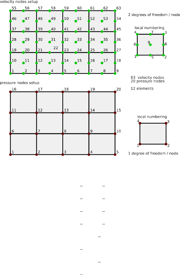
17 fieldstone: solving the full saddle point problem
The details of the numerical setup are presented in Section 5.
The main difference is that we no longer use the penalty formulation and therefore keep both velocity and pressure
as unknowns. Therefore we end up having to solve the following system:
K G
GT0·V
P=f
hor,A·X=rhs
Each block K,Gand vector f,hare built separately in the code and assembled into the matrix Aand vector rhs
afterwards. Aand rhs are then passed to the solver. We will see later that there are alternatives to solve this approach
which do not require to build the full Stokes matrix A.
Each element has m= 4 vertices so in total ndof V ×m= 8 velocity dofs and a single pressure dof, commonly
situated in the center of the element. The total number of velocity dofs is therefore NfemV =nnp ×ndofV while
the total number of pressure dofs is N femP =nel. The total number of dofs is then Nfem =NfemV +NfemP .
As a consequence, matrix Khas size NfemV, NfemV and matrix Ghas size NfemV, Nf emP . Vector fis of size
NfemV and vector his of size N femP .
features
•Q1×P0element
•incompressible flow
•mixed formulation
•Dirichlet boundary conditions (no-slip)
•direct solver (?)
•isothermal
•isoviscous
•analytical solution
•pressure smoothing
41
Unlike the results obtained with the penalty formualtion (see Section 5), the pressure showcases a very strong
checkerboard pattern, similar to the one in [16].
Left: pressure solution as shown in [16]; Right: pressure solution obtained with fieldstone.
Rather interestingly, the nodal pressure (obtained with a simple center-to-node algorithm) fails to recover a correct
pressure at the four corners.
42

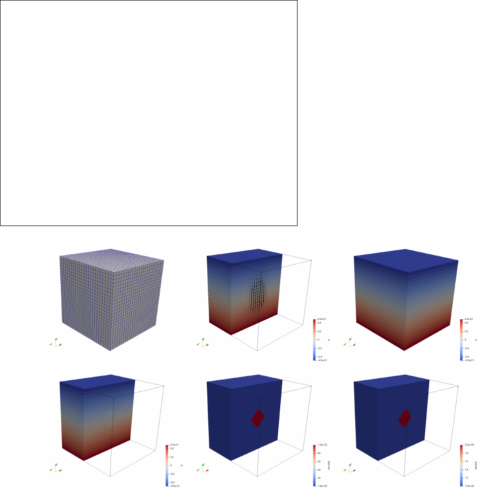
18 fieldstone: solving the full saddle point problem in 3D
When using Q1×P0elements, this benchmark fails because of the Dirichlet b.c. on all 6 sides and all three components.
However, as we will see, it does work well with Q2×Q1elements. .
This benchmark begins by postulating a polynomial solution to the 3D Stokes equation [14]:
v=
x+x2+xy +x3y
y+xy +y2+x2y2
−2z−3xz −3yz −5x2yz
(58)
and
p=xyz +x3y3z−5/32 (59)
While it is then trivial to verify that this velocity field is divergence-free, the corresponding body force of the Stokes
equation can be computed by inserting this solution into the momentum equation with a given viscosity µ(constant
or position/velocity/strain rate dependent). The domain is a unit cube and velocity boundary conditions simply use
Eq. (58). Following [7], the viscosity is given by the smoothly varying function
µ= exp(1 −β(x(1 −x) + y(1 −y) + z(1 −z))) (60)
One can easily show that the ratio of viscosities µ?in the system follows µ?= exp(−3β/4) so that choosing β= 10
yields µ?'1808 and β= 20 yields µ?'3.269 ×10⁶.
We start from the momentum conservation equation:
−∇p+∇·(2µ˙
) = f
The x-component of this equation writes
fx=−∂p
∂x +∂
∂x (2µ˙xx) + ∂
∂y (2µ˙xy ) + ∂
∂z (2µ˙xz ) (61)
=−∂p
∂x + 2µ∂
∂x ˙xx + 2µ∂
∂y ˙xy + 2µ∂
∂z ˙xz + 2 ∂µ
∂x ˙xx + 2 ∂µ
∂y ˙xy + 2 ∂µ
∂z ˙xz (62)
Let us compute all the block separately:
˙xx = 1 + 2x+y+ 3x2y
˙yy = 1 + x+ 2y+ 2x2y
˙zz =−2−3x−3y−5x2y
2˙xy = (x+x3)+(y+ 2xy2) = x+y+ 2xy2+x3
2˙xz = (0) + (−3z−10xyz) = −3z−10xyz
2˙yz = (0) + (−3z−5x2z) = −3z−5x2z
In passing, one can verify that ˙xx + ˙yy + ˙zz = 0. We further have
∂
∂x 2 ˙xx = 2(2 + 6xy)
∂
∂y 2 ˙xy = 1 + 4xy
∂
∂z 2 ˙xz =−3−10xy
∂
∂x 2 ˙xy = 1 + 2y2+ 3x2
∂
∂y 2 ˙yy = 2(2 + 2x2)
∂
∂z 2 ˙yz =−3−5x2
∂
∂x 2 ˙xz =−10yz
∂
∂y 2 ˙yz = 0
∂
∂z 2 ˙zz = 2(0)
43

∂p
∂x =yz + 3x2y3z(63)
∂p
∂y =xz + 3x3y2z(64)
∂p
∂z =xy +x3y3(65)
Pressure normalisation Here again, because Dirichlet boundary conditions are prescribed on all sides the pressure
is known up to an arbitrary constant. This constant can be determined by (arbitrarily) choosing to normalised the
pressure field as follows: ZΩ
p dΩ = 0 (66)
This is a single constraint associated to a single Lagrange multiplier λand the global Stokes system takes the form
K G 0
GT0C
0CT0
V
P
λ
In this particular case the constraint matrix Cis a vector and it only acts on the pressure degrees of freedom because
of Eq.(66). Its exact expression is as follows:
ZΩ
p dΩ = X
eZΩe
p dΩ = X
eZΩeX
i
Np
ipidΩ = X
eX
iZΩe
Np
idΩpi=X
eCe·pe
where peis the list of pressure dofs of element e. The elemental constraint vector contains the corresponding pressure
basis functions integrated over the element. These elemental constraints are then assembled into the vector C.
18.0.1 Constant viscosity
Choosing β= 0 yields a constant velocity µ(x, y, z) = exp(1) '2.718 (and greatly simplifies the right-hand side) so
that
∂
∂x µ(x, y, z) = 0 (67)
∂
∂y µ(x, y, z) = 0 (68)
∂
∂z µ(x, y, z) = 0 (69)
and
fx=−∂p
∂x + 2µ∂
∂x ˙xx + 2µ∂
∂y ˙xy + 2µ∂
∂z ˙xz
=−(yz + 3x2y3z) + 2(2 + 6xy) + (1 + 4xy)+(−3−10xy)
=−(yz + 3x2y3z) + µ(2 + 6xy)
fy=−∂p
∂y + 2µ∂
∂x ˙xy + 2µ∂
∂y ˙yy + 2µ∂
∂z ˙yz
=−(xz + 3x3y2z) + µ(1 + 2y2+ 3x2) + µ2(2 + 2x2) + µ(−3−5x2)
=−(xz + 3x3y2z) + µ(2 + 2x2+ 2y2)
fz=−∂p
∂z + 2µ∂
∂x ˙xz + 2µ∂
∂y ˙yz + 2µ∂
∂z ˙zz
=−(xy +x3y3) + µ(−10yz)+0+0
=−(xy +x3y3) + µ(−10yz)
Finally
f=−
yz + 3x2y3z
xz + 3x3y2z
xy +x3y3
+µ
2+6xy
2+2x2+ 2y2
−10yz
Note that there seems to be a sign problem with Eq.(26) in [7].
44
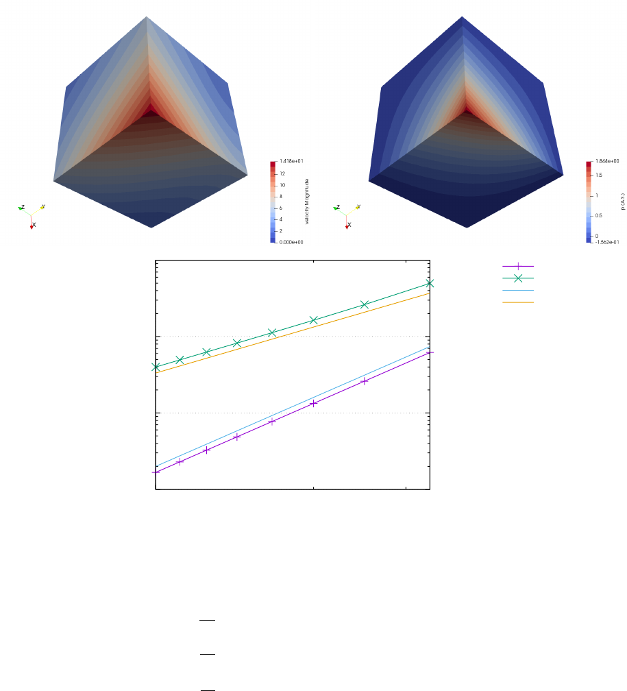
0.00001
0.00010
0.00100
0.01000
0.1
error
h
velocity
pressure
x3
x2
18.0.2 Variable viscosity
The spatial derivatives of the viscosity are then given by
∂
∂x µ(x, y, z) = −(1 −2x)βµ(x, y, z)
∂
∂y µ(x, y, z) = −(1 −2y)βµ(x, y, z)
∂
∂z µ(x, y, z) = −(1 −2z)βµ(x, y, z)
and thr right-hand side by
f=−
yz + 3x2y3z
xz + 3x3y2z
xy +x3y3
+µ
2+6xy
2+2x2+ 2y2
−10yz
(70)
−(1 −2x)βµ(x, y, z)
2˙xx
2˙xy
2˙xz
−(1 −2y)βµ(x, y, z)
2˙xy
2˙yy
2˙yz
−(1 −2z)βµ(x, y, z)
2˙xz
2˙yz
2˙zz
=−
yz + 3x2y3z
xz + 3x3y2z
xy +x3y3
+µ
2+6xy
2+2x2+ 2y2
−10yz
−(1 −2x)βµ
2+4x+ 2y+ 6x2y
x+y+ 2xy2+x3
−3z−10xyz
−(1 −2y)βµ
x+y+ 2xy2+x3
2+2x+ 4y+ 4x2y
−3z−5x2z
−(1 −2z)βµ
−3z−10xyz
−3z−5x2z
−4−6x−6y−10x2y
Note that at (x, y, z) = (0,0,0), µ= exp(1), and at (x, y, z) = (0.5,0.5,0.5), µ= exp(1 −3β/4) so that the
45

maximum viscosity ratio is given by
µ?=exp(1 −3β/4)
exp(1) = exp(−3β/4)
By varying βbetween 1 and 22 we can get up to 7 orders of magnitude viscosity difference.
features
•Q1×P0element
•incompressible flow
•saddle point system
•Dirichlet boundary conditions (free-slip)
•direct solver
•isothermal
•non-isoviscous
•3D
•elemental b.c.
•analytical solution
46
19 fieldstone: solving the full saddle point problem with Q2×Q1ele-
ments
The details of the numerical setup are presented in Section 5.
Each element has mV= 9 vertices so in total ndofV×mV= 18 velocity dofs and ndofP∗mP= 4 pressure dofs.
The total number of velocity dofs is therefore NfemV =nnp ×ndof V while the total number of pressure dofs is
NfemP =nel. The total number of dofs is then Nfem =Nf emV +N femP .
As a consequence, matrix Khas size NfemV, NfemV and matrix Ghas size NfemV, Nf emP . Vector fis of size
NfemV and vector his of size N femP .
renumber all nodes to start at zero!! Also internal numbering does not work here
The velocity shape functions are given by:
NV
0=1
2r(r−1)1
2s(s−1)
NV
1=1
2r(r+ 1)1
2s(s−1)
NV
2=1
2r(r+ 1)1
2s(s+ 1)
NV
3=1
2r(r−1)1
2s(s+ 1)
NV
4= (1 −r2)1
2s(s−1)
NV
5=1
2r(r+ 1)(1 −s2)
NV
6= (1 −r2)1
2s(s+ 1)
NV
7=1
2r(r−1)(1 −s2)
NV
8= (1 −r2)(1 −s2)
47

and their derivatives:
∂NV
0
∂r =1
2(2r−1)1
2s(s−1)
∂NV
1
∂r =1
2(2r+ 1)1
2s(s−1)
∂NV
2
∂r =1
2(2r+ 1)1
2s(s+ 1)
∂NV
3
∂r =1
2(2r−1)1
2s(s+ 1)
∂NV
4
∂r = (−2r)1
2s(s−1)
∂NV
5
∂r =1
2(2r+ 1)(1 −s2)
∂NV
6
∂r = (−2r)1
2s(s+ 1)
∂NV
7
∂r =1
2(2r−1)(1 −s2)
∂NV
8
∂r = (−2r)(1 −s2)
∂NV
0
∂s =1
2r(r−1)1
2(2s−1)
∂NV
1
∂s =1
2r(r+ 1)1
2(2s−1)
∂NV
2
∂s =1
2r(r+ 1)1
2(2s+ 1)
∂NV
3
∂s =1
2r(r−1)1
2(2s+ 1)
∂NV
4
∂s = (1 −r2)1
2(2s−1)
∂NV
5
∂s =1
2r(r+ 1)(−2s)
∂NV
6
∂s = (1 −r2)1
2(2s+ 1)
∂NV
7
∂s =1
2r(r−1)(−2s)
∂NV
8
∂s = (1 −r2)(−2s)
features
•Q2×Q1element
•incompressible flow
•mixed formulation
•Dirichlet boundary conditions (no-slip)
•isothermal
•isoviscous
•analytical solution
48
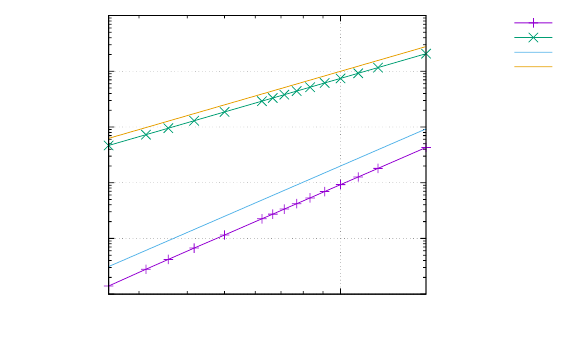
0.0000001
0.0000010
0.0000100
0.0001000
0.0010000
0.0100000
0.1
error
h
velocity
pressure
x3
x2
49
20 fieldstone: The non-conforming Q1×P0element
features
•Non-conforming Q1×P0element
•incompressible flow
•mixed formulation
•isothermal
•non-isoviscous
•analytical solution
•pressure smoothing
try Q1 mapping instead of isoparametric.
50

22 fieldstone: compressible flow (1)
We first start with an isothermal Stokes flow, so that we disregard the heat transport equation and the equations we
wish to solve are simply:
−∇ · 2η˙ε(v)−1
3(∇ · v)1+∇p=ρgin Ω,(71)
∇ · (ρv) = 0 in Ω (72)
The second equation can be rewritten ∇ · (ρv) = ρ∇ · v+v·∇ρ= 0 or,
∇ · v+1
ρv·∇ρ= 0
Note that this presupposes that the density is not zero anywhere in the domain.
We use a mixed formulation and therefore keep both velocity and pressure as unknowns. We end up having to
solve the following system:
K G
GT+Z0·V
P=f
hor,A·X=rhs
Where Kis the stiffness matrix, Gis the discrete gradient operator, GTis the discrete divergence operator, Vthe
velocity vector, Pthe pressure vector. Note that the term ZVderives from term v·∇ρin the continuity equation.
Each block K,G,Zand vectors fand hare built separately in the code and assembled into the matrix Aand
vector rhs afterwards. Aand rhs are then passed to the solver. We will see later that there are alternatives to solve
this approach which do not require to build the full Stokes matrix A.
Remark: the term ZVis often put in the rhs (i.e. added to h) so that the matrix Aretains the same structure as
in the incompressible case. This is indeed how it is implemented in ASPECT. This however requires more work since
the rhs depends on the solution and some form of iterations is needed.
In the case of a compressible flow the strain rate tensor and the deviatoric strain rate tensor are no more equal
(since ∇·v6= 0). The deviatoric strainrate tensor is given by2
˙
d(v) = ˙
(v)−1
3T r(˙
)1=˙
(v)−1
3(∇·v)1
In that case:
˙d
xx =∂u
∂x −1
3∂u
∂x +∂v
∂y =2
3
∂u
∂x −1
3
∂v
∂y (73)
˙d
yy =∂v
∂y −1
3∂u
∂x +∂v
∂y =−1
3
∂u
∂x +2
3
∂v
∂y (74)
2˙d
xy =∂u
∂y +∂v
∂x (75)
and then
˙
d(v) =
2
3
∂u
∂x −1
3
∂v
∂y
1
2
∂u
∂y +1
2
∂v
∂x
1
2
∂u
∂y +1
2
∂v
∂x −1
3
∂u
∂x +2
3
∂v
∂y
From ~τ = 2η~dwe arrive at:
τxx
τyy
τxy
= 2η
˙d
xx
˙d
yy
˙d
xy
= 2η
2/3−1/3 0
−1/3 2/3 0
0 0 1/2
·
∂u
∂x
∂v
∂y
∂u
∂y +∂v
∂x
=η
4/3−2/3 0
−2/3 4/3 0
0 0 1
·
∂u
∂x
∂v
∂y
∂u
∂y +∂v
∂x
or,
~τ =CηBV
2See the ASPECT manual for a justification of the 3 value in the denominator in 2D and 3D.
52

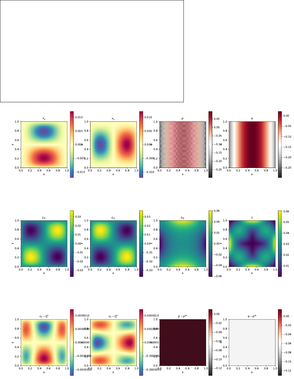
In order to test our implementation we have created a few manufactured solutions:
•benchmark #1 (ibench=1)): Starting from a density profile of:
ρ(x, y) = xy (76)
We derive a velocity given by:
vx(x, y) = Cx
x, vy(x, y) = Cy
y(77)
With gx(x, y) = 1
xand gy(x, y) = 1
y, this leads us to a pressure profile:
p=−η4Cx
3x2+4Cy
3y2+xy +C0(78)
This gives us a strain rate:
˙xx =−Cx
x2˙yy =−Cy
y2˙xy = 0
In what follows, we choose η= 1 and Cx=Cy= 1 and for a unit square domain [1 : 2] ×[1 : 2] we compute C0
so that the pressure is normalised to zero over the whole domain and obtain C0=−1.
•benchmark #2 (ibench=2): Starting from a density profile of:
ρ= cos(x) cos(y) (79)
We derive a velocity given by:
vx=Cx
cos(x), vy=Cy
cos(y)(80)
With gx=1
cos(y)and gy=1
cos(x), this leads us to a pressure profile:
p=η 4Cxsin(x)
3 cos2(x)+4Cysin(y)
3 cos2(y)!+ (sin(x) + sin(y)) + C0(81)
˙xx =Cx
sin(x)
cos2(x)˙yy =Cy
sin(y)
cos2(y)˙xy = 0
We choose η= 1 and Cx=Cy= 1. The domain is the unit square [0 : 1] ×[0 : 1] and we obtain C0as before
and obtain
C0= 2 −2 cos(1) + 8/3( 1
cos(1) −1) '3.18823730
(thank you WolframAlpha)
•benchmark #3 (ibench=3)
•benchmark #4 (ibench=4)
•benchmark #5 (ibench=5)
features
•Q1×P0element
•incompressible flow
•mixed formulation
•Dirichlet boundary conditions (no-slip)
•isothermal
•isoviscous
•analytical solution
•pressure smoothing
ToDo:
•pbs with odd vs even number of elements
•q is ’fine’ everywhere except in the corners - revisit pressure smoothing paper?
•redo A v d Berg benchmark (see Tom Weir thesis)
53

23 fieldstone: compressible flow (2)
23.1 The physics
Let us start with some thermodynamics. Every material has an equation of state. The equilibrium thermodynamic
state of any material can be constrained if any two state variables are specified. Examples of state variables include
the pressure pand specific volume ν= 1/ρ, as well as the temperature T.
After linearisation, the density depends on temperature and pressure as follows:
ρ(T, p) = ρ0((1 −α(T−T0) + βTp)
where αis the coefficient of thermal expansion, also called thermal expansivity:
α=−1
ρ∂ρ
∂T p
αis the percentage increase in volume of a material per degree of temperature increase; the subscript pmeans that
the pressure is held fixed.
βTis the isothermal compressibility of the fluid, which is given by
βT=1
K=1
ρ∂ρ
∂P T
with Kthe bulk modulus. Values of βT= 10−12 −10−11 Pa−1are reasonable for Earth’s mantle, with values decreasing
by about a factor of 5 between the shallow lithosphere and core-mantle boundary. This is the percentage increase
in density per unit change in pressure at constant temperature. Both the coefficient of thermal expansion and the
isothermal compressibility can be obtained from the equation of state.
The full set of equations we wish to solve is given by
−∇ · 2η˙
d(v)+∇p=ρ0((1 −α(T−T0) + βTp)gin Ω (82)
∇ · v+1
ρv·∇ρ= 0 in Ω (83)
ρCp∂T
∂t +v· ∇T−∇·k∇T=ρH + 2η˙
d:˙
d+αT ∂p
∂t +v· ∇pin Ω,(84)
Note that this presupposes that the density is not zero anywhere in the domain.
23.2 The numerics
We use a mixed formulation and therefore keep both velocity and pressure as unknowns. We end up having to solve
the following system: K G +W
GT+Z0·V
P=f
hor,A·X=rhs
Where Kis the stiffness matrix, Gis the discrete gradient operator, GTis the discrete divergence operator, Vthe
velocity vector, Pthe pressure vector. Note that the term ZVderives from term v·∇ρin the continuity equation.
As perfectly explained in the step 32 of deal.ii3, we need to scale the Gterm since it is many orders of magnitude
smaller than K, which introduces large inaccuracies in the solving process to the point that the solution is nonsensical.
This scaling coefficient is η/L. After building the Gblock, it is then scaled as follows: G0=η
LGso that we now solve
K G0+W
G0T+Z0·V
P0=f
h
After the solve phase, we recover the real pressure with P=η
LP0.
adapt notes since I should scale Wand Ztoo.hshould be caled too !!!!!!!!!!!!!!!
Each block K,G,Zand vectors fand hare built separately in the code and assembled into the matrix Aand
vector rhs afterwards. Aand rhs are then passed to the solver. We will see later that there are alternatives to solve
this approach which do not require to build the full Stokes matrix A.
Remark 1: the terms ZVand WPare often put in the rhs (i.e. added to h) so that the matrix Aretains the
same structure as in the incompressible case. This is indeed how it is implemented in ASPECT, see also appendix A
of [33]. This however requires more work since the rhs depends on the solution and some form of iterations is needed.
3https://www.dealii.org/9.0.0/doxygen/deal.II/step 32.html
54

Remark 2: Very often the adiabatic heating term αT (v· ∇p) is simplified as follows: If you assume the vertical
component of the gradient of the dynamic pressure to be small compared to the gradient of the total pressure (in
other words, the gradient is dominated by the gradient of the hydrostatic pressure), then −ρg'∇pand then
αT (v· ∇p)' −αρT v·g. We will however not be using this approximation in what follows.
We have already established that
~τ =CηBV
The following measurements are carried out:
•The root mean square velocity (vrms):
vrms =s1
VZV
v2dV
•The average temperature (Tavrg):
< T >=1
VZV
T dV
•The total mass (mass):
M=ZV
ρdV
•The Nusselt number (Nu):
Nu =−1
Lx
1
∆TZLx
0
∂T (x, y =Ly)
∂y dx
•The kinetic energy (EK):
EK=ZV
1
2ρv2dV
•The work done against gravity
< W >=−ZV
ρgyvydV
•The total viscous dissipation (visc diss)
<Φ>=ZΦdV =1
VZ2η˙
ε:˙
εdV
•The gravitational potential energy (EG)
EG=ZV
ρgy(Ly−y)dV
•The internal thermal energy (ET)
ET=ZV
ρ(0)CpT dV
Remark 3: Measuring the total mass can be misleading: indeed because ρ=ρ0(1 −αT ), then measuring the
total mass amounts to measuring a constant minus the volume-integrated temperature, and there is no reason
why the latter should be zero, so that there is no reason why the total mass should be zero...!
23.3 The experimental setup
The setup is as follows: the domain is Lx =Ly = 3000km. Free slip boundary conditions are imposed on all four
sides. The initial temperature is given by:
T(x, y) = Ly−y
Ly −0.01 cos(πx
Lx
) sin( πy
Ly )∆T+Tsurf
with ∆T= 4000K, Tsurf =T0= 273.15K. The temperature is set to ∆T+Tsurf at the bottom and Tsurf at the top.
We also set k= 3, Cp= 1250, |g|= 10, ρ0= 3000 and we keep the Rayleigh number Ra and dissipation number Di
as input parameters:
Ra =αg∆T L3ρ2
0Cp
ηk Di =αgL
Cp
55

From the second equation we get α=DiCp
gL , which we can insert in the first one:
Ra =DiC2
p∆T L2ρ2
0
ηk or, η =DiC2
p∆T L2ρ2
0
Ra k
For instance, for Ra = 104and Di = 0.75, we obtain α'3·10−5and η'1025 which are quite reasonable values.
23.4 Scaling
Following [31], we non-dimensionalize the equations using the reference values for density ρr, thermal expansivity
αr, temperature contrast ∆Tr(refTemp), thermal conductivity kr, heat capacity Cp, depth of the fluid layer Land
viscosity ηr. The non-dimensionalization for velocity, ur, pressure prand time, trbecome
ur=kr
ρrCpL(refvel)
pr=ηrkr
ρrCpL2(refpress)
tr=ρrCpL2
kr
(reftime)
In the case of the setup described hereabove, and when choosing Ra = 104and Di = 0.5, we get:
alphaT 2.083333e-05
eta 8.437500e+24
reftime 1.125000e+19
refvel 2.666667e-13
refPress 7.500000e+05
23.5 Conservation of energy 1
23.5.1 under BA and EBA approximations
Following [33], we take the dot product of the momentum equation with the velocity vand integrate over the whole
volume4:ZV
[−∇ · τ+∇p]·vdV =ZV
ρg·vdV
or,
−ZV
(∇ · τ)·vdV +ZV
∇p·vdV =ZV
ρg·vdV
Let us look at each block separately:
−ZV
(∇ · τ)·vdV =−ZS
τ v ·n
|{z}
=0 (b.c.)
dS +ZV
τ:∇vdV =ZV
τ:˙
εdV =ZV
ΦdV
which is the volume integral of the shear heating. Then,
ZV
∇p·vdV =ZS
pv·n
|{z}
=0 (b.c.)
dS −ZV
∇·v
|{z}
=0 (incomp.)
pdV = 0
which is then zero in the case of an incompressible flow. And finally
ZV
ρg·vdV =W
which is the work against gravity.
Conclusion for an incompressible fluid: we should have
ZV
ΦdV =ZV
ρg·vdV (85)
4Check: this is akin to looking at the power, force*velocity, says Arie
56
This formula is hugely problematic: indeed, the term ρin the rhs is the full density. We know that to the value of ρ0
corresponds a lithostatic pressure gradient pL=ρ0gy. In this case one can write ρ=ρ0+ρ0and p=pL+p0so that
we also have ZV
[−∇ · τ+∇p0]·vdV =ZV
ρ0g·vdV
which will ultimately yield ZV
ΦdV =ZV
ρ0g·vdV =ZV
(ρ−ρ0)g·vdV (86)
Obviously Eqs.(85) and (86) cannot be true at the same time. The problem comes from the nature of the (E)BA
approximation: ρ=ρ0in the mass conservation equation but it is not constant in the momentum conservation
equation, which is of course inconsistent. Since the mass conservation equation is ∇·v= 0 under this approximation
then the term RV∇p·vdV is always zero for any pressure (full pressure p, or overpressure p−pL), hence the paradox.
This paradox will be lifted when a consistent set of equations will be used (compressible formulation). On a practical
note, Eqs.(85) is not verified by the code, while (86) is.
In the end: ZV
ΦdV
| {z }
visc diss
=ZV
(ρ−ρ0)g·vdV
| {z }
work grav
(87)
23.5.2 under no approximation at all
ZV
∇p·vdV =ZS
pv·n
|{z}
=0 (b.c.)
dS −ZV
∇·vpdV = 0 (88)
=ZV
1
ρv·∇ρ pdV = 0 (89)
(90)
ToDo:see section 3 of [33] where this is carried out with the Adams-Williamson eos.
23.6 Conservation of energy 2
Also, following the Reynold’s transport theorem [37],p210, we have for a property A(per unit mass)
d
dt ZV
AρdV =ZV
∂
∂t (Aρ)dV +ZS
Aρv·ndS
Let us apply to this to A=CpTand compute the time derivative of the internal energy:
d
dt ZV
ρCpT dV =ZV
∂
∂t (ρCpT)dV +ZS
Aρ v·n
|{z}
=0 (b.c.)
dS =ZV
CpT∂ρ
∂t dV
| {z }
I
+ZV
ρCp
∂T
∂t dV
| {z }
II
(91)
In order to expand I, the mass conservation equation will be used, while the heat transport equation will be used
for II:
I=ZV
CpT∂ρ
∂t dV =−ZV
CpT∇·(ρv)dV =−ZV
CpT ρ v·n
|{z}
=0 (b.c.)
dS +ZV
ρCp∇T·vdV (92)
II =ZV
ρCp
∂T
∂t dV =ZV−ρCpv·∇T+∇·k∇T+ρH +Φ+αT ∂p
∂t +v·∇pdV (93)
=ZV−ρCpv·∇T+ρH +Φ+αT ∂p
∂t +v·∇pdV +ZV
∇·k∇T dV (94)
=ZV−ρCpv·∇T+ρH +Φ+αT ∂p
∂t +v·∇pdV +ZS
k∇T·ndS (95)
=ZV−ρCpv·∇T+ρH +Φ+αT ∂p
∂t +v·∇pdV −ZS
q·ndS (96)
Finally:
57
I+II =d
dt ZV
ρCpT dV
| {z }
ET
=ZVρH +Φ+αT ∂p
∂t +v·∇pdV −ZS
q·ndS (97)
=ZV
ρHdV +ZV
ΦdV
| {z }
visc diss
+ZV
αT ∂p
∂t dV
| {z }
extra
+ZV
αT v·∇pdV
| {z }
adiab heating
−ZS
q·ndS
| {z }
heatflux boundary
(98)
This was of course needlessly complicated as the term ∂ρ/∂t is always taken to be zero, so that I= 0 automatically.
The mass conservation equation is then simply ∇·(ρv) = 0. Then it follows that
0 = ZV
CpT∇·(ρv)dV =−ZV
CpT ρ v·n
|{z}
=0 (b.c.)
dS +ZV
ρCp∇T·vdV (99)
=ZV
ρCp∇T·vdV (100)
so that the same term in Eq.(96) vanishes too, and then Eq.(98) is always valid, although one should be careful when
computing ETin the BA and EBA cases as it should use ρ0and not ρ.
23.7 The problem of the onset of convection
[wiki] In geophysics, the Rayleigh number is of fundamental importance: it indicates the presence and strength of
convection within a fluid body such as the Earth’s mantle. The mantle is a solid that behaves as a fluid over geological
time scales.
The Rayleigh number essentially is an indicator of the type of heat transport mechanism. At low Rayleigh numbers
conduction processes dominate over convection ones. At high Rayleigh numbers it is the other way around. There is
a so-called critical value of the number with delineates the transition from one regime to the other.
This problem has been studied and approached both theoretically and numerically [55, e.g.] and it was found that
the critical Rayleigh number Racis
Rac= (27/4)π4'657.5
in setups similar to ours.
VERY BIG PROBLEM
The temperature setup is built as follows: Tsurf is prescribed at the top, Tsurf + ∆Tis prescribed at the bottom.
The initial temperature profile is linear between these two values. In the case of BA, the actual value of Tsurf is of no
consequence. However, for the EBA the full temperature is present in the adiabatic heating term on the rhs of the hte,
and the value of Tsurf will therefore influence the solution greatly. This is very problematic as there is no real way to
arrive at the surface temperature from the King paper. On top of this, the density uses a reference temperature T0
which too will influence the solution without being present in the controlling Ra and Di numbers!!
In light thereof, it will be very difficult to recover the values of King et al for EBA!
58

features
•Q1×P0element
•compressible flow
•mixed formulation
•Dirichlet boundary conditions (no-slip)
•isoviscous
•analytical solution
•pressure smoothing
Relevant literature: [4, 28, 50, 33, 31, 34, 35, 24]
ToDo:
•heat flux is at the moment elemental, so Nusselt and heat flux on boundaries measurements not as accurate as
could be.
•implement steady state detection
•do Ra = 105and Ra = 106
•velocity average at surface
•non dimensional heat flux at corners [5]
•depth-dependent viscosity (case 2 of [5])
59
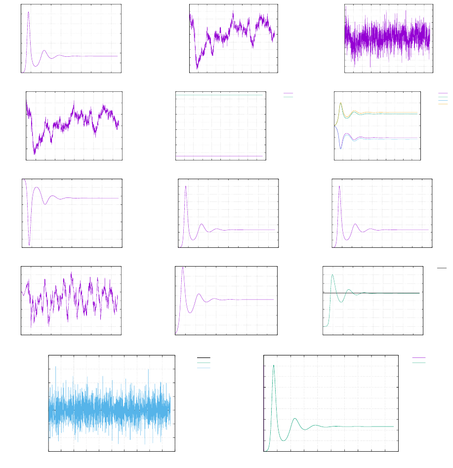
23.8 results - BA - Ra = 104
These results were obtained with a 64x64 resolution, and CFL number of 1. Steady state was reached after about
1250 timesteps.
(a)
0
1x10⁻⁶
2x10⁻⁶
3x10⁻⁶
4x10⁻⁶
5x10⁻⁶
6x10⁻⁶
7x10⁻⁶
0 10000 20000 30000 40000 50000 60000 70000 80000 90000 100000
EK
time (Myr)
(b)
7.67188x10²²
7.67188x10²²
7.67188x10²²
7.67188x10²²
7.67188x10²²
7.67188x10²²
7.67188x10²²
7.67188x10²²
7.67188x10²²
0 10000 20000 30000 40000 50000 60000 70000 80000 90000 100000
ET
time (Myr)
(c)
-7.73687x10²³
-7.73687x10²³
-7.73687x10²³
-7.73687x10²³
-7.73687x10²³
-7.73687x10²³
-7.73687x10²³
-7.73687x10²³
-7.73687x10²³
-7.73687x10²³
-7.73687x10²³
0 10000 20000 30000 40000 50000 60000 70000 80000 90000 100000
EG
time (Myr)
(d)
2273.15
2273.15
2273.15
2273.15
2273.15
2273.15
2273.15
0 10000 20000 30000 40000 50000 60000 70000 80000 90000 100000
<T>
time (Myr)
(e)
0
500
1000
1500
2000
2500
3000
3500
4000
4500
0 10000 20000 30000 40000 50000 60000 70000 80000 90000 100000
Temperature
time (Myr)
min(T)
max(T)
(f)
-0.0015
-0.001
-0.0005
0
0.0005
0.001
0.0015
0 10000 20000 30000 40000 50000 60000 70000 80000 90000 100000
velocity
time (Myr)
min(u)
max(u)
min(v)
max(v)
(g)
-80000
-70000
-60000
-50000
-40000
-30000
-20000
-10000
0
0 10000 20000 30000 40000 50000 60000 70000 80000 90000 100000
adiabatic heating
time (Myr)
(h)
0
10000
20000
30000
40000
50000
60000
70000
80000
90000
0 10000 20000 30000 40000 50000 60000 70000 80000 90000 100000
viscous dissipation
time (Myr)
(i)
0
10000
20000
30000
40000
50000
60000
70000
80000
90000
0 10000 20000 30000 40000 50000 60000 70000 80000 90000 100000
work against gravity
time (Myr)
(j)
-5x10⁻⁸
-4x10⁻⁸
-3x10⁻⁸
-2x10⁻⁸
-1x10⁻⁸
0
1x10⁻⁸
2x10⁻⁸
3x10⁻⁸
0 10000 20000 30000 40000 50000 60000 70000 80000 90000 100000
heat flux
time (Myr)
(k)
0
0.01
0.02
0.03
0.04
0.05
0.06
0.07
0 10000 20000 30000 40000 50000 60000 70000 80000 90000 100000
vrms (cm/yr)
time (Myr)
(l)
0
1
2
3
4
5
6
7
8
0 10000 20000 30000 40000 50000 60000 70000 80000 90000 100000
Nu
time (Myr)
4.88
(l)
-6x10⁻⁷
-4x10⁻⁷
-2x10⁻⁷
0
2x10⁻⁷
4x10⁻⁷
6x10⁻⁷
8x10⁻⁷
0 1x10¹⁰
2x10¹⁰
3x10¹⁰
4x10¹⁰
5x10¹⁰
6x10¹⁰
7x10¹⁰
8x10¹⁰
9x10¹⁰
1x10¹¹
time (Myr)
0
HF
dETdt
(m)
0
10000
20000
30000
40000
50000
60000
70000
80000
90000
0 1x10¹⁰
2x10¹⁰
3x10¹⁰
4x10¹⁰
5x10¹⁰
6x10¹⁰
7x10¹⁰
8x10¹⁰
9x10¹⁰
1x10¹¹
time (Myr)
VD
WG
AH: adiabatic heating, VD: viscous dissipation, HF: heat flux, WG: work against gravity
Eq.(98) is verified by (l) and Eq.(87) is verified by (m).
60
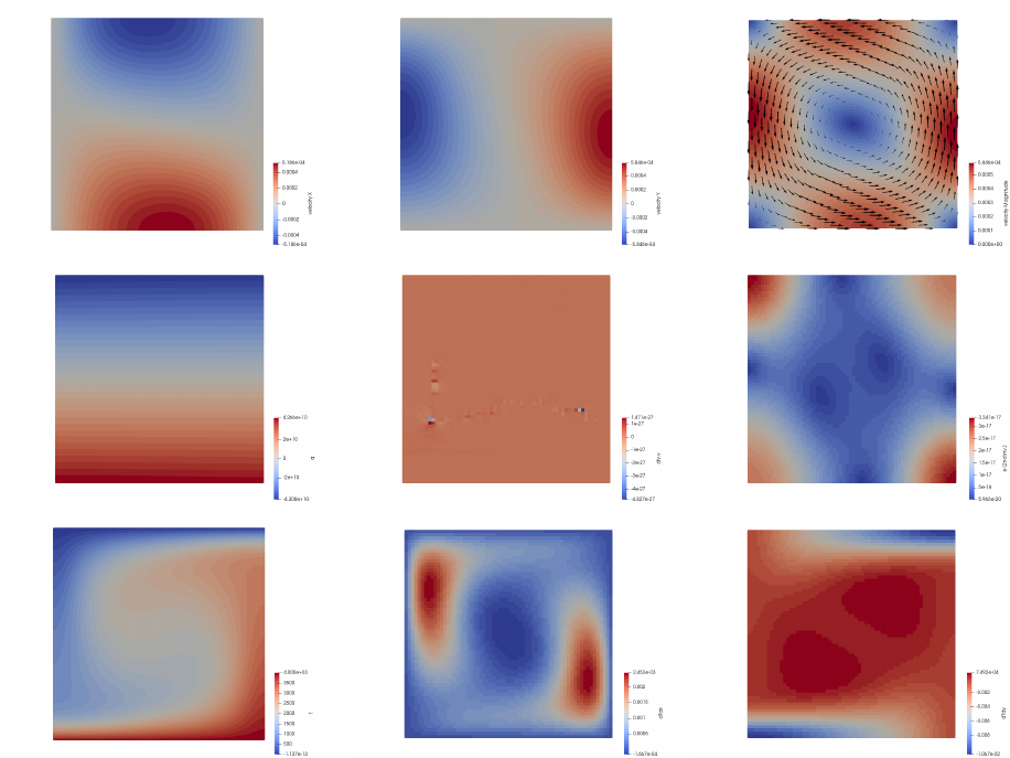
(a) (b) (c)
(d) (e) (f)
(g) (h) (i)
61
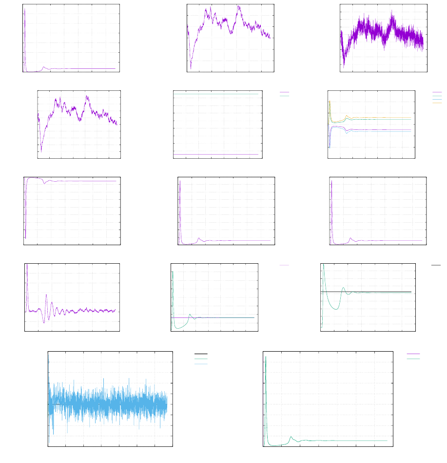
23.9 results - BA - Ra = 105
These results were obtained with a 64x64 resolution, and CFL number of 1. Steady state was reached after about
1250 timesteps.
(a)
0
0.0001
0.0002
0.0003
0.0004
0.0005
0.0006
0.0007
0 5000 10000 15000 20000 25000 30000 35000
EK
time (Myr)
(b)
7.67188x10²²
7.67188x10²²
7.67188x10²²
7.67188x10²²
7.67188x10²²
7.67188x10²²
7.67188x10²²
0 5000 10000 15000 20000 25000 30000 35000
ET
time (Myr)
(c)
-7.73687x10²³
-7.73687x10²³
-7.73687x10²³
-7.73687x10²³
-7.73687x10²³
-7.73687x10²³
-7.73687x10²³
-7.73687x10²³
-7.73687x10²³
-7.73687x10²³
0 5000 10000 15000 20000 25000 30000 35000
EG
time (Myr)
(d)
2273.149999999
2273.149999999
2273.149999999
2273.150000000
2273.150000000
2273.150000000
2273.150000000
2273.150000000
2273.150000001
2273.150000001
2273.150000001
0 5000 10000 15000 20000 25000 30000 35000
<T>
time (Myr)
(e)
0
500
1000
1500
2000
2500
3000
3500
4000
4500
0 5000 10000 15000 20000 25000 30000 35000
Temperature
time (Myr)
min(T)
max(T)
(f)
-0.015
-0.01
-0.005
0
0.005
0.01
0.015
0 5000 10000 15000 20000 25000 30000 35000
velocity
time (Myr)
min(u)
max(u)
min(v)
max(v)
(g)
-900000
-800000
-700000
-600000
-500000
-400000
-300000
-200000
-100000
0
0 5000 10000 15000 20000 25000 30000 35000
adiabatic heating
time (Myr)
(h)
0
100000
200000
300000
400000
500000
600000
700000
800000
900000
0 5000 10000 15000 20000 25000 30000 35000
viscous dissipation
time (Myr)
(i)
0
100000
200000
300000
400000
500000
600000
700000
800000
900000
0 5000 10000 15000 20000 25000 30000 35000
work against gravity
time (Myr)
(j)
-1x10⁻⁶
-5x10⁻⁷
0
5x10⁻⁷
1x10⁻⁶
1.5x10⁻⁶
2x10⁻⁶
2.5x10⁻⁶
0 5000 10000 15000 20000 25000 30000 35000
heat flux
time (Myr)
(k)
0
0.1
0.2
0.3
0.4
0.5
0.6
0.7
0.8
0 5000 10000 15000 20000 25000 30000 35000
vrms (cm/yr)
time (Myr)
193.2150
(l)
0
2
4
6
8
10
12
14
16
18
0 5000 10000 15000 20000 25000 30000 35000
Nu
time (Myr)
10.53
(l)
-8x10⁻⁶
-6x10⁻⁶
-4x10⁻⁶
-2x10⁻⁶
0
2x10⁻⁶
4x10⁻⁶
6x10⁻⁶
8x10⁻⁶
1x10⁻⁵
0 5x10⁹ 1x10¹⁰
1.5x10¹⁰
2x10¹⁰
2.5x10¹⁰
3x10¹⁰
3.5x10¹⁰
time (Myr)
0
HF
dETdt
(m)
0
100000
200000
300000
400000
500000
600000
700000
800000
900000
0 5x10⁹ 1x10¹⁰ 1.5x10¹⁰ 2x10¹⁰ 2.5x10¹⁰ 3x10¹⁰ 3.5x10¹⁰
time (Myr)
VD
WG
AH: adiabatic heating, VD: viscous dissipation, HF: heat flux, WG: work against gravity
Eq.(98) is verified by (l) and Eq.(87) is verified by (m).
62
23.10 results - BA - Ra = 106
63
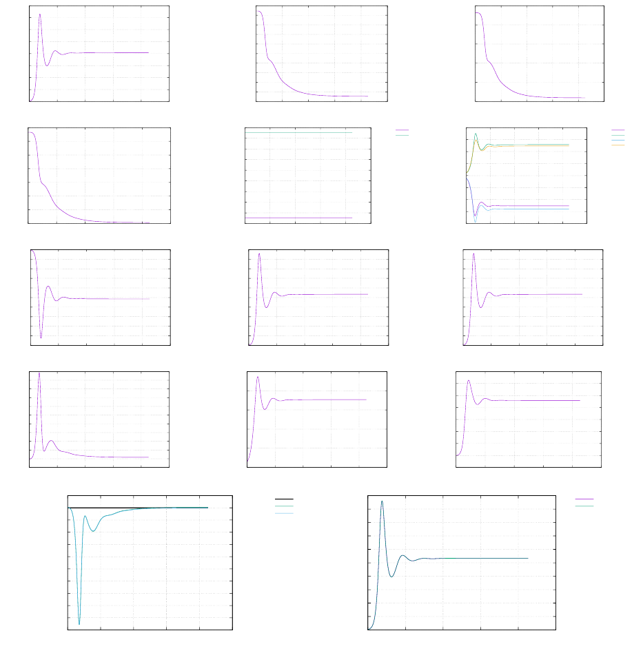
23.11 results - EBA - Ra = 104
These results were obtained with a 64x64 resolution, and CFL number of 1. Steady state was reached after about
2500 timesteps
(a)
0
1x10⁻⁷
2x10⁻⁷
3x10⁻⁷
4x10⁻⁷
5x10⁻⁷
6x10⁻⁷
7x10⁻⁷
8x10⁻⁷
0 50000 100000 150000 200000 250000
EK
time (Myr)
(b)
7.2x10²²
7.25x10²²
7.3x10²²
7.35x10²²
7.4x10²²
7.45x10²²
7.5x10²²
7.55x10²²
7.6x10²²
7.65x10²²
7.7x10²²
0 50000 100000 150000 200000 250000
ET
time (Myr)
(c)
-7.76x10²³
-7.755x10²³
-7.75x10²³
-7.745x10²³
-7.74x10²³
-7.735x10²³
0 50000 100000 150000 200000 250000
EG
time (Myr)
(d)
2140
2160
2180
2200
2220
2240
2260
2280
0 50000 100000 150000 200000 250000
<T>
time (Myr)
(e)
0
500
1000
1500
2000
2500
3000
3500
4000
4500
0 50000 100000 150000 200000 250000
Temperature
time (Myr)
min(T)
max(T)
(f)
-0.0004
-0.0003
-0.0002
-0.0001
0
0.0001
0.0002
0.0003
0.0004
0 50000 100000 150000 200000 250000
velocity
time (Myr)
min(u)
max(u)
min(v)
max(v)
(g)
-10000
-9000
-8000
-7000
-6000
-5000
-4000
-3000
-2000
-1000
0
0 50000 100000 150000 200000 250000
adiabatic heating
time (Myr)
(h)
0
1000
2000
3000
4000
5000
6000
7000
8000
9000
10000
0 50000 100000 150000 200000 250000
viscous dissipation
time (Myr)
(i)
0
1000
2000
3000
4000
5000
6000
7000
8000
9000
10000
0 50000 100000 150000 200000 250000
work against gravity
time (Myr)
(j)
-1000
0
1000
2000
3000
4000
5000
6000
7000
8000
9000
10000
0 50000 100000 150000 200000 250000
heat flux
time (Myr)
(k)
0
0.005
0.01
0.015
0.02
0.025
0 50000 100000 150000 200000 250000
vrms (cm/yr)
time (Myr)
(l)
0.8
1
1.2
1.4
1.6
1.8
2
2.2
2.4
0 50000 100000 150000 200000 250000
Nu
time (Myr)
(l)
-10000
-9000
-8000
-7000
-6000
-5000
-4000
-3000
-2000
-1000
0
1000
0 50000 100000 150000 200000 250000
time (Myr)
0
AH+VD+HF
dETdt
(m)
0
1000
2000
3000
4000
5000
6000
7000
8000
9000
10000
0 50000 100000 150000 200000 250000
time (Myr)
VD
WG
AH: adiabatic heating, VD: viscous dissipation, HF: heat flux, WG: work against gravity
Eq.(98) is verified by (l) and Eq.(87) is verified by (m).
64
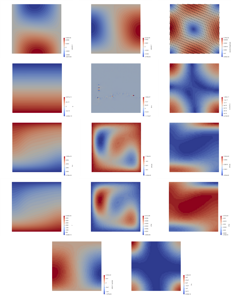
a) b) c)
d) e) f)
g) h) i)
j) k) l)
m) n)
65
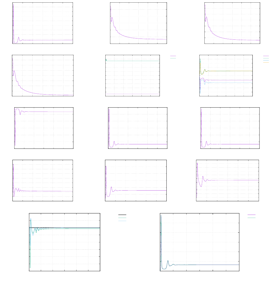
23.12 results - EBA - Ra = 105
These results were obtained with a 64x64 resolution, and CFL number of 1. Simulation was stopped after about 4300
timesteps.
(a)
0
1x10⁻⁵
2x10⁻⁵
3x10⁻⁵
4x10⁻⁵
5x10⁻⁵
6x10⁻⁵
7x10⁻⁵
8x10⁻⁵
9x10⁻⁵
0 20000 40000 60000 80000 100000 120000
EK
time (Myr)
(b)
7.4x10²²
7.45x10²²
7.5x10²²
7.55x10²²
7.6x10²²
7.65x10²²
7.7x10²²
0 20000 40000 60000 80000 100000 120000
ET
time (Myr)
(c)
-7.75x10²³
-7.748x10²³
-7.746x10²³
-7.744x10²³
-7.742x10²³
-7.74x10²³
-7.738x10²³
-7.736x10²³
0 20000 40000 60000 80000 100000 120000
EG
time (Myr)
(d)
2200
2210
2220
2230
2240
2250
2260
2270
2280
0 20000 40000 60000 80000 100000 120000
<T>
time (Myr)
(e)
0
500
1000
1500
2000
2500
3000
3500
4000
4500
5000
0 20000 40000 60000 80000 100000 120000
Temperature
time (Myr)
min(T)
max(T)
(f)
-0.005
-0.004
-0.003
-0.002
-0.001
0
0.001
0.002
0.003
0.004
0.005
0 20000 40000 60000 80000 100000 120000
velocity
time (Myr)
min(u)
max(u)
min(v)
max(v)
(g)
-120000
-100000
-80000
-60000
-40000
-20000
0
0 20000 40000 60000 80000 100000 120000
adiabatic heating
time (Myr)
(h)
0
20000
40000
60000
80000
100000
120000
0 20000 40000 60000 80000 100000 120000
viscous dissipation
time (Myr)
(i)
0
20000
40000
60000
80000
100000
120000
0 20000 40000 60000 80000 100000 120000
work against gravity
time (Myr)
(j)
-20000
-10000
0
10000
20000
30000
40000
50000
60000
70000
0 20000 40000 60000 80000 100000 120000
heat flux
time (Myr)
(k)
0
0.05
0.1
0.15
0.2
0.25
0.3
0 20000 40000 60000 80000 100000 120000
vrms (cm/yr)
time (Myr)
(l)
0.5
1
1.5
2
2.5
3
3.5
4
4.5
5
5.5
6
0 20000 40000 60000 80000 100000 120000
Nu
time (Myr)
(l)
-60000
-50000
-40000
-30000
-20000
-10000
0
10000
20000
0 20000 40000 60000 80000 100000 120000
time (Myr)
0
AH+VD+HF
dETdt
(m)
0
20000
40000
60000
80000
100000
120000
0 20000 40000 60000 80000 100000 120000
time (Myr)
VD
WG
AH: adiabatic heating, VD: viscous dissipation, HF: heat flux, WG: work against gravity
66

23.13 Onset of convection
The code can be run for values of Ra between 500 and 1000, at various resolutions for the BA formulation. The value
vrms(t)−vrms(0) is plotted as a function of Ra and for the 10 first timesteps. If the vrms is found to decrease, then
the Rayleigh number is not high enough to allow for convection and the initial temperature perturbation relaxes by
diffusion (and then vrms(t)−vrms(0) <0. If the vrms is found to increase, then vrms(t)−vrms(0) >0 and the system
is going to showcase convection. The zero value of vrms(t)−vrms(0) gives us the critical Rayleigh number, which is
found between 775 and 790.
-4x10-15
-2x10-15
0
2x10-15
4x10-15
6x10-15
8x10-15
1000
vrms trend
Ra
16x16
32x32
48x48
64x64
-3.5x10⁻¹⁶
-3x10-16
-2.5x10⁻¹⁶
-2x10-16
-1.5x10⁻¹⁶
-1x10-16
-5x10-17
0
5x10-17
1x10-16
1.5x10⁻¹⁶
770 775 780 785 790
vrms trend
Ra
16x16
32x32
48x48
64x64
67
A The main codes in computational geodynamics
In what follows I make a quick inventory of the main codes of computational geodynamics, for crust, lithosphere
and/or mantle modelling.
A.1 ADELI
A.2 ASPECT
A.3 CITCOMS and CITCOMCU
A.4 DOUAR
A.5 GAIA
A.6 GALE
A.7 GTECTON
A.8 ELVIS
A.9 ELEFANT
A.10 ELLIPSIS
A.11 FANTOM
A.12 FLUIDITY
A.13 LAMEM
A.14 MILAMIN
A.15 PARAVOZ/FLAMAR
A.16 PTATIN
A.17 RHEA
A.18 SEPRAN
A.19 SOPALE
A.20 STAGYY
A.21 SULEC
SULEC is a finite element code that solves the incompressible Navier-Stokes equations for slow creeping flows. The
code is developed by Susan Ellis (GNS Sciences, NZ) and Susanne Buiter (NGU).
A.22 TERRA
A.23 UNDERWORLD 1&2
68
B fieldstone.py
69

C fieldstone stokes sphere.py
D fieldstone convection box.py
70

E fieldstone solcx.py
71

F fieldstone indentor.py
72

G fieldstone saddlepoint.py
73
References
[1] M. Albers. A local mesh refinement multigrid method for 3D convection problems with strongly variable viscosity.
J. Comp. Phys., 160:126–150, 2000.
[2] K.-J. Bathe. Finite Element Procedures in Engineering Analysis. Prentice-Hall, 1982.
[3] M. Benzi, G.H. Golub, and J. Liesen. Numerical solution of saddle point problems. Acta Numerica, 14:1–137,
2005.
[4] D. Bercovici, G. Schubert, and G.A. Glatzmaier. Three-dimensional convection of an infinite Prandtl-number
compressible fluid in a basally heated spherical shell. J. Fluid Mech., 239:683–719, 1992.
[5] B. Blankenbach, F. Busse, U. Christensen, L. Cserepes, D. Gunkel, U. Hansen, H. Harder, G. Jarvis, M. Koch,
G. Marquart, D. Moore, P. Olson, H. Schmeling, and T. Schnaubelt. A benchmark comparison for mantle
convection codes. Geophys. J. Int., 98:23–38, 1989.
[6] H.H. Bui, R. Fukugawa, K. Sako, and S. Ohno. Lagrangian meshfree particles method (SPH) for large deformation
and failure flows of geomaterial using elasticplastic soil constitutive model. Int. J. Numer. Anal. Geomech.,
32(12):1537–1570, 2008.
[7] C. Burstedde, G. Stadler, L. Alisic, L.C. Wilcox, E. Tan, M. Gurnis, and O. Ghattas. Large-scale adaptive mantle
convection simulation. Geophy. J. Int., 192:889–906, 2013.
[8] Edmund Christiansen and Knud D. Andersen. Computation of collapse states with von mises type yield condition.
International Journal for Numerical Methods in Engineering, 46:1185–1202, 1999.
[9] Edmund Christiansen and Ole S. Pedersen. Automatic mesh refinement in limit analysis. International Journal
for Numerical Methods in Engineering, 50:1331–1346, 2001.
[10] C. Cuvelier, A. Segal, and A.A. van Steenhoven. Finite Element Methods and Navier-Stokes Equations. D. Reidel
Publishing Company, 1986.
[11] D.R. Davies, C.R. Wilson, and S.C. Kramer. Fluidity: A fully unstructured anisotropic adaptive mesh computa-
tional modeling framework for geodynamics. Geochem. Geophys. Geosyst., 12(6), 2011.
[12] P. Davy and P. Cobbold. Indentation tectonics in nature and experiment. 1. experiments scaled for gravity.
Bulletin of the Geological Institutions of Uppsala, 14:129–141, 1988.
[13] Y. Deubelbeiss and B.J.P. Kaus. Comparison of Eulerian and Lagrangian numerical techniques for the Stokes
equations in the presence of strongly varying viscosity. Phys. Earth Planet. Interiors, 171:92–111, 2008.
[14] C.R. Dohrmann and P.B. Bochev. A stabilized finite element method for the Stokes problem based on polynomial
pressure projections. Int. J. Num. Meth. Fluids, 46:183–201, 2004.
[15] J. Donea and A. Huerta. Finite Element Methods for Flow Problems. 2003.
[16] J. Donea and A. Huerta. Finite Element Methods for Flow Problems. John Wiley & Sons, 2003.
[17] Jean Donea and Antonio Huerta. Finite Element Methods for Flow Problems. John Wiley & Sons, 2003.
[18] T. Duretz, D.A. May, T.V. Gerya, and P.J. Tackley. Discretization errors and free surface stabilisation in the finite
difference and marker-in-cell method for applied geodynamics: A numerical study. Geochem. Geophys. Geosyst.,
12(Q07004), 2011.
[19] M. Gerbault, A.N.B. Poliakov, and M. Daignieres. Prediction of faulting from the theories of elasticity and
plasticity: what are the limits? Journal of Structural Geology, 20:301–320, 1998.
[20] Taras Gerya. Numerical Geodynamic Modelling. Cambridge University Press, 2010.
[21] T.V. Gerya, D.A. May, and T. Duretz. An adaptive staggered grid finite difference method for modeling geody-
namic Stokes flows with strongly variable viscosity. Geochem. Geophys. Geosyst., 14(4), 2013.
[22] G.H. Golub and C.F. van Loan. Matrix Computations, 4th edition. John Hopkins University Press, 2013.
[23] M. Gunzburger. Finite Element Methods for Viscous Incompressible Flows: A Guide to Theory, Practice and
Algorithms. Academic, Boston, 1989.
74
[24] T. Heister, J. Dannberg, R. Gassm¨oller, and W. Bangerth. High Accuracy Mantle Convection Simulation through
Modern Numerical Methods. II: Realistic Models and Problems. Geophy. J. Int., 210(2):833–851, 2017.
[25] T.J.R. Hughes. The Finite Element Method. Linear Static and Dynamic Finite Element Analysis. Dover Publi-
cations, Inc., 2000.
[26] T.J.R. Hughes, W.K. Liu, and A. Brooks. Finite element analysis of Incompressible viscous flows by the penalty
function formulation. J. Comp. Phys., 30:1–60, 1979.
[27] Hoon Huh, Choong Ho Lee, and Wei H. Yang. A general algorithm for plastic flow simulation by finite element
limit analysis. International Journal of Solids and Structures, 36:1193–1207, 1999.
[28] J. Ita and S.D. King. Sensitivity of convection with an endothermic phase change to the form of governing
equations, initial conditions, boundary conditions, and equation of state. J. Geophys. Res., 99(B8):15,919–15,938,
1994.
[29] L. Jolivet, P. Davy, and P. Cobbold. Right-lateral shear along the Northwest Pacific margin and the India-Eurasia
collision. Tectonics, 9(6):1409–1419, 1990.
[30] L.M. Kachanov. Fundamentals of the Theory of Plasticity. Dover Publications, Inc., 2004.
[31] S. King, C. Lee, P. van Keken, W. Leng, S. Zhong, E. Tan, N. Tosi, and M. Kameyama. A community benchmark
for 2D Cartesian com- pressible convection in the Earths mantle. Geophy. J. Int., 180:7387, 2010.
[32] M. Kronbichler, T. Heister, and W. Bangerth. High accuracy mantle convection simulation through modern
numerical methods . Geophy. J. Int., 191:12–29, 2012.
[33] W. Leng and S. Zhong. Viscous heating, adiabatic heating and energetic consistency in compressible mantle
convection. Geophy. J. Int., 173:693–702, 2008.
[34] W. Leng and S. Zhong. Implementation and application of adaptive mesh refinement for thermochemical mantle
convection studies. Geochem. Geophys. Geosyst., 12(4), 2011.
[35] X. Liu and S. Zhong. Analyses of marginal stability, heat transfer and boundary layer properties for thermal
convection in a compressible fluid with infinite Prandtl number. Geophy. J. Int., 194:125–144, 2013.
[36] D.S. Malkus and T.J.R. Hughes. Mixed finite element methods - reduced and selective integration techniques: a
unification of concepts. Comput. Meth. Appl. Mech. Eng., 15:63–81, 1978.
[37] L.E. Malvern. Introduction to the mechanics of a continuous medium. Prentice-Hall, Inc., 1969.
[38] P. Molnar and P. Tapponnier. Relation of the tectonics of eastern China to the India-Eurasia collision: Application
of the slip-line field theory to large-scale continental tectonics. Geology, 5:212–216, 1977.
[39] L. Moresi, S. Quenette, V. Lemiale, C. M´eriaux, B. Appelbe, and H.-B. M¨uhlhaus. Computational approaches to
studying non-linear dynamics of the crust and mantle. Phys. Earth. Planet. Inter., 163:69–82, 2007.
[40] G. Peltzer and P. Tapponnier. Formation and evolution of strike-slip faults, rifts, and basins during the india-asia
collision: an experimental approach. J. Geophys. Res., 93(B12):15085–15177, 1988.
[41] A.E. Pusok, B.J.P. Kaus, and A.A. Popov. On the Quality of Velocity Interpolation Schemes for Marker-in-Cell
Method and Staggered Grids. Pure and Applied Geophysics, pages doi:10.1007/s00024–016–1431–8, 2016.
[42] T. Rabczuk, P.M.A. Areias, and T. Belytschko. A simplified mesh-free method for shear bands with cohesive
surfaces . Int. J. Num. Meth. Eng., 69:993–1021, 2007.
[43] J.N. Reddy. On penalty function methods in the finite element analysis of flow problems. Int. J. Num. Meth. Flu-
ids, 2:151–171, 1982.
[44] J. Revenaugh and B. Parsons. Dynamic topography and gravity anomalies for fluid layers whose viscosity varies
exponentially with depth. Geophysical Journal of the Royal Astronomical Society, 90(2):349–368, 1987.
[45] H. Schmeling, A.Y. Babeyko, A. Enns, C. Faccenna, F. Funiciello, T. Gerya, G.J. Golabek, S. Grigull, B.J.P.
Kaus, G. Morra, S.M. Schmalholz, and J. van Hunen. A benchmark comparison of spontaneous subduction
models - Towards a free surface. Phys. Earth. Planet. Inter., 171:198–223, 2008.
[46] D.W. Schmid and Y.Y. Podlachikov. Analytical solutions for deformable elliptical inclusions in general shear.
Geophy. J. Int., 155:269–288, 2003.
75
[47] G. Schubert, D.L. Turcotte, and P. Olson. Mantle Convection in the Earth and Planets. Cambridge University
Press, 2001.
[48] J. Suckale, J.-C. Nave, and B.H. Hager. It takes three to tango: 1. Simulating buoyancy-driven flow in the
presence of large viscosity contrasts. J. Geophys. Res., 115(B07409), 2010.
[49] P. Tackley. Three-dimensional models of mantle convection: Influence of phase transitions and temperature-
dependent viscosity. PhD thesis, California Institute of Technology, 1994.
[50] E. Tan and M. Gurnis. Compressible thermochemical convection and application to lower mantle structures.
J. Geophys. Res., 112(B06304), 2007.
[51] Paul Tapponnier and Peter Molnar. Slip-line field theory and large-scale continental tectonics. Nature, 264:319–
324, November 1976.
[52] M. Thielmann, D.A. May, and B.J.P. Kaus. Discretization errors in the Hybrid Finite Element Particle-In-Cell
Method. Pure and Applied Geophysics, 2014.
[53] C. Thieulot, P. Fullsack, and J. Braun. Adaptive octree-based finite element analysis of two- and three-dimensional
indentation problems. J. Geophys. Res., 113:B12207, 2008.
[54] R.A. Trompert and U. Hansen. On the Rayleigh number dependence of convection with a strongly temperature-
dependent viscosity. Physics of Fluids, 10(2):351–360, 1998.
[55] D.L. Turcotte and G. Schubert. Geodynamics, 2nd edition. Cambridge, 2012.
[56] X. Yu and F. Tin-Loi. A simple mixed finite element for static limit analysis. Computers and Structures, 84:1906–
1917, 2006.
[57] S. Zhong. Analytic solutions for Stokes flow with lateral variations in viscosity. Geophys. J. Int., 124:18–28, 1996.
[58] O. Zienkiewicz and S. Nakazawa. The penalty function method and its application to the numerical solution of
boundary value problems. The American Society of Mechanical Engineers, 51, 1982.
[59] O.C. Zienkiewicz, M. Huang, and M. Pastor. Localization problems in plasticity using finite elements with
adaptive remeshing. International Journal for Numerical and Analytical Methods in Geomechanics, 19:127–148,
1995.
[60] O.C. Zienkiewicz, C. Humpheson, and R.W. Lewis. Associated and non-associated visco-plasticity and plasticity
in soil mechanics . G´eotechnique, 25(4):671–689, 1975.
76
Index
Q1×P0, 20, 26, 32, 38, 41, 53, 59
Q2×Q1, 43, 48
analytical solution, 20, 26, 41, 48, 50, 53, 59
arithmetic mean, 38
basis functions, 12
Boussinesq, 8
bulk modulus, 54
bulk viscosity, 5
compressibility, 54
compressible flow, 59
dynamic viscosity, 5
Gauss quadrature, 10
geometric mean, 38
harmonic mean, 38
incompressible flow, 26, 32, 38, 41, 48, 50, 53
isothermal, 20, 26, 32, 38, 41, 48, 50, 53
isoviscous, 20, 41, 48, 53, 59
Legendre polynomial, 10
midpoint rule, 9
mixed formulation, 41, 48, 50, 53, 59
Newton-Cotes, 10
non-isoviscous, 26, 32, 38, 50
nonconforming Q1×P0, 50
nonlinear rheology, 32
particle-in-cell, 38
penalty formulation, 14, 20, 26, 32, 38
pressure normalisation, 44
pressure smoothing, 41, 50, 53, 59
quadrature, 10
rectangle rule, 9
second viscosity, 5
thermal expansion, 54
trapezoidal rule, 9
weak form, 16
work against gravity, 56
77
