Manual

User Manual:

Open the PDF directly: View PDF .
Page Count: 29

Example 1: bandit task
Example 2: Two-step Markov decision task
- Reference

cbm manual

Payam Piray

June 18, 2019

This document serves as the manual of cbm (computational and behavioral modeling) toolbox.

cbm provides tools for hierarchical Bayesian inference (HBI). See the corresponding manuscript

(here) for more information about the HBI and its comparison with other methods. You can down-

load cbm here. In this manual, I present two well-known examples and explain how cbm tools

should be used to perform Bayesian model comparison, parameter estimation and inference at the

group level. To be able to follow this manual, you need to be familiar with matlab syntax (cbm

will be published soon in other languages, particularly python).

1 Example 1: bandit task

I assume that the current directory contains this manual and “codes” directory, as well as “exam-

ple_RL_task” and “example_2step_task” directories. The codes directory contains all cbm matlab

functions.

For using cbm tools, you need to know what is your model-space and code your own models.

You can then use cbm to make inference. For this example, models code and data have been stored

in the example_RL_task directory.

Suppose you have 40 subjects’ choice data in a 2-armed bandit task, in which subjects chose

between two actions and received binary outcomes.

All data have been stored in a mat-ﬁle called all_data.mat in a cell format, in which each cell

contains choice data and outcomes for one subject. First, enter the example_RL_task directory and

then load those data:

In [1]: % enter the example_RL_task folder,

% which contains data and models for this example

% (assuming that you are in the directory of the manual)

cd(fullfile('example_RL_task'));

In [2]: % load data

fdata = load('all_data.mat');

data = fdata.data;

% data for each subject

subj1 = data{1}; % subject 1

subj2 = data{2}; % subject 2

% and so on

For example, subj1 contains information of subject 1: subj1.actions are all actions and

subj1.outcome are the corresponding outcomes.

Also suppose you have 2 candidate models. An RL model, which has a learning rate (alpha)

and a decision noise (beta) parameter. The other model is a dual-alpha RL model with two sep-

arate learning rates for positive and negative prediction errors (alpha1 and alpha2, respectively)

and a decision noise (beta) parameter. See matlab functions model_RL and model_dualRL as ex-

amples.

It is important to remember that cbm does not care how your model works! It assumes that

your models take parameters and data (of one subject) as input and produce a log-probability of

data given the parameters (i.e. log-likelihood function). Tools in cbm only require that the input

and output of models follow a speciﬁc format:

loglik = model(parameters,subj)

For example, for the model_RL, we have:

loglik = model_RL(parameters,subj1)

here parameters is a vector, which its size depends on the number of parameters of the

model_RL (for model_RL, its size is 2). subj1 is the structure containing data of subject 1 as

indicated above. loglik is the log-likelihood of subj1 data given parameters, as computed by

model_RL.

We now use cbm tools to ﬁt models to data. For this example, we use the two models im-

plemented in model_RL and model_dualRL together with the data stored in all_data.mat. Data

stored in all_data is a synthetic dataset of 40 subjects. The data of the ﬁrst 10 subjects are generated

by model_RL and the data of the next 30 subjects are generated by model_dualRL. Note, however,

that cbm is not meant to provide a collection of different computational models. You should code

your models for questions of your interest yourself. The tools in cbm ﬁt your models to your data

and compare the models given the data.

First, make sure that cbm is added to your matlab path and then load the data:

In [3]: addpath(fullfile('..','codes'));

% load data from all_data.mat file

fdata = load('all_data.mat');

data = fdata.data;

Before using cbm tools, it is always good to check whether the format of the models is com-

patible with the cbm. To do that, create a random vector parameters and call the models:

In [4]: % data of subject 1

subj1 = data{1};

parameters = randn(1,2);

F1 = model_RL(parameters,subj1)

parameters = randn(1,3);

F2 = model_dualRL(parameters,subj1)

F1 =

-200.9599

F2 =

-57.2434

Note that because parameters were randomly drawn, when you run the same code, it gen-

erates different values for F1 and F2. Also note that parameters are drawn from a normal dis-

tribution. In theory, RL models require constrained parameters (e.g. alpha between 0 and 1). In

model_RL and model_dualRL, some transformations applied to the normally-distributed param-

eters to meet their theoretical bounds (see model_RL and model_dualRL). I’ll explain later a bit

more about transforming (normally-distributed) parameters in your models.

We checked the models with some random parameters. It is also good to check them with

more extreme parameter values:

In [5]: parameters = [-10 10];

F1 = model_RL(parameters,subj1)

parameters = [-10 10 10];

F2 = model_dualRL(parameters,subj1)

F1 =

-654.4651

F2 =

-169.2246

Again, F1 and F2 should be real negative scalers.

After making sure that model_RL and model_dualRl work ﬁne, we now use cbm tools to ﬁt

models to data.

First, we should run cbm_lap, which ﬁts every model to each subject data separately (i.e. in a

non-hierarchical fashion). cbm_lap employs Laplace approximation, which needs a normal prior

for every parameter. We set zero as the prior mean. We also assume that the prior variance for

all parameters is 6.25. This variance is large enough to cover a wide range of parameters with no

excessive penalty (see supplementary materials of the reference article for more details on how

this variance is calculated).

In [6]: v = 6.25;

prior_RL = struct('mean',zeros(2,1),'variance',v); % note dimension of 'mean'

prior_dualRL = struct('mean',zeros(3,1),'variance',v); % note dimension of 'mean'

We also need to specify a ﬁle-address for saving the output of each model:

In [7]: fname_RL = 'lap_RL.mat';

fname_dualRL = 'lap_dualRL.mat';

Now we run cbm_lap for each model. Note that model_RL and model_dualRL are both in the

current directory.

In [8]: cbm_lap(data, @model_RL, prior_RL, fname_RL);

% Running this command, prints a report on your matlab output

% (e.g. on the command window)

cbm_lap 18-Jun-2019 22:04:28

======================================================================

Number of samples: 40

Number of parameters: 2

Number of initializations: 14

----------------------------------------------------------------------

Subject: 01

Subject: 02

Subject: 03

Subject: 04

Subject: 05

Subject: 06

Subject: 07

Subject: 08

Subject: 09

Subject: 10

Subject: 11

Subject: 12

Subject: 13

Subject: 14

Subject: 15

Subject: 16

Subject: 17

Subject: 18

Subject: 19

Subject: 20

Subject: 21

Subject: 22

Subject: 23

Subject: 24

Subject: 25

Subject: 26

Subject: 27

Subject: 28

Subject: 29

Subject: 30

Subject: 31

Subject: 32

Subject: 33

Subject: 34

Subject: 35

Subject: 36

Subject: 37

Subject: 38

Subject: 39

Subject: 40

done :]

Also run cbm_lap for model_dualRL

In [9]: cbm_lap(data, @model_dualRL, prior_dualRL, fname_dualRL);

% Running this command, prints a report on your matlab output

% (e.g. on the command window)

cbm_lap 18-Jun-2019 22:04:35

======================================================================

Number of samples: 40

Number of parameters: 3

Number of initializations: 21

----------------------------------------------------------------------

Subject: 01

Subject: 02

Subject: 03

Subject: 04

Subject: 05

Subject: 06

Subject: 07

Subject: 08

Subject: 09

Subject: 10

Subject: 11

Subject: 12

Subject: 13

Subject: 14

Subject: 15

Subject: 16

Subject: 17

Subject: 18

Subject: 19

Subject: 20

Subject: 21

Subject: 22

Subject: 23

Subject: 24

Subject: 25

Subject: 26

Subject: 27

Subject: 28

Subject: 29

Subject: 30

Subject: 31

Subject: 32

Subject: 33

Subject: 34

Subject: 35

Subject: 36

Subject: 37

Subject: 38

Subject: 39

Subject: 40

done :]

Let’s take a look at the ﬁle saved by the cbm_lap:

In [10]: fname = load('lap_RL.mat');

cbm = fname.cbm;

% look at fitted parameters

cbm.output.parameters

ans =

-0.9099 -0.1596

-2.2959 0.2281

-1.8879 0.0641

-2.9416 0.6446

0.1626 -1.7082

-2.3983 -0.2423

-2.2385 -0.3139

-1.1035 -0.1045

-0.1508 -1.0967

-3.1319 0.3766

-1.6312 2.8806

-1.9657 1.4585

1.3684 1.3809

0.2462 1.2869

0.5822 1.6409

0.1195 0.7961

0.2869 1.3080

-0.9798 2.4429

-0.2855 1.3087

0.6944 2.0278

1.3887 1.4371

0.0819 1.0805

-0.5053 1.9617

0.4317 1.4263

0.1695 0.8347

0.6204 -0.8997

0.0504 2.2729

-0.2048 -0.2258

0.4743 1.2425

0.5359 0.7142

1.0363 0.0334

0.7106 0.2387

-1.4016 1.7652

0.0332 2.4478

-0.8369 1.4053

-0.0262 0.6052

0.1145 1.2742

0.3787 1.6922

0.0006 2.0756

1.6417 0.6821

Note that these values are normally-distributed parameters (I’ll explain later how to obtain

bounded parameters). The order of parameters depend on how they have been coded in the corre-

sponding model. In model_RL, the ﬁrst parameter is alpha and the second one is beta. Therefore,

here the ﬁrst column corresponds to alpha and the second one to beta.

Now we can do hierarchical Bayesian inference using cbm_hbi. cbm_hbi needs 4 inputs. The

good news is that you already have all of them!

In [11]: % 1st input: data for all subjects

fdata = load('all_data.mat');

data = fdata.data;

% 2nd input: a cell input containing function handle to models

models = {@model_RL, @model_dualRL};

% note that by handle, I mean @ before the name of the function

% 3rd input: another cell input containing file-address to files saved by cbm_lap

fcbm_maps = {'lap_RL.mat','lap_dualRL.mat'};

% note that they corresponds to models (so pay attention to the order)

% 4th input: a file address for saving the output

fname_hbi = 'hbi_RL_dualRL.mat';

Now, we are ready to run cbm_hbi:

In [12]: cbm_hbi(data,models,fcbm_maps,fname_hbi);

% Running this command, prints a report on your matlab output

% (e.g. on the command window)

cbm_hbi_hbi 18-Jun-2019 22:04:43

Running hierarchical bayesian inference (HBI)...

HBI has been initialized according to

lap_RL.mat [for model 1]

lap_dualRL.mat [for model 2]

Number of samples: 40

Number of models: 2

======================================================================

Iteration 01

Iteration 02

model frequencies (percent)

model 1: 50.5| model 2: 49.5|

dL: 6.62

dm: 49.48

dx: 0.22

Iteration 03

model frequencies (percent)

model 1: 48.6| model 2: 51.4|

dL: 2.14

dm: 1.91

dx: 0.12

Iteration 04

model frequencies (percent)

model 1: 46.3| model 2: 53.7|

dL: 3.09

dm: 2.30

dx: 0.13

Iteration 05

model frequencies (percent)

model 1: 43.3| model 2: 56.7|

dL: 4.28

dm: 3.04

dx: 0.16

Iteration 06

model frequencies (percent)

model 1: 39.4| model 2: 60.6|

dL: 4.91

dm: 3.84

dx: 0.18

Iteration 07

model frequencies (percent)

model 1: 35.6| model 2: 64.4|

dL: 4.10

dm: 3.81

dx: 0.17

Iteration 08

model frequencies (percent)

model 1: 32.7| model 2: 67.3|

dL: 3.42

dm: 2.93

dx: 0.15

Iteration 09

model frequencies (percent)

model 1: 31.2| model 2: 68.8|

dL: 2.08

dm: 1.47

dx: 0.11

Iteration 10

model frequencies (percent)

model 1: 30.5| model 2: 69.5|

dL: 1.40

dm: 0.72

dx: 0.12

Iteration 11

model frequencies (percent)

model 1: 30.0| model 2: 70.0|

dL: 0.99

dm: 0.53

dx: 0.10

Iteration 12

model frequencies (percent)

model 1: 29.6| model 2: 70.4|

dL: 0.65

dm: 0.34

dx: 0.08

Iteration 13

model frequencies (percent)

model 1: 29.4| model 2: 70.6|

dL: 0.44

dm: 0.21

dx: 0.06

Iteration 14

model frequencies (percent)

model 1: 29.3| model 2: 70.7|

dL: 0.30

dm: 0.13

dx: 0.04

Iteration 15

model frequencies (percent)

model 1: 29.2| model 2: 70.8|

dL: 0.21

dm: 0.07

dx: 0.03

Iteration 16

model frequencies (percent)

model 1: 29.2| model 2: 70.8|

dL: 0.15

dm: 0.04

dx: 0.02

Iteration 17

model frequencies (percent)

model 1: 29.1| model 2: 70.9|

dL: 0.11

dm: 0.02

dx: 0.01

Iteration 18

model frequencies (percent)

model 1: 29.1| model 2: 70.9|

dL: 0.08

dm: 0.01

dx: 0.01

Iteration 19

model frequencies (percent)

model 1: 29.1| model 2: 70.9|

dL: 0.06

dm: 0.00

dx: 0.01

Converged :]

Runnig cbm_hbi writes a report on your standard output (often the screen). On every iteration,

cbm_hbi reports model frequency, which is the estimate of how many individual datasets (i.e. sub-

jects) is explained by each model (in percent). Furthermore, on every iteration, there are 3 metrics

showing the changes relative to the previous iteration: dL is the change in the log-likelihood of

all data given the model space (more speciﬁcally a variational approximation of log-likelihood);

dm is the (percentage of) change in model frequencies; dx indicates changes in (normalized value

of) parameters. Although either of these measures or their combination can be used as stopping

criteria, cbm_hbi uses dx as the stopping criteria. By default, cbm_hbi stops when dx<0.01.

Let’s now take a look at the saved ﬁle:

In [13]: fname_hbi = load('hbi_RL_dualRL.mat');

cbm = fname_hbi.cbm;

cbm.output

ans =

struct with fields:

parameters: {2x1 cell}

responsibility: [40x2 double]

group_mean: {[-1.8854 -0.0098] [1.0678 -0.2944 1.1510]}

group_hierarchical_errorbar: {[0.2954 0.0409] [0.1183 0.1038 0.0912]}

model_frequency: [0.2913 0.7087]

exceedance_prob: [0.0041 0.9959]

protected_exceedance_prob: [NaN NaN]

Almost all useful parameters are stored in cbm.output, which we explain them here.

First, let’s look at model_frequency, which is the HBI estimate of how much each model is

expressed across the group:

In [14]: model_frequency = cbm.output.model_frequency

model_frequency =

0.2913 0.7087

Note that the model_frequency is normalized here (so it sums to 1 across all models). Also

note that the order depends on the order of models fed into to HBI as input. Therefore, in this

example, HBI estimated that about 29% of all subjects are explained by the model_RL and about

71% by the model_dualRL.

Now let’s take a look at estimated group mean stored in cbm.output.group_mean.

In [15]: group_mean_RL = cbm.output.group_mean{1}

% group mean for parameters of model_RL

group_mean_dualRL = cbm.output.group_mean{2}

% group mean for parameters of model_dualRL

group_mean_RL =

-1.8854 -0.0098

group_mean_dualRL =

1.0678 -0.2944 1.1510

Note that these are normally distributed parameters. That’s the reason that group learning

rate (which is typically constrained to be between zero and one) is negative here. This is because

HBI (and other tools in the cbm) assume that parameters are normally distributed. Therefore, if

you have a model with some constraints on parameters (e.g. an RL), you should transform the

normally distributed parameter in your model function. To make this point clear, take a look at

the model_RL function. On the ﬁrst two lines of this function, you see these codes:

nd_alpha = parameters(1); % normally-distributed alpha

alpha = 1/(1+exp(-nd_alpha)); % alpha (transformed to be between zero and one)

Here, nd_alpha is the normally-distributed parameter passed to the model (for example by

cbm tools). Before using it, the model transformed it to alpha, which is bounded between 0 and 1

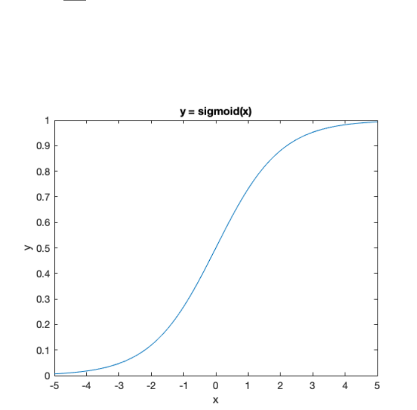
and is served as the effective learning rate. To do this, a sigmoid function has been used:

sigmoid(x) = 1

1+e−x

which is illustrated here:

In [16]: x = -5:.1:5;

y=1./(1+exp(-x));

plot(x,y);

title('y = sigmoid(x)'); xlabel('x'); ylabel('y');

As you see, sigmoid is a monotonically increasing function, which transforms its input (x) to an

output (y) between 0 and 1. Therefore, if you want to obtain the parameters of your model in their

theoretical range (e.g. a learning rate between 0 and 1), you should apply the same transformation

(e.g. the sigmoid) to the normally distributed parameter (e.g. to the group_mean_RL(1)).

The second parameter of the model_RL is the decision noise parameter, which is theoretically

constrained to be positive. For transforming this one, we did an exponential-transformation to the

second parameter passed to the model_RL:

nd_beta = parameters(2);

beta = exp(nd_beta);

The HBI also quantiﬁes (hierarchical) errorbar of the group_mean parameters, which is saved

in cbm.output.group_hierarchical_errorbar:

In [17]: group_errorbar_RL = cbm.output.group_hierarchical_errorbar{1};

group_errorbar_dualRL = cbm.output.group_hierarchical_errorbar{2};

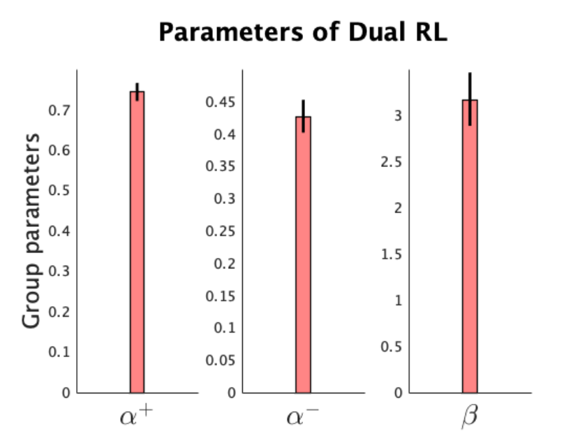
You can use the group_mean and group_hierarchical_errorbar values to plot group parame-

ters, or use cbm_hbi_plot to plot the main outputs of the HBI.

In [18]: % 1st input is the file-address of the file saved by cbm_hbi

fname_hbi = 'hbi_RL_dualRL.mat';

% 2nd input: a cell input containing model names

model_names = {'RL','Dual RL'};

% note that they corresponds to models (so pay attention to the order)

% 3rd input: another cell input containing parameter names of the winning model

param_names = {'\alpha^+','\alpha^-','\beta'};

% note that '\alpha^+'is in the latex format, which generates a latin alpha

% 4th input: another cell input containing transformation function associated with each parameter of the winning model

transform = {'sigmoid','sigmoid','exp'};

% note that if you use a less usual transformation function, you should pass the handle here (instead of a string)

cbm_hbi_plot(fname_hbi, model_names, param_names, transform)

% this function creates a model comparison plot (exceednace probability and model frequency) as well as

% a plot of transformed parameters of the most frequent model.

plotting the group parameters of the most frequenct modelThere is no protected exceedance probability as cbm_hbi_null has not been executed

Plotting exceedance probability instead...

Similar to a t-test, you can use the hierarchical errorbars to make an inference about a param-

eter at the population level. We explain that feature in the next example.

The value of individual parameters are saved in the cbm.output.parameters

In [19]: parameters_RL = cbm.output.parameters{1};

parameters_dualRL = cbm.output.parameters{2};

Also you can look at the estimated responsibility that each model generated each individual

dataset. Across models, responsibilities sum to 1 for each subject.

In [20]: responsibility = cbm.output.responsibility

responsibility =

0.9755 0.0245

0.9992 0.0008

0.9993 0.0007

0.9996 0.0004

0.9990 0.0010

0.9995 0.0005

0.9923 0.0077

0.9934 0.0066

0.9972 0.0028

1.0000 0.0000

0.0000 1.0000

0.0002 0.9998

0.0000 1.0000

0.0007 0.9993

0.6553 0.3447

0.0000 1.0000

0.5644 0.4356

0.0000 1.0000

0.0007 0.9993

0.3221 0.6779

0.1548 0.8452

0.0000 1.0000

0.0002 0.9998

0.0000 1.0000

0.0012 0.9988

The ﬁrst and second columns indicate the responsibility of model_RL and model_dualRL in

generating the corresponding subject data, respectively.

Look at the estimated responsibility of model_dualRL:

In [21]: plot(responsibility(:,2)); ylim([-.1 1.1])

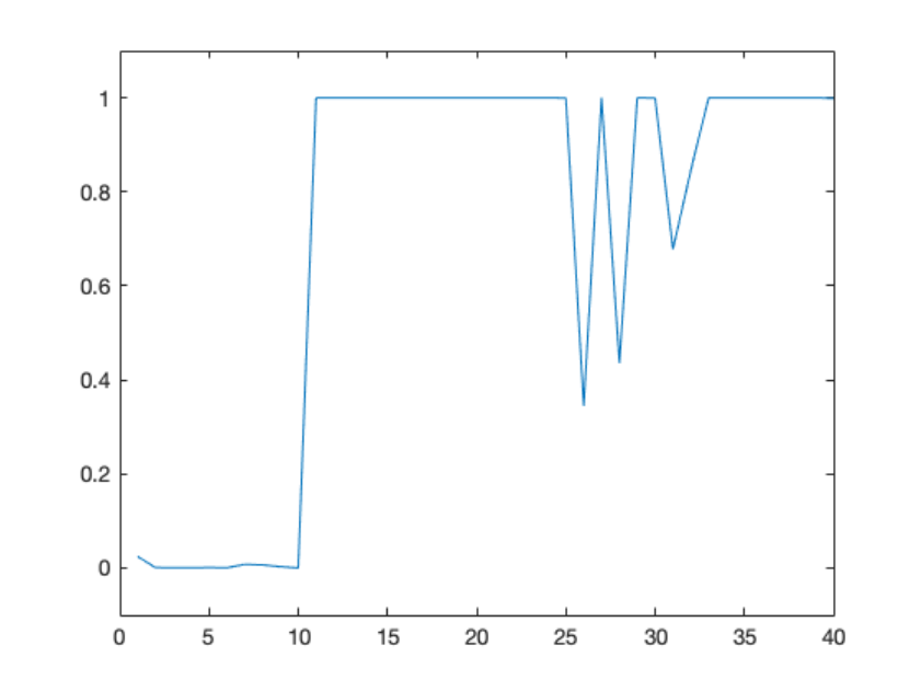
As you see, the estimated responsibility of model_dualRL for the ﬁrst 10 subjects is almost

zero. These results make sense as this is a synthetic dataset and the ﬁrst 10 subjects are actually

generated using model_RL. The next 30 individual datasets are generated using model_dualRL.

Let’s also take a look at exceedance probability, a metric typically used for model selection.

In [22]: xp = cbm.output.exceedance_prob

xp =

0.0041 0.9959

The exceedance probability indicates the probability that each model is the most likely model

across the group.

A more useful metric is called protected exceedance probability, which also takes into account

the null hypothesis that no model in the model space is most likely across the population (i.e. any

difference between model frequencies is due to chance).

In [23]: pxp = cbm.output.protected_exceedance_prob

pxp =

NaN NaN

As you see, this is currently only NaN values. This is because for computing protected ex-

ceedance probabilities, the HBI should be re-run under the (prior) null hypothesis.

This is how you can do it:

In [24]: fdata = load('all_data.mat');

data = fdata.data;

fname_hbi = 'hbi_RL_dualRL';

% 1st input is data,

% 2nd input is the file-address of the file saved by cbm_hbi

cbm_hbi_null(data,fname_hbi);

% Running this command, prints a report on your matlab output

% (e.g. on the command window)

cbm_hbi_hbi 18-Jun-2019 22:05:01

Running hierarchical bayesian inference (HBI)- null mode...

HBI has been initialized according to

lap_RL.mat [for model 1]

lap_dualRL.mat [for model 2]

Number of samples: 40

Number of models: 2

======================================================================

Iteration 01

Iteration 02

dL: 5.07

dx: 0.15

Iteration 03

dL: 1.14

dx: 0.05

Iteration 04

dL: -0.08

dx: 0.02

Iteration 05

dL: 0.06

dx: 0.01

Iteration 06

dL: 0.08

dx: 0.01

Converged :]

cbm_hbi_null saves a new ﬁle ‘hbi_RL_dualRL_null.mat’ and it also updates the cbm in

hbi_RL_dualRL.mat.

Load again hbi_RL_dualRL.mat and look at the protected exceedance probability

In [25]: fname_hbi = load('hbi_RL_dualRL.mat');

cbm = fname_hbi.cbm;

pxp = cbm.output.protected_exceedance_prob

pxp =

0.0041 0.9959

Note that here values of xp and pxp are not really different (their difference is very small). In

many datasets, however, their difference might be quite substantial.

2 Example 2: Two-step Markov decision task

We now use cbm tools for computational modeling in the two-step Markov decision task intro-

duced by Daw et al. (2011). This task is a well-known paradigm to distinguish two behavioral

modes, model-based and model-free learning. Daw et al. have proposed three reinforcement

learning accounts, a model-based, a model-free and their hybrid (which nests the other two and

combines their estimates according to a weight parameter), to disentangle contribution of these

two behavioral modes on choices.

For this example, we use an empirical dataset reported in Piray et al. (2016) (20 subjects for

this example), which is stored in the example_2step_task directory.

The hybrid, model-based and model-free algorithms contain 7, 4 and 6 parameters, respec-

tively. Please see Daw et al. for formal description of the models.

loglik = model(parameters,subj);

Now enter the example_2step_task directory and load data.

In [26]: % assuming that the current directory is example_RL_task

cd(fullfile('..','example_2step_task'));

% load data from all_data.mat file

fdata = load('all_data.mat');

data = fdata.data;

subj1 = data{1};

subj1

subj1 =

struct with fields:

choice1: [201x1 double]

transit: [201x1 double]

state2: [201x1 double]

choice2: [201x1 double]

outcome: [201x1 double]

description: {5x1 cell}

See subj1.description for a description of information stored for each subject.

Now, you should call cbm_lap with each model separately.

In [27]: prior_mb = struct('mean',zeros(4,1),'variance',6.25);

fname_mb = 'lap_mb.mat';

cbm_lap(data, @model_mb, prior_mb, fname_mb);

% Running this command, prints a report on your matlab output

% (e.g. on the command window)

If you have many subjects or a model with many parameters, the cbm_lap can take a long

time to ﬁt all of them. If you have access to cluster computing, however, you can run cbm_lap in

parallel for subjects. For example, here we ﬁt model_mf to the data of only subject 1:

In [28]: % create a directory for individual output files:

mkdir('lap_subjects');

% 1st input: data

% now the input data should be the data of subject 1

data_subj = data(1);

% 2nd input: function handle of model (i.e. @model_mf)

% 3rd input: a prior struct. The size of mean should

% be equal to the number of parameters

prior_mf = struct('mean',zeros(6,1),'variance',6.25);

% 4th input: output file

% note that here the output is associated with subject 1

% we save all output files in the lap_subjects directory

fname_mf_subj = fullfile('lap_subjects','lap_mf_1.mat');

cbm_lap(data_subj, @model_mf, prior_mf, fname_mf_subj);

Warning: Directory already exists.

cbm_lap 18-Jun-2019 22:05:04

======================================================================

Number of samples: 1

Number of parameters: 6

Number of initializations: 42

----------------------------------------------------------------------

Subject: 01

done :]

After all jobs ﬁnished, you should call cbm_lap_aggregate to aggregate individual ﬁles:

In [29]: % first make a list of lap_mf_* files:

fname_subjs = cell(20,1);

for n=1:length(fname_subjs)

fname_subjs{n} = fullfile('lap_subjects',['lap_mf_'num2str(n) '.mat']);

end

fname_subjs

fname_subjs =

20x1 cell array

{'lap_subjects/lap_mf_1.mat'}

{'lap_subjects/lap_mf_2.mat'}

{'lap_subjects/lap_mf_3.mat'}

{'lap_subjects/lap_mf_4.mat'}

{'lap_subjects/lap_mf_5.mat'}

{'lap_subjects/lap_mf_6.mat'}

{'lap_subjects/lap_mf_7.mat'}

{'lap_subjects/lap_mf_8.mat'}

{'lap_subjects/lap_mf_9.mat'}

{'lap_subjects/lap_mf_10.mat'}

{'lap_subjects/lap_mf_11.mat'}

{'lap_subjects/lap_mf_12.mat'}

{'lap_subjects/lap_mf_13.mat'}

{'lap_subjects/lap_mf_14.mat'}

{'lap_subjects/lap_mf_15.mat'}

{'lap_subjects/lap_mf_16.mat'}

{'lap_subjects/lap_mf_17.mat'}

{'lap_subjects/lap_mf_18.mat'}

{'lap_subjects/lap_mf_19.mat'}

{'lap_subjects/lap_mf_20.mat'}

Now specify the ﬁnal output ﬁle-address and call cbm_lap_aggregate

In [30]: fname_mf = 'lap_mf.mat';

cbm_lap_aggregate(fname_subjs,fname_mf);

% Running this command prints a report on your matlab output

% (e.g. on the command window)

Aggregation is done over 20 subjects :]

You see that lap_mf.mat is saved by cbm_lap_aggregate. Similarly, you can ﬁt model_hybrid

to data using cbm_lap. I did that and saved lap_hybrid.mat.

Now that we have ﬁtted models to data using cbm_lap, we can run cbm_hbi. Note that you

can conﬁgure the algorithm using optional inputs:

In [31]: % 1st input: data for all subjects

fdata = load('all_data.mat');

data = fdata.data;

% 2nd input: a cell input containing function handle to models

models = {@model_hybrid, @model_mb, @model_mf};

% note that by handle, I mean @ before the name of the function

% 3rd input: another cell input containing file-address to files saved by cbm_lap

fcbm_maps = {'lap_hybrid.mat','lap_mb.mat','lap_mf.mat'};

% note that they corresponds to models (so pay attention to the order)

% 4th input: a file address for saving the output

fname_hbi = 'hbi_2step.mat';

cbm_hbi(data,models,fcbm_maps,fname_hbi);

% Running this command prints a report on your matlab output

% (e.g. on the command window)

Now, we look at the hbi_2step.mat ﬁle saved by the cbm_hbi

In [32]: fname_hbi = load('hbi_2step.mat');

cbm = fname_hbi.cbm;

First, take a look at model frequencies:

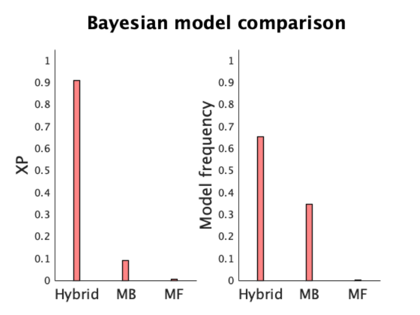
In [33]: cbm.output.model_frequency

ans =

0.6531 0.3469 0.0000

As you see the hybrid model takes about 65% of responsibility. Now let’s take a look at the

exceedance probability

In [34]: cbm.output.exceedance_prob

ans =

0.9102 0.0897 0.0000

Note that for computing the protected exceedance probability, the HBI should be re-run under

the (prior) null hypothesis cbm_hbi_null.

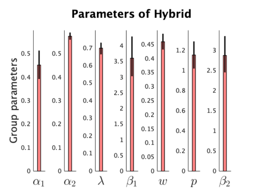
Next, we look at the parameters of the hybrid model:

In [35]: cd(fullfile('..','example_2step_task'))

% 1st input is the file-address of the file saved by cbm_hbi

fname_hbi = 'hbi_2step.mat';

% 2nd input: a cell input containing model names

model_names = {'Hybrid','MB','MF'};

% note that they corresponds to models (so pay attention to the order)

% 3rd input: another cell input containing parameter names of the winning model

param_names = {'\alpha_1','\alpha_2','\lambda','\beta_1','w','p','\beta_2'};

% 4th input: another cell input containing transformation function associated with each parameter of the winning model

transform = {'sigmoid','sigmoid','sigmoid','exp','sigmoid','none','exp'};

% note that no transformation applied to parameter p (i.e perserveration) in the hybrid model, so we just pass 'none'.

cbm_hbi_plot(fname_hbi, model_names, param_names, transform)

% this function creates a model comparison plot (exceednace probability and model frequency) as well as

% a plot of transformed parameters of the most frequent model.

plotting the group parameters of the most frequenct modelThere is no protected exceedance probability as cbm_hbi_null has not been executed

Plotting exceedance probability instead...

A critical parameter of the hybrid model is the weight parameter, which indicates the degree

to which choices inﬂuenced by model-based and model-free values. Since the weight parameter is

also constrained to be between 0 (i.e. pure model-free) and 1 (i.e. pure model-based), the normally

distributed parameter has been transformed in model_hybrid using the sigmoid function.

Similar to a t-test, you can use the hierarchical errorbars to make an inference about a param-

eter at the population level. For example, suppose you are interested to test whether the subjects

show signiﬁcantly more model-based than model-free behavior. In terms of the hybrid model,

this can be examined by testing whether the (transformed) weight parameter is signiﬁcantly dif-

ferent from 0.5 (which indicates equal contribution of model-based and model-free values). Since

sigmoid function transforms 0 to 0.5, we should test whether the normally distributed weight

parameter is signiﬁcantly different from 0. cbm_hbi_ttest performs this inference according to a

Student’s t-distribution:

In [36]: % 1st input: the fitted cbm by cbm_hbi

fname_hbi = 'hbi_2step';

% 2nd input: the index of the model of interest in the cbm file

k=1;% as the hybrid is the first model fed to cbm_hbi

% 3rd input: the test will be done compared with this value (i.e. this value indicates the null hypothesis)

m=0;% here the weight parameter should be tested against m=0

% 4th input: the index of the parameter of interest

i=5;% here the weight parameter is the 5th parameter of the hybrid model

[p,stats] = cbm_hbi_ttest(cbm,k,m,i)

p =

0.1667

stats =

struct with fields:

tstat: -1.4585

pval: 0.1667

df: 14.0626

We see that the p-value is not smaller than 0.05, so there is no signigicant evidence that the

weight is different from 0. In other words, there is no signiﬁcant evidence that subjects are more

inﬂuenced by model-based or model-free values.

As another example, let’s see whether the perseveration paramater is signiﬁcantly different

from 0 (parameter p in the above plot). This parameter indicates whether subjects repeat their

choices (or avoid if p<0) regardless of the estimated values. This parameter has not been trans-

formed, so the test should be against m=0.

In [37]: % 1st input: the fitted cbm by cbm_hbi

fname_hbi = 'hbi_2step';

% 2nd input: the index of the model of interest in the cbm file

k=1;% as the hybrid is the first model fed to cbm_hbi

% 3rd input: the test will be done compared with this value (i.e. this value indicates the null hypothesis)

m=0;% here the perseveration parameter should be tested against m=0

% 4th input: the index of the parameter of interest

d=6;% here the perseveration parameter is the 6th parameter of the hybrid model

[p,stats] = cbm_hbi_ttest(cbm,k,m,d)

p =

6.1737e-07

stats =

struct with fields:

tstat: 8.5369

pval: 6.1737e-07

df: 14.0626

Therefore, the perseveration parameter is signiﬁcantly larger than zero (p<0.001).

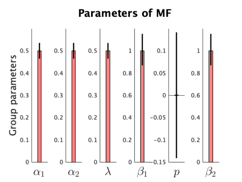
In this example, the model-free model does not take any responsibility. In this situation, the

HBI assigns prior values to the individual parameters (with a large variance). This prior value

is 0 before transformation. Therefore, for parameters bounded in the unit range (e.g. learning

rate), this prior value (after transformation) is 0.5, for decision noise parameter is 1 and for the

reservation parameter is 0.

In [38]: % 1st input is the file-address of the file saved by cbm_hbi

fname_hbi = 'hbi_2step.mat';

% 2nd input: a cell input containing model names

model_names = {'Hybrid','MB','MF'};

% note that they corresponds to models (so pay attention to the order)

% 3rd input: another cell input containing parameter names of the winning model

param_names = {'\alpha_1','\alpha_2','\lambda','\beta_1','p','\beta_2'};

% 4th input: another cell input containing transformation function associated with each parameter of the winning model

transform = {'sigmoid','sigmoid','sigmoid','exp','none','exp'};

% note that no transformation applied to parameter p (i.e perserveration) in the hybrid model, so we just pass 'none'.

cbm_hbi_plot(fname_hbi, model_names, param_names, transform, 3)

% this function creates a model comparison plot (exceednace probability and model frequency) as well as

% a plot of transformed parameters of the most frequent model.

There is no protected exceedance probability as cbm_hbi_null has not been executed

Plotting exceedance probability instead...

2.1 Reference

If you use cbm, please cite this paper:

Piray P, Dezfouli A, Heskes T, Frank MJ, Daw ND. Hierarchical Bayesian in-

ference for concurrent model ﬁtting and comparison for group studies. bioRxiv

https://journals.plos.org/ploscompbiol/article?id=10.1371/journal.pcbi.1007043

For a more formal description of the HBI algorithm, please see this paper.

Manual

Navigation menu

Versions of this User Manual:

Views

Navigation