Manual
User Manual:
Open the PDF directly: View PDF ![]() .
.
Page Count: 654 [warning: Documents this large are best viewed by clicking the View PDF Link!]
- Preface
- Next generation assembly editing with Gap5
- Gap5 Databases
- Contig Selector / Comparator
- Template Display
- Editing in Gap5
- Moving the visible segment of the contig
- Names
- Editing
- Cut and Paste Control of Sequence
- Selecting Sequences
- Annotations
- Searching
- Search by Annotation Comments
- Search by Tag Type
- Search by Padded Position
- Search by Unpadded Position
- Search by Sequence
- Search by Reading Name
- Search by Reference InDel
- Search by Consensus Quality
- Search by Consensus Discrepancy
- Search by Consensus Heterozygosity
- Search by Low Coverage
- Search by High Coverage
- The Settings Menu
- Primer Selection
- Traces
- The Editor Information Line
- The Join Editor
- Using Several Editors at Once
- Quitting the Editor
- Summary
- Plotting Restriction Enzymes
- Importing and Exporting Data
- Finding Sequence Matches
- Checking Assemblies and Removing Readings
- Removing Readings and Breaking Contigs
- Tidying up alignments
- Calculating Consensus Sequences
- Other Miscellany
- Sequence assembly and finishing using Gap4
- Organisation of the gap4 Manual
- Introduction
- Contig Selector
- Contig Comparator
- Contig Overviews
- Editing in Gap4
- Moving the visible segment of the contig
- Names
- Editing
- Selections
- Annotations
- Searching
- Search by Position
- Search by Problem
- Search by Annotation Comments
- Search by Tag Type
- Search by Sequence
- Search by Quality
- Search by Consensus Quality
- Search by file
- Search by Reading Name
- Search by Edit
- Search by Evidence for Edit (1)
- Search by Evidence for Edit (2)
- Search by Discrepancies
- Search by Consensus Discrepancies
- The Commands Menu
- The Settings Menu
- Status Line
- Trace Display
- Auto-display Traces
- Show Read-pair Traces
- Auto-diff Traces
- Y scale differences
- Consensus Algorithm
- Group Readings
- Highlight Disagreements
- Compare Strands
- Toggle auto-save
- 3 Character Amino Acids
- Show Reading and Consensus Quality
- Show edits
- Show Unpadded Positions
- Show Template Names
- Set Active Tags
- Set Output List
- Set Default Confidences
- Set or unset saving of undo
- Removing Readings
- Primer Selection
- Traces
- Reference Sequence and Traces
- Template Status Codes
- The Editor Information Line
- The Join Editor
- Using Several Editors at Once
- Quitting the Editor
- Editing Techniques
- Summary
- Assembling and Adding Readings to a Database
- Ordering and Joining Contigs
- Checking Assemblies and Removing Readings
- Removing Readings and Breaking Contigs
- Finishing Experiments
- Calculating Consensus Sequences
- Miscellaneous functions
- Results Manager
- Lists
- Notes
- Gap4 Database Files
- Copy Readings
- Check Database
- Doctor Database
- Configuring
- Command Line Arguments
- Searching for point mutations using pregap4 and gap4
- Introduction to mutation detection
- Mutation Detection Programs
- Mutation Detection Reference Data
- Reference Sequences
- Reference Traces
- Using The Template Display With Mutation Data
- Configuring The Gap4 Editor For Mutation Data
- Using The Gap4 Editor With Mutation Data
- Processing Batches Of Mutation Data Trace Files
- Processing Batches Of Mutation Data Trace Files Using Pregap4
- Configuration Of Pregap4 For Mutation Data
- Discussion Of Mutation Data Processing Methods
- Introduction to mutation detection
- Preparing readings for assembly using pregap4
- Organisation of the Pregap4 Manual
- Introduction
- Specifying Files to Process
- Running Pregap4
- Configuring the Pregap4 User Interface
- Configuring Modules
- General Configuration
- Estimate Base Accuracies
- Phred
- ATQA
- Trace Format Conversion
- Initialise Experiment Files
- Augment Experiment Files
- Quality Clip
- Sequencing Vector Clip
- Cross_match
- Cloning Vector Clip
- Screen for Unclipped Vector
- Screen Sequences
- Blast Screen
- Interactive Clipping
- Extract Sequence
- RepeatMasker
- Tag Repeats
- Mutation Detection
- Reference Traces and Reference Sequences
- Trace Difference
- Mutation Scanner
- Gap4 Shotgun Assembly
- Cap2 Assembly
- Cap3 Assembly
- FakII Assembly
- Phrap Assembly
- Enter Assembly into Gap4
- Old Cloning Vector Clip - Obsolete
- ALF/ABI to SCF Conversion - Obsolete
- Using Config Files
- Pregap4 Naming Schemes
- Pregap4 Components
- Information Sources
- Adding and Removing Modules
- Low Level Pregap4 Configuration
- Low Level Global Configuration
- Low Level Component Configuration
- Low Level Module Configuration
- General Configuration
- ALF/ABI to SCF Conversion
- Estimate Base Accuracies
- Phred
- ATQA
- Trace Format Conversion
- Initialise Experiment Files
- Augment Experiment Files
- Uncalled Base Clip
- Quality Clip
- Sequencing Vector Clip
- Cross_match
- Cloning Vector Clip
- Old Cloning Vector Clip
- Screen for Unclipped Vector
- Screen Sequences
- Blast Screen
- Interactive Clipping
- Extract Sequence
- Tag Repeats
- RepeatMasker
- Mutation Detection
- Gap4 Shotgun Assembly
- Cap2 Assembly
- Cap3 Assembly
- FakII Assembly
- Phrap Assembly
- Enter Assembly into Gap4
- Shutdown
- Writing New Modules
- Marking poor quality and vector segments of readings
- Screening Against Vector Sequences
- Screening Readings for Contaminant Sequences
- Viewing and editing trace data using trev
- Analysing and comparing sequences using spin
- Organisation of the Spin Manual
- Introduction
- Spin's Analytical Functions
- Spin Comparison Functions
- Controlling and Managing Results
- The Spin User Interface
- Controlling and Managing Results
- Reading and Managing Sequences
- User Interface
- File Formats
- SCF
- ZTR
- Header
- Chunk Format
- Data format 0 - Raw
- Data format 1 - Run Length Encoding
- Data format 2 - ZLIB
- Data format 64/0x40 - 8-bit delta
- Data format 65/0x41 - 16-bit delta
- Data format 66/0x42 - 32-bit delta
- Data format 67-69/0x43-0x45 - reserved
- Data format 70/0x46 - 16 to 8 bit conversion
- Data format 71/0x47 - 32 to 8 bit conversion
- Data format 72/0x48 - "follow" predictor
- Data format 73/0x49 - floating point 16-bit chebyshev polynomial predictor
- Data format 74/0x4A - integer based 16-bit chebyshev polynomial predictor
- Chunk Types
- Text Identifiers
- References
- Experiment File
- Restriction Enzyme File
- Vector_primer File
- Vector Sequence Format
- Man Pages
- References
- General Index
- File Index
- Variable Index
- Function Index

The Staden Package Manual
Last update on 25 April 2016
James Bonfield, Kathryn Beal, Mark Jordan,
Yaping Cheng and Rodger Staden

Copyright c
1999-2002, Medical Research Council, Laboratory of Molecular Biology. Made
available under the standard BSD licence.
Copyright c
2002-2006, Genome Research Limited (GRL). Made available under the stan-
dard BSD licence.
Portions of this code are derived from a modified Primer3 library. This bears the following
copyright notice:
Copyright c
1996,1997,1998 Whitehead Institute for Biomedical Research. All rights re-
served.
Redistribution and use in source and binary forms, with or without modification, are per-
mitted provided that the following conditions are met:
1. Redistributions must reproduce the above copyright notice, this list of conditions and
the following disclaimer in the documentation and/or other materials provided with the
distribution. Redistributions of source code must also reproduce this information in the
source code itself.
2. If the program is modified, redistributions must include a notice (in the same places as
above) indicating that the redistributed program is not identical to the version distributed
by Whitehead Institute.
3. All advertising materials mentioning features or use of this software must display the
following acknowledgment: This product includes software developed by the Whitehead
Institute for Biomedical Research.
4. The name of the Whitehead Institute may not be used to endorse or promote products
derived from this software without specific prior written permission.
We also request that use of this software be cited in publications as
Steve Rozen, Helen J. Skaletsky (1996,1997,1998) Primer3. Code available at http://www-
genome.wi.mit.edu/genome software/other/primer3.html
THIS SOFTWARE IS PROVIDED BY THE WHITEHEAD INSTITUTE “AS IS” AND
ANY EXPRESS OR IMPLIED WARRANTIES, INCLUDING, BUT NOT LIMITED
TO, THE IMPLIED WARRANTIES OF MERCHANTABILITY AND FITNESS FOR A
PARTICULAR PURPOSE ARE DISCLAIMED. IN NO EVENT SHALL THE WHITE-
HEAD INSTITUTE BE LIABLE FOR ANY DIRECT, INDIRECT, INCIDENTAL,
SPECIAL, EXEMPLARY, OR CONSEQUENTIAL DAMAGES (INCLUDING, BUT
NOT LIMITED TO, PROCUREMENT OF SUBSTITUTE GOODS OR SERVICES;
LOSS OF USE, DATA, OR PROFITS; OR BUSINESS INTERRUPTION) HOWEVER
CAUSED AND ON ANY THEORY OF LIABILITY, WHETHER IN CONTRACT,
STRICT LIABILITY, OR TORT (INCLUDING NEGLIGENCE OR OTHERWISE)
ARISING IN ANY WAY OUT OF THE USE OF THIS SOFTWARE, EVEN IF
ADVISED OF THE POSSIBILITY OF SUCH DAMAGE.
Permission is given to duplicate this manual in both paper and electronic forms.
i
Short Contents
1 Next generation assembly editing with Gap5 ............... 3
2 Sequence assembly and finishing using Gap4 .............. 95
3 Searching for point mutations using pregap4 and gap4 ..... 309
4 Preparing readings for assembly using pregap4 ............ 325
5 Marking poor quality and vector segments of readings . . . . . . 399
6 Screening Against Vector Sequences .................... 401
7 Screening Readings for Contaminant Sequences ........... 413
8 Viewing and editing trace data using trev ................ 417
9 Analysing and comparing sequences using spin............ 429
10 User Interface ...................................... 523
11 File Formats ....................................... 533
12 Man Pages ......................................... 569
References ............................................. 611
General Index .......................................... 613
File Index ............................................. 625
Variable Index ......................................... 627
Function Index ......................................... 629
iii
Table of Contents
Preface.............................................................. 1
1 Next generation assembly editing with Gap5
................................................. 3
1.1 Gap5 Databases................................................ 4
1.1.1 Creating databases ........................................ 4
1.1.2 Opening/closing databases ................................ 5
1.1.3 Changing directories....................................... 5
1.1.4 Check Database ........................................... 6
1.2 Contig Selector / Comparator .................................. 7
1.2.1 Contig Selector ............................................ 7
1.2.1.1 Selecting Contigs ..................................... 7
1.2.1.2 Changing the Contig Order ........................... 9
1.2.1.3 The Contig Selector Menus ........................... 9
1.2.2 Contig Comparator....................................... 10
1.2.2.1 Examining Results and Using Them to Select
Commands .............................................. 11
1.2.2.2 Automatic Match Navigation ........................ 12
1.3 Template Display ............................................. 14
1.3.1 Filtering data ............................................ 15
1.3.2 Template plot ............................................ 15
1.3.2.1 Controlling The Y Layout............................ 17
1.3.3 Depth / Coverage Plot ................................... 20
1.4 Editing in Gap5............................................... 21
1.4.1 Moving the visible segment of the contig .................. 22
1.4.2 Names ................................................... 23
1.4.3 Editing .................................................. 25
1.4.3.1 Moving the editing cursor ........................... 26
1.4.3.2 Adjusting the Quality Values ........................ 26
1.4.3.3 Adjusting the alignment coordinates ................. 27
1.4.3.4 Adjusting the Cutoff Data ........................... 27
1.4.3.5 Summary of Editing Commands ..................... 27
1.4.4 Cut and Paste Control of Sequence ....................... 28
1.4.5 Selecting Sequences ...................................... 29
1.4.6 Annotations.............................................. 29
1.4.6.1 Annotation Macros .................................. 31
1.4.7 Searching ................................................ 32
1.4.7.1 Search by Annotation Comments .................... 32
1.4.7.2 Search by Tag Type ................................. 33
1.4.7.3 Search by Padded Position .......................... 33
1.4.7.4 Search by Unpadded Position ........................ 33
1.4.7.5 Search by Sequence.................................. 33
1.4.7.6 Search by Reading Name ............................ 33
1.4.7.7 Search by Reference InDel ........................... 33

iv The Staden Package Manual
1.4.7.8 Search by Consensus Quality ........................ 34
1.4.7.9 Search by Consensus Discrepancy .................... 34
1.4.7.10 Search by Consensus Heterozygosity ................ 34
1.4.7.11 Search by Low Coverage............................ 34
1.4.7.12 Search by High Coverage ........................... 34
1.4.8 The Settings Menu ....................................... 34
1.4.8.1 Group Readings ..................................... 35
1.4.8.2 Highlight Disagreements ............................. 36
1.4.8.3 Pack Sequences...................................... 36
1.4.8.4 Hide Annotations ................................... 36
1.4.9 Primer Selection ......................................... 36
1.4.10 Traces .................................................. 38
1.4.11 The Editor Information Line ............................ 40
1.4.11.1 Reading Information ............................... 41
1.4.11.2 Contig Information ................................. 42
1.4.11.3 Tag Information.................................... 42
1.4.12 The Join Editor ......................................... 43
1.4.13 Using Several Editors at Once ........................... 44
1.4.14 Quitting the Editor ..................................... 44
1.4.15 Summary ............................................... 44
1.4.15.1 Keyboard summary for editing window ............. 44
1.4.15.2 Mouse summary for editing window ................ 45
1.4.15.3 Mouse summary for names window ................. 46
1.4.16 Plotting Restriction Enzymes............................ 47
1.4.16.1 Selecting Enzymes.................................. 47
1.4.16.2 Examining the Plot ................................ 48
1.4.16.3 Reconfiguring the Plot ............................. 48
1.4.16.4 Textual Outputs ................................... 48
1.5 Importing and Exporting Data ................................ 50
1.5.1 Assembly ................................................ 50
1.5.1.1 Importing with tg index ............................. 50
1.5.1.2 Importing fasta/fastq files ........................... 52
1.5.1.3 Mapped assembly by bwa aln ........................ 52
1.5.1.4 Mapped assembly by bwa dbwtsw ................... 52
1.5.2 Importing GFF .......................................... 54
1.5.3 Export Tags ............................................. 54
1.5.4 Export Sequences ........................................ 55
1.6 Finding Sequence Matches .................................... 56
1.6.1 Find Internal Joins ....................................... 56
1.6.1.1 Find Internal Joins Dialogue......................... 59
1.6.2 Find Repeats............................................. 62
1.6.3 Find Read Pairs.......................................... 64
1.6.3.1 Find Read Pairs Graphical Output .................. 64
1.6.4 Sequence Search.......................................... 67
1.7 Checking Assemblies and Removing Readings.................. 69
1.7.0.1 Checking Assemblies ................................ 70
1.7.1 Removing Readings and Breaking Contigs ................ 72
1.7.1.1 Breaking Contigs .................................... 73
v
1.7.1.2 Disassembling Readings ............................. 74
1.7.1.3 Delete Contigs ...................................... 75
1.8 Tidying up alignments ........................................ 76
1.8.1 Shuffle Pads.............................................. 76
1.8.2 Remove Pad Columns .................................... 77
1.8.3 Remove Contig Holes..................................... 78
1.9 Calculating Consensus Sequences .............................. 79
1.9.1 Normal Consensus Output ............................... 80
1.9.2 The Consensus Algorithms ............................... 81
1.9.2.1 Consensus Calculation Using Base Frequencies ....... 83
1.9.2.2 Consensus Calculation Using Weighted Base Frequencies
......................................................... 83
1.9.2.3 Consensus Calculation Using Confidence values . . . . . . 84
1.9.2.4 The Quality Calculation ............................. 85
1.9.3 List Consensus Confidence................................ 86
1.9.4 List Base Confidence ..................................... 87
1.10 Other Miscellany............................................. 89
1.10.1 List Libraries ........................................... 89
1.10.2 Results Manager ........................................ 91
1.10.3 Lists .................................................... 92
1.10.3.1 Special List Names ................................. 92
1.10.3.2 Basic List Commands .............................. 92
1.10.3.3 Contigs To Readings Command .................... 93
1.10.3.4 Search Sequence Names ............................ 93
2 Sequence assembly and finishing using Gap4
................................................ 95
2.1 Organisation of the gap4 Manual .............................. 95
2.2 Introduction .................................................. 95
2.2.1 Summary of the Files used and the Preprocessing Steps . . . 97
2.2.2 Summary of Gap4’s Functions ............................ 99
2.2.3 Introduction to the gap4 User Interface .................. 101
2.2.3.1 Introduction to the Contig Selector ................. 102
2.2.3.2 Introduction to the Contig Comparator ............. 103
2.2.3.3 Introduction to the Template Display ............... 105
2.2.3.4 Introduction to the Consistency Display ............ 107
2.2.3.5 Introduction to the Restriction Enzyme Map ....... 109
2.2.3.6 Introduction to the Stop Codon Map ............... 110
2.2.3.7 Introduction to the Contig Editor .................. 111
2.2.3.8 Introduction to the Contig Joining Editor........... 114
2.2.4 Gap4 Menus ............................................ 115
2.2.4.1 Gap4 File menu .................................... 115
2.2.4.2 Gap4 Edit menu ................................... 115
2.2.4.3 Gap4 View menu ................................... 115
2.2.4.4 Gap4 Options menu ................................ 116
2.2.4.5 Gap4 Experiments menu ........................... 116
2.2.4.6 Gap4 Lists menu ................................... 116
2.2.4.7 Gap4 Assembly menu .............................. 117
vi The Staden Package Manual
2.2.5 The use of numerical estimates of base calling accuracy . . 118
2.2.6 Use of the "hidden"poor quality data ................... 120
2.2.7 Annotating and masking readings and contigs ........... 121
2.2.7.1 Standard tag types ................................. 121
2.2.7.2 Active tags and masking ........................... 121
2.3 Contig Selector .............................................. 123
2.3.1 Selecting Contigs........................................ 123
2.3.2 Changing the Contig Order.............................. 125
2.3.3 The Contig Selector Menus .............................. 125
2.4 Contig Comparator .......................................... 126
2.4.1 Examining Results and Using Them to Select Commands
........................................................... 127
2.4.2 Automatic Match Navigation ............................ 128
2.5 Contig Overviews ............................................ 130
2.5.1 Template Display ....................................... 130
2.5.1.1 Reading and Template Plot......................... 132
2.5.1.2 Reading and Template Plot Display ................ 132
2.5.1.3 Reading and Template Plot Options ................ 135
2.5.1.4 Reading and Template Plot Operations ............. 136
2.5.1.5 Quality Plot ....................................... 137
2.5.1.6 Restriction Enzyme Plot ........................... 139
2.5.2 Consistency Display ..................................... 140
2.5.2.1 Confidence Values Graph ........................... 142
2.5.2.2 Reading Coverage Histogram ....................... 142
2.5.2.3 Read-Pair Coverage Histogram ..................... 143
2.5.2.4 Strand Coverage ................................... 144
2.5.2.5 2nd-Highest Confidence ............................ 145
2.5.2.6 Diploid Graph...................................... 147
2.5.3 SNP Candidates ........................................ 147
2.5.4 Plotting Consensus Quality.............................. 153
2.5.4.1 Examining the Quality Plot ........................ 153
2.5.5 Plotting Stop Codons ................................... 156
2.5.5.1 Examining the Plot ................................ 156
2.5.5.2 Updating the Plot .................................. 156
2.5.6 Plotting Restriction Enzymes............................ 157
2.5.6.1 Selecting Enzymes.................................. 157
2.5.6.2 Examining the Plot ................................ 158
2.5.6.3 Reconfiguring the Plot ............................. 158
2.5.6.4 Creating Tags for Cut Sites......................... 158
2.5.6.5 Textual Outputs ................................... 158
2.6 Editing in Gap4 ............................................. 160
2.6.1 Moving the visible segment of the contig................. 162
2.6.2 Names .................................................. 163
2.6.3 Editing ................................................. 165
2.6.3.1 Moving the editing cursor .......................... 165
2.6.3.2 Editing Modes ..................................... 166
2.6.3.3 Adjusting the Quality Values ....................... 169
2.6.3.4 Adjusting the Cutoff Data .......................... 169
vii
2.6.3.5 Summary of Editing Commands .................... 169
2.6.4 Selections ............................................... 170
2.6.5 Annotations............................................. 171
2.6.6 Searching ............................................... 174
2.6.6.1 Search by Position ................................. 174
2.6.6.2 Search by Problem ................................. 175
2.6.6.3 Search by Annotation Comments ................... 175
2.6.6.4 Search by Tag Type ................................ 175
2.6.6.5 Search by Sequence ................................ 175
2.6.6.6 Search by Quality .................................. 175
2.6.6.7 Search by Consensus Quality ....................... 175
2.6.6.8 Search by file....................................... 176
2.6.6.9 Search by Reading Name ........................... 176
2.6.6.10 Search by Edit .................................... 176
2.6.6.11 Search by Evidence for Edit (1) ................... 176
2.6.6.12 Search by Evidence for Edit (2) ................... 176
2.6.6.13 Search by Discrepancies ........................... 177
2.6.6.14 Search by Consensus Discrepancies ................ 177
2.6.7 The Commands Menu ................................... 177
2.6.7.1 Search ............................................. 177
2.6.7.2 Create Tag ......................................... 177
2.6.7.3 Edit Tag ........................................... 177
2.6.7.4 Delete Tag ......................................... 177
2.6.7.5 Save Contig ........................................ 177
2.6.7.6 Dump Contig to File ............................... 178
2.6.7.7 Save Consensus Trace .............................. 178
2.6.7.8 List Confidence .................................... 178
2.6.7.9 Report Mutations .................................. 178
2.6.7.10 Select Primer ..................................... 179
2.6.7.11 Align ............................................. 179
2.6.7.12 Remove Reading .................................. 179
2.6.7.13 Break Contig...................................... 179
2.6.8 The Settings Menu ...................................... 179
2.6.8.1 Status Line ........................................ 180
2.6.8.2 Trace Display ...................................... 181
2.6.8.3 Auto-display Traces ................................ 181
2.6.8.4 Show Read-pair Traces ............................. 182
2.6.8.5 Auto-diff Traces .................................... 182
2.6.8.6 Y scale differences .................................. 183
2.6.8.7 Consensus Algorithm ............................... 183
2.6.8.8 Group Readings .................................... 183
2.6.8.9 Highlight Disagreements ............................ 184
2.6.8.10 Compare Strands ................................. 184
2.6.8.11 Toggle auto-save .................................. 184
2.6.8.12 3 Character Amino Acids ......................... 184
2.6.8.13 Show Reading and Consensus Quality ............. 184
2.6.8.14 Show edits ........................................ 185
2.6.8.15 Show Unpadded Positions ......................... 185
viii The Staden Package Manual
2.6.8.16 Show Template Names ............................ 185
2.6.8.17 Set Active Tags ................................... 186
2.6.8.18 Set Output List ................................... 186
2.6.8.19 Set Default Confidences ........................... 186
2.6.8.20 Set or unset saving of undo........................ 186
2.6.9 Removing Readings ..................................... 186
2.6.10 Primer Selection ....................................... 187
2.6.10.1 Parameters........................................ 188
2.6.10.2 Template selection ................................ 188
2.6.11 Traces ................................................. 188
2.6.12 Reference Sequence and Traces ......................... 191
2.6.12.1 Reference sequences ............................... 191
2.6.12.2 Reference traces................................... 191
2.6.13 Template Status Codes................................. 192
2.6.14 The Editor Information Line ........................... 193
2.6.14.1 Reading Information .............................. 194
2.6.14.2 Contig Information................................ 195
2.6.14.3 Tag Information................................... 195
2.6.14.4 Base Information.................................. 195
2.6.15 The Join Editor........................................ 196
2.6.16 Using Several Editors at Once .......................... 197
2.6.17 Quitting the Editor .................................... 197
2.6.18 Editing Techniques..................................... 197
2.6.18.1 Consensus and Quality Cutoffs .................... 198
2.6.18.2 Editing by Base Change or Confidence ............ 199
2.6.18.3 Base Overcalls .................................... 199
2.6.18.4 Base Undercalls ................................... 200
2.6.18.5 Multiple Base Disagreements ...................... 200
2.6.18.6 Poor Quality ...................................... 201
2.6.18.7 Checking for Errors ............................... 201
2.6.19 Summary .............................................. 202
2.6.19.1 Keyboard summary for editing window ............ 202
2.6.19.2 Mouse summary for editing window ............... 203
2.6.19.3 Mouse summary for names window ................ 203
2.6.19.4 Mouse summary for scrollbar ...................... 204
2.7 Assembling and Adding Readings to a Database .............. 205
2.7.1 Normal Shotgun Assembly .............................. 205
2.7.1.1 Assemble Independently ............................ 209
2.7.1.2 Assemble Into Single Stranded Regions ............. 209
2.7.1.3 Stack Readings ..................................... 210
2.7.1.4 Put All Readings In Separate Contigs .............. 211
2.7.2 Directed Assembly ...................................... 211
2.7.3 Screen Only............................................. 213
2.7.4 General Comments and Tips on Assembly ............... 215
2.7.5 Assembly Failure Codes ................................. 216
2.8 Ordering and Joining Contigs ................................ 217
2.8.1 Order contigs ........................................... 219
2.8.2 Find Read Pairs ........................................ 222
ix
2.8.2.1 Find Read Pairs Graphical Output ................. 222
2.8.2.2 Find Read Pairs Text Output ...................... 224
2.8.2.3 The Template Lines ................................ 224
2.8.2.4 The Reading Lines ................................. 225
2.8.3 Find Internal Joins ...................................... 227
2.8.3.1 Find Internal Joins Dialogue........................ 230
2.8.4 Find Repeats ........................................... 233
2.9 Checking Assemblies and Removing Readings ................ 235
2.9.0.1 Checking Assemblies ............................... 236
2.9.1 Removing Readings and Breaking Contigs ............... 238
2.9.1.1 Breaking Contigs ................................... 239
2.9.1.2 Disassembling Readings ............................ 240
2.10 Finishing Experiments ...................................... 241
2.10.1 Double Stranding ...................................... 241
2.10.2 Suggest Primers........................................ 243
2.10.3 Suggest Long Readings................................. 245
2.10.4 Compressions and Stops................................ 247
2.10.5 Suggest Probes ........................................ 249
2.11 Calculating Consensus Sequences............................ 251
2.11.1 Normal Consensus Output ............................. 252
2.11.2 Extended Consensus Output ........................... 253
2.11.3 Unfinished Consensus Output .......................... 255
2.11.4 Quality Consensus Output ............................. 255
2.11.5 The Consensus Algorithms ............................. 257
2.11.5.1 Consensus Calculation Using Base Frequencies..... 258
2.11.5.2 Consensus Calculation Using Weighted Base
Frequencies............................................. 259
2.11.5.3 Consensus Calculation Using Confidence values . . . . 259
2.11.5.4 The Quality Calculation........................... 261
2.11.6 List Consensus Confidence ............................. 261
2.11.7 List Base Confidence ................................... 263
2.12 Miscellaneous functions ..................................... 265
2.12.1 Complement a Contig .................................. 265
2.12.2 Enter Tags............................................. 265
2.12.3 Shuffle Pads ........................................... 265
2.12.4 Show Relationships .................................... 267
2.12.5 Contig Navigation ..................................... 269
2.12.6 Sequence Search ....................................... 271
2.12.7 Extract Readings ...................................... 273
2.12.8 Automatic Clipping by Quality and Sequence Similarity
........................................................... 274
2.12.8.1 Difference Clipping ................................ 274
2.12.8.2 Quality Clipping .................................. 275
2.12.8.3 Quality Clip Ends ................................. 275
2.12.8.4 N-Base Clipping .................................. 276
2.13 Results Manager ............................................ 277
2.14 Lists........................................................ 278
2.14.1 Special List Names..................................... 278
x The Staden Package Manual
2.14.2 Basic List Commands .................................. 278
2.14.3 Contigs To Readings Command ........................ 279
2.14.4 Minimal Coverage Command ........................... 279
2.14.5 Unattached Readings Command........................ 279
2.14.6 Highlight Readings List ................................ 279
2.14.7 Search Sequence Names ................................ 279
2.14.8 Search Template Names ................................ 280
2.14.9 Search Annotation Contents............................ 280
2.15 Notes ....................................................... 281
2.15.1 Selecting Notes ........................................ 281
2.15.2 Editing Notes .......................................... 282
2.15.3 Special Note Types .................................... 282
2.16 Gap4 Database Files ........................................ 284
2.16.1 Directories ............................................. 284
2.16.2 Opening a New Database .............................. 285
2.16.3 Opening an Existing Database ......................... 285
2.16.4 Making Backups of Databases .......................... 285
2.16.5 Reading and Contig Names and Numbers .............. 286
2.17 Copy Readings ............................................. 287
2.17.1 Introduction ........................................... 287
2.17.1.1 Copy Reads Dialogue ............................. 287
2.18 Check Database ............................................ 290
2.18.1 Database Checks ....................................... 290
2.18.2 Contig Checks ......................................... 290
2.18.3 Reading Checks ........................................ 291
2.18.4 Annotation Checks..................................... 292
2.18.5 Note Checks ........................................... 292
2.18.6 Template Checks....................................... 292
2.18.7 Vector Checks ......................................... 292
2.18.8 Clone Checks .......................................... 292
2.19 Doctor Database............................................ 293
2.19.1 Structures Menu ....................................... 294
2.19.1.1 Database Structure................................ 295
2.19.1.2 Reading Structure................................. 295
2.19.1.3 Contig Structure .................................. 295
2.19.1.4 Annotation Structure ............................. 296
2.19.1.5 Template Structure ............................... 296
2.19.1.6 Original Clone Structure .......................... 296
2.19.1.7 Note Structure .................................... 296
2.19.2 Ignoring Check Database............................... 296
2.19.3 Extending Structures .................................. 296
2.19.4 Listing and Removing Annotations ..................... 296
2.19.5 Shift Readings ......................................... 297
2.19.6 Delete Contig .......................................... 297
2.19.7 Reset Contig Order .................................... 297
2.20 Configuring ................................................. 298
2.20.1 Introduction ........................................... 298
2.20.2 Consensus Algorithm .................................. 299
xi
2.20.3 Set Maxseq/Maxdb .................................... 299
2.20.4 Set Fonts .............................................. 299
2.20.5 Configuring Menus ..................................... 300
2.20.6 Set Genetic Code ...................................... 300
2.20.7 Alignment Scores ...................................... 301
2.20.8 Trace File Location .................................... 302
2.20.9 The Tag Selector....................................... 304
2.20.10 The GTAGDB File ................................... 304
2.20.11 Template Status ...................................... 305
2.21 Command Line Arguments.................................. 306
3 Searching for point mutations using pregap4
and gap4..................................... 309
3.1 Introduction to mutation detection ........................... 309
3.1.1 Mutation Detection Programs ........................... 314
3.1.2 Mutation Detection Reference Data ..................... 314
3.1.3 Reference Sequences..................................... 314
3.1.4 Reference Traces ........................................ 315
3.1.5 Using The Template Display With Mutation Data ....... 317
3.1.6 Configuring The Gap4 Editor For Mutation Data . . . . . . . . 318
3.1.7 Using The Gap4 Editor With Mutation Data ............ 319
3.1.8 Processing Batches Of Mutation Data Trace Files. . . . . . . . 320
3.1.9 Processing Batches Of Mutation Data Trace Files Using
Pregap4 ................................................... 322
3.1.10 Configuration Of Pregap4 For Mutation Data .......... 323
3.1.11 Discussion Of Mutation Data Processing Methods . . . . . . 324
4 Preparing readings for assembly using pregap4
............................................... 325
4.1 Organisation of the Pregap4 Manual ......................... 325
4.2 Introduction ................................................. 326
4.2.1 Summary of the Files used and the Processing Steps ..... 326
4.2.2 Introduction to the Pregap4 User Interface .............. 330
4.2.2.1 Introduction to the Files to Process Window ........ 332
4.2.2.2 Introduction to the Configure Modules Window..... 334
4.2.2.3 Introduction to the Textual Output Window . . . . . . . . 335
4.2.2.4 Introduction to Running Pregap4 ................... 335
4.2.3 Pregap4 Menus ......................................... 336
4.2.3.1 Pregap4 File menu ................................. 336
4.2.3.2 Pregap4 Modules menu............................. 336
4.2.3.3 Pregap4 Information source menu .................. 336
4.2.3.4 Pregap4 Options menu ............................. 337
4.3 Specifying Files to Process ................................... 337
4.4 Running Pregap4 ............................................ 338
4.5 Configuring the Pregap4 User Interface ....................... 341
4.5.1 Fonts and Colours....................................... 341
4.5.2 Window Styles .......................................... 341

xii The Staden Package Manual
4.6 Configuring Modules ......................................... 342
4.6.1 General Configuration................................... 344
4.6.2 Estimate Base Accuracies ............................... 344
4.6.3 Phred................................................... 344
4.6.4 ATQA .................................................. 345
4.6.5 Trace Format Conversion................................ 345
4.6.6 Initialise Experiment Files............................... 346
4.6.7 Augment Experiment Files .............................. 346
4.6.8 Quality Clip ............................................ 347
4.6.9 Sequencing Vector Clip.................................. 348
4.6.10 Cross match ........................................... 350
4.6.11 Cloning Vector Clip .................................... 350
4.6.12 Screen for Unclipped Vector ............................ 351
4.6.13 Screen Sequences....................................... 351
4.6.14 Blast Screen ........................................... 352
4.6.15 Interactive Clipping .................................... 352
4.6.16 Extract Sequence ...................................... 353
4.6.17 RepeatMasker ......................................... 353
4.6.18 Tag Repeats ........................................... 354
4.6.19 Mutation Detection .................................... 354
4.6.20 Reference Traces and Reference Sequences .............. 356
4.6.21 Trace Difference ....................................... 357
4.6.22 Mutation Scanner ...................................... 359
4.6.23 Gap4 Shotgun Assembly ............................... 361
4.6.24 Cap2 Assembly ........................................ 362
4.6.25 Cap3 Assembly ........................................ 362
4.6.26 FakII Assembly ........................................ 362
4.6.27 Phrap Assembly ....................................... 363
4.6.28 Enter Assembly into Gap4 ............................. 364
4.6.29 Email.................................................. 364
4.6.30 Old Cloning Vector Clip - Obsolete ..................... 365
4.6.31 ALF/ABI to SCF Conversion - Obsolete ............... 365
4.7 Using Config Files ........................................... 366
4.8 Pregap4 Naming Schemes .................................... 366
4.8.1 Mutation Detection Naming Scheme..................... 366
4.8.2 Old Sanger Centre Naming Scheme ...................... 367
4.8.3 New Sanger Centre Naming Scheme ..................... 368
4.8.4 Writing Your Own Naming Schemes ..................... 369
4.9 Pregap4 Components ........................................ 371
4.10 Information Sources......................................... 371
4.10.1 Simple Text Database .................................. 371
4.10.2 Experiment File Line Types ............................ 373
4.11 Adding and Removing Modules ............................. 375
4.12 Low Level Pregap4 Configuration ........................... 377
4.12.1 Low Level Global Configuration ........................ 377
4.12.2 Low Level Component Configuration ................... 378
4.12.3 Low Level Module Configuration ....................... 378
4.12.3.1 General Configuration ............................. 379

xiii
4.12.3.2 ALF/ABI to SCF Conversion ..................... 379
4.12.3.3 Estimate Base Accuracies ......................... 380
4.12.3.4 Phred ............................................. 380
4.12.3.5 ATQA ............................................ 380
4.12.3.6 Trace Format Conversion .......................... 381
4.12.3.7 Initialise Experiment Files......................... 381
4.12.3.8 Augment Experiment Files ........................ 382
4.12.3.9 Uncalled Base Clip ................................ 382
4.12.3.10 Quality Clip ..................................... 382
4.12.3.11 Sequencing Vector Clip........................... 383
4.12.3.12 Cross match ..................................... 384
4.12.3.13 Cloning Vector Clip .............................. 385
4.12.3.14 Old Cloning Vector Clip ......................... 385
4.12.3.15 Screen for Unclipped Vector ...................... 386
4.12.3.16 Screen Sequences................................. 387
4.12.3.17 Blast Screen ..................................... 387
4.12.3.18 Interactive Clipping .............................. 388
4.12.3.19 Extract Sequence ................................ 388
4.12.3.20 Tag Repeats ..................................... 388
4.12.3.21 RepeatMasker ................................... 389
4.12.3.22 Mutation Detection .............................. 389
4.12.3.23 Gap4 Shotgun Assembly ......................... 390
4.12.3.24 Cap2 Assembly .................................. 391
4.12.3.25 Cap3 Assembly .................................. 391
4.12.3.26 FakII Assembly .................................. 392
4.12.3.27 Phrap Assembly ................................. 393
4.12.3.28 Enter Assembly into Gap4 ....................... 393
4.12.3.29 Email ............................................ 394
4.12.3.30 Shutdown ........................................ 394
4.13 Writing New Modules ....................................... 395
4.13.1 An Overview of a Module .............................. 395
4.13.2 Functions .............................................. 395
4.13.3 Module Variables ...................................... 397
4.13.4 Global Variables ....................................... 397
4.13.5 Builtin Functions ...................................... 398
4.13.6 An Example Module ................................... 398
5 Marking poor quality and vector segments of
readings...................................... 399
Introduction to read clipping ...................................... 399

xiv The Staden Package Manual
6 Screening Against Vector Sequences........ 401
6.1 Algorithms .................................................. 402
6.2 Options...................................................... 404
6.3 Parameters (defaults in brackets)............................. 404
6.4 Error codes .................................................. 405
6.5 Examples .................................................... 406
6.6 Vector Primer file format .................................... 407
6.7 Vector Primer File Notes .................................... 408
6.8 Defining Cloning and Primer Sites for Vector Clip ............ 408
6.9 Finding the Cloning and Primer Sites ........................ 410
7 Screening Readings for Contaminant Sequences
............................................... 413
7.1 Parameters .................................................. 413
7.2 Limits ....................................................... 414
7.3 Error codes .................................................. 414
7.4 Examples .................................................... 415
8 Viewing and editing trace data using trev
............................................... 417
8.1 Introduction ................................................. 417
8.2 Opening trace files ........................................... 420
8.2.1 Opening a trace file from the command line ............. 420
8.2.2 Opening a trace file from within Trev.................... 421
8.3 Viewing the trace ............................................ 421
8.3.1 Searching ............................................... 422
8.3.2 Information ............................................. 422
8.4 Editing ...................................................... 422
8.4.1 Setting the left and right cutoffs ......................... 422
8.4.2 Editing the sequence .................................... 423
8.4.3 Undoing clip edits....................................... 423
8.5 Saving a trace file ............................................ 423
8.6 Processing multiple files ...................................... 423
8.7 Printing a trace .............................................. 424
8.7.1 Page options ............................................ 424
8.7.1.1 Paper options ...................................... 424
8.7.1.2 Panels ............................................. 425
8.7.1.3 Fonts .............................................. 425
8.7.2 Trace options ........................................... 425
8.7.2.1 Title ............................................... 425
8.7.2.2 Line width and colour .............................. 425
8.7.2.3 Dash pattern ....................................... 426
8.7.2.4 Print bases ......................................... 426
8.7.2.5 Print magnification................................. 426
8.7.3 Example ................................................ 427
8.8 Quitting ..................................................... 427
xv
9 Analysing and comparing sequences using spin
............................................... 429
9.1 Organisation of the Spin Manual ............................. 429
9.2 Introduction ................................................. 429
9.2.1 Summary of the Spin Single Sequence Functions ......... 429
9.2.2 Summary of the Spin Comparison Functions ............. 430
9.2.3 Introduction to the Spin User Interface .................. 431
9.2.3.1 Introduction to the Spin Plot ....................... 432
9.2.3.2 Introduction to the Spin Sequence Display .......... 437
9.2.3.3 Introduction to the Spin Sequence Comparison Plot
........................................................ 439
9.2.3.4 Introduction to the Spin Sequence Comparison Display
........................................................ 443
9.2.4 Spin Menus ............................................. 444
9.2.4.1 Spin File Menu..................................... 444
9.2.4.2 Spin View Menu ................................... 444
9.2.4.3 Spin Options Menu................................. 444
9.2.4.4 Spin Sequences Menu............................... 445
9.2.4.5 Spin Statistics Menu ............................... 445
9.2.4.6 Spin Translation Menu ............................. 445
9.2.4.7 Spin Search Menu .................................. 446
9.2.4.8 Spin Comparison Menu............................. 446
9.3 Spin’s Analytical Functions .................................. 446
9.3.1 Count Sequence Composition............................ 446
9.3.2 Count Dinucleotide Frequencies ......................... 447
9.3.3 Plot base composition ................................... 447
9.3.4 Calculate codon usage................................... 448
9.3.5 Set genetic code......................................... 451
9.3.6 Translation - general .................................... 453
9.3.7 Find open reading frames ............................... 454
9.3.8 Restriction enzyme search ............................... 456
9.3.8.1 Selecting Enzymes.................................. 457
9.3.8.2 Examining the Plot ................................ 457
9.3.8.3 Reconfiguring the Plot ............................. 458
9.3.8.4 Printing the sites ................................... 458
9.3.9 Subsequence search ..................................... 460
9.3.10 Motif search ........................................... 462
9.3.11 Gene finding ........................................... 463
9.3.11.1 Start codon search ................................ 464
9.3.11.2 Stop codon search ................................. 464
9.3.11.3 Codon usage method .............................. 466
9.3.11.4 Positional base preferences ........................ 472
9.3.11.5 Author test ....................................... 473
9.3.11.6 Uneven positional base preferences ................ 477
9.3.11.7 Splice site search .................................. 478
9.3.11.8 tRNA search ...................................... 480
9.4 Spin Comparison Functions .................................. 482
9.4.1 Finding Similar Spans ................................... 483
xvi The Staden Package Manual
9.4.2 Finding Matching Words ................................ 485
9.4.3 Finding the Best Diagonals.............................. 487
9.4.4 Aligning Sequences Globally............................. 489
9.4.5 Aligning Sequences Locally .............................. 493
9.5 Controlling and Managing Results............................ 497
9.5.1 Probabilities and expected numbers of matches .......... 498
9.5.2 Changing the maximum number of matches ............. 498
9.5.3 Changing the default number of matches ................ 498
9.5.4 Hide duplicate matches.................................. 499
9.5.5 Changing the score matrix .............................. 499
9.5.6 Set protein alignment symbols........................... 501
9.6 The Spin User Interface ...................................... 501
9.6.1 SPIN Sequence Plot ..................................... 502
9.6.1.1 Cursors ............................................ 505
9.6.1.2 Crosshairs.......................................... 506
9.6.1.3 Zoom .............................................. 506
9.6.1.4 Drag and drop ..................................... 506
9.6.2 Sequence display ........................................ 509
9.6.2.1 Search ............................................. 510
9.6.2.2 Save ............................................... 511
9.6.3 SPIN Sequence Comparison Plot ........................ 512
9.6.3.1 Cursors ............................................ 513
9.6.3.2 Crosshairs.......................................... 513
9.6.3.3 Zoom .............................................. 513
9.6.3.4 Drag and drop ..................................... 514
9.6.4 Sequence Comparison Display ........................... 514
9.7 Controlling and Managing Results............................ 515
9.7.1 Result manager ......................................... 515
9.7.1.1 Information ........................................ 517
9.7.1.2 List ................................................ 517
9.7.1.3 Configure .......................................... 517
9.7.1.4 Hide ............................................... 517
9.7.1.5 Reveal ............................................. 517
9.7.1.6 Remove ............................................ 517
9.8 Reading and Managing Sequences ............................ 517
9.8.1 Use of feature tables in spin ............................. 517
9.8.2 Reading in sequences .................................... 518
9.8.2.1 Simple search ...................................... 518
9.8.2.2 Extracting a sequence from a personal archive file. . . 519
9.8.3 Sequence manager....................................... 519
9.8.3.1 Change the active sequence......................... 520
9.8.3.2 Set the range....................................... 520
9.8.3.3 Copy Sequence ..................................... 520
9.8.3.4 Sequence type ...................................... 520
9.8.3.5 Complement sequence .............................. 520
9.8.3.6 Interconvert t and u ................................ 520
9.8.3.7 Translate sequence ................................. 520
9.8.3.8 Scramble sequence ................................. 521
xvii
9.8.3.9 Rotate sequence .................................... 521
9.8.3.10 Save sequence ..................................... 521
9.8.3.11 Delete sequence ................................... 522
9.8.4 Selecting a sequence..................................... 522
10 User Interface ............................... 523
Introduction ...................................................... 523
10.2 Basic Interface Controls..................................... 523
10.2.1 Buttons................................................ 523
10.2.2 Menus ................................................. 524
10.2.3 Text Windows ......................................... 524
10.2.4 Text Entry Boxes ...................................... 525
10.3 Standard Mouse Operations................................. 526
10.4 The Output and Error Windows ............................ 526
10.5 Graphics Window........................................... 528
10.5.1 Zooming ............................................... 528
10.6 Colour Selector ............................................. 529
10.7 File Browser ................................................ 529
10.7.1 Directories and Files ................................... 530
10.7.2 Filters ................................................. 530
10.8 Font Selection .............................................. 531
11 File Formats ................................. 533
11.1 SCF ........................................................ 533
11.1.1 Header Record ......................................... 533
11.1.2 Sample Points. ......................................... 535
11.1.3 Sequence Information................................... 536
11.1.4 Comments. ............................................ 537
11.1.5 Private data............................................ 537
11.1.6 File structure. ......................................... 538
11.1.7 Notes .................................................. 538
11.1.7.1 Byte ordering and integer representation. .......... 538
11.1.7.2 Compression of SCF Files ......................... 539
11.2 ZTR........................................................ 540
11.2.1 Header................................................. 540
11.2.2 Chunk Format ......................................... 540
11.2.2.1 Data format 0 - Raw .............................. 541
11.2.2.2 Data format 1 - Run Length Encoding............. 541
11.2.2.3 Data format 2 - ZLIB ............................. 542
11.2.2.4 Data format 64/0x40 - 8-bit delta ................. 542
11.2.2.5 Data format 65/0x41 - 16-bit delta ................ 542
11.2.2.6 Data format 66/0x42 - 32-bit delta ................ 543
11.2.2.7 Data format 67-69/0x43-0x45 - reserved ........... 543
11.2.2.8 Data format 70/0x46 - 16 to 8 bit conversion . . . . . . 543
11.2.2.9 Data format 71/0x47 - 32 to 8 bit conversion . . . . . . 543
11.2.2.10 Data format 72/0x48 - "follow"predictor......... 544
11.2.2.11 Data format 73/0x49 - floating point 16-bit chebyshev
polynomial predictor ................................... 544

xviii The Staden Package Manual
11.2.2.12 Data format 74/0x4A - integer based 16-bit chebyshev
polynomial predictor ................................... 544
11.2.3 Chunk Types .......................................... 545
11.2.3.1 SAMP ............................................ 545
11.2.3.2 SMP4............................................. 546
11.2.3.3 BASE............................................. 546
11.2.3.4 BPOS............................................. 547
11.2.3.5 CNF4 ............................................. 547
11.2.3.6 TEXT ............................................ 548
11.2.3.7 CLIP ............................................. 548
11.2.3.8 CR32 ............................................. 548
11.2.3.9 COMM ........................................... 549
11.2.4 Text Identifiers ........................................ 549
11.2.5 References ............................................. 551
11.3 Experiment File ............................................ 552
11.3.1 Records................................................ 552
11.3.2 Explanation of Records ................................ 554
11.3.3 Example ............................................... 563
11.3.4 Unsupported Additions (From LaDeana Hillier) . . . . . . . . 564
11.4 Restriction Enzyme File .................................... 566
11.5 Vector primer File .......................................... 567
11.6 Vector Sequence Format .................................... 568
12 Man Pages................................... 569
12.1 Convert trace............................................... 570
NAME ........................................................ 570
SYNOPSIS .................................................... 570
DESCRIPTION ............................................... 570
OPTIONS ..................................................... 570
EXAMPLES ................................................... 571
NOTES........................................................ 571
SEE ALSO .................................................... 572
12.2 Copy db.................................................... 573
NAME ........................................................ 573
SYNOPSIS .................................................... 573
DESCRIPTION ............................................... 573
OPTIONS ..................................................... 573
EXAMPLES ................................................... 573
NOTES........................................................ 573
12.3 Copy reads ................................................. 574
NAME ........................................................ 574
SYNOPSIS .................................................... 574
DESCRIPTION ............................................... 574
OPTIONS ..................................................... 574
EXAMPLE .................................................... 576
12.4 Eba ........................................................ 577
NAME ........................................................ 577
SYNOPSIS .................................................... 577

xix
DESCRIPTION ............................................... 577
EXAMPLES ................................................... 577
SEE ALSO .................................................... 577
12.5 Extract seq ................................................. 578
NAME ........................................................ 578
SYNOPSIS .................................................... 578
DESCRIPTION ............................................... 578
OPTIONS ..................................................... 578
SEE ALSO .................................................... 578
12.6 Extract fastq ............................................... 579
NAME ........................................................ 579
SYNOPSIS .................................................... 579
DESCRIPTION ............................................... 579
OPTIONS ..................................................... 579
SEE ALSO .................................................... 579
12.7 Find renz................................................... 580
NAME ........................................................ 580
SYNOPSIS .................................................... 580
DESCRIPTION ............................................... 580
OPTIONS ..................................................... 580
SEE ALSO .................................................... 580
12.8 GetABIfield ................................................ 581
NAME ........................................................ 581
SYNOPSIS .................................................... 581
DESCRIPTION ............................................... 581
OPTIONS ..................................................... 581
EXAMPLES ................................................... 582
SEE ALSO .................................................... 582
12.9 Get comment ............................................... 583
NAME ........................................................ 583
SYNOPSIS .................................................... 583
DESCRIPTION ............................................... 583
OPTIONS ..................................................... 583
SEE ALSO .................................................... 583
12.10 Get scf field ............................................... 584
NAME ........................................................ 584
SYNOPSIS .................................................... 584
DESCRIPTION ............................................... 584
OPTIONS ..................................................... 584
SEE ALSO .................................................... 584
12.11 Hash exp .................................................. 585
NAME ........................................................ 585
SYNOPSIS .................................................... 585
DESCRIPTION ............................................... 585
SEE ALSO .................................................... 585
12.12 Hash extract .............................................. 586
NAME ........................................................ 586
SYNOPSIS .................................................... 586

xx The Staden Package Manual
DESCRIPTION ............................................... 586
OPTIONS ..................................................... 586
SEE ALSO .................................................... 586
12.13 Hash list .................................................. 587
NAME ........................................................ 587
SYNOPSIS .................................................... 587
DESCRIPTION ............................................... 587
OPTIONS ..................................................... 587
SEE ALSO .................................................... 587
12.14 Hash tar .................................................. 587
NAME ........................................................ 587
SYNOPSIS .................................................... 587
DESCRIPTION ............................................... 587
OPTIONS ..................................................... 588
EXAMPLES ................................................... 588
SEE ALSO .................................................... 589
12.15 Init exp ................................................... 590
NAME ........................................................ 590
SYNOPSIS .................................................... 590
DESCRIPTION ............................................... 590
OPTIONS ..................................................... 590
NOTES........................................................ 590
SEE ALSO .................................................... 590
12.16 MakeSCF.................................................. 591
NAME ........................................................ 591
SYNOPSIS .................................................... 591
DESCRIPTION ............................................... 591
OPTIONS ..................................................... 591
EXAMPLES ................................................... 591
NOTES........................................................ 592
SEE ALSO .................................................... 592
12.17 Make weights.............................................. 593
NAME ........................................................ 593
SYNOPSIS .................................................... 593
DESCRIPTION ............................................... 593
OPTIONS ..................................................... 595
EXAMPLE .................................................... 596
SEE ALSO .................................................... 596
12.18 PolyA clip................................................. 597
NAME ........................................................ 597
SYNOPSIS .................................................... 597
OPTIONS ..................................................... 597
DESCRIPTION ............................................... 597
SEE ALSO .................................................... 597
12.19 Qclip ...................................................... 597
NAME ........................................................ 597
SYNOPSIS .................................................... 597
DESCRIPTION ............................................... 598

xxi
OPTIONS ..................................................... 598
EXAMPLE .................................................... 599
SEE ALSO .................................................... 599
12.20 Screen seq ................................................. 600
NAME ........................................................ 600
SYNOPSIS .................................................... 600
DESCRIPTION ............................................... 600
OPTIONS ..................................................... 600
EXAMPLES ................................................... 601
NOTES........................................................ 601
SEE ALSO .................................................... 602
12.21 TraceDiff .................................................. 603
NAME ........................................................ 603
SYNOPSIS .................................................... 603
DESCRIPTION ............................................... 603
OPTIONS ..................................................... 603
12.22 Trace dump ............................................... 606
NAME ........................................................ 606
SYNOPSIS .................................................... 606
DESCRIPTION ............................................... 606
SEE ALSO .................................................... 606
12.23 Vector clip ................................................ 607
NAME ........................................................ 607
SYNOPSIS .................................................... 607
DESCRIPTION ............................................... 607
OPTIONS ..................................................... 607
EXAMPLES ................................................... 608
NOTES........................................................ 610
SEE ALSO .................................................... 610
References ........................................ 611
Publications ...................................................... 611
General Index .................................... 613
File Index......................................... 625
Variable Index.................................... 627
Function Index ................................... 629
1
Preface
This manual describes the sequence handling and analysis software developed at the Medical
Research Council Laboratory of Molecular Biology, Cambridge, UK, which has come to be
known as the Staden Package.
The vast bulk of work on the package was done at LMB within Rodger Staden’s group,
which over time has consisted of Tim Gleeson, Simon Dear, James Bonfield, Kathryn Beal,
Mark Jordan and Yaping Cheng. Besides the group members a number of people have
made important contributions; most notably including David Judge and John Taylor for
feedback / tutorials and developing the Windows release respectively.
Since mid-2003 the group in LMB no longer exists. The package became “open source”
and moved onto SourceForge in early 2004. The only active maintainer (James Bonfield)
now works at the Wellcome Trust Sanger Institute. The new package homepage may be
found at
http://staden.sourceforge.net/ and the SourceForge project page is at
https://sourceforge.net/projects/staden/ .
The focus of the development since 1990 has been to produce improved methods for
processing the data for large scale sequencing projects, and this is reflected in the scope of
the package: the most advanced components (trev, prefinish, pregap4 and gap4) are those
used in that area. Nevertheless the package also contains a program (spin) for the analysis
and comparison of finished sequences. The latter also provides a graphical user interface to
EMBOSS.
Since the LMB group disbanded it has become necessary to reduce the scope of further
development, so active work is primarily being directed to the Gap4 program.
Gap4 performs sequence assembly, contig ordering based on read pair data, contig joining
based on sequence comparisons, assembly checking, repeat searching, experiment sugges-
tion, read pair analysis and contig editing. It has graphical views of contigs, templates,
readings and traces which all scroll in register. Contig editor searches and experiment sug-
gestion routines use confidence values to calculate the confidence of the consensus sequence
and hence identify only places requiring visual trace inspection or extra data. The result is
extremely rapid finishing and a consensus of known accuracy.
Pregap4 provides a graphical user interface to set up the processing required to prepare
trace data for assembly or analysis. It also automates these processes. The possible pro-
cesses which can be set up and automated include trace format conversion, quality analysis,
vector clipping, contaminant screening, repeat searching and mutation detection.
Trev is a rapid and flexible viewer and editor for ABI, ALF, SCF and ZTR trace files.
Prefinish analyses partially completed sequence assemblies and suggests the most efficient
set of experiments to help finish the project.
Tracediff and hetscan automatically locate mutations by comparing trace data against
reference traces. They annotate the mutations found ready for viewing in gap4.
Spin analyses nucleotide sequences to find genes, restriction sites, motifs, etc. It can
perform translations, find open reading frames, count codons, etc. Many results are pre-
2 The Staden Package Manual
sented graphically and a sliding sequence window is linked to the graphics cursor. Spin also
compares pairs of sequences in many ways. It has very rapid dot matrix analysis, global and
local alignment algorithms, plus a sliding sequence window linked to the graphical plots. It
can compare nucleic acid against nucleic acid, protein against protein, and protein against
nucleic acid.
The manual describes, in turn, each of the main programs in the package: gap4, and
then pregap4 and its associated programs such as trev, and then spin. This is followed by a
description of the graphical user interface, the ZTR, SCF and Experiment file formats used
by our software, UNIX manpages for several of the smaller programs, and finally a list of
papers published about the software. The description for each of the programs includes an
introductory section which is intended to be sufficient to enable people to start using them,
although in order to get the most from the programs, and to find the most efficient ways of
using them we recommend that the whole manual is read once. The mini-manual is made
up from the introductory sections for each of the main programs.
Chapter 1: Next generation assembly editing with Gap5 3
1 Next generation assembly editing with Gap5

4 The Staden Package Manual
1.1 Gap5 Databases
1.1.1 Creating databases
Gap5 cannot directly work on assembly formats in their native format. This is a substantial
difference from things like BAM file viewers, but the reason is simply that the other formats
do not have data structured in a manner that is suitable for in-place editing. Gap5 is first
and foremost an assembly editor.
Gap5 databases are currently created external to Gap5 using a command-line program
named tg_index.
tg_index [options] input file ...
The most general usage is simply to specify one or more data files (it accepts SAM/BAM,
CAF, ACE, BAF, MAQ and in a more limited fashion fasta/fastq), optionally specifying
the output database with -o database name. This will then create a database suitable for
editing by Gap5.
Valid options are:
-m Input is MAQ format
-M Input is MAQ-long format
-A Input is ACE format
-B Input is BAF format
-C Input is CAF format
-f Input is FASTA format
-F Input is FASTQ format
-b Input is BAM format
-s Input is SAM format (with @SQ headers)
-u Also store unmapped reads (SAM/BAM only)
-x Also store auxillary records (SAM/BAM only)
-r Store reference-position data (on) (SAM/BAM only)
-R Don’t store reference-position data (SAM/BAM only)
-D Do not remove duplicates (SAM/BAM only)
-p Link read-pairs together (default on)
-P Do not link read-pairs together
-q value Number of reads to queue in memory while waiting for pairing. Use to reduce
memory requirements for assemblies with lots of single reads at the expense of
running time. 0 for all in memory, suggest 1000000 if used (default 0).
-a Append to existing db
-n New contigs always (relevant if appending)

Chapter 1: Next generation assembly editing with Gap5 5
-g When appending to an existing db, assume the alignment was performed against
an ungapped copy of the existing consensus. Add gaps back in to reads and/or
consensus as needed.
-t Index sequence names (default)
-T Do not index sequence names
-z value Specify minimum bin size (default is ’4k’)
-f Fast mode: read-pair links are unidirectional large databases, eg n.seq >100
million.
-d data_types
Only copy over certain data types. This is a comma separated list containing
one or more words from: seq, qual, anno, name, all or none
-c method
Specifies the compression method. This shold be one of ’none’, ’zlib’ or ’lzma’.
Zlib is the default.
-[1-9] Use a fixed compression level from 1 to 9
-v version_num
Request a specific database formation version
To merge existing gap5 databases you will need to export either one or both into an
intermediate format (we suggest SAM) and then use tg index to import data again.
1.1.2 Opening/closing databases
The Open menu item is in the main gap5 File menu. It brings up a file browser allowing
selection of the gap5 database name. Databases consist of two files - a main data block
(.g5d) and a data index (.g5x). It does not matter which you choose as gap5 will open both.
Alternatively you can specify the database name on the command line when launching
gap5. Additionally this supports read-only access if you specify the -ro flag. For example
to open a database named Egu.0 (the old Gap4 convention implying version 0) in read-only
mode we would type:
gap5 -ro Egu.0 &
1.1.3 Changing directories
By default gap5 changes to the directory containing the database you have open. All local
output files specified (for example Save Consensus or Export Sequences) will be relative
to that location unless you use a full pathname. The current working directory may be
changed by using the Change Direction dialogue, found in the main File menu.
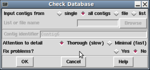
6 The Staden Package Manual
1.1.4 Check Database
This function (which is available from the Gap5 File menu) is used to perform a check on
the logical consistency of the database. No user intervention is required. If the checks are
passed the program will report zero errors. Otherwise a report of each error is displayed.
On a large database these checks can take a considerable amount of time. The default
is a thorough, but slow, check. However a faster mode is available which only performs
gross contig and contig-binning level checks, omitting the per sequence and per annotation
validation.
The dialogue also offers the choice of attempting to fix any problems that are found.
It is strongly recommended that you back the gap5 database up prior to performing fixes
as depending on the nature of the corruption the choices made may not necessarily be an
improvement. Note that this also may not fix every problem that is found, or the fixes
themselves may cause other errors to be found so it is best to recheck again.
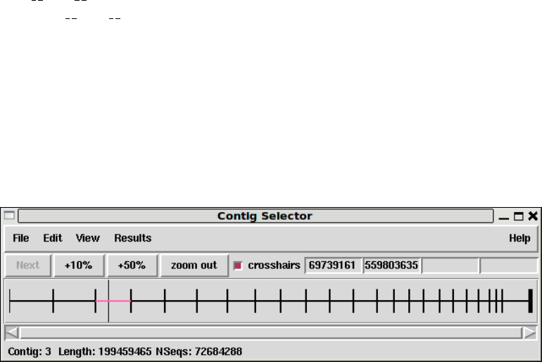
Chapter 1: Next generation assembly editing with Gap5 7
1.2 Contig Selector / Comparator
1.2.1 Contig Selector
The prog Contig Selector is used to display, select and reorder contigs. It can be invoked
from the prog View menu, but will automatically appear when a database is opened.
In the Contig Selector all contigs are shown as colinear horizontal lines separated by short
vertical lines. The length of the horizontal lines is proportional to the length of the contigs
and their left to right order represents the current ordering of the contigs. This Contig Order
is stored in the gap database and users can change it by dragging the lines representing the
contigs in the display. The Contig Selector can also be used to select contigs for processing.
Unlike gap4, gap5 does not display annotations within the Contig Selector window.
The figure shows a typical display from the Contig Selector. At the top are the File, View
and Results menus. Below that are buttons for zooming and for displaying the crosshair.
The four boxes to the right are used to display the X and Y coordinates of the crosshair.
The rightmost two display the Y coordinates when the contig selector is transformed into
the contig comparator (see Section 2.4 [Contig Comparator], page 126). The two leftmost
boxes display the X coordinates: the leftmost is the position in the contig and the other is
the position in the overall consensus. The crosshair is the vertical line spanning the panel
below.
This panel shows the lines that represent the contigs and the currently active tags. Those
tags shown above the contig lines are on readings and those below are on the consensus.
Right clicking on a tag gives a menu containing “information” (to see the tag contents) and
“Edit contig at tag” which invokes the contig editor centred on the selected tag.
The information line is showing data for the contig that is currently under the crosshair.
1.2.1.1 Selecting Contigs
Contigs can be selected by either clicking with the left mouse button on the line representing
the required contig in the contig selector window or alternatively by choosing the "List
contigs"option from the "View"menu. This option invokes a "Contig List"list box where
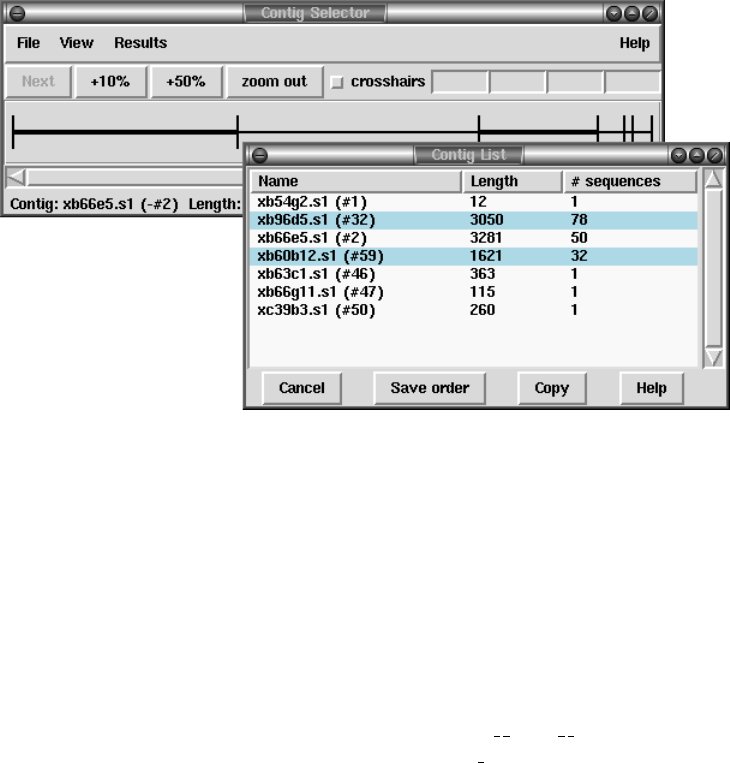
8 The Staden Package Manual
the contig names and numbers are listed in the same order as they appear in the contig
selector window.
Within this list box the contig names can be sorted alphabetically on contig name or
numerically on contig number. This is done by selecting the corresponding item from the
sort menu at the top of the list box. Clicking on a name within the list box is equivalent
to clicking on the corresponding contig in the contig selector. More than one contig can
be selected by dragging out a region with the left mouse button. Dragging the mouse off
the bottom of the list will scroll it to allow selection of a range larger than the displayed
section of the list. When the left button is pressed any existing selection is cleared. To
select several disjoint entries in the list press control and the left mouse button. The “Copy”
button copies the current selection to the paste buffer.
Most commands require a contig identifier, which can be the contig name itself or the
name/number of any reading within that contig. Prog always knows reading record
numbers, but depending on the options used in tg index when creating the assembly data-
base the reading names may not be indexed. To specify a reading by record number, precede
it by a # character, e.g. “#10000” means reading record number 10000, but “10000” means
the contig or reading with name 10000.
Also any currently active dialogue boxes that require a contig to be selected can be
updated simply by clicking on a contig in the contig selector or clicking on an entry in
the "Contig Names"list box. For example, if the Edit contig command is selected from
the Edit menu it will bring up a dialogue requesting the identity of the contig to edit. If
the user clicks the left mouse button on a contig in the contig selector window, the contig
editor dialogue will automatically change to contain the name of the selected contig. Some
commands, such as the Contig Editor, can be selected from a popup menu that is activated
by clicking the right mouse button on the contig line in the Contig Selector or clicking the
right mouse button on the corresponding name within the "Contig List"list box. This
simultaneously defines the contig to operate on and so the command starts up without
dialogue.
Chapter 1: Next generation assembly editing with Gap5 9
Several contigs can be selected at once by either clicking on each contig with the left
mouse button or dragging out a selection rectangle by holding the left mouse button down.
Contigs which are entirely enclosed within the rectangle will be selected. Alternatively,
selecting several contigs from the "Contig Names"list box will also result in each contig
being selected. Selected contigs are highlighted in bold. Selecting the same contig again
will unselect it.
The currently selected contigs are also kept in a ’list’ named contigs.
1.2.1.2 Changing the Contig Order
The order of contigs is shown by the order of the lines representing them within the Contig
Selector. The order of contigs can be changed by moving these lines using the middle
mouse button, or Alt left mouse button. Several contigs may be moved at once by selecting
several contigs using the above method. After selection, move the contigs with the middle
mouse button, or Alt left mouse button, and position the mouse cursor where you want the
selection to be moved to. Upon release of the mouse button the contigs will be shuffled to
reflect their new order. The separator line at the point the contig was moved from increases
in height.
The contig order is saved automatically whenever a contig is created or removed (eg auto
assemble), including operations like disassemble which temporarily create contigs. The order
can be saved manually using the Save Contig Order option on the File menu.
1.2.1.3 The Contig Selector Menus
The File menu contains only one command; "Exit". This simply quits the contig selector
display.
The View menu gives access to the Results Manager (see Section 2.13 [Results Manager],
page 277), allows contigs to be selected using a list box containing the contig names (See
Section 2.3.1 [Selecting Contigs], page 123), and the list of selected contigs to be cleared.
The Results menu is updated on the fly to contain cascading menus for each of the
plots shown when the contig selector is in its 2D Contig Comparator mode (see Section 2.4
[Contig Comparator], page 126). The contents of these cascading menus are identical to
the pulldown menus available from within the Results Manager.

10 The Staden Package Manual
1.2.2 Contig Comparator
Prog commands such as Find Internal Joins (see Section 2.8.3 [Find Internal Joins],
page 227) and Find Repeats (see Section 2.8.4 [Find Repeats], page 233) automatically
transform the Contig Selector (see Section 2.3 [Contig Selector], page 123) to produce the
Contig Comparator. To produce this transformation a copy of the Contig Selector is added
at right angles to the original window to create a two dimensional rectangular surface
on which to display the results of comparing or checking contigs. Each of the functions
plots its results as diagonal lines of different colours. If the plotted points are close to the
main diagonal they represent results from pairs of contigs that are in the correct relative
order. Lines parallel to the main diagonal represent contigs that are in the correct relative
orientation to one another. Those perpendicular to the main diagonal show results for which
one contig would need to be reversed before the pair could be joined. The manual contig
dragging procedure can be used to change the relative positions of contigs. See Section 2.3.2
[Changing the Contig Order], page 125. As the contigs are dragged the plotted results will
be automatically moved to their corresponding new positions. This means that if users
drag the contigs to move their plotted results close to the main diagonal they will be
simultaneously putting their contigs into the correct relative positions.
By use of popup menus the plotted results can be used to invoke a subset of commands.
For example if the user clicks the right mouse button over a result from Find Internal Joins
a menu containing Invoke Join Editor (see Section 2.6.15 [The Join Editor], page 196) and
Invoke Contig Editors (see Section 2.6 [Editing in prog ], page 160) will pop up. If
the user selects Invoke Join Editor the Join Editor will be started with the two contigs
aligned at the match position contained in the result. If required one of the contigs will be
complemented to allow their alignment.
A typical display from the Contig Comparator is shown below. It includes results for
Find Internal Joins in black, Find Repeats in red and Sequence Search in green. The
currently highlighted item is shown in pink with a summary at the bottom of the screen.
The orientation of this is from top-left to bottom-right indicating that the match is in the
same orientation within both contigs (we can see some in the opposite orientation indicating
that we need to reverse complement either of the two contigs before attempting any joins,
although this will happen automatically). The crosshairs show the positions for a pair of
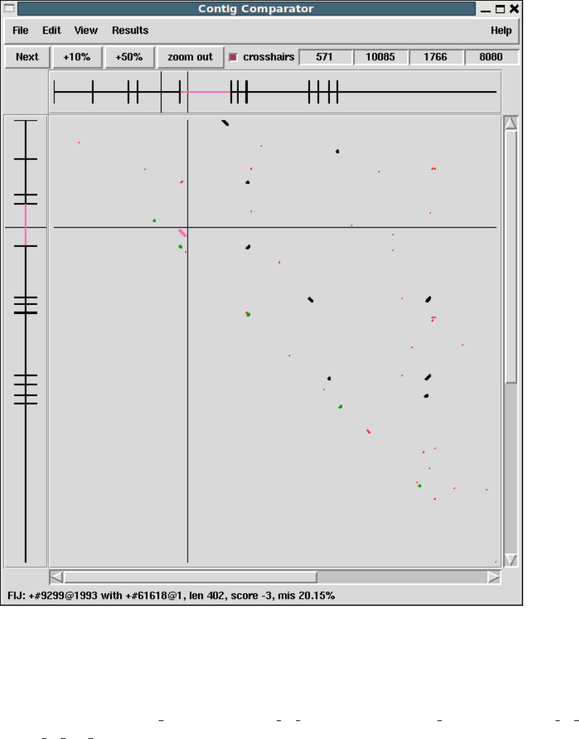
Chapter 1: Next generation assembly editing with Gap5 11
contigs. The vertical line continues into the Contig Selector part of the display, and the
position represented by the horizontal line is also duplicated there.
1.2.2.1 Examining Results and Using Them to Select Commands
Moving the cursor over plotted results highlights them, and the information line gives a
brief description of the currently highlighted match. This is in the form:
match name:contig1 number@position in contig1, with contig2 number@position in contig2,
length of the match
For Find Internal Joins the percentage mismatch is also displayed.
12 The Staden Package Manual
Several operations can be performed on each match. Pressing the right mouse button
over a match invokes a popup menu. This menu will contain a set of options which depends
on the type of result to which the match corresponds. The following is a complete list, but
not all will appear for each type of result.
Information
Sends a textual description of the match to the Output Window.
Hide Removes the match from the Contig Comparator. The match can be revealed
again by using "Reveal all"within the Results Manager.
Invoke contig editors
Invoke join editors
When invoked these options bring up their respective displays to show the
match in greater detail.
Remove Removes the match from the Contig Comparator. The match cannot be re-
vealed again by using "Reveal all"within the Results Manager.
One of the items in the popup menu may have an asterisk next to it. This is the default
operation which can also be performed by double clicking the left mouse button on the
match. For Repeat or Find Internal Joins matches this will normally be the Join Editor,
or two Contig Editors when the match is between two points in the same contig.
The crosshairs can be toggled on and off and a diagonal line going from top left to bottom
right of the plot can also be displayed if required. This is useful as a guide for moving the
contigs such that their matches lie upon the diagonal line.
The "Results"menu on the contig selector window provides a similar mechanism of
accessing results, but at the level of all matches in a particular search. This is simply a
menu driven interface to the Results Manager window (see Section 2.13 [Results Manager],
page 277), but containing only the results relevant to the contig comparator window.
1.2.2.2 Automatic Match Navigation
The "Next"button of the contig comparator window automatically invokes the default
operation on the next match from the current active result. This provides a mechanism to
step through each match in turn ensuring that no matches have been missed.
With a single result (set of matches) plotted, the "Next"button simply steps through
each match in turn until all have been seen. Moving the mouse above the "Next"button,
without pressing it, highlights the next match and displays brief information about it in
the status line at the bottom of the window. To step through the matches in "best first"
order, select the "Sort Matches"option from the relevant name in the Results menu. The
exact order is dependent on the result in question, but is generally arranged to be the most
interesting ones first.
Bringing up another result now directs "Next"to step through each of the new matches.
To change the result that "Next"operates on, use the Result menu to select the "Use for
’Next’"option in the desired result. Alternatively, double clicking on a match also causes
"Next"to process the list starting from the selected result.
Chapter 1: Next generation assembly editing with Gap5 13
The "Next"scheme remembers any matches that have been previously examined ei-
ther by itself or by manually double clicking, and will skip these. To clear this ’visited’
information select "Reset ’Next’"in the Results Manager.
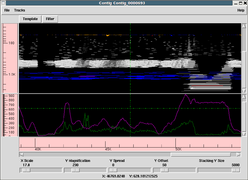
14 The Staden Package Manual
1.3 Template Display
The template display is a graphical overview of a single contig. It allows us to see how much
data we have, how long the fragments are and how they relate to each other (whether they
are forming valid pairs).
The window consists of one or more tracks, by default showing the reading template
layout at the top and a sequence / read-pair coverage plot at the bottom. The Tracks menu
allows us to turn these on and off.
Below the main menu bar is a series of buttons that bring up new dialogues for controlling
how the data is to be display and what is to be displayed.
Then come a graphic plot per track. A cross-hair automatically tracks the cursor, indi-
cating the X and Y coordinates (in appropriate units) in the status line at the bottom of
the window. The track displays can be moved by either using the horizontal and vertical
scrollbars at the bottom and right hand edges of the window, or by clicking and dragging
the contents of the window. While dragging the display will not update to show newly
visible regions of a contig until the left mouse button is released.
Finally the bottom contains a scrollbar and ruler for positioning and a series of controls.
The X scale simply controls how many base-pairs of the contig are covered by he window.
The X scale number is arbitrary, but is interpreted in an exponential manner so it is easy
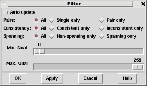
Chapter 1: Next generation assembly editing with Gap5 15
to rapidly zoom in or zoom out. All other controls in the bottom panel do not affect the
reading coverage track, so they are covered in the template track section below.
1.3.1 Filtering data
By default all templates are used for drawing the tracks, but there are times when we may
wish to focus on specific problem data or to exclude it from our graphics.
The Filter button at the top of the Template Display brings up the dialogue shown
above. Making changes to this dialogue either have an instant impact on the display (when
“Auto update” is enabled) or instead only when we hit Apply or OK to dismiss the dialogue.
The Pairs: section allows us to select either reads on all templates, reads that are the sole
read for that template, or reads that are paired on a template. Note that the definition of a
pair here is strictly dependant on how many reads for a template are in the gap5 database
rather than the library preparation strategy. So a paired-end template for which only one
read is in the gap5 database (perhaps due to failure to map) is classified as “single”.
The Consistency section can be used to select all, consistent only or inconsistent only
data. This requires read-paired data (single reads cannot be inconsistent as so are considered
as consistent). The interpretation of inconsistent currently is that the two reads of a pair
do not point towards one another, but in future releases this is planned to check the correct
orientation for that library type as for some constructions it is normal to have reads pointing
in the same orientation.
The Spanning section governs whether to display read pairs with one read in this contig
and the other read in another contig. Handling templates with more than two reads is still
on-going work, but when finished a spanning read-pair will be one with any read not in this
contig.
Underneath these are two sliders applied in addition to the above filters. They allow
removal of any read or read-pair (depending on the type of data being plotted) with a
mapping quality outside the selected range.
1.3.2 Template plot
This is the main body of the template display window. The default plot will be showing read-
pairs, mainly coloured by mapping quality with the insert size governing the Y coordinate.
Larger inserts are at the bottom of the track while shorter ones are at the top.
16 The Staden Package Manual
The colours used are as follows:
blue This is a template with only one reading present. It could be either a pair with
one end not in this assembly, or a true single-ended sequencing experiment. The
horizontal size of the line is now the length of the individual sequence rather
than the computed length of the insert.
orange This is a template with one reading present in another contig. The size of the
line is derived from the size of the data in this contig (typically a single reading).
red This template is considered as inconsistent in some manner, typically due to
the relative position and orientation of the forward and reverse sequences being
incorrect.
grey (variety of)
Any consistent read-pair is coloured by the mapping quality, by default using the
average of the individual sequence mapping qualities. Lighter shades represent
higher mapping qualities.
The row of scale bars at the bottom of the window control how data is to be plotted.
They are:
X Scale Controls how many base-pairs in the contig to plot. Higher values indicate more
base pairs, but with an exponentially growing scale.
Y Magnification
Governs the amount of vertical space consumed by the template track. This
has no impact on the depth track.
Y Offset Adds a small shift to the Y position of data prior to plotting. This is of little
use unless Separate Strands has also been selected, where upon this allows the
two halves of the plot to be brought closer together. (Effectively meaning the
a plot can go from -1000 to -100 and +100 to +1000 instead of -1000 to +1000
with a blank area in the middle if our sequences are a minimum of 100 bases
long.)
Stacking Y Size
Only of use in Stacking Y-Position mode. This vertically groups together data
of similar length, allowing a basic approach of separating short-read and long-
read technologies. The Y layout is performed in steps of “Stacking Y Size”. To
pack reads tightly together regardless of length, set this to the maximum value
possible.
Y Spread This adds a small perturbation to the computed Y coordinates of lines in the
template track. When the Y coordinate is derived based on the insert size of
the read-pair it is not always clear whether a line represents a single item or
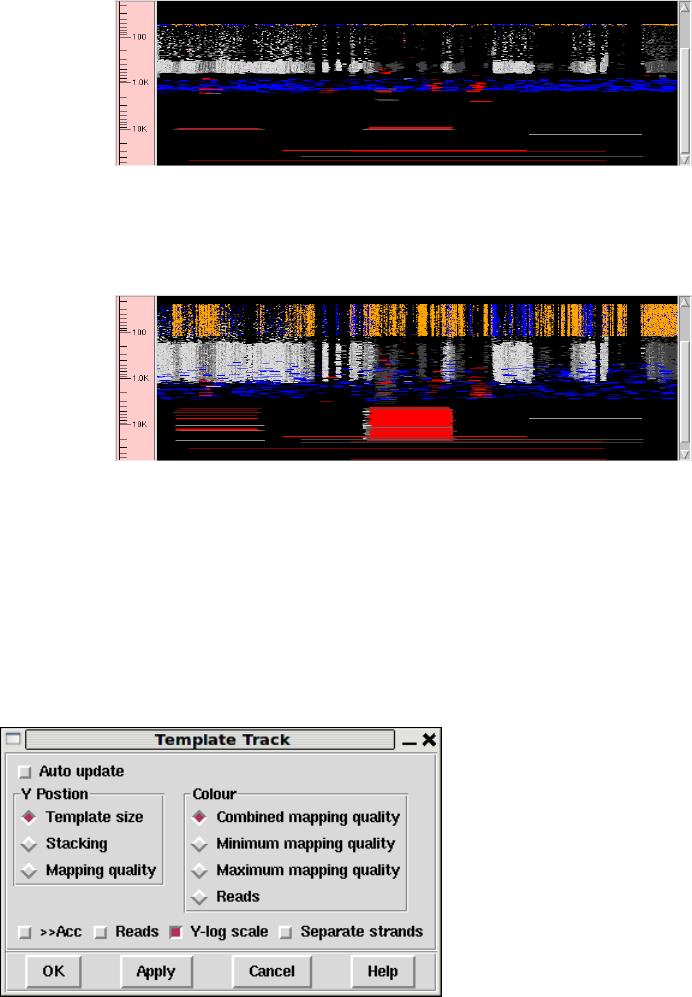
Chapter 1: Next generation assembly editing with Gap5 17
many items stacked perfectly on top of one another. The Y spread control
compensates for this.
Template track with Y spread of 0.
Template track with Y spread of 50.
1.3.2.1 Controlling The Y Layout.
The layout and type of data in the template track can be controlled using the Template
button at the top of the main template display window.
The Y Position section controls how the Y coordinates are computed when plotting data
(with X being tied to the position in the assembly or reference). It can be one of three
settings.
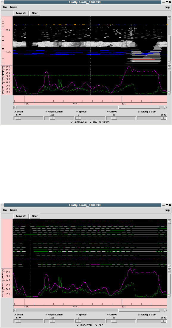
18 The Staden Package Manual
Template size
The default mode. The size of an object is defined to be the number of bases it
spans. This is normally the size of a read-pair, or if the pair spans contigs or if
only readings are shown it is the size of a single reading instead. Larger objects
are at the bottom of the window. This Y method very clearly reveals indels in
a mapped assembly. It sometimes also sometimes reveals misassemblies.
Given that items of identical size will stack on top of one another, of particular
use to this display mode is the Y Spread control in the main window.
Stacking
A more traditional view - each and every item is allocated its own
non-overlapping Y coordinate (although low Y magnifications may imply these
are drawn at the same Y pixel).

Chapter 1: Next generation assembly editing with Gap5 19
It is still possible to partially group items by their insert size using the “Stacking
Y Size” control in the main window.
Mapping Quality
Finally we can display data collated by the mapping score. This is typically only
available for mapped assemblies. This plot sometimes helps to reveal regions
where all the data present is of poor mapping quality, indicating a likely repeat.
Adjacent to the Y Position frame is the Colour frame. This controls the colour of the
lines drawn in the template display rather than their location.
Combined mapping quality
Minimum mapping quality
Maximum mapping quality
For templates with multiple reads visible, we have a variety of mapping qualities.
Often these individual sequence mapping qualities will differ, but we wish to
draw a single line for the template with a single colour. These three methods
control whether we take the average, minimum or maximum values from the
individual sequences on this template.
Reads The line typically represents the entire span of the insert, but we may not have
sequence data for all of the template. This colour mode will also draw the
portions of the template that we have known sequence for, in green for forward
strand sequences and magenta for reverse strand sequences. Any remaining
portion of template between the reads is drawn using the combined mapping
quality.
At the bottom of this dialogue is a row of check buttons.
“>>Acc” enables accurate mode, but be warned this can be very slow. When the template
display is drawn it fetches all data within the visible portion plus a little bit ether side.
From this reads from the same template are paired up. However when a template spans
20 The Staden Package Manual
a substantially larger range than is shown we may only have fetched one read for this
template. We do know that such a template forms a pair, but we do not know the exact
location of the other end or even whether it is in this contig. The assumption is that it is
not, and the template is drawn in orange. Enabling accurate mode will work out the precise
location of the other end and if it is present elsewhere within this contig then the insert size
will be correctly determined and the plot adjusted accordingly.
The “Reads” checkbutton (not to be confused with the Reads colour selector) disables
all drawing of read-pairing and template lines, instead drawing lines to represent the known
DNA sequence instead.
“Y-log scale” controls whether we plot our Y values using log or linear scales.
“Separate strands” attempts to classify all templates as coming from the top or bottom
strand of DNA (based on the orientation of the sequences on that template, although
sometimes these are conflicting). It then splits the plot in two, forming an approximate
mirror image. This may be of use in some transcriptome sequencing experiments.
1.3.3 Depth / Coverage Plot
The depth track shows coverage of both individual readings and read-pairs, where a read-
pair counts as +1 coverage over the entire length it spans rather than just the portion
directly sequenced.
The filter options for (in)consistent read pairs also apply here, giving the option to only
show depth of consistent pairs.
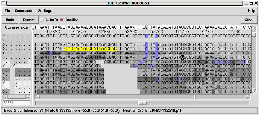
Chapter 1: Next generation assembly editing with Gap5 21
1.4 Editing in Gap5
The Gap5 Contig Editor is designed to allow rapid checking and editing of characters
in assembled readings. Very large savings in time can be achieved by its sophisticated
problem finding procedures which automatically direct the user only to the bases that
require attention. The following is a selection of screenshots to give an overview of its use.
The figure above shows a screendump from the Contig Editor showing the consensus for
a small region of a contig and the aligned reads. The main components are, top-most menu
bar; common buttons and controls beneath this; the main name and sequence panels to the
left and right; scrollbars and jog-control; a status text line at the bottom.
The names panel on the left can show either reading names or a small ASCII diagram
representing their position, orientation and mapping quality as a grey-scale. The sequences
to the right in the screenshot has base quality shown in grey (dark being poor, light being
good) with disagreements to the consensus at the top shown in blue. The consensus line
also shows base qualities. You may notice we have a mixture of long and short sequences,
with the longer ones being at the top. This screenshot is from a mixed assembly of Illumina
short-read data and ABI Sanger-method capillary sequences.
One base is drawn in inverse video (a “G”). This is the current location of the editing
cursor. We can move this we arrow keys or clicking with the left mouse button. It behaves
much like the editing cursor in a word processor and need not be visible in the portion of
the contig we are viewing.
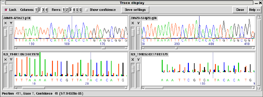
22 The Staden Package Manual
Also visible is a set of bases coloured yellow. These are an OLIGO annotation. Gap5
supports a wide variety of annotation types (often also referred to as “tags”). These are
covered later in more detail.
This figure is an example of the Trace Display showing three capillary traces and an
Illumina trace from readings in the previous Contig Editor screendumps. Note that this
demonstrates the possibility of showing the raw trace data for new short-read sequencing
technologies, but typically this is not available due to the high storage size.
1.4.1 Moving the visible segment of the contig
The contig editor displays only one segment of the entire contig, although several contig
editors can be in use at once. Below the sequence is a scrollbar and below that a “jog”
control. The scrollbar behaves as expected, allowing rapid positioning anywhere within the
contig using the middle mouse button or left-clicking and dragging the slider. However with
extremely long contigs (for example 100Mb) it can become tricky to move by the desired
amount. Each pixel on the scrollbar may represent 100Kb worth of data, so dragging the
scrollbar is only approximate positioning. Equally so clicking in the trough to move a
screen-full at a time can be too small. This is where the jog-control can be of use.
By default this is always centred. Clicking and dragging this left or right starts to scroll
the editor, at a speed proportional to how far away from the centre the jog is dragged.
Releasing the mouse button stops automatically scrolling and recentres the jog control.
The final, more precise, manner of positioning the editor view is with the text entry box
in the bottom left corner. Type in any coordinate here and press return to jump straight
to that location. Note however that Gap5’s coordinates are currently always in padded
form; that is to say that a gap in the consensus caused by an insertion in one of the aligned
sequences is still counted as a base position.
For particularly deep displays the vertical scrollbar on the right edge of the window will
also be useful. While scrolling in X, the editor attempts to keep the same sequences visible
on screen. To do this it may automatically adjust the Y scrollbar for you due to changing
layout of sequences. (By default the top-most sequence is always the sequence that starts
furthest left and the bottom most is the sequence starting furthest right.)
Chapter 1: Next generation assembly editing with Gap5 23
If you have a mouse wheel, this may also be used for small scrolling. By itself it scrolls
in Y one sequence at a time. With the Control key held down it scrolls in larger incre-
ments. Using the Shift key in conjunction with the mouse wheel scrolls in X instead, with
Shift+Control to scroll in larger increments.
The displayed portion of the contig is separate from the current location of the editing
cursor. This is displayed as a black rectangle with typically a light coloured letter inside it.
Any editing keys operate on the base underneath this or to the base immediately preceding
it for Delete. We cover the topic of editing later (see Section 2.6.3 [Editing], page 165),
however moving the editing cursor is also another way of scrolling the editor.
Finally the Page Up and Page Down keys scroll the editor left or right by 90% of current
screen width. Used with Shift the moves in increments of 1Kb, with Control in increments
of 10Kb and with both Shift and Control in increments of 100Kb. The Home and End
keys jump to the start or end of the current item underneath the editing curosr - either a
sequence or the consensus.
1.4.2 Names
At the left side of the editor window is the “names panel”. This either displays an ASCII
pictorial summary of the sequence layout or the actual sequence names themselves depend-
ing on the settings in use. Between the names panel and the sequences panel is a vertical
line, visible at the right edge of the above image. This can be dragged left and right to
adjust the proportion of display dedicated to the names and sequence panels.
The default name display looks like this:
This plot is a mini diagram of the way the sequences overlap. Here the >and <symbols
represent the start of sequences, assembled on either the forward or reverse strand, with
the ... sections reflecting their relative lengths. The background shading indicates the
mapping quality of the sequence (which may not be available in many cases, depending on
how the assembly was derived). This should indicate the likelihood that the sequence has
been assembled to the correct point. Sequence that appears to map elsewhere, e.g. due to
a repeat, will be dark grey while unique sequence will be light grey or white. Moving the
mouse cursor over a sequence will tell you the precise mapping quality along with additional
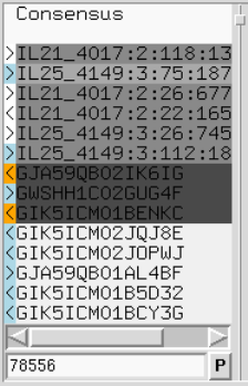
24 The Staden Package Manual
information such as the sequence name, the technology used (Sanger, Illumina, 454, etc),
and whether it is part of a pair of sequences.
In the editor Settings menu is a checkbox labelled “Pack Sequences”. When checked we
permit multiple sequences to be drawn in the same row. Unchecking this reverts to the
Gap4 style of display where each sequence has its own dedicated row. This also has an
affect on the names panel, which switches to showing the sequence names, as below.
This still uses the >and <symbols to reflect strand and grey scales for representing the
mapping quality. The >and <are now also coloured independently.
•light blue The read is not paired
•white Forms a consistent pair
•grey Paired, but the insert size is too large or too small
•red Paired, but in an invalid orientation
•orange Paired, but the other end is in another contig
At the bottom of the names panel is an editable text field containing the current display
position. Adjacent to this is a small “P” indicating these coordinates are “padded”. Clicking
this will alternate with “R” to indicate reference coordinates, although these may not be
available in all situations. Note that currently, for speed reasons, it cannot directly display
unpadded coordinates.
Typing into this position entry-box allows us to direct the editor to a specific location. If
we end the number with “u” it performs an unpadded to padded conversion before jumping
to this location.
Left clicking on a name will toggle the background between the current grey to a shade
of blue (with luminosity once again reflecting mapping quality). This indicates that the
sequence name has been added to the “readings” list. Multiple names may be selected and
deselecting by pressing and holding the left mouse button while moving the mouse cursor.
In both display modes, pressing the right mouse button brings up a context sensitive
menu containing operations relevant to that specific sequence. This may contain the fol-
lowing commands.
Chapter 1: Next generation assembly editing with Gap5 25
Copy name to clipboard
Copy #number to clipboard
These copy the sequence name or the record number to the clipboard for use
in a subsequent paste operation. Note that there is no visual cue that this
has happened. The same function may also be achieved by left-clicking and
dragging the mouse horiztonally, as if attempting to highlight a region of text.
These two items are also available when right clicking on the Consensus label,
but in this case it copies the contig name or number to the clipboard instead.
Goto... This lists other sequences sharing the same template, such as the other end of
a read-pair. Selecting this command will jump the editor to the left-most base
in that sequence. If the sequence is in another contig then a new editor will be
created, unless one already exists for that contig in which case that other editor
will be moved accordingly.
Join to... In the case of read-pairs that span contigs, the join to function will bring up
the join editor for both contigs involved, automatically complementing the other
contig if appropriate based on the library pair orientation statistics.
Right clicking on the contig name also pops up a menu. In here are otions to change
the contig name or the starting coordinate. These options are also available in the editor
Commands menu.
1.4.3 Editing
Editing can take up a significant portion of the time taken to finish a sequencing project.
Gap5 has a selection of searches (see Section 2.6.6 [Searching], page 174) designed to speed
up this process. The problems that require most attention are conflicts between good bases.
Where base confidence values are present it should be unnecessary to edit all conflicting
bases as, generally, this will amount to adjusting poor quality data to agree with good
quality data in which case the consensus sequence should be correct anyway.
Pads in the consensus should not be considered a problem requiring edits because it
is possible to output the consensus sequence (from the main Gap5 File menu) with pads
stripped out. Obviously poorly defined pads (a mixture of several alignment padding char-
acters and real bases) require checking in the same manner as other poorly defined consensus
bases.
To change a base simply overtype with a new base call, one of a,c,g or t in lowercase.
Alternatively a base can be changed to an alignment padding character by pressing “*”.
These new bases and pads automatically get given a quality value of 100, but see below for
how to adjust this. The consensus cannot be edited in this manner.
To insert a gap into sequence press “i” or the Insert key. At present only alignment pads
can be inserted, not bases, although the pads can subsequently be edited to turn them into
bases. The “i” and Insert keys also permits insertions of gaps into the consensus, which it
achieves by inserting into every sequence aligned at that position.
Bases may be deleted by pressing the Delete or Backspace key. This deletes the base
immediately to the left of the current editing cursor. Note that if Delete or Backspace is
pressed with the editing cursor on the consensus this removes an entire column of data.
26 The Staden Package Manual
Deleting anything other than alignment padding characters (either in sequences or the
consensus) is a dangerous operation needing careful thought. To prevent accidental removal
of data therefore, to delete anything other than “*” you must press Control in conjunction
with Delete or Backspace.
1.4.3.1 Moving the editing cursor
Nearly all editing operations happen at the location of the editing cursor. This cursor
appears as a black block containing the base in a light colour, instead of the usual black
base on a light background.
The simplest mechanism of moving the cursor is using the left mouse button. Alterna-
tively the following keys can be used.
Left arrow or Control b Move left one base
Right arrow or Control f Move right one base
Up arrow or Control p Move up one base
Down arrow or Control n Move down one base
Control a Move editing cursor to start of sequence
Control e Move editing cursor to end of sequence
Home Move editing cursor to start of sequence
End Move editing cursor to end of sequence
Meta or Alt < Move editing cursor to start of contig
Meta or Alt > Move editing cursor to end of contig
If any of these move the editing cursor outside of the visible region, the editor will scroll
to accommodate. Control-a and Control-e with the editor on the consensus line will also
jump to the start and end of the contig.
If “Cutoffs” are shown (see Section 2.6.3.4 [Adjust the Cutoff Data], page 169) the cursor
may be placed in the cutoff data too. Note that turning off displaying cutoff data would
then leave the editor on an invisible base, so it is moved to the consensus line instead.
1.4.3.2 Adjusting the Quality Values
Each base has its own quality value. Assembly will allow only values between 1 and 99
inclusive. A quality value of 0 means that this base should be ignored. A quality value of
100 means that this base is definitely correct and the consensus will be forced to be the
same base type and will be given a consensus confidence of 100. If two conflicting bases
both have a quality of 100 the consensus will be a dash with a confidence of 0.
Newly added bases or replaced bases are assigned a quality of 100.
Several keyboard commands are available to edit the quality value of an individual base.
[ Set quality to 0 and move cursor right
] Set quality to 100 and move cursor right
Shift Up-Arrow Increment quality by 1
Control Up-Arrow Increment quality by 10
Shift Down-Arrow Decrement quality by 1
Control Down-Arrow Decrement quality by 10
Chapter 1: Next generation assembly editing with Gap5 27
Finally note that quality values can also be made visible by clicking on the “Quality”
checkbutton at the top of the editor. This shows the quality by use of a grey scale.
1.4.3.3 Adjusting the alignment coordinates
On rare occasions we may need to move an entire sequence a small amount to achieve an
optimal alignment, rather than simply inserting or deleting pads.
This is achieved by using Control plus the left and right arrow keys while the editing
cursor is anywhere on the sequence.
Control Left-Arrow Shift sequence left
Control Right-Arrow Shift sequence right
1.4.3.4 Adjusting the Cutoff Data
Sequences typically consist of a good quality “used” portion and poor quality “clipped”
or “cutoff” portions at the 5’ and 3’ ends of the sequence. Although for short sequencing
technologies it’s quite likely we have no cutoff data at all. The reason for this is that the
low quality ends of sequences may have a sufficient number of errors that the sequence
alignment algorithms are no longer confident they have the correct bases aligned, or event
that the sequence simply disagrees too much.
By default these are not shown, although you may see blank lines in the display as room
is left for this sequence even when it is not visible. The cutoff data may be displayed by
pressing the “Cutoffs” check-button at the top of the editor. The cutoff sequence will then
be displayed in grey. We call the boundary between the cutoff data and the used data the
cutoff position. These positions can be adjusted by pressing the “<” (left cutoff) or “>”
(right cutoff) keys. In both cases the cutoff point is between the base with the editing
cursor and the base to the left of the editing cursor.
Using the “<” and “>” keys with the editing cursor in the consensus performs bulk
versions of these edits by clipping every single sequence to that poinit. One small difference
here though is that the bulk versions only ever shrink cutoff data and do not grow it.
< In sequence: set left cutoff position
> In sequence: set right cutoff position
< In consensus: bulk clip left cutoff
> In consensus: bulk clip right cutoff
1.4.3.5 Summary of Editing Commands
A brief summary of these editing operations can be seen below:
Key Location Action
----------------------------- --------------------
a,c,g,t,* Reading Change base
i, Insert Reading Insert pad
Delete Reading Delete * to left
Ctrl Delete Reading Delete any base to left
Control Left Reading Move reading left
28 The Staden Package Manual
Control Right Reading Move reading right
[ Reading Set quality to 0
] Reading Set quality to 100
Shift Up Reading Incr. quality by 1
Shift Down Reading Decr. quality by 1
Ctrl Up Reading Incr. quality by 10
Ctrl Down Reading Decr. quality by 10
< Reading Set left cutoff
> Reading Set right cutoff
i, Insert Consensus Insert column of pads
Delete Consensus Delete * to left
Ctrl Delete Consensus Delete any base to left
< Consensus Bulk clip left cutoff
> Consensus Bulk clip right cutoff
1.4.4 Cut and Paste Control of Sequence
It is possible to highlight an area of a reading or the consensus sequence in preparation for
performing some further action upon it. Such examples of actions are: creating annotations
and pasting into a new window. We call these highlighted areas “selections”. They are
displayed as an underlined region.
The simplest way to make a selection is using the left mouse button. Pressing the mouse
button marks the base beneath the cursor as the start of the selection. Then, without
releasing the button, moving the mouse cursor adjusts the end of the selection. Finally
releasing the button will allow normal use of the mouse again. If while marking a selection
we reach the edge of the window then the editor will automatically start scrolling for us.
Sometimes we may wish to make a particularly long selection, or just extend an existing
selection after we’ve already released the mouse button. This can be done by using shift
left mouse button to adjust the end of the selection. Hence we can mark the start of the
selection using the left button, scroll along the contig to the desired position, and set the
end using the shift left button.
The selection is stored in the “clipboard”. This allows for the usual “cut and paste”
operations between applications, although the contig editor only supports this in one direc-
tion (as it is not possible to “paste” into the window). The mechanism employed for this
follows the usual X Windows standard of using the middle mouse button.
A quick summary of the mouse selection commands follows.
Left button Position editing cursor to mouse cursor
Left button (drag) Mark start and end of selection
Shift left button Adjust end of selection
Middle button (in another window) Copy selected sequence

Chapter 1: Next generation assembly editing with Gap5 29
1.4.5 Selecting Sequences
The list named “readings” is used for all sequences selected in all editors. This is automat-
ically updated whenever a sequence is selected or deselected.
Inividual sequence names can be (de)selected by clicking on them with the left mouse
button, or clicking and dragging out a region. This works well for a few sequences.
If you need to select all readings overlapping a specific consensus base or a region of
consensus bases mark the range of the consensus you wish to select over by pressing and
dragging the left mouse button (as if you were going to create an annotation) and then
either right click in the consensus or use the Commands menu to choose Select Reads.
When using the Commands menu you get a dialogue asking for confirmation of the start
and end positions and the option of whether to select sequences that overlap this range
or only those which are entirely containing within that range. When using the right-click
popup on the consensus it simply takes the defaults (overlapping sequences).
Deselection follows the same procedure.
1.4.6 Annotations
Annotations (or tags) can be placed at any position on readings or on the consensus. They
are usually used to record positions of primers for walking, or to mark sites, such as repeats
or compressions, that have caused problems during sequencing. Each annotation has a type
such as “primer”, a position, a length, a strand (forward, reverse or both) and an optional
comment. Each type and strand has an associated colour that will be shown on the display.
For information on searching for annotations see Section 2.6.6.4 [Searching by Tag Type],
page 175, and Section 2.6.6.3 [Searching by Annotation Comments], page 175.
FIXME: not all of the tag editor features are supported yet; specifically the Move/Copy
functionality is currently missing.
To create an annotation, make a selection and then select “Create Tag” from the contig
editor commands menu at the top of the editor or by pressing the right mouse button.
See Section 2.6.7 [The Commands Menu], page 177. This will bring up a further window;
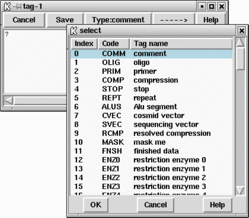
30 The Staden Package Manual
the “tag editor” (shown above). The “Type:” button at the top of the editor invokes a
selectable list from which tag types can be chosen. See below.
Use this to select the desired type of annotation.
Next the strand of the annotation can be selected. This will be displayed as one of
“<—->”, “<—-”, “—->” and “?—-?” indicating both strands, top strand only, bottom
strand only, and stranded but unknown strand respectively. These mirror the GFF strand
definitions. The comment (the box beneath the buttons) can be edited using the usual
combination of keyboard input and arrow keys. The “Save” button will exit the tag editor
and create the annotation. To abandon editing without creating the annotation use the
“Cancel” button.
To edit an existing annotation, position the editing cursor within a annotation and select
“Edit Tag” from the commands menu. This will be a cascading menu, typically showing
one tag. If multiple tags coincide at the same sequence position you will be able to chose
which tag to edit. Once again the tag editor will be invoked and operates as before. The
F11 key is also a shortcut for editing the top-most tag underneath the editor cursor. When
editing, the “Save” will save the edited changes and “Cancel” will abandon changes.
Removing a annotation involves positioning the editing cursor within an annotation and
selecting “Delete Tag” from the commands menu. As with “Edit Tag” this is a cascading
menu to allow you to chose which tag at a specific point to delete. The F12 key is a shortcut
to remove the top-most tag underneath the editor cursor.
As usual, “undo” can be used to undo any of these annotation creations, edits and
removals.
Some tags may contain graphical controls instead of the usual text panel. These are
encoded with the master gap4/5 tag database (GTAGDB) by specifying the default tag
text to be a piece of “ACD” code. A full description of the (modified for gap4/5) ACD

Chapter 1: Next generation assembly editing with Gap5 31
syntax is not available currently, but it is strongly modelled on the the EMBOSS ACD
syntax which has documentation at
http://www.emboss.org/Acd/index.html .
It is possible to add your own tag types by modifying either the system GTAGDB file
or creating your own GTAGDB file in your home directory (for all your databases) or the
current directory (for just those in that directory).
For rapid editing and deleting the F11 and F12 keys may be used. These edit and
delete the top-most tag underneath the editing cursor. If you wish to edit or delete the
tag underneath the mouse cursor instead (and hence save a mouse click) use Shift F11 and
Shift F12 for edit and delete.
The Control-Q key sequence may be used to toggle the displaying of tags. Pressing it
once will prevent all tags from being displayed in the editor. This is sometimes useful to see
any colouring information underneath the tag. Pressing Control-Q once more will redisplay
them.
1.4.6.1 Annotation Macros
For rapid annotating a series of 10 macros may be programmed. Press Shift and a
function key between F1 and F10 to bring up the macro editor. This look much like the
normal tag editor except that Save is replaced with Save Macro and saving does not actually
create a tag on the sequence. To use the macro, highlight the bases you wish and press the
function key corresponding to that macro - F1 to F10. For a single base pair tag you do
not need to underline a region as the tag will automatically cover the base underneath the
editing cursor. To remember these permanently use the “Save Tag Macros” option in the
“Settings” menu.
If you have an existing tag you wish to rapidly duplicate to many places, use Control
plus a function key to copy the tag underneath the editing cursor to that numbered tag
macro. This is simply a short cut for Shift and the function key, but without needing to
manually replicate the tag type and textual comment.
You may find that some function keys are already programmed to do other things (such
as raise or lower windows), depending on the windowing environment in use. If this is the
case either modify the configuration of your windowing system or simply use another macro
key.
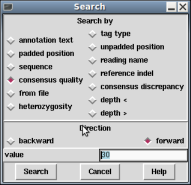
32 The Staden Package Manual
Shift F1-F10 Create a tag macro via a dialogue window
Control F1-F10 Create a tag macro from tag at editor cursor
F1-F10 Apply a tag macro (create a real tag)
1.4.7 Searching
The contig editor’s searching ability and its links to the consensus calculation algorithm
are crucial in determining the efficiency with which contigs can be checked and corrected.
The consensus is calculated “on the fly” and changes in response to edits. For editing, the
most important search functions are those which reveal problems in the consensus whilst
ignoring all bases that are adequately well determined. The standard search type is therefore
by consensus quality. By default this is done in the forward direction and for a quality value
of 30, although this is configurable by changing the collowing lines in the gap5rc file.
set_def CONTIG_EDITOR.SEARCH.DEFAULT_TYPE consquality
set_def CONTIG_EDITOR.SEARCH.DEFAULT_DIRECTION forward
set_def CONTIG_EDITOR.SEARCH.CONSQUALITY_DEF 30
Pressing the “Search” button brings up a separate search window. This allows the user
to select the direction of search, the type of search, and a value to search on. The value
is entered into a value text box, then pressing the “search” button performs the search. If
successful, the cursor is positioned accordingly.
The Control-s and Control-r key bindings in the editor are equivalent to searching for
the next or previous match. Both key bindings will bring up the search window if it is not
currently displayed (and not search), otherwise they perform the search currently selected
in that window. Additionally with the mouse focus in the search dialogue window the Page
Up and Page Down keys will perform previous and next search too.
As is described below, there are several search modes.
1.4.7.1 Search by Annotation Comments
This positions the cursor at the start of the next tag which has a comment containing the
string specified in the value box. The search performed is a regular expression search, and
Chapter 1: Next generation assembly editing with Gap5 33
certain characters have special meaning. Be careful when your string contains “.”, “*”, “[“,
“]”, “\”, “^” or “$”. The search can be performed either forwards or backwards from the
current cursor position. Searching with an empty value will find all tags.
1.4.7.2 Search by Tag Type
This positions the cursor at the start of the next tag of the specified type. To change the
type, click on the currently listed tag type, which displays a tag type selection dialogue.
The search can be performed either forwards or backwards of the current cursor position.
To find all tags, use “Search by Annotation Comments”, with an empty text box.
1.4.7.3 Search by Padded Position
This jumps to a padded location in the editor and is directly equivalent to typing a number
into the position entry box in the bottom left corner of the editor followed by “p”.
It is also possible to do relative searches by prefixing the location with +or -. So +100
will skip ahead 100 bases.
1.4.7.4 Search by Unpadded Position
As per the padded search, but this jumps to an unpadded coordinate - essentially the number
of non-* bases since the start of the contig, regardless of whether the first consensus base
is labelled as base 1.
1.4.7.5 Search by Sequence
This positions the cursor at the start of the next segment of sequence that matches the
value specified in the text box. The search is case insensitive, ignores pads, and can allow
a specified number of mismatches. Unlike Gap4, Gap5’s sequence search only looks in the
consensus sequence. It also operates either forwards or backwards from the current editing
cursor position.
1.4.7.6 Search by Reading Name
This positions the cursor at the left end of the reading specified in the value text box.
Note that not all reading names may be indexed by Gap5 and that the search will not
find unindexed names. See tg_index -t for information on creating Gap5 databases with
reading name indices.
The reading name has to be an exact match and so currently does not find prefix strings.
If multiple sequences exist with the same name (which should be strongly discouraged) then
it is undefined which will be found first.
1.4.7.7 Search by Reference InDel
Note: this information may not be available in all scenarios. If you imported the gap5
database from a SAM or BAM file there is an implicit set of reference coordinates used within
SAM/BAM. Gap5 can keep track of the relationship between gap5’s padded coordinate
system and the reference coordinates. This function uses this data to search for the next
or previous reference insertion or deletion.
34 The Staden Package Manual
1.4.7.8 Search by Consensus Quality
This positions the cursor on the consensus at the next position where the quality of the
consensus is below a given threshold. The quality threshold should be entered into the value
box and should be within the range of 0 to 100 inclusive.
1.4.7.9 Search by Consensus Discrepancy
The consensus algorithm can keep track of the expected number of differences to the consen-
sus given sequence depth and sequence quality values. This search looks for locations where
the actual number of differences exceeds the expected amount by more than a specified
factor.
1.4.7.10 Search by Consensus Heterozygosity
The consensus algorithm has a simple heterozygous calling method. Rather than simply
weighing up the evidence for the base being A, C, G, T or a pad it also considers that it
may be a combination of any two of these values. The consensus scores for the individual
bases as well as the highest scoring consensus base can be seen in the editor information
line when the mouse cursor is moved over a consensus base.
This search is looking for consensus bases where the best heterozygous score is greater
than or equal to the specified value.
1.4.7.11 Search by Low Coverage
This jumps to the next or previous location where the sequence coverage drops below a
specified value.
1.4.7.12 Search by High Coverage
This jumps to the next or previous location where the sequence coverage is higher than a
specified value. Regions of extreme depth are often indication of misassemblies.
1.4.8 The Settings Menu
The purpose of this menu is to configure the operation of the contig editor. Settings can
be saved using the “Save settings” button, which also saves preferences for the editor width
and height and the location of the divider between the names and sequence panels. It does
not save tag macros though; these may be saved separately using the “Save Macros” option.
Settings for the following options can be changed.
•Group Readings
•Highlight Disagreements
•By dots
•By foreground colour
•By background colour
•Case sensitive
•Set quality threshold
•Pack sequences
•Hide annoations
Chapter 1: Next generation assembly editing with Gap5 35
•Background stripes
•Show Mapping Quality
•Show Template Status
•Padded coordinates
•Reference coordinates
•Save tag macros
•Save settings
1.4.8.1 Group Readings
Sequences have an “X” location in the editor defined by the location within the contig that
they align to. The “Y” location though is determined by the sequence layout algorithm,
governed by the Pack Sequences setting and Group Readings options.
By default sequences are grouped into distinct technologies, typically with longer se-
quences up the top (capillary) and shorter ones at the bottom (Illumina, SOLiD). Within
these technology groups the sequences are then sorted by their start location, so the top-
most sequences start earlier and the bottom most sequences start later.
The Group Readings menu allows user control over these primary and secondary collating
orders. The sorting methods are defined below.
By technology
Sorted in order of unknown, sanger (capillary), Illumina, SOLiD, 454.
By clipped start
Sorted by the visible (non-cutoff) start position.
By start Sorted by the start position, regardless of whether the base is in cutoff data or
not.
By template
Sorted by template name. In Gap5 this is always defined to be a prefix of
the sequence name, or optionally the same as the sequence name. The sorting
method is using a simple ASCII collation order.
By strand Sorts data into the top strand first followed by the bottom strand data.
By base This sort order is different from all others in that it depends on the location of
the editor cursor.
Sorts sequences by the base type overlapping the last editor cursor location in
the consensus. The collation order is A, C, G, T, N and *. Sequences that
do not overlap that consensus location or those that only overlap in the cutoff
portion are not sorted by this method. If this is used as the primary sort then
these other sequences will be sorted using the secondary sort. If the secondary
sort is By Base then an implicit tertiary sort order of By Start is used.
Note that moving the editing cursor around sequences will not update the Y
order. Only placement of the editing cursor on the consensus will update this.
36 The Staden Package Manual
1.4.8.2 Highlight Disagreements
This toggles between the normal sequence display (showing the current base assignments)
and one in which those assignments that differ from the consensus are highlighted. It makes
scanning for problems by eye much easier.
Several modes of highlighting are available: “By dots” will only display the bases that
differ from the consensus, displaying all other bases as full stops if they match or colons if
they mismatch but are poor quality. The definition of poor quality here can be adjusted
using the “Set quality threshold” option of the Settings menu. The base colours are as
normal (ie reflecting tags and quality).
Highlight disagreements “By foreground colour” and “By background colour” displays
all base characters, but colours those that differ from the consensus. Bases which differ
by are below the difference quality threshold are shaded in light blue while high quality
differences are dark blue. This allows easier visual scanning of the context that a difference
occurs in, but it may be wise to disable the displaying of tags (hint: control-Q toggles tags
on and off).
Finally the “Case sensitive” toggle controls whether upper and lower case bases of the
same base type should be considered as differences.
1.4.8.3 Pack Sequences
This controls whether the editor allocates one row per sequence or whether it is permitted
to pack multiple sequences onto a single row, assuming they do not overlap.
The latter allows for a more compact plot which is desirable when dealing with short
sequences, however it has the side effect that the reading names can no longer be listed in
the names panel to the left.
1.4.8.4 Hide Annotations
Sometimes we need to see the background shading underneath an annotation, for example to
see the base quality or if we have Highlight Disagreements turned on using the by background
colour mode. This option simply hides all annotations from display until it is selected again
to reveal them once more.
The Control-Q keyboard shortcut has the same effect.
1.4.9 Primer Selection
The “Find Primer Walk” function from the Commands menu is an interface to the Primer3
program (builtin to Gap5 so it does not need an external installation). Currently it only
allows for selection of a single internal oligo suitable for “walking” along a template. It is
designed for manual finishing work and is not appropriate for automatic finishing. Future
plans are to add PCR support.
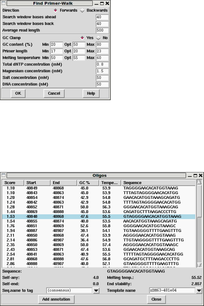
Chapter 1: Next generation assembly editing with Gap5 37
The command brings up its own dialogue window.
The top portion of this window controls where to look for primers. By default it will be
either side of the editing cursor location. We also specify here what strand we wish to run
our experiment on.
Below this are a series of Primer3 parameters. Please see the Primer3 documentation
for a full description of these.
Upon hitting OK, and assuming that some primers can be found, a new window showing
the available choices is presented.
38 The Staden Package Manual
The primers show are sorted by Primer3 score, with lower being better. Clicking on any
of the other headings in the table allows the data to be re-sorted by that column. Clicking
the left mouse button on any line will show the location of this primer in the main editor
window as an underlined region. It also updates the bottom half of the Oligos window with
further details.
At the bottom of the window are two editable selections. The left most labelled “Seq.
name to tag” allows us to pick a sequence we wish to place an oligo (OLIG) annotation on,
which defaults to the consensus sequence. The right selection box labelled “Template name”
is an list of identified templates at this region, however this is not necessarily exhaustive as
it only includes the sequences at this position and may miss some read-pairs that span this
region. If you have a specific template in mind you can also type in the name of it to here.
Pressing the “Add annotation” button then creates an oligo annotation. The text asso-
ciated with the annotation will depend on the primer chosen, but an example follows.
Sequence AACACATGGTAAAGCAGATG
Template zDH64-714h06
GC 40.0
Temperature 53.45
Score 1.54377204143
Date_picked Thu Aug 12 17:31:18 BST 2010
Oligoname ??
1.4.10 Traces
The original trace data from which the readings where derived can be displayed by double
clicking (two quick clicks) with the left or middle mouse button on the area of interest.
Control-t has the same effect. The trace will be displayed centred around the base clicked
upon and the name of the reading in the contig editor will be highlighted. Double clicking
on the consensus displays traces for all the readings covering that position.
Moving the mouse pointer over a trace base causes the display of an information line at
the bottom of the window. This gives the base type, its position in the sequence, and its
confidence value.
There are two forms of trace display which are selected using the “Compact” button at
the top of the Trace display. The compact form differs by not showing the Info, Diff, Comp.
and Cancel buttons at the left of each trace.
Note that Gap5 does not store the trace files in the project database: it stores only their
names and reads them when required. By default it will attempt to look for them in the
current working directory (likely the same directory as the gap database). However this
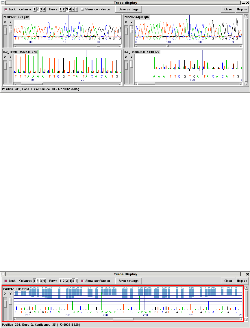
Chapter 1: Next generation assembly editing with Gap5 39
can be adjusted to look in other directories or via URLs using “Trace file location” in the
main Gap5 configure menu (see Section 2.20.8 [Trace File Location], page 302).
This figure is an example of the Trace Display showing three capillary traces and an
Illumina trace. On the top line, the Lock checkbutton keeps the trace data in sync with the
editor cursor position. The layout is controlled by the Columns and Rows selectors at the
top of the window; 2 column by up to 3 rows in the above screenshot. Show confidence draws
coloured bars and a numerical value representing the quality of each individual base-call.
The main trace panels each have the sequence name displayed in the top left corner.
Below this are X and Y zoom controls on the left and the actual trace data on the right.
The style of this will depend on the type of trace. Sanger chromatograms take multiple
samples per base and are subsequently analysed (base-called) to identify the peaks and
the number/type of bases represented by that peak. These are drawn using smooth lines,
examples of which can be seen in the top row of the image above. Illumina GA instruments
are “clocked” in that each and every measurement corresponds to one base. These are
drawn using a stick plot, as seen in the bottom row of the screen-shot. Note that it is quite
likely you will not have the processed trace data available for Illumina GA sequences due
to size constraints, so the above is simply an example of what could be viewed rather than
a typical example.
454 instruments use pyro-sequencing and so produce a variable number of bases per mea-
surement, with each measurement being clocked to a specific cycle (flow) on the sequencing
instrument. Hence 454 data is also drawn using a stick plot, although with potentially
multiple bases per measurement. An example is visible below.
40 The Staden Package Manual
The horizontal rulers in this plot correspond to normalised peak intensities for 1.0, 2.0
and so on to indicate 1, 2, 3... bases per flow. Clearly visible are flows of approximate
height 1 (C T A G T on the left), 2 (the following AA) and 0 (the G between the left most
C and T). Above these the confidence bars are visible.
Right clicking on a trace will bring up a popup menu containing the following options.
Information
Displays some basic textual information about the trace. The information avail-
able will vary by trace type, but it may include details such as the length,
instrument and run-date.
Save Saves the trace in ZTR format to a local file on disk. This can be useful for
when you are using a remote service for fetching traces or extracting them from
an archive such as .sff or .srf file.
Complement
Reverse complements the trace display. This does not modify data in any way,
but simply adjusts how it is drawn.
Quit Removes this trace from the trace window. If it is the last displayed trace then
the window will be removed too.
1.4.11 The Editor Information Line
The very bottom line of the editor display is text line used by the editor to display pieces
of useful information. Currently this gives information on individual bases, readings, the
contig, and tags, as the mouse is moved over the appropriate object. Each type of object
we move the mouse pointer over (sequence base, consensus base, sequence name panel,
annotation) has its own list of information to display which can be configured using a
format string stored in your $HOME/.gap5rc file.
Typically you will not need to modify these, but if you choose to do so the default values
to start from are shown below.
# Mouse-over a sequence the reading name panel
set_def READ_BRIEF_FORMAT \
Reading:%n(#%Rn) Tech:%V Length:%l(%L) MappingQ:%m%**/%*m Pos:%S%p / %*S%*p
# Mouse-over the "Consensus" label in the name panel
set_def CONTIG_BRIEF_FORMAT \
Contig:%n(#%Rn) Length:%l Start:%s End:%e
# Mouse-over a base in a sequence
set_def BASE_BRIEF_FORMAT1 \
Base %b confidence:%4.1c (Prob. %Rc, raw %4.1A %4.1C %4.1G %4.1T) Position %Rp %n
# Mouse-over a base in the consensus
set_def BASE_BRIEF_FORMAT2 \
Base confidence:%4.1c (Prob. %Rc) A=%4.1A C=%4.1C G=%4.1G T=%4.1T *=%4.1* Po-
sition %p
# Mouse-over an annotation
set_def TAG_BRIEF_FORMAT \
Tag type:%t Comment:"%.100c"

Chapter 1: Next generation assembly editing with Gap5 41
The text output is as listed above, but replacing percent-code strings with a relevant
piece of text. In many cases a capital R indicates raw mode to display a numerical value
instead of a string. For example %n in READ BRIEF FORMAT will be replaced by the
sequence name while %Rn will be replaced by the sequence record number. The full syntax
of percent expansion is as follows:
•A percent sign.
•An optional minus sign to request left alignment of the information. When displaying
information in a specific field with where that data does not fill the entire space allowed
the information will, by default, be right justified. Adding a minus character here
requests left justification.
•An optional minimum field width. This is a decimal number indicating how much space
to leave for this information.
•An optional precision for numbers or maximum field width for strings. This is given
as a fullstop followed by a decimal number.
•An optional ’R’ to specify Raw mode. This changes the meaning of many (but not all)
of the expansion requests to give a numercial representation of the data. For example
%n is a reading name and %Rn is a reading number.
•Th expansion type itself. This is either one or two letters. See below for full details of
their meanings.
To programmers this syntax may seem very similar to printf. This is intentional, but
do not assume it is the same. Specifically the print syntax of %#,%+ and %0 will not work.
1.4.11.1 Reading Information
Used when we move the mouse over a sequence name in the names panel or a sequence
base-call. Example output is Reading:xc04a1.s1(#74) Tech:Sanger Length:295(474) Map-
pingQ:50. Note that not all expansions make sense when used in the names panel as no
cursor X position is available.
%% A single % sign
%n Reading name. Raw mode: record number
%# Reading record number
%p Position in sequence. Raw mode: position in contig.
%l Clipped sequence length
%L Unclipped sequence length
%s Start of clip
%e End of clip
%S Sense (whether complemented) - “<<” or “>>”. Raw mode: 0/1
%d Strand - “+” or “-”. Raw mode: 0/1
%b Base call
%c Confidence value of called base (phred style). Raw mode: probability

42 The Staden Package Manual
%A
%C
%G
%T Individual confidence (phred style) of A,C,G,T component in log-odds form.
Raw mode: probability value.
%m Mapping Quality. Raw mode: probability of correctly mapped.
%V Instrument type - Sanger, Illumina, SOLiD, 454 or Unknown.
1.4.11.2 Contig Information
For the CONTIG BRIEF FORMAT and BASE BRIEF FORMAT2 the following expan-
sions apply. These operate on contigs and the consensus sequence.
%% Single % sign
%n Contig name. Raw mode: contig record number.
%# Contig record number
%p Position in contig
%l Length of contig
%s Contig start coordinate
%e Contig end coordinate
%b Called consensus base
%c Score for called consensus base. Raw mode: probability value
%A
%C
%G
%T
%* Individual confidence for A,C,G,T,* base types in log-odds form. Raw mode:
as a probability value.
1.4.11.3 Tag Information
The TAG BRIEF FORMAT string is used to display annotation summaries. The possible
percent encodings are as follows.
%% Single % sign
%p Tag position
%t Tag type (always 4 characters)
%l Tag length
%# Tag number (0 if unknown)
%c Tag comment
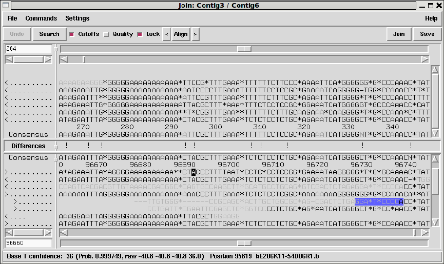
Chapter 1: Next generation assembly editing with Gap5 43
1.4.12 The Join Editor
Contigs are joined interactively using the Join Editor. This is simply a pair of contig editor
displays stacked above one another. The top editor is flipped in Y so that the consensus
appears at the bottom. This allows the two consensus sequences to be adjacent to one
another, separated only by a “differences” line. Note that it is essential to align the contigs
over the full length of their overlap. It is much more difficult to achieve this after a join has
been made, and until the alignment is correct, the consensus sequence will be nonsense.
The few differences between the Join Editor and the Contig Editor can be seen in the
figure below. Otherwise all the commands and operations are the same as those for the
Contig Editor
One difference is the Lock button. When set (as it is in the illustration) scrolling either
contig will also scroll the other contig.
The Align button aligns the overlapping consensus sequences and adds pads as necessary.
The alignment routine assumes that the two contigs are already in approximately the right
relative position (as they are immediately after the Join Editor has been invoked from Find
Internal Joins, or Find Repeats). If they are not you may get better results by manually
positioning then before hand.
The “<” and “>” buttons either side of the “Align” button perform the alignment from
the editing cursor to the start of the contig and and from the cursor to the end of the contig
only. Alignment end-gaps are penalised at the curosr position but not for the alignment
end at the contig start/end position. These buttons are useful for when multiple alignment
positions may be valid, such as is the case with an overlap consisting entirely of a short
tandem repeat.
44 The Staden Package Manual
It should be noted that each of the pair of editors comprising the Contig Editor maintains
its own undo history, and using Align is likely to add to both undo histories. There is only
one Undo button, but it applies to the editor last clicked within. A hint is given as to which
of the two editors this is by highlighting the editor in a red border when the mouse is moved
over the Undo button.
Pressing the Join button will display a small dialogue box informing you of the length
and percentage match of the overlap between the two contigs. At this point you can decide
to make the join, to not make the join (both of which remove the editors from the screen)
or to cancel which leaves the join editor visible still to permit further editing.
1.4.13 Using Several Editors at Once
Several editors can be used simultaneously, even on the same contig. In the latter case, it
is useful to understand the difference between the data and the view of the data.
Each operating Contig Editor is a view of the data for a particular contig. With two
editors viewing the same contig, making changes in either will modify the data that both
are viewing, hence the change will be visible in both editors. Similarly, using Undo in either
will undo the changes to both.
Interaction between Contig Editors and Join Editors is more complicated and generally
isn’t advised. However such interactions work consistently with the notion of views of
contigs. For example, suppose there are two Contig Editors open on two separate contigs,
and in addition to these a Join Editor displaying both contigs. Making the join in the Join
Editor will update the two stand-alone Contig Editors so that they are each viewing the
correct positions in the new contig, even though they’re both now viewing the same contig.
1.4.14 Quitting the Editor
The Exit operation in the File menu quits the editor. If changes have been made since the
last save you will be asked whether you wish to save these changes. Answering “Cancel”
abandons the exit process and provides control of the editor again, otherwise the appropriate
action will be taken and the editor quitted.
1.4.15 Summary
1.4.15.1 Keyboard summary for editing window
(“Left”, “Right”, “Up”, “Down” refer to the appropriate arrow keys.)
Page Up Scroll left by 1Kb
Shift-Page Up Scroll left by 10Kb
Control-Page Up Scroll left by 100Kb
Shift-Control-Page Up Scroll left by 1Mb
Page Down Scroll right by 1Kb
Shift-Page Down Scroll right by 10Kb
Control-Page Down Scroll right by 100Kb
Shift-Control-Page Down Scroll right by 1Mb
Left arrow or Control-b Move editing cursor left one base
Chapter 1: Next generation assembly editing with Gap5 45
Right arrow or Control-f Move editing cursor right one base
Up arrow or Control-p Move editing cursor up one base
Down arrow or Control-n Move editing cursor down one base
Control-a or Home Move editing cursor to start of sequence
Control-e or End Move editing cursor to end of sequence
Alt-comma Move editing cursor to start of contig
Alt-fullstop Move editing cursor to end of contig
Control-t Display trace
Control-s Search forward
Control-r Search backwards
Control-q Toggle tag display
< Set left cutoff clip point (in sequence)
> Set right cutoff clip point (in sequence)
< Bulk clip left cutoff (in consensus)
> Bulk clip right cutoff (in consensus)
[ Set confidence to 0
] Set confidence to 100
Shift Up Increase confidence of base by 1
Shift Down Decrease confidence of base by 1
Control Up Increase confidence of base by 10
Control Down Decrease confidence of base by 10
a, c, g, t or * Overwrite base with a new call.
i or Insert Insert pad (or column if in consensus)
Backspace or Delete Delete padding character
Ctrl-Backspace or Ctrl-Delete Delete base (any base type)
Control-right arrow Move sequence right 1 base-pair
Control-left arrow Move sequence left 1 base-pair
F11 Edit tag under editing cursor
F12 Delete tag under editing cursor
Shift F1 to Shift F10 Edit tag macro 1 to 10
Control F1 to Control F10 Copy tag at editing cursor to macro 1 to 10
F1 to F10 Create tag from macro 1 to 10
1.4.15.2 Mouse summary for editing window
Left button Position editing cursor to mouse cursor
Left button (drag) Mark start and end of selection
Shift left button Adjust end of selection
46 The Staden Package Manual
Left button (double click) Display trace
Right button Display commands menu
Mouse-wheel Vertically scroll the editor
Control mouse-wheel Vertically scroll the editor, fast
Shift mouse-wheel Horizontally scroll the editor
Shift Control mouse-wheel Horizontally scroll the editor, fast
1.4.15.3 Mouse summary for names window
Left button + drag Copy sequence name to clip-board
Right button Display popup menu
Mouse-wheel Vertically scroll the editor
Control mouse-wheel Vertically scroll the editor, fast

Chapter 1: Next generation assembly editing with Gap5 47
1.4.16 Plotting Restriction Enzymes
The restriction enzyme map function finds and displays restriction sites within a specified
region of a contig. It is invoked from the gap4 View menu. Users can select the enzyme
types to search for and can save the sites found as tags within the database.
This figure shows a typical view of the Restriction Enzyme Map in which the results for
each enzyme type have been configured by the user to be drawn in different colours. On
the left of the display the enzyme names are shown adjacent to the lines of plotted results.
If no result is found for any particular enzyme eg here APAI, the line will still be drawn
so that zero cutters can be identified. Three of the enzymes types have been selected and
are shown highlighted. The results can be scrolled vertically (and horizontally if the plot is
zoomed in). A ruler is shown along the base and the current cursor position (the vertical
black line) is shown in the left hand box near the top right of the display. If the user clicks,
in turn, on two restriction sites their separation in base pairs will appear in the top right
hand box. Information about the last site touched is shown in the Information line at the
bottom of the display. At the top the edit menu is shown torn off and can be used to create
tags for highlighted enzyme types.
1.4.16.1 Selecting Enzymes
Files of restriction enzyme names and their cut sites are stored in disk files. For the format
of these files and notes about creating new ones see Section 11.4 [Restriction enzyme files],
page 566.
When the file is read, the list of enzymes is displayed in a scrolling window. To select
enzymes press and drag the left mouse button within the list. Dragging the mouse off the
bottom of the list will scroll it to allow selection of a range larger than the displayed section
of the list. When the left button is pressed any existing selection is cleared. To select several
disjoint entries in the list press control and the left mouse button. Once the enzymes have
been chosen, pressing OK will create the plot.
48 The Staden Package Manual
1.4.16.2 Examining the Plot
Positioning the cursor over a match will cause its name and cut position to appear in
the information line. If the right mouse button is pressed over a match, a popup menu
containing Information and Configure will appear. The Information function in this menu
will display the data for this cut site and enzyme in the Output Window.
It is possible to find the distance between any two cut sites. Pressing the left mouse
button on a match will display "Select another cut"at the bottom of the window. Then,
pressing the left button on another match will display the distance, in bases, between the
two sites. This is shown in a box located at the top right corner of the window.
1.4.16.3 Reconfiguring the Plot
The plot displays the results for each restriction enzyme on a separate line. Enzymes with
no sites are also shown. The order of these lines may be changed by pressing and dragging
the middle mouse button or alt +left mouse button on one of the displayed names at the
left side of the screen.
The results are plotted as black lines but users can select colours for each enzyme type
by pressing the right button on any of its matches. A menu containing Information and
Configure will pop up. Configure will display a colour selection dialogue. Adjusting the
colour here will adjust the colour for all matches for this restriction enzyme.
1.4.16.4 Textual Outputs
The Results menu of the plot contains options to list the restriction enzyme sites found.
One option sorts the results by enzyme name and the other by the positions of the matches.
The output below shows the textual output from "Output enzyme by enzyme". The
Fragment column gives the size of the fragments between each of the cut sites. The Lengths
column contains the fragment sizes sorted on size.
Contig zf98g12.r1 (#801)
Number of enzymes = 3
Number of matches = 7
Matches found= 1
Name Sequence Position Fragment lengths
1 AATII GACGT’C 7130 7129 556
556 7129
Matches found= 5
Name Sequence Position Fragment lengths
1 ACCI GT’CGAC 414 413 189
2 ACCI GT’CTAC 1296 882 413
3 ACCI GT’CTAC 3871 2575 882
4 ACCI GT’CTAC 5816 1945 1681
5 ACCI GT’CGAC 7497 1681 1945
189 2575
Matches found= 1
Name Sequence Position Fragment lengths
1 AHAII GA’CGTC 7127 7126 559
Chapter 1: Next generation assembly editing with Gap5 49
559 7126
The output below shows the textual output from "Output ordered on position".
Contig zf98g12.r1 (#801)
Number of enzymes = 3
Number of matches = 7
Name Sequence Position Fragment lengths
1 ACCI GT’CGAC 414 413 3
2 ACCI GT’CTAC 1296 882 189
3 ACCI GT’CTAC 3871 2575 367
4 ACCI GT’CTAC 5816 1945 413
5 AHAII GA’CGTC 7127 1311 882
6 AATII GACGT’C 7130 3 1311
7 ACCI GT’CGAC 7497 367 1945
189 2575

50 The Staden Package Manual
1.5 Importing and Exporting Data
1.5.1 Assembly
There are two main types of assembly - denovo and mapped - with the latter not really
being a true assembly at all.
Denovo assembly consists of an assembly of DNA fragments without typically knowing
any of the goal target sequence. Hence it compares sequence fragments against each other
in order to form contigs. Mapped assembly makes uses of a known reference sequence and
compares all sequence fragments against the reference, which is a far simpler and faster
process than denovo assembly.
Gap5 however has neither denovo or mapped assembly built-in. Instead it relies on
externally running standard command-line tools. At present this consists purely of using
bwa for a mapped assembly, but in future this will be expanded upon.
This means that the Assembly menu currently only contains a “Map Reads” sub-menu,
which is turn has multiple choices for bwa usage. You will not be directly able to join contigs
using these facilities or to fill holes in the contig, although this is possible by manually
following some of the steps outlined below and using an alternate step for generating the
SAM file.
1.5.1.1 Importing with tg index
To enable efficient editing of data, Gap5 needs its own database format for storing sequence
assemblies. Formats such as BAM are good at random access for read-only viewing, but
are not at all amenable to actions such as reverse complementing a contig and joining it to
another.
Hence we need a tool that can take existing assembly formats and convert them to a
form suitable for Gap5. The tg_index program performs this task. It is strictly a command
line tool, although in some specific cases Gap5 has basic GUI dialogues to wrap it up.
One or more input files may be specified. The general form is:
tg_index [options] -o gap5 db name input file name ...
An example usage is:
tg_index -z 16384 -o test_data.g5 test_data.bam
gap5 test_data.g5 &
File formats supported are SAM, BAM, ACE, MAQ (both short and long variants), CAF,
BAF, Fasta and Fastq. The latter two have no assembly and/or alignment information so
they are simply loaded as single-read contigs instead. Tg index typically automatically
detects the type of file, but in rare cases you may need to explicitly state the input file type.
Tg index options:
-o filename
Creates a gap5 database named filename and filename.aux If not specified the
default is “g db”.

Chapter 1: Next generation assembly editing with Gap5 51
-a Append to an existing database, instead of creating a new one (which is the
default action).
-n When appending, the default behaviour is to add reads to existing contigs if
contigs with the appropriate names already exist. This option always forces
creation of new contigs instead.
-g When appending to an existing database, assume that the alignment has been
performed against an ungapped copy of the consensus exported from this data-
base. (This is internally used when performing mapped assemblies as they
consist of exporting the consensus, running the external mapped alignment
tool, and then importing the newly generated alignments.)
-m
-M Forces the input to be treated as MAQ, both short (-m) and long (-M) formats
are supported. By default the file format is automatically detected.
-A Forces the input to be treads as ACE format.
-B Forces the input to be treads as BAF format.
-C Forces the input to be treads as CAF format.
-b
-s Forces the input to be treads as BAM (-b) or SAM (-s) format. SAM must
have @SQ headers present. Both need to be sorted by position.
-z bin size Modifies the size of the smallest allowable contig bin. Large contigs will contain
child bins, each of which will contain smaller bins, recursing down to a mini-
mum bin size. Sequences are then placed in the smallest bin they entirely fit
within. The default minimum bin size is 4096 bytes. For very shallow assem-
blies increasing this will improve performance and the decrease disk space used.
Ideally 5,000 to 10,000 sequences per bin is an approximate figure to aim for.
-u Store unmapped reads only (from SAM/BAM only)
-x Store SAM/BAM auxillary key:value records too.
-p
-P Enable (-p) or disable (-P) read-pairing. By default this is enabled. The purpose
of this is to link sequences from the same template to each other such that gap5
knows the insert size and read-pairings. Generally this is desirable, but it adds
extra time and memory to identify the pairs. Hence for single-ended runs the
option exists to disable attempts at read-pairing.
-f Attempt a faster form of read-pairing. In this mode we link the second occur-
rence of a template to the first occurrence, but not vice versa. This is sufficient
for the template display graphical views to work, but will cause other parts of
the program to behave inconsistently. For example the contig editor “goto...”
popup menu will sometimes be missing.
-t
-T Controls whether to index (-t) or not (-T) the sequence names. By default this
is disabled. Adding a sequence name index permits us to search by sequence

52 The Staden Package Manual
name or to use a sequence name in any dialogue that requires a contig identifier.
However it consumes more disc space to store this index and it can be time
consuming to construct it.
-r nseq Reserves space for at least nseq sequences. This generally isn’t necessary, but
if the total number of records extends above 2 million (equivalent to 2 billion
sequences, or less if we have lots of contigs, bins and annotation records to write)
then we run out of suitable sequence record numbers. This option preallocates
the lower record numbers and reserves them solely for sequence records.
-c compression method
Specifies an alternate compression method. This defaults to zlib, but can be set
to either none for fastest speed or lzma for best compression.
1.5.1.2 Importing fasta/fastq files
Sometimes we have a few individual sequences we wish to import as single-read contigs.
That is we won’t align them against each other or against existing data, but just load them
into our gap5 database so we can then run tools such as Find Repeats or Find Internal
Joins on them. (This can be ideal for importing consensus sequences.)
The “Import Fasta/Fastq as single-read contigs” function is designed for this purpose.
Behind the scenes it is nothing more than running tg_index -a to add a fasta or fastq file.
1.5.1.3 Mapped assembly by bwa aln
This function runs the bwa program using the “aln” method for aligning sequences. It is
appropriate for matching most types of short-read data.
The GUI is little more than a wrapper around command line tools, which can essentially
be repeatedly manually as follows.
1. Calculate and save the consensus for all contigs in the database in fastq format.
2. Index the consensus sequence using “bwa index”.
3. Map our input data against the bwa index using “bwa aln”. Repeat for reverse matches
too.
4. Generate SAM format from the alignments using “bwa samse” or “bwa sampe”.
5. Convert to BAM and sort by position.
6. Import the BAM file, appending to the existing gap5 database (equivalent to tg_index
-a).
1.5.1.4 Mapped assembly by bwa dbwtsw
This function runs the bwa program using the “dbwtsw” method for aligning sequences.
This should be used when attempting to align longer sequences or data with lots of indels.
The GUI is little more than a wrapper around command line tools, which can essentially
be repeatedly manually as follows.
1. Calculate and save the consensus for all contigs in the database in fastq format.
2. Index the consensus sequence using “bwa index”.
3. Map our input data against the bwa index using “bwa dbwtsw”.
Chapter 1: Next generation assembly editing with Gap5 53
4. Convert to BAM and sort by position.
5. Import the BAM file, appending to the existing gap5 database (equivalent to tg_index
-a).
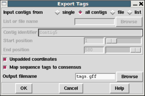
54 The Staden Package Manual
1.5.2 Importing GFF
Annotations within GFF files can be imported to Gap5 as annotations (sometimes referred
to as tags). The “Import GFF Annotatons” function in the main File menu performs
this task. Note that in order for this to work the contigs should not have been edited or
complemented since the GFF file was created, otherwise the coordinates in the GFF file
will not match.
One caveat to this relates to sequence gaps. By default consensus gaps/padding char-
acters are excluded from the contig consensus sequences when counting GFF sequence
coordinates. In some cases we may wish to support annotations in a gapped sequence, so
the “GFF coordinates are already padded” checkbox may be used to disable this coordinate
de-padding process.
1.5.3 Export Tags
This dialogue allows annotations (“tags”) to be written to disk as a GFF version 3 file.
Currently this just uses the GFF “remark” type, but future plans will be to support a
more wide variety of GFF types.
By default the coordinates generated are de-padded, such that “*”s in the consensus
sequence are not counted when identifying the coordinate of an annotation. This may be
disabled by deselecting the “Unpadded coordinates” checkbox.
The object a tag is attached to is typically the contig it is within, with the contig name
being used in the first column of the GFF file. This applies even for annotations place on
a sequence rather than the consensus. This feature may also be disabled by deselecting the
“Map sequence tags to consensus” checkbox.
Example GFF output follows, with “...” to denote lines truncated for illustrative pur-
poses.
Contig6 gap5 remark 4745 4745 . . . type=COMM;Note=Possible SNP?
Contig2 gap5 remark 3178 3196 . . . type=OLIG;Note=Template%09xb63f10%0AOligoname%09??%0A...
Note we can see URL style percent encoding being used to avoid GFF format metachar-
acters, as per the GFFv3 specification.
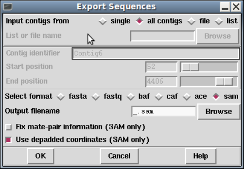
Chapter 1: Next generation assembly editing with Gap5 55
1.5.4 Export Sequences
This function exports sequence and annotation data from a Gap5 database to a variety of
assembly formats.
The fasta and fastq formats are basic sequence-only or sequence plus quality, with no
support for contigs or alignments. The BAF, CAF, ACE and SAM formats all hold assem-
bly data and so are reasonably complete representatives of data within Gap5. Note that
ACE does not directly support quality values and this export function does not create the
associated phdball file that houses this data.
There is also no direct support for BAM, however command line tools like samtools or
picard can convert the SAM file into BAM format. The SAM file should already be sorted
by position.
For SAM only there are additional options: whether to fix mate-pair information and
whether to use depadded coordinates. This former will ensure that the MRNM (Mate
Reference Name), MPOS and ISIZE fields are filled out. Note that this considerably slows
down the speed of exporting, so it is disabled by default.
56 The Staden Package Manual
1.6 Finding Sequence Matches
1.6.1 Find Internal Joins
The purpose of this function (which is invoked from the Gap5 View menu) is to use sequences
already in the database to find possible joins between contigs. Generally these will be joins
that were missed or judged to be unsafe during assembly and this function allows users to
examine the overlaps and decide if they should be made. During assembly joins may have
been missed because of poor data, or not been made because the sequence was repetitive.
Also it may be possible to find potential joins by extending the consensus sequences with
the data from the 3’ ends of readings which was considered to be too unreliable to align
during assembly i.e. we can search in the "hidden data".
If it has not already occurred, use of this function will automatically transform the
Contig Selector into the Contig Comparator. Each match found is plotted as a diagonal
line in the Contig Comparator, and is written as an alignment in the Output Window. The
length of the diagonal line is proportional to the length of the aligned region. If the match
is for two contigs in the same orientation the diagonal will be parallel to the main diagonal,
if they are not in the same orientation the line will be perpendicular to the main diagonal.
The matches displayed in the Contig Comparator can be used to invoke the Join Editor (see
Section 2.6.15 [The Join Editor], page 196) or Contig Editor. See Section 2.6 [Editing in
gap5], page 160. Alternatively, the "Next"button at the top left of the Contig Comparator
can be used to select each result in turn, starting with the best, and ending with the worst.
When this is in use, users can find the match in the Contig Comparator which corresponds
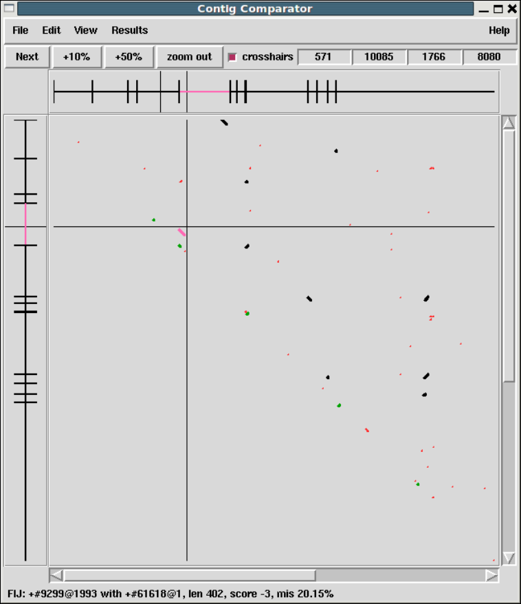
Chapter 1: Next generation assembly editing with Gap5 57
to the next result by placing the cursor over the Next button. The plotted match and the
contigs involved will turn white.
A typical display from the Contig Comparator is shown in the figure above.
To define the match all numbering is relative to base number one in the contig: matches
to the left (i.e. in the hidden data) have negative positions, matches off the right end of
the contig (i.e. in the hidden data) have positions greater than that of the contig length.
The convention for reporting the positions of overlaps is as follows: if neither contig needs
to be complemented the positions are as shown. If the program says "contig x in the -
sense"then the positions shown assume contig x has been complemented. For example, in
58 The Staden Package Manual
the results given below the positions for the first overlap are as reported, but those for the
second assume that the contig in the minus sense (i.e. 443) has been complemented.
Possible join between contig 445 in the + sense and contig 405
Percentage mismatch after alignment = 4.9
412 422 432 442 452 462
405 TTTCCCGACT GGAAAGCGGG CAGTGAGCGC AACGCAATTA ATGTGAG,TT AGCTCACTCA
::::::::: : :::::::: ::::: ::: :::::::::: :::::::::: ::::::::::
445 *TTCCCGACT G,AAAGCGGG TAGTGA,CGC AACGCAATTA ATGTGAG*TT AGCTCACTCA
-127 -117 -107 -97 -87 -77
472 482 492 502 512
405 TTAGGCACCC CAGGCTTTAC ACTTTATGCT TCCGGCTCGT AT
:::::::::: :::::::::: :::::::::: :::::::::: ::
445 TTAGGCACCC CAGGCTTTAC ACTTTATGCT TCCGGCTCGT AT
-67 -57 -47 -37 -27
Possible join between contig 443 in the - sense and contig 423
Percentage mismatch after alignment = 10.4
64 74 84 94 104 114
423 ATCGAAGAAA GAAAAGGAGG AGAAGATGAT TTTAAAAATG AAACG*CGAT GTCAGATGGG
:::: ::::: :::::::::: :::::::::: :::::: :: ::::: :::: :::::::::
443 ATCG,AGAAA GAAAAGGAGG AGAAGATGAT TTTAAA,,TG AAACGACGAT GTCAGATGG,
3610 3620 3630 3640 3650 3660
124 134 144 154 164
423 TTG*ATGAAG TAGAAGTAGG AG*AGGTGGA AGAGAAGAGA GTGGGA
::: :::::: :::::::::: :: ::::::: ::: ::::: :: ::
443 TTGGATGAAG TAGAAGTAGG AGGAGGTGGA ,GAG,AGAGA GTTGG*
3670 3680 3690 3700 3710
Chapter 1: Next generation assembly editing with Gap5 59
1.6.1.1 Find Internal Joins Dialogue
The contigs to use in the search can be defined as "all contigs", a list of contigs in a file
"file", or a list of contigs in a list "list". If "file"or "list"is selected the browse button
is activated and gives access to file or list browsers. Two types of search can be selected:
one, "Probe all against all"compares all the contigs defined against one another; the other
"Probe with single contig", compares one contig against all the contigs in the list. If this
option is selected the Contig identifier panel in the dialogue box is ungreyed. Both sense of
the sequences are compared.
If users elect not to "Use standard consensus"they can either "Mark active tags"or
"Mask active tags", in which cases the "Select tags"button will be activated. Clicking on
this button will bring up a check box dialogue to enable the user to select the tags types
they wish to activate. Masking the active tags means that all segments covered by tags that
are "active"will not be used by the matching algorithms. A typical use of this mode is to
avoid finding matches in segments covered by tags of type ALUS (ie segments thought to
be Alu sequence) or REPT (ie segment that are known to be repeated elsewhere in the data
60 The Staden Package Manual
(see Section 2.2.7.1 [Tag types], page 121). "Marking"is of less use: matches will be found
in marked segments during searching, but in the alignment shown in the Output Window,
marked segments will be shown in lower case.
Some alignments may be very large. For speed and ease of scrolling Gap5 does not
display the textual form of the longest alignments, although they are still visible within the
contig comparator window. The maximum length of the alignment to print up is controlled
by the “Maximum alignment length to list (bp)” control.
The default setting for the consensus is to "Use hidden data"which means that where
possible the contigs are extended using the poor quality data from the readings near their
ends. To ensure that this additional data is not so poor that matches will be missed, the
program uses algorithms which can be configured from the "Edit hidden data parameters"
dialogue. Two algorithms are available. Both slide a window along the reading until a set
criteria is met. By default an algorithm which sums confidence values within the window is
used. It stops when a window with < "Minimum average confidence"is found. The other
algorithm counts the number of uncalled bases in the window and stops when the total
reaches "Max number of uncalled bases in window". The selected algorithm is applied to
all the readings near the ends of contigs and the data that extends the contig the furthest
is added to its consensus sequence.
If your total consensus sequence length (including a 20 character header for each contig
that is used internally by the program) plus any hidden data at the ends of contigs is greater
than the current value of a parameter called maxseq, Find Internal Joins may produce an
error message advising you to increase maxseq. Maxseq can be set on the command line
(see Section 2.21 [Command line arguments], page 306) or by using the options menu (see
Section 2.20.3 [Set Maxseq], page 299).
The search algorithms first finds matching words of length "Word length", and only
considers overlaps of length at least "Minimum overlap". Only alignments better than
"Maximum percent mismatches"will be reported.
There are three search algorithms: “Sensitive”, “Quick” and “Fastest”. The quick or
fastest algorithm should be applied first, and then the sensitive one employed to find any
less obvious overlaps.
The sensitive algorithm sums the lengths of the matching words of length "Word length"
on each diagonal. It then finds the centre of gravity of the most significant diagonals.
Significant diagonals are those whose probability of occurence is < "Diagonal threshold". It
then uses a dynamic programming algorithm to align around the centre of gravity, using a
band size of "Alignment band size (percent)". For example: if the overlap was 1000 bases
long and the percentage set at 5, the aligner would only consider alignments within 50 bases
either side of the centre of gravity. Obviously the larger the percentage and the overlap,
the slower the aligment.
The fastest and quick algorithms can find overlaps and align 100,000 base sequences in a
few seconds by considering, in its initial phase only matching segments of length "Minimum
initial match length". However it does a dynamic programming alignment of all the chunks
between the matching segments, and so produces an optimal alignment. Again a banded
dynamic algorithm can be selected, but as this only applies to the chunks between matching
Chapter 1: Next generation assembly editing with Gap5 61
segments, which for good alignments will be very short, it should make little difference to the
speed. the fastest and quick methods only differ in how aggressively they prune potential
alignments before entering the dynamic programming phase.
After the search the results will be sorted so that the best matches are at the top of a list
where best is defined as a combination of alignment length and alignment percent identity.
This list can be stepped through, one result at a time using the Contig Joining Editor, by
clicking on the "Next"button at the top left of the Contig Comparator.

62 The Staden Package Manual
1.6.2 Find Repeats
The purpose of this function (which is invoked from the Gap5 View menu) is to find exact
repeats in contig consensus sequences. An exact repeat is defined as a run of consecutive
identical ACGT characters; no mismatches or gaps are permitted.
If it has not already occurred, selection of this function will automatically transform
the Contig Selector into the Contig Comparator. See Section 2.4 [Contig Comparator],
page 126. Each match found is plotted as a diagonal line in the Contig Comparator. The
length of the diagonal line is proportional to the length of the match.
If the match is for two contigs in the same orientation the diagonal will be parallel to
the main diagonal, if they are not the line will be perpendicular to the main diagonal. The
matches displayed in the Contig Comparator can be used to invoke the Join Editor (see
Section 2.6.15 [The Join Editor], page 196) or Contig Editors (see Section 2.6 [Editing in
Gap5], page 160), and an Information button will display data about the match in the
Output window. e.g.
Repeat match
From contig xb54a3.s1(#26) at 78
With contig xb62h3.s1(#3) at 1
Length 37
This means that position 78 in the contig with xb54a3.s1 (reading number 26) at its left
end matches 37 bases at position 1 in the contig with xb62h3.s1 (number 3) at its left end.
Users can elect to search a "single"contig, or compare "all contigs", or a subset of
contigs defined in a list or a file. If "file"or "list"is selected the browse button is activated
and gives access to file or list browsers. If they choose to analyse a single contig the
dialogue concerned with selecting the contig and the region to search becomes activated.
Chapter 1: Next generation assembly editing with Gap5 63
The "Minimum Repeat"defines the smallest match that the algorithm will report. The
algorithm will search only for repeats in the forward direction "Find direct repeats", or
only those in the reverse direction "Find inverted repeats", or both "Find both".
If "Mask active tags"is selected the "Select tags"button is activated. Clicking on this
button will bring up a check box dialogue to enable the user to select the tags types they
wish to activate. Masking the active tags means that all segments covered by tags that are
"active"will not be used in the matching algorithm. A typical use of this mode is to avoid
finding matches in segments covered by tags of type ALUS (ie segments thought to be Alu
sequence) or that already covered by REPT tags. See Section 2.2.7.1 [Tag types], page 121.
After the search is complete clicking on "Yes"in the "Save tags to file"panel will activate
the "File name"box and all repeats on the list will be written to a file. This file can be
used with "Enter tags"(see Section 2.12.2 [Enter Tags], page 265) to create REPT tags
for all the repeats found. Note that "Enter tags"will remove all the results plotted in the
contig comparator.
Note that the current version of Find Repeats has a limit to the number of repeats it
can store. The limit depends on the current maximum consensus length, so if you want to
increase the limit, reset the maximum consensus length. This can be done using the "Set
maxseq"item in the "Options"menu.
64 The Staden Package Manual
1.6.3 Find Read Pairs
This function is used to check the positions and orientations of readings taken from the
same templates. It is invoked from the gap5 View menu.
For each template the relative position of its readings and the contigs they are in are
examined. This analysis can give information about the relative order, separation and
orientations of contigs and also show possible problems in the data. The search can be
over the whole database or a subset of contigs named in a list (see Section 2.14 [Lists],
page 278) or file of file names. The results are written to the Output Window and plotted
in the Contig Comparator (See Section 2.4 [Contig Comparator], page 126.). Read pair
information is also used to colour code the results displayed in the Template Display (see
Section 2.5.1 [Template Display], page 130).
Note that during assembly the template names and lengths are copied from the exper-
iment files into the gap database. See Section 11.3 [Experiment Files], page 552. The
accuracy of the lengths will depend upon some size selection being performed during the
cloning procedures.
Users choose to process "all contigs"or a subset selected from a file of file names ("file")
or a list ("list"). If either of the subset options is selected the "browse"button will be
activated and can be clicked on to call up a file or list browser dialogue.
1.6.3.1 Find Read Pairs Graphical Output
The contig comparator is used to plot all templates with readings that span contigs. That
is, the lines drawn on the contig comparator are a visual representation of the relationship
Chapter 1: Next generation assembly editing with Gap5 65
(orientation and overlap) between contigs. When a template spans more than two contigs,
all the combinations of pairs of contigs are plotted. However such cases are uncommon.
The figure above shows a typical Contig Comparator plot which includes several types
of result in addition to those from Read Pair analysis.
The lines for the read-pairs are, by default, shown in blue. The length of the line is the
average length of the two readings within the pair. The slope of the line represents the
relative orientation of the two readings. If they are both the same orientation (including
both complemented) the line is drawn from top left to bottom right, otherwise the line is
drawn from top right to bottom left.
Chapter 1: Next generation assembly editing with Gap5 67
1.6.4 Sequence Search
The purpose of this function (which is available from the prog View menu) is to find
matches between the consensus sequence and short segments of sequence defined by the
user. The segments of sequence (or "strings") can be typed into the dialogue provided
or can be the sequences covered by consensus tag types (see Section 2.2.7.1 [Tag types],
page 121) selected by the user. The latter mode hence provides a way of checking to see
if a tagged segment of the sequence occurs elsewhere in the consensus. The function was
previously known as "Find Oligos".
Users can elect to search against a "single"contig, "all contigs", or a subset of contigs
defined in a list (see Section 2.14 [Lists], page 278) or a file. If "file"or "list"is selected
the browse button is activated and gives access to file or list browsers. If they choose to
analyse a single contig the dialogue concerned with selecting the contig and the region to
search becomes activated.
Both strands of the consensus are scanned using a very simple algorithm: insertions and
deletions are not allowed, but mismatches are. The "Minimum percent match"defines the
smallest percentage match which will be reported by the algorithm. A value of 75 means
that at least 75% of the bases must match the target sequence.
The user can elect to use tags or to specify their own sequences for the search. Selecting
"Use tags"will activate the "Select tags"browse button. Clicking on this button will bring
up a check box dialogue to enable the user to select the tags types they wish to activate.
Alternatively selecting "Enter sequence"will activate a text entry box and the user can
enter a string of characters. Only the characters ACGTU are allowed and there is no limit
to the length of the string.
If it has not already occurred, selection of this function will automatically transform
the Contig Selector into the Contig Comparator. See Section 2.4 [Contig Comparator],
page 126. Each match found is plotted as a diagonal line in the Contig Comparator. The
length of the diagonal line is proportional to the length of the search string. Self matches
from the tag search are not reported.

68 The Staden Package Manual
If the match between the search string and the contig are in the same orientation,
the diagonal match line will be parallel to the main diagonal, otherwise the line will be
perpendicular to the main diagonal. Matches found between a tag and a contig can be used
to invoke the Join Editor (see Section 2.6.15 [The Join Editor], page 196) or Contig Editors
(see Section 2.6 [Editing in prog ], page 160). Matches between a specified sequence and
a contig will only invoke the Contig Editor. All of the matches found are displayed in the
Output Window e.g.
Match found between tag on contig 315 in the + sense and contig 495
Percentage mismatch 16.7
957 967 977 987 997
315 CATAAGGATTTCCAATATTTTATTCCAGTTGGGCATCCTAGT
:: ::::::::::: :::::::::::::::::: ::::
495 GATTGGGATTTCCAATGTTTTATTCCAGTTGGGCACCCTAAG
2 12 22 32 42
Chapter 1: Next generation assembly editing with Gap5 69
1.7 Checking Assemblies and Removing Readings
After assembly, and prior to editing, it can be useful to examine the quality of the alignments
between individual readings and the sections of the consensus which they overlap. This may
reveal doubtful joins between sections of contigs, poorly aligned readings, or readings that
have been misplaced. By using this analysis in combination with other gap5 functions such
as Find internal joins (see Section 2.8.3 [Find Internal Joins], page 227) and Find repeats
(see Section 2.8.4 [Find Repeats], page 233), it is also possible to discover if readings have
been positioned in the wrong copies of repeat elements.
If readings are found to be misplaced or need removing for other reasons, gap5 has func-
tions for breaking contigs (see Section 2.9.1.1 [Breaking Contigs], page 239), and removing
readings (see Section 2.9.1.2 [Disassembling Readings], page 240). These functions can be
accessed through the main gap5 Edit menu or from within the Contig Editor.
If readings are removed from contigs to start new contigs of one reading, these contigs can
then be processed by Find internal joins (see Section 2.8.3 [Find Internal Joins], page 227)
and the Join editor (see Section 2.6.15 [The Join Editor], page 196), which should reveal all
the other positions at which the reading matches.
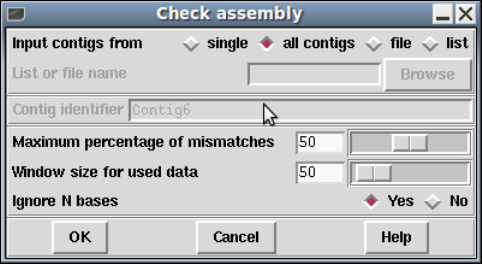
70 The Staden Package Manual
1.7.0.1 Checking Assemblies
The Check Assembly routine (which is invoked from the gap5 View menu) is used to check
contigs for potentially misassembled readings by comparing them against the segment of
the consensus which they overlap. It simply slides a small window along the sequence
identifying regions of high disagreement between that portion of sequence and the consensus.
Results are displayed in the Output Window and plotted on the main diagonal in the Contig
Comparator. See Section 2.4 [Contig Comparator], page 126.
From the Contig Comparator the user can invoke the Contig Editor to examine the
alignment of any problem reading. See Section 2.6 [Editing in gap5], page 160. If the
reading appears to be correctly positioned the user can either edit it, or instead select the
name to add it to the “readings” list for subsequent disassembly or removal.
Users select either to search only one contig ("single"), all contigs ("all contigs"), or a
subset of contigs contained in a "file"or a "list". If "file"or "list"is selected the "browse"
button will be activated and clicking on it will invoke a file or list browser. If a single contig
is selected the "Contig identifier"dialogue will be activated and users should enter a contig
name.
The percentage disagreement and over what size of window are both configurable pa-
rameters. Additionally there is a parameter to control whether N bases in the sequence
should be considered as disagreements or not. The choice will depend on whether you are
looking for sequences that appear to be in the wrong place (ignore Ns) or simply sequences
that appear to have a large number of incorrect base calls (keep Ns).
The "Information"window produced by selecting "Information"from the Contig Com-
parator "Results"menu produces a summary of the results sorted in order os percentage
mismatch.
By clicking with the right mouse button on results plotted in the Contig Comparator
a pop-up menu is revealed which can be used to invoke the Contig Editor (see Section 2.6
[Editing in gap4], page 160). The editor will start up with the cursor positioned on the
problem reading. If the reading is found to be misplaced it can be marked for removal
from within the Editor (see Section 2.6.7.12 [Remove Reading], page 179). However, prior
to this it may be beneficial to use some of the other analyses such as Find internal joins
(see Section 2.8.3 [Find Internal Joins], page 227) and Find repeats (see Section 2.8.4 [Find
Repeats], page 233), which may help to find its correct location. Both of these functions
72 The Staden Package Manual
1.7.1 Removing Readings and Breaking Contigs
Occasionally contigs require more drastic changes than simple basecall edits. Sometimes it
is necessary to remove readings that have been put in the wrong place, or to break contigs
that should not have been joined. Gap5 contains functions to help with these problems,
and two types of interface.
If a contig needs to be broken cleanly into two new contigs, with all the readings, other
than the two at the incorrect join, still linked together, then Break Contig (see Section 2.9.1.1
[Breaking Contigs], page 239), or (see Section 2.6.7.13 [Break Contig], page 179) should be
used. The former interface is available via the main gap5 Edit menu, and the latter as an
option in the Contig Editor.
If one or more readings need removing from from contig(s), even if their removal will
break the contiguity of a contig, then (see Section 2.9.1.2 [Disassemble Readings], page 240),
or (see Section 2.6.7.12 [Remove Reading], page 179) should be used. The former interface
is available via the main gap5 Edit menu, and the latter as an option in the Contig Editor.
Readings can be removed from the database completely, or moved to start individual new
contigs, one for each reading.
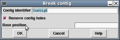
Chapter 1: Next generation assembly editing with Gap5 73
1.7.1.1 Breaking Contigs
The Break Contig function (which is available from the gap5 Edit menu) enables contigs to
be broken by removing the link between two adjacent readings. The user defines the contig
coordinate to break at. All sequences starting to the right of that position will be placed
into a new contig.
Breaking contig can somtimes cause more holes to be created. The “Remove contig
holes” will also cause subsequent breaks to happen at these cases, producing more than one
additional contig. If we have aligned against a reference and expect regions of zero coverage
then this option should be disabled.
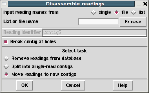
74 The Staden Package Manual
1.7.1.2 Disassembling Readings
This function is used to remove readings from a database or move readings to new contigs.
If readings are removed from the database all reference to them is deleted. If a reading
is moved to a “single-read contig” a new contig will be created containing this one single
reading, which may then be re-processed by Find Internal Joins (see Section 2.8.3 [Find In-
ternal Joins], page 227) and the Join editor (see Section 2.6.15 [The Join Editor], page 196),
which should reveal all the other positions at which the reading matches.
More useful is the general “Move readings to new contigs”. This will keep any assembly
relationships intact between the set of readings to be disassembled. For example if three
readings overlap then when disassembled all three will end up in a single new contig. This
function is particularly useful for pulling apart false joins or repeats.
The set of readings to be processed can be read from a “file” or a “list” and clicking on
the “browse” button will invoke an appropriate browser. If just a single reading is to be
assembled choose “single” and enter the reading name instead of the file or list of filenames.
Removal via a “list” is a particularly powerful option when controlled via the list gen-
eration functions within the contig editor. For example break contig could be viewed as
disassembling a list of readings selected using “Select this reading and all to right”.
Unlike gap4, gap5 can cope with having holes in contigs. (This is obviously a requirement
when dealing with mapped alignments.) Hence gap5 gives us a choice whether to break
contigs into two (or more) pieces when removing sequences produces holes in the contigs.
By default this is enabled.
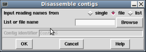
Chapter 1: Next generation assembly editing with Gap5 75
1.7.1.3 Delete Contigs
While Disassemble Readings is capable of removing entire contigs, it is inefficient for this
task as it has a lot of additional house-keeping to perform.
Delete Contigs should be used when we wish to remove entire contigs. Be careful not
to accidentally choose this over disassemble readings as even when giving a single sequence
name, this function will interpret it as a request for removing all other sequences in that
contig too.
There is no Undo feature, so backups are advised before hand.
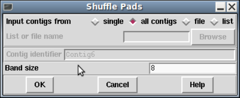
76 The Staden Package Manual
1.8 Tidying up alignments
The Shuffle Pads, Remove pad Columns and Remove Contig Holes all share a common goal
of tidying up sequence alignments, possibly also breaking the contig up.
1.8.1 Shuffle Pads
This function is an implementation of the Anson and Myers “ReAligner” algorithm. It anal-
yses multiple sequence alignments to detect locations where the number of disagreements
to the consensus could be reduced by realignment of sequences, possibly also correcting the
consensus in the process. For example:
Sequence1: GATTCAAAGAC
Sequence2: TTCAA*GACGG
Sequence3: TC*AAGAC
Consensus: GATTCAAAGACGGATC
The consensus contains AAA, but the corrected alignment only has two As:
Sequence1: GATTCAAAGAC
Sequence2: TTC*AAGACGG
Sequence3: TC*AAGAC
Consensus: GATTC*AAGACGGATC
For speed we acknowledge that the new alignment will only deviate slightly from the old
one and so a narrow “band size” is used. This paramater may be adjusted if required, but
at the expense of speed.
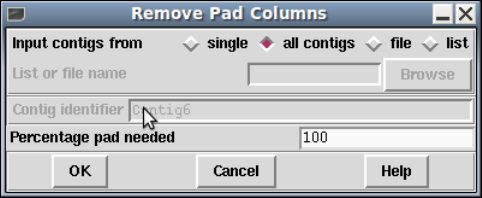
Chapter 1: Next generation assembly editing with Gap5 77
1.8.2 Remove Pad Columns
There are cases where we may have multiple alignments where every single sequence has a
padding character such that the complete column is “*”. This can occur when disassembling
data from a falsely made join.
The Shuffle Pads algorithm will remove entire columns of pads when it finds them, but
it is time consuming and it may also edit alignments elsewhere. The Remove Pad Columns
function is a faster, more specific solution to this problem.
By default the function will only ever delete columns where 100% of the sequences have a
pad/gap. However with appropriate due care it is possible to reduce this and allow removal
of columns where a few sequences have a real base provided the overall percentage is still
high. This is achieved by reducing the “Percentage pad needed” parameter.
Reducing from 100% is not recommended though as it is removal of data purely for
tidyness sake, while the consensus algorithm will automatically find the correct solution.
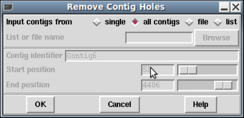
78 The Staden Package Manual
1.8.3 Remove Contig Holes
Unlike Gap4, Gap5 permits contig regions with zero coverage. These can naturally occur
when using sequence mapping to known references. However in a denovo assembly context
they are not desireable.
Some algorithms have check boxes querying whether you wish holes to be removed by
breaking contigs up, but this dialogue offers a choice of fixing the holes at a later stage.
It identifies all regions of zero coverage and will break the contig into multiple fragments.
Chapter 1: Next generation assembly editing with Gap5 79
1.9 Calculating Consensus Sequences
In this section we describe the types of consensus which gap4 can produce, the formats they
can be written in, and the algorithms that can be used. The algorithms are not only used
to produce consensus sequence files, but in many other places throughout gap4 where an
analysis of the current quality of the data is required. One important place is inside the
Contig Editor (see Section 2.6 [Editing in gap4], page 160) where they are used to produce
an "on-the-fly"consensus, responding to every edit made by the user.
The currently active consensus algorithm is selected from the "Consensus algorithm"di-
alogue in the main gap4 Options menu (see Section 2.20.2 [Consensus Algorithm], page 299).
There are four main types of consensus sequence file that can be produced by the pro-
gram: Normal, Extended, Unfinished, and Quality. They are all invoked from the File
menu.
"Normal"is the type of consensus file that would be expected: a consensus from the
non-hidden parts of a contig. "Extended"is the same as "Normal"but the consensus is
extended by inclusion of the hidden, non-vector sequence, from the ends of the contig.
"Unfinished"is the same as "Normal"except that any position where the consensus
does not have good data for both strands is written using A,C,G,T characters, and the rest
(which has good data for both strands) is written using a different set of symbols. This
sequence can be used for screening against new readings: only the regions needing more
readings will produce matches. By screening readings in this way, prior to assembly, users
can avoid entering readings which will not help finish the project, and which may require
further editing work to be performed.
"Quality"produces a sequence of characters of the same length as the consensus, but
they instead encode the reliability of the consensus at each point.
Consensus sequence files can also encode the positions of the currently active tag types
by changing the case of the tagged characters (marking) or writing them in a different
character set (masking) (see Section 2.2.7.2 [Active tags and masking], page 121).
The consensus algorithms are usually configured to produce only the characters A,C,G,T
and "-", but it is possible to set them to produce the complete set of IUB codes. This mode
is useful for some types of work and allows the range of observed base types at any position
to be coded in the consensus. How the IUB codes are chosen is described in the introduction
to the consensus algorithms (see Section 2.11.5 [The Consensus Algorithms], page 257).
Depending on the type of consensus produced, the consensus sequence files can be written
in three different formats: Experiment files (see Section 11.3 [Experiment File], page 552),
FASTA (Pearson,W.R. Using the FASTA program to search protein and DNA sequence
databases. Methods in Molecular Biology. 25, 365-389 (1994)) or staden formats. If ex-
periment file format is selected a further menu appears that allows users to select for the
inclusion of tag data in the output file. For FASTA format the sequence headers include the
contig identfier as the sequence name and the project database name, version number and
the number of the leftmost reading in the contig as comments. e.g. ">xyzzy.s1 B0334.0.274"
is database B0334, copy 0, and the left most reading for the contig is number 274, which has
a name of xyzzy.s1. For staden format the headers include the project database name and

80 The Staden Package Manual
the number of the leftmost reading in the contig. e.g. "<B0334.00274——->" is database
B0334 and the left most reading for the contig is number 274. Staden format is maintained
only for historical reasons - i.e. there may still be a few unfortunate people using it. Ob-
viously Experiment file format can contain much more information, and can serve as the
basis of a submission to the sequence library.
1.9.1 Normal Consensus Output
This is the usual consensus type that will be calculated (and is available from the gap4
File menu). The currently active consensus algorithm is selected from the "Consensus algo-
rithm"dialogue in the main gap4 Options menu (see Section 2.20.2 [Consensus Algorithm],
page 299).
Contigs can be selected from a file of file names or a list. In addition, tagged regions can
be masked or marked (see Section 2.2.7.2 [Active tags and masking], page 121), and output
can be in Experiment file, fasta or staden formats. If experiment file format is selected a
further menu appears that allows users to select for the inclusion of tag data in the output
file.
The contigs for which to calculate a consensus can be a particular "single"contig, "all
contigs", or a subset of contigs whose names are stored in a "file"or a "list". If a file or list
is selected the browse button will be activated, and if it is clicked, an appropriate browser
will be invoked. If the user selects "single"then the dialogue for choosing the contig, and
the section to process, becomes active.
If the user selects either "mask active tags"or "mark active tags"the "Select tags"
button is activated, and if it is clicked, a dialogue panel appears to enable the user to select
which tag types should be used in these processes. If "mask"is selected all segments covered
Chapter 1: Next generation assembly editing with Gap5 81
by the tag types chosen will not be written as ACGT but as defi symbols. If "mark"is
selected the tagged segments will be written in lowercase characters. Masking is useful for
producing a sequence to screen against other sequences: only the unmasked segments will
produce hits.
The "strip pads"option will remove pads ("*"s) from the consensus sequence. In the
case of experiment files this will also automatically adjust the position and length of the
annotations to ensure that they still mark the correct segment of sequence.
Normally the consensus sequences are named after the left-most reading in each contig.
For the purposes of single-template based sequencing projects (eg cDNA assemblies) the
option exists to “Name consensus by left-most template” instead of by left-most reading.
The routine can write its consensus sequence (plus extra data for experiment files) in
"experiment file","fasta"and "staden"formats. The output file can be chosen with the
aid of a file browser. If experiment file format is selected the user can choose whether or not
to have "all annotations","annotations except in hidden", or "no annotations"written out
with the sequence. If the user elects to include annotations the "select tags"button will
become active, and if it is clicked, a dialogue for selecting the types to include will appear.
1.9.2 The Consensus Algorithms
The consensus calculation is a very important component of gap4. It is used to produce
an "on-the-fly"consensus, responding to every individual change in the Contig Editor (see
Section 2.6 [Editing in gap4], page 160) and is used to produce the final sequence for
submission to the sequence libraries. Some years ago Bonfield, J.K. and Staden, R. The
application of numerical estimates of base calling accuracy to DNA sequencing projects.
Nucleic Acids Res. 23, 1406-1410 (1995) we put forward the idea of using base call accuracy
estimates in sequencing projects, and this has been partially realised with the values from
the Phred program (Ewing, B. and Green, P. Base-Calling of Automated Sequencer Traces
Using Phred. II. Error Probabilities. Genome Research. Vol 8 no 3. 186-194 (1998)).
These values are widely used and have defined a decibel type scale for base call confidence
values and gap4 is currently set to use confidence values defined on this scale. An overview
of our use of confidence values is contained in the introductory sections of the manual (see
Section 2.2.5 [The use of numerical estimates of base calling accuracy], page 118).
As is described elsewhere (see Section 2.11.6 [List Consensus Confidence], page 261)
being able to calculate the confidence for each base in the consensus sequence makes it
possible to estimate the number of errors it contains, and hence the number of errors that
will be removed if particular bases are checked and, if necessary, edited.
Gap4 caters for base calls with and without confidence values and hence provides a
choice of algorithms. There are currently three consensus algorithms that may be used.
The choice of the best algorithm will depend on the data that you have available and the
purpose for which you are using gap4.
The currently active consensus algorithm is selected from the "Consensus algorithm"di-
alogue in the main gap4 Options menu (see Section 2.20.2 [Consensus Algorithm], page 299).
The only way to produce a consensus sequence for which the reliability of each base is
known, is to use reading data with base call confidence values. Their use, in combination
82 The Staden Package Manual
with the Confidence Value algorithm (see Section 2.11.5.3 [Consensus Calculation Using
Confidence Values], page 259). is strongly recommended.
For base calls without confidence values use the Base Frequencies algorithm (see
Section 2.11.5.1 [Consensus Calculation Using Base Frequencies], page 258). This is also
a fast algorithm so it may be appopriate for very high depth assemblies such those for
mutation studies.
For data with simple base call accuracy estimates rather than those on the decibel scale,
the Weighted Base Frequencies algorithm should be used (see Section 2.11.5.2 [Consensus
Calculation Using Weighted Base Frequencies], page 259).
All confidence values lie in the range 0 to 100. When readings are entered into a data-
base, gap4 assigns a confidence of 99 to all bases without confidence values. For all three
algorithms, a base with confidence of 100 is used to force the consensus base to that base
type and to have a confidence of 100. However,if two or more base types at any position
have confidence 100, the consensus will be set to "unknown", i.e. "-", and will have a
confidence of 0. Note that dash ("-") is our preferred symbol for "unknown"as, within a
sequence, it is more easily distinguished from A,C,G,T than "N".
The consensus sequence is also assigned a confidence, even when base call confidence
values are not used to calculate it. The scale and meaning of the consensus confidence
changes between consensus algorithms. However the consensus cutoff parameter always has
the same meaning. A consensus base with a confidence ’X’ will be called as a dash when
’X’ is lower than the consensus cutoff, otherwise it is the determined base type.
Both the consensus cutoff and quality cutoff values can be set by using the "Config-
ure cutoffs"command in the "Consensus algorithm"dialogue in the main gap4 Options
menu (see Section 2.20.2 [Consensus Algorithm], page 299). Within the Contig Editor (see
Section 2.6 [Editing in gap4], page 160) these values can be adjusted by clicking on the "<"
and ">" symbols adjacent to the "C:"(consensus cutoff) and "Q:"(quality cutoff) displays
in the top left corner of the editor. These buttons are repeating buttons - the values will
adjust for as long as the left mouse button is held down. Changing these values lasts only
as long as that invocation of the contig editor.
The consensus algorithms are usually configured to produce only the characters
A,C,G,T,* and "-", but it is possible to set them to produce the complete set of IUB
codes. This mode is useful for some types of work and allows the range of observed base
types at any position to be coded in the consensus. The IUB code at any position is
determined in the following way.
We assume that the user wants to know which base types have occurred at any point,
but may want some control over the quality and relative frequency of those that are used to
calculate the "consensus". For the simplest consensus algorithm there is no control over the
quality of the base calls that are included, but the Consensus Cutoff can be used to control
how the relative frequency affects the chosen IUB code. All base types whose computed
"confidence"exceeds the Consensus Cutoff will be included in the selection of the IUB code.
For example if only base type T reaches the Consenus Cutoff the IUB code will be T; if both
T and C reach the cutoff the code will be Y; if A, C and T each reach the cutoff the code
will be H; if A, C, G and T all reach the cutoff the code will be "N". For the Confidence
Chapter 1: Next generation assembly editing with Gap5 83
Value algorithm the Quality Cutoff can be used to exclude base calls of low quality, so that
all those that do not reach the Quality Cutoff are excluded from the IUB code calculation.
Otherwise the logic of the code selection is the same as for the two simpler algorithms.
Both the consensus cutoff and quality cutoff values can be set by using the "Configure
cutoffs"command in the "Consensus algorithm"dialogue in the main gap4 Options menu
(see Section 2.20.2 [Consensus Algorithm], page 299).
The algorithms are explained below.
1.9.2.1 Consensus Calculation Using Base Frequencies
This algorithm can be used for any data, with or without confidence values. Each standard
base type is given the same weight. The consensus will be the most frequent base type in a
given column provided that the consensus cutoff parameter is low enough. All unrecognised
base types, including IUB codes, are treated as dashes. Dashes are given a weight of
1/10th that of recognised base types. Pads are given a weight which is the average of their
neighbouring bases.
The confidence of a consensus base for this method is expressed as a percentage. So for
example a column of bases of A, A, A and T will give a consensus base of A and a confidence
of 75. Therefore a consensus cutoff of 76 or higher will give a consensus base of "-".
In the event that more than one base type is calculated to have the same confidence, and
this exceeds the consensus cutoff, the bases are assigned in descending order of precedence:
A, C, G and T.
The quality cutoff parameter (Q in the Contig Editor) has no effect on this algorithm.
1.9.2.2 Consensus Calculation Using Weighted Base Frequencies
This method can be used when simple, unquantified, base call quality values are available.
Instead of simply counting base type frequencies it sums the quality values. Hence a column
of 4 bases A, A, A and T with confidence values 10, 10, 10 and 50 would give combined
totals of 30/80 for A and 50/80 for T (compared to 3/4 for A and 1/4 for T when using
frequencies). As with the unweighted frequency method this sets the confidence value of
the consensus base to be the the fraction of the chosen base type weights over the total
weights (62.5 in the above example).
The quality cutoff parameter controls which bases are used in the calculation. Only bases
with quality values greater than or equal to the quality cutoff are used, otherwise they are
completely ignored and have no effect on either the base type chosen for the consensus or
the consensus confidence value. In the above example setting the quality cutoff to 20 would
give a T with confidence 100 (100 * 50/50).
In the event that more than one base type is calculated to have the same weight, and
this exceeds the consensus cutoff, the bases are assigned in descending order of precedence:
A, C, G and T.
This is Rule IV of Bonfield,J.K. and Staden,R. The application of numerical estimates
of base calling accuracy to DNA sequencing projects. Nucleic Acids Research 23, 1406-1410
(1995).
84 The Staden Package Manual
1.9.2.3 Consensus Calculation Using Confidence values
This is the prefered consensus algorithm for reading data with Phred decibel scale confidence
values. As will become clear from the follwing description, it is more complicated than the
other algorithms, but produces a much more useful result.
A difficulty in designing an algorithm to calculate the confidence for a consensus derived
from several readings, possibly using different chemistries, and hopefully from both strands
of the DNA, is knowing the level of independence of the results from different experiments
- namely the readings. Given that sequencing traces are sequence dependent, we do not
regard readings as wholly independent, but at the same time, repeated readings which
confirm base calls may give us more confidence in their accuracy. In addition, if we get a
particularly good sequencing run, with consequently high base call confidence values, we
are more likely to believe its base call and confidence value assignments. The final point in
this preamble is that the Phred confidence values refer only to the probability for the called
base, and they tell us nothing about the relative likelihood of each of the other 3 base types
appearing at the same position. These difficulties are taken into account by our algorithm,
which is described below.
In what follows, a particular position in an alignment of readings is referred to as a
"column". The base calls in a column are classified by their chemistry and strand. We
currently group them into "top strand dye primer","top strand dye terminator","bottom
strand dye primer"and "bottom strand dye terminator"classes.
Within each class there may be zero or many base calls. For each class we check for
multiple occurrences of the same base type. For each base type we find the highest confidence
value, and then increase it by an amount dependent on the number of confirming reads.
Then Bayes formula is used to derive the probabilities and hence the confidence values for
each base type.
To further describe the method it is easiest to work through an example. Suppose we
have 5 readings with the following characteristics covering a particular column.
Dye primer, top strand, ’A’, confidence 20
Dye primer, top strand, ’A’, confidence 10
Dye primer, top strand, ’T’, confidence 20
Dye terminator, top strand, ’T’, confidence 10
Dye primer, bottom strand, ’A’, confidence 5
Hence there are three possible classes.
Examining the "dye primer top strand"class we see there are three readings (A, A and
T). The highest A is 20. We add to this a fixed quantity to indicate one other occurence
of an A in this set. For this example we add 5. Now we have an adjusted confidence of
25 for A and 20 for T. This is equivalent to a .997 probability of A being correct and .99
probability of T being correct. To use Bayes we split the remaining probabilies evenly. A
has a probability of .997 and so the remaining .003 is spread amongst the other base types.
Similarly for the .01 of the T. The result is shown in the table below.
|ACGT
--+-----------------------
A | .997 .001 .001 .001
Chapter 1: Next generation assembly editing with Gap5 85
T | .0033 .0033 .0033 .990
Bayesian calculations on this table then give us probabilities of approximately .766 for
A, .00154 for C, .00154 for G and .231 for T.
The other classes give probalities of .033 for A, C, G and .9 for T, and .316 for A, and
.228 for C, G and T.
To combine the values for each class we produce a table for a further Bayesian calculation.
Once again we fill in the probabilities and spread the remainder evenly amongst the other
base types.
| A C G T
-----------+--------------------------
Primer Top | .766 .00154 .00154 .231
Term Top | .0333 .0333 .0333 .9
Primer Bot | .316 .228 .228 .228
From this Bayes gives the final probabilities of .135 for A, .0002 for C, .0002 for G and
.854 for T. This is what would be expected intuitively: the T signal was present in both
dye primer and dye terminator experiments with 1/100 and 1/10 error rates whilst the A
signal was present on both strands with 1/100 and 1/3 error rates. Hence the consensus
base is T with confidence 8.4 (-10*log10(1-.854)).
If a padding character is present in a column we consider the pad as a separate base
type and then evenly divide the remaining probabilities by 4 instead of 3.
1.9.2.4 The Quality Calculation
The Quality Calculation described here (which is available from the gap4 File menu) applies
either of the two simple consensus calculations (see Section 2.11.5.1 [Consensus Calculation
Using Base Frequencies], page 258) and (see Section 2.11.5.2 [Consensus Calculation Using
Weighted Base Frequencies], page 259) to the data for each strand of the DNA separately.
It produces, not a consensus sequence, but an encoding of the "quality"of the data which
defines whether it has been determined on both strands, and whether the strands agree.
This quality is used as the basis for problem searches, such as find next problem, and the
Quality Display within the Template Display (see Section 2.5.1.5 [Quality Plot], page 137).
The categories of data and the codes produced are shown in the table. For example ’c’
means bad data on one strand is aligned with good data on the other.
+Strand -Strand
aGood Good (in agreement)
bGood Bad
cBad Good
dGood None
eNone Good
fBad Bad
gBad None

86 The Staden Package Manual
hNone Bad
iGood Good (disagree)
jNone None
the "Configure cutoffs"command in the
In the "Consensus algorithm"dialogue in the main gap4 Options menu (see
Section 2.20.2 [Consensus Algorithm], page 299), setting the configuration to treat readings
flagged using the "Special Chemistry"Experiment File line (CH field) (see Section 11.3
[Experiment File], page 552) affects this calculation. When set, the reading counts for
both strands in the Consensus and Quality Calculations, and hence is equivalent to having
data on both strands.
1.9.3 List Consensus Confidence
The Confidence Value consensus algorithm (see Section 2.11.5.3 [Consensus Calculation
Using Confidence Values], page 259) produces a consensus sequence for which the expected
error rate for each base is known. The option described here (which is available from the
gap4 View menu) uses this information to calculate the expected number of errors in a
particular consensus sequence and to tabulate them.
The decibel type scale introduced in the Phred program uses the formula
-10xlog10(error rate) to produce confidence values for the base calls. A confidence value of
10 corresponds to an error rate of 1/10; 20 to 1/100; 30 to 1/1000; etc.
So for example, if 50 bases in the consensus had confidence 10, we would expect those 50
bases (with an error rate of 1/10) to contain 5 errors; and if 200 bases had confidence 20, we
would expect them to contain 2 errors. If these 50 bases with confidence 10, and 200 bases
with confidence 20 were the least accurate parts of the consensus, they are the bases which
we should check and edit first. In so doing we would be dealing with the places most likely
to be wrong, and would raise the confidence of the whole consensus. The output produced
by List Confidence shows the effect of working through all the lowest quality bases first,
until the desired level of accuracy is reached. To do this it shows the cumulative number
of errors that would be fixed by checking every consensus base with a confidence value less
than a particular threshold.
The List Confidence option is available from within the Commands menu of the Contig
Editor and the main gap4 View menu. From the main menu the dialogue simply allows
selection of one or more contigs. Pressing OK then produces a table similar to the following:
Sequence length = 164068 bases.
Expected errors = 168.80 bases (1/971 error rate).
Value Frequencies Expected Cumulative Cumulative Cumulative
errors frequencies errors error rate
--------------------------------------------------------------------------
0 0 0.00 0 0.00 1/971
1 1 0.79 1 0.79 1/976
2 0 0.00 1 0.79 1/976
3 3 1.50 4 2.30 1/985

Chapter 1: Next generation assembly editing with Gap5 87
4 30 11.94 34 14.24 1/1061
5 2 0.63 36 14.87 1/1065
6 263 66.06 299 80.94 1/1867
7 151 30.13 450 111.06 1/2841
8 164 25.99 614 137.06 1/5168
9 96 12.09 710 149.14 1/8344
10 80 8.00 790 157.14 1/14069
The output above states that there are 164068 bases in the consensus sequence with an
expected 169 errors (giving an average error rate of one in 971). Next it lists each confidence
value along with its frequency of occurrence and the expected number of errors (as explained
above, frequency x error rate). For any particular confidence value the cumulative columns
state: how many bases in the sequence have the same or lower confidence, how many errors
are expected in those bases, and the new error rate if all these bases were checked and all
the errors fixed.
Above it states that there are 790 bases with confidence values of 10 or less, and estimates
there to be 157 errors in those 790 bases. As we expect there to be about 169 errors in the
whole consenus this implies that manually checking those 790 bases would leave only 12
undetected errors. Given that the sequence length is 164068 bases this means an average
error rate of 1 in 14069. It is important to note that by using this editing strategy, this
error rate would be achieved by checking only 0.48% of the total number of consensus bases.
This strategy is realised by use of the consensus quality search in the gap4 Contig Editor
(see Section 2.6.6.7 [Search by Consensus Quality], page 175).
1.9.4 List Base Confidence
The various base-callers may produce a confidence value for each base call. Previous sections
describe how this may be used to produce a consensus sequence along with a consensus
confidence.
This function tabulates the frequency of each base confidence value along with a count
of how many times is matches or mismatches the consensus. Given that the standard scale
for confidence values follows the -10log10(probability of error) formula we can determine
what the expected frequency of mismatches should be for any particular confidence value.
By comparing this with our observed frequencies we then have a powerful summary of the
amount of misassembled data.
Total bases considered : 45270
Problem score : 1.337130
Conf. Match Mismatch Expected Over-
value freq freq freq representation
---------------------------------------------------------------------
0 0 0 0.00 0.00
1 0 0 0.00 0.00
2 0 0 0.00 0.00
3 0 0 0.00 0.00
4 37 22 23.49 0.94
5 0 0 0.00 0.00
88 The Staden Package Manual
6 89 46 33.91 1.36
7 119 26 28.93 0.90
8 256 37 46.44 0.80
9 368 30 50.11 0.60
10 669 31 70.00 0.44
...
In the above example we see that there are 59 sequence bases with confidence 4, of which
37 match the consensus and 22 do not. If we work on the assumption that the consensus
is correct then we would expect approximately 40% of these to be incorrect, but we have
measured 37% to be incorrect (22/59) giving 0.94 fraction of the expected amount.
For a more problematic assembly, we may see a section of output like this:
Total bases considered : 1617511
Problem score : 311.591358
Conf. Match Mismatch Expected Over-
value freq freq freq representation
---------------------------------------------------------------------
...
20 13432 384 138.16 2.78
21 23384 851 192.51 4.42
22 18763 487 121.46 4.01
23 13712 300 70.23 4.27
24 21182 363 85.77 4.23
25 20466 218 65.41 3.33
26 9752 123 24.80 4.96
27 23071 282 46.60 6.05
28 13816 158 22.15 7.13
29 27514 166 34.85 4.76
30 15664 140 15.80 8.86
...
We can see here that the observed mismatch frequency is greatly more than the expected
number. This indicates the number of misassemblies (or SNPs in the case of mixed samples)
within this project and is reflected by the combined “Problem score”. This score is simply
the sum of the final column (or 1 over that column for values less than 1.0).
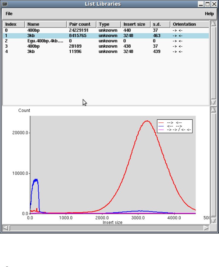
Chapter 1: Next generation assembly editing with Gap5 89
1.10 Other Miscellany
1.10.1 List Libraries
The List Libraries window is perhaps misnamed as it handles arbitrary groups of reads,
possibly due to the use of multiple libraries, multiple instrument types or simply multiple
lanes on a single instrument. For SAM/BAM files this informations comes from the @RG
header lines. For other formats Gap5 typically makes use of the input filename to group
data together.
The basic plot shows a list of library names and how frequently read pairs have been
identified as matching to the same contig. This is computed at the time of import via
tg index and so will not be updated on contig joining or breakage. The Type field indicates
the instrument platform type (for example Illumina or 454), although this is often absent
from the input BAM files.
90 The Staden Package Manual
The Insert size and standard deviation (s.d.) are derived from the sequence alignments,
with assumptions of an approximately Gaussian distribution. While not entirely accurate
this is typically sufficient for most libraries when viewed in a summary table. Finally the
Orientation field indicates the relative orientation in which most of the read-pairs have been
assembled. This will be one of “-> <-”, “<- ->” or “-> -> / <- <-” to indicate the relative
orientations of the read-pair. Whether the observed orientation is correct will depend on
the particular sequencing strategy used.
Underneath the list is a histogram of observed insert sizes for the currently selected
library. The graph is currently very rudimentary with no controls, but it will auto-scale
to fit the data. The example shown above is an Illumina large insert library showing two
distinct distributions with the smaller being where the biotin enrichment failed and short
templates were included in the library. (Note in this example the sequence orientations
have been flipped so the bulk of the data is in the orientation expected by other tools.)

Chapter 1: Next generation assembly editing with Gap5 91
1.10.2 Results Manager
Some commands within prog produce "results"that are updated automatically as data
is edited. The Result Manager provides a way to list these results, and to interact with
them.
A result is an abstract term used to define any collection of data. Typically this data can
be displayed, manipulated and is usually updated automatically when changes are made that
affect it. Each set of matches from a particular search plotted on the Contig Comparator
(see Section 2.4 [Contig Comparator], page 126) is a result, as are entire displays such as
the Template Display.
The "results"window, shown above, can be invoked either from the View menu in the
main display or from the View menu of the Contig Comparator. Each result is listed in the
window on a separate line containing the time that the result was created (which may not
be the same as when it was last updated), the name of the function that created the result,
and the result number. The number is simply a unique identifier to help distinguish two
results produced by the same function.
Each item in the list is consuming memory on your computer. Running functions over
and over again without removing the previous results will slow down your machine and it
will, eventually, run out of memory. Removing items from the list solves this.
Pressing the right mouse button over an listed item will display a popup menu of oper-
ations that can be performed on this result. The operations available will always contain
"Remove"which will delete this result and shut down any associated window, but others
listed will depend on the result selected. In the illustration above the popup menu for the
"Repeat search"can be seen. Here the operations relate to a set of repeat matches currently
being displayed in the Contig Comparator (not shown).
The Contig Comparator functions ("Find internal joins","Find read pairs","Find re-
peats","Check assembly"and "Find Sequences") are all listed in the Results Manager
once per usage of the function. It is worth remembering that the only places to completely
remove the plots from one of these functions is using the "Remove"command within the
Results Manager or to use the "Clear"button within the Contig Comparator to remove all
plots.

92 The Staden Package Manual
1.10.3 Lists
For many operations it is convenient to be able to process sets of data together - for example
to calculate a consensus sequence for a subset of the contigs. To facilitate this prog uses
lists.
Most prog commands dealing with batches of files or sets of readings or contigs can
use either files of filenames or lists. When selecting list names from within dialogues the
"browse"button will display a window containing all the currently existing lists. To select
a list simply double click on the list name. Alternatively the name may simply be typed in.
The List menu on the main menubar contains commands to Edit, Create, Delete, Copy,
Load, and Save lists. Some of these display a list editor. This is simply a scrollable text
window supporting simple editing facilities (see Section 10.2.3 [Text Windows], page 524).
The "Clear"button clears the list. The "Ok"button removes the list editor window.
It is not necessary to use "Ok"here before supplying the list name for input to another
option.
1.10.3.1 Special List Names
Some lists are automatically updated or are generated on-the-fly as needed. The lists named
"contigs"and "readings"correspond to the currently selected contigs in the contig selector
window and the currently selected readings in the template displays. Note that lists (with
any names) can also be created from selected items in the contig editor. See Section 2.6.8.18
[Set Output List], page 186. The "allcontigs"and "allreadings"lists are created as needed
and always contain an identifier for every contig and every reading identifier.
Because of the way the lists are implemented, as is outlined below, there are some useful
"tricks"that can be employed. A list name consisting of a contig identifier surrounded by
square brackets (’[’ and ’]’) will cause the creation of a list containing all of the readings
within that contig. For example, to use the Extract Readings option (see Section 2.12.7
[Extract Readings], page 273) to extract all the readings from contig ’xb54f8.s1’, the list
name given in the Extract Readings dialogue would be ’[xb54f8.s1]’.
A list name surrounded by curly brackets (’{’ and ’}’) will cause the creation of a list
containing all of the readings in the contigs named in the specified list name. So ’{contigs}’
is equivalent to all the readings in the contigs contained in the ’contigs’ list. Hence the
’allreadings’ list is identical to ’{allcontigs}’.
These tricks can be used anywhere where a list name is required except for editing and
deletion of lists. As a final example, to produce a file of filenames for the currently selected
contigs, save the list named ’{contigs}’ to a file.
1.10.3.2 Basic List Commands
The basic operations that can be performed on lists include copying, loading, saving, editing,
creation and deletion. Joining and splitting can only be performed using the list editors
and using cut and paste between windows.
The Load and Save commands require a list name and a file name. If only the name of
the file is given the list is assumed to have the same name. If it is desired to load or save

Chapter 1: Next generation assembly editing with Gap5 93
a list from/to a file of a different name then both should be specified. Creating a list that
already exists (or loading a file into an already existing list) is allowed, but will produce a
warning message.
The “Reading list” option controls whether the list to be loaded is a list of reading names
(which is normally the case). This will then turn on hyperlinking in any text views of this
list. Double-left clicking on an underlined reading name will bring up the contig editor
while right-clicking will bring up a command menu.
1.10.3.3 Contigs To Readings Command
This command produces a list or file of reading names for a single contig or for a set of
contigs. The user interface provides a dialogue to select the contigs and to select a list name
or filename.
1.10.3.4 Search Sequence Names
This command allows searching for sequences matching a prefix. The function produces both
a list in the text output window and a prog "list"of reading names. The highlighted
output is clickable, with the left mouse button invoking the contig editor and the right mouse
button displaying a popup-menu allowing additional operations (contig editor, template
display, reading notes and contig notes).
All searches are case sensitive and prefix only.
Chapter 2: Sequence assembly and finishing using Gap4 95
2 Sequence assembly and finishing using Gap4
2.1 Organisation of the gap4 Manual
The main body of the gap4 manual is divided, where possible, into sections covering related
topics. If appropriate, these sections commence with an overview of the functions they
contain. After the Introduction, the manual contains chapters on some important compo-
nents of the user interface: the Contig Selector (see Section 2.3 [Contig Selector], page 123),
the Contig Comparator (see Section 2.4 [Contig Comparator], page 126), and then, in the
chapter on Contig Overviews (see Section 2.5 [Contig Overviews], page 130) we describe the
Template Display (see Section 2.5.1 [Template Display], page 130), and its subcomponents
the Stop Codon Plot (see Section 2.5.5 [Stop Codon Map], page 156), and the Restriction
Enzyme Plot (see Section 2.5.6 [Restriction Enzyme Search], page 157).
Then there is a long chapter on the powerful Contig Editor (see Section 2.6 [Editor
introduction], page 160), followed by a chapter describing the many assembly engines and
assembly modes which gap4 can offer (see Section 2.7 [Assembly Introduction], page 205).
Gap4 contains functions to use the data in an assembly database to find the left to
right order of contigs, and to compare their consensus sequences to look for joins that
may have been missed during assembly. A "read-pair"is obtained by sequencing a DNA
template (or "insert") from both ends: we then know the relative orientations of the two
readings, and if we know the approximate template length, we know how far apart they
should be after assembly. The next chapter is on the use of read-pair data for ordering
contigs and checking assemblies and on the use of consensus comparisons for finding joins
(see Section 2.8 [Ordering and Joining Contigs], page 217).
The next chapter is on checking assemblies and removing readings (see Section 2.9
[Checking Assemblies and Removing Readings], page 235). The following chapter describes
gap4’s methods for suggesting experiments for helping to finish a sequencing project (see
Section 2.10 [Finishing Experiments], page 241). Then we describe the various consensus cal-
culation algorithms, and the options for creating consensus sequence files (see Section 2.11.5
[The Consensus Calculation], page 257). Next is the description of a set of miscellaneous
functions (see Section 2.12 [Miscellaneous functions], page 265), followed by chapters on
the Results Manager (see Section 2.13 [Results Manager], page 277), Lists (see Section 2.14
[Lists Introduction], page 278), Notes (see Section 2.15 [Notes], page 281), Configuring gap4
(see Section 2.20.1 [Options Menu], page 298), gap4 Database Files (see Section 2.16 [Gap
Database Files], page 284), Checking Databases for corruptions (see Section 2.18 [Check
Database], page 290) and Doctoring corrupted databases (see Section 2.19 [Doctor data-
base], page 293).
2.2 Introduction
Gap4 is a Genome Assembly Program. The program contains all the tools that would
be expected from an assembly program plus many unique features and a very easily used
interface. The original version was described in Bonfield,J.K., Smith,K.F. and Staden,R. A
new DNA sequence assembly program. Nucleic Acids Res. 24, 4992-4999 (1995)
96 The Staden Package Manual
Gap4 is very big and powerful. Everybody employs a subset of options and has their
favourite way of accessing and using them. Although there is a lot of it, users are encouraged
to go through the whole of the documentation once, just to discover what is possible, and
the way that best suits their own work. At the very least, the whole of this introductory
chapter should be read, as in the long run, it will save time.
This chapter serves as a cross reference point, to give an overview of the program and to
introduce some of the important ideas which it uses. The main topics that are introduced
are listed in the current section. We introduced the use of base call accuracy values for
speeding up sequencing projects (see Section 2.2.5 [The use of numerical estimates of base
calling accuracy], page 118). The ability to annotate segments of readings and the consensus
can be very convenient (see Section 2.2.7 [Annotating and masking readings and contigs],
page 121). Generally the 3’ ends of readings from sequencing instruments are of too low
a quality to be used to create reliable consensus, but they can be useful, for example, for
finding joins between contigs (see Section 2.2.6 [Use of the "hidden"poor quality data],
page 120).
One of the most powerful features of gap4 is its graphical user interface which enables
the data to be viewed and manipulated at several levels of resolution. The displays which
provide these different views are introduced, with several screenshots (see Section 2.2.3
[Introduction to the gap4 User Interface], page 101).
It is important to understand the different files used by our sequence assembly software,
and how the data is processed before it reaches gap4 (see Section 2.2.1 [Summary of the
Files used and the Preprocessing Steps], page 97).
Note that gap4 is a very flexible program, and is designed so that it can easily be
configured to suit different purposes and ways of working. For example it is easy to create
a beginners version of gap4 which has only a subset of functions. What is described in this
manual is the full version, and so is likely to contain some perhaps more esoteric options
that few people will need to use. This introductory section also contains a complete list of
the options in the gap4 main menus (see Section 2.2.4 [Gap4 Menus], page 115).
In addition to sequence assembly, gap4 can be used for managing mutation study data
and for helping to discover and check for mutations (see Section 3.1 [Introduction to Search-
ing for Mutations], page 309).
Two further useful facilities of gap4 are "Lists"and "Notes". For many operations it is
convenient to be able to process sets of data together - for example to calculate a consensus
sequence for a subset of the contigs. To facilitate this gap4 uses lists (see Section 2.14 [Lists
Introduction], page 278) A ‘Note’ (see Section 2.15 [Notes], page 281) is an arbitrary piece
of text which can be attached to any reading, any contig, or to the database in general.
Chapter 2: Sequence assembly and finishing using Gap4 97
2.2.1 Summary of the Files used and the Preprocessing Steps
Gap4 stores the data for an assembly project in a gap4 database. Before being entered into
the gap4 database the data must be passed through several preassembly steps, usually via
pregap4 (see Section 4.2 [Pregap4 introduction], page 326). These steps are outlined below.
The programs can handle data produced by a variety of sequencing instruments. They
can also handle data entered using digitisers or that has been typed in by hand. Usually
the trace files in proprietary format, such as those of ABI, are converted to SCF files (see
Section 11.1 [SCF introduction], page 533) or ZTR files. As originally put forward in Bon-
field,J.K. and Staden,R. The application of numerical estimates of base calling accuracy to
DNA sequencing projects. Nucleic Acids Research 23, 1406-1410 (1995). gap4 makes im-
portant use of basecall confidence values, (see Section 2.2.5 [The use of numerical estimates
of base calling accuracy], page 118) which are normally stored in the reading’s SCF file.
One of the first steps in the preprocessing is to copy the base calls from the trace files
to text files known as Experiment files (see Section 11.3 [Experiment files], page 552). All
the subsequent processes operate on the Experiment files. Other preassembly steps include
quality and vector clipping. Each step is performed by a specific program controlled by the
program pregap4 (see Section 4.2 [Pregap4 introduction], page 326).
Experiment file format is similar to that of EMBL sequence entries in that each record
starts with a two letter identifier, but we have invented new records specific to sequencing
experiments. One of pregap4’s tasks is to augment the Experiment files to include data
about the vectors, primers and templates used in the production of each reading, and if
necessary it can extract this information from external databases. Some of the information
is needed by pregap4 and some by gap4. (Note that in order to get the most from gap4 it is
essential to make sure that it is supplied, via the Experiment files, with all the information
it needs.)
The trace files are not altered, but are kept as archival data so that it is always possible
to check the original base calls and traces. Any changes to the data prior to assembly (and
we recommend that none are made until readings can be viewed aligned with others) are
made to the copy of the sequence in the Experiment file.
The reading data, in Experiment file format, is entered into the project database (see
Section 2.16 [Gap Database Files], page 284), usually via one of the assembly engines.
Because Experiment file format was based on EMBL file format, EMBL files can also be
entered and their feature tables will be convered to tags. There is no limit to the length of
readings which can be entered.
All the changes to the data made by gap4 are made to the copies of the data in the
project database. Once the data has been copied into the gap4 database the Experiment
files are no longer required.
Gap4 uses the trace files to display the traces (see Section 2.6.11 [Traces], page 188),
and to compare the edited bases with the original base calls (see Section 2.6.6.11 [Search by
Evidence for Edit (1)], page 176), (see Section 2.6.6.12 [Search by Evidence for Edit (2)],
page 176). However gap4 databases do not store trace files: they record only the names
of the trace files (which are copied from the readings’ Experiment files). This means that
if the trace files for a project are not in the same directory/folder as the gap4 database,

98 The Staden Package Manual
gap4 needs to be told where they are, otherwise it cannot use them. Ideally, all the trace
files for a project should be stored in one directory. To tell gap4 where they are the "Trace
file location"command in the Options menu should be used (see Section 2.20.8 [Trace File
Location], page 302).
Gap4 databases have a number of size constraints, some of which can be altered by users
and others which are fixed.
While gap4 is running it often needs to calculate a consensus. The maximum size of
this sequence is controlled by a variable "maxseq". Most routines are able to automatically
increase the value of maxseq while they are running, but some of the older functions,
including some of the original assembly engines, are not. This means that it is important
for users to set maxseq to a sufficiently high value before running these elderly routines.
By default maxseq is currently set to 100000, but users can set it on the command line or
from within the Options menu.
Gap4 databases contain one record for each reading and one for each contig. The sum of
these two sets of records is the "database size", and the maximum value that database size
is permitted to reach is "maxdb". When databases are initialised maxdb is set, by default,
to 8000. Users can alter this value on the command line or from within the Options menu
of gap4.
Gap4 databases also limit the number and names of readings so that various output
routines know how many character positions are required: the maximum number imposed
in this way is 99,999,999, and the maximum reading name length is 40.
Currently we have sites with single gap4 databases containing over 200,000 readings with
consensus sequences in excess of 7,000,000 bases.
A gap4 database can be used by several users simultaneously, but only one is allowed
to change the contents of the database, and the others are given "readonly"access. As
part of its mechanism to prevent more than one person editing a database at once gap4
uses a "BUSY"file to signify that the database is opened for writing. Before opening a
database for writing, gap4 checks to see if the BUSY file for that database exists. If it does,
the database is opened only for reading, if not it creates the file, so that any additional
attempts to open the database for writing will be blocked. When the user with write access
closes the database, the BUSY file is deleted, hence re-enabling its ability to be opened
for changes. It is worth remembering that a side effect of this mechanism, is that in the
event of a program or system crash the BUSY file will be left on the disk, even though the
database is not being used. In this case users must remove the BUSY file before using the
database (see Section 2.16 [Gap4 Database Files], page 284).
The final result from a sequencing project is a consensus sequence (see Section 2.11.5
[The Consensus Calculation], page 257) and gap4 can write these in Experiment file format,
fasta format or staden format. Of course the whole database and all the trace files are also
useful for future reference as they allow any queries about the accuracy of the sequence to
be answered.
Chapter 2: Sequence assembly and finishing using Gap4 99
2.2.2 Summary of Gap4’s Functions
The tasks which gap4 can perform can be roughly divided into assembly (see Section 2.7
[Assembly Introduction], page 205), finishing (see Section 2.10 [Finishing Experiments],
page 241), and editing (see Section 2.6 [Editor introduction], page 160). But gap4 contains
many other functions which can help to complete a sequencing project with the minimum
amount of effort, and some of these are listed below.
Readings are entered into the gap4 database using the assembly algorithms (see
Section 2.7 [Assembly Introduction], page 205). In general these algorithms will build
the largest contigs they can by finding overlaps between the readings, however some,
perhaps more doubtful, joins between contigs may be missed, and these can be discovered,
checked and made using Find Internal Joins (see Section 2.8.3 [Find Internal Joins],
page 227), Find repeats (see Section 2.8.4 [Find repeats], page 233) and Join Contigs
(see Section 2.6.15 [The Join Editor], page 196). Find Internal Joins compares the ends
of contigs to see if there are possible overlaps and then presents the overlap in the Contig
Joining Editor, from where the user can view the traces, make edits and join the contigs.
Find Repeats can be used in a similar way, but unlike Find Internal Joins it does not
require the matches it finds to continue to the ends of contigs.
Read-pair data can be used to automatically put contigs into the correct order (see
Section 2.8.1 [Ordering Contigs], page 219), and information about contigs which share
templates can be plotted out (see Section 2.8.2 [Find Read Pairs], page 222). The re-
lationships of readings and templates, within and between contigs can also be shown by
the Template Display (see Section 2.5.1 [Template Display], page 130) which has a wide
selection of display modes and uses.
Problems with the assembly can be revealed by use of Check Assembly (see Section 2.9
[Checking Assemblies], page 236), Find repeats (see Section 2.8.4 [Find repeats], page 233),
and Restriction Enzyme mapping (see Section 2.5.6 [Plotting Restriction Enzymes],
page 157). Check Assembly compares every reading with the segment of the consensus it
overlaps to see how well it aligns. Those that align poorly are plotted out in the Contig
Comparator. Find Repeats also presents its results in the Contig Comparator, so if used in
conjunction with Check Assembly, it can show cases where readings have been assembled
into the wrong copy of a repeated element. At the end of a project the Restriction Enzyme
map function can be used to compare the consensus sequence with a restriction digest of
the target sequence. Problems can also be found by use of the various Coverage Plots
available in the Consistency Display (see Section 2.5.2 [Consistency Display], page 140).
These plots will show regions of low or high reading coverage (see Section 2.5.2.2 [Reading
Coverage Histogram], page 142), places with data for only one strand (see Section 2.5.2.4
[Strand Coverage], page 144), or where there is no read-pair coverage (see Section 2.5.2.3
[Read-Pair Coverage Histogram], page 143). Errors can be corrected by Disassemble
Readings (see Section 2.9.1.2 [Disassembling Readings], page 240) and Break Contig (see
Section 2.9.1.1 [Breaking Contigs], page 239) which can remove readings from contigs or
databases or can break contigs.
The general level of completeness of the consensus sequence can be seen diagrammatically
using the Quality Plot (see Section 2.5.1.5 [Quality Plot], page 137), and the confidence
100 The Staden Package Manual
values for each base in the consensus sequence can be plotted (see Section 2.5.2.1 [Confidence
Values Graph], page 142).
The most powerful component of gap4 is its Contig Editor (see Section 2.6 [Editor
introduction], page 160). which has many display modes and search facilities to enable very
rapid discovery and fixing of base call errors.
If working on a protein coding sequence, the consensus can be analysed using the Stop
Codon Map (see Section 2.5.5 [Stop Codon Map], page 156), and its translation viewed
using the Contig Editor (see Section 2.6.8.1 [Status Line], page 180).
The final result from a sequencing project is a consensus sequence (see Section 2.11.5
[The Consensus Calculation], page 257).
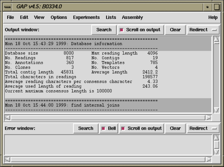
Chapter 2: Sequence assembly and finishing using Gap4 101
2.2.3 Introduction to the gap4 User Interface
Gap4 has a main window from which all the main options are selected from menus. When a
database is open it also has a Contig Selector which will transform into a Contig Comparator
whenever needed. In addition many of the gap4 functions, such as the Contig Editor or the
Template Display will create their own windows when they are activated. All the graphical
displays and the Contig Editor can be scrolled in register. The base of the graphical display
windows usually contains an Information Line for showing short textual data about results
or items touched by the mouse cursor. Gap4 is best operated using a three button mouse,
but alternative keybindings are available. Full details of the user interface are described
elsewhere (see [User Interface], page 523), and here we give an introduction based around
a series of screenshots.
The main window (shown below) contains an Output window for textual results, an Error
window for error messages, and a series of menus arranged along the top. The contents of
the two text windows can be searched, edited and saved. Each set of results is preceded by
a header containing the time and date when it was generated.
Some of the text will be underlined and shaded differently. These are hyperlinks which
perform an operation when clicked (with the left mouse button) on, typically invoking a
graphical display such as the contig editor. Clicking on these with the right mouse button
will bring up a menu of additional operations. At present only a few commands (Show
Relationships and the Search functions) produce hypertext, but if there is sufficient interest
this may be expanded on.
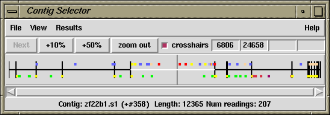
102 The Staden Package Manual
2.2.3.1 Introduction to the Contig Selector
The gap4 Contig Selector is used to display, select and reorder contigs. In the Contig
Selector all contigs are shown as colinear horizontal lines separated by short vertical lines.
The length of the horizontal lines is proportional to the length of the contigs and their
left to right order represents the current ordering of the contigs. Users can change the
contig order by dragging the lines representing the contigs. This is done by clicking and
holding the middle mouse button, or Alt left mouse button, on a line and then moving
the mouse cursor. The Contig Selector can also be used to select contigs for processing.
For example, clicking with the right mouse button on the line representing a contig will
invoke a menu containing the commands which can be performed on that contig. There
are several alternative ways of specifying which contig an operation should be performed
on. Contigs are identified by the name or number of any reading they contain. When a
dialogue is requesting a contig name, using the left mouse button to click on the contig in
the Contig Selector will transfer its name to the dialogue box. Other methods are available
(see Section 2.3.1 [Selecting Contigs], page 123).
As the mouse is moved over a contig, it is highlighted and the contig name (left most
reading name) and length are displayed in the Information Line. The number in brackets
is the contig number (actually the number of its leftmost reading). Tags or annotations
(see Section 2.2.7 [Annotating and masking readings and contigs], page 121) can also be
displayed in the Contig Selector window.
The figure shows a typical display from the Contig Selector. At the top are the File, View
and Results menus. Below that are buttons for zooming and for displaying the crosshair.
The four boxes to the right are used to display the X and Y coordinates of the crosshair. The
rightmost two display the Y coordinates when the contig selector is transformed into the
Contig Comparator. The two leftmost boxes display the X coordinates: the leftmost is the
position in the contig and the other is the position in the overall consensus. The crosshair
is the vertical line spanning the panel below. Tags are shown as coloured rectangles above
and below the lines (see Section 2.3 [Contig Selector], page 123).
Chapter 2: Sequence assembly and finishing using Gap4 103
2.2.3.2 Introduction to the Contig Comparator
Gap4 commands such as Find Internal Joins (see Section 2.8.3 [Find Internal Joins],
page 227), Find Repeats (see Section 2.8.4 [Find Repeats], page 233), Check Assembly
(see Section 2.9 [Check Assembly], page 236), and Find Read Pairs (see Section 2.8.2 [Find
Read Pairs], page 222) automatically transform the Contig Selector (see Section 2.3 [Contig
Selector], page 123) to produce the Contig Comparator. To produce this transformation a
copy of the Contig Selector is added at right angles to the original window to create a two
dimensional rectangular surface on which to display the results of comparing or checking
contigs.
Each of the functions plots its results as diagonal lines of different colours. In general, if
the plotted points are close to the main diagonal they represent results from pairs of contigs
that are in the correct relative order. Lines parallel to the main diagonal represent contigs
that are in the correct relative orientation to one another. Those perpendicular to the
main diagonal show results for which one contig would need to be reversed before the pair
could be joined. The manual contig dragging procedure can be used to change the relative
positions of contigs. See Section 2.3.2 [Changing the Contig Order], page 125. As the
contigs are dragged the plotted results will automatically be moved to their corresponding
new positions. This means that, in general, if users drag the contigs to move their plotted
results close to the main diagonal they will simultaneously be putting their contigs into the
correct relative positions.
This plot can simultaneously show the results of independent types of search, making it
easy for users to see if different analyses produce corroborating evidence for the ordering of
contigs. Indications that a reading may have been assembled in an incorrect position can
also be seen - if for example a result from Check Assembly lies on the same horizontal or
vertical projection as a result from Find Repeats, users can see the alternative position to
place the doubtful reading.
The plotted results can be used to invoke a subset of commands by the use of pop-up
menus. For example if the user clicks the right mouse button over a result from Find
Internal Joins a menu containing Invoke Join Editor (see Section 2.6.15 [The Join Editor],
page 196) and Invoke Contig Editors (see Section 2.6 [Editing in gap4], page 160) will pop
up. If the user selects Invoke Join Editor the Join Editor will be started with the two contigs
aligned at the match position contained in the result. If required one of the contigs will be
complemented to allow their alignment.

104 The Staden Package Manual
A typical display from the Contig Comparator is shown above. It includes results for
Find Internal Joins in black, Find Repeats in red, Check Assembly in green, and Find Read
Pairs in blue. Notice that there are several internal joins, read pairs and repeats close to the
main diagonal near the top left of the display. This indicates that the contigs represented in
that area are likely to be in the correct positions relative to one another. In the middle of
the bottom right quadrant there is a blue diagonal line perpendicular to the main diagonal.
This indicates a pair of contigs that are in the wrong relative orientation. The crosshairs
show the positions for a pair of contigs. The vertical line continues into the Contig Selector
part of the display, and the position represented by the horizontal line is also duplicated
there (see Section 2.4 [Contig Comparator], page 126).
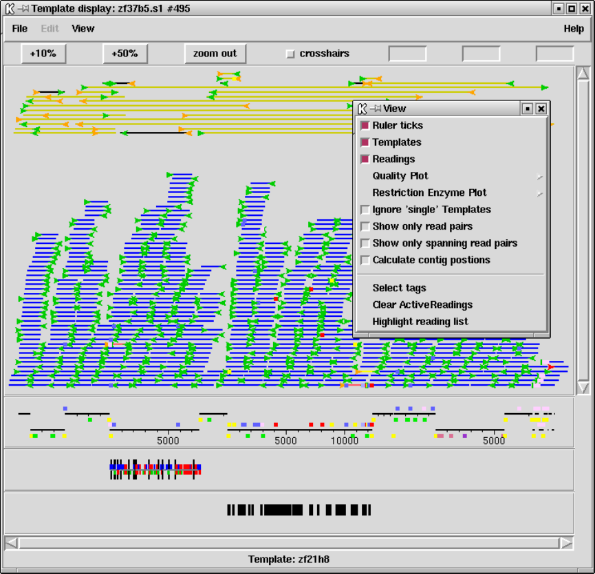
Chapter 2: Sequence assembly and finishing using Gap4 105
2.2.3.3 Introduction to the Template Display
The Template Display can show schematic plots of readings, templates, tags, restriction
enzyme sites and the consensus quality. Colour coding distinguishes reading, primer and
template types. The Template Display can also be used to reorder contigs and to invoke
the Contig Editor.
An example showing all these information types can be seen in the Figure below.
The large top section contains lines and arrows representing readings and templates.
Beneath this are rulers; one for each contig, and below those is the quality plot. The
template and reading section of the display is in two parts. The top part contains the
templates which have been sequenced from both ends but which are in some way inconsistent
- for example given the current relative positions of their readings, they may have a length
that is larger or greater than that expected, or the two readings may, as it were, face
106 The Staden Package Manual
away from one another. Colour coding is used to distinguish between different types of
inconsistency, and whether or not the inconsistency involves readings within or between
contigs. For example, most of the problems shown in the screendump above are coloured
dark yellow, indicating an inconsistency between a pair of contigs. The rest of the data,
(mostly dark blue indicating templates sequenced from only one end), is plotted below the
data for the inconsistent templates. Forward readings are light blue and reverse readings
are orange. Templates in bright yellow have been sequenced from both ends, are consistent
and span a pair of contigs (and so indicating the relative orientation and separation of the
contigs).
At the bottom is the restriction enzyme plot. The coloured blocks immediately above
and below the ruler are tags. Those above the ruler can also be seen on their corresponding
readings in the large top section. The display can be zoomed. The position of a crosshair
is shown in the two left most boxes in the top right hand corner. The leftmost shows the
distance in bases between the crosshair and the start of the contig underneath the crosshair.
The middle box shows the distance between the crosshair and the start of the first contig.
The right box shows the distance between two selected cut sites in the restriction enzyme
plots (see Section 2.5.1 [Template Display], page 130).

Chapter 2: Sequence assembly and finishing using Gap4 107
2.2.3.4 Introduction to the Consistency Display
The Consistency Display provides plots designed to highlight potential problems in contigs.
It is invoked from the main gap4 View menu by selecting any of its plots. Once a plot has
been displayed, any of the other types of consistency plot can be displayed within the same
frame from the View menu of the Consistency Display.
An example showing the Confidence Values Graph and the corresponding Reading Cov-
erage Histogram, Read-Pair Coverage Histogram and Strand Coverage is shown below.
108 The Staden Package Manual
If more than one contig is displayed, the contigs are drawn immediately after one another
but are staggered in the y direction.
The ruler ticks can be turned on or off from the View menu of the consistency dis-
play. The plots can be enlarged or reduced using the standard zooming mechanism. See
Section 10.5.1 [Zooming], page 528.
The crosshair toggle button controls whether the crosshair is visible. This is shown as a
black vertical and horizontal line. The position of the crosshair is shown in the 3 boxes to
the right of the crosshair toggle. The first box indicates the cursor position in the current
contig. The second box indicates the overall position of the cursor in the consensus. The
last box shows the y position of the crosshair. (see Section 2.5.2 [Consistency Display],
page 140).

Chapter 2: Sequence assembly and finishing using Gap4 109
2.2.3.5 Introduction to the Restriction Enzyme Map
The restriction enzyme map function finds and displays restriction sites within a specified
region of a contig. Users can select the enzyme types to search for and can save the sites
found as tags within the database.
This figure shows a typical view of the Restriction Enzyme Map in which the results for
each enzyme type have been configured by the user to be drawn in different colours. On the
left of the display the enzyme names are shown adjacent to their rows of plotted results.
If no result is found for any particular enzyme eg here APAI, the row will still be shown
so that zero cutters can be identified. Three of the enzymes types have been selected and
are shown highlighted. The results can be scrolled vertically (and horizontally if the plot is
zoomed in). A ruler is shown along the base and the current cursor position (the vertical
black line) is shown in the left hand box near the top right of the display. If the user clicks,
in turn, on two restriction sites their separation in base pairs will appear in the top right
hand box. Information about the last site touched is shown in the Information line at the
bottom of the display. At the top the edit menu is shown and can be used to create tags
for highlighted enzyme types (see Section 2.5.6 [Restriction Enzyme Search], page 157).

110 The Staden Package Manual
2.2.3.6 Introduction to the Stop Codon Map
The Stop Codon Map plots the positions of all the stop codons on one or both strands of
a contig consensus sequence. If the Contig Editor is being used on the same contig, the
Refresh button will be enabled, and if used, will fetch the current consensus from the editor,
repeat the search and replot the stop codons.
The figure shows a typical zoomed in view of the Stop Codon Map display. The positions
for the stop codons in each reading frame (here all six frames are shown) are displayed in
horizontal strips. Along the top are buttons for zooming, the crosshair toggle, a refresh
button and two boxes for showing the crosshair position. The left box shows the current
position and the right-hand box the separation of the last two stop codons selected by the
user. Below the display of stop codons is a ruler and a horizontal scrollbar. The information
line is showing the data for the last stop codon the user has touched with the cursor. Also
shown on the left is the View menu which is used to select the reading frames to display
(see Section 2.5.5 [Stop Codon Map], page 156).
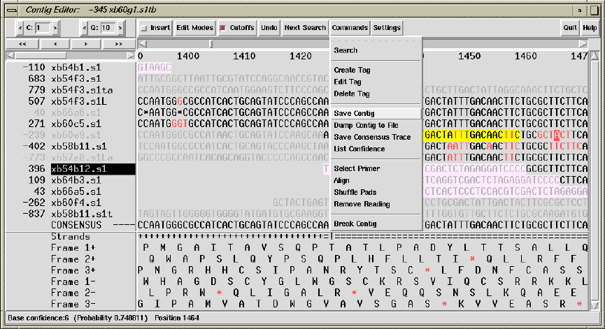
Chapter 2: Sequence assembly and finishing using Gap4 111
2.2.3.7 Introduction to the Contig Editor
The gap4 Contig Editor is designed to allow rapid checking and editing of characters in
assembled readings. Very large savings in time can be achieved by its sophisticated prob-
lem finding procedures which automatically direct the user only to the bases that require
attention. The following is a selection of screenshots to give an overview of its use.
The figure above shows a screendump from the Contig Editor which contains segments
of aligned readings, their consensus and a six phase translation. The Commands menu is
also shown. The main components are: the controls at the top; reading names on the left;
sequences to their right; and status lines at the bottom. Some of the reading names are
written in light grey which indicates that their traces/chromatograms are being displayed
(in another window, see below).
One reading name is written with inverse colours, which indicates that it has been
selected by the user. To the left of each reading name is the reading number, which is
negative for readings which have been reversed and complemented. The first of the status
lines, labelled "Strands", is showing a summary of strand coverage. The left half of the
segment of sequence being displayed is covered only by readings from one strand of the
DNA, but the right half contains data from both strands.
Along the top of the editor window is a row of command buttons and menus. The
rightmost pair of buttons provide help and exit. To their left are two menus, one of which
is currently in use. To the left of this is a button which initially displays a search dialogue,
and then pressing it again, will perform the selected search. Further left is the undo button:
each time the user clicks on this box the program reverses the previous edit command. The
next button, labelled "Cutoffs"is used to toggle between showing or hiding the reading
data that is of poor quality or is vector sequence. In this figure it has been activated,
showing the poor quality data in light grey. Within this, sequencing vector is displayed in
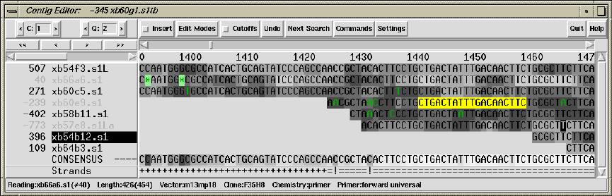
112 The Staden Package Manual
lilac. The next button to the left is the Edit Modes menu which allows users to select which
editing commands are enabled. The next command toggles between insert and replace and
so governs the effect of typing in the edit window.
One of the readings contains a yellow tag, and elsewhere some bases are coloured red,
which indicates they are of poor quality. The Information Line at the bottom of the window
can show information about readings, annotations and base calls. In this case it is showing
information about the reliability of the base beneath the editing cursor.
A better way of displaying the accuracy of bases is to shade their surroundings so that
the lighter the background the better the data. In the figure above, this grey scale encoding
of the base accuracy or confidence has been activated for bases in the readings and the con-
sensus. This screenshot also shows the Contig Editor displaying disagreements and edits.
Disagreements between the consensus and individual base calls are shown in dark green.
Notice that these disagreements are in poor quality base calls. Edits (here they are all pads)
are shown with a light green background. When they are present, replacements/insertions
are shown in pink, deletions in red and confidence value changes in purple. The consensus
confidence takes into account several factors, including individual base confidences, sequenc-
ing chemistry, and strand coverage. It can be seen that the consensus for the section covered
by data from only one strand has been calculated to be of lower confidence than the rest.
The Status Line includes two positions marked with exclamation marks (!) which means
that the sequence is covered by data from both strands, but that the consensus for each of
the two strands is different. The Information Line at the bottom of the window is showing

Chapter 2: Sequence assembly and finishing using Gap4 113
information about the reading under the cursor: its name, number, clipped length, full
length, sequencing vector and BAC clone name.
The Contig Editor can rapidly display the traces for any reading or set of readings. The
number of rows and columns of traces displayed can be set by the user. The traces scroll in
register with one another, and with the cursor in the Contig Editor. Conversely, the Contig
Editor cursor can be scrolled by the trace cursor. A typical view is shown above.
This figure is an example of the Trace Display showing three traces from readings in
the previous two Contig Editor screendumps. These are the best two traces from each
strand plus a trace from a reading which contains a disagreement with the consensus. The
program can be configured to automatically bring up this combination of traces for each
problem located by the "Next search"option. The histogram or vertical bars plotted top
down show the confidence value for each base call. The reading number, together with the
direction of the reading (+or -) and the chemistry by which it was determined, is given
at the top left of each sub window. There are three buttons (’Info’, ’Diff’, and ’Quit’)
arranged vertically with X and Y scale bars to their right. The Info button produces a
window like the one shown in the bottom right hand corner. The Diff button is mostly used
for mutation detection, and causes a pair of traces to be subtracted from one another and
the result plotted, hence revealing their differences. (see Section 2.6.11 [Traces], page 188).
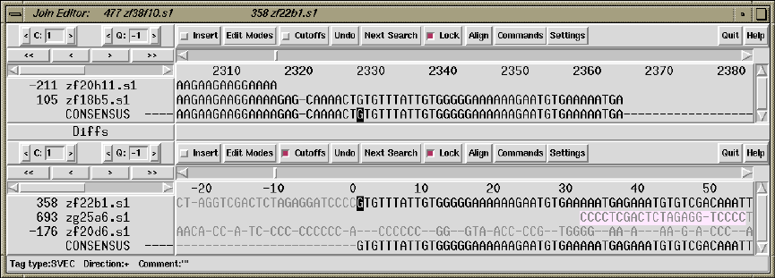
114 The Staden Package Manual
2.2.3.8 Introduction to the Contig Joining Editor
Contigs are joined interactively using the Join Editor. This is simply a pair of contig editor
displays stacked one above the other with a "differences"line in between. The Contig Join
Editor is usually invoked by clicking on a Find Internal Joins, or Find Repeats result in the
Contig Comparator. In which case the two contigs will appear with the match found by
these searches displayed.
The few differences between the Join Editor and the Contig Editor can be seen in the
figure below. Otherwise all the commands and operations are the same as those for the
Contig Editor.
In this figure the Cutoff or Hidden data is being displayed for the right hand contig. One
difference between the Contig Editor and the Join Editor is the Lock button. When set
(as it is in the illustration) the two contigs scroll in register, otherwise they can be scrolled
independently.
The Align button aligns the overlapping consensus sequences (see Section 2.6.15 [Editor
joining], page 196).
Chapter 2: Sequence assembly and finishing using Gap4 115
2.2.4 Gap4 Menus
The main window for gap4 contains File, Edit, View, Options, Experiments, Lists and
Assembly menus.
2.2.4.1 Gap4 File menu
The File menu includes database opening and copying functions and consensus calculation
options.
•Change Directory (see Section 2.16.1 [Directories], page 284)
•Check Database (see Section 2.18 [Check Database], page 290)
•New (see Section 2.16.2 [Opening a New Database], page 285)
•Open (see Section 2.16.3 [Opening an Existing Database], page 285)
•Copy Database (see Section 2.16.4 [Making Backups of Databases], page 285)
•Copy Readings (see Section 2.17.1 [Copying Readings], page 287)
•Save Consensus (see Section 2.11.5 [The Consensus Calculation], page 257)
•Extract Readings (see Section 2.12.7 [Extract Readings], page 273)
2.2.4.2 Gap4 Edit menu
The Edit menu contains options that alter the contents of the database.
•Edit Contig (see Section 2.6 [Editor introduction], page 160)
•Join Contigs (see Section 2.6.15 [Editor joining], page 196)
•Save Contig Order (see Section 2.8.1 [Order Contigs], page 219)
•Break Contig (see Section 2.9.1.1 [Break Contig], page 239)
•Complement a Contig (see Section 2.12.1 [Complement a Contig], page 265)
•Order Contigs (see Section 2.8.1 [Order Contigs], page 219)
•Quality Clip (see Section 2.12.8.2 [Quality Clipping], page 275)
•Quality Clip Ends (see Section 2.12.8.3 [Quality Clip Ends], page 275)
•Difference Clip (see Section 2.12.8.1 [Difference Clipping], page 274)
•N-Base Clip (see Section 2.12.8.4 [N-Base Clipping], page 276)
•Double Strand (see Section 2.10.1 [Double Strand], page 241)
•Disassemble Readings (see Section 2.9.1.1 [Break Contig], page 239)
•Enter Tags (see Section 2.12.2 [Enter Tags], page 265)
•Edit Notebooks (see Section 2.15 [Notes], page 281)
•Doctor Database (see Section 2.19 [Doctor database], page 293)
2.2.4.3 Gap4 View menu
The View menu contains options to look at the data at several levels of detail, and analytic
functions which present their results graphically.
•Contig Selector (see Section 2.3 [Contig Selector], page 123)
•ResultsManager (see Section 2.13 [Results Manager], page 277)
•Find Internal Joins (see Section 2.8.3 [Find Internal Joins], page 227)
116 The Staden Package Manual
•Find Read Pairs (see Section 2.8.2 [Find Read Pairs], page 222)
•Find Repeats (see Section 2.8.4 [Find repeats], page 233)
•Check Assembly (see Section 2.9 [Check Assembly], page 236)
•Sequence Search (see Section 2.12.6 [Find Oligos], page 271)
•Template Display (see Section 2.5.1 [Template Display], page 130)
•Show Relationships (see Section 2.12.4 [Show Relationships], page 267)
•Restriction Enzyme map (see Section 2.5.6 [Restriction Enzyme Search], page 157)
•Stop Codon Map (see Section 2.5.5 [Stop Codon Map], page 156)
•Quality Plot (see Section 2.5.1.5 [Quality Plot], page 137)
•List Confidence (see Section 2.11.6 [List Confidence], page 261)
•Reading Coverage Histogram (see Section 2.5.2.2 [Reading Coverage Histogram],
page 142)
•Read-Pair Coverage Histogram (see Section 2.5.2.3 [Read-Pair Coverage Histogram],
page 143)
•Strand Coverage (see Section 2.5.2.4 [Strand Coverage], page 144)
•Confidence Values Graph (see Section 2.5.2.1 [Confidence Values Graph], page 142)
2.2.4.4 Gap4 Options menu
The Options menu contains options for configuring gap4.
•Consensus Algorithm (see Section 2.20.2 [Consensus Algorithm], page 299)
•Set Maxseq (see Section 2.20.3 [Set Maxseq], page 299)
•Set Fonts (see Section 2.20.4 [Set Fonts], page 299)
•Configure Menus (see Section 2.20.5 [Configuring Menus], page 300)
•Set Genetic Code (see Section 2.20.6 [Set Genetic Code], page 300)
•Alignment Scores (see Section 2.20.7 [Alignment Scores], page 301)
•Trace File Location (see Section 2.20.8 [Trace File Location], page 302)
2.2.4.5 Gap4 Experiments menu
The Experiments menu contains options to analyse the contigs and to suggest experimental
solutions to problems.
•Suggest Long Readings (see Section 2.10.3 [Suggest Long Readings], page 245)
•Suggest Primers (see Section 2.10.2 [Suggest Primers], page 243)
•Compressions and Stops (see Section 2.10.4 [Compressions and Stops], page 247)
•Suggest Probes (see Section 2.10.5 [Suggest Probes], page 249)
2.2.4.6 Gap4 Lists menu
The Lists menu contains a set of options for creating and editing lists for use in various
parts of the program.
•Creation and Editing (see Section 2.14 [Lists Introduction], page 278)
•Contigs To Readings (see Section 2.14.3 [Contigs To Readings Command], page 279)
Chapter 2: Sequence assembly and finishing using Gap4 117
•Minimal Coverage (see Section 2.14.4 [Minimum Coverage], page 279)
•Unattached Readings (see Section 2.14.5 [Unattached Readings], page 279)
•Highlight Readings List (see Section 2.14.6 [Highlight Readings List], page 279)
•Search Sequence Names (see Section 2.14.7 [Search Sequence Names], page 279)
•Search Template Names (see Section 2.14.8 [Search Template Names], page 280)
•Search Annotation Contents (see Section 2.14.9 [Search Annotation Contents],
page 280)
2.2.4.7 Gap4 Assembly menu
The Assembly menu contains various assembly and data entry methods.
•Normal Shotgun Assembly (see Section 2.7.1 [Normal Shotgun Assembly], page 205)
•Directed Assembly (see Section 2.7.2 [Directed Assembly], page 211)
•Screen Only (see Section 2.7.3 [Assembly Screen Only], page 213)
•Assembly Independently (see Section 2.7.1.1 [Assembly Independently], page 209)
118 The Staden Package Manual
2.2.5 The use of numerical estimates of base calling accuracy
In this section we give an overview of our use, when available, of base call accuracy estimates
or confidence values. We also explain the importance of the consensus calculations used by
gap4, and their role in minimising the work needed to complete sequencing projects.
We first put forward the idea of using numerical estimates of base calling accuracy in
our paper describing SCF format Dear, S. and Staden, R, 1992. A standard file format
for data from DNA sequencing instruments. DNA Sequence 3, 107-110 and then expanded
on their use for editing and assembly in Bonfield,J.K. and Staden,R. The application of
numerical estimates of base calling accuracy to DNA sequencing projects. Nucleic Acids
Res. 23, 1406-1410 (1995).
In Bonfield and Staden (1995), we stated "...the most useful outcome of having a se-
quence reading determined by a computer-controlled instrument would be that each base
was assigned a numerical estimate of its probability of having been called correctly... having
numerical estimates of base accuracy is the key to further automation of data handling for
sequencing projects. ... The simple procedure we propose in this paper is a method of using
the numerical estimates of base calling accuracy to obviate much of the tedious and time
consuming trace checking currently performed during a sequencing project. In summary
we propose that the numerical estimates of base accuracy should be used by software to
decide if conflicts between readings require human expertise to help adjudicate. We argue
that if the accuracy estimates are reasonably reliable then the majority of conflicts can be
ignored... and so the time taken to check and edit a contig will be greatly reduced."
This has been achieved by making the consensus calculations (see Section 2.11.5 [The
Consensus Calculation], page 257) central to gap4, and by providing calculations which
make use of base call accuracy estimates to give each consensus base a quality measure.
The consensus is not stored in the gap4 database but is calculated when required by each
function that needs it, and hence always takes into account the current data. In the Contig
Editor the consensus is updated instantly to reflect any change made by the user.
In 1998 the first useable probability values became available through the program Phred
(Ewing, B. and Green, P. Base-Calling of Automated Sequencer Traces Using Phred. II.
Error Probabilities. Genome Research. Vol 8 no 3. 186-194 (1998)). Phred produces a
confidence value that defines the probability that the base call is correct. This was an
important step forward and these values are widely used and have defined a decibel type
scale for base call confidence values. Gap4 is currently set to use confidence values defined
on this scale.
The confidence value is given by the formula
C_value = -10*log10(probability of error)
A confidence value of 10 corresponds to an error rate of 1/10; 20 to 1/100; 30 to 1/1000;
and so on. Using the main gap4 consensus algorithm they enable the production of a
consensus sequence for which the expected error rate for each base is known.
As is described elsewhere (see Section 2.11.6 [List Consensus Confidence], page 261)
being able to calculate the confidence for each base in the consensus sequence makes it
possible to estimate the number of errors it contains, and hence the number of errors that
will be removed if particular bases are checked and, if necessary, edited. For example, if
Chapter 2: Sequence assembly and finishing using Gap4 119
1000 bases in the consensus had confidence 20, we would expect those 1000 bases (with an
error rate of 1/100) to contain 10 errors.
Another program which produces decibel scale confidence values for ABI 377 data is
ATQA Daniel H. Wagner, Associates, at http://www.wagner.com/.
For gap4 the confidence values are expected to lie in the range 1 to 99, with 0 and 100
having special meanings to the program.
The confidence values are stored in SCF or Experiment files and copied into gap4 data-
bases during assembly or data entry.
The searches provided by the Contig Editor (see Section 2.6.6 [Searching], page 174)
are one of gap4’s most important time saving features. The user selects a search type, for
example to find places where the confidence for the consensus falls below a given threshold,
and the search automatically moves the cursor to the next such position in the consensus.
The Contig Editor locates the next problem by applying the consensus calculation to the
contig. To edit a contig the user selects "Search"repeatedly, knowing that it will only
move to places where there is a conflict between good data or where the data is poor. Note
that the program is usually configured to automatically display the relevant traces for each
position located by the search option.
The main result is that far fewer disagreements between data are brought to the attention
of the user and fewer traces have to be inspected by eye, and so the whole process is faster.
Another consequence of the strategy is that, as fewer bases need changing to produce the
correct consensus, most of what appears on the screen will be the original base calls. Indeed
we have taken this a step further and suggest that if a base needs changing because it has
a high accuracy estimate, and is conflicting with other good data, then rather than change
the character shown on the screen, the user should lower its accuracy value. By so doing
more of the original base calls are left unchanged and hence are visible to the user. There
is a function within the contig editor to reset the accuracy value for the current base to 0.
Alternatively the accuracy value for the base that is thought to be correct can be set within
the contig editor to 100.

120 The Staden Package Manual
2.2.6 Use of the "hidden"poor quality data
In general sequences obtained from machines contain segments such as vector sequence and
poor quality data that need either to be removed or ignored during assembly and editing.
In our package we do not remove such segments but instead we mark them so that the
programs can deal with them appropriately. In gap4 such data is referred to as "hidden".
The positions to hide are determined initially by preprocessing programs such as vector clip
(see Chapter 6 [Screening Against Vector Sequences], page 401) and qclip (see Section 12.19
[qclip], page 597).
The hidden data can be revealed in the Contig Editor by toggling the Cutoffs button (see
Section 2.6.3.4 [Adjusting the Cutoff data], page 169); can be used to search for possible
joins between contigs (see Section 2.8.3 [Find Internal Joins], page 227), and can be included
in the consensus sequence (see Section 2.11.2 [Extended consensus], page 253) to be used
by external screening programs. For these cases the program can distinguish data that is
hidden because it is vector and data that is hidden because it is of poor quality: only poor
quality data is included.
The position of hidden data can be changed interactively in the Contig Editor. In
addition the Double Strand function (see Section 2.10.1 [Double stranding], page 241) will
reduce the amount of hidden data for readings that cover single stranded regions of contigs,
if the data aligns well with that on the other strand.
Chapter 2: Sequence assembly and finishing using Gap4 121
2.2.7 Annotating and masking readings and contigs
Gap4 can label segments of readings and contigs using "tags"(see Section 2.6.5 [Create
Tag], page 171). The program recognises a set of standard tags types and users can also
invent their own. Each tag type has a unique four character identifier, a name, a direction,
a colour and a text string for recording notes. Tags can be created, edited and removed
by users and by internal routines. Tags can also be input along with readings. This is
important when reference sequences are used during mutation detection (see Section 3.1.3
[Reference sequences], page 314).
2.2.7.1 Standard tag types
The standard tag types include those shown below plus the FT records from EMBL sequence
file entries. Users can also invent their own and add them to their personal GTAGDB. This is
a file that describes the available tag types and their colours (see Section 2.20.10 [Configure
the tag database], page 304).
Code Function
COMM Comment
COMP Compression
RCMP Resolved compression
STOP Stop
OLIG Oligo (primer)
REPT Repeat
ALUS Alu sequence
SVEC Sequencing vector
CVEC Cloning vector
MASK Mask me
FNSH Finished segment
ENZ0 Restriction enzyme 0
ENZ9 Restriction enzyme 9
MUTN Mutation
DIFF Sequence different to consensus
HETE Heterozygous mutation
HET+ Heterozygous mutation False +ve
HET- Heterozygous mutation False -ve
HOM+ Homozygous mutation False +ve
HOM- Homozygous mutation False -ve
FCDS FEATURE: CDS
F*** All other (60) EMBL FT record types
2.2.7.2 Active tags and masking
Tags are used for a variety of purposes and for each function in the program the user can
choose which tag types are currently "active". Where they are being used to provide visual
clues this will determine which tag types appear in the displays, but for other functions
they can be used to control which parts of the sequence are omitted from processing. This
mode of tag use is called "masking". For example the program contains a routine to search
122 The Staden Package Manual
for repeats, and if any are found, the user needs to know if such sequence duplications
are caused by incorrect assembly or are genuine repeats. Once the user has checked a
duplication reported by the program and found it to be a repeat, it can be labelled with a
REPT tag. If the repeat routine is run in masking mode and with REPT tags active, any
segment covered by a REPT tag will not be reported as a match. So once the "problem"
has been dealt with it can be labelled so it is not reported on subsequent searches. In
addition the tag is available to provide annotation for the completed sequence when it is
sent to the data libraries.
A more complicated application of masking is available for two of the other search
procedures in the program: (see Section 2.7.1 [Shotgun assembly], page 205) and (see
Section 2.8.3 [Find Internal Joins], page 227). The former is the general assembly function
and the latter is used to find potential joins between contigs in the database. Below we
describe how masking can be used during assembly and similar comments apply to Find
Internal Joins.
In the assembly function the user can choose to employ masking and then select the types
of tags to be used as masks. Readings are compared in two stages: first the program looks
for exact matches of some minimum length and then for each possible overlap it performs
an alignment. If the masking mode is selected the masked regions are not used during the
search for exact matches, but they are used during alignment. The effect of this is that
new readings that would lie entirely inside masked regions will not produce exact matches
and so will not be entered. However readings that have sufficient data outside of masked
segments can produce matches and will be correctly aligned even if they overlap the masked
data. A common use for masking during assembly or Find Internal Joins is to avoid finding
matches that are entirely contained in Alu segments.
A further mode related to masking is "marking". Marking is available for the consensus
calculation (see Section 2.11 [Consensus calculation], page 251) and for Find Internal Joins
(see Section 2.8.3 [Find Internal Joins], page 227). Instead of masking the regions covered by
active tags these routines simply write these sections of the consensus sequence in lowercase
letters. That is they make it easy for users to see where the tagged segments are. Marking
has no other effect.
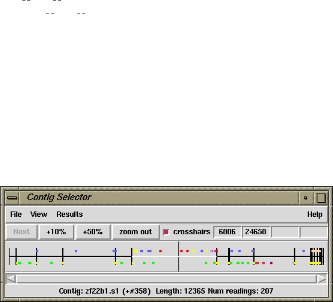
Chapter 2: Sequence assembly and finishing using Gap4 123
2.3 Contig Selector
The prog Contig Selector is used to display, select and reorder contigs. It can be invoked
from the prog View menu, but will automatically appear when a database is opened.
In the Contig Selector all contigs are shown as colinear horizontal lines separated by short
vertical lines. The length of the horizontal lines is proportional to the length of the contigs
and their left to right order represents the current ordering of the contigs. This Contig Order
is stored in the gap database and users can change it by dragging the lines representing the
contigs in the display. The Contig Selector can also be used to select contigs for processing.
Tags (see Section 2.2.7 [Annotating and masking readings and contigs], page 121) can
also be displayed in the Contig Selector window. As the mouse is moved over a contig, it
is highlighted and the contig name (left most reading name) and length are displayed in
the status line. The number in brackets is the contig number. Unlike gap4, gap5 does not
display annotations within the Contig Selector window.
The figure shows a typical display from the Contig Selector. At the top are the File, View
and Results menus. Below that are buttons for zooming and for displaying the crosshair.
The four boxes to the right are used to display the X and Y coordinates of the crosshair.
The rightmost two display the Y coordinates when the contig selector is transformed into
the contig comparator (see Section 2.4 [Contig Comparator], page 126). The two leftmost
boxes display the X coordinates: the leftmost is the position in the contig and the other is
the position in the overall consensus. The crosshair is the vertical line spanning the panel
below.
This panel shows the lines that represent the contigs and the currently active tags. Those
tags shown above the contig lines are on readings and those below are on the consensus.
Right clicking on a tag gives a menu containing “information” (to see the tag contents) and
“Edit contig at tag” which invokes the contig editor centred on the selected tag.
The information line is showing data for the contig that is currently under the crosshair.
2.3.1 Selecting Contigs
Contigs can be selected by either clicking with the left mouse button on the line representing
the required contig in the contig selector window or alternatively by choosing the "List
contigs"option from the "View"menu. This option invokes a "Contig List"list box where
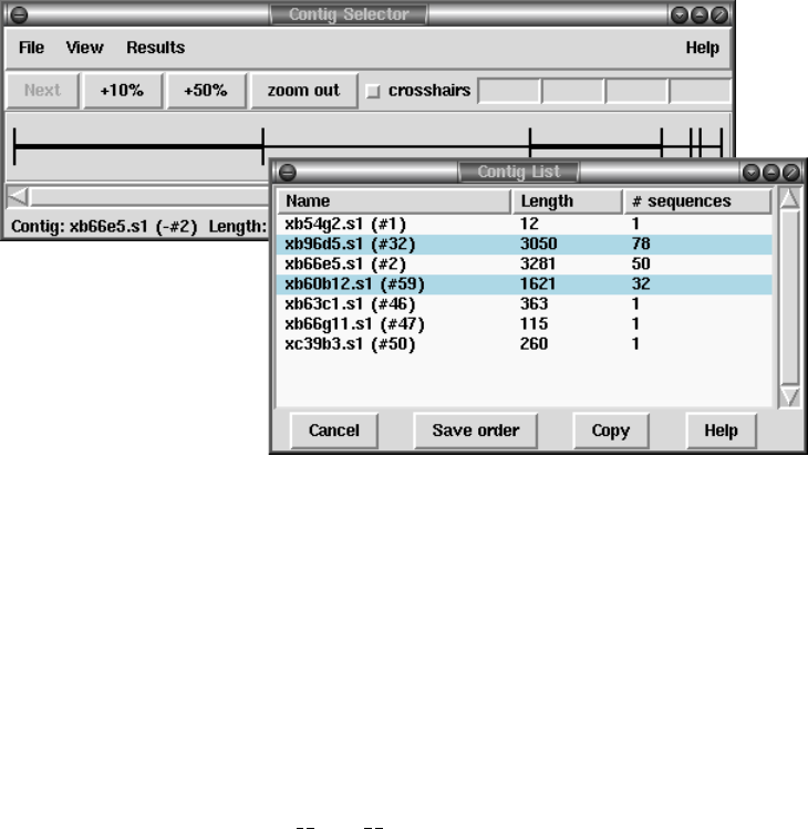
124 The Staden Package Manual
the contig names and numbers are listed in the same order as they appear in the contig
selector window.
Within this list box the contig names can be sorted alphabetically on contig name or
numerically on contig number. This is done by selecting the corresponding item from the
sort menu at the top of the list box. Clicking on a name within the list box is equivalent
to clicking on the corresponding contig in the contig selector. More than one contig can
be selected by dragging out a region with the left mouse button. Dragging the mouse off
the bottom of the list will scroll it to allow selection of a range larger than the displayed
section of the list. When the left button is pressed any existing selection is cleared. To
select several disjoint entries in the list press control and the left mouse button. The “Copy”
button copies the current selection to the paste buffer.
Most commands require a contig identifier (which can be the name or number of any
reading on the contig) and prog contains several mechanisms for obtaining this infor-
mation from users. The names or numbers can be typed or cut and pasted into dialogue
boxes (note that a reading number must be preceded by a # character, e.g. "#102"means
reading number 102 but "102"means the reading with name 102).
Also any currently active dialogue boxes that require a contig to be selected can be
updated simply by clicking on a contig in the contig selector or clicking on an entry in
the "Contig Names"list box. For example, if the Edit contig command is selected from
the Edit menu it will bring up a dialogue requesting the identity of the contig to edit. If
the user clicks the left mouse button on a contig in the contig selector window, the contig
editor dialogue will automatically change to contain the name of the selected contig. Some
commands, such as the Contig Editor, can be selected from a popup menu that is activated
by clicking the right mouse button on the contig line in the Contig Selector or clicking the
right mouse button on the corresponding name within the "Contig List"list box. This
simultaneously defines the contig to operate on and so the command starts up without
dialogue.
Chapter 2: Sequence assembly and finishing using Gap4 125
Several contigs can be selected at once by either clicking on each contig with the left
mouse button or dragging out a selection rectangle by holding the left mouse button down.
Contigs which are entirely enclosed within the rectangle will be selected. Alternatively,
selecting several contigs from the "Contig Names"list box will also result in each contig
being selected. Selected contigs are highlighted in bold. Selecting the same contig again
will unselect it.
The currently selected contigs are also kept in a ’list’ named contigs.
2.3.2 Changing the Contig Order
The order of contigs is shown by the order of the lines representing them within the Contig
Selector. The order of contigs can be changed by moving these lines using the middle
mouse button, or Alt left mouse button. Several contigs may be moved at once by selecting
several contigs using the above method. After selection, move the contigs with the middle
mouse button, or Alt left mouse button, and position the mouse cursor where you want the
selection to be moved to. Upon release of the mouse button the contigs will be shuffled to
reflect their new order. The separator line at the point the contig was moved from increases
in height.
The contig order is saved automatically whenever a contig is created or removed (eg auto
assemble), including operations like disassemble which temporarily create contigs. The order
can be saved manually using the Save Contig Order option on the File menu.
2.3.3 The Contig Selector Menus
The File menu contains only one command; "Exit". This simply quits the contig selector
display.
The View menu gives access to the Results Manager (see Section 2.13 [Results Manager],
page 277), allows contigs to be selected using a list box containing the contig names (See
Section 2.3.1 [Selecting Contigs], page 123), allows active tags (see Section 2.20.9 [TagSe-
lector], page 304) to be selected, and the list of selected contigs to be cleared.
The Results menu is updated on the fly to contain cascading menus for each of the
plots shown when the contig selector is in its 2D Contig Comparator mode (see Section 2.4
[Contig Comparator], page 126). The contents of these cascading menus are identical to
the pulldown menus available from within the Results Manager.

126 The Staden Package Manual
2.4 Contig Comparator
Prog commands such as Find Internal Joins (see Section 2.8.3 [Find Internal Joins],
page 227), Find Repeats (see Section 2.8.4 [Find Repeats], page 233), Check Assembly (see
Section 2.9 [Check Assembly], page 236), and Find Read Pairs (see Section 2.8.2 [Find
Read Pairs], page 222) automatically transform the Contig Selector (see Section 2.3 [Contig
Selector], page 123) to produce the Contig Comparator. To produce this transformation a
copy of the Contig Selector is added at right angles to the original window to create a two
dimensional rectangular surface on which to display the results of comparing or checking
contigs. Each of the functions plots its results as diagonal lines of different colours. If the
plotted points are close to the main diagonal they represent results from pairs of contigs
that are in the correct relative order. Lines parallel to the main diagonal represent contigs
that are in the correct relative orientation to one another. Those perpendicular to the
main diagonal show results for which one contig would need to be reversed before the pair
could be joined. The manual contig dragging procedure can be used to change the relative
positions of contigs. See Section 2.3.2 [Changing the Contig Order], page 125. As the
contigs are dragged the plotted results will be automatically moved to their corresponding
new positions. This means that if users drag the contigs to move their plotted results
close to the main diagonal they will be simultaneously putting their contigs into the correct
relative positions.
Because this plot can simultaneously show the results of independent types of search,
users can see if different analyses produce corroborating evidence for the ordering of contigs.
Also, if for example, a result from Check Assembly lies on the same horizontal or vertical
projection as a result from Find Repeats, users can see the alternative position to place the
doubtful reading. Ie this is an indication that a reading may have been assembled in an
incorrect position.
By use of popup menus the plotted results can be used to invoke a subset of commands.
For example if the user clicks the right mouse button over a result from Find Internal Joins
a menu containing Invoke Join Editor (see Section 2.6.15 [The Join Editor], page 196) and
Invoke Contig Editors (see Section 2.6 [Editing in prog ], page 160) will pop up. If
the user selects Invoke Join Editor the Join Editor will be started with the two contigs
aligned at the match position contained in the result. If required one of the contigs will be
complemented to allow their alignment.
A typical display from the Contig Comparator is shown below. It includes results for
Find Internal Joins in black, Find Repeats in red, Check Assembly in green, and Find
Read Pairs in blue. Notice that there are several Find Internal Joins, Find Read Pairs and
Find Repeats results close to the main diagonal near the top left of the display, indicating
that the contigs represented in that area are likely to be in the correct relative positions
to one another. In the middle of the bottom right quadrant there is a blue diagonal line
perpendicular to the main diagonal which indicates a pair of contigs that are in the wrong
relative orientation. The crosshairs show the positions for a pair of contigs. The vertical
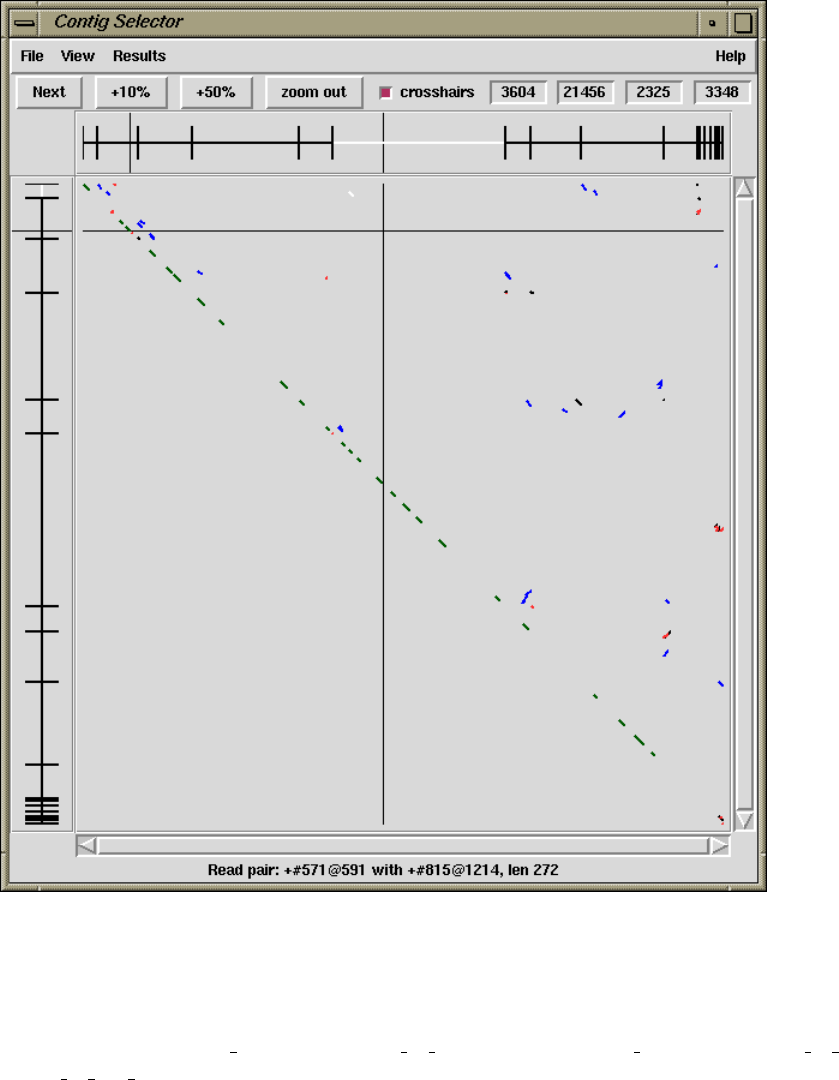
Chapter 2: Sequence assembly and finishing using Gap4 127
line continues into the Contig Selector part of the display, and the position represented by
the horizontal line is also duplicated there.
2.4.1 Examining Results and Using Them to Select Commands
Moving the cursor over plotted results highlights them, and the information line gives a
brief description of the currently highlighted match. This is in the form:
match name:contig1 number@position in contig1, with contig2 number@position in contig2,
length of the match
For Find Internal Joins the percentage mismatch is also displayed.
128 The Staden Package Manual
Several operations can be performed on each match. Pressing the right mouse button
over a match invokes a popup menu. This menu will contain a set of options which depends
on the type of result to which the match corresponds. The following is a complete list, but
not all will appear for each type of result.
Information
Sends a textual description of the match to the Output Window.
Hide Removes the match from the Contig Comparator. The match can be revealed
again by using "Reveal all"within the Results Manager.
Invoke contig editors
Invoke join editors
Invoke template display
When invoked these options bring up their respective displays to show the
match in greater detail.
Remove Removes the match from the Contig Comparator. The match cannot be re-
vealed again by using "Reveal all"within the Results Manager.
One of the items in the popup menu may have an asterisk next to it. This is the default
operation which can also be performed by double clicking the left mouse button on the
match. For Repeat or Find Internal Joins matches this will normally be the Join Editor,
or two Contig Editors when the match is between two points in the same contig. For Read
Pairs two Template Displays are shown.
The crosshairs can be toggled on and off and a diagonal line going from top left to bottom
right of the plot can also be displayed if required. This is useful as a guide for moving the
contigs such that their matches lie upon the diagonal line.
The "Results"menu on the contig selector window provides a similar mechanism of
accessing results, but at the level of all matches in a particular search. This is simply a
menu driven interface to the Results Manager window (see Section 2.13 [Results Manager],
page 277), but containing only the results relevant to the contig comparator window.
2.4.2 Automatic Match Navigation
The "Next"button of the contig comparator window automatically invokes the default
operation on the next match from the current active result. This provides a mechanism to
step through each match in turn ensuring that no matches have been missed.
With a single result (set of matches) plotted, the "Next"button simply steps through
each match in turn until all have been seen. Moving the mouse above the "Next"button,
without pressing it, highlights the next match and displays brief information about it in
the status line at the bottom of the window. To step through the matches in "best first"
order, select the "Sort Matches"option from the relevant name in the Results menu. The
exact order is dependent on the result in question, but is generally arranged to be the most
interesting ones first. For example, Find Internal Joins shows the lowest mismatch first
whilst Check Assembly shows the highest mismatches first.
Bringing up another result now directs "Next"to step through each of the new matches.
To change the result that "Next"operates on, use the Result menu to select the "Use for
Chapter 2: Sequence assembly and finishing using Gap4 129
’Next’"option in the desired result. Alternatively, double clicking on a match also causes
"Next"to process the list starting from the selected result.
The "Next"scheme remembers any matches that have been previously examined ei-
ther by itself or by manually double clicking, and will skip these. To clear this ’visited’
information select "Reset ’Next’"in the Results Manager.
130 The Staden Package Manual
2.5 Contig Overviews
Gap4 provides views of the data for an assembly project at 3 levels of resolution: the whole
project can be seen from the Contig Selector (see Section 2.3 [Contig Selector], page 123),
the most detail from the Contig Editor (see Section 2.6 [Editing in gap4], page 160), and
the Contig Overview Displays, described in this section, provide an intermediate level of
information and data manipulation. They are available from the main gap4 View menu.
These middle level resolution displays provide graphical overviews of individual contigs
or sets of contigs. The possible information shown includes readings, templates, tags, re-
striction enzyme sites, stop codons, plots of the consensus quality, read coverage, read-pair
coverage, strand coverage and consensus confidence. The displays of readings, templates,
tags, restriction enzyme sites and plots of the consensus quality can be shown in a single
window called the Template Display (see Section 2.5.1 [Template Display], page 130). The
plots of reading coverage, read-pair coverage, strand coverage and consensus confidence can
be shown in a single display called the Consistency Display (see Section 2.5.2 [Consistency
Display], page 140), or as separate plots. The Stop Codon Plot (see Section 2.5.5 [Plotting
Stop Codons], page 156) and a more informative version of the Restriction Enzyme Plot (see
Section 2.5.6 [Plotting Restriction Enzymes], page 157) can be shown in separate windows.
2.5.1 Template Display
The Template Display can show schematic plots of readings, templates, tags, restriction
enzyme sites and the consensus quality. It can be used to reorder contigs, create tags and
invoke the Contig Editor. It is invoked from the main gap4 View menu.

Chapter 2: Sequence assembly and finishing using Gap4 131
An example showing all these information types can be seen in the Figure below.
The large top section contains lines and arrows representing readings and templates.
Beneath this are rulers; one for each contig, and below those is the quality plot. The
template and reading section of the display is in two parts. The top part contains the
templates which have been sequenced from both ends but which are in some way inconsistent
- for example given the current relative positions of their readings, they may have a length
that is larger or greater than that expected, or the two readings may, as it were, face
away from one another. Colour coding is used to distinguish between different types of
inconsistency, and whether or not the inconsistency involves readings within or between
contigs. For example, most of the problems shown in the screendump above are coloured
dark yellow, indicating an inconsistency between a pair of contigs. The rest of the data,
(mostly dark blue indicating templates sequenced from only one end), is plotted below the
data for the inconsistent templates. Forward readings are blue and reverse readings are
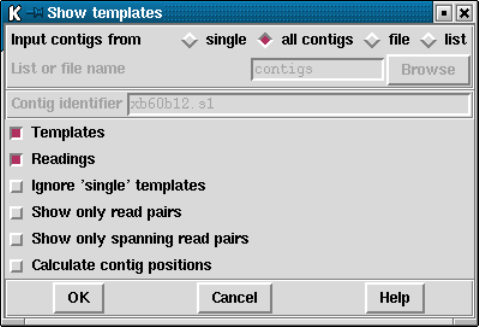
132 The Staden Package Manual
orange. Templates in bright yellow have been sequenced from both ends, are consistent
and span a pair of contigs (and so indicate the relative orientation and separation of the
contigs).
The coloured blocks immediately above and below the ruler are tags. Those above the
ruler can also be seen on their corresponding readings in the large top section. Zooming is
available. The position of a crosshair is shown in the two left most boxes in the top right
hand corner. The leftmost shows the distance in bases between the crosshair and the start
of the contig underneath the crosshair. The middle box shows the distance between the
crosshair and the start of the first contig. The right box shows the distance between two
selected cut sites in the restriction enzyme plots.
As seen in the dialogue above, users can choose to display a single contig, all contigs, or
a subset of contigs from a file of filenames ("file") or a list ("list"). If either the file or list
options are chosen, the "browse"button will be activated and can be used to call up a file
or list browser dialogue.
The items to be shown in the initial template display can be selected from the list of
checkboxes. The default is to display all templates and readings. However, it is possible to
display only templates with more than one reading ("Ignore ’single’ templates) or templates
with both forward and reverse readings ("Show only read pairs"). These latter two options
may be beneficial if the database is very large.
In the section below we give details about the individual components of the overall
Template Display.
2.5.1.1 Reading and Template Plot
The Reading and Template Plot shows templates and readings. The following sections
describe the display, its options, and the operations which it can be used to perform. It is
invoked from the main gap4 View menu.
2.5.1.2 Reading and Template Plot Display
The Reading and Template Plot shows templates and readings. Colour is used to provide
additional information. The reading colour is used to convey the primer information. The
default colours are:

Chapter 2: Sequence assembly and finishing using Gap4 133
red primer unknown
green forwards primer
orange reverse primer
dark cyan custom forward primer
orange-red
custom reverse primer
Colour is used to distinguish the number and the location of the readings derived from
each template. Templates with readings derived from only one end are drawn in blue. Those
with readings from both ends are pink when both ends are contained within the same contig.
Those with readings from both ends are green when the readings are in different contigs
and one of the contigs is not being plotted.
For each template gap4 stores an expected length, as a range between two values. From
an assembly it is often possible to work out the actual length of a template based upon the
positions within a contig of readings sequenced using the forward and reverse primers. The
forward and reverse readings on a single template (called a read pair) are considered to be
inconsistent if this observed distance is outside of the range of acceptable sizes and then
the template is drawn in black. Alternatively it may be possible that both forward and
reverse readings are assembled on the same strand (in which case both arrows will point in
the same direction). This too is a problem and hence the templates are drawn in black.
If more than one contig is displayed then the distance between adjacent contigs is de-
termined from any read pair information. If there are spanning templates between two
adjacent contigs and the readings on that template are consistent, i.e. are in the correct
orientation, the template is coloured yellow. Templates which span non-adjacent contigs in
the display or contain inconsistent readings are coloured dark yellow.
A summary of the default template colours follows.
blue the template contains only readings from one end
pink the template contains both forward and reverse readings in the same contig
green the template contains both forward and reverse readings, but they are in sepa-
rate contigs, and one of the contigs is not being displayed.
black the readings on the template are within the same contig but are in contradictory
orientations or are an unexpected distance apart
yellow the readings on the template are within different contigs (both of which are
being displayed) and are consistent
dark yellow
the readings on the template are within different contigs (both of which are
being displayed) and are inconsistent
If more than one contig is displayed, the contigs are positioned in the same left to right
order as the input contig list, (which need not necessarily be in the same order as the
contig selector). Overlapping contigs are drawn as staggered lines. If the user selects the
134 The Staden Package Manual
"Calculate contig positions"option from the menu the horizontal distance between adjacent
contigs is determined from any available read pair information. Otherwise, or in the absence
of any read pair information, the second contig is positioned immediately following the first
contig, but will be drawn staggered in the vertical direction. If the readings on a template
spanning two contigs are consistent, the distance between the contigs is determined using the
template’s mean length. If there are several templates spanning a pair of contigs an average
distance is calculated and used as the final offset between the contigs. Templates which
span non-adjacent contigs or contain inconsistent readings are not used in the calculation
of the contig offsets. It is possible that data in the database is inconsistent to such an
extent that, although spanning templates have consistent readings, the averaging can lead
to a display which shows the templates to have inconsistent readings, eg the readings are
pointing in opposite directions.
A summary of the templates and readings used to calculate the distance between two
contigs is displayed in the output window. An example is given below:
============================================================
Wed 02 Apr 10:35:51 1997: template display
------------------------------------------------------------
Contig zf98g12.r1(651) and Contig zf23d2.s1(348)
Template zf22h7( 376) length 1893
Reading zf22h7.r1( +10R), pos 6257 +208, contig 651
Reading zf22h7.s1( -376F), pos 145 +331, contig 348
Template zf49f5( 536) length 1510
Reading zf49f5.r1( +255R), pos 6562 +239, contig 651
Reading zf49f5.s1( -536F), pos 227 +135, contig 348
Gap between contigs = -11
Offset of contig 348 from the beginning = 7674
The contig names and numbers are given in the top line. Below this, the spanning
template name, number and length is displayed. Below this the reading name, whether the
reading has been complemented (+: original -: complemented), number, primer information,
starting position, length and contig number. This is of similar format to that displayed by
the read pairs output. See Section 2.8.2.2 [Find Read Pairs], page 224. The average gap
between the contigs is given and finally the distance in bases between the start of the second
contig and the start of the left most contig in the display.
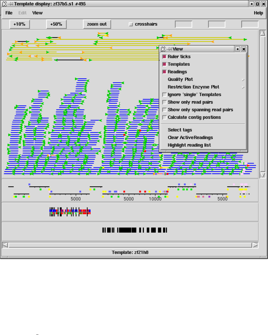
Chapter 2: Sequence assembly and finishing using Gap4 135
2.5.1.3 Reading and Template Plot Options
Within the figure shown above the contents of the View menu are visible. The "Tem-
plates","Readings","Quality Plot"and "Restriction Enzyme Plot"commands control
which attributes are displayed. The graphics are always scaled to fit the information within
the window size, subject to the current zoom level. This means that turning off templates,
but leaving readings displayed, will improve visibility of the reading information.
The "Ruler ticks"checkbox determines whether to draw numerical ticks on the contigs.
The number of ticks is defined in the .gaprc (see Section 2.20.1 [Options Menu], page 298)
file as NUM TICKS although the actual number of ticks per contig that will be displayed
also depends on the space available on the screen.
The "ignore ’single’ templates"toggle controls whether to display all templates or only
those containing more than one reading. The "show only read pairs"toggle controls whether
136 The Staden Package Manual
all templates or only those containing both forward and reverse readings are displayed.
Hence when set the templates displayed are those with a known (observed) length. The
"Show only spanning read pairs"toggle controls whether to display all templates or only
those containing forward and reverse readings which are in different contigs.
The plot can be enlarged or reduced using the standard zooming mechanism. See
Section 10.5.1 [Zooming], page 528.
The crosshair toggle button controls whether the cursor is visible. This is shown as a
black vertical line. The position of the crosshair is displayed in the two boxes to the right
of the crosshair toggle. The first box indicates the cursor position in the current contig.
The second box indicates the overall position of the cursor in the consensus. The third
box is used to show the distance between restriction enzyme cut sites. See Section 2.5.1.6
[Restriction Enzyme Plot], page 139.
Tags that are on the consensus can only be seen on the ruler. These are marked beneath
the ruler line. Tags on readings can be seen both on the ruler (above the line) and on
their appropriate readings within the template window. To configure the tag types that
are shown use the "select Tags"command in the View menu. This brings up the usual tag
selection dialog box. See Section 2.20.9 [Tag Selector], page 304.
2.5.1.4 Reading and Template Plot Operations
The contig editor can be invoked by double clicking the middle mouse button, or Alt the left
mouse button, in any of the displays, ie template, ruler, quality or restriction enzyme plots.
The editor will start up with the editing cursor on the base that corresponds to the position
clicked on in the Template Display. If more than one contig is currently being displayed
the editor decides which contig to show using the following rules. If the user clicks on the
Quality Plot, the contig lines or the Restriction Enzyme Display, the corresponding contigs
will be shown. If the user clicks on a gap between these displays the nearest contig will be
selected. If the user clicks on the template or reading lines, the editor will show the contig
whose left end is to the left of and closest to the cursor.
The long blue vertical line seen in the previous figure is the position of the editing cursor
within a Contig Editor. Each editor will produce its own cursor and each will be visible.
Moving the editing cursor within a contig editor automatically moves its cursor within the
Template Display. Similarly, clicking and dragging the editor cursor with the middle mouse
button, or Alt left mouse button, within the Template Display scrolls the associated Contig
Editor.
The order of the contigs can be changed within the Template Display by clicking with
the middle mouse button, or Alt left mouse button, on a contig line and dragging the line to
the new position. The Template Display will update automatically once the mouse button
is released. The change of a dark yellow template to bright yellow is indicative that the two
contigs are now in consistent positions and orientations. The order of the contigs in the
gap4 database, as displayed in the contig selector, can be updated by selecting the "Update
contig order"command in the Edit menu.
By clicking on any of the contig lines in the ruler a popup menu is invoked. From this,
information on the contig can be obtained, the contig editor can be started, the contig

Chapter 2: Sequence assembly and finishing using Gap4 137
can be complemented, and the templates within the contig can be highlighted (shown by
changing their line width).
A list named readings always exists. It contains the list of readings that are highlighted
in all the currently shown template displays. See Section 2.14 [Lists], page 278. The
highlighting mechanism used is to draw the readings as thicker, bolder, lines. The "clear
Active Readings"command from the View menu clears this list. The "highlight reading
list"command loads a new set of readings to use for the "readings"list and then highlights
these.
To interactively add and remove readings from the active list use the left mouse button.
Clicking on an individual reading will toggle its state from active to non active and back
again. Pressing and holding the left mouse button, and moving the mouse, will drag out a
bounding box. When the button is released all readings that are contained entirely within
the bounding box will be toggled.
Activating a reading (using any of the above methods) when an editor is running, will
also highlight the reading within the editor. Similarly, highlighting the reading in the editor
activates it within the template display and adds it to the active reading list.
2.5.1.5 Quality Plot
This option can be invoked from the main gap4 View menu, in which case it appears as a
single plot, or from the View menu of the Template Display, in which case it will appear as
part of the Template Display.
This display provides an overview of the quality of the consensus. The Contig Editor
can be used to examine the problems revealed. A typical plot is displayed below.
For each base in the consensus a quality is computed based on the accuracy of the data
on each strand. As can be seen in the Figure above, this information is then plotted using
colour and height to distinguish between the different quality assignments. The colour and
height codes are explained below.
138 The Staden Package Manual
Colour Height Meaning
grey 0 to 0 OK on both strands, both agree
blue 0 to 1 OK on plus strand only
green -1 to 0 OK on minus strand only
red -1 to 1 Bad on both strands
black -2 to 2 OK on both strands but they disagree
For example, in the figure we see that the first four hundred or so bases are mostly only
well determined on the forward strand.
Note that when a large number of bases are being displayed the limited screen resolution
causes the quality codes for adjacent bases to be drawn as single pixels. However the use of
varying heights ensures that all problematic bases will be visible. Hence when the quality
plot consists of a single grey line all known quality problems have been resolved, at the
current consensus and quality cutoffs.
To check problems the contig editor can be invoked by double clicking on the middle
mouse button, or Alt left mouse button. It will appear centred on the base corresponding
to the position on which the mouse was clicked.
The quality plot appears as "Calculate quality"in the Results Manager window (see
Section 2.13 [Results Manager], page 277).
Within the Results Manager commands available, using the right mouse button, include
"Information", which lists a summary of the distribution of quality types to the output
window, and "List"which lists the actual quality values for each base to the output window.
These quality values are written in a textual form of single letters per base and are listed
below.
+Strand -Strand
aGood Good (in agreement)
bGood Bad
cBad Good
dGood None
eNone Good
fBad Bad
gBad None
hNone Bad
iGood Good (disagree)
jNone None
An example of the output using "Information"and "List"follows.
============================================================
Wed 02 Apr 12:14:06 1997: quality summary
Chapter 2: Sequence assembly and finishing using Gap4 139
------------------------------------------------------------
Contig xb56b6.s1 (#11)
81.00 OK on both strands and they agree(a)
3.94 OK on plus strand only(b,d)
11.98 OK on minus strand only(c,e)
1.85 Bad on both strands(f,g,h,j)
1.22 OK on both strands but they disagree(i)
============================================================
Wed 02 Apr 12:14:09 1997: quality listing
------------------------------------------------------------
Contig xb56b6.s1 (#11)
10 20 30 40 50 60
eeeeeeeeee eeeeeeeeee eeeeeeeeee eeeeeeehee eeeeeeeeee eeeeeeeeee
70 80 90 100 110 120
eeeeeeeeee eeeeeeeeee eeeeeeeeee eeeeeeeeee eeeeeeeeee eeeeeeeeee
130 140 150 160 170 180
eeeeeeeeee eeeeeeeeee eeeeeeeeee eeeeeeeeee eeeeeeeeee eeeeeeeeee
190 200 210 220 230 240
eeeeeeeeee eeeeeeeeee heeeeeeeee eeeeeeeici iiaiaciiia aaaaaaaaac
250 260 270 280 290 300
aaaacaaaaa aaaaaaaiia aaaaaaaaaa aaaaaaaaaa aaaabaaaaa aaaaaaaaaa
310 320 330 340 350 360
aaaaaaaaaa aaaaaaaaaa aaaaaaaaaa aaaaaaaaaa aaaaaaaaaa faaaaaaaaa
[ output removed for brevity ]
2.5.1.6 Restriction Enzyme Plot
The restriction enzyme plot within the template display is a reduced version of the main
Restriction Enzyme Map function. The dialogue used for choosing the restriction enzymes
is identical and is described with the main function. See Section 2.5.6 [Plotting Restriction
Enzymes], page 157. It is invoked from the Template Display View menu. An example plot
from the template display can be seen below.
140 The Staden Package Manual
Here we see the searches for two restriction enzymes. Each vertical line is drawn at the
cut position of the matched restriction site. Unlike the main restriction enzyme plot here
all matches are plotted on a single horizontal plot. Initially all sites are drawn in black.
To distinguish one site from another either touch the site with the mouse cursor and read
the template display information line, or place the mouse cursor above a site and press the
right mouse button. This pops up a menu containing "Information"and "Configure". The
"Configure"option can be used to change the colour of all matches found for this enzyme.
In the figure above we have changed the initial colours for both of the restriction enzymes
searched for. The "Information"command displays information for all sites found in the
text output window.
As with the main Restriction Enzyme Map function, clicking the left mouse button on
two restriction sites in turn displays the distance between the chosen sites in the information
line. This figure is also displayed in the box at the top right hand corner of the template
display.
2.5.2 Consistency Display
The Consistency Display provides plots designed to highlight potential problems in contigs.
It is invoked from the main gap4 View menu by selecting any of its plots. Once a plot has
been displayed, any of the other types of consistency plot can be displayed within the same
frame from the View menu of the Consistency Display.
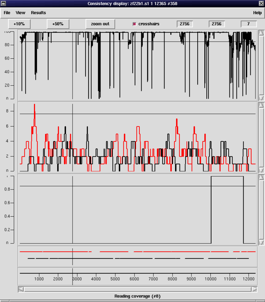
Chapter 2: Sequence assembly and finishing using Gap4 141
An example showing the Confidence Values Graph and the corresponding Reading Cov-
erage Histogram, Read-Pair Coverage Histogram and Strand Coverage is shown below.
One or more contigs can be displayed and are drawn in the same order at the input
contig list (which need not necessarily be in the same order as the contig selector). If more
than one contig is displayed, the contigs are drawn immediately after one another but are
staggered in the y direction.
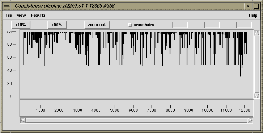
142 The Staden Package Manual
The ruler ticks can be turned on or off from the View menu of the consistency display.
The plots can be enlarged or reduced using the standard zooming mechanism. See
Section 10.5.1 [Zooming], page 528.
The crosshair toggle button controls whether the crosshair is visible. This is shown as a
black vertical and horizontal line. The position of the crosshair is shown in the 3 boxes to
the right of the crosshair toggle. The first box indicates the cursor position in the current
contig. The second box indicates the overall position of the cursor in the consensus. The
last box shows the y position of the crosshair.
2.5.2.1 Confidence Values Graph
This option can be invoked from the main gap4 View menu, in which case it appears as a
single plot, or from the View menu of the Consistency Display in which case it appear part
of the Consistency Display.
The confidence values are determined from the current consensus algorithm (see
Section 2.11.5 [The Consensus Algorithms], page 257).
Please note that this plot can be very slow for long contigs. This is caused by the large
number of points (not the calculation) and we hope to speed it up in a future release.
2.5.2.2 Reading Coverage Histogram
This option can be invoked from the main gap4 View menu, in which case it appears as a
single plot, or from the View menu of the Consistency Display in which case it will appear
as part of the Consistency Display.
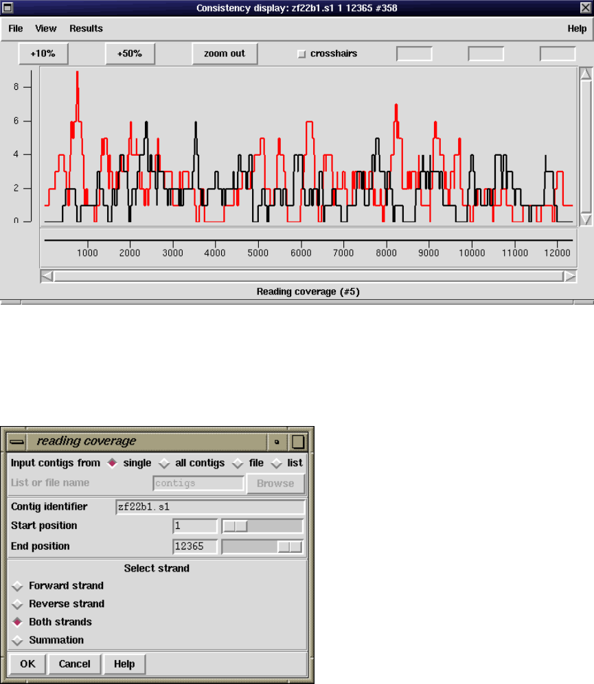
Chapter 2: Sequence assembly and finishing using Gap4 143
The number of readings which cover each base position along the contig are plotted as
a histogram.
As can be seen in the dialogue below, the user can select the contigs(s) to display, and
whether to plot: Forward strand only, Reverse strand only, Both strands or the Summation
of both strands. In the example shown above both strands have been plotted: forward in
red and reverse in black.
2.5.2.3 Read-Pair Coverage Histogram
This option can be invoked from the main gap4 View menu, in which case it appears as a
single plot, or from the View menu of the Consistency Display in which case it will appear
as part of the Consistency Display.
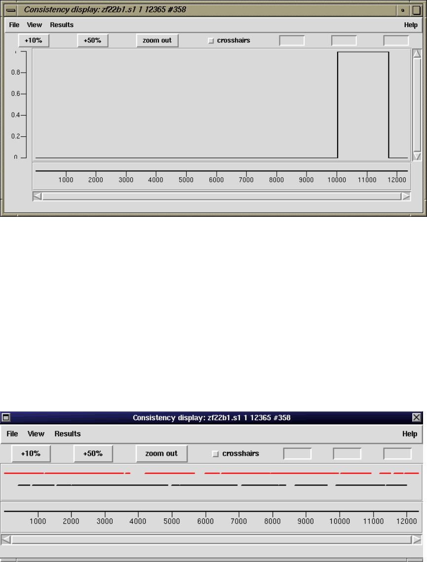
144 The Staden Package Manual
The number of read-pairs which cover each base position along the contig are plotted as
a histogram.
2.5.2.4 Strand Coverage
This option can be invoked from the main gap4 View menu, in which case it appears as a
single plot, or from the View menu of the Consistency Display in which case it will appear
as part of the Consistency Display.
The display is used to show which regions of the data are covered by readings from each
of the two strands of the DNA. A separate line is drawn for each strand: forward in red and
reverse in black. The function works in two complementary modes: it can plot the positions
which are covered, or the positions which are not. The latter is probably the most useful
as it directs users to the places requiring further data.
The figure below shows the covered positions, and the figure below that shows the
uncovered positions for the same contig.
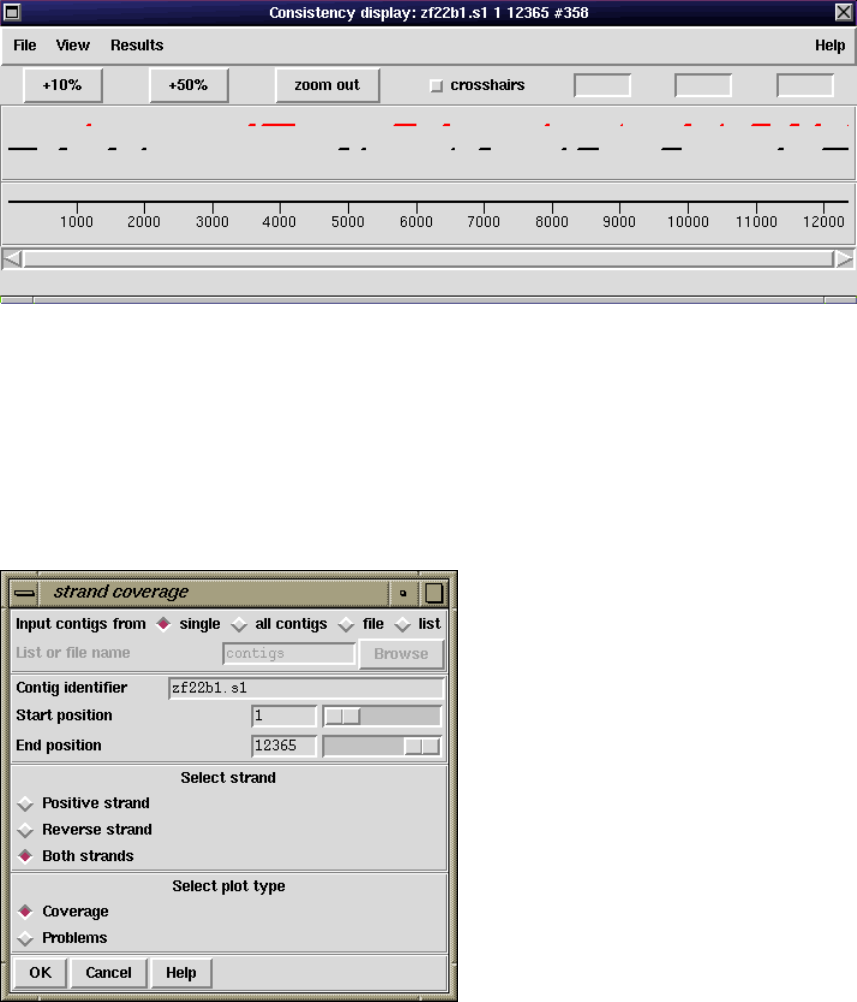
Chapter 2: Sequence assembly and finishing using Gap4 145
The plot can be regarded as a coarse version of the Quality Plot (see Section 2.5.1.5
[Quality Plot], page 137), in that it shows the strand coverage using the Quality Calculation
(see Section 2.11.5.4 [The Quality Calculation], page 261), but does not reveal problems with
individual base positions.
The dialogue allows user to select the contig(s) and strands to analyse and whether to
plot Coverage or Problems.
2.5.2.5 2nd-Highest Confidence
The traditional way to compute the consensus confidence values is to take into account
both the matching and mismatching bases within each individual column. If instead we
work on the hypothesis that a contig may have more than one sequence present then we
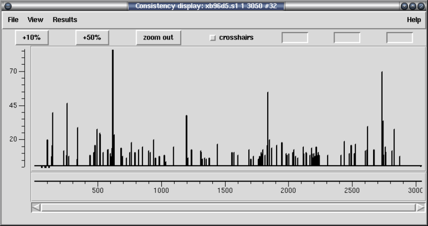
146 The Staden Package Manual
can instead compute five consensus confidence values at every point (four bases plus pad)
by only totally up the bases that agree and ignoring those that mismatch.
In the case of zero conflicts the highest confidence value will be the same as the standard
consensus confidence. When a conflict occurs, the second highest confidence value can be
used as a measure of how strong the conflict could be. It is this value is plotted.
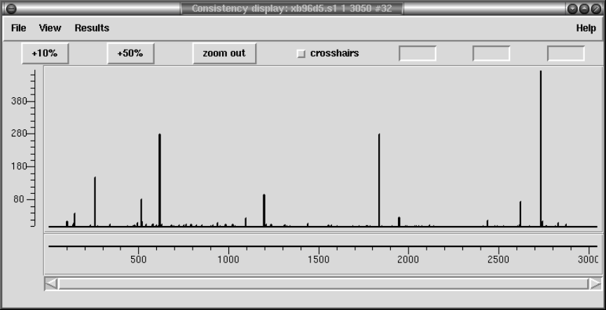
Chapter 2: Sequence assembly and finishing using Gap4 147
2.5.2.6 Diploid Graph
At present this is a rather specialist function written for a particular in-house purpose. This
plot relates very closely to the 2nd-Highest Confidence plot (see Section 2.5.2.5 [2nd-Highest
Confidence], page 145), but it also takes into account depth information.
Specifically as assumption is made that a contig may consist of two alleles with approx-
imately 50/50 ratio. Any discrepancies visible by looking at the second highest confidence
value should therefore also be backed up by a 50/50 split in sequence depth.
2.5.3 SNP Candidates
The 2nd-Highest Confidence (see Section 2.5.2.5 [2nd-Highest Confidence], page 145) and
the Diploid Graph (see Section 2.5.2.6 [Diploid Graph], page 147 both plot indicators of
how likely an alignment column is to be made up of 2 or more sequence populations.
By studying these in further detail we should be able to spot correlated differences and
to start assigning haplotypes. The SNP Candidate plot initially brings up a dialogue asking
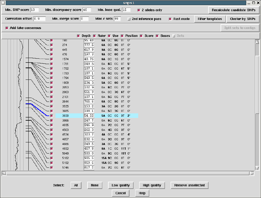
148 The Staden Package Manual
for a single contig and range. After selecting this a window is displayed showing the likely
locations of SNPs as seen below.
The top row of this has controls to define how the 2nd-Highest Confidence or Diploid
Graph results are analysed in order to pick candidate locations for SNPs.
Going from right to left, the “2 alleles only” toggle switches between the two algorithms;
when enabled it uses the additional assumption coded into the Diploid Graph of their being
only two populations in approximately 50:50 ratio. Next the minimum base quality may
be adjusted. Any difference with a poorer quality than this is completely ignored. The
minimum discrepancy score is a threshold (with high indicating a strong SNP) applied to
the results of the consistency plot results. A spike in this plot needs to be at least as
high as this score to be accepted. This score is then adjusted for immediate proximity to
other SNPs (e.g. it forms a run of bases) and this adjusted score is compared against the
minimum SNP score parameter. Typically this can be left low. If any of these parameters
are modified press the “Recalculate candidate SNPs” button to recompute.
The large central panel contains a vertically scrolled representation of the candidate
SNPs found. By default the left-most plot contains a pictorial view of the sequence depth.
Next to this is a vertical ruler showing the relative positions of candidate SNPs. Both of
these two plots are to scale based on the sequence itself. To the right of these come a series
of text based items with one row per candidate SNP. Initially this consists only of a check
Chapter 2: Sequence assembly and finishing using Gap4 149
button (“Use”), Position, Score and the frequency of base types observed at that consensus
column. Double clicking on any row will bring up the contig editor at that position showing
the potential SNP. You may manually curate which ones you consider to be true or not
by enabling or disabling it use the “Use” checkbox on that row. The score may also be
manually adjusted allowing certain differences to be forced apart by using a very high score.
The second row from the top contains a row of options controlling how the correlation
between candidate SNPs is used to assign haplotypes. For every template in the contig
the algorithm produces a fake sequence consistencing only of the bases considered to be
a candidate SNP and enabled by having the “Use” checkbox set. These fake sequences
are then clustered to form groups. No re-alignment is performed as the existing multiple
alignment has already been made (although you may wish to run the Shuffle Pads algorithm
before hand if the existing sequence alignment is poor).
This is a fairly standard clustering algorithm that starts with each sequence being the
sole member of a set. All sets are compared with each other based on the correlation between
sets using an adjusted correlation score (achieved by subtracting “Correlation offset”) and
then the overlaps are ranked by score. The best scoring sets are then merged together. If
Fast Mode is not being used the merged set is then compared against everything else once
more to obtain new scores, otherwise a simple adjustment is guessed at. Skipping this step
speeds up the algorithm considerably and generally gives sufficient results; hence the Fast
Mode toggle. This process is repeated until no two sets have an overlap score of greater
than or equal to the “Minimum merge score”.
The Filter Templates button brings up a new dialogue box containing an editable list
(initially blank) of template names. Adding a template name here will force this template
to be ignored by the clustering algorithm. You may also enter reading names here too
and they will be automatically converted to template names, hence filtering out all other
readings from the same template. If you or suspect specific templates from being chimeric
then this is where they should be listed.
The Cluster by SNPs button starts the clustering process running. It cannot be inter-
rupted and may take a few minutes. After completion the “Sets” component (rightmost) of
the central plot is updated as seen in the below screenshot. Each set is a group of templates
clustered together based on the candidate SNPs. They are sorted in left to right order
such that the left-most set contains the most number of templates and the right most set
contains the fewest. The consensus for members of that set is displayed in each square and
the quality of the consensus is shown in a similar fashion to the contig editor, with white
being good quality and dark grey being poor (usually due to being low coverage within that
set).
The background to the entire row is also shaded to indicate the observed quality of that
SNP in the context of this clustering. A white background indicates that two or more sets
exist with high quality consensus bases (>= quality 90) that differ. A light grey background
is used where the consensus bases differ but not with high quality bases. A dark grey
background is used to indicate that the consensus in all sets covering that SNP candidate
agree. This typically happens when either the clustering has failed or when a candidate
SNP is not a real indicator of which haplotype a sequence belongs to, such as a base calling
150 The Staden Package Manual
error or a random fluctuation in homopolymer length. If you wish to force this SNP to be
used for clustering then try increasing its score and re-clustering again.
Hence in the above example we see two distinct good quality sets made from the SNPs
between 1503 and 2334 and two more good quality sets from 12039 onwards. This indicates
that we have no templates where one end spans SNPs in the 1503-2334 region and the other
end spans SNPs in the 12039 onwards region. We also have a series of smaller sets which
probably arise due to incorrect base calls or more rarely due to chimeras.
Now if we double click to get the contig editor up it will display an additional window
labelled “Tabs”. NOTE: this does not happen if a contig editor for this contig is already
being displayed. If so shut that one down first. Notice that the sequence names are also
coloured. This indicates the set the sequence has been assigned to. The picture below also
has the “Highlight Disagreements” mode enabled with a difference quality cutoff sufficient
Chapter 2: Sequence assembly and finishing using Gap4 151
set to match the one used in the SNP Candidates plot. Two clear SNP positions can be
seen.
The tabs window lists the set numbers and their size (except for “All”). Selecting a set
will show just sequences from that set. This allows for the set consensus and quality values
to be viewed. The editor also allows for sequences to be moved from one set to another,
but for now this is purely serves a visual purpose and the movements are not passed back
to the main SNP candidates window (although this is an obvious change to make).
Moving back to the main SNP Candidates window note that we have a series of selection
buttons at the bottom of the window. These control automatic selection of rows (SNPs)
based on their quality assigned by observing the set consensus sequences. The clustering
algorithm only works on selected sets so this allows for poor quality SNPs to be removed from
further calculations. Additionally to simplify the view unselected SNPs may be removed
by pressing the “Remove unselected” button.
Above each set has a checkbutton above it (not visible in the screenshot). Initially these
are not enabled, but they indicate which sets certain operations should be performed on.
Pressing the right mouse button over a set (or a set checkbox) brings up a menu indicating
the following operations.
Delete set
Merge selected sets
This removes either the clicked upon set or all enabled sets (those that have
their checkbox set) from the display.
152 The Staden Package Manual
Save this consensus
Save consensus for selected sets
This brings up a dialogue box allowing the consensus for a single or selected
sets to be saved in FASTA format. The set numbers is a space separated list
of numbers representing the sets to save, starting with the leftmost set being
numbered as 1. Initially this is either the one you clicked on or all the selected
ones, but it may be edited in this dialogue too prior to saving. Strip pads
removes padding characters (’*’) from the consensus.
“Incorporate ungrouped templates” controls how template sequences that were
not assigned to at least one set are dealt with. It could be considered that se-
quences covering regions where no SNPs have been detected should be included
when computing the consensus, and this is the default action. However this can
be disabled such that only sequences that were specifically used for breaking
the assembly apart into sets form the consensus.
Produce fofn for this set
Produce fofn for selected sets
These options allow a file or list of reading names to be saved. A single fofn is
produced but multiple sets may be grouped together in one fofn. Here the set
number “0” is a placeholder for all of the sequences that were not assigned to
a set.
The final set of controls to discuss in the SNP Candidates window control the splitting
of sets into contigs. This is a one-way action which cannot be undone, so make sure you
backup the database using Copy Database before hand.
The “Split sets to contigs” button moves the readings in each selected set to its own
contig. In some cases a set may be non-contiguous. Remember that templates are assigned
to sets, but a template may often only have the end sequence known with the middle portion
being unsequenced. Gap4 does not currently handle scaffolds and super-contigs so in order
to keep such sets held together in a single contig the “Add fake consensus” option may
be used. This adds an additional sequence to the contig that contains the consensus for
the set (including from readings that were unassigned). This also handily means that new
contigs produced from multiple sets are already aligned and base coordinates are directly
comparable. Hence two such sets may be viewed in the Join Editor by typing their names
into the main Join Contigs dialogue. (Find Internal Joins will attempt to realign the contigs
and often fails if the set contains many regions of unknown consensus.)
Chapter 2: Sequence assembly and finishing using Gap4 153
2.5.4 Plotting Consensus Quality
This option can be invoked from the main gap4 View menu, in which case it appears as a
single plot, or from the View menu of the Template Display, in which case it will appear as
part of the Template Display.
For each base in the consensus a "quality"code is computed based on the accuracy of
the data on each strand and whether or not the two strands agree. In a future release it
will be renamed the "Strand Comparison Plot"This "quality"is then plotted using colour
and height to distinguish the quality codes shown below.
Colour Height Meaning
grey 0 to 0 OK on both strands, both agree
blue 0 to 1 OK on plus strand only
green -1 to 0 OK on minus strand only
red -1 to 1 Bad on both strands
black -2 to 2 OK on both strands but they disagree
For example, in the figure we see that the first four hundred or so bases are mostly only
well determined on the forward strand.
2.5.4.1 Examining the Quality Plot
Note that when displaying many bases the screen resolution implies that the quality codes
for many bases will appear in the same screen pixel. However the use of varying heights
ensures that all problematic regions will be visible, even when the problem is only with a
single base position. Hence when the quality plot consists of a single grey line all known
quality problems have been resolved, at the current consensus and quality cutoffs.
The quality plot appears as "Calculate quality"in the Results Manager window (see
Section 2.13 [Results Manager], page 277).
Within the Results Manager commands available, using the right mouse button, include
"Information", which lists a summary of the distribution of quality types to the output
window, and "List"which lists the actual quality values for each base to the output window.
These quality values are written in a textual form of single letters per base and are listed
below.
154 The Staden Package Manual
+Strand -Strand
aGood Good (in agreement)
bGood Bad
cBad Good
dGood None
eNone Good
fBad Bad
gBad None
hNone Bad
iGood Good (disagree)
jNone None
An example of the output using "Information"and "List"follows.
============================================================
Wed 02 Apr 12:14:06 1997: quality summary
------------------------------------------------------------
Contig xb56b6.s1 (#11)
81.00 OK on both strands and they agree(a)
3.94 OK on plus strand only(b,d)
11.98 OK on minus strand only(c,e)
1.85 Bad on both strands(f,g,h,j)
1.22 OK on both strands but they disagree(i)
============================================================
Wed 02 Apr 12:14:09 1997: quality listing
------------------------------------------------------------
Contig xb56b6.s1 (#11)
10 20 30 40 50 60
eeeeeeeeee eeeeeeeeee eeeeeeeeee eeeeeeehee eeeeeeeeee eeeeeeeeee
70 80 90 100 110 120
eeeeeeeeee eeeeeeeeee eeeeeeeeee eeeeeeeeee eeeeeeeeee eeeeeeeeee
130 140 150 160 170 180
eeeeeeeeee eeeeeeeeee eeeeeeeeee eeeeeeeeee eeeeeeeeee eeeeeeeeee
190 200 210 220 230 240
eeeeeeeeee eeeeeeeeee heeeeeeeee eeeeeeeici iiaiaciiia aaaaaaaaac
250 260 270 280 290 300
aaaacaaaaa aaaaaaaiia aaaaaaaaaa aaaaaaaaaa aaaabaaaaa aaaaaaaaaa
Chapter 2: Sequence assembly and finishing using Gap4 155
310 320 330 340 350 360
aaaaaaaaaa aaaaaaaaaa aaaaaaaaaa aaaaaaaaaa aaaaaaaaaa faaaaaaaaa
[ output removed for brevity ]
156 The Staden Package Manual
2.5.5 Plotting Stop Codons
The Stop Codon Map plots the positions of all the stop codons on one or both strands of
a contig consensus sequence. It can be invoked from the gap4 View menu. If the Contig
Editor is being used on the same contig, the Refresh button will be enabled and if used will
fetch the current consensus from the editor, repeat the search and replot the stop codons.
The figure shows a typical zoomed in view of the Stop Codon Map display. The positions
for the stop codons in each reading frame (here all six frames are shown) are displayed in
horizontal strips. Along the top are buttons for zooming, the crosshair toggle, a refresh
button and two boxes for showing the crosshair position. The left box shows the current
position and the right-hand box the separation of the last two stops codons selected by the
user. Below the display of stop codons is a ruler and a horizontal scrollbar. The information
line is showing the data for the last stop codon the user has touched with the cursor. Also
shown on the left is a copy of the View menu which is user to select the reading frames to
display.
2.5.5.1 Examining the Plot
Positioning the cursor over a plotted point will cause its codon and position to appear in
the information line.
It is possible to find the distance between any two stop codons. Pressing the left mouse
button on a plotted point will display "Select another codon"at the bottom of the window.
Then, pressing the left button on another plotted point will display the distance, in bases,
between the two sites. This is shown in the box located at the top right corner of the
window.
2.5.5.2 Updating the Plot
If the Contig Editor (see Section 2.6 [Editing in gap4], page 160) is currently running on the
same contig as is being displayed as a Stop Codon Map, the Refresh button will be shown
in bold lettering and hence be active, otherwise it will be greyed out. Pressing the button
will fetch the current consensus from the Contig Editor and replot its stop codons. Hence
the plot can be kept current with the changes being made in the editor.
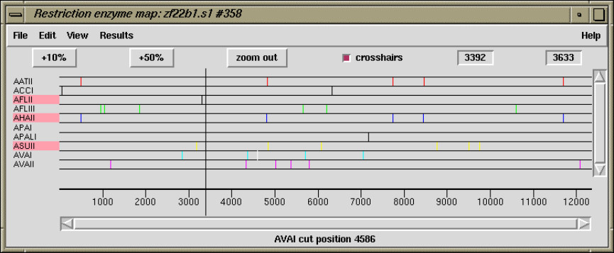
Chapter 2: Sequence assembly and finishing using Gap4 157
2.5.6 Plotting Restriction Enzymes
The restriction enzyme map function finds and displays restriction sites within a specified
region of a contig. It is invoked from the gap4 View menu. Users can select the enzyme
types to search for and can save the sites found as tags within the database.
This figure shows a typical view of the Restriction Enzyme Map in which the results for
each enzyme type have been configured by the user to be drawn in different colours. On
the left of the display the enzyme names are shown adjacent to the lines of plotted results.
If no result is found for any particular enzyme eg here APAI, the line will still be drawn
so that zero cutters can be identified. Three of the enzymes types have been selected and
are shown highlighted. The results can be scrolled vertically (and horizontally if the plot is
zoomed in). A ruler is shown along the base and the current cursor position (the vertical
black line) is shown in the left hand box near the top right of the display. If the user clicks,
in turn, on two restriction sites their separation in base pairs will appear in the top right
hand box. Information about the last site touched is shown in the Information line at the
bottom of the display. At the top the edit menu is shown torn off and can be used to create
tags for highlighted enzyme types.
2.5.6.1 Selecting Enzymes
Files of restriction enzyme names and their cut sites are stored in disk files. For the format
of these files and notes about creating new ones see Section 11.4 [Restriction enzyme files],
page 566.
When the file is read, the list of enzymes is displayed in a scrolling window. To select
enzymes press and drag the left mouse button within the list. Dragging the mouse off the
bottom of the list will scroll it to allow selection of a range larger than the displayed section
of the list. When the left button is pressed any existing selection is cleared. To select several
disjoint entries in the list press control and the left mouse button. Once the enzymes have
been chosen, pressing OK will create the plot.
158 The Staden Package Manual
2.5.6.2 Examining the Plot
Positioning the cursor over a match will cause its name and cut position to appear in
the information line. If the right mouse button is pressed over a match, a popup menu
containing Information and Configure will appear. The Information function in this menu
will display the data for this cut site and enzyme in the Output Window.
It is possible to find the distance between any two cut sites. Pressing the left mouse
button on a match will display "Select another cut"at the bottom of the window. Then,
pressing the left button on another match will display the distance, in bases, between the
two sites. This is shown in a box located at the top right corner of the window.
2.5.6.3 Reconfiguring the Plot
The plot displays the results for each restriction enzyme on a separate line. Enzymes with
no sites are also shown. The order of these lines may be changed by pressing and dragging
the middle mouse button or alt +left mouse button on one of the displayed names at the
left side of the screen.
The results are plotted as black lines but users can select colours for each enzyme type
by pressing the right button on any of its matches. A menu containing Information and
Configure will pop up. Configure will display a colour selection dialogue. Adjusting the
colour here will adjust the colour for all matches for this restriction enzyme.
2.5.6.4 Creating Tags for Cut Sites
Clicking the left mouse button on an enzyme name at the left of the display toggles a
highlight. The Create tags command from the Edit menu will add tags to the database for
all the matches whose enzyme names are highlighted. The command displays a dialogue
box listing the enzyme names on the left, and the tag type to create for that enzyme on the
right. Tag types must be chosen for all the listed restriction enzyme types before the tags
can be created. Suitable tag types to choose are the ENZ0, ENZ1 (etc) tags.
2.5.6.5 Textual Outputs
The Results menu of the plot contains options to list the restriction enzyme sites found.
One option sorts the results by enzyme name and the other by the positions of the matches.
The output below shows the textual output from "Output enzyme by enzyme". The
Fragment column gives the size of the fragments between each of the cut sites. The Lengths
column contains the fragment sizes sorted on size.
Contig zf98g12.r1 (#801)
Number of enzymes = 3
Number of matches = 7
Matches found= 1
Name Sequence Position Fragment lengths
1 AATII GACGT’C 7130 7129 556
556 7129
Matches found= 5
Name Sequence Position Fragment lengths
1 ACCI GT’CGAC 414 413 189
Chapter 2: Sequence assembly and finishing using Gap4 159
2 ACCI GT’CTAC 1296 882 413
3 ACCI GT’CTAC 3871 2575 882
4 ACCI GT’CTAC 5816 1945 1681
5 ACCI GT’CGAC 7497 1681 1945
189 2575
Matches found= 1
Name Sequence Position Fragment lengths
1 AHAII GA’CGTC 7127 7126 559
559 7126
The output below shows the textual output from "Output ordered on position".
Contig zf98g12.r1 (#801)
Number of enzymes = 3
Number of matches = 7
Name Sequence Position Fragment lengths
1 ACCI GT’CGAC 414 413 3
2 ACCI GT’CTAC 1296 882 189
3 ACCI GT’CTAC 3871 2575 367
4 ACCI GT’CTAC 5816 1945 413
5 AHAII GA’CGTC 7127 1311 882
6 AATII GACGT’C 7130 3 1311
7 ACCI GT’CGAC 7497 367 1945
189 2575
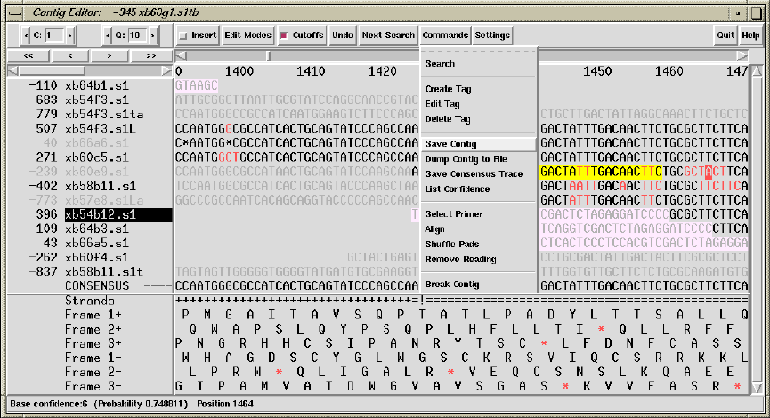
160 The Staden Package Manual
2.6 Editing in Gap4
The gap4 Contig Editor is designed to allow rapid checking and editing of characters in
assembled readings. Very large savings in time can be achieved by its sophisticated prob-
lem finding procedures which automatically direct the user only to the bases that require
attention. The following is a selection of screenshots to give an overview of its use.
The figure above shows a screendump from the Contig Editor which contains segments
of aligned readings, their consensus and a six phase translation. The Commands menu is
also shown. The main components are: the controls at the top; reading names on the left;
sequences to their right; and status lines at the bottom. Some of the reading names are
written in light grey which indicates that their traces/chromatograms are being displayed
(in another window, see below).
One reading name is written with inverse colours, which indicates that it has been
selected by the user. To the left of each reading name is the reading number, which is
negative for readings which have been reversed and complemented. The first of the status
lines, labelled “Strands”, is showing a summary of strand coverage. The left half of the
segment of sequence being displayed is covered only by readings from one strand of the
DNA, but the right half contains data from both strands.
Along the top of the editor window is a row of command buttons and menus. The
rightmost pair of buttons provide help and exit. To their left are two menus, one of which
is currently in use. To the left of this is a button which initially displays a search dialogue,
and then pressing it again, will perform the selected search. Further left is the undo button:
each time the user clicks on this box the program reverses the previous edit command. The
next button, labelled “Cutoffs” is used to toggle between showing or hiding the reading
data that is of poor quality or is vector sequence. In this figure it has been activated,
revealing the poor quality data in light grey. Within this, sequencing vector is displayed in

Chapter 2: Sequence assembly and finishing using Gap4 161
lilac. The next button to the left is the Edit Modes menu which allows users to select which
editing commands are enabled. The next command toggles between insert and replace and
so governs the effect of typing in the edit window. The 2 entryboxes on the left hand side
labelled C and Q set the consensus and quality cutoff values (see Section 2.6.18.1 [Consensus
and Quality Cutoffs], page 198).
One of the readings contains a yellow tag, and elsewhere some bases are coloured red,
which indicates they are of poor quality. The Information Line at the bottom of the window
can show information about readings, annotations and base calls. In this case it is showing
information about the reliability of the base beneath the editing cursor.
A better way of displaying the accuracy of bases is to shade their surroundings so that
the lighter the background the better the data. In the figure above, this grey scale encoding
of the base accuracy or confidence has been activated for bases in the readings and the con-
sensus. This screenshot also shows the Contig Editor displaying disagreements and edits.
Disagreements between the consensus and individual base calls are shown in dark green.
Notice that these disagreements are in poor quality base calls. Edits (here they are all pads)
are shown with a light green background. When they are present, replacements/insertions
are shown in pink, deletions in red and confidence value changes in purple. The consensus
confidence takes into account several factors, including individual base confidences, sequenc-
ing chemistry, and strand coverage. It can be seen that the consensus for the section covered
by data from only one strand has been calculated to be of lower confidence than the rest.
The Status Line includes two positions marked with exclamation marks (!) which means
that the sequence is covered by data from both strands, but that the consensus for each of
the two strands is different. The Information Line at the bottom of the window is showing
information about the reading under the cursor: its name, number, clipped length, full
length, sequencing vector and BAC clone name.
The Contig Editor can rapidly display the traces for any reading or set of readings. The
number of rows and columns of traces displayed can be set by the user. The traces scroll in
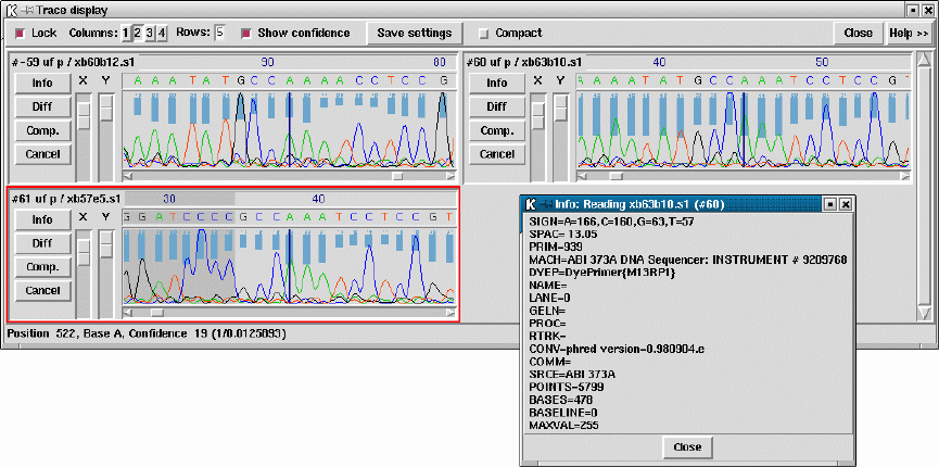
162 The Staden Package Manual
register with one another, and with the cursor in the Contig Editor. Conversely, the Contig
Editor cursor can be scrolled by the trace cursor. A typical view is shown below.
This figure is an example of the Trace Display showing three traces from readings in
the previous two Contig Editor screendumps. These are the best two traces from each
strand plus a trace from a reading which contains a disagreement with the consensus. The
program can be configured to automatically bring up this combination of traces for each
problem located by the “Next search” option. The histogram or vertical bars plotted top
down show the confidence value for each base call. The reading number, together with the
direction of the reading (+or -) and the chemistry by which it was determined, is given
at the top left of each sub window. There are three buttons (’Info’, ’Diff’, and ’Quit’)
arranged vertically with X and Y scale bars to their right. The Info button produces a
window like the one shown in the bottom right hand corner. The Diff button is mostly used
for mutation detection, and causes a pair of traces to be subtracted from one another and
the result plotted, hence revealing their differences. (see Section 2.6.11 [Traces], page 188).
2.6.1 Moving the visible segment of the contig
The contig editor displays only one segment of the entire contig, although several contig
editors can be in use at once. Above the sequence display is a “scrollbar”. This line
represents the entire contig, with a greyed section representing the currently displayed
segment. To change the displayed segment put the mouse cursor in the scrollbar and use
the mouse buttons. The available controls are:
Middle Mouse Button Set displayed section
Alt Left Mouse Button Set displayed section
Left Mouse Button Scroll left or right one screenful
On the far right side of the contig is a vertically oriented scrollbar. Typically the editor
will be showing all available data, in which case the vertical scrollbar cannot be scrolled.
In regions of exceptionally deep coverage, the editor makes sure that the controls, the
Chapter 2: Sequence assembly and finishing using Gap4 163
consensus, and any status lines are visible. The remaining space is taken up with however
many sequences fit. The vertical scrollbar can then be used, using the mouse buttons listed
above, to scroll through the sequences.
In addition to the scrollbars there are four buttons on the left hand side for scrolling by
fixed amounts.
<< Scroll left half a screenful
< Scroll left one base
> Scroll right one base
>> Scroll right half a screenful
Within the editor window itself two more key combinations can be used for scrolling
forwards and backwards an entire screenful. These, and several others, are modelled after
the Emacs key bindings.
Control v Scroll right one screenful
Meta v Scroll left one screenful
Finally, moving the editing cursor will always adjust the displayed section so that the
editing cursor is visible. Hence this can also be used to scroll around the editor in both
horizontal and vertical fashions.
2.6.2 Names
At the left side of the editor window is a display containing the reading names and numbers.
Each line consists of its orientation (“+” or “-”), reading number, a coloured template
consistency status and its name. The bottom line is always CONSENSUS. Also on the bottom
line is the current edit status. This is modelled on Emacs, and consists of one of ----,-%%-
and -**-, to symbolise “No unsaved edits made”, “No edits made - editor is in read only
mode”, and “Unsaved edits made”.
The maximum length of a reading name is 40 characters. Additionally there are 7
characters taken up with the direction and number of a reading. By default the names
display only shows 23 characters (enough to show 16 letters of a reading name). A horizontal
scrollbar just above the reading names can be used to scroll the reading names. Note that
the numbers and orientation are always visible. To change the width of the editor names
display set the CONTIG_EDITOR.NAMES_WIDTH setting in your ‘.gaprc’. For example:
set_def CONTIG_EDITOR.NAMES_WIDTH 23
The foreground colour for the text reveals whether the trace for this reading is shown
- a grey foreground indicates that the trace is visible. The background colour represents a
user highlight and the disassembly mode. The default background colour is light grey (the
same colour as the general editor background). Clicking the left mouse button on a reading
name toggles the background of the name component of number-name pair to black. This
is particularly useful for keeping track of an individual reading whilst scrolling the editor.
As the editor scrolls an individual reading will move up and down the editor display. By
highlighting this reading it becomes easy to track. The number component of the number-
name pair is used to highlight readings that are to be disassembled. See Section 2.9.1.2
[Disassemble Readings], page 240. In this case the background is dark grey.
164 The Staden Package Manual
If the template display is in use, highlighting a reading name in the editor will select
this reading in the template display (by marking it as bold). Similarly selecting a reading
in the template display (left mouse button) will highlight the reading in the contig editor.
Additionally the contig editor cursor is visible within the template display allowing the
position of the editor to be controllable from the template display and connected plots
(such as the quality plot). See Section 2.5.1 [Template Display], page 130.
The readings contained within the “readings” list are automatically highlighted when
the editor starts. Toggling the highlighted names in the editor updates the “readings” list
accordingly. See Section 2.14.1 [Special List Names], page 278.
Once an output list for the editor has been set, pressing the middle mouse button,
or Alt left mouse button, on the names display has the same effect as the using the left
button, except that it adds (and never removes) the reading name to the specified list. See
Section 2.6.8.18 [Set Output List], page 186. This is similar to using the left mouse button
to add names to the “readings” list, except that it allows for multiple lists to be built up.
Pressing the right mouse button on a name will popup a menu containing a variety of
operations to perform for that specific reading.
Goto... This is a cascading menu containing all other readings on the same template,
including ones on other contigs. Selecting the appropriate read name will move
the editor to the left-most base in that sequence. If the sequence is in another
editor then either the other editor will be moved (and created if needed).
Join to... This is only shown when a template has more than one reading in it and the
readings are within separate contigs. when this is the case a cascading menu
presents the list of readings in other contigs. Selecting one of these will bring up
the join editor with both sequences visible (so that you will need to manually
scroll to approximately the correct position in order to find the join).
Select this reading
Select this reading and all to right
Deselect this reading
Deselect this reading and all to right
Select readings on this template
Deselect readings on this template
These commands (de)select one or several readings. “Select this reading” is the
most simple method and this acts in the same way as simply left clicking on a
sequence name.
The other modes allow the (de)selection of sequences on this template (regard-
less of which contig they are in) or ranges. The “and all to right” modes are
designed with disassemble readings in mind. Disassembling all readings from
a specific point onwards using the “Move readings to new contigs” mode is
analogous to using break contig. Selecting all readings within a range may
be achieved by a combination of “select this reading and all to right” and a
subsequence “deselect this reading and all to right” further along the contig.
List notes
Chapter 2: Sequence assembly and finishing using Gap4 165
This invokes the note selector with this reading already listed (see Section 2.15.1
[Selecting Notes], page 281).
Set as reference sequence
This marks the sequence as the Reference sequence (see Section 2.6.12.1 [Ref-
erence sequences], page 191).
Set as reference trace
This marks the trace as a Reference trace for use with trace differencing (see
Section 2.6.12.2 [Reference traces], page 191).
Remove reading (this only)
Remove reading and all to right
This marks one or more readings as ready for removal by disassemble readings
(see Section 2.6.9 [Removing readings from the contig], page 186). You will
then be prompted when you exit the editor whether you wish to disassemble
the chosen readings.
Clear selection
This clears the current reading selection.
2.6.3 Editing
Editing can take up a significant portion of the time taken to finish a sequencing project.
Gap4 has a selection of searches (see Section 2.6.6 [Searching], page 174) designed to speed
up this process. The problems that require most attention are conflicts between good bases.
Where base confidence values are present it should be unnecessary to edit all conflicting
bases as, in general, this will amount to adjusting poor quality data to agree with good
quality data, in which case the consensus sequence should be correct anyway.
Pads in the consensus should not be considered a problem requiring edits because it
is possible to output the consensus sequence (from the main Gap4 File menu) with pads
stripped out. Obviously poorly defined pads (a mixture of several pads and real bases)
require checking in the same manner as other poorly defined consensus bases.
If you wish to check all base conflicts set the consensus algorithm to Frequency (see
Section 2.11.5 [The Consensus Algorithms], page 257) and the consensus cutoff to 100. The
consensus will then be a dash in all places where there is not a 100% agreement in the
sequences. The “Next Problem” editor button will then step one at a time through each
conflict.
2.6.3.1 Moving the editing cursor
Nearly all editing operations happen at the location of the editing cursor. This cursor
appears as a solid block. The simplest mechanism of moving the cursor is simply use the
left mouse button. Alternatively the following keys can be used.
166 The Staden Package Manual
Left arrow or Control b Move left one base
Right arrow or Control f Move right one base
Up arrow or Control p Move up one base
Down arrow or Control n Move down one base
Control a Move editing cursor to start of used
Control e Move editing cursor to end of used
Meta a Move editing cursor to start of cutoff
Meta e Move editing cursor to end of cutoff
Meta < Move editing cursor to start of contig
Meta > Move editing cursor to end of contig
The difference between the last four Control and Meta key combinations depends on
whether “Cutoffs” is set. If it is, then “Control a” will move to the start of the used data
for this reading and “Meta a” will move to the start of the cutoff data for this reading.
Otherwise they both move to the same point (the used data start). Similarly for “Control
e” and “Meta e”. The action of these four key presses in the consensus line is simply to
move to the start or end of the entire consensus sequence.
The cursor can be placed on any sequence data shown in the editor.
2.6.3.2 Editing Modes
The editor operates in two main edit modes - Replace and Insert. Replace allows a character
to be replaced by another and Insert allows characters to be inserted. Replace is the default
mode. The mode can be changed by pressing the button marked “Insert”. The checkbox
next to the button will be set (filled by a dark colour) when the mode is “Insert”. By
default these modes are restricted until the Edit Modes menu is used to change them.
The Edit Modes menu consists of a series of checkboxes and radiobuttons which control
which editing options are enabled.
Allow insert in read
Allow del in read
Insertion or deletion within a reading will shift the sequence characters and
so will alter their alignment. This is acceptable provided action is taken to
correct it, by either shifting the reading or by inserting or deleting a base
elsewhere. This functionality is disabled by default and is enabled by checking
the appropriate checkbox. Note though that insertion and deletion of bases
within the cutoff data will shuffle the cutoff data rather than the reading itself
and hence will not break alignment. However this operation still requires the
edit mode to be enabled.
Allow insert any in cons
Allow del dash in cons
Allow del any in cons
These operations control the editing actions allowed for the consensus. By
default the only operations allowed are insertion and deletion of pads. This is
because consensus editing is typically used for removing columns of pads where
a single reading has been overcalled.
Chapter 2: Sequence assembly and finishing using Gap4 167
When editing at 100% disagreement, such cases will be dashes in the consensus,
so “Allow del dash in cons” enables deletion of both dash and pads.
“Allow insert any in cons” and “Allow del any in cons” allow any column to
be completely inserted or deleted. These are potentially dangerous actions,
however the “Evidence for edits” options can detect such edits.
Allow replace in cons
Replacing a base in the consensus changes all of the bases in readings at this
point that disagree with the typed base. The actual edit performed depends
upon the “Edit by base type” and “Edit by confidence” radiobuttons.
Allow reading shift
To shift a reading place the cursor at the far left end of the reading. If cutoffs
is set this should be the far left end of the cutoff data. Then typing space or
delete will move the reading right or left respectively by one position. This
operation is disabled by default.
Allow transpose any
Moving pads within a reading is often a useful procedure, and the ’movement’
of a pad alone will not break the alignment. For this reason it is possible to
move pads around without using insert/delete. Placing the cursor over a pad
in a reading and pressing “Control l” or “Control r” will move that pad left or
right one base. This operation will not work with the cursor on the consensus.
Pad movement is allowed at all times. The selection of “Allow transpose any”
allows any pair of adjacent characters to be swapped.
Allow uppercase
A rule often followed by users is to type all modifications in lower case which
makes edited characters easier to see. The “Allow uppercase” checkbox controls
whether this rule is enforced or not. By default “Allow uppercase” is checked
which means that the rule is not enforced.
Edit by base type
Edit by confidence
These two selections are radiobuttons, and are mutually exclusive. They control
the outcome when replacing bases in the consensus. When editing the consensus
“Edit by base type” changes bases that disagree with the consensus to the base
typed. “Edit by confidence” changes the confidence of disagreeing bases to 0.
If the consensus quality cutoff value is greater than or equal to zero, characters
with an accuracy value of 0 are ignored in the consensus calculation. That
is, although the characters still appear in the reading, they are not used to
calculate the consensus. In this way it is possible to maintain the original base
calls for visual inspection, but get the correct consensus.
Note that “Edit by confidence” will not work if the “frequency” consensus
algorithm is in use (see Section 2.11.5 [The Consensus Calculation], page 257).
168 The Staden Package Manual
If you wish to use “Edit by confidence”, make sure that the quality cutoff is zero
or higher, otherwise the frequency consensus algorithm will be used instead.
Allow F12 for fast tag deletion
F12 and Shift-F12 may be use to delete the tag underneath the contig editor
cursor (F12) or the mouse pointer (Shift-F12). Initially these are disabled to
prevent accidental deletions.
Mode set 1
Mode set 2
To make it easier to set the editing modes two user definable sets are available.
By default these are as follows.
Mode set 1:
−Disallow insert in read
−Disallow del in read
−Disallow insert any in cons
−Allow del dash in cons
−Disallow del any in cons
−Disallow replace in cons
−Disallow reading shift
−Disallow transpose any
−Allow uppercase
−Edit by confidence
Mode set 2:
−Allow insert in read
−Allow del in read
−Allow insert any in cons
−Allow del dash in cons
−Disallow del any in cons
−Allow replace in cons
−Allow reading shift
−Disallow transpose any
−Allow uppercase
−Edit by confidence
Currently the only way of redefining these sets is to add lines to your ‘.gaprc’
file. See Section 2.20.1 [Options Menu], page 298. The method is to define a
list of 1s and 0s to specify the states in the order listed above. The two default
sets are defined as follows.
set_def CONTIG_EDITOR.SE_SET.1 {0 0 0 1 0 0 0 0 1 1}
set_def CONTIG_EDITOR.SE_SET.2 {1 1 1 1 0 1 1 0 1 1}
Chapter 2: Sequence assembly and finishing using Gap4 169
2.6.3.3 Adjusting the Quality Values
Each base has its own quality value. Assembly will allow only values between 1 and 99
inclusive. A quality value of 0 means that this base should be ignored. A quality value of
100 means that this base is definitely correct and the consensus will be forced to be the
same base type and will be given a consensus confidence of 100. If two conflicting bases
both have a quality of 100 the consensus will be a dash with a confidence of 0.
Newly added bases or replaced bases are assigned their own quality values. By default
these are both 100. The “Set Default Confidence” option in the settings menu allows these
values to be changed.
Several keyboard commands are available to edit the quality value of an individual base.
The ’[’ and ’]’ keys set the quality to 0 and 100 repsectively. To increment or decrement
the confidence of a base by 1 use Shift plus the Up and Down arrow keys. To increment
or decrement by 10 use Control plus the Up and Down arrow keys. The editor will beep if
you reach quality 0 or 100. Finally note that quality values can also be made visible by the
use of grey scales for the sequence background colour. See Section 2.6.8.13 [Show Quality],
page 184.
2.6.3.4 Adjusting the Cutoff Data
The cutoff data is displayed by pressing the “Cutoffs” toggle at the top of the editor. The
cutoff sequence will be displayed in grey. We call the boundary between the cutoff data
and the used data the cutoff position. These positions can be shifted left or right for each
end of the reading using the Meta Left-arrow and Meta Right-arrow keys respectively. As
keyboards may not have a meta key, Control Left-arrow and Control Right-arrow also have
the same effect. These key combinations adjust the cutoff positions by a single base at
a time. They only work when the cursor is on the very first or very last “used” base,
depending on which cutoff you wish to adjust.
If large changes are required the cutoffs can be “zapped” to new positions using the “<”
and “>” keys. To use these, place the editing cursor to the position required (which may be
within the cutoff data or the used data) and press the “<” key to set the left cutoff to the
base between the cursor and the base leftwards of the cursor. Similarly “>” sets the right
cutoff to the base between the cursor and the base leftwards of the cursor. Note that many
keyboards have “<” and “>” above the “,” and “.” keys. In this case you will need to press
Shift in conjunction with “,” and “.” to perform the operations.
2.6.3.5 Summary of Editing Commands
A brief summary of these editing operations and which (if any) edit modes are required can
be seen below:
Key Location Ins/Rep Edit Mode Action
--------------------------------------------------------------------------
base/* Reading Replace any Change base
base/* Reading Insert Insert in read Change base
delete Reading both Delete in read Del base left & move
Ctrl delete Reading both Delete in read Delete base to left
Ctrl d Reading both Delete in read Delete under cursor
170 The Staden Package Manual
delete Read start both Readint shift Shift left
space Read start both Reading shift Shift right
Ctrl l Reading both any Move pad left
Ctrl r Reading both any Move pad right
Ctrl l Reading both Transpose any Move base left
Ctrl r Reading both Transpose any Move base left
[ Reading both any Set quality to 0
] Reading both any Set quality to 100
Shift Up Reading both any Incr. quality by 1
Shift Down Reading both any Decr. quality by 1
Ctrl Up Reading both any Incr. quality by 10
Ctrl Down Reading both any Decr. quality by 10
< Reading both any Set left cutoff
> Reading both any Set right cutoff
Meta left Reading both any Adjust left cutoff
Meta right Reading both any Adjust right cutoff
* Consensus both any Insert pad column
base Consensus Insert Insert any in cons Insert column
base Consensus Replace any Replace column
delete * Consensus both any Delete column
delete - Consensus both Del dash in con Delete column
delete any Consensus both Del any in cons Delete column
Ctrl d Consensus both Del dash/any Delete column
Shift F1-10 Read/Cons both any Create tag macro
F1 to F10 Read/Cons both any Use tag macro
F11 Read/Cons both any Edit tag under cursor
Shift F11 Read/Cons both any Edit tag under pointer
F12 Read/Cons both Fast tag deletion Delete tag under cursor
Shift F12 Read/Cons both Fast tag deletion Del. tag under pointer
2.6.4 Selections
It is possible to highlight an area of a reading or the consensus sequence in preparation for
performing some further action upon it. Such examples of actions are: creating annotations
and aligning sequence. We call these highlighted areas “selections”. They will be displayed
as an underlined region.
The simplest way to make a selection is using the left mouse button. Pressing the mouse
button marks the base beneath the cursor as the start of the selection. Then, without
releasing the button, moving the mouse cursor adjusts the end of the selection. Finally
releasing the button will allow normal use of the mouse again.
Sometimes we may wish to make a selection longer than is visible on the screen, or to
extend our current selection. This can be done by using shift left mouse button to adjust
the end of the selection. Hence we can mark the start of the selection using the left button,
scroll along the contig to the desired position, and set the end using the shift left button.
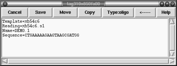
Chapter 2: Sequence assembly and finishing using Gap4 171
The selection is stored in a “cut buffer”. This allows for the usual “cut and paste”
operations between applications, although the contig editor only supports this in one direc-
tion (as it is not possible to “paste” into the window). The mechanism employed for this
follows the usual X Windows standard of using the middle mouse button (or Alt left mouse
button). For example, to send a piece of sequence to a text editor (eg Emacs) mark the
desired region using the left mouse button in the editor window and then press the middle
button, or Alt left mouse button, whilst the mouse cursor is in the text editor window. The
sequence will then be inserted into the text editor.
A quick summary of the mouse commands follows.
Left button Position editing cursor to mouse cursor
Left button (drag) Mark start and end of selection
Shift left button Adjust end of selection
Middle button (another window) Copy selected sequence
Alt left button (another window) Copy selected sequence
2.6.5 Annotations
Annotations (or tags) can be placed at any position on readings or on the consensus. They
are usually used to record positions of primers for walking, or to mark sites, such as repeats
or compressions, that have caused problems during sequencing. They can also be used to
contain feature table data as read from an EMBL format sequence file (see Section 3.1.3
[Reference sequences], page 314). Each annotation has a type such as “primer”, a position, a
length, a strand (forward, reverse or both) and an optional comment. Each type and strand
has an associated colour that will be shown on the display. For information on searching
for annotations see Section 2.6.6.4 [Searching by Tag Type], page 175, and Section 2.6.6.3
[Searching by Annotation Comments], page 175.
To create an annotation, make a selection and then select “Create Tag” from the contig
editor commands menu. See Section 2.6.7 [The Commands Menu], page 177. This will

172 The Staden Package Manual
bring up a further window; the “tag editor” (shown above). The “Type:” button at the
top of the editor invokes a selectable list from which tag types can be chosen. See below.
Use this to select the desired type of annotation.
Next the strand of the annotation can be selected. This will be displayed as one of “<—
–>”, “<—–” and “—–>”. The comment (the box beneath the buttons) can be edited using
the usual combination of keyboard input and arrow keys. The “Save” button will exit the
tag editor and create the annotation. To abandon editing without creating the annotation
use the “Cancel” button.
To edit an existing annotation, position the editing cursor within a annotation and select
“Edit Tag” from the commands menu. This will be a cascading menu, typically showing
one tag. If multiple tags coincide at the same sequence position you will be able to chose
which tag to edit. Once again the tag editor will be invoked and operates as before. The
F11 key is also a shortcut for editing the top-most tag underneath the editor cursor. When
editing, the “Save” will save the edited changes and “Cancel” will abandon changes.
Removing a annotation involves positioning the editing cursor within an annotation and
selecting “Delete Tag” from the commands menu. As with “Edit Tag” this is a cascading
menu to allow you to chose which tag at a specific point to delete.
Within a tag editor two buttons “Move” and “Copy” may be used to reposition existing
tags. When editing a tag, the current location of the tag is underlined within the editor.
If a new region is highlighted (on the consensus, a different reading, or even in a different
contig) and either of these buttons are pressed the tag will be saved to the new location
and removed from the previous location if “Move” was used. This can be used as an easy
way to adjust the extents of an existing tag or as a way to annotation multiple locations
with the same tag contents.

Chapter 2: Sequence assembly and finishing using Gap4 173
As usual, “undo” can be used to undo any of these annotation creations, edits and
removals.
Some tags may contain graphical controls instead of the usual text panel. These are
encoded with the master gap4 tag database (GTAGDB) by specifying the default tag text
to be a piece of “ACD” code. A full description of the (modified for gap4) ACD syntax is
not available currently, but it is strongly modelled on the the EMBOSS ACD syntax which
has documentation at
http://www.emboss.org/Acd/index.html .
It is possible to add your own tag types by modifying either the system GTAGDB file
or creating your own GTAGDB file in your home directory (for all your databases) or the
current directory (for just those in that directory).
For rapid annotating a series of 10 macros may be programmed. Press Shift and a
function key between F1 and F10 to bring up the macro editor. This look much like the
normal tag editor except that Save is replaced with Save Macro and saving does not actually
create a tag on the sequence. To use the macro, highlight the bases you wish and press
the function key corresponding to that macro - F1 to F10. For a single base pair tag you
do not need to underline a region as the tag will automatically cover the base underneath
the editing cursor. To remember these permanently use the “Save Macros” option in the
“Settings” menu.
You may find that some function keys are already programmed to do other things (such
as raise or lower windows), depending on the windowing environment in use. If this is the
case either modify the configuration of your windowing system or simply use another macro
key.
For rapid editing and deleting the F11 and F12 keys may be used. These edit and
delete the top-most tag underneath the editing cursor. If you wish to edit or delete the
tag underneath the mouse cursor instead (and hence save a mouse click) use Shift F11 and
Shift F12 for edit and delete.
The Control-Q key sequence may be used to toggle the displaying of tags. Pressing it
once will prevent all tags from being displayed in the editor. This is sometimes useful to see
any colouring information underneath the tag. Pressing Control-Q once more will redisplay
them.

174 The Staden Package Manual
2.6.6 Searching
The contig editor’s searching ability and its links to the consensus calculation algorithm
are crucial in determining the efficiency with which contigs can be checked and corrected.
The consensus is calculated “on the fly” and changes in response to edits. For editing, the
most important search functions are those which reveal problems in the consensus whilst
ignoring all bases that are adequately well determined. The default search type is therefore
by consensus quality. By default this is done in the forward direction and for a quality value
of 30, although this is configurable by changing the collowing lines in the gaprc file.
set_def CONTIG_EDITOR.SEARCH.DEFAULT_TYPE consquality
set_def CONTIG_EDITOR.SEARCH.DEFAULT_DIRECTION forward
set_def CONTIG_EDITOR.SEARCH.CONSQUALITY_DEF 30
Selecting “Next Search” brings up a window which can remain present during normal
editor operation. The window allows the user to select the direction of search, the type of
search, and a value to search on. The value is entered into a value text box, then pressing
the “search” button performs the search. If successful, the cursor is positioned accordingly.
An audible tone indicates failure. Pressing the “Cancel” button removes the search window.
The search window is automatically removed when the contig editor is exited.
The “Cutoffs” button can be used to select whether or not searching should find matches
within the cutoff data.
The Control-s key binding in the editor is equivalent to searching forward for the next
match. The Escape Control-s key sequence performs a reverse search. Both key bindings
will bring up the search window if it is not currently displayed.
As is described below, there are thirteen different search modes.
2.6.6.1 Search by Position
The presence of padding characters in the consensus can greatly alter the length of the
sequence, and the positions of the bases along it. Positions can therefore be defined in two
Chapter 2: Sequence assembly and finishing using Gap4 175
ways: those which include pads and those which do not. This option (termed a search!)
moves the cursor to a specified position. The numeric position is specified in the value text
box. Eg a value of “1234” causes the cursor to be placed at base number 1234 in the contig.
Positioning within a reading is achieved by prefixing the number with the “@” character, eg
“@123” positions the cursor at base 123 of the sequence in which the cursor lies. Relative
positions can be specified by prefixing the number with a plus or minus character. Eg
“+1234” will advance the cursor 1234 bases. If possible, the cursor is positioned within the
same sequence. The direction buttons have no effect on this operation.
2.6.6.2 Search by Problem
This positions the cursor at the next place in the consensus sequence which is “*”, “-” or
“N”. The search can be performed either forwards or backwards from the current cursor
position. Obviously the characters appearing in the consensus depend on the selected
consensus calculation algorithm and the thresholds set.
2.6.6.3 Search by Annotation Comments
This positions the cursor at the start of the next tag which has a comment containing the
string specified in the value box. Only currently active tag types are searched. The search
performed is a regular expression search, and certain characters have special meaning. Be
careful when your string contains “.”, “*”, “[“, “]”, “\”, “^” or “$”. The search can be
performed either forwards or backwards from the current cursor position. Searching with
an empty value will find all tags.
2.6.6.4 Search by Tag Type
This positions the cursor at the start of the next tag of the specified type. If the tag type
is not active, the tag will be found and underlined but will remain invisible. To change the
type, select from the menu that pops up when the mouse is clicked on the button labeled
“Type:”. The search can be performed either forwards or backwards of the current cursor
position. To find all tags, use “Search by Annotation Comments”, with an empty text box.
2.6.6.5 Search by Sequence
This positions the cursor at the start of the next segment of sequence that matches the
value specified in the text box. The search is case insensitive, ignores pads, and can allow a
specified number of mismatches. It may be performed on sequence only, consensus only or
both. It also operates either forwards or backwards from the current editing cursor position.
2.6.6.6 Search by Quality
This positions the cursor at the next place in the consensus sequence where the consensus
for each of the two strands disagree. Where there is only data for one strand the search
will stop at every base. The search can be performed either forwards or backwards from
the current cursor position.
2.6.6.7 Search by Consensus Quality
This positions the cursor on the consensus at the next position where the quality of the
consensus is below a given threshold. The quality of the consensus is calculated by the
176 The Staden Package Manual
consensus algorithm. For this search the quality threshold should be entered into the value
box and should be within the range of 0 to 100 inclusive.
2.6.6.8 Search by file
This steps the cursor through a set of positions specified in a file. The format for the
positions in the file is one per line with each line consisting of a reading name, a position
within that reading, and an optional comment. If a position is relative to the start of the
contig rather than the start of any particular reading, then simply use the first reading in
the contig. Positions that are beyond the ends for the reading are still valid, although the
editing cursor is moved onto the consensus sequence.
The comment can consist of any string. Multiline comments are possible, but they
must be written using \n in the comment string rather than an actual newline character
(which would signify the start of the next record). The comment for the current position
is displayed at the bottom of the editor search window in a text panel which is visible only
when in the “search by file” mode.
Any record containing a reading name that is not in the current contig is silently ignored.
This allows for a search file to have positions for all contigs. However at present there is no
mechanism for stepping through an entire search file bringing up editors for each contig as
required. This will be implemented in the future.
An example file follows.
xb63c7.s2 102
xb63c7.s2 30 A multi-\nline comment.
xb32a2.s1 56 Oligo, of length 12
xa17b1.r1 5714 Repeat from 5714 to 5780
2.6.6.9 Search by Reading Name
This positions the cursor at the left end of the reading specified in the value text box. If
the value is prefixed with a hash sign it is assumed to be a reading number. Otherwise it is
assumed to be a reading name. Eg “#123” positions the cursor at the left end of reading
number 123. “a16a12.s1” positions at the start of reading a16a12.s1. If the value was “a16”
the cursor is positioned at the first reading which starts with “a16”.
2.6.6.10 Search by Edit
This positions the cursor at the next place in the contig where an edit has been made. Edits
include base insertions, deletions, replacements and confidence value changes.The search can
be performed either forwards or backwards from the current cursor position.
2.6.6.11 Search by Evidence for Edit (1)
The Evidence for Edit (1) option checks edited bases to find bases in the consensus for
which there is no evidence in the original readings. The definition of evidence is that at
least one reading had this original base call. Currently this search operates only in the
forward direction.
2.6.6.12 Search by Evidence for Edit (2)
p
Chapter 2: Sequence assembly and finishing using Gap4 177
The Evidence for Edit (2) option checks edited bases to find bases in the consensus for
which there is no evidence in the original readings. The definition of evidence is that at
least one reading from each strand had this original base call. Currently this searches only
in the forward direction.
2.6.6.13 Search by Discrepancies
This finds positions where two or more bases are above a particular quality level, but in
disagreement. The quality threshold is given in the value box and should be within the
range of 0 to 100 inclusive.
2.6.6.14 Search by Consensus Discrepancies
This finds positions where there is a significant disagreement in a particular consensus
base. Unlike “by Discrepancies” this does not look for individual base confidence values,
but rather it combines multiple bases together for each base type and searches for the second
highest confidence at any point. This is the same method use in the 2nd-highest confidence
graph (see Section 2.5.2.5 [2nd-Highest Confidence], page 145).
2.6.7 The Commands Menu
The Commands menu is available by either pressing the Commands button at the top of
the contig editor window, or by pressing the Control key and the left mouse button, or by
pressing right mouse button with the mouse cursor anywhere within the sequence display
section of the contig editor. A menu will be revealed containing the following options (which
are described in greater detail below).
2.6.7.1 Search
This Contig Editor Commands menu function Performs a search. See Section 2.6.6 [Search-
ing], page 174.
2.6.7.2 Create Tag
This Contig Editor Commands menu function Creates an annotation. See Section 2.6.5
[Annotations], page 171.
2.6.7.3 Edit Tag
This Contig Editor Commands menu function Edits an annotation. See Section 2.6.5 [An-
notations], page 171.
2.6.7.4 Delete Tag
This Contig Editor Commands menu function Removes an annotation. See Section 2.6.5
[Annotations], page 171.
2.6.7.5 Save Contig
This Contig Editor Commands menu function writes any edited data to disk. The undo
history is cleared and it is no longer possible to quit and abandon these saved changes. The
Control-x followed by Control-s will also save the contig editor in the same manner as the
Save command.
178 The Staden Package Manual
2.6.7.6 Dump Contig to File
This Contig Editor Commands menu function outputs the current contig, as currently shown
(e.g. with status lines) to a file. The user can select the region to dump, the length of each
line, and the file name to use. The sequence names can be up to 40 characters, but often
projects do not use the full length. To avoid wasted space in the output the number of
columns to use for sequence names can be adjusted.
2.6.7.7 Save Consensus Trace
This Contig Editor Commands menu function produces a trace file for the consensus se-
quence by averaging the traces of the readings. The command brings up a dialogue con-
taining controls to specify the filename, the consensus start and end positions, the strand,
and whether to use matching reads.
As the trace of a reading is dependent on the direction it was read, the consensus trace
can be computed from all the reads in either the forward or reverse directions, but not both
at once. When the “Use only matching reads” toggle is set to “Yes” only the readings of
the correct strand that have the same base call as the consensus sequence are used. The
option is useful for producing wild-type trace files for a mutation analysis project.
2.6.7.8 List Confidence
This Contig Editor Commands menu function operates in a very similar manner to the main
Gap4 List Confidence command (see Section 2.11.6 [List Confidence], page 261), except that
it only operates on the current contig, and it uses the current editor consensus confidences
rather than the ones saved to disk. It displays a dialogue requesting a range within the
contig and a question asking if only summary of the results is required.
Pressing OK or Apply will add to the editor information line a count of the expected
number of errors and the error rate. If the “Only update information line” question was
answered “No” then the full frequency table will also be output. It will appear in the main
text output window in the same format as the “List Confidence” command in the main
Gap4 View menu. The Apply button can be used to calculate the number of errors without
removing the dialogue.
It is often the very ends of contigs (which are generally low coverage and bad quality)
that have most of the errors, and so it is sometimes useful to set a range which includes all
of the contig except for around 1000 bases from each end.
2.6.7.9 Report Mutations
This Contig Editor Commands menu function is used to produce a list of all the bases
annotated with mutation tags (or those bases which differ from the consensus/reference
sequence). If the tags or differences are within segments of sequence which are also an-
notated with EMBL feature table CDS records, the report will include data describing its
effect. The report, which can be sorted by sequence or position, includes the reading names,
mutation positions relative to the reference sequence, the actual change, its effect, and the
evidence. An example is shown below.

Chapter 2: Sequence assembly and finishing using Gap4 179
001321_11aF 33885T>Y (silent F) (strand - only)
001321_11aF 34407G>K (expressed E>[ED]) (strand - only)
001321_11cF 35512T>Y (silent L) (double stranded)
001321_11cF 35813C>Y (expressed P>[PL]) (double stranded)
001321_11dF 36314A>R (expressed E>[EG]) (double stranded)
001321_11eF 36749A>R (expressed K>[KR]) (double stranded)
001321_11eF 37313T>K (noncoding) (strand - only)
000256_11eF 36749A>G (expressed K>R) (double stranded)
Here the first record is for reading 001321 11aF, position 33885, T changed to T and C
(i.e. is heterozygous) to produce no amino acid change, with evidence coming only from
the complementary strand. The last record is for reading 000256 11eF, position 36749, A
changed to G, producing an amino acid change K to R, with evidence from both strands of
the sequence. The penultimate record denotes a heterozygote in a noncoding region.
2.6.7.10 Select Primer
This Contig Editor Commands menu function allows the user to employ the primer selection
algorithm OSP to find primers for sequencing experiments. See Section 2.6.10 [Searching
for Primers], page 187.
2.6.7.11 Align
This Contig Editor Commands menu function performs a sequence alignment between the
currently selected segment of a reading and the consensus sequence. It provides a simple
way of extending the visible part of a reading to use its hidden data, which is often useful to
double strand a short section of consensus without the need to perform further experiments.
On a sequence, highlight the cutoff data to align along with a small section of the good
quality non-cutoff data. Then select the align command and adjust the cutoff point as
desired. Pads are inserted in the consensus and readings as necessary, although pads will
not be inserted in the cutoff data of other sequences.
2.6.7.12 Remove Reading
This Contig Editor Commands menu function marks a reading for subsequent removal. See
Section 2.6.9 [Removing readings from the contig], page 186
2.6.7.13 Break Contig
This Contig Editor Commands menu function breaks the contig so that the reading under-
neath the editing cursor is the left end of a new contig. In order to perform this operation
all edits are saved automatically first. Once saved these edits cannot be undone. This
operation is identical to the Break Contig command in the main menu. See Section 2.9.1.1
[Break Contig], page 239.
2.6.8 The Settings Menu
The purpose of this menu is to configure the operation of the contig editor, including the
consensus calculation, the active tags and the status lines. Settings can be saved using the
“Save settings” button, but this does not save any tag macros. These may be saved using
the “Save Macros” option. Settings for the following options can be changed.
180 The Staden Package Manual
•Status Line
•Trace Display
•Consensus algorithm
•Highlight Disagreements
•Compare Strands
•Toggle auto-save
•3 Character Amino Acids
•Show reading quality
•Show consensus quality
•Show edits
•Show unpadded positions
•Show template names
•Set Active Tags
•Set Output List
•Set Default Confidences
•Store Undo Set or unset saving of undo
2.6.8.1 Status Line
The contig editor can display several additional text lines underneath the consensus se-
quence. This “status” data is of textual form and can provide additional information about
the data displayed above. Currently, there are two forms of status line available. These are
“Strands” and “Translate Frame”. Both status line types update automatically as edits are
made that change the consensus.
The status line menu is accessed by cascading off the settings menu. It contains the
following.
•Show Strands
•Translate using feature tables
•Translate frame 1+
•Translate frame 2+
•Translate frame 3+
•Translate frame 1-
•Translate frame 2-
•Translate frame 3-
•Translate +frames
•Translate - frames
•Translate all frames
•Remove all
“Show Strands” creates a single line consisting of the +, -, = and ! characters. These
indicate: positive strand only, negative strand only, both strands (in agreement) and both
strands (in disagreement) respectively.
Chapter 2: Sequence assembly and finishing using Gap4 181
The frame translation status lines provide translations in each of the six available reading
frames. Alternatively, using the “Translate using feature tables”, only segments described
in CDS records will be translated. The CDS records are those contained in the reference
sequence. Translations can be displayed in either the single character or the three character
amino acid codes.
Pressing the right mouse button on the ’name’ segment of the status line (on the left
hand side) pops up a menu. The commands available may depend on the type of the status
line chosen, however currently it will always only contain the “Remove” command. This,
as expected, removes the status line from the display. To remove all status lines use the
“Remove all” command from the “Status Line” cascading menu.
Note that the data in the status line cannot be cut and pasted, modified or searched; it
is not possible to move the cursor into these lines.
2.6.8.2 Trace Display
This is a cascading menu containing various options for configuring the trace views within
the editor.
2.6.8.3 Auto-display Traces
When switched on, auto-display traces will direct certain searches to automatically display
relevant traces to aid in solving problems. This works in conjunction with most appropriate
searches. The traces chosen to solve the “problem” will, by default, be the best trace from
each strand which agrees with the consensus (which is calculated at a low consensus cutoff)
and the best trace from each strand which disagrees with the consensus. This selection
of traces may be adjusted by modifying the CONTIG_EDITOR.AUTO_DISPLAY_TRACES_CONF
configuration variable. The default setting of this is “+ - +d -d”. Each of the space sepa-
rated elements in this string corresponds to a trace file to choose. If one cannot be found,
then it is ignored. The order listed here is the order in which they will be displayed in the
trace window. The complete list of available trace specifiers is:
+Best +ve strand trace agreeing with consensus
+p Best +ve strand dye-primer trace agreeing with consensus
+t Best +ve strand dye-terminator trace agreeing with consensus
-Best -ve strand trace agreeing with consensus
-p Best -ve strand dye-primer trace agreeing with consensus
-t Best -ve strand dye-terminator trace agreeing with consensus
dBest trace disagreeing with consensus
+d Best +ve strand trace disagreeing with consensus
-d Best -ve strand trace disagreeing with consensus
+2 Second best +ve strand trace agreeing with consensus
+2p Second best +ve strand dye-primer trace agreeing with consensus
+2t Second best +ve strand dye-terminator trace agreeing with consensus
182 The Staden Package Manual
-2 Second best -ve strand trace agreeing with consensus
-2p Second best -ve strand dye-primer trace agreeing with consensus
-2t Second best -ve strand dye-terminator trace agreeing with consensus
2d Second best trace disagreeing with consensus
+2d Second best +ve strand trace disagreeing with consensus
-2d Second best -ve strand trace disagreeing with consensus
2.6.8.4 Show Read-pair Traces
When double-clicking on a sequence to view a trace this option will automatically identify
traces on both strands of this template. Both the forward strand and reverse strand traces
will then be shown, in that order.
2.6.8.5 Auto-diff Traces
Once this is activated, whenever the user double clicks on a base in the editor sequence
display, not only is the reading’s trace displayed, but also its designated reference trace
plus the difference between them. If its complementary reading is available, its trace and
reference trace and their differences are also displayed.
If no traces have been specified to be the reference traces then Gap4 will attempt to
automatically pick two. It choses the highest quality pair of traces that come from the
same template and disagree with either the forward or reverse strand of the trace initially
double-clicked upon.
Trace differences display
Chapter 2: Sequence assembly and finishing using Gap4 183
As is shown in the figure below, it is also possible to set the trace difference display to
use positive and negative references
For further information about mutation detection, see Section 3.1 [Search for Mutations],
page 309.
2.6.8.6 Y scale differences
When performing trace alignments and differencing (using Auto-diff traces or via the manual
“difference” option in the trace display) this option controls whether to perform a trace
peak-height normalisation on both traces prior to alignment and substraction.
2.6.8.7 Consensus Algorithm
This allows selection of the consensus algorithm to use within the Contig Editor. Like the
consensus and quality cutoff parameters, it is local to the specific editor being used. The
main Consensus algorithm option should be used to globally change the algorithm being
used. See Section 2.20.2 [Consensus Algorithm], page 299.
2.6.8.8 Group Readings
This is a cascading menu allowing the readings viewed in the editor to be sorted and grouped
by different criteria. By default the order (in Y) that readings are listed in the editor is
sorted by the position of the left-most used based. This option provides a choice of by
position, strand (plus first, then minus), name, number, template and clone.
Where appropriate an automatic sub-ordering is applied. For example sorting by strand
will group the readings primarily into “+” and “-” groups, but within the group the readings
are still sorted by position. When grouping by template the sub-grouping is by strand.
184 The Staden Package Manual
2.6.8.9 Highlight Disagreements
This toggles between the normal sequence display (showing the current base assignments)
and one in which those assignments that differ from the consensus are highlighted. It makes
scanning for problems by eye much easier.
Several modes of highlighting are available: “By dots” will only display the bases that
differ from the consensus, displaying all other bases as full stops if they match or colons if
they mismatch but are poor quality. The definition of poor quality here can be adjusted
using the “Set quality threshold” option of the Settings menu. The base colours are as
normal (ie reflecting tags and quality).
Highlight disagreements “By foreground colour” and “By background colour” displays all
base characters, but colours those that differ from the consensus. Bases which differ by are
below the difference quality threshold are not coloured. This allows easier visual scanning
of the context that a difference occurs in, but it may be wise to disable the displaying of
tags (hint: control-Q toggles tags on and off).
Finally the “Case sensitive” toggle controls whether upper and lower case bases of the
same base type should be considered as differences.
2.6.8.10 Compare Strands
This toggles the consensus calculation routine between treating both strands together or
independently. In the independent case any difference between the two strands is shown
in the consensus as a ’-’. Hence these clashes are found as problems by the “Search by
problem” option.
2.6.8.11 Toggle auto-save
Selecting auto-save toggles the auto save feature. Initially this is turned off each time the
contig editor is invoked. Once toggled the adjacent checkbox will be set to indicate the
feature is enabled and the contig will be saved. From that point onwards the contig editor
will write its data to disk every 50 edits. Each time an auto save is performed it is announced
in the output window. Saving more frequently can still be performed manually by using
“Save Contig”.
Unlike “saves” made using the manual “Save Contig” command, the “Undo” button will
allow the user to undo edits regardless of when the last auto save occurred.
2.6.8.12 3 Character Amino Acids
By default, the codon translation within the status line displays single character amino acid
codes. Selecting “3 Character Amino Acids” will toggle the status line to display three
character amino acid codes.
2.6.8.13 Show Reading and Consensus Quality
When the quality cutoff value is 0 or higher and either of the “show reading quality” or
“show consensus quality” toggles is set, the background for bases is shaded in a grey level
dependent on their quality. There are ten levels of shading with the darkest representing
poor data and the lightest representing good data. So with the quality cutoff set to 50,
all bases with a quality of less than fifty are shown with a red foreground and a dark grey
Chapter 2: Sequence assembly and finishing using Gap4 185
background, bases with quality just above 50 will have the darkest grey background, and
bases with a quality of 100 will have the lightest background. When tags are present the
background colour is that of the tag rather than the quality.
The colours used are adjustable by modifying your ‘.gaprc’ file. The defaults are shown
below.
set_def CONTIG_EDITOR.QUAL0_COLOUR "#494949"
set_def CONTIG_EDITOR.QUAL1_COLOUR "#696969"
set_def CONTIG_EDITOR.QUAL2_COLOUR "#898989"
set_def CONTIG_EDITOR.QUAL3_COLOUR "#a9a9a9"
set_def CONTIG_EDITOR.QUAL4_COLOUR "#b9b9b9"
set_def CONTIG_EDITOR.QUAL5_COLOUR "#c9c9c9"
set_def CONTIG_EDITOR.QUAL6_COLOUR "#d9d9d9"
set_def CONTIG_EDITOR.QUAL7_COLOUR "#e0e0e0"
set_def CONTIG_EDITOR.QUAL8_COLOUR "#e8e8e8"
set_def CONTIG_EDITOR.QUAL9_COLOUR "#f0f0f0"
set_def CONTIG_EDITOR.QUAL_IGNORE "#ff5050"
2.6.8.14 Show edits
When set, any change between the bases displayed and the original sequence held in the
trace files is shown by changing the background colour of the changed base. The detection
of these edits depends on the quality values and the “original position” data. Hence the
traces do not need to be present in order to detect edits. The colour of the bases reflects the
type of change found. The colours are adjustable by editing the ‘.gaprc’ file. The following
table lists the colour, gaprc variable name and the meaning.
red CONTIG_EDITOR.EDIT_DEL_COLOUR — Deletion
pink CONTIG_EDITOR.EDIT_BASE_COLOUR — Base change or insertion
green CONTIG_EDITOR.EDIT_PAD_COLOUR — Padding character
purple CONTIG_EDITOR.EDIT_CONF_COLOUR — Confidence value
2.6.8.15 Show Unpadded Positions
The ruler at the top of the contig editor displays every tenth base number in the consensus
sequence. Without “show unpadded positions” enabled any character in the consensus is
counted, including padding characters. If “show unpadded positions” is enabled the ruler
will only count non pad (“*”) characters. Please note that this may considerably slow down
the editor on large databases as the full consensus needs to be calculated in order to plot
the ruler. If you just need to obtain the occasional unpadded position it is better to press
the Enter key or to use the “unpadded position” search.
2.6.8.16 Show Template Names
The names panel on the left hand side of the editor normally shows the reading names.
This option may be used to toggle this display to show the template names instead. When
enabled the trace display also switches from showing reading names to template names.
186 The Staden Package Manual
2.6.8.17 Set Active Tags
“Set Active Tags” allows configuration of which tag types should be displayed within the
editor. Note that searches for tag annotations will only examine active tags, but searching
for a specific tag type will find tags even when tags of this type are not visible. In this
situation the tag will still be invisible, but as usual the tag location will be underlined.
This option is particularly useful for exploring cases where a section of sequence has many
overlapping tags. An alternative to using this dialogue is using the Control-Q key, which
toggles the display of active tags.
2.6.8.18 Set Output List
“Set output list” pops up a dialogue asking for a list name to be used when outputting
reading names (see Section 2.14 [Lists], page 278). Once an output list has been specified,
pressing the middle button, or Alt left mouse button, on a reading name will add the name
to the end of list. Note that selecting the same name more than once will add the name to
the list more than once. The list is never cleared by the editor. This allows multiple editors
to append to the same list. If required, use the list menu to clear the list.
2.6.8.19 Set Default Confidences
Replacing bases or inserting new bases in the editor can assign new confidence values to
those bases. The default setting is to set these confidence values to 100 which has the effect
of forcing the consensus to be that base. The “Set Default Confidences” dialogue allows
these default values to be changed. The allowable range of confidence values for a base
is from 0 to 100 inclusive. The dialogue also allows selection of confidence -1. This tells
the editor to not change the confidence value. When replacing a base this keeps the same
confidence value of the base that is being replaced. When inserting a base this uses the
average of the confidence value of the two surrounding bases.
2.6.8.20 Set or unset saving of undo
Storing the undo information takes up a great deal of computer memory and slows down the
alignment algorithm. Particularly when using the Join Editor for very large overlaps (e.g.
after copying batches of readings from one database to another), it can be useful to turn
off the saving of undo information. For this reason the settings menu contains an option to
turn off (or on) the saving of undo information.
2.6.9 Removing Readings
It is often desirable to completely remove a reading from a contig. When not using the editor
this is typically performed using the Disassemble Readings function. See Section 2.9.1.2
[Disassemble Readings], page 240. When using the editor, the “Remove Reading” option
on the editor commands menu performs a similar task.
The command marks the reading underneath the editing cursor to be removed once the
editor is quitted. Until then, the reading number in the names section of the display is
shown with a dark grey background. The reading will also not be used in the calculation
of the consensus. Thus, if all readings at a particular section of consensus are marked for
removal the consensus sequence will be shown as dashes. Selecting the “Removing Reading”
command again with the editing cursor on a reading already marked for removal will cancel
Chapter 2: Sequence assembly and finishing using Gap4 187
the removal request. The keyboard command of Control-H may also be used as a shortcut
to the “Removing Reading” command.
Once the editor has been quitted you will be asked whether you wish to disassemble the
marked readings. Answering “No” will simply quit the editor as normal without removing
any readings. Answering “Yes” will bring up the usual “Disassemble Readings” dialogue.
The options here allow removal of all readings from this contig, or non-crucial only. A crucial
reading is one that will cause this contig to be broken into two or more segments. A choice
is also given as to whether the readings should be completely removed from this database,
or for each reading to be placed in its own contig. Pressing “OK” now will remove the
readings from the contig, breaking the contig if necessary, and will quit the editor. Pressing
“Cancel” will close the “Disassemble Readings” dialogue without making any changes and
will not quit the editor.
At any time, quitting the editor and not disassembling the readings will leave a List
(see Section 2.14 [Lists], page 278) named “disassemble” containing the readings marked
for removal. These may then be disassembled at a later stage if necessary. However the list
will only be available until the next editor is quit (at which stage that editor will create its
own, possibly blank, disassemble list), so make a copy if necessary.
2.6.10 Primer Selection
The oligo selection engine is the one used in the program OSP. It is described in Hillier,
L., and Green, P. (1991). “OSP: an oligonucleotide selection program,” PCR Methods and
Applications, 1:124-128. Oligo selection is a complex operation. The normal mode of use
is outlined below:
1. Open the oligo selection window, by selecting “Select Primer” from the contig editor
commands menu.
2. Position the cursor to where you want the oligo to be chosen. While the oligo selection
window is visible, you will still have complete control over positioning and editing
within the contig editor.
3. Indicate the strand for which you require an oligo. This is done by toggling the direction
arrows (“—–>” or “<——”).
4. Press the “Find Oligos” button to find all suitable oligos (see the “Parameters” sub-
section below for further information on controlling this procedure). Information for
the closest suitable oligo to the cursor position is given in the output text window and
at the bottom of the editor in the information line. In the contig editor the position of
the oligo is marked by a temporary tag on the consensus. The window is recentered if
the oligo is off the screen.
5. If this oligo is not suitable (it may have been used before, and failed) the next closest
oligo can be viewed by pressing “Next”.
6. Suitable templates are automatically identified for the currently displayed oligo (see the
“Template selection” subsection below). By default, the template is that closest to the
oligo site. If the choice is not suitable (it may be known to be a poor quality template,
say) another can be chosen from the “Choose from” pull-down menu. Templates that
do not appear on the menu can be specified by selecting simply typing their name in
188 The Staden Package Manual
the “Template name” entry box. However, the template must be on the correct strand
and be upstream of the oligo.
7. A tag can be created for the current oligo by pressing the button “Accept”. The
annotation for this tag holds the name of the template and the oligo primer sequence.
There are fields to allow the user to specify their own primer name (“serial#”) and
comments (“flags”) for this tag. An example of oligo tag annotation:
serial#=
template=a16a9.s1
sequence=CGTTATGACCTATATTTTGTATG
flags=
8. The oligo selection window is closed when “Accept” or “Quit” is selected.
2.6.10.1 Parameters
The parameters controlling the selection of oligos can be changed by pressing the “Edit
parameters” button. This invokes a dialogue box which allows the specification of further
parameters.
By default, the oligos are selected from a window that extends 40 bases either side of the
cursor. The size and location of this window relative to the cursor position can be changed
in the “Edit parameters” window.
Primer constraints can be specified by melting temperature, length and G+C content.
In gap4 oligos are ranked according to their overall score, where the best oligos have
lower scores.
2.6.10.2 Template selection
For simplicity, each reading is considered to represent a template. In practice, many readings
can be made off the same template. Suitable templates that are identified are those that
satisfy all of the following conditions:
1. are in the appropriate sense,
2. have 5’ ends that start upstream of the oligo,
3. are sufficiently close to the oligo to be useful.
This last criterion relates to the insert size for the templates used for sequencing and the
average reading length. A template is considered useful if a full reading can be made from
it, taking into account both of these factors. The default insert size is 1000 bases (although
the size range should be included in the experiment file for each reading, and hence the
default would not be required), and the default average reading length is 400 bases. These
values can be changed in the “Edit parameters” window.
2.6.11 Traces
The original trace data from which the readings where derived can be displayed by double
clicking (two quick clicks) with the left or middle mouse button on the area of interest.
Control t has the same effect. The trace will be displayed centred around the base clicked
upon and the name of the reading in the contig editor will be highlighted. Double clicking on
the consensus displays all the readings covering that position. Double clicking on a reading

Chapter 2: Sequence assembly and finishing using Gap4 189
which already has its trace displayed will cause the corresponding trace to be surrounded
by a red border.
Moving the mouse pointer over a base causes the display of an information line at the
bottom of the window. This gives the base type, its position in the sequence, and its
confidence value.
There are two forms of trace display which are selected using the “Compact” button at
the top of the Trace display. The compact form differs by not showing the Info, Diff, Comp.
and Cancel buttons at the left of each trace.
Note that gap4 does not store the trace files in the project database: it stores only their
names and reads them when required. However it does not know which directory they are
stored in, unless this is specified using the “Trace File Location” option (see Section 2.20.8
[Trace File Location], page 302).
The picture shows an example of three displayed traces. The reading number, together
with the direction of the reading (+or -) and the chemistry by which it was determined,
is given at the top left of each sub window. The chemistry information is found from
comments in the experiment file. ’uf’ and ’ur’ indicate universal forward and universal
reverse, ’cf’ and ’cf’ indicate custom forward and custom reverse, and ’p’ and ’t’ indicate
primer and terminator. There are four buttons (’Info’, ’Diff’, ’Comp.’ and ’Cancel’) below
this information, and X and Y scale bars to the right.
The “Info” button will display a window like the one shown at the bottom right of the
picture. This contains the comments from the relevant SCF file.
The “Diff” buttons are used to produce a new trace showing the differences between two
existing traces. To use this, press “Diff” in any window. The mouse cursor then changes
to a cross symbol. Pressing the left mouse button anywhere on another trace that has a
“Diff” button will create the difference trace. Any other button cancels the operation. The
algorithm used for computing the difference trace is adjustable by parameters in the settings
190 The Staden Package Manual
menu (see Section 2.6.8.2 [Trace Display Settings], page 181). The trace differencing was
originally designed for visual inspection of suspected mutations Bonfield, J.K., Rada, C.
and Staden, R. Automated detection of point mutations using fluorescent sequence trace
subtraction. Nucleic Acids Res. 26, 3404-3409 (1998).
The “Comp.” button complements the displayed trace. If the sequence in the editor
has been complemented then the trace will automatically be shown in the complementary
sense. This button may be used to toggle the complementarity.
The “Cancel” button will remove the trace.
The X and Y scale bars zoom the trace in the appropriate direction. The default Y scale
is to fit the highest peak on the screen without clipping. When the “Show confidence” check-
button is selected, the confidence value for each base call will be displayed as a histogram,
overlayed on the trace displays. The base confidence values are not computed by gap4, but
rather are read from the SCF file which is assumed to have been generated by one of the
programs that compute confidence values (such as phred, ATQA or eba). When ABI files
are in use, confidence values may not be shown.
The trace is displayed on the right with a scrollbar directly below it and with the reading
name in the top left corner. The vertical line seen in these three traces shows the location
of the editing cursor in the contig editor window. The lock button on the trace displays
ties the editing cursor movement to the scrolling of the trace windows and vice versa.
The trace display supports the display of up to four columns of traces, and can display
any number of rows. The number of columns and rows can be configured and saved using
the buttons at the top of the window. A scrollbar is provided if there are more traces to
display than can be viewed with the current settings.
To modify the number of traces that are shown at any one time, and the heights of these,
add (and edit) the following lines to your ‘$HOME/.gaprc’ file.
set_def TRACE_DISPLAY.ROWS 5
set_def TRACE_DISPLAY.COLUMNS 2
set_def TRACE_DISPLAY.TRACE_HEIGHT 150
New traces are always added to the bottom right of the window.
Resizing the width of the trace window, moving the trace window and adjusting the X
magnification are all remembered and used when bringing up new trace displays.
The “Close” button at the top right of the Trace Display removes the Trace Display.
Chapter 2: Sequence assembly and finishing using Gap4 191
An example of the “Compact” form of the trace display is shown below.
2.6.12 Reference Sequence and Traces
Reference sequences can be used to provide standard base numbering for contigs. If they
have feature table tags which contain CDS records the Contig Editor can use them to
translate only the known coding segments, and in the correct reading frame. The primary
use for reference sequences is in mutation detection.
Reference Traces provide standards, both positive and negative for mutation detection
by trace comparison.
2.6.12.1 Reference sequences
In order to put readings and their mutations in context we use a reference sequence and
feature table. This enables mutations to be reported using positions defined by the reference
sequence, and also allows the effect of the mutations to be noted. To facilitate this gap4 is
able to store entries from the EMBL sequence library complete with their feature tables.
These feature tables are converted to gap4 database annotations (tags), which means that
they can be selectively displayed in the template display and editor, and used to translate
only the exons (in the correct reading frame). The reference sequence can be designated
(or reassigned) by right clicking on its name. Once set it should appear labelled “S” at the
left edge of the editor.
2.6.12.2 Reference traces
From the “settings” menu of the editor the trace display can be set to “Auto-Diff traces”.
Once this is activated, whenever the user double clicks on a base in the editor sequence
display, not only is the reading’s trace displayed, but also its designated reference trace
plus the difference between them. If its complementary reading is available, its trace and
reference trace and their differences are also displayed.
192 The Staden Package Manual
The preferred way of assigning reference traces to readings is by use of “naming con-
ventions”; that is to have a simple set of rules which control the names given to the trace
files. It can be seen in the figures showing the editor that forward and reverse readings from
the same patient have names with a common root but which end either F or R. This both
ties the two together (so the software knows which is the corresponding complementary
trace when the user double clicks on a reading) and also enables the association of readings
and their reference traces. Once a convention has been adopted the rules can be defined
for pregap4 by loading them via the “Load Naming Scheme” option in its File menu (see
Section 4.8 [Pregap4 Naming Schemes], page 366). For any batch of readings the reference
traces are defined within pregap4’s “Reference Traces” module.
Within the Contig Editor reference traces can be set by right clicking on their names in
the editor. When this is done a menu will popup. This allows the user to select whether
the trace is to be used as a positive or negative control.
2.6.13 Template Status Codes
Adjacent to the reading name is a coloured block indicating the reliability of the template.
Red Strand conflict (e.g. two forward readings are assembled on opposing strands)
Blue Position conflict (e.g. the start of this template can be derived at multiple
positions due to more than one universal primer sequence, but at positions >
100 base pairs apart).
Pink One end is not present in this contig, but is in another contig.
Light grey One template end sequence is not present in this database (ie not a read-pair)
Medium grey
The measured template size is too large or too small
Dark grey Multiple problems
These correspond to the (larger) set of single-letter codes that are listed in the editor
information line
The “go to” and “select all readings from this template” commands (obtained by right
clicking on the reading name) are particularly useful when dealing with inconsistent tem-
plates.
The colour codes map to the (larger) set of single-letter identifiers used in the information
line (see Section 2.6.14 [The Editor Information Line], page 193). The letter codes are:
DDistance (negative in size)
dDistance (too large/small)
PPrimer position
SStrand
EGuessed start or end position of template
ISpans contigs and contig-end distance is large
OSpans contigs, but contig-end distance is small
Chapter 2: Sequence assembly and finishing using Gap4 193
ok No problems
?Unknown problem
For templates with read-pairs spanning two contigs the distance from the end of each
contig (in the direction that the template ’reads’ in) is summed together to compute whether
a contig join is viable. This in turn yields the “O” and “I” codes.
2.6.14 The Editor Information Line
The very bottom line of the editor display is text line used by the editor to display pieces
of useful information. Currently this gives information on individual bases, readings, the
contig, and tags, as the mouse is moved over the appropriate object. For bases (in both
readings and the consensus) this information is only displayed when a mouse button is
pressed. The left mouse button displays with format BASE_BRIEF_FORMAT1 and format
BASE_BRIEF_FORMAT2 is displayed when pressing ’Enter’. By default the only difference
between the two is that ’Enter’ will display the “unpadded position” of a base in the
consensus - ie its position in the consensus after pads have been removed. The contents
and format of the information displayed is completely configurable by adding the relevant
definitions to your ‘.gaprc’ file. The defaults are as follows.
set_def READ_BRIEF_FORMAT \
{%n(#%Rn) Clone:%Cn Vector:%Tv Type:%P;%a Tmpl:%Tc %c}
set_def CONTIG_BRIEF_FORMAT \
{Contig:%n(#%Rn) Length:%l %c}
set_def TAG_BRIEF_FORMAT \
{Tag type:%t Direction:%d Comment:"%.100c"}
set_def BASE_BRIEF_FORMAT1 \
{Base confidence:%c (Probability %p) Position %P}
set_def BASE_BRIEF_FORMAT2 \
{Base confidence:%c (Probability %p) Position %P \
Unpadded position %U}
Tag information is shown when the mouse is moved over an annotation. Read information
is shown when the mouse is moved over the reading name in the names section of the
display. Contig information is displayed when the mouse is moved over the “Consensus”
line in the names display. If you wish to leave the contig editor window without changing
the information line contents as the mouse moves over other information press and hold the
Shift key whilst moving the mouse. This disables the automatic highlighting. The same
mechanism also works for other windows (such as the template display).
The general style of the formats is the string to display with particular strings substi-
tuting % characters. For instance in the reading format %n is substituted by the reading
name. The general format of a % expansion is:
•A percent sign.
194 The Staden Package Manual
•An optional minus sign to request left alignment of the information. When displaying
information in a specific field with where that data does not fill the entire space allowed
the information will, by default, be right justified. Adding a minus character here
requests left justification.
•An optional minimum field width. This is a decimal number indicating how much space
to leave for this information.
•An optional precision for numbers or maximum field width for strings. This is given
as a fullstop followed by a decimal number.
•An optional ’R’ to specify Raw mode. This changes the meaning of many (but not all)
of the expansion requests to give a numercial representation of the data. For example
%n is a reading name and %Rn is a reading number.
•Th expansion type itself. This is either one or two letters. See below for full details of
their meanings.
To programmers this syntax may seem very similar to printf. This is intentional, but
do not assume it is the same. Specifically the print syntax of %#,%+ and %0 will not work.
2.6.14.1 Reading Information
Example output is Reading:xc04a1.s1(#74) Length:295(474) Vector:m13mp18 Clone:test
Chemistry:primer Primer:forward universal.
%% A single % sign
%n Reading name. Raw mode: number
%# Reading number
%t Trace name
%p Position
%l Clipped length
%L Total length
%s Start of clip
%e End of clip
%S Sense (whether complemented) - “+” or “-”. Raw mode: 0/1
%a Chemistry (eg “BigDyeV3”). Raw mode: integer version
%d Strand - “+” or “-”. Raw mode: 0/1
%P Primer - “unknown”, “forward universal”, “reverse universal”, “forward cus-
tom” or “reverse custom”. Raw mode: 0/1/2/3/4
%Tn Template name. Raw mode: template number
%T# Template number
%Tv Template vector. Raw mode: template vector number
%Ti Template insert size
Chapter 2: Sequence assembly and finishing using Gap4 195
%Tc Template consistency (a mix of “DdPSEO?” or “ok”). Raw mode: as a number
%Cn Clone name. Raw mode: clone number
%C# Clone number
%Cv Clone vector. Raw mode: clone vector number
%t Trace filename.
%c User defined text, taken from the the first note of type INFO.
2.6.14.2 Contig Information
Example output is Contig:xc04a1.s1(#74) Length:1316.
%% Single % sign
%n Left most reading name. Raw mode: reading number
%s (As %n)
%e Right most reading name. Raw mode: reading number
%# Contig number
%l Contig length
%E Expected number of errors (can be slow on large contigs)
%c User defined text, taken from the the first note of type INFO.
2.6.14.3 Tag Information
Example output is Tag type:OLIG Direction:- Comment:”template=xc04a1 sequence=
CGATTGCAGAATAAGACG”.
%% Single % sign
%p Tag position
%d Tag direction - “+”, “-” or “=”. Raw mode: 0/1/2
%D Tag direction - “—–>”, “<—–” or “<—->”. Raw mode: 0/1/2
%t Tag type (always 4 characters)
%l Tag length
%# Tag number (0 if unknown)
%c Tag comment
2.6.14.4 Base Information
Example output is Base confidence:13 (Probability 0.954020) Position 3805 Unpadded po-
sition 3678.
%% Single % sign
%c Confidence value (phred style)
196 The Staden Package Manual
%p Confidence value (as probability)
%P Padded consensus base position
%U Unpadded consensus base position
2.6.15 The Join Editor
Contigs are joined interactively using the Join Editor. This is simply a pair of contig editor
displays stacked above one another with a “differences” line in between. Note that it is
essential to align the contigs over the full length of their overlap. It is much more difficult
to achieve this after a join has been made, and until the alignment is correct, the consensus
sequence will be nonsense.
The few differences between the Join Editor and the Contig Editor can be seen in the
figure below. Otherwise all the commands and operations are the same as those for the
Contig Editor
One difference is the Lock button. When set (as it is in the illustration) scrolling either
contig, by using the scrollbar or the four movement buttons, will also scroll the other contig.
The Align button aligns the overlapping consensus sequences and adds pads The align-
ment routine assumes that the two contigs are already in approximately the right relative
position (as they are immediately after the Join Editor has been invoked from Find Internal
Joins, or Find Repeats). If they are not they must be positioned manually before using the
Align button.
The “<” and “>” buttons either side of the “Align” button perform the alignment from
the editing cursor to the start of the contig and and from the cursor to the end of the contig
only. Alignment end-gaps are penalised at the curosr position but not for the alignment
end at the contig start/end position. These buttons are useful for when multiple alignment
positions may be valid, such as is the case with an overlap consisting entirely of a STR.
It should be noted that each of the pair of editors comprising the Contig Editor maintains
its own undo history, and using Align is likely to add to both undo histories. Hence, to
undo the results of the Align command the Undo button in both editors must be used.
Note also that storing the undo information takes up a great deal of computer memory
and slows down the alignment process. For this reason the settings menu contains an option
Chapter 2: Sequence assembly and finishing using Gap4 197
to turn off (or on) the saving of undo information. When aligning very long overlaps it is
advisable to turn off the undo saving.
When “Join/Quit” is pressed a dialogue box is displayed containing the percentage
mismatch of the overlap, and asking if the join should be made. For joins above a certain
level of mismatch (20 percent by default) a second confirmation is required.
2.6.16 Using Several Editors at Once
Several editors can be used simultaneously, even on the same contig. In the latter case, it
is useful to understand the difference between the data and the view of the data.
Each operating Contig Editor is a view of the data for a particular contig. With two
editors viewing the same contig, making changes in either will effect the data that both are
viewing, hence the change will be visible in both editors. Similarly, using Undo in either
will undo the changes to both.
When quitting and saving changes, other editors for the same contig will act as if a “Save
Contig” request has been made by using the “Commands” menu (ie changes are written to
disk and the undo information will be reset). Answering “no” to the “Save changes” query,
simply shuts down the editor without saving. If there is no other editor for this contig then
the changes will be lost, otherwise the changes will be retained until the last editor for the
contig is exited.
Interaction between Contig Editors and Join Editors is more complicated and generally
isn’t advised. However such interactions work consistently with the notion of views of
contigs. For example, suppose there are two Contig Editors open on two separate contigs,
and in addition to these a Join Editor displaying both contigs. Making the join in the Join
Editor will update the two stand-alone Contig Editors so that they are each viewing the
correct positions in the new contig, even though they’re both now viewing the same contig.
2.6.17 Quitting the Editor
The “Quit” button quits the editor. If changes have been made since the last save (either a
“Save Contig” or an auto- save) you will be asked whether you wish to save these changes.
Answering “Cancel” abandons the quit process and provides control of the editor again,
otherwise the appropriate action will be taken and the editor quitted.
Within a join editor, the “Quit” button is changed to “Join/Quit”. Pressing it will
prompt for making the join. You will be told the percentage mismatch of the overlapping
consensus sequences. The join can either be accepted, rejected, or cancelled (in which case
the editor is not quitted and the join is not made).
2.6.18 Editing Techniques
The editor documentation describes the available controls, but not how these should be used
most efficiently. Some editing is performed in a local style or is personal preference, but a
great deal of the common editing tasks are best dealt with in specific ways. This section
aims to give example methods of resolving the common problems. Typically, problems
will be found using one of the editor searches (such as “consensus quality” or “problem”).
Used in conjunction with “Auto-display traces” (see Section 2.6.8.2 [Trace Display Settings],
page 181) this will automatically bring up a set of traces that are likely to be of assistance

198 The Staden Package Manual
in resolving the problem. Prior to working on a contig it can be helpful to use “Shuffle
Pads” to try to align padding characters. See Section 2.12.3 [Shuffle Pads], page 265..
2.6.18.1 Consensus and Quality Cutoffs
The most rapid editing technique (see Section 2.2.5 [The use of numerical estimates of base
calling accuracy], page 118) is only available if base call confidence values have been assigned
to the reading data using a scale proportional to -log(error rate). Using the “confidence”
consensus method will make use of confidence values to give the most probable consensus
sequence and a probability of each base being correct. Using the editor “consensus quality”
search then provides an extremely quick way of identifying the lowest quality consensus
bases. The List Confidence command will give information on the expected number of
errors that can be fixed by examining all consensus bases with a quality less than a particular
amount. This gives a good indication to the choice of theshold to use in the consensus quality
search. Additionally you will also be told the expected error rates. With this system it is
possible to stop editing once a particular average quality has been achieved.
Care should be taken in considering your desired error rate. An average error rate of
1 in 10,000 may be easily achievable. However there could still be consensus bases with
very low confidence. Hence it is perhaps best to choose both an average error rate and a
minimum consensus confidence for your finishing criteria. The consensus confidence values
are scaled such that a confidence of 20 is a 1 in 100 error rate, 30 is 1 in 1000, 40 is 1 in
10000 and so on.
The rest of this section described methods to use when the aforementioned confidence
values are not available.
The Consensus and Quality cutoff values used whilst editing are personal preference.
Rather than state suggested values, we discuss the merits of using example values.
The meaning of the consensus and quality cutoff values changes slightly depending on
the consensus algorithm in use. For more information on the algorithms and these values
see Section 2.11.5 [The Consensus Calculation], page 257.
With the “Base type frequencies” and “Quality weighted base type” methods, a con-
sensus cutoff value of 100 means that every sequence disagreement will yield a dash in the
consensus. Hence the “Next Search” button when in “problem” search mode can be used
to verify every potential problem. This is a lot of work, but if you wish to make sure that
all disagreements are checked this is the easiest way.
With a quality cutoff of -1, lowering the consensus cutoff value to (eg) 90 means that
a base in the consensus will only be a dash when over 10% of the bases disagree with the
majority at that point. So a base covered by 11 sequences, 10 of which state Aand one of
which states Cwould not be considered a problem and would not be found by the problem
search. Note that this is regardless of the strand information. So if the As are on the positive
strand and the single Cis on the negative strand then this is still not considered a problem.
However, see below.
Still working with the “Base type frequencies” and “Quality weighted base type” con-
sensus methods, changing the quality cutoff to be 0 or more means that the consensus base
is derived from the relative quality of bases instead of simple frequency counts. A quality
Chapter 2: Sequence assembly and finishing using Gap4 199
cutoff of 0 and a consensus cutoff of 90 means that the base will be a dash only when the
sum of the quality values for the most common base type (defined by the highest quality
sum) is less than 90% of the total. In comparison with a quality cutoff of -1, this means
that the above example of 10 Abases and 1 Cbase would be considered a problem if the C
base had a sufficiently high quality.
If you have confidence values for each base available you may consider it unnecessary
to check disagreements caused by poor quality data disagreeing with good quality data,
although disagreements between good data and good data should always be checked. How-
ever it should be obvious from this that with a quality cutoff of 0 and a consensus cutoff
of 100% every sequence conflict is still considered a potential problem. A specific change
in the consensus cutoff (eg from 100% to 90%) will typically find less problems when the
quality cutoff is 0 than when it is -1. This is entirely due to differences between good quality
data and poor quality data being excluded.
Finally, the “Compare Strands” editor setting calculates two independent consensus
sequences; one for each strand. The consensus shown is then the base calculated in each
of the two consensus sequences if they agree, or dash if they do not. The “confidence”
consensus algorithm already takes into account strand and chemistry when calculating the
consensus base type and confidence, but will only lower the confidence value for strand
disagreements, rather than setting the consensus base to be a dash. For all consensus
methods enabling “Compare Strands” will force you to check all consensus bases where the
evidence from each strand is conflicting.
2.6.18.2 Editing by Base Change or Confidence
Once a location has been found where an edit needs to be made there are two possible
methods of resolving the problem. Assuming that the edit is a base replacement, the first
way is to simply replace the differing base with the corrected base. This adds the new
base at 100% quality. A second solution is to set the confidence of the differing base to 0.
Assuming that we have the quality cutoff set to zero or more, this will remove the differing
base from the consensus calculation, thus enabling the consensus to be 100% identical.
Both of these methods may be used when replacing bases in the consensus and are
selectable using the “Edit Modes” menu. Fixing a problem by adjusting its confidence
leaves the original, conflicting, base visible on the screen. However if the changed reading is
the only one on a strand then adjusting the confidence means that the point only has good
data on one strand.
2.6.18.3 Base Overcalls
A common problem is that of base overcalls that will result in perhaps one reading having
and extra base, and all the others being padded by the alignment routines:
Read1 ACC*AG
Read2 ACC*AG
Read3 ACC*AG
Read4 ACCCAG
Read5 ACC*AG
Consensus ACC*AG
200 The Staden Package Manual
In this first case we see that Read4 has an extra C, probably due to an overcall. Check
that the trace for Read4 shows an overcall. It is a good idea to check good quality traces
for both strands as well as the trace with the apparent problem. Also note that enabling
“Show reading quality” (Settings menu) will show the reading quality as grey scales.
We now need to remove the column. It would appear that this could be done by removing
the *from each of Readings 1, 2, 3 and 5, and removing the Cfrom Reading 4. However
this will only make edits to those five readings. As we’re trying to remove an entire column
from the contig, we need to shift to the left by a single base the position of any readings to
the right. Naturally this is not the ideal method.
By placing the editing cursor in the consensus (on the second A) we can press Delete to
remove the entire column. This automatically makes sure that everything is consistent. If
we are editing at 100% consensus cutoff then this consensus base will be a ’-’ instead of a
’*’. For this to work we need to make sure that we have “Allow del dash in cons” enabled
in the Edit Modes menu. See Section 2.6.3.2 [Editing Modes], page 166.
2.6.18.4 Base Undercalls
Read1 ACCCAG
Read2 ACCCAG
Read3 ACCCAG
Read4 ACC*AG
Read5 ACCCAG
Consensus ACCCAG
In the above case we see that Read4 has a Cmissing. Once again we must check the traces
to be sure that we wish to edit the reading. If so, then we can either make an edit specifically
to Read4 itself (in “replace” mode) or type Cin the consensus at this column. The latter
will change either the base type of the *in Read4 to c, or will change its confidence value
to 0. This depends upon the value of the “Edit by base type”/”Edit by confidence” setting
in the Edit Modes menu.
When replacing base types, it is preferable to use lowercase letters. This makes the
modified base stand out. However even when using uppercase letters it is always possible
to search for edits at a later stage, although they won’t be as obvious to the human eye.
Finally, note that the “Allow replace in cons” mode must be set to to enable this solution.
2.6.18.5 Multiple Base Disagreements
Read1 ACCGAG
Read2 ACCGAG
Read3 AC*GAG
Read4 ACCGAG
Read5 AC*GAG
Consensus AC-GAG
Now we have a more complex case. Two disagreements out of five readings. Care should
be taken to check these traces. Also note the strand of each reading. If the database is
highly repetitive, and Read1,Read2, and Read4 are all from one strand, with Read3 and
Chapter 2: Sequence assembly and finishing using Gap4 201
Read5 from the opposite strand then there is a chance that a misassembly has occurred or
that the problem is a strand dependent sequencing artifact.
Typically this is clear when using the “Highlight disagreements” mode. See
Section 2.6.8.9 [Highlight Disagreements], page 184. By selecting this mode and by also
highlighting the reading names (see Section 2.6.2 [The sequence names display], page 163)
scanning along the contig will quickly show whether there are other disagreements in
common with these two readings versus the other three (which would support the evidence
of misassembly).
If any misassembled readings have been spotted then mark them for disassembly (see
Section 2.6.9 [Remove Readings], page 186) and they’ll no longer cause conflicts in the
consensus. If the problem is a simple case of needing to edit, then making the edit in the
consensus will require only one key stroke instead of the two needed to edit the individual
readings.
2.6.18.6 Poor Quality
Read1 ACC*AGT*CGTA
Read2 ACC*AGT*CGTA
Read3 ACC*AGT*CGTA
Read4 ACCCAGTCCG
Read5 ACC*AGT*CGTA
Consensus ACC*AGT*CGTA
This is identical to the first case, except we have two edits within Read4 in close proximity.
This is usually due to a poor quality reading, which can be checked by examining the trace
and confidence values. Whilst we could continue to make edits in the normal fashion it may
be wiser to take another approach.
One technique is to adjust the cutoff data for Read4. By marking the data as hidden,
this portion of the reading will no longer be used for producing the consensus. However we
can only extend the cutoff data at one end or the other; it is not possible to have “hidden”
data part way through a reading except by modifying its confidence. Note though that
adjusting the cutoff data may mean that we have no data for one strand, which should be
solved by extra experiments.
If the reading is poor quality along its entire length, then disassembly is also a vi-
able option. Using Highlight Disagreements (see Section 2.6.8.9 [Highlight Disagreements],
page 184. ) or Check Assembly (see Section 2.9 [Check Assembly], page 236) is a good way
of finding such readings. Note that disassembling readings may have other implications. It
could cause a hole in the contig (in which case it will be broken in two) or it could cause
a single stranded segment. If this is the case, the user needs to weigh up the work in-
volved with making many edits along the length of this reading against performing another
experiment to obtain better quality data.
2.6.18.7 Checking for Errors
It is important to check the final sequence for any errors introduced by incorrect editing.
We strongly advise this when making use of the more dangerous options in “Edit Modes”
202 The Staden Package Manual
as it is possible to accidentally make changes. The editor provides several methods for
checking the edits performed on the data.
The search menu contains two search types (see Section 2.6.6.11 [Search for evidence for
edits(1)], page 176) and (see Section 2.6.6.12 [Search for evidence for edits(2)], page 176).
“Evidence for edits (1)” searches for the next edited place where none of the original readings
agree with the consensus. This helps to spot cases where entire columns have been inserted
or deleted. “Evidence for edits (2)” performs the same checks as “Evidence for edits (1)”,
but on each strand independently. So it will find all edited places where there is not evidence
from both strands.
Further checks may be performed outside the editor. Using the Find Read Pairs com-
mand all templates containing both forward and reverse readings will be checked to make
sure that the relative orientation and distance of the sequences is correct. See Section 2.8.2
[Find Read Pairs], page 222.
Finally, the Check Assembly command can either check the hidden data for each reading
to check that it does not diverge from the consensus sequence, or the visible data can be
examined to locate segments with a high proportion of disagreements with the consensus.
See Section 2.9 [Check Assembly], page 236. Such cases arise from unnoticed section of
vector sequence, chimeric reads, or due to a reading being in the wrong copy of a repeated
element.
2.6.19 Summary
2.6.19.1 Keyboard summary for editing window
(“Left”, “Right”, “Up”, “Down” refer to the appropriate arrow keys.)
Escape/Control v Scroll right one screenful
Meta/Alt v Scroll left one screenful
Left or Control b Move editing cursor left one base
Right or Control f Move editing cursor right one base
Up or Control p Move editing cursor up one base
Down or Control n Move editing cursor down one base
Control a Move editing cursor to start of used
Control e Move editing cursor to end of used
Meta/Alt/Escape a Move editing cursor to start of cutoff
Meta/Alt/Escape e Move editing cursor to end of cutoff
Meta/Alt/Escape comma Move editing cursor to start of contig
Meta/Alt/Escape fullstop Move editing cursor to end of contig
Meta/Control/Alt Left Extend left cutoff data
Meta/Control/Alt Right Extend right cutoff data
Control l Move pad left
Control r Move pad right
< Zap left cutoff data
> Zap right cutoff data
Chapter 2: Sequence assembly and finishing using Gap4 203
[ Set confidence to 0
] Set confidence to 100
Shift Up Increase confidence of base by 1
Shift Down Decrease confidence of base by 1
Control Up Increase confidence of base by 10
Control Down Decrease confidence of base by 10
Delete Delete base or Shift reading left
Backspace Delete base or Shift reading left
Control Delete Delete base from left and move left
Control d Delete base from right; do not move
Space Shift reading right
Undo key or Control underscore Perform an undo
Control i Toggle insert mode
Control h Toggle a sequence for removal
Control t Display trace
Control s Search forward
Escape Control s Search backwards
Control x Control s Save editor
Control q Toggle tag display
Control c or Control Insert Copy underlined region to paste buffer
Insert Insert a padding character (*)
any ACGT1234DVBHKLMNRY5678*- Insert or change base (both cases allowed)
2.6.19.2 Mouse summary for editing window
Left button Position editing cursor to mouse cursor
Update editor information line
Left button (drag) Mark start and end of selection
Shift left button Adjust end of selection
Enter key Update editor information line (unpadded pos.)
Return key As Enter key, but also moves editing cursor
Left button (double click) Display trace
Middle button (double click) Display trace
Control left button Display commands menu
Right button Display commands menu
Mouse-wheel Vertically scroll the editor
Shift mouse-wheel Vertically scroll the editor, slow
Control mouse-wheel Vertically scroll the editor, fast
2.6.19.3 Mouse summary for names window
Left button Toggle user highlight (not in status line)
Middle button/Alt left button Add name to output list (if set)
Right button Display popup menu
204 The Staden Package Manual
2.6.19.4 Mouse summary for scrollbar
Middle button Set scrollbar position
Alt left button Set scrollbar position
Left button Scroll left or right one screenful
In addition to the scrollbar manipulation, the “<<”, “<”, “>”, “>>” buttons also scroll
the editor left or right by half a screenful or one base.
Chapter 2: Sequence assembly and finishing using Gap4 205
2.7 Assembling and Adding Readings to a Database
Assembly is performed by selecting one of the functions from the Assembly menu. The
options available are:
•Normal shotgun assembly
•Assemble independently
•Assembly into single stranded regions
•Stack readings
•Put all readings in separate contigs
•Directed assembly
•Enter pre-assembled data
•Screen only
The data for a project is stored in an assembly database (See Section 2.16 [Gap Database
Files], page 284.) All modes of assembly except CAP2, CAP3 and FAKII can either assemble
all the readings for a project in a single operation or can add batches of new data as they
are produced. CAP2, CAP3 and FAKII can only be used to assemble all the data for a
project as a single operation.
For all modes the names of the readings to assemble are read from a list or file of file
names, and the names of readings that fail to be entered are written to a list or a file of file
names. If only a single read is to be assembled the "single"button may be pressed and the
filename entered instead of the file of filenames.
Now that a sufficient number of readings to get close to contiguity can be obtained quite
quickly, and that more repetitive genomes are being sequenced it is sensible to use a "global"
algorithm for assembly, such as Cap2, Cap3, FakII or Phrap. These algorithms compare
each reading against all of the others to work out their most likely left to right order and
so have a better chance of correctly assembling repetitive elements than an algorithm that
only compares readings to the ones already assembled.
There is no limit to the length of the individual readings which can be assembled. Hence
reference sequences for use in mutation studies or for use as guide sequences can be assem-
bled.
Note that Normal shotgun assembly (see Section 2.7.1 [Normal Shotgun Assembly],
page 205), Assemble independently (see Section 2.7.1 [Assembly Independently], page 205),
Assembly into single stranded regions (see Section 2.7.1.2 [Assembly Single], page 209),
Screen only (see Section 2.7.3 [Screen Only], page 213), Put all readings in separate contigs
(see Section 2.7.1.4 [Assembly new], page 211), may require the parameters maxseq and
maxdb to be set beforehand (see Section 2.20.3 [Set Maxseq], page 299). The maxseq
parameter defines the maximum length of consensus that can be created, and the maxdb
parameter the maximum number of readings and contigs that the database can hold (i.e.
number of readings +number of contigs).
2.7.1 Normal Shotgun Assembly
In the absence of any of the external assembly engines, which are in general superior,
particularly for repetitive data, this is the mode that most users will employ for all assembly.
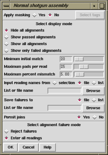
206 The Staden Package Manual
It takes one reading at a time and compares it with all the data already assembled in the
database. If a reading matches it is aligned. If the alignment is good enough the reading is
entered into the database. If a reading aligns well with two contigs it is entered into one of
them, then the two contigs are compared. If they align well they are joined. If the reading
does not match it starts a new contig. If a reading matches but does not align well it can
either be entered as a new contig or rejected.
A submode allows tagged regions of contigs to be masked and hence restricts the areas
into which data is entered. Users select the types of tags to be used as masks. As outlined
above readings are compared in two stages: first the program looks for exact matches of
some minimum length, and then for each possible overlap it performs an alignment. If
the masking mode is selected the masked regions are not used during the search for exact
matches, but they are used during alignment. The effect of this is that new readings that
would lie entirely inside masked regions will not produce exact matches and so will not be
entered. However readings that have sufficient data outside of masked areas can produce
hits and will be correctly aligned even if they overlap the masked data. For this mode the
names of readings that do not produce matches are written to the error file with code 5.
Note that new readings that carry tags of the types being used for masking will be masked
only after they have been entered.
As explained above the user can select to "Apply masking", and if so, the "Select tags"
button will be activated and if it is clicked will bring up a dialogue to allow tag types to be
selected. See Section 2.20.9 [Tag Selector], page 304.
Chapter 2: Sequence assembly and finishing using Gap4 207
The "display mode"dialogue allows the type of output produced to be set. "Hide all
alignments"means that only the briefest amount of output will be produced. "Show passed
alignments"means that only alignments that fall inside the entry criteria will be displayed.
"Show all alignments"means that all alignments, including those that fail the entry criteria,
are displayed. "Show only failed alignments"displays alignments only for the readings that
fail the entry criteria. Adding text to the text output window will increase the processing
time.
When comparing each reading the program looks first for a "Minimum initial match",
and for each such matching region found it will produce an alignment. If the "Maximum
pads per read"and the "Maximum percent mismatch"are not exceeded the reading will
be entered. The maximum pads can be inserted in both the reading and the consensus. If
users agree we would prefer to swap the maximum pads criteria for a minimum overlap. i.e.
only overlaps of some minimum length would be accepted.
Assembly usually works on sets of reading names and they can be read from either a
"file"or a "list"and an appropriate browser is available to enable users to choose the name
of the file or list. If just a single reading is to be assembled choose "single"and enter the
filename instead of the file or list of filenames.
The routine writes the names of all the readings that are not entered to a "file"or a
"list"and an appropriate browser is available to enable users to choose the name of the file
or list. Occasionally it might be convenient to forbid joins between contigs to be made if a
new reading overlaps them both, but the default is to "Permit joins".
If a reading is found to match but does not align within the alignment criteria it can be
entered as a new contig or rejected. These two choices are described as "Enter all readings"
or "Reject failures". Pressing the "OK"button will start the assembly process.
Note that this option may require the parameter maxseq to be set beforehand (see
Section 2.20.3 [Set Maxseq], page 299). This parameter defines the maximum length of
consensus that can be created.
Typical output would be:
(Output removed to save space)
>>>>>>>>>>>>>>>>>>>>>>>>>>>>>>>>>>>>>>>>>>>>>>
Processing 51 in batch
Reading name xb61h12.s1
Reading length 104
Total matches found 2
Contig 9 position 590 matches strand -1 at position 1
Contig 36 position 92 matches strand -1 at position 1
Trying to align with contig 9
Percent mismatch 2.1, pads in contig 0, pads in gel 1
Percentage mismatch 2.1
590 600 610 620 630 640
Consensus TTGAAAAATTAAAAACTTTTTTTGAAAATAAAAAAGAGTGAAAGTAAAGTAAAAGACAAG
::::::::::::::::::::::::::::::::::::::::::::::::::::::::::::
208 The Staden Package Manual
Reading TTGAAAAATTAAAAACTTTTTTTGAAAATAAAAAAGAGTGAAAGTAAAGTAAAAGACAAG
1 11 21 31 41 51
650 660 670 680
Consensus TAGCATGTAAATCAACTAAAAATAACTAATATTTT
::::::::::::::::::::::::: ::::::::
Reading TAGCATGTAAATCAACTAAAAATAA,TAATATTT-
61 71 81 91
Trying to align with contig 36
Percent mismatch 0.0, pads in contig 0, pads in gel 0
Percentage mismatch 0.0
92 102
Consensus TTGAAAAATTAAAAACTTTT
::::::::::::::::::::
Reading TTGAAAAATTAAAAACTTTT
1 11
Overlap between contigs 36 and 9
Length of overlap between the contigs 111
Entering the new reading into contig 9
This gel reading has been given the number 47
Complementing contig 36
Complementing contig 9
Trying to align the two contigs
Percent mismatch 4.4, pads in contig 0, pads in gel 3
Percentage mismatch 5.3
86 96 106 116 126 136
Consensus AAAAGTTTTTAATTTTTCAATTGTTTGGGTGTTCCTTTGACTATTAGAAAAACACCCCCC
::::::::::::::::::::::::::::::::::::::::::::::::::: :: :::::
Consensus AAAAGTTTTTAATTTTTCAATTGTTTGGGTGTTCCTTTGACTATTAGAAAA,CA,CCCCC
1 11 21 31 41 51
146 156 166 176 186 196
Consensus TTGCTCCTGTTGTGCAATTTTTGTTTTAAGTTTTCAATC*TTT*TATTTTAATA
::::::::::::::::::::::::::::::::::: ::: ::: :::::: :::
Consensus TTGCTCCTGTTGTGCAATTTTTGTTTTAAGTTTTC-ATC,TTTTTATTTT-ATA
61 71 81 91 101 111
Editing contig 36
Completing the join between contigs 47 and 36
>>>>>>>>>>>>>>>>>>>>>>>>>>>>>>>>>>>>>>>>>>>>>>
(Output removed to save space)
Batch finished
100 sequences processed
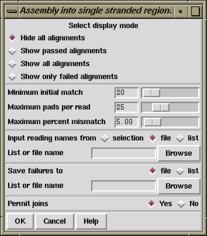
Chapter 2: Sequence assembly and finishing using Gap4 209
96 sequences entered into database
11 joins made
9 joins failed
2.7.1.1 Assemble Independently
This mode works in exactly the same way as normal shotgun assembly (see Section 2.7.1
[Normal Shotgun Assembly], page 205) with all its options and settings, except that the
new batch of data is assembled independently of all the data already in the database. This
means that the only overlaps found will be between the readings in the current batch. One
role for this mode would be to assemble a batch of data that was known from the way it
was produced (say a set of nested clones covering some problem region such as a repeat)
to overlap. Use of Assemble Independently will ensure that the batch of readings will only
be overlapped with one another, and will not be aligned with other similar regions of the
consensus. Once assembled in this way they can be joined to other contigs using Find
Internal Joins. See Section 2.8.3 [Find Internal Joins], page 227.
2.7.1.2 Assemble Into Single Stranded Regions
This mode works like normal assembly (see Section 2.7.1 [Normal Shotgun Assembly],
page 205) with masking, except that the masking is done for regions that already have
sufficient data on both strands of the sequence. This means that new readings will only be
assembled into regions that are single stranded or which border, and overlap, such segments.
Note that this means that readings that do not match are not entered, therefore those that
would actually lie between contigs are rejected.
The "display mode"dialogue allows the type of output produced to be set. "Hide all
alignments"means that only the briefest amount of output will be produced. "Show passed
alignments"means that only alignments that fall inside the entry criteria will be displayed.
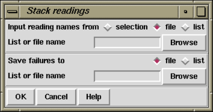
210 The Staden Package Manual
"Show all alignments"means that all alignments, including those that fail the entry criteria,
are displayed. "Show only failed alignments"displays alignments only for the readings that
fail the entry criteria.
When comparing each reading the program looks first for a "Minimum initial match",
and for each such matching region found it will produce an alignment. If the "Maximum
pads per read"and the "Maximum percent mismatch"are not exceeded the reading will
be entered. The maximum pads can be inserted in both the reading and the consensus. If
users agree we would prefer to swap the maximum pads criteria for a minimum overlap. i.e.
only overlaps of some minimum length would be accepted.
Assembly usually works on sets of reading names and they can be read from either a
"file"or a "list"and an appropriate browser is available to enable users to choose the name
of the file or list. If just a single reading is to be assembled choose "single"and enter the
filename instead of the file or list of filenames.
The routine writes the names of all the readings that are not entered to a "file"or a
"list"and an appropriate browser is available to enable users to choose the name of the file
or list. Occasionally it might be convenient to forbid joins between contigs to be made if a
new reading overlaps them both, but the default is to "Permit joins".
Pressing the "OK"button will start the assembly process.
Note that this option may require the parameter maxseq to be set beforehand (see
Section 2.20.3 [Set Maxseq], page 299). This parameter defines the maximum length of
consensus that can be created.
2.7.1.3 Stack Readings
This assembly mode assumes that all the readings are already aligned and simply stacks
them on top of one another in a new contig.
Assembly usually works on sets of reading names and they can be read from either a
"file"or a "list"and an appropriate browser is available to enable users to choose the name
of the file or list. If just a single reading is to be assembled choose "single"and enter the
filename instead of the file or list of filenames.
The routine writes the names of all the readings that are not entered to a "file"or a
"list"and an appropriate browser is available to enable users to choose the name of the file
or list.
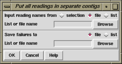
Chapter 2: Sequence assembly and finishing using Gap4 211
2.7.1.4 Put All Readings In Separate Contigs
This algorithm simply loads the readings into the database without comparing them, each
starting a new contig. This can be of use to those employing the database for storage rather
than assembly.
Assembly usually works on sets of reading names and they can be read from either a
"file"or a "list"and an appropriate browser is available to enable users to choose the name
of the file or list. If just a single reading is to be assembled choose "single"and enter the
filename instead of the file or list of filenames.
The routine writes the names of all the readings that are not entered to a "file"or a
"list"and an appropriate browser is available to enable users to choose the name of the file
or list.
2.7.2 Directed Assembly
This assembly method assumes that a preprocessing program, such as an external assembly
engine, has been used to map the relative positions of the readings to within a reasonable
level of accuracy or tolerance. The assembly is "directed"by use of special "Assembly
Position"or AP records included in each reading’s experiment file. It is expected that
these AP records will be added to the experiment files by the preprocessing program, or by
a program which parses the output from such a program, and so the details given below are
not of interest to the average user.
The experiment file for each reading must contain a special "Assembly Position"or AP
line that defines the position at which to assemble the reading. The position is not defined
absolutely, but relative to any other reading (the "anchor reading") that has already been
assembled. The definition includes the name of the anchor reading, the sense of the new
reading, its offset relative to the anchor reading and the tolerance. i.e.:
AP anchor_reading sense offset tolerance
The sense is defined using +or - symbols.
The offset can be of any size and can be positive or negative. Offset positions are defined
from 0. i.e. the first base in a contig or a reading is base number 0.
For normal use tolerance is a non-negative value, and the first base of the new reading
must be aligned at plus or minus "tolerance"bases of "offset". If tolerance is zero, after
alignment the position must be exactly "offset"relative to the anchor reading. If tolerance
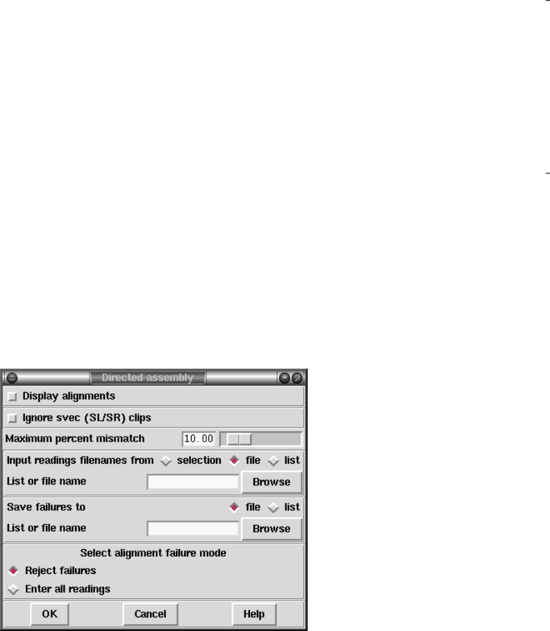
212 The Staden Package Manual
is negative then alignment is not performed and the reading is simply entered at position
"offset"relative to the anchor reading.
To start a new contig the reading must include an AP line containing the anchor reading
*new* and the sense.
Example AP line:
AP fred.021 + 1002 40
Example AP line to start a new contig:
AP *new* +
The algorithm is as follows. Get the next reading name, read the AP line, find the
anchor reading in the database, get the consensus for the region defined by anchor reading
+offset +/- tolerance. Perform an alignment with the new reading, check the position and
the percentage mismatch. If OK enter the reading.
Obviously the way the positions of readings are specified is very flexible but one example
of use would be to employ a file of file names containing a left-to-right ordered list of reading
names, with each reading using the one to its left as its anchor reading. In this way whole
contigs can be entered.
Although not specifically designed for the purpose this mode of assembly can be used
for "assembly onto template".
If required, the alignments can be shown in the Output window by selecting "Display
alignments". Only readings for which the "Maximum percent mismatch"after alignment
is not exceeded will be entered into the database, unless the "enter all readings"box is
checked. In that case a reading that does not match well enough will be placed in a
new contig. Specifying a "Maximum percent mismatch"of zero has a special meaning; it
implies that there should be no mismatches and so no alignments need to be performed,
and hence the consensus does not need to be computed either. For data that has already
been padded and aligned using an external tool (such as an external assembly program)
Chapter 2: Sequence assembly and finishing using Gap4 213
setting Maximum percent mismatch to zero can have a significant improvement in the speed
of Directed Assembly.
The “Ignore svec (SL/SR) clips” option controls whether sequencing vector clip points
should be considered when setting the hidden data sections for the sequence. With this
option enabled only the quality clip (QL/QR) experiment file records will be used.
Assembly usually works on sets of reading names and they can be read from either a
"file"or a "list"and an appropriate browser is available to enable users to choose the name
of the file or list. If just a single reading is to be assembled choose "single"and enter the
filename instead of the file or list of filenames.
The routine writes the names of all the readings that are not entered to a "file"or a
"list"and an appropriate browser is available to enable users to choose the name of the file
or list.
It is important to note that the algorithm assumes that readings are entered in the
correct order, i.e. a reading can only be entered into the defined AP position after the
reading relative to which its position is defined. The order of the readings is defined by the
order in the list or file of file names, and hence should be ordered by the external assembly
engine. But if the browser is used to select a batch of sequences, they are unlikely to be
in the correct order by chance, so care must be taken in its use. If reading X specifies an
anchor reading that has not been entered the algorithm will start a new contig starting with
X.
2.7.3 Screen Only
This function is used to compare a batch of readings against the data in an assembly
database without entering them. It performs "normal shotgun assembly"and records the
percentage mismatch for each matching reading in a file. If required, this file could then
be sorted on percentage mismatch and used as a file of file names for "normal shotgun
assembly"; in which case the best matches would be entered first. The readings in the
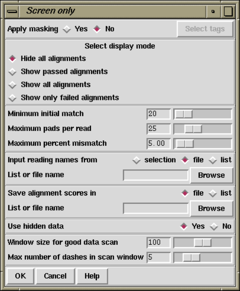
214 The Staden Package Manual
batch are only compared to the current contents of the assembly database, and are not
compared against the other readings in the batch.
As explained in normal assembly (see Section 2.7.1 [Normal Shotgun Assembly],
page 205) the user can select to "Apply masking", and if so, the "Select tags"button will
be activated and if it is clicked will bring up a dialogue to allow tag types to be selected.
See Section 2.20.9 [Tag Selector], page 304.
The "display mode"dialogue allows the type of output produced to be set. "Hide all
alignments"means that only the briefest amount of output will be produced. "Show passed
alignments"means that only alignments that fall inside the entry criteria will be displayed.
"Show all alignments"means that all alignments, including those that fail the entry criteria,
are displayed. "Show only failed alignments"displays alignments only for the readings that
fail the entry criteria.
When comparing each reading the program looks first for a "Minimum initial match",
and for each such matching region found it will produce an alignment. If the "Maximum
pads per read"and the "Maximum percent mismatch"are not exceeded the reading will
be entered. The maximum pads can be inserted in both the reading and the consensus. If
users agree we would prefer to swap the maximum pads criteria for a minimum overlap. i.e.
only overlaps of some minimum length would be accepted.
Screening usually works on sets of reading names and they can be read from either a
"file"or a "list"and an appropriate browser is available to enable users to choose the name
Chapter 2: Sequence assembly and finishing using Gap4 215
of the file or list. If just a single reading is to be assembled choose "single"and enter the
filename instead of the file or list of filenames.
The routine writes the names of all the readings and their alignment scores expressed
as percentage mismatches to a "file"or a "list"and an appropriate browser is available to
enable users to choose the name of the file or list.
Previous versions of the package also had the ability to search for matches in the "hidden"
poor quality data at the ends of contigs. This feature is no longer available.
Note that this option may require the parameter maxseq to be set beforehand (see
Section 2.20.3 [Set Maxseq], page 299). This parameter defines the maximum length of
consensus that can be created.
2.7.4 General Comments and Tips on Assembly
The program has several methods for assembly and it may not be obvious which is most ap-
propriate for a given problem. The following notes may help. They also contain information
on methods for checking the correctness of an assembly.
If you have access to an external program that can generate the order and approximate
positions of readings then Directed Assembly can be used. The same is true if the ex-
perimental method used generates an ordered set of readings (see Section 2.7.2 [Directed
Assembly], page 211).
If you have access to a external global assembly program that can produce an assembly
and write out correct experiment files then Directed Assembly can still be used by specifying
a"tolerance"of -1 (in the experiment file AP lines).
For routine shotgun assembly of whole data-sets or incremental data-sets Normal Shot-
gun Assembly can be used. Through the idea of "Masked assembly"this option also can
also restrict the assembly to particular regions of the consensus (see Section 2.7.1 [Normal
shotgun assembly], page 205).
Note that Normal shotgun assembly (see Section 2.7.1 [Normal Shotgun Assembly],
page 205), Assemble independently (see Section 2.7.1 [Assembly Independently], page 205),
Assembly into single stranded regions (see Section 2.7.1.2 [Assembly Single], page 209),
Screen only (see Section 2.7.3 [Screen Only], page 213), Put all readings in separate contigs
(see Section 2.7.1.4 [Assembly new], page 211), may require the parameter maxseq to be
set beforehand (see Section 2.20.3 [Set Maxseq], page 299). This parameter defines the
maximum length of consensus that can be created. If you find that the assembly process is
only entering the first few hundred of a batch of readings, try increasing maxseq.
If you have a batch of readings that are known to overlap one another, but which, due
to repeats, may also match other places in the consensus, then it can be helpful to use
Assemble Independently. This will ensure that the batch of readings are compared only
to one another, and hence will not be assembled into the wrong places (see Section 2.7.1.1
[Assemble independently], page 209).
Almost all readings are assembled automatically in their first pass through the assembly
routine. Those that are not can be dealt with in two ways. Either they can be put through
assembly again with less stringent parameters, or entered using the "Put all readings in
216 The Staden Package Manual
new contigs"routine and then joined to the contig they overlap using Find Internal Joins
See Section 2.8.3 [Find Internal Joins], page 227.. If it is found that readings are not being
assembled in their first pass through the assembler, then it is likely that the contigs require
some editing to improve the consensus. Also it may be that poor quality data is being used,
possibly by users over-interpreting films or traces. In the long term it can be more efficient
to stop reading early and save time on editing. For those using fluorescent sequencing
machines the unused data can be incorporated after assembly using the Contig Editor and
Double Strand.
An independent and important check on assembly is obtained by sequencing both ends
of templates. Providing the correct information is given in the experiment files gap can
check the positions and orientations of readings from the same template (see Section 2.8.2
[Find read pairs], page 222). Any inconsistencies are shown both textually and graphically.
In addition this information can be used to find possible joins between contigs.
2.7.5 Assembly Failure Codes
0The reading file was not found or is of invalid format
1The reading file was too short (less than the minimum match length)
2The reading appeared to match somewhere but failed to align sufficiently well
(too many padding characters or too high a percentage mismatch)
3A reading of the same name was already present in the database
4This error number is no longer used
5During a masked assembly, no sequence match with this reading was found.
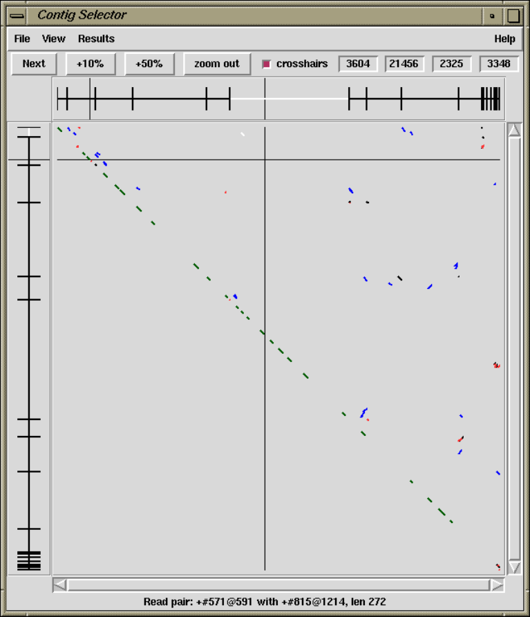
Chapter 2: Sequence assembly and finishing using Gap4 217
2.8 Ordering and Joining Contigs
After the initial rounds of assembly it is likely that the data for a sequencing project will
still not be contiguous. In order to minimise the number of experiments required to finish
the project it is useful to be able to get as much from the existing data as possible. The
functions described in this section can help to get the current set of contigs into a consistent
left to right order, can discover joins between contigs which were missed or overlooked by
the assembly engines, and can help in the analysis of repeats which may cause problems for
assembly. It is one of the strengths of gap4 that the results from several of these independent
types of analysis can be combined in a single display (see Section 2.4 [Contig Comparator],
page 126), and where they are seen to reinforce one another, users can feel more confident
in their decisions.
218 The Staden Package Manual
A typical Contig Comparator display is shown in the figure above. It is showing results
from other functions, as well as the ones described in this section.
The first function (see Section 2.8.1 [Order Contigs], page 219) automatically orders
contigs based on read-pair data. The orderings found can be examined in the Template
Display (see Section 2.5.1 [Template Display], page 130)
The next function (see Section 2.8.2 [Find read pairs], page 222) also examines read-pair
data, but instead of automatically ordering the contigs, plots out their relationships in the
Contig Comparator, from where the user can invoke the Template Display to check them,
and use the Contig Selector to reorder them.
Sometimes assembly engines will miss or regard some weak joins as too uncertain to be
made. The Find Internal Joins function (see Section 2.8.3 [Find Internal Joins], page 227),
compares contigs, including their hidden data, to find matches between the ends of contigs.
Again results are presented in the Contig Comparator, and users can invoke the Contig
Joining Editor (see Section 2.6.15 [The Join Editor], page 196) to examine and make joins.
Whereas Find Internal Joins makes sure that alignments between contigs continue right
to their ends, another search, Find Repeats (see Section 2.8.4 [Find Repeats], page 233) finds
any identical segments of sequence, wherever they lie in the consensus. This has several
uses. It gives another way of finding potential joins, and it provides a way of anotating
(tagging) repeats so that their positions are obvious to users, and can be taken into account
by other search procedures. Again results are presented in the Contig Comparator, and
users can invoke the Contig Joining Editor (see Section 2.6.15 [The Join Editor], page 196)
to examine and make joins.
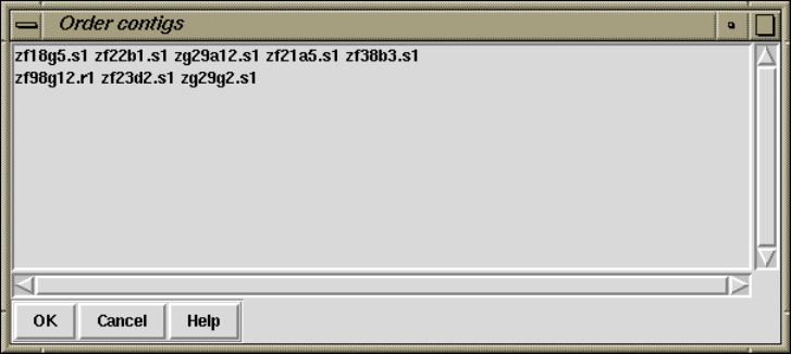
Chapter 2: Sequence assembly and finishing using Gap4 219
2.8.1 Order contigs
This routine uses read-pair information to try to work out the left to right order of sets of
contigs. It is invoked from the gap4 Edit menu. At present it attempts to order all the
contigs in the database, and when finished it produces a listbox window which containing
one or more sets (one set per line) of contigs listed by the names of their leftmost readings.
By clicking on their names in the listbox the user can request that these "super contigs"
should be shown in the standard Template display window (see Section 2.5.1 [Template
Display], page 130).
Using the tools available within this window the user can manually move or complement
any contigs which appear to have been misplaced. The combination of automatic ordering
and the facility to view the results by eye and manually correct any errors make this a
powerful tool. The new contig order can be saved to the database by selecting the "Update
contig order"command from the "Edit"menu of the Template display. Note, however, that
unlike the editing operations in the Contig editor, which are only committed to the disk
copy of the database at the user’s request, all the complementing operations in gap4 are
always performed both in memory and on the disk. This means that any complementing
done as part of the contig ordering process will be immediately committed to disk.
An example of the "Super contig"listbox is shown here.
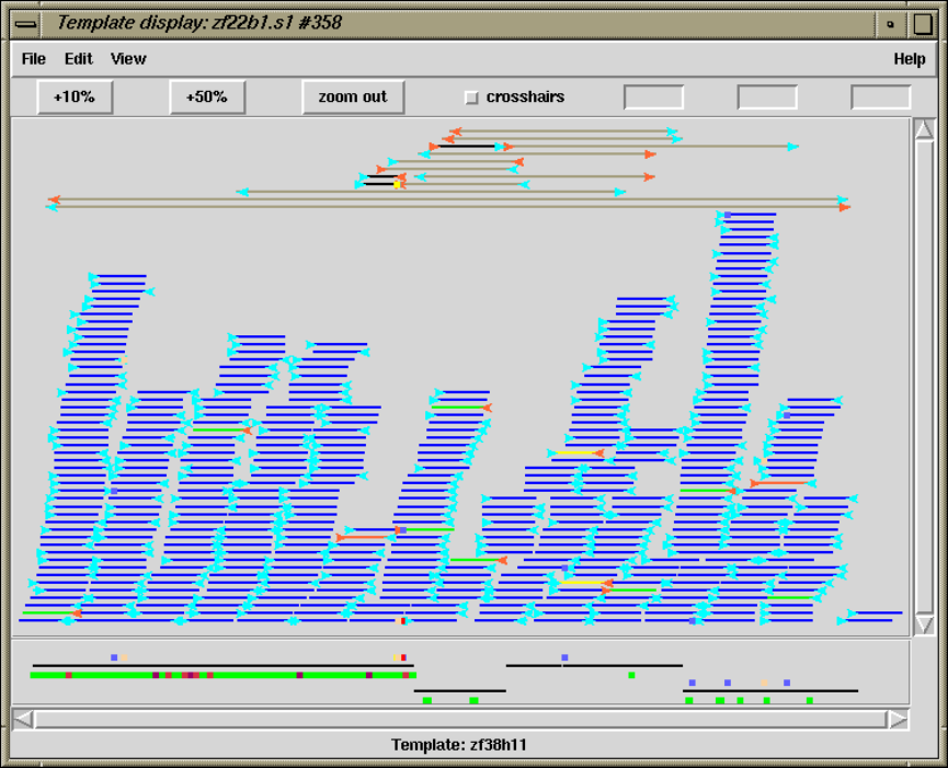
220 The Staden Package Manual
The example seen in the figures shows a Template display before and after the application
of the algorithm.
Before ordering
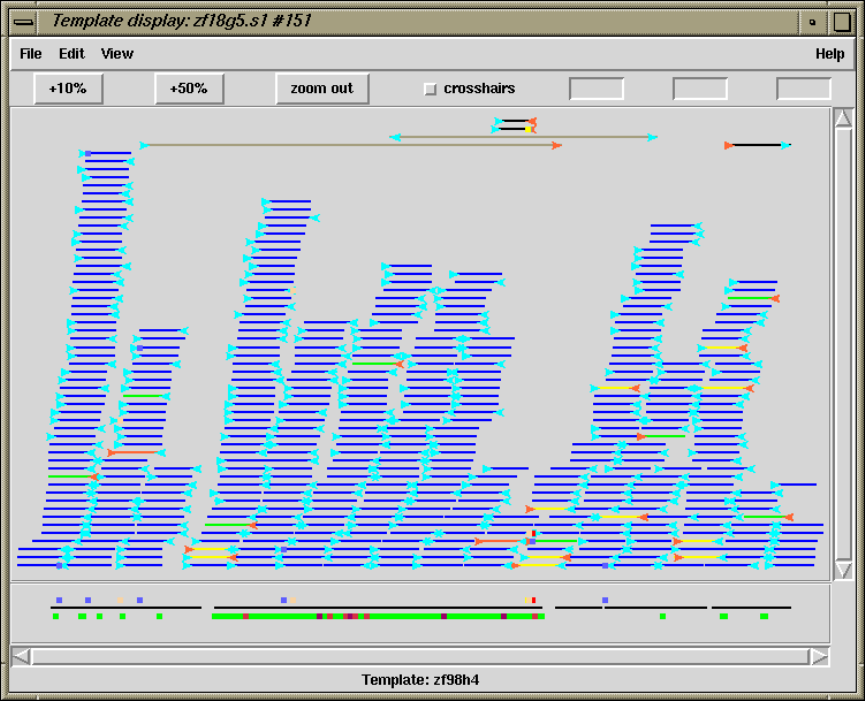
Chapter 2: Sequence assembly and finishing using Gap4 221
After ordering
Notice how the operation has reduced the large number of dark yellow (inconsistent)
templates by ordering and complementing the contigs so that they are now consistent and
show in bright yellow. The few remaining dark yellow templates represent problems, pos-
sibly with misassembly or with misnaming of readings. The reliability of these dark yellow
templates is also questionable when noting that one or the other of the readings are typically
within the middle of large contigs, and hence are not likely to be spanning contigs. The
gaps between the contigs, shown in the ruler at the bottom of the template display, are real
estimates of size of the missing data, based on the expected lengths of the templates.
The algorithm is based on ideas used to build cosmid contigs using hybridisation data
Zhang,P, Schon,EA, Fischer,SG, Cayanis,E, Weiss,J, Kistler,S and Bourne,P, (1994) "An
algorithm based on graph theory for the assembly of contigs in physical mapping of DNA",
CABIOS 10, 309-317. A difficulty for algorithms of this type is dealing with errors in the
data, i.e. pairs of readings that have been incorrectly assigned to the same template (often
by simple typing errors made prior to the creation of the experiment files). Our algorithm
uses several simple heuristics to deal with such problems but one known problem is that
it does not correctly deal with cases where templates span non-adjacent contigs, or where
such contigs interleave.
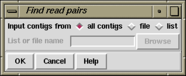
222 The Staden Package Manual
2.8.2 Find Read Pairs
This function is used to check the positions and orientations of readings taken from the
same templates. It is invoked from the gap4 View menu.
For each template the relative position of its readings and the contigs they are in are
examined. This analysis can give information about the relative order, separation and
orientations of contigs and also show possible problems in the data. The search can be
over the whole database or a subset of contigs named in a list (see Section 2.14 [Lists],
page 278) or file of file names. The results are written to the Output Window and plotted
in the Contig Comparator (See Section 2.4 [Contig Comparator], page 126.). Read pair
information is also used to colour code the results displayed in the Template Display (see
Section 2.5.1 [Template Display], page 130).
Note that during assembly the template names and lengths are copied from the exper-
iment files into the gap database. See Section 11.3 [Experiment Files], page 552. The
accuracy of the lengths will depend upon some size selection being performed during the
cloning procedures.
Users choose to process "all contigs"or a subset selected from a file of file names ("file")
or a list ("list"). If either of the subset options is selected the "browse"button will be
activated and can be clicked on to call up a file or list browser dialogue.
2.8.2.1 Find Read Pairs Graphical Output
The contig comparator is used to plot all templates with readings that span contigs. That
is, the lines drawn on the contig comparator are a visual representation of the relationship

Chapter 2: Sequence assembly and finishing using Gap4 223
(orientation and overlap) between contigs. When a template spans more than two contigs,
all the combinations of pairs of contigs are plotted. However such cases are uncommon.
The figure above shows a typical Contig Comparator plot which includes several types
of result in addition to those from Read Pair analysis.
The lines for the read-pairs are, by default, shown in blue. The length of the line is the
average length of the two readings within the pair. The slope of the line represents the
relative orientation of the two readings. If they are both the same orientation (including
both complemented) the line is drawn from top left to bottom right, otherwise the line is
drawn from top right to bottom left.
224 The Staden Package Manual
Clicking with the right mouse button on a read pair line brings up a menu containing,
amongst other things, "Invoke template display"(see Section 2.5.1 [Template Display],
page 130). This creates a template display of the two contigs. The spanning template will
be coloured bright yellow if the readings on the template are consistent with one another,
or dark yellow if they are not. The ordering of the contigs may need to be altered, or one
contig may need complementing, before the readings on the template become consistent.
Using the "Invoke join editor"command (see Section 2.6.15 [The Join Editor], page 196)
from the same menu will bring up the Join Editor with the two contigs shown end to end.
2.8.2.2 Find Read Pairs Text Output
Two types of results are written to the Output Window: those containing apparently con-
sistent data about the relative orientations and positions of contigs, and those that show
inconsistencies in the data. The inconsistencies will be due to misassembly or to misnaming
of readings and templates.
In the Output Window the program writes a line of information for each template and a
line of information for each reading from that template. In order to restrict this information
to fit on a standard 80 column display a few abbreviations are used. An example for two
consistent and one problematic template is shown below. Templates with possible problems
are separated from those without. The templates shown are sorted by problem; consistent
templates at the top followed by increasingly inconsistent templates at the bottom.
Template zf18c8( 117), length 1400-2000(expected 1700)
Reading zf18a2.s1( +1F), pos 5620 +91, contig 46
Reading zf18c8.s1( -117F), pos 1084 +288, contig 127
Template zf98f4( 659), length 1400-2000(computed 7263)
Reading zf98f4.s1( -659F), pos 27 +238, contig 548
Reading zf98f4.r1( +800R), pos 5392 +211, contig 46
*** Possibly problematic templates listed below ***
Template zf24g6( 262), length 1400-2000(observed 1365)
D Reading zf24g6.r1( +808R), pos 463 +206, contig 46
D Reading zf24g6.s1( -262F), pos 1559 +268, contig 46
2.8.2.3 The Template Lines
To describe the format of the template line we provide a detailed explanation of the lines
above for the last Template block.
"Template zf24g6( 262)"
This is template with name "zf24g6"and number 262.
length 1400-2000
These are the minimum and maximum lengths specified for this template.
observed(1365)
This section has the general format of "comment(distance)", where "comment"
is one of the following.
Chapter 2: Sequence assembly and finishing using Gap4 225
observed The template has both forward and reverse readings within this
contig. From this information the actual size of the template can
be seen. In the example this is "1365".
expected The template length is estimated as the average of the specified
minimum and maximum size. This will be seen when the template
does not span contigs and does not have both forward and reverse
primers visible.
computed The template has forward and reverse readings in different contigs.
The length is computed by butting the two contigs together, end
to end, and finding the resultant separation of the template ends.
It is not possible to tell whether the two contigs overlap, and if
so by how much. Hence the "computed"lengths should not be
considered as absolute.
2.8.2.4 The Reading Lines
"?DPS" The first four characters may be either space or one of "?","D","P"or "S".
The meaning of each of these is as follows.
?No primer information is available for these readings.
DThe distance between forward and reverse primers (ie the template
length) is not as expected.
PThe primer information for readings on this template is inconsis-
tent. An example of this is where two forward readings exist, both
using the universal primer, and the readings are not in close prox-
imity to each other.
SThe template strand information is inconsistent. This problem can
be seen when the forward and reverse readings are from the same
strand, or two forward readings are pointing in opposite directions.
Absence of all of these characters means that the template is consistent.
"Reading zf24g6.r1"
The reading name
"( +808R)"
The reading number. The "+" or "-"character preceding the number represents
whether the reading has been complemented ("+" for original, "-"for comple-
mented). The letter following the number indicates the primer information
found for this reading. It may be one of:
?Unknown
FForward, universal primer
fForward, custom primer (eg a walk)
RReverse, universal primer
rReverse, custom primer
226 The Staden Package Manual
"pos 463 +206"
The position and the length of the reading within the contig. In this case the
reading starts at position 463 and extends for 206 bases. For a complemented
reading the position marks the 3’ end of the reading. For both cases the position
can be considered as the ’left end’ of the reading as displayed within the contig.
"contig 46"
The reading number of the left most reading within this contig.
In the above example the template has two readings. It can be seen that the template
starts at contig position 463 and finishes at position 1827. The observed length is 1365,
which is just below the expected minimum length of 1400. Hence the template is flagged
as having an invalid distance. There are no other inconsistencies for this template and so
it is likely that the only "problem"is that the experimental size selection process was not
as precise as was thought.
Chapter 2: Sequence assembly and finishing using Gap4 227
2.8.3 Find Internal Joins
The purpose of this function (which is invoked from the gap4 View menu) is to use sequences
already in the database to find possible joins between contigs. Generally these will be joins
that were missed or judged to be unsafe during assembly and this function allows users to
examine the overlaps and decide if they should be made. During assembly joins may have
been missed because of poor data, or not been made because the sequence was repetitive.
Also it may be possible to find potential joins by extending the consensus sequences with
the data from the 3’ ends of readings which was considered to be too unreliable to align
during assembly i.e. we can search in the "hidden data".
If it has not already occurred, use of this function will automatically transform the
Contig Selector into the Contig Comparator. Each match found is plotted as a diagonal
line in the Contig Comparator, and is written as an alignment in the Output Window. The
length of the diagonal line is proportional to the length of the aligned region. If the match
is for two contigs in the same orientation the diagonal will be parallel to the main diagonal,
if they are not in the same orientation the line will be perpendicular to the main diagonal.
The matches displayed in the Contig Comparator can be used to invoke the Join Editor (see
Section 2.6.15 [The Join Editor], page 196) or Contig Editor. See Section 2.6 [Editing in
gap4], page 160. Alternatively, the "Next"button at the top left of the Contig Comparator
can be used to select each result in turn, starting with the best, and ending with the worst.
When this is in use, users can find the match in the Contig Comparator which corresponds
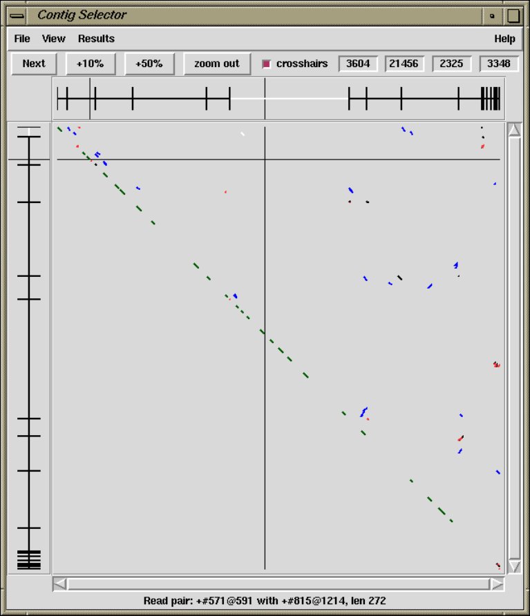
228 The Staden Package Manual
to the next result by placing the cursor over the Next button. The plotted match and the
contigs involved will turn white.
A typical display from the Contig Comparator is shown in the figure above.
To define the match all numbering is relative to base number one in the contig: matches
to the left (i.e. in the hidden data) have negative positions, matches off the right end of
the contig (i.e. in the hidden data) have positions greater than that of the contig length.
The convention for reporting the positions of overlaps is as follows: if neither contig needs
to be complemented the positions are as shown. If the program says "contig x in the -
sense"then the positions shown assume contig x has been complemented. For example, in
Chapter 2: Sequence assembly and finishing using Gap4 229
the results given below the positions for the first overlap are as reported, but those for the
second assume that the contig in the minus sense (i.e. 443) has been complemented.
Possible join between contig 445 in the + sense and contig 405
Percentage mismatch after alignment = 4.9
412 422 432 442 452 462
405 TTTCCCGACT GGAAAGCGGG CAGTGAGCGC AACGCAATTA ATGTGAG,TT AGCTCACTCA
::::::::: : :::::::: ::::: ::: :::::::::: :::::::::: ::::::::::
445 *TTCCCGACT G,AAAGCGGG TAGTGA,CGC AACGCAATTA ATGTGAG*TT AGCTCACTCA
-127 -117 -107 -97 -87 -77
472 482 492 502 512
405 TTAGGCACCC CAGGCTTTAC ACTTTATGCT TCCGGCTCGT AT
:::::::::: :::::::::: :::::::::: :::::::::: ::
445 TTAGGCACCC CAGGCTTTAC ACTTTATGCT TCCGGCTCGT AT
-67 -57 -47 -37 -27
Possible join between contig 443 in the - sense and contig 423
Percentage mismatch after alignment = 10.4
64 74 84 94 104 114
423 ATCGAAGAAA GAAAAGGAGG AGAAGATGAT TTTAAAAATG AAACG*CGAT GTCAGATGGG
:::: ::::: :::::::::: :::::::::: :::::: :: ::::: :::: :::::::::
443 ATCG,AGAAA GAAAAGGAGG AGAAGATGAT TTTAAA,,TG AAACGACGAT GTCAGATGG,
3610 3620 3630 3640 3650 3660
124 134 144 154 164
423 TTG*ATGAAG TAGAAGTAGG AG*AGGTGGA AGAGAAGAGA GTGGGA
::: :::::: :::::::::: :: ::::::: ::: ::::: :: ::
443 TTGGATGAAG TAGAAGTAGG AGGAGGTGGA ,GAG,AGAGA GTTGG*
3670 3680 3690 3700 3710
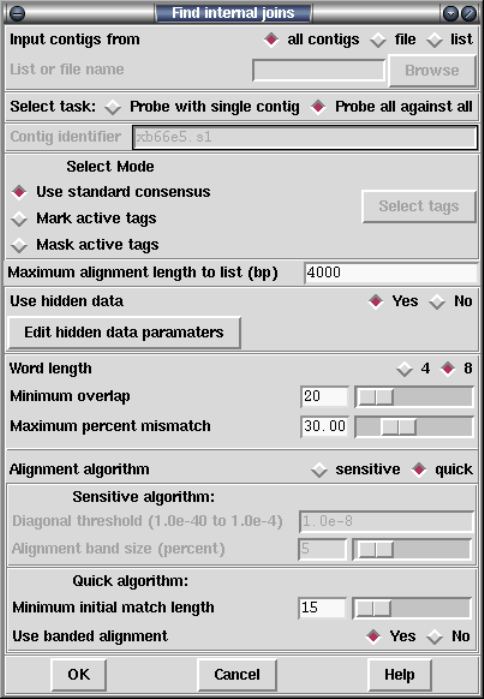
230 The Staden Package Manual
2.8.3.1 Find Internal Joins Dialogue
The contigs to use in the search can be defined as "all contigs", a list of contigs in a file
"file", or a list of contigs in a list "list". If "file"or "list"is selected the browse button
is activated and gives access to file or list browsers. Two types of search can be selected:
one, "Probe all against all"compares all the contigs defined against one another; the other
"Probe with single contig", compares one contig against all the contigs in the list. If this
option is selected the Contig identifier panel in the dialogue box is ungreyed. Both sense of
the sequences are compared.
If users elect not to "Use standard consensus"they can either "Mark active tags"or
"Mask active tags", in which cases the "Select tags"button will be activated. Clicking on
this button will bring up a check box dialogue to enable the user to select the tags types
they wish to activate. Masking the active tags means that all segments covered by tags that
are "active"will not be used by the matching algorithms. A typical use of this mode is to
avoid finding matches in segments covered by tags of type ALUS (ie segments thought to
be Alu sequence) or REPT (ie segment that are known to be repeated elsewhere in the data
(see Section 2.2.7.1 [Tag types], page 121). "Marking"is of less use: matches will be found
Chapter 2: Sequence assembly and finishing using Gap4 231
in marked segments during searching, but in the alignment shown in the Output Window,
marked segments will be shown in lower case.
Some alignments may be very large. For speed and ease of scrolling Gap4 does not
display the textual form of the longest alignments, although they are still visible within the
contig comparator window. The maximum length of the alignment to print up is controlled
by the “Maximum alignment length to list (bp)” control.
The default setting for the consensus is to "Use hidden data"which means that where
possible the contigs are extended using the poor quality data from the readings near their
ends. To ensure that this additional data is not so poor that matches will be missed, the
program uses algorithms which can be configured from the "Edit hidden data parameters"
dialogue. Two algorithms are available. Both slide a window along the reading until a set
criteria is met. By default an algorithm which sums confidence values within the window is
used. It stops when a window with < "Minimum average confidence"is found. The other
algorithm counts the number of uncalled bases in the window and stops when the total
reaches "Max number of uncalled bases in window". The selected algorithm is applied to
all the readings near the ends of contigs and the data that extends the contig the furthest
is added to its consensus sequence.
If your total consensus sequence length (including a 20 character header for each contig
that is used internally by the program) plus any hidden data at the ends of contigs is greater
than the current value of a parameter called maxseq, Find Internal Joins may produce an
error message advising you to increase maxseq. Maxseq can be set on the command line
(see Section 2.21 [Command line arguments], page 306) or by using the options menu (see
Section 2.20.3 [Set Maxseq], page 299).
The search algorithms first finds matching words of length "Word length", and only
considers overlaps of length at least "Minimum overlap". Only alignments better than
"Maximum percent mismatches"will be reported.
There are two search algorithms: "Sensitive"or "Quick". The quick algorithm should
be applied first, and then the sensitive one employed to find any less obvious overlaps.
The sensitive algorithm sums the lengths of the matching words of length "Word length"
on each diagonal. It then finds the centre of gravity of the most significant diagonals.
Significant diagonals are those whose probability of occurence is < "Diagonal threshold". It
then uses a dynamic programming algorithm to align around the centre of gravity, using a
band size of "Alignment band size (percent)". For example: if the overlap was 1000 bases
long and the percentage set at 5, the aligner would only consider alignments within 50 bases
either side of the centre of gravity. Obviously the larger the percentage and the overlap,
the slower the aligment.
The quick algorithm can find overlaps and align 100,000 base sequences in a few seconds
by considering, in its initial phase only matching segments of length "Minimum initial match
length". However it does a dynamic programming alignment of all the chunks between
the matching segments, and so produces an optimal alignment. Again a banded dynamic
algorithm can be selected, but as this only applies to the chunks between matching segments,
which for good alignments will be very short, it should make little difference to the speed.
232 The Staden Package Manual
After the search the results will be sorted so that the best matches are at the top of a list
where best is defined as a combination of alignment length and alignment percent identity
(in some earlier Gap4 releases this was scored purely on percent identity). This list can be
stepped through, one result at a time using the Contig Joining Editor, by clicking on the
"Next"button at the top left of the Contig Comparator.
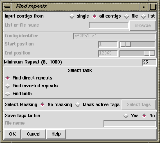
Chapter 2: Sequence assembly and finishing using Gap4 233
2.8.4 Find Repeats
The purpose of this function (which is invoked from the gap4 View menu) is to find exact
repeats in contig consensus sequences. An exact repeat is defined as a run of consecutive
identical ACGT characters; no mismatches or gaps are permitted.
If it has not already occurred, selection of this function will automatically transform
the Contig Selector into the Contig Comparator. See Section 2.4 [Contig Comparator],
page 126. Each match found is plotted as a diagonal line in the Contig Comparator. The
length of the diagonal line is proportional to the length of the match.
If the match is for two contigs in the same orientation the diagonal will be parallel to
the main diagonal, if they are not the line will be perpendicular to the main diagonal.
The matches displayed in the Contig Comparator can be used to invoke the Join Editor
(see Section 2.6.15 [The Join Editor], page 196) or Contig Editors (see Section 2.6 [Editing
in gap4], page 160), and an Information button will display data about the match in the
Output window. e.g.
Repeat match
From contig xb54a3.s1(#26) at 78
With contig xb62h3.s1(#3) at 1
Length 37
This means that position 78 in the contig with xb54a3.s1 (reading number 26) at its left
end matches 37 bases at position 1 in the contig with xb62h3.s1 (number 3) at its left end.
Users can elect to search a "single"contig, or compare "all contigs", or a subset of
contigs defined in a list or a file. If "file"or "list"is selected the browse button is activated
and gives access to file or list browsers. If they choose to analyse a single contig the
dialogue concerned with selecting the contig and the region to search becomes activated.
234 The Staden Package Manual
The "Minimum Repeat"defines the smallest match that the algorithm will report. The
algorithm will search only for repeats in the forward direction "Find direct repeats", or
only those in the reverse direction "Find inverted repeats", or both "Find both".
If "Mask active tags"is selected the "Select tags"button is activated. Clicking on this
button will bring up a check box dialogue to enable the user to select the tags types they
wish to activate. Masking the active tags means that all segments covered by tags that are
"active"will not be used in the matching algorithm. A typical use of this mode is to avoid
finding matches in segments covered by tags of type ALUS (ie segments thought to be Alu
sequence) or that already covered by REPT tags. See Section 2.2.7.1 [Tag types], page 121.
After the search is complete clicking on "Yes"in the "Save tags to file"panel will activate
the "File name"box and all repeats on the list will be written to a file. This file can be
used with "Enter tags"(see Section 2.12.2 [Enter Tags], page 265) to create REPT tags
for all the repeats found. Note that "Enter tags"will remove all the results plotted in the
contig comparator.
Note that the current version of Find Repeats has a limit to the number of repeats it
can store. The limit depends on the current maximum consensus length, so if you want to
increase the limit, reset the maximum consensus length. This can be done using the "Set
maxseq"item in the "Options"menu.
Chapter 2: Sequence assembly and finishing using Gap4 235
2.9 Checking Assemblies and Removing Readings
After assembly, and prior to editing, it can be useful to examine the quality of the alignments
between individual readings and the sections of the consensus which they overlap. This may
reveal doubtful joins between sections of contigs, poorly aligned readings, or readings that
have been misplaced. By using this analysis in combination with other gap4 functions such
as Find internal joins (see Section 2.8.3 [Find Internal Joins], page 227) and Find repeats (see
Section 2.8.4 [Find Repeats], page 233), it is also possible to discover if readings have been
positioned in the wrong copies of repeat elements. The functions for checking the alignment
of readings in contigs are described below. See Section 2.9 [Checking Assemblies], page 236.
If readings are found to be misplaced or need removing for other reasons, gap4 has func-
tions for breaking contigs (see Section 2.9.1.1 [Breaking Contigs], page 239), and removing
readings (see Section 2.9.1.2 [Disassembling Readings], page 240). These functions can be
accessed through the main gap4 Edit menu or from within the Contig Editor.
If readings are removed from contigs to start new contigs of one reading, these contigs can
then be processed by Find internal joins (see Section 2.8.3 [Find Internal Joins], page 227)
and the Join editor (see Section 2.6.15 [The Join Editor], page 196), which should reveal all
the other positions at which the reading matches.
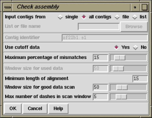
236 The Staden Package Manual
2.9.0.1 Checking Assemblies
The Check Assembly routine (which is invoked from the gap4 View menu) is used to check
contigs for potentially misassembled readings by comparing them against the segment of
the consensus which they overlap. It has two modes of use: the first simply counts the
percentage mismatch between each reading and the consensus it overlaps, and the second
performs an alignment between the hidden data for a reading and the consensus it overlaps.
If the percentage is above a user defined maximum, a result is produced. That is, one mode
compares the "visible"part of the readings, and the other aligns and compares the hidden
data. Results are displayed in the Output Window and plotted on the main diagonal in the
Contig Comparator. See Section 2.4 [Contig Comparator], page 126.
From the Contig Comparator the user can invoke the Contig Editor to examine the
alignment of any problem reading. See Section 2.6 [Editing in gap4], page 160. If the
reading appears to be correctly positioned the user can either edit it, or in the case of poor
alignment of the hidden data, place a tag, so that it does not produce a result if the search
is done again. Note however such data will then also be ignored by the automatic double
stranding routine. See Section 2.10.1 [Double Stranding], page 241. A typical textual output
from the analysis of hidden data is shown below.
Reading 802(fred.s1) has percentage mismatch of 25.86
375 385 395 405 415 425
Reading *CCTGTTTTAAATTG-TGG-C-CCCG*-TTAACCGGGGT*CAAC**CTGGGTTGCTTA
: ::::: :::::: :: : ::::: ::: ::: :::::: ::::: ::::: :
Consensus ACATGTTT*AAATTGATGAACACCCG*AATAAACGGTGT*CAAAA*CTGGATTGCTAA
2929 2939 2949 2959 2969 2979
Users select either to search only one contig ("single"), all contigs ("all contigs"), or a
subset of contigs contained in a "file"or a "list". If "file"or "list"is selected the "browse"
button will be activated and clicking on it will invoke a file or list browser. If a single contig
is selected the "Contig identifier"dialogue will be activated and users should enter a contig
name.
Chapter 2: Sequence assembly and finishing using Gap4 237
Selecting between analysing the visible or hidden data is done by clicking on "yes"or
"no"in the "Use cutoff data"dialogue. All alignments that are worse than "Maximum
percentage of mismatches"will produce a result in the Output Window and the Contig
Comparator. If "Use cutoff data"is selected then dialogue to enable the user to restrict the
quality and length of the hidden data that the program aligns is activated. First, to avoid
finding very short mismatching regions (where percentage mismatch figures could be very
high) users can set a "Minimum length of alignment"figure. Secondly to ensure that the
hidden data is not so bad that alignments will necessarily be poor, the program uses the
following algorithm. It slides a window of size "Window size for good data scan"along the
hidden data for each reading and stops if it finds a window that contains more than "Max
dashes in scan window"non-ACGT characters.
To check the used data for each reading ("Use cutoff data"is set to "No") the program
compares all segments of size ’window’ against the consensus sequence that they lie above
(obviously no alignment is required). If the percentage mismatch within any segment is
above the specified amount, then the entire ’alignment’ of the reading and consensus is
displayed. Note that in the output the program will first give the percentage mismatch
over the window length, and then the percentage over the whole reading. To check the
overall percentage mismatch of readings, simply set the "Window size for used data"to be
longer than the reading lengths. To check for divergence of segments within readings set
the window size accordingly.
The "Information"window produced by selecting "Information"from the Contig Com-
parator "Results"menu produces a summary of the results sorted in order os percentage
mismatch.
By clicking with the right mouse button on results plotted in the Contig Comparator
a pop-up menu is revealed which can be used to invoke the Contig Editor (see Section 2.6
[Editing in gap4], page 160). The editor will start up with the cursor positioned on the
problem reading. If the reading is found to be misplaced it can be marked for removal
from within the Editor (see Section 2.6.7.12 [Remove Reading], page 179). However, prior
to this it may be beneficial to use some of the other analyses such as Find internal joins
(see Section 2.8.3 [Find Internal Joins], page 227) and Find repeats (see Section 2.8.4 [Find
Repeats], page 233), which may help to find its correct location. Both of these functions
produce results plotted in the Contig Comparator (see Section 2.4 [Contig Comparator],
page 126) and any alternative locations will give matches on the same vertical or horizontal
projection as the problem reading.
238 The Staden Package Manual
2.9.1 Removing Readings and Breaking Contigs
Occasionally contigs require more drastic changes than simple basecall edits. Sometimes it
is necessary to remove readings that have been put in the wrong place, or to break contigs
that should not have been joined. Gap4 contains functions to help with these problems,
and two types of interface.
If a contig needs to be broken cleanly into two new contigs, with all the readings, other
than the two at the incorrect join, still linked together, then Break Contig (see Section 2.9.1.1
[Breaking Contigs], page 239), or (see Section 2.6.7.13 [Break Contig], page 179) should be
used. The former interface is available via the main gap4 Edit menu, and the latter as an
option in the Contig Editor.
If one or more readings need removing from from contig(s), even if their removal will
break the contiguity of a contig, then (see Section 2.9.1.2 [Disassemble Readings], page 240),
or (see Section 2.6.7.12 [Remove Reading], page 179) should be used. The former interface
is available via the main gap4 Edit menu, and the latter as an option in the Contig Editor.
Readings can be removed from the database completely, or moved to start individual new
contigs, one for each reading.
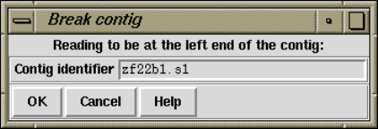
Chapter 2: Sequence assembly and finishing using Gap4 239
2.9.1.1 Breaking Contigs
The Break Contig function (which is available from the gap4 Edit menu) enables contigs to
be broken by removing the link between two adjacent readings. The user defines the name
or number of the reading that, after the break, will be at the left end of the new contig.
That is, the break is made between the named reading and the reading to its left.
It is also possible to interactive select places to break the contig when using the Contig
Editor. See Section 2.6.7.13 [Break Contig], page 179.
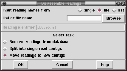
240 The Staden Package Manual
2.9.1.2 Disassembling Readings
This function is used to remove readings from a database or move readings to new contigs.
There are two interfaces which allow sets of readings to be disassembled. One is to identify
the readings interactively when using the Contig Editor (see Section 2.6.9 [Remove Read-
ings], page 186), and the other, described below, is available as a separate option from the
main gap4 Edit menu.
If readings are removed from the database all reference to them is deleted. If a reading
is moved to a “single-read contig” a new contig will be created containing this one single
reading, which may then be re-processed by Find Internal Joins (see Section 2.8.3 [Find In-
ternal Joins], page 227) and the Join editor (see Section 2.6.15 [The Join Editor], page 196),
which should reveal all the other positions at which the reading matches.
More useful is the general “Move readings to new contigs”. This will keep any assembly
relationships intact between the set of readings to be disassembled. For example if three
readings overlap then when disassembled all three will end up in a single new contig. This
function is particularly useful for pulling apart false joins or repeats.
The set of readings to be processed can be read from a “file” or a “list” and clicking on
the “browse” button will invoke an appropriate browser. If just a single reading is to be
assembled choose “single” and enter the reading name instead of the file or list of filenames.
Removal via a “list” is a particularly powerful option when controlled via the list gen-
eration functions within the contig editor. For example break contig could be viewed as
disassembling a list of readings selected using “Select this reading and all to right”.
Chapter 2: Sequence assembly and finishing using Gap4 241
2.10 Finishing Experiments
Gap4 contains several functions for helping to select experiments to finish an assembly
project. These functions (which are all available from the gap4 Experiments menu) are
able to automatically analyse the contigs to find the regions which need attention, and to
suggest appropriate experiments.
Prior to performing any experiments it can be worthwhile to try to make the most of
the existing data by moving the boundary between the hidden and visible data of readings
to cover single stranded readings. (see Section 2.10.1 [Double Strand], page 241)
The following "Experiment Suggestion"functions analyse the contigs to find problems,
and then suggest the best templates to use for further experiments.
Primers and templates for primer walking experiments can be suggested. (see
Section 2.10.2 [Suggest Primers], page 243). Sometimes resequencing on a long gel machine
will help to fill a single stranded region or join a pair of contigs. (see Section 2.10.3 [Suggest
Long Readings], page 245). Compressions and stops can be solved by resequencing using
an different chemistry. (see Section 2.10.4 [Compressions and Stops], page 247). In order
to select oligos to use as probes for clones near the ends of contigs a further function is
available. (see Section 2.10.5 [Suggest Probes], page 249).
2.10.1 Double Stranding
The purpose of this function (which is available from the gap4 Edits menu) is to use hidden
data to fill regions of contigs that have data on only one strand (see Section 2.2.6 [Use
of the "hidden"poor quality data], page 120). First the routine finds a region that has
data for only one strand. Then it examines the nearby readings on the other strand to
see if they have hidden data that covers the single stranded region. If so it finds the best
alignment between this hidden data and the consensus over the region. If this alignment is
good enough the data is converted from hidden to visible. This process is continued over
all the selected contigs. The function can be run on a subsection of a single contig, on all
contigs, or on a subset of contigs that are named in a file of a list.
Significant portions of the sequence can be covered by this operation, hence saving a
great deal of experimental work, and it can be used as a standard part of cleaning up a
sequencing project. However it must be noted that an increased number of edits may be
required after its application. The amount of cutoff data used depends on the number of
mismatches and the percentage mismatch in the alignment. That is, it depends on the
quality of the alignment, not the quality of the data: if it aligns it is assumed to be correct!
The program reports its progress in the Output window as shown in the following ex-
ample.
Wed 03:52:46 PM: double strand
------------------------------------------------------------
Double stranding contig xf48g3.s1 between 1 and 6189
Double stranded zf23b2.s1 by 121 bases at offset 3752
Double stranded zf18g11.s1 by 194 bases at offset 5652
Positive strand :
Double stranded 315 bases with 2 inserts into consensus
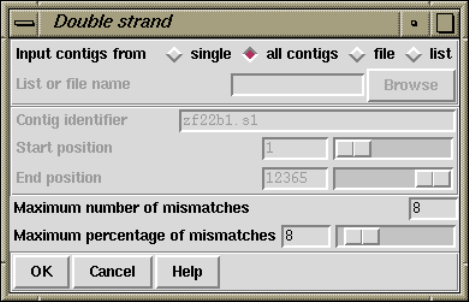
242 The Staden Package Manual
Filled 0 holes
Complementing contig 358
Double stranded zg29a11.s1 by 42 bases at offset 5265 - Filled
Double stranded zf38c7.s1 by 131 bases at offset 5015 - Filled
Negative strand :
Double stranded 174 bases with 1 insert into consensus
Filled 2 holes
The contigs to process can be a particular "single"contig, "all contigs", or a subset of
contigs whose names are stored in a "file"or a "list". If a file or list is selected the browse
button will be activated, and if it is clicked, an appropriate browser will be invoked. If the
user selects "single"then the dialogue for choosing the contig and the section to process
becomes active.
Only alignments with not more than "Maximum number of mismatches"and "Maximum
percentage of mismatches"will be accepted.
Chapter 2: Sequence assembly and finishing using Gap4 243
2.10.2 Suggest Primers
The purpose of this function (which is available from the gap4 Experiments menu) is to
suggest custom primer experiments to extend and "double strand"contigs. First the routine
finds regions of contigs with data on only one strand. Then it selects templates and primers,
which if used in sequencing experiments, would produce data to cover these single stranded
regions. This information is written to a file or a list and also appears in the Output window.
For each primer suggested a tag is automatically created containing the template name and
the sequence. See also Section 2.10.3 [Suggest Long], page 245, and Section 2.10.1 [Double
Strand], page 241.
The following example shows how the results appear in the Output window.
Wed 04:53:08 PM: Suggest Primers
------------------------------------------------------------
Selecting oligos for contig xf23a3.s1 between 1 and 12379
At 3873 - template zf23b2, primer GAAACTGGATAATACGAC, number 1
At 5847 - template zf18g11, primer CCTCCAATAGCGTGAAG, number 2
At 7924 - template zf22d11, primer GTAAAGTGTAATTCAAGGAAG, number 3
At 9033 - template zf97c10, primer ATGATAGAAATCTCGTGG, number 4
At 9972 - template zf98b5, primer GCGGAAAGTTGAAAGAG, number 5
At 10506 - template zg09a9, primer ACACATCATTTCGGAGG, number 6
At 10958 - template zf24c1, primer CAGTTTACGAGAAAGTCC, number 7
At 11529 - template zg29a12, primer ACCTTCCCAAAAGTTCC, number 8
At 11897 - template zf97d7, primer AACCCGATTTTCGTAATG, number 9
Complementing contig 358
At 11400 - template zf38b1, primer CGAAGACCCAAAGAAAG, number 11
At 9902 - template zf98a4, primer CTTTTCTCTTTCAACTTTCC, number 12
At 7104 - template zf22h10, primer GTTGTCACGAAAATCGC, number 13
At 6564 - template zf21e6, primer CGGATCAAATATGGATGG, number 14
At 1499 - template zf98a11, primer CGTGATTTTTACACTATTTCC, number 15
At 774 - template zf19c4, primer TCCAATTTTGATTCAGGC, number 16
Complementing contig 46
The following shows the contents of the corresponding file. The fields are template name,
reading name,primer name,primer sequence,position and direction.
zf23b2 zf23b2.s1 B0334.1 GAAACTGGATAATACGAC 3818 +
zf18g11 zf18g11.s1 B0334.2 CCTCCAATAGCGTGAAG 5789 +
zf22d11 zf22d11.s1 B0334.3 GTAAAGTGTAATTCAAGGAAG 7883 +
zf97c10 zf97c10.s1 B0334.4 ATGATAGAAATCTCGTGG 8984 +
zf98b5 zf98b5.s1 B0334.5 GCGGAAAGTTGAAAGAG 9932 +
zg09a9 zg09a9.s1 B0334.6 ACACATCATTTCGGAGG 10460 +
zf24c1 zf24c1.s1 B0334.7 CAGTTTACGAGAAAGTCC 10902 +
zg29a12 zg29a12.r1 B0334.8 ACCTTCCCAAAAGTTCC 11487 +
zf97d7 zf97d7.s1 B0334.9 AACCCGATTTTCGTAATG 11855 +
zf23a3 zf23a3.s1 B0334.10 CAAAGCAATGTCCCCAG 12339 +
zf38b1 zf38b1.s1 B0334.11 CGAAGACCCAAAGAAAG 930 -
zf98a4 zf98a4.s1 B0334.12 CTTTTCTCTTTCAACTTTCC 2427 -
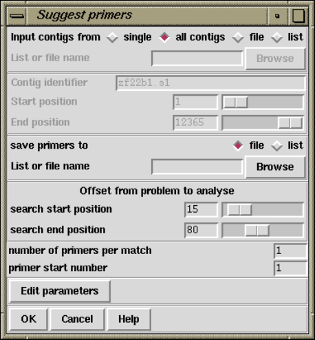
244 The Staden Package Manual
zf22h10 zf22h10.s1 B0334.13 GTTGTCACGAAAATCGC 5220 -
zf21e6 zf21e6.s1 B0334.14 CGGATCAAATATGGATGG 5771 -
zf98a11 zf98a11.s1 B0334.15 CGTGATTTTTACACTATTTCC 10833 -
zf19c4 zf19c4.s1 B0334.16 TCCAATTTTGATTCAGGC 11565 -
The contigs to process can be a particular "single"contig, "all contigs", or a subset of
contigs whose names are stored in a "file"or a "list". If a file or list is selected the browse
button will be activated and, if it is clicked, an appropriate browser will be invoked. If the
user selects "single", then the dialogue for choosing the contig and the section to process
becomes active.
The primer sequences, their template names and their reading names can be written to
a file or a list and an appropriate browser can be used to aid its selection.
For each single stranded region located, the program will search for a primer on its 5’
side in the region "search start position", to "search end position". That is, it will try to
locate a primer starting at "search start position"and then will look increasingly further
away until it reaches "search end position".
If required, by employing the "number of primers per match"entry box, the user can
request that the program tries to suggest more than one primer per problem. The "primer
start number"is an attempt to generate a unique name for each primer suggested. If the
number was set to, say 11, and the database was named B0334, then the first primer would
be named B0334.11, the next B0334.12, etc in the output file.
The "Edit parameters"button invokes a dialogue box which allows the specification of
further parameters. Primer constraints can be specified by melting temperature, length and
G+C content.
Chapter 2: Sequence assembly and finishing using Gap4 245
2.10.3 Suggest Long Readings
This routine (which is available from the gap4 Experiments menu) suggests which templates
could be resequenced on a long gel machine to fill in single stranded regions or extend contigs.
The "Estimated long reading length"tells the routine the expected length of reading that
will be produced by the sequencing machine. The routine finds all single stranded regions,
and where possible suggests solutions. Solutions will not be suggested using readings from
templates that have inconsistent read-pair information.
The example output below shows a list of problem segments followed by suggested tem-
plates.
Prob 1..1: Extend contig start for joining.
Long c91d3.s1 367. T_pos=366, T_size=1000..1500 (1250), cov 189
Long c99e12.s1 340. T_pos=191, T_size=1000..1500 (1250), cov 216
Prob 1..456: No +ve strand data.
No solution.
Prob 1597..1736: No +ve strand data.
Long c53c6.s1 1074. T_pos=341, T_size=1000..1500 (1250), cov 32
Long e04c11.s1 1076. T_pos=376, T_size=1000..1500 (1250), cov 34
Long e05h9.s1 1081. T_pos=377, T_size=1000..1500 (1250), cov 39
Long e05a1.s1 1198. T_pos=329, T_size=1000..1500 (1250), cov 156*
Long c53b11.s1 1382. T_pos=216, T_size=1000..1500 (1250), cov 340*
Prob 2530..2532: No +ve strand data.
Long e03a8.s1 2283. T_pos=199, T_size=1000..1500 (1250), cov 308*
Long e05b10.s1 2331. T_pos=200, T_size=1000..1500 (1250), cov 356*
Prob 3974..4067: No -ve strand data.
No solution.
Prob 4067..4067: Extend contig end for joining.
D Long e06a3.s1 3588. T_pos=366, T_size=1000..1500 (1582), cov 76
Long c53b1.s1 3709. T_pos=360, T_size=1000..1500 (1250), cov 197
Some brief notes on the above output; looking at the suggested rerun of reading e05a1.s1.
Prob 1597..1736: No +ve strand data.
A single stranded region has been identified in this contig at bases 1597 to 1736
inclusive.
"?D Long" The optional two letters before the word "Long"are used to flag possibly incon-
sistent templates (templates that are definitely inconsistent are ignored). "?"
means that no primer information is available for the template that the reading
is from. "D"means that the template size is not within the expected minimum
and maximum. In this case the observed size is displayed (see below).
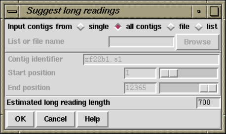
246 The Staden Package Manual
"Long e05a1.s1 1198."
A possible solution; rerun reading e05a1.s1 as a long gel. The first used base
at the 5’ end of this reading is at position 1198 in the contig. Typically this
roughly corresponds to the primer position for this reading in the contig.
T_pos=329
The last used base at the 3’ end of the reading is estimated to be the 329th base
of the template. Together with the template lengths this gives us an estimate
of how much template there is available for a long gel or for walking.
T_size=1000..1500 (1250)
The estimated size for this template is 1250 bases. Gap4 is supplied a minimum
and maximum size when a reading is assembled. In this case the minimum is
1000 bases, and the maximum 1500. When forward and reverse reads assembled
into the same contig estimate the real length reasonably accurately. Otherwise
(as can be seen here), the estimated length is simply the average of the supplied
minimum and maximum lengths.
cov 156* We would expect a long gel to cover our "hole"by 156 bases. This estimate is
based purely on the position of the start of the reading in relation to the start
of the hole, and the estimated length of a long gel. The asterisk here marks that
this coverage is more than enough to completely solve the problem by plugging
the positive strand hole.
For the problem "3974..4067"there is "No solution"listed. This is due to the fact that
there are no suitable readings within the estimated long gel reading length of this problem.

Chapter 2: Sequence assembly and finishing using Gap4 247
2.10.4 Compressions and Stops
This option (which is available from the gap4 Experiments menu) searches through a region
of a contig looking for stop (STOP) or compression (COMP) tags. These tags could have
been added using the Contig Editor or by a suitable external program which can analyse
traces to detect these types of problems. For each such tag found the routine produces a
list of readings that could be resequenced to try to solve the problem. Obviously the types
of experiments available will change as the technology improves but at present the program
produces output that suggests "Taq terminator"experiments. We welcome suggestions for
other experiment types or news of any programs that can automatically assign the tags.
The results, in the form of suggestions, are written to the Output window.
Note that the Taq reading length is used as a guideline for deciding which readings are
suitable candidates for solving a problem. All readings in the correct orientation and with
their 5’ ends within this length are assumed to solve the problem. The actual distance is
listed in the output; an example of this is shown below.
Prob 1544..1545: COMP tag on strand 0 (forward)
Taq for xd26d8.s1 1365 179
Prob 1554..1554: STOP tag on strand 0 (forward)
Taq for xd26d8.s1 1365 189
Prob 5276..5288: COMP tag on strand 1 (reverse)
Taq for xc34g11.s1 5299 23
Taq for xc34g11.s1t 5298 22
Taq for xc34d6.s1 5316 40
Taq for xc45e1.s1 5463 187
Prob 24042..24046: COMP tag on strand 1 (reverse)
Taq for xc50a12.s1 24167 125
Taq for xc33d1.s1 24188 146
Taq for xc36h4.s1 24208 166
Taq for xc51c8.s1 24232 190
The format of the above output is:
248 The Staden Package Manual
Prob <start>..<end>: <type> tag on strand <st>
Taq for <read> @ <pos> <distance>
...
Where:
<start>..<end>
marks the inclusive range for the tag in the contig.
<type> is the type of the current tag.
<st> is the strand of the reading that the tag is placed upon
<read> is the gel reading name.
<pos> is the position of the 5’ end of <read>in the contig.
<distance>
is the distance of the 5’ end from the tag.
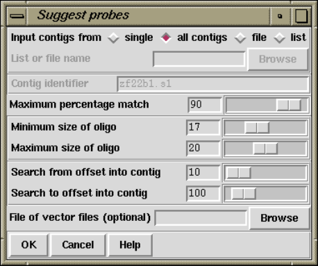
Chapter 2: Sequence assembly and finishing using Gap4 249
2.10.5 Suggest Probes
The suggest probes function (which is available from the gap4 Experiments menu) looks for
oligos at the end of each contig suitable for use with an oligo probing strategy invented by
Jonathan Flint. Flint,J., Sims,M., Clark,K., Staden,R. and Thomas,K. An oligo-screening
strategy to fill gaps found during shotgun sequencing projects. DNA Sequence 8, 241-245.
The probing strategy is used part way through a sequencing project to find clones which
should help to extend contigs. The gap4 function described here is used to select oligos from
readings that are near the ends of the current contigs. These oligos are synthesised and
then used to probe a pool of sequencing clones. Those which it selects are then sequenced
in the hope that they will lengthen the contigs.
The dialogue contains the usual methods of selecting the set of contigs to operate on.
For each end of the selected contigs, oligos are chosen using the OSP Hillier, L., and Green,
P. (1991). "OSP: an oligonucleotide selection program,"PCR Methods and Applications,
1:124-128. selection criteria which is dependent on the maximum and minimum size of
oligos specified. The "search from"and "search to"parameters control the area of consensus
sequence in which to search for oligos. For example, if they are set to 10 and 100 respectively
the a section of consensus sequence used is 90 bases long and starts 10 bases from the end
of the contig.
Once an oligo is found it is screened against all the existing consensus sequence. An oligo
is rejected if it matches with a score greater than or equal to the "maximum percentage
match". If a file of vector filenames has been specified then the oligos are also screened
against the vector sequences.
Typical output for a single contig follows. The output shows all oligos that have passed
the screening process. The information listed includes the distance of this oligo from the
end of the contig (Dist ??), the score returned from the OSP selection (primer=??), the
melting temperature (Tm=??), the best percentage match found (match=??%) and the oligo
sequence.
Contig zf37b5.s1(495): Start
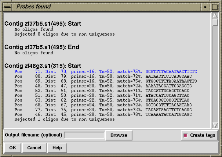
250 The Staden Package Manual
Rejected 8 oligos due to non uniqueness
Contig zf37b5.s1(495): End
No oligos found
Contig zf48g3.s1(315): Start
Pos 71, Dist 70, primer=16, Tm=52, match=75%, GCGTTTTACAATAACTTCTC
Pos 80, Dist 79, primer=16, Tm=50, match=72%, AATAACTTCTCAGGCAAC
Pos 69, Dist 68, primer=16, Tm=52, match=75%, GTGCGTTTTACAATAACTTC
Pos 48, Dist 47, primer=20, Tm=50, match=72%, AAAATACCATTGCAGCTC
Pos 52, Dist 51, primer=20, Tm=55, match=71%, TACCATTGCAGCTCACC
Pos 51, Dist 50, primer=20, Tm=52, match=71%, ATACCATTGCAGCTCAC
Pos 63, Dist 62, primer=22, Tm=55, match=76%, CTCACCGTGCGTTTTAC
Pos 68, Dist 67, primer=24, Tm=50, match=72%, CGTGCGTTTTACAATAAC
Pos 77, Dist 76, primer=24, Tm=50, match=72%, TACAATAACTTCTCAGGC
Pos 46, Dist 45, primer=28, Tm=50, match=78%, TCAAAATACCATTGCAGC
Rejected 1 oligo due to non uniqueness
This output is sent to both the Output Window and additionally to a suggest probes
output window. This latter window (shown below) allows selection of oligos from those
available for each contig by clicking the left mouse button on a line of the output. The
selected oligos are shown in blue. By default the first in each set is automatically selected.
The selected oligos can then be written to a file by filling in the "output filename"and
will have OLIG tags created for them when the "Create tags"checkbutton is selected. This
output window vanishes once OK is pressed, but the text in the main Output Window is
left intact.
Chapter 2: Sequence assembly and finishing using Gap4 251
2.11 Calculating Consensus Sequences
In this section we describe the types of consensus which gap4 can produce, the formats they
can be written in, and the algorithms that can be used. The algorithms are not only used
to produce consensus sequence files, but in many other places throughout gap4 where an
analysis of the current quality of the data is required. One important place is inside the
Contig Editor (see Section 2.6 [Editing in gap4], page 160) where they are used to produce
an "on-the-fly"consensus, responding to every edit made by the user.
The currently active consensus algorithm is selected from the "Consensus algorithm"di-
alogue in the main gap4 Options menu (see Section 2.20.2 [Consensus Algorithm], page 299).
There are four main types of consensus sequence file that can be produced by the pro-
gram: Normal, Extended, Unfinished, and Quality. They are all invoked from the File
menu.
"Normal"is the type of consensus file that would be expected: a consensus from the
non-hidden parts of a contig. "Extended"is the same as "Normal"but the consensus is
extended by inclusion of the hidden, non-vector sequence, from the ends of the contig.
"Unfinished"is the same as "Normal"except that any position where the consensus
does not have good data for both strands is written using A,C,G,T characters, and the rest
(which has good data for both strands) is written using a different set of symbols. This
sequence can be used for screening against new readings: only the regions needing more
readings will produce matches. By screening readings in this way, prior to assembly, users
can avoid entering readings which will not help finish the project, and which may require
further editing work to be performed.
"Quality"produces a sequence of characters of the same length as the consensus, but
they instead encode the reliability of the consensus at each point.
Consensus sequence files can also encode the positions of the currently active tag types
by changing the case of the tagged characters (marking) or writing them in a different
character set (masking) (see Section 2.2.7.2 [Active tags and masking], page 121).
The consensus algorithms are usually configured to produce only the characters A,C,G,T
and "-", but it is possible to set them to produce the complete set of IUB codes. This mode
is useful for some types of work and allows the range of observed base types at any position
to be coded in the consensus. How the IUB codes are chosen is described in the introduction
to the consensus algorithms (see Section 2.11.5 [The Consensus Algorithms], page 257).
Depending on the type of consensus produced, the consensus sequence files can be written
in three different formats: Experiment files (see Section 11.3 [Experiment File], page 552),
FASTA (Pearson,W.R. Using the FASTA program to search protein and DNA sequence
databases. Methods in Molecular Biology. 25, 365-389 (1994)) or staden formats. If ex-
periment file format is selected a further menu appears that allows users to select for the
inclusion of tag data in the output file. For FASTA format the sequence headers include the
contig identfier as the sequence name and the project database name, version number and
the number of the leftmost reading in the contig as comments. e.g. ">xyzzy.s1 B0334.0.274"
is database B0334, copy 0, and the left most reading for the contig is number 274, which has
a name of xyzzy.s1. For staden format the headers include the project database name and
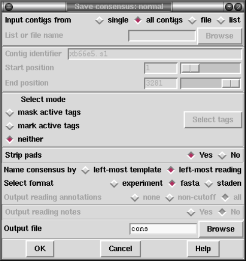
252 The Staden Package Manual
the number of the leftmost reading in the contig. e.g. "<B0334.00274——->" is database
B0334 and the left most reading for the contig is number 274. Staden format is maintained
only for historical reasons - i.e. there may still be a few unfortunate people using it. Ob-
viously Experiment file format can contain much more information, and can serve as the
basis of a submission to the sequence library.
2.11.1 Normal Consensus Output
This is the usual consensus type that will be calculated (and is available from the gap4
File menu). The currently active consensus algorithm is selected from the "Consensus algo-
rithm"dialogue in the main gap4 Options menu (see Section 2.20.2 [Consensus Algorithm],
page 299).
Contigs can be selected from a file of file names or a list. In addition, tagged regions can
be masked or marked (see Section 2.2.7.2 [Active tags and masking], page 121), and output
can be in Experiment file, fasta or staden formats. If experiment file format is selected a
further menu appears that allows users to select for the inclusion of tag data in the output
file.
The contigs for which to calculate a consensus can be a particular "single"contig, "all
contigs", or a subset of contigs whose names are stored in a "file"or a "list". If a file or list
is selected the browse button will be activated, and if it is clicked, an appropriate browser
will be invoked. If the user selects "single"then the dialogue for choosing the contig, and
the section to process, becomes active.
If the user selects either "mask active tags"or "mark active tags"the "Select tags"
button is activated, and if it is clicked, a dialogue panel appears to enable the user to select
which tag types should be used in these processes. If "mask"is selected all segments covered
Chapter 2: Sequence assembly and finishing using Gap4 253
by the tag types chosen will not be written as ACGT but as defi symbols. If "mark"is
selected the tagged segments will be written in lowercase characters. Masking is useful for
producing a sequence to screen against other sequences: only the unmasked segments will
produce hits.
The "strip pads"option will remove pads ("*"s) from the consensus sequence. In the
case of experiment files this will also automatically adjust the position and length of the
annotations to ensure that they still mark the correct segment of sequence.
Normally the consensus sequences are named after the left-most reading in each contig.
For the purposes of single-template based sequencing projects (eg cDNA assemblies) the
option exists to “Name consensus by left-most template” instead of by left-most reading.
The routine can write its consensus sequence (plus extra data for experiment files) in
"experiment file","fasta"and "staden"formats. The output file can be chosen with the
aid of a file browser. If experiment file format is selected the user can choose whether or not
to have "all annotations","annotations except in hidden", or "no annotations"written out
with the sequence. If the user elects to include annotations the "select tags"button will
become active, and if it is clicked, a dialogue for selecting the types to include will appear.
2.11.2 Extended Consensus Output
This consensus type (which is available from the gap4 File menu) is useful for those who
are too impatient to complete their sequence and want to compare it, in its fullest extent,
to other data. The sequence produced therefore includes hidden data from the ends of the
contigs.
The currently active consensus algorithm is selected from the "Consensus algorithm"di-
alogue in the main gap4 Options menu (see Section 2.20.2 [Consensus Algorithm], page 299).
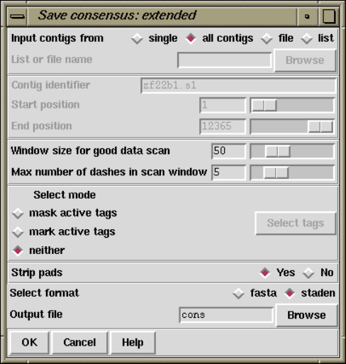
254 The Staden Package Manual
Contigs can be selected from a file of file names or a list. In addition tagged regions can
be masked or marked (see Section 2.2.7.2 [Active tags and masking], page 121), and output
can be in fasta or staden formats.
The contigs for which to calculate a consensus can be a particular "single"contig, "all
contigs", or a subset of contigs whose names are stored in a "file"or a "list". If a file or list
is selected the browse button will be activated, and if it is clicked, an appropriate browser
will be invoked. If the user selects "single"then the dialogue for choosing the contig and
the section to process becomes active.
Where possible the contigs are extended using the poor quality data from the readings
near their ends. To ensure that this additional data is not too poor the program uses the
following algorithm. It slides a window of size "Window size for good data scan"along
the hidden data for each reading and stops if it finds a window that contains more than
"Max dashes in scan window"non-ACGT characters. The data that extends the contig the
furthest is added to its consensus sequence.
If the user selects either "mask active tags"or "mark active tags"the "Select tags"
button is activated, and if it is clicked, a dialogue panel appears to enable the user to select
which tag types should be used in these processes. If "mask"is selected all segments covered
by the tag types chosen will not be written as ACGT but as defi symbols. If "mark"is
selected the tagged segments will be written in lowercase characters. Masking is useful for
producing a sequence to screen against other sequences: only the unmasked segments will
produce hits.
The "strip pads"option will remove pads ("*"s) from the consensus sequence.
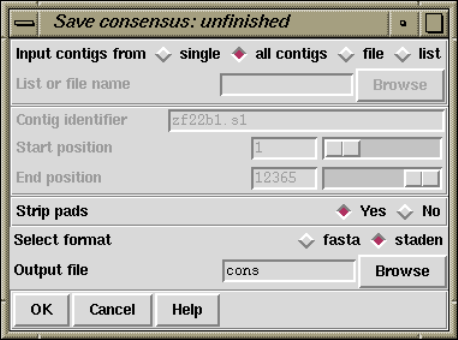
Chapter 2: Sequence assembly and finishing using Gap4 255
The routine can write its consensus sequence in "fasta"and "staden"formats. The
output file can be chosen with the aid of a file browser.
2.11.3 Unfinished Consensus Output
This option is available from the gap4 File menu. An "Unfinished"consensus is one in
which any position where the consensus does not have good data for both strands is written
using A,C,G,T characters, and the rest (which has good data for both strands) is written
using a different set of symbols (d,e,f,i). This sequence can be used for screening against
new readings: only the regions needing more readings will produce matches. By screening
readings in this way, prior to assembly, users can avoid entering readings which will not
help finish the project, and which may require further editing to be performed. This type
of consensus when written in staden format, consists of A,C,G,T for single stranded regions
and d,e,f,i for finished sequence (d=a,e=c,f=g,i=t).
The currently active consensus algorithm is selected from the "Consensus algorithm"di-
alogue in the main gap4 Options menu (see Section 2.20.2 [Consensus Algorithm], page 299).
Contigs can be selected from a file of file names or a list, and output can be in fasta or
staden formats.
The contigs for which to calculate a consensus can be a particular "single"contig, "all
contigs", or a subset of contigs whose names are stored in a "file"or a "list". If a file or list
is selected the browse button will be activated, and if it is clicked, an appropriate browser
will be invoked. If the user selects "single"then the dialogue for choosing the contig and
the section to process becomes active.
The "strip pads"option will remove pads ("*"s) from the consensus sequence.
The routine can write its consensus sequence in "fasta"and "staden"formats. The
output file can be chosen with the aid of a file browser.
2.11.4 Quality Consensus Output
The Quality Consensus Output option described here (which is available from the gap4 File
menu) applies either of the two simple consensus calculations (see Section 2.11.5.1 [Con-
sensus Calculation Using Base Frequencies], page 258) and (see Section 2.11.5.2 [Consensus
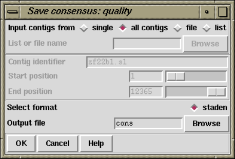
256 The Staden Package Manual
Calculation Using Weighted Base Frequencies], page 259) to the data for each strand of
the DNA separately. The currently active consensus algorithm is selected from the "Con-
sensus algorithm"dialogue in the main gap4 Options menu (see Section 2.20.2 [Consensus
Algorithm], page 299).
It produces, not a consensus sequence, but an encoding of the "quality"of the data
which defines whether it has been determined on both strands, and whether the strands
agree. The categories of data and the codes produced are shown in the table. For example
’c’ means bad data on one strand is aligned with good data on the other.
aGood Good (in agreement)
bGood Bad
cBad Good
dGood None
eNone Good
fBad Bad
gBad None
hNone Bad
iGood Good (disagree)
jNone None
The contigs for which to calculate a consensus can be a particular "single"contig, "all
contigs", or a subset of contigs whose names are stored in a "file"or a "list". If a file or list
is selected the browse button will be activated, and if it is clicked, an appropriate browser
will be invoked. If the user selects "single"then the dialogue for choosing the contig and
the section to process becomes active.
The routine can only write its consensus sequence in "staden"format. The output file
can be chosen with the aid of a file browser.
Chapter 2: Sequence assembly and finishing using Gap4 257
2.11.5 The Consensus Algorithms
The consensus calculation is a very important component of gap4. It is used to produce
an "on-the-fly"consensus, responding to every individual change in the Contig Editor (see
Section 2.6 [Editing in gap4], page 160) and is used to produce the final sequence for
submission to the sequence libraries. Some years ago Bonfield, J.K. and Staden, R. The
application of numerical estimates of base calling accuracy to DNA sequencing projects.
Nucleic Acids Res. 23, 1406-1410 (1995) we put forward the idea of using base call accuracy
estimates in sequencing projects, and this has been partially realised with the values from
the Phred program (Ewing, B. and Green, P. Base-Calling of Automated Sequencer Traces
Using Phred. II. Error Probabilities. Genome Research. Vol 8 no 3. 186-194 (1998)).
These values are widely used and have defined a decibel type scale for base call confidence
values and gap4 is currently set to use confidence values defined on this scale. An overview
of our use of confidence values is contained in the introductory sections of the manual (see
Section 2.2.5 [The use of numerical estimates of base calling accuracy], page 118).
As is described elsewhere (see Section 2.11.6 [List Consensus Confidence], page 261)
being able to calculate the confidence for each base in the consensus sequence makes it
possible to estimate the number of errors it contains, and hence the number of errors that
will be removed if particular bases are checked and, if necessary, edited.
Gap4 caters for base calls with and without confidence values and hence provides a
choice of algorithms. There are currently three consensus algorithms that may be used.
The choice of the best algorithm will depend on the data that you have available and the
purpose for which you are using gap4.
The currently active consensus algorithm is selected from the "Consensus algorithm"di-
alogue in the main gap4 Options menu (see Section 2.20.2 [Consensus Algorithm], page 299).
The only way to produce a consensus sequence for which the reliability of each base is
known, is to use reading data with base call confidence values. Their use, in combination
with the Confidence Value algorithm (see Section 2.11.5.3 [Consensus Calculation Using
Confidence Values], page 259). is strongly recommended.
For base calls without confidence values use the Base Frequencies algorithm (see
Section 2.11.5.1 [Consensus Calculation Using Base Frequencies], page 258). This is also
a fast algorithm so it may be appopriate for very high depth assemblies such those for
mutation studies.
For data with simple base call accuracy estimates rather than those on the decibel scale,
the Weighted Base Frequencies algorithm should be used (see Section 2.11.5.2 [Consensus
Calculation Using Weighted Base Frequencies], page 259).
All confidence values lie in the range 0 to 100. When readings are entered into a data-
base, gap4 assigns a confidence of 99 to all bases without confidence values. For all three
algorithms, a base with confidence of 100 is used to force the consensus base to that base
type and to have a confidence of 100. However,if two or more base types at any position
have confidence 100, the consensus will be set to "unknown", i.e. "-", and will have a
confidence of 0. Note that dash ("-") is our preferred symbol for "unknown"as, within a
sequence, it is more easily distinguished from A,C,G,T than "N".
258 The Staden Package Manual
The consensus sequence is also assigned a confidence, even when base call confidence
values are not used to calculate it. The scale and meaning of the consensus confidence
changes between consensus algorithms. However the consensus cutoff parameter always has
the same meaning. A consensus base with a confidence ’X’ will be called as a dash when
’X’ is lower than the consensus cutoff, otherwise it is the determined base type.
Both the consensus cutoff and quality cutoff values can be set by using the "Config-
ure cutoffs"command in the "Consensus algorithm"dialogue in the main gap4 Options
menu (see Section 2.20.2 [Consensus Algorithm], page 299). Within the Contig Editor (see
Section 2.6 [Editing in gap4], page 160) these values can be adjusted by clicking on the "<"
and ">" symbols adjacent to the "C:"(consensus cutoff) and "Q:"(quality cutoff) displays
in the top left corner of the editor. These buttons are repeating buttons - the values will
adjust for as long as the left mouse button is held down. Changing these values lasts only
as long as that invocation of the contig editor.
The consensus algorithms are usually configured to produce only the characters
A,C,G,T,* and "-", but it is possible to set them to produce the complete set of IUB
codes. This mode is useful for some types of work and allows the range of observed base
types at any position to be coded in the consensus. The IUB code at any position is
determined in the following way.
We assume that the user wants to know which base types have occurred at any point,
but may want some control over the quality and relative frequency of those that are used to
calculate the "consensus". For the simplest consensus algorithm there is no control over the
quality of the base calls that are included, but the Consensus Cutoff can be used to control
how the relative frequency affects the chosen IUB code. All base types whose computed
"confidence"exceeds the Consensus Cutoff will be included in the selection of the IUB code.
For example if only base type T reaches the Consenus Cutoff the IUB code will be T; if both
T and C reach the cutoff the code will be Y; if A, C and T each reach the cutoff the code
will be H; if A, C, G and T all reach the cutoff the code will be "N". For the Confidence
Value algorithm the Quality Cutoff can be used to exclude base calls of low quality, so that
all those that do not reach the Quality Cutoff are excluded from the IUB code calculation.
Otherwise the logic of the code selection is the same as for the two simpler algorithms.
Both the consensus cutoff and quality cutoff values can be set by using the "Configure
cutoffs"command in the "Consensus algorithm"dialogue in the main gap4 Options menu
(see Section 2.20.2 [Consensus Algorithm], page 299).
The algorithms are explained below.
2.11.5.1 Consensus Calculation Using Base Frequencies
This algorithm can be used for any data, with or without confidence values. Each standard
base type is given the same weight. The consensus will be the most frequent base type in a
given column provided that the consensus cutoff parameter is low enough. All unrecognised
base types, including IUB codes, are treated as dashes. Dashes are given a weight of
1/10th that of recognised base types. Pads are given a weight which is the average of their
neighbouring bases.
Chapter 2: Sequence assembly and finishing using Gap4 259
The confidence of a consensus base for this method is expressed as a percentage. So for
example a column of bases of A, A, A and T will give a consensus base of A and a confidence
of 75. Therefore a consensus cutoff of 76 or higher will give a consensus base of "-".
In the event that more than one base type is calculated to have the same confidence, and
this exceeds the consensus cutoff, the bases are assigned in descending order of precedence:
A, C, G and T.
The quality cutoff parameter (Q in the Contig Editor) has no effect on this algorithm.
2.11.5.2 Consensus Calculation Using Weighted Base Frequencies
This method can be used when simple, unquantified, base call quality values are available.
Instead of simply counting base type frequencies it sums the quality values. Hence a column
of 4 bases A, A, A and T with confidence values 10, 10, 10 and 50 would give combined
totals of 30/80 for A and 50/80 for T (compared to 3/4 for A and 1/4 for T when using
frequencies). As with the unweighted frequency method this sets the confidence value of
the consensus base to be the the fraction of the chosen base type weights over the total
weights (62.5 in the above example).
The quality cutoff parameter controls which bases are used in the calculation. Only bases
with quality values greater than or equal to the quality cutoff are used, otherwise they are
completely ignored and have no effect on either the base type chosen for the consensus or
the consensus confidence value. In the above example setting the quality cutoff to 20 would
give a T with confidence 100 (100 * 50/50).
In the event that more than one base type is calculated to have the same weight, and
this exceeds the consensus cutoff, the bases are assigned in descending order of precedence:
A, C, G and T.
This is Rule IV of Bonfield,J.K. and Staden,R. The application of numerical estimates
of base calling accuracy to DNA sequencing projects. Nucleic Acids Research 23, 1406-1410
(1995).
2.11.5.3 Consensus Calculation Using Confidence values
This is the prefered consensus algorithm for reading data with Phred decibel scale confidence
values. As will become clear from the follwing description, it is more complicated than the
other algorithms, but produces a much more useful result.
A difficulty in designing an algorithm to calculate the confidence for a consensus derived
from several readings, possibly using different chemistries, and hopefully from both strands
of the DNA, is knowing the level of independence of the results from different experiments
- namely the readings. Given that sequencing traces are sequence dependent, we do not
regard readings as wholly independent, but at the same time, repeated readings which
confirm base calls may give us more confidence in their accuracy. In addition, if we get a
particularly good sequencing run, with consequently high base call confidence values, we
are more likely to believe its base call and confidence value assignments. The final point in
this preamble is that the Phred confidence values refer only to the probability for the called
base, and they tell us nothing about the relative likelihood of each of the other 3 base types
appearing at the same position. These difficulties are taken into account by our algorithm,
which is described below.
260 The Staden Package Manual
In what follows, a particular position in an alignment of readings is referred to as a
"column". The base calls in a column are classified by their chemistry and strand. We
currently group them into "top strand dye primer","top strand dye terminator","bottom
strand dye primer"and "bottom strand dye terminator"classes.
Within each class there may be zero or many base calls. For each class we check for
multiple occurrences of the same base type. For each base type we find the highest confidence
value, and then increase it by an amount dependent on the number of confirming reads.
Then Bayes formula is used to derive the probabilities and hence the confidence values for
each base type.
To further describe the method it is easiest to work through an example. Suppose we
have 5 readings with the following characteristics covering a particular column.
Dye primer, top strand, ’A’, confidence 20
Dye primer, top strand, ’A’, confidence 10
Dye primer, top strand, ’T’, confidence 20
Dye terminator, top strand, ’T’, confidence 10
Dye primer, bottom strand, ’A’, confidence 5
Hence there are three possible classes.
Examining the "dye primer top strand"class we see there are three readings (A, A and
T). The highest A is 20. We add to this a fixed quantity to indicate one other occurence
of an A in this set. For this example we add 5. Now we have an adjusted confidence of
25 for A and 20 for T. This is equivalent to a .997 probability of A being correct and .99
probability of T being correct. To use Bayes we split the remaining probabilies evenly. A
has a probability of .997 and so the remaining .003 is spread amongst the other base types.
Similarly for the .01 of the T. The result is shown in the table below.
|ACGT
--+-----------------------
A | .997 .001 .001 .001
T | .0033 .0033 .0033 .990
Bayesian calculations on this table then give us probabilities of approximately .766 for
A, .00154 for C, .00154 for G and .231 for T.
The other classes give probalities of .033 for A, C, G and .9 for T, and .316 for A, and
.228 for C, G and T.
To combine the values for each class we produce a table for a further Bayesian calculation.
Once again we fill in the probabilities and spread the remainder evenly amongst the other
base types.
| A C G T
-----------+--------------------------
Primer Top | .766 .00154 .00154 .231
Term Top | .0333 .0333 .0333 .9
Primer Bot | .316 .228 .228 .228
From this Bayes gives the final probabilities of .135 for A, .0002 for C, .0002 for G and
.854 for T. This is what would be expected intuitively: the T signal was present in both
Chapter 2: Sequence assembly and finishing using Gap4 261
dye primer and dye terminator experiments with 1/100 and 1/10 error rates whilst the A
signal was present on both strands with 1/100 and 1/3 error rates. Hence the consensus
base is T with confidence 8.4 (-10*log10(1-.854)).
If a padding character is present in a column we consider the pad as a separate base
type and then evenly divide the remaining probabilities by 4 instead of 3.
2.11.5.4 The Quality Calculation
The Quality Calculation described here (which is available from the gap4 File menu) applies
either of the two simple consensus calculations (see Section 2.11.5.1 [Consensus Calculation
Using Base Frequencies], page 258) and (see Section 2.11.5.2 [Consensus Calculation Using
Weighted Base Frequencies], page 259) to the data for each strand of the DNA separately.
It produces, not a consensus sequence, but an encoding of the "quality"of the data which
defines whether it has been determined on both strands, and whether the strands agree.
This quality is used as the basis for problem searches, such as find next problem, and the
Quality Display within the Template Display (see Section 2.5.1.5 [Quality Plot], page 137).
The categories of data and the codes produced are shown in the table. For example ’c’
means bad data on one strand is aligned with good data on the other.
+Strand -Strand
aGood Good (in agreement)
bGood Bad
cBad Good
dGood None
eNone Good
fBad Bad
gBad None
hNone Bad
iGood Good (disagree)
jNone None
the "Configure cutoffs"command in the
In the "Consensus algorithm"dialogue in the main gap4 Options menu (see
Section 2.20.2 [Consensus Algorithm], page 299), setting the configuration to treat readings
flagged using the "Special Chemistry"Experiment File line (CH field) (see Section 11.3
[Experiment File], page 552) affects this calculation. When set, the reading counts for
both strands in the Consensus and Quality Calculations, and hence is equivalent to having
data on both strands.
2.11.6 List Consensus Confidence
The Confidence Value consensus algorithm (see Section 2.11.5.3 [Consensus Calculation
Using Confidence Values], page 259) produces a consensus sequence for which the expected

262 The Staden Package Manual
error rate for each base is known. The option described here (which is available from the
gap4 View menu) uses this information to calculate the expected number of errors in a
particular consensus sequence and to tabulate them.
The decibel type scale introduced in the Phred program uses the formula
-10xlog10(error rate) to produce confidence values for the base calls. A confidence value of
10 corresponds to an error rate of 1/10; 20 to 1/100; 30 to 1/1000; etc.
So for example, if 50 bases in the consensus had confidence 10, we would expect those 50
bases (with an error rate of 1/10) to contain 5 errors; and if 200 bases had confidence 20, we
would expect them to contain 2 errors. If these 50 bases with confidence 10, and 200 bases
with confidence 20 were the least accurate parts of the consensus, they are the bases which
we should check and edit first. In so doing we would be dealing with the places most likely
to be wrong, and would raise the confidence of the whole consensus. The output produced
by List Confidence shows the effect of working through all the lowest quality bases first,
until the desired level of accuracy is reached. To do this it shows the cumulative number
of errors that would be fixed by checking every consensus base with a confidence value less
than a particular threshold.
The List Confidence option is available from within the Commands menu of the Contig
Editor and the main gap4 View menu. From the main menu the dialogue simply allows
selection of one or more contigs. Pressing OK then produces a table similar to the following:
Sequence length = 164068 bases.
Expected errors = 168.80 bases (1/971 error rate).
Value Frequencies Expected Cumulative Cumulative Cumulative
errors frequencies errors error rate
--------------------------------------------------------------------------
0 0 0.00 0 0.00 1/971
1 1 0.79 1 0.79 1/976
2 0 0.00 1 0.79 1/976
3 3 1.50 4 2.30 1/985
4 30 11.94 34 14.24 1/1061
5 2 0.63 36 14.87 1/1065
6 263 66.06 299 80.94 1/1867
7 151 30.13 450 111.06 1/2841
8 164 25.99 614 137.06 1/5168
9 96 12.09 710 149.14 1/8344
10 80 8.00 790 157.14 1/14069
The output above states that there are 164068 bases in the consensus sequence with an
expected 169 errors (giving an average error rate of one in 971). Next it lists each confidence
value along with its frequency of occurrence and the expected number of errors (as explained
above, frequency x error rate). For any particular confidence value the cumulative columns
state: how many bases in the sequence have the same or lower confidence, how many errors
are expected in those bases, and the new error rate if all these bases were checked and all
the errors fixed.
Chapter 2: Sequence assembly and finishing using Gap4 263
Above it states that there are 790 bases with confidence values of 10 or less, and estimates
there to be 157 errors in those 790 bases. As we expect there to be about 169 errors in the
whole consenus this implies that manually checking those 790 bases would leave only 12
undetected errors. Given that the sequence length is 164068 bases this means an average
error rate of 1 in 14069. It is important to note that by using this editing strategy, this
error rate would be achieved by checking only 0.48% of the total number of consensus bases.
This strategy is realised by use of the consensus quality search in the gap4 Contig Editor
(see Section 2.6.6.7 [Search by Consensus Quality], page 175).
2.11.7 List Base Confidence
The various base-callers may produce a confidence value for each base call. Previous sections
describe how this may be used to produce a consensus sequence along with a consensus
confidence.
This function tabulates the frequency of each base confidence value along with a count
of how many times is matches or mismatches the consensus. Given that the standard scale
for confidence values follows the -10log10(probability of error) formula we can determine
what the expected frequency of mismatches should be for any particular confidence value.
By comparing this with our observed frequencies we then have a powerful summary of the
amount of misassembled data.
Total bases considered : 45270
Problem score : 1.337130
Conf. Match Mismatch Expected Over-
value freq freq freq representation
---------------------------------------------------------------------
0 0 0 0.00 0.00
1 0 0 0.00 0.00
2 0 0 0.00 0.00
3 0 0 0.00 0.00
4 37 22 23.49 0.94
5 0 0 0.00 0.00
6 89 46 33.91 1.36
7 119 26 28.93 0.90
8 256 37 46.44 0.80
9 368 30 50.11 0.60
10 669 31 70.00 0.44
...
In the above example we see that there are 59 sequence bases with confidence 4, of which
37 match the consensus and 22 do not. If we work on the assumption that the consensus
is correct then we would expect approximately 40% of these to be incorrect, but we have
measured 37% to be incorrect (22/59) giving 0.94 fraction of the expected amount.
For a more problematic assembly, we may see a section of output like this:
Total bases considered : 1617511
Problem score : 311.591358
264 The Staden Package Manual
Conf. Match Mismatch Expected Over-
value freq freq freq representation
---------------------------------------------------------------------
...
20 13432 384 138.16 2.78
21 23384 851 192.51 4.42
22 18763 487 121.46 4.01
23 13712 300 70.23 4.27
24 21182 363 85.77 4.23
25 20466 218 65.41 3.33
26 9752 123 24.80 4.96
27 23071 282 46.60 6.05
28 13816 158 22.15 7.13
29 27514 166 34.85 4.76
30 15664 140 15.80 8.86
...
We can see here that the observed mismatch frequency is greatly more than the expected
number. This indicates the number of misassemblies (or SNPs in the case of mixed samples)
within this project and is reflected by the combined “Problem score”. This score is simply
the sum of the final column (or 1 over that column for values less than 1.0).
Chapter 2: Sequence assembly and finishing using Gap4 265
2.12 Miscellaneous functions
2.12.1 Complement a Contig
This function (which is available from the gap4 Edit menu) is used to complement a contig,
which means that it will complement and reverse all its readings and reorder them to
produce a contig with the opposite orientation. It operates on a single contig selected via a
dialogue box.
2.12.2 Enter Tags
This routine (which is available from the gap4 Edit menu) is used to add a set of tags (see
Section 2.2.7 [Annotation readings and contigs], page 121) stored in a file, to the database.
The file format (see below) is identical to the output produced by the "save tags to file"
option of "Find Repeats". See Section 2.8.4 [Find Repeats], page 233. The format is a
subset of the experiment file format. See Section 11.3 [Experiment Files], page 552. The
two are close enough for Enter tags to use an experiment file as input. The only input
required is the name of the file to read and a file browser can be used to aid its selection.
Note that "Enter tags"will remove any results plotted in the Contig Comparator.
The start of a typical file is shown below.
CC Repeat number 0, end 1
ID zf48g3.s1
TC REPT b 1031..1072
TC Repeats with contig zf48g3.s1, offset 957
CC Repeat number 0, end 2
ID zf48g3.s1
TC REPT b 957..998
TC Repeats with contig zf48g3.s1, offset 1031
CC
CC Repeat number 1, end 1
ID zf48g3.s1
TC REPT b 1102..1130
TC Repeats with contig zf48g3.s1, offset 953
CC Repeat number 1, end 2
ID zf48g3.s1
TC REPT b 953..981
TC Repeats with contig zf48g3.s1, offset 1102
2.12.3 Shuffle Pads
This function realigns all of the sequences within a contig to improve pad placement. This
can be considered as the replacement to the old Shuffle Pads command within the contig
editor. (Being outside of the editor allows this to be autoamtically scripted.) The contigs
to realign are specified as either a single contig, all contigs or to input a contig names from
a file or a gap4 list. Currently the entire contig will be shuffled, which can take some time
on large contigs. In future we plan to allow regions to be specified.
266 The Staden Package Manual
Padding (gapping) problems originate in many sequence assembly algorithms, including
gap4’s, where sequences are aligned against a consensus rather than a profile. As an example
let us consider aligning TCAAGAC (Sequence4) to the following contig:
Sequence1: GATTCAAAGAC
Sequence2: TTCAA*GACGG
Sequence3: CAAAGACGGATC
Consensus: GATTCAAAGACGGATC
The consensus contains a triple A because that is the most likely sequence, however we
have three possible ways to align a sequence containing double A:
alignment1: TCAA*GAC
alignment1: TCA*AGAC
alignment1: TC*AAGAC
Consensus: GATTCAAAGACGGATC
All of these have identical alignment scores because the cost of inserting a gap into the
sequence is identical at all points. Alignment algorithms typically always pick the same end
to place pads (ie left end or right end), but after contigs get complemented and more data
inserted this often yields pads at both as, as follows:
Sequence1: GATTCAAAGAC
Sequence2: TTCAA*GACGG
Sequence3: CAAAGACGGATC
Sequence4: TC*AAGAC
Consensus: GATTCAAAGACGGATC
The new Shuffle Pads algorithm implements the same ideas put forward by Anson and
Myers in ReAligner. It aligns each sequence against a consensus vector where the entire
column of bases in the consensus are used to compute match, mismatch and indel scores.
The result is that pads generally get shuffled to the same end (not necessarily always left
or always right) and the total number of disagreements to the consensus reduces.
For speed we acknowledge that the new alignment will only deviate slightly from the old
one and so a narrow “band size” is used. This paramater may be adjusted if required, but
at the expense of speed.
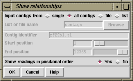
Chapter 2: Sequence assembly and finishing using Gap4 267
2.12.4 Show Relationships
This function (which is available from the gap4 View menu) is used to show the relationships
of the gel readings in the database in three ways.
1. All contig descriptor lines followed by all gel descriptor lines.
2. All contigs one after the other sorted, i.e. for each contig show its contig descriptor
line followed by all its gel descriptor lines sorted on position from left to right
3. Selected contigs: show the contig line and, in left to right order, the gel readings. This
can be done for a list or a file of contigs. For a single contig the output can be restricted
to a user-defined region.
In the above illustration, a single contig, all contigs, a file or list of contigs can be selected.
For a single contig, the contig identifier and range selector becomes enabled. Choosing a
file or list enables the "browse"button which will invoke either the file or list browser
respectively. When "all"contigs is selected a further choice is available: whether to ‘Show
readings in positional order’. This question determines whether to output in method
1 (No) or 2 (Yes) listed above.
The function is particularly useful for creating files or lists of reading names. To create a
list of reading names run Show Relationships to produce the desired output to the Output
Window. Then either use cut and paste from this window to a list editor, or use the right
mouse button in the output window to request the "Output to list"option. In this latter
case the header "CONTIG LINES" and "GEL LINES" lines should be removed (although most
functions will happily ignore, with warnings, a list containing unknown reading names).
In the output window the reading names are underlined, indicating that they are hyper-
links. Double clicking on a name with the left mouse button will bring up the contig editor
showing the start of that sequence, or it will move an existing contig editor to display that
position. (You may wish to turn off the "Scroll on output"button if you do not wish the
text output window to scroll to the bottom as it displays the "Edit contig"title.) Clicking
on a reading name with the right mouse button will bring up a popup menu containing Edit
contig, Template display, List reading notes and List contig notes.
Below is an example showing a contig from position 1 to 689. The left gel reading is
number 6 and has archive name HINW.010, the rightmost gel reading is number 2 and is
has archive name HINW.004. On each gel descriptor line is shown: the name of the archive
268 The Staden Package Manual
version, the gel number, the position of the left end of the gel reading relative to the left
end of the contig, the length of the gel reading (if this is negative it means that the gel
reading is in the opposite orientation to its archive), the number of the gel reading to the
left and the number of the gel reading to the right.
CONTIG LINES
CONTIG LINE LENGTH ENDS
LEFT RIGHT
48 689 6 2
GEL LINES
NAME NUMBER POSITION LENGTH NEIGHBOURS
LEFT RIGHT
HINW.010 6 1 -279 0 3
HINW.007 3 91 -265 6 5
HINW.009 5 137 -299 3 17
HINW.999 17 140 273 5 12
HINW.017 12 193 265 17 18
HINW.031 18 385 -245 12 2
HINW.004 2 401 -289 18 0
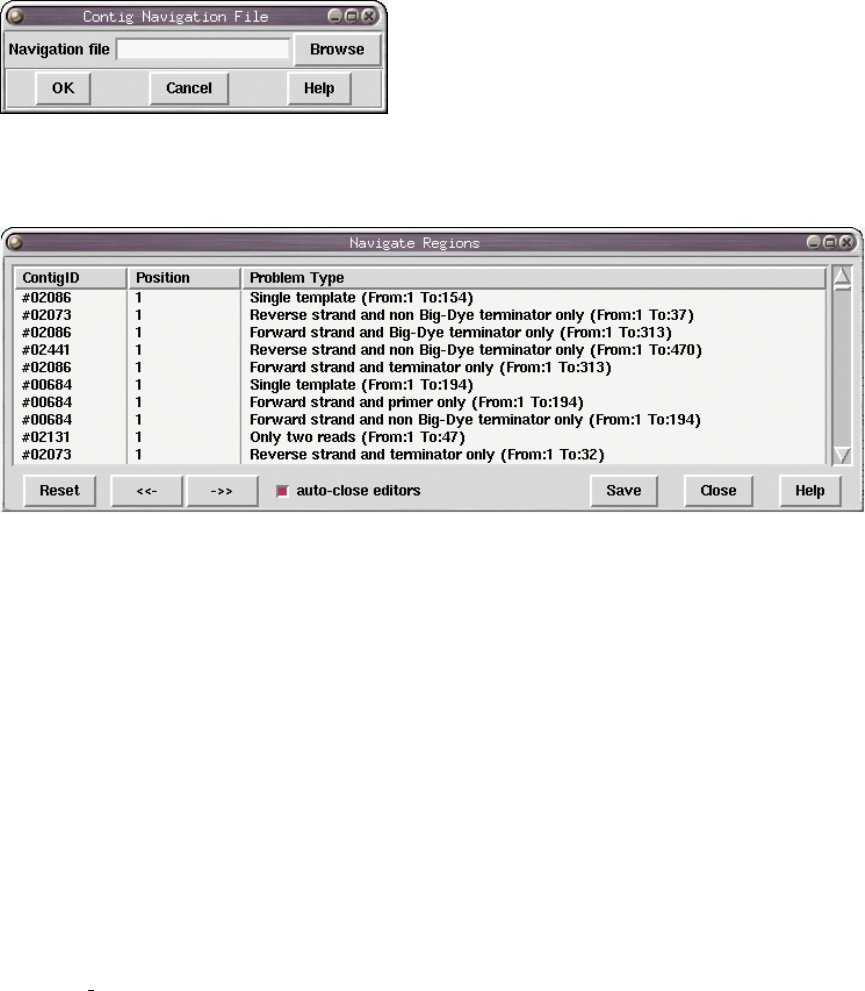
Chapter 2: Sequence assembly and finishing using Gap4 269
2.12.5 Contig Navigation
This function, which can be found under the view menu, allows the user to navigate to
areas of interest within contigs. When Contig navigation is selected a dialog box is raised
asking for a filename containing the regions. The format is the same as the search by file
function. See Section 2.6.6.8 [Search by file], page 176.
The user can either enter the name of the file or browse for it using the browse button.
Once ok is hit, the file is loaded into a table for viewing.
The table has three fixed headers, contigID, Position and Problem Type. Clicking on
any of these cause the whole table to be sorted on that column. The regions can be viewed
by either randomly double clicking on a row , by selecting a row and using the next (->>)
and previous (<<-) buttons at the bottom, or by pressing the Page Up and Page Down keys.
The corresponding contig editor will be opened and moved to the position indicated. Once
a row has been clicked on it’s background will be changed to highlight that it has been
visited.
The reset button will clear the table and re-read the data from file. Auto-close editors
is set on by default. It closes any un-needed editors when the user selects a region on a
different contig. The Show Traces mode will automatically display some traces based on
the same mechanisms used in the editors ’Auto-display Traces’ option (see Section 2.6.8.2
[Trace Display Settings], page 181). Save will save the table list, including all rows previously
marked as selected, back to the file. If this file is re-read at a later stage then the table will
have the same sort order and tagging as when saved.
The format of the input file is as follows:
contig identifier position comment
If the comment contains “To:” and a number then the region indicator at the bottom of
the navigator window updates to show the size of the element, otherwise it just has a line
270 The Staden Package Manual
showing the position of the start. Finally the comment may end in the ’nul’ character to
indicate that it has already been visited. (This is utilised by the Save command.)

Chapter 2: Sequence assembly and finishing using Gap4 271
2.12.6 Sequence Search
The purpose of this function (which is available from the prog View menu) is to find
matches between the consensus sequence and short segments of sequence defined by the
user. The segments of sequence (or "strings") can be typed into the dialogue provided
or can be the sequences covered by consensus tag types (see Section 2.2.7.1 [Tag types],
page 121) selected by the user. The latter mode hence provides a way of checking to see
if a tagged segment of the sequence occurs elsewhere in the consensus. The function was
previously known as "Find Oligos".
Users can elect to search against a "single"contig, "all contigs", or a subset of contigs
defined in a list (see Section 2.14 [Lists], page 278) or a file. If "file"or "list"is selected
the browse button is activated and gives access to file or list browsers. If they choose to
analyse a single contig the dialogue concerned with selecting the contig and the region to
search becomes activated.
Both strands of the consensus are scanned using a very simple algorithm: insertions and
deletions are not allowed, but mismatches are. The "Minimum percent match"defines the
smallest percentage match which will be reported by the algorithm. A value of 75 means
that at least 75% of the bases must match the target sequence.
The user can elect to use tags or to specify their own sequences for the search. Selecting
"Use tags"will activate the "Select tags"browse button. Clicking on this button will bring
up a check box dialogue to enable the user to select the tags types they wish to activate.
Alternatively selecting "Enter sequence"will activate a text entry box and the user can
enter a string of characters. Only the characters ACGTU are allowed and there is no limit
to the length of the string.
If it has not already occurred, selection of this function will automatically transform
the Contig Selector into the Contig Comparator. See Section 2.4 [Contig Comparator],
page 126. Each match found is plotted as a diagonal line in the Contig Comparator. The
length of the diagonal line is proportional to the length of the search string. Self matches
from the tag search are not reported.

272 The Staden Package Manual
If the match between the search string and the contig are in the same orientation,
the diagonal match line will be parallel to the main diagonal, otherwise the line will be
perpendicular to the main diagonal. Matches found between a tag and a contig can be used
to invoke the Join Editor (see Section 2.6.15 [The Join Editor], page 196) or Contig Editors
(see Section 2.6 [Editing in prog ], page 160). Matches between a specified sequence and
a contig will only invoke the Contig Editor. All of the matches found are displayed in the
Output Window e.g.
Match found between tag on contig 315 in the + sense and contig 495
Percentage mismatch 16.7
957 967 977 987 997
315 CATAAGGATTTCCAATATTTTATTCCAGTTGGGCATCCTAGT
:: ::::::::::: :::::::::::::::::: ::::
495 GATTGGGATTTCCAATGTTTTATTCCAGTTGGGCACCCTAAG
2 12 22 32 42
Chapter 2: Sequence assembly and finishing using Gap4 273
2.12.7 Extract Readings
This function (which is available from the gap4 File menu) is used to produce copies of
readings stored in the assembly database. The readings, and information about them,
are written to disk in experiment file format (see Section 11.3 [Experiment file format],
page 552) and will include any edits made and tags created. They are written in their
original orientation. No change is made to the copies in the assembly database: this process
creates copies and should not be confused with "Disassemble readings". See Section 2.9.1.2
[Disassemble Readings], page 240. The names of the readings to extract can be read from a
list or a file of file names. Clicking on the browse button will invoke an appropriate browser
dialogue. If just a single reading is to be assembled choose "single"and enter the filename
instead of the file or list of filenames. The files are written into the "Destination directory"
with their original file names.
If required, the files will include additional information suitable for processing by either
"Enter pre-assembled data"or "Directed assembly"(see Section 11.3.1 [Experiment file
format explained], page 552). Both contain the ON and AV Experiment File records. Pre-
assembled data also contains SE and PC records whilst Directed assembly contains AP
records. It is recommended that Directed Assembly format is always used in preference to
the Preassemble format.
To merge databases use the "Directed assembly"format to output the contigs required.
Then, within the database you wish to merge the data use the Directed Assembly (see
Section 2.7.2 [Directed Assembly], page 211) command. By using Directed Assembly with
new blank databases it is also possible to create database subsets or to split databases.
274 The Staden Package Manual
2.12.8 Automatic Clipping by Quality and Sequence Similarity
Our consensus calculation algorithms use the data for all the unclipped bases covering
each position in a contig. However, some assembly engines may leave the ends of readings
unaligned, and these unaligned bases could therefore lead to the production of an incorrect
consensus. The two clipping methods described here (which are available from the gap4
Edit menu) are designed to overcome this potential problem.
In addition to improving the reliability of the consensus calculation, clipping in this
way tidies up the alignments, so helping the user to concentrate on the better data. It is
important to note that in no case is the clipped sequence thrown away. The contig editor
can show this hidden data, and the clip points may be manually adjusted to reveal any
clipped sequence.
2.12.8.1 Difference Clipping
The difference clipping method (which is available from the gap4 Edit menu) works
in stages. First it calculates the most likely consensus sequence. Then it compares each
reading with that consensus sequence and identifies areas at the ends of the reading where
there are enough differences to indicate the possibility of badly aligned bases. The clip
points are adjusted accordingly.
To identify the clip points for each reading the algorithm first finds a good matching
segment near the middle of the reading. Then steps, base by base, from this point to the
left accumulating a score as it goes by using +1 for a match and -2 for a mismatch. It
sets the left clip point at the position of the highest score. The right clip point is set in
an equivalent way. These new clip points are used only if they are more severe than the
existing ones. The portions of readings which have been clipped are then tagged using a
DIFF tag type. To see which segments have been clipped use the contig editor search tool.
After clipping the algorithm then identifies any holes (breaks in the contigs) that may
have been created and fills them up again by extending the sequence(s) with the fewest
number(s) of expected errors.
Chapter 2: Sequence assembly and finishing using Gap4 275
2.12.8.2 Quality Clipping
The quality clipping function (which is available from the gap4 Edit menu) clips the
ends of readings when the average (over 31 bases) confidence value is lower than a user
defined threshold. As with the difference clipping method the clips are only adjusted when
the newly calculated clip points are more stringent than the originals.
After clipping Gap4 then identifies any holes (breaks in the contigs) that may have been
created and fills them up again by extending the sequence(s) with the fewest number of
expected errors.
An example output follows.
Hole from 32652 to 32725: extend #1378 and #1385 with 3.157324 expected errors
We have observed that when using confidence values expressed as -10*log(err rate), it is
sometimes better not to clip using the confidence values, but to use the difference clipping
method (see Section 2.12.8.1 [Difference Clipping], page 274).
2.12.8.3 Quality Clip Ends
This function performs a similar analysis to Quality Clipping, but only trimming the
ends of contigs. This can be useful as Phrap automatically clips where sequences disagree,
but the ends of contigs will not be trimmed in such a manner. By trimming such poor
quality from the end Find Internal Joins may find some problematic matches.
276 The Staden Package Manual
2.12.8.4 N-Base Clipping
The purpose of this function is to remove runs of Ns or -s from the ends of sequences.
Other bases may be interspersed in a run of dashes and the run will still be clipped, pro-
vided there are a sufficient number of non-A/C/G/T base calls. The exact algorithm for
determining where a ’run’ will stop is as follows:
1. Set score to zero
2. For each base call add 1 for Nor -, -1 for A,C,Gor T, zero for anything else.
3. Terminate when the score <-10.
4. Set the clip point at the highest score observed.
Generally this will have no effect (when on good data). It can never ’grow’ a sequence
(by extending the cutoffs into the good data). It will never form a hole in a contig by
clipping all sequences in a region (as it will extend the data from both ends of the hole to
join it back together again).

Chapter 2: Sequence assembly and finishing using Gap4 277
2.13 Results Manager
Some commands within prog produce "results"that are updated automatically as data
is edited. The Result Manager provides a way to list these results, and to interact with
them.
A result is an abstract term used to define any collection of data. Typically this data can
be displayed, manipulated and is usually updated automatically when changes are made that
affect it. Each set of matches from a particular search plotted on the Contig Comparator
(see Section 2.4 [Contig Comparator], page 126) is a result, as are entire displays such as
the Template Display.
The "results"window, shown above, can be invoked either from the View menu in the
main display or from the View menu of the Contig Comparator. Each result is listed in the
window on a separate line containing the time that the result was created (which may not
be the same as when it was last updated), the name of the function that created the result,
and the result number. The number is simply a unique identifier to help distinguish two
results produced by the same function.
Each item in the list is consuming memory on your computer. Running functions over
and over again without removing the previous results will slow down your machine and it
will, eventually, run out of memory. Removing items from the list solves this.
Pressing the right mouse button over an listed item will display a popup menu of oper-
ations that can be performed on this result. The operations available will always contain
"Remove"which will delete this result and shut down any associated window, but others
listed will depend on the result selected. In the illustration above the popup menu for the
"Repeat search"can be seen. Here the operations relate to a set of repeat matches currently
being displayed in the Contig Comparator (not shown).
The Contig Comparator functions ("Find internal joins","Find read pairs","Find re-
peats","Check assembly"and "Find Sequences") are all listed in the Results Manager
once per usage of the function. It is worth remembering that the only places to completely
remove the plots from one of these functions is using the "Remove"command within the
Results Manager or to use the "Clear"button within the Contig Comparator to remove all
plots.

278 The Staden Package Manual
2.14 Lists
For many operations it is convenient to be able to process sets of data together - for example
to calculate a consensus sequence for a subset of the contigs. To facilitate this prog uses
lists.
Most prog commands dealing with batches of files or sets of readings or contigs can
use either files of filenames or lists. When selecting list names from within dialogues the
"browse"button will display a window containing all the currently existing lists. To select
a list simply double click on the list name. Alternatively the name may simply be typed in.
The List menu on the main menubar contains commands to Edit, Create, Delete, Copy,
Load, and Save lists. Some of these display a list editor. This is simply a scrollable text
window supporting simple editing facilities (see Section 10.2.3 [Text Windows], page 524).
The "Clear"button clears the list. The "Ok"button removes the list editor window.
It is not necessary to use "Ok"here before supplying the list name for input to another
option.
2.14.1 Special List Names
Some lists are automatically updated or are generated on-the-fly as needed. The lists named
"contigs"and "readings"correspond to the currently selected contigs in the contig selector
window and the currently selected readings in the template displays. Note that lists (with
any names) can also be created from selected items in the contig editor. See Section 2.6.8.18
[Set Output List], page 186. The "allcontigs"and "allreadings"lists are created as needed
and always contain an identifier for every contig and every reading identifier.
Because of the way the lists are implemented, as is outlined below, there are some useful
"tricks"that can be employed. A list name consisting of a contig identifier surrounded by
square brackets (’[’ and ’]’) will cause the creation of a list containing all of the readings
within that contig. For example, to use the Extract Readings option (see Section 2.12.7
[Extract Readings], page 273) to extract all the readings from contig ’xb54f8.s1’, the list
name given in the Extract Readings dialogue would be ’[xb54f8.s1]’.
A list name surrounded by curly brackets (’{’ and ’}’) will cause the creation of a list
containing all of the readings in the contigs named in the specified list name. So ’{contigs}’
is equivalent to all the readings in the contigs contained in the ’contigs’ list. Hence the
’allreadings’ list is identical to ’{allcontigs}’.
These tricks can be used anywhere where a list name is required except for editing and
deletion of lists. As a final example, to produce a file of filenames for the currently selected
contigs, save the list named ’{contigs}’ to a file.
2.14.2 Basic List Commands
The basic operations that can be performed on lists include copying, loading, saving, editing,
creation and deletion. Joining and splitting can only be performed using the list editors
and using cut and paste between windows.
The Load and Save commands require a list name and a file name. If only the name of
the file is given the list is assumed to have the same name. If it is desired to load or save

Chapter 2: Sequence assembly and finishing using Gap4 279
a list from/to a file of a different name then both should be specified. Creating a list that
already exists (or loading a file into an already existing list) is allowed, but will produce a
warning message.
The “Reading list” option controls whether the list to be loaded is a list of reading names
(which is normally the case). This will then turn on hyperlinking in any text views of this
list. Double-left clicking on an underlined reading name will bring up the contig editor
while right-clicking will bring up a command menu.
2.14.3 Contigs To Readings Command
This command produces a list or file of reading names for a single contig or for a set of
contigs. The user interface provides a dialogue to select the contigs and to select a list name
or filename.
2.14.4 Minimal Coverage Command
This command produces a minimal list of readings that together span the entire length of
a contig. The dialogue allows contigs names to be defined using a list or a file of filenames.
The output produced, can be sent to a list or a file of filenames. An example use of this
function is to determine a minimal set of overlapping readings for resequencing.
2.14.5 Unattached Readings Command
This command finds the contigs that consist of single readings. The output can be written
to a list or a file of filenames. One example use of the option is for tidying up projects by
removing the trivial and unrequired contigs. In this case the list would be used as input to
disassemble readings (see Section 2.9.1.2 [Disassembling Readings], page 240).
2.14.6 Highlight Readings List
This simply loads the “readings” list so that the template display and contig editor auto-
highlight the chosen readings. This function is the same as the Highlight Readings List
option in the template display.
2.14.7 Search Sequence Names
This command allows searching for sequences matching a given pattern. The function
produces both a list in the text output window and a prog "list"of reading names.
The highlighted output is clickable, with the left mouse button invoking the contig editor
and the right mouse button displaying a popup-menu allowing additional operations (contig
editor, template display, reading notes and contig notes).
The text search may be performed as either case-sensitive or case-insensitive. Addition-
ally the pattern search types are available.
sub-string Matches any reading name where the pattern matches all or part of the name.
wild-cards Searches for a pattern using normal filename wild-card matching syntax. So *
matches any sequence of characters, ?matches any single character, [chars]
matches a set of characters defined by chars, and \char matches the literal
character char. Character sets may use a minus sign to match a range. For
example x*.[fr][1-9] matches any name starting with xand ending with
280 The Staden Package Manual
fullstop followed by either for rfollowed by a single digit between 1 and 9
inclusive. To match a substring using wild-cards prepend or append the search
string with *.
regular expression
This uses the Tcl regular expression syntax to perform a match. These pat-
terns are naturally sub-strings unless anchored to one or both ends using the
^expression$syntax. A full description of regular expressions is beyond the
scope of this manual.
2.14.8 Search Template Names
This searches for template names matching a given pattern. The list produced will contain
just the template names, but the information listed in the text output window lists the
template names and the readings contained within each template. The reading names
are hyperlinks and so double left-clicking on them will bring up the contig editor whilst
right-clicking brings up a popup menu.
For a description of the types of template search patterns see Section 2.14.7 [Search
Sequence Names], page 279.
2.14.9 Search Annotation Contents
This searches the contents of annotations on both the individual reading sequences and the
consensus sequences. A gap4 list will be produce containing the annotation number, contig
and position. In the text output window a more complete description is available listing the
annotation type and the contents of each annotation. Both the list and text-output window
will contain a highlighted section which is a hyperlink. Double clicking on this with the left
mouse button will bring up the contig editor at that point. Clicking with the right mouse
button will display a popup-menu with further options.
For a description of the types of annotation search patterns see Section 2.14.7 [Search
Sequence Names], page 279.
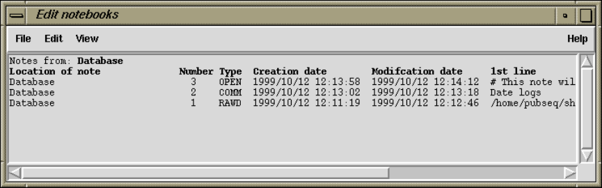
Chapter 2: Sequence assembly and finishing using Gap4 281
2.15 Notes
A ‘Note’ is an arbitrary piece of text which can be attached to any reading, any contig,
or to a database as a whole. Each note also contains a note type, a creation date and a
modification date. Any number of notes can be attached to each reading, contig or database.
They can be considered as positionless tags.
2.15.1 Selecting Notes
The primary interface to creating, viewing and editing notes is the Note Selector window.
This is accessable from a variety of places, including anywhere a contig or reading name (or
line in a graphical plot) is displayed, and also by using the "Edit Notebooks"command in
the main gap4 Edit menu.
The Note Selector initially starts up showing the database notes (unless selected from
a specific contig or reading plot). The picture above shows three notes attached to the
main gap4 database record. These are of type OPEN and RAWD, both of which have a specific
meaning to gap4, and type COMM.
The View Menu is used to see a list of notes for readings or contigs. If Reading Notes or
Contig Notes is selected, the interface will ask for a reading or contig identifier by adding
an extra line to the Note Selector Window, just beneath the menus. Typing one in and
pressing return will then list the notes for that reading or contig.
To speed up selection, it is possible to use the right mouse button on the Contig Selector
Window and in the contig rulers at the bottom of many plots (such as the Template Display),
to select the "List Notes"option. This will start the Note Selector if it is not already
running, and will direct it to display notes for the desired contig. Similarly, the right mouse
button can be used to popup a menu from a reading in the Template Display or from a
reading name in the Contig Editor.
To edit a note, double click anywhere in the Note Selector on the line for the note.
To delete a note, single click on the note line to highlight it and then select "Delete"
from the Note Selector Edit menu. To delete several notes at once, first highlight a range
by left clicking and dragging the mouse to mark a region of notes, and then use Delete.
Alternatively notes may be deleted by double clicking to bring up the note editor and
selecting Delete from the Note Editor File menu.
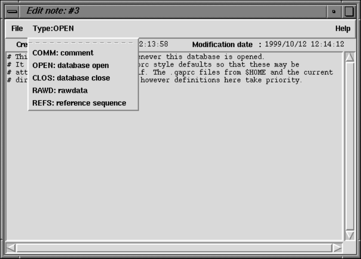
282 The Staden Package Manual
To create a new note use the "New"command from the Edit menu. The note will be
added to whatever data type is currently shown. To create a note for a particular contig,
select that contig using the Contig Notes option in the View menu, and then use New to
create a new note. New notes will have type COMM and the contents can be in any format.
2.15.2 Editing Notes
Double clicking on a note in the Note Selector, or creating a new note, will bring up the
Note Editor Window. This is simple text editor, allowing use of keyboard arrow keys and
the mouse to position and edit text. It also has keyboard bindings for many of the simple
emacs movement commands.
At the top of the Notes Editor are three buttons. The leftmost is the File menu which
contains the "Save","Delete"and "Exit"options. Next to this is the Type selector. This
menu name displays the currently selected note type. To change the note type select the
appropriate type from the Type menu. The final button gives access to the online Help.
Listed underneath the menu are the creation and modification dates. The creation date
if fixed when a note is created. The modification date is adjusted every time a note is
edited. (Simply viewing a note will not update the modification date, but saving changes
to it will.)
Underneath these is the note text itself. For convenience, the first line of each note is
shown in the note selector window (so it can be helpful to make it identifiable).
2.15.3 Special Note Types
Several types of note have special meanings. These include the OPEN,CLOS and RAWD note
types.

Chapter 2: Sequence assembly and finishing using Gap4 283
OPEN
CLOS Notes of type OPEN and CLOS should contain pure Tcl code. If they exist,
they will be executed when the database is opened (OPEN) and closed (CLOS).
Take great care in creating and editing a note with these types! The purpose
is to allow configuration options to be attached to a database, and hence allow
for different gap4 configurations to be used when a UNIX directory contains
more than one database. In general use of the ‘.gaprc’ file (see Section 2.20.1
[Options Menu], page 298) is probably safer.
If there is a problem with a database containing a malformed OPEN or CLOS
note, it may be opened using gap4 -no_exec_notes. This will prevent gap4
from executing the OPEN and CLOS notes and so allow them to be fixed using
the Note Editor.
RAWD This note specifies an alternative to the RAWDATA environment variable and
should be set to be the full directory name for the location of the trace files for
the database. If both the environment variable and the note are exist then the
note will take priority. This automatic use of this note can be disabled be using
the -no_rawdata_note command line option to gap4.
INFO When created on a reading or a contig, this note may be displayed in the contig
editor "information line"(see Section 2.6.14 [The Editor Information Line],
page 193) when the user moves the mouse over the editor sequence name list.
It is possible to create your own types by editing the ‘$STADENROOT/tables/NOTEDB’
file. The format is fairly self explainatory, and is very similar to the ‘GTAGDB’ file. Each
note type should consist of the long name followed by a colon and id=4 letter short name,
optionally followed by dt="any default text for this note". Lines may be split at colons by
adding a backslash to the end of the line. See the standard ‘NOTEDB’ file for examples.
284 The Staden Package Manual
2.16 Gap4 Database Files
Gap4 stores the data for each sequencing project (e.g. the data for a single cosmid or BAC)
in a gap4 assembly database, so at the start of a sequencing project the user should employ
gap4 to create the database for the project (see Section 2.16.2 [Opening a New Database],
page 285). New database are created with sufficient index space for around 8000 readings,
but this can be extended if required.
Gel reading data in experiment file format (see Section 11.3 [Experiment File Format],
page 552) is entered into the database using the methods available from the assembly menu
(see Section 2.7 [Entering Readings into the Database (Assembly)], page 205).
To assemble more data for the project or to edit or analyse readings already entered
the user should open the same project database (see Section 2.16.3 [Opening an Existing
Database], page 285).
Although the database files are designed to be free of corruption it is advisable to make
regular backups (see Section 2.16.4 [Making Backups of Databases], page 285).
Database names can have from one to 240 letters and must not include a full stop or
spaces. The database itself consists of two files; a file of records and an index file. If the
database is called ‘FRED’ then version 0 of the database comprises the pair of files named
‘FRED.0’ and ‘FRED.0.aux’, the latter of these being the index file. The "version"is the
character after the full stop in these filenames. Versions are not limited to numbers alone,
but must be single characters.
When a database is opened for writing a ‘BUSY’ file is created. For the ‘FRED’ database
this will be named ‘FRED.0.BUSY’. When the database is closed the file is deleted. The
file is used by gap4 to signify that the database is opened for writing and is part of its
mechanism to prevent more than one person editing a database at any time. Before opening
a database for writing, gap4 checks to see if the BUSY file for that database exists. If it
does the database is opened only for reading, if not it creates the file, so that any additional
attempts to open the database for writing will be blocked. A side effect of this mechanism,
is that in the event of a program or system crash the BUSY file will be left on the disk,
even though the database is not being used. In this case users must remove the BUSY file
(after checking that it really isn’t in use!) using, on UNIX the rm command before opening
the database. Eg "rm FRED.0.BUSY". On Windows use the Recycle Bin.
The gap4 database is robustly designed. Killing the program whilst updating the data-
base should never yield an inconsistent state. A "roll-back"mechanism is utilised to undo
any partially written updates and revert to the last consistent database. Hence quitting
abnormally may result in the loss of some data. Always quit using the Exit command within
the File menu.
However it is advised that copies of the database are made regularly to safeguard against
any software bugs or disk corruptions.
2.16.1 Directories
By default, Gap4 expects files to be in the current directory. In dialogues which request
filenames, full pathnames can be specified, however it is generally tidier to keep files specific
to a particular project in the same directory as the project database. Creating new databases
Chapter 2: Sequence assembly and finishing using Gap4 285
and opening new databases will change directory to the directory containing the opened
project.
It is possible to change the current directory by selecting "Change directory"from the
File menu. Be warned that changing to a directory other than that containing the database
and the trace files may mean that gap4 can no longer find the trace files. The solutions to
this problem are discussed elsewhere (see Section 2.20.8 [Trace File Location], page 302).
2.16.2 Opening a New Database
To create a new gap4 database select the "New"command from the File menu. This brings
up a dialogue prompting the the new filename. Type the name of the database to create
without specifying the version number. To create version 0 of a database named ‘FRED’
typing FRED will create the two database files, ‘FRED.0’ and ‘FRED.0.aux’.
If the database already exists you will be asked whether you wish to overwrite it. Any
database that was already open will be closed before the new database is created. The new
database is then opened, ready for input.
Note that Gap4 database names are case sensitive.
2.16.3 Opening an Existing Database
To open an existing database select the "Open..."command from the File menu. This brings
up a file browser where the database name can be selected. The databases will be listed in
aNAME.V notation (where Vis the version number). Double clicking on the database name
will then open this database.
If the program already had a database open it will close it before the new one is opened.
If the new database is already in use by gap4 a dialogue will appear warning you that the
database has been opened in read only mode. This mode prevents any edits from being
made to the database by greying out certain options and disabling the editing capabilities
in the contig editor.
A database may also be opened by specifying the database name and version on the
unix command line. To open version 0 of the database ‘FRED’ use "gap4 FRED.0".
2.16.4 Making Backups of Databases
The importance of making regular backups of your data cannot be over stated. Using
the "Copy database"command from the File menu brings up a dialogue asking for a new
database version. Type in a single character for the new version and press "ok"or return.
If the new database already exists you will be asked whether you wish to overwrite it. Any
subsequent changes you make will still be to the database that you originally opened, not
to the database you have just saved to.
The database file may sometimes become fragmented. An option available when saving
is to use garbage collection. This creates the new database by only copying over the used
portions of data (and hence reduces fragmentation). However it is quite a lot slower than
the standard "Copy database"mechanism, so if this causes problems add "set_def COPY_
DATABASE.COLLECT 0" to your ‘.gaprc’ file to change the default to no garbage collection.
It should be noted that garbage collection also performs a rigorous database consistency
check.

286 The Staden Package Manual
Do not always use the same version character for you backups. Instead keep several differ-
ent backups. Otherwise you may find that both your current database and the backup have
problems. It is also wise to run "check database"to verify data integrity. See Section 2.18
[Check Database], page 290.
It is also possible to backup databases from outside gap4 by using standard unix com-
mands to copy both the record and index files. Care should be taken when doing this
to ensure that the database is not being modified whilst copying. See your unix or Win-
dows manuals for further details or the copy_db manual page (see Section 12.2 [Copy db],
page 573) for the external garbage collecting database copy program.
2.16.5 Reading and Contig Names and Numbers
For various reasons there are restrictions on the characters used in file names and the length
of the file names.
Characters permitted in file names:
ABCDEFGHIJKLMNOPQRSTUVWXYZabcdefghijklmnopqrstuvwxyz0123456789._-
A reading name or experiment file name must not be longer than 40 characters.
These restrictions also apply to SCF files which means, in turn, also to the names given
to samples obtained from sequencing instruments. For example do not give sample names
such as 27/OCT/96/r.1 when using and ABI machine: the / symbols will be interpreted as
directory name separators on UNIX!
As each reading is entered into a project database it is given a unique number. The first
is numbered 1, the second 2 and so on. Their reading names are read from the ID line in
the experiment files and copied into the database. As new readings are created and existing
ones removed the reading numbers change in an unpredictable fashion. Hence when taking
notes on a project always record the reading name instead of the reading number.
The maximum number of readings a database can hold is 99,999,999.
Many options ask for a reading or contig identifier. A contig identifier is simply any
reading name or number within that contig. A reading identifier is either the reading name
or the hash ("#") character followed by the number. For example, if the reading name is
fred.gel with number 99 users could type "fred.gel" or "#99" when asked to identify
the contig.
Generally when prompting for a contig or reading name a default is supplied. This is
the last name you used, or if you’ve only just opened the database, the name of the longest
contig in the database. For more information about selecting contigs within the program
see See Section 2.3.1 [Selecting Contigs], page 123..
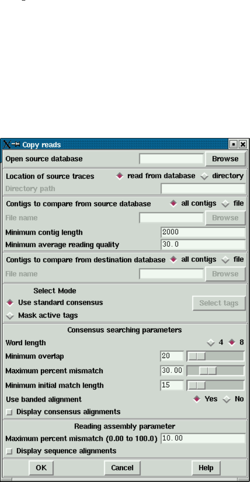
Chapter 2: Sequence assembly and finishing using Gap4 287
2.17 Copy Readings
2.17.1 Introduction
During large scale sequencing projects where the genome is cloned into e.g. BACs prior to
being subcloned into sequencing vectors it is generally the case that the ends of the DNA
from one BAC will overlap that of two other BACs. Unless it is being used for quality
control, it is a waste of time to sequence the overlapping regions twice, and so most labs
transfer the relevant data between the adjacent gap4 databases. This is the function of
copy reads which copies readings from a "source"database to a "destination"database.
The consensus sequences for user selected contigs in each of the two databases are com-
pared in both orientations. If an overlapping region is found, readings of sufficient quality
are automatically assembled into the destination database. In the source database read-
ings which have been added to the destination database will be tagged with a "LENT"
tag and the equivalent readings in the destination databse will be tagged with a "BORO"
(borrowed) tag.
2.17.1.1 Copy Reads Dialogue
288 The Staden Package Manual
The Copy reads function is available from either the File menu of gap4 or from the
command line.
The program must be able to write to both databases. It is recommended that you create
backups of both databases before commencing using "Copy database". See Section 2.16.4
[Making Backups of Databases], page 285.
From within gap4: The source database must be entered into the "Open source database"
entry box at the top of the dialogue box. The adjacent Browse buttons will list only gap4
databases, that is files ending in aux. Either select from the browser by double clicking on
the name or type in the database name. The ending of .aux is ignored. The destination
database is always the database which is currently open in gap4.
The location of the traces of the source database can either be determined from the
rawdata note (see Section 2.20.8 [Trace File Location], page 302) held within the database
("read from database") or can be entered via the "directory"option. The program will
add the location of the source traces into the rawdata note of the destination database.
If the environment variable RAWDATA is set, this will be taken to be the location of the
destination database traces and will also be added to the rawdata note of the destination
database. If there are no traces for the source database, no rawdata note will be created.
One or more contigs from the source database can be compared. These are selected
either by clicking on "all contigs"or providing a file containing a list of contig names (any
reading name from within that contig, typically the first reading name). Only contigs
over a user defined length will be used. A minimum reading quality can be set so that
only readings with an average quality over the specified amount will be entered into the
destination database.
Contigs from the destination database can be chosen by either selecting "all contigs"or
providing a file of contig names.
The consensus sequence is determined for each contig in both databases using either the
standard consensus algorithm or "Mask active tags". The latter option will activate the
"Select tags"button. Clicking on this button will bring up a check box dialogue to enable
the user to select the tags types they wish to activate. Masking the active tags means that
all segments covered by tags that are "active"will not be used by the matching algorithms.
A typical use of this mode is to avoid finding matches in segments covered by tags of type
ALUS (ie segments thought to be Alu sequence) or REPT (ie segment that are known to
be repeated elsewhere in the data (see Section 2.2.7.1 [Tag types], page 121).
The consensus searching parameters are equivalent to those found in the find internal
joins algorithm (see Section 2.8.3 [Find Internal Joins], page 227). The search algorithm
first finds matching words of length "Word length", and only considers overlaps of length
at least "Minimum overlap". Only alignments better than "Maximum percent mismatch"
will be reported. Find internal joins has the option of either a quick or sensitive algorithm.
Here, it is only necessary to use the quick algorithm. The quick algorithm can find overlaps
and align 100,000 base sequences in a few seconds by considering, in its initial phase only
matching segments of length "Minimum initial match length". However it does a dynamic
programming alignment of all the chunks between the matching segments, and so produces
an optimal alignment. A banded dynamic algorithm can be selected, but as this only applies

Chapter 2: Sequence assembly and finishing using Gap4 289
to the chunks between matching segments, which for good alignments will be very short, it
should make little difference to the speed. The alignments between the consensus sequences
can be displayed in the text output window by selecting "Display consensus alignments".
If a match between two consensus sequences is found, the readings in that overlap
are assembled into the destination database using the "directed assembly"function (see
Section 2.7.2 [Directed Assembly], page 211). Only readings for which the "Maximum per-
cent mismatch"is not exceeded, and which have an average reading quality higher than the
specified minimum, will be entered into the database. Again, the alignments can be shown
in the Output window by selecting "Display sequence alignments".
From the command line:
copy reads [-win] [-source trace dir ("")] [-contigs from <file>(all contigs)]
[-min contig len (2000)] [-min average qual (30.0)] [-contigs to <file>(all contigs)] [-mask
<none mask>(none)] [-tag types <list>("")] [-word length (8)] [-min overlap (20)]
[-max pmismatch (30.0)] [-min match (20)] [-band (1)] [-display cons] [-align max mism
(10.0)] [-display seq] [source database] [destination database]
The values in brackets () are the default values. The only mandatory values are the
source and destintation databases. Details on these values are given in the copy reads man
page (see Section 12.3 [Copy reads], page 574).
The -win option will bring up a new program which presently only has one function
(copy reads). This is accessed from the "File"menu. This brings up a dialogue the same
as that from within gap4 except for an extra entry box to select the destination database.

290 The Staden Package Manual
2.18 Check Database
This function (which is available from the gap4 File menu) is used to perform a check on
the logical consistency of the database. No user intervention is required. If the checks are
passed the message "Database is logically consistent"is written to the Output Window. If
the database is not found to be consistent diagnostic messages will appear in the Output
Window and Doctor Database from the Edit menu should be used to correct the problem.
See Section 2.19 [Doctor Database], page 293.
Several options, such as assembly, automatically perform a check database prior to ex-
ecuting. If the database is found to be inconsistent the option will not continue. However
some checks are considered as "non fatal"and will not block such operations. Currently
the only non fatal checks are the positional checks for annotations and for readings that
are never used. To fix the database, use the Doctor Database "ignore check database"
setting to disable the inconsistency checking. See Section 2.19.2 [Ignoring Check Database],
page 296.
The following sections define the checks and the order in which they are performed.
2.18.1 Database Checks
•Number of contigs used is <= number allocated
•Disk and memory values for "number of contigs"are consistent
•Number of readings used is <= number allocated
•Disk and memory values for "number of readings"are consistent
•Disk and memory values for "actual database size"are consistent
•Actual database size <= maximum size
•Data class is either DNA(0) or protein(1).
•Number of free annotations >= 0 and <= number allocated
•Contig order is consistent
•Number of free notes >= 0 and <= number allocated
•First note has prev type as GT Database
•Detect note loops
2.18.2 Contig Checks
•Has a left reading number
•Has a right reading number
•The left reading has no left neighbour
•The right reading has no right neighbour
•Chain right to
−check loops
−check holes
−flag a reading as used
•When finished chaining
−check length is correct

Chapter 2: Sequence assembly and finishing using Gap4 291
−check right reading number is correct
•Reference only valid reading numbers
•Chain left to
−check loops
−flag readings as used, if not done so in right chaining;
•When finished chaining, check left reading number is correct
•Chain along annotation list to
−flag as used
−detect annotation loops
−annotation is within the contig
−annotation is rightwards of previous
•First note has prev type as GT Contigs
•Detect note loops
2.18.3 Reading Checks
•Memory and disk values tally for
−left neighbour
−right neighbour
−relative position
−length +sense
•Left neighbour is a valid reading number
•Right neighbour is a valid reading number
•Reading is not used zero times
•Reading is not used more than once
•Hand holding: (lnbr[rnbr[reading]] == reading)
•Relative position of reading >= position of left neighbour
•Length != 0
•Used sequence length == "right clip position"-"left clip position"
•Has valid strand (0 or 1)
•Has valid primer
•Has valid sense (0 or 1)
•Chain along annotation list to
−flag as used
−detect annotation loops;
−annotation is rightwards of previous
•First note has prev type as GT Readings
•Detect note loops

292 The Staden Package Manual
2.18.4 Annotation Checks
•No loops in free annotation list
•Is neither used nor is on the free list
•Annotation is not used more than once
•Is used, yet is still on the free list
•Length >= 0
•Has valid strand (0 or 1)
2.18.5 Note Checks
•No loops in free note list
•Is neither used nor is on the free list
•Hand holding: (note->next->prev == note)
•Note is not used more than once
•Is used, yet is still on the free list
2.18.6 Template Checks
•Minimum insert length <= maximum insert length
•Has valid vector
•Has valid clone
•Has valid strand
2.18.7 Vector Checks
•Level >0
•Level <= MAX LEVEL (MAX LEVEL currently is 10; a "feasibility"check)
2.18.8 Clone Checks
•Has valid vector

Chapter 2: Sequence assembly and finishing using Gap4 293
2.19 Doctor Database
Doctor Database (which is available from the gap4 Edit menu) is used to make arbitrary
changes to the database. It should be extremely unlikely that is use will be required, and
if so, is for experts only. Very few checks are performed on the user’s input and there
are few limitations on what can be done. Consequently this option should never be used
without first making a backup using "Copy database". See Section 2.16.4 [Making Backups
of Databases], page 285. It is very easy to create inconsistencies within the database. Do
not feel that values (such as the maximum gel reading length) can be safely changed simply
because they are shown in a dialogue.
The main window consists of a menubar containing "File","Structures"and "Com-
mands"menus. The menus contain:
•File
−New
−Quit
•Structures
−Database
−Reading
−Contig
−Annotation
−Template
−Original clone
−Vector
−Note
•Commands
−Check
−Ignore check database
−Extend structures
−Reading
−Annotation
−Template
−Clone
−Vector
−Delete contig
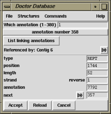
294 The Staden Package Manual
−Shift readings
−Reset contig order
−Output annotations to file
−Delete annotations
The New command in the Commands menu brings up another Doctor Database window
complete with its own menubar. This is useful for comparing structures. Whilst Doctor
Database is running all other program dialogues, including the main gap4 menubar, are
blocked. Control is reenabled once the last Doctor Database window is removed. Remem-
ber to perform a Check Database (Commands menu) before quitting to double check for
database consistency.
2.19.1 Structures Menu
The gap4 database consists of records of several predefined types. The types correspond to
the commands available within the Structures menu. All of these, except for the "Database"
command, insert a dialogue between the menubar and whatever is underneath it. In the
picture below we have selected "Annotations"from the menu which has prompted for
"Which annotation (1-380)"(the 1-380 is the valid range of inputs available).
In the panel beneath the "Which annotation"question is a panel detailing another
annotation structure. In general the structure type and number are shown at the top of the
panel (in this case annotation number 100). Beneath this are the structure fields on the
left followed by the values for these fields on the right. Sometimes gap4 may store a value
as numeric, but display the structure as both a numeric and a string describing this value.
For instance here the annotation strand is "1"which is gap4’s way of storing "reverse".
Some values have an arrow next to them, such as with the "next"field in the illustration.
Clicking on this arrow will display the structure referenced by this value. Here it is another
annotation (annotation 357). It is stated that the annotation is part of Contig number 6.
Clicking on the arrow next to this will reveal that contig structure.

Chapter 2: Sequence assembly and finishing using Gap4 295
Selected notes on editing the structures follows.
2.19.1.1 Database Structure
There is only a single Database structure. A description of its more important fields follows.
num contigs
The number of currently used contigs
num readings
The number of currently used readings
Ncontigs The number of currently allocated contigs
Nreadings The number of currently allocated readings
contigs
readings
annotations
templates
clones
vectors
notes Record numbers of arrays holding the record numbers of each item
free annotations
A linked list of unused annotations
free notes A linked list of unused notes
2.19.1.2 Reading Structure
Some Reading Structure fields reference the record number in the gap4 database of a string.
Where this string is short, such as the reading name, both the record number and the
contents of the string can be edited. To edit a single name the string should be changed.
To swap two reading names around either edit both strings or swap the two name record
numbers.
The annotations value references an annotation number. If this is zero then this reading
has no annotations.
The length is the complete length of sequence, including hidden data. The
sequence length is the length of only the used sequence. The location of the hidden data
is specified by the start and end values. Note that sequence length=end-start-1.
Aleft or right value of zero means that this reading has no left or right neighbour.
2.19.1.3 Contig Structure
A Contig Structure is defined as a list of readings. The left and right values specify the
first and last reading numbers in the doubly linked list representing the contig.
296 The Staden Package Manual
2.19.1.4 Annotation Structure
Annotations are stored as linked lists. Each reading and each contig has a (possibly blank)
list. All other unused annotations are held on the free list. The next value is used to
reference the next annotation number. A value of zero represents the end of the list.
2.19.1.5 Template Structure
The Template name field can be edited as both a string and the record number pointing to
that string. The Template Structure display has links to a vector number and a clone.
2.19.1.6 Original Clone Structure
The original clone name is often the name of the database. The use of original clones is
primarily for large scale sequencing. When breaking down a sequence into cosmids and then
into sequencing templates, we say that each cosmid is a clone.
2.19.1.7 Note Structure
A Note may be considered as a positonless annotation (without the position, length or
strand fields). Notes store both their creation and last-modification dates. Notes may be
attached, in a linked-list fashion, to readings, contigs, or the database structure.
2.19.2 Ignoring Check Database
Many functions use the Check Database function to determine whether the database is
consistent. Often editing an inconsistent database can yield more and more inconsistencies.
However it is sometimes useful to use such an editing function in the process of fixing the
database. In such cases, the "Ignore check database"toggle should be set.
An example of the use is for the Break Contig function. If we find that a database is
inconsistent due there being a gap in the contig, the obvious solution is to fix this using
Break Contig. But Break Contig checks for consistency, and refuses to work if the database
is inconsistent.
2.19.3 Extending Structures
Sometimes it is required to allocate new structures. The "Extend structure"item on the
command menu reveals a cascading menu containing the different structure types. Once a
type has been selected a dialogue appears asking how many extra structures to create.
The new structures created can then be modified using the Structures menu. Expect
strange behaviour if these structures are not initialised correctly.
2.19.4 Listing and Removing Annotations
The Commands menu contains two commands for manipulating lists of annotations. Output
annotations to file saves a list of annotations to file. The dialogue requests a filename
to save the annotations to and an annotation type. Only one type can be specified.
The format of the file is "Annotation_number Type Position Length Strand".
The "Delete annotations"command requests a file of annotations in this format. The
function then removes these annotations from readings and contigs and adds them to the
free annotation list.
Chapter 2: Sequence assembly and finishing using Gap4 297
2.19.5 Shift Readings
The Shift Readings option allows the user to change the relative positions of a set of neigh-
bouring readings starting at a selected reading. Hence it can be used to change the alignment
of readings within a contig. It prompts for the number of the first reading to shift and then
the relative distance to move by. A negative shift will move the readings leftwards.
The reading and all its rightward neighbours are moved by the requested distance. Tags
on the readings and the consensus are moved accordingly. The command also automatically
updates then length of the contig.
2.19.6 Delete Contig
The Delete Contig function removes a contig and all its readings. Annotations on the
removed readings and contig are added to the free annotations list.
2.19.7 Reset Contig Order
The contig order information contains a list of contig numbers. If a contig number does
not appear within this list, or if it appears more than once, then the contig order is incon-
sistent and windows such as the Contig Selector may not work. The Reset Contig Order
function resets the contig order to a consistent state, but will lose the existing contig order
information.

298 The Staden Package Manual
2.20 Configuring
2.20.1 Introduction
The Options menu allows selection of the Consensus algorithm and the genetic code to use,
and adjustment of various parameters used throughout gap4. It also provides a way of
setting more trivial things such as fonts and colours.
Most of these options have "OK Permanent"buttons in addition to the normal "OK"
button. The "OK Permanent"button will save the current settings to the ‘.gaprc’ file in
the user’s home directory. On Windows 95 this may be C:\.
In general users will not need to be aware of this method as the most important configu-
ration options are all available from within the graphical user interface. However there are
many additional configurable parameters which may be referred to throughout the manual.
These too are stored in the ‘.gaprc’ files.
When gap4 starts up it will first load the complete set of configurations from the
‘$STADENROOT/tables/gaprc’ file. Next it loads ‘.gaprc’ from the user’s home directory,
and finally ‘.gaprc’ from the user’s current project directory. This means that the setting
stored in the ‘.gaprc’ file in the user’s project directory will have priority over those found
in the home directory, which, in turn, have priority of those found in the Staden Package
installation directories.
Note that searching for the ‘.gaprc’ files only applies when starting gap4 and not when
opening new or different databases. Hence if the user double clicks on a database ‘.aux’
file then gap4 will read the ‘.gaprc’ file found in the same directory as the database. If
users start up gap4 from the Start menu and then open the project, the ‘.gaprc’ file in the
project directory will not be read.
The format of commands in the ‘.gaprc’ file are:
"#"followed by anything is a comment.
"set def VARIABLE value"sets the parameter "VARIABLE"to the value
"value". Note that value must be enclosed in double quotes if it contains
spaces.
"set defx temp VARIABLE value"sets a parameter in a temporary list named
"temp". This has no effect unless it is then used within a set def command. In
this case we use "$temp"as the "value"parameter of a set def command.
An example follows:
set_def FIJ.MAXMIS.VALUE 30.00
set_def TEMPLATE.PRIMER_REVERSE_COLOUR "green"
set_def CONTIG_EDITOR.DISAGREE_MODE 2
set_def CONTIG_EDITOR.DISAGREE_CASE 0
set_def CONTIG_EDITOR.MAX_HEIGHT 25
Chapter 2: Sequence assembly and finishing using Gap4 299
Note that some adjustments will effect more than just gap4. For example, the colours
of traces are stored in the ‘.tk_utilsrc’ file, and this file is used by both gap4 and trev.
For colour blind users it can be useful to change these particular settings. For example the
following is a ‘.tk_utilsrc’ file to change the colours for the trace displays.
set_def TRACE.COLOUR_A white
set_def TRACE.COLOUR_C blue
set_def TRACE.COLOUR_G black
set_def TRACE.COLOUR_T "#ff8000"
set_def TRACE.LINE_WIDTH 2
2.20.2 Consensus Algorithm
Gap4 currently contains 3 consensus algorithms (see Section 2.11.5 [The Consensus Algo-
rithms], page 257). This option (which is available from the gap4 Options menu) allows the
algorithm to be selected.
Note the consensus algorithm is used in several places throughout gap4: Assembly
(see Section 2.7.1 [Normal Shotgun Assembly], page 205), producing a consensus sequence
file (see Section 2.11.5 [The Consensus Algorithms], page 257), in the Contig Editor (see
Section 2.6 [Editor introduction], page 160), for Experiment Suggestion (see Section 2.10
[Finishing Experiments], page 241), and in the plot of the confidence values (see Section 2.5.2
[Consistency Display], page 140).
2.20.3 Set Maxseq/Maxdb
The "Set maxseq/maxdb"option (which is available from the gap4 Options menu) may be
used to adjust the maximum size of the total consensus sequence contained within gap4.
This includes concatenations of consensus sequences (with extra space for text headers) and
the cutoff data at either end of each contig.
When opening an already assembled project, maxseq is automatically increased accord-
ingly (if required), so "Set maxseq"only needs to be used when adding in more data, such
as when using the sequence assembly algorithms.
The maxdb option controls the maximum combined number of readings and contigs
allowed. Note that changing this does not take effect on the currently opened database so
be sure to set it before opening your database.
Both these values can also be adjusted by using the -maxseq and -maxdb command line
arguments. See Section 2.21 [Command Line Arguments], page 306.
2.20.4 Set Fonts
"Set fonts"(which is available from the gap4 Options menu) controls the fonts used for the
various components of gap4’s windows. Note that for the correct operation of some displays,
careful font selection is necessary. For example it is not wise to chose a proportional font
for the Contig Editor, which displays fixed width sequence alignments. For more complete
documentation, see Section 10.8 [Font Selection], page 531..

300 The Staden Package Manual
2.20.5 Configuring Menus
When used for the first time gap4 will start up in beginner mode. What this means is that
some of the less widely used options will not appear in the menus. The "Configure menus"
command in the Options menu may be used to change between "beginner"and "expert"
mode. In expert mode all the menu items will be displayed.
To permanently set the menu level users select the appropriate level and press the "OK
Permanent"button. This will save the menu level information to the ‘.gaprc’ file in their
home directory.
If desired, other menu levels may be created by the package administrator. This is
achieved by editing the ‘$STADENROOT/tables/gaprc_menu_full’ file, changing the MENU_
LEVELS definition and adding the appropriate labels to the end of each command. Each
command specified in the menu file ends in a list of menu levels in which it is active. To
make a command active for several levels, enclose the level identifiers in a Tcl list, such as
{m e}. If this is missing, the command will be active at all menu levels.
2.20.6 Set Genetic Code
This function allows the user to change the genetic used in all the options. The codes are
defined as a set of codon tables stored in the directory tables/gcodes distributed with the
package. The current list of codes and their codon table file names is shown at the end of
this section.
The user interface consists of the dialogue shown below. The user selects the required
code by clicking on it, and then clicking "OK"or "OK permanent". The former choice
selects the code for immediate use, and the latter also selects it for future uses of the
program.
When the dialogue is left the codon table selected will be displayed, as below, in the
Output Window.
===============================================
F ttt S tct Y tat C tgt
Chapter 2: Sequence assembly and finishing using Gap4 301
F ttc S tcc Y tac C tgc
L tta S tca * taa W tga
L ttg S tcg * tag W tgg
===============================================
L ctt P cct H cat R cgt
L ctc P ccc H cac R cgc
L cta P cca Q caa R cga
L ctg P ccg Q cag R cgg
===============================================
I att T act N aat S agt
I atc T acc N aac S agc
M ata T aca K aaa G aga
M atg T acg K aag G agg
===============================================
V gtt A gct D gat G ggt
V gtc A gcc D gac G ggc
V gta A gca E gaa G gga
V gtg A gcg E gag G ggg
===============================================
The following table shows the list of available genetic codes and the files in which they
are stored for use by the package. They were created from genetic code files obtained from
the NCBI.
code_1 Standard
code_2 Vertebrate Mitochondrial
code_3 Yeast Mitochondrial
code_4 Coelenterate Mitochondrial
code_4 Mold Mitochondrial
code_4 Protozoan Mitochondrial
code_4 Mycoplasma
code_4 Spiroplasma
code_5 Invertebrate Mitochondrial
code_6 Ciliate Nuclear
code_6 Dasycladacean Nuclear
code_6 Hexamita Nuclear
code_9 Echinoderm Mitochondrial
code_10 Euplotid Nuclear
code_11 Bacterial
code_12 Alternative Yeast Nuclear
code_13 Ascidian Mitochondrial
code_14 Flatworm Mitochondrial
code_15 Blepharisma Macronuclear
2.20.7 Alignment Scores
The Alignment Scores command (which is available from the gap4 Options menu) may
be used to adjust the gap open and gap extension penalties for some of the alignment

302 The Staden Package Manual
algorithms used within gap4. At present this will affect all alignments except the Find
Internal Joins function and most of the assembly algorithms.
For dealing with sequences where the alignment differences have been caused by real
evolutionary events, these parameters will probably need changing from the defaults. The
default values are set up with the assumption that any alignment differences are due to
base calling errors, and hence the gap extension penalty will be high.
The alignment matrix may also be adjusted, but this is not listed in the dialogue.
To do this take a copy of ‘$STADENROOT/tables/nuc_matrix’, edit the copy, and set the
ALIGNMENT.MATRIX_FILE parameter in your ‘.gaprc’ file.
2.20.8 Trace File Location
Gap4 does not store the trace data within the gap4 database. Instead it stores the filename
of the trace file. Usually the trace files are kept within the same directory as the gap4
database. If this is not the case gap4 needs to know where they are.
To make sure that gap4 can still display the traces we need to specify any alternative
locations where traces may be found. The "Trace File Location"command (which is avail-
able from the gap4 Options menu) performs this task. It brings up a dialogue asking for
the directory names. If there is just one directory to specify, its name should be typed in.
If there are several directories to search through, they must all be typed in, separated by
the colon character (":"). To include a directory name that contains a colon, use a double
colon.
For example, on windows to specify two directories, use (eg) "F::\tfiles1:G::\tfiles2".
In addition to specifying directories, RAWDATA may also be used to indicate that
the trace files come from a variety of other sources using the general format SOURCE-
TYPE=path. These can be combined with directories if desired. For example “.:/trace_
cache:TAR=/traces/archived.tar”.
TAR=filename.tar
Searches for the trace name in the Unix tar archive named filename.tar.
If filename.tar.index exists and is of the format created using the index_tar
program then the trace name will be looked up in the index instead of se-
quentially scanning through the tar file. In order to speed up accessing of
traces within the tar file a command line utility named index_tar may be
used. This produces a text index containing the filenames held within the tar
and their offsets within it. Programs will then use this index file to provide
a fast way of accessing the trace. The syntax for index_tar is: index_tar
tar filename >tar filename.index. (For example "index_tar traces.tar >
traces.tar.index".)
SFF=filename.sff
Searches for the trace name in a 454 SFF archive named filename.sff. SFF files
have their own binary-sorted index which allows for random access.
HASH=archive.hash
This method supersedes the TAR= accessor. Tar files may be “hashed” using
the hash_tar tool. Similarly 454 SFF archives may be hashed using hash_sff.
Chapter 2: Sequence assembly and finishing using Gap4 303
In theory any type of archive may be indexed as a “.hash” provided that the
traces are stored uncompressed (or compressed only using their own methods,
such as with ZTR) so that random access is possible within the archive.
The Hash file contains a precomputed binary index of all the traces contained
within it stored in such a way that random access is very fast.
URL=url
This uses the external wget tool (not supplied as part of the Staden
Package) to fetch a given url. Anywhere that %s occurs within the
specified url will be replaced by the trace name. Hence, for example,
URL=http://trace.server.org/cgi-bin/lookup.pl?trace=%s could be
used to fetch named traces from a remote site. There are plans for such URL
access to be made available via the Ensembl TraceArchive.
If the gap4 database has been opened with write-access this directory location will be
stored as a database RAWD note (see Section 2.15.3 [Special Note Types], page 282), which
is read by gap4 when it opens the database. The demonstration data supplied with the
package includes an example database (named DEMO.0) that has a RAWD note to specify
that traces are fetched from a tar file within the same directory.
An alternative way of specifying the trace file location is by setting the RAWDATA en-
vironment variable. On Unix and Windows NT this is straightforward (although system
and shell specific). However on Windows 95 this may prove difficult (and at least require a
reboot), so manually setting the environment variable is no longer recommended.
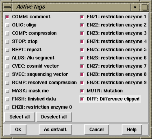
304 The Staden Package Manual
2.20.9 The Tag Selector
Each command using tags (for example to mask tagged sequence segments) can utilise the
Tag Selector to determine which tag types are to be used. As each command has its own
particular use for tags, the default tags are command specific.
The Tag Selector dialogue (which is available from the relevant gap4 options) consists
of a set of checkbuttons plus commands to select all tags or to deselect all tags. The "OK"
button quits the display and accepts the selected list as the current list of active tags.
The "Cancel"button quits the display without making any changes. The "As default"
button marks the current selected tags as the defaults to be used for all future uses of
this command. These selections are not saved to disk and will be lost when the program
quits. To permanently set the default tag types, users must modify their ‘.gaprc’ file.
Brief instructions on how to edit this file follow. They are also contained within the copy of
the file distributed with the package: ‘$STADENROOT/tables/gaprc’. Search for "Tag type
lists".
2.20.10 The GTAGDB File
To plot tags, gap uses a file describing the available tag types and their colours. It is possible
for users to edit their own local copies of this file to create new tag types.
The environment variable GTAGDB is used to specify the location of tag type databases.
The GTAGDB variable consists of one or more file pathnames separated by colons. The first
file read defines a set of tags and colours. Subsequent files can define additional tags and also
override the earlier tag definitions. To achieve this gap4 loads each file from the GTAGDB
variable in the order of rightmost first to leftmost last. Thus, as is similar to the unix
shell PATH variable, the leftmost pathnames have highest precedence for the resultant tag
definitions. The default GTAGDB specified in the staden login and profile scripts is:
GTAGDB:$HOME/GTAGDB:$STADTABL/GTAGDB
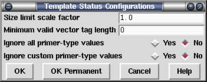
Chapter 2: Sequence assembly and finishing using Gap4 305
Hence the ‘$STADTABL/GTAGDB’ file is read and the ‘$HOME/GTAGDB’ and ‘GTAGDB’ (a file
in the current directory) files are merged if present. To add a new tag type only to the
database local to the current directory, create a ‘GTAGDB’ file in the current directory.
The BNF grammar for the tag database is as follows:
<tag_db> ::= <tag> <tag_db> | <empty>
<tag> ::= <tag_long_name> ’:’ <element_list> ’\n’
<element_list> ::= <element> | <element> ’:’ <element_list> | <empty>
<element> ::= <option_name> ’=’ <string>
<option_name> ::= ’id’ | ’bg’ | ’dt’
Quoting strings is optional for single words, but necessary when writing a string con-
taining spaces. In plain English, this means that to define the compression tag (COMP) to
be displayed in red, with no default annotation string we write:
compression: id="COMP": bg=red
Any lines starting with hash (‘#’) are considered as comments. Lines ending in backslash
(‘\’) are joined with the next line. Hence the above definition can be written in a clearer
form using:
# For marking compressions
compression: \
id="COMP": \
bg=red:
An example including a default annotation string of "default string"follows:
# For general comments
comment: \
id="COMM": \
bg=MediumBlue: \
dt="default string"
Allowed names for colours are those recognised by the windowing system.
2.20.11 Template Status
This option allows control over computation of the template status. The validity of a
template is computed by checking the size (based on the locations of assembled readings
and position of vector tags) and the orientation of sequences (based on their “primer type”
values).

306 The Staden Package Manual
The most likely item to need changing is the “size limit scale factor”. The expected
range of template sizes for a ligation are specified in each template record as a minimum-
to-maximum range. Gap4 takes a very simple approach as anything within this range is
valid and anything outside it is invalid. The scale factor is applied such that the maximum
range becomes “max * scale” and the minimum range becomes “min / scale”. So a scale
factor of 2 would adjust a range from 1.0-1.4Kb to 0.5-2.8Kb.
The “minimum valid vector tag length” is designed to workaround problems where some
assemblies end up with SVEC tags of 1 or 2 bases long (which are common when converting
from phrap for some reason). The start and end of a template may be derived from observing
a single reading with sequencing vector at both ends, so the presence of very short falsely
added SVEC tags will mark many templates as inconsistent.
The “Ignore all primer-type values” and “Ignore custom primer-type values” are methods
to disable Gap4’s trust in the primer type information for each sequence. Normally this
will be one of universal-forward, universal-reverse, custom-forward (e.g. from a primer-walk)
and custom-reverse.
2.21 Command Line Arguments
-bitsize Specifies whether the database file size is 32-bit or 64-bit. Practically speaking
due to the use of signed numbers in places and the restriction of 32-bit for the
number of records in a database (even when using -bitsize 64 for 64-bit file
offsets) the practical limits are 2Gb filesize for -bitsize 32 and somewhere
around about 100-million sequences for -bitsize 64.
Gap4 only needs this option for creating new databases. The bit-size of existing
databases is automatically detected when they are opened.
Databases produced in 64-bit format are not compatible with older versions of
Gap4, but old and newly created 32-bit databases still work with the 64-bit
Gap4 (and are maintained in 32-bit format so editing them will not invalidate
their use by older Gap4s). The copy_db program (see Section 12.2 [Copy db],
page 573) can be used to convert file formats.
-maxdb Specifies the maximum number of readings plus contigs. This value is not
automatically adjusted whilst the program is running, but is not allowed to be
set to a value too small for the database to be opened. It controls the size of
some areas of memory (approximately 16*maxdb bytes) used during execution
of gap. The default value is 8000.
-maxseq Specifies the maximum number of characters used in the concatenated consensus
sequences. This parameter is generally not required as the value is normally
computed and adjusted automatically. However a few functions (such as as-
sembly) still need to know a maximum size before hand. The default is 100000
bases.

Chapter 2: Sequence assembly and finishing using Gap4 307
-ro
-read_only
Opens the database (if specified on the command line) in read only mode. This
does not apply to databases opened using the file browser.
-check
-no_check
Specifies whether to run the "Check Database"option when opening new data-
bases. -check forces this to always be done and -nocheck forces it to never be
done. By default Check Database is always performed when opening databases
in read-write mode and never performed when opening in read-only mode.
-exec_notes
-no_exec_notes
Controls whether to search for and execute any Notes of type OPEN or CLOS.
This may be an important security measure if you are using foreign databases.
Gap4 defaults to -no check notes.
-rawdata_note
-no_rawdata_note
Controls whether to make use of the RAWD note type for specifying the trace file
search path. Defaults to -rawdata note.
-csel
-no_csel Controls whether to automatically start up the contig selector when opening
a new gap4 database. In some cases (such as when dealing with many EST
clusters each in their own contig) the contig selector is not a practical tool; this
simply offers a way of speeding up database opening. Defaults to -csel.
-- Treat this as the last command line option. Only useful if the database name
is specified and the name starts with a minus character (not recommended!).

Chapter 3: Searching for point mutations using pregap4 and gap4 309
3 Searching for point mutations using pregap4
and gap4
The original version of these methods was described in James K Bonfield, Cristina Rada
and Rodger Staden, "Automated detection of point mutations using fluorescent sequence
trace subtraction", Nucleic Acids Res. 26, 3404-3409, 1998.. The more recent work has
been done by Mark Jordan and James Bonfield with advice from Graham Taylor, Andrew
Wallace, Will Wang and others.
3.1 Introduction to mutation detection
Our methods for detecting mutations are based on the alignment and comparison of the
fluorescent traces produced by Sanger DNA sequencing. To use clinical terminology, samples
from patients are compared to standard reference traces. Patient and reference traces should
be produced using the same primers and sequencing chemistry, ideally from both strands
of the DNA. The data shown in the examples below is from exon 11 of the BRCA1 gene.
The basic idea is illustrated in the following two figures which are screen dumps from
our program gap4(see Section 2.2 [Gap4 introduction], page 95). The first shows a sample
containing a point mutation and the second contains a heterozygous base position. The
displays are bisected vertically: at the top left is the sample trace from one strand of
the DNA, below that the reference trace for that strand, and underneath the difference
between these traces which is obtained by subtracting one from the other. On the right is
corresponding data from the other DNA strand (shown complemented).

310 The Staden Package Manual
Figure 1. Top and bottom strand differences for a point mutation.
Figure 2. Top and bottom strand differences for a heterozygous base.
As can be seen, although no vertical scaling is performed the difference trace is quite
flat or is consistently either above or below the mid-line, except at the sites of mutations.
Near these are strong peaks, but notice that only for the mutated base are there peaks both
above and below the mid-line. The context effects caused by the mutation produce peaks
only in one direction.
It is perhaps necessary to point out that analysis of the traces is essential because base
callers make mistakes: they can assign the wrong base types and also assign single bases
where the DNA is heterozygous. An example of the latter can be observed in Figure 2:
on one strand the base caller has assigned a "-"symbol at position 251, at least indicating
uncertainty, but on the other strand it has assigned "T". The DNA is clearly heterozygous
at this position. This means that simply looking for differences between patient sequences
and reference sequences will cause point mutations and heterozygous bases to be missed (of
course base calling errors will also create false differences).
These trace displays alone are very useful for visual inspection of data and are all some
users want. However we also have programs which automatically analyse the trace differ-
ences and tag the bases which have significant peaks as possible sites of mutation.
Trace viewing is initiated from within the gap4 editor(see Section 2.6 [Editing in gap4],
page 160). Each record in the editor shows an individual reading with its number and name
at the left. Negative numbers denote readings which have been complemented. Several
sequences have special status. At the top is a sequence labelled with a letter S at the
left edge. This is the reference sequence, here the EMBL entry HSLBRCA1 which covers
the entirety of the BRCA1 gene. The numbering at the top of the display corresponds to
positions in this reference sequence. The program has also coloured (green) all exons on the
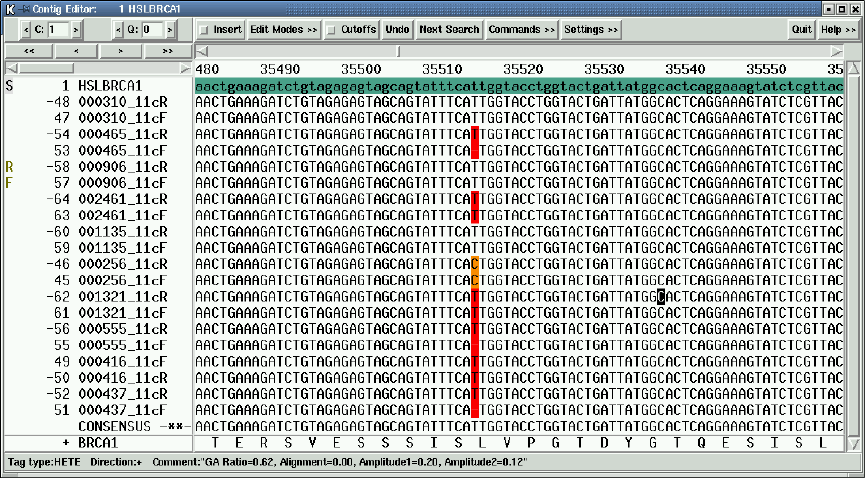
Chapter 3: Searching for point mutations using pregap4 and gap4 311
reference sequence. The bottom DNA sequence in the editor is labelled "CONSENSUS".
For mutation detection work this sequence is forced to be identical to the reference. Below
the CONSENSUS sequence is the amino acid sequence for the reference. This is calculated
on the fly using the feature table of the reference sequence and so translates only exons and
in their correct reading frames. Two other sequences (near the top) are labelled R and F.
These are the readings providing the reverse and forward reference traces for this segment
of the data.
Figure 3. A set of aligned sequence readings displayed in the gap4 editor.
At the very bottom of the editor is an information line which is used to display data
about items touched by the mouse cursor. Here it is showing data about one of the positions
tagged as possibly being heterozygous. It includes the observed base types (G and A) and
the scores achieved by the automated analysis.
The editor can be set to show only differences between readings and the reference; all
matching bases appear as dots. For example, Figure 4. shows the same data as Figure 3,
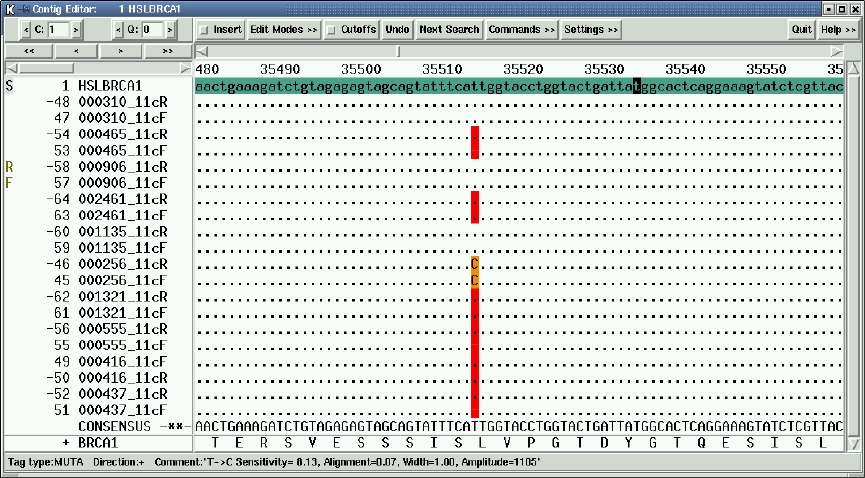
312 The Staden Package Manual
but with the editor set to show differences, and the information line showing details about
a possible mutation.
Figure 4. An alternative view of aligned sequence readings in the gap4 editor.
One column contains several bases tagged in red, signifying possible heterozygotes, and
some in orange denoting possible point mutations. During visual inspection the program
can be made to move the cursor from one tag to the next and to display the aligned traces
as shown above in Figures 1 and 2.
It is also possible to have positive controls for displaying the trace differences; i.e. refer-
ence traces which contain the mutation. In this case the traces appear as shown in figure 5.
Here the forward and reverse positive controls are shown to the right of the normal plots.
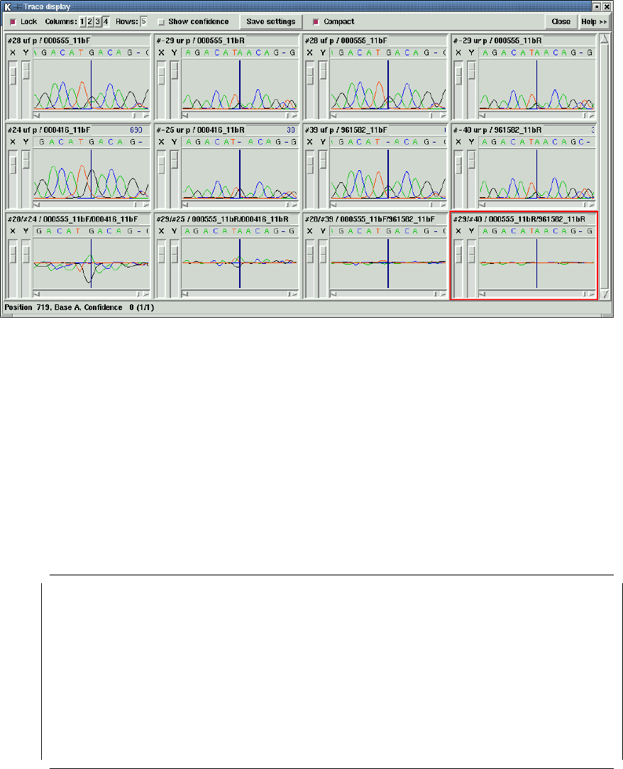
Chapter 3: Searching for point mutations using pregap4 and gap4 313
In Figure 5 the positive control difference plots are quite flat hence, in this case, providing
confirmation of the presence of the heterozygous base.
Figure 5. Top and bottom strand differences and positive control for a heterozygous
base.
As mentioned above the package contains programs which can automatically compare
the traces and their reference sequences. The output from these programs are the tags
shown in the editor. Users can check the traces at these positions using the displays shown
in Figures 1, 2 and 5; if necessary removing or adding tags. Alternatively users can rely
entirely on visual inspection and create all tags themselves.
Once all the mutations are correctly tagged the program can produce a report which
includes the reading names, mutation positions relative to the reference sequence, the actual
change, its effect, and the evidence. An example is shown below in Figure 6.
001321_11aF 33885T>Y (silent F) (strand - only)
001321_11aF 34407G>K (expressed E>[ED]) (strand - only)
001321_11cF 35512T>Y (silent L) (double stranded)
001321_11cF 35813C>Y (expressed P>[PL]) (double stranded)
001321_11dF 36314A>R (expressed E>[EG]) (double stranded)
001321_11eF 36749A>R (expressed K>[KR]) (double stranded)
001321_11eF 37313T>K (noncoding) (strand - only)
000256_11eF 36749A>G (expressed K>R) (double stranded)
Figure 6. How gap4 reports mutations.

314 The Staden Package Manual
Here the first record is for reading 001321 11aF, position 33885, T changed to T and C
(i.e. is heterozygous) to produce no amino acid change, with evidence coming only from
the complementary strand. The last record is for reading 000256 11eF, position 36749, A
changed to G, producing an amino acid change K to R, with evidence from both strands of
the sequence. The penultimate record denotes a heterozygote in a noncoding region.
3.1.1 Mutation Detection Programs
The software handles batches of trace data from sequencing instruments. It performs all
processing except base calling (although it can employ third party programs such as phred
for this step). This includes file format conversions, quality clipping, scanning for mutations
and heterozygotes, multiple sequence alignment, easy visual inspection of traces, produc-
tion of reports, and the accumulation and storage of readings and traces. The software also
handles the initialisation/configuration of standard reference files and databases for any
project. The two main programs are pregap4 and gap4. Pregap4 (see Section 4.2 [Pregap4
introduction], page 326) prepares data for gap4 by automatically using a variety of smaller
programs, including those used to search for mutations: mutscan (see Section 4.6.22 [Mu-
tation Scanner], page 359. Gap4 (see Section 2.2 [Gap4 introduction], page 95) is used to
store the aligned readings, to view the sequences and traces, and to produce a report listing
the observed mutations.
Any number of sequences can be processed in a single run, and for each individual patient
sample the operation is generally performed in two steps. First, via pregap4, the traces are
aligned and compared to the reference traces and any possible mutations or heterozygous
bases marked. Secondly, the data is transfered into a gap4 database from where users can
visually check the differences between the reference and patient traces.
The program mutscan (see Section 4.6.22 [Mutation Scanner], page 359) can automati-
cally compare patient and reference traces to find point mutations and heterozygous bases.
Users can set parameters which control the sensistivity of the algorithms (and hence which
determine the ratio of false negative and positive results). Mutscan adds tags of type
“mutation” or “heterozygous” to the patient files. The tags contain the numerical scores
achieved at the site of the reported base changes, and they can be viewed via the gap4
editor(see Section 2.6 [Editing in gap4], page 160). Mutscan is normally run via pregap4
(see Section 4.2 [Pregap4 introduction], page 326).
The description of the programs given below is presented in reverse order of use i.e. gap4
then pregap4, but first we give further details about the use of reference data.
3.1.2 Mutation Detection Reference Data
The mutation detection methods require reference traces and optionally reference sequences.
Reference traces are used for automatic mutation detection and for visual inspection of trace
differences. Reference sequences are used in gap4 to provide a base numbering standard, and
if required to provide feature table entries to control translation and mutation reporting.
3.1.3 Reference Sequences
Reference sequences are used in gap4 (see Section 2.2 [Gap4 introduction], page 95). Here
they can be used to define a numbering system independent of gaps introduced to produce
alignments. The numbering can start at any point in the reference sequence. If the reference
Chapter 3: Searching for point mutations using pregap4 and gap4 315
sequence is entered with a feature table the features are converted to tags and can be used
to control translation of the sequence in the contig editor. For mutation detection work the
reference sequence and feature table enable mutations to be reported using positions defined
by the reference sequence, and also allows the effect of the mutations to be noted. Gap4
is able to store entries from the EMBL sequence library complete with their feature tables.
These feature tables are converted to gap4 database annotations (tags), which means that
they can be selectively displayed in the template display and editor, and used to translate
only the exons (in the correct reading frame). Obviously it may be useful to augment the
feature tables with the sites of known polymorphisms or deleterious mutations so that they
can be displayed in gap4 as landmarks. When it comes to producing a report of the observed
mutations the feature table is used to work out if a mutation is expressed and if so what
the amino acid change is. Additional tags can be created to specify the positions of the
primers or restriction sites used to obtain data covering segments of the sequence. For any
project the reference sequence need only be set up once. Either project databases can be
started with the reference sequence already configured or the reference can be assembled
along with the reading data. The reference sequence can be designated (or reassigned) as
follows. In pregap4 (see Section 4.2 [Pregap4 introduction], page 326) it can be named in
the module "Reference Traces". In the gap4 editor it can be set by right clicking on its
name. Once set it should appear labelled "S"at the left edge of the editor.
3.1.4 Reference Traces
References traces are used by the automatic mutation detection program mutscan (see
Section 4.6.22 [Mutation Scanner], page 359, and by the trace difference display in the gap4
editor(see Section 2.6 [Editing in gap4], page 160). Ideally forward and reverse reference
traces should be available and should be obtained using the same primers and sequencing
chemistry as the patient data. From the "settings"menu of the editor the trace display can
be set to "Auto-Diff traces". Once this is activated, whenever the user double clicks on a
base in the editor sequence display, not only is the reading’s trace displayed, but also its
designated reference trace plus the difference between them. If its complementary reading
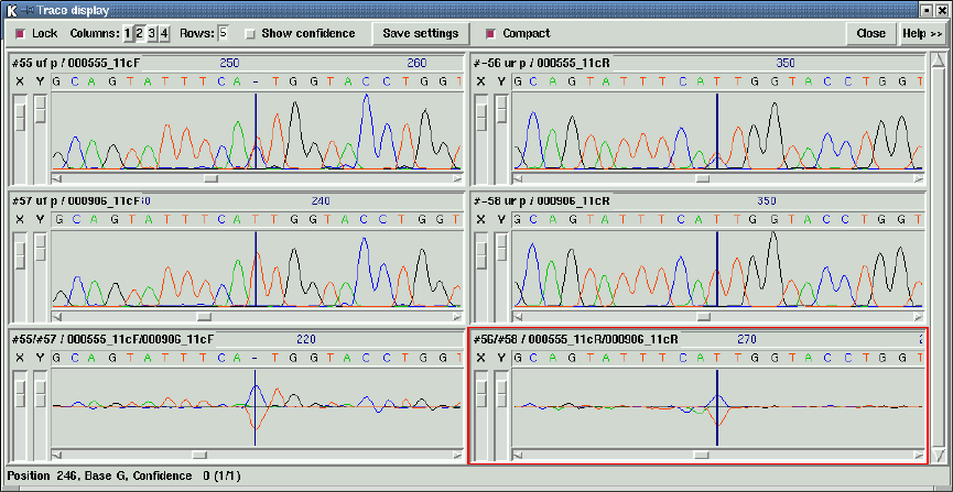
316 The Staden Package Manual
is available, its trace and reference trace and their differences are also displayed. These
trace displays and the editing cursor scroll in synch.
Top and bottom strand differences for a heterozygous base.
The preferred way of assigning reference traces to readings is by use of "naming con-
ventions"; that is to have a simple set of rules which control the names given to the trace
files. It can be seen in the figures showing the editor that forward and reverse readings from
the same patient have names with a common root but which end either F or R. This both
ties the two together (so the software knows which is the corresponding complementary
trace when the user double clicks on a reading) and also enables the association of readings
and their reference traces. Once a convention has been adopted the rules can be defined
for pregap4 by loading them via the "Load Naming Scheme"option in its File menu (see
Section 4.8 [Pregap4 Naming Schemes], page 366). For any batch of readings the reference
traces are defined within pregap4’s "Reference Traces"module. Note that this mode of
operation, by allowing the specification of only one forward and one reverse trace, limits
each batch of traces processed to those which correspond to a given pair of reference traces.
The size of the batch is unlimited.
The alternative way of specifying the reference traces is to right click on their names in
the editor. This also allows positive trace controls to be specified (which is not possible in
pregap4).
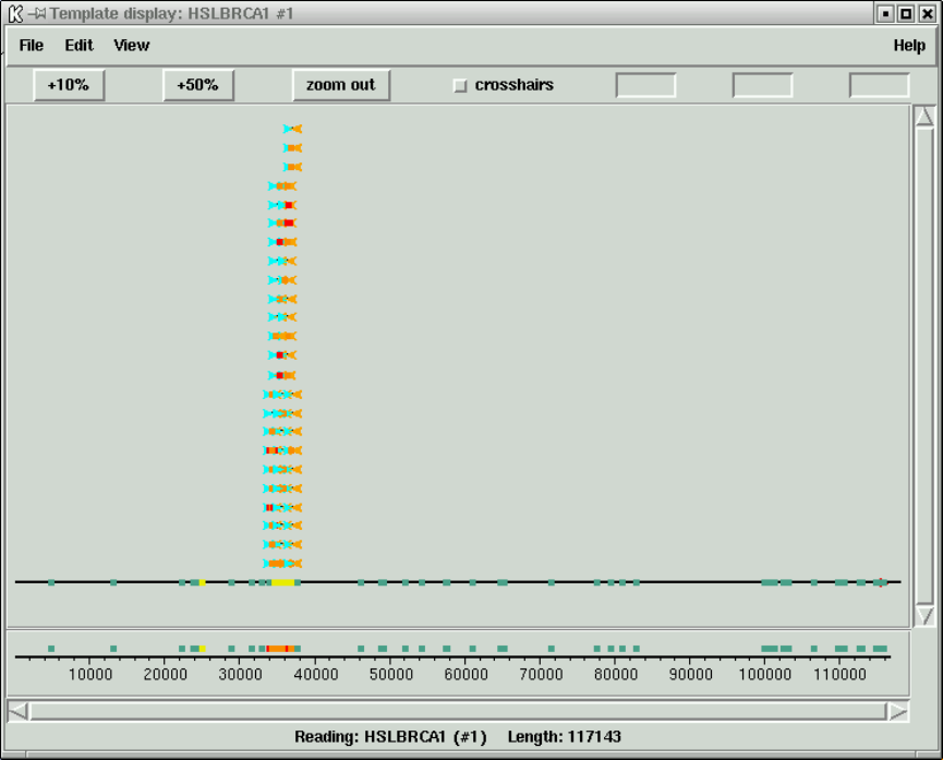
Chapter 3: Searching for point mutations using pregap4 and gap4 317
3.1.5 Using The Template Display With Mutation Data
Figure 7. The template display showing the whole of the BRCA1 gene (exons in green).
The view obtained from the Template display and shown in Figure 7 is not of practical
use but serves here to illustrate the overall arrangement of the data for our chosen example
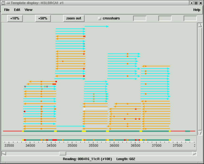
318 The Staden Package Manual
the BRCA1 gene. This figure shows the entirety of the EMBL entry HSLBRCA1 with its
exons marked in green. Only exon 11 has patient trace data stacked above it.
Figure 8. A zoomed-in version of the data shown in Figure 7.
Here we can see all the readings covering exon 11. Forward readings are light blue,
reverse readings orange, primers are marked in yellow, mutations in red and orange. A
common mutation appears in the leftmost set of readings and illustrates the value of using
the template display for visualising the overall pattern of the tagged mutations.
3.1.6 Configuring The Gap4 Editor For Mutation Data
The current version of the gap4 editor contains very many options that are not needed
for mutation data. Given sufficient demand a version tailored for mutation studies could
be produced. For now it might make it easier to understand the program if its origin as
a genome assembly program is borne in mind. Here we outline the options and settings
relevant to mutation studies. The assignment of reference sequence and traces is described
above. From the editor they can be set by right clicking on the reading names.
Gap4 enables segments of sequences to be annotated (or tagged). Each tag has a type
(eg primer) and each type has an associated colour. Each instance of a tag can include
Chapter 3: Searching for point mutations using pregap4 and gap4 319
editable text. This text can be viewed and edited by right clicking on the tag and selecting
"Edit tag", after which a text box will appear. Gap4 can display annotations/tags as
background colour and the user can specify which tag types are shown. For mutation
studies the following tag types may usefully be activated, and all others turned off. Using
the "Set Active Tags"option in the "Settings"menu first click on "Clear all". Then click
on "primer". To add further types you must hold down the "Ctrl"key on the keyboard
while clicking. Now scroll down and click on "Mutation","Heterozygous"and "FEATURE
CDS". Add any others required, then click "OK".
The following configurations are performed via the "Settings"menu.
Gap4 has three consensus generation algorithms. When using a reference sequence it
is convenient if the consensus shown in the editor is forced to be the same as the refer-
ence. This will be the case if either the "Weighted base frequencies"or the "Confidence
values"consensus algorithms are being used. This selection is made using the "Consensus
algorithm"option.
Translations are shown in what gap4 refers to as the "Status"line. To enable automatic
translation of the exons defined in the reference sequence, in the "Status Line"option set
"Translate using feature tables".
To enable automatic display of trace diferences, in the "Trace Display"option set "Auto-
Diff Traces".
To show only the base differences between the consensus/reference, set "Highlight Dis-
agreements". These can be shown by dots or colour.
To show base confidence values set "Show reading quality"and also make sure that the
value in the box labelled "Q"at the top left of the editor is set to 0 or greater.
To force forward and reverse reading pairs to be shown in adjacent records in the editor
set "Group readings by templates"(NB this assumes that an appropriate naming scheme
has been used).
If a reference sequence is assigned, the numbering at the top of the sequence will reflect
the base positions in that sequence. Any pads in the reference sequence are ignored. If
no reference sequence is assigned, the numbering will ignore pads if the "Show unpadded
positions"option is activated.
At the bottom of the "Settings"menu is an option to "Save settings". Use of this will
mean that the current configuration will be set automatically next time the editor is used
(and hence the steps just described only need to be performed once).
3.1.7 Using The Gap4 Editor With Mutation Data
The current version of the editor has a fixed width and a maximum height. If too many
sequences are present at any position a vertical scrollbar on the right edge can be used to
move them up and down. The CONSENSUS line will always be visible, but at present,
the reference sequence is scrolled along with all the other sequences and so may disappear.
Horizontal scrolling is achieved in the usual ways, plus by use of the >,>> and <,<< buttons.
The reading names can be moved left and right using the scrollbar above them.
Configure the editor as described above.
320 The Staden Package Manual
The traces for readings (and their reverse) can be examined over their full length one at
a time by simply double clicking on them then scrolling along. Any mutations observed can
be labelled by right clicking on the base in the editor display and invoking the "Create tag"
option. This brings up a dialogue box. At the top is a button marked "Type:comment";
clicking on this will bring up another dialogue with a list of all the tag types; choose the
appropriate one ("Heterozygous"or "Mutation"). There are obviously many advantages to
examining the traces like this using gap4. However, if the automated mutation detection
methods are trusted, or used in way that makes them trustworthy for the type of study
being undertaken, then there are quicker ways of examining the data.
The "Next Search"button at the top of the editor gives access to many types of
search, one of which is "tag type". If this is selected a button appears labelled "Tag
type COMM(Comment)". Clicking on this will bring up a dialogue showing all the avail-
able tag types. If the user selects, say "Mutation", each time the "Next Search"button is
used the program will position the editing cursor on the next mutation tag. Double click-
ing will automatically bring up the appropriate traces as shown in figures 1, 2 and 5 (see
Section 3.1 [Introduction to mutation detection], page 309). The user can view the traces
and if necessary alter the tag (eg delete it if it is a false positive).
Once all the data has been checked and all mutations and heterozygous bases have
been tagged a report can be generated using the "Report Mutations"option in the editor
"Commands"menu. Note that it is also possible to simply report all differences between
base calls and the reference, but the usual procedure is for the program to report all bases
tagged as "Mutation"or "Heterozygous". Example output is shown above in Figure 6 (see
Section 3.1 [Introduction to mutation detection], page 309). The report appears in the gap4
"Output window"which can be saved to disk by right clicking on the text and selecting
"Output to disk".
3.1.8 Processing Batches Of Mutation Data Trace Files
It is not clear which is the best way of organising the data for the simplest and most efficient
processing using the current programs, but for now we make the following suggestions.
We assume that the region of the DNA being studied has a standard set of forward and
reverse primer pairs covering all segments of interest and that a standard reference sequence
in EMBL format is available.
We recommend that batches of data from single primer pair combinations are processed
separately, using separate temporary gap4 databases. For example, exon 11 of BRCA1 can
be covered by five pairs of forward and reverse primers and we suggest that batches of traces
obtained from each of these primer pairs should be processed using five gap4 databases.
Each processing run should create a new database and should enter, not only the new
sets of patient data for that particular primer pair, but also the corresponding reference
sequence and reference traces.
Obviously when several primer pairs are needed to cover a given region of the DNA (eg
for BRCA1) the same reference sequence would be used for all the primer pairs.
An alternative to the above is to create a template database for each primer pair which
contains the data for the corresponding forward and reverse reference traces plus the fully
Chapter 3: Searching for point mutations using pregap4 and gap4 321
annotated reference sequence. These template databases are copied to create a temporary
database for each new batch of data for the given primer pair.
Whichever of these two strategies is adopted each batch of new data is processed, anal-
ysed and assembled into these temporary databases, inspected visually, and a mutation
report generated.
The use of separate temporary databases simplifies the assignment of reference traces
and the use of the report generation function.
Figure 9. An overview of a database containing data for only one primer pair of BRCA1
For long term storage and to facilitate larger studies, the content of each of these tempo-
rary databases is then transferred to archive databases, after which the temporary databases
are no longer needed. The archive databases could be restricted to individual primer pairs
or could accommodate data covering the whole of the reference sequence.
322 The Staden Package Manual
3.1.9 Processing Batches Of Mutation Data Trace Files Using
Pregap4
All the data processing other than visual inspection of traces and report generation is
handled by the program pregap4 (see Section 4.2 [Pregap4 introduction], page 326). Pregap4
achieves this by running a set of individual programs selected by the user.
Figure 10. The pregap4 Configure Modules window showing a typical list of mutation
data option selections.
The "Configure Modules"window shown in Figure 10. is used to select which programs
to apply to a batch of data, and to configure their usage. On the left is a list of programs
and options, with "x"showing the ones that have been selected. If the user clicks on an
option name its name is given a blue background and its configurable parameters are shown
in the right hand panel to enable the user to alter them. Here "Reference Traces"has been
selected which enables the user to set the reference traces and sequence.
The other selected options (marked with "x") are typical of the ones used for mutation
detection studies. Below we describe the use of each plus a few alternatives. All of the
options are descibed in more detail elsewhere in our documentation, our intention here is
to give an overview of their use during mutation studies.
Note that the window labelled "Files to Process"is used to tell the program which files
to process as a batch.
Chapter 3: Searching for point mutations using pregap4 and gap4 323
3.1.10 Configuration Of Pregap4 For Mutation Data
General Configuration
This option allows the user to select whether the trace names used for the
samples should be the same as their file names or should be the names stored
inside the files.
Phred
Phred is a base caller which also assigns confidence values to each base. Gen-
erally the data passed to pregap4 has already been base called. However not
all base callers assign confidence values and so it can be useful to apply phred
or ATQA (which does not base call but does assign confidence values). Alter-
natively "Estimate Base Accuracies"can be applied which is a simple program
for providing numerical values which reflect the signal to noise ratio for each
base, and which can be used instead of confidence values. (Note that if quality
clipping is used, its score thresholds depend on whether confidence values of
eba values are used).
Trace Format Conversion
This option can be used to convert bulky files such as those of ABI to a compact
format such as SCF or ZTR without loss of the data required for trace display.
Initialise Experiment Files
The input to gap4 and several of the other programs used here is a data for-
mat known as Experiment file format. This step, which has no configurable
parameters is essential for mutation data processing.
Augment Experiment Files
The section on Reference Traces outlined the use of "Naming Schemes"for
associating pairs of forward and reverse readings, and for assigning reference
traces. The naming scheme must be loaded from pregap4’s File menu. "Aug-
ment Experiment Files"must be activated in order for the naming scheme to
be applied. No parameters need be set.
Quality Clip
The reliability of the base calls varies with position along the sequence. Near
to both ends the data is less reliable. The "Quality Clip"option trims the ends
of the sequences by analysing their confidence values or accuracy estimates (if
present) or the density of unknown bases in the sequence. By observing these
"clip points"other processing programs will work more reliably.
Reference Traces
As explained above it is necessary to specify a reference trace (preferably one
for each strand of the data if processing data from both strands). The Reference
sequence can also be set here. Note that even if our suggestion to preload the
reference traces into the gap4 database is followed, it is still necessary to specify
them here for use by the mutation detection modules.
Trace Difference
This is the program which compares the patient and reference traces to search
for possible mutations. It adds data to the experiment files to mark each pre-
dicted mutation, and this data will appear as tags in the gap4 database. It
324 The Staden Package Manual
can also create a new trace file containing the difference of the reference and
the sample. The numerical parameters control the sensitivity of the algorithms,
and hence the ratio between the numbers of false positive and negative results.
Heterozygote Scanner
This is the program which compares the patient and reference traces to search
for possible heterozygous bases. It adds data to the experiment files to mark
each predicted heterozygous base, and this data will appear as tags in the gap4
database. The numerical parameters control the sensitivity of the algorithms,
and hence the ratio between the numbers of false positive and negative results.
Gap4 shotgun assembly
In order to be able report the positions of mutations relative to the reference
sequence, and to be able to compare sets of samples from patients, it is necessary
to perform multiple sequence alignment on the data. This is termed "assembly"
and is usually performed by gap4, although other programs can be operated
via pregap4. If following the suggestion to preload the reference sequence to
a temporary database for each batch, supply the name of this database here.
Otherwise a new database should be named and created from this option. (If
this strategy is adopted make sure that the reference sequence and the references
traces are assembled!) The parameters that control the assembly process and
are described elsewhere.
Note that pregap4 has the facility to save its configuration and parameter settings. This
means that the current configuration will be set automatically next time the program is
used (and hence the steps just described only need to be performed once). In addition
pregap4 can be run non-interactively by typing a single line on the command line. Taking
thse two capabilities together, means that only one line need be typed in order to process all
subsequent batches of data (assuming the file names are reused, which is easy to arrange.)
3.1.11 Discussion Of Mutation Data Processing Methods
At present pregap4 and gap4 clearly show their primary usage in the field of genome as-
sembly, but versions tailored to mutation studies can be created once the requirements are
agreed. Ideally all processing should be controlled by a single program which once config-
ured for any project should require users to provide only the project name - all other file
names and parameters could be preset, and all processing, including archiving and backup,
performed automatically, leaving the data ready for visual inspection.
The automatic mutation and heterozygote detection programs work well on all the test
data we have but now they require evaluation by external groups. Such analysis would
enable us to improve the algorithms and to tune their parameters. At present we know that
sometimes a base will be declared both as a mutation and as a heterozygous position when
visual inspection shows that it is one or the other.
There is still much that can be done overall to improve the methods, but the text above
summarises their status in July 2002. Although currently valuable for real scientific and
clinical work they should perhaps be viewed as prototypes.
Chapter 4: Preparing readings for assembly using pregap4 325
4 Preparing readings for assembly using pregap4
4.1 Organisation of the Pregap4 Manual
Pregap4 is a relatively simple program to use. It is also very flexible and extendable, and so
much of the manual is taken up by explaining to programmers and system managers how
it can be configured. The average user need not be concerned with these details.
The Introductory section of the manual is meant to give an overview of the program:
what it is for, the files it uses and functions it performs, and how to use it. It is very
important for all users to have a basic understanding of the files used by pregap4 and the
processes through which it can pass their data (see Section 4.2.1 [Summary of the Files used
and the Processing Steps], page 326). The next section of the Introduction (see Section 4.2.3
[Pregap4 Menus], page 336) tabulates the program’s menus. This is followed by an overview
of the pregap4 user interface (see Section 4.2.2 [Introduction to the Pregap4 User Interface],
page 330) which should give a clear idea of how to actually use the program, and concludes
the introductory section.
More detail about how to define the set of files to be processed (see Section 4.3 [Specifying
Files to Process], page 337) is followed by a section showing how to run pregap4 and
giving examples of its use (see Section 4.4 [Running Pregap4], page 338). Next are sections
on configuring the pregap4 user interface (see Section 4.5 [Configuring the Pregap4 User
Interface], page 341).
The next part of the manual describes how to use the Configure Modules Window
to select the modules to apply and to set their parameters (see Section 4.6 [Configuring
Modules], page 342). This is one of the longest and most detailed parts of the manual in
that it describes how to configure all the current possible modules, many of which will not
be available at all sites, and several of which perform identical functions. Obviously, only
the entries which describe the functions that are available at a site, are of interest.
One of the important tasks of pregap4 is to make sure that each reading’s Experiment file
contains all the information needed by gap4 to ensure the accuracy of the final consensus
sequence and to make the project proceed as efficiently as possible. Pregap4 provides
several methods for sourcing this information. One of these, as for example employed at
the Sanger Centre in the UK, is to encode some information about a reading in its reading
name. Pregap4 contains flexible mechanisms to enable a variety of the "Naming schemes"
or "Naming conventions"to be used as a source of information to augment the Experiment
files (see Section 4.8 [Pregap4 Naming Schemes], page 366). Alternatively pregap4 can
use simple text databases as an information source (see Section 4.10 [Information Sources],
page 371), or the user can set up some Experiment file record types for use with a batch of
readings (see Section 11.3.1 [Experiment file format record types], page 552).
The rest of the manual deals with increasingly complicated matters, and the average user
should never need to consult these sections. First there is a section on adding an removing
modules (see Section 4.11 [Adding and Removing Modules], page 375). This describes how
to control the list of modules which appear in the Configure Modules Window. The package
is usually shipped with this list set to contain more modules than are likely to be available
at any one site and so it might be found useful to remove those that are not available.
326 The Staden Package Manual
The next two sections, as their names imply, are for programmers only (see Section 4.12
[Low Level Pregap4 Configuration], page 377) and (see Section 4.13 [Writing New Modules],
page 395).
4.2 Introduction
Before entry into a gap4 database the raw data from sequencing instruments needs to be
passed through several processes, such as screening for vectors, quality evaluation, and
conversion of data formats. Pregap4 is used to pass a batch of readings through these
steps in an automatic way. It provides an interface for setting up and configuring the
processing and for controlling the passage of the readings through each stage. The separate
tasks are termed "modules"and each module is typically managed by a dedicated program.
Pregap4 wraps all of these modules into a single easy to use environment, whilst maintaining
the flexibility to select and extend the processing modules. It is an, as yet, unpublished
replacement of the program pregap Bonfield, J.K. and Staden, R. Experiment files and their
application during large-scale sequencing projects. DNA Sequence 6, 109-117 (1996).
4.2.1 Summary of the Files used and the Processing Steps
Gap4 stores the data for an assembly project in a gap4 database. Before being entered into
the gap4 database the data must be passed through several steps via pregap4. The range of
tasks that can be peformed using pregap4 are shown schematically in the following figure.
Chapter 4: Preparing readings for assembly using pregap4 327
328 The Staden Package Manual
The package can handle data produced by a variety of sequencing instruments, and also
data entered using digitisers or that has been typed in by hand. One of the first steps is to
convert trace files, such as those of ABI, which are in proprietary format, to SCF files (see
Section 11.1 [SCF introduction], page 533).
Next, as originally put forward in Bonfield,J.K. and Staden,R. The application of numer-
ical estimates of base calling accuracy to DNA sequencing projects. Nucleic Acids Research
23, 1406-1410 (1995) (see Section 2.2.5 [The use of numerical estimates of base calling ac-
curacy], page 118), if they are not already included in the files, base call confidence values
are calculated, and are normally stored in the reading’s SCF file.
Next the base calls are copied from the trace files to text files known as Experiment files
(see Section 11.3 [Experiment files], page 552).
Note it is also possible to enter sequence readings in the form of FASTA files for use at this
stage of the processing, in which case they will be automatically converted to Experiment
file format.
All the subsequent processes operate on the Experiment files.
Experiment file format is similar to that of EMBL sequence entries in that each record
starts with a two letter identifier, but we have invented new records specific to sequencing
experiments. Gap4 can make use of information about readings which may not be contained
within the raw data files, such as sequencing chemistry and whether it is a forward or
reverse reading. Gap4 will work without this information, but at a reduced level. For
instance knowing which forward and reverse readings belong together allows gap4 to check
the validity of assembly and for automatic ordering of contigs.
One of pregap4’s next tasks is to augment the Experiment files to include data about
the chemistry, vectors, primers and templates used in the production of each reading, and
if necessary it can extract this information from external databases (see Section 4.10 [Infor-
mation Sources], page 371), or via local reading name conventions (see Section 4.8 [Pregap4
Naming Schemes], page 366). Once the Experiment file for a reading contains all the nec-
essary information the remaining processing programs can be used in turn to analyse the
data.
First the reading is marked at both ends to define the range of reasonable quality base
calls (see Section 4.6.8 [Quality Clip], page 347).
Then the reading is searched for the presence of sequencing vector at the 5’ end 3’ ends
(see Section 4.6.9 [Sequencing Vector Clip], page 348).
Next the sequence is checked for the presence of "cloning"vector, i.e. non-sequencing
vectors, such as those of BACs (see Section 4.6.11 [Cloning Vector Clip], page 350).
The final check of this type is to screen the reading for any vector that may have been
missed in the previous searches (see Section 4.6.12 [Screen for Unclipped Vector], page 351).
The next check is to screen the reading for any set of sequences which it may be con-
taminated by, such as E. coli (see Section 4.6.13 [Screen Sequences], page 351).
Note that vector sequence files are normally stored in the package vectors direc-
tory/folder. If a file of vector file names is used the vector sequences can also be stored in

Chapter 4: Preparing readings for assembly using pregap4 329
its directory/folder. Files of file names and vector-primer files can also contain environment
variables to define the location of vector files.
Vector primer files, vector sequence files and files of file names must be stored in plain
text files (see Section 11.5 [Vector primer Files], page 567), (see Section 11.6 [Vector se-
quence format], page 568).
Pregap4 is usually used non-interactively once the modules have been configured, but
some groups prefer (or have the time) to check the data by eye using the program trev (see
Section 8.1 [Trev], page 417) at this stage.
Another option is to search the readings for families of known repeats (see Section 4.6.18
[Tag Repeats], page 354). This will tag any regions which are found to match known repeats.
Some groups are using the package for mutation studies and the final pregap4 option,
prior to assembly is to use the mutation scanner program (see Section 3.1 [Introduction
to mutation detection], page 309) to search the readings for mutations (see Section 4.6.22
[Mutation Scanner], page 359.
Pregap4 can also be used to assemble the readings into a gap4 database (see
Section 4.6.23 [Gap4 Shotgun Assembly], page 361), or to assemble the readings using an
external assembly engine such as FAKII (see Section 4.6.26 [FakII Assembly], page 362),
and then to enter that assembly into a gap4 database (see Section 4.6.28 [Enter Assembly
into Gap4], page 364).
It is unlikely that any particular user will want to employ all of these options and one
of pregap4’s modes of use is to enable users to configure the program for their work (see
Section 4.6 [Configuring Modules], page 342). Not only can they select which tasks should
be performed, and which of the alternative programs ("modules") should be used for them,
but also the order in which they are applied. Although it is very rarely a problem, this
high level of flexibility comes at a price in the current version of pregap4: pregap4 does not
include code to check on the logicality of the configuration set by a user and will attempt to
execute the modules in the order given. There are some users, who having read this section,
will configure pregap4 to perform assembly before creating the Experiment files from the
trace files. Pregap4 will attempt to do this and no data will be assembled as the files given
to the assembly engine will be in the wrong format. This is just something to be aware of.
Pregap4 uses configuration files to remember the setup for each user or project.
These files define which modules are activated and what their parameter settings are
(see Section 4.7 [Using Config Files], page 366). These files, which can obviously save
considerable amounts of time, are created automatically and can be saved from the
Configure Modules Window once the configuration is complete.
The trace files are not altered, but are kept as archival data so that it is always possible
to check the original base calls and traces. The trace files are used by gap4 to display traces
and to compare the final consensus sequence with the original data, therefore they must be
kept online for the lifetime of the project. To save disk space it is best to use SCF files and,
if they were derived from a proprietary format such as that of ABI, to remove the originals.
Any changes to the data prior to assembly (and we recommend that none are made until
readings can be viewed aligned with others) are made to the copy of the sequence in the
330 The Staden Package Manual
Experiment file. For example the results of all the searching procedures outlined above are
added as new records to each reading’s Experiment file. The reading data, in Experiment
file format, is entered into the project database (see Section 2.16 [Gap Database Files],
page 284), usually via one of the assembly engines. All the changes to the data made by
gap4 are made to the copies of the data in the project database. Once the data has been
copied into the gap4 database the Experiment files are no longer required.
During processing pregap4 uses temporary files. The number and nature of these files
depends on the modules used. At the very least pregap4 will produce files containing the
names of the input files and the result of their processing. Those that were processed
successfully will be stored in a file with a name ending ".passed"and those that failed in
one ending ".failed". The ".passed"file can be used as a file of input file names for assembly
into gap4 (assuming that a pregap4 assembly module has not already been used).
While it is running, pregap4 will create files with a file name prefix defined by the user,
and store them in an output directory of the user’s choice (see Section 4.3 [Specifying Files
to Process], page 337).
When processing has finished pregap4 will produce a report containing information from
each module and the final list of passed and failed sequences.
4.2.2 Introduction to the Pregap4 User Interface
Pregap4 provides interfaces to define the batch of data files to be processed, which modules
are to applied to them; to configure the modules, and to start the processing. It also
provides mechanisms for adding and removing modules, but this facility will be used far
less often than the others.
Chapter 4: Preparing readings for assembly using pregap4 331
Pregap4 supports two styles of windowing. The default method is a compact mode, with
the alternative being "separate"mode - similar to gap4 and spin.
This is the "separate"window style. Here the main window is always visible, with
commands in the main window bringing up new windows. In the picture above the configure
window can be seen on top of the main window.
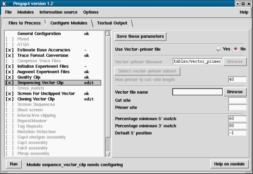
332 The Staden Package Manual
The second style is "compact"mode.
In the compact picture above the most common top level windows are "pages"in a
tabbed notebook. The benefit is greatly reduced screen space and quicker controls, but the
text output window is no longer permanently visible. The Window Style can be changed
using the options menu (see Section 4.5.2 [Window Styles], page 341).
4.2.2.1 Introduction to the Files to Process Window
Pregap4 operates on batches of files. These files can be binary trace files (in ABI, ALF or
SCF format), Experiment Files, or plain text, and do not need to all be in the same format.
The Files to Process Window is used to define which files are to be processed. The "Files

Chapter 4: Preparing readings for assembly using pregap4 333
to Process"dialogue (see below) can be brought up from the File menu, or by pressing the
appropriate tab when in compact_win mode.
On the left hand side of the figure is the current list of files to process. This list can be
edited simply by clicking with the mouse and typing.
On the right side of the panel is the pregap4 output filename prefix, the output directory
name, and several buttons. The filename prefix is used when pregap4 needs to create files.
For example after processing there may be prefix.passed, prefix.failed files. All files will be
created within the output directory.
The buttons allow selection of the files to process. The "Add files"button will bring
up a file browser, which will allow one or more files to be selected. Pressing Ok on the file
browser will then add the selected files to the "List of files to process"panel on the left side
of the pregap4 window.
The "Add file of filenames"button may be used to select a list of files whose filenames
have been written to a ‘file of filenames’.
The "Clear current list"button will remove all filenames from the list.
Both the "Add files"and "Add file of filenames"button append their selections to the
list of files to process, so to replace the current list the "Clear current list"button must
first be used.

334 The Staden Package Manual
The "Save current list to..."button may be used to produce a new file of filenames,
containing the combined list of files to process.
4.2.2.2 Introduction to the Configure Modules Window
The "Configure Modules"dialogue is available from the Modules menu or, when using the
compact window style, by pressing the Configure Modules tab.
As can be seen in the figure below, the left side of the display contains a list of the
currently loaded modules. One module in this list will be highlighted. The right side of the
display shows the configuration panel for this highlighted module and is module specific.
The module list shown on the left consists of a series of module names and their status,
and is termed the "enable status". The tick or cross at the left of the name indicates whether
this module is enabled. The text to the right of the module name indicates whether the
module has been given all the parameters needed for it to run. This will be one of "ok"
(all configuration options have been filled in), "-"(no configuration options exist for this
module), "edit"(further configuration is required") or blank (this module is disabled).
The "enable status"can be toggled by left clicking on the tick/cross to the left of the
module name. The enable status can be written to the current Pregap4 configuration file
using the "Save Module List"or "Save All Parameters"commands in the Modules menu.
Left clicking anywhere on a module name in the module list will switch the pane on the right
side of the window to display any available parameters for this module. Not all modules
will have parameters to configure.
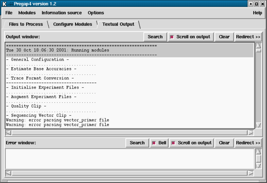
Chapter 4: Preparing readings for assembly using pregap4 335
For modules that do have parameters, the top line of the configuration panel will contain
two buttons labelled "Select params to save"and "Save these parameters". The "Select
params to save"button will add check boxes next to each parameter. Clicking on these check
boxes allows selection of individual parameters to save for this module. Once these have
been selected pressing the "Save"will save only those selected to the pregap4 configuration
file. Pressing the "Save these parameters"button will save all parameters for this module
to the configuration file.
The bottom strip of the window is an "Information Line".
4.2.2.3 Introduction to the Textual Output Window
Pregap4 has a main text output window identical to that of gap4 and spin. It is used for
showing textual results in the top section and error messages in the lower part. Full details
of the user interface are given elsewhere (see [User Interface], page 523), but an example of
the Text Output Window is given below.
4.2.2.4 Introduction to Running Pregap4
When pregap4 is started the user first needs to select the files to process. This is done using
the "Files to Process"command (from the File menu).
The "Configure Modules"tab allows for the currently available modules to be enabled
or disabled, and the module parameters edited accordingly.
336 The Staden Package Manual
Once all modules have been configured (so that none have edit listed next to their
name) pregap4 is ready to begin processing. This is started by pressing "Run"or by
selecting "Run"from the File menu.
When pregap4 has a setup that would be useful in the future "Save All Parameters (in
all modules)"from the Modules menu can be used, and pregap4 will store all the module
parameters to a configuration file ready for subsequent runs.
When processing has finished pregap4 will produce a report containing information from
each module and the final list of passed and failed sequences.
If for any reason pregap4 fails a particular step in the processing, users are strongly
recommended to correct whatever has caused the module to fail, clean up any files it has
created, and then repeat the whole process. That is, until users have a good understanding
of what happens at each stage of processing, it is better to repeat all the steps with the
original list of files, than to try to guess which step to continue from.
4.2.3 Pregap4 Menus
The main window of pregap4 contains File, Modules, Information source and Options
menus.
4.2.3.1 Pregap4 File menu
The File menu includes functions to set the files for processing, loading configuration files
and naming schemes, including configuration components, starting processing and exiting.
•Set Files to Process (see Section 4.3 [Specifying Files to Process], page 337)
•Load New Config File (see Section 4.7 [Using Config Files], page 366)
•Load Naming Scheme (see Section 4.8 [Pregap4 Naming Schemes], page 366)
•Include Config Component (see Section 4.9 [Pregap4 Components], page 371)
•Save All Parameters (in all modules) (see Section 4.6 [Configuring Modules], page 342)
•Save All Parameters (in all modules) to: (see Section 4.6 [Configuring Modules],
page 342)
•Save Module List (see Section 4.6 [Configuring Modules], page 342)
•Exit
4.2.3.2 Pregap4 Modules menu
The pregap4 Modules menu contains options for adding and configuring modules, and run-
ning pregap4.
•Add/Remove Modules (see Section 4.11 [Adding and Removing Modules], page 375)
•Configure Modules (see Section 4.6 [Configuring Modules], page 342)
•Select all modules
•Deselect all modules
4.2.3.3 Pregap4 Information source menu
The Information source menu contains options for specifying how the information required
for the experiment files is to be obtained. These menu options can also be entered from the
"Augment Experiment Files"module.
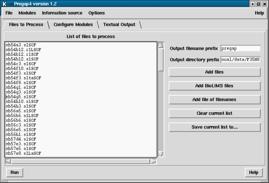
Chapter 4: Preparing readings for assembly using pregap4 337
•Simple Text Database (see Section 4.10.1 [Simple text Database], page 371)
•Experiment File Line Types (see Section 4.10.2 [Experiment File Line Types], page 373)
4.2.3.4 Pregap4 Options menu
The Options menu contains options for setting fonts and colours and defining the style of
the user interface.
•Set Fonts (see Section 4.5.1 [Fonts and Colours], page 341)
•Set Colours (see Section 4.5.1 [Fonts and Colours], page 341)
•Compact Window Style (see Section 4.5.2 [Window Styles], page 341)
•Separate Window Style (see Section 4.5.2 [Window Styles], page 341)
4.3 Specifying Files to Process
Pregap4 needs to be given a list of files to process. These files can be binary trace files
(in ABI, ALF, SCF, CTF or ZTR format), Experiment Files, FASTA, or plain text. The
files to process do not need to all be in the same format. FASTA files will be converted to
Experiment files.
Refering to the figure above, the "Files to Process"dialogue can be brought up from the
File menu, or just by pressing the appropriate tab when in compact_win mode.
On the left hand side we have the current list of files to process. This list can be
edited simply by clicking with the mouse and typing as normal. This only edits Pregap4’s
338 The Staden Package Manual
temporary copy of this list and does not modify the contents of any file of filenames that
the list was obtained from.
On the right side of the panel is the pregap4 output filename prefix, the output directory
name, and several buttons. The filename prefix is used when Pregap4 needs to create files
for its own use, both for temporary and not so temporary files. For example after processing
there may be prefix.passed, prefix.failed files. The prefix defaults to ‘pregap’ until a file of
filenames is loaded, in which case it switches to the last used file of filenames. All files
will be created within the output directory, regardless of where the input files reside. The
output directory defaults to the current directory or to the last used input directory.
The buttons allow selection of the files to process. The "Add files"button will bring
up a file browser, which will allow one or more file to be selected. Pressing Ok on the file
browser will then add the selected files to the "List of files to process"panel on the left side
of the pregap4 window. The "Add file of filenames"button may be used to select a list of
files whose filenames have been written to a ‘file of filenames’. The list of files to process
may be edited within pregap4, allowing new filenames to be added or removed. The "Clear
current list"will remove all filenames from the list. Both the "Add files"and "Add file of
filenames"button append their selections to the list of files to process, so to replace the
current list the "Clear current list"button must first be used. Finally the "Save current
list to..."button may be used to produce a new file of filenames, containing the combined
list of files to process.
4.4 Running Pregap4
When the Run button or Run command (File menu) is used, pregap4 starts processing the
files using the selected modules and their configurations. If the configuration is invalid an
error message will be produced. For example the following may be written to the error
window, and the configure modules panel will be selected with the problematic module
automatically highlighted.
Fri 10 Jul 10:04:25 1998 Run: Module sequence_vector_clip needs configuring
Assuming that the configuration is correct, the processing will start and output will be
sent to the output window as progress is made. The progress within each module is shown

Chapter 4: Preparing readings for assembly using pregap4 339
by a series of fullstops (.) for each correctly processed sequence, and an exclamation mark
(!) for each failed sequence.
The text output window above shows the early processing stages of 20 sequences. When
finished pregap4 will produce a report containing information from each module and the
final list of passed and failed sequences. For example:
- Report Production -
Passed files:
xb54a3.s1.exp (xb54a3.s1SCF.gz) : type EXP
xb54b12.r1L.exp (xb54b12.r1LSCF.gz) : type EXP
xb54b12.r1.exp (xb54b12.r1SCF.gz) : type EXP
xb54b12.s1.exp (xb54b12.s1SCF.gz) : type EXP
xb54c3.s1.exp (xb54c3.s1SCF.gz) : type EXP
Failed files:
xb54g5.s1.exp (xb54g5.s1SCF.gz) ’screen_vector_clip: sequence too short’
- Report from ’Augment Experiment Files’ -
xb54a3.s1.exp : added fields SF CF SC SP TN ST PR SI CH.
xb54b12.r1L.exp : added fields SF CF SC SP TN ST PR SI CH.
xb54b12.r1.exp : added fields SF CF SC SP TN ST PR SI CH.
xb54b12.s1.exp : added fields SF CF SC SP TN ST PR SI CH.

340 The Staden Package Manual
xb54g5.s1.exp : added fields SF CF SC SP TN ST PR SI CH.
xb54c3.s1.exp : added fields SF CF SC SP TN ST PR SI CH.
- Report from ’Tag Repeats’ -
xb54a3.s1.exp : no repeat found.
xb54b12.r1L.exp : no repeat found.
xb54b12.r1.exp : no repeat found.
xb54b12.s1.exp : no repeat found.
xb54c3.s1.exp : no repeat found.
*** Processing finished ***
The list of passed and failed files are written to prefix.passed and prefix.failed, where
prefix is the output filename prefix specified in the "Files to Process"panel. The reports
are written to prefix.report. The passed and failed files contain the most recent filenames
associated with each sequence. So if a sequence fails early on it could be listed as something
like xb54a3.s1SCF.gz and if it fails later it will be listed like xb54a3.s1.exp. This is
because it is the final filename which is important for later processing, such as for assembly
into gap4.
Aprefix.log file is also created containing a list of passed files, failed files, and the file-
name history for each file (the intermediates will still exist). The format of the passed
section is "filename (file type) PASSED". The format of the failed section is "filename
(file type) ERROR: error message". The format of the file history lines is a series of "file-
name (file type)" segments separated by "<-", with the original filename listed to the
right. Filenames containing Tcl meta-characters may be ‘escaped’ using curly braces or
back slashes. (The Tcl subst command may be used to generate the original name.) An
example of a log file follows. This was produced with the command line "pregap4 "Sample
671" WT5.exp zf89a2.s1.scf xb56e5.s1.scf".
[passed files]
ha59a6.s1.exp (EXP) PASSED
WT5.exp (EXP) PASSED
xb56e5.s1.exp (EXP) PASSED
[failed files]
zf89a2.s1.exp (UNK) ERROR: screen_vector_clip: sequence too short
[passed file history]
ha59a6.s1.exp (EXP) <- ha59a6.s1.scf (SCF) <- {Sample 671} (ABI)
WT5.exp (EXP)
xb56e5.s1.exp (EXP) <- xb56e5.s1.scf
[failed file history]
zf89a2.s1.exp (UNK) <- zf89a2.s1.scf
Some modules may also keep their own separate records, such as an assembly log. Where
this is the case, it will be explained in the help specific to that module.

Chapter 4: Preparing readings for assembly using pregap4 341
After running pregap4 it is time to either assemble the data (if this was not done using
pregap4) or to edit it. If the data has already been assembled with Pregap4 then you
will need to start up gap4 and use ‘Open Database’. Otherwise one of the gap4 assembly
functions should be used, with the filename prefix.passed file. For more information on
this see the Gap4 manual.
4.5 Configuring the Pregap4 User Interface
4.5.1 Fonts and Colours
The pregap4 Options menu contains options for modifying the fonts and colours used. These
options are common to many programs and so are documented elsewhere. See Section 10.8
[Font Selection], page 531. See Section 10.6 [Colour Selector], page 529.
4.5.2 Window Styles
Pregap4 supports two styles of windowing. The default method is a compact mode, with
the alternative being "separate"mode - similar to gap4 and spin.
This is the "separate"window style. Here the main window is always visible, with
commands in the main window bringing up new windows. In the picture above the configure
window can be seen on top of the main window.

342 The Staden Package Manual
The second style is "compact"mode.
In the compact picture above the most common top level windows are "pages"in a
tabbed notebook.
The benefit is greatly reduced screen space and quicker controls, but the text output
window is no longer permanently visible.
To switch styles select the "Compact Window Style"and "Separate Windows Style"
commands from the Options menu.
4.6 Configuring Modules
The "Configure Modules"dialogue is available from the Modules menu or, when using the
compact window style, by pressing the Configure Modules tab.
This dialogue contains the main interface through which most of the user’s interaction
with pregap4 will be performed. The left side of the display contains a list of the currently
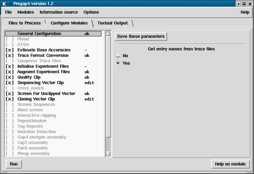
Chapter 4: Preparing readings for assembly using pregap4 343
loaded modules. One module in this list will be highlighted. The right side of the display
shows the configuration panel for this highlighted module.
The module list shown on the left consists of a series of module names and their status,
and is termed the "enable status". The [ ] and [x] strings at the left of the name indicates
whether this module is enabled; crossed boxes are enabled modules. The highlighting is
another indication of whether the module is enabled. The "General Configuration"module
is mandatory and cannot be disabled. The text to the right of the module name indicates
whether the module has been given all the parameters needed for it to process. This will
be one of "ok"(all configuration options have been filled in), "-"(no configuration options
exist for this module), "edit"(further configuration is required") or blank (this module is
disabled).
The "enable status"can be toggled by left clicking on the "[ ]" to the left of the module
name. The enable status can be written to the current Pregap4 configuration file using the
"Save Module List"or "Save All Parameters"commands in the Modules menu. Left clicking
anywhere on a module name in the module list will switch the pane on the right side of
the window to display any available parameters for this module. Not all modules will have
parameters to configure.
For modules that do have parameters, the top line of the configuration panel will contain
a button labelled "Save these parameters". This button will save all parameters for this
module to the configuration file. Note that this is not the same as the "Save all parameters"
option in the main Modules menu, as this saves all parameters in all modules.
344 The Staden Package Manual
4.6.1 General Configuration
Description
This is a mandatory module. It is always the first module executed and will
not appear in the "Add/Remove Modules"list. Its purpose is to set general
parameters which affect several other modules. At present it contains just two
items.
Option: Get entry names from trace files
Many trace formats include storage for a sequence "sample name". This option
controls whether or not the sample name should be used instead of deriving the
name from the filename. If "No"is answered to this question then the sequence
sample name will be generated by removing the filename suffix; for example
xb55a2.s1.ztr will become xb55a2.s1.
4.6.2 Estimate Base Accuracies
Description
This module analyses the traces at each base call to estimate a confidence value
for the called base. It does this by simply looking at the area underneath the
trace for the called base and dividing this by the highest area under the trace
for the three uncalled bases. This is a very simplistic statistic which should
ideally only be used for measuring the average reliability of the entire sequence
rather than any individual base. If another program (eg Phred, or ATQA) is
available then this should be used in preference. From the 2002 release the eba
values are normalised to the phred scale (this was achieved by comaring the
original eba values and phred values for 4.6 million base calls of Sanger Centre
data).
There are no adjustable parameters for this module.
4.6.3 Phred
Phred is not included as part of the Staden Package. It is available from Phil Green.
http://www.genome.washington.edu/UWGC/analysistools/phred.htm
Description
Phred is an ABI base caller. Ewing, B. and Green, P. 1998. Base-Calling of
Automated Sequencer Traces Using Phred. II. Error Probabilities. Genome
Res. 8, 186-194. It will analyse the chromatogram data to produce new base
calls. For each base it assigns confidence value indicating how likely this base
call is to be correct. These confidence values are significantly more reliable
than those produced by eba and they are compatible with the Phrap assembly
program and the gap4 consensus algorithm.
Phred can process either ABI or SCF files, but pregap4 will automatically
convert all input to SCF format first. This means that the phred pregap4
module will be able to process any supported trace format.
Chapter 4: Preparing readings for assembly using pregap4 345
There are no adjustable parameters for this module.
4.6.4 ATQA
ATQA is not include as part of the Staden package. It is available from its developers,
Daniel H. Wagner, Associates, at
http://www.wagner.com/ .
Description
The ATQA program estimates confidence values for each called base in a lane
file. A confidence value corresponds to the probability that the associated base
call is incorrect by the formula
score = -10*log10(probability of error).
(This is the same log scale used by Phred.) In fact, the ATQA program com-
putes four confidence values for each called base. The first three values corre-
spond to the probabilities of substitution, insertion, and deletion errors, respec-
tively. The fourth value is a combined score representing the probability that
the called base is an error of any sort. Currently, only the combined confidence
value is used by Staden package software.
Unlike Phred, the ATQA program does not produce base calls. Rather, it
assigns confidence values to each base call in a lane file based on features of the
trace data. The current version of the ATQA program is tuned to base calls
made by the ABI base caller and to trace data from the ABI 377 sequencer.
Although ATQA can read ABI files, it will not create SCF files in such circum-
stances. However pregap4 will always convert any non SCF trace files into SCF
format before running ATQA, so an explicit conversion is not required.
4.6.5 Trace Format Conversion
Description
This converts files between the various supported trace formats. At present it
can read ABI, ALF, SCF, CTF and ZTR formats, and can write SCF, CTF
and ZTR. Of these formats, ZTR typically represents the smallest size and is
fast due to its own internal compression routines.
The Trace Format Conversion may also be used to apply some simple edit-
ing methods to the traces. These include down-scaling (to reduce file size),
background subtraction, and amplitude normalisation.
Option: Output format
This selects the format for the output trace files. If the output format is the
same as the input format then the input files will not be overridden. Instead
new files will be produced with names based on the input names, generated by
replacing (for example) ".scf"with "..scf". The available output format choices
are ZTR, CTF and SCF.
346 The Staden Package Manual
Option: Downscale sample range
Option: Range
These select whether to reduce the scale used to store the amplitudes, and if so
to what range. ABI files typically range from 0 to 1600 (which is approximately
11-bit data). Shrinking this down to 0 to 255 (8-bit) will usually be visually
comparable as the trace displays in Gap4 and Trev are typically smaller than
255 pixels high, although if the Y scale is increased differences will still be
detectable. The purpose of this is to further reduce file size.
Option: Subtract background
This attempts to eliminate the trace background by a simple technique of de-
ducting the lowest of the four amplitudes from all of the four amplitudes. This
is an overly crude method which should only be used when the preprocessing
software included on the sequencing manufacturer’s instruments has not been
used.
Option: Normalise amplitudes
This uses a sliding window to compute the average single strengths. From this
it scales the data to try and provide, on average, more uniform peak heights
along the trace. Again this is a very simplistic method and so it is not advisable
unless their is a problem with the sequencing manufacturer’s own software.
Option: Delete temporary files
When pregap4 can determine that a trace file is neither the original input or
the final output then it is considered to be a temporary file which may be
suitable for deletion. An example would be using Phred with ABI files and
then converting to ZTR. Phred produces SCF files and so we have ABI to SCF
to ZTR, in which the SCF files may be safely deleted.
4.6.6 Initialise Experiment Files
Description
This modules creates an Experiment File from a trace file (of any format). It
uses the init_exp program to write ID,EN,LN,LT,AQ and SQ Experiment File
line types. This module is mandatory for many subsequent modules, such as
vector clipping/screening and assembly.
There are no adjustable parameters for this module.
4.6.7 Augment Experiment Files
Description
This module adds further data to the Experiment File, with the additional
information typically obtained from external sources. Such information could
be the data required by the vector clipping program, or template information
needed by gap4.
The parameters for this module may be configured by using the "Simple Text
Database"(see Section 4.10.1 [Simple text Database], page 371) or "Experiment
File Line Types"(see Section 4.10.2 [Experiment File Line Types], page 373)
Chapter 4: Preparing readings for assembly using pregap4 347
dialogues. These both allow setting of the Experiment File records to be written
during the Augment stage.
4.6.8 Quality Clip
Description
This module determines where the sequence quality is too poor to use for re-
liable assembly. It supercedes the Uncalled Base Clip module. This uses the
qclip program which reads and writes to Experiment Files. Its default quality
evaluation is based on the range of values produced by the Estimate Base Accu-
racies module (quality value 70, averaged over 100 bases). For use with phred,
try lower values such as quality value 15 averaged over 50 bases. When quality
values are not available it will use the same method as the Uncalled Base Clip
module; to analyse the base calls and count the number of undetermined bases
within a given window of sequence. Both 5’ and 3’ ends may be quality clipped.
For the confidence mode of clipping the method starts from the point of highest
average quality, and then steps outwards in both directions until the average
quality is below a defined threshold.
For the sequence mode of clipping the method starts from a defined position
and steps outwards in both directions until the number of uncalled bases within
a given window length exceeds a predefined threshold. For more details see the
qclip documentation (see Section 12.19 [qclip], page 597).
Note that the Phrap assembly algorithm works best without quality clipping
and it can make use of the full length of readings (due to the use of the Phred
confidence values).
Option: Clip mode
This may be one of "by sequence"or "by confidence". The "by sequence"
mode is equivalent to the Uncalled Clip module. The "by confidence"mode
uses Phred-scaled confidence values to determine the quality for clipping. This
does not work with eba confidence values.
Option: Minimum extent
The lowest allowable 5’ clip position.
Option: Maximum extent
The largest allowable 3’ clip position.
Option: Minimum length
If after quality clipping the good portion of a sequence is shorter than the
specified length, then this file will be rejected with the message "qclip: Sequence
too short".
Option: Window length
The window length over which the confidence will be averaged. This option is
only relevant for the "clip by confidence"mode.

348 The Staden Package Manual
Option: Average confidence
The minimum average confidence (over ‘window length’ bases) for sequence
to be accepted as good quality. This option is only relevant for the "clip by
confidence"mode.
Option: Start offset
The base number to start the 5’ and 3’ good quality searches from. This option
is only relevant for the "clip by sequence"mode.
Option: 3’ window length
The window length in which to count uncalled bases. This option is only rele-
vant for the "clip by sequence"mode.
Option: 3’ number of uncalled bases
The maximum allowed count of uncalled bases in a single window length. This
option is only relevant for the "clip by sequence"mode.
Option: 5’ window length
The window length in which to count uncalled bases. This option is only rele-
vant for the "clip by sequence"mode.
Option: 5’ number of uncalled bases
The maximum allowed count of uncalled bases in a single window length. This
option is only relevant for the "clip by sequence"mode.
4.6.9 Sequencing Vector Clip
Description
This module uses the vector_clip program to identify and mark the sequenc-
ing vector (those used to produce templates for sequencing, eg m13mp18 or
puc18). To achieve this task it needs to know information about the vector
including the cut site position and the position of the primer site relative to the
cut site. See Section 6.8 [Defining the Positions of Cloning and Primer Sites for
Vector Clip], page 408..
Option: Use Vector-primer file
Vector clip may be told to search through a series of vectors and primers held
within an external file. Alternatively we can request that it looks only at one
specific, known, vector. This question is to determine which of the two mutually
exclusive methods to use. In general it is still important for the Experiment
File to contain primer and template data. The Vector-primer module can be
used to add the primer and sequencing vector information to the Experiment
File but not the template name.
Option: Vector-primer filename.
This is only used if the "Use Vector-primer file"question was answered with
"Yes". Each input sequence will be compared against each vector-primer pair

Chapter 4: Preparing readings for assembly using pregap4 349
to find the best match. This provides a simple way of comparing against mul-
tiple vectors or comparing against both forward and reverse primers of a single
vector. For further details on creating this vector-primer file, see Section 6.6
[Vector Primer file format], page 407..
Option: Select vector-primer subset
This is used in conjuction with the vector-primer filename to indicate which of
the vector-primer pairs listed in this file should be used. Initially this is set
to all vector-primer pairs, but efficiency will be greatly increased if just the
required subset is selected. (Internally pregap4 will then temporarily produce
a new vector-primer filename each time vector_clip requires one, containing
just the selected items.) To select more than one vector-primer pair use the
standard listbox mouse bindings: single left click to pick an item; click and drag
to select a range; and control left click to toggle a single item. The selected list
will be saved to the pregap4 configuration file whenever all the parameters for
this module are saved.
Option: Max primer to cut-site length
This parameter is only used when a vector-primer file is defined. The sequence
stored in the vector-primer file may be considerably longer than we expect to
see at the start of the sequences being analysed. By defining the maximum
length of sequence we expect to see, vector_clip may be more sensitive and
slightly faster.
Option: Vector file name
This, and the following two options, are only used if the "Use Vector-primer
file"question was answered with "No". The vector file name should be the
name of a file containing just the vector bases or white space, in a plain text
format.
Option: Cut site
The cut site specified as a base count from the start of the vector file.
Option: Primer site
The primer site specified as a base offset from the cut site. e.g. for m13mp18
forward primers the value is 41. If, instead of the usual single value, two values
are specified separated by a slash, then this gives the values for the universal
forward and reverse primers (for example "41/-24"). Only use this format if
the PR (primer type) experiment file line type is known AND will be specified
in the experiment file. If the PR record is not specified in the experiment file,
the primer site position will be set to zero, and the vector clipping is unlikely
to work correctly. (PR values do not have to be known if they can be derived
using naming schemes such as those used by the Sanger Centre). If the primer
site indicates a custom primer sequence then the primer site is taken to be 0.

350 The Staden Package Manual
Option: Percentage minimum 5’ match
Option: Percentage minimum 3’ match
Both ends of the sequence are checked using a dynamic programming algorithm
to find the optimal alignment. An end is marked as vector if the percentage
match is at least as high as this supplied parameter.
Option: Default 5’ position
This specifies the value to use for marking the 5’ sequencing vector if none is
detected. Specifying this as -1 will cause the absolute value given for the primer
site (which is specified as relative to the cut site).
4.6.10 Cross match
Cross match is not included as part of the Staden Package. It is available from Phil Green.
http://www.genome.washington.edu/UWGC/analysistools/swat.htm
Description
This uses the cross_match program to search for sequencing vector. (Future
versions may also check for other cloning vectors.) This allows for searching
of multiple vector files. However as cross match does not make use of primer
and cut site information the vector detection is inherently less sensitive than
vector_clip (see Chapter 6 [Screening against Vector Sequences], page 401).
Option: FASTA vector file name
This specifies a fasta format file of one or more sequencing vector sequences.
Option: Minimum match length
Minimum length of matching word for SWAT comparison.
Option: Minimum score
Minimum SWAT score.
4.6.11 Cloning Vector Clip
Description
This module searches for non "sequencing"vectors used in the shotgunning
process, eg for Cosmid or YAC. Any fragment in any orientation of this vector
could be present so there is no need for the cut sites to be known. The vector_
clip program is used for this task (see Chapter 6 [Screening against Vector
Sequences], page 401).
Option: Vector file name
The filename containing the vector sequence. At present this should be a file
containing a single plain text sequence containing just the bases or white space.

Chapter 4: Preparing readings for assembly using pregap4 351
Option: Max probability
For each match its probability of occurring by chance is calculated. Any match
with a probability lower than ‘Max probability’ is accepted.
4.6.12 Screen for Unclipped Vector
Description
This module may be used to identify undetected segments of sequencing vector
or to detect recombinations. After searching and marking sequencing vector,
any further strong matches to the sequencing vector indicate a possible problem.
This module uses the vector_clip program (see Chapter 6 [Screening against
Vector Sequences], page 401).
Note that this module requires the Sequencing Vector Clip module to be used
before screening, otherwise all sequences containing unclipped vector will be
falsely rejected.
Option: Minimum length of match
If a match of at least this length is found then the sequence currently being
processed will be rejected.
4.6.13 Screen Sequences
Description
This module can perform very fast matches between the sequences to process
and one or more screen sequences. Any sequence containing a significant match
is rejected. An example of use for this module is to reject sequences prior to
assembly that appear to be contaminated with E. coli. This uses the screen_
seq program (see Section 12.20 [Screen seq], page 600).
Option: Screen single sequence
This is yes/no question used to determine whether the screen sequence filename
is the filename of a single sequence or a filename of a file containing a series of
sequence filenames. To compare just one file select "Yes".
Option: Screen sequence file (of filenames)
This is either the filename of a single sequence or the filename of a file of
filenames, depending on the answer to the previous question. The sequence
files must be in plain text format containing just the bases or white space.
Option: Maximum screen sequence length
The maximum length of any individual screen sequence.
Option: Minimum match length
Any fragment containing an exact match longer than this length will be rejected.
352 The Staden Package Manual
4.6.14 Blast Screen
Description
This module uses the blastall program to compare all the input sequences
against a prebuilt blast database of screen sequences. It is not possible to
compare against a subset of the database - to do this build a new blast database
using formatdb. This module is an alternative to the Screen Sequences module
which uses the screen_seq program.
Blast may be used for either completely rejecting sequences or for simply tagging
the matching segments, or for both. If you wish to tag with several tag types,
then several instances of the Blast screen module need to be used.
Blast is not included as part of the Staden Package. It is available from the
NCBI.
Option: BLAST database
This is the filename of the BLAST database to screen against, with the ‘.nhr’,
‘.nin’ and ‘.nsq’ suffixes removed.
Option: E value
This specifies the ‘E value’ used by blast when determining which hits should
be considered as real.
Option: Match fraction
This is the total percentage of the sequence which much have a blast match
somewhere in the BLAST database searched in order to reject this sequence.
Segments of the input sequence that match multiple components in the BLAST
database are only counted once when computing this percentage, but the loca-
tions of the matches in the BLAST database do not need to be consecutive.
If you wish to accept everything, but still want to tag the matches, then set the
match fraction to greater than 1.0.
Option: Tag type
The default for this is <none> which indicates no tagging is required. Otherwise
this should be a 4 letter tag type (such as REPT) known to gap4.
4.6.15 Interactive Clipping
Description
This modules invokes the trev program to view the raw chromatogram files.
The user can then adjust the quality and vector clip positions if desired. The
trev window will contain Next and Previous buttons to skip from trace to trace.
The Reject buttons allows a trace to be rejected, in which case it is added to
the failure file with the message "interactive clip: manually rejected".
There are no adjustable parameters for this module.
Chapter 4: Preparing readings for assembly using pregap4 353
4.6.16 Extract Sequence
Description
This module uses the extract_seq program to extract the sequence information
from binary trace files, Experiment files, or from the old Staden format plain
files. The output contains the sequences split onto lines of at most 60 characters
each, in plain or fasta format. The input files are passed unchanged onto
subsequent modules.
Option: Output only the good sequence
When reading an experiment file or trace file containing clip marks, output only
the good sequence which is contained within the boundaries marked by the QL,
QR,SL,SR,CL,CR and CS line types.
Option: Consider cosmid as good sequence
When the Output only the good sequence option is specified this controls
whether the cosmid sequence should be considered good.
Option: Output in fasta format
Specifies that the output should be in fasta format rather than plain text.
Option: Output in one file only
If this option is selected then the output from every sequence is sent to one
file. This is best used with the Output in fasta format option selected, and
is useful for feeding into BLAST searches, for example. The file to write to is
specified in the File name filed.
If this option is unselected then the output is sent to separate files, one per
sequence. The output files have the same name as the input files, except with
an extra suffix specified in the File name suffix field.
4.6.17 RepeatMasker
RepeatMasker is not included as part of the Staden Package. It is available from Arian
Smit.
http://ftp.genome.washington.edu/RM/RepeatMasker.html
Description
This module uses the RepeatMasker program. This is a program which searches
for a comprehensive set of repeat sequences. Any matches which are found will
be tagged with a comment indicating the type of repeat. These tags will then
be visible from within gap4. Full documentation is available from the author
of RepeatMasker, or from typing RepeatMasker -h.
Option: Repeat library
This specifies the directory containing the library of repeat sequences. Only
one library directory may be specified. The library "<default>" will let Repeat-
Masker use its own default library.
354 The Staden Package Manual
Option: RepeatMasker cutoff
This specifies the cutoff score for RepeatMasker. The documentation with
RepeatMasker states that a cutoff of 250 will guarantee no false positives.
Option: Gap4 tag type
When a repeat is found a tag will be added to the Experiment File. This
specifies the tag type to use. It should be one of the tag types available to
Gap4, but other tag types may be used if desired (they will be coloured as is
COMMent tags in gap4).
Option: Types of repeat to screen against
The default setting of RepeatMasker is to search for primate repeats, however
it may be told to search for other repeat families or to restrict its search to only
ALU primate repeats. The full list of options here are Alu only, Rodent only,
Simple only, Mammalian excluding primate/rodent, and no low complexity.
These are as defined in the RepeatMasker documentation. It is not known
what effect enabling mutually exclusive options will have.
4.6.18 Tag Repeats
Description
This module uses the repe program to identify and mark known repetitive
elements within the sequences. An example usage is to tag all ALU fragments.
This information may be used by the gap4 assembly algorithm to improve
the assembly by initially ignoring matches between two ALU fragments which
may otherwise produce incorrect assemblies. If available, we recommend using
RepeatMasker instead of this module.
Option: Repeat file name
This is the filename of a file of filenames, each of which contain a single repeat
to search for. The format of these individual files is plain text consisting of just
the nucleotides and white space.
Option: Repeat score
This is the minimum score for classifying a matched segment as a repeat.
Option: Tag type
This is the gap4 tag type to use for identifying this repeat segment. It is not
possible to choose different tag types for different repeats, although the tag
comments contain the match score and match filename.
4.6.19 Mutation Detection
Description
Superceded by the newer modules: (see Section 4.6.21 [Trace Difference],
page 357) and (see Section 4.6.22 [Mutation Scanner], page 359).

Chapter 4: Preparing readings for assembly using pregap4 355
This module compares each sequence chromatogram against a "wild type"or
reference chromatogram to detect point mutations. The mutations are detected
by aligning and subtracting each trace from the wild type trace to produce a
"difference trace". The difference trace is then analysed to identify point muta-
tions which are written back to the Experiment File and MUTN tags. This uses
the trace_diff program Bonfield, J.K., Rada, C. and Staden, R. Automated
detection of point mutations using fluorescent sequence trace subtraction. Nu-
cleic Acids Res. 26, 3404-3409 (1998).
Obviously the reference traces should be as similar as possible to the ones
being compared against it. It should be prepared by sequencing the wild type
from the same primer, and using the same chemistry as the readings being
screened. One good way to produce a reference trace is to run the wild type
sequence on the gel along with the other samples. It is also possible to get
gap4 to produce a consensus trace. This requires using pregap4 twice. Firstly
process the sequences through pregap4 with all the appropriate options except
with the mutation detection module disabled. Assemble these sequences into
gap4. Within gap4, for each contig start up the Contig Editor and select Save
Consensus Trace from the command menu. This will produce a trace which is
the average of the traces in that contig. Then delete the gap4 database and
reprocess the sequences using Pregap4, this time using mutation detection to
compare against the consensus trace.
Option: Wild type file (+ve strand)
Option: Wild type file (-ve strand)
These are the filenames of the chromatogram for the wild type sequence on
each strand. These may be in any allow trace format (SCF, ZTR, ABI, CTF
or ALF). In the augment stage, these are represented in the WT line type using
plus filename|minus filename notation.
Option: Start position
Option: End position
These define the range within each sequence in which to identify mutations. The
algorithm works better on good quality data so including very bad sequence may
give errors.
Option: Score
This a threshold used to determine when a peak in the difference trace is con-
sidered to be a mutation. The higher the value the more stringent the test.
Option: Alignment band width
The trace alignment is performed by firstly doing a sequence alignment on
the text sequences contained in the two files. This parameter specifies the band
width for this alignment. Smaller values give quicker alignments, but only work
if the alignment is sufficiently close to the main diagonal.

356 The Staden Package Manual
Option: Other arguments
This allows for any other arguments to be passed to the trace_diff program.
See the trace diff documentation for more details.
The module above is superceded by the newer modules: (see Section 4.6.21 [Trace
Difference], page 357) and (see Section 4.6.22 [Mutation Scanner], page 359).
4.6.20 Reference Traces and Reference Sequences
Description
This module specifies the reference traces and reference sequences used by the
two mutation detection modules (see Section 4.6.21 [Trace Difference], page 357
and see Section 4.6.22 [Mutation Scanner], page 359). The left and right clip
points for each trace can also be specified.
A reference trace should be as similar as possible to the ones being compared
against. It should be prepared by sequencing the wild type from the same
primer and using the same chemistry as the readings being screened. One good
way to produce a reference trace is to run the wild type sequence on the gel
along with the other samples.
If the input files have been sequenced from both strands, reference traces from
each strand may be specified here.
NOTE: In order for pregap4 to choose the appropriate wild type trace it needs
to know the strand for each input sequence. This is specified by the PR record in
the experiment file which is typically generated using a naming convention (see
Section 4.8 [Pregap4 Naming Schemes], page 366) If pregap4 cannot determine
the strand, or if only one reference trace is specified, then each input sequence
will be compared against the +ve strand reference trace.
The reference data supplied in this module, when entered with gap4 shotgun
assembly, will add REFS and REFT notes (see Section 2.15 [Notes], page 281) to
the gap4 database. A reference sequence is used to number bases in the Contig
Editor (see Section 2.6.12 [Reference sequences and traces], page 191) and in
reporting the positions of mutations (see Section 2.6.7.9 [Report Mutations],
page 178.)
Option: Reference Trace (+ve strand)
Option: Reference Trace (-ve strand)
These are the filenames of the chromatogram for the reference trace on each
strand. These may be in any allowable trace format (ZTR, SCF, ABI, CTF or
ALF). The filenames are entered into the experiment file as WT records by the
"Augment Database"phase of pregap4, so this module must also be enabled.
Option: Clip left
Option: Clip right
These values determine which region of the reference trace (in bases) is used
for mutation detection. This can be used to exclude poor quality regions, or
restrict the range over which mutation detection occurs. Restricting the range
will also speed up the algorithms. If you specify -1 for any value, mutscan
Chapter 4: Preparing readings for assembly using pregap4 357
will use the clip point QL/QR records within the reference trace experiment
file (provided they exist). If they don’t exist, then the entire reference trace is
used. i.e. No clipping occurs. If the range specified is too small, the mutation
detection algorithms may report an error, since there must be a useful overlap
between the sequences in order to process them.
Option: Reference Sequence
This specifies the reference sequence, which is typically an annotated EMBL
entry. This field is optional.
Option: Start base number
If a reference sequence was specified this indicates which base number it will
start counting from within Gap4’s contig editor. It also defines the posi-
tions of mutations, as output by the Report mutations function of gap4 See
Section 2.6.7.9 [Report Mutations], page 178..
Option: Circular
Option: Sequence length
If the reference sequence is defined to be circular then the length needs to be
known too. When the base number reaches the sequence length the next base
in the sequence will be renumbered to base 1. This may be useful if the cir-
cular reference sequence needs to be chopped to form a linear sequence at a
different position than the standard numbering. (For example this is typical
when sequencing the mitochondrial variable loop, which by standard conven-
tions contains base number 1.)
Note that it is possible (though no longer recommended) to use gap4 to produce a consen-
sus trace. This requires using pregap4 twice. Firstly process the sequences through pregap4
with all the appropriate options except with the mutation detection modules disabled. As-
semble these sequences into gap4. Within gap4, for each contig start up the Contig Editor
and select Save Consensus Trace from the command menu (available only in expert mode).
This will produce a trace which is the average of the traces in that contig. Then delete
the gap4 database and reprocess the sequences using Pregap4, this time using mutation
detection to compare against the consensus trace. Best results are usually obtained by first
deleting pads in the consensus sequence. You should inspect the resulting consensus trace
carefully to ensure there are no discontinuities introduced as a result of the pad deletions.
4.6.21 Trace Difference
Description
This module compares each sequence chromatogram against a "wild type"or
reference chromatogram to detect point mutations. The mutations are detected
by aligning and subtracting each trace from the wild type trace to produce a
"difference trace". The difference trace is then analysed to identify point mu-
tations which are written back to the Experiment File as MUTA tags. The basic
idea is explained in the paper Bonfield, J.K., Rada, C. and Staden, R. Auto-
mated detection of point mutations using fluorescent sequence trace subtraction.
Nucleic Acids Res. 26, 3404-3409 (1998).

358 The Staden Package Manual
This implementation is the second version of the algorithm. The previous ver-
sion used basecalls to do trace alignment. This led to problems when bases were
called in error (often the case around mutations). The new algorithm ignores
the basecalls completely and aligns the trace signals themselves, avoiding such
problems. This is much more computationally intensive, but it has proved to
be fast enough for interactive use.
If the input files have sequenced from both strands then two wild type se-
quences may be given. In order for pregap4 to choose the appropriate wild
type trace it needs to know the strand for each input sequence, which is typ-
ically generated using the naming convention. A simple naming scheme is
provided with pregap4 (in the lib/pregap4/naming schemes directory) called
"mutation detection.p4t". This can be loaded from the pregap4 file menu. It
assumes that trace names have an ’f’ or ’r’ suffix, denoting the forward and
reverse strands respectively. If you need something more complex, then you’ll
have to create and load your own naming scheme. If pregap4 cannot determine
the strand, or if only one wild type is specified, then each input sequence will
be compared against the +ve strand wild type.
The reference or wild type traces for tracediff are specified in the see
Section 4.6.20 [Reference Traces module], page 356.
Option: Sensitivity
This threshold is used to determine when an above/below baseline double peak
in the difference trace is considered to be a mutation. It is specified in standard
deviations from the mean over the analysis window. The higher the value, the
more stringent the test. This value is reduced dynamically by the algorithm in
the presense of mutations since small mutations near larger ones can often be
missed with a uniform sensitivity setting. It’s likely that some experimentation
with this parameter will be required for optimal mutation detection in your
data.
Option: Noise threshold
This threshold is used to filter out low level noise during the analysis phase. It
is specified as a percentage of the maximum peak-to-peak trace difference value.
A high threshold will lead to fewer false positives but you run the additional
risk of missing low level mutations.
Option: Analysis window length
Analysis of the trace difference is done over a local region to counter the effects
of non-stationarity in the trace signal. The analysis region is defined by a short
window whose length is specified in bases. The window is asymmetric in that
it’s located to the left of the base it’s positioned on. This avoids measurement
problems when mutations are encountered. The window size is a tradeoff. If
it’s too big, low level mutations may be missed. If it’s too small, there may be
insufficient data to give unbiased measurements leading to many false positives.

Chapter 4: Preparing readings for assembly using pregap4 359
Option: Maximum peak alignment deviation
The centres of each individual half-peak of a double peak above and below
the baseline must align reasonably well for them to be considered to be real
mutations. The amount of half-peak alignment deviation allowable is specified
in bases by this parameter, usually as a fraction of one base.
Option: Maximum peak width
During analysis, the width of each peak is measured to avoid problems caused
by gel artifacts. These often appear as broad peaks that overlay many bases.
The maximum peak width is specified in bases. A lower value will lead to fewer
false positives, but you run the additional risk of missing smeared mutations
towards the end of a trace.
Option: Complement bases on reverse strand tags
After mutation detection and after readings have been assembled into a GAP4
database, GAP4 displays both forward and reverse readings in a single direction
in the contig editor. This makes it much easier to compare sequences and traces
in both directions simultaneously. When the corresponding traces are displayed,
any reverse strand traces are complemented automatically such that the bases
are interchanged. In this case, the original mutation tag generated by tracediff
will then be of the wrong sense, so if checked, this option complements the tag
base labels to match the complemented trace displayed by GAP4.
Option: Write difference traces out to disk
After trace difference analysis, the generated traces are normally discarded and
not written to disk. Checking this option lets you save the trace difference files
to the same directory as the original traces. The .ZTR trace format is used
for this purpose. The original filename is retained and a "diff.ztr"suffix is
appended.
4.6.22 Mutation Scanner
Description
This module compares each input sequence chromatagram against a reference
chromatogram (or trace) to detect mutations. The reference traces are speci-
fied in the see Section 4.6.20 [Reference Traces module], page 356. Using this
method it is possible to detect both base-change mutations and heterozygous
mutations.
It works by aligning the reference trace with the input trace and then examining
the peak pairs for each individual base separately. It does not use basecalls
as these are prone to error and their use generates too many false positives.
After normalisation, the amplitude ratios of peak pairs which are abnormal are
analysed more closely. For heterozygotes, a drop in peak height with respect to
the reference of about 50% is expected. The final set of candidate mutations are
validated against a difference trace to ensure it contains a double peak at that
location, thus confirming the mutation to be real. After chromatagram analysis
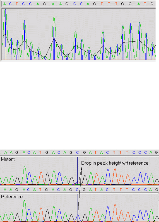
360 The Staden Package Manual
has been completed, mutation tags are written back to the Experiment File as
HETE and MUTA tags.
Option: Adaptive Noise Floor
Traces are very noisy difficult to process signals. To find valid peaks in a trace
an adaptive noise threshold based on envelope height is used to eliminate all low
level noise from consideration. The effect of this parameter can be seen in the
trace below. By default this parameter is set to 25% of envelope peak height.
If set lower, too much noise is picked up; if set higher, low level mutations may
be missed.
Option: Upper and Lower Peak Drop Thresholds
For heterozygote mutations, the peak height of the mutant drops by 50% with
respect to the normalised reference trace as shown in the trace below. For
accurate detection, we use this information to validate potential mutations.
Due to overzealous preprocessing done by sequencing machine software, the
peak height drops are often not 50%, but typically hover between 20% and
70% of reference peak height. Any potential heterozygote whose peak height
drop with respect to the normalised reference trace that lies within this range
is considered to be a real mutation.
Option: Peak Alignment Search Window Size
In an ideal world, heterozygote peaks in a trace would be perfectly aligned
on top of each other. In practice however, they can often be skewed due to
gel chemistry problems or inaccurate mobility correction as shown in the trace
below. When mutscan looks for peak pairs, it allows for this skew by looking
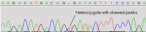
Chapter 4: Preparing readings for assembly using pregap4 361
either side of the current position for nearby peaks. This parameter is the
distance mutscan looks in bases around each candidate position.
Option: Heterozygote SNR Threshold
For a normal trace containing normal bases, the signal-to-noise ratio (SNR) is
the ratio of the highest base peak to the second highest trace level. Mutscan
computes this value in decibels (dB) as 20*log10(S/N). For normal bases, this
usually in the region of 20-30dB or higher. However, for heterozygotes, the
SNR as defined by this measure degrades significantly to around 2-5dB. This
is the mechanism mutscan uses to accurately determine the mutation tag type.
If the candidate mutation’s SNR is equal to or below this threshold, mutscan
designates it to be heterozygous, otherwise it’s considered to be a normal base-
change mutation.
Option: Trace Alignment Failure Threshold
Mutscan works by aligning a mutant trace against a reference trace and com-
paring the peaks. However, if the traces are too different, the alignment may
fail and as a consequence, large numbers of false positive mutation tags are
generated. Typically, within each trace there are only one or two mutations, so
if we find 15 mutations, then we can confidently predict that things have gone
badly wrong! This parameter sets a threshold, beyond which an alignment fail-
ure error message is printed, rather than outputting large numbers of invalid
mutation tags.
Option: Complement Bases on Reverse Strand Tags
After mutation detection and after readings have been assembled into a GAP4
database, GAP4 displays both forward and reverse readings in a single direction
in the contig editor. This makes it much easier to compare sequences and traces
in both directions simultaneously. When the corresponding traces are displayed,
any reverse strand traces are complemented automatically such that the bases
are interchanged. In this case, the original mutation tag generated by mutscan
will then be of the wrong sense. If checked, this option complements the tag
base labels to match the complemented trace displayed by GAP4.
4.6.23 Gap4 Shotgun Assembly
Description
This module assembles the processed sequences into gap4 using gap4’s own
assembly engine. Note that this is incompatible with use of "Enter assembly
into Gap4", which should only be used for external (to gap4) assembly engines.
362 The Staden Package Manual
Option: Gap4 database name
Option: Gap4 database version
The name and version of the database to assemble into.
Option: Create new database
This is a toggle to define whether the specified gap4 database should be cre-
ated or appended to. Be warned that at present creating a new database will
overwrite existing one of the same name, in the same directory, without any
warnings.
Option: Minimum exact match
Option: Maximum number of pads
Option: Maximum percentage mismatch
These control the main assembly parameters within gap4. For more details see
Section 2.7.1 [Normal shotgun assembly], page 205.
4.6.24 Cap2 Assembly
Cap2 is not included as part of the Staden Package. It is available from Xiaoqiu Huang ().
Description
This module uses the cap2 program to perform shotgun assembly. Output
will be placed in the fofn.assembly directory, where fofn is the filename prefix
listed in the "Files to Process"panel. The output is in a format suitable for
directed assembly within gap4. This can also be performed by using the "Enter
Assembly into Gap4"module.
There are no adjustable parameters for this module.
4.6.25 Cap3 Assembly
Cap3 is not included as part of the Staden Package. It is available from Xiaoqiu Huang ().
Description
This module uses the cap3 program to perform shotgun assembly. Output
will be placed in the fofn.assembly directory, where fofn is the filename prefix
listed in the "Files to Process"panel. The output is in a format suitable for
directed assembly within gap4. This can also be performed by using the "Enter
Assembly into Gap4"module. Cap3 differs from Cap2 in that it can make use
of confidence values (in the range supplied from phred) and constraints.
Option: Auto-generate constraints
When enabled, this uses the reading direction (forward / reverse primers), the
template name and the insert size, to produce a file containing data to constrain
how the readings may be assembled.
4.6.26 FakII Assembly
FakII is not included as part of the Staden Package. It is available from Susan Miller ().
Chapter 4: Preparing readings for assembly using pregap4 363
Description
This module uses the FakII suite of programs to perform shotgun assembly.
Output will be placed in the fofn.assembly directory, where fofn is the filename
prefix listed in the "Files to Process"panel. The output is in a format suitable
for directed assembly within gap4. This can also be performed by using the
"Enter Assembly into Gap4"module.
Option: E limit
Option: D limit
Option: O threshold
These parameters control the graph component of FakII, which is used to find
the initial overlaps between sequences.
Option: Auto-generate constraints
When enabled, this uses the reading direction (forward / reverse primers), the
template name and the insert size, to produce a file containing data to constrain
how the readings may be assembled.
Option: E rate
Option: O threshold
Option: D threshold
These parameters control the assemble component of FakII, which is used for
determining the best construction of sequences from the overlap graph.
Option: Assembly number
This allows for non optimum assemblies to be chosen. The optimum assembly
is assembly number 1, with the next optimum being number 2, and so on.
4.6.27 Phrap Assembly
Phrap is not included as part of the Staden Package. It is available from Phil Green.
http://www.genome.washington.edu/UWGC/analysistools/phrap.htm
Description
This module uses the phrap program to perform shotgun assembly. Output will
be placed in the fofn.assembly directory, where fofn is the filename prefix listed
in the "Files to Process"panel. The output is in a format suitable for directed
assembly within gap4. This can also be performed by using the "Enter Assembly
into Gap4"module. Phrap can make use of the confidence value information
written by the phred program to produce better assemblies. Phrap also uses
the full length of the sequence and will ignore any quality clipping. It is still
necessary to clip sequencing vector.
Option: Minimum exact match
Minimum length of matching word for SWAT comparison.
364 The Staden Package Manual
Option: Minimum SWAT score
Minimum SWAT score.
Option: Other phrap arguments
Any other phrap command line arguments.
4.6.28 Enter Assembly into Gap4
Description
This module is used to enter assemblies into gap4 which have been generated
externally to gap4 (ie all assembly engines except "Gap4 shotgun assembly").
This is achieved by using the gap4 "Directed Assembly"function. The assembly
is read from the fofn.assembly directory, where fofn is the filename prefix listed
in the "Files to Process"panel.
Option: Gap4 database name
Option: Gap4 database version
The name and version of the database to assemble into.
Option: Create new database
This is a toggle to define whether the specified gap4 database should be cre-
ated or appended to. Be warned that at present creating a new database will
overwrite existing one of the same name, in the same directory, without any
warnings.
Option: Post-assembly quality clipping
Option: Lowest (average) quality to use
This can be used to direct gap4 to run the "Quality Clip"function after entering
the assembly. This performs quality clipping by identifying segments where the
average quality is below a particular threshold. This should only be necessary
if quality clipping was not performed earlier (eg because Phrap was used for
assembly), and even then it is usually better to use difference clipping instead.
Option: Post-assembly difference clipping
This can be used to direct gap4 to run the "Difference Clip"function after
entering the assembly. This identifies ends of readings where the alignment be-
tween readings and consensus is bad and marks these ends as hidden data. This
is primarily designed for use after the Phrap assembly engine, which sometimes
leaves poorly aligned end fragments.
4.6.29 Email
Description
This module can be used to send an E-mail indicating that the processing of
Pregap4 has reached a given point. This may be of use when running pregap4 in
batch mode, where the GUI is not visible. Typically the email module is placed

Chapter 4: Preparing readings for assembly using pregap4 365
at the end of the module list to indicate that pregap4 has (almost) finished,
however it may be used elsewhere in the module list if desired.
Option: Email address
The email address to send a message to.
Option: Email program
The mail agent used for sending the message.
Option: Program arguments
The arguments (except for the email address) to the mail agent. These could
include options for setting the email subject.
4.6.30 Old Cloning Vector Clip - Obsolete
Description
This is an older version of the Cloning Vector Clip module. It still uses the
vector_clip program to perform this task, but does not use the newer proba-
bilistic model for analysing matches. It is still present as an option for people
who have tuned the parameters for their data and are happy with this. The
probability mode is recommended (see Chapter 6 [Screening against Vector
Sequences], page 401).
Option: Vector file name
The filename containing the vector sequence. At present this should be a file
containing a single plain text sequence containing just the bases or white space.
Option: Word length
Option: Number of diagonals
Option: Diagonal score
The searching method involves hashing words to quickly identify matches and
then combining these words along the best and neighbouring diagonals to pro-
duce an overall score which is compared against the diagonal score to determine
whether this is vector sequence. The score is normalised from 0 (no match) to
1.0 (perfect match). For full details on this see the vector clip manual.
4.6.31 ALF/ABI to SCF Conversion - Obsolete
Description
This module converts ABI and ALF files to SCF format using the makeSCF
program. SCF format is not required by programs such as gap4, but it is
considerably smaller and has been designed to give high compression ratios.
Option: SCF bit size
This selects the data size for the chromatogram data. An 8 bit value can
store 256 possible values, which is typically good enough for display purposes.
If Y scaling is required (for instance because the signal strength diminishes

366 The Staden Package Manual
significantly along the length of the trace), or further computational analysis
of the trace is required, a 16 bit data size should be chosen. As the majority of
the trace file is the sample data, using 8 bit data typically saves about half of
the disk space.
This module may also be used for converting 16-bit SCF files to 8-bit SCF files.
4.7 Using Config Files
Pregap4 uses configuration files to remember the setup for each user or project. These
files define which modules are activated and what their parameter settings are. The files,
which can obviously save considerable amounts of time, are created automatically and can
be saved from the Configure Modules Window once the configuration is complete.
The "Load New Config File"option, available from the File menu, may be used to
switch to a new (existing) configuration file. Pregap4 will display a file browser window to
enable selection of another configuration file. Once chosen, Pregap4 will discard the existing
configuration and use the new one. From this point onwards, any modifications and saving
in Pregap4 will be to the new configuration file.
4.8 Pregap4 Naming Schemes
The "Load Naming Scheme"command is in the File menu. It will bring up a dialogue re-
questing the pathname of a naming scheme file. The browse button will automatically bring
up the file browser in the pregap4 naming scheme directory, however naming schemes can
be loaded from elsewhere if desired. The "Save to config file"query determines whether the
component is also copied to the current pregap4 configuration file to make this component
the default for subsequent pregap4 runs.
The use of naming schemes within pregap4 is specifically for extracting information from
a reading name in order to supply paramaters to other pregap4 modules or to gap4. For
example a naming scheme may be used to indicate where both the forward and reverse
primers have been used to generate two sequences, which gap4 can then use for checking
assembly and suggesting possible contig joins.
Currently only two naming schemes are supplied with pregap4, both of which are from
the Sanger Centre. To create your own naming schemes please see Section 4.8.4 [Writing
Your Own Naming Scheme], page 369.
4.8.1 Mutation Detection Naming Scheme
Filename mutation detection.p4t
Description
This naming scheme can be used for other purposes too, but its primary goal is
to provide the simplest scheme possible suitable for handling pairs of sequences
for the mutation detection module.
Any sequence with a name ending with for Fis assumed to be a forward reading
and any sequence with a naming ending with ror Ris assumed to be a reverse
reading. The rest of the name (i.e. everything except the last character) is used

Chapter 4: Preparing readings for assembly using pregap4 367
as the template name and so needs to exactly match between the forward and
reverse reading pair.
Configuration section
[naming_scheme]
Configuration elements
PR_com,TN_com.
4.8.2 Old Sanger Centre Naming Scheme
Filename sanger names old.p4t
Description
This scheme extracts information from sequence names by assuming that they
adhere to the old-style Sanger Centre naming scheme. The information ex-
tracted consists of the template name, primer type and chemistry information.
The format of a reading name is as follows.
<template name>.<strand><primer><conditions><repetition>
In the above, strand and primer are each one character long and are defined
according to the following tables. Conditions can be 0, 1 or 2 characters indi-
cating none, one or two sequencing conditions. Repetitions is optional and is
used purely for creating unique names when resequencing a template with the
same strand, primer and conditions as a previous sequencing reaction.
Strand Description
s,fForward, single stranded template.
rReverse, single stranded template.
pForward, double stranded template.
qReverse, double stranded template.
Primer Description
1Universal primer (end of insert).
2,3, etc Custom primer.
Conditions Description
tDye terminator chemistry.
lLong gel
Repetition Description

368 The Staden Package Manual
a,b,c, ... Any letter except l and t
For example "U16F10.p1t" is a forward dye-terminator sequence from the dou-
ble stranded template named U16F10 using the universal primer.
Configuration section
[naming_scheme]
Configuration elements
PR_com,TN_com,CH_com.
4.8.3 New Sanger Centre Naming Scheme
Filename sanger names new.p4t
Description
This scheme extracts information from sequence names by assuming that they
adhere to the new-style (~1997) Sanger Centre naming scheme. This is ex-
plained clearly on the Sanger Centre’s web pages at
The information extracted consists of the template name, primer type and
chemistry information. The format of a reading name is as follows.
<template name>.<strand><primer><chemistry>
The strand,primer and chemistry fields are each one character long and are
mandatory. They are defined by the following tables.
Strand Description
pForward, double stranded template.
qReverse, double stranded template.
rReverse, single stranded template.
sForward, single stranded template.
Primer Description
1Universal primer (end of insert).
2Custom primer.
Conditions Description
tstandard (ABI) terminator
ddRhodamine terminator

Chapter 4: Preparing readings for assembly using pregap4 369
pstandard (ABI) primer
eenergy transfer primer
bbig dye primer
cbig dye terminator
llicor
For example "U16F10.p1t" is a forward standard (ABI) terminator sequence
from the double stranded template named U16F10 using the universal primer.
Configuration section
[naming_scheme]
Configuration elements
PR_com,TN_com,CH_com.
4.8.4 Writing Your Own Naming Schemes
The naming schemes are defined in the "component"files. At present two examples exist;
both are naming schemes taken from the Sanger Centre. It is possible to define your own
naming scheme, or indeed any other component. A component is basically just a file which
you want to add (in its entirety) to the user’s pregap4 configuration file. Typically these
files end in the extension ‘.p4t’.
The naming schemes are defined by use of three variables: ns name,ns regexp and ns lt.
ns name is simply a text name for the naming scheme.
ns regexp is a regular expression which will be matched against each sequence identifier.
The bracketed segments are assigned to Tcl variables which can be referenced as $1,$2,$3
etc.
ns lt is an array indexed by Experiment File line types. The contents of a particular
array element is either a string containing the value for that line type or the word subst
followed by a substitution list of the following format:
subst {string {pattern replacement}... default replacement}
In addition to this we need a bit of preamble stating that the following component is
part of the pregap4 naming scheme section. This can be done by making sure the first line
of the component file is [naming_scheme].
A completely new example naming scheme may be, in English, as follows:
The reading identifier will consist of the template name, followed by a full stop, followed
by two characters to determine the primer type and position, a single character to determine
the chemistry, and any extra characters needed to create a unique name. Forward and
reverse readings from the same "insert"or "template"will share the same template name.
This in turn allows for gap4 to know the relative positions, orientations and distances of
two such readings and hence will allow it to point out possible problems.
370 The Staden Package Manual
Putting this more specifically: a template name is any string of alpha-numerics (a-z, 0-9
and underscore). The primer type could be defined as:
uf universal forward primer item ur universal reverse primer
cf custom forward primer
cr custom reverse primer
The chemistry can be defined as:
pDye-Primer
PBig dye-primer
tDye-Terminator
TBig dye-terminator
For example fred.ufp,fred.urp and bert.cfT are all valid names.
The above variable definitions may seem complex so we shall work through the example
naming scheme. Firstly we need to define the regular expression. To new users this can
be complex, but is described in great detail in many places (try the Unix "grep"manual
page). In the shortest form: dot (.) matches any character; square brackets delimit a set
of characters, any one of which is allowed (or if it starts with ^it is the complement set -
any except those listed). Following a character or set with +indicates one or more copies
of the preceeding expression, *is for zero or more copies, and ?is for zero or one copy.
So to define our example names we would start our component file with:
[naming_scheme]
set ns_name "Example naming scheme"
set ns_regexp {([^.]*)\.(..)(.).*}
The backslash in the above text is to state that we want to match a real full stop
character instead of the "any character"that regular expressions usually regard full stop as
meaning. The ns_regexp will store the three bracketed segments in $1,$2 and $3.
The first segment is the template name. To use this we simply add:
set ns_lt(TN) {$1}
The next segment is the primer type. The primer type is defined for gap4 as a single
digit number. 0 is for unknown, 1 is universal forward primer, 2 is universal reverse primer,
3 is custom forward primer, and 4 is custom reverse primer. So we wish to map uf to 1,ur
to 2,cf to 3,cr to 4, and anything else to 0. This is done with the following command:
set ns_lt(PR) {subst {$2 {uf 1} {ur 2} {cf 3} {cr 4} 0}}
The final segment is the chemistry. At present gap4 only distinguishes between dye-
primer and dye-terminators, although our naming scheme also "knows about"big dyes.
So we wish to map both pand Pto chemistry type 0, and tand Tto chemistry type 1.
Anything else we’ll also assume is dye-primer. In much the same way that the regular
expressions work, we can use square brackets in our patterns to say "any of these letters".
So the command for this is:
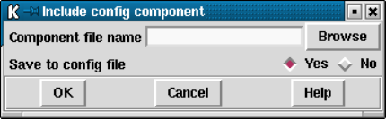
Chapter 4: Preparing readings for assembly using pregap4 371
set ns_lt(CH) {subst {$3 {[pP] 0} {[tT] 1} 0}}
The final line to add to the component file is set_name_scheme. This is a pregap4
command which tells it that you have finished defining the naming scheme. So the completed
component file is simply:
[naming_scheme]
set ns_name "Example naming scheme"
set ns_regexp {([^.]*)\.(..)(.).*}
set ns_lt(TN) {$1}
set ns_lt(PR) {subst {$2 {uf 1} {ur 2} {cf 3} {cr 4} 0}}
set ns_lt(CH) {subst {$3 {[pP] 0} {[tT] 1} 0}}
set_name_scheme
4.9 Pregap4 Components
A"Component"in pregap4 is a predefined section of a pregap4 configuration file. It will
generally be used to add on complex configurations which are not easily created using
the GUI. Currently there are only two predefined components, both of which specify a
naming scheme and so are easiest loaded using the Load Naming Convention function; see
Section 4.8 [Load Naming Convention], page 366.
The "Include Config Component"command in the File menu is used to load a compo-
nent. The "browse"button will bring up a file browser listing the default pregap4 compo-
nent directory, however components can be loaded from elsewhere if desired. The "Save to
config file"query determines whether the component is also copied to the current pregap4
configuration file to make this component the default for subsequent pregap4 runs.
Note that a component may have a configuration section listed within it. If this is present
the component will replace any configuration with the same section name.
4.10 Information Sources
The "Information Sources"menu contains options to obtain information from external
data sources, such as a text database. This does not include information encoded inside a
reading name convention. At present there are only two options - Simple Text Database
and Experiment File Line Types - although it is hoped that a link up to a robust relational
database could also be included here.
4.10.1 Simple Text Database
This option allows interrogation of a very simple format text database with one line per
sequence. The sequence identifier is the first word of a line with one or more additional
columns of information relating to specific information about that sequence. All columns
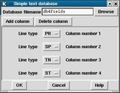
372 The Staden Package Manual
in the database file must have the same format and only one database file may be used at
any one time.
For example, we may wish to store the primer type, primer site, template name and the
number of strands on the template for each sequence. This corresponds to the PR,SP,TN
and ST Experiment File line types. We could then create a text database looking something
like the following:
# ID PR SP TN ST
xb54a3.s1 1 41 xb54a3 1
xb54b12.s1 1 41 xb54b12 2
xb54b12.r1 2 -24 xb54b12 2
xb54b12.r1L 2 -24 xb54b12 2
(The first line, starting with #is just a comment. Pregap4 does not use this; it is purely
so that we know which information is in which column.)
We can then direct pregap4 to extract the information from each of these four columns
for each reading being processed and to store this information in the Experiment File. This
information can then be utilised by the vector clipping and assembly modules.
The Simple Text Database interface consists of an entry box to specify the database file
name, add and delete buttons, and a line type selector for each column in the database
(excluding the reading name column). The above picture contains the database setup
for extracting the primer type, primer position, template name and number of strands as
described in the above example.
The "Add column"button adds a new line type selector at the bottom of the window.
This contains an option menu which can be clicked to choose a new Experiment File line
type and a label indicating the column number. The "Delete column"button removes the
bottom-most line type selector.
The "Ok"button will accept this configuration and will also write the details to the
current pregap4 configuration file. To disable a previously setup Simple Database Config-
uration press delete until there are no line types listed and then press Ok once more.
Chapter 4: Preparing readings for assembly using pregap4 373
The simple text database does not need to include a record for every reading and special
characters can be used to encode names so that readings produced in similar ways can be
grouped. For example, if the first 6 letters of the name encode a "plate"name, and all the
sequences on that plate have been sequenced using the same vector then we could create a
database file as follows.
# ID SF SC SP
6abz91* m13mp18.seq 6249 41/-24
6aca68* puc18.seq 248 40/-28
6aca69* puc18.seq 248 40/-28
6aca70* puc18.seq 248 40/-28
6acb21* m13mp18.seq 6249 41/-24
6acd49* puc18.seq 248 40/-28
6acd51* puc18.seq 248 40/-28
The sequence identifier (ID) is searched for using a pattern matching rule (as dictated by
the Tcl string match command). The pattern matching uses special characters as follows:
*Matches any sequence of characters in the reading identifier, including an empty
string.
?Matches any single character in the reading identifier.
[chars ]Matches any character in the set given by chars. If a sequence of the form r-v
appears in chars, then any character between rand v, inclusive, will match
(rstuv).
\xMatches the single character x. This provides a way of avoiding the special
interpretation of the characters *?[]\ in the reading identifier.
4.10.2 Experiment File Line Types
A list of Experiment File line types may be viewed and edited using this option (see
Section 11.3.1 [Experiment file format record types], page 552). A table of the Experi-
ment File line types is displayed along with their current values. A brief description of the
line type underneath the mouse cursor is displayed in the Information Line at the bottom
of the window. The table consists of three columns. The first is a label identifying the line
374 The Staden Package Manual
being edited. The second column is an option menu from which either Value or Command
may be selected. The third column is the current value or command.
Line type values will be used for every sequence. The Augment Experiment Files module
will add this line type to each Experiment File. This is suitable for specifying information
which is constant across an entire batch, such as insert size (SI) or operator (OP). The
Line type commands are executed each time the Augment Experiment Files module adds
that line to the Experiment File. Hence the commands are used for information which may
change from sequence to sequence. This table should be used for editing line type values,
but we do not recommend that you use it for editing commands (although it is useful to
know which commands have been set).
In the above example the PR, SP and ST commands were generated using the Simple
Text Database interface, whilst the SC and SF values come from the Sequencing Vector
Clip module parameters and the SI value was typed in by hand using this table.
The "OK (in memory)"and "OK (and save)"buttons will accept the currently displayed
values and commands. The "OK (in memory)"button will use these settings for the current
pregap4 runs. The "OK (and save)"button will use them for the current session and all
subsequent pregap4 sessions as it saves the information to the pregap4 configuration file.
Chapter 4: Preparing readings for assembly using pregap4 375
4.11 Adding and Removing Modules
This section details how to select newly written modules in Pregap4, or how to change the
order of existing modules.
It is for system managers and advanced users only.
Pregap4 has a default set of modules to use. Any module within this list may be enabled
or disabled. If you only need to screen a set of experiment files using blast or screen_
seq it may be tempting to use the Add/Remove Modules screen (from Modules menu) to
remove everything else. This is not necessary; just disable the unwanted modules. The real
purpose of Add/Remove Modules is to define the contents and order of the list that appears
in the Configure Modules screen. This may be required if you create your own modules, or
if you wish to never use certain modules. (Removing them from the list instead of simply
disabling them will speed up starting Pregap4.)
It is possible for a module to be used more than once. For example if you wish to use
blast to screen against several databases then this control may be used to add two "Blast
screen"items to the Configure Modules screen. Note though, that this is not applicable to
many modules. For example it is not possible to screen against multiple vectors by simply
using multiple Sequencing Vector Clip modules (rather this should be done using a file of
vector-primer information). No error checking is performed with the Add/Remove Modules
screen.
A pregap4 module is a specific piece of Tcl/Tk code that interfaces between pregap4 (by
providing a run procedure and an optional GUI for configuration) and an external program
to do the main work (as Tcl itself is generally too slow for anything except the most simple
376 The Staden Package Manual
of operations). The exact specification of a module can be found elsewhere (Section 4.13
[Writing New Modules], page 395).
All modules must end in ‘.p4m’. Pregap4 uses a module search path to search for files
with this suffix. The module search path is a space separated list. By default it will be set to
$STADENROOT/lib/pregap4/modules. It may be adjusted temporarily within the program,
or permanently by setting the MODULE PATH variable within your ‘.pregap4rc’ or run-
specific configuration files. For example:
set MODULE_PATH "$env(STADLIB)/pregap4/modules ."
The two lists shown in the dialogue represent the current modules to use (on the left)
and the total list of known modules. Modules may be added to the left (to use) list by
clicking any mouse button on the right hand list, dragging the mouse cursor to a location
within the left list, and then release the mouse button. To remove a module from the ’to
use’ list simply drag and drop from left to right. This mechanism also allows for changing
the order of modules within the left list.
The order of modules is vitally important and in the current version of Pregap4 the
validity of the order is not checked. Common sense should prevent most problems. For
instance it is pointless to assemble and enter into gap4 before vector clipping. The best
source of information on the possible orderings comes from the documentation for each
individual module. Some modules are directly incompatible with each other as they perform
the same or mutually exclusive tasks. For example it is only possible to use one of the
assembly methods.

Chapter 4: Preparing readings for assembly using pregap4 377
Once the modules have been selected press "Apply"to reinitialise Pregap4. If you wish
to make your newly selected list the default for subsequent Pregap4 runs use the "Save
Module List"command in the Modules menu.
4.12 Low Level Pregap4 Configuration
Most users will never need to configure pregap4 at this level. However by understanding the
methods that pregap4 uses you will see how to tailor Pregap4 in a more flexible manner.
The pregap4 configuration file consists of several sections. Each section is started with
"[section name]". The main pregap4 sections are [module_list],[global_variables],
and one section per module named [::module name].
4.12.1 Low Level Global Configuration
The [module_list] section contains definitions of the MODULE_PATH and MODULES variables.
The MODULE_PATH is a space delimited list of directory names in which to search for the
pregap4 modules (*.p4m files). The MODULES variable is the default list of modules to list
in the configuration window. The order of modules in this list determines the order that
they will be executed in. The default [module_list] section is as follows:
[module_list]
set MODULE_PATH "$env(STADLIB)/pregap4/modules ."
set MODULES {
phred
atqa
convert_trace
eba
compress_trace
init_exp
augment_exp
quality_clip
trace_clip
sequence_vector_clip
cross_match_svec
cloning_vector_clip
screen_vector
screen_seq
blast
interactive_clip
repeat_masker
tag_repeats
trace_diff
gap4_assemble
cap2_assemble
cap3_assemble
fakii_assemble
phrap_assemble
enter_assembly

378 The Staden Package Manual
email
}
The [global_variables] section defines the values for each of the Experiment File
line types. These are currently primarily used by the Augment Experiment Files module,
but may also be used by the vector clipping and mutation detection modules. The default
[global_variables] section is blank.
As an example, the following section defines the sequencing vector file for each sequence
to be m13mp18.vector with 6249 and 41 as the cut site and primer site. Each sequence
has a primer type of 1 (forward universal primer) and the template name is derived from
the sequence name by taking the segment of the string preceding the full stop.
[global_variables]
set SF m13mp18.vector
set SC 6249
set SP 41
set PR 1
proc TN_com {} { global lines; return [lindex [split $lines(ID) .] 0] }
4.12.2 Low Level Component Configuration
Pregap4 Components may each contain their own configuration section. Where several
components are mutually exclusive, such as components describing naming conventions, it
makes sense to give each component the same configuration section. This will ensure that
loading a new component will overwrite the old one. At present the only defined components
both create a [naming_scheme] section.
Components may redefine items which could appear in other configuration sections. In
this case the last definition of that setting will take priority. For instance if a component
defines the TN_com procedure and this is also defined in the [global_variables] section
then the component will only take priority if it is after the global section in the configuration
file.
Components may also be used to define parameters for modules. Once again the com-
ponents need to be listed after the module definitions being overridden. To define module
components in this way, use the module command. An example follows.
module tag_repeats {set repeat_file repeats.list}
4.12.3 Low Level Module Configuration
Each module has its own configuration section named after the module name. The config-
uration section will be "[::module filename prefix ]" where module filename prefix is the
filename of the module with the .p4m extension removed. For example, the init_exp.p4m
module has a configuration section of [::init_exp].
Each module is loaded into its own namespace, also named after the module in the
same manner. Thus in the above example the Initialise Experiment Files module uses the
namespace ::init_exp. This means that all local variables within that module will be
within that name space and will not clash with identical named variables in other modules.
When pregap4 reads the configuration file any configuration section starting in double colon
Chapter 4: Preparing readings for assembly using pregap4 379
is taken to be a name space and the following configuration is executed in that namespace.
So the following example enables the Initialise Experiment Files module, but disables the
Estimate Base Accuracies module.
[::init_exp]
set enabled 1
[::eba]
set enabled 0
In the following sections the variables, inputs and outputs of each module are listed.
Every module has an enabled local variable. This may be either 0for disabled or 1for
enabled. Disabled modules are still listed in the configuration panel, although they will not
be executed.
The tables in each section below list the module filename, the local variables and a very
brief description of their valid values, the files used or produced by this module, the possible
sequence specific errors that can be produced (which will be written to the failure file as the
reason for failure), and the format of any SEQ lines in the module report. Other information
may also be reported, but the SEQ lines are easily recognisable to facilitate easy parsing of
results.
4.12.3.1 General Configuration
Filename init.p4m
Local variables
use_sample_name 0/1
Files (none)
Errors init: Unreadable or nonexistent file
init: Unknown file type
Report (None)
4.12.3.2 ALF/ABI to SCF Conversion
Filename to_scf.p4m
Local variables
bit_size 8/16
Files Creates the SCF files if required.
380 The Staden Package Manual
Errors makeSCF: makeSCF error message
Report SEQ seqid: created from old seqid
4.12.3.3 Estimate Base Accuracies
Filename eba.p4m
Local variables
(none)
Files Modified SCF files with new confidence values.
Errors eba: eba error message
Report (none)
4.12.3.4 Phred
Filename phred.p4m
Local variables
(none)
Files fofn.tmp — temporary
fofn.scf_dir — temporary directory
phred.log — phred log file
Creates the SCF files if required.
Errors phred: phred error message
Report SEQ seqid: created from old seqid
SEQ seqid: re-base-called
4.12.3.5 ATQA
Filename atqa.p4m
Local variables
(none)

Chapter 4: Preparing readings for assembly using pregap4 381
Files Updates the confidence values within SCF files.
Errors ATQA: ATQA error message
Report SEQ seqid: confidences recalculated by ATQA.
4.12.3.6 Trace Format Conversion
Filename convert_trace.p4m
Local variables
output_format ZTR/CTF/ZTR
down_scale 0/1
down_scale_range integer
subtract_background 0/1
normalise 0/1
del_temp_files 0/1
Files Creates Trace files.
Errors convert_trace: convert trace error message
Report SEQ seqid: created from old seqid
4.12.3.7 Initialise Experiment Files
Filename init_exp.p4m
Local variables
(none)
Files Creates Experiment files.
Errors init_exp: init exp error message
Report SEQ seqid: created from old seqid
382 The Staden Package Manual
4.12.3.8 Augment Experiment Files
Filename augment_exp.p4m
Local variables
(none)
Global variables
All the XX and XX _com variables that define the two letter Experiment File line
types.
Files Updates Experiment files.
Errors (none)
Report SEQ seqid: added fields field names
4.12.3.9 Uncalled Base Clip
Filename uncalled_clip.p4m
Local variables
offset integer
min_extent integer
max_extent integer
right_win_length integer
right_num_uncalled integer
left_win_length integer
left_num_uncalled integer
Files Modifies Experiment files
Errors clip: clip error message
Report SEQ seqid: clipped using ’clip’
4.12.3.10 Quality Clip
Filename quality_clip.p4m
Chapter 4: Preparing readings for assembly using pregap4 383
Local variables
clip_mode sequence/confidence
window_length integer
conf_val integer
min_extent integer
max_extent integer
min_length integer
offset integer
right_win_length integer
right_num_uncalled integer
left_win_length integer
left_num_uncalled integer
Files Modifies Experiment files
Errors qclip: qclip error message qclip: Sequence too short (length=%d)
Report SEQ seqid: clipped using ’qclip’
4.12.3.11 Sequencing Vector Clip
Filename sequence_vector_clip.p4m
Local variables
min_5_match float
min_3_match float
def_5_pos integer
update_exp_file 0/1
use_vp_file 0/1
vp_file filename
vector_list string
vp_length integer
Global variables
SP
SP_com

384 The Staden Package Manual
SC
SC_com
SF
SF_com
Files fofn.tmp — temporary
fofn.svec_passed
fofn.svec_failed
Errors sequence_vector_clip: No SF, SC or SP information
sequence_vector_clip: vector clip error message
sequence_vector_clip: lost file
Report SEQ seqid: passed
SEQ seqid: failed (reason)
SEQ seqid: lost
4.12.3.12 Cross match
Filename cross_match_svec.p4m
Local variables
minmatch integer
minscore integer
vector_file filename
gap_size integer
tag_type string
Global variables
SF
SF_com
Files fofn.tmp — temporary
fofn.tmp.log — temporary
fofn.tmp.screen — temporary
Errors cross_match: cross match error message
cross_match: entirely vector

Chapter 4: Preparing readings for assembly using pregap4 385
Report SEQ seqid: masked start to end
SEQ seqid: no matches
4.12.3.13 Cloning Vector Clip
Filename cloning_vector_clip.p4m
Local variables
word_length integer
probability float
update_exp_file 0/1
Global variables
CF
CF_com
Files fofn.tmp — temporary
fofn.cvec_passed
fofn.cvec_failed
Errors sequence_vector_clip: No CF information
sequence_vector_clip: vector clip error message
sequence_vector_clip: lost file
Report SEQ seqid: checked
SEQ seqid: failed (reason)
SEQ seqid: lost
4.12.3.14 Old Cloning Vector Clip
Filename old_cloning_vector_clip.p4m
Local variables
word_length integer
num_diags integer
diag_score float
update_exp_file 0/1

386 The Staden Package Manual
Global variables
CF
CF_com
Files fofn.tmp — temporary
fofn.cvec_passed
fofn.cvec_failed
Errors sequence_vector_clip: No CF information
sequence_vector_clip: vector clip error message
sequence_vector_clip: lost file
Report SEQ seqid: checked
SEQ seqid: failed (reason)
SEQ seqid: lost
4.12.3.15 Screen for Unclipped Vector
Filename screen_vector.p4m
Local variables
min_match integer
update_exp_file 0/1
Global variables
SF
SF_com
Files fofn.tmp — temporary
fofn.screenvec_passed
fofn.screenvec_failed
Errors sequence_vector_clip: No CF information
sequence_vector_clip: vector clip error message
sequence_vector_clip: lost file
Report SEQ seqid: passed
SEQ seqid: failed (reason)
SEQ seqid: lost

Chapter 4: Preparing readings for assembly using pregap4 387
4.12.3.16 Screen Sequences
Filename screen_seq.p4m
Local variables
min_match integer
max_length integer
screen_mode single/fofn
screen_file filename
Files fofn.tmp — temporary
fofn.screenseq_passed
fofn.screenseq_failed
Errors screen_seq: screen seq error message
screen_seq: lost file
Report SEQ seqid: passed
SEQ seqid: failed (reason)
SEQ seqid: lost
4.12.3.17 Blast Screen
Filename blast.p4m
Local variables
database filename prefix
match_fraction float
e_value float
tag_type string
Files fofn.blast
Errors blast: match fraction fraction
Report SEQ seqid: total match length = match length (fract=match fraction)

388 The Staden Package Manual
4.12.3.18 Interactive Clipping
Filename interactive_clip.p4m
Local variables
(none)
Files May modify Experiment files.
Errors interactive_clip: manually rejected
Report SEQ seqid: accepted
SEQ seqid: rejected
4.12.3.19 Extract Sequence
Filename extract_seq.p4m
Local variables
(none)
Files User specified
Errors extract_seq: extract seq error message
Report (none)
4.12.3.20 Tag Repeats
Filename tag_repeats.p4m
Local variables
repeat_file filename
score float
tag_types string
Files fofn.tmp — temporary
fofn.tagrep_free
fofn.tagrep_repeat
Chapter 4: Preparing readings for assembly using pregap4 389
fofn.tagrep_log
Errors tag_repeats: lost file
Report SEQ seqid: no repeat found
SEQ seqid: repeat found (details)
4.12.3.21 RepeatMasker
Filename repeat_masker.p4m
Local variables
tag_type string
alu_only 0/1
simple_only 0/1
no_primate_rodent 0/1
rodent_only 0/1
no_low_complexity 0/1
library directory
cutoff integer
Files fofn.fasta.cat
fofn.fasta.masked
fofn.fasta.masked.log
fofn.fasta.out
fofn.fasta.out.xm
fofn.fasta.tbl
Errors (none)
Report SEQ seqid: Repeat repeat name
4.12.3.22 Mutation Detection
Filename trace_diff.p4m
Local variables
score float

390 The Staden Package Manual
start int
end int
band_width int
other_args string
update_exp_file 0/1
Global variables
WT
WT_com
Files May modify Experiment files.
Errors trace_diff: No wildtype information
trace_diff: trace diff error message
Report SEQ seqid: mutations at positions
SEQ seqid: no mutations
4.12.3.23 Gap4 Shotgun Assembly
Filename gap4_assemble.p4m
Local variables
database_name string
database_version character
create 0/1
min_match integer
max_pads integer
max_pmismatch float
enter_all 0/1
Files database name.database version
database name.database version.aux
Errors gap4_assemble: failed with code error code
Report SEQ seqid: failed (assembly error code)

Chapter 4: Preparing readings for assembly using pregap4 391
SEQ seqid: failed (filename contains spaces)
SEQ seqid: skipping - not in correct format
SEQ seqid: assembled
4.12.3.24 Cap2 Assembly
Filename cap2_assemble.p4m
Local variables
(none)
Files fofn.tmp — temporary
fofn.assembly/fofn
fofn.assembly/cap2_stdout
fofn.assembly/cap2_stderr
Errors cap2_s: cap2 s error message
cap2_s: rejected
Report SEQ seqid: rejected
SEQ seqid: assembled
SEQ seqid: failed (filename contains spaces)
4.12.3.25 Cap3 Assembly
Filename cap3_assemble.p4m
Local variables
generate_constraints 0/1
Files fofn.tmp — temporary
fofn.assembly/fofn
fofn.assembly/cap3_stdout
fofn.assembly/cap3_stderr
fofn.con
fofn.con.results
fofn.cap3_info
fofn.contigs.qual

392 The Staden Package Manual
Errors cap3_s: cap3 s error message
cap3_s: rejected
Report SEQ seqid: rejected
SEQ seqid: assembled
SEQ seqid: failed (filename contains spaces)
4.12.3.26 FakII Assembly
Filename fakii_assemble.p4m
Local variables
graph_e_limit float
graph_o_threshold float
graph_d_limit float
assem_number integer
assem_e_rate float
assem_o_threshold float
assem_d_threshold float
generate_constraints 0/1
Files fofn.tmp — temporary
fofn.assembly/fofn
fofn.assembly/graph_stderr
fofn.assembly/graph.dat
fofn.assembly/constraints_stderr
fofn.assembly/constraints.ascii
fofn.assembly/constraints.dat
fofn.assembly/assemble_stderr
fofn.assembly/assemble.dat
fofn.assembly/write_exp_file_stdout
fofn.assembly/write_exp_file_stderr
Errors fakii: rejected
Report SEQ seqid: assembled
SEQ seqid: rejected
Chapter 4: Preparing readings for assembly using pregap4 393
4.12.3.27 Phrap Assembly
Filename phrap_assemble.p4m
Local variables
minmatch integer
minscore integer
other_args string
Files fofn.tmp — temporary
fofn.assembly/fofn
fofn.assembly/phrap_stdout
fofn.assembly/phrap_stderr
fofn.contigs
fofn.contigs.qual
fofn.singlets
fofn.phrap_log
Errors phrap: singlet
phrap: failed
Report SEQ seqid: assembled
SEQ seqid: singlet
SEQ seqid: failed
4.12.3.28 Enter Assembly into Gap4
Filename enter_assembly.p4m
Local variables
database_name string
database_version character
create 0/1
quality_clip 0/1
quality integer
difference_clip 0/1
Files fofn.assembly/fofn — reads

394 The Staden Package Manual
fofn.assembly/* — reads
database name.database version
database name.database version.aux
Errors (none)
Report SEQ seqid: failed
4.12.3.29 Email
Filename email.p4m
Local variables
email_program string
email_args string
email_address string
Files (none)
Errors (none)
Report (none)
4.12.3.30 Shutdown
Filename shutdown.p4m
Local variables
(none)
Files fofn.passed
fofn.failed
fofn.log
fofn.report
Errors (none)
Report This module collates the reports from all other modules.
Chapter 4: Preparing readings for assembly using pregap4 395
4.13 Writing New Modules
4.13.1 An Overview of a Module
A pregap4 module is a single file containing a series of functions with predefined interfaces.
Pregap4 uses these functions to communicate with module.
This section is for system managers and programmers only.
The module itself is written using the Tcl/Tk language. A definition of this language is
outside the scope of this manual, however several books exist on the subject. Each modules
executes inside a Tcl "namespace". This means that modules may make use of global
variables and global function names without fear of clashing with other modules. Indeed
the use of specific function names and global variables is of considerable importance for
designing a new module.
4.13.2 Functions
The basic structure of a module is that it has a series of known functions which pregap4
expects to use. Some of these functions are mandatory, whilst others will only be called by
pregap4 if they have been defined.
name Mandatory.
Arguments: none
Returns: The textual name of the module.
This function is used to query a human readable name for the module (eg
"ALF/ABI to SCF Conversion"). This name is used in the module list at the
left side of the pregap4 window.
init Optional.
Arguments: None
Returns: None
This sets up any data structures needed for this module. It can be used for
providing defaults for global variables when they are not known (eg they have
no settings in the system or user pregap4rc files) and for setting up any other
data structures required.
run Optional.
Arguments: A Tcl list of files to process
Returns: A new Tcl list of files for subsequent processing.
This is the main work horse. It is optional, however in all but the most esoteric
cases, it will be needed.
The single argument is a Tcl list of sequence names. These are either filenames
on disk or identifiers used for fetching data from a database. The module should
loop through the sequences which it can process (which may not be all of them,
depending on the known information and file types).

396 The Staden Package Manual
When finished, it needs to return a new list of files. If a file has been rejected
by this module (eg it is completely sequencing vector) then this sequence name
should be omitted from the returned list. However do make sure that all failed
files have an error string attached to them by setting the file error(seq name)
array element.
shutdown Optional.
Arguments: A Tcl list of files to process
Returns: A new Tcl list of files for subsequent processing.
Deallocates any data structures that have been setup during the init or run
stages. Most modules will not need this function. As with the run module, the
returned value should be the list of passed files, which is generally the same as
the list passed into this function.
A special module, which is always included by pregap4, is the shutdown.p4m
module. This is always the last module to have shutdown called. It produces
the reports for pregap4 and does some general house keeping.
create dialogue
Optional.
Arguments: A tk pathname
Returns: None
This create a dialogue controlling the parameters for this module. The tk
pathname passed into this function should be the root for all components of
this dialogue. (Note though that this is not a toplevel window, but a subwindow
of the main pregap4 dialogue.)
check params
Optional.
Arguments: None
Returns: A variable name or a blank string.
This checks that this module has valid answers to all of its mandatory questions.
If this is the case a blank string is returned, otherwise the first variable name
which needs a value is returned.
process dialogue
Optional.
Arguments: A tk pathname
Returns: 0 for failure, 1 for success
This is executed in all modules before the run functions are executed. It’s
purpose is to extract any information from user editable entries or checkboxes

Chapter 4: Preparing readings for assembly using pregap4 397
ready for the run function to utilise. It may also be used to check that the data
entered is valid.
The return code is used to indicate whether this module has sufficient data to
execute. If 0 is returned pregap4 will beep and make sure that the dialogue
’tab’ for this module is displayed. Further processing then stops until the ’Run’
button is pressed again.
For instance if a module needs to know the sequencing vector to screen against,
then this should check if the value has been entered or can be obtained via a
command. If so it returns 1.
configure dialogue path mode
Optional.
Arguments: A tk pathname, the configure mode
Returns: None
If this function is present pregap4 will add a button to the top of the mod-
ule dialogue inviting the user to save the parameters for this module to the
configuration file.
In early releases of pregap4 (2000.0 and before) a "Select parameters to save"
button was also available. To maintain compatibility with older modules the
"mode"parameter is still used. If you wish the module to be backwards com-
patible with old pregap4 releases then this needs to be checked to make sure
that it contains "save all". If it does not then no action should be taken. In the
2001 release and newer the "mode"parameter will always contain "save all"so
no check is required.
To save the dialogue information this function should use the pregap4 mod save
and glob save functions.
4.13.3 Module Variables
mandatory
The existence of this variable (set to anything) states that this module cannot
be disabled.
hidden
The existence of this variable states that its name shall not appear in the module
list (although it will still be used).
report The contents of this variable are displayed at the end of the pregap run by the
shutdown.p4m module.
4.13.4 Global Variables
Several global variables exist which may need to be updated within the modules. For
successful operation it is required to update these when applicable.

398 The Staden Package Manual
file type This is a Tcl array indexed by file name. It is initialised by the General Con-
figuration module to be one of ABI,ALF,EXP,PLN,SCF or UNK.
file error This is a global array indexed by the current file name. If a file has been rejected
by a module (ie not returned from the run function) then the appropriate array
element must be filled with a reason. Typically the format for this reason
will start with the module name followed by a colon. For example "makeSCF:
unknown file type".
file id This is a global array, indexed by filenames, containing the sequence identifiers
(which are often different to the sequence filenames). It is initialised by the
General Configuration module.
file orig name
This is a global array holding any original filename for each currently processed
file. It is initialised by the General Configuration module such that each file
points to its own filename.
When creating and returning a new file (such as when switching from SCF files to
Experiment Files in the Initialise Experiment Files module) it is required that the arrays
are all updated correctly. This involves creating new array elements for each of the above
four arrays. The file type array element, indexed by a new name should contain the new
file type (eg set file_type(seq10.exp) EXP). The file error array element should be set
to a blank string. The file id should inherit the sequence identifier from the original file
(eg set file_id(seq10.exp) $file_id(seq10.scf)). The file orig name array element
should point to the old filename (not the original filename pointed to by the old filename).
In this way file orig name could be considered as a list of the intermediate files generated
for each final sequence file.
4.13.5 Builtin Functions
Apologies, but this section of documentation is still unfinished.
The full definition of these functions may be found in the Tcl code for Pregap4 itself.
It is recommended that you use the Unix grep utility to find the definitions and example
uses.
4.13.6 An Example Module
The best examples are the existing modules. Try looking at the Compress Trace Files mod-
ule as an example. This may be found in ‘$STADENROOT/lib/pregap4/modules/compress_trace.p4m’.
Chapter 5: Marking poor quality and vector segments of readings 399
5 Marking poor quality and vector segments of
readings
Introduction to read clipping
For most assembly routines to work well it is necessary to present them with data of rea-
sonable quality. Generally sequences produced by machines suffer from having poor quality
data at one or both ends and so methods are needed to define where the data is too poor
to use. Some base callers include an increased number of "N"symbols in the sequence
in doubtful regions and so these can be searched for. In the ideal situation base accuracy
estimates or confidence values for each base call will be available, and then these can be
searched to find where the average confidence value becomes too low for reliable assembly.
The program qclip (see Section 12.19 [qclip], page 597) performs both type of analysis.

Chapter 6: Screening Against Vector Sequences 401
6 Screening Against Vector Sequences
For most assembly engines to work well it is necessary to present them with data of good
quality and which contains only the target sequence. One pre-assembly task is to locate
and mark all segments of readings which contain vectors used in their production. In our
package this task is performed by vector clip which compares batches of readings against
vector sequences. Sequence readings are stored in experiment file format (see Section 11.3
[Experiment File], page 552) and, for the majority of projects each experiment file should
contain the data required by vector clip: the file names of the vectors to screen against,
and, for the sequencing vector, the position of the cloning and primer sites. See Section 6.6
[Vector Primer files], page 407 for an alternative and simpler method of defining vector
data for vector clip. The program pregap4 (see Section 4.2 [Pregap4], page 326), contains
modules for creating experiment files from trace files, and for adding data about the vectors
used. When vector clip runs it adds records to the reading’s experiment file to denote the
start and end of any segments which are found to match the vectors.
For conventional sequencing projects there are two types of vector for which readings
will need to be screened: the sequencing vector, and, for cases where, say, whole cosmids or
BACs have been shotgunned, the cloning vector. These two screening tasks are different.
When screening for the sequencing vector we may expect to find data to exclude, both from
the primer region and, when the insert is short, from the other side of the cloning site.
It is also a wise precaution to check for rearrangements of the sequencing vector. When
screening out cosmid vector we may find that either the 5’ end, or the 3’ end, or the whole of
the sequence is vector. Also for the cloning vector search we need to compare both strands
of the sequence.
In order to filter out readings that contain the sequences of contaminant DNA such as
E. coli, a separate program screen seq should be used (see Chapter 7 [Screening for known
possible contaminant sequences], page 413)
A further type of search is required for a new method that is being developed at MRC
HGMP, Hinxton, UK. This new method (M. Starkey, personal communication) is an ap-
plication of a technology described as "molecular indexing"Unrau, P. and Deugau, K.V.
(1994) Non-cloning amplification of specific DNA fragments from whole genomic DNA di-
gests using DNA indexers. Gene 145, 163-169. It produces sequences with a primer at their
3’ ends which need to be found and removed.
Some groups are using transposons to produce random start points for sequencing reac-
tions, and vector clip contains an experimental search procedure for dealing with the data
generated by such methods.
Vector clip is usually run as part of the pregap4 process (see Section 4.2 [Pregap4],
page 326) and will usually be called three times: the first to locate and mark the sequencing
vector; next to check for vector rearrangements; and finally to locate and mark cosmid vector
segments.
Vector clip operates on batches of readings using files of file names: one input file and
two output files - one for the names of the readings that pass and one for those that fail.
The program also modifies the reading files.

402 The Staden Package Manual
In earlier versions of vector clip all the information needed about the vector (i.e. its
name, location on disk, the cloning and primer sites used) for each reading was expected
to be stored in the reading’s experiment file (See Section 11.3 [Experiment File], page 552.)
but, as is explained in the next paragraph, the newest version employs an alternative method
for providing data about sequencing vectors. For notes on defining the cloning and primer
sites, see Section 6.8 [Defining the Positions of Cloning and Primer Sites for Vector Clip],
page 408.
The 1999.0 release of the package contained an experimental new method of providing
vector clip with data about the vectors to search for. Using feedback from the trial period
we have simplified the method and improved the algorithm.
The new method uses files containing, not the complete vector sequences, but the seg-
ments of sequence between the primers and the cloning site. These files are termed "vec-
tor primer"files see Section 6.6 [Vector Primer files], page 407, and the vector primer mode
of vector clip uses the data in these files to search for the vectors.
The vector primer file can contain the data for up to (at present) 100 vector and primer
combinations, although it would not be efficient to compare each reading against an un-
necessarily large number of records. When vector clip finds a match to one of the vectors
defined in the vector primer file it can not only mark the matching segment in the reading,
but also adds the name of the file containing the vector sequence, and the primer type to
the readings experiment file. The vector file name can then be used by vector clip in its
search for vector rearrangements, and the primer type can be used by gap4 in its analysis
of read pairs (Note, however, that for read pair analysis, gap4 still needs to know which
readings came from the same template, so that data must be added to the Experiment file
in some other way).
A big advantage of the vector primer file method, is that it simplifies the task of providing
vector clip with data. In addition, the task of creating the vector primer files is simplified in
that the -V option in vector clip removes the necessity for the records in the vector primer
file to contain precisely the sequence between the primer and the cloning site Section 6.7
[Vector Primer File Notes], page 408.
Vector primer files are also used by the search for transposon data.
If setting up these programs seems a little daunting, it is important to realise that the
majority users need not concern themselves with the details of vector clip and the creation
of experiment files for their readings; or if they do, these configuration operations are only
performed once per project, and are made relatively easy by the use of pregap4.
6.1 Algorithms
For locating sequencing vector the program uses a dynamic programming algorithm and
two percentage matches as cutoffs - one for the 5’ end and another for the 3’ end. Both
searches include the poor quality data at the ends of the readings. This mode writes the
SL and SR records in experiment files.
If the users selects the vector primer file mode of vector clip the program searches the 5’
end of each reading for all of the forward and reverse sequence segments in the primer vector
file and notes the one which matches best. If this one is above the user defined threshold the

Chapter 6: Screening Against Vector Sequences 403
5’ clip point will be set and the experiment file will be modified accordingly. The program
then compares the rest of the reading with all of the segments in the vector primer file to find
the one which matches best. Again if the user defined threshold is reached the experiment
file will be modified accordingly. If the best 5’ and 3’ matches come from different records
in the vector primer file a warning message is printed. If a 5’ match is found it will be used
to determine the file name of the vector sequence and the primer type. If only a 3’ match
is found it will be used to determine these items. If no match is found no PR record is
written. This mode writes the SL, SR SF and PR records in experiment files. If the vector
file name is missing from the vector primer file record, the SF record is not written.
For locating cloning vector two algorithms are available, both of which use hashing. The
original method needs a "Word length"(word length), the "Number of diagonals to com-
bine"(num diags) and a "Cutoff score"(diagonal score). The word length is the minimum
number of consecutive bases that will count as a match. The algorithm treats the problem
like a dot matrix comparison. First it finds all matches of length word length; then it locates
the diagonal with the highest normalised score. Then it adds the scores for the adjacent
diagonals (num diags). If the combined score is at least "diagonal score"the experiment
file is updated to indicate the location of the vector sequence. The score represents the
proportion of a diagonal that contains matching words, and the maximum score for any
diagonal is 1.0. This mode writes the CS records in experiment files. If the whole reading
is cloning vector this mode writes a PS record containing "all cloning vector",
A newer method also hashes using "word length"consecutive bases and accumulates the
hits for each diagonal, but instead of using a score cutoff, it decides if there is a match using
a probability threshold "P"supplied by the user. For each length of diagonal vector clip
calculates "E"the score that would be expected for probability "P", and then compares it
with the observed score "O". If for any diagonal O>E a match is declared and expressed as
100(O-E)/E. This new method is an attempt to overcome the problem that even though the
scores on diagonals are normalised to lie in the range 0.0 to 1.0 the scores are still a function
of the diagonal length. The probability P hence allows vector clip to use a different cutoff
score for each length of diagonal. Tests have shown that the probability based algorithm
is very much more reliable than the older one. By default the program still uses the old
algorithm, the probability based one being switched on by the user specifying a probability
cutoff (option -P). It is strongly recommended that the probability based method is used
and for our data we have found that a probability of 0.0000000000001 or 1.0e-13 gives good
results. This mode writes the CS records in experiment files. If the whole reading is cloning
vector this mode writes a PS record containing "all cloning vector".
The search for "vector rearrangements"uses a simple algorithm which looks only for
a match of length "minimum match". All readings that contain a string of characters of
at least this length that match a segment of the vector sequence exactly will be classed as
"vector rearrangements"and their names will not be written to the file of passed file names.
This mode writes a PS record containing "vector rearrangement"in experiment files if a
match is found. Note that if a reading’s Experiment file does not contain an SF (i.e. name
of sequencing vector file) the vector rearrangements search does not fail the reading: its
name goes into the pass file.
The search for transposon generated data is somewhat complicated, as is explained
below.

404 The Staden Package Manual
The transposon ends must be stored in a vector primer file. The vector sequence file
should be named in the SF record. Numerous scores are required.
First get the transposon end sequences from the vector primer file. Then get the vector
sequence and rotate it around the cloning site. Next use dynamic programming to search
with both of the transposon end sequences and note the highest score. If above score L
reset SL. Now use hashing to search the 20 bases after SL for a match to any part of the
vector, on both strands. If the best match is above score l, use dynamic programming to try
to align from the match point to the cloning site. If the alignment score is >= score R reset
SL. If the previous two steps fail to find a match to vector we assume that the transposon
inserted into the target DNA and not the vector. The reading could hence run into vector
at its 3’ end so we use dynamic programming to search from SL onwards, for the sequences
either side of the cloning site (we do not know the orientation of the transposon (and hence
the read) relative to the vector). If we find a match >= score R reset SR.
6.2 Options
Usage: vector_clip [options] file_of_filenames
Where options are:
[-s mark sequencing vector] [-c mark cloning vector]
[-h hgmp primer] [-r vector rearrangements]
[-w word_length (4)] [-n num_diags (7)]
[-d diagonal score (0.35)] [-l minimum match (20)]
[-L minimum % 5’ match (60)] [-R minimum % 3’ match (80)]
[-m default 5’ position] [-t test only]
[-M Max vector length (100000)] [-P max Probability]
[-v vector_primer filename] [-i vector_primer filename]
[-V vector_primer length]
[-p passed fofn] [-f failed fofn]
Options:
-s Mark sequencing vector. Searches for 5’ primer, 3’ running into vector.
-c Mark cloning vector. Searches both strands for cloning vector.
-h Hgmp primer. Searches 3’ end for a primer.
-i vector_primer filename
Mark transposon data.
-r Vector rearrangements. Searches for sequencing vector rearrangements.
-t Test only. Does not change the experiment files, displays hits.
6.3 Parameters (defaults in brackets)
-L minimum percentage match 5’ end (60)
sequencing vector searches and transposon search
-R minimum percentage match 3’ end (80)
sequencing vector searches and transposon search

Chapter 6: Screening Against Vector Sequences 405
-m minimum 5’ position
allows a minimum 5’ end cutoff to be set if a sufficiently good match is not
found (i.e. it is really a default 5’ cutoff position). If a value of -1 is used
the program will set the cutoff to be the distance between the primer and the
cloning site.
-v vector-primer-pair filename
sequencing vector search using vector-primer-pair file
-V vector primer length
the length of the sequence stored in the vector primer file to use for the 5’
search
-w word length (4)
cloning vector search hash length
-P probability
cloning vector search, (a score less likely than P is a match)
-n num diags (7)
cloning vector search, old score based algorithm: number of diagonals to com-
bine
-d diagonal score (0.35)
cloning vector search, old score based algorithm
-l minimum match (20)
sequencing vector rearrangements and transposon search minimum match
length
-M maximum vector length (100000)
all algorithms, reset for vectors >100000 bases
-p passed fofn
file of file names for passed files
-f failed fofn
file of file names for failed files
input fofn ...
input file of file names
6.4 Error codes
The following errors can occur.
1. Error: could not open experiment file
2. Error: no sequence in experiment file
3. Error: sequence too short
4. Error: missing vector file name
5. Error: missing cloning site
6. Error: missing primer site
7. Error: could not open vector file

406 The Staden Package Manual
8. Error: could not write to experiment file
9. Error: could not read vector file
10. Error: missing primer sequence
11. Error: hashing problem
12. Error: alignment problem
13. Error: invalid cloning site
14. Warning: sequence now too short (no message)
15. Warning: sequence entirely cloning vector (no message)
16. Warning: possible vector rearrangement (no message)
17. Warning: error parsing vector primer file
18. Warning: primer pair mismatch!
19. Aborting: more than X entries in vector primer file
6.5 Examples
Screen for sequencing vector using 5’ cutoff of 70%, a 3’ cutoff of 90% and default 5’ primer
position of 30. The batch of files to process are named in files.in, the names of the passed
files are written to files.pass and the names of those that fail to files.fail.
vector_clip -s -L70 -R90 -m30 -pfiles.pass -f files.fail files.in
Screen for sequencing vector using 5’ cutoff of 60%, a 3’ cutoff of 80% and default 5’
primer position of 30. The batch of files to process are named in files.in, the names of the
passed files are written to files.pass and the names of those that fail to files.fail. This shows
that the default search is for sequencing vector.
vector_clip -m30 -pfiles.pass -f files.fail files.in
Screen for sequencing vector using 5’ cutoff of 60%, a 3’ cutoff of 80% and a vector-
primer-pair file called vpfile. Only the 20 bases closest to the cloning site will be used for
the 5’ search. The batch of files to process are named in files.in, the names of the passed
files are written to files.pass and the names of those that fail to files.fail.
vector_clip -v vpfile -V20 -pfiles.pass -f files.fail files.in
Screen transposon data using 5’ cutoff of 80%, a 3’ cutoff of 85%, a match length of
10 and a vector-primer-pair file called vector primer file. The batch of files to process are
named in files.in, the names of the passed files are written to files.pass and the names of
those that fail to files.fail.
vector_clip -i vector_primer_file -L 80 -R 85 -l 10 -pfiles.pass \
-f files.fail files.in
Screen for cloning vector using the old algorithm with a word length of 4, summing 7
diagonals and diagonal cutoff score of 0.4. The batch of files to process are named in files.in,
the names of the passed files are written to files.pass and the names of those that fail to
files.fail.
vector_clip -c -w4 -n7 -d0.4 -pfiles.pass -f files.fail files.in

Chapter 6: Screening Against Vector Sequences 407
Screen for cloning vector using the probability based algorithm with a word length of
4 and probability cutoff of 1.0e-13. The batch of files to process are named in files.in, the
names of the passed files are written to files.pass and the names of those that fail to files.fail.
vector_clip -c -P 1.0e-13 -pfiles.pass -f files.fail files.in
Screen for 3’ primer using a cutoff of 75%. The batch of files to process are named in
files.in, the names of the passed files are written to files.pass and the names of those that
fail to files.fail.
vector_clip -h -R75 -pfiles.pass -f files.fail files.in
Screen for sequencing vector rearrangements using a cutoff of 20 bases. The batch of
files to process are named in files.in, the names of the passed files are written to files.pass
and the names of those that fail to files.fail.
vector_clip -r -l20 -pfiles.pass -f files.fail files.in
6.6 Vector Primer file format
The vector primer files store the data for each vector/primer pair combination as a single
record (line) and up to 100 records can be contained in a file. The items on each line
must be separated by spaces or tabs (only the file name can contain spaces) and a newline
character ends the record. It is important to realise that the format has been simplified
since the first version of the method appeared in release 1999.0 and any files created for the
1999.0 release will need to be edited!
The items in a record are:
name seq r seq f file name
name is an arbitrary record name. seq r is the sequence between the reverse primer and
the cloning site. seq f is the sequence between the forward primer and the cloning site.
file name is the name of the file containing the complete vector sequence.
An example file containing two entries (for m13mp18, and a vector called f1) is shown
below. "\" symbols have been used to denote wrapped lines and so it can be seen that the
first record is shown on two lines and the next on 1.
m13mp18 attacgaattcgagctcggtaccc ggggatcctctagagtcgacctgcaggcatgcaagcttggc \
/pubseq/tables/vectors/m13mp18.seq
f1 CCGGGAATTCGCGGCCGCGTCGACT CTAGACTCGAGTTATGCATGCA af_clones_vec
Note that the segments of sequence can be longer (or shorter) than the sequences between
the primer and the cloning site. The -V option of vector clip allows the user to specifiy that
a fixed number of bases closest to the cloning site be used for any particular run, and so the
same record in the vector primer file could be used for several primers as long as the cloning
site was the same. If it is necessary to get the sequence segments precisely defined refer to
the figure below. This contains an annotated section of the m13mp18 vector around the
SmaI site, to see how it corresponds to the first record in the vector primer file. The primers
shown are the 16mer reverse(-21) and the 17mer forward(-20), and the vector primer record
is the sequence between the primers with a space at the cloning site,

408 The Staden Package Manual
followed by a file name.
SmaI
++++++++10++
---20--------10---------123456789012
r(-21) 432109876543210987654321
aacagctatgaccatg
acacaggaaacagctatgaccatgattacgaattcgagctcggtacccggggatcctcta
6210 6220 6230 6240 6250 6260
++++++20++++++++30++++++++40+
34567890123456789012345678901 f(-20)
tgaccggcagcaaaatg
gagtcgacctgcaggcatgcaagcttggcactggccgtcgttttacaacgtcgtgactgg
6270 6280 6290 6300 6310 6320
6.7 Vector Primer File Notes
There are several consequences of using vector primer files to specify the sequencing vector
details. Please read a description of the vector primer file algorithm in the algorithms
section Section 6.1 [Vector clip algorithms], page 402.
Firstly, to get the vector segments of readings marked correctly it is not necessary to
include the relevant data in their experiment files.
Secondly, because vector clip compares all the primer-vector pairs in the primer vector
file it would be inefficient to include very large numbers of records in these files. Instead it
would be better to have a master vector primer file which contained all the combinations
used in the lab and then to copy the relevant ones to project specific files.
Thirdly, even though vector clip can write the PR record (primer type) into the exper-
iment file if it finds a match, gap4 still needs the template name data in order to do read
pair analysis.
Finally note that the -V option for vector clip means that the segments of sequence in
the vector primer file need not be made exactly the right length when the files are created:
it matters only that the cloning site is correctly specified and that there is sufficient length
of sequence on either side. For example, vector primer files could be created in which all
records included 40 bases from either side of the cloning sites. The -V option allows the
alignment to be limited to the segment of sequence closest to the cloning site. For example,
-V 20 specifies that at most 20 bases around the cloning site are used.
6.8 Defining Cloning and Primer Sites for Vector Clip
Vector sequences should be stored in simple text files with up to 80 characters of data
per line. Sequencing vectors are those vectors such as m13 used to produce templates for
sequencing. All other vectors, such as cosmid vectors, that are used to purify and grow the
DNA prior to it being subcloned into sequencing vectors are termed "cloning vectors". It is
important that the files containing cloning vector sequences which are used by vector clip

Chapter 6: Screening Against Vector Sequences 409
are arranged so that the cloning site follows the last base in the file. For example (where X
is the cloning site):
start of file
acatacatacatatata
acatagatagatacaga
.
.
.
cagatataX
end of file
Cloning Vector File Base Ordering
In order for vector clip to search readings for segments of sequencing vectors it either
needs to use a vector primer file or it needs to know the positions of the cloning site and
primers. If not using a vector primer file, each reading’s experiment file should contain SC
and SP records, and also a primer type record (PR). The following section explains the
numbering system used with an example for m13mp18, and then describes how to use spin
(see Section 9.2 [Introduction], page 429) to work out the values for other vector, cloning
site, and primer combinations.
The position of the cloning site depends on the ordering of the bases in the particular
vector sequence file being used. That is, as the sequences are circular, the file may be
arranged to start at any base and still give the same circular sequence. Vector Clip must
be told the correct position of the cloning site, then, relative to that, the position of the
first base that will be included in the reading. i.e. the relative position of the first base 3’
of the primer.
Below we use EMBL entry M13MP18 as an example. The figure includes a double
stranded listing of 120 characters of m13mp18 around the SmaI site at 6249, and some of
the restriction sites. Between the restriction sites and the sequence we have added lines
to explain the numbering used by vector clip. The numbers below the row of "+" symbols
show positive positions (to the right of the SmaI cloning site), and the numbers below the
"-"symbols show negative positions (to the left of the cloning site). Below these lines we
show the sequences of the 16mer reverse primer "r(-21)"which is at relative position -24,
and the 17mer forward primer "f(-20)"which is at relative position 41.
The positions of SmaI site and forward and reverse primers for M13MP18
EcoRI
. TaqI
. . SacI
. . . XmaI
. . . .HpaII
. . . ..AsuC2I
. . . ..SmaI
. . . ... BamHI
. . . ... MboI

410 The Staden Package Manual
. . . ... Sau3AI
. . . ... XhoII
. . . ... . PspN4I
. . . ... . . XbaI
++++++++10++
---20--------10---------123456789012
r(-21) 432109876543210987654321
aacagctatgaccatg
acacaggaaacagctatgaccatgattacgaattcgagctcggtacccggggatcctcta
6210 6220 6230 6240 6250 6260
tgtgtcctttgtcgatactggtactaatgcttaagctcgagccatgggcccctaggagat
HinfI
. SalI
. .AccI
. .. SdaI
. .. . BspMI
. .. . . BbuI CfrI
. .. . . Hsp92II . BshI
. .. . . PaeI . HaeIII
. .. . . SphI . PalI
. .. . . . Cac8I . .Bse1I MaeII
. .. . . . HindIII . .BseNI . TaiI
. .. . . . . AluI . .BsrI . TscI
. .. . . . . . MwoI . .TspRI . .Tsp45I
++++++20++++++++30++++++++40+
34567890123456789012345678901 f(-20)
tgaccggcagcaaaatg
gagtcgacctgcaggcatgcaagcttggcactggccgtcgttttacaacgtcgtgactgg
6270 6280 6290 6300 6310 6320
ctcagctggacgtccgtacgttcgaaccgtgaccggcagcaaaatgttgcagcactgacc
6.9 Finding the Cloning and Primer Sites
The problem addressed here is how to work out the positions of the cloning and primer
sites for vector clip. The numbers can be worked out from listings of the vector sequences
but once you know how, it is far easier to use the restriction enzyme search in spin (see
Section 9.2 [Introduction], page 429) to do it, and that is what we explain here. Some
familiarity with spin will help. To use the restriction enzyme search in spin it is necessary to
have created a file containing the definitions of the sequences to search for (see Section 11.4
[Restriction enzyme files], page 566) These files give each enzyme a name and a set of strings
(with cut positions marked by "’"). The name is terminated by "/"and each string by "/".
An extra "/"terminates all the data for each enzyme. For example "fred/aaa’ttt/gatc’a//"
defines enzyme fred to have two recognition sequences aaattt and gatca with cut positions
denoted by "’".
Chapter 6: Screening Against Vector Sequences 411
For our current purpose we treat the primer sequences as restriction enzymes which each
have a single recognition sequence; making sure that the sequence is the sense of the primer
that is present in the sequence being searched, and that the "cut positions"define the 3’
ends (i.e. the end where the new sequence will start). Again if we use the m13mp18 vector,
its SmaI cloning site and the 17mer (-20) forward and 16mer (-21) reverse primers as an
example. The reverse primer has the sequence 5’aacagctatgaccatg3’ and the forward one is
5’gtaaaacgacggccagt3’, and the SmaI site is ccc’ggg where "’"defines the cutsite.
The restriction enzyme file should contain the following:
f(-20)/’actggccgtcgttttac//
SmaI/CCC’GGG//
r(-21)/aacagctatgaccatg’//
This names the 17mer forward primer as f(-20) and defines its recognition sequence as
’actggccgtcgttttac. Note that this is the complement of the primer (which is what appears
in the sequence being searched) and that the "cut position"is defined by the "’"symbol.
SmaI is named and defined in the next record by SmaI/CCC’GGG//. The 16mer reverse
primer is named r(-21) and defined by r(-21)/aacagctatgaccatg’//, and this time we search
for the sequence of the primer and the "cut position"is again at the 3’ end.
Having started spin and read in the m13mp18 sequence select "Restriction enzyme
map"from the "search"menu. A dialogue will appear requesting "Select input source"
and with "6 cutter file"as the default. Select "personal"and give the name of the
file for m13mp18 (a file containing the definitions shown above should be found in
$STADTABL/m13mp18 primers). The names "f(-20), SmaI and r(-21)"should appear in
the selection box in the dialogue. Select all three and the graphical result should appear.
Magnify the plot by hitting the "+50%"button and then scroll to the region around 6249
which should look as shown below.
This plot and the functionality of spin are sufficient to work out the numbers for vec-
tor clip, but there is also a way of getting the values printed in the text output window
(this is described later). To obtain the numbers from the plot first touch the line showing
the SmaI site, its position (6249) will be written in the information line at the bottom of
the plot. This is the position of the cloning site and hence is the value for the SC record
in the experiment file. Now click on the line for the SmaI site and the information line will
display "Select another cut"; click on the line for the forward primer; the distance between
412 The Staden Package Manual
the SmaI site and the forward primer (41) will be displayed in the information line, and
in the top right hand box of the plot. Being to the right of the cloning site, this gives a
positive value for the experiment file SP record. Clicking on the SmaI site, and then the
line for the reverse primer, gives 24 which, being to the left, is a negative value for the SP
record.
To get the numbers displayed in the text output window, select the "Output ordered
on position"item from the "Results"menu of the "Restriction enzyme map"plot. For the
example given here they will appear as shown below.
Finally it is also possible to work out the numbering by using the restriction enzyme
search in the spin "sequence display"which can be selected from the "View"menu. It will
appear as shown below.

Chapter 7: Screening Readings for Contaminant Sequences 413
7 Screening Readings for Contaminant Sequences
This section explains how to use the program screen seq to filter out unwanted readings:
i.e. how to search for and separate readings containing the sequences of extraneous DNA,
such as vector or bacterial sequences. We have separated this task from that of locating
and marking the extents of sequencing vector and other cloning vectors. There we require
precise identification of the junction between the vectors and the target DNA. The filtering
process described here is designed to spot strong matches between readings and a panel of
possible contaminating sequences, and it splits readings into passes and fails. Readings that
fail have a PS line containing the word "contaminant"and a "CONT"tag added to their
experiment file.
Normal usage would be to compare a batch of readings in experiment file format against
a batch of possible contaminant sequences stored in (at present) simple text files. Each
batch is presented to the program as a file of file names, and the program will write out
two new files of file names: one containing the names of the files that do not match any of
the contaminant sequences (the passes), and the other those that do match (the fails). It
is also possible to compare single readings and single contaminant files by giving their file
names (i.e. it is not necessary to use a file of file names for single files).
Given the frequent need to compare against the full E. coli genome the algorithm is de-
signed to be fast. Only one parameter is required: the minimum match length, min match.
All readings which contain a segment of sequence of length min match which exactly
matches a possible contaminant sequence are filtered out.
The search is conducted only over the clipped portion of the readings. On our aging
Alpha machine it takes about 1 second to compare both strands of a reading against the
4.7 million bases of E. coli.
7.1 Parameters
-l Length of minimum match (25).
all readings with a match of this length are hits
-m Maximum vector length.
the length of the longest sequence to screen against (100000).
-i Input file of reading file names.
the file names of the readings to screen.
-I Input file of single reading to screen.
the file name of the reading to screen.
-s Input file of sequence file names.
the file names of the sequences to screen against.
-S Input file name of single sequence to screen against.
-p Passed output file of file names.
for the names of the readings that do not match.
-f Failed output file of file names.
for the names of the readings that match.

414 The Staden Package Manual
-t Test only mode.
results are only written to stdout and the experiment files are not altered.
7.2 Limits
Screen seq is currently set to be able to process a maximum of 10,000 readings and 5000
screening sequences in a single run. The maximum length of any screening sequence is
100,000 although this can be overridden by use of the -m parameter (set it to 5000000 for
E. coli). At present the sequences to screen against must be stored in simple text files
containing individual sequences, with no entry names, and <100 characters per line.
7.3 Error codes
The following errors can occur.
1. "Failed to open file of file names to screen against". Fatal failure to open the file of file
names to screen against.
2. "Failed to open single file to screen against". Fatal failure to open the file to screen
against.
3. "Failed to open file of file names to screen". Fatal failure to open the file of file names
to screen.
4. "Failed to open single file to screen". Fatal failure to open the file to screen.
5. "Failed to open file of passed file names". Fatal failure to open the file of file names
for readings that do not match.
6. "Failed to open file of failed file names". Fatal failure to open the file of file names for
readings that match.
7. "Error: could not open vector file". An individual sequence file could not be opened.
8. "Error: could not read vector file". An individual sequence file could not be read.
9. "Error: could not hash vector file". An individual sequence file could not be prepared
for comparison.
10. "Error: could not open experiment file". The file does not exist or is unreadable.
11. "Error: no sequence in experiment file".
12. "Error: sequence too short". The reading is shorter than the minimum match length.
13. "Error: could not write to experiment file". The disk is full or the file is write protected.
14. "Error: hashing problem". An error occurred in the comparison algorithm. Please
report to staden-package@mrc-lmb.cam.ac.uk
Inconsistencies in the selection of options, such as selecting -I and -i, should also cause
the usage message (shown below) to appear, and the program to terminate.
Usage: screen_seq [options and paramters]
Where options and parameters are:
[-l minimum match (25)] [-m Max vector length (100000)]
[-i readings to screen fofn] [-I reading to screen]
[-s seqs to screen against fofn] [-S seq to screen against]
[-t test only]
[-p passed fofn] [-f failed fofn]
Chapter 7: Screening Readings for Contaminant Sequences 415
7.4 Examples
Screen the readings whose names are stored in fofn against a batch of possible contaminant
sequences whose names are stored in vnames. Write the names of the readings that pass
to file p and those that fail to file f. Increase the maximum sequence length to 5000,000
characters and require a minimum match of 20.
screen_seq -i fofn -s vnames -p p -f f -l20 -m5000000
Screen the single reading stored in xpg33.g1 against a batch of possible contaminant
sequences whose names are stored in vnames. If the reading does not match write its name
to file p, otherwise to file f. Increase the maximum sequence length to 5000,000 characters
and require a minimum match of 20.
screen_seq -I xpg33.g1 -s vnames -p p -f f -l20 -m5000000
Screen the readings whose names are stored in fofn against a single possible contaminant
sequence stored in ecoli.seq. Write the names of the readings that pass to file pass and
those that fail to file fails. Increase the maximum sequence length to 5000,000 characters
and require minimum match of 20.
screen_seq -i fofn -S ecoli.seq -p pass -f fails -l20 -m5000000
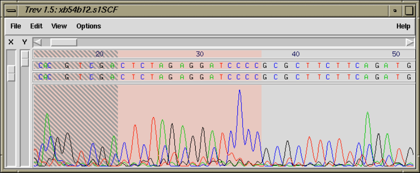
Chapter 8: Viewing and editing trace data using trev 417
8 Viewing and editing trace data using trev
8.1 Introduction
For some types of sequencing project it is convenient to view and edit the chromatogram
data prior to assembly into a gap4 database (see Section 2.2 [Gap4 Introduction], page 95),
and this is the function of the program trev.
Trev displays the original trace data, its base calls and confidence values, and it allows
the sequence of the trace to be edited and the left and right cutoffs to be defined. Several file
formats can be read in addition to our own Experiment Files (see Section 11.3 [Experiment
File], page 552), and ’SCF’ files (see Section 11.1 [scf], page 533). Any edits made are
normally saved to Experiment files, not to the chromatogram files which we regard as
archival data.
A typical display from trev is shown below. It includes the trace data, the original
sequence, the edited sequence, the menu bar, and the name of the sequence being edited.
The left cutoff region is shown shaded.
The trace can be scrolled using the scrollbar directly beneath the menubar. The trace
can be magnified in the vertical and horizontal directions using the scale bars to the left of
the trace.
The base numbers, original sequence, edited sequence, confidence values and the trace
can each be switched on or off, and the font for the original and edited sequence is selectable.
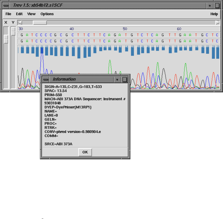
418 The Staden Package Manual
The figure below shows the bases, edited bases, a histogram of the confidence values, the
traces, and the Information Window which can be switched on from the View Menu.
Trev uses “io lib” for handling the various sequencing instrument file formats. This
means it has support for ABI, MegaBace (when saved in ABI format), SCF (used by LiCor
and some other manufacturers), ZTR and SFF (454).
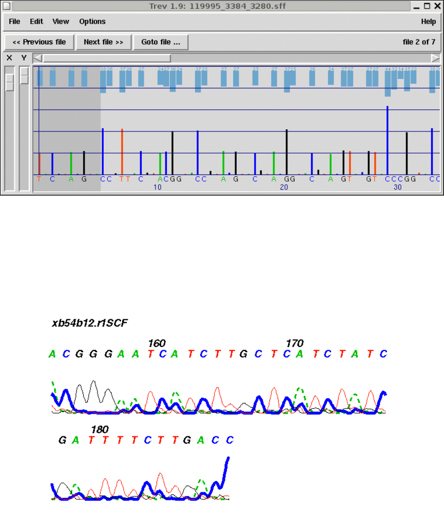
Chapter 8: Viewing and editing trace data using trev 419
The above pictures all come from instruments using the Sanger sequencing method,
however more recently support has been added for pyrosequencing methods (as used by 454
Life Sciences amongst others). An example of this is below.
Trev can be used to produce postscript files of the traces so that they can be printed.
The colours, line widths, etc are configurable. An example is shown in the figure below.
Note that we strongly recommend that readings are not edited prior to assembly as it is
far better to edit them when their alignment with other readings can be seen.
420 The Staden Package Manual
8.2 Opening trace files
Trace files can be opened either on the command line or from within Trev. In both cases
it is possible to open several traces at once. In this case trev will add Next File, Previous
File and Goto File buttons to allow quick navigation between traces.
On the command line, this is simply done by specifying several files. With the "Open"
dialogue from within trev multiple files may be selected by dragging with the left mouse
button or using shift+left button and control+left button to extend regions or to toggle
loading of individual files.
8.2.1 Opening a trace file from the command line
usage: trev [-{ABI,ALF,EXP,SCF,PLN,Any}] [-edits value] [-editscf] [-xmag
value] [-ymag value] [-restrict] [tracefilename ...]
-ABI, -ALF, -EXP, -SCF, -PLN, -Any
Optional. Defaults to Any. These define the possible input trace formats avail-
able. Currently these are ’ABI’, ’ALF’, experiment (see Section 11.3 [Experi-
ment File], page 552), ’SCF’ (see Section 11.1 [scf], page 533), plain ASCII text
or ’any’ in which case the program attempts to establish the file format from
information contained within the trace file.
-edits value
Optional. Defaults to 1. If value is 1, the trace sequence can be edited. If value
is 0, no edit line is displayed in Trev and the sequence may not be edited.
-editscf Optional. By default writing to SCF is disabled for safety and reasons of prefer-
ence (we feel that all edits should be contained within an associated Experiment
File thus leaving the original trace file intact). Specifying -editscf allows writ-
ing to SCF files.
-pregap_mode
Optional. Only used by Pregap4. This adds a Reject button to Trev and
disables certain file operations. This argument should only be used by programs
that run Trev as subprocesses for processing batches of files.
-restrict
Optional. Restricts the use of the trace editor to a single file by disabling the
ability to open another file from within Trev. The main use of this option is
for calling Trev from within scripts.
-xmag value
Optional. Defaults to 150. Specifies the magnification along the X axis of the
trace. Larger values represent higher magnifications.
Chapter 8: Viewing and editing trace data using trev 421
-ymag value
Optional. Defaults to 10. Specifies the magnification along the Y axis of the
trace. The value should be between 10 and 100 with 10 showing all the trace
and 100 being the largest magnification.
8.2.2 Opening a trace file from within Trev
To open a trace file select the "Open..."command from the File menu. This brings up a
file browser from where the trace name can be selected. See Section 10.7 [File Browser],
page 529. The format of the trace file should be selected from the row of Format buttons.
Currently these are ’ABI’, ’ALF’, Experiment File (see Section 11.3 [Experiment File],
page 552), ’SCF’ (see Section 11.1 [SCF File], page 533), plain ASCII text or ’any’ in which
case the program attempts to establish the file format from information contained within
the trace file. Opening an experiment file opens the trace file named within the experiment
file. Double clicking on the trace name will open this trace file.
If a trace file is already open, it is closed before the new one is opened. If the previous
trace has been edited, but not saved, a dialogue box is displayed, asking if you wish to
save the file before loading a new file. Selecting "Yes"will automatically save the file to its
current filename. Selecting "No"will discard any changes that have been made.
8.3 Viewing the trace
The trace can be scrolled using the scrollbar directly beneath the menubar. The trace can
be magnified both in the vertical and horizontal directions using the two scales to the left
of the trace.
The base numbers, original sequence, edited sequence, confidence values and the trace
can each be switched on or off by using the check buttons in the "Display"option of the
View menu.
The font for the original and edited sequence can be chosen from three sizes, selectable
by using the Font submenu of the View menu.
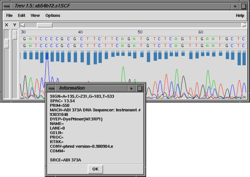
422 The Staden Package Manual
The figure below shows the bases, edited bases, a histogram of the confidence values, the
traces, and the Information Window which can be switched on from the View Menu.
8.3.1 Searching
Selecting the "Search..."command in the View menu brings up a window into which a
text string can be entered. Pressing the "Next"button positions the cursor at the start
of the next piece of sequence that matches the string specified in the text box. Pressing
"Previous", finds the previous match. The search is case insensitive.
8.3.2 Information
The comments from the SCF file of the trace can be displayed using the "Information"
option in the View menu.
8.4 Editing
8.4.1 Setting the left and right cutoffs
Poor data at the left and right ends of the trace can be marked using the "Left Quality"and
"Right Quality"options in the Edit menu. Alternatively a keyboard shortcut for editing
the cutoff is to press Control L or Control R to edit left or right cutoff respectively. To
select the left cutoff, choose the "Left Quality"option from the menu. Then click the left
mouse button at the required position in the trace display. The region from the start of
Chapter 8: Viewing and editing trace data using trev 423
the sequence to this position will be highlighted in grey. To select the right hand cutoff,
choose the "Right Quality"option in the Edit menu and click the required position in the
trace display. The region between the left boundary and the end of the sequence will be
highlighted. To prevent accidentally changing the cutoffs once these have been selected,
choose the "Sequence"option in the Edit menu.
If vector sequence has been marked trev will also display these in a similar fashion to the
quality cutoffs except in a peach colour. These cutoffs can be changed by selecting "Left
Vector"and "Right Vector"in the same fashion as editing the quality cutoffs. Where both
quality and vector cutoffs coincide trev draws the regions by striping between both peach
and grey.
8.4.2 Editing the sequence
If the ability to edit has not been disabled, there will be two windows showing the trace
sequence. The original sequence is displayed in the upper window. The window below this,
which contains the blue cursor, is the editing window. To edit this sequence, select the
"Sequence"option in the Edit menu. The editing cursor is positioned by clicking with the
left mouse button within the display. Bases are deleted to the left of the cursor using the
delete key of the keyboard. Additional bases are inserted to the left of the cursor. Only A,
a, C, c, G, g, T, and t are allowed. It is recommended that edits are entered in lower case
to distinguish them from the original bases.
8.4.3 Undoing clip edits
It is often easy to accidently forget which editing mode you are in and adjust a quality
or vector clip point by mistake. Trev keeps track of all clip edits and hence these may be
"Undone"by selecting "Undo Clipping"from the Edit menu. This will remove the last clip
edit. It is not yet possible to undo sequence edits.
8.5 Saving a trace file
To save a trace file to a different file name or format choose the "Save As..."command from
the File menu. Select the format the file is to be saved in using the Format buttons. The
output formats are CTF, SCF, ZTR, experiment and plain text. Type a new name into
the Selection box or select an existing name from the list of file names. Experiment format
traces can be saved to their existing name using the "Save"option in the File menu.
8.6 Processing multiple files
When several trace files are specified on the command line to Trev, it will add Previous File,
Next File, and Goto File buttons. The Previous File and Next File simply step through the
specified trace files. The Goto File button will bring up a scrollable list of all the trace files
specified. Clicking on any trace filename in this list will jump to that file.
If Trev was brought up from Pregap4, or the -pregap_mode command line switch was
used, Trev will also display a Reject button. This may be used to indicate to Pregap4 that
the trace file shown is not worthy of any clipping at all and should be sent to the Pregap4
"failed"file.
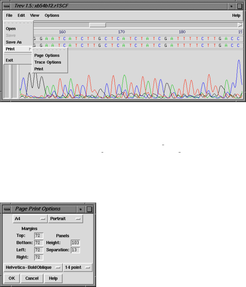
424 The Staden Package Manual
8.7 Printing a trace
The Print option is available via the File menu, as shown below.
It produces a PostScript file which you must then send to the printer yourself.
All sizes given in the dialogues explained below should be in PostScript points (72pt =
1inch).
Defaults and available options are specified in the file tk utilsrc. These can be changed
by copying the relevant line from tk utilsrc into a file called .tk utilsrc in your home or
working directory, and then altering the settings as desired.
Note that it is not yet possible to include the histogram of confidence values in the
postscript output.
8.7.1 Page options
8.7.1.1 Paper options
Currently available page sizes:
A4 (842 x 595)
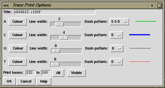
Chapter 8: Viewing and editing trace data using trev 425
A3 (1191 x 842)
US Letter (792 x 612)
Please note that the page size and orientation options do not determine the paper format
that your printer will use. This must be set externally to trev.
8.7.1.2 Panels
Traces are printed width-ways across the page. When the right-hand margin of the page is
reached, printing continues below the current section and from the left-hand side. A ’panel’
is one page-width’s worth of trace (minus margins).
The trace and the sequence and sequence number information are printed entirely within
the given height of the panel, and the separation gives the amount of space that is left
between panels. Thus they, together with the page height and top and bottom margins,
determine how many panels will be printed per page.
8.7.1.3 Fonts
All fonts listed should be available to most PostScript printers. Most printers will default
to Courier if a selected font is not recognised.
8.7.2 Trace options
8.7.2.1 Title
The title is printed in the top left hand corner of every page. The default is the name of
the trace file.
8.7.2.2 Line width and colour
The defaults are those used by the trev display. The colours shown in the selection dialogue
may not correspond exactly to those printed, depending on the capabilities of your printer.
Different colours will usually be printed using grey-scales on black and white printers.

426 The Staden Package Manual
8.7.2.3 Dash pattern
Dash pattern is in PostScript dash format:
dash 1 gap 1... dash n gap n offset
’dash n’ and ’gap n’ are the lengths of dashes and the gaps between them. The dash
pattern starts at dash 1, continues to gap n, then starts again at dash 1, until the whole
line has been drawn. If n = 0, i.e. no values are given for ’dash’ and ’gap’, the result is a
normal unbroken line. Offset must be given, and is the distance into the dash pattern at
which the pattern should be started. The dash pattern is not demonstrated by the example
line on the ps trace setup dialogue.
8.7.2.4 Print bases
Allows a subsection of the trace to be printed.
The ’Visible’ button sets the region to that currently displayed in the main trev window.
If the display is altered, the print base settings will not change unless ’Visible’ is pressed
again. The whole sequence is printed if the start position is greater than the end position.
The OK button will not work if the start or end positions given are outside the range of
the sequence.
8.7.2.5 Print magnification
The X and Y scales are taken from the trev display, and cannot be set independently for
PostScript output.

Chapter 8: Viewing and editing trace data using trev 427
8.7.3 Example
The segment of output displayed below indicates the effects of the settings given in the
example dialogue screendumps shown above. NB: the page has been clipped to save space.
The section shown is the top part of an A4 page.
8.8 Quitting
To exit Trev, select the "Exit"command from the File menu. If the sequence has been
edited but not saved, a dialogue box is displayed, asking if you wish to save the file before
quitting. Selecting "Yes"will automatically save the file to it’s current filename. Selecting
"No"will discard any changes that have been made.
Chapter 9: Analysing and comparing sequences using spin 429
9 Analysing and comparing sequences using spin
9.1 Organisation of the Spin Manual
The Introductory section of the manual gives an overview of the functions (see Section 9.2.1
[Summary of the Spin Functions], page 429), the menus (see Section 9.2.4 [Spin Menus],
page 444) and the user interface (see Section 9.2.3 [Introduction to the Spin User Interface],
page 431). The Introduction to the user interface includes a range of screen dumps which
give an overview of what spin can do, and taken as a whole, the introduction should contain
sufficient information to enable users to start using the program.
The next section describes in turn each of the main functions (see Section 9.3 [The Spin
Functions], page 446). This is followed by a detailed description of the spin user interface
(see Section 9.6 [The Spin User Interface], page 501). Next is a section describing how users
can control the results from the functions, and how they can be manipulated once they have
been obtained (see Section 9.7 [Controlling and Managing Results], page 515). The final
part of the manual describes how to read sequences into spin and the kinds of manipulations
which can be performed on them to prepare them for analysis (see Section 9.8 [Reading and
Managing Sequences], page 517).
9.2 Introduction
Spin is an interactive and graphical program for analysing and comparing sequences. It
contains functions to search for restriction sites, consensus sequences/motifs and protein
coding regions, can analyse the composition of the sequence and translate DNA to protein.
It also contains functions for locating segments of similarity within and between sequences,
and for finding global and local alignments between pairs of sequences. To help assess the
statistical significance of comparisons the program can calculate tables of expected and
observed score frequencies for each score level. Most analytical functions which operate on
single sequences add their graphical results to a "SPIN Sequence Plot"that is associated
with the sequence being analysed. (An exception is the restriction enzyme search which
produces its own separate window.) Most functions which compare pairs of sequences add
their results to a "SPIN Sequence Comparison Plot". The SPIN Sequence Plot and the SPIN
Sequence Comparison Plot each have associated sequence display windows: the Sequence
Display and the Sequence Comparison Display. These allow the text of the sequences to be
viewed and use cursors to show the corresponding positions in the graphical displays. The
graphical plots can be zoomed, and cursors or crosshairs can be used to locate the positions
of the individual results. Plots can be superimposed.
9.2.1 Summary of the Spin Single Sequence Functions
Spin’s main single sequence analytical functions are accessed via the Statistics, Translation
and Search menus. The "Statistics"menu contains options to count and plot the base
composition (see Section 9.3.3 [Plot Base Composition], page 447) and also to count the
dinucleotide frequencies (see Section 9.3.2 [Dinucleotide Frequencies], page 447).
The "Translation"menu contains options to set the genetic code (see Section 9.3.5 [Set
Genetic Code], page 451), translate to protein (see Section 9.3.6 [Translation], page 453),
find open reading frames and write the results in either feature table format or as fasta
430 The Staden Package Manual
format protein sequence files (see Section 9.3.7 [Find Open Reading Frames], page 454),
and to calculate codon tables.
The "Search"menu contains a variety of different searching techniques. "Protein genes"
has four methods for finding protein genes (see Section 9.3.11.3 [Codon Usage Method],
page 466) (see Section 9.3.11.5 [Author Test], page 473), (see Section 9.3.11.4 [Positional
base Preferences], page 472) (accessed as a subcomponent of the Codon Usage Method), and
(see Section 9.3.11.6 [Uneven Positional base Frequencies], page 477). There is also a method
to search for tRNA genes (see Section 9.3.11.8 [tRNA Search], page 480). It is also possible
to perform subsequence or string searches (see Section 9.3.9 [String search], page 460)
and restriction enzyme searches (see Section 9.3.8 [Restriction enzyme search], page 456).
There are searches for start (see Section 9.3.11.1 [Start Codon Search], page 464) and stop
codons (see Section 9.3.11.2 [Stop Codon Search], page 464), splice junction searches (see
Section 9.3.11.7 [Splice Site Search], page 478), and general motif searches using weight
matrices (see Section 9.3.10 [Motif Search], page 462).
9.2.2 Summary of the Spin Comparison Functions
This section outlines the functions obtained from the Comparison menu. All produce graph-
ical and textual output. Using a score matrix, the "Find similar spans"function compares
every segment of one sequence with all those of the other and reports those that reach a user
defined score. The segments are of a fixed length (span) set by the user (see Section 9.4.1
[Finding Similar Spans], page 483). To look for short matching segments of any length, and
allowing gaps, a local dynamic programming routine can be used (see Section 9.4.5 [Align-
ing Sequences Locally], page 493). The fastest routine for locating segments of similarity
(and generally only suitable for DNA sequences) finds all identical subsequences (or words)
(see Section 9.4.2 [Finding Matching Words], page 485). For a quick global comparison of
sequences using a combination of the Matching Words and Matching Spans algorithms the
"Find best diagonals"algorithm can be used (see Section 9.4.3 [Finding the Best Diagonals],
page 487). Global alignments can be produced and plotted using a dynamic programming
algorithm (see Section 9.4.4 [Aligning Sequences Globally], page 489).
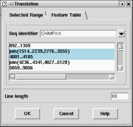
Chapter 9: Analysing and comparing sequences using spin 431
9.2.3 Introduction to the Spin User Interface
Spin has several main displays. The first is a top level window from which all the main
options are selected and which receives textual results. Most analytical functions which
operate on single sequences add their graphical results to a "SPIN Sequence Plot"that
is associated with the sequence being analysed. (An exception is the restriction enzyme
search which produces its own separate window.) Most functions which compare pairs of
sequences add their results to a "SPIN Sequence Comparison Plot". The SPIN Sequence
Plot and the SPIN Sequence Comparison Plot each have associated sequence display win-
dows: the Sequence Display and the Sequence Comparison Display. These allow the text
of the sequences to be viewed and use cursors to show the corresponding positions in the
graphical displays.
Spin is best operated using a three button mouse, but alternative keybindings are
available. Full details of the user interface are described elsewhere (see [User Interface],
page 523), and here we give an introduction based around a series of screenshots.
The main window (shown below) contains an Output Window for textual results, an Er-
ror window for error messages, and a series of menus arranged along the top (see Section 9.2.4
[Spin menus], page 444). The contents of the two text windows can be searched, edited and
saved. Each set of results is preceded by a header containing the time and date when it was
generated.
As can be seen the main menu bar contains File, View, Options, Sequences, Statistics,
Translation, Comparison, Search and Emboss menus. In general most functions add their
graphical results to a "SPIN Sequence Plot", but those obtained from the Comparison menu
add their results to a "SPIN Sequence Comparison Plot".
432 The Staden Package Manual
9.2.3.1 Introduction to the Spin Plot
Most of the spin functions display their results in a two-dimensional plot called a "spin
plot"(see Section 9.6.1 [Spin plot], page 502). Sets of matches from a single invocation of
a function are termed "a result". Each result is plotted using a single colour which can be
configured via the results manager (see Section 9.7.1 [Result manager], page 515).
The figure shown below shows a spin plot window containing the results of a gene
search method based on codon usage, superimposed on a search for stop codons (see
Section 9.3.11.3 [Codon Usage Method], page 466). Each plot window contains a cross
hair. Its x position is shown in sequence base numbers in the left hand box above the plot,
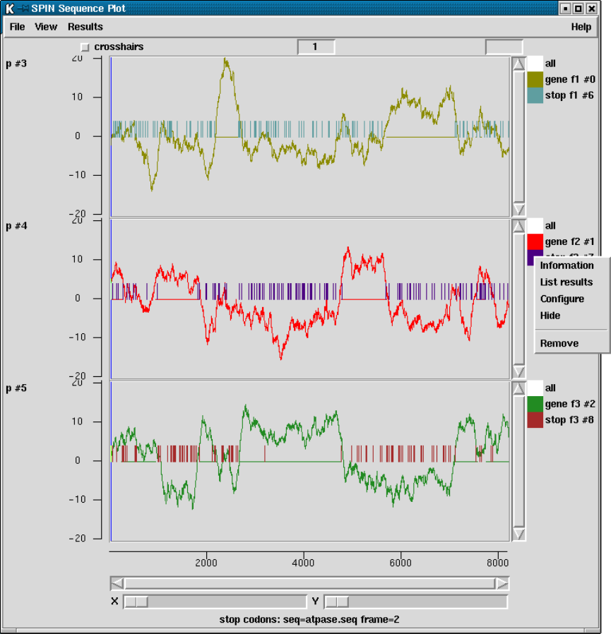
Chapter 9: Analysing and comparing sequences using spin 433
and the y coordinate, expressed using the score values of the gene search, is shown in the
right hand box.
At the right hand side of each panel is a set of square boxes with the same colours as
the lines drawn in the adjacent plot. These icon-like objects represent individual results
and allow the user to operate on them. For example at the right of the middle panel is a
pop-up menu containing the items: "Information","List results","Configure","Hide"and
"Remove". (see Section 9.7.1 [Result manager], page 515).
These icons can also be used to drag and drop the results to which they correspond.
This is activated by pressing the middle mouse button, or Alt left mouse button, over the

434 The Staden Package Manual
box and then moving the cursor over the spin plot to the new location or anywhere outside
the spin plot (see Section 9.6.1.4 [Drag and drop], page 506)
Each spin plot window also contains a cursor that denotes the position of the cursor in
the Sequence display window (see Section 9.6.2 [Spin Sequence Display], page 509). The
user can move a cursor by clicking and dragging with the middle mouse button, or Alt
left mouse button. This will move the cursor in the sequence display and all other cursors
displayed that relate to the sequence.
The graphical results can be zoomed and scrolled in both x and y directions. Zooming
is achieved using the X and Y scale bars at the top left hand corner of the plot. The
individual plots can be scrolled in y using the scroll bars attached to their right hand edge.
The sequence can be scrolled using the scroll bar at the base of the plot.
To illustrate further uses of the program we include some more screen dumps below.

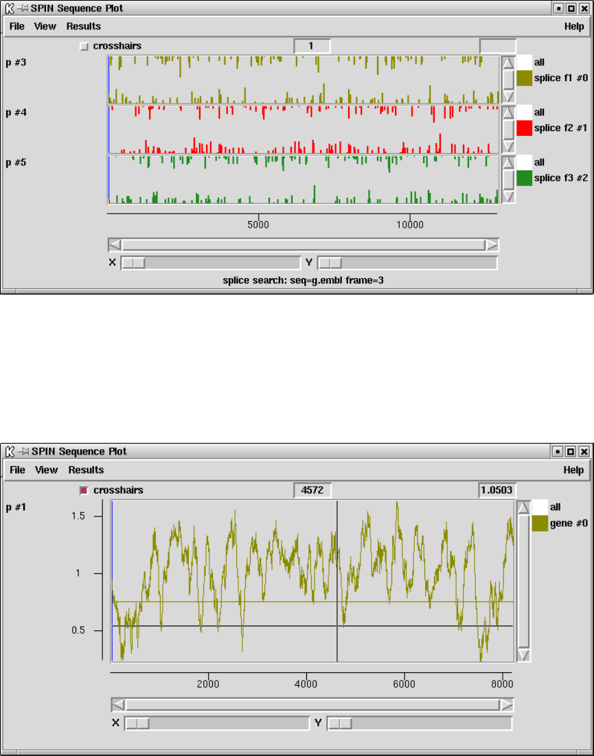
436 The Staden Package Manual
The figure above shows the way in which the results of weight matrix searches for motifs
are plotted (see Section 9.3.10 [Motif Search], page 462).
The figure about shows the way in which the results of searches for splice junctions are
plotted. The donor and acceptor predictions are separated and a different colour is used
for each reading frame (see Section 9.3.11.7 [Splice Site Search], page 478).
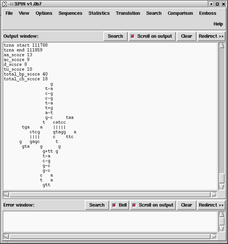
Chapter 9: Analysing and comparing sequences using spin 437
The figure above shows a method for finding protein coding regions which does not dis-
tinguish reading frame or strand (see Section 9.3.11.6 [Uneven Positional base Frequencies],
page 477).
The figure above shows how results from the tRNA gene search function are displayed
in the Output window (see Section 9.3.11.8 [tRNA Search], page 480).
9.2.3.2 Introduction to the Spin Sequence Display
Spin also has a sequence display window in which the user can view the sequence in textual
form. This window allows the user to scroll along the sequence. Users can view one or both
strands, can switch on displays of the encoded amino acids in up to six reading frames, can
switch on a display of the restriction enzyme sites, and can perform other simple subsequence
or string searches to locate features in the sequence. In the figure shown below the user has

438 The Staden Package Manual
switched on a three phase translation on the top strand, double stranded sequence, and a
restriction enzyme search.
The sequence cursor can be under the control of the graphics cursor i.e. the cursor in
the sequence viewer can be moved by the user dragging the cursor in the graphics window.
Similarly the cursor in the graphics plots can be moved by the sequence viewer cursor.
Chapter 9: Analysing and comparing sequences using spin 439
9.2.3.3 Introduction to the Spin Sequence Comparison Plot
All of the spin comparison functions display their results as points or lines in a two-
dimensional plot called a "Spin Sequence Comparison Plot"(see Section 9.6.3 [Spin Se-
quence Comparison Plot], page 512). Sets of matches from a single invocation of a compar-
ison command are termed "a result". Each result is plotted using a single colour which can
be configured via the results manager (see Section 9.7.1 [Result manager], page 515).
The diagram above shows the results of a "Find similar spans"search (olive) (see
Section 9.4.1 [Finding Similar Spans], page 483), and a "Find matching words"(red) (see
Section 9.4.2 [Finding Matching Words], page 485).
At the right hand side is a set of square boxes with the same colours as the dots drawn
in the adjacent plot. These icon-like objects represent individual results and allow the user
to operate on them. For example clicking with the right mouse button brings up the pop-up
menu beneath the "matching words"result contains the results menu for this result (see
Section 9.7.1 [Result manager], page 515). These icons can also be used to drag and drop the
results to which they correspond. This is activated by pressing the middle mouse button,
or Alt left mouse button, over the box and then moving the cursor over the Spin Sequence
440 The Staden Package Manual
Comparison Plot to the new location or anywhere outside the Spin Sequence Comparison
Plot (see Section 9.6.3.4 [Drag and drop], page 514).
Crosshairs can be turned on or off using the check button labelled "crosshairs". The x
and y positions of the crosshairs are indicated in the two boxes to the right of the check
box.
Each sequence displayed in a Spin Sequence Comparison Plot will have a cursor of a
particular colour. In the picture above, the sequence on the horizontal axis has a vertical
blue cursor whereas the sequence on the vertical axis has a horizontal olive green cursor.
In general, the same sequence displayed in several Spin Sequence Comparison Plots will
have a cursor of the same colour. The user can move a cursor by clicking and dragging
with the middle mouse button, or with Alt left mouse button. This will move all other
cursors displayed that relate to the sequence, whether they are in different Spin Sequence
Comparison Plots or within the sequence display.
Plots can be enlarged either by resizing the window or zooming. Zooming is achieved by
holding down the control key and right mouse button and dragging out a rectangle. This
process can be repeated. The Back button will restore the plot to the previous magnification.
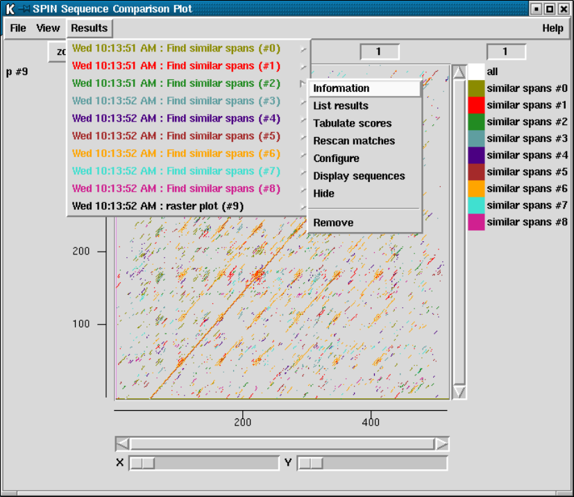
Chapter 9: Analysing and comparing sequences using spin 441
To illustrate further uses of the program we include some more screen dumps below.
The picture above shows the results after performing a "Find similar spans"comparison
between the three reading frames of two DNA sequences, producing nine superimposed sets
of results.
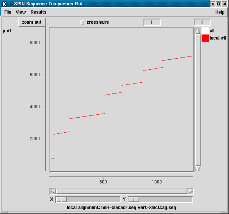
442 The Staden Package Manual
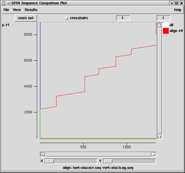
Chapter 9: Analysing and comparing sequences using spin 443
Local alignment searches join similar segments with lines. The above screen dump
shows such an analysis in which genomic DNA containing 7 exons and is compared to its
corresponding cDNA.
The above screendump shows a global alignment of the same pair of sequences.
9.2.3.4 Introduction to the Spin Sequence Comparison Display
A sequence comparison display is associated with a single set of results and can be invoked
by bringing up a pop up menu for the required result, either from the Results manager
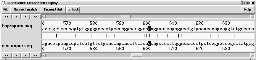
444 The Staden Package Manual
(see Section 9.7.1 [Result manager], page 515), the Results menu in the Spin Sequence
Comparison Plot, or the coloured square icon on the right of the plot.
The horizontal sequence is drawn above the vertical sequence and the central panel
indicates characters which are identical. The buttons (< >) and (<< >>) scroll the sequences.
Pressing the Lock button forces the sequences to scroll together. Movement of the sequences
is also controlled by the scrollbars or by moving the corresponding cursor in the Spin
Sequence Comparison Plot. The black cursors in the sequence display correspond to the
position of the cursor in the Spin Sequence Comparison Plot. The sequences can be made
to ’jump’ to the nearest match in those results by pressing the "Nearest match"or "Nearest
dot"buttons.
9.2.4 Spin Menus
The main window for spin contains File, View, Options, Sequences, Statistics, Translation,
Search, Comparison and Emboss menus.
9.2.4.1 Spin File Menu
The File menu includes sequence reading, saving and management options.
•Load sequences (see Section 9.8.2 [Reading in sequences], page 518)
•Save (see Section 9.8.3.10 [Save], page 521)
•Change directory
•Sequence manager (see Section 9.8.3 [Sequence manager], page 519)
•Exit
9.2.4.2 Spin View Menu
The View menu contains options to give access to the Results Manager, and to the Sequence
Display.
•Results manager (see Section 9.7.1 [Result manager], page 515)
•Sequence display (see Section 9.6.2 [Sequence display], page 509)
9.2.4.3 Spin Options Menu
The Options menu contains options for configuring spin and its functions.
•Change protein score matrix (see Section 9.5.5 [Changing the score matrix], page 499)
•Set protein alignment symbols (see Section 9.5.6 [Set protein alignment symbols],
page 501)
Chapter 9: Analysing and comparing sequences using spin 445
•Configure maximum number of matches (see Section 9.5.2 [Changing the maximum
number of matches], page 498)
•Configure default number of matches (see Section 9.5.3 [Changing the default number
of matches], page 498)
•Hide duplicate matches (see Section 9.5.4 [Hide duplicate matches], page 499)
•Set fonts
•Colours
9.2.4.4 Spin Sequences Menu
The Sequences menu contain options for manipulating the sequences currently loaded into
spin. All these operations are also obtainable from a pop up menu in the sequence manager
(see Section 9.8.3 [Sequence manager], page 519).
•Horizontal (see Section 9.8.3.1 [Change the active sequence], page 520)
•Vertical (see Section 9.8.3.1 [Change the active sequence], page 520)
•Set range (see Section 9.8.3.2 [Set the range], page 520)
•Copy (see Section 9.8.3.3 [Copy sequence], page 520)
•Complement sequence (see Section 9.8.3.5 [Complement sequence], page 520)
•Interconvert t and u (see Section 9.8.3.6 [Interconvert t and u], page 520)
•Translate sequence (see Section 9.8.3.7 [Translate sequence], page 520)
•Scramble sequence (see Section 9.8.3.8 [Scramble sequence], page 521)
•Sequence type (see Section 9.8.3.4 [Sequence type], page 520)
•Rotate sequence (see Section 9.8.3.9 [Rotate sequence], page 521)
•Save (see Section 9.8.3.10 [Save sequence], page 521)
•Delete (see Section 9.8.3.11 [Delete sequence], page 522)
9.2.4.5 Spin Statistics Menu
The Statistics menu contains the spin functions for analysing and plotting the composition
of sequences.
•Count sequence composition (see Section 9.3.1 [Count Sequence Composition],
page 446)
•Plot base composition (see Section 9.3.3 [Plot Base Composition], page 447)
•Count dinucleotide frequencies (see Section 9.3.2 [Dinucleotide Frequencies], page 447).
9.2.4.6 Spin Translation Menu
The "Translation"menu contains options to set the genetic code, translate to protein, find
open reading frames and to calculate codon tables.
•Set genetic code (see Section 9.3.5 [Set Genetic Code], page 451)
•Translate (see Section 9.3.6 [Translation], page 453),
•Find open reading frames (see Section 9.3.7 [Find Open Reading Frames], page 454)
•Calculate and write codon table to disk (see Section 9.3.4 [Calculate codon usage],
page 448)
446 The Staden Package Manual
9.2.4.7 Spin Search Menu
The "Search"menu contains a variety of different searching and analysis techniques.
•Protein genes: Codon pref (see Section 9.3.11.3 [Codon Usage Method], page 466)
•Protein genes: Author test (see Section 9.3.11.5 [Author Test], page 473)
•Protein genes: Base bias (see Section 9.3.11.6 [Uneven Positional base Frequencies],
page 477)
•tRNA genes (see Section 9.3.11.8 [tRNA Search], page 480)
•Search for string (DNA) (see Section 9.3.9 [Subsequence search], page 460)
•Restriction enzyme map (see Section 9.3.8 [Restriction enzyme search], page 456)
•Plot start codons (see Section 9.3.11.1 [Start Codon Search], page 464)
•Plot stop codons (see Section 9.3.11.2 [Stop Codon Search], page 464)
•Search for splice junctions (see Section 9.3.11.7 [Splice Site Search], page 478)
•Search using weight matrix (see Section 9.3.10 [Motif Search], page 462)
9.2.4.8 Spin Comparison Menu
The Comparison menu contains the spin analytical functions for comparing and aligning
the sequences.
•Find similar spans (see Section 9.4.1 [Finding Similar Spans], page 483)
•Find matching words (see Section 9.4.2 [Finding Matching Words], page 485)
•Find best diagonals (see Section 9.4.3 [Finding the Best Diagonals], page 487)
•Align sequences (see Section 9.4.4 [Aligning Sequences Globally], page 489)
•Local alignment (see Section 9.4.5 [Aligning Sequences Locally], page 493)
9.3 Spin’s Analytical Functions
Spin contains both simple and sophisticated analytical functions, mostly producing graphi-
cal results. The following sections describe the functions, approximately in order of increas-
ing complexity.
9.3.1 Count Sequence Composition
When a sequence is read into the program its composition is displayed in the Output
Window to provide a simple check that the data has been read correctly. The values can
also be requested from the "Statistics"menu, when a dialogue will allow subsections of the
sequence to be analysed. The results are displayed as shown below.
Chapter 9: Analysing and comparing sequences using spin 447
============================================================
Wed 12 Nov 17:10:25 1997: sequence composition
------------------------------------------------------------
A 1966 (24.17%) C 1996 (24.54%) G 2185 (26.86%) T 1987 (24.43%) - 0 (0.00%)
Or for protein sequences:
============================================================
Mon 14 Oct 17:11:04 2002: sequence composition
------------------------------------------------------------
Sequence MYSA_DROME: 1 to 2411
Protein
AAABCDEFGHIKLMN
N 201 0 30 150 281 74 127 45 126 233 243 43 121
% 8.3 0.0 1.2 6.2 11.7 3.1 5.3 1.9 5.2 9.7 10.1 1.8 5.0
M 14287 0 3094 17263 36281 10891 7246 6171 14258 29865 27498 5642 13807
AAPQRSTVWYZX*-
N 55 167 141 96 93 108 14 63 0 0 0 0
% 2.3 6.9 5.8 4.0 3.9 4.5 0.6 2.6 0.0 0.0 0.0 0.0
M 5341 21398 22022 8360 9403 10706 2607 10280 0 0 0 0
M 5341 21398 22022 8360 9403 10706 2607 10280 0 0 0 0
9.3.2 Count Dinucleotide Frequencies
This routine simply counts dinucleotide frequencies for the selected region of the sequence.
It also calculates an expected distribution based on the base composition. The output looks
like:
ACGT
Obs Expected Obs Expected Obs Expected Obs Expected
A 7.91 5.84 5.64 5.93 5.05 6.49 5.57 5.91
C 5.91 5.93 5.14 6.02 7.38 6.59 6.10 5.99
G 6.11 6.49 7.56 6.59 6.30 7.22 6.90 6.56
T 4.24 5.91 6.18 5.99 8.14 6.56 5.86 5.97
9.3.3 Plot base composition
The composition of the sequence can be displayed graphically. A window is slid along the
sequence one base at a time, and at each point the number of occurrences of each selected
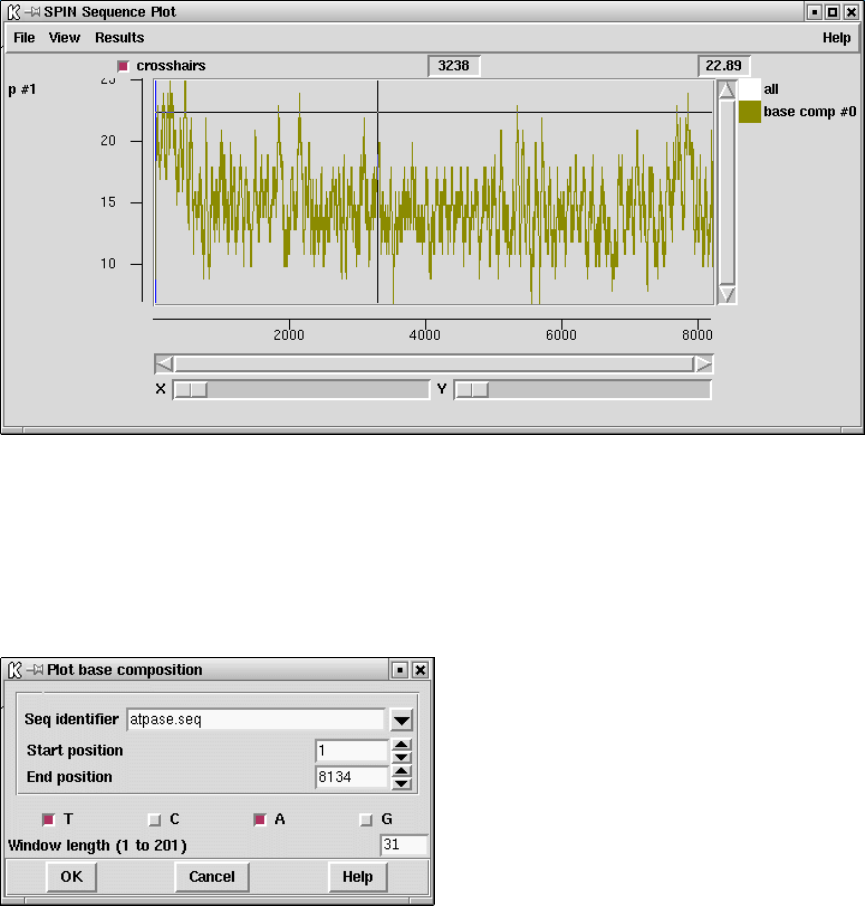
448 The Staden Package Manual
base type is counted and plotted. Users can select which base types are counted, the size
of the window used and the region of the sequence to analyse.
For example the A and T composition can be plotted by selecting base types A and T
in the dialogue. As usual the values can also be listed in the text Output Window. Note
that this "result", i.e. the base composition counts for every position along the sequence,
will persist until the user explicitly removes it. To save memory delete results as soon as
they are no longer required.
9.3.4 Calculate codon usage
Codon usage tables can be calculated and written to the Output Window, and written to
disk. If required the values found can be added to the counts in a pre-existing codon table,
or when written out to disk they can be concatenated with an existing codon table file. In
the first case the existing file will be read and added to the values calculated for the region
defined by the user. In the latter, the values calculated for the region defined by the user
will be written immediately after those from the existing table, hence producing a pair of

Chapter 9: Analysing and comparing sequences using spin 449
tables joined end to end. An example of this is shown at the end of this section, and a more
typical result is shown below.
Refering to the figure of the dialogue below, the user can select the range and strand
over which to count. Note that irrespective of the strand being counted, the positions in
the sequence are always defined from the current 5’ end. i.e. to count over bases 1 to 100
the user should set the Start position to 1 and the End position to 100. The values in the
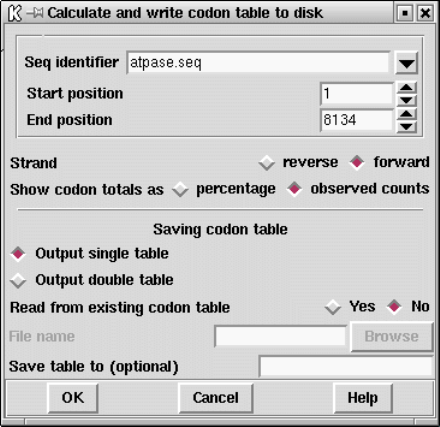
450 The Staden Package Manual
table can be expressed as observed counts or as percentages of usage for the cognate amino
acid.
The table can be output as a single table (as shown above), or as a double table (shown
below). The user can request that the counts from an existing table be read and added to
the counts which are about to be calculated, in which case the "File name"text window
will be activated. If the user selects to output a double table, this dialogue will also be
activated. To save the output in the selected form to a file, the user should fill in the "Save
table to"text window.
Two of the protein coding search functions (see Section 9.3.11.3 [Codon Usage Method],
page 466) and (see Section 9.3.11.5 [Author Test], page 473) work best using a double codon
table. The top table should contain the codon usage for the coding regions and the bottom
table the usage for non-coding regions. A typical double codon table of this sort is shown
below.
===============================================
F ttt 4 S tct 30 Y tat 5 C tgt 9
F ttc 35 S tcc 21 Y tac 15 C tgc 5
L tta 4 S tca 7 * taa 0 * tga 0
L ttg 24 S tcg 9 * tag 0 W tgg 15
===============================================
L ctt 71 P cct 1 H cat 17 R cgt 37
L ctc 39 P ccc 2 H cac 15 R cgc 18
L cta 0 P cca 14 Q caa 87 R cga 1
L ctg 4 P ccg 0 Q cag 18 R cgg 1
===============================================
I att 33 T act 30 N aat 12 S agt 2
I atc 53 T acc 20 N aac 59 S agc 5
Chapter 9: Analysing and comparing sequences using spin 451
I ata 1 T aca 3 K aaa 23 R aga 38
M atg 32 T acg 0 K aag 117 R agg 0
===============================================
V gtt 30 A gct 71 D gat 58 G ggt 5
V gtc 22 A gcc 54 D gac 32 G ggc 1
V gta 7 A gca 6 E gaa 76 G gga 49
V gtg 5 A gcg 0 E gag 101 G ggg 1
===============================================
===============================================
F ttt 10 S tct 8 Y tat 7 C tgt 4
F ttc 12 S tcc 2 Y tac 4 C tgc 3
L tta 6 S tca 4 * taa 7 * tga 10
L ttg 11 S tcg 3 * tag 4 W tgg 6
===============================================
L ctt 5 P cct 3 H cat 4 R cgt 0
L ctc 6 P ccc 1 H cac 4 R cgc 0
L cta 3 P cca 1 Q caa 9 R cga 5
L ctg 6 P ccg 3 Q cag 5 R cgg 2
===============================================
I att 13 T act 6 N aat 7 S agt 4
I atc 7 T acc 0 N aac 3 S agc 2
I ata 12 T aca 5 K aaa 9 R aga 16
M atg 7 T acg 3 K aag 4 R agg 4
===============================================
V gtt 6 A gct 2 D gat 8 G ggt 4
V gtc 2 A gcc 1 D gac 3 G ggc 1
V gta 5 A gca 1 E gaa 9 G gga 9
V gtg 4 A gcg 0 E gag 3 G ggg 0
===============================================
To calculate such a table using spin the following steps are required. First calculate the
codon usage for a typical coding segment and save the resulting table in table A. Then use
the option again, but this time select to "Output double table", and type the name of table
A into the "File name"text box. Next define the start and end points of a non-coding
region, and save the results to double table B. The file containing double table B is now
suitable for use by the protein gene searching functions.
9.3.5 Set genetic code
This function allows the user to change the genetic used in all the options. The codes are
defined as a set of codon tables stored in the directory tables/gcodes distributed with the
package. The current list of codes and their codon table file names is shown at the end of
this section.
The user interface consists of the dialogue shown below. The user selects the required
code by clicking on it, and then clicking "OK"or "OK permanent". The former choice
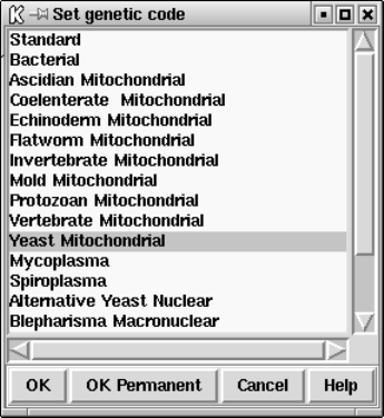
452 The Staden Package Manual
selects the code for immediate use, and the latter also selects it for future uses of the
program.
When the dialogue is left the codon table selected will be displayed, as below, in the
Output Window.
===============================================
F ttt S tct Y tat C tgt
F ttc S tcc Y tac C tgc
L tta S tca * taa W tga
L ttg S tcg * tag W tgg
===============================================
L ctt P cct H cat R cgt
L ctc P ccc H cac R cgc
L cta P cca Q caa R cga
L ctg P ccg Q cag R cgg
===============================================
I att T act N aat S agt
I atc T acc N aac S agc
M ata T aca K aaa G aga
M atg T acg K aag G agg
===============================================
V gtt A gct D gat G ggt
V gtc A gcc D gac G ggc
V gta A gca E gaa G gga
V gtg A gcg E gag G ggg
===============================================
The following table shows the list of available genetic codes and the files in which they
are stored for use by the package. They were created from genetic code files obtained from
the NCBI.
code_1 Standard

Chapter 9: Analysing and comparing sequences using spin 453
code_2 Vertebrate Mitochondrial
code_3 Yeast Mitochondrial
code_4 Coelenterate Mitochondrial
code_4 Mold Mitochondrial
code_4 Protozoan Mitochondrial
code_4 Mycoplasma
code_4 Spiroplasma
code_5 Invertebrate Mitochondrial
code_6 Ciliate Nuclear
code_6 Dasycladacean Nuclear
code_6 Hexamita Nuclear
code_9 Echinoderm Mitochondrial
code_10 Euplotid Nuclear
code_11 Bacterial
code_12 Alternative Yeast Nuclear
code_13 Ascidian Mitochondrial
code_14 Flatworm Mitochondrial
code_15 Blepharisma Macronuclear
9.3.6 Translation - general
Translations of the sequence can be obtained in three ways. The first is an option available
within the "Sequence manager"or the "Sequences"menu (see Section 9.8.3 [Sequence
manager], page 519).
The second is an option in the Sequence display (see Section 9.6.2 [Spin Sequence Dis-
play], page 509) which enables the translation to be shown with the scrolling sequence.
The third, which has two methods of defining the segments to translate, is described
here. The translations are written to the Output window, from where they can be saved to
disk. A segment of a typical display is shown below.
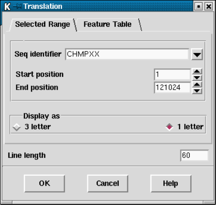
454 The Staden Package Manual
Users select either to use a feature table to define the segments to translate or can
simply enter a start and end position. In the latter case a six phase transtation over that
one segment is written out. If a feature table is used (and this assumes the sequence file was
an EMBL entry complete with features), the CDS records from the table will be listed in the
dialogue window and the user can select which ones should be used (see Section 9.8.1 [Use
of feature tables in spin], page 517). The translations produced will be written in FASTA
format ready to be saved to disk (which the next release of spin will do automatically!).
The user can also choose the line length, and whether one or three letter amino acid
symbols are produced.
9.3.7 Find open reading frames
This function will find open reading frames greater than an specified length. The results
can be output in two ways, either in feature table format
FT CDS 120..233
FT CDS 161..256
FT CDS 301..396
FT CDS 333..497
FT CDS 512..736
FT CDS 525..965
FT CDS 740..952
FT CDS 754..876
FT CDS 956..1789
or as a fasta file.
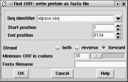
Chapter 9: Analysing and comparing sequences using spin 455
>120 120..233
VISENISLLKIGAKNHHWLLKQLLKMSMGGFCCVNVIY*
>161 161..256
EPSLAVKTVIKNVNGWFLLCKCHLLNRYLFLD*
>301 301..396
ICCARTCAICDLKHALSPVFTRYLQFFMIEQG*
>333 333..497
SEARFITSVYALFTVFHDRTGLAEKSQLYALEKYLNIYSPFGYLLFEITGAHRII*
>512 512..736
CLTLSLKESFIRHAAYLEGSRSEKRDVCVARESKRCSEASARSVTGGDSKWIAVQPQRPL
LGRLCNKRGPGSLSA*
>525 525..965
ALKKVLYDTRHTSKGAGVKNVMSVSLVSRNVARKLLLVQLLVVIASGLLFSLKDPFWGVS
AISGGLAVFLPNVLFMIFAWRHQAHTPAKGRVAWTFAFGEAFKVLAMLVLLVVALAVLKA
VFLPLIVTWVLVLVVQILAPAVINNKG*
>740 740..952
RFVYDICLASPGAYTSERPGGLDIRIWRSFQSSGDVGVTGGGVGGFKGGILAADRYVGFG
AGGSDTGTGCN*
>754 754..876
YLPGVTRRIHQRKAGWPGHSHLAKLSKFWRCWCYWWWRWRF*
>956 956..1789
QQRVKGIMASENMTPQDYIGHHLNNLQLDLRTFSLVDPQNPPATFWTINIDSMFFSVVLG
LLFLVLFRSVAKKATSGVPGKFQTAIELVIGFVNGSVKDMYHGKSKLIAPLALTIFVWVF
LMNLMDLLPIDLLPYIAEHVLGLPALRVVPSADVNVTLSMALGVFILILFYSIKMKGIGG
FTKELTLQPFNHWAFIPVNLILEGVSLLSKPVSLGLRLFGNMYAGELIFILIAGLLPWWS
QWILNVPWAIFHILIITLQAFIFMVLTIVYLSMASEEH*
The user can select that start and end points over which to do the search, which strand
to search (either the forward, reverse or both) and the minimum length of the open reading
frame in codons. If the output is being written in fasta format, the name of file is also
required.
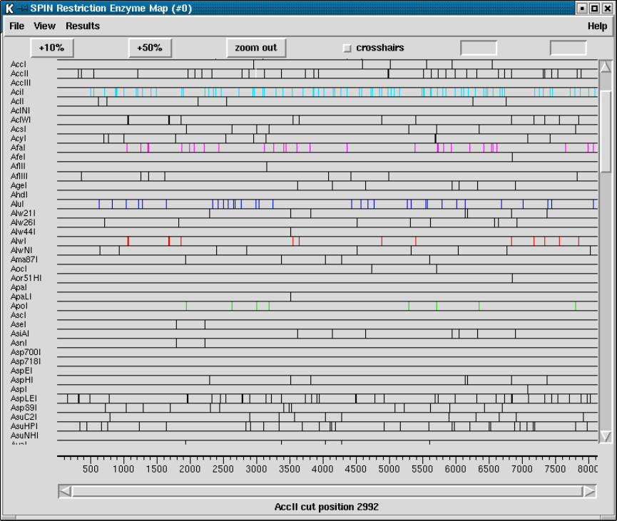
456 The Staden Package Manual
9.3.8 Restriction enzyme search
The restriction enzyme map function finds and displays restriction sites found within a
specified region of a sequence. Users can select the enzyme types to search for.
This figure shows a typical view of the Restriction Enzyme Map function in which the
results for most enzyme types are shown as black vertical lines opposite the enzyme names,
but in which some of the enzymes sites have been configured by the user to be drawn in
different colours. If no result is found for any particular enzyme eg here AccIII, the line will
still be drawn so that zero cutters can be identified. The results can be scrolled vertically
(and horizontally if the plot is zoomed in). A ruler is shown along the base and the current
cursor (the vertical black line) position is shown in the left hand box near the top right of
the display. If the user clicks, in turn, on two restriction sites their separation in base pairs
will appear in the top right hand box. Information about the last site touched is shown in
the Information line at the bottom of the display.

Chapter 9: Analysing and comparing sequences using spin 457
9.3.8.1 Selecting Enzymes
Files of restriction enzyme names and their cut sites are stored in disk files. For the format
of these files see Section 11.4 [Restriction enzyme files], page 566. Standard four-cutter,
six-cutter and all-enzymes files are available and the users can use their own "personal"
files. To create your own file of enzymes you may need to extract the information from the
currently defined files. These are pointed to by the RENZYM.4,RENZYM.6 and RENZYM.ALL
environment variables.
When the file is read the list of enzymes is displayed in a scrolling window. To select
enzymes press and drag the left mouse button within the list. Dragging the mouse off the
bottom of the list will scroll to allow selection of a range larger than the displayed section of
the list. When the left button is pressed any existing selection is cleared. To select several
disjoint entries in the list press control and the left mouse button. Once the enzymes have
been chosen, pressing OK will create the plot.
9.3.8.2 Examining the Plot
Positioning the cursor over a match will cause its name and cut position to appear in
the information line. If the right mouse button is pressed over a match, a popup menu
containing Information and Configure will appear. The Information function in this menu
will display the data for this cut site and enzyme in the output window.
It is possible to find the distance between any two cut sites. Pressing the left mouse
button on a match will display "Select another cut"at the bottom of the window. Then,
pressing the left button on another match will display the distance, in bases, between the
two sites. This is shown in a box located at the top right corner of the window.

458 The Staden Package Manual
9.3.8.3 Reconfiguring the Plot
The plot displays the results for each restriction enzyme on a separate line. Enzymes with
no sites are also shown. The order of these lines may be changed by pressing and dragging
the middle mouse button, or Alt left mouse button, on one of the displayed names at the
left side of the screen. For example the figure below shows the results seen above but after
the coloured (i.e. non-black) rows of sites have been dragged and dropped to be vertically
adjacent.
The results are plotted as black lines but users can select colours for each enzyme type
by pressing the right button on any of its matches. A menu containing Information and
Configure will pop up. Configure will display a colour selection dialogue. Adjusting the
colour here will adjust the colour for all matches found with this restriction enzyme.
9.3.8.4 Printing the sites
From the Result manager (see Section 9.7.1 [Result manager], page 515), menu a pop-up
menu for restriction sites results can be used to write the results in two forms to the the
Output window - from here the results can be saved to a file. The two choices of format are
Chapter 9: Analysing and comparing sequences using spin 459
"Output enzyme by enzyme"and "Output ordered on position", brief examples of which
are shown below. The output also appears in an "Information"window. Note that these
listings are also available from gap4.
The restriction enzyme results output ordered "enzyme by enzyme". The enzymes sites
are numbered and named and the actual cut site from the sequence is written, followed by
the position of the cut, the fragment size, and finally a sorted list of fragment sizes. A list
of zero cutters is written underneath.
Matches found= 1
Name Sequence Position Fragment lengths
1 ApaLI G’TGCAC 3506 3505 3505
4629 4629
Matches found= 8
Name Sequence Position Fragment lengths
1 ApoI A’AATTC 1939 1938 184
2 ApoI G’AATTT 2632 693 339
3 ApoI A’AATTT 2996 364 364
4 ApoI G’AATTC 3180 184 419
5 ApoI A’AATTT 5283 2103 639
6 ApoI G’AATTC 5702 419 693
7 ApoI A’AATTC 6341 639 1455
8 ApoI A’AATTC 7796 1455 1938
339 2103
Matches found= 2
Name Sequence Position Fragment lengths
1 AseI AT’TAAT 1790 1789 435
2 AseI AT’TAAT 2225 435 1789
Zero cutters:
Acc65I
AccIII
AclNI
AhdI
ApaI
AscI
Asp700I
Asp718I
AspEI
AsuNHI
AvrII
5910 5910
The restriction enzyme results output ordered on position. The enzymes sites are num-
bered and named and the actual cut site from the sequence is written, followed by the
position of the cut, the fragment size, and finally a sorted list of cut sizes.
460 The Staden Package Manual
============================================================
Wed 19 Nov 15:42:38 1997: Restriction enzymes result list
------------------------------------------------------------
Sequence /nfs/skye/home10/rs/work/doc/spin/atpase.dat
Number of enzymes = 80
Number of matches = 597
Name Sequence Position Fragment lengths
1 AspLEI GCG’C 157 156 0
2 AccII CG’CG 313 156 0
3 AspLEI GCG’C 313 0 0
4 AviII TGC’GCA 322 9 0
5 AspLEI GCG’C 323 1 0
6 AsuHPI ’CGCTTTATCACC 342 19 0
7 AflIII A’CGCGT 362 20 0
8 AccII CG’CG 364 2 0
9 BcgI ’AACAGGGTTAGCAGAAAAGTCG 389 25 0
10 BcgI GCAGAAAAGTCGCAATTGTATGCA’ 423 34 0
11 AsuHPI ’CATTTATTCACC 440 17 0
12 AspLEI GCG’C 486 46 0
13 AciI C’CGC 502 16 0
14 AciI G’CGG 552 50 0
15 AccII CG’CG 552 0 0
16 AclI AA’CGTT 614 62 0
9.3.9 Subsequence search
Two subsequence or string searches are available. One, selected from the "Search"menu on
the Output Window, produces both graphical and textual output, and the other, selected
from the "Search"button in the Sequence display, moves the cursor to the position of the
next match. Here we document the use of the first search, and the other is described in
Section 9.6.2.1 [Sequence display string search], page 510.
As shown in the dialogue the user selects the range and strand over which the search
should be performed, the search algorithm, the minimum percentage match, and the sub-
sequence/string for which to search. The search algorithm allows either NC-IUB codes
Cornish-Bowden, A. (1985) Nucl. Acids Res. 13, 3021-3030 or a literal search. The literal
search will search for exact matches eg inputting a search string of "n"will search for the
letter "n". The NC-IUB codes option can use any of the NC-IUB symbols shown in the
figure below and the search is not case sensitive.
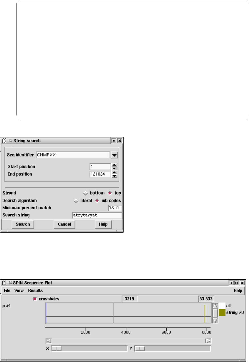
Chapter 9: Analysing and comparing sequences using spin 461
NC-IUB SYMBOLS
A,C,G,T
R (A,G) ’puRine’
Y (T,C) ’pYrimidine’
W (A,T) ’Weak’
S (C,G) ’Strong’
M (A,C) ’aMino’
K (G,T) ’Keto’
H (A,T,C) ’not G’
B (G,C,T) ’not A’
V (G,A,C) ’not T’
D (G,A,T) ’not C’
N (G,A,C,T) ’aNy’
The matches are plotted as vertical lines at the match positions with the heights of the
lines in proportion to their score. The matches are also written in the Output Window as
shown below.

462 The Staden Package Manual
============================================================
Tue 19 Oct 11:52:50 1999: string search
------------------------------------------------------------
Position 7837 score 9 percent match 90.000000
Percentage mismatch 10.0
1
string atrytayrat
::..::..:
atpase.seq atgctatgag
7837
9.3.10 Motif search
This option is used to search for motifs such as binding sites. The motifs are defined
using weight matrices which are stored as files that need to be created beforehand. These
matrices are usually calculated from alignments of trusted examples of the motif. The make_
weights program can be used to create weight matrices from sets of aligned sequences (see
Section 12.17 [Make weights], page 593) We also plan to build up a library of matrix files
which we will place in our ftp site.
An example weight matrix file is shown below. It consists of a title record; a record
defining the motif size, an offset and the score range; 2 records which need to be present
but which are ignored; 4 records defining the base frequencies calculated from the trusted
examples.
An example weight matrix file is shown below. The first line gives the title (’Mount
acceptors’ in this example). The next line gives the motif length (18), the "mark position"
(15), and the minimum and maximum scores (0.0 and 10.0). The "mark position"is an
offset which is added to the position of any matches reported by the search routine in
spin. The next two lines are ignored by the programs. The first of them gives the matrix
column positions, and the next gives the total counts in each column. The final lines (4 for
DNA weight matrices) give the counts for each character type at each position in the motif.
These counts are converted into weights that are used during the searches. Any position
in a sequence which scores at least as high as the minimum score is reported as a match,
and if the results are plotted they are scaled to fit the range defined by the minimum and
maximum scores.
Mount acceptors
18 15 0.0 10.0
P -14 -13 -12 -11 -10 -9 -8 -7 -6 -5 -4 -3 -2 -1 0 1 2 3
N 113 113 113 113 113 113 113 113 113 113 113 113 113 113 113 113 113 113
T 58 50 57 59 67 56 58 49 47 66 64 31 34 0 0 11 41 31
C 21 28 34 25 29 33 35 32 42 40 33 25 74 0 0 23 28 41
A 17 11 11 18 7 17 12 23 15 3 10 29 5 113 0 24 21 21
G 17 24 11 11 10 7 8 9 9 4 6 28 0 0 113 55 23 20
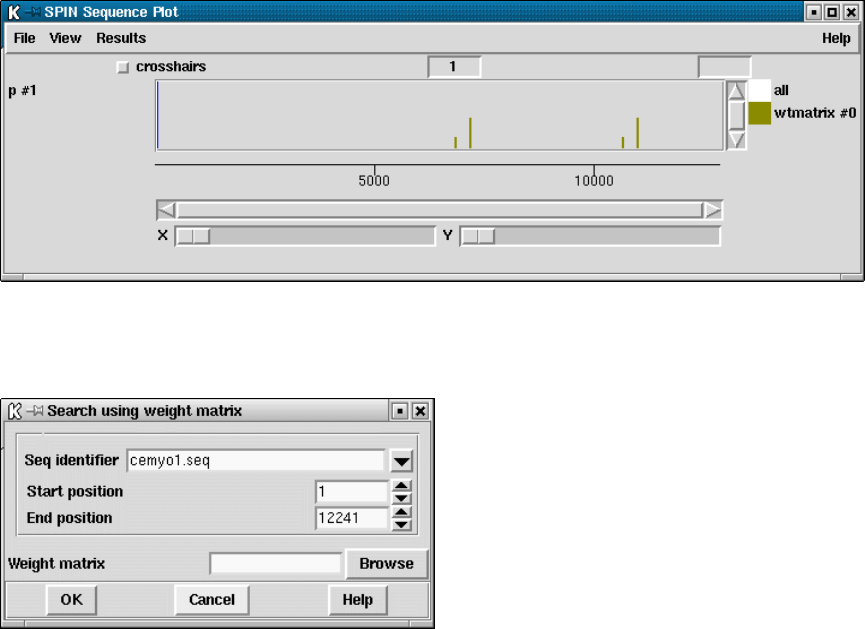
Chapter 9: Analysing and comparing sequences using spin 463
Search results are plotted as log-odds and appear as shown below.
The dialogue for the option is shown below.
9.3.11 Gene finding
Many years ago Staden R. (1984) Graphic methods to determine the function of nucleic
acid sequences. Nucl. Acids Res. 12, 521-538 we separated methods for searching for genes
and their control regions into two classes: "gene search by signal", and "gene search by
content".Staden R. (1985) Computer methods to locate genes and signals in nucleic acid
sequences, Genetic Engineering: Principles and Methods Vol. 7, Edited by J. K. Setlow
and A. Hollaender, Plenum Publishing Corp.. Signal searches look for short segments of
sequences such as promoters, ribosome binding sites, splice junctions, etc, whereas content
searches look for the sequence patterns that are characteristic of protein coding regions, or
RNA genes. Protein coding sequences produce particular amino acid sequences, often using
preferred codons, and this leaves patterns in the sequence that can be used to distinguish
them from non-protein-coding DNA. tRNA genes must produce stable cloverleaf structures
and "standard"tRNAs must contain particular (conserved) bases at locations within the
cloverleaf. These features can be used to locate tRNA genes, and probably other RNA
genes could be sought in a similar way.
The methods described in the following sections are either "content"or "signal"searches
and spin’s graphical presentation of results can be used to see if together they produce a
consistent gene prediction.

464 The Staden Package Manual
9.3.11.1 Start codon search
This function plots the positions of all start codons using the default genetic code in all 3
reading frames. The positions can be listed to the Output Window. The start codons are
plotted beneath the centre of the plot (in contrast to the stop codons which are plotted
above the centre). If any of the gene search methods are currently being displayed, the start
codons will automatically be plotted on top of the corresponding frame, otherwise they will
be plotted in three separate plots. These plots can be dragged and dropped in the usual
manner.
9.3.11.2 Stop codon search
Stop codons can be searched for on either (or both) strands of the sequence. The stop
codons are displayed graphically, with a different colour used for each reading frame, and
their positions can also be listed in the Output Window. If any of the gene search methods
are currently being displayed, the stop codons will automatically be plotted on top of the

Chapter 9: Analysing and comparing sequences using spin 465
corresponding frame. As usual the graphical plots can be dragged and dropped to new
locations.
In the example below we show the stop codon search results after they have been drawn
on a plot containing results from a protein gene search method. Here we can see that
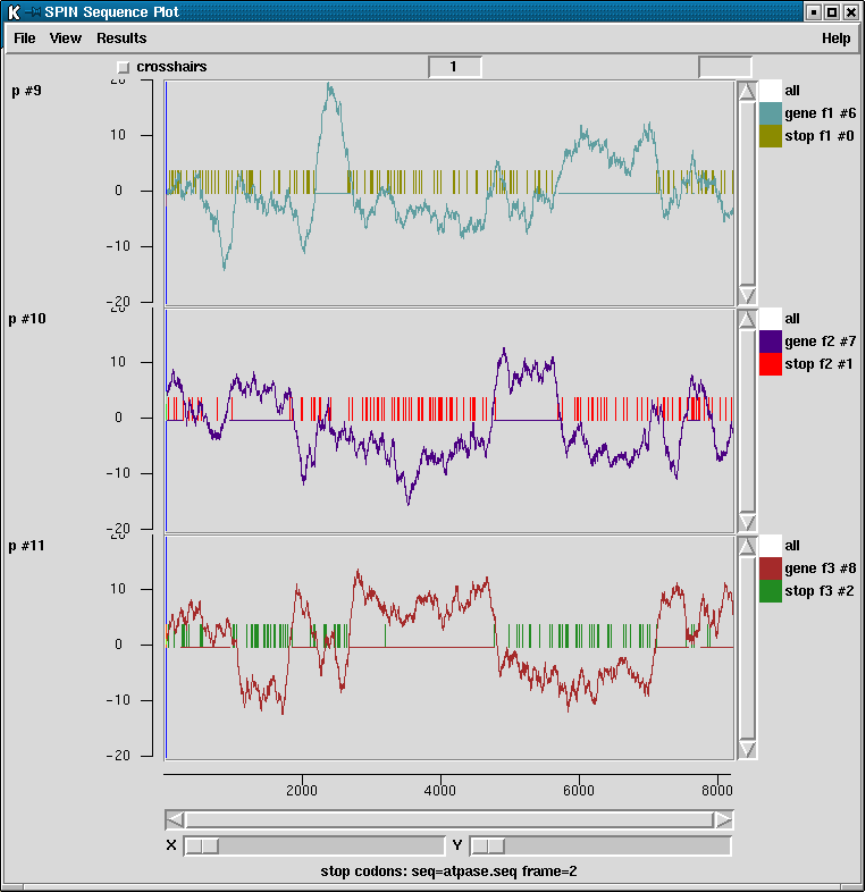
466 The Staden Package Manual
the open reading frames coincide with the highest scoring segments from the protein gene
prediction plots.
9.3.11.3 Codon usage method
This gene finding method is based on Staden, R. and McLachlan, A.D. (1982) Codon
preference and its use in identifying protein coding regions in long DNA sequences. Nucl.
Acid Res. 10, 141-156.
The current method contains a number of improvements on the original one. We are
trying to decide if each segment of the sequence is coding or non-coding. Each possibility is
represented by a model consisting of a table of expected codon usage. The calculation finds
Chapter 9: Analysing and comparing sequences using spin 467
the odds that each segment of the sequence fits either the coding or non-coding model, and
the results are plotted as log odds.
The results for each reading frame are plotted in the graphics window with frame 1 in
the top panel, frame 2 the middle and frame 3 in the bottom panel. Frame 1 is the frame
of the first base in the active region. At each position along the sequence the program
also plots a single dot for the reading frame with the highest score. These dots appear at
the midpoints of the three panels and will form a continuous line if one reading frame is
consistently the highest scoring.
The figure shown below shows a SPIN Sequence Plot containing the results of the codon
usage method on a sequence from C. elegans. This sequence has strong codon usage bias
and so produces clear results for the method. Here the results are for the standard codon
usage employing only the codon usage table shown below and a window length of 67 codons
(i.e. no table of codon usage for non-coding sequence was supplied, and no normalisation
was performed on the coding table). Compare the results to the other screen dump shown
later, which also uses a window of 67 codons.
Also visible in the figure are the cross hairs. Their x position is shown in sequence base
numbers in the left hand box above the plot, and the y coordinate, expressed using the score
values of the gene search, is shown in the right hand box. Each line in the window has its
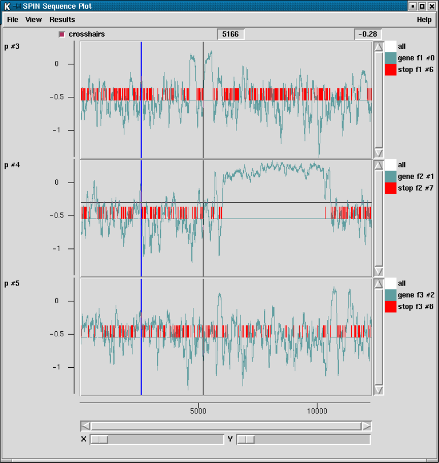
468 The Staden Package Manual
own colour and can be dragged and dropped to new locations to reorganise the plot. The
cursor in the plot can be used to control the position of the cursor in the sequence display.
As can be seen in the dialogue below the user can define the size of the scan window
in codons (note that the window length must be odd), the name of the file containing the
codon usage table, and the region of the sequence to be analysed. The longer the window
the smoother the plots but the more difficult it is to finds the ends of the coding segments.
The stronger the codon preference in the codon table the higher the discrimination between
coding and non-coding (assuming the sequence being analysed has the same preferences as
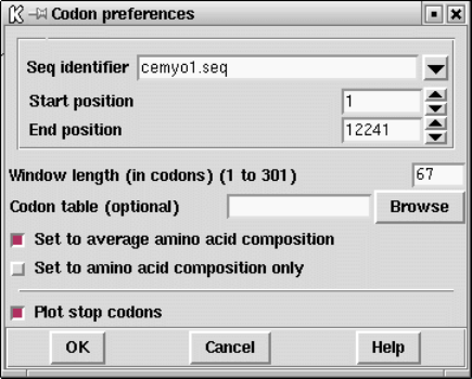
Chapter 9: Analysing and comparing sequences using spin 469
those of the table). Note also that the amino acid composition represented in the table will
also influence the results.
The user should supply the name of a file containing two concatenated codon usage
tables - the first being from coding sequence and the second from noncoding sequence.
This double codon table can be calculated by spin using the Codon Usage function (see
Section 9.3.4 [Calculate codon usage], page 448).
If the user gives the name of a file that contains only a single codon table the algorithm
will assume that it is from coding sequence, and will generate a noncoding table that consists
of the frequencies that would be expected if the sequence being analysed was random but
had the same base composition as the codon table.
If no table is specified the program will generate a codon usage table corresponding
to an average amino acid composition, and then derive a non-coding table from its base
composition. This is equivalent to the "positional base preferences"method, and hence
replaces it. More information about this method is given further down (see Section 9.3.11.4
[Positional base Preferences], page 472)
In addition the user can select to set the amino acid composition of the coding table to
have an average amino acid composition, and/or to have no codon preference (i.e. for each
amino acid the codon counts are equal, i.e. (TTT = TTC); (TTA = TTG = CTT = CTC
= CTA = CTG); ...; (GGT = GGC = GGA = GGG)). In the latter case the search uses
amino acid composition only.
The average amino composition used to normalise the values in the codon table is that
described by McCaldon and Argos McCaldon and Argos (1988), Proteins 4, 99-122.
The dialogue also allows the user to control whether or not the positions of stop codons
are included in the display.
Codon tables are scaled so that the sum of their values is 1000 and then any zero entries
are set to 1/1000. Stop codons in the coding table are made to be neutral by setting them
to the mean value for the table.
470 The Staden Package Manual
Example of the tables employed/calculated for an input coding table, no non-coding
table, and normalise to average amino acid composition.
Table read in:
===============================================
F ttt 3 S tct 29 Y tat 5 C tgt 9
F ttc 35 S tcc 21 Y tac 15 C tgc 5
L tta 2 S tca 6 * taa 0 * tga 0
L ttg 23 S tcg 9 * tag 0 W tgg 15
===============================================
L ctt 70 P cct 1 H cat 17 R cgt 37
L ctc 39 P ccc 2 H cac 15 R cgc 18
L cta 0 P cca 14 Q caa 87 R cga 1
L ctg 4 P ccg 0 Q cag 17 R cgg 1
===============================================
I att 32 T act 30 N aat 11 S agt 1
I atc 53 T acc 20 N aac 56 S agc 5
I ata 1 T aca 3 K aaa 21 R aga 36
M atg 31 T acg 0 K aag 115 R agg 0
===============================================
V gtt 28 A gct 69 D gat 57 G ggt 5
V gtc 22 A gcc 52 D gac 32 G ggc 1
V gta 7 A gca 6 E gaa 76 G gga 48
V gtg 4 A gcg 0 E gag 99 G ggg 1
===============================================
Chapter 9: Analysing and comparing sequences using spin 471
Program generates non-coding table from the base
composition of the coding table:
===============================================
F ttt 13 S tct 13 Y tat 12 C tgt 18
F ttc 13 S tcc 12 Y tac 12 C tgc 17
L tta 12 S tca 12 * taa 11 * tga 16
L ttg 18 S tcg 17 * tag 16 W tgg 24
===============================================
L ctt 13 P cct 12 H cat 12 R cgt 17
L ctc 12 P ccc 12 H cac 11 R cgc 17
L cta 12 P cca 11 Q caa 11 R cga 16
L ctg 17 P ccg 17 Q cag 16 R cgg 23
===============================================
I att 12 T act 12 N aat 11 S agt 16
I atc 12 T acc 11 N aac 11 S agc 16
I ata 11 T aca 11 K aaa 11 R aga 15
M atg 16 T acg 16 K aag 15 R agg 22
===============================================
V gtt 18 A gct 17 D gat 16 G ggt 24
V gtc 17 A gcc 17 D gac 16 G ggc 23
V gta 16 A gca 16 E gaa 15 G gga 22
V gtg 24 A gcg 23 E gag 22 G ggg 31
===============================================
472 The Staden Package Manual
Program generates coding table with average amino acid
composition and stops set to mean:
===============================================
F ttt 3 S tct 28 Y tat 8 C tgt 11
F ttc 36 S tcc 20 Y tac 24 C tgc 6
L tta 1 S tca 6 * taa 16 * tga 16
L ttg 15 S tcg 9 * tag 16 W tgg 13
===============================================
L ctt 46 P cct 3 H cat 12 R cgt 23
L ctc 25 P ccc 6 H cac 10 R cgc 11
L cta 0 P cca 42 Q caa 33 R cga 1
L ctg 3 P ccg 0 Q cag 7 R cgg 1
===============================================
I att 19 T act 33 N aat 7 S agt 1
I atc 32 T acc 22 N aac 37 S agc 5
I ata 1 T aca 3 K aaa 9 R aga 22
M atg 24 T acg 0 K aag 48 R agg 0
===============================================
V gtt 30 A gct 45 D gat 34 G ggt 7
V gtc 24 A gcc 34 D gac 19 G ggc 1
V gta 8 A gca 4 E gaa 27 G gga 63
V gtg 4 A gcg 0 E gag 35 G ggg 1
===============================================
9.3.11.4 Positional base preferences
This method for finding protein coding regions is a variant of the codon usage method.
Here, instead of measuring the closeness to an table of codon frequencies whose main dis-
criminating power is due codon preferences, we look for similarity to the codon usage that
would be expected from a protein sequence of average amino acid composition, but with no
codon preference. The method is surprisingly effective: When tested against all the E. coli
sequences in the EMBL sequence library it correctly identified the coding frame for 91% of
window positions. (The E. coli sequences were chosen only for technical reasons: we have no
reason to think the method would work less well on other organisms with roughly even base
composition.) Staden R. (1990) Finding protein coding regions in genomic sequences. In
Doolittle, R,R (ed), Methods in Enzymology, 183, Academic Press, San Diego, CA, 163-180.
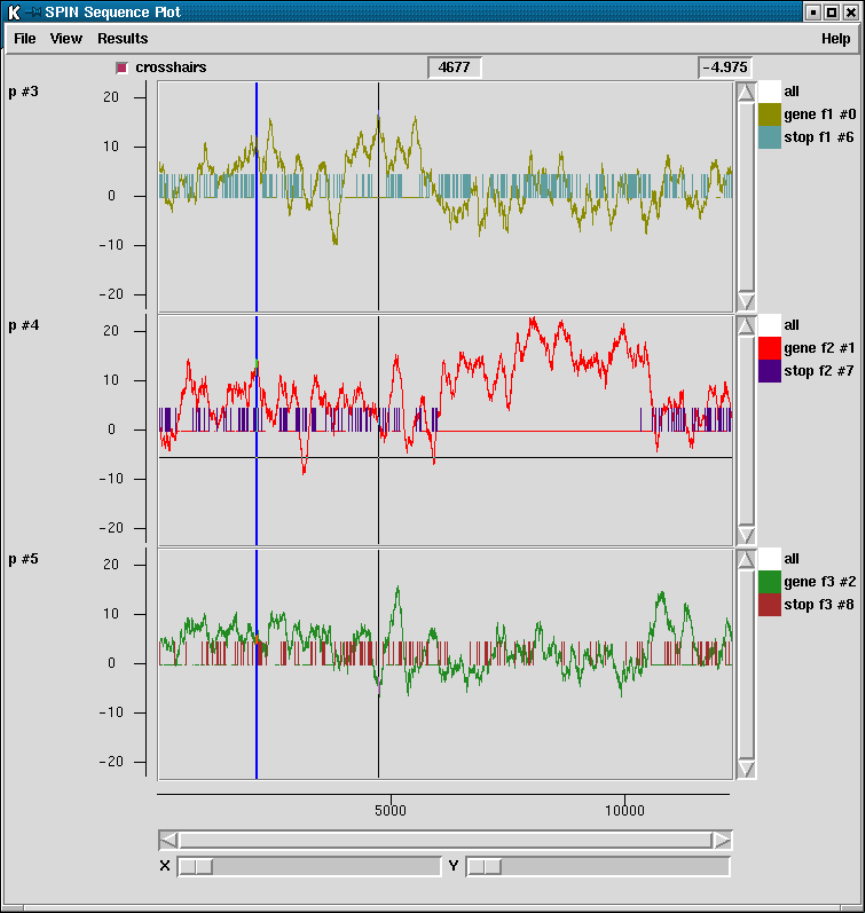
Chapter 9: Analysing and comparing sequences using spin 473
The average amino composition used to derive the values in the codon table is that
described by McCaldon and Argos McCaldon and Argos (1988), Proteins 4, 99-122.
Above is the result of applying this method to the C. elegans sequence analysed above
with a codon preference table. Note that, as would be expected, the main difference is the
that the range of observed scores is very much reduced.
9.3.11.5 Author test
This is an unpublished method for distinguishing between coding and noncoding segments
of a DNA sequence. It is basically an extension of the Codon Usage method in which we
compare the sequence to two tables of codon usage to see which of the two it is most like.
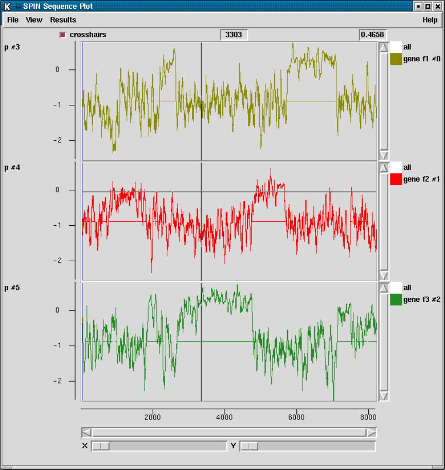
474 The Staden Package Manual
One table should contain typical codon usage from a coding sequence and the other typical
codon usage from a noncoding region. It is based on methods used to decide authorship of
text - is the usage of words (codons) more like that of author A (coding) or that of author
B (noncoding)?
The results for each reading frame are plotted in the graphics window with frame 1 in the
top panel, frame 2 the middle and frame 3 in the bottom panel. Frame 1 is the frame of the
first base in the active region. At each position along the sequence the program also plots a
single dot for the reading frame with the highest score. These dots appear at the midpoints
of the three panels and will form a continuous line if one reading frame is consistently the
highest scoring. The figure shows a SPIN Sequence Plot containing the results of the author
Chapter 9: Analysing and comparing sequences using spin 475
test method on a sequence from E. coli. Also visible are the cross hairs. Their x position is
shown in sequence base numbers in the left hand box above the plot, and the y coordinate,
expressed using the score values of the gene search, is shown in the right hand box. Each
line in the window has its own colour and can be dragged and dropped to new locations to
reorganise the plot. The cursor in the plot can be used to control the position of the cursor
in the sequence display.
476 The Staden Package Manual
A typical pair of concatenated codon tables for use by the Author test
===============================================
F ttt 0 S tct 6 Y tat 2 C tgt 3
F ttc 3 S tcc 8 Y tac 6 C tgc 0
L tta 0 S tca 0 * taa 0 * tga 0
L ttg 1 S tcg 0 * tag 0 W tgg 0
===============================================
L ctt 1 P cct 0 H cat 0 R cgt 12
L ctc 1 P ccc 0 H cac 4 R cgc 5
L cta 1 P cca 2 Q caa 2 R cga 0
L ctg 19 P ccg 7 Q cag 12 R cgg 0
===============================================
I att 5 T act 3 N aat 2 S agt 2
I atc 22 T acc 6 N aac 7 S agc 1
I ata 0 T aca 1 K aaa 8 R aga 0
M atg 8 T acg 0 K aag 2 R agg 0
===============================================
V gtt 14 A gct 12 D gat 7 G ggt 16
V gtc 1 A gcc 4 D gac 9 G ggc 11
V gta 7 A gca 8 E gaa 14 G gga 0
V gtg 4 A gcg 5 E gag 2 G ggg 0
===============================================
===============================================
F ttt 16 S tct 8 Y tat 8 C tgt 12
F ttc 7 S tcc 0 Y tac 4 C tgc 8
L tta 7 S tca 9 * taa 14 * tga 6
L ttg 7 S tcg 5 * tag 2 W tgg 17
===============================================
L ctt 4 P cct 5 H cat 7 R cgt 4
L ctc 1 P ccc 0 H cac 7 R cgc 8
L cta 2 P cca 2 Q caa 3 R cga 4
L ctg 6 P ccg 1 Q cag 7 R cgg 4
===============================================
I att 5 T act 3 N aat 3 S agt 4
I atc 2 T acc 5 N aac 1 S agc 1
I ata 6 T aca 8 K aaa 13 R aga 7
M atg 4 T acg 5 K aag 9 R agg 6
===============================================
V gtt 5 A gct 2 D gat 3 G ggt 3
V gtc 3 A gcc 4 D gac 3 G ggc 5
V gta 2 A gca 4 E gaa 3 G gga 2
V gtg 5 A gcg 5 E gag 2 G ggg 5
===============================================
The mathematical treatment of the data is very different from that of the codon usage
method.
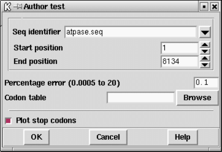
Chapter 9: Analysing and comparing sequences using spin 477
Given the two tables of codon usage the algorithm works out the optimal weighting to
give each codon to obtain the best discrimination between coding and noncoding sequence.
The user sets the expected error rate as a percentage and the algorithm will choose the
corresponding window length to use for the analysis.
The user should supply the name of a file containing two concatenated codon usage
tables - the first being from coding sequence and the second from noncoding sequence.
This double codon table can be calculated by spin using the Codon Usage function (see
Section 9.3.4 [Calculate codon usage], page 448).
If the user gives the name of a file that contains only a single codon table the algorithm
will assume that it is from coding sequence, and will generate a noncoding table that consists
of the frequencies that would be expected if the sequence being analysed was random. The
region to be analysed can also be set.
9.3.11.6 Uneven positional base preferences
This method is used to find regions of a sequence that code for a protein. It is based on
the method of Fickett Fickett,J. (1982) Nucl. Acid Res.10, and unlike the other methods
currently in the package does not attempt to say either which strand or frame is likely to
be coding, only which regions of the sequence.
The method looks for sections of the sequence in which the frequencies at which each of
the four bases occupy the three positions in codons is nonrandom. The level of nonrandom-
ness is plotted on a scale that shows the probability that the sequence is coding. At each
position along a sequence the calculation gives the same value for all six possible reading
frames, so only one value is plotted. Seventy six percent of coding regions score above 0.78
and 76% of noncoding regions below 0.78. No known window in a coding region has a value
below 0.4, but 14% of windows in noncoding sequences score below it. No known window
in a noncoding region reaches a score of 1.34, but this score is reached by 16% of known
coding regions. These statements are now very much out of date.
The method was first described in Staden R. (1984) Nucl. Acid Res. 12, 551-567. It
looks through the sequence in one fixed phase and counts the number of times each base ap-
pears in each of the three codon positions: for each window position it counts A1,A2,A3 and
C1,C2,C3 and G1,G2,G3 and T1,T2,T3 and calculates AMEAN=(A1+A2+A3)/3, and simi-
larly CMEAN, GMEAN and TMEAN; it then calculates ADIF=abs(A1- AMEAN)+abs(A2-
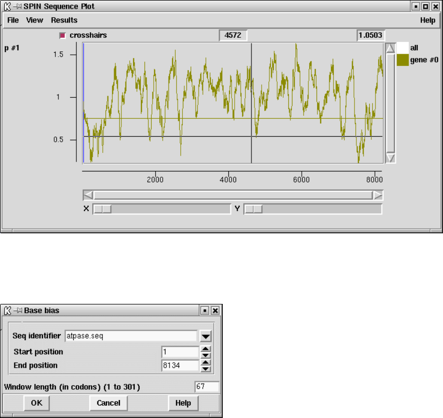
478 The Staden Package Manual
AMEAN)+abs(A3-AMEAN) and similarly CDIF, GDIF and TDIF to measure the differ-
ences between an even base usage for all positions in the codons and the observed usage.
The routine then calculates and plots the sum ADIF+CDIF+GDIF+TDIF.
In the figure shown below it will be seen that much of the sequence being analysed
appears to be coding, and this is indeed the case. Many of the troughs between peaks
correspond to the ends of genes in this E. coli sequence (which was not a good choice to
illustrate the method!). The horizontal line is at 76%. 76% of coding regions achieve values
above this line and 76% of noncoding regions achieve scores below the line.
As can be seen in the dialogue below the user can set the window length in codons
(although around 67 codons is generally suitable) and can restrict the search to a sub
region of the sequence. Note that the window length must be odd.
9.3.11.7 Splice site search
This method is used to search for mRNA splice junctions using a weight matrix. The default
weight matrix is still that derived from the paper of Mount S.M, (1982) Nucl. Acids Res.
10, 459-472, but we are about to create a whole new set which will be organism specific,
and will include them in later releases and make them available via ftp.
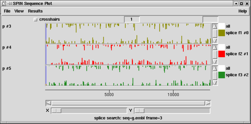
Chapter 9: Analysing and comparing sequences using spin 479
The results are displayed in three colours, one colour for each reading frame. The donors
are plotted upwards from the base of the panel and the acceptors are plotted downwards
from the top of the panel. The donors and acceptors with the same colour are compatible;
eg red donors are compatible with red acceptors. Of course it is the combination of reading
frame and splice sites that really matters, so donors and acceptors drawn in different colours
can be compatible if the reading frame changes. By default all the sites are drawn in the
same plot but in the figure shown below they have been separated by reading frame using
the programs ability to reorganise the positions of graphical results. This layout of the
donors and acceptors is designed to fit with the gene search methods and stop codon plots.
The results are plotted as Log-Odds.
The frequency table shown below is used as a weight matrix and AG and GT are oblig-
atory at the appropriate positions.
Mount acceptors redone 16-4-91
18 15 0.0 10.0
P -14 -13 -12 -11 -10 -9 -8 -7 -6 -5 -4 -3 -2 -1 0 1 2 3
N 113 113 113 113 113 113 113 113 113 113 113 113 113 113 113 113 113 113
T 58 50 57 59 67 56 58 49 47 66 64 31 34 0 0 11 41 31
C 21 28 34 25 29 33 35 32 42 40 33 25 74 0 0 23 28 41
A 17 11 11 18 7 17 12 23 15 3 10 29 5 113 0 24 21 21
G 17 24 11 11 10 7 8 9 9 4 6 28 0 0 113 55 23 20
Mount donors redone 16-4-91
12 4 0.0 8.0
P-2-10123456789
N 136 136 136 136 136 136 136 136 136 136 136 136
T 28 8 15 17 0 136 9 16 7 84 30 36
C 41 60 16 7 0 0 3 13 3 17 28 39
A 40 56 89 12 0 0 83 91 12 23 53 33
G 27 12 16 100 136 0 41 16 114 12 25 28
480 The Staden Package Manual
9.3.11.8 tRNA search
This method is used to find segments of a sequence that might code for tRNAs. It looks for
potential cloverleaf forming structures and then for the presence of the expected conserved
bases. It presents results graphically and draws out the cloverleafs.
The algorithm uses a large number of parameters including some loop lengths, scores for
each of the four stems, and scores for the conserved bases, but we have not yet included an
interface for setting these. We apologise for this and plan to add the interface in a future
release. Using individual base pair scores of A-T = G-C = 2, G-T = 1, in its present form
the algorithm is set to search for segments of sequence satisfying the following minimum
scores:
•aminoacyl stem 12
•tu stem 9
•anticodon stem 8
•du stem 4
•minimum total stem score 36
•minimum number of conserved bases 16
•no introns
The algorithm was first described in Staden,R. (1980) A computer program to search for
tRNA genes. Nucl. Acid Res 8, 817-825, but has been completely rewritten since then. The
tRNAs that have been sequenced so far have two characteristics that can be used to locate
their genes within long DNA sequences. Firstly they have a common secondary structure -
the cloverleaf - and secondly, particular bases almost always appear at certain positions in
the cloverleaf. The cloverleaf is composed of four base-paired stems and four loops. Three of
the stems are of fixed length but the fourth, the dhu stem which usually has four base pairs,
sometimes has only three. All of the loops can vary in size. The following relationships
between the stems in the cloverleaf are assumed in the program: (a) there are no bases
between one end of the aminoacyl stem and the adjoining tuc stem; (b) there are two bases
between the aminoacyl stem and the dhu stem; (c) there is one base between the dhu stem
and the anticodon stem; (d) there are at least three bases between the anticodon stem and
the tuc stem. The program looks first for cloverleaf structure and then for conserved bases.
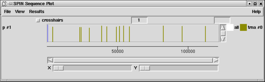
Chapter 9: Analysing and comparing sequences using spin 481
The output shows the position of the possible gene in the sequence by a vertical line
the height of which shows the number of basepairs made in the stems. Typical graphical
output:

482 The Staden Package Manual
The cloverleaf structure is also drawn in the text Output Window. Typical text output:
9.4 Spin Comparison Functions
Spin contains three functions for finding local segments of similarity between pairs
of sequences (see Section 9.4.1 [Finding Similar Spans], page 483), (see Section 9.4.2
[Finding Matching Words], page 485) and (see Section 9.4.5 [Aligning Sequences Locally],
page 493), and two for finding global similarity (see Section 9.4.3 [Finding the Best
Diagonals], page 487) and (see Section 9.4.4 [Aligning Sequences Globally], page 489).
All functions produce results which are plotted in a dot matrix display called a SPIN
Sequence Comparison Plot. Obviously global similarity consists of many small matching
segments and so the local similarity searches, when plotted, will also reveal any larger
scale relationships.

Chapter 9: Analysing and comparing sequences using spin 483
9.4.1 Finding Similar Spans
This method was first described by McLachlan Mclachlan,A.D. Tests for comparing related
amino acid sequences J. Mol. Biol. 61, 409-424 (1971). It involves calculating a score for
each position in the plot by summing points found when looking forwards and backwards
along a diagonal line of a given length (window length). The algorithm does not simply look
for identity but uses a score matrix that contains scores for every possible pair of character
types. At each point that the score is above a minimum score, a match is saved. The matches
are plotted as a single point in the SPIN Sequence Comparison Plot, corresponding to the
centre of the matching span (see Section 9.6.3 [SPIN Sequence Comparison Plot], page 512)
(Although see "Rescan matches, below).
The dialogue box (shown above) requests the horizontal and vertical sequences and their
ranges (see Section 9.8.4 [Selecting a sequence], page 522), the window span length and the
minimum score. Only results above this minimum score are plotted. The default value
for the minimum score is one that would produce approximately 500 matches between two
random sequences of the same composition as the two under investigation (see Section 9.5.1
[Probabilities and expected number of matches], page 498). This value of 500 can be changed
using the "Configure default number of matches"option of the "Options"menu on the main
menubar (see Section 9.5.3 [Changing the default number of matches], page 498). The upper
and lower limits of the minimum score are similarly determined except that the expected
number of matches for the upper limit is 0 and for the lower limit is "maximum number of
matches". The "maximum number of matches"value can be altered if more matches are
required to be plotted by using the "Configure maximum number of matches"option of the
"Options"menu (see Section 9.5.2 [Changing the maximum number of matches], page 498).
Further operations available for find similiar spans are:
Information
This command gives a brief description of the sequences used in the comparison,
the input parameters used and the number of matches found.
484 The Staden Package Manual
horizontal EMBL: hsproperd
vertical EMBL: mmproper
window length 11 min match 9
number of matches 1772
Results
A detailed listing of all the hits found is displayed in the Output Window.
Positions 2 h 630 v and score 9
Percentage mismatch 18.2
2 12
H agcctatcaac
::::::: : :
V agcctatgagc
630 640
Positions 7 h 369 v and score 9
Percentage mismatch 18.2
7 17
H atcaacccaga
: ::::::::
V aggaacccaga
369 379
Tabulate Scores
This option lists scores, probabilities, and their expected and observed numbers
of matches.
score 9 probability 1.73e-04 expected 365 observed 1772
score 10 probability 1.17e-05 expected 25 observed 601
score 11 probability 3.60e-07 expected 1 observed 149
Rescan matches
It is also possible to plot a dot for each residue with a score above a minimum
value within each matching span using the "Rescan matches"command. This is
only a temporary result and will be destroyed if the SPIN Sequence Comparison
Plot is altered (see Section 9.5 [Controlling and Managing Results], page 497).
Configure This option allows the line width and colour of the matches to be altered. See
Section 10.6 [Colour Selector], page 529. A colour browser is displayed from
which the desired line width or colour can be configured. Pressing OK will
update the SPIN Sequence Comparison Plot.
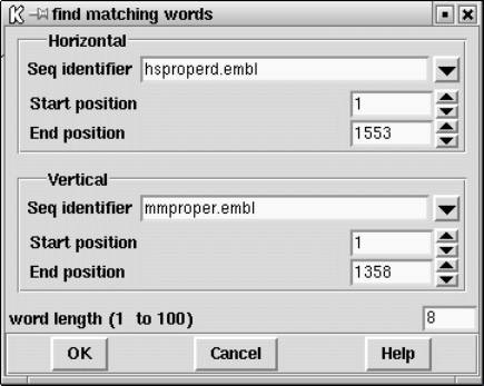
Chapter 9: Analysing and comparing sequences using spin 485
Display sequences
Selecting this command invokes the SPIN Sequence Comparison Display (see
Section 9.6.4 [Sequence comparison display], page 514). Moving the cursor in
the sequence display will move the cursors of the same sequence in any SPIN
Sequence Comparison Plot (see Section 9.6.3.1 [Cursors], page 513). To force
the sequence display to show the nearest match, use the "nearest match"button
in the sequence display plot. To force the sequences to maintain their current
register activate the "Lock"button.
Hide This option removes the points from the SPIN Sequence Comparison Plot but
retains the information in memory.
Reveal This option will redisplay previously hidden points in the SPIN Sequence Com-
parison Plot.
Remove This command removes all the information regarding this particular invocation
of Find similar spans and access to this data lost.
9.4.2 Finding Matching Words
The find matching words routine finds runs of identical characters in the sequence. Its main
value is speed, being hundreds of times faster than the find similar spans function. It is of
course not very sensitive but is useful for long DNA sequences.
The dialogue allows the horizontal and vertical sequences and their ranges to be selected
(see Section 9.8.4 [Selecting a sequence], page 522). The word length is the minimum number
of consecutive matching characters. All runs of identical characters that are at least as long
as the word length will produce a line on the SPIN Sequence Comparison Plot of length
proportional to the actual word length (see Section 9.6.3 [SPIN Sequence Comparison Plot],
page 512).
Further operations available for find matching words are:
Information
This command gives a brief description of the sequences used in the comparison,
the input parameters used and the number of hits found.
486 The Staden Package Manual
horizontal EMBL: hsproperd
vertical EMBL: mmproper
word length 8
Number of matches 140
Results A detailed listing of all the matching words is obtained in the Output Window.
The horizontal (h) and vertical (v) positions of the beginning of the match are
listed along with the length of the match and the match itself.
Positions 162 h 4 v and length 14
ttcacccagtatga
Positions 225 h 67 v and length 18
gaagactgctgtctcaac
Positions 509 h 118 v and length 8
ctctgtca
Positions 276 h 118 v and length 9
ctctgtcag
Positions 288 h 130 v and length 8
tgcaggtc
Positions 626 h 131 v and length 8
gcaggtct
Positions 1208 h 144 v and length 8
atggtcag
Tabulate scores
This option lists scores, probabilities, and their expected and observed numbers
of matches.
Chapter 9: Analysing and comparing sequences using spin 487
score 8 probability 2.06e-05 expected 43 observed 140
score 9 probability 5.35e-06 expected 11 observed 67
score 10 probability 1.39e-06 expected 3 observed 45
score 11 probability 3.60e-07 expected 1 observed 35
score 12 probability 9.35e-08 expected 0 observed 22
score 13 probability 2.43e-08 expected 0 observed 18
score 14 probability 6.30e-09 expected 0 observed 17
score 15 probability 1.63e-09 expected 0 observed 11
score 16 probability 4.24e-10 expected 0 observed 9
score 17 probability 1.10e-10 expected 0 observed 9
score 18 probability 2.86e-11 expected 0 observed 8
score 19 probability 7.42e-12 expected 0 observed 6
score 20 probability 1.93e-12 expected 0 observed 5
score 21 probability 5.00e-13 expected 0 observed 3
score 22 probability 1.30e-13 expected 0 observed 2
score 23 probability 3.37e-14 expected 0 observed 2
score 24 probability 8.74e-15 expected 0 observed 2
Configure This option allows the line width and colour of the matches to be altered. See
Section 10.6 [Colour Selector], page 529. A colour browser is displayed from
which the desired line width or colour can be configured. Pressing OK will
update the SPIN Sequence Comparison Plot.
Display sequences
Selecting this command invokes the sequence display (see Section 9.6.4 [Se-
quence comparison display], page 514). Moving the cursor in the sequence
display will move the cursors of the same sequence in any SPIN Sequence Com-
parison Plot (see Section 9.6.3.1 [Cursors], page 513). To force the sequence
display to show the nearest match, use the "nearest match"button in the se-
quence display plot.
Hide This option removes the points from the SPIN Sequence Comparison Plot but
retains the information in memory.
Reveal This option will redisplay previously hidden points in the SPIN Sequence Com-
parison Plot.
Remove This command removes all the information regarding this particular invocation
of Find matching words, and access to this data is lost.
9.4.3 Finding the Best Diagonals
This option is among the fastest and can be useful for a quick comparison of two long
DNA sequences. The algorithm is as follows. First it finds the positions of runs of identical
characters ("words") of length word length, as for the find matching words algorithm. These
words are accumulated in an imaginary SPIN Sequence Comparison Plot and the number
of hits on each diagonal is summed to produce a histogram. The histogram is analysed
to find its mean and standard deviation. The diagonals that lie above some cutoff score
(defined in standard deviation units), are rescanned using the find similar spans algorithm.

488 The Staden Package Manual
Any window lengths reaching the cutoff score produce a dot which is plotted in the usual
way.
The dialogue box requests horizontal and vertical sequences and their ranges (see
Section 9.8.4 [Selecting a sequence], page 522), the minimum number of identical characters
in a run "word length", the minimum standard deviation, the window length and the
minimum score.
The points are plotted to the SPIN Sequence Comparison Plot (see Section 9.6.3 [SPIN
Sequence Comparison Plot], page 512).
Further operations available for find best diagonals are:
Information
This command gives a brief description of the sequences used in the comparison
and the input parameters used.
horizontal EMBL: hsproperd
vertical EMBL: mmproper
window length 11 minimum score 9 word length 8 minimum sd 3.000000
Results A listing of all the matches is obtained in the Output Window. The horizontal
(h) and vertical (v) positions of the beginning of the match are listed.
Chapter 9: Analysing and comparing sequences using spin 489
Positions 1066 h 905 v
Positions 1067 h 906 v
Positions 1068 h 907 v
Positions 1069 h 908 v
Positions 1070 h 909 v
Positions 1071 h 910 v
Positions 1072 h 911 v
Positions 1073 h 912 v
Positions 1074 h 913 v
Configure This option allows the line width and colour of the matches to be altered. See
Section 10.6 [Colour Selector], page 529. A colour browser is displayed from
which the desired line width or colour can be configured. Pressing OK will
update the SPIN Sequence Comparison Plot.
Display sequences
Selecting this command invokes the sequence display (see Section 9.6.4 [Se-
quence comparison display], page 514). Moving the cursor in the sequence
display will move the cursors of the same sequence in any SPIN Sequence Com-
parison Plot (see Section 9.6.3.1 [Cursors], page 513). To force the sequence
display to show the nearest match, use the "nearest match"button in the se-
quence display plot.
Hide This option removes the points from the SPIN Sequence Comparison Plot but
retains the information in memory.
Reveal This option will redisplay previously hidden points in the SPIN Sequence Com-
parison Plot.
Remove This command removes all the information regarding this particular invocation
of Find best diagonals, and access to this data is lost.
9.4.4 Aligning Sequences Globally
This function will produce an optimal global alignment of two segments of the sequence.
The dynamic programming alignment algorithm is based on Huang,X On global sequence
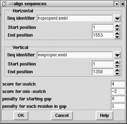
490 The Staden Package Manual
alignment. CABIOS 10 227-235 (1994). There is no length limit of the sequences but the
sequences to be aligned should be of the same type i.e. both be DNA or both protein.
A dialogue box (shown above) requests the horizontal and vertical sequences and the
ranges over which they are to be aligned (see Section 9.8.4 [Selecting a sequence], page 522)
and the gap start penalty and the gap extension penalty. In addition, if the sequence is
DNA, the "score for match"and "score for mis-match"must be provided. These values are
used to generate a score matrix. For protein sequences, the score matrix can be changed
from the "Options"menu (see Section 9.5.5 [Changing the score matrix], page 499).
The alignment is displayed in the Output Window along with the percentage mismatch
(see below) and on the SPIN Sequence Comparison Plot as a line. The line represents the
path of the alignment.
The following plot shows a global alignment of two Xenopus Laevis sequences. The
vertical sequence (xlactcag) is genomic DNA, and the horizontal sequence (xlacacr) is the

Chapter 9: Analysing and comparing sequences using spin 491
corresponding cDNA. The vertical sections of the plotted path correspond to introns in the
genomic DNA, which are obviously absent from the cDNA.
Below we show a typical alignment (from a different pair of sequences) as produced in
the Output Window.

492 The Staden Package Manual
Percentage mismatch 29.6
1 11 21 31 41 51
hsproperd gagcctatcaacccagataaagcgggacctcctctctggtagaggtgcagggggcagtac
mmproper ************************************************************
-157 -147 -137 -127 -117 -107
61 71 81 91 101 111
hsproperd tcaacatgatcacagagggagcgcaggcccctcgattgttgctgccgccgctgctcctgc
mmproper ************************************************************
-97 -87 -77 -67 -57 -47
121 131 141 151 161 171
hsproperd tgctcaccctgccagccacaggctcagaccccgtgctctgcttcacccagtatgaagaat
:: :::::::::::::: :: :
mmproper **************************************tgtttcacccagtatgaggagt
-37 -27 -17 -7 3 13
181 191 201 211 221 231
hsproperd cctccggcaagtgcaagggcctcctggggggtggtgtcagcgtggaagactgctgtctca
:::: :::: :::::: ::::: :: ::: : : :::: :: ::::::::::::::::
mmproper cctctggcaggtgcaaaggcctacttgggagagacatcagggtagaagactgctgtctca
23 33 43 53 63 73
The two aligned sequences are automatically saved in memory and can be accessed
through the sequence manager. They are assigned default filenames which are based on
the parent with the addition of a"number"where "number"is a unique identifier (see the
twelth and thirteenth entries of the sequence manager picture (see Section 9.8.3 [Sequence
manager], page 519).
Further operations available for align sequences are:
Information
This command gives a brief description of the sequences used in the comparison
and the input parameters used.
horizontal PERSONAL: m13mp18.seq from 1 to 7250
vertical PERSONAL: lawrist7.seq from 1 to 5261
Configure This option allows the line width and colour of the matches to be altered. See
Section 10.6 [Colour Selector], page 529. A colour browser is displayed from
which the desired line width or colour can be configured. Pressing OK will
update the SPIN Sequence Comparison Plot.
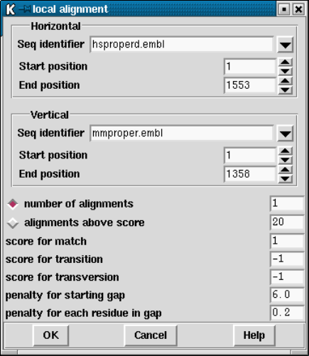
Chapter 9: Analysing and comparing sequences using spin 493
Display sequences
Selecting this command invokes the Sequence Comparison Display (see
Section 9.6.4 [Sequence comparison display], page 514). Moving the cursor in
the sequence display will move the cursors of the same sequence in any SPIN
Sequence Comparison Plot (see Section 9.6.3.1 [Cursor], page 513). To force
the sequence display to show the nearest match, use the "nearest match"
button in the sequence display plot.
Hide This option removes the points from the SPIN Sequence Comparison Plot but
retains the information in memory.
Reveal This option will redisplay previously hidden points in the SPIN Sequence Com-
parison Plot.
Remove This command removes all the information regarding this particular invocation
of Align sequences, and access to this data is lost.
9.4.5 Aligning Sequences Locally
The local alignment routine is based around the program SIM by Huang and Miller which
is an implementation of the Smith-Waterman algorithm Huang,X.Q. & Miller, W. A Time-
Efficient, Linear-Space Local Similarity Algorithm. Advances in Applied Mathematics 12
337-357 (1991).
SIM finds k best non-intersecting alignments between two sequences or within a single
sequence using dynamic programming techniques. The alignments are reported in order of
decreasing similarity score and share no aligned pairs. SIM requires space proportional to
the sum of the input sequence lengths and the output alignment lengths, so it accommodates
100,000-base sequences on a workstation. Both sequences must be of the same type, ie both
be DNA or both be protein.
494 The Staden Package Manual
A dialogue box (shown above) requests the horizontal and vertical sequences and the
ranges over which they are to be aligned (see Section 9.8.4 [Selecting a sequence], page 522).
Either a specified number of alignments can be requested or alternatively, all alignments
above a certain score. If the sequence is DNA, the scores for a matching aligned pair, a
transition and a transversion must be provided. These values are used to generate a score
matrix. For protein sequences, the score matrix can be changed from the "Options"menu
(see Section 9.5.5 [Changing the score matrix], page 499). Both DNA and protein sequences
require the penalty for opening a gap and the penalty for gap extension.
The alignments are displayed in the Output Window along with the percentage mismatch
(see below) and on the SPIN Sequence Comparison Plot as a series of lines, each line
corresonding to a single alignment. The line represents the path of alignments.
The following two plots show local alignments of two Xenopus Laevis sequences. The
vertical sequence (xlactcag) is genomic DNA, and the horizontal sequence (xlacacr) is the
corresponding cDNA.
The first plot is of a local alignment using a higher than default penalty for each residue
in the gap (1 as opposed to 0.2). It has also been specified that all alignments scoring more
than 20 are to be shown. The result of this is seven aligned regions, represented by seven

Chapter 9: Analysing and comparing sequences using spin 495
diagonal lines in the plot. These regions correspond to the exons that are present in both
sequences, separated by the introns that are only present in the genomic sequence.
The second plot shows the result for the same two sequences when the default gap
penalty is accepted and when only the highest scoring alignment is displayed. This best
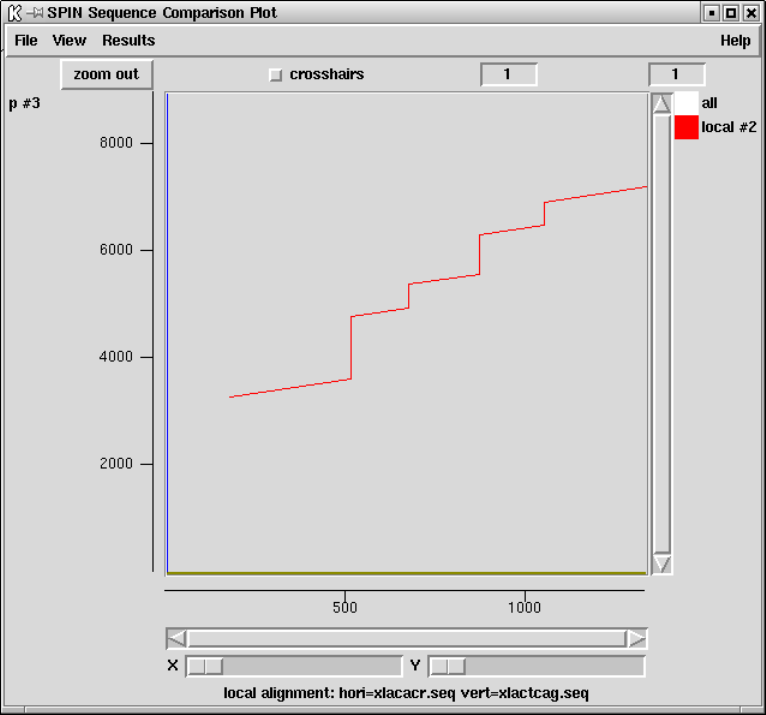
496 The Staden Package Manual
alignment covers five of the seven exons identified in the previous plot, with the lower gap
penalty allowing it to span the introns that separate them.
Below is a typical aligment as written to the Output Window.
Percentage mismatch 35.7
438 448 458 468 478 488
h caggcctgtgaggaccagcagtgctgtcctgagatgggcggctggtctggctgggggccc
::::::::::: :::: :: ::: :: :: : :::: : :::::: :::
m caggcctgtgacacccagaagacctgccccacacatggggcctgggcatcctggggcccc
451 461 471 481 491 501
498 508 518
h tgggagccttgctctgtcacctgc
::: :: :::: : :::::
m tggagcccccgctcaggatcctgc
511 521 531
Chapter 9: Analysing and comparing sequences using spin 497
Further operations available for local alignments are:
Information
This command gives a brief description of the sequences used in the comparison
and the input parameters used.
horizontal PERSONAL: h from 1 to 1553
vertical PERSONAL: m from 1 to 1358
number of alignments 3
score for match 1
score for transition -1
score for transversion -1
penalty for starting gap 6
penalty for each residue in gap 0.2
Configure This option allows the line width and colour of the matches to be altered. See
Section 10.6 [Colour Selector], page 529. A colour browser is displayed from
which the desired line width or colour can be configured. Pressing OK will
update the SPIN Sequence Comparison Plot.
Display sequences
Selecting this command invokes the Sequence Comparison Display (see
Section 9.6.4 [Sequence comparison display], page 514). Moving the cursor in
the sequence display will move the cursors of the same sequence in any SPIN
Sequence Comparison Plot (see Section 9.6.3.1 [Cursor], page 513). To force
the sequence display to show the nearest match, use the "nearest match"
button in the sequence display plot.
Hide This option removes the points from the SPIN Sequence Comparison Plot but
retains the information in memory.
Reveal This option will redisplay previously hidden points in the SPIN Sequence Com-
parison Plot.
Remove This command removes all the information regarding this particular invocation
of Local alignment, and access to this data is lost.
9.5 Controlling and Managing Results
Spin allows the parameters for each analytical option to be set in dialogues immediately
prior to their execution, but there are other global parameters which can influence the
results obtained, and they are described here.
This section also covers, in its description of the "Results Manager"how results can be
manipulated after they have been obtained. As this implies, almost all searches conducted
by spin produce results that are retained until the user explicitly deletes them, and these
are termed "Permanent results". Any other results are termed "Temporary". At present,
the only temporary results are those produced by a variant of the Similar Spans algorithm,
(see Section 9.4.1 [Finding Similar Spans], page 483), in which the plot can be overlayed by
marking every identical character in each matching span with separate dots. These extra
498 The Staden Package Manual
dots are not stored as results and any changes to the SPIN Sequence Comparison Plot, for
example plotting new data, will destroy them.
9.5.1 Probabilities and expected numbers of matches
To suggest reasonable ranges of cutoff scores for the Similar Spans (see Section 9.4.1 [Finding
Similar Spans], page 483) and Matching Words (see Section 9.4.2 [Finding Matching Words],
page 485) comparison functions, and later to help users assess the significance of the matches
found between sequences, spin calculates their probabilities and the expected number of
matches Staden R, Methods for calculating the probabilities of finding patterns in sequences.
CABIOS 5 89-96 (1989). For both algorithms the probability depends on the composition
of the two sequences, the cutoff score, and, for the matching spans algorithm, the score
matrix. The probability is the chance of finding the given score in infinitely long random
sequences of the same composition as the pair being compared. The expected number of
matches for any score is calculated by multiplying its probability value by the product of
the lengths of the two sequences. Note that no correction is made for the case of comparing
a sequence against itself.
The matches found for these two algorithms can be assessed by selecting the Tabulate
Scores option, which will produce a list of observed and expected results as shown in the
example below.
score 9 probability 1.73e-04 expected 365 observed 1772
score 10 probability 1.17e-05 expected 25 observed 601
score 11 probability 3.60e-07 expected 1 observed 149
In this case there are clearly many more matches at each score level than would be
expected by chance.
9.5.2 Changing the maximum number of matches
The maximum number of matches is a guideline limit to the number of matches that a
comparison function is allowed to produce. In conjunction with the probability calculations
its value is used to determine the range of scores allowed for an option - for example, the
lowest "minimum score"for the "find similar spans"function (see Section 9.4.1 [Finding
Similar Spans], page 483). Altering the maximum number of matches value will in turn
alter the range of scores available in a function. Note that this maximum only provides a
guideline and each function will always attempt to calculate all matches. However, if the
scores are set too low, and the sequences are long, very large numbers of matches matches
may be produced and the functions may run slowly as the program gobbles up increasing
amounts of memory to store them.
The maximum number of matches is altered using the Options menu.
9.5.3 Changing the default number of matches
The default number of matches is used to determine the default score in the function
dialogue boxes. If the two sequences being analysed were scrambled (i.e. had the order of
their bases or amino acids changed randomly) and then compared using the default score,
they should be found to contain approximately the default number of matches. Hence this
Chapter 9: Analysing and comparing sequences using spin 499
number provides users with a crude assessment of the significance of the matches found: if
more than the default number are found, the sequences are more similar than is likely by
chance.
The default number of matches is altered using the Options menu.
9.5.4 Hide duplicate matches
If the horizontal and vertical sequences are the same the comparison plots would be a mirror
image about the main diagonal. In this case the default is that only the lower half of the
plot is calculated. If the "Hide duplicate matches"checkbutton is not set the entire plot
will be displayed. It is important to note this property of the algorithms: if only one half
of the plot is displayed the main diagonal has been found to be identical!
9.5.5 Changing the score matrix
This option allows users to select their own score matrix for protein sequence comparison
and is available from the "Options"menu which invokes a dialogue box. Enter the full
filename of the matrix in the entry box. Clicking on the "browse"button will invoke a file
browser. See Section 10.7 [File Browser], page 529.
The recommended format for the matrices is that used by blast Altschul, Stephen F.,
Warren Gish, Webb Miller, Eugene W. Myers, and David J. Lipman. Basic local alignment
search tool. J. Mol. Biol. 215:403-10 (1990). Note that the NCBI make a whole range of
protein score matrices available in this format and we include the one shown below in the
package tables directory in a file named pam250.
#
# This matrix was produced by "pam" Version 1.0.6 [28-Jul-93]
#
# PAM 250 substitution matrix, scale = ln(2)/3 = 0.231049
#
# Expected score = -0.844, Entropy = 0.354 bits
#
# Lowest score = -8, Highest score = 17
#
ARNDCQEGHILKMFPSTWYVBZX*
A 2 -2 0 0 -2 0 0 1 -1 -1 -2 -1 -1 -3 1 1 1 -6 -3 0 0 0 0 -8
R -2 6 0 -1 -4 1 -1 -3 2 -2 -3 3 0 -4 0 0 -1 2 -4 -2 -1 0 -1 -8
N 0 0 2 2 -4 1 1 0 2 -2 -3 1 -2 -3 0 1 0 -4 -2 -2 2 1 0 -8
D 0 -1 2 4 -5 2 3 1 1 -2 -4 0 -3 -6 -1 0 0 -7 -4 -2 3 3 -1 -8
C -2 -4 -4 -5 12 -5 -5 -3 -3 -2 -6 -5 -5 -4 -3 0 -2 -8 0 -2 -4 -5 -3 -8
Q 0 1 1 2 -5 4 2 -1 3 -2 -2 1 -1 -5 0 -1 -1 -5 -4 -2 1 3 -1 -8
E 0 -1 1 3 -5 2 4 0 1 -2 -3 0 -2 -5 -1 0 0 -7 -4 -2 3 3 -1 -8
G 1 -3 0 1 -3 -1 0 5 -2 -3 -4 -2 -3 -5 0 1 0 -7 -5 -1 0 0 -1 -8
H -1 2 2 1 -3 3 1 -2 6 -2 -2 0 -2 -2 0 -1 -1 -3 0 -2 1 2 -1 -8
I -1 -2 -2 -2 -2 -2 -2 -3 -2 5 2 -2 2 1 -2 -1 0 -5 -1 4 -2 -2 -1 -8
L -2 -3 -3 -4 -6 -2 -3 -4 -2 2 6 -3 4 2 -3 -3 -2 -2 -1 2 -3 -3 -1 -8
K -1 3 1 0 -5 1 0 -2 0 -2 -3 5 0 -5 -1 0 0 -3 -4 -2 1 0 -1 -8
M -1 0 -2 -3 -5 -1 -2 -3 -2 2 4 0 6 0 -2 -2 -1 -4 -2 2 -2 -2 -1 -8
500 The Staden Package Manual
F -3 -4 -3 -6 -4 -5 -5 -5 -2 1 2 -5 0 9 -5 -3 -3 0 7 -1 -4 -5 -2 -8
P 1 0 0 -1 -3 0 -1 0 0 -2 -3 -1 -2 -5 6 1 0 -6 -5 -1 -1 0 -1 -8
S 1 0 1 0 0 -1 0 1 -1 -1 -3 0 -2 -3 1 2 1 -2 -3 -1 0 0 0 -8
T 1 -1 0 0 -2 -1 0 0 -1 0 -2 0 -1 -3 0 1 3 -5 -3 0 0 -1 0 -8
W -6 2 -4 -7 -8 -5 -7 -7 -3 -5 -2 -3 -4 0 -6 -2 -5 17 0 -6 -5 -6 -4 -8
Y -3 -4 -2 -4 0 -4 -4 -5 0 -1 -1 -4 -2 7 -5 -3 -3 0 10 -2 -3 -4 -2 -8
V 0 -2 -2 -2 -2 -2 -2 -1 -2 4 2 -2 2 -1 -1 -1 0 -6 -2 4 -2 -2 -1 -8
B 0 -1 2 3 -4 1 3 0 1 -2 -3 1 -2 -4 -1 0 0 -5 -3 -2 3 2 -1 -8
Z 0 0 1 3 -5 3 3 0 2 -2 -3 0 -2 -5 0 0 -1 -6 -4 -2 2 3 -1 -8
X 0 -1 0 -1 -3 -1 -1 -1 -1 -1 -1 -1 -1 -2 -1 0 0 -4 -2 -1 -1 -1 -1 -8
* -8 -8 -8 -8 -8 -8 -8 -8 -8 -8 -8 -8 -8 -8 -8 -8 -8 -8 -8 -8 -8 -8 -8 1
But for historical reasons the default matrix used by the program is the one shown below.
CSTPAGNDEQBZHRKMILVFYW-X?
C221087876555557655848610210101010
S 10 12 11 11 11 11 11 10 10 9 10 10 9 10 10 8 9 7 9 7 7 8 10 10 10 10
T 8 11 13 10 11 10 10 10 10 9 10 10 9 9 10 9 10 8 10 7 7 5 10 10 10 10
P 7 11 10 16 11 9 9 9 9 10 9 10 10 10 9 8 8 7 9 5 5 4 10 10 10 10
A 8 11 11 11 12 11 10 10 10 10 10 10 9 8 9 9 9 8 10 6 7 4 10 10 10 10
G 7 11 10 9 11 15 10 11 10 9 10 10 8 7 8 7 7 6 9 5 5 3 10 10 10 10
N 6 11 10 9 10 10 12 12 11 11 12 11 12 10 11 8 8 7 8 6 8 6 10 10 10 10
D 5 10 10 9 10 11 12 14 13 12 13 12 11 9 10 7 8 6 8 4 6 3 10 10 10 10
E 5 10 10 9 10 10 11 13 14 12 12 13 11 9 10 8 8 7 8 5 6 3 10 10 10 10
Q 5 9 9 10 10 9 11 12 12 14 11 13 13 11 11 9 8 8 8 5 6 5 10 10 10 10
B 5 10 10 9 10 10 12 13 12 11 13 11 11 10 10 8 8 6 8 5 7 4 10 10 10 10
Z 5 10 10 10 10 10 11 12 13 13 11 14 12 10 10 8 8 8 8 5 6 4 10 10 10 10
H 7 9 9 10 9 8 12 11 11 13 11 12 16 12 10 8 8 8 8 8 10 7 10 10 10 10
R 6 10 9 10 8 7 10 9 9 11 10 10 12 16 13 10 8 7 8 6 6 12 10 10 10 10
K 5 10 10 9 9 8 11 10 10 11 10 10 10 13 15 10 8 7 8 5 6 7 10 10 10 10
M 5 8 9 8 9 7 8 7 8 9 8 8 8 10 10 16 12 14 12 10 8 6 10 10 10 10
I 8 9 10 8 9 7 8 8 8 8 8 8 8 8 8 12 15 12 14 11 9 5 10 10 10 10
L 4 7 8 7 8 6 7 6 7 8 6 8 8 7 7 14 12 16 12 12 9 8 10 10 10 10
V 8 9 10 9 10 9 8 8 8 8 8 8 8 8 8 12 14 12 14 9 8 4 10 10 10 10
F 6 7 7 5 6 5 6 4 5 5 5 5 8 6 5 10 11 12 9 19 17 10 10 10 10 10
Y 10 7 7 5 7 5 8 6 6 6 7 6 10 6 6 8 9 9 8 17 20 10 10 10 10 10
W2854436335447127658410102710101010
- 10 10 10 10 10 10 10 10 10 10 10 10 10 10 10 10 10 10 10 10 10 10 10 10 10 10
X 10 10 10 10 10 10 10 10 10 10 10 10 10 10 10 10 10 10 10 10 10 10 10 10 10 10
? 10 10 10 10 10 10 10 10 10 10 10 10 10 10 10 10 10 10 10 10 10 10 10 10 10 10
10 10 10 10 10 10 10 10 10 10 10 10 10 10 10 10 10 10 10 10 10 10 10 10 10 10
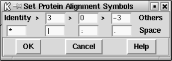
Chapter 9: Analysing and comparing sequences using spin 501
9.5.6 Set protein alignment symbols
This option allows users to set their own sequence similarity levels and alignment symbols
for protein sequence alignments. The dialogue (shown below) provides for setting a symbol
for identical characters and for three levels of similarity with corresponding symbols.
9.6 The Spin User Interface
Spin has several displays. The first is a top level window from which all the main options
are selected and which receives textual results. Most analytical functions which operate on
single sequences add their graphical results to a "SPIN Sequence Plot"that is associated
with the sequence being analysed. (An exception is the restriction enzyme search which
produces its own separate window.) Most functions which compare pairs of sequences add
their results to a "SPIN Sequence Comparison Plot". The SPIN Sequence Plot and the SPIN
Sequence Comparison Plot each have associated sequence display windows: the Sequence
Display and the Sequence Comparison Display. These allow the text of the sequences to be
viewed and use cursors to show the corresponding positions in the graphical displays.
Spin is best operated using a three button mouse, but alternative keybindings are
available. Full details of the user interface are described elsewhere (see [User Interface],
page 523).
The main window (shown below) contains an Output Window for textual results, an Er-
ror window for error messages, and a series of menus arranged along the top (see Section 9.2.4
[Spin menus], page 444). The contents of the two text windows can be searched, edited and

502 The Staden Package Manual
saved. Each set of results is preceded by a header containing the time and date when it was
generated.
As can be seen the main menu bar contains File, View, Options, Sequences, Statistics,
Translation, Comparison, Search and Emboss menus.
9.6.1 SPIN Sequence Plot
Graphical results are shown in separate windows. Most functions add their graphical re-
sults to a SPIN Sequence Plot that is associated with the sequence being analysed, but
some functions such as the restriction enzyme search produce their own separate windows.
Each set of graphical results has its own particular default drawing method, but individual
results can be "dragged and dropped"by users, hence allowing plots to rearranged and
superimposed. Plots can also be extracted from the main graphics window and dropped
to create new independent windows. The graphical results can be zoomed and scrolled in
both x and y directions. Zooming is achieved using the X and Y scale bars at the bottom
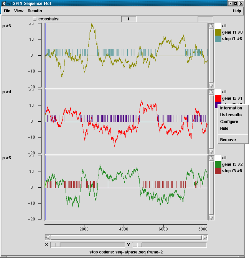
Chapter 9: Analysing and comparing sequences using spin 503
of the plot. The individual plots can be scrolled in y using the scroll bars attached to their
right hand edge. The sequence can be scrolled using the scroll bar at the base of the plot.
The figure shows a SPIN Sequence Plot containing the results of a gene search method
based on codon usage, upon which is superimposed a search for start codons and stop
codons. The vertical blue line represents the cursor. The x position of the cursor is shown
in the left hand box above the plot. Each result in the window has its own colour. At the
right hand side of each panel is a set of square boxes with the same colours as the lines
drawn in the adjacent plot. These icon-like objects represent individual results and allow
the user to operate on them. For example at the right of the middle panel is a pop-up menu
504 The Staden Package Manual
containing the items: "Information","List results","Configure","Hide"and "Remove".
(see Section 9.7.1 [Result manager], page 515).
The square icons can also be used to move the corresponding results to new locations.
These operations are explained below (see Section 9.6.1.4 [Drag and drop], page 506). The
cursor in the plot can be used to control the position of the cursor in the sequence display.
The SPIN Sequence Plot contains three menus: "File","View"and "Results". The
"File"menu contains the "Exit"command which closes down the plot; the "View"menu
contains the "Results manager"command (see Section 9.7.1 [Result manager], page 515);
and the "Results"menu contains a list of the results, colour coded i.e. the text is written
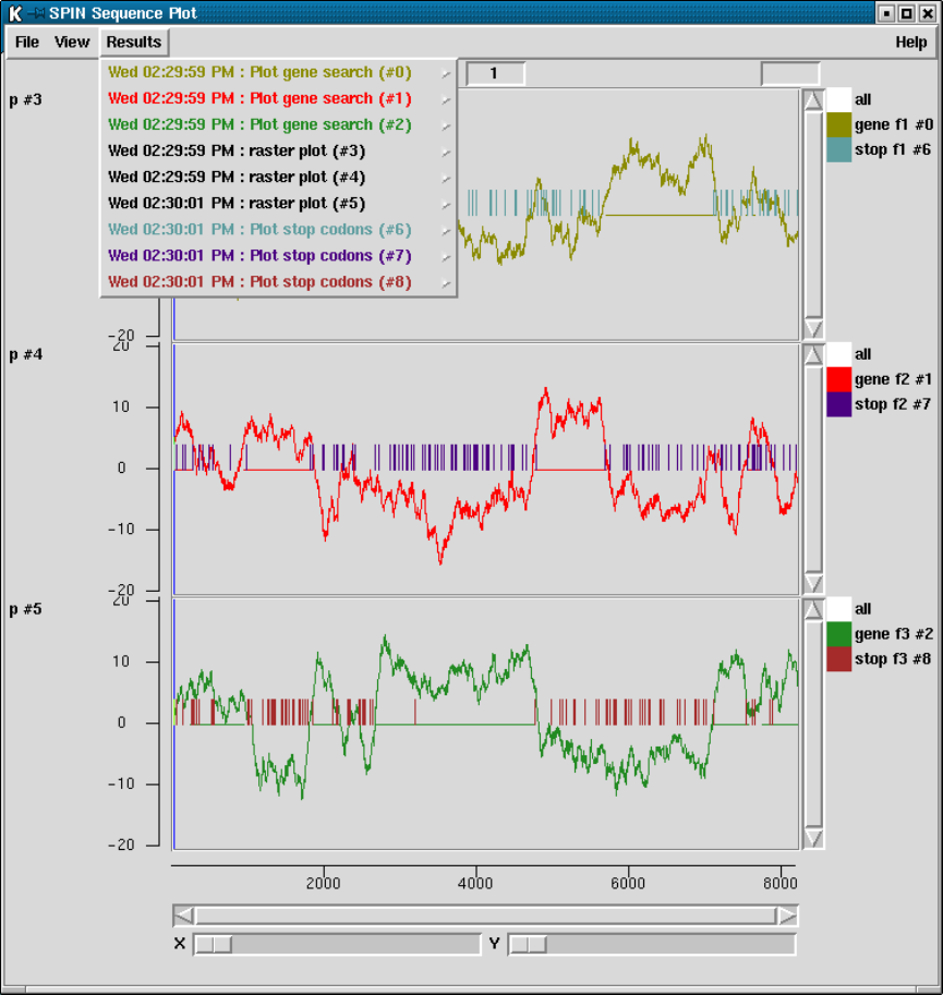
Chapter 9: Analysing and comparing sequences using spin 505
in the same colour as the plot. For each result a series of commands can be accessed from
a cascading menu. (see Section 9.7.1 [Result manager], page 515).
9.6.1.1 Cursors
Each sequence displayed in a SPIN Sequence Plot will have a corresponding cursor of a
particular colour. The same sequence displayed in several SPIN Sequence Plots will have
a cursor of the same colour. To move a cursor, click on it with the middle mouse button,
or Alt left mouse button, held down and drag the mouse. The cursor will move all other
cursors displayed that relate to that sequence, whether these be in different SPIN Sequence
Plots or within the sequence display.
506 The Staden Package Manual
9.6.1.2 Crosshairs
Crosshairs can be turned on or off using the check button labelled "crosshairs". The x and
y positions of the crosshairs are indicated in the two boxes to the right of the check box
respectively. The x value is the base position in the sequence and the y value the score for
the corresponding plot.
9.6.1.3 Zoom
The graphical results can be zoomed and scrolled in both x and y directions. Zooming is
achieved using the X and Y scale bars at the bottom the plot. The individual plots can be
scrolled in y using the scroll bars attached to their right hand edge. The sequence can be
scrolled using the scroll bar at the base of the plot.
9.6.1.4 Drag and drop
The square boxes at the right edge of the SPIN Sequence Plot panels have the same colours
as the individual results in the display. These icons can be used to drag and drop the results
to which they correspond. This is activated by pressing the middle mouse button, or Alt
left mouse button, over the box and then moving the cursor over the SPIN Sequence Plot
to the new location. As the cursor moves over each part of the plot rectangular boxes will
appear to indicate the position that the dragged result will occupy if the mouse button is
released. Results can be dropped on top of another plot (signified by a rectangle drawn
over the centre of the plot), above another plot (signified by a rectangle drawn in the top
third of the plot), or below another plot (signified by a rectangle drawn in the bottom third
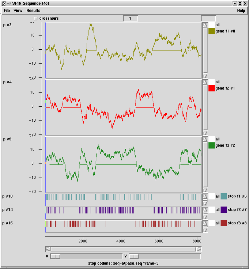
Chapter 9: Analysing and comparing sequences using spin 507
of the plot). The figure below shows three panels containing a protein gene prediction and
three panels showing the positions of stop codons in each of the reading frames.
508 The Staden Package Manual
The figure below shows the same SPIN Sequence Plot but with the rectangle indicating
where the user has dragged the frame 1 stop codon results.
Chapter 9: Analysing and comparing sequences using spin 509
The figure below shows the result of releasing the middle mouse button, or Alt left mouse
button: the stop codon plot has moved to be superimposed on the gene prediction plot.
9.6.2 Sequence display
Each sequence shown in the "Sequence manager"list can have its own "Sequence display"
window. The Sequence display provides a way of viewing and scrolling along the characters
of the sequence. It can also show translations to protein and the positions of restriction
enzyme cutting sites. Movement along the sequence is controlled by standard mouse and
cursor commands and by the use of a subsequence/string search routine. The cursor can
also be controlled by dragging the cursor in the programs’ graphical displays.
510 The Staden Package Manual
When restriction enzyme cutting sites are shown in the Sequence display window the
number of rows of text to be displayed at any position along the sequence varies with the
density of the sites. This presents a tricky problem about how to position the lines of
text relative to the top and bottom of the window. Should the height of the window grow
and shrink vertically as the user scrolls? Should the window maintain a fixed height, in
which case should the top or the bottom be clipped if the number of lines of text exceeds
the window height? We have programmed it so that the nucleotide sequence remains at
a fixed height to provide a constant reference and the user can select this height by use
of a vertical scroll bar and by growing or shrinking the window. The scroll bar will allow
vertical movement when the number of lines of text exceeds the current window size.
9.6.2.1 Search
The Sequence display contains a subsequence or string search function which moves the
cursor to the position of the next match. As shown in the dialogue the user selects the
direction and strand over which the search should be performed, the search algorithm, the
minimum percentage match, and the subsequence/string for which to search. The search
algorithm allows either NC-IUB codes Cornish-Bowden, A. (1985) Nucl. Acids Res. 13,
3021-3030 or a literal search. The literal search will search for exact matches eg inputting
a search string of "n"will search for the letter "n". The NC-IUB codes option can use any
of the NC-IUB symbols shown in the figure below. Once activated the Search dialogue will
remain visible until the user clicks on the "Cancel"button. The cursor will move to the
Chapter 9: Analysing and comparing sequences using spin 511
next matching position each time the user clicks on the "Search"button, or will "beep"if
there is no such match.
NC-IUB SYMBOLS
A,C,G,T
R (A,G) ’puRine’
Y (T,C) ’pYrimidine’
W (A,T) ’Weak’
S (C,G) ’Strong’
M (A,C) ’aMino’
K (G,T) ’Keto’
H (A,T,C) ’not G’
B (G,C,T) ’not A’
V (G,A,C) ’not T’
D (G,A,T) ’not C’
N (G,A,C,T) ’aNy’
9.6.2.2 Save
Saving the contents of the sequence display to a file
The Sequence display contents can be dumped to a file by selecting the "Save"option
from the menu. Whatever options are currently activated (i.e. which of restriction enzyme
sites, translation, ruler and strands) will be written to disk. The user can define the region
of the sequence for which to dump the results and the name of the file to use.

512 The Staden Package Manual
9.6.3 SPIN Sequence Comparison Plot
When a comparison function has been run on a pair of sequences a SPIN Sequence Com-
parison Plot will appear. The results from each comparison can be viewed in a "Sequence
Comparison Display"in which the two sequences can be scrolled passed one another.
The SPIN Sequence Comparison Plot display shows the results of comparison algorithms.
Each match is represented as either a single dot ("Find similar spans","Find best diago-
nals") or a line ("Find matching words","Align sequences","Local alignment"). Sets of
matches from a single invocation of a comparison command are termed "a result". Each
result is plotted using a single colour which can be configured via the results manager (see
Section 9.7.1 [Result manager], page 515). The maximum dimensions of the SPIN Sequence
Comparison Plot are indicated on the rulers at the bottom and left hand side. It is possible
within spin to compare many different sequences. This means that there may be more than
one horizontal or vertical sequence shown in the spin plot. All the points are scaled to the
largest sequence in each direction. Plots can also be extracted from or added to each SPIN
Sequence Comparison Plot.
Chapter 9: Analysing and comparing sequences using spin 513
The diagram above shows the results of a "find similar spans"search (olive) (see
Section 9.4.1 [Finding Similar Spans], page 483), and a "find matching words"(red) (see
Section 9.4.2 [Finding Matching Words], page 485), between human and mouse properdin
(hsproperd and mmproper). At the right hand side is a set of square boxes with the same
colours as the dots drawn in the adjacent plot. These icon-like objects represent individual
results and allow the user to operate on them. For example, in the figure above, the
user has clicked the right mouse button on the icon to raise a pop-up menu beneath the
"matching words"result (see Section 9.7.1 [Result manager], page 515).
The square icons can also be used to move the corresponding results to new locations.
These operations are explained below (see Section 9.6.3.4 [Drag and drop], page 514).
The SPIN Sequence Comparison Plot has 3 menus, "File","View"and "Results".
The "File"menu contains the "Exit"command to quit the SPIN Sequence Comparison
Plot. This shuts down the SPIN Sequence Comparison Plot display removes all the results
displayed in that plot.
The "View"menu contains the "Results manager"command, see Section 9.7.1 [Result
manager], page 515.
The "Results"menu provides a quick method of interfacing with the menu obtainable
via the "Results manager"(see Section 9.7.1 [Result manager], page 515).
9.6.3.1 Cursors
Each sequence displayed in a SPIN Sequence Comparison Plot will have a corresponding
cursor of a particular colour. In the picture above, the sequence on the horizontal axis
has a vertical blue cursor whereas the sequence on the vertical axis has a horizontal olive
green cursor. The same sequence displayed in several SPIN Sequence Comparison Plots
will have a cursor of the same colour unless the sequence has been plotted on a different
axis. The x and y positions of the cursors are indicated in the two boxes to the right of
the crosshair check box respectively. To move a cursor, click on it with the middle mouse
button, or Alt left mouse button, held down and drag the mouse. The cursor will move
all other cursors displayed that relate to that sequence, whether they are in different SPIN
Sequence Comparison Plots or within the sequence display.
9.6.3.2 Crosshairs
Crosshairs can be turned on or off using the check button labelled "crosshairs". The x
and y positions of the crosshairs are indicated in the two boxes to the right of the check
box. The position of the crosshairs can be "frozen"at a particular position by pressing the
control button and moving the mouse cursor outside the SPIN Sequence Comparison Plot
window.
9.6.3.3 Zoom
Plots can be enlarged either by resizing the window or zooming. Zooming is achieved in
two ways: either using the buttons at the base of the plot; or by holding down the control
key and right mouse button and dragging out a rectangle around the region to be zoomed.
Rectangles that are too small are ignored and a warning bell will sound. The Back button
will restore the plot to the previous magnification. Zooming will increase the magnification
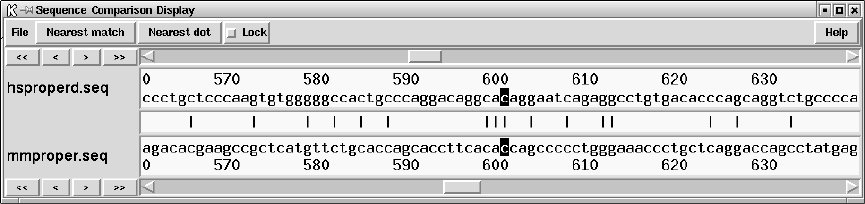
514 The Staden Package Manual
of the plot so that the contents of the dragged out rectangle fill the display. The scrollbars
allow the SPIN Sequence Comparison Plot to be scrolled in both directions.
It is not possible to zoom the results from Rescan matches (see Section 9.4.1 [Finding
Similar Spans], page 483).
9.6.3.4 Drag and drop
The square boxes at the right edge of the SPIN Sequence Comparison Plot panels have the
same colours as the individual results in the display. These icons can be used to drag and
drop the results to which they correspond. This is activated by pressing the middle mouse
button, or Alt left mouse button, over the box and then moving the cursor over the SPIN
Sequence Comparison Plot to the new location or anywhere outside the SPIN Sequence
Comparison Plot. As the cursor moves over each part of the plot rectangular boxes will
appear to indicate the position that the dragged result will occupy if the mouse button is
released. Results can be dropped on top of another plot (signified by a rectangle drawn
over the centre of the plot), above another plot (signified by a rectangle drawn in the top
third of the plot), or below another plot (signified by a rectangle drawn in the bottom third
of the plot). Moving the mouse cursor outside the SPIN Sequence Comparison Plot and
releasing the mouse button will create a new SPIN Sequence Comparison Plot containing
that result.
9.6.4 Sequence Comparison Display
A sequence display is associated with a single set of results (see Section 9.7.1 [Result man-
ager], page 515). To invoke a Sequence Comparison Display, bring up a pop up menu for the
required result, either from the Results manager, the Results menu in the SPIN Sequence
Comparison Plot, or the coloured square icon on the right of the spin plot. From the menu,
select the "Display sequences"option.
The horizontal sequence is drawn above the vertical sequence. In the picture above,
"hsproperd"is the horizontal sequence and "mmproper"is the vertical sequence. The
central panel indicates characters which are identical between the horizontal and vertical
sequences. The buttons to the left of the sequences allow scrolling of the sequences either 1
character at a time (<or >) or a screen width (<< or >>). Pressing the Lock button "locks"
the two sequences together and they can be scrolled as one. Movement of the sequences
is also controlled by the scrollbars or by moving the corresponding cursor in the SPIN
Sequence Comparison Plot (see Section 9.6.3 [SPIN Sequence Comparison Plot], page 512).
The black cursors in the sequence display correspond to the position of the cursor in the
SPIN Sequence Comparison Plot. The sequences can be made to ’jump’ to the nearest
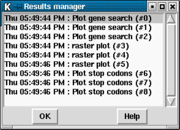
Chapter 9: Analysing and comparing sequences using spin 515
match in those results by pressing the "Nearest match"or "Nearest dot"buttons. Nearest
match means the match whose x,y coordinate in sequence character positions is closest,
whereas Nearest dot means the match which appears closest in screen coordinates. If the
display edges were proportional to the sequence lengths the Nearest dot and Nearest match
would be equivalent.
9.7 Controlling and Managing Results
9.7.1 Result manager
Many functions within spin produce "results"which are plotted to the SPIN Sequence
Plot (see Section 9.6.1 [SPIN Sequence Plot], page 502) or the SPIN Sequence Comparison
Plot (see Section 9.6.3 [SPIN Sequence Comparison Plot], page 512). The Result Manager
provides a mechanism to interrogate and operate on these results.
The Result Manager can be accessed via the "Results manager"command in the View
menu on either the main menu or the menu bar of the SPIN Sequence Plot. Alternatively the
results can be accessed as a menu attached to the "Results"option on the SPIN Sequence

516 The Staden Package Manual
Plot menu bar. In this case the individual results are written in the same colour as the
plots they refer to:
Each result is listed in the window containing the time the result was created, the name
of the function which created the result and the result number. The number is simply a
unique identifier to help distinguish between multiple results produced by the same function.
The results are listed in time order, the oldest at the top.
Each item in the list is consuming memory on your computer. Running functions over
and over again without removing the previous results will slow down your machine and it
will, eventually, run out of memory. Removing items from the list solves this.
Chapter 9: Analysing and comparing sequences using spin 517
Pressing the right mouse button over an listed item will display a popup menu of oper-
ations to perform on this result.
9.7.1.1 Information
This option in the pop-up writes data about the parameters used to obtain the corresponding
result.
9.7.1.2 List
This option in the pop-up writes all the numerical values for the result to the Output
Window. This should be used sparingly as it requires a lot of memory.
9.7.1.3 Configure
This option allows the line width and colour of the matches to be altered (see Section 10.6
[Colour Selector], page 529). A colour browser is displayed from which the desired line
width or colour can be configured. Pressing OK will update the SPIN Sequence Plot.
9.7.1.4 Hide
This option removes the points from the SPIN Sequence Plot but retains the information
in memory.
9.7.1.5 Reveal
This option will redisplay previously hidden points in the SPIN Sequence Plot.
9.7.1.6 Remove
This command removes all the information regarding this particular result and access to
this data is lost.
9.8 Reading and Managing Sequences
Spin manages sequences at two levels. First it provides for reading sequences into the
program from disk files, and secondly it contains a range of facilities for deriving new
sequences from them. For example it can internally produce protein sequences from DNA
sequences, or produce the complement of a DNA sequence, rotate it about any position, or
scramble it. Each of these types of internal operation produces a new sequence which can
be analysed using the comparison functions, or which can be saved to disk. In the same
way, performing a sequence alignment produces two new sequences which can be analysed
or saved to disk.
The sections below deals first with reading sequences from disk, and then with what can
be done to produce new sequences in memory. New sequences are obtained from disk using
the Load sequences option in the File menu, and sequences are managed internally using
the Sequences menu.
9.8.1 Use of feature tables in spin
At present spin can only read feature tables from EMBL style files and use them to perform
translations to protein. Like many components of spin, for us this was an exercise in doing
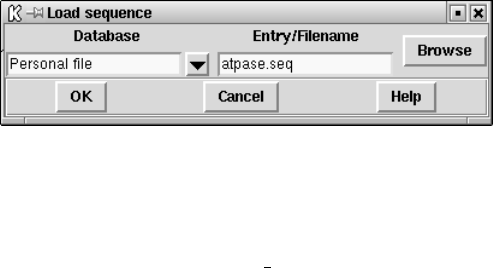
518 The Staden Package Manual
the hard part (ie parsing and using the table), but we still need to apply it to many other
tasks. We also need to generalise it to read genbank files.
We also limited the types of record we accepted: only those with precisely
defined endpoints. This means we do not store records which for example in-
clude <1..2000 or 1001.1005 but would store and use those with (1001..2000) or
complement(join(2691..4571,4918..5163)).
9.8.2 Reading in sequences
This section describes how sequences are obtained from disk files.
Personal sequence files can be in plain text, "Staden", EMBL, Genbank, PIR, FASTA
and GCG formats. If supported by the format, personal files can contain multiple entries
preceded by entry names. As is explained below a browser is available for selecting entries
from such files. The file format is worked out automatically.
New sequences are entered into spin using the "Load sequence"option in the File menu.
If a sequence is entered which has the same name as one already loaded, its name within
the program is changed by the addition of ’#number’ where ’number’ is a unique identifer.
For example, if the sequence "hsproperd"has already been loaded and this sequence is
loaded again, the name of this second sequence is changed to "hsproperd#0".
If only one sequence has been loaded, the comparison functions will compare this se-
quence against itself.
9.8.2.1 Simple search
This allows the selection of personal files. The second option button is an "Entry"
/"Filename"selection menu and the entry box next to this should be completed with
either an entryname or file name accordingly. If a personal file is selected, the filename
should be entered in the entrybox. The Browse buttons at the far right of the dialogue box
either invoke a library browser or a file browser, see Section 10.7 [File Browser], page 529
depending on whether a sequence library or personal file has been selected. From the file
browser multiple files can be entered by use of the Ctrl key and mouse. Library access is
only available via EMBOSS.
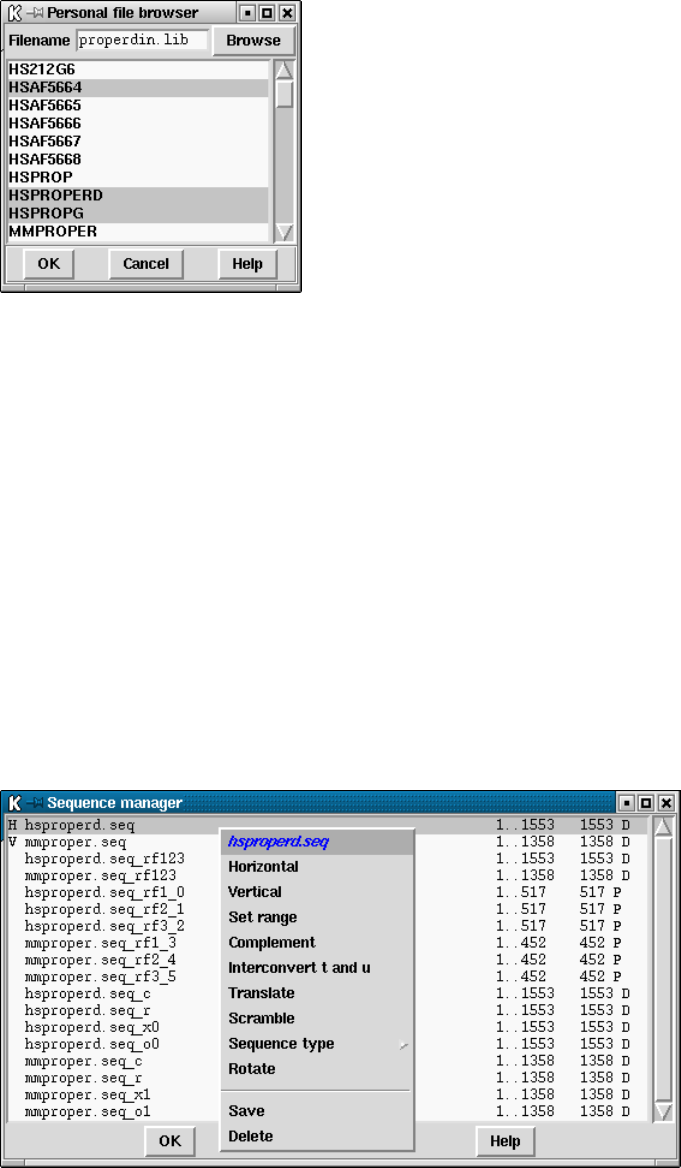
Chapter 9: Analysing and comparing sequences using spin 519
9.8.2.2 Extracting a sequence from a personal archive file
This method invokes an archive browser. Enter the filename of the personal file in the
entrybox. The Browse button to the right will invoke a file browser, see Section 10.7 [File
Browser], page 529. If the file contains multiple entries, these will be displayed in the list
box. It is necessary to press "Enter"after entering the filename in order for the entries to
be displayed. Select the required entryname(s) and press OK. The selected entries should
now have been loaded into spin.
9.8.3 Sequence manager
Spin allows more than two sequences to be available to the user. The sequence manager
allows the user to perform operations on the sequences which have been loaded into spin.
The same operations can also be invoked from the "Sequences"menu. The sequence man-
ager is invoked from the "File"menu. This command invokes a list box showing all the
sequences which have been read into spin together with their ranges, lengths and whether
they are DNA (D) or Protein (P). The currently active horizontal and vertical sequences
are marked with "H"and "V"respectively. In the picture below, these are "hsproperd"
and "mmproper".

520 The Staden Package Manual
Clicking on the sequence name in the sequence manager with the right mouse button
invokes a pop-up menu containing operations which may be performed on that sequence.
The operations available depends on whether the sequence is DNA or protein.
These options are described in greater detail below.
9.8.3.1 Change the active sequence
To change the currently active horizontal or vertical sequence, use either the "Sequences"
menu or select the sequence from the Sequence manager. Select "Horizontal"or "Vertical"
from the menu. This sequence will now be the active "Horizontal"or "Vertical"sequence.
9.8.3.2 Set the range
If you are only interested in a particular region of a sequence, it is possible to specify the
start and end positions of this region to create a new entry in the Sequence manager. The
new sequence will have the same name as the parent, with the addition of a "s"plus a
unique number. The third entry in the picture above shows the range has been set from
100 to 1000, giving a total length of 901 bases for the sequence "hsproperd".
9.8.3.3 Copy Sequence
This option in the Sequences menu allows a sequence to be duplicated or copied. This
simply creates a new entry in the Sequence Manager. The user can select which sequence
and the segment start and end points to be copied.
9.8.3.4 Sequence type
This option allows the user to change the status of a sequence to become either circular or
linear.
9.8.3.5 Complement sequence
This function will reverse and complement nucleic acid sequences. Select the "Complement"
command from either the "Sequences"menu or the sequence manager pop-up menu. A
new sequence will be added to the sequence manager list box with the same name as the
parent but with "c"appended to the end. The forth entry in the picture above is the
complemented sequence of "hsproperd".
9.8.3.6 Interconvert t and u
This function interconverts T and U characters i.e. between DNA and RNA. A new sequence
is added to the sequence manager list box with the same name as the parent but the addition
to the end of "r". The fifth entry is the picture above is the transcribed sequence of
"hsproperd".
9.8.3.7 Translate sequence
This operation is only available for DNA sequences. Select the "Translate"command
from either the "Sequences"menu or the sequence manager pop-up menu. It is possible
to translate in any particular frame by selecting the appropriate check box. For each
translation, a new sequence will be added to the sequence manager list box with the same
name as the parent but with the addition to the end of either "rf1","rf2"or "rf3"to
signify reading frames 1, 2 or 3 respectively.

Chapter 9: Analysing and comparing sequences using spin 521
The "all together"option will produce a single new sequence in the sequence manager,
with the extension "rf123", exemplified by the ninth entry in the picture above. Although
at this point the sequence is still DNA, when it is used in a comparison function the program
will translate it automatically into the three reading frames. The important point is that
the results from the three reading frames will be superimposed in the plot, hence enabling
frameshift errors to be spotted.
For example to compare a DNA sequence in all it’s reading frames with a protein:
1. Convert the DNA sequence using the "all together"command
2. Select this sequence as horizontal
3. Select the protein sequence as vertical
4. Invoke the relevant comparison function
9.8.3.8 Scramble sequence
This function produces a version of a given DNA or protein sequence in which the characters
are randomly reordered. i.e. the new sequence has the same length and composition as the
original but with the characters in a random order. The new sequence will be added to
the sequence manager list box with the same name as the parent except with "x"plus a
unique number appended to the end. The tenth entry in the picture above is the scrambled
version of "hsproperd". For long sequences, scrambling and then comparing should produce
similar numbers of matches as are predicted by the probability calculations (see Section 9.5.1
[Probabilities and expected number of matches], page 498).
9.8.3.9 Rotate sequence
This function allows the user to specify a new origin for a sequence. A new sequence is
added to the sequence manager list box with the same name as the parent except with "o"
plus a unique number appended to the end. The eleventh entry in the picture above is of
a rotated version of "mmproper". This operation is not allowed for sub-sequences ie those
created using "Set range".
9.8.3.10 Save sequence
To save a sequence to a file, select the "Save"option from either the "File"menu, the
"Sequences"menu or the sequence manager pop-up menu. This command invokes a file
name entry box. The browse button to the right of the dialogue box invokes a filebrowser.
See Section 10.7 [File Browser], page 529. The sequence is written as either EMBL or
FASTA format. If EMBL is selected and the sequence has an associated feature table,
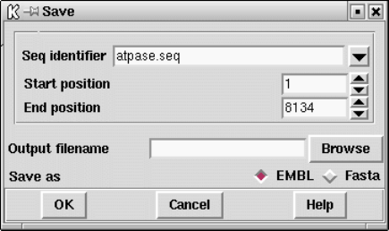
522 The Staden Package Manual
the feature table will also be written out (see Section 9.8.1 [Use of feature tables in spin],
page 517).
9.8.3.11 Delete sequence
To delete a sequence, select the "Delete"option from either the "Sequences"menu or the
sequence manager pop-up menu. This command will remove the sequence from the sequence
manager and all plots and results that were produced from it.
9.8.4 Selecting a sequence
All the comparison functions request a horizontal and a vertical sequence and the ranges
over which the function will operate. It is therefore possible to compare the same sequence
over different ranges. The default sequences which appear when the dialogue box for the
comparison function is brought up, are the current "active"sequences (see Section 9.8.3
[Sequence manager], page 519). To select a different sequence for this invocation of the
function, press the Browse button to the right of the "Seq identifier"box. This will invoke
a Sequence manager if one is not already displayed. Clicking with the left mouse button on
the name of the required sequence in the sequence manager will update the function dialogue
box with the sequence name and it’s currently defined range. To change the range, enter
the new start and end positions. These positions will be remembered for future invocations
of any of the comparison functions for this sequence.
Chapter 10: User Interface 523
10 User Interface
Introduction
This chapter describes the graphical user interface implemented in the programs gap4,
pregap4, spin and trev.
10.2 Basic Interface Controls
The key components of any graphical interface are menus, buttons and text entry boxes.
These are usually grouped together into ’panels’ or ’dialogues’. For the sake of simplifying
the rest of the documentation we describe the operation and control of the user interface
here.
10.2.1 Buttons
There are three basic types of button; command buttons, radio buttons and check buttons.
Buttons are used by moving the mouse pointer over the button (it will then be highlighted,
as is "Choice 3"below) and pressing the left mouse button. The illustration below demon-
strates each of the three types.
The buttons labelled "Command 1","Command 2"and "Command 3"are command
buttons. These perform a particular action, which is usually determined by the text within
the button. Typically command buttons have a slightly raised look. A typical example is
the "Clear"button visible on the main gap4 window. See the illustration in Section 10.4
[Output and Error Windows], page 526.
The buttons underneath, labelled "Choice 1","Choice 2"and "Choice 3"are radio
buttons. These have small diamonds to the left of each name. Only one of these boxes in
each group of radio buttons (it is possible to have several distinct groups) may be set at any
one time. In this example "Choice 1"has been selected. For example, selecting "Choice 3"
will now clear the diamond next to "Choice 1"and fill the diamond next to "Choice 3".
The bottom row of buttons are check buttons. These each have small boxes to the left of
each name. They act similarly to radio buttons except that more than one can be selected at
any one time. Here we have "Check 2"and "Check 3"selected, with "Check 1"deselected.
Pressing a check button will toggle it; so clicking the left mouse button on "Check 2"would
deselect it and clear the neighbouring box. The "Scroll on output"button is an example of
a check button. See the illustration in Section 10.4 [Output and Error Windows], page 526.
524 The Staden Package Manual
10.2.2 Menus
When many operations are available it is impractical to arrange them all in command
buttons. For this reason we have menus. Typically we will use a "menubar"consisting of
several menus arranged side by side
The menubar is a series of menu buttons arranged side by side. In the above picture, the
menus are "File"through to "Help". Selecting an item from a menu is done by pressing and
holding the left mouse button whilst the cursor is above the menu button. The available
menu choices will then be displayed. Whilst still pressing the mouse button, move down to
the desired choice and then release the mouse button. Releasing the mouse button when the
mouse cursor is not over a menu item will remove the menu without executing any options.
Alternatively, it is possible to press and release the left mouse button whilst the cursor is
above a menu button. The menu options will be revealed. Now move down and press and
release the left button once more once on the selected item.
To see an overview of the menu contents press the left mouse button over a menu button
and move the mouse cursor over the other menu buttons. As each menu button is highlighted
the appropriate options for this menu will be shown.
Some menu items lead to further menus. These are called cascading menus. Treat these
exactly as normal menus.
To tear off a menu pull down the menu using the left mouse button, select the dashed
perforation line, and release the button. The menu will be redrawn with a title bar which
can be used to move it to any position on the screen. Not all menus support tearing off.
10.2.3 Text Windows
A text window is simply an area of the screen set aside for displaying textual information.
A typical example is the Output and Error windows seen on the main gap4 screen. See the
illustration in Section 10.4 [Output and Error Windows], page 526.
The most basic use of text windows is to display data. If the data is large then there
will usually be scrollbars on the right and bottom sides of the text display. If the data is of
an editable nature (such as the comments in a tag in gap4) we may perform many editing
operations on the text. The simplest commands follow.
Chapter 10: User Interface 525
Arrow keys Moves the editing cursor
Left mouse button Sets the editing cursor
Middle mouse button Panning - controls both scrollbars at once
Alt left mouse button Panning - controls both scrollbars at once
Delete Deletes the character to the left of the cursor
Most other keys Adds text to the window
In addition to the above, some more advanced features are available, mostly following
the Emacs style of key bindings.
Delete Delete region (when highlighted), otherwise as above
Control D Delete character to the right of the cursor
Control N Down one line
Control P Up one line
Control B Move back on character
Control F Move forward on character
Control A Move to start of line
Control E Move to end of line
Meta b Move back one word
Meta f Move forward one word
Meta < Move to start
Meta > Move to end
Control Up Move up one paragraph
Control Down Move down one paragraph
Next Move done one page
Prev Move up one page
Control K Delete to end of line
Control T Transpose two characters
Drag left button Highlights a region (for cut and paste)
Control / Select all (for cut and paste)
Control \ Deselect all (for cut and paste)
10.2.4 Text Entry Boxes
An entry box is basically a small, one line, text window. All of the same editing commands
exist, although many are redundant for such a small window.
A typical entry box can be seen in the gap4 dialogue for opening new databases. Here
the ringed region to the right of the "Enter new filename"text is the entry box. The current
contents of this entry is "file". The vertical black line visible is the text entry point.
526 The Staden Package Manual
10.3 Standard Mouse Operations
The same mouse buttons are used for similar operations throughout the programs. A brief
description of the mouse control is listed below. On UNIX three button mice are used, but
on Windows or Linux two buttons are more common, and so the alternative of Alt-left-
mouse button is used for the middle button.
Left button Select
In a dialogue this selects an item from a list of items. Within a graphical display
(eg the template display) this "selects"an item. Selected items are shown in
bold. Selecting an already selected item will deselect it.
Drag left button Select region
This operates only for the graphical displays. A rectangular box can be dragged
out between where the left button was pressed (and held down) to the current
mouse cursor position. Releasing the left button will then select all items con-
tained entirely within the rectangle. Within the contig editor such selections
are displayed by underlining the region instead.
Drag middle button Move
This currently operates only for the contig selector. The selected items (or the
item under the mouse pointer if none are selected) are dragged until the middle
button is released.
Drag Alt left button Move
This currently operates only for the contig selector. The selected items (or the
item under the mouse pointer if none are selected) are dragged until the button
is released.
Right button Popup menu
Within some displays this will pop up a menu displaying a list of commands
that can be used on the selected item.
10.4 The Output and Error Windows
The main screen has three portions; the menubar, the output window and the error window.
Of these, the output and error windows are identical except for the data that appears within

Chapter 10: User Interface 527
them. Here we describe the general operation of the output window only, although the
details apply to the error window too.
The output window consists of a text window with a set of labels and buttons above
it. At the top left is the window name followed by a colon. After the colon the name of
the current output file will be shown in blue italic letters. All new output appearing in
this window will also be sent to this file. Initially no output file is specified and this label
is blank (as can be seen in the error window). Using the "Redirect"menu located at the
top right of the window a new file can be opened, or an existing one closed (in which case
output is no longer sent to the specified file). The output and error windows may both have
redirection files.
The "Search"button invokes a dialogue box requesting a string to search and whether
to search forwards or backwards from the current position of the cursor. The search is case
insensitive. Hitting the the OK button finds the next match.The bell is sounded if no more
matches can be found.
The "Scroll on output"check button toggles whether the window should automatically
scroll when new output appears to ensure that it is visible. The default (as seen in the
illustration) state is to scroll. The "Clear"button removes all output from the window.
Each command, when run, adds a title to the output window. This contains the current
time together with the command name. Output for this command then appears beneath
the header. In the illustration the output from three commands is visible. Of these the
"edit contig"command produces no output, but still has a header.
528 The Staden Package Manual
Pressing the right button with the cursor above a piece of output (either in its header
or the text beneath it) will pop up a menu of operations. This operation is not valid for
the error window. The commands are:
Show input parameters
Inserts the input parameters of the command, if any, beneath the command
header
Remove
Deletes this text from the output window
Output to disk
Sends this text to a specified file
Output to list
Sends this text to a specified list
The output operations allow the user to specify whether the header, input parameters
or text for the command, in any combination, are sent to the output.
The text in the error window has a different format to the output window. Instead of
large portions of text separated by headers, each item in the error window consists of a
single line containing the date, the name of the function producing the error, and a brief
description of the error. Many error messages will be displayed in their own dialogue boxes
(eg not having write access to a file) and hence will not appear in the error window. Each
time an error message is added the bell is rung.
10.5 Graphics Window
The graphical displays have several features in common. Commands are selected from
buttons and menus ranged along the top of the window. Menus can be "torn off"and
positioned anywhere on the screen. Zooming is allowed using the mouse. The "Zoom out"
button undoes the previous zoom command. Crosshairs and cursors can be toggled on and
off, and their coordinates in base positions appear in boxes in the top right hand corner of
the displays. Items plotted in the graphical displays have text attached, and as the cursor
passes over an item, it is highlighted and its text appears in an Information line at the
bottom of the display.
10.5.1 Zooming
Plots can be enlarged either by resizing the window or zooming. In some plots zooming
is achieved by holding down the control key and right mouse button and dragging out a
rectangle. Rectangles that are too small are ignored and a warning bell will sound. The
content of the window is magnified such that the contents of the zoom box fill the window.
The Zoom out button will restore the plot to the previous magnification. In other plots, x
and y scale boxes achieve similar effects.
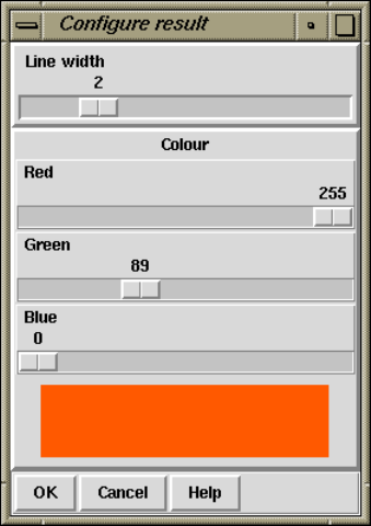
Chapter 10: User Interface 529
10.6 Colour Selector
A common operation is to change the colour of a plot. For this we use the colour selector
dialogue shown below. The three sliders control the red, green, and blue intensities to
use in producing the desired colour. The shaded box at the bottom illustrates the current
colour. In some displays this will also interactively update the colour in the associated plot
simultaneously.
Pressing the "OK"button will quit the colour selector and update the appropriate
colours in the plot. Pressing "Cancel"will quit the colour selector without making any
changes to the plot. Note that some colour dialogues may also be combined with extra
controls for adjusting other graphical styles, such as the line width.
Many programs have a "Colours"command in the Options menu. This displays two
colour selectors; one for each of the foreground and background colours. This can be used
to adjust the main colour scheme used for the program. Pressing "OK"selects this colour
scheme and keeps it in use until the program exits. Pressing "OK Permanent"accepts this
colour scheme, but also updates the ‘$HOME/.tk_utilsrc’ file. This means that the colour
scheme will be used for all future program uses. To revert to the default colours, manually
edit the ‘$HOME/.tk_utilsrc’ file.
10.7 File Browser
The file browser is a dialogue that allows the user to select files from any directory. It is
typically used when choosing a file for a particular action, such as opening a database in
gap or saving a trace file in trev. The precise details of the layout may change depending
on this context. In some circumstances, such as loading sequences into spin several files
may be selected (in which case the dialogue will be titled "Open multiple files"), in others
only a single file can be selected. The illustration below shows the file browser as displayed

530 The Staden Package Manual
when opening files from within trev. The ‘Formats’ and ‘Filter’ section here are used to
select different file types. These dialogue components may not appear in all file browsers.
The ‘OK’, ‘Filter’ and ‘Cancel’ buttons perform their usual tasks; ‘OK’ accepts the file
currently shown in the selection component, and ‘Cancel’ quits the dialogue.
10.7.1 Directories and Files
The main component of the file browser dialogue consists of two scroll lists placed side by
side. The left list is labelled "Directory"and shows a list of other directories to choose
from. The right list is the list of files in the currently displayed directory.
Double clicking with the left mouse button on a directory updates the file list. If a filter
file browser component is visible then the current directory will be displayed as the start of
the filter. The directory named ".."is the parent directory of the current directory.
Single clicking on a file name updates the Selection component. Double clicking on a file
name chooses this file and removes the dialogue. That is, it is equivalent to single clicking
on the file to update the selection followed by pressing the ‘OK’ button.
When the dialogue allows multiple files to be selected (then titled "Open multiple files")
holding down the Ctrl key will retain items already chosen.
10.7.2 Filters
The top component of the file browser shown in the introduction contained a Filter
component. This consists of a text entry window containing a string of the form
directory name/file pattern.
Some dialogues may not have a Filter component. In these cases the file pattern is taken
to be "*". Hence all files will be listed. The directory name is the directory that the current
list of files are contained within. The file pattern is used to specify which of the files within
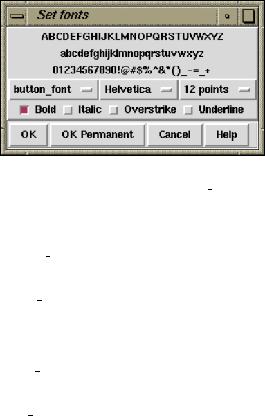
Chapter 10: User Interface 531
this directory should be listed in the file list. The pattern uses the same form as UNIX shell
wild card matching. To summarise this see the following table of simple examples.
*Every filename
xb* Every filename starting in "xb"
a*b Every filename starting with "a"and ending with "b"
a?b Every three letter filename with "a"as the first letter and "b"as the last letter.
*scf Every filename ending in "scf"
*[sS]cf Every filename ending with "scf"or "Scf".
*{scf,SCF}
Every filename ending with "scf"or "SCF".
Some file browsers also include a Formats component. This is used to select the input or
output format of the selected file. Updating the format will typically also update the filter.
10.8 Font Selection
The Options menu of most programs contains a "Set fonts"command. This brings up a
font selection dialogue consisting of some sample text, three option menus to select the font
name, family and size, and some check buttons for font styles.
In the above picture, button font is the currently selected font name. This option menu
contains several of the following font types. The exact ones available depends on the program
being used.
button font
Used for buttons, labels, checkbuttons and radiobuttons.
menu font Used for menu buttons and their contents, including pull down menu contents.
text font Used for textual displays, such as the main output windows. This should be
chosen to be a fixed width font, such as Courier.
sheet font Used for the scrolled text displays such as the contig editor in gap4 and the
sequence displays in spin. This too needs to be chosen as a fixed width font.
title font Used as for headings within text windows such as contig names in the gap4
suggest probes function.

532 The Staden Package Manual
menu title font
Used in the title line of popup menus.
trace font Used for the sequence and number displays in the trace displays for both gap4
and Trev.
Next to the font name is the font family selector. The contents of this menu will depend
on the fonts available to your system. Some may be inappropriate, or not even in the correct
language. Next to the family selector is the size menu. This contains a range of sizes in
both pixel and point units. If a font of a particular size is not available, the nearest font or
size will be automatically chosen. Specifying fonts to be a fixed number of points states that
the font should have a specific physical size, regardless of monitor size or screen resolution.
There are 72.27 points to the inch. Underneath these we have Bold, Italic, Overstrike and
Underline check buttons.
Whilst choosing the font, the fonts used in the entire program automatically update to
show you how things will look. Pressing "Cancel"will reset the fonts back to their original
state. Pressing "OK"will keep these chosen fonts, until the program is exited. Pressing "OK
Permanent"will keep these fonts, but will also add them to the user’s ‘$HOME/.tk_utilsrc’
file. This file is processed when the programs start up, and so your font choice will be per-
manently chosen. To remove this font choice, manual editing of the ‘$HOME/.tk_utilsrc’
file is required.

Chapter 11: File Formats 533
11 File Formats
This section introduces the various file formats used by the package, but first we describe
some limitations on the names of files.
There are restrictions on the characters used in file names and the length of the file
names.
Characters permitted in file names:
QWERTYUIOPASDFGHJKLZXCVBNMqwertyuiopasdfghjklzxcvbnm1234567890. -
A reading name or experiment file name used in a sequence assembly project must not
be longer than 16 characters.
These restrictions also apply to SCF files which means, in turn, also to the names given
to samples obtained from sequencing instruments. For example do not give sample names
such as 27/OCT/96/r.1 when using and ABI machine: the / symbols will be interpreted as
directory name separators on UNIX!
Currently the formats used by the package include the following.
11.1 SCF
SCF format files are used to store data from DNA sequencing instruments. Each file contains
the data for a single reading and includes: its trace sample points, its called sequence, the
positions of the bases relative to the trace sample points, and numerical estimates of the
accuracy of each base. Comments and "private data"can also be stored. The format is
machine independent and the first version was described in Dear, S and Staden, R. "A
standard file format for data from DNA sequencing instruments", DNA Sequence 3, 107-
110, (1992).
Since then it has undergone several important changes. The first allowed for different
sample point resolutions. The second, in response to the need to reduce file sizes for large
projects, involved a major reorganisation of the ordering of the data items in the file and
also in the way they are represented. Note that despite these changes we have retained the
original data structures into which the data is read. Also this reorganisation in itself has
not made the files smaller but it has produced files that are more effectively compressed
using standard programs such as gzip. The io library included in the package contains
routines that can read and write all the different versions of the format (including reading
of compressed files). The header record was not affected by this change. This documentation
covers both the format of scf files and the data structures that are used by the io library.
Prior to version 3.00 these two things corresponded much more closely.
11.1.1 Header Record
The file begins with a 128 byte header record that describes the location and size of the
chromatogram data in the file. Nothing is implied about the order in which the components
(samples, sequence and comments) appear. The version field is a 4 byte character array
representing the version and revision of the SCF format. The current value of this field is
"3.00".
534 The Staden Package Manual
/*
* Basic type definitions
*/
typedef unsigned int uint_4;
typedef signed int int_4;
typedef unsigned short uint_2;
typedef signed short int_2;
typedef unsigned char uint_1;
typedef signed char int_1;
/*
* Type definition for the Header structure
*/
#define SCF_MAGIC (((((uint_4)’.’<<8)+(uint_4)’s’<<8) \
+(uint_4)’c’<<8)+(uint_4)’f’)
typedef struct {
uint_4 magic_number;
uint_4 samples; /* Number of elements in Samples matrix */
uint_4 samples_offset; /* Byte offset from start of file */
uint_4 bases; /* Number of bases in Bases matrix */
uint_4 bases_left_clip; /* OBSOLETE: No. bases in left clip (vector) */
uint_4 bases_right_clip; /* OBSOLETE: No. bases in right clip (qual) */
uint_4 bases_offset; /* Byte offset from start of file */
uint_4 comments_size; /* Number of bytes in Comment section */
uint_4 comments_offset; /* Byte offset from start of file */
char version[4]; /* "version.revision", eg ’3’ ’.’ ’0’ ’0’ */
uint_4 sample_size; /* Size of samples in bytes 1=8bits, 2=16bits*/
uint_4 code_set; /* code set used (but ignored!)*/
uint_4 private_size; /* No. of bytes of Private data, 0 if none */
uint_4 private_offset; /* Byte offset from start of file */
uint_4 spare[18]; /* Unused */
} Header;
For versions of SCF files 2.0 or greater (Header.version is ‘greater than’ "2.00"),
the version number, precision of data, the uncertainty code set are specified in
the header. Otherwise, the precision is assumed to be 1 byte, and the code set
to be the default code set. The following uncertainty code sets are recognised
(but still ignored by our programs!).
0 {A,C,G,T,-} (default)
1 Staden
2 IUPAC (NC-IUB)
3 Pharmacia A.L.F. (NC-IUB)
4 {A,C,G,T,N} (ABI 373A)
5 IBI/Pustell
6 DNA*
7 DNASIS

Chapter 11: File Formats 535
8 IG/PC-Gene
9 MicroGenie
11.1.2 Sample Points.
The trace information is stored at byte offset Header.samples offset from the start of the file.
For each sample point there are values for each of the four bases. Header.sample size holds
the precision of the sample values. The precision must be one of "1"(unsigned byte) and
"2"(unsigned short). The sample points need not be normalised to any particular value,
though it is assumed that they represent positive values. This is, they are of unsigned type.
With the introduction of scf version 3.00, in an attempt to produce efficiently compressed
files, the sample points are stored in A,C,G,T order; i.e. all the values for base A, followed
by all those for C, etc. In addition they are stored, not as their original magnitudes, but in
terms of the differences between successive values. The C language code used to transform
the values for precision 2 samples is shown below.
void delta_samples2 ( uint_2 samples[], int num_samples, int job) {
/* If job == DELTA_IT:
* change a series of sample points to a series of delta delta values:
* ie change them in two steps:
* first: delta = current_value - previous_value
* then: delta_delta = delta - previous_delta
* else
* do the reverse
*/
int i;
uint_2 p_delta, p_sample;
if ( DELTA_IT == job ) {
p_delta = 0;
for (i=0;i<num_samples;i++) {
p_sample = samples[i];
samples[i] = samples[i] - p_delta;
p_delta = p_sample;
}
p_delta = 0;
for (i=0;i<num_samples;i++) {
p_sample = samples[i];
samples[i] = samples[i] - p_delta;
p_delta = p_sample;
}
}
else {
p_sample = 0;
for (i=0;i<num_samples;i++) {
samples[i] = samples[i] + p_sample;

536 The Staden Package Manual
p_sample = samples[i];
}
p_sample = 0;
for (i=0;i<num_samples;i++) {
samples[i] = samples[i] + p_sample;
p_sample = samples[i];
}
}
}
The io library data structure is as follows:
/*
* Type definition for the Sample data
*/
typedef struct {
uint_1 sample_A; /* Sample for A trace */
uint_1 sample_C; /* Sample for C trace */
uint_1 sample_G; /* Sample for G trace */
uint_1 sample_T; /* Sample for T trace */
} Samples1;
typedef struct {
uint_2 sample_A; /* Sample for A trace */
uint_2 sample_C; /* Sample for C trace */
uint_2 sample_G; /* Sample for G trace */
uint_2 sample_T; /* Sample for T trace */
} Samples2;
11.1.3 Sequence Information.
Information relating to the base interpretation of the trace is stored at byte offset
Header.bases offset from the start of the file. Stored for each base are: its character
representation and a number (an index into the Samples data structure) indicating its
position within the trace. The relative probabilities of each of the 4 bases occurring at the
point where the base is called can be stored in prob A ,prob C ,prob G and prob T.
From version 3.00 these items are stored in the following order: all "peak indexes", i.e.
the positions in the sample points to which the bases corresponds; all the accuracy estimates
for base type A, all for C,G and T; the called bases; this is followed by 3 sets of empty int1
data items. These values are read into the following data structure by the routines in the
io library.
/*
* Type definition for the sequence data
*/
typedef struct {
uint_4 peak_index; /* Index into Samples matrix for base posn */
uint_1 prob_A; /* Probability of it being an A */
uint_1 prob_C; /* Probability of it being an C */

Chapter 11: File Formats 537
uint_1 prob_G; /* Probability of it being an G */
uint_1 prob_T; /* Probability of it being an T */
char base; /* Called base character */
uint_1 spare[3]; /* Spare */
} Base;
11.1.4 Comments.
Comments are stored at offset Header.comments offset from the start of the file. Lines in
this section are of the format:
<Field-ID>=<Value>
<Field-ID>can be any string, though several have special meaning and their use is
encouraged.
ID Field Example
MACH Sequencing machine model MACH=Pharmacia A.L.F.
TPSW Trace processing software TPSW=A.L.F. Analysis
version Program, Version=1.67
BCSW Base calling software version BCSW=A.L.F. Analysis
Program, Version=1.67
DATF Data source format DATF=AM_Version=2.0
DATN Data source name DATN=a10c.alf
CONV Format conversion software CONV=makeSCF v2.0
Other fields might include:
ID Field Example
OPER Operator OPER=sd
STRT Time run started STRT=Aug 05 1991 12:25:01
STOP Time run stopped STOP=Aug 05 1991 16:26:25
PROC Time processed PROC=Aug 05 1991 18:50:13
EDIT Time edited EDIT=Aug 05 1991 19:06:18
NAME Sample name NAME=a21b1.s1
SIGN Average signal strength SIGN=A=56,C=66,G=13,T=18
SPAC Average base spacing SPAC=12.04
SCAL Factor used in scaling traces SCAL=0.5
ACMP Compression annotation COMP=99,6
ASTP Stop annotation STOP=143,12
/*
* Type definition for the comments
*/
typedef char Comments[]; /* Zero terminated list of
\n separated entries */
11.1.5 Private data.
The private data section is provided to store any information required that is not supported
by the SCF standard. If the field in the header is 0 then there is no private data section.
We impose no restrictions upon the format of this section. However we feel it maybe a good
538 The Staden Package Manual
idea to use the first four bytes as a magic number identifying the used format of the private
data.
11.1.6 File structure.
From SCF version 3.0 onwards the in memory structures and the data on the disk are not in
the same format. The overview of the data on disk for the different versions is summarised
below.
Versions 1 and 2
(Note Samples1 can be replaced by Samples2 as appropriate.)
Length in bytes Data
---------------------------------------------------------------------
128 header
Number of samples * 4 * sample size Samples1 or Samples2 structure
Number of bases * 12 Base structure
Comments size Comments
Private data size private data
Version 3
Length in bytes Data
---------------------------------------------------------------------------
128 header
Number of samples * sample size Samples for A trace
Number of samples * sample size Samples for C trace
Number of samples * sample size Samples for G trace
Number of samples * sample size Samples for T trace
Number of bases * 4 Offset into peak index for each base
Number of bases Accuracy estimate bases being ’A’
Number of bases Accuracy estimate bases being ’C’
Number of bases Accuracy estimate bases being ’G’
Number of bases Accuracy estimate bases being ’T’
Number of bases The called bases
Number of bases * 3 Reserved for future use
Comments size Comments
Private data size Private data
---------------------------------------------------------------------------
11.1.7 Notes
11.1.7.1 Byte ordering and integer representation.
"Forward byte and reverse bit"ordering will be used for all integer values. This is the same
as used in the MC680x0 and SPARC processors, but the reverse of the byte ordering used
on the Intel 80x86 processors.

Chapter 11: File Formats 539
Off+0 Off+1
+-------+-------+
uint_2 | MSB | LSB |
+-------+-------+
Off+0 Off+1 Off+2 Off+3
+-------+-------+-------+-------+
uint_4 | MSB | ... | ... | LSB |
+-------+-------+-------+-------+
To read integers on systems with any byte order use something like this:
uint_2 read_uint_2(FILE *fp)
{
unsigned char buf[sizeof(uint_2)];
fread(buf, sizeof(buf), 1, fp);
return (uint_2)
(((uint_2)buf[1]) +
((uint_2)buf[0]<<8));
}
uint_4 read_uint_4(FILE *fp)
{
unsigned char buf[sizeof(uint_4)];
fread(buf, sizeof(buf), 1, fp);
return (uint_4)
(((unsigned uint_4)buf[3]) +
((unsigned uint_4)buf[2]<<8) +
((unsigned uint_4)buf[1]<<16) +
((unsigned uint_4)buf[0]<<24));
}
11.1.7.2 Compression of SCF Files
The SCF format version 3.00 has been designed with file compression in mind. No new
information is recorded when compared to the version 2.02 format, except the data is
stored in a manner conducive to efficient compression.
Experimentation1has shown that 16 bit SCF version 3.00 files can achieve a 9:1 com-
pression ratio and 8 bit SCF files a 14.5:1 compression ratio. These figures are for SCF files
without quality values compressed using the bzip utility. gzip tends to give between 20
to 40% larger files than bzip. Compressed SCF files containing accuracy values tend to be
around 10% larger than those without accuracy values.
Whilst compression is not a specific part of the SCF standard, the size of trace files and
the compression ratios attainable suggests that it is wise to handle compressed files. The
1Analysed using a data set of 100 ABI (and their SCF equivalent) files
540 The Staden Package Manual
Staden Package utilities, such as gap4 and trev, automatically uncompress and compress
SCF files as needed.
Note that at present, on the fly compression, as just described, is not implemented for
the Windows version of the package.
11.2 ZTR
The ZTR format is used for storing analogue chromotogram data from DNA sequencing
instruments.
11.2.1 Header
The header consists of an 8 byte magic number (see below), followed by a 1-byte major
version number and 1-byte minor version number.
Changes in minor numbers should not cause problems for parsers. It indicates a change
in chunk types (different contents), but the file format is the same.
The major number is reserved for any incompatible file format changes (which hopefully
should be never).
/* The header */
typedef struct {
unsigned char magic[8]; /* 0xae5a54520d0a1a0a (be) */
unsigned char version_major; /* 1 */
unsigned char version_minor; /* 2 */
} ztr_header_t;
/* The ZTR magic numbers */
#define ZTR_MAGIC "\256ZTR\r\n\032\n"
#define ZTR_VERSION_MAJOR 1
#define ZTR_VERSION_MINOR 2
So the total header will consist of:
Byte number 0 1 2 3 4 5 6 7 8 9
+--+--+--+--+--+--+--+--+--+--+
Hex values |ae 5a 54 52 0d 0a 1a 0d|01 02|
+--+--+--+--+--+--+--+--+--+--+
11.2.2 Chunk Format
The basic structure of a ZTR file is (header,chunk*) - ie header followed by zero or more
chunks. Each chunk consists of a type, some meta-data and some data, along with the
lengths of both the meta-data and data.
Byte number 0 1 2 3 4 5 6 7 8 9
+--+--+--+--+---+---+---+---+--+--+ - +--+--+--+--+--+-- - --+
Hex values | type |meta-data length | meta-data |data length| data .. |
+--+--+--+--+---+---+---+---+--+--+ - +--+--+--+--+--+-- - --+
Ie in C:
Chapter 11: File Formats 541
typedef struct {
uint4 type; /* chunk type (be) */
uint4 mdlength; /* length of meta-data field (be) */
char *mdata; /* meta data */
uint4 dlength; /* length of data field (be) */
char *data; /* a format byte and the data itself */
} ztr_chunk_t;
All 2 and 4-byte integer values are stored in big endian format.
The meta-data is uncompressed (and so it does not start with a format byte). The
format of the meta-data is chunk specific, and many chunk types will have no meta-data.
In this case the meta-data length field will be zero and this will be followed immediately by
the data-length field.
The data length is the length in bytes of the entire ’data’ block, including the format
information held within it.
The first byte of the data consists of a format byte. The most basic format is zero -
indicating that the data is "as is"; it’s the real thing. Other formats exist in order to encode
various filtering and compression techniques. The information encoded in the next bytes
will depend on the format byte.
11.2.2.1 Data format 0 - Raw
Byte number 0 1 2 N
+--+--+-- - --+
Hex values | 0| raw data |
+--+--+-- - --+
Raw data has no compression or filtering. It just contains the unprocessed data. It
consists of a one byte header (0) indicating raw format followed by N bytes of data.
11.2.2.2 Data format 1 - Run Length Encoding
Byte number 0 1 2 3 4 5 6 7 8 N
+--+----+----+-----+-----+-------+--+--+--+-- - --+--+--+
Hex values | 1| Uncompressed length | guard | run length encoded data|
+--+----+----+-----+-----+-------+--+--+--+-- - --+--+--+
Run length encoding replaces stretches of N identical bytes (with value V) with the
guard byte G followed by N and V. All other byte values are stored as normal, except for
occurrences of the guard byte, which is stored as G 0. For example with a guard value of 8:
Input data:
209999910987
Output data:
1 (rle format)
0 0 0 10 (original length)
8 (guard)
20 8 5 9 10 9 8 0 7 (rle data)

542 The Staden Package Manual
11.2.2.3 Data format 2 - ZLIB
Byte number 0 1 2 3 4 5 6 7 N
+--+----+----+-----+-----+--+--+--+-- - --+
Hex values | 2| Uncompressed length | Zlib encoded data|
+--+----+----+-----+-----+--+--+--+-- - --+
This uses the zlib code to compress a data stream. The ZLIB data may itself be encoded
using a variety of methods (LZ77, Huffman), but zlib will automatically determine the
format itself. Often using zlib mode Z HUFFMAN ONLY will provide best compression
when combined with other filtering techniques.
11.2.2.4 Data format 64/0x40 - 8-bit delta
Byte number 0 1 2 N
+--+-------------+-- - --+
Hex values |40| Delta level | data |
+--+-------------+-- - --+
This technique replaces successive bytes with their differences. The level indicates how
many rounds of differencing to apply, which should be between 1 and 3. For determining
the first difference we compare against zero. All differences are internally performed using
unsigned values with automatic an wrap-around (taking the bottom 8-bits). Hence 2-1 is 1
and 1-2 is 255.
For example, with level set to 1:
Input data:
10 20 10 200 190 5
Output data:
1 (delta1 format)
1 (level)
10 10 246 190 246 71 (delta data)
For level set to 2:
Input data:
10 20 10 200 190 5
Output data:
1 (delta1 format)
2 (level)
10 0 236 200 56 81 (delta data)
11.2.2.5 Data format 65/0x41 - 16-bit delta
Byte number 0 1 2 N
+--+-------------+-- - --+
Hex values |41| Delta level | data |
+--+-------------+-- - --+
Chapter 11: File Formats 543
This format is as data format 64 except that the input data is read in 2-byte values, so
we take the difference between successive 16-bit numbers. For example "0x10 0x20 0x30
0x10"(4 8-bit numbers; 2 16-bit numbers) yields "0x10 0x20 0x1f 0xf0". All 16-bit input
data is assumed to be aligned to the start of the buffer and is assumed to be in big-endian
format.
11.2.2.6 Data format 66/0x42 - 32-bit delta
Byte number 0 1 2 3 4 N
+--+-------------+--+--+-- - --+
Hex values |42| Delta level | 0| 0| data |
+--+-------------+--+--+-- - --+
This format is as data formats 64 and 65 except that the input data is read in 4-byte
values, so we take the difference between successive 32-bit numbers.
Two padding bytes (2 and 3) should always be set to zero. Their purpose is to make
sure that the compressed block is still aligned on a 4-byte boundary (hence making it easy
to pass straight into the 32to8 filter).
11.2.2.7 Data format 67-69/0x43-0x45 - reserved
At present these are reserved for dynamic differencing where the ’level’ field varies - applying
the appropriate level for each section of data. Experimental at present...
11.2.2.8 Data format 70/0x46 - 16 to 8 bit conversion
Byte number 0
+--+-- - --+
Hex values |46| data |
+--+-- - --+
This method assumes that the input data is a series of big endian 2-byte signed integer
values. If the value is in the range of -127 to +127 inclusive then it is written as a single
signed byte in the output stream, otherwise we write out -128 followed by the 2-byte value
(in big endian format). This method works well following one of the delta techniques as
most of the 16-bit values are typically then small enough to fit in one byte.
Example input data:
0 10 0 5 -1 -5 0 200 -4 -32 (bytes)
(As 16-bit big-endian values: 10 5 -5 200 -800)
Output data:
70 (16-to-8 format)
10 5 -5 -128 0 200 -128 -4 -32
11.2.2.9 Data format 71/0x47 - 32 to 8 bit conversion
Byte number 0
+--+-- - --+
Hex values |47| data |
+--+-- - --+

544 The Staden Package Manual
This format is similar to format 70, but we are reducing 32-bit numbers (big endian) to
8-bit numbers.
11.2.2.10 Data format 72/0x48 - "follow"predictor
Byte number 0 1 FF 100 101 N
+--+-- - - - --+-- - --+
Hex values |48| follow bytes | data |
+--+-- - - - --+-- - --+
For each symbol we compute the most frequent symbol following it. This is stored in the
"follow bytes"block (256 bytes). The first character in the data block is stored as-is. Then
for each subsequent character we store the difference between the predicted character value
(obtained by using follow[previous character]) and the real value. This is a very crude,
but fast, method of removing some residual non-randomness in the input data and so will
reduce the data entropy. It is best to use this prior to entropy encoding (such as huffman
encoding).
11.2.2.11 Data format 73/0x49 - floating point 16-bit chebyshev
polynomial predictor
Version 1.1 only. Replaced by format 74 in Version 1.2.
WARNING: This method was experimental and has been replaced with an integer equiv-
alent. The floating point method may give system specific results.
Byte number 0 1 2 N
+--+--+-- - --+
Hex values |49| 0| data |
+--+--+-- - --+
This method takes big-endian 16-bit data and attempts to curve-fit it using chebyshev
polynomials. The exact method employed uses the 4 preceeding values to calculate cheby-
shev polynomials with 5 coefficents. Of these 5 coefficients only 4 are used to predict the
next value. Then we store the difference between the predicted value and the real value.
This procedure is repeated throughout each 16-bit value in the data. The first four 16-bit
values are stored with a simple 1-level 16-bit delta function. Reversing the predictor follows
the same procedure, except now adding the differences between stored value and predicted
value to get the real value.
11.2.2.12 Data format 74/0x4A - integer based 16-bit chebyshev
polynomial predictor
Version 1.2 onwards This replaces the floating point code in ZTR v1.1.
Byte number 0 1 2 N
+--+--+-- - --+
Hex values |4A| 0| data |
+--+--+-- - --+
This method takes big-endian 16-bit data and attempts to curve-fit it using chebyshev
polynomials. The exact method employed uses the 4 preceeding values to calculate cheby-
shev polynomials with 5 coefficents. Of these 5 coefficients only 4 are used to predict the
Chapter 11: File Formats 545
next value. Then we store the difference between the predicted value and the real value.
This procedure is repeated throughout each 16-bit value in the data. The first four 16-bit
values are stored with a simple 1-level 16-bit delta function. Reversing the predictor follows
the same procedure, except now adding the differences between stored value and predicted
value to get the real value.
11.2.3 Chunk Types
As described above, each chunk has a type. The format of the data contained in the
chunk data field (when written in format 0) is described below. Note that no chunks are
mandatory. It is valid to have no chunks at all. However some chunk types may depend on
the existance of others. This will be indicated below, where applicable.
Each chunk type is stored as a 4-byte value. Bit 5 of the first byte is used to indicate
whether the chunk type is part of the public ZTR spec (bit 5 of first byte == 0) or is a
private/custom type (bit 5 of first byte == 1). Bit 5 of the remaining 3 bytes is reserved -
they must always be set to zero.
Practically speaking this means that public chunk types consist entirely of upper case
letters (eg TEXT) whereas private chunk types start with a lowercase letter (eg tEXT).
Note that in this example TEXT and tEXT are completely independent types and they
may have no more relationship with each other than (for example) TEXT and BPOS types.
It is valid to have multiples of some chunks (eg text chunks), but not for others (such as
base calls). The order of chunks does not matter unless explicitly specified.
A chunk may have meta-data associated with it. This is data about the data chunk.
For example the data chunk could be a series of 16-bit trace samples, while the meta-data
could be a label attached to that trace (to distinguish trace A from traces C, G and T).
Meta-data is typically very small and so it is never need be compressed in any of the public
chunk types (although meta-data is specific to each chunk type and so it would be valid to
have private chunks with compressed meta-data if desirable).
The first byte of each chunk data when uncompressed must be zero, indicating raw
format. If, having read the chunk data, this is not the case then the chunk needs decom-
pressing or reverse filtering until the first byte is zero. There may be a few padding bytes
between the format byte and the first element of real data in the chunk. This is to make file
processing simpler when the chunk data consists of 16 or 32-bit words; the padding bytes
ensure that the data is aligned to the appropriate word size. Any padding bytes required
will be listed in the appopriate chunk definition below.
The following lists the chunk types available in 32-bit big-endian format. In all cases
the data is presented in the uncompressed form, starting with the raw format byte and any
appropriate padding.
11.2.3.1 SAMP
Meta-data:
Byte number 0 1 2 3
+--+--+--+--+
Hex values | data name |
+--+--+--+--+
546 The Staden Package Manual
Data:
Byte number 0 1 2 3 4 5 6 7 N
+--+--+--+--+--+--+--+--+- -+
Hex values | 0| 0| data| data| data| - |
+--+--+--+--+--+--+--+--+- -+
This encodes a series of 16-bit trace samples. The first data byte is the format (raw); the
second data byte is present for padding purposes only. After that comes a series of 16-bit
big-endian values.
The meta-data for this chunk contains a 4-byte name associated with the trace. If a name
is shorter than 4 bytes then it should be right padded with nul characters to 4 bytes. For
sequencing traces the four lanes representig A, C, G and T signals have names "A\0\0\0",
"C\0\0\0","G\0\0\0"and "T\0\0\0".
At present other names are not reserved, but it is recommended that (for consistency
with elsewhere) you label private trace arrays with names starting in a lowercase letter
(specifically, bit 5 is 1).
For sequencing traces it is expected that there will be four SAMP chunks, although the
order is not specified.
11.2.3.2 SMP4
Meta-data: none present
Data:
Byte number 0 1 2 3 4 5 6 7 N
+--+--+--+--+--+--+--+--+- -+
Hex values | 0| 0| data| data| data| - |
+--+--+--+--+--+--+--+--+- -+
The first byte is 0 (raw format). Next is a single padding byte (also 0). Then follows a
series of 2-byte big-endian trace samples for the "A"trace, followed by a series of 2-byte
big-endian traces samples for the "C"trace, also followed by the "G"and "T"traces (in
that order). The assumption is made that there is the same number of data points for all
traces and hence the length of each trace is simply the number of data elements divided by
four.
This chunk is mutually exclusive with the SAMP chunks. If both sets are defined then
the last found in the file should be used. Experimentation has shown that this gives around
3% saving over 4 separate SAMP chunks.
11.2.3.3 BASE
Meta-data: none present
Data:
Byte number 0 1 2 3 N
+--+--+--+-- - --+
Hex values | 0| base calls |
Chapter 11: File Formats 547
+--+--+--+-- - --+
The first byte is 0 (raw format). This is followed by the base calls in ASCII format (one
base per byte). The base call case an encoding set should be IUPAC characters [1].
11.2.3.4 BPOS
Meta-data: none present
Data:
Byte number 0 1 2 3 4 5 6 7
+--+--+--+--+--+--+--+--+- -+--+--+--+--+
Hex values | 0| padding| data | - | data |
+--+--+--+--+--+--+--+--+- -+--+--+--+--+
This chunk contains the mapping of base call (BASE) numbers to sample (SAMP)
numbers; it defines the position of each base call in the trace data. The position here is
defined as the numbering of the 16-bit positions held in the SAMP array, counting zero as
the first value.
The format is 0 (raw format) followed by three padding bytes (all 0). Next follows a
series of 4-byte big-endian numbers specifying the position of each base call as an index into
the sample arrays (when considered as a 2-byte array with the format header stripped off).
Excluding the format and padding bytes, the number of 4-byte elements should be
identical to the number of base calls. All sample numbers are counted from zero. No
sample number in BPOS should be beyond the end of the SAMP arrays (although it should
not be assumed that the SAMP chunks will be before this chunk). Note that the BPOS
elements may not be totally in sorted order as the base calls may be shifted relative to one
another due to compressions.
11.2.3.5 CNF4
Meta-data: none present
Data:
Byte number 0 1 N 4N
+--+--+-- - --+--+----- - -----+
Hex values | 0| call confidence | A/C/G/T conf |
+--+--+-- - --+--+----- - -----+
(N == number of bases in BASE chunk)
The first byte of this chunk is 0 (raw format). This is then followed by a series confidence
values for the called base. Next comes all the remaining confidence values for A, C, G and
T excluding those that have already been written (ie the called base). So for a sequence
AGT we would store confidences A1 G2 T3 C1 G1 T1 A2 C2 T2 A3 C3 G3.
The purpose of this is to group the (likely) highest confidence value (those for the called
base) at the start of the chunk followed by the remaining values. Hence if phred confidence
values are written in a CNF4 chunk the first quarter of chunk will consist of phred confidence
548 The Staden Package Manual
values and the last three quarters will (assuming no ambiguous base calls) consist entirely
of zeros.
For the purposes of storage the confidence value for a base call that is not A, C, G or T
(in any case) is stored as if the base call was T.
The confidence values should be from the "-10 * log10 (1-probability)". These values
are then converted to their nearest integral value. If a program wishes to store confidence
values in a different range then this should be stored in a different chunk type.
If this chunk exists it must exist after a BASE chunk.
11.2.3.6 TEXT
Meta-data: none present
Data: 0
+--+- - -+--+- - -+--+- -+- - -+--+- - -+--+--+
Hex values | 0| ident | 0| value | 0| - | ident | 0| value | 0| 0|
+--+- - -+--+- - -+--+- -+- - -+--+- - -+--+--+
This contains a series of "identifier\0value\0"pairs.
The identifiers and values may be any length and may contain any data except the nul
character. The nul character marks the end of the identifier or the end of the value. Multiple
identifier-value pairs are allowable, with a double nul character marking the end of the list.
Identifiers starting with bit 5 clear (uppercase) are part of the public ZTR spec. Any
public identifier not listed as part of this spec should be considered as reserved. Identifiers
that have bit 6 set (lowercase) are for private use and no restriction is placed on these.
See below for the text identifier list.
11.2.3.7 CLIP
Meta-data: none present
Data:
Byte number 0 1 2 3 4 5 6 7 8
+--+--+--+--+--+--+--+--+--+
Hex values | 0| left clip | right clip|
+--+--+--+--+--+--+--+--+--+
This contains suggested quality clip points. These are stored as zero (raw data) followed
by a 4-byte big endian value for the left clip point and a 4-byte big endian value for the
right clip point. Clip points are defined in units of base calls, with a value of 1 clipping the
first base (so zero indicates no left clip and NumberOfBases+1 indicates no right clip).
11.2.3.8 CR32
Meta-data: none present
Data:
Byte number 0 1 2 3 4

Chapter 11: File Formats 549
+--+--+--+--+--+
Hex values | 0| CRC-32 |
+--+--+--+--+--+
This chunk is always just 4 bytes of data containing a CRC-32 checksum, computed
according to the widely used ANSI X3.66 standard. If present, the checksum will be a
check of all of the data since the last CR32 chunk. This will include checking the header if
this is the first CR32 chunk, and including the previous CRC32 chunk if it is not. Obviously
the checksum will not include checks on this CR32 chunk.
11.2.3.9 COMM
Meta-data: none present
Data:
Byte number 0 1 N
+--+-- - --+
Hex values | 0| free text |
+--+-- - --+
This allows arbitrary textual data to be added. It does not require a identifier-value
pairing or any nul termination.
11.2.4 Text Identifiers
These are for use in the TEXT segments. None are required, but if any of these identifiers
are present they must confirm to the description below. Much (currently all) of this list has
been taken from the NCBI Trace Archive [2] documentation. It is duplicated here as the
ZTR spec is not tied to the same revision schedules as the NCBI trace archive (although it
is intended that any suitable updates to the trace archive should be mirrored in this ZTR
spec).
The Trace Archive specifies a maximum length of values. The ZTR spec does not have
length limitations, but for compatibility these sizes should still be observed.
The Trace Archive also states some identifiers are mandatory; these are marked by
asterisks below. These identifiers are not mandatory in the ZTR spec (but clearly they
need to exist if the data is to be submitted to the NCBI).
Finally, some fields are not appropriate for use in the ZTR spec, such as BASE FILE
(the name of a file containing the base calls). Such fields are included only for compatibility
with the Trace Arhive. It is not expected that use of ZTR would allow for the base calls to
be read from an external file instead of the ZTR BASE chunk.
[ Quoted from TraceArchiveRFC v1.17 ]
Identifier Size Meaning Example value(s)
---------- ----- ---------------------------- -----------------
TRACE_NAME * 250 name of the trace HBBBA1U2211
as used at the center
unique within the center
but not among centers.
550 The Staden Package Manual
SUBMISSION_TYPE * - type of submission
CENTER_NAME * 100 name of center BCM
CENTER_PROJECT 200 internal project name HBBB
used within the center
TRACE_FILE * 200 file name of the trace ./traces/TRACE001.scf
relative to the top of
the volume.
TRACE_FORMAT * 20 format of the tracefile
SOURCE_TYPE * - source of the read
INFO_FILE 200 file name of the info file
INFO_FILE_FORMAT 20
BASE_FILE 200 file name of the base calls
QUAL_FILE 200 file name of the base calls
TRACE_DIRECTION - direction of the read
TRACE_END - end of the template
PRIMER 200 primer sequence
PRIMER_CODE which primer was used
STRATEGY - sequencing strategy
TRACE_TYPE_CODE - purpose of trace
PROGRAM_ID 100 creator of trace file phred-0.990722.h
program-version
TEMPLATE_ID 20 used for read pairing HBBBA2211
CHEMISTRY_CODE - code of the chemistry (see below)
ITERATION - attempt/redo 1
(int 1 to 255)
CLIP_QUALITY_LEFT left clip of the read in bp due to quality
CLIP_QUALITY_RIGHT right " " " " "
CLIP_VECTOR_LEFT left clip of the read in bp due to vector
CLIP_VECTOR_RIGHT right " " " " "
SVECTOR_CODE 40 sequencing vector used (in table)
SVECTOR_ACCESSION 40 sequencing vector used (in table)
Chapter 11: File Formats 551
CVECTOR_CODE 40 clone vector used (in table)
CVECTOR_ACCESSION 40 clone vector used (in table)
INSERT_SIZE - expected size of insert 2000,10000
in base pairs (bp)
(int 1 to 2^32)
PLATE_ID 32 plate id at the center
WELL_ID well 1-384
SPECIES_CODE * - code for species
SUBSPECIES_ID 40 name of the subspecies
Is this the same as strain
CHROMOSOME 8 name of the chromosome ChrX, Chr01, Chr09
LIBRARY_ID 30 the source library of the clone
CLONE_ID 30 clone id RPCI11-1234
ACCESSION 30 NCBI accession number AC00001
PICK_GROUP_ID 30 an id to group traces picked
at the same time.
PREP_GROUP_ID 30 an id to group traces prepared
at the same time
RUN_MACHINE_ID 30 id of sequencing machine
RUN_MACHINE_TYPE 30 type/model of machine
RUN_LANE 30 lane or capillary of the trace
RUN_DATE - date of run
RUN_GROUP_ID 30 an identifier to group traces
run on the same machine
[ End of quote from TraceArchiveRFC ]
More detailed information on the format of these values should be obtained
from the Trace Archive RFC [2].
11.2.5 References
[1] IUPAC: http://www.chem.qmw.ac.uk/iubmb/misc/naseq.html
[2] http://www.ncbi.nlm.nih.gov/Traces/TraceArchiveRFC.html
552 The Staden Package Manual
11.3 Experiment File
Experiment files contain gel readings plus information about them, and are used during
the processing of the sequence. They are used to carry data between programs: they
provide input to the programs and programs may in turn add to or modify them. When
the experiment file for a reading reaches the assembly program it should be carrying all the
data needed for its subsequent processing. The assembly program will copy what it needs
into the assembly database. The file format is based on that of EMBL sequence entries
and, if required, can be read as such by programs like spin.
11.3.1 Records
It is important to note that the assembly program gap4 (see Section 2.2 [Gap4 introduction],
page 95) will not operate to its full effect if it is not given all the necessary data. For example
gap4 contains many functions that can analyse the positions and relative orientations of
readings from the same template in order to check the correctness of the assembly and
determine the contig order. However if the records that name templates and their estimated
lengths, and define the primers used to obtain readings from them are missing, none of these
valuable analyses can be performed reliably. One way to ensure that all the necessary fields
are present is to use the program pregap4 (see Section 4.2 [Pregap4 introduction], page 326).
In the descriptions below records containing * are those read into the database during
normal assembly; those with ** are extra items required when entering pre-assembled data;
those with *** are read from SCF files (after the experiment file has been read to obtain
the SCF file name); (see Section 11.1 [SCF introduction], page 533) the record marked ****
is an extra item required for Directed Assembly.
The order of records in the file is not important. They are listed here in alphabetical
order with, where possible, reasons for the origin of their names. Several are redundant and
no group is likely to make use of them all. Obviously others can be added in the future.
Initially they might be of local use but if their use becomes wider they can be added to the
standard set. Standard EMBL records such as FT are assumed to be included.
AC ACcession number
AP Assembly Position ****
AQ AVerage Quality for bases 100..200
AV Accuracy values for externally assembled data **, ***
BC Base Calling software
CC Comment line
CF Cloning vector sequence File
CH Special CHemistry
CL Cloning vector Left end
CN Clone Name
CR Cloning vector Right end
CS Cloning vector Sequence present in sequence *
Chapter 11: File Formats 553
CV Cloning Vector type
DR Direction of Read
DT DaTe of experiment
EN Entry Name
EX EXperimental notes
FM sequencing vector Fragmentation Method
ID IDentifier *
LE was Library Entry, but now identifies a well in a micro titre dish
LI was subclone LIbrary but now identifies a micro titre dish
LN Local format trace file Name *
LT Local format trace file Type *
MC MaChine on which experiment ran
MN Machine generated trace file Name
MT Machine generated trace file Type
ON Original base Numbers (positions) **
OP OPerator
PC Position in Contig **
PD Primer data (the sequence of a primer)
PN Primer Name
PR PRimer type *
PS Processing Status
QL poor Quality sequence present at Left (5’) end *
QR poor Quality sequence present at Right (3’) end *
RS Reference Sequence for numbering and mutation detection
SC Sequencing vector Cloning site
SE SEnse (ie whether complemented) **
SF Sequencing vector sequence File
SI Sequencing vector Insertion length *
SL Sequencing vector sequence present at Left (5’) end *
SP Sequencing vector Primer site (relative to cloning site)
SQ SeQuence *
SR Sequencing vector sequence present at Right (3’) end *
SS Screening Sequence

554 The Staden Package Manual
ST STrands *
SV Sequencing Vector type *
TG Gel reading Tag *
TC Contig Tag *
TN Template Name *
WT Wild type trace
11.3.2 Explanation of Records
Record AC, ACcession line
Format AC string
Explanation
A unique identifier for the reading.
Record AP, Assembly Position
Format AP Name of anchor reading sense offset tolerance
Explanation
For readings whose position has been mapped by an external program, these
records tell the "directed assembly"algorithm where to assemble the data.
Positions are defined as offsets from an "anchor reading"which is the name
of any reading already in the database, an orientation (sense, +or -), and a
tolerance. Readings are aligned at relative position offset +or - tolerance.
Record AQ, Average Quality of the reading.
Format AQ Numeric value in range 1 - 99.
Explanation
The average value of the "numerical estimate of base calling accuracy"as cal-
culated by program eba. The value is useful for monitoring data quality and
could also be used for deciding on an order of assembly - for example assemble
the highest quality readings first.
Record AV, Accuracy Values
Format AV q1 q2 q3 . . . or a1,c1,g1,t1 a2,c2,g2,t2 . . .
Explanation
The accuracy values lie in the range 1-99. Either 1 per base (eg 89 50 . . . or
4 per base (eg 0,89,5,2 50,3,7,10). Bonfield,J.K and Staden,R. The application
of numerical estimates of base calling accuracy to DNA sequencing projects.
Nucleic Acids Res. 23 1406-1410, (1995).

Chapter 11: File Formats 555
Record BC, Base Calling software
Record CC, Comment line
Format CC string
Explanation
Any comments can be added on any number of lines.
Record CF, Cloning vector sequence File
Format CF string
Explanation
The name of the file containing the sequence of the cloning vector, to be used
by vector clip (see Chapter 6 [Screening Against Vector Sequences], page 401).
Record CH, Special CHemistry
Format CH number
Explanation
Used to flag readings as having been sequenced using a "special chemistry".
The number is a bit pattern with a bit for each chemistry type, thus allowing
combinations of chemistries to be listed. Currently bit 0 is used to distinguish
between dye-primer (0) and dye-terminator (1) chemistries. Bits 1 to 4 inclusive
indicate the type of chemistry: unknown (0, 0000), ABI Rhodamine (1, 0001),
ABI dRhodamine (2, 0010), BigDye (3, 0011), Energy Transfer (4, 0100) and
LiCor (5, 0101). So for example a BigDye Terminator has bits 00111 set which
is 7 in decimal.
Record CL, Cloning vector Left end
Format CL number
Explanation
The base position in the sequence that contains the last base in the cloning
vector. Currently gap4 only uses the CS line.
Record CN, Clone Name
Format CN string
Explanation
The name of the segment of DNA that the reading has been derived from.
Typically the name of a physical map clone.

556 The Staden Package Manual
Record CR, Cloning vector Right end
Format CR number
Explanation
The base position in the sequence that contains the first base in the cloning
vector. Currently gap4 only uses the CS line.
Record CS, Cloning vector Sequence present in sequence
Format CS range
Explanation
Regions of sequence found by vector clip (see Chapter 6 [Screening Against
Vector Sequences], page 401) to be cloning vector. Used in assembly to exclude
unwanted sequence.
Record CV, Cloning Vector type
Format CV string
Explanation
The type of the cloning vector used.
Record DR, Direction of Read
Format DR direction
Explanation
Whether forward or reverse primers were used. Allows mapping of forward and
reverse reads off the same template. NOTE however that we do not encourage
the use of this method as the terms direction, sense and strand can be confusing.
Instead we encourage the use of the PRimer line.
Record DT, DaTe of experiment
Format DT dd-mon-yyyy
Explanation
Any date information.
Record EN, Entry Name
Format EN string
Explanation
The name given to the reading
Chapter 11: File Formats 557
Record EX, EXperimental notes
Format EX string
Explanation
Another type of comment line for additional information.
Record FM, sequencing vector Fragmentation Method
Format FM string
Explanation
Fragmentation method used to create sequencing library.
Record ID, IDentifier
Format ID string
Explanation
This is the name given to the reading inside the assembly database and is
equivalent to the ID line of an EMBL entry.
Record LE, Can be used to identify the location of materials
Format LE string
Explanation
Originally a micro titre dish well number. Used in combination with LI.
Record LI, Can be used to identify the location of materials
Format LI string
Explanation
Originally a micro titre dish identifier. Used in combination with LE.
Record LN, Local format trace file Name
Format LN string
Explanation
The name of the local format trace file. This information is passed onto gap4,
and allows for local formats to be used.
Record LT, Local format trace file Type
558 The Staden Package Manual
Format LT string
Explanation
The type of the local trace file type (usually SCF).
Record MC, MaChine on which sequencing experiment was run
Format MC string
Explanation
The lab’s name for the sequencing machine used to create the data. Used for
logging the performance of individual machines.
Record MN, Machine generated trace file Name
Format MN string
Explanation
The name of the trace file generated by the sequencing machine MC.
Record MT, Machine generated trace file Type
Format MT string
Explanation
The type of machine generated trace file.
Record ON, Original base Numbers (positions)
Format ON (eg) 1..43 0 45..63 65..74 0 75..536
Explanation
The A..B notation means that values A to B inclusive, so this example reads
that bases 1 to 43 are unchanged, there is a change at 44, etc.
Record OP, OPerator
Format OP string
Explanation
Someone’s name, possibly the person who ran the sequencing machine. Useful,
with expansion of the string field for monitoring the performance of individuals!
Record PC, Position in Contig
Chapter 11: File Formats 559
Format PC number
Explanation
For preassembled data, the position to put the left end of the reading.
Record PD, Primer Data
Format PD sequence
Explanation
The primer sequence.
Record PN, Primer Name
Format PN string
Explanation
Name of primer used, using local naming convention. Could be a universal
primer.
Record PR, PRimer type
Format PR number
Explanation
This record shows the direction of the reading and distinguishes between primers
from the ends of the insert and those that are internal. It is important for the
analysis of the relative orientations and positions of readings on templates.
When the positions of readings on templates are analysed (see Section 2.8.2
[Find read pairs], page 222) primer types 1,2,3 and 4 are represented using the
symbols F,R,f and r respectively.
0Unknown
1Forward from beginning of insert
2Reverse from end of insert
3Custom forward i.e. a forward primer other than type 1.
4Custom reverse i.e. a reverse primer other than type 2.
Record PS, Processing Status
Format PS explanation
Explanation
Indication of processing status.

560 The Staden Package Manual
Record QL, poor Quality sequence present at Left (5’) end
Format QL position
Explanation
The sequence up to and including the base at the marked position are considered
to be of too poor quality to be used. It may overlap with other marked sequences
- CS, SL or SR. Used in assembly to exclude unwanted sequence.
Record QR, poor Quality sequence present at Right (3’) end
Format QR position
Explanation
The sequence from and including the base at the marked position to the end
is considered to be of too poor quality to be used. It may overlap with other
marked sequences - CS, SL or SR. Used in assembly to exclude unwanted se-
quence.
Record RS, Reference Sequence
Format RS string
Explanation
The name of a sequence, usually in EMBL format, used to define the target se-
quence, base numbering and feature table data for a project. Used to define the
numbering and changes produced by mutations in individual sequence readings
(see Section 3.1 [Introduction to mutation detection], page 309).
Record SC, Sequencing vector Cloning site
Format SC position
Explanation
The cloning site of the sequence vector. Used by vector clip (see Chapter 6
[Screening Against Vector Sequences], page 401).
Record SE, SEnse (ie whether complemented)
Format SE number
Explanation
For preassembled data, the sense of the reading (0 for forward, 1 for reverse).
Record SF, Sequencing vector sequence File

Chapter 11: File Formats 561
Format SF string
Explanation
The name of the file containing the sequence of the sequencing vector, to be used
by vector clip (see Chapter 6 [Screening Against Vector Sequences], page 401).
Record SI, Sequencing vector Insertion length
Format SI range
Explanation
Expected insertion length of sequence in sequencing vector. Useful for selecting
templates for further experiments.
Record SL, Sequencing vector sequence present at Left (5’) end
Format SL position
Explanation
The sequence up to and including the base at the marked position are consid-
ered to be sequencing vector. Written by vector clip (see Chapter 6 [Screening
Against Vector Sequences], page 401).
Record SP, Sequencing vector Primer site (relative to cloning site)
Format SP position
Explanation
Location of the primer using to sequence relative to cloning site. Used by
vector clip (see Chapter 6 [Screening Against Vector Sequences], page 401).
Record SQ, SeQuence
Format SQ \nsequence blocks. . .\n//\n
Explanation
Complete sequence, as determined by the sequencing machine. The sequence is
broken into blocks of 10 bases with 6 blocks per line separated by a space (see
the example below).
Record SR, Sequencing vector sequence present at Right (3’) end
Format SR position
Explanation
The sequence from and including the base at the marked position to the end
are considered to be sequencing vector. Written by vector clip (see Chapter 6
[Screening Against Vector Sequences], page 401).

562 The Staden Package Manual
Record SS, Screening Sequence
Format SS string
Explanation
Note that in earlier versions of this documentation this field was explained
incorrectly. Due to this the field is not currently being used by any of our
programs. The original meaning was to specify a sequence to screen against.
Any number of SS lines could be present to denote any number of screening
sequences. In the future we may change the meaning of this field to be a single
SS line containing a file of filenames of screening sequences. If this causes
problems for people then we will choose a new line type, so please inform us
now. Also note that contrary to previous documentation, vector clip does not
use this field (it uses the SF field instead).
Record ST, STrands
Format ST number
Explanation
Denotes whether this is a single or double stranded template. This is useful for
deducing suitable templates for later experiments.
Record SV, Sequencing Vector type
Format SV string
Explanation
Type of sequencing vector used. Can be used for choosing templates for custom
primer experiments.
Record TC, Tag to be placed on the Consensus.
Format TC TYPE S position..length
Explanation
These lines instruct gap4 to place tags on the consensus. The format defines the
tag type which is a 4 character identifier and should start at column position
5), its strand ( "+","-"or "="which means both strands), its start position
followed by the position of its end. These two values are separated by "..".
Following lines starting TG with space characters up to column 10 are written
into the comment field of the tag. For example the next three lines define a tag
of type comment that is to be on both strands over the range 100 to 110 and
the comment field will contain "This comment contains several lines".
TC COMM = 100..110
TC This comment contains
TC several lines
Chapter 11: File Formats 563
Record TG, Tag to be placed on the reading.
Format TG TYPE S position..length
Explanation
These lines instruct gap4 to place tags on the reading. See TC for further
information.
Record TN, Template Name
Format TN string
Explanation
The name of the template used in the experiment.
Record WT, Wild Type trace file
Format WT string
Explanation
The filename of the wild type trace file. Used for mutation studies.
11.3.3 Example
ID h4a01h6.s1
EN h4a01h6.s1
TN h4a01h6
EX lane 18, run time 10 hrs
MN Sample 18
MC A
MT ABI
LN h4a01h6.s1SCF
LT SCF
DT 08-Jan-1993
OP ak
TN h4a01h6
SV M13mp18
SF /pubseq/seqlibs/vectors/m13mp18.seq
SI 1000..2000
SC 6249
PN -21
PR 1
DR +
SP 41
ST 1
CN 3G9
CV sCos-1
CF /pubseq/seqlibs/vectors/sCos-1.seq
564 The Staden Package Manual
SS /pubseq/seqlibs/vectors/m13mp18.seq
SQ
GCTTGCATGC CTGCAGGTCG ACTCTAGAGG ATCCCCAACC AGTAAGGCAA CCCCGCCAGC
CTAGCCGGGT CCTCAACGAC AGGAGCACGA TCATGCGCAC CCGTCAGATC CAGACATGAT
AAGATACATT GATGAGTTTG GACAAACCAC AACTAGAATG CAGT-AAAAA AATGCTTTAT
TTGTGAAATT TGTGATGCTA TTGCTTTATT TGTAACCATT ATAAGCTGCA ATAAACAAGT
TAACAACAAC AATTGCATTC ATTTTATGTT TCAGGTTCAG GGGGAGGTGT GGGAGGTTTT
TTAAAGCAAG TAAAACCTCT ACAAATGTGG TATGGCTGAT TATGATCTCT AGTCAAGGCA
CTATACATCA AATATT-CCT TATTAACCCC CTTTACAAAT TTAAAAGGCT -AAAGGGTCC
ACAATTTTTG -GCCTAGGTA TTAATAGCCG GCACTTCTT- TGCCTGTTTT GG-GTAGGG-
AAAACCGGTA TGTTT-TGGT T-TTC
//
QL 0
QR 281
SL 36
SR 506
CS 37..280
PS Completely cloning vector
11.3.4 Unsupported Additions (From LaDeana Hillier)
Note the clash on AP which the io-lib uses for "Assembly Position"and PC which is used
for "Position in Contig"
People to track:
TP Template Prep person
QP Sequencer Person, person who does sequencing reactions
LP Loader Person
AL Agar Loader person (when they run a gel to determine SI)
AP Agar reaction Person (person who does the reactions to prepare
the template to be run on a gel)
Gel specific information
GN Gel Name
GL Gel Lane
GP Gel Pourer person
AG Agar Gel name (sizing gel)
AF Agar Fate, no insert, no bands, what else?
Name of library
LB Library name, probably not critical to assembly even though
one CN may have more than one library. But it is important
to the cDNA project although I could put it in CN, since
the cDNA project wouldn’t have a CN otherwise.
Processing information
PC processing comment (a comment about PS)
I think PS should just hold pass or fail and PC should hold
Chapter 11: File Formats 565
additional information about why things passed.
Trace information gotten from the ABI machine (from info field in SCF file):
TS Trace Spacing
DP Dye Primer
HA signal strengtH A
HG signal strengtH G
HC signal strengtH C
HT signal strengtH T
(NOTE rs suggested these should go in a single record
PP Primer Position (position at which primer peak was detected in trace)
Stuff most likely specific to the cDNA project:
MP Map Position
TT Tissue Type of the library
EI dbEst Id
ER dbEst Remark
OE Other Est’s which are similar
NI NCBI ID
GB GenBank accession number
SD Submission Date (when est was submitted)
UD Update date (when it was last updated)
CI citation associated with this cDNA
566 The Staden Package Manual
11.4 Restriction Enzyme File
Restriction enzymes and their recognition sequences used by the package must be stored
in the format described below. Updates of the files can be obtained from the REBASE
restriction enzyme database of Dr R Roberts. Contact roberts@neb.com or macelis@neb.com
to join the mailing list and state that you want the files sent in "staden"format.
Standard four-cutter, six-cutter and all-enzymes files are supplied with the package and
users can create and use their own "personal"files. To create your own file of enzymes you
may need to extract the information from the currently defined files. These are stored in
the tables directory (folder) distributed with the package, and are named:
RENZYM.4
RENZYM.6
RENZYM.ALL
We call the recognition sequences "strings". The format is as follows: each string or
set of strings must be preceded by a name, each string must be preceded and terminated
with a slash (/), and each set of strings by 2 slashes. For example AATII/GACGT’C//
defines the name AATII, its recognition sequence GACGTC and its cut site with the
’ symbol; ACCI/GT’MKAC// defines the name ACCI and its recognition sequence
includes IUB symbols for incompletely defined symbols in nucleic acid sequences;
BBVI/GCAGCNNNNNNNN’/’NNNNNNNNNNNNGCTGC// defines the name BBVI
and this time two recognition sequences and cut sites are specified to enable the definition
of the cut position relative to the recognition sequence. If no cut site is included the first
base of the recognition sequence is displayed as being on the 3’ side of the recognition
sequence.
A section of a typical file follows:
AATII/GACGT’C//
ACCI/GT’MKAC//
AFLII/C’TTAAG//
AVAII/G’GWCC//
AVRII/C’CTAGG//
BANI/G’GYRCC//
BANII/GRGCY’C//
BBVI/GCAGCNNNNNNNN’/’NNNNNNNNNNNNGCTGC//
BCLI/T’GATCA//
BGLI/GCCNNNN’NGGC//
BGLII/A’GATCT//
BINI/GGATCNNNN’/’NNNNNGATCC//
BSMI/GAATGCN’/NG’CATTC//
BSP1286/GDGCH’C//

Chapter 11: File Formats 567
11.5 Vector primer File
The vector primer files store the data for each vector/primer pair combination as a single
record (line) and up to 100 records can be contained in a file. The items on each line
must be separated by spaces or tabs (only the file name can contain spaces) and a newline
character ends the record.
The items in a record are:
name seq r seq f file name
name is an arbitrary record name. seq r is the sequence between the reverse primer and
the cloning site. seq f is the sequence between the forward primer and the cloning site.
file name is the name of the file containing the complete vector sequence.
An example file containing two entries (for m13mp18, and a vector called f1) is shown
below. "\" symbols have been used to denote wrapped lines and so it can be seen that the
first record is shown on two lines and the next on 1.
m13mp18 attacgaattcgagctcggtaccc ggggatcctctagagtcgacctgcaggcatgcaagcttggc \
/pubseq/tables/vectors/m13mp18.seq
f1 CCGGGAATTCGCGGCCGCGTCGACT CTAGACTCGAGTTATGCATGCA af_clones_vec
See Section 6.6 [Vector Primer files], page 407 for information about creating new vec-
tor primer file entries.

568 The Staden Package Manual
11.6 Vector Sequence Format
Sequences such as vectors or E. coli which are compared against readings using vector clip
(see hundefinedi[Vector clip], page hundefinedi) and screen seq (see Chapter 7 [Screening
for known possible contaminant sequences], page 413, usually via pregap4 (see Section 4.2
[Pregap4], page 326), must be stored as plain text. i.e. the files should contain only the
sequence data (no header or title) on records (lines) of up to 60 characters. Each record
should be terminated by a newline character. No other characters should appear in the file.
Chapter 12: Man Pages 569
12 Man Pages

570 The Staden Package Manual
12.1 Convert trace
NAME
convert trace — Converts trace file formats
SYNOPSIS
convert_trace [-in_format format] [-out_format format] [-fofn file of filenames] [-
passed fofn] [-failed fofn] [-name id] [-subtract_background] [-normalise] [-scale
range] [-compress mode] [-abi_data counts] [informat outformat]
DESCRIPTION
convert_trace converts between the various DNA sequence chromatogram formats, op-
tionally performing trace processing actions too. It can read ABI (raw or processed), ALF,
CTF, SCF and ZTR formats. It can write CTF, EXP, PLN, SCF and ZTR formats. (Note
that EXP (Experiment File) and PLN formats are text sequences rather than a binary
trace.)
There are two main modes of operation; either with a file of filenames specified using
the -fofn filename option, or acting as a filter to process one single file. In this case the
input and output file format may be specified as the last two options on the command line.
OPTIONS
-abi_data counts
Only of use when processing ABI files. This indicates which ABI DATA chan-
nel numbers to use. For sequencing files this defaults to "9,10,11,12"which
corresponds to the processed data. To read the raw data use "1,2,3,4".
-compress mode
Specifies the name of a program to use to compress the trace data prior to
writing. Due to limitations in the current implementation this option does not
work when convert_trace is operating as a filter (and so requires use of the
-fofn option). Valid values for mode are compress, bzip, bzip2, gzip, pack and
szip. Note that for ZTR, ZTR2 and ZTR3 format files specifying compression
modes will not reduce the file size as this format already contains internal
compression algorithms. The ZTR1 format does not internally compress and
so -compress will have an effect.
-failed fofn
Produces a file listing the filenames which have failed to be converted. This
only makes sense when also using -fofn.
-fofn file of filenames
Processes several files instead of one, with the filenames to read from and
written to being listed in file of filenames with one pair (input and output
filenames) being listed per line, separated by spaces. If the filenames con-
tain spaces then these may be "escaped"using backslashes. Similarly back-
slashes should be escaped using a double backslash. For example to convert
"file a.scf"and "fileb.scf"to "file a.ztr"and "fileb.ztr"respectively we would
use a file of filenames containing:

Chapter 12: Man Pages 571
file\ a.scf file\ a.ztr
fileb.scf fileb.ztr
-in_format format
Specifies the format for the input data. Typically the input format is automat-
ically determined so this may not be required. format should be one of ABI,
ALF, CTF, EXP, PLN, SCF, ZTR, ZTR1, ZTR2 or ZTR3. The ZTR formats
all conform to the ZTR specification, but this indicates the compression level
to be used.
-name id When producing an Experiment File this specifies the value of the ID line.
Without this option default Experiment File ID line is the output filename, or
if this is stdout it is the input filename.
-normalise
Attempts to normalise the trace amplitudes to produce more even height peaks.
This may be useful to compensate for large spikes at either the start or end of
the trace.
-out_format format
Specifies the output format for all files, whether read from a file of filenames or
via a filter. format should be one of ABI, ALF, CTF, EXP, PLN, SCF, ZTR,
ZTR1, ZTR2 or ZTR3. The ZTR formats all conform to the ZTR specification,
but this indicates the compression level to be used.
-passed fofn
Produces a file listing the filenames which have been successfully converted.
This only makes sense when also using -fofn.
-scale range
Scales all trace amplitudes so that they fit within the range of 0 to range
inclusive. Any integer value of range may be used between 1 and 65535, but
this option is designed for down-scaling traces in order to reduce file size.
-subtract_background
Attempts to remove background trace levels by analysing each trace channel
independently to determine the baseline. This option is mainly used when
processing raw data.
EXAMPLES
To convert several files to ZTR format using the same example file of filenames listed in the
-fofn option above:
convert_trace -out_format ZTR -fofn filename
To subtract the background from a raw ABI file and save this as an SCF file:
convert_trace -abi_data 1,2,3,4 -subtract_background ABI SCF < a.abi > a.scf
NOTES
If ABI files are manually edited before input to convert trace then the internal formats of
these files may differ to the format expected by convert trace.

Chapter 12: Man Pages 573
12.2 Copy db
NAME
copy db — a garbage collecting gap4 database copier and merger
SYNOPSIS
copy_db [-v] [-f] [-b 32/64 ] [-T]from.vers ... to.vers
DESCRIPTION
Copy_db copies one or more gap4 databases to a new name by physically extracting the
information from the first databases and writing it to the last database listed on the com-
mand line. This operation can be considered analogous to copying files into a directory.
This is slower than a direct cp command, but has the advantage of merging several data-
bases together and the resulting database will have been garbage collected. That is, any
fragmentation in the original databases is removed (as much as is possible).
NOTE: Care should be taken when merging database. No checks are performed to make
sure that the databases do not already contain the same readings. Thus attempting to copy
the same database several times will cause problems later on. No merging of vector, clone
or template information is performed either.
OPTIONS
-v Enable verbose output. This gives a running summary of the current piece of
information being copied.
-f Attempts to spot and fix various database corruptions. A corrupted gap4 data-
base may not be corruption free after this, but there’s more chance of being
able to recover data.
-T Removes annotation tags while copying. (Of limited use.)
-b bitsize Generates the new database using a given bitsize, where bitsize is either 32 or
64.
EXAMPLES
To merge database X with database Y to give a new database Z use:
copy_db X.0 Y.0 Z.0
NOTES
To copy a database quickly without garbage collecting the UNIX cp command can be used
as follows. This copies version F of database DB to version T of database XYZZY.
cp DB.F XYZZY.T; cp DB.F.aux XYZZY.T.aux
Care must be taken to check for the busy file (‘DB.F.BUSY’) before making the copy. If
the database is written to during the operation of the copy command then the new database
may be corrupted.

574 The Staden Package Manual
12.3 Copy reads
NAME
copy reads — copies overlapping reads from a source database to a destination database
SYNOPSIS
Usage:
copy_reads [-win] [-source_trace_dir directory of source traces] [-contigs_from file
of contigs in source database] [-min_contig_len minimum contig length] [-min_average_
qual minimum average read quality] [-contigs_to file of contigs in destination data-
base] [-mask masking mode] [-tag_types list of tag types] [-word_length word length] [-
min_overlap minimum overlap] [-max_pmismatch maximum percentage mismatch] [-min_
match minimum match] [-band use banding algorithm] [-display_cons display consensus
alignments] [-align_max_mism maximum percent mismatch] [-display_seq display reading
alignments]source database destination database
DESCRIPTION
During large scale sequencing projects where the genome is cloned into e.g. BACs prior to
being subcloned into sequencing vectors it is generally the case that the ends of the DNA
from one BAC will overlap that of two other BACs. Unless it is being used for quality
control, it is a waste of time to sequence the overlapping regions twice, and so most labs
transfer the relevant data between the adjacent gap4 databases. This is the function of
copy_reads which copies readings from a "source"database to a "destination"database.
The consensus sequences for user selected contigs in each of the two databases are com-
pared in both orientations. If an overlapping region is found, readings of sufficient quality
are automatically assembled into the destination database. In the source database read-
ings which have been added to the destination database will be tagged with a "LENT"
tag and the equivalent readings in the destination databse will be tagged with a "BORO"
(borrowed) tag.
OPTIONS
-win Bring up a dialogue window
-source_trace_dir directory of source traces
The location of the traces of the source database can either be specified by giving
the directory name or if this is not specified, determined from the rawdata note
(see Section 2.20.8 [Trace File Location], page 302) held within the database.
The program will add the location of the source traces into the rawdata note of
the destination database. If the environment variable RAWDATA is set, this
will be taken to be the location of the destination database traces and will also
be added to the rawdata note of the destination database. If there are no traces
for the source database, no rawdata note will be created.
-contigs_from file of contigs in source database
One or more contigs from the source database can be compared. These are
selected either by providing a file containing a list of contig names (any reading
Chapter 12: Man Pages 575
name from within that contig, typically the first reading name). If no file is
specified, all contigs will be compared.
-min_contig_len minimum contig length
Only contigs in the source database over a user defined length will be used.
The default is 2000 bases.
-min_average_qual minimum average read quality
A minimum reading quality can be set so that only readings with an average
quality over the specified amount will be entered into the destination database.
The default is 30.0.
-contigs_to file of contigs in destination database
One or more contigs from the destination database can be compared. These are
selected either by providing a file containing a list of contig names (any reading
name from within that contig, typically the first reading name). If no file is
specified, all contigs will be compared.
-mask masking mode
The consensus sequence is determined for each contig in both databases using
either the standard consensus algorithm (none) or "Mask active tags"(mask).
Masking the active tags means that all segments covered by tags that are "ac-
tive"will not be used by the matching algorithms. A typical use of this mode
is to avoid finding matches in segments covered by tags of type ALUS (ie seg-
ments thought to be Alu sequence) or REPT (ie segment that are known to be
repeated elsewhere in the data (see Section 2.2.7.1 [Tag types], page 121). The
default is none.
-tag_types list of tag types
A list of tag types to be used when the -mask option (above) is specified to be
in "mask"mode. The list is delimited by "".
-word_length word length
The consensus searching parameters are equivalent to those found in the find
internal joins algorithm (see Section 2.8.3 [Find Internal Joins], page 227). The
search algorithm first finds matching words of length Word length. Possible
values are 4 or 8. The default is 8.
-min_overlap minimum overlap
The search algorithm only considers overlaps of length at least Minimum over-
lap. The default is 20.
-max_pmismatch maximum percentage mismatch
Only alignments better than Maximum percent mismatch will be reported. The
default is 30.0.
-min_match minimum match
The algorithm considers in its initial phase only matching segments of length
Minimum initial match length. However it does a dynamic programming align-
ment of all the chunks between the matching segments, and so produces an
optimal alignment. The default is 15.
576 The Staden Package Manual
-band use banding algorithm
A banded dynamic algorithm can be selected, but as this only applies to the
chunks between matching segments, which for good alignments will be very
short and it should make little difference to the speed. Possible values are 0
(no) or 1 (yes). The default is 1.
-display_cons display consensus alignments
This allows the alignments between the consensus sequences to be displayed.
-align_max_mism maximum percent mismatch
If a match between two consensus sequences is found, the readings in that over-
lap are assembled into the destination database using the "directed assembly"
function (see Section 2.7.2 [Directed Assembly], page 211). Only readings for
which the maximum percent mismatch is not exceeded, and which have an av-
erage reading quality higher than the specified minimum, will be entered into
the database. The default value is 10.0.
-display_seq display reading alignments
This allows the alignments between the source database readings and the des-
tination consensus to be displayed.
EXAMPLE
To copy readings from ‘source_db’ to ‘destination_db’ and display the consensus match
copy_reads -display_cons source_db destination_db

Chapter 12: Man Pages 577
12.4 Eba
NAME
eba — Estimates Base Accuracy in an SCF or ZTR file
SYNOPSIS
eba [trace file]
DESCRIPTION
Eba will calculate numerical estimates of base accuracy for each base in an SCF or ZTR
file. The figures calculated should not be considered as reliable and better values can be
obtained from phred or ATQA.
The method employed by eba to estimate the base accuracies performs the following
calculation for each base. Calculate the area under the peaks for each base type. Divide
the area under the called base by the largest area under the other three bases. From the
2002 release these values are normalised to the phred scale (this was achieved by comaring
the original eba values and phred values for 4.6 million base calls of Sanger Centre data).
With no filename as an argument eba reads from standard input and writes to standard
output. This enables eba to be used as a filter, or to estimate base accuracies for unwritable
files. If a file is specified on the command line then the accuracy figures will be written to
this file.
EXAMPLES
To write base accuracy figures to an SCF file named e04f10.s1SCF.
eba e04f10.s1SCF
To write base accuracy figures on the original eba scale to an SCF file named
e04f10.s1SCF.
eba -old_scale e04f10.s1SCF
To write base accuracy figures to a ZTR file named e04f10.s1.ztr in another users
directory, and to store the updated file in the current directory:
eba < ~user/e04f10.s1.ztr > e04f10.s1.ztr
SEE ALSO
See Section 11.1 [scf(4)], page 533.

578 The Staden Package Manual
12.5 Extract seq
NAME
extract seq — extracts sequence from a trace or experiment file.
SYNOPSIS
extract_seq [-r] [-(abi|alf|scf|ztr|exp|pln)] [-good_only] [-clip_cosmid] [-fasta_
out] [-output output name] [input name]...
DESCRIPTION
extract_seq extracts the sequence information from binary trace files, Experiment files,
or from the old Staden format plain files. The input can be read either from files or from
standard input, and the output can be written to either a file or standard output. Multiple
input files can be specified. The output contains the sequences split onto lines of at most
60 characters each.
OPTIONS
-r Directs reading of experiment file to attempt extraction of sequence from the
referenced (LN and LT line types) trace file. Without this option, or when the
trace file cannot be found, the sequence output is that listed in the Experiment
File. This option has no effect for other input format types.
-abi,-alf,-scf,-ztr,-exp,-pln
Specify an input file format. This is not usually required as extract_seq
will automatically determine the correct input file type. This option is supplied
incase the automatic determination is incorrect (which is possible, but has never
been observed).
-good_only
When reading an experiment file or SCF file containing clip marks, output only
the good sequence which is contained within the boundaries marked by the QL,
QR,SL,SR,CL,CR and CS line types.
-clip_cosmid
When the -good_only argument is specified this controls whether the cosmid
sequence should be considered good data. Without this argument cosmid se-
quence is considered good.
-fasta_out
Specifies that the output should be in fasta format
-output file
The sequence will be written to file instead of standard output.
SEE ALSO
See Section 11.3 [ExperimentFile(4)], page 552. See Section 11.1 [scf(4)], page 533. See
hundefinedi[extract fastq.1], page hundefinedi.Read(4)

Chapter 12: Man Pages 579
12.6 Extract fastq
NAME
extract fastq — extracts sequence and quality from a trace or experiment file.
SYNOPSIS
extract_fastq [-(abi|alf|scf|ztr|exp|pln)] [-good_only] [-clip_cosmid]
[-fasta_out] [-output output name] [input name]...
DESCRIPTION
extract_fastq extracts the sequence and quality information from binary trace files or
Experiment files. The input can be read either from standard input or read from files listed
directly as arguments or contained within a “file of filenames”. Output is either sent to
standard output or a named file. It contains the sequence and confidence stored in single-line
fastq format.
OPTIONS
-abi,-alf,-scf,-ztr,-exp,-pln
Specify an input file format. This is not usually required as extract_seq
will automatically determine the correct input file type. This option is supplied
incase the automatic determination is incorrect (which is possible, but has never
been observed).
-output file
The sequence will be written to file instead of standard output.
-fofn file of filenames
Read the reading names from file of filenames with one per line.
SEE ALSO
See Section 11.3 [ExperimentFile(4)], page 552. See Section 11.1 [scf(4)], page 533. See
hundefinedi[extract seq.1], page hundefinedi.Read(4)

580 The Staden Package Manual
12.7 Find renz
NAME
find renz — Identifies the position of a cut site within a sequence
SYNOPSIS
find_renz [-vp]enzyme filename ...
DESCRIPTION
find_renz may be used to determine the position that an enzyme cuts a sequence. It’s
use as a command line utility is primarily designed for internal use within pregap4 and
as a user utility for producing vector-primer files for use with vector_clip. As such it is
dedicated to finding one and only one such cut site and considers no cuts sites or multiple
cut sites to be an error.
Only one enzyme may be specified, which is given by the enzyme name (upper or lower
case is not important). One or more filenames may be specified. If an enzyme does not
cut a sequence the message "Enzyme not found in sequence"will be sent to stderr. If an
enzyme cuts a sequence more than once the message "Found more than one match"will be
sent to stderr. Otherwise output is produced to stdout. This means that wildcards may be
used (find_renz -vp smai *.seq >> vpfile) with the output redirected without needing
to consider whether the enzyme is suitable for all files matching the wildcard pattern.
OPTIONS
-vp Specifies that the output should be in a format suitable for saving to a vector-
primer file (to use with vector clip). Without this only the cut site position is
listed.
SEE ALSO
See Section 12.23 [vector clip(1)], page 607.
Chapter 12: Man Pages 581
12.8 GetABIfield
NAME
getABIfield — extract arbitrary components from an ABI file
SYNOPSIS
getABIfield [OPTIONS]filename [Field-ID [Count]] ...
DESCRIPTION
The getABIfield command extracts specified blocks from an ABI file and displays them
in a variety of formats. The ABI file may be considered as a directory structure with files
(data blocks) contained within it. Supply just the ABI filename as an argument will give a
listing of the blocks.
To extract specific data one or more “name count” pairs need to be specified.
OPTIONS
-a Dump all blocks.
-D separator
Sets the output field separator for elements within a date and time format.
Dates default to “yyyy/mm/dd” format and times default to “hh:mm:ss.xx”.
-F separator
Sets the output field separator to be a specified character. This defaults to
space.
-f format Reformat the data to a specific style. By default the data is listed in the format
specified within the ABI file. format should be chosen of 1(1-byte integer),
4(2-byte integer), 5(4-byte integer), 7(4-byte real), 8(8-byte real), 10(date),
11(time), 18(Pascal-string), 19(C-string).
-h Displays data in hex format. By default the output format will be chosen based
on the data type (eg string, integer, floating point).
-I fofn Instead of reading the single file specified on the argument list this reads a list of
filenames from fofn. If fofn is “-” then the file of filenames is read from ’stdin’.
-L separator
Sets the line separator between multiple blocks listed within a single file. De-
faults to newline.
-l Sets the output field separator to be a newline.
Query mode. Here no output is displayed, but it simply returns true or false
depending on whether any of requested comments were found.
-r Displays data in raw byte format.
-t Enable tagged output format. Each name/count pair are listed on a single line
in the format “filename name count data...”.

582 The Staden Package Manual
EXAMPLES
To extract the run dates in a tagged format for all the ab1 files in the current working
directory:
ls *.ab1 | getABIfield -t -I - RUND
To see the order of the processed data channels (e.g. “GATC”) on a single file:
getABIfield 3150.ab1 FWO_
To see the processed trace data for the first channel (e.g. “G”) with one sample point
per line:
getABIfield -l 3150.ab1 DATA 9
To obtain the version numbers of the various trace processing steps:
getABIfield -t 3150.ab1 SVER 1 SVER 2 SVER 3
SEE ALSO
See Section 12.9 [get comment(1)], page 583. See Section 11.1 [scf(4)], page 533.

Chapter 12: Man Pages 583
12.9 Get comment
NAME
get comment — extract comments from trace files
SYNOPSIS
get_comment [-c ] [ Field-ID ... ]
DESCRIPTION
The get_comment command extracts text fields from a variety of trace formats, read in
from stdin. Each comment is of the form Field-ID=comment, regardless of the file format.
Field-ID is typically 4 character identifier.
With no Field-ID arguments specified all comments are listed. Otherwise only those
specified on the command line are listed.
OPTIONS
-h Display the usage help.
-c Suppresses the output of the Field-ID. Only the right hand side of the comment
is displayed. The default action is the display the full comment in the form listed
above.
SEE ALSO
See Section 12.10 [get scf field(1)], page 584.

584 The Staden Package Manual
12.10 Get scf field
NAME
get scf field — extract comments from an SCF file
SYNOPSIS
get_scf_field [-cqs ]filename [Field-ID ... ]
DESCRIPTION
The get_scf_field command extracts comments from an SCF file. Each comment is of
the form Field-ID=comment. Where Field-ID is a 4 character identifier.
With no Field-ID arguments specified all comments are listed. Otherwise only those
specified on the command line are listed.
OPTIONS
-c Suppresses the output of the Field-ID. Only the right hand side of the comment
is displayed. The default action is the display the full comment in the form listed
above.
-q Query mode. Here no output is displayed, but it simply returns true or false
depending on whether any of requested comments were found.
-s Silent mode. No error messages are produced, except for usage messages. It
returns true or false for success or failure.
SEE ALSO
See Section 12.9 [get comment(1)], page 583. See Section 11.1 [scf(4)], page 533.

Chapter 12: Man Pages 585
12.11 Hash exp
NAME
hash exp — produces an index for a file of concatenated experiment files.
SYNOPSIS
hash_exp exp archive
DESCRIPTION
hash_exp adds a hash-table index on to the end of a concatenated file of experiment files.
It’s purpose is simply to provide random access to experiment files while also reducing the
number of separate disk files.
The hash_list program will list the contents of the hashed archive. The entry names
stored in the archive are taken from the ID lines in the experiment files rather than their
original filenames.
Within Gap4 you can assemble a hashed experiment file archive and it will automatically
assemble all files within it. For finer grain control use hash_list to produce a file of
filenames and then edit this accordingly before supplying it as a “fofn” to gap4. In this case
you will also need to configure Gap4 to set the EXP_PATH environment variable to contain
HASH=exp archive filename.
SEE ALSO
See Section 11.3 [ExperimentFile(4)], page 552. See Section 12.13 [hash list(1)], page 587.
Read(4)

586 The Staden Package Manual
12.12 Hash extract
NAME
hash extract — Extracts entries from a hashed archive
SYNOPSIS
hash_extract [-I fofn]archive [filename ...]
DESCRIPTION
hash_extract outputs to stdout the specified filenames from a hashed archive file (regard-
less of whether it was a tar file, SFF file, exp file or some other original format). If multiple
filenames are specified they are concatenated together.
OPTIONS
-I fofn Specifies a file of filenames to extract instead of reading from the argument list.
SEE ALSO
See Section 11.3 [ExperimentFile(4)], page 552. See Section 12.13 [hash list(1)], page 587.
See Section 12.14 [hash tar(1)], page 587.Read(4)

Chapter 12: Man Pages 587
12.13 Hash list
NAME
hash list — lists the contents of a hashed archive.
SYNOPSIS
hash_list [-l]exp archive
DESCRIPTION
hash_list lists the contents of a hashed file. It may be used to produce a file of filenames
to supply to other tools, such as gap4 or convert trace.
OPTIONS
-l “Long” format: also reports the position and size of each file in the archive.
SEE ALSO
See Section 11.3 [ExperimentFile(4)], page 552. See Section 12.12 [hash extract(1)],
page 586.Read(4)
12.14 Hash tar
NAME
hash tar — Adds a hash table index to a tar file
SYNOPSIS
hash_tar [OPTIONS] tarfile >tarfile.hash
hash_tar -A [OPTIONS] tarfile >> tarfile
DESCRIPTION
hash_tar adds an index to a tar file so that random access may be performed on it. It is a
successor to the index_tar program.
The index is a hash table which may be appended, prepended or stored in a separate
file. Then the hash_list and hash_extract programs may be used to query the contents
and to extract contents from the indexed tar archive. Note that it’s not possible to add to
such tar archives without also having to rebuild the index.
Various io lib based tools also support transparent reading out of tar files when indexed
using this tool, so this provides a quick and easy way to remove the clutter of thousands of
small trace files on disk.
In separate file mode the hash index is stored in its own file. It’s the most flexible method
as it means that the tar file can be modified and appended to with ease provided that the
hash index is recomputed. In order for this to work the hash index file also needs to store
the filename of its associated tar file (see the -a option).

588 The Staden Package Manual
In append mode the hash index is assumed to be appended on the end of the tar file
itself. As tar files normally end in a blank block this does not damage the tar and tar tvf
will still work correctly. However appending to the tar file will cause problems.
In prepend mode the hash index comes first and the tar follows. This breaks normal
tar commands, but is the the fastest way to retrieve data (it avoids a read and a seek call
compared to append mode).
For space saving reasons it’s possible to add a header and a footer to each entry too. In
this case a named entry from the tar file is prepended or appended at extraction time.
OPTIONS
-a archive filename
Use this if reading from stdin and you wish to create a hash index that is to be
stored as a separate file.
-A Append mode. No archive name will be stored in the index and so the extraction
tools assume the index is appended to the same file as the archive itself.
-b Store the “base name” of the tar file names. That is if the tar holds file a/b/c
then the item held in the index will be c.
-d Index directory names too. (Most likely a useless feature!)
-f name Set tar entry ’name’ to be a file footer
-h name Set tar entry ’name’ to be a file header
-O Prepend mode. It is assumed that all offsets within the archive file start from
the end of the index (ie the index is the first bit in the file).
-v Verbose mode.
EXAMPLES
The most common usage is just to append an index to an existing tar file. Then extract a
file from it.
hash_tar -A file.tar >> file.tar
hash_extract file.tar xyzzy/plugh > plugh
For absolute maximum speed maybe you wish to prepend the hash index. This speeds
up the “magic number” detection and avoids unnecessary seeks.
hash_tar -O file.tar > file.tar.hash
cat file.tar.hash file.tar > hashedfile.tar
Finally, if we have a tar file of Experiment Files maybe we wish to add a footer indicating
a date and comment to each experiment file so that upon extraction we get a concatenation
of the original experiment file and the footer.
(echo "CC Comment";date "+DT %Y-%m-%d") > exp_foot
tar rf file.tar exp_foot
hash_tar -f exp_foot -A file.tar >> file.tar
# Now test:


590 The Staden Package Manual
12.15 Init exp
NAME
init exp — create and initialise an Experiment File
SYNOPSIS
init_exp [-(abi|alf|scf|pln)] [-output file] [-name entry name] [-conf]file
DESCRIPTION
init_exp initiates an Experiment File for a binary trace file or a plain sequence file. The
Experiment File created contains the ID,EN,LN,LT and SQ lines.
The experiment file is, by default, sent to standard output, unless an output file is
specified using the -output option. The default entry name for the Experiment File is
derived from the filenames used. If an output file has been specified, then this is taken as
the EN field. Otherwise the input file name is used. The user can override the default by
using the -name option.
OPTIONS
-abi,-alf,-scf,-pln
Specify an input file format. This is not usually required as init_exp will
automatically determine the correct input file type. This option is supplied
incase the automatic determination is incorrect (which is possible, but has never
been observed).
-output file
The experiment file will be written to file instead of standard output. Addition-
ally the value of the EN and ID fields, assuming -name has not been specified,
will be file.
-name name
Sets the ID and EN fields to name, regardless of the output filename used.
-conf Fills out the AV field with the quality values found in the SCF file.
NOTES
This program was formerly known as expGetSeq.
SEE ALSO
See Section 11.3 [ExperimentFile(4)], page 552.Read(4)

Chapter 12: Man Pages 591
12.16 MakeSCF
NAME
makeSCF — Converts trace files to SCF files.
SYNOPSIS
makeSCF [-8] [-2] [-3] -(abi|alf|scf|pln)input name [-compress compression mode] [-
normalise [-output output name]
DESCRIPTION
MakeSCF converts trace files to the SCF format. It can input ABI 373A, Pharmacia A.L.F.,
or previously created SCF files (although converting from SCF to SCF serves no useful
purpose!).
OPTIONS
-8 Force conversion to 8 bit sample data. This shrinks the size of SCF files using
16 bit sample values, but at a loss of resolution. For trace display purposes this
accuracy loss is acceptable.
-2 Force the output to be written in SCF version 2. By default the latest version
(3) is used.
-3 Force the output to be written in SCF version 3. This is the default.
-s Silent mode. This prevents the output of the copyright message.
-abi,-alf,-scf,-any
Specify an input file format. A file format of "any"will force makeSCF to
automatically determine the correct input file type.
-compress compression mode
Requests the generated SCF file to be passed through a separate compression
program before writing to disk. makeSCF does not contain any compression
algorithms itself. It requires the appropriately named tool to be on the system
and in the user’s PATH. Valid responses for compression mode are (in order
of best compression first) bzip,gzip,compress and pack. Note that bzip at
present is only bzip version 1 and that bzip version 2 is incompatible.
-normalise
Performs some very simple trace normalisation. This subtracts the background
signal (by defining the background signal to be the lowest of the four traces)
and rescales the peak heights, averaging the height over a ‘window’ of 1000
trace sample points. This option may be useful for some unscaled ALF files.
-output file
Specifies the filename for the SCF file to be produced. If this is not specified
the SCF file will be sent to standard output.
EXAMPLES
To convert an ABI 373A trace:

592 The Staden Package Manual
makeSCF -8 -abi trace.abi -output trace.scf
To convert an ALF archive to individual SCF files (Warning! this will most certainly
fail if your clone names contain spaces):
alfsplit trace.alf | awk ’/^Clone/ {print $3 "ALF"}’ > trace.files
sh -c ’for i in ‘cat trace.files‘;do makeSCF -alf $i -output
$i.scf;done
NOTES
If ABI and A.L.F files are edited before input to makeSCF the contents of the resulting
SCF files are unpredictable. To use Pharmacia A.L.F. files the alfsplit program should
first be used. Then makeSCF should be run on each of the split files. See the example above.
SEE ALSO
See Section 11.1 [scf(4)], page 533. See Section 12.1 [convert trace(1)], page 570. See
Section 12.4 [eba(1)], page 577.

Chapter 12: Man Pages 593
12.17 Make weights
NAME
make weights — makes weight matrices from sequence alignments
SYNOPSIS
make_weights [-v] [-m mark position] [-c minimum score] [-C maximum score]
[-w input weight matrix file name] [-o output weight matrix file name] [input aligned
sequences file]
DESCRIPTION
make_weights is used to create weight matrix files from a file of aligned sequences. These
weight matrices are for use with spin.
The simplest usage is to read in a file of aligned sequence motifs, and write out a weight
matrix file created from their observed character frequencies at each position. The only
command line input required is the name of the file of aligned sequence and the name for
the output weight matrix file. In this mode, make weights reads in the file of aligned motifs,
counts the character frequencies at each position, calculates weights from these, and then
applies the weights to all the input sequences, recording the score for each. By default the
two cutoff scores written to the weight matrix file will be set to the minimum and maximum
scores obtained from this process. In this mode nothing will be written to the output screen.
If no output file is supplied, none is written, but the scores for all the input sequences
are written to the screen. In this way the user can decide whether to override the cutoff
scores written to the weight matrix file. To set these values they can be supplied on the
command line using the -c and -C options.
To see the range of scores for a set of aligned sequences and an existing weight matrix
file, the -w option should be used. In this case the matrix file is read, applied to the set of
aligned sequences, and the scores are listed on the screen.
The -m option is used to set the mark position and the -v option simply lists the current
version number of the program.
The screen output produced by make weights can be used as input to make weights. An
example is shown below.
Input to make_weights:
HSTGM1A acagcggaccgtgtgaccat comments
HSARAF1G aagtctaacagtatctatct
HSU01337 aagtctaacagtatctatct
HSA132695 gccgattgccgtatgtaaaa
HSCEL ctctctgcaggtctcgggat
Output from make_weights:
HSTGM1A acagcggaccgtgtgaccat 0 0.049247 comments

594 The Staden Package Manual
HSARAF1G aagtctaacagtatctatct 1 0.010509
HSU01337 aagtctaacagtatctatct 2 0.010509
HSA132695 gccgattgccgtatgtaaaa 3 0.133783
HSCEL ctctctgcaggtctcgggat 4 0.206426
The output has added two extra columns between the sequences and the comments: a
motif number and its score. This file could be passed through a sorting program to shift
the lowest scoring motifs to the bottom of the file, and then the records with poor scores
investigated, and perhaps removed. On UNIX the following creates a file as shown above,
called don.s, and then sorts it on score to create the ordered file don.ss.
make_weights don.mw > don.s
sort -n -r +3 -o don.ss don.s
The weights are calculated in the following way.
The algorithm deals with the problem of zero counts by adding a small amount to every
element. For alignments with few sequences the effect will be quite marked, but for large
datasets it will be very small.
The score for unknown characters found in sequences is set to the mean for the column.
In calculating the log odds it is assumed that probability of each base type in a random
sequence is 0.25
Let the counts for each position (column) and character type in the alignment be stored
in counts, and put the weights in matrix. Both are two dimensional arrays. Char set size
is the character set size which is 4 for DNA.
for each column sum the counts to get the total
set small to 1 if total = 0 otherwise 1/total
set column total to total + small*char_set_size
for each character type
set matrix to counts + small
p = matrix/total
p=log(p/0.25)
matrix = p
set unknown char (matrix) to mean for the column
end
Aligned sequences file format
name sequence comments
The file containing the aligned sequences should consist entirely of records containing
data. Each record should contain a name, followed by the sequence, followed by arbitrary
comments. Each record must be less that 2048 characters. At present make weights is set
to handle up to 10,000 records. Within a record fields (other than within the comments
section) are separated by spaces. It is assumed that the sequences are aligned and do not
contain leading spaces. For example, the last but 1 record below is not aligned in the file,
but will be aligned after parsing.
AB002455 ctgacagaaggtgccagggt 1
Chapter 12: Man Pages 595
AB002456 ccctggctgggtgagtatct 1
AB002456 tttgctccaggtagacactg 2
HSE27 atgtttgagggtgagggccc 1
AB002460 atccccaaaggtgccacagc 1 unusual
AB002461 cagggcccaggtaagggcgg 1
AB003312 aatgctcaaggtacagagac 1
A weight matrix file (as shown below) consists of a single record title (here test matrix), a
record containing the motif length (here 11), the "mark position"(here 5), and the minimum
and maximum scores (here 0.0 and 10.0). The "mark position"is an offset which is added
to the position of any matches reported by the search routine in spin. The next two records
are ignored by the programs. The first gives the matrix column positions, and the next
the total counts in each column. The final records (4 for DNA weight matrices) give the
counts for each character type at each position in the motif. These counts are converted
into weights that are used during the searches. Any position in a sequence which scores at
least as high as the minimum score (here 0.0) is reported as a match, and if the results are
plotted they are scaled to fit the range defined by the minimum and maximum scores (here
0.0 and 10.0).
test matrix
11 5 0.0 10.0
P012345678910
n 8067 8067 8069 8067 8069 8069 8069 8069 8069 8069 8068
a 2572 4755 700 61 73 3759 5667 542 1236 2082 1624
c 3137 1109 301 33 89 260 671 518 1282 1803 2379
g 1515 1146 6343 7897 103 3759 1060 6502 1821 2879 2098
t 845 1059 725 77 7803 288 670 506 3728 1303 1967
The maximum number of columns in a record is 20. Longer motifs will have weight
matrix files with sufficient blocks of 20 columns. For example the one shown below has 22
positions and so a second block has been started.
title
22 0 0.0 3.0
P 0 1 2 3 4 5 6 7 8 9 10 11 12 13 14 15 16 17 18 19
n44444444444444444444
a22222222200022222222
c11111111100011111111
g00000000144300000000
t11111111000111111111
P 20 21
n44
a22
c11
g00
t11
OPTIONS
-v Show the version number of the program.
596 The Staden Package Manual
-m Set the mark position. When matches are found using the weight matrix offset
m is added to the reported match position.
-c Set the minimum score. When the weight matrix is used to search a new
sequence all positions which reach this score are reported as a match.
-C Set the maximum score. When the weight matrix is used to search a new
sequence, matches are plotted using this value as the maximum.
-w Apply an input weight matrix to the set of aligned motifs. Write the scores for
each motif on the screen, but do not create a new weight matrix file.
-o The file name for the weight matrix created.
EXAMPLE
make_weights
Usage: make_weights [options] input_file
Where options are:
[-w input weights filename] [-o output filename]
[-c min score] [-C max score]
[-m mark position] [-v version]
SEE ALSO
See Section 9.3.10 [Motif search], page 462.

Chapter 12: Man Pages 597
12.18 PolyA clip
NAME
polyA clip — Mark polyA and polyT heads and tails.
SYNOPSIS
polyA_clip [-vt] [-t] [-x min length(0)] [ppercent cutoff(95)] [wwindow length(50)] files...
OPTIONS
-v Enable verbose output. This outputs information on which files are currently
being clipped.
-t Test mode. The SL and SR information is written to stdout instead of being
appended to the Experiment file.
-x min length
Sequences which after clipping are shorter than min length are reported.
-w window length
The length of the window that is slid along the sequence to analyse the com-
position.
-p percentage
Windows containing this percentage of A or T bases are considered as polyA
or polyT
DESCRIPTION
PolyA clip searches the 5’ and 3’ ends of sequence readings for the presence of polyA and
polyT heads and tails. It marks them using the SL and SR experiment file records, and
hence should be applied after quality clipping and sequence vector clipping. Any number
of files can be processed in a single run. The algorithm is as follows. The user supplies
window length and percentage. From MIN(QR,SR) slide the window left until percent A <
percentage and percent T <percentage. Then from the right edge of the window look left
until a C or G is found. Mark this base SR. Do the equivalent for the 5’ end and mark SL.
SEE ALSO
See Section 11.3 [ExperimentFile(4)], page 552.
12.19 Qclip
NAME
qclip — an Experiment File sequence clipper
SYNOPSIS
Usage when confidence values are available (default mode):
qclip [-c] [-vt] [-m minimum extent] [-M maximum extent] [-w window length]
[-q average quality]

598 The Staden Package Manual
Usage when confidence values are not available or are to be ignored:
qclip [-c] [-vt] [-m minimum extent] [-M maximum extent] [-s start offset] [-R r length]
[-r r unknown] [-L l length] [-l l unknown]
DESCRIPTION
Qclip is a simple program to decide how much of the 5’ and 3’ ends of a sequence, stored
as an Experiment File, should be clipped off i.e. marked to be ignored during assembly.
The decision is made either by analysing the average confidence levels stored in the
Experiment file (or an associated trace file), or by counting the numbers of unknown bases
(eg -or N) found within windows slid left to right along the sequence.
Large numbers of files can be processed in a single run and each file argument is assumed
to be a valid Experiment File. The sequence is read from the Experiment File SQ record
and the trace is read using the LN and LT identifiers; clipping is performed and QL and QR
identifiers are appended to the file.
For the default mode of clipping by confidence levels, the program firstly finds the
region of highest average quality. A window is then slid from this point both rightwards
and leftwards until the average quality over that window length (specified with the -w
argument) drops below the average quality argument. The exact position of the clip point
within that window is determined by successively decreasing the window length.
When confidence values are not available, or when the -n argument is used, only the
sequence base calls are analysed. In this case the right clip position is calculated by sliding
a window of length r_length rightwards along the sequence, starting from base start_
offset, and stopping when a window containing at least r_unknown unknown bases is
found. The left clip position is calculated by sliding a window leftwards from base start_
offset. The algorithm used is identical to the right clip position except that the l_unknown
and l_length parameters are used.
The default arguments are "-c -m 0 -M 9999 -w 30 -q 10."
OPTIONS
-v Enable verbose output. This outputs information on which files are currently
being clipped.
-t Test mode. The QL and QR information is written to stdout instead of being
appended to the Experiment file.
-c Clip by confidence levels. This is the default mode of operation.
-n Clip by unknown base calls, even when confidence values are available.
-m extent If the clip algorithm returns a QL clip value of less than extent, use extent as
the QL value.
-M extent If the clip algorithm returns a QR clip value of more than extent, use extent as
the QR value.
-w Only used for the confidence level clipping mode. The window length over
which to compute the average confidence value.
Chapter 12: Man Pages 599
-q Only used for the confidence level clipping mode. The minimum average con-
fidence in any given window for this window to be considered as good quality
sequence.
-s offset Only used for the unknown base clipping mode. Force the first window to start
the calculations from position offset in the sequence. This can be useful to
avoid poor data at the 5’ end of a sequence.
-R length Only used for the unknown base clipping mode. Set the length for the first
rightwards window to length
-r unknown
Only used for the unknown base clipping mode. Stop sliding the first rightwards
window when there are greater than or equal to unknown bases within the
current window.
-L length Only used for the unknown base clipping mode. Set the length for the second
rightwards window to length. Setting this value to zero prevents the second
window calculations from being performed.
-l unknown
Only used for the unknown base clipping mode. Stop sliding the second right-
wards window when there are greater than or equal to unknown bases within
the current window.
EXAMPLE
To clip a batch of sequences listed in the ‘fofn’ file with a minimum left clip value of 20
bases use:
qclip -m 20 ‘cat fofn‘
SEE ALSO
See Section 11.3 [ExperimentFile(4)], page 552.

600 The Staden Package Manual
12.20 Screen seq
NAME
screen seq — filters out sequence readings containing contaminating DNA
SYNOPSIS
screen_seq -[lcwmiIsSpft] [-l Length of minimum match (25)] [-m Maximum vector
length (100000)] [-i Input file of reading file names] [-I Input file of single reading to
screen] [-s Input file of sequence file names] [-S Input file of single sequence to screen
against] [-p Passed output file of file names] [-f Failed output file of file names] [-t Test
only mode]
DESCRIPTION
screen_seq searches sequence readings to filter out those from extraneous DNA such as
vector or bacterial sequences. We have separated this task from that of locating and mark-
ing the extents of sequencing vector and other cloning vectors. There we require precise
identification of the junction between the vectors and the target DNA. The filtering process
described here is designed to spot strong matches between readings and a panel of possible
contaminating sequences, and it splits readings into passes and fails. Readings that fail
have a PS line containing the word "contaminant"and a tag of type "CONT"added to
their experiment file.
Normal usage would be to compare a batch of readings in experiment file format against
a batch of possible contaminant sequences stored in (at present) simple text files. Each
batch is presented to the program as a file of file names, and the program will write out
two new files of file names: one containing the names of the files that do not match any of
the contaminant sequences (the passes), and the other those that do match (the fails). It
is also possible to compare single readings and single contaminant files by giving their file
names (i.e. it is not necessary to use a file of file names for single files).
Given the frequent need to compare against the full E. coli genome the algorithm is
designed to be fast. The user controls the speed and sensitivity by supplying a single pa-
rameter, "min match". The program will find the longest exact match of at least min match
characters.
The search is conducted only over the clipped portion of the readings. On our Alpha
machine it takes about 1 second to compare both strands of a reading against the 4.7 million
bases of E. coli.
OPTIONS
-l Length of minimum match (25)
The length of match required to initiate a closer search.
-m Maximum vector length (100000)
The maximum length of the longest sequence to screen the readings against.

Chapter 12: Man Pages 601
-i Input file of reading file names
-I Input file of single reading to screen
-s Input file of sequence file names to screen against
-S Input file of single sequence to screen against
-p Passed output file of file names
-f Failed output file of file names
-t Test only mode
In test mode no experiment files are changed and the results are written to std-
out. When not in test mode a dot "."is written to stdout for each comparison,
and an exclamation mark "!"for each error detected.
EXAMPLES
Usage: screen_seq [options and paramters]
Where options and parameters are:
[-l minimum match (25)] [-m Max vector length (100000)]
[-i readings to screen fofn] [-I reading to screen]
[-s seqs to screen against fofn] [-S seq to screen against]
[-t test only]
[-p passed fofn] [-f failed fofn]
1. Screen the readings whose names are stored in fofn against a batch of possible con-
taminant sequences whose names are stored in vnames. Write the names of the readings
that pass to file p and those that fail to file f. Increase the maximum sequence length to
5000,000 characters and require a minimum match of 20.
screen_seq -i fofn -s vnames -p p -f f -l20 -m5000000
2. Screen the single reading stored in xpg33.g1 against a batch of possible contaminant
sequences whose names are stored in vnames. If the reading does not match write its name
to file p, otherwise to file f. Increase the maximum sequence length to 5000,000 characters
and require a minimum match of 20.
screen_seq -I xpg33.g1 -s vnames -p p -f f -l20 -m5000000
3. Screen the readings whose names are stored in fofn against a single possible contami-
nant sequence stored in ecoli.seq. Write the names of the readings that pass to file pass and
those that fail to file fails. Increase the maximum sequence length to 5000,000 characters
and require minimum match of 20.
screen_seq -i fofn -S ecoli.seq -p pass -f fails -l20 -m5000000
NOTES
Limits
Screen seq is currently set to be able to process a maximum of 10,000 readings and
5000 screening sequences in a single run. The maximum length of any screening sequence
is 100,000 although this can be overridden by use of the -m parameter (set it to 5000000
for E. coli). At present the sequences to screen against must be stored in simple text files
containing individual sequences, with no entry names, and <100 characters per line.
The following errors can be reported.
602 The Staden Package Manual
1. "Failed to open file of file names to screen against". Fatal failure to open the file of file
names to screen against.
2. "Failed to open single file to screen against". Fatal failure to open the file to screen
against.
3. "Failed to open file of file names to screen". Fatal failure to open the file of file names
to screen.
4. "Failed to open single file to screen". Fatal failure to open the file to screen.
5. "Failed to open file of passed file names". Fatal failure to open the file of file names
for readings that do not match.
6. "Failed to open file of failed file names". Fatal failure to open the file of file names for
readings that match.
7. "Failed to open single file to screen". Fatal failure to open the file to screen.
8. "Error: could not open vector file". An individual sequence file could not be opened.
9. "Error: could not read vector file". An individual sequence file could not be read.
10. "Error: could not hash vector file". An individual sequence file could not be prepared
for comparison.
11. "Error: could not open experiment file". The file does not exist or is unreadable.
12. "Error: no sequence in experiment file".
13. "Error: sequence too short". The reading is shorter than the minimum match length.
14. "Error: could not write to experiment file". The disk is full or the file is write protected.
15. "Error: hashing problem". An error occurred in the comparison algorithm. Please
report to staden-package@mrc-lmb.cam.ac.uk
Inconsistencies in the selection of options, such as selecting -I and -i, should also cause
the usage message (shown below) to appear, and the program to terminate.
PS record added to the experiment file for any reading that matches.
SEE ALSO
See Section 11.3 [Experiment File], page 552. See Chapter 6 [Screening Against Vector
Sequences], page 401.

Chapter 12: Man Pages 603
12.21 TraceDiff
NAME
tracediff — Compare two trace files for differences to detect mutations.
SYNOPSIS
tracediff [-a peak-alignment-deviation] [-c complement-reverse-strand-tags] [-d
output-difference-traces] [-f file-of-filenames] [-n analysis-window-length] [-q quiet-mode]
[-s analysis-sensitivity] [-t noise-threshold ] [-w maximum-peak-width]experiment file(s)
DESCRIPTION
tracediff compares a pair of traces to look for mutations. It aligns the traces, and then
subtracts one trace from the other to produce a "difference trace". This difference trace is
analysed to distinguish between mutations and incorrect base calls. Bonfield,JK, Rada,C
and Staden,R Automated detection of point mutations using fluorescent sequence trace
subtraction. Nucl. Acids Res. 26, 3404-3409 (1998).
For an overview and more details about mutation detection see Section 3.1 [Search for
Mutations], page 309..
To detect mutations, compute the mean and standard deviation of the difference trace,
and then locate bases associated with a significant pair of peaks, one positive, the other
negative. For example a base change from an Ato Twill cause a positive Atrace difference
and a negative Ttrace difference. If both the positive and negative differences are more
than num sd multiples of the standard deviation from the mean, then this is flagged as a
potential mutation. Mutations are written to the experiment file as MUTA tags.
The experiment file contains records specifying the input trace, the reference trace and
the strand direction. It also contains the clipping points for the input trace. A minimal
experiment file for tracediff might look like this:
LN 27 17f.ztr PR 1 QL 10 QR 839 WT C:/my dataset/09 5f
Where the LN record specifies the name of the input trace, the PR record specifies the
strand direction 1=forward, 2=reverse, the QL and QR records specify the input trace left
and right clip points respectively, and the WT record specifies the wildtype trace. You can
also optionally specify clip points for the wildtype trace as WL and WR records. Pregap4
generates suitable experiment files automatically, so these would not normally be created
manually.
OPTIONS
-a peak-alignment-deviation
The centres of each individual half-peak of a double peak above and below
the baseline must align reasonably well for them to be considered to be a real
mutation. The amount of half-peak alignment deviation allowable is specified
in bases by this parameter, usually as a fraction of one base.
-c complement-reverse-strand-tags
After mutation detection and after readings have been assembled into a GAP4
database, GAP4 displays both forward and reverse readings in a single direction

604 The Staden Package Manual
in the contig editor. This makes it much easier to compare sequences and traces
in both directions simultaneously. When the corresponding traces are displayed,
any reverse strand traces are complemented automatically such that the bases
are interchanged. In this case, the original mutation tag generated by tracediff
will then be of the wrong sense, so if checked, this option complements the tag
base labels to match the complemented trace displayed by GAP4.
-d output-difference-traces
After trace difference analysis, the generated traces are normally discarded and
not written to disk. Checking this option lets you save the trace difference files
to the same directory as the original traces. The .ZTR trace format is used
for this purpose. The original filename is retained and a "diff.ztr"suffix is
appended.
-f file-of-filenames
Specifies the filename of a simple text file containing a list of experiment files
to be processed by tracediff.
-n analysis-window-length
Analysis of the trace difference is done over a local region to counter the effects
of non-stationarity in the trace signal. The analysis region is defined by a short
window whose length is specified in bases. The window is asymmetric in that
it’s located to the left of the base it’s positioned on. This avoids measurement
problems when mutations are encountered. The window size is a tradeoff. If
it’s too big, low level mutations may be missed. If it’s too small, there may be
insufficient data to give unbiased measurements leading to many false positives.
-q quiet-mode
If specified, no information is output to stdout. The mutations will still be
written to the experiment file as tags.
-s analysis-sensitivity
This threshold is used to determine when an above/below baseline double peak
in the difference trace is considered to be a mutation. It is specified in standard
deviations from the mean over the analysis window. The higher the value, the
more stringent the test. This value is reduced dynamically by the algorithm in
the presense of mutations since small mutations near larger ones can often be
missed with a uniform sensitivity setting. It’s likely that some experimentation
with this parameter will be required for optimal mutation detection in your
data.
-t noise-threshold
This threshold is used to filter out low level noise during the analysis phase. It
is specified as a percentage of the maximum peak-to-peak trace difference value.
A high threshold will lead to fewer false positives but you run the additional
risk of missing low level mutations.
-w maximum-peak-width
During analysis, the width of each peak is measured to avoid problems caused
by gel artifacts. These often appear as broad peaks that overlay many bases.
The maximum peak width is specified in bases. A lower value will lead to fewer
Chapter 12: Man Pages 605
false positives, but you run the additional risk of missing smeared mutations
towards the end of a trace.

606 The Staden Package Manual
12.22 Trace dump
NAME
trace dump — lists in a textual form the contents of a trace file.
SYNOPSIS
trace_dump file
DESCRIPTION
trace_dump extracts the contents of a trace file and lists it in textual format. It is primarily
a debugging tool for use with io lib, but can serve as a useful way to query the contents of
a trace file outside of graphical programs such as Trev. The file may be of any supported
trace format (and so this tool replaces the older scf_dump program).
Each portion of the trace file is listed in its own block. The block names output
are “[Trace]” (containing general information such as the number of samples), “[Bases]”,
“[A Trace]”, “[C Trace]”, “[G Trace]”, “[T Trace]” and “[Info]” (containing the free text
comments).
SEE ALSO
See Section 11.1 [scf(4)], page 533. See Section 11.2 [ztr(4)], page 540.Read(4)

Chapter 12: Man Pages 607
12.23 Vector clip
NAME
vector clip — finds and marks vector segments in sequence readings
SYNOPSIS
vector_clip -[schr] [-w word length (4)] [-n num diags (7)] [-d diagonal score (0.35)] [-l
minimum match (20/70%)] [-m minimum 5’ position] [-t] [-p passed fofn] [-f failed fofn]
input fofn
DESCRIPTION
vector_clip finds and marks vector segments in sequence readings stored in experiment
file format. For sequencing vectors it can be used to find the 5’ primer and, for short inserts,
the sequence to the 3’ side of the cloning site. It can also be used to find 3’ primer sequences.
A further option can do a final check for any vector rearrangements that could be missed
by the more specific searches around the cloning site. For cloning vectors it will search
both orientations of the sequence and mark any segments found. The vector sequences
must be stored as simple text files. For cloning vector searches the reading’s experiment file
must contain the name of the cloning vector file. For sequencing vector searches, either the
experiment file for each reading must contain the information about the vector sequence (the
file name, cloning site and primer offset) or vector-primer files must be used. Vector-primer
files contain sets of sequences from around cloning sites, and vector clip can use these to
find the vector that matches each reading best. If the match is above the cutoff score the
reading is clipped. Vector-primer files are the simplest method of providing vector clip with
the data it needs for finding sequencing vectors. More information is available elsewhere
(see Chapter 6 [Screening Against Vector Sequences], page 401).
The program processes batches of readings by the use of file of file names: one is used
for input and two for output. The input file lists the names of all the readings to process,
one name per line. One output file contains the names of all the readings that pass the
screening and the other contains the names of those that fail.
OPTIONS
-s Mark sequencing vector. Searches for 5’ primer, 3’ running into vector.
-c Mark cloning vector. Searches both strands for cloning vector.
-h Hgmp primer. Searches 3’ end for a primer.
-i vector_primer filename
Mark transposon data.
-r Vector rearrangements. Searches for sequencing vector rearrangements.
-t Test only. Does not change the experiment files, displays hits.
-L minimum percentage match 5’ end (60)
sequencing vector searches and transposon search
-R minimum percentage match 3’ end (80)
sequencing vector searches and transposon search

608 The Staden Package Manual
-m minimum 5’ position
allows a minimum 5’ end cutoff to be set if a sufficiently good match is not
found (i.e. it is really a default 5’ cutoff position). If a value of -1 is used
the program will set the cutoff to be the distance between the primer and the
cloning site.
-v vector-primer-pair filename
sequencing vector search using vector-primer-pair file
-V vector primer length
the length of the sequence stored in the vector primer file to use for the 5’
search
-w word length (4)
cloning vector search hash length
-P probability
cloning vector search, (a score less likely than P is a match)
-n num diags (7)
cloning vector search, old score based algorithm: number of diagonals to com-
bine
-d diagonal score (0.35)
cloning vector search, old score based algorithm
-l minimum match (20)
sequencing vector rearrangements and transposon search minimum match
length
-M maximum vector length (100000)
all algorithms, reset for vectors >100000 bases
-p passed fofn
file of file names for passed files
-f failed fofn
file of file names for failed files
input fofn ...
input file of file names
EXAMPLES
Usage: vector_clip [options] file_of_filenames
Where options are:
[-s mark sequencing vector] [-c mark cloning vector]
[-h hgmp primer] [-r vector rearrangements]
[-w word_length (4)] [-n num_diags (7)]
[-d diagonal score (0.35)] [-l minimum match (20)]
[-L minimum % 5’ match (60)] [-R minimum % 3’ match (80)]
[-m default 5’ position] [-t test only]
[-M Max vector length (100000)] [-P max Probability]
[-v vector_primer filename] [-i vector_primer filename]

Chapter 12: Man Pages 609
[-V vector_primer length]
[-p passed fofn] [-f failed fofn]
Screen for sequencing vector using 5’ cutoff of 70%, a 3’ cutoff of 90% and default 5’
primer position of 30. The batch of files to process are named in files.in, the names of the
passed files are written to files.pass and the names of those that fail to files.fail.
vector_clip -s -L70 -R90 -m30 -pfiles.pass -f files.fail files.in
Screen for sequencing vector using 5’ cutoff of 60%, a 3’ cutoff of 80% and default 5’
primer position of 30. The batch of files to process are named in files.in, the names of the
passed files are written to files.pass and the names of those that fail to files.fail. This shows
that the default search is for sequencing vector.
vector_clip -m30 -pfiles.pass -f files.fail files.in
Screen for sequencing vector using 5’ cutoff of 60%, a 3’ cutoff of 80% and a vector-
primer-pair file called vector primer file. The batch of files to process are named in files.in,
the names of the passed files are written to files.pass and the names of those that fail to
files.fail.
vector_clip -v vector_primer_file -pfiles.pass -f files.fail files.in
Screen transposon data using 5’ cutoff of 80%, a 3’ cutoff of 85%, a match length of
10 and a vector-primer-pair file called vector primer file. The batch of files to process are
named in files.in, the names of the passed files are written to files.pass and the names of
those that fail to files.fail.
vector_clip -i vector_primer_file -L 80 -R 85 -l 10 -pfiles.pass \
-f files.fail files.in
Screen for cloning vector using the old algorithm with a word length of 4, summing 7
diagonals and diagonal cutoff score of 0.4. The batch of files to process are named in files.in,
the names of the passed files are written to files.pass and the names of those that fail to
files.fail.
vector_clip -c -w4 -n7 -d0.4 -pfiles.pass -f files.fail files.in
Screen for cloning vector using the probability based algorithm with a word length of
4 and probability cutoff of 1.0e-13. The batch of files to process are named in files.in, the
names of the passed files are written to files.pass and the names of those that fail to files.fail.
vector_clip -c -P 1.0e-13 -pfiles.pass -f files.fail files.in
Screen for 3’ primer using a cutoff of 75%. The batch of files to process are named in
files.in, the names of the passed files are written to files.pass and the names of those that
fail to files.fail.
vector_clip -h -R75 -pfiles.pass -f files.fail files.in
Screen for sequencing vector rearrangements using a cutoff of 20 bases. The batch of
files to process are named in files.in, the names of the passed files are written to files.pass
and the names of those that fail to files.fail.
vector_clip -r -l20 -pfiles.pass -f files.fail files.in

610 The Staden Package Manual
NOTES
The following error messages can be generated.
1. Error: could not open experiment file
2. Error: no sequence in experiment file
3. Error: sequence too short
4. Error: missing vector file name
5. Error: missing cloning site
6. Error: missing primer site
7. Error: could not open vector file
8. Error: could not write to experiment file
9. Error: could not read vector file
10. Error: missing primer sequence
11. Error: hashing problem
12. Error: alignment problem
13. Error: invalid cloning site
14. Warning: sequence now too short (no message)
15. Warning: sequence entirely cloning vector (no message)
16. Warning: possible vector rearrangement (no message)
17. Warning: error parsing vector primer file
18. Warning: primer pair mismatch!
19. Aborting: more than X entries in vector primer file
SL,SR,CL,CR,CS,PS,PR and SF records are written to the experiment files.
SEE ALSO
See Section 11.3 [Experiment File], page 552.
For notes on defining the cloning and primer sites, See Section 6.8 [Defining the Positions
of Cloning and Primer Sites for Vector Clip], page 408.
See Section 11.1 [scf(4)], page 533.
References 611
References
Publications
1. Bonfield, James K. and Staden, Rodger. ZTR: a new format for DNA sequence trace
data. Bioinformatics 18, 3-10, (2002).
2. Bonfield, James, K., Beal, Kathryn F., Betts, Matthew J. and Staden, Rodger. Trev:
a DNA trace editor and viewer. Bioinformatics 18, 194-195, (2002)
3. Rodger Staden, David P. Judge and James K. Bonfield Sequence assembly and finishing
methods Bioinformatics. A Practical Guide to the Analysis of Genes and Proteins.
Second Edition Eds. Andreas D. Baxevanis and B. F. Francis Ouellette. John Wiley
& Sons, New York, NY, USA, (2001)
4. The C. elegans Sequencing Consortium. Genome Sequence of the Nematode C. elegans:
A Platform for Investigating Biology. Science 282, 2012-2018 (1998)
5. Rodger Staden, Kathryn F. Beal and James K. Bonfield The Staden Package, 1998.
Computer Methods in Molecular Biology Eds Stephen Misener and Steve Krawetz. The
Humana Press Inc., Totowa, NJ 07512
6. Bonfield, J.K., Rada, C. and Staden, R. Automated detection of point mutations using
flourescent sequence trace subtraction. Nucleic Acids Res. 26, 3404-3409 (1998)
7. Flint, J., Sims, M., Clark, K., Staden, R. and Thomas, K. An Oligo-Screening Strategy
to Fill Gaps Found During Shotgun Sequencing Projects. DNA Sequence 8, 241-245
(1998)
8. Staden, R. The Staden Sequence Analysis Package. Molecular Biotechnology 5, 233-241
(1996)
9. Bonfield, J.K. and Staden, R. Experiment files and their application during large-scale
sequencing projects. DNA Sequence 6, 109-117 (1996)
10. Staden, R. Indexing and using sequence databases. Methods in Enzymology 266, 105-
114 (1996)
11. Bonfield, J.K., Smith, K.F. and Staden, R. A new DNA sequence assembly program.
Nucleic Acids Res. 24, 4992-4999 (1995)
12. Bonfield, J.K. and Staden, R. The application of numerical estimates of base calling
accuracy to DNA sequencing projects. Nucleic Acids Res. 23, 1406-1410 (1995)
13. Dear, S. and Staden, R. A standard file format for data from DNA sequencing instru-
ments. DNA Sequence 3, 107-110 (1992)
14. Staden, R. and Dear, S. Indexing the sequence libraries: Software providing a common
indexing system for all the standard sequence libraries. DNA Sequence 3, 99-105 (1992).
15. Dear, S. and Staden, R. A sequence assembly and editing program for efficient man-
agement of large projects. Nucleic Acid Res. 19, 3907-3911 (1991).
16. Staden, R. Screening protein and nucleic acid sequences against libraries of patterns.
DNA Sequence 1, 369-374 (1991).
17. Staden, R. Searching for patterns in protein and nucleic acid sequences. Methods in
Enzymology 183, 193-211. (1990).
612 The Staden Package Manual
18. Staden, R. Finding protein coding regions in genomic sequences. Methods in Enzymol-
ogy 183, 163-180. (1990).
19. Staden, R. Methods for discovering novel motifs in nucleic acid sequences. CABIOS 5,
293-298 (1989)
20. Staden R, Methods for calculating the probabilities of finding patterns in sequences.
CABIOS 5 89-96 (1989)
21. Staden R, Methods to define and locate patterns of motifs in sequences. CABIOS 4,
53-60 (1988)
22. Staden, R. Graphic methods to determine the function of nucleic acid sequences. Nu-
cleic Acid Res. 12, 521-538 (1984)
23. Staden, R. Computer methods to locate signals in nucleic acid sequences. Nucleic Acid
Res. 12, 505-519 (1984)
24. Staden, R. A computer program to enter DNA gel reading data into a computer.
Nucleic Acid Res. 12, 499-503 (1984)
25. Staden, R. Measurements of the effects that coding for a protein has on a DNA sequence
and their use for finding genes. Nucleic Acid Res. 12, 551-567 (1984)
26. Staden, R. and McLachlan, A.D. Codon preference and its use in identifying protein
coding regions in long DNA sequences. Nucleic Acid Res. 10 141-156 (1982)
27. Staden, R. Automation of the computer handling of gel reading data produced by the
shotgun method of DNA sequencing. Nucleic Acid Res. 10, 4731-4751 (1982)
28. Staden, R. An interactive graphics program for comparing and aligning nucleic acid
and amino acid sequences. Nucleic Acid Res. 10, 2951-2961 (1982)
29. Staden, R. A new computer method for the storage and manipulation of DNA gel
reading data. Nucleic Acid Res. 8, 3673-3694 (1980)
30. Staden, R. A computer program to search for tRNA genes. Nucleic Acid Res. 8,
817-825 (1980)

General Index 613
General Index
-
-bitsize ....................................... 306
-check ........................................ 307
-csel.......................................... 307
-exec notes ................................... 307
-maxdb ...................................... 306
-maxseq ...................................... 306
-no csel ...................................... 307
-no exec notes ............................... 307
-no rawdata note............................. 307
-nocheck ..................................... 307
-rawdata note ................................ 307
-read only .................................... 307
.
.gaprc ........................................ 298
.tk utilsrc .................................... 298
2
2nd-Highest Confidence....................... 145
3
3 Character Amino Acids: contig editor ....... 184
6
64-bit Gap4 databases ........................ 306
A
AC: experiment file line type ................. 554
Active sequence: spin ......................... 520
Active tags ................................... 121
Adding modules .............................. 375
ALF/ABI to SCF conversion configuration . . . . 379
ALF/ABI to SCF conversion module ......... 365
Align sequences: spin ....................... .. 489
Align: contig editor ........................... 179
aligned readings: printing ..................... 178
aligned readings: saving to file ................ 178
aligned readings: sorted on alignment score . . . . 70,
237
Alignment local: spin ......................... 493
Alignment matrix file ......................... 301
Alignment scores ............................. 301
allcontigs list ............................. 92,278
Allow del any in cons: contig editor ........... 166
Allow del dash cons: contig editor............. 166
Allow del in read: contig editor ............... 166
Allow F12 for fast tag deletion: contig editor . . 168
Allow insert any in cons: contig editor ........ 166
Allow insert in read: contig editor............. 166
Allow reading shift: contig editor ............. 167
Allow replace in cons: contig editor ........... 167
Allow transpose any: contig editor ...... ...... 167
Allow uppercase: contig editor ................ 167
allreadings list ............................ 92,278
Alt left mouse button: overview ............... 526
Annotating contigs ........................... 121
Annotating readings .......................... 121
Annotation Selector .......................... 304
Annotation structure: doctor database ........ 296
Annotations, searching for .................... 280
Annotations: contig editor ................ 29,171
Annotations: deleting (Doctor Database) ...... 296
annotations: entering from a file .............. 265
Annotations: outputting to file (Doctor Database)
......................................... 296
AP: experiment file line type ................. 554
AQ: experiment file line type ................. 554
Assemble: independently i.e. ignoring previous
data ..................................... 209
Assembly ................................. 50,205
assembly problems: breaking contigs ...... 69,235
assembly problems: disassembling readings . . . . 69,
235
assembly problems: removing readings..... 69,235
Assembly: bwa aln ............................. 52
Assembly: bwa dbwtsw ........................ 52
Assembly: directed ........................... 211
Assembly: failure codes ....................... 216
Assembly: fasta/fastq .......................... 52
Assembly: into new contigs ................... 211
Assembly: into one contig..................... 210
Assembly: into separate contigs ............... 211
Assembly: large projects ...................... 205
Assembly: limits .............................. 205
Assembly: maxdb............. ................ 205
Assembly: maxseq ............................ 205
Assembly: resetting limits .................... 205
Assembly: screen only ........................ 213
Assembly: shotgun ........................... 205
Assembly: single stranded regions ............. 209
Assembly: stack readings ...... ............... 210
Assembly: tg index ............................ 50
Assembly: tips................................ 215
ATQA configuration .......................... 380
ATQA module ............................... 345
Augment Experiment files configuration....... 382
Augment Experiment files module ............ 346
Augment, by line types ...... ................. 373
Augment, by text database ................... 371
Author test:spin .............................. 473
Auto-diff traces: contig editor ................. 182
Auto-display Traces: contig editor ............ 181
Auto-save: contig editor ...................... 184

614 The Staden Package Manual
AV: experiment file line type.................. 554
B
Backing up databases......................... 285
Base accuracies - use of ....................... 118
Base composition plotting:spin................ 447
Base: SCF structure .......................... 536
BASE BRIEF FORMAT1 ................ 41,195
BASE BRIEF FORMAT2 ................ 42,195
BC: experiment file line type ................. 555
bitsize (command line option) ................ 306
Blast screen configuration .................... 387
Blast screen module .......................... 352
Break contig .............................. 73,239
Break contig: contig editor.................... 179
Busy file ..................................... 284
BUSY files .................................... 97
Buttons ...................................... 523
Buttons: mouse overview ......... ............ 526
bwa ........................................... 52
Byte ordering: SCF........................... 538
C
Calculate consensus ....................... 79,251
Calculate consensus: algorithm ............ 81,257
Calculate consensus: confidence ........... 86,261
Calculate consensus: extended consensus ...... 253
Calculate consensus: normal consensus . . . . 80,252
Calculate consensus: quality .................. 255
Calculate consensus: reliability ............ 86,261
Calculate consensus: unfinished consensus ..... 255
Cap2 assembly configuration.................. 391
Cap2 assembly module ....................... 362
Cap3 assembly configuration.................. 391
Cap3 assembly module ....................... 362
CC: experiment file line type ................. 555
CF: experiment file line type.................. 555
CH: experiment file line type ................. 555
Change directory ............................... 5
Changing the default number of matches: spin
......................................... 498
Changing the maximum number of matches: spin
......................................... 498
Changing the score matrix: spin .............. 499
check (command line option) ................. 307
Check assembly ........................... 70,236
Check database ............................ 6,290
Check database: annotation checks............ 292
Check database: clone checks ................. 292
Check database: contig checks ................ 290
Check database: database checks.............. 290
Check database: ignoring ..................... 296
Check database: note checks .................. 292
Check database: reading checks .. ............. 291
Check database: template checks.............. 292
Check database: vector checks ................ 292
Chunks, ZTR........................... ...... 540
circular sequences:spin ........................ 520
CL: experiment file line type.................. 555
Clear: in output window ...................... 526
Clipping by differences ....................... 274
Clipping by N bases .......................... 276
Clipping by quality ............. .............. 275
Clipping by quality, ends only ................ 275
clipping readings ............................. 399
Clipping within Gap4......................... 274
Clone structure: doctor database.............. 296
Cloning site, defining .. ....................... 408
Cloning site, finding .. ........................ 410
Cloning vector clip configuration .............. 385
Cloning vector clip configuration (old style) . . . 385
Cloning vector clip module ................... 350
Cloning vector clip module (old style)......... 365
CLOS note type .............................. 283
Cloverleaf:spin................................ 480
CN: experiment file line type ................. 555
Codon composition:spin ...................... 448
Codon frequencies:spin ....................... 448
Codon tables:spin ............................ 448
Codon usage method:spin..................... 466
Codon usage tables:spin ................ . 466,473
Codon usage:spin ............................. 448
Colour blindness.............................. 298
Colour selector ............................... 529
Colour: contig editor highlight disagreements . . 36,
184
Colours ...................................... 341
Command line arguments..................... 306
Command line arguments: Trev ............... 420
Commands menu: contig editor ............... 177
Comments: SCF .............................. 537
Comparator window ...................... 10,126
Compare Strands: contig editor ............... 184
Complement contig ........................... 219
Complement sequence: spin ................... 520
Component configuration ..................... 378
Components.................................. 371
Composition: sequence:spin ................... 447
Compressions: suggested experiments ......... 247
Confidence in contig editor ................... 186
Confidence of base calls ................... 87,263
Confidence of consensus ................... 86,261
Confidence values - use of..................... 118
Confidence values graph ...................... 142
Confidence values: editing techniques ......... 199
Configuration files ............................ 366
configuration files: pregap4 ................... 329
Configuration: pregap4 low level .............. 377
Configure menus ............................. 300
configure: contig editor.................... 34,179
Configure: restriction enzymes ............ 48,158
Configure: restriction enzymes: spin ........... 458
Configuring modules ..................... 342,378
Configuring pregap4 .......................... 341
General Index 615
Configuring: fonts ............................ 531
Consensus algorith in contig editor............ 183
Consensus calculation confidence .......... 86,261
Consensus calculation method......... .... 81,257
Consensus discrepancies: searching for in contig
editor.................................... 177
consensus IUB codes ............. 79,81,251,257
Consensus Trace.............................. 178
Consensus: contig editor .................. 34,179
Consensus: outputting .................... 79,251
Conserved bases in tRNA:spin ................ 480
Consistency display........................... 140
Contig breaking .............................. 179
Contig Comparator ....................... 10,126
Contig comparator: auto navigation ....... 12,128
Contig Comparator: manipulating results . . 11,127
Contig comparator: next button ........... 12,128
Contig complementing ........................ 219
Contig Editor: 3 Character Amino Acids ...... 184
Contig Editor: align .......................... 179
Contig Editor: alignment coordinates .......... 27
Contig Editor: allow del any in cons .......... 166
Contig Editor: allow del dash in cons ......... 166
Contig Editor: Allow del in read .............. 166
Contig Editor: Allow F12 for fast tag deletion
......................................... 168
Contig Editor: allow insert any in cons ........ 166
Contig Editor: allow insert in read ............ 166
Contig Editor: allow reading shift ............. 167
Contig Editor: allow replace in cons........... 167
Contig Editor: allow transpose any............ 167
Contig Editor: allow uppercase ............... 167
Contig Editor: annotations ................ 29,171
Contig Editor: Auto-diff traces................ 182
Contig Editor: auto-display traces ............ 181
Contig Editor: auto-save ...................... 184
Contig editor: break contig ................... 179
Contig Editor: commands menu .. ............ 177
Contig Editor: Compare Strands .............. 184
Contig editor: confidence values ............... 199
Contig Editor: cursor ..................... 26,165
Contig Editor: cursor movement .............. 162
Contig Editor: cutoff data................. 27,169
Contig Editor: cutoff values ............... 26,169
Contig editor: disassemble readings ........... 186
Contig Editor: Dump Contig.................. 178
Contig Editor: edit by base confidence ........ 167
Contig Editor: edit by base type .............. 167
Contig Editor: edit mode sets ................. 168
Contig Editor: edit modes .................... 166
Contig Editor: editing features ............ 25,165
Contig Editor: editing keys................ 27,169
Contig Editor: editing techniques ............. 197
Contig Editor: group readings ................ 183
Contig Editor: Group Readings ................ 35
Contig Editor: Highlight Disagreements . . . 36,184
Contig Editor: highlighting readings....... 23,163
Contig Editor: information line............ 40,193
Contig Editor: joining..................... 43,196
Contig Editor: List Confidence................ 178
Contig Editor: mode sets ..................... 168
Contig Editor: multiple editors ......... ... 44,197
Contig Editor: mutation reporting ............ 178
Contig Editor: names display.............. 23,163
Contig Editor: oligo selection .. ............... 179
Contig Editor: primer selection ............... 179
Contig Editor: Primer selection ........... 36,187
Contig Editor: quality values ......... ..... 26,169
Contig Editor: quitting.................... 44,197
Contig Editor: Reference sequence ............ 191
Contig Editor: Reference traces ............... 191
Contig editor: remove reading................. 186
Contig Editor: Save Consensus Trace ......... 178
Contig Editor: saving ......................... 177
Contig Editor: saving configuration........ 34,179
Contig Editor: saving settings ............. 34,179
Contig Editor: saving to file .................. 178
Contig Editor: scrolling ........................ 22
Contig Editor: searching .................. 32,174
Contig Editor: selecting sequences ............. 29
Contig Editor: selections .................. 28,170
Contig Editor: set active tags ................. 186
Contig Editor: set default confidences ......... 186
Contig Editor: Set or unset saving of undo . . . . 186
Contig Editor: set output list ................. 186
Contig Editor: settings menu.............. 34,179
Contig Editor: show consensus quality ........ 184
Contig Editor: show edits..................... 185
Contig Editor: show reading quality........... 184
Contig Editor: Show Strands ...... ........... 180
Contig Editor: status line ..................... 180
Contig Editor: summary .................. 44,202
Contig Editor: tags ....................... 29,171
Contig Editor: techniques..................... 197
Contig Editor: template names ............... 185
Contig Editor: template status ................ 192
Contig Editor: toggle auto-save .. ............. 184
Contig Editor: trace display ............... 38,188
Contig Editor: Trace Display menu ........... 181
Contig Editor: translations ................... 180
Contig Editor: translations using feature tables
......................................... 180
contig joining ............................. 56,227
Contig names ................................ 286
contig naming ............................. 7,123
Contig navigation ............................ 269
Contig order, reset: doctor database .......... 297
Contig order: Contig Selector............... 7,123
Contig region................................. 269
Contig Selector: changing the contig order . . 9,125
Contig Selector: Contig order............... 7,123
Contig Selector: menus ...... ............... 9,125
Contig Selector: saving the contig order . . . . 9,125
Contig Selector: selecting contigs .. ......... 7,123
Contig structure: doctor database............. 295
Contig, deletion of: doctor database........... 297

616 The Staden Package Manual
Contig: template display ...... ................ 133
CONTIG BRIEF FORMAT .............. 42,195
contigs - identifying ........................ 7,123
contigs list ................................ 92,278
Contigs marking .............................. 121
Contigs masking.............................. 121
Contigs to Readings: lists ................. 93,279
Contigs: printing ............................. 178
Contigs: saving to file......................... 178
convert trace ............. .................... 345
convert trace: man page ...................... 570
Copy Database ............................... 285
Copy list ................................. 92,278
copy reads...... .............................. 287
Copy reads: dialogue ......................... 287
Copy sequence: spin .......................... 520
Copy db: man page .......................... 573
Copy reads: man page........................ 574
CR: experiment file line type ................ . 556
Create list ................................ 92,278
Creating a new database...................... 285
Cross match configuration .................... 384
Cross match module................ .......... 350
Crosshairs: spin.......................... 506,513
CS: experiment file line type .................. 556
Cursor dragging:spin ......................... 509
Cursor linking:spin ........................... 509
Cursor positioning:spin ....................... 509
Cursor: contig editor ...................... 26,165
Cursor: spin ............................. 505,513
Cut sites: restriction enzymes ................. 158
Cutoff data: contig editor ................ . 27,169
Cutoff data: Trev ............................. 422
Cutoff values: contig editor................ 26,169
Cutting sites: restriction enzymes:spin ........ 511
CV: experiment file line type ................. 556
D
data hidden .................................. 120
database creation ............................... 4
Database integration ......................... 371
database limits ................................ 97
Database merging ............................ 273
database readonly access....................... 97
Database splitting ............................ 273
Database structure: doctor database .......... 295
database write access .......................... 97
Database, plain text format...... ............. 371
Database: backups............................ 285
Database: busy file ........................... 284
Database: creating new ....................... 285
Database: gap4 filenames ..................... 284
database: gap4 maxdb ......................... 97
database: gap4 maxseq ........................ 97
Database: locked ............................. 284
Database: maximum size ..................... 286
Database: new................................ 285
Database: opening ............................ 285
Database: readonly ........................... 284
Delete annotations ........................... 296
Delete contig: doctor database ................ 297
Delete Contigs................................. 75
Delete list ................................ 92,278
Delete sequence: spin ......................... 522
detection of mutations: introduction .......... 309
Difference clipping............................ 274
Dinucleotide frequencies:spin ................. 447
Diploid Graph ................................ 147
Directed assembly ............................ 211
Directories ................................... 284
Directories: file browser ....................... 530
directories: trace files .......................... 97
Disassemble readings...................... 74,240
Disassembly: contig editor .................... 186
Discrepancies: searching for in contig editor . . . 177
Display interaction:spin....................... 509
DNA character set ........................... 510
DNA translation:spin ......................... 453
Doctor Database ............................. 293
Doctor database: annotation structure ........ 296
Doctor database: clone structure .............. 296
Doctor database: contig order............. .... 297
Doctor database: contig structure ............. 295
Doctor database: database structure .......... 295
Doctor database: delete contig ................ 297
Doctor database: extending structures ........ 296
Doctor database: note structure .............. 296
Doctor database: original clone structure...... 296
Doctor database: reading structure ........... 295
Doctor database: reset contig order ........... 297
Doctor database: shift readings ............... 297
Doctor database: template structure .......... 296
Dot plot: spin ................................ 512
Dots: contig editor highlight disagreements . . . . 36,
184
Double strand ................................ 241
Double stranded sequence listing:spin ......... 511
DR: experiment file line type ................. 556
Drag and drop graphics: spin ............ 506,514
DT: experiment file line type ................. 556
Dump Contig: contig editor................... 178
Dumping results to file:spin................... 511
Duplicate matches: spin ...................... 499
E
eba: man page ................................ 577
Edit by base confidence: contig editor ......... 167
Edit by base type: contig editor............... 167
Edit list .................................. 92,278
Edit mode sets: contig editor ................. 168
Edit modes: contig editor ..................... 166
Edit notebooks ............................... 281
Editing and base accuracies................... 118
Editing techniques............................ 197

General Index 617
Editing techniques: confidence values ......... 199
Editing techniques: overcalls ................ .. 199
Editing the sequence: Trev.................... 423
Editing: contig editor ..................... 25,165
Editing: Trev ................................. 422
Email configuration........................... 394
Email module ................................ 364
EMBOSS ................................ 444,518
EN: experiment file line type ................. 556
Enter assembly configuration ............. .... 393
Enter assembly module ....................... 364
entering annotations from file ................. 265
Entering readings .................... 50,205,284
entering tags from file ........................ 265
Entry boxes .................................. 525
Entry sequence: spin.......................... 518
error codes in screen seq...................... 414
error codes in vector clip ..................... 405
error messages: find internal joins ......... 61,232
error messages: maxseq ................... 61,232
Error window ................................ 526
Estimate base accuracies configuration ........ 380
Estimate base accuracies module.............. 344
Evidence for Edit1: contig editor............. . 176
Evidence for Edit2: contig editor............. . 176
EX: experiment file line type ................. 557
Example code ................................ 398
Example experiment file ...................... 563
Expected number of matches in spin .......... 498
Experiment File line types .. .................. 373
Experiment file name length restrictions ...... 286
Experiment file name restrictions ........ 286,533
Experiment file: example ..................... 563
Experiment file: explanation of records ........ 554
Experiment file: unsupported additions ....... 564
Experiment files .............................. 552
Experiment files: record types ................ 552
Export GFF ................................... 54
Export Sequences.................... .......... 55
Export Tags ................................... 54
Extended consensus .......................... 253
Extending structures: doctor database ........ 296
Extension penalty for alignments ............. 301
Extract sequence configuration ............... 388
Extract Sequence module ..................... 353
extract fastq: man page ...................... 579
extract seq: man page ........................ 578
extraneous readings: filtering out ............. 413
F
FakII assembly configuration ................. 392
FakII assembly module ....................... 362
FASTA files: pregap4 ......................... 328
Fasta output from Gap ................... 80,252
feature tables................................. 517
Feature tables: Translation in Contig Editor . . 180
File browser .................................. 529
File browser: directories ...................... 530
File browser: files .................... ......... 530
File browser: filters ........................... 530
File browser: formats ......................... 531
File browser: introduction ......... ........... 529
file formats for vectors ........................ 408
File menu: Contig Selector ................. 9,125
File name restrictions .................... 286,533
File of filenames generation ............... 93,279
File structure: SCF ........................... 538
Filebrowser: Trev ............................. 421
Files, specifying .............................. 337
Files: file browser ....................... ...... 530
filtering out extraneous readings .............. 413
Filters: file browser ....................... .... 530
Find best diagonals: spin ...... ............... 487
Find internal joins ........................ 56,227
Find internal joins: dialogue............... 59,230
Find matching words: spin.................... 485
Find oligos ............................... 67,271
Find open reading frames:spin ................ 454
Find read pairs ........................... 64,222
Find read pairs: display ................... 64,222
Find read pairs: example ..................... 224
Find read pairs: output ....................... 224
Find read pairs: reading lines ................. 225
Find read pairs: template lines ................ 224
Find repeats .............................. 62,233
Find sequences ........................... 67,271
Find similar spans: spin ...................... 483
find renz: man page .......................... 580
Finding genes: Introduction:spin .............. 463
finding joins .............................. 56,227
finding overlaps ........................... 56,227
Finding protein genes:spin .......... 466,473,477
Finding strings:spin...................... 460,510
FM: experiment file line type ................. 557
Fonts .................................... 341,531
fonts, adjusting ............................... 299
Fonts, within trev ............................ 421
Format of protein score matrix ............... 499
format: vector sequences ...................... 568
format: vector primer files ............... 407,567
Formats: file browser ......................... 531
formats: vector files........................... 408
Functions, builtin............................. 398
Functions, in modules .................... .... 395
G
Gap penalties for alignments...... ............ 301
Gap4 .......................................... 95
gap4 assembly limits....................... ... 205
gap4 database limits: resetting ................. 97
gap4 database sizes ....................... ..... 97
gap4 database sizes: resetting .................. 97
gap4 database: maxdb ......................... 97
gap4 database: maxseq .. ...................... 97

618 The Staden Package Manual
gap4 database: reading length limits ........... 97
gap4 database: resetting sizes ................. 205
Gap4 shotgun assembly configuration ......... 390
Gap4 shotgun assembly module ............... 361
gap4: resetting assembly limits................ 205
gap4: viewing trace files ....................... 97
gaprc................ ......................... 298
Gene finding: Introduction:spin ............... 463
General configuration configuration ........... 379
General configuration module ................. 344
Genetic code ................................. 300
Genetic code:spin.. ........................... 451
Get sequence: spin............................ 518
get comment: man page ...................... 583
get scf field: man page ....................... 584
getABIfield: man page ........................ 581
GFF: exporting................................ 54
GFF: importing from .......................... 54
Global variables ......................... 377,397
Goto file button, trev ......................... 423
Graphics rearrangement: spin ............ 506,514
Graphics windows: user interface.............. 528
Group Readings: contig editor.. ........... 35,183
GTAGDB .................................... 304
H
Haplotype assignment ........................ 147
HASH= RAWDATA accessor ................. 302
hash exp: man page .......................... 585
hash extract: man page....................... 586
hash list: man page............. .............. 587
hash tar: man page ........................... 587
Header record: SCF .......................... 533
Header: SCF structure........................ 533
hidden data .......................... 56,227,399
Hidden data .................................. 120
Hidden data: contig editor ................ 27,169
Hide duplicate matches: spin.................. 499
Hide, in Contig Comparator...... ......... 12,128
Highlight Disagreements: contig editor . . . . 36,184
Highlight readings list ........................ 279
Highlighting readings in the editor ........ 23,163
I
ID: experiment file line type .................. 557
identifying contigs ......................... 7,123
Ignore check database ........................ 296
Ignore single templates: template display...... 132
Import GFF Annotations ...................... 54
Include config component ..................... 371
INFO note type .............................. 283
Information line: bases in contig editor ........ 195
Information line: contig editor............. 40,193
Information line: contig in contig editor . . . 42,195
Information line: readings in contig editor ..... 41,
194
Information line: tags in contig editor ..... 42,195
Information sources........................... 371
Information, in Contig Comparator ....... 12,128
Information: Trev ............................ 422
init exp: man page ........................... 590
Initialise Experiment Files configuration ...... 381
Initialise Experiment files module ............. 346
Insert Sizes .................................... 89
Interaction of displays:spin ................... 509
Interactive clipping configuration ............. 388
Interactive clipping module ................... 352
Interconvert t and u: spin..................... 520
Introduction.................................. 326
Intron in tRNA:spin ............. ............. 480
Intron/exon boundaries:spin .................. 478
Invoke contig editors, in Contig Comparator . . . 12,
128
Invoke contig join editors, in Contig Comparator
...................................... 12,128
Invoke template display, in Contig Comparator
......................................... 128
IUB codes: consensus ............. 79,81,251,257
IUB symbols:spin............................. 510
J
Join Editor ............................... 43,196
joining contigs ............................ 56,227
K
Keyboard summary (contig editor) ........ 44,202
L
Labelling contigs ......... .................... 121
Labelling readings ............................ 121
LE: experiment file line type .................. 557
Left mouse button: overview .................. 526
LI: experiment file line type .................. 557
Line types, in experiment file ................. 373
List base confidence....................... 87,263
List confidence............................ 86,261
List confidence: contig editor ................. 178
List Libraries .................................. 89
Listbox....................................... 219
Lists...................................... 92,278
Lists: commands .......................... 92,278
Lists: Contigs to Readings .. .............. 93,279
Lists: copy ................................ 92,278
Lists: create .............................. 92,278
Lists: delete .............................. 92,278
Lists: edit ................................ 92,278
Lists: highlight readings list................ ... 279
Lists: load ................................ 92,278
Lists: minimal coverage ....................... 279
Lists: save ................................ 92,278
Lists: Search annotation contents ............. 280

General Index 619
Lists: search sequence names .............. 93,279
Lists: Search template names ................. 280
Lists: special names .................... ... 92,278
Lists: unattached readings .................... 279
LN: experiment file line type.................. 557
Load list.................................. 92,278
Load naming scheme ......................... 366
Load sequence: spin .......................... 518
Local alignment: spin .................... ..... 493
locked database .............................. 284
Long readings: suggestion of ...... ............ 245
low level pregap4 configuration ............... 377
LT: experiment file line type .................. 557
M
Magic number: SCF .......................... 533
Make weights: man page ..................... 593
makeSCF: man page.......................... 591
marking .................................. 56,227
Marking contigs .............................. 121
masking .................................. 56,227
Masking contigs .............................. 121
Match probabilities in spin ................... 498
Matching strings:spin .................... 460,510
Matrix for alignments ........................ 301
maxdb (command line option) ................ 306
maxdb: gap4 assembly ........................ 205
maximum sequence length .................... 299
maxseq....................................... 299
maxseq (command line option) ............... 306
maxseq: find internal joins ................ 61,232
maxseq: gap4 assembly ....................... 205
MC: experiment file line type ................. 558
Memory saving: spin.................... ...... 516
Memory saving:spin .......................... 447
Memory usage:spin ........................... 447
Menus.. ...................................... 524
Menus, configuring ........................... 300
Merging databases............................ 273
Middle mouse button: overview ............... 526
minimal coverage: lists........................ 279
MN: experiment file line type .. ............... 558
Mode sets: contig editor ...... ................ 168
Module functions ............................. 395
Module variables .. ........................... 397
Module, example code ................ ........ 398
Modules, adding and removing................ 375
Modules, configuring..................... 342,378
Modules, creating ............................ 395
Modules, overview ............................ 395
Motif searching: percentage matches:spin ..... 460,
510
Motif searching:spin .......................... 462
motifs: spin .................................. 463
Mouse buttons: overview ..................... 526
Mouse control: overview ...................... 526
MT: experiment file line type ................. 558
Multiple files in Trev ......................... 423
Mutation detection configuration ............. 389
Mutation detection module ................... 354
Mutation detection naming scheme ........... 366
Mutation detection: introduction ............. 309
mutation detection: reference sequences ....... 314
mutation detection: reference traces........... 315
mutation report .................... .......... 313
Mutation reporting: contig editor ............. 178
Mutation scanner module..................... 359
N
N-base clipping ............................... 276
names in the editor ....................... 23,163
naming contigs............................. 7,123
Naming schemes.............................. 366
Naming schemes, creating. .................... 369
naming schemes: mutation detection .......... 356
naming schemes: pregap4 ..................... 356
NC-IUB symbols:spin................ ......... 510
New database creation........................ 285
Next button, in Contig comparator........ 12,128
Next button, trev .................... ........ 423
nocheck (command line option) ............... 307
Normal consensus ......................... 80,252
Normalisation: codon usage tables:spin . . . 466,473
Note structure: doctor database............... 296
Notes ........................................ 281
Notes: editing ................................ 282
Notes: selecting............................... 281
Notes: special types .......................... 282
Nucleotide symbols .................... ....... 510
O
Old cloning vector clip configuration .......... 385
Oligo search .............................. 67,271
Oligo searching:spin ..................... 460,510
Oligo selection: contig editor ......... 36,179,187
Oligos: choosing for probes ................... 249
ON: experiment file line type ................. 558
OP: experiment file line type ................ . 558
Open database ................................. 5
OPEN note type ............................. 283
Open penalty for alignments .................. 301
Open reading frames:spin .. .............. 454,464
Opening databases ........................... 285
Opening trace files: Trev...................... 420
Ordering contigs:gap4 ........................ 219
Output annotations to file ...... .............. 296
Output enzyme by enzyme: restriction enzymes
plot .................................. 48,158
Output ordered on position: restriction enzymes
plot .................................. 48,158
Output window .............................. 526
Overcalls: editing techniques ...... ............ 199
overlap finding ........................... . 56,227

620 The Staden Package Manual
P
pads: realigning .............................. 265
PC: experiment file line type.................. 558
PD: primer data - the sequence of a primer . . . 559
Percentage matches:spin ................. 460,510
Persistence of results:spin ..................... 447
Personal search: spin ......................... 519
Phrap assembly configuration ................. 393
Phrap assembly module ...................... 363
Phred configuration .......................... 380
Phred module ................................ 344
plain text .................................... 568
Plot stop codons ............................. 156
Plot stop codons: examining the plot ......... 156
Plot stop codons: updating the plot ........... 156
Plotting base composition:spin................ 447
PN: experiment file line type ................. 559
polyA clipping ...... ......................... 597
polyA clip: man page......................... 597
polyT clipping........................... ..... 597
PR: experiment file line type ................. 559
Pregap4 ...................................... 326
pregap4: FASTA files ................ ......... 328
pregap4: naming schemes ..................... 356
pregap4: Reference sequence .................. 356
pregap4: temporary files ...................... 330
pregap4rc files ................................ 329
Previous button, trev ......................... 423
Primer selection: contig editor ............. ... 179
Primer Selection: contig editor .. .......... 36,187
Primer site, defining .......................... 408
Primer site, finding ........................... 410
Primer types, ignoring ........................ 305
Primers: suggestion of ........................ 243
Printing contigs .............................. 178
printing: aligned readings ..................... 178
Private data: SCF ............................ 537
Probabilities in spin .......................... 498
protein alignment symbols: spin............... 501
Protein score matrix format .................. 499
Protein:spin .................................. 453
PS: experiment file line type .................. 559
Q
Qclip: man page .............................. 597
QL: experiment file line type.................. 560
QR: experiment file line type ................. 560
Quality calculation algorithm ............. 85,261
quality clip configuration ..................... 382
Quality clip ends .................... ......... 275
Quality clip module .......................... 347
Quality clipping .............................. 275
Quality codes .................... ............ 255
Quality in contig editor....................... 186
Quality plot .................................. 153
Quality plot: examining the plot .............. 153
Quality plot: template display ................ 137
Quality values - use of ........................ 118
Quality values: contig editor, displayed........ 184
Quality values: contig editor, use within . . . 26,169
Quality: output for consensus ................. 255
Quit: Trev.................................... 427
Quitting: contig editor .................... 44,197
R
Range: spin .................................. 520
RAWD note type ............................. 283
RAWDATA ................ ............. 283,302
Read groups: SAM RG tags.................... 89
Read pair data and contig ordering ........... 219
Read pairs ................................ 64,222
read raid ..................................... 287
Read sequence: spin .......................... 518
Read-pair coverage ........................... 143
Read-pairs, trace display ..................... 182
READ BRIEF FORMAT ............. .... 41,194
read only (command line option) ............. 307
reading clipping .............................. 399
Reading coverage ............................. 142
Reading frame:spin ........................... 478
reading length limits in gap4................... 97
Reading name length restrictions ............. 286
Reading name restrictions ............... 286,533
Reading names ............................... 286
reading names in the editor ............... 23,163
Reading names, searching for ............. 93,279
Reading numbers ............................. 286
reading percent mismatch ................. 70,237
Reading plot: template display................ 132
Reading structure: doctor database ........... 295
readings list .............................. 92,278
Readings list: template display................ 136
readings: copying to other databases .......... 287
readings: entering ............................ 284
readings: extraneous .......................... 413
Readings: maximum in a database ......... ... 286
readings: sorted on alignment score........ 70,237
readonly .................................. 97,284
readonly database ............................ 284
reads: copying to other databases ............. 287
realigning sequences .......................... 265
Records in experiment files ................... 552
Redirect output .............................. 526
Reference sequence: contig editor ............. 191
Reference sequence: pregap4 .................. 356
reference sequences ........................... 314
Reference trace module ....................... 356
reference traces ............................... 315
Reference traces: contig editor ................ 191
references .................................... 611
Reject button, trev ....................... .... 423
Remove Contig Holes .. ........................ 78
Remove Pad Columns ......................... 77
Remove reading: contig editor ................ 186

General Index 621
Remove, in Contig Comparator ........... 12,128
Removing contigs .............................. 75
removing extraneous readings ................. 413
Removing modules .................... ....... 375
Removing readings........................ 74,240
Removing results ......................... 91,277
Repeat search ............................ 62,233
RepeatMasker configuration .................. 389
RepeatMasker module ........................ 353
Report mutations: contig editor ............... 178
Restriction enzyme files......... .............. 566
Restriction enzyme sites:spin ................. 511
Restriction enzymes......... .............. 47,157
Restriction enzymes: configuring .......... 48,158
Restriction enzymes: configuring: spin......... 458
Restriction enzymes: cut sites................. 158
Restriction enzymes: examining the plot. . . 48,158
Restriction enzymes: examining the plot: spin
......................................... 457
Restriction enzymes: introduction: spin ....... 456
Restriction enzymes: selecting enzymes . . . . 47,157
Restriction enzymes: selecting enzymes: spin . . 457
Restriction enzymes: tags, creation of ......... 158
Restriction enzymes: template display......... 139
Restriction enzymes: textual output ....... 48,158
Restriction site listing:spin.................... 458
Restriction site printing:spin .................. 458
Restrictions on experiment file names ......... 533
Restrictions on file names..................... 533
Restrictions on reading names ................ 533
Restrictions on sample names ................. 533
Restrictions on SCF file names................ 533
Results manager .......................... 91,277
Results manager: introduction ............ 91,277
Results manager: spin ........................ 515
Results menu: Contig Selector.............. 9,125
Results: removing ......................... 91,277
Right mouse button: overview .. .............. 526
Rotate sequence: spin...... ................... 521
RS: experiment file line type .................. 560
Ruler: template display ............. .......... 133
Run command................................ 338
S
sample name restrictions ..................... 286
Sample name restrictions ..................... 533
Sample points: SCF .......................... 535
Samples1: SCF structure ..................... 535
Samples2: SCF structure ..................... 535
Sanger Centre naming scheme, new ........... 368
Sanger Centre naming scheme, old ............ 367
Save As ........................... ........... 285
Save Consensus Trace: contig editor........... 178
Save list ........................... ....... 92,278
Save sequence: spin ........................... 521
saving contigs to file .......................... 178
Saving: contig editor.......................... 177
Saving: Trev.................................. 423
SC: experiment file line type .................. 560
Scaling: Trev ................................. 421
SCF.......................................... 533
SCF file name restrictions................ 286,533
SCF header record ........................... 533
SCF magic number ........................... 533
SCF: byte ordering ........................... 538
SCF: comments .............................. 537
SCF: file structure ............................ 538
SCF: private data ............................ 537
SCF: Sample points .......................... 535
SCF: sequence................................ 536
Score matrix format .......................... 499
Scramble sequence: spin ...................... 521
Screen for unclipped vector configuration ..... 386
Screen for unclipped vector module ........... 351
Screen only: assembly ........................ 213
Screen sequences configuration ................ 387
Screen sequences module ..................... 351
screen seq .................................... 413
Screen seq ................................... 413
screen seq, limits ............................. 414
Screen seq: error codes................... 414,601
screen seq: man page ......................... 600
Screening against vector sequence ............. 401
screening for bacterial sequences .............. 413
screening for vectors ....................... ... 413
Screening readings for contaminant sequences
......................................... 413
Scroll on output .............................. 526
SE: experiment file line type .................. 560
Search annotation contents: lists ......... ..... 280
Search from file.. ............................. 269
Search sequence names: lists ......... ..... 93,279
Search template names: lists .................. 280
Search: in the output window ................. 526
Searching by annotation comments: contig editor
......................................... 175
Searching by consensus discrepancies: contig editor
......................................... 177
Searching by consensus quality: contig editor . . 175
Searching by discrepancies: contig editor ...... 177
Searching by edits: contig editor .............. 176
Searching by Evidence for Edit1: contig editor
......................................... 176
Searching by Evidence for Edit2: contig editor
......................................... 176
Searching by file: contig editor ................ 176
Searching by position: contig editor ........... 174
Searching by problem: contig editor ........... 175
Searching by quality: contig editor ............ 175
Searching by sequence: contig editor .......... 175
Searching by tag type: contig editor........... 175
Searching by Verify AND: contig editor ....... 176
Searching by Verify OR: contig editor ......... 176
Searching for motifs:spin...................... 462
Searching for oligos:spin ................. 460,510
622 The Staden Package Manual
Searching for strings:spin .. .............. 460,510
Searching reading name: contig editor......... 176
Searching: contig editor ................... 32,174
Searching: motifs:spin ........................ 463
Searching: open reading frames:spin.. ......... 464
Searching: protein genes:spin. . . 463,464,466,473,
477,478
Searching: splice sites:spin .................... 478
Searching: start codons:spin .................. 464
Searching: stop codons:spin ................... 464
Searching: Trev ............................... 422
Searching: tRNA genes:spin .............. 463,480
Searching:spin ................................ 462
Second highest confidence graph .. ............ 145
security ...................................... 307
Select tags: template display.................. 135
Selecting a sequence: spin..................... 522
selecting contigs: Contig Selector ........... 7,123
Selecting sequences: contig editor .............. 29
Selections: contig editor ................... 28,170
Seq identifier: spin ............................ 522
Sequence composition:spin ............... 446,447
Sequence display: spin ........................ 514
Sequence display:spin ......................... 509
Sequence interpretation: finding protein genes:spin
..................................... 473,477
Sequence interpretation: tRNA gene search:spin
......................................... 480
sequence length, maximum ................... 299
Sequence manager: spin ......... ............. 519
Sequence names, searching for............. 93,279
Sequence scrolling:spin ....................... 509
Sequence Search .......................... 67,271
Sequence viewer:spin ......................... 509
Sequence: SCF ............................... 536
Sequencing vector clip configuration .......... 383
Sequencing vector clip module ................ 348
Set Active Tags: contig editor................. 186
Set Default Confidences: contig editor......... 186
Set genetic code .............................. 300
Set genetic code:spin ......................... 451
Set or unset saving of undo: contig editor ..... 186
Set Output List: contig editor ................ 186
Set the range: spin ........................... 520
Settings menu: contig editor............... 34,179
Settings: saving in contig editor ........... 34,179
SF: experiment file line type .................. 560
SFF= RAWDATA accessor ................... 302
Shift readings: doctor database ............... 297
Shotgun assembly ............................ 205
Show consensus quality: contig editor ......... 184
Show Edits: contig editor ...... ............... 185
Show only read pairs: template display........ 132
Show read-pair Traces ........................ 182
Show reading quality: contig editor ........... 184
Show relationships............................ 267
Show Strands: contig editor...... ............. 180
Show template names ........................ 185
Show unpadded positions ..................... 185
shuffle pads .................................. 265
Shuffle Pads ................................... 76
Shutdown configuration....................... 394
SI: experiment file line type................... 561
Significance of matches in spin ................ 498
Sim: spin ..................................... 493
Simple search: spin ........................... 518
Simple Text Database ........................ 371
simultaneous database access .................. 97
Single stranded regions: assembling into....... 209
Single stranded sequence listing:spin .......... 511
Sites: restriction enzymes:spin ................ 511
SL: experiment file line type .................. 561
Smith-Waterman: spin ........................ 493
SNP candidates .............................. 147
Sort Matches ............................. 12,128
SP: experiment file line type .................. 561
Spin......... ................................. 429
SPIN Sequence Comparison Plot: spin ........ 512
SPIN Sequence Plot: spin..................... 502
Spin: copy sequence ....................... ... 520
Spin: sequence type (linear or circular)........ 520
Splice junctions:spin .......................... 478
Splice sites:spin............................... 478
Splitting databases ........................... 273
SQ: experiment file line type.................. 561
SR: experiment file line type .................. 561
SS: experiment file line type .................. 562
ST: experiment file line type .................. 562
Start codons:spin ............................. 464
Status line: contig editor ............. 40,180,193
Stems and loops:spin ......................... 480
Stop codons display .......................... 156
Stop codons: examining the plot .............. 156
Stop codons: updating the plot ............. .. 156
Stop codons:spin.. ....................... 466,473
Stops: suggested experiments ................. 247
strand coverage............................... 144
String finding:spin ....................... 460,510
String matching:spin ..................... 460,510
string search .............................. 67,271
String searching:spin ..................... 460,510
Styles of windows............................. 341
Subsequence searching:spin .............. 460,510
Suggest long readings......................... 245
Suggest primers .............................. 243
Suggest probes ............................... 249
Summary of editing commands: contig editor . . 27,
169
Summary: contig editor ................... 44,202
Super contigs................................. 219
Superedit: contig editor....................... 166
SV: experiment file line type .................. 562
T
Tag database ................................. 304

General Index 623
Tag repeats configuration ..................... 388
Tag repeats module .......................... 354
Tag Selector .................................. 304
TAG BRIEF FORMAT .................. 42,195
Tags ......................................... 121
Tags, searching for ...... ..................... 280
Tags: contig editor ........................ 29,171
tags: entering from a file ...................... 265
Tags: restriction enzymes plot ................ 158
Tags: template display ........................ 135
TAR= RAWDATA accessor .................. 302
TC: experiment file line type ................. 563
Techniques of editing ......................... 197
Template Display ......................... 14,130
Template display and contig ordering ......... 219
Template display: active readings ............. 136
Template display: contig ...................... 133
Template display: ignore single templates ..... 132
Template display: quality plot ................ 137
Template Display: reading plot ............... 132
Template display: readings list ................ 136
Template display: restriction enzymes ......... 139
Template display: ruler ......... .............. 133
Template display: select tags.................. 135
Template display: show only read pairs .. ..... 132
Template display: tags........................ 135
Template Display: template plot .............. 132
Template names, searching for ............. ... 280
Template plot: template display .............. 132
Template size tolerance ....................... 305
Template Status .............................. 305
Template Status Codes .................... ... 192
Template structure: doctor database .......... 296
Template: find read pairs ..................... 224
Templates: grouping readings in contig editor
......................................... 183
temporary files ............................... 330
Text windows ................................ 524
TG: experiment file line type ................. 562
tg index .................................... 4,50
Tips on assembly ........................... .. 215
tk utilsrc ..................................... 298
TN: experiment file line type ................. 563
Toggle auto-save: contig editor ................ 184
Trace difference module .................... .. 357
Trace differences: contig editor................ 182
Trace differences: Y scaling ................... 183
Trace Display menu: contig editor ............ 181
Trace displays: contig editor............... 38,188
Trace file location .................... ........ 302
trace files: defining location .................... 97
trace files: location ............................ 97
Trace Format Conversion ................ ..... 345
Trace Format Conversion configuration ....... 381
Trace: Consensus Trace ....................... 178
trace dump: man page........................ 606
tracediff: man page ........................... 603
Transcribe sequence: spin ..................... 520
Translate sequence: spin ...................... 520
Translation to protein:spin ............... 453,511
Translations: contig editor .................... 180
Trev ......................................... 417
Trev: editing ................................. 422
Trev: editing the sequence .................... 423
Trev: fonts ................................... 421
Trev: information............................. 422
Trev: introduction ............................ 417
Trev: opening trace files ...................... 420
Trev: page options ............................ 424
Trev: paper options........................... 424
Trev: print fonts .............................. 425
Trev: print panels ............................ 425
Trev: printing a trace......................... 424
Trev: quit .................................... 427
Trev: saving a trace file ....................... 423
Trev: scaling ................................. 421
Trev: searching ............................... 422
Trev: setting cutoffs .......................... 422
Trev: trace print bases........................ 426
Trev: trace print colour and line width ........ 425
Trev: trace print dash pattern ................ 426
Trev: trace print example ..................... 427
Trev: trace print magnification................ 426
Trev: trace print options...................... 425
Trev: trace print title ......................... 425
Trev: undo ................................... 423
Trev: vector sequence......................... 422
tRNA gene search:spin ....................... 480
tRNA introns:spin ............................ 480
U
Unattached readings: lists .................... 279
Uncalled base clip configuration .............. 382
Undo clip edits, trev.......................... 423
Undo toggle: contig editor ................ .... 186
Undo: contig editor ........................... 186
Uneven positional base frequencies:spin ....... 477
Unfinished consensus ......................... 255
Unpadded base positions .................. 40,193
Unpadded positions in editor ................. 185
Update contig order .......................... 219
URL= RAWDATA accessor .................. 303
User interface ................................ 523
User interface: buttons ....................... 523
User interface: colour selector ................. 529
User interface: entry boxes.................... 525
User interface: introduction ................... 523
User interface: menus......................... 524
User interface: text windows .................. 524
User interface: Zooming graphics.............. 528
User levels ................................... 300
V
Variables, global to all modules ............... 397

624 The Staden Package Manual
Variables, in modules .................... ..... 397
vector file formats ............................ 408
Vector sequence: screening .................... 401
vector sequences format ...................... 568
Vector Clip .............................. .... 401
Vector Clip: cloning site, defining ............. 408
Vector Clip: error codes ................. 405,610
vector clip: man page......................... 607
Vector Clip: primer site, defining ............. 408
Vector primer files............................ 407
Vector Primer files ........................... 567
Vectors, in Trev .............................. 422
Verfiy AND: contig editor .................... 176
Verfiy OR: contig editor ...................... 176
View menu: Contig Selector ................ 9,125
W
Weight matrix: splice sites:spin ............. .. 478
Weight matrix:spin ........................... 462
Window styles............. ................... 341
WT: wild type trace file ...................... 563
Y
Y scale differences ............................ 183
Z
Zoom: spin .............................. 506,513
Zooming graphics ............................ 528
ZTR ......................................... 540
ZTR Chunk format ........................... 540
ZTR Chunk types ............................ 545
ZTR header .................................. 540
ZTR References .............................. 551
ZTR Text Identifiers ......................... 549
File Index 625
File Index
.
.assembly/assemble.dat ..................... 392
.assembly/assemble_stderr ................. 392
.assembly/cap2_stderr ...................... 391
.assembly/cap2_stdout ...................... 391
.assembly/cap3_stderr ...................... 391
.assembly/cap3_stdout ...................... 391
.assembly/constraints.ascii ............... 392
.assembly/constraints.dat ................. 392
.assembly/constraints_stderr .............. 392
.assembly/fofn .................... 391,392,393
.assembly/graph.dat ........................ 392
.assembly/graph_stderr ..................... 392
.assembly/phrap_stderr ..................... 393
.assembly/phrap_stdout ..................... 393
.assembly/write_exp_file_stderr .......... 392
.assembly/write_exp_file_stdout .......... 392
.aux..................................... 390,393
.blast ....................................... 387
.cap3_info .................................. 391
.con ......................................... 391
.con.results ................................ 391
.contigs ..................................... 393
.contigs.qual .......................... 391,393
.cvec_failed ........................... 385,386
.cvec_passed ........................... 385,386
.failed ................................. 340,394
.fasta.cat .................................. 389
.fasta.masked ............................... 389
.fasta.masked.log .......................... 389
.fasta.out .................................. 389
.fasta.out.xm ............................... 389
.fasta.tbl .................................. 389
.log..................................... 340,394
.passed ................................. 340,394
.phrap_log .................................. 393
.pregap4rc .................................. 376
.report ................................. 340,394
.scf_dir ..................................... 380
.screenseq_failed .......................... 387
.screenseq_passed .......................... 387
.screenvec_failed .......................... 386
.screenvec_passed .......................... 386
.singlets.................................... 393
.svec_failed ................................ 384
.svec_passed ................................ 384
.tagrep_free ................................ 388
.tagrep_log ................................. 388
.tagrep_repeat .............................. 388
A
atqa.p4m ................................ 345,380
augment_exp.p4m ........................ 346,382
B
blast.p4m ............................... 352,387
C
cap2_assemble.p4m ...................... 362,391
cap3_assemble.p4m ...................... 362,391
cloning_vector_clip.p4m ............... 350,385
convert_trace.p4m ...................... 345,381
cross_match_svec.p4m .................. 350,384
E
eba.p4m ................................. 344,380
email.p4m ............................... 364,394
enter_assembly.p4m .................... 364,393
extract_seq.p4m ........................ 353,388
F
fakii_assemble.p4m .................... 362,392
G
gap4_assemble.p4m ...................... 361,390
I
init.p4m ................................ 344,379
init_exp.p4m ........................... 346,381
interactive_clip.p4m .................. 352,388
M
mutation_detection.p4t ..................... 366
O
old_cloning_vector_clip.p4m .......... 365,385
P
phrap_assemble.p4m .................... 363,393
phred.log.................................... 380
phred.p4m ............................... 344,380
pregap4rc.................................... 376
Q
quality_clip.p4m ....................... 347,382
626 The Staden Package Manual
R
repeat_masker.p4m .......................... 353
repeats_masker.p4m ......................... 389
S
sanger_names_new.p4t ....................... 368
sanger_names_old.p4t ....................... 367
screen_seq.p4m ......................... 351,387
screen_vector.p4m ...................... 351,386
sequence_vector_clip.p4m.............. 348,383
shutdown.p4m ................................ 394
T
tag_repeats.p4m ........................ 354,388
to_scf.p4m .................................. 379
trace_diff.p4m ......................... 354,389
U
uncalled_clip.p4m .......................... 382

Variable Index 627
Variable Index
_com ......................................... 382
A
alu_only ..................................... 389
assem_d_threshold .......................... 392
assem_e_rate ................................ 392
assem_number ................................ 392
assem_o_threshold .......................... 392
B
band_width .................................. 389
bit_size ..................................... 379
C
CF............................................ 385
clip_mode.................................... 382
conf_val ..................................... 382
create .................................. 390,393
cutoff ....................................... 389
D
database_name .......................... 390,393
database_version ....................... 390,393
def_5_pos.................................... 383
diag_score .................................. 385
difference_clip ............................. 393
E
email_address ............................... 394
email_args .................................. 394
email_progam ................................ 394
enabled ...................................... 379
end .......................................... 389
enter_all.................................... 390
F
file_error .................................. 398
file_id ...................................... 398
file_type.................................... 398
G
generate_constraints ....................... 392
graph_d_limit ............................... 392
graph_e_limit ............................... 392
graph_o_threshold .......................... 392
H
hidden ....................................... 397
L
left_num_uncalled .......................... 382
left_win_length ............................. 382
library ...................................... 389
M
mandatory.................................... 397
match_fraction .............................. 387
max_extent .................................. 382
max_length .................................. 387
max_pads ..................................... 390
max_pmismatch ............................... 390
min_3_match ................................. 383
min_5_match ................................. 383
min_extent .................................. 382
min_length .................................. 382
min_match .......................... 386,387,390
minmatch ................................ 384,393
minscore ................................ 384,393
MODULE_PATH....................... ...... 376,377
MODULES ...................................... 377
N
no_low_complexity .......................... 389
no_primate_rodent .......................... 389
num_diags.................................... 385
O
offset ....................................... 382
other_args .............................. 389,393
P
probability ................................. 385
Q
quality_clip ................................ 393
R
repeat_file ................................. 388
report ....................................... 397
right_num_uncalled ......................... 382
right_win_length....................... ..... 382
628 The Staden Package Manual
S
SC............................................ 383
score ................................... 388,389
screen_file ................................. 387
screen_mode ................................. 387
SF .................................. 383,384,386
simple_only ................................. 389
SP............................................ 383
start ........................................ 389
T
tag_type ..................................... 389
tag_types.................................... 388
U
update_exp_file ................... 383,386,389
update_expfile .............................. 385
use_sample_name ............................. 379
use_vp_file ................................. 383
V
vector_file ................................. 384
vector_list ................................. 383
vp_file ...................................... 383
vp_length.................................... 383
W
window_length ............................... 382
word_length ................................. 385
WT............................................ 389
Function Index 629
Function Index
C
check_params ................................ 396
configure_dialogue ......................... 397
create_dialogue ............................. 396
I
init ......................................... 395
N
name ......................................... 395
P
process_dialogue....................... ..... 396
R
run .......................................... 395
S
shutdown ..................................... 396
