Manual
User Manual:
Open the PDF directly: View PDF ![]() .
.
Page Count: 242 [warning: Documents this large are best viewed by clicking the View PDF Link!]
- Introduction
- List of tutorials
- The physical equations
- The heat transport equation - energy conservation equation
- The momentum conservation equations
- The mass conservation equations
- The equations in ASPECT manual
- the Boussinesq approximation: an Incompressible flow
- Stokes equation for elastic medium
- The strain rate tensor in all coordinate systems
- Boundary conditions
- Meaningful physical quantities
- The building blocks of the Finite Element Method
- Solving the flow equations with the FEM
- strong and weak forms
- Which velocity-pressure pair for Stokes?
- Families
- The bi/tri-linear velocity - constant pressure element (Q1P0)
- The bi/tri-quadratic velocity - discontinuous linear pressure element (Q2 P-1)
- The bi/tri-quadratic velocity - bi/tri-linear pressure element (Q2 Q1)
- The stabilised bi/tri-linear velocity - bi/tri-linear pressure element (Q1Q1-stab)
- The MINI triangular element (P1+P1)
- The quadratic velocity - linear pressure triangle (P2P1)
- The Crouzeix-Raviart triangle (P2+P-1)
- Other elements
- The penalty approach for viscous flow
- The mixed FEM for viscous flow
- Solving the elastic equations
- Solving the heat transport equation
- Additional techniques and features
- Picard and Newton
- The SUPG formulation for the energy equation
- Tracking materials and/or interfaces
- Dealing with a free surface
- Convergence criterion for nonlinear iterations
- Static condensation
- The method of manufactured solutions
- Assigning values to quadrature points
- Matrix (Sparse) storage
- Mesh generation
- Visco-Plasticity
- Pressure smoothing
- Pressure scaling
- Pressure normalisation
- The choice of solvers
- The GMRES approach
- The consistent boundary flux (CBF)
- The value of the timestep
- mappings
- Exporting data to vtk format
- Runge-Kutta methods
- Am I in or not?
- Error measurements and convergence rates
- The initial temperature field
- Single layer with imposed heat flux b.c.
- Single layer with imposed heat flux and temperature b.c.
- Kinematic boundary conditions
- fieldstone_01: simple analytical solution
- fieldstone_02: Stokes sphere
- fieldstone_03: Convection in a 2D box
- fieldstone_04: The lid driven cavity
- fieldstone_05: SolCx benchmark
- fieldstone_06: SolKz benchmark
- fieldstone_07: SolVi benchmark
- fieldstone_08: the indentor benchmark
- fieldstone_09: the annulus benchmark
- fieldstone_10: Stokes sphere (3D) - penalty
- fieldstone_11: stokes sphere (3D) - mixed formulation
- fieldstone_12: consistent pressure recovery
- fieldstone_13: the Particle in Cell technique (1) - the effect of averaging
- fieldstone_f14: solving the full saddle point problem
- fieldstone_f15: saddle point problem with Schur complement approach - benchmark
- fieldstone_f16: saddle point problem with Schur complement approach - Stokes sphere
- fieldstone_17: solving the full saddle point problem in 3D
- fieldstone_18: solving the full saddle point problem with Q2Q1 elements
- fieldstone_19: solving the full saddle point problem with Q3Q2 elements
- fieldstone_20: the Busse benchmark
- fieldstone_21: The non-conforming Q1 P0 element
- fieldstone_22: The stabilised Q1 Q1 element
- fieldstone_23: compressible flow (1) - analytical benchmark
- fieldstone_24: compressible flow (2) - convection box
- fieldstone_25: Rayleigh-Taylor instability (1) - instantaneous
- fieldstone_26: Slab detachment benchmark (1) - instantaneous
- fieldstone_27: Consistent Boundary Flux
- fieldstone_28: convection 2D box - Tosi et al, 2015
- fieldstone_29: open boundary conditions
- fieldstone_30: conservative velocity interpolation
- fieldstone_31: conservative velocity interpolation 3D
- fieldstone_32: 2D analytical sol. from stream function
- fieldstone_33: Convection in an annulus
- fieldstone_34: the Cartesian geometry elastic aquarium
- fieldstone_35: 2D analytical sol. in annulus from stream function
- fieldstone_36: the annulus geometry elastic aquarium
- fieldstone_37: marker advection and population control
- fieldstone_38: Critical Rayleigh number
- fieldstone: Gravity: buried sphere
- Problems, to do list and projects for students
- Three-dimensional applications
- Codes in geodynamics
- Matrix properties
The Finite Element Method in Geodynamics
C. Thieulot
April 19, 2019
Contents
1 Introduction 6
1.1 Philosophy ............................................ 6
1.2 Acknowledgments......................................... 6
1.3 Essentialliterature........................................ 6
1.4 Installation ............................................ 6
1.5 Whatisafieldstone?....................................... 6
1.6 Why the Finite Element method? . . . . . . . . . . . . . . . . . . . . . . . . . . . . . . . . 7
1.7 Notations ............................................. 7
1.8 Colour maps for visualisation . . . . . . . . . . . . . . . . . . . . . . . . . . . . . . . . . . 7
2 List of tutorials 8
3 The physical equations 10
3.1 The heat transport equation - energy conservation equation . . . . . . . . . . . . . . . . . 10
3.2 The momentum conservation equations . . . . . . . . . . . . . . . . . . . . . . . . . . . . 11
3.3 The mass conservation equations . . . . . . . . . . . . . . . . . . . . . . . . . . . . . . . . 11
3.4 The equations in ASPECT manual . . . . . . . . . . . . . . . . . . . . . . . . . . . . . . . 12
3.5 the Boussinesq approximation: an Incompressible flow . . . . . . . . . . . . . . . . . . . . 13
3.6 Stokes equation for elastic medium . . . . . . . . . . . . . . . . . . . . . . . . . . . . . . . 14
3.7 The strain rate tensor in all coordinate systems . . . . . . . . . . . . . . . . . . . . . . . . 15
3.7.1 Cartesiancoordinates .................................. 15
3.7.2 Polarcoordinates..................................... 15
3.7.3 Cylindrical coordinates . . . . . . . . . . . . . . . . . . . . . . . . . . . . . . . . . 15
3.7.4 Spericalcoordinates ................................... 15
3.8 Boundaryconditions....................................... 16
3.8.1 TheStokesequations................................... 16
3.8.2 The heat transport equation . . . . . . . . . . . . . . . . . . . . . . . . . . . . . . 16
3.9 Meaningful physical quantities . . . . . . . . . . . . . . . . . . . . . . . . . . . . . . . . . 17
4 The building blocks of the Finite Element Method 19
4.1 Numericalintegration ...................................... 19
4.1.1 in1D-theory ...................................... 19
4.1.2 in1D-examples..................................... 21
4.1.3 in2D/3D-theory .................................... 22
4.2 Themesh ............................................. 22
4.3 AbitofFEterminology..................................... 22
4.4 Elements and basis functions in 1D . . . . . . . . . . . . . . . . . . . . . . . . . . . . . . . 23
4.4.1 Linear basis functions (Q1) ............................... 23
4.4.2 Quadratic basis functions (Q2) ............................. 23
4.4.3 Cubic basis functions (Q3) ............................... 24
4.5 Elements and basis functions in 2D . . . . . . . . . . . . . . . . . . . . . . . . . . . . . . . 26
4.5.1 Bilinear basis functions in 2D (Q1)........................... 27
4.5.2 Biquadratic basis functions in 2D (Q2)......................... 29
1
4.5.3 Eight node serendipity basis functions in 2D (Qs
2) .................. 30
4.5.4 Bicubic basis functions in 2D (Q3) ........................... 31
4.5.5 Linear basis functions for triangles in 2D (P1)..................... 32
4.5.6 Quadratic basis functions for triangles in 2D (P2)................... 32
4.5.7 Cubic basis functions for triangles (P3) ........................ 33
4.6 Elements and basis functions in 3D . . . . . . . . . . . . . . . . . . . . . . . . . . . . . . . 34
4.6.1 Linear basis functions in tetrahedra (P1)........................ 34
4.6.2 Triquadratic basis functions in 3D (Q2) ........................ 35
5 Solving the flow equations with the FEM 36
5.1 strongandweakforms...................................... 36
5.2 Which velocity-pressure pair for Stokes? . . . . . . . . . . . . . . . . . . . . . . . . . . . . 36
5.2.1 The compatibility condition (or LBB condition) . . . . . . . . . . . . . . . . . . . . 36
5.3 Families .............................................. 36
5.3.1 The bi/tri-linear velocity - constant pressure element (Q1×P0)........... 36
5.3.2 The bi/tri-quadratic velocity - discontinuous linear pressure element (Q2×P−1) . 36
5.3.3 The bi/tri-quadratic velocity - bi/tri-linear pressure element (Q2×Q1) ...... 36
5.3.4 The stabilised bi/tri-linear velocity - bi/tri-linear pressure element (Q1×Q1-stab) 37
5.3.5 The MINI triangular element (P+
1×P1)........................ 37
5.3.6 The quadratic velocity - linear pressure triangle (P2×P1).............. 37
5.3.7 The Crouzeix-Raviart triangle (P+
2×P−1) ...................... 37
5.4 Otherelements .......................................... 37
5.5 The penalty approach for viscous flow . . . . . . . . . . . . . . . . . . . . . . . . . . . . . 38
5.6 The mixed FEM for viscous flow . . . . . . . . . . . . . . . . . . . . . . . . . . . . . . . . 40
5.6.1 inthreedimensions.................................... 40
5.6.2 Goingfrom3Dto2D .................................. 46
5.7 Solving the elastic equations . . . . . . . . . . . . . . . . . . . . . . . . . . . . . . . . . . . 47
5.8 Solving the heat transport equation . . . . . . . . . . . . . . . . . . . . . . . . . . . . . . 47
6 Additional techniques and features 50
6.1 PicardandNewton........................................ 50
6.2 The SUPG formulation for the energy equation . . . . . . . . . . . . . . . . . . . . . . . . 50
6.3 Tracking materials and/or interfaces . . . . . . . . . . . . . . . . . . . . . . . . . . . . . . 50
6.4 Dealingwithafreesurface.................................... 50
6.5 Convergence criterion for nonlinear iterations . . . . . . . . . . . . . . . . . . . . . . . . . 50
6.6 Staticcondensation........................................ 50
6.7 The method of manufactured solutions . . . . . . . . . . . . . . . . . . . . . . . . . . . . . 51
6.7.1 AnalyticalbenchmarkI ................................. 51
6.7.2 Analytical benchmark II . . . . . . . . . . . . . . . . . . . . . . . . . . . . . . . . 52
6.7.3 Analytical benchmark III . . . . . . . . . . . . . . . . . . . . . . . . . . . . . . . . 53
6.7.4 Analytical benchmark IV . . . . . . . . . . . . . . . . . . . . . . . . . . . . . . . . 54
6.8 Assigning values to quadrature points . . . . . . . . . . . . . . . . . . . . . . . . . . . . . 55
6.9 Matrix(Sparse)storage ..................................... 58
6.9.1 2D domain - One degree of freedom per node . . . . . . . . . . . . . . . . . . . . . 58
6.9.2 2D domain - Two degrees of freedom per node . . . . . . . . . . . . . . . . . . . . 59
6.9.3 infieldstone........................................ 60
6.10Meshgeneration ......................................... 61
6.11Visco-Plasticity.......................................... 64
6.11.1 Tensorinvariants..................................... 64
6.11.2 Scalarviscoplasticity................................... 65
6.11.3 about the yield stress value Y.............................. 65
6.12Pressuresmoothing........................................ 66
6.13Pressurescaling.......................................... 68
6.14Pressurenormalisation...................................... 69
6.15Thechoiceofsolvers....................................... 70
6.15.1 The Schur complement approach . . . . . . . . . . . . . . . . . . . . . . . . . . . . 70
2

6.16TheGMRESapproach...................................... 74
6.17 The consistent boundary flux (CBF) . . . . . . . . . . . . . . . . . . . . . . . . . . . . . . 75
6.17.1 applied to the Stokes equation . . . . . . . . . . . . . . . . . . . . . . . . . . . . . 75
6.17.2 applied to the heat equation . . . . . . . . . . . . . . . . . . . . . . . . . . . . . . . 75
6.17.3 implementation - Stokes equation . . . . . . . . . . . . . . . . . . . . . . . . . . . . 76
6.18Thevalueofthetimestep .................................... 79
6.19mappings ............................................. 80
6.20 Exporting data to vtk format . . . . . . . . . . . . . . . . . . . . . . . . . . . . . . . . . . 81
6.21Runge-Kuttamethods ...................................... 83
6.22AmIinornot?.......................................... 84
6.22.1 Two-dimensionalspace.................................. 84
6.22.2 Three-dimensional space . . . . . . . . . . . . . . . . . . . . . . . . . . . . . . . . . 84
6.23 Error measurements and convergence rates . . . . . . . . . . . . . . . . . . . . . . . . . . 87
6.24 The initial temperature field . . . . . . . . . . . . . . . . . . . . . . . . . . . . . . . . . . . 88
6.24.1 Single layer with imposed temperature b.c. . . . . . . . . . . . . . . . . . . . . . . 88
6.25 Single layer with imposed heat flux b.c. . . . . . . . . . . . . . . . . . . . . . . . . . . . . 89
6.26 Single layer with imposed heat flux and temperature b.c. . . . . . . . . . . . . . . . . . . 89
6.26.1 Halfcoolingspace .................................... 89
6.26.2 Platemodel........................................ 89
6.26.3 McKenzieslab ...................................... 89
6.27 Kinematic boundary conditions . . . . . . . . . . . . . . . . . . . . . . . . . . . . . . . . . 90
6.27.1 In-out flux boundary conditions for lithospheric models . . . . . . . . . . . . . . . 90
7fieldstone 01: simple analytical solution 91
8fieldstone 02: Stokes sphere 93
9fieldstone 03: Convection in a 2D box 94
10 fieldstone 04: The lid driven cavity 97
10.1 the lid driven cavity problem (ldc=0) ............................. 97
10.2 the lid driven cavity problem - regularisation I (ldc=1).................... 97
10.3 the lid driven cavity problem - regularisation II (ldc=2) ................... 97
11 fieldstone 05: SolCx benchmark 99
12 fieldstone 06: SolKz benchmark 101
13 fieldstone 07: SolVi benchmark 102
14 fieldstone 08: the indentor benchmark 104
15 fieldstone 09: the annulus benchmark 106
16 fieldstone 10: Stokes sphere (3D) - penalty 108
17 fieldstone 11: stokes sphere (3D) - mixed formulation 109
18 fieldstone 12: consistent pressure recovery 110
19 fieldstone 13: the Particle in Cell technique (1) - the effect of averaging 112
20 fieldstone f14: solving the full saddle point problem 116
21 fieldstone f15: saddle point problem with Schur complement approach - benchmark
118
3

22 fieldstone f16: saddle point problem with Schur complement approach - Stokes
sphere 121
23 fieldstone 17: solving the full saddle point problem in 3D 123
23.0.1 Constantviscosity .................................... 125
23.0.2 Variableviscosity..................................... 126
24 fieldstone 18: solving the full saddle point problem with Q2×Q1elements 128
25 fieldstone 19: solving the full saddle point problem with Q3×Q2elements 130
26 fieldstone 20: the Busse benchmark 132
27 fieldstone 21: The non-conforming Q1×P0element 134
28 fieldstone 22: The stabilised Q1×Q1element 135
28.1 The Donea & Huerta benchmark . . . . . . . . . . . . . . . . . . . . . . . . . . . . . . . . 136
28.2 The Dohrmann & Bochev benchmark . . . . . . . . . . . . . . . . . . . . . . . . . . . . . 136
28.3 The falling block experiment . . . . . . . . . . . . . . . . . . . . . . . . . . . . . . . . . . 137
29 fieldstone 23: compressible flow (1) - analytical benchmark 138
30 fieldstone 24: compressible flow (2) - convection box 141
30.1Thephysics ............................................ 141
30.2Thenumerics ........................................... 141
30.3Theexperimentalsetup ..................................... 143
30.4Scaling............................................... 143
30.5Conservationofenergy1..................................... 144
30.5.1 under BA and EBA approximations . . . . . . . . . . . . . . . . . . . . . . . . . . 144
30.5.2 under no approximation at all . . . . . . . . . . . . . . . . . . . . . . . . . . . . . . 145
30.6Conservationofenergy2..................................... 145
30.7 The problem of the onset of convection . . . . . . . . . . . . . . . . . . . . . . . . . . . . . 146
30.8 results - BA - Ra = 104..................................... 148
30.9 results - BA - Ra = 105..................................... 150
30.10results - BA - Ra = 106..................................... 151
30.11results - EBA - Ra = 104.................................... 152
30.12results - EBA - Ra = 105.................................... 154
30.13Onsetofconvection........................................ 155
31 fieldstone 25: Rayleigh-Taylor instability (1) - instantaneous 157
32 fieldstone 26: Slab detachment benchmark (1) - instantaneous 159
33 fieldstone 27: Consistent Boundary Flux 161
34 fieldstone 28: convection 2D box - Tosi et al, 2015 165
34.0.1 Case 0: Newtonian case, a la Blankenbach et al., 1989 . . . . . . . . . . . . . . . . 166
34.0.2 Case1........................................... 167
34.0.3 Case2........................................... 169
34.0.4 Case3........................................... 171
34.0.5 Case4........................................... 173
34.0.6 Case5........................................... 175
35 fieldstone 29: open boundary conditions 177
4

36 fieldstone 30: conservative velocity interpolation 180
36.1Couetteflow............................................ 180
36.2SolCx ............................................... 180
36.3Streamlineflow.......................................... 180
37 fieldstone 31: conservative velocity interpolation 3D 181
38 fieldstone 32: 2D analytical sol. from stream function 182
38.1Backgroundtheory........................................ 182
38.2Asimpleapplication ....................................... 182
39 fieldstone 33: Convection in an annulus 186
40 fieldstone 34: the Cartesian geometry elastic aquarium 188
41 fieldstone 35: 2D analytical sol. in annulus from stream function 190
41.1Linkingwithourpaper...................................... 193
41.2 No slip boundary conditions . . . . . . . . . . . . . . . . . . . . . . . . . . . . . . . . . . . 193
41.3 Free slip boundary conditions . . . . . . . . . . . . . . . . . . . . . . . . . . . . . . . . . . 194
42 fieldstone 36: the annulus geometry elastic aquarium 196
43 fieldstone 37: marker advection and population control 199
44 fieldstone 38: Critical Rayleigh number 200
45 fieldstone: Gravity: buried sphere 202
46 Problems, to do list and projects for students 204
A Three-dimensional applications 206
B Codes in geodynamics 207
C Matrix properties 209
C.1 Symmetricmatrices ....................................... 209
C.2 Schurcomplement ........................................ 209
5
WARNING: this is work in progress
1 Introduction
1.1 Philosophy
This document was writing with my students in mind, i.e. 3rd and 4th year Geology/Geophysics stu-
dents at Utrecht University. I have chosen to use jargon as little as possible unless it is a term that is
commonly found in the geodynamics literature (methods paper as well as application papers). There is
no mathematical proof of any theorem or statement I make. These are to be found in generic Numerical
Analysic, Finite Element and Linear Algebra books.
The codes I provide here are by no means optimised as I value code readability over code efficiency. I
have also chosen to avoid resorting to multiple code files or even functions to favour a sequential reading of
the codes. These codes are not designed to form the basis of a real life application: Existing open source
highly optimised codes shoud be preferred, such as ASPECT [297, 253], CITCOM, LAMEM, PTATIN,
PYLITH, ...
All kinds of feedback is welcome on the text (grammar, typos, ...) or on the code(s). You will have
my eternal gratitude if you wish to contribute an example, a benchmark, a cookbook.
All the python scripts and this document are freely available at
https://github.com/cedrict/fieldstone
1.2 Acknowledgments
I have benefitted from many discussions, lectures, tutorials, coffee machine discussions, debugging ses-
sions, conference poster sessions, etc ... over the years. I wish to name these instrumental people in
particular and in alphabetic order: Wolfgang Bangerth, Jean Braun, Rens Elbertsen, Philippe Fullsack,
Menno Fraters, Anne Glerum, Timo Heister, Robert Myhill, John Naliboff, E. Gerry Puckett, Lukas van
de Wiel, Arie van den Berg, Tom Weir, and the whole ASPECT family/team.
1.3 Essential literature
http://www-udc.ig.utexas.edu/external/becker/Geodynamics557.pdf
1.4 Installation
python3.6 -m pip install --user numpy scipy matplotlib
1.5 What is a fieldstone?
Simply put, it is stone collected from the surface of fields where it occurs naturally. It also stands for the
bad acronym: finite element deformation of stones which echoes the primary application of these codes:
geodynamic modelling.
6
1.6 Why the Finite Element method?
The Finite Element Method (FEM) is by no means the only method to solve PDEs in geodynamics, nor
is it necessarily the best one. Other methods are employed very succesfully, such as the Finite Difference
Method (FDM), the Finite Volume Method (FVM), and to a lesser extent the Discrete Element Method
(DEM) [152, 153, 184], or the Element Free Galerkin Method (EFGM) [247].
1.7 Notations
Scalars such as temperature, density, pressure, etc ... are simply obtained in L
A
T
E
Xby using the math
mode: T,ρ,p. Although it is common to lump vectors and matrices/tensors together by using bold
fonts, I have decided in the interest of clarity to distinguish between those: vectors are denoted by an
arrow atop the quantity, e.g.
ν,g, while matrices and tensors are in bold M,σ, etc ...
Also I use the ·notation between two vectors to denote a dot product u ·v =uivior a matrix-vector
multiplication M·a =Mij aj. If there is no ·between vectors, it means that the result a
b=aibjis a
matrix. Case in point,
∇ ·
νis the velocity divergence while
∇
νis the velocity gradient tensor.
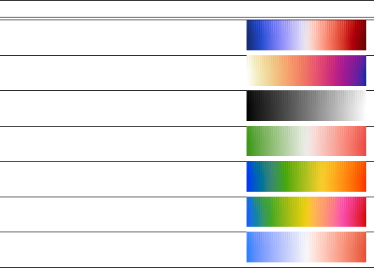
1.8 Colour maps for visualisation
In an attempt to homogenise the figures obtained with ParaView, I have decided to use a fixed colour
scale for each field throughout this document. These colour scales were obtained from this link and are
Perceptually Uniform Colour Maps [296].
Field colour code
Velocity/displacement CET-D1A
Pressure CET-L17
Velocity divergence CET-L1
Density CET-D3
Strain rate CET-R2
Viscosity CET-R3
Temperature CET-D9
7

2 List of tutorials
tutorial number
element outer solver formulation physical problem
3D
temperature
time stepping
nonlinear
compressible
analytical benchmark
numerical benchmark
elastomechanics
1Q1×P0penalty analytical benchmark †
2Q1×P0penalty Stokes sphere
3Q1×P0penalty Blankenbach et al., 1989 † †
4Q1×P0penalty Lid driven cavity
5Q1×P0penalty SolCx benchmark
6Q1×P0penalty SolKz benchmark
7Q1×P0penalty SolVi benchmark
8Q1×P0penalty Indentor †
9Q1×P0penalty annulus benchmark
10 Q1×P0penalty Stokes sphere †
11 Q1×P0full matrix mixed Stokes sphere †
12 Q1×P0penalty analytical benchmark
+ consistent press recovery
13 Q1×P0penalty Stokes sphere
+ markers averaging
14 Q1×P0full matrix mixed analytical benchmark
15 Q1×P0Schur comp. CG mixed analytical benchmark
16 Q1×P0Schur comp. PCG mixed Stokes sphere
17 Q2×Q1full matrix mixed Burstedde benchmark †
18 Q2×Q1full matrix mixed analytical benchmark
19 Q3×Q2full matrix mixed analytical benchmark
20 Q1×P0penalty Busse et al., 1993 † † †
21 Q1×P0R-T penalty analytical benchmark
22 Q1×Q1-
stab
full matrix mixed analytical benchmark
23 Q1×P0mixed analytical benchmark †
24 Q1×P0mixed convection box † † †
8

tutorial number
element outer solver formulation physical problem
3D
temperature
time stepping
nonlinear
compressible
analytical benchmark
numerical benchmark
elastomechanics
25 Q1×P0full matrix mixed Rayleigh-Taylor instability
26 Q1×P0full matrix mixed Slab detachment †
27 Q1×P0full matrix mixed CBF benchmarks † †
28 Q1×P0full matrix mixed Tosi et al, 2015 † † † †
29 Q1×P0full matrix mixed Open Boundary conditions †
30 Q1, Q2X X Cons. Vel. Interp (cvi) † †
31 Q1, Q2X X Cons. Vel. Interp (cvi) † † †
32 Q1×P0full matrix mixed analytical benchmark †
33 Q1×P0penalty convection in annulus † † †
34 Q1elastic Cartesian aquarium † † †
35
36 Q1elastic annulus aquarium † † †
37 Q1, Q2X X population control, bmw test † †
38 Critical Rayleigh number
XX
Analytical benchmark means that an analytical solution exists while numerical benchmark means that a comparison with other code(s) has been carried
out.
9

3 The physical equations
Symbol meaning unit
tTime s
x, y, z Cartesian coordinates m
r, θ Polar coordinates m,-
r, θ, z Cylindrical coordinates m,-,m
r, θ, φ Spherical coordinates m,-,-
νvelocity vector m·s−1
ρmass density kg/m3
ηdynamic viscosity Pa·s
λpenalty parameter Pa·s
Ttemperature K
∇gradient operator m−1
∇· divergence operator m−1
ppressure Pa
˙
ε(
ν) strain rate tensor s−1
αthermal expansion coefficient K−1
kthermal conductivity W/(m ·K)
CpHeat capacity J/K
Hintrinsic specific heat production W/kg
βTisothermal compressibility Pa−1
τdeviatoric stress tensor Pa
σfull stress tensor Pa
3.1 The heat transport equation - energy conservation equation
Let us start from the heat transport equation as shown in Schubert, Turcotte and Olson [416]:
ρCp
DT
Dt −αT Dp
Dt =
∇ · k
∇T+Φ+ρH
with D/Dt being the total derivatives so that
DT
Dt =∂T
∂t +
ν·
∇TDp
Dt =∂p
∂t +
ν·
∇p
Solving for temperature, this equation is often rewritten as follows:
ρCp
DT
Dt −
∇ · k
∇T=αT Dp
Dt +Φ+ρH
A note on the shear heating term Φ: In many publications, Φ is given by Φ = τij ∂jui=τ:
∇
ν.
10

Φ = τij ∂jui
= 2η˙εd
ij ∂jui
= 2η1
2˙εd
ij ∂jui+ ˙εd
ji∂iuj
= 2η1
2˙εd
ij ∂jui+ ˙εd
ij ∂iuj
= 2η˙εd
ij
1
2(∂jui+∂iuj)
= 2η˙εd
ij ˙εij
= 2η˙
εd:˙
ε
= 2η˙
εd:˙
εd+1
3(
∇ ·
ν)1
= 2η˙
εd:˙
εd+ 2η˙
εd:1(
∇ ·
ν)
= 2η˙
εd:˙
εd(1)
Finally
Φ = τ:
∇
ν= 2η˙
εd:˙
εd= 2η( ˙εd
xx)2+ ( ˙εd
yy)2+ 2( ˙εd
xy)2
3.2 The momentum conservation equations
Because the Prandlt number is virtually zero in Earth science applications the Navier Stokes equations
reduce to the Stokes equation:
∇ · σ+ρg = 0
Since
σ=−p1+τ
it also writes
−
∇p+
∇ · τ+ρg = 0
Using the relationship τ= 2η˙
εdwe arrive at
−
∇p+
∇ · (2η˙
εd) + ρg = 0
3.3 The mass conservation equations
The mass conservation equation is given by
Dρ
Dt +ρ
∇ ·
ν= 0
or,
∂ρ
∂t +
∇ · (ρ
ν)=0
In the case of an incompressible flow, then ∂ρ/∂t = 0 and
∇ρ= 0, i.e. Dρ/Dt = 0 and the remaining
equation is simply:
∇ ·
ν= 0
11

3.4 The equations in ASPECT manual
The following is lifted off the ASPECT manual. We focus on the system of equations in a d= 2- or
d= 3-dimensional domain Ω that describes the motion of a highly viscous fluid driven by differences in
the gravitational force due to a density that depends on the temperature. In the following, we largely
follow the exposition of this material in Schubert, Turcotte and Olson [416].
Specifically, we consider the following set of equations for velocity u, pressure pand temperature T:
−
∇ · 2η˙
ε(
ν)−1
3(
∇ ·
ν)1+
∇p=ρg in Ω,(2)
∇ · (ρv) = 0 in Ω,(3)
ρCp∂T
∂t +
ν·
∇T−
∇ · k
∇T=ρH
+ 2η˙ε(v)−1
3(
∇ ·
ν)1:˙ε(v)−1
3(
∇ ·
ν)1(4)
+αT v·
∇pin Ω,
where ˙
ε(
ν) = 1
2(
∇
ν+
∇
νT) is the symmetric gradient of the velocity (often called the strain rate).
In this set of equations, (253) and (254) represent the compressible Stokes equations in which v=
v(x, t) is the velocity field and p=p(x, t) the pressure field. Both fields depend on space xand time
t. Fluid flow is driven by the gravity force that acts on the fluid and that is proportional to both the
density of the fluid and the strength of the gravitational pull.
Coupled to this Stokes system is equation (255) for the temperature field T=T(x, t) that contains
heat conduction terms as well as advection with the flow velocity v. The right hand side terms of this
equation correspond to
•internal heat production for example due to radioactive decay;
•friction (shear) heating;
•adiabatic compression of material;
In order to arrive at the set of equations that ASPECT solves, we need to
•neglect the ∂p/∂t.WHY?
•neglect the ∂ρ/∂t .WHY?
from equations above.
—————————————-
Also, their definition of the shear heating term Φ is:
Φ = kB(∇·v)2+ 2η˙
εd:˙
εd
For many fluids the bulk viscosity kBis very small and is often taken to be zero, an assumption known
as the Stokes assumption: kB=λ+ 2η/3 = 0. Note that ηis the dynamic viscosity and λthe second
viscosity. Also,
τ= 2η˙
ε+λ(∇·v)1
but since kB=λ+ 2η/3 = 0, then λ=−2η/3 so
τ= 2η˙
ε−2
3η(∇·v)1= 2η˙
εd
12

3.5 the Boussinesq approximation: an Incompressible flow
[from aspect manual] The Boussinesq approximation assumes that the density can be considered constant
in all occurrences in the equations with the exception of the buoyancy term on the right hand side of
(253). The primary result of this assumption is that the continuity equation (254) will now read
∇·v= 0
This implies that the strain rate tensor is deviatoric. Under the Boussinesq approximation, the equations
are much simplified:
−∇ · [2η˙
ε(v)] + ∇p=ρgin Ω,(5)
∇ · (ρv) = 0 in Ω,(6)
ρ0Cp∂T
∂t +v· ∇T−∇·k∇T=ρH in Ω (7)
Note that all terms on the rhs of the temperature equations have disappeared, with the exception of the
source term.
13

3.6 Stokes equation for elastic medium
What follows is mostly borrowed from Becker & Kaus lecture notes.
The strong form of the PDE that governs force balance in a medium is given by
∇·σ+f=0
where σis the stress tensor and fis a body force.
The stress tensor is related to the strain tensor through the generalised Hooke’s law:
σij =X
kl
Cijklkl (8)
where Cis the fourth-order elastic tensor. In the case of an isotropic material, this relationship simplifies
to
σij =λkkδij + 2µij or, σ=λ(∇·u)1+ 2µ(9)
where λis the Lam´e parameter and µis the shear modulus1. The term ∇·uis the isotropic dilation.
The strain tensor is related to the displacement as follows:
=1
2(∇u+∇uT)
The incompressibility (bulk modulus), K, is defined as p=−K∇·uwhere pis the pressure with
p=−1
3T r(σ)
=−1
3[λ(∇·u)T r[1]+2µT r[]]
=−1
3[λ(∇·u)3 + 2µ(∇·u)]
=−[λ+2
3µ](∇·u) (10)
so that K=λ+2
3µ.
Remark : Eq. (8) and (9) are analogous to the ones that one has to solve in the context of viscous
flow using the penalty method. In this case λis the penalty coefficient, uis the velocity, and µis then
the dynamic viscosity.
The Lam´e parameter and the shear modulus are also linked to νthe poisson ratio, and E, Young’s
modulus:
λ=µ2ν
1−2ν=νE
(1 + ν)(1 −2ν)with E= 2µ(1 + ν)
The shear modulus, expressed often in GPa, describes the material’s response to shear stress. The poisson
ratio describes the response in the direction orthogonal to uniaxial stress. The Young modulus, expressed
in GPa, describes the material’s strain response to uniaxial stress in the direction of this stress.
1It is also sometimes written G
14

3.7 The strain rate tensor in all coordinate systems
The strain rate tensor ˙
εis given by
˙
ε=1
2(
∇
ν+
∇
νT) (11)
3.7.1 Cartesian coordinates
˙εxx =∂u
∂x (12)
˙εyy =∂v
∂y (13)
˙εzz =∂w
∂z (14)
˙εyx = ˙εxy =1
2∂u
∂y +∂v
∂x (15)
˙εzx = ˙εxz =1
2∂u
∂z +∂w
∂x (16)
˙εzy = ˙εyz =1
2∂v
∂z +∂w
∂y (17)
3.7.2 Polar coordinates
˙εrr =∂vr
∂r (18)
˙εθθ =vr
r+1
r
∂vθ
∂θ (19)
˙εθr = ˙εrθ =1
2∂vθ
∂r −vθ
r+1
r
∂vr
∂θ (20)
3.7.3 Cylindrical coordinates
http://eml.ou.edu/equation/FLUIDS/STRAIN/STRAIN.HTM
3.7.4 Sperical coordinates
˙εrr =∂vr
∂r (21)
˙εθθ =vr
r+1
r
∂vθ
∂θ (22)
˙εφφ =1
rsin θ
∂vφ
∂φ (23)
˙εθr = ˙εrθ =1
2r∂
∂r (vθ
r) + 1
r
∂vr
∂θ (24)
˙εφr = ˙εrφ =1
21
rsin θ
∂vr
∂φ +r∂
∂r (vφ
r)(25)
˙εφθ = ˙εθφ =1
2sin θ
r
∂
∂θ (vφ
sin θ) + 1
rsin θ
∂vθ
∂φ (26)
15
3.8 Boundary conditions
In mathematics, the Dirichlet (or first-type) boundary condition is a type of boundary condition, named
after Peter Gustav Lejeune Dirichlet. When imposed on an ODE or PDE, it specifies the values that a
solution needs to take on along the boundary of the domain. Note that a Dirichlet boundary condition
may also be referred to as a fixed boundary condition.
The Neumann (or second-type) boundary condition is a type of boundary condition, named after Carl
Neumann. When imposed on an ordinary or a partial differential equation, the condition specifies the
values in which the derivative of a solution is applied within the boundary of the domain.
It is possible to describe the problem using other boundary conditions: a Dirichlet boundary condition
specifies the values of the solution itself (as opposed to its derivative) on the boundary, whereas the Cauchy
boundary condition, mixed boundary condition and Robin boundary condition are all different types of
combinations of the Neumann and Dirichlet boundary conditions.
3.8.1 The Stokes equations
You may find the following terms in the computational geodynamics literature:
•free surface: this means that no force is acting on the surface, i.e. σ·n =
0. It is usually used on
the top boundary of the domain and allows for topography evolution.
•free slip:
ν·n = 0 and (σ·n)×n =
0. This condition ensures a frictionless flow parallel to the
boundary where it is prescribed.
•no slip: this means that the velocity (or displacement) is exactly zero on the boundary, i.e.
ν=
0.
•prescribed velocity:
ν=
νbc
•stress b.c.:
•open .b.c.: see fieldstone 29.
3.8.2 The heat transport equation
There are two types of boundary conditions for this equation: temperature boundary conditions (Dirichlet
boundary conditions) and heat flux boundary conditions (Neumann boundary conditions).
16

3.9 Meaningful physical quantities
•Velocity (m/s):
•Root mean square velocity (m/s):
νrms =RΩ|
ν|2dΩ
RΩdΩ1/2
=1
VΩZΩ|
ν|2dΩ1/2
(27)
In Cartesian coordinates, for a cuboid domain of size Lx ×Ly×Lz, the vrms is simply given by:
νrms = 1
LxLyLzZLx
0ZLy
0ZLz
0
(u2+v2+w2)dxdydz!1/2
(28)
In the case of an annulus domain, although calculations are carried out in Cartesian coordinates,
it makes sense to look at the radial velocity component vrand the tangential velocity component
vθ, and their respective root mean square averages:
vr|rms =1
VΩZΩ
v2
rdΩ1/2
(29)
vθ|rms =1
VΩZΩ
v2
θdΩ1/2
(30)
•Pressure (Pa):
•Stress (Pa):
•Strain (X):
•Strain rate (s−1):
•Rayleigh number (X):
•Prandtl number (X):
•Nusselt number (X): the Nusselt number (Nu) is the ratio of convective to conductive heat transfer
across (normal to) the boundary. The conductive component is measured under the same conditions
as the heat convection but with a (hypothetically) stagnant (or motionless) fluid.
In practice the Nusselt number Nu of a layer (typically the mantle of a planet) is defined as follows:
Nu = q
qc
(31)
where qis the heat transferred by convection while qc=k∆T/D is the amount of heat that would
be conducted through a layer of thickness Dwith a temperature difference ∆Tacross it with k
being the thermal conductivity.
For 2D Cartesian systems of size (Lx,Ly) the Nu is computed [55]
Nu =
1
LxRLx
0k∂T
∂y (x, y =Ly)dx
−1
LxRLx
0kT (x, y = 0)/Lydx =−LyRLx
0
∂T
∂y (x, y =Ly)dx
RLx
0T(x, y = 0)dx
i.e. it is the mean surface temperature gradient over the mean bottom temperature.
finish. not happy with definition. Look at literature
Note that in the case when no convection takes place then the measured heat flux at the top is the
one obtained from a purely conductive profile which yields Nu=1.
Note that a relationship Ra ∝Nuαexists between the Rayleigh number Ra and the Nusselt number
Nu in convective systems, see [505] and references therein.
17

Turning now to cylindrical geometries with inner radius R1and outer radius R2, we define f=
R1/R2. A small value of fcorresponds to a high degree of curvature. We assume now that
R2−R1= 1, so that R2= 1/(1 −f) and R1=f/(1 −f). Following [276], the Nusselt number at
the inner and outer boundaries are:
Nuinner =fln f
1−f
1
2πZ2π
0∂T
∂r r=R1
dθ (32)
Nuouter =ln f
1−f
1
2πZ2π
0∂T
∂r r=R2
dθ (33)
Note that a conductive geotherm in such an annulus between temperatures T1and T2is given by
Tc(r) = ln(r/R2)
ln(R1/R2)=ln(r(1 −f))
ln f
so that ∂Tc
∂r =1
r
1
ln f
We then find:
Nuinner =fln f
1−f
1
2πZ2π
0∂Tc
∂r r=R1
dθ =fln f
1−f
1
R1
1
ln f= 1 (34)
Nuouter =ln f
1−f
1
2πZ2π
0∂Tc
∂r r=R2
dθ =ln f
1−f
1
R2
1
ln f= 1 (35)
As expected, the recovered Nusselt number at both boundaries is exactly 1 when the temperature
field is given by a steady state conductive geotherm.
derive formula for Earth size R1 and R2
•Temperature (K):
•Viscosity (Pa.s):
•Density (kg/m3):
•Heat capacity cp(J.K−1.kg−1): It is the measure of the heat energy required to increase the
temperature of a unit quantity of a substance by unit degree.
•Heat conductivity, or thermal conductivity k(W.m−1.K−1). It is the property of a material that
indicates its ability to conduct heat. It appears primarily in Fourier’s Law for heat conduction.
•Heat diffusivity: κ=k/(ρcp) (m2.s−1). Substances with high thermal diffusivity rapidly adjust
their temperature to that of their surroundings, because they conduct heat quickly in comparison
to their volumetric heat capacity or ’thermal bulk’.
•thermal expansion α(K−1): it is the tendency of a matter to change in volume in response to a
change in temperature.
check aspect manual The 2D cylindrical shell benchmarks by Davies et al. 5.4.12
18

4 The building blocks of the Finite Element Method
4.1 Numerical integration
As we will see later, using the Finite Element method to solve problems involves computing integrals
which are more often than not too complex to be computed analytically/exactly. We will then need to
compute them numerically.
[wiki] In essence, the basic problem in numerical integration is to compute an approximate solution
to a definite integral Zb
a
f(x)dx
to a given degree of accuracy. This problem has been widely studied and we know that if f(x) is a
smooth function, and the domain of integration is bounded, there are many methods for approximating
the integral to the desired precision.
There are several reasons for carrying out numerical integration.
•The integrand f(x) may be known only at certain points, such as obtained by sampling. Some
embedded systems and other computer applications may need numerical integration for this reason.
•A formula for the integrand may be known, but it may be difficult or impossible to find an an-
tiderivative that is an elementary function. An example of such an integrand is f(x) = exp(−x2),
the antiderivative of which (the error function, times a constant) cannot be written in elementary
form.
•It may be possible to find an antiderivative symbolically, but it may be easier to compute a numerical
approximation than to compute the antiderivative. That may be the case if the antiderivative is
given as an infinite series or product, or if its evaluation requires a special function that is not
available.
4.1.1 in 1D - theory
The simplest method of this type is to let the interpolating function be a constant function (a polynomial
of degree zero) that passes through the point ((a+b)/2, f((a+b)/2)).
This is called the midpoint rule or rectangle rule.
Zb
a
f(x)dx '(b−a)f(a+b
2)
insert here figure
The interpolating function may be a straight line (an affine function, i.e. a polynomial of degree 1)
passing through the points (a, f(a)) and (b, f(b)).
This is called the trapezoidal rule.
Zb
a
f(x)dx '(b−a)f(a) + f(b)
2
insert here figure
For either one of these rules, we can make a more accurate approximation by breaking up the interval
[a, b] into some number n of subintervals, computing an approximation for each subinterval, then adding
up all the results. This is called a composite rule, extended rule, or iterated rule. For example, the
composite trapezoidal rule can be stated as
Zb
a
f(x)dx 'b−a
n f(a)
2+
n−1
X
k=1
f(a+kb−a
n) + f(b)
2!
where the subintervals have the form [kh, (k+ 1)h], with h= (b−a)/n and k= 0,1,2, . . . , n −1.
19
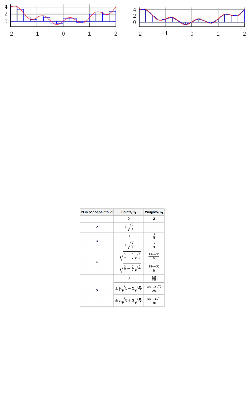
a) b)
The interval [−2,2] is broken into 16 sub-intervals. The blue lines correspond to the approximation of
the red curve by means of a) the midpoint rule, b) the trapezoidal rule.
There are several algorithms for numerical integration (also commonly called ’numerical quadrature’,
or simply ’quadrature’) . Interpolation with polynomials evaluated at equally spaced points in [a, b] yields
the NewtonCotes formulas, of which the rectangle rule and the trapezoidal rule are examples. If we allow
the intervals between interpolation points to vary, we find another group of quadrature formulas, such
as the Gauss(ian) quadrature formulas. A Gaussian quadrature rule is typically more accurate than a
NewtonCotes rule, which requires the same number of function evaluations, if the integrand is smooth
(i.e., if it is sufficiently differentiable).
An n−point Gaussian quadrature rule, named after Carl Friedrich Gauss, is a quadrature rule con-
structed to yield an exact result for polynomials of degree 2n−1 or less by a suitable choice of the points
xiand weights wifor i= 1, . . . , n.
The domain of integration for such a rule is conventionally taken as [−1,1], so the rule is stated as
Z+1
−1
f(x)dx =
n
X
iq=1
wiqf(xiq)
In this formula the xiqcoordinate is the i-th root of the Legendre polynomial Pn(x).
It is important to note that a Gaussian quadrature will only produce good results if the function f(x)
is well approximated by a polynomial function within the range [−1,1]. As a consequence, the method
is not, for example, suitable for functions with singularities.
Gauss-Legendre points and their weights.
As shown in the above table, it can be shown that the weight values must fulfill the following condition:
X
iq
wiq= 2 (36)
and it is worth noting that all quadrature point coordinates are symmetrical around the origin.
Since most quadrature formula are only valid on a specific interval, we now must address the problem
of their use outside of such intervals. The solution turns out to be quite simple: one must carry out a
change of variables from the interval [a, b] to [−1,1].
We then consider the reduced coordinate r∈[−1,1] such that
r=2
b−a(x−a)−1
20
This relationship can be reversed such that when ris known, its equivalent coordinate x∈[a, b] can be
computed:
x=b−a
2(1 + r) + a
From this it follows that
dx =b−a
2dr
and then Zb
a
f(x)dx =b−a
2Z+1
−1
f(r)dr 'b−a
2
n
X
iq=1
wiqf(riq)
4.1.2 in 1D - examples
example 1 Since we know how to carry out any required change of variables, we choose for simplicity
a=−1, b= +1. Let us take for example f(x) = π. Then we can compute the integral of this function
over the interval [a, b] exactly:
I=Z+1
−1
f(x)dx =πZ+1
−1
dx = 2π
We can now use a Gauss-Legendre formula to compute this same integral:
Igq =Z+1
−1
f(x)dx =
nq
X
iq=1
wiqf(xiq) =
nq
X
iq=1
wiqπ=π
nq
X
iq=1
wiq
| {z }
=2
= 2π
where we have used the property of the weight values of Eq.(36). Since the actual number of points was
never specified, this result is valid for all quadrature rules.
example 2 Let us now take f(x) = mx +pand repeat the same exercise:
I=Z+1
−1
f(x)dx =Z+1
−1
(mx +p)dx = [1
2mx2+px]+1
−1= 2p
Igq =Z+1
−1
f(x)dx=
nq
X
iq=1
wiqf(xiq)=
nq
X
iq=1
wiq(mxiq+p)= m
nq
X
iq=1
wiqxiq
| {z }
=0
+p
nq
X
iq=1
wiq
| {z }
=2
= 2p
since the quadrature points are symmetric w.r.t. to zero on the x-axis. Once again the quadrature is able
to compute the exact value of this integral: this makes sense since an n-point rule exactly integrates a
2n−1 order polynomial such that a 1 point quadrature exactly integrates a first order polynomial like
the one above.
example 3 Let us now take f(x) = x2. We have
I=Z+1
−1
f(x)dx =Z+1
−1
x2dx = [1
3x3]+1
−1=2
3
and
Igq =Z+1
−1
f(x)dx=
nq
X
iq=1
wiqf(xiq)=
nq
X
iq=1
wiqx2
iq
•nq= 1: x(1)
iq = 0, wiq= 2. Igq = 0
•nq= 2: x(1)
q=−1/√3, x(2)
q= 1/√3, w(1)
q=w(2)
q= 1. Igq =2
3
•It also works ∀nq>2 !
21
4.1.3 in 2D/3D - theory
Let us now turn to a two-dimensional integral of the form
I=Z+1
−1Z+1
−1
f(x, y)dxdy
The equivalent Gaussian quadrature writes:
Igq '
nq
X
iq=1
nq
X
jq
f(xiq, yjq)wiqwjq
4.2 The mesh
4.3 A bit of FE terminology
We introduce here some terminology for efficient element descriptions [239]:
•For triangles/tetrahedra, the designation Pm×Pnmeans that each component of the velocity is
approximated by continuous piecewise complete Polynomials of degree mand pressure by continuous
piecewise complete Polynomials of degree n. For example P2×P1means
u∼a1+a2x+a3y+a4xy +a5x2+a6y2
with similar approximations for v, and
p∼b1+b2x+b3y
Both velocity and pressure are continuous across element boundaries, and each triangular element
contains 6 velocity nodes and three pressure nodes.
•For the same families, Pm×P−nis as above, except that pressure is approximated via piecewise
discontinuous polynomials of degree n. For instance, P2×P−1is the same as P2P1except that
pressure is now an independent linear function in each element and therefore discontinuous at
element boundaries.
•For quadrilaterals/hexahedra, the designation Qm×Qnmeans that each component of the velocity
is approximated by a continuous piecewise polynomial of degree min each direction on the quadri-
lateral and likewise for pressure, except that the polynomial is of degree n. For instance, Q2×Q1
means
u∼a1+a2x+a3y+a4xy +a5x2+a6y2+a7x2y+a8xy2+a9x2y2
and
p∼b1+b2x+b3y+b4xy
•For these same families, Qm×Q−nis as above, except that the pressure approximation is not
continuous at element boundaries.
•Again for the same families, Qm×P−nindicates the same velocity approximation with a pressure
approximation that is a discontinuous complete piecewise polynomial of degree n(not of degree n
in each direction !)
•The designation P+
mor Q+
mmeans that some sort of bubble function was added to the polynomial
approximation for the velocity. You may also find the term ’enriched element’ in the literature.
•Finally, for n= 0, we have piecewise-constant pressure, and we omit the minus sign for simplicity.
Another point which needs to be clarified is the use of so-called ’conforming elements’ (or ’non-
conforming elements’). Following again [239], conforming velocity elements are those for which the
basis functions for a subset of H1for the continuous problem (the first derivatives and their squares are
integrable in Ω). For instance, the rotated Q1×P0element of Rannacher and Turek (see section ??) is
such that the velocity is discontinous across element edges, so that the derivative does not exist there.
Another typical example of non-conforming element is the Crouzeix-Raviart element [125].
22
4.4 Elements and basis functions in 1D
4.4.1 Linear basis functions (Q1)
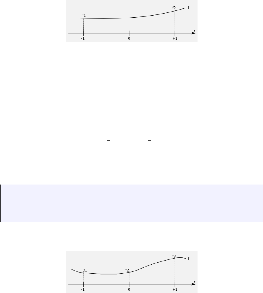
Let f(r) be a C1function on the interval [−1 : 1] with f(−1) = f1and f(1) = f2.
Let us assume that the function f(r) is to be approximated on [−1,1] by the first order polynomial
f(r) = a+br (37)
Then it must fulfill
f(r=−1) = a−b=f1
f(r= +1) = a+b=f2
This leads to
a=1
2(f1+f2)b=1
2(−f1+f2)
and then replacing a, b in Eq. (37) by the above values on gets
f(r) = 1
2(1 −r)f1+1
2(1 + r)f2
or
f(r) =
2
X
i=1
Ni(r)f1
with
N1(r) = 1
2(1 −r)
N2(r) = 1
2(1 + r) (38)
4.4.2 Quadratic basis functions (Q2)
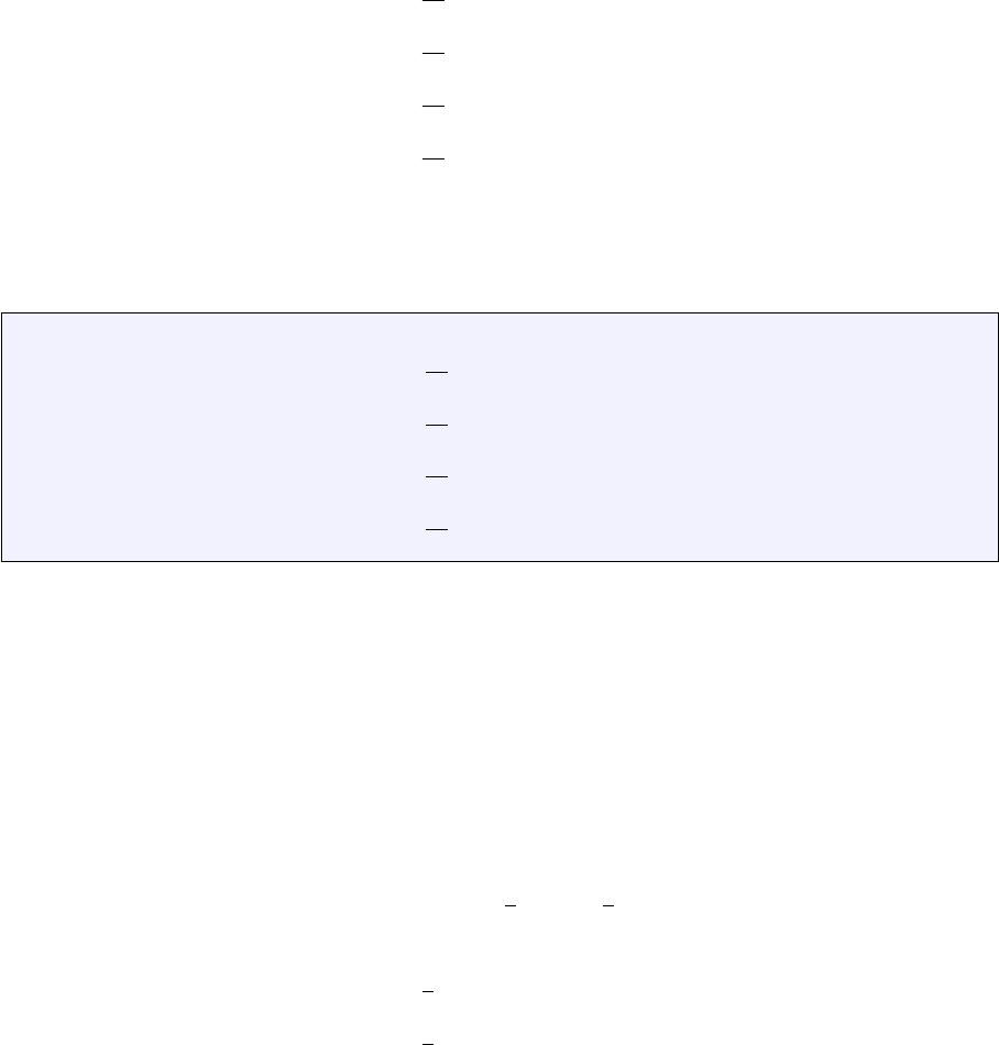
Let f(r) be a C1function on the interval [−1 : 1] with f(−1) = f1,f(0) = f2and f(1) = f3.
Let us assume that the function f(r) is to be approximated on [−1,1] by the second order polynomial
f(r) = a+br +cr2(39)
Then it must fulfill
f(r=−1) = a−b+c=f1
f(r= 0) = a=f2
f(r= +1) = a+b+c=f3
23
This leads to
a=f2b=1
2(−f1 + f3) c=1
2(f1+f3−2f2)
and then replacing a, b, c in Eq. (39) by the above values on gets
f(r) = 1
2r(r−1)f1+ (1 −r2)f2+1
2r(r+ 1)f3
or,
f(r) =
3
X
i=1
Ni(r)fi
with
N1(r) = 1
2r(r−1)
N2(r) = (1 −r2)
N3(r) = 1
2r(r+ 1) (40)
4.4.3 Cubic basis functions (Q3)
The 1D basis polynomial is given by
f(r) = a+br +cr2+dr3
with the nodes at position -1,-1/3, +1/3 and +1.
f(−1) = a−b+c−d=f1
f(−1/3) = a−b
3+c
9−d
27 =f2
f(+1/3) = a−b
3+c
9−d
27 =f3
f(+1) = a+b+c+d=f4
Adding the first and fourth equation and the second and third, one arrives at
f1+f4= 2a+ 2c f2+f3= 2a+2c
9
and finally:
a=1
16 (−f1+ 9f2+ 9f3−f4)
c=9
16 (f1−f2−f3+f4)
Combining the original 4 equations in a different way yields
2b+ 2d=f4−f1
2b
3+2d
27 =f3−f2
so that
b=1
16 (f1−27f2+ 27f3−f4)
d=9
16 (−f1+ 3f2−3f3+f4)
Finally,
24
f(r) = a+b+cr2+dr3
=1
16(−1 + r+ 9r2−9r3)f1
+1
16(9 −27r−9r2+ 27r3)f2
+1
16(9 + 27r−9r2−27r3)f3
+1
16(−1−r+ 9r2+ 9r3)f4
=
4
X
i=1
Ni(r)fi
where
N1=1
16(−1 + r+ 9r2−9r3)
N2=1
16(9 −27r−9r2+ 27r3)
N3=1
16(9 + 27r−9r2−27r3)
N4=1
16(−1−r+ 9r2+ 9r3)
Verification:
•Let us assume f(r) = C, then
ˆ
f(r) = XNi(r)fi=X
i
NiC=CX
i
Ni=C
so that a constant function is exactly reproduced, as expected.
•Let us assume f(r) = r, then f1=−1, f2=−1/3, f3= 1/3 and f4= +1. We then have
ˆ
f(r) = XNi(r)fi
=−N1(r)−1
3N2(r) + 1
3N3(r) + N4(r)
= [−(−1 + r+ 9r2−9r3)
−1
3(9 −27r−9r2−27r3)
+1
3(9 + 27r−9r2+ 27r3)
+(−1−r+ 9r2+ 9r3)]/16
= [−r+ 9r+ 9r−r]/16 + ...0...
=r(41)
The basis functions derivative are given by
25
∂N1
∂r =1
16(1 + 18r−27r2)
∂N2
∂r =1
16(−27 −18r+ 81r2)
∂N3
∂r =1
16(+27 −18r−81r2)
∂N4
∂r =1
16(−1 + 18r+ 27r2)
Verification:
•Let us assume f(r) = C, then
∂ˆ
f
∂r =X
i
∂Ni
∂r fi
=CX
i
∂Ni
∂r
=C
16[(1 + 18r−27r2)
+(−27 −18r+ 81r2)
+(+27 −18r−81r2)
+(−1 + 18r+ 27r2)]
= 0
•Let us assume f(r) = r, then f1=−1, f2=−1/3, f3= 1/3 and f4= +1. We then have
∂ˆ
f
∂r =X
i
∂Ni
∂r fi
=1
16[−(1 + 18r−27r2)
−1
3(−27 −18r+ 81r2)
+1
3(+27 −18r−81r2)
+(−1 + 18r+ 27r2)]
=1
16[−2 + 18 + 54r2−54r2]
= 1
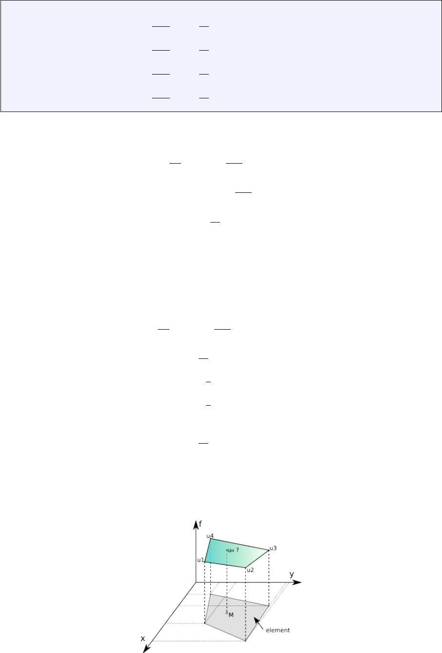
4.5 Elements and basis functions in 2D
Let us for a moment consider a single quadrilateral element in the xy-plane, as shown on the following
figure:
26

Let us assume that we know the values of a given field uat the vertices. For a given point Minside
the element in the plane, what is the value of the field uat this point? It makes sense to postulate that
uM=u(xM, yM) will be given by
uM=φ(u1, u2, u3, u4, xM, yM)
where φis a function to be determined. Although φis not unique, we can decide to express the value
uMas a weighed sum of the values at the vertices ui. One option could be to assign all four vertices the
same weight, say 1/4 so that uM= (u1+u2+u3+u4)/4, i.e. uMis simply given by the arithmetic mean
of the vertices values. This approach suffers from a major drawback as it does not use the location of
point Minside the element. For instance, when (xM, yM)→(x2, y2) we expect uM→u2.
In light of this, we could now assume that the weights would depend on the position of Min a
continuous fashion:
u(xM, yM) =
4
X
i=1
Ni(xM, yM)ui
where the Niare continous (”well behaved”) functions which have the property:
Ni(xj, yj) = δij
or, in other words:
N3(x1, y1) = 0 (42)
N3(x2, y2) = 0 (43)
N3(x3, y3) = 1 (44)
N3(x4, y4) = 0 (45)
The functions Niare commonly called basis functions.
Omitting the Msubscripts for any point inside the element, the velocity components uand vare
given by:
ˆu(x, y) =
4
X
i=1
Ni(x, y)ui(46)
ˆv(x, y) =
4
X
i=1
Ni(x, y)vi(47)
Rather interestingly, one can now easily compute velocity gradients (and therefore the strain rate tensor)
since we have assumed the basis functions to be ”well behaved” (in this case differentiable):
˙xx(x, y) = ∂u
∂x =
4
X
i=1
∂Ni
∂x ui(48)
˙yy(x, y) = ∂v
∂y =
4
X
i=1
∂Ni
∂y vi(49)
˙xy (x, y) = 1
2
∂u
∂y +1
2
∂v
∂x =1
2
4
X
i=1
∂Ni
∂y ui+1
2
4
X
i=1
∂Ni
∂x vi(50)
How we actually obtain the exact form of the basis functions is explained in the coming section.
4.5.1 Bilinear basis functions in 2D (Q1)
In this section, we place ourselves in the most favorables case, i.e. the element is a square defined by
−1< r < 1, −1< s < 1 in the Cartesian coordinates system (r, s):
27

3===========2
| | (r_0,s_0)=(-1,-1)
| | (r_1,s_1)=(+1,-1)
| | (r_2,s_2)=(+1,+1)
| | (r_3,s_3)=(-1,+1)
| |
0===========1
This element is commonly called the reference element. How we go from the (x, y) coordinate system
to the (r, s) once and vice versa will be dealt later on. For now, the basis functions in the above reference
element and in the reduced coordinates system (r, s) are given by:
N1(r, s)=0.25(1 −r)(1 −s)
N2(r, s)=0.25(1 + r)(1 −s)
N3(r, s)=0.25(1 + r)(1 + s)
N4(r, s)=0.25(1 −r)(1 + s)
The partial derivatives of these functions with respect to rans sautomatically follow:
∂N1
∂r (r, s) = −0.25(1 −s)∂N1
∂s (r, s) = −0.25(1 −r)
∂N2
∂r (r, s) = +0.25(1 −s)∂N2
∂s (r, s) = −0.25(1 + r)
∂N3
∂r (r, s) = +0.25(1 + s)∂N3
∂s (r, s) = +0.25(1 + r)
∂N4
∂r (r, s) = −0.25(1 + s)∂N4
∂s (r, s) = +0.25(1 −r)
Let us go back to Eq.(47). And let us assume that the function v(r, s) = Cso that vi=Cfor
i= 1,2,3,4. It then follows that
ˆv(r, s) =
4
X
i=1
Ni(r, s)vi=C
4
X
i=1
Ni(r, s) = C[N1(r, s) + N2(r, s) + N3(r, s) + N4(r, s)] = C
This is a very important property: if the vfunction used to assign values at the vertices is constant, then
the value of ˆvanywhere in the element is exactly C. If we now turn to the derivatives of vwith respect
to rand s:
∂ˆv
∂r (r, s) =
4
X
i=1
∂Ni
∂r (r, s)vi=C
4
X
i=1
∂Ni
∂r (r, s) = C[−0.25(1 −s)+0.25(1 −s)+0.25(1 + s)−0.25(1 + s)] = 0
∂ˆv
∂s (r, s) =
4
X
i=1
∂Ni
∂s (r, s)vi=C
4
X
i=1
∂Ni
∂s (r, s) = C[−0.25(1 −r)−0.25(1 + r)+0.25(1 + r)+0.25(1 −r)] = 0
We reassuringly find that the derivative of a constant field anywhere in the element is exactly zero.
28
If we now choose v(r, s) = ar +bs with aand btwo constant scalars, we find:
ˆv(r, s) =
4
X
i=1
Ni(r, s)vi(51)
=
4
X
i=1
Ni(r, s)(ari+bsi) (52)
=a
4
X
i=1
Ni(r, s)ri
| {z }
r
+b
4
X
i=1
Ni(r, s)si
| {z }
s
(53)
=a[0.25(1 −r)(1 −s)(−1) + 0.25(1 + r)(1 −s)(+1) + 0.25(1 + r)(1 + s)(+1) + 0.25(1 −r)(1 + s)(−1)]
+b[0.25(1 −r)(1 −s)(−1) + 0.25(1 + r)(1 −s)(−1) + 0.25(1 + r)(1 + s)(+1) + 0.25(1 −r)(1 + s)(+1)]
=a[−0.25(1 −r)(1 −s)+0.25(1 + r)(1 −s)+0.25(1 + r)(1 + s)−0.25(1 −r)(1 + s)]
+b[−0.25(1 −r)(1 −s)−0.25(1 + r)(1 −s)+0.25(1 + r)(1 + s)+0.25(1 −r)(1 + s)]
=ar +bs (54)
verify above eq. This set of bilinear shape functions is therefore capable of exactly representing a bilinear
field. The derivatives are:
∂ˆv
∂r (r, s) =
4
X
i=1
∂Ni
∂r (r, s)vi(55)
=a
4
X
i=1
∂Ni
∂r (r, s)ri+b
4
X
i=1
∂Ni
∂r (r, s)si(56)
=a[−0.25(1 −s)(−1) + 0.25(1 −s)(+1) + 0.25(1 + s)(+1) −0.25(1 + s)(−1)]
+b[−0.25(1 −s)(−1) + 0.25(1 −s)(−1) + 0.25(1 + s)(+1) −0.25(1 + s)(+1)]
=a
4[(1 −s) + (1 −s) + (1 + s) + (1 + s)]
+b
4[(1 −s)−(1 −s) + (1 + s)−(1 + s)]
=a(57)
Here again, we find that the derivative of the bilinear field inside the element is exact: ∂ˆv
∂r =∂v
∂r .
However, following the same methodology as above, one can easily prove that this is no more true
for polynomials of degree strivtly higher than 1. This fact has serious consequences: if the solution to
the problem at hand is for instance a parabola, the Q1shape functions cannot represent the solution
properly, but only by approximating the parabola in each element by a line. As we will see later, Q2
basis functions can remedy this problem by containing themselves quadratic terms.
4.5.2 Biquadratic basis functions in 2D (Q2)
This element is part of the so-called LAgrange family.
citation needed
Inside an element the local numbering of the nodes is as follows:
3=====6=====2
| | | (r_0,s_0)=(-1,-1) (r_4,s_4)=( 0,-1)
| | | (r_1,s_1)=(+1,-1) (r_5,s_5)=(+1, 0)
7=====8=====5 (r_2,s_2)=(+1,+1) (r_6,s_6)=( 0,+1)
| | | (r_3,s_3)=(-1,+1) (r_7,s_7)=(-1, 0)
| | | (r_8,s_8)=( 0, 0)
0=====4=====1
The basis polynomial is then
f(r, s) = a+br +cs +drs +er2+fs2+gr2s+hrs2+ir2s2
29
The velocity shape functions are given by:
N0(r, s) = 1
2r(r−1)1
2s(s−1)
N1(r, s) = 1
2r(r+ 1)1
2s(s−1)
N2(r, s) = 1
2r(r+ 1)1
2s(s+ 1)
N3(r, s) = 1
2r(r−1)1
2s(s+ 1)
N4(r, s) = (1 −r2)1
2s(s−1)
N5(r, s) = 1
2r(r+ 1)(1 −s2)
N6(r, s) = (1 −r2)1
2s(s+ 1)
N7(r, s) = 1
2r(r−1)(1 −s2)
N8(r, s) = (1 −r2)(1 −s2)
and their derivatives by:
∂N0
∂r =1
2(2r−1)1
2s(s−1) ∂N0
∂s =1
2r(r−1)1
2(2s−1)
∂N1
∂r =1
2(2r+ 1)1
2s(s−1) ∂N1
∂s =1
2r(r+ 1)1
2(2s−1)
∂N2
∂r =1
2(2r+ 1)1
2s(s+ 1) ∂N2
∂s =1
2r(r+ 1)1
2(2s+ 1)
∂N3
∂r =1
2(2r−1)1
2s(s+ 1) ∂N3
∂s =1
2r(r−1)1
2(2s+ 1)
∂N4
∂r = (−2r)1
2s(s−1) ∂N4
∂s = (1 −r2)1
2(2s−1)
∂N5
∂r =1
2(2r+ 1)(1 −s2)∂N5
∂s =1
2r(r+ 1)(−2s)
∂N6
∂r = (−2r)1
2s(s+ 1) ∂N6
∂s = (1 −r2)1
2(2s+ 1)
∂N7
∂r =1
2(2r−1)(1 −s2)∂N7
∂s =1
2r(r−1)(−2s)
∂N8
∂r = (−2r)(1 −s2)∂N8
∂s = (1 −r2)(−2s)
4.5.3 Eight node serendipity basis functions in 2D (Qs
2)
Inside an element the local numbering of the nodes is as follows:
3=====6=====2
| | | (r_0,s_0)=(-1,-1) (r_4,s_4)=( 0,-1)
| | | (r_1,s_1)=(+1,-1) (r_5,s_5)=(+1, 0)
7=====+=====5 (r_2,s_2)=(+1,+1) (r_6,s_6)=( 0,+1)
| | | (r_3,s_3)=(-1,+1) (r_7,s_7)=(-1, 0)
|||
0=====4=====1
The main difference with the Q2element resides in the fact that there is no node in the middle of the
element The basis polynomial is then
f(r, s) = a+br +cs +drs +er2+fs2+gr2s+hrs2
30
Note that absence of the r2s2term which was previously associated to the center node. We find that
N0(r, s) = 1
4(1 −r)(1 −s)(−r−s−1) (58)
N1(r, s) = 1
4(1 + r)(1 −s)(r−s−1) (59)
N2(r, s) = 1
4(1 + r)(1 + s)(r+s−1) (60)
N3(r, s) = 1
4(1 −r)(1 + s)(−r+s−1) (61)
N4(r, s) = 1
2(1 −r2)(1 −s) (62)
N5(r, s) = 1
2(1 + r)(1 −s2) (63)
N6(r, s) = 1
2(1 −r2)(1 + s) (64)
N7(r, s) = 1
2(1 −r)(1 −s2) (65)
The shape functions at the mid side nodes are products of a second order polynomial parallel to side
and a linear function perpendicular to the side while shape functions for corner nodes are modifications
of the bilinear quadrilateral element:
verify those
4.5.4 Bicubic basis functions in 2D (Q3)
Inside an element the local numbering of the nodes is as follows:
12===13===14===15 (r,s)_{00}=(-1,-1) (r,s)_{08}=(-1,+1/3)
|| || || || (r,s)_{01}=(-1/3,-1) (r,s)_{09}=(-1/3,+1/3)
08===09===10===11 (r,s)_{02}=(+1/3,-1) (r,s)_{10}=(+1/3,+1/3)
|| || || || (r,s)_{03}=(+1,-1) (r,s)_{11}=(+1,+1/3)
04===05===06===07 (r,s)_{04}=(-1,-1/3) (r,s)_{12}=(-1,+1)
|| || || || (r,s)_{05}=(-1/3,-1/3) (r,s)_{13}=(-1/3,+1)
00===01===02===03 (r,s)_{06}=(+1/3,-1/3) (r,s)_{14}=(+1/3,+1)
(r,s)_{07}=(+1,-1/3) (r,s)_{15}=(+1,+1)
The velocity shape functions are given by:
N1(r)=(−1 + r+ 9r2−9r3)/16 N1(t)=(−1 + t+ 9t2−9t3)/16
N2(r) = (+9 −27r−9r2+ 27r3)/16 N2(t) = (+9 −27t−9t2+ 27t3)/16
N3(r) = (+9 + 27r−9r2−27r3)/16 N3(t) = (+9 + 27t−9t2−27t3)/16
N4(r)=(−1−r+ 9r2+ 9r3)/16 N4(t)=(−1−t+ 9t2+ 9t3)/16
31

N01(r, s) = N1(r)N1(s)=(−1 + r+ 9r2−9r3)/16 ∗(−1 + t+ 9s2−9s3)/16
N02(r, s) = N2(r)N1(s) = (+9 −27r−9r2+ 27r3)/16 ∗(−1 + t+ 9s2−9s3)/16
N03(r, s) = N3(r)N1(s) = (+9 + 27r−9r2−27r3)/16 ∗(−1 + t+ 9s2−9s3)/16
N04(r, s) = N4(r)N1(s)=(−1−r+ 9r2+ 9r3)/16 ∗(−1 + t+ 9s2−9s3)/16
N05(r, s) = N1(r)N2(s) = (−1 + r+ 9r2−9r3)/16 ∗(9 −27s−9s2+ 27s3)/16
N06(r, s) = N2(r)N2(s) = (+9 −27r−9r2+ 27r3)/16 ∗(9 −27s−9s2+ 27s3)/16
N07(r, s) = N3(r)N2(s) = (+9 + 27r−9r2−27r3)/16 ∗(9 −27s−9s2+ 27s3)/16
N08(r, s) = N4(r)N2(s)=(−1−r+ 9r2+ 9r3)/16 ∗(9 −27s−9s2+ 27s3)/16
N09(r, s) = N1(r)N3(s) = (66)
N10(r, s) = N2(r)N3(s) = (67)
N11(r, s) = N3(r)N3(s) = (68)
N12(r, s) = N4(r)N3(s) = (69)
N13(r, s) = N1(r)N4(s) = (70)
N14(r, s) = N2(r)N4(s) = (71)
N15(r, s) = N3(r)N4(s) = (72)
N16(r, s) = N4(r)N4(s) = (73)
4.5.5 Linear basis functions for triangles in 2D (P1)
2
|\
| \ (r_0,s_0)=(0,0)
| \ (r_1,s_1)=(1,0)
| \ (r_2,s_2)=(0,2)
0=======1
The basis polynomial is then
f(r, s) = a+br +cs
and the shape functions:
N0(r, s)=1−r−s(74)
N1(r, s) = r(75)
N2(r, s) = s(76)
4.5.6 Quadratic basis functions for triangles in 2D (P2)
2
|\
| \ (r_0,s_0)=(0,0) (r_3,s_3)=(1/2,0)
5 4 (r_1,s_1)=(1,0) (r_4,s_4)=(1/2,1/2)
| \ (r_2,s_2)=(0,1) (r_5,s_5)=(0,1/2)
| \
0===3===1
The basis polynomial is then
f(r, s) = c1+c2r+c3s+c4r2+c5rs +c6s2
32

We have
f1=f(r1, s1) = c1
f2=f(r2, s2) = c1+c2+c4
f3=f(r3, s3) = c1+c3+c6
f4=f(r4, s4) = c1+c2/2 + c4/4
f5=f(r5, s5) = c1+c2/2 + c3/2
+c4/4 + c5/4 + c6/4
f6=f(r6, s6) = c1+c3/2 + c6/4
This can be cast as f=A·cwhere Ais a 6x6 matrix:
A=
100000
110100
101001
1 1/201/4 0 0
1 1/2 1/2 1/4 1/4 1/4
101/2 0 0 1/4
It is rather trivial to compute the inverse of this matrix:
A−1=
1 0 0 0 0 0
−3−1 0 4 0 0
−3 0 −1004
220−4 0 0
400−4 4 −4
2 0 2 0 0 −4
In the end, one obtains:
f(r, s) = f1+ (−3f1−f2+ 4f4)r+ (−3f1−f3+ 4f6)s
+(2f1+ 2f2−4f4)r2+ (4f1−4f4+ 4f5−4f6)rs
+(2f1+ 2f3−4f6)s2
=
6
X
i=1
Ni(r, s)fi(77)
with
N1(r, s)=1−3r−3s+ 2r2+ 4rs + 2s2
N2(r, s) = −r+ 2r2
N3(r, s) = −s+ 2s2
N4(r, s)=4r−4r2−4rs
N5(r, s)=4rs
N6(r, s)=4s−4rs −4s2
4.5.7 Cubic basis functions for triangles (P3)
2
|\ (r_0,s_0)=(0,0) (r_5,s_5)=(2/3,1/3)
| \ (r_1,s_1)=(1,0) (r_6,s_6)=(1/3,2/3)
7 6 (r_2,s_2)=(0,1) (r_7,s_7)=(0,2/3)
| \ (r_3,s_3)=(1/3,0) (r_8,s_8)=(0,1/3)
8 9 5 (r_4,s_4)=(2/3,0) (r_9,s_9)=(1/3,1/3)
| \
0==3==4==1
33

The basis polynomial is then
f(r, s) = c1+c2r+c3s+c4r2+c5rs +c6s2+c7r3+c8r2s+c9rs2+c10s3
N0(r, s) = 9
2(1 −r−s)(1/3−r−s)(2/3−r−s) (78)
N1(r, s) = 9
2r(r−1/3)(r−2/3) (79)
N2(r, s) = 9
2s(s−1/3)(s−2/3) (80)
N3(r, s) = 27
2(1 −r−s)r(2/3−r−s) (81)
N4(r, s) = 27
2(1 −r−s)r(r−1/3) (82)
N5(r, s) = 27
2rs(r−1/3) (83)
N6(r, s) = 27
2rs(r−2/3) (84)
N7(r, s) = 27
2(1 −r−s)s(s−1/3) (85)
N8(r, s) = 27
2(1 −r−s)s(2/3−r−s) (86)
N9(r, s) = 27rs(1 −r−s) (87)
verify those
4.6 Elements and basis functions in 3D
4.6.1 Linear basis functions in tetrahedra (P1)
(r_0,s_0) = (0,0,0)
(r_1,s_1) = (1,0,0)
(r_2,s_2) = (0,2,0)
(r_3,s_3) = (0,0,1)
The basis polynomial is given by
f(r, s, t) = c0+c1r+c2s+c3t
f1=f(r1, s1, t1) = c0(88)
f2=f(r2, s2, t2) = c0+c1(89)
f3=f(r3, s3, t3) = c0+c2(90)
f4=f(r4, s4, t4) = c0+c3(91)
which yields:
c0=f1c1=f2−f1c2=f3−f1c3=f4−f1
f(r, s, t) = c0+c1r+c2s+c3t
=f1+ (f2−f1)r+ (f3−f1)s+ (f4−f1)t
=f1(1 −r−s−t) + f2r+f3s+f4t
=X
i
Ni(r, s, t)fi
Finally,
34

N1(r, s, t)=1−r−s−t
N2(r, s, t) = r
N3(r, s, t) = s
N4(r, s, t) = t
4.6.2 Triquadratic basis functions in 3D (Q2)
N1= 0.5r(r−1) 0.5s(s−1) 0.5t(t−1)
N2= 0.5r(r+ 1) 0.5s(s−1) 0.5t(t−1)
N3= 0.5r(r+ 1) 0.5s(s+ 1) 0.5t(t−1)
N4= 0.5r(r−1) 0.5s(s+ 1) 0.5t(t−1)
N5= 0.5r(r−1) 0.5s(s−1) 0.5t(t+ 1)
N6= 0.5r(r+ 1) 0.5s(s−1) 0.5t(t+ 1)
N7= 0.5r(r+ 1) 0.5s(s+ 1) 0.5t(t+ 1)
N8= 0.5r(r−1) 0.5s(s+ 1) 0.5t(t+ 1)
N9= (1.−r2) 0.5s(s−1) 0.5t(t−1)
N10 = 0.5r(r+ 1) (1 −s2) 0.5t(t−1)
N11 = (1.−r2) 0.5s(s+ 1) 0.5t(t−1)
N12 = 0.5r(r−1) (1 −s2) 0.5t(t−1)
N13 = (1.−r2) 0.5s(s−1) 0.5t(t+ 1)
N14 = 0.5r(r+ 1) (1 −s2) 0.5t(t+ 1)
N15 = (1.−r2) 0.5s(s+ 1) 0.5t(t+ 1)
N16 = 0.5r(r−1) (1 −s2) 0.5t(t+ 1)
N17 = 0.5r(r−1) 0.5s(s−1) (1 −t2)
N18 = 0.5r(r+ 1) 0.5s(s−1) (1 −t2)
N19 = 0.5r(r+ 1) 0.5s(s+ 1) (1 −t2)
N20 = 0.5r(r−1) 0.5s(s+ 1) (1 −t2)
N21 = (1 −r2) (1 −s2) 0.5t(t−1)
N22 = (1 −r2) 0.5s(s−1) (1 −t2)
N23 = 0.5r(r+ 1) (1 −s2) (1 −t2)
N24 = (1 −r2) 0.5s(s+ 1) (1 −t2)
N25 = 0.5r(r−1) (1 −s2) (1 −t2)
N26 = (1 −r2) (1 −s2) 0.5t(t+ 1)
N27 = (1 −r2) (1 −s2) (1 −t2)
35

5 Solving the flow equations with the FEM
In the case of an incompressible flow, we have seen that the continuity (mass conservation) equation takes
the simple form
∇·v = 0. In other word flow takes place under the constraint that the divergence of its
velocity field is exactly zero eveywhere (solenoidal constraint), i.e. it is divergence free.
We see that the pressure in the momentum equation is then a degree of freedom which is needed to
satisfy the incompressibilty constraint (and it is not related to any constitutive equation) [142]. In other
words the pressure is acting as a Lagrange multiplier of the incompressibility constraint.
Various approaches have been proposed in the literature to deal with the incompressibility constraint
but we will only focus on the penalty method (section 5.5) and the so-called mixed finite element method
5.6.
5.1 strong and weak forms
The strong form consists of the governing equation and the boundary conditions, i.e. the mass, momentum
and energy conservation equations supplemented with Dirichlet and/or Neumann boundary conditions
on (parts of) the boundary.
To develop the finite element formulation, the partial differential equations must be restated in an
integral form called the weak form. In essence the PDEs are first multiplied by an arbitrary function and
integrated over the domain.
5.2 Which velocity-pressure pair for Stokes?
The success of a mixed finite element formulation crucially depends on a proper choice of the local
interpolations of the velocity and the pressure.
5.2.1 The compatibility condition (or LBB condition)
5.3 Families
Taylor-Hood
USE [278] section 3.6.2
5.3.1 The bi/tri-linear velocity - constant pressure element (Q1×P0)
discussed in example 3.71 of [278]
5.3.2 The bi/tri-quadratic velocity - discontinuous linear pressure element (Q2×P−1)
5.3.3 The bi/tri-quadratic velocity - bi/tri-linear pressure element (Q2×Q1)
This element, implemented in penalised form, is discussed in [45] and the follow-up paper [46]. CHECK
Biquadratic velocities, bilinear pressure. See Hood and Taylor. The element satisfies the inf-sup
condition [259]p215.
36
5.3.4 The stabilised bi/tri-linear velocity - bi/tri-linear pressure element (Q1×Q1-stab)
5.3.5 The MINI triangular element (P+
1×P1)
discussed in section 3.6.1 of [278]
5.3.6 The quadratic velocity - linear pressure triangle (P2×P1)
From [417]. Taylor-Hood elements (Taylor and Hood 1973) are characterized by the fact that the
pressure is continuous in the region Ω. A typical example is the quadratic triangle (P2P1 element).
In this element the velocity is approximated by a quadratic polynomial and the pressure by a linear
polynomial. One can easily verify that both approximations are continuous over the element boundaries.
It can be shown, Segal (1979), that this element is admissible if at least 3 elements are used. The
quadrilateral counterpart of this triangle is the Q2×Q1element.
5.3.7 The Crouzeix-Raviart triangle (P+
2×P−1)
From [130]: seven-node Crouzeix-Raviart triangle with quadratic velocity shape functions enhanced
by a cubic bubble function and discontinuous linear interpolation for the pressure field [e.g., Cuvelier et
al., 1986]. This element is stable and no additional stabilization techniques are required [Elman et al.,
2005].
From [417]. These elements are characterized by a discontinuous pressure; discontinuous on element
boundaries. For output purposes (printing, plotting etc.) these discontinuous pressures are averaged in
vertices for all the adjoining elements.
The most simple Crouzeix-Raviart element is the non-conforming linear triangle with constant pressure
(P1×P0).
p248 of Elman book. satisfies LBB condition.
5.4 Other elements
P1P0 example 3.70 in [278]
37

P1P1
Q2Q2
P2P2
5.5 The penalty approach for viscous flow
In order to impose the incompressibility constraint, two widely used procedures are available, namely the
Lagrange multiplier method and the penalty method [30, 259]. The latter is implemented in elefant,
which allows for the elimination of the pressure variable from the momentum equation (resulting in a
reduction of the matrix size).
Mathematical details on the origin and validity of the penalty approach applied to the Stokes problem
can for instance be found in [129], [398] or [243].
The penalty formulation of the mass conservation equation is based on a relaxation of the incompress-
ibility constraint and writes
∇ ·
ν+p
λ= 0 (92)
where λis the penalty parameter, that can be interpreted (and has the same dimension) as a bulk
viscosity. It is equivalent to say that the material is weakly compressible. It can be shown that if one
chooses λto be a sufficiently large number, the continuity equation
∇ ·
ν= 0 will be approximately
satisfied in the finite element solution. The value of λis often recommended to be 6 to 7 orders of
magnitude larger than the shear viscosity [144, 260].
Equation (92) can be used to eliminate the pressure in Eq. (??) so that the mass and momentum
conservation equations fuse to become :
∇ · (2η˙ε(
ν)) + λ
∇(
∇ ·
ν) = ρg= 0 (93)
[330] have established the equivalence for incompressible problems between the reduced integration of
the penalty term and a mixed Finite Element approach if the pressure nodes coincide with the integration
points of the reduced rule.
In the end, the elimination of the pressure unknown in the Stokes equations replaces the original
saddle-point Stokes problem [43] by an elliptical problem, which leads to a symmetric positive definite
(SPD) FEM matrix. This is the major benefit of the penalized approach over the full indefinite solver
with the velocity-pressure variables. Indeed, the SPD character of the matrix lends itself to efficient
solving stragegies and is less memory-demanding since it is sufficient to store only the upper half of the
matrix including the diagonal [225] .
list codes which use this approach
The stress tensor σis symmetric (i.e. σij =σji). For simplicity I will now focus on a Stokes flow in
two dimensions.
Since the penalty formulation is only valid for incompressible flows, then ˙
=˙
dso that the dsuper-
script is ommitted in what follows. The stress tensor can also be cast in vector format:
σxx
σyy
σxy
=
−p
−p
0
+ 2η
˙xx
˙yy
˙xy
=λ
˙xx + ˙yy
˙xx + ˙yy
0
+ 2η
˙xx
˙yy
˙xy
=
λ
110
110
000
| {z }
K
+η
200
020
001
| {z }
C
·
∂u
∂x
∂v
∂y
∂u
∂y +∂v
∂x
Remember that
∂u
∂x =
4
X
i=1
∂Ni
∂x ui
∂v
∂y =
4
X
i=1
∂Ni
∂y vi
38
∂u
∂y +∂v
∂x =
4
X
i=1
∂Ni
∂y ui+
4
X
i=1
∂Ni
∂x vi
so that
∂u
∂x
∂v
∂y
∂u
∂y +∂v
∂x
=
∂N1
∂x 0∂N2
∂x 0∂N3
∂x 0∂N4
∂x 0
0∂N1
∂y 0∂N2
∂y 0∂N3
∂y 0∂N4
∂y
∂N1
∂y
∂N1
∂x
∂N2
∂y
∂N2
∂x
∂N3
∂y
∂N3
∂x
∂N3
∂y
∂N4
∂x
| {z }
B
·
u1
v1
u2
v2
u3
v3
u4
v4
| {z }
V
Finally,
σ =
σxx
σyy
σxy
= (λK+ηC)·B·V
We will now establish the weak form of the momentum conservation equation. We start again from
∇ · σ+
b=
0
For the Ni’s ’regular enough’, we can write:
ZΩe
Ni
∇ · σdΩ + ZΩe
NibdΩ=0
We can integrate by parts and drop the surface term2:
ZΩe
∇Ni·σdΩ = ZΩe
NibdΩ
or,
ZΩe
∂Ni
∂x 0∂Ni
∂y
0∂Ni
∂y
∂Ni
∂x
·
σxx
σyy
σxy
dΩ = ZΩe
NibdΩ
Let i= 1,2,3,4 and stack the resulting four equations on top of one another.
ZΩe
∂N1
∂x 0∂N1
∂y
0∂N1
∂y
∂N1
∂x
·
σxx
σyy
σxy
dΩ = ZΩe
N1bx
bydΩ (94)
ZΩe
∂N2
∂x 0∂N2
∂y
0∂N2
∂y
∂N2
∂x
·
σxx
σyy
σxy
dΩ = ZΩe
Nibx
bydΩ (95)
ZΩe
∂N3
∂x 0∂N3
∂y
0∂N3
∂y
∂N3
∂x
·
σxx
σyy
σxy
dΩ = ZΩe
N3bx
bydΩ (96)
ZΩe
∂N4
∂x 0∂N4
∂y
0∂N4
∂y
∂N4
∂x
·
σxx
σyy
σxy
dΩ = ZΩe
N4bx
bydΩ (97)
We easily recognize BTinside the integrals! Let us define
NT
b= (N1bx, N1by, ...N4bx, N4by)
2We will come back to this at a later stage
39
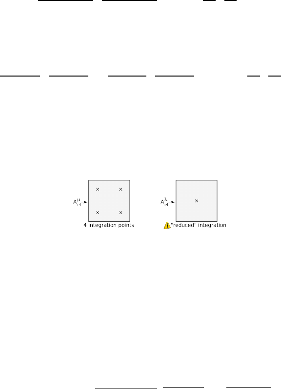
then we can write
ZΩe
BT·
σxx
σyy
σxy
dΩ = ZΩe
NbdΩ
and finally: ZΩe
BT·[λK+ηC]·B·VdΩ = ZΩe
NbdΩ
Since Vcontains the velocities at the corners, it does not depend on the xor ycoordinates so it can be
taking outside of the integral:
ZΩe
BT·[λK+ηC]·BdΩ
| {z }
Ael(8×8)
·V
|{z}
(8x1)
=ZΩe
NbdΩ
| {z }
Bel(8×1)
or,
ZΩe
λBT·K·BdΩ
| {z }
Aλ
el(8×8)
+ZΩe
ηBT·C·BdΩ
| {z }
Aη
el(8×8)
·V
|{z}
(8x1)
=ZΩe
NbdΩ
| {z }
Bel(8×1)
INTEGRATION - MAPPING
reduced integration [260]
1. partition domain Ω into elements Ωe,e= 1, ...nel.
2. loop over elements and for each element compute Ael,Bel
3. a node belongs to several elements
→need to assemble Ael and Bel in A,B
4. apply boundary conditions
5. solve system: x=A−1·B
6. visualise/analyse x
5.6 The mixed FEM for viscous flow
5.6.1 in three dimensions
In what follows the flow is assumed to be incompressible, isoviscous and isothermal.
The methodology to derive the discretised equations of the mixed system is quite similar to the one
we have used in the case of the penalty formulation. The big difference comes from the fact that we are
now solving for both velocity and pressure at the same time, and that we therefore must solve the mass
and momentum conservation equations together. As before, velocity inside an element is given by
νh(r) =
mv
X
i=1
Nν
i(r)
νi(98)
40

where Nv
iare the polynomial basis functions for the velocity, and the summation runs over the mvnodes
composing the element. A similar expression is used for pressure:
ph(r) =
mp
X
i=1
Np
i(r)pi(99)
Note that the velocity is a vector of size while pressure (and temperature) is a scalar. There are then ndofv
velocity degrees of freedom per node and ndofppressure degrees of freedom. It is also very important
to remember that the numbers of velocity nodes and pressure nodes for a given element are more often
than not different and that velocity and pressure nodes need not be colocated. Indeed, unless co-called
’stabilised elements’ are used, we have mv> mp, which means that the polynomial order of the velocity
field is higher than the polynomial order of the pressure field (usually by value 1).
insert here link(s) to manual and literature
Other notations are sometimes used for Eqs.(98) and (99):
uh(r) =
Nν·u vh(r) =
Nν·v wh(r) =
Nν·w ph(r) =
Np·p (100)
where
ν= (u, v, w) and
Nνis the vector containing all basis functions evaluated at location r:
Nv=Nν
1(r), Nν
2(r), Nν
3(r),...Nν
mv(r)(101)
Np=Np
1(r), Np
2(r), Np
3(r),...Np
mp(r)(102)
and with
u = (u1, u2, u3,...umv) (103)
v = (v1, v2, v3,...vmv) (104)
w = (w1, w2, w3,...wmv) (105)
p =p1, p2, p3,...pmp(106)
We will now establish the weak form of the momentum conservation equation. We start again from
∇ · σ+
b=
0 (107)
∇ ·v = 0 (108)
For the Nν
i’s and Np
i’regular enough’, we can write:
ZΩe
Nν
i
∇ · σdΩ + ZΩe
Nν
i
b dΩ =
0 (109)
ZΩe
Np
i
∇ ·vdΩ = 0 (110)
We can integrate by parts and drop the surface term3:
ZΩe
∇Nν
i·σdΩ = ZΩe
Nν
i
bdΩ (111)
ZΩe
Np
i
∇ ·vdΩ = 0 (112)
or,
ZΩe
∂Nν
i
∂x 0 0 ∂Nν
i
∂y
∂Nν
i
∂z 0
0∂Nν
i
∂y 0∂Nν
i
∂x 0∂Nν
i
∂z
0 0 ∂Nν
i
∂z 0∂Nν
i
∂x
∂Nν
i
∂y
·
σxx
σyy
σzz
σxy
σxz
σyz
dΩ = ZΩe
Nν
i
b dΩ (113)
3We will come back to this at a later stage
41

As before (see section XXX) the above equation can ultimately be written:
ZΩe
BT·
σxx
σyy
σzz
σxy
σxz
σyz
dΩ = ZΩe
NbdΩ (114)
We have previously established that the strain rate vector
˙εis:
˙ε=
∂u
∂x
∂v
∂y
∂w
∂z
∂u
∂y +∂v
∂x
∂u
∂z +∂w
∂x
∂v
∂z +∂w
∂y
=
P
i
∂Nν
i
∂x ui
P
i
∂Nν
i
∂y vi
P
i
∂Nν
i
∂z wi
P
i
(∂Nν
i
∂y ui+∂Nν
i
∂x vi)
P
i
(∂Nν
i
∂z ui+∂Nν
i
∂x wi)
P
i
(∂Nν
i
∂z vi+∂Nν
i
∂y wi)
=
∂Nν
1
∂x 0 0 ··· ∂Nν
mv
∂x 0 0
0∂Nν
1
∂y 0··· 0∂Nν
mv
∂y 0
0 0 ∂Nν
1
∂z ··· 0 0 ∂Nν
mv
∂z
∂Nν
1
∂y
∂Nν
1
∂x 0··· ∂Nν
mv
∂x
∂Nν
mv
∂x 0
∂Nν
1
∂z 0∂Nν
1
∂x ··· ∂Nν
mv
∂z 0∂Nν
mv
∂x
0∂Nν
1
∂z
∂Nν
1
∂y ··· 0∂Nν
mv
∂z
∂Nν
mv
∂y
| {z }
B
·
u1
v1
w1
u2
v2
w2
u3
v3
. . .
umv
vmv
wmv
| {z }
~
V
(115)
or,
˙ε=B·
Vwhere Bis the gradient matrix and
Vis the vector of all vector degrees of freedom for the
element. The matrix Bis then of size 3 ×mvand the vector
Vis mvlong. we have
σxx =−p+ 2η˙εd
xx (116)
σyy =−p+ 2η˙εd
yy (117)
σzz =−p+ 2η˙εd
zz (118)
σxy = 2η˙εd
xy (119)
σxz = 2η˙εd
xz (120)
σyz = 2η˙εd
yz (121)
Since we here only consider incompressible flow, we have ˙
εd=˙
εso
σ =−
1
1
1
0
0
0
p+C·
˙ε=−
1
1
1
0
0
0
Np·
P+C·B·
V(122)
with
C=η
200000
020000
002000
000100
000010
000001
˙ε=
˙εxx
˙εyy
˙εzz
2 ˙εxy
2 ˙εxz
2 ˙εyz
(123)
42

Let us define matrix Npof size 6 ×mp:
Np=
1
1
1
0
0
0
Np=
Np
Np
Np
0
0
0
(124)
so that
σ =−Np·
P+C·B·
V(125)
finally ZΩe
BT·[−Np·
P+C·B·
V]dΩ = ZΩe
NbdΩ (126)
or, −ZΩe
BT·NpdΩ
| {z }
G
·
P+ZΩe
BT·C·BdΩ
| {z }
K
·
V=ZΩe
NbdΩ
| {z }
~
f
(127)
where the matrix Kis of size (mv∗ndofv×mv∗ndofv), and matrix Gis of size (mv∗ndofv×mp∗ndofp).
43

Turning now to the mass conservation equation:
0 = ZΩe
Np
∇ ·v dΩ
=ZΩe
Np
mv
X
i=1 ∂Nν
i
∂x ui+∂N ν
i
∂y vi+∂N ν
i
∂z widΩ
=ZΩe
Np
1mv
P
i=1
∂Nν
i
∂x ui+
mv
P
i=1
∂Nν
i
∂y vi+
mv
P
i=1
∂Nν
i
∂z wi
Np
2mv
P
i=1
∂Nν
i
∂x ui+
mv
P
i=1
∂Nν
i
∂y vi+
mv
P
i=1
∂Nν
i
∂z wi
Np
3mv
P
i=1
∂Nν
i
∂x ui+
mv
P
i=1
∂Nν
i
∂y vi+
mv
P
i=1
∂Nν
i
∂z wi
. . .
Np
mpmv
P
i=1
∂Nν
i
∂x ui+
mv
P
i=1
∂Nν
i
∂y vi+
mv
P
i=1
∂Nν
i
∂z wi
dΩ
=ZΩe
Np
1Np
1Np
1000
Np
2Np
2Np
2000
Np
3Np
3Np
3000
.
.
..
.
..
.
..
.
..
.
..
.
.
Np
mpNp
mpNp
mp000
·
P
i
∂Nν
i
∂x ui
P
i
∂Nν
i
∂y vi
P
i
∂Nν
i
∂z wi
P
i
(∂Nν
i
∂y ui+∂Nν
i
∂x vi)
P
i
(∂Nν
i
∂z ui+∂Nν
i
∂x wi)
P
i
(∂Nν
i
∂z vi+∂Nν
i
∂y wi)
dΩ
=ZΩe
Np
1Np
1Np
1000
Np
2Np
2Np
2000
Np
3Np
3Np
3000
.
.
..
.
..
.
..
.
..
.
..
.
.
Np
mpNp
mpNp
mp000
|{z }
Np
·
˙ε dΩ
=ZNp·BdΩ·
V
=−GT
e·
V(128)
say something about minus sign?
Ultimately we obtain the following system for each element:
KeGe
−GT
e0·
V
P=
fe
0
Such a matrix is then generated for each element and then must me assembled into the global F.E. matrix.
Note that in this case the elemental Stokes matrix is antisymmetric. One can also define the following
symmetric modified Stokes matrix:
KeGe
GT
e0·
V
P=
fe
0
This matrix is symmetric, but indefinite. It is non-singular if ker(GT) = 0, which is the case if t he
compatibility condition holds.
44

CHECK: Matrix Kis the viscosity matrix. Its size is (ndofv∗Nv)×(ndofv∗Nv) where ndofvis
the number of velocity degrees of freedom per node (typically 1,2 or 3) and Nvis the number of velocity
nodes. The size of matrix Gis (ndofv∗Nv)×(ndofp∗Np) where ndofp(= 1) is the number of velocity
degrees of freedom per node and Npis the number of pressure nodes. Conversely, the size of matrix GT
is (ndofp∗Np)×(ndofv∗Nv). The size of the global FE matrix is N=ndofv∗Nv+ndofp∗NpNote
that matrix Kis analogous to a discrete Laplacian operator, matrix Gto a discrete gradient operator,
and matrix GTto a discrete divergence operator.
On the physical dimensions of the Stokes matrix blocks We start from the Stokes equations:
−
∇p+
∇ · (2η˙
ε) + ρg= 0 (129)
∇ ·
ν= 0 (130)
The dimensions of the terms in the first equation are: ML−2T−2. The blocks Kand Gstem from
the weak form which obtained by multiplying the strong form equations by the (dimensionless) basis
funstions and integrating over the domain, so that it follows that
[K·
V]=[G·
P]=[
f] = ML−2T−2L3=MLT −2
We can then easily deduce:
[K] = MT −1[G] = L2
On elemental level mass balance. Note that in what is above no assumption has been made about
whether the pressure basis functions are continuous or discontinuous from one element to another.
Indeed, as mentioned in [239], since the weak formulation of the momentum equation involves inte-
gration by parts of
∇p, the resulting weak form contains no derivatives of pressure. This introduces the
possibility of approximating it by functions (piecewise polynomials, of course) that are not C0-continuous,
and indeed this has been done and is quite popular/useful.
It is then worth noting that only discontinuous pressure elements assure an element-level mass balance
[239]: if for instance Np
iis piecewise-constant on element e(of value 1), the elemental weak form of the
mass conservervation equation is
ZΩe
Np
i
∇ ·
ν=ZΩe
∇ ·
ν=ZΓe
n ·
ν= 0
One potentially unwelcome consequence of using discontinuous pressure elements is that they do not
possess uniquely defined pressure on the element boundaries; they are dual valued there, and often
multi-valued at certain velocity nodes.
On the Cmatrix The relationship between deviatoric stress and deviatoric strain rate tensor is
τ= 2η˙
εd(131)
= 2η˙
ε−1
3(
∇ ·v)1(132)
= 2η
˙εxx ˙εxy ˙εxz
˙εyx ˙εyy ˙εyz
˙εzx ˙εzy ˙εzz
−1
3( ˙εxx + ˙εyy + ˙εzz)
100
010
001
(133)
=2
3η
2 ˙εxx −˙εyy −˙εzz 3 ˙εxy 3 ˙εxz
3 ˙εyx −˙εyy + 2 ˙εyy −˙εyy 3 ˙εyz
3 ˙εzx 3 ˙εzy −˙εxx −˙εyy2 ˙εzz
(134)
45

so that
τ =2
3η
2 ˙εxx −˙εyy −˙εzz
−˙εyy + 2 ˙εyy −˙εyy
−˙εxx −˙εyy + 2 ˙εzz
3 ˙εxy
3 ˙εxz
3 ˙εyz
=η
3
4−2−2000
−2 4 −2000
−2−2 4 0 0 0
0 0 0 3 0 0
0 0 0 0 3 0
0 0 0 0 0 3
| {z }
Cd
·
˙εxx
˙εyy
˙εzz
2 ˙εxy
2 ˙εxz
2 ˙εyz
=Cd·
˙ε(135)
In the case where we assume incompressible flow from the beginning, i.e. ε=εd, then
τ =η
200000
020000
002000
000100
000010
000001
| {z }
C
·
˙εxx
˙εyy
˙εzz
2 ˙εxy
2 ˙εxz
2 ˙εyz
=C·
˙ε(136)
On the ’forgotten’ surface terms
5.6.2 Going from 3D to 2D
The world is three-dimensional. However, for many different reasons one may wish to solve problems
which are two-dimensional.
Following ASPECT manual, we will think of two-dimensional models in the following way:
•We assume that the domain we want to solve on is a two-dimensional cross section (in the x−y
plane) that extends infinitely far in both negative and positive zdirection.
•We assume that the velocity is zero in the zdirection and that all variables have no variation in
the zdirection.
As a consequence, two-dimensional models are three-dimensional ones in which the zcomponent of the
velocity is zero and so are all zderivatives. This allows to reduce the momentum conservation equations
from 3 equations to 2 equations. However, contrarily to what is often seen, the 3D definition of the
deviatoric strain rate remains, i.e. in other words:
˙
εd=˙
ε−1
3(
∇ ·v)1(137)
and not 1/2. In light of all this, the full strain rate tensor and the deviatoric strain rate tensor in 2D are
given by:
ε=
˙εxx ˙εxy ˙εxz
˙εyx ˙εyy ˙εyz
˙εzx ˙εzy ˙εzz
=
∂u
∂x
1
2∂u
∂y +∂v
∂x 0
1
2∂u
∂y +∂v
∂x ∂v
∂y 0
0 0 0
(138)
˙
εd=1
3
2∂u
∂x −∂v
∂y
1
2∂u
∂y +∂v
∂x 0
1
2∂u
∂y +∂v
∂x −∂u
∂x + 2∂v
∂y 0
0 0 −∂u
∂x −∂v
∂y
(139)
Although the bottom right term may be surprising, it is of no consequence when this expression of the
deviatoric strain rate is used in the Stokes equation:
∇ · 2η˙
εd=
46

FINISH!
In two dimensions the velocity is then
ν= (u, v) and the FEM building blocks and matrices are
simply:
˙ε=
˙εxx
˙εyy
2 ˙εxy
=
∂u
∂x
∂v
∂y
∂u
∂y +∂v
∂x
=
∂Nν
1
∂x 0∂Nν
2
∂x 0∂Nν
3
∂x 0. . . ∂Nν
mv
∂x 0
0∂Nν
1
∂y 0∂Nν
2
∂y 0∂Nν
3
∂y . . . 0∂Nν
mv
∂x
∂Nν
1
∂y
∂Nν
1
∂x
∂Nν
2
∂y
∂Nν
2
∂x
∂Nν
3
∂y
∂Nν
3
∂x . . . ∂Nν
mv
∂y
∂Nν
mv
∂x
| {z }
B
·
u1
v1
u2
v2
u3
v3
. . .
umv
vmv
| {z }
~
V
(140)
we have
σxx =−p+ 2η˙εxx (141)
σyy =−p+ 2η˙εyy (142)
σxy = +2η˙εxy (143)
so
σ =−
1
1
0
p+C·
˙ε=−
1
1
0
Np·
P+C·B·
V(144)
with
C=η
200
020
001
or C=η
3
4−2 0
−240
0 0 3
(145)
check the right C
Finally the matrix Npis of size 3 ×mp:
Np=
1
1
0
Np=
Np
Np
0
(146)
5.7 Solving the elastic equations
5.8 Solving the heat transport equation
We start from the ’bare-bones’ heat transport equation (source terms are omitted):
ρcp∂T
∂t +
ν·
∇T=
∇ · k
∇T(147)
In what follows we assume that the velocity vield
νis known so that temperature is the only unknwon.
Let Nθbe the temperature basis functions so that the temperature inside an element is given by4:
Th(r) =
mT
X
i=1
Nθ(r)Ti=
Nθ·
T(148)
where
Tis a vector of length mTThe weak form is then
ZΩ
Nθ
iρcp∂T
∂t +
ν·
∇TdΩ = ZΩ
Nθ
i
∇ · k
∇T dΩ (149)
4the θsuperscript has been chosen to denote temperature so as to avoid confusion with the transpose operator
47

ZΩ
Nθ
iρcp
∂T
∂t dΩ
| {z }
I
+ZΩ
Nθ
iρcp
ν·
∇T dΩ
| {z }
II
=ZΩ
Nθ
i
∇ · k
∇T dΩ
| {z }
III
i= 1, mT
Looking at the first term:
ZΩ
Nθ
iρcp
∂T
∂t dΩ = ZΩ
Nθ
iρcp
Nθ·˙
T dΩ (150)
(151)
so that when we assemble all contributions for i= 1, mTwe get:
I=ZΩ
Nθρcp
Nθ·˙
T dΩ = ZΩ
ρcp
Nθ
NθdΩ·˙
T=MT·˙
T
where MTis the mass matrix of the system of size (mT×mT) with
MT
ij =ZΩ
ρcpNθ
iNθ
jdΩ
Turning now to the second term:
ZΩ
Nθ
iρcp
ν·
∇T dΩ = ZΩ
Nθ
iρcp(u∂T
∂x +v∂T
∂y )dΩ (152)
=ZΩ
Nθ
iρcp(u∂
Nθ
∂x +v∂
Nθ
∂y )·
T dΩ (153)
(154)
so that when we assemble all contributions for i= 1, mTwe get:
II = ZΩ
ρcp
Nθ(u∂
Nθ
∂x +v∂
Nθ
∂y )dΩ!·
T=Ka·
T
where Kais the advection term matrix of size (mT×mT) with
(Ka)ij =ZΩ
ρcpNθ
i u∂Nθ
j
∂x +v∂N θ
j
∂y !dΩ
Now looking at the third term, we carry out an integration by part and neglect the surface term for now,
so that
ZΩ
Nθ
i
∇ · k
∇T dΩ = −ZΩ
k
∇Nθ
i·
∇T dΩ (155)
=−ZΩ
k
∇Nθ
i·
∇(
Nθ·
T)dΩ (156)
(157)
with
∇
Nθ=
∂xNθ
1∂xNθ
2. . . ∂xNθ
mT
∂yNθ
1∂yNθ
2. . . ∂yNθ
mT
so that finally:
III =−ZΩ
k(
∇
Nθ)T·
∇
NθdΩ·
T=−Kd·
T
where Kdis the diffusion term matrix:
Kd=ZΩ
k(
∇
Nθ)T·
∇
NθdΩ
48
Ultimately terms I, II, III together yield:
Mθ·˙
T+ (Ka+Kd)·
T=
0
What now remains to be done is to address the time derivative on the temperature vector. The most
simple approach would be to use an explicit Euler one, i.e.:
∂
T
∂t =
T(k)−
T(k−1)
δt
where
T(k)is the temperature field at time step kand δt is the time interval between two consecutive
time steps. In this case the discretised heat transport equation is:
Mθ+ (Ka+Kd)δt·
T(k)=Mθ·
T(k−1)
other time discr schemes!
49
6 Additional techniques and features
6.1 Picard and Newton
6.2 The SUPG formulation for the energy equation
6.3 Tracking materials and/or interfaces
6.4 Dealing with a free surface
6.5 Convergence criterion for nonlinear iterations
6.6 Static condensation
50

6.7 The method of manufactured solutions
The method of manufactured solutions is a relatively simple way of carrying out code verification. In
essence, one postulates a solution for the PDE at hand (as well as the proper boundary conditions),
inserts it in the PDE and computes the corresponding source term. The same source term and boundary
conditions will then be used in a numerical simulation so that the computed solution can be compared
with the (postulated) true analytical solution.
Examples of this approach are to be found in [142, 96, ?].
python codes/fieldstone
python codes/fieldstone saddlepoint
python codes/fieldstone saddlepoint q2q1
python codes/fieldstone saddlepoint q3q2
python codes/fieldstone burstedde
6.7.1 Analytical benchmark I
Taken from [144]. We consider a two-dimensional problem in the square domain Ω = [0,1] ×[0,1],
which possesses a closed-form analytical solution. The problem consists of determining the velocity field
ν= (u, v) and the pressure psuch that
−η∆
ν+
∇p+
b=
0 in Ω
∇·v= 0 in Ω
v=0on Γ
where the fluid viscosity is taken as η= 1. The components of the body force bare prescribed as
bx= (12 −24y)x4+ (−24 + 48y)x3+ (−48y+ 72y2−48y3+ 12)x2
+(−2 + 24y−72y2+ 48y3)x+ 1 −4y+ 12y2−8y3
by= (8 −48y+ 48y2)x3+ (−12 + 72y−72y2)x2
+(4 −24y+ 48y2−48y3+ 24y4)x−12y2+ 24y3−12y4
With this prescribed body force, the exact solution is
u(x, y) = x2(1 −x)2(2y−6y2+ 4y3)
v(x, y) = −y2(1 −y)2(2x−6x2+ 4x3)
p(x, y) = x(1 −x)−1/6
Note that the pressure obeys RΩp dΩ = 0 One can turn to the spatial derivatives of the fields:
∂u
∂x = (2x−6x2+ 4x3)(2y−6y2+ 4y3) (158)
∂v
∂y =−(2x−6x2+ 4x3)(2y−6y2+ 4y3) (159)
with of course
∇ ·
ν= 0 and
∂p
∂x = 1 −2x(160)
∂p
∂y = 0 (161)
The velocity and pressure fields look like:
51
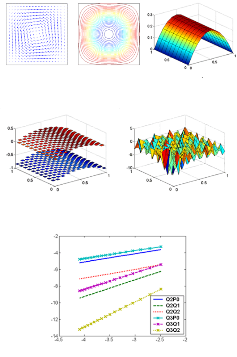
http://ww2.lacan.upc.edu/huerta/exercises/Incompressible/Incompressible Ex1.htm
As shown in [144], If the LBB condition is not satisfied, spurious oscillations spoil the pressure
approximation. Figures below show results obtained with a mesh of 20x20 Q1P0 (left) and P1P1 (right)
elements:
]]
http://ww2.lacan.upc.edu/huerta/exercises/Incompressible/Incompressible Ex1.htm
Taking into account that the proposed problem has got analytical solution, it is easy to analyze
convergence of the different pairs of elements:
http://ww2.lacan.upc.edu/huerta/exercises/Incompressible/Incompressible Ex1.htm
6.7.2 Analytical benchmark II
Taken from [141]. It is for a unit square with ν=µ/ρ = 1 and the smooth exact solution is
u(x, y) = x+x2−2xy +x3−3xy2+x2y(162)
v(x, y) = −y−2xy +y2−3x2y+y3−xy2(163)
p(x, y) = xy +x+y+x3y2−4/3 (164)
52

Note that the pressure obeys RΩp dΩ=0
bx=−(1 + y−3x2y2) (165)
by=−(1 −3x−2x3y) (166)
6.7.3 Analytical benchmark III
This benchmark begins by postulating a polynomial solution to the 3D Stokes equation [141]:
v=
x+x2+xy +x3y
y+xy +y2+x2y2
−2z−3xz −3yz −5x2yz
(167)
and
p=xyz +x3y3z−5/32 (168)
While it is then trivial to verify that this velocity field is divergence-free, the corresponding body force
of the Stokes equation can be computed by inserting this solution into the momentum equation with a
given viscosity µ(constant or position/velocity/strain rate dependent). The domain is a unit cube and
velocity boundary conditions simply use Eq. (229). Note that the pressure fulfills
ZΩ
p(r)dΩ=0.
Constant viscosity In this case, the right hand side writes:
f=−∇p+µ
2+6xy
2+2x2+ 2y2
−10yz
=−
yz + 3x2y3z
xz + 3x3y2z
xy +x3y3
+µ
2+6xy
2+2x2+ 2y2
−10yz
We can compute the components of the strainrate tensor:
˙εxx = 1 + 2x+y+ 3x2y(169)
˙εyy = 1 + x+ 2y+ 2x2y(170)
˙εzz =−2−3x−3y−5x2y(171)
˙εxy =1
2(x+y+ 2xy2+x3) (172)
˙εxz =1
2(−3z−10xyz) (173)
˙εyz =1
2(−3z−5x2z) (174)
Note that we of course have ˙εxx + ˙εyy + ˙εzz = 0.
Variable viscosity In this case, the right hand side is obtains through
f=−∇p+µ
2+6xy
2+2x2+ 2y2
−10yz
+
2 ˙εxx
2 ˙εxy
2 ˙εxz
∂µ
∂x +
2 ˙εxy
2 ˙εyy
2 ˙εyz
∂µ
∂y +
2 ˙εxz
2 ˙εyz
2 ˙εzz
∂µ
∂z (175)
53

The viscosity can be chosen to be a smooth varying function:
µ=exp(1 −β(x(1 −x) + y(1 −y) + z(1 −z))) (176)
Choosing β= 0 yields a constant velocity µ=e1(and greatly simplifies the right-hand side). One can
easily show that the ratio of viscosities µ?in the system follows µ?= exp(−3β/4) so that choosing β= 10
yields µ?'1808 and β= 20 yields µ?'3.269 ×10⁶. In this case
∂µ
∂x =−4β(1 −2x)µ(x, y, z) (177)
∂µ
∂y =−4β(1 −2y)µ(x, y, z) (178)
∂µ
∂z =−4β(1 −2z)µ(x, y, z) (179)
[96] has carried out this benchmark for β= 4, i.e.:
µ(x, y, z) = exp(1 −4(x(1 −x) + y(1 −y) + z(1 −z)))
In a unit cube, this yields a variable viscosity such that 0.1353 < µ < 2.7182, i.e. a ratio of approx. 20
within the domain. We then have:
∂µ
∂x =−4(1 −2x)µ(x, y, z) (180)
∂µ
∂y =−4(1 −2y)µ(x, y, z) (181)
∂µ
∂z =−4(1 −2z)µ(x, y, z) (182)
sort out mess wrt Eq 26 of busa13
6.7.4 Analytical benchmark IV
From [45]. The two-dimensional domain is a unit square. The body forces are:
fx= 128[x2(x−1)212(2y−1) + 2(y−1)(2y−1)y(12x2−12x+ 2)]
fy= 128[y2(y−1)212(2x−1) + 2(x−1)(2x−1)y(12y2−12y+ 2)]
(183)
The solution is
u=−256x2(x−1)2y(y−1)(2y−1)
v= 256x2(y−1)2x(x−1)(2x−1)
p= 0 (184)
Another choice:
fx= 128[x2(x−1)212(2y−1) + 2(y−1)(2y−1)y(12x2−12x+ 2)] + y−1/2
fy= 128[y2(y−1)212(2x−1) + 2(x−1)(2x−1)y(12y2−12y+ 2)] + x−1/2
(185)
The solution is
u=−256x2(x−1)2y(y−1)(2y−1)
v= 256x2(y−1)2x(x−1)(2x−1)
p= (x−1/2)(y−1/2) (186)
54

6.8 Assigning values to quadrature points
As we have seen in Section ??, the building of the elemental matrix and rhs requires (at least) to assign
a density and viscosity value to each quadrature point inside the element. Depending on the type of
modelling, this task can prove more complex than one might expect and have large consequences on the
solution accuracy.
Here are several options:
•The simplest way (which is often used for benchmarks) consists in computing the ’real’ coordinates
(xq, yq, zq) of a given quadrature point based on its reduced coordinates (rq, sq, tq), and passing these
coordinates to a function which returns density and/or viscosity at this location. For instance, for
the Stokes sphere:
def rho(x,y):
if (x-.5)**2+(y-0.5)**2<0.123**2:
val=2.
else:
val=1.
return val
def mu(x,y):
if (x-.5)**2+(y-0.5)**2<0.123**2:
val=1.e2
else:
val=1.
return val
This is very simple, but it has been shown to potentially be problematic. In essence, it can introduce
very large contrasts inside a single element and perturb the quadrature. Please read section 3.3
of [253] and/or have a look at the section titled ”Averaging material properties” in the ASPECT
manual.
•another similar approach consists in assigning a density and viscosity value to the nodes of the FE
mesh first, and then using these nodal values to assign values to the quadrature points. Very often
,and quite logically, the shape functions are used to this effect. Indeed we have seen before that for
any point (r, s, t) inside an element we have
fh(r, s, t) =
m
X
i
fiNi(r, s, t)
where the fiare the nodal values and the Nithe corresponding basis functions.
In the case of linear elements (Q1basis functions), this is straightforward. In fact, the basis functions
Nican be seen as moving weights: the closer the point is to a node, the higher the weight (basis
function value).
However, this is quite another story for quadratic elements (Q2basis functions). In order to
illustrate the problem, let us consider a 1D problem. The basis functions are
N1(r) = 1
2r(r−1) N2(r)=1−r2N3(r) = 1
2r(r+ 1)
Let us further assign: ρ1=ρ2= 0 and ρ3= 1. Then
ρh(r) =
m
X
i
ρiNi(r) = N3(r)
There lies the core of the problem: the N3(r) basis function is negative for r∈[−1,0]. This means
that the quadrature point in this interval will be assigned a negative density, which is nonsensical
and numerically problematic!
use 2X Q1. write about it !
55

The above methods work fine as long as the domain contains a single material. As soon as there are
multiple fluids in the domain a special technique is needed to track either the fluids themselves or their
interfaces. Let us start with markers. We are then confronted to the infernal trio (a menage a trois?)
which is present for each element, composed of its nodes, its markers and its quadrature points.
Each marker carries the material information (density and viscosity). This information must ul-
timately be projected onto the quadrature points. Two main options are possible: an algorithm is
designed and projects the marker-based fields onto the quadrature points directly or the marker fields
are first projected onto the FE nodes and then onto the quadrature points using the techniques above.
————————–
At a given time, every element econtains nemarkers. During the FE matrix building process, viscosity
and density values are needed at the quadrature points. One therefore needs to project the values carried
by the markers at these locations. Several approaches are currently in use in the community and the
topic has been investigated by [139] and [149] for instance.
elefant adopts a simple approach: viscosity and density are considered to be elemental values, i.e.
all the markers within a given element contribute to assign a unique constant density and viscosity value
to the element by means of an averaging scheme.
While it is common in the literature to treat the so-called arithmetic, geometric and harmonic means
as separate averagings, I hereby wish to introduce the notion of generalised mean, which is a family of
functions for aggregating sets of numbers that include as special cases the arithmetic, geometric and
harmonic means.
If pis a non-zero real number, we can define the generalised mean (or power mean) with exponent p
of the positive real numbers a1, ... anas:
Mp(a1, ...an) = 1
n
n
X
i=1
ap
i!1/p
(187)
and it is trivial to verify that we then have the special cases:
M−∞ = lim
p→−∞ Mp= min(a1, ...an) (minimum) (188)
M−1=n
1
a1+1
a2+··· +1
an
(harm.avrg.) (189)
M0= lim
p→0Mp=n
Y
i=1
ai1/n
(geom.avrg.) (190)
M+1 =1
n
n
X
i=1
ai(arithm.avrg.) (191)
M+2 =v
u
u
t1
n
n
X
i=1
a2
i(root mean square) (192)
M+∞= lim
p→+∞Mp= max(a1, ...an) (maximum) (193)
Note that the proofs of the limit convergence are given in [83].
An interesting property of the generalised mean is as follows: for two real values pand q, if p < q
then Mp≤Mq. This property has for instance been illustrated in Fig. 20 of [414].
One can then for instance look at the generalised mean of a randomly generated set of 1000 viscosity
values within 1018P a.s and 1023P a.s for −5≤p≤5. Results are shown in the figure hereunder and the
arithmetic, geometric and harmonic values are indicated too. The function Mpassumes an arctangent-
like shape: very low values of p will ultimately yield the minimum viscosity in the array while very high
values will yield its maximum. In between, the transition is smooth and occurs essentially for |p| ≤ 5.
56
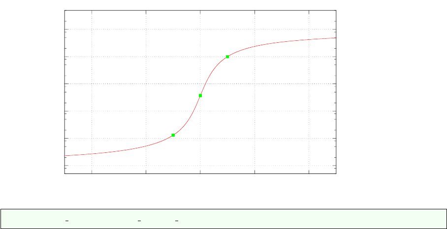
1e+18
1e+19
1e+20
1e+21
1e+22
1e+23
-4 -2 0 2 4
M(p)
p
geom.
arithm.
harm.
python codes/fieldstone markers avrg
57
6.9 Matrix (Sparse) storage
The FE matrix is the result of the assembly process of all elemental matrices. Its size can become quite
large when the resolution is being increased (from thousands of lines/columns to tens of millions).
One important property of the matrix is its sparsity. Typically less than 1% of the matrix terms is
not zero and this means that the matrix storage can and should be optimised. Clever storage formats
were designed early on since the amount of RAM memory in computers was the limiting factor 3 or 4
decades ago. [407]
There are several standard formats:
•compressed sparse row (CSR) format
•compressed sparse column format (CSC)
•the Coordinate Format (COO)
•Skyline Storage Format
•...
I focus on the CSR format in what follows.
6.9.1 2D domain - One degree of freedom per node
Let us consider again the 3 ×2 element grid which counts 12 nodes.
8=======9======10======11
||||
| (3) | (4) | (5) |
||||
4=======5=======6=======7
||||
| (0) | (1) | (2) |
||||
0=======1=======2=======3
In the case there is only a single degree of freedom per node, the assembled FEM matrix will look
like this:
X X X X
X X X X X X
X X X X X X
X X X X
X X X X X X
X X X X X X X X X
X X X X X X X X X
X X X X X X
X X X X
X X X X X X
X X X X X X
X X X X
where the Xstand for non-zero terms. This matrix structure stems from the fact that
•node 0 sees nodes 0,1,4,5
•node 1 sees nodes 0,1,2,4,5,6
•node 2 sees nodes 1,2,3,5,6,7
•...
58

•node 5 sees nodes 0,1,2,4,5,6,8,9,10
•...
•node 10 sees nodes 5,6,7,9,10,11
•node 11 sees nodes 6,7,10,11
In light thereof, we have
•4 corner nodes which have 4 neighbours (counting themselves)
•2(nnx-2) nodes which have 6 neighbours
•2(nny-2) nodes which have 6 neighbours
•(nnx-2)×(nny-2) nodes which have 9 neighbours
In total, the number of non-zero terms in the matrix is then:
NZ = 4 ×4+4×6+2×6+2×9 = 70
In general, we would then have:
NZ = 4 ×4 + [2(nnx −2) + 2(nny −2)] ×6+(nnx −2)(nny −2) ×9
Let us temporarily assume nnx =nny =n. Then the matrix size (total number of unknowns) is
N=n2and
NZ = 16 + 24(n−2) + 9(n−2)2
A full matrix array would contain N2=n4terms. The ratio of N Z (the actual number of reals to store)
to the full matrix size (the number of reals a full matrix contains) is then
R=16 + 24(n−2) + 9(n−2)2
n4
It is then obvious that when nis large enough R∼1/n2.
CSR stores the nonzeros of the matrix row by row, in a single indexed array A of double precision
numbers. Another array COLIND contains the column index of each corresponding entry in the A array.
A third integer array RWPTR contains pointers to the beginning of each row, which an additional pointer
to the first index following the nonzeros of the matrix A. A and COLIND have length NZ and RWPTR
has length N+1.
In the case of the here-above matrix, the arrays COLIND and RWPTR will look like:
COLIND = (0,1,4,5,0,1,2,4,5,6,1,2,3,5,6,7, ..., 6,7,10,11)
RW P T R = (0,4,10,16, ...)
6.9.2 2D domain - Two degrees of freedom per node
When there are now two degrees of freedom per node, such as in the case of the Stokes equation in
two-dimensions, the size of the Kmatrix is given by
NfemV=nnp∗ndofV
In the case of the small grid above, we have NfemV=24. Elemental matrices are now 8 ×8 in size.
We still have
•4 corner nodes which have 4 ,neighbours,
•2(nnx-2) nodes which have 6 neighbours
•2(nny-2) nodes which have 6 neighbours
59

•(nnx-2)x(nny-2) nodes which have 9 neighbours,
but now each degree of freedom from a node sees the other two degrees of freedom of another node too.
In that case, the number of nonzeros has been multiplied by four and the assembled FEM matrix looks
like:
X X X X X X X X
X X X X X X X X
X X X X X X X X X X X X
X X X X X X X X X X X X
X X X X X X X X X X X X
X X X X X X X X X X X X
X X X X X X X X
X X X X X X X X
X X X X X X X X X X X X
X X X X X X X X X X X X
X X X X X X X X X X X X X X X X X X
X X X X X X X X X X X X X X X X X X
X X X X X X X X X X X X X X X X X X
X X X X X X X X X X X X X X X X X X
X X X X X X X X X X X X
X X X X X X X X X X X X
X X X X X X X X
X X X X X X X X
X X X X X X X X X X X X
X X X X X X X X X X X X
X X X X X X X X X X X X
X X X X X X X X X X X X
X X X X X X X X
X X X X X X X X
Note that the degrees of freedom are organised as follows:
(u0, v0, u1, v1, u2, v2, ...u11, v11)
In general, we would then have:
NZ = 4 [4 ×4 + [2(nnx −2) + 2(nny −2)] ×6+(nnx −2)(nny −2) ×9]
and in the case of the small grid, the number of non-zero terms in the matrix is then:
NZ = 4 [4 ×4+4×6+2×6+2×9] = 280
In the case of the here-above matrix, the arrays COLIND and RWPTR will look like:
COLIND = (0,1,2,3,8,9,10,11,0,1,2,3,8,9,10,11, ...)
RW P T R = (0,8,16,28, ...)
6.9.3 in fieldstone
The majority of the codes have the FE matrix being a full array
a mat = np . z e r os ( ( Nfem , Nfem ) , dtype=np . f l o a t 6 4 )
and it is converted to CSR format on the fly in the solve phase:
s o l = s ps . l i n a l g . s p s o l v e ( s ps . c s r m a t r i x ( a mat ) , r hs )
Note that linked list storages can be used (lil matrix). Substantial memory savings but much longer
compute times.
60
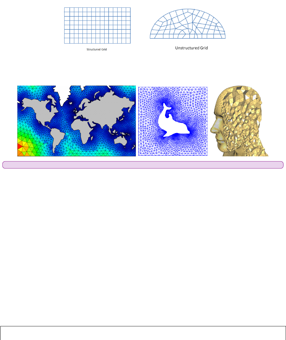
6.10 Mesh generation
Before basis functions can be defined and PDEs can be discretised and solved we must first tesselate the
domain with polygons, e.g. triangles and quadrilaterals in 2D, tetrahedra, prisms and hexahedra in 3D.
When the domain is itself simple (e.g. a rectangle, a sphere, ...) the mesh (or grid) can be (more or
less) easily produced and the connectivity array filled with straightforward algorithms [452]. However,
real life applications can involve etremely complex geometries (e.g. a bridge, a human spine, a car chassis
and body, etc ...) and dedicated algorithms/softwares must be used (see [456, 180, 507]).
We usually distinguish between two broad classes of grids: structured grids (with a regular connec-
tivity) and unstructured grids (with an irregular connectivity).
On the following figure are shown various triangle- tetrahedron-based meshes. These are obviously
better suited for simulations of complex geometries:
add more examples coming from geo
Let us now focus on the case of a rectangular computational domain of size Lx ×Ly with a regular
mesh composed of nelx×nely=nel quadrilaterals. There are then nnx×nny=nnp grid points. The
elements are of size hx×hy with hx=Lx/nelx.
We have no reason to come up with an irregular/ilogical node numbering so we can number nodes
row by row or column by column as shown on the example hereunder of a 3×2 grid:
8=======9======10======11 2=======5=======8======11
||||||||
| (3) | (4) | (5) | | (1) | (3) | (5) |
||||||||
4=======5=======6=======7 1=======4=======7======10
||||||||
| (0) | (1) | (2) | | (0) | (2) | (4) |
||||||||
0=======1=======2=======3 0=======3=======6=======9
"row by row" "column by column"
The numbering of the elements themselves could be done in a somewhat chaotic way but we follow
the numbering of the nodes for simplicity. The row by row option is the adopted one in fieldstoneand
the coordinates of the points are computed as follows:
x = np . empty (nnp , dtype=np . f l o a t 6 4 )
y = np . empty (nnp , dtype=np . f l o a t 6 4 )
61

co u nt er = 0
f o r jin range ( 0 , nny ) :
f o r ii n r a ng e ( 0 , nnx ) :
x [ c ou nt er ]= i ∗hx
y [ c ou nt er ]= j ∗hy
co u nt er += 1
The inner loop has iranging from 0to nnx-1 first for j=0, 1, ... up to nny-1 which indeed corresponds
to the row by row numbering.
We now turn to the connectivity. As mentioned before, this is a structured mesh so that the so-called
connectivity array, named icon in our case, can be filled easily. For each element we need to store the
node identities of its vertices. Since there are nel elements and m=4 corners, this is a m×nel array. The
algorithm goes as follows:
i c o n =np . z e r o s ( (m, n e l ) , dtype=np . i n t 1 6 )
co u nt er = 0
f o r jin range ( 0 , n e l y ) :
f o r ii n r a ng e ( 0 , n e l x ) :
i c o n [ 0 , c o u n t er ] = i + j ∗nnx
i c o n [ 1 , c o u n t er ] = i + 1 + j ∗nnx
i c o n [ 2 , c o u n t er ] = i + 1 + ( j + 1 ) ∗nnx
i c o n [ 3 , c o u n t er ] = i + ( j + 1 ) ∗nnx
co u nt er += 1
In the case of the 3×2 mesh, the icon is filled as follows:
element id→0 1 2 3 4 5
node id↓
0 0 1 2 4 5 6
1 1 2 3 5 6 7
2 56791011
3 4 5 6 8 9 10
It is to be understood as follows: element #4 is composed of nodes 5, 6, 10 and 9. Note that nodes are
always stored in a counter clockwise manner, starting at the bottom left. This is very important since
the corresponding basis functions and their derivatives will be labelled accordingly.
In three dimensions things are very similar. The mesh now counts nelx×nely×nelz=nel elements
which represent a cuboid of size Lx×Ly×Lz. The position of the nodes is obtained as follows:
x = np . empty (nnp , dtype=np . f l o a t 6 4 )
y = np . empty (nnp , dtype=np . f l o a t 6 4 )
z = np . empty (nnp , dtype=np . f l o a t 6 4 )
co u nt er=0
f o r iin range ( 0 , nnx ) :
f o r jin range ( 0 , nny ) :
f o r kin range ( 0 , nnz ) :
x [ c ou nt er ]= i ∗hx
y [ c ou nt er ]= j ∗hy
z [ c ou nte r ]=k∗hz
co u nt er += 1
The connectivity array is now of size m×nel with m=8:
i c o n =np . z e r o s ( (m, n e l ) , dtype=np . i n t 1 6 )
co u nt er = 0
f o r iin range ( 0 , n e l x ) :
f o r jin range ( 0 , n e l y ) :
f o r kin range ( 0 , n e l z ) :
i c o n [ 0 , c o u n t er ]=nny∗nnz∗( i )+nnz ∗( j )+k
i c o n [ 1 , c o u n t er ]=nny∗nnz∗( i +1)+nnz ∗( j )+k
i c o n [ 2 , c o u n t er ]=nny∗nnz∗( i +1)+nnz ∗( j +1)+k
i c o n [ 3 , c o u n t er ]=nny∗nnz∗( i )+nnz ∗( j +1)+k
i c o n [ 4 , c o u n t er ]=nny∗nnz∗( i )+nnz ∗( j )+k+1
i c o n [ 5 , c o u n t er ]=nny∗nnz∗( i +1)+nnz ∗( j )+k+1
i c o n [ 6 , c o u n t er ]=nny∗nnz∗( i +1)+nnz ∗( j +1)+k+1
i c o n [ 7 , c o u n t er ]=nny∗nnz∗( i )+nnz ∗( j +1)+k+1
co u nt er += 1
62

produce drawing of node numbering
63
6.11 Visco-Plasticity
6.11.1 Tensor invariants
Before we dive into the world of nonlinear rheologies it is necessary to introduce the concept of tensor
invariants since they are needed further on. Unfortunately there are many different notations used in the
literature and these can prove to be confusing.
Given a tensor T, one can compute its (moment) invariants as follows:
•first invariant :
TI|2D=T r[T] = Txx +Tyy
TI|3D=T r[T] = Txx +Tyy +Tzz
•second invariant :
TII |2D=1
2T r[T2] = 1
2X
ij
Tij Tji =1
2(T2
xx +T2
yy) + T2
xy
TII |3D=1
2T r[T2] = 1
2X
ij
Tij Tji =1
2(T2
xx +T2
yy +T2
yy) + T2
xy +T2
xz +T2
yz
•third invariant :
TIII =1
3T r[T3] = 1
3X
ijk
Tij TjkTki
The implementation of the plasticity criterions relies essentially on the second invariants of the (de-
viatoric) stress τand the (deviatoric) strainrate tensors ˙
ε:
τII |2D=1
2(τ2
xx +τ2
yy) + τ2
xy
=1
4(σxx −σyy)2+σ2
xy
=1
4(σ1−σ2)2
τII |3D=1
2(τ2
xx +τ2
yy +τ2
zz) + τ2
xy +τ2
xz +τ2
yz
=1
6(σxx −σyy )2+ (σyy −σzz)2+ (σxx −σzz)2+σ2
xy +σ2
xz +σ2
yz
=1
6(σ1−σ2)2+ (σ2−σ3)2+ (σ1−σ3)2
εII |2D=1
2( ˙εd
xx)2+ ( ˙εd
yy)2+ ( ˙εd
xy)2
=1
21
4( ˙εxx −˙εyy)2+1
4( ˙εyy −˙εxx)2+ ˙ε2
xy
=1
4( ˙εxx −˙εyy)2+ ˙ε2
xy
εII |3D=1
2( ˙εd
xx)2+ ( ˙εd
yy)2+ ( ˙εd
zz)2+ ( ˙εd
xy)2+ ( ˙εd
xz)2+ ( ˙εd
yz)2
=1
6(˙xx −˙yy)2+ (˙yy −˙zz)2+ ( ˙xx −˙zz)2+ ˙2
xy + ˙2
xz + ˙2
yz
Note that these (second) invariants are almost always used under a square root so we define:
64
τII =√τII ˙εII =p˙εII
Note that these quantities have the same dimensions as their tensor counterparts, i.e. Pa for stresses and
s−1for strain rates.
6.11.2 Scalar viscoplasticity
This formulation is quite easy to implement. It is widely used, e.g. [501, 454, 429], and relies on the
assumption that a scalar quantity ηp(the ’effective plastic viscosity’) exists such that the deviatoric stress
tensor
τ= 2ηp˙
ε(194)
is bounded by some yield stress value Y. From Eq. (194) it follows that τII = 2ηp˙εII =Ywhich yields
ηp=Y
2˙εII
This approach has also been coined the Viscosity Rescaling Method (VRM) [280].
insert here the rederivation 2.1.1 of spmw16
It is at this stage important to realise that (i) in areas where the strainrate is low, the resulting effective
viscosity will be large, and (ii) in areas where the strainrate is high, the resulting effective viscosity will be
low. This is not without consequences since (effective) viscosity contrasts up to 8-10 orders of magnitude
have been observed/obtained with this formulation and it makes the FE matrix very stiff, leading to
(iterative) solver convergence issues. In order to contain these viscosity contrasts one usually resorts to
viscosity limiters ηmin and ηmax such that
ηmin ≤ηp≤ηmax
Caution must be taken when choosing both values as they may influence the final results.
python codes/fieldstone indentor
6.11.3 about the yield stress value Y
In geodynamics the yield stress value is often given as a simple function. It can be constant (in space
and time) and in this case we are dealing with a von Mises plasticity yield criterion. . We simply assume
YvM =Cwhere Cis a constant cohesion independent of pressure, strainrate, deformation history, etc ...
Another model is often used: the Drucker-Prager plasticity model. A friction angle φis then intro-
duced and the yield value Ytakes the form
YDP =psin φ+Ccos φ
and therefore depends on the pressure p. Because φis with the range [0◦,45◦], Yis found to increase
with depth (since the lithostatic pressure often dominates the overpressure).
Note that a slightly modified verion of this plasticity model has been used: the total pressure pis
then replaced by the lithostatic pressure plith.
65
6.12 Pressure smoothing
It has been widely documented that the use of the Q1×P0element is not without problems. Aside from
the consequences it has on the FE matrix properties, we will here focus on another unavoidable side
effect: the spurious pressure checkerboard modes.
These modes have been thoroughly analysed [240, 107, 408, 409]. They can be filtered out [107] or
simply smoothed [302].
On the following figure (a,b), pressure fields for the lid driven cavity experiment are presented for
both an even and un-even number of elements. We see that the amplitude of the modes can sometimes
be so large that the ’real’ pressure is not visible and that something as simple as the number of elements
in the domain can trigger those or not at all.
a) b)
c)
a) element pressure for a 32x32 grid and for a 33x33 grid;
b) image from [142, p307] for a manufactured solution;
c) elemental pressure and smoothed pressure for the punch experiment [454]
The easiest post-processing step that can be used (especially when a regular grid is used) is explained in
[454]: ”The element-to-node interpolation is performed by averaging the elemental values from elements
common to each node; the node-to-element interpolation is performed by averaging the nodal values
element-by-element. This method is not only very efficient but produces a smoothing of the pressure that
is adapted to the local density of the octree. Note that these two steps can be repeated until a satisfying
level of smoothness (and diffusion) of the pres- sure field is attained.”
In the codes which rely on the Q1×P0element, the (elemental) pressure is simply defined as
p=np . z e r o s ( ne l , dtype=np . f l o a t 6 4 )
while the nodal pressure is then defined as
q=np . z e r os ( nnp , dtype=np . f l o a t 6 4 )
The element-to-node algorithm is then simply (in 2D):
cou nt=np . z e r o s ( nnp , dtype=np . i n t 1 6 )
f o r i e l in range ( 0 , n e l ) :
q [ i c o n [ 0 , i e l ]]+=p [ i e l ]
q [ i c o n [ 1 , i e l ]]+=p [ i e l ]
q [ i c o n [ 2 , i e l ]]+=p [ i e l ]
q [ i c o n [ 3 , i e l ]]+=p [ i e l ]
co un t [ i c o n [ 0 , i e l ]]+=1
co un t [ i c o n [ 1 , i e l ]]+=1
co un t [ i c o n [ 2 , i e l ]]+=1
co un t [ i c o n [ 3 , i e l ]]+=1
q=q/ count
66


6.13 Pressure scaling
As perfectly explained in the step 32 of deal.ii5, we often need to scale the Gterm since it is many orders
of magnitude smaller than K, which introduces large inaccuracies in the solving process to the point that
the solution is nonsensical. This scaling coefficient is η/L. We start from
K G
GT0·V
P=f
h
and introduce the scaling coefficient as follows (which in fact does not alter the solution at all):
Kη
LG
η
LGT0·V
L
ηP=f
η
Lh
We then end up with the modified Stokes system:
K G
GT0·V
P=f
h
where
G=η
LGP=L
ηPh=η
Lh
After the solve phase, we recover the real pressure with P=η
LP0.
5https://www.dealii.org/9.0.0/doxygen/deal.II/step 32.html
68

6.14 Pressure normalisation
When Dirichlet boundary conditions are imposed everywhere on the boundary, pressure is only present
by its gradient in the equations. It is thus determined up to an arbitrary constant. In such a case, one
commonly impose the average of the pressure over the whole domain or on a subsect of the boundary to
be have a zero average, i.e. ZΩ
pdV = 0
Another possibility is to impose the pressure value at a single node.
Let us assume that we are using Q1×P0elements. Then the pressure is constant inside each element.
The integral above becomes:
ZΩ
pdV =X
eZΩe
pdV =X
e
peZΩe
dV =X
e
peAe=
where the sum runs over all elements eof area Ae. This can be rewritten
LTP= 0
and it is a constraint on the pressure. As we have seen before ??, we can associate to it a Lagrange
multiplier λso that we must solve the modified Stokes system:
K G 0
GT0L
0LT0
·
V
P
λ
=
f
h
0
When higher order spaces are used for pressure (continuous or discontinuous) one must then carry out
the above integration numerically by means of (usually) a Gauss-Legendre quadrature.
python codes/fieldstone stokes sphere 3D saddlepoint/
python codes/fieldstone burstedde/
python codes/fieldstone busse/
python codes/fieldstone RTinstability1/
python codes/fieldstone saddlepoint q2q1/
python codes/fieldstone compressible2/
python codes/fieldstone compressible1/
python codes/fieldstone saddlepoint q3q2/
69

6.15 The choice of solvers
Let us first look at the penalty formulation. In this case we are only solving for velocity since pressure is
recovered in a post-processing step. We also know that the penalty factor is many orders of magnitude
higher than the viscosity and in combination with the use of the Q1×P0element the resulting matrix
condition number is very high so that the use of iterative solvers in precluded. Indeed codes such as
SOPALE [183], DOUAR [66], or FANTOM [450] relying on the penalty formulation all use direct solvers
(BLKFCT, MUMPS, WSMP).
The main advantage of direct solvers is used in this case: They can solve ill-conditioned matrices.
However memory requirements for the storage of number of nonzeros in the Cholesky matrix grow very fast
as the number of equations/grid size increases, especially in 3D, to the point that even modern computers
with tens of Gb of RAM cannot deal with a 1003element mesh. This explains why direct solvers are often
used for 2D problems and rarely in 3D with noticeable exceptions [454, 510, 67, 323, 11, 12, 13, 499, 356].
In light of all this, let us start again from the (full) Stokes system:
K G
GT0·V
P=f
h
We need to solve this system in order to obtain the solution, i.e. the Vand Pvectors. But how?
Unfortunately, this question is not simple to answer and the ’right’ depends on many parameters.
How big is the matrix ? what is the condition number of the matrix K? Is it symmetric ? (i.e. how are
compressible terms handled?).
6.15.1 The Schur complement approach
Let us write the above system as two equations:
KV+GP=f(195)
GTV=h(196)
The first line can be re-written V=K−1(f−GP) and can be inserted in the second:
GTV=GT[K−1(f−GP)] = h
or,
GTK−1GP=GTK−1f−h
The matrix S=GTK−1Gis called the Schur complement. It is Symmetric (since Kis symmetric) and
Postive-Definite6(SPD) if Ker(G) = 0. look in donea-huerta book for details Having solved this equation
(we have obtained P), the velocity can be recovered by solving KV=f−GP. For now, let us assume
that we have built the Smatrix and the right hand side ˜
f=GTK−1f−h. We must solve SP=˜
f.
Since Sis SPD, the Conjugate Gradient (CG) method is very appropriate to solve this system. Indeed,
looking at the definition of Wikipedia: In mathematics, the conjugate gradient method is an algorithm for
the numerical solution of particular systems of linear equations, namely those whose matrix is symmetric
and positive-definite. The conjugate gradient method is often implemented as an iterative algorithm,
applicable to sparse systems that are too large to be handled by a direct implementation or other direct
methods such as the Cholesky decomposition. Large sparse systems often arise when numerically solving
partial differential equations or optimization problems.
The Conjugate Gradient algorithm is as follows:
6Mpositive definite ⇐⇒ xTM x > 0∀x∈Rn\0
70
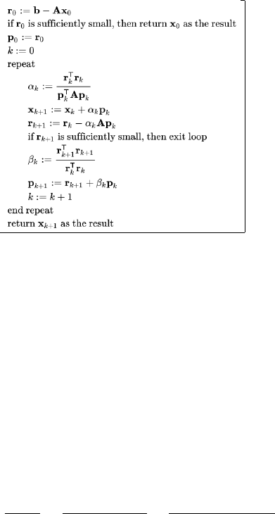
Algorithm obtained from https://en.wikipedia.org/wiki/Conjugate_gradient_method
Let us look at this algorithm up close. The parts which may prove to be somewhat tricky are those
involving the matrix (in our case the Schur complement). We start the iterations with a guess pressure
P0( and an initial guess velocity which could be obtained by solving KV0=f−GP0).
r0=˜
f−SP0(197)
=GTK−1f−h−(GTK−1G)P0(198)
=GTK−1(f−GP0)−h(199)
=GTK−1KV0−h(200)
=GTV0−h(201)
(202)
We now turn to the αkcoefficient:
αk=rT
krk
pkSpk
=rT
krk
pkGTK−1Gpk
=rT
krk
(Gpk)TK−1(Gpk)
We then define ˜pk=Gpk, so that αkcan be computed as follows:
1. compute ˜pk=Gpk
2. solve Kdk= ˜pk
3. compute αk= (rT
krk)/(˜pT
kdk)
Then we need to look at the term Spk:
Spk=GTK−1Gpk=GTK−1˜pk=GTdk
We can then rewrite the CG algorithm as follows [525]:
•r0=GTV0−h
•if r0is sufficiently small, then return (V0,P0) as the result
•p0=r0
•k= 0
•repeat
–compute ˜pk=Gpk
–solve Kdk= ˜pk
–compute αk= (rT
krk)/(˜pT
kdk)
71

–Pk+1 =Pk+αkpk
–rk+1 =rk−αkGTdk
–if rk+1 is sufficiently small, then exit loop
–βk= (rT
k+1rk+1)/(rT
krk)
–pk+1 =rk+1 +βkpk
–k=k+ 1
•return Pk+1 as result
We see that we have managed to solve the Schur complement equation with the Conjugate Gradient
method without ever building the matrix S. Having obtained the pressure solution, we can easily recover
the corresponding velocity with KVk+1 =f−GPk+1. However, this is rather unfortunate because it
requires yet another solve with the Kmatrix. As it turns out, we can slightly alter the above algorithm
to have it update the velocity as well so that this last solve is unnecessary.
We have
Vk+1 =K−1(f−GPp+1) = K−1(f−G(Pk+αkpk)) = K−1(f−GPk)−αkK−1Gpk=V−αkK−1˜pk=Vk−αkdk
and we can insert this minor extra calculation inside the algorithm and get the velocity solution nearly
for free. The final CG algorithm is then
solver cg:
•compute V0=K−1(f−GP0)
•r0=GTV0−h
•if r0is sufficiently small, then return (V0,P0) as the result
•p0=r0
•k= 0
•repeat
–compute ˜pk=Gpk
–solve Kdk= ˜pk
–compute αk= (rT
krk)/(˜pT
kdk)
–Pk+1 =Pk+αkpk
–Vk+1 =Vk−αkdk
–rk+1 =rk−αkGTdk
–if rk+1 is sufficiently small (|rk+1|2/|r0|2< tol), then exit loop
–βk= (rT
k+1rk+1)/(rT
krk)
–pk+1 =rk+1 +βkpk
–k=k+ 1
•return Pk+1 as result
This iterative algorithm will converge to the solution with a rate which depends on the condition
number of the Smatrix, which is not easily obtainable since Sis never built. Also, we know that large
viscosity contrasts in the domain will influence this too. Finally, we notice that this algorithm requires
one solve with matrix Kper iteration but says nothing about the method employed to do so.
One thing we know improves the convergence of any iterative solver is the use of a preconditioner
matrix and therefore use the Preconditioned Conjugate Gradient method:
72
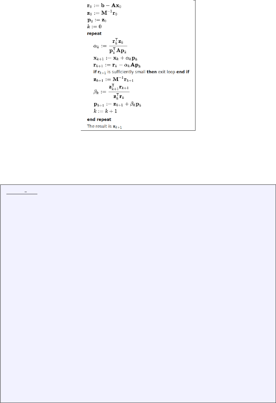
Algorithm obtained from https://en.wikipedia.org/wiki/Conjugate_gradient_method
In the algorithm above the preconditioner matrix Mhas to be symmetric positive-definite and fixed,
i.e., cannot change from iteration to iteration.
We see that this algorithm introduces an additional vector zand a solve with the matrix Mat each
iteration, which means that Mmust be such that solving Mx =fwhere fis a given rhs vector must be
cheap. Ultimately, the PCG algorithm applied to the Schur complement equation takes the form:
solver pcg:
•compute V0=K−1(f−GP0)
•r0=GTV0−h
•if r0is sufficiently small, then return (V0,P0) as the result
•z0=M−1r0
•p0=z0
•k= 0
•repeat
–compute ˜pk=Gpk
–solve Kdk= ˜pk
–compute αk= (rT
kzk)/(˜pT
kdk)
–Pk+1 =Pk+αkpk
–Vk+1 =Vk−αkdk
–rk+1 =rk−αkGTdk
–if rk+1 is sufficiently small (|rk+1|2/|r0|2< tol), then exit loop
–zk+1 =M−1rk+1
–βk= (zT
k+1rk+1)/(zT
krk)
–pk+1 =zk+1 +βkpk
–k=k+ 1
•return Pk+1 as result
73

how to compute Mfor the Schur complement ?
6.16 The GMRES approach
74

6.17 The consistent boundary flux (CBF)
The Consistent Boundary Flux technique was devised to alleviate the problem of the accuracy of primary
variables derivatives (mainly velocity and temperature) on boundaries, where basis function (nodal)
derivatives do not exist. These derivatives are important since they are needed to compute the heat flux
(and therefore the NUsselt number) or dynamic topography and geoid.
The idea was first introduced in [343] and later used in geodynamics [520]. It was finally implemented
in the CitcomS code [522] and more recently in the ASPECT code (dynamic topography postprocessor).
Note that the CBF should be seen as a post-processor step as it does not alter the primary variables
values.
The CBF method is implemented and used in ??.
6.17.1 applied to the Stokes equation
We start from the strong form:
∇·σ=b
and then write the weak form: ZΩ
N∇·σdV =ZΩ
NbdV
where Nis any test function. We then use the two equations:
∇·(Nσ) = N∇·σ+∇N·σ(chain rule)
ZΩ
(∇·f)dV =ZΓ
f·ndS (divergence theorem)
Integrating the first equation over Ω and using the second, we can write:
ZΓ
Nσ·ndS −ZΩ∇N·σdV =ZΩ
NbdV
On Γ, the traction vector is given by t=σ·n:
ZΓ
NtdS =ZΩ∇N·σdV +ZΩ
NbdV
Considering the traction vector as an unknown living on the nodes on the boundary, we can expand (for
Q1elements)
tx=
2
X
i=1
tx|iNity=
2
X
i=1
ty|iNi
on the boundary so that the left hand term yields a mass matrix M0. Finally, using our previous experience
of discretising the weak form, we can write:
M0· T =−KV − GP+f
where Tis the vector of assembled tractions which we want to compute and Vand Tare the solutions
of the Stokes problem. Note that the assembly only takes place on the elements along the boundary.
Note that the assembled mass matrix is tri-diagonal can be easily solved with a Conjugate Gradient
method. With a trapezoidal integration rule (i.e. Gauss-Lobatto) the matrix can even be diagonalised
and the resulting matrix is simply diagonal, which results in a very cheap solve [520].
6.17.2 applied to the heat equation
We start from the strong form of the heat transfer equation (without the source terms for simplicity):
ρcp∂T
∂t +v·∇T=∇·k∇T
75
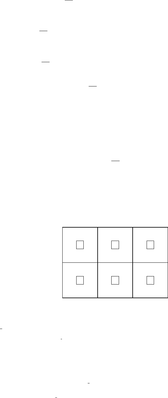
The weak form then writes:
ZΩ
Nρcp
∂T
∂t dV +ρcpZΩ
Nv·∇T dV =ZΩ
N∇·k∇T dV
Using once again integration by parts and divergence theorem:
ZΩ
Nρcp
∂T
∂t dV +ρcpZΩ
Nv·∇T dV =ZΓ
Nk∇T·ndΓ−ZΩ
∇N·k∇T dV
On the boundary we are interested in the heat flux q=−k∇T
ZΩ
Nρcp
∂T
∂t dV +ρcpZΩ
Nv·∇T dV =−ZΓ
Nq·ndΓ−ZΩ
∇N·k∇T dV
or, ZΓ
Nq·ndΓ = −ZΩ
Nρcp
∂T
∂t dV −ρcpZΩ
Nv·∇T dV −ZΩ
∇N·k∇T dV
Considering the normal heat flux qn=q·nas an unknown living on the nodes on the boundary,
qn=
2
X
i=1
qn|iNi
so that the left hand term becomes a mass matrix for the shape functions living on the boundary. We
have already covered the right hand side terms when building the FE system to solve the heat transport
equation, so that in the end
M0· Qn=−M·∂T
∂t −Ka·T−Kd·T
where Qnis the assembled vector of normal heat flux components. Note that in all terms the assembly
only takes place over the elements along the boundary.
Note that the resulting matrix is symmetric.
6.17.3 implementation - Stokes equation
Let us start with a small example, a 3x2 element FE grid:
012
345
0 1 2 3
4 5 6 7
8 9 10 11
01234567
891011 1213 1415
16 17 18 19 20 21 22 23
Red color corresponds to the dofs in the x direction, blue color indicates a dof in the y direction.
We have nnp=12, nel=6, NfemV=24. Let us assume that free slip boundary conditions are applied.
The fix bc array is then:
bc fix=[ TTTTTTTTTTTTTTTTTTTTTTTT]
Note that since corners belong to two edges, we effectively prescribed no-slip boundary conditions on
those.
We wish to compute the tractions on the boundaries, and more precisely for the dofs for which
a Dirichlecht velocity boundary condition has been prescribed. The number of (traction) unknowns
NfemTr is then the number of Tin the bc fix array. In our specific case, we wave NfemTr= . This means
that we need for each targeted dof to be able to find its identity/number between 0 and NfemTr-1. We
therefore create the array bc nb which is filled as follows:
76

bc nb=[TTTTTTTTTTTTTTTTTTTTTTTT]
This translates as follows in the code:
NfemTr=np . sum ( b c f i x )
bc nb=np . z e r o s (NfemV , d type=np . i n t 3 2 )
co u nt er=0
f o r iin range ( 0 , NfemV ) :
i f ( b c f i x [ i ] ) :
bc nb [ i ]= c ou nte r
co u nt er+=1
Algorithm 1 dksjfhfjk ghdf
0: kjhg kf
0: gfhfk
The algorithm is then as follows
A Prepare two arrays to store the matrix Mcbf and its right hand side rhscbf
B Loop over all elements
C For each element touching a boundary, compute the residual vector Rel =−fel +KelVel +GelPel
D Loop over the four edges of the element using the connectivity array
E For each edge loop over the number of degrees of freedom (2 in 2D)
F For each edge assess whether the dofs on both ends are target dofs.
G If so, compute the mass matrix Medge for this edge
H extract the 2 values off the element residual vector and assemble these in rhscbf
I Assemble Medge into NfemTrxNfemTr matrix using bc nb
M cbf = np . z e r os ( ( NfemTr , NfemTr ) , np . f l o a t 6 4 ) # A
r h s c b f = np . z e r os ( NfemTr , np . f l o a t 6 4 )
f o r i e l in range ( 0 , n e l ) : # B
. . . compute e l e m e n t a l r e s i d u a l . . . # C
#boundary 0−1 # D
f o r ii n r a ng e ( 0 , ndofV ) : # E
i d o f 0 =2∗i c o n [ 0 , i e l ]+ i
i d o f 1 =2∗i c o n [ 1 , i e l ]+ i
i f ( b c f i x [ i d o f 0 ] and b c f i x [ i d o f 1 ] ) : # F
i d o f T r 0=bc n b [ i d o f 0 ]
i d o f T r 1=bc n b [ i d o f 1 ]
r h s c b f [ i d o f T r 0 ]+= r e s e l [0+ i ] # H
r h s c b f [ i d o f T r 1 ]+= r e s e l [2+ i ]
M cbf [ i d o f Tr 0 , i d o f T r 0 ]+=M edge [ 0 , 0 ] #
M cbf [ i d o f Tr 0 , i d o f T r 1 ]+=M edge [ 0 , 1 ] # I
M cbf [ i d o f Tr 1 , i d o f T r 0 ]+=M edge [ 1 , 0 ] #
M cbf [ i d o f Tr 1 , i d o f T r 1 ]+=M edge [ 1 , 1 ] #
#boundary 1−2 #[D]
...
#boundary 2−3 #[D]
...
77

#boundary 3−0 #[D]
...
78

6.18 The value of the timestep
The chosen time step dt used for time integration is chosen to comply with the Courant-Friedrichs-Lewy
condition [14].
δt =Cmin h
max |v|,h2
κ
where his a measure of the element size, κ=k/ρcpis the thermal diffusivity and C is the so-called CFL
number chosen in [0,1[.
In essence the CFL condition arises when solving hyperbolic PDEs . It limits the time step in many
explicit time-marching computer simulations so that the simulation does not produce incorrect results.
This condition is not needed when solving the Stokes equation but it is mandatory when solving
the heat transport equation or any kind of advection-diffusion equation. Note that any increase of grid
resolution (i.e. hbecomes smaller) yields an automatic decrease of the time step value.
79
6.19 mappings
The name isoparametric derives from the fact that the same (’iso’) functions are used as basis functions
and for the mapping to the reference element.
80

6.20 Exporting data to vtk format
This format seems to be the universally accepted format for 2D and 3D visualisation in Computational
Geodynamics. Such files can be opened with free softwares such as Paraview 7, MayaVi 8or Visit 9.
Unfortunately it is my experience that no simple tutorial exists about how to build such files. There
is an official document which describes the vtk format10 but it delivers the information in a convoluted
way. I therefore describe hereafter how fieldstone builds the vtk files.
I hereunder show vtk file corresponding to the 3x2 grid presented earlier 6.10. In this particular
example there are:
•12 nodes and 6 elements
•1 elemental field: the pressure p)
•2 nodal fields: 1 scalar (the smoothed pressure q), 1 vector (the velocity field u,v,0)
Note that vtk files are inherently 3D so that even in the case of a 2D simulation the z-coordinate of the
points and for instance their z-velocity component must be provided. The file, usually called solution.vtu
starts with a header:
<VTKFile typ e= ’ U ns tr u ct u re d Gr i d ’ v e r s i o n= ’ 0 . 1 ’ b y t e o r d e r= ’ Big End ian ’>
<UnstructuredGrid>
<P i e c e N umberOfPoi nts= ’ 1 2 ’ N umb erO fC ell s= ’ 6 ’>
We then proceed to write the node coordinates as follows:
<Poi nts >
<DataArray t ype= ’ F lo at 3 2 ’ NumberOfComponents= ’ 3 ’ Format= ’ a s c i i ’>
0. 0 00 00 0 e+00 0. 00 00 00 e+00 0 . 00 00 00 e+00
3.333333e−01 0. 00 0 00 0 e+00 0 . 00 00 00 e+00
6.666667e−01 0. 00 0 00 0 e+00 0 . 00 00 00 e+00
1. 0 00 00 0 e+00 0. 00 00 00 e+00 0 . 00 00 00 e+00
0. 000 000 e+00 5 .0 000 00 e−01 0 .0 0 00 00 e+00
3.333333e−01 5. 00 000 0 e−01 0. 00 0 00 0 e+00
6.666667e−01 5. 00 000 0 e−01 0. 00 0 00 0 e+00
1. 000 000 e+00 5 .0 000 00 e−01 0 .0 0 00 00 e+00
0. 0 00 00 0 e+00 1. 00 00 00 e+00 0 . 00 00 00 e+00
3.333333e−01 1. 00 0 00 0 e+00 0 . 00 00 00 e+00
6.666667e−01 1. 00 0 00 0 e+00 0 . 00 00 00 e+00
1. 0 00 00 0 e+00 1. 00 00 00 e+00 0 . 00 00 00 e+00
</DataArray>
</Po ints >
These are followed by the elemental field(s):
<Ce ll Dat a S c a l a r s= ’ s c a l a r s ’>
<DataArray t ype= ’ F lo at 32 ’ Name= ’ p ’ Format= ’ a s c i i ’>
−1.333333 e+00
−3. 104414 e −10
1. 3 33 33 3 e+00
−1.333333 e+00
8.278417e−17
1. 3 33 33 3 e+00
</DataArray>
</CellData>
Nodal quantities are written next:
<Poi ntData S c a l a r s= ’ s c a l a r s ’>
<DataArray t ype= ’ F lo at 3 2 ’ NumberOfComponents= ’ 3 ’ Name= ’ v e l o c i t y ’ Format= ’ a s c i i ’>
0. 0 00 00 0 e+00 0. 00 00 00 e+00 0 . 00 00 00 e+00
0. 0 00 00 0 e+00 0. 00 00 00 e+00 0 . 00 00 00 e+00
0. 0 00 00 0 e+00 0. 00 00 00 e+00 0 . 00 00 00 e+00
0. 0 00 00 0 e+00 0. 00 00 00 e+00 0 . 00 00 00 e+00
7https://www.paraview.org/
8https://docs.enthought.com/mayavi/mayavi/
9https://wci.llnl.gov/simulation/computer-codes/visit/
10https://www.vtk.org/wp-content/uploads/2015/04/file-formats.pdf
81

0. 0 00 00 0 e+00 0. 00 00 00 e+00 0 . 00 00 00 e+00
8.888885e−08 −8.278 405 e −24 0. 0 00 00 0 e+00
8.888885e−08 1. 65 568 2 e−23 0. 00 0 00 0 e+00
0. 0 00 00 0 e+00 0. 00 00 00 e+00 0 . 00 00 00 e+00
1. 0 00 00 0 e+00 0. 00 00 00 e+00 0 . 00 00 00 e+00
1. 0 00 00 0 e+00 0. 00 00 00 e+00 0 . 00 00 00 e+00
1. 0 00 00 0 e+00 0. 00 00 00 e+00 0 . 00 00 00 e+00
1. 0 00 00 0 e+00 0. 00 00 00 e+00 0 . 00 00 00 e+00
</DataArray>
<DataArray t ype= ’ F lo at 3 2 ’ NumberOfComponents= ’ 1 ’ Name= ’ q ’ Format= ’ a s c i i ’>
−1.333333 e+00
−6. 666664 e −01
6.666664e−01
1. 3 33 33 3 e+00
−1.333333 e+00
−6. 666664 e −01
6.666664e−01
1. 3 33 33 3 e+00
−1.333333 e+00
−6. 666664 e −01
6.666664e−01
1. 3 33 33 3 e+00
</DataArray>
</PointData>
To these informations we must append 3 more datasets. The first one is the connectivity, the second
one is the offsets and the third one is the type. The first one is trivial since said connectivity is needed
for the Finite Elements. The second must be understood as follows: when reading the connectivity
information in a linear manneer the offset values indicate the beginning of each element (omitting the
zero value). The third simply is the type of element as given in the vtk format document (9 corresponds
to a generic quadrilateral with an internal numbering consistent with ours).
<Cells>
<DataArray t ype= ’ I nt 32 ’ Name= ’ c o n n e c t i v i t y ’ Format= ’ a s c i i ’>
0 1 5 4
1 2 6 5
2 3 7 6
4 5 9 8
5 6 10 9
6 7 11 10
</DataArray>
<DataArray t ype= ’ In t 3 2 ’ Name= ’ o f f s e t s ’ Format= ’ a s c i i ’>
4
8
12
16
20
24
</DataArray>
<DataArray t ype= ’ In t 3 2 ’ Name= ’ ty pe s ’ Format= ’ a s c i i ’>
9
9
9
9
9
9
</DataArray>
</C e l l s >
The file is then closed with
</Pi ece >
</UnstructuredGrid>
</VTKFile>
The solution.vtu file can then be opened with ParaView, MayaVi or Visit and the reader is advised
to find tutorials online on how to install and use these softwares.
82
6.21 Runge-Kutta methods
These methods were developed around 1900 by the German mathematicians Carl Runge and Martin
Kutta. The RK methods are methods for the numerical integration of ODEs. These methods are well
documented in any numerical analysis textbook and the reader is referred to [206, 268].
Any Runge-Kutta method is uniquely identified by its Butcher tableau.
The following method is called the Runge-Kutta-Fehlberg method and is commonly abbreviated
RKF45. Its Butcher tableau is as follows:
0
1/4 1/4
3/8 3/32 9/32
12/13 1932/2197 -7200/2197 7296/2197
1 439/216 -8 3680/513 -845/4104
1/2 -8/27 2 -3544/2565 1859/4104 -11/40
16/135 0 6656/12825 28561/56430 -9/50 2/55
25/216 0 1408/2565 2197/4104 -1/5 0
The first row of coefficients at the bottom of the table gives the fifth-order accurate method, and the
second row gives the fourth-order accurate method.
83
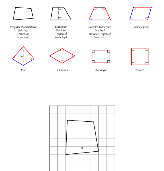
6.22 Am I in or not?
It is quite common that at some point one must answer the question: ”Given a mesh and its connectivity
on the one hand, and the coordinates of a point on the other, how do I accurately and quickly determine
in which element the point resides?”
One typical occurence of such a problem is linked to the use of the Particle-In-Cell technique: particles
are advected and move through the mesh, and need to be localised at every time step. This question could
arise in the context of a benchmark where certain quantities need to be measured at specific locations
inside the domain.
6.22.1 Two-dimensional space
We shall first focus on quadrilaterals. There are many kinds of quadrilaterals as shown hereunder:
I wish to arrive at a single algorithm which is applicable to all quadrilaterals and therefore choose an
irregular quadrilateral. For simplicity, let us consider a Q1element, with a single node at each corner.
01
23
M
Several rather simple options exist:
•we could subdivide the quadrilateral into two triangles and check whether point Mis inside any of
them (as it turns out, this problem is rather straightforward for triangles. Simply google it.)
•We could check that point Mis always on the left side of segments 0 →1, 1 →2, 2 →3, 3 →0.
•...
Any of these approaches will work although some might be faster than others. In three-dimensions
all will however become cumbersome to implement and might not even work at all. Fortunately, there is
an elegant way to answer the question, as detailed in the following subsection.
6.22.2 Three-dimensional space
If point Mis inside the quadrilateral, there exist a set of reduced coordinates r, s, t ∈[−1 : 1]3such that
4
X
i=1
Ni(rM, s, t)xi=xM
4
X
i=1
Ni(rM, s, t)yi=yM
4
X
i=1
Ni(rM, s, t)zi=zM
84
This can be cast as a system of three equations and three unknowns. Unfortunately, each shape function
Nicontains a term rst (as well as rs,rt, and st) so that it is not a linear system and standard techniques
are not applicable. We must then use an iterative technique: the algorithm starts with a guess for values
r, s, t and improves on their value iteration after iteration.
The classical way of solving nonlinear systems of equations is Newton’s method. We can rewrite the
equations above as F(r, s, t) = 0:
8
X
i=1
Ni(r, s, t)xi−xM= 0
8
X
i=1
Ni(r, s, t)yi−yM= 0
8
X
i=1
Ni(r, s, t)zi−zM= 0 (203)
or,
Fr(r, s, t)=0
Fs(r, s, t)=0
Ft(r, s, t)=0
so that we now have to find the zeroes of continuously differentiable functions F:R→R. The
recursion is simply:
rk+1
sk+1
tk+1
=
rk
sk
tk
−JF(rk, sk, tk)−1
Fr(rk, sk, tk)
Fs(rk, sk, tk)
Ft(rk, sk, tk)
where Jthe Jacobian matrix:
JF(rk, sk, tk) =
∂Fr
∂r (rk, sk, tk)∂Fr
∂s (rk, sk, tk)∂Fr
∂t (rk, sk, tk)
∂Fs
∂r (rk, sk, tk)∂Fs
∂s (rk, sk, tk)∂Fs
∂t (rk, sk, tk)
∂Ft
∂r (rk, sk, tk)∂Ft
∂s (rk, sk, tk)∂Ft
∂t (rk, sk, tk)
=
8
P
i=1
∂Ni
∂r (rk, sk, tk)xi
8
P
i=1
∂Ni
∂s (rk, sk, tk)xi
8
P
i=1
∂Ni
∂t (rk, sk, tk)xi
8
P
i=1
∂Ni
∂r (rk, sk, tk)yi
8
P
i=1
∂Ni
∂s (rk, sk, tk)yi
8
P
i=1
∂Ni
∂t (rk, sk, tk)yi
8
P
i=1
∂Ni
∂r (rk, sk, tk)zi
8
P
i=1
∂Ni
∂s (rk, sk, tk)zi
8
P
i=1
∂Ni
∂t (rk, sk, tk)zi
In practice, we solve the following system:
JF(rk, sk, tk)
rk+1
sk+1
tk+1
−
rk
sk
tk
=−
Fr(rk, sk, tk)
Fs(rk, sk, tk)
Ft(rk, sk, tk)
Finally, the algorithm goes as follows:
•set guess values for r, s, t (typically 0)
•loop over k=0,...
•Compute rhs= −F(rk, sk, tk)
•Compute matrix JF(rk, sk, tk)
85
•solve system for (drk, dsk, dtk)
•update rk+1 =rk+drk,sk+1 =sk+dsk,tk+1 =tk+dtk
•stop iterations when (drk, dsk, dtk) is small
•if rk, sk, tk∈[−1,1]3then Mis inside.
This method converges quickly but involves iterations, and multiple solves of 3 ×3 systems which, when
carried out for each marker and at each time step can prove to be expensive. A simple modification can
be added to the above algorithm: iterations should be carried out only when the point Mis inside of a
cuboid of size [min
ixi: max
ixi]×[min
iyi: max
iyi]×[min
izi: max
izi] where the sums run over the vertices
of the element. In 2D this translates as follows: only carry out Newton iterations when Mis inside the
red rectangle!
01
23
M
Note that the algorithm above extends to high degree elements such as Q2and higher, even with
curved sides.
86

6.23 Error measurements and convergence rates
What follows is written in the case of a two-dimensional model. Generalisation to 3D is trivial. What
follows is mostly borrowed from [449].
When measuring the order of accuracy of the primitive variables vand p, it is standard to report
errors in both the L1and the L2norm. For a scalar quantity Ψ, the L1and L2norms are computed as
||Ψ||1=ZV|Ψ|dV ||Ψ||2=sZV
Ψ2dV
For a vector quantity k= (kx, ky), the L1and L2norms are defined as:
||k||1=ZV
(|kx|+|ky|)dV ||k||2=sZV
(k2
x+k2
y)dV
To compute the respective norms the integrals in the above norms can be approximated by splitting
them into their element-wise contributions. The element volume integral can then be easily computed by
numerical integration using GaussLegendre quadrature.
The respective L1and L2norms for the pressure error can be evaluated via
||ep||1=
ne
X
i=1
nq
X
q=1 |ep(rq)|wq|Jq| ||ep||2=v
u
u
t
ne
X
i=1
nq
X
q=1 |ep(rq)|2wq|Jq|
where
ep(rq) = p(rq)−pth(rq)
is the pressure error evaluated at the qth quadrature associated with the ith element. neand nqrefer to
the number of elements and the number of quadrature points per element. wqand Jqare the quadrature
weight of the Jacobian associated with point q.
The velocity error evis evaluated using the following two norms
||ev||1=
ne
X
i=1
nq
X
q=1
[|eu(rq)|+|ev(rq)|]wq|Jq| ||ev||2=v
u
u
t
ne
X
i=1
nq
X
q=1
[|eu(rq)|2+ev(rq)|2]wq|Jq|
where
eu(rq) = u(rq)−uth(rq)ev(rq) = v(rq)−vth(rq)
We compute the different error norms for epand evfor a set of numerical experiments with varying
resolution h. We expect the error norms to follow the following relationships:
||ev||1=Chrv||ev||2=Chr0
v
||ep||1=Chrp||ep||2=Chr0
p
where Cis a resolution-independent constant and rp,r0
pand rv,r0
vare the convergence rates for pressure
and velocity, respectively. Using linear regression on the logarithm of the respective error norm and the
resolution, we compute the convergence rates of the numerical solutions.
•For Q1P0, the theoretical lower bound for r0
vis 2 and for r0
pit is 1
•For Q2P−1, the theoretical lower bound for r0
vis 3 and for r0
pit is 2
We note that when using discontinuous pressure space (e.g., P0,P−1), these bounds remain valid even
when the viscosity is discontinuous provided that the element boundaries conform to the discontinuity.
87
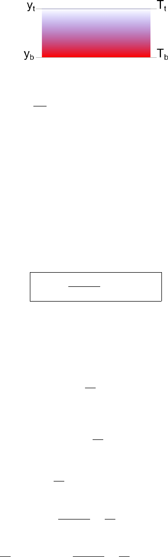
6.24 The initial temperature field
6.24.1 Single layer with imposed temperature b.c.
Let us take a single layer of material characterised by a heat capacity cp, a heat conductivity kand a
heat production term H.
The Heat transport equation writes
ρcp(∂T
∂t +v ·
∇T) =
∇ · (k
∇T) + ρH
At steady state and in the absence of a velocity field, and assuming that the material properties to be
independent of time and space, and that there is no heat production (H= 0), this equation simplifies to
∆T= 0
Assuming the layer to be parallel to the x-axis, this yields to write
T(x, y) = T(y) = αT +β
In order to specify the constants αand β, we need two constraints.
At the bottom of the layer y=yba temperature Tbis prescribed while a temperature Ttis prescribed
at the top with y=yt. This ultimately yields a temperature field in the layer given by
T(y) = Tt−Tb
yt−yb
(y−yb) + Tb
If now the heat production coefficient is not zero, the differential equation reads
k∆T+H= 0
The temperature field is then expected to be of the form
T(y) = −H
2ky2+αy +β
Supplied again with the same boundary conditions, this leads to
β=Tb+H
2ky2
b−αyb
ie,
T(y) = −H
2k(y2−y2
b) + α(y−yb) + Tb
and finally
α=Tt−Tb
yt−yb
+H
2k(yb+yt)
or,
T(y) = −H
2k(y2−y2
b) + Tt−Tb
yt−yb
+H
2k(yb+yt)(y−yb) + Tb
Taking H= 0 in this equation obviously yields the temperature field obtained previously. Taking
k= 2.25, Tt= 0C,Tb= 550C,yt= 660km,yb= 630km yields the following temperature profiles and
heat fluxes when the heat production Hvaries:
88
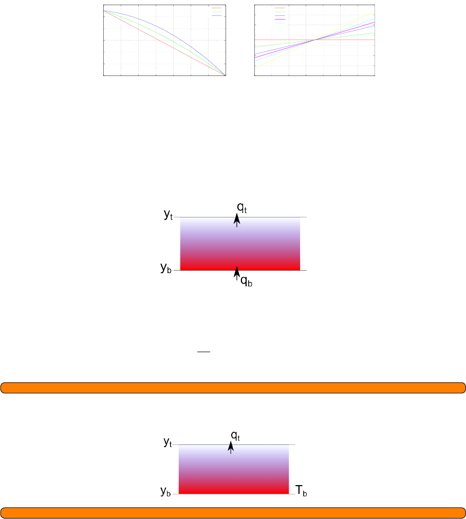
0
100
200
300
400
500
600
625000 630000 635000 640000 645000 650000 655000 660000
Temperature (C)
y
H=0.0e-6
H=0.8e-6
H=1.6e-6
0
0.01
0.02
0.03
0.04
0.05
0.06
0.07
625000 630000 635000 640000 645000 650000 655000 660000
heat flux (W/m2)
y
H=0.0e-6
H=0.4e-6
H=0.8e-6
H=1.0e-6
H=1.2e-6
H=1.6e-6
Looking at the values at the top, which are somewhat estimated to be about 55 −65mW/m2[277, table
8.6], one sees that value H= 0.8e−6 yields a very acceptable heat flux. Looking at the bottom, the heat
flux is then about 0.03W/m2which is somewhat problematic since the heat flux at the Moho is reported
to be somewhere between 10 and 20 mW/m2in [277, table 7.1].
6.25 Single layer with imposed heat flux b.c.
Let us now assume that heat fluxes are imposed at the top and bottom of the layer:
We start again from the ODE
k∆T+H= 0
but only integrate it once:
kdT
dy +Hy +α= 0
At the bottom q=k(dT/dy)|y=yb=qband at the top q=k(dT/dy)|y=yt=qtso that
to finish
6.26 Single layer with imposed heat flux and temperature b.c.
to finish
6.26.1 Half cooling space
6.26.2 Plate model
6.26.3 McKenzie slab
89
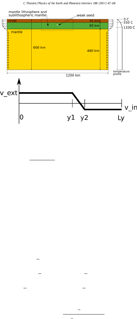
6.27 Kinematic boundary conditions
6.27.1 In-out flux boundary conditions for lithospheric models
The velocity on the side is given by
u(y) = vext y < L1
u(y) = vin −vext
y2−y1
(y−y1) + vext y1< y < y2
u(y) = vin y > y2
The requirement for volume conservation is:
Φ = ZLy
0
u(y)dy = 0
Having chosen vin (the velocity of the plate), one can then compute vext as a function of y1and y2.
Φ = Zy1
0
u(y)dy +Zy2
y1
u(y)dy +ZLy
y2
u(y)dy
=vexty1+1
2(vin +vext)(y2−y1)+(Ly−y2)vin
=vext[y1+1
2(y2−y1)] + vin[1
2(y2−y1)+(Ly−y2)]
=vext
1
2(y1+y2) + vin[Ly−1
2(y1+y1)]
and finally
vext =−vin
Ly−1
2(y1+y1)
1
2(y1+y2)
90

7fieldstone 01: simple analytical solution
This fieldstone was developed in collaboration with Job Mos.
From [142]. In order to illustrate the behavior of selected mixed finite elements in the solution of
stationary Stokes flow, we consider a two-dimensional problem in the square domain Ω = [0,1] ×[0,1],
which possesses a closed-form analytical solution. The problem consists of determining the velocity field
v= (u, v) and the pressure psuch that
−ν∆v+∇p=bin Ω
∇·v= 0 in Ω
v=0on Γ
where the fluid viscosity is taken as ν= 1.
features
•Q1×P0element
•incompressible flow
•penalty formulation
•Dirichlet boundary conditions (no-slip)
•direct solver
•isothermal
•isoviscous
•analytical solution
91
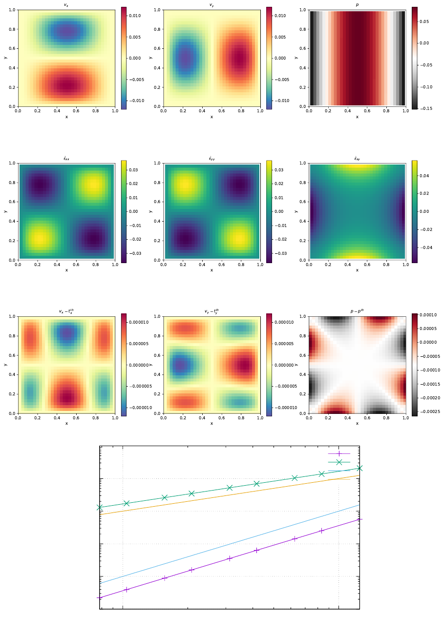
0.000001
0.000010
0.000100
0.001000
0.010000
0.100000
0.01 0.1
error
h
velocity
pressure
x2
x1
Quadratic convergence for velocity error, linear convergence for pressure error, as expected.
92
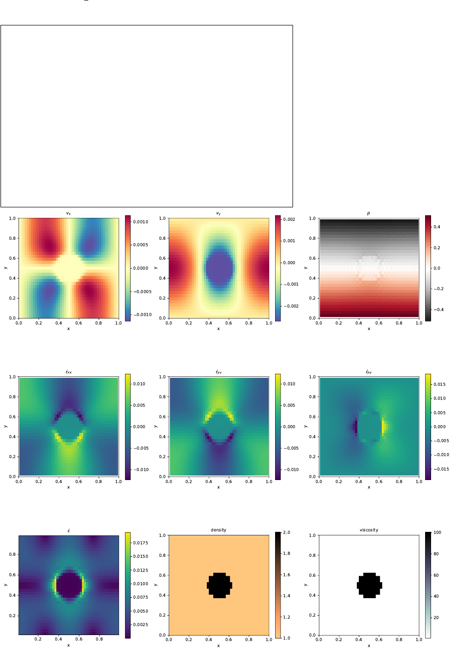
8fieldstone 02: Stokes sphere
Viscosity and density directly computed at the quadrature points.
features
•Q1×P0element
•incompressible flow
•penalty formulation
•Dirichlet boundary conditions (free-slip)
•isothermal
•non-isoviscous
•buoyancy-driven flow
•Stokes sphere
93

9fieldstone 03: Convection in a 2D box
This benchmark deals with the 2-D thermal convection of a fluid of infinite Prandtl number in a rect-
angular closed cell. In what follows, I carry out the case 1a, 1b, and 1c experiments as shown in [55]:
steady convection with constant viscosity in a square box.
The temperature is fixed to zero on top and to ∆Tat the bottom, with reflecting symmetry at the
sidewalls (i.e. ∂xT= 0) and there are no internal heat sources. Free-slip conditions are implemented on
all boundaries.
The Rayleigh number is given by
Ra =αgy∆T h3
κν =αgy∆T h3ρ2cp
kµ (204)
In what follows, I use the following parameter values: Lx=Ly= 1,ρ0=cP=k=µ= 1, T0= 0,
α= 10−2,g= 102Ra and I run the model with Ra = 104,105and 106.
The initial temperature field is given by
T(x, y) = (1 −y)−0.01 cos(πx) sin(πy) (205)
The perturbation in the initial temperature fields leads to a perturbation of the density field and sets the
fluid in motion.
Depending on the initial Rayleigh number, the system ultimately reaches a steady state after some
time.
The Nusselt number (i.e. the mean surface temperature gradient over mean bottom temperature) is
computed as follows [55]:
Nu =LyR∂T
∂y (y=Ly)dx
RT(y= 0)dx (206)
Note that in our case the denominator is equal to 1 since Lx= 1 and the temperature at the bottom is
prescribed to be 1.
Finally, the steady state root mean square velocity and Nusselt number measurements are indicated in
Table ?? alongside those of [55] and [438]. (Note that this benchmark was also carried out and published
in other publications [460, 6, 206, 136, 307] but since they did not provide a complete set of measurement
values, they are not included in the table.)
Blankenbach et al Tackley [438]
Ra = 104Vrms 42.864947 ±0.000020 42.775
Nu 4.884409 ±0.000010 4.878
Ra = 105Vrms 193.21454 ±0.00010 193.11
Nu 10.534095 ±0.000010 10.531
Ra = 106Vrms 833.98977 ±0.00020 833.55
Nu 21.972465 ±0.000020 21.998
Steady state Nusselt number N u and Vrms measurements as reported in the literature.
94
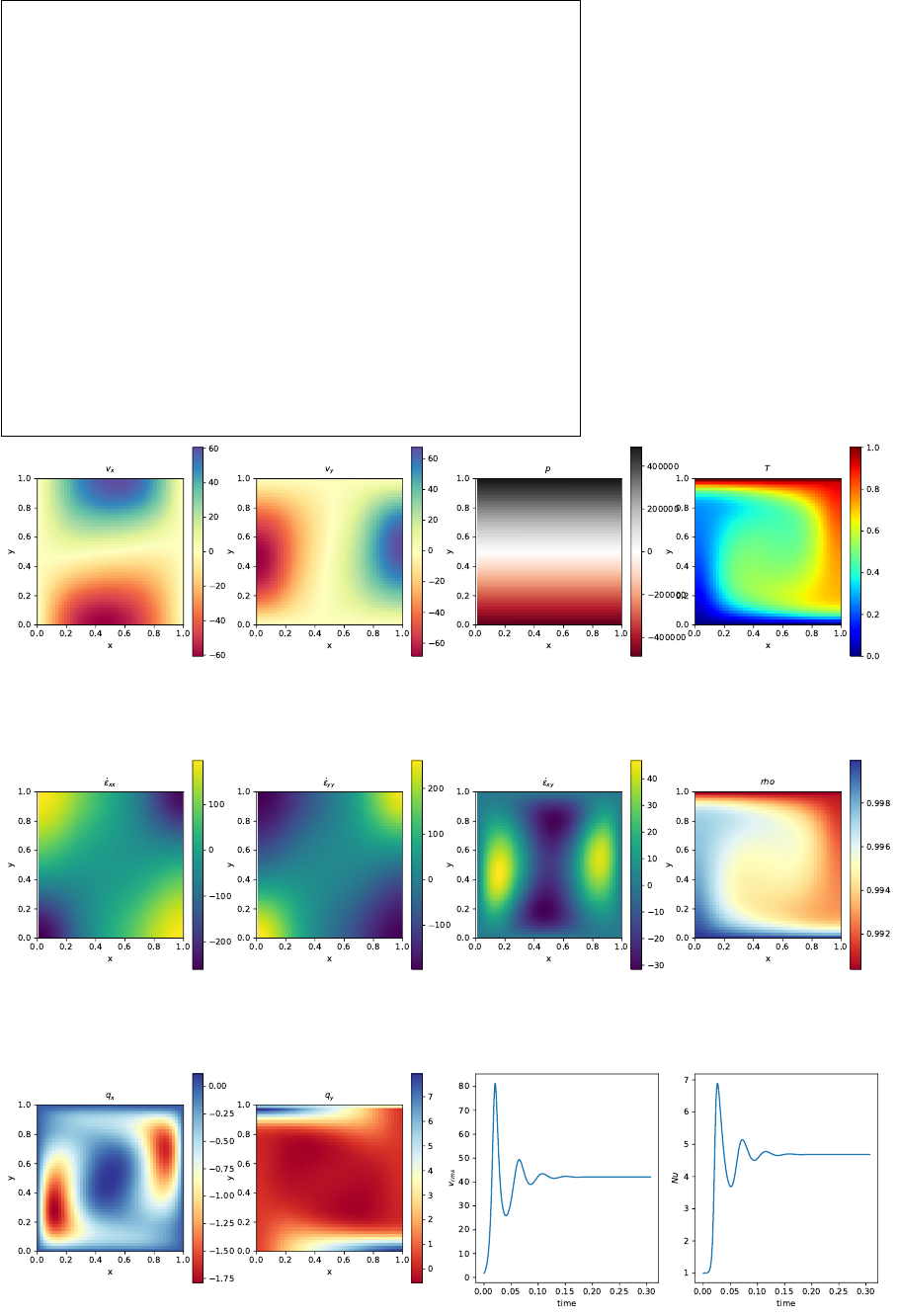
features
•Q1×P0element
•incompressible flow
•penalty formulation
•Dirichlet boundary conditions (free-slip)
•Boussinesq approximation
•direct solver
•non-isothermal
•buoyancy-driven flow
•isoviscous
•CFL-condition
95
ToDo:
implement steady state criterion
reach steady state
do Ra=1e4, 1e5, 1e6
plot against blankenbach paper and aspect
look at critical Ra number
96

10 fieldstone 04: The lid driven cavity
The lid driven cavity is a famous Computational Fluid Dynamics test case and has been studied in
countless publications with a wealth of numerical techniques (see [161] for a succinct review) and also in
the laboratory [295].
It models a plane flow of an isothermal isoviscous fluid in a rectangular (usually square) lid-driven
cavity. The boundary conditions are indicated in the Fig. ??a. The gravity is set to zero.
10.1 the lid driven cavity problem (ldc=0)
In the standard case, the upper side of the cavity moves in its own plane at unit speed, while the other
sides are fixed. This thereby introduces a discontinuity in the boundary conditions at the two upper
corners of the cavity and yields an uncertainty as to which boundary (side or top) the corner points
belong to. In this version of the code the top corner nodes are considered to be part of the lid. If these
are excluded the recovered pressure showcases and extremely large checkboard pattern.
This benchmark is usually dicussed in the context of low to very high Reynolds number with the full
Navier-Stokes equations being solved (with the noticeable exception of [408, 409, 107, 154] which focus
on the Stokes equation). In the case of the incompressible Stokes flow, the absence of inertia renders this
problem instantaneous so that only one time step is needed.
10.2 the lid driven cavity problem - regularisation I (ldc=1)
We avoid the top corner nodes issue altogether by prescribing the horizontal velocity of the lid as follows:
u(x) = x2(1 −x)2.(207)
In this case the velocity and its first derivative is continuous at the corners. This is the so-called regularised
lid-driven cavity problem [372].
10.3 the lid driven cavity problem - regularisation II (ldc=2)
Another regularisation was presented in [138]. Here, a regularized lid driven cavity is studied which is
consistent in the sense that ∇·v= 0 holds also at the corners of the domain. There are no-slip conditions
at the boundaries x= 0, x= 1, and y= 0.
The velocity at y= 1 is given by
u(x)=1−1
41−cos(x1−x
x1
π)2
x∈[0, x1]
u(x)=1 x∈[x1,1−x1]
u(x)=1−1
41−cos(x−(1 −x1)
x1
π)2
x∈[1 −x1,1] (208)
Results are obtained with x1= 0.1.
features
•Q1×P0element
•incompressible flow
•penalty formulation
•isothermal
•isoviscous
97
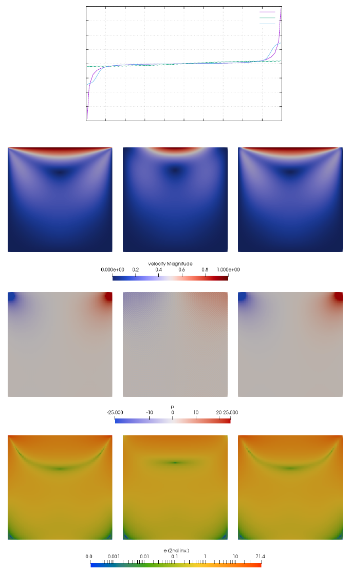
A 100x100 element grid is used. No-slip boundary conditions are prescribed on sides and bottom. A
zero vertical velocity is prescribed at the top and the exact form of the prescribed horizontal velocity is
controlled by the ldc parameter.
-200
-150
-100
-50
0
50
100
150
200
0 0.1 0.2 0.3 0.4 0.5 0.6 0.7 0.8 0.9 1
pressure
x
ldc0
ldc1
ldc2
98

11 fieldstone 05: SolCx benchmark
The SolCx benchmark is intended to test the accuracy of the solution to a problem that has a large jump
in the viscosity along a line through the domain. Such situations are common in geophysics: for example,
the viscosity in a cold, subducting slab is much larger than in the surrounding, relatively hot mantle
material.
The SolCx benchmark computes the Stokes flow field of a fluid driven by spatial density variations,
subject to a spatially variable viscosity. Specifically, the domain is Ω = [0,1]2, gravity is g= (0,−1)T
and the density is given by
ρ(x, y) = sin(πy) cos(πx) (209)
Boundary conditions are free slip on all of the sides of the domain and the temperature plays no role in
this benchmark. The viscosity is prescribed as follows:
µ(x, y) = 1for x < 0.5
106for x > 0.5(210)
Note the strongly discontinuous viscosity field yields a stagnant flow in the right half of the domain and
thereby yields a pressure discontinuity along the interface.
The SolCx benchmark was previously used in [149] (references to earlier uses of the benchmark are
available there) and its analytic solution is given in [519]. It has been carried out in [297] and [210].
Note that the source code which evaluates the velocity and pressure fields for both SolCx and SolKz is
distributed as part of the open source package Underworld ([348], http://underworldproject.org).
In this particular example, the viscosity is computed analytically at the quadrature points (i.e. tracers
are not used to attribute a viscosity to the element). If the number of elements is even in any direction,
all elements (and their associated quadrature points) have a constant viscosity(1 or 106). If it is odd, then
the elements situated at the viscosity jump have half their integration points with µ= 1 and half with
µ= 106(which is a pathological case since the used quadrature rule inside elements cannot represent
accurately such a jump).
features
•Q1×P0element
•incompressible flow
•penalty formulation
•Dirichlet boundary conditions (free-slip)
•direct solver
•isothermal
•non-isoviscous
•analytical solution
99
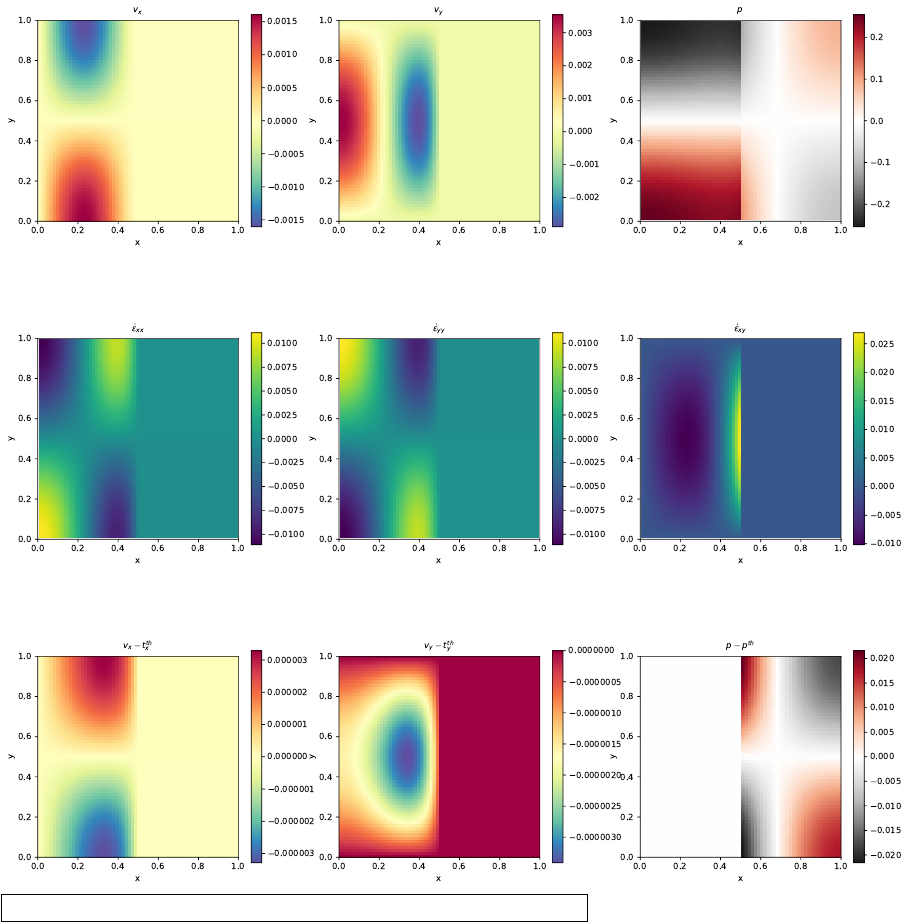
What we learn from this
100
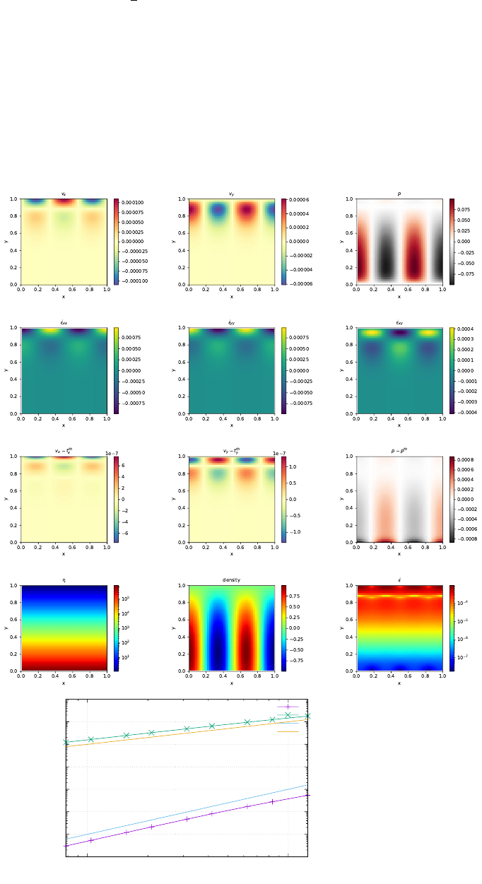
12 fieldstone 06: SolKz benchmark
The SolKz benchmark [399] is similar to the SolCx benchmark. but the viscosity is now a function of the
space coordinates:
µ(y) = exp(By) with B= 13.8155 (211)
It is however not a discontinuous function but grows exponentially with the vertical coordinate so that
its overall variation is again 106. The forcing is again chosen by imposing a spatially variable density
variation as follows:
ρ(x, y) = sin(2y) cos(3πx) (212)
Free slip boundary conditions are imposed on all sides of the domain. This benchmark is presented in
[519] as well and is studied in [149] and [210].
0.00000001
0.00000010
0.00000100
0.00001000
0.00010000
0.00100000
0.01000000
0.10000000
0.01 0.1
error
h
velocity
pressure
x2
x1
101

13 fieldstone 07: SolVi benchmark
Following SolCx and SolKz, the SolVi inclusion benchmark solves a problem with a discontinuous viscosity
field, but in this case the viscosity field is chosen in such a way that the discontinuity is along a circle.
Given the regular nature of the grid used by a majority of codes and the present one, this ensures that the
discontinuity in the viscosity never aligns to cell boundaries. This in turns leads to almost discontinuous
pressures along the interface which are difficult to represent accurately. [415] derived a simple analytic
solution for the pressure and velocity fields for a circular inclusion under simple shear and it was used in
[139], [436], [149], [297] and [210].
Because of the symmetry of the problem, we only have to solve over the top right quarter of the
domain (see Fig. ??a).
The analytical solution requires a strain rate boundary condition (e.g., pure shear) to be applied far
away from the inclusion. In order to avoid using very large domains and/or dealing with this type of
boundary condition altogether, the analytical solution is evaluated and imposed on the boundaries of
the domain. By doing so, the truncation error introduced while discretizing the strain rate boundary
condition is removed.
A characteristic of the analytic solution is that the pressure is zero inside the inclusion, while outside
it follows the relation
pm= 4˙µm(µi−µm)
µi+µm
r2
i
r2cos(2θ) (213)
where µi= 103is the viscosity of the inclusion and µm= 1 is the viscosity of the background media,
θ= tan−1(y/x), and ˙= 1 is the applied strain rate.
[139] thoroughly investigated this problem with various numerical methods (FEM, FDM), with and
without tracers, and conclusively showed how various averagings lead to different results. [149] obtained
a first order convergence for both pressure and velocity, while [297] and [210] showed that the use of
adaptive mesh refinement in respectively the FEM and FDM yields convergence rates which depend on
refinement strategies.
102
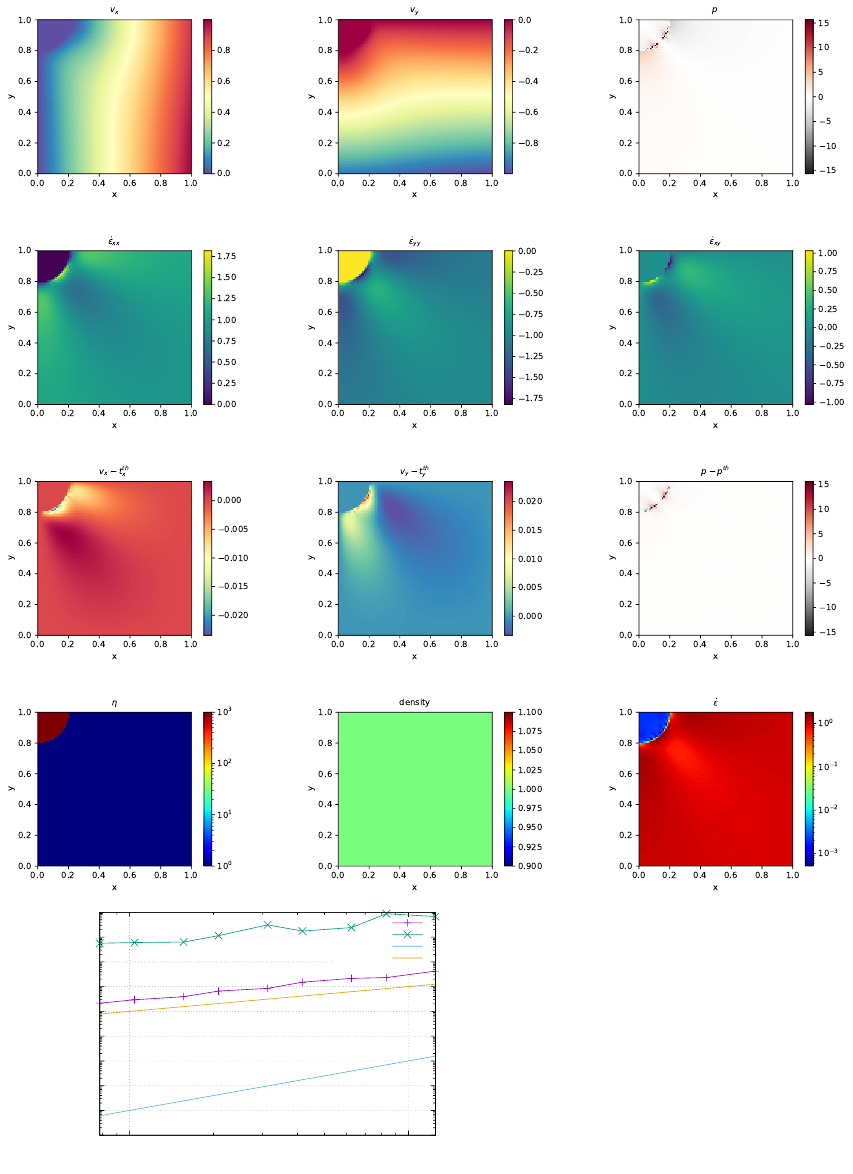
0.00000001
0.00000010
0.00000100
0.00001000
0.00010000
0.00100000
0.01000000
0.10000000
1.00000000
10.00000000
0.01 0.1
error
h
velocity
pressure
x2
x1
103

14 fieldstone 08: the indentor benchmark
The punch benchmark is one of the few boundary value problems involving plastic solids for which there
exists an exact solution. Such solutions are usually either for highly simplified geometries (spherical or
axial symmetry, for instance) or simplified material models (such as rigid plastic solids) [280].
In this experiment, a rigid punch indents a rigid plastic half space; the slip line field theory gives exact
solutions as shown in Fig. ??a. The plane strain formulation of the equations and the detailed solution
to the problem were derived in the Appendix of [454] and are also presented in [200].
The two dimensional punch problem has been extensively studied numerically for the past 40 years
[531, 530, 112, 111, 261, 513, 74, 397] and has been used to draw a parallel with the tectonics of eastern
China in the context of the India-Eurasia collision [443, 344]. It is also worth noting that it has been
carried out in one form or another in series of analogue modelling articles concerning the same region,
with a rigid indenter colliding with a rheologically stratified lithosphere [367, 137, 279].
Numerically, the one-time step punch experiment is performed on a two-dimensional domain of purely
plastic von Mises material. Given that the von Mises rheology yield criterion does not depend on pressure,
the density of the material and/or the gravity vector is set to zero. Sides are set to free slip boundary
conditions, the bottom to no slip, while a vertical velocity (0,−vp) is prescribed at the top boundary for
nodes whose xcoordinate is within [Lx/2−δ/2, Lx/2 + δ/2].
The following parameters are used: Lx= 1, Ly= 0.5, µmin = 10−3,µmax = 103,vp= 1, δ=
0.123456789 and the yield value of the material is set to k= 1.
The analytical solution predicts that the angle of the shear bands stemming from the sides of the
punch is π/4, that the pressure right under the punch is 1 + π, and that the velocity of the rigid blocks
on each side of the punch is vp/√2 (this is simply explained by invoking conservation of mass).
104
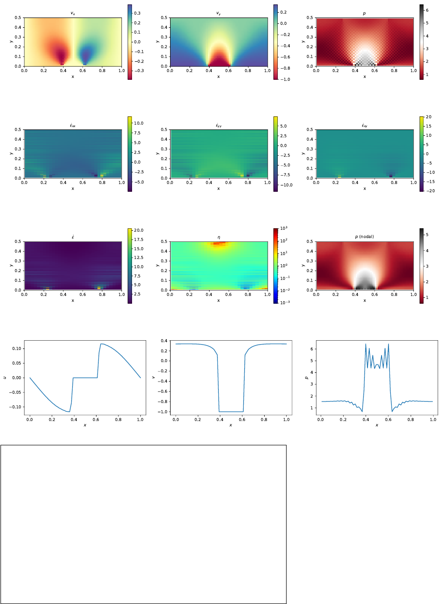
ToDo: smooth punch
features
•Q1×P0element
•incompressible flow
•penalty formulation
•Dirichlet boundary conditions (no-slip)
•isothermal
•non-isoviscous
•nonlinear rheology
105

15 fieldstone 09: the annulus benchmark
This fieldstone was developed in collaboration with Prof. E.G.P. Puckett.
This benchmark is based on Thieulot & Puckett [Subm.] in which an analytical solution to the
isoviscous incompressible Stokes equations is derived in an annulus geometry. The velocity and pressure
fields are as follows:
vr(r, θ) = g(r)ksin(kθ),(214)
vθ(r, θ) = f(r) cos(kθ),(215)
p(r, θ) = kh(r) sin(kθ),(216)
ρ(r, θ) = ℵ(r)ksin(kθ),(217)
with
f(r) = Ar +B/r, (218)
g(r) = A
2r+B
rln r+C
r,(219)
h(r) = 2g(r)−f(r)
r,(220)
ℵ(r) = g00 −g0
r−g
r2(k2−1) + f
r2+f0
r,(221)
A=−C2(ln R1−ln R2)
R2
2ln R1−R2
1ln R2
,(222)
B=−CR2
2−R2
1
R2
2ln R1−R2
1ln R2
.(223)
The parameters Aand Bare chosen so that vr(R1) = vr(R2) = 0, i.e. the velocity is tangential to
both inner and outer surfaces. The gravity vector is radial and of unit length. In the present case, we
set R1= 1, R2= 2 and C=−1.
features
•Q1×P0element
•incompressible flow
•penalty formulation
•Dirichlet boundary conditions
•direct solver
•isothermal
•isoviscous
•analytical solution
•annulus geometry
•elemental boundary conditions
106
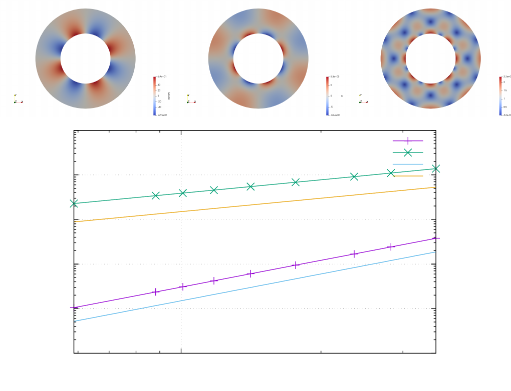
0.0001
0.001
0.01
0.1
1
10
0.01
error
h
velocity
pressure
x2
x1
107
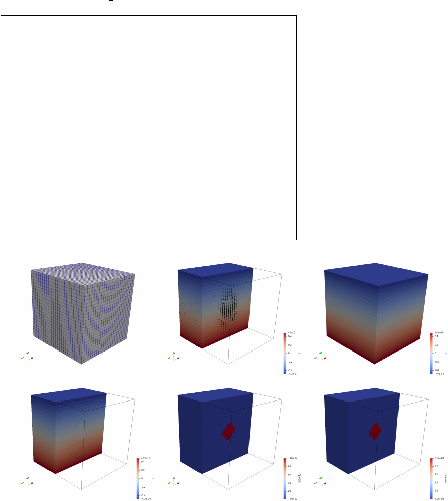
16 fieldstone 10: Stokes sphere (3D) - penalty
features
•Q1×P0element
•incompressible flow
•penalty formulation
•Dirichlet boundary conditions (free-slip)
•direct solver
•isothermal
•non-isoviscous
•3D
•elemental b.c.
•buoyancy driven
resolution is 24x24x24
108


18 fieldstone 12: consistent pressure recovery
What follows is presented in [529]. The second part of their paper wishes to establish a simple and
effective numerical method to calculate variables eliminated by the penalisation process. The method
involves an additional finite element solution for the nodal pressures using the same finite element basis
and numerical quadrature as used for the velocity.
Let us start with:
p=−λ∇·v
which lead to
(q, p) = −λ(q, ∇·v)
and then ZN N dΩ·P=−λZN∇NdΩ·V
or,
M·P=−D·V
and finally
P=−M−1·D·V
with Mof size (np ×np), Dof size (np ∗ndof ×np ∗ndof) and Vof size (np ∗ndof). The vector P
contains the np nodal pressure values directly, with no need for a smoothing scheme. The mass matrix
Mis to be evaluated at the full integration points, while the constraint part (the right hand side of the
equation) is to be evaluated at the reduced integration point.
As noted by [529], it is interesting to note that when linear elements are used and the lumped matrices
are used for the Mthe resulting algebraic equation is identical to the smoothing scheme based on the
averaging method only if the uniform square finite element mesh is used. In this respect this method is
expected to yield different results when elements are not square or even rectangular.
——-
q1is smoothed pressure obtained with the center-to-node approach.
q2is recovered pressure obtained with [529].
All three fulfill the zero average condition: RpdΩ = 0.
110
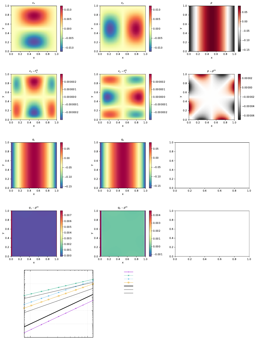
0.000001
0.000010
0.000100
0.001000
0.010000
0.100000
0.01 0.1
error
h
velocity
pressure (el)
pressure (q1)
pressure (q2)
x2
x1.5
x1
In terms of pressure error, q2is better than q1which is better than elemental.
QUESTION: why are the averages exactly zero ?!
TODO:
•add randomness to internal node positions.
•look at elefant algorithms
111

19 fieldstone 13: the Particle in Cell technique (1) - the effect
of averaging
This fieldstone is being developed in collaboration with BSc student Eric Hoogen.
features
•Q1×P0element
•incompressible flow
•penalty formulation
•Dirichlet boundary conditions (no-slip)
•isothermal
•non-isoviscous
•particle-in-cell
After the initial setup of the grid, markers can then be generated and placed in the domain. One
could simply randomly generate the marker positions in the whole domain but unless a very large number
of markers is used, the chance that an element does not contain any marker exists and this will prove
problematic. In order to get a better control over the markers spatial distribution, one usually generates
the marker per element, so that the total number of markers in the domain is the product of the number
of elements times the user-chosen initial number of markers per element.
Our next concern is how to actually place the markers inside an element. Two methods come to mind:
on a regular grid, or in a random manner, as shown on the following figure:
In both cases we make use of the basis shape functions: we generate the positions of the markers
(random or regular) in the reference element first (rim, sim), and then map those out to the real element
as follows:
xim =
m
X
i
Ni(rim, sim)xiyim =
m
X
i
Ni(rim, sim)yi(224)
where xi, yiare the coordinates of the vertices of the element.
A third option consists in the use of the so-called Poisson-disc sampling which produces points that
are tightly-packed, but no closer to each other than a specified minimum distance, resulting in a more
natural pattern 11. Note that the Poisson-disc algorithm fills the whole domain at once, not element after
element.
say smthg about avrg dist
insert here theory and link about Poisson disc
11https://en.wikipedia.org/wiki/Supersampling
112
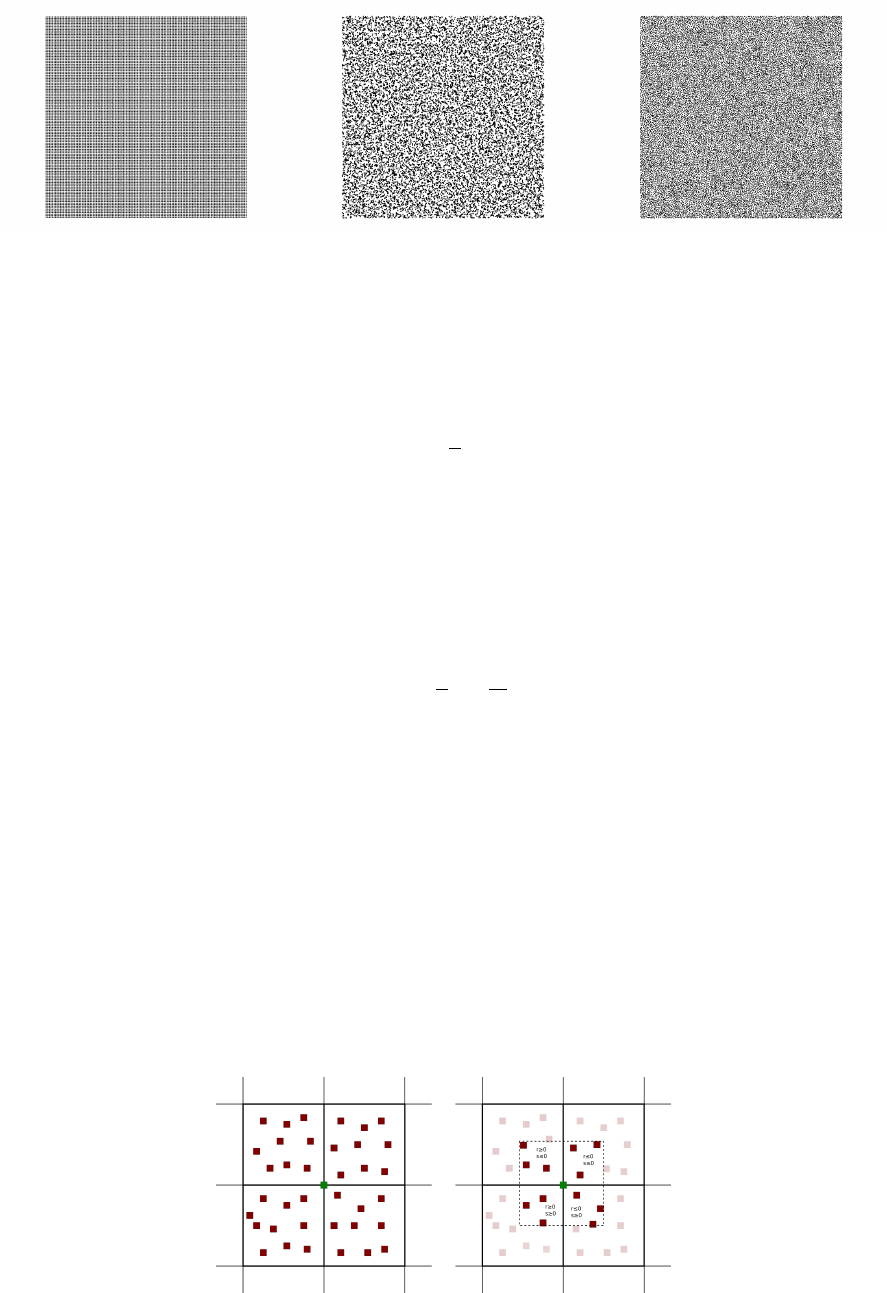
Left: regular distribution, middle: random, right: Poisson disc.
16384 markers (32x32 grid, 16 markers per element).
When using active markers, one is faced with the problem of transferring the properties they carry to
the mesh on which the PDEs are to be solved. As we have seen, building the FE matrix involves a loop
over all elements, so one simple approach consists of assigning each element a single property computed as
the average of the values carried by the markers in that element. Often in colloquial language ”average”
refers to the arithmetic mean:
hφiam =1
n
n
X
k
φi(225)
where < φ >am is the arithmetic average of the nnumbers φi. However, in mathematics other means
are commonly used, such as the geometric mean:
hφigm = n
Y
i
φi!(226)
and the harmonic mean:
hφihm = 1
n
n
X
i
1
φi!−1
(227)
Furthermore, there is a well known inequality for any set of positive numbers,
hφiam ≥ hφigm ≥ hφihm (228)
which will prove to be important later on.
Let us now turn to a simple concrete example: the 2D Stokes sphere. There are two materials
in the domain, so that markers carry the label ”mat=1” or ”mat=2”. For each element an average
density and viscosity need to be computed. The majority of elements contains markers with a single
material label so that the choice of averaging does not matter (it is trivial to verify that if φi=φ0then
hφiam =hφigm =hφihm =φ0. Remain the elements crossed by the interface between the two materials:
they contain markers of both materials and the average density and viscosity inside those depends on 1)
the total number of markers inside the element, 2) the ratio of markers 1 to markers 2, 3) the type of
averaging.
This averaging problem has been studied and documented in the literature [414, 139, 449, 381]
Nodal projection. Left: all markers inside elements to which the green node belongs to are taken into account.
Right: only the markers closest to the green node count.
113

Let kbe the green node of the figures above. Let (r, s) denote the coordinates of a marker inside its
element. For clarity, we define the follow three nodal averaging schemes:
•nodal type A:
fk=sum of values carried by markers in 4 neighbour elements
number of markers in 4 neighbour elements
•nodal type B:
fk=sum of values carried by markers inside dashed line
number of markers in area delimited by the dashed line
•nodal type C
fk=sum of values carried by markers in 4 neighbour elements ∗Np(r, s)
sum of Np(r, s)
where Npis the Q1basis function corresponding to node pdefined on each element. Since these
functions are 1 on node kand then linearly decrease and become zero on the neighbouring nodes,
this effectively gives more weight to those markers closest to node k.
This strategy is adopted in [1, 341] (although it is used to interpolate onto the nodes of Q2P−1
elements. It is formulated as follows:
”We assume that an arbitrary material point property f, is discretized via f(x)'δ(x−xp)fp. We
then utilize an approximate local L2projection of fponto a continuous Q1finite element space.
The corner vertices of each Q2finite element define the mesh fpis projected onto. The local
reconstruction for a node i is defined by
ˆ
fi=RΩiNi(x)f(x)
RΩiNi(x)'PpNi(xp)fp
PpNi(xp)
where the summation over pincludes all material points contained within the support Ωiof the
trilinear interpolant Ni”.
The setup is identical to the Stokes sphere experiment. The bash script script runall runs the code
for many resolutions, both initial marker distribution and all four averaging types. The viscosity of the
sphere has been set to 103while the viscosity of the surrounding fluid is 1. The average density is always
computed with an arithmetic mean.
Conclusions:
•With increasing resolution (h→0) vrms values seem to converge towards a single value, irrespective
of the number of markers.
•At low resolution, say 32x32 (i.e. h=0.03125), vrms values for the three averagings differ by about
10%. At higher resolution, say 128x128, vrms values are still not converged.
•The number of markers per element plays a role at low resolution, but less and less with increasing
resolution.
•Results for random and regular marker distributions are not identical but follow a similar trend
and seem to converge to the same value.
•elemental values yield better results (espcecially at low resolutions)
•harmonic mean yields overal the best results
114
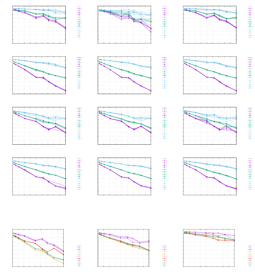
Root mean square velocity results are shown hereunder:
0.001
0.002
0.003
0.004
0.005
0.006
0.007
0.008
0.009
0.01
0.01 0.02 0.03 0.04 0.05 0.06 0.07 0.08 0.09 0.1
vrms
h
random markers, elemental proj
am, 09 m
am, 16 m
am, 25 m
am, 36 m
am, 48 m
am, 64 m
gm, 09 m
gm, 16 m
gm, 25 m
gm, 36 m
gm, 48 m
gm, 64 m
hm, 09 m
hm, 16 m
hm, 25 m
hm, 36 m
hm, 48 m
hm, 64 m
0.001
0.002
0.003
0.004
0.005
0.006
0.007
0.008
0.009
0.01
0.01 0.02 0.03 0.04 0.05 0.06 0.07 0.08 0.09 0.1
vrms
h
random PD markers, elemental proj
am, 09 m
am, 16 m
am, 25 m
am, 36 m
am, 48 m
am, 64 m
gm, 09 m
gm, 16 m
gm, 25 m
gm, 36 m
gm, 48 m
gm, 64 m
hm, 09 m
hm, 16 m
hm, 25 m
hm, 36 m
hm, 48 m
hm, 64 m
0.001
0.002
0.003
0.004
0.005
0.006
0.007
0.008
0.009
0.01
0.01 0.02 0.03 0.04 0.05 0.06 0.07 0.08 0.09 0.1
vrms
h
regular markers, elemental proj
am, 09 m
am, 16 m
am, 25 m
am, 36 m
am, 48 m
am, 64 m
gm, 09 m
gm, 16 m
gm, 25 m
gm, 36 m
gm, 48 m
gm, 64 m
hm, 09 m
hm, 16 m
hm, 25 m
hm, 36 m
hm, 48 m
hm, 64 m
0.001
0.002
0.003
0.004
0.005
0.006
0.007
0.008
0.009
0.01
0.01 0.02 0.03 0.04 0.05 0.06 0.07 0.08 0.09 0.1
vrms
h
random markers, nodal proj A
am, 09 m
am, 16 m
am, 25 m
am, 36 m
am, 48 m
am, 64 m
gm, 09 m
gm, 16 m
gm, 25 m
gm, 36 m
gm, 48 m
gm, 64 m
hm, 09 m
hm, 16 m
hm, 25 m
hm, 36 m
hm, 48 m
hm, 64 m
0.001
0.002
0.003
0.004
0.005
0.006
0.007
0.008
0.009
0.01
0.01 0.02 0.03 0.04 0.05 0.06 0.07 0.08 0.09 0.1
vrms
h
random PD markers, nodal proj A
am, 09 m
am, 16 m
am, 25 m
am, 36 m
am, 48 m
am, 64 m
gm, 09 m
gm, 16 m
gm, 25 m
gm, 36 m
gm, 48 m
gm, 64 m
hm, 09 m
hm, 16 m
hm, 25 m
hm, 36 m
hm, 48 m
hm, 64 m
0.001
0.002
0.003
0.004
0.005
0.006
0.007
0.008
0.009
0.01
0.01 0.02 0.03 0.04 0.05 0.06 0.07 0.08 0.09 0.1
vrms
h
regular markers, nodal proj A
am, 09 m
am, 16 m
am, 25 m
am, 36 m
am, 48 m
am, 64 m
gm, 09 m
gm, 16 m
gm, 25 m
gm, 36 m
gm, 48 m
gm, 64 m
hm, 09 m
hm, 16 m
hm, 25 m
hm, 36 m
hm, 48 m
hm, 64 m
0.001
0.002
0.003
0.004
0.005
0.006
0.007
0.008
0.009
0.01
0.01 0.02 0.03 0.04 0.05 0.06 0.07 0.08 0.09 0.1
vrms
h
random markers, nodal proj B
am, 09 m
am, 16 m
am, 25 m
am, 36 m
am, 48 m
am, 64 m
gm, 09 m
gm, 16 m
gm, 25 m
gm, 36 m
gm, 48 m
gm, 64 m
hm, 09 m
hm, 16 m
hm, 25 m
hm, 36 m
hm, 48 m
hm, 64 m
0.001
0.002
0.003
0.004
0.005
0.006
0.007
0.008
0.009
0.01
0.01 0.02 0.03 0.04 0.05 0.06 0.07 0.08 0.09 0.1
vrms
h
regular markers, nodal proj B
am, 09 m
am, 16 m
am, 25 m
am, 36 m
am, 48 m
am, 64 m
gm, 09 m
gm, 16 m
gm, 25 m
gm, 36 m
gm, 48 m
gm, 64 m
hm, 09 m
hm, 16 m
hm, 25 m
hm, 36 m
hm, 48 m
hm, 64 m
0.001
0.002
0.003
0.004
0.005
0.006
0.007
0.008
0.009
0.01
0.01 0.02 0.03 0.04 0.05 0.06 0.07 0.08 0.09 0.1
vrms
h
random markers, nodal proj C
am, 09 m
am, 16 m
am, 25 m
am, 36 m
am, 48 m
am, 64 m
gm, 09 m
gm, 16 m
gm, 25 m
gm, 36 m
gm, 48 m
gm, 64 m
hm, 09 m
hm, 16 m
hm, 25 m
hm, 36 m
hm, 48 m
hm, 64 m
0.001
0.002
0.003
0.004
0.005
0.006
0.007
0.008
0.009
0.01
0.01 0.02 0.03 0.04 0.05 0.06 0.07 0.08 0.09 0.1
vrms
h
regular markers, nodal proj C
am, 09 m
am, 16 m
am, 25 m
am, 36 m
am, 48 m
am, 64 m
gm, 09 m
gm, 16 m
gm, 25 m
gm, 36 m
gm, 48 m
gm, 64 m
hm, 09 m
hm, 16 m
hm, 25 m
hm, 36 m
hm, 48 m
hm, 64 m
Left column: random markers, middle column: Poisson disc, right column: regular markers. First row: elemental
projection, second row: nodal 1 projection, third row: nodal 2 projection, fourth row: nodal 3 projection.
0.001
0.002
0.003
0.004
0.005
0.006
0.007
0.008
0.009
0.01
0.01 0.02 0.03 0.04 0.05 0.06 0.07 0.08 0.09 0.1
vrms
h
64 markers per element, arithmetic avrg
reg, el
rand, el
pd, el
reg, nodA
rand, nodA
pd, nodA
reg, nodB
rand, nodB
pd, nodB
reg, nodC
rand, nodC
pd, nodC
0.001
0.002
0.003
0.004
0.005
0.006
0.007
0.008
0.009
0.01
0.01 0.02 0.03 0.04 0.05 0.06 0.07 0.08 0.09 0.1
vrms
h
64 markers per element, geometric avrg
reg, el
rand, el
pd, el
reg, nodA
rand, nodA
pd, nodA
reg, nodB
rand, nodB
pd, nodB
reg, nodC
rand, nodC
pd, nodC
0.001
0.002
0.003
0.004
0.005
0.006
0.007
0.008
0.009
0.01
0.01 0.02 0.03 0.04 0.05 0.06 0.07 0.08 0.09 0.1
vrms
h
64 markers per element, harmonic avrg
reg, el
rand, el
pd, el
reg, nodA
rand, nodA
pd, nodA
reg, nodB
rand, nodB
pd, nodB
reg, nodC
rand, nodC
pd, nodC
Left to right: arithmetic, geometric, harmonic averaging for viscosity.
115

20 fieldstone f14: solving the full saddle point problem
The details of the numerical setup are presented in Section ??.
The main difference is that we no longer use the penalty formulation and therefore keep both velocity
and pressure as unknowns. Therefore we end up having to solve the following system:
K G
GT0·V
P=f
hor,A·X=rhs
Each block K,Gand vector f,hare built separately in the code and assembled into the matrix A
and vector rhs afterwards. Aand rhs are then passed to the solver. We will see later that there are
alternatives to solve this approach which do not require to build the full Stokes matrix A.
Each element has m= 4 vertices so in total ndofV ×m= 8 velocity dofs and a single pressure
dof, commonly situated in the center of the element. The total number of velocity dofs is therefore
NfemV =nnp ×ndofV while the total number of pressure dofs is NfemP =nel. The total number of
dofs is then Nfem =NfemV +N femP .
As a consequence, matrix Khas size N femV, N femV and matrix Ghas size N femV, N femP . Vector
fis of size NfemV and vector his of size N femP .
features
•Q1×P0element
•incompressible flow
•mixed formulation
•Dirichlet boundary conditions (no-slip)
•direct solver (?)
•isothermal
•isoviscous
•analytical solution
•pressure smoothing
116
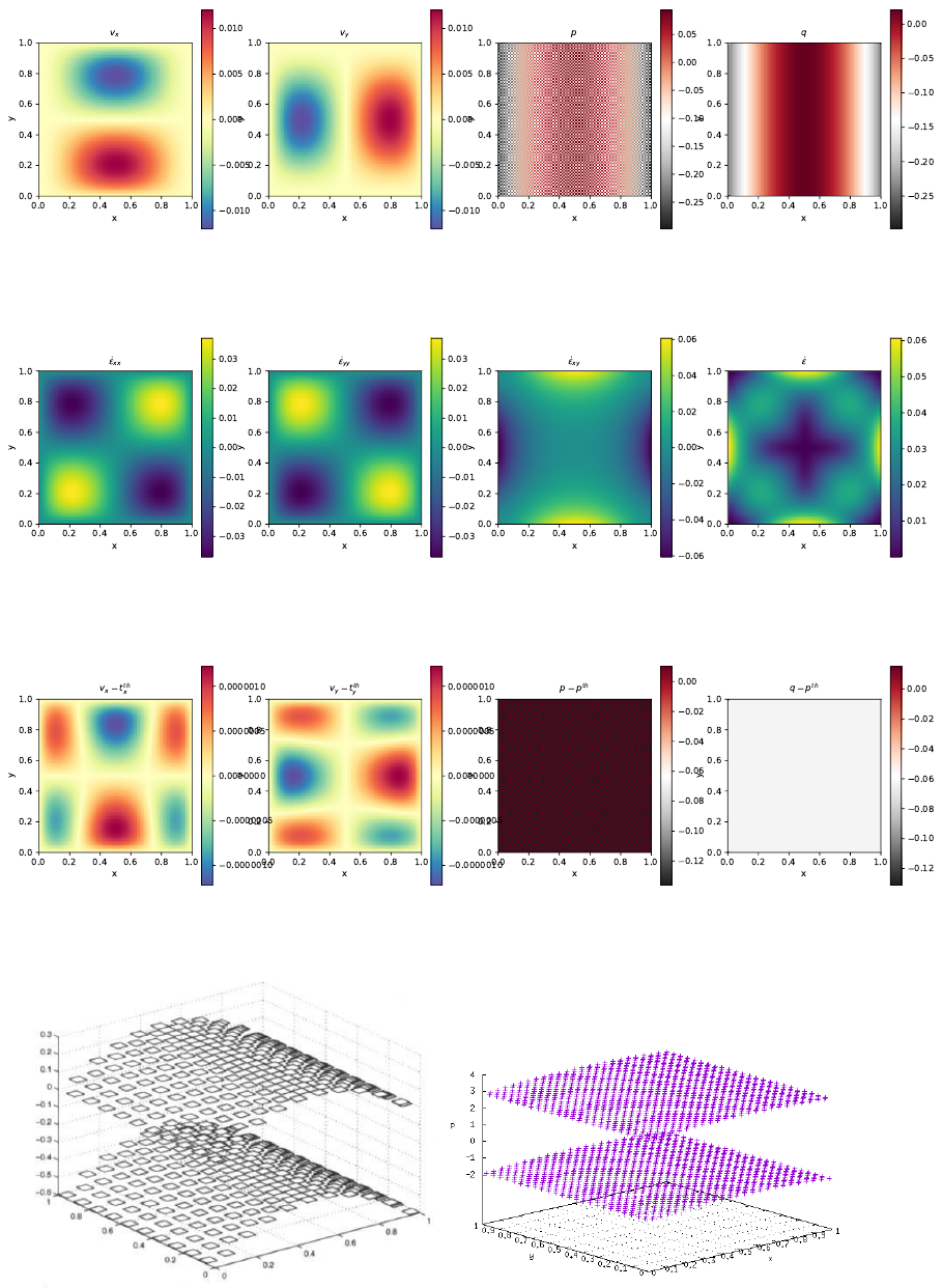
Unlike the results obtained with the penalty formualtion (see Section ??), the pressure showcases a
very strong checkerboard pattern, similar to the one in [143].
Left: pressure solution as shown in [143]; Right: pressure solution obtained with fieldstone.
Rather interestingly, the nodal pressure (obtained with a simple center-to-node algorithm) fails to
recover a correct pressure at the four corners.
117
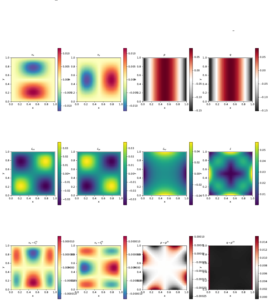
21 fieldstone f15: saddle point problem with Schur comple-
ment approach - benchmark
The details of the numerical setup are presented in Section ??. The main difference resides in the Schur
complement approach to solve the Stokes system, as presented in Section 6.15 (see solver cg). This
iterative solver is very easy to implement once the blocks Kand G, as well as the rhs vectors fand h
have been built.
Rather interestingly the pressure checkerboard modes are not nearly as present as in Section ?? which
uses a full matrix approach.
Looking at the discretisation errors for velocity and pressure, we of course recover the same rates and
values as in the full matrix case.
118
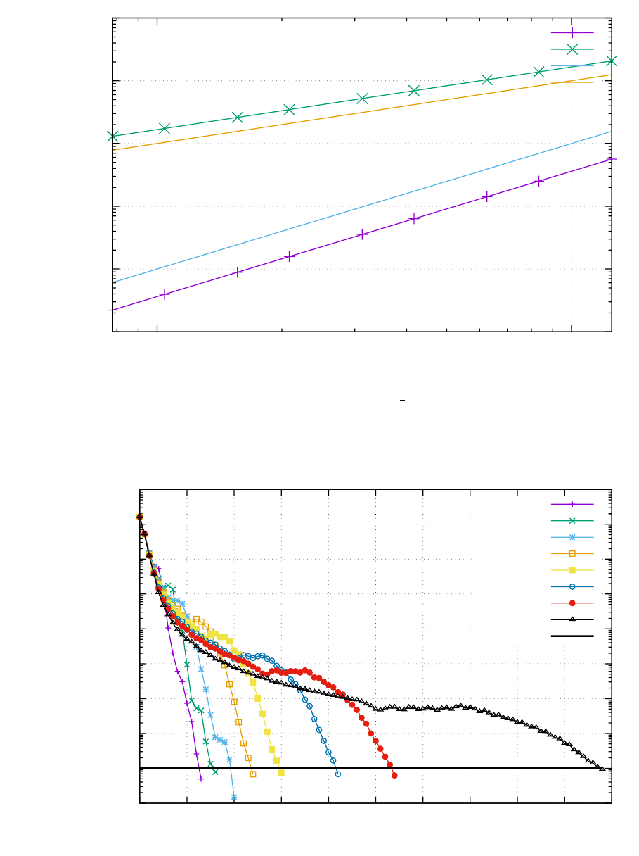
0.000001
0.000010
0.000100
0.001000
0.010000
0.100000
0.01 0.1
error
h
velocity
pressure
x2
x1
Finally, for each experiment the normalised residual (see solver cg) was recorded. We see that all
things equal the resolution has a strong influence on the number of iterations the solver must perform to
reach the required tolerance. This is one of the manifestations of the fact that the Q1×P0element is
not a stable element: the condition number of the matrix increases with resolution. We will see that this
is not the case of stable elements such as Q2×Q1.
0.000000001
0.000000010
0.000000100
0.000001000
0.000010000
0.000100000
0.001000000
0.010000000
0.100000000
1.000000000
0 10 20 30 40 50 60 70 80 90 100
normalised residual
# iteration
8x8
12x12
16x16
24x24
32x32
48x48
64x64
128x128
1e-8
119
features
•Q1×P0element
•incompressible flow
•mixed formulation
•Schur complement approach
•isothermal
•isoviscous
•analytical solution
build S and have python compute its smallest and largest eigenvalues as a function of resolution?
120
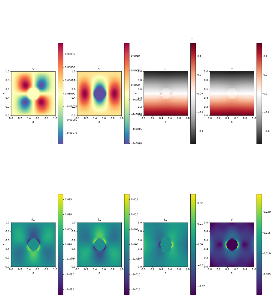
22 fieldstone f16: saddle point problem with Schur comple-
ment approach - Stokes sphere
We are revisiting the 2D Stokes sphere problem, but this time we use the Schur complement approach
to solve the Stokes system, Because there are viscosity contrasts in the domain, it is advisable to use the
Preconditioned Conjugate Gradient as presented in Section 6.15 (see solver pcg).
The normalised residual (see solver pcg) was recorded. We see that all things equal the resolution
has a strong influence on the number of iterations the solver must perform to reach the required tolerance.
However, we see that the use of the preconditioner can substantially reduce the number of iterations inside
the Stokes solver. At resolution 128x128, this number is halved.
121
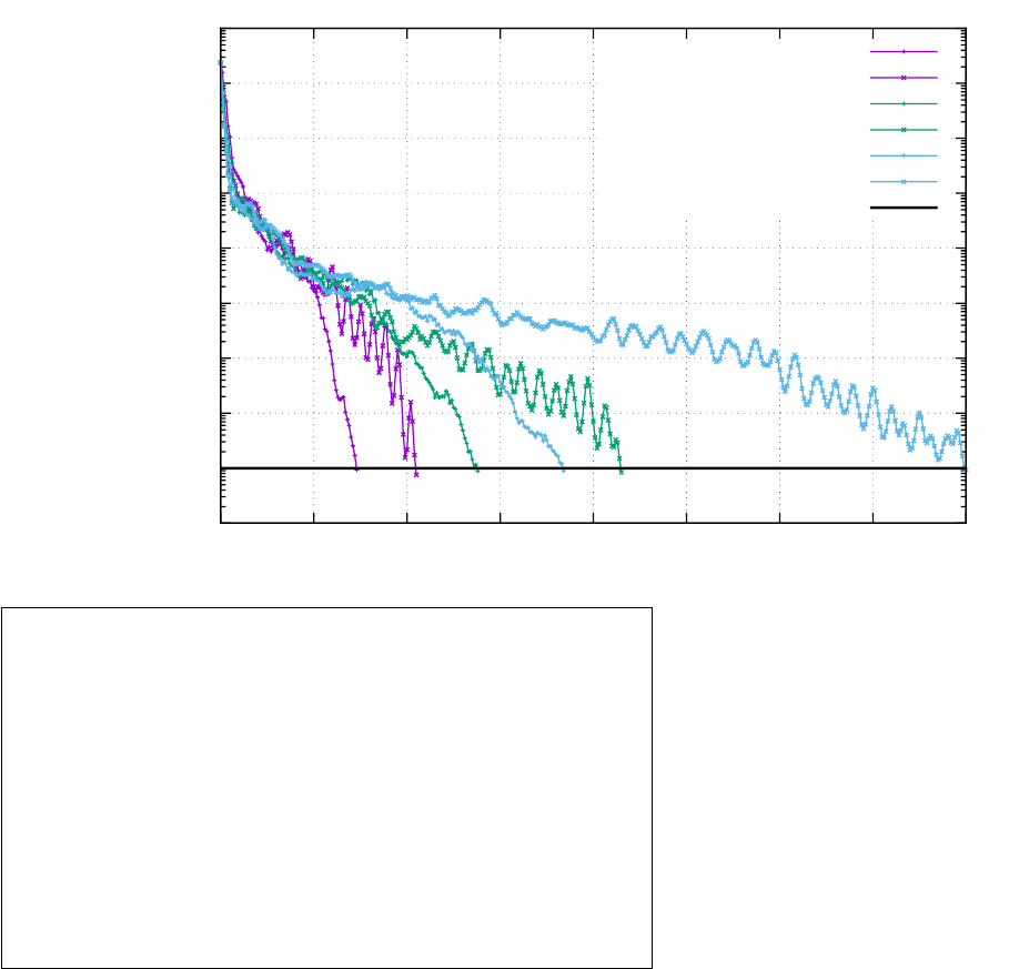
0.000000001
0.000000010
0.000000100
0.000001000
0.000010000
0.000100000
0.001000000
0.010000000
0.100000000
1.000000000
0 50 100 150 200 250 300 350 400
normalised residual
# iteration
32x32 (prec.)
32x32 (no prec.)
64x64 (prec.)
64x64 (no prec.)
128x128 (prec.)
128x128 (no prec.)
1e-8
features
•Q1×P0element
•incompressible flow
•mixed formulation
•Schur complement approach
•isothermal
•non-isoviscous
•Stokes sphere
122

23 fieldstone 17: solving the full saddle point problem in 3D
When using Q1×P0elements, this benchmark fails because of the Dirichlet b.c. on all 6 sides and all
three components. However, as we will see, it does work well with Q2×Q1elements. .
This benchmark begins by postulating a polynomial solution to the 3D Stokes equation [141]:
v=
x+x2+xy +x3y
y+xy +y2+x2y2
−2z−3xz −3yz −5x2yz
(229)
and
p=xyz +x3y3z−5/32 (230)
While it is then trivial to verify that this velocity field is divergence-free, the corresponding body force
of the Stokes equation can be computed by inserting this solution into the momentum equation with a
given viscosity µ(constant or position/velocity/strain rate dependent). The domain is a unit cube and
velocity boundary conditions simply use Eq. (229). Following [96], the viscosity is given by the smoothly
varying function
µ= exp(1 −β(x(1 −x) + y(1 −y) + z(1 −z))) (231)
One can easily show that the ratio of viscosities µ?in the system follows µ?= exp(−3β/4) so that
choosing β= 10 yields µ?'1808 and β= 20 yields µ?'3.269 ×10⁶.
We start from the momentum conservation equation:
−∇p+∇·(2µ˙
) = f
The x-component of this equation writes
fx=−∂p
∂x +∂
∂x (2µ˙xx) + ∂
∂y (2µ˙xy) + ∂
∂z (2µ˙xz) (232)
=−∂p
∂x + 2µ∂
∂x ˙xx + 2µ∂
∂y ˙xy + 2µ∂
∂z ˙xz + 2∂µ
∂x ˙xx + 2∂µ
∂y ˙xy + 2∂µ
∂z ˙xz (233)
Let us compute all the block separately:
˙xx = 1 + 2x+y+ 3x2y
˙yy = 1 + x+ 2y+ 2x2y
˙zz =−2−3x−3y−5x2y
2˙xy = (x+x3)+(y+ 2xy2) = x+y+ 2xy2+x3
2˙xz = (0) + (−3z−10xyz) = −3z−10xyz
2˙yz = (0) + (−3z−5x2z) = −3z−5x2z
123

In passing, one can verify that ˙xx + ˙yy + ˙zz = 0. We further have
∂
∂x 2 ˙xx = 2(2 + 6xy)
∂
∂y 2 ˙xy = 1 + 4xy
∂
∂z 2 ˙xz =−3−10xy
∂
∂x 2 ˙xy = 1 + 2y2+ 3x2
∂
∂y 2 ˙yy = 2(2 + 2x2)
∂
∂z 2 ˙yz =−3−5x2
∂
∂x 2 ˙xz =−10yz
∂
∂y 2 ˙yz = 0
∂
∂z 2 ˙zz = 2(0)
∂p
∂x =yz + 3x2y3z(234)
∂p
∂y =xz + 3x3y2z(235)
∂p
∂z =xy +x3y3(236)
Pressure normalisation Here again, because Dirichlet boundary conditions are prescribed on all
sides the pressure is known up to an arbitrary constant. This constant can be determined by (arbitrarily)
choosing to normalised the pressure field as follows:
ZΩ
p dΩ = 0 (237)
This is a single constraint associated to a single Lagrange multiplier λand the global Stokes system takes
the form
K G 0
GT0C
0CT0
V
P
λ
In this particular case the constraint matrix Cis a vector and it only acts on the pressure degrees of
freedom because of Eq.(237). Its exact expression is as follows:
ZΩ
p dΩ = X
eZΩe
p dΩ = X
eZΩeX
i
Np
ipidΩ = X
eX
iZΩe
Np
idΩpi=X
eCe·pe
where peis the list of pressure dofs of element e. The elemental constraint vector contains the correspond-
ing pressure basis functions integrated over the element. These elemental constraints are then assembled
into the vector C.
124
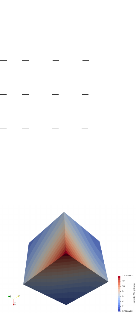
23.0.1 Constant viscosity
Choosing β= 0 yields a constant velocity µ(x, y, z) = exp(1) '2.718 (and greatly simplifies the right-
hand side) so that
∂
∂x µ(x, y, z) = 0 (238)
∂
∂y µ(x, y, z) = 0 (239)
∂
∂z µ(x, y, z) = 0 (240)
and
fx=−∂p
∂x + 2µ∂
∂x ˙xx + 2µ∂
∂y ˙xy + 2µ∂
∂z ˙xz
=−(yz + 3x2y3z) + 2(2 + 6xy) + (1 + 4xy)+(−3−10xy)
=−(yz + 3x2y3z) + µ(2 + 6xy)
fy=−∂p
∂y + 2µ∂
∂x ˙xy + 2µ∂
∂y ˙yy + 2µ∂
∂z ˙yz
=−(xz + 3x3y2z) + µ(1 + 2y2+ 3x2) + µ2(2 + 2x2) + µ(−3−5x2)
=−(xz + 3x3y2z) + µ(2 + 2x2+ 2y2)
fz=−∂p
∂z + 2µ∂
∂x ˙xz + 2µ∂
∂y ˙yz + 2µ∂
∂z ˙zz
=−(xy +x3y3) + µ(−10yz)+0+0
=−(xy +x3y3) + µ(−10yz)
Finally
f=−
yz + 3x2y3z
xz + 3x3y2z
xy +x3y3
+µ
2+6xy
2+2x2+ 2y2
−10yz
Note that there seems to be a sign problem with Eq.(26) in [96].
125
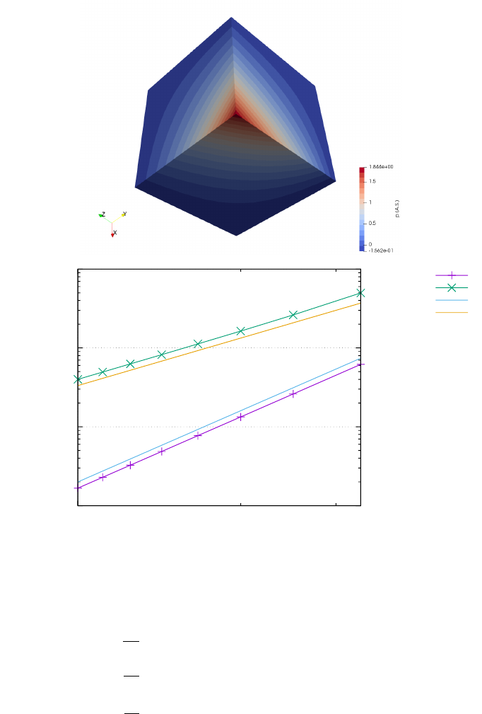
0.00001
0.00010
0.00100
0.01000
0.1
error
h
velocity
pressure
x3
x2
23.0.2 Variable viscosity
The spatial derivatives of the viscosity are then given by
∂
∂x µ(x, y, z) = −(1 −2x)βµ(x, y, z)
∂
∂y µ(x, y, z) = −(1 −2y)βµ(x, y, z)
∂
∂z µ(x, y, z) = −(1 −2z)βµ(x, y, z)
126

and thr right-hand side by
f=−
yz + 3x2y3z
xz + 3x3y2z
xy +x3y3
+µ
2+6xy
2+2x2+ 2y2
−10yz
(241)
−(1 −2x)βµ(x, y, z)
2˙xx
2˙xy
2˙xz
−(1 −2y)βµ(x, y, z)
2˙xy
2˙yy
2˙yz
−(1 −2z)βµ(x, y, z)
2˙xz
2˙yz
2˙zz
=−
yz + 3x2y3z
xz + 3x3y2z
xy +x3y3
+µ
2+6xy
2+2x2+ 2y2
−10yz
−(1 −2x)βµ
2+4x+ 2y+ 6x2y
x+y+ 2xy2+x3
−3z−10xyz
−(1 −2y)βµ
x+y+ 2xy2+x3
2+2x+ 4y+ 4x2y
−3z−5x2z
−(1 −2z)βµ
−3z−10xyz
−3z−5x2z
−4−6x−6y−10x2y
Note that at (x, y, z) = (0,0,0), µ= exp(1), and at (x, y, z) = (0.5,0.5,0.5), µ= exp(1 −3β/4) so
that the maximum viscosity ratio is given by
µ?=exp(1 −3β/4)
exp(1) = exp(−3β/4)
By varying βbetween 1 and 22 we can get up to 7 orders of magnitude viscosity difference.
features
•Q1×P0element
•incompressible flow
•saddle point system
•Dirichlet boundary conditions (free-slip)
•direct solver
•isothermal
•non-isoviscous
•3D
•elemental b.c.
•analytical solution
127
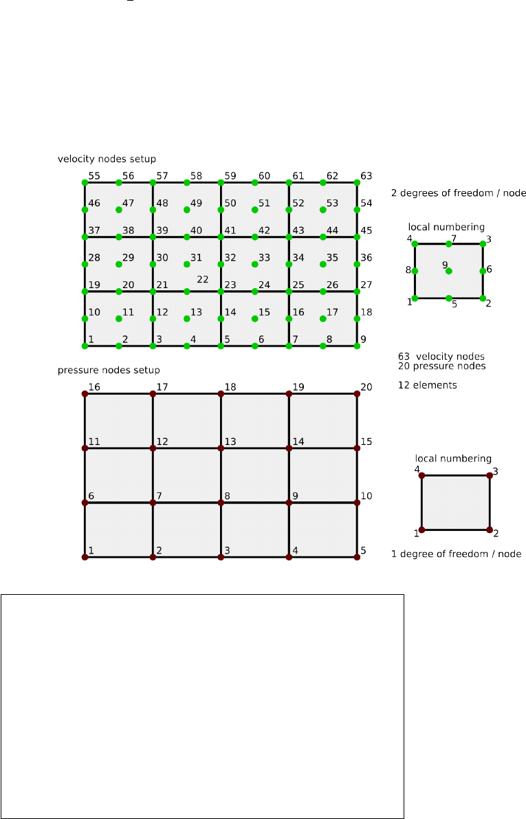
24 fieldstone 18: solving the full saddle point problem with
Q2×Q1elements
The details of the numerical setup are presented in Section ??.
Each element has mV= 9 vertices so in total ndofV×mV= 18 velocity dofs and ndofP∗mP= 4
pressure dofs. The total number of velocity dofs is therefore Nf emV =nnp ×ndofV while the total
number of pressure dofs is N femP =nel. The total number of dofs is then Nfem =N f emV +N femP .
As a consequence, matrix Khas size N femV, N femV and matrix Ghas size N femV, N femP . Vector
fis of size NfemV and vector his of size N femP .
renumber all nodes to start at zero!! Also internal numbering does not work here
features
•Q2×Q1element
•incompressible flow
•mixed formulation
•Dirichlet boundary conditions (no-slip)
•isothermal
•isoviscous
•analytical solution
128
0.0000001
0.0000010
0.0000100
0.0001000
0.0010000
0.0100000
0.1
error
h
velocity
pressure
x3
x2
129

25 fieldstone 19: solving the full saddle point problem with
Q3×Q2elements
The details of the numerical setup are presented in Section ??.
Each element has mV= 16 vertices so in total ndofV×mV= 32 velocity dofs and ndofP∗mP= 9
pressure dofs. The total number of velocity dofs is therefore Nf emV =nnp ×ndofV while the total
number of pressure dofs is N femP =nel. The total number of dofs is then Nfem =N f emV +N femP .
As a consequence, matrix Khas size N femV, N femV and matrix Ghas size N femV, N femP . Vector
fis of size NfemV and vector his of size N femP .
60===61===62===63===64===65===66===67===68===70
|| || || ||
50 51 52 53 54 55 56 57 58 59
|| || || ||
40 41 42 43 44 45 46 47 48 49
|| || || ||
30===31===32===33===34===35===36===37===38===39
|| || || ||
20 21 22 23 24 25 26 27 28 29
|| || || ||
10 11 12 13 14 15 16 17 18 19
|| || || ||
00===01===02===03===04===05===06===07===08===09
Example of 3x2 mesh. nnx=10, nny=7, nnp=70, nelx=3, nely=2, nel=6
12===13===14===15 06=====07=====08
|| || || || || || ||
08===09===10===11 || || ||
|| || || || 03=====04=====05
04===05===06===07 || || ||
|| || || || || || ||
00===01===02===03 00=====01=====02
Velocity (Q3) Pressure (Q2)
(r,s)_{00}=(-1,-1) (r,s)_{00}=(-1,-1)
(r,s)_{01}=(-1/3,-1) (r,s)_{01}=(0,-1)
(r,s)_{02}=(+1/3,-1) (r,s)_{02}=(+1,-1)
(r,s)_{03}=(+1,-1) (r,s)_{03}=(-1,0)
(r,s)_{04}=(-1,-1/3) (r,s)_{04}=(0,0)
(r,s)_{05}=(-1/3,-1/3) (r,s)_{05}=(+1,0)
(r,s)_{06}=(+1/3,-1/3) (r,s)_{06}=(-1,+1)
(r,s)_{07}=(+1,-1/3) (r,s)_{07}=(0,+1)
(r,s)_{08}=(-1,+1/3) (r,s)_{08}=(+1,+1)
(r,s)_{09}=(-1/3,+1/3)
(r,s)_{10}=(+1/3,+1/3)
(r,s)_{11}=(+1,+1/3)
(r,s)_{12}=(-1,+1)
(r,s)_{13}=(-1/3,+1)
(r,s)_{14}=(+1/3,+1)
(r,s)_{15}=(+1,+1)
Write about 4 point quadrature.
130
features
•Q3×Q2element
•incompressible flow
•mixed formulation
•isothermal
•isoviscous
•analytical solution
1x10⁻¹⁰
1x10⁻⁹
1x10⁻⁸
1x10⁻⁷
1x10⁻⁶
1x10⁻⁵
0.0001
0.1
error
h
velocity
pressure
x4
x3
velocity error rate is cubic, pressure superconvergent since the pressure field is quadratic and therefore
lies into the Q2 space.
131
26 fieldstone 20: the Busse benchmark
This three-dimensional benchmark was first proposed by [97]. It has been subsequently presented in
[438, 460, 6, 362, 136, 297]. We here focus on Case 1 of [97]: an isoviscous bimodal convection experiment
at Ra = 3 ×10⁵.
The domain is of size a×b×hwith a= 1.0079h,b= 0.6283hwith h= 2700km. It is filled
with a Newtonian fluid characterised by ρ0= 3300kg.m−3,α= 10−5K−1,µ= 8.0198 ×10²³Pa.s,
k= 3.564W.m−1.K−1,cp= 1080J.K−1.kg−1. The gravity vector is set to g= (0,0,−10)T. The
temperature is imposed at the bottom (T= 3700◦C) and at the top (T= 0◦C).
The various measurements presented in [97] are listed hereafter:
•The Nusselt number N u computed at the top surface following Eq. (206):
Nu =LzRRz=Lz
∂T
∂y dxdy
RRz=0 T dxdy
•the root mean square velocity vrms and the temperature mean square velocity Trms
•The vertical velocity wand temperature Tat points x1= (0,0, Lz/2), x2= (Lx,0, Lz/2), x3=
(0, Ly, Lz/2) and x4= (Lx, Ly, Lz/2);
•the vertical component of the heat flux Qat the top surface at all four corners.
The values plotted hereunder are adimensionalised by means of a reference temperature (3700K), a
reference lengthscale 2700km, and a reference time L2
z/κ.
0.0001
0.0002
0.0003
0.0004
0.0005
0.0006
0.0007
0.0008
0.0009
0 2x10⁸ 4x10⁸ 6x10⁸ 8x10⁸ 1x10⁹ 1.2x10⁹
1.4x10⁹
1.6x10⁹
vrms
time/year
2115
2116
2117
2118
2119
2120
2121
2122
2123
2124
0 2x10⁸ 4x10⁸ 6x10⁸ 8x10⁸ 1x10⁹ 1.2x10⁹
1.4x10⁹
1.6x10⁹
<T>
time/year
132

-0.002
-0.0015
-0.001
-0.0005
0
0.0005
0.001
0.0015
0.002
0 2x10⁸ 4x10⁸ 6x10⁸ 8x10⁸ 1x10⁹ 1.2x10⁹
1.4x10⁹
1.6x10⁹
w at Lz/2
time/year
-3.5
-3
-2.5
-2
-1.5
-1
-0.5
0
1x10⁸ 1.5x10⁸ 2x10⁸ 2.5x10⁸ 3x10⁸ 3.5x10⁸
heat flux
time/year
features
•Q1×P0element
•incompressible flow
•mixed formulation
•Dirichlet boundary conditions (free-slip)
•direct solver
•isothermal
•non-isoviscous
•3D
•elemental b.c.
•buoyancy driven
ToDo: look at energy conservation. run to steady state and make sure the expected values are
retrieved.
133

27 fieldstone 21: The non-conforming Q1×P0element
features
•Non-conforming Q1×P0element
•incompressible flow
•mixed formulation
•isothermal
•non-isoviscous
•analytical solution
•pressure smoothing
try Q1 mapping instead of isoparametric.
134
28 fieldstone 22: The stabilised Q1×Q1element
The details of the numerical setup are presented in Section ??.
We will here focus on the Q1×Q1element, which, unless stabilised, violates the LBB stability
condition and therefore is unusable. Stabilisation can be of two types: least-squares (see for example
[144]) [447, 285, ?], or by means of an additional term in the weak form as first introduced in [141, 56].
It is further analysed in [359, 310]. Note that an equal-order velocity-pressure formulation that does not
exhibit spurious pressure modes (without stabilisaion) has been presented in [400].
This element corresponds to Bilinear velocities, bilinear pressure (equal order interpolation for both
velocity and pressure) which is very convenient in terms of data structures since all dofs are colocated.
In geodynamics, it is used in the Rhea code [430, 96] and in Gale. It is also used in [307] in its
stabilised form, in conjunction with AMR.
The stabilisation term Centers the Stokes matrix in the (2,2) position:
K G
GTC·V
P=f
h
Let us take a simple example: a 3x2 element grid.
012
345
0123
4567
8 9 10 11
0,1 2,3 4,5 6,7
8,9 10,11 12,13 14,15
16,17 18,19 20,21 22,23
The Kmatrix is of size NfemV ×Nf emV with N femV =ndofV ×nnp = 2 ×12 = 24. The G
matrix is of size NfemV ×NfemP with N f emP =ndofP ×nnp = 1 ×12 = 12. The Cmatrix is of
size NfemP ×Nf emP .
A corner pdof sees 4 vdofs, a side pdof sees 12 vdofs and an inside pdof sees 18 vdofs, so that the
total number of nonzeros in Gcan be computed as follows:
NZG= 4
|{z}
corners
+ 2(nnx −2) ∗12
| {z }
2hor.sides
+ 2(nny −2) ∗12
| {z }
2vert.sides
+ (nnx −2)(nny −2) ∗18
| {z }
insidenodes
Concretely,
•pdof #0 sees vdofs 0,1,2,3,8,9,10,11
•pdof #1 sees vdofs 0,1,2,3,4,5,8,9,10,11,12,13
•pdof #5 sees vdofs 0,1,2,3,4,5,8,9,10,11,12,13,16,17,18,19,20,21
so that the GTmatrix non-zero structure then is as follows:
135
0
1
2
3
4
5
6
7
8
9
10
11
0 1 2 3 4 5 6 7 8 9 10 11 12 13 14 15 16 17 18 19 20 21 22 23
We will here use the formulation of [141], which is very appealing since it does not require any free
(user-chosen) parameter. Furthermore the matrix Cis rather simple to compute as we will see hereafter.
We also impose RpdV = 0 which means that the following constraint is added to the Stokes matrix:
K G 0
GTC L
0LT0
·
V
P
λ
=
f
h
0
28.1 The Donea & Huerta benchmark
As in [144] we solve the benchmark problem presented in section 6.7.1.
0.00001
0.00010
0.00100
0.01000
0.10000
0.1
error
h
velocity
pressure
x2
x1.5
28.2 The Dohrmann & Bochev benchmark
As in [141] we solve the benchmark problem presented in section 6.7.2.
136

29 fieldstone 23: compressible flow (1) - analytical benchmark
This work is part of the MSc thesis of T. Weir (2018).
We first start with an isothermal Stokes flow, so that we disregard the heat transport equation and
the equations we wish to solve are simply:
−∇ · 2η˙ε(v)−1
3(∇ · v)1+∇p=ρgin Ω,(242)
∇ · (ρv) = 0 in Ω (243)
The second equation can be rewritten ∇ · (ρv) = ρ∇ · v+v·∇ρ= 0 or,
∇ · v+1
ρv·∇ρ= 0
Note that this presupposes that the density is not zero anywhere in the domain.
We use a mixed formulation and therefore keep both velocity and pressure as unknowns. We end up
having to solve the following system:
K G
GT+Z0·V
P=f
hor,A·X=rhs
Where Kis the stiffness matrix, Gis the discrete gradient operator, GTis the discrete divergence operator,
Vthe velocity vector, Pthe pressure vector. Note that the term ZVderives from term v·∇ρin the
continuity equation.
Each block K,G,Zand vectors fand hare built separately in the code and assembled into the
matrix Aand vector rhs afterwards. Aand rhs are then passed to the solver. We will see later that
there are alternatives to solve this approach which do not require to build the full Stokes matrix A.
Remark: the term ZVis often put in the rhs (i.e. added to h) so that the matrix Aretains the same
structure as in the incompressible case. This is indeed how it is implemented in ASPECT. This however
requires more work since the rhs depends on the solution and some form of iterations is needed.
In the case of a compressible flow the strain rate tensor and the deviatoric strain rate tensor are no
more equal (since ∇·v6= 0). The deviatoric strainrate tensor is given by12
˙
d(v) = ˙
(v)−1
3T r(˙
)1=˙
(v)−1
3(∇·v)1
In that case:
˙d
xx =∂u
∂x −1
3∂u
∂x +∂v
∂y =2
3
∂u
∂x −1
3
∂v
∂y (244)
˙d
yy =∂v
∂y −1
3∂u
∂x +∂v
∂y =−1
3
∂u
∂x +2
3
∂v
∂y (245)
2˙d
xy =∂u
∂y +∂v
∂x (246)
and then
˙
d(v) =
2
3
∂u
∂x −1
3
∂v
∂y
1
2
∂u
∂y +1
2
∂v
∂x
1
2
∂u
∂y +1
2
∂v
∂x −1
3
∂u
∂x +2
3
∂v
∂y
From τ = 2ηdwe arrive at:
τxx
τyy
τxy
= 2η
˙d
xx
˙d
yy
˙d
xy
= 2η
2/3−1/3 0
−1/3 2/3 0
0 0 1/2
·
∂u
∂x
∂v
∂y
∂u
∂y +∂v
∂x
=η
4/3−2/3 0
−2/3 4/3 0
0 0 1
·
∂u
∂x
∂v
∂y
∂u
∂y +∂v
∂x
or,
τ =CηBV
12See the ASPECT manual for a justification of the 3 value in the denominator in 2D and 3D.
138

In order to test our implementation we have created a few manufactured solutions:
•benchmark #1 (ibench=1)): Starting from a density profile of:
ρ(x, y) = xy (247)
We derive a velocity given by:
vx(x, y) = Cx
x, vy(x, y) = Cy
y(248)
With gx(x, y) = 1
xand gy(x, y) = 1
y, this leads us to a pressure profile:
p=−η4Cx
3x2+4Cy
3y2+xy +C0(249)
This gives us a strain rate:
˙xx =−Cx
x2˙yy =−Cy
y2˙xy = 0
In what follows, we choose η= 1 and Cx=Cy= 1 and for a unit square domain [1 : 2] ×[1 : 2] we
compute C0so that the pressure is normalised to zero over the whole domain and obtain C0=−1.
•benchmark #2 (ibench=2): Starting from a density profile of:
ρ= cos(x) cos(y) (250)
We derive a velocity given by:
vx=Cx
cos(x), vy=Cy
cos(y)(251)
With gx=1
cos(y)and gy=1
cos(x), this leads us to a pressure profile:
p=η 4Cxsin(x)
3 cos2(x)+4Cysin(y)
3 cos2(y)!+ (sin(x) + sin(y)) + C0(252)
˙xx =Cx
sin(x)
cos2(x)˙yy =Cy
sin(y)
cos2(y)˙xy = 0
We choose η= 1 and Cx=Cy= 1. The domain is the unit square [0 : 1] ×[0 : 1] and we obtain C0
as before and obtain
C0= 2 −2 cos(1) + 8/3( 1
cos(1) −1) '3.18823730
(thank you WolframAlpha)
•benchmark #3 (ibench=3)
•benchmark #4 (ibench=4)
•benchmark #5 (ibench=5)
features
•Q1×P0element
•incompressible flow
•mixed formulation
•Dirichlet boundary conditions (no-slip)
•isothermal
•isoviscous
•analytical solution
•pressure smoothing
139
ToDo:
•pbs with odd vs even number of elements
•q is ’fine’ everywhere except in the corners - revisit pressure smoothing paper?
•redo A v d Berg benchmark (see Tom Weir thesis)
140

30 fieldstone 24: compressible flow (2) - convection box
This work is part of the MSc thesis of T. Weir (2018).
30.1 The physics
Let us start with some thermodynamics. Every material has an equation of state. The equilibrium
thermodynamic state of any material can be constrained if any two state variables are specified. Examples
of state variables include the pressure pand specific volume ν= 1/ρ, as well as the temperature T.
After linearisation, the density depends on temperature and pressure as follows:
ρ(T, p) = ρ0((1 −α(T−T0) + βTp)
where αis the coefficient of thermal expansion, also called thermal expansivity:
α=−1
ρ∂ρ
∂T p
αis the percentage increase in volume of a material per degree of temperature increase; the subscript p
means that the pressure is held fixed.
βTis the isothermal compressibility of the fluid, which is given by
βT=1
K=1
ρ∂ρ
∂P T
with Kthe bulk modulus. Values of βT= 10−12 −10−11 Pa−1are reasonable for Earth’s mantle, with
values decreasing by about a factor of 5 between the shallow lithosphere and core-mantle boundary. This
is the percentage increase in density per unit change in pressure at constant temperature. Both the
coefficient of thermal expansion and the isothermal compressibility can be obtained from the equation of
state.
The full set of equations we wish to solve is given by
−∇ · 2η˙
d(v)+∇p=ρ0((1 −α(T−T0) + βTp)gin Ω (253)
∇ · v+1
ρv·∇ρ= 0 in Ω (254)
ρCp∂T
∂t +v· ∇T−∇·k∇T=ρH + 2η˙
d:˙
d+αT ∂p
∂t +v· ∇pin Ω,(255)
Note that this presupposes that the density is not zero anywhere in the domain.
30.2 The numerics
We use a mixed formulation and therefore keep both velocity and pressure as unknowns. We end up
having to solve the following system:
K G +W
GT+Z0·V
P=f
hor,A·X=rhs
Where Kis the stiffness matrix, Gis the discrete gradient operator, GTis the discrete divergence operator,
Vthe velocity vector, Pthe pressure vector. Note that the term ZVderives from term v·∇ρin the
continuity equation.
As perfectly explained in the step 32 of deal.ii13, we need to scale the Gterm since it is many orders
of magnitude smaller than K, which introduces large inaccuracies in the solving process to the point that
the solution is nonsensical. This scaling coefficient is η/L. After building the Gblock, it is then scaled
as follows: G0=η
LGso that we now solve
13https://www.dealii.org/9.0.0/doxygen/deal.II/step 32.html
141

K G0+W
G0T+Z0·V
P0=f
h
After the solve phase, we recover the real pressure with P=η
LP0.
adapt notes since I should scale Wand Ztoo.hshould be caled too !!!!!!!!!!!!!!!
Each block K,G,Zand vectors fand hare built separately in the code and assembled into the
matrix Aand vector rhs afterwards. Aand rhs are then passed to the solver. We will see later that
there are alternatives to solve this approach which do not require to build the full Stokes matrix A.
Remark 1: the terms ZVand WPare often put in the rhs (i.e. added to h) so that the matrix
Aretains the same structure as in the incompressible case. This is indeed how it is implemented in
ASPECT, see also appendix A of [306]. This however requires more work since the rhs depends on the
solution and some form of iterations is needed.
Remark 2: Very often the adiabatic heating term αT (v· ∇p) is simplified as follows: If you assume
the vertical component of the gradient of the dynamic pressure to be small compared to the gradient of
the total pressure (in other words, the gradient is dominated by the gradient of the hydrostatic pressure),
then −ρg'∇pand then αT (v· ∇p)' −αρT v·g. We will however not be using this approximation in
what follows.
We have already established that
τ =CηBV
The following measurements are carried out:
•The root mean square velocity (vrms):
vrms =s1
VZV
v2dV
•The average temperature (Tavrg):
< T >=1
VZV
T dV
•The total mass (mass):
M=ZV
ρdV
•The Nusselt number (Nu):
Nu =−1
Lx
1
∆TZLx
0
∂T (x, y =Ly)
∂y dx
•The kinetic energy (EK):
EK=ZV
1
2ρv2dV
•The work done against gravity
< W >=−ZV
ρgyvydV
•The total viscous dissipation (visc diss)
<Φ>=ZΦdV =1
VZ2η˙
ε:˙
εdV
•The gravitational potential energy (EG)
EG=ZV
ρgy(Ly−y)dV
142

•The internal thermal energy (ET)
ET=ZV
ρ(0)CpT dV
Remark 3: Measuring the total mass can be misleading: indeed because ρ=ρ0(1 −αT ), then
measuring the total mass amounts to measuring a constant minus the volume-integrated tempera-
ture, and there is no reason why the latter should be zero, so that there is no reason why the total
mass should be zero...!
30.3 The experimental setup
The setup is as follows: the domain is Lx =Ly = 3000km. Free slip boundary conditions are imposed
on all four sides. The initial temperature is given by:
T(x, y) = Ly−y
Ly −0.01 cos(πx
Lx
) sin( πy
Ly )∆T+Tsurf
with ∆T= 4000K, Tsurf =T0= 273.15K. The temperature is set to ∆T+Tsurf at the bottom and
Tsurf at the top. We also set k= 3, Cp= 1250, |g|= 10, ρ0= 3000 and we keep the Rayleigh number
Ra and dissipation number Di as input parameters:
Ra =αg∆T L3ρ2
0Cp
ηk Di =αgL
Cp
From the second equation we get α=DiCp
gL , which we can insert in the first one:
Ra =DiC2
p∆T L2ρ2
0
ηk or, η =DiC2
p∆T L2ρ2
0
Ra k
For instance, for Ra = 104and Di = 0.75, we obtain α'3·10−5and η'1025 which are quite reasonable
values.
30.4 Scaling
Following [286], we non-dimensionalize the equations using the reference values for density ρr, thermal
expansivity αr, temperature contrast ∆Tr(refTemp), thermal conductivity kr, heat capacity Cp, depth
of the fluid layer Land viscosity ηr. The non-dimensionalization for velocity, ur, pressure prand time,
trbecome
ur=kr
ρrCpL(refvel)
pr=ηrkr
ρrCpL2(refpress)
tr=ρrCpL2
kr
(reftime)
In the case of the setup described hereabove, and when choosing Ra = 104and Di = 0.5, we get:
alphaT 2.083333e-05
eta 8.437500e+24
reftime 1.125000e+19
refvel 2.666667e-13
refPress 7.500000e+05
143

30.5 Conservation of energy 1
30.5.1 under BA and EBA approximations
Following [306], we take the dot product of the momentum equation with the velocity vand integrate
over the whole volume14:ZV
[−∇ · τ+∇p]·vdV =ZV
ρg·vdV
or,
−ZV
(∇ · τ)·vdV +ZV
∇p·vdV =ZV
ρg·vdV
Let us look at each block separately:
−ZV
(∇ · τ)·vdV =−ZS
τ v ·n
|{z}
=0 (b.c.)
dS +ZV
τ:∇vdV =ZV
τ:˙
εdV =ZV
ΦdV
which is the volume integral of the shear heating. Then,
ZV
∇p·vdV =ZS
pv·n
|{z}
=0 (b.c.)
dS −ZV
∇·v
|{z}
=0 (incomp.)
pdV = 0
which is then zero in the case of an incompressible flow. And finally
ZV
ρg·vdV =W
which is the work against gravity.
Conclusion for an incompressible fluid: we should have
ZV
ΦdV =ZV
ρg·vdV (256)
This formula is hugely problematic: indeed, the term ρin the rhs is the full density. We know that to the
value of ρ0corresponds a lithostatic pressure gradient pL=ρ0gy. In this case one can write ρ=ρ0+ρ0
and p=pL+p0so that we also have
ZV
[−∇ · τ+∇p0]·vdV =ZV
ρ0g·vdV
which will ultimately yield
ZV
ΦdV =ZV
ρ0g·vdV =ZV
(ρ−ρ0)g·vdV (257)
Obviously Eqs.(256) and (257) cannot be true at the same time. The problem comes from the nature
of the (E)BA approximation: ρ=ρ0in the mass conservation equation but it is not constant in the
momentum conservation equation, which is of course inconsistent. Since the mass conservation equation
is ∇·v= 0 under this approximation then the term RV∇p·vdV is always zero for any pressure (full
pressure p, or overpressure p−pL), hence the paradox. This paradox will be lifted when a consistent set
of equations will be used (compressible formulation). On a practical note, Eqs.(256) is not verified by
the code, while (257) is.
In the end: ZV
ΦdV
| {z }
visc diss
=ZV
(ρ−ρ0)g·vdV
| {z }
work grav
(258)
14Check: this is akin to looking at the power, force*velocity, says Arie
144

30.5.2 under no approximation at all
ZV
∇p·vdV =ZS
pv·n
|{z}
=0 (b.c.)
dS −ZV
∇·vpdV = 0 (259)
=ZV
1
ρv·∇ρ pdV = 0 (260)
(261)
ToDo:see section 3 of [306] where this is carried out with the Adams-Williamson eos.
30.6 Conservation of energy 2
Also, following the Reynold’s transport theorem [331],p210, we have for a property A(per unit mass)
d
dt ZV
AρdV =ZV
∂
∂t (Aρ)dV +ZS
Aρv·ndS
Let us apply to this to A=CpTand compute the time derivative of the internal energy:
d
dt ZV
ρCpT dV =ZV
∂
∂t (ρCpT)dV +ZS
Aρ v·n
|{z}
=0 (b.c.)
dS =ZV
CpT∂ρ
∂t dV
| {z }
I
+ZV
ρCp
∂T
∂t dV
| {z }
II
(262)
In order to expand I, the mass conservation equation will be used, while the heat transport equation
will be used for II:
I=ZV
CpT∂ρ
∂t dV =−ZV
CpT∇·(ρv)dV =−ZV
CpT ρ v·n
|{z}
=0 (b.c.)
dS +ZV
ρCp∇T·vdV (263)
II =ZV
ρCp
∂T
∂t dV =ZV−ρCpv·∇T+∇·k∇T+ρH +Φ+αT ∂p
∂t +v·∇pdV (264)
=ZV−ρCpv·∇T+ρH +Φ+αT ∂p
∂t +v·∇pdV +ZV
∇·k∇T dV(265)
=ZV−ρCpv·∇T+ρH +Φ+αT ∂p
∂t +v·∇pdV +ZS
k∇T·ndS(266)
=ZV−ρCpv·∇T+ρH +Φ+αT ∂p
∂t +v·∇pdV −ZS
q·ndS (267)
Finally:
I+II =d
dt ZV
ρCpT dV
| {z }
ET
=ZVρH +Φ+αT ∂p
∂t +v·∇pdV −ZS
q·ndS (268)
=ZV
ρHdV +ZV
ΦdV
| {z }
visc diss
+ZV
αT ∂p
∂t dV
| {z }
extra
+ZV
αT v·∇pdV
| {z }
adiab heating
−ZS
q·ndS
| {z }
heatflux boundary
(269)
This was of course needlessly complicated as the term ∂ρ/∂t is always taken to be zero, so that I= 0
automatically. The mass conservation equation is then simply ∇·(ρv) = 0. Then it follows that
0 = ZV
CpT∇·(ρv)dV =−ZV
CpT ρ v·n
|{z}
=0 (b.c.)
dS +ZV
ρCp∇T·vdV (270)
=ZV
ρCp∇T·vdV (271)
so that the same term in Eq.(267) vanishes too, and then Eq.(269) is always valid, although one should
be careful when computing ETin the BA and EBA cases as it should use ρ0and not ρ.
145

30.7 The problem of the onset of convection
[wiki] In geophysics, the Rayleigh number is of fundamental importance: it indicates the presence and
strength of convection within a fluid body such as the Earth’s mantle. The mantle is a solid that behaves
as a fluid over geological time scales.
The Rayleigh number essentially is an indicator of the type of heat transport mechanism. At low
Rayleigh numbers conduction processes dominate over convection ones. At high Rayleigh numbers it is
the other way around. There is a so-called critical value of the number with delineates the transition
from one regime to the other.
This problem has been studied and approached both theoretically and numerically [461, e.g.] and it
was found that the critical Rayleigh number Racis
Rac= (27/4)π4'657.5
in setups similar to ours.
VERY BIG PROBLEM
The temperature setup is built as follows: Tsurf is prescribed at the top, Tsurf + ∆Tis prescribed
at the bottom. The initial temperature profile is linear between these two values. In the case of BA, the
actual value of Tsurf is of no consequence. However, for the EBA the full temperature is present in the
adiabatic heating term on the rhs of the hte, and the value of Tsurf will therefore influence the solution
greatly. This is very problematic as there is no real way to arrive at the surface temperature from the
King paper. On top of this, the density uses a reference temperature T0which too will influence the
solution without being present in the controlling Ra and Di numbers!!
In light thereof, it will be very difficult to recover the values of King et al for EBA!
features
•Q1×P0element
•compressible flow
•mixed formulation
•Dirichlet boundary conditions (no-slip)
•isoviscous
•analytical solution
•pressure smoothing
Relevant literature: [44, 269, 441, 306, 286, 307, 321, 253]
ToDo:
•heat flux is at the moment elemental, so Nusselt and heat flux on boundaries measurements not as
accurate as could be.
146
30.8 results - BA - Ra = 104
These results were obtained with a 64x64 resolution, and CFL number of 1. Steady state was reached
after about 1250 timesteps.
(a)
0
1x10⁻⁶
2x10⁻⁶
3x10⁻⁶
4x10⁻⁶
5x10⁻⁶
6x10⁻⁶
7x10⁻⁶
0 10000 20000 30000 40000 50000 60000 70000 80000 90000 100000
EK
time (Myr)
(b)
7.67188x10²²
7.67188x10²²
7.67188x10²²
7.67188x10²²
7.67188x10²²
7.67188x10²²
7.67188x10²²
7.67188x10²²
7.67188x10²²
0 10000 20000 30000 40000 50000 60000 70000 80000 90000 100000
ET
time (Myr)
(c)
-7.73687x10²³
-7.73687x10²³
-7.73687x10²³
-7.73687x10²³
-7.73687x10²³
-7.73687x10²³
-7.73687x10²³
-7.73687x10²³
-7.73687x10²³
-7.73687x10²³
-7.73687x10²³
0 10000 20000 30000 40000 50000 60000 70000 80000 90000 100000
EG
time (Myr)
(d)
2273.15
2273.15
2273.15
2273.15
2273.15
2273.15
2273.15
0 10000 20000 30000 40000 50000 60000 70000 80000 90000 100000
<T>
time (Myr)
(e)
0
500
1000
1500
2000
2500
3000
3500
4000
4500
0 10000 20000 30000 40000 50000 60000 70000 80000 90000 100000
Temperature
time (Myr)
min(T)
max(T)
(f)
-0.0015
-0.001
-0.0005
0
0.0005
0.001
0.0015
0 10000 20000 30000 40000 50000 60000 70000 80000 90000 100000
velocity
time (Myr)
min(u)
max(u)
min(v)
max(v)
(g)
-80000
-70000
-60000
-50000
-40000
-30000
-20000
-10000
0
0 10000 20000 30000 40000 50000 60000 70000 80000 90000 100000
adiabatic heating
time (Myr)
(h)
0
10000
20000
30000
40000
50000
60000
70000
80000
90000
0 10000 20000 30000 40000 50000 60000 70000 80000 90000 100000
viscous dissipation
time (Myr)
(i)
0
10000
20000
30000
40000
50000
60000
70000
80000
90000
0 10000 20000 30000 40000 50000 60000 70000 80000 90000 100000
work against gravity
time (Myr)
(j)
-5x10⁻⁸
-4x10⁻⁸
-3x10⁻⁸
-2x10⁻⁸
-1x10⁻⁸
0
1x10⁻⁸
2x10⁻⁸
3x10⁻⁸
0 10000 20000 30000 40000 50000 60000 70000 80000 90000 100000
heat flux
time (Myr)
(k)
0
0.01
0.02
0.03
0.04
0.05
0.06
0.07
0 10000 20000 30000 40000 50000 60000 70000 80000 90000 100000
vrms (cm/yr)
time (Myr)
(l)
0
1
2
3
4
5
6
7
8
0 10000 20000 30000 40000 50000 60000 70000 80000 90000 100000
Nu
time (Myr)
4.88
(l)
-6x10⁻⁷
-4x10⁻⁷
-2x10⁻⁷
0
2x10⁻⁷
4x10⁻⁷
6x10⁻⁷
8x10⁻⁷
0 1x10¹⁰
2x10¹⁰
3x10¹⁰
4x10¹⁰
5x10¹⁰
6x10¹⁰
7x10¹⁰
8x10¹⁰
9x10¹⁰
1x10¹¹
time (Myr)
0
HF
dETdt
(m)
0
10000
20000
30000
40000
50000
60000
70000
80000
90000
0 1x10¹⁰
2x10¹⁰
3x10¹⁰
4x10¹⁰
5x10¹⁰
6x10¹⁰
7x10¹⁰
8x10¹⁰
9x10¹⁰
1x10¹¹
time (Myr)
VD
WG
AH: adiabatic heating, VD: viscous dissipation, HF: heat flux, WG: work against gravity
Eq.(269) is verified by (l) and Eq.(258) is verified by (m).
148
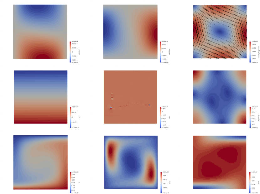
(a) (b) (c)
(d) (e) (f)
(g) (h) (i)
149
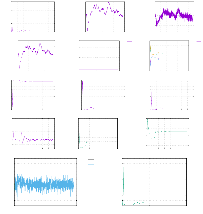
30.9 results - BA - Ra = 105
These results were obtained with a 64x64 resolution, and CFL number of 1. Steady state was reached
after about 1250 timesteps.
(a)
0
0.0001
0.0002
0.0003
0.0004
0.0005
0.0006
0.0007
0 5000 10000 15000 20000 25000 30000 35000
EK
time (Myr)
(b)
7.67188x10²²
7.67188x10²²
7.67188x10²²
7.67188x10²²
7.67188x10²²
7.67188x10²²
7.67188x10²²
0 5000 10000 15000 20000 25000 30000 35000
ET
time (Myr)
(c)
-7.73687x10²³
-7.73687x10²³
-7.73687x10²³
-7.73687x10²³
-7.73687x10²³
-7.73687x10²³
-7.73687x10²³
-7.73687x10²³
-7.73687x10²³
-7.73687x10²³
0 5000 10000 15000 20000 25000 30000 35000
EG
time (Myr)
(d)
2273.149999999
2273.149999999
2273.149999999
2273.150000000
2273.150000000
2273.150000000
2273.150000000
2273.150000000
2273.150000001
2273.150000001
2273.150000001
0 5000 10000 15000 20000 25000 30000 35000
<T>
time (Myr)
(e)
0
500
1000
1500
2000
2500
3000
3500
4000
4500
0 5000 10000 15000 20000 25000 30000 35000
Temperature
time (Myr)
min(T)
max(T)
(f)
-0.015
-0.01
-0.005
0
0.005
0.01
0.015
0 5000 10000 15000 20000 25000 30000 35000
velocity
time (Myr)
min(u)
max(u)
min(v)
max(v)
(g)
-900000
-800000
-700000
-600000
-500000
-400000
-300000
-200000
-100000
0
0 5000 10000 15000 20000 25000 30000 35000
adiabatic heating
time (Myr)
(h)
0
100000
200000
300000
400000
500000
600000
700000
800000
900000
0 5000 10000 15000 20000 25000 30000 35000
viscous dissipation
time (Myr)
(i)
0
100000
200000
300000
400000
500000
600000
700000
800000
900000
0 5000 10000 15000 20000 25000 30000 35000
work against gravity
time (Myr)
(j)
-1x10⁻⁶
-5x10⁻⁷
0
5x10⁻⁷
1x10⁻⁶
1.5x10⁻⁶
2x10⁻⁶
2.5x10⁻⁶
0 5000 10000 15000 20000 25000 30000 35000
heat flux
time (Myr)
(k)
0
0.1
0.2
0.3
0.4
0.5
0.6
0.7
0.8
0 5000 10000 15000 20000 25000 30000 35000
vrms (cm/yr)
time (Myr)
193.2150
(l)
0
2
4
6
8
10
12
14
16
18
0 5000 10000 15000 20000 25000 30000 35000
Nu
time (Myr)
10.53
(l)
-8x10⁻⁶
-6x10⁻⁶
-4x10⁻⁶
-2x10⁻⁶
0
2x10⁻⁶
4x10⁻⁶
6x10⁻⁶
8x10⁻⁶
1x10⁻⁵
0 5x10⁹ 1x10¹⁰
1.5x10¹⁰
2x10¹⁰
2.5x10¹⁰
3x10¹⁰
3.5x10¹⁰
time (Myr)
0
HF
dETdt
(m)
0
100000
200000
300000
400000
500000
600000
700000
800000
900000
0 5x10⁹ 1x10¹⁰ 1.5x10¹⁰ 2x10¹⁰ 2.5x10¹⁰ 3x10¹⁰ 3.5x10¹⁰
time (Myr)
VD
WG
AH: adiabatic heating, VD: viscous dissipation, HF: heat flux, WG: work against gravity
Eq.(269) is verified by (l) and Eq.(258) is verified by (m).
150
30.10 results - BA - Ra = 106
151
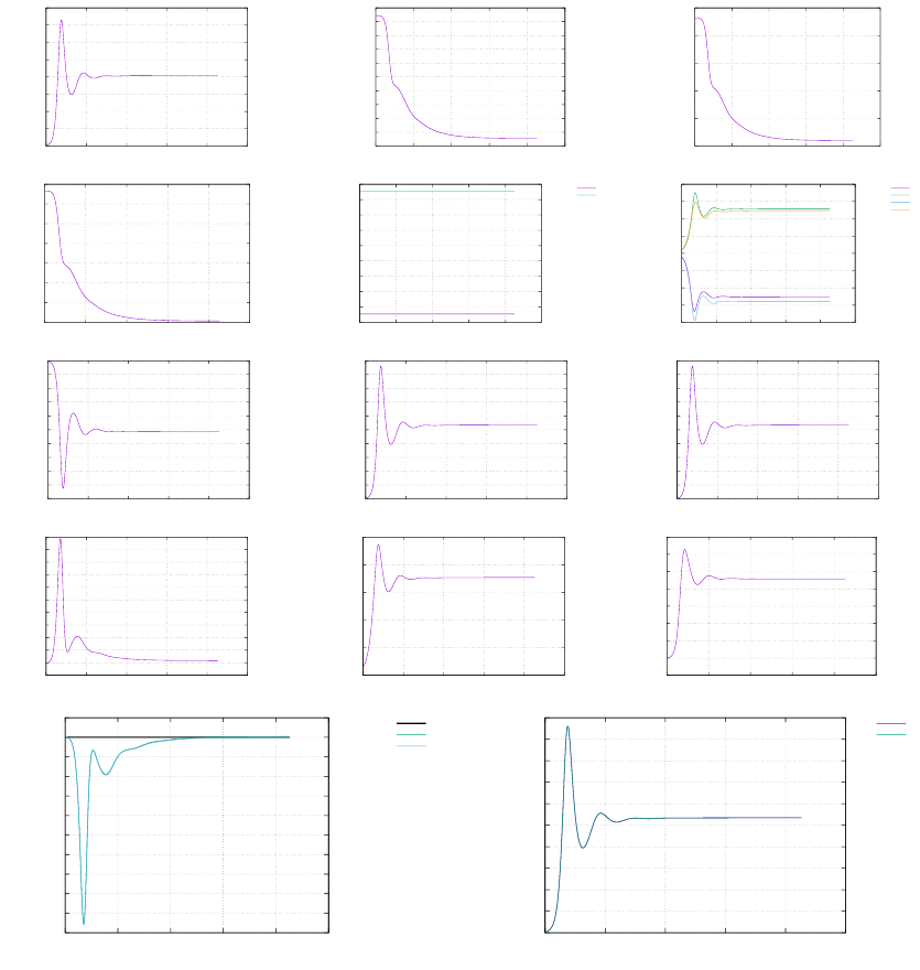
30.11 results - EBA - Ra = 104
These results were obtained with a 64x64 resolution, and CFL number of 1. Steady state was reached
after about 2500 timesteps
(a)
0
1x10⁻⁷
2x10⁻⁷
3x10⁻⁷
4x10⁻⁷
5x10⁻⁷
6x10⁻⁷
7x10⁻⁷
8x10⁻⁷
0 50000 100000 150000 200000 250000
EK
time (Myr)
(b)
7.2x10²²
7.25x10²²
7.3x10²²
7.35x10²²
7.4x10²²
7.45x10²²
7.5x10²²
7.55x10²²
7.6x10²²
7.65x10²²
7.7x10²²
0 50000 100000 150000 200000 250000
ET
time (Myr)
(c)
-7.76x10²³
-7.755x10²³
-7.75x10²³
-7.745x10²³
-7.74x10²³
-7.735x10²³
0 50000 100000 150000 200000 250000
EG
time (Myr)
(d)
2140
2160
2180
2200
2220
2240
2260
2280
0 50000 100000 150000 200000 250000
<T>
time (Myr)
(e)
0
500
1000
1500
2000
2500
3000
3500
4000
4500
0 50000 100000 150000 200000 250000
Temperature
time (Myr)
min(T)
max(T)
(f)
-0.0004
-0.0003
-0.0002
-0.0001
0
0.0001
0.0002
0.0003
0.0004
0 50000 100000 150000 200000 250000
velocity
time (Myr)
min(u)
max(u)
min(v)
max(v)
(g)
-10000
-9000
-8000
-7000
-6000
-5000
-4000
-3000
-2000
-1000
0
0 50000 100000 150000 200000 250000
adiabatic heating
time (Myr)
(h)
0
1000
2000
3000
4000
5000
6000
7000
8000
9000
10000
0 50000 100000 150000 200000 250000
viscous dissipation
time (Myr)
(i)
0
1000
2000
3000
4000
5000
6000
7000
8000
9000
10000
0 50000 100000 150000 200000 250000
work against gravity
time (Myr)
(j)
-1000
0
1000
2000
3000
4000
5000
6000
7000
8000
9000
10000
0 50000 100000 150000 200000 250000
heat flux
time (Myr)
(k)
0
0.005
0.01
0.015
0.02
0.025
0 50000 100000 150000 200000 250000
vrms (cm/yr)
time (Myr)
(l)
0.8
1
1.2
1.4
1.6
1.8
2
2.2
2.4
0 50000 100000 150000 200000 250000
Nu
time (Myr)
(l)
-10000
-9000
-8000
-7000
-6000
-5000
-4000
-3000
-2000
-1000
0
1000
0 50000 100000 150000 200000 250000
time (Myr)
0
AH+VD+HF
dETdt
(m)
0
1000
2000
3000
4000
5000
6000
7000
8000
9000
10000
0 50000 100000 150000 200000 250000
time (Myr)
VD
WG
AH: adiabatic heating, VD: viscous dissipation, HF: heat flux, WG: work against gravity
Eq.(269) is verified by (l) and Eq.(258) is verified by (m).
152
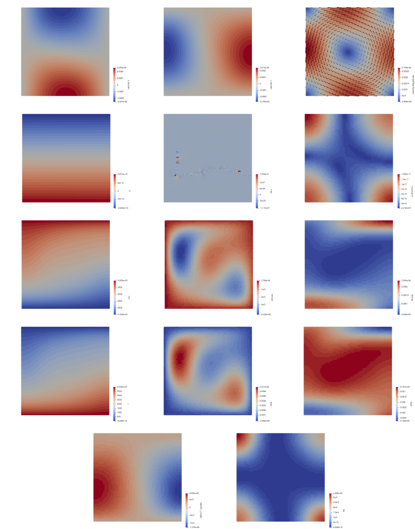
a) b) c)
d) e) f)
g) h) i)
j) k) l)
m) n)
153
30.12 results - EBA - Ra = 105
These results were obtained with a 64x64 resolution, and CFL number of 1. Simulation was stopped after
about 4300 timesteps.
(a)
0
1x10⁻⁵
2x10⁻⁵
3x10⁻⁵
4x10⁻⁵
5x10⁻⁵
6x10⁻⁵
7x10⁻⁵
8x10⁻⁵
9x10⁻⁵
0 20000 40000 60000 80000 100000 120000
EK
time (Myr)
(b)
7.4x10²²
7.45x10²²
7.5x10²²
7.55x10²²
7.6x10²²
7.65x10²²
7.7x10²²
0 20000 40000 60000 80000 100000 120000
ET
time (Myr)
(c)
-7.75x10²³
-7.748x10²³
-7.746x10²³
-7.744x10²³
-7.742x10²³
-7.74x10²³
-7.738x10²³
-7.736x10²³
0 20000 40000 60000 80000 100000 120000
EG
time (Myr)
(d)
2200
2210
2220
2230
2240
2250
2260
2270
2280
0 20000 40000 60000 80000 100000 120000
<T>
time (Myr)
(e)
0
500
1000
1500
2000
2500
3000
3500
4000
4500
5000
0 20000 40000 60000 80000 100000 120000
Temperature
time (Myr)
min(T)
max(T)
(f)
-0.005
-0.004
-0.003
-0.002
-0.001
0
0.001
0.002
0.003
0.004
0.005
0 20000 40000 60000 80000 100000 120000
velocity
time (Myr)
min(u)
max(u)
min(v)
max(v)
(g)
-120000
-100000
-80000
-60000
-40000
-20000
0
0 20000 40000 60000 80000 100000 120000
adiabatic heating
time (Myr)
(h)
0
20000
40000
60000
80000
100000
120000
0 20000 40000 60000 80000 100000 120000
viscous dissipation
time (Myr)
(i)
0
20000
40000
60000
80000
100000
120000
0 20000 40000 60000 80000 100000 120000
work against gravity
time (Myr)
(j)
-20000
-10000
0
10000
20000
30000
40000
50000
60000
70000
0 20000 40000 60000 80000 100000 120000
heat flux
time (Myr)
(k)
0
0.05
0.1
0.15
0.2
0.25
0.3
0 20000 40000 60000 80000 100000 120000
vrms (cm/yr)
time (Myr)
(l)
0.5
1
1.5
2
2.5
3
3.5
4
4.5
5
5.5
6
0 20000 40000 60000 80000 100000 120000
Nu
time (Myr)
(l)
-60000
-50000
-40000
-30000
-20000
-10000
0
10000
20000
0 20000 40000 60000 80000 100000 120000
time (Myr)
0
AH+VD+HF
dETdt
(m)
0
20000
40000
60000
80000
100000
120000
0 20000 40000 60000 80000 100000 120000
time (Myr)
VD
WG
AH: adiabatic heating, VD: viscous dissipation, HF: heat flux, WG: work against gravity
154
30.13 Onset of convection
The code can be run for values of Ra between 500 and 1000, at various resolutions for the BA formulation.
The value vrms(t)−vrms(0) is plotted as a function of Ra and for the 10 first timesteps. If the vrms is
found to decrease, then the Rayleigh number is not high enough to allow for convection and the initial
temperature perturbation relaxes by diffusion (and then vrms(t)−vrms(0) <0. If the vrms is found to
increase, then vrms(t)−vrms(0) >0 and the system is going to showcase convection. The zero value of
vrms(t)−vrms(0) gives us the critical Rayleigh number, which is found between 775 and 790.
-4x10-15
-2x10-15
0
2x10-15
4x10-15
6x10-15
8x10-15
1000
vrms trend
Ra
16x16
32x32
48x48
64x64
-3.5x10⁻¹⁶
-3x10-16
-2.5x10⁻¹⁶
-2x10-16
-1.5x10⁻¹⁶
-1x10-16
-5x10-17
0
5x10-17
1x10-16
1.5x10⁻¹⁶
770 775 780 785 790
vrms trend
Ra
16x16
32x32
48x48
64x64
155
Appendix: Looking for the right combination of parameters for the King benchmark.
I run a quadruple do loop over L, ∆T,ρ0and η0between plausible values (see code targets.py) and
write in a file only the combination which yields the required Rayleigh and Dissipation number values
(down to 1% accuracy).
alp ha=3e−5
g=10
hcapa =1250
hcond=3
DTmin=1000 ; DTmax=4000 ; DTnpts=251
Lmin=1e6 ; Lmax=3e6 ; Lnpts=251
rhomin =3000 ; rhomax=3500 ; rh on pt s=41
etam in =19 ; etamax=25 ; e t a n p t s =100
On the following plots the ’winning’ combinations of these four parameters are shown:
0.24
0.245
0.25
0.255
0.26
9600 9800 10000 10200 10400
Di
Ra
1x10⁶
1.005x10⁶
1.01x10⁶
1.015x10⁶
1.02x10⁶
1.025x10⁶
1.03x10⁶
1.035x10⁶
1.04x10⁶
1.045x10⁶
1.05x10⁶
500 1000 1500 2000 2500 3000 3500 4000 4500
L
DT
1x10²³
2x10²³
3x10²³
4x10²³
5x10²³
6x10²³
7x10²³
8x10²³
9x10²³
2800 3000 3200 3400 3600 3800 4000 4200
eta
rho
We see that:
•the parameter L(being to the 3rd power in the Ra number) cannot vary too much. Although it is
varied between 1000 and 3000km there seems to be a ’right’ value at about 1040 km. (why?)
•viscosities are within 1023 and 1024 which are plausible values (although a bit high?).
•densities can be chosen freely between 3000 and 3500
•∆Tseems to be the most problematic value since it can range from 1000 to 4000K ...
156
31 fieldstone 25: Rayleigh-Taylor instability (1) - instantaneous
This numerical experiment was first presented in [478]. It consists of an isothermal Rayleigh-Taylor
instability in a two-dimensional box of size Lx = 0.9142 and Ly= 1. Two Newtonian fluids are present
in the system: the buoyant layer is placed at the bottom of the box and the interface between both fluids
is given by y(x) = 0.2+0.02 cos πx
LxThe bottom fluid is parametrised by its mass density ρ1and its
viscosity µ1, while the layer above is parametrised by ρ2and µ2.
No-slip boundary conditions are applied at the bottom and at the top of the box while free-slip
boundary conditions are applied on the sides.
In the original benchmark the system is run over 2000 units of dimensionless time and the timing
and position of various upwellings/downwellings is monitored. In this present experiment only the root
mean square velocity is measured at t= 0: the code is indeed not yet foreseen of any algorithm capable
of tracking deformation.
Another approach than the ones presented in the extensive literature which showcases results of this
benchmark is taken. The mesh is initially fitted to the fluids interface and the resolution is progressively
increased. This results in the following figure:
0.00001
0.00010
0.00100
0.01000
0.01 0.1
vrms
hx
The green line indicates results obtained with my code ELEFANT with grids up to 2000x2000 with the
exact same methodology.
157
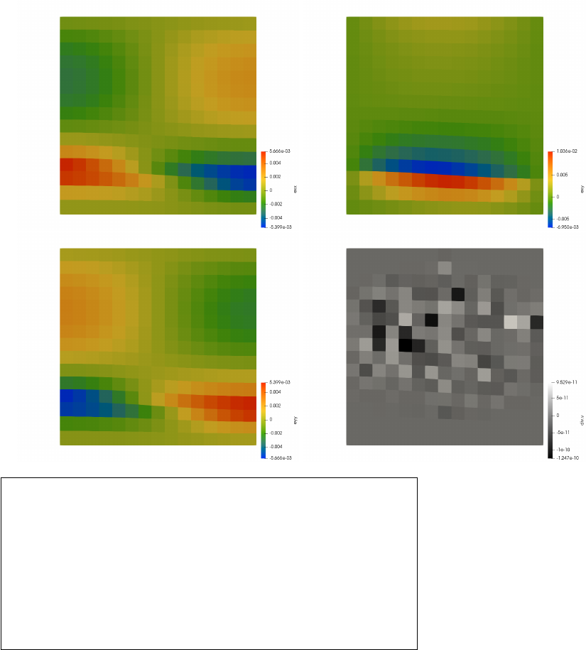
features
•Q1×P0element
•incompressible flow
•mixed formulation
•isothermal
•numerical benchmark
158
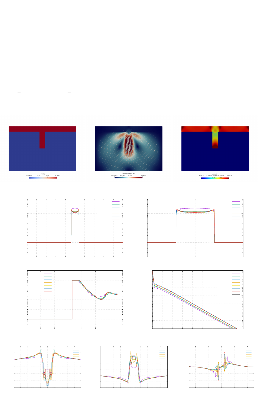
32 fieldstone 26: Slab detachment benchmark (1) - instanta-
neous
As in [413], the computational domain is 1000km ×660km. No-slip boundary conditions are imposed
on the sides of the system while free-slip boundary conditions are imposed at the top and bottom. Two
materials are present in the domain: the lithosphere (mat.1) and the mantle (mat.2). The overriding
plate (mat.1) is 80km thick and is placed at the top of the domain. An already subducted slab (mat.1)
of 250km length hangs vertically under this plate. The mantle occupies the rest of the domain.
The mantle has a constant viscosity η0= 1021P a.s and a density ρ= 3150kg/m3. The slab has a
density ρ= 3300kg/m3and is characterised by a power-law flow law so that its effective viscosity depends
on the second invariant of the strainrate I2as follows:
ηeff =1
2A−1/nsI1/ns−1
2=1
2[(2 ×4.75×1011)−ns]−1/nsI1/ns−1
2= 4.75×10¹¹I1/ns−1
2=η0I1/ns−1
2(272)
with ns= 4 and A= (2 ×4.75×1011)−ns, or η0= 4.75 ×10¹¹.
Fields at convergence for 151x99 grid.
1x10²⁰
1x10²¹
1x10²²
1x10²³
1x1024
0 100 200 300 400 500 600 700 800 900 1000
viscosity (Pa.s)
x (km)
nelx=32
nelx=48
nelx=51
nelx=64
nelx=100
nelx=128
nelx=151
1x10²⁰
1x10²¹
1x10²²
1x10²³
1x1024
400 450 500 550 600
viscosity (Pa.s)
x (km)
nelx=32
nelx=48
nelx=51
nelx=64
nelx=100
nelx=128
nelx=151
1x10²⁰
1x10²¹
1x10²²
1x10²³
1x1024
1x1025
1x1026
0 100 200 300 400 500 600 700
viscosity (Pa.s)
y (km)
nelx=32
nelx=48
nelx=51
nelx=64
nelx=100
nelx=128
nelx=151
0.0000001
0.0000010
0.0000100
0.0001000
0.0010000
0.0100000
0.1000000
1.0000000
0 5 10 15 20 25 30 35 40 45
normalised nonlinear residual
y (km)
nelx=32
nelx=48
nelx=51
nelx=64
nelx=100
nelx=128
nelx=151
1e-7
-8x10-16
-6x10-16
-4x10-16
-2x10-16
0
2x10-16
4x10-16
0 100 200 300 400 500 600 700 800 900 1000
exx
x (km)
nelx=32
nelx=48
nelx=51
nelx=64
nelx=100
nelx=128
nelx=151
-4x10-16
-2x10-16
0
2x10-16
4x10-16
6x10-16
8x10-16
1x10-15
0 100 200 300 400 500 600 700 800 900 1000
eyy
x (km)
nelx=32
nelx=48
nelx=51
nelx=64
nelx=100
nelx=128
nelx=151
-1.5x10⁻¹⁵
-1x10-15
-5x10-16
0
5x10-16
1x10-15
1.5x10⁻¹⁵
0 100 200 300 400 500 600 700 800 900 1000
exy
x (km)
nelx=32
nelx=48
nelx=51
nelx=64
nelx=100
nelx=128
nelx=151
159
Along the horizontal line
-1x10-15
-8x10-16
-6x10-16
-4x10-16
-2x10-16
0
2x10-16
4x10-16
0 100 200 300 400 500 600 700
exx
y (km)
nelx=32
nelx=48
nelx=51
nelx=64
nelx=100
nelx=128
nelx=151
-4x10-16
-2x10-16
0
2x10-16
4x10-16
6x10-16
8x10-16
1x10-15
0 100 200 300 400 500 600 700
eyy
y (km)
nelx=32
nelx=48
nelx=51
nelx=64
nelx=100
nelx=128
nelx=151
-6x10-17
-4x10-17
-2x10-17
0
2x10-17
4x10-17
6x10-17
8x10-17
0 100 200 300 400 500 600 700
exy
y (km)
nelx=32
nelx=48
nelx=51
nelx=64
nelx=100
nelx=128
nelx=151
Along the vertical line
features
•Q1×P0element
•incompressible flow
•mixed formulation
•isothermal
•nonlinear rheology
•nonlinear residual
Todo: nonlinear mantle, pressure normalisation
160
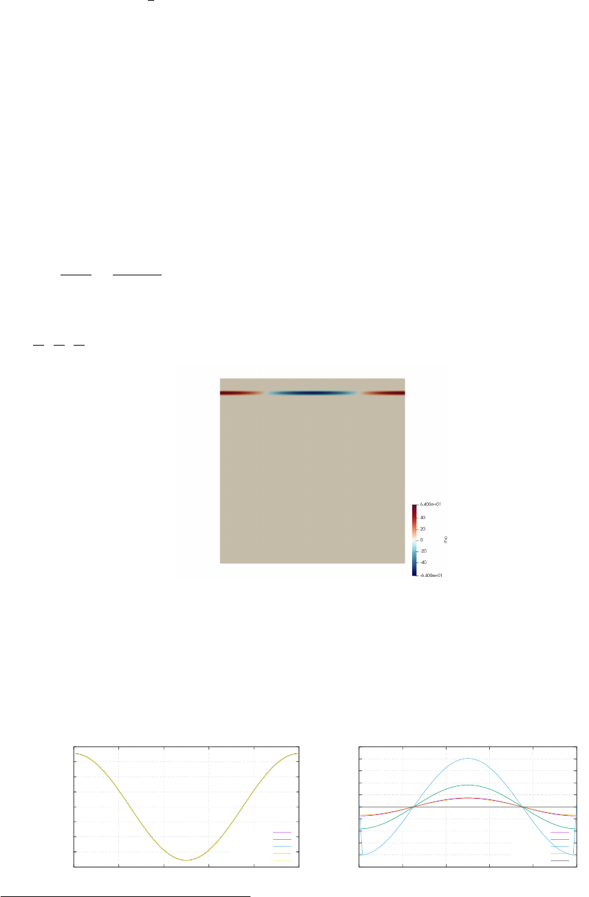
33 fieldstone 27: Consistent Boundary Flux
In what follows we will be re-doing the numerical experiments presented in Zhong et al. [520].
The first benchmark showcases a unit square domain with free slip boundary conditions prescribed
on all sides. The resolution is fixed to 64 ×64 Q1×P0elements. The flow is isoviscous and the buoyancy
force fis given by
fx= 0
fy=ρ0αT (x, y)
with the temperature field given by
T(x, y) = cos(kx)δ(y−y0)
where k= 2π/λ and λis a wavelength, and y0represents the location of the buoyancy strip. We set
gy=−1 and prescribe ρ(x, y) = ρ0αcos(kx)δ(y−y0) on the nodes of the mesh.
One can prove ([520] and refs. therein) that there is an analytic solution for the surface stress σzz 15
σyy
ραgh =cos(kx)
sinh2(k)[k(1 −y0) sinh(k) cosh(ky0)−ksinh(k(1 −y0)) + sinh(k) sinh(ky0)]
We choose ρ0α= 64, η= 1 (note that in this case the normalising coefficient of the stress is exactly
1 (since h=Lx/nelx = 1/64) so it is not implemented in the code). λ= 1 is set to 1 and we explore
y0=63
64 ,62
64 ,59
64 and y0= 32/64. Under these assumptions the density field for y0= 59/64 is:
We can recover the stress at the boundary by computing the yy component of the stress tensor in the
top row of elements:
σyy =−p+ 2η˙yy
Note that pressure is by definition elemental, and that strain rate components are then also computed in
the middle of each element.
These elemental quantities can be projected onto the nodes (see section ??) by means of the C→N
algorithm or a least square algorithm (LS).
-0.2
-0.15
-0.1
-0.05
0
0.05
0.1
0.15
0.2
0 0.2 0.4 0.6 0.8 1
σyy
x
y0=32/64
analytical
elemental
C-N
LS
cbf
-0.001
-0.0008
-0.0006
-0.0004
-0.0002
0
0.0002
0.0004
0.0006
0.0008
0.001
0 0.2 0.4 0.6 0.8 1
σyy error
x
y0=32/64
elemental
C-N
LS
cbf
0.
15Note that in the paper the authors use ραg which does not have the dimensions of a stress
161
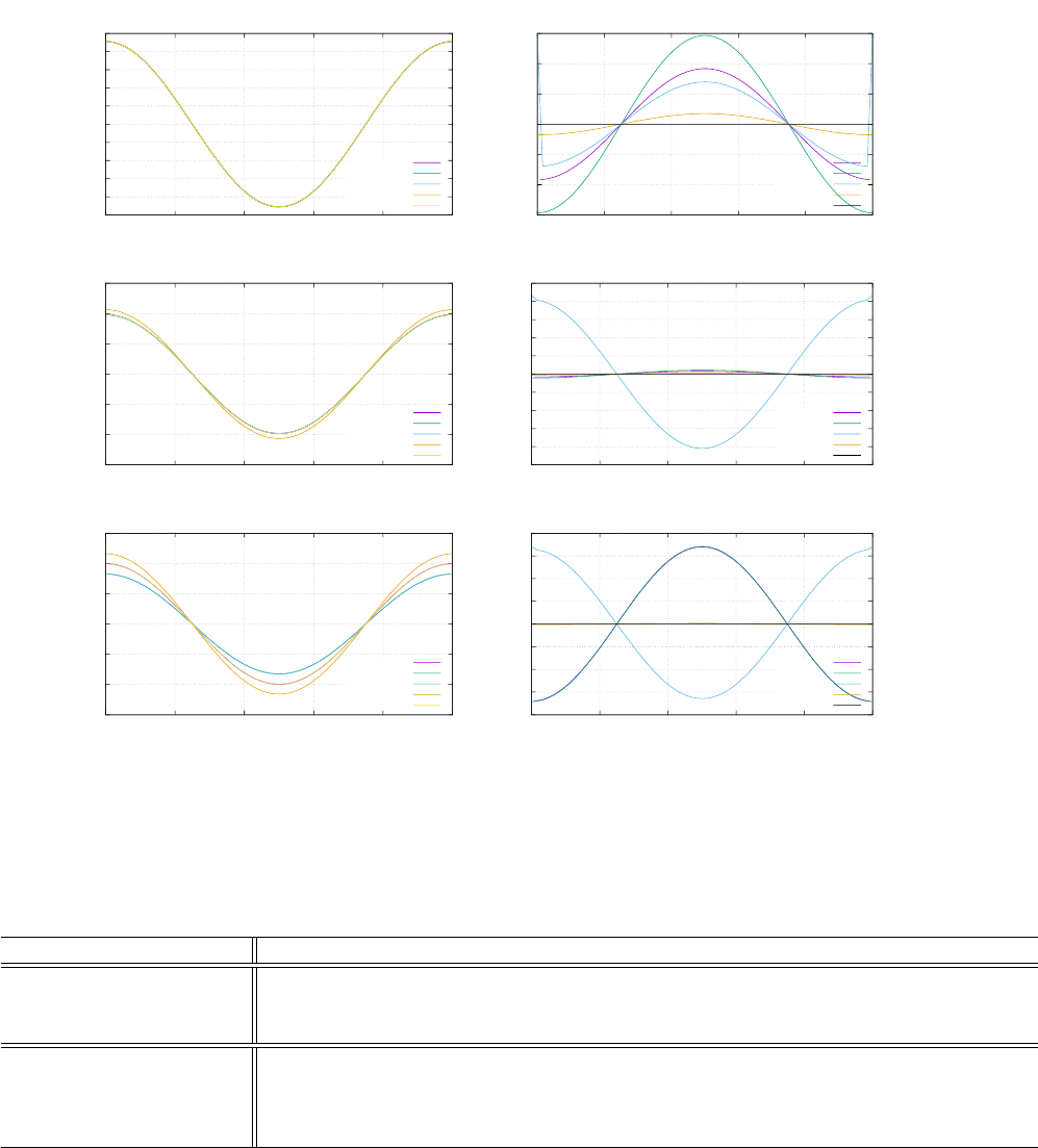
-1
-0.8
-0.6
-0.4
-0.2
0
0.2
0.4
0.6
0.8
1
0 0.2 0.4 0.6 0.8 1
σyy
x
y0=59/64
analytical
elemental
C-N
LS
cbf
-0.003
-0.002
-0.001
0
0.001
0.002
0.003
0 0.2 0.4 0.6 0.8 1
σyy error
x
y0=59/64
elemental
C-N
LS
cbf
0.
-1.5
-1
-0.5
0
0.5
1
1.5
0 0.2 0.4 0.6 0.8 1
σyy
x
y0=62
analytical
elemental
C-N
LS
cbf
-0.1
-0.08
-0.06
-0.04
-0.02
0
0.02
0.04
0.06
0.08
0.1
0 0.2 0.4 0.6 0.8 1
σyy error
x
y0=62
elemental
C-N
LS
cbf
0.
-1.5
-1
-0.5
0
0.5
1
1.5
0 0.2 0.4 0.6 0.8 1
σyy
x
y0=63/64
analytical
elemental
C-N
LS
cbf
-0.2
-0.15
-0.1
-0.05
0
0.05
0.1
0.15
0.2
0 0.2 0.4 0.6 0.8 1
σyy error
x
y0=63/64
elemental
C-N
LS
cbf
0.
The consistent boundary flux (CBF) method allows us to compute traction vectors t=σ·non the
boundary of the domain. On the top boundary, n= (0,1) so that t= (σxy, σyy)Tand tyis the quantity
we need to consider and compare to other results.
In the following table are shown the results presented in [520] alongside the results obtained with
Fieldstone:
Method y0= 63/64 y0= 62/64 y0= 59/64 16 y0= 32/64
Analytic solution 0.995476 0.983053 0.912506 0.178136
Pressure smoothing [520] 1.15974 1.06498 0.911109 n.a.
CBF [520] 0.994236 0.982116 0.912157 n.a.
fieldstone: elemental 0.824554 (-17.17 %) 0.978744 (-0.44%) 0.909574 (-0.32 %) 0.177771 (-0.20 %)
fieldstone: nodal (C→N) 0.824554 (-17.17 %) 0.978744 (-0.44%) 0.909574 (-0.32 %) 0.177771 (-0.20 %)
fieldstone: LS 1.165321 ( 17.06 %) 1.070105 ( 8.86%) 0.915496 ( 0.33 %) 0.178182 ( 0.03 %)
fieldstone: CBF 0.994236 ( -0.13 %) 0.982116 (-0.10%) 0.912157 (-0.04 %) 0.177998 (-0.08 %)
We see that we recover the published results with the same exact accuracy, thereby validating our
implmentation.
On the following figures are shown the velocity, pressure and traction fields for two cases y0= 32/64
and y0= 63/64.
162
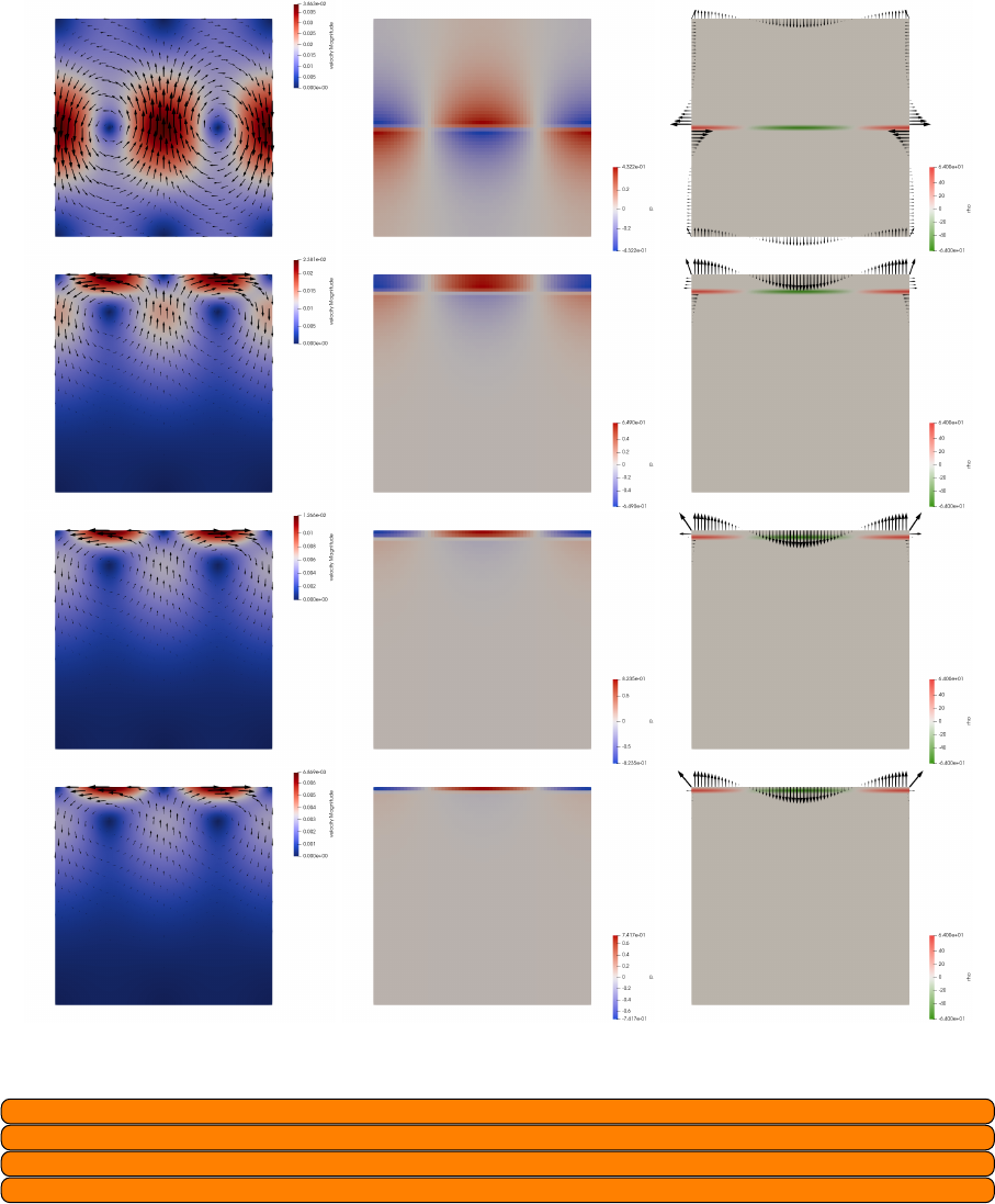
Here lies the superiority of our approach over the one presented in the original article: our code
computes all traction vectors on all boundaries at once.
explain how Medge is arrived at!
compare with ASPECT ??!
gauss-lobatto integration?
pressure average on surface instead of volume ?
163

features
•Q1×P0element
•incompressible flow
•mixed formulation
•isothermal
•isoviscous
•analytical solution
•pressure smoothing
•consistent boundary flux
164

34 fieldstone 28: convection 2D box - Tosi et al, 2015
This fieldstone was developed in collaboration with Rens Elbertsen.
The viscosity field µis calculated as the harmonic average between a linear part µlin that depends
on temperature only or on temperature and depth d, and a non-linear, plastic part µplast dependent on
the strain rate:
µ(T, z, ˙
)=21
µlin(T, z)+1
µplast(˙
)−1
.(273)
The linear part is given by the linearized Arrhenius law (the so-called Frank-Kamenetskii approxima-
tion [?]):
µlin(T, z) = exp(−γTT+γzz),(274)
where γT= ln(∆µT) and γz= ln(∆µz) are parameters controlling the total viscosity contrast due to
temperature (∆µT) and pressure (∆µz). The non-linear part is given by [?]:
µplast(˙
) = µ∗+σY
√˙
:˙
,(275)
where µ∗is a constant representing the effective viscosity at high stresses [?] and σYis the yield
stress, also assumed to be constant. In 2-D, the denominator in the second term of equation (275) is
given explicitly by
√˙
:˙
=p˙ij ˙ij =s∂ux
∂x 2
+1
2∂ux
∂y +∂uy
∂x 2
+∂uy
∂y 2
.(276)
The viscoplastic flow law (equation 273) leads to linear viscous deformation at low stresses (equation
(274)) and to plastic deformation for stresses that exceed σY(equation (275)), with the decrease in
viscosity limited by the choice of µ∗[?].
In all cases that we present, the domain is a two-dimensional square box. The mechanical boundary
conditions are for all boundaries free-slip with no flux across, i.e. τxy =τyx = 0 and u·n= 0, where
ndenotes the outward normal to the boundary. Concerning the energy equation, the bottom and top
boundaries are isothermal, with the temperature Tset to 1 and 0, respectively, while side-walls are
assumed to be insulating, i.e. ∂T/∂x = 0. The initial distribution of the temperature field is prescribed
as follows:
T(x, y) = (1 −y) + Acos(πx) sin(πy),(277)
where A= 0.01 is the amplitude of the initial perturbation.
In the following Table ??, we list the benchmark cases according to the parameters used.
Case Ra ∆µT∆µyµ∗σYConvective regime
1 1021051 – – Stagnant lid
2 1021051 10−31 Mobile lid
3 10210510 – – Stagnant lid
4 10210510 10−31 Mobile lid
5a 10210510 10−34 Periodic
5b 10210510 10−33 – 5 Mobile lid – Periodic – Stagnant lid
Benchmark cases and corresponding parameters.
In Cases 1 and 3 the viscosity is directly calculated from equation (274), while for Cases 2, 4, 5a, and
5b, we used equation (273). For a given mesh resolution, Case 5b requires running simulations with yield
stress varying between 3 and 5
In all tests, the reference Rayleigh number is set at the surface (y= 1) to 102, and the viscosity
contrast due to temperature ∆µTis 105, implying therefore a maximum effective Rayleigh number of
107for T= 1. Cases 3, 4, 5a, and 5b employ in addition a depth-dependent rheology with viscosity
contrast ∆µz= 10. Cases 1 and 3 assume a linear viscous rheology that leads to a stagnant lid regime.
165
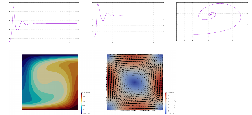
Cases 2 and 4 assume a viscoplastic rheology that leads instead to a mobile lid regime. Case 5a also
assumes a viscoplastic rheology but a higher yield stress, which ultimately causes the emergence of a
strictly periodic regime. The setup of Case 5b is identical to that of Case 5a but the test consists in
running several simulations using different yield stresses. Specifically, we varied σYbetween 3 and 5 in
increments of 0.1 in order to identify the values of the yield stress corresponding to the transition from
mobile to periodic and from periodic to stagnant lid regime.
34.0.1 Case 0: Newtonian case, a la Blankenbach et al., 1989
0
10
20
30
40
50
60
70
80
90
0 0.05 0.1 0.15 0.2 0.25 0.3 0.35
vrms
time
0
1
2
3
4
5
6
7
0 0.05 0.1 0.15 0.2 0.25 0.3 0.35
Nu
time
0
1
2
3
4
5
6
7
0 10 20 30 40 50 60 70 80 90
Nu
vrms
166
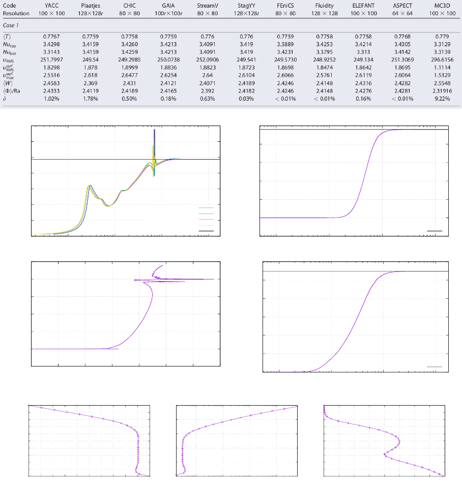
34.0.2 Case 1
In this case µ?= 0 and σY= 0 so that µplast can be discarded. The CFL number is set to 0.5 and the
viscosity is given by µ(T, z, ˙
) = µlin(T, z). And since ∆µz= 1 then γz= 0 so that µlin(T, z) = exp(−γTT)
0
50
100
150
200
250
300
350
0.001 0.01 0.1 1
vrms
time
ELEFANT, 32x32
ELEFANT, 48x48
ELEFANT, 64x64
ELEFANT, 100x100
243.872
0.5
1
1.5
2
2.5
3
3.5
0.001 0.01 0.1 1
Nu
time
3.3987
0.5
1
1.5
2
2.5
3
3.5
0 50 100 150 200 250 300 350
Nu
vrms
0.5
0.55
0.6
0.65
0.7
0.75
0.8
0.001 0.01 0.1 1
<T>
time
0.77368
0
0.1
0.2
0.3
0.4
0.5
0.6
0.7
0.8
0.9
1
0 0.1 0.2 0.3 0.4 0.5 0.6 0.7 0.8 0.9 1
y
T
0
0.2
0.4
0.6
0.8
1
0.00010 0.00100 0.01000 0.10000
y
viscosity
0
0.1
0.2
0.3
0.4
0.5
0.6
0.7
0.8
0.9
1
0 50 100 150 200 250 300 350 400
y
velocity
167
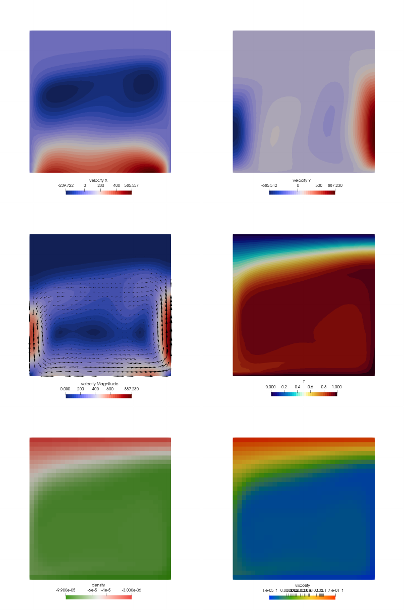
168
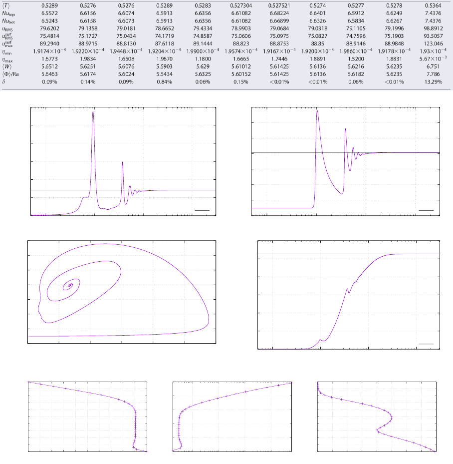
34.0.3 Case 2
0
100
200
300
400
500
600
0.001 0.01 0.1 1
vrms
time
141.518
0
2
4
6
8
10
12
14
0.001 0.01 0.1 1
Nu
time
8.17154
0
2
4
6
8
10
12
14
0 100 200 300 400 500 600
Nu
vrms
0.5
0.52
0.54
0.56
0.58
0.6
0.62
0.001 0.01 0.1 1
<T>
time
0.60521
0
0.1
0.2
0.3
0.4
0.5
0.6
0.7
0.8
0.9
1
0 0.1 0.2 0.3 0.4 0.5 0.6 0.7 0.8 0.9 1
y
T
0
0.2
0.4
0.6
0.8
1
0.00010 0.00100 0.01000 0.10000
y
viscosity
0
0.1
0.2
0.3
0.4
0.5
0.6
0.7
0.8
0.9
1
0 50 100 150 200 250 300 350 400
y
velocity
169
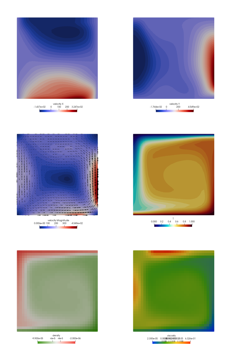
170
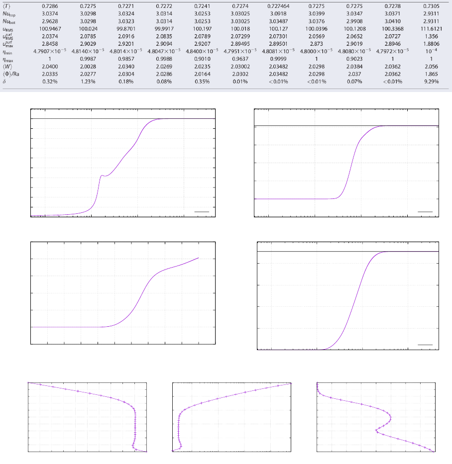
34.0.4 Case 3
0
10
20
30
40
50
60
70
80
90
100
110
0.001 0.01 0.1 1
vrms
time
100.018
0.5
1
1.5
2
2.5
3
3.5
0.001 0.01 0.1 1
Nu
time
3.03472
0.5
1
1.5
2
2.5
3
3.5
0 10 20 30 40 50 60 70 80 90 100 110
Nu
vrms
0.5
0.55
0.6
0.65
0.7
0.75
0.001 0.01 0.1 1
<T>
time
0.7277
0
0.1
0.2
0.3
0.4
0.5
0.6
0.7
0.8
0.9
1
0 0.1 0.2 0.3 0.4 0.5 0.6 0.7 0.8 0.9 1
y
T
0
0.2
0.4
0.6
0.8
1
0.00010 0.00100 0.01000 0.10000
y
viscosity
0
0.1
0.2
0.3
0.4
0.5
0.6
0.7
0.8
0.9
1
0 50 100 150 200 250 300 350 400
y
velocity
171
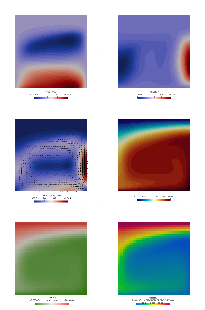
172
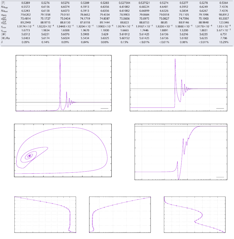
34.0.5 Case 4
0
50
100
150
200
250
300
350
400
450
500
0.001 0.01 0.1 1
vrms
time
79.4746
0
2
4
6
8
10
12
14
16
0.001 0.01 0.1 1
Nu
time
6.40359
0
2
4
6
8
10
12
14
16
0 50 100 150 200 250 300 350 400 450 500
Nu
vrms
0.495
0.5
0.505
0.51
0.515
0.52
0.525
0.53
0.001 0.01 0.1 1
<T>
time
0.528634
0
0.1
0.2
0.3
0.4
0.5
0.6
0.7
0.8
0.9
1
0 0.1 0.2 0.3 0.4 0.5 0.6 0.7 0.8 0.9 1
y
T
0
0.2
0.4
0.6
0.8
1
0.00010 0.00100 0.01000 0.10000
y
viscosity
0
0.1
0.2
0.3
0.4
0.5
0.6
0.7
0.8
0.9
1
0 50 100 150 200 250 300 350 400
y
velocity
173
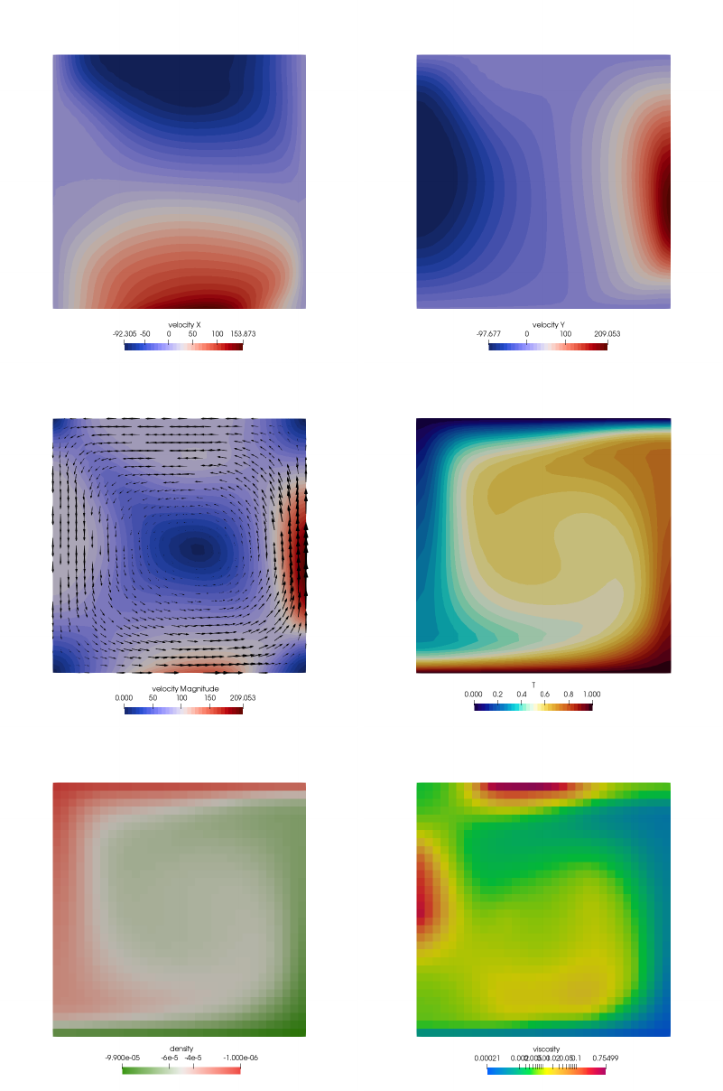
174
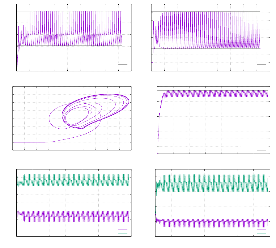
34.0.6 Case 5
0
20
40
60
80
100
0 0.5 1 1.5 2 2.5 3 3.5 4 4.5
vrms
time
41.61
98.183
0
1
2
3
4
5
6
7
8
0 0.5 1 1.5 2 2.5 3 3.5 4 4.5
Nu
time
2.6912
7.0763
0
1
2
3
4
5
6
7
8
0 10 20 30 40 50 60 70 80 90 100
Nu
vrms
0.5
0.52
0.54
0.56
0.58
0.6
0.62
0.64
0.66
0.68
0 1 2 3 4 5 6 7
<T>
time
0.66971
0.65206
-200
-150
-100
-50
0
50
100
150
200
0 1 2 3 4 5 6 7
u
time
min(u)
max(u)
-150
-100
-50
0
50
100
150
200
250
300
0 1 2 3 4 5 6 7
v
time
min(v)
max(v)
175
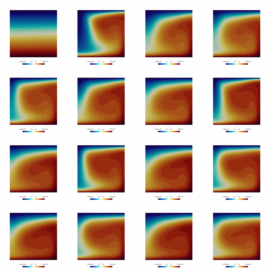
176
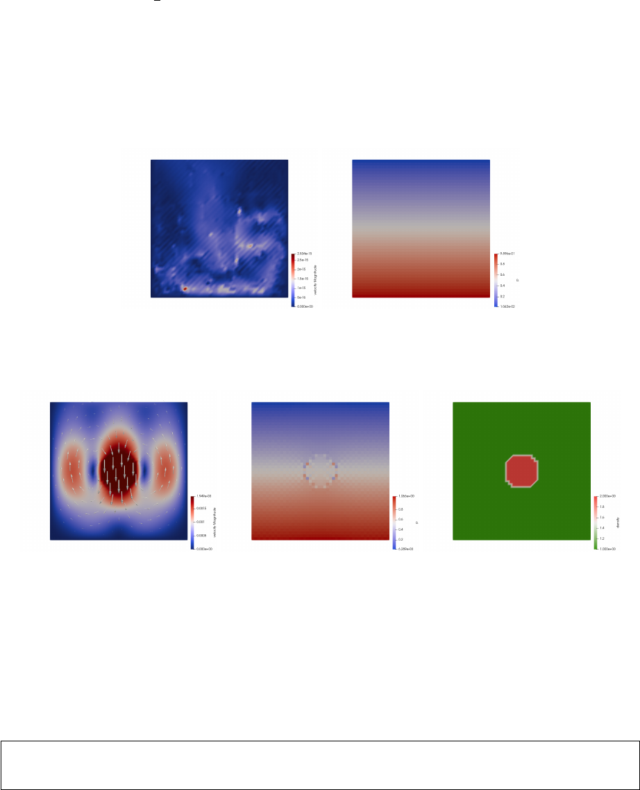
35 fieldstone 29: open boundary conditions
In what follows we will investigate the use of the so-called open boundary conditions in the very simple
context of a 2D Stokes sphere experiment.
We start with a domain without the sphere. Essentially, it is what people would call an aquarium.
Free slip boundary conditions are prescribed on the sides and no-slip conditions at the bottom. The top
surface is left free. The fluid has a density ρ0= 1 and a viscosity η0= 1. In the absence of any density
difference in the domain there is no active buoyancy force so that we expect a zero velocity field and a
lithostatic pressure field. This is indeed what we recover:
If we now implement a sphere parametrised by its density ρs=ρ0+ 1, its viscosity ηs= 103and
its radius Rs= 0.123 in the middle of the domain, we see clear velocity field which logically shows the
sphere falling downward and a symmetric return flow of the fluid on each side:
Unfortunately it has been widely documented that the presence of free-slip boundary conditions
affects the evolution of subduction [109], even when these are placed rather far from the subduction zone.
A proposed solution to this problem is the use of ’open boundary conditions’ which are in fact stress
boundary conditions. The main idea is to prescribe a stress on the lateral boundaries (instead of free
slip) so that it balances out exactly the existing lithostatic pressure inside the domain along the side
walls. Only pressure deviations with respect to the lithostatic are responsible for flow and such boundary
conditions allow flow across the boundaries.
We need the lithostatic pressure and compute it before hand (which is trivial in our case but can
prove to be a bit more tedious in real life situations when for instance density varies in the domain as a
function of temperature and/or pressure).
p l i t h = np . z e r os ( nnp , dtype=np . f l o a t 6 4 )
f o r iin range ( 0 , nnp ) :
p l i t h [ i ]= (Ly−y [ i ] ) ∗rho0 ∗abs ( gy )
Let us start with a somewhat pathological case: even in the absence of the sphere, what happens when
no boundary conditions are prescribed on the sides? The answer is simple: think about an aquarium
without side walls, or a broken dam. The velocity field indeed shows a complete collapse of the fluid left
and right of the bottom.
177
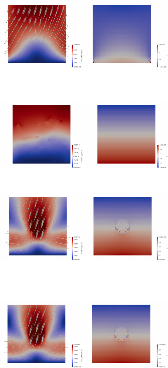
Let us then continue (still with no sphere) but let us now switch on the open boundary conditions.
Since the side boundary conditions match the lithostatic pressure we expect no flow at all in the absence
of any density perturbation in the system. This is indeed what is recovered:
Finally, let us reintroduce the sphere. This time flow is allowed through the left and right side
boundaries:
Finally, although horizontal velocity Dirichlet boundary conditions and open boundary conditions
are not compatible, the same is not true for the vertical component of the velocity: the open b.c.
implementation acts on the horizontal velocity dofs only, so that one can fix the vertical component to
zero, as is shown hereunder:
We indeed see that the in/outflow on the sides is perpendicular to the boundaries.
Turning now to the actual implementation, we see that it is quite trivial, since all element edges are
vertical, and all have the same vertical dimension hx. Since we use a Q0approximation for the pressure
178

we need to prescribe a single pressure value in the middle of the element. Finally because of the sign of
the normal vector projection onto the x-axis, we obtain:
i f open bc left and x [ i c o n [ 0 , i e l ] ] <eps : # l e f t s i d e
pmid =0. 5∗( p l i t h [ i co n [ 0 , i e l ] ]+ p l i t h [ i co n [ 3 , i e l ] ] )
f e l [0 ]+= 0.5∗hy∗pmid
f e l [6 ]+= 0.5∗hy∗pmid
i f open bc right and x [ i c o n [ 1 , i e l ] ] >Lx−e ps : # r i g h t s i d e
pmid =0. 5∗( p l i t h [ i co n [ 1 , i e l ] ]+ p l i t h [ i co n [ 2 , i e l ] ] )
f e l [2 ] −= 0. 5∗hy∗pmid
f e l [4 ] −= 0. 5∗hy∗pmid
These few lines of code are added after the elemental matrices and rhs are built, and before the
application of other Dirichlet boundary conditions, and assembly.
features
•Q1×P0element
•incompressible flow
•mixed formulation
•open boundary conditions
•isoviscous
179
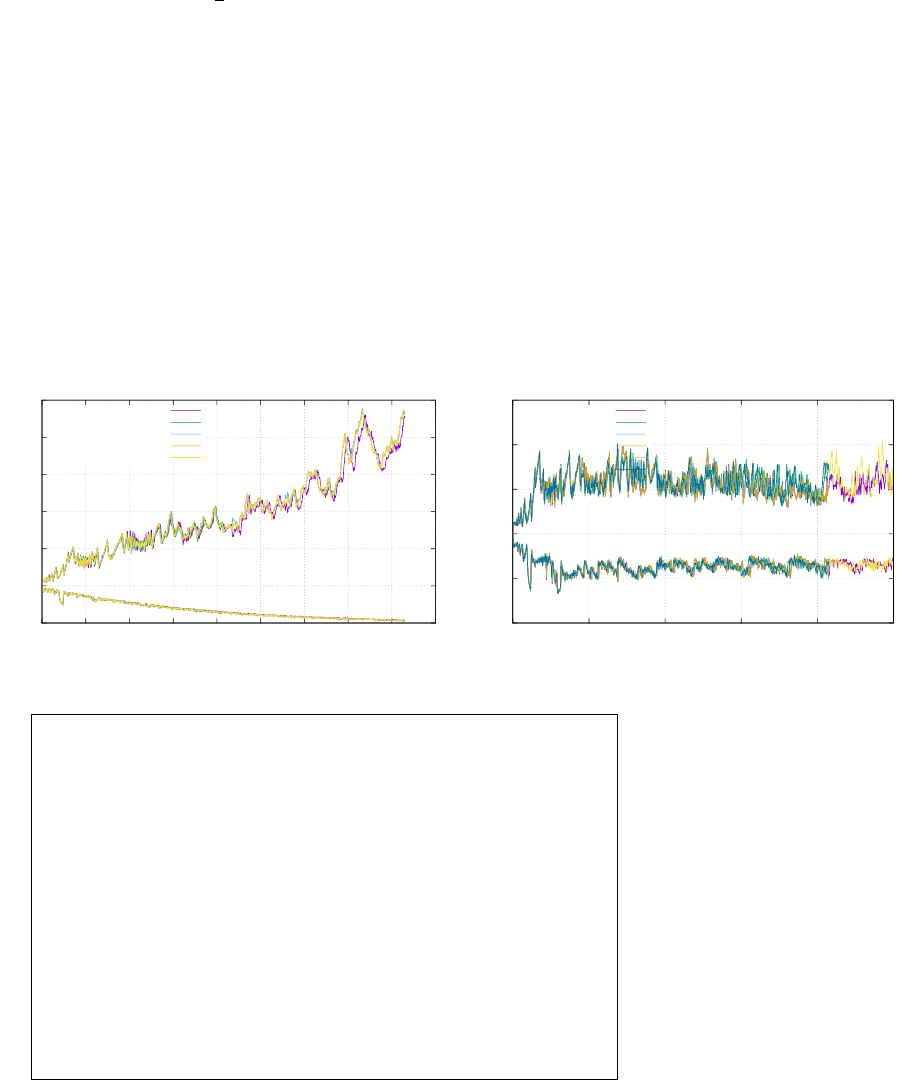
36 fieldstone 30: conservative velocity interpolation
In this the Stokes equations are not solved. It is a 2D implementation of the cvi algorithm as introduced
in [490] which deals with the advection of markers. Q1and Q2basis functions are used and in both cases
the cvi algorithm can be toggled on/off. Markers can be distributed regularly or randomly at startup.
Three velocity fields are prescribed on the mesh:
•the so-called Couette flow of [490]
•the SolCx solution
•a flow created by means of a stream line function (see fieldstone 32)
36.1 Couette flow
36.2 SolCx
36.3 Streamline flow
0
1
2
3
4
5
6
0 0.1 0.2 0.3 0.4 0.5 0.6 0.7 0.8 0.9
nmarker
time
Q1, no cvi, RK1
Q1, cvi, RK1
Q2, no cvi, RK1
Q2, cvi, RK1
Q1, no cvi, RK1, **
0
0.5
1
1.5
2
2.5
0 0.2 0.4 0.6 0.8 1
nmarker
time
Q1, no cvi, RK2
Q1, cvi, RK2
Q1, no cvi, RK4
Q1, no cvi, RK5
Q2, no cvi, RK2
Q2, no cvi, RK4
In this case RK order seems to be more important that cvi.
Explore why ?!
features
•Q1×P0element
•incompressible flow
•penalty formulation
•Dirichlet boundary conditions (free-slip)
•direct solver
•isothermal
•non-isoviscous
•analytical solution
180

37 fieldstone 31: conservative velocity interpolation 3D
181
38 fieldstone 32: 2D analytical sol. from stream function
38.1 Background theory
The stream function is a function of coordinates and time of an inviscid liquid. It allows to determine
the components of velocity by differentiating the stream function with respect to the space coordinates.
A family of curves Ψ = const represent streamlines, i.e. the stream function remains constant along a
streamline. Although also valid in 3D, this approach is mostly used in 2D because of its relative simplicity
REFERENCES.
In two dimensions the velocity is obtained as follows:
v=∂Ψ
∂y ,−∂Ψ
∂x (278)
Provided the function Ψ is a smooth enough function, this automatically insures that the flow is incom-
pressible:
∇·v=∂u
∂x +∂v
∂y =∂2Ψ
∂xy −∂2Ψ
∂xy = 0 (279)
Assuming constant viscosity, the Stokes equation writes:
−∇p+µ∆v=ρg(280)
Let us introduce the vector Wfor convenience such that in each dimension:
Wx=−∂p
∂x +µ∂2u
∂x2+∂2u
∂xy=ρgx(281)
Wy=−∂p
∂y +µ∂2v
∂x2+∂2v
∂xy=ρgy(282)
Taking the curl of the vector Wand only considering the component perpendicular to the xy-plane:
∂Vy
∂x −∂Vx
∂y =∂ρgy
∂x −∂ρgx
∂y (283)
The advantage of this approach is that the pressure terms cancel out (the curl of a gradient is always
zero), so that:
∂
∂x µ(∂2v
∂x2+∂2v
∂xy−∂
∂y µ∂2u
∂x2+∂2u
∂xy=∂ρgy
∂x −∂ρgx
∂y (284)
and then replacing u, v by the their stream function derivatives yields (for a constant viscosity):
µ∂4Ψ
∂x4+∂4Ψ
∂y4+ 2 ∂4Ψ
∂x2y2=∂ρgy
∂x −∂ρgx
∂y (285)
or,
∇4Ψ = ∂2
∂x2+∂2
∂y2∂2
∂x2+∂2
∂y2Ψ = ∂ρgy
∂x −∂ρgx
∂y (286)
These equations are also to be found in the geodynamics literature, eee Eq. 1.43 of Tackley book, p 70-71
of Gerya book.
38.2 A simple application
I wish to arrive at an analytical formulation for a 2D incompressible flow in the square domain [−1 :
1] ×[−1 : 1] The fluid has constant viscosity µ= 1 and is subject to free slip boundary conditions on all
sides. For reasons that will become clear in what follows I postulate the following stream function:
Ψ(x, y) = sin(mπx) sin(nπy) (287)
182
We have the velocity being defined as:
v= (u, v) = ∂Ψ
∂y ,−∂Ψ
∂x = (nπ sin(mπx) cos(nπy),−mπ cos(mπx) sin(nπy)) (288)
The strain rate components are then:
˙εxx =∂u
∂x =mnπ2cos(mπx) cos(nπy) (289)
˙εyy =∂v
∂y =−mnπ2cos(mπx) cos(nπy) (290)
2 ˙εxy =∂u
∂y +∂v
∂x (291)
=∂2Ψ
∂y2−∂2Ψ
∂x2(292)
=−n2π2Ψ + m2π2Ψ (293)
= (m2−n2)π2sin(mπx) sin(nπy) (294)
Note that if m=nthe last term is identically zero, which is not desirable (flow is too ’simple’) so in
what follows we will prefer m6=n.
It is also easy to verify that u= 0 on the sides and v= 0 at the top and bottom and that the term
˙εxy is nul on all four sides, thereby garanteeing free slip.
Our choice of stream function yields:
∇4Ψ = ∂4Ψ
∂x4+∂4Ψ
∂y4+ 2 ∂2Ψ
∂x2y2=π4(m4Ψ + n4Ψ+2m2n2Ψ) = (m4+n4+ 2m2n2)π4Ψ
We assume gx= 0 and gy=−1 so that we simply have
(m4+n4+ 2m2n2)π4Ψ = −∂ρ
∂x (295)
so that (assuming the integration constant to be zero):
ρ(x, y) = m4+n4+ 2m2n2
mπ3cos(mπx) sin(nπy)
The x-component of the momentum equation is
−∂p
∂x +∂2u
∂x2+∂2u
∂y2=−∂p
∂x −m2nπ3sin(mπx) cos(nπy)−n3π3sin(mπx) cos(nπy)=0
so ∂p
∂x =−(m2n+n3)π3sin(mπx) cos(nπy)
and the pressure field is then (once again neglecting the integration constant):
p(x, y) = m2n+n3
mπ2cos(πx) cos(πy)
Note that in this case RpdV = 0 so that volume normalisation of the pressure is turned on (when free
slip boundary conditions are prescribed on all sides the pressure is known up to a constant and this
undeterminacy can be lifted by adding an additional constraint to the pressure field).
183
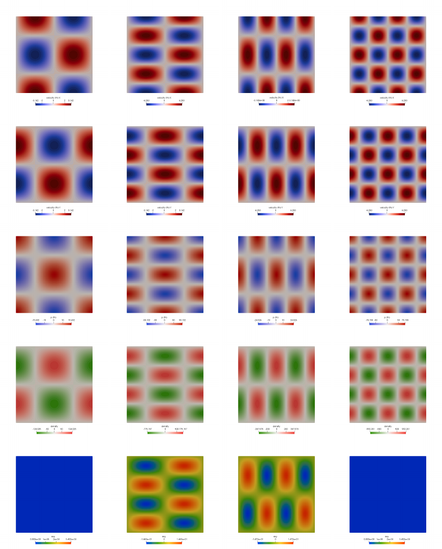
Top to bottom: Velocity components uand v, pressure p, density ρand strain rate ˙εxy . From left to right:
(m, n) = (1,1), (m, n) = (1,2), (m, n) = (2,1), (m, n) = (2,2)
184
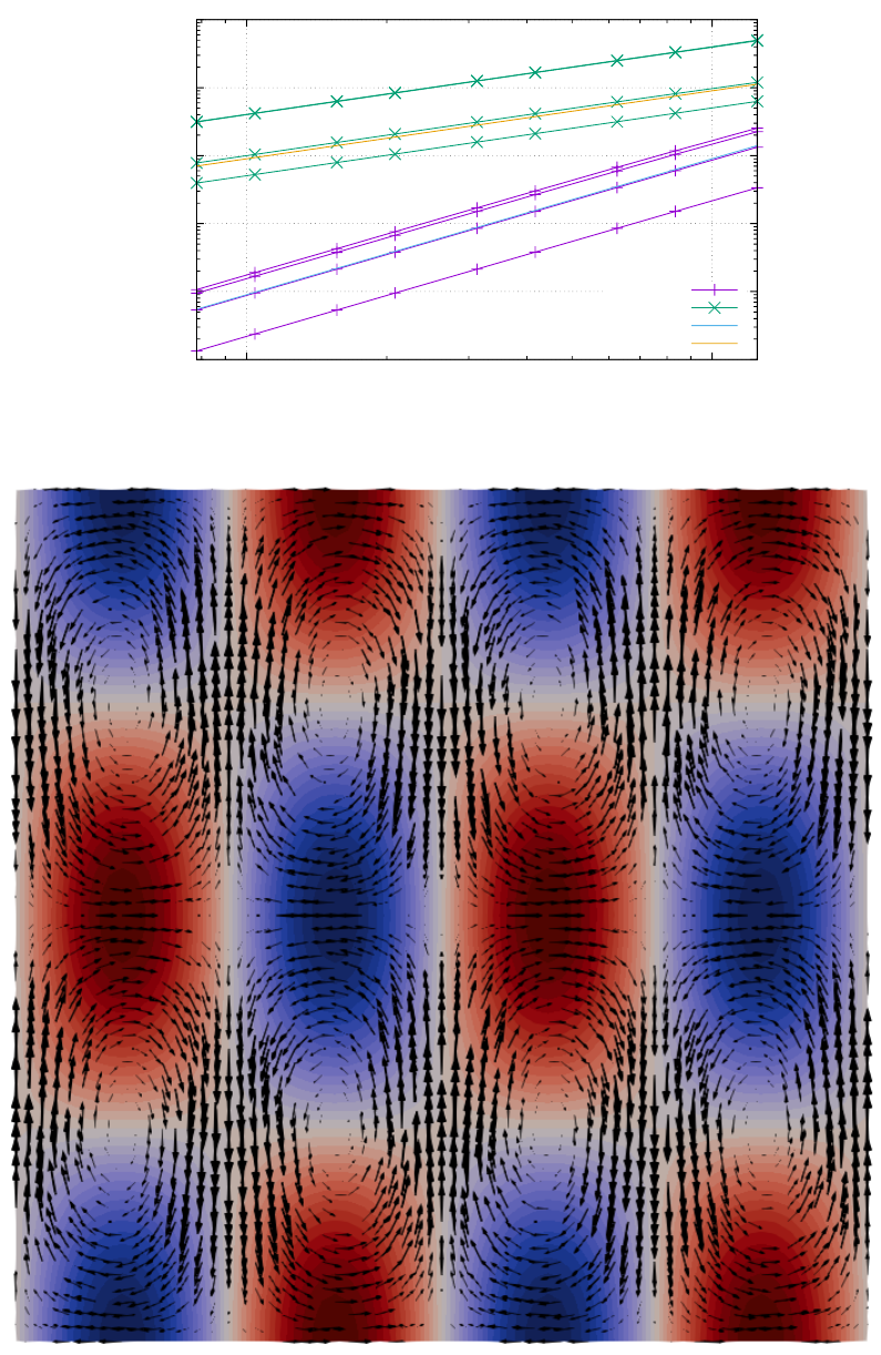
0.001
0.01
0.1
1
10
100
0.01 0.1
error
h
velocity
pressure
x2
x1
Errors for velocity and pressure for (m, n) = (1,1),(1,2),(2,1),(2,2)
Velocity arrows for (m, n) = (2,1)
185
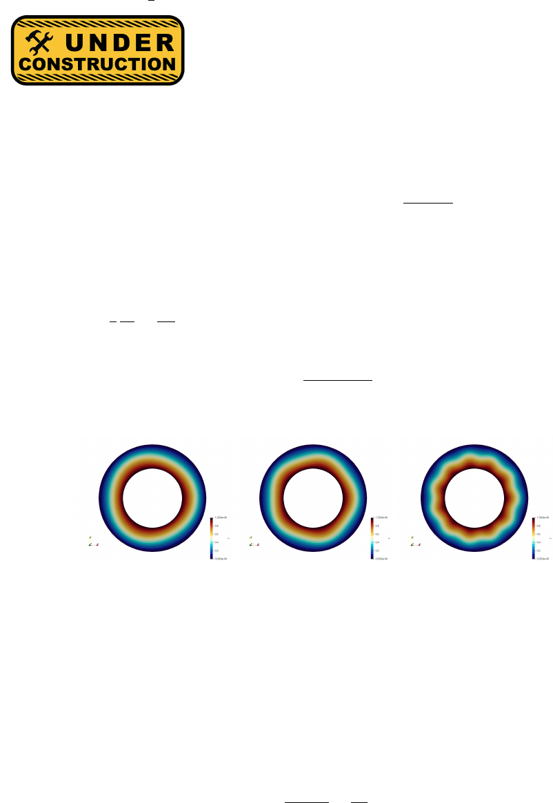
39 fieldstone 33: Convection in an annulus
This fieldstone was developed in collaboration with Rens Elbertsen.
This is based on the community benchmark for viscoplastic thermal convection in a 2D square box
[458] as already carried out in ??.
In this experiment the geometry is an annulus of inner radius R1= 1.22 and outer radius R2= 2.22.
The rheology and buoyancy forces are identical to those of the box experiment. The initial temperature
is now given by:
T(r, θ) = Tc(r) + A s(1 −s) cos(N0θ)s=R2−r
R2−R1∈[0,1]
where sin the normalised depth, Ais the amplitude of the perturbation and N0the number of lobes. In
this equation Tc(r) stands for the steady state purely conductive temperature solution which is obtained
by solving the Laplace’s equation in polar coordinates (all terms in θare dropped because of radial
symmetry) supplemented with two boundary conditions:
∆Tc=1
r
∂
∂r r∂T
∂r = 0 T(r=R1) = T1= 1 T(r=R2) = T2= 0
We obtain
Tc(r) = log(r/R2)
log(R1/R2)
Note that this profile differs from the straight line that is used in [458] and in section 34.
Examples of initial temperature fields for N0= 3,5,11
Boundary conditions can be either no-slip or free-slip on both inner and outer boundary. However,
when free-slip is used on both a velocity null space exists and must be filtered out. In other words, the
solver may be able to come up with a solution to the Stokes operator, but that solution plus an arbitrary
rotation is also an equally valid solution. This additional velocity field can be problematic since it is used
for advecting temperature (and/or compositions) and it also essentially determines the time step value
for a chosen mesh size (CFL condition).
For these reasons the nullspace must be removed from the obtained solution after every timestep.
There are two types of nullspace removal: removing net angular momentum, and removing net rotations.
We calculate the following output parameters:
•the average temperature < T >
hTi=RΩT dΩ
RΩdΩ=1
VΩZΩ
T dΩ (296)
•the root mean square velocity vrms as given by equation (27).
•the root mean square of the radial and tangential velocity components as given by equations (29)
and (30).
186

•the heat transfer through both boundaries Q:
Qinner,outer =ZΓi,o
q·ndΓ (297)
•the Nusselt number at both boundaries N u as given by equations (32) and (33).
•the power spectrum of the temperature field:
P Sn(T) = ZΩ
T(r, θ)einθdΩ
2
.(298)
features
•Q1×P0element
•incompressible flow
•penalty formulation
•Dirichlet boundary conditions
•non-isothermal
•non-isoviscous
•annulus geometry
187
40 fieldstone 34: the Cartesian geometry elastic aquarium
This fieldstone was developed in collaboration with Lukas van de Wiel.
The setup is as follows: a 2D square of elastic material of size Lis subjected to the following boundary
conditions: free slip on the sides, no slip at the bottom and free at the top. It has a density ρand is
placed is a gravity field g=−gey. For an isotropic elastic medium the stress tensor is given by:
σ=λ(∇·u)1+ 2µε
where λis the Lam´e parameter and µis the shear modulus. The displacement field is u= (0, uy(y))
because of symmetry reasons (we do not expect any of the dynamic quantities to depend on the x
coordinate and also expect the horizontal displacement to be exactly zero). The velocity divergence is
then ∇·u=∂uy/∂y and the strain tensor:
ε= 0 0
0∂uy
∂y !
so that the stress tensor is:
σ= λ∂uy
∂y 0
0 (λ+ 2µ)∂uy
∂y !
∇·σ= (∂x∂y)· λ∂uy
∂y 0
0 (λ+ 2µ)∂uy
∂y != 0
(λ+ 2µ)∂2uy
∂y2!=0
ρg
so that the vertical displacement is then given by:
uy(y) = 1
2
ρg
λ+ 2µy2+αy +β
where αand βare two integration constants. We need now to use the two boundary conditions: the
first one states that the displacement is zero at the bottom, i.e. uy(y= 0) = 0 which immediately
implies β= 0. The second states that the stress at the top is zero (free surface), which implies that
∂uy/∂y(y=L) = 0 which allows us to compute α. Finally:
uy(y) = ρg
λ+ 2µ(y2
2−Ly)
The pressure is given by
p=−(λ+2
3µ)∇·u= (λ+2
3µ)ρg
λ+ 2µ(L−y) = λ+2
3µ
λ+ 2µρg(L−y) = 1 + 2µ
3λ
1+2µ/λ ρg(L−y)
In the incompressible limit, the poisson ratio is ν∼0.5. Materials are characterised by a finite Young’s
modulus E, which is related to νand λ:
λ=Eν
(1 + ν)(1 −2ν)µ=E
2(1 + ν)
It is then clear that for incompressible parameters λbecomes infinite while µremains finite. In that case
the pressure then logically converges to the well known formula:
p=ρg(L−y)
188
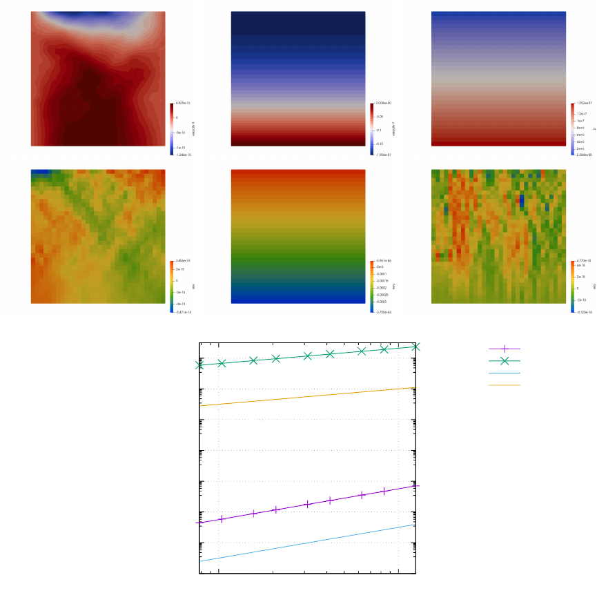
In what follows we set L= 1000m, ρ= 2800, ν= 0.25, E= 6 ·1010,g= 9.81.
0.000001
0.000100
0.010000
1.000000
100.000000
10000.000000
1000000.000000
100000000.000000
0.01 0.1
error
h
velocity
pressure
x2
x1
189

41 fieldstone 35: 2D analytical sol. in annulus from stream
function
We seek an exact solution to the incompressible Stokes equations for an isoviscous, isothermal fluid in
an annulus.Given the geometry of the problem, we work in polar coordinates. We denote the orthonormal
basis vectors by erand eθ, the inner radius of the annulus by R1and the outer radius by R2. Further,
we assume that the viscosity µis constant, which we set to µ= 1 we set the gravity vector to g=−grer
with gr= 1.
Given these assumptions, the incompressible Stokes equations in the annulus are [416]
Ar=∂2vr
∂r2+1
r
∂vr
∂r +1
r2
∂2vr
∂θ2−vr
r2−2
r2
∂uθ
∂θ −∂p
∂r =ρgr(299)
Aθ=∂2vθ
∂r2+1
r
∂vθ
∂r +1
r2
∂2vθ
∂θ2+2
r2
∂vr
∂θ −vθ
r2−1
r
∂p
∂θ = 0 (300)
1
r
∂(rvr)
∂r +1
r
∂vθ
∂θ = 0 (301)
Equations (299) and (300) are the momentum equations in polar coordinates while Equation (301) is the
incompressibility constraint. The components of the velocity are obtained from the stream function as
follows:
vr=1
r
∂Ψ
∂θ vθ=−∂Ψ
∂r
where vris the radial component and vθis the tangential component of the velocity vector.
The stream function is defined for incompressible (divergence-free) flows in 2D (as well as in 3D with
axisymmetry). The stream function can be used to plot streamlines, which represent the trajectories of
particles in a steady flow. From calculus it is known that the gradient vector ∇Ψ is normal to the curve
Ψ = C. It can be shown that everywhere u·∇Ψ = 0 using the formula for uin terms of Ψ which proves
that level curves of Ψ are streamlines:
u· ∇Ψ = vr
∂Ψ
∂r +vθ
1
r
∂Ψ
∂θ =1
r
∂Ψ
∂θ
∂Ψ
∂r −∂Ψ
∂r
1
r
∂Ψ
∂θ = 0
In polar coordinates the curl of a vector Ais:
∇×A=1
r∂(rAθ)
∂r −∂Ar
∂θ
Taking the curl of vector Ayields:
1
r∂(rAθ)
∂r −∂Ar
∂θ =1
r−∂(ρgr)
∂θ
Multiplying on each side by r
∂(rAθ)
∂r −∂Ar
∂θ =−∂ρgr
∂θ
If we now replace Arand Aθby their expressions as a function of velocity and pressure, we see that the
pressure terms cancel out and assuming the viscosity and the gravity vector to be constant we get: Let
us assume the following separation of variables Ψ(r, θ) = φ(r)ξ(θ). Then
vr=1
r
∂Ψ
∂θ =φξ0
rvθ=−∂Ψ
∂r =−φ0ξ
190

Let us first express Arand Aθas functions of Ψ and
Ar=∂2vr
∂r2+1
r
∂vr
∂r +1
r2
∂2vr
∂θ2−vr
r2−2
r2
∂uθ
∂θ (302)
=∂2
∂r2(φξ0
r) + 1
r
∂
∂r (φξ0
r) + 1
r2
∂2
∂θ2(φξ0
r)−1
r2(φξ0
r)−2
r2
∂
∂θ (−φ0ξ) (303)
= (φ00
r−2φ0
r2+ 2 φ
r3)ξ0+ ( φ0
r2−φ
r3)ξ0+φ
r3ξ000 −φξ0
r3+2
r2φ0ξ0(304)
=φ00ξ0
r+φ0ξ0
r2+φξ000
r3(305)
∂Ar
∂θ =φ00ξ00
r+φ0ξ00
r2+φξ0000
r3(306)
(307)
Aθ=∂2vθ
∂r2+1
r
∂vθ
∂r +1
r2
∂2vθ
∂θ2+2
r2
∂vr
∂θ −vθ
r2(308)
=∂2
∂r2(−φ0ξ) + 1
r
∂
∂r (−φ0ξ) + 1
r2
∂2
∂θ2(−φ0ξ) + 2
r2
∂
∂θ (φξ0
r)−1
r2(−φ0ξ) (309)
=−φ000ξ−φ00ξ
r−φ0ξ00
r2+2φξ00
r2+φ0ξ
r2(310)
∂(rAθ)
∂r = (311)
191
WRONG:
∂(r∆v)
∂r =∂
∂r ∂
∂r r∂v
∂r +1
r
∂2v
∂θ2(312)
=∂2
∂r2r∂v
∂r +∂
∂r 1
r
∂2v
∂θ2(313)
=∂2
∂r2r∂
∂r (−∂Ψ
∂r )+∂
∂r 1
r
∂2
∂θ2(−∂Ψ
∂r )(314)
=−∂2
∂r2r∂2Ψ
∂r2−∂
∂r 1
r
∂3Ψ
∂θ2∂r (315)
=−2∂3Ψ
∂r3−r∂4Ψ
∂r4+1
r2
∂3Ψ
∂θ2∂r −1
r
∂4Ψ
∂θ2∂r2(316)
∂∆u
∂θ =∂
∂θ 1
r
∂
∂r r∂u
∂r +1
r2
∂2u
∂θ2(317)
=∂
∂θ 1
r
∂
∂r r∂u
∂r +1
r2
∂3u
∂θ3(318)
=∂
∂θ 1
r
∂
∂r r∂
∂r (1
r
∂Ψ
∂θ )+1
r2
∂3
∂θ3(1
r
∂Ψ
∂θ ) (319)
=1
r3
∂2Ψ
∂θ2−1
r2
∂3Ψ
∂r∂θ2+1
r
∂4Ψ
∂r2∂θ2+1
r3
∂4Ψ
∂θ4(320)
Assuming the following separation of variables Ψ(r, θ) = φ(r)ξ(θ):
∂(r∆v)
∂r =−2φ000ξ−rφ0000ξ+1
r2φ0ξ00 −1
rφ00ξ00 (321)
∂∆u
∂θ =1
r3φξ00 −1
r2φ0ξ00 +1
rφ00ξ00 +1
r3φξ0000 (322)
so that
∂(r∆v)
∂r −∂∆u
∂θ =−2φ000ξ−rφ0000ξ+1
r2φ0ξ00 −1
rφ00ξ00 −1
r3φξ00 +1
r2φ0ξ00 −1
rφ00ξ00 −1
r3φξ0000
Further assuming ξ(θ) = cos(kθ) , then ξ00 =−k2ξand ξ0000 =k4ξthen
∂(r∆v)
∂r −∂∆u
∂θ =−2φ000ξ−rφ0000ξ−k21
r2φ0ξ+k21
rφ00ξ+k21
r3φξ −k21
r2φ0ξ+k21
rφ00ξ−k41
r3φξ
By choosing ρsuch that ρ=λ(r)Υ(θ) and such that ∂θΥ = ξ= cos(kθ) then we have
−2φ000ξ−rφ0000ξ−k21
r2φ0ξ+k21
rφ00ξ+k21
r3φξ −k21
r2φ0ξ+k21
rφ00ξ−k41
r3φξ =−1
ηλξgr
and then dividing by ξ: (IS THIS OK ?)
−2φ000 −rφ0000 −k21
r2φ0+k21
rφ00 +k21
r3φ−k21
r2φ0+k21
rφ00 −k41
r3φ=−1
ηλgr
−2φ000 −rφ0000 −2k21
r2φ0+ 2k21
rφ00 + (k2−k4)1
r3φ=−1
ηλgr
so
λ(r) = η
gr2φ000 +rφ0000 + 2k21
r2φ0−2k21
rφ00 −(k2−k4)1
r3φ
Also not forget Υ = 1
ksin(kθ)
192
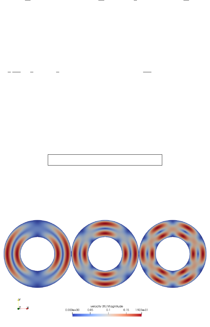
41.1 Linking with our paper
We have
φ(r) = −rg(r) (323)
φ0(r) = −g(r)−rg0(r) = −f(r) (324)
φ00(r) = −f0(r) (325)
φ000(r) = −f00(r) (326)
φ0000(r) = −f000(r) (327)
f(r) = η0
g02f00(r) + rf000(r)+2k21
r2f(r)−2k21
rf0(r)+(k2−k4)1
r2g(r)
41.2 No slip boundary conditions
No-slip boundary conditions inside and outside impose that all components of the velocity must be zero
on both boundaries, i.e.
v(r=R1) = v(r=R2) = 0
Due to the separation of variables, and since ξ(θ) = cos(kθ) we have
u(r, θ) = 1
r
∂Ψ
∂θ =1
rφξ0=−1
rφ(r)ksin(kθ)v(r, θ) = −∂Ψ
∂r =−φ0(r)ξ=−φ0(r) cos(kθ)
It is obvious that the only way to insure no-slip boundary conditions is to have
φ(R1) = φ(R2) = φ0(R1) = φ0(R2) = 0
We could then choose
φ(r)=(r−R1)2(r−R2)2F(r) (328)
φ0(r) = 2(r−R1)(r−R2)2F(r) + 2(r−R1)2(r−R2)F(r)+(r−R1)2(r−R2)2F0(r) (329)
which are indeed identically zero on both boundaries. Here F(r) is any (smooth enough) function of r.
We would then have
Ψ(r, θ)=(r−R1)2(r−R2)2F(r) cos(kθ)
In what follows we will take F(r) = 1 for simplicity.
193
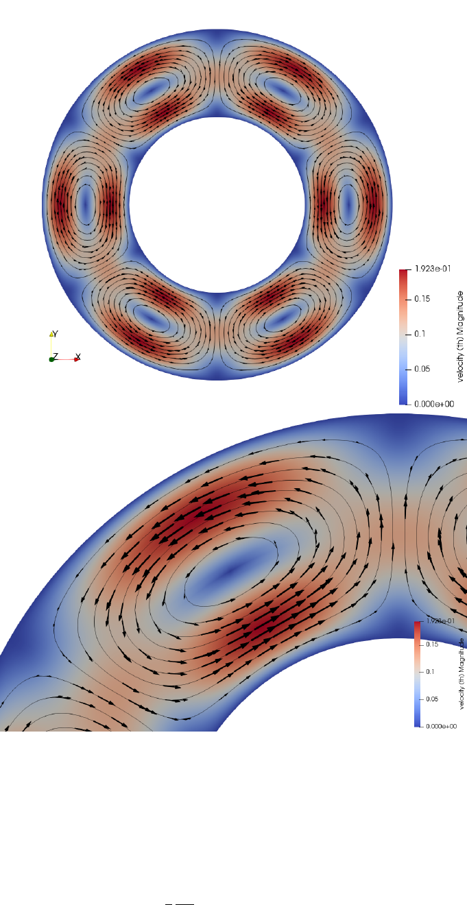
COMPUTE ffrom φand then the pressure.
41.3 Free slip boundary conditions
Before postulating the form of φ(r), let us now turn to the boundary conditions that the flow must fulfill,
i.e. free-slip on both boundaries. Two conditions must be met:
•v·n= 0 (no flow through the boundaries) which yields u(r=R1) = 0 and u(r=R2) = 0, :
1
r
∂Ψ
∂θ (r=R1, R2) = 0 ∀θ
194

which gives us the first constraint since Ψ(r, θ) = φ(r)ξ(θ):
φ(r=R1) = φ(r=R2)=0
•(σ·n)×n=0(the tangential stress at the boundary is zero) which imposes: σθr = 0, with
σθr = 2η·1
2∂v
∂r −v
r+1
r
∂u
∂θ =η∂
∂r (−∂Ψ
∂r )−1
r(−∂Ψ
∂r ) + 1
r
∂
∂θ (1
r
∂Ψ
∂θ )
Finally Ψ must fulfill (on the boundaries!):
−∂2Ψ
∂r2+1
r
∂Ψ
∂r +1
r2
∂2Ψ
∂θ2= 0
−φ00ξ+1
rφ0ξ+1
r2φξ00 = 0
or,
−φ00 +1
rφ0−k21
r2φ= 0
Note that this equation is a so-called Euler Differential Equation17. Since we are looking for a
solution φsuch that φ(R1) = φ(R2) = 0 then the 3rd term of the equation above is by definition
zero on the boundaries. We have to ensure the following equality on the boundary:
−φ00 +1
rφ0= 0 for r=R1, R2
The solution of this ODE is of the form φ(r) = ar2+band it becomes evident that it cannot satisfy
φ(r=R1) = φ(r=R2) = 0.
Separation of variables leads to solutions which cannot fulfill the free slip boundary conditions
17http://mathworld.wolfram.com/EulerDifferentialEquation.html
195
42 fieldstone 36: the annulus geometry elastic aquarium
This fieldstone was developed in collaboration with Lukas van de Wiel.
The domain is an annulus with inner radius R1and outer radius R2. It is filled with a single elastic
material characterised by a Young’s modulus Eand a Poisson ratio ν, a density ρ0. The gravity g=−g0er
is pointing towards the center of the domain.
The problem at hand is axisymmetric so that the tangential component of the displacement vector vθ
is assumed to be zero as well as all terms containing ∂θ. The components of the strain tensor are
εrr =∂vr
∂r (330)
εθθ =vr
r+1
r
∂vθ
∂θ =vr
r(331)
εrθ =1
2∂vθ
∂r −vθ
r+1
r
∂vr
∂θ = 0 (332)
so that the tensor simply is
ε=εrr εrθ
εrθ εθθ =∂vr
∂r 0
0vr
r(333)
The pressure is
p=−λ∇·v=−λ1
r
∂(rvr)
∂r (334)
and finally the stress tensor:
σ=−p1+ 2µε= λ1
r
∂(rvr)
∂r + 2µ∂vr
∂r 0
0λ1
r
∂(rvr)
∂r + 2µvr
r!(335)
The divergence of the stress tensor is given by [416]:
∇·σ=
∂σrr
∂r +σrr −σθθ
r+1
r
∂σθr
∂θ
∂σrθ
∂r +1
r
σθθ
∂θ +σrθ +σθr
r
(336)
Given the diagonal nature of the stress tensor this simplifies to (also remember that ∂θ= 0):
∇·σ=
∂σrr
∂r +σrr −σθθ
r
0
(337)
Focusing on the r-component of the stress divergence:
(∇·σ)r=∂σrr
∂r +σrr −σθθ
r(338)
=∂
∂r λ1
r
∂(rvr)
∂r + 2µ∂vr
∂r +1
rλ1
r
∂(rvr)
∂r + 2µ∂vr
∂r −λ1
r
∂(rvr)
∂r −2µvr
r(339)
=λ∂
∂r
1
r
∂(rvr)
∂r + 2µ∂2vr
∂r2+λ1
r2
∂(rvr)
∂r +2µ
r
∂vr
∂r −λ1
r2
∂(rvr)
∂r −2µvr
r2(340)
=λ(−vr
r2+1
r
∂vr
∂r +∂2vr
∂r2)+2µ∂2vr
∂r2+2µ
r
∂vr
∂r −2µvr
r2(341)
=−(2µ+λ)vr
r2+ (2µ+λ)1
r
∂vr
∂r + (2µ+λ)∂2vr
∂r2(342)
So the momentum conservation in the rdirection is
(∇·σ+ρ0g)r=−(2µ+λ)vr
r2+ (2µ+λ)1
r
∂vr
∂r + (2µ+λ)∂2vr
∂r2−ρ0g0= 0 (343)
196
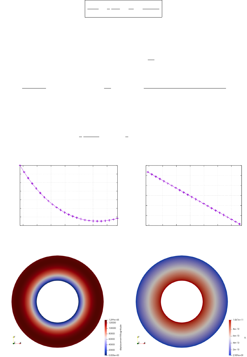
or,
∂2vr
∂r2+1
r
∂vr
∂r −vr
r2=ρ0g0
λ+ 2µ(344)
We now look at the boundary conditions. On the inner boundary we prescribe vr(r=R1) = 0 while free
surface boundary conditions are prescribed on the outer boundary, i.e. σ·n= 0 (i.e. there is no force
applied on the surface).
The general form of the solution can then be obtained:
vr(r) = C1r2+C2r+C3
r(345)
with
C1=ρ0g0
3(λ+ 2µ)C2=−C1R1−C3
R2
1
C3=k1+k2
(R2
1+R2
2)(2µ+λ)+(R2
2−R2
1)λ(346)
and
k1= (2µ+λ)C1(2R2
1R3
2−R3
1R2
2)k2=λC1(R2
1R3
2−R3
1R2
2) (347)
Pressure can then be computed as follows:
p=−λ∇·v=−λ1
r
∂(rvr)
∂r =−λ1
r(3C1r2+ 2C2r)=−λ(3C1r+ 2C2) (348)
We choose R1= 2890km, R2= 6371km, g0= 9.81ms−2,ρ0= 3300, E= 6 ·1010,ν= 0.49.
-140000
-120000
-100000
-80000
-60000
-40000
-20000
0
3x10⁶ 3.5x10⁶ 4x10⁶ 4.5x10⁶ 5x10⁶ 5.5x10⁶ 6x10⁶
radial displacement
r
0
2x10¹⁰
4x10¹⁰
6x10¹⁰
8x10¹⁰
1x10¹¹
1.2x10¹¹
3x10⁶ 3.5x10⁶ 4x10⁶ 4.5x10⁶ 5x10⁶ 5.5x10⁶ 6x10⁶
radial displacement
r
radial profiles of the displacement and pressure fields
displacement and pressure fields in the domain
197
0.000001
0.000100
0.010000
1.000000
100.000000
10000.000000
0.01
error
h
velocity
pressure
x2
x1
198

43 fieldstone 37: marker advection and population control
The domain is a unit square. The Stokes equations are not solved, the velocity is prescribed everywhere
in the domain as follows:
u=−(z−0.5) (349)
v= 0 (350)
w= (x−0.5) (351)
At the moment, velocity is computed on the marker itself (rk0 algorithm). When markers are advected
outside, they are arbitrarily placed at location (-0.0123,-0.0123).
in construction.
199
44 fieldstone 38: Critical Rayleigh number
This fieldstone was developed in collaboration with Arie van den Berg.
The system is a layer of fluid between y= 0 and y= 1, with boundary conditions T(x, y = 0) = 1
and T(x, y = 1) = 0, characterized by ρ,cp,k,η0. The Rayleigh number of the system is
Ra = ρ0g0α∆T h3
η0κ
We have ∆T= 1, h= 1 and choose κ= 1 so that the Rayleigh number simplifies to Ra = ρ0g0α/η0.
The Stokes equation is
∇ · σ+
b=
0 with
b=ρg. Then the components of the this equation on the
x- and y−axis are:
(
∇ · σ)x=−ρg ·ex= 0 (352)
(
∇ · σ)y=−ρg ·ey=ρg0(353)
since g and eyare in opposite directions (g =−g0ey, with g0>0). The stream function formulation of
the incompressible isoviscous Stokes equation is then
∇4Ψ = g0
η0
∂ρ
∂x
Assuming a linearised density field with regards to temperature ρ(T) = ρ0(1 −αT ) we have
∂ρ
∂x =−ρ0α∂T
∂x
and then
∇4Ψ = −ρ0g0α
η0
g∂T
∂x =−Ra ∂T
∂x (354)
For small perturbations of the conductive state T0(y)=1−ywe define the temperature perturbation
T1(x, y) such that
T(x, y) = T0(y) + T1(x, y)
The temperature perturbation T1satisfies the homogeneous boundary conditions T1(x, y = 0) = 0 and
T1(x, y = 1) = 0. The temperature equation is
ρcp
DT
Dt =ρcp∂T
∂t +
ν·
∇T=ρcp∂T0+T1
∂t +
ν·
∇(T0+T1)=k∆(T0+T1)
and can be simplified as follows:
ρcp∂T1
∂t +
ν·
∇T0=k∆T1
since T0does not depend on time, ∆T0= 0 and we assume the nonlinear term
ν·
∇T1to be second
order (temperature perturbations and coupled velocity changes are assumed to be small). Using the
relationship between velocity and stream function vy=−∂xΨ we have v·∇T0=−vy=∂xΨ and since
κ=k/ρcp= 1 we get
∂T1
∂t −κ∆T1=−∂Ψ
∂x (355)
Looking at these equations, we immediately think about a separation of variables approach to solve these
equations. Both equations showcase the Laplace operator ∆, and the eigenfunctions of the biharmonic
operator and the Laplace operator are the same. We then pose that Ψ and T1can be written:
Ψ(x, y, t) = AΨexp(pt) exp(±ikxx) exp(±ikyy) = AΨEψ(x, y, t) (356)
T1(x, y, t) = ATexp(pt) exp(±ikxx) exp(±ikyy) = ATET(x, y, t) (357)
where kxand kyare the horizontal and vertical wave number respectively. Note that we then have
∇2Ψ = −(k2
x+k2
y)Ψ ∇2T1=−(k2
x+k2
y)T1
200

The boundary conditions on T1, coupled with a choice of a real function for the xdependence yields:
ET(x, y, t) = exp(pt) cos(kxx) sin(nπy).
from here onwards check for minus signs!
The velocity boundary conditions are vy(x, y = 0) = 0 and vy(x, y = 1) = 0 which imposes conditions
on ∂Ψ/∂x and we find that we can use the same ydependence as for T1. Choosing again for a real
function for the xdependence yields:
EΨ(x, y, t) = exp(pt) sin(kxx) sin(nπz)
We then have
Ψ(x, y, t) = AΨexp(pt) sin(kxx) sin(nπz) = AΨEψ(x, y, t) (358)
T1(x, y, t) = ATexp(pt) cos(kxx) sin(nπz) = ATET(x, y, t) (359)
In what follows we simplify notations: k=kx. Then the two PDEs become:
pT1+κ(k2+n2π2)−kAΨexp(pt) cos(kxx) sin(nπz) = kAΨEθ(360)
−RaATcos(kx) sin(nπz) + κ(k2+n2π2)2AΨ=−RaATEΨ+κ(k2+n2π2)2AΨ= 0 (361)
These equations must then be verified for all ... which leads to write:
p+ (k2+n2π2)−k
−Ra k (k2+n2π2)2 Aθ
AΨ=0
0
The determinant of such system must be nul otherwise there is only a trivial solution to the problem, i.e.
Aθ= 0 and AΨ= 0 which is not helpful. CHECK/REPHRASE
D= [p+ (k2+n2π2)](k2+n2π2)2−Ra k2= 0
or,
p=Ra k2−(k2+n2π2)3
(k2+n2π2)2
The coefficient pdetermines the stability of the system: if it is negative, the system is stable and both
Ψ and T1will decay to zero (return to conductive state). If p= 0, then the system is meta-stable, and if
p > 0 then the system is unstable and the perturbations will grow. The threshold is then p= 0 and the
solution of the above system is
201
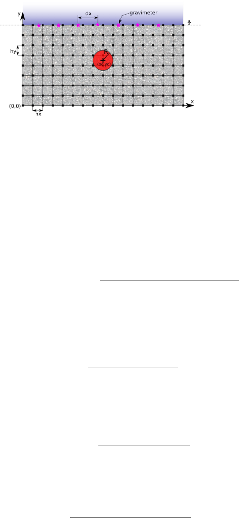
45 fieldstone: Gravity: buried sphere
Before you proceed further, please read :
http://en.wikipedia.org/wiki/Gravity_anomaly
http://en.wikipedia.org/wiki/Gravimeter
Let us consider a vertical domain Lx ×Ly where Lx= 1000km and Ly = 500km. This domain
is discretised by means of a grid which counts nnp =nnx ×nny nodes. This grid then counts nel =
nelx ×nely = (nnx −1) ×(nny −1) cells. The horizontal spacing between nodes is hx and the vertical
spacing is hy.
Assume that this domain is filled with a rock type which mass density is given by ρmedium =
3000kg/m3, and that there is a circular inclusion of another rock type (ρsphere = 3200kg/m3) at lo-
cation (xsphere,ysphere) of radius rsphere. The density in the system is then given by
ρ(x, y) = ρsphere inside the circle
ρmedium outside the circle
Let us now assume that we place nsurf gravimeters at the surface of the model. These are placed
equidistantly between coordinates x= 0 and coordinates x=Lx. We will use the arrays xsurf and ysurf
to store the coordinates of these locations. The spacing between the gravimeters is δx=Lx/(nsurf −1).
At any given point (xi, yi) in a 2D space, one can show that the gravity anomaly due to the presence
of a circular inclusion can be computed as follows:
g(xi, yi)=2πG(ρsphere −ρ0)R2yi−ysphere
(xi−xsphere)2+ (yi−ysphere)2(362)
where rsphere is the radius of the inclusion, (xsphere, ysphere) are the coordinates of the center of the
inclusion, and ρ0is a reference density.
However, the general formula to compute the gravity anomaly at a given point (xi, yi) in space due
to a density anomaly of any shape is given by:
g(xi, yi)=2GZ ZΩ
∆ρ(x, y)(y−yi)
(x−xi)2+ (y−yi)2dxdy (363)
where Ω is the area of the domain on which the integration is to be carried out. Furthermore the density
anomaly can be written : ∆ρ(x, y) = ρ(x, y)−ρ0. We can then carry out the integration for each cell
and sum their contributions:
g(xi, yi)=2G
nel
X
ic=1 Z ZΩe
(ρ(x, y)−ρ0)(y−yi)
(x−xi)2+ (y−yi)2dxdy (364)
where Ωeis now the area of a single cell. Finally, one can assume the density to be constant within each
cell so that ρ(x, y)→ρ(ic) and RRΩedxdy →hx ×hy and then
g(xi, yi) = 2G
nel
X
ic=1
(ρ(ic)−ρ0)(y(ic)−yi)
(x(ic)−xi)2+ (y(ic)−yi)2sxsy(365)
We will then use the array gsurf to store the value of the gravity anomaly measured at each gravimeter
at the surface.
202
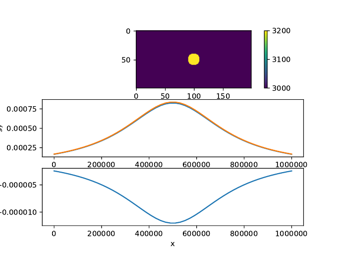
To go further
•explore the effect of the size of the inclusion on the gravity profile.
•explore the effect of the ρ0value.
•explore the effect of the grid resolution.
•measure the time that is required to compute the gravity. How does this time vary with nsurf ?
how does it vary when the grid resolution is doubled ?
•Assume now that ρ2< ρ1. What does the gravity profile look like ?
•what happens when the gravimeters are no more at the surface of the Earth but in a satellite ?
•if you feel brave, redo the whole exercise in 3D...
203

46 Problems, to do list and projects for students
•Darcy flow. redo WAFLE (see http://cedricthieulot.net/wafle.html)
•carry out critical Rayleigh experiments for various geometries/aspect ratios. Use Arie’s notes.
•Newton solver
•Corner flow
•elasticity with markers
•Indentor/punch with stress b.c. ?
•chunk grid
•read in crust 1.0 in 2D on chunk
•compute gravity based on tetrahedra
•compare Q2 with Q2-serendipity
•NS a la http://ww2.lacan.upc.edu/huerta/exercises/Incompressible/Incompressible Ex2.htm
•produce example of mckenzie slab temperature
•write about impose bc on el matrix
•constraints
•discontinuous galerkin
•formatting of code style
•navier-stokes ? (LUKAS) use dohu matlab code
•nonlinear poiseuille
•Finish nonlinear cavity case5.
•write about mappings
•write about stream functions
•periodic boundary conditions
•free surface
•zaleski disk advection
•better yet simple matrix storage ?
•write Scott about matching compressible2 setup with his paper
•deal with large matrices.
•compositions, marker chain
•free-slip bc on annulus and sphere . See for example p540 Gresho and Sani book.
•non-linear rheologies (two layer brick spmw16, tosn15)
•Picard vs Newton
•including phase changes (w. R. Myhill)
•compute strainrate in middle of element or at quad point for punch?
204
•GEO1442 code
•GEO1442 indenter setup in plane ?
•in/out flow on sides for lith modelling
•Fehlberg RK advection
•redo puth17 2 layer experiment
•create stone for layeredflow (see folder one up)
205

A Three-dimensional applications
In the following table I list many papers which showcase high-resolution models of geodynamical processes
(subduction, rifting, mantle flow, plume transport, ...). Given the yearly output of our community and
the long list of journal in which research can be disseminated, this list can not be exhaustive.
Ref. topic resolution
[27] Small-scale sublithospheric convection in the Pacific 448 ×56 ×64
[433] Migration and morphology of subducted slabs in the upper mantle 50 ×50 ×25
[388] Subduction scissor across the South Island of New Zealand 17 ×9×9
[339] Influence of a buoyant oceanic plateau on subduction zones 80 ×40 ×80
[103] Subduction dynamics, origin of Andean orogeny and the Bolivian orocline 96 ×96 ×64
[157] Feedback between rifting and diapirism, ultrahigh-pressure rocks exhumation 100 ×64 ×20
[11] Numerical modeling of upper crustal extensional systems 160 ×160 ×12
[12] Rift interaction in brittle-ductile coupled systems 160 ×160 ×23
[378] Kinematic interpretation of the 3D shapes of metamorphic core complexes 67 ×67 ×33
[271] Role of rheology and slab shape on rapid mantle flow: the Alaska slab edge 960 ×648 ×160
[102] Complex mantle flow around heterogeneous subducting oceanic plates 96 ×96 ×64
[72] Oblique rifting and continental break-up 150 ×50 ×30
[47] Influence of mantle plume head on dynamics of a retreating subduction zone 80 ×40 ×80
[71] Rift to break-up evolution of the Gulf of Aden 83 ×83 ×40
[73] Thermo-mechanical impact of plume arrival on continental break-up 100 ×70 ×20
[104] Subduction and slab breakoff controls on Asian indentation tectonics 96 ×96 ×64
[163] Modeling of upper mantle deformation and SKS splitting calculations 96 ×64 ×96
[411] Backarc extension/shortening, slab induced toroidal/poloidal mantle flow 352 ×80 ×64
[328] Sediment transports in the context of oblique subduction modelling 500 ×164 ×100
[527] Crustal growth at active continental margins 404 ×164 ×100
[301] Dynamics of India-Asia collision 257 ×257 ×33
[499] Strain-partitioning in the Himalaya 256 ×256 ×40
[311] Collision of continental corner from 3-D numerical modeling 500 ×340 ×164
[382] Dependence of mid-ocean ridge morphology on spreading rate 196 ×196 ×100
[162] Mid mantle seismic anisotropy around subduction zones 197 ×197 ×53
[252] Oblique rifting of the Equatorial Atlantic 120 ×80 ×20
[346] Dynamics of continental accretion 256 ×96 ×96
[405] Thrust wedges: infl. of decollement strength on transfer zones 309 ×85 ×149
[91] Asymmetric three-dimensional topography over mantle plumes 500 ×500 ×217
[455] modelled crustal systems undergoing orogeny and subjected to surface processes 96 ×32 ×14
[314] Thermo-mechanical modeling ontinental rifting and seafloor spreading 197 ×197 ×197
206

B Codes in geodynamics
In what follows I make a quick inventory of the main codes of computational geodynamics, for crust,
lithosphere and/or mantle modelling.
in order to find all CIG-codes citations go to: https://geodynamics.org/cig/news/publications-refbase/
•ABAQUS [198] [298] [334] [355] [369]
•ADELI [249] [487] [57] [58] [196] [221] [493] [106]
•ASPECT
This code is hosted by CIG at https://geodynamics.org/cig/software/aspect/
[29] [297] [22] [458] [133] [188] [518] [251] [131] [253] [403] [404] [21] [451] [69] [361] [439] [515] [132]
[363] [223] [254] [189] [368] [379] [68] [31] [434] [122] [320]
•CitcomS and CITCOMCU
These codes are hosted by CIG at https://geodynamics.org/cig/software/citcomcu/ and
https://geodynamics.org/cig/software/citcoms/.
[428] [349] [521] [476] [524] [245] [50] [442] [475] [119] [51] [426] [52] [38] [373] [440] [41] [120] [53]
[523] [332] [525] [28] [401] [351] [118] [222] [187] [522] [258] [313] [18] [517] [15] [176] [87] [82] [484]
[27] [88] [516] [39] [304] [472] [308] [318] [271] [54] [59] [267] [427] [257] [62] [63] [272] [392] [360] [19]
[121] [175] [81] [281] [20] [492] [419] [5] [327] [528] [61] [60] [422] [134] [473] [494] [491] [490] [248]
[444] [309] [498] [497] [326] [179] [250] [256]
cross check with CIG database
•CONMAN This code is hosted by CIG at https://geodynamics.org/cig/software/conman/
[290] [269] [287] [288] [270] [40] [289]
•DOUAR
[66] [454] [510] [67] [323] [352] [499] [356]
•GAIA
•GALE
This code is hosted by CIG at https://geodynamics.org/cig/software/gale/
[168] [49] [126] [378] [19]
ADD:
Cruz, L.; Malinski, J.; Hernandez, M.; Take, A.; Hilley, G. Erosional control of the kinematics of the
Aconcagua fold-and-thrust belt from numerical simulations and physical experiments 2011 Geology
Goyette, S.; Takatsuka, M.; Clark, S.; Mller, R.D.; Rey, P.; Stegman, D.R. Increasing the usability
and accessibility of geodynamic modelling tools to the geoscience community: UnderworldGUI 2008
Visual Geosciences
Li, Y.; Qi, J. Salt-related Contractional Structure and Its Main Controlling Factors of Kelasu
Structural Zone in Kuqa Depression: Insights from Physical and Numerical Experiments 2012
Procedia Engineering
•GTECTON [230] [231] [77] [78] [232] [177] [322] [24] [25] [335]
•ELEFANT
[458] [325] [80] [299] [451] [375]
•ELLIPSIS
[347] [362] [348] [150] [364] [388] [308] [305]
207
•FANTOM
[450] [11] [12] [13] [160] [455] [158] [159]
•FLUIDITY [136] [186]
•the I2(3)E(L)VIS code
[215][216][214] [217][218][212] [86] [75][204][227][208] [205][226] [414][207][462][164][526] [209] [202][357]
[147][149][312][203][211] [123][146][514] [311][354][328][469][468][527][151][210][337] [148][382][405][489][26][315][435][333]
[91][228][26][470] [145][463][406][213][406] [2][329][174]
•LAMEM [414] [282] [300] [340] [301] [117] [170] [169] [380] [171] [116] [283]
•LITMOD [181] [3] [4] [182]
•MILAMIN [130] [511] [193] [324] [194] [448] [275] [336]
•PARAVOZ/FLAMAR [376] [93] [89] [23] [115] [246] [199] [244] [201] [459] [92] [508] [94] [509] [197]
[510] [17] [196] [242] [195] [165] [178] [185] [90] [506] [338] [192] [140]
•PTATIN [370] [1] [341]
•RHEA [95] [430] [9] [96]
•SEPRAN [464] [488] [113] [474] [480] [481] [482] [483] [418] [316] [317] [479] [65] [64] [374] [486] [465]
[437] [477] [466] [42] [109] [16] [110] [350] [467]
•SLIM3D
[377] [396] [72] [73] [71] [70] [252] [294] [114]
•SOPALE
[183] [502] [32] [183] [155] [36] [500] [385] [37] [34] [264] [386] [263] [485] [503] [390] [35] [387] [384]
[156] [191] [190] [266] [383] [421] [265] [128] [345] [420] [495] [496] [284] [33] [79] [234] [425] [8] [7]
[235] [389] [127] [101] [262] [236] [237] [293] [233] [273] [99] [108] [172] [173] [229] [238] [292] [358]
[274] [224] [10] [100] [255] [319] [98]
•STAGYY [402] [512] [124]
•SULEC SULEC is a finite element code that solves the incompressible Navier-Stokes equations for
slow creeping flows. The code is developed by Susan Ellis (GNS Sciences, NZ) and Susanne Buiter
(NGU).
[393] [157] [76] [445] [123] [241] [219] [220] [394] [395] [353] [532] [446]
•TERRA [85] [84] [371] [505] [504] [135] [471]
•the YACC code
[458] [457]
•UNDERWORLD 1&2 [432] [348] [410] [303] [365] [105] [339] [433] [431] [167] [103] [102] [47] [411]
[163] [166] [391] [48] [412] [423] [424] [366] [291] [342]
208
C Matrix properties
C.1 Symmetric matrices
Any symmetric matrix has only real eigenvalues, is always diagonalizable, and has orthogonal eigenvectors.
A symmetric N×Nreal matrix Mis said to be
•positive definite if x ·M·x > 0 for every non-zero vector x of n real numbers. All the eigenvalues
of a Symmetric Positive Definite (SPD) matrix are positive. If A and B are positive definite, then
so is A+B. The matrix inverse of a positive definite matrix is also positive definite. An SPD matrix
has a unique Cholesky decomposition. In other words the matrix Mis positive definite if and only
if there exists a unique lower triangular matrix L, with real and strictly positive diagonal elements,
such that M=LLT(the product of a lower triangular matrix and its conjugate transpose). This
factorization is called the Cholesky decomposition of M.
•positive semi-definite if x ·M·x ≥0
•negative definite if x ·M·x < 0
•negative semi-definite if x ·M·x ≤0
The Stokes linear system K G
GT0·v
p=f
g
is indefinite (i.e. it has positive as well as negative eigenvalues).
A square matrix that is not invertible is called singular or degenerate. A square matrix is singular if
and only if its determinant is 0. Singular matrices are rare in the sense that if you pick a random square
matrix, it will almost surely not be singular.
C.2 Schur complement
From wiki. In linear algebra and the theory of matrices, the Schur complement of a matrix block (i.e.,
a submatrix within a larger matrix) is defined as follows. Suppose A,B,C,Dare respectively p×p,
p×q,q×pand q×qmatrices, and Dis invertible. Let
M=A B
C D
so that Mis a (p+q)×(p+q) matrix. Then the Schur complement of the block Dof the matrix Mis
the p×pmatrix
S=A−B·D−1·C
Application to solving linear equations: The Schur complement arises naturally in solving a system of
linear equations such as
A·x +B·y =
f
C·x +D·y =g
where x,
fare p-dimensional vectors, y,g are q-dimensional vectors, and A,B,C,Dare as above.
Multiplying the bottom equation by B·D−1and then subtracting from the top equation one obtains
(A−B·D−1·C)·x =
f−B·D−1·g
Thus if one can invert Das well as the Schur complement of D, one can solve for x, and then by using the
equation C·x+D·y =g one can solve for y. This reduces the problem of inverting a (p+q)×(p+q) matrix
to that of inverting a p×pmatrix and a q×qmatrix. In practice one needs Dto be well-conditioned in
order for this algorithm to be numerically accurate.
Considering now the Stokes system:
K G
GT−C·v
p =
f
g
209
Factorising for p we end up with a velocity-Schur complement. Solving for p in the second equation
and inserting the expression for p into the first equation we have
Sv·v =
fwith Sv=K+G·C−1·GT
Factorising for v we get a pressure-Schur complement.
Sp·p =GT·K−1·
fwith Sp=GT·K−1·G+C
210
References
[1] pTatin3D: High-Performance Methods for Long-Term Lithospheric Dynamics, 2014.
[2] A. Koptev aand E. Burov, E. Calais, S. Leroy, T. Gerya, L. Guillou-Frottier, and S. Cloetingh.
Contrasted continental rifting via plume-craton interaction: Applications to Central East African
Rift. Geoscience Frontiers, 7:221–236, 2016.
[3] J. C. Afonso, M. Fernandez, G. Ranalli, W.L. Griffin, and J.A.D. Connolly. Integrated geophysical-
petrological modeling of the lithosphere and sublithospheric upper mantle: Methodology and ap-
plications. Geochem. Geophys. Geosyst., 9(5):doi:10.1029/2007GC001834, 2008.
[4] J.C. Afonso, G. Ranalli, and M. Fernandez. Density structure and buoyancy of the oceanic litho-
sphere revisited. Geophys. Res. Lett., 34:L10302, 2007.
[5] R. Agrusta, J. van Hunen, and S. Goes. The effect of metastable pyroxene on the slab dynamics.
Geophys. Res. Lett., 41:8800–8808, 2014.
[6] M. Albers. A local mesh refinement multigrid method for 3D convection problems with strongly
variable viscosity. J. Comp. Phys., 160:126–150, 2000.
[7] M. Albertz and C. Beaumont. An investigation of salt tectonic structural styles in the Scotian Basin,
offshore Atlantic Canada: 2. Comparison of observations with geometrically complex numerical
models. Tectonics, 29(TC4018), 2010.
[8] M. Albertz, C. Beaumont, J.W. Shimeld, S.J. Ingsand, and S. Gradmann. An investigation of salt
tectonic structural styles in the Scotian Basin, offshore Atlantic Canada: Part 1, comparison of
observations with geometrically simple numerical models. Tectonics, 29, 2010.
[9] L. Alisic, M. Gurnis, G. Stadler, C. Burstedde, and O. Ghattas. Multi-scale dynamics and rheology
of mantle flow with plates. J. Geophys. Res., 117:doi:10.1029/2012JB009234, 2012.
[10] J. Allen and C. Beaumont. Continental Margin Syn-Rift Salt Tectonics at Intermediate Width
Margins. Basin Research, page doi: 10.1111/bre.12123, 2014.
[11] V. Allken, R. Huismans, and C. Thieulot. Three dimensional numerical modelling of upper crustal
extensional systems. J. Geophys. Res., 116:B10409, 2011.
[12] V. Allken, R. Huismans, and C. Thieulot. Factors controlling the mode of rift interaction in brittle-
ductile coupled systems: a 3d numerical study. Geochem. Geophys. Geosyst., 13(5):Q05010, 2012.
[13] V. Allken, R.S. Huismans, H. Fossen, and C. Thieulot. 3D numerical modelling of graben interaction
and linkage: a case study of the Canyonlands grabens, Utah. Basin Research, 25:1–14, 2013.
[14] J.D. Anderson. Computational Fluid Dynamics. McGraw-Hill, 1995.
[15] E.R. Andrews and M.I. Billen. Rheologic controls on the dynamics of slab detachment. Tectono-
physics, 464:60–69, 2009.
[16] A. Androvicova, H. ˇ
C´ıˇzkov´a, and A. van den Berg. The effects of rheological decoupling on slab
deformation in the Earth’s upper mantle. Stud. Geophys. Geod., 57:460–481, 2013.
[17] S. Angiboust, S. Wolf, E. Burov, P. Agard, and P. Yamato. Effect of fluid circulation on
subduction interface tectonic processes: Insights from thermo-mechanical numerical modelling.
Earth Planet. Sci. Lett., 357-358:238–248, 2012.
[18] J.J. Armitage, T.J. Henstock, T.A. Minshull, and J.R. Hopper. Lithospheric controls on melt
production during continental breakup at slow rates of extension: Application to the North Atlantic.
Geochem. Geophys. Geosyst., 10(6), 2009.
[19] P.-A. Arrial and M.I. Billen. Influence of geometry and eclogitization on oceanic plateau subduction
.Earth Planet. Sci. Lett., 363:34–43, 2013.
211
[20] P.A. Arrial, N. Flyer, G.B. Wright, and L.H. Kellogg. On the sensitivity of 3-D thermal convection
codes to numerical discretization: a model intercomparison. Geosci. Model Dev., 7:2065–2076, 2014.
[21] J. Austermann, J. X. Mitrovica, P. Huybers, and A. Rovere. Detection of a dynamic topography
signal in last interglacial sea-level records. Science Advances, 3(7):1700457, 2017.
[22] J. Austermann, D. Pollard, J. X. Mitrovica, R. Moucha, A. M. Forte, R. M. DeConto, D. B. Rowley,
and M. E. Raymo. The impact of dynamic topography change on antarctic ice sheet stability during
the mid-pliocene warm period. Geology, 43(10):927–930, 2015.
[23] A.Yu. Babeyko, S.V. Sobolev, R.B. Trumbull, O. Oncken, and L.L. Lavier. Numerical
models of crustal scale convection and partial melting beneath the Altiplano-Puna plateau.
Earth Planet. Sci. Lett., 199:373–388, 2002.
[24] M. Baes, R. Govers, and R. Wortel. Subduction initiation along the inherited weakness zone at the
edge of a slab: Insights from numerical models. Geophys. J. Int., 184:991–1008, 2011.
[25] M. Baes, R. Govers, and R. Wortel. Switching between alternative responses of the lithosphere to
continental collision. Geophys. J. Int., 2011.
[26] B. Baitsch-Ghirardello, Taras V. Gerya, and J.-P. Burg. Geodynamic regimes of intra-oceanic
subduction: Implications for arc extension vs. shortening processes. Gondwana Research, 25:546–
560, 2014.
[27] M.D. Ballmer, G. Ito, J. van Hunen, and P.J. Tackley. Small-scale sublithospheric convection
reconcilies geochemistry and geochronology of ’Superplume’ volcanism in th western and south
pacific. Earth Planet. Sci. Lett., 290:224–232, 2010.
[28] M.D. Ballmer, J. van Hunen, G. Ito, P.J. Tackley, and T.A. Bianco. Non-hotspot vol-
cano chains originating from small-scale sublithospheric convection. Geophys. Res. Lett.,
34(L23310):doi:10.1029/2007GL031636, 2007.
[29] W. Bangerth, R. Hartmann, and G. Kanschat. deal.II - a general purpose object oriented finite
element library. ACM Transaction on mathematical software, 33(4), 2007.
[30] K.-J. Bathe. Finite Element Procedures in Engineering Analysis. Prentice-Hall, 1982.
[31] A. Bauville and T. S. Baumann. geomio: an open-source matlab toolbox to create the initial
configuration of 2d/3d thermo-mechanical simulations from 2d vector drawings. Geochemistry,
Geophysics, Geosystems, 2019.
[32] C. Beaumont, P. Fullsack, and J. Hamilton. Styles of crustal deformation in compressional orogens
caused by subduction of the underlying lithosphere. Tectonophysics, 232:119–132, 1994.
[33] C. Beaumont, R.A. Jamieson, J.P. Butler, and C.J. Warren. Crustal structure: A key constraint
on the mechanism of ultra-high-pressure rock exhumation. Earth Planet. Sci. Lett., 287:116–129,
2009.
[34] C. Beaumont, R.A. Jamieson, M.H. Nguyen, and B. Lee. Himalayan tectonics explained by extru-
sion of a low-viscosity crustal channel coupled to focused surface denudation. Nature, 414:738–742,
2001.
[35] C. Beaumont, R.A. Jamieson, M.H. Nguyen, and S. Medvedev. Crustal channel flows: 1. Numerical
models with applications to the tectonics of the Himalayan-Tibetan orogen. J. Geophys. Res.,
109(B06406), 2004.
[36] C. Beaumont, P.J. Kamp, J. Hamilton, and P. Fullsack. The continental collision zone, south
island, new zealand: comparison of geodynamical models and observations. J. Geophys. Res.,
101:3333–3359, 1996.
[37] C. Beaumont, J.A. Munoz, J. Hamilton, and P. Fullsack. Factors controlling the alpine evolu-
tion of the central pyrenees inferred from a comparison of observations and geodynamical models.
J. Geophys. Res., 105:8121–8145, 2000.
212
[38] T.W. Becker. On the effect of temperature and strain-rate dependent viscosity on global mantle
flow, net rotation, and plate-driving forces. Geophy. J. Int., 167:943–957, 2006.
[39] T.W. Becker and C. Faccenna. Mantle conveyor beneath the Tethyan collisional belt.
Earth Planet. Sci. Lett., 310:453–461, 2011.
[40] T.W. Becker, C. Faccenna, R. O’Connell, and D. Giardini. The development of slabs in the upper
mantle: Insights from numerical and laboratory experiments. J. Geophys. Res., 104(B7):15,207–
15,226, 1999.
[41] T.W. Becker, V. Schulte-Pelkum, D.K. Blackman, J.B. Kellogg, and R.J. O’Connell. Mantle flow
under the western United States from shear wave splitting. Earth Planet. Sci. Lett., 247:235–251,
2006.
[42] A.K. Bengtson and P.E. van Keken. Three-dimensional thermal structure of subduction zones:
effects of obliquity and curvature. Solid Earth, 3:365–373, 2012.
[43] M. Benzi, G.H. Golub, and J. Liesen. Numerical solution of saddle point problems. Acta Numerica,
14:1–137, 2005.
[44] D. Bercovici, G. Schubert, and G.A. Glatzmaier. Three-dimensional convection of an infinite
Prandtl-number compressible fluid in a basally heated spherical shell. J. Fluid Mech., 239:683–
719, 1992.
[45] M. Bercovier and M. Engelman. A finite-element for the numerical solution of viscous incompressible
flows. J. Comp. Phys., 30:181–201, 1979.
[46] M. Bercovier and M. Engelman. A finite-element method for incompressible Non-Newtonian flows.
J. Comp. Phys., 36:313–326, 1980.
[47] P.G. Betts, W.G. Mason, and L. Moresi. The influence of a mantle plume head on the dynamics of
a retreating subduction zone. Geology, 40(8):739–742, 2012.
[48] P.G. Betts, L. Moresi, M.S. Miller, and D. Willis. Geodynamics of oceanic plateau and plume head
accretion and their role in Phanerozoic orogenic systems of China. Geoscience Frontiers, 6:49–59,
2015.
[49] E. Beutel, J. van Wijk, C. Ebinger, D. Keir, and A. Agostini. Formation and stability of magmatic
segments in the Main Ethiopian and Afar rifts. Earth Planet. Sci. Lett., 293:225–235, 2010.
[50] M.I. Billen and M. Gurnis. A low wedge in subduction zones. Earth Planet. Sci. Lett., 193:227–236,
2001.
[51] M.I. Billen and M. Gurnis. Comparison of dynamic flow models for the Central Aleutian and
Tonga-Kermadec subduction zones. Geochem. Geophys. Geosyst., 4(4), 2003.
[52] M.I. Billen and G. Hirth. Newtonian versus non-Newtonian upper mantle viscosity: Implications
for subduction initiation. Geophys. Res. Lett., 32(L19304):doi:10.1029/2005GL023457, 2005.
[53] M.I. Billen and G. Hirth. Rheologic controls on slab dynamics. Geochem. Geophys. Geosyst.,
8(8):doi:10.1029/2007GC001597, 2007.
[54] M.I. Billen and M. Jadamec. Origin of localized fast mantle f low velocity in numerical models of
subduction. Geochem. Geophys. Geosyst., 13(1):doi:10.1029/2011GC003856, 2012.
[55] B. Blankenbach, F. Busse, U. Christensen, L. Cserepes, D. Gunkel, U. Hansen, H. Harder, G. Jarvis,
M. Koch, G. Marquart, D. Moore, P. Olson, H. Schmeling, and T. Schnaubelt. A benchmark
comparison for mantle convection codes. Geophys. J. Int., 98:23–38, 1989.
[56] P. B. Bochev, C. R. Dohrmann, and M. D. Gunzburger. Stabilization of low-order mixed finite
elements for the stokes equations. SIAM J. Numer. Anal., 44(1):82–101, 2006.
213
[57] M.-A. Bonnardot, R. Hassani, and E. Tric. Numerical modelling of lithosphereasthenosphere inter-
action in a subduction zone. Earth Planet. Sci. Lett., 272:698–708, 2008.
[58] M.-A. Bonnardot, R. Hassani, E. Tric, E. Ruellan, and M. Regnier. Effect of margin curvature on
plate deformation in a 3-D numerical model of subduction zones. Geophy. J. Int., 173:1084–1094,
2008.
[59] A.D. Bottrill, J. van Hunen, and M.B. Allen. Insight into collision zone dynamics from topography:
numerical modelling results and observations. Solid Earth, 3:387–399, 2012.
[60] P. Bouilhol, V. Magni, J. van Hunen, and L. Kaislaniemi. A numerical approach to melting in
warm subduction zones. Earth Planet. Sci. Lett., 411:37–44, 2015.
[61] D.J. Bower, M. Gurnis, and N. Flament. Assimilating lithosphere and slab history in 4-D Earth
models. Phys. Earth. Planet. Inter., 238:8–22, 2015.
[62] D.J. Bower, M. Gurnis, and M. Seton. Lower mantle structure from paleogeographically constrained
dynamic Earth models. Geochem. Geophys. Geosyst., 14(1):44–63, 2012.
[63] D.J. Bower, M. Gurnis, and D. Sun. Dynamic origins of seismic wavespeed variation in D”.
Phys. Earth. Planet. Inter., 214:74–86, 2013.
[64] J.P. Brandenburg and P.E. van Keken. Deep storage of oceanic crust in a vigorously convecting
mantle. J. Geophys. Res., 112(B06403), 2007.
[65] J.P. Brandenburg and P.E. van Keken. Methods for thermochemical convection in Earths mantle
with force-balanced plates. Geochem. Geophys. Geosyst., 8(11), 2007.
[66] J. Braun, C. Thieulot, P. Fullsack, M. DeKool, and R.S. Huismans. DOUAR: a new three-
dimensional creeping flow model for the solution of geological problems. Phys. Earth. Planet. Inter.,
171:76–91, 2008.
[67] J. Braun and P. Yamato. Structural evolution of a three-dimensional, finite-width crustal wedge.
Tectonophysics, 484:181–192, doi:10.1016/j.tecto.2009.08.032, 2009.
[68] E. Bredow and B. Steinberger. Variable melt production rate of the kerguelen hotspot due to
long-term plume-ridge interaction. Geophysical Research Letters, 45(1):126–136, 2018.
[69] E. Bredow, B. Steinberger, R. Gassm¨oller, and J. Dannberg. How plume-ridge interaction shapes
the crustal thickness pattern of the r´eunion hotspot track. Geochemistry, Geophysics, Geosystems,
2017.
[70] S. Brune. Evolution of stress and fault patterns in oblique rift systems: 3-D numerical lithospheric-
scale experiments from rift to breakup. Geochem. Geophys. Geosyst., 15:3392–3415, 2014.
[71] S. Brune and J. Autin. The rift to break-up evolution of the Gulf of Aden: Insights from 3D
numerical lithospheric-scale modelling. Tectonophysics, 607:65–79, 2013.
[72] S. Brune, A.A. Popov, and S. Sobolev. Modeling suggests that oblique extension facilitates rifting
and continental break-up. J. Geophys. Res., 117(B08402), 2012.
[73] S. Brune, A.A. Popov, and S. Sobolev. Quantifying the thermo-mechanical impact of plume arrival
on continental break-up. Tectonophysics, 604:51–59, 2013.
[74] H.H. Bui, R. Fukugawa, K. Sako, and S. Ohno. Lagrangian meshfree particles method (SPH) for
large deformation and failure flows of geomaterial using elasticplastic soil constitutive model. Int.
J. Numer. Anal. Geomech., 32(12):1537–1570, 2008.
[75] S. Buiter, A.Y. Babeyko, S. Ellis, T.V. Gerya, B.J.P. Kaus, A. Kellner, G. Schreurs, and Y. Yamada.
The numerical sandbox: comparison of model results for a shortening and an extension experiment.
Analogue and Numerical Modelling of Crustal-Scale Processes. Geological Society, London. Special
Publications, 253:29–64, 2006.
214
[76] S.J.H. Buiter. A review of brittle compressional wedge models. Tectonophysics, 530:1–17, 2012.
[77] S.J.H. Buiter, R. Govers, and M.J.R. Wortel. A modelling study of vertical surface displacements
at convergent plate margins. Geophy. J. Int., 147:415–427, 2001.
[78] S.J.H. Buiter, R. Govers, and M.J.R. Wortel. Two-dimensional simulations of surface deformation
caused by slab detachment. Tectonophysics, 354:195–210, 2002.
[79] S.J.H. Buiter, O.A. Pfiffner, and C. Beaumont. Inversion of extensional sedimentary basins: A
numerical evaluation of the localisation of shortening. Earth Planet. Sci. Lett., 288:492–504, 2009.
[80] S.J.H. Buiter, G. Schreurs, M. Albertz, T.V. Gerya, B. Kaus, W. Landry, L. le Pourhiet, Y. Mishin,
D.L. Egholm, M. Cooke, B. Maillot, C. Thieulot, T. Crook, D. May, P. Souloumiac, and C. Beau-
mont. Benchmarking numerical models of brittle thrust wedges. Journal of Structural Geology,
92:140–177, 2016.
[81] A.L. Bull, M. Domeier, and T.H. Torsvik. The effect of plate motion history on the longevity of
deep mantle heterogeneities. Earth Planet. Sci. Lett., 401:172–182, 2014.
[82] A.L. Bull, A.K. McNamara, T.W. Becker, and J. Ritsema. Global scale models of the mantle flow
field predicted by synthetic tomography models. Phys. Earth. Planet. Inter., 182:129–138, 2010.
[83] P.S. Bullen. Handbook of Means and Their Inequalities. Springer; 2nd edition, 2003.
[84] H.-P. Bunge, M. Richards, C. Lithgow-Bertelloni, J.R. Baumgardner, S.P. Grand, and B. Romanow-
icz. Time scales and heterogeneous structure in geodynamic Earth models. Science, 280:91–95,
1998.
[85] H.-P. Bunge, M.A. Richards, and J.R. Baumgardner. A sensitivity study of three-dimensional
spherical mantle convection at 108Rayleigh number: Effects of depth-dependent viscosity, heating
mode, and endothermic phase change . J. Geophys. Res., 102(B6):11,991–12,007, 1997.
[86] J.-P. Burg and T.V. Gerya. The role of viscous heating in Barrovian metamorphism of collisional
orogens: thermomechanical models and application to the Lepontine Dome in the Central Alps. J.
Metamorphic Geology, 23:75–95, 2005.
[87] E.R. Burkett and M.I. Billen. Dynamics and implications of slab detachment due to ridge-trench
collision. J. Geophys. Res., 114(B12402), 2009.
[88] E.R. Burkett and M.I. Billen. Three-dimensionality of slab detachment due to ridge-trench collision:
Laterally simultaneous boudinage versus tear propagation. Geochem. Geophys. Geosyst., 11(11),
2010.
[89] E. Burov and A.Poliakov. Erosion and rheology controls on synrift and postrift evolution: Verifying
old and new ideas using a fully coupled numerical model. J. Geophys. Res., 106(B8):16,461–16,481,
2001.
[90] E. Burov, T. Francois, P. Agard, L. Le Pourhiet, B. Meyer, C. Tirel, S. Lebedev, P. Yamato, and
J.-P. Brun. Rheological and geodynamic controls on the mechanisms of subduction and HP/UHP
exhumation of crustal rocks during continental collision: Insights from numerical models. Tectono-
physics, 2014.
[91] E. Burov and T. Gerya. Asymmetric three-dimensional topography over mantle plumes. Nature,
513:doi:10.1038/nature13703, 2014.
[92] E. Burov and L. Guillou-Frottier. The plume head-continental lithosphere interaction using a
tectonically realistic formulation for the lithosphere. Geophy. J. Int., 161:469–490, 2005.
[93] E. Burov, L. Jolivet, L. Le Pourhiet, and A. Poliakov. A thermomechanical model of exhumation
of high pressure (HP) and ultra-high pressure (UHP) metamorphic rocks in Alpine-type collision
belts. Tectonophysics, 342:113–136, 2001.
215
[94] E. Burov and G. Toussaint. Surface processes and tectonics: Forcing of continental subduction and
deep processes. Global and Planetary Change, 58:141–164, 2007.
[95] C. Burstedde, O. Ghattas, M. Gurnis, G. Stadler, E. Tan, T. Tu, L.C. Wilcox, and S. Zhong.
Scalable Adaptive Mantle Convection Simulation on Petascale Supercomputers. ACM/IEEE SC
Conference Series, 2008, 2008.
[96] C. Burstedde, G. Stadler, L. Alisic, L.C. Wilcox, E. Tan, M. Gurnis, and O. Ghattas. Large-scale
adaptive mantle convection simulation. Geophy. J. Int., 192:889–906, 2013.
[97] F.H. Busse, U. Christensen, R. Clever, L. Cserepes, C. Gable, E. Giannandrea, L. Guillou, G. House-
man, H.-C. Nataf, M. Ogawa, M. Parmentier, C. Sotin, and B. Travis. 3D convection at infinite
Prandtl number in Cartesian geometry - a benchmark comparison. Geophys. Astrophys. Fluid
Dynamics, 75:39–59, 1993.
[98] J.P. Butler and C. Beaumont. Subduction zone decoupling/retreat modeling explains south
Tibet (Xigaze) and other supra-subduction zone ophiolites and their UHP mineral phases.
Earth Planet. Sci. Lett., 463:101–117, 2017.
[99] J.P. Butler, C. Beaumont, and R.A. Jamieson. The Alps 1: A woring geodynamic model for burial
and exhumation of (ultra)high-pressure rocks in Alpine-type orogens. Earth Planet. Sci. Lett.,
337-378:114–131, 2013.
[100] J.P. Butler, C. Beaumont, and R.A. Jamieson. Paradigm lost: Buoyancy thwarted by the
strength of the Western Gneiss Region (ultra)high-pressure terrane, Norway. Lithosphere, page
doi:10.1130/L426.1, 2015.
[101] J.P. Butler, C. Veaumont, and R.A. Jamieson. Crustal emplacement of exhuming (ultra)high-
pressure rocks: Will that be pro- or retro-side ? Geology, 39:635–638, 2011.
[102] F.A. Capitanio and M. Faccenda. Complex mantle flow around heterogeneous subducting oceanic
plates. Earth Planet. Sci. Lett., 353-354:29–37, 2012.
[103] F.A. Capitanio, C. Faccenna, S. Zlotnik, and D.R. Stegman. Subduction dynamics and the origin
of Andean orogeny and the Bolivian orocline. Nature, 480:doi:10.1038/nature10596, 2011.
[104] F.A. Capitanio and A. Replumaz. Subduction and slab breakoff controls on Asian inden-
tation tectonics and Himalayan western syntaxis formation . Geochem. Geophys. Geosyst.,
14(9):doi:10.1002/ggge.20171, 2013.
[105] F.A. Capitanio, D.R. Stegman, L.N. Moresi, and W. Sharples. Upper plate controls on deep
subduction, trench migrations and deformations at convergent margins. Tectonophysics, 483:80–92,
2010.
[106] N.G. Cerpa, R. Araya, M. Gerbault, and R. Hassani. Relationship between slab dip and topography
segmentation in an oblique subduction zone: Insights from numerical modeling. Geophys. Res. Lett.,
41:10.1002/2015GL064047, 2015.
[107] J.S. Chen, C. Pan, and T.Y.P. Chang. On the control of pressure oscillation in bilinear-displacement
constant-pressure element. Comput. Methods Appl. Mech. Engrg., 128:137–152, 1995.
[108] P. Chenin and C. Beaumont. Influence of offset weak zones on the development of rift basins:
Activation and abandonment during continental extension and breakup. J. Geophys. Res., 118:1–
23, 2013.
[109] M.V. Chertova, T. Geenen, A. van den Berg, and W. Spakman. Using open sidewalls for modelling
self-consistent lithosphere subduction dynamics . Solid Earth, 3:313–326, 2012.
[110] M.V. Chertova, W. Spakman, T. Geenen, A.P. van den Berg, and D.J.J. van Hinsbergen. Under-
pinning tectonic reconstructions of the western Mediterranean region with dynamic slab evolution
from 3-D numerical modeling. J. Geophys. Res., 119:10.1002/ 2014JB011150, 2014.
216
[111] Edmund Christiansen and Knud D. Andersen. Computation of collapse states with von mises type
yield condition. International Journal for Numerical Methods in Engineering, 46:1185–1202, 1999.
[112] Edmund Christiansen and Ole S. Pedersen. Automatic mesh refinement in limit analysis. Interna-
tional Journal for Numerical Methods in Engineering, 50:1331–1346, 2001.
[113] H. Ciskova, J. van Hunen, A.P. van den Berg, and N.J. Vlaar. The inuence of rheological weakening
and yield stress on the interaction of slabs with the 670 km discontinuity. Earth Planet. Sci. Lett.,
199:447–457, 2002.
[114] P.D. Clift, S. Brune, and J. Quinteros. Climate changes control offshore crustal structure at South
China Sea continental margin. Earth Planet. Sci. Lett., 420:66–72, 2015.
[115] S. Cloetingh, E. Burov, F. Beekman, B. Andeweg, P.A.M. Andriessen, D. Garcia-
Castellanos, G. de Vicente, and R. Vegas. Lithospheric folding in Iberia. Tectonics,
21(5):10.1029/2001TC901031, 2002.
[116] M. Collignon, N. Fernandez, and B.J.P. Kaus. Influence of surface processes and initial topography
on lateral fold growth and fold linkage mode. Tectonics, 34:1622–1645, 2015.
[117] M. Collignon, B.J.P. Kaus, D.A. May, and N. fernandez. Influences of surface pro-
cesses on fold growth during 3-D detachment folding. Geochem. Geophys. Geosyst.,
15:doi:10.1002/2014GC005450, 2014.
[118] C.P. Conrad, M.D. Behn, and P.G. Silver. Global mantle flow and the development of seismic
anisotropy: Differences between the oceanic and continental upper mantle. J. Geophys. Res.,
112(B07317), 2007.
[119] C.P. Conrad and M. Gurnis. Seismic tomography, surface uplift, and the breakup of Gondwanaland:
Integrating mantle convection backwards in time. Geochem. Geophys. Geosyst., 4(3), 2003.
[120] C.P. Conrad and C. Lithgow-Bertelloni. Influence of continental roots and asthenosphere on plate-
mantle coupling. Geophys. Res. Lett., 33(L05312), 2006.
[121] C.P. Conrad, B. Steinberger, and T.H. Torsvik. Stability of active mantle upwelling revealed by
net characteristics of plate tectonics. Nature, 498:479, 2013.
[122] G. Corti, R. Cioni, Z. Franceschini, F. Sani, St´ephane Scaillet, P. Molin, I. Isola, F. Mazzarini,
S. Brune, D. Keir, A. Erbello, A. Muluneh, F. Illsley-Kemp, and A. Glerum. Aborted propagation
of the ethiopian rift caused by linkage with the kenyan rift. Nature Communications, 10, 2019.
[123] F. Crameri, H. Schmeling, G.J. Golabek, T. Duretz, R. Orendt, S.J.H. Buiter, D.A. May, B.J.P.
Kaus, T.V. Gerya, and P.J. Tackley. A comparison of numerical surface topography calculations in
geodynamic modelling: an evaluation of the ’sticky air’ method. Geophy. J. Int., 189:38–54, 2012.
[124] F. Crameri and P.J. Tackley. Spontaneous development of arcuate single-sided subduction in global
3-D mantle convection models with a free surface. J. Geophys. Res., 119:doi:10.1002/2014JB010939,
2014.
[125] M. Crouzeix and P.-A. Raviart. Conforming and nonconforming finite element methods for solving
the stationary Stokes equations I. R.A.I.R.O., 7(3):33–75, 1973.
[126] L. Cruz, J. Malinski, A. Wilson, W.A. Take, and G. Hilley. Erosional control of kinematics and
geometry of fold-and-thrust belts imaged in a physical and numerical sandbox. J. Geophys. Res.,
115(B09404):doi:10.1029/2010JB007472, 2010.
[127] C.A. Currie and C. Beaumont. Are diamond-bearing Cretaceous kimberlites related to low-angle
subduction beneath western North America. Earth Planet. Sci. Lett., 303:59–70, 2011.
[128] C.A. Currie, C. Beaumont, and R.S. Huismans. The fate of subducted sediments: a case for backarc
intrusion and underplating. Geology, 35(12):1111–1114, 2007.
217
[129] C. Cuvelier, A. Segal, and A.A. van Steenhoven. Finite Element Methods and Navier-Stokes Equa-
tions. D. Reidel Publishing Company, 1986.
[130] M. Dabrowski, M. Krotkiewski, and D.W. Schmid. Milamin: Matlab based finite element solver
for large problems. Geochem. Geophys. Geosyst., 9(4):Q04030, doi:10.1029/2007GC001719, 2008.
[131] J. Dannberg, Z. Eilon, U. Faul, R. Gassmoeller, P. Moulik, and R. Myhill. The importance of grain
size to mantle dynamics and seismological observations. Geochem. Geophys. Geosyst., 18:3034–3061,
2017.
[132] J. Dannberg and R. Gassm¨oller. Chemical trends in ocean islands explained by plume-slab inter-
action. PNAS, 115(17):4351–4356, 2018.
[133] J. Dannberg and T. Heister. Compressible magma/mantle dynamics: 3-D, adaptive simulations in
ASPECT. Geophy. J. Int., 207:1343–1366, 2016.
[134] J. Dannberg and S.V. Sobolev. Low-buoyancy thermochemical plumes resolve controversy of clas-
sical mantle plume concept. Nature Communications, 6(6960):doi:10.1038/ncomms7960, 2015.
[135] D.R. Davies, J.H. Davies, P.C. Bollada, O. Hassan, K. Morgan, and P. Nithiarasu. A hierarchical
mesh refinement technique for global 3-D spherical mantle convection modelling. Geosci. Model
Dev., 6:1095–1107, 2013.
[136] D.R. Davies, C.R. Wilson, and S.C. Kramer. Fluidity: A fully unstructured anisotropic adaptive
mesh computational modeling framework for geodynamics. Geochem. Geophys. Geosyst., 12(6),
2011.
[137] P. Davy and P. Cobbold. Indentation tectonics in nature and experiment. 1. experiments scaled for
gravity. Bulletin of the Geological Institutions of Uppsala, 14:129–141, 1988.
[138] J. de Frutos, V. John, and J. Novo. Projection methods for incompressible ow problems with
WENO nite difference schemes. J. Comp. Phys., 309:368–386, 2016.
[139] Y. Deubelbeiss and B.J.P. Kaus. Comparison of Eulerian and Lagrangian numerical techniques for
the Stokes equations in the presence of strongly varying viscosity. Phys. Earth Planet. Interiors,
171:92–111, 2008.
[140] A.E. Svartman Dias, L.L. Lavier, and N.W. Hayman. Conjugate rifted margins width and asymme-
try: The interplay between lithospheric strength and thermomechanical processes. J. Geophys. Res.,
120:8672–8700, 2015.
[141] C.R. Dohrmann and P.B. Bochev. A stabilized finite element method for the Stokes problem based
on polynomial pressure projections. Int. J. Num. Meth. Fluids, 46:183–201, 2004.
[142] J. Donea and A. Huerta. Finite Element Methods for Flow Problems. 2003.
[143] J. Donea and A. Huerta. Finite Element Methods for Flow Problems. John Wiley & Sons, 2003.
[144] Jean Donea and Antonio Huerta. Finite Element Methods for Flow Problems. John Wiley & Sons,
2003.
[145] T. Duretz, Ph. Agard, Ph. Yamato, C. Ducassou, E.B. Burov, and T.V. Gerya. Thermo-mechanical
modeling of the obduction process based on the Oman Ophiolite case. Gondwana Research, 2015.
[146] T. Duretz, T.V. Gerya, B.J.P. Kaus, and T.B. Andersen. Thermomechanical modeling of slab
eduction. J. Geophys. Res., 117(B08411), 2012.
[147] T. Duretz, T.V. Gerya, and D.A. May. Numerical modelling of spontaneous slab breakoff and
subsequent topographic response. Tectonophysics, 502:244–256, 2011.
[148] T. Duretz, T.V. Gerya, and W. Spakman. Slab detachment in laterally varying subduction zones:
3-D numerical modeling. Geophys. Res. Lett., 41:1951–1956, 2014.
218
[149] T. Duretz, D.A. May, T.V. Gerya, and P.J. Tackley. Discretization errors and free surface stabilisa-
tion in the finite difference and marker-in-cell method for applied geodynamics: A numerical study.
Geochem. Geophys. Geosyst., 12(Q07004), 2011.
[150] S. Dyksterhuis, P. Rey, R.D. Mueller, and L. Moresi. Effects of initial weakness on rift architecture.
Geological Society, London, Special Publications, 282:443–455, 2007.
[151] D. Dymkova and T. Gerya. Porous fluid flow enables oceanic subduction initiation on Earth.
Geophys. Res. Lett., 2013.
[152] David L. Egholm. A new strategy for discrete element numerical models: 1. Theory. J. Geo-
phys. Res., 112:B05203, doi:10.1029/2006JB004557, 2007.
[153] David L. Egholm, Mike Sandiford, Ole R. Clausen, and Søren B. Nielsen. A new strategy
for discrete element numerical models: 2. Sandbox applications. J. Geophys. Res., 112:B05204,
doi:10.1029/2006JB004558, 2007.
[154] R. Eid. Higher order isoparametric finite element solution of Stokes flow . Applied Mathematics
and Computation, 162:1083–1101, 2005.
[155] S. Ellis, P. Fullsack, and C. Beaumont. Oblique convergence of the crust driven by basal forcing:
implications for length-scales of deformation and strain partitioning in orogens. Geophys. J. Int.,
120:24–44, 1995.
[156] S. Ellis, G. Schreurs, and M. Panien. Comparisons between analogue and numerical models of
thrust wedge development. Journal of Structural Geology, 26:1649–1675, 2004.
[157] S.M. Ellis, T.A. Little, L.M. Wallace, B.R. Hacker, and S.J.H. Buiter. Feedback between rifting
and diapirism can exhume ultrahigh-pressure rocks. Earth Planet. Sci. Lett., 311:427–438, 2011.
[158] Z. Erdos, R.S. huismans, and P. van der Beek. First-order control of syntectonic sedimentation on
crustal-scale structure of mountain belts . J. Geophys. Res., 120:doi:10.1002/2014JB011785, 2015.
[159] Z. Erdos, R.S. Huismans, and P. van der Beek. Control of increased sedimentation on orogenic fold-
and-thrust belt structure - insights into the evolution of the Western Alps. Solid Earth, 10:391–404,
2019.
[160] Z. Erdos, R.S. huismans, P. van der Beek, and C. Thieulot. Extensional inheritance
and surface processes as controlling factors of mountain belt structure. J. Geophys. Res.,
119:doi:10.1002/2014JB011408, 2014.
[161] E. Erturk. Discussions on Driven Cavity Flow. Int. J. Num. Meth. Fluids, 60:275–294, 2009.
[162] M. Faccenda. Mid mantle seismic anisotropy around subduction zones. Phys. Earth. Planet. Inter.,
227:1–19, 2014.
[163] M. Faccenda and F.A. Capitanio. Seismic anisotropy around subduction zones: Insights from three-
dimensional modeling of upper mantle deformation and SKS splitting calculations . Geochem. Geo-
phys. Geosyst., 14(1):doi:10.1029/2012GC004451, 2013.
[164] M. Faccenda, T.V. Gerya, and S. Chakraborty. Styles of post-subduction collisional orogeny:
Influence of convergence velocity, crustal rheology and radiogenic heat production. Lithos, 103:257–
287, 2008.
[165] M. Faccenda, T.V. Gerya, N.S. Mancktelow, and L. Moresi. Fluid flow during slab unbending
and dehydration: Implications for intermediate-depth seismicity, slab weakening and deep water
recycling. Geochem. Geophys. Geosyst., 13(1):doi:10.1029/2011GC003860, 2012.
[166] R.J. Farrington, L.-N. Moresi, and F.A. Capitanio. The role of viscoelasticity in subducting plates.
Geochem. Geophys. Geosyst., 15:4291–4304, 2014.
[167] R.J. Farrington, D.R. Stegman, L.N. Moresi, M. Sandiford, and D.A. May. Interactions of 3D
mantle flow and continental lithosphere near passive margins. Tectonophysics, 483:20–28, 2010.
219
[168] N.P. Fay, R.A. Bennett, J.C. Spinler, and E.D. Humphreys. Small-scale upper mantle convection
and crustal dynamics in southern California. Geochem. Geophys. Geosyst., 9(8), 2008.
[169] N. Fernandez and B. Kaus. Influence of pre-existing salt diapirs on 3D folding patterns . Tectono-
physics, 637:354–369, 2014.
[170] N. Fernandez and B. Kaus. Fold interaction and wavelength selection in 3D models of multilayer
detachment folding. Tectonophysics, 632:199–217, 2014.
[171] N. Fernandez and B. Kaus. Pattern formation in 3-D numerical models of down-built diapirs
initiated by a RayleighTaylor instability. Geophy. J. Int., 202:1253–1270, 2015.
[172] C. Fillon, R.S. Huismans, and P. van der Beek. Syntectonic sedimentation effects on the growth of
fold-and-thrust belts . Geology, 41(1):83–86, 2013.
[173] C. Fillon, R.S. Huismans, P. van der Beek, and J.A. Mu noz. Syntectonic sedimentation controls
on the evolution of the southern Pyrenean fold-and-thrust belt: Inferences from coupled tectonic-
surface processes models. J. Geophys. Res., 118:5665–5680, 2013.
[174] R. Fischer and T. Gerya. Early Earth plume-lid tectonics: A high-resolution 3D numerical modelling
approach. Journal of Geodynamics, 100:198–214, 2016.
[175] N. Flament, M. Gurnis, S. Williams, M. Seton, J. Skogseid, C. Heine, and D. M¨uller. Topographic
asymmetry of the South Atlantic from global models of mantle flow and lithospheric stretching.
Earth Planet. Sci. Lett., 387:107–119, 2014.
[176] B.J. Foley and T.W. Becker. Generation of plate-like behavior and mantle hetero-
geneity from a spherical, viscoplastic convection model. Geochem. Geophys. Geosyst.,
10(8):doi:10.1029/2009GC002378, 2009.
[177] R. De Franco, R. Govers, and R. Wortel. Numerical comparison of different convergent plate
contacts: subduction channel and subduction fault. Geophy. J. Int., pages doi: 10.1111/j.1365–
246X.2006.03498.x, 2006.
[178] T. Francois, E. Burov, P. Agard, and B. Meyer. Buildup of a dynamically supported orogenic
plateau: Numerical modeling of the Zagros/Central Iran case study. Geochem. Geophys. Geosyst.,
15:doi:10.1002/ 2013GC005223, 2014.
[179] R. Freeburn, P. Bouilhol, B. Maunder, V. Magni, and J. van Hunen. Numerical models of the
magmatic processes induced by slab breakoff. Earth Planet. Sci. Lett., 478:203–213, 2017.
[180] P.J. Frey and P.-L. George. Mesh generation. Hermes Science, 2000.
[181] J. Fullea, J.C. Afonso, J.A.D. Connolly, M. Fernandez, D. Garcia-Castellanos, and H. Zeyen. Lit-
Mod3D: An interactive 3-D software to model the thermal, compositional, density, seismological,
and rheological structure of the lithosphere and sublithospheric upper mantle. Geochem. Geo-
phys. Geosyst., 10(8):doi:10.1029/2009GC002391, 2009.
[182] J. Fullea, M. Fernandez, J.C. Afonso, J. Verges, and H. Zeyen. iThe structure and evolution of the
lithosphereasthenosphere boundary beneath the AtlanticMediterranean Transition Region. Lithos,
2010.
[183] P. Fullsack. An arbitrary Lagrangian-Eulerian formulation for creeping flows and its application in
tectonic models. Geophy. J. Int., 120:1–23, 1995.
[184] M. Furuichi and D. Nishiura. Robust coupled fluid-particle simulation scheme in Stokes-flow
regime: Toward the geodynamic simulation including granular media. Geochem. Geophys. Geosyst.,
15:2865–2882, 2014.
[185] J. Ganne, M. Gerbault, and S. Block. Thermo-mechanical modeling of lower crust exhumationCon-
straints from the metamorphic record of the Palaeoproterozoic Eburnean orogeny, West African
Craton. Precambrian Research, 243:88–109, 2014.
220
[186] F. Garel, S. Goes, D.R. Davies, J.H. Davies, S.C. Kramer, and C.R. Wilson. Interaction of sub-
ducted slabs with the mantle transition-zone: A regime diagram from 2-D thermo-mechanical
models with a mobile trench and an overriding plate. Geochem. Geophys. Geosyst., 15(1739–
1765):doi:10.1002/2014GC005257, 2014.
[187] E.J. Garnero and A.K. McNamara. Structure and Dynamics of Earths Lower Mantle. Science,
320:626–628, 2008.
[188] R. Gassm¨oller, J. Dannberg, E. Bredow, B. Steinberger, and T. H. Torsvik. Major influence
of plume-ridge interaction, lithosphere thickness variations, and global mantle flow on hotspot
volcanism-the example of tristan. Geochem. Geophys. Geosyst., 17(4):1454–1479, 2016.
[189] R. Gassm¨oller, H. Lokavarapu, E. M. Heien, E. G. Puckett, and W. Bangerth. Flexible and
scalable particle-in-cell methods with adaptive mesh refinement for geodynamic computations.
Geochem. Geophys. Geosyst., 19(9):3596–3604, 2018.
[190] L. Gemmer, C. Beaumont, and S. Ings. Dynamic modelling of passive margin salt tectonics: effects
of water loading, sediment properties and sedimentation patterns. Basin Research, 17:383–402,
2005.
[191] L. Gemmer, S.J. Ings, S. Medvedev, and C. Beaumont. Salt tectonics driven by differential sediment
loading: stability analysis and finite-element experiments. Basin Research, 16:199–218, 2004.
[192] L. Geoffroy, E.B. Burov, and P. Werner. Volcanic passive margins: another way to break up
continents. Scientific Reports, 5:DOi:10.1038/srep14828, 2015.
[193] M. Gerault, T.W. Becker, B.J.P. Kaus, C. Faccenna, L. Moresi, and L. Husson. The role of slabs
and oceanic plate geometry in the net rotation of the lithosphere, trench motions, and slab return
flow. Geochem. Geophys. Geosyst., 13(4):Q04001, doi:10.1029/2011GC003934, 2012.
[194] M. G´erault, L. Husson, M.S. Miller, and E.D. Humphreys. Flat-slab subduction, topography, and
mantle dynamics in southwestern Mexico. Tectonics, 34:10.1002/2015TC003908, 2015.
[195] M. Gerbault. Pressure conditions for shear and tensile failure around a circular magma chamber;
insight from elasto-plastic modelling. Geological Society, London, Special Publications, 367:111–130,
2012.
[196] M. Gerbault, F. Cappa, and R. Hassani. Elasto-plastic and hydromechanical mod-
els of failure around an infinitely long magma chamber. Geochem. Geophys. Geosyst.,
13(3):doi:10.1029/2011GC003917, 2012.
[197] M. Gerbault, J. Cembrano, C. Mpodozis, M. Farias, and M. Pardo. Continental margin deforma-
tion along the Andean subduction zone: Thermo-mechanical models. Phys. Earth. Planet. Inter.,
177:180–205, 2009.
[198] M. Gerbault, F. Davey, and S. Henrys. Three-dimensional lateral crustal thickening in continental
oblique collision: an example from the Southern Alps, New Zealand. Geophy. J. Int., 150:770–779,
2002.
[199] M. Gerbault, S. Henrys, and F. Davey. Numerical models of lithospheric deformation forming the
Southern Alps of New Zealand. J. Geophys. Res., 108(B7), 2003.
[200] M. Gerbault, A.N.B. Poliakov, and M. Daignieres. Prediction of faulting from the theories of
elasticity and plasticity: what are the limits? Journal of Structural Geology, 20:301–320, 1998.
[201] M. Gerbault and W. Willingshofer. Lower crust indentation or horizontal ductile flow during
continental collision? Tectonophysics, 387:169–187, 2004.
[202] T. Gerya. Dynamical instability produces transform faults at mid-ocean ridges. Science, 329:1047–
1050, 2010.
[203] T. Gerya. Future directions in subduction modeling. Journal of Geodynamics, 52:344–378, 2011.
221
[204] T. Gerya and B. St¨ockhert. Two-dimensional numerical modeling of tectonic and metamorphic
histories at active continental margins. Int J Earth Sci (Geol Rundsch), 95:250–274, 2006.
[205] T. Gerya and D.A. Yuen. Robust characteristics method for modelling multiphase visco-elasto-
plastic thermo-mechanical problems. Phys. Earth. Planet. Inter., 163:83–105, 2007.
[206] Taras Gerya. Numerical Geodynamic Modelling. Cambridge University Press, 2010.
[207] T.V. Gerya, J.A.D. Connolly, and D.A. Yuen. Why is terrestrial subduction one-sided ? Geology,
36(1):43–46, 2008.
[208] T.V. Gerya, J.A.D. Connolly, D.A. Yuen, W. Gorczyk, and A.M. Capel. Seismic implications of
mantle wedge plumes. Phys. Earth. Planet. Inter., 156:59–74, 2006.
[209] T.V. Gerya, D. Fossati, C. Cantieni, and D. Seward. Dynamic effects of aseismic ridge subduction:
numerical modelling. Eur. J. Mineral, 21:649–661, 2009.
[210] T.V. Gerya, D.A. May, and T. Duretz. An adaptive staggered grid finite difference method for
modeling geodynamic Stokes flows with strongly variable viscosity. Geochem. Geophys. Geosyst.,
14(4), 2013.
[211] T.V. Gerya and F.I. Meilick. Geodynamic regimes of subduction under an active margin: effects
of rheological weakening by fluids and melts. Journal of Metamorphic Geology, 29:7–31, 2011.
[212] T.V. Gerya, L.L. Perchuk, W.V. Maresch, and A.P. Willner. Inherent gravitational instability of
hot continental crust: Implications for doming and diapirism in granulite facies terrains. Geological
Society of America, 380:97–115, 2004.
[213] T.V. Gerya, R.J. Stern, M.Baes, S.V. Sobolev, and S.A. Whattam. Plate tectonics on the Earth
triggered by plume-induced subduction initiation. Nature, 527, 2015.
[214] T.V. Gerya, R. Uken, J. Reinhardt, M. Watkeys, W.V. Maresch, and B.M. Clarke. Cold fingers in
a hot magma: Numerical modeling of country-rock diapirs in the Bushveld Complex, South Africa.
Geology, 31(9):753–756, 2003.
[215] T.V. Gerya and D.A. Yuen. Characteristics-based marker-in-cell method with conservative finite-
differences schemes for modeling geological flows with strongly variable transport properties.
Phys. Earth. Planet. Inter., 140:293–318, 2003.
[216] T.V. Gerya and D.A. Yuen. Rayleigh-Taylor instabilities from hydration and melting propel ’cold
plumes’ at subduction zones. Earth Planet. Sci. Lett., 212:47–62, 2003.
[217] T.V. Gerya, D.A. Yuen, and W.V. Maresch. Thermomechanical modelling of slab detachment.
Earth Planet. Sci. Lett., 226:101–116, 2004.
[218] T.V. Gerya, D.A. Yuen, and E.O.D. Sevre. Dynamical causes for incipient magma chambers above
slabs. Geology, 32(1):89–92, 2004.
[219] R.K. Ghazian and S.J.H. Buiter. A numerical investigation of continental collision styles. GJI,
2013.
[220] R.K. Ghazian and S.J.H. Buiter. Numerical modelling of the role of salt in continental collision:
An application to the southeast Zagros fold-and-thrust belt. Tectonophysics, in press, 2014.
[221] G. Gibert, M. Gerbault, R. Hassani, and E. Tric. Dependency of slab geometry on absolute velocities
and conditions for cyclicity: insights from numerical modelling. Geophy. J. Int., 189:747–760, 2012.
[222] E. Di Giuseppe, J. van Hunen, F. Funiciello, C. Faccenna, and D. Giardini. Slab stiffness control
of trench motion: Insights from numerical models. Geochem. Geophys. Geosyst., 9(2), 2008.
[223] A. Glerum, C. Thieulot, M. Fraters, C. Blom, and W. Spakman. Nonlinear viscoplasticity in
ASPECT: benchmarking and applications to subduction. Solid Earth, 9:267–294, 2018.
222
[224] Oguz H. Gogus. Rifting and subsidence following lithospheric removal in continental back arcs.
Geology, page doi:10.1130/G36305.1, 2014.
[225] G.H. Golub and C.F. van Loan. Matrix Computations, 4th edition. John Hopkins University Press,
2013.
[226] W. Gorczyk, T.V. Gerya, J.A.D. Connolly, and D.A. Yuen. Growth and mixing dynamics of mantle
wedge plumes. Geology, 35(7):587–590, 2007.
[227] W. Gorczyk, T.V. Gerya, J.A.D. Connolly, D.A. Yuen, and M. Rudolph. Large-scale rigid-body
rotation in the mantle wedge and its implications for seismic tomography . Geochem. Geo-
phys. Geosyst., 7(5):10.1029/2005GC001075, 2006.
[228] W. Gorczyk, H. Smithies, F. Korhonen, H. Howard, and R. Quentin De Gromard. Ultra-hot
Mesoproterozoic evolution of intracontinental central Australia. Geoscience Frontiers, 6(1):23–37,
2014.
[229] R. Goteti, C. Beaumont, and S.J. Ings. Factors controlling early stage salt tectonics at rifted
continental margins and their thermal consequences. J. Geophys. Res., 117:1–31, 2013.
[230] R. Govers and M.J.R. Wortel. Extension of stable continental lithosphere and the initiation of
lithospheric scale faults. Tectonics, 14(4):1041–1055, 1995.
[231] R. Govers and M.J.R. Wortel. Some remarks on the relation between vertical motions of the
lithosphere during extension and the necking depth parameter inferred from kinematic modeling
studies. J. Geophys. Res., 104:23,245–23,253, 1999.
[232] R. Govers and M.J.R. Wortel. Lithosphere tearing at STEP faults: Response to edges of subduction
zones . Earth Planet. Sci. Lett., 236:505–523, 2005.
[233] S. Gradmann and C. Beaumont. Coupled fluid flow and sediment deformation in margin-scale salt-
tectonic systems: 2. Layered sediment models and application to the northwestern Gulf of Mexico.
Tectonics, 31(TC4011), 2012.
[234] S. Gradmann, C. Beaumont, and M. Albertz. Factors controlling the evolution of the Perdido Fold
Belt, northwestern Gulf of Mexico, determined from numerical models. Tectonics, 28(TC2002),
2009.
[235] R. Gray and R.N. Pysklywec. Geodynamic models of Archean continental collision and the forma-
tion of mantle lithosphere keels. Geophys. Res. Lett., 37(L19301), 2010.
[236] R. Gray and R.N. Pysklywec. Geodynamic models of mature continental collision: Evolution of
an orogen from lithospheric subduction to continental retreat/delamination. J. Geophys. Res.,
117(B03408), 2012.
[237] R. Gray and R.N. Pysklywec. Influence of sediment deposition on deep lithospheric tectonics.
Geophys. Res. Lett., 39(L11312), 2012.
[238] R. Gray and R.N. Pysklywec. Influence of viscosity pressure dependence on deep lithospheric
tectonics during continental collision. J. Geophys. Res., 118, 2013.
[239] P.M. Gresho and R.L. Sani. Incompressible flow and the Finite Element Method, vol II. John Wiley
and Sons, Ltd, 2000.
[240] D. Griffiths and D. Silvester. Unstable modes of the q1-p0 element. Technical Report 257, University
of MAnchester/UMIST, 1994.
[241] S.G. Grigull, S.M. Ellis, T.A. Little, M.P. Hill, and S.J.H. Buiter. Rheological constraints on
quartz derived from scaling relationships and numerical models of sheared brittle-ductile quartz
veins, central Southern alps, New Zealand. Journal of Structural Geology, 37:200–222, 2012.
223
[242] L. Guillou-Frottier, E. Burov, S. Cloetingh, E. Le Goff, Y. Deschamps, B. Huet, and V. Bou-
chot. Plume-induced dynamic instabilities near cratonic blocks: Implications for PTt paths and
metallogeny. Global and Planetary Change, 90-91:37–50, 2012.
[243] M. Gunzburger. Finite Element Methods for Viscous Incompressible Flows: A Guide to Theory,
Practice and Algorithms. Academic, Boston, 1989.
[244] M. Gurnis, C. Hall, and L. Lavier. Evolving force balance during incipient subduction.
Geochem. Geophys. Geosyst., 5(7), 2004.
[245] M. Gurnis, J.X. Mitrovica, J. Ritsema, and H.-J. van Heijst. Constraining mantle density structure
using geological evidence of surface uplift rates: The case of the African superplume. Geochem. Geo-
phys. Geosyst., 1, 2000.
[246] C.E. Hall, M. Gurnis, M. Sdrolias, L.L. Lavier, and R.D. Mueller. Catastrophic initiation of
subduction following forced convergence across fracture zones. Earth Planet. Sci. Lett., 212:15–30,
2003.
[247] D.L. Hansen. A meshless formulation for geodynamic modeling. J. Geophys. Res.,
108:doi:10.1029/2003JB002460, 2003.
[248] R. Hassan, N. Flament, M. Gurnis, D.J. Bower, and D. M´uller. Provenance of plumes in global
convection models. Geochem. Geophys. Geosyst., 16:1465–1489, 2015.
[249] R. Hassani, D. Jongmans, and Jean Ch´ery. Study of plate deformation and stress in subduction
processes using two-dimensional numerical models. J. Geophys. Res., 102(B8):17,951–17,96, 1997.
[250] K.L. Haynie and M.A. Jadamec. Tectonic drivers of the Wrangell block: Insights on fore-arc sliver
processes from 3-D geodynamic models of Alaska. Tectonics, 36, 2017.
[251] Y. He, E.G. Puckett, and M.I. Billen. A discontinuous Galerkin method with a bound preserving
limiter for the advection of non-diffusive fields in solid Earth geodynamics. Phys. Earth. Planet. In-
ter., 263:23–37, 2017.
[252] C. Heine and S. Brune. Oblique rifting of the Equatorial Atlantic: Why there is no Saharan Atlantic
Ocean. Geology, 42(3):211–214, 2014.
[253] T. Heister, J. Dannberg, R. Gassm¨oller, and W. Bangerth. High Accuracy Mantle Convection
Simulation through Modern Numerical Methods. II: Realistic Models and Problems. Geophy. J. Int.,
210(2):833–851, 2017.
[254] P. J. Heron, R. N. Pysklywec, R. Stephenson, and J. van Hunen. Deformation driven by deep and
distant structures: Influence of a mantle lithosphere suture in the ouachita orogeny, southeastern
united states. Geology, 2018.
[255] P.J. Heron, R.N. Pysklywec, and R. Stephenson. Intraplate orogenesis within accreted and scarred
lithosphere: Example of the Eurekan Orogeny, Ellesmere Island. Tectonophysics, 2015.
[256] B.H. Heyn, C.P. Conrad, and R.G. Tronnes. Stabilizing Effect of Compositional Viscosity Contrasts
on Thermochemical Piles. Geophys. Res. Lett., 45:7523–7532, 2018.
[257] J.M. Hines and M.I. Billen. Sensitivity of the short- to intermediate-wavelength geoid to rheologic
structure in subduction zones. J. Geophys. Res., 117(B05410), 2012.
[258] T. H¨oink and A. Lenardic. Three-dimensional mantle convection simulations with a low-viscosity
asthenosphere and the relationship between heat flow and the horizontal length scale of convection.
Geophys. Res. Lett., 35(L10304), 2008.
[259] T.J.R. Hughes. The Finite Element Method. Linear Static and Dynamic Finite Element Analysis.
Dover Publications, Inc., 2000.
[260] T.J.R. Hughes, W.K. Liu, and A. Brooks. Finite element analysis of Incompressible viscous flows
by the penalty function formulation. J. Comp. Phys., 30:1–60, 1979.
224
[261] Hoon Huh, Choong Ho Lee, and Wei H. Yang. A general algorithm for plastic flow simulation by
finite element limit analysis. International Journal of Solids and Structures, 36:1193–1207, 1999.
[262] R. Huismans and C. Beaumont. Depth-dependent extension, two-stage breakup and cratonic un-
derplating at rifted margins. Nature, 473:74–79, 2011.
[263] R. S. Huismans and C. Beaumont. Symmetric and asymmetric lithospheric extension:
Relative effects of frictional-plastic and viscous strain softening. J. Geophys. Res., 108
(B10)(2496):doi:10.1029/2002JB002026, 2003.
[264] R.S. Huismans and C. Beaumont. Complex rifted continental margins explained by dynamical
models of depth-dependent lithospheric extension. Geology, 30(3):211–214, 2002.
[265] R.S. Huismans and C. Beaumont. Roles of lithospheric strain softening and heterogeneity in de-
termining the geometry of rifts and continental margins. In Imaging, Mapping and Modelling
Continental Lithosphere Extension and Breakup, volume 282, pages 111–138. Geological Society,
London, Special Publications, 2007.
[266] R.S. Huismans, S.J.H. Buiter, and C. Beaumont. Effect of plastic-viscous layering and strain
softening on mode selection during lithospheric extension. J. Geophys. Res., 110:B02406, 2005.
[267] L. Husson, C.P. Conrad, and C. Faccenna. Plate motions, Andean orogeny, and volcanism above
the South Atlantic convection cell. Earth Planet. Sci. Lett., 317-318:126–135, 2012.
[268] Alik Ismail-Zadeh and Paul Tackley. Computational Methods for Geodynamics. Cambridge Uni-
versity Press, 2010.
[269] J. Ita and S.D. King. Sensitivity of convection with an endothermic phase change to the form of gov-
erning equations, initial conditions, boundary conditions, and equation of state. J. Geophys. Res.,
99(B8):15,919–15,938, 1994.
[270] J. Ita and S.D. King. The influence of thermodynamic formulation on simulations of subduction
zone geometry and history. Geophys. Res. Lett., 25(9):1463–1466, 1998.
[271] M.A. Jadamec and M.I. Billen. The role of rheology and slab shape on rapid mantle flow: Three-
dimensional numerical models of the Alaska slab edge. J. Geophys. Res., 117(B02304), 2012.
[272] M.A. Jadamec, M.I. Billen, and S.M. Roeske. Three-dimensional numerical models of flat slab sub-
duction and the Denali fault driving deformation in south-central Alaska. Earth Planet. Sci. Lett.,
376:29–42, 2013.
[273] S. Jammes and R.S. Huismans. Structural styles of mountain building: Controls of lithospheric
rheologic stratification and extensional inheritance. J. Geophys. Res., 117, 2012.
[274] S. Jammes, R.S. Huismans, and J.A. Mu˜noz. Lateral variation in structural style of mountain
building: controls of rheological and rift inheritance. Terra Nova, 0:doi:10.1111/ter.12087, 2013.
[275] Y. Jaquet, Th. Duretz, and S.M. Schmalholz. Dramatic effect of elasticity on thermal softening
and strain localization during lithospheric shortening. Geophy. J. Int., 204:780–784, 2016.
[276] G.T. Jarvis. Effects of curvature on two-dimensional models of mantle convection: cylindrical polar
coordinates. J. Geophys. Res., 98(B3):4477–4485, 1993.
[277] C. Jaupart and J.-C. Mareschal. Heat Generation and Transport in the Earth. Cambridge, 2011.
[278] V. John. Finite Element Methods for Incompressible Flow Problems . Springer, 2016.
[279] L. Jolivet, P. Davy, and P. Cobbold. Right-lateral shear along the Northwest Pacific margin and
the India-Eurasia collision. Tectonics, 9(6):1409–1419, 1990.
[280] L.M. Kachanov. Fundamentals of the Theory of Plasticity. Dover Publications, Inc., 2004.
225
[281] L. Kaislaniemi and J. van Hunen. Dynamics of lithospheric thinning and mantle melting by
edge-driven convection: Application to Moroccan Atlas mountains. Geochem. Geophys. Geosyst.,
15:3175–3189, 2014.
[282] B.J.P. Kaus, H. M¨uhlhaus, and D.A. May. A stabilization algorithm for geodynamic numerical
simulations with a free surface. Phys. Earth. Planet. Inter., 181:12–20, 2010.
[283] B.J.P. Kaus, A.A. Popov, T.S. Baumann, A.E. Pusok, A. Bauville, N. Fernandez, and M. Col-
lignon. Forward and Inverse Modelling of Lithospheric Deformation on Geological Timescales. NIC
Symposium 2016, pages 299–307, 2016.
[284] D.F. Keppie, C.A. Currie, and C. Warren. Subduction erosion modes: comparing finite element
numerical models with the geological record. Earth Planet. Sci. Lett., 287:241–254, 2009.
[285] M. Kimmritz and M. Braack. iDiscretization of the hydrostatic Stokes system by stabilized finite
elements of equal order.
[286] S. King, C. Lee, P. van Keken, W. Leng, S. Zhong, E. Tan, N. Tosi, and M. Kameyama. A commu-
nity benchmark for 2D Cartesian compressible convection in the Earths mantle. Geophy. J. Int.,
180:7387, 2010.
[287] S.D. King and D.L. Anderson. An alternative mechanism of flood basalt formation.
Earth Planet. Sci. Lett., 136:269–279, 1995.
[288] S.D. King and D.L. Anderson. Edge-driven convection. Earth Planet. Sci. Lett., 160:289–296, 1998.
[289] S.D. King, D.J. Frost, and D.C. Rubie. Why cold slabs stagnate in the transition zone. Geology,
page doi:10.1130/G36320.1, 2015.
[290] S.D. King, A. Raefsky, and B.H. Hager. ConMan: Vectorizing a finite element code for incompress-
ible two-dimensional convection in the Earths mantle. Phys. Earth. Planet. Inter., 59:195–208,
1990.
[291] A. Kiraly, F.A. Capitanio, F. Funiciello, and C. Faccenna. Subduction zone interaction: Controls
on arcuate belts. Geology, 2016.
[292] Erik A. Kneller, Markus Albertz, Garry D. Karner, , and Christopher A. Johnson. Testing inverse
kinematic models of paleocrustal thickness in extensional systems with high- resolution forward
thermo-mechanical models. Geochem. Geophys. Geosyst., 2013.
[293] T. Komut, R. Gray, R. Pysklywec, and O. Gogus. Mantle flow uplift of western Anatolia and the
Aegean: Interpretation from geophysical analyses and geodynamic modeling. J. Geophys. Res.,
117(B11412), 2012.
[294] H. Koopmann, S. Brune, D. Franke, and S. Breuer. Linking rift propagation barriers to excess
magmatism at volcanic rifted margins. Geology, page doi:10.1130/G36085.1, 2014.
[295] J.R. Koseff and R.L. Street. The Lid-Driven Cavity Flow: A Synthesis of Qualitative and Quanti-
tative Observations. J. Fluids Eng, 106:390–398, 1984.
[296] Peter Kovesi. Good colour maps: How to design them. CoRR, abs/1509.03700, 2015.
[297] M. Kronbichler, T. Heister, and W. Bangerth. High accuracy mantle convection simulation through
modern numerical methods . Geophy. J. Int., 191:12–29, 2012.
[298] D. Kurfess and O. Heidbach. CASQUS: A new simulation tool for coupled 3D finite element
modeling of tectonic and surface processes based on ABAQUS and CASCADE. Computers and
Geosciences, 35:1959–1967, 2009.
[299] A. Lavecchia, C. Thieulot, F. Beekman, S. Cloetingh, and S. Clark. Lithosphere erosion and con-
tinental breakup: Interaction of extension, plume upwelling and melting. Earth Planet. Sci. Lett.,
467:89–98, 2017.
226
[300] S.M. Lechmann, D.A. May, B.J.P. Kaus, and S.M. Schmalholz. Comparing thin-sheet models with
3-D multilayer models for continental collision. Geophy. J. Int., 187:10–33, 2011.
[301] S.M. Lechmann, S.M. Schmalholz, G. Hetenyi, D.A. May, and B.J.P. Kaus. Quantifying the impact
of mechanical layering and underthrusting on the dynamics of the modern India-Asia collisional
system with 3-D numerical models. J. Geophys. Res., 119:doi:10.1002/2012JB009748, 2014.
[302] R. Lee, P. Gresho, and R. Sani. Smooting techniques for certain primitive variable solutions of the
Navier-Stokes equations. . Int. Journal for Numerical Methods in Engineering, 14:1785–1804, 1979.
[303] V. Lemiale, H.-B. M¨uhlhaus, L. Moresi, and J. Stafford. Shear banding analysis of plastic models
formulated for incompressible viscous flows. Phys. Earth. Planet. Inter., 171:177–186, 2008.
[304] A. Lenardic, L. Moresi, A.M. Jellinek, C.J. O’Neill, C.M. Cooper, and C.T. Lee. Continents, super-
continents, mantle thermal mixing, and mantle thermal isolation: Theory, numerical simulations,
and laboratory experiments. Geochem. Geophys. Geosyst., 12(10), 2011.
[305] W. Leng, M. Gurnis, and P. Asimov. From basalts to boninites: The geodynamics of volcanic
expression during induced subduction initiation. Initiation and Termination of Subduction: Rock
Re- cord, Geodynamic Models, Modern Plate Boundaries, 2012.
[306] W. Leng and S. Zhong. Viscous heating, adiabatic heating and energetic consistency in compressible
mantle convection. Geophy. J. Int., 173:693–702, 2008.
[307] W. Leng and S. Zhong. Implementation and application of adaptive mesh refinement for thermo-
chemical mantle convection studies. Geochem. Geophys. Geosyst., 12(4), 2011.
[308] Wei Leng and Michael Gurnis. Dynamics of subduction initiation with different evolutionary path-
ways. Geochem. Geophys. Geosyst., 12(12):Q12018, doi:10.1029/2011GC003877, 2011.
[309] Wei Leng and Michael Gurnis. Subduction initiation at relic arcs. Geophys. Res. Lett., 42:7014–
7021, 2015.
[310] J. Li, Y. He, and Z. Chen. Performance of several stabilized finite element methods for the Stokes
equations based on the lowest equal-order pairs. Computing, 86:37–51, 2009.
[311] Z.-H. Li, Z. Xu, T. Gerya, and J.-P. Burg. Collision of continental corner from 3-D numerical
modeling. Earth Planet. Sci. Lett., 380:98–111, 2013.
[312] Z.H. Li, Z.Q. Xu, and T.V. Gerya. Flat versus steep subduction: Contrasting modes for the
formation and exhumation of high- to ultrahigh-pressure rocks in continental collision zones.
Earth Planet. Sci. Lett., 301:65–77, 2011.
[313] Z.-X. Lia and S. Zhong. Supercontinentsuperplume coupling, true polar wander and plume mobility:
Plate dominance in whole-mantle tectonics. Phys. Earth. Planet. Inter., 176:143–156, 2009.
[314] J. Liao and T. Gerya. From continental rifting to seafloor spreading: Insight from 3D thermo-
mechanical modeling. Gondwana Research, 2014.
[315] J. Liao and T. Gerya. Influence of lithospheric mantle stratification on craton exten-
sion: Insight from two-dimensional thermo-mechanical modeling. Tectonophysics, page
doi:10.1016/j.tecto.2014.01.020, 2014.
[316] S.-C. Lin and P.E. van Keken. Dynamics of thermochemical plumes: 1. Plume formation and
entrainment of a dense layer. Geochem. Geophys. Geosyst., 7(2), 2006.
[317] S.-C. Lin and P.E. van Keken. Dynamics of thermochemical plumes: 2. Complexity of plume
structures and its implications for mapping mantle plumes . Geochem. Geophys. Geosyst., 7(3),
2006.
[318] L. Liu and D.R. Stegman. Segmentation of the Farallon slab. Earth Planet. Sci. Lett., 311:1–10,
2011.
227
[319] S. Liu and C.A. Currie. Farallon plate dynamics prior to the Laramide orogeny: Numerical models
of flat subduction. Tectonophysics, 666:33–47, 2016.
[320] S. Liu and S.D. King. A benchmark study of incompressible Stokes flow in a 3-D spherical shell
using ASPECT. Geophy. J. Int., 217:650–667, 2019.
[321] X. Liu and S. Zhong. Analyses of marginal stability, heat transfer and boundary layer properties for
thermal convection in a compressible fluid with infinite Prandtl number. Geophy. J. Int., 194:125–
144, 2013.
[322] Z. Liu and P. Bird. Two-dimensional and three-dimensional finite element modelling of mantle
processes beneath central South Island, New Zealand. Geophy. J. Int., 165:1003–1028, 2006.
[323] C. Loiselet, J. Braun, L. Husson, C. Le Carlier de Veslud, C. Thieulot, P. Yamato, and
D. Grujic. Subducting slabs: Jellyfishes in the Earth’s mantle. Geochem. Geophys. Geosyst.,
11(8):doi:10.1029/2010GC003172, 2010.
[324] G. Lu, B.J.P. Kaus, L. Zhao, and T. Zheng. Self-consistent subduction initiation induced by mantle
flow. Terra Nova, page doi: 10.1111/ter.12140, 2015.
[325] M. Maffione, C. Thieulot, D.J.J. van Hinsbergen, A. Morris, O. Pl¨umper, and W. Spakman. Dynam-
ics of intraoceanic subduction initiation: 1. Oceanic detachment fault inversion and the formation
of supra-subduction zone ophiolites. Geochem. Geophys. Geosyst., 16:1753–1770, 2015.
[326] V. Magni, M.B. Allen, J. van Hunen, and P. Bouilhol. Continental underplating after slab break-off.
Earth Planet. Sci. Lett., 474:59–67, 2017.
[327] V. Magni, P. Bouilhol, and J. van Hunen. Deep water recycling through time. Geochem. Geo-
phys. Geosyst., 15:4203–4216, 2014.
[328] C. Malatesta, T. Gerya, L. Crispini, L. Federico, and G. Capponi. Oblique subduction modelling
indicates along-trench tectonic transport of sediments. Nature Communications, 4, 2013.
[329] C. Malatesta, T. Gerya, L. Crispini, L. Federico, and G. Capponi. Interplate deformation at early-
stage oblique subduction: 3-D thermomechanical numerical modeling. Tectonics, 35:1610–1625,
2016.
[330] D.S. Malkus and T.J.R. Hughes. Mixed finite element methods - reduced and selective integration
techniques: a unification of concepts. Comput. Meth. Appl. Mech. Eng., 15:63–81, 1978.
[331] L.E. Malvern. Introduction to the mechanics of a continuous medium. Prentice-Hall, Inc., 1969.
[332] V. Manea and M. Gurnis. Subduction zone evolution and low viscosity wedges and channels.
Earth Planet. Sci. Lett., 264:22–45, 2007.
[333] V.C. Manea, W.P. Leeman, T. Gerya, M. Manea, and G. Zhu. Subduction of fracture zones
controls mantle melting and geochemical signature above slabs. Nature Communications, page
doi:10.1038/ncomms6095, 2014.
[334] G. Maniatis, D. Kurfess, A. Hampel, and O. Heidbach. Slip acceleration on normal faults due
to erosion and sedimentation Results from a new three-dimensional numerical model coupling
tectonics and landscape evolution. Earth Planet. Sci. Lett., 284:570–582, 2009.
[335] G. Marketos, R. Govers, and C.J. Spiers. Ground motions induced by a producing hydrocarbon
reservoir that is overlain by a viscoelastic rocksalt layer: a numerical model. Geophy. J. Int.,
203:228–242, 2015.
[336] F.O. Marques and B.J.P. Kaus. Speculations on the impact of catastrophic subduction initiation
on the Earth System. Journal of Geodynamics, 93:1–16, 2016.
[337] F.O. Marques, K. Nikolaeva, M. Assumpcao, T.V. Gerya, F.H.R. Bezerra, A.F. do Nascimento,
and J.M. Ferreira. Testing the influence of far-field topographic forcing on subduction initiation at
a passive margin. Tectonophysics, 608:517–524, 2013.
228
[338] J. Martinod, V. Regard, Y. Letourmy, H. Henry, R. Hassani, S. Baratchart, and S. Carretier. How
do subduction processes contribute to forearc Andean uplift? Insights from numerical models.
Journal of Geodynamics, 2015.
[339] W.G. Mason, L. Moresi, P.G. Betts, and M.S. Miller. Three-dimensional numerical models of the
influence of a buoyant oceanic plateau on subduction zones. Tectonophysics, 483:71–79, 2010.
[340] D.A. May. Volume reconstruction of point cloud data sets derived from computational geodynamic
simulations. Geochem. Geophys. Geosyst., 13(5):Q05019, 2012.
[341] D.A. May, J. Brown, and L. Le Pourhiet. A scalable, matrix-free multigrid preconditioner for finite
element discretizations of heterogeneous Stokes flow. Computer Methods in Applied Mechanics and
Engineering, 290:496–523, 2015.
[342] C.A. M´eriaux, A. May D, J. Mansour, Z. Chen, and O. Kaluza. Benchmark of three-dimensional
numerical models of subduction against a laboratory experiment. Phys. Earth. Planet. Inter.,
283:110–121, 2018.
[343] A. Mizukami. A mixed Finite Element method for boundary flux computation. Computer Methods
in Applied Mechanics and Engineering, 57:239–243, 1986.
[344] P. Molnar and P. Tapponnier. Relation of the tectonics of eastern China to the India-Eurasia
collision: Application of the slip-line field theory to large-scale continental tectonics. Geology,
5:212–216, 1977.
[345] C. Morency, R.S. Huismans, C. Beaumont, and P. Fullsack. A numerical model for coupled fluid
flow and matrix deformation with applications to disequilibrium compaction and delta stability.
J. Geophys. Res., 112(B10407), 2007.
[346] L. Moresi, P.G. Betts, M.S. Miller, and R.A. Cayley. Dynamics of continental accretion. Nature,
2014.
[347] L. Moresi, F. Dufour, and H.B. Muhlhaus. A Lagrangian integration point finite element method
for large deformation modeling of visco-elastic geomaterials. J. Comp. Phys., 184:476–497, 2003.
[348] L. Moresi, S. Quenette, V. Lemiale, C. M´eriaux, B. Appelbe, and H.-B. M¨uhlhaus. Computational
approaches to studying non-linear dynamics of the crust and mantle. Phys. Earth. Planet. Inter.,
163:69–82, 2007.
[349] L. Moresi and V. Solomatov. Mantle convection with a brittle lithosphere: thoughts on the global
tectonics styles of the earth and venus. Geophys. J. Int., 133:669–682, 1998.
[350] M. Morishige and P.E. van Keken. Along-arc variation in the 3-D thermal structure around the
junction between the Japan and Kurile arcs. Geochem. Geophys. Geosyst., 15:2225–2240, 2014.
[351] R. Moucha, A.M. Forte, J.X. Mitrovica, and A. Daradich. Lateral variations in mantle rheology: im-
plications for convection related surface observables and inferred viscosity models. Geophy. J. Int.,
169:113–135, 2007.
[352] M.A. Murphy, M.H. Taylor, J. Gosse, C.R.P. Silver, D.M. Whipp, and C. Beaumont. Limit of strain
partitioning in the Himalaya marked by large earthquakes in western Nepal. Nature Geoscience,
2013.
[353] J. Naliboff and S.J.H. Buiter. Rift reactivation and migration during multiphase extension.
Earth Planet. Sci. Lett., 421:58–67, 2015.
[354] J.B. Naliboff, M.I. Billen, T. Gerya, and J. saunders. Dynamics of outer-rise faulting in oceanic-
continental subduction systems. Geochem. Geophys. Geosyst., 14(7):10.1002/ggge.20155, 2013.
[355] J.B. Naliboff, C. Lithgow-Bertelloni, L.J. Ruff, and N. de Koker. The effects of lithospheric thickness
and density structure on Earths stress field. Geophy. J. Int., 188:1–17, 2012.
229
[356] M. Nettesheim, T.A. Ehlers, D.M. Whipp, and A. Koptev. The influence of upper-plate advance
and erosion on overriding plate deformation in orogen syntaxes. Solid Earth, 9:1207–1224, 2018.
[357] K. Nikolaeva, T.V. Gerya, and F.O. Marques. Subduction initiation at passive margins: numerical
modeling. J. Geophys. Res., 115(B03406), 2010.
[358] F. Nilfouroushan, R. Pysklywec, A. Cruden, and H. Koyi. Thermal-mechanical modeling of salt-
based mountain belts with pre-existing basement faults: Application to the Zagros fold and thrust
belt, southwest Iran. Tectonics, 32:1212–1226, 2013.
[359] S. Norburn and D. Silvester. Fourier analysis of stabilized Q1-Q1 mixed finite element approxima-
tion. SIAM J. Numer. Anal., 39:817–833, 2001.
[360] P. Olson, R. Deguen, L.A. Hinnov, and S. Zhong. Controls on geomagnetic reversals and core
evolution by mantle convection in the Phanerozoic. Phys. Earth. Planet. Inter., 214:87–103, 214.
[361] C. O’Neill, S. Marchi, S. Zhang, and W. Bottke. Impact-driven subduction on the hadean earth.
Nature Geoscience, 10(10):793, 2017.
[362] C. O’Neill, L. Moresi, D. M¨uller, R. Albert, and F. Dufour. Ellipsis 3D: a particle-in-cell finite
element hybrid code for modelling mantle convection and lithospheric deformation. Computers and
Geosciences, 32:1769–1779, 2006.
[363] C. J. O’Neill and S. Zhang. Lateral mixing processes in the hadean. Journal of geophysical research.,
123:7074¡96¿ 7089, 2018.
[364] C.J. O’Neill, A. Lenardic, W.L. Griffin, and S.Y. O’Reilly. Dynamics of cratons in an evolving
mantle. Lithos, 102:12–24, 2008.
[365] M. OzBench, K. Regenauer-Lieb, D.R. Stegman, G. Morra, R. Farrington, A. Hale, D.A. May,
J. Freeman, L. Bourgoin, H.-B. M¨uhlhaus, and L. Moresi. A model comparison study of large-scale
mantle-lithosphere dynamics driven by subduction. Phys. Earth. Planet. Inter., 171:224–234, 2008.
[366] C. ONeill, A. Lenardic, M. Weller, L. Moresi, S. Quenette, and S. Zhang. A window for plate
tectonics in terrestrial planet evolution? Phys. Earth. Planet. Inter., 255(80–92), 2016.
[367] G. Peltzer and P. Tapponnier. Formation and evolution of strike-slip faults, rifts, and basins during
the india-asia collision: an experimental approach. J. Geophys. Res., 93(B12):15085–15177, 1988.
[368] J. Perry-Houts and L. Karlstrom. Anisotropic viscosity and time-evolving lithospheric instabilities
due to aligned igneous intrusions. Geophysical Journal International, 216(2):794–802, 2018.
[369] M. Peters, M. Veveakis, T. Poulet, A. Karrech, M. Herwegh, and K. Regenauer-Lieb. Boudinage as
a material instability of elasto-visco-plastic rocks. Journal of Structural Geology, 78:86–102, 2015.
[370] Thomas Philippe. Single viscous layer fold interplay and linkage. PhD thesis, ETH Zurich, 2013.
[371] B.R. Phillips, H.-P. Bunge, and K. Schaber. True polar wander in mantle convection models with
multiple, mobile continents. Gondwana Research, 15:288–296, 2009.
[372] A. Pinelli and A. Vacca. Chebyshev collocation method and multidomain decomposition for the
incompressible Navier-Stokes equations. International Journal for numerical methods in fluids,
18:781–799, 1994.
[373] C. Piromallo, T.W. Becker, F. Funiciello, and C. Faccenna. Three-dimensional instantaneous mantle
flow induced by subduction. Geophys. Res. Lett., 33(L08304), 2006.
[374] T. Plank and P.E. van Keken. The ups and downs of sediments. Nature Geoscience, 1:17, 2008.
[375] A. Plunder, C. Thieulot, and D.J.J. van Hinsbergen. The effect of obliquity on temperature in
subduction zones: insights from 3D numerical modeling. Solid Earth, 9:759–776, 2018.
230
[376] A. Poliakov, P. Cundall, P. Podlachikov, and V. Lyakhovsky. An explicit inertial method for the
simulation of viscoelastic flow: an evaluation of elastic effects on diapiric flow in two- and three-
layers models. In Flow and creep in the solar system: Observations, Modeling and theory, pages
175–195. Kluwer Academic Publishers, 1993.
[377] A.A. Popov and S.V. Sobolev. SLIM3D: a tool for three-dimensional thermomechanical modelling of
lithospheric deformation with elasto-visco-plastic rheology. Phys. Earth. Planet. Inter., 171:55–75,
2008.
[378] L. Le Pourhiet, B. Huet, D.A. May, L. Labrousse, and L. Jolivet. Kinematic interpretation of the
3D shapes of metamorphic core complexes. Geochem. Geophys. Geosyst., 13(Q09002), 2012.
[379] E. G. Puckett, D. L. Turcotte, Y. He, H. Lokavarapu, J. M. Robey, and L. H. Kellogg. New
numerical approaches for modeling thermochemical convection in a compositionally stratified fluid.
Physics of the Earth and Planetary Interiors, 276:10–35, 2018.
[380] A.E. Pusok and B.J.P. Kaus. Development of topography in 3D continental collision models.
Geochem. Geophys. Geosyst., page doi:10.1002/2015GC005732, 2015.
[381] A.E. Pusok, B.J.P. Kaus, and A.A. Popov. On the Quality of Velocity Interpolation
Schemes for Marker-in-Cell Method and Staggered Grids. Pure and Applied Geophysics, pages
doi:10.1007/s00024–016–1431–8, 2016.
[382] C. P¨uthe and T. Gerya. Dependence of mid-ocean ridge morphology on spreading rate in numerical
3-D models. Gondwana Research, 25:270–283, 2014.
[383] R.N. Pysklywec. Surface erosion control on the evolution of the deep lithosphere. Geology, 34:225–
228, 2006.
[384] R.N. Pysklywec and C. Beaumont. Intraplate tectonics: feedback between radioactive thermal weak-
ening and crustal deformation driven by mantle lithosphere instabilities. Earth Planet. Sci. Lett.,
221:275–292, 2004.
[385] R.N. Pysklywec, C. Beaumont, and P. Fullsack. Modeling the behavior of continental mantle
lithosphere during plate convergence. Geology, 28(7):655–658, 2000.
[386] R.N. Pysklywec, C. Beaumont, and P. Fullsack. Lithospheric deformation during the early stages
of continental collision: Numerical experiments and comparison with South Island, New Zealand.
J. Geophys. Res., 107(B72133), 2002.
[387] R.N. Pysklywec and A.R. Cruden. Coupled crust-mantle dynamics and intraplate tectonics: Two-
dimensional numerical and three-dimensional analogue modeling. Geochem. Geophys. Geosyst.,
5(10), 2004.
[388] R.N. Pysklywec, S.M. Ellis, and A.R. Gorman. Three-dimensional mantle lithosphere deformation
at collisional plate boundaries: A subduction scissor across the South Island of New Zealand.
Earth Planet. Sci. Lett., 289:334–346, 2010.
[389] R.N. Pysklywec, O. Gogus, J. Percival, A.R. Cruden, and C. Beaumont. Insights from geodynamical
modeling on possible fates of continental mantle lithosphere: collision, removal, and overturn. Can.
J. Earth Sci., 47:541–563, 2010.
[390] R.N. Pysklywec, J.X. Mitrovica, and M. Ishii. Mantle avalanche as a driving force for tectonic
reorganization in the southwest Pacic. Earth Planet. Sci. Lett., 209:29–38, 2003.
[391] S. Quenette, Y. Xi, J. Mansour, L. Moresi, and D. Abramson. Underworld-GT Applied to Guang-
dong, a Tool to Explore the Geothermal Potential of the Crust. Journal of Earth Sciences, 26(1):78–
88, 2015.
[392] S. Quere, J.P. Lowman, J. Arkani-Hamed, J.H. Roberts, and R. Moucha. Subcontinental sinking
slab remnants in a spherical geometry mantle model. J. Geophys. Res., 118:1760–1777, 2013.
231
[393] Matthieu E.T. Quinquis, Suzanne J.H. Buiter, and Susan Ellis. The role of boundary conditions in
numerical models of subduction zone dynamics. Tectonophysics, 497:57–70, 2011.
[394] M.E.T. Quinquis and S.J.H. Buiter. Testing the effects of basic numerical implementations of water
migration on models of subduction dynamics. Solid Earth, 5:537–555, 2014.
[395] M.E.T. Quinquis, S.J.H. Buiter, N. Tosi, C. Thieulot, P. Maierova, J. Quinteros, D. Dolejs, , and
S. Ellis. A numerical comparison study of thermo-mechanical subduction. In Prep., 2014.
[396] J. Quinteros, S.V. Sobolev, and A.A. Popov. Viscosity in transition zone and lower mantle: Impli-
cations for slab penetration . Geophys. Res. Lett., 37(L09307,), 2010.
[397] T. Rabczuk, P.M.A. Areias, and T. Belytschko. A simplified mesh-free method for shear bands
with cohesive surfaces . Int. J. Num. Meth. Eng., 69:993–1021, 2007.
[398] J.N. Reddy. On penalty function methods in the finite element analysis of flow problems.
Int. J. Num. Meth. Fluids, 2:151–171, 1982.
[399] J. Revenaugh and B. Parsons. Dynamic topography and gravity anomalies for fluid layers whose
viscosity varies exponentially with depth. Geophysical Journal of the Royal Astronomical Society,
90(2):349–368, 1987.
[400] J.G. Rice and R.J. Schnipke. An equal-order velocity-pressure formulation that does not exhibit
spurious pressure modes. Computer Methods in Applied Mechanics and Engineering, 58:135–149,
1986.
[401] J. Ritsema, A.K. McNamara, and A.L. Bull. Tomographic filtering of geodynamic models: Impli-
cations for model interpretation and large-scale mantle structure. J. Geophys. Res., 112(B01303),
2007.
[402] T. Rolf and P.J. Tackley. Focussing of stress by continents in 3D spherical mantle convection with
selfconsistent plate tectonics. Geophys. Res. Lett., 38(L18301):10.1029/2011GL048677, 2011.
[403] I. Rose, B. Buffet, and T. Heister. Stability and accuracy of free surface time integration in viscous
flows. Phys. Earth. Planet. Inter., 262:90–100, 2017.
[404] I. Rose and B. Buffett. Scaling rates of true polar wander in convecting planets and moons. Physics
of the Earth and Planetary Interiors, 2017.
[405] J.B. Ruh, T. Gerya, and J.-P. Burg. High-resolution 3D numerical modeling of thrust wedges:
Influence of d´ecollement strength on transfer zones. Geochem. Geophys. Geosyst., 14(4):1131–1155,
2014.
[406] J.B. Ruh, L. Le Pourhiet, Ph. Agard, E. Burov, and T. Gerya. Tectonic slicing of subduct-
ing oceanic crust along plate interfaces: Numerical modeling. Geochem. Geophys. Geosyst.,
16:10.1002/2015GC005998, 2015.
[407] Y. Saad. Iterative methods for sparse linear systems. SIAM, 2003.
[408] R.L. Sani, P.M. Gresho, R.L. Lee, and D.F. Griffiths. The cause and cure (?) of the spurious
pressures generated by certain FEM solutions of the incompressible Navier-Stokes equations: part
1. Int. J. Num. Meth. Fluids, 1:17–43, 1981.
[409] R.L. Sani, P.M. Gresho, R.L. Lee, D.F. Griffiths, and M. Engelman. The cause and cure (?) of the
spurious pressures generated by certain fem solutions of the incompressible navier-stokes equations:
part 2. Int. J. Num. Meth. Fluids, 1:171–204, 1981.
[410] W.P. Schellart, J. Freeman, D.R. Stegman, L. Moresi, and D. May. Evolution and diversity of
subduction zones controlled by slab width. Nature, 446:308–311, 2007.
[411] W.P. Schellart and L. Moresi. A new driving mechanism for backarc extension and backarc short-
ening through slab sinking induced toroidal and poloidal mantle flow: Results from dynamic sub-
duction models with an overriding plate. J. Geophys. Res., 118:1–28, 2013.
232
[412] W.P. Schellart and W. Spakman. Australian plate motion and topography linked to fossil New
Guinea slab below Lake Eyre. Earth Planet. Sci. Lett., 421:107–116, 2015.
[413] S.M. Schmalholz. A simple analytical solution for slab detachment. Earth Planet. Sci. Lett.,
304:45–54, 2011.
[414] H. Schmeling, A.Y. Babeyko, A. Enns, C. Faccenna, F. Funiciello, T. Gerya, G.J. Golabek,
S. Grigull, B.J.P. Kaus, G. Morra, S.M. Schmalholz, and J. van Hunen. A benchmark comparison of
spontaneous subduction models - Towards a free surface. Phys. Earth. Planet. Inter., 171:198–223,
2008.
[415] D.W. Schmid and Y.Y. Podlachikov. Analytical solutions for deformable elliptical inclusions in
general shear. Geophy. J. Int., 155:269–288, 2003.
[416] G. Schubert, D.L. Turcotte, and P. Olson. Mantle Convection in the Earth and Planets. Cambridge
University Press, 2001.
[417] A. Segal. Finite element methods for the incompressible Navier-Stokes equations. 2012.
[418] A. Segal and N.P. Praagman. The sepran fem package. Technical report, Technical Report, Inge-
nieursbureau Sepra, The Netherlands. http://ta.twi.tudelft.nl/sepran/sepran.html, 2005.
[419] P. Sekhar and S.D. King. 3D spherical models of Martian mantle convection constrained by melting
history. Earth Planet. Sci. Lett., 388:27–37, 2014.
[420] C. Selzer, S.J.H. Buiter, and O.A. Pfiffner. Numerical modeling of frontal and basal accretion at
collisional margins. Tectonics, 27(TC3001):doi:10.1029/2007TC002169, 2008.
[421] Cornelia Selzer. Tectonic accretion styles at convergent margins: A numerical modelling study. PhD
thesis, University of Bern, 2006.
[422] M. Seton, N. Flament, J. Whittaker, R.D. M¨uller, M. Gurnis, and D.J. Bower. Ridge sub-
duction sparked reorganization of the Pacific plate-mantle system 6050 million years ago. Geo-
phys. Res. Lett., 42:doi:10.1002/2015GL063057, 2015.
[423] W. Sharples, L.-N. Moresi, and M. A. Jadamec andJ. Revote. Styles of rifting and fault spacing in
numerical models of crustal extension. J. Geophys. Res., 120:4379–4404, 2015.
[424] W. Sharples, L.N. Moresi, M. Velic, M.A. Jadamec, and D.A. May. Simulating faults and plate
boundaries with a transversely isotropic plasticity model. Phys. Earth. Planet. Inter., 252:77–90,
2016.
[425] K. Simon, R.S. Huismans, and C. Beaumont. Dynamical modelling of lithospheric extension and
small-scale convection: implications for magmatism during the formation of volcanic rifted margins.
Geophy. J. Int., 176:327–350, 2009.
[426] V.S. Solomatov. Initiation of subduction by small-scale convection. J. Geophys. Res., 109(B01412),
2004.
[427] V.S. Solomatov. Localized subcritical convective cells in temperature-dependent viscosity fluids.
Phys. Earth. Planet. Inter., 200-201:63–71, 2012.
[428] V.S. Solomatov and L.-N. Moresi. Stagnant lid convection on Venus. J. Geophys. Res.,
101(E2):4737–4753, 1996.
[429] M. Spiegelman, D.A. May, and C. Wilson. On the solvability of incompressible Stokes with vis-
coplastic rheologies in geodynamics. Geochem. Geophys. Geosyst., 17:2213–2238, 2016.
[430] G. Stadler, M. Gurnis, C. Burstedde, L.C. Wilcox, L. Alisic, and O. Ghattas. The dynamics of
plate tectonics and mantle flow: from local to global scales. Science, 329:1033–1038, 2010.
[431] D.R. Stegman, R. Farrington, F.A. Capitanio, and W.P. Schellart. A regime diagram for subduction
styles from 3-D numerical models of free subduction. Tectonophysics, 483:29–45, 2010.
233
[432] D.R. Stegman, J. Freeman, W.P. Schellart, L. Moresi, and D. May. Influence of trench width
on subduction hinge retreat rates in 3-D models of slab rollback. Geochem. Geophys. Geosyst.,
7(3):doi:10.1029/2005GC001056, 2006.
[433] D.R. Stegman, W.P. Schellart, and J. Freeman. Competing influences of plate width and far-field
boundary conditions on trench migration and morphology of subducted slabs in the upper mantle.
Tectonophysics, 483:46–57, 2010.
[434] B. Steinberger, E. Bredow, S. Lebedev, A. Schaeffer, and T. H. Torsvik. Widespread volcanism in
the greenland-north atlantic region explained by the iceland plume. Nature Geoscience, 12(1):61,
2019.
[435] P. Sternai, L. Jolivet, A. Menant, and T. Gerya. Driving the upper plate surface deformation by
slab rollback and mantle flow. Earth Planet. Sci. Lett., 405:110–118, 2014.
[436] J. Suckale, J.-C. Nave, and B.H. Hager. It takes three to tango: 1. Simulating buoyancy-driven
flow in the presence of large viscosity contrasts. J. Geophys. Res., 115(B07409), 2010.
[437] E.M. Syracuse, P.E. van Keken, and G.A. Abers. The global range of subduction zone thermal
models. Phys. Earth. Planet. Inter., 183:73–90, 2010.
[438] P. Tackley. Three-dimensional models of mantle convection: Influence of phase transitions and
temperature-dependent viscosity. PhD thesis, California Institute of Technology, 1994.
[439] K. Takeyama, T. R. Saitoh, and J. Makino. Variable inertia method: A novel numerical method
for mantle convection simulation. New Astronomy, 2017.
[440] E. Tan, E. Choi, P. Thoutireddy, M. Gurnis, and M. Aivazis. GeoFramework: Coupling multiple
models of mantle convection within a computational framework. Geochem. Geophys. Geosyst.,
7(6):10.1029/2005GC001155, 2006.
[441] E. Tan and M. Gurnis. Compressible thermochemical convection and application to lower mantle
structures. J. Geophys. Res., 112(B06304), 2007.
[442] E. Tan, M. Gurnis, and L. Han. Slabs in the lower mantle and their modulation of plume formation.
Geochem. Geophys. Geosyst., 3(11), 2002.
[443] Paul Tapponnier and Peter Molnar. Slip-line field theory and large-scale continental tectonics.
Nature, 264:319–324, November 1976.
[444] J.M. Taramon, J. Rodriguez-Gonzalez, A.M. Negredo, and M.I. Billen. Influence of cratonic litho-
sphere on the formation and evolution of flat slabs: Insights from 3-D time-dependent modeling.
Geochem. Geophys. Geosyst., 16:doi:10.1002/2015GC005940, 2015.
[445] J.L. Tetreault and S.J.H. Buiter. Geodynamic models of terrane accretion: Testing the fate of
island arcs, oceanic plateaus, and continental fragments in subduction zones. J. Geophys. Res.,
2012.
[446] J.L. Tetreault and S.J.H. Buiter. The influence of extension rate and crustal rheology on the
evolution of passive margins from rifting to break-up. Tectonophysics, 2017.
[447] T.E. Tezduyar, S. Mittal, S.E. Ray, and R. Shih. Incompressible flow computations with stabilized
bilinear and linear equal-order-interpolation velocity-pressure elements. Comput. Methods Appl.
Mech. Engrg., 95:221–242, 1992.
[448] M. Thielmann, B.J.P. Kaus, and A.A. Popov. Lithospheric stresses in RayleighBe nard convection:
effects of a free surface and a viscoelastic Maxwell rheology. Geophy. J. Int., 203:2200–2219, 2015.
[449] M. Thielmann, D.A. May, and B.J.P. Kaus. Discretization errors in the Hybrid Finite Element
Particle-In-Cell Method. Pure and Applied Geophysics, 2014.
[450] C. Thieulot. FANTOM: two- and three-dimensional numerical modelling of creeping flows for the
solution of geological problems. Phys. Earth. Planet. Inter., 188:47–68, 2011.
234
[451] C. Thieulot. Analytical solution for viscous incompressible stokes flow in a spherical shell. Solid
Earth Discussions, 2017:1–19, 2017.
[452] C. Thieulot. GHOST: Geoscientific Hollow Sphere Tesselation. Solid Earth, 9(1–9), 2018.
[453] C. Thieulot and W. Bangerth. On the use of equal order elements in geodynamics. Solid Earth,
2019.
[454] C. Thieulot, P. Fullsack, and J. Braun. Adaptive octree-based finite element analysis of two- and
three-dimensional indentation problems. J. Geophys. Res., 113:B12207, 2008.
[455] C. Thieulot, P. Steer, and R.S. Huismans. Three-dimensional numerical simulations of crustal
systems undergoing orogeny and subjected to surface processes. Geochem. Geophys. Geosyst.,
15:doi:10.1002/2014GC005490, 2014.
[456] J.F. Thompson, B.K. Soni, and N.P. Weatherill. Handbook of grid generation. CRC press, 1998.
[457] N. Tosi, P. Maierov´a, and D.A. Yuen. Influence of Variable Thermal Expansivity and Conductivity
on Deep Subduction. In Subduction Dynamics: From Mantle Flow to Mega Disasters, Geophysical
Monograph 211, pages 115–133. John Wiley & Sons, Inc., 2016.
[458] N. Tosi, C. Stein, L. Noack, C. Huettig, P. Maierova, H. Samuel, D.R. Davies, C.R. Wilson,
S.C. Kramer, C. Thieulot, A. Glerum, M. Fraters, W. Spakman, A. Rozel, and P.J. Tackley. A
community benchmark for viscoplastic thermal convection in a 2-D square box. Geochem. Geo-
phys. Geosyst., 16(7):21752196, 2015.
[459] G. Toussaint, E. Burov, and J.-P. Avouac. Tectonic evolution of a continental collision zone: A
thermomechanical numerical model. Tectonics, 23(TC6003):doi:10.1029/2003TC001604, 2004.
[460] R.A. Trompert and U. Hansen. On the Rayleigh number dependence of convection with a strongly
temperature-dependent viscosity. Physics of Fluids, 10(2):351–360, 1998.
[461] D.L. Turcotte and G. Schubert. Geodynamics, 2nd edition. Cambridge, 2012.
[462] K. Ueda, T. Gerya, and S.V. Sobolev. Subduction initiation by thermalchemical plumes: Numerical
studies. Phys. Earth. Planet. Inter., 171:296–312, 2008.
[463] K. Ueda, S.D. Willett, T. Gerya, and J. Ruh. Geomorphologicalthermo-mechanical modeling:
Application to orogenic wedge dynamics. Tectonophysics, 659:12–30, 2015.
[464] A. van den Berg, P.E. van Keken, and D.A. Yuen. The effects of a composite non-Newtonian and
Newtonian rheology on mantle convection. Geophy. J. Int., 115:62–78, 1993.
[465] A.P. van den Berg, M.V. De Hoop, D.A. Yuen, A. Duchkov, R.D. van der Hilst, and M.H.G. Jacobs.
Geodynamical modeling and multiscale seismic expression of thermo-chemical heterogeneity and
phase transitions in the lowermost mantle. Phys. Earth. Planet. Inter., 180:244–257, 2010.
[466] A.P. van den Berg, G. Segal, and D. Yuen. SEPRAN: A Versatile Finite-Element Package for
Realistic Problems in Geosciences. International Workshop of Deep Geothermal Systems, Wuhan,
China, June 29-30, 2012.
[467] A.P. van den Berg, G. Segal, and D.A. Yuen. SEPRAN: A Versatile Finite-Element Package for a
Wide Variety of Problems in Geosciences. Journal of Earth Science, 26(1):089–095, 2015.
[468] Y. van Dinther, T.V. Gerya, L.A. Dalguer, F. Corbi, F. Funiciello, and P.M. Mai. The seismic
cycle at subduction thrusts: 2. Dynamic implications of geodynamic simulations validated with
laboratory models. J. Geophys. Res., 118:1502–1525, 2013.
[469] Y. van Dinther, T.V. Gerya, L.A. Dalguer, P.M. Mai, G. Morra, and D. Giardini. The seismic
cycle at subduction thrusts: Insights from seismo-thermo-mechanical models. J. Geophys. Res.,
118:1–20, 2013.
235
[470] Y. van Dinther, P.M. Mai, L.A. Dalguer, and T.V. Gerya. Modeling the seismic cycle in subduction
zones: The role and spatiotemporal occurrence of off-megathrust earthquakes. Geophys. Res. Lett.,
41:1194–1201, 2014.
[471] H.J. van Heck, J.H. Davies, T. Elliott, and D. Porcelli. Global-scale modelling of melting and
isotopic evolution of Earths mantle: melting modules for TERRA. Geosci. Model Dev., 9:1399–
1411, 2016.
[472] J. van Hunen and M.B. Allen. Continental collision and slab break-off: A comparison of 3-D
numerical models with observations. Earth Planet. Sci. Lett., 302:27–37, 2011.
[473] J. van Hunen and M.S. Miller. Collisional processes and links to episodic changes in subduction
zones. Elements, 11:119–124, 2015.
[474] J. van Hunen, A.P. van den Berg, and N.J. Vlaar. On the role of subducting oceanic plateaus in
the development of shallow flat subduction. Tectonophysics, 352(3-4):317–333, 2002.
[475] J. van Hunen and S. Zhong. New insight in the Hawaiian plume swell dynamics from scaling laws.
Geophys. Res. Lett., 30(15):doi:10.1029/2003GL017646,, 2003.
[476] P. van Keken and S. Zhong. Mixing in a 3D spherical model of present-day mantle convection.
Earth Planet. Sci. Lett., 171:533–547, 1999.
[477] P.E. van Keken, B.R. Hacker, E.M. Syracuse, and G.A. Abers. Subduction factory: 4. Depthde-
pendent flux of H2O from subducting slabs worldwide. J. Geophys. Res., 116(B01401), 2011.
[478] P.E. van Keken, S.D. King, H. Schmeling, U.R. Christensen, D. Neumeister, and M.-P. Doin.
A comparison of methods for the modeling of thermochemical convection. J. Geophys. Res.,
102(B10):22,477–22,495, 1997.
[479] P. van Thienen. Convective vigour and heat flow in chemically differentiated systems. Geo-
phy. J. Int., 169(2):747–766, 2007.
[480] P. van Thienen, A.P. van den Berg, J.H. de Smet, J. van Hunen, and M.R. Drury. Interac-
tion between small-scale mantle diapirs and a continental root. Geochem. Geophys. Geosyst.,
4(2):doi:10.1029/2002GC000338, 2003.
[481] P. van Thienen, A.P. van den Berg, and N.J. Vlaar. On the formation of continental silicic melts
in thermochemical mantle convection models: implications for early Earth. Tectonophysics, 394(1-
2):111–124, 2004.
[482] P. van Thienen, N.J. Vlaar, and A.P. van den Berg. Plate tectonics on the terrestrial planets.
Phys. Earth. Planet. Inter., 142:61–74, 2004.
[483] P. van Thienen, N.J. Vlaar, and A.P. van den Berg. Assessment of the cooling capacity of plate
tectonics and flood volcanism in the evolution of Earth, Mars and Venus. Phys. Earth. Planet. Inter.,
150:287–315, 2005.
[484] J.W. van Wijk, W.S. Baldridge, J. van Hunen, S. Goes, R. Aster, D.D. Coblentz, S.P. Grand, and
J. Ni. Small-scale convection at the edge of the Colorado Plateau: Implications for topography,
magmatism, and evolution of Proterozoic lithosphere. Geology, 38:611–614, 2010.
[485] O. Vanderhaeghe, S. Medvedev, P. Fullsack, C. Beaumont, and R.A. Jamieson. Evolution of oro-
genic wedges and continental plateaux: insights from crustal thermal-mechanical overlying subduc-
tion mantle lithosphere. Geophys. J. Int., 153:27–51, 2003.
[486] J. Vatteville, P.E. van Keken, A. Limare, and A. Davaille. Starting laminar
plumes: Comparison of laboratory and numerical modeling. Geochem. Geophys. Geosyst.,
10(12):doi:10.1029/2009GC002739, 2009.
[487] Ph. Vernant and J. Chery. Mechanical modelling of oblique convergence in the Zagros, Iran.
Geophy. J. Int., 165:991–1002, 2006.
236
[488] N.J. Vlaar, P.E. van Keken, and A.P. van den Berg. Cooling of the Earth in the Archean: Conse-
quences of pressure-release melting in a hotter mantle. Earth Planet. Sci. Lett., 121:1–18, 1994.
[489] K. Vogt and T. Gerya. Deep plate serpentinization triggers skinning of subducting slabs. Geology,
page doi:10.1130/G35565.1, 2014.
[490] H. Wang, R. Agrusta, and J. van Hunen. Advantages of a conservative velocity interpolation
(CVI) scheme for particle-in-cell methods with application in geodynamic modeling. Geochem. Geo-
phys. Geosyst., 16:doi:10.1002/2015GC005824, 2015.
[491] H. Wang, J. van Hunen, , and D.G. Pearson. The thinning of subcontinental lithosphere: The roles
of plume impact and metasomatic weakening. Geochem. Geophys. Geosyst., 16:1156–1171, 2015.
[492] H. Wang, J. van Hunen, D.G. Pearson, and M.B. Allen. Craton stability and longevity: The roles
of composition-dependent rheology and buoyancy. Earth Planet. Sci. Lett., 391:224–233, 2014.
[493] X. Wang, J. He, L. Ding, and R. Gao. A possible mechanism for the initiation of the Yinggehai
Basin: A visco-elasto-plastic model. Journal of Asian Earth Sciences, 74:25–36, 2013.
[494] Y. Wang, J. Huang, and S. Zhong. Episodic and multistaged gravitational instability of cra-
tonic lithosphere and its implications for reactivation of the North China Craton. Geochem. Geo-
phys. Geosyst., 16:815–833, 2015.
[495] C.J. Warren, C. Beaumont, and R.A. Jamieson. Formation and exhumation of ultra-high-pressure
rocks during continental collision: Role of detachment in the subduction channel. Geochem. Geo-
phys. Geosyst., 9:doi:10.1029/2007GC001839, 2008.
[496] C.J. Warren, C. Beaumont, and R.A. Jamieson. Modelling tectonic styles and ultra-high pressure
(UHP) rock exhumation during the transition from oceanic subduction to continental collision.
Earth Planet. Sci. Lett., 267:129–145, 2008.
[497] M.B. Weller and A. Lenardic. The energetics and convective vigor of mixed-mode heating: Velocity
scalings and implications for the tectonics of exoplanets. Geophys. Res. Lett., 43, 2016.
[498] M.B. Weller, A. Lenardic, and W.B. Moore. Scaling relationships and physics for mixed heating
convection in planetary interiors: Isoviscous spherical shells. J. Geophys. Res., 121, 2016.
[499] D.M. Whipp, C. Beaumont, and J. Braun. Feeding the aneurysm: Orogen-parallel mass
transport into Nanga Parbat and the western Himalayan syntaxis. J. Geophys. Res.,
119:doi:10.1002/2013JB010929, 2014.
[500] S. D. Willett. Rheological dependence of extension in wedge models of convergent orogens. Tectono-
physics, 305:419–435, 1999.
[501] S.D. Willett. Dynamic and kinematic growth and change of a coulomb wedge. In K.R. McClay,
editor, Thrust Tectonics, pages 19–31. Chapman and Hall, 1992.
[502] S.D. Willett and C. Beaumont. Subduction of Asian lithosphere mantle beneath Tibet inferred
from models of continental collision. Nature, 369:642–645, 1994.
[503] Sean D. Willett and Daniel C. Pope. Thermo-mechanical models of convergent orogenesis: Thermal
and rheologic dependence of crustal deformation. In Rheology and deformation of the lithosphere
at continental margins., pages 166–222. Columbia University Press, 2003.
[504] M. Wolstencroft and J.H. Davies. Influence of the Ringwoodite-Perovskite transition on mantle
convection in spherical geometry as a function of Clapeyron slope and Rayleigh number. Solid
Earth, 2:315–326, 2011.
[505] M. Wolstencroft, J.H. Davies, and D.R. Davies. NusseltRayleigh number scaling for spherical shell
Earth mantle simulation up to a Rayleigh number of 109.Phys. Earth. Planet. Inter., 176:132–141,
2009.
237
[506] G. Wu, L.L. Lavier, and E. Choi. Modes of continental extension in a crustal wedge.
Earth Planet. Sci. Lett., 421:89–97, 2015.
[507] H. Xing, W. Yu, and J. Zhang. In Advances in Geocomputing, Lecture Notes in Earth Sciences.
Springer-Verlag, Berlin Heidelberg, 2009.
[508] P. Yamato, P. Agard, E. Burov, L. Le Pourhiet, L. Jolivet, and C. Tiberi. Burial and exhumation
in a subduction wedge: Mutual constraints from thermomechanical modeling and natural P-T-t
data (Schistes Lustres, western Alps). J. Geophys. Res., 112(B07410):doi:10.1029/2006JB004441,
2007.
[509] P. Yamato, E. Burov, P. Agard, L. Le Pourhiet, and L. Jolivet. HP-UHP exhumation during slow
continental subduction: Self-consistent thermodynamically and thermomechanically coupled model
with application to the Western Alps. Earth Planet. Sci. Lett., 271:63–74, 2008.
[510] P. Yamato, L. Husson, J. Braun, C. Loiselet, and C. Thieulot. Influence of surrounding plates on
3D subduction dynamics. Geophys. Res. Lett., 36(L07303):doi:10.1029/2008GL036942, 2009.
[511] Ph. Yamato, B.J.P. Kaus, F. Mouthereau, and S. Castelltort. Dynamic constraints on the crustal-
scale rheology of the Zagros fold belt, Iran. Geology, 39(9):815–818, 2011.
[512] C. Yao, F. Deschamps, J.P. Lowman, C. Sanchez-Valle, and P.J. Tackley. Stagnant lid convection in
bottom-heated thin 3-D spherical shells: Influence of curvature and implications for dwarf planets
and icy moons. J. Geophys. Res., 119:1895–1913, 2014.
[513] X. Yu and F. Tin-Loi. A simple mixed finite element for static limit analysis. Computers and
Structures, 84:1906–1917, 2006.
[514] Z. Xu Z. Li and T.V. Gerya. Numerical Geodynamic Modeling of Continental Convergent Margins,
Earth Sciences. In Dr. Imran Ahmad Dar, editor, Earth Sciences. InTech, 2012.
[515] N. Zhang and Z-X Li. Formation of mantle ‘‘lone plumes’’ in the global downwelling zone – a case
for subduction-controlled plume generation beneath the south china sea. Tectonophysics, 2017.
[516] N. Zhang, S. Zhong, W. Leng, , and Z.X. Li. A model for the evolution of the Earths mantle
structure since the Early Paleozoic. J. Geophys. Res., 115(B06401), 2010.
[517] N. Zhang, S. Zhong, and A.K. McNarmara. Supercontinent formation from stochastic collision and
mantle convection models. Gondwana Research, 15:267–275, 2009.
[518] S. Zhang and C. O’Neill. The early geodynamic evolution of mars-type planets. Icarus, 265:187–208,
2016.
[519] S. Zhong. Analytic solutions for Stokes flow with lateral variations in viscosity. Geophys. J. Int.,
124:18–28, 1996.
[520] S. Zhong, M. Gurnis, and G. Hulbert. Accurate determination of surface normal stress in viscous
flow from a consistent boundary flux method. Phys. Earth. Planet. Inter., 78:1–8, 1993.
[521] S. Zhong, M. Gurnis, and L. Moresi. Role of faults, nonlinear rheology, and viscosity structure in
generating plates from instantaneous mantle flow models. J. Geophys. Res., 103(B7):15,255–15,268,
1998.
[522] S. Zhong, A. McNamara, E. Tan, L. Moresi, and M. Gurnis. A benchmark study on mantle
convection in a 3-D spherical shell using CITCOMS. Geochem. Geophys. Geosyst., 9(10), 2008.
[523] S. Zhong, N. Zhang, Z.-X. Li, and J.H. Roberts. Supercontinent cycles, true polar wander, and
very long-wavelength mantle convection. Earth Planet. Sci. Lett., 261:551–564, 2007.
[524] S. Zhong, M.T. Zuber, L.N. Moresi, and M. Gurnis. The role of temperature-dependent viscosity
and surface plates in spherical shell models of mantle convection. J. Geophys. Res., 105(B5):11,063–
11,082, 2000.
238
[525] S.J. Zhong, D.A. Yuen, and L.N. Moresi. Treatise on Geophysics Volume 7 : Mantle Dynamics.
Elsevier B.V., 2007.
[526] G. Zhu, T. Gerya, D.A. Yuen, S. Honda, T. Yoshida, and T. Connolly. Three-dimensional dynamics
of hydrous thermal-chemical plumes in oceanic subduction zones. Geochem. Geophys. Geosyst.,
10:doi:10.1029/2009GC002625, 2009.
[527] G. Zhu, T.V. Gerya, P.J. Tackley, and E. Kissling. Four-dimensional numerical modeling of crustal
growth at active continental margins. J. Geophys. Res., 118:4682–4698, 2013.
[528] T. Zhu. Tomography-based mantle flow beneath Mongolia-Baikal area. Phys. Earth. Planet. Inter.,
237:40–50, 2014.
[529] O. Zienkiewicz and S. Nakazawa. The penalty function method and its application to the numerical
solution of boundary value problems. The American Society of Mechanical Engineers, 51, 1982.
[530] O.C. Zienkiewicz, M. Huang, and M. Pastor. Localization problems in plasticity using finite ele-
ments with adaptive remeshing. International Journal for Numerical and Analytical Methods in
Geomechanics, 19:127–148, 1995.
[531] O.C. Zienkiewicz, C. Humpheson, and R.W. Lewis. Associated and non-associated visco-plasticity
and plasticity in soil mechanics . G´eotechnique, 25(4):671–689, 1975.
[532] F. Zwaan, G. Scheurs, J. Naliboff, and S.J.H. Buiter. Insights into the effects of oblique extension
on continental rift interaction from 3D analogue and numerical models. Tectonophysics, 2016.
239
Index
P1, 32, 34
P2, 32
P3, 33
Pm×Pn, 22
Pm×P−n, 22
Q1×P0, 91, 97, 99, 105, 112, 116, 120, 122, 139,
146, 158, 160, 164, 179, 180
Q1, 23, 27
Q2×Q1, 22, 123, 128
Q2, 23, 29, 35
Qs
2, 30
Q3×Q2, 131
Q3, 24, 31
Qm×P−n, 22
Qm×Qn, 22
Qm×Q−n, 22
analytical solution, 91, 99, 116, 120, 128, 131, 134,
139, 146, 164, 180
arithmetic mean, 113
basis functions, 27
Boussinesq, 13
bubble function, 22
bulk modulus, 14, 141
bulk viscosity, 12
buoyancy-driven flow, 93
CBF, 164
CG, 70
checkerboard, 66
cohesion, 65
Compressed Sparse Column, 58
Compressed Sparse Row, 58
compressibility, 141
compressible flow, 146
conforming element, 22
conjugate gradient, 70
connectivity array, 62
convex polygon, 61
CSC, 58
CSR, 58
Dirichlet boundary condition, 16
divergence free, 36
Drucker-Prager, 65
dynamic viscosity, 12
Gauss quadrature, 20
geometric mean, 113
harmonic mean, 113
hyperbolic PDE, 79
incompressible flow, 99, 105, 112, 116, 120, 122,
128, 131, 134, 139, 158, 160, 164, 179, 180
isoparametric, 80
isothermal, 91, 97, 99, 105, 112, 116, 120, 122, 128,
131, 134, 139, 158, 160, 164, 180
isoviscous, 91, 97, 116, 120, 128, 131, 139, 146, 164,
179
Lam´e parameter, 14
Legendre polynomial, 20
method of manufactured solutions, 51
midpoint rule, 19
mixed formulation, 116, 120, 122, 128, 131, 134,
139, 146, 158, 160, 164, 179
MMS, 51
Neumann boundary condition, 16
Newton’s method, 85
Newton-Cotes, 20
non-conforming element, 22
non-isoviscous, 99, 105, 112, 122, 134, 180
nonconforming Q1×P0, 134
nonlinear, 160
nonlinear rheology, 105
numerical benchmark, 158
open boundary conditions, 179
particle-in-cell, 112
penalty formulation, 38, 91, 93, 97, 99, 105, 112,
180
piecewise, 22
Poisson ratio, 14
preconditioned conjugate gradient, 72
pressure normalisation, 124
pressure scaling, 68
pressure smoothing, 66, 116, 134, 139, 146, 164
quadrature, 20
rectangle rule, 19
Rens Elbertsen, 165, 186
Schur complement, 70
Schur complement approach, 120, 122
second viscosity, 12
shear modulus, 14
SPD, 70
static condensation, 50
Stokes sphere, 93, 122
strain tensor, 14
strong form, 36
structured grid, 61
240

Notes
ofinish. not happy with definition. Look at literature . . . . . . . . . . . . . . . . . . . . . . . . 17
oderive formula for Earth size R1 and R2 . . . . . . . . . . . . . . . . . . . . . . . . . . . . . . . 18
ocheck aspect manual The 2D cylindrical shell benchmarks by Davies et al. 5.4.12 . . . . . . . . 18
oinsertherefigure ............................................ 19
oinsertherefigure ............................................ 19
ocitationneeded ............................................. 29
overifythose ............................................... 31
overifythose ............................................... 34
olist codes which use this approach . . . . . . . . . . . . . . . . . . . . . . . . . . . . . . . . . . 38
oinsert here link(s) to manual and literature . . . . . . . . . . . . . . . . . . . . . . . . . . . . . 41
osaysomethingaboutminussign?................................... 44
oothertimediscrschemes! ....................................... 49
osortoutmesswrtEq26ofbusa13 .................................. 54
oadd more examples coming from geo . . . . . . . . . . . . . . . . . . . . . . . . . . . . . . . . . 61
oproduce drawing of node numbering . . . . . . . . . . . . . . . . . . . . . . . . . . . . . . . . . 63
oinsert here the rederivation 2.1.1 of spmw16 . . . . . . . . . . . . . . . . . . . . . . . . . . . . . 65
oproducefiguretoexplainthis ..................................... 67
olinktoprotopaper .......................................... 67
olink to least square and nodal derivatives . . . . . . . . . . . . . . . . . . . . . . . . . . . . . . 67
ohow to compute MfortheSchurcomplement?........................... 73
otofinish................................................. 89
otofinish................................................. 89
obuild S and have python compute its smallest and largest eigenvalues as a function of resolution?120
oexplainhowMedgeisarrivedat! ................................... 163
ocomparewithASPECT??! ...................................... 163
ogauss-lobattointegration?....................................... 163
opressure average on surface instead of volume ? . . . . . . . . . . . . . . . . . . . . . . . . . . . 163
ocrosscheckwithCIGdatabase .................................... 207
242
