Manual
manual
User Manual:
Open the PDF directly: View PDF ![]() .
.
Page Count: 31
DBAT — The Damped Bundle Adjustment
Toolbox for Matlab
v0.7.6.1
Niclas Börlin1and Pierre Grussenmeyer2
1Department of Computing Science, Umeå University, Sweden,
niclas.borlin@cs.umu.se
2ICube Laboratory UMR 7357, Photogrammetry and Geomatics Group,
INSA Strasbourg, France,
pierre.grussenmeyer@insa-strasbourg.fr
Oct 25, 2018
With contributions from:
•Arnaud Durand, ICube-SERTIT, University of Strasbourg, France.
•Jan Hieronymus, TU Berlin, Germany.
•Jean-François Hullo, EDF, France.
•Fabio Menna, Fondazione Bruno Kessler, Trento, Italy.
•Arnadi Murtiyoso, ICube, INSA Strasbourg, France.
•Kostas Naskou, University of Nottingham, UK.
•Erica Nocerino, Fondazione Bruno Kessler, Trento, Italy.
•Deni Suwardhi, Bandung Institute of Technology, Indonesia.
1
Contents
1 Introduction 3
1.1 Purpose ................................. 3
1.2 Contents................................. 3
1.2.1 Code .............................. 3
1.2.2 Data............................... 4
1.3 Legal .................................. 5
2 Installation 5
3 Usage 7
3.1 Demos.................................. 7
3.1.1 Plotting............................. 7
3.1.2 Camera calibration . . . . . . . . . . . . . . . . . . . . . . . 7
3.1.3 Bundle adjustment . . . . . . . . . . . . . . . . . . . . . . . 12
3.1.4 Errordetection ......................... 14
3.2 Usingyourowndata .......................... 15
3.2.1 Photoscan............................ 15
3.2.2 PhotoModeler.......................... 15
A Appendices 19
A.1 Enabling text export from PhotoModeler . . . . . . . . . . . . . . . . 19
A.2 Cameramodel.............................. 19
A.3 Result file with missing observations . . . . . . . . . . . . . . . . . . 19
A.4 Result file with single-ray observations . . . . . . . . . . . . . . . . . 19
A.5 Result file with missing datum . . . . . . . . . . . . . . . . . . . . . 20
A.6 Successful result file example . . . . . . . . . . . . . . . . . . . . . . 22
2
1 Introduction
1.1 Purpose
This purpose of the Damped Bundle Adjustment toolbox is to be a high-level tool-
box for photogrammetry in general and bundle adjustment in particular. It is the hope
of the authors that the high-level nature of the code will inspire algorithm develop-
ment. The code is written in Matlab and is verified to work with Matlab version 8.6
(release R2015b). The intention is that at least the computation routines will be Octave-
compatible. This has however not been tested yet.
1.2 Contents
1.2.1 Code
The toolbox currently includes routines for (Matlab function names within parenthe-
ses):
•File handling:
–Reading PhotoModeler-style text export files (loadpm), and 2D/3D point
table exports files (loadpm2dtbl and loadpm3dtbl, respectively).
–Reading PhotoScan native (.psz) files (loadpsz).
–Writing PhotoModeler-style text result files (bundle_result_file).
•Post-processing:
–Post-processing of PhotoScan projects (ps_postproc). Includes object
point filtering on low ray count and low intersection angles. For self-
calibration post-processing, see the help text for ps_postproc.
–As of version 0.7.0.0, DBAT supports both lens distortion models used by
Photomodeler and Photoscan.
•Photogrammetric calculations, including:
–Spatial resection (resect).
–Forward intersection (forwintersect).
–Absolute orientation (rigidbody).
–Relative orientation based on the Nistér 5-point algorithm (Stewénius et al.,
2006) will be added in the future.
•Bundle adjustment
–Bundle adjustment proper (bundle), with or without self-calibration, us-
ing either Classical Gauss-Markov, Gauss-Newton-Armijo, Levenberg-Marquardt,
or Levenberg-Marquardt-Powell damping schemes (Börlin and Grussen-
meyer, 2013a, 2014, 2016).
3

–Posterior covariance calculations (bundle_cov) from the bundle result.
•Analysis of camera networks, including:
–Detection of structural rank deficiency (Matlab’s dmperm,sprank). Use-
ful as a sanity check on input data. Structural rank deficiency is typically
caused by trying to estimate a parameter with too few direct observations.
–Null-space analysis if the normal matrix is singular using spnrank (Fos-
ter, 2009). This might, e.g. be caused by insufficient datum specification.
The result of the analysis, including suggestions for what parameters may be im-
possible to estimate are written by to the report file by (bundle_result_file).
•Various plotting functions, including:
–Plot image covered by measurements (plotcoverage).
–Plot camera network (plotnetwork), either static (as-loaded) or as an
illustration of the bundle iterations.
–Plot .psz project (loadplotpsz).
–Plot of the iteration trace of parameters estimated by bundle (plotparams).
–Plots of quality statistics from the bundle result (plotimagestats,
plotopstats).
•Demo functions using the above functions. The demo functions are detailed in
Section 3.1. The available demos are listed by executing the command help
dbatdemos.
This manual does not contain detailed information about how to use each function.
More information may be found by typing help <function name> at the Matlab
prompt, studying the source code of the demo functions, and reading the source code
of each file directly.
1.2.2 Data
The toolbox contains several datasets, including datasets for the Börlin and Grussen-
meyer (2016); Murtiyoso et al. (2017) papers.
•PhotoModeler export files or PhotoScan projects.
•Images. To reduce the size of the distribution package, only low resolution im-
ages are included in the package1. The corresponding high resolution images can
be downloaded from http://www.cs.umu.se/~niclas/dbat_images.
Further instructions are found in README.txt files in the respective image di-
rectories.
The simplest way to access the data sets is through the demos, described in Section 3.1.
1No images are included in the StPierre data set.
4
1.3 Legal
The licence detail are described in the LICENSE.txt file included in the distribution.
In summary:
•You use the code at your own risk.
•You may use the code for any purpose, including commercial, as long as you
give due credit. Specifically, if you use the code, or derivatives thereof, for
scientific publications, you should refer to on or more of the papers Börlin and
Grussenmeyer (2013a,b, 2014, 2016); Börlin et al. (2018) that the code is based
on.
•You may modify and redistribute the code as long as the licensing details are also
redistributed.
2 Installation (from INSTALL.txt)
# == INSTALLATION ==
#
# You can either install DBAT by downloading the source code or (if
# you use a git client) by cloning the repository.
#
# === Download ===
#
# 1) Download the package file dbat-master.zip (from the main page) or
# dbat-x.y.z.w.zip/dbat-x.y.z.w.tar.gz (from the releases page) of
# https://github.com/niclasborlin/dbat/
#
# 2) Unpack the file into a directory, e.g. c:\dbat or ~/dbat.
#
# === Clone ===
#
# At the unix/windows command line, write:
#
# git clone https://github.com/niclasborlin/dbat.git
#
# to clone the repository into the directory ’dbat’. Use
#
# git clone https://github.com/niclasborlin/dbat.git <dir-name>
#
# to clone the repository to another directory.
#
# If you use a graphical git client, e.g., tortoisegit
# (https://tortoisegit.org), select Git Clone... and enter
# https://github.com/niclasborlin/dbat.git or
# git@github.com:niclasborlin/dbat.git as the URL.
#
#
# ==== Download high-resolution images ====
#
# To reduce the size of the repository and hence download times, only
# low-resolution images are included in the repository. High-resolution
# images can be downloaded from http://www.cs.umu.se/~niclas/dbat_images/.
5
# For further details, consult the README.txt files in the respective
# image directories.
#
#
# == TESTING THE INSTALLATION ==
#
# 1) Start Matlab. Inside Matlab, do the following initialization:
# 1.1) cd c:\dbat % (change to where you unpacked the files)
# 1.2) dbatSetup % will set the necessary paths, etc.
#
# 2) To test the demos, do ’help dbatdemos’ or consult the manual.
#
#
# == UPDATING THE INSTALLATION==
#
# === Git ===
#
# If you cloned the archive, updating to the latest release is a
# simple as (replace ~/dbat and c:\dbat with where you cloned the
# repository):
#
# cd ~/dbat
# git pull
#
# at the command line. In TortoiseGit, right-click on the folder
# c:\dbat, select Git Sync... followed by Pull.
#
# === Download ===
#
# If you downloaded the code, repeat the download process under
# INSTALLATION. Most of the time it should be ok to unzip the new
# version on top of the old. However, we suggest you unzip the new
# version into a new directory, e.g. dbat-x-y-z-w, where x-y-z-w is
# the version number.
#
#
6

−20
−10
0
10
20
0
5
10
15
20
25
30
−10
−5
0
5
Roma data (computed by Photomodeler)
Figure 1: The figure generated by the loadplotdemo demo.
3 Usage
3.1 Demos
Hint: You may wish to use the command close all between the demos to close
all windows.
A summary of the demos is found in Table 1.
3.1.1 Plotting
The loadplotdemo function load and plots the content of a PhotoModeler text ex-
port file. Two examples are included in the toolbox: ROMA and CAM.
ROMA loadplotdemo(’roma’) loads a modified PhotoModeler text export file
of the 60-camera, 26000-point project used in Börlin and Grussenmeyer (2013a). The
camera network, as computed by PhotoModeler, is plotted with camera 1 aligned to the
cardinal axes. The result should look like Figure 1. The figure is a standard Matlab 3D
figure and may e.g. be rotated or zoomed using the camera toolbar.
CAM loadplotdemo(’cam’) demo loads a modified PhotoModeler text export
file of a 21-camera, 100-point camera calibration project. The camera network, as
computed by PhotoModeler, is plotted and should look like Figure 2. The figure is a
standard Matlab 3D figure and may e.g. be rotated or zoomed using the camera toolbar.
3.1.2 Camera calibration
The camcaldemo demo loads the camera calibration export file from Section 3.1.1
and runs a camera calibration. The EXIF focal length is used as the initial value. The
other values are set to “default” values, e.g. the principal point at the center of the
sensor and all lens distortion parameters equal to zero. The initial value for the EO
parameters are computed by spatial resection (Haralick et al., 1994; McGlone et al.,
7

−0.5
0
0.5
1
1.5
2
−0.5
0
0.5
1
1.5
2
0
0.5
1
1.5
2
Camera calibration data set (computed by Photomodeler)
Figure 2: The figure generated by the loadplotdemo2 demo.
2004, Chap. 11.1.3.4) using the control points defined for the PhotoModeler calibration
sheet. The initial OP coordinates are subsequently computed by forward intersection.
The bundle adjustment is run with Gauss-Newton-Armijo damping (Börlin and
Grussenmeyer, 2013a). The result is given in a number of plot windows and a Photo-
modeler-style result text file. The result plots are of two kinds: Plots that show the
evolution of the iterations and plots that show the quality of the input or output data.
The former plots may be useful to understand how the bundle adjustment works but
also to “debug” a difficult network that has convergence difficulties. The latter plots
give information about the quality of the result and may also provide clues on how to
improve a network when the bundle did converge.
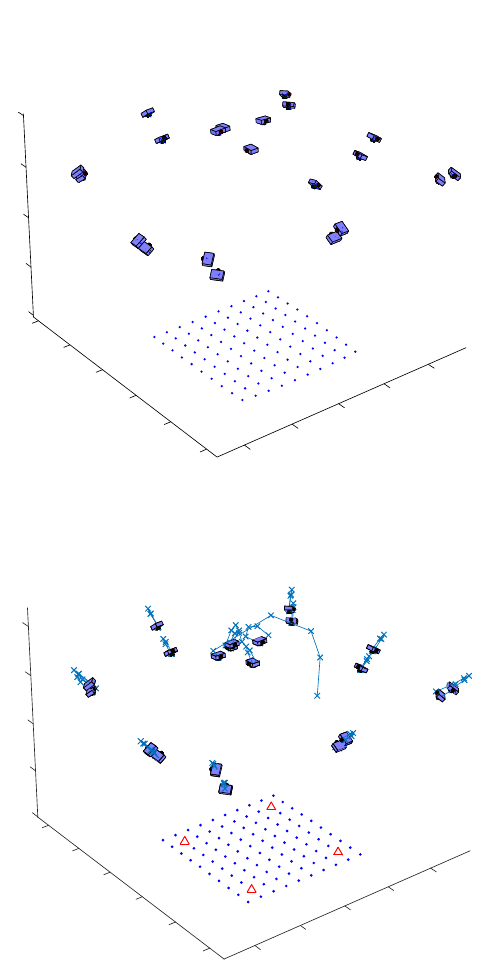
Evolution plots The evolution plots are collected in figures 3–7. Figure 3 shows a
snapshot of the 3D trace figure at the beginning and end of the iterations. As default,
the evolution is presented iteration by iteration with intervening presses of the return
key. The figure window is interactive and may be rotated, zoomed, etc. In this example,
it is clear in Figure 3b that one camera station had poorer initial values than the rest.
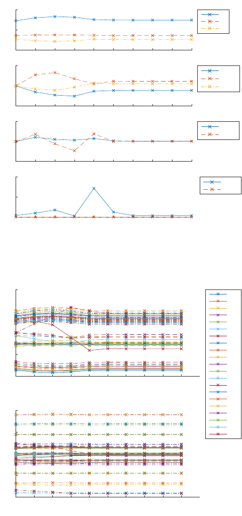
Figures 4–6 contain three plots showing the evolution of the internal orientation
(IO), external orientation (EO), and object point (OP), respectively, during the itera-
tions. The IO plot is split into a focal/principal point panel and a radial and tangential
distortion panel, where the radial distortion parameters are scaled to provide more in-
formation. The EO plot contains a camera center panel and an ω-φ-κEuler angle panel.
The EO and OP plots are interactive. Lines in the plots or legends may be selected and
all corresponding lines will be highlighted. In the top panel of Figure 5, the motion of
one camera stands out. Clicking that line reveals that it belongs to camera station 21,
which can be further investigated to decide if it should be excluded from the calibration.
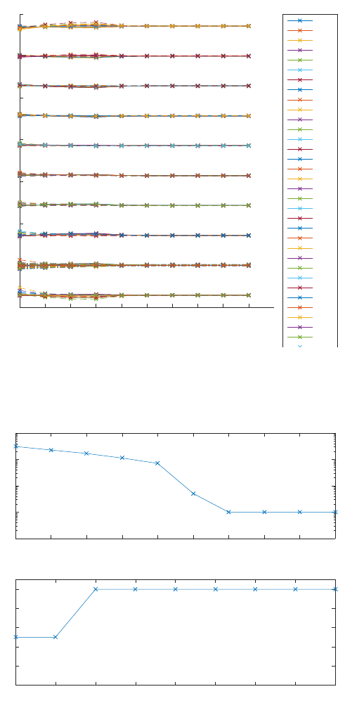
The final evolution plot, shown in Figure 7, illustrates the evolution of the norm of
the total residual and the damping behaviour, if any, during the bundle iterations. In this
example, the Gauss-Newton-Armijo linesearch damping is active during the first two
iterations. For further details on the damping, see Börlin and Grussenmeyer (2013a).
8
−0.5
0
0.5
1
1.5
−0.5
0
0.5
1
1.5
2
0
0.5
1
1.5
2
Initial network
(a) Initial network configuration.
0
0.5
2
1
1.5
1.5
1.5
1
2
Damping: gna. Iteration 9 of 9
1
0.5 0.5
00
-0.5
-0.5
(b) Network configuration after convergence, with camera center
trace lines.
Figure 3: 3D network evolution during the iterations. Only the EO and OP parameters
are illustrated. In this example, the variation of the OP coordinates is barely visible.
9
0
5
10 Focal length, principal point (gna)
f
px
py
-20
0
20 Radial distortion
10 3K1
10 5K2
10 6K3
-500
0
500 Tangential distortion
10 5P1
10 5P2
0123456789
Iteration count
0
50
100 Affine distortion
10 4B1
B2
Figure 4: Evolution of IO parameters during the iteration sequence.
0123456789
-1
0
1
2
3Camera center (gna)
C1
C2
C3
C4
C5
C6
C7
C8
C9
C10
C11
C12
C13
C14
C15
C16
C17
C18
C19
C20
C21
0123456789
Iteration count
-200
-100
0
100
200 Euler angles [degrees]
Figure 5: Evolution of EO parameters during the iteration sequence.
10
0 1 2 3 4 5 6 7 8 9
Iteration count
-0.2
0
0.2
0.4
0.6
0.8
1
1.2 Object points (gna)
P1
P2
P3
P4
P5
P6
P7
P8
P9
P10
P11
P12
P13
P14
P15
P16
P17
P18
P19
P20
P21
P22
P23
P24
P25
P26
P27
P28
P29
P30
P31
P32
P33
P34
Figure 6: Evolution of OP coordinates during the iteration sequence.
0123456789
10 1
10 2
10 3
10 4
10 5Residual norm (gna)
123456789
Iteration count
0
0.2
0.4
0.6
0.8
1
Step length (alpha)
Figure 7: Residual evolution and damping behaviour during the iterations.
11
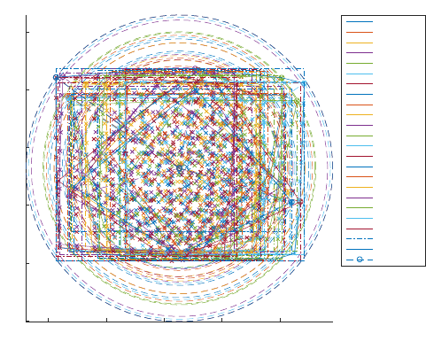
0 500 1000 1500 2000
Rectangular/convex hull/radial coverage = 92% / 87% / 92%.
-500
0
500
1000
1500
2000
Coverage for all images
Image 1
Image 2
Image 3
Image 4
Image 5
Image 6
Image 7
Image 8
Image 9
Image 10
Image 11
Image 12
Image 13
Image 14
Image 15
Image 16
Image 17
Image 18
Image 19
Image 20
Image 21
Rect hull
Convex hull
Radial hull
Figure 8: Plots of input/output statistics: Image coverage.
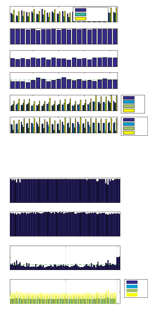
Quality plots The quality plots a gathered in figures 8–10. Per-image quality statis-
tics is shown in Figure 9. The statistics presented for each image are the image coverage
(rectangular coverage, convex hull coverage, and radial coverage); the number of mea-
sured points; the average (RMS) point residual; and the standard deviations for the EO
parameters for the camera stations. In this example, the data does not give any obvious
support to exclude the suspected image 21 from the calibration.
The image coverage is detailed in a separate Figure 8. The plotted data is selectable.
All observations from a specific image, including their convex hull, will be highlighted
when a point or line is selected.
Finally, the per-OP quality statistics in Figure 10 show the number of observations
per OP; the maximum ray intersection angle; the average (RMS) point residual; and
the OP coordinate standard deviation. The presentation may be zoomed to show only
a subset of the OPs by activating the “zoom” function of the figure window.
Result file The result file is modelled after the PhotoModeler result file. The result
file is listed in Appendix A.6.
3.1.3 Bundle adjustment
ROMA The romabundledemo function loads the project from Section 3.1.1 and
present essentially the same plots and the camcaldemo. This demo uses the Photo-
Modeler file as input to the bundle adjustment that runs a few iterations until conver-
gence. The same result file and result plots as camcaldemo are essentially gener-
ated. Since the project is larger (60 cams/26 000 points) than the previous example (20
cams/100 points), the computation will take a bit longer. Computation time was around
12
0
50
100 Image coverage (percent)
Rectangular
Convex
Radial
0
50
100 Point count
0
50
Camera ray angles
0
0.2
0.4 RMS point residuals (-- = global RMS)
0
5
Project units
×10 -4
Spatial standard deviations (camera station)
X
Y
Z
Total
5 10 15 20
Image number
0
1
2
Degrees
×10 -3
Rotational standard deviations (camera station)
omega
phi
kappa
Total
Figure 9: Plots of input/output statistics: Image statistics.
0
10
20
Point count
0
50
Maximum intersection angles
0
0.5
1RMS point residuals (-- = global RMS)
OP id
0
1
2
Project units
×10 -4 OP standard deviations
2
52
1001
1004
X
Y
Z
Total
Figure 10: Plots of input/output statistics: Object point statistics.
13
one minute running on a HP compaq dc7800 with an Intel Core2 Quad CPU Q9300 @
2.50GHz under 64-bit Ubuntu 12.04 (kernel 3.5.0-45).
PRAGUE’16 The prague2016_pm function displays six projects that compare the
result of the bundle adjustment procedure in DBAT and the results of PhotoModeler
(Börlin and Grussenmeyer, 2016). Similarily, the prague2016_ps function displays
the results of a comparison between DBAT and PhotoScan.
The v0.5.1.6 release includes a fix to a bug the distributed the image observation
weights incorrectly. The result is slightly different estimation results than in Börlin and
Grussenmeyer (2016). However, the conclusions remain valid.
HAMBURG’17 The stpierrebundledemo_ps function runs a self-calibration
bundle on a Photoscan project included in the StPierre data set.
3.1.4 Error detection
Three demos are included to illustrate the error detection capabilities of sprank
(dmperm) and spnrank. All are modelled from =camcaldemo=.
Missing observations The camcaldemo_missing_obs demo contains a data
file where the image observations of two object points (id 13 and 60, respectively) have
been deleted. With no observations of either point, the rank deficiency detected by
sprank is six. In the generated result file (Section A.3), the X/Y/Z coordinates of
both points number 12 and 59 (with id 13 and 60, respectively) are indeed listed as
suspicious.
Single-ray observations The camcaldemo_1ray demo contains a data file that
contains only one observation of object point with id 88. Since two observations (one
2D point) is present but three parameter (one 3D point) is to be estimated, the rank
deficiency is one, the rank deficiency detected by sprank is one. The generated result
file (Section A.4) lists one coordinate of point 87 (with id 88) as suspicious.
Missing datum The camcaldemo_no_datum demo contains a demo where no
datum has been specified. As in the previous problems, the result is a numerical prob-
lem with a singular (rank deficient) normal matrix. However, in this case the problem
is manifested by that many or all parameters are linearly dependent of each other. This
will not be detected by sprank. In such a case, the null-space of the normal matrix
will carry information about what parameters are linearly dependent, i.e. what param-
eters are part of the problem. However, when the normal matrix is large, computing
the null-space of the normal matrix in the conventional way using the Matlab function
null will be intractable. Instead, the spnrank (Foster, 2009) function is used to
estimate the rank deficiency of the normal matrix, i.e. the dimension of the null-space.
Given the dimension of the null-space, a basis for the null-space is found using Mat-
lab’s eigs function. For this demo, the generated result file (Section A.5) lists many
14
EO parameters as suspicious. The cause of the problem is less straight-forward to de-
termine from the list. However, the listed rank deficiency of seven should be a strong
hint of a datum problem.
3.2 Using your own data
3.2.1 Photoscan
DBAT can read native Photoscan Archive (.psz) files. DBAT cannot read Photoscan
Project (.psx) files. If you have a .psx project, use the Save as... menu in
Photoscan and save the project as a Photoscan Archive (.psz). DBAT has been tested
with Photoscan file versions up to 1.4.0, Photoscan program version 1.4.4.
The ps_postproc function can be used to post-process a Photoscan project.
loadplotpsz may be useful to visualize the project, as computed by Photoscan.
Known limitations DBAT cannot handle all Photoscan coordinate systems. If you
get strange results, you may have to convert to Local Coordinates. loadplotpsz
may be useful for debugging the input.
3.2.2 PhotoModeler
This section describes how to import you own data using PhotoModeler text export
files. If you have another type of input file, you may be able to write your own loader.
Otherwise, if you have a text file you wish to import, feel free to mail the file to the
the toolbox authors and request an import function. Althought we cannot guarantee
anything, we may adhere to the request, time permitting.
Export from PhotoModeler To import a PhotoModeler project into the toolbox, the
following steps are valid in PhotoModeler Scanner 2012:
1. Export the project using the Export Text File menu command. If the command is
not available, follow the instructions in Appendix A.1.
2. After export, open the Project/Cameras... dialog and select the camera that was
used in your project.
3. Open the generated text file in a text editor.
(a) On the 2nd line (usually reading 0.00005 20), append the width and
height in pixels of your images, e.g. to 0.000500 20 5616 3744.
(b) Inspect the 4th line. For instance, the original data in roma.txt was
(some trailing zeros removed):
24.3581 18.1143 12.0 35.96404 24.0 0.00022 -0.0 0.0
0.0 0.0
The values correspond to the following camera parameters:
focal pp_x pp_y format_w format_h K1 K2 K3 P1 P2.
15

Demo Description Datum Self-calibration
loadplotdemo Load and plot - -
romabundledemo Bundle adjustment Relative dependent orientation no
romabundledemo_selfcal Bundle adjustment Relative dependent orientation yes
camcaldemo Camera calibration Hard-coded control pts yes
camcaldemo_missing_obs Exact singular normal matrix Hard-coded control pts yes
camcaldemo_1ray Exact singular normal matrix Hard-coded control pts yes
camcaldemo_no_datum Numerically singular normal matrix Missing yes
prague2016_pm(’c1’) Camera calibration Hard-coded fixed control points yes
prague2016_pm(’c2’) Camera calibration Hard-coded weighted control points yes
prague2016_pm(’s1’) Bundle adjustment Fixed ctrl pts from text file no
prague2016_pm(’s2’) Bundle adjustment Weighted ctrl pts from text file no
prague2016_pm(’s4’) Bundle adjustment Weighted ctrl pts from text file no
prague2016_ps(’s5’) Photoscan post-processing Weighted ctrl pts from psz file no
ps_postproc(”) Photoscan post-processing Weighted ctrl pts from psz file no
stpierrebundledemo_ps Photoscan post-processing Weighted ctrl pts from psz file yes
Table 1: Summary of demos.
Notice that most of the significant digits of K1–K3 were lost in the text
export.
(c) Update the parameter values on the 4th line with values from the cam-
era dialog for each parameter with a larger number of significant digits in
the dialog. This usually means all parameters except format_w. In the
roma.txt test case, the 4th line was modified to:
24.3581 18.1143 12 35.96404 24 2.174e-4 -1.518e-7 0
0 0.
Loading into Matlab
1. In Matlab, run step 2 from Section 2 if not already done.
2. Call loadplotdemo with the name of your text export file as first parameter.
A figure with your camera network, aligned with the first camera and rotated to
have +Z ’up’, should now have been generated.
Using the bundle adjustment of DBAT Modify either of the demo functions to
match what you want to do. If you run into any problems, send us an email. The
interesting results may either be in the plots or in the result file.
17
References
N. Börlin and P. Grussenmeyer. Bundle adjustment with and without damping. Pho-
togrammetric Record, 28(144):396–415, Dec. 2013a. doi: 10.1111/phor.12037.
N. Börlin and P. Grussenmeyer. Experiments with metadata-derived initial values and
linesearch bundle adjustment in architectural photogrammetry. ISPRS Annals of the
Photogrammetry, Remote Sensing, and Spatial Information Sciences, II-5/W1:43–
48, Sept. 2013b.
N. Börlin and P. Grussenmeyer. Camera calibration using the damped bundle adjust-
ment toolbox. ISPRS Annals of the Photogrammetry, Remote Sensing, and Spatial
Information Sciences, II(5):89–96, June 2014.
N. Börlin and P. Grussenmeyer. External verification of the bundle adjustment in pho-
togrammetric software using the damped bundle adjustment toolbox. International
Archives of Photogrammetry, Remote Sensing, and Spatial Information Sciences,
XLI-B5:7–14, July 2016.
N. Börlin, A. Murtiyoso, P. Grussenmeyer, F. Menna, and E. Nocerino. Modular bun-
dle adjustment for photogrammeric computations. International Archives of Pho-
togrammetry, Remote Sensing, and Spatial Information Sciences, XLII(2):?, June
2018. Paper accepted for the ISPRS TC II mid-term symposium in Riva del Garda,
Italy, Jun 3-7, 2018.
L. Foster. Calculating the rank of sparse matrices using spnrank.
http://www.math.sjsu.edu/singular/matrices/software/SJsingular/Doc/spnrank.pdf,
Apr. 2009.
R. M. Haralick, C.-N. Lee, K. Ottenberg, and M. Nölle. Review and analysis of solu-
tions of the three point perspective pose estimation problem. Int J Comp Vis, 13(3):
331–356, 1994.
C. McGlone, E. Mikhail, and J. Bethel, editors. Manual of Photogrammetry. ASPRS,
5th edition, July 2004. ISBN 1-57083-071-1.
A. Murtiyoso, P. Grussenmeyer, and N. Börlin. Reprocessing close range terrestrial
and UAV photogrammetric projects with the DBAT toolbox for independent
verification and quality control. ISPRS - International Archives of the Pho-
togrammetry, Remote Sensing and Spatial Information Sciences, XLII-2/W8:
171–177, 2017. doi: 10.5194/isprs-archives-XLII-2-W8-171-2017. URL https:
//www.int-arch-photogramm-remote-sens-spatial-inf-sci.
net/XLII-2-W8/171/2017/.
H. Stewénius, C. Engels, and D. Nistér. Recent developments on direct relative orien-
tation. ISPRS J Photogramm, 60(4):284–294, June 2006.
18
A Appendices
A.1 Enabling text export from PhotoModeler
Some versions of PhotoModeler do not have the text file export option enabled by
default. In that case, the following steps worked in PhotoModeler Scanner 2012:
1. Right-click on the main window toolbar, select Customize toolbar....
2. In the Commands tab, select the File category.
3. Drag the Export Text File... command to a toolbar of your choice.
4. Now you should be able to export your project as a text file by clicking on the
Export Text File button.
A.2 Camera model
Currently, the only supported camera model is the omega-phi-kappa Euler angle cam-
era model (McGlone et al., 2004, Ch. 2.1.2.3).
A.3 Result file with missing observations
Damped Bundle Adjustment Toolbox result file
Project Name: Bundle Soln PhotoModeler Calibration Project
Problems and suggestions:
Project Problems:
Structural rank: 417 (deficiency: 6)
DMPERM suggests the following parameters have problems:
OX-12/13
OY-12/13
OZ-12/13
OX-59/60
OY-59/60
OZ-59/60
Numerical rank: not tested.
Problems related to the processing: (1)
Bundle failed with code -4 (see below for details).
.
.
.
A.4 Result file with single-ray observations
Damped Bundle Adjustment Toolbox result file
Project Name: Bundle Soln PhotoModeler Calibration Project
Problems and suggestions:
Project Problems:
Structural rank: 422 (deficiency: 1)
DMPERM suggests the following parameters have problems:
OZ-87/88
Numerical rank: not tested.
Problems related to the processing: (1)
Bundle failed with code -4 (see below for details).
.
.
.
19
A.5 Result file with missing datum
Damped Bundle Adjustment Toolbox result file
Project Name: Bundle Soln PhotoModeler Calibration Project
Problems and suggestions:
Project Problems:
Structural rank: ok.
Numerical rank: 428 (deficiency: 7)
Null-space suggest the following parameters are part of the problem:
Vector 1 (eigenvalue 1.36254e-18):
(EX-21, -0.156)
(EX-9, -0.13)
(EX-13, -0.12)
(EX-10, -0.119)
(EX-11, -0.115)
(EX-12, -0.108)
(EX-14, -0.104)
Vector 2 (eigenvalue -1.60532e-17):
(EX-21, 0.207)
(EY-21, 0.195)
(EY-1, 0.192)
(EY-2, 0.178)
(EX-13, 0.167)
(EY-15, 0.166)
(EY-3, 0.166)
(EY-4, 0.163)
(EY-16, 0.161)
(EX-14, 0.157)
(EX-15, 0.151)
(EX-11, 0.149)
(EY-18, 0.147)
(EX-12, 0.146)
(EX-16, 0.145)
(EY-20, 0.133)
(EY-17, 0.128)
Vector 3 (eigenvalue 5.21745e-17):
(om-21, -0.16)
(EX-3, -0.155)
(EX-4, -0.151)
(EX-5, -0.147)
(EX-6, -0.136)
(EZ-7, 0.132)
(om-13, -0.129)
(EX-1, -0.129)
(om-15, -0.127)
(om-16, -0.125)
(EZ-8, 0.125)
(om-14, -0.125)
(EZ-9, 0.122)
(EX-2, -0.117)
(om-11, -0.116)
(EZ-10, 0.116)
(om-12, -0.114)
(om-18, -0.113)
(om-20, -0.113)
(EZ-11, 0.111)
(EX-7, -0.111)
(EZ-12, 0.11)
(om-19, -0.109)
(om-9, -0.108)
(EZ-5, 0.107)
(om-1, -0.106)
(om-17, -0.106)
(om-2, -0.105)
(om-10, -0.105)
Vector 4 (eigenvalue -5.5516e-17):
(EZ-21, -0.174)
(EX-5, -0.13)
20
(EX-7, -0.129)
(EX-8, -0.12)
(EX-6, -0.119)
(EY-9, -0.114)
(EY-11, -0.111)
Vector 5 (eigenvalue -1.45759e-16):
(EY-7, 0.158)
(EY-5, 0.154)
(EY-8, 0.153)
(EY-9, 0.151)
(om-4, -0.147)
(EY-19, 0.147)
(om-3, -0.144)
(EY-6, 0.143)
(EY-10, 0.143)
(EY-17, 0.133)
(EZ-3, -0.132)
(EZ-4, -0.129)
(om-17, -0.126)
(om-19, -0.126)
(om-18, -0.125)
(om-1, -0.124)
(om-9, -0.124)
(om-2, -0.124)
(EY-18, 0.121)
(om-10, -0.121)
(EY-20, 0.12)
(om-20, -0.12)
(om-5, -0.12)
(EZ-2, -0.118)
(EZ-1, -0.118)
(om-6, -0.116)
(ph-9, -0.114)
(ph-7, -0.113)
(ph-11, -0.112)
(EY-11, 0.112)
(ph-12, -0.111)
(ph-8, -0.11)
(ph-10, -0.109)
(ph-5, -0.108)
(om-11, -0.108)
(EY-12, 0.107)
(EZ-5, -0.106)
(ph-13, -0.106)
(om-7, -0.104)
(ph-19, -0.104)
(om-12, -0.104)
(ph-14, -0.104)
Vector 6 (eigenvalue -1.54875e-16):
(om-21, 0.185)
(ph-9, -0.174)
(EZ-21, 0.174)
(ph-10, -0.169)
(ph-11, -0.167)
(ph-7, -0.167)
(ph-8, -0.165)
(ph-12, -0.164)
(EX-9, -0.152)
(EX-7, -0.151)
(EX-8, -0.151)
(EY-11, -0.148)
(EY-12, -0.146)
(EX-10, -0.146)
(EZ-15, 0.142)
(EZ-16, 0.137)
(EY-13, -0.136)
(ph-5, -0.135)
(EY-14, -0.133)
21
(EZ-13, 0.127)
(ph-13, -0.127)
(EZ-14, 0.126)
(ph-14, -0.124)
(ph-6, -0.123)
(ph-19, -0.12)
(EY-21, -0.117)
Vector 7 (eigenvalue 1.9046e-16):
(ph-1, 0.194)
(ph-2, 0.194)
(ph-15, 0.173)
(EX-2, 0.173)
(om-5, -0.173)
(ph-16, 0.169)
(ph-4, 0.169)
(EX-1, 0.168)
(ph-3, 0.164)
(om-8, -0.163)
(om-7, -0.16)
(om-6, -0.16)
(ph-21, 0.157)
(EY-21, -0.138)
(EY-5, 0.138)
(EY-6, 0.132)
(om-3, -0.127)
(ph-20, 0.126)
(om-4, -0.125)
Problems related to the processing: (1)
Bundle failed with code -2 (see below for details).
.
.
.
A.6 Successful result file example
Damped Bundle Adjustment Toolbox result file
Project Name: Bundle Soln PhotoModeler Calibration Project
Problems and suggestions:
Project Problems:
Structural rank: ok.
Numerical rank: ok.
Problems related to the processing: (1)
One or more of the camera parameter has a high correlation (see below).
Information from last bundle
Last Bundle Run: 25-Oct-2018 20:55:37
DBAT version: 0.7.6.1 (2018-10-25)
MATLAB version: 8.6.0.267246 (R2015b)
Host system: GLNXA64
Host name: slartibartfast
Status: OK
Sigma0: 1.6148
Sigma0 (pixels): 0.16148
Processing options:
Orientation: on
Global optimization: on
Calibration: on
Constraints: off
Maximum # of iterations: 20
Convergence tolerance: 1e-06
Termination criteria: relative
Singular test: on
Chirality veto: off
Damping: gna
Camera unit (cu): mm
Object space unit (ou): m
Initial value comment: Camera calibration from EXIF value
Total error:
22
Number of stages: 1
Number of iterations: 9
First error: 30882.3
Last error: 98.556
Execution time (s): 0.78
Lens distortion models:
Backward (Photogrammetry) model 3
Cameras:
Calibration: yes (Xp Yp f K1 K2 K3 P1 P2 aspect)
Camera1
Lens distortion model:
Backward (Photogrammetry) model 3
Focal Length:
Value: 7.457 mm
Deviation: 0.00105 mm
Xp - principal point x:
Value: 3.61546 mm
Deviation: 0.00082 mm
Yp - principal point y:
Value: 2.61329 mm
Deviation: 0.00098 mm
Fw - format width:
Value: 7.25301 mm
Fh - format height:
Value: 5.43764 mm
K1 - radial distortion 1:
Value: 0.00458861 mm^(-3)
Deviation: 2.21e-05 mm^(-3)
Significance: p=1.00
K2 - radial distortion 2:
Value: -4.51351e-05 mm^(-5)
Deviation: 2.65e-06 mm^(-5)
Significance: p=1.00
Correlations over 95%: K3:-97.9%.
K3 - radial distortion 3:
Value: -2.05253e-06 mm^(-7)
Deviation: 1.01e-07 mm^(-7)
Significance: p=1.00
Correlations over 95%: K2:-97.9%.
P1 - decentering distortion 1:
Value: -6.12803e-05 mm^(-3)
Deviation: 3.52e-06 mm^(-3)
Significance: p=1.00
P2 - decentering distortion 2:
Value: -4.41172e-05 mm^(-3)
Deviation: 3.94e-06 mm^(-3)
Significance: p=1.00
B1 - aspect ratio:
Value: 0.000389598
Deviation: 2.08e-05
Significance: p=1.00
B2 - skew:
Value: 0
Iw - image width:
Value: 2272 px
Ih - image height:
Value: 1704 px
Xr - X resolution:
Value: 313.371 px/mm
Yr - Y resolution:
Value: 313.371 px/mm
Pw - pixel width:
Value: 0.00319235 mm
Ph - pixel height:
Value: 0.0031911 mm
Rated angle of view (h,v,d): (52, 40, 63) deg
Largest distortion: 0.37 mm (116.4 px, 8.2% of half-diagonal)
Precisions / Standard Deviations:
23
Photograph Standard Deviations:
Photo 1: P8250021.JPG
Omega:
Value: -39.413082 deg
Deviation: 0.0085 deg
Phi:
Value: -1.183179 deg
Deviation: 0.00761 deg
Kappa:
Value: -179.838467 deg
Deviation: 0.00275 deg
Xc:
Value: 0.454947 ou
Deviation: 0.000155 ou
Yc:
Value: 1.793849 ou
Deviation: 0.000179 ou
Zc:
Value: 1.468066 ou
Deviation: 0.000207 ou
Photo 2: P8250022.JPG
Omega:
Value: -39.734523 deg
Deviation: 0.00816 deg
Phi:
Value: -1.813688 deg
Deviation: 0.00886 deg
Kappa:
Value: -90.123062 deg
Deviation: 0.00289 deg
Xc:
Value: 0.470305 ou
Deviation: 0.000186 ou
Yc:
Value: 2.026401 ou
Deviation: 0.000219 ou
Zc:
Value: 1.639148 ou
Deviation: 0.000232 ou
Photo 3: P8250023.JPG
Omega:
Value: -27.227000 deg
Deviation: 0.0105 deg
Phi:
Value: -28.559177 deg
Deviation: 0.00753 deg
Kappa:
Value: -141.839170 deg
Deviation: 0.00538 deg
Xc:
Value: -0.644442 ou
Deviation: 0.000188 ou
Yc:
Value: 1.466578 ou
Deviation: 0.000179 ou
Zc:
Value: 1.580187 ou
Deviation: 0.000243 ou
Photo 4: P8250024.JPG
Omega:
Value: -28.556794 deg
Deviation: 0.00881 deg
Phi:
Value: -30.289704 deg
Deviation: 0.00923 deg
Kappa:
Value: -49.786720 deg
Deviation: 0.00467 deg
24
Xc:
Value: -0.643144 ou
Deviation: 0.000198 ou
Yc:
Value: 1.490295 ou
Deviation: 0.000202 ou
Zc:
Value: 1.637492 ou
Deviation: 0.000246 ou
Photo 5: P8250025.JPG
Omega:
Value: 4.385418 deg
Deviation: 0.00943 deg
Phi:
Value: -34.659929 deg
Deviation: 0.00863 deg
Kappa:
Value: -87.134063 deg
Deviation: 0.00519 deg
Xc:
Value: -0.671014 ou
Deviation: 0.000158 ou
Yc:
Value: 0.417412 ou
Deviation: 0.000144 ou
Zc:
Value: 1.409244 ou
Deviation: 0.000193 ou
Photo 6: P8250026.JPG
Omega:
Value: 2.063986 deg
Deviation: 0.0103 deg
Phi:
Value: -33.988460 deg
Deviation: 0.00823 deg
Kappa:
Value: 1.485869 deg
Deviation: 0.00587 deg
Xc:
Value: -0.712797 ou
Deviation: 0.000177 ou
Yc:
Value: 0.476083 ou
Deviation: 0.000155 ou
Zc:
Value: 1.465130 ou
Deviation: 0.000203 ou
Photo 7: P8250027.JPG
Omega:
Value: 27.342174 deg
Deviation: 0.00854 deg
Phi:
Value: -28.292503 deg
Deviation: 0.00875 deg
Kappa:
Value: -44.210389 deg
Deviation: 0.00445 deg
Xc:
Value: -0.534821 ou
Deviation: 0.000154 ou
Yc:
Value: -0.349595 ou
Deviation: 0.000157 ou
Zc:
Value: 1.402489 ou
Deviation: 0.000212 ou
Photo 8: P8250028.JPG
Omega:
25
Value: 26.875970 deg
Deviation: 0.0107 deg
Phi:
Value: -28.129516 deg
Deviation: 0.00757 deg
Kappa:
Value: 44.840805 deg
Deviation: 0.00553 deg
Xc:
Value: -0.718081 ou
Deviation: 0.000218 ou
Yc:
Value: -0.466107 ou
Deviation: 0.000204 ou
Zc:
Value: 1.715475 ou
Deviation: 0.000264 ou
Photo 9: P8250029.JPG
Omega:
Value: 30.383673 deg
Deviation: 0.00856 deg
Phi:
Value: 0.193844 deg
Deviation: 0.00776 deg
Kappa:
Value: 0.084838 deg
Deviation: 0.00248 deg
Xc:
Value: 0.524897 ou
Deviation: 0.000161 ou
Yc:
Value: -0.543737 ou
Deviation: 0.000167 ou
Zc:
Value: 1.533003 ou
Deviation: 0.000208 ou
Photo 10: P8250030.JPG
Omega:
Value: 30.975069 deg
Deviation: 0.0085 deg
Phi:
Value: 1.702984 deg
Deviation: 0.00879 deg
Kappa:
Value: 89.537060 deg
Deviation: 0.00264 deg
Xc:
Value: 0.554430 ou
Deviation: 0.000176 ou
Yc:
Value: -0.592328 ou
Deviation: 0.000194 ou
Zc:
Value: 1.617413 ou
Deviation: 0.000216 ou
Photo 11: P8250031.JPG
Omega:
Value: 27.620051 deg
Deviation: 0.0106 deg
Phi:
Value: 30.742857 deg
Deviation: 0.00756 deg
Kappa:
Value: 42.343765 deg
Deviation: 0.00584 deg
Xc:
Value: 1.770052 ou
Deviation: 0.000191 ou
26
Yc:
Value: -0.425243 ou
Deviation: 0.00018 ou
Zc:
Value: 1.551302 ou
Deviation: 0.000241 ou
Photo 12: P8250032.JPG
Omega:
Value: 24.647784 deg
Deviation: 0.00901 deg
Phi:
Value: 30.199261 deg
Deviation: 0.00965 deg
Kappa:
Value: 133.199858 deg
Deviation: 0.00493 deg
Xc:
Value: 1.864503 ou
Deviation: 0.000201 ou
Yc:
Value: -0.480191 ou
Deviation: 0.000202 ou
Zc:
Value: 1.614517 ou
Deviation: 0.000255 ou
Photo 13: P8250033.JPG
Omega:
Value: 0.519301 deg
Deviation: 0.00941 deg
Phi:
Value: 33.141786 deg
Deviation: 0.00865 deg
Kappa:
Value: 88.708362 deg
Deviation: 0.00499 deg
Xc:
Value: 1.630951 ou
Deviation: 0.000165 ou
Yc:
Value: 0.497645 ou
Deviation: 0.000151 ou
Zc:
Value: 1.470402 ou
Deviation: 0.000199 ou
Photo 14: P8250034.JPG
Omega:
Value: -1.707201 deg
Deviation: 0.0105 deg
Phi:
Value: 33.605390 deg
Deviation: 0.00835 deg
Kappa:
Value: 180.179674 deg
Deviation: 0.00585 deg
Xc:
Value: 1.795963 ou
Deviation: 0.000196 ou
Yc:
Value: 0.525690 ou
Deviation: 0.000177 ou
Zc:
Value: 1.598647 ou
Deviation: 0.000218 ou
Photo 15: P8250035.JPG
Omega:
Value: -30.757132 deg
Deviation: 0.00869 deg
Phi:
27
Value: 28.161929 deg
Deviation: 0.00893 deg
Kappa:
Value: 138.427120 deg
Deviation: 0.00462 deg
Xc:
Value: 1.671692 ou
Deviation: 0.000177 ou
Yc:
Value: 1.554494 ou
Deviation: 0.000178 ou
Zc:
Value: 1.500046 ou
Deviation: 0.000239 ou
Photo 16: P8250036.JPG
Omega:
Value: -29.841912 deg
Deviation: 0.0105 deg
Phi:
Value: 26.976407 deg
Deviation: 0.00757 deg
Kappa:
Value: -134.657860 deg
Deviation: 0.00543 deg
Xc:
Value: 1.693214 ou
Deviation: 0.000204 ou
Yc:
Value: 1.619159 ou
Deviation: 0.000189 ou
Zc:
Value: 1.590375 ou
Deviation: 0.000252 ou
Photo 17: P8250037.JPG
Omega:
Value: -8.536369 deg
Deviation: 0.00979 deg
Phi:
Value: -0.515819 deg
Deviation: 0.00956 deg
Kappa:
Value: 179.396590 deg
Deviation: 0.00198 deg
Xc:
Value: 0.424677 ou
Deviation: 0.000287 ou
Yc:
Value: 0.824641 ou
Deviation: 0.000288 ou
Zc:
Value: 1.971217 ou
Deviation: 0.000246 ou
Photo 18: P8250038.JPG
Omega:
Value: -4.760952 deg
Deviation: 0.00959 deg
Phi:
Value: 0.661695 deg
Deviation: 0.00919 deg
Kappa:
Value: 88.788380 deg
Deviation: 0.00189 deg
Xc:
Value: 0.483059 ou
Deviation: 0.000268 ou
Yc:
Value: 0.925982 ou
Deviation: 0.000284 ou
28
Zc:
Value: 1.885017 ou
Deviation: 0.000229 ou
Photo 19: P8250039.JPG
Omega:
Value: -4.415305 deg
Deviation: 0.00923 deg
Phi:
Value: -0.416632 deg
Deviation: 0.00926 deg
Kappa:
Value: 88.245577 deg
Deviation: 0.00186 deg
Xc:
Value: 0.462946 ou
Deviation: 0.000275 ou
Yc:
Value: 0.578695 ou
Deviation: 0.000271 ou
Zc:
Value: 1.874858 ou
Deviation: 0.00021 ou
Photo 20: P8250040.JPG
Omega:
Value: -7.619745 deg
Deviation: 0.00935 deg
Phi:
Value: -1.571494 deg
Deviation: 0.0103 deg
Kappa:
Value: -180.050126 deg
Deviation: 0.00199 deg
Xc:
Value: 0.701429 ou
Deviation: 0.000319 ou
Yc:
Value: 0.784042 ou
Deviation: 0.000278 ou
Zc:
Value: 1.925303 ou
Deviation: 0.00024 ou
Photo 21: P8250041.JPG
Omega:
Value: -8.708623 deg
Deviation: 0.00925 deg
Phi:
Value: 1.058407 deg
Deviation: 0.0102 deg
Kappa:
Value: -182.614638 deg
Deviation: 0.00203 deg
Xc:
Value: 0.269149 ou
Deviation: 0.000314 ou
Yc:
Value: 0.822761 ou
Deviation: 0.000266 ou
Zc:
Value: 1.904844 ou
Deviation: 0.000243 ou
Quality
Photographs
Total number: 21
Numbers used: 21
Cameras
Total number: 1
Camera1:
Calibration: yes
29
Number of photos using camera: 21
Photo point coverage:
Rectangular: 41%-83% (61% average, 92% union)
Convex hull: 31%-62% (46% average, 87% union)
Radial: 60%-92% (73% average, 92% union)
Photo Coverage
References points outside calibrated region:
none
Point Measurements
Number of control pts: 4
Number of check pts: 0
Number of object pts: 96
CP ray count: 21-21 (21.0 avg)
4 points with 21 rays.
CCP ray count: -
OP ray count: 16-21 (20.7 avg)
1 points with 16 rays.
1 points with 17 rays.
2 points with 18 rays.
3 points with 19 rays.
5 points with 20 rays.
84 points with 21 rays.
Point Marking Residuals
Overall point RMS: 0.216 pixels
Mark point residuals:
Maximum: 0.955 pixels (OP 1003 on photo 5)
Object point residuals (RMS over all images of a point):
Minimum: 0.095 pixels (OP 65 over 21 images)
Maximum: 0.553 pixels (OP 1004 over 21 images)
Photo residuals (RMS over all points in an image):
Minimum: 0.153 pixels (photo 4 over 97 points)
Maximum: 0.281 pixels (photo 11 over 100 points)
Point Precision
Total standard deviation (RMS of X/Y/Z std):
Minimum: 8.2e-05 (OP 49)
Maximum: 0.00011 (OP 90)
Maximum X standard deviation: 5e-05 (OP 90)
Maximum Y standard deviation: 5.3e-05 (OP 90)
Maximum Z standard deviation: 8.5e-05 (OP 90)
Points with high correlations
Points with correlation above 95%: 0
Points with correlation above 99%: 0
Point Angles
CP
Minimum: 83.4 degrees (CP 1003)
Maximum: 85.8 degrees (CP 1002)
Average: 84.7 degrees
CCP
Minimum: -
Maximum: -
Average: -
OP
Minimum: 79.6 degrees (OP 90)
Maximum: 90.0 degrees (OP 59)
Average: 86.5 degrees
Smallest angles (ID, angle [deg], vis in cameras)
90: 79.61 ( 1 2 3 5 8 9 11 13 14 15 16 17 18 19 20 21)
8: 81.00 ( 1 2 3 4 5 7 9 10 11 12 13 14 15 17 18 19 20 21)
92: 81.15 ( 1 2 3 4 5 7 8 9 10 11 13 14 15 16 17 18 19 20 21)
Ctrl measurements
Prior
id, x, y, z, stdx, stdy, stdz, label
1001, 0.000, 1.000, 0.000, 0, 0, 0,
1002, 1.000, 1.000, 0.000, 0, 0, 0,
1003, 0.000, 0.000, 0.000, 0, 0, 0,
1004, 1.000, 0.000, 0.000, 0, 0, 0,
Posterior
id, x, y, z, stdx, stdy, stdz, rays, label
30
1001, 0.000, 1.000, 0.000, 0, 0, 0, 21,
1002, 1.000, 1.000, 0.000, 0, 0, 0, 21,
1003, 0.000, 0.000, 0.000, 0, 0, 0, 21,
1004, 1.000, 0.000, 0.000, 0, 0, 0, 21,
Diff (pos=abs diff, std=rel diff)
id, x, y, z, xy, xyz, stdx, stdy, stdz, rays, label
1001, 0.000, 0.000, 0.000, 0.000, 0.000, 0.0%, 0.0%, 0.0%, 21,
1002, 0.000, 0.000, 0.000, 0.000, 0.000, 0.0%, 0.0%, 0.0%, 21,
1003, 0.000, 0.000, 0.000, 0.000, 0.000, 0.0%, 0.0%, 0.0%, 21,
1004, 0.000, 0.000, 0.000, 0.000, 0.000, 0.0%, 0.0%, 0.0%, 21,
Ctrl point delta
Max: 0.000 ou (, pt 1001)
Max X,Y,Z
X: 0.000 ou (, pt 1001)
Y: 0.000 ou (, pt 1001)
Z: 0.000 ou (, pt 1001)
RMS: 0.000 ou (from 4 items)
Check measurements
none
31
