Manual

User Manual:

Open the PDF directly: View PDF .
Page Count: 21

USER’S MANUAL

ATLAS-1.0

Atmospheric Lagrangian Dispersion

Model

Version release: November 2018

Reckziegel Florencia(1)

Folch Arnau(2)

Viramonte Jos´e(1)

(1)INENCO/GEONORTE, Univ. Nacional de Salta, CONICET, Salta,

Argentina

(2)Barcelona Supercomputing Center (BSC), Barcelona, Spain

Contents

1 Introduction 2

2 Atmospheric dispersion model 2

2.1 Physicalmodel .......................... 2

2.2 Diﬀusion.............................. 2

2.3 Sedimentation........................... 3

2.4 Meteorological data . . . . . . . . . . . . . . . . . . . . . . . . 4

2.5 Sourceterm ............................ 5

2.6 Particle aggregation . . . . . . . . . . . . . . . . . . . . . . . . 7

3 Running ATLAS 8

4 Input ﬁles 8

4.1 The input ﬁle name.inp . . . . . . . . . . . . . . . . . . . . . . 8

4.2 The input ﬁle name Phasei.inp . . . . . . . . . . . . . . . . . 12

4.3 The input ﬁle name Phase i.tgsd . . . . . . . . . . . . . . . . 14

4.4 The input ﬁle name.pts . . . . . . . . . . . . . . . . . . . . . . 14

4.5 The input ﬁle name model.nc . . . . . . . . . . . . . . . . . . 14

4.6 The input ﬁle out name.rest . . . . . . . . . . . . . . . . . . . 15

4.7 The input ﬁle name.bkw . . . . . . . . . . . . . . . . . . . . . 15

5 Output ﬁles 15

5.1 outnamepart.nc ......................... 15

5.2 outname.kml ........................... 16

5.3 name.tps.point name.res . . . . . . . . . . . . . . . . . . . . . 16

5.4 namePhasei.tgsd......................... 16

5.5 namePhasei.grn ......................... 16

5.6 out name meteo.nc . . . . . . . . . . . . . . . . . . . . . . . . 17

5.7 outname.rest ........................... 17

5.8 name.log.............................. 17

6 Program Installation and execution 18

7 Example 18

1 Introduction

ATLAS-1.0 (ATmospheric LAgrangian diSpersion) is an atmospheric disper-

sion and sedimentation Lagrangian model tailored to volcanic tephra/ash.

The model solves the Advection-Diﬀusion-Sedimentation equation across mul-

tiple scales (from regional to global) and can be driven oﬀ-line by diﬀerent

numerical weather prediction models in combination. ATLAS can be used

in forward mode to forecast ash dispersal from a volcano (or from extended

sources) or in backward mode to integrate trajectories backwards in time

and constrain unknown source term characteristics. Multiple source terms

can be deﬁned, with diﬀerent granulometric characteristics on a single model

execution. The model is written in FORTRAN 90 for Unix-Linux OS.

2 Atmospheric dispersion model

In this section is presented a brief description of ATLAS main equations.

2.1 Physical model

ATLAS uses a zero acceleration scheme to integrate particle trajectories in

time. Given the position of a particle x(t) at time t, the position at time

t+ ∆tis computed as:

x(t+ ∆t) = x(t)+(va(x, t) + vd(x, t) + vs(x, t)) ∆t(1)

where the velocity vector v(x, t) is composed of the wind advection (passive

transport), atmospheric diﬀusion, and particle sedimentation.

2.2 Diﬀusion

The diﬀusive velocity is obtained from the Langevin equation:

dv =adt +bdW, (2)

where ais the deterministic term of the lagrangian velocity (equation 3), bis

the aleatory term related to turbulent statistical properties, and dW is the

diﬀerential Wiener process with zero mean and variance dt which follows a

Markov process. The term bdW describes the diﬀusion process (equation 4).

In the planetary boundary layer (PBL), the Hanna scheme [Hanna, 1982] is

utilized, parameterizing the wind ﬂuctuations, depending on the atmospheric

conditions (stable, neutral, and unstable):

a=−v

Ti,L

,(3)

b=s2σ2

Ti,L

,(4)

where, σ2

vis the variance of the wind speed, and Ti,L is the Lagrangian

integral time scale. In the free troposphere, a constant horizontal diﬀusivity

of 50m2/s is considered along xand ycomponents whereas the zcomponent

is set to 0 [Stohl et al., 2005]. In contrast, in the stratosphere, a vertical

diﬀusivity of 0.1m2/s is ﬁxed and no horizontal diﬀusivity is assumed [Legras

et al., 2003].

2.3 Sedimentation

Assuming that particles settle down at its terminal velocity, the sedimenta-

tion velocity is given by:

|vs|=vs=s4g(ρp−ρa)d

3Cdρa

(5)

where ρaand ρpare the air and particle densities respectively, dis the par-

ticle equivalent diameter, and Cdis the drag coeﬃcient that depends on the

Reynolds number Re =dvs/νa, being νathe air kinematic viscosity (i.e.

νa=µa/ρawhere µais the air dynamic viscosity). ATLAS admits as em-

pirical parameterisations for the terminal velocity diﬀerent models that the

user need to choose:

1. Arastoopour model [Arastoopour et al., 1982]. Model valid for spherical

particles in which the drag coeﬃcient is calculated as:

Cd=24

Re (1 + 0.15Re0.687)Re ≤988.947

0.44 Re > 988.947 (6)

2. Ganser model [Ganser, 1993]. In this model the drag coeﬃcient is

obtained as:

Cd=24

ReK11+0.1118(ReK1K2)0.6567+0.4305K2

1 + 3305

ReK1K2

(7)

where K1= 3/[(dn/d)+2ψ−0.5] and K2= 101.8148(−Logψ)0.5743 are two

form factors, dnis the average between the particle minimum and max-

imum axes sizes, dis the diameter of the equivalent volume sphere, and

ψis the particle sphericity, calculated as the Wadell sphericity [Aschen-

brenner, 1956, Wadell, 1933] based on the three particle dimensions and

its volume:

ψw= 12.8(P2Q)1/3

1 + P(1 + Q)+6p1 + P2(1 + Q2)(8)

with P=S/I, Q =I/L, where Lis the largest dimension, Iis the

largest perpendicular to L, and Sis the direction perpendicular to L

and I.

3. Wilson model [Walker et al., 1971, Wilson and Huang, 1979]. This

model uses the interpolation suggested by Pfeiﬀer et al. [2005] for the

drag coeﬃcient:

Cd=





Re ϕ−0.828 + 2√1−ϕ Re ≤102

1−1−Cd|Re=102

900 (103−Re) 102≤Re ≤103

1Re ≥103

(9)

where ϕ= (b+c)/2ais a particle form factor, (a≥b≥care the

particle semi-axes).

4. Dellino model [Dellino et al., 2005]. This model gives the sedimentation

velocity (for particle diameters constrained to those used in the Dellino

et al. [2005] experiment) without need of iteratively solving eq. (5):

vs= 1.2605νa

d(Arξ1.6)0.5206 (10)

where Ar =gd3(ρp−ρa)ρa/µ2

qis the Arquimedes number, gthe gravity

acceleration, and ξa particle form factor.

2.4 Meteorological data

ATLAS requires of time-dependent meteorological data (wind velocity, air

temperature and density, friction velocity, atmospheric boundary layer height,

and Monin-Obukhov length) and the terrain topography. This ﬁrst version

of the model admits data from the Weather Research and Forecast (WRF)

mesoscale model and/or from the Global Forecast System (GFS) produced by

the National Centers for Environmental Prediction (NCEP). ATLAS trans-

forms values of meteorological ﬁelds from pressure levels to the background

mesh terrain-following coordinates. It is desirable that the user indicate as

the spatial resolution of this background (interpolation) mesh, a similar to

that of the driving meteorological model. ATLAS background mesh resolu-

tions ﬁner than that of the meteorological model increase the computational

cost without improving model accuracy whereas coarser background mesh

resolutions cause a loss of information. In the case of more than one meteo-

rological input being used, ATLAS stores at each grid point the value of the

meteorological model with higher resolution and performs a smooth blending

at the interfaces.

2.5 Source term

ATLAS-1.0 admits diﬀerent types of source term:

1. Eruption source, used to simulate tephra/ash dispersal from an erup-

tion column or co-ignimbritic cloud. This type of source is automat-

ically generated by the model for diﬀerent parameterizations of the

vertical distribution of mass released along the column and of the mass

eruption rate depending on column height and wind conditions (see

below).

2. Diﬀused source, intended for simulation of ash resuspension events or to

assimilate ash cloud observations from satellites. Diﬀused source terms

are read from an external ﬁle containing the position (coordinates)

and the characteristics of the particles. For now, only is possible read a

diﬀused source in term of a partiles set dispersed to simulate backwards

in time.

3. Restart source, used to continue a previous simulation from a set of

particles that remained airborne at the end of a previous run.

Diﬀerent sources and/or diﬀerent types of sources can coexist. In the case of

eruption source(s), particles are released at each time integration step and

distributed in vertical above the vent using one of the following options, that

the user needs to specify,

•POINT SOURCE, all the particles are released at a heigh equal to that

of the eruption column:

M(z) = M0z=H

0z < H (11)

where M(z) is the is the mass vertical distribution function, M0is the

(total) eruption mass ﬂow rate (in kg/s), His the maximum column

height (above the terrain), and zis the vertical coordinate (0 ≤z≤H).

•TOP HAT, particles are equally distributed and released within a height

slab determined by the maximum column height Hand thickness W:

M(z) = M0

W(H−W)≤z≤H

0z < (H−W)(12)

•LINEAR, particles are linearly distributed between the vent and the

column height:

M(z) = 2Mo

Hz

H(13)

•SUZUKI, particles are vertically distributed according to [Pfeiﬀer et al.,

2005, Suzuki, 1983]:

M(z) = M0h1−z

HeA(z

H−1)iλ(14)

where Aand λare dimensionless parameters. The parameter Acontrols

the vertical location of the maximum whereas the parameter λcontrols

the distribution of mass around the maximum.

Regardless of the type of vertical distribution adopted, diﬀerent parameter-

isations exist in ATLAS to compute the total mass ﬂow rate Mofrom the

(time-dependent) column height and, eventually, from atmospheric condi-

tions. The user needs to specify one of this if it is the case,

•MASTIN [Mastin et al., 2009]. Simple and classical relationship be-

tween column height and mass eruption rate based on best-ﬁt of ground

deposit data:

H= 2Mo

ρ0.241

(15)

where ρis the deposit density (Dense Rock Equivalent).

•DEGRUYTER [Degruyter and Bonadonna, 2012]. In this parameteri-

sation the mass ﬂow rate Mois estimated from column height H, wind

velocity vand air potential temperature θaproﬁles, and source enthalpy

as:

M=πρa0

g0 25

2α2N3

H4+β2N2v3

6H3!(16)

where β(≈0.5) and α(≈0.1) are wind entrainment coeﬃcents,

z1= 2.8 is a non-dimensional height, vand Nare the average buoy-

ancy frequency (Brunt-V¨ais¨al¨a frequency) and wind velocity across the

plume height:

N2=1

HZH

N2(z)dz =1

HZH

ca0θa01 + ca0

dθa(z)

dz dz (17)

v=1

HZH

v(z)dz (18)

gis the gravity acceleration, ρa0,ca0, and θa0are reference (vent) air

density, heat capacity, and potential temperature respectively, and g0

is deﬁned as:

g0=gc0θ0−ca0θa0

ca0θa0

,(19)

•WOODHOUSE [Woodhouse et al., 2013]. In this parameterisation the

mass ﬂow rate Mois estimated from column height Has

H= 0.318M0.253 1+1.373Ws

1+4.266Ws+ 0.3527W2

(20)

with

Ws=1.44V1

NH1

(21)

where V1=V(H1) is the wind velocity at a reference height H1(e.g.

the tropopause), and Nis the Brunt-V¨ais¨al¨a frequency.

2.6 Particle aggregation

ATLAS considers aggregation phenomena in a simplistic way and assumes

that the aggregation processes occur only in the eruption column. Aggrega-

tion is taken into account by modifying the TGSD ﬁle a priori, i.e. adding an

additional aggregate particle class and depleting the mass fraction of lower-

size particle classes. Two options are available when aggregation modeling

is activated:

1. PERCENTAGE [Sulpizio et al., 2012]. This option extracts a user-

deﬁned percentage from all particle classes having a particle diameter

lower than that of the aggregate.

2. CORNELL [Cornell et al., 1983, Costa et al., 2012]. This option, based

on observations from the Y-5 layer of the Campaginan Ignimbrite, adds

to the aggregated class a 50% of particles with a diameter between

3<Φ<4, a 75% of particles with a diameter between 4 <Φ<5, and

90% of particles with Φ >5.

3 Running ATLAS

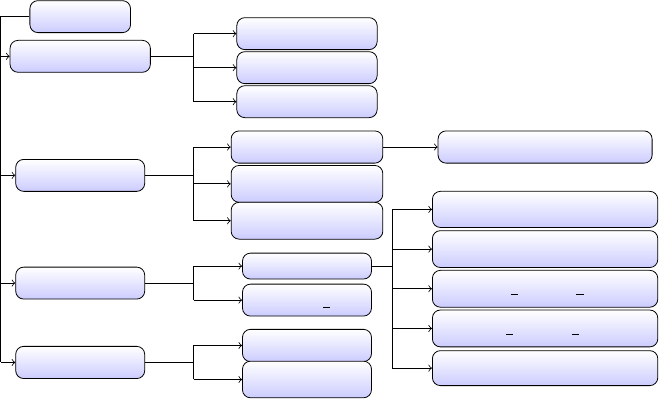
ATLAS-1.0 is provided with a scheme of directories and ﬁles, see scheme in

ﬁgure 1. In this scheme, the user can create folders and ﬁles for each study

case. The main folder is ATLAS and whitin it, are folders divided according

their functionality.

ATLAS

ATLAS-1.0 Resources

Sources

ATLAS.1.0.x

Data

wrf-nc name.wrf.nc

gfs1deg-nc

gfs1deg-grib

Runs name

name.inp

name.Phase1.inp

name phase 1.grn

name phase 1.tgsd

name.pts

name B

Utilities Grib2nc

Scripts

Figure 1: Directories and ﬁles scheme of ATLAS 1.0

To run ATLAS-1.0 is necesary to complete data in the required input ﬁles.

ATLAS-1.0 can be used in forward mode with speciﬁc input ﬁles indicating all

the simulation information required to obtain ﬁnally the tephra trajectories,

concentrations, and load accumulation. The ATLAS-1.0 ﬂow for forward

mode is presenting in ﬁgure 2. In backward case, there is a dispersed set of

particles which are necesary to model backaward in time. Then, the input

ﬁles are diﬀerent. The ATLAS-1.0 ﬂow for backward runs is presented in

ﬁgure 3. When ATLAS-1.0 is executed, all the output ﬁles are saved on the

same directory. There are examples input ﬁles in the Sources directory.

4 Input ﬁles

4.1 The input ﬁle name.inp

The main input ﬁle include the principal information needed to simulate.

This ﬁle is divided in blocks.

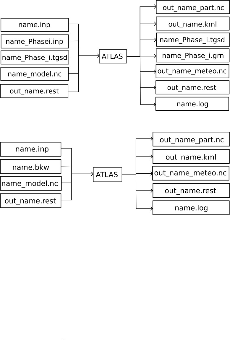
Figure 2: ATLAS-1.0 ﬂow for forward mode

Figure 3: ATLAS-1.0 ﬂow for backward mode

The ﬁrst block, with simulation time information must be completed, line

per line, as follows,

•YEAR, a four-digit integer value referring the year in which the simu-

lation begins.

•MONTH, a two-digit integer value with the month in which the simu-

lation begins.

•DAY, a two-digit integer value with the day in which the simulation

begins.

•SIMULATION START, an integer value, in hours from 00:00 UTC of

the DAY/MONTH/YEAR

•SIMULATION END, an integer value, in hours from 00:00 UTC of

the DAY/MONTH/YEAR. In this part, is important to note that if

SIMULATION END is less tha SIMULATION START, a backwards

integration is performed.

•TIME STEP : Simulation Increment Time in seconds.

•RESTART, the options are YES or NO. If the present simulations

consist of the continuation of a previous one, then is important to start

this with the particle suspended and deposited information to continue

the transport and accumulate the deposit.

It follows a computational domain block. The computational domain is the

grid where the information is restored, but it is not an Eulerian grid. In this

block, the user must complete the following information,

•LATMAX, maximium latitude in degrees. A value between -90 and 90.

•LATMIN, minimium latitude in degrees. A value between -90 and 90.

•LONMAX, maximium longitude in degrees. A value between -180 and

180.

•LONMIN, minimium longitude in degrees. A value between -180 and

180.

•ZTOP, maximium modeling height. A value in meters, which should be

higher than the volcanic column height in case to simulate an eruption.

•VERTICAL RESOLUTION, value in meters. Set the vertical spacing

to store the interpolated meteorological information to calculate the

particle transport. It is recomended to set it as the meteorological ﬁle

resolution.

•LONGITUDE RESOLUTION, value in degree. Set the xhorizontal

spacing to store the interpolated meteorological information to calcu-

late the particle transport. It is recomended to set it as the meteoro-

logical ﬁle resolution.

•LATITUDE RESOLUTION, value in degree. Set the yhorizontal spac-

ing to store the interpolated meteorological information to calculate the

particle transport. It is recomended to set it as the meteorological ﬁle

resolution.

The next block is referred to the output grid characteristics,

•OUTPUT LATMAX, maximium limits for output ﬁle. Value in degree.

•OUTPUT LATMIN, minimium limits for output ﬁle. Value in degree.

•OUTPUT LONMAX, maximium limits for output ﬁle. Value in degree.

•OUTPUT LONMIN, minimium limits for output ﬁle. Value in degree.

•OUTPUT FREQUENCY, time interval to extract information, in hours.

•VERTICAL LAYERS, distance between vertical layers (only one num-

ber) or vertical leyers enumerated, in meters.

•LONGITUDE RESOLUTION, value in degrees.

•LATITUDE RESOLUTION, value in degrees.

•OUTPUT CLASSES, options are YES/NO. If yes, then the output ﬁle

include output variables per particle classes.

•OUTPUT PHASES, options are YES/NO, If yes, then the output ﬁle

include output variables per particle phases.

•OUTPUT TRACK POINTS, options are YES/NO. If yes, an extra

output ﬁle is generated per track point with load information in that

location.

The next block contain physics information. For now, only the vertical ve-

locity model in consideration for the simulation.

•TERMINAL VELOCITY MODEL, options are 0,1,2,3,4. Where 0 cor-

respond to the Stokes model, 1 is the Arastoopour model, 2 the Ganser,

3 is the model of Wilson & Huang, and 4 is Dellino model. Select the

model to parameterize the terminal velocity.

A meteorological data information block is added. Diferent meteo models

can be considered simultaneously. Each meteo model is deﬁned by the tags

METEO MODEL DEFINITION and END METEO MODEL DEFINITON

Between this, is necessary to complete the information:

•Activate, options are yes/no. If yes, this meteorological ﬁle is used in

the simulations.

•MODEL TYPE, options are WRF/GFS/DEBUG.

•FILE, indicate the ﬁle path.

•POSTPROCESS, options are yes/no. If yes, an output ﬁle is generated,

showing the meteorological variables used in the simulation.

Finally, Diﬀerent sources (phases) can be considered simultaneously. Each

phase is deﬁned by the tags PHASE DEFINITION and END PHASE DEFINITION.

Between these, is necessary to complete the information,

•ACTIVATE, options are yes/no. If yes, this pahse is used in the simu-

lation.

•INCLUDE, indicate the ﬁle path coresponding to the secondary input

ﬁle. Where is detailed the phase charaacteristics.

4.2 The input ﬁle name Phasei.inp

This input ﬁle contain all the information about the source term. If the

user want to run with nsource terms, then is necessary to complete the

ﬁle name Phasei.inp for ifrom 1 to n, i.e. so many ﬁles as source term to

model.This ﬁle contain the next information,

•NUMBER PARTICLES, an integer denoting the total number of par-

ticles in this phase. (can be slightly modiﬁed by ATLAS to make it as

a multiple of the number of time steps.

•PHASE NAME, character denoting the name of this phase.

•PHASE TYPE, options are ERUPTION/SATELITE/RESUSPENSION.

For now, is only available the type ERUPTION.

•INITIAL TIME, start time in hours since simulation start indicated in

the name.inp ﬁle. This time is referred to the eruption start. Multiple

values are possible if there are changed in the column height.

•END TIME, in hours since simulation start indicated in the name.inp

ﬁle. Only one value.

•SOURCE TYPE, options are point/linear/top-hat/suzuki. Only for

eruption type.

•COLUMN HEIGHT, value in meters, above Vent.

•MASS FLOW RATE, options are a value in KG/s or ESTIMATE-

MASTIN/ESTIMATE-DEGRUYTER/ESTIMATE-WOODHOUSE.

•A SUZUKI, value only for Suzuki source type.

•L SUZUKI, value. only for Suzuki source type.

•D TOP HAT, value in meters. only for Top-hat source type.

•VOLCANO NAME, Volcano name or unknown.

•SOURCE LONGITUDE, value in degree.

•SOURCE LATITUDE, value in degree.

•SOURCE ELEVATION, value in meters.

•PHASE GRANULOMETRY, Path where the granulometry ﬁle is/ﬁle name.ext

or “NONE”. If in the previous line a directory and graulometry ﬁle is

provided, the next 7 lines are not necessary, else (if “NONE” option

was used) ATLAS generate a TGSD distribution according the next

lines:

•DISTRIBUTION, o GAUSSIAN/BIGAUSSIAN.

•NUMBER OF BINS, an integer indicating the number of groups to

divide the TGSD.

•FI MEAN, mean value of grain diameter. A second value is used if

DISTRIBUTION=BIGAUSSIAN.

•FI DISP standard deviation value of grain diameter. A second value is

used if DISTRIBUTION=BIGAUSSIAN.

•FI RANGE, minimium and maximium values of grain diameter.

•DENSITY RANGE, minimium and maximium values of particles den-

sity (a linear interpolation is used to asign density values to all bins).

•SPHERICITY RANGE, minimium and maximium values for spheric-

ity (a linear interpolation is used to asign density values to all bins).

•AGGREGATION MODEL, options are NONE/CORNELL/PERCENTAGE,a

ccording the model to consider aggregation.

•AGGREGATE SIZE : value in microns.

•AGGREGATE DENSITY, density for the aggregate class.

•PERCENTAGE ( %), value in percentage, only for Percentage Model.

4.3 The input ﬁle name Phase i.tgsd

This input ﬁle can be ceated by ATLAS, providing all the necessary informa-

tion. But, if there is available a total grain size distribution, is better provide

a ﬁle with the speciﬁc information. The format of this ﬁle is shown in table

Table 1: name Phase i.tgsd ﬁle format

diam(1) rho(1) sphe(1) fc(1)

...

diam(nc) rho(nc) sphe(nc) fc(nc)

4.4 The input ﬁle name.pts

This is an optional input ﬁle in ATAS. Only added if the user wants to obtain

information (thickness and load deposited) in speciﬁc points. This is a ﬁle

in ASCII format and contain the points geographical information (longitude

and laitude). The ﬁle format is presented in table 2, in which, nis the toal

number of points, name is the user deﬁned name for each point, lon and lat

are the point longitude and latitude. A point characteristics are deﬁned per

row.

Table 2: name.pts ﬁle format

name(1) lon(1) lat(1)

...

name(n) lon(n) lat(n)

4.5 The input ﬁle name model.nc

ATLAS needs meteoroogical data (topography and time dependant data as

the wind ﬁeld, temperature, humidity, etc.) to simulate the particle trans-

port. ATLAS read only data in netCD format. WRF data comes in that

format, then the user only needs to indicate in the input ﬁle name.inp the

meteorological ﬁle directory and name. Instead, GFS data comes in grib

format. Then, ﬁrst is necessary transform it to netCDF format. For this, a

utility program is added. The GRIB2NC is the utility program provided with

FALL3D model. Once the GFS ﬁle is transformed in netCDF format, the

user only needs to indicate the ﬁle path and name in the input ﬁle name.inp.

4.6 The input ﬁle out name.rest

This ﬁle is generated as output ﬁle in each simulation. If the user want

to continue the simulaton, then need to copy this output ﬁle obtained in

the previous (in time) simulation to the new directory and rename it as

out name.rest, where name is the new name.

4.7 The input ﬁle name.bkw

If the user want to simulate in backward mode (backwards in time) is nec-

essary this ﬁle with the particle dispersed information (deposited or in air).

This is asn ASCII ﬁle, the format is showed in table 3, where np is the total

number of particles descripted below, iis the particles numbering, rho is the

particle density, diam is the ddiameter, mass the particle mass, and sphe the

sphericity. In continuity the geogprahical information mut be added, lon,lat,

and zare the longitude, latitude and height respectively. Each row contain

the information for one particle.

Table 3: name.bkw ﬁle format

TOTAL PARTICLES = np

1 rho(1) diam(1) mass(1) sphe(1) lon(1) lat(1) z(1)

... ... ... ... ... ... ... ...

i rho(i) diam(i) mass(i) sphe(i) lon(i) lat(i) z(i)

... ... ... ... ... ... ... ...

np rho(np) diam(np) mass(np) sphe(np) lon(np) lat(np) z(np)

5 Output ﬁles

When the simulaton is end or during the execution, ATLAS produce the next

output ﬁles.

5.1 out name part.nc

This ﬁle is written in netCDF format. There are several free rograms to

open netCDF ﬁles and generate images and animations. This ﬁle contain

information about

•Topography

•Ash load on ground. Also, if the user indicated, the ash load per particle

classes and/or particle phases.

•Ash concentrations in diﬀerent speciﬁc heights indicated by the user in

the input ﬁle. Also, if the user indicated so, the ash concentrations at

the same height levels per particle class or per particle phase.

•Column mass.

5.2 out name.kml

This ﬁle is written in kml format. Could be open in Google Earth to look

the particles trajectories.

5.3 name.tps.point name.res

This optional output ﬁle is written in ASCII format. Contain information

about load (kg/m2) and thickness (cm) deposited on the point point name

for each time step.

5.4 name Phase i.tgsd

This is an output ﬁle only if the user does not included it as input. ATLAS

generate this ﬁle automatically with a Gaussian or bi-Gaussian distribution.

5.5 name Phase i.grn

This ﬁle is in ASCII format and it is generated by ATLAS since the name Pase i.tgsd

ﬁle, where iis the phase number in consideration. Is necessary to have one

per phase. This ﬁle take into account the aggregation class. The ﬁle format

is shown in table 4, where nc is the total number of particle classes (this nc

could be diﬀerent than the used in the name Pase i.tgsd ﬁle when aggrega-

tion is considered), rho is the class density, sphe the sphericity, fc is the mass

fraction asociated to each class and their values are between 0 and 1, and

satisfy that Pfc = 1. Finally, class is the label which describes the class as

a particle class or as the aggregate class.

Table 4: Formato del archivo name Phase i.grn

diam(1) rho(1) sphe(1) fc(1) class(1) (e.g. class-01)

...

diam(nc) rho(nc) sphe(nc) fc(nc) class(nc) (e.g. aggregate)

5.6 out name meteo.nc

This optional output ﬁle is written in netCDF format. Contain the following

information,

•The computational domain used for the simulation, Lonngitude, lati-

tude aand height information.

•Times in which the variables are readed.

•Time an spatial resolution.

•Longitude, latitude and heights of the grid where the information is

stored.

•Topography.

•Meteorological model used in each grid point (usefule when more than

one meteorological ﬁle is used).

•Meteorological variables used to simulate.

5.7 out name.rest

This ﬁle is written in ASCII format and can be used to obtain succesive

execution of ATLAS activating the restart option in the input ﬁle. This ﬁle

is created at the end of the simulation. If the user wnat to obtain a simulation

that continues the present, need to copy this ﬁle to the new directory and

rename it, and conﬁgure the input ﬁle indicating “YES” in the RESTART

option inside the SIMULATION TIME block.

5.8 name.log

This ﬁle cntain a detailed onformation about the simulation, error and warn-

ing messages. This ﬁle is written in ASCII format ad give information about

the program version, times (initial, ﬁnal) for the simulation, names and di-

rectories for input and output ﬁles, meteorological range used, parameters

used, information about concentration during the simulation, among others.

6 Program Installation and execution

ATLLAS-1.0 is written in FORTRAN 90, tested in UNIX/Linux. To compile

the code, available only in serial version is required:

•FORTRAN 90 compiler.

•Library netCDF installed. This is available from https://www.unidata.ucar.edu/software/netcdf/

•To use the GRIB2NC utility program to decode meteorological GRIB

ﬁles from GFS is necessary to have wgrib or wgrib2 available from

http://www.cpc.ncep.noaa.gov/products/wesley/wgrib.html. For more

information about GRIB2NC, see FALL3D references [??].

To install ATLAS-1.0 is necessary to edit the Makeﬁle according the spe-

ciﬁc netCDF directory and fortran compiler. Then, in a terminal move to

the ATLAS source directory ($cd ATLAS/ATLAS-1.0/Sources/), and exe-

cuted the command: $make The executable ﬁle is installed in the directory

ATLAS-1.0.

To run ATLAS go to the corresponding folder name inside the Run directory,

complete all the inputs ﬁle and make a dinamic link to the executable ﬁle

and run $ ./ATLAS-1.0.exe name

All the output ﬁles will be created and saved in the same name directory.

7 Example

A run example is proposed with a GFS meteorological ﬁle, which is in format

netCDF on the directory Data/gfs1deg-nc, called ejemplo.gfs1deg.nc. In the

directory Runs/ejemplo are tree input ﬁles: ejemplo.inp,ejemplo.Phase1.inp,

and ejemplo.Phase2.inp. Note that this is not a real example, only fulﬁlls

the rol of testing ATLAS-1.0.

To run this example the user need to modify the input ﬁle ejemplo.inp with

the correct directory where the ﬁles (see meteorological block and phases

block, and change the word “COMPLETE...” by the correct directory) are

in the pc, and then go to the directory Runs/ejemplo, copy or make a dynamic

link to Atlas.1.0.exe in this directory and execute:

./Atlas.1.0 ejemplo

References

H. Arastoopour, C. Wang, and S. Weil. Particle-particle interaction force in

a dilute gas-solid system. Chemical Engineering Science, 37(9):1379–1376,

1982.

B. Aschenbrenner. A new method of expressing particle sphericity. Journal

of Sedimentary Petrology, 26:15–31, 1956.

W. Cornell, S. Carey, and H. Sigurdsson. Computer simulation and trans-

port of the Campanian Y5 ash. Journal of Volcanology and Geothermal

Research, 17:89–109, 1983.

A. Costa, A. Folch, G. Macedonio, B. Giaccio, R. Isaia, and V. Smith.

Quantifying volcanic ash dispersal and impact from Campanian Ignimbrite

super-eruption. Geophysical Research Letters, 39(L10310), 2012.

W. Degruyter and C. Bonadonna. Improving on mass ﬂow rate estimates of

volcanic eruptions. Geophysical Research Letters, 39(L16308), 2012.

P. Dellino, D. Mele, R. Bonasia, G. Braia, L. La Volpe, and R. Sulpizio.

The analysis of the inﬂuence of pumice shape on its terminal velocity.

Geophysical Research Letters, 32(21):4, 2005.

H. Ganser. A rational approach to drag prediction of spherical and non

spherical particles. Powder Technology, 77:143–152, 1993.

S. R. Hanna. Application in air pollution modeling. In Nieuwstadt F.T.M.

and H. van Dop, editors, Atmospheric Turbulence and Air Pollution Mod-

elling. D. Reidel Publishing Company, Dordrecht, Holland, 1982.

B. Legras, B. Jospeh, and F. Lefevre. Vertical diﬀusivity in the lower

stratosphere from Lagrangian back-trajectory reconstructions of ozone

proﬁles. Journal of Geophysical Research, 108(D18), 2003. doi:

10.1029/2002JD003045.

L. Mastin, M. Guﬀanti, R. Servranckx, P. Webley, S. Barsotti, K. Dean,

A. Durant, J. Ewert, A. Neri, W. Rose, D. Schneider, L. Siebert, B. Stun-

der, G. Swanson, A. Tupper, A. Volentik, and C. Waythomas. A multidis-

ciplinary eﬀort to assign realistic source parameters to models of volcanic

ash-cloud transport and dispersion during eruptions. Journal of Volcanol-

ogy and Geothermal Research, 186:10–21, 2009.

T. Pfeiﬀer, A. Costa, and G. Macedonio. A model for the numerical sim-

ulation of tephra fall deposits. Journal of Volcanology and Geothermal

Research, 140(4):273–294, 2005.

A. Stohl, C. Forster, A. Frank, P. Seibert, and G. Wotawa. Technical note:

The lagrangian particle dispersion model FLEXPART version 6.2. At-

mospheric Chemistry and Physics, 5(9):2461–2474, 2005.

R. Sulpizio, A. Folch, A. Costa, C. Scaini, and P. Dellino. Hazard assessment

of farrange volcanic ash dispersal from a violent strombolian eruption at

SommaVesuvius volcano, Naples, Italy: implications on civil aviation.

Bulletin of volcanology, 74(9):2205–2218, 2012.

T. Suzuki. A theoretical model for dispersion of tephra. In D. Shimozuru

and Yokoyama, editors, Arc Volcanism: Physics and Tectonics, pages 93–

113. Terra Scientiﬁc Publishing Company (TERRAPUB), Tokyo, 1 edi-

tion, 1983.

H. Wadell. Sphericity and roundness of rock particles. The Journal of Geol-

ogy, 41:310–331, 1933.

G. Walker, L. Wilson, and E. Bowell. Explosive volcanic eruptions I. rate of

fall of pyroclasts. Geophysical Journal of the Royal Astronomical Society,

22:377–383, 1971.

L. Wilson and T. Huang. The inﬂuence of shape on the atmospheric settling

velocity of volcanic ash particles. Earth and Planetary Science Letters, 44:

311–324, 1979.

M. Woodhouse, A. Hogg, J. Phillips, and R. Sparks. Interaction between vol-

canic plumes and wind during the 2010 Eyjafjallaj¨okull eruption, Iceland.

Journal of Geophysical Research, 118:92–109, 2013.

Manual

Navigation menu

Versions of this User Manual:

Views

Navigation