Manual
manual
manual
User Manual:
Open the PDF directly: View PDF ![]() .
.
Page Count: 6
GSnet User Manual
Maintainer: Jinhwan Kim hwanistic@unist.ac.kr
2018-07-12
1. 2 Ways to Start GSnet
① Run following codes on R console.
>library(‘shiny’)
>runGitHub(‘epn’, ‘jhk0530’)
It is simple but may take a few minutes to download the data. To save the time, we
recommend users to use second way.
② Download ZIP file and run app in R
- Access to the GSnet GitHub page (https://github.com/jhk0530/epn)
- Download the ZIP file by clicking ‘Clone or download’ and ‘Download ZIP’ button.
- Unzip the downloaded file
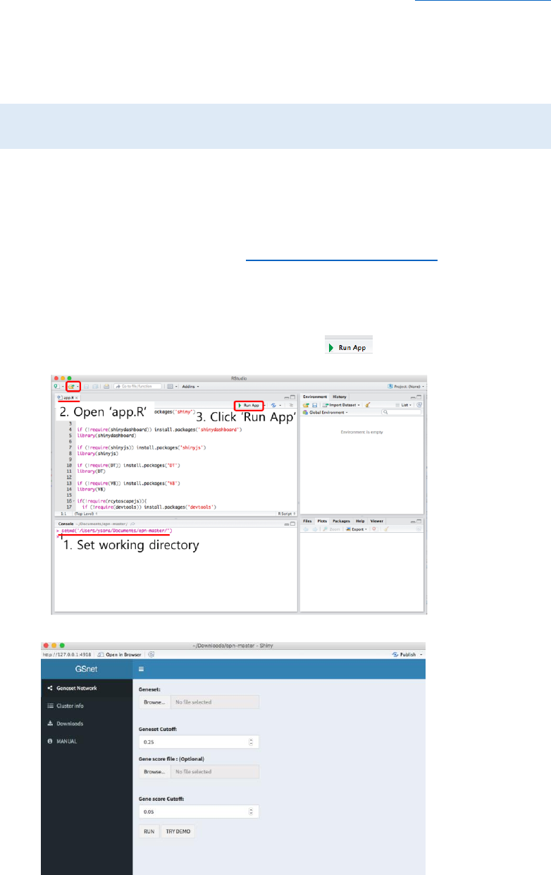
- Open R studio and set working directory to where the unzipped file exists.
- Open the file ‘app.R’ and click ‘Run App’ button .
Figure 1. Running GSnet using downloaded ZIP file
Figure 2. Initial screen of GSnet
* Note: GSnet can be run on both R display screen and web browser (by clicking ‘Open in
Browser’ button in the R display screen). Running app on web browser is usually faster.
2. How to use
① Upload input data
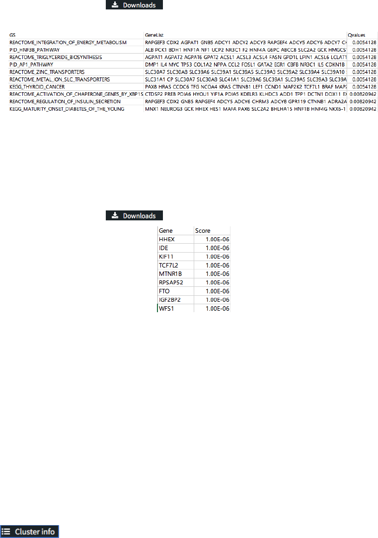
- Geneset: Gene-set analysis (GSA) result file. It is a tab-delimited text file composed
of 3 columns including gene-set name, member genes and q-value. The header line
is required. Gene-set members must be separated by space. Example file is available
from ‘Downloads’ tab .
Figure 3. Example of gene-set analysis result file
- Geneset Cutoff: The significance cutoff for gene-sets to be included in the gene-set
network. Default=0.25
- Gene score file (optional): Gene score file. It consists of gene name and gene p-
value columns (tab-delimited). The header line is required. Example file is available
from ‘Downloads’ tab .
Figure 4. Example of gene score file
- Gene score Cutoff: The significance off for genes to be included in the gene network.
Default=0.05.
- After uploading data and setting parameters, click ‘RUN’ to generate gene-set and
gene networks. ‘TRY DEMO’ will show the example network for gene sets significantly
altered in Type 2 Diabetes Mellitus.
② Exploring the Gene-set Network
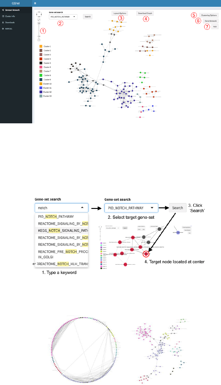
In the result panel, the gene-set network graph is displayed, and the gene-set clusters are
represented by different colors (fig. 5). Gene-sets included in multiple clusters are colored
with dark gray. The detailed clustering result is represented as table in ‘Cluster info’ tab
( ), and users can save the result as text file by clicking
‘CLUSTERING_RESULT’ button below the result table.
Figure 5. Result panel. Each number represents useful function introduced below.
Functions
1. Graph control panel: Users can zoom in/out or move the graph by simple mouse
control or using graph control panel ( in fig 5) in the top left of the result panel.
2. Gene-set search: To find a specific gene-set node, type a search word in Gene-set
search box ( in fig 5), select target gene-set, and click ‘Search’ button. Then
corresponding gene-set node will be located at the center of the result panel (fig. 6).
Figure 6. Search for the position of a gene-set node
3. Layout option: Click ‘Layout Option’ button (- in fig 5) and choose circle or cola
layout (fig. 7).
Figure 7. Circle (left) and Cola (right) layout
4. Download Graph: Users can download a vector image file (.SVG) for current plot by
clicking ‘Download Graph’ button ( in fig 5).
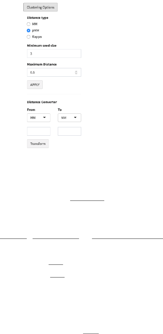
5. Clustering Options: The distance type, minimum seed size and maximum distance
allowed between gene-sets can be set in ‘Clustering Options’ ( in fig 5). After setting
these parameters, click ‘APPLY’ to change the gene-set network graph. We present
detailed explanation for each parameter.
Figure 8. Clustering Options and Distance Converter
Distance type
✓ MM: Meet/Min distance (MM) is defined for two gene-sets A and B as:
Where |A| is the size of A.
✓ pMM: PPI weighted Meet/Min (pMM) is defined as:
Where P is PPI score matrix, P(x,y) is PPI score of two genes x and y, and
And pMM(B) is symmetrically defined, Then,
✓ Kappa: 1-Cohen’s Kappa distance is defined as:

Where
(U=list of total genes) is the observed rate of
agreement of two gene-sets, and
is the expected rate of
agreement of two gene-sets.
The default distance is pMM with a cutoff (minimum seed distance) that corresponds
to same percentile as MM=0.5. For example, if 0.5 ranks the top 1% among all the
MM scores, the top 1% pMM score is set as default.
Minimum seed size: The minimum cluster size allowed. Default = 3.
Maximum Distance: Maximum distance between gene-sets to be connected. The
default value is described above.
Distance converter: For user convenience, we also provide distance converter. For
example, to identify the Kappa distance matched to MM=0.5, select MM in ‘From’ box,
type 0.5 below, select Kappa in ‘To’ box, and then click ‘Transform’ button. Then
corresponding Kappa distance will be represented.
6. Gene Network
GSnet provides gene network plot of each cluster based on STRING human PPI data.
For example, if you want to see the gene network in cluster 4, do as follows:
① Click the ‘Gene Network’ button ( in fig 5).
② Choose the cluster number (‘4’ in this case) from ‘Gene Network in Cluster’ box.
③ Set the PPI cutoff (default=700)
④ Select edge type. We provide 8 edge types such as
A. Combined PPI score (The stronger PPI, the thicker an edge is)
B. Neighborhood
C. Gene fusion
D. Co-occurrence
E. Co-expression
F. Experiments
G. Databases
H. Text mining
Detailed explanation for each PPI evidence type is described in STRING web
page https://string-db.org/cgi/help.pl .
⑤ Click ‘Draw Gene Network’ button. Then it will show the network for genes in
cluster 4 with selected edge types (fig 9).
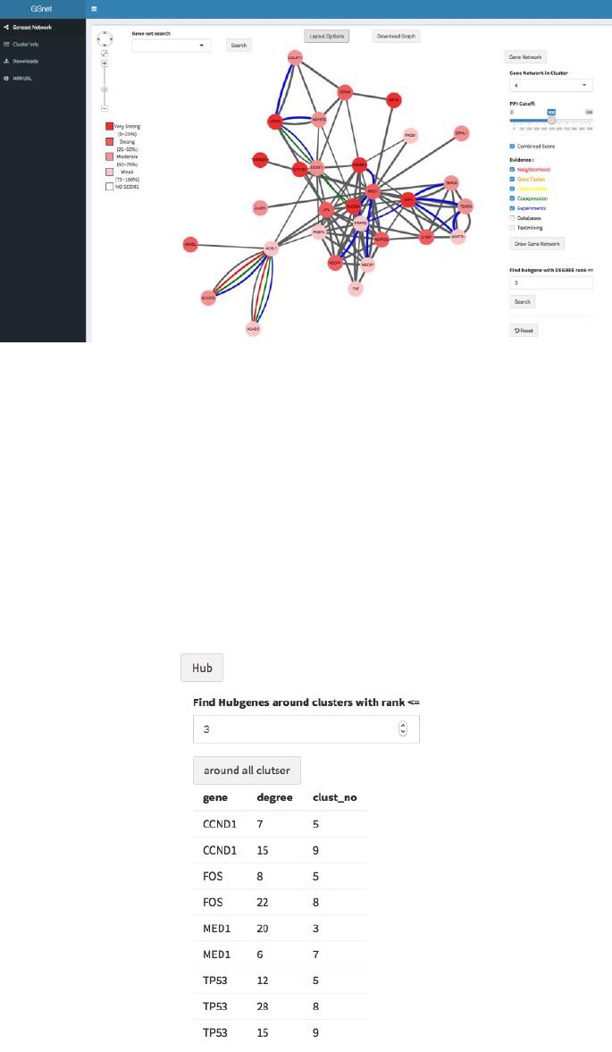
Figure 9. Gene network for a specific cluster
Hub gene: To find top-ranked hub genes in selected cluster, just type degree rank in
the box below (Find hub gene with DEGREE rank<=; default=3) and click ‘Search’.
To see the gene-set network again, click ‘Reset’ button.
7. Hub
If the user clicks the ‘Hub’ button ( in fig 5) and type a degree rank N in the box, the
genes within N-degree rank for at least two clusters will be listed (fig. 10). We expect that
such genes have multiple biological roles related to the phenotype.
Figure 10. Hub genes observed in at least two clusters