Q Chem 5.1 User's Manual
User Manual:
Open the PDF directly: View PDF ![]() .
.
Page Count: 1091 [warning: Documents this large are best viewed by clicking the View PDF Link!]
- Introduction
- Installation, Customization, and Execution
- Q-Chem Inputs
- IQmol
- General Form
- Molecular Coordinate Input ($molecule)
- Job Specification: The $rem Input Section
- Additional Input Sections
- Comments ($comment)
- User-Defined Basis Sets ($basis and $aux_basis)
- User-Defined Effective Core Potential ($ecp)
- User-Defined Exchange-Correlation Density Functionals ($xc_functional)
- User-defined Parameters for DFT Dispersion Correction ($empirical_dispersion)
- Addition of External Point Charges ($external_charges)
- Applying a Multipole Field ($multipole_field)
- User-Defined Occupied Guess Orbitals ($occupied and $swap_occupied_virtual)
- Polarizable Continuum Solvation Models ($pcm)
- SS(V)PE Solvation Modeling ($svp and $svpirf)
- User-Defined van der Waals Radii ($van_der_waals)
- Effective Fragment Potential Calculations ($efp_fragments and $efp_params)
- Natural Bond Orbital Package ($nbo)
- Orbitals, Densities and Electrostatic Potentials on a Mesh ($plots)
- Intracules ($intracule)
- Geometry Optimization with Constraints ($opt)
- Isotopic Substitutions ($isotopes)
- Multiple Jobs in a Single File: Q-Chem Batch Jobs
- Q-Chem Output File
- Self-Consistent Field Ground-State Methods
- Overview
- Theoretical Background
- Basic SCF Job Control
- SCF Initial Guess
- Converging SCF Calculations
- Introduction
- Basic Convergence Control Options
- Direct Inversion in the Iterative Subspace (DIIS)
- Geometric Direct Minimization (GDM)
- Direct Minimization (DM)
- Maximum Overlap Method (MOM)
- Relaxed Constraint Algorithm (RCA)
- User-Customized Hybrid SCF Algorithm
- Internal Stability Analysis and Automated Correction for Energy Minima
- Small-Gap Systems
- Examples
- Large Molecules and Linear Scaling Methods
- Introduction
- Continuous Fast Multipole Method (CFMM)
- Linear Scaling Exchange (LinK) Matrix Evaluation
- Incremental and Variable Thresh Fock Matrix Building
- Fourier Transform Coulomb Method
- Resolution of the Identity Fock Matrix Methods
- PARI-K Fast Exchange Algorithm
- CASE Approximation
- occ-RI-K Exchange Algorithm
- Examples
- Dual-Basis Self-Consistent Field Calculations
- Hartree-Fock and Density-Functional Perturbative Corrections
- Unconventional SCF Calculations
- Ground State Method Summary
- References and Further Reading
- Density Functional Theory
- Introduction
- Kohn-Sham Density Functional Theory
- Overview of Available Functionals
- Basic DFT Job Control
- DFT Numerical Quadrature
- Range-Separated Hybrid Density Functionals
- DFT Methods for van der Waals Interactions
- Empirical Corrections for Basis Set Superposition Error
- Double-Hybrid Density Functional Theory
- Asymptotically Corrected Exchange-Correlation Potentials
- Derivative Discontinuity Restoration
- Thermally-Assisted-Occupation Density Functional Theory (TAO-DFT)
- Methods Based on ``Constrained'' DFT
- References and Further Reading
- Wave Function-Based Correlation Methods
- Introduction
- Treatment and the Definition of Core Electrons
- Møller-Plesset Perturbation Theory
- Exact MP2 Methods
- Local MP2 Methods
- Auxiliary Basis (Resolution of the Identity) MP2 Methods
- Attenuated MP2
- Coupled-Cluster Methods
- Non-Iterative Corrections to Coupled Cluster Energies
- Coupled Cluster Active Space Methods
- Frozen Natural Orbitals in CCD, CCSD, OD, QCCD, and QCISD Calculations
- Non-Hartree-Fock Orbitals in Correlated Calculations
- Analytic Gradients and Properties for Coupled-Cluster Methods
- Memory Options and Parallelization of Coupled-Cluster Calculations
- Simplified Coupled-Cluster Methods Based on a Perfect-Pairing Active Space
- Geminal Models
- Variational Two-Electron Reduced-Density-Matrix Methods
- References and Further Reading
- Open-Shell and Excited-State Methods
- General Excited-State Features
- Uncorrelated Wave Function Methods
- Time-Dependent Density Functional Theory (TDDFT)
- Maximum Overlap Method (MOM) for SCF Excited States
- Restricted Open-Shell Kohn-Sham Method for -SCF Calculations of Excited States
- Correlated Excited State Methods: The CIS(D) Family
- Coupled-Cluster Excited-State and Open-Shell Methods
- Excited States via EOM-EE-CCSD
- EOM-XX-CCSD and CI Suite of Methods
- Spin-Flip Methods for Di- and Triradicals
- EOM-DIP-CCSD
- EOM-CC Calculations of Core-Level States: Core-Valence Separation within EOM-CCSD
- EOM-CC Calculations of Metastable States: Super-Excited Electronic States, Temporary Anions, and More
- Charge Stabilization for EOM-DIP and Other Methods
- Frozen Natural Orbitals in CC and IP-CC Calculations
- Approximate EOM-CC Methods: EOM-MP2 and EOM-MP2T
- Approximate EOM-CC Methods: EOM-CCSD-S(D) and EOM-MP2-S(D)
- Implicit solvent models in EOM-CC/MP2 calculations.
- EOM-CC Jobs: Controlling Guess Formation and Iterative Diagonalizers
- Equation-of-Motion Coupled-Cluster Job Control
- Examples
- Non-Hartree-Fock Orbitals in EOM Calculations
- Analytic Gradients and Properties for the CCSD and EOM-XX-CCSD Methods
- EOM-CC Optimization and Properties Job Control
- EOM(2,3) Methods for Higher-Accuracy and Problematic Situations (CCMAN only)
- Active-Space EOM-CC(2,3): Tricks of the Trade (CCMAN only)
- Job Control for EOM-CC(2,3)
- Non-Iterative Triples Corrections to EOM-CCSD and CCSD
- Potential Energy Surface Crossing Minimization
- Dyson Orbitals for Ionized or Attached States within the EOM-CCSD Formalism
- Interpretation of EOM/CI Wave Functions and Orbital Numbering
- Correlated Excited State Methods: The ADC(n) Family
- The Algebraic Diagrammatic Construction (ADC) Scheme
- Resolution of the Identity ADC Methods
- Spin Opposite Scaling ADC(2) Models
- Core-Excitation ADC Methods
- Spin-Flip ADC Methods
- Properties and Visualization
- Excited States in Solution with ADC/SS-PCM
- Frozen-Density Embedding: FDE-ADC methods
- ADC Job Control
- Examples
- Restricted Active Space Spin-Flip (RAS-SF) and Configuration Interaction (RAS-CI)
- Core Ionization Energies and Core-Excited States
- Real-Time SCF Methods (RT-TDDFT, RT-HF, OSCF2)
- Visualization of Excited States
- References and Further Reading
- Basis Sets
- Effective Core Potentials
- Exploring Potential Energy Surfaces: Critical Points and Molecular Dynamics
- Equilibrium Geometries and Transition-State Structures
- Improved Algorithms for Transition-Structure Optimization
- Constrained Optimization
- Potential Energy Scans
- Intrinsic Reaction Coordinate
- Nonadiabatic Couplings and Optimization of Minimum-Energy Crossing Points
- Ab Initio Molecular Dynamics
- Ab initio Path Integrals
- References and Further Reading
- Molecular Properties and Analysis
- Introduction
- Wave Function Analysis
- Interface to the NBO Package
- Orbital Localization
- Visualizing and Plotting Orbitals, Densities, and Other Volumetric Data
- Spin and Charge Densities at the Nuclei
- Atoms in Molecules
- Distributed Multipole Analysis
- Intracules
- Harmonic Vibrational Analysis
- Anharmonic Vibrational Frequencies
- Linear-Scaling Computation of Electric Properties
- NMR and Other Magnetic Properties
- Finite-Field Calculation of (Hyper)Polarizabilities
- General Response Theory
- Electronic Couplings for Electron- and Energy Transfer
- Population of Effectively Unpaired Electrons
- Molecular Junctions
- References and Further Reading
- Molecules in Complex Environments: Solvent Models, QM/MM and QM/EFP Features, Density Embedding
- Fragment-Based Methods
- Introduction
- Specifying Fragments in the $molecule Section
- FRAGMO Initial Guess for SCF Methods
- Locally-Projected SCF Methods
- The First-Generation ALMO-EDA and Charge-Transfer Analysis (CTA)
- Job Control for Locally-Projected SCF Methods
- The Second-Generation ALMO-EDA Method
- The MP2 ALMO-EDA Method
- The Adiabatic ALMO-EDA Method
- ALMO-EDA Involving Excited-State Molecules
- The Explicit Polarization (XPol) Method
- Symmetry-Adapted Perturbation Theory (SAPT)
- The XPol+SAPT (XSAPT) Method
- Energy Decomposition Analysis based on SAPT/cDFT
- The Many-Body Expansion Method
- Ab Initio Frenkel Davydov Exciton Model (AIFDEM)
- TDDFT for Molecular Interactions
- The ALMO-CIS and ALMO-CIS+CT Methods
- References and Further Reading
- Geometry Optimization with Q-Chem
- AOInts
- Introduction
- Historical Perspective
- AOInts: Calculating ERIs with Q-Chem
- Shell-Pair Data
- Shell-Quartets and Integral Classes
- Fundamental ERI
- Angular Momentum Problem
- Contraction Problem
- Quadratic Scaling
- Algorithm Selection
- More Efficient Hartree–Fock Gradient and Hessian Evaluations
- User-Controllable Variables
- References and Further Reading
- Q-Chem Quick Reference
- Q-Chem Text Input Summary
- Keyword: $molecule
- Keyword: $rem
- Keyword: $basis
- Keyword: $comment
- Keyword: $ecp
- Keyword: $empirical_dispersion
- Keyword: $external_charges
- Keyword: $intracule
- Keyword: $isotopes
- Keyword: $multipole_field
- Keyword: $nbo
- Keyword: $occupied
- Keyword: $opt
- Keyword: $svp
- Keyword: $svpirf
- Keyword: $plots
- Keyword: $localized_diabatization
- Keyword: $van_der_waals
- Keyword: $xc_functional
- Geometry Optimization with General Constraints
- $rem Variable List
- General
- SCF Control
- DFT Options
- Large Molecules
- Correlated Methods
- Correlated Methods Handled by CCMAN and CCMAN2
- Perfect pairing, Coupled cluster valence bond, and related methods
- Excited States: CIS, TDDFT, SF-XCIS and SOS-CIS(D)
- Excited States: EOM-CC and CI Methods
- Geometry Optimizations
- Vibrational Analysis
- Reaction Coordinate Following
- NMR Calculations
- Wave function Analysis and Molecular Properties
- Symmetry
- Printing Options
- Resource Control
- Alphabetical Listing of $rem Variables
- References and Further Reading
- Q-Chem Text Input Summary
Q-Chem 5.1 User’s Manual
Version 5.1
May, 2018
Q-CHEM User’s Manual
Version 5.1 was edited by:
Dr. Andrew Gilbert
Prof. John Herbert
Version 5.0 was edited by:
Dr. Andrew Gilbert
Version 4 editors:
Prof. John Herbert
Prof. Anna Krylov
Dr. Narbe Mardirossian
Prof. Martin Head-Gordon
Dr. Emil Proynov
Dr. Andrew Gilbert
Dr. Jing Kong
The contributions of individual developers to each version are highlighted in “New Features”,
Section 1.3
Published by: Customer Support:
Q-Chem, Inc. Telephone: (412) 687-0695
6601 Owens Dr. Facsimile: (412) 687-0698
Suite 105 email: support@q-chem.com
Pleasanton, CA 94588 website: www.q-chem.com
Q-CHEM is a trademark of Q-Chem, Inc. All rights reserved.
The information in this document applies to version 5.1 of Q-CHEM.
This document version generated on October 20, 2018.
© Copyright 2000–2018 Q-Chem, Inc. This document is protected under the U.S. Copyright Act of 1976 and state
trade secret laws. Unauthorized disclosure, reproduction, distribution, or use is prohibited and may violate federal and
state laws.

CONTENTS 3
Contents
1 Introduction 15
1.1 About This Manual ............................................ 15
1.1.1 Overview .............................................. 15
1.1.2 Chapter Summaries ........................................ 15
1.2 Q-CHEM, Inc. ............................................... 16
1.2.1 Contact Information and Customer Support ............................ 16
1.2.2 About the Company ........................................ 16
1.2.3 Company Mission ......................................... 16
1.3 Q-CHEM Features ............................................. 16
1.3.1 New Features in Q-CHEM 5.1 ................................... 17
1.3.2 New Features in Q-CHEM 5.0 ................................... 18
1.3.3 New Features in Q-CHEM 4.4 ................................... 19
1.3.4 New Features in Q-CHEM 4.3 ................................... 20
1.3.5 New Features in Q-CHEM 4.2 ................................... 21
1.3.6 New Features in Q-CHEM 4.1 ................................... 22
1.3.7 New Features in Q-CHEM 4.0.1 .................................. 23
1.3.8 New Features in Q-CHEM 4.0 ................................... 23
1.3.9 Summary of Features in Q-CHEM versions 3. x.......................... 26
1.3.10 Summary of Features Prior to Q-CHEM 3.0 ............................ 28
1.4 Citing Q-CHEM .............................................. 29
References and Further Reading ......................................... 31
2 Installation, Customization, and Execution 32
2.1 Installation Requirements ......................................... 32
2.1.1 Execution Environment ...................................... 32
2.1.2 Hardware Platforms and Operating Systems ........................... 32
2.1.3 Memory and Disk Requirements ................................. 32
2.2 Installing Q-CHEM ............................................ 33
2.3 Q-CHEM Auxiliary files ($QCAUX)................................... 33
2.4 Q-CHEM Run-time Environment Variables ................................ 34
2.5 User Account Adjustments ........................................ 34
2.6 Further Customization: .qchemrc and preferences Files ......................... 35
2.7 Running Q-CHEM ............................................. 36
2.8 Parallel Q-CHEM Jobs .......................................... 37
2.9 IQMOL Installation Requirements .................................... 38
2.10 Testing and Exploring Q-CHEM ..................................... 39
3 Q-CHEM Inputs 40
3.1 IQMOL .................................................. 40
3.2 General Form ............................................... 40
3.3 Molecular Coordinate Input ($molecule)................................. 42
3.3.1 Specifying the Molecular Coordinates Manually ......................... 42
3.3.2 Reading Molecular Coordinates from a Previous Job or File ................... 46

CONTENTS 4
3.4 Job Specification: The $rem Input Section ................................ 46
3.5 Additional Input Sections ......................................... 48
3.5.1 Comments ($comment)...................................... 48
3.5.2 User-Defined Basis Sets ($basis and $aux_basis)......................... 48
3.5.3 User-Defined Effective Core Potential ($ecp)........................... 48
3.5.4 User-Defined Exchange-Correlation Density Functionals ($xc_functional)........... 48
3.5.5 User-defined Parameters for DFT Dispersion Correction ($empirical_dispersion)........ 49
3.5.6 Addition of External Point Charges ($external_charges)..................... 49
3.5.7 Applying a Multipole Field ($multipole_field).......................... 49
3.5.8 User-Defined Occupied Guess Orbitals ($occupied and $swap_occupied_virtual)........ 50
3.5.9 Polarizable Continuum Solvation Models ($pcm)......................... 50
3.5.10 SS(V)PE Solvation Modeling ($svp and $svpirf )......................... 50
3.5.11 User-Defined van der Waals Radii ($van_der_waals)....................... 50
3.5.12 Effective Fragment Potential Calculations ($efp_fragments and $efp_params)......... 50
3.5.13 Natural Bond Orbital Package ($nbo)............................... 50
3.5.14 Orbitals, Densities and Electrostatic Potentials on a Mesh ($plots)................ 51
3.5.15 Intracules ($intracule)....................................... 51
3.5.16 Geometry Optimization with Constraints ($opt)......................... 51
3.5.17 Isotopic Substitutions ($isotopes)................................. 51
3.6 Multiple Jobs in a Single File: Q-CHEM Batch Jobs ........................... 51
3.7 Q-CHEM Output File ........................................... 52
4 Self-Consistent Field Ground-State Methods 54
4.1 Overview ................................................. 54
4.2 Theoretical Background .......................................... 55
4.2.1 SCF and LCAO Approximations ................................. 55
4.2.2 Hartree-Fock Theory ....................................... 57
4.3 Basic SCF Job Control .......................................... 58
4.3.1 Overview .............................................. 58
4.3.2 Additional Options ......................................... 62
4.3.3 Examples .............................................. 65
4.3.4 Symmetry ............................................. 65
4.4 SCF Initial Guess ............................................. 67
4.4.1 Introduction ............................................ 67
4.4.2 Simple Initial Guesses ....................................... 68
4.4.3 Reading MOs from Disk ...................................... 69
4.4.4 Modifying the Occupied Molecular Orbitals ........................... 70
4.4.5 Basis Set Projection ........................................ 72
4.4.6 Examples .............................................. 74
4.5 Converging SCF Calculations ....................................... 76
4.5.1 Introduction ............................................ 76
4.5.2 Basic Convergence Control Options ................................ 76
4.5.3 Direct Inversion in the Iterative Subspace (DIIS) ......................... 78
4.5.4 Geometric Direct Minimization (GDM) .............................. 80
4.5.5 Direct Minimization (DM) .................................... 81
4.5.6 Maximum Overlap Method (MOM) ................................ 81
4.5.7 Relaxed Constraint Algorithm (RCA) ............................... 82
4.5.8 User-Customized Hybrid SCF Algorithm ............................. 84
4.5.9 Internal Stability Analysis and Automated Correction for Energy Minima ............ 86
4.5.10 Small-Gap Systems ........................................ 89
4.5.11 Examples .............................................. 92
4.6 Large Molecules and Linear Scaling Methods .............................. 94
4.6.1 Introduction ............................................ 94

CONTENTS 5
4.6.2 Continuous Fast Multipole Method (CFMM) ........................... 95
4.6.3 Linear Scaling Exchange (LinK) Matrix Evaluation ....................... 97
4.6.4 Incremental and Variable Thresh Fock Matrix Building ..................... 97
4.6.5 Fourier Transform Coulomb Method ............................... 98
4.6.6 Resolution of the Identity Fock Matrix Methods .........................100
4.6.7 PARI-K Fast Exchange Algorithm ................................102
4.6.8 CASE Approximation .......................................102
4.6.9 occ-RI-K Exchange Algorithm ..................................103
4.6.10 Examples ..............................................106
4.7 Dual-Basis Self-Consistent Field Calculations ..............................107
4.7.1 Dual-Basis MP2 ..........................................107
4.7.2 Dual-Basis Dynamics .......................................107
4.7.3 Basis-Set Pairings .........................................107
4.7.4 Job Control .............................................108
4.7.5 Examples ..............................................110
4.8 Hartree-Fock and Density-Functional Perturbative Corrections .....................112
4.8.1 Theory ...............................................112
4.8.2 Job Control .............................................112
4.8.3 Examples ..............................................114
4.9 Unconventional SCF Calculations ....................................114
4.9.1 Polarized Atomic Orbital (PAO) Calculations ...........................114
4.9.2 SCF Meta-Dynamics .......................................115
4.10 Ground State Method Summary .....................................120
References and Further Reading .........................................121
5 Density Functional Theory 124
5.1 Introduction ................................................124
5.2 Kohn-Sham Density Functional Theory .................................124
5.3 Overview of Available Functionals ....................................126
5.3.1 Suggested Density Functionals ..................................128
5.3.2 Exchange Functionals .......................................129
5.3.3 Correlation Functionals ......................................130
5.3.4 Exchange-Correlation Functionals ................................131
5.3.5 Specialized Functionals ......................................136
5.3.6 User-Defined Density Functionals .................................137
5.4 Basic DFT Job Control ..........................................140
5.5 DFT Numerical Quadrature ........................................142
5.5.1 Angular Grids ...........................................142
5.5.2 Standard Quadrature Grids ....................................143
5.5.3 Consistency Check and Cutoffs ..................................145
5.5.4 Multi-resolution Exchange-Correlation (MRXC) Method ....................145
5.5.5 Incremental DFT ..........................................147
5.6 Range-Separated Hybrid Density Functionals ..............................148
5.6.1 Semi-Empirical RSH Functionals .................................148
5.6.2 User-Defined RSH Functionals ..................................149
5.6.3 Tuned RSH Functionals ......................................153
5.6.4 Tuned RSH Functionals Based on the Global Density-Dependent Condition ..........154
5.7 DFT Methods for van der Waals Interactions ...............................155
5.7.1 Non-Local Correlation (NLC) Functionals ............................155
5.7.2 Empirical Dispersion Corrections: DFT-D ............................158
5.7.3 Exchange-Dipole Model (XDM) .................................164
5.7.4 Tkatchenko-Scheffler van der Waals Model (TS-vdW) ......................168
5.7.5 Many-Body Dispersion (MBD) Method .............................170

CONTENTS 6
5.8 Empirical Corrections for Basis Set Superposition Error .........................172
5.9 Double-Hybrid Density Functional Theory ................................173
5.10 Asymptotically Corrected Exchange-Correlation Potentials .......................178
5.10.1 LB94 Scheme ...........................................178
5.10.2 Localized Fermi-Amaldi (LFA) Schemes .............................179
5.11 Derivative Discontinuity Restoration ...................................180
5.12 Thermally-Assisted-Occupation Density Functional Theory (TAO-DFT) ................182
5.13 Methods Based on “Constrained” DFT ..................................185
5.13.1 Theory ...............................................185
5.13.2 CDFT Job Control and Examples .................................187
5.13.3 Configuration Interaction with Constrained DFT (CDFT-CI) ...................190
5.13.4 CDFT-CI Job Control and Examples ...............................192
References and Further Reading .........................................196
6 Wave Function-Based Correlation Methods 205
6.1 Introduction ................................................205
6.2 Treatment and the Definition of Core Electrons .............................207
6.3 Møller-Plesset Perturbation Theory ....................................208
6.3.1 Introduction ............................................208
6.3.2 Theoretical Background ......................................208
6.4 Exact MP2 Methods ............................................209
6.4.1 Algorithm .............................................209
6.4.2 Algorithm Control and Customization ..............................211
6.4.3 Example ..............................................212
6.5 Local MP2 Methods ............................................212
6.5.1 Local Triatomics in Molecules (TRIM) Model ..........................212
6.5.2 EPAO Evaluation Options .....................................214
6.5.3 Algorithm Control and Customization ..............................215
6.5.4 Examples ..............................................217
6.6 Auxiliary Basis (Resolution of the Identity) MP2 Methods .......................217
6.6.1 RI-MP2 Energies and Gradients. .................................218
6.6.2 Example ..............................................219
6.6.3 OpenMP Implementation of RI-MP2 ...............................219
6.6.4 GPU Implementation of RI-MP2 .................................220
6.6.5 Spin-Biased MP2 Methods (SCS-MP2, SOS-MP2, MOS-MP2, and O2) ............222
6.6.6 Examples ..............................................225
6.6.7 RI-TRIM MP2 Energies ......................................227
6.6.8 Dual-Basis MP2 ..........................................228
6.7 Attenuated MP2 ..............................................228
6.8 Coupled-Cluster Methods .........................................229
6.8.1 Coupled Cluster Singles and Doubles (CCSD) ..........................230
6.8.2 Quadratic Configuration Interaction (QCISD) ..........................231
6.8.3 Optimized Orbital Coupled Cluster Doubles (OD) ........................232
6.8.4 Quadratic Coupled Cluster Doubles (QCCD) ...........................233
6.8.5 Resolution of the Identity with CC (RI-CC) ............................233
6.8.6 Cholesky decomposition with CC (CD-CC) ...........................234
6.8.7 Job Control Options ........................................234
6.8.8 Examples ..............................................237
6.9 Non-Iterative Corrections to Coupled Cluster Energies .........................238
6.9.1 (T) Triples Corrections ......................................238
6.9.2 (2) Triples and Quadruples Corrections ..............................239
6.9.3 (dT) and (fT) corrections .....................................239
6.9.4 Job Control Options ........................................239

CONTENTS 7
6.9.5 Examples ..............................................242
6.10 Coupled Cluster Active Space Methods .................................243
6.10.1 Introduction ............................................243
6.10.2 VOD and VOD(2) Methods ....................................244
6.10.3 VQCCD ..............................................244
6.10.4 CCVB-SD .............................................244
6.10.5 Local Pair Models for Valence Correlations Beyond Doubles ..................245
6.10.6 Convergence Strategies and More Advanced Options .......................247
6.10.7 Examples ..............................................250
6.11 Frozen Natural Orbitals in CCD, CCSD, OD, QCCD, and QCISD Calculations ............251
6.11.1 Job Control Options ........................................252
6.11.2 Example ..............................................253
6.12 Non-Hartree-Fock Orbitals in Correlated Calculations ..........................253
6.13 Analytic Gradients and Properties for Coupled-Cluster Methods ....................253
6.13.1 Job Control Options ........................................254
6.13.2 Examples ..............................................255
6.14 Memory Options and Parallelization of Coupled-Cluster Calculations .................255
6.14.1 Serial and Shared Memory Parallel Jobs .............................256
6.14.2 Distributed Memory Parallel Jobs .................................256
6.14.3 Summary of Keywords ......................................257
6.15 Simplified Coupled-Cluster Methods Based on a Perfect-Pairing Active Space .............257
6.15.1 Perfect pairing (PP) ........................................259
6.15.2 Coupled Cluster Valence Bond (CCVB) .............................260
6.15.3 Second-order Correction to Perfect Pairing: PP(2) ........................263
6.15.4 Other GVBMAN Methods and Options ..............................264
6.16 Geminal Models ..............................................272
6.16.1 Reference Wave Function .....................................272
6.16.2 Perturbative Corrections ......................................273
6.17 Variational Two-Electron Reduced-Density-Matrix Methods ......................273
6.17.1 Introduction ............................................273
6.17.2 Theory ...............................................274
6.17.3 Examples ..............................................276
6.17.4 v2RDM Job Control ........................................277
References and Further Reading .........................................282
7 Open-Shell and Excited-State Methods 287
7.1 General Excited-State Features ......................................287
7.2 Uncorrelated Wave Function Methods ..................................289
7.2.1 Single Excitation Configuration Interaction (CIS) ........................290
7.2.2 Random Phase Approximation (RPA) ...............................291
7.2.3 Extended CIS (XCIS) .......................................291
7.2.4 Spin-Flip Extended CIS (SF-XCIS) ................................292
7.2.5 Spin-Adapted Spin-Flip CIS ....................................292
7.2.6 CIS Analytical Derivatives ....................................293
7.2.7 Non-Orthogonal Configuration Interaction ............................293
7.2.8 Basic CIS Job Control Options ..................................295
7.2.9 CIS Job Customization ......................................298
7.2.10 Examples ..............................................301
7.3 Time-Dependent Density Functional Theory (TDDFT) .........................305
7.3.1 Brief Introduction to TDDFT ...................................305
7.3.2 TDDFT within a Reduced Single-Excitation Space ........................306
7.3.3 Job Control for TDDFT ......................................307
7.3.4 TDDFT Coupled with C-PCM for Excitation Energies and Properties Calculations .......310

CONTENTS 8
7.3.5 Analytical Excited-State Hessian in TDDFT ...........................311
7.3.6 Calculations of Spin-Orbit Couplings Between TDDFT States ..................314
7.3.7 Various TDDFT-Based Examples .................................317
7.4 Maximum Overlap Method (MOM) for SCF Excited States .......................321
7.5 Restricted Open-Shell Kohn-Sham Method for ∆-SCF Calculations of Excited States .........326
7.6 Correlated Excited State Methods: The CIS(D) Family .........................327
7.6.1 CIS(D) Theory ...........................................327
7.6.2 Resolution of the Identity CIS(D) Methods ............................328
7.6.3 SOS-CIS(D) Model ........................................329
7.6.4 SOS-CIS(D0) Model ........................................329
7.6.5 CIS(D) Job Control and Examples ................................329
7.6.6 RI-CIS(D), SOS-CIS(D), and SOS-CIS(D0): Job Control ....................333
7.6.7 Examples ..............................................337
7.7 Coupled-Cluster Excited-State and Open-Shell Methods .........................338
7.7.1 Excited States via EOM-EE-CCSD ................................338
7.7.2 EOM-XX-CCSD and CI Suite of Methods ............................340
7.7.3 Spin-Flip Methods for Di- and Triradicals ............................341
7.7.4 EOM-DIP-CCSD .........................................341
7.7.5 EOM-CC Calculations of Core-Level States: Core-Valence Separation within EOM-CCSD . . 341
7.7.6 EOM-CC Calculations of Metastable States: Super-Excited Electronic States, Temporary
Anions, and More .........................................344
7.7.7 Charge Stabilization for EOM-DIP and Other Methods .....................345
7.7.8 Frozen Natural Orbitals in CC and IP-CC Calculations ......................345
7.7.9 Approximate EOM-CC Methods: EOM-MP2 and EOM-MP2T .................345
7.7.10 Approximate EOM-CC Methods: EOM-CCSD-S(D) and EOM-MP2-S(D) ...........346
7.7.11 Implicit solvent models in EOM-CC/MP2 calculations. .....................346
7.7.12 EOM-CC Jobs: Controlling Guess Formation and Iterative Diagonalizers ............346
7.7.13 Equation-of-Motion Coupled-Cluster Job Control ........................347
7.7.14 Examples ..............................................359
7.7.15 Non-Hartree-Fock Orbitals in EOM Calculations .........................370
7.7.16 Analytic Gradients and Properties for the CCSD and EOM-XX-CCSD Methods ........370
7.7.17 EOM-CC Optimization and Properties Job Control ........................373
7.7.18 EOM(2,3) Methods for Higher-Accuracy and Problematic Situations (CCMAN only) . . . . . 385
7.7.19 Active-Space EOM-CC(2,3): Tricks of the Trade (CCMAN only) ................386
7.7.20 Job Control for EOM-CC(2,3) ...................................387
7.7.21 Non-Iterative Triples Corrections to EOM-CCSD and CCSD ..................390
7.7.22 Potential Energy Surface Crossing Minimization .........................393
7.7.23 Dyson Orbitals for Ionized or Attached States within the EOM-CCSD Formalism .......396
7.7.24 Interpretation of EOM/CI Wave Functions and Orbital Numbering ...............404
7.8 Correlated Excited State Methods: The ADC(n) Family .........................406
7.8.1 The Algebraic Diagrammatic Construction (ADC) Scheme ...................407
7.8.2 Resolution of the Identity ADC Methods .............................408
7.8.3 Spin Opposite Scaling ADC(2) Models ..............................408
7.8.4 Core-Excitation ADC Methods ..................................408
7.8.5 Spin-Flip ADC Methods ......................................409
7.8.6 Properties and Visualization ....................................409
7.8.7 Excited States in Solution with ADC/SS-PCM ..........................410
7.8.8 Frozen-Density Embedding: FDE-ADC methods .........................415
7.8.9 ADC Job Control .........................................415
7.8.10 Examples ..............................................425
7.9 Restricted Active Space Spin-Flip (RAS-SF) and Configuration Interaction (RAS-CI) .........435
7.9.1 The Restricted Active Space (RAS) Scheme ...........................436
7.9.2 Second-Order Perturbative Corrections to RAS-CI ........................437

CONTENTS 9
7.9.3 Short-Range Density Functional Correlation within RAS-CI ...................437
7.9.4 Excitonic Analysis of the RAS-CI Wave Function ........................437
7.9.5 Job Control for the RASCI1 Implementation ...........................438
7.9.6 Job Control Options for RASCI2 .................................443
7.9.7 Examples ..............................................445
7.10 Core Ionization Energies and Core-Excited States ............................447
7.10.1 Calculations of States Involving Core Excitation/Ionization with (TD)DFT ...........449
7.11 Real-Time SCF Methods (RT-TDDFT, RT-HF, OSCF2) .........................450
7.12 Visualization of Excited States ......................................453
7.12.1 Attachment/Detachment Density Analysis ............................453
7.12.2 Natural Transition Orbitals ....................................454
References and Further Reading .........................................455
8 Basis Sets 461
8.1 Introduction ................................................461
8.2 Built-In Basis Sets ............................................461
8.3 Basis Set Symbolic Representation ....................................462
8.3.1 Customization ...........................................462
8.4 User-Defined Basis Sets ($basis).....................................466
8.4.1 Introduction ............................................466
8.4.2 Job Control .............................................466
8.4.3 Format for User-Defined Basis Sets ................................467
8.4.4 Example ..............................................468
8.5 Mixed Basis Sets .............................................468
8.6 Dual Basis Sets ..............................................470
8.7 Auxiliary Basis Sets for RI (Density Fitting) ...............................471
8.8 Ghost Atoms and Basis Set Superposition Error .............................473
References and Further Reading .........................................475
9 Effective Core Potentials 476
9.1 Introduction ................................................476
9.2 ECP Fitting ................................................477
9.3 Built-In ECPs ...............................................477
9.3.1 Overview ..............................................477
9.3.2 Combining ECPs .........................................478
9.3.3 Examples ..............................................478
9.4 User-Defined ECPs ............................................480
9.4.1 Job Control for User-Defined ECPs ................................480
9.4.2 Example ..............................................482
9.5 ECPs and Electron Correlation ......................................483
9.6 Forces and Vibrational Frequencies with ECPs ..............................483
9.7 A Brief Guide to Q-CHEM’s Built-In ECPs ...............................484
9.7.1 The fit-HWMB ECP at a Glance .................................485
9.7.2 The fit-LANL2DZ ECP at a Glance ................................486
9.7.3 The fit-SBKJC ECP at a Glance ..................................487
9.7.4 The fit-CRENBS ECP at a Glance .................................488
9.7.5 The fit-CRENBL ECP at a Glance ................................489
9.7.6 The SRLC ECP at a Glance ....................................490
9.7.7 The SRSC ECP at a Glance ....................................491
9.7.8 The Karlsruhe “def2” ECP at a Glance ..............................492
References and Further Reading .........................................493
10 Exploring Potential Energy Surfaces: Critical Points and Molecular Dynamics 495

CONTENTS 10
10.1 Equilibrium Geometries and Transition-State Structures .........................495
10.1.1 Overview ..............................................495
10.1.2 Job Control .............................................496
10.1.3 Hessian-Free Characterization of Stationary Points ........................502
10.2 Improved Algorithms for Transition-Structure Optimization .......................505
10.2.1 Freezing String Method ......................................505
10.2.2 Hessian-Free Transition-State Search ...............................507
10.2.3 Improved Dimer Method .....................................508
10.3 Constrained Optimization .........................................509
10.3.1 Geometry Optimization with General Constraints ........................510
10.3.2 Frozen Atoms ...........................................510
10.3.3 Dummy Atoms ...........................................511
10.3.4 Dummy Atom Placement in Dihedral Constraints ........................511
10.3.5 Additional Atom Connectivity ...................................512
10.3.6 Application of External Forces ..................................513
10.4 Potential Energy Scans ..........................................514
10.5 Intrinsic Reaction Coordinate .......................................518
10.6 Nonadiabatic Couplings and Optimization of Minimum-Energy Crossing Points ............521
10.6.1 Nonadiabatic Couplings ......................................521
10.6.2 Job Control and Examples .....................................522
10.6.3 Minimum-Energy Crossing Points ................................525
10.6.4 Job Control and Examples .....................................526
10.6.5 State-Tracking Algorithm .....................................531
10.7 Ab Initio Molecular Dynamics ......................................532
10.7.1 Overview and Basic Job Control .................................532
10.7.2 Additional Job Control and Examples ...............................537
10.7.3 Thermostats: Sampling the NVT Ensemble ............................540
10.7.4 Vibrational Spectra ........................................543
10.7.5 Quasi-Classical Molecular Dynamics ...............................545
10.7.6 Fewest-Switches Surface Hopping ................................548
10.8 Ab initio Path Integrals ..........................................553
10.8.1 Theory ...............................................553
10.8.2 Job Control and Examples .....................................555
References and Further Reading .........................................558
11 Molecular Properties and Analysis 561
11.1 Introduction ................................................561
11.2 Wave Function Analysis .........................................561
11.2.1 Population Analysis ........................................562
11.2.2 Multipole Moments ........................................567
11.2.3 Symmetry Decomposition .....................................568
11.2.4 Localized Orbital Bonding Analysis ...............................569
11.2.5 Basic Excited-State Analysis of CIS and TDDFT Wave Functions ................570
11.2.6 General Excited-State Analysis ..................................572
11.3 Interface to the NBO Package .......................................574
11.4 Orbital Localization ............................................575
11.5 Visualizing and Plotting Orbitals, Densities, and Other Volumetric Data ................576
11.5.1 Visualizing Orbitals Using MOLDEN and MACMOLPLT ....................576
11.5.2 Visualization of Natural Transition Orbitals ............................578
11.5.3 Generation of Volumetric Data Using $plots ...........................579
11.5.4 Direct Generation of “Cube” Files ................................584
11.5.5 NCI Plots .............................................587
11.5.6 Electrostatic Potentials .......................................587

CONTENTS 11
11.6 Spin and Charge Densities at the Nuclei .................................589
11.7 Atoms in Molecules ............................................590
11.8 Distributed Multipole Analysis ......................................590
11.9 Intracules .................................................590
11.9.1 Position Intracules .........................................591
11.9.2 Momentum Intracules .......................................592
11.9.3 Wigner Intracules .........................................593
11.9.4 Intracule Job Control .......................................594
11.9.5 Format for the $intracule Section .................................596
11.10 Harmonic Vibrational Analysis ......................................597
11.10.1 Job Control .............................................598
11.10.2 Isotopic Substitutions .......................................599
11.10.3 Partial Hessian Vibrational Analysis ...............................601
11.10.4 Localized Mode Vibrational Analysis ...............................604
11.11 Anharmonic Vibrational Frequencies ...................................606
11.11.1 Vibration Configuration Interaction Theory ............................607
11.11.2 Vibrational Perturbation Theory ..................................608
11.11.3 Transition-Optimized Shifted Hermite Theory ..........................608
11.11.4 Job Control .............................................609
11.12 Linear-Scaling Computation of Electric Properties ............................612
11.12.1 $fdpfreq Input Section .......................................613
11.12.2 Job Control for the MOProp Module ...............................614
11.12.3 Examples ..............................................619
11.13 NMR and Other Magnetic Properties ...................................619
11.13.1 NMR Chemical Shifts and J-Couplings ..............................619
11.13.2 Linear-Scaling NMR Chemical Shift Calculations ........................625
11.13.3 Additional Magnetic Field-Related Properties ..........................627
11.14 Finite-Field Calculation of (Hyper)Polarizabilities ............................629
11.14.1 Numerical Calculation of Static Polarizabilities ..........................629
11.14.2 Romberg Finite-Field Procedure .................................630
11.15 General Response Theory .........................................633
11.15.1 Job Control .............................................634
11.15.2 $response Section and Operator Specification ..........................639
11.15.3 Examples Including $response Section ..............................641
11.16 Electronic Couplings for Electron- and Energy Transfer .........................642
11.16.1 Eigenstate-Based Methods .....................................642
11.16.2 Diabatic-State-Based Methods ..................................649
11.17 Population of Effectively Unpaired Electrons ..............................657
11.18 Molecular Junctions ............................................660
References and Further Reading .........................................675
12 Molecules in Complex Environments: Solvent Models, QM/MM and QM/EFP Features, Density
Embedding 681
12.1 Introduction ................................................681
12.2 Chemical Solvent Models .........................................681
12.2.1 Kirkwood-Onsager Model .....................................684
12.2.2 Polarizable Continuum Models ..................................686
12.2.3 PCM Job Control .........................................691
12.2.4 Linear-Scaling QM/MM/PCM Calculations ...........................710
12.2.5 Isodensity Implementation of SS(V)PE ..............................713
12.2.6 Composite Method for Implicit Representation of Solvent (CMIRS) ...............721
12.2.7 COSMO ..............................................724
12.2.8 SM8, SM12, and SMD Models ..................................724

CONTENTS 12
12.2.9 Langevin Dipoles Model .....................................730
12.2.10 Poisson Boundary Conditions ...................................733
12.3 Stand-Alone QM/MM Calculations ....................................746
12.3.1 Available QM/MM Methods and Features ............................746
12.3.2 Using the Stand-Alone QM/MM Features ............................747
12.3.3 Additional Job Control Variables .................................755
12.3.4 QM/MM Examples ........................................757
12.4 Q-CHEM/CHARMM Interface ......................................760
12.5 Effective Fragment Potential Method ...................................764
12.5.1 Theoretical Background ......................................764
12.5.2 Excited-State Calculations with EFP ...............................767
12.5.3 Extension to Macromolecules: Fragmented EFP Scheme .....................768
12.5.4 Running EFP Jobs .........................................769
12.5.5 Library of Fragments .......................................770
12.5.6 Calculation of User-Defined EFP Potentials ...........................772
12.5.7 fEFP Input Structure ........................................773
12.5.8 Input keywords ..........................................775
12.5.9 Examples ..............................................780
12.6 Projector-Based Density Embedding ...................................782
12.6.1 Theory ...............................................783
12.6.2 Job Control for Density Embedding Calculations .........................783
12.7 Frozen-Density Embedding Theory based methods ...........................786
12.7.1 FDE-ADC .............................................786
References and Further Reading .........................................792
13 Fragment-Based Methods 798
13.1 Introduction ................................................798
13.2 Specifying Fragments in the $molecule Section .............................799
13.3 FRAGMO Initial Guess for SCF Methods ................................800
13.4 Locally-Projected SCF Methods .....................................804
13.4.1 Locally-Projected SCF Methods with Single Roothaan-Step Correction .............805
13.4.2 Roothaan-Step Corrections to the FRAGMO Initial Guess ....................806
13.4.3 Automated Evaluation of the Basis-Set Superposition Error ...................806
13.5 The First-Generation ALMO-EDA and Charge-Transfer Analysis (CTA) ................807
13.5.1 Energy Decomposition Analysis Based on Absolutely Localized Molecular Orbitals ......807
13.5.2 Analysis of Charge-Transfer Based on Complementary Occupied/Virtual Pairs .........810
13.6 Job Control for Locally-Projected SCF Methods .............................812
13.7 The Second-Generation ALMO-EDA Method ..............................815
13.7.1 Generalized SCFMI Calculations and Additional Features ....................815
13.7.2 Polarization Energy with a Well-defined Basis Set Limit .....................817
13.7.3 Further Decomposition of the Frozen Interaction Energy .....................819
13.7.4 Job Control for EDA2 .......................................822
13.8 The MP2 ALMO-EDA Method ......................................826
13.9 The Adiabatic ALMO-EDA Method ...................................827
13.10 ALMO-EDA Involving Excited-State Molecules .............................831
13.10.1 Theory ...............................................831
13.10.2 Job Control .............................................833
13.11 The Explicit Polarization (XPol) Method .................................835
13.11.1 Theory ...............................................835
13.11.2 Supplementing XPol with Empirical Potentials ..........................836
13.11.3 Job Control Variables for XPol ..................................837
13.11.4 Examples ..............................................838
13.12 Symmetry-Adapted Perturbation Theory (SAPT) ............................840

CONTENTS 13
13.12.1 Theory ...............................................840
13.12.2 Job Control for SAPT Calculations ................................843
13.13 The XPol+SAPT (XSAPT) Method ...................................846
13.13.1 Theory ...............................................846
13.13.2 AO-XSAPT(KS)+aiD.......................................848
13.14 Energy Decomposition Analysis based on SAPT/cDFT .........................851
13.15 The Many-Body Expansion Method ...................................854
13.15.1 Theory and Implementation Details ................................854
13.15.2 Job Control and Examples .....................................855
13.16 Ab Initio Frenkel Davydov Exciton Model (AIFDEM) ..........................859
13.16.1 Theory ...............................................859
13.16.2 Job Control .............................................861
13.16.3 Derivative Couplings .......................................862
13.16.4 Job Control for AIFDEM Derivative Couplings ..........................863
13.17 TDDFT for Molecular Interactions ....................................864
13.17.1 Theory ...............................................864
13.17.2 Job Control .............................................864
13.18 The ALMO-CIS and ALMO-CIS+CT Methods .............................865
13.18.1 Theory ...............................................865
13.18.2 Job Control .............................................866
References and Further Reading .........................................868
A Geometry Optimization with Q-CHEM 871
A.1 Introduction ................................................871
A.2 Theoretical Background ..........................................872
A.3 Eigenvector-Following (EF) Algorithm ..................................874
A.4 Delocalized Internal Coordinates .....................................875
A.5 Constrained Optimization .........................................878
A.6 Delocalized Internal Coordinates .....................................880
A.7 GDIIS ...................................................881
References and Further Reading .........................................882
B AOINTS 884
B.1 Introduction ................................................884
B.2 Historical Perspective ...........................................884
B.3 AOINTS: Calculating ERIs with Q-CHEM ................................885
B.4 Shell-Pair Data ..............................................886
B.5 Shell-Quartets and Integral Classes ....................................886
B.6 Fundamental ERI .............................................886
B.7 Angular Momentum Problem .......................................887
B.8 Contraction Problem ...........................................887
B.9 Quadratic Scaling .............................................887
B.10 Algorithm Selection ............................................888
B.11 More Efficient Hartree–Fock Gradient and Hessian Evaluations .....................888
B.12 User-Controllable Variables ........................................888
References and Further Reading .........................................888
C Q-CHEM Quick Reference 891
C.1 Q-CHEM Text Input Summary ......................................891
C.1.1 Keyword: $molecule ........................................891
C.1.2 Keyword: $rem ..........................................892
C.1.3 Keyword: $basis ..........................................892
C.1.4 Keyword: $comment ........................................892

Chapter 0: CONTENTS 14
C.1.5 Keyword: $ecp ...........................................893
C.1.6 Keyword: $empirical_dispersion .................................893
C.1.7 Keyword: $external_charges ...................................893
C.1.8 Keyword: $intracule ........................................894
C.1.9 Keyword: $isotopes ........................................894
C.1.10 Keyword: $multipole_field ....................................894
C.1.11 Keyword: $nbo ..........................................894
C.1.12 Keyword: $occupied ........................................895
C.1.13 Keyword: $opt ...........................................895
C.1.14 Keyword: $svp ...........................................895
C.1.15 Keyword: $svpirf .........................................896
C.1.16 Keyword: $plots ..........................................896
C.1.17 Keyword: $localized_diabatization ................................896
C.1.18 Keyword: $van_der_waals ....................................896
C.1.19 Keyword: $xc_functional .....................................897
C.2 Geometry Optimization with General Constraints ............................897
C.3 $rem Variable List .............................................898
C.3.1 General ...............................................898
C.3.2 SCF Control ............................................898
C.3.3 DFT Options ............................................899
C.3.4 Large Molecules ..........................................899
C.3.5 Correlated Methods ........................................899
C.3.6 Correlated Methods Handled by CCMAN and CCMAN2 ....................899
C.3.7 Perfect pairing, Coupled cluster valence bond, and related methods ...............900
C.3.8 Excited States: CIS, TDDFT, SF-XCIS and SOS-CIS(D) ....................900
C.3.9 Excited States: EOM-CC and CI Methods ............................900
C.3.10 Geometry Optimizations ......................................901
C.3.11 Vibrational Analysis ........................................901
C.3.12 Reaction Coordinate Following ..................................901
C.3.13 NMR Calculations .........................................901
C.3.14 Wave function Analysis and Molecular Properties ........................901
C.3.15 Symmetry .............................................902
C.3.16 Printing Options ..........................................902
C.3.17 Resource Control .........................................902
C.4 Alphabetical Listing of $rem Variables ..................................902
References and Further Reading .........................................1090
Chapter 1
Introduction
1.1 About This Manual
1.1.1 Overview
This manual is intended as a general-purpose user’s guide for Q-CHEM, a modern electronic structure program. The
manual contains background information that describes Q-CHEM methods and user-selected parameters. It is assumed
that the user has some familiarity with the Unix/Linux environment, an ASCII file editor, and a basic understanding of
quantum chemistry.
After installing Q-CHEM and making necessary adjustments to your user account, it is recommended that particular
attention be given to Chapters 3and 4. The latter, which describes Q-CHEM’s self-consistent field capabilities, has
been formatted so that advanced users can quickly find the information they require while supplying new users with
a moderate level of important background information. This format has been maintained throughout the manual, and
every attempt has been made to guide the user forward and backward to other relevant information so that a logical
progression through this manual is not necessary.
Documentation for IQMOL, a graphical user interface designed for use with Q-CHEM, can be found on the www.
iqmol.org. IQMOL functions as a molecular structure builder, as an interface for local or remote submission of
Q-CHEM jobs, and as a post-calculation visualization program for densities and molecular orbitals.
1.1.2 Chapter Summaries
Ch. 1: General overview of Q-CHEM’s features, contributors, and contact information.
Ch. 2: Procedures to install, test, and run Q-CHEM on your machine.
Ch. 3: Overview of the Q-CHEM command-line input.
Ch. 4: Running ground-state self-consistent field calculations.
Ch. 5: Details specific to running density functional theory (DFT) calculations.
Ch. 6: Running post-Hartree-Fock correlated wave function calculations for ground states.
Ch. 7: Running calculations for excited states and open-shell species.
Ch. 8: Using Q-CHEM’s built-in basis sets, or specifying a user-defined basis set.
Ch. 9: Using Q-CHEM’s effective core potential capabilities.
Ch. 10: Options available for exploring potential energy surfaces, such as determining critical points (transition states
and local minima on a single surface, or minimum-energy crossing points between surfaces) as well as ab initio
molecular dynamics.

Chapter 1: Introduction 16
Ch. 11: Molecular properties and a posteriori wave function analysis.
Ch. 12: Methods for molecules in complex environments, including implicit solvation models, QM/MM models, the
Effective Fragment Potential, and density embedding.
Ch. 13: Fragment-based approaches for efficient calculations on large systems, calculation of non-covalent interac-
tions, and energy decomposition analysis.
App. A: Overview of the OPTIMIZE package used for determining molecular geometry critical points.
App. B: Overview of the AOINTS library, which contains some of the fastest two-electron integral code currently
available.
App. C: Quick-reference section containing an alphabetized list of job control variables.
1.2 Q-CHEM, Inc.
1.2.1 Contact Information and Customer Support
For general information regarding Q-CHEM program, visit www.q-chem.com. Full customer support is promptly
provided via telephone or email (support@q-chem.com) for those customers who have purchased Q-CHEM’s
“QMP” maintenance contract. In addition to free customer support, this contract provides discounts on future updates
and releases of Q-CHEM. For details of the maintenance contract please see www.q-chem.com.
1.2.2 About the Company
Q-CHEM, Inc. was founded in 1993 and was based in Pittsburgh, PA until 2013, when it relocated to Pleasanton,
CA. Q-CHEM’s scientific contributors include leading quantum chemists around the world. The company is governed
by the Board of Directors which currently consists of Peter Gill (Canberra), Anna Krylov (USC), John Herbert (Ohio
State), and Hilary Pople. Fritz Schaefer (Georgia) is a Board Member Emeritus. Martin Head-Gordon is a Scientific
Advisor to the Board. The close coupling between leading university research groups and Q-CHEM Inc. ensures that
the methods and algorithms available in Q-CHEM are state-of-the-art.
In order to create this technology, the founders of Q-CHEM, Inc. built entirely new methodologies from the ground up,
using the latest algorithms and modern programming techniques. Since 1993, well over 300 person-years have been
devoted to the development of the Q-CHEM program. The author list of the program shows the full list of contributors
to the current version, and the journal citations for Q-CHEM versions 2, 3, and 41,3,4illustrate the breadth of the Q-
CHEM developer community. The current group of developers consist of more than 100 people in 9 countries. A brief
history of Q-CHEM is given in the recent article Q-Chem: An Engine for Innovation.2
1.2.3 Company Mission
The mission of Q-CHEM, Inc. is to develop, distribute, and support innovative and sustainable quantum chemistry soft-
ware for industrial, government and academic researchers in the chemical, petrochemical, biochemical, pharmaceutical
and material sciences.
1.3 Q-CHEM Features
Quantum chemistry methods have proven invaluable for studying chemical and physical properties of molecules. The
Q-CHEM system brings together a variety of advanced computational methods and tools in an integrated ab initio
software package, greatly improving the speed and accuracy of calculations being performed. In addition, Q-CHEM
will accommodate larger molecular structures than previously possible, with no loss in accuracy, thereby bringing the

Chapter 1: Introduction 17
power of quantum chemistry to critical research projects for which this tool was previously unavailable. Below is a
reverse-chronological listing of new features added to Q-CHEM.
1.3.1 New Features in Q-CHEM 5.1
• Improved OpenMP parallelization for:
–SCF vibrational frequency calculations (Z. Gan)
–RIMP2 gradient (F. Rob, Joonho Lee, X. Feng, & E. Epifanovsky)
• Complete active space self-consistent field (CASSCF) and adaptive sampling CI (D. Levine, M. Head-Gordon)
• Tkatchenko-Scheffler van der Waals method (Section 5.7.4) and many-body dispersion method (Section 5.7.5)
(D. Barton, Ka Un Lao, & R. DiStasio)
• Enhancements to the coupled-cluster package:
–Core/valence separation for EOM-CCSD core-level excited and ionized states (M. Vidal, A.I. Krylov, X.
Feng, E. Epifanovsky & S. Coriani), Section 7.7.5.
–NTO analysis of two-photon transitions (K. Nanda & A.I. Krylov), Section 7.7.16.1.
–NTO analysis of the complex-valued EOM wave functions (A.I. Krylov, W. Skomorowski), Section 7.7.16.
–Analytic gradients for Cholesky-decomposed and resolution-of-identity CCSD and EOM-CCSD (X. Feng,
A.I. Krylov).
–Improved performance, reduced disk usage by coupled-cluster methods (E. Epifanovsky, I. Kaliman, & X.
Feng).
• New features in NTO analysis: Energies of NTOs (A.I. Krylov), Section 11.2.6.
• Finite-difference evaluation of non-linear properties (M. de Wergifosse & A.I. Krylov), Section 11.14.2.
• Poisson boundary conditions for SCF calculations (M. Coons & J. Herbert), Section 12.2.10.
–Enables quantum chemistry calculations in an arbitrary (anisotropic and inhomogeneous) dielectric envi-
ronment.
–Nonequilibrium solvent corrections for vertical ionization energies.
• Energy decomposition analysis (EDA):
–EDA based on symmetry-adapted perturbation theory and constrained DFT (SAPT/cDFT-EDA), Section 13.14
(Ka Un Lao, K. Fenk, & J. Herbert)
–ALMO-EDA for CIS and TDDFT/TDA excited states, Section 13.10 (Qinghui Ge, Yuezhi Mao, & M.
Head-Gordon)
–Perturbative ALMO-CTA and COVP analysis in EDA2 (Yuezhi Mao & M. Head-Gordon)
• Analytic derivative couplings for computing excitation/vibration energy couplings within the ab initio Frenkel-
Davydov exciton model (A. Morrison & J. Herbert), Section 13.16.3.
• Hyperfine spin-spin couplings and nuclear electric quadrupole couplings, Section 11.13.3 (E. Berquist & D.
Lambrecht)
• Variational two-electron reduced-density-matrix (v2RDM) and v2RDM-driven complete active space self-consistent
field (v2RDM-CASSCF) method (G. Gidofalvi, L. Koulias, J.W. Mullinax, & A.E. DePrince III)
• Frozen and restrained potential energy scans, Section 10.4 (Yihan Shao)
• Extended ESP charge fitting procedure to the computation of RESP charges (Yihan Shao)

Chapter 1: Introduction 18
1.3.2 New Features in Q-CHEM 5.0
• Enhancements to the coupled-cluster package:
–Analytic gradients for Cholesky-decomposed CCSD and EOM-CCSD; efficiency improvement for canon-
ical CCSD and EOM-CCSD gradients (X. Feng, E. Epifanovsky).
–CAP-EOM-CCSD analytic gradients (Z. Benda and T.-C. Jagau) and Dyson orbitals for metastable states
(T.-C. Jagau, A.I. Krylov), Section 7.7.6).
–CAP-EOM-MP2 method (A. Kunitsa, K. Bravaya).
–Evaluation of polarizabilities using CCSD and EOM-CCSD (EE and SF) wave functions using full deriva-
tive formulation (K. Nanda and A. Krylov, Section 7.7.16.4).
–Evaluation of hS2ifor EOM-CCSD wave functions (X. Feng).
–Evaluation of NACs for EOM-CCSD wave functions (S. Faraji, A. Krylov, E. Epifanovski, X. Feng, Section
7.7.16.3).
–Efficiency improvement and new multicore-parallel code for (T) correction (I. Kaliman).
–New coupled-cluster based methods for core states (A. Krylov).
• New capabilities for implicit solvation modeling:
–PCM capabilities for computing vertical excitation, ionization, and electron attachment energies at EOM-
CC and MP2 levels (Section 7.7.11).
–State-specific equilibrium and non-equilibrium solvation for all orders and variants of ADC (J. M. Mewes
and A. Dreuw; Section 7.8.7).
–Poisson equation boundary conditions allowing use of an arbitrary, anisotropic dielectric function ε(r),
with full treatment of volume polarization (M. P. Coons and J. M. Herbert; Section 12.2.10).
–Composite Model for Implicit Representation of Solvent (CMIRS), an accurate model for free energies of
solvation (Section 12.2.6)
• New density functionals (N. Mardirossian and M. Head-Gordon; Section 5.3):
–GGA functionals: BEEF-vdW, HLE16, KT1, KT2, KT3, rVV10
–Meta-GGA functionals: B97M-rV, BLOC, mBEEF, oTPSS, TM
–Hybrids: CAM-QTP(00), CAM-QTP(01), HSE-HJS, LC-ωPBE08, MN15, rCAM-B3LYP, WC04, WP04
–Double hybrids: B2GP-PLYP, DSD-PBEB95-D3, DSD-PBEP86-D3, DSD-PBEPBE-D3, LS1DH-PBE,
PBE-QIDH, PTPSS-D3, PWPB95-D3
–Grimme’s PBEh-3c “low-cost” composite method
–rVV10 non-local correlation functional
• Additional DFT developments:
–New forms of DFT-D3 (J. Witte; Section 5.7.2).
–New standard integration grids, SG-2 and SG-3 (S. Dasgupta and J. M. Herbert; Section 5.5.2).
–More efficient propagator algorithms for real-time TDDFT (Y. Zhu and J. M. Herbert; Section 7.11).
• New integral package for for computing effective core potential (ECP) integrals (S. C. McKenzie, E. Epi-
fanovsky; Chapter 9).
–More efficient analytic algorithms for energies and first derivatives.
–Support for arbitrary projector angular momentum.
–Support up to hangular momentum in the basis set.

Chapter 1: Introduction 19
• Analytic derivative couplings for the ab initio Frenkel-Davydov exciton model (A. F. Morrison and J. M. Herbert;
Section 13.16.3).
• New ALMO-based energy decomposition analysis (EDA) methods:
–The second-generation ALMO-EDA methods for DFT (P. R. Horn, Y. Mao and M. Head-Gordon; Sec-
tion 13.7)
–The extension of ALMO-EDA to RIMP2 theory (J. Thirman and M. Head-Gordon; Section 13.8)
–The “adiabatic" EDA method for decomposing changes in molecular properties (Y. Mao, P. R. Horn and
M. Head-Gordon; Section 13.9)
• Wave function correlation capabilities:
–Coupled cluster valence bond (CCVB) method for describing open-shell molecules with strong spin corre-
lations (D. W. Small and M. Head-Gordon; Section 6.15.2).
–Implementation of coupled-cluster valence bond with singles and doubles (CCVB-SD) for closed-shell
species (J. Lee, D. W. Small and M. Head-Gordon; Section 6.10.4).
Note: Several important changes in Q-CHEM’s default settings have occurred since version 4.4.
• Core electrons are now frozen by default in most post-Hartree-Fock calculations; see Section 6.2.
• The keywords for calculation of SOCs and NACs were renamed for consistency between different meth-
ods.
• Some newer density functionals now use either the SG-2 or SG-3 quadrature grid by default, whereas
all functionals used SG-1 by default in v. 4.4. Table 5.3 lists the default grid for various classes of
functionals.
1.3.3 New Features in Q-CHEM 4.4
• occ-RI-K algorithm for the evaluation of exact exchange in energy and force calculations (S. Manzer, F. Rob and
M. Head-Gordon; Section 4.6.9)
• Combinatorially-optimized exchange-correlation functionals (N. Mardirossian and M. Head-Gordon; Section 5.3):
–ωB97M-V (range-separated hybrid, meta-GGA functional with VV10 non-local correlation)
–B97M-V (meta-GGA functional with VV10 non-local correlation)
–ωB97X-V (range-separated hybrid functional with VV10 non-local correlation)
• Implementation of new exchange-correlation functionals from the literature (N. Mardirossian and M. Head-
Gordon; Section 5.3). These include:
–MGGA_MS0, MGGA_MS1, MGGA_MS2, MGGA_MS2h, MGGA_MVS, MGGA_MVSh, PKZB, revTPSS,
revTPSSh, SCAN, SCAN0, PBEsol, revPBE, revPBE0
–N12, N12-SX, GAM, MN12-L, MN12-SX, MN15-L, dlDF
–VV10, LC-VV10
–B97-K, B97-D3(0), B97-3, τ-HCTH, τ-HCTHh
–SRC1-R1, SRC1-R2, SRC2-R1, SRC2-R2
–B1LYP, B1PW91, MPW1K, LRC-BOP, BHH, BB1K, PW6B95, PWB6K, B2PLYP
• Hessian-free minimum point verification (S. M. Sharada and M. Head-Gordon; Section 10.2.2)
• Exciton-based excited-state models:

Chapter 1: Introduction 20
–Ab initio Frenkel-Davydov model for coupled excitations in multi-chromophore systems (A. F. Morrison
and J. M. Herbert; Section 13.16).
–TDDFT for molecular interactions [TDDFT(MI)], a set of local excitation approximations for efficient
TDDFT calculations in multi-chromophore systems and for single chromophores in the presence of explicit
solvent molecules (J. Liu and J. M. Herbert; Section 13.17).
• Improvements to many-body and XSAPT methods (K. U. Lao and J. M. Herbert)
–MPI-parallelized many-body expansion with analytic gradient (Section 13.15).
–Efficient atomic orbital implementation of XSAPT for both closed- and open-shell systems (Section 13.13.2).
• Thermostats for ab initio molecular dynamics (R. P. Steele and J. M. Herbert).
• Analytic energy gradient for the Ewald summation in QM/MM calculations (Z. C. Holden and J. M. Herbert)
• Zeolite QM/MM methods (J. Gomes and M. Head-Gordon).
• EOM-MP2 methods for excitation, ionization and electron attachment energies (A. Kunitsa and K. Bravaya;
Section 7.7.9).
• Evaluation of polarizabilities using CCSD and EOM-CCSD wave functions (Section 7.7.16.4, K. Nanda and A. I.
Krylov)
• Distributed-memory parallel implementation of CC and EOM-CC methods and performance improvements in
disk-based algorithms (E. Epifanovsky, I. Kaliman, and A. I. Krylov)
• Improvements to the maximum overlap method (MOM) for SCF calculations (A. T. B. Gilbert; Section 7.4).
• Non-equilibrium PCM method to describe solvent effects in ADC excited-state calculations (J.-M. Mewes and
A. Dreuw; Section 7.8.7).
• Spin-flip ADC method (D. Lefrancois and A. Dreuw; Section 7.8.5).
1.3.4 New Features in Q-CHEM 4.3
• Analytic derivative couplings (i.e., non-adiabatic couplings) between electronic states computed at the CIS, spin-
flip CIS, TDDFT, and spin-flip TDDFT levels (S. Fatehi, Q. Ou, J. E. Subotnik, X. Zhang, and J. M. Herbert;
Section 10.6).
• A third-generation (“+D3”) dispersion potential for XSAPT (K. U. Lao and J. M. Herbert; Section 13.13).
• Non-equilibrium PCM for computing vertical excitation energies (at the TDDFT level) and ionization energies
in solution (Z.-Q. You and J. M. Herbert; Section 12.2.2.3).
• Spin-orbit couplings between electronic states for CC and EOM-CC wave functions (E. Epifanovsky, J. Gauss,
and A. I. Krylov; Section 7.7.16.2).
• PARI-K method for evaluation of exact exchange, which affords dramatic speed-ups for triple-ζand larger basis
sets in hybrid DFT calculations (S. Manzer and M. Head-Gordon).
• Transition moments and cross sections for two-photon absorption using EOM-CC wave functions (K. Nanda and
A. I. Krylov; Section 7.7.16.1).
• New excited-state analysis for ADC and CC/EOM-CC methods (M. Wormit; Section 11.2.6).
• New Dyson orbital code for EOM-IP-CCSD and EOM-EA-CCSD (A. Gunina and A. I. Krylov; Section 7.7.23).
• Transition moments, state dipole moments, and Dyson orbitals for CAP-EOM-CCSD (T.-C. Jagau and A. I. Krylov;
Sections 7.7.6 and 7.7.23).

Chapter 1: Introduction 21
• TAO-DFT: Thermally-assisted-occupation density functional theory (J.-D. Chai; Section 5.12).
• MP2[V], a dual basis method that approximates the MP2 energy (J. Deng and A. Gilbert).
• Iterative Hirshfeld population analysis for charged systems, and CM5 semi-empirical charge scheme (K. U. Lao
and J. M. Herbert; Section 11.2.1).
• New DFT functionals: (Section 5.3):
–Long-range corrected functionals with empirical dispersion-: ωM05-D, ωB97X-D3 and ωM06-D3 (Y.-S.
Lin, K. Hui, and J.-D. Chai.
–PBE0_DH and PBE0_2 double-hybrid functionals (K. Hui and J.-D. Chai; Section 5.9).
–AK13 (K. Hui and J.-D. Chai).
–LFAs asymptotic correction scheme (P.-T. Fang and J.-D. Chai).
• LDA/GGA fundamental gap using a frozen-orbital approximation (K. Hui and J.-D. Chai; Section 5.11).
1.3.5 New Features in Q-CHEM 4.2
• Input file changes:
–New keyword METHOD simplifies input in most cases by replacing the pair of keywords EXCHANGE and
CORRELATION (see Chapter 4).
–Keywords for requesting excited-state calculations have been modified and simplified (see Chapter 7for
details).
–Keywords for solvation models have been modified and simplified (see Section 12.2 for details).
• New features for NMR calculations including spin-spin couplings (J. Kussmann, A. Luenser, and C. Ochsenfeld;
Section 11.13.1).
• New built-in basis sets (see Chapter 8).
• New features and performance improvements in EOM-CC:
–EOM-CC methods extended to treat meta-stable electronic states (resonances) via complex scaling and
complex absorbing potentials (D. Zuev, T.-C. Jagau, Y. Shao, and A. I. Krylov; Section 7.7.6).
–New features added to EOM-CC iterative solvers, such as methods for interior eigenvalues and user-
specified guesses (D. Zuev; Section 7.7.12).
–Multi-threaded parallel code for (EOM-)CC gradients and improved CCSD(T) performance.
• New features and performance improvements in ADC methods (M. Wormit, A. Dreuw):
–RI-ADC can tackle much larger systems at reduced cost (Section 7.8.2).
–SOS-ADC methods (Section 7.8.3).
–State-to-state properties for ADC (Section 7.8.6).
• SM12 implicit solvation model (A. V. Marenich, D. G. Truhlar, and Y. Shao; Section 12.2.8.1).
• Interface to NBO v. 6 (Section 11.3).
• Optimization of MECPs between electronic states at the SOS-CIS(D) and TDDFT levels (X. Zhang and J. M.
Herbert; Section 10.6.3).
• ROKS method for ∆SCF calculations of excited states (T. Kowalczyk and T. Van Voorhis; Section 7.5).
• Fragment-based initial guess for SCF methods (Section 13.3).

Chapter 1: Introduction 22
• Pseudo-fractional occupation number method for improved SCF convergence in small-gap systems (D. S. Lam-
brecht; Section 4.5.10).
• Density embedding scheme (B. J. Albrecht, E. Berquist, and D. S. Lambrecht; Section 12.6).
• New features and enhancements in fragment-based many-body expansion methods (K. U. Lao and J. M. Herbert):
–XSAPT(KS)+D: A dispersion corrected version of symmetry-adapted perturbation theory for fast and ac-
curate calculation of interaction energies in non-covalent clusters (Section 13.13).
–Many-body expansion and fragment molecular orbital (FMO) methods for clusters (Section 13.15).
• Periodic boundary conditions with proper Ewald summation, for energies only (Z. C. Holden and J. M. Herbert;
Section 12.3).
1.3.6 New Features in Q-CHEM 4.1
• Fundamental algorithms:
–Improved parallel performance at all levels including new OpenMP capabilities for Hartree-Fock, DFT,
MP2, and coupled cluster theory (Z. Gan, E. Epifanovsky, M. Goldey, and Y. Shao; Section 2.8).
–Significantly enhanced ECP capabilities, including gradients and frequencies in all basis sets for which the
energy can be evaluated (Y. Shao and M. Head-Gordon; Chap. 9).
• SCF and DFT capabilities:
–TDDFT energy with the M06, M08, and M11 series of functionals.
–XYGJ-OS analytical energy gradient.
–TDDFT/C-PCM excitation energies, gradient, and Hessian (J. Liu and W. Liang; Section 7.3.4).
–Additional features in the maximum overlap method (MOM) approach for converging difficult SCF calcu-
lations (N. A. Besley; Section 4.5.6).
• Wave function correlation capabilities:
–RI and Cholesky decomposition implementation of all CC and EOM-CC methods enabling applications to
larger systems with reduced disk and memory requirements and improved performance (E. Epifanovsky,
X. Feng, D. Zuev, Y. Shao, and A. I. Krylov; Sections 6.8.5 and 6.8.6).
–Attenuated MP2 theory in the aug-cc-pVDZ and aug-cc-pVTZ basis sets, which truncates two-electron
integrals to cancel basis set superposition error, yielding results for intermolecular interactions that are much
more accurate than standard MP2 in the same basis set (M. Goldey and M. Head-Gordon; Section 6.7).
–Extended RAS-nSF methodology for ground and excited states involving strong non-dynamical correlation
(P. M. Zimmerman, D. Casanova, and M. Head-Gordon; Section 7.9).
–Coupled cluster valence bond (CCVB) method for describing molecules with strong spin correlations (D. W.
Small and M. Head-Gordon; Section 6.15.2).
• Searching and scanning potential energy surfaces:
–Potential energy surface scans (Y. Shao; Section 10.4).
–Improvements in automatic transition structure searching via the “freezing string” method, including the
ability to perform such calculations without a Hessian calculation (S. M. Sharada and M. Head-Gordon;
Section 10.2.2).
–Enhancements to partial Hessian vibrational analysis (N. A. Besley; Section 11.10.3).
• Calculating and characterizing inter- and intramolecular interactions

Chapter 1: Introduction 23
–Extension of EFP to macromolecules: fEFP approach (A. Laurent, D. Ghosh, A. I. Krylov, and L. V.
Slipchenko; Section 12.5.3).
–Symmetry-adapted perturbation theory level at the “SAPT0” level, for intermolecular interaction energy de-
composition analysis into physically-meaningful components such as electrostatics, induction, dispersion,
and exchange. An RI version is also available (L. D. Jacobson, J. M. Herbert; Section 13.12).
–The “explicit polarization” (XPol) monomer-based SCF calculations to compute many-body polarization
effects in linear-scaling time via charge embedding (Section 13.11), which can be combined either with
empirical potentials (e.g., Lennard-Jones) for the non-polarization parts of the intermolecular interactions,
or better yet, with SAPT for an ab initio approach called XSAPT that extends SAPT to systems containing
more that two monomers (L. D. Jacobson and J. M. Herbert; Section 13.13).
–Extension of the absolutely-localized molecular orbital (ALMO)-based energy decomposition analysis to
unrestricted cases (P. R. Horn and M. Head-Gordon; Section 13.5).
–Calculation of the populations of “effectively unpaired electrons” in low-spin state using DFT, a new
method of evaluating localized atomic magnetic moments within Kohn-Sham without symmetry break-
ing, and Mayer-type bond order analysis with inclusion of static correlation effects (E. I. Proynov; Sec-
tion 11.17).
• Quantum transport calculations including electron transmission functions and electron tunneling currents under
applied bias voltage (B. D. Dunietz and N. Sergueev; Section 11.18).
• Searchable online version of the Q-CHEM PDF manual (J. M. Herbert and E. Epifanovsky).
1.3.7 New Features in Q-CHEM 4.0.1
• Remote submission capability in IQMOL (A. T. B. Gilbert).
• Scaled nuclear charge and charge-cage stabilization capabilities (T. Kús and A. I. Krylov; Section 7.7.7).
• Calculations of excited state properties including transition dipole moments between different excited states in
CIS and TDDFT as well as couplings for electron and energy transfer (Z.-Q. You and C.-P. Hsu; Section 11.16).
1.3.8 New Features in Q-CHEM 4.0
• New exchange-correlation functionals (Section 5.3):
–Density-functional dispersion using Becke and Johnson’s XDM model in an efficient, analytic form (Z. Gan,
E. I. Proynov, and J. Kong; Section 5.7.3).
–Van der Waals density functionals vdW-DF-04 and vdW-DF-10 of Langreth and coworkers (O. Vydrov;
Section 5.7.1).
–VV09 and VV10, new analytic dispersion functionals (O. Vydrov, T. Van Voorhis; Section 5.7.1)
–DFT-D3 empirical dispersion methods for non-covalent interactions (S.-P. Mao and J.-D. Chai; Section 5.7.2).
–ωB97X-2, a double-hybrid functional based on the long-range corrected B97 functional, with improved
accounting for medium- and long-range interactions (J.-D. Chai and M. Head-Gordon; Section 5.9).
–XYGJ-OS, a double-hybrid functional for predictions of non-bonded interactions and thermochemistry at
nearly chemical accuracy (X. Xu, W. A. Goddard, and Y. Jung; Section 5.9).
–Short-range corrected functional for calculation of near-edge X-ray absorption spectra (N. A. Besley; Sec-
tion 7.10.1).
–LB94 asymptotically-corrected exchange-correlation functional for TDDFT (Y.-C. Su and J.-D. Chai; Sec-
tion 5.10.1).

Chapter 1: Introduction 24
–Non-dynamical correlation in DFT with an efficient RI implementation of the Becke05 model in a fully
analytic formulation (E. I. Proynov, Y. Shao, F. Liu, and J. Kong; Section 5.3).
–TPSS and its hybrid version TPSSh, and rPW86 (F. Liu and O. Vydrov).
–Double-hybrid functional B2PLYP-D (J.-D. Chai).
–Hyper-GGA functional MCY2 from Mori-Sánchez, Cohen, and Yang (F. Liu).
–SOGGA, SOGGA11 and SOGGA11-X family of GGA functionals (R. Peverati, Y. Zhao, and D. G. Truh-
lar).
–M08-HX and M08-SO suites of high HF exchange meta-GGA functionals (Y. Zhao and D. G. Truhlar).
–M11-L and M11 suites of meta-GGA functionals (R. Peverati, Y. Zhao, D. G. Truhlar).
• Improved DFT algorithms:
–Multi-resolution exchange-correlation (mrXC) for fast calculation of grid-based XC quadrature (S. T.
Brown, C.-M. Chang, and J. Kong; Section 5.5.4).
–Efficient computation of the XC part of the dual basis DFT (Z. Gan and J. Kong; Section 4.4.5).
–Fast DFT calculation with “triple jumps” between different sizes of basis set and grid, and different levels
of functional (J. Deng, A. T. B. Gilbert, and P. M. W. Gill; Section 4.8).
–Faster DFT and HF calculation with an atomic resolution-of-identity algorithm (A. Sodt and M. Head-
Gordon; Section 4.6.6).
• Post-Hartree–Fock methods:
–Significantly enhanced coupled-cluster code rewritten for better performance on multi-core architectures,
including energy and gradient calculations with CCSD and energy calculations with EOM-EE/SF/IP/EA-
CCSD, and CCSD(T) energy calculations (E. Epifanovsky, M. Wormit, T. Kús, A. Landau, D. Zuev,
K. Khistyaev, I. Kaliman, A. I. Krylov, and A. Dreuw; Chaps. 6and 7).
–Fast and accurate coupled-cluster calculations with frozen natural orbitals (A. Landau, D. Zuev, and A. I.
Krylov; Section 6.11).
–Correlated excited states with the perturbation-theory based, size-consistent ADC scheme (M. Wormit and
A. Dreuw; Section 7.8).
–Restricted active space, spin-flip method for multi-configurational ground states and multi-electron excited
states (P. M. Zimmerman, F. Bell, D. Casanova, and M. Head-Gordon; Section 7.2.4).
• Post-Hartree–Fock methods for describing strong correlation:
–“Perfect quadruples” and “perfect hextuples” methods for strong correlation problems (J. A. Parkhill and
M. Head-Gordon; Section 6.10.5).
–Coupled-cluster valence bond (CCVB) methods for multiple-bond breaking (D. W. Small, K. V. Lawler,
and M. Head-Gordon; Section 6.15).
• TDDFT for excited states:
–Nuclear gradients for TDDFT (Z. Gan, C.-P. Hsu, A. Dreuw, M. Head-Gordon, and J. Kong; Section 7.3.1).
–Direct coupling of charged states for study of charge transfer reactions (Z.-Q. You and C.-P. Hsu; Sec-
tion 11.16.2).
–Analytical excited-state Hessian for TDDFT within the Tamm-Dancoff approximation (J. Liu and W. Liang;
Section 7.3.5).
–Self-consistent excited-states with the maximum overlap method (A. T. B. Gilbert, N. A. Besley, and
P. M. W. Gill; Section 7.4).

Chapter 1: Introduction 25
–Calculation of reactions via configuration interactions of charge-constrained states computed with con-
strained DFT (Q. Wu, B. Kaduk and T. Van Voorhis; Section 5.13).
–Overlap analysis of the charge transfer in a TDDFT excited state (N. A. Besley; Section 7.3.2).
–Localizing diabatic states with Boys or Edmiston-Ruedenberg localization, for charge or energy transfer
(J. E Subotnik, R. P. Steele, N. Shenvi, and A. Sodt; Section 11.16.1.2).
–Non-collinear formalism for spin-flip TDDFT (Y. Shao, Y. A. Bernard, and A. I. Krylov; Section 7.3)
• Solvation and condensed-phase modeling
–Smooth free energy surface for solvated molecules via SWIG-PCMs, for QM and QM/MM calculations,
including a linear-scaling QM/MM/PCM algorithm (A. W. Lange and J. M. Herbert; Sections 12.2.2 and
12.2.4).
–Klamt’s COSMO solvation model with DFT energy and gradient (Y. Shao; Section 12.2.7).
–Polarizable explicit solvent via EFP, for ground- and excited-state calculations at the DFT/TDDFT and
CCSD/EOM-CCSD levels, as well as CIS and CIS(D). A library of effective fragments for common sol-
vents is also available, along with energy and gradient for EFP–EFP calculations (V. Vanovschi, D. Ghosh,
I. Kaliman, D. Kosenkov, C. F. Williams, J. M. Herbert, M. S. Gordon, M. W. Schmidt, Y. Shao, L. V.
Slipchenko, and A. I. Krylov; Section 12.5).
• Optimizations, vibrations, and dynamics:
–“Freezing” and “growing” string methods for efficient automated reaction-path finding (A. Behn, P. M.
Zimmerman, A. T. Bell, and M. Head-Gordon; Section 10.2.1).
–Improved robustness of the intrinsic reaction coordinate (IRC)-following code (M. Head-Gordon).
–Quantum-mechanical treatment of nuclear motion at equilibrium via path integrals (R. P. Steele; Sec-
tion 10.8).
–Calculation of local vibrational modes of interest with partial Hessian vibrational analysis (N. A. Besley;
Section 11.10.3).
–Accelerated ab initio molecular dynamics MP2 and/or dual-basis methods, based on Z-vector extrapolation
(R. P. Steele; Section 4.7.2).
–Quasi-classical ab initio molecular dynamics (D. S. Lambrecht and M. Head-Gordon; Section 10.7.5).
• Fragment-based methods:
–Symmetry-adapted perturbation theory (SAPT) for computing and analyzing dimer interaction energies
(L. D. Jacobson, M. A. Rohrdanz, and J. M. Herbert; Section 13.12).
–Many-body generalization of SAPT (“XSAPT”), with empirical dispersion corrections for high accuracy
and low cost in large clusters (L. D. Jacobson, K. U. Lao, and J. M. Herbert; Section 13.13).
–Methods based on a truncated many-body expansion, including the fragment molecular orbital (FMO)
method (K. U. Lao and J. M. Herbert; Section 13.15).
• Properties and wave function analysis:
–Analysis of metal oxidation states via localized orbital bonding analysis (A. J. W. Thom, E. J. Sundstrom,
and M. Head-Gordon; Section 11.2.4).
–Hirshfeld population analysis (S. Yeganeh; Section 11.2.1).
–Visualization of non-covalent bonding using Johnson and Yang’s NCI algorithm (Y. Shao; Section 11.5.5).
–Electrostatic potential on a grid for transition densities (Y. Shao; Section 11.5.6).
• Support for modern computing platforms

Chapter 1: Introduction 26
–Efficient multi-threaded parallel performance for CC, EOM, and ADC methods.
–Better performance for multi-core systems with shared-memory parallel DFT and Hartree-Fock (Z. Gan,
Y. Shao, and J. Kong) and RI-MP2 (M. Goldey and M. Head-Gordon; Section 6.14).
–Accelerated RI-MP2 calculation on GPUs (R. Olivares-Amaya, M. Watson, R. Edgar, L. Vogt, Y. Shao, and
A. Aspuru-Guzik; Section 6.6.4).
• Graphical user interfaces:
–Input file generation, Q-CHEM job submission, and visualization is supported by IQMOL, a fully integrated
GUI developed by Andrew Gilbert. IQMOL is a free software and does not require purchasing a Q-CHEM
license. See www.iqmol.org for details and installation instructions.
–Other graphical interfaces are also available, including MOLDEN, MACMOLPLT, and AVOGADRO (Chap-
ter 11 and elsewhere).
1.3.9 Summary of Features in Q-CHEM versions 3. x
• DFT functionals and algorithms:
–Long-ranged corrected (LRC) functionals, also known as range-separated hybrid functionals (M. A. Rohrdanz
and J. M. Herbert)
–Constrained DFT (Q. Wu and T. Van Voorhis)
–Grimme’s “DFT-D” empirical dispersion corrections (C.-D. Sherrill)
–“Incremental” DFT method that significantly accelerates exchange-correlation quadrature in later SCF cy-
cles (S. T. Brown)
–Efficient SG-0 quadrature grid with approximately half the number of grid points relative to SG-1 (S.-H.
Chien)
• Solvation models:
–SM8 model (A. V. Marenich, R. M. Olson, C. P. Kelly, C. J. Cramer, and D. G. Truhlar)
–Onsager reaction-field model (C.-L. Cheng, T. Van Voorhis, K. Thanthiriwatte, and S. R. Gwaltney)
–Chipman’s SS(V)PE model (S. T. Brown)
• Second-order perturbation theory algorithms for ground and excited states:
–Dual-basis RIMP2 energy and analytical gradient (R. P. Steele, R. A. DiStasio Jr., and M. Head-Gordon)
–O2 energy and gradient (R. C. Lochan and M. Head-Gordon)
–SOS-CIS(D), SOS-CIS(D0), and RI-CIS(D) for excited states (D. Casanova, Y. M. Rhee, and M. Head-
Gordon)
–Efficient resolution-of-identity (RI) implementations of MP2 and SOS-MP2 (including both energies and
gradients), and of RI-TRIM and RI-CIS(D) energies (Y. Jung, R. A. DiStasio, Jr., R. C. Lochan, and Y. M.
Rhee)
• Coupled-cluster methods (P. A. Pieniazek, E. Epifanovsky, A. I. Krylov):
–IP-CISD and EOM-IP-CCSD energy and gradient
–Multi-threaded (OpenMP) parallel coupled-cluster calculations
–Potential energy surface crossing minimization with CCSD and EOM-CCSD methods (E. Epifanovsky)
–Dyson orbitals for ionization from the ground and excited states within CCSD and EOM-CCSD methods
(M. Oana)
• QM/MM methods (H. L. Woodcock, A. Ghysels, Y. Shao, J. Kong, and H. B. Brooks)

Chapter 1: Introduction 27
–Q-CHEM/CHARMM interface (H. L. Woodcock)
–Full QM/MM Hessian evaluation and approximate mobile-block-Hessian evaluation
–Two-layer ONIOM model (Y. Shao).
–Integration with the MOLARIS simulation package (E. Rosta).
• Improved two-electron integrals package
–Rewrite of the Head-Gordon–Pople algorithm for modern computer architectures (Y. Shao)
–Fourier Transform Coulomb method for linear-scaling construction of the Coulomb matrix, even for basis
sets with high angular moment and diffuse functions (L. Fusti-Molnar)
• Dual basis self-consistent field calculations, offering an order-of-magnitude reduction in the cost of large-basis
DFT calculations (J. Kong and R. P. Steele)
• Enhancements to the correlation package including:
–Most extensive range of EOM-CCSD methods available including EOM-SF-CCSD, EOM-EE-CCSD, EOM-
DIP-CCSD, EOM-IP/EA-CCSD (A. I. Krylov).
–Available for RHF, UHF, and ROHF references.
–Analytic gradients and properties calculations (permanent and transition dipoles etc..).
–Full use of Abelian point-group symmetry.
• Coupled-cluster perfect-paring methods applicable to systems with >100 active electrons (M. Head-Gordon)
• Transition structure search using the “growing string” algorithm (A. Heyden and B. Peters):
•Ab initio molecular dynamics (J. M. Herbert)
• Linear scaling properties for large systems (J. Kussmann, C. Ochsenfeld):
–NMR chemical shifts
–Static and dynamic polarizabilities
–Static hyper-polarizabilities, optical rectification, and electro-optical Pockels effect
• Anharmonic frequencies (C. Y. Lin)
• Wave function analysis tools:
–Analysis of intermolecular interactions with ALMO-EDA (R. Z. Khaliullin and M. Head-Gordon)
–Electron transfer analysis (Z.-Q. You and C.-P. Hsu)
–Spin densities at the nuclei (V. A. Rassolov)
–Position, momentum, and Wigner intracules (N. A. Besley and D. P. O’Neill)
• Graphical user interface options:
–IQMOL, a fully integrated GUI. IQMOL includes input file generator and contextual help, molecular builder,
job submission tool, and visualization kit (molecular orbital and density viewer, frequencies, etc). For
the latest version and download/installation instructions, please see the IQMOL homepage (www.iqmol.
org).
–Seamless integration with the SPARTAN package (see www.wavefun.com).
–Support for several other public-domain visualization programs:
*WEBMO
www.webmo.net
*AVOGADRO
https://avogadro.cc

Chapter 1: Introduction 28
*MOLDEN
http://www.cmbi.ru.nl/molden
*MACMOLPLT (via a MOLDEN-formatted input file)
https://brettbode.github.io/wxmacmolplt
*JMOL
www.sourceforge.net/project/showfiles.php?group_id=23629&release_id=
66897
1.3.10 Summary of Features Prior to Q-CHEM 3.0
• Efficient algorithms for large-molecule density functional calculations:
–CFMM for linear scaling Coulomb interactions (energies and gradients) (C. A. White).
–Second-generation J-engine and J-force engine (Y. Shao).
–LinK for exchange energies and forces (C. Ochsenfeld and C. A. White).
–Linear scaling DFT exchange-correlation quadrature.
• Local, gradient-corrected, and hybrid DFT functionals:
–Slater, Becke, GGA91 and Gill ‘96 exchange functionals.
–VWN, PZ81, Wigner, Perdew86, LYP and GGA91 correlation functionals.
–EDF1 exchange-correlation functional (R. Adamson).
–B3LYP, B3P and user-definable hybrid functionals.
–Analytical gradients and analytical frequencies.
–SG-0 standard quadrature grid (S.-H. Chien).
–Lebedev grids up to 5294 points (S. T. Brown).
• High level wave function-based electron correlation methods
–Efficient semi-direct MP2 energies and gradients.
–MP3, MP4, QCISD, CCSD energies.
–OD and QCCD energies and analytical gradients.
–Triples corrections (QCISD(T), CCSD(T) and OD(T) energies).
–CCSD(2) and OD(2) energies.
–Active space coupled cluster methods: VOD, VQCCD, VOD(2).
–Local second order Møller-Plesset (MP2) methods (DIM and TRIM).
–Improved definitions of core electrons for post-HF correlation (V. A. Rassolov).
• Extensive excited state capabilities:
–CIS energies, analytical gradients and analytical frequencies.
–CIS(D) energies.
–Time-dependent density functional theory energies (TDDFT).
–Coupled cluster excited state energies, OD and VOD (A. I. Krylov).
–Coupled-cluster excited-state geometry optimizations.
–Coupled-cluster property calculations (dipoles, transition dipoles).
–Spin-flip calculations for CCSD and TDDFT excited states (A. I. Krylov and Y. Shao).
• High performance geometry and transition structure optimization (J. Baker):

Chapter 1: Introduction 29
–Optimizes in Cartesian, Z-matrix or delocalized internal coordinates.
–Impose bond angle, dihedral angle (torsion) or out-of-plane bend constraints.
–Freezes atoms in Cartesian coordinates.
–Constraints do not need to be satisfied in the starting structure.
–Geometry optimization in the presence of fixed point charges.
–Intrinsic reaction coordinate (IRC) following code.
• Evaluation and visualization of molecular properties
–Onsager, SS(V)PE and Langevin dipoles solvation models.
–Evaluate densities, electrostatic potentials, orbitals over cubes for plotting.
–Natural Bond Orbital (NBO) analysis.
–Attachment/detachment densities for excited states via CIS, TDDFT.
–Vibrational analysis after evaluation of the nuclear coordinate Hessian.
–Isotopic substitution for frequency calculations (R. Doerksen).
–NMR chemical shifts (J. Kussmann).
–Atoms in Molecules (AIMPAC) support (J. Ritchie).
–Stability analysis of SCF wave functions (Y. Shao).
–Calculation of position and momentum molecular intracules A. Lee, N. A. Besley, and D. P. O’Neill).
• Flexible basis set and effective core potential (ECP) functionality: (Ross Adamson and Peter Gill)
–Wide range of built-in basis sets and ECPs.
–Basis set superposition error correction.
–Support for mixed and user-defined basis sets.
–Effective core potentials for energies and gradients.
–Highly efficient PRISM-based algorithms to evaluate ECP matrix elements.
–Faster and more accurate ECP second derivatives for frequencies.
1.4 Citing Q-CHEM
Users who publish papers based on Q-CHEM calculations are asked to cite the official peer-reviewed literature citation
for the software. For versions corresponding to 4.0 and later, this is:
Y. Shao, Z. Gan, E. Epifanovsky, A. T. B. Gilbert, M. Wormit, J. Kussmann, A. W. Lange, A. Behn, J. Deng,
X. Feng, D. Ghosh, M. Goldey P. R. Horn, L. D. Jacobson, I. Kaliman, R. Z. Khaliullin, T. Kús, A. Landau, J. Liu,
E. I. Proynov, Y. M. Rhee, R. M. Richard, M. A. Rohrdanz, R. P. Steele, E. J. Sundstrom, H. L. Woodcock III,
P. M. Zimmerman, D. Zuev, B. Albrecht, E. Alguire, B. Austin, G. J. O. Beran, Y. A. Bernard, E. Berquist,
K. Brandhorst, K. B. Bravaya, S. T. Brown, D. Casanova, C.-M. Chang, Y. Chen, S. H. Chien, K. D. Closser,
D. L. Crittenden, M. Diedenhofen, R. A. DiStasio Jr., H. Dop, A. D. Dutoi, R. G. Edgar, S. Fatehi, L. Fusti-
Molnar, A. Ghysels, A. Golubeva-Zadorozhnaya, J. Gomes, M. W. D. Hanson-Heine, P. H. P. Harbach, A. W.
Hauser, E. G. Hohenstein, Z. C. Holden, T.-C. Jagau, H. Ji, B. Kaduk, K. Khistyaev, J. Kim, J. Kim, R. A. King,
P. Klunzinger, D. Kosenkov, T. Kowalczyk, C. M. Krauter, K. U. Lao, A. Laurent, K. V. Lawler, S. V. Levchenko,
C. Y. Lin, F. Liu, E. Livshits, R. C. Lochan, A. Luenser, P. Manohar, S. F. Manzer, S.-P. Mao, N. Mardirossian,
A. V. Marenich, S. A. Maurer, N. J. Mayhall, C. M. Oana, R. Olivares-Amaya, D. P. O’Neill, J. A. Parkhill,
T. M. Perrine, R. Peverati, P. A. Pieniazek, A. Prociuk, D. R. Rehn, E. Rosta, N. J. Russ, N. Sergueev, S. M.
Sharada, S. Sharmaa, D. W. Small, A. Sodt, T. Stein, D. Stück, Y.-C. Su, A. J. W. Thom, T. Tsuchimochi, L. Vogt,
O. Vydrov, T. Wang, M. A. Watson, J. Wenzel, A. White, C. F. Williams, V. Vanovschi, S. Yeganeh, S. R. Yost,

Chapter 1: Introduction 30
Z.-Q. You, I. Y. Zhang, X. Zhang, Y. Zhou, B. R. Brooks, G. K. L. Chan, D. M. Chipman, C. J. Cramer, W. A.
Goddard III, M. S. Gordon, W. J. Hehre, A. Klamt, H. F. Schaefer III, M. W. Schmidt, C. D. Sherrill, D. G.
Truhlar, A. Warshel, X. Xua, A. Aspuru-Guzik, R. Baer, A. T. Bell, N. A. Besley, J.-D. Chai, A. Dreuw, B. D.
Dunietz, T. R. Furlani, S. R. Gwaltney, C.-P. Hsu, Y. Jung, J. Kong, D. S. Lambrecht, W. Liang, C. Ochsenfeld,
V. A. Rassolov, L. V. Slipchenko, J. E. Subotnik, T. Van Voorhis, J. M. Herbert, A. I. Krylov, P. M. W. Gill,
and M. Head-Gordon. Advances in molecular quantum chemistry contained in the Q-Chem 4 program package.
[Mol. Phys.113, 184–215 (2015)]
Literature citations for Q-CHEM v. 2.01and v. 3.03are also available, and the most current list of Q-CHEM authors
can always be found on the website, www.q-chem.com. The primary literature is extensively referenced throughout
this manual, and users are urged to cite the original literature for particular theoretical methods. This is how our large
community of academic developers gets credit for its effort.

Chapter 1: Introduction 31
References and Further Reading
[1] J. Kong, C. A. White, A. I. Krylov, D. Sherrill, R. D. Adamson, T. R. Furlani, M. S. Lee, A. M. Lee, S. R. Gwaltney,
T. R. Adams, C. Ochsenfeld, A. T. B. Gilbert, G. S. Kedziora, V. A. Rassolov, D. R. Maurice, N. Nair, Y. Shao,
N. A. Besley, P. E. Maslen, J. P. Dombroski, H. Daschel, W. Zhang, P. P. Korambath, J. Baker, E. F. C. Byrd, T. Van
Voorhis, M. Oumi, S. Hirata, C.-P. Hsu, N. Ishikawa, J. Florian, A. Warshel, B. G. Johnson, P. M. W. Gill, M. Head-
Gordon, and J. A. Pople. J. Comput. Chem., 21:1532, 2000. DOI: 10.1002/1096-987X(200012)21:16<1532::AID-
JCC10>3.0.CO;2-W.
[2] A. I. Krylov and P. M. W. Gill. Wiley Interdiscip. Rev.: Comput. Mol. Sci., 3:317, 2013. DOI: 10.1002/wcms.1122.
[3] Y. Shao, L. Fusti-Molnar, Y. Jung, J. Kussmann, C. Ochsenfeld, S. T. Brown, A. T. B. Gilbert, L. V. Slipchenko,
S. V. Levchenko, D. P. O’Neill, R. A. DiStasio Jr., R. C. Lochan, T. Wang, G. J. O. Beran, N. A. Besley, J. M.
Herbert, C. Y. Lin, T. Van Voorhis, S. H. Chien, A. Sodt, R. P. Steele, V. A. Rassolov, P. E. Maslen, P. P. Korambath,
R. D. Adamson, B. Austin, J. Baker, E. F. C. Byrd, H. Dachsel, R. J. Doerksen, A. Dreuw, B. D. Dunietz, A. D.
Dutoi, T. R. Furlani, S. R. Gwaltney, A. Heyden, S. Hirata, C.-P. Hsu, G. Kedziora, R. Z. Khalliulin, P. Klunzinger,
A. M. Lee, M. S. Lee, W. Liang, I. Lotan, N. Nair, B. Peters, E. I. Proynov, P. A. Pieniazek, Y. M. Rhee, J. Ritchie,
E. Rosta, C. D. Sherrill, A. C. Simmonett, J. E. Subotnik, H. L. Woodcock III, W. Zhang, A. T. Bell, A. K.
Chakraborty, D. M. Chipman, F. J. Keil, A. Warshel, W. J. Hehre, H. F. Schaefer III, J. Kong, A. I. Krylov, P. M. W.
Gill, and M. Head-Gordon. Phys. Chem. Chem. Phys., 8:3172, 2006. DOI: 10.1039/B517914A.
[4] Y. Shao, Z. Gan, E. Epifanovsky, A. T. B. Gilbert, M. Wormit, J. Kussmann, A. W. Lange, A. Behn, J. Deng,
X. Feng, D. Ghosh, M. Goldey, P. R. Horn, L. D. Jacobson, I. Kaliman, R. Z. Khaliullin, T. Kús, A. Landau, J. Liu,
E. I. Proynov, Y. M. Rhee, R. M. Richard, M. A. Rohrdanz, R. P. Steele, E. J. Sundstrom, H. L. Woodcock III, P. M.
Zimmerman, D. Zuev, B. Albrecht, E. Alguire, B. Austin, G. J. O. Beran, Y. A. Bernard, E. Berquist, K. Brandhorst,
K. B. Bravaya, S. T. Brown, D. Casanova, C.-M. Chang, Y. Chen, S. H. Chien, K. D. Closser, D. L. Crittenden,
M. Diedenhofen, R. A. DiStasio Jr., H. Dop, A. D. Dutoi, R. G. Edgar, S. Fatehi, L. Fusti-Molnar, A. Ghysels,
A. Golubeva-Zadorozhnaya, J. Gomes, M. W. D. Hanson-Heine, P. H. P. Harbach, A. W. Hauser, E. G. Hohenstein,
Z. C. Holden, T.-C. Jagau, H. Ji, B. Kaduk, K. Khistyaev, J. Kim, J. Kim, R. A. King, P. Klunzinger, D. Kosenkov,
T. Kowalczyk, C. M. Krauter, K. U. Lao, A. Laurent, K. V. Lawler, S. V. Levchenko, C. Y. Lin, F. Liu, E. Livshits,
R. C. Lochan, A. Luenser, P. Manohar, S. F. Manzer, S.-P. Mao, N. Mardirossian, A. V. Marenich, S. A. Maurer,
N. J. Mayhall, C. M. Oana, R. Olivares-Amaya, D. P. O’Neill, J. A. Parkhill, T. M. Perrine, R. Peverati, P. A.
Pieniazek, A. Prociuk, D. R. Rehn, E. Rosta, N. J. Russ, N. Sergueev, S. M. Sharada, S. Sharmaa, D. W. Small,
A. Sodt, T. Stein, D. Stück, Y.-C. Su, A. J. W. Thom, T. Tsuchimochi, L. Vogt, O. Vydrov, T. Wang, M. A. Watson,
J. Wenzel, A. White, C. F. Williams, V. Vanovschi, S. Yeganeh, S. R. Yost, Z.-Q. You, I. Y. Zhang, X. Zhang,
Y. Zhou, B. R. Brooks, G. K. L. Chan, D. M. Chipman, C. J. Cramer, W. A. Goddard III, M. S. Gordon, W. J.
Hehre, A. Klamt, H. F. Schaefer III, M. W. Schmidt, C. D. Sherrill, D. G. Truhlar, A. Warshel, X. Xua, A. Aspuru-
Guzik, R. Baer, A. T. Bell, N. A. Besley, J.-D. Chai, A. Dreuw, B. D. Dunietz, T. R. Furlani, S. R. Gwaltney, C.-P.
Hsu, Y. Jung, J. Kong, D. S. Lambrecht, W. Liang, C. Ochsenfeld, V. A. Rassolov, L. V. Slipchenko, J. E. Subotnik,
T. Van Voorhis, J. M. Herbert, A. I. Krylov, P. M. W. Gill, and M. Head-Gordon. Mol. Phys., 113:184, 2015. DOI:
10.1080/00268976.2014.952696.
Chapter 2
Installation, Customization, and Execution
2.1 Installation Requirements
2.1.1 Execution Environment
Q-CHEM is shipped as a single executable along with several scripts. No compilation is required. Once the package is
installed it is ready to run. Please refer to the installation notes for your particular platform, which are distributed with
the software. The system software required to run Q-CHEM on your platform is minimal, and includes:
• A suitable operating system.
• Run-time libraries (usually provided with your operating system).
• Vendor implementation of MPI or MPICH libraries (for the MPI-based parallel version only).
Please check the Q-CHEM web site (www.q-chem.com), or contact Q-CHEM support (support@q-chem.com)
if further details are required.
2.1.2 Hardware Platforms and Operating Systems
Q-CHEM runs on a wide varieties of computer systems, ranging from Intel and AMD microprocessor-based PCs and
workstations, to high-performance server nodes used in clusters and supercomputers. Q-CHEM supports the Linux,
Mac, and Windows operating systems. To determine the availability of a specific platform or operating system, please
contact support@q-chem.com.
2.1.3 Memory and Disk Requirements
Memory
Q-CHEM, Inc. has endeavored to minimize memory requirements and maximize the efficiency of its use. Still, the
larger the structure or the higher the level of theory, the more memory is needed. Although Q-CHEM can be run
successfully in very small-memory environments, this is seldom an issue nowadays and we recommend 1 Gb as a
minimum. Q-CHEM also offers the ability for user control of important, memory-intensive aspects of the program. In
general, the more memory your system has, the larger the calculation you will be able to perform.
Q-CHEM uses two types of memory: a chunk of static memory that is used by multiple data sets and managed by the
code, and dynamic memory which is allocated using system calls. The size of the static memory is specified by the
user through the $rem variable MEM_STATIC and has a default value of 64 Mb.

Chapter 2: Installation, Customization, and Execution 33
The $rem word MEM_TOTAL specifies the limit of the total memory the user’s job can use. The default value is suf-
ficiently large that on most machines it will allow Q-CHEM to use all the available memory. This value should be
reduced on machines where this is undesirable (for example if the machine is used by multiple users). The limit for
the dynamic memory allocation is given by (MEM_TOTAL −MEM_STATIC). The amount of MEM_STATIC needed
depends on the size of the user’s particular job. Please note that one should not specify an excessively large value for
MEM_STATIC, otherwise it will reduce the available memory for dynamic allocation. Memory settings in CC, EOM,
and ADC calculations are described in Section 6.14. The use of $rem variables will be discussed in the next Chapter.
Disk
The Q-CHEM executables, shell scripts, auxiliary files, samples and documentation require between 360–400 Mb of
disk space, depending on the platform. The default Q-CHEM output, which is printed to the designated output file,
is usually only a few kilobytes. This will be exceeded, of course, in difficult geometry optimizations, QM/MM and
QM/EFP jobs, as well as in cases where users invoke non-default print options. In order to maximize the capabilities
of your copy of Q-CHEM, additional disk space is required for scratch files created during execution, and these are
automatically deleted on normal termination of a job. The amount of disk space required for scratch files depends
critically on the type of job, the size of the molecule and the basis set chosen.
Q-CHEM uses direct methods for Hartree-Fock and density functional theory calculations, which do not require large
amount of scratch disk space. Wave function-based correlation methods, such as MP2 and coupled-cluster theory
require substantial amounts of temporary (scratch) disk storage, and the faster the access speeds, the better these jobs
will perform. With the low cost of disk drives, it is feasible to have between 100 and 1000 Gb of scratch space available
as a dedicated file system for these large temporary job files. The more you have available, the larger the jobs that will
be feasible and in the case of some jobs, like MP2, the jobs will also run faster as two-electron integrals are computed
less often.
Although the size of any one of the Q-CHEM temporary files will not exceed 2 Gb, a user’s job will not be limited by
this. Q-CHEM writes large temporary data sets to multiple files so that it is not bounded by the 2 Gb file size limitation
on some operating systems.
2.2 Installing Q-CHEM
Users are referred to the detailed installation instructions distributed with your copy of Q-CHEM.
An encrypted license file, qchem.license.dat, must be obtained from your vendor before you will be able to use Q-
CHEM. This file should be placed in the directory $QCAUX/license and must be able to be read by all users of the
software. This file is node-locked, i.e., it will only operate correctly on the machine for which it was generated. Further
details about obtaining this file, can be found in the installation instructions.
Do not alter the license file unless directed by Q-CHEM, Inc.
2.3 Q-CHEM Auxiliary files ($QCAUX)
The $QCAUX environment variable determines the directory where Q-CHEM searches for auxiliary files and the ma-
chine license. If not set explicitly, it defaults to $QC/qcaux.
The $QCAUX directory contains files required to run Q-CHEM calculations, including basis set and ECP specifica-
tions, SAD guesses (see Chapter 4), library of standard effective fragments (see Section 12.5), and instructions for the
AOINTS package for generating two-electron integrals efficiently.

Chapter 2: Installation, Customization, and Execution 34
2.4 Q-CHEM Run-time Environment Variables
Q-CHEM requires the following shell environment variables setup prior to running any calculations:
QC Defines the location of the Q-CHEM directory structure. The qchem.install shell script
determines this automatically.
QCAUX Defines the location of the auxiliary information required by Q-CHEM, which includes
the license required to run Q-CHEM. If not explicitly set by the user, this defaults to
$QC/qcaux.
QCSCRATCH Defines the directory in which Q-CHEM will store temporary files. Q-CHEM will
usually remove these files on successful completion of the job, but they can be saved,
if so wished. Therefore, $QCSCRATCH should not reside in a directory that will
be automatically removed at the end of a job, if the files are to be kept for further
calculations.
Note that many of these files can be very large, and it should be ensured that the
volume that contains this directory has sufficient disk space available. The $QC-
SCRATCH directory should be periodically checked for scratch files remaining from
abnormally terminated jobs. $QCSCRATCH defaults to the working directory if not
explicitly set. Please see section 2.7 for details on saving temporary files and consult
your systems administrator.
QCLOCALSCR On certain platforms, such as Linux clusters, it is sometimes preferable to write the
temporary files to a disk local to the node. $QCLOCALSCR specifies this directory.
The temporary files will be copied to $QCSCRATCH at the end of the job, unless the
job is terminated abnormally. In such cases Q-CHEM will attempt to remove the files
in $QCLOCALSCR, but may not be able to due to access restrictions. Please specify
this variable only if required.
2.5 User Account Adjustments
In order for individual users to run Q-CHEM, User file access permissions must be set correctly so that the user can
read, write and execute the necessary Q-CHEM files. It may be advantageous to create a qchem user group on your
machine and recursively change the group ownership of the Q-CHEM directory to qchem group.
The Q-CHEM run-time environment need to be initiated prior to running any Q-CHEM calculations, which is done
by sourcing the environment setup script qcenv.sh (for bash) or qcenv.csh (for csh and tcsh) placed in your Q-CHEM
top directory after a successful installation. It might be more convenient for user to include the Q-CHEM environment
setup in their shell startup script, e.g.,.cshrc/.tcshrc for csh/tcsh or .bashrc for bash.
If using the csh or tcsh shell, add the following lines to the .cshrc file in the user’s home directory:
#
setenv QC qchem_root_directory_name
setenv QCSCRATCH scratch_directory_name
source $QC/qcenv.csh
#
If using the Bourne-again shell (bash), add the following lines to the .bashrc file in the user’s home directory:
#
export QC=qchem_root_directory_name
export QCSCRATCH=scratch_directory_name
. $QC/qcenv.sh
#

Chapter 2: Installation, Customization, and Execution 35
2.6 Further Customization: .qchemrc and preferences Files
Q-CHEM has developed a simple mechanism for users to set user-defined long-term defaults to override the built-in
program defaults. Such defaults may be most suited to machine specific features such as memory allocation, as the total
available memory will vary from machine to machine depending on specific hardware and accounting configurations.
However, users may identify other important uses for this customization feature. Q-CHEM obtains input initialization
variables from four sources:
1. User input file
2. $HOME/.qchemrc file
3. $QC/config/preferences file
4. “Factory installed” program defaults
Input mechanisms higher in this list override those that are lower. Mechanisms #2 and #3 allow the user to specify
alternative default settings for certain variables that will override the Q-CHEM “factory-installed” defaults. This can
be done by a system administrator via a preferences file added to the $QC/config directory, or by an individual user by
means of a .qchemrc file in her home directory.
Note: The .qchemrc and preferences files are not requisites for running Q-CHEM and currently only support keywords
in the $rem input section.
The format of the .qchemrc and preferences files consists of a $rem keyword section, as in the Q-CHEM input file,
terminated with the usual $end keyword. Any other $whatever section will be ignored. To aid in reproducibility, a
copy of the .qchemrc file (if present) is included near the top of the job’s output file. (The .qchemrc and preferences
files must have file permissions such that they are readable by the user invoking Q-CHEM.) The format of both of these
files is as follows:
$rem
rem_variable option comment
rem_variable option comment
...
$end
Example 2.1 An example of a .qchemrc file to override default $rem settings for all of the user’s Q-CHEM jobs.
$rem
INCORE_INTS_BUFFER 4000000 More integrals in memory
DIIS_SUBSPACE_SIZE 5 Modify max DIIS subspace size
THRESH 10 10**(-10) threshold
MAX_SCF_CYCLES 100 More than the default of 50
$end
The following $rem variables are specifically recommended as those that a user might want to customize:
•AO2MO_DISK
•INCORE_INTS_BUFFER
•MEM_STATIC
•SCF_CONVERGENCE
•THRESH
•MAX_SCF_CYCLES
•GEOM_OPT_MAX_CYCLES

Chapter 2: Installation, Customization, and Execution 36
2.7 Running Q-CHEM
Once installation is complete, and any necessary adjustments are made to the user account, the user is now able to run
Q-CHEM. There are several ways to invoke Q-CHEM:
1. IQMOL offers a fully integrated graphical interface for the Q-CHEM package and includes a sophisticated input
generator with contextual help which is able to guide you through the many Q-CHEM options available. It also
provides a molecular builder, job submission and monitoring tools, and is able to visualize molecular orbitals,
densities and vibrational frequencies. For the latest version and download/installation instructions, please see the
IQMOL homepage (www.iqmol.org).
2. qchem command line shell script. The simple format for command line execution is given below. The remainder
of this manual covers the creation of input files in detail.
3. Via a third-party GUI. The two most popular ones are:
• A general web-based interface for electronic structure software, WEBMO
(www.webmo.net).
• Wavefunction’s SPARTAN user interface on some platforms. Contact Wavefunction, Inc.
(www.wavefun.com) or Q-CHEM for full details of current availability.
Using the Q-CHEM command line shell script (qchem) is straightforward provided Q-CHEM has been correctly in-
stalled on your machine and the necessary environment variables have been set in your .cshrc,.profile, or equivalent
login file. If done correctly, the necessary changes will have been made to the $PATH variable automatically on login
so that Q-CHEM can be invoked from your working directory.
The qchem shell script can be used in either of the following ways:
qchem infile outfile
qchem infile outfile savename
qchem -save infile outfile savename
where infile is the name of a suitably formatted Q-CHEM input file (detailed in Chapter 3, and the remainder of this
manual), and the outfile is the name of the file to which Q-CHEM will place the job output information.
Note: If the outfile already exists in the working directory, it will be overwritten.
The use of the savename command line variable allows the saving of a few key scratch files between runs, and is
necessary when instructing Q-CHEM to read information from previous jobs. If the savename argument is not given,
Q-CHEM deletes all temporary scratch files at the end of a run. The saved files are in $QCSCRATCH/savename/, and
include files with the current molecular geometry, the current molecular orbitals and density matrix and the current
force constants (if available). The –save option in conjunction with savename means that all temporary files are saved,
rather than just the few essential files described above. Normally this is not required. When $QCLOCALSCR has
been specified, the temporary files will be stored there and copied to $QCSCRATCH/savename/ at the end of normal
termination.
The name of the input parameters infile,outfile and save can be chosen at the discretion of the user (usual UNIX file
and directory name restrictions apply). It maybe helpful to use the same job name for infile and outfile, but with varying
suffixes. For example:
localhost-1> qchem water.in water.out &
invokes Q-CHEM where the input is taken from water.in and the output is placed into water.out. The &places the job
into the background so that you may continue to work in the current shell.

Chapter 2: Installation, Customization, and Execution 37
localhost-2> qchem water.com water.log water &
invokes Q-CHEM where the input is assumed to reside in water.com, the output is placed into water.log and the key
scratch files are saved in a directory $QCSCRATCH/water/.
Note: A checkpoint file can be requested by setting GUI = 2 in the $rem section of the input. The checkpoint file name
is determined by the $GUIFILE environment variable which by default is set to ${input}.fchk
2.8 Parallel Q-CHEM Jobs
Parallel execution of Q-CHEM can be threaded across multiple processors on a single node, using the OpenMP protocol,
or using the message-passing interface (MPI) protocol to parallelize over multiple processor cores and/or multiple
compute nodes. A hybrid MPI + OpenMP scheme is also available for certain calculations, in which each MPI process
spawns several OpenMP threads. In this hybrid scheme, cross-node communication is handled by the MPI protocol
and intra-node communication is done implicitly using OpenMP threading for efficient utilization of shared-memory
parallel (SMP) systems. This parallelization strategy reflects current trends towards multi-core architectures in cluster
computing.
As of the v. 4.2 release, the OpenMP parallelization is fully supported by HF/DFT, RIMP2, CC, EOM-CC, and
ADC methods. The MPI parallel capability is available for SCF, DFT, CIS, and TDDFT methods. The hybrid
MPI+OpenMP parallelization is introduced in v. 4.2 for HF/DFT energy and gradient calculations only. Distributed
memory MPI+OpenMP parallelization of CC and EOM-CC methods was added in Q-CHEM v. 4.3. Table 2.1 summa-
rizes the parallel capabilities of Q-CHEM v. 5.0.
Method OpenMP MPI MPI+OpenMP
HF energy & gradient yes yes yes
DFT energy & gradient yes yes yes
CDFT/CDFT-CI yes no no
RI-MP2 energy yes no no
Attenuated RI-MP2 energy yes no no
Integral transformation yes no no
CCMAN & CCMAN2 methods yes yes yes
ADC methods yes no no
CIS energy & gradient yes yes no
TDDFT energy & gradient yes yes no
HF & DFT analytical Hessian yes yes no
Table 2.1: Parallel capabilities of Q-CHEM v. 5.0
To run Q-CHEM calculation with OpenMP threads specify the number of threads (nthreads) using qchem command
option -seq -nt. Since each thread uses one CPU core, you should not specify more threads than the total number of
available CPU cores for performance reason. When unspecified, the number of threads defaults to 1 (serial calculation).
qchem -seq -nt nthreads infile outfile
qchem -seq -nt nthreads infile outfile save
qchem -save -seq -nt nthreads infile outfile save
Similarly, to run parallel calculations with MPI use the option -np to specify the number of MPI processes to be
spawned.
qchem -np nprocs infile outfile
qchem -np nprocs infile outfile savename
qchem -save -np nprocs infile outfile savename

Chapter 2: Installation, Customization, and Execution 38
where nprocs is the number of processors to use. If the -np switch is not given, Q-CHEM will default to running locally
on a single node.
To run hybrid MPI+OpenMP HF/DFT calculations use combined options -np and -nt together, where -np followed by
the number of MPI processes to be spawned and -nt followed by the number of OpenMP threads used in each MPI
process.
qchem -np nprocs -nt nthreads infile outfile
qchem -np nprocs -nt nthreads infile outfile savename
qchem -save -np nprocs -nt nthreads infile outfile savename
When the additional argument savename is specified, the temporary files for MPI-parallel Q-CHEM are stored in
$QCSCRATCH/savename.0 At the start of a job, any existing files will be copied into this directory, and on successful
completion of the job, be copied to $QCSCRATCH/savename/ for future use. If the job terminates abnormally, the files
will not be copied.
To run parallel Q-CHEM using a batch scheduler such as PBS, users may need to set QCMPIRUN environment variable
to point to the mpirun command used in the system. For further details users should read the $QC/README.Parallel
file, and contact Q-CHEM if any problems are encountered (support@q-chem.com).
2.9 IQMOL Installation Requirements
IQMOL provides a fully integrated molecular builder and viewer for the Q-CHEM package. It is available for the
Windows, Linux, and Mac OS X platforms and instructions for downloading and installing the latest version can be
found at www.iqmol.org/downloads.html.
IQMOL can be run as a stand-alone package which is able to open existing Q-CHEM input/output files, but it can also be
used as a fully functional front end which is able to submit and monitor Q-CHEM jobs, and to analyze the resulting out-
put. By default, IQMOL submits Q-CHEM jobs to a server that is owned by Q-CHEM, Inc., which provides prospective
users with the opportunity to run short Q-CHEM demonstration jobs for free simply by downloading IQMOL, without
the need to install Q-CHEM.
For customers who own Q-CHEM, it is necessary to configure IQMOL to submit jobs to an appropriate server. To do
this, first ensure Q-CHEM has been correctly installed on the target machine and can be run from the command line.
Second, open IQMOL and carry out the following steps:
1. Select the Calculation→Edit Servers menu option. A dialog will appear with a list of configured servers (which
will initially be empty).
2. Click the Add New Server button with the ‘+’ icon. This opens a dialog which allows the new server to be
configured. The server is the machine which has your Q-CHEM installation.
3. Give the server a name (this is simply used to identify the current server configuration and does not have to match
the actual machine name) and select if the machine is local (i.e. the same machine as IQMOL is running on) or
remote.
4. If there is PBS software running on the server, select the PBS ‘Type’ option, otherwise in most cases the Basic
option should be sufficient. Please note that the server must be Linux based and cannot be a Windows server.
5. If required, the server can be further configured using the Configure button. Details on this can be found in the
embedded IQMOL help which can be accessed via the Help→Show Help menu option.
6. For non-PBS servers the number of concurrent Q-CHEM jobs can be limited using a simple inbuilt queuing
system. The maximum number of jobs is set by the Job Limit control. If the Job Limit is set to zero the queue is
disabled and any number of jobs can be run concurrently. Please note that this limit applies to the current IQMOL
session and does not account for jobs submitted by other users or by other IQMOL sessions.

Chapter 2: Installation, Customization, and Execution 39
7. The $QC environment variable should be entered in the given box.
8. For remote servers the address of the machine and your user name are also required. IQMOL uses SSH2 to
connect to remote machines and the most convenient way to set this up is by using authorized keys ()for details
on how these can be set up). IQMOL can then connect via the SSH Agent and will not have to prompt you for
your password. If you are not able to use an SSH Agent, several other authentication methods are offered:
•Public Key This requires you to enter your SSH passphrase (if any) to unlock your private key file. The
passphrase is stored in memory, not disk, so you will need to re-enter this each time IQMOL is run.
•Password Prompt This requires each server password to be entered each time IQMOL is run. Once the
connection has been established the memory used to hold the password is overwritten to reduce the risk of
recovery from a core dump.
Further configuration of SSH options should not be required unless your public/private keys are stored in a
non-standard location.
It is recommended that you test the server configuration to ensure everything is working before attempting to submit a
job. Multiple servers can be configured if you have access to more than one copy of Q-CHEM or have different account
configurations. In this case the default server is the first on the list and if you want to change this you should use the
arrow buttons in the Server List dialog. The list of configured servers will be displayed when submitting Q-CHEM jobs
and you will be able to select the desired server for each job.
Please note that while Q-CHEM is file-based, as of version 2.1 IQMOL uses a directory to keep the various files from a
calculation. More details can be found in the IQMOL user manual.
2.10 Testing and Exploring Q-CHEM
Q-CHEM is shipped with a small number of test jobs which are located in the $QC/samples directory. If you wish to
test your version of Q-CHEM, run the test jobs in the samples directory and compare the output files with the reference
files (suffixed .out) of the same name.
These test jobs are not an exhaustive quality control test (a small subset of the test suite used at Q-CHEM, Inc.), but
they should all run correctly on your platform. If any fault is identified in these, or any output files created by your
version, do not hesitate to contact customer service immediately.
These jobs are also an excellent way to begin learning about Q-CHEM’s text-based input and output formats in detail.
In many cases you can use these inputs as starting points for building your own input files, if you wish to avoid reading
the rest of this manual!
Please check the Q-CHEM web page (www.q-chem.com) and the README files in the $QC/bin directory for
updated information.
Chapter 3
Q-CHEM Inputs
3.1 IQMOL
The easiest way to run Q-CHEM is by using the IQMOL interface which can be downloaded for free from www.
iqmol.org. Before submitting a Q-CHEM job from you will need to configure a Q-CHEM server and details on how
to do this are given in Section 2.9 of this manual.
IQMOL provides a free-form molecular builder and a comprehensive interface for setting up the input for Q-CHEM
jobs. Additionally calculations can be submitted to either the local or a remote machine and monitored using the
built in job monitor. The output can also be analyzed allowing visualization of molecular orbitals and densities, and
animation of vibrational modes and reaction pathways. A more complete list of features can be found at www.iqmol.
org/features.html.
The IQMOL program comes with a built-in help system that details how to set up and submit Q-CHEM calculations.
This help can be accessed via the Help→Show Help menu option.
3.2 General Form
IQMOL (or another graphical interface) is the simplest way to control Q-CHEM. However, the low level command
line interface is available to enable maximum customization and allow the user to exploit all Q-CHEM’s features. The
command line interface requires a Q-CHEM input file which is simply an ASCII text file. This input file can be created
using your favorite editor (e.g., vi, emacs, jot, etc.) following the basic steps outlined in the next few chapters.
Q-CHEM’s input mechanism uses a series of keywords to signal user input sections of the input file. As required, the
Q-CHEM program searches the input file for supported keywords. When Q-CHEM finds a keyword, it then reads the
section of the input file beginning at the keyword until that keyword section is terminated the $end keyword. A short
description of all Q-CHEM keywords is provided in Table 3.1 and the following sections. The user must understand
the function and format of the $molecule (Section 3.3) and $rem (Section 3.4) keywords, as these keyword sections are
where the user places the molecular geometry information and job specification details.
The keywords $rem and $molecule are required in any Q-CHEM input file
As each keyword has a different function, the format required for specific keywords varies somewhat, to account for
these differences (format requirements are summarized in Appendix C). However, because each keyword in the input
file is sought out independently by the program, the overall format requirements of Q-CHEM input files are much less
stringent. For example, the $molecule section does not have to occur at the very beginning of the input file.

Chapter 3: Q-CHEM Inputs 41
Section Name Description
$molecule Contains the molecular coordinate input (input file requisite).
$rem Job specification and customization parameters (input file requisite).
$basis User-defined basis set information (Chapter 8).
$cdft Options for the constrained DFT method (Section 5.13).
$chem_sol Job control for the Q-CHEM/CHEMSOL interface (Langevin dipoles
model; Section 12.2.9).
$comment User comments for inclusion into output file.
$complex_ccman Contains parameters for complex-scaled and CAP-augmented EOM-CC
calculations (Chapter 7.7).
$ecp User-defined effective core potentials (Chapter 9).
$efei Application of external forces in a geometry optimization (Section 10.3.6).
$efp_fragments Specifies labels and positions of EFP fragments (Section 12.5).
$efp_params Contains user-defined parameters for effective fragments (Section 12.5).
$empirical_dispersion User-defined van der Waals parameters for DFT dispersion correction
(Section 5.7.2).
$eom_user_guess User-defined guess for EOM-CC calculations (Chapter 7.7).
$external_charges Specifies external point charges and their positions.
$force_field_params Force-field parameters for QM/MM calculations (Section 12.3).
$intracule Intracule parameters (Section 11.9).
$isotopes Isotopic substitutions for vibrational calculations (Section 11.10.2).
$localized_diabatization Information for mixing together multiple adiabatic states into diabatic
states (Chapter 11).
$magnet Job control for magnetic field-related response properties (Section 11.13.3).
$multipole_field Details of an external multipole field (Section 3.5.7).
$nbo Options for the Natural Bond Orbital package (Section 11.3).
$occupied Guess orbitals to be occupied (Section 4.4.4).
$opt Constraint definitions for geometry optimizations (Section 10.3).
$pcm Job control for polarizable continuum models (Section 12.2.3).
$plots Generate plotting information over a grid of points (Section 11.5).
$qct_active_modes
Information for quasi-classical trajectory calculations (Section 10.7.5).$qct_vib_distribution
$qct_vib_phase
$qm_atoms Specify the QM region for QM/MM calculations (Section 12.3).
$response Job control for the generalized response solver (Section 11.15).
$solvent Additional parameters and variables for implicit solvent models
(Section 12.2).
$smx Job control for SMximplicit solvent models (Section 12.2.8).
$swap_occupied_virtual Guess orbitals to be swapped (Section 4.4.4).
$svp Special parameters for the iso-density SS(V)PE module (Section 12.2.5).
$svpirf Initial guess for the iso-density SS(V)PE module (Section 12.2.5).
$2pa Additional parameters for two-photon absorption calculations
(Section 7.7.16.1).
$van_der_waals User-defined atomic radii for Langevin dipoles solvation (Section 12.2.9)
and PCMs (Section 12.2.2).
$xc_functional User-defined DFT exchange-correlation functional (Section 5.3.6).
Table 3.1: A list of Q-CHEM input sections; the first two ($molecule and $rem) are required for all jobs, whereas the
rest are required only for certain job types, or else are optional places to specify additional job-control variables. Each
input section (“$section”) should be terminated with $end. See the $QC/samples directory that is included with your
release for specific examples of Q-CHEM input files using these keywords.

Chapter 3: Q-CHEM Inputs 42
Note: (1) Users are able to enter keyword sections in any order.
(2) Each keyword section must be terminated with the $end keyword.
(3) The $rem and $molecule sections must be included.
(4) It is not necessary to have all keywords in an input file.
(5) Each keyword section is described in Appendix C.
(6) The entire Q-CHEM input is case-insensitive.
The second general aspect of Q-CHEM input is that there are effectively four input sources:
• User input file (required)
•.qchemrc file in $HOME (optional)
•preferences file in $QC/config (optional)
• Internal program defaults and calculation results (built-in)
The order of preference is as shown, i.e., the input mechanism offers a program default override for all users, default
override for individual users and, of course, the input file provided by the user overrides all defaults. Refer to Sec-
tion 2.6 for details of .qchemrc and preferences. Currently, Q-CHEM only supports the $rem keyword in .qchemrc and
preferences files.
In general, users will need to enter variables for the $molecule and $rem keyword section and are encouraged to add a
$comment for future reference. The necessity of other keyword input will become apparent throughout the manual.
3.3 Molecular Coordinate Input ($molecule)
The $molecule section communicates to the program the charge, spin multiplicity, and geometry of the molecule being
considered. The molecular coordinates input begins with two integers: the net charge and the spin multiplicity of the
molecule. The net charge must be between −50 and 50, inclusive (0 for neutral molecules, 1 for cations, −1 for anions,
etc.). The multiplicity must be between 1 and 10, inclusive (1 for a singlet, 2 for a doublet, 3 for a triplet, etc.). Each
subsequent line of the molecular coordinate input corresponds to a single atom in the molecule (or dummy atom),
regardless of whether using Z-matrix internal coordinates or Cartesian coordinates.
Note: The coordinate system used for declaring an initial molecular geometry by default does not affect that used in
a geometry optimization procedure. See Appendix Awhich discusses the OPTIMIZE package in further detail.
Q-CHEM begins all calculations by rotating and translating the user-defined molecular geometry into a Standard Nu-
clear Orientation whereby the center of nuclear charge is placed at the origin. This is a standard feature of most quantum
chemistry programs. This action can be turned off by using SYM_IGNORE TRUE.
Note: SYM_IGNORE =TRUE will also turn off determining and using of the point group symmetry.
Note: Q-CHEM ignores commas and equal signs, and requires all distances, positions and angles to be entered as
Ångstroms and degrees unless the INPUT_BOHR $rem variable is set to TRUE, in which case all lengths are
assumed to be in bohr.
3.3.1 Specifying the Molecular Coordinates Manually
3.3.1.1 Cartesian Coordinates
Q-CHEM can accept a list of Natoms and their 3NCartesian coordinates. The atoms can be entered either as atomic
numbers or atomic symbols where each line corresponds to a single atom. The Q-CHEM format for declaring a
molecular geometry using Cartesian coordinates (in Ångstroms) is:

Chapter 3: Q-CHEM Inputs 43
atom x-coordinate y-coordinate z-coordinate
Note: The geometry can by specified in bohr by setting the $rem variable INPUT_BOHR equal to TRUE.
Example 3.1 Atomic number Cartesian coordinate input for H2O. The first line species the molecular charge and
multiplicity, respectively.
$molecule
0 1
8 0.000000 0.000000 -0.212195
1 1.370265 0.000000 0.848778
1 -1.370265 0.000000 0.848778
$end
Example 3.2 Atomic symbol Cartesian coordinate input for H2O.
$molecule
0 1
O 0.000000 0.000000 -0.212195
H 1.370265 0.000000 0.848778
H -1.370265 0.000000 0.848778
$end
Note: (1) Atoms can be declared by either atomic number or symbol.
(2) Coordinates can be entered either as variables/parameters or real numbers.
(3) Variables/parameters can be declared in any order.
(4) A single blank line separates parameters from the atom declaration.
Once all the molecular Cartesian coordinates have been entered, terminate the molecular coordinate input with the $end
keyword.
3.3.1.2 Z-matrix Coordinates
For small molecules, Z-matrix notation is a common input format. The Z-matrix defines the positions of atoms relative
to previously defined atoms using a length, an angle and a dihedral angle. Again, note that all bond lengths and angles
must be in Ångstroms and degrees, unless INPUT_BOHR is set to TRUE, in which case bond lengths are specified in
bohr.
Note: As with the Cartesian coordinate input method, Q-CHEM begins a calculation by taking the user-defined coor-
dinates and translating and rotating them into a Standard Nuclear Orientation.
The first three atom entries of a Z-matrix are different from the subsequent entries. The first Z-matrix line declares
a single atom. The second line of the Z-matrix input declares a second atom, refers to the first atom and gives the
distance between them. The third line declares the third atom, refers to either the first or second atom, gives the
distance between them, refers to the remaining atom and gives the angle between them. All subsequent entries begin
with an atom declaration, a reference atom and a distance, a second reference atom and an angle, a third reference atom
and a dihedral angle. This can be summarized as:
1. First atom.
2. Second atom, reference atom, distance.
3. Third atom, reference atom A, distance between A and the third atom, reference atom B, angle defined by atoms
A, B and the third atom.
4. Fourth atom, reference atom A, distance, reference atom B, angle, reference atom C, dihedral angle (A, B, C and
the fourth atom).

Chapter 3: Q-CHEM Inputs 44
5. All subsequent atoms follow the same basic form as (4)
Example 3.3 Z-matrix for hydrogen peroxide
O1
O2 O1 oo
H1 O1 ho O2 hoo
H2 O2 ho O1 hoo H1 hooh
Line 1 declares an oxygen atom (O1). Line 2 declares the second oxygen atom (O2), followed by a reference to the
first atom (O1) and a distance between them denoted oo. Line 3 declares the first hydrogen atom (H1), indicates it is
separated from the first oxygen atom (O1) by a distance HO and makes an angle with the second oxygen atom (O2)
of hoo. Line 4 declares the fourth atom and the second hydrogen atom (H2), indicates it is separated from the second
oxygen atom (O2) by a distance HO and makes an angle with the first oxygen atom (O1) of hoo and makes a dihedral
angle with the first hydrogen atom (H1) of hooh.
Some further points to note are:
• Atoms can be declared by either atomic number or symbol.
–If declared by atomic number, connectivity needs to be indicated by Z-matrix line number.
–If declared by atomic symbol either number similar atoms (e.g., H1, H2, O1, O2 etc.) and refer connectivity
using this symbol, or indicate connectivity by the line number of the referred atom.
• Bond lengths and angles can be entered either as variables/parameters or real numbers.
–Variables/parameters can be declared in any order.
–A single blank line separates parameters from the Z-matrix.

Chapter 3: Q-CHEM Inputs 45
All the following examples are equivalent in the information forwarded to the Q-CHEM program.
Example 3.4 Using parameters to define bond lengths and angles, and using numbered symbols to define atoms and
indicate connectivity.
$molecule
0 1
O1
O2 O1 oo
H1 O1 ho O2 hoo
H2 O2 ho O1 hoo H1 hooh
oo = 1.5
oh = 1.0
hoo = 120.0
hooh = 180.0
$end
Example 3.5 Not using parameters to define bond lengths and angles, and using numbered symbols to define atoms
and indicate connectivity.
$molecule
0 1
O1
O2 O1 1.5
H1 O1 1.0 O2 120.0
H2 O2 1.0 O1 120.0 H1 180.0
$end
Example 3.6 Using parameters to define bond lengths and angles, and referring to atom connectivities by line number.
$molecule
0 1
8
8 1 oo
1 1 ho 2 hoo
1 2 ho 1 hoo 3 hooh
oo = 1.5
oh = 1.0
hoo = 120.0
hooh = 180.0
$end
Example 3.7 Referring to atom connectivities by line number, and entering bond length and angles directly.
$molecule
0 1
8
8 1 1.5
1 1 1.0 2 120.0
1 2 1.0 1 120.0 3 180.0
$end
Obviously, a number of the formats outlined above are less appealing to the eye and more difficult for us to interpret
than the others, but each communicates exactly the same Z-matrix to the Q-CHEM program.

Chapter 3: Q-CHEM Inputs 46
3.3.1.3 Dummy Atoms
Dummy atoms are indicated by the identifier Xand followed, if necessary, by an integer. (e.g.,X1,X2. Dummy
atoms are often useful for molecules where symmetry axes and planes are not centered on a real atom, and have also
been useful in the past for choosing variables for structure optimization and introducing symmetry constraints.
Note: Dummy atoms play no role in the quantum mechanical calculation, and are used merely for convenience in
specifying other atomic positions or geometric variables.
3.3.2 Reading Molecular Coordinates from a Previous Job or File
Often users wish to perform several calculations in sequence, where the later calculations rely on results obtained from
the previous ones. For example, a geometry optimization at a low level of theory, followed by a vibrational analysis and
then, perhaps, single-point energy at a higher level. Rather than having the user manually transfer the coordinates from
the output of the optimization to the input file of a vibrational analysis or single point energy calculation, Q-CHEM can
transfer them directly from job to job.
To achieve this requires that:
• The READ variable is entered into the molecular coordinate input
• Scratch files from a previous calculation have been saved. These may be obtained explicitly by using the save
option across multiple job runs as described below and in Chapter 2, or implicitly when running multiple calcu-
lations in one input file, as described in Section 3.6.
Example 3.8 Reading a geometry from a prior calculation.
$molecule
READ
$end
localhost-1> qchem job1.in job1.out job1
localhost-2> qchem job2.in job2.out job1
In this example, the job1 scratch files are saved in a directory $QCSCRATCH/job1 and are then made available to the
job2 calculation.
Note: The program must be instructed to read specific scratch files by the input of job2.
The READ function can also be used to read molecular coordinates from a second input file. The format for the
coordinates in the second file follows that for standard Q-CHEM input, and must be delimited with the $molecule and
$end keywords.
Example 3.9 Reading molecular coordinates from another file. filename may be given either as the full file path, or
path relative to the working directory.
$molecule
READ filename
$end
3.4 Job Specification: The $rem Input Section
The $rem section in the input file is the means by which users specify the type of calculation that they wish to perform
(i.e., level of theory, basis set, convergence criteria, additional special features, etc.). The keyword $rem signals the

Chapter 3: Q-CHEM Inputs 47
beginning of the overall job specification. Within the $rem section the user inserts $rem variables (one per line) which
define the essential details of the calculation. The allowed format is either
REM_VARIABLE VALUE [ comment ]
or alternatively
REM_VARIABLE = VALUE [ comment ]
The “=” sign is automatically discarded and only the first two remaining arguments are read, so that all remaining text is
ignored and can be used to place comments in the input file. Thus the $rem section that provides Q-CHEM job control
takes the form shown in the following example.
Example 3.10 General format of the $rem section of the text input file.
$rem
REM_VARIABLE value [ comment ]
REM_VARIABLE value [ comment ]
...
$end
Note: (1) Tab stops can be used to format input.
(2) A line prefixed with an exclamation mark ‘!’ is treated as a comment and will be ignored by the program.
(3) $rem variables are case-insensitive (as is the whole Q-CHEM input file).
(4) Depending on the particular $rem variable, “value” may be a keyword (string), an integer, or a logical
value (true or false).
(5) A complete list of $rem variables can be found in Appendix C.
In this manual, $rem variables will be described using the following format:
REM_VARIABLE_NAME
A short description of what the variable controls.
TYPE:
The type of variable (INTEGER, LOGICAL or STRING)
DEFAULT:
The default value, if any.
OPTIONS:
A list of the options available to the user.
RECOMMENDATION:
A brief recommendation, where appropriate.
If a default setting is indicated for a particular $rem variable, then it is not necessary to declare that variable in order for
the default setting to be used. For example, the default value for the variable JOBTYPE is SP, indicating a single-point
energy calculation, so to perform such a calculation the user does not need to set the JOBTYPE variable. To perform a
geometry optimization, however, it is necessary to override this default by setting JOBTYPE =OPT. System adminis-
trator preferences for default $rem settings can be specified in the $QC/config/preferences file, and user preferences in
a$HOME/.qchemrc file, both of which are described in Section 2.6.
Q-CHEM provides defaults for most $rem variables, but the user will always have to stipulate a few others. In a single
point energy calculation, for example, the minimum requirements will be BASIS (defining the basis set) and METHOD

Chapter 3: Q-CHEM Inputs 48
(defining the level of theory for correlation and exchange). For example, METHOD =HF invokes a Hartree-Fock
calculation, whereas METHOD =CIS specifies a CIS excited-state calculation.
Example 3.11 Example of minimal $rem requirements to run an MP2/6-31G* single-point energy calculation.
$rem
BASIS 6-31G*Just a small basis set
METHOD mp2 MP2
$end
The level of theory can alternatively be specified by setting values for two other $rem variables, EXCHANGE (defining
the level of theory to treat exchange) and CORRELATION (defining the level of theory to treat electron correlation, if
required). For excited states computed using equation-of-motion (EOM) methods (Chapter 7), there is a third $rem
variable, EOM_CORR, which specifies the level of correlation for the target states.
For DFT calculations, METHOD specifies an exchange-correlation functional; see Section 5.4 for a list of supported
functionals. For wave function approaches, supported values of METHOD can be found in Section 6.1 for ground-state
methods and in Section 7.1 for excited-state methods. If a wave function-based correlation treatment such as MP2 or
CC is requested using the CORRELATION keyword, then HF is taken as the default for EXCHANGE.
3.5 Additional Input Sections
The $molecule and $rem sections are required for all Q-CHEM jobs, but depending on the details of the job a number of
other input sections may be required. These are summarized briefly below, with references to more detailed descriptions
to be found later in this manual.
3.5.1 Comments ($comment)
Users are able to add comments to the input file outside keyword input sections, which will be ignored by the program.
This can be useful as reminders to the user, or perhaps, when teaching another user to set up inputs. Comments can also
be provided in a $comment block, which is actually redundant given that the entire input deck is copied to the output
file.
3.5.2 User-Defined Basis Sets ($basis and $aux_basis)
By setting the $rem keyword BASIS =GEN, the user indicates that the basis set will be user defined. In that case, the
$basis input section is used to specify the basis set. Similarly, if AUX_BASIS =GEN then the $aux_basis input section
is used to specify the auxiliary basis set. See Chapter 8for details on how to input a user-defined basis set.
3.5.3 User-Defined Effective Core Potential ($ecp)
By setting ECP =GEN, the user indicates that the effective core potentials (pseudopotentials, which replace explicit core
electrons) to be used will be defined by the user. In that case, the $ecp section is used to specify these pseudopotentials.
See Chapter 9for further details.
3.5.4 User-Defined Exchange-Correlation Density Functionals
($xc_functional)
If the keyword EXCHANGE =GEN then a DFT calculation will be performed using a user-specified combination of
exchange and correlation functional(s), as described in Chapter 4. Custom functionals of this sort can be constructed

Chapter 3: Q-CHEM Inputs 49
as any linear combination of exchange and/or correlation functionals that are supported by Q-CHEM; see Section 5.4
for a list of supported functionals. The format for the $xc_functional input section is the following:
$xc_functional
X exchange_symbol coefficient
X exchange_symbol coefficient
...
C correlation_symbol coefficient
C correlation_symbol coefficient
...
K coefficient
$end
Note: The coefficients must be real numbers.
3.5.5 User-defined Parameters for DFT Dispersion Correction
($empirical_dispersion)
If a user wants to change from the default values recommended by Grimme, then user-defined parameters can be
specified using the $empirical_dispersion input section. See Section 5.7.2 for details.
3.5.6 Addition of External Point Charges ($external_charges)
If the $external_charges keyword is present, Q-CHEM scans for a set of external charges to be incorporated into a
calculation. The format is shown below and consists of Cartesian coordinates and the value of the point charge, with
one charge per line. The charge is in atomic units and the coordinates are in Ångstroms, unless bohrs are selected by
setting the $rem keyword INPUT_BOHR to TRUE. The external charges are rotated with the molecule into the standard
nuclear orientation.
Example 3.12 General format for incorporating a set of external charges.
$external_charges
x-coord1 y-coord1 z-coord1 charge1
x-coord2 y-coord2 z-coord2 charge2
x-coord3 y-coord3 z-coord3 charge3
$end
In addition, the user can request to add a charged cage around the molecule (for so-called “charge stabilization” calcu-
lations) using the keyword ADD_CHARGED_CAGE. See Section 7.7.7 for details.
3.5.7 Applying a Multipole Field ($multipole_field)
A multipole field can be applied to the molecule under investigation by specifying the $multipole_field input section.
Each line in this section consists of a single component of the applied field, in the following format.
Example 3.13 General format for imposing a multipole field.
$multipole_field
field_component_1 value_1
field_component_2 value_2
$end
Each field_component is stipulated using the Cartesian representation e.g., X, Y, and/or Z, (dipole field components);

Chapter 3: Q-CHEM Inputs 50
XX, XY, and/or YY (quadrupole field components); XXX, XXY, etc.. The value (magnitude) of each field component
should be provided in atomic units.
3.5.8 User-Defined Occupied Guess Orbitals ($occupied and
$swap_occupied_virtual)
It is sometimes useful for the occupied guess orbitals to be different from the lowest Nα(or Nα+Nβ) orbitals.
Q-CHEM allows the occupied guess orbitals to be defined using the $occupied keyword. Using the $occupied input
section, the user can choose which orbitals (by number) to occupy by specifying the α-spin orbitals on the first line of
the $occupied section and the β-spin orbitals on the second line. For large molecules where only a few occupied →
virtual promotions are desired, it is simpler to use the $swap_occupied_virtual input section. Details can be found in
Section 4.4.4.
3.5.9 Polarizable Continuum Solvation Models ($pcm)
The $pcm section provides fine-tuning of the job control for polarizable continuum models (PCMs), which are requested
by setting the $rem keyword SOLVENT_METHOD equal to PCM. Supported PCMs include C-PCM, IEF-PCM, and
SS(V)PE, which share a common set of job-control variables. Details are provided in Section 12.2.2.
3.5.10 SS(V)PE Solvation Modeling ($svp and $svpirf )
The $svp section is available to specify special parameters to the solvation module such as cavity grid parameters and
modifications to the numerical integration procedure. The $svpirf section allows the user to specify an initial guess for
the solution of the cavity charges. As discussed in section 12.2.5, the $svp and $svpirf input sections are used to specify
parameters for the iso-density implementation of SS(V)PE. An alternative implementation of the SS(V)PE mode, based
on a more empirical definition of the solute cavity, is available in the PCM (see Section 12.2.2) and controlled from
within the $pcm input section.
3.5.11 User-Defined van der Waals Radii ($van_der_waals)
The $van_der_waals section of the input enables the user to customize the van der Waals radii that are important
parameters in the Langevin dipoles solvation model; see Section 12.2.
3.5.12 Effective Fragment Potential Calculations ($efp_fragments and $efp_params)
These keywords are used to specify positions and parameters for effective fragments in EFP calculations. Details are
provided in Section 12.5.
3.5.13 Natural Bond Orbital Package ($nbo)
When NBO is set to TRUE in the $rem section, a natural bond orbital (NBO) calculation is performed, using the
Q-CHEM interface to the NBO 5.0 and NBO 6.0 packages. In such cases, the $nbo section may contain standard
parameters and keywords for the NBO program.

Chapter 3: Q-CHEM Inputs 51
3.5.14 Orbitals, Densities and Electrostatic Potentials on a Mesh ($plots)
The $plots part of the input permits the evaluation of molecular orbitals, densities, electrostatic potentials, transition
densities, electron attachment and detachment densities on a user-defined mesh of points. Q-CHEM will print out the
raw data, but can also format these data into the form of a “cube” file that is a standard input format for volumetric data
that can be read various visualization programs. See Section 11.5 for details.
3.5.15 Intracules ($intracule)
Setting the $rem keyword INTRACULE =TRUE requests a molecular intracule calculation, in which case additional
customization is possible using the $intracule input section. See Section 11.9.
3.5.16 Geometry Optimization with Constraints ($opt)
For JOBTYPE =OPT, Q-CHEM scans the input file for the $opt section. Here, the user may specify distance, angle,
dihedral and out-of-plane bend constraints to be imposed on the optimization procedure, as described in Chapter 10.
3.5.17 Isotopic Substitutions ($isotopes)
For vibrational frequency calculations (JOBTYPE =FREQ), nuclear masses are set by default to be those corresponding
to the most abundant naturally-occurring isotopes. Alternative masses for one or more nuclei can be requested by
setting ISOTOPES =TRUE in the $rem section, in which case the $isotopes section is used to specify the desired masses
as described in Section 11.10.2. Isotopic substitutions incur negligible additional cost in a frequency calculation.
3.6 Multiple Jobs in a Single File: Q-CHEM Batch Jobs
It is sometimes useful to place a sequence of jobs into a single Q-CHEM input file, where the individual inputs should
be separated from one another by a line consisting of the string @@@. The output from these jobs is then appended
sequentially to a single output file. This is useful to (a) use information obtained in a prior job (i.e., an optimized
geometry) in a subsequent job; or (b) keep related calculations together in a single output file.
Some limitations should be kept in mind:
• The first job will overwrite any existing output file of the same name in the working directory. Restarting the job
will also overwrite any existing file.
• Q-CHEM reads all the jobs from the input file immediately and stores them. Therefore no changes can be made
to the details of subsequent jobs following command-line initiation of Q-CHEM, even if these subsequent jobs
have not yet run.
• If any single job fails, Q-CHEM proceeds to the next job in the batch file, for good or ill.
• No check is made to ensure that dependencies are satisfied, or that information is consistent. For example, in a
geometry optimization followed by a frequency calculation, no attempt is made by the latter to check that the
optimization was successful. When reading MO coefficients from a previous job, it is the user’s responsibility to
ensure that the basis set is the same in both calculations, as this is assumed by the program.
• Scratch files are saved from one job to the next in a batch job, so that information from previous jobs can be shared
with subsequent ones, but are deleted upon completion of the entire batch job unless the –save command-line
argument is supplied, as discussed in Chapter 2.

Chapter 3: Q-CHEM Inputs 52
The following example requests a batch job consisting of (i) a HF/6-31G* geometry optimization; followed by (ii) a
frequency calculation at the same level of theory that uses the previously-optimized geometry (and also reads in the
final MOs from the optimization job); and finally (iii) a single-point calculation at the same geometry but at a higher
level of theory, MP2/6-311G(d,p).
Example 3.14 Example of using information from previous jobs in a single input file.
$comment
Optimize H-H at HF/6-31G*
$end
$molecule
0 1
H
H1r
r = 1.1
$end
$rem
JOBTYPE opt Optimize the bond length
METHOD hf
BASIS 6-31G*
$end
@@@
$comment
Now calculate the frequency of H-H at the same level of theory.
$end
$molecule
read
$end
$rem
JOBTYPE freq Calculate vibrational frequency
METHOD hf
BASIS 6-31G*
SCF_GUESS read Read the MOs from disk
$end
@@@
$comment
Now a single point calculation at at MP2/6-311G(d,p)//HF/6-31G*
$end
$molecule
read
$end
$rem
METHOD mp2
BASIS 6-311G(d,p)
$end
3.7 Q-CHEM Output File
When Q-CHEM is invoked using

Chapter 3: Q-CHEM Inputs 53
qchem infile outfile
the output file outfile contains a variety of information, depending on the type of job(s), but in general consists of the
following.
• Q-CHEM citation
• User input (for record-keeping purposes)
• Molecular geometry in Cartesian coordinates
• Molecular point group, nuclear repulsion energy, number of α- and β-spin electrons
• Basis set information (number of functions, shells and function pairs)
• SCF details (method, guess, and convergence procedure)
• Energy and DIIS error for each SCF iteration
• Results of any post-SCF calculation that is requested
• Results of any excited-state calculation that is requested
• Molecular orbital symmetries and energies
• Wave function analysis
• Message signaling successful job completion
Note: If outfile above already exists when the job is started, then the existing file is overwritten with the results of the
new calculation.
Chapter 4
Self-Consistent Field Ground-State Methods
4.1 Overview
Theoretical “model chemistries"28 involve two principle approximations. One must specify, first of all, the type of
atomic orbital (AO) basis set that will be used to construct molecular orbitals (MOs), via the “linear combination of
atomic orbitals” (LCAO) ansatz, available options for which are discussed in Chapters 8and 9. Second, one must
specify the manner in which the instantaneous interactions between electrons (“electron correlation”) are to be treated.
Self-consistent field (SCF) methods, in which electron correlation is described in a mean-field way, represent the sim-
plest, most affordable, and most widely-used electronic structure methods. The SCF category of methods includes both
Hartree-Fock (HF) theory as well as Kohn-Sham (KS) density functional theory (DFT). This Chapter summarizes Q-
CHEM’s SCF capabilities, while Chapter 5provides further details specific to DFT calculations. Chapter 6describes the
more sophisticated (but also more computationally expensive!) post-HF, wave function-based methods for describing
electron correlation. If you are new to quantum chemistry, we recommend an introductory textbook such as Refs. 28,
62,or31.
Section 4.2 provides the theoretical background behind SCF methods, including both HF and KS-DFT. In some sense,
the former may be considered as a special case of the latter, and job-control $rem variables are much the same in both
cases. Basic SCF job control is described in Section 4.3. Later sections introduce more specialized options that can be
consulted as needed. Of particular note are the following:
• Initial guesses for SCF calculations (Section 4.4). Modification of the guess is recommended in cases where the
SCF calculation fails to converge.
• Changing the SCF convergence algorithm (Section 4.5) is also a good strategy when the SCF calculation fails to
converge.
• Linear-scaling [“O(N)”] and other reduced-cost methods are available for large systems (see Section 4.6).
• Unconventional SCF calculations. Some non-standard SCF methods with novel physical and mathematical fea-
tures are available. These include:
–Dual-basis SCF calculations (Section 4.7) and DFT perturbation theory (Section 4.8), which facilitate large-
basis quality results but require self-consistent iterations only in a smaller basis set.
–SCF meta-dynamics (Section 4.9.2), which can be used to locate multiple solutions to the SCF equations
and to help check that the solution obtained is actually the lowest minimum.
Some of these unconventional SCF methods are available exclusively in Q-CHEM.

Chapter 4: Self-Consistent Field Ground-State Methods 55
4.2 Theoretical Background
4.2.1 SCF and LCAO Approximations
The fundamental equation of non-relativistic quantum chemistry is the time-independent Schrödinger equation,
ˆ
H(R,r) Ψ(R,r) = E(R) Ψ(R,r).(4.1)
In quantum chemistry, this equation is solved as a function of the electronic variables (r), for fixed values of the nuclear
coordinates (R). The Hamiltonian operator in Eq. (4.1), in atomic units, is
ˆ
H=−1
2
N
X
i=1 ∇2
i−1
2
M
X
A=1
1
MA∇2
A−
N
X
i=1
M
X
A=1
ZA
riA
+
N
X
i=1
N
X
j>i
1
rij
+
M
X
A=1
M
X
B>A
ZAZB
RAB
(4.2)
where
∇2=∂2
∂x2+∂2
∂y2+∂2
∂z2.(4.3)
In Eq. (4.2), Zis the nuclear charge, MAis the ratio of the mass of nucleus Ato the mass of an electron, RAB =
|RA−RB|is the distance between nuclei Aand B,rij =|ri−rj|is the distance between the ith and jth electrons,
riA =|ri−RA|is the distance between the ith electron and the Ath nucleus, Mis the number of nuclei and Nis the
number of electrons. The total energy Eis an eigenvalue of ˆ
H, with a corresponding eigenfunction (wave function) Ψ.
Separating the motions of the electrons from that of the nuclei, an idea originally due to Born and Oppenheimer,7yields
the electronic Hamiltonian operator:
ˆ
Helec =−1
2
N
X
i=1 ∇2
i−
N
X
i=1
M
X
A=1
ZA
riA
+
N
X
i=1
N
X
j>i
1
rij
(4.4)
The solution of the corresponding electronic Schrödinger equation,
ˆ
HelecΨelec =EelecΨelec ,(4.5)
affords the total electronic energy, Eelec, and electronic wave function, Ψelec, which describes the distribution of the
electrons for fixed nuclear positions. The total energy is obtained by simply adding the nuclear–nuclear repulsion
energy [the fifth term in Eq. (4.2)] to the total electronic energy:
Etot =Eelec +Enuc .(4.6)
Solving the eigenvalue problem in Eq. (4.5) yields a set of eigenfunctions (Ψ0,Ψ1,Ψ2. . .) with corresponding eigen-
values E0≤E1≤E2≤. . ..
Our interest lies in determining the lowest eigenvalue and associated eigenfunction which correspond to the ground
state energy and wave function of the molecule. However, solving Eq. (4.5) for other than the most trivial systems is
extremely difficult and the best we can do in practice is to find approximate solutions.
The first approximation used to solve Eq. (4.5) is the independent-electron (mean-field) approximation, in which the
wave function is approximated as an antisymmetrized product of one-electron functions, namely, the MOs. Each MO
is determined by considering the electron as moving within an average field of all the other electrons. This affords the
well-known Slater determinant wave function52,53
Ψ = 1
√n!
χ1(1) χ2(1) ··· χn(1)
χ1(2) χ2(2) ··· χn(2)
.
.
..
.
..
.
.
χ1(n)χ2(n)··· χn(n)
,(4.7)
where χi, a spin orbital, is the product of a molecular orbital ψiand a spin function (αor β).

Chapter 4: Self-Consistent Field Ground-State Methods 56
One obtains the optimum set of MOs by variationally minimizing the energy in what is called a “self-consistent field”
or SCF approximation to the many-electron problem. The archetypal SCF method is the Hartree-Fock (HF) approxi-
mation, but these SCF methods also include KS-DFT (Chapter 5). All SCF methods lead to equations of the form
ˆ
f(i)χ(xi) = ε χ(xi),(4.8)
where the Fock operator ˆ
f(i)for the ith electron is
ˆ
f(i) = −1
2∇2
i+υeff (i).(4.9)
Here xiare spin and spatial coordinates of the ith electron, the functions χare spin orbitals and υeff is the effective
potential “seen” by the ith electron, which depends on the spin orbitals of the other electrons. The nature of the effective
potential υeff depends on the SCF methodology, i.e., on the choice of density-functional approximation.
The second approximation usually introduced when solving Eq. (4.5) is the introduction of an AO basis {φµ}linear
combinations of which will then determine the MOs. There are many standardized, atom-centered Gaussian basis sets
and details of these are discussed in Chapter 8.
After eliminating the spin components in Eq. (4.8) and introducing a finite basis,
ψi=X
µ
cµiφµ,(4.10)
Eq. (4.8) reduces to the Roothaan-Hall matrix equation
FC =εSC .(4.11)
Here, Fis the Fock matrix, Cis a square matrix of molecular orbital coefficients, Sis the AO overlap matrix with
elements
Sµν =Zφµ(r)φν(r)dr(4.12)
and εis a diagonal matrix containing the orbital energies. Generalizing to an unrestricted formalism by introducing
separate spatial orbitals for αand βspin in Eq. (4.7) yields the Pople-Nesbet equations42
FαCα=εαSCα
FβCβ=εβSCβ(4.13)
In SCF methods, an initial guess is for the MOs is first determined, and from this, an average field seen by each elec-
tron can be calculated. A new set of MOs can be obtained by solving the Roothaan-Hall or Pople-Nesbet eigenvalue
equations, resulting in the restricted or unrestricted finite-basis SCF approximation. This procedure is repeated until
the new MOs differ negligibly from those of the previous iteration. The Hartree-Fock approximation for the effective
potential in Eq. (4.9) inherently neglects the instantaneous electron-electron correlations that are averaged out by the
SCF procedure, and while the chemistry resulting from HF calculations often offers valuable qualitative insight, quan-
titative energetics are often poor. In principle, the DFT methodologies are able to capture all the correlation energy,
i.e., the difference in energy between the HF energy and the true energy. In practice, the best-available density func-
tionals perform well but not perfectly, and conventional post-HF approaches to calculating the correlation energy (see
Chapter 6) are often required.
That said, because SCF methods often yield acceptably accurate chemical predictions at low- to moderate computa-
tional cost, self-consistent field methods are the cornerstone of most quantum-chemical programs and calculations. The
formal costs of many SCF algorithms is O(N4), that is, they grow with the fourth power of system size, N. This is
slower than the growth of the cheapest conventional correlated methods, which scale as O(N5)or worse, algorithmic
advances available in Q-CHEM can reduce the SCF cost to O(N)in favorable cases, an improvement that allows SCF
methods to be applied to molecules previously considered beyond the scope of ab initio quantum chemistry.
Types of ground-state energy calculations currently available in Q-CHEM are summarized in Table 4.1.

Chapter 4: Self-Consistent Field Ground-State Methods 57
Calculation $rem Variable JOBTYPE
Single point energy (default) SINGLE_POINT or SP
Force (energy + gradient) FORCE
Equilibrium structure search OPTIMIZATION or OPT (Ch. 10)
Transition structure search TS (Ch. 10)
Intrinsic reaction pathway RPATH (Sec. 10.5)
Potential energy scan PES_SCAN (Sec. 10.4)
Vibrational frequency calculation FREQUENCY or FREQ (Sec. 11.10 and 11.11)
Polarizability and relaxed dipole POLARIZABILITY,DIPOLE (Sec. 11.14.1)
NMR chemical shift NMR (Sec. 11.13.1)
Indirect nuclear spin-spin coupling ISSC (Sec. 11.13.1)
Ab initio molecular dynamics AIMD (Sec. 10.7)
Ab initio path integrals PIMD,PIMC (Sec. 10.8)
BSSE (counterpoise) correction BSSE (Sec. 13.4.3)
Energy decomposition analysis EDA (Sec. 13.5)
Table 4.1: The type of calculation to be run by Q-CHEM is controlled by the $rem variable JOBTYPE.
4.2.2 Hartree-Fock Theory
As with much of the theory underlying modern quantum chemistry, the HF approximation was developed shortly after
publication of the Schrödinger equation, but remained a qualitative theory until the advent of the computer. Although
the HF approximation tends to yield qualitative chemical accuracy, rather than quantitative information, and is generally
inferior to many of the DFT approaches available, it remains as a useful tool in the quantum chemist’s toolkit. In
particular, for organic chemistry, HF predictions of molecular structure are very useful.
Consider once more the Roothaan-Hall equations, Eq. (4.11), or the Pople-Nesbet equations, Eq. (4.13), which can
be traced back to Eq. (4.8), in which the effective potential υeff depends on the SCF methodology. In a restricted HF
(RHF) formalism, the effective potential can be written as
υeff =
N/2
X
a2ˆ
Ja(1) −ˆ
Ka(1)−
M
X
A=1
ZA
r1A
(4.14)
where the Coulomb and exchange operators are defined as
ˆ
Ja(1) = Zψ∗
a(2) 1
r12
ψa(2) dr2(4.15)
and
ˆ
Ka(1)ψi(1) = Zψ∗
a(2) 1
r12
ψi(2) dr2ψa(1) (4.16)
respectively. By introducing an atomic orbital basis, we obtain Fock matrix elements
Fµν =Hcore
µν +Jµν −Kµν (4.17)
where the core Hamiltonian matrix elements
Hcore
µν =Tµν +Vµν (4.18)
consist of kinetic energy elements
Tµν =Zφµ(r)−1
2∇2φν(r)dr(4.19)
and nuclear attraction elements
Vµν =Zφµ(r) −X
A
ZA
|RA−r|!φν(r)dr(4.20)

Chapter 4: Self-Consistent Field Ground-State Methods 58
The Coulomb and exchange elements are given by
Jµν =X
λσ
Pλσ (µν|λσ)(4.21)
and
Kµν =1
2X
λσ
Pλσ (µλ|νσ)(4.22)
respectively, where the density matrix elements are
Pµν = 2
N/2
X
a=1
CµaCνa (4.23)
and the two electron integrals are
(µν|λσ) = Z Z φµ(r1)φν(r1)1
r12 φλ(r2)φσ(r2)dr1dr2.(4.24)
Note: The formation and utilization of two-electron integrals is a topic central to the overall performance of SCF
methodologies. The performance of the SCF methods in new quantum chemistry software programs can be
quickly estimated simply by considering the quality of their atomic orbital integrals packages. See Appendix B
for details of Q-CHEM’s AOINTS package.
Substituting the matrix element in Eq. (4.17) back into the Roothaan-Hall equations, Eq. (4.11), and iterating until
self-consistency is achieved will yield the RHF energy and wave function. Alternatively, one could have adopted the
unrestricted form of the wave function by defining separate αand βdensity matrices:
Pα
µν =
nα
X
a=1
Cα
µaCα
νa
Pβ
µν =
nβ
X
a=1
Cβ
µaCβ
νa
(4.25)
The total electron density matrix P=Pα+Pβ. The unrestricted αFock matrix,
Fα
µν =Hcore
µν +Jµν −Kα
µν ,(4.26)
differs from the restricted one only in the exchange contributions, where the αexchange matrix elements are given by
Kα
µν =
N
X
λ
N
X
σ
Pα
λσ (µλ|νσ)(4.27)
4.3 Basic SCF Job Control
4.3.1 Overview
As of version 5.1, Q-CHEM uses a new SCF package, GEN_SCFMAN, developed by E. J. Sundstrom, P. R. Horn
and many other coworkers. In addition to supporting the basic features of the previous SCF package (e.g. restricted,
unrestricted and restricted open-shell HF/KS-DFT calculations), many new features are now available in Q-CHEM,
including:
• Addition of several useful SCF convergence algorithms and support for user-specified hybrid algorithm (Sect.
4.5.8).
• More general and user-friendly internal stability analysis and automatic correction for the energy minimum (Sect.
4.5.9).

Chapter 4: Self-Consistent Field Ground-State Methods 59
GEN_SCFMAN also supports a wider range of orbital types, including complex orbitals. A full list of supported
orbitals is:
• Restricted (R): typically appropriate for closed shell molecules at their equilibrium geometry, where electrons
occupy orbitals in pairs.
• Unrestricted (U): - appropriate for radicals with an odd number of electrons, and also for molecules with even
numbers of electrons where not all electrons are paired, e.g., stretched bonds and diradicals.
• Restricted open-shell (RO): for open-shell molecules, where the αand βorbitals are constrained to be identical.
• Open-shell singlet ROSCF (OS_RO): see the “ROKS" method documented in Section 7.5.
• Generalized (G): i.e., each MO is associated with both αand βspin components.
• The use of complex orbitals (with Hartree-Fock only): restricted (CR), unrestricted (CU), and generalized (CG).
Aspects of an SCF calculation such as the SCF guess, the use of efficient algorithms to construct the Fock matrix like
occ-RI-K (see Section 4.6.9), are unaffected by the use of GEN_SCFMAN. Likewise, using GEN_SCFMAN does not
make any difference to the post-SCF procedures such as correlated methods, excited state calculations and evaluation
of molecular properties.
It should be noted that many special features (e.g. dual-basis SCF, CDFT, etc.) based on Q-CHEM’s old SCF code are
not yet supported in GEN_SCFMAN. They will become available in the future.
4.3.1.1 Job Control
The following two $rem variables must be specified in order to run HF calculations:
METHOD
Specifies the exchange-correlation functional.
TYPE:
STRING
DEFAULT:
No default
OPTIONS:
NAME Use METHOD =NAME, where NAME is either HF for Hartree-Fock theory or
else one of the DFT methods listed in Section 5.3.4.
RECOMMENDATION:
In general, consult the literature to guide your selection. Our recommendations for DFT are
indicated in bold in Section 5.3.4.
BASIS
Specifies the basis sets to be used.
TYPE:
STRING
DEFAULT:
No default basis set
OPTIONS:
General, Gen User defined ($basis keyword required).
Symbol Use standard basis sets as per Chapter 8.
Mixed Use a mixture of basis sets (see Chapter 8).
RECOMMENDATION:
Consult literature and reviews to aid your selection.
In addition, the following $rem variables can be used to customize the SCF calculation:

Chapter 4: Self-Consistent Field Ground-State Methods 60
GEN_SCFMAN
Use GEN_SCFMAN for the present SCF calculation.
TYPE:
BOOLEAN
DEFAULT:
TRUE
OPTIONS:
FALSE Use the previous SCF code.
TRUE Use GEN_SCFMAN.
RECOMMENDATION:
Set to FALSE in cases where features not yet supported by GEN_SCFMAN are needed.
PRINT_ORBITALS
Prints orbital coefficients with atom labels in analysis part of output.
TYPE:
INTEGER/LOGICAL
DEFAULT:
FALSE
OPTIONS:
FALSE Do not print any orbitals.
TRUE Prints occupied orbitals plus 5 virtual orbitals.
NVIRT Number of virtual orbitals to print.
RECOMMENDATION:
Use true unless more virtual orbitals are desired.
SCF_CONVERGENCE
SCF is considered converged when the wave function error is less that 10−SCF_CONVERGENCE.
Adjust the value of THRESH at the same time. (Starting with Q-CHEM 3.0, the DIIS error is
measured by the maximum error rather than the RMS error as in earlier versions.)
TYPE:
INTEGER
DEFAULT:
5 For single point energy calculations.
8 For geometry optimizations and vibrational analysis.
8 For SSG calculations, see Chapter 6.
OPTIONS:
User-defined
RECOMMENDATION:
Tighter criteria for geometry optimization and vibration analysis. Larger values provide more
significant figures, at greater computational cost.
UNRESTRICTED
Controls the use of restricted or unrestricted orbitals.
TYPE:
LOGICAL
DEFAULT:
FALSE Closed-shell systems.
TRUE Open-shell systems.
OPTIONS:
FALSE Constrain the spatial part of the alpha and beta orbitals to be the same.
TRUE Do not Constrain the spatial part of the alpha and beta orbitals.
RECOMMENDATION:
Use the default unless ROHF is desired. Note that for unrestricted calculations on systems with
an even number of electrons it is usually necessary to break α/βsymmetry in the initial guess, by
using SCF_GUESS_MIX or providing $occupied information (see Section 4.4 on initial guesses).

Chapter 4: Self-Consistent Field Ground-State Methods 61
The calculations using other more special orbital types are controlled by the following $rem variables (they are not
effective if GEN_SCFMAN = FALSE):
OS_ROSCF
Run an open-shell singlet ROSCF calculation with GEN_SCFMAN.
TYPE:
BOOLEAN
DEFAULT:
FALSE
OPTIONS:
TRUE OS_ROSCF calculation is performed.
FALSE Do not run OS_ROSCF (it will run a close-shell RSCF calculation instead).
RECOMMENDATION:
Set to TRUE if desired.
GHF
Run a generalized Hartree-Fock calculation with GEN_SCFMAN.
TYPE:
BOOLEAN
DEFAULT:
FALSE
OPTIONS:
TRUE Run a GHF calculation.
FALSE Do not use GHF.
RECOMMENDATION:
Set to TRUE if desired.
COMPLEX
Run an SCF calculation with complex MOs using GEN_SCFMAN.
TYPE:
BOOLEAN
DEFAULT:
FALSE
OPTIONS:
TRUE Use complex orbitals.
FALSE Use real orbitals.
RECOMMENDATION:
Set to TRUE if desired.
COMPLEX_MIX
Mix a certain percentage of the real part of the HOMO to the imaginary part of the LUMO.
TYPE:
INTEGER
DEFAULT:
0
OPTIONS:
0–100 The mix angle = π·COMPLEX_MIX/100.
RECOMMENDATION:
It may help find the stable complex solution (similar idea as SCF_GUESS_MIX).

Chapter 4: Self-Consistent Field Ground-State Methods 62
Example 4.1 Restricted open-shell singlet ROSCF calculation for the first excited state of formaldehyde using GEN_SCFMAN.
The first job provides the guess orbitals through a restricted SCF calculation.
$molecule
0 1
H -0.940372 0.000000 1.268098
H 0.940372 0.000000 1.268098
C 0.000000 0.000000 0.682557
O 0.000000 0.000000 -0.518752
$end
$rem
GEN_SCFMAN true
METHOD wb97x-d
BASIS def2-svpd
THRESH 14
SCF_CONVERGENCE 9
SYM_IGNORE true
$end
@@@
$molecule
read
$end
$rem
JOBTYPE sp
METHOD wb97x-d
BASIS def2-svpd
GEN_SCFMAN true
OS_ROSCF true
THRESH 14
SCF_CONVERGENCE 9
SCF_ALGORITHM diis
SYM_IGNORE true
SCF_GUESS read
$end
4.3.2 Additional Options
Listed below are a number of useful options to customize an SCF calculation. This is only a short summary of the
function of these $rem variables. A full list of all SCF-related variables is provided in Appendix C. Several important
sub-topics are discussed separately, including O(N)methods for large molecules (Section 4.6), customizing the initial
guess (Section 4.4), and converging the SCF calculation (Section 4.5).
INTEGRALS_BUFFER
Controls the size of in-core integral storage buffer.
TYPE:
INTEGER
DEFAULT:
15 15 Megabytes.
OPTIONS:
User defined size.
RECOMMENDATION:
Use the default, or consult your systems administrator for hardware limits.

Chapter 4: Self-Consistent Field Ground-State Methods 63
DIRECT_SCF
Controls direct SCF.
TYPE:
LOGICAL
DEFAULT:
Determined by program.
OPTIONS:
TRUE Forces direct SCF.
FALSE Do not use direct SCF.
RECOMMENDATION:
Use the default; direct SCF switches off in-core integrals.
METECO
Sets the threshold criteria for discarding shell-pairs.
TYPE:
INTEGER
DEFAULT:
2 Discard shell-pairs below 10−THRESH.
OPTIONS:
1 Discard shell-pairs four orders of magnitude below machine precision.
2 Discard shell-pairs below 10−THRESH.
RECOMMENDATION:
Use the default.
THRESH
Cutoff for neglect of two electron integrals. 10−THRESH (THRESH ≤14).
TYPE:
INTEGER
DEFAULT:
8 For single point energies.
10 For optimizations and frequency calculations.
14 For coupled-cluster calculations.
OPTIONS:
nfor a threshold of 10−n.
RECOMMENDATION:
Should be at least three greater than SCF_CONVERGENCE. Increase for more significant figures,
at greater computational cost.
STABILITY_ANALYSIS
Performs stability analysis for a HF or DFT solution.
TYPE:
LOGICAL
DEFAULT:
FALSE
OPTIONS:
TRUE Perform stability analysis.
FALSE Do not perform stability analysis.
RECOMMENDATION:
Set to TRUE when a HF or DFT solution is suspected to be unstable.

Chapter 4: Self-Consistent Field Ground-State Methods 64
SCF_PRINT
Controls level of output from SCF procedure to Q-CHEM output file.
TYPE:
INTEGER
DEFAULT:
0 Minimal, concise, useful and necessary output.
OPTIONS:
0 Minimal, concise, useful and necessary output.
1 Level 0 plus component breakdown of SCF electronic energy.
2 Level 1 plus density, Fock and MO matrices on each cycle.
3 Level 2 plus two-electron Fock matrix components (Coulomb, HF exchange
and DFT exchange-correlation matrices) on each cycle.
RECOMMENDATION:
Proceed with care; can result in extremely large output files at level 2 or higher. These levels are
primarily for program debugging.
SCF_FINAL_PRINT
Controls level of output from SCF procedure to Q-CHEM output file at the end of the SCF.
TYPE:
INTEGER
DEFAULT:
0 No extra print out.
OPTIONS:
0 No extra print out.
1 Orbital energies and break-down of SCF energy.
2 Level 1 plus MOs and density matrices.
3 Level 2 plus Fock and density matrices.
RECOMMENDATION:
The break-down of energies is often useful (level 1).

Chapter 4: Self-Consistent Field Ground-State Methods 65
4.3.3 Examples
Provided below are examples of Q-CHEM input files to run ground state, HF single point energy calculations.
Example 4.2 Example Q-CHEM input for a single point energy calculation on water. Note that the declaration of the
single point $rem variable is redundant because it is the same as the Q-CHEM default.
$molecule
0 1
O
H1 O oh
H2 O oh H1 hoh
oh = 1.2
hoh = 120.0
$end
$rem
JOBTYPE sp Single Point energy
METHOD hf Hartree-Fock
BASIS sto-3g Basis set
$end
Example 4.3 UHF/6-311G calculation on the Li atom. Note that correlation and the job type were not indicated
because Q-CHEM defaults automatically to no correlation and single point energies. Note also that, since the number
of αand βelectron differ, MOs default to an unrestricted formalism.
$molecule
0,2
Li
$end
$rem
METHOD HF Hartree-Fock
BASIS 6-311G Basis set
$end
Example 4.4 ROHF/6-311G calculation on the Lithium atom.
$molecule
0,2
3
$end
$rem
METHOD hf Hartree-Fock
UNRESTRICTED false Restricted MOs
BASIS 6-311G Basis set
$end
4.3.4 Symmetry
Symmetry is a powerful branch of mathematics and is often exploited in quantum chemistry, both to reduce the com-
putational workload and to classify the final results obtained.20,21,63 Q-CHEM is able to determine the point group
symmetry of the molecular nuclei and, on completion of the SCF procedure, classify the symmetry of molecular or-
bitals, and provide symmetry decomposition of kinetic and nuclear attraction energy (see Chapter 11).
Molecular systems possessing point group symmetry offer the possibility of large savings of computational time, by
avoiding calculations of integrals which are equivalent i.e., those integrals which can be mapped on to one another

Chapter 4: Self-Consistent Field Ground-State Methods 66
under one of the symmetry operations of the molecular point group. The Q-CHEM default is to use symmetry to reduce
computational time, when possible.
There are several keywords that are related to symmetry, which causes frequent confusion. SYM_IGNORE controls
symmetry throughout all modules. The default is FALSE. In some cases it may be desirable to turn off symmetry
altogether, for example if you do not want Q-CHEM to reorient the molecule into the standard nuclear orientation,
or if you want to turn it off for finite difference calculations. If the SYM_IGNORE keyword is set to TRUE then the
coordinates will not be altered from the input, and the point group will be set to C1.
The SYMMETRY keyword controls symmetry in some integral routines. It is set to FALSE by default. Note that
setting it to FALSE does not turn point group symmetry off, and does not disable symmetry in the coupled-cluster suite
(CCMAN and CCMAN2), which is controlled by CC_SYMMETRY (see Chapters 6and 7), although we noticed that
sometimes it may interfere with the determination of orbital symmetries, possibly due to numerical noise. In some
cases, SYMMETRY =TRUE can cause problems (poor convergence and wildly incorrect SCF energies) and turning it
off can avoid these problems.
Note: The user should be aware about different conventions for defining symmetry elements. The arbitrari-
ness affects, for example, C2vpoint group. The specific choice affects how the irreducible represen-
tations in the affected groups are labeled. For example, b1and b2irreducible representations in C2v
are flipped when using different conventions. Q-CHEM uses non-Mulliken symmetry convention. See
http://iopenshell.usc.edu/howto/symmetry for detailed explanations.
SYMMETRY
Controls the efficiency through the use of point group symmetry for calculating integrals.
TYPE:
LOGICAL
DEFAULT:
TRUE Use symmetry for computing integrals.
OPTIONS:
TRUE Use symmetry when available.
FALSE Do not use symmetry. This is always the case for RIMP2 jobs
RECOMMENDATION:
Use the default unless benchmarking. Note that symmetry usage is disabled for RIMP2, FFT,
and QM/MM jobs.
SYM_IGNORE
Controls whether or not Q-CHEM determines the point group of the molecule and reorients the
molecule to the standard orientation.
TYPE:
LOGICAL
DEFAULT:
FALSE Do determine the point group (disabled for RIMP2 jobs).
OPTIONS:
TRUE/FALSE
RECOMMENDATION:
Use the default unless you do not want the molecule to be reoriented. Note that symmetry usage
is disabled for RIMP2 jobs.

Chapter 4: Self-Consistent Field Ground-State Methods 67
SYM_TOL
Controls the tolerance for determining point group symmetry. Differences in atom locations less
than 10−SYM_TOL are treated as zero.
TYPE:
INTEGER
DEFAULT:
5 Corresponding to 10−5.
OPTIONS:
User defined.
RECOMMENDATION:
Use the default unless the molecule has high symmetry which is not being correctly identified.
Note that relaxing this tolerance too much may introduce errors into the calculation.
4.4 SCF Initial Guess
4.4.1 Introduction
The Roothaan-Hall and Pople-Nesbet equations of SCF theory are non-linear in the molecular orbital coefficients. Like
many mathematical problems involving non-linear equations, prior to the application of a technique to search for a
numerical solution, an initial guess for the solution must be generated. If the guess is poor, the iterative procedure
applied to determine the numerical solutions may converge very slowly, requiring a large number of iterations, or at
worst, the procedure may diverge.
Thus, in an ab initio SCF procedure, the quality of the initial guess is of utmost importance for (at least) two main
reasons:
• To ensure that the SCF converges to an appropriate ground state. Often SCF calculations can converge to different
local minima in wave function space, depending upon which part of “LCAO space” in which the initial guess
lands.
• When considering jobs with many basis functions requiring the recalculation of ERIs at each iteration, using a
good initial guess that is close to the final solution can reduce the total job time significantly by decreasing the
number of SCF iterations.
For these reasons, sooner or later most users will find it helpful to have some understanding of the different options
available for customizing the initial guess. Q-CHEM currently offers six options for the initial guess:
• Superposition of Atomic Density (SAD)
• Purified SAD guess (provides molecular orbitals; SADMO)
• Core Hamiltonian (CORE)
• Generalized Wolfsberg-Helmholtz (GWH)
• Reading previously obtained MOs from disk. (READ)
• Basis set projection (BASIS2)
The first four of these guesses are built-in, and are briefly described in Section 4.4.2. The option of reading MOs from
disk is described in Section 4.4.3. The initial guess MOs can be modified, either by mixing, or altering the order of
occupation. These options are discussed in Section 4.4.4. Finally, Q-CHEM’s novel basis set projection method is
discussed in Section 4.4.5.

Chapter 4: Self-Consistent Field Ground-State Methods 68
4.4.2 Simple Initial Guesses
There are four simple initial guesses available in Q-CHEM. While they are all simple, they are by no means equal in
quality, as we discuss below.
1. Superposition of Atomic Densities (SAD): The SAD guess is almost trivially constructed by summing together
atomic densities that have been spherically averaged to yield a trial density matrix. The SAD guess is far superior
to the other two options below, particularly when large basis sets and/or large molecules are employed. There
are three issues associated with the SAD guess to be aware of:
(a) No molecular orbitals are obtained, which means that SCF algorithms requiring orbitals (the direct mini-
mization methods discussed in Section 4.5) cannot directly use the SAD guess, and,
(b) The SAD guess is not available for general (read-in) basis sets. All internal basis sets support the SAD
guess.
(c) The SAD guess is not idempotent and thus requires at least two SCF iterations to ensure proper SCF
convergence (idempotency of the density).
2. Purified Superposition of Atomic Densities (SADMO): This guess is similar to the SAD guess, with two
critical differences, namely, the removal of issues 1a and 1c above. The functional difference to the SAD guess
is that the density matrix obtained from the superposition is diagonalized to obtain natural molecular orbitals,
after which an idempotent density matrix is created by aufbau occupation of the natural orbitals. Since the initial
density matrix is created with the SAD guess, the SADMO guess is not available either for a general (read-in)
basis set.
3. Generalized Wolfsberg-Helmholtz (GWH): The GWH guess procedure74 uses a combination of the overlap
matrix elements in Eq. (4.12), and the diagonal elements of the Core Hamiltonian matrix in Eq. (4.18). This
initial guess is most satisfactory in small basis sets for small molecules. It is constructed according to the relation
given below, where cxis a constant typically chosen as cx= 1.75.
Hµυ =cxSµυ(Hµµ +Hυυ)/2.(4.28)
4. Core Hamiltonian: The core Hamiltonian guess simply obtains the guess MO coefficients by diagonalizing the
core Hamiltonian matrix in Eq. (4.18). This approach works best with small basis sets, and degrades as both the
molecule size and the basis set size are increased.
The selection of these choices (or whether to read in the orbitals) is controlled by the following $rem variables:

Chapter 4: Self-Consistent Field Ground-State Methods 69
SCF_GUESS
Specifies the initial guess procedure to use for the SCF.
TYPE:
STRING
DEFAULT:
SAD Superposition of atomic densities (available only with standard basis sets)
GWH For ROHF where a set of orbitals are required.
FRAGMO For a fragment MO calculation
OPTIONS:
CORE Diagonalize core Hamiltonian
SAD Superposition of atomic density
SADMO Purified superposition of atomic densities (available only with standard basis sets)
GWH Apply generalized Wolfsberg-Helmholtz approximation
READ Read previous MOs from disk
FRAGMO Superimposing converged fragment MOs
RECOMMENDATION:
SAD or SADMO guess for standard basis sets. For general basis sets, it is best to use the BASIS2
$rem. Alternatively, try the GWH or core Hamiltonian guess. For ROHF it can be useful to
READ guesses from an SCF calculation on the corresponding cation or anion. Note that because
the density is made spherical, this may favor an undesired state for atomic systems, especially
transition metals. Use FRAGMO in a fragment MO calculation.
SCF_GUESS_ALWAYS
Switch to force the regeneration of a new initial guess for each series of SCF iterations (for use
in geometry optimization).
TYPE:
LOGICAL
DEFAULT:
False
OPTIONS:
False Do not generate a new guess for each series of SCF iterations in an
optimization; use MOs from the previous SCF calculation for the guess,
if available.
True Generate a new guess for each series of SCF iterations in a geometry
optimization.
RECOMMENDATION:
Use the default unless SCF convergence issues arise
4.4.3 Reading MOs from Disk
There are two methods by which MO coefficients can be used from a previous job by reading them from disk:
1. Running two independent jobs sequentially invoking Q-CHEM with three command line variables:.
localhost-1> qchem job1.in job1.out save
localhost-2> qchem job2.in job2.out save
Note: (1) The $rem variable SCF_GUESS must be set to READ in job2.in.
(2) Scratch files remain in $QCSCRATCH/save on exit.
2. Running a batch job where two jobs are placed into a single input file separated by the string @@@ on a single line.
Note: (1) SCF_GUESS must be set to READ in the second job of the batch file.
(2) A third qchem command line variable is not necessary.
(3) As for the SAD guess, Q-CHEM requires at least two SCF cycles to ensure proper
SCF convergence (idempotency of the density).

Chapter 4: Self-Consistent Field Ground-State Methods 70
Note: It is up to the user to make sure that the basis sets match between the two jobs. There is no internal checking
for this, although the occupied orbitals are re-orthogonalized in the current basis after being read in. If you
want to project from a smaller basis into a larger basis, consult section 4.4.5.
4.4.4 Modifying the Occupied Molecular Orbitals
It is sometimes useful for the occupied guess orbitals to be other than the lowest Nα(or Nβ) orbitals. Reasons why
one may need to do this include:
• To converge to a state of different symmetry or orbital occupation.
• To break spatial symmetry.
• To break spin symmetry, as in unrestricted calculations on molecules with an even number of electrons.
There are two mechanisms for modifying a set of guess orbitals: either by SCF_GUESS_MIX, or by specifying the or-
bitals to occupy. Q-CHEM users may define the occupied guess orbitals using the $occupied or $swap_occupied_virtual
keywords. In the former, occupied guess orbitals are defined by listing the αorbitals to be occupied on the first line
and βon the second. In the former, only pair of orbitals that needs to be swapped is specified.

Chapter 4: Self-Consistent Field Ground-State Methods 71
Note: (1) To prevent Q-CHEM to change orbital occupation during SCF procedure, MOM_START option is often used
in combination with $occupied or $swap_occupied_virtual keywords.
(2) The need for orbitals renders these options incompatible with the SAD guess. Most often, they are used
with SCF_GUESS =READ.
Example 4.5 Format for modifying occupied guess orbitals.
$occupied
1 2 3 4 ... NAlpha
1 2 3 4 ... NBeta
$end
Example 4.6 Alternative format for modifying occupied guess orbitals.
$swap_occupied_virtual
<spin> <io1> <iv1>
<spin> <io2> <iv2>
$end
Example 4.7 Example of swapping guess orbitals.
$swap_occupied_virtual
alpha 5 6
beta 6 7
$end
This is identical to:
Example 4.8 Example of specifying occupied guess orbitals.
$occupied
1234657
1234576
$end
or
Example 4.9 Example of specifying occupied guess orbitals.
$occupied
1:4 6 5 7
1:5 7 6
$end
The other $rem variables related to altering the orbital occupancies are:

Chapter 4: Self-Consistent Field Ground-State Methods 72
SCF_GUESS_PRINT
Controls printing of guess MOs, Fock and density matrices.
TYPE:
INTEGER
DEFAULT:
0
OPTIONS:
0 Do not print guesses.
SAD
1 Atomic density matrices and molecular matrix.
2 Level 1 plus density matrices.
CORE and GWH
1 No extra output.
2 Level 1 plus Fock and density matrices and, MO coefficients and
eigenvalues.
READ
1 No extra output
2 Level 1 plus density matrices, MO coefficients and eigenvalues.
RECOMMENDATION:
None
SCF_GUESS_MIX
Controls mixing of LUMO and HOMO to break symmetry in the initial guess. For unrestricted
jobs, the mixing is performed only for the alpha orbitals.
TYPE:
INTEGER
DEFAULT:
0 (FALSE) Do not mix HOMO and LUMO in SCF guess.
OPTIONS:
0 (FALSE) Do not mix HOMO and LUMO in SCF guess.
1 (TRUE) Add 10% of LUMO to HOMO to break symmetry.
nAdd n×10% of LUMO to HOMO (0<n<10).
RECOMMENDATION:
When performing unrestricted calculations on molecules with an even number of electrons, it is
often necessary to break alpha/beta symmetry in the initial guess with this option, or by specify-
ing input for $occupied.
4.4.5 Basis Set Projection
Q-CHEM also includes a novel basis set projection method developed by Dr Jing Kong of Q-CHEM Inc. It permits a
calculation in a large basis set to bootstrap itself up via a calculation in a small basis set that is automatically spawned
when the user requests this option. When basis set projection is requested (by providing a valid small basis for BASIS2),
the program executes the following steps:
• A simple DFT calculation is performed in the small basis, BASIS2, yielding a converged density matrix in this
basis.
• The large basis set SCF calculation (with different values of EXCHANGE and CORRELATION set by the input)
begins by constructing the DFT Fock operator in the large basis but with the density matrix obtained from the
small basis set.
• By diagonalizing this matrix, an accurate initial guess for the density matrix in the large basis is obtained, and
the target SCF calculation commences.

Chapter 4: Self-Consistent Field Ground-State Methods 73
Two different methods of projection are available and can be set using the BASISPROJTYPE $rem. The OVPROJECTION
option expands the MOs from the BASIS2 calculation in the larger basis, while the FOPPROJECTION option constructs
the Fock matrix in the larger basis using the density matrix from the initial, smaller basis set calculation. Basis set
projection is a very effective option for general basis sets, where the SAD guess is not available. In detail, this initial
guess is controlled by the following $rem variables:
BASIS2
Sets the small basis set to use in basis set projection.
TYPE:
STRING
DEFAULT:
No second basis set default.
OPTIONS:
Symbol. Use standard basis sets as per Chapter 8.
BASIS2_GEN General BASIS2
BASIS2_MIXED Mixed BASIS2
RECOMMENDATION:
BASIS2 should be smaller than BASIS. There is little advantage to using a basis larger than a
minimal basis when BASIS2 is used for initial guess purposes. Larger, standardized BASIS2
options are available for dual-basis calculations (see Section 4.7).
BASISPROJTYPE
Determines which method to use when projecting the density matrix of BASIS2
TYPE:
STRING
DEFAULT:
FOPPROJECTION (when DUAL_BASIS_ENERGY=false)
OVPROJECTION (when DUAL_BASIS_ENERGY=true)
OPTIONS:
FOPPROJECTION Construct the Fock matrix in the second basis
OVPROJECTION Projects MOs from BASIS2 to BASIS.
RECOMMENDATION:
None
Note: BASIS2 sometimes affects post-Hartree-Fock calculations. It is recommended to split such jobs into two sub-
sequent one, such that in the first job a desired Hartree-Fock solution is found using BASIS2, and in the second
job, which performs a post-HF calculation, SCF_GUESS =READ is invoked.

Chapter 4: Self-Consistent Field Ground-State Methods 74
4.4.6 Examples
Example 4.10 Input where basis set projection is used to generate a good initial guess for a calculation employing a
general basis set, for which the default initial guess is not available.
$molecule
0 1
O
H1r
H1r2a
r 0.9
a 104.0
$end
$rem
METHOD mp2
BASIS general
BASIS2 sto-3g
$end
$basis
O 0
S 3 1.000000
3.22037000E+02 5.92394000E-02
4.84308000E+01 3.51500000E-01
1.04206000E+01 7.07658000E-01
SP 2 1.000000
7.40294000E+00 -4.04453000E-01 2.44586000E-01
1.57620000E+00 1.22156000E+00 8.53955000E-01
SP 1 1.000000
3.73684000E-01 1.00000000E+00 1.00000000E+00
SP 1 1.000000
8.45000000E-02 1.00000000E+00 1.00000000E+00
****
H 0
S 2 1.000000
5.44717800E+00 1.56285000E-01
8.24547000E-01 9.04691000E-01
S 1 1.000000
1.83192000E-01 1.00000000E+00
****
$end

Chapter 4: Self-Consistent Field Ground-State Methods 75
Example 4.11 Input for an ROHF calculation on the OH radical. One SCF cycle is initially performed on the cation,
to get reasonably good initial guess orbitals, which are then read in as the guess for the radical. This avoids the use of
Q-CHEM’s default GWH guess for ROHF, which is often poor.
$comment
OH radical, part 1. Do 1 iteration of cation orbitals.
$end
$molecule
1 1
O 0.000 0.000 0.000
H 0.000 0.000 1.000
$end
$rem
BASIS = 6-311++G(2df)
METHOD = hf
MAX_SCF_CYCLES = 1
THRESH = 10
$end
@@@
$comment
OH radical, part 2. Read cation orbitals, do the radical
$end
$molecule
0 2
O 0.000 0.000 0.000
H 0.000 0.000 1.000
$end
$rem
BASIS = 6-311++G(2df)
METHOD = hf
UNRESTRICTED = false
SCF_ALGORITHM = dm
SCF_CONVERGENCE = 7
SCF_GUESS = read
THRESH = 10
$end
Example 4.12 Input for an unrestricted HF calculation on H2in the dissociation limit, showing the use of SCF_GUESS_MIX
= 2 (corresponding to 20% of the alpha LUMO mixed with the alpha HOMO). Geometric direct minimization with DIIS
is used to converge the SCF, together with MAX_DIIS_CYCLES = 1 (using the default value for MAX_DIIS_CYCLES,
the DIIS procedure just oscillates).
$molecule
0 1
H 0.000 0.000 0.0
H 0.000 0.000 -10.0
$end
$rem
UNRESTRICTED = true
METHOD = hf
BASIS = 6-31g**
SCF_ALGORITHM = diis_gdm
MAX_DIIS_CYCLES = 1
SCF_GUESS = gwh
SCF_GUESS_MIX = 2
$end

Chapter 4: Self-Consistent Field Ground-State Methods 76
4.5 Converging SCF Calculations
4.5.1 Introduction
As for any numerical optimization procedure, the rate of convergence of the SCF procedure is dependent on the initial
guess and on the algorithm used to step towards the stationary point. Q-CHEM features a number of SCF optimization
algorithms which can be selected via the $rem variable SCF_ALGORITHM, including:
Methods that are based on extrapolation/interpolation:
• The highly successful DIIS procedures. These are the default (except for restricted open-shell SCF calculations)
and are available for all orbital types (see Section 4.5.3).
• ADIIS (the augmented DIIS algorithm developed by Hu and Yang,30 available for R and U only).
Methods that make use of orbital gradient:
• Direct Minimization (DM), which has been re-implemented as simple steepest descent with line search, and is
available for all orbital types. DM can be invoked after a few DIIS iterations.
• Geometric Direct Minimization (GDM) which is an improved and highly robust version of DM and is the recom-
mended fall-back when DIIS fails. Like DM, It can also be invoked after a few iterations with DIIS to improve
the initial guess. GDM is the default algorithm for restricted open-shell SCF calculations and is available for all
orbital types (see Section 4.5.4).
• GDM_LS (it is essentially a preconditioned (using orbital energy differences as the preconditioner) L-BFGS
algorithm with line search, available for R, U, RO and OS_RO).
Methods that require orbital Hessian:
• NEWTON_CG/NEWTON_MINRES (solve Hd =−gfor the update direction with CG/MINRES solvers).
• SF_NEWTON_CG (the “saddle-free" version of NEWTON_CG).
The analytical orbital Hessian is available for R/U/RO/G/CR unless special density functionals (e.g. those containing
VV10) are used, while the use of finite-difference Hessian is available for all orbital types by setting FD_MAT_VEC_PROD
= TRUE.
In addition to these algorithms, there is also the maximum overlap method (MOM) which ensures that DIIS always
occupies a continuous set of orbitals and does not oscillate between different occupancies. MOM can also be used to
obtain higher-energy solutions of the SCF equations (see Section 7.4). The relaxed constraint algorithm (RCA), which
guarantees that the energy goes down at every step, is also available via the old SCF code (set GEN_SCFMAN =FALSE).
Nevertheless, the performance of the ADIIS algorithm should be similar to it.
Since the code in GEN_SCFMAN is highly modular, the availability of different SCF algorithms to different SCF
(orbital) types is largely extended in general. For example, the old ROSCF implementation requires the use of the
GWH guess and the GDM algorithm exclusively. Such a limitation has been eliminated in GEN_SCFMAN based RO
calculations.
4.5.2 Basic Convergence Control Options
See also more detailed options in the following sections, and note that the SCF convergence criterion and the integral
threshold must be set in a compatible manner, (this usually means THRESH should be set to at least 3 higher than
SCF_CONVERGENCE).

Chapter 4: Self-Consistent Field Ground-State Methods 77
MAX_SCF_CYCLES
Controls the maximum number of SCF iterations permitted.
TYPE:
INTEGER
DEFAULT:
50
OPTIONS:
n n > 0User-selected.
RECOMMENDATION:
Increase for slowly converging systems such as those containing transition metals.
SCF_ALGORITHM
Algorithm used for converging the SCF.
TYPE:
STRING
DEFAULT:
DIIS Pulay DIIS.
OPTIONS:
DIIS Pulay DIIS.
DM Direct minimizer.
DIIS_DM Uses DIIS initially, switching to direct minimizer for later iterations
(See THRESH_DIIS_SWITCH,MAX_DIIS_CYCLES).
DIIS_GDM Use DIIS and then later switch to geometric direct minimization
(See THRESH_DIIS_SWITCH,MAX_DIIS_CYCLES).
GDM Geometric Direct Minimization.
RCA Relaxed constraint algorithm
RCA_DIIS Use RCA initially, switching to DIIS for later iterations (see
THRESH_RCA_SWITCH and MAX_RCA_CYCLES described
later in this chapter)
ROOTHAAN Roothaan repeated diagonalization.
RECOMMENDATION:
Use DIIS unless performing a restricted open-shell calculation, in which case GDM is rec-
ommended. If DIIS fails to find a reasonable approximate solution in the initial iterations,
RCA_DIIS is the recommended fallback option. If DIIS approaches the correct solution but
fails to finally converge, DIIS_GDM is the recommended fallback.
SCF_CONVERGENCE
SCF is considered converged when the wave function error is less that 10−SCF_CONVERGENCE.
Adjust the value of THRESH at the same time. Note as of Q-CHEM 3.0 the DIIS error is measured
by the maximum error rather than the RMS error.
TYPE:
INTEGER
DEFAULT:
5 For single point energy calculations.
7 For geometry optimizations and vibrational analysis.
8 For SSG calculations, see Chapter 6.
OPTIONS:
nCorresponding to 10−n
RECOMMENDATION:
Tighter criteria for geometry optimization and vibration analysis. Larger values provide more
significant figures, at greater computational cost.
In some cases besides the total SCF energy, one needs its separate energy components, like kinetic energy, exchange en-
ergy, correlation energy, etc. The values of these components are printed at each SCF cycle if one specifies SCF_PRINT

Chapter 4: Self-Consistent Field Ground-State Methods 78
= 1 in the input.
4.5.3 Direct Inversion in the Iterative Subspace (DIIS)
The SCF implementation of the Direct Inversion in the Iterative Subspace (DIIS) method43,44 uses the property of an
SCF solution that requires the density matrix to commute with the Fock matrix:
SPF −FPS =0.(4.29)
During the SCF cycles, prior to achieving self-consistency, it is therefore possible to define an error vector ei, which is
non-zero except at convergence:
SPiFi−FiPiS=ei(4.30)
Here Piis obtained by diagonalizing Fi, and
Fk=
k−1
X
j=1
cjFj(4.31)
The DIIS coefficients ck, are obtained by a least-squares constrained minimization of the error vectors, viz
Z= X
k
ckek!· X
k
ckek!(4.32)
where the constraint Pkck= 1 is imposed to yield a set of linear equations, of dimension N+ 1:
e1·e1··· e1·eN1
.
.
.....
.
..
.
.
eN·e1··· eN·eN1
1··· 1 0
c1
.
.
.
cN
λ
=
0
.
.
.
0
1
.(4.33)
Convergence criteria require the largest element of the Nth error vector to be below a cutoff threshold, usually 10−5
a.u. for single point energies, but often increased to 10−8a.u. for optimizations and frequency calculations.
The rate of convergence may be improved by restricting the number of previous Fock matrices used for determining
the DIIS coefficients,
Fk=
k−1
X
j=k−(L+1)
cjFj.(4.34)
Here Lis the size of the DIIS subspace, which is set using the $rem variable DIIS_SUBSPACE_SIZE. As the Fock matrix
nears self-consistency, the linear matrix equations in Eq. (4.33) tend to become severely ill-conditioned and it is often
necessary to reset the DIIS subspace (this is automatically carried out by the program).
Finally, on a practical note, we observe that DIIS has a tendency to converge to global minima rather than local minima
when employed for SCF calculations. This seems to be because only at convergence is the density matrix in the DIIS
iterations idempotent. On the way to convergence, one is not on the true energy surface, and this seems to permit DIIS
to “tunnel” through barriers in wave function space. This is usually a desirable property, and is the motivation for
the options that permit initial DIIS iterations before switching to direct minimization to converge to the minimum in
difficult cases.
The following $rem variables permit some customization of the DIIS iterations:

Chapter 4: Self-Consistent Field Ground-State Methods 79
DIIS_SUBSPACE_SIZE
Controls the size of the DIIS and/or RCA subspace during the SCF.
TYPE:
INTEGER
DEFAULT:
15
OPTIONS:
User-defined
RECOMMENDATION:
None
DIIS_PRINT
Controls the output from DIIS SCF optimization.
TYPE:
INTEGER
DEFAULT:
0
OPTIONS:
0 Minimal print out.
1 Chosen method and DIIS coefficients and solutions.
2 Level 1 plus changes in multipole moments.
3 Level 2 plus Multipole moments.
4 Level 3 plus extrapolated Fock matrices.
RECOMMENDATION:
Use the default
Note: In Q-CHEM 3.0 the DIIS error is determined by the maximum error rather than the RMS error. For backward
compatibility the RMS error can be forced by using the following $rem:
DIIS_ERR_RMS
Changes the DIIS convergence metric from the maximum to the RMS error.
TYPE:
LOGICAL
DEFAULT:
FALSE
OPTIONS:
TRUE, FALSE
RECOMMENDATION:
Use the default, the maximum error provides a more reliable criterion.

Chapter 4: Self-Consistent Field Ground-State Methods 80
DIIS_SEPARATE_ERRVEC
Control optimization of DIIS error vector in unrestricted calculations.
TYPE:
LOGICAL
DEFAULT:
FALSE Use a combined αand βerror vector.
OPTIONS:
FALSE Use a combined αand βerror vector.
TRUE Use separate error vectors for the αand βspaces.
RECOMMENDATION:
When using DIIS in Q-CHEM a convenient optimization for unrestricted calculations is to sum
the αand βerror vectors into a single vector which is used for extrapolation. This is often
extremely effective, but in some pathological systems with symmetry breaking, can lead to
false solutions being detected, where the αand βcomponents of the error vector cancel ex-
actly giving a zero DIIS error. While an extremely uncommon occurrence, if it is suspected, set
DIIS_SEPARATE_ERRVEC = TRUE to check.
4.5.4 Geometric Direct Minimization (GDM)
Troy Van Voorhis, working at Berkeley with Martin Head-Gordon, has developed a novel direct minimization method
that is extremely robust, and at the same time is only slightly less efficient than DIIS. This method is called geometric
direct minimization (GDM) because it takes steps in an orbital rotation space that correspond properly to the hyper-
spherical geometry of that space. In other words, rotations are variables that describe a space which is curved like a
many-dimensional sphere. Just like the optimum flight paths for airplanes are not straight lines but great circles, so
too are the optimum steps in orbital rotation space. GDM takes this correctly into account, which is the origin of its
efficiency and its robustness. For full details, we refer the reader to Ref. 66. GDM is a good alternative to DIIS for SCF
jobs that exhibit convergence difficulties with DIIS.
Recently, Barry Dunietz, also working at Berkeley with Martin Head-Gordon, has extended the GDM approach to
restricted open-shell SCF calculations. Their results indicate that GDM is much more efficient than the older direct
minimization method (DM).
In section 4.5.3, we discussed the fact that DIIS can efficiently head towards the global SCF minimum in the early
iterations. This can be true even if DIIS fails to converge in later iterations. For this reason, a hybrid scheme has been
implemented which uses the DIIS minimization procedure to achieve convergence to an intermediate cutoff threshold.
Thereafter, the geometric direct minimization algorithm is used. This scheme combines the strengths of the two meth-
ods quite nicely: the ability of DIIS to recover from initial guesses that may not be close to the global minimum, and
the ability of GDM to robustly converge to a local minimum, even when the local surface topology is challenging for
DIIS. This is the recommended procedure with which to invoke GDM (i.e., setting SCF_ALGORITHM = DIIS_GDM).
This hybrid procedure is also compatible with the SAD guess, while GDM itself is not, because it requires an initial
guess set of orbitals. If one wishes to disturb the initial guess as little as possible before switching on GDM, one should
additionally specify MAX_DIIS_CYCLES = 1 to obtain only a single Roothaan step (which also serves up a properly
orthogonalized set of orbitals).
$rem options relevant to GDM are SCF_ALGORITHM which should be set to either GDM or DIIS_GDM and the follow-
ing:

Chapter 4: Self-Consistent Field Ground-State Methods 81
MAX_DIIS_CYCLES
The maximum number of DIIS iterations before switching to (geometric) direct minimization
when SCF_ALGORITHM is DIIS_GDM or DIIS_DM. See also THRESH_DIIS_SWITCH.
TYPE:
INTEGER
DEFAULT:
50
OPTIONS:
1 Only a single Roothaan step before switching to (G)DM
n n DIIS iterations before switching to (G)DM.
RECOMMENDATION:
None
THRESH_DIIS_SWITCH
The threshold for switching between DIIS extrapolation and direct minimization of the SCF
energy is 10−THRESH_DIIS_SWITCH when SCF_ALGORITHM is DIIS_GDM or DIIS_DM. See
also MAX_DIIS_CYCLES
TYPE:
INTEGER
DEFAULT:
2
OPTIONS:
User-defined.
RECOMMENDATION:
None
4.5.5 Direct Minimization (DM)
Direct minimization (DM) is a less sophisticated forerunner of the geometric direct minimization (GDM) method
discussed in the previous section. DM does not properly step along great circles in the hyper-spherical space of orbital
rotations, and therefore converges less rapidly and less robustly than GDM, in general. DM is retained in Q-CHEM
only for legacy purposes. In general, the input options are the same as for GDM, with the exception of the specification
of SCF_ALGORITHM, which can be either DIIS_DM (recommended) or DM.
PSEUDO_CANONICAL
When SCF_ALGORITHM =DM, this controls the way the initial step, and steps after subspace
resets are taken.
TYPE:
LOGICAL
DEFAULT:
FALSE
OPTIONS:
FALSE Use Roothaan steps when (re)initializing
TRUE Use a steepest descent step when (re)initializing
RECOMMENDATION:
The default is usually more efficient, but choosing TRUE sometimes avoids problems with orbital
reordering.
4.5.6 Maximum Overlap Method (MOM)
In general, the DIIS procedure is remarkably successful. One difficulty that is occasionally encountered is the problem
of an SCF that occupies two different sets of orbitals on alternating iterations, and therefore oscillates and fails to

Chapter 4: Self-Consistent Field Ground-State Methods 82
converge. This can be overcome by choosing orbital occupancies that maximize the overlap of the new occupied
orbitals with the set previously occupied. Q-CHEM contains the maximum overlap method (MOM),26 developed by
Andrew Gilbert and Peter Gill.
MOM is therefore is a useful adjunct to DIIS in convergence problems involving flipping of orbital occupancies. It
is controlled by the $rem variable MOM_START, which specifies the SCF iteration on which the MOM procedure is
first enabled. There are two strategies that are useful in setting a value for MOM_START. To help maintain an initial
configuration it should be set to start on the first cycle. On the other hand, to assist convergence it should come on later
to avoid holding on to an initial configuration that may be far from the converged one.
The MOM-related $rem variables in full are the following:.
MOM_PRINT
Switches printing on within the MOM procedure.
TYPE:
LOGICAL
DEFAULT:
FALSE
OPTIONS:
FALSE Printing is turned off
TRUE Printing is turned on.
RECOMMENDATION:
None
MOM_START
Determines when MOM is switched on to stabilize DIIS iterations.
TYPE:
INTEGER
DEFAULT:
0 (FALSE)
OPTIONS:
0 (FALSE) MOM is not used
nMOM begins on cycle n.
RECOMMENDATION:
Set to 1 if preservation of initial orbitals is desired. If MOM is to be used to aid convergence, an
SCF without MOM should be run to determine when the SCF starts oscillating. MOM should be
set to start just before the oscillations.
MOM_METHOD
Determines the target orbitals with which to maximize the overlap on each SCF cycle.
TYPE:
INTEGER
DEFAULT:
3
OPTIONS:
3 Maximize overlap with the orbitals from the previous SCF cycle.
13 Maximize overlap with the initial guess orbitals.
RECOMMENDATION:
If appropriate guess orbitals can be obtained, then MOM_METHOD = 13 can provide more
reliable convergence to the desired solution.
4.5.7 Relaxed Constraint Algorithm (RCA)
The relaxed constraint algorithm (RCA) is an ingenious and simple means of minimizing the SCF energy that is
particularly effective in cases where the initial guess is poor. The latter is true, for example, when employing a user-

Chapter 4: Self-Consistent Field Ground-State Methods 83
specified basis (when the “core” or GWH guess must be employed) or when near-degeneracy effects imply that the
initial guess will likely occupy the wrong orbitals relative to the desired converged solution.
Briefly, RCA begins with the SCF problem as a constrained minimization of the energy as a function of the density
matrix, E(P).8,9The constraint is that the density matrix be idempotent, P·P=P, which basically forces the occu-
pation numbers to be either zero or one. The fundamental realization of RCA is that this constraint can be relaxed to
allow sub-idempotent density matrices, P·P≤P. This condition forces the occupation numbers to be between zero
and one. Physically, we expect that any state with fractional occupations can lower its energy by moving electrons from
higher energy orbitals to lower ones. Thus, if we solve for the minimum of E(P)subject to the relaxed sub-idempotent
constraint, we expect that the ultimate solution will nonetheless be idempotent. In fact, for Hartree-Fock this can be
rigorously proven. For density functional theory, it is possible that the minimum will have fractional occupation num-
bers but these occupations have a physical interpretation in terms of ensemble DFT. The reason the relaxed constraint is
easier to deal with is that it is easy to prove that a linear combination of sub-idempotent matrices is also sub-idempotent
as long as the linear coefficients are between zero and one. By exploiting this property, convergence can be accelerated
in a way that guarantees the energy will go down at every step.
The implementation of RCA in Q-CHEM closely follows the “Energy DIIS” implementation of the RCA algorithm.32
Here, the current density matrix is written as a linear combination of the previous density matrices:
P(x) = X
i
xiPi(4.35)
To a very good approximation (exact for Hartree-Fock) the energy for P(x)can be written as a quadratic function of x:
E(x) = X
i
Eixi+1
2X
i
xi(Pi−Pj)·(Fi−Fj)xj(4.36)
At each iteration, xis chosen to minimize E(x)subject to the constraint that all of the xiare between zero and one.
The Fock matrix for P(x)is further written as a linear combination of the previous Fock matrices,
F(x) = X
i
xiFi+δFxc(x)(4.37)
where δFxc(x)denotes a (usually quite small) change in the exchange-correlation part that is computed once xhas been
determined. We note that this extrapolation is very similar to that used by DIIS. However, this procedure is guaranteed
to reduce the energy E(x)at every iteration, unlike DIIS.
In practice, the RCA approach is ideally suited to difficult convergence situations because it is immune to the erratic
orbital swapping that can occur in DIIS. On the other hand, RCA appears to perform relatively poorly near conver-
gence, requiring a relatively large number of steps to improve the precision of a good approximate solution. It is thus
advantageous in many cases to run RCA for the initial steps and then switch to DIIS either after some specified number
of iterations or after some target convergence threshold has been reached. Finally, note that by its nature RCA considers
the energy as a function of the density matrix. As a result, it cannot be applied to restricted open shell calculations
which are explicitly orbital-based. Note: RCA interacts poorly with INCDFT, so INCDFT is disabled by default when
an RCA or RCA_DIIS calculation is requested. To enable INCDFT with such a calculation, set INCDFT = 2 in the
$rem section. RCA may also have poor interactions with incremental Fock builds; if RCA fails to converge, setting
INCFOCK = FALSE may improve convergence in some cases.
Job-control variables for RCA are listed below, and an example input can be found in Section 4.5.11.

Chapter 4: Self-Consistent Field Ground-State Methods 84
RCA_PRINT
Controls the output from RCA SCF optimizations.
TYPE:
INTEGER
DEFAULT:
0
OPTIONS:
0 No print out
1 RCA summary information
2 Level 1 plus RCA coefficients
3 Level 2 plus RCA iteration details
RECOMMENDATION:
None
MAX_RCA_CYCLES
The maximum number of RCA iterations before switching to DIIS when SCF_ALGORITHM is
RCA_DIIS.
TYPE:
INTEGER
DEFAULT:
50
OPTIONS:
N N RCA iterations before switching to DIIS
RECOMMENDATION:
None
THRESH_RCA_SWITCH
The threshold for switching between RCA and DIIS when SCF_ALGORITHM is RCA_DIIS.
TYPE:
INTEGER
DEFAULT:
3
OPTIONS:
N Algorithm changes from RCA to DIIS when Error is less than 10−N.
RECOMMENDATION:
None
4.5.8 User-Customized Hybrid SCF Algorithm
It is often the case that a single algorithm is not able to guarantee SCF convergence. Meanwhile, some SCF algorithms
(e.g., ADIIS) can accelerate convergence at the beginning of an SCF calculation but becomes less efficient near the
convergence. While a few hybrid algorithms (DIIS_GDM,RCA_DIIS) have been enabled in Q-CHEM’s original SCF
implementation, in GEN_SCFMAN, we seek for a more flexible setup for the use of multiple SCF algorithms so that
users can have a more precise control on the SCF procedure. With the current implementation, at most four distinct
algorithms (usually more than enough) can be employed in one single SCF calculation based on GEN_SCFMAN, and
the basic job control is as follows:

Chapter 4: Self-Consistent Field Ground-State Methods 85
GEN_SCFMAN_HYBRID_ALGO
Use multiple algorithms in an SCF calculation based on GEN_SCFMAN.
TYPE:
BOOLEAN
DEFAULT:
FALSE
OPTIONS:
FALSE Use a single SCF algorithm (given by SCF_ALGORITHM).
TRUE Use multiple SCF algorithms (to be specified).
RECOMMENDATION:
Set it to TRUE when the use of more than one algorithm is desired.
GEN_SCFMAN_ALGO_1
The first algorithm to be used in a hybrid-algorithm calculation.
TYPE:
STRING
DEFAULT:
0
OPTIONS:
All the available SCF_ALGORITHM options, including the GEN_SCFMAN additions (Section 4.3.1).
RECOMMENDATION:
None
GEN_SCFMAN_ITER_1
Maximum number of iterations given to the first algorithm. If used up, switch to the next algo-
rithm.
TYPE:
INTEGER
DEFAULT:
50
OPTIONS:
User-defined
RECOMMENDATION:
None
GEN_SCFMAN_CONV_1
The convergence criterion given to the first algorithm. If reached, switch to the next algorithm.
TYPE:
INTEGER
DEFAULT:
0
OPTIONS:
n10−n
RECOMMENDATION:
None

Chapter 4: Self-Consistent Field Ground-State Methods 86
Note: $rem variables GEN_SCFMAN_ALGO_X,GEN_SCFMAN_ITER_X,GEN_SCFMAN_CONV_X (X = 2, 3, 4) are
defined and used in a similar way.
Example 4.13 B3LYP/3-21G calculation for a cadmium-imidazole complex using the ADIIS + DIIS algorithm (an
example from Ref. 30). Due to the poor quality of the CORE guess, using a single algorithm such as DIIS or GDM fails
to converge.
$molecule
2 1
Cd 0.000000 0.000000 0.000000
N 0.000000 0.000000 -2.260001
N -0.685444 0.000000 -4.348035
C 0.676053 0.000000 -4.385069
C 1.085240 0.000000 -3.091231
C -1.044752 0.000000 -3.060220
H 1.231530 0.000000 -5.300759
H 2.088641 0.000000 -2.711077
H -2.068750 0.000000 -2.726515
H -1.313170 0.000000 -5.174718
$end
$rem
JOBTYPE SP
EXCHANGE B3LYP
BASIS 3-21g
UNRESTRICTED FALSE
SYMMETRY FALSE
SYM_IGNORE TRUE
THRESH 14
SCF_GUESS CORE
GEN_SCFMAN TRUE
GEN_SCFMAN_HYBRID_ALGO TRUE
GEN_SCFMAN_ALGO_1 ADIIS
GEN_SCFMAN_CONV_1 3 !switch to DIIS when error < 1E-3
GEN_SCFMAN_ITER_1 50
GEN_SCFMAN_ALGO_2 DIIS
GEN_SCFMAN_CONV_2 8
GEN_SCFMAN_ITER_2 50
$end
4.5.9 Internal Stability Analysis and Automated Correction for Energy Minima
At convergence, the SCF energy will be at a stationary point with respect to changes in the MO coefficients. However,
this stationary point is not guaranteed to be an energy minimum, and in cases where it is not, the wave function is said
to be unstable. Even if the wave function is at a minimum, this minimum may be an artifact of the constraints placed
on the form of the wave function. For example, an unrestricted calculation will usually give a lower energy than the
corresponding restricted calculation, and this can give rise to an RHF →UHF instability.
Based on our experience, even for very simple data set such as the G2 atomization energies,11 using the default algo-
rithm (DIIS) produces unstable solutions for several species (even for single atoms with some density functionals). In
such cases, failure to check the internal stability of SCF solutions can result in flawed benchmark results. Although in
general the use of gradient-based algorithms such as GDM is more likely to locate the true minimum, it still cannot
entirely eliminate the possibility of finding an unstable solution.
To understand what instabilities can occur, it is useful to consider the most general form possible for the spin orbitals:
χi(r, ζ) = ψα
i(r)α(ζ) + ψβ
i(r)β(ζ).(4.38)
Here, ψα
iand ψβ
iare complex-valued functions of the Cartesian coordinates r, and αand βare spin eigenfunctions of
the spin-variable ζ. The first constraint that is almost universally applied is to assume the spin orbitals depend only on

Chapter 4: Self-Consistent Field Ground-State Methods 87
one or other of the spin-functions αor β. Thus, the spin-functions take the form
χi(r, ζ) = ψα
i(r)α(ζ) or χi(r, ζ) = ψβ
i(r)β(ζ).(4.39)
In addition, most SCF calculations use real functions, and this places an additional constraint on the form of the wave
function. If there exists a complex solution to the SCF equations that has a lower energy, the wave function exhibits a
real →complex instability. The final constraint that is commonly placed on the spin-functions is that ψα
i=ψβ
i,i.e.,
that the spatial parts of the spin-up and spin-down orbitals are the same. This gives the familiar restricted formalism
and can lead to an RHF →UHF instability as mentioned above. Further details about the possible instabilities can be
found in Ref. 48.
Wave function instabilities can arise for several reasons, but frequently occur if
• There exists a singlet diradical at a lower energy then the closed-shell singlet state.
• There exists a triplet state at a lower energy than the lowest singlet state.
• There are multiple solutions to the SCF equations, and the calculation has not found the lowest energy solution.
Q-CHEM’s previous stability analysis package suffered from the following limitations:
• It is only available for restricted (close-shell) and unrestricted SCF calculations.
• It requires the analytical orbital Hessian of the wave function energy.
• The calculation terminates after the corrected MOs are generated, and a second job is needed to read in these
orbitals and run another SCF calculation.
The implementation of internal stability analysis in GEN_SCFMAN overcomes almost all these shortcomings. Its
availability has been extended to all the implemented orbital types. As in the old code, when the analytical Hessian
of the given orbital type and theory (e.g. RO/B3LYP) is available, it computes matrix-vector products analytically for
the Davidson algorithm.14 If the analytical Hessian is not available, users can still run stability analysis by using the
finite-difference matrix-vector product technique developed by Sharada et al.,51 which requires the gradient (related to
the Fock matrix) only:
Hb1=∇E(X0+ξb1)− ∇E(X0−ξb1)
2ξ(4.40)
where His the Hessian matrix, b1is a trial vector, X0stands for the current stationary point, and ξis the finite step
size. With this method, internal stability analysis is available for all the implemented orbital types in GEN_SCFMAN.
It should be noted that since the second derivative of NLC functionals such as VV10 is not available in Q-CHEM, this
finite-difference method will be used by default for the evaluation of Hessian-vector products.
GEN_SCFMAN allows multiple SCF calculations and stability analyses to be performed in a single job so that it can
make use of the corrected MOs and locate the true minimum automatically. The MOs are displaced along the direction
of the lowest-energy eigenvector (with line search) if an SCF solution is found to be unstable. A new SCF calculation
that reads in these corrected MOs as initial guess will be launched automatically if INTERNAL_STABILITY_ITER > 0.
Such macro-loops will keep going until a stable solution is reached.
Note: The stability analysis package can be used to analyze both HF and DFT wave functions.

Chapter 4: Self-Consistent Field Ground-State Methods 88
4.5.9.1 Job Control
INTERNAL_STABILITY
Perform internal stability analysis in GEN_SCFMAN.
TYPE:
BOOLEAN
DEFAULT:
FALSE
OPTIONS:
FALSE Do not perform internal stability analysis after convergence.
TRUE Perform internal stability analysis and generate the corrected MOs.
RECOMMENDATION:
Turn it on when the SCF solution is prone to unstable solutions, especially for open-shell species.
FD_MAT_VEC_PROD
Compute Hessian-vector product using the finite difference technique.
TYPE:
BOOLEAN
DEFAULT:
FALSE (TRUE when the employed functional contains NLC)
OPTIONS:
FALSE Compute Hessian-vector product analytically.
TRUE Use finite difference to compute Hessian-vector product.
RECOMMENDATION:
Set it to TRUE when analytical Hessian is not available.
Note: For simple R and U calculations, it can always be set to FALSE, which indicates that
only the NLC part will be computed with finite difference.
INTERNAL_STABILITY_ITER
Maximum number of new SCF calculations permitted after the first stability analysis is per-
formed.
TYPE:
INTEGER
DEFAULT:
0 (automatically set to 1 if INTERNAL_STABILITY = TRUE)
OPTIONS:
n n new SCF calculations permitted.
RECOMMENDATION:
Give a larger number if 1 is not enough (still unstable).
INTERNAL_STABILITY_DAVIDSON_ITER
Maximum number of Davidson iterations allowed in one stability analysis.
TYPE:
INTEGER
DEFAULT:
50
OPTIONS:
nPerform up to nDavidson iterations.
RECOMMENDATION:
Use the default.

Chapter 4: Self-Consistent Field Ground-State Methods 89
INTERNAL_STABILITY_CONV
Convergence criterion for the Davidson solver (for the lowest eigenvalues).
TYPE:
INTEGER
DEFAULT:
4 (3 when FD_MAT_ON_VECS = TRUE)
OPTIONS:
nTerminate Davidson iterations when the norm of the residual vector is below 10−n.
RECOMMENDATION:
Use the default.
INTERNAL_STABILITY_ROOTS
Number of lowest Hessian eigenvalues to solve for.
TYPE:
INTEGER
DEFAULT:
2
OPTIONS:
nSolve for nlowest eigenvalues.
RECOMMENDATION:
Use the default.
Example 4.14 Unrestricted SCF calculation of triplet B2using B97M-V/6-31g with the GDM algorithm. A dis-
placement is performed when the first solution is characterized as a saddle point, and the second SCF gives a stable
solution.
$molecule
0 3
b
b1R
R = 1.587553
$end
$rem
JOBTYPE sp
METHOD b97m-v
BASIS 6-31g
UNRESTRICTED true
THRESH 14
SYMMETRY false
SYM_IGNORE true
SCF_FINAL_PRINT 1
SCF_ALGORITHM gdm
SCF_CONVERGENCE 8
INTERNAL_STABILITY true !turn on internal stability analysis
FD_MAT_VEC_PROD false !use finite-diff for the vv10 part only
$end
4.5.10 Small-Gap Systems
SCF calculations for systems with zero or small HOMO-LUMO gap (such as metals) can exhibit very slow convergence
or may even fail to converge. This problem arises because the energetic ordering of orbitals and states can switch during
the SCF optimization leading to discontinuities in the optimization. Using fractional MO occupation numbers can

Chapter 4: Self-Consistent Field Ground-State Methods 90
improve the convergence for small-gap systems. In this approach, the occupation numbers of MOs around the Fermi
level are allowed to assume non-integer values. This “occupation smearing” allows one to include multiple electron
configurations in the same optimization, which improves the stability of the optimization.
We follow the pseudo-Fractional Occupation Number (pFON) method of Rabuck and Scuseria45 that scales the MO
occupation used to construct the AO density:
Pµν =
N
X
p=1
npCµpCνp.(4.41)
For a conventional (integer occupation number) SCF run, the occupation number npis either one (occupied) or zero
(virtual). In pFON, the occupation numbers are following a Fermi-Dirac distribution,
np=1 + e(p−F)/kT −1,(4.42)
where pis the respective orbital energy and kT the Boltzmann constant and temperature, respectively. The Fermi
energy Fis set to (HOMO +LUMO)/2in our implementation. To ensure conservation of the total number of electrons,
the pFON approach re-scales the occupation numbers so that Ppnp=Nel.
There are several parameters to control the electronic temperature Tthroughout a pFON SCF run. The temperature
can either be held constant at finite temperature (Tinit =Tfinal), or the system can be cooled from a higher temperature
down to the final temperature. So far, no zero-temperature extrapolation has been implemented.
OCCUPATIONS
Activates pFON calculation.
TYPE:
INTEGER
DEFAULT:
0
OPTIONS:
0 Integer occupation numbers
1 Not yet implemented
2 Pseudo-fractional occupation numbers (pFON)
RECOMMENDATION:
Use pFON to improve convergence for small-gap systems.
FON_T_START
Initial electronic temperature (in K) for FON calculation.
TYPE:
INTEGER
DEFAULT:
1000
OPTIONS:
Any desired initial temperature.
RECOMMENDATION:
Pick the temperature to either reproduce experimental conditions (e.g. room temperature) or as
low as possible to approach zero-temperature.

Chapter 4: Self-Consistent Field Ground-State Methods 91
FON_T_END
Final electronic temperature for FON calculation.
TYPE:
INTEGER
DEFAULT:
0
OPTIONS:
Any desired final temperature.
RECOMMENDATION:
Pick the temperature to either reproduce experimental conditions (e.g. room temperature) or as
low as possible to approach zero-temperature.
FON_NORB
Number of orbitals above and below the Fermi level that are allowed to have fractional occupan-
cies.
TYPE:
INTEGER
DEFAULT:
4
OPTIONS:
n number of active orbitals
RECOMMENDATION:
The number of valence orbitals is a reasonable choice.
FON_T_SCALE
Determines the step size for the cooling.
TYPE:
INTEGER
DEFAULT:
90
OPTIONS:
n temperature is scaled by 0.01 ·nin each cycle (cooling method 1)
n temperature is decreased by n K in each cycle (cooling method 2)
RECOMMENDATION:
The cooling rate should be neither too slow nor too fast. Too slow may lead to final energies
that are at undesirably high temperatures. Too fast may lead to convergence issues. Reasonable
choices for methods 1 and 2 are 98 and 50, respectively. When in doubt, use constant tempera-
ture.
FON_E_THRESH
DIIS error below which occupations will be kept constant.
TYPE:
INTEGER
DEFAULT:
4
OPTIONS:
n freeze occupations below DIIS error of 10−n
RECOMMENDATION:
This should be one or two numbers bigger than the desired SCF convergence threshold.

Chapter 4: Self-Consistent Field Ground-State Methods 92
FON_T_METHOD
Selects cooling algorithm.
TYPE:
INTEGER
DEFAULT:
1
OPTIONS:
1 temperature is scaled by a factor in each cycle
2 temperature is decreased by a constant number in each cycle
RECOMMENDATION:
We have made slightly better experience with a constant cooling rate. However, choose constant
temperature when in doubt.
4.5.11 Examples
Example 4.15 Input for a UHF calculation using geometric direct minimization (GDM) on the phenyl radical, after
initial iterations with DIIS.
$molecule
0 2
c1
x1 c1 1.0
c2 c1 rc2 x1 90.0
x2 c2 1.0 c1 90.0 x1 0.0
c3 c1 rc3 x1 90.0 c2 tc3
c4 c1 rc3 x1 90.0 c2 -tc3
c5 c3 rc5 c1 ac5 x1 -90.0
c6 c4 rc5 c1 ac5 x1 90.0
h1 c2 rh1 x2 90.0 c1 180.0
h2 c3 rh2 c1 ah2 x1 90.0
h3 c4 rh2 c1 ah2 x1 -90.0
h4 c5 rh4 c3 ah4 c1 180.0
h5 c6 rh4 c4 ah4 c1 180.0
rc2 = 2.672986
rc3 = 1.354498
tc3 = 62.851505
rc5 = 1.372904
ac5 = 116.454370
rh1 = 1.085735
rh2 = 1.085342
ah2 = 122.157328
rh4 = 1.087216
ah4 = 119.523496
$end
$rem
BASIS = 6-31G*
METHOD = hf
SCF_ALGORITHM = diis_gdm
SCF_CONVERGENCE = 7
THRESH = 10
$end

Chapter 4: Self-Consistent Field Ground-State Methods 93
Example 4.16 An example showing how to converge a ROHF calculation on the 3
A2state of DMX. Note the use of
reading in orbitals from a previous closed-shell calculation and the use of MOM to maintain the orbital occupancies.
The 3B1is obtained if MOM is not used.
$molecule
+1 1
C 0.000000 0.000000 0.990770
H 0.000000 0.000000 2.081970
C -1.233954 0.000000 0.290926
C -2.444677 0.000000 1.001437
H -2.464545 0.000000 2.089088
H -3.400657 0.000000 0.486785
C -1.175344 0.000000 -1.151599
H -2.151707 0.000000 -1.649364
C 0.000000 0.000000 -1.928130
C 1.175344 0.000000 -1.151599
H 2.151707 0.000000 -1.649364
C 1.233954 0.000000 0.290926
C 2.444677 0.000000 1.001437
H 2.464545 0.000000 2.089088
H 3.400657 0.000000 0.486785
$end
$rem
UNRESTRICTED false
METHOD hf
BASIS 6-31+G*
SCF_GUESS core
$end
@@@
$molecule
read
$end
$rem
UNRESTRICTED false
METHOD hf
BASIS 6-31+G*
SCF_GUESS read
MOM_START 1
$end
$occupied
1:26 28
1:26 28
$end
@@@
$molecule
-1 3
read
$end
$rem
UNRESTRICTED false
METHOD hf
BASIS 6-31+G*
SCF_GUESS read
$end

Chapter 4: Self-Consistent Field Ground-State Methods 94
Example 4.17 RCA_DIIS algorithm applied a radical
$molecule
0 2
H 1.004123 -0.180454 0.000000
O -0.246002 0.596152 0.000000
O -1.312366 -0.230256 0.000000
$end
$rem
UNRESTRICTED true
METHOD hf
BASIS cc-pVDZ
SCF_GUESS gwh
SCF_ALGORITHM RCA_DIIS
THRESH 9
$end
Example 4.18 pFON calculation of a metal cluster.
$molecule
0 1
Pt -0.20408 1.19210 0.54029
Pt 2.61132 1.04687 0.66196
Pt 0.83227 0.03296 -1.49084
Pt 0.95832 -1.05360 0.92253
Pt -1.66760 -1.07875 -1.02416
$end
$rem
METHOD pbe
ECP fit-lanl2dz
SYMMETRY false
OCCUPATIONS 2 ! pseudo-fractional occupation numbers
FON_NORB 10
FON_T_START 300 ! electronic temperature: 300 K
FON_T_END 300
FON_E_THRESH 5 ! freeze occupation numbers once DIIS error is 10^-5
$end
4.6 Large Molecules and Linear Scaling Methods
4.6.1 Introduction
Construction of the effective Hamiltonian, or Fock matrix, has traditionally been the rate-determining step in self-
consistent field calculations, due primarily to the cost of two-electron integral evaluation, even with the efficient meth-
ods available in Q-CHEM (see Appendix B). However, for large enough molecules, significant speedups are possible
by employing linear-scaling methods for each of the nonlinear terms that can arise. Linear scaling means that if the
molecule size is doubled, then the computational effort likewise only doubles. There are three computationally signifi-
cant terms:
• Electron-electron Coulomb interactions, for which Q-CHEM incorporates the Continuous Fast Multipole Method
(CFMM) discussed in section 4.6.2
• Exact exchange interactions, which arise in hybrid DFT calculations and Hartree-Fock calculations, for which
Q-CHEM incorporates the LinK method discussed in section 4.6.3 below.

Chapter 4: Self-Consistent Field Ground-State Methods 95
• Numerical integration of the exchange and correlation functionals in DFT calculations, which we have already
discussed in section 5.5.
Q-CHEM supports energies and efficient analytical gradients for all three of these high performance methods to permit
structure optimization of large molecules, as well as relative energy evaluation. Note that analytical second derivatives
of SCF energies do not exploit these methods at present.
For the most part, these methods are switched on automatically by the program based on whether they offer a significant
speedup for the job at hand. Nevertheless it is useful to have a general idea of the key concepts behind each of these
algorithms, and what input options are necessary to control them. That is the primary purpose of this section, in addition
to briefly describing two more conventional methods for reducing computer time in large calculations in Section 4.6.4.
There is one other computationally significant step in SCF calculations, and that is diagonalization of the Fock matrix,
once it has been constructed. This step scales with the cube of molecular size (or basis set size), with a small pre-factor.
So, for large enough SCF calculations (very roughly in the vicinity of 2000 basis functions and larger), diagonalization
becomes the rate-determining step. The cost of cubic scaling with a small pre-factor at this point exceeds the cost of the
linear scaling Fock build, which has a very large pre-factor, and the gap rapidly widens thereafter. This sets an effective
upper limit on the size of SCF calculation for which Q-CHEM is useful at several thousand basis functions.
4.6.2 Continuous Fast Multipole Method (CFMM)
The quantum chemical Coulomb problem, perhaps better known as the DFT bottleneck, has been at the forefront of
many research efforts throughout the 1990s. The quadratic computational scaling behavior conventionally seen in the
construction of the Coulomb matrix in DFT or HF calculations has prevented the application of ab initio methods to
molecules containing many hundreds of atoms. Q-CHEM Inc., in collaboration with White and Head-Gordon at the
University of California at Berkeley, and Gill now at the Australian National University, were the first to develop the
generalization of Greengard’s Fast Multipole Method27 (FMM) to continuous charged matter distributions in the form
of the CFMM, which is the first linear scaling algorithm for DFT calculations. This initial breakthrough has since lead
to an increasing number of linear scaling alternatives and analogies, but for Coulomb interactions, the CFMM remains
state of the art. There are two computationally intensive contributions to the Coulomb interactions which we discuss in
turn:
• Long-range interactions, which are treated by the CFMM
• Short-range interactions, corresponding to overlapping charge distributions, which are treated by a specialized
“J-matrix engine” together with Q-CHEM’s state-of-the art two-electron integral methods.
The Continuous Fast Multipole Method was the first implemented linear scaling algorithm for the construction of
the Jmatrix. In collaboration with Q-CHEM Inc., Dr. Chris White began the development of the CFMM by more
efficiently deriving68 the original Fast Multipole Method before generalizing it to the CFMM.72 The generalization
applied by White et al. allowed the principles underlying the success of the FMM to be applied to arbitrary (subject
to constraints in evaluating the related integrals) continuous, but localized, matter distributions. White and coworkers
further improved the underlying CFMM algorithm,69,70 then implemented it efficiently,73 achieving performance that
is an order of magnitude faster than some competing implementations.
The success of the CFMM follows similarly with that of the FMM, in that the charge system is subdivided into a
hierarchy of boxes. Local charge distributions are then systematically organized into multipole representations so that
each distribution interacts with local expansions of the potential due to all distant charge distributions. Local and distant
distributions are distinguished by a well-separated (WS) index, which is the number of boxes that must separate two
collections of charges before they may be considered distant and can interact through multipole expansions; near-field
interactions must be calculated directly. In the CFMM each distribution is given its own WS index and is sorted on
the basis of the WS index, and the position of their space centers. The implementation in Q-CHEM has allowed the
efficiency gains of contracted basis functions to be maintained.
The CFMM algorithm can be summarized in five steps:

Chapter 4: Self-Consistent Field Ground-State Methods 96
1. Form and translate multipoles.
2. Convert multipoles to local Taylor expansions.
3. Translate Taylor information to the lowest level.
4. Evaluate Taylor expansions to obtain the far-field potential.
5. Perform direct interactions between overlapping distributions.
Accuracy can be carefully controlled by due consideration of tree depth, truncation of the multipole expansion and the
definition of the extent of charge distributions in accordance with a rigorous mathematical error bound. As a rough
guide, 10 poles are adequate for single point energy calculations, while 25 poles yield sufficient accuracy for gradient
calculations. Subdivision of boxes to yield a one-dimensional length of about 8 boxes works quite well for systems
of up to about one hundred atoms. Larger molecular systems, or ones which are extended along one dimension, will
benefit from an increase in this number. The program automatically selects an appropriate number of boxes by default.
For the evaluation of the remaining short-range interactions, Q-CHEM incorporates efficient J-matrix engines, orig-
inated by White and Head-Gordon.71 These are analytically exact methods that are based on standard two-electron
integral methods, but with an interesting twist. If one knows that the two-electron integrals are going to be summed
into a Coulomb matrix, one can ask whether they are in fact the most efficient intermediates for this specific task. Or,
can one instead find a more compact and computationally efficient set of intermediates by folding the density matrix
into the recurrence relations for the two-electron integrals. For integrals that are not highly contracted (i.e., are not
linear combinations of more than a few Gaussians), the answer is a dramatic yes. This is the basis of the J-matrix
approach, and Q-CHEM includes the latest algorithm developed by Yihan Shao working with Martin Head-Gordon at
Berkeley for this purpose. Shao’s J-engine is employed for both energies49 and forces,50 and gives substantial speedups
relative to the use of two-electron integrals without any approximation—roughly a factor of 10 for energies and 30 for
forces at the level of an uncontracted dddd shell quartet, and increasing with angular momentum). Its use is automat-
ically selected for integrals with low degrees of contraction, while regular integrals are employed when the degree of
contraction is high, following the state of the art PRISM approach of Gill and coworkers.5
The CFMM is controlled by the following input parameters:
CFMM_ORDER
Controls the order of the multipole expansions in CFMM calculation.
TYPE:
INTEGER
DEFAULT:
15 For single point SCF accuracy
25 For tighter convergence (optimizations)
OPTIONS:
nUse multipole expansions of order n
RECOMMENDATION:
Use the default.

Chapter 4: Self-Consistent Field Ground-State Methods 97
GRAIN
Controls the number of lowest-level boxes in one dimension for CFMM.
TYPE:
INTEGER
DEFAULT:
-1 Program decides best value, turning on CFMM when useful
OPTIONS:
-1 Program decides best value, turning on CFMM when useful
1 Do not use CFMM
n≥8Use CFMM with nlowest-level boxes in one dimension
RECOMMENDATION:
This is an expert option; either use the default, or use a value of 1 if CFMM is not desired.
4.6.3 Linear Scaling Exchange (LinK) Matrix Evaluation
Hartree-Fock calculations and the popular hybrid density functionals such as B3LYP also require two-electron integrals
to evaluate the exchange energy associated with a single determinant. There is no useful multipole expansion for the
exchange energy, because the bra and ket of the two-electron integral are coupled by the density matrix, which carries
the effect of exchange. Fortunately, density matrix elements decay exponentially with distance for systems that have
a HOMO/LUMO gap.47 The better the insulator, the more localized the electronic structure, and the faster the rate of
exponential decay. Therefore, for insulators, there are only a linear number of numerically significant contributions to
the exchange energy. With intelligent numerical thresholding, it is possible to rigorously evaluate the exchange matrix
in linear scaling effort. For this purpose, Q-CHEM contains the linear scaling K (LinK) method41 to evaluate both
exchange energies and their gradients40 in linear scaling effort (provided the density matrix is highly sparse). The
LinK method essentially reduces to the conventional direct SCF method for exchange in the small molecule limit (by
adding no significant overhead), while yielding large speedups for (very) large systems where the density matrix is
indeed highly sparse. For full details, we refer the reader to the original papers.40,41 LinK can be explicitly requested
by the following option (although Q-CHEM automatically switches it on when the program believes it is the preferable
algorithm).
LIN_K
Controls whether linear scaling evaluation of exact exchange (LinK) is used.
TYPE:
LOGICAL
DEFAULT:
Program chooses, switching on LinK whenever CFMM is used.
OPTIONS:
TRUE Use LinK
FALSE Do not use LinK
RECOMMENDATION:
Use for HF and hybrid DFT calculations with large numbers of atoms.
4.6.4 Incremental and Variable Thresh Fock Matrix Building
The use of a variable integral threshold, operating for the first few cycles of an SCF, is justifiable on the basis that the
MO coefficients are usually of poor quality in these cycles. In Q-CHEM, the integrals in the first iteration are calculated
at a threshold of 10−6(for an anticipated final integral threshold greater than, or equal to 10−6) to ensure the error in
the first iteration is solely sourced from the poor MO guess. Following this, the integral threshold used is computed as
tmp_thresh =varthresh ×DIIS_error (4.43)

Chapter 4: Self-Consistent Field Ground-State Methods 98
where the DIIS_error is that calculated from the previous cycle, varthresh is the variable threshold set by the
program (by default) and tmp_thresh is the temporary threshold used for integral evaluation. Each cycle requires
recalculation of all integrals. The variable integral threshold procedure has the greatest impact in early SCF cycles.
In an incremental Fock matrix build,46 Fis computed recursively as
Fm=Fm−1+ ∆Jm−1−1
2∆Km−1(4.44)
where mis the SCF cycle, and ∆Jmand ∆Kmare computed using the difference density
∆Pm=Pm−Pm−1(4.45)
Using Schwartz integrals and elements of the difference density, Q-CHEM is able to determine at each iteration which
ERIs are required, and if necessary, recalculated. As the SCF nears convergence, ∆Pmbecomes sparse and the number
of ERIs that need to be recalculated declines dramatically, saving the user large amounts of computational time.
Incremental Fock matrix builds and variable thresholds are only used when the SCF is carried out using the direct SCF
algorithm and are clearly complementary algorithms. These options are controlled by the following input parameters,
which are only used with direct SCF calculations.
INCFOCK
Iteration number after which the incremental Fock matrix algorithm is initiated
TYPE:
INTEGER
DEFAULT:
1 Start INCFOCK after iteration number 1
OPTIONS:
User-defined (0 switches INCFOCK off)
RECOMMENDATION:
May be necessary to allow several iterations before switching on INCFOCK.
VARTHRESH
Controls the temporary integral cut-off threshold. tmp_thresh = 10−VARTHRESH ×
DIIS_error
TYPE:
INTEGER
DEFAULT:
0 Turns VARTHRESH off
OPTIONS:
nUser-defined threshold
RECOMMENDATION:
3 has been found to be a practical level, and can slightly speed up SCF evaluation.
4.6.5 Fourier Transform Coulomb Method
The Coulomb part of the DFT calculations using ordinary Gaussian representations can be sped up dramatically using
plane waves as a secondary basis set by replacing the most costly analytical electron repulsion integrals with numerical
integration techniques. The main advantages to keeping the Gaussians as the primary basis set is that the diagonalization
step is much faster than using plane waves as the primary basis set, and all electron calculations can be performed
analytically.
The Fourier Transform Coulomb (FTC) technique24,25 is precise and tunable and all results are practically identical with
the traditional analytical integral calculations. The FTC technique is at least 2–3 orders of magnitude more accurate

Chapter 4: Self-Consistent Field Ground-State Methods 99
then other popular plane wave based methods using the same energy cutoff. It is also at least 2–3 orders of magnitude
more accurate than the density fitting (resolution-of-identity) technique. Recently, an efficient way to implement the
forces of the Coulomb energy was introduced,22 and a new technique to localize filtered core functions. Both of these
features have been implemented within Q-CHEM and contribute to the efficiency of the method.
The FTC method achieves these spectacular results by replacing the analytical integral calculations, whose computa-
tional costs scales as O(N4)(where Nis the number of basis function) with procedures that scale as only O(N2). The
asymptotic scaling of computational costs with system size is linear versus the analytical integral evaluation which is
quadratic. Research at Q-CHEM Inc. has yielded a new, general, and very efficient implementation of the FTC method
which work in tandem with the J-engine and the CFMM (Continuous Fast Multipole Method) techniques.23
In the current implementation the speed-ups arising from the FTC technique are moderate when small or medium
Pople basis sets are used. The reason is that the J-matrix engine and CFMM techniques provide an already highly
efficient solution to the Coulomb problem. However, increasing the number of polarization functions and, particularly,
the number of diffuse functions allows the FTC to come into its own and gives the most significant improvements.
For instance, using the 6-311G+(df,pd) basis set for a medium-to-large size molecule is more affordable today then
before. We found also significant speed ups when non–Pople basis sets are used such as cc-pvTZ. The FTC energy and
gradients calculations are implemented to use up to f-type basis functions.
FTC
Controls the overall use of the FTC.
TYPE:
INTEGER
DEFAULT:
0
OPTIONS:
0 Do not use FTC in the Coulomb part
1 Use FTC in the Coulomb part
RECOMMENDATION:
Use FTC when bigger and/or diffuse basis sets are used.
FTC_SMALLMOL
Controls whether or not the operator is evaluated on a large grid and stored in memory to speed
up the calculation.
TYPE:
INTEGER
DEFAULT:
1
OPTIONS:
1 Use a big pre-calculated array to speed up the FTC calculations
0 Use this option to save some memory
RECOMMENDATION:
Use the default if possible and use 0 (or buy some more memory) when needed.

Chapter 4: Self-Consistent Field Ground-State Methods 100
FTC_CLASS_THRESH_ORDER
Together with FTC_CLASS_THRESH_MULT, determines the cutoff threshold for included a shell-
pair in the dd class, i.e., the class that is expanded in terms of plane waves.
TYPE:
INTEGER
DEFAULT:
5 Logarithmic part of the FTC classification threshold. Corresponds to 10−5
OPTIONS:
nUser specified
RECOMMENDATION:
Use the default.
FTC_CLASS_THRESH_MULT
Together with FTC_CLASS_THRESH_ORDER, determines the cutoff threshold for included a
shell-pair in the dd class, i.e., the class that is expanded in terms of plane waves.
TYPE:
INTEGER
DEFAULT:
5 Multiplicative part of the FTC classification threshold. Together with
the default value of the FTC_CLASS_THRESH_ORDER this leads to
the 5×10⁻⁵threshold value.
OPTIONS:
nUser specified.
RECOMMENDATION:
Use the default. If diffuse basis sets are used and the molecule is relatively big then tighter FTC
classification threshold has to be used. According to our experiments using Pople-type diffuse
basis sets, the default 5×10⁻⁵value provides accurate result for an alanine5 molecule while
1×10⁻⁵threshold value for alanine10 and 5×10⁻⁶value for alanine15 has to be used.
4.6.6 Resolution of the Identity Fock Matrix Methods
Evaluation of the Fock matrix (both Coulomb, J, and exchange, K, pieces) can be sped up by an approximation known
as the resolution-of-the-identity approximation (RI-JK). Essentially, the full complexity in common basis sets required
to describe chemical bonding is not necessary to describe the mean-field Coulomb and exchange interactions between
electrons. That is, ρin the left side of
(µν|ρ) = X
λσ
(µν|λσ)Pλσ (4.46)
is much less complicated than an individual λσ function pair. The same principle applies to the FTC method in
subsection 4.6.5, in which case the slowly varying piece of the electron density is replaced with a plane-wave expansion.
With the RI-JK approximation, the Coulomb interactions of the function pair ρ(r) = λσ(r)Pλσ are fit by a smaller set
of atom-centered basis functions. In terms of J:
X
λσ Zd3r1Pλσλσ(r1)1
|r1−r|≈X
KZd3r1PKK(r1)1
|r1−r|(4.47)
The coefficients PKmust be determined to accurately represent the potential. This is done by performing a least-
squared minimization of the difference between Pλσλσ(r1)and PKK(r1),with differences measured by the Coulomb
metric. This requires a matrix inversion over the space of auxiliary basis functions, which may be done rapidly by
Cholesky decomposition.
The RI method applied to the Fock matrix may be further enhanced by performing local fitting of a density or function
pair element. This is the basis of the atomic-RI method (ARI), which has been developed for both Coulomb (J)

Chapter 4: Self-Consistent Field Ground-State Methods 101
matrix54 and exchange (K) matrix evaluation.55 In ARI, only nearby auxiliary functions K(r)are employed to fit the
target function. This reduces the asymptotic scaling of the matrix-inversion step as well as that of many intermediate
steps in the digestion of RI integrals. Briefly, atom-centered auxiliary functions on nearby atoms are only used if they
are within the “outer” radius (R1) of the fitting region. Between R1and the “inner” radius (R0), the amplitude of
interacting auxiliary functions is smoothed by a function that goes from zero to one and has continuous derivatives. To
optimize efficiency, the van der Waals radius of the atom is included in the cutoff so that smaller atoms are dropped
from the fitting radius sooner. The values of R0and R1are specified as REM variables as described below.
RI_J
Toggles the use of the RI algorithm to compute J.
TYPE:
LOGICAL
DEFAULT:
FALSE RI will not be used to compute J.
OPTIONS:
TRUE Turn on RI for J.
RECOMMENDATION:
For large (especially 1D and 2D) molecules the approximation may yield significant improve-
ments in Fock evaluation time when used with ARI.
RI_K
Toggles the use of the RI algorithm to compute K.
TYPE:
LOGICAL
DEFAULT:
FALSE RI will not be used to compute K.
OPTIONS:
TRUE Turn on RI for K.
RECOMMENDATION:
For large (especially 1D and 2D) molecules the approximation may yield significant improve-
ments in Fock evaluation time when used with ARI.
ARI
Toggles the use of the atomic resolution-of-the-identity (ARI) approximation.
TYPE:
LOGICAL
DEFAULT:
FALSE ARI will not be used by default for an RI-JK calculation.
OPTIONS:
TRUE Turn on ARI.
RECOMMENDATION:
For large (especially 1D and 2D) molecules the approximation may yield significant improve-
ments in Fock evaluation time.
ARI_R0
Determines the value of the inner fitting radius (in Ångstroms)
TYPE:
INTEGER
DEFAULT:
4 A value of 4 Å will be added to the atomic van der Waals radius.
OPTIONS:
nUser defined radius.
RECOMMENDATION:
For some systems the default value may be too small and the calculation will become unstable.

Chapter 4: Self-Consistent Field Ground-State Methods 102
ARI_R1
Determines the value of the outer fitting radius (in Ångstroms)
TYPE:
INTEGER
DEFAULT:
5 A value of 5 Å will be added to the atomic van der Waals radius.
OPTIONS:
nUser defined radius.
RECOMMENDATION:
For some systems the default value may be too small and the calculation will become unstable.
This value also determines, in part, the smoothness of the potential energy surface.
4.6.7 PARI-K Fast Exchange Algorithm
PARI-K36 is an algorithm that significantly accelerates the construction of the exchange matrix in Hartree-Fock and
hybrid density functional theory calculations with large basis sets. The speedup is made possible by fitting products of
atomic orbitals using only auxiliary basis functions found on their respective atoms. The PARI-K implementation in
Q-CHEM is an efficient MO-basis formulation similar to the AO-basis formulation of Merlot et al. 38 PARI-K is highly
recommended for calculations using basis sets of size augmented triple-zeta or larger, and should be used in conjunction
with the standard RI-J algorithm for constructing the Coulomb matrix.67 The exchange fitting basis sets of Weigend67
(cc-pVTZ-JK and cc-pVQZ-JK) are recommended for use in conjunction with PARI-K. The errors associated with the
PARI-K approximation appear to be only slightly worse than standard RI-HF.38
PARI_K
Controls the use of the PARI-K approximation in the construction of the exchange matrix
TYPE:
LOGICAL
DEFAULT:
FALSE Do not use PARI-K.
OPTIONS:
TRUE Use PARI-K.
RECOMMENDATION:
Use for basis sets aug-cc-pVTZ and larger.
4.6.8 CASE Approximation
The Coulomb Attenuated Schrödinger Equation (CASE) approximation6follows from the KWIK algorithm19 in which
the Coulomb operator is separated into two pieces using the error function, Eq. (5.12). Whereas in Section 5.6 this par-
tition of the Coulomb operator was used to incorporate long-range Hartree-Fock exchange into DFT, within the CASE
approximation it is used to attenuate all occurrences of the Coulomb operator in Eq. (4.2), by neglecting the long-range
portion of the identity in Eq. (5.12). The parameter ωin Eq. (5.12) is used to tune the level of attenuation. Although
the total energies from Coulomb attenuated calculations are significantly different from non-attenuated energies, it is
found that relative energies, correlation energies and, in particular, wave functions, are not, provided a reasonable value
of ωis chosen.
By virtue of the exponential decay of the attenuated operator, ERIs can be neglected on a proximity basis yielding a
rigorous O(N)algorithm for single point energies. CASE may also be applied in geometry optimizations and frequency
calculations.

Chapter 4: Self-Consistent Field Ground-State Methods 103
OMEGA
Controls the degree of attenuation of the Coulomb operator.
TYPE:
INTEGER
DEFAULT:
No default
OPTIONS:
nCorresponding to ω=n/1000, in units of bohr−1
RECOMMENDATION:
None
INTEGRAL_2E_OPR
Determines the two-electron operator.
TYPE:
INTEGER
DEFAULT:
-2 Coulomb Operator.
OPTIONS:
-1 Apply the CASE approximation.
-2 Coulomb Operator.
RECOMMENDATION:
Use the default unless the CASE operator is desired.
4.6.9 occ-RI-K Exchange Algorithm
The occupied orbital RI-K (occ-RI-K) algorithm37 is a new scheme for building the exchange matrix (K) partially in
the MO basis using the RI approximation. occ-RI-K typically matches current alternatives in terms of both the accuracy
(energetics identical to standard RI-K) and convergence (essentially unchanged relative to conventional methods). On
the other hand, this algorithm exhibits significant speedups over conventional integral evaluation (14x) and standard
RI-K (3.3x) for a test system, a graphene fragment (C68H22) using cc-pVQZ basis set (4400 basis functions), whereas
the speedup increases with the size of the AO basis set. Thus occ-RI-K helps to make larger basis set hybrid DFT
calculations more feasible, which is quite desirable for achieving improved accuracy in DFT calculations with modern
functionals.
The idea of the occ-RI-K formalism comes from a simple observation that the exchange energy EKand its gradient
can be evaluated from the diagonal elements of the exchange matrix in the occupied-occupied block Kii, and occupied-
virtual block Kia, respectively, rather than the full matrix in the AO representation, Kµν . Mathematically,
EK=−X
µν
Pµν Kµν =−X
µν
cµiKµν cνi =−X
i
Kii (4.48)
and ∂EK
∂∆ai
= 2Kai (4.49)
where ∆is a skew-symmetric matrix used to parameterize the unitary transformation U, which represents the variations
of the MO coefficients as follows:
U=e(∆−∆T).(4.50)
From Eq. 4.48 and 4.49 it is evident that the exchange energy and gradient need just Kiν rather than Kµν .
In regular RI-K one has to compute two quartic terms,67 whereas there are three quartic terms for the occ-RI-K algo-
rithm. The speedup of the latter with respect to former can be explained from the following ratio of operations; refer to
Ref. 37 for details.

Chapter 4: Self-Consistent Field Ground-State Methods 104
# of RI-K quartic operations
# of occ-RI-K quartic operations =oNX2+oN2X
o2X2+o2NX +o2NX =N(X+N)
o(X+ 2N)(4.51)
With a conservative approximation of X≈2N, the speedup is 3
4(N/o). The occ-RI-K algorithm also involves some
cubic steps which should be negligible in the very large molecule limit. Tests in the Ref. 37 suggest that occ-RI-K for
small systems with large basis will gain less speed than a large system with small basis, because the cubic terms will
be more dominant for the former than the latter case.
In the course of SCF iteration, the occ-RI-K method does not require us to construct the exact Fock matrix explicitly.
Rather, kiν contributes to the Fock matrix in the mixed MO and AO representations (Fiν ) and yields orbital gradient and
DIIS error vectors for converging SCF. On the other hand, since occ-RI-K does not provide exactly the same unoccupied
eigenvalues, the diagonalization updates can differ from the conventional SCF procedure. In Ref. 37, occ-RI-K was
found to require, on average, the same number of SCF iterations to converge and to yield accurate energies.
OCC_RI_K
Controls the use of the occ-RI-K approximation for constructing the exchange matrix
TYPE:
LOGICAL
DEFAULT:
False Do not use occ-RI-K.
OPTIONS:
True Use occ-RI-K.
RECOMMENDATION:
Larger the system, better the performance
4.6.9.1 occ-RI-K for exchange energy gradient evaluation
A very attractive feature of occ-RI-K framework is that one can compute the exchange energy gradient with respect to
nuclear coordinates with the same leading quartic-scaling operations as the energy calculation.
The occ-RI-K formulation yields the following formula for the gradient of exchange energy in global Coulomb-metric
RI:
Ex
K= (ij|ij)x
=X
µνP X
ij
cµicνj CP
ij (µν|P)x−X
RS X
ij
CR
ij CS
ij (R|S)x.(4.52)
The superscript xrepresents the derivative with respect to a nuclear coordinate. Note that the derivatives of the MO
coefficients cµi are not included here, because they are already included in the total energy derivative calculation by
Q-CHEM via the derivative of the overlap matrix.
In Eq. 4.52, the construction of the density fitting coefficients (CP
µν ) has the worst scaling of O(M4)because it involves
MO to AO back transformations:
CP
µν =X
ij
cµicνj CP
ij (4.53)
where the operation cost is o2NX +o[NB2]X.

Chapter 4: Self-Consistent Field Ground-State Methods 105
RI_K_GRAD
Turn on the nuclear gradient calculations
TYPE:
LOGICAL
DEFAULT:
FALSE Do not invoke occ-RI-K based gradient
OPTIONS:
TRUE Use occ-RI-K based gradient
RECOMMENDATION:
Use "RI_J false"

Chapter 4: Self-Consistent Field Ground-State Methods 106
4.6.10 Examples
Example 4.19 Q-CHEM input for a large single point energy calculation. The CFMM is switched on automatically
when LinK is requested.
$comment
HF/3-21G single point calculation on a large molecule
read in the molecular coordinates from file
$end
$molecule
read dna.inp
$end
$rem
METHOD HF Hartree-Fock
BASIS 3-21G Basis set
LIN_K TRUE Calculate K using LinK
$end
Example 4.20 Q-CHEM input for a large single point energy calculation. This would be appropriate for a medium-
sized molecule, but for truly large calculations, the CFMM and LinK algorithms are far more efficient.
$comment
HF/3-21G single point calculation on a large molecule
read in the molecular coordinates from file
$end
$molecule
read dna.inp
$end
$rem
METHOD HF Hartree-Fock
BASIS 3-21G Basis set
INCFOCK 5 Incremental Fock after 5 cycles
VARTHRESH 3 1.0d-03 variable threshold
$end
Example 4.21 Q-CHEM input for a energy and gradient calculations with occ-RI-K method.
$molecule
read C30H62.inp
$end
$rem
JOBTYPE force
EXCHANGE HF
BASIS cc-pVTZ
AUX_BASIS cc-pVTZ-JK
OCC_RI_K 1
RI_K_GRAD 1
INCFOCK 0
PURECART 1111
$end

Chapter 4: Self-Consistent Field Ground-State Methods 107
4.7 Dual-Basis Self-Consistent Field Calculations
The dual-basis approximation18,35,56,58–60 to self-consistent field (HF or DFT) energies provides an efficient means for
obtaining large basis set effects at vastly less cost than a full SCF calculation in a large basis set. First, a full SCF
calculation is performed in a chosen small basis (specified by BASIS2). Second, a single SCF-like step in the larger,
target basis (specified, as usual, by BASIS) is used to perturbatively approximate the large basis energy. This correction
amounts to a first-order approximation in the change in density matrix, after the single large-basis step:
Etotal =Esmall basis +tr[(∆P)F]large basis .(4.54)
Here F(in the large basis) is built from the converged (small basis) density matrix. Thus, only a single Fock build is
required in the large basis set. Currently, HF and DFT energies (SP) as well as analytic first derivatives (FORCE or OPT)
are available.
Note: As of version 4.0, first derivatives of unrestricted dual-basis DFT energies—though correct—require a code-
efficiency fix. We do not recommend use of these derivatives until this improvement has been made.
Across the G3 set10,12,13 of 223 molecules, using cc-pVQZ, dual-basis errors for B3LYP are 0.04 kcal/mol (energy)
and 0.03 kcal/mol (atomization energy per bond) and are at least an order of magnitude less than using a smaller basis
set alone. These errors are obtained at roughly an order of magnitude savings in cost, relative to the full, target-basis
calculation.
4.7.1 Dual-Basis MP2
The dual-basis approximation can also be used for the reference energy of a correlated second-order Møller-Plesset
(MP2) calculation.58,60 When activated, the dual-basis HF energy is first calculated as described above; subsequently,
the MO coefficients and orbital energies are used to calculate the correlation energy in the large basis. This technique
is particularly effective for RI-MP2 calculations (see Section 6.6), in which the cost of the underlying SCF calculation
often dominates.
Furthermore, efficient analytic gradients of the DB-RI-MP2 energy have been developed18 and added to Q-CHEM.
These gradients allow for the optimization of molecular structures with RI-MP2 near the basis set limit. Typical
computational savings are on the order of 50% (aug-cc-pVDZ) to 71% (aug-cc-pVTZ). Resulting dual-basis errors are
only 0.001 Å in molecular structures and are, again, significantly less than use of a smaller basis set alone.
4.7.2 Dual-Basis Dynamics
The ability to compute SCF and MP2 energies and forces at reduced cost makes dual-basis calculations attractive for
ab initio molecular dynamics simulations, which are described in Section 10.7. Dual-basis BOMD has demonstrated61
savings of 58%, even relative to state-of-the-art, Fock-extrapolated BOMD. Savings are further increased to 71% for
dual-basis RI-MP2 dynamics. Notably, these timings outperform estimates of extended Lagrangian (“Car-Parrinello”)
dynamics, without detrimental energy conservation artifacts that are sometimes observed in the latter.29
Two algorithm improvements make modest but worthwhile improvements to dual-basis dynamics. First, the iterative,
small-basis calculation can benefit from Fock matrix extrapolation.29 Second, extrapolation of the response equations
(“Z-vector” equations) for nuclear forces further increases efficiency.57 (See Section 10.7.) Q-CHEM automatically
adjusts to extrapolate in the proper basis set when DUAL_BASIS_ENERGY is activated.
4.7.3 Basis-Set Pairings
We recommend using basis pairings in which the small basis set is a proper subset of the target basis (6-31G into
6-31G*, for example). They not only produce more accurate results; they also lead to more efficient integral screening
in both energies and gradients. Subsets for many standard basis sets (including Dunning-style cc-pVXZ basis sets and

Chapter 4: Self-Consistent Field Ground-State Methods 108
their augmented analogs) have been developed and thoroughly tested for these purposes. A summary of the pairings is
provided in Table 4.7.3; details of these truncations are provided in Figure 4.1.
A new pairing for 6-31G*-type calculations is also available. The 6-4G subset (named r64G in Q-CHEM) is a subset
by primitive functions and provides a smaller, faster alternative for this basis set regime.56 A case-dependent switch in
the projection code (still OVPROJECTION) properly handles 6-4G. For DB-HF, the calculations proceed as described
above. For DB-DFT, empirical scaling factors (see Ref. 56 for details) are applied to the dual-basis correction. This
scaling is handled automatically by the code and prints accordingly.
As of Q-CHEM version 3.2, the basis set projection code has also been adapted to properly account for linear depen-
dence,60 which can often be problematic for large, augmented (aug-cc-pVTZ, etc.) basis set calculations. The same
standard keyword (LIN_DEP_THRESH) is used to determine linear dependence in the projection code. Because of the
scheme used to account for linear dependence, only proper-subset pairings are now allowed.
Like single-basis calculations, user-specified general or mixed basis sets may be employed (see Chapter 8) with dual-
basis calculations. The target basis specification occurs in the standard $basis section. The smaller, secondary basis
is placed in a similar $basis2 section; the syntax within this section is the same as the syntax for $basis. General and
mixed small basis sets are activated by BASIS2 =BASIS2_GEN and BASIS2 =BASIS2_MIXED, respectively.
BASIS BASIS2
cc-pVTZ rcc-pVTZ
cc-pVQZ rcc-pVQZ
aug-cc-pVDZ racc-pVDZ
aug-cc-pVTZ racc-pVTZ
aug-cc-pVQZ racc-pVQZ
6-31G* r64G, 6-31G
6-31G** r64G, 6-31G
6-31++G** 6-31G*
6-311++G(3df,3pd) 6-311G*, 6-311+G*
Table 4.2: Summary and nomenclature of recommended dual-basis pairings
4.7.4 Job Control
Dual-basis calculations are controlled with the following $rem.DUAL_BASIS_ENERGY turns on the dual-basis approx-
imation. Note that use of BASIS2 without DUAL_BASIS_ENERGY only uses basis set projection to generate the initial
guess and does not invoke the dual-basis approximation (see Section 4.4.5). OVPROJECTION is used as the default
projection mechanism for dual-basis calculations; it is not recommended that this be changed. Specification of SCF
variables (e.g.,THRESH) will apply to calculations in both basis sets.
DUAL_BASIS_ENERGY
Activates dual-basis SCF (HF or DFT) energy correction.
TYPE:
LOGICAL
DEFAULT:
FALSE
OPTIONS:
Analytic first derivative available for HF and DFT (see JOBTYPE)
Can be used in conjunction with MP2 or RI-MP2
See BASIS, BASIS2, BASISPROJTYPE
RECOMMENDATION:
Use dual-basis to capture large-basis effects at smaller basis cost. Particularly useful with RI-
MP2, in which HF often dominates. Use only proper subsets for small-basis calculation.

Chapter 4: Self-Consistent Field Ground-State Methods 109
H-He:
s
p
s d
p
s
s
p
s−
−
s
Li-Ne:
s
p
s d
p f
s d
p
s
s
p
s d
p−
s d
p
s
cc-pVTZ rcc-pVTZ cc-pVTZ rcc-pVTZ
H-He:
s
p
s d
p f
s d
p
s
s
−
s−
p−
s−
−
s
Li-Ne:
s
p
s d
p f
s d g
p f
s d
p
s
s
p
s d
p−
s d −
p−
s d
p
s
cc-pVQZ rcc-pVQZ cc-pVQZ rcc-pVQZ
H-He:
s
p
s
p
s0
s
p
s
−
s0
Li-Ne:
s
p
s d
p
s d0
p0
s0
s
p
s d
p
s−
p0
s0
aug-cc-pVDZ racc-pVDZ aug-cc-pVDZ racc-pVDZ
H-He:
s
p
s d
p
s d0
p0
s0
s
p
s−
p
s−
−
s0
Li-Ne:
s
p
s d
p f
s d
p f0
s d0
p0
s0
s
p
s d
p−
s d
p−
s−
p0
s0
aug-cc-pVTZ racc-pVTZ aug-cc-pVTZ racc-pVTZ
H-He:
s
p
s d
p f
s d
p f0
s d0
p0
s0
s
p
s−
p−
s−
p−
s−
−
s0
Li-Ne:
s
p
s d
p f
s d g
p f
s d g0
p f0
s d0
p0
s0
s
p
s d
p−
s d −
p−
s d −
p−
s−
p0
s0
aug-cc-pVQZ racc-pVQZ aug-cc-pVQZ racc-pVQZ
Figure 4.1: Structure of the truncated basis set pairings for cc-pV(T,Q)Z and aug-cc-pV(D,T,Q)Z. The most compact
functions are listed at the top. Primed functions depict diffuse function augmentation. Dashes indicate eliminated
functions, relative to the paired standard basis set. In each case, the truncations for hydrogen and heavy atoms are
shown, along with the nomenclature used in Q-CHEM.

Chapter 4: Self-Consistent Field Ground-State Methods 110
4.7.5 Examples
Example 4.22 Input for a dual-basis B3LYP single-point calculation.
$molecule
0 1
H
H 1 0.75
$end
$rem
JOBTYPE sp
METHOD b3lyp
BASIS 6-311++G(3df,3pd)
BASIS2 6-311G*
DUAL_BASIS_ENERGY true
$end
Example 4.23 Input for a dual-basis B3LYP single-point calculation with a minimal 6-4G small basis.
$molecule
0 1
H
H 1 0.75
$end
$rem
JOBTYPE sp
METHOD b3lyp
BASIS 6-31G*
BASIS2 r64G
DUAL_BASIS_ENERGY true
$end
Example 4.24 Input for a dual-basis RI-MP2 geometry optimization.
$molecule
0 1
H
H 1 0.75
$end
$rem
JOBTYPE opt
METHOD rimp2
AUX_BASIS rimp2-aug-cc-pVDZ
BASIS aug-cc-pVDZ
BASIS2 racc-pVDZ
DUAL_BASIS_ENERGY true
$end

Chapter 4: Self-Consistent Field Ground-State Methods 111
Example 4.25 Input for a dual-basis RI-MP2 single-point calculation with mixed basis sets.
$molecule
0 1
H
O 1 1.1
H 2 1.1 1 104.5
$end
$rem
JOBTYPE opt
METHOD rimp2
AUX_BASIS aux_mixed
BASIS mixed
BASIS2 basis2_mixed
DUAL_BASIS_ENERGY true
$end
$basis
H 1
cc-pVTZ
****
O 2
aug-cc-pVTZ
****
H 3
cc-pVTZ
****
$end
$basis2
H 1
rcc-pVTZ
****
O 2
racc-pVTZ
****
H 3
rcc-pVTZ
****
$end
$aux_basis
H 1
rimp2-cc-pVTZ
****
O 2
rimp2-aug-cc-pVTZ
****
H 3
rimp2-cc-pVTZ
****
$end

Chapter 4: Self-Consistent Field Ground-State Methods 112
4.8 Hartree-Fock and Density-Functional Perturbative Corrections
4.8.1 Theory
Closely related to the dual-basis approach of Section 4.7, but somewhat more general, is the Hartree-Fock perturbative
correction (HFPC) developed by Deng et al..15,16 An HFPC calculation consists of an iterative HF calculation in a
small primary basis followed by a single Fock matrix formation, diagonalization, and energy evaluation in a larger,
secondary basis. In the following, we denote a conventional HF calculation by HF/basis, and a HFPC calculation by
HFPC/primary/secondary. Using a primary basis of nfunctions, the restricted HF matrix elements for a 2m-electron
system are
Fµν =hµν +
n
X
λσ
Pλσ (µν|λσ)−1
2(µλ|νσ)(4.55)
Solving the Roothaan-Hall equation in the primary basis results in molecular orbitals and an associated density matrix,
P. In an HFPC calculation, Pis subsequently used to build a new Fock matrix, F[1], in a larger secondary basis of N
functions
F[1]
ab =hab +
n
X
λσ
Pλσ (ab|λσ)−1
2(aλ|bσ)(4.56)
where λ,σindicate primary basis functions and a,brepresent secondary basis functions. Diagonalization of F[1]
affords improved molecular orbitals and an associated density matrix P[1]. The HFPC energy is given by
EHFPC =
N
X
ab
P[1]
ab hab +1
2
N
X
abcd
P[1]
ab P[1]
cd 2(ab|cd)−(ac|bd)(4.57)
where a,b,cand drepresent secondary basis functions. This differs from the DBHF energy evaluation where PP[1],
rather than P[1]P[1], is used. The inclusion of contributions that are quadratic in PP[1] is the key reason for the fact
that HFPC is more accurate than DBHF.
Unlike dual-basis HF, HFPC does not require that the small basis be a proper subset of the large basis, and is therefore
able to jump between any two basis sets. Benchmark study of HFPC on a large and diverse data set of total and reaction
energies demonstrate that, for a range of primary/secondary basis set combinations, the HFPC scheme can reduce the
error of the primary calculation by around two orders of magnitude at a cost of about one third that of the full secondary
calculation.15,16
A density-functional version of HFPC (“DFPC”)17 seeks to combine the low cost of pure DFT calculations using small
bases and grids, with the high accuracy of hybrid calculations using large bases and grids. The DFPC approach is mo-
tivated by the dual-functional method of Nakajima and Hirao39 and the dual-grid scheme of Tozer et al.65 Combining
these features affords a triple perturbation: to the functional, to the grid, and to the basis set. We call this approach
density-functional “triple jumping”.
4.8.2 Job Control
HFPC/DFPC calculations are controlled with the following $rem.HFPT turns on the HFPC/DFPC approximation. Note
that HFPT_BASIS specifies the secondary basis set.

Chapter 4: Self-Consistent Field Ground-State Methods 113
HFPT
Activates HFPC/DFPC calculation.
TYPE:
LOGICAL
DEFAULT:
FALSE
OPTIONS:
Single-point energy only
RECOMMENDATION:
Use Dual-Basis to capture large-basis effects at smaller basis cost. See reference for recom-
mended basis set, functional, and grid pairings.
HFPT_BASIS
Specifies the secondary basis in a HFPC/DFPC calculation.
TYPE:
STRING
DEFAULT:
None
OPTIONS:
None
RECOMMENDATION:
See reference for recommended basis set, functional, and grid pairings.
DFPT_XC_GRID
Specifies the secondary grid in a HFPC/DFPC calculation.
TYPE:
STRING
DEFAULT:
None
OPTIONS:
None
RECOMMENDATION:
See reference for recommended basis set, functional, and grid pairings.
DFPT_EXCHANGE
Specifies the secondary functional in a HFPC/DFPC calculation.
TYPE:
STRING
DEFAULT:
None
OPTIONS:
None
RECOMMENDATION:
See reference for recommended basis set, functional, and grid pairings.

Chapter 4: Self-Consistent Field Ground-State Methods 114
4.8.3 Examples
Example 4.26 Input for a HFPC single-point calculation.
$molecule
0 1
H
H 1 0.75
$end
$rem
JOBTYPE sp
EXCHANGE hf
BASIS cc-pVDZ ! primary basis
HFPT_BASIS cc-pVQZ ! secondary basis
PURECART 1111 ! set to purecart of the target basis
HFPT true
$end
Example 4.27 Input for a DFPC single-point calculation.
$molecule
0 1
H
H 1 0.75
$end
$rem
JOBTYPE sp
METHOD blyp ! primary functional
DFPT_EXCHANGE b3lyp ! secondary functional
DFPT_XC_GRID 00075000302 ! secondary grid
XC_GRID 0 ! primary grid
HFPT_BASIS 6-311++G(3df,3pd) ! secondary basis
BASIS 6-311G*! primary basis
PURECART 1111
HFPT true
$end
4.9 Unconventional SCF Calculations
4.9.1 Polarized Atomic Orbital (PAO) Calculations
Polarized atomic orbital (PAO) calculations are an interesting unconventional SCF method, in which the molecular
orbitals and the density matrix are not expanded directly in terms of the basis of atomic orbitals. Instead, an intermediate
molecule-optimized minimal basis of polarized atomic orbitals (PAOs) is used.33 The polarized atomic orbitals are
defined by an atom-blocked linear transformation from the fixed atomic orbital basis, where the coefficients of the
transformation are optimized to minimize the energy, at the same time as the density matrix is obtained in the PAO
representation. Thus a PAO-SCF calculation is a constrained variational method, whose energy is above that of a
full SCF calculation in the same basis. However, a molecule optimized minimal basis is a very compact and useful
representation for purposes of chemical analysis, and it also has potential computational advantages in the context of
MP2 or local MP2 calculations, as can be done after a PAO-HF calculation is complete to obtain the PAO-MP2 energy.
PAO-SCF calculations tend to systematically underestimate binding energies (since by definition the exact result is
obtained for atoms, but not for molecules). In tests on the G2 database, PAO-B3LYP/6-311+G(2df,p) atomization
energies deviated from full B3LYP/6-311+G(2df,p) atomization energies by roughly 20 kcal/mol, with the error being
essentially extensive with the number of bonds. This deviation can be reduced to only 0.5 kcal/mol with the use of

Chapter 4: Self-Consistent Field Ground-State Methods 115
a simple non-iterative second order correction for “beyond-minimal basis” effects.34 The second order correction is
evaluated at the end of each PAO-SCF calculation, as it involves negligible computational cost. Analytical gradients
are available using PAOs, to permit structure optimization. For additional discussion of the PAO-SCF method and its
uses, see the references cited above.
Calculations with PAOs are determined controlled by the following $rem variables. PAO_METHOD =PAO invokes
PAO-SCF calculations, while the algorithm used to iterate the PAOs can be controlled with PAO_ALGORITHM.
PAO_ALGORITHM
Algorithm used to optimize polarized atomic orbitals (see PAO_METHOD)
TYPE:
INTEGER
DEFAULT:
0
OPTIONS:
0 Use efficient (and riskier) strategy to converge PAOs.
1 Use conservative (and slower) strategy to converge PAOs.
RECOMMENDATION:
None
PAO_METHOD
Controls evaluation of polarized atomic orbitals (PAOs).
TYPE:
STRING
DEFAULT:
EPAO For local MP2 calculations Otherwise no default.
OPTIONS:
PAO Perform PAO-SCF instead of conventional SCF.
EPAO Obtain EPAOs after a conventional SCF.
RECOMMENDATION:
None
4.9.2 SCF Meta-Dynamics
As the SCF equations are non-linear in the electron density, there are in theory very many solutions, i.e., sets of orbitals
where the energy is stationary with respect to changes in the orbital subset. Most often sought is the solution with
globally minimal energy as this is a variational upper bound to the true eigenfunction in this basis. The SCF methods
available in Q-CHEM allow the user to converge upon an SCF solution, and (using STABILITY_ANALYSIS) ensure it is
a minimum, but there is no known method of ensuring that the found solution is a global minimum; indeed in systems
with many low-lying energy levels the solution converged upon may vary considerably with initial guess.
SCF meta-dynamics64 is a technique which can be used to locate multiple SCF solutions, and thus gain some confidence
that the calculation has converged upon the global minimum. It works by searching out a solution to the SCF equations.
Once found, the solution is stored, and a biasing potential added so as to avoid re-converging to the same solution. More
formally, the distance between two solutions, wand x, can be expressed as d2
wx =hw
Ψ|wˆρ−xˆρ|w
Ψi, where w
Ψis a
Slater determinant formed from the orthonormal orbitals, w
φi, of solution w, and wˆρis the one-particle density operator
for w
Ψ. This definition is equivalent to d2
wx =N−w
Pµν Sνσ ·x
Pστ Sτµ.and is easily calculated. The function d2
wx is
between zero and the number of electrons, and can be taken as the distance between two solutions. As an example, any
singly-excited determinant (which will not in general be another SCF solution) is a distance 1 away from the reference
(unexcited) determinant.
In a manner analogous to classical meta-dynamics, to bias against the set of previously located solutions, x, we create

Chapter 4: Self-Consistent Field Ground-State Methods 116
a new Lagrangian,
˜
E=E+X
x
Nxe−λxd2
0x(4.58)
where 0represents the present density. From this we may derive a new effective Fock matrix,
˜
Fµν =Fµν +X
x
x
Pµν Nxλxe−λxd2
0x(4.59)
This may be used with very little modification within a standard DIIS procedure to locate multiple solutions. When
close to a new solution, the biasing potential is removed so the location of that solution is not affected by it. If the
calculation ends up re-converging to the same solution, Nxand λxcan be modified to avert this. Once a solution is
found it is added to the list of solutions, and the orbitals mixed to provide a new guess for locating a different solution.
This process can be customized by the REM variables below. Both DIIS and GDM methods can be used, but
it is advisable to turn on MOM when using DIIS to maintain the orbital ordering. Post-HF correlation methods
can also be applied. By default they will operate for the last solution located, but this can be changed with the
SCF_MINFIND_RUNCORR variable.
The solutions found through meta-dynamics also appear to be good approximations to diabatic surfaces where the
electronic structure does not significantly change with geometry. In situations where there are such multiple electronic
states close in energy, an adiabatic state may be produced by diagonalizing a matrix of these states, i.e., through a
configuration interaction (CI) procedure. As they are distinct solutions of the SCF equations, these states are non-
orthogonal (one cannot be constructed as a single determinant made out of the orbitals of another), and so the CI is a
little more complicated and is a non-orthogonal CI (NOCI). More information on NOCI can be found in Section 7.2.7.
SCF_SAVEMINIMA
Turn on SCF meta-dynamics and specify how many solutions to locate.
TYPE:
INTEGER
DEFAULT:
0
OPTIONS:
0 Do not use SCF meta-dynamics
nAttempt to find ndistinct SCF solutions.
RECOMMENDATION:
Perform SCF Orbital meta-dynamics and attempt to locate ndifferent SCF solutions. Note that
these may not all be minima. Many saddle points are often located. The last one located will be
the one used in any post-SCF treatments. In systems where there are infinite point groups, this
procedure cannot currently distinguish between spatial rotations of different densities, so will
likely converge on these multiply.

Chapter 4: Self-Consistent Field Ground-State Methods 117
SCF_READMINIMA
Read in solutions from a previous SCF meta-dynamics calculation
TYPE:
INTEGER
DEFAULT:
0
OPTIONS:
nRead in nprevious solutions and attempt to locate them all.
−nRead in nprevious solutions, but only attempt to locate solution n.
RECOMMENDATION:
This may not actually locate all solutions required and will probably locate others too. The
SCF will also stop when the number of solutions specified in SCF_SAVEMINIMA are found.
Solutions from other geometries may also be read in and used as starting orbitals. If a solution
is found and matches one that is read in within SCF_MINFIND_READDISTTHRESH, its orbitals
are saved in that position for any future calculations. The algorithm works by restarting from the
orbitals and density of a the minimum it is attempting to find. After 10 failed restarts (defined by
SCF_MINFIND_RESTARTSTEPS), it moves to another previous minimum and attempts to locate
that instead. If there are no minima to find, the restart does random mixing (with 10 times the
normal random mixing parameter).
SCF_MINFIND_WELLTHRESH
Specify what SCF_MINFIND believes is the basin of a solution
TYPE:
INTEGER
DEFAULT:
5
OPTIONS:
nfor a threshold of 10−n
RECOMMENDATION:
When the DIIS error is less than 10−n, penalties are switched off to see whether it has converged
to a new solution.
SCF_MINFIND_RESTARTSTEPS
Restart with new orbitals if no minima have been found within this many steps
TYPE:
INTEGER
DEFAULT:
300
OPTIONS:
nRestart after nsteps.
RECOMMENDATION:
If the SCF calculation spends many steps not finding a solution, lowering this number may speed
up solution-finding. If the system converges to solutions very slowly, then this number may need
to be raised.

Chapter 4: Self-Consistent Field Ground-State Methods 118
SCF_MINFIND_INCREASEFACTOR
Controls how the height of the penalty function changes when repeatedly trapped at the same
solution
TYPE:
INTEGER
DEFAULT:
10100 meaning 1.01
OPTIONS:
abcde corresponding to a.bcde
RECOMMENDATION:
If the algorithm converges to a solution which corresponds to a previously located solution,
increase both the normalization N and the width lambda of the penalty function there. Then do a
restart.
SCF_MINFIND_INITLAMBDA
Control the initial width of the penalty function.
TYPE:
INTEGER
DEFAULT:
02000 meaning 2.000
OPTIONS:
abcde corresponding to ab.cde
RECOMMENDATION:
The initial inverse-width (i.e., the inverse-variance) of the Gaussian to place to fill solution’s well.
Measured in electrons(−1). Increasing this will repeatedly converging on the same solution.
SCF_MINFIND_INITNORM
Control the initial height of the penalty function.
TYPE:
INTEGER
DEFAULT:
01000 meaning 1.000
OPTIONS:
abcde corresponding to ab.cde
RECOMMENDATION:
The initial normalization of the Gaussian to place to fill a well. Measured in hartrees.
SCF_MINFIND_RANDOMMIXING
Control how to choose new orbitals after locating a solution
TYPE:
INTEGER
DEFAULT:
00200 meaning .02 radians
OPTIONS:
abcde corresponding to a.bcde radians
RECOMMENDATION:
After locating an SCF solution, the orbitals are mixed randomly to move to a new position in
orbital space. For each occupied and virtual orbital pair picked at random and rotate between
them by a random angle between 0 and this. If this is negative then use exactly this number, e.g.,
−15708 will almost exactly swap orbitals. Any number<−15708 will cause the orbitals to be
swapped exactly.

Chapter 4: Self-Consistent Field Ground-State Methods 119
SCF_MINFIND_NRANDOMMIXES
Control how many random mixes to do to generate new orbitals
TYPE:
INTEGER
DEFAULT:
10
OPTIONS:
nPerform nrandom mixes.
RECOMMENDATION:
This is the number of occupied/virtual pairs to attempt to mix, per separate density (i.e., for
unrestricted calculations both alpha and beta space will get this many rotations). If this is negative
then only mix the highest 25% occupied and lowest 25% virtuals.
SCF_MINFIND_READDISTTHRESH
The distance threshold at which to consider two solutions the same
TYPE:
INTEGER
DEFAULT:
00100 meaning 0.1
OPTIONS:
abcde corresponding to ab.cde
RECOMMENDATION:
The threshold to regard a minimum as the same as a read in minimum. Measured in electrons. If
two minima are closer together than this, reduce the threshold to distinguish them.
SCF_MINFIND_MIXMETHOD
Specify how to select orbitals for random mixing
TYPE:
INTEGER
DEFAULT:
0
OPTIONS:
0 Random mixing: select from any orbital to any orbital.
1 Active mixing: select based on energy, decaying with distance from the Fermi level.
2 Active Alpha space mixing: select based on energy, decaying with distance from the
Fermi level only in the alpha space.
RECOMMENDATION:
Random mixing will often find very high energy solutions. If lower energy solutions are desired,
use 1 or 2.
SCF_MINFIND_MIXENERGY
Specify the active energy range when doing Active mixing
TYPE:
INTEGER
DEFAULT:
00200 meaning 00.200
OPTIONS:
abcde corresponding to ab.cde
RECOMMENDATION:
The standard deviation of the Gaussian distribution used to select the orbitals for mixing (cen-
tered on the Fermi level). Measured in Hartree. To find less-excited solutions, decrease this
value

Chapter 4: Self-Consistent Field Ground-State Methods 120
SCF_MINFIND_RUNCORR
Run post-SCF correlated methods on multiple SCF solutions
TYPE:
INTEGER
DEFAULT:
0
OPTIONS:
If this is set >0, then run correlation methods for all found SCF solutions.
RECOMMENDATION:
Post-HF correlation methods should function correctly with excited SCF solutions, but their
convergence is often much more difficult owing to intruder states.
4.10 Ground State Method Summary
To summarize the main features of Q-CHEM’s ground state self-consistent field capabilities, the user needs to consider:
• Input a molecular geometry ($molecule keyword)
–Cartesian
–Z-matrix
–Read from prior calculations
• Declare the job specification ($rem keyword)
–JOBTYPE
*Single point
*Optimization
*Frequency
*See Table 4.1 for further options
–BASIS
*Refer to Chapter 8(note: $basis keyword for user defined basis sets)
*Effective core potentials (if desired); refer to Chapter 9
–METHOD
*Single method specification for exchange and correlation. Alternatively these can be specified sepa-
rately.
–EXCHANGE
*Linear scaling algorithms for all methods
*Arsenal of exchange density functionals
*User definable functionals and hybrids
–CORRELATION
*DFT or wave function-based methods
*Linear scaling (CPU and memory) incorporation of correlation with DFT
*Arsenal of correlation density functionals
*User definable functionals and hybrids
*See Chapter 6for wave function-based correlation methods.
• Exploit Q-CHEM’s special features
–CFMM, LinK large molecule options
–SCF rate of convergence increased through improved guesses and alternative minimization algorithms
–Explore novel methods if desired: CASE approximation, PAOs.

Chapter 4: Self-Consistent Field Ground-State Methods 121
References and Further Reading
[1] AOINTS (Appendix B).
[2] Molecular Properties Analysis (Chapter 11).
[3] Basis Sets (Chapter 8) and Effective Core Potentials (Chapter 9).
[4] Molecular Geometry and Critical Points (Chapter 10).
[5] T. R. Adams, R. D. Adamson, and P. M. W. Gill. J. Chem. Phys., 107:124, 1997. DOI: 10.1063/1.474359.
[6] R. D. Adamson, J. P. Dombroski, and P. M. W. Gill. Chem. Phys. Lett., 254:329, 1996. DOI: 10.1016/0009-
2614(96)00280-1.
[7] M. Born and J. R. Oppenheimer. Ann. Phys., 84:457, 1927. DOI: 10.1002/andp.19273892002.
[8] E. Cancès. J. Chem. Phys., 114:10616, 2001. DOI: 10.1063/1.1373430.
[9] E. Cancès and C. Le Bris. Int. J. Quantum Chem., 79:82, 2000. DOI: 10.1002/1097-461X(2000)79:2<82::AID-
QUA3>3.0.CO;2-I.
[10] L. A. Curtiss, K. Raghavachari, G. W. Trucks, and J. A. Pople. J. Chem. Phys., 94:7221, 1991. DOI:
10.1063/1.460205.
[11] L. A. Curtiss, K. Raghavachari, P. C. Redfern, and J. A. Pople. J. Chem. Phys., 106:1063, 1997. DOI:
10.1063/1.473182.
[12] L. A. Curtiss, K. Raghavachari, P. C. Redfern, V. Rassolov, and J. A. Pople. J. Chem. Phys., 109:7764, 1998.
DOI: 10.1063/1.477422.
[13] L. A. Curtiss, K. Raghavachari, P. C. Redfern, and J. A. Pople. J. Chem. Phys., 112:7374, 2000. DOI:
10.1063/1.481336.
[14] E. R. Davidson. 17:87, 1975. DOI: 10.1016/0021-9991(75)90065-0.
[15] J. Deng, A. T. B. Gilbert, and P. M. W. Gill. J. Chem. Phys., 130:231101, 2009. DOI: 10.1063/1.3152864.
[16] J. Deng, A. T. B. Gilbert, and P. M. W. Gill. J. Chem. Phys., 133:044116, 2009. DOI: 10.1063/1.3463800.
[17] J. Deng, A. T. B. Gilbert, and P. M. W. Gill. Phys. Chem. Chem. Phys., 12:10759, 2010. DOI:
10.1039/c0cp00242a.
[18] R. A. DiStasio, Jr., R. P. Steele, and M. Head-Gordon. Mol. Phys., 105:2731, 2007. DOI:
10.1080/00268970701624687.
[19] J. P. Dombroski, S. W. Taylor, and P. M. W. Gill. J. Phys. Chem., 100:6272, 1996. DOI: 10.1021/jp952841b.
[20] M. Dupuis and H. F. King. Int. J. Quantum Chem., 11:613, 1977. DOI: 10.1002/qua.560110408.
[21] M. Dupuis and H. F. King. J. Chem. Phys., 68:3998, 1978. DOI: 10.1063/1.436313.
[22] L. Fusti-Molnar. J. Chem. Phys., 119:11080, 2003. DOI: 10.1063/1.1622922.
[23] L. Fusti-Molnar and J. Kong. J. Chem. Phys., 122:074108, 2005. DOI: 10.1063/1.1849168.
[24] L. Fusti-Molnar and P. Pulay. J. Chem. Phys., 116:7795, 2002. DOI: 10.1063/1.1467901.
[25] L. Fusti-Molnar and P. Pulay. J. Chem. Phys., 117:7827, 2002. DOI: 10.1063/1.1510121.
[26] A. T. B. Gilbert, N. A. Besley, and P. M. W. Gill. J. Phys. Chem. A, 112:13164, 2008. DOI: 10.1021/jp801738f.
[27] L. Greengard. The Rapid Evaluation of Potential Fields in Particle Systems. MIT Press, London, 1987.

Chapter 4: Self-Consistent Field Ground-State Methods 122
[28] W. J. Hehre, L. Radom, P. v. R. Schleyer, and J. A. Pople. Ab Initio Molecular Orbital Theory. Wiley, New York,
1986.
[29] J. M. Herbert and M. Head-Gordon. J. Chem. Phys., 121:11542, 2004. DOI: 10.1063/1.1814934.
[30] X. Hu and W. Yang. J. Chem. Phys., 132:054109, 2010. DOI: 10.1063/1.3304922.
[31] F. Jensen. Introduction to Computational Chemistry. Wiley, New York, 1994.
[32] K. N. Kudin, G. E. Scuseria, and E. Cancès. J. Chem. Phys., 116:8255, 2002. DOI: 10.1063/1.1470195.
[33] M. S. Lee and M. Head-Gordon. J. Chem. Phys., 107:9085, 1997. DOI: 10.1063/1.475199.
[34] M. S. Lee and M. Head-Gordon. Comp. Chem., 24:295, 2000. DOI: 10.1016/S0097-8485(99)00086-8.
[35] W. Z. Liang and M. Head-Gordon. J. Phys. Chem. A, 108:3206, 2004. DOI: 10.1021/jp0374713.
[36] S. F. Manzer, E. Epifanovsky, and M. Head-Gordon. J. Chem. Theory Comput., 11:518, 2015. DOI:
10.1021/ct5008586.
[37] S. F. Manzer, P. R. Horn, N. Mardirossian, and M. Head-Gordon. J. Chem. Phys., 143:024113, 2015. DOI:
10.1063/1.4923369.
[38] P. Merlot, T. Kjaergaard, T. Helgaker, R. Lindh, F. Aquilante, S. Reine, and T. B. Pedersen. J. Comput. Chem.,
34:1486, 2013. DOI: 10.1002/jcc.23284.
[39] T. Nakajima and K. Hirao. J. Chem. Phys., 124:184108, 2006. DOI: 10.1063/1.2198529.
[40] C. Ochsenfeld. Chem. Phys. Lett., 327:216, 2000. DOI: 10.1016/S0009-2614(00)00865-4.
[41] C. Ochsenfeld, C. A. White, and M. Head-Gordon. J. Chem. Phys., 109:1663, 1998. DOI: 10.1063/1.476741.
[42] J. A. Pople and R. K. Nesbet. J. Chem. Phys., 22:571, 1954. DOI: 10.1063/1.1740120.
[43] P. Pulay. Chem. Phys. Lett., 73:393, 1980. DOI: 10.1016/0009-2614(80)80396-4.
[44] P. Pulay. J. Comput. Chem., 3:556, 1982. DOI: 10.1002/jcc.540030413.
[45] A. D. Rabuck and G. E. Scuseria. J. Chem. Phys., 110:695, 1999. DOI: 10.1063/1.478177.
[46] E. Schwegler and M. Challacombe. J. Chem. Phys., 106:9708, 1996. DOI: 10.1063/1.473833.
[47] E. Schwegler, M. Challacombe, and M. Head-Gordon. J. Chem. Phys., 106:9708, 1997. DOI: 10.1063/1.473833.
[48] R. Seeger and J. A. Pople. J. Chem. Phys., 66:3045, 1977. DOI: 10.1063/1.434318.
[49] Y. Shao and M. Head-Gordon. Chem. Phys. Lett., 323:425, 2000. DOI: 10.1016/S0009-2614(00)00524-8.
[50] Y. Shao and M. Head-Gordon. J. Chem. Phys., 114:6572, 2001. DOI: 10.1063/1.1357441.
[51] S. M. Sharada, D. Stück, E. J. Sundstrom, A. T. Bell, and M. Head-Gordon. Mol. Phys., 113:1802, 2015. DOI:
10.1080/00268976.2015.1014442.
[52] J. C. Slater. Phys. Rev., 34:1293, 1929. DOI: 10.1103/PhysRev.34.1293.
[53] J. C. Slater. Phys. Rev., 35:509, 1930. DOI: 10.1103/PhysRev.35.509.
[54] A. Sodt and M. Head-Gordon. J. Chem. Phys., 125:074116, 2006. DOI: 10.1063/1.2370949.
[55] A. Sodt and M. Head-Gordon. J. Chem. Phys., 128:104106, 2008. DOI: 10.1063/1.2828533.
[56] R. P. Steele and M. Head-Gordon. Mol. Phys., 105:2455, 2007. DOI: 10.1080/00268970701519754.
[57] R. P. Steele and J. C. Tully. Chem. Phys. Lett., 500:167, 2010. DOI: 10.1016/j.cplett.2010.10.003.

Chapter 4: Self-Consistent Field Ground-State Methods 123
[58] R. P. Steele, R. A. DiStasio, Jr., Y. Shao, J. Kong, and M. Head-Gordon. J. Chem. Phys., 125:074108, 2006. DOI:
10.1063/1.2234371.
[59] R. P. Steele, Y. Shao, R. A. DiStasio, Jr., and M. Head-Gordon. J. Phys. Chem. A, 110:13915, 2006. DOI:
10.1021/jp065444h.
[60] R. P. Steele, R. A. DiStasio, Jr., and M. Head-Gordon. J. Chem. Theory Comput., 5:1560, 2009. DOI:
10.1021/ct900058p.
[61] R. P. Steele, M. Head-Gordon, and J. C. Tully. J. Phys. Chem. A, 114:11853, 2010. DOI: 10.1021/jp107342g.
[62] A. Szabo and N. S. Ostlund. Modern Quantum Chemistry. Dover, 1996.
[63] T. Takada, M. Dupuis, and H. F. King. J. Chem. Phys., 75:332, 1981. DOI: 10.1063/1.441785.
[64] A. J. W. Thom and M. Head-Gordon. Phys. Rev. Lett., 101:193001, 2008. DOI: 10.1103/Phys-
RevLett.101.193001.
[65] D. J. Tozer, M. E. Mura, R. D. Amos, and N. C. Handy. In Computational Chemistry, AIP Conference Proceed-
ings, page 3, 1994.
[66] T. Van Voorhis and M. Head-Gordon. Mol. Phys., 100:1713, 2002. DOI: 10.1080/00268970110103642.
[67] F. Weigend. Phys. Chem. Chem. Phys., 4:4285, 2002. DOI: 10.1039/b204199p.
[68] C. A. White and M. Head-Gordon. J. Chem. Phys., 101:6593, 1994. DOI: 10.1063/1.468354.
[69] C. A. White and M. Head-Gordon. J. Chem. Phys., 105:5061, 1996. DOI: 10.1063/1.472369.
[70] C. A. White and M. Head-Gordon. Chem. Phys. Lett., 257:647, 1996. DOI: 10.1016/0009-2614(96)00574-X.
[71] C. A. White and M. Head-Gordon. J. Chem. Phys., 104:2620, 1996. DOI: 10.1063/1.470986.
[72] C. A. White, B. G. Johnson, P. M. W. Gill, and M. Head-Gordon. Chem. Phys. Lett., 230:8, 1994. DOI:
10.1016/0009-2614(94)01128-1.
[73] C. A. White, B. G. Johnson, P. M. W. Gill, and M. Head-Gordon. Chem. Phys. Lett., 253:268, 1996. DOI:
10.1016/0009-2614(96)00175-3.
[74] M. Wolfsberg and L. Helmholtz. J. Chem. Phys., 20:837, 1952. DOI: 10.1063/1.1700580.
Chapter 5
Density Functional Theory
5.1 Introduction
DFT106,112,148,253 has emerged as an accurate, alternative first-principles approach to quantum mechanical molecular
investigations. DFT calculations account for the overwhelming majority of all quantum chemistry calculations, not
only because of its proven chemical accuracy, but also because of its relatively low computational expense, comparable
to Hartree-Fock theory but with treatment of electron correlation that is neglected in a HF calculation. These two
features suggest that DFT is likely to remain a leading method in the quantum chemist’s toolkit well into the future.
Q-CHEM contains fast, efficient and accurate algorithms for all popular density functionals, making calculations on
large molecules possible and practical.
DFT is primarily a theory of electronic ground state structures based on the electron density, ρ(r), as opposed to
the many-electron wave function, Ψ(r1,...,rN). (Its excited-state extension, time-dependent DFT, is discussed in
Section 7.3.) There are a number of distinct similarities and differences between traditional wave function approaches
and modern DFT methodologies. First, the essential building blocks of the many-electron wave function Ψare single-
electron orbitals, which are directly analogous to the Kohn-Sham orbitals in the DFT framework. Second, both the
electron density and the many-electron wave function tend to be constructed via a SCF approach that requires the
construction of matrix elements that are conveniently very similar.
However, traditional ab initio approaches using the many-electron wave function as a foundation must resort to a post-
SCF calculation (Chapter 6) to incorporate correlation effects, whereas DFT approaches incorporate correlation at the
SCF level. Post-SCF methods, such as perturbation theory or coupled-cluster theory are extremely expensive relative
to the SCF procedure. On the other hand, while the DFT approach is exact in principle, in practice it relies on modeling
an unknown exchange-correlation energy functional. While more accurate forms of such functionals are constantly
being developed, there is no systematic way to improve the functional to achieve an arbitrary level of accuracy. Thus,
the traditional approaches offer the possibility of achieving a systematically-improvable level of accuracy, but can be
computationally demanding, whereas DFT approaches offer a practical route, but the theory is currently incomplete.
5.2 Kohn-Sham Density Functional Theory
The density functional theory by Hohenberg, Kohn, and Sham90,105 stems from earlier work by Dirac,62 who showed
that the exchange energy of a uniform electron gas can be computed exactly from the charge density along. However,
while this traditional density functional approach, nowadays called “orbital-free” DFT, makes a direct connection to
the density alone, in practice it is constitutes a direct approach where the necessary equations contain only the electron
density, difficult to obtain decent approximations for the kinetic energy functional. Kohn and Sham sidestepped this
difficulty via an indirect approach in which the kinetic energy is computed exactly for a noninteracting reference

Chapter 5: Density Functional Theory 125
system, namely, the Kohn-Sham determinant.105 It is the Kohn-Sham approach that first made DFT into a practical tool
for calculations.
Within the Kohn-Sham formalism,105 the ground state electronic energy, E, can be written as
E=ET+EV+EJ+EXC (5.1)
where ETis the kinetic energy, EVis the electron–nuclear interaction energy, EJis the Coulomb self-interaction of the
electron density, ρ(r)and EXC is the exchange-correlation energy. Adopting an unrestricted format, the αand βtotal
electron densities can be written as
ρα(r) =
nα
X
i=1 |ψα
i|2
ρβ(r) =
nβ
X
i=1 |ψβ
i|2
(5.2)
where nαand nβare the number of alpha and beta electron respectively, and ψiare the Kohn-Sham orbitals. Thus, the
total electron density is
ρ(r) = ρα(r) + ρβ(r)(5.3)
Within a finite basis set, the density is represented by170
ρ(r) = X
µν
Pµν φµ(r)φν(r),(5.4)
where the Pµν are the elements of the one-electron density matrix; see Eq. (4.23) in the discussion of Hartree-Fock
theory. The various energy components in Eq. (5.1) can now be written
ET=
nα
X
i=1 ψα
i−1
2ˆ
∇2ψα
i+
nβ
X
i=1 ψβ
i−1
2ˆ
∇2ψβ
i
=X
µν
Pµν φµ(r)−1
2ˆ
∇2φν(r)(5.5)
EV=−
M
X
A=1
ZAZρ(r)
|r−RA|dr
=−X
µν
Pµν X
Aφµ(r)
ZA
|r−RA|φν(r)(5.6)
EJ=1
2ρ(r1)
1
|r1−r2|ρ(r2)
=1
2X
µν X
λσ
Pµν Pλσ (µν|λσ)(5.7)
EXC =Zfρ(r),ˆ
∇ρ(r), . . .ρ(r)dr.(5.8)
Minimizing Ewith respect to the unknown Kohn-Sham orbital coefficients yields a set of matrix equations exactly anal-
ogous to Pople-Nesbet equations of the UHF case, Eq. (4.13), but with modified Fock matrix elements [cf. Eq. (4.26)]
Fα
µν =Hcore
µν +Jµν −FXCα
µν
Fβ
µν =Hcore
µν +Jµν −FXCβ
µν .(5.9)
Here, FXCαand FXCβare the exchange-correlation parts of the Fock matrices and depend on the exchange-correlation
functional used. UHF theory is recovered as a special case simply by taking FXCα
µν =Kα
µν , and similarly for β. Thus,
the density and energy are obtained in a manner analogous to that for the HF method. Initial guesses are made for the
MO coefficients and an iterative process is applied until self-consistency is achieved.

Chapter 5: Density Functional Theory 126
5.3 Overview of Available Functionals
Q-CHEM currently has more than 30 exchange functionals as well as more than 30 correlation functionals, and in
addition over 150 exchange-correlation (XC) functionals, which refer to functionals that are not separated into exchange
and correlation parts, either because the way in which they were parameterized renders such a separation meaningless
(e.g., B97-D75 or ωB97X44) or because they are a standard linear combination of exchange and correlation (e.g.,
PBE155 or B3LYP20,190). User-defined XC functionals can be created as specified linear combinations of any of the
30+ exchange functionals and/or the 30+ correlation functionals.
KS-DFT functionals can be organized onto a ladder with five rungs, in a classification scheme (“Jacob’s Ladder”)
proposed by John Perdew157 in 2001. The first rung contains a functional that only depends on the (spin-)density ρσ,
namely, the local spin-density approximation (LSDA). These functionals are exact for the infinite uniform electron gas
(UEG), but are highly inaccurate for molecular properties whose densities exhibit significant inhomogeneity. To im-
prove upon the weaknesses of the LSDA, it is necessary to introduce an ingredient that can account for inhomogeneities
in the density: the density gradient, ∇ρσ. These generalized gradient approximation (GGA) functionals define the sec-
ond rung of Jacob’s Ladder and tend to improve significantly upon the LSDA. Two additional ingredients that can be
used to further improve the performance of GGA functionals are either the Laplacian of the density ∇2ρσ, and/or the
kinetic energy density,
τσ=
nσ
X
i|∇ψi,σ|2.(5.10)
While functionals that employ both of these options are available in Q-CHEM, the kinetic energy density is by far the
more popular ingredient and has been used in many modern functionals to add flexibility to the functional form with
respect to both constraint satisfaction (non-empirical functionals) and least-squares fitting (semi-empirical parameter-
ization). Functionals that depend on either of these two ingredients belong to the third rung of the Jacob’s Ladder
and are called meta-GGAs. These meta-GGAs often further improve upon GGAs in areas such as thermochemistry,
kinetics (reaction barrier heights), and even non-covalent interactions.
Functionals on the fourth rung of Jacob’s Ladder are called hybrid density functionals. This rung contains arguably
the most popular density functional of our time, B3LYP, the first functional to see widespread application in chemistry.
“Global” hybrid (GH) functionals such as B3LYP (as distinguished from the “range-separated hybrids" introduced
below) add a constant fraction of “exact” (Hartree-Fock) exchange to any of the functionals from the first three rungs.
Thus, hybrid LSDA, hybrid GGA, and hybrid meta-GGA functionals can be constructed, although the latter two types
are much more common. As an example, the formula for the B3LYP functional, as implemented in Q-CHEM, is
EB3LYP
xc =cxEHF
x+ (1 −cx−ax)ESlater
x+axEB88
x+ (1 −ac)EVWN1RPA
c+acELYP
c(5.11)
where cx= 0.20,ax= 0.72, and ac= 0.81.
A more recent approach to introducing exact exchange into the functional form is via range separation. Range-separated
hybrid (RSH) functionals split the exact exchange contribution into a short-range (SR) component and a long-range
(LR) component, often by means of the error function (erf) and complementary error function (erfc ≡1−erf):
1
r12
=erfc(ωr12)
r12
+erf(ωr12)
r12
(5.12)
The first term on the right in Eq. (5.12) is singular but short-range, and decays to zero on a length scale of ∼1/ω,
while the second term constitutes a non-singular, long-range background. An RSH XC functional can be expressed
generically as
ERSH
xc =cx,SREHF
x,SR +cx,LREHF
x,LR + (1 −cx,SR)EDFT
x,SR + (1 −cx,LR)EDFT
x,LR +EDFT
c,(5.13)
where the SR and LR parts of the Coulomb operator are used, respectively, to evaluate the HF exchange energies EHF
x,SR
and EHF
x,LR. The corresponding DFT exchange functional is partitioned in the same manner, but the correlation energy
EDFT
cis evaluated using the full Coulomb operator, r−1
12 . Of the two linear parameters in Eq. (5.13), cx,LR is usually
either set to 1 to define long-range corrected (LRC) RSH functionals (see Section 5.6) or else set to 0, which defines
screened-exchange (SE) RSH functionals. On the other hand, the fraction of short-range exact exchange (cx,SR) can

Chapter 5: Density Functional Theory 127
either be determined via least-squares fitting, theoretically justified using the adiabatic connection, or simply set to zero.
As with the global hybrids, RSH functionals can be fashioned using all of the ingredients from the lower three rungs.
The rate at which the local DFT exchange is turned off and the non-local exact exchange is turned on is controlled by
the parameter ω. Large values of ωtend to lead to attenuators that are less smooth (unless the fraction of short-range
exact exchange is very large), while small values of (e.g.,ω=0.2–0.3 bohr−1) are the most common in semi-empirical
RSH functionals.
The final rung on Jacob’s Ladder contains functionals that use not only occupied orbitals (via exact exchange), but
virtual orbitals as well (via methods such as MP2 or the random phase approximation, RPA). These double hybrids
(DH) are the most expensive density functionals available in Q-CHEM, but can also be very accurate. The most basic
form of a DH functional is
EDH
xc =cxEHF
x+ (1 −cx)EDFT
x+ccEMP2
x+ (1 −cc)EDFT
c.(5.14)
As with hybrids, the coefficients can either be theoretically motivated or empirically determined. In addition, double
hybrids can use exact exchange both globally or via range-separation, and their components can be as primitive as
LSDA or as advanced as in meta-GGA functionals. More information on double hybrids can be found in Section 5.9.
Finally, the last major advance in KS-DFT in recent years has been the development of methods that are capable of
accurately describing non-covalent interactions, particularly dispersion. All of the functionals from Jacob’s Ladder
can technically be combined with these dispersion corrections, although in some cases the combination is detrimental,
particularly for semi-empirical functionals that were parameterized in part using data sets of non-covalent interactions,
and already tend to overestimate non-covalent interaction energies. The most popular such methods available in Q-
CHEM are:
• Non-local correlation (NLC) functionals (Section 5.7.1), including those of Vydrov and Van Voorhis213,215
(VV09 and VV10) and of Lundqvist and Langreth60,61 (vdW-DF-04 and vdW-DF-10). The revised VV10 NLC
functional of Sabatini and coworkers (rVV10) is also available182.
• Damped, atom–atom pairwise empirical dispersion potentials from Grimme and others45,75,77,78,184,187 [DFT-
D2, DFT-CHG, DFT-D3(0), DFT-D3(BJ), DFT-D3(CSO), DFT-D3M(0), DFT-D3M(BJ), and DFT-D3(op)]; see
Section 5.7.2.
• The exchange-dipole models (XDM) of Johnson and Becke (XDM6 and XDM10); see Section 5.7.3.
• The Tkatchenko-Scheffler (TS) method for dispersion interactions199; see Section 5.7.4.
• The Many-Body Dispersion (MBD) method for van der Waals interactions11,200; see Section 5.7.5.
Below, we categorize the functionals that are available in Q-CHEM, including exchange functionals (Section 5.3.2),
correlation functionals (Section 5.3.3), and exchange-correlation functionals (Section 5.3.4). Within each category
the functionals will be categorized according to Jacob’s Ladder. Exchange and correlation functionals can be invoked
using the $rem variables EXCHANGE and CORRELATION, while the exchange-correlation functionals can be invoked
either by setting the $rem variable METHOD or alternatively (in most cases, and for backwards compatibility with
earlier versions of Q-CHEM) by using the $rem variable EXCHANGE. Some caution is warranted here. While setting
METHOD to PBE, for example, requests the Perdew-Burke-Ernzerhof (PBE) exchange-correlation functional,155 which
includes both PBE exchange and PBE correlation, setting EXCHANGE = PBE requests only the exchange component
and setting CORRELATION = PBE requests only the correlation component. Setting both of these values is equivalent
to specifying METHOD = PBE.
Finally, Table 5.1 provides a summary, arranged according to Jacob’s Ladder, of which categories of functionals are
available with analytic first derivatives (for geometry optimizations) or second derivatives (for vibrational frequency
calculations). If analytic derivatives are not available for the requested job type, Q-CHEM will automatically generate
them via finite difference. Tests of the finite-difference procedure, in cases where analytic second derivatives are
available, suggest that finite-difference frequencies are accurate to <1cm−1, except for very low-frequency, non-
bonded modes.128 Also listed in Table 5.1 are which functionals are available for excited-state time-dependent DFT
(TDDFT) calculations, as described in Section 7.3. Lastly, Table 5.1 describes which functionals have been parallelized
with OpenMP and/or MPI.

Chapter 5: Density Functional Theory 128
Single-Point Optimization Frequency
Ground State
LSDA†?LSDA†?LSDA?
GGA†?GGA†?GGA?
meta-GGA†?meta-GGA†—
GH†?GH†?GH?
RSH†?RSH†?RSH?
NLC†?NLC†?—
DFT-D DFT-D DFT-D
XDM — —
TDDFT
LSDA†?LSDA†?LSDA
GGA†?GGA†?GGA
meta-GGA†?— —
GH†?GH†?GH
RSH†?RSH†?—
— — —
DFT-D DFT-D DFT-D
— — —
†OpenMP parallelization available
?MPI parallelization available
Table 5.1: Available analytic properties and parallelization for SCF calculations.
5.3.1 Suggested Density Functionals
Q-CHEM contains over 150 exchange-correlation functionals, not counting those that can be straightforwardly ap-
pended with a dispersion correction (such as B3LYP-D3). Therefore, we suggest a few functionals from the second
through fourth rungs of Jacob’s Ladder in order to guide functional selection. Most of these suggestions come from a
benchmark of over 200 density functionals on a vast database of nearly 5000 data points, covering non-covalent inter-
actions, isomerization energies, thermochemistry, and barrier heights. The single recommended method from each
category is indicated in bold.
From the GGAs on Rung 2, we recommend:
•B97-D3(BJ):METHOD B97-D3 and DFT_D D3_BJ
• revPBE-D3(BJ): METHOD revPBE and DFT_D D3_BJ
• BLYP-D3(BJ): METHOD BLYP and DFT_D D3_BJ
• PBE: METHOD PBE
From the meta-GGAs on Rung 3, we recommend:
•B97M-rV:METHOD B97M-rV
• MS1-D3(0): METHOD MS1 and DFT_D D3_ZERO
• MS2-D3(0): METHOD MS2 and DFT_D D3_ZERO
• M06-L-D3(0): METHOD M06-L and DFT_D D3_ZERO
• TPSS-D3(BJ): METHOD TPSS and DFT_D D3_BJ
From the hybrid GGAs on Rung 4, we recommend:

Chapter 5: Density Functional Theory 129
•ωB97X-V:METHOD wB97X-V
•ωB97X-D3: METHOD wB97X-D3
•ωB97X-D: METHOD wB97X-D
• B3LYP-D3(BJ): METHOD B3LYP and DFT_D D3_BJ
• revPBE0-D3(BJ): METHOD revPBE0 and DFT_D D3_BJ
From the hybrid meta-GGAs on Rung 4, we recommend:
•ωB97M-V:METHOD wB97M-V
•ωM05-D: METHOD wM05-D
• M06-2X-D3(0): METHOD M06-2X and DFT_D D3_ZERO
• TPSSh-D3(BJ): METHOD TPSSh and DFT_D D3_BJ
5.3.2 Exchange Functionals
Note: All exchange functionals in this section can be invoked using the $rem variable EXCHANGE. Popular and/or
recommended functionals within each class are listed first and indicated in bold. The rest are in alphabetical
order.
◦Local Spin-Density Approximation (LSDA)
•Slater: Slater-Dirac exchange functional (Xαmethod with α= 2/3)62
•SR_LSDA (BNL): Short-range version of the Slater-Dirac exchange functional68
◦Generalized Gradient Approximation (GGA)
•PBE: Perdew, Burke, and Ernzerhof exchange functional155
•B88: Becke exchange functional from 198819
•revPBE: Zhang and Yang one-parameter modification of the PBE exchange functional240
•AK13: Armiento-Kümmel exchange functional from 201312
•B86: Becke exchange functional (Xαβγ) from 198616
•G96: Gill exchange functional from 199666
•mB86: Becke “modified gradient correction” exchange functional from 198617
•mPW91: modified version (Adamo and Barone) of the 1991 Perdew-Wang exchange functional6
•muB88 (µB88): Short-range version of the B88 exchange functional by Hirao and coworkers92
•muPBE (µPBE): Short-range version of the PBE exchange functional by Hirao and coworkers92
•srPBE: Short-range version of the PBE exchange functional by Goll and coworkers71,72
•optB88: Refit version of the original B88 exchange functional (for use with vdW-DF-04) by Michaelides
and coworkers104
•OPTX: Two-parameter exchange functional by Handy and Cohen83
•PBEsol: PBE exchange functional modified for solids159
•PW86: Perdew-Wang exchange functional from 1986151
•PW91: Perdew-Wang exchange functional from 1991154
•RPBE: Hammer, Hansen, and Norskov exchange functional (modification of PBE)81

Chapter 5: Density Functional Theory 130
•rPW86: Revised version (Murray et al.) of the 1986 Perdew-Wang exchange functional144
•SOGGA: Second-order GGA functional by Zhao and Truhlar246
•wPBE (ωPBE): Henderson et al. model for the PBE GGA short-range exchange hole85
◦Meta-Generalized Gradient Approximation (meta-GGA)
•TPSS: Tao, Perdew, Staroverov, and Scuseria exchange functional197
•revTPSS: Revised version of the TPSS exchange functional161
•BLOC: Minor modification of the TPSS exchange functional that works best with TPSSloc correlation
(both by Della Sala and coworkers)55
•modTPSS: One-parameter version of the TPSS exchange functional158
•oTPSS: TPSS exchange functional with 5 refit parameters (for use with oTPSS correlation) by Grimme and
coworkers69
•PBE-GX: First exchange functional based on a finite uniform electron gas (rather than an infinite UEG) by
Pierre-François Loos131
•PKZB: Perdew, Kurth, Zupan, and Blaha exchange functional156
•regTPSS: Regularized (fixed order of limits issue) version of the TPSS exchange functional181
•SCAN: Strongly Constrained and Appropriately Normed exchange functional195
•TM: Tao-Mo exchange functional derived via an accurate modeling of the conventional exchange hole196
5.3.3 Correlation Functionals
Note: All correlation functionals in this section can be invoked using the $rem variable CORRELATION. Popular and/
or recommended functionals within each class are listed first and indicated in bold. The rest are in alphabetical
order.
◦Local Spin-Density Approximation (LSDA)
•PW92: Perdew-Wang parameterization of the LSDA correlation energy from 1992152
•VWN5 (VWN): Vosko-Wilk-Nusair parameterization of the LSDA correlation energy #5211
•srVWN: Short-range version of the VWN correlation functional by Toulouse and coworkers201
•Liu-Parr: Liu-Parr ρ1/3model from the functional expansion formulation129
•PK09: Proynov-Kong parameterization of the LSDA correlation energy from 2009173
•PW92RPA: Perdew-Wang parameterization of the LSDA correlation energy from 1992 with RPA values152
•srPW92: Short-range version of the PW92 correlation functional by Paziani and coworkers149
•PZ81: Perdew-Zunger parameterization of the LSDA correlation energy from 1981153
•VWN1: Vosko-Wilk-Nusair parameterization of the LSDA correlation energy #1211
•VWN1RPA: Vosko-Wilk-Nusair parameterization of the LSDA correlation energy #1 with RPA values211
•VWN2: Vosko-Wilk-Nusair parameterization of the LSDA correlation energy #2211
•VWN3: Vosko-Wilk-Nusair parameterization of the LSDA correlation energy #3211
•VWN4: Vosko-Wilk-Nusair parameterization of the LSDA correlation energy #4211
•Wigner:Wigner correlation functional (simplification of LYP)191,221
◦Generalized Gradient Approximation (GGA)
•PBE: Perdew, Burke, and Ernzerhof correlation functional155
•LYP: Lee-Yang-Parr opposite-spin correlation functional121

Chapter 5: Density Functional Theory 131
•P86: Perdew-Wang correlation functional from 1986 based on the PZ81 LSDA functional150
•P86VWN5: Perdew-Wang correlation functional from 1986 based on the VWN5 LSDA functional150
•PBEloc: PBE correlation functional with a modified beta term by Della Sala and coworkers54
•PBEsol: PBE correlation functional modified for solids159
•srPBE: Short-range version of the PBE correlation functional by Goll and coworkers71,72
•PW91: Perdew-Wang correlation functional from 1991154
•regTPSS: Slight modification of the PBE correlation functional (also called vPBEc)181
◦Meta-Generalized Gradient Approximation (meta-GGA)
•TPSS:Tao, Perdew, Staroverov, and Scuseria correlation functional197
•revTPSS: Revised version of the TPSS correlation functional161
•B95: Becke’s two-parameter correlation functional from 199522
•oTPSS: TPSS correlation functional with 2 refit parameters (for use with oTPSS exchange) by Grimme and
coworkers69
•PK06: Proynov-Kong “tLap” functional with τand Laplacian dependence171
•PKZB: Perdew, Kurth, Zupan, and Blaha correlation functional156
•SCAN: Strongly Constrained and Appropriately Normed correlation functional195
•TM: Tao-Mo correlation functional, representing a minor modification to the TPSS correlation functional196
•TPSSloc: The TPSS correlation functional with the PBE component replaced by the PBEloc correlation
functional54
5.3.4 Exchange-Correlation Functionals
Note: All exchange-correlation functionals in this section can be invoked using the $rem variable METHOD. For
backwards compatibility, all of the exchange-correlation functionals except for the ones marked with an asterisk
can be used with the $rem variable EXCHANGE. Popular and/or recommended functionals within each class
are listed first and indicated in bold. The rest are in alphabetical order.
◦Local Spin-Density Approximation (LSDA)
•SPW92*: Slater LSDA exchange + PW92 LSDA correlation
•LDA: Slater LSDA exchange + VWN5 LSDA correlation
•SVWN5*: Slater LSDA exchange + VWN5 LSDA correlation
◦Generalized Gradient Approximation (GGA)
•B97-D3(0): B97-D with a fitted DFT-D3(0) tail instead of the original DFT-D2 tail77
•B97-D: 9-parameter dispersion-corrected (DFT-D2) functional by Grimme75
•PBE*: PBE GGA exchange + PBE GGA correlation
•BLYP*: B88 GGA exchange + LYP GGA correlation
•revPBE*: revPBE GGA exchange + PBE GGA correlation
•BEEF-vdW: 31-parameter semi-empirical exchange functional developed via a Bayesian error estimation
framework paired with PBE correlation and vdW-DF-10 NLC218
•BOP: B88 GGA exchange + BOP “one-parameter progressive” GGA correlation203
•BP86*: B88 GGA exchange + P86 GGA correlation
•BP86VWN*: B88 GGA exchange + P86VWN5 GGA correlation

Chapter 5: Density Functional Theory 132
•BPBE*: B88 GGA exchange + PBE GGA correlation
•EDF1: Modification of BLYP to give good performance in the 6-31+G* basis set9
•EDF2: Modification of B3LYP to give good performance in the cc-pVTZ basis set for frequencies124
•GAM: 21-parameter non-separable gradient approximation functional by Truhlar and coworkers236
•HCTH93 (HCTH/93): 15-parameter functional trained on 93 systems by Handy and coworkers82
•HCTH120 (HCTH/120): 15-parameter functional trained on 120 systems by Boese et al.34
•HCTH147 (HCTH/147): 15-parameter functional trained on 147 systems by Boese et al.34
•HCTH407 (HCTH/407): 15-parameter functional trained on 407 systems by Boese and Handy31
•HLE16 – HCTH/407 exchange functional enhanced by a factor of 1.25 + HCTH/407 correlation functional
enhanced by a factor of 0.5210
•KT1: GGA functional designed specifically for shielding constant calculations100
•KT2: GGA functional designed specifically for shielding constant calculations100
•KT3: GGA functional with improved results for main-group nuclear magnetic resonance shielding con-
stants101
•mPW91*: mPW91 GGA exchange + PW91 GGA correlation
•N12: 21-parameter non-separable gradient approximation functional by Peverati and Truhlar166
•OLYP*: OPTX GGA exchange + LYP GGA correlation
•PBEOP: PBE GGA exchange + PBEOP “one-parameter progressive” GGA correlation203
•PBEsol*: PBEsol GGA exchange + PBEsol GGA correlation
•PW91*: PW91 GGA exchange + PW91 GGA correlation
•RPBE*: RPBE GGA exchange + PBE GGA correlation
•rVV10*: rPW86 GGA exchange + PBE GGA correlation + rVV10 non-local correlation182
•SOGGA*: SOGGA GGA exchange + PBE GGA correlation
•SOGGA11: 20-parameter functional by Peverati, Zhao, and Truhlar169
•VV10: rPW86 GGA exchange + PBE GGA correlation + VV10 non-local correlation215
◦Meta-Generalized Gradient Approximation (meta-GGA)
•B97M-V: 12-parameter combinatorially-optimized, dispersion-corrected (VV10) functional by Mardirossian
and Head-Gordon134
•B97M-rV*: B97M-V density functional with the VV10 NLC functional replaced by the rVV10 NLC
functional136
•M06-L: 34-parameter functional by Zhao and Truhlar244
•TPSS*: TPSS meta-GGA exchange + TPSS meta-GGA correlation
•revTPSS*: revTPSS meta-GGA exchange + revTPSS meta-GGA correlation
•BLOC*: BLOC meta-GGA exchange + TPSSloc meta-GGA correlation
•M11-L: 44-parameter dual-range functional by Peverati and Truhlar165
•mBEEF: 64-parameter exchange functional paired with the PBEsol correlation functional219
•MGGA_MS0: MGGA_MS0 meta-GGA exchange + regTPSS GGA correlation192
•MGGA_MS1: MGGA_MS1 meta-GGA exchange + regTPSS GGA correlation193
•MGGA_MS2: MGGA_MS2 meta-GGA exchange + regTPSS GGA correlation193
•MGGA_MVS: MGGA_MVS meta-GGA exchange + regTPSS GGA correlation194
•MN12-L: 58-parameter meta-nonseparable gradient approximation functional by Peverati and Truhlar167

Chapter 5: Density Functional Theory 133
•MN15-L: 58-parameter meta-nonseparable gradient approximation functional by Yu, He, and Truhlar238
•oTPSS*: oTPSS meta-GGA exchange + oTPSS meta-GGA correlation
•PKZB*: PKZB meta-GGA exchange + PKZB meta-GGA correlation
•SCAN*: SCAN meta-GGA exchange + SCAN meta-GGA correlation
•t-HCTH (τ-HCTH): 16-parameter functional by Boese and Handy32
•TM*: TM meta-GGA exchange + TM meta-GGA correlation196
•VSXC: 21-parameter functional by Voorhis and Scuseria207
◦Global Hybrid Generalized Gradient Approximation (GH GGA)
– B3LYP: 20% HF exchange + 8% Slater LSDA exchange + 72% B88 GGA exchange + 19% VWN1RPA
LSDA correlation + 81% LYP GGA correlation20,190
– PBE0: 25% HF exchange + 75% PBE GGA exchange + PBE GGA correlation7
– revPBE0: 25% HF exchange + 75% revPBE GGA exchange + PBE GGA correlation
– B97: Becke’s original 10-parameter density functional with 19.43% HF exchange23
–B1LYP: 25% HF exchange + 75% B88 GGA exchange + LYP GGA correlation5
–B1PW91: 25% HF exchange + 75% B88 GGA exchange + PW91 GGA correlation5
–B3LYP5: 20% HF exchange + 8% Slater LSDA exchange + 72% B88 GGA exchange + 19% VWN5 LSDA
correlation + 81% LYP GGA correlation20,190
–B3P86: 20% HF exchange + 8% Slater LSDA exchange + 72% B88 GGA exchange+ 19% VWN1RPA
LSDA correlation + 81% P86 GGA correlation
–B3PW91: 20% HF exchange + 8% Slater LSDA exchange + 72% B88 GGA exchange+ 19% PW92 LSDA
correlation + 81% PW91 GGA correlation20
–B5050LYP: 50% HF exchange + 8% Slater LSDA exchange + 42% B88 GGA exchange + 19% VWN5
LSDA correlation + 81% LYP GGA correlation186
–B97-1: Self-consistent parameterization of Becke’s B97 density functional with 21% HF exchange82
–B97-2: Re-parameterization of B97 by Tozer and coworkers with 21% HF exchange223
–B97-3: 16-parameter version of B97 by Keal and Tozer with ≈26.93% HF exchange102
–B97-K: Re-parameterization of B97 for kinetics by Boese and Martin with 42% HF exchange33
–BHHLYP: 50% HF exchange + 50% B88 GGA exchange + LYP GGA correlation
–HFLYP*: 100% HF exchange + LYP GGA correlation
–MPW1K: 42.8% HF exchange + 57.2% mPW91 GGA exchange + PW91 GGA correlation132
–MPW1LYP: 25% HF exchange + 75% mPW91 GGA exchange + LYP GGA correlation6
–MPW1PBE: 25% HF exchange + 75% mPW91 GGA exchange + PBE GGA correlation6
–MPW1PW91: 25% HF exchange + 75% mPW91 GGA exchange + PW91 GGA correlation6
–O3LYP: 11.61% HF exchange + ≈7.1% Slater LSDA exchange + 81.33% OPTX GGA exchange + 19%
VWN5 LSDA correlation + 81% LYP GGA correlation89
–PBEh-3c: Low-cost composite scheme of Grimme and coworkers for use with the def2-mSVP basis set
only79

Chapter 5: Density Functional Theory 134
–PBE50: 50% HF exchange + 50% PBE GGA exchange + PBE GGA correlation28
–SOGGA11-X: 21-parameter functional with 40.15% HF exchange by Peverati and Truhlar163
–WC04: Hybrid density functional optimized for the computation of 13C chemical shifts222
–WP04: Hybrid density functional optimized for the computation of 1H chemical shifts222
–X3LYP: 21.8% HF exchange + 7.3% Slater LSDA exchange + ≈54.24% B88 GGA exchange + ≈16.66%
PW91 GGA exchange + 12.9% VWN1RPA LSDA correlation + 87.1% LYP GGA correlation234
◦Global Hybrid Meta-Generalized Gradient Approximation (GH meta-GGA)
•M06-2X: 29-parameter functional with 54% HF exchange by Zhao and Truhlar248
•M08-HX: 47-parameter functional with 52.23% HF exchange by Zhao and Truhlar247
•TPSSh: 10% HF exchange + 90% TPSS meta-GGA exchange + TPSS meta-GGA correlation189
•revTPSSh: 10% HF exchange + 90% revTPSS meta-GGA exchange + revTPSS meta-GGA correlation58
•B1B95: 28% HF exchange + 72% B88 GGA exchange + B95 meta-GGA correlation22
•B3TLAP: 17.13% HF exchange + 9.66% Slater LSDA exchange + 72.6% B88 GGA exchange + PK06
meta-GGA correlation171,172
•BB1K: 42% HF exchange + 58% B88 GGA exchange + B95 meta-GGA correlation250
•BMK: Boese-Martin functional for kinetics with 42% HF exchange33
•dlDF: Dispersion-less density functional (based on the M05-2X functional form) by Szalewicz and cowork-
ers162
•M05: 22-parameter functional with 28% HF exchange by Zhao, Schultz, and Truhlar251
•M05-2X: 19-parameter functional with 56% HF exchange by Zhao, Schultz, and Truhlar252
•M06: 33-parameter functional with 27% HF exchange by Zhao and Truhlar248
•M06-HF: 32-parameter functional with 100% HF exchange by Zhao and Truhlar245
•M08-SO: 44-parameter functional with 56.79% HF exchange by Zhao and Truhlar247
•MGGA_MS2h: 9% HF exchange + 91 % MGGA_MS2 meta-GGA exchange + regTPSS GGA correla-
tion193
•MGGA_MVSh: 25% HF exchange + 75 % MGGA_MVS meta-GGA exchange + regTPSS GGA correla-
tion194
•MN15: 59-parameter functional with 44% HF exchange by Truhlar and coworkers237
•MPW1B95: 31% HF exchange + 69% mPW91 GGA exchange + B95 meta-GGA correlation242
•MPWB1K: 44% HF exchange + 56% mPW91 GGA exchange + B95 meta-GGA correlation242
•PW6B95: 6-parameter combination of 28 % HF exchange, 72 % optimized PW91 GGA exchange, and
re-optimized B95 meta-GGA correlation by Zhao and Truhlar243
•PWB6K: 6-parameter combination of 46 % HF exchange, 54 % optimized PW91 GGA exchange, and
re-optimized B95 meta-GGA correlation by Zhao and Truhlar243
•SCAN0: 25% HF exchange + 75% SCAN meta-GGA exchange + SCAN meta-GGA correlation91
•t-HCTHh (τ-HCTHh): 17-parameter functional with 15% HF exchange by Boese and Handy32
•TPSS0: 25% HF exchange + 75% TPSS meta-GGA exchange + TPSS meta-GGA correlation73
◦Range-Separated Hybrid Generalized Gradient Approximation (RSH GGA)
•wB97X-V (ωB97X-V): 10-parameter combinatorially-optimized, dispersion-corrected (VV10) functional
with 16.7% SR HF exchange, 100% LR HF exchange, and ω= 0.3133
•wB97X-D3 (ωB97X-D3): 16-parameter dispersion-corrected (DFT-D3(0)) functional with ≈19.57% SR
HF exchange, 100% LR HF exchange, and ω= 0.25126

Chapter 5: Density Functional Theory 135
•wB97X-D (ωB97X-D): 15-parameter dispersion-corrected (DFT-CHG) functional with ≈22.2% SR HF
exchange, 100% LR HF exchange, and ω= 0.245
•CAM-B3LYP: Coulomb-attenuating method functional by Handy and coworkers235
•CAM-QTP00: Re-parameterized CAM-B3LYP designed to satisfy the IP-theorem for all occupied orbitals
of the water molecule209
•CAM-QTP01: Re-parameterized CAM-B3LYP optimized to satisfy the valence IPs of the water molecule,
34 excitation states, and G2-1 atomization energies94
•HSE-HJS: Screened-exchange “HSE06” functional with 25% SR HF exchange, 0% LR HF exchange, and
ω=0.11, using the updated HJS PBE exchange hole model85,110
•LC-rVV10*: LC-VV10 density functional with the VV10 NLC functional replaced by the rVV10 NLC
functional136
•LC-VV10: 0% SR HF exchange + 100% LR HF exchange + ωPBE GGA exchange + PBE GGA correlation
+ VV10 non-local correlation (ω=0.45)215
•LC-wPBE08 (LC-ωPBE08): 0% SR HF exchange + 100% LR HF exchange + ωPBE GGA exchange +
PBE GGA correlation (ω=0.45)217
•LRC-BOP (LRC-µBOP): 0% SR HF exchange + 100% LR HF exchange + muB88 GGA exchange + BOP
GGA correlation (ω=0.47)188
•LRC-wPBE (LRC-ωPBE): 0% SR HF exchange + 100% LR HF exchange + ωPBE GGA exchange + PBE
GGA correlation (ω=0.3)178
•LRC-wPBEh (LRC-ωPBEh): 20% SR HF exchange + 100% LR HF exchange + 80% ωPBE GGA ex-
change + PBE GGA correlation (ω=0.2)179
•N12-SX: 26-parameter non-separable GGA with 25% SR HF exchange, 0% LR HF exchange, and ω=
0.11168
•rCAM-B3LYP: Re-fit CAM-B3LYP with the goal of minimizing many-electron self-interaction error52
•wB97 (ωB97): 13-parameter functional with 0% SR HF exchange, 100% LR HF exchange, and ω= 0.444
•wB97X (ωB97X): 14-parameter functional with ≈15.77% SR HF exchange, 100% LR HF exchange, and
ω= 0.344
•wB97X-rV* (ωB97X-rV): ωB97X-V density functional with the VV10 NLC functional replaced by the
rVV10 NLC functional136
◦Range-Separated Hybrid Meta-Generalized Gradient Approximation (RSH meta-GGA)
•wB97M-V (ωB97M-V): 12-parameter combinatorially-optimized, dispersion-corrected (VV10) functional
with 15% SR HF exchange, 100% LR HF exchange, and ω= 0.3135
•M11: 40-parameter functional with 42.8% SR HF exchange, 100% LR HF exchange, and ω= 0.25164
•MN12-SX: 58-parameter non-separable meta-GGA with 25% SR HF exchange, 0% LR HF exchange, and
ω= 0.11168
•wB97M-rV* (ωB97X-rV): ωB97M-V density functional with the VV10 NLC functional replaced by the
rVV10 NLC functional136
•wM05-D (ωM05-D): 21-parameter dispersion-corrected (DFT-CHG) functional with ≈36.96% SR HF
exchange, 100% LR HF exchange, and ω= 0.2125
•wM06-D3 (ωM06-D3): 25-parameter dispersion-corrected [DFT-D3(0)] functional with ≈27.15% SR HF
exchange, 100% LR HF exchange, and ω= 0.3126
◦Double Hybrid Generalized Gradient Approximation (DH GGA)
Note: In order to use the resolution-of-the-identity approximation for the MP2 component, specify an auxiliary basis
set with the $rem variable AUX_BASIS

Chapter 5: Density Functional Theory 136
•DSD-PBEPBE-D3: 68% HF exchange + 32% PBE GGA exchange + 49% PBE GGA correlation + 13%
SS MP2 correlation + 55% OS MP2 correlation with DFT-D3(BJ) tail109
•wB97X-2(LP) (ωB97X-2(LP)): 13-parameter functional with ≈67.88% SR HF exchange, 100% LR HF
exchange, ≈58.16% SS MP2 correlation, ≈47.80% OS MP2 correlation, and ω= 0.346
•wB97X-2(TQZ) (ωB97X-2(TQZ)): 13-parameter functional with ≈63.62% SR HF exchange, 100% LR
HF exchange, ≈52.93% SS MP2 correlation, ≈44.71% OS MP2 correlation, and ω= 0.346
•XYG3: 80.33% HF exchange - 1.4% Slater LSDA exchange + 21.07% B88 GGA exchange + 67.89% LYP
GGA correlation + 32.11% MP2 correlation (evaluated with B3LYP orbitals)241
•XYGJ-OS: 77.31% HF exchange + 22.69% Slater LSDA exchange + 23.09% VWN1RPA LSDA correla-
tion + 27.54% LYP GGA correlation + 43.64% OS MP2 correlation (evaluated with B3LYP orbitals)239
•B2PLYP: 53% HF exchange + 47% B88 GGA exchange + 73% LYP GGA correlation + 27% MP2 corre-
lation74
•B2GPPLYP: 65% HF exchange + 35% B88 GGA exchange + 64% LYP GGA correlation + 36% MP2
correlation99
•DSD-PBEP86-D3: 69% HF exchange + 31% PBE GGA exchange + 44% P86 GGA correlation + 22% SS
MP2 correlation + 52% OS MP2 correlation with DFT-D3(BJ) tail109
•LS1DH-PBE: 75% HF exchange + 25% PBE GGA exchange + 57.8125% PBE GGA correlation + 42.1875%
MP2 correlation202
•PBE-QIDH: 69.3361% HF exchange + 30.6639% PBE GGA exchange + 66.6667% PBE GGA correlation
+ 33.3333% MP2 correlation37
•PBE0-2: ≈79.37% HF exchange + ≈20.63% PBE GGA exchange + 50% PBE GGA correlation + 50%
MP2 correlation47
•PBE0-DH: 50% HF exchange + 50% PBE GGA exchange + 87.5% PBE GGA correlation + 12.5% MP2
correlation36
◦Double Hybrid Meta-Generalized Gradient Approximation (DH MGGA)
•PTPSS-D3: 50% HF exchange + 50% Re-Fit TPSS meta-GGA exchange + 62.5% Re-Fit TPSS meta-GGA
correlation + 37.5% OS MP2 correlation with DFT-D3(0) tail70
•DSD-PBEB95-D3: 66% HF exchange + 34% PBE GGA exchange + 55% B95 GGA correlation + 9% SS
MP2 correlation + 46% OS MP2 correlation with DFT-D3(BJ) tail109
•PWPB95-D3: 50% HF exchange + 50% Re-Fit PW91 GGA exchange + 73.1% Re-Fit B95 meta-GGA
correlation + 26.9% OS MP2 correlation with DFT-D3(0) tail70
5.3.5 Specialized Functionals
• SRC1-R1: TDDFT short-range corrected functional [Eq. (1) in Ref. 29, 1st row atoms]
• SRC1-R2: TDDFT short-range corrected functional [Eq. (1) in Ref. 29, 2nd row atoms]
• SRC2-R1: TDDFT short-range corrected functional [Eq. (2) in Ref. 29, 1st row atoms]
• SRC2-R2: TDDFT short-range corrected functional [Eq. (2) in Ref. 29, 2nd row atoms]
• BR89: Becke-Roussel meta-GGA exchange functional modeled after the hydrogen atom26
• B94: meta-GGA correlation functional by Becke that uses the BR89 exchange functional to compute the Coulomb
potential21
• B94hyb: modified version of the B94 correlation functional for use with the BR89B94hyb exchange-correlation
functional21

Chapter 5: Density Functional Theory 137
• BR89B94h: 15.4% HF exchange + 84.6% BR89 meta-GGA exchange + BR89hyb meta-GGA correlation21
• BRSC: Exchange component of the original B05 exchange-correlation functional24
• MB05: Exchange component of the modified B05 (BM05) exchange-correlation functional175
• B05: A full exact-exchange Kohn-Sham scheme of Becke that uses the exact-exchange energy density (RI) and
accounts for static correlation24,174,176
• BM05 (XC): Modified B05 hyper-GGA scheme that uses MB05 instead of BRSC as the exchange functional175
• PSTS: Hyper-GGA (100% HF exchange) exchange-correlation functional of Perdew, Staroverov, Tao, and Scuse-
ria160
• MCY2: Mori-Sánchez-Cohen-Yang adiabatic connection-based hyper-GGA exchange-correlation functional51,127,142
5.3.6 User-Defined Density Functionals
Users can also request a customized density functional consisting of any linear combination of exchange and/or corre-
lation functionals available in Q-CHEM. A “general” density functional of this sort is requested by setting EXCHANGE
=GEN and then specifying the functional by means of an $xc_functional input section consisting of one line for each
desired exchange (X) or correlation (C) component of the functional, and having the format shown below.
$xc_functional
X exchange_symbol coefficient
X exchange_symbol coefficient
...
C correlation_symbol coefficient
C correlation_symbol coefficient
...
K coefficient
$end
Each line requires three variables: X or C to designate whether this is an exchange or correlation component; the
symbolic representation of the functional, as would be used for the EXCHANGE or CORRELATION keywords variables
as described above; and a real number coefficient for each component. Note that Hartree-Fock exchange can be

Chapter 5: Density Functional Theory 138
designated either as “X" or as “K". Examples are shown below.
Example 5.1 Q-CHEM input for H2O with the B3tLap functional.
$molecule
0 1
O
H1 O oh
H2 O oh H1 hoh
oh = 0.97
hoh = 120.0
$end
$rem
EXCHANGE gen
CORRELATION none
BASIS g3large ! recommended for high accuracy
THRESH 14 ! and better convergence
$end
$xc_functional
X Becke 0.726
X S 0.0966
C PK06 1.0
K 0.1713
$end
Example 5.2 Q-CHEM input for H2O with the BR89B94hyb functional.
$molecule
0 1
O
H1 O oh
H2 O oh H1 hoh
oh = 0.97
hoh = 120.0
$end
$rem
EXCHANGE gen
CORRELATION none
BASIS g3large ! recommended for high accuracy
THRESH 14 ! and better convergence
$end
$xc_functional
X BR89 0.846
C B94hyb 1.0
K 0.154
$end
The next two examples illustrate the use of the RI-B05 and RI-PSTS functionals. These are presently available only for
single-point calculations, and convergence is greatly facilitated by obtaining converged SCF orbitals from, e.g., an LDA
or HF calculation first. (LDA is used in the example below but HF can be substituted.) Use of the RI approximation

Chapter 5: Density Functional Theory 139
(Section 6.6) requires specification of an auxiliary basis set.
Example 5.3 Q-CHEM input of H2using RI-B05.
$comment
H2, example of SP RI-B05. First do a well-converged LSD, G3LARGE is the
basis of choice for good accuracy. The input lines
PURECART 2222
SCF_GUESS CORE
are obligatory for the time being here.
$end
$molecule
0 1
H 0. 0. 0.0
H 0. 0. 0.7414
$end
$rem
SCF_GUESS core
METHOD lda
BASIS g3large
PURECART 2222
THRESH 14
INCDFT false
SYM_IGNORE true
SYMMETRY false
SCF_CONVERGENCE 9
$end
@@@
$comment
For the time being the following input lines are obligatory:
PURECART 2222
AUX_BASIS riB05-cc-pvtz
DFT_CUTOFFS 0
MAX_SCF_CYCLES 0
$end
$molecule
read
$end
$rem
SCF_GUESS read
EXCHANGE b05 ! or set to psts for ri-psts
PURECART 2222
BASIS g3large
AUX_BASIS rib05-cc-pvtz ! the aux basis for both RI-B05 and RI-PSTS
THRESH 4
PRINT_INPUT true
INCDFT false
SYM_IGNORE true
SYMMETRY false
MAX_SCF_CYCLES 0
DFT_CUTOFFS 0
$end

Chapter 5: Density Functional Theory 140
5.4 Basic DFT Job Control
Basic SCF job control was described in Section 4.3 in the context of Hartree-Fock theory and is largely the same for
DFT. The keywords METHOD and BASIS are required, although for DFT the former could be substituted by specifying
EXCHANGE and CORRELATION instead.
METHOD
Specifies the exchange-correlation functional.
TYPE:
STRING
DEFAULT:
No default
OPTIONS:
NAME Use METHOD =NAME, where NAME is either HF for Hartree-Fock theory or
else one of the DFT methods listed in Section 5.3.4.
RECOMMENDATION:
In general, consult the literature to guide your selection. Our recommendations for DFT are
indicated in bold in Section 5.3.4.
EXCHANGE
Specifies the exchange functional (or most exchange-correlation functionals for backwards com-
patibility).
TYPE:
STRING
DEFAULT:
No default
OPTIONS:
NAME Use EXCHANGE =NAME, where NAME is either:
1) One of the exchange functionals listed in Section 5.3.2
2) One of the XC functionals listed in Section 5.3.4 that is not marked with an
asterisk.
3) GEN, for a user-defined functional (see Section 5.3.6).
RECOMMENDATION:
In general, consult the literature to guide your selection. Our recommendations are indicated in
bold in Sections 5.3.4 and 5.3.2.
CORRELATION
Specifies the correlation functional.
TYPE:
STRING
DEFAULT:
NONE
OPTIONS:
NAME Use CORRELATION =NAME, where NAME is one of the correlation functionals
listed in Section 5.3.3.
RECOMMENDATION:
In general, consult the literature to guide your selection. Our recommendations are indicated in
bold in Section 5.3.3.
The following $rem variables are related to the choice of the quadrature grid required to integrate the XC part of the
functional, which does not appear in Hartree-Fock theory. DFT quadrature grids are described in Section 5.5.

Chapter 5: Density Functional Theory 141
FAST_XC
Controls direct variable thresholds to accelerate exchange-correlation (XC) in DFT.
TYPE:
LOGICAL
DEFAULT:
FALSE
OPTIONS:
TRUE Turn FAST_XC on.
FALSE Do not use FAST_XC.
RECOMMENDATION:
Caution: FAST_XC improves the speed of a DFT calculation, but may occasionally cause the
SCF calculation to diverge.
XC_GRID
Specifies the type of grid to use for DFT calculations.
TYPE:
INTEGER
DEFAULT:
Functional-dependent; see Table 5.3.
OPTIONS:
0 Use SG-0 for H, C, N, and O; SG-1 for all other atoms.
nUse SG-nfor all atoms, n= 1,2, or 3
XY A string of two six-digit integers Xand Y, where Xis the number of radial points
and Yis the number of angular points where possible numbers of Lebedev angular
points, which must be an allowed value from Table 5.2 in Section 5.5.
−XY Similar format for Gauss-Legendre grids, with the six-digit integer Xcorresponding
to the number of radial points and the six-digit integer Yproviding the number of
Gauss-Legendre angular points, Y= 2N2.
RECOMMENDATION:
Use the default unless numerical integration problems arise. Larger grids may be required for
optimization and frequency calculations.
NL_GRID
Specifies the grid to use for non-local correlation.
TYPE:
INTEGER
DEFAULT:
1
OPTIONS:
Same as for XC_GRID
RECOMMENDATION:
Use the default unless computational cost becomes prohibitive, in which case SG-0 may be used.
XC_GRID should generally be finer than NL_GRID.

Chapter 5: Density Functional Theory 142
XC_SMART_GRID
Uses SG-0 (where available) for early SCF cycles, and switches to the (larger) target grid speci-
fied by XC_GRID for final cycles of the SCF.
TYPE:
LOGICAL
DEFAULT:
FALSE
OPTIONS:
TRUE (or 1) Use the smaller grid for the initial cycles.
FALSE (or 0) Use the target grid for all SCF cycles.
RECOMMENDATION:
The use of the smart grid can save some time on initial SCF cycles.
5.5 DFT Numerical Quadrature
In practical DFT calculations, the forms of the approximate exchange-correlation functionals used are quite compli-
cated, such that the required integrals involving the functionals generally cannot be evaluated analytically. Q-CHEM
evaluates these integrals through numerical quadrature directly applied to the exchange-correlation integrand. Several
standard quadrature grids are available (“SG-n”, n= 0,1,2,3), with a default value that is automatically set according
to the complexity of the functional in question.
The quadrature approach in Q-CHEM is generally similar to that found in many DFT programs. The multi-center
XC integrals are first partitioned into “atomic” contributions using a nuclear weight function. Q-CHEM uses the
nuclear partitioning of Becke,18 though without the “atomic size adjustments” of Ref. 18. The atomic integrals are then
evaluated through standard one-center numerical techniques. Thus, the exchange-correlation energy is obtained as
EXC =
atoms
X
A
points
X
i∈A
wAif(rAi),(5.15)
where the function fis the aforementioned XC integrand and the quantities wAi are the quadrature weights. The sum
over iruns over grid points belonging to atom A, which are located at positions rAi =RA+ri, so this approach
requires only the choice of a suitable one-center integration grid (to define the ri), which is independent of nuclear
configuration. These grids are implemented in Q-CHEM in a way that ensures that the EXC is rotationally-invariant,
i.e., that is does not change when the molecule undergoes rigid rotation in space.95
Quadrature grids are further separated into radial and angular parts. Within Q-CHEM, the radial part is usually treated
by the Euler-Maclaurin scheme proposed by Murray et al.,143 which maps the semi-infinite domain [0,∞)onto [0,1)
and applies the extended trapezoid rule to the transformed integrand. Alternatively, Gill and Chien proposed a radial
scheme based on a Gaussian quadrature on the interval [0,1] with a different weight function.49 This “MultiExp" radial
quadrature is exact for integrands that are a linear combination of a geometric sequence of exponential functions, and
is therefore well suited to evaluating atomic integrals. However, the task of generating the MultiExp quadrature points
becomes increasingly ill-conditioned as the number of radial points increases, so that a “double exponential" radial
quadrature137,138 is used for the largest standard grids in Q-CHEM,137,138 namely SG-2 and SG-3.59 (See Section 5.5.2.)
5.5.1 Angular Grids
For a fixed value of the radial spherical-polar coordinate r, a function f(r)≡f(r, θ, φ)has an exact expansion in
spherical harmonic functions,
f(r, θ, φ) = ∞
X
`=0
`
X
m=−`
c`mY`m(θ, φ).(5.16)

Chapter 5: Density Functional Theory 143
No. Points Degree No. Points Degree No. Points Degree
(`max) (`max) (`max)
6 3 230 25 1730 71
14 5 266 27 2030 77
26 7 302 29 2354 83
38 9 350 31 2702 89
50 11 434 35 3074 95
74 13 590 41 3470 101
86 15 770 47 3890 107
110 17 974 53 4334 113
146 19 1202 59 4802 119
170 21 1454 65 5294 125
194 23
Table 5.2: Lebedev angular quadrature grids available in Q-CHEM.
Angular quadrature grids are designed to integrate f(r, θ, φ)for fixed r, and are often characterized by their degree,
meaning the maximum value of `for which the quadrature is exact, as well as by their efficiency, meaning the number
of spherical harmonics exactly integrated per degree of freedom in the formula. Q-CHEM supports the following two
types of angular grids.
•Lebedev grids. These are specially-constructed grids for quadrature on the surface of a sphere,117–120 based on
the octahedral point group. Lebedev grids available in Q-CHEM are listed in Table 5.2. These grids typically have
near-unit efficiencies, with efficiencies exceeding unity in some cases. A Lebedev grid is selected by specifying
the number of grid points (from Table 5.2) using the $rem keyword XC_GRID, as discussed below.
•Gauss-Legendre grids. These are spherical direct-product grids in the two spherical-polar angles, θand φ.
Integration in over θis performed using a Gaussian quadrature derived from the Legendre polynomials, while
integration over φis performed using equally-spaced points. A Gauss-Legendre grid is selected by specifying
the total number of points, 2N2, to be used for the integration, which specifies a grid consisting of 2Nφpoints in
φand Nθin θ, for a degree of 2N−1. Gauss-Legendre grids exhibit efficiencies of only 2/3, and are thus lower
in quality than Lebedev grids for the same number of grid points, but have the advantage that they are defined for
arbitrary (and arbitrarily-large) numbers of grid points. This offers a mechanism to achieve arbitrary accuracy in
the angular integration, if desired.
Combining these radial and angular schemes yields an intimidating selection of quadratures, so it is useful to stan-
dardize the grids. This is done for the convenience of the user, to facilitate comparisons in the literature, and also
for developers wishing to compared detailed results between different software programs, because the total electronic
energy is sensitive to the details of the grid, just as it is sensitive to details of the basis set. Standard quadrature grids
are discussed next.
5.5.2 Standard Quadrature Grids
Four different “standard grids" are available in Q-CHEM, designated SG-n, for n= 0,1,2, or 3; both quality and the
computational cost of these grids increases with n. These grids are constructed starting from a “parent” grid (Nr, NΩ)
consisting of Nrradial spheres with NΩangular (Lebedev) grid points on each, then systematically pruning the number
of angular points in regions where sophisticated angular quadrature is not necessary, such as near the nuclei where the
charge density is nearly spherically symmetric and at long distance from the nuclei where it varies slowly. A large
number of points is retained in the valence region where angular accuracy is critical. The SG-ngrids are summarized
in Table 5.3. While many electronic structure programs use some kind of procedure to delete unnecessary grid points
in the interest of computational efficiency, Q-CHEM’s SG-ngrids are notable in that the complete grid specifications

Chapter 5: Density Functional Theory 144
Pruned Ref. Parent Grid No. Grid Points Default Grid for
Grid (Nr, NΩ) (C atom)aWhich Functionals?b
SG-0 50 (23, 170) 1,390 (36%) None
SG-1 67 (50, 194) 3,816 (39%) LDA, most GGAs and hybrids
SG-2 59 (75, 302) 7,790 (34%) Meta-GGAs; B95- and B97-based functionals
SG-3 59 (99, 590) 17,674 (30%) Minnesota functionals
aNumber in parenthesis is the fraction of points retained from the parent grid
bReflects Q-CHEM versions since v. 4.4.2
Table 5.3: Standard quadrature grids available in Q-CHEM, along with the number of grid points for a carbon atom,
showing the reduction in grid points due to pruning.
are available in the peer-reviewed literature,50,59,67 to facilitate reproduction of Q-CHEM DFT calculations using other
electronic structure programs. Just as computed energies may vary quite strongly with the choice of basis set, so too in
DFT may they vary strongly with the choice of quadrature grid. In publications, users should always specify the grid
that is used, and it is suggested to cite the appropriate literature reference from Table 5.3.
The SG-0 and SG-1 grids are designed for calculations on large molecules using GGA functionals. SG-1 affords
integration errors on the order of ∼0.2 kcal/mol for medium-sized molecules and GGA functionals, including for
demanding test cases such as reaction enthalpies for isomerizations. (Integration errors in total energies are no more
than a few µhartree, or ∼0.01 kcal/mol.) The SG-0 grid was derived in similar fashion, and affords a root-mean-square
error in atomization energies of 72 µhartree with respect to SG-1, while relative energies are reproduced well.50 In
either case, errors of this magnitude are typically considerably smaller than the intrinsic errors in GGA energies, and
hence acceptable. As seen in Table 5.3, SG-1 retains <40% of the grid points of its parent grid, which translates
directly into cost savings.
Both SG-0 and SG-1 were optimized so that the integration error in the energy falls below a target threshold, but
derivatives of the energy (including such properties as (hyper)polarizabilities40) are often more sensitive to the quality
of the integration grid. Special care is required, for example, when imaginary vibrational frequencies are encountered,
as low-frequency (but real) vibrational frequencies can manifest as imaginary if the grid is sparse. If imaginary fre-
quencies are found, or if there is some doubt about the frequencies reported by Q-CHEM, the recommended procedure
is to perform the geometry optimization and vibrational frequency calculations again using a higher-quality grid. (The
optimization should converge quite quickly if the previously-optimized geometry is used as an initial guess.)
SG-1 was the default DFT integration grid for all density functionals for Q-CHEM versions 3.2–4.4. Beginning with
Q-CHEM v. 4.4.2, however, the default grid is functional-dependent, as summarized in Table 5.3. This is a reflection
of the fact that although SG-1 is adequate for energy calculations using most GGA and hybrid functionals (although
care must be taken for some other properties, as discussed below), it is not adequate to integrate many functionals
developed since ∼2005. These include meta-GGAs, which are more complicated due to their dependence on the kinetic
energy density (τσin Eq. (5.10)) and/or the Laplacian of the density (∇2ρσ). Functionals based on B97, along with
the Minnesota suite of functionals,248,249 contain relatively complicated expressions for the exchange inhomogeneity
factor, and are therefore also more sensitive to the quality of the integration grid.59,133,220 To integrate these modern
density functionals, the SG-2 and SG-3 grids were developed,59 which are pruned versions of the medium-quality
(75, 302) and high-quality (99, 590) integration grids, respectively. Tests of properties known to be highly sensitive to
the quality of the integration grid, such as vibrational frequencies, hyper-polarizabilities, and potential energy curves
for non-bonded interactions, demonstrate that SG-2 is usually adequate for meta-GGAs and B97-based functionals, and
in many cases is essentially converged with respect to an unpruned (250, 974) grid.59 The Minnesota functionals are
more sensitive to the grid, and while SG-3 is often adequate, it is not completely converged in the case of non-bonded
interactions.59

Chapter 5: Density Functional Theory 145
Note: (1) SG-0 was re-optimized for Q-CHEM v. 3.0, so results may differ slightly as compared to older versions of
the program.
(2) The SG-2 and SG-3 grids use a double-exponential radial quadrature,59 whereas a general grid (selected
by setting XC_GRID =XY , as described in Section 5.4) uses an Euler-MacLaurin radial quadrature. As such,
absolute energies cannot be compared between, e.g., SG-2 and XC_GRID =000075000302, even though SG-2
uses a pruned (75, 302) grid. However, energy differences should be quite similar between the two.
5.5.3 Consistency Check and Cutoffs
Whenever Q-CHEM calculates numerical density functional integrals, the electron density itself is also integrated nu-
merically as a test of the quality of the numerical quadrature. The extent to which this numerical result differs from
the number of electrons is an indication of the accuracy of the other numerical integrals. A warning message is printed
whenever the relative error in the numerical electron count reaches 0.01%, indicating that the numerical XC results
may not be reliable. If the warning appears on the first SCF cycle it is probably not serious, because the initial-guess
density matrix is sometimes not idempotent. This is the case with the SAD guess discussed in Section 4.4, and also
with a density matrix that is taken from a previous geometry optimization cycle, and in such cases the problem will
likely correct itself in subsequent SCF iterations. If the warning persists, however, then one should consider either
using a finer grid or else selecting an alternative initial guess.
By default, Q-CHEM will estimate the magnitude of various XC contributions on the grid and eliminate those deter-
mined to be numerically insignificant. Q-CHEM uses specially-developed cutoff procedures which permits evaluation
of the XC energy and potential in only O(N)work for large molecules. This is a significant improvement over the
formal O(N3)scaling of the XC cost, and is critical in enabling DFT calculations to be carried out on very large
systems. In rare cases, however, the default cutoff scheme can be too aggressive, eliminating contributions that should
be retained; this is almost always signaled by an inaccurate numerical density integral. An example of when this could
occur is in calculating anions with multiple sets of diffuse functions in the basis. A remedy may be to increase the size
of the quadrature grid.
5.5.4 Multi-resolution Exchange-Correlation (MRXC) Method
The multi-resolution exchange-correlation (MRXC) method is a new approach, courtesy of the Q-CHEM development
team,48,107,180 for accelerating computation of the exchange-correlation (XC) energy and matrix for any given density
functional. As explained in Section 4.6.5, XC functionals are sufficiently complicated integration of them is usually
performed by numerical quadrature. There are two basic types of quadrature. One is the atom-centered grid (ACG), a
superposition of atomic quadrature described in Section 4.6.5. The ACG has high density of points near the nucleus to
handle the compact core density and low density of points in the valence and non-bonding region where the electron
density is smooth. The other type is even-spaced cubic grid (ESCG), which is typically used together with pseudopo-
tentials and plane-wave basis functions where only the valence and non-bonded electron density is assumed smooth.
In quantum chemistry, an ACG is more often used as it can handle accurately all-electron calculations of molecules.
MRXC combines those two integration schemes seamlessly to achieve an optimal computational efficiency by placing
the calculation of the smooth part of the density and XC matrix onto the ESCG. The computation associated with the
smooth fraction of the electron density is the major bottleneck of the XC part of a DFT calculation and can be done at a
much faster rate on the ESCG due to its low resolution. Fast Fourier transform and B-spline interpolation are employed
for the accurate transformation between the two types of grids such that the final results remain the same as they would
be on the ACG alone, yet a speedup of several times is achieved for the XC matrix. The smooth part of the calculation
with MRXC can also be combined with FTC (see Section 4.6.5) to achieve a further gain in efficiency.

Chapter 5: Density Functional Theory 146
MRXC
Controls the use of MRXC.
TYPE:
INTEGER
DEFAULT:
0
OPTIONS:
0 Do not use MRXC
1 Use MRXC in the evaluation of the XC part
RECOMMENDATION:
MRXC is very efficient for medium and large molecules, especially when medium and large
basis sets are used.
The following two keywords control the smoothness precision. The default value is carefully selected to maintain high
accuracy.
MRXC_CLASS_THRESH_MULT
Controls the of smoothness precision
TYPE:
INTEGER
DEFAULT:
1
OPTIONS:
im An integer
RECOMMENDATION:
A prefactor in the threshold for MRXC error control: im ×10−io
MRXC_CLASS_THRESH_ORDER
Controls the of smoothness precision
TYPE:
INTEGER
DEFAULT:
6
OPTIONS:
io An integer
RECOMMENDATION:
The exponent in the threshold of the MRXC error control: im ×10−io
The next keyword controls the order of the B-spline interpolation:
LOCAL_INTERP_ORDER
Controls the order of the B-spline
TYPE:
INTEGER
DEFAULT:
6
OPTIONS:
nAn integer
RECOMMENDATION:
The default value is sufficiently accurate

Chapter 5: Density Functional Theory 147
5.5.5 Incremental DFT
Incremental DFT (IncDFT) uses the difference density and functional values to improve the performance of the DFT
quadrature procedure by providing a better screening of negligible values. Using this option will yield improved
efficiency at each successive iteration due to more effective screening.
INCDFT
Toggles the use of the IncDFT procedure for DFT energy calculations.
TYPE:
LOGICAL
DEFAULT:
TRUE
OPTIONS:
FALSE Do not use IncDFT
TRUE Use IncDFT
RECOMMENDATION:
Turning this option on can lead to faster SCF calculations, particularly towards the end of the
SCF. Please note that for some systems use of this option may lead to convergence problems.
INCDFT_DENDIFF_THRESH
Sets the threshold for screening density matrix values in the IncDFT procedure.
TYPE:
INTEGER
DEFAULT:
SCF_CONVERGENCE + 3
OPTIONS:
nCorresponding to a threshold of 10−n.
RECOMMENDATION:
If the default value causes convergence problems, set this value higher to tighten the threshold.
INCDFT_GRIDDIFF_THRESH
Sets the threshold for screening functional values in the IncDFT procedure
TYPE:
INTEGER
DEFAULT:
SCF_CONVERGENCE + 3
OPTIONS:
nCorresponding to a threshold of 10−n.
RECOMMENDATION:
If the default value causes convergence problems, set this value higher to tighten the threshold.

Chapter 5: Density Functional Theory 148
INCDFT_DENDIFF_VARTHRESH
Sets the lower bound for the variable threshold for screening density matrix values in the IncDFT
procedure. The threshold will begin at this value and then vary depending on the error in the
current SCF iteration until the value specified by INCDFT_DENDIFF_THRESH is reached. This
means this value must be set lower than INCDFT_DENDIFF_THRESH.
TYPE:
INTEGER
DEFAULT:
0 Variable threshold is not used.
OPTIONS:
nCorresponding to a threshold of 10−n.
RECOMMENDATION:
If the default value causes convergence problems, set this value higher to tighten accuracy. If this
fails, set to 0 and use a static threshold.
INCDFT_GRIDDIFF_VARTHRESH
Sets the lower bound for the variable threshold for screening the functional values in the IncDFT
procedure. The threshold will begin at this value and then vary depending on the error in the
current SCF iteration until the value specified by INCDFT_GRIDDIFF_THRESH is reached. This
means that this value must be set lower than INCDFT_GRIDDIFF_THRESH.
TYPE:
INTEGER
DEFAULT:
0 Variable threshold is not used.
OPTIONS:
nCorresponding to a threshold of 10−n.
RECOMMENDATION:
If the default value causes convergence problems, set this value higher to tighten accuracy. If this
fails, set to 0 and use a static threshold.
5.6 Range-Separated Hybrid Density Functionals
Whereas RSH functionals such as LRC-ωPBE are attempts to add 100% LR Hartree-Fock exchange with minimal
perturbation to the original functional (PBE, in this example), other RSH functionals are of a more empirical nature
and their range-separation parameters have been carefully parameterized along with all of the other parameters in the
functional. These cases are functionals are discussed first, in Section 5.6.1, because their range-separation parameters
should be taken as fixed. User-defined values of the range-separation parameter are discussed in Section 5.6.2, and
Section 5.6.3 discusses a procedure for which an optimal, system-specific value of this parameter (ωor µ) can be
chosen for functionals such as LRC-ωPBE or LRC-µPBE.
5.6.1 Semi-Empirical RSH Functionals
Semi-empirical RSH functionals for which the range-separation parameter should be considered fixed include the
ωB97, ωB97X, and ωB97X-D functionals developed by Chai and Head-Gordon;44,45 ωB97X-V and ωB97M-V from
Mardirossian and Head-Gordon;133,135 M11 from Peverati and Truhlar;164 ωB97X-D3, ωM05-D, and ωM06-D3 from
Chai and coworkers;125,126 and the screened exchange functionals N12-SX and MN12-SX from Truhlar and co-
workers.168 More recently, Mardirossian and Head-Gordon developed two RSH functionals, ωB97X-V and ωB97M-V,
via a combinatorial approach by screening over 100,000 possible functionals in the first case and over 10 billion pos-
sible functionals in the second case. Both of the latter functionals use the VV10 non-local correlation functional in
order to improve the description of non-covalent interactions and isomerization energies. ωB97M-V is a 12-parameter

Chapter 5: Density Functional Theory 149
meta-GGA with 15% short-range exact exchange and 100% long-range exact exchange and is one of the most ac-
curate functionals available through rung 4 of Jacob’s Ladder, across a wide variety of applications. This has been
verified by benchmarking the functional on nearly 5000 data points against over 200 alternative functionals available
in Q-CHEM.135
5.6.2 User-Defined RSH Functionals
As pointed out in Ref. 64 and elsewhere, the description of charge-transfer excited states within density functional
theory (or more precisely, time-dependent DFT, which is discussed in Section 7.3) requires full (100%) non-local HF
exchange, at least in the limit of large donor–acceptor distance. Hybrid functionals such as B3LYP20,190 and PBE08
that are well-established and in widespread use, however, employ only 20% and 25% HF exchange, respectively. While
these functionals provide excellent results for many ground-state properties, they cannot correctly describe the distance
dependence of charge-transfer excitation energies, which are enormously underestimated by most common density
functionals. This is a serious problem in any case, but it is a catastrophic problem in large molecules and in non-
covalent clusters, where TDDFT often predicts a near-continuum of spurious, low-lying charge transfer states.113,114
The problems with TDDFT’s description of charge transfer are not limited to large donor–acceptor distances, but have
been observed at ∼2 Å separation, in systems as small as uracil–(H2O)4.113 Rydberg excitation energies also tend to
be substantially underestimated by standard TDDFT.
One possible avenue by which to correct such problems is to parameterize functionals that contain 100% HF ex-
change, though few such functionals exist to date. An alternative option is to attempt to preserve the form of common
GGAs and hybrid functionals at short range (i.e., keep the 25% HF exchange in PBE0) while incorporating 100%
HF exchange at long range, which provides a rigorously correct description of the long-range distance dependence
of charge-transfer excitation energies, but aims to avoid contaminating short-range exchange-correlation effects with
additional HF exchange. The separation is accomplished using the range-separation ansatz that was introduced in Sec-
tion 5.3. In particular, functionals that use 100% HF exchange at long range (cx,LR = 1 in Eq. (5.13)) are known as
“long-range-corrected” (LRC) functionals. An LRC version of PBE0 would, for example, have cx,SR = 0.25.
To fully specify an LRC functional, one must choose a value for the range separation parameter ωin Eq. (5.12). In
the limit ω→0, the LRC functional in Eq. (5.13) reduces to a non-RSH functional where there is no “SR” or “LR”,
because all exchange and correlation energies are evaluated using the full Coulomb operator, r−1
12 . Meanwhile the
ω→ ∞ limit corresponds to a new functional, ERSH
xc =Ec+EHF
x. Full HF exchange is inappropriate for use with
most contemporary GGA correlation functionals, so the latter limit is expected to perform quite poorly. Values of
ω > 1.0bohr−1are likely not worth considering, according to benchmark tests.115,178
Evaluation of the short- and long-range HF exchange energies is straightforward,10 so the crux of any RSH functional
is the form of the short-range GGA exchange functional, and several such functionals are available in Q-CHEM. These
include short-range variants of the B88 and PBE exchange described by Hirao and co-workers,92,188 called µB88 and
µPBE in Q-CHEM,177 and an alternative formulation of short-range PBE exchange proposed by Scuseria and co-
workers,85 which is known as ωPBE. These functionals are available in Q-CHEM thanks to the efforts of the Herbert
group.178,179 By way of notation, the terms “µPBE”, “ωPBE”, etc., refer only to the short-range exchange functional,
EDFT
x,SR in Eq. (5.13). These functionals could be used in “screened exchange” mode, as described in Section 5.3, as for
example in the HSE03 functional,87 therefore the designation “LRC-ωPBE”, for example, should only be used when
the short-range exchange functional ωPBE is combined with 100% Hartree-Fock exchange in the long range.
In general, LRC-DFT functionals have been shown to remove the near-continuum of spurious charge-transfer excited
states that appear in large-scale TDDFT calculations.115 However, certain results depend sensitively upon the value
of the range-separation parameter ω,114,115,178,179,204 especially in TDDFT calculations (Section 7.3) and therefore the
results of LRC-DFT calculations must therefore be interpreted with caution, and probably for a range of ωvalues. This
can be accomplished by requesting a functional that contains some short-range GGA exchange functional (ωPBE or
µPBE, in the examples mentioned above), in combination with setting the $rem variable LRC_DFT =TRUE, which
requests the addition of 100% Hartree-Fock exchange in the long-range. Basic job-control variables and an example
can be found below. The value of the range-separation parameter is then controlled by the variable OMEGA, as shown
in the examples below.

Chapter 5: Density Functional Theory 150
LRC_DFT
Controls the application of long-range-corrected DFT
TYPE:
LOGICAL
DEFAULT:
FALSE
OPTIONS:
FALSE (or 0) Do not apply long-range correction.
TRUE (or 1) Add 100% long-range Hartree-Fock exchange to the requested functional.
RECOMMENDATION:
The $rem variable OMEGA must also be specified, in order to set the range-separation parameter.
OMEGA
Sets the range-separation parameter, ω, also known as µ, in functionals based on Hirao’s RSH
scheme.
TYPE:
INTEGER
DEFAULT:
No default
OPTIONS:
nCorresponding to ω=n/1000, in units of bohr−1
RECOMMENDATION:
None
COMBINE_K
Controls separate or combined builds for short-range and long-range K
TYPE:
LOGICAL
DEFAULT:
FALSE
OPTIONS:
FALSE (or 0) Build short-range and long-range K separately (twice as expensive as a global hybrid)
TRUE (or 1) Build short-range and long-range K together (≈as expensive as a global hybrid)
RECOMMENDATION:
Most pre-defined range-separated hybrid functionals in Q-CHEM use this feature by default.
However, if a user-specified RSH is desired, it is necessary to manually turn this feature on.

Chapter 5: Density Functional Theory 151
Example 5.4 Application of LRC-BOP to (H2O)−
2.
$comment
The value of omega is 0.47 by default but can
be overwritten by specifying OMEGA.
$end
$molecule
-1 2
O 1.347338 -0.017773 -0.071860
H 1.824285 0.813088 0.117645
H 1.805176 -0.695567 0.461913
O -1.523051 -0.002159 -0.090765
H -0.544777 -0.024370 -0.165445
H -1.682218 0.174228 0.849364
$end
$rem
EXCHANGE LRC-BOP
BASIS 6-31(1+,3+)G*
LRC_DFT TRUE
OMEGA 300 ! = 0.300 bohr**(-1)
$end
Rohrdanz et al.179 published a thorough benchmark study of both ground- and excited-state properties using the LRC-
ωPBEh functional, in which the “h” indicates a short-range hybrid (i.e., the presence of some short-range HF exchange).
Empirically-optimized parameters of cx,SR = 0.2(see Eq. (5.13)) and ω= 0.2bohr−1were obtained,179 and these
parameters are taken as the defaults for LRC-ωPBEh. Caution is warranted, however, especially in TDDFT calculations
for large systems, as excitation energies for states that exhibit charge-transfer character can be rather sensitive to the
precise value of ω.114,179 In such cases (and maybe in general), the “tuning” procedure described in Section 5.6.3 is

Chapter 5: Density Functional Theory 152
recommended.
Example 5.5 Application of LRC-ωPBEh to the C2H4–C2F4dimer at 5 Å separation.
$comment
This example uses the "optimal" parameter set discussed above.
It can also be run by setting METHOD = LRC-wPBEh.
$end
$molecule
0 1
C 0.670604 0.000000 0.000000
C -0.670604 0.000000 0.000000
H 1.249222 0.929447 0.000000
H 1.249222 -0.929447 0.000000
H -1.249222 0.929447 0.000000
H -1.249222 -0.929447 0.000000
C 0.669726 0.000000 5.000000
C -0.669726 0.000000 5.000000
F 1.401152 1.122634 5.000000
F 1.401152 -1.122634 5.000000
F -1.401152 -1.122634 5.000000
F -1.401152 1.122634 5.000000
$end
$rem
EXCHANGE GEN
BASIS 6-31+G*
LRC_DFT TRUE
OMEGA 200 ! = 0.2 a.u.
CIS_N_ROOTS 4
CIS_TRIPLETS FALSE
$end
$xc_functional
C PBE 1.00
X wPBE 0.80
X HF 0.20
$end
Both LRC functionals and also the asymptotic corrections that will be discussed in Section 5.10.1 are thought to reduce
self-interaction error in approximate DFT. A convenient way to quantify—or at least depict—this error is by plotting
the DFT energy as a function of the (fractional) number of electrons, N, because E(N)should in principle consist of
a sequence of line segments with abrupt changes in slope (the so-called derivative discontinuity53,141) at integer values
of N, but in practice these E(N)plots bow away from straight-line segments.53 Examination of such plots has been
suggested as a means to adjust the fraction of short-range exchange in an LRC functional,13 while the range-separation

Chapter 5: Density Functional Theory 153
parameter is tuned as described in Section 5.6.3.
Example 5.6 Example of a DFT job with a fractional number of electrons. Here, we make the −1.x anion of fluoride
by subtracting a fraction of an electron from the HOMO of F2−.
$comment
Subtracting a whole electron recovers the energy of F-.
Adding electrons to the LUMO is possible as well.
$end
$rem
EXCHANGE b3lyp
BASIS 6-31+G*
FRACTIONAL_ELECTRON -500 ! divide by 1000 to get the fraction, -0.5 here.
GEN_SCFMAN FALSE ! not yet available in new scf code
$end
$molecule
-2 2
F
$end
FRACTIONAL_ELECTRON
Add or subtract a fraction of an electron.
TYPE:
INTEGER
DEFAULT:
0
OPTIONS:
0 Use an integer number of electrons.
nAdd n/1000 electrons to the system.
RECOMMENDATION:
Use only if trying to generate E(N)plots. If n < 0, a fraction of an electron is removed from
the system.
5.6.3 Tuned RSH Functionals
Whereas the range-separation parameters for the functionals described in Section 5.6.1 are wholly empirical in nature
and should not be adjusted, for the functionals described in Section 5.6.2 some adjustment was suggested, especially
for TDDFT calculations and for any properties that require interpretation of orbital energies, e.g., HOMO/LUMO gaps.
This adjustment can be performed in a non-empirical, albeit system-specific way, by “tuning” the value of ωin order
to satisfy certain criteria that ought rigorously to be satisfied by an exact density functional.
System-specific optimization of ωis based on the Koopmans condition that would be satisfied for the exact density
functional, namely, that for an N-electron molecule14
−εHOMO(N) = IE(N)≡E(N−1) −E(N).(5.17)
In other words, the HOMO eigenvalue should be equal to minus the ionization energy (IE), where the latter is defined
by a ∆SCF procedure.205,231 When an RSH functional is used, all of the quantities in Eq. (5.17) are ω-dependent, so
this parameter is adjusted until the condition in Eq. (5.17) is met, which requires a sequence of SCF calculations on both
the neutral and ionized species, using different values of ω. For proper description of charge-transfer states, Baer and
co-workers14 suggest finding the value of ωthat (to the extent possible) satisfies both Eq. (5.17) for the neutral donor
molecule and its analogue for the anion of the acceptor species. Note that for a given approximate density functional,
there is no guarantee that the IE condition can actually be satisfied for any value of ω, but in practice it usually can
be, and published benchmarks suggest that this system-specific approach affords the most accurate values of IEs and

Chapter 5: Density Functional Theory 154
TDDFT excitation energies.14,130,183 It should be noted, however, that the optimal value of ωcan very dramatically with
system size, e.g., it is very different for the cluster anion (H2O)−
6than it is for cluster (H2O)−
70.204
A script that optimizes ω, called OptOmegaIPEA.pl, is located in the $QC/bin directory. The script scans ωover
the range 0.1–0.8 bohr−1, corresponding to values of the $rem variable OMEGA in the range 100–800. See the script
for the instructions how to modify the script to scan over a wider range. To execute the script, you need to create three
inputs for a BNL job using the same geometry and basis set, for a neutral molecule (N.in), its anion (M.in), and its
cation (P.in), and then run the command
OptOmegaIPEA.pl >& optomega
which both generates the input files (N_*,P_*,M_*) and runs Q-CHEM on them, writing the optimization output into
optomega. This script applies the IE condition to both the neutral molecule and its anion, minimizing the sum of
(IE +εHOMO)2for these two species. A similar script, OptOmegaIP.pl, uses Eq. (5.17) for the neutral molecule
only.
Note: (i) If the system does not have positive EA, then the tuning should be done according to the IP condition only.
The IP/EA script will yield an incorrect value of ωin such cases.
(ii) In order for the scripts to work, one must specify SCF_FINAL_PRINT = 1 in the inputs. The scripts look for
specific regular expressions and will not work correctly without this keyword.
Although the tuning procedure was originally developed by Baer and co-workers using the BNL functional,14,130,183 it
has more recently been applied using functionals such as LRC-ωPBE (see, e.g., Ref. 204), and the scripts will work
with functionals other than BNL.
5.6.4 Tuned RSH Functionals Based on the Global Density-Dependent Condition
The value of range-separation parameter based on IP tuning procedure (ωIP) exhibits a troublesome dependence on sys-
tem size.57,65,146,204,208 An alternative method to select ωis the global density-dependent (GDD) tuning procedure,139
in which the optimal value
ωGDD =Chd2
xi−1/2(5.18)
is related to the average of the distance dxbetween an electron in the outer regions of a molecule and the exchange
hole in the region of localized valence orbitals. The quantity Cis an empirical parameter for a given LRC functional,
which was determined for LRC-ωPBE (C= 0.90) and LRC-ωPBEh (C= 0.75) using the def2-TZVPP basis set.139
(A slightly different value, C= 0.885, was determined for Q-CHEM’s implementation of LRC-ωPBE.116) Since LRC-
ωPBE(ωGDD) provides a better description of polarizabilities in polyacetylene as compared to ωIP 84, it is anticipated
that using ωGDD in place of ωIP may afford more accurate molecular properties, especially in conjugated systems.
GDD tuning of an RSH functional is involving by setting the $rem variable OMEGA_GDD =TRUE. The electron
density is obviously needed to compute ωGDD in Eq. (5.18) and this is accomplished using the converged SCF density
computed using the RSH functional with the value of ωgiven by the $rem variable OMEGA. The value of ωGDD
therefore depends, in principle, upon the value of OMEGA, although in practice it is not very sensitive to this value.
OMEGA_GDD
Controls the application of ωGDD tuning for long-range-corrected DFT
TYPE:
LOGICAL
DEFAULT:
FALSE
OPTIONS:
FALSE (or 0) Do not apply ωGDD tuning.
TRUE (or 1) Use ωGDD tuning.
RECOMMENDATION:
The $rem variable OMEGA must also be specified, in order to set the initial range-separation
parameter.

Chapter 5: Density Functional Theory 155
OMEGA_GDD_SCALING
Sets the empirical constant Cin ωGDD tuning procedure.
TYPE:
INTEGER
DEFAULT:
885
OPTIONS:
nCorresponding to C=n/1000.
RECOMMENDATION:
The quantity n= 885 was determined by Lao and Herbert in Ref. 116 using LRC-ωPBE and def2-
TZVPP augmented with diffuse functions on non-hydrogen atoms that are taken from Dunning’s
aug-cc-pVTZ basis set.
Example 5.7 Sample input illustrating a calculation to determine the ωvalue for LRC-ωPBE based on the ωGDD
tuning procedure.
$comment
The initial omega value has to set.
$end
$rem
exchange gen
basis aug-cc-pvdz
lrc_dft true
omega 300
omega_gdd true
$end
$xc_functional
x wPBE 1.0
c PBE 1.0
$end
$molecule
0 1
O -0.042500 0.091700 0.110000
H 0.749000 0.556800 0.438700
H -0.825800 0.574700 0.432500
$end
5.7 DFT Methods for van der Waals Interactions
This section describes five different procedures for obtaining a better description of dispersion (van der Waals) interac-
tions in DFT calculations: non-local correlation functionals (Section 5.7.1), empirical atom–atom dispersion potentials
(“DFT-D”, Section 5.7.2), the Becke-Johnson exchange-dipole model (XDM, Section 5.7.3), the Tkatchenko-Scheffler
van der Waals method (TS-vdW, Section 5.7.4), and finally the many-body dispersion method (MBD, Section 5.7.5).
5.7.1 Non-Local Correlation (NLC) Functionals
From the standpoint of the electron density, the vdW interaction is a non-local one: even for two non-overlapping,
spherically-symmetric charge densities (two argon atoms, say), the presence of molecule B in the non-covalent A···B
complex induces ripples in the tail of A’s charge distribution, which are the hallmarks of non-covalent interactions.56
(This is the fundamental idea behind the non-covalent interaction plots described in Section 11.5.5; the vdW interaction
manifests as large density gradients in regions of space where the density itself is small.) Semi-local GGAs that depend

Chapter 5: Density Functional Theory 156
only on the density and its gradient cannot describe this long-range, correlation-induced interaction, and meta-GGAs at
best describe it at middle-range via the Laplacian of the density and/or the kinetic energy density. A proper description
of long-range electron correlation requires a non-local functional, i.e., an exchange-correlation potential having the
form
vnl
c(r) = Zf(r,r0)dr0.(5.19)
In this way, a perturbation at a point r0(due to B, say) then induces an exchange-correlation potential at a (possibly
far-removed) point r(on A).
Q-CHEM includes four such functionals that can describe dispersion interactions:
• vdW-DF-04, developed by Langreth, Lundqvist, and coworkers,60,61 implemented as described in Ref. 216.
• vdW-DF-10 (also known as vdW-DF2), which is a re-parameterization of vdW-DF-04.122
• VV09, developed213 and implemented214 by Vydrov and Van Voorhis.
• VV10 by Vydrov and Van Voorhis.215
• rVV10 by Sabatini and coworkers.182
Each of these functionals is implemented in a self-consistent manner, and analytic gradients with respect to nuclear
displacements are available.214–216 The non-local correlation is governed by the $rem variable NL_CORRELATION,
which can be set to one of the four values: vdW-DF-04,vdW-DF-10,VV09, or VV10. The vdW-DF-04, vdW-DF-10, and
VV09 functionals are used in combination with LSDA correlation, which must be specified explicitly. For instance,
vdW-DF-10 is invoked by the following keyword combination:
CORRELATION PW92
NL_CORRELATION vdW-DF-10
VV10 is used in combination with PBE correlation, which must be added explicitly. In addition, the values of two
parameters, Cand b(see Ref. 216), must be specified for VV10. These parameters are controlled by the $rem variables
NL_VV_C and NL_VV_B, respectively. For instance, to invoke VV10 with C= 0.0093 and b= 5.9, the following
input is used:
CORRELATION PBE
NL_CORRELATION VV10
NL_VV_C 93
NL_VV_B 590
The variable NL_VV_C may also be specified for VV09, where it has the same meaning. By default, C= 0.0089 is
used in VV09 (i.e. NL_VV_C is set to 89). However, in VV10 neither Cnor bare assigned a default value and must
always be provided in the input.
Unlike local (LSDA) and semi-local (GGA and meta-GGA) functionals, for non-local functionals evaluation of the
correlation energy requires a double integral over the spatial variables, as compared to the single integral [Eq. (5.8)]
required for semi-local functionals:
Enl
c=Zvnl
c(r)dr=Zf(r,r0)ρ(r)drdr0.(5.20)
In practice, this double integration is performed numerically on a quadrature grid.214–216 By default, the SG-1 quadra-
ture (described in Section 5.5.2 below) is used to evaluate Enl
c, but a different grid can be requested via the $rem
variable NL_GRID. The non-local energy is rather insensitive to the fineness of the grid such that SG-1 or even SG-0
grids can be used in most cases, but a finer grid may be required to integrate other components of the functional. This
is controlled by the XC_GRID variable discussed in Section 5.5.2.

Chapter 5: Density Functional Theory 157
The two functionals originally developed by Vydrov and Van Voorhis can be requested by specifying METHOD =
VV10 or METHOD LC-VV10. In addition, the combinatorially-optimized functionals of Mardirossian and Head-Gordon
(ωB97X-V, B97M-V, and ωB97M-V) make use of non-local correlation and can be invoked by setting METHOD to
wB97X-V,B97M-V, or wB97M-V.
Example 5.8 Geometry optimization of the methane dimer using VV10 with rPW86 exchange.
$molecule
0 1
C 0.000000 -0.000140 1.859161
H -0.888551 0.513060 1.494685
H 0.888551 0.513060 1.494685
H 0.000000 -1.026339 1.494868
H 0.000000 0.000089 2.948284
C 0.000000 0.000140 -1.859161
H 0.000000 -0.000089 -2.948284
H -0.888551 -0.513060 -1.494685
H 0.888551 -0.513060 -1.494685
H 0.000000 1.026339 -1.494868
$end
$rem
JOBTYPE opt
BASIS aug-cc-pVTZ
EXCHANGE rPW86
CORRELATION PBE
XC_GRID 2
NL_CORRELATION VV10
NL_GRID 1
NL_VV_C 93
NL_VV_B 590
$end
In the above example, the SG-2 grid is used to evaluate the rPW86 exchange and PBE correlation, but a coarser SG-1
grid is used for the non-local part of VV10. Furthermore, the above example is identical to specifying METHOD = VV10.
NL_CORRELATION
Specifies a non-local correlation functional that includes non-empirical dispersion.
TYPE:
STRING
DEFAULT:
None No non-local correlation.
OPTIONS:
None No non-local correlation
vdW-DF-04 the non-local part of vdW-DF-04
vdW-DF-10 the non-local part of vdW-DF-10 (also known as vdW-DF2)
VV09 the non-local part of VV09
VV10 the non-local part of VV10
RECOMMENDATION:
Do not forget to add the LSDA correlation (PW92 is recommended) when using vdW-DF-04,
vdW-DF-10, or VV09. VV10 should be used with PBE correlation. Choose exchange function-
als carefully: HF, rPW86, revPBE, and some of the LRC exchange functionals are among the
recommended choices.

Chapter 5: Density Functional Theory 158
NL_VV_C
Sets the parameter Cin VV09 and VV10. This parameter is fitted to asymptotic van der Waals
C6coefficients.
TYPE:
INTEGER
DEFAULT:
89 for VV09
No default for VV10
OPTIONS:
nCorresponding to C=n/10000
RECOMMENDATION:
C= 0.0093 is recommended when a semi-local exchange functional is used. C= 0.0089 is
recommended when a long-range corrected (LRC) hybrid functional is used. For further details
see Ref. 215.
NL_VV_B
Sets the parameter bin VV10. This parameter controls the short range behavior of the non-local
correlation energy.
TYPE:
INTEGER
DEFAULT:
No default
OPTIONS:
nCorresponding to b=n/100
RECOMMENDATION:
The optimal value depends strongly on the exchange functional used. b= 5.9is recommended
for rPW86. For further details see Ref. 215.
USE_RVV10
Used to turn on the rVV10 NLC functional
TYPE:
LOGICAL
DEFAULT:
FALSE
OPTIONS:
FALSE Use VV10 NLC (the default for NL_CORRELATION)
TRUE Use rVV10 NLC
RECOMMENDATION:
Set to TRUE if the rVV10 NLC is desired.
5.7.2 Empirical Dispersion Corrections: DFT-D
A major development in DFT during the mid-2000s was the recognition that, first of all, semi-local density functionals
do not properly capture dispersion (van der Waals) interactions, a problem that has been addressed only much more
recently by the non-local correlation functionals discussed in Section 5.7.1; and second, that a cheap and simple solution
to this problem is to incorporate empirical potentials of the form −C6/R6, where the C6coefficients are pairwise
atomic parameters. This approach, which is an alternative to the use of a non-local correlation functional, is known as
dispersion-corrected DFT (DFT-D).76,80
There are currently three unique DFT-D methods in Q-CHEM. These are requested via the $rem variable DFT_D and
are discussed below.

Chapter 5: Density Functional Theory 159
DFT_D
Controls the empirical dispersion correction to be added to a DFT calculation.
TYPE:
LOGICAL
DEFAULT:
None
OPTIONS:
FALSE (or 0) Do not apply the DFT-D2, DFT-CHG, or DFT-D3 scheme
EMPIRICAL_GRIMME DFT-D2 dispersion correction from Grimme75
EMPIRICAL_CHG DFT-CHG dispersion correction from Chai and Head-Gordon45
EMPIRICAL_GRIMME3 DFT-D3(0) dispersion correction from Grimme (deprecated as
of Q-CHEM 5.0)
D3_ZERO DFT-D3(0) dispersion correction from Grimme et al.77
D3_BJ DFT-D3(BJ) dispersion correction from Grimme et al.78
D3_CSO DFT-D3(CSO) dispersion correction from Schröder et al.184
D3_ZEROM DFT-D3M(0) dispersion correction from Smith et al.187
D3_BJM DFT-D3M(BJ) dispersion correction from Smith et al.187
D3_OP DFT-D3(op) dispersion correction from Witte et al.224
D3 Automatically select the "best" available D3 dispersion correction
RECOMMENDATION:
Use the D3 option, which selects the empirical potential based on the density functional specified
by the user.
The oldest of these approaches is DFT-D2,75 in which the empirical dispersion potential has the aforementioned form,
namely, pairwise atomic −C/R6terms:
ED2
disp =−s6
atoms
X
A
atoms
X
B<A C6,AB
R6
AB fD2
damp(RAB).(5.21)
This function is damped at short range, where R−6
AB diverges, via
fD2
damp(RAB) = h1 + e−d(RAB /R0,AB −1)i−1(5.22)
which also helps to avoid double-counting of electron correlation effects, since short- to medium-range correlation is
included via the density functional. (The quantity R0,AB is the sum of the van der Waals radii for atoms Aand B,
and dis an additional parameter.) The primary parameters in Eq. (5.21) are atomic coefficients C6,A, from which the
pairwise parameters in Eq. (5.21) are obtained as geometric means, as is common in classical force fields:
C6,AB =C6,AC6,B1/2(5.23)
The total energy in DFT-D2 is of course EDFT-D2 =EKS-DFT +ED2
disp.
DFT-D2 is available in Q-CHEM including analytic gradients and frequencies, thanks to the efforts of David Sherrill’s
group. The D2 correction can be used with any density functional that is available in Q-CHEM, although its use with
the non-local correlation functionals discussed in Section 5.7.1 seems inconsistent and is not recommended. The global
parameter s6in Eq. (5.21) was optimized by Grimme for four different functionals,75 and Q-CHEM uses these as the
default values: s6= 0.75 for PBE, s6= 1.2for BLYP, s6= 1.05 for BP86, and s6= 1.05 for B3LYP. For all other
functionals, s6= 1 by default. The D2 parameters, including the C6,A coefficients and the atomic van der Waals radii,
can be modified using a $empirical_dispersion input section. For example:
$empirical_dispersion
S6 1.1
D 10.0
C6 Ar 4.60 Ne 0.60
VDW_RADII Ar 1.60 Ne 1.20
$end

Chapter 5: Density Functional Theory 160
Values not specified explicitly default to the values optimized by Grimme.
Note: (i) DFT-D2 is only defined for elements up to Xe.
(ii) B97-D is an exchange-correlation functional that automatically employs the DFT-D2 dispersion correction
when used via METHOD = B97-D.
An alternative to Grimme’s DFT-D2 is the empirical dispersion correction of Chai and Head-Gordon,45 which uses the
same form as Eq. (5.21) but with a slightly different damping function:
fCHG
damp(RAB ) = 1 + a(RAB /R0,AB )−12−1(5.24)
This version is activated by setting DFT_D = EMPIRICAL_CHG, and the damping parameter ais controlled by the
keyword DFT_D_A.
DFT_D_A
Controls the strength of dispersion corrections in the Chai–Head-Gordon DFT-D scheme,
Eq. (5.24).
TYPE:
INTEGER
DEFAULT:
600
OPTIONS:
nCorresponding to a=n/100.
RECOMMENDATION:
Use the default.
Note: (i) DFT-CHG is only defined for elements up to Xe.
(ii) The ωB97X-D and ωM05-D functionals automatically employ the DFT-CHG dispersion correction when
used via METHOD =wB97X-D or wM05-D.
Grimme’s more recent DFT-D3 method77 constitutes an improvement on his D2 approach, and is also available along
with analytic first and second derivatives, for any density functional that is available in Q-CHEM. The D3 correction
includes a potential akin to that in D2 but including atomic C8terms as well:
ED3,2-body =−
atoms
X
A
atoms
X
B<A s6C6,AB
R6
AB fdamp,6(RAB) + s8C8,AB
R8
AB fdamp,8(RAB).(5.25)
The total D3 dispersion correction consists of this plus a three-body term of the Axilrod-Teller-Muto (ATM) triple-
dipole variety, so that the total D3 energy is EDFT-D3 =EKS-DFT +ED3,2-body +EATM,3-body
Several versions of DFT-D3 are available as of Q-CHEM 5.0, which differ in the choice of the two damping functions.
Grimme’s formulation,77 which is now known as the “zero-damping” version [DFT-D3(0)], uses damping functions of
the form
fD3(0)
damp,n(RAB) = "1+6RAB
sr,nR0,AB −βn#−1
(5.26)
for n= 6 or 8, β6= 12, and β8= 14. The parameters R0,AB come from atomic van der Waals radii, sr,6is a
functional-dependent parameter, and sr,8= 1. Typically s6is set to unity and s8is optimized for the functional in
question.
The more recent Becke–Johnson-damping version of DFT-D3,78 DFT-D3(BJ), is designed to be finite (but non-zero)
as RAB →0. The damping functions used in DFT-D3(BJ) are
fD3(BJ)
damp,n(RAB) = Rn
AB
Rn
AB + (α1R0,AB +α2)n(5.27)
where α1and α2are adjustable parameters fit for each density functional. As in DFT-D3(0), s6is generally fixed to
unity and s8is optimized for each functional. DFT-D3(BJ) generally outperforms the original DFT-D3(0) version.78

Chapter 5: Density Functional Theory 161
The C6-only (CSO) approach of Schröder et al.184 discards the C8term in Eq. (5.25) and uses a damping function with
one parameter, α1:
fD3(CSO)
damp,6(RAB) = C6
AB
R6
AB + (2.5Å)6s6+α1
1 + exp[RAB −(2.5Å)R0,AB].(5.28)
The DFT-D3(BJ) approach was re-parameterized by Smith et al.187 to yield the “modified” DFT-D3(BJ) approach,
DFT-D3M(BJ), whose parameterization relied heavily on non-equilibrium geometries. The same authors also intro-
duces a modification DFT-D3M(0) of the original zero-damping correction, which introduces one additional parameter
(α1) as compared to DFT-D3(0):
fD3M(0)
damp,n (RAB) = "1+6RAB
sr,nR0,AB
+α1R0,AB−βn#−1
.(5.29)
Finally, optimized power approach of Witte et al.224 treats the exponent, β6, as an optimizable parameter, given by
fD3(op)
damp,n(RAB) = Rβn
AB
Rβn
AB + (α1R0,AB +α2)βn
.(5.30)
Note that β8=β6+ 2.
To summarize this bewildering array of D3 damping functions:
•DFT-D3(0) is requested by setting DFT_D =D3_ZERO. The model depends on four scaling parameters (s6,sr,6,
s8, and sr,8), as defined in Eq. (5.26).
•DFT-D3(BJ) is requested by setting DFT_D =D3_BJ. The model depends on four scaling parameters (s6,s8,α1,
and α2), as defined in Eq. (5.27).
•DFT-D3(CSO) is requested by setting DFT_D =D3_CSO. The model depends on two scaling parameters (s6and
α1), as defined in Eq. (5.28).
•DFT-D3M(0) is requested by setting DFT_D =D3_ZEROM. The model depends on five scaling parameters (s6,
s8,sr,6,sr,8, and α1), as defined in Eq. (5.29).
•DFT-D3M(BJ) is requested by setting DFT_D =D3_BJM. The model depends on four scaling parameters (s6,
s8,α1, and α2), as defined in Eq. (5.27).
•DFT-D3(op) is requested by setting DFT_D =D3_OP. The model depends on four scaling parameters (s6,s8,α1,
α2, and β6), as defined in Eq. (5.27).
The scaling parameters in these damping functions can be modified using the $rem variables described below. Alterna-
tively, one may simply set DFT_D =D3, and a D3 dispersion correction will be selected automatically, if one is available
for the selected functional.
Note: (i) DFT-D3(0) is defined for elements up to Pu (Z= 94).
(ii) The B97-D3(0), ωB97X-D3, ωM06-D3 functionals automatically employ the DFT-D3(0) dispersion cor-
rection when invoked by setting METHOD equal to B97-D3,wB97X-D3, or wM06-D3.
(iii) The old way of invoking DFT-D3, namely through the use of EMPIRICAL_GRIMME3, is still supported,
though its use is discouraged since D3_ZERO accomplishes the same thing but with additional precision for the
relevant parameters.
(iv) When DFT_D =D3, parameters may not be overwritten, with the exception of DFT_D3_3BODY; this is
intended as a user-friendly option. This is also the case when EMPIRICAL_GRIMME3 is employed for a func-
tional parameterized in Q-CHEM. When any of D3_ZERO,D3_BJ, etc. are chosen, Q-CHEM will automatically
populate the parameters with their default values, if they available for the desired functional, but these defaults
can still be overwritten by the user.

Chapter 5: Density Functional Theory 162
DFT_D3_S6
The linear parameter s6in eq. (5.25). Used in all forms of DFT-D3.
TYPE:
INTEGER
DEFAULT:
100000
OPTIONS:
nCorresponding to s6=n/100000.
RECOMMENDATION:
NONE
DFT_D3_RS6
The nonlinear parameter sr,6in Eqs. (5.26) and Eq. (5.29). Used in DFT-D3(0) and DFT-
D3M(0).
TYPE:
INTEGER
DEFAULT:
100000
OPTIONS:
nCorresponding to sr,6=n/100000.
RECOMMENDATION:
NONE
DFT_D3_S8
The linear parameter s8in Eq. (5.25). Used in DFT-D3(0), DFT-D3(BJ), DFT-D3M(0), DFT-
D3M(BJ), and DFT-D3(op).
TYPE:
INTEGER
DEFAULT:
100000
OPTIONS:
nCorresponding to s8=n/100000.
RECOMMENDATION:
NONE
DFT_D3_RS8
The nonlinear parameter sr,8in Eqs. (5.26) and Eq. (5.29). Used in DFT-D3(0) and DFT-
D3M(0).
TYPE:
INTEGER
DEFAULT:
100000
OPTIONS:
nCorresponding to sr,8=n/100000.
RECOMMENDATION:
NONE

Chapter 5: Density Functional Theory 163
DFT_D3_A1
The nonlinear parameter α1in Eqs. (5.27), (5.28), (5.29), and (5.30). Used in DFT-D3(BJ),
DFT-D3(CSO), DFT-D3M(0), DFT-D3M(BJ), and DFT-D3(op).
TYPE:
INTEGER
DEFAULT:
100000
OPTIONS:
nCorresponding to α1=n/100000.
RECOMMENDATION:
NONE
DFT_D3_A2
The nonlinear parameter α2in Eqs. (5.27) and (5.30). Used in DFT-D3(BJ), DFT-D3M(BJ), and
DFT-D3(op).
TYPE:
INTEGER
DEFAULT:
100000
OPTIONS:
nCorresponding to α2=n/100000.
RECOMMENDATION:
NONE
DFT_D3_POWER
The nonlinear parameter β6in Eq. (5.30). Used in DFT-D3(op). Must be greater than or equal to
6 to avoid divergence.
TYPE:
INTEGER
DEFAULT:
600000
OPTIONS:
nCorresponding to β6=n/100000.
RECOMMENDATION:
NONE
The three-body interaction term, E(3),77 must be explicitly turned on, if desired.
DFT_D3_3BODY
Controls whether the three-body interaction in Grimme’s DFT-D3 method should be applied (see
Eq. (14) in Ref. 77).
TYPE:
LOGICAL
DEFAULT:
FALSE
OPTIONS:
FALSE (or 0) Do not apply the three-body interaction term
TRUE Apply the three-body interaction term
RECOMMENDATION:
NONE

Chapter 5: Density Functional Theory 164
Example 5.9 Applications of B3LYP-D3(0) with custom parameters to a methane dimer.
$comment
Geometry optimization, followed by single-point calculations using a larger
basis set.
$end
$molecule
0 1
C 0.000000 -0.000323 1.755803
H -0.887097 0.510784 1.390695
H 0.887097 0.510784 1.390695
H 0.000000 -1.024959 1.393014
H 0.000000 0.001084 2.842908
C 0.000000 0.000323 -1.755803
H 0.000000 -0.001084 -2.842908
H -0.887097 -0.510784 -1.390695
H 0.887097 -0.510784 -1.390695
H 0.000000 1.024959 -1.393014
$end
$rem
JOBTYPE opt
EXCHANGE B3LYP
BASIS 6-31G*
DFT_D D3_ZERO
DFT_D3_S6 100000
DFT_D3_RS6 126100
DFT_D3_S8 170300
DFT_D3_3BODY FALSE
$end
@@@
$molecule
read
$end
$rem
JOBTYPE sp
EXCHANGE B3LYP
BASIS 6-311++G**
DFT_D D3_ZERO
DFT_D3_S6 100000
DFT_D3_RS6 126100
DFT_D3_S8 170300
DFT_D3_3BODY FALSE
$end
5.7.3 Exchange-Dipole Model (XDM)
Becke and Johnson have proposed an exchange dipole model (XDM) of dispersion.24,96 The attractive dispersion energy
arises in this model via the interaction between the instantaneous dipole moment of the exchange hole in one molecule,
and the induced dipole moment in another. This is a conceptually simple yet powerful approach that has been shown to
yield very accurate dispersion coefficients without fitting parameters. This allows the calculation of both intermolecular
and intramolecular dispersion interactions within a single DFT framework. The implementation and validation of this
method in the Q-CHEM code is described in Ref. 108.

Chapter 5: Density Functional Theory 165
The dipole moment of the exchange hole function hσ(r,r0)is given at point rby
dσ(r) = −r−Zhσ(r,r0)r0dr0,(5.31)
where σ=α, β. This depends on a model of the exchange hole, and the implementation in Q-CHEM uses the Becke-
Roussel (BR) model.26 In most implementations the BR model, hσis not available in analytic form and its value must
be numerically at each grid point. Q-CHEM developed for the first time an analytical expression for this function,108
based on non-linear interpolation and spline techniques, which greatly improves efficiency as well as the numerical
stability.
Two different damping functions have been used with XDM. One of them relies only the intermolecular C6coefficient,
and its implementation in Q-CHEM is denoted as “XDM6”. In this version the dispersion energy is
EvdW =
atoms
X
A
atoms
X
B<A
EvdW,AB =−
atoms
X
A
atoms
X
B<A
C6,AB
R6
AB +k C6,AB/Ecorr
AB
(5.32)
where kis a universal parameter, and Ecorr
AB is the sum of the absolute values of the correlation energies of the free
atoms Aand B. The dispersion coefficients C6,AB is computed according to
C6,ij =hd2
XiAhd2
XiBαAαB
hd2
XiAαB+hd2
XiBαA
(5.33)
where hd2
XiAis the square of the exchange-hole dipole moment of atom A, whose effective polarizability (in the
molecule) is αA.
The XDM6 scheme can be further generalized to include higher-order dispersion coefficients, which leads to the
“XDM10” model in Q-CHEM:
EvdW =−
atoms
X
A
atoms
X
B<A C6,AB
R6
vdW,AB +R6
AB
+C8,AB
R8
vdW,AB +R8
AB
+C10,AB
R10
vdW,AB +R10
AB !.(5.34)
The higher-order dispersion coefficients are computed using higher-order multipole moments of the exchange hole.97
The quantity RvdW,AB is the sum of the effective van der Waals radii of atoms Aand B,
RvdW,AB =a1Rcrit,AB +a2(5.35)
with a critical distance
Rcrit,AB =1
3"C8,AB
C6,AB 1/2
+C10,AB
C6,AB 1/4
+C10,AB
C8,AB 1/2#.(5.36)
XDM10 contains two universal parameters, a1and a2, whose default values of 0.83 and 1.35, respectively, were fit to
reproduce intermolecular interaction energies.96 Becke later suggested several other XC functional combinations with
XDM, which employ different values of a1and a2. The user is advised to consult the recent literature for details.25,98
As in DFT-D, the van der Waals energy is added as a post-SCF correction. Analytic gradients and Hessians are available
for both XDM6 and XDM10. Additional job control and customization options are listed below.
DFTVDW_JOBNUMBER
Basic vdW job control
TYPE:
INTEGER
DEFAULT:
0
OPTIONS:
0 Do not apply the XDM scheme.
1 Add vdW as energy/gradient correction to SCF.
2 Add vDW as a DFT functional and do full SCF (this option only works with XDM6).
RECOMMENDATION:
None

Chapter 5: Density Functional Theory 166
DFTVDW_METHOD
Choose the damping function used in XDM
TYPE:
INTEGER
DEFAULT:
1
OPTIONS:
1 Use Becke’s damping function including C6term only.
2 Use Becke’s damping function with higher-order (C8and C10) terms.
RECOMMENDATION:
None
DFTVDW_MOL1NATOMS
The number of atoms in the first monomer in dimer calculation
TYPE:
INTEGER
DEFAULT:
0
OPTIONS:
0–Natoms
RECOMMENDATION:
None
DFTVDW_KAI
Damping factor kfor C6-only damping function
TYPE:
INTEGER
DEFAULT:
800
OPTIONS:
10–1000
RECOMMENDATION:
None
DFTVDW_ALPHA1
Parameter in XDM calculation with higher-order terms
TYPE:
INTEGER
DEFAULT:
83
OPTIONS:
10-1000
RECOMMENDATION:
None

Chapter 5: Density Functional Theory 167
DFTVDW_ALPHA2
Parameter in XDM calculation with higher-order terms.
TYPE:
INTEGER
DEFAULT:
155
OPTIONS:
10-1000
RECOMMENDATION:
None
DFTVDW_USE_ELE_DRV
Specify whether to add the gradient correction to the XDM energy. only valid with Becke’s C6
damping function using the interpolated BR89 model.
TYPE:
LOGICAL
DEFAULT:
1
OPTIONS:
1 Use density correction when applicable.
0 Do not use this correction (for debugging purposes).
RECOMMENDATION:
None
DFTVDW_PRINT
Printing control for VDW code
TYPE:
INTEGER
DEFAULT:
1
OPTIONS:
0 No printing.
1 Minimum printing (default)
2 Debug printing
RECOMMENDATION:
None

Chapter 5: Density Functional Theory 168
Example 5.10 Sample input illustrating a frequency calculation of a vdW complex consisted of He atom and N2
molecule.
$molecule
0 1
He 0.000000 0.00000 3.800000
N 0.000000 0.000000 0.546986
N 0.000000 0.000000 -0.546986
$end
$rem
JOBTYPE FREQ
IDERIV 2
EXCHANGE B3LYP
INCDFT 0
SCF_CONVERGENCE 8
BASIS 6-31G*
!vdw parameters settings
DFTVDW_JOBNUMBER 1
DFTVDW_METHOD 1
DFTVDW_PRINT 0
DFTVDW_KAI 800
DFTVDW_USE_ELE_DRV 0
$end
The original XDM implementation by Becke and Johnson used Hartree-Fock exchange but XDM can be used in
conjunction with GGA, meta-GGA, or hybrid functionals, or with a specific meta-GGA exchange and correlation (the
BR89 exchange and BR94 correlation functionals, for example). Encouraging results have been obtained using XDM
with B3LYP.108 Becke has found more recently that this model can be efficiently combined with the P86 exchange
functional, with the hyper-GGA functional B05. Using XDM together with PBE exchange plus LYP correlation, or
PBE exchange plus BR94 correlation, has been also found fruitful. See Refs. 98 and 145 for some recent choices in
this regard.
5.7.4 Tkatchenko-Scheffler van der Waals Model (TS-vdW)
Tkatchenko and Scheffler199 have developed a pairwise method for van der Waals (vdW, i.e., dispersion) interactions,
based on a scaling approach that yields in situ atomic polarizabilities (α), dispersion coefficients (C6), and vdW radii
(RvdW) that reflect to the local electronic environment, based on scaling the free-atom values of these parameters in
order to account for how the volume of a given atom is modified by its molecular environment. The size of an atom in
a molecule is determined using the Hirshfeld partition of the electron density. (Hirshfeld or “stockholder” partitioning,
which also affords one measure of atomic charges in a molecule, is described in Section 11.2.1). In the resulting
“TS-vdW” approach, only a single empirical range-separation parameter (sR) is required, which depends upon the
underlying exchange-correlation functional.
Note: The parameter sRis currently implemented only for the PBE, PBE0, BLYP, B3LYP, revPBE, M06L, and M06
functionals.
The TS-vdW energy expression is based on a pairwise-additive model for the dispersion energy,
ETS
vdW =−1
2
atoms
X
A
A
X
B6=A Ceff
6,AB
R6
AB !fdamp(RAB).(5.37)
As in DFT-D the R−6potentials in Eq. (5.37) must be damped at short range, and the TS-vdW model uses the damping
function
fdamp(RAB) = 1
1 + exp−d(RAB/sRReff
vdW,AB −1)(5.38)

Chapter 5: Density Functional Theory 169
PBE PBE0 BLYP B3LYP revPBE M06L M06
sR0.94 0.96 0.62 0.84 0.60 1.26 1.16
Table 5.4: Optimized damping parameters [Eq. (5.37)] for the TS-vdW model, from Ref. 199.
with d= 20 and an empirical parameter sRthat is optimized in a functional-specific way to reproduce intermolecular
interaction energies.199 Optimized values for several different functionals are listed in Table 5.4.
The pairwise coefficients Ceff
6,AB in Eq. (5.37) are constructed from the corresponding atomic parameters Ceff
6,A via
Ceff
6,AB =2Ceff
6,ACeff
6,B
α0,eff
B/α0,eff
ACeff
6,A +α0,eff
A/α0,eff
BCeff
6,B
,(5.39)
as opposed to the simple geometric mean that is used for C6,AB parameters in the empirical DFT-D methods [Eq. (5.23)].
These are “effective” C6coefficients in the sense that they account for the local electronic environment. As indicated
above, this is accomplished by scaling the corresponding free-atom values, i.e.,
Ceff
6,A =Cfree
6,A VA,eff
VA,free 2
(5.40)
where VA,eff is the effective volume of atom Ain the molecule, as determined using Hirshfeld partitioning. Effective
atomic polarizabilities and vdW radii are obtained analogously:
α0,eff
A=α0,free
AVA,eff
VA,free (5.41)
Reff
vdW,A=Rfree
vdW,AVA,eff
VA,free 1/3
.(5.42)
All three of these atom-specific parameters are therefore functionals of the electron density.
As with DFT-D, the cost to evaluate the dispersion correction in Eq. (5.37) is essentially zero in comparison to the
cost of a DFT calculation. A recent review86 shows that the performance of the TS-vdW model is on par with that of
other pairwise dispersion corrections. For example, for intermolecular interaction energies in the S66 data set,212 the
TS-vdW correction added to PBE affords a mean absolute error of 0.4 kcal/mol and a maximum error of 1.5 kcal/mol,
whereas the corresponding errors for PBE alone are 2.2 kcal/mol (mean) and 7.2 kcal/mol (maximum).
During the implementation of the TS-vdW scheme in Q-CHEM, it was noted that evaluation of the free-atom volumes
affords substantially different results as compared to the implementations in the FHI-AIMS and QUANTUM ESPRESSO
codes, e.g.,VH,free = 8.68 a.u. (Q-CHEM), 10.32 a.u. (FHI-AIMS), and 10.39 a.u. (QUANTUM ESPRESSO) for hydrogen
atom using the PBE functional.15 These discrepancies were traced to different implementations of Hirshfeld partition-
ing. In Q-CHEM, the free-atom volumes are computed from an unrestricted atomic SCF calculation and then spherically
averaged to obtain spherically-symmetric atomic densities. In FHI-AIMS and QUANTUM ESPRESSO they are obtained
by solving a one-dimensional radial Schrödinger equation, which automatically affords spherically-symmetric atomic
densities but must be used with fractional occupation numbers for open-shell atoms. Q-CHEM’s value for the free-atom
volume of hydrogen atom (7.52 a.u. at the Hartree-Fock/aug-cc-pVQZ level) is very to the analytic result (7.50 a.u.),
lending credence to Q-CHEM’s implementation of Hirshfeld partitioning and suggesting that it probably makes sense
to re-parameterize the damping function in Eq. (5.38) for use with Q-CHEM, where the representation of the electronic
structure is quite different as compared to that in either FHI-AIMS or QUANTUM ESPRESSO.
This has not been done, however, and the parameters were simply taken from a previous implementation.199 It was
then noted that for S66 interaction energies212 the PBE+TS-vdW results obtained using FHI-AIMS and QUANTUM
ESPRESSO are slightly closer to the benchmarks as compared to results from Q-CHEM’s implementation of the same
method, with root-mean-square deviations of 0.55 kcal/mol (QUANTUM ESPRESSO) versus 0.70 kcal/mol (Q-CHEM).
Comparing ratios VA,eff/VA,free between Q-CHEM and FHI-AIMS, and performing linear regression analysis, affords
scaling factors that can be applied to these atomic volume ratios, in order to obtain results from Q-CHEM that are

Chapter 5: Density Functional Theory 170
consistent with those from the other two codes using the same damping function.15 Use of these scaling factors is
controlled by the $rem variable HIRSHMOD, as described below.
The TS-vdW dispersion energy is requested by setting TSVDW =TRUE. Energies and analytic gradients are available.
TSVDW
Flag to switch on the TS-vdW method
TYPE:
INTEGER
DEFAULT:
0
OPTIONS:
0 Do not apply TS-vdW.
1 Apply the TS-vdW method to obtain the TS-vdW energy.
2 Apply the TS-vdW method to obtain the TS-vdW energy and corresponding gradients.
RECOMMENDATION:
Since TS-vdW is itself a form of dispersion correction, it should not be used in conjunction with
any of the dispersion corrections described in Section 5.7.2.
HIRSHFELD_CONV
Set different SCF convergence criterion for the calculation of the single-atom Hirshfeld calcula-
tions
TYPE:
INTEGER
DEFAULT:
same as SCF_CONVERGENCE
OPTIONS:
nCorresponding to 10−n
RECOMMENDATION:
5
HIRSHMOD
Apply modifiers to the free-atom volumes used in the calculation of the scaled TS-vdW parame-
ters
TYPE:
INTEGER
DEFAULT:
4
OPTIONS:
0 Do not apply modifiers to the Hirshfeld volumes.
1 Apply built-in modifier to H.
2 Apply built-in modifier to H and C.
3 Apply built-in modifier to H, C and N.
4 Apply built-in modifier to H, C, N and O
RECOMMENDATION:
Use the default
5.7.5 Many-Body Dispersion (MBD) Method
Unlike earlier DFT-D methods that were strictly (atomic) pairwise-additive, DFT-D3 includes three-body (triatomic)
corrections. These terms are significant for non-covalent complexes assembled from large monomers,116 especially
those that contain a large number of polarizable centers.63 The many-body dispersion (MBD) method of Tkatchenko
et al.11,200 represents a more general and less empirical approach that goes beyond the pairwise-additive treatment

Chapter 5: Density Functional Theory 171
of dispersion. This is accomplished by including n-body contributions to the dispersion energy up to the number of
atoms, and polarization screening contributions to infinite order. Even in small systems such as benzene dimer, the
MBD approach consistently outperforms other popular vdW methods.30
The essential idea behind MBD is to approximate the dynamic response of a system by that of dipole-coupled quantum
harmonic oscillators (QHOs), each of which represents a fragment of the system of interest. The correlation energy of
such a system can then be evaluated exactly by diagonalizing the corresponding Hamiltonian:86
ˆ
HMBD =1
2
atoms
X
A
ˆ
∇2
ξA+1
2
atoms
X
A
ω2
Aξ2
A+1
2
atoms
X
A,B
ωAωB(α0
Aα0
B)1/2ξATABξB.(5.43)
Here, ξA=m1/2
A|rA−RA|is the mass-weight displacement of oscillator Afrom its center RA,ωAis the characteristic
frequency, and α0
Ais the static polarizability. TAB is the dipole potential between the oscillators Aand B. The MBD
Hamiltonian is obtained through coarse-graining of the long-range correlation (through the long-range dipole tensor
Tlr) and approximating the short-range polarizability via the adiabatic connection fluctuation-dissipation formula:
EMBD
c,lr =−∞
X
n=2
(−1)n
nZ∞
0
du
2πX
AB
trh(αeff Tlr)nAB (iu)i.(5.44)
This approximation expresses the dynamic polarizability αeff (of a given fragment) in terms of the polarizability of the
corresponding QHO,
αQHO
A(u) = q2
A
mA(ω2
A−u2−iδu)(5.45)
in which qAis the charge, mAthe mass, and ωAthe characteristic frequency of the oscillator. The integration in
the frequency domain in Eq. (5.44) can be done analytically, leading to the so-called plasmon pole formula for the
correlation energy,
Ec=1
2
3N
X
p=1
(¯ωp−ωp)(5.46)
in which Nis the number of fragments, ¯ωpare the frequencies of the interacting (dipole-coupled) system, and ωpare
the frequencies of the non-interacting system (i.e., the collection of independent QHOs). The sum runs over all 3N
characteristic frequencies of the system.
A particular method within the MBD framework is defined by the models for the static polarizability (α0
eff,A), the
non-interacting characteristic frequencies (ωA), and the damping function [f(R)] used to define Tlr. In Q-CHEM,
the MBD method is implemented following the “MBD@rsSCS” approach, where “rsSCS” stands for range-separated
self-consistent screening.11 In this approach, α0
eff,A is obtained in a two-step process:
1. The free-volume scaling approach is applied to the free-atom polarizabilities, using the Hirshfeld-partitioned
molecular electron density. This is the same procedure used in the TS-vdW method described in Section 5.7.4.
2. The short-range atomic polarizabilities αsr,AB(iu)are obtained by applying a Dyson-like screening on only the
short range part of the polarizabilities. The same range-separation will later be used to define Tlr.
The short-range atomic polarizabilities are summed up along one fragment coordinate to obtain the local effective
dynamic polarizability, i.e.,α0
eff,A =PBαsr,AB , and are then spherically averaged. The range-separation (damping)
function f(R)used to construct αsr,AB(iu)and Tlr is the same as that in Eq. (5.38), except with d= 6 instead of
d= 20, and again sRfor a given functional obtained by fitting to interaction energies for non-bonded complexes.
The MBD energy is than calculated by diagonalizing the Hamiltonian Eq. (5.43) and using the plasmon-pole formula,
Eq. (5.46).
The MBD-vdW approach greatly improves the accuracy of the interaction energies for S66212 test set, even if a simple
functional like PBE is used, with a mean absolute error of 0.3 kcal/mol and a maximum error of 1.3 kcal/mol, as
compared to 2.3 kcal/mol (mean) and 7.2 kcal/mol (max) for plain PBE. In general, the MBD-vdW method is superior
to pairwise a posteriori dispersion corrections.86

Chapter 5: Density Functional Theory 172
As mentioned above in the context of the TS-vdW method (Section 5.7.4), the FHI-AIMS or QUANTUM ESPRESSO
codes cannot perform exact unrestricted SCF calculations for the atoms and this leads to inconsistent free-atom volumes
as compared to the sphericalized ones computed in Q-CHEM, and thus inconsistent values for the vdW correction. Since
the parameters of the TS-vdW and MBD-vdW models were fitted for use with FHI-AIMS and QUANTUM ESPRESSO,
results obtained using these codes are slightly closer to S66 benchmarks and thus scalar modifiers are available for
the internally-computed Hirshfeld volume ratios in Q-CHEM. For S66, the use of these modifiers leads to negligible
differences between results obtained from all three codes.15
The MBD-vdW correction is requested by setting MBDVDM =TRUE in the $rem section. Other job control variables,
including the aforementioned modifiers for the free-atom volume ratios, are the same as those for the TS-vdW method
and are described in Section 5.7.4.
MBDVDW
Flag to switch on the MBD-vdW method
TYPE:
INTEGER
DEFAULT:
0
OPTIONS:
0 Do not calculate MBD.
1 Calculate the MBD-vdW contribution to the energy.
2 Calculate the MBD-vdW contribution to the energy and the gradient.
RECOMMENDATION:
NONE
5.8 Empirical Corrections for Basis Set Superposition Error
This section describes DFT-C,225 an empirical correction for basis set superposition error (BSSE) in DFT calculations
that is an adaptation of Grimme’s geometrical counterpoise (gCP) correction.111 Unlike the traditional Boys-Bernardi
counterpoise correction (Section 8.8),35 the cost of the DFT-C correction is essentially zero (on the scale of a DFT
calculation), and the latter provides an estimate of both inter- and intramolecular BSSE. The form of this correction is
EDFT-C =σ
atoms
X
A
cA
atoms
X
B6=A
gDFT-C
AB∗(RAB)hAB∗({A, B, . . .})(5.47)
where gDFT-C
AB∗is a damped, pairwise BSSE correction,
gDFT-C
AB∗(RAB) = d(RAB )fDFT-C
AB∗(RAB) + 1−d(RAB )fDFT-C
AB∗(Rcov,AB).(5.48)
The quantity
fDFT-C
AB∗(RAB) = cAB exp−αAB R2
AB +βABRAB (5.49)
is the undamped pairwise BSSE and
d(RAB) = 1
1 + k1,AB(RAB /R0,AB )−k2,AB (5.50)
is a damping function. The quantity hAB∗({A, B, ...})is a many-body correction to the two-body BSSE correction,
given by
hAB∗({A, B, ...}) =
1 + X
C6=A,B
Nvirt
C
Nvirt
B
terfc (RAC , RAB) terfc (RBC , RAB)
−1
(5.51)
where
terfc(x, y)=1−1
2erf(x+y) + erf(x−y).(5.52)

Chapter 5: Density Functional Theory 173
The parameters cA,cAB,αAB , and βAB are basis-set-dependent, and the overall scaling parameter σis loosely method-
dependent. All of these parameters are set internally based on the method and basis $rem specifications.
Note: Currently, only the def2-SVPD basis set is supported for use with DFT-C.
The DFT-C correction is governed by the $rem variable DFT_C; to invoke the DFT-C method, simply add this to your
input:
DFT_C TRUE
The DFT-C method can be applied to any local, GGA, or meta-GGA density functional, as in the following example.
Example 5.11 Geometry optimization of the methane dimer using B97M-V-C/def2-SVPD, i.e., the B97M-V functional
with the DFT-C BSSE correction in the def2-SVPD basis set.
$molecule
0 1
C 0.000000 -0.000140 1.859161
H -0.888551 0.513060 1.494685
H 0.888551 0.513060 1.494685
H 0.000000 -1.026339 1.494868
H 0.000000 0.000089 2.948284
C 0.000000 0.000140 -1.859161
H 0.000000 -0.000089 -2.948284
H -0.888551 -0.513060 -1.494685
H 0.888551 -0.513060 -1.494685
H 0.000000 1.026339 -1.494868
$end
$rem
JOBTYPE opt
BASIS def2-SVPD
METHOD b97m-v
DFT_C true
$end
DFT_C
Controls whether the DFT-C empirical BSSE correction should be added.
TYPE:
LOGICAL
DEFAULT:
FALSE
OPTIONS:
FALSE (or 0) Do not apply the DFT-C correction
TRUE (or 1) Apply the DFT-C correction
RECOMMENDATION:
NONE
5.9 Double-Hybrid Density Functional Theory
Double-hybrid density functional theory27,74,185,198,241 (DH-DFT) has demonstrated tremendous potential for approach-
ing the chemical accuracy with a computational cost comparable to the second-order Møller-Plesset perturbation theory
(MP2). In a DH-DFT, a Kohn-Sham (KS) DFT calculation is performed first, followed by a treatment of non-local or-
bital correlation energy at the level of second-order Møller-Plesset perturbation theory (MP2).140 This MP2 correlation
correction includes a a same-spin (ss) component, Ess
c, as well as an opposite-spin (os) component, Eos
c, which are

Chapter 5: Density Functional Theory 174
added to the total energy obtained from the KS-DFT calculation. Two scaling parameters, css and cos, are introduced
in order to avoid double-counting correlation:
EDH-DFT =EKS-DFT +cssEss
c+cosEos
c(5.53)
A starting point for understanding where a functional form like Eq. (5.53) might come from is the adiabatic connection
formula that provides a rigorous way to define double-hybrid functionals. One considers an adiabatic path between the
fictitious non-interacting KS reference system (λ= 0) and the real physical system (λ= 1), while holding the electron
density fixed at its value for the real system, for all λ. Then
EXC [ρ] = Z1
0
UXC,λ[ρ]dλ , (5.54)
where UXC,λ is the exchange-correlation energy at a coupling strength λ, meaning that the exchange-correlation energy
if the electron–electron terms in the Hamiltonian had the form λ/rij rather than 1/rij . Using a linear model of this
quantity,
UXC,λ =a+bλ , (5.55)
one obtains the popular hybrid functional that includes the HF exchange (or occupied orbitals) such as B3LYP.20,190 If
one further uses the Gorling-Levy’s perturbation theory (GL2) to define the initial slope at λ= 0, one obtains the doubly
hybrid functional form in Eq. (5.53) that includes MP2 type perturbative terms (PT2) involving virtual orbitals:103
UXC,λ =∂UXC,λ
λλ=0
= 2EGL2
C.(5.56)
The adiabatic connection formula has been used to develop double hybrid functionals such as XYG3.241 Note that
XYG3 as implemented in Q-CHEM uses B3LYP orbitals to generate the density and evaluate the PT2 terms. This is
different from B2PLYP, an earlier doubly hybrid functional from Grimme.74 The latter uses truncated KS orbitals while
XYG3 uses converged KS orbitals to evaluate the PT2 terms. The performance of XYG3 is not only comparable to
that of the G2 or G3 theory for thermochemistry, but barrier heights and non-covalent interactions, including stacking
interactions, are also very well described by XYG3.241
Note: The recommended basis set for XYG3 is 6-311+G(3df,2p).
Due to the inclusion of PT2 terms, the cost of double-hybrid calculations is formally O(N5), as in conventional MP2,
thereby not applicable to large systems and partly losing DFT’s cost advantages. However, the highly successful SOS-
MP2 and local SOS-MP2 algorithms in Q-CHEM can be leveraged to develop double-hybrid functionals based on
these O(N4)methods. A version of XYG3 that uses SOS-MP2 is the XYGJ-OS functional.239 This functional has 4
parameters that are optimized using thermochemical data. It is not only faster than XYG3, but comparable to XYG3
(or perhaps slightly better) in accuracy. If the local SOS-MP2 algorithm is applied, the scaling of XYGJ-OS is further
reduced to O(N3). Recently, XYGJ-OS became the first double-hybrid functional whose analytic energy gradient has
been derived and implemented.93
Other more empirical double-hybrid functionals have been implemented in Q-CHEM. Among the ωB97 series of
functionals, ωB97X-246 is a long-range corrected double hybrid that can greatly reduce the self-interaction errors (due
to its high fraction of HF exchange), and has been shown significantly superior to other functionals for systems with
both bonded and non-bonded interactions. Due to the sensitivity of PT2 correlation energy with respect to the choices
of basis sets, ωB97X-2 was parameterized with two different basis sets: the ωB97X-2(LP) was parameterized for use
with 6-311++G(3df,3pd), while ωB97X-2(TQZ) was parameterized with the T/Q (triple-ζ/quadruple-ζ) extrapolation
to the basis set limit. A careful reading of Ref. 46 is highly advised before using either of these two functionals.
Job control variables for double-hybrid DFT are described below. Note that the PT2 correlation energy can also be
computed with the efficient resolution-of-identity (RI) methods; see Section 6.6.

Chapter 5: Density Functional Theory 175
DH
Controls the application of DH-DFT scheme.
TYPE:
LOGICAL
DEFAULT:
FALSE
OPTIONS:
FALSE (or 0) Do not apply the DH-DFT scheme
TRUE (or 1) Apply DH-DFT scheme
RECOMMENDATION:
NONE
The following to $rem variables pertain to the ωB97X-2(LP) and ωB97X-2(TQZ) functionals.
SSS_FACTOR
Controls the strength of the same-spin component of PT2 correlation energy.
TYPE:
INTEGER
DEFAULT:
0
OPTIONS:
nCorresponding to css =n/106in Eq. (5.53).
RECOMMENDATION:
NONE
SOS_FACTOR
Controls the strength of the opposite-spin component of PT2 correlation energy.
TYPE:
INTEGER
DEFAULT:
0
OPTIONS:
nCorresponding to cos =n/106in Eq. (5.53).
RECOMMENDATION:
NONE

Chapter 5: Density Functional Theory 176
Example 5.12 Applications of B2PLYP functional to LiH.
$comment
Single-point calculation on LiH without RI, followed by a single-point
calculation with RI.
$end
$molecule
0 1
H
Li H 1.6
$end
$rem
JOBTYPE sp
EXCHANGE B2PLYP
BASIS cc-pvtz
$end
@@@
$molecule
read
$end
$rem
JOBTYPE sp
EXCHANGE B2PLYP
BASIS cc-pvtz
AUX_BASIS rimp2-cc-pvtz
$end

Chapter 5: Density Functional Theory 177
Example 5.13 Application of ωB97X-2(TQZ) functional (with and without RI) to LiH molecules.
$comment
Single-point calculation on LiH (with RI).
$end
$molecule
0 1
H
Li H 1.6
$end
$rem
JOBTYPE sp
EXCHANGE omegaB97X-2(TQZ)
BASIS cc-pvqz
AUX_BASIS rimp2-cc-pvqz
$end
@@@
$comment
Single-point calculation on LiH (without RI).
$end
$molecule
read
$end
$rem
JOBTYPE sp
EXCHANGE omegaB97X-2(TQZ)
BASIS cc-pvqz
$end
In the following example of XYG3, Q-CHEM automatically performs a B3LYP calculation first, then uses the resulting
orbitals to evaluate the PT2 correlation terms. Once can also use XYG3 combined with the RI approximation; use
EXCHANGE = XYG3RI to do so, along with an appropriate choice of auxiliary basis set.
Example 5.14 XYG3 calculation of N2
$molecule
0 1
N 0.000000 0.000000 0.547775
N 0.000000 0.000000 -0.547775
$end
$rem
EXCHANGE xyg3
BASIS 6-311+G(3df,2p)
$end
The next example illustrates XYGJ-OS. This functional uses the RI approximation by default, so it is necessary to

Chapter 5: Density Functional Theory 178
specify an auxiliary basis set.
Example 5.15 XYGJ-OS calculation of N2
$molecule
0 1
N 0.000000 0.000000 0.547775
N 0.000000 0.000000 -0.547775
$end
$rem
EXCHANGE xygjos
BASIS 6-311+G(3df,2p)
AUX_BASIS rimp2-cc-pVtZ
PURECART 1111
TIME_MP2 true
$end
The final example uses the local version of XYGJ-OS, which is the same as the original XYGJ-OS but with the use
of the attenuated Coulomb metric to solve the RI coefficients. Here, the keyword omega determines the locality of the
metric.
Example 5.16 Local XYGJ-OS calculation of N2
$molecule
0 1
N 0.000 0.000 0.54777500
N 0.000 0.000 -0.54777500
$end
$rem
EXCHANGE lxygjos
OMEGA 200
BASIS 6-311+G(3df,2p)
AUX_BASIS rimp2-cc-pVtZ
PURECART 1111
$end
5.10 Asymptotically Corrected Exchange-Correlation Potentials
No GGA exchange functional can simultaneously produce the correct contribution to the exchange energy density and
exchange potential in the asymptotic region of molecular systems,206 and existing GGA exchange-correlation (XC)
potentials decay much faster than the correct −1/r XC potential in the asymptotic region.38 High-lying occupied
orbitals and low-lying virtual orbitals are therefore too loosely bound, and −εHOMO becomes far smaller than the
ionization energy, despite the exact condition that these should be the same for the exact functional.205,231 Moreover,
response properties may be poorly predicted from TDDFT calculations with GGA functionals.205 Long-range corrected
hybrid DFT (LRC-DFT), described in Section 5.6, has greatly remedied this situation, but is more expensive that KS-
DFT with GGA functionals due to the use of Hatree-Fock exchange. The asymptotic corrections described in this
section are designed to remedy the same problems but within the GGA framework.
5.10.1 LB94 Scheme
An asymptotically corrected (AC) exchange potential proposed by van Leeuwen and Baerends is206
vLB
x=−βx2
1+3βsinh−1(x)(5.57)

Chapter 5: Density Functional Theory 179
where x=kˆ
∇ρk/ρ4/3is the reduced density gradient. For an exponentially-decaying density, this potential reduces
to −1/r in the asymptotic region of molecular systems. The LB94 xc potential is formed by a linear combination of
LDA XC potential and the LB exchange potential:206
vLB94
xc =vLDA
xc +vLB
x.(5.58)
The parameter βin Eq. (5.57) was determined by fitting to the exact XC potential for Be atom. As mentioned in
Refs. 39 and 88, for TDDFT calculations, it is sufficient to include the AC XC potential for ground-state calculations
followed by TDDFT calculations with an adiabatic LDA XC kernel. The implementation of the LB94 XC potential in
Q-CHEM takes this approach, using the LB94 XC potential for the ground state calculations, followed by a TDDFT
calculation with an adiabatic LDA XC kernel. This TDLDA/LB94 approach has been widely applied to study excited-
state properties of large molecules.
Since the LB exchange potential in Eq. (5.57) does not come from the functional derivative of an exchange energy
functional, the Levy-Perdew virial relation123 is used instead to obtain the exchange energy:
ELB
x=−ZvLB
x[ρ](r)3ρ(r) + r·ˆ
∇ρ(r)dr(5.59)
An LB94 calculation is requested by setting EXCHANGE = LB94 in the $rem section. Additional job control and
examples appear below.
LB94_BETA
Sets the βparameter for the LB94 XC potential
TYPE:
INTEGER
DEFAULT:
500
OPTIONS:
nCorresponding to β=n/10000.
RECOMMENDATION:
Use the default.
Example 5.17 Applications of LB94 XC potential to N2molecule.
$comment
TDLDA/LB94 calculation is performed for excitation energies.
$end
$molecule
0 1
N 0.0000 0.0000 0.0000
N 1.0977 0.0000 0.0000
$end
$rem
JOBTYPE = sp
EXCHANGE = lb94
BASIS = 6-311(2+,2+)G**
CIS_N_ROOTS = 30
RPA = true
$end
5.10.2 Localized Fermi-Amaldi (LFA) Schemes
Another alternative, proposed by Pan, Fang and Chai,147 is to use a localized version of Fermi-Amaldi exchange-
correlation functional. The resulting exchange density functional, whose functional derivative has the correct −1/r

Chapter 5: Density Functional Theory 180
asymptotic behavior, can be directly added to any semi-local density functional. Three variants of this method were
proposed in Ref. 147. The simplest of these, the strictly-localized Fermi-Amaldi (LFAs) scheme, is implemented in
Q-CHEM, for molecules consisting of atoms with Z≤55.
Example 5.18 LFAs-PBE single-point TD-DFT calculation with water molecule
$comment
Use LFAs-PBE potential for ground-state calculations, followed by
TDDFT calculations with an adiabatic PBE XC kernel.
$end
$molecule
0 1
O
H1 O oh
H2 O oh H1 hoh
oh = 1.0
hoh = 110.0
$end.
$rem
JOBTYPE sp
EXCHANGE gen
BASIS 6-311(2+,2+)G**
CIS_N_ROOTS 30
RPA true
$end
$xc_functional
X PBE 1.0
C PBE 1.0
X LFAs 1.0
$end
5.11 Derivative Discontinuity Restoration
From the perspective of perturbation theory, Chai and Chen43 proposed a systematic procedure for the evaluation of
the derivative discontinuity of the exchange-correlation energy functional in Kohn-Sham (KS) DFT, wherein the exact
derivative discontinuity can in principle be obtained by summing up all the perturbation corrections to infinite order.
Truncation of the perturbation series at low order yields an efficient scheme for obtaining the approximate derivative
discontinuity. In particular, the first-order correction term is equivalent to the frozen-orbital approximation method. Its
implementation in Q-CHEM supports only local and GGA functionals at present, not meta-GGA, hybrid, or non-local
functionals. Job control variables and examples appear below.
FOA_FUNDGAP
Compute the frozen-orbital approximation of the fundamental gap.
TYPE:
Boolean
DEFAULT:
FALSE
OPTIONS:
FALSE Do not compute FOA derivative discontinuity and fundamental gap.
TRUE Compute and print FOA fundamental gap information. Implies KS_GAP_PRINT.
RECOMMENDATION:
Use in conjunction with KS_GAP_UNIT if true.

Chapter 5: Density Functional Theory 181
KS_GAP_PRINT
Control printing of (generalized Kohn-Sham) HOMO-LUMO gap information.
TYPE:
Boolean
DEFAULT:
false
OPTIONS:
false (default) do not print gap information
true print gap information
RECOMMENDATION:
Use in conjunction with KS_GAP_UNIT if true.
KS_GAP_UNIT
Unit for KS_GAP_PRINT and FOA_FUNDGAP (see Section 5.11)
TYPE:
INTEGER
DEFAULT:
0
OPTIONS:
0 (default) hartrees
1 eV
RECOMMENDATION:
none

Chapter 5: Density Functional Theory 182
Example 5.19 frozen-orbital approximation of derivative discontinuity with PBE and LFAs-PBE functionals on carbon
atom
$comment
Frozen-orbital derivative discontinuity, C atom, PBE
$end
$molecule
0 3
C
$end
$rem
BASIS 6-31G*
METHOD PBE
FOA_FUNDGAP true
KS_GAP_UNIT 1 ! print gap info in eV
THRESH 14
$end
@@@
$comment
with LFAs-PBE functional instead
$end
$molecule
READ
$end
$rem
BASIS 6-31G*
SCF_GUESS READ
EXCHANGE gen
FOA_FUNDGAP true
KS_GAP_UNIT 1
THRESH 14
$end
$xc_functional
X PBE 1.0
X LFAs 1.0
C PBE 1.0
$end
5.12 Thermally-Assisted-Occupation Density Functional Theory (TAO-DFT)
Aiming to study the ground-state properties of large, strongly correlated systems with minimum computational com-
plexity, Prof. Jeng-Da Chai recently developed thermally-assisted-occupation density functional theory (TAO-DFT).41
Unlike conventional multi-reference methods, the computational complexity of TAO-DFT increases very insignifi-
cantly with the size of the active space (i.e., an active space restriction is not needed for TAO-DFT calculations), and
TAO-DFT appears to be very promising for the study of large poly-radical systems. TAO-DFT is a DFT scheme with
fractional orbital occupations produced by the Fermi-Dirac distribution, controlled by a fictitious temperature θ, and
existing XC functionals (e.g., LDA or GGAs) can be used in TAO-DFT.42 The computational cost of the method is
similar to that of KS-DFT for single-point energy calculations and analytical nuclear gradients, and reduces to the cost
of KS-DFT in the absence of strong static correlation effects.

Chapter 5: Density Functional Theory 183
There are several $rem variables that are used for TAO-DFT.
TAO_DFT
Controls whether to use TAO-DFT.
TYPE:
Boolean
DEFAULT:
false
OPTIONS:
false Do not use TAO-DFT
true Use TAO-DFT
RECOMMENDATION:
NONE
TAO_DFT_THETA
Controls the value of the fictitious temperature θin TAO-DFT.
TYPE:
INTEGER
DEFAULT:
7
OPTIONS:
m θ =m×10−n(hartrees), where nis the value of TAO_DFT_THETA_NDP
RECOMMENDATION:
NONE
TAO_DFT_THETA_NDP
Controls the value of the fictitious temperature θin TAO-DFT.
TYPE:
INTEGER
DEFAULT:
3
OPTIONS:
n θ =m×10−n(hartrees), where mis the value of TAO_DFT_THETA
RECOMMENDATION:
NONE
Note that setting TAO_DFT_THETA = 0 recovers ordinary KS-DFT.41 In addition to the XC functional, a functional
Eθ[ρ]is needed in TAO-DFT. Currently available in Q-CHEM are an LDA version41 (the ETheta_LDA functional) as
well as a version based on the gradient expansion approximation42 (GEA) (ETheta_GEA functional), and the latter

Chapter 5: Density Functional Theory 184
may be substituted for the former in the sample jobs below.
Example 5.20 TAO-LDA calculation on Be atom
$molecule
0 1
Be
$end
$rem
JOBTYPE sp
BASIS 6-31G*
EXCHANGE gen
TAO_DFT true
TAO_DFT_THETA 7 ! default, theta=7 mhartree
TAO_DFT_THETA_NDP 3 ! default
$end
$xc_functional
X S 1.0
C PW92 1.0
X ETheta_LDA 1.0
$end
Example 5.21 TAO-PBE, spin-restricted calculation on stretched N2
$molecule
0 1
N1
N2 N1 4.5
$end
$rem
JOBTYPE sp
BASIS 6-31G*
EXCHANGE gen
TAO_DFT true
TAO_DFT_THETA 40 ! theta = 40 mhartree
TAO_DFT_THETA_NDP 3
$end
$xc_functional
X PBE 1.0
C PBE 1.0
X ETheta_LDA 1.0
$end

Chapter 5: Density Functional Theory 185
Example 5.22 TAO-PBE, spin-unrestricted calculation on stretched N2
$molecule
0 1
N1
N2 N1 5.0
$end
$rem
JOBTYPE opt
UNRESTRICTED true
BASIS 6-31G*
EXCHANGE gen
TAO_DFT true
TAO_DFT_THETA 40 ! theta = 40 mhartrees
TAO_DFT_THETA_NDP 3 ! can omit this line
SCF_GUESS gwh
SCF_GUESS_MIX 3 ! mix in 30% LUMO in alpha to break symmetry
GEN_SCFMAN FALSE
$end
$xc_functional
X PBE 1.0
C PBE 1.0
X ETheta_LDA 1.0
$end
5.13 Methods Based on “Constrained” DFT
5.13.1 Theory
Under certain circumstances it is desirable to apply constraints to the electron density during an SCF calculation. For
example, in a transition metal complex it may be desirable to constrain the net spin density on a particular metal atom
to integrate to a value consistent with the MSvalue expected from ligand field theory. Similarly, in a donor/acceptor
complex one might be interested in constraining the total density on the acceptor group so that the formal charge on the
acceptor is either neutral or negatively charged, depending as the molecule is in its neutral or its charge-transfer state.
In these situations, one is interested in controlling the average value of some observable, O(r), to take on a given value,
N:Zρ(r)O(r)dr=N(5.60)
There are of course many states that satisfy such a constraint, but in practice one is usually looking for the lowest
energy such state. To solve the resulting constrained minimization problem, one introduces a Lagrange multiplier, V,
and solves for the stationary point of
V[ρ, V ] = E[ρ]−VZρ(r)O(r)dr−N(5.61)
where E[ρ]is the energy of the system described using density functional theory (DFT). At convergence, the functional
Wgives the density, ρ, that satisfies the constraint exactly (i.e., it has exactly the prescribed number of electrons on the
acceptor or spins on the metal center) but has the lowest energy possible. The resulting self-consistent procedure can
be efficiently solved by ensuring at every SCF step the constraint is satisfied exactly. The Q-CHEM implementation of
these equations closely parallels those in Ref. 226.
The first step in any constrained DFT calculation is the specification of the constraint operator, O(r). Within Q-CHEM,
the user is free to specify any constraint operator that consists of a linear combination of the Becke’s atomic partitioning

Chapter 5: Density Functional Theory 186
functions:18
O(r) =
atoms
X
AX
σ=α,β
Cσ
AwA(r)(5.62)
Here the summation runs over the atoms in the system and over electron spins. The weight function wAis designed
to be ≈1near the nucleus of atom Aand rapidly fall to zero near the nucleus of any other atom in the system.18 The
user-specified coefficients Cσ
Aare input using a $cdft input section having the following format.
$cdft
CONSTRAINT_VALUE_X
COEFFICIENT1_X FIRST_ATOM1_X LAST_ATOM1_X TYPE1_X
COEFFICIENT2_X FIRST_ATOM2_X LAST_ATOM2_X TYPE2_X
...
CONSTRAINT_VALUE_Y
COEFFICIENT1_Y FIRST_ATOM1_Y LAST_ATOM1_Y TYPE1_Y
COEFFICIENT2_Y FIRST_ATOM2_Y LAST_ATOM2_Y TYPE2_Y
...
$end
Here, each CONSTRAINT_VALUE is a real number that specifies the desired average value (N) of the ensuing linear
combination of atomic partition functions. Each COEFFICIENT specifies the coefficient of a partition function or
group of partition functions in the constraint operator O. For each coefficient, all the atoms between the integers
FIRST_ATOM and LAST_ATOM contribute with the specified weight in the constraint operator. Finally, TYPE specifies
the type of constraint being applied—either “CHARGE” or “SPIN”. For a CHARGE constraint the spin up and spin
down densities contribute equally (Cα
A=Cβ
A=CA) yielding the total number of electrons on the atom A. For a SPIN
constraint, the spin up and spin down densities contribute with opposite sign (Cα
A−Cβ
A=CA) resulting in a measure
of the net spin on the atom A. Each separate CONSTRAINT_VALUE creates a new operator whose average is to be
constrained—for instance, the example above includes several independent constraints: X,Y,. . .. Q-CHEM can handle
an arbitrary number of constraints and will minimize the energy subject to all of these constraints simultaneously.
If an atom is not included in a particular operator, then the coefficient of that atoms partition function is set to zero
for that operator. The TYPE specification is optional, and the default is to perform a charge constraint. Further, note
that any charge constraint is on the net atomic charge. That is, the constraint is on the difference between the average
number of electrons on the atom and the nuclear charge. Thus, to constrain CO to be negative, the constraint value
would be 1 and not 15.
Note: Charge constraint in $cdft specifies the number of excess electrons on a fragment, not the total charge, i.e., the
value 1.0 means charge =−1, whereas charge constraint of −1.0 corresponds to the total +1 charge.
The choice of which atoms to include in different constraint regions is left entirely to the user and in practice must be
based somewhat on chemical intuition. Thus, for example, in an electron transfer reaction the user must specify which
atoms are in the “donor” and which are in the “acceptor”. In practice, the most stable choice is typically to make the
constrained region as large as physically possible. Thus, for the example of electron transfer again, it is best to assign
every atom in the molecule to one or the other group (donor or acceptor), recognizing that it makes no sense to assign
any atoms to both groups. On the other end of the spectrum, constraining the formal charge on a single atom is highly
discouraged. The problem is that while our chemical intuition tells us that the lithium atom in LiF should have a formal
charge of +1, in practice the quantum mechanical charge is much closer to +0.5 than +1. Only when the fragments are
far enough apart do our intuitive pictures of formal charge actually become quantitative.
Note that the atomic populations that Q-CHEM prints out are Mulliken populations, not the Becke weight populations.
As a result, the printed populations will not generally add up to the specified constrained values, even though the
constraint is exactly satisfied. You can print Becke populations to confirm that the computed states have the desired
charge/spin character.
Finally, we note that SCF convergence is typically more challenging in constrained DFT calculations as compared
to their unconstrained counterparts. This effect arises because applying the constraint typically leads to a broken

Chapter 5: Density Functional Theory 187
symmetry, diradical-like state. As SCF convergence for these cases is known to be difficult even for unconstrained
states, it is perhaps not surprising that there are additional convergence difficulties in this case. See Section 4.5 on
SCF convergence algorithms for ideas on how to improve convergence for constrained calculations. Also, CDFT is
more sensitive to grid size than ground-state DFT, so sometimes increasing the integration grid to SG-2 or SG-3 (see
Section 5.5.2), instead of the default SG-1 grid, improves the convergence.
Note: (i) To improve convergence, use the fewest possible constraints. For example, if your system consists of two
fragments, specify the constrains for one of them only. The overall charge and multiplicity will force the
“unconstrained” fragment to attain the right charge and multiplicity.
(ii) The direct minimization methods are not available for constrained calculations. Hence, some combination
of DIIS and RCA must be used to obtain convergence. Further, it is often necessary to break symmetry in the
initial guess (using SCF_GUESS_MIX) to ensure that the lowest energy solution is obtained.
Analytic gradients are available for constrained DFT calculations.227 Second derivatives are only available by finite
difference of analytic gradients. For details on how to apply constrained DFT to compute magnetic exchange couplings,
see Ref. 228. For details on using constrained DFT to compute electron transfer parameters, see Ref. 229.
5.13.2 CDFT Job Control and Examples
A CDFT calculation is requested by setting CDFT =TRUE in the $rem section, as as by specifying a $cdft input section
as described above. Additional job control variables are described below.
CDFT
Initiates a constrained DFT calculation
TYPE:
LOGICAL
DEFAULT:
FALSE
OPTIONS:
TRUE Perform a Constrained DFT Calculation
FALSE No Density Constraint
RECOMMENDATION:
Set to TRUE if a Constrained DFT calculation is desired.
CDFT_POSTDIIS
Controls whether the constraint is enforced after DIIS extrapolation.
TYPE:
LOGICAL
DEFAULT:
TRUE
OPTIONS:
TRUE Enforce constraint after DIIS
FALSE Do not enforce constraint after DIIS
RECOMMENDATION:
Use the default unless convergence problems arise, in which case it may be beneficial to exper-
iment with setting CDFT_POSTDIIS to FALSE. With this option set to TRUE, energies should be
variational after the first iteration.

Chapter 5: Density Functional Theory 188
CDFT_PREDIIS
Controls whether the constraint is enforced before DIIS extrapolation.
TYPE:
LOGICAL
DEFAULT:
FALSE
OPTIONS:
TRUE Enforce constraint before DIIS
FALSE Do not enforce constraint before DIIS
RECOMMENDATION:
Use the default unless convergence problems arise, in which case it may be beneficial to experi-
ment with setting CDFT_PREDIIS to TRUE. Note that it is possible to enforce the constraint both
before and after DIIS by setting both CDFT_PREDIIS and CDFT_POSTDIIS to TRUE.
CDFT_THRESH
Threshold that determines how tightly the constraint must be satisfied.
TYPE:
INTEGER
DEFAULT:
5
OPTIONS:
N Constraint is satisfied to within 10−N.
RECOMMENDATION:
Use the default unless problems occur.
CDFT_CRASHONFAIL
Whether the calculation should crash or not if the constraint iterations do not converge.
TYPE:
LOGICAL
DEFAULT:
TRUE
OPTIONS:
TRUE Crash if constraint iterations do not converge.
FALSE Do not crash.
RECOMMENDATION:
Use the default.
CDFT_BECKE_POP
Whether the calculation should print the Becke atomic charges at convergence
TYPE:
LOGICAL
DEFAULT:
TRUE
OPTIONS:
TRUE Print Populations
FALSE Do not print them
RECOMMENDATION:
Use the default. Note that the Mulliken populations printed at the end of an SCF run will not
typically add up to the prescribed constraint value. Only the Becke populations are guaranteed
to satisfy the user-specified constraints.

Chapter 5: Density Functional Theory 189
Example 5.23 Charge separation on FAAQ
$molecule
0 1
C -0.64570736 1.37641945 -0.59867467
C 0.64047568 1.86965826 -0.50242683
C 1.73542663 1.01169939 -0.26307089
C 1.48977850 -0.39245666 -0.15200261
C 0.17444585 -0.86520769 -0.27283957
C -0.91002699 -0.02021483 -0.46970395
C 3.07770780 1.57576311 -0.14660056
C 2.57383948 -1.35303134 0.09158744
C 3.93006075 -0.78485926 0.20164558
C 4.16915637 0.61104948 0.08827557
C 5.48914671 1.09087541 0.20409492
H 5.64130588 2.16192921 0.11315072
C 6.54456054 0.22164774 0.42486947
C 6.30689287 -1.16262761 0.53756193
C 5.01647654 -1.65329553 0.42726664
H -1.45105590 2.07404495 -0.83914389
H 0.85607395 2.92830339 -0.61585218
H 0.02533661 -1.93964850 -0.19096085
H 7.55839768 0.60647405 0.51134530
H 7.13705743 -1.84392666 0.71043613
H 4.80090178 -2.71421422 0.50926027
O 2.35714021 -2.57891545 0.20103599
O 3.29128460 2.80678842 -0.23826460
C -2.29106231 -0.63197545 -0.53957285
O -2.55084900 -1.72562847 -0.95628300
N -3.24209015 0.26680616 0.03199109
H -2.81592456 1.08883943 0.45966550
C -4.58411403 0.11982669 0.15424004
C -5.28753695 1.14948617 0.86238753
C -5.30144592 -0.99369577 -0.39253179
C -6.65078185 1.06387425 1.01814801
H -4.73058059 1.98862544 1.26980479
C -6.66791492 -1.05241167 -0.21955088
H -4.76132422 -1.76584307 -0.92242502
C -7.35245187 -0.03698606 0.47966072
H -7.18656323 1.84034269 1.55377875
H -7.22179827 -1.89092743 -0.62856041
H -8.42896369 -0.10082875 0.60432214
$end
$rem
JOBTYPE FORCE
METHOD B3LYP
BASIS 6-31G*
SCF_PRINT TRUE
CDFT TRUE
$end
$cdft
2
1 1 25
-1 26 38
$end

Chapter 5: Density Functional Theory 190
Example 5.24 Cu2-Ox High Spin
$molecule
2 3
Cu 1.4674 1.6370 1.5762
O 1.7093 0.0850 0.3825
O -0.5891 1.3402 0.9352
C 0.6487 -0.3651 -0.1716
N 1.2005 3.2680 2.7240
N 3.0386 2.6879 0.6981
N 1.3597 0.4651 3.4308
H 2.1491 -0.1464 3.4851
H 0.5184 -0.0755 3.4352
H 1.3626 1.0836 4.2166
H 1.9316 3.3202 3.4043
H 0.3168 3.2079 3.1883
H 1.2204 4.0865 2.1499
H 3.8375 2.6565 1.2987
H 3.2668 2.2722 -0.1823
H 2.7652 3.6394 0.5565
Cu -1.4674 -1.6370 -1.5762
O -1.7093 -0.0850 -0.3825
O 0.5891 -1.3402 -0.9352
C -0.6487 0.3651 0.1716
N -1.2005 -3.2680 -2.7240
N -3.0386 -2.6879 -0.6981
N -1.3597 -0.4651 -3.4308
H -2.6704 -3.4097 -0.1120
H -3.6070 -3.0961 -1.4124
H -3.5921 -2.0622 -0.1485
H -0.3622 -3.1653 -3.2595
H -1.9799 -3.3721 -3.3417
H -1.1266 -4.0773 -2.1412
H -0.5359 0.1017 -3.4196
H -2.1667 0.1211 -3.5020
H -1.3275 -1.0845 -4.2152
$end
$rem
JOBTYPE SP
METHOD B3LYP
BASIS 6-31G*
SCF_PRINT TRUE
CDFT TRUE
$end
$cdft
2
1 1 3 s
-1 17 19 s
$end
5.13.3 Configuration Interaction with Constrained DFT (CDFT-CI)
There are some situations in which a system is not well-described by a DFT calculation on a single configuration. For
example, transition states are known to be poorly described by most functionals, with the computed barrier being too
low. We can, in particular, identify homolytic dissociation of diatomic species as situations where static correlation
becomes extremely important. Existing DFT functionals have proved to be very effective in capturing dynamic cor-
relation, but frequently exhibit difficulties in the presence of strong static correlation. Configuration Interaction, well

Chapter 5: Density Functional Theory 191
known in wave function methods, is a multi-reference method that is quite well-suited for capturing static correlation;
the CDFT-CI technique allows for CI calculations on top of DFT calculations, harnessing both static and dynamic
correlation methods.
Constrained DFT is used to compute densities (and Kohn-Sham wave functions) for two or more diabatic-like states;
these states are then used to build a CI matrix. Diagonalizing this matrix yields energies for the ground and excited
states within the configuration space. The coefficients of the initial diabatic states are printed, to show the characteristics
of the resultant states.
Since DFT only gives converged densities, not actual wave functions, computing the off-diagonal coupling elements
H12 is not completely straightforward, as the physical meaning of the Kohn-Sham wave function is not entirely clear.
We can, however, perform the following manipulation:230
H12 =1
2hh1|H+VC1ωC1−VC1ωC1|2i+h1|H+VC2ωC2−VC2ωC2|2ii
=1
2h(E1+VC1NC1+E2+VC2NC2)h1|2i − VC1h1|ωC1|2i − VC2h1|ωC2|2ii(5.63)
where the converged states |iiare assumed to be the ground state of H+VCiωCiwith eigenvalue Ei+VCiNCi). This
manipulation eliminates the two-electron integrals from the expression, and experience has shown that the use of Slater
determinants of Kohn-Sham orbitals is a reasonable approximation for the quantities h1|2iand h1|ωCi|2i.
Note that since these constrained states are eigenfunctions of different Hamiltonians (due to different constraining
potentials), they are not orthogonal states, and we must set up our CI matrix as a generalized eigenvalue problem.
Symmetric orthogonalization is used by default, though the overlap matrix and Hamiltonian in non-orthogonal basis are
also printed at higher print levels so that other orthogonalization schemes can be used after-the-fact. In a limited number
of cases, it is possible to find an orthogonal basis for the CDFT-CI Hamiltonian, where a physical interpretation can be
assigned to the orthogonal states. In such cases, the matrix representation of the Becke weight operator is diagonalized,
and the (orthogonal) eigenstates can be characterized.232 This matrix is printed as the “CDFT-CI Population Matrix” at
increased print levels.
In order to perform a CDFT-CI calculation, the Ninteracting states must be defined, which is accomplished using a
$cdft input section in a fashion similar to the specification of CDFT states:
$cdft
STATE_1_CONSTRAINT_VALUE_X
COEFFICIENT1_X FIRST_ATOM1_X LAST_ATOM1_X TYPE1_X
COEFFICIENT2_X FIRST_ATOM2_X LAST_ATOM2_X TYPE2_X
...
STATE_1_CONSTRAINT_VALUE_Y
COEFFICIENT1_Y FIRST_ATOM1_Y LAST_ATOM1_Y TYPE1_Y
COEFFICIENT2_Y FIRST_ATOM2_Y LAST_ATOM2_Y TYPE2_Y
...
---
STATE_2_CONSTRAINT_VALUE_X
COEFFICIENT1_X FIRST_ATOM1_X LAST_ATOM1_X TYPE1_X
COEFFICIENT2_X FIRST_ATOM2_X LAST_ATOM2_X TYPE2_X
...
STATE_2_CONSTRAINT_VALUE_Y
COEFFICIENT1_Y FIRST_ATOM1_Y LAST_ATOM1_Y TYPE1_Y
COEFFICIENT2_Y FIRST_ATOM2_Y LAST_ATOM2_Y TYPE2_Y
...
$end
Each state is specified with the CONSTRAINT_VALUE and the corresponding weights on sets of atoms whose average
value should be the constraint value. Different states are separated by a single line containing three or more dash
characters.

Chapter 5: Density Functional Theory 192
If it is desired to use an unconstrained state as one of the interacting configurations, charge and spin constraints of zero
may be applied to the atom range from 0 to 0.
Note: It is mandatory to specify a spin constraint corresponding to every charge constraint (and it must be immediately
following that charge constraint in the input deck), for reasons described below.
In addition to the $cdft input section of the input file, a CDFT-CI calculation must also set the CDFTCI flag to TRUE
for the calculation to run. Note, however, that the CDFT flag is used internally by CDFT-CI, and should not be set in
the input deck. The variable CDFTCI_PRINT may also be set manually to control the level of output. The default is 0,
which will print the energies and weights (in the diabatic basis) of the NCDFT-CI states. Setting it to 1 or above will
also print the CDFT-CI overlap matrix, the CDFT-CI Hamiltonian matrix before the change of basis, and the CDFT-CI
Population matrix. Setting it to 2 or above will also print the eigenvectors and eigenvalues of the CDFT-CI Population
matrix. Setting it to 3 will produce more output that is only useful during application debugging.
For convenience, if CDFTCI_PRINT is not set in the input file, it will be set to the value of SCF_PRINT.
As mentioned in the previous section, there is a disparity between our chemical intuition of what charges should be
and the actual quantum-mechanical charge. The example was given of LiF, where our intuition gives the lithium
atom a formal charge of +1; we might similarly imagine performing a CDFT-CI calculation on H2, with two ionic
states and two spin-constrained states. However, this would result in attempting to force both electrons of H2onto
the same nucleus, and this calculation is impossible to converge (since by the nature of the Becke weight operators,
there will be some non-zero amount of the density that gets proportioned onto the other atom, at moderate internuclear
separations). To remedy problems such as this, we have adopted a mechanism by which to convert the formal charges of
our chemical intuition into reasonable quantum-mechanical charge constraints. We use the formalism of “promolecule”
densities, wherein the molecule is divided into fragments (based on the partitioning of constraint operators), and a DFT
calculation is performed on these fragments, completely isolated from each other.232 (This step is why both spin and
charge constraints are required, so that the correct partitioning of electrons for each fragment may be made.) The
resulting promolecule densities, converged for the separate fragments, are then added together, and the value of the
various weight operators as applied to this new density, is used as a constraint for the actual CDFT calculations on the
interacting states. The promolecule density method compensates for the effect of nearby atoms on the actual density
that will be constrained.
The comments about SCF convergence for CDFT calculations also apply to the calculations used for CDFT-CI, with
the addition that if the SCF converges but CDFT does not, it may be necessary to use a denser integration grid or reduce
the value of CDFT_THRESH.
Analytic gradients are not available. Many of the CDFT-related rem variables are also applicable to CDFT-CI calcula-
tions. For details on using CDFT-CI to calculate reaction barrier heights, see Ref. 233.
5.13.4 CDFT-CI Job Control and Examples
CDFTCI
Initiates a constrained DFT-configuration interaction calculation
TYPE:
LOGICAL
DEFAULT:
FALSE
OPTIONS:
TRUE Perform a CDFT-CI Calculation
FALSE No CDFT-CI
RECOMMENDATION:
Set to TRUE if a CDFT-CI calculation is desired.

Chapter 5: Density Functional Theory 193
CDFTCI_PRINT
Controls level of output from CDFT-CI procedure to Q-CHEM output file.
TYPE:
INTEGER
DEFAULT:
0
OPTIONS:
0 Only print energies and coefficients of CDFT-CI final states
1 Level 0 plus CDFT-CI overlap, Hamiltonian, and population matrices
2 Level 1 plus eigenvectors and eigenvalues of the CDFT-CI population matrix
3 Level 2 plus promolecule orbital coefficients and energies
RECOMMENDATION:
Level 3 is primarily for program debugging; levels 1 and 2 may be useful for analyzing the
coupling elements
CDFT_LAMBDA_MODE
Allows CDFT potentials to be specified directly, instead of being determined as Lagrange multi-
pliers.
TYPE:
BOOLEAN
DEFAULT:
FALSE
OPTIONS:
FALSE Standard CDFT calculations are used.
TRUE Instead of specifying target charge and spin constraints, use the values
from the input deck as the value of the Becke weight potential
RECOMMENDATION:
Should usually be set to FALSE. Setting to TRUE can be useful to scan over different strengths of
charge or spin localization, as convergence properties are improved compared to regular CDFT(-
CI) calculations.
CDFTCI_SKIP_PROMOLECULES
Skips promolecule calculations and allows fractional charge and spin constraints to be specified
directly.
TYPE:
BOOLEAN
DEFAULT:
FALSE
OPTIONS:
FALSE Standard CDFT-CI calculation is performed.
TRUE Use the given charge/spin constraints directly, with no promolecule calculations.
RECOMMENDATION:
Setting to TRUE can be useful for scanning over constraint values.
Note: CDFT_LAMBDA_MODE and CDFTCI_SKIP_PROMOLECULES are mutually incompatible.

Chapter 5: Density Functional Theory 194
CDFTCI_SVD_THRESH
By default, a symmetric orthogonalization is performed on the CDFT-CI matrix before diago-
nalization. If the CDFT-CI overlap matrix is nearly singular (i.e., some of the diabatic states are
nearly degenerate), then this orthogonalization can lead to numerical instability. When comput-
ing S−1/2, eigenvalues smaller than 10−CDFTCI_SVD_THRESH are discarded.
TYPE:
INTEGER
DEFAULT:
4
OPTIONS:
nfor a threshold of 10−n.
RECOMMENDATION:
Can be decreased if numerical instabilities are encountered in the final diagonalization.
CDFTCI_STOP
The CDFT-CI procedure involves performing independent SCF calculations on distinct con-
strained states. It sometimes occurs that the same convergence parameters are not successful
for all of the states of interest, so that a CDFT-CI calculation might converge one of these dia-
batic states but not the next. This variable allows a user to stop a CDFT-CI calculation after a
certain number of states have been converged, with the ability to restart later on the next state,
with different convergence options.
TYPE:
INTEGER
DEFAULT:
0
OPTIONS:
nStop after converging state n(the first state is state 1)
0Do not stop early
RECOMMENDATION:
Use this setting if some diabatic states converge but others do not.
CDFTCI_RESTART
To be used in conjunction with CDFTCI_STOP, this variable causes CDFT-CI to read already-
converged states from disk and begin SCF convergence on later states. Note that the same $cdft
section must be used for the stopped calculation and the restarted calculation.
TYPE:
INTEGER
DEFAULT:
0
OPTIONS:
nStart calculations on state n+ 1
RECOMMENDATION:
Use this setting in conjunction with CDFTCI_STOP.

Chapter 5: Density Functional Theory 195
Example 5.25 CDFT-CI calculation of couplings between the anionic GFP chromophore (CHR:1-27) and a tyrosine
(TYR:28-43) residue. The two diabatic states are Chro-(MS= 0). . .Tyr(MS= 0) and Chro(MS= 1/2). . .Tyr-
(MS= 1/2).
$molecule
-1 1
C -1.453000 -1.953000 -0.264000
N -0.278000 -1.402000 -0.440000
N -1.804000 -2.052000 1.091000
C -0.687000 -1.548000 1.806000
O -0.688000 -1.514000 3.031000
C 0.291000 -1.140000 0.799000
C 1.500000 -0.563000 1.254000
H 1.585000 -0.660000 2.346000
C 2.608000 0.030000 0.605000
C 2.763000 0.182000 -0.865000
H 1.926000 -0.073000 -1.543000
C 3.733000 0.548000 1.313000
H 3.682000 0.571000 2.326000
C 3.821000 0.875000 -1.473000
H 3.844000 1.102000 -2.575000
C 4.938000 1.111000 0.700000
H 5.734000 1.441000 1.308000
C 5.037000 1.228000 -0.739000
O 6.011000 1.818000 -1.261000
C -3.000000 -2.533000 1.832000
H -2.859000 -2.250000 2.892000
H -3.829000 -2.121000 1.354000
C -2.373000 -2.282000 -1.448000
H -1.790000 -3.026000 -2.045000
H -2.626000 -1.300000 -1.865000
H -3.054000 -3.631000 1.855000
H -3.308000 -2.854000 -1.357000
C 7.648000 -5.429000 0.303000
H 8.028000 -4.514000 0.845000
H 7.274000 -5.098000 -0.671000
C 6.499001 -5.986000 1.016000
C 6.462999 -6.032001 2.390000
H 7.284000 -5.579000 2.957000
C 5.243000 -6.435000 3.018000
H 5.190001 -6.315001 4.035000
C 4.242001 -7.048000 2.189000
O 3.095000 -7.615000 2.715000
H 2.500999 -7.869000 1.979000
C 5.454000 -6.469000 0.200000
H 5.565001 -6.363000 -0.835000
C 4.294001 -7.003000 0.803000
H 3.469000 -7.324000 0.139000
H 8.511000 -6.108000 0.245000
$end
$rem
SYMMETRY = off
SYM_IGNORE = true
METHOD = b3lyp
BASIS = cc-pvdz
UNRESTRICTED = true
SCF_CONVERGENCE = 8
MAX_SCF_CYCLES = 200
CDFTCI = true
CDFTCI_PRINT = 2
CDFT_THRESH = 7
$end
$cdft
1.0
1.0 1 27
0.0
1.0 1 27 S
--------------
0.0
1.0 1 27
-1.0
1.0 1 27 S
$end

Chapter 5: Density Functional Theory 196
References and Further Reading
[1] AOINTS (Appendix B).
[2] Molecular Properties Analysis (Chapter 11).
[3] Basis Sets (Chapter 8) and Effective Core Potentials (Chapter 9).
[4] Molecular Geometry and Critical Points (Chapter 10).
[5] C. Adamo and V. Barone. Chem. Phys. Lett., 274:242, 1997. DOI: 10.1016/S0009-2614(97)00651-9.
[6] C. Adamo and V. Barone. J. Chem. Phys., 108:664, 1998. DOI: 10.1063/1.475428.
[7] C. Adamo and V. Barone. J. Chem. Phys., 110:6158, 1999. DOI: 10.1063/1.478522.
[8] C. Adamo, G. E. Scuseria, and V. Barone. J. Chem. Phys., 111:2889, 1999. DOI: 10.1063/1.479571.
[9] R. D. Adamson, P. M. W. Gill, and J. A. Pople. Chem. Phys. Lett., 284:6, 1998. DOI: 10.1016/S0009-
2614(97)01282-7.
[10] R. D. Adamson, J. P. Dombroski, and P. M. W. Gill. J. Comput. Chem., 20:921, 1999. DOI: 10.1002/(SICI)1096-
987X(19990715)20:9<921::AID-JCC3>3.0.CO;2-K.
[11] A. Ambrosetti, A. M. Reilly, R. A. DiStasio, Jr., and A. Tkatchenko. J. Chem. Phys., 140:18A508, 2014. DOI:
10.1063/1.4865104.
[12] R. Armiento and S. Kümmel. Phys. Rev. Lett., 111:036402, 2013. DOI: 10.1103/PhysRevLett.111.036402.
[13] J. Autschbach and M. Srebro. Acc. Chem. Res., 47:2592, 2014. DOI: 10.1021/ar500171t.
[14] R. Baer, E. Livshits, and U. Salzner. Annu. Rev. Phys. Chem., 61:85, 2010. DOI: 10.1146/an-
nurev.physchem.012809.103321.
[15] D. Barton, K. U. Lao, R. A. DiStasio, Jr., and A. Tkatchenko. Tkatchenko-Scheffler and many-body dispersion
frameworks: Implementation, validation and reproducibility in FHI-aims, Quantum Espresso and Q-Chem. (in
preparation).
[16] A. D. Becke. J. Chem. Phys., 84:4524, 1986. DOI: 10.1063/1.450025.
[17] A. D. Becke. J. Chem. Phys., 85:7184, 1986. DOI: 10.1063/1.451353.
[18] A. D. Becke. J. Chem. Phys., 88:2547, 1988. DOI: 10.1063/1.454033.
[19] A. D. Becke. Phys. Rev. A, 38:3098, 1988. DOI: 10.1103/PhysRevA.38.3098.
[20] A. D. Becke. J. Chem. Phys., 98:5648, 1993. DOI: 10.1063/1.464913.
[21] A. D. Becke. Int. J. Quantum Chem. Symp., 28:625, 1994. DOI: 10.1002/qua.560520855.
[22] A. D. Becke. J. Chem. Phys., 104:1040, 1996. DOI: 10.1063/1.470829.
[23] A. D. Becke. J. Chem. Phys., 107:8554, 1997. DOI: 10.1063/1.475007.
[24] A. D. Becke and E. R. Johnson. J. Chem. Phys., 122:154104, 2005. DOI: 10.1063/1.1884601.
[25] A. D. Becke and F. O. Kannemann. Can. J. Chem., 88:1057, 2010. DOI: 10.1139/V10-073.
[26] A. D. Becke and M. R. Roussel. Phys. Rev. A, 39:3761, 1989. DOI: 10.1103/PhysRevA.39.3761.
[27] T. Benighaus, R. A. DiStasio, Jr., R. C. Lochan, J.-D. Chai, and M. Head-Gordon. J. Phys. Chem. A, 112:2702,
2008. DOI: 10.1021/jp710439w.
[28] Yves A. Bernard, Yihan Shao, and Anna I. Krylov. J. Chem. Phys., 136:204103, 2012. DOI: 10.1063/1.4714499.

Chapter 5: Density Functional Theory 197
[29] N. A. Besley, M. J. G. Peach, and D. J. Tozer. Phys. Chem. Chem. Phys., 11:10350, 2009. DOI:
10.1039/b912718f.
[30] M. A. Blood-Forsythe, T. Markovich, R. A. DiStasio, Jr., R. Car, and A. Aspuru-Guzik. Chem. Sci., 7:1712,
2016. DOI: 10.1039/C5SC03234B.
[31] A. D. Boese and N. C. Handy. J. Chem. Phys., 114:5497, 2001. DOI: 10.1063/1.1347371.
[32] A. D. Boese and N. C. Handy. J. Chem. Phys., 116:9559, 2002. DOI: 10.1063/1.1476309.
[33] A. D. Boese and J. M. L. Martin. J. Chem. Phys., 121:3405, 2004. DOI: 10.1063/1.1774975.
[34] A. D. Boese, N. L. Doltsinis, N. C. Handy, and M. Sprik. J. Chem. Phys., 112:1670, 2000. DOI:
10.1063/1.480732.
[35] S. F. Boys and F. Bernardi. Mol. Phys., 19:553, 1970. DOI: 10.1080/00268977000101561.
[36] E. Brémond and C. Adamo. J. Chem. Phys., 135:024106, 2011. DOI: 10.1063/1.3604569.
[37] É. Brémond, J. C. Sancho-García, Á. J. Pérez-Jiménez, and C. Adamo. J. Chem. Phys., 141:031101, 2014. DOI:
10.1063/1.4890314.
[38] M. E. Casida and D. R. Salahub. J. Chem. Phys., 113:8918, 2000. DOI: 10.1063/1.1319649.
[39] M. E. Casida, C. Jamorski, K. C. Casida, and D. R. Salahub. J. Chem. Phys., 108:4439, 1998. DOI:
10.1063/1.475855.
[40] F. Castet and B. Champagne. J. Chem. Theory Comput., 8:2044, 2012. DOI: 10.1021/ct300174z.
[41] J.-D. Chai. J. Chem. Phys., 136:154104, 2012. DOI: 10.1063/1.3703894.
[42] J.-D. Chai. J. Chem. Phys., 140:18A521, 2014. DOI: 10.1063/1.4867532.
[43] J.-D. Chai and P.-T. Chen. Phys. Rev. Lett., 110:033002, 2013. DOI: 10.1103/PhysRevLett.110.033002.
[44] J.-D. Chai and M. Head-Gordon. J. Chem. Phys., 128:084106, 2008. DOI: 10.1063/1.2834918.
[45] J.-D. Chai and M. Head-Gordon. Phys. Chem. Chem. Phys., 10:6615, 2008. DOI: 10.1039/b810189b.
[46] J.-D. Chai and M. Head-Gordon. J. Chem. Phys., 131:174105, 2009. DOI: 10.1063/1.3244209.
[47] J.-D. Chai and S.-P. Mao. Chem. Phys. Lett., 538:121, 2012. DOI: 10.1016/j.cplett.2012.04.045.
[48] C.-M. Chang, N. J. Russ, and J. Kong. Phys. Rev. A, 84:022504, 2011. DOI: 10.1103/PhysRevA.84.022504.
[49] S.-H. Chien and P. M. W. Gill. J. Comput. Chem., 24:732, 2003. DOI: 10.1002/jcc.10211.
[50] S.-H. Chien and P. M. W. Gill. J. Comput. Chem., 27:730, 2006. DOI: 10.1002/jcc.20383.
[51] A. J. Cohen, P. Mori-Sánchez, and W. Yang. J. Chem. Phys., 127:034101, 2007. DOI: 10.1063/1.2749510.
[52] A. J. Cohen, P. Mori-Sánchez, and W. Yang. J. Chem. Phys., 126:191109, 2007. DOI: 10.1063/1.2741248.
[53] A. J. Cohen, P. Mori-Sánchez, and W. Yang. Science, 321:792, 2008. DOI: 10.1126/science.1158722.
[54] L. A. Constantin, E. Fabiano, and F. Della Sala. Phys. Rev. B, 86:035130, 2012. DOI: 10.1103/Phys-
RevB.86.035130.
[55] L. A. Constantin, E. Fabiano, and F. Della Sala. J. Chem. Theory Comput., 9:2256, 2013. DOI:
10.1021/ct400148r.
[56] J. Contreras-García, E. R. Johnson, S. Keinan, B. Chaudret, J.-P. Piquemal, D. N. Beratan, and W. Yang. J. Chem.
Theory Comput., 7:625, 2011. DOI: 10.1021/ct100641a.

Chapter 5: Density Functional Theory 198
[57] M. P. Coons, Z.-Q. You, and J. M. Herbert. J. Am. Chem. Soc., 138:10879, 2016. DOI: 10.1021/jacs.6b06715.
[58] G. I. Csonka, J. P. Perdew, and A. Ruzsinszky. J. Chem. Theory Comput., 6:3688, 2010. DOI:
10.1021/ct100488v.
[59] S. Dasgupta and J. M. Herbert. J. Comput. Chem., 38:869, 2017. DOI: 10.1002/jcc.24761.
[60] M. Dion, H. Rydberg, E. Schröder, D. C. Langreth, and B. I. Lundqvist. Phys. Rev. Lett., 92:246401, 2004. DOI:
10.1103/PhysRevLett.92.246401.
[61] M. Dion, H. Rydberg, E. Schröder, D. C. Langreth, and B. I. Lundqvist. Phys. Rev. Lett., 95:109902, 2005. DOI:
10.1103/PhysRevLett.95.109902.
[62] P. A. M. Dirac. P. Camb. Philos. Soc., 26:376, 1930. DOI: 10.1017/S0305004100016108.
[63] J. F. Dobson. Int. J. Quantum Chem., 114:1157, 2014. DOI: 10.1002/qua.24635.
[64] A. Dreuw, J. L. Weisman, and M. Head-Gordon. J. Chem. Phys., 119:2943, 2003. DOI: 10.1063/1.1590951.
[65] K. Garrett, X. A. S. Vazquez, S. B. Egri, J. Wilmer, L. E. Johnson, B. H. Robinson, and C. M. Isborn. J. Chem.
Theory Comput., 10:3821, 2014. DOI: 10.1021/ct500528z.
[66] P. M. W. Gill. Mol. Phys., 89:433, 1996. DOI: 10.1080/002689796173813.
[67] P. M. W. Gill, B. G. Johnson, and J. A. Pople. Chem. Phys. Lett., 209:506, 1993. DOI: 10.1016/0009-
2614(93)80125-9.
[68] P. M. W. Gill, R. D. Adamson, and J. A. Pople. Mol. Phys., 88:1005, 1996. DOI: 10.1080/00268979609484488.
[69] L. Goerigk and S. Grimme. J. Chem. Theory Comput., 6:107, 2010. DOI: 10.1021/ct900489g.
[70] L. Goerigk and S. Grimme. J. Chem. Theory Comput., 7:291, 2011. DOI: 10.1021/ct100466k.
[71] E. Goll, H.-J. Werner, and H. Stoll. Phys. Chem. Chem. Phys., 7:3917, 2005. DOI: 10.1039/B509242F.
[72] E. Goll, H.-J. Werner, H. Stoll, T. Leininger, P. Gori-Giorgi, and A. Savin. Chem. Phys., 329:276, 2006. DOI:
10.1016/j.chemphys.2006.05.020.
[73] S. Grimme. J. Phys. Chem. A, 109:3067, 2005. DOI: 10.1021/jp050036j.
[74] S. Grimme. J. Chem. Phys., 124:034108, 2006. DOI: 10.1063/1.2148954.
[75] S. Grimme. J. Comput. Chem., 27:1787, 2006. DOI: 10.1002/jcc.20495.
[76] S. Grimme. Wiley Interdiscip. Rev.: Comput. Mol. Sci., 1:211, 2011. DOI: 10.1002/wcms.30.
[77] S. Grimme, J. Antony, S. Ehrlich, and H. Krieg. J. Chem. Phys., 132:154104, 2010. DOI: 10.1063/1.3382344.
[78] S. Grimme, S. Ehrlich, and L. Goerigk. J. Comput. Chem., 32:1456, 2011. DOI: 10.1002/jcc.21759.
[79] S. Grimme, J. G. Brandenburg, C. Bannwarth, and A. Hansen. J. Chem. Phys., 143:054107, 2015. DOI:
10.1063/1.4927476.
[80] S. Grimme, A. Hansen, J. G. Brandenburg, and C. Bannwarth. Chem. Rev., 116:5105, 2016. DOI:
10.1021/acs.chemrev.5b00533.
[81] B. Hammer, L. B. Hansen, and J. K. Nørskov. Phys. Rev. B, 59:7413, 1999. DOI: 10.1103/PhysRevB.59.7413.
[82] F. A. Hamprecht, A. J. Cohen, D. J. Tozer, and N. C. Handy. J. Chem. Phys., 109:6264, 1998. DOI:
10.1063/1.477267.
[83] N. C. Handy and A. J. Cohen. Mol. Phys., 99:403, 2001. DOI: 10.1080/00268970010018431.

Chapter 5: Density Functional Theory 199
[84] M. Hapka, L. Rajchel, M. Modrzejewski, G. Chałasi`
nski, and M. M. Szcze¸´
sniak. J. Chem. Phys., 141:134120,
2014. DOI: 10.1063/1.4896608.
[85] T. M. Henderson, B. G. Janesko, and G. E. Scuseria. J. Chem. Phys., 128:194105, 2008. DOI:
10.1063/1.2921797.
[86] J. Hermann, R. A. DiStasio Jr., and A. Tkatchanko. Chem. Rev., 117:4714, 2017. DOI:
10.1021/acs.chemrev.6b00446.
[87] J. Heyd, G. E. Scuseria, and M. Ernzerhof. J. Chem. Phys., 118:8207, 2003. DOI: 10.1063/1.1564060.
[88] S. Hirata and M. Head-Gordon. Chem. Phys. Lett., 314:291, 1999. DOI: 10.1016/S0009-2614(99)01149-5.
[89] W.-M. Hoe, A. J. Cohen, and N. H. Handy. Chem. Phys. Lett., 341:319, 2001. DOI: 10.1016/S0009-
2614(01)00581-4.
[90] P. Hohenberg and W. Kohn. Phys. Rev. B, 136:864, 1964. DOI: 10.1103/PhysRev.136.B864.
[91] K. Hui and J.-D. Chai. J. Chem. Phys., 144:044114, 2016. DOI: 10.1063/1.4940734.
[92] H. Iikura, T. Tsuneda, T. Yanai, and K. Hirao. J. Chem. Phys., 115:3540, 2001. DOI: 10.1063/1.1383587.
[93] H. Ji, Y. Shao, W. A. Goddard, and Yousung Jung. J. Chem. Theory Comput., 9:1971, 2013. DOI:
10.1021/ct400050d.
[94] Y. Jin and R. J. Bartlett. J. Chem. Phys., 145:034107, 2016. DOI: 10.1063/1.4955497.
[95] B. G. Johnson, P. M. W. Gill, and J. A. Pople. Chem. Phys. Lett., 220:377, 1994. DOI: 10.1016/0009-
2614(94)00199-5.
[96] E. R. Johnson and A. D. Becke. J. Chem. Phys., 123:024101, 2005. DOI: 10.1063/1.1949201.
[97] E. R. Johnson and A. D. Becke. J. Chem. Phys., 124:174104, 2006. DOI: 10.1063/1.2190220.
[98] F. O. Kannemann and A. D. Becke. J. Chem. Theory Comput., 6:1081, 2010. DOI: 10.1021/ct900699r.
[99] A. Karton, A. Tarnopolsky, J.-F. Lamère, G. C. Schatz, and J. M. L. Martin. J. Phys. Chem. A, 112:12868, 2008.
DOI: 10.1021/jp801805p.
[100] T. W. Keal and D. J. Tozer. J. Chem. Phys., 119:3015, 2003. DOI: 10.1063/1.1590634.
[101] T. W. Keal and D. J. Tozer. J. Chem. Phys., 121:5654, 2004. DOI: 10.1063/1.1784777.
[102] T. W. Keal and D. J. Tozer. J. Chem. Phys., 123:121103, 2005. DOI: 10.1063/1.2061227.
[103] J. Kim and Y. Jung. J. Chem. Theory Comput., 11:45, 2015. DOI: 10.1021/ct500660k.
[104] J. Klimeš, D. R. Bowler, and A. Michaelides. J. Phys. Condens. Matter, 22:022201, 2010. DOI: 10.1088/0953-
8984/22/2/022201.
[105] W. Kohn and L. J. Sham. Phys. Rev. A, 140:1133, 1965. DOI: 10.1103/PhysRev.140.A1133.
[106] W. Kohn, A. D. Becke, and R. G. Parr. J. Phys. Chem., 100:12974, 1996. DOI: 10.1021/jp960669l.
[107] J. Kong, S. T. Brown, and L. Fusti-Molnar. J. Chem. Phys., 124:094109, 2006. DOI: 10.1063/1.2173244.
[108] J. Kong, Z. Gan, E. Proynov, M. Freindorf, and T. Furlani. Phys. Rev. A, 79:042510, 2009. DOI: 10.1103/Phys-
RevA.79.042510.
[109] S. Kozuch and J. M. L. Martin. J. Comput. Chem., 34:2327, 2013. DOI: 10.1002/jcc.23391.
[110] A. V. Krukau, O. A. Vydrov, A. F. Izmaylov, and G. E. Scuseria. J. Chem. Phys., 125:224106, 2006. DOI:
10.1063/1.2404663.

Chapter 5: Density Functional Theory 200
[111] H. Kruse and S. Grimme. J. Chem. Phys., 136:154101, 2012. DOI: 10.1063/1.3700154.
[112] B. B. Laird, R. B. Ross, and T. Ziegler, editors. volume 629 of ACS Symposium Series. American Chemical
Society, Washington, D.C., 1996.
[113] A. Lange and J. M. Herbert. J. Chem. Theory Comput., 3:1680, 2007. DOI: 10.1021/ct700125v.
[114] A. W. Lange and J. M. Herbert. J. Am. Chem. Soc., 131:124115, 2009. DOI: 10.1021/ja808998q.
[115] A. W. Lange, M. A. Rohrdanz, and J. M. Herbert. J. Phys. Chem. B, 112:6304, 2008. DOI: 10.1021/jp802058k.
[116] K. U. Lao and J. M. Herbert. J. Chem. Theory Comput., 14:2955, 2018. DOI: 10.1021/acs.jctc.8b00058.
[117] V. I. Lebedev. Zh. Vychisl. Mat. Mat. Fix., 15:48, 1975. DOI: 10.1016/0041-5553(75)90133-0.
[118] V. I. Lebedev. Zh. Vychisl. Mat. Mat. Fix., 16:293, 1976. DOI: 10.1016/0041-5553(76)90100-2.
[119] V. I. Lebedev. Sibirsk. Mat. Zh., 18:132, 1977.
[120] V. I. Lebedev and D. N. Laikov. Dokl. Math., 366:741, 1999.
[121] C. Lee, W. Yang, and R. G. Parr. Phys. Rev. B, 37:785, 1988. DOI: 10.1103/PhysRevB.37.785.
[122] K. Lee, É. D. Murray, L. Kong, B. I. Lundqvist, and D. C. Langreth. Phys. Rev. B, 82:081101(R), 2010. DOI:
10.1103/PhysRevB.82.081101.
[123] M. Levy and J. P. Perdew. Phys. Rev. A, 32:2010, 1985. DOI: 10.1103/PhysRevA.32.2010.
[124] C. Y. Lin, M. W. George, and P. M. W. Gill. Aust. J. Chem., 57:365, 2004. DOI: 10.1071/CH03263.
[125] Y.-S. Lin, C.-W. Tsai, G.-D. Li, and J.-D. Chai. J. Chem. Phys., 136:154109, 2012. DOI: 10.1063/1.4704370.
[126] Y.-S. Lin, G.-D. Li, S.-P. Mao, and J.-D. Chai. J. Chem. Theory Comput., 9:263, 2013. DOI: 10.1021/ct300715s.
[127] F. Liu, E. Proynov, J.-G. Yu, T. R. Furlani, and J. Kong. J. Chem. Phys., 137:114104, 2012. DOI:
10.1063/1.4752396.
[128] K.-Y. Liu, J. Liu, and J. M. Herbert. J. Comput. Chem., 38:1678, 2017. DOI: 10.1002/jcc.24811.
[129] S. Liu and R. G. Parr. J. Mol. Struct. (Theochem), 501:29, 2000. DOI: 10.1016/S0166-1280(99)00410-8.
[130] E. Livshits and R. Baer. Phys. Chem. Chem. Phys., 9:2932, 2007. DOI: 10.1039/b617919c.
[131] P.-F. Loos. J. Chem. Phys., 146:114108, 2017. DOI: 10.1063/1.4978409.
[132] B. J. Lynch, P. L. Fast, M. Harris, and D. G. Truhlar. J. Phys. Chem. A, 104:4811, 2000. DOI: 10.1021/jp000497z.
[133] N. Mardirossian and M. Head-Gordon. Phys. Chem. Chem. Phys., 16:9904, 2014. DOI: 10.1039/c3cp54374a.
[134] N. Mardirossian and M. Head-Gordon. J. Chem. Phys., 142:074111, 2015. DOI: 10.1063/1.4907719.
[135] N. Mardirossian and M. Head-Gordon. J. Chem. Phys., 144:214110, 2016. DOI: 10.1063/1.4952647.
[136] N. Mardirossian, L. R. Pestana, J. C. Womack, C.-K. Skylaris, T. Head-Gordon, and M. Head-Gordon. J. Phys.
Chem. Lett., 8:35, 2017. DOI: 10.1021/acs.jpclett.6b02527.
[137] M. Mitani. Theor. Chem. Acc., 130:645, 2011. DOI: 10.1007/s00214-011-0985-x.
[138] M. Mitani and Y. Yoshioka. Theor. Chem. Acc., 131:1169, 2012. DOI: 10.1007/s00214-012-1169-z.
[139] M. Modrzejewski, L. Rajchel, G. Chalasinski, and M. M. Szczesniak. J. Phys. Chem. A, 117:11580, 2013. DOI:
10.1021/jp4088404.
[140] C. Møller and M. S. Plesset. Phys. Rev., 46:618, 1934. DOI: 10.1103/PhysRev.46.618.

Chapter 5: Density Functional Theory 201
[141] P. Mori-Sánchez and A. J. Cohen. Phys. Chem. Chem. Phys., 16:14378, 2014. DOI: 10.1039/C4CP01170H.
[142] P. Mori-Sánchez, A. J. Cohen, and W. Yang. J. Chem. Phys., 124:091102, 2006. DOI: 10.1063/1.2179072.
[143] C. W. Murray, N. C. Handy, and G. J. Laming. Mol. Phys., 78:997, 1993. DOI: 10.1080/00268979300100651.
[144] É. D. Murray, K. Lee, and D. C. Langreth. J. Chem. Theory Comput., 5:2754, 2009. DOI: 10.1021/ct900365q.
[145] A. Otero-de-la-Roza and E. R. Johnson. J. Chem. Phys., 138:204109, 2013. DOI: 10.1063/1.4807330.
[146] M. B. Oviedo, N. V. Ilawe, and B. M. Wong. J. Chem. Theory Comput., 12:3593, 2016. DOI:
10.1021/acs.jctc.6b00360.
[147] C.-R. Pan, P.-T. Fang, and J.-D. Chai. Phys. Rev. A, 87:052510, 2013. DOI: 10.1103/PhysRevA.87.052510.
[148] R. G. Parr and W. Yang. Density-Functional Theory of Atoms and Molecules. Oxford University Press, New
York, 1989.
[149] S. Paziani, S. Moroni, P. Gori-Giorgi, and G. B. Bachelet. Phys. Rev. B, 73:155111, 2006. DOI: 10.1103/Phys-
RevB.73.155111.
[150] J. P. Perdew. Phys. Rev. B, 33:8822, 1986. DOI: 10.1103/PhysRevB.33.8822.
[151] J. P. Perdew and Y. Wang. Phys. Rev. B, 33:8800, 1986. DOI: 10.1103/PhysRevB.33.8800.
[152] J. P. Perdew and Y. Wang. Phys. Rev. B, 45:13244, 1992. DOI: 10.1103/PhysRevB.45.13244.
[153] J. P. Perdew and A. Zunger. Phys. Rev. B, 23:5048, 1981. DOI: 10.1103/PhysRevB.23.5048.
[154] J. P. Perdew, J. A. Chevary, S. H. Vosko, K. A. Jackson, M. R. Pederson, D. J. Singh, and C. Fiolhais. Phys.
Rev. B, 46:6671, 1992. DOI: 10.1103/PhysRevB.46.6671.
[155] J. P. Perdew, K. Burke, and M. Ernzerhof. Phys. Rev. Lett., 77:3865, 1996. DOI: 10.1103/PhysRevLett.77.3865.
[156] J. P. Perdew, S. Kurth, A. Zupan, and P. Blaha. Phys. Rev. Lett., 82:2544, 1999. DOI: 10.1103/Phys-
RevLett.82.2544.
[157] J. P. Perdew, A. Ruzsinszky, J. Tao, V. N. Staroverov, G. E. Scuseria, and G. I. Csonka. J. Chem. Phys., 123:
062201, 2005. DOI: 10.1063/1.1904565.
[158] J. P. Perdew, A. Ruzsinszky, J. Tao, G. I. Csonka, and G. E. Scuseria. Phys. Rev. A, 76:042506, 2007. DOI:
10.1103/PhysRevA.76.042506.
[159] J. P. Perdew, A. Ruzsinszky, G. I. Csonka, O. A. Vydrov, G. E. Scuseria, L. A. Constantin, X. Zhou, and
K. Burke. Phys. Rev. Lett., 100:136406, 2008. DOI: 10.1103/PhysRevLett.100.136406.
[160] J. P. Perdew, V. N. Staroverov, J. Tao, and G. E. Scuseria. Phys. Rev. A, 78:052513, 2008. DOI: 10.1103/Phys-
RevA.78.052513.
[161] J. P. Perdew, A. Ruzsinszky, G. I. Csonka, L. A. Constantin, and J. Sun. Phys. Rev. Lett., 103:026403, 2009.
DOI: 10.1103/PhysRevLett.103.026403.
[162] K. Pernal, R. Podeszwa, K. Patkowski, and K. Szalewicz. Phys. Rev. Lett., 103:263201, 2009. DOI:
10.1103/PhysRevLett.103.263201.
[163] R. Peverati and D. G. Truhlar. J. Chem. Phys., 135:191102, 2011. DOI: 10.1063/1.3663871.
[164] R. Peverati and D. G. Truhlar. J. Phys. Chem. Lett., 2:2810, 2011. DOI: 10.1021/jz201170d.
[165] R. Peverati and D. G. Truhlar. J. Phys. Chem. Lett., 3:117, 2012. DOI: 10.1021/jz201525m.
[166] R. Peverati and D. G. Truhlar. J. Chem. Theory Comput., 8:2310, 2012. DOI: 10.1021/ct3002656.
[167] R. Peverati and D. G. Truhlar. Phys. Chem. Chem. Phys., 14:13171, 2012. DOI: 10.1039/c2cp42025b.

Chapter 5: Density Functional Theory 202
[168] R. Peverati and D. G. Truhlar. Phys. Chem. Chem. Phys., 14:16187, 2012. DOI: 10.1039/c2cp42576a.
[169] R. Peverati, Y. Zhao, and D. G. Truhlar. J. Phys. Chem. Lett., 2:1991, 2011. DOI: 10.1021/jz200616w.
[170] J. A. Pople, P. M. W. Gill, and B. G. Johnson. Chem. Phys. Lett., 199:557, 1992. DOI: 10.1016/0009-
2614(92)85009-Y.
[171] E. Proynov and J. Kong. J. Chem. Theory Comput., 3:746, 2007. DOI: 10.1021/ct600372t.
[172] E. Proynov and J. Kong. In G. Vaysilov and T. Mineva, editors, Theoretical Aspects of Catalysis. Heron Press,
Birmingham, UK, 2008.
[173] E. Proynov and J. Kong. Phys. Rev. A, 79:014103, 2009. DOI: 10.1103/PhysRevA.79.014103.
[174] E. Proynov, Y. Shao, and J. Kong. Chem. Phys. Lett., 493:381, 2010. DOI: 10.1016/j.cplett.2010.05.029.
[175] E. Proynov, F. Liu, and J. Kong. Chem. Phys. Lett., 525:150, 2012. DOI: 10.1016/j.cplett.2011.12.069.
[176] E. Proynov, F. Liu, Y. Shao, and J. Kong. J. Chem. Phys., 136:034102, 2012. DOI: 10.1063/1.3676726.
[177] R. M. Richard and J. M. Herbert. J. Chem. Theory Comput., 7:1296, 2011. DOI: 10.1021/ct100607w.
[178] M. A. Rohrdanz and J. M. Herbert. J. Chem. Phys., 129:034107, 2008. DOI: 10.1063/1.2954017.
[179] M. A. Rohrdanz, K. M. Martins, and J. M. Herbert. J. Chem. Phys., 130:054112, 2009. DOI: 10.1063/1.3073302.
[180] N. J. Russ, C.-M. Chang, and J. Kong. Can. J. Chem., 89:657, 2011. DOI: 10.1139/v11-063.
[181] A. Ruzsinszky, J. Sun, B. Xiao, and G. Csonka. J. Chem. Theory Comput., 8:2078, 2012. DOI:
10.1021/ct300269u.
[182] R. Sabatini, T. Gorni, and S. de Gironcoli. Phys. Rev. B, 87:041108, 2013. DOI: 10.1103/PhysRevB.87.041108.
[183] U. Salzner and R. Baer. J. Chem. Phys., 131:231101, 2009. DOI: 10.1063/1.3269030.
[184] H. Schröder, A. Creon, and T. Schwabe. J. Chem. Theory Comput., 11:3163, 2015. DOI:
10.1021/acs.jctc.5b00400.
[185] T. Schwabe and S. Grimme. Phys. Chem. Chem. Phys., 9:3397, 2007. DOI: 10.1039/b704725h.
[186] Y. Shao, M. Head-Gordon, and A. I. Krylov. J. Chem. Phys., 118:4807, 2003. DOI: 10.1063/1.1545679.
[187] D. G. Smith, L. A. Burns, K. Patkowski, and C. D. Sherrill. J. Phys. Chem. Lett., 7:2197, 2016. DOI:
10.1021/acs.jpclett.6b00780.
[188] J. W. Song, T. Hirosawa, T. Tsuneda, and K. Hirao. J. Chem. Phys., 126:154105, 2007. DOI: 10.1063/1.2721532.
[189] V. N. Staroverov, G. E. Scuseria, J. Tao, and J. P. Perdew. J. Chem. Phys., 119:12129, 2003. DOI:
10.1063/1.1626543.
[190] P. J. Stephens, F. J. Devlin, C. F. Chabolowski, and M. J. Frisch. J. Phys. Chem., 98:11623, 1994. DOI:
10.1021/j100096a001.
[191] P. A. Stewart and P. M. W. Gill. J. Chem. Soc. Faraday Trans., 91:4337, 1995. DOI: 10.1039/FT9959104337.
[192] J. Sun, B. Xiao, and A. Ruzsinszky. J. Chem. Phys., 137:051101, 2012. DOI: 10.1063/1.4742312.
[193] J. Sun, R. Haunschild, B. Xiao, I. W. Bulik, G. E. Scuseria, and J. P. Perdew. J. Chem. Phys., 138:044113, 2013.
DOI: 10.1063/1.4789414.
[194] J. Sun, J. P. Perdew, and A. Ruzsinszky. Proc. Natl. Acad. Sci. USA, 112:685, 2015. DOI:
10.1073/pnas.1423145112.

Chapter 5: Density Functional Theory 203
[195] J. Sun, A. Ruzsinszky, and J. P. Perdew. Phys. Rev. Lett., 115:036402, 2015. DOI: 10.1103/Phys-
RevLett.115.036402.
[196] J. Tao and Y. Mo. Phys. Rev. Lett., 117:073001, 2016. DOI: 10.1103/PhysRevLett.117.073001.
[197] J. Tao, J. P. Perdew, V. N. Staroverov, and G. E. Scuseria. Phys. Rev. Lett., 91:146401, 2003. DOI: 10.1103/Phys-
RevLett.91.146401.
[198] A. Tarnopolsky, A. Karton, R. Sertchook, D. Vuzman, and J. M. L. Martin. J. Phys. Chem. A, 112:3, 2008. DOI:
10.1021/jp710179r.
[199] A. Tkatchenko and M. Scheffler. Phys. Rev. Lett., 102:073005, 2009. DOI: 10.1103/PhysRevLett.102.073005.
[200] A. Tkatchenko, R. A. DiStasio, Jr., Roberto Car, and M. Scheffler. Phys. Rev. Lett., 108:236402, 2012. DOI:
10.1103/PhysRevLett.108.236402.
[201] J. Toulouse, A. Savin, and H.-J. Flad. Int. J. Quantum Chem., 100:1047, 2004. DOI: 10.1002/qua.20259.
[202] J. Toulouse, K. Sharkas., É. Brémond, and C. Adamo. J. Chem. Phys., 135:101102, 2011. DOI:
10.1063/1.3640019.
[203] T. Tsuneda, T. Suzumura, and K. Hirao. J. Chem. Phys., 110:10664, 1999. DOI: 10.1063/1.479012.
[204] F. Uhlig, J. M. Herbert, M. P. Coons, and P. Jungwirth. J. Phys. Chem. A, 118:7507, 2014. DOI:
10.1021/jp5004243.
[205] S. J. A. van Gisbergen, V. P. Osinga, O. V. Gritsenko, R. van Leeuwen, J. G. Snijders, and E. J. Baerends.
J. Chem. Phys., 105:3142, 1996. DOI: 10.1063/1.472182.
[206] R. van Leeuwen and E. J. Baerends. Phys. Rev. A, 49:2421, 1994. DOI: 10.1103/PhysRevA.49.2421.
[207] T. Van Voorhis and G. E. Scuseria. J. Chem. Phys., 109:400, 1998. DOI: 10.1063/1.476577.
[208] X. A. S. Vazquez and C. M. Isborn. J. Chem. Phys., 143:244105, 2015. DOI: 10.1063/1.4937417.
[209] P. Verma and R. J. Bartlett. J. Chem. Phys., 140:18A534, 2014. DOI: 10.1063/1.4871409.
[210] P. Verma and D. G. Truhlar. J. Phys. Chem. Lett., 8:380, 2017. DOI: 10.1021/acs.jpclett.6b02757.
[211] S. H. Vosko, L. Wilk, and M. Nusair. Can. J. Phys., 58:1200, 1980. DOI: 10.1139/p80-159.
[212] J. ˇ
Rezáˇ
c, K. E. Riley, and P. Hobza. J. Chem. Theory Comput., 7:2427, 2011. DOI: 10.1021/ct2002946.
[213] O. A. Vydrov and T. Van Voorhis. Phys. Rev. Lett., 103:063004, 2009. DOI: 10.1103/PhysRevLett.103.063004.
[214] O. A. Vydrov and T. Van Voorhis. J. Chem. Phys., 132:164113, 2010. DOI: 10.1063/1.3398840.
[215] O. A. Vydrov and T. Van Voorhis. J. Chem. Phys., 133:244103, 2010. DOI: 10.1063/1.3521275.
[216] O. A. Vydrov, Q. Wu, and T. Van Voorhis. J. Chem. Phys., 129:014106, 2008. DOI: 10.1063/1.2948400.
[217] E. Weintraub, T. M. Henderson, and G. E. Scuseria. J. Chem. Theory Comput., 5:754, 2009. DOI:
10.1021/ct800530u.
[218] J. Wellendorff, K. T. Lundgaard, A. Møgelhøj, V. Petzold, D. D. Landis, J. K. Nørskov, T. Bligaard, and K. W.
Jacobsen. Phys. Rev. B, 85:235149, 2012. DOI: 10.1103/PhysRevB.85.235149.
[219] J. Wellendorff, K. T. Lundgaard, K. W. Jacobsen, and T. Bligaard. J. Chem. Phys., 140:144107, 2014. DOI:
10.1063/1.4870397.
[220] S. E. Wheeler and K. N. Houk. J. Chem. Theory Comput., 6:395, 2010. DOI: 10.1021/ct900639j.
[221] E. P. Wigner. Trans. Faraday Soc., 34:678, 1938. DOI: 10.1039/tf9383400678.

Chapter 5: Density Functional Theory 204
[222] K. W. Wiitala, T. R. Hoye, and C. J. Cramer. J. Chem. Theory Comput., 2:1085, 2006. DOI: 10.1021/ct6001016.
[223] P. J. Wilson, T. J. Bradley, and D. J. Tozer. J. Chem. Phys., 115:9233, 2001. DOI: 10.1063/1.1412605.
[224] J. Witte, N. Mardirossian, J. B. Neaton, and M. Head-Gordon. J. Chem. Theory Comput., 13:2043, 2017. DOI:
10.1021/acs.jctc.7b00176.
[225] J. Witte, J. B. Neaton, and M. Head-Gordon. J. Chem. Phys., 146:234105, 2017. DOI: 10.1063/1.4986962.
[226] Q. Wu and T. Van Voorhis. Phys. Rev. A, 72:024502, 2005. DOI: 10.1103/PhysRevA.72.024502.
[227] Q. Wu and T. Van Voorhis. J. Phys. Chem. A, 110:9212, 2006. DOI: 10.1021/jp061848y.
[228] Q. Wu and T. Van Voorhis. J. Chem. Theory Comput., 2:765, 2006. DOI: 10.1021/ct0503163.
[229] Q. Wu and T. Van Voorhis. J. Chem. Phys., 125:164105, 2006. DOI: 10.1063/1.2360263.
[230] Q. Wu and T. Van Voorhis. J. Chem. Phys., 125:164105, 2006. DOI: 10.1063/1.2360263.
[231] Q. Wu, P. W. Ayers, and W. Yang. J. Chem. Phys., 119:2978, 2003. DOI: 10.1063/1.1590631.
[232] Q. Wu, C. L. Cheng, and T. Van Voorhis. J. Chem. Phys., 127:164119, 2007. DOI: 10.1063/1.2800022.
[233] Q. Wu, B. Kaduk, and T. Van Voorhis. J. Chem. Phys., 130:034109, 2009. DOI: 10.1063/1.3059784.
[234] X. Xu and W. A. Goddard III. Proc. Natl. Acad. Sci. USA, 101:2673, 2004. DOI: 10.1073/pnas.0308730100.
[235] T. Yanai, D. Tew, and N. Handy. Chem. Phys. Lett., 393:51, 2004. DOI: 10.1016/j.cplett.2004.06.011.
[236] H. S. Yu, W. Zhang, P. Verma, X. He, and D. G. Truhlar. Phys. Chem. Chem. Phys., 17:12146, 2015. DOI:
10.1039/C5CP01425E.
[237] H. S. Yu, X. He, S. L. Li, and D. G. Truhlar. Chem. Sci., 7:5032, 2016. DOI: 10.1039/C6SC00705H.
[238] H. S. Yu, X. He, and D. G. Truhlar. J. Chem. Theory Comput., 12:1280, 2016. DOI: 10.1021/acs.jctc.5b01082.
[239] I. Y. Zhang, X. Xin, Y. Jung, and W. A. Goddard III. Proc. Natl. Acad. Sci. USA, 108:19896, 2011. DOI:
10.1073/pnas.1115123108.
[240] Y. Zhang and W. Yang. Phys. Rev. Lett., 80:890, 1998. DOI: 10.1103/PhysRevLett.80.890.
[241] Y. Zhang, X. Xu, and W. A. Goddard III. Proc. Natl. Acad. Sci. USA, 106:4963, 2009. DOI:
10.1073/pnas.1115123108.
[242] Y. Zhao and D. G. Truhlar. J. Phys. Chem. A, 108:6908, 2004. DOI: 10.1021/jp048147q.
[243] Y. Zhao and D. G. Truhlar. J. Phys. Chem. A, 109:5656, 2005. DOI: 10.1021/jp050536c.
[244] Y. Zhao and D. G. Truhlar. J. Chem. Phys., 125:194101, 2006. DOI: 10.1063/1.2370993.
[245] Y. Zhao and D. G. Truhlar. J. Phys. Chem. A, 110:13126, 2006. DOI: 10.1021/jp066479k.
[246] Y. Zhao and D. G. Truhlar. J. Chem. Phys., 128:184109, 2006. DOI: 10.1063/1.2912068.
[247] Y. Zhao and D. G. Truhlar. J. Chem. Theory Comput., 4:1849, 2007. DOI: 10.1021/ct800246v.
[248] Y. Zhao and D. G. Truhlar. Theor. Chem. Acc., 120:215, 2008. DOI: 10.1007/s00214-007-0310-x.
[249] Y. Zhao and D. G. Truhlar. Chem. Phys. Lett., 502:1, 2011. DOI: 10.1016/j.cplett.2010.11.060.
[250] Y. Zhao, B. J. Lynch, and D. G. Truhlar. J. Phys. Chem. A, 108:2715, 2004. DOI: 10.1021/jp049908s.
[251] Y. Zhao, N. E. Schultz, and D. G. Truhlar. J. Chem. Phys., 123:161103, 2005. DOI: 10.1063/1.2126975.
[252] Y. Zhao, N. E. Schultz, and D. G. Truhlar. J. Chem. Theory Comput., 2:364, 2006. DOI: 10.1021/ct0502763.
[253] T. Ziegler. Chem. Rev., 91:651, 1991. DOI: 10.1021/cr00005a001.
Chapter 6
Wave Function-Based Correlation Methods
6.1 Introduction
The Hartree-Fock procedure, while often qualitatively correct, is frequently quantitatively deficient. The deficiency
is due to the underlying assumption of the Hartree-Fock approximation: that electrons move independently within
molecular orbitals subject to an averaged field imposed by the remaining electrons. The error that this introduces is
called the correlation energy and a wide variety of procedures exist for estimating its magnitude. The purpose of this
Chapter is to introduce the main wave function-based methods available in Q-CHEM to describe electron correlation.
Wave function-based electron correlation methods concentrate on the design of corrections to the wave function beyond
the mean-field Hartree-Fock description. This is to be contrasted with the density functional theory methods discussed
in the previous Chapter. While density functional methods yield a description of electronic structure that accounts
for electron correlation subject only to the limitations of present-day functionals (which, for example, omit dispersion
interactions), DFT cannot be systematically improved if the results are deficient. Wave function-based approaches for
describing electron correlation4,5offer this main advantage. Their main disadvantage is relatively high computational
cost, particularly for the higher-level theories.
There are four broad classes of models for describing electron correlation that are supported within Q-CHEM. The first
three directly approximate the full time-independent Schrödinger equation. In order of increasing accuracy, and also
increasing cost, they are:
1. Perturbative treatment of pair correlations between electrons, typically capable of recovering 80% or so of the
correlation energy in stable molecules.
2. Self-consistent treatment of pair correlations between electrons (most often based on coupled-cluster theory),
capable of recovering on the order of 95% or so of the correlation energy.
3. Non-iterative corrections for higher than double substitutions, which can account for more than 99% of the
correlation energy. They are the basis of many modern methods that are capable of yielding chemical accuracy
for ground state reaction energies, as exemplified by the G217 and G3 methods.18
These methods are discussed in the following subsections.
There is also a fourth class of methods supported in Q-CHEM, which have a different objective. These active space
methods aim to obtain a balanced description of electron correlation in highly correlated systems, such as diradicals,
or along bond-breaking coordinates. Active space methods are discussed in Section 6.10. Finally, equation-of-motion
(EOM) methods provide tools for describing open-shell and electronically excited species. Selected configuration
interaction (CI) models are also available.
In order to carry out a wave function-based electron correlation calculation using Q-CHEM, three $rem variables need
to be set:

Chapter 6: Wave Function-Based Correlation Methods 206
•BASIS to specify the basis set (see Chapter 8)
•METHOD for treating correlation
•N_FROZEN_CORE frozen core electrons (FC default, optionally FC, or n)
For wave function-based correlation methods, the default option for exchange is Hartree-Fock. If desired, correlated
calculations can employ DFT orbitals, which should be set up using a pair of EXCHANGE and CORRELATION key-
words. EXCHANGE should be set to a specific DFT method (see Section 6.12).
Additionally, for EOM or CI calculations the number of target states of each type (excited, spin-flipped, ionized,
attached, etc.) in each irreducible representation (irrep) should be specified (see Section 7.7.13). The level of correlation
of the target EOM states may be different from that used for the reference, and can be specified by EOM_CORR keyword.
The full range of ground and excited state wave function-based correlation methods available (i.e. the recognized
options to the METHOD keyword) are as follows. Ground-state methods are also a valid option for the CORRELATION
keyword.
METHOD
Specifies the level of theory, either DFT or wave function-based.
TYPE:
STRING
DEFAULT:
HF No correlation, Hartree-Fock exchange
OPTIONS:
MP2 Sections 6.3 and 6.4
RI-MP2 Section 6.6
Local_MP2 Section 6.5
RILMP2 Section 6.6.1
ATTMP2 Section 6.7
ATTRIMP2 Section 6.7
ZAPT2 A more efficient restricted open-shell MP2 method.51
MP3 Section 6.3
MP4SDQ Section 6.3
MP4 Section 6.3
CCD Section 6.8
CCD(2) Section 6.9
CCSD Section 6.8
CCSD(T) Section 6.9
CCSD(2) Section 6.9
CCSD(fT) Section 6.9.3
CCSD(dT) Section 6.9.3
QCISD Section 6.8
QCISD(T) Section 6.9
OD Section 6.8
OD(T) Section 6.9
OD(2) Section 6.9
VOD Section 6.10
VOD(2) Section 6.10
QCCD Section 6.8
QCCD(T)
QCCD(2)
VQCCD Section 6.10
RECOMMENDATION:
Consult the literature for guidance.

Chapter 6: Wave Function-Based Correlation Methods 207
6.2 Treatment and the Definition of Core Electrons
Treatment of core electrons is controlled by N_FROZEN_CORE. Starting from version Q-CHEM 5.0, the core electrons
are frozen by default in most post-Hartree–Fock calculations. Selected virtual orbitals can also be frozen by using
N_FROZEN_VIRTUAL keyword (the default for this is zero).
The number of core electrons in an atom is relatively well-defined, and consists of certain atomic shells. (Note that
ECPs are available in both “small-core” and “large-core” varieties; see Chapter 9.) For example, in phosphorus the
core consists of 1s, 2s, and 2pshells, for a total of ten electrons. In molecular systems, the core electrons are usually
chosen as those occupying the n/2lowest energy orbitals, where nis the number of core electrons in the constituent
atoms. In some cases, particularly in the lower parts of the periodic table, this definition is inappropriate and can lead to
significant errors in the correlation energy. Vitaly Rassolov has implemented an alternative definition of core electrons
within Q-CHEM which is based on a Mulliken population analysis, and which addresses this problem.84
The current implementation is restricted to n-kl type basis sets such as 3-21 or 6-31, and related bases such as 6-
31+G(d). There are essentially two cases to consider, the outermost 6G functions (or 3G in the case of the 3-21G basis
set) for Na, Mg, K and Ca, and the 3d functions for the elements Ga—Kr. Whether or not these are treated as core or
valence is determined by the CORE_CHARACTER $rem, as summarized in Table 6.2.
CORE_CHARACTER Outermost 6G (3G) 3d (Ga–Kr)
for Na, Mg, K, Ca
1 valence valence
2 valence core
3 core core
4 core valence
Table 6.1: A summary of the effects of different core definitions
N_FROZEN_CORE
Sets the number of frozen core orbitals in a post-Hartree–Fock calculation.
TYPE:
INTEGER
DEFAULT:
FC
OPTIONS:
FC Frozen Core approximation (all core orbitals frozen).
nFreeze ncore orbitals (if set to 0, all electrons will be active).
RECOMMENDATION:
Correlated calculations calculations are more efficient with frozen core orbitals. Use default if
possible.
N_FROZEN_VIRTUAL
Sets the number of frozen virtual orbitals in a post-Hartree–Fock calculation.
TYPE:
INTEGER
DEFAULT:
0
OPTIONS:
nFreeze nvirtual orbitals.
RECOMMENDATION:
None

Chapter 6: Wave Function-Based Correlation Methods 208
CORE_CHARACTER
Selects how the core orbitals are determined in the frozen-core approximation.
TYPE:
INTEGER
DEFAULT:
0
OPTIONS:
0 Use energy-based definition.
1-4 Use Mulliken-based definition (see Table 6.2 for details).
RECOMMENDATION:
Use the default, unless performing calculations on molecules with heavy elements.
PRINT_CORE_CHARACTER
Determines the print level for the CORE_CHARACTER option.
TYPE:
INTEGER
DEFAULT:
0
OPTIONS:
0 No additional output is printed.
1 Prints core characters of occupied MOs.
2 Print level 1, plus prints the core character of AOs.
RECOMMENDATION:
Use the default, unless you are uncertain about what the core character is.
6.3 Møller-Plesset Perturbation Theory
6.3.1 Introduction
Møller-Plesset Perturbation Theory74 is a widely used method for approximating the correlation energy of molecules.
In particular, second-order Møller-Plesset perturbation theory (MP2) is one of the simplest and most useful levels of
theory beyond the Hartree-Fock approximation. Conventional and local MP2 methods available in Q-CHEM are dis-
cussed in detail in Sections 6.4 and 6.5 respectively. The MP3 method is still occasionally used, while MP4 calculations
are quite commonly employed as part of the G2 and G3 thermochemical methods.17,18 In the remainder of this section,
the theoretical basis of Møller-Plesset theory is reviewed.
6.3.2 Theoretical Background
The Hartree-Fock wave function Ψ0and energy E0are approximate solutions (eigenfunction and eigenvalue) to the
exact Hamiltonian eigenvalue problem or Schrödinger’s electronic wave equation, Eq. (4.5). The HF wave function
and energy are, however, exact solutions for the Hartree-Fock Hamiltonian H0eigenvalue problem. If we assume that
the Hartree-Fock wave function Ψ0and energy E0lie near the exact wave function Ψand energy E, we can now write
the exact Hamiltonian operator as
H=H0+λV (6.1)
where Vis the small perturbation and λis a dimensionless parameter. Expanding the exact wave function and energy
in terms of the HF wave function and energy yields
E=E(0) +λE(1) +λ2E(2) +λ3E(3) +. . . (6.2)
and
Ψ = Ψ0+λΨ(1) +λ2Ψ(2) +λ3Ψ(3) +. . . (6.3)

Chapter 6: Wave Function-Based Correlation Methods 209
Substituting these expansions into the Schrödinger equation and collecting terms according to powers of λyields
H0Ψ0=E(0)Ψ0(6.4)
H0Ψ(1) +VΨ0=E(0)Ψ(1) +E(1)Ψ0(6.5)
H0Ψ(2) +VΨ(1) =E(0)Ψ(2) +E(1)Ψ(1) +E(2)Ψ0(6.6)
and so forth. Multiplying each of the above equations by Ψ0and integrating over all space yields the following
expression for the nth-order (MPn) energy:
E(0) =hΨ0|H0|Ψ0i(6.7)
E(1) =hΨ0|V|Ψ0i(6.8)
E(2) =DΨ0|V|Ψ(1)E(6.9)
Thus, the Hartree-Fock energy
E0=hΨ0|H0+V|Ψ0i(6.10)
is simply the sum of the zeroth- and first- order energies
E0=E(0) +E(1) (6.11)
The correlation energy can then be written
Ecorr =E(2)
0+E(3)
0+E(4)
0+. . . (6.12)
of which the first term is the MP2 energy.
It can be shown that the MP2 energy can be written (in terms of spin-orbitals) as
E(2)
0=−1
4
virt
X
ab
occ
X
ij
|hab||iji|2
εa+εb−εi−εj
(6.13)
where
hab kij i=hab|abijiji−hab|abjijii(6.14)
and
hab|abcdcdi=Zψa(r1)ψc(r1)1
r12 ψb(r2)ψd(r2)dr1dr2(6.15)
which can be written in terms of the two-electron repulsion integrals
hab|abcdcdi=X
µX
νX
λX
σ
CµaCνcCλbCσd (µν|λσ)(6.16)
Expressions for higher order terms follow similarly, although with much greater algebraic and computational complex-
ity. MP3 and particularly MP4 (the third and fourth order contributions to the correlation energy) are both occasionally
used, although they are increasingly supplanted by the coupled-cluster methods described in the following sections.
The disk and memory requirements for MP3 are similar to the self-consistent pair correlation methods discussed in
Section 6.8 while the computational cost of MP4 is similar to the (T) corrections discussed in Section 6.9.
6.4 Exact MP2 Methods
6.4.1 Algorithm
Second-order Møller-Plesset theory74 (MP2) is probably the simplest useful wave function-based electron correla-
tion method. Revived in the mid-1970s, it remains highly popular today, because it offers systematic improvement
in optimized geometries and other molecular properties relative to Hartree-Fock (HF) theory.47 Indeed, in a recent

Chapter 6: Wave Function-Based Correlation Methods 210
comparative study of small closed-shell molecules,48 MP2 outperformed much more expensive singles and doubles
coupled-cluster theory for such properties! Relative to state-of-the-art Kohn-Sham density functional theory (DFT)
methods, which are the most economical methods to account for electron correlation effects, MP2 has the advantage
of properly incorporating long-range dispersion forces. The principal weaknesses of MP2 theory are for open shell
systems, and other cases where the HF determinant is a poor starting point.
Q-CHEM contains an efficient conventional semi-direct method to evaluate the MP2 energy and gradient.44 These
methods require OV N memory (O,V,Nare the numbers of occupied, virtual and total orbitals, respectively), and
disk space which is bounded from above by OV N2/2. The latter can be reduced to IV N 2/2by treating the occupied
orbitals in batches of size I, and re-evaluating the two-electron integrals O/I times. This approach is tractable on
modern workstations for energy and gradient calculations of at least 500 basis functions or so, or molecules of between
15 and 30 first row atoms, depending on the basis set size. The computational cost increases between the 3rd and 5th
power of the size of the molecule, depending on which part of the calculation is time-dominant.
The algorithm and implementation in Q-CHEM is improved over earlier methods,34,45 particularly in the following
areas:
• Uses pure functions, as opposed to Cartesians, for all fifth-order steps. This leads to large computational savings
for basis sets containing pure functions.
• Customized loop unrolling for improved efficiency.
• The sort-less semi-direct method avoids a read and write operation resulting in a large I/O savings.
• Reduction in disk and memory usage.
• No extra integral evaluation for gradient calculations.
• Full exploitation of frozen core approximation.
The implementation offers the user the following alternatives:
• Direct algorithm (energies only).
• Disk-based sort-less semi-direct algorithm (energies and gradients).
• Local occupied orbital method (energies only).
The semi-direct algorithm is the only choice for gradient calculations. It is also normally the most efficient choice for
energy calculations. There are two classes of exceptions:
• If the amount of disk space available is not significantly larger than the amount of memory available, then the
direct algorithm is preferred.
• If the calculation involves a very large basis set, then the local orbital method may be faster, because it performs
the transformation in a different order. It does not have the large memory requirement (no OV N array needed),
and always evaluates the integrals four times. The AO2MO_DISK option is also ignored in this algorithm, which
requires up to O2V N megabytes of disk space.
There are three important options that should be wisely chosen by the user in order to exploit the full efficiency of
Q-CHEM’s direct and semi-direct MP2 methods (as discussed above, the LOCAL_OCCUPIED method has different
requirements).
•MEM_STATIC: The value specified for this $rem variable must be sufficient to permit efficient integral evaluation
(10-80Mb) and to hold a large temporary array whose size is OV N, the product of the number of occupied,
virtual and total numbers of orbitals.

Chapter 6: Wave Function-Based Correlation Methods 211
•AO2MO_DISK: The value specified for this $rem variable should be as large as possible (i.e., perhaps 80% of the
free space on your $QCSCRATCH partition where temporary job files are held). The value of this variable will
determine how many times the two-electron integrals in the atomic orbital basis must be re-evaluated, which is a
major computational step in MP2 calculations.
•N_FROZEN_CORE: The computational requirements for MP2 are proportional to the number of occupied orbitals
for some steps, and the square of that number for other steps. Therefore the CPU time can be significantly reduced
if your job employs the frozen core approximation. Additionally the memory and disk requirements are reduced
when the frozen core approximation is employed.
6.4.2 Algorithm Control and Customization
The direct and semi-direct integral transformation algorithms used by Q-CHEM (e.g., MP2, CIS(D)) are limited by
available disk space, D, and memory, C, the number of basis functions, N, the number of virtual orbitals, Vand the
number of occupied orbitals, O, as discussed above. The generic description of the key $rem variables are:
MEM_STATIC
Sets the memory for Fortran AO integral calculation and transformation modules.
TYPE:
INTEGER
DEFAULT:
64 corresponding to 64 Mb.
OPTIONS:
nUser-defined number of megabytes.
RECOMMENDATION:
For direct and semi-direct MP2 calculations, this must exceed OVN + requirements for AO
integral evaluation (32–160 Mb), as discussed above.
MEM_TOTAL
Sets the total memory available to Q-CHEM, in megabytes.
TYPE:
INTEGER
DEFAULT:
2000 Corresponding to 2000 Mb.
OPTIONS:
nUser-defined number of megabytes.
RECOMMENDATION:
Use the default, or set equal to the physical memory of your machine. Note that if the memory
allocation total more than 1 Gb for a CCMAN job, the memory is allocated as follows
12% MEM_STATIC
50% CC_MEMORY
35% Other memory requirements:
AO2MO_DISK
Sets the amount of disk space (in megabytes) available for MP2 calculations.
TYPE:
INTEGER
DEFAULT:
2000 Corresponding to 2000 Mb.
OPTIONS:
nUser-defined number of megabytes.
RECOMMENDATION:
Should be set as large as possible, discussed in Section 6.4.1.

Chapter 6: Wave Function-Based Correlation Methods 212
CD_ALGORITHM
Determines the algorithm for MP2 integral transformations.
TYPE:
STRING
DEFAULT:
Program determined.
OPTIONS:
DIRECT Uses fully direct algorithm (energies only).
SEMI_DIRECT Uses disk-based semi-direct algorithm.
LOCAL_OCCUPIED Alternative energy algorithm (see 6.4.1).
RECOMMENDATION:
Semi-direct is usually most efficient, and will normally be chosen by default.
6.4.3 Example
Example 6.1 Example of an MP2/6-31G* calculation employing the frozen core approximation. Note that the
EXCHANGE $rem variable will default to HF
$molecule
0 1
O
H1 O oh
H2 O oh H1 hoh
oh = 1.01
hoh = 105
$end
$rem
METHOD mp2
BASIS 6-31g*
N_FROZEN_CORE fc
$end
6.5 Local MP2 Methods
6.5.1 Local Triatomics in Molecules (TRIM) Model
The development of what may be called “fast methods” for evaluating electron correlation is a problem of both fun-
damental and practical importance, because of the unphysical increases in computational complexity with molecular
size which afflict “exact” implementations of electron correlation methods. Ideally, the development of fast methods
for treating electron correlation should not impact either model errors or numerical errors associated with the original
electron correlation models. Unfortunately this is not possible at present, as may be appreciated from the following
rough argument. Spatial locality is what permits re-formulations of electronic structure methods that yield the same
answer as traditional methods, but faster. The one-particle density matrix decays exponentially with a rate that relates
to the HOMO-LUMO gap in periodic systems. When length scales longer than this characteristic decay length are
examined, sparsity will emerge in both the one-particle density matrix and also pair correlation amplitudes expressed
in terms of localized functions. Very roughly, such a length scale is about 5 to 10 atoms in a line, for good insulators
such as alkanes. Hence sparsity emerges beyond this number of atoms in 1-D, beyond this number of atoms squared
in 2-D, and this number of atoms cubed in 3-D. Thus for three-dimensional systems, locality only begins to emerge for
systems of between hundreds and thousands of atoms.

Chapter 6: Wave Function-Based Correlation Methods 213
If we wish to accelerate calculations on systems below this size regime, we must therefore introduce additional errors
into the calculation, either as numerical noise through looser tolerances, or by modifying the theoretical model, or
perhaps both. Q-CHEM’s approach to local electron correlation is based on modifying the theoretical models describing
correlation with an additional well-defined local approximation. We do not attempt to accelerate the calculations by
introducing more numerical error because of the difficulties of controlling the error as a function of molecule size, and
the difficulty of achieving reproducible significant results. From this perspective, local correlation becomes an integral
part of specifying the electron correlation treatment. This means that the considerations necessary for a correlation
treatment to qualify as a well-defined theoretical model chemistry apply equally to local correlation modeling. The
local approximations should be
•Size-consistent: meaning that the energy of a super-system of two non-interacting molecules should be the sum
of the energy obtained from individual calculations on each molecule.
•Uniquely defined: Require no input beyond nuclei, electrons, and an atomic orbital basis set. In other words, the
model should be uniquely specified without customization for each molecule.
•Yield continuous potential energy surfaces: The model approximations should be smooth, and not yield energies
that exhibit jumps as nuclear geometries are varied.
To ensure that these model chemistry criteria are met, Q-CHEM’s local MP2 methods46,65 express the double substitu-
tions (i.e., the pair correlations) in a redundant basis of atom-labeled functions. The advantage of doing this is that local
models satisfying model chemistry criteria can be defined by performing an atomic truncation of the double substitu-
tions. A general substitution in this representation will then involve the replacement of occupied functions associated
with two given atoms by empty (or virtual) functions on two other atoms, coupling together four different atoms. We
can force one occupied to virtual substitution (of the two that comprise a double substitution) to occur only between
functions on the same atom, so that only three different atoms are involved in the double substitution. This defines
the triatomics in molecules (TRIM) local model for double substitutions. The TRIM model offers the potential for
reducing the computational requirements of exact MP2 theory by a factor proportional to the number of atoms. We
could also force each occupied to virtual substitution to be on a given atom, thereby defining a more drastic diatomics
in molecules (DIM) local correlation model.
The simplest atom-centered basis that is capable of spanning the occupied space is a minimal basis of core and valence
atomic orbitals on each atom. Such a basis is necessarily redundant because it also contains sufficient flexibility to
describe the empty valence anti-bonding orbitals necessary to correctly account for non-dynamical electron correlation
effects such as bond-breaking. This redundancy is actually important for the success of the atomic truncations because
occupied functions on adjacent atoms to some extent describe the same part of the occupied space. The minimal
functions we use to span the occupied space are obtained at the end of a large basis set calculation, and are called
extracted polarized atomic orbitals (EPAOs).64 We discuss them briefly below. It is even possible to explicitly perform
an SCF calculation in terms of a molecule-optimized minimal basis of polarized atomic orbitals (PAOs) (see Chapter 4).
To span the virtual space, we use the full set of atomic orbitals, appropriately projected into the virtual space.
We summarize the situation. The number of functions spanning the occupied subspace will be the minimal basis set
dimension, M, which is greater than the number of occupied orbitals, O, by a factor of up to about two. The virtual
space is spanned by the set of projected atomic orbitals whose number is the atomic orbital basis set size N, which
is fractionally greater than the number of virtuals V NO. The number of double substitutions in such a redundant
representation will be typically three to five times larger than the usual total. This will be more than compensated by
reducing the number of retained substitutions by a factor of the number of atoms, A, in the local triatomics in molecules
model, or a factor of A2in the diatomics in molecules model.
The local MP2 energy in the TRIM and DIM models are given by the following expressions, which can be compared
against the full MP2 expression given earlier in Eq. (6.13). First, for the DIM model:
EDIM MP2 =−1
2X
¯
P , ¯
Q
(¯
P|¯
Q)( ¯
P|| ¯
Q)
∆¯
P+ ∆ ¯
Q
(6.17)

Chapter 6: Wave Function-Based Correlation Methods 214
The sums run over the linear number of atomic single excitations after they have been canonicalized. Each term in the
denominator is thus an energy difference between occupied and virtual levels in this local basis. Similarly, the TRIM
model corresponds to the following local MP2 energy:
ETRIM MP2 =−X
¯
P ,jb
(¯
P|jb)( ¯
P||jb)
∆¯
P+εb−εj−EDIM MP2 (6.18)
where the sum is now mixed between atomic substitutions ¯
P, and non-local occupied jto virtual bsubstitutions. See
Refs. 46,65 for a full derivation and discussion.
The accuracy of the local TRIM and DIM models has been tested in a series of calculations.46,65 In particular, the TRIM
model has been shown to be quite faithful to full MP2 theory via the following tests:
• The TRIM model recovers around 99.7% of the MP2 correlation energy for covalent bonding. This is signifi-
cantly higher than the roughly 98–99% correlation energy recovery typically exhibited by the Saebo-Pulay local
correlation method.89 The DIM model recovers around 95% of the correlation energy.
• The performance of the TRIM model for relative energies is very robust, as shown in Ref. 65 for the chal-
lenging case of torsional barriers in conjugated molecules. The RMS error in these relative energies is only
0.031 kcal/mol, as compared to around 1 kcal/mol when electron correlation effects are completely neglected.
• For the water dimer with the aug-cc-pVTZ basis, 96% of the MP2 contribution to the binding energy is recovered
with the TRIM model, as compared to 62% with the Saebo-Pulay local correlation method.
• For calculations of the MP2 contribution to the G3 and G3(MP2) energies with the larger molecules in the G3-99
database,19 introduction of the TRIM approximation results in an RMS error relative to full MP2 theory of only
0.3 kcal/mol, even though the absolute magnitude of these quantities is on the order of tens of kcal/mol.
6.5.2 EPAO Evaluation Options
When a local MP2 job (requested by the LOCAL_MP2 option for CORRELATION) is performed, the first new step
after the SCF calculation is converged is to extract a minimal basis of polarized atomic orbitals (EPAOs) that spans
the occupied space. There are three valid choices for this basis, controlled by the PAO_METHOD and EPAO_ITERATE
keywords described below.
•Non-iterated EPAOs: The initial guess EPAOs are the default for local MP2 calculations, and are defined
as follows. For each atom, the covariant density matrix (SPS) is diagonalized, giving eigenvalues which are
approximate natural orbital occupancies, and eigenvectors which are corresponding atomic orbitals. The m
eigenvectors with largest populations are retained (where mis the minimal basis dimension for the current
atom). This non-orthogonal minimal basis is symmetrically orthogonalized, and then modified as discussed in
Ref. 64 to ensure that these functions rigorously span the occupied space of the full SCF calculation that has just
been performed. These orbitals may be denoted as EPAO(0) to indicate that no iterations have been performed
after the guess. In general, the quality of the local MP2 results obtained with this option is very similar to the
EPAO option below, but it is much faster and fully robust. For the example of the torsional barrier calculations
discussed above,65 the TRIM RMS deviations of 0.03 kcal/mol from full MP2 calculations are increased to only
0.04 kcal/mol when EPAO(0) orbitals are employed rather than EPAOs.
•EPAOs: EPAOs are defined by minimizing a localization functional as described in Ref. 64. These functions
were designed to be suitable for local MP2 calculations, and have yielded excellent results in all tests performed
so far. Unfortunately the functional is difficult to converge for large molecules, at least with the algorithms that
have been developed to this stage. Therefore it is not the default, but is switched on by specifying a (large) value
for EPAO_ITERATE, as discussed below.

Chapter 6: Wave Function-Based Correlation Methods 215
•PAO: If the SCF calculation is performed in terms of a molecule-optimized minimal basis, as described in
Chapter 4, then the resulting PAO-SCF calculation can be corrected with either conventional or local MP2 for
electron correlation. PAO-SCF calculations alter the SCF energy, and are therefore not the default. This can be
enabled by specifying PAO_METHOD as PAO, in a job which also requests CORRELATION as LOCAL_MP2.
PAO_METHOD
Controls the type of PAO calculations requested.
TYPE:
STRING
DEFAULT:
EPAO For local MP2, EPAOs are chosen by default.
OPTIONS:
EPAO Find EPAOs by minimizing delocalization function.
PAO Do SCF in a molecule-optimized minimal basis.
RECOMMENDATION:
None
EPAO_ITERATE
Controls iterations for EPAO calculations (see PAO_METHOD).
TYPE:
INTEGER
DEFAULT:
0 Use non-iterated EPAOs based on atomic blocks of SPS.
OPTIONS:
nOptimize the EPAOs for up to niterations.
RECOMMENDATION:
Use the default. For molecules that are not too large, one can test the sensitivity of the results to
the type of minimal functions by the use of optimized EPAOs in which case a value of n= 500
is reasonable.
EPAO_WEIGHTS
Controls algorithm and weights for EPAO calculations (see PAO_METHOD).
TYPE:
INTEGER
DEFAULT:
115 Standard weights, use 1st and 2nd order optimization
OPTIONS:
15 Standard weights, with 1st order optimization only.
RECOMMENDATION:
Use the default, unless convergence failure is encountered.
6.5.3 Algorithm Control and Customization
A local MP2 calculation (requested by the LOCAL_MP2 option for CORRELATION) consists of the following steps:
• After the SCF is converged, a minimal basis of EPAOs are obtained.
• The TRIM (and DIM) local MP2 energies are then evaluated (gradients are not yet available).
Details of the efficient implementation of the local MP2 method described above are reported in the recent thesis of Dr.
Michael Lee.63 Here we simply summarize the capabilities of the program. The computational advantage associated
with these local MP2 methods varies depending upon the size of molecule and the basis set. As a rough general estimate,

Chapter 6: Wave Function-Based Correlation Methods 216
TRIM MP2 calculations are feasible on molecule sizes about twice as large as those for which conventional MP2
calculations are feasible on a given computer, and this is their primary advantage. Our implementation is well suited
for large basis set calculations. The AO basis two-electron integrals are evaluated four times. DIM MP2 calculations
are performed as a by-product of TRIM MP2 but no separately optimized DIM algorithm has been implemented.
The resource requirements for local MP2 calculations are as follows:
•Memory: The memory requirement for the integral transformation does not exceed OON, and is thresholded so
that it asymptotically grows linearly with molecule size. Additional memory of approximately 32N2is required
to complete the local MP2 energy evaluation.
•Disk: The disk space requirement is only about 8OV N, but is not governed by a threshold. This is a very large
reduction from the case of a full MP2 calculation, where, in the case of four integral evaluations, OV N2/4 disk
space is required. As the local MP2 disk space requirement is not adjustable, the AO2MO_DISK keyword is
ignored for LOCAL_MP2 calculations.
The evaluation of the local MP2 energy does not require any further customization. An adequate amount of MEM_STATIC
(80 to 160 Mb) should be specified to permit efficient AO basis two-electron integral evaluation, but all large scratch
arrays are allocated from MEM_TOTAL.

Chapter 6: Wave Function-Based Correlation Methods 217
6.5.4 Examples
Example 6.2 A relative energy evaluation using the local TRIM model for MP2 with the 6-311G** basis set. The
energy difference is the internal rotation barrier in propenal, with the first geometry being planar trans, and the second
the transition structure.
$molecule
0 1
C
C 1 1.32095
C 2 1.47845 1 121.19
O 3 1.18974 2 123.83 1 180.00
H 1 1.07686 2 121.50 3 0.00
H 1 1.07450 2 122.09 3 180.00
H 2 1.07549 1 122.34 3 180.00
H 3 1.09486 2 115.27 4 180.00
$end
$rem
METHOD local_mp2
BASIS 6-311g**
$end
@@@
$molecule
0 1
C
C 1 1.31656
C 2 1.49838 1 123.44
O 3 1.18747 2 123.81 1 92.28
H 1 1.07631 2 122.03 3 -0.31
H 1 1.07484 2 121.43 3 180.28
H 2 1.07813 1 120.96 3 180.34
H 3 1.09387 2 115.87 4 179.07
$end
$rem
CORRELATION local_mp2
BASIS 6-311g**
$end
6.6 Auxiliary Basis (Resolution of the Identity) MP2 Methods
For a molecule of fixed size, increasing the number of basis functions per atom,n, leads to O(n4)growth in the number
of significant four-center two-electron integrals, since the number of non-negligible product charge distributions, |µνi,
grows as O(n2). As a result, the use of large (high-quality) basis expansions is computationally costly. Perhaps the
most practical way around this “basis set quality” bottleneck is the use of auxiliary basis expansions.25,32,55 The ability
to use auxiliary basis sets to accelerate a variety of electron correlation methods, including both energies and analytical
gradients, is a major feature of Q-CHEM.
The auxiliary basis {|Ki} is used to approximate products of Gaussian basis functions:
|µνi≈|fµνi=X
K|KiCK
µν (6.19)
Auxiliary basis expansions were introduced long ago, and are now widely recognized as an effective and powerful
approach, which is sometimes synonymously called resolution of the identity (RI) or density fitting (DF). When using

Chapter 6: Wave Function-Based Correlation Methods 218
auxiliary basis expansions, the rate of growth of computational cost of large-scale electronic structure calculations with
nis reduced to approximately n3.
If nis fixed and molecule size increases, auxiliary basis expansions reduce the pre-factor associated with the computa-
tion, while not altering the scaling. The important point is that the pre-factor can be reduced by 5 or 10 times or more.
Such large speedups are possible because the number of auxiliary functions required to obtain reasonable accuracy, X,
has been shown to be only about 3 or 4 times larger than N.
The auxiliary basis expansion coefficients, C, are determined by minimizing the deviation between the fitted distribu-
tion and the actual distribution, hµν −fµν|µν −fµνi, which leads to the following set of linear equations:
X
LhK|LiCL
µν =hK|µν i(6.20)
Evidently solution of the fit equations requires only two- and three-center integrals, and as a result the (four-center)
two-electron integrals can be approximated as the following optimal expression for a given choice of auxiliary basis
set:
hµν|λσi ≈ hfµν|f
λσi=X
K,L
CL
µν hL|KiCK
λσ (6.21)
In the limit where the auxiliary basis is complete (i.e. all products of AOs are included), the fitting procedure described
above will be exact. However, the auxiliary basis is invariably incomplete (as mentioned above, X≈3N)because this
is essential for obtaining increased computational efficiency.
Standardized auxiliary basis sets have been developed by the Karlsruhe group for second-order perturbation (MP2)
calculations of the correlation energy.109,110 Using these basis sets, absolute errors in the correlation energy are small
(e.g., below 60 µHartree per atom), and errors in relative energies are smaller still At the same time, speedups of 3–
30×are realized. This development has made the routine use of auxiliary basis sets for electron correlation calculations
possible.
Correlation calculations that can take advantage of auxiliary basis expansions are described in the remainder of this
section (MP2, and MP2-like methods) and in Section 6.15 (simplified active space coupled cluster methods such as PP,
PP(2), IP, RP). These methods automatically employ auxiliary basis expansions when a valid choice of auxiliary basis
set is supplied using the AUX_BASIS keyword which is used in the same way as the BASIS keyword. The PURECART
$rem is no longer needed here, even if using a auxiliary basis that does not have a predefined value. There is a built-in
automatic procedure that provides the effect of the PURECART $rem in these cases by default.
6.6.1 RI-MP2 Energies and Gradients.
Following common convention, the MP2 energy evaluated approximately using an auxiliary basis is referred to as
“resolution of the identity” MP2, or RI-MP2 for short. RI-MP2 energy and gradient calculations are enabled simply
by specifying the AUX_BASIS keyword discussed above. As discussed above, RI-MP2 energies32 and gradients23,108
are significantly faster than the best conventional MP2 energies and gradients, and cause negligible loss of accuracy,
when an appropriate standardized auxiliary basis set is employed. Therefore they are recommended for jobs where
turnaround time is an issue. Disk requirements are very modest; one merely needs to hold various 3-index arrays.
Memory requirements grow more slowly than our conventional MP2 algorithms—only quadratically with molecular
size. The minimum memory requirement is approximately 3X2, where Xis the number of auxiliary basis functions, for
both energy and analytical gradient evaluations, with some additional memory being necessary for integral evaluation
and other small arrays.
In fact, for molecules that are not too large (perhaps no more than 20 or 30 heavy atoms) the RI-MP2 treatment of
electron correlation is so efficient that the computation is dominated by the initial Hartree-Fock calculation. This is
despite the fact that as a function of molecule size, the cost of the RI-MP2 treatment still scales more steeply with
molecule size (it is just that the pre-factor is so much smaller with the RI approach). Its scaling remains 5th order with
the size of the molecule, which only dominates the initial SCF calculation for larger molecules. Thus, for RI-MP2

Chapter 6: Wave Function-Based Correlation Methods 219
energy evaluation on moderate size molecules (particularly in large basis sets), it is desirable to use the dual basis HF
method to further improve execution times (see Section 4.7).
6.6.2 Example
Example 6.3 Q-CHEM input for an RI-MP2 geometry optimization.
$molecule
0 1
O
H 1 0.9
F 1 1.4 2 100.
$end
$rem
JOBTYPE opt
METHOD rimp2
BASIS cc-pvtz
AUX_BASIS rimp2-cc-pvtz
SYMMETRY false
$end
For the size of required memory, the followings need to be considered.
MEM_STATIC
Sets the memory for AO-integral evaluations and their transformations.
TYPE:
INTEGER
DEFAULT:
64 corresponding to 64 Mb.
OPTIONS:
nUser-defined number of megabytes.
RECOMMENDATION:
For RI-MP2 calculations, 150(ON +V)of MEM_STATIC is required. Because a number of
matrices with N2size also need to be stored, 32–160 Mb of additional MEM_STATIC is needed.
MEM_TOTAL
Sets the total memory available to Q-CHEM, in megabytes.
TYPE:
INTEGER
DEFAULT:
2000 2 Gb
OPTIONS:
nUser-defined number of megabytes.
RECOMMENDATION:
Use the default, or set to the physical memory of your machine. The minimum requirement is
3X2.
6.6.3 OpenMP Implementation of RI-MP2
An OpenMP RI-MP2 energy algorithm is used by default in Q-CHEM 4.1 onward. This can be invoked by using
CORR=primp2 for older versions, but note that in 4.01 and below, only RHF/RI-MP2 was supported. Now UHF/RI-
MP2 is supported, and the formation of the ‘B’ matrices as well as three center integrals are parallelized. This algorithm

Chapter 6: Wave Function-Based Correlation Methods 220
uses the remaining memory from the MEM_TOTAL allocation for all computation, which can drastically reduce hard
drive reads in the formation of t-amplitudes.
Example 6.4 Example of OpenMP-parallel RI-MP2 job.
$molecule
0 1
C1
H1 C1 1.077260
H2 C1 1.077260 H1 131.608240
$end
$rem
JOBTYPE SP
EXCHANGE HF
CORRELATION pRIMP2
BASIS cc-pVTZ
AUX_BASIS rimp2-cc-pVTZ
PURECART 11111
SYMMETRY false
THRESH 12
SCF_CONVERGENCE 8
MAX_SUB_FILE_NUM 128
!TIME_MP2 true
$end
6.6.4 GPU Implementation of RI-MP2
6.6.4.1 Requirements
Q-CHEM currently offers the possibility of accelerating RI-MP2 calculations using graphics processing units (GPUs).
Currently, this is implemented for CUDA-enabled NVIDIA graphics cards only, such as (in historical order from 2008)
the GeForce, Quadro, Tesla and Fermi cards. More information about CUDA-enabled cards is available at
http://www.nvidia.com/object/cuda_gpus.html
It should be noted that these GPUs have specific power and motherboard requirements.
Software requirements include the installation of the appropriate NVIDIA CUDA driver (at least version 1.0, currently
3.2) and linear algebra library, CUBLAS (at least version 1.0, currently 2.0). These can be downloaded jointly in
NVIDIA’s developer website:
http://developer.nvidia.com/object/cuda_3_2_downloads.html
We have implemented a mixed-precision algorithm in order to get better than single precision when users only have
single-precision GPUs. This is accomplished by noting that RI-MP2 matrices have a large fraction of numerically
“small” elements and a small fraction of numerically “large” ones. The latter can greatly affect the accuracy of the
calculation in single-precision only calculations, but calculation involves a relatively small number of compute cycles.
So, given a threshold value δ, we perform a separation between “small” and “large” elements and accelerate the former
compute-intensive operations using the GPU (in single-precision) and compute the latter on the CPU (using double-
precision). We are thus able to determine how much double-precision we desire by tuning the δparameter, and tailoring
the balance between computational speed and accuracy.

Chapter 6: Wave Function-Based Correlation Methods 221
6.6.4.2 Options
CUDA_RI-MP2
Enables GPU implementation of RI-MP2
TYPE:
LOGICAL
DEFAULT:
FALSE
OPTIONS:
FALSE GPU-enabled MGEMM off
TRUE GPU-enabled MGEMM on
RECOMMENDATION:
Necessary to set to 1 in order to run GPU-enabled RI-MP2
USECUBLAS_THRESH
Sets threshold of matrix size sent to GPU (smaller size not worth sending to GPU).
TYPE:
INTEGER
DEFAULT:
250
OPTIONS:
n user-defined threshold
RECOMMENDATION:
Use the default value. Anything less can seriously hinder the GPU acceleration
USE_MGEMM
Use the mixed-precision matrix scheme (MGEMM) if you want to make calculations in your
card in single-precision (or if you have a single-precision-only GPU), but leave some parts of the
RI-MP2 calculation in double precision)
TYPE:
LOGICAL
DEFAULT:
FALSE
OPTIONS:
FALSE MGEMM disabled
TRUE MGEMM enabled
RECOMMENDATION:
Use when having single-precision cards
MGEMM_THRESH
Sets MGEMM threshold to determine the separation between “large” and “small” matrix ele-
ments. A larger threshold value will result in a value closer to the single-precision result. Note
that the desired factor should be multiplied by 10000 to ensure an integer value.
TYPE:
INTEGER
DEFAULT:
10000 (corresponds to 1)
OPTIONS:
nUser-specified threshold
RECOMMENDATION:
For small molecules and basis sets up to triple-ζ, the default value suffices to not deviate too
much from the double-precision values. Care should be taken to reduce this number for larger
molecules and also larger basis-sets.

Chapter 6: Wave Function-Based Correlation Methods 222
6.6.4.3 Input examples
Example 6.5 RI-MP2 double-precision calculation
$molecule
0 1
c
h1 c 1.089665
h2 c 1.089665 h1 109.47122063
h3 c 1.089665 h1 109.47122063 h2 120.
h4 c 1.089665 h1 109.47122063 h2 -120.
$end
$rem
JOBTYPE sp
EXCHANGE hf
METHOD rimp2
BASIS cc-pvdz
AUX_BASIS rimp2-cc-pvdz
CUDA_RIMP2 1
$end
Example 6.6 RI-MP2 calculation with MGEMM
$molecule
0 1
c
h1 c 1.089665
h2 c 1.089665 h1 109.47122063
h3 c 1.089665 h1 109.47122063 h2 120.
h4 c 1.089665 h1 109.47122063 h2 -120.
$end
$rem
JOBTYPE sp
EXCHANGE hf
METHOD rimp2
BASIS cc-pvdz
AUX_BASIS rimp2-cc-pvdz
CUDA_RIMP2 1
USE_MGEMM 1
MGEMM_THRESH 10000
$end
6.6.5 Spin-Biased MP2 Methods (SCS-MP2, SOS-MP2, MOS-MP2, and O2)
The accuracy of MP2 calculations can be significantly improved by semi-empirically scaling the opposite-spin (OS)
and same-spin (SS) correlation components with separate scaling factors, as shown by Grimme.41 Scaling with 1.2
and 0.33 (or OS and SS components) defines the SCS-MP2 method, but other parameterizations are desirable for
systems involving intermolecular interactions, as in the SCS-MI-MP2 method, which uses 0.40 and 1.29 (for OS and
SS components).20
Results of similar quality for thermochemistry can be obtained by only retaining and scaling the opposite spin cor-
relation (by 1.3), as was recently demonstrated.54 Furthermore, the SOS-MP2 energy can be evaluated using the RI
approximation together with a Laplace transform technique, in effort that scales only with the 4th power of molecular
size. Efficient algorithms for the energy54 and the analytical gradient69 of this method are available since Q-CHEM
v. 3.0, and offer advantages in speed over MP2 for larger molecules, as well as statistically significant improvements in
accuracy.

Chapter 6: Wave Function-Based Correlation Methods 223
However, we note that the SOS-MP2 method does systematically underestimate long-range dispersion (for which the
appropriate scaling factor is 2 rather than 1.3) but this can be accounted for by making the scaling factor distance-
dependent, which is done in the modified opposite spin variant (MOS-MP2) that has recently been proposed and
tested.68 The MOS-MP2 energy and analytical gradient are also available in Q-CHEM 3.0 at a cost that is essentially
identical with SOS-MP2. Timings show that the 4th-order implementation of SOS-MP2 and MOS-MP2 yields sub-
stantial speedups over RI-MP2 for molecules in the 40 heavy atom regime and larger. It is also possible to customize
the scale factors for particular applications, such as weak interactions, if required.
A fourth order scaling SOS-MP2/MOS-MP2 energy calculation can be invoked by setting the CORRELATION keyword
to either SOSMP2 or MOSMP2. MOS-MP2 further requires the specification of the $rem variable OMEGA, which tunes
the level of attenuation of the MOS operator:68
gω(r12) = 1
r12
+cMOS
erf (ωr12)
r12
(6.22)
The recommended OMEGA value is ω= 0.6bohr−1.68 The fast algorithm makes use of auxiliary basis expansions and
therefore, the keyword AUX_BASIS should be set consistently with the user’s choice of BASIS. Fourth-order scaling
analytical gradient for both SOS-MP2 and MOS-MP2 are also available and is automatically invoked when JOBTYPE is
set to OPT or FORCE. The minimum memory requirement is 3X2, where X= the number of auxiliary basis functions,
for both energy and analytical gradient evaluations. Disk space requirement for closed shell calculations is ∼2OV X
for energy evaluation and ∼4OV X for analytical gradient evaluation.
More recently, Brueckner orbitals (BO) are introduced into SOSMP2 and MOSMP2 methods to resolve the problems
of symmetry breaking and spin contamination that are often associated with Hartree-Fock orbitals. So the molecular
orbitals are optimized with the mean-field energy plus a correlation energy taken as the opposite-spin component of the
second-order many-body correlation energy, scaled by an empirically chosen parameter. This “optimized second-order
opposite-spin” (O2) method67 requires fourth-order computation on each orbital iteration. O2 is shown to yield pre-
dictions of structure and frequencies for closed-shell molecules that are very similar to scaled MP2 methods. However,
it yields substantial improvements for open-shell molecules, where problems with spin contamination and symmetry
breaking are shown to be greatly reduced.
Summary of key $rem variables to be specified:
CORRELATION RIMP2
SOSMP2
MOSMP2
JOBTYPE sp (default) single point energy evaluation
opt geometry optimization with analytical gradient
force evaluation with analytical gradient
BASIS user’s choice (standard or user-defined: GENERAL or MIXED)
AUX_BASIS corresponding auxiliary basis (standard or user-defined:
AUX_GENERAL or AUX_MIXED
OMEGA no default n; use ω=n/1000. The recommended value is
n= 600 (ω= 0.6bohr−1)
N_FROZEN_CORE Optional
N_FROZEN_VIRTUAL Optional
SCS Turns on spin-component scaling with SCS-MP2(1),
SOS-MP2(2), and arbitrary SCS-MP2(3)

Chapter 6: Wave Function-Based Correlation Methods 224

Chapter 6: Wave Function-Based Correlation Methods 225
6.6.6 Examples
Example 6.7 Example of SCS-MP2 geometry optimization
$molecule
0 1
C
H 1 1.0986
H 1 1.0986 2 109.5
H 1 1.0986 2 109.5 3 120.0 0
H 1 1.0986 2 109.5 3 -120.0 0
$end
$rem
JOBTYPE opt
EXCHANGE hf
CORRELATION rimp2
BASIS aug-cc-pvdz
AUX_BASIS rimp2-aug-cc-pvdz
BASIS2 racc-pvdz Optional Secondary basis
THRESH 12
SCF_CONVERGENCE 8
MAX_SUB_FILE_NUM 128
SCS 1 Turn on spin-component scaling
DUAL_BASIS_ENERGY true Optional dual-basis approximation
N_FROZEN_CORE fc
SYMMETRY false
SYM_IGNORE true
$end
Example 6.8 Example of SCS-MI-MP2 energy calculation
$molecule
0 1
C 0.000000 -0.000140 1.859161
H -0.888551 0.513060 1.494685
H 0.888551 0.513060 1.494685
H 0.000000 -1.026339 1.494868
H 0.000000 0.000089 2.948284
C 0.000000 0.000140 -1.859161
H 0.000000 -0.000089 -2.948284
H -0.888551 -0.513060 -1.494685
H 0.888551 -0.513060 -1.494685
H 0.000000 1.026339 -1.494868
$end
$rem
EXCHANGE hf
CORRELATION rimp2
BASIS aug-cc-pvtz
AUX_BASIS rimp2-aug-cc-pvtz
BASIS2 racc-pvtz Optional Secondary basis
THRESH 12
SCF_CONVERGENCE 8
MAX_SUB_FILE_NUM 128
SCS 3 Spin-component scale arbitrarily
SOS_FACTOR 0400000 Specify OS parameter
SSS_FACTOR 1290000 Specify SS parameter
DUAL_BASIS_ENERGY true Optional dual-basis approximation
N_FROZEN_CORE fc
SYMMETRY false
SYM_IGNORE true
$end

Chapter 6: Wave Function-Based Correlation Methods 226
Example 6.9 Example of SOS-MP2 geometry optimization
$molecule
0 3
C1
H1 C1 1.07726
H2 C1 1.07726 H1 131.60824
$end
$rem
JOBTYPE opt
METHOD sosmp2
BASIS cc-pvdz
AUX_BASIS rimp2-cc-pvdz
UNRESTRICTED true
SYMMETRY false
$end
Example 6.10 Example of MOS-MP2 energy evaluation with frozen core approximation
$molecule
0 1
Cl
Cl 1 2.05
$end
$rem
JOBTYPE sp
METHOD mosmp2
OMEGA 600
BASIS cc-pVTZ
AUX_BASIS rimp2-cc-pVTZ
N_FROZEN_CORE fc
THRESH 12
SCF_CONVERGENCE 8
$end
Example 6.11 Example of O2 methodology applied to O(N4)SOSMP2
$molecule
1 2
F
H 1 1.001
$end
$rem
UNRESTRICTED TRUE
JOBTYPE FORCE Options are SP/FORCE/OPT
EXCHANGE HF
DO_O2 1 O2 with O(N^4) SOS-MP2 algorithm
SOS_FACTOR 1000000 Opposite Spin scaling factor = 1.0
SCF_ALGORITHM DIIS_GDM
SCF_GUESS GWH
BASIS sto-3g
AUX_BASIS rimp2-vdz
SCF_CONVERGENCE 8
THRESH 14
SYMMETRY FALSE
PURECART 1111
$end

Chapter 6: Wave Function-Based Correlation Methods 227
Example 6.12 Example of O2 methodology applied to O(N4)MOSMP2
$molecule
1 2
F
H 1 1.001
$end
$rem
UNRESTRICTED TRUE
JOBTYPE FORCE Options are SP/FORCE/OPT
EXCHANGE HF
DO_O2 2 O2 with O(N^4) MOS-MP2 algorithm
OMEGA 600 Omega = 600/1000 = 0.6 a.u.
SCF_ALGORITHM DIIS_GDM
SCF_GUESS GWH
BASIS sto-3g
AUX_BASIS rimp2-vdz
SCF_CONVERGENCE 8
THRESH 14
SYMMETRY FALSE
PURECART 1111
$end
6.6.7 RI-TRIM MP2 Energies
The triatomics in molecules (TRIM) local correlation approximation to MP2 theory65 was described in detail in Sec-
tion 6.5.1 which also discussed our implementation of this approach based on conventional four-center two-electron
integrals. Starting from Q-CHEM v. 3.0, an auxiliary basis implementation of the TRIM model is available. The new
RI-TRIM MP2 energy algorithm21 greatly accelerates these local correlation calculations (often by an order of magni-
tude or more for the correlation part), which scale with the 4th power of molecule size. The electron correlation part
of the calculation is speeded up over normal RI-MP2 by a factor proportional to the number of atoms in the molecule.
For a hexadecapeptide, for instance, the speedup is approximately a factor of 4.21 The TRIM model can also be applied
to the scaled opposite spin models discussed above. As for the other RI-based models discussed in this section, we
recommend using RI-TRIM MP2 instead of the conventional TRIM MP2 code whenever run-time of the job is a sig-
nificant issue. As for RI-MP2 itself, TRIM MP2 is invoked by adding AUX_BASIS $rems to the input deck, in addition
to requesting CORRELATION =RILMP2.
Example 6.13 Example of RI-TRIM MP2 energy evaluation
$molecule
0 3
C1
H1 C1 1.07726
H2 C1 1.07726 H1 131.60824
$end
$rem
METHOD rilmp2
BASIS cc-pVDZ
AUX_BASIS rimp2-cc-pVDZ
PURECART 1111
UNRESTRICTED true
SYMMETRY false
$end

Chapter 6: Wave Function-Based Correlation Methods 228
6.6.8 Dual-Basis MP2
The successful computational cost speedups of the previous sections often leave the cost of the underlying SCF calcu-
lation dominant. The dual-basis method provides a means of accelerating the SCF by roughly an order of magnitude,
with minimal associated error (see Section 4.7). This dual-basis reference energy may be combined with RI-MP2
calculations for both energies98,99 and analytic first derivatives.22 In the latter case, further savings (beyond the SCF
alone) are demonstrated in the gradient due to the ability to solve the response (Z-vector) equations in the smaller basis
set. Refer to Section 4.7 for details and job control options.
6.7 Attenuated MP2
MP2(attenuator, basis) approximates MP2 by splitting the Coulomb operator in two pieces and preserving only short-
range two-electron interactions, akin to the CASE approximation,6,24 but without modification of the underlying SCF
calculation. While MP2 is a comparatively efficient method for estimating the correlation energy, it converges slowly
with basis set size — and, even in the complete basis limit, contains fundamentally inaccurate physics for long-range
interactions. Basis set superposition error and the MP2-level treatment of long-range interactions both typically ar-
tificially increase correlation energies for non-covalent interactions. Attenuated MP2 improves upon MP2 for inter-
and intramolecular interactions, with significantly better performance for relative and binding energies of non-covalent
complexes, frequently outperforming complete basis set estimates of MP2.39,40
Attenuated MP2, denoted MP2(attenuator, basis) is implemented in Q-CHEM based on the complementary terf func-
tion, below:
s(r) = terfc(r,r0) = 1
2{erfc [ω(r −r0)] + erfc [ω(r + r0)]}(6.23)
By choosing the terfc short-range operator, we optimally preserve the short-range behavior of the Coulomb operator
while smoothly and rapidly switching off around the distance r0. Since this directly addresses basis set superposition
error, parameterization must be done for specific basis sets. This has been performed for the basis sets, aug-cc-pVDZ39
and aug-cc-pVTZ.40 Other basis sets are not recommended for general use until further testing has been done.
Energies and gradients are functional with and without the resolution of the identity approximation using correlation

Chapter 6: Wave Function-Based Correlation Methods 229
keywords ATTMP2 and ATTRIMP2.
Example 6.14 Example of RI-MP2(terfc, aug-cc-pVDZ) energy evaluation
$molecule
0 1
O -1.551007 -0.114520 0.000000
H -1.934259 0.762503 0.000000
H -0.599677 0.040712 0.000000
$end
$rem
JOBTYPE sp
METHOD attrimp2
BASIS aug-cc-pvdz
AUX_BASIS rimp2-aug-cc-pvdz
N_FROZEN_CORE fc
$end
Example 6.15 Example of MP2(terfc, aug-cc-pVTZ) geometry optimization
$molecule
0 1
H 0.0 0.0 0.0
H 0.0 0.0 0.9
$end
$rem
JOBTYPE opt
METHOD attmp2
BASIS aug-cc-pvtz
N_FROZEN_CORE fc
$end
6.8 Coupled-Cluster Methods
The following sections give short summaries of the various coupled-cluster based methods available in Q-CHEM, most
of which are variants of coupled-cluster theory. The basic object-oriented tools necessary to permit the implementation
of these methods in Q-CHEM was accomplished by Profs. Anna Krylov and David Sherrill, working at Berkeley with
Martin Head-Gordon, and then continuing independently at the University of Southern California and Georgia Tech,
respectively. While at Berkeley, Krylov and Sherrill also developed the optimized orbital coupled-cluster method, with
additional assistance from Ed Byrd. The extension of this code to MP3, MP4, CCSD and QCISD is the work of Prof.
Steve Gwaltney at Berkeley, while the extensions to QCCD were implemented by Ed Byrd at Berkeley. The original
tensor library and CC/EOM suite of methods are handled by the CCMAN module of Q-CHEM. Recently, a new code
(termed CCMAN2) has been developed in Krylov group by Evgeny Epifanovsky and others, and a gradual transition
from CCMAN to CCMAN2 has begun. During the transition time, both codes will be available for users via the
CCMAN2 keyword.

Chapter 6: Wave Function-Based Correlation Methods 230
CORRELATION
Specifies the correlation level of theory handled by CCMAN/CCMAN2.
TYPE:
STRING
DEFAULT:
None No Correlation
OPTIONS:
CCMP2 Regular MP2 handled by CCMAN/CCMAN2
MP3 CCMAN and CCMAN2
MP4SDQ CCMAN
MP4 CCMAN
CCD CCMAN and CCMAN2
CCD(2) CCMAN
CCSD CCMAN and CCMAN2
CCSD(T) CCMAN and CCMAN2
CCSD(2) CCMAN
CCSD(fT) CCMAN and CCMAN2
CCSD(dT) CCMAN
CCVB-SD CCMAN2
QCISD CCMAN and CCMAN2
QCISD(T) CCMAN and CCMAN2
OD CCMAN
OD(T) CCMAN
OD(2) CCMAN
VOD CCMAN
VOD(2) CCMAN
QCCD CCMAN
QCCD(T) CCMAN
QCCD(2) CCMAN
VQCCD CCMAN
VQCCD(T) CCMAN
VQCCD(2) CCMAN
RECOMMENDATION:
Consult the literature for guidance.
Note: All methods implemented in CCMAN2 can be executed in combination with the C-PCM implicit solvent model
(section 7.7.11) and with the EFP method (section 12.5). Only energies and unrelaxed properties are available
(no gradient).
6.8.1 Coupled Cluster Singles and Doubles (CCSD)
The standard approach for treating pair correlations self-consistently are coupled-cluster methods where the cluster
operator contains all single and double substitutions,81 abbreviated as CCSD. CCSD yields results that are only slightly
superior to MP2 for structures and frequencies of stable closed-shell molecules. However, it is far superior for reactive
species, such as transition structures and radicals, for which the performance of MP2 is quite erratic.
A full textbook presentation of CCSD is beyond the scope of this manual, and several comprehensive references are
available. However, it may be useful to briefly summarize the main equations. The CCSD wave function is:
|ΨCCSDi= exp ˆ
T1+ˆ
T2|Φ0i(6.24)

Chapter 6: Wave Function-Based Correlation Methods 231
where the single and double excitation operators may be defined by their actions on the reference single determinant
(which is normally taken as the Hartree-Fock determinant in CCSD):
ˆ
T1|Φ0i=
occ
X
i
virt
X
a
ta
i|Φa
ii(6.25)
ˆ
T2|Φ0i=1
4
occ
X
ij
virt
X
ab
tab
ij Φab
ij (6.26)
It is not feasible to determine the CCSD energy by variational minimization of hEiCCSD with respect to the singles and
doubles amplitudes because the expressions terminate at the same level of complexity as full configuration interaction
(!). So, instead, the Schrödinger equation is satisfied in the subspace spanned by the reference determinant, all single
substitutions, and all double substitutions. Projection with these functions and integration over all space provides
sufficient equations to determine the energy, the singles and doubles amplitudes as the solutions of sets of nonlinear
equations. These equations may be symbolically written as follows:
ECCSD =hΦ0|ˆ
H|ΨCCSDi
=Φ0ˆ
H1 + ˆ
T1+1
2ˆ
T2
1+ˆ
T2Φ0C
(6.27)
0 = DΦa
iˆ
H−ECCSDΨCCSDE
=Φa
iˆ
H1 + ˆ
T1+1
2ˆ
T2
1+ˆ
T2+ˆ
T1ˆ
T2+1
3! ˆ
T3
1Φ0C
(6.28)
0 = DΦab
ij ˆ
H−ECCSDΨCCSDE
=Φab
ij ˆ
H1 + ˆ
T1+1
2ˆ
T2
1+ˆ
T2+ˆ
T1ˆ
T2+1
3! ˆ
T3
1
+1
2ˆ
T2
2+1
2ˆ
T2
1ˆ
T2+1
4! ˆ
T4
1Φ0C
(6.29)
The result is a set of equations which yield an energy that is not necessarily variational (i.e., may not be above the true
energy), although it is strictly size-consistent. The equations are also exact for a pair of electrons, and, to the extent
that molecules are a collection of interacting electron pairs, this is the basis for expecting that CCSD results will be of
useful accuracy.
The computational effort necessary to solve the CCSD equations can be shown to scale with the 6th power of the
molecular size, for fixed choice of basis set. Disk storage scales with the 4th power of molecular size, and involves a
number of sets of doubles amplitudes, as well as two-electron integrals in the molecular orbital basis. Therefore the
improved accuracy relative to MP2 theory comes at a steep computational cost. Given these scalings it is relatively
straightforward to estimate the feasibility (or non feasibility) of a CCSD calculation on a larger molecule (or with a
larger basis set) given that a smaller trial calculation is first performed. Q-CHEM supports both energies and analytic
gradients for CCSD for RHF and UHF references (including frozen-core). For ROHF, only energies and unrelaxed
properties are available.
6.8.2 Quadratic Configuration Interaction (QCISD)
Quadratic configuration interaction with singles and doubles (QCISD)77 is a widely used alternative to CCSD, that
shares its main desirable properties of being size-consistent, exact for pairs of electrons, as well as being also non
variational. Its computational cost also scales in the same way with molecule size and basis set as CCSD, although
with slightly smaller constants. While originally proposed independently of CCSD based on correcting configuration

Chapter 6: Wave Function-Based Correlation Methods 232
interaction equations to be size-consistent, QCISD is probably best viewed as approximation to CCSD. The defining
equations are given below (under the assumption of Hartree-Fock orbitals, which should always be used in QCISD).
The QCISD equations can clearly be viewed as the CCSD equations with a large number of terms omitted, which are
evidently not very numerically significant:
EQCISD =DΦ0ˆ
H1 + ˆ
T2Φ0EC(6.30)
0 = DΦa
iˆ
Hˆ
T1+ˆ
T2+ˆ
T1ˆ
T2Φ0EC(6.31)
0 = Φab
ij ˆ
H1 + ˆ
T1+ˆ
T2+1
2ˆ
T2
2Φ0C
(6.32)
QCISD energies are available in Q-CHEM, and are requested with the QCISD keyword. As discussed in Section 6.9,
the non iterative QCISD(T) correction to the QCISD solution is also available to approximately incorporate the effect
of higher substitutions.
6.8.3 Optimized Orbital Coupled Cluster Doubles (OD)
It is possible to greatly simplify the CCSD equations by omitting the single substitutions (i.e., setting the T1operator
to zero). If the same single determinant reference is used (specifically the Hartree-Fock determinant), then this defines
the coupled-cluster doubles (CCD) method, by the following equations:
ECCD =DΦ0ˆ
H1 + ˆ
T2Φ0EC(6.33)
0 = Φab
ij ˆ
H1 + ˆ
T2+1
2ˆ
T2
2Φ0C
(6.34)
The CCD method cannot itself usually be recommended because while pair correlations are all correctly included, the
neglect of single substitutions causes calculated energies and properties to be significantly less reliable than for CCSD.
Single substitutions play a role very similar to orbital optimization, in that they effectively alter the reference determi-
nant to be more appropriate for the description of electron correlation (the Hartree-Fock determinant is optimized in
the absence of electron correlation).
This suggests an alternative to CCSD and QCISD that has some additional advantages. This is the optimized orbital
CCD method (OO-CCD), which we normally refer to as simply optimized doubles (OD).91 The OD method is defined
by the CCD equations above, plus the additional set of conditions that the cluster energy is minimized with respect to
orbital variations. This may be mathematically expressed by
∂ECCD
∂θa
i
= 0 (6.35)
where the rotation angle θa
imixes the ith occupied orbital with the ath virtual (empty) orbital. Thus the orbitals that
define the single determinant reference are optimized to minimize the coupled-cluster energy, and are variationally best
for this purpose. The resulting orbitals are approximate Brueckner orbitals.
The OD method has the advantage of formal simplicity (orbital variations and single substitutions are essentially re-
dundant variables). In cases where Hartree-Fock theory performs poorly (for example artificial symmetry breaking, or
non-convergence), it is also practically advantageous to use the OD method, where the HF orbitals are not required,
rather than CCSD or QCISD. Q-CHEM supports both energies and analytical gradients using the OD method. The
computational cost for the OD energy is more than twice that of the CCSD or QCISD method, but the total cost of
energy plus gradient is roughly similar, although OD remains more expensive. An additional advantage of the OD
method is that it can be performed in an active space, as discussed later, in Section 6.10.

Chapter 6: Wave Function-Based Correlation Methods 233
6.8.4 Quadratic Coupled Cluster Doubles (QCCD)
The non variational determination of the energy in the CCSD, QCISD, and OD methods discussed in the above subsec-
tions is not normally a practical problem. However, there are some cases where these methods perform poorly. One such
example are potential curves for homolytic bond dissociation, using closed shell orbitals, where the calculated energies
near dissociation go significantly below the true energies, giving potential curves with unphysical barriers to formation
of the molecule from the separated fragments.104 The Quadratic Coupled Cluster Doubles (QCCD) method105 recently
proposed by Troy Van Voorhis at Berkeley uses a different energy functional to yield improved behavior in problem
cases of this type. Specifically, the QCCD energy functional is defined as
EQCCD =Φ01 + ˆ
Λ2+1
2ˆ
Λ2
2ˆ
Hexp ˆ
T2Φ0C
(6.36)
where the amplitudes of both the ˆ
T2and ˆ
Λ2operators are determined by minimizing the QCCD energy functional.
Additionally, the optimal orbitals are determined by minimizing the QCCD energy functional with respect to orbital
rotations mixing occupied and virtual orbitals.
To see why the QCCD energy should be an improvement on the OD energy, we first write the latter in a different way
than before. Namely, we can write a CCD energy functional which when minimized with respect to the ˆ
T2and ˆ
Λ2
operators, gives back the same CCD equations defined earlier. This energy functional is
ECCD =DΦ01 + ˆ
Λ2ˆ
Hexp ˆ
T2Φ0EC(6.37)
Minimization with respect to the ˆ
Λ2operator gives the equations for the ˆ
T2operator presented previously, and, if those
equations are satisfied then it is clear that we do not require knowledge of the ˆ
Λ2operator itself to evaluate the energy.
Comparing the two energy functionals, Eqs. (6.36) and (6.37), we see that the QCCD functional includes up through
quadratic terms of the Maclaurin expansion of exp(ˆ
Λ2)while the conventional CCD functional includes only linear
terms. Thus the bra wave function and the ket wave function in the energy expression are treated more equivalently in
QCCD than in CCD. This makes QCCD closer to a true variational treatment104 where the bra and ket wave functions
are treated precisely equivalently, but without the exponential cost of the variational method.
In practice QCCD is a dramatic improvement relative to any of the conventional pair correlation methods for processes
involving more than two active electrons (i.e., the breaking of at least a double bond, or, two spatially close single
bonds). For example calculations, we refer to the original paper,105 and the follow-up paper describing the full im-
plementation.15 We note that these improvements carry a computational price. While QCCD scales formally with the
6th power of molecule size like CCSD, QCISD, and OD, the coefficient is substantially larger. For this reason, QCCD
calculations are by default performed as OD calculations until they are partly converged. Q-CHEM also contains some
configuration interaction models (CISD and CISDT). The CI methods are inferior to CC due to size-consistency issues,
however, these models may be useful for benchmarking and development purposes.
6.8.5 Resolution of the Identity with CC (RI-CC)
The RI approximation (see Section 6.6) can be used in coupled-cluster calculations, which substantially reduces the
cost of integral transformation and disk storage requirements. The RI approximations may be used for integrals only
such that integrals are generated in conventional MO form and canonical CC/EOM calculations are performed, or
in a more complete version when modified CC/EOM equations are used such that the integrals are used in their RI
representation. The latter version allows for more substantial savings in storage and in computational speed-up.
The RI for integrals is invoked when AUX_BASIS is specified. All two-electron integrals are used in RI decomposed
form in CC when AUX_BASIS is specified.
By default, the integrals will be stored in the RI form and special CC/EOM code will be invoked. Keyword CC_DIRECT_RI
allows one to use RI generated integrals in conventional form (by transforming RI integrals back to the standard format)
invoking conventional CC procedures.

Chapter 6: Wave Function-Based Correlation Methods 234
Note: RI for integrals is available for all CCMAN/CCMAN2 methods. CCMAN requires that the unrestricted ref-
erence be used, CCMAN2 does not have this limitation. In addition, while RI is available for jobs that need
analytical gradients, only energies and properties are computed using RI. Energy derivatives are calculated
using regular electron repulsion integral derivatives. Full RI implementation (with integrals used in decom-
posed form) is only available for CCMAN2. For maximum computational efficiency, combine with FNO (see
Sections 6.11 and 7.7.8) when appropriate.
6.8.6 Cholesky decomposition with CC (CD-CC)
Two-electron integrals can be decomposed using Cholesky decomposition27 giving rise to the same representation as
in RI and substantially reducing the cost of integral transformation, disk storage requirements, and improving parallel
performance:
(µν|λσ)≈
M
X
P=1
BP
µν BP
λσ,(6.38)
The rank of Cholesky decomposition, M, is typically 3-10 times larger than the number of basis functions N(Ref. 7);
it depends on the decomposition threshold δand is considerably smaller than the full rank of the matrix, N(N+ 1)/2
(Refs. 7,10,111). Cholesky decomposition removes linear dependencies in product densities (µν|,7allowing one to
obtain compact approximation to the original matrix with accuracy, in principle, up to machine precision.
Decomposition threshold δis the only parameter that controls accuracy and the rank of the decomposition. Cholesky
decomposition is invoked by specifying CHOLESKY_TOL that defines the accuracy with which decomposition should
be performed. For most calculations tolerance of δ= 10−3gives a good balance between accuracy and compactness
of the rank. Tolerance of δ= 10−2can be used for exploratory calculations and δ= 10−4for high-accuracy calcu-
lations. Similar to RI, Cholesky-decomposed integrals can be transformed back, into the canonical MO form, using
CC_DIRECT_RI keyword.
Note: Cholesky decomposition is available for all CCMAN2 methods. Analytic gradients are not yet available; only
energies and properties are computed using CD. For maximum computational efficiency, combine with FNO
(see Sections 6.11 and 7.7.8) when appropriate.
6.8.7 Job Control Options
There are a large number of options for the coupled-cluster singles and doubles methods. They are documented in
Appendix C, and, as the reader will find upon following this link, it is an extensive list indeed. Fortunately, many of
them are not necessary for routine jobs. Most of the options for non-routine jobs concern altering the default iterative
procedure, which is most often necessary for optimized orbital calculations (OD, QCCD), as well as the active space
and EOM methods discussed later in Section 6.10. The more common options relating to convergence control are
discussed there, in Section 6.10.6. Below we list the options that one should be aware of for routine calculations.
For memory options and parallel execution, see Section 6.14.

Chapter 6: Wave Function-Based Correlation Methods 235
CC_CONVERGENCE
Overall convergence criterion for the coupled-cluster codes. This is designed to ensure at least n
significant digits in the calculated energy, and automatically sets the other convergence-related
variables (CC_E_CONV,CC_T_CONV,CC_THETA_CONV,CC_THETA_GRAD_CONV) [10−n].
TYPE:
INTEGER
DEFAULT:
6 Energies.
7 Gradients.
OPTIONS:
nCorresponding to 10−nconvergence criterion. Amplitude convergence is set
automatically to match energy convergence.
RECOMMENDATION:
Use the default
Note: For single point calculations, CC_E_CONV = 6 and CC_T_CONV = 4. Tighter amplitude convergence
(CC_T_CONV = 5) is used for gradients and EOM calculations.
CC_DOV_THRESH
Specifies minimum allowed values for the coupled-cluster energy denominators. Smaller values
are replaced by this constant during early iterations only, so the final results are unaffected, but
initial convergence is improved when the HOMO-LUMO gap is small or when non-conventional
references are used.
TYPE:
INTEGER
DEFAULT:
0
OPTIONS:
abcde Integer code is mapped to abc ×10−de,e.g.,2502 corresponds to 0.25
RECOMMENDATION:
Increase to 0.25, 0.5 or 0.75 for non convergent coupled-cluster calculations.
CC_SCALE_AMP
If not 0, scales down the step for updating coupled-cluster amplitudes in cases of problematic
convergence.
TYPE:
INTEGER
DEFAULT:
0 no scaling
OPTIONS:
abcd Integer code is mapped to abcd ×10−2,e.g.,90 corresponds to 0.9
RECOMMENDATION:
Use 0.9 or 0.8 for non convergent coupled-cluster calculations.

Chapter 6: Wave Function-Based Correlation Methods 236
CC_MAX_ITER
Maximum number of iterations to optimize the coupled-cluster energy.
TYPE:
INTEGER
DEFAULT:
200
OPTIONS:
nup to niterations to achieve convergence.
RECOMMENDATION:
None
CC_PRINT
Controls the output from post-MP2 coupled-cluster module of Q-CHEM
TYPE:
INTEGER
DEFAULT:
1
OPTIONS:
0−7higher values can lead to deforestation.. .
RECOMMENDATION:
Increase if you need more output and don’t like trees
CHOLESKY_TOL
Tolerance of Cholesky decomposition of two-electron integrals
TYPE:
INTEGER
DEFAULT:
3
OPTIONS:
nCorresponds to a tolerance of 10−n
RECOMMENDATION:
2 - qualitative calculations, 3 - appropriate for most cases, 4 - quantitative (error in total energy
typically less than 1 µhartree)
CC_DIRECT_RI
Controls use of RI and Cholesky integrals in conventional (undecomposed) form
TYPE:
LOGICAL
DEFAULT:
FALSE
OPTIONS:
FALSE use all integrals in decomposed format
TRUE transform all RI or Cholesky integral back to conventional format
RECOMMENDATION:
By default all integrals are used in decomposed format allowing significant reduction of mem-
ory use. If all integrals are transformed back (TRUE option) no memory reduction is achieved
and decomposition error is introduced, however, the integral transformation is performed signif-
icantly faster and conventional CC/EOM algorithms are used.

Chapter 6: Wave Function-Based Correlation Methods 237
6.8.8 Examples
Example 6.16 A series of jobs evaluating the correlation energy (with core orbitals frozen) of the ground state of the
NH2radical with three methods of coupled-cluster singles and doubles type: CCSD itself, OD, and QCCD.
$molecule
0 2
N
H1 N 1.02805
H2 N 1.02805 H1 103.34
$end
$rem
METHOD ccsd
BASIS 6-31g*
N_FROZEN_CORE fc
$end
@@@
$molecule
read
$end
$rem
METHOD od
BASIS 6-31g*
N_FROZEN_CORE fc
$end
@@@
$molecule
read
$end
$rem
METHOD qccd
BASIS 6-31g*
N_FROZEN_CORE fc
$end
Example 6.17 A job evaluating CCSD energy of water using RI-CCSD
$molecule
0 1
O
H1 O OH
H2 O OH H1 HOH
OH = 0.947
HOH = 105.5
$end
$rem
METHOD ccsd
BASIS aug-cc-pvdz
AUX_BASIS rimp2-aug-cc-pvdz
$end

Chapter 6: Wave Function-Based Correlation Methods 238
Example 6.18 A job evaluating CCSD energy of water using CD-CCSD (tolerance = 10−3)
$molecule
0 1
O
H1 O OH
H2 O OH H1 HOH
OH = 0.947
HOH = 105.5
$end
$rem
METHOD ccsd
BASIS aug-cc-pvdz
CHOLESKY_TOL 3
$end
Example 6.19 A job evaluating CCSD energy of water using CD-CCSD (tolerance = 10−3) with FNO
$molecule
0 1
O
H1 O OH
H2 O OH H1 HOH
OH = 0.947
HOH = 105.5
$end
$rem
METHOD ccsd
BASIS aug-cc-pvdz
CHOLESKY_TOL 3
CC_FNO_THRESH 9950
$end
6.9 Non-Iterative Corrections to Coupled Cluster Energies
6.9.1 (T) Triples Corrections
To approach chemical accuracy in reaction energies and related properties, it is necessary to account for electron
correlation effects that involve three electrons simultaneously, as represented by triple substitutions relative to the mean
field single determinant reference, which arise in MP4. The best standard methods for including triple substitutions are
the CCSD(T)82 and QCISD(T) methods.77 The accuracy of these methods is well-documented for many cases,66 and
in general is a very significant improvement relative to the starting point (either CCSD or QCISD). The cost of these
corrections scales with the 7th power of molecule size (or the 4th power of the number of basis functions, for a fixed
molecule size), although no additional disk resources are required relative to the starting coupled-cluster calculation.
Q-CHEM supports the evaluation of CCSD(T) and QCISD(T) energies, as well as the corresponding OD(T) correction
to the optimized doubles method discussed in the previous subsection. Gradients and properties are not yet available
for any of these (T) corrections.

Chapter 6: Wave Function-Based Correlation Methods 239
6.9.2 (2) Triples and Quadruples Corrections
While the (T) corrections discussed above have been extraordinarily successful, there is nonetheless still room for
further improvements in accuracy, for at least some important classes of problems. They contain judiciously chosen
terms from 4th- and 5th-order Møller-Plesset perturbation theory, as well as higher order terms that result from the fact
that the converged cluster amplitudes are employed to evaluate the 4th- and 5th-order order terms. The (T) correction
therefore depends upon the bare reference orbitals and orbital energies, and in this way its effectiveness still depends
on the quality of the reference determinant. Since we are correcting a coupled-cluster solution rather than a single
determinant, this is an aspect of the (T) corrections that can be improved. Deficiencies of the (T) corrections show up
computationally in cases where there are near-degeneracies between orbitals, such as stretched bonds, some transition
states, open shell radicals, and diradicals.
Prof. Steve Gwaltney, while working at Berkeley with Martin Head-Gordon, has suggested a new class of non iterative
correction that offers the prospect of improved accuracy in problem cases of the types identified above.42 Q-CHEM
contains Gwaltney’s implementation of this new method, for energies only. The new correction is a true second-order
correction to a coupled-cluster starting point, and is therefore denoted as (2). It is available for two of the cluster
methods discussed above, as OD(2) and CCSD(2).42,43 Only energies are available at present.
The basis of the (2) method is to partition not the regular Hamiltonian into perturbed and unperturbed parts, but rather
to partition a similarity-transformed Hamiltonian, defined as ˜
H=e−ˆ
Tˆ
He ˆ
T. In the truncated space (call it the p-space)
within which the cluster problem is solved (e.g., singles and doubles for CCSD), the coupled-cluster wave function is a
true eigenvalue of ˜
H. Therefore we take the zero order Hamiltonian, ˜
H(0), to be the full ˜
Hin the p-space, while in the
space of excluded substitutions (the q-space) we take only the one-body part of ˜
H(which can be made diagonal). The
fluctuation potential describing electron correlations in the q-space is ˜
H−˜
H(0), and the (2) correction then follows
from second-order perturbation theory.
The new partitioning of terms between the perturbed and unperturbed Hamiltonians inherent in the (2) correction leads
to a correction that shows both similarities and differences relative to the existing (T) corrections. There are two types
of higher correlations that enter at second-order: not only triple substitutions, but also quadruple substitutions. The
quadruples are treated with a factorization ansatz, that is exact in 5th order Møller-Plesset theory,57 to reduce their
computational cost from N9to N6. For large basis sets this can still be larger than the cost of the triples terms, which
scale as the 7th power of molecule size, with a factor twice as large as the usual (T) corrections.
These corrections are feasible for molecules containing between four and ten first row atoms, depending on computer
resources, and the size of the basis set chosen. There is early evidence that the (2) corrections are superior to the (T)
corrections for highly correlated systems.42 This shows up in improved potential curves, particularly at long range
and may also extend to improved energetic and structural properties at equilibrium in problematical cases. It will be
some time before sufficient testing on the new (2) corrections has been done to permit a general assessment of the
performance of these methods. However, they are clearly very promising, and for this reason they are available in
Q-CHEM.
6.9.3 (dT) and (fT) corrections
Alternative inclusion of non-iterative N7triples corrections is described in Section 7.7.21. These methods called
(dT) and (fT) are of similar accuracy to other triples corrections. CCSD(dT) and CCSD(fT) are equivalent to the
CR-CCSD(T)Land CR-CCSD(T)2methods of Piecuch and coworkers.76
Note: Due to a violation of orbital invariance, the (dT) correction can sometimes lead to spurious results. Therefore,
its use is discouraged. Use (fT) instead!
6.9.4 Job Control Options
The evaluation of a non-iterative (T) or (2) correction after a coupled-cluster singles and doubles level calculation
(either CCSD, QCISD or OD) is controlled by the correlation keyword, and the specification of any frozen orbitals via

Chapter 6: Wave Function-Based Correlation Methods 240
N_FROZEN_CORE (and possibly N_FROZEN_VIRTUAL).
For the (2) correction, it is possible to apply the frozen core approximation in the reference coupled cluster calculation,
and then correlate all orbitals in the (2) correction. This is controlled by CC_INCL_CORE_CORR, described below.
The default is to include core and core-valence correlation automatically in the CCSD(2) or OD(2) correction, if the
reference CCSD or OD calculation was performed with frozen core orbitals. The reason for this choice is that core
correlation is economical to include via this method (the main cost increase is only linear in the number of core orbitals),
and such effects are important to account for in accurate calculations. This option should be made false if a job with
explicitly frozen core orbitals is desired. One good reason for freezing core orbitals in the correction is if the basis set
is physically inappropriate for describing core correlation (e.g., standard Pople basis sets, and Dunning cc-pVxZ basis
sets are designed to describe valence-only correlation effects). Another good reason is if a direct comparison is desired
against another method such as CCSD(T) which is always used in the same orbital window as the CCSD reference.
There are several implementations of non-iterative triples available in Q-CHEM. In the original CCMAN suite, (T), (2),
and (dT)/(fT) corrections can be computed. The parallel scaling of this code is very modest (4 cores max). CCMAN2
currently allows only the calculation of (T) correction for CCSD wave fucntions. By default, the CCMAN2 code is
used for (T). The CCMAN code CCMAN2 is set to false. There are two versions of (T) in CCMAN2: The default
version (native CCMAN2) and a new version using libpt. The implementation based on libpt is in-core MPI/OpenMP
distributed-parallel. It is significantly faster in most realistic calculations (but it does not use point group symmetry, so
it might show slower performance for small jobs with high symmetry). The libpt code is enabled by setting USE_LIBPT
to true.
Note: For the best performance of libpt (T) code, parallel execution should be requested, see Section 2.8.
USE_LIBPT
Enable libpt for CCSD(T) calculations in CCMAN2.
TYPE:
LOGICAL
DEFAULT:
FALSE
OPTIONS:
TRUE FALSE
RECOMMENDATION:
libpt is now used by default in all real-valued CC/EOM-CC calculations
CC_INCL_CORE_CORR
Whether to include the correlation contribution from frozen core orbitals in non iterative (2)
corrections, such as OD(2) and CCSD(2).
TYPE:
LOGICAL
DEFAULT:
TRUE
OPTIONS:
TRUE FALSE
RECOMMENDATION:
Use the default unless no core-valence or core correlation is desired (e.g., for comparison with
other methods or because the basis used cannot describe core correlation).

Chapter 6: Wave Function-Based Correlation Methods 241

Chapter 6: Wave Function-Based Correlation Methods 242
6.9.5 Examples
Example 6.20 Two jobs that compare the correlation energy calculated via the standard CCSD(T) method with the
new CCSD(2) approximation, both using the frozen core approximation. This requires that CC_INCL_CORE_CORR
must be specified as FALSE in the CCSD(2) input.
$molecule
0 2
O
H O 0.97907
$end
$rem
METHOD ccsd(t)
BASIS cc-pvtz
N_FROZEN_CORE fc
$end
@@@
$molecule
read
$end
$rem
METHOD ccsd(2)
BASIS cc-pvtz
N_FROZEN_CORE fc
CC_INCL_CORE_CORR false
$end
Example 6.21 Using libpt for a standard CCSD(T) calculation
$molecule
0 2
O
H O 0.97907
$end
$rem
METHOD ccsd(t)
BASIS cc-pvtz
N_FROZEN_CORE fc
USE_LIBPT true
$end
Example 6.22 Water: Ground state CCSD(dT) calculation using RI
$molecule
0 1
O
H1 O OH
H2 O OH H1 HOH
OH = 0.957
HOH = 104.5
$end
$rem
JOBTYPE SP
BASIS cc-pvtz
AUX_BASIS rimp2-cc-pvtz
METHOD CCSD(dT)
$end

Chapter 6: Wave Function-Based Correlation Methods 243
6.10 Coupled Cluster Active Space Methods
6.10.1 Introduction
Electron correlation effects can be qualitatively divided into two classes. The first class is static or non-dynamical
correlation: long wavelength low-energy correlations associated with other electron configurations that are nearly
as low in energy as the lowest energy configuration. These correlation effects are important for problems such as
homolytic bond breaking, and are the hardest to describe because by definition the single configuration Hartree-Fock
description is not a good starting point. The second class is dynamical correlation: short wavelength high-energy
correlations associated with atomic-like effects. Dynamical correlation is essential for quantitative accuracy, but a
reasonable description of static correlation is a prerequisite for a calculation being qualitatively correct.
In the methods discussed in the previous several subsections, the objective was to approximate the total correlation
energy. However, in some cases, it is useful to model directly the non-dynamical and dynamical correlation energies
separately. The reasons for this are pragmatic: with approximate methods, such a separation can give a more balanced
treatment of electron correlation along bond-breaking coordinates, or reaction coordinates that involve diradicaloid in-
termediates. The non-dynamical correlation energy is conveniently defined as the solution of the Schrödinger equation
within a small basis set composed of valence bonding, anti-bonding and lone pair orbitals: the so-called full valence
active space. Solved exactly, this is the so-called full valence complete active space SCF (CASSCF),86 or equivalently,
the fully optimized reaction space (FORS) method.88
Full valence CASSCF and FORS involve computational complexity which increases exponentially with the number
of atoms, and is thus unfeasible beyond systems of only a few atoms, unless the active space is further restricted on a
case-by-case basis. Q-CHEM includes two relatively economical methods that directly approximate these theories us-
ing a truncated coupled-cluster doubles wave function with optimized orbitals.56 They are active space generalizations
of the OD and QCCD methods discussed previously in Sections 6.8.3 and 6.8.4, and are discussed in the following two
subsections. By contrast with the exponential growth of computational cost with problem size associated with exact so-
lution of the full valence CASSCF problem, these cluster approximations have only 6th-order growth of computational
cost with problem size, while often providing useful accuracy.
The full valence space is a well-defined theoretical chemical model. For these active space coupled-cluster doubles
methods, it consists of the union of valence levels that are occupied in the single determinant reference, and those that
are empty. The occupied levels that are to be replaced can only be the occupied valence and lone pair orbitals, whose
number is defined by the sum of the valence electron counts for each atom (i.e., 1 for H, 2 for He, 1 for Li, etc..). At
the same time, the empty virtual orbitals to which the double substitutions occur are restricted to be empty (usually
anti-bonding) valence orbitals. Their number is the difference between the number of valence atomic orbitals, and the
number of occupied valence orbitals given above. This definition (the full valence space) is the default when either of
the “valence” active space methods are invoked (VOD or VQCCD)
There is also a second useful definition of a valence active space, which we shall call the 1:1 or perfect pairing active
space. In this definition, the number of occupied valence orbitals remains the same as above. The number of empty
correlating orbitals in the active space is defined as being exactly the same number, so that each occupied orbital may
be regarded as being associated 1:1 with a correlating virtual orbital. In the water molecule, for example, this means
that the lone pair electrons as well as the bond-orbitals are correlated. Generally the 1:1 active space recovers more
correlation for molecules dominated by elements on the right of the periodic table, while the full valence active space
recovers more correlation for molecules dominated by atoms to the left of the periodic table.
If you wish to specify either the 1:1 active space as described above, or some other choice of active space based on
your particular chemical problem, then you must specify the numbers of active occupied and virtual orbitals. This is
done via the standard “window options”, documented earlier in this Chapter.
Finally we note that the entire discussion of active spaces here leads only to specific numbers of active occupied and
virtual orbitals. The orbitals that are contained within these spaces are optimized by minimizing the trial energy with
respect to all the degrees of freedom previously discussed: the substitution amplitudes, and the orbital rotation angles
mixing occupied and virtual levels. In addition, there are new orbital degrees of freedom to be optimized to obtain the

Chapter 6: Wave Function-Based Correlation Methods 244
best active space of the chosen size, in the sense of yielding the lowest coupled-cluster energy. Thus rotation angles
mixing active and inactive occupied orbitals must be varied until the energy is stationary. Denoting inactive orbitals by
primes and active orbitals without primes, this corresponds to satisfying
∂ECCD
∂θj0
i
= 0 (6.39)
Likewise, the rotation angles mixing active and inactive virtual orbitals must also be varied until the coupled-cluster
energy is minimized with respect to these degrees of freedom:
∂ECCD
∂θb0
a
= 0 (6.40)
6.10.2 VOD and VOD(2) Methods
The VOD method is the active space version of the OD method described earlier in Section 6.8.3. Both energies and
gradients are available for VOD, so structure optimization is possible. There are a few important comments to make
about the usefulness of VOD. First, it is a method that is capable of accurately treating problems that fundamentally
involve 2 active electrons in a given local region of the molecule. It is therefore a good alternative for describing single
bond-breaking, or torsion around a double bond, or some classes of diradicals. However it often performs poorly for
problems where there is more than one bond being broken in a local region, with the non variational solutions being
quite possible. For such problems the newer VQCCD method is substantially more reliable.
Assuming that VOD is a valid zero order description for the electronic structure, then a second-order correction,
VOD(2), is available for energies only. VOD(2) is a version of OD(2) generalized to valence active spaces. It per-
mits more accurate calculations of relative energies by accounting for dynamical correlation.
6.10.3 VQCCD
The VQCCD method is the active space version of the QCCD method described earlier in Section 6.8.3. Both en-
ergies and gradients are available for VQCCD, so that structure optimization is possible. VQCCD is applicable to a
substantially wider range of problems than the VOD method, because the modified energy functional is not vulnerable
to non variational collapse. Testing to date suggests that it is capable of describing double bond breaking to similar
accuracy as full valence CASSCF, and that potential curves for triple bond-breaking are qualitatively correct, although
quantitatively in error by a few tens of kcal/mol. The computational cost scales in the same manner with system size
as the VOD method, albeit with a significantly larger prefactor.
6.10.4 CCVB-SD
Working with Prof. Head-Gordon at Berkeley, Dr. D. W. Small and Joonho Lee have developed and implemented a
novel single-reference coupled-cluster method with singles and doubles, called CCVB-SD.50,94 CCVB-SD improves
upon a more crude model CCVB (Section 6.15.2) and can be considered a simple modification to restricted CCSD
(RCCSD). CCVB-SD inherits good properties from CCVB and RCCSD; it is spin-pure, size-extensive, and capable
of breaking multiple bonds as long as only the valence space is correlated. It is a full doubles model and thus scales
O(N6). However, its energy is invariant under rotations in occupied space and virtual space, which makes it much
more black-box than CCVB. Its energy function follows
ECCVB−SD =*Φ01 + ˆ
Λˆ
H exp ˆ
T−ˆ
IS
ˆ
Q2
2!Φ0+C
(6.41)
where ˆ
ISis a singlet projection operator and ˆ
Qis a quintet doubles operator. Unlike QCCD, CCVB-SD improves
the right eigenfunction while leaving the left eigenfunction unchanged. The quintet term in Eq. (6.41) represents
approximate connected quadruples which are responsible for describing strong correlation. The cost of CCVB-SD is

Chapter 6: Wave Function-Based Correlation Methods 245
only twice as expensive as RCCSD, and it is better suited for strong correlation than QCCD/VQCCD in the sense that
the method becomes exact at the dissociation limits of most multiple bond breaking whereas QCCD does not except
special cases.
Although CCVB-SD can be used without the active space constraints, we recommend that users use it with the valence
active space in general. For benchmarking purposes, using a minimal basis will automatically provide the valence
space correctly with frozen cores. Both the energy and nuclear gradients of CCVB-SD are available through CCMAN2.
It should be noted that there is no orbital optimization implemented for CCVB-SD at the moment. This means that
using basis sets larger than minimal basis requires choosing right valence orbitals to use. Therefore, we recommend
that users run GVB-PP (or CCVB) to obtain orbitals to begin with. Orbital optimization (i.e. CCVB-OD) will soon
be implemented and running CCVB-OD will be much more black-box than CCVB-SD as it does not require selecting
proper valence space orbitals.
Furthermore, CCVB-SD can be applied to only closed-shell molecules at the moment. The extension to open-shell
molecules is under development.
Example 6.23 A CCVB-SD force calculation of benzene in a minimal basis.
$comment
CCVB-SD job for benzene
It will compute energy+gradients.
It will also print out natural orbital occupation numbers (NOONs)
$end
$molecule
0 1
C 0.000000 0.698200 0.000000
C 0.000000 -0.698200 0.000000
C 1.209318 1.396400 0.000000
C 1.209318 -1.396400 0.000000
C 2.418636 0.698200 0.000000
C 2.418636 -0.698200 0.000000
H -0.931410 1.235950 0.000000
H -0.931410 -1.235950 0.000000
H 1.209318 2.471900 0.000000
H 1.209318 -2.471900 0.000000
H 3.350046 1.235950 0.000000
H 3.350046 -1.235950 0.000000
$end
$rem
JOBTYPE = force
BASIS = sto-3g
METHOD = ccvbsd
THRESH = 14
SCF_ALGORITHM = gdm
SCF_CONVERGENCE = 10
CC_REF_PROP = true
SYMMETRY = false
SYM_IGNORE = true
$end
6.10.5 Local Pair Models for Valence Correlations Beyond Doubles
Working with Prof. Head-Gordon at Berkeley, John Parkhill has developed implementations for pair models which
couple 4 and 6 electrons together quantitatively. Because these truncate the coupled cluster equations at quadruples and
hextuples respectively they have been termed the “Perfect Quadruples” and “Perfect Hextuples” models. These can be
viewed as local approximations to CASSCF. The PQ and PH models are executed through an extension of Q-CHEM’s

Chapter 6: Wave Function-Based Correlation Methods 246
coupled cluster code, and several options defined for those models will have the same effects although the mechanism
may be different (CC_DIIS_START, CC_DIIS_SIZE, CC_DOV_THRESH, CC_CONV, etc.).
In the course of implementation, the non-local coupled cluster models were also implemented up to ˆ
T6. Because the
algorithms are explicitly sparse their costs relative to the existing implementations of CCSD are much higher (and
should never be used in lieu of an existing CCMAN code), but this capability may be useful for development purposes,
and when computable, models above CCSDTQ are highly accurate. To use PQ, PH, their dynamically correlated “+SD”
versions or this machine generated cluster code set: METHOD = MGC.
MGC_AMODEL
Choice of approximate cluster model.
TYPE:
INTEGER
DEFAULT:
Determines how the CC equations are approximated:
OPTIONS:
0 Local Active-Space Amplitude iterations (pre-calculate GVB orbitals with your method of choice
(RPP is good)).
7 Optimize-Orbitals using the VOD 2-step solver.
(Experimental-only use with MGC_AMPS = 2, 24 ,246)
8 Traditional Coupled Cluster up to CCSDTQPH.
9 MR-CC version of the Pair-Models. (Experimental)
RECOMMENDATION:
None
MGC_NLPAIRS
Number of local pairs on an amplitude.
TYPE:
INTEGER
DEFAULT:
None
OPTIONS:
Must be greater than 1, which corresponds to the PP model. 2 for PQ, and 3 for PH.
RECOMMENDATION:
None
MGC_AMPS
Choice of Amplitude Truncation
TYPE:
INTEGER
DEFAULT:
None
OPTIONS:
2≤n≤123456, a sorted list of integers for every amplitude
which will be iterated. Choose 1234 for PQ and 123456 for PH
RECOMMENDATION:
None

Chapter 6: Wave Function-Based Correlation Methods 247
MGC_LOCALINTS
Pair filter on an integrals.
TYPE:
LOGICAL
DEFAULT:
FALSE
OPTIONS:
Enforces a pair filter on the 2-electron integrals, significantly
reducing computational cost. Generally useful. for more than 1 pair locality.
RECOMMENDATION:
None
MGC_LOCALINTER
Pair filter on an intermediate.
TYPE:
LOGICAL
DEFAULT:
FALSE
OPTIONS:
Any nonzero value enforces the pair constraint on intermediates,
significantly reducing computational cost. Not recommended for ≤2 pair locality
RECOMMENDATION:
None
6.10.6 Convergence Strategies and More Advanced Options
These optimized orbital coupled-cluster active space methods enable the use of the full valence space for larger sys-
tems than is possible with conventional complete active space codes. However, we should note at the outset that often
there are substantial challenges in converging valence active space calculations (and even sometimes optimized orbital
coupled cluster calculations without an active space). Active space calculations cannot be regarded as “routine” calcu-
lations in the same way as SCF calculations, and often require a considerable amount of computational trial and error
to persuade them to converge. These difficulties are largely because of strong coupling between the orbital degrees of
freedom and the amplitude degrees of freedom, as well as the fact that the energy surface is often quite flat with respect
to the orbital variations defining the active space.
Being aware of this at the outset, and realizing that the program has nothing against you personally is useful information
for the uninitiated user of these methods. What the program does have, to assist in the struggle to achieve a converged
solution, are accordingly many convergence options, fully documented in Appendix C. In this section, we describe the
basic options and the ideas behind using them as a starting point. Experience plays a critical role, however, and so
we encourage you to experiment with toy jobs that give rapid feedback in order to become proficient at diagnosing
problems.
If the default procedure fails to converge, the first useful option to employ is CC_PRECONV_T2Z, with a value of
between 10 and 50. This is useful for jobs in which the MP2 amplitudes are very poor guesses for the converged cluster
amplitudes, and therefore initial iterations varying only the amplitudes will be beneficial:

Chapter 6: Wave Function-Based Correlation Methods 248
CC_PRECONV_T2Z
Whether to pre-converge the cluster amplitudes before beginning orbital optimization in opti-
mized orbital cluster methods.
TYPE:
INTEGER
DEFAULT:
0 (FALSE)
10 If CC_RESTART,CC_RESTART_NO_SCF or CC_MP2NO_GUESS are TRUE
OPTIONS:
0 No pre-convergence before orbital optimization.
nUp to niterations in this pre-convergence procedure.
RECOMMENDATION:
Experiment with this option in cases of convergence failure.
Other options that are useful include those that permit some damping of step sizes, and modify or disable the standard
DIIS procedure. The main choices are as follows.
CC_DIIS
Specify the version of Pulay’s Direct Inversion of the Iterative Subspace (DIIS) convergence
accelerator to be used in the coupled-cluster code.
TYPE:
INTEGER
DEFAULT:
0
OPTIONS:
0 Activates procedure 2 initially, and procedure 1 when gradients are smaller
than DIIS12_SWITCH.
1 Uses error vectors defined as differences between parameter vectors from
successive iterations. Most efficient near convergence.
2 Error vectors are defined as gradients scaled by square root of the
approximate diagonal Hessian. Most efficient far from convergence.
RECOMMENDATION:
DIIS1 can be more stable. If DIIS problems are encountered in the early stages of a calculation
(when gradients are large) try DIIS1.
CC_DIIS_START
Iteration number when DIIS is turned on. Set to a large number to disable DIIS.
TYPE:
INTEGER
DEFAULT:
3
OPTIONS:
nUser-defined
RECOMMENDATION:
Occasionally DIIS can cause optimized orbital coupled-cluster calculations to diverge through
large orbital changes. If this is seen, DIIS should be disabled.

Chapter 6: Wave Function-Based Correlation Methods 249
CC_DOV_THRESH
Specifies minimum allowed values for the coupled-cluster energy denominators. Smaller values
are replaced by this constant during early iterations only, so the final results are unaffected, but
initial convergence is improved when the guess is poor.
TYPE:
INTEGER
DEFAULT:
2502 Corresponding to 0.25
OPTIONS:
abcde Integer code is mapped to abc ×10−de
RECOMMENDATION:
Increase to 0.5 or 0.75 for non convergent coupled-cluster calculations.
CC_THETA_STEPSIZE
Scale factor for the orbital rotation step size. The optimal rotation steps should be approximately
equal to the gradient vector.
TYPE:
INTEGER
DEFAULT:
100 Corresponding to 1.0
OPTIONS:
abcde Integer code is mapped to abc ×10−de
If the initial step is smaller than 0.5, the program will increase step
when gradients are smaller than the value of THETA_GRAD_THRESH,
up to a limit of 0.5.
RECOMMENDATION:
Try a smaller value in cases of poor convergence and very large orbital gradients. For example,
a value of 01001 translates to 0.1
An even stronger—and more-or-less last resort—option permits iteration of the cluster amplitudes without changing
the orbitals:
CC_PRECONV_T2Z_EACH
Whether to pre-converge the cluster amplitudes before each change of the orbitals in optimized
orbital coupled-cluster methods. The maximum number of iterations in this pre-convergence
procedure is given by the value of this parameter.
TYPE:
INTEGER
DEFAULT:
0 (FALSE)
OPTIONS:
0 No pre-convergence before orbital optimization.
nUp to niterations in this pre-convergence procedure.
RECOMMENDATION:
A very slow last resort option for jobs that do not converge.

Chapter 6: Wave Function-Based Correlation Methods 250
6.10.7 Examples
Example 6.24 Two jobs that compare the correlation energy of the water molecule with partially stretched bonds,
calculated via the two coupled-cluster active space methods, VOD, and VQCCD. These are relatively “easy” jobs to
converge, and may be contrasted with the next example, which is not easy to converge. The orbitals are restricted.
$molecule
0 1
O
H1r
H1ra
r = 1.5
a = 104.5
$end
$rem
METHOD vod
BASIS 6-31G
$end
@@@
$molecule
read
$end
$rem
METHOD vqccd
BASIS 6-31G
$end

Chapter 6: Wave Function-Based Correlation Methods 251
Example 6.25 The water molecule with highly stretched bonds, calculated via the two coupled-cluster active space
methods, VOD, and VQCCD. These are “difficult” jobs to converge. The convergence options shown permitted the job
to converge after some experimentation (thanks due to Ed Byrd for this!). The difficulty of converging this job should
be contrasted with the previous example where the bonds were less stretched. In this case, the VQCCD method yields
far better results than VOD!.
$molecule
0 1
O
H1r
H1ra
r = 3.0
a = 104.5
$end
$rem
METHOD vod
BASIS 6-31G
SCF_CONVERGENCE 9
THRESH 12
CC_PRECONV_T2Z 50
CC_PRECONV_T2Z_EACH 50
CC_DOV_THRESH 7500
CC_THETA_STEPSIZE 3200
CC_DIIS_START 75
$end
@@@
$molecule
read
$end
$rem
METHOD vqccd
BASIS 6-31G
SCF_CONVERGENCE 9
THRESH 12
CC_PRECONV_T2Z 50
CC_PRECONV_T2Z_EACH 50
CC_DOV_THRESH 7500
CC_THETA_STEPSIZE 3200
CC_DIIS_START 75
$end
6.11 Frozen Natural Orbitals in CCD, CCSD, OD, QCCD, and QCISD Cal-
culations
Large computational savings are possible if the virtual space is truncated using the frozen natural orbital (FNO) ap-
proach. For example, using a fraction fof the full virtual space results in a 1/(1 −f)4-fold speed up for each CCSD
iteration (CCSD scales with the forth power of the virtual space size). FNO-based truncation for ground-states CC
methods was introduced by Bartlett and coworkers.97,101,102 Extension of the FNO approach to ionized states within
EOM-CC formalism was recently introduced and benchmarked;58 see Section 7.7.8.
The FNOs are computed as the eigenstates of the virtual-virtual block of the MP2 density matrix [O(N5)scaling], and
the eigenvalues are the occupation numbers associated with the respective FNOs. By using a user-specified threshold,

Chapter 6: Wave Function-Based Correlation Methods 252
the FNOs with the smallest occupations are frozen in CC calculations. This could be done in CCSD, CCSD(T),
CCSD(2), CCSD(dT), CCSD(fT) as well as CCD, OD,QCCD, VQCCD, and all possible triples corrections for these
wave functions.
The truncation can be performed using two different schemes. The first approach is to simply specify the total number
of virtual orbitals to retain, e.g., as the percentage of total virtual orbitals, as was done in Refs. 101,102. The second
approach is to specify the percentage of total natural occupation (in the virtual space) that needs to be recovered in the
truncated space. These two criteria are referred to as the POVO (percentage of virtual orbitals) and OCCT (occupation
threshold) cutoffs, respectively.58
Since the OCCT criterion is based on the correlation in a specific molecule, it yields more consistent results than POVO.
For ionization energy calculations employing 99–99.5% natural occupation threshold should yields errors (relative
to the full virtual space values) below 1 kcal/mol.58 The errors decrease linearly as a function of the total natural
occupation recovered, which can be exploited by extrapolating truncated calculations to the full virtual space values.
This extrapolation scheme is called the extrapolated FNO (XFNO) procedure.58 The linear behavior is exhibited by
the total energies of the ground and the ionized states as a function of OCCT. Therefore, the XFNO scheme can be
employed even when the two states are not calculated on the same level, e.g., in adiabatic energy differences and
EOM-IP-CC(2,3) calculations (more on this in Ref. 58).
The FNO truncation often causes slower convergence of the CCSD and EOM procedures. Nevertheless, despite larger
number of iterations, the FNO-based truncation of orbital space reduces computational cost considerably, with a negli-
gible decline in accuracy.58
6.11.1 Job Control Options
CC_FNO_THRESH
Initialize the FNO truncation and sets the threshold to be used for both cutoffs (OCCT and
POVO)
TYPE:
INTEGER
DEFAULT:
None
OPTIONS:
range 0000-10000
abcd Corresponding to ab.cd%
RECOMMENDATION:
None
CC_FNO_USEPOP
Selection of the truncation scheme
TYPE:
INTEGER
DEFAULT:
1 OCCT
OPTIONS:
0 POVO
RECOMMENDATION:
None

Chapter 6: Wave Function-Based Correlation Methods 253
6.11.2 Example
Example 6.26 CCSD(T) calculation using FNO with POVO=65%
$molecule
0 1
O
H 1 1.0
H 1 1.0 2 100.
$end
$rem
METHOD = CCSD(T)
BASIS = 6-311+G(2df,2pd)
CC_FNO_THRESH = 6500 65% of the virtual space
CC_FNO_USEPOP = 0
$end
6.12 Non-Hartree-Fock Orbitals in Correlated Calculations
In cases of problematic open-shell references, e.g., strongly spin-contaminated doublet radicals, one may choose to use
DFT orbitals, which can yield significantly improved results.11 This can be achieved by first doing DFT calculation
and then reading the orbitals and turning the Hartree-Fock procedure off. A more convenient way is just to spec-
ify EXCHANGE,e.g.,EXCHANGE =B3LYP means that B3LYP orbitals will be computed and used in the CCMAN/
CCMAN2 module, as in the following example.
Example 6.27 CCSD calculation of triplet methylene using B3LYP orbitals
$molecule
0 3
C
H 1 CH
H 1 CH 2 HCH
CH = 1.07
HCH = 111.0
$end
$rem
JOBTYPE sp single point
EXCHANGE b3lyp
CORRELATION ccsd
BASIS cc-pvdz
N_FROZEN_CORE 1
$end
6.13 Analytic Gradients and Properties for Coupled-Cluster Methods
Analytic gradients are available for CCSD, OO-CCD/VOD, CCD, and QCCD/VQCCD methods for both closed- and
open-shell references (UHF and RHF only), including frozen core and/or virtual functionality. Analytic gradients are
available for CCVB-SD for only closed-shell references (RHF). In addition, gradients for selected GVB models are
available.
For the CCSD and OO-CCD wave functions, Q-CHEM can also calculate dipole moments, hR2i(as well as XX, YY
and ZZ components separately, which is useful for assigning different Rydberg states, e.g.,3pxvs. 3s,etc.), and the

Chapter 6: Wave Function-Based Correlation Methods 254
hS2ivalues. Interface of the CCSD and (V)OO-CCD codes with the NBO 5.0 package is also available. This code is
closely related to EOM-CCSD properties/gradient calculations (Section 7.7.16). Solvent models available for CCSD
are described in Chapter 12.2.
Limitations: Gradients and fully relaxed properties for ROHF and non-HF (e.g., B3LYP) orbitals as well as RI approx-
imation are not yet available.
Note: If gradients or properties are computed with frozen core/virtual, the algorithm will replace frozen orbitals to
restricted. This will not affect the energies, but will change the orbital numbering in the CCMAN printout.
6.13.1 Job Control Options
CC_REF_PROP
Whether or not the non-relaxed (expectation value) or full response (including orbital relaxation
terms) one-particle CCSD properties will be calculated. The properties currently include perma-
nent dipole moment, the second moments hX2i,hY2i, and hZ2iof electron density, and the total
hR2i=hX2i+hY2i+hZ2i(in atomic units). Incompatible with JOBTYPE=FORCE, OPT, FREQ.
TYPE:
LOGICAL
DEFAULT:
FALSE (no one-particle properties will be calculated)
OPTIONS:
FALSE, TRUE
RECOMMENDATION:
Additional equations need to be solved (lambda CCSD equations) for properties with the cost
approximately the same as CCSD equations. Use the default if you do not need properties. The
cost of the properties calculation itself is low. The CCSD one-particle density can be analyzed
with NBO package by specifying NBO=TRUE,CC_REF_PROP=TRUE and JOBTYPE=FORCE.
CC_REF_PROP_TE
Request for calculation of non-relaxed two-particle CCSD properties. The two-particle proper-
ties currently include hS2i. The one-particle properties also will be calculated, since the addi-
tional cost of the one-particle properties calculation is inferior compared to the cost of hS2i. The
variable CC_REF_PROP must be also set to TRUE.
TYPE:
LOGICAL
DEFAULT:
FALSE (no two-particle properties will be calculated)
OPTIONS:
FALSE, TRUE
RECOMMENDATION:
The two-particle properties are computationally expensive, since they require calculation and use
of the two-particle density matrix (the cost is approximately the same as the cost of an analytic
gradient calculation). Do not request the two-particle properties unless you really need them.

Chapter 6: Wave Function-Based Correlation Methods 255
CC_FULLRESPONSE
Fully relaxed properties (including orbital relaxation terms) will be computed. The variable
CC_REF_PROP must be also set to TRUE.
TYPE:
LOGICAL
DEFAULT:
FALSE (no orbital response will be calculated)
OPTIONS:
FALSE, TRUE
RECOMMENDATION:
Not available for non UHF/RHF references and for the methods that do not have analytic gradi-
ents (e.g., QCISD).
6.13.2 Examples
Example 6.28 CCSD geometry optimization of HHeF followed up by properties calculations
$molecule
0 1
H 0.000000 0.000000 -1.886789
He 0.000000 0.000000 -1.093834
F 0.000000 0.000000 0.333122
$end
$rem
JOBTYPE OPT
METHOD CCSD
BASIS aug-cc-pVDZ
GEOM_OPT_TOL_GRADIENT 1
GEOM_OPT_TOL_DISPLACEMENT 1
GEOM_OPT_TOL_ENERGY 1
$end
@@@
$molecule
read
$end
$rem
JOBTYPE SP
METHOD CCSD
BASIS aug-cc-pVDZ
SCF_GUESS READ
CC_REF_PROP 1
CC_FULLRESPONSE 1
$end
6.14 Memory Options and Parallelization of Coupled-Cluster Calculations
The coupled-cluster suite of methods, which includes ground-state methods mentioned earlier in this Chapter and
excited-state methods in the next Chapter, has been parallelized to take advantage of distributed memory and multi-
core architectures. The code is parallelized at the level of the underlying tensor algebra library.26

Chapter 6: Wave Function-Based Correlation Methods 256
6.14.1 Serial and Shared Memory Parallel Jobs
Parallelization on multiple CPUs or CPU cores is achieved by breaking down tensor operations into batches and running
each batch in a separate thread. Because each thread occupies one CPU core entirely, the maximum number of threads
must not exceed the total available number of CPU cores. If multiple computations are performed simultaneously, they
together should not run more threads than available cores. For example, an eight-core node can accommodate one
eight-thread calculation, two four-thread calculations, and so on.
The number of threads to be used in a calculation is specified as a command line option (-nt nthreads). Here nthreads
should be given a positive integer value. If this option is not specified, the job will run in the serial mode.
Both CCMAN (old version of the couple-cluster codes) and CCMAN2 (default) have shared-memory parallel capabil-
ities. However, they have different memory requirements as described below.
Setting the memory limit correctly is very important for attaining high performance when running large jobs. To
roughly estimate the amount of memory required for a coupled-cluster calculation use the following formula:
Memory =(Number of basis set functions)4
131072 Mb (6.42)
If CCMAN2 is used and the calculation is based on a RHF reference, the amount of memory needed is a half of that
given by the formula. If forces or excited states are calculated, the amount should be multiplied by a factor of two.
Because the size of data increases steeply with the size of the molecule computed, both CCMAN and CCMAN2 are
able to use disk space to supplement physical RAM if so required. The strategies of memory management in CCMAN
and CCMAN2 slightly differ, and that should be taken into account when specifying memory-related keywords in the
input file.
The MEM_STATIC keyword specifies the amount of memory in megabytes to be made available to routines that run prior
to coupled-clusters calculations: Hartree-Fock and electronic repulsion integrals evaluation. A safe recommended value
is 500 Mb. The value of MEM_STATIC should not exceed 2000 Mb even for very large jobs.
The memory limit for coupled-clusters calculations is set by CC_MEMORY. When running CCMAN, CC_MEMORY
value is used as the recommended amount of memory, and the calculation can in fact use less or run over the limit. If
the job is to run exclusively on a node, CC_MEMORY should be given 50% of all RAM. If the calculation runs out of
memory, the amount of CC_MEMORY should be reduced forcing CCMAN to use memory-saving algorithms.
CCMAN2 uses a different strategy. It allocates the entire amount of RAM given by CC_MEMORY before the calculation
and treats that as a strict memory limit. While that significantly improves the stability of larger jobs, it also requires the
user to set the correct value of CC_MEMORY to ensure high performance. The default value is computed automatically
based on the job size, but may not always be appropriate for large calculations, especially if the node has more resources
available. When running CCMAN2 exclusively on a node, CC_MEMORY should be set to 75–80% of the total available
RAM.
Note: When running small jobs, using too large CC_MEMORY in CCMAN2 is not recommended because Q-CHEM
will allocate more resources than needed for the calculation, which may affect other jobs that you may wish to
run on the same node.
For large disk-based coupled cluster calculations it is recommended to use a new tensor contraction code available in
CCMAN2 via libxm, which can significantly speed up calculations on Linux nodes. Use the CC_BACKEND variable
to switch on libxm. The new algorithm represents tensor contractions as multiplications of large matrices, which
are performed using efficient BLAS routines. Tensor data is stored on disk and is asynchronously prefetched to fast
memory before evaluating contractions. The performance of the code is not affected by the amount of RAM after about
128 GB if fast disks (such as SAS array in RAID0) are available on the system.
6.14.2 Distributed Memory Parallel Jobs
CCMAN2 has capabilities to run ground and excited state energy and property calculations on computer clusters and
supercomputers using the Cyclops Tensor Framework96 (CTF) as a computational back-end. To switch on the use

Chapter 6: Wave Function-Based Correlation Methods 257
of CTF, use the CC_BACKEND keyword. In addition, Q-CHEM should be invoked with the -np nproc command line
option to specify the number of processors for a distributed calculation as nproc. Consult Section 2.8 for more details
about running Q-CHEM in parallel.
6.14.3 Summary of Keywords
MEM_STATIC
Sets the memory for individual Fortran program modules
TYPE:
INTEGER
DEFAULT:
240 corresponding to 240 Mb or 12% of MEM_TOTAL
OPTIONS:
nUser-defined number of megabytes.
RECOMMENDATION:
For direct and semi-direct MP2 calculations, this must exceed OVN + requirements for AO
integral evaluation (32–160 Mb). Up to 2000 Mb for large coupled-clusters calculations.
CC_MEMORY
Specifies the maximum size, in Mb, of the buffers for in-core storage of block-tensors in CCMAN
and CCMAN2.
TYPE:
INTEGER
DEFAULT:
50% of MEM_TOTAL. If MEM_TOTAL is not set, use 1.5 Gb. A minimum of
192 Mb is hard-coded.
OPTIONS:
nInteger number of Mb
RECOMMENDATION:
Larger values can give better I/O performance and are recommended for systems with large mem-
ory (add to your .qchemrc file. When running CCMAN2 exclusively on a node, CC_MEMORY
should be set to 75–80% of the total available RAM. )
CC_BACKEND
Used to specify the computational back-end of CCMAN2.
TYPE:
STRING
DEFAULT:
VM Default shared-memory disk-based back-end
OPTIONS:
XM libxm shared-memory disk-based back-end
CTF Distributed-memory back-end for MPI jobs
RECOMMENDATION:
Use XM for large jobs with limited memory or when the performance of the default disk-based
back-end is not satisfactory, CTF for MPI jobs
6.15 Simplified Coupled-Cluster Methods Based on a Perfect-Pairing Active
Space
The methods described below are related to valence bond theory and are handled by the GVBMAN module. The
following models are available:

Chapter 6: Wave Function-Based Correlation Methods 258
CORRELATION
Specifies the correlation level in GVB models handled by GVBMAN.
TYPE:
STRING
DEFAULT:
None No Correlation
OPTIONS:
PP
CCVB
GVB_IP
GVB_SIP
GVB_DIP
OP
NP
2P
RECOMMENDATION:
As a rough guide, use PP for biradicaloids, and CCVB for polyradicaloids involving strong spin
correlations. Consult the literature for further guidance.
Molecules where electron correlation is strong are characterized by small energy gaps between the nominally occupied
orbitals (that would comprise the Hartree-Fock wave function, for example) and nominally empty orbitals. Examples
include so-called diradicaloid molecules,53 or molecules with partly broken chemical bonds (as in some transition-state
structures). Because the energy gap is small, electron configurations other than the reference determinant contribute to
the molecular wave function with considerable amplitude, and omitting them leads to a significant error.
Including all possible configurations however, is a vast overkill. It is common to restrict the configurations that one
generates to be constructed not from all molecular orbitals, but just from orbitals that are either “core” or “active”. In
this section, we consider just one type of active space, which is composed of two orbitals to represent each electron
pair: one nominally occupied (bonding or lone pair in character) and the other nominally empty, or correlating (it is
typically anti-bonding in character). This is usually called the perfect pairing active space, and it clearly is well-suited
to represent the bonding/anti-bonding correlations that are associated with bond-breaking.
The quantum chemistry within this (or any other) active space is given by a Complete Active Space SCF (CASSCF)
calculation, whose exponential cost growth with molecule size makes it prohibitive for systems with more than about
14 active orbitals. One well-defined coupled cluster (CC) approximation based on CASSCF is to include only double
substitutions in the valence space whose orbitals are then optimized. In the framework of conventional CC theory, this
defines the valence optimized doubles (VOD) model,56 which scales as O(N6)(see Section 6.10.2). This is still too
expensive to be readily applied to large molecules.
The methods described in this section bridge the gap between sophisticated but expensive coupled cluster methods and
inexpensive methods such as DFT, HF and MP2 theory that may be (and indeed often are) inadequate for describing
molecules that exhibit strong electron correlations such as diradicals. The coupled cluster perfect pairing (PP),12,16
imperfect pairing103 (IP) and restricted coupled cluster106 (RCC) models are local approximations to VOD that include
only a linear and quadratic number of double substitution amplitudes respectively. They are close in spirit to generalized
valence bond (GVB)-type wave functions,38 because in fact they are all coupled cluster models for GVB that share the
same perfect pairing active space. The most powerful method in the family, the Coupled Cluster Valence Bond (CCVB)
method,92–94 is a valence bond approach that goes well beyond the power of GVB-PP and related methods, as discussed
below in Sec. 6.15.2.

Chapter 6: Wave Function-Based Correlation Methods 259
6.15.1 Perfect pairing (PP)
To be more specific, the coupled cluster PP wave function is written as
|Ψi= exp nactive
X
i=1
tiˆa†
i∗ˆa†
¯
i∗ˆa¯
iˆai!|Φi(6.43)
where nactive is the number of active electrons, and the tiare the linear number of unknown cluster amplitudes,
corresponding to exciting the two electrons in the ith electron pair from their bonding orbital pair to their anti-bonding
orbital pair. In addition to ti, the core and the active orbitals are optimized as well to minimize the PP energy. The
algorithm used for this is a slight modification of the GDM method, described for SCF calculations in Section 4.5.4.
Despite the simplicity of the PP wave function, with only a linear number of correlation amplitudes, it is still a useful
theoretical model chemistry for exploring strongly correlated systems. This is because it is exact for a single electron
pair in the PP active space, and it is also exact for a collection of non-interacting electron pairs in this active space.
Molecules, after all, are in a sense a collection of interacting electron pairs! In practice, PP on molecules recovers
between 60% and 80% of the correlation energy in its active space.
If the calculation is perfect pairing (CORRELATION = PP), it is possible to look for unrestricted solutions in addition to
restricted ones. Unrestricted orbitals are the default for molecules with odd numbers of electrons, but can also be spec-
ified for molecules with even numbers of electrons. This is accomplished by setting GVB_UNRESTRICTED = TRUE.
Given a restricted guess, this will, however usually converge to a restricted solution anyway, so additional REM vari-
ables should be specified to ensure an initial guess that has broken spin symmetry. This can be accomplished by using
an unrestricted SCF solution as the initial guess, using the techniques described in Chapter 4. Alternatively a restricted
set of guess orbitals can be explicitly symmetry broken just before the calculation starts by using GVB_GUESS_MIX,
which is described below. There is also the implementation of Unrestricted-in-Active Pairs (UAP),62 which is the de-
fault unrestricted implementation for GVB methods. This method simplifies the process of unrestriction by optimizing
only one set of ROHF MO coefficients and a single rotation angle for each occupied-virtual pair. These angles are used
to construct a series of 2x2 Given’s rotation matrices which are applied to the ROHF coefficients to determine the α
spin MO coefficients and their transpose is applied to the ROHF coefficients to determine the βspin MO coefficients.
This algorithm is fast and eliminates many of the pathologies of the unrestricted GVB methods near the dissociation
limit. To generate a full potential curve we find it is best to start at the desired UHF dissociation solution as a guess for
GVB and follow it inwards to the equilibrium bond distance.
GVB_UNRESTRICTED
Controls restricted versus unrestricted PP jobs. Usually handled automatically.
TYPE:
LOGICAL
DEFAULT:
same value as UNRESTRICTED
OPTIONS:
TRUE/FALSE
RECOMMENDATION:
Set this variable explicitly only to do a UPP job from an RHF or ROHF initial guess. Leave this
variable alone and specify UNRESTRICTED = TRUE to access the new Unrestricted-in-Active-
Pairs GVB code which can return an RHF or ROHF solution if used with GVB_DO_ROHF

Chapter 6: Wave Function-Based Correlation Methods 260
GVB_DO_ROHF
Sets the number of Unrestricted-in-Active Pairs to be kept restricted.
TYPE:
INTEGER
DEFAULT:
0
OPTIONS:
nUser-Defined
RECOMMENDATION:
If nis the same value as GVB_N_PAIRS returns the ROHF solution for GVB, only works with
the UNRESTRICTED = TRUE implementation of GVB with GVB_OLD_UPP = 0 (its default value)
GVB_OLD_UPP
Which unrestricted algorithm to use for GVB.
TYPE:
INTEGER
DEFAULT:
0
OPTIONS:
0 Use Unrestricted-in-Active Pairs described in Ref. 62
1 Use Unrestricted Implementation described in Ref. 12
RECOMMENDATION:
Only works for Unrestricted PP and no other GVB model.
GVB_GUESS_MIX
Similar to SCF_GUESS_MIX, it breaks alpha/beta symmetry for UPP by mixing the alpha HOMO
and LUMO orbitals according to the user-defined fraction of LUMO to add the HOMO. 100
corresponds to a 1:1 ratio of HOMO and LUMO in the mixed orbitals.
TYPE:
INTEGER
DEFAULT:
0
OPTIONS:
nUser-defined, 0≤n≤100
RECOMMENDATION:
25 often works well to break symmetry without overly impeding convergence.
Whilst all of the description in this section refers to PP solved via projection, it is also possible, as described in Sec.
6.15.2 below, to solve variationally for the PP energy. This variational PP solution is the reference wave function for the
CCVB method. In most cases use of spin-pure CCVB is preferable to attempting to improve restricted PP by permitting
the orbitals to spin polarize.
6.15.2 Coupled Cluster Valence Bond (CCVB)
Cases where PP needs improvement include molecules with several strongly correlated electron pairs that are all lo-
calized in the same region of space, and therefore involve significant inter-pair, as well as intra-pair correlations. For
some systems of this type, Coupled Cluster Valence Bond (CCVB) is an appropriate method.92,93 CCVB is designed to
qualitatively treat the breaking of covalent bonds. At the most basic theoretical level, as a molecular system dissociates
into a collection of open-shell fragments, the energy should approach the sum of the ROHF energies of the fragments.
CCVB is able to reproduce this for a wide class of problems, while maintaining proper spin symmetry. Along with
this, CCVB’s main strength, come many of the spatial symmetry breaking issues common to the GVB-CC methods.

Chapter 6: Wave Function-Based Correlation Methods 261
Like the other methods discussed in this section, the leading contribution to the CCVB wave function is the perfect
pairing wave function, which is shown in Eq. (6.43). One important difference is that CCVB uses the PP wave function
as a reference in the same way that other GVBMAN methods use a reference determinant.
The PP wave function is a product of simple, strongly orthogonal singlet geminals. Ignoring normalization, two equiv-
alent ways of displaying these geminals are
(φiφi+tiφ∗
iφ∗
i)(αβ −βα) (Natural-orbital form)
χiχ0
i(αβ −βα) (Valence-bond form),(6.44)
where on the left and right we have the spatial part (involving φand χorbitals) and the spin coupling, respectively. The
VB-form orbitals are non-orthogonal within a pair and are generally AO-like. The VB form is used in CCVB and the
NO form is used in the other GVBMAN methods. It turns out that occupied UHF orbitals can also be rotated (without
affecting the energy) into the VB form (here the spin part would be just αβ), and as such we store the CCVB orbital
coefficients in the same way as is done in UHF (even though no one spin is assigned to an orbital in CCVB).
These geminals are uncorrelated in the same way that molecular orbitals are uncorrelated in a HF calculation. Hence,
they are able to describe uncoupled, or independent, single-bond-breaking processes, like that found in C2H6→2
CH3, but not coupled multiple-bond-breaking processes, such as the dissociation of N2. In the latter system the three
bonds may be described by three singlet geminals, but this picture must somehow translate into the coupling of two
spin-quartet N atoms into an overall singlet, as found at dissociation. To achieve this sort of thing in a GVB context,
it is necessary to correlate the geminals. The part of this correlation that is essential to bond breaking is obtained by
replacing clusters of singlet geminals with triplet geminals, and re-coupling the triplets to an overall singlet. A triplet
geminal is obtained from a singlet by simply modifying the spin component accordingly. We thus obtain the CCVB
wave function:
|Ψi=|Φ0i+X
k<l
tkl|Φ(kl)i+X
k<l<m<n tkltmn|Φ(kl)(mn)i
+tkmtln|Φ(km)(ln)i+tkntlm|Φ(kn)(lm)i+··· .(6.45)
In this expansion, the summations go over the active singlet pairs, and the indices shown in the labellings of the kets
correspond to pairs that are being coupled as described just above. We see that this wave function couples clusters
composed of even numbers of geminals. In addition, we see that the amplitudes for clusters containing more than 2
geminals are parameterized by the amplitudes for the 2-pair clusters. This approximation is important for computational
tractability, but actually is just one in a family of CCVB methods: it is possible to include coupled clusters of odd
numbers of pairs, and also to introduce independent parameters for the higher-order amplitudes. At present, only the
simplest level is included in Q-CHEM.
Older methods which attempt to describe substantially the same electron correlation effects as CCVB are the IP103 and
RCC106 wave functions. In general CCVB should be used preferentially. It turns out that CCVB relates to the GVB-IP
model. In fact, if we were to expand the CCVB wave function relative to a set of determinants, we would see that for
each pair of singlet pairs, CCVB contains only one of the two pertinent GVB-IP doubles amplitudes. Hence, for CCVB
the various computational requirements and timings are very similar to those for GVB-IP. The main difference between
the two models lies in how the doubles amplitudes are used to parameterize the quadruples, sextuples, etc., and this is
what allows CCVB to give correct energies at full bond dissociation.
A CCVB calculation is invoked by setting CORRELATION = CCVB. The number of active singlet geminals must be
specified by GVB_N_PAIRS. After this, an initial guess is chosen. There are three main options for this, specified by
the following keyword

Chapter 6: Wave Function-Based Correlation Methods 262
CCVB_GUESS
Specifies the initial guess for CCVB calculations
TYPE:
INTEGER
DEFAULT:
NONE
OPTIONS:
1 Standard GVBMAN guess (orbital localization via GVB_LOCAL + Sano procedure).
2 Use orbitals from previous GVBMAN calculation, along with SCF_GUESS = read.
3 Convert UHF orbitals into pairing VB form.
RECOMMENDATION:
Option 1 is the most useful overall. The success of GVBMAN methods is often dependent
on localized orbitals, and this guess shoots for these. Option 2 is useful for comparing results to
other GVBMAN methods, or if other GVBMAN methods are able to obtain a desired result more
efficiently. Option 3 can be useful for bond-breaking situations when a pertinent UHF solution
has been found. It works best for small systems, or if the unrestriction is a local phenomenon
within a larger molecule. If the unrestriction is non-local and the system is large, this guess will
often produce a solution that is not the global minimum. Any UHF solution has a certain number
of pairs that are unrestricted, and this will be output by the program. If GVB_N_PAIRS exceeds
this number, the standard GVBMAN initial-guess procedure will be used to obtain a guess for
the excess pairs
For potential energy surfaces, restarting from a previously computed CCVB solution is recommended. This is invoked
by GVB_RESTART = TRUE. Whenever this is used, or any time orbitals are being read directly into CCVB from another
calculation, it is important to also set:
•SCF_GUESS = READ
•MP2_RESTART_NO_SCF = TRUE
•SCF_ALGORITHM = DIIS
This bypasses orthogonalization schemes used elsewhere within Q-CHEM that are likely to jumble the CCVB guess.
In addition to the parent CCVB method as discussed up until now, we have included two related schemes for energy
optimization, whose operation is controlled by the following keyword:
CCVB_METHOD
Optionally modifies the basic CCVB method
TYPE:
INTEGER
DEFAULT:
1
OPTIONS:
1 Standard CCVB model
3 Independent electron pair approximation (IEPA) to CCVB
4 Variational PP (the CCVB reference energy)
RECOMMENDATION:
Option 1 is generally recommended. Option 4 is useful for preconditioning, and for obtaining
localized-orbital solutions, which may be used in subsequent calculations. It is also useful for
cases in which the regular GVBMAN PP code becomes variationally unstable. Option 3 is a
simple independent-amplitude approximation to CCVB. It avoids the cubic-scaling amplitude
equations of CCVB, and also is able to reach the correct dissociation energy for any molecular
system (unlike regular CCVB which does so only for cases in which UHF can reach a correct dis-
sociate limit). However the IEPA approximation to CCVB is sometimes variationally unstable,
which we have yet to observe in regular CCVB.

Chapter 6: Wave Function-Based Correlation Methods 263
Example 6.29 N2molecule in the intermediately dissociated region. In this case, SCF_ALGORITHM DIIS is necessary
to obtain the symmetry unbroken RHF solution, which itself is necessary to obtain the proper CCVB solution. Note
that many keywords general to GVBMAN are also used in CCVB.
$molecule
0 1
N000
N 0 0 2.0
$end
$rem
JOBTYPE = sp
UNRESTRICTED = false
BASIS = 6-31g*
EXCHANGE = hf
CORRELATION = ccvb
GVB_N_PAIRS = 3
CCVB_METHOD = 1
CCVB_GUESS = 1
GVB_LOCAL = 2
GVB_ORB_MAX_ITER = 100000
GVB_ORB_CONV = 7
GVB_RESTART = false
SCF_CONVERGENCE = 10
THRESH = 14
SCF_GUESS = sad
MP2_RESTART_NO_SCF = false
SCF_ALGORITHM = diis
MAX_SCF_CYCLES = 2000
SYMMETRY = false
SYM_IGNORE = true
PRINT_ORBITALS = true
$end
6.15.3 Second-order Correction to Perfect Pairing: PP(2)
The PP and CCVB models are potential replacements for HF theory as a zero order description of electronic structure
and can be used as a starting point for perturbation theory. They neglect all correlations that involve electron configu-
rations with one or more orbitals that are outside the active space. Physically this means that the so-called “dynamic
correlations”, which correspond to atomic-like correlations involving high angular momentum virtual levels are ne-
glected. Therefore, the GVB models may not be very accurate for describing energy differences that are sensitive to
this neglected correlation energy, e.g., atomization energies. It is desirable to correct them for this neglected correlation
in a way that is similar to how the HF reference is corrected via MP2 perturbation theory.
For this purpose, the leading (second-order) correction to the PP model, termed PP(2),13 has been formulated and ef-
ficiently implemented for restricted and unrestricted orbitals (energy only). PP(2) improves upon many of the worst
failures of MP2 theory (to which it is analogous), such as for open shell radicals. PP(2) also greatly improves rela-
tive energies relative to PP itself. PP(2) is implemented using a resolution of the identity (RI) approach to keep the
computational cost manageable. This cost scales in the same 5th-order way with molecular size as RI-MP2, but with a
pre-factor that is about 5 times larger. It is therefore vastly cheaper than CCSD or CCSD(T) calculations which scale
with the 6th and 7th powers of system size respectively. PP(2) calculations are requested with CORRELATION = PP(2).
Since the only available algorithm uses auxiliary basis sets, it is essential to also provide a valid value for AUX_BASIS
to have a complete input file.
The example below shows a PP(2) input file for the challenging case of the N2 molecule with a stretched bond. For
this reason a number of the non-standard options discussed in Sec. 6.15.1 and Sec. 6.15.4 for orbital convergence are

Chapter 6: Wave Function-Based Correlation Methods 264
enabled here. First, this case is an unrestricted calculation on a molecule with an even number of electrons, and so it
is essential to break the alpha/beta spin symmetry in order to find an unrestricted solution. Second, we have chosen to
leave the lone pairs uncorrelated, which is accomplished by specifying GVB_N_PAIRS.
Example 6.30 A non-standard PP(2) calculation. UPP(2) for stretched N2 with only 3 correlating pairs Try Boys
localization scheme for initial guess.
$molecule
0 1
N
N 1 1.65
$end
$rem
UNRESTRICTED true
CORRELATION pp(2)
EXCHANGE hf
BASIS cc-pvdz
AUX_BASIS rimp2-cc-pvdz must use RI with PP(2)
SCF_GUESS_MIX 10 mix SCF guess 100{\%}
GVB_GUESS_MIX 25 mix GVB guess 25{\%} also!
GVB_N_PAIRS 3 correlate only 3 pairs
GVB_ORB_CONV 6 tighter convergence
GVB_LOCAL 1 use Boys initial guess
$end
6.15.4 Other GVBMAN Methods and Options
In Q-CHEM, the unrestricted and restricted GVB methods are implemented with a resolution of the identity (RI)
algorithm that makes them computationally very efficient.95,107 They can be applied to systems with more than 100
active electrons, and both energies and analytical gradients are available. These methods are requested via the standard
CORRELATION keyword. If AUX_BASIS is not specified, the calculation uses four-center two-electron integrals by
default. Much faster auxiliary basis algorithms (see Section 6.6 for an introduction), which are used for the correlation
energy (not the reference SCF energy), can be enabled by specifying a valid string for AUX_BASIS. The example below
illustrates a simple IP calculation.
Example 6.31 Imperfect pairing with auxiliary basis set for geometry optimization.
$molecule
0 1
H
F 1 1.0
$end
$rem
JOBTYPE opt
CORRELATION gvb_ip
BASIS cc-pVDZ
AUX_BASIS rimp2-cc-pVDZ
$end
If further improvement in the orbitals are needed, the GVB_SIP, GVB_DIP, OP, NP and 2P models are also included.62
The GVB_SIP model includes all the amplitudes of GVB_IP plus a set of quadratic amplitudes the represent the single
ionization of a pair. The GVB_DIP model includes the GVB_SIP models amplitudes and the doubly ionized pairing
amplitudes which are analogous to the correlation of the occupied electrons of the ith pair exciting into the virtual
orbitals of the jth pair. These two models have the implementation limit of no analytic orbital gradient, meaning that a
slow finite differences calculation must be performed to optimize their orbitals, or they must be computed using orbitals
from a different method. The 2P model is the same as the GVB_DIP model, except it only allows the amplitudes to

Chapter 6: Wave Function-Based Correlation Methods 265
couple via integrals that span only two pairs. This allows for a fast implementation of it’s analytic orbital gradient and
enables the optimization of it’s own orbitals. The OP method is like the 2P method except it removes the “direct”-like
IP amplitudes and all of the same-spin amplitudes. The NP model is the GVB_IP model with the DIP amplitudes. This
model is the one that works best with the symmetry breaking corrections that will be discussed later. All GVB methods
except GVB_SIP and GVB_DIP have an analytic nuclear gradient implemented for both regular and RI four-center
two-electron integrals.
There are often considerable challenges in converging the orbital optimization associated with these GVB-type calcula-
tions. The situation is somewhat analogous to SCF calculations but more severe because there are more orbital degrees
of freedom that affect the energy (for instance, mixing occupied active orbitals amongst each other, mixing active vir-
tual orbitals with each other, mixing core and active occupied, mixing active virtual and inactive virtual). Furthermore,
the energy changes associated with many of these new orbital degrees of freedom are rather small and delicate. As a
consequence, in cases where the correlations are strong, these GVB-type jobs often require many more iterations than
the corresponding GDM calculations at the SCF level. This is a reflection of the correlation model itself. To deal with
convergence issues, a number of REM values are available to customize the calculations, as listed below.
GVB_ORB_MAX_ITER
Controls the number of orbital iterations allowed in GVB-CC calculations. Some jobs, particu-
larly unrestricted PP jobs can require 500–1000 iterations.
TYPE:
INTEGER
DEFAULT:
256
OPTIONS:
User-defined number of iterations.
RECOMMENDATION:
Default is typically adequate, but some jobs, particularly UPP jobs, can require 500–1000 itera-
tions if converged tightly.
GVB_ORB_CONV
The GVB-CC wave function is considered converged when the root-mean-square orbital gradient
and orbital step sizes are less than 10−GVB_ORB_CONV. Adjust THRESH simultaneously.
TYPE:
INTEGER
DEFAULT:
5
OPTIONS:
nUser-defined
RECOMMENDATION:
Use 6 for PP(2) jobs or geometry optimizations. Tighter convergence (i.e. 7 or higher) cannot
always be reliably achieved.
GVB_ORB_SCALE
Scales the default orbital step size by n/1000.
TYPE:
INTEGER
DEFAULT:
1000 Corresponding to 100%
OPTIONS:
nUser-defined, 0–1000
RECOMMENDATION:
Default is usually fine, but for some stretched geometries it can help with convergence to use
smaller values.

Chapter 6: Wave Function-Based Correlation Methods 266
GVB_AMP_SCALE
Scales the default orbital amplitude iteration step size by n/1000 for IP/RCC. PP amplitude
equations are solved analytically, so this parameter does not affect PP.
TYPE:
INTEGER
DEFAULT:
1000 Corresponding to 100%
OPTIONS:
nUser-defined, 0–1000
RECOMMENDATION:
Default is usually fine, but in some highly-correlated systems it can help with convergence to use
smaller values.
GVB_RESTART
Restart a job from previously-converged GVB-CC orbitals.
TYPE:
LOGICAL
DEFAULT:
FALSE
OPTIONS:
TRUE/FALSE
RECOMMENDATION:
Useful when trying to converge to the same GVB solution at slightly different geometries, for
example.
GVB_REGULARIZE
Coefficient for GVB_IP exchange type amplitude regularization to improve the convergence of
the amplitude equations especially for spin-unrestricted amplitudes near dissociation. This is the
leading coefficient for an amplitude dampening term −(c/10000)(etp
ij −1)/(e1−1)
TYPE:
INTEGER
DEFAULT:
0 For restricted
1 For unrestricted
OPTIONS:
cUser-defined
RECOMMENDATION:
Should be increased if unrestricted amplitudes do not converge or converge slowly at dissocia-
tion. Set this to zero to remove all dynamically-valued amplitude regularization.
GVB_POWER
Coefficient for GVB_IP exchange type amplitude regularization to improve the convergence of
the amplitude equations especially for spin-unrestricted amplitudes near dissociation. This is
the leading coefficient for an amplitude dampening term included in the energy denominator:
-(c/10000)(etp
ij −1)/(e1−1)
TYPE:
INTEGER
DEFAULT:
6
OPTIONS:
pUser-defined
RECOMMENDATION:
Should be decreased if unrestricted amplitudes do not converge or converge slowly at dissocia-
tion, and should be kept even valued.

Chapter 6: Wave Function-Based Correlation Methods 267
GVB_SHIFT
Value for a statically valued energy shift in the energy denominator used to solve the coupled
cluster amplitude equations, n/10000.
TYPE:
INTEGER
DEFAULT:
0
OPTIONS:
nUser-defined
RECOMMENDATION:
Default is fine, can be used in lieu of the dynamically valued amplitude regularization if it does
not aid convergence.
Another issue that a user of these methods should be aware of is the fact that there is a multiple minimum challenge
associated with GVB calculations. In SCF calculations it is sometimes possible to converge to more than one set of
orbitals that satisfy the SCF equations at a given geometry. The same problem can arise in GVB calculations, and
based on our experience to date, the problem in fact is more commonly encountered in GVB calculations than in SCF
calculations. A user may therefore want to (or have to!) tinker with the initial guess used for the calculations. One way
is to set GVB_RESTART = TRUE (see above), to replace the default initial guess (the converged SCF orbitals which are
then localized). Another way is to change the localized orbitals that are used in the initial guess, which is controlled by
the GVB_LOCAL variable, described below. Sometimes different localization criteria, and thus different initial guesses,
lead to different converged solutions. Using the new amplitude regularization keywords enables some control over the
solution GVB optimizes.61 A calculation can be performed with amplitude regularization to find a desired solution, and
then the calculation can be rerun with GVB_RESTART = TRUE and the regularization turned off to remove the energy
penalty of regularization.
GVB_LOCAL
Sets the localization scheme used in the initial guess wave function.
TYPE:
INTEGER
DEFAULT:
2 Pipek-Mezey orbitals
OPTIONS:
0 No Localization
1 Boys localized orbitals
2 Pipek-Mezey orbitals
RECOMMENDATION:
Different initial guesses can sometimes lead to different solutions. It can be helpful to try both
to ensure the global minimum has been found.
GVB_DO_SANO
Sets the scheme used in determining the active virtual orbitals in a Unrestricted-in-Active Pairs
GVB calculation.
TYPE:
INTEGER
DEFAULT:
2
OPTIONS:
0 No localization or Sano procedure
1 Only localizes the active virtual orbitals
2 Uses the Sano procedure
RECOMMENDATION:
Different initial guesses can sometimes lead to different solutions. Disabling sometimes can aid
in finding more non-local solutions for the orbitals.

Chapter 6: Wave Function-Based Correlation Methods 268
Other $rem variables relevant to GVB calculations are given below. It is possible to explicitly set the number of active
electron pairs using the GVB_N_PAIRS variable. The default is to make all valence electrons active. Other reasonable
choices are certainly possible. For instance all electron pairs could be active (nactive =nβ). Or alternatively one could
make only formal bonding electron pairs active (nactive =NSTO−3G −nα). Or in some cases, one might want only the
most reactive electron pair to be active (nactive =1). Clearly making physically appropriate choices for this variable is
essential for obtaining physically appropriate results!
GVB_N_PAIRS
Alternative to CC_REST_OCC and CC_REST_VIR for setting active space size in GVB and va-
lence coupled cluster methods.
TYPE:
INTEGER
DEFAULT:
PP active space (1 occ and 1 virt for each valence electron pair)
OPTIONS:
nuser-defined
RECOMMENDATION:
Use the default unless one wants to study a special active space. When using small active spaces,
it is important to ensure that the proper orbitals are incorporated in the active space. If not, use
the $reorder_mo feature to adjust the SCF orbitals appropriately.
GVB_PRINT
Controls the amount of information printed during a GVB-CC job.
TYPE:
INTEGER
DEFAULT:
0
OPTIONS:
nUser-defined
RECOMMENDATION:
Should never need to go above 0 or 1.
GVB_TRUNC_OCC
Controls how many pairs’ occupied orbitals are truncated from the GVB active space.
TYPE:
INTEGER
DEFAULT:
0
OPTIONS:
nUser-defined
RECOMMENDATION:
This allows for asymmetric GVB active spaces removing the nlowest energy occupied orbitals
from the GVB active space while leaving their paired virtual orbitals in the active space. Only the
models including the SIP and DIP amplitudes (ie NP and 2P) benefit from this all other models
this equivalent to just reducing the total number of pairs.

Chapter 6: Wave Function-Based Correlation Methods 269
GVB_TRUNC_VIR
Controls how many pairs’ virtual orbitals are truncated from the GVB active space.
TYPE:
INTEGER
DEFAULT:
0
OPTIONS:
nUser-defined
RECOMMENDATION:
This allows for asymmetric GVB active spaces removing the nhighest energy occupied orbitals
from the GVB active space while leaving their paired virtual orbitals in the active space. Only the
models including the SIP and DIP amplitudes (ie NP and 2P) benefit from this all other models
this equivalent to just reducing the total number of pairs.
GVB_REORDER_PAIRS
Tells the code how many GVB pairs to switch around.
TYPE:
INTEGER
DEFAULT:
0
OPTIONS:
n0≤n≤5
RECOMMENDATION:
This allows for the user to change the order the active pairs are placed in after the orbitals are
read in or are guessed using localization and the Sano procedure. Up to 5 sequential pair swaps
can be made, but it is best to leave this alone.
GVB_REORDER_1
Tells the code which two pairs to swap first.
TYPE:
INTEGER
DEFAULT:
0
OPTIONS:
nUser-defined XXXYYY
RECOMMENDATION:
This is in the format of two 3-digit pair indices that tell the code to swap pair XXX with
YYY, for example swapping pair 1 and 2 would get the input 001002. Must be specified in
GVB_REORDER_PAIRS ≥1.
GVB_REORDER_2
Tells the code which two pairs to swap second.
TYPE:
INTEGER
DEFAULT:
0
OPTIONS:
nUser-defined XXXYYY
RECOMMENDATION:
This is in the format of two 3-digit pair indices that tell the code to swap pair XXX with
YYY, for example swapping pair 1 and 2 would get the input 001002. Must be specified in
GVB_REORDER_PAIRS ≥2.

Chapter 6: Wave Function-Based Correlation Methods 270
GVB_REORDER_3
Tells the code which two pairs to swap third.
TYPE:
INTEGER
DEFAULT:
0
OPTIONS:
nUser-defined XXXYYY
RECOMMENDATION:
This is in the format of two 3-digit pair indices that tell the code to swap pair XXX with
YYY, for example swapping pair 1 and 2 would get the input 001002. Must be specified in
GVB_REORDER_PAIRS ≥3.
GVB_REORDER_4
Tells the code which two pairs to swap fourth.
TYPE:
INTEGER
DEFAULT:
0
OPTIONS:
nUser-defined XXXYYY
RECOMMENDATION:
This is in the format of two 3-digit pair indices that tell the code to swap pair XXX with
YYY, for example swapping pair 1 and 2 would get the input 001002. Must be specified in
GVB_REORDER_PAIRS ≥4.
GVB_REORDER_5
Tells the code which two pairs to swap fifth.
TYPE:
INTEGER
DEFAULT:
0
OPTIONS:
nUser-defined XXXYYY
RECOMMENDATION:
This is in the format of two 3-digit pair indices that tell the code to swap pair XXX with
YYY, for example swapping pair 1 and 2 would get the input 001002. Must be specified in
GVB_REORDER_PAIRS ≥5.
It is known that symmetry breaking of the orbitals to favor localized solutions over non-local solutions is an issue with
GVB methods in general. A combined coupled-cluster perturbation theory approach to solving symmetry breaking (SB)
using perturbation theory level double amplitudes that connect up to three pairs has been examined in the literature,59,60
and it seems to alleviate the SB problem to a large extent. It works in conjunction with the GVB_IP, NP, and 2P levels
of correlation for both restricted and unrestricted wave functions (barring that there is no restricted implementation of
the 2P model, but setting GVB_DO_ROHF to the same number as the number of pairs in the system is equivalent).

Chapter 6: Wave Function-Based Correlation Methods 271
GVB_SYMFIX
Should GVB use a symmetry breaking fix.
TYPE:
INTEGER
DEFAULT:
0
OPTIONS:
0 no symmetry breaking fix
1 symmetry breaking fix with virtual orbitals spanning the active space
2 symmetry breaking fix with virtual orbitals spanning the whole virtual space
RECOMMENDATION:
It is best to stick with type 1 to get a symmetry breaking correction with the best results coming
from CORRELATION=NP and GVB_SYMFIX = 1.
GVB_SYMPEN
Sets the pre-factor for the amplitude regularization term for the SB amplitudes.
TYPE:
INTEGER
DEFAULT:
160
OPTIONS:
γUser-defined
RECOMMENDATION:
Sets the pre-factor for the amplitude regularization term for the SB amplitudes:
−(γ/1000)(e(c∗100)∗t2−1).
GVB_SYMSCA
Sets the weight for the amplitude regularization term for the SB amplitudes.
TYPE:
INTEGER
DEFAULT:
125
OPTIONS:
cUser-defined
RECOMMENDATION:
Sets the weight for the amplitude regularization term for the SB amplitudes:
−(γ/1000)(e(c∗100)∗t2−1).
We have already mentioned a few issues associated with the GVB calculations: the neglect of dynamic correlation
[which can be remedied with PP(2)], the convergence challenges and the multiple minimum issues. Another weakness
of these GVB methods is the occasional symmetry-breaking artifacts that are a consequence of the limited number of
retained pair correlation amplitudes. For example, benzene in the PP approximation prefers D3hsymmetry over D6h
by 3 kcal/mol (with a 2˚ distortion), while in IP, this difference is reduced to 0.5 kcal/mol and less than 1˚.103 Likewise
the allyl radical breaks symmetry in the unrestricted PP model,12 although to a lesser extent than in restricted open
shell HF. Another occasional weakness is the limitation to the perfect pairing active space, which is not necessarily
appropriate for molecules with expanded valence shells, such as in some transition metal compounds (e.g. expansion
from 4s3dinto 4s4p3d) or possibly hyper-valent molecules (expansion from 3s3pinto 3s3p3d). The singlet strongly
orthogonal geminal method (see the next section) is capable of dealing with expanded valence shells and could be used
for such cases. The perfect pairing active space is satisfactory for most organic and first row inorganic molecules.
To summarize, while these GVB methods are powerful and can yield much insight when used properly, they do have
enough pitfalls for not to be considered true “black box” methods.

Chapter 6: Wave Function-Based Correlation Methods 272
6.16 Geminal Models
6.16.1 Reference Wave Function
Computational models that use single reference wave function describe molecules in terms of independent electrons
interacting via mean Coulomb and exchange fields. It is natural to improve this description by using correlated electron
pairs, or geminals, as building blocks for molecular wave functions. Requirements of computational efficiency and size
consistency constrain geminals to have Sz= 0,83 with each geminal spanning its own subspace of molecular orbitals.8
Geminal wave functions were introduced into computational chemistry by Hurley, Lennard-Jones, and Pople.49 An
excellent review of the history and properties of geminal wave functions is given by Surjan.100
We implemented a size consistent model chemistry based on Singlet type Strongly orthogonal Geminals (SSG). In
SSG, the number of molecular orbitals in each singlet electron pair is an adjustable parameter chosen to minimize total
energy. Open-shell orbitals remain uncorrelated. The SSG wave function is computed by setting SSG $rem variable to
1. Both spin-restricted (RSSG) and spin-unrestricted (USSG) versions are available, chosen by the UNRESTRICTED
$rem variable.
The wave function has the form
ΨSSG =ˆ
Aψ1(r1,r2). . . ψnβ(r2nβ−1,r2nβ)φi(r2nβ+1). . . φj(rnβ+nα)
ψa(r1,r2) = X
k∈A
DA
i
√2[φk(r1)¯
φk(r2)−φk(r2)¯
φk(r1)] (6.46)
φk(r1) = X
λ
Ck
λχλ(r1)
¯
φk(r1) = X
λ
¯
Ck
λχλ(r1)
with the coefficients C,D, and subspaces Achosen to minimize the energy
ESSG =hΨSSG|ˆ
H|ΨSSGi
hΨSSG|ΨSSGi(6.47)
evaluated with the exact Hamiltonian ˆ
H. A constraint ¯
Ck
λ=Ck
λfor all MO coefficients yields a spin-restricted version
of SSG.
SSG model can use any orbital-based initial guess. It is often advantageous to compute Hartree-Fock orbitals and then
read them as initial guess for SSG. The program distinguishes Hartree-Fock and SSG initial guess wave functions,
and in former case makes preliminary assignment of individual orbital pairs into geminals. The verification of orbital
assignments is performed every ten wave function optimization steps, and the orbital pair is reassigned if total energy
is lowered.
The convergence algorithm consists of combination of three types of minimization steps. Direct minimization steps90
seek a minimum along the gradient direction, rescaled by the quantity analogous to the orbital energy differences
in SCF theory.83 If the orbitals are nearly degenerate or inverted, a perturbative re-optimization of single geminal is
performed. Finally, new set of the coefficients Cand Dis formed from a linear combination of previous iterations,
in a manner similar to DIIS algorithm.79,80 The size of iterative subspace is controlled by the DIIS_SUBSPACE_SIZE
keyword.
After convergence is achieved, SSG reorders geminals based on geminal energy. The energy, along with geminal
expansion coefficients, is printed for each geminal. Presence of any but the leading coefficient with large absolute
value (value of 0.1 is often used for the definition of “large”) indicates the importance of electron correlation in the
system. The Mulliken population analysis is also performed for each geminal, which enables easy assignment of
geminals into such chemical objects as core electron pairs, chemical bonds, and lone electron pairs.
As an example, consider the sample calculation of ScH molecule with 6-31G basis set at the experimental bond distance
of 1.776 Å. In its singlet ground state the molecule has 11 geminals. Nine of them form core electrons on Sc. Two

Chapter 6: Wave Function-Based Correlation Methods 273
remaining geminals are:
Geminal 10 E = -1.342609
0.99128 -0.12578 -0.03563 -0.01149 -0.01133 -0.00398
Geminal 11 E = -0.757086
0.96142 -0.17446 -0.16872 -0.12414 -0.03187 -0.01227 -0.01204 -0.00435 -0.00416 -0.00098
Mulliken population analysis shows that geminal 10 is delocalized between Sc and H, indicating a bond. It is moder-
ately correlated, with second expansion coefficient of a magnitude 0.126. The geminal of highest energy is localized
on Sc. It represents 4s2electrons and describes their excitation into 3dorbitals. Presence of three large expansion
coefficients show that this effect cannot be described within GVB framework.14
6.16.2 Perturbative Corrections
The SSG description of molecular electronic structure can be improved by perturbative description of missing inter-
geminal correlation effects. We have implemented Epstein-Nesbet form of perturbation theory28,75 that permits a
balanced description of one- and two-electron contributions to excited states’ energies in SSG model. This form of
perturbation theory is especially accurate for calculation of weak intermolecular forces. Also, two-electron [i¯
j, j¯
i]
integrals are included in the reference Hamiltonian in addition to intra-geminal [i¯
j, i¯
j]integrals that are needed for
reference wave function to be an eigenfunction of the reference Hamiltonian.85
All perturbative contributions to the SSG(EN2) energy (second-order Epstein-Nesbet perturbation theory of SSG wave
function) are analyzed in terms of largest numerators, smallest denominators, and total energy contributions by the
type of excitation. All excited states are subdivided into dispersion-like with correlated excitation within one geminal
coupled to the excitation within another geminal, single, and double electron charge transfer. This analysis permits
careful assessment of the quality of SSG reference wave function. Formally, the SSG(EN2) correction can be applied
both to RSSG and USSG wave functions. Experience shows that molecules with broken or nearly broken bonds may
have divergent RSSG(EN2) corrections. USSG(EN2) theory is balanced, with largest perturbative corrections to the
wave function rarely exceeding 0.1 in magnitude.
SSG
Controls the calculation of the SSG wave function.
TYPE:
INTEGER
DEFAULT:
0
OPTIONS:
0 Do not compute the SSG wave function
1 Do compute the SSG wave function
RECOMMENDATION:
See also the UNRESTRICTED and DIIS_SUBSPACE_SIZE $rem variables.
6.17 Variational Two-Electron Reduced-Density-Matrix Methods
6.17.1 Introduction
The methods described in this section involve the direct variational optimization of the two-electron reduced-density
matrix (2-RDM, 2D), subject to necessary ensemble N-representability conditions.30,31,35,36,73,87 Such conditions place
restrictions on the 2-RDM in order to ensure that it is derivable from an antisymmetrized N-electron wavefunction. In

Chapter 6: Wave Function-Based Correlation Methods 274
the limit that the N-representability of the 2-RDM is exactly enforced, the variational 2-RDM (v2RDM) approach is
equivalent to full configuration interaction (CI). Such computations are, in general, computationally infeasible, so the
v2RDM optimization is typically carried out under a subset of two- or three-particle conditions. When only partially
enforcing N-representability, the v2RDM approach yields a lower bound to the full CI energy.
In Q-Chem, all v2RDM optimizations are carried out under the following conditions:
• the 2-RDM is positive semidefinite
• the one-electron reduced-density matrix (1-RDM) is positive semidefinite
• the trace of the 2-RDM is equal to the number of pairs of electrons, N(N−1)
• each spin block of the 2-RDM properly contracts to the appropriate spin block of the 1-RDM
• the expectation value of ˆ
MSis 1
2(Nα−Nβ)(the maximal spin projection)
Additionally, an optional spin constraint can be placed on the 2-RDM such that hS2i=S(S+ 1), where the Sis
the spin quantum number. Note that this constraint on the expectation value of ˆ
S2does not strictly guarantee that
the 2-RDM corresponds to an eigenfunction of ˆ
S2. Without additional constraints, a v2RDM optimization would
yield poor-quality 2-RDMs with energies far below those of full CI. Reasonable results require, at a minimum, that
one enforce the positivity of additional pair-probability density matrices, including the two-hole reduced-density ma-
trix (2Q) and the particle-hole reduced-density matrix (2G). The positivity of 2D,2Q, and 2Gconstitute the DQG
constraints of Garrod and Percus.36 For many systems, the DQG constraints yield a reasonable description of the elec-
tronic structure. However, if high accuracy is desired, it is sometimes necessary to consider constraints on higher-order
reduced-density matrices (e.g. the three-electron reduced-density matrix [3-RDM]). In Q-Chem, v2RDM optimiza-
tions can be performed under the T1 and T2 partial three-particle conditions,29,112 which do not explicitly depend
upon the 3-RDM. The positivity conditions imposed in v2RDM computations are controlled through the $rem keyword
RDM_POSITIVITY.
The main utility of the v2RDM approach is in the context of active-space-based descriptions of strong or nondynamical
correlation. The most common active-space-based approach for strong correlation is the compete active space self-
consistent field (CASSCF) method. By performing a v2RDM computation within an active space and coupling v2RDM
to an orbital optimization procedure, one can achieve a v2RDM-driven CASSCF procedure33,37,71 that provides a lower
bound the conventional CI-based CASSCF energy. Because the v2RDM-CASSCF method scales polynomially with
respect to the number of active orbitals, v2RDM-CASSCF can handle much larger active spaces (e.g., 50 electrons in
50 orbitals) compared to CI-CASSCF (e.g., 18 electrons in 18 orbitals).
The current v2RDM and v2RDM-CASSCF implementations can make use of the density fitting (DF) approximation
to the two-electron integrals. The use of DF integrals is particularly advantageous for v2RDM-CASSCF computations
with large active spaces because of the increased efficiency in the orbital optimization/integral transformation step.
The use of DF integrals is triggered by using the $rem keyword AUX_BASIS. Analytic gradients are only available
for DF integrals and are not available when frozen molecular orbitals are requested. Specification of the active space
is demonstrated in the examples below. Additionally, a GPU-accelerated implementation of v2RDM and v2RDM-
CASSCF employing the DQG conditions is available.
6.17.2 Theory
The electronic energy is an exact functional of the 1-RDM and 2-RDM
E=1
2X
pqrs
2Dpq
rs (pr|qs) + X
pq
1Dp
qhpq,(6.48)
where the 1-RDM (1D) and 2-RDM are represented in a given spin-orbital basis indexed by p,q,r, and s. The one-hole
RDM (1Q), 2Q,2G, and partial three-particle RDMs (T1 and T2) are linear functions of 1Dand 2D.33 Minimizing
the electronic energy with respect to 2Dwhile enforcing the linear relations among these RDMs, the contraction and

Chapter 6: Wave Function-Based Correlation Methods 275
spin constraints placed on 2D, and the positive semidefinite property of all RDMs constitutes a semidefinite program
(SDP). The current v2RDM implementation uses a boundary-point SDP (BPSDP) algorithm to solve the SDP.70,72,78
The primal formulation of the SDP is
minimize Eprimal =cT·x(6.49)
such that Ax =b
and M(x)0.
Here, xrepresents the primal solution vector, the vector ccontains all information defining the quantum system (the
one- and two-electron integrals), and the mapping M(x)maps the primal solution onto the set of positive semidefinite
RDMs
M(x) =
1D0 0 0 0 0 0
01Q0 0 0 0 0
0 0 2D0 0 0 0
0 0 0 2Q0 0 0
0 0 0 0 2G0 0
0 0 0 0 0 T1 0
0 0 0 0 0 0 T2
0.(6.50)
The action of the constraint matrix, A, on xis a compact representation of the N-representability conditions. A
maintains the appropriate mappings between each block of M(x)and enforces the appropriate spin and contraction
conditions. Alternatively, one could consider the dual formulation of the semidefinite problem, expressed as
maximize Edual =bT·y(6.51)
such that z=c−ATy
and M(z)0
where yand zare the dual solutions, and M(z)is constrained to be positive semidefinite.
The BPSDP algorithm involves an iterative two-step procedure:
1. Solve AATy=A(c−z) + τµ(b−Ax)for yby conjugate gradient methods.
2. Update xand zby separating U=M(µx+ATy−c)into its positive and negative components (by diagonal-
ization). The updated primal and dual solutions xand zare given by M(x) = U(+)/µ and M(z) = −U(−).
Here, τis a step-length parameter that lies in the interval [1.0,1.6]72. The penalty parameter µcontrols how strictly the
primal or dual constraints are enforced and is updated dynamically according to the protocol outlined in Ref. 72. The
frequency with which µis updated is controlled by the $rem keyword RDM_MU_UPDATE_FREQUENCY. The algorithm
is considered converged when the primal error ||Ax −b||, the dual error ||ATy−c+z||, and the primal/dual energy
gap |Eprimal −Edual|are sufficiently small. The convergence in the primal/dual errors and the primal/dual energy
gap are controlled by the $rem keywords RDM_EPS_CONVERGENCE and RDM_E_CONVERGENCE, respectively. The
BPSDP algorithm scales n6for the DQG conditions and n9for the T1 and T2 conditions where nis the number of
active orbitals in the v2RDM computation. In v2RDM-CASSCF (if the $rem keyword RDM_OPTIMIZE_ORBITALS is
set to true), the molecular orbitals are optimized after a chosen number of v2RDM iterations (Steps 1. and 2. above)
indicated by the $rem keyword RDM_ORBOPT_FREQUENCY.

Chapter 6: Wave Function-Based Correlation Methods 276
6.17.3 Examples
Example 6.32 Single-point v2RDM/STO-3G energy computation.
$molecule
0 1
O 0.0000 0.0000 0.1173
H 0.0000 0.7572 -0.4692
H 0.0000 -0.7572 -0.4692
$end
$rem
jobtype sp
basis sto-3g
method rdm
unrestricted false
rdm_solver vector
rdm_positivity dqg
rdm_constrain_spin true
rdm_mu_update_frequency 200
rdm_eps_convergence 4
rdm_e_convergence 4
rdm_maxiter 500000
rdm_tau 10
rdm_print 1
rdm_optimize_orbitals false
$end
Example 6.33 Single-point v2RDM/STO-3G energy computation with frozen core orbital.
$molecule
0 1
O 0.0000 0.0000 0.1173
H 0.0000 0.7572 -0.4692
H 0.0000 -0.7572 -0.4692
$end
$rem
jobtype sp
basis sto-3g
method rdm
unrestricted false
rdm_solver vector
rdm_positivity dqg
rdm_constrain_spin true
rdm_mu_update_frequency 200
rdm_eps_convergence 4
rdm_e_convergence 4
rdm_maxiter 500000
rdm_tau 10
rdm_print 1
rdm_optimize_orbitals false
$end
$rdm_active_space
1 0 0 0 ! frozen orbitals
0 0 0 0 ! restricted orbitals
3 0 2 1 ! active orbitals
$end

Chapter 6: Wave Function-Based Correlation Methods 277
Example 6.34 Single-point v2RDM-CASSCF/cc-pVDZ energy computation.
$molecule
0 1
O 0.0000 0.0000 0.1173
H 0.0000 0.7572 -0.4692
H 0.0000 -0.7572 -0.4692
$end
$rem
jobtype sp
basis cc-pvdz
method rdm
unrestricted false
rdm_solver vector
rdm_positivity dqg
rdm_constrain_spin true
rdm_mu_update_frequency 200
rdm_eps_convergence 4
rdm_e_convergence 4
rdm_maxiter 500000
rdm_tau 10
rdm_print 1
rdm_optimize_orbitals true
rdm_orbopt_energy_convergence 7
rdm_orbopt_gradient_convergence 4
rdm_orbopt_frequency 500
rdm_orbopt_maxiter 5
$end
$rdm_active_space
0 0 0 0 ! frozen orbitals
1 0 0 0 ! restricted orbitals
3 0 2 1 ! active orbitals
$end
6.17.4 v2RDM Job Control
RDM_POSITIVITY
Indicates positivity conditions enforced in the v2RDM optimization.
TYPE:
STRING
DEFAULT:
DQG
OPTIONS:
DQG, Two-electron conditions
DQGT1 Two-electron conditions plus the T1 partial three-electron conditions
DQGT2 Two-electron conditions plus the T2 partial three-electron conditions
DQGT1T2 Two-electron conditions plus the T1 and T2 partial three-electron conditions
RECOMMENDATION:
Use DQGT1T2 or DQGT2 for best accuracy, but such computations may become infeasible for
large active spaces.

Chapter 6: Wave Function-Based Correlation Methods 278
RDM_E_CONVERGENCE
The threshold for the primal-dual energy gap.
TYPE:
INTEGER
DEFAULT:
4
OPTIONS:
Nfor a threshold of 10−N
RECOMMENDATION:
Increase for gradient computations.
RDM_EPS_CONVERGENCE
The threshold for the error in the primal and dual constraints.
TYPE:
INTEGER
DEFAULT:
4
OPTIONS:
Nfor a threshold of 10−N
RECOMMENDATION:
Increase for gradient computations.
RDM_MAXITER
Maximum number of diagonalization steps in the BPSDP solver.
TYPE:
INTEGER
DEFAULT:
50000
OPTIONS:
N > 0
RECOMMENDATION:
Increase for computations that are difficult to converge.
RDM_CG_CONVERGENCE
The minimum threshold for the conjugate gradient solver.
TYPE:
INTEGER
DEFAULT:
12
OPTIONS:
Nfor a threshold of 10−N
RECOMMENDATION:
Should be at least (RDM_EPS_CONVERGENCE+2).

Chapter 6: Wave Function-Based Correlation Methods 279
RDM_CG_MAXITER
Maximum number of iterations for each conjugate gradient computations in the BPSDP algo-
rithm.
TYPE:
INTEGER
DEFAULT:
1000
OPTIONS:
N > 0
RECOMMENDATION:
Use default unless problems arise.
RDM_TAU
Step-length parameter used in the BPSDP solver.
TYPE:
INTEGER
DEFAULT:
10
OPTIONS:
Nfor a value of 0.1 * N
RECOMMENDATION:
RDM_TAU should range between 10 and 16 for 1.0≤τ≤1.6.
RDM_MU_UPDATE_FREQUENCY
The number of v2RDM iterations after which the penalty parameter µis updated.
TYPE:
INTEGER
DEFAULT:
200
OPTIONS:
N > 0
RECOMMENDATION:
Change if convergence problems arise.
RDM_SOLVER
Indicates which solver to use for the v2RDM optimization.
TYPE:
STRING
DEFAULT:
VECTOR
OPTIONS:
VECTOR Picks the hand-tuned loop-based code.
BLOCK_TENSOR Picks the libtensor-based code.
RECOMMENDATION:
Use the default.

Chapter 6: Wave Function-Based Correlation Methods 280
RDM_CONSTRAIN_SPIN
Indicates if the spin-constraints are enforced.
TYPE:
BOOLEAN
DEFAULT:
TRUE
OPTIONS:
TRUE Enforce spin-constraints.
FALSE Do not enforce spin-constraints.
RECOMMENDATION:
Use default.
RDM_OPTIMIZE_ORBITALS
Indicates if the molecular orbitals will be optimized.
TYPE:
BOOLEAN
DEFAULT:
TRUE
OPTIONS:
TRUE Optimize orbitals.
FALSE Do not optimize orbitals.
RECOMMENDATION:
Use default unless all orbitals are active.
RDM_ORBOPT_FREQUENCY
The number of v2RDM iterations after which the orbital optimization routine is called.
TYPE:
INTEGER
DEFAULT:
500
OPTIONS:
N > 0
RECOMMENDATION:
Use default unless convergence problems arise.
RDM_ORBOPT_GRADIENT_CONVERGENCE
The threshold for the orbital gradient during orbital optimization.
TYPE:
INTEGER
DEFAULT:
4
OPTIONS:
Nfor threshold of 10−N
RECOMMENDATION:
Tighten for gradient computations.

Chapter 6: Wave Function-Based Correlation Methods 281
RDM_ORBOPT_ENERGY_CONVERGENCE
The threshold for energy convergence during orbital optimization.
TYPE:
INTEGER
DEFAULT:
8
OPTIONS:
Nfor threshold of 10−N
RECOMMENDATION:
Tighten for gradient computations.
RDM_ORBOPT_MAXITER
The maximum number of orbital optimization steps each time the orbital optimization routine is
called.
TYPE:
INTEGER
DEFAULT:
20
OPTIONS:
N > 0
RECOMMENDATION:
Use default unless convergence problems arise.
RDM_PRINT
Controls the amount of printing.
TYPE:
INTEGER
DEFAULT:
0
OPTIONS:
0 Print minimal information.
1 Print information about all iterations.
RECOMMENDATION:
Use 1 to analyze convergence issues.

Chapter 6: Wave Function-Based Correlation Methods 282
References and Further Reading
[1] Self-Consistent Field Methods (Chapter 4).
[2] Excited-State Calculations (Chapter 7).
[3] Basis Sets (Chapter 8) and Effective Core Potentials (Chapter 9).
[4] For a general textbook introduction to electron correlation methods and their respective strengths and weak-
nesses, see Ref. 52.
[5] For a tutorial introduction to electron correlation methods based on wavefunctions, see Ref. 9.
[6] R. D. Adamson, J. P. Dombroski, and P. M. W. Gill. Chem. Phys. Lett., 254:329, 1996. DOI: 10.1016/0009-
2614(96)00280-1.
[7] F. Aquilante, T. B. Pedersen, and R. Lindh. Theor. Chem. Acc., 124:1, 2009. DOI: 10.1007/s00214-009-0608-y.
[8] T. Arai. J. Chem. Phys., 33:95, 1960. DOI: 10.1063/1.1731142.
[9] R. J. Bartlett and J. F. Stanton. In K. B. Lipkowitz and D. B. Boyd, editors, Reviews in Computational Chemistry,
volume 5, chapter 2, page 65. Wiley-VCH, New York, 1994. DOI: 10.1002/9780470125823.ch2.
[10] N. H. F. Beebe and J. Linderberg. Int. J. Quantum Chem., 12:683, 1977. DOI: 10.1002/qua.560120408.
[11] G. J. O. Beran, S. R. Gwaltney, and M. Head-Gordon. Phys. Chem. Chem. Phys., 5:2488, 2003. DOI:
10.1039/b304542k.
[12] G. J. O. Beran, B. Austin, A. Sodt, and M. Head-Gordon. J. Phys. Chem. A, 109:9183, 2005. DOI:
10.1021/jp053780c.
[13] G. J. O. Beran, M. Head-Gordon, and S. R. Gwaltney. J. Chem. Phys., 124:114107, 2006. DOI:
10.1063/1.2176603.
[14] F. W. Bobrowicz and W. A. Goddard III. In H. F. Schaefer III, editor, Methods of Electronic Structure Theory,
volume 3, page 79. Plenum, New York, 1977.
[15] E. F. C. Byrd, T. Van Voorhis, and M. Head-Gordon. J. Phys. Chem. B, 106:8070, 2002. DOI:
10.1021/jp020255u.
[16] J. Cullen. Chem. Phys., 202:217, 1996. DOI: 10.1016/0301-0104(95)00321-5.
[17] L. A. Curtiss, K. Raghavachari, G. W. Trucks, and J. A. Pople. J. Chem. Phys., 94:7221, 1991. DOI:
10.1063/1.460205.
[18] L. A. Curtiss, K. Raghavachari, P. C. Redfern, V. Rassolov, and J. A. Pople. J. Chem. Phys., 109:7764, 1998.
DOI: 10.1063/1.477422.
[19] L. A. Curtiss, K. Raghavachari, P. C. Redfern, and J. A. Pople. J. Chem. Phys., 112:7374, 2000. DOI:
10.1063/1.481336.
[20] R. A. DiStasio, Jr. and M. Head-Gordon. Mol. Phys., 105:1073, 2007. DOI: 10.1080/00268970701283781.
[21] R. A. DiStasio, Jr., Y. Jung, and M. Head-Gordon. J. Chem. Theory Comput., 1:862, 2005. DOI:
10.1021/ct050126s.
[22] R. A. DiStasio, Jr., R. P. Steele, and M. Head-Gordon. Mol. Phys., 105:2731, 2007. DOI:
10.1080/00268970701624687.
[23] R. A. DiStasio, Jr., R. P. Steele, Y. M. Rhee, Y. Shao, and M. Head-Gordon. J. Comput. Chem., 28:839, 2007.
DOI: 10.1002/jcc.20604.

Chapter 6: Wave Function-Based Correlation Methods 283
[24] J. P. Dombroski, S. W. Taylor, and P. M. W. Gill. J. Phys. Chem., 100:6272, 1996. DOI: 10.1021/jp952841b.
[25] B. I. Dunlap. Phys. Chem. Chem. Phys., 2:2113, 2000. DOI: 10.1039/b000027m.
[26] E. Epifanovsky, M. Wormit, T. Ku´
s, A. Landau, D. Zuev, K. Khistyaev, P. Manohar, I. Kaliman, A. Dreuw, and
A. I. Krylov. J. Comput. Chem., 34:2293, 2013. DOI: 10.1002/jcc.23377.
[27] E. Epifanovsky, D. Zuev, X. Feng, K. Khistyaev, Y. Shao, and A.I. Krylov. J. Chem. Phys., 139:134105, 2013.
DOI: 10.1063/1.4820484.
[28] P. S. Epstein. Phys. Rev., 28:695, 1926. DOI: 10.1103/PhysRev.28.695.
[29] R. M. Erdahl. Int. J. Quantum Chem., 13:697, 1978. DOI: 10.1002/qua.560130603.
[30] R. M. Erdahl. Rep. Math. Phys., 15:147, 1979. DOI: 10.1016/0034-4877(79)90015-6.
[31] R. M. Erdahl, C. Garrod, B. Golli, and M. Rosina. J. Math. Phys., 20:1366, 1979. DOI: 10.1063/1.524243.
[32] M. Feyereisen, G. Fitzgerald, and A. Komornicki. Chem. Phys. Lett., 208:359, 1993. DOI: 10.1016/0009-
2614(93)87156-W.
[33] J. Fooso-Tande, T.-S. Nguyen, G. Gidofalvi, and A. E. DePrince. J. Chem. Theory Comput., 12:2260, 2016.
DOI: 10.1021/acs.jctc.6b00190.
[34] M. J. Frisch, M. Head-Gordon, and J. A. Pople. Chem. Phys. Lett., 166:275, 1990. DOI: 10.1016/0009-
2614(90)80029-D.
[35] C. Garrod and J. K. Percus. J. Math. Phys., 5:1756, 1964. DOI: 10.1063/1.1704098.
[36] C. Garrod, M. V. Mihailovi´
c, and M. Rosina. J. Math. Phys., 16:868, 1975. DOI: 10.1063/1.522634.
[37] G. Gidofalvi and D. A. Mazziotti. J. Chem. Phys., 129:134108, 2008. DOI: 10.1063/1.2983652.
[38] W. A. Goddard III and L. B. Harding. Annu. Rev. Phys. Chem., 29:363, 1978. DOI: 10.1146/an-
nurev.pc.29.100178.002051.
[39] M. Goldey and M. Head-Gordon. J. Phys. Chem. Lett., 3:3592, 2012. DOI: 10.1021/jz301694b.
[40] M. Goldey, A. Dutoi, and M. Head-Gordon. Phys. Chem. Chem. Phys., 15:15869, 2013. DOI:
10.1039/c3cp51826d.
[41] S. Grimme. J. Chem. Phys., 118:9095, 2003. DOI: 10.1063/1.1569242.
[42] S. R. Gwaltney and M. Head-Gordon. Chem. Phys. Lett., 323:21, 2000. DOI: 10.1016/S0009-2614(00)00423-1.
[43] S. R. Gwaltney and M. Head-Gordon. J. Chem. Phys., 115:5033, 2001. DOI: 10.1063/1.1383589.
[44] M. Head-Gordon. Mol. Phys., 96:673, 1999. DOI: 10.1080/00268979909483003.
[45] M. Head-Gordon, J. A. Pople, and M. J. Frisch. Chem. Phys. Lett., 153:503, 1988. DOI: 10.1016/0009-
2614(88)85250-3.
[46] M. Head-Gordon, M. S. Lee, and P. E. Maslen. In L. R. Pratt and G. Hummer, editors, Simulation and Theory of
Electrostatic Interactions in Solution, volume 492 of AIP Conference Proceedings, page 301. American Institute
of Physics, New York, 1999.
[47] W. J. Hehre, L. Radom, P. v. R. Schleyer, and J. A. Pople. Ab Initio Molecular Orbital Theory. Wiley, New
York, 1986.
[48] T. Helgaker, J. Gauss, P. Jorgensen, and J. Olsen. J. Chem. Phys., 106:6430, 1997. DOI: 10.1063/1.473634.
[49] A. C. Hurley, J. E. Lennard-Jones, and J. A. Pople. Proc. Roy. Soc. London A, 220:446, 1953. DOI:
10.1098/rspa.1953.0198.

Chapter 6: Wave Function-Based Correlation Methods 284
[50] E. Epifanovsky J. Lee, D. W. Small and M. Head-Gordon. J. Chem. Theory Comput., 13:602, 2017. DOI:
10.1021/acs.jctc.6b01092.
[51] D. Jayatilaka and T. J. Lee. Chem. Phys. Lett., 199:211, 1992. DOI: 10.1016/0009-2614(92)80108-N.
[52] F. Jensen. Introduction to Computational Chemistry. Wiley, New York, 1994.
[53] Y. Jung and M. Head-Gordon. ChemPhysChem, 4:522, 2003. DOI: 10.1002/cphc.200200668.
[54] Y. Jung, R. C. Lochan, A. D. Dutoi, and M. Head-Gordon. J. Chem. Phys., 121:9793, 2004. DOI:
10.1063/1.1809602.
[55] Y. Jung, A. Sodt, P. M. W. Gill, and M. Head-Gordon. Proc. Natl. Acad. Sci. USA, 102:6692, 2005. DOI:
0.1073/pnas.0408475102.
[56] A. I. Krylov, C. D. Sherrill, E. F. C. Byrd, and M. Head-Gordon. J. Chem. Phys., 109:10669, 1998. DOI:
10.1063/1.477764.
[57] S. A. Kucharski and R. J. Bartlett. J. Chem. Phys., 108:5243, 1998. DOI: 10.1063/1.475961.
[58] A. Landau, K. Khistyaev, S. Dolgikh, and A. I. Krylov. J. Chem. Phys., 132:014109, 2010. DOI:
10.1063/1.3276630.
[59] K. V. Lawler, G. J. O. Beran, and M. Head-Gordon. J. Chem. Phys., 128:024107, 2008. DOI: 10.1063/1.2817600.
[60] K. V. Lawler, J. A. Parkhill, and M. Head-Gordon. Mol. Phys., 106:2309, 2008. DOI:
10.1080/00268970802443482.
[61] K. V. Lawler, J. A. Parkhill, and M. Head-Gordon. J. Chem. Phys., 130:184113, 2009. DOI: 10.1063/1.3134223.
[62] K. V. Lawler, D. W. Small, and M. Head-Gordon. J. Phys. Chem. A, 114:2930, 2010. DOI: 10.1021/jp911009f.
[63] M. S. Lee. PhD thesis, University of California, Berkeley, CA, 2000.
[64] M. S. Lee and M. Head-Gordon. Int. J. Quantum Chem., 76:169, 2000. DOI: 10.1002/(SICI)1097-
461X(2000)76:2<169::AID-QUA7>3.0.CO;2-G.
[65] M. S. Lee, P. E. Maslen, and M. Head-Gordon. J. Chem. Phys., 112:3592, 2000. DOI: 10.1063/1.480512.
[66] T. J. Lee and G. E. Scuseria. In S. R. Langhoff, editor, Quantum Mechanical Calculations with Chemical
Accuracy, page 47. Kluwer, Dordrecht, 1995.
[67] R. C. Lochan and M. Head-Gordon. J. Chem. Phys., 126:164101, 2007. DOI: 10.1063/1.2718952.
[68] R. C. Lochan, Y. Jung, and M. Head-Gordon. J. Phys. Chem. A, 109:7598, 2005. DOI: 10.1021/jp0514426.
[69] R. C. Lochan, Y. Shao, and M. Head-Gordon. J. Chem. Theory Comput., 3:988, 2007. DOI: 10.1021/ct600292h.
[70] J. Malick, J. Povh, F. Rendl, and A. Wiegele. SIAM J. Optim., 20:336, 2009. DOI: 10.1137/070704575.
[71] E. Maradzike, G. Gidofalvi, J. M. Turney, H. F. Schaefer, and A. E. DePrince. J. Chem. Theory Comput., 13:
4113, 2017. DOI: 10.1021/acs.jctc.7b00366.
[72] D. A. Mazziotti. Phys. Rev. Lett., 106:083001, 2011. DOI: 10.1103/PhysRevLett.106.083001.
[73] M. V. Mihailovi´
c and M. Rosina. Nucl. Phys. A, 237:221, 1975. DOI: 10.1016/0375-9474(75)90420-0.
[74] C. Møller and M. S. Plesset. Phys. Rev., 46:618, 1934. DOI: 10.1103/PhysRev.46.618.
[75] R. K. Nesbet. Proc. Roy. Soc. Ser. A, 230:312, 1955. DOI: 10.1098/rspa.1955.0134.
[76] P. Piecuch and M. Włoch. J. Chem. Phys., 123:224105, 2005. DOI: 10.1063/1.2137318.
[77] J. A. Pople, M. Head-Gordon, and K. Raghavachari. J. Chem. Phys., 87:5968, 1987. DOI: 10.1063/1.453520.

Chapter 6: Wave Function-Based Correlation Methods 285
[78] J. Povh, F. Rendl, and A. Wiegele. Computing, 78:277, 2006. DOI: 10.1007/s00607-006-0182-2.
[79] P. Pulay. Chem. Phys. Lett., 73:393, 1980. DOI: 10.1016/0009-2614(80)80396-4.
[80] P. Pulay. J. Comput. Chem., 3:556, 1982. DOI: 10.1002/jcc.540030413.
[81] G. D. Purvis and R. J. Bartlett. J. Chem. Phys., 76:1910, 1982. DOI: 10.1063/1.443164.
[82] K. Raghavachari, G. W. Trucks, J. A. Pople, and M. Head-Gordon. Chem. Phys. Lett., 157:479, 1989. DOI:
10.1016/S0009-2614(89)87395-6.
[83] V. A. Rassolov. J. Chem. Phys., 117:5978, 2002. DOI: 10.1063/1.1503773.
[84] V. A. Rassolov, J. A. Pople, P. C. Redfern, and L. A. Curtiss. Chem. Phys. Lett., 350:573, 2001. DOI:
10.1016/S0009-2614(01)01345-8.
[85] V. A. Rassolov, F. Xu, and S. Garaschchuk. J. Chem. Phys., 120:10385, 2004. DOI: 10.1063/1.1738110.
[86] B. O. Roos. Adv. Chem. Phys., 69:399, 1987. DOI: 10.1002/9780470142943.ch7.
[87] M. Rosina and C. Garrod. J. Comput. Phys., 18:300, 1975. DOI: 10.1016/0021-9991(75)90004-2.
[88] K. Ruedenberg, M. W. Schmidt, M. M. Gilbert, and S. T. Elbert. Chem. Phys., 71:41, 1982. DOI: 10.1016/0301-
0104(82)87004-3.
[89] S. Saebo and P. Pulay. Annu. Rev. Phys. Chem., 44:213, 1993. DOI: 10.1146/annurev.pc.44.100193.001241.
[90] R. Seeger and J. A. Pople. J. Chem. Phys., 65:265, 1976. DOI: 10.1063/1.432764.
[91] C. D. Sherrill, A. I. Krylov, E. F. C. Byrd, and M. Head-Gordon. J. Chem. Phys., 109:4171, 1998. DOI:
10.1063/1.477023.
[92] D. W. Small and M. Head-Gordon. J. Chem. Phys., 130:084103, 2009. DOI: 10.1063/1.3069296.
[93] D. W. Small and M. Head-Gordon. Phys. Chem. Chem. Phys., 13:19285, 2011. DOI: 10.1039/c1cp21832h.
[94] D. W. Small and M. Head-Gordon. J. Chem. Phys., 137:114103, 2012. DOI: 10.1063/1.4751485.
[95] A. Sodt, G. J. O. Beran, Y. Jung, B. Austin, and M. Head-Gordon. J. Chem. Theory Comput., 2:300, 2006. DOI:
10.1021/ct050239b.
[96] E. Solomonik, D. Matthews, J. R. Hammond, J. F. Stanton, and J. Demmel. J. Parallel Dist. Comp., 74:3176,
2014. DOI: 0.1016/j.jpdc.2014.06.002.
[97] C. Sosa, J. Geertsen, G. W. Trucks, and R. J. Bartlett. Chem. Phys. Lett., 159:148, 1989. DOI: 10.1016/0009-
2614(89)87399-3.
[98] R. P. Steele, R. A. DiStasio, Jr., Y. Shao, J. Kong, and M. Head-Gordon. J. Chem. Phys., 125:074108, 2006.
DOI: 10.1063/1.2234371.
[99] R. P. Steele, R. A. DiStasio, Jr., and M. Head-Gordon. J. Chem. Theory Comput., 5:1560, 2009. DOI:
10.1021/ct900058p.
[100] P. R. Surján. Topics Curr. Chem., 203:63, 1999. DOI: 10.1007/3-540-48972-X_4.
[101] A. G. Taube and R. J. Bartlett. Collect. Czech. Chem. Commun., 70:837, 2005. DOI: 10.1135/cccc20050837.
[102] A. G. Taube and R. J. Bartlett. J. Chem. Phys., 128:164101, 2008. DOI: 10.1063/1.2902285.
[103] T. Van Voorhis and M. Head-Gordon. Chem. Phys. Lett., 317:575, 2000. DOI: 10.1016/S0009-2614(99)01413-
X.
[104] T. Van Voorhis and M. Head-Gordon. J. Chem. Phys., 113:8873, 2000. DOI: 10.1063/1.1319643.

Chapter 6: Wave Function-Based Correlation Methods 286
[105] T. Van Voorhis and M. Head-Gordon. Chem. Phys. Lett., 330:585, 2000. DOI: 10.1016/S0009-2614(00)01137-4.
[106] T. Van Voorhis and M. Head-Gordon. J. Chem. Phys., 115:7814, 2001. DOI: 10.1063/1.1406536.
[107] T. Van Voorhis and M. Head-Gordon. J. Chem. Phys., 117:9190, 2002. DOI: 10.1063/1.1515319.
[108] F. Weigend and M. Häser. Theor. Chem. Acc., 97:331, 1997. DOI: 10.1007/s002140050269.
[109] F. Weigend, M. Häser, H. Patzelt, and R. Ahlrichs. Chem. Phys. Lett., 294:143, 1998. DOI: 10.1016/S0009-
2614(98)00862-8.
[110] F. Weigend, A. Kohn, and C. Hättig. J. Chem. Phys., 116:3175, 2002. DOI: 10.1063/1.1445115.
[111] S. Wilson. Comput. Phys. Commun., 58:71–81, 1990. DOI: 10.1016/0010-4655(90)90136-O.
[112] Z. Zhao, B. J. Braams, M. Fukuda, M. L. Overton, and J. K. Percus. J. Chem. Phys., 120:2095, 2004. DOI:
10.1063/1.1636721.
Chapter 7
Open-Shell and Excited-State Methods
7.1 General Excited-State Features
As for ground state calculations, performing an adequate excited-state calculation involves making an appropriate
choice of method and basis set. The development of effective approaches to modeling electronic excited states has
historically lagged behind advances in treating the ground state. In part this is because of the much greater diversity in
the character of the wave functions for excited states, making it more difficult to develop broadly applicable methods
without molecule-specific or even state-specific specification of the form of the wave function. Recently, however,
a hierarchy of single-reference ab initio methods has begun to emerge for the treatment of excited states. Broadly
speaking, Q-CHEM contains methods that are capable of giving qualitative agreement, and in many cases quantitative
agreement with experiment for lower optically allowed states. The situation is less satisfactory for states that involve
two-electron excitations, although even here reasonable results can sometimes be obtained. Moreover, some of the
excited state methods can treat open-shell wave functions, e.g. diradicals, ionized and electron attachment states and
more.63
In excited-state calculations, as for ground state calculations, the user must strike a compromise between cost and
accuracy. This chapter summarizes Q-CHEM’s capabilities in four general classes of excited state methods:
• Single-electron wave function-based methods (Section 7.2). These are excited state treatments of roughly the
same level of sophistication as the Hartree-Fock ground state method, in the sense that electron correlation is
essentially ignored. Single excitation configuration interaction (CIS) is the workhorse method of this type. The
spin-flip variant of CIS extends it to diradicals.
• Time-dependent density functional theory (TDDFT, Section 7.3). TDDFT is a widely used extension of DFT
to excited states. For a cost that is only a little larger than that of a CIS calculation, TDDFT typically affords
significantly greater accuracy due to a treatment of electron correlation. It, too, has a spin-flip variant that can be
used to study di- and tri-radicals as well as bond breaking.
• The Maximum Overlap Method (MOM) for excited SCF states (Section 7.4). This method overcomes some of
the deficiencies of TDDFT and, in particular, can be used for modeling charge-transfer and Rydberg transitions
as well as core-excited states.
• Restricted open-shell Kohn-Sham (ROKS) method is another ∆-SCF approach for excited states (Section 7.5).
• Wave function-based electron correlation treatments (Sections 7.6,7.8,7.9 and 7.7). Roughly speaking, these
are excited state analogues of the ground state wave function-based electron correlation methods discussed in
Chapter 6. They are more accurate than the methods of Section 7.2, but also significantly more computationally
expensive. These methods can also describe certain multi-configurational wave functions, for example, problem-
atic doublet radicals, diradicals, triradicals, and more.

Chapter 7: Open-Shell and Excited-State Methods 288
Note: Core electrons are frozen by default in most correlated excited-state calculations (see Section 6.2).
In general, a basis set appropriate for a ground state density functional theory or a Hartree-Fock calculation will be
appropriate for describing valence excited states. However, many excited states involve significant contributions from
diffuse Rydberg orbitals, and, therefore, it is often advisable to use basis sets that include additional diffuse functions.
The 6-31+G* basis set is a reasonable compromise for the low-lying valence excited states of many organic molecules.
To describe true Rydberg excited states, Q-CHEM allows the user to add two or more sets of diffuse functions (see
Chapter 8). For example the 6-311(2+)G* basis includes two sets of diffuse functions on heavy atoms and is generally
adequate for description of both valence and Rydberg excited states.
Q-CHEM supports four main types of excited state calculation:
•Vertical absorption spectrum
This is the calculation of the excited states of the molecule at the ground state geometry, as appropriate for
absorption spectroscopy. The methods supported for performing a vertical absorption calculation are: CIS, RPA,
XCIS, SF-XCIS, CIS(D), ADC(2)-s, ADC(2)-x, ADC(3), RAS-SF, EOM-CCSD and EOM-OD, each of which
will be discussed in turn. The calculation of core-excited states for the simulation of X-ray absorption spectra
can be performed with TDDFT as well as EOM-CCSD and ADC within the CVS approximation (Section 7.10.
All ADC- and EOM-based methods can be combined with the polarizable continuum model (PCM) to model the
absorption spectrum in solution following state-specific non-equilibrium approach. Most EOM methods can be
combined with explicit solvent treatments using classical (QM/MM) and polarizable (QM/EFP) embedding.
•Visualization
It is possible to visualize the excited states either by attachment/detachment density analysis (available for CIS,
RPA, TDDFT, ADC, EOM-CC) or by plotting the transition density (see $plots descriptions in Chapters 3and
11). Transition densities can be calculated for CIS, EOM-CCSD, and ADC methods. The theoretical basis
of the attachment/detachment density analysis is discussed in Section 7.12.1 of this Chapter (more details are
given in Section 11.2.6. In addition Dyson orbitals can be calculated and plotted for ionization from the ground
and electronically excited states or detachment from electron-attached states for CCSD and EOM-CCSD wave
functions. For the RAS-SF method (Section 7.9), one can plot the natural orbitals of a computed electronic state.
•Excited-state optimization
Optimization of the geometry of stationary points on excited state potential energy surfaces is valuable for under-
standing the geometric relaxation that occurs between the ground and excited state. Analytic first derivatives are
available for UCIS, RCIS, TDDFT and EOM-CCSD. Excited state optimizations may also be performed using
finite difference methods, however, these can be very time-consuming to perform.
•Optimization of the crossings between potential energy surfaces
Seams between potential energy surfaces can be located and optimized by using analytic gradients within EOM-
CCSD, CIS, and TD-DFT formalisms.
•Properties
Properties such as dipole moments, spatial extent of electron densities and hS2ivalues can be computed for ADC,
EOM-CCSD, EOM-MP2, EOM-OD, RAS-SF and CIS wave functions. Static polarizabilities are available for
CCSD, EOM-EE-CCSD, and EOM-SF-CCSD methods.
•Transition properties and state interactions
Transition dipole moments and oscillator strengths can be computed with practically all excited-state methods.
Matrix elements and cross-sections for two-photon absorption are available for EOM-EE-CCSD and ADC meth-
ods. Spin-orbit couplings can be computed for EOM-CCSD, CIS, and TDDFT wave functions. Dyson orbitals
are available for EOM-CC wave functions. Transition properties can be computed between the reference and
target states (e.g., HF-CIS) or between different target states (e.g., CIS-CIS).
•Excited-state vibrational analysis
Given an optimized excited state geometry, Q-CHEM can calculate the force constants at the stationary point to
predict excited state vibrational frequencies. Stationary points can also be characterized as minima, transition

Chapter 7: Open-Shell and Excited-State Methods 289
structures or nth-order saddle points. Analytic excited state vibrational analysis can only be performed using
the UCIS, RCIS, and TDDFT methods, for which efficient analytical second derivatives are available. EOM-
CCSD frequencies are also available using analytic first derivatives and second derivatives obtained from finite
difference methods. EOM-OD frequencies are only available through finite difference calculations.
Note: EOM-CC and most of the CI codes are part of CCMAN and CCMAN2. CCMAN is a legacy code which is
being phased out. All new developments and performance-enhancing features are implemented in CCMAN2.
METHOD
Specifies the level of theory.
TYPE:
STRING
DEFAULT:
None No Correlation
OPTIONS:
CIS Section 7.2.1
CIS(D) Section 7.6.1
RI-CIS(D) Section 7.6.2
SOS-CIS(D) Section 7.6.3
SOS-CIS(D0) Section 7.6.4
CISD Section 7.7.2
CISDT Section 7.7.2
EOM-OD Section 7.7.2
EOM-CCSD Section 7.7.2
EOM-MP2 Section 7.7.9
EOM-MP2T Section 7.7.9
EOM-CCSD-S(D) Section 7.7.10
EOM-MP2-S(D) Section 7.7.10
EOM-CCSD(dT) Section 7.7.21
EOM-CCSD(fT) Section 7.7.21
EOM-CC(2,3) Section 7.7.18
ADC(0) Section 7.8
ADC(1) Section 7.8
ADC(2) Section 7.8
ADC(2)-X Section 7.8
ADC(3) Section 7.8
SOS-ADC(2) Section 7.8
SOS-ADC(2)-X Section 7.8
CVS-ADC(1) Section 7.8
CVS-ADC(2) Section 7.8
CVS-ADC(2)-X Section 7.8
CVS-ADC(3) Section 7.8
RAS-CI Section 7.9
RAS-CI-2 Section 7.9
RECOMMENDATION:
Consult the literature for guidance.
7.2 Uncorrelated Wave Function Methods
Q-CHEM includes several excited state methods which do not incorporate correlation: CIS, XCIS and RPA. These
methods are sufficiently inexpensive that calculations on large molecules are possible, and are roughly comparable to

Chapter 7: Open-Shell and Excited-State Methods 290
the HF treatment of the ground state in terms of performance. They tend to yield qualitative rather than quantitative
insight. Excitation energies tend to exhibit errors on the order of an electron volt, consistent with the neglect of electron
correlation effects, which are generally different in the ground state and the excited state.
7.2.1 Single Excitation Configuration Interaction (CIS)
The derivation of the CI-singles energy and wave function30,36 begins by selecting the HF single-determinant wave
function as reference for the ground state of the system:
ΨHF =1
√n!det {χ1χ2···χiχj···χn}(7.1)
where nis the number of electrons, and the spin orbitals
χi=
N
X
µ
cµiφµ(7.2)
are expanded in a finite basis of Natomic orbital basis functions. Molecular orbital coefficients {cµi}are usually found
by SCF procedures which solve the Hartree-Fock equations
FC =εSC ,(7.3)
where Sis the overlap matrix, Cis the matrix of molecular orbital coefficients, εis a diagonal matrix of orbital
eigenvalues and Fis the Fock matrix with elements
Fµυ =Hµυ +X
λσ X
i
cµicυi (µλ || υσ)(7.4)
involving the core Hamiltonian and the anti-symmetrized two-electron integrals
(µµ||λσ) = Z Z φµ(r1)φν(r2)1
r12 φλ(r1)φσ(r2)−φσ(r1)φλ(r2)dr1dr2(7.5)
On solving Eq. (7.3), the total energy of the ground state single determinant can be expressed as
EHF =X
µυ
PHF
µυ Hµυ +1
2X
µυλσ
PHF
µυ PHF
λσ (µλ || υσ) + Vnuc (7.6)
where PHF is the HF density matrix and Vnuc is the nuclear repulsion energy.
Equation (7.1) represents only one of many possible determinants made from orbitals of the system; there are in fact
n(N−n)possible singly substituted determinants constructed by replacing an orbital occupied in the ground state (i,
j,k, . . .) with an orbital unoccupied in the ground state (a,b,c, . . .). Such wave functions and energies can be written
Ψa
i=1
√n!det {χ1χ2···χaχj···χn}(7.7)
Eia =EHF +εa−εi−(ia || ia)(7.8)
where we have introduced the anti-symmetrized two-electron integrals in the molecular orbital basis
(pq || rs) = X
µυλσ
cµpcυqcλrcσs (µλ || υσ)(7.9)
These singly excited wave functions and energies could be considered crude approximations to the excited states of the
system. However, determinants of the form Eq. (7.7) are deficient in that they:
• do not yield pure spin states

Chapter 7: Open-Shell and Excited-State Methods 291
• resemble more closely ionization rather than excitation
• are not appropriate for excitation into degenerate states
These deficiencies can be partially overcome by representing the excited state wave function as a linear combination of
all possible singly excited determinants,
ΨCIS =X
ia
aa
iΨa
i(7.10)
where the coefficients {aia}can be obtained by diagonalizing the many-electron Hamiltonian, A, in the space of all
single substitutions. The appropriate matrix elements are:
Aia,jb =hΨa
i|HΨb
j= (εa−εj)δij δab −(ja || ib)(7.11)
According to Brillouin’s, theorem single substitutions do not interact directly with a reference HF determinant, so the
resulting eigenvectors from the CIS excited state represent a treatment roughly comparable to that of the HF ground
state. The excitation energy is simply the difference between HF ground state energy and CIS excited state energies,
and the eigenvectors of Acorrespond to the amplitudes of the single-electron promotions.
CIS calculations can be performed in Q-CHEM using restricted (RCIS),30,36 unrestricted (UCIS), or restricted open-
shell85 (ROCIS) spin orbitals.
7.2.2 Random Phase Approximation (RPA)
The Random Phase Approximation (RPA),14,41 also known as time-dependent Hartree-Fock (TD-HF) theory, is an
alternative to CIS for uncorrelated calculations of excited states. It offers some advantages for computing oscillator
strengths, e.g., exact satisfaction of the Thomas-Reike-Kuhn sum rule,90 and is roughly comparable in accuracy to CIS
for singlet excitation energies, but is inferior for triplet states. RPA energies are non-variational, and in moving around
on excited-state potential energy surfaces, this method can occasionally encounter singularities that prevent numerical
solution of the underlying equations,28 whereas such singularities are mathematically impossible in CIS calculations.
7.2.3 Extended CIS (XCIS)
The motivation for the extended CIS procedure86 (XCIS) stems from the fact that ROCIS and UCIS are less effective
for radicals that CIS is for closed shell molecules. Using the attachment/detachment density analysis procedure,44 the
failing of ROCIS and UCIS methodologies for the nitromethyl radical was traced to the neglect of a particular class of
double substitution which involves the simultaneous promotion of an αspin electron from the singly occupied orbital
and the promotion of a βspin electron into the singly occupied orbital. The spin-adapted configurations
˜
Ψa
i(1)E=1
√6|Ψ¯a
¯
ii−|Ψa
ii+2
√6|Ψa¯p
p¯
ii(7.12)
are of crucial importance. (Here, a, b, c, . . . are virtual orbitals; i, j, k, . . . are occupied orbitals; and p, q, r, . . . are
singly-occupied orbitals.) It is quite likely that similar excitations are also very significant in other radicals of interest.
The XCIS proposal, a more satisfactory generalization of CIS to open shell molecules, is to simultaneously include a
restricted class of double substitutions similar to those in Eq. (7.12). To illustrate this, consider the resulting orbital
spaces of an ROHF calculation: doubly occupied (d), singly occupied (s) and virtual (v). From this starting point we
can distinguish three types of single excitations of the same multiplicity as the ground state: d→s,s→vand d→v.
Thus, the spin-adapted ROCIS wave function is
|ΨROCISi=1
√2
dv
X
ia
aa
i|Ψa
ii+|Ψ¯a
¯
ii+
sv
X
pa
aa
p|Ψa
pi+
ds
X
ip
a¯p
¯
i|Ψ¯p
¯
ii(7.13)

Chapter 7: Open-Shell and Excited-State Methods 292
The extension of CIS theory to incorporate higher excitations maintains the ROHF as the ground state reference and
adds terms to the ROCIS wave function similar to that of Eq. (7.13), as well as those where the double excitation occurs
through different orbitals in the αand βspace:
|ΨXCISi=1
√2
dv
X
ia
aa
i|Ψa
ii+|Ψ¯a
¯
ii+
sv
X
pa
aa
p|Ψa
pi+
ds
X
ip
a¯p
¯
i|Ψ¯p
¯
ii
+
dvs
X
iap
˜aa
i(p)|˜
Ψa
i(p)i+
dv,ss
X
ia,p6=q
aa¯q
p¯
i|Ψa¯q
p¯
ii
(7.14)
XCIS is defined only from a restricted open shell Hartree-Fock ground state reference, as it would be difficult to
uniquely define singly occupied orbitals in a UHF wave function. In addition, βunoccupied orbitals, through which the
spin-flip double excitation proceeds, may not match the half-occupied αorbitals in either character or even symmetry.
For molecules with closed shell ground states, both the HF ground and CIS excited states emerge from diagonalization
of the Hamiltonian in the space of the HF reference and singly excited substituted configuration state functions. The
XCIS case is different because the restricted class of double excitations included could mix with the ground state and
lower its energy. This mixing is avoided to maintain the size consistency of the ground state energy.
With the inclusion of the restricted set of doubles excitations in the excited states, but not in the ground state, it could be
expected that some fraction of the correlation energy be recovered, resulting in anomalously low excited state energies.
However, the fraction of the total number of doubles excitations included in the XCIS wave function is very small and
those introduced cannot account for the pair correlation of any pair of electrons. Thus, the XCIS procedure can be
considered one that neglects electron correlation.
The computational cost of XCIS is approximately four times greater than CIS and ROCIS, and its accuracy for open
shell molecules is generally comparable to that of the CIS method for closed shell molecules. In general, it achieves
qualitative agreement with experiment. XCIS is available for doublet and quartet excited states beginning from a
doublet ROHF treatment of the ground state, for excitation energies only.
7.2.4 Spin-Flip Extended CIS (SF-XCIS)
Spin-flip extended CIS (SF-XCIS)20 is a spin-complete extension of the spin-flip single excitation configuration inter-
action (SF-CIS) method.59 The method includes all configurations in which no more than one virtual level of the high
spin triplet reference becomes occupied and no more than one doubly occupied level becomes vacant.
SF-XCIS is defined only from a restricted open shell Hartree-Fock triplet ground state reference. The final SF-XCIS
wave functions correspond to spin-pure MS= 0 (singlet or triplet) states. The fully balanced treatment of the half-
occupied reference orbitals makes it very suitable for applications with two strongly correlated electrons, such as single
bond dissociation, systems with important diradical character or the study of excited states with significant double
excitation character.
The computational cost of SF-XCIS scales in the same way with molecule size as CIS itself, with a pre-factor 13 times
larger.
7.2.5 Spin-Adapted Spin-Flip CIS
Spin-Adapted Spin-Flip CIS (SA-SF-CIS)140 is a spin-complete extension of the spin-flip single excitation configura-
tion interaction (SF-CIS) method.59 Unlike SF-XCIS, SA-SF-CIS only includes the minimal set of necessary electronic
configurations to remove the spin contamination in the conventional SF-CIS method. The target SA-SF-CIS states have
spin eigenvalues one less than the reference ROHF state. Based on a tensor equation-of-motion formalism,140 the di-
mension of the CI vectors in SA-SF-CIS remains exactly the same as that in conventional SF-CIS. Currently, the DFT
correction to SA-SF-CIS is added in an ad hoc way.140

Chapter 7: Open-Shell and Excited-State Methods 293
7.2.6 CIS Analytical Derivatives
While CIS excitation energies are relatively inaccurate, with errors of the order of 1 eV, CIS excited state properties,
such as structures and frequencies, are much more useful. This is very similar to the manner in which ground state
Hartree-Fock (HF) structures and frequencies are much more accurate than HF relative energies. Generally speaking,
for low-lying excited states, it is expected that CIS vibrational frequencies will be systematically 10% higher or so rel-
ative to experiment.38,120,142 If the excited states are of pure valence character, then basis set requirements are generally
similar to the ground state. Excited states with partial Rydberg character require the addition of one or preferably two
sets of diffuse functions.
Q-CHEM includes efficient analytical first and second derivatives of the CIS energy,84,87 to yield analytical gradients,
excited state vibrational frequencies, force constants, polarizabilities, and infrared intensities. Analytical gradients
can be evaluated for any job where the CIS excitation energy calculation itself is feasible, so that efficient excited-
state geometry optimizations and vibrational frequency calculations are possible at the CIS level. In such cases, it is
necessary to specify on which Born-Oppenheimer potential energy surface the optimization should proceed, and care
must be taken to ensure that the optimization remains on the excited state of interest, as state crossings may occur. (A
“state-tracking” algorithm, as discussed in Section 10.6.5, can aid with this.)
Sometimes it is precisely the crossings between Born-Oppenheimer potential energy surfaces (i.e., conical intersec-
tions) that are of interest, as these intersections provide pathways for non-adiabatic transitions between electronic
states.48,83 A feature of Q-CHEM that is not otherwise widely available in an analytic implementation (for both CIS
and TDDFT) of the non-adiabatic couplings that define the topology around conical intersections.34,99,138,139 Due to
the analytic implementation, these couplings can be evaluated at a cost that is not significantly greater than the cost of
a CIS or TDDFT analytic gradient calculation, and the availability of these couplings allows for much more efficient
optimization of minimum-energy crossing points along seams of conical intersection, as compared to when only ana-
lytic gradients are available.138 These features, including a brief overview of the theory of conical intersections, can be
found in Section 10.6.1.
For CIS vibrational frequencies, a semi-direct algorithm similar to that used for ground-state Hartree-Fock frequen-
cies is available, whose computer time scales as approximately O(N3)for large molecules.86 The main complication
associated with analytical CIS frequency calculations is ensuring that Q-CHEM has sufficient memory to perform the
calculations. Default settings are adequate for many purposes but if a large calculation fails due to a memory limitation,
then the following additional information may be useful.
The memory requirements for CIS (and HF) analytic frequencies primarily come from dynamic memory, defined as
dynamic memory = MEM_TOTAL −MEM_STATIC .
This quantity must be large enough to contain several arrays whose size is 3NatomsN2
basis. Meanwhile the value of
the $rem variable MEM_STATIC, which obviously reduces the available dynamic memory, must be sufficiently large to
permit integral evaluation, else the job may fail. For most purposes, setting MEM_STATIC to about 80 Mb is sufficient,
and by default MEM_TOTAL is set to a larger value that what is available on most computers, so that the user need not
guess or experiment about an appropriate value of MEM_TOTAL for low-memory jobs. However, a memory allocation
error will occur if the calculation demands more memory than available.
Note: Unlike Q-CHEM’s MP2 frequency code, the analytic CIS second derivative code currently does not support
frozen core or virtual orbitals. These approximations do not lead to large savings at the CIS level, as all
computationally-expensive steps are performed in the atomic orbital basis.
7.2.7 Non-Orthogonal Configuration Interaction
Systems such as transition metals, open-shell species, and molecules with highly-stretched bonds often exhibit mul-
tiple, near-degenerate solutions to the SCF equations. Multiple solutions can be located using SCF meta-dynamics
(Section 4.9.2), but given the approximate nature of the SCF calculation in the first place, there is in such cases no clear
reason to choose one of these solutions over another. These SCF solutions are not subject to any non-crossing rule, and

Chapter 7: Open-Shell and Excited-State Methods 294
often do cross (i.e., switch energetic order) as the geometry is changed, so the lowest energy state may switch abruptly
with consequent discontinuities in the energy gradients. It is therefore desirable to have a method that treats all of these
near-degenerate SCF solutions on an equal footing an might yield a smoother, qualitatively correct potential energy
surface. This can be achieved by using multiple SCF solutions (obtained, e.g., via SCF meta-dynamics) as a basis for a
configuration interaction (CI) calculation. Since the various SCF solutions are not orthogonal to one another—meaning
that one solution cannot be constructed as a single determinant composed of orbitals from another solution—this CI is
a bit more complicated and is denoted as a non-orthogonal CI (NOCI).123
NOCI can be viewed as an alternative to CASSCF within an “active space” consisting of the SCF states of interest,
and has the advantage that the SCF states, and thus the NOCI wave functions, are size-consistent. In common with
CASSCF, it is able to describe complicated phenomena such as avoided crossings (where states mix instead of passing
through each other) as well as conical intersections (whereby via symmetry or else accidental reasons, there is no
coupling between the states, and they pass cleanly through each other at a degeneracy).
Another use for a NOCI calculation is that of symmetry restoration. At some geometries, the SCF states break spatial
or spin symmetry to achieve a lower energy single determinant than if these symmetries were conserved. As these
symmetries still exist within the proper electron Hamiltonian, its exact eigenfunctions should preserve them. In the case
of spin this manifests as spin contamination and for spatial symmetries it usually manifests as artefactual localization.
To recover a (yet lower energy) wave function retaining the correct symmetries, one can include these broken-symmetry
states (with all relevant symmetry permutations) in a NOCI calculation; the resultant eigenfunction will have the true
symmetries restored, as a linear combination of the broken-symmetry states.
A common example occurs in the case of a spin-contaminated UHF reference state. Performing a NOCI calculation
in a basis consisting of this state, plus a second state in which all αand βorbitals have been switched, often reduces
spin contamination in the same way as the half-projected Hartree-Fock method,89 although there is no guarantee that
the resulting wave function is an eigenfunction of ˆ
S2. Another example consists in using a UHF wave function with
MS= 0 along with its spin-exchanged version (wherein all α↔βorbitals are switched), which two new NOCI
eigenfunctions, one with even S(a mixture of S= 0,2, . . .), and one with odd S(mixing S= 1,3, . . .). These may be
used to approximate singlet and triplet wave functions.
NOCI can be enabled by specifying CORRELATION_NOCI, and will automatically use all of the states located with
SCF meta-dynamics. Two spin-exchanged versions of a UHF wave function can be requested simply by not turning on
meta-dynamics. For more customization, a $noci input section can be included having, e.g., the following format:
$noci
12-24
2
$end
In this particular case, the first line specifies that states 1, 2, and 4 are to be included in the NOCI calculation, along
with state “−2”, which indicates the spin-exchanged version of state 2. The second (optional) line indicates which
eigenvalue is to be returned to Q-CHEM, with the convention that 0 indicates the lowest state so the $noci input section
above is requesting the third state.
Analytic gradients are not available for NOCI but geometry optimizations can be performed automatically using finite-
difference gradients.

Chapter 7: Open-Shell and Excited-State Methods 295
NOCI_PRINT
Specify the debug print level of NOCI.
TYPE:
INTEGER
DEFAULT:
1
OPTIONS:
nPositive integer
RECOMMENDATION:
Increase this for additional debug information.
7.2.8 Basic CIS Job Control Options
CIS-type jobs are requested by setting the $rem variable EXCHANGE =HF and CORRELATION =NONE, as in a
ground-state Hartree-Fock calculation, but then also specifying a number of excited-state roots using the $rem keyword
CIS_N_ROOTS.
Note: For RHF case, nsinglets and ntriplets will be computed, unless specified otherwise by using CIS_TRIPLETS
and CIS_SINGLETS.
CIS_N_ROOTS
Sets the number of CI-Singles (CIS) excited state roots to find.
TYPE:
INTEGER
DEFAULT:
0 Do not look for any excited states.
OPTIONS:
n n > 0Looks for nCIS excited states.
RECOMMENDATION:
None
CIS_SINGLETS
Solve for singlet excited states in RCIS calculations (ignored for UCIS).
TYPE:
LOGICAL
DEFAULT:
TRUE
OPTIONS:
TRUE Solve for singlet states.
FALSE Do not solve for singlet states.
RECOMMENDATION:
None

Chapter 7: Open-Shell and Excited-State Methods 296
CIS_TRIPLETS
Solve for triplet excited states in RCIS calculations (ignored for UCIS).
TYPE:
LOGICAL
DEFAULT:
TRUE
OPTIONS:
TRUE Solve for triplet states.
FALSE Do not solve for triplet states.
RECOMMENDATION:
None
RPA
Do an RPA calculation in addition to a CIS or TDDFT/TDA calculation.
TYPE:
LOGICAL/INTEGER
DEFAULT:
FALSE
OPTIONS:
FALSE Do not do an RPA calculation.
TRUE Do an RPA calculation.
2 Do an RPA calculation without running CIS or TDDFT/TDA first.
RECOMMENDATION:
None
CIS_STATE_DERIV
Sets CIS state for excited state optimizations and vibrational analysis.
TYPE:
INTEGER
DEFAULT:
0 Does not select any of the excited states.
OPTIONS:
nSelect the nth state.
RECOMMENDATION:
Check to see that the states do not change order during an optimization, due to state crossings.
SPIN_FLIP
Selects whether to perform a standard excited state calculation, or a spin-flip calculation. Spin
multiplicity should be set to 3 for systems with an even number of electrons, and 4 for systems
with an odd number of electrons.
TYPE:
LOGICAL
DEFAULT:
FALSE
OPTIONS:
TRUE/FALSE
RECOMMENDATION:
None

Chapter 7: Open-Shell and Excited-State Methods 297
SPIN_FLIP_XCIS
Do a SF-XCIS calculation.
TYPE:
LOGICAL
DEFAULT:
FALSE
OPTIONS:
FALSE Do not do an SF-XCIS calculation.
TRUE Do an SF-XCIS calculation (requires ROHF triplet ground state).
RECOMMENDATION:
None
SFX_AMP_OCC_A
Defines a customer amplitude guess vector in SF-XCIS method.
TYPE:
INTEGER
DEFAULT:
0
OPTIONS:
nbuilds a guess amplitude with an α-hole in the nth orbital (requires SFX_AMP_VIR_B).
RECOMMENDATION:
Only use when default guess is not satisfactory.
SFX_AMP_VIR_B
Defines a user-specified amplitude guess vector in SF-XCIS method.
TYPE:
INTEGER
DEFAULT:
0
OPTIONS:
nbuilds a guess amplitude with a β-particle in the nth orbital (requires SFX_AMP_OCC_A).
RECOMMENDATION:
Only use when default guess is not satisfactory.
XCIS
Do an XCIS calculation in addition to a CIS calculation.
TYPE:
LOGICAL
DEFAULT:
FALSE
OPTIONS:
FALSE Do not do an XCIS calculation.
TRUE Do an XCIS calculation (requires ROHF ground state).
RECOMMENDATION:
None

Chapter 7: Open-Shell and Excited-State Methods 298
SASF_RPA
Do an SA-SF-CIS/DFT calculation.
TYPE:
LOGICAL
DEFAULT:
FALSE
OPTIONS:
FALSE Do not do an SA-SF-CIS/DFT calculation.
TRUE Do an SA-SF-CIS/DFT calculation (requires ROHF ground state).
RECOMMENDATION:
None
7.2.9 CIS Job Customization
N_FROZEN_CORE
Controls the number of frozen core orbitals.
TYPE:
INTEGER/STRING
DEFAULT:
0 No frozen core orbitals.
OPTIONS:
FC Frozen core approximation.
nFreeze ncore orbitals.
RECOMMENDATION:
There is no computational advantage to using frozen core for CIS, and analytical derivatives are
only available when no orbitals are frozen. It is helpful when calculating CIS(D) corrections (see
Sec. 7.6).
N_FROZEN_VIRTUAL
Controls the number of frozen virtual orbitals.
TYPE:
INTEGER
DEFAULT:
0 No frozen virtual orbitals.
OPTIONS:
nFreeze nvirtual orbitals.
RECOMMENDATION:
There is no computational advantage to using frozen virtuals for CIS, and analytical derivatives
are only available when no orbitals are frozen.
MAX_CIS_CYCLES
Maximum number of CIS iterative cycles allowed.
TYPE:
INTEGER
DEFAULT:
30
OPTIONS:
nUser-defined number of cycles.
RECOMMENDATION:
Default is usually sufficient.

Chapter 7: Open-Shell and Excited-State Methods 299
MAX_CIS_SUBSPACE
Maximum number of subspace vectors allowed in the CIS iterations
TYPE:
INTEGER
DEFAULT:
As many as required to converge all roots
OPTIONS:
nUser-defined number of subspace vectors
RECOMMENDATION:
The default is usually appropriate, unless a large number of states are requested for a large
molecule. The total memory required to store the subspace vectors is bounded above by 2nOV ,
where Oand Vrepresent the number of occupied and virtual orbitals, respectively. ncan be
reduced to save memory, at the cost of a larger number of CIS iterations. Convergence may be
impaired if nis not much larger than CIS_N_ROOTS.
CIS_CONVERGENCE
CIS is considered converged when error is less than 10−CIS_CONVERGENCE
TYPE:
INTEGER
DEFAULT:
6 CIS convergence threshold 10−6
OPTIONS:
nCorresponding to 10−n
RECOMMENDATION:
None
CIS_DYNAMIC_MEM
Controls whether to use static or dynamic memory in CIS and TDDFT calculations.
TYPE:
LOGICAL
DEFAULT:
FALSE
OPTIONS:
FALSE Partly use static memory
TRUE Fully use dynamic memory
RECOMMENDATION:
The default control requires static memory (MEM_STATIC) to hold a temporary array whose
minimum size is OV ×CIS_N_ROOTS. For a large calculation, one has to specify a large value
for MEM_STATIC, which is not recommended (see Chapter 2). Therefore, it is recommended to
use dynamic memory for large calculations.
CIS_RELAXED_DENSITY
Use the relaxed CIS density for attachment/detachment density analysis.
TYPE:
LOGICAL
DEFAULT:
FALSE
OPTIONS:
FALSE Do not use the relaxed CIS density in analysis.
TRUE Use the relaxed CIS density in analysis.
RECOMMENDATION:
None

Chapter 7: Open-Shell and Excited-State Methods 300
CIS_GUESS_DISK
Read the CIS guess from disk (previous calculation).
TYPE:
LOGICAL
DEFAULT:
FALSE
OPTIONS:
FALSE Create a new guess.
TRUE Read the guess from disk.
RECOMMENDATION:
Requires a guess from previous calculation.
CIS_GUESS_DISK_TYPE
Determines the type of guesses to be read from disk
TYPE:
INTEGER
DEFAULT:
Nil
OPTIONS:
0 Read triplets only
1 Read triplets and singlets
2 Read singlets only
RECOMMENDATION:
Must be specified if CIS_GUESS_DISK is TRUE.
STS_MOM
Control calculation of the transition moments between excited states in the CIS and TDDFT
calculations (including SF-CIS and SF-DFT).
TYPE:
LOGICAL
DEFAULT:
FALSE
OPTIONS:
FALSE Do not calculate state-to-state transition moments.
TRUE Do calculate state-to-state transition moments.
RECOMMENDATION:
When set to true requests the state-to-state dipole transition moments for all pairs of excited
states and for each excited state with the ground state.
Note: This option is not available for SF-XCIS.
CIS_MOMENTS
Controls calculation of excited-state (CIS or TDDFT) multipole moments.
TYPE:
LOGICAL
DEFAULT:
FALSE
OPTIONS:
FALSE Do not calculate excited-state moments.
TRUE Calculate moments for each excited state.
RECOMMENDATION:
Set to TRUE if excited-state moments are desired. (This is a trivial additional calculation.) The
MULTIPOLE_ORDER controls how many multipole moments are printed.

Chapter 7: Open-Shell and Excited-State Methods 301
7.2.10 Examples
Example 7.1 A basic CIS excitation energy calculation on formaldehyde at the HF/6-31G* optimized ground state
geometry, which is obtained in the first part of the job. Above the first singlet excited state, the states have Rydberg
character, and therefore a basis with two sets of diffuse functions is used.
$molecule
0 1
C
O 1 CO
H1CH2A
H1CH2A3D
CO = 1.2
CH = 1.0
A = 120.0
D = 180.0
$end
$rem
JOBTYPE = opt
EXCHANGE = hf
BASIS = 6-31G*
$end
@@@
$molecule
read
$end
$rem
EXCHANGE = hf
BASIS = 6-311(2+)G*
CIS_N_ROOTS = 15 Do 15 states
CIS_SINGLETS = true Do do singlets
CIS_TRIPLETS = false Don’t do Triplets
$end

Chapter 7: Open-Shell and Excited-State Methods 302
Example 7.2 An XCIS calculation of excited states of an unsaturated radical, the phenyl radical, for which double
substitutions make considerable contributions to low-lying excited states.
$comment
C6H5 phenyl radical C2v symmetry MP2(full)/6-31G*= -230.7777459
$end
$molecule
0 2
c1
x1 c1 1.0
c2 c1 rc2 x1 90.0
x2 c2 1.0 c1 90.0 x1 0.0
c3 c1 rc3 x1 90.0 c2 tc3
c4 c1 rc3 x1 90.0 c2 -tc3
c5 c3 rc5 c1 ac5 x1 -90.0
c6 c4 rc5 c1 ac5 x1 90.0
h1 c2 rh1 x2 90.0 c1 180.0
h2 c3 rh2 c1 ah2 x1 90.0
h3 c4 rh2 c1 ah2 x1 -90.0
h4 c5 rh4 c3 ah4 c1 180.0
h5 c6 rh4 c4 ah4 c1 180.0
rh1 = 1.08574
rh2 = 1.08534
rc2 = 2.67299
rc3 = 1.35450
rh4 = 1.08722
rc5 = 1.37290
tc3 = 62.85
ah2 = 122.16
ah4 = 119.52
ac5 = 116.45
$end
$rem
BASIS = 6-31+G*
EXCHANGE = hf
MEM_STATIC = 80
INTSBUFFERSIZE = 15000000
SCF_CONVERGENCE = 8
CIS_N_ROOTS = 5
XCIS = true
$end

Chapter 7: Open-Shell and Excited-State Methods 303
Example 7.3 A SF-XCIS calculation of ground and excited states of trimethylenemethane (TMM) diradical, for which
double substitutions make considerable contributions to low-lying excited states.
$molecule
0 3
C
C 1 CC1
C 1 CC2 2 A2
C 1 CC2 2 A2 3 180.0
H 2 C2H 1 C2CH 3 0.0
H 2 C2H 1 C2CH 4 0.0
H 3 C3Hu 1 C3CHu 2 0.0
H 3 C3Hd 1 C3CHd 4 0.0
H 4 C3Hu 1 C3CHu 2 0.0
H 4 C3Hd 1 C3CHd 3 0.0
CC1 = 1.35
CC2 = 1.47
C2H = 1.083
C3Hu = 1.08
C3Hd = 1.08
C2CH = 121.2
C3CHu = 120.3
C3CHd = 121.3
A2 = 121.0
$end
$rem
UNRESTRICTED = false SF-XCIS runs from ROHF triplet reference
EXCHANGE = HF
BASIS = 6-31G*
SCF_CONVERGENCE = 10
SCF_ALGORITHM = DM
MAX_SCF_CYCLES = 100
SPIN_FLIP_XCIS = true Do SF-XCIS
CIS_N_ROOTS = 3
CIS_SINGLETS = true Do singlets
CIS_TRIPLETS = true Do triplets
$end

Chapter 7: Open-Shell and Excited-State Methods 304
Example 7.4 An SA-SF-DFT calculation of singlet ground and excited states of ethylene.
$molecule
0 3
C
C 1 B1
H 1 B2 2 A1
H 1 B3 2 A2 3 D1
H 2 B4 1 A3 3 D2
H 2 B5 1 A4 3 D3
B1 1.32808942
B2 1.08687297
B3 1.08687297
B4 1.08687297
B5 1.08687297
A1 121.62604150
A2 121.62604150
A3 121.62604150
A4 121.62604150
D1 180.00000000
D2 0.00000000
D3 180.00000000
$end
$rem
unrestricted 0
jobtype sp
basis cc-pvtz
basis2 sto-3g
exchange bhhlyp
cis_n_roots 5
sasf_rpa 1
cis_triplets false
$end

Chapter 7: Open-Shell and Excited-State Methods 305
Example 7.5 This example illustrates a CIS geometry optimization followed by a vibrational frequency analysis on
the lowest singlet excited state of formaldehyde. This n→π∗excited state is non-planar, unlike the ground state. The
optimization converges to a non-planar structure with zero forces, and all frequencies real.
$molecule
0 1
C
O 1 CO
H1CH2A
H1CH2A3D
CO = 1.2
CH = 1.0
A = 120.0
D = 150.0
$end
$rem
JOBTYPE = opt
EXCHANGE = hf
BASIS = 6-31+G*
CIS_STATE_DERIV = 1 Optimize state 1
CIS_N_ROOTS = 3 Do 3 states
CIS_SINGLETS = true Do do singlets
CIS_TRIPLETS = false Don’t do Triplets
$end
@@@
$molecule
read
$end
$rem
JOBTYPE = freq
EXCHANGE = hf
BASIS = 6-31+G*
CIS_STATE_DERIV = 1 Focus on state 1
CIS_N_ROOTS = 3 Do 3 states
CIS_SINGLETS = true Do do singlets
CIS_TRIPLETS = false Don’t do Triplets
$end
7.3 Time-Dependent Density Functional Theory (TDDFT)
7.3.1 Brief Introduction to TDDFT
Excited states may be obtained from density functional theory by time-dependent density functional theory,25,31 which
calculates poles in the response of the ground state density to a time-varying applied electric field. These poles are Bohr
frequencies, or in other words the excitation energies. Operationally, this involves solution of an eigenvalue equation
A B
B†A† x
y=ω−1 0
0 1 x
y(7.15)
where the elements of the matrix Asimilar to those used at the CIS level, Eq. (7.11), but with an exchange-correlation
correction.49 Elements of Bare similar. Equation (7.15) is solved iteratively for the lowest few excitation energies, ω.

Chapter 7: Open-Shell and Excited-State Methods 306
Alternatively, one can make a CIS-like Tamm-Dancoff approximation (TDA),50 in which the “de-excitation” ampli-
tudes Yare neglected, the Bmatrix is not required, and Eq. (7.15) reduces to Ax =ωx.
TDDFT is popular because its computational cost is roughly similar to that of the simple CIS method, but a description
of differential electron correlation effects is implicit in the method. It is advisable to only employ TDDFT for low-lying
valence excited states that are below the first ionization potential of the molecule,25 or more conservatively, below the
first Rydberg state, and in such cases the valence excitation energies are often remarkably improved relative to CIS,
with an accuracy of ∼0.3 eV for many functionals.69 The calculation of the nuclear gradients of full TDDFT and within
the TDA is implemented.74
On the other hand, standard density functionals do not yield a potential with the correct long-range Coulomb tail, owing
to the so-called self-interaction problem, and therefore excitation energies corresponding to states that sample this tail
(e.g., diffuse Rydberg states and some charge transfer excited states) are not given accurately.26,67,124 The extent to
which a particular excited state is characterized by charge transfer can be assessed using an a spatial overlap metric
proposed by Peach, Benfield, Helgaker, and Tozer (PBHT).101 (However, see Ref. 108 for a cautionary note regarding
this metric.)
Standard TDDFT also does not yield a good description of static correlation effects (see Section 6.10), because it is
based on a single reference configuration of Kohn-Sham orbitals. Recently, a new variation of TDDFT called spin-flip
(SF) DFT was developed by Yihan Shao, Martin Head-Gordon and Anna Krylov to address this issue.115 SF-DFT is
different from standard TDDFT in two ways:
• The reference is a high-spin triplet (quartet) for a system with an even (odd) number of electrons;
• One electron is spin-flipped from an alpha Kohn-Sham orbital to a beta orbital during the excitation.
SF-DFT can describe the ground state as well as a few low-lying excited states, and has been applied to bond-breaking
processes, and di- and tri-radicals with degenerate or near-degenerate frontier orbitals. Recently, we also implemented7
a SF-DFT method with a non-collinear exchange-correlation potential from Tom Ziegler et al.,114,129 which is in many
case an improvement over collinear SF-DFT.115 Recommended functionals for SF-DFT calculations are 5050 and
PBE50 (see Ref. 7for extensive benchmarks). See also Section 7.7.3 for details on wave function-based spin-flip
models.
7.3.2 TDDFT within a Reduced Single-Excitation Space
Much of chemistry and biology occurs in solution or on surfaces. The molecular environment can have a large effect
on electronic structure and may change chemical behavior. Q-CHEM is able to compute excited states within a local
region of a system through performing the TDDFT (or CIS) calculation with a reduced single excitation subspace,8
in which some of the amplitudes xin Eq. (7.15) are excluded. (This is implemented within the TDA, so y≡0.)
This allows the excited states of a solute molecule to be studied with a large number of solvent molecules reducing
the rapid rise in computational cost. The success of this approach relies on there being only weak mixing between the
electronic excitations of interest and those omitted from the single excitation space. For systems in which there are
strong hydrogen bonds between solute and solvent, it is advisable to include excitations associated with the neighboring
solvent molecule(s) within the reduced excitation space.
The reduced single excitation space is constructed from excitations between a subset of occupied and virtual orbitals.
These can be selected from an analysis based on Mulliken populations and molecular orbital coefficients. For this
approach the atoms that constitute the solvent needs to be defined. Alternatively, the orbitals can be defined directly.
The atoms or orbitals are specified within a $solute block. These approach is implemented within the TDA and has
been used to study the excited states of formamide in solution,11 CO on the Pt(111) surface,9and the tryptophan
chromophore within proteins.109

Chapter 7: Open-Shell and Excited-State Methods 307
7.3.3 Job Control for TDDFT
Input for time-dependent density functional theory calculations follows very closely the input already described for the
uncorrelated excited state methods described in the previous section (in particular, see Section 7.2.8). There are several
points to be aware of:
• The exchange and correlation functionals are specified exactly as for a ground state DFT calculation, through
EXCHANGE and CORRELATION.
• If RPA is set to TRUE, a “full” TDDFT calculation will be performed, however the default value is RPA =FALSE,
which invokes the TDA,50 in which the de-excitation amplitudes Yin Eq. (7.15) are neglected, which is usually
a good approximation for excitation energies, although oscillator strengths within the TDA no longer formally
satisfy the Thomas-Reiche-Kuhn sum rule.25 For RPA =TRUE, a TDA calculation is performed first and used as
the initial guess for the full TDDFT calculation. The TDA calculation can be skipped altogether using RPA = 2
• If SPIN_FLIP is set to TRUE when performing a TDDFT calculation, a SF-DFT calculation will also be performed.
At present, SF-DFT is only implemented within TDDFT/TDA so RPA must be set to FALSE. Remember to set
the spin multiplicity to 3 for systems with an even-number of electrons (e.g., diradicals), and 4 for odd-number
electron systems (e.g., triradicals).
TRNSS
Controls whether reduced single excitation space is used.
TYPE:
LOGICAL
DEFAULT:
FALSE Use full excitation space.
OPTIONS:
TRUE Use reduced excitation space.
RECOMMENDATION:
None
TRTYPE
Controls how reduced subspace is specified.
TYPE:
INTEGER
DEFAULT:
1
OPTIONS:
1 Select orbitals localized on a set of atoms.
2 Specify a set of orbitals.
3 Specify a set of occupied orbitals, include excitations to all virtual orbitals.
RECOMMENDATION:
None

Chapter 7: Open-Shell and Excited-State Methods 308
N_SOL
Specifies number of atoms or orbitals in the $solute section.
TYPE:
INTEGER
DEFAULT:
No default.
OPTIONS:
User defined.
RECOMMENDATION:
None
CISTR_PRINT
Controls level of output.
TYPE:
LOGICAL
DEFAULT:
FALSE Minimal output.
OPTIONS:
TRUE Increase output level.
RECOMMENDATION:
None
CUTOCC
Specifies occupied orbital cutoff.
TYPE:
INTEGER
DEFAULT:
50
OPTIONS:
0-200 CUTOFF = CUTOCC/100
RECOMMENDATION:
None
CUTVIR
Specifies virtual orbital cutoff.
TYPE:
INTEGER
DEFAULT:
0 No truncation
OPTIONS:
0-100 CUTOFF = CUTVIR/100
RECOMMENDATION:
None

Chapter 7: Open-Shell and Excited-State Methods 309
PBHT_ANALYSIS
Controls whether overlap analysis of electronic excitations is performed.
TYPE:
LOGICAL
DEFAULT:
FALSE
OPTIONS:
FALSE Do not perform overlap analysis.
TRUE Perform overlap analysis.
RECOMMENDATION:
None
PBHT_FINE
Increases accuracy of overlap analysis.
TYPE:
LOGICAL
DEFAULT:
FALSE
OPTIONS:
FALSE
TRUE Increase accuracy of overlap analysis.
RECOMMENDATION:
None
SRC_DFT
Selects form of the short-range corrected functional.
TYPE:
INTEGER
DEFAULT:
No default
OPTIONS:
1 SRC1 functional.
2 SRC2 functional.
RECOMMENDATION:
None
OMEGA
Sets the Coulomb attenuation parameter for the short-range component.
TYPE:
INTEGER
DEFAULT:
No default
OPTIONS:
nCorresponding to ω=n/1000, in units of bohr−1
RECOMMENDATION:
None

Chapter 7: Open-Shell and Excited-State Methods 310
OMEGA2
Sets the Coulomb attenuation parameter for the long-range component.
TYPE:
INTEGER
DEFAULT:
No default
OPTIONS:
nCorresponding to ω2 = n/1000, in units of bohr−1
RECOMMENDATION:
None
HF_SR
Sets the fraction of Hartree-Fock exchange at r12 = 0.
TYPE:
INTEGER
DEFAULT:
No default
OPTIONS:
nCorresponding to HF_SR = n/1000
RECOMMENDATION:
None
HF_LR
Sets the fraction of Hartree-Fock exchange at r12 =∞.
TYPE:
INTEGER
DEFAULT:
No default
OPTIONS:
nCorresponding to HF_LR = n/1000
RECOMMENDATION:
None
WANG_ZIEGLER_KERNEL
Controls whether to use the Wang-Ziegler non-collinear exchange-correlation kernel in a SF-
DFT calculation.
TYPE:
LOGICAL
DEFAULT:
FALSE
OPTIONS:
FALSE Do not use non-collinear kernel.
TRUE Use non-collinear kernel.
RECOMMENDATION:
None
7.3.4 TDDFT Coupled with C-PCM for Excitation Energies and Properties Calculations
As described in Section 12.2 (and especially Section 12.2.2), continuum solvent models such as C-PCM allow one to
include solvent effect in the calculations. TDDFT/C-PCM allows excited-state modeling in solution. Q-CHEM also

Chapter 7: Open-Shell and Excited-State Methods 311
features TDDFT coupled with C-PCM which extends TDDFT to calculations of properties of electronically-excited
molecules in solution. In particular, TDDFT/C-PCM allows one to perform geometry optimization and vibrational
analysis.77
When TDDFT/C-PCM is applied to calculate vertical excitation energies, the solvent around vertically excited solute is
out of equilibrium. While the solvent electron density equilibrates fast to the density of the solute (electronic response),
the relaxation of nuclear degrees of freedom (e.g., orientational polarization) takes place on a slower timescale. To de-
scribe this situation, an optical dielectric constant is employed. To distinguish between equilibrium and non-equilibrium
calculations, two dielectric constants are used in these calculations: a static constant (ε0), equal to the equilibrium bulk
value, and a fast constant (εfast) related to the response of the medium to high frequency perturbations. For vertical
excitation energy calculations (corresponding to the unrelaxed solvent nuclear degrees of freedom), it is recommended
to use the optical dielectric constant for εfast), whereas for the geometry optimization and vibrational frequency cal-
culations, the static dielectric constant should be used.77
The example below illustrates TDDFT/C-PCM calculations of vertical excitation energies. More information concern-
ing the C-PCM and the various PCM job control options can be found in Section 12.2.
Example 7.6 TDDFT/C-PCM low-lying vertical excitation energy
$molecule
0 1
C 0.0 0.0 0.0
O 0.0 0.0 1.21
$end
$rem
EXCHANGE B3lyp
CIS_N_ROOTS 10
CIS_SINGLETS true
CIS_TRIPLETS true
RPA TRUE
BASIS 6-31+G*
XC_GRID 1
SOLVENT_METHOD pcm
$end
$pcm
Theory CPCM
Method SWIG
Solver Inversion
Radii Bondi
$end
$solvent
Dielectric 78.39
OpticalDielectric 1.777849
$end
7.3.5 Analytical Excited-State Hessian in TDDFT
To carry out vibrational frequency analysis of an excited state with TDDFT,75,76 an optimization of the excited-state
geometry is always necessary. Like the vibrational frequency analysis of the ground state, the frequency analysis of the
excited state should be also performed at a stationary point on the excited state potential surface. The $rem variable
CIS_STATE_DERIV should be set to the excited state for which an optimization and frequency analysis is needed, in
addition to the $rem keywords used for an excitation energy calculation.
Compared to the numerical differentiation method, the analytical calculation of geometrical second derivatives of the
excitation energy needs much less time but much more memory. The computational cost is mainly consumed by the

Chapter 7: Open-Shell and Excited-State Methods 312
steps to solve both the CPSCF equations for the derivatives of molecular orbital coefficients Cxand the CP-TDDFT
equations for the derivatives of the transition vectors, as well as to build the Hessian matrix. The memory usages for
these steps scale as O(3mN2), where Nis the number of basis functions and m is the number of atoms. For large
systems, it is thus essential to solve all the coupled-perturbed equations in segments. In this case, the $rem variable
CPSCF_NSEG is always needed.
In the calculation of the analytical TDDFT excited-state Hessian, one has to evaluate a large number of energy-
functional derivatives: the first-order to fourth-order functional derivatives with respect to the density variables as well
as their derivatives with respect to the nuclear coordinates. Therefore, a very fine integration grid for DFT calculation
should be adapted to guarantee the accuracy of the results.
Analytical TDDFT/C-PCM Hessian has been implemented in Q-CHEM. Normal mode analysis for a system in solution
can be performed with the frequency calculation by TDDFT/C-PCM method. The $rem and $pcm variables for the
excited state calculation with TDDFT/C-PCM included in the vertical excitation energy example above are needed.
When the properties of large systems are calculated, you must pay attention to the memory limit. At present, only a
few exchange correlation functionals, including Slater+VWN, BLYP, B3LYP, are available for the analytical Hessian
calculation.
Example 7.7 A B3LYP/6-31G* optimization in gas phase, followed by a frequency analysis for the first excited state
of the peroxy radical
$molecule
0 2
C 1.004123 -0.180454 0.000000
O -0.246002 0.596152 0.000000
O -1.312366 -0.230256 0.000000
H 1.810765 0.567203 0.000000
H 1.036648 -0.805445 -0.904798
H 1.036648 -0.805445 0.904798
$end
$rem
JOBTYPE opt
EXCHANGE b3lyp
CIS_STATE_DERIV 1
BASIS 6-31G*
CIS_N_ROOTS 10
CIS_SINGLETS true
CIS_TRIPLETS false
XC_GRID 000075000302
RPA 0
$end
@@@
$molecule
read
$end
$rem
JOBTYPE freq
EXCHANGE b3lyp
CIS_STATE_DERIV 1
BASIS 6-31G*
CIS_N_ROOTS 10
CIS_SINGLETS true
CIS_TRIPLETS false
XC_GRID 000075000302
RPA 0
$end

Chapter 7: Open-Shell and Excited-State Methods 313
Example 7.8 The optimization and Hessian calculation for low-lying excited state of 9-Fluorenone + 2 methanol in
methanol solution using TDDFT/C-PCM
$molecule
0 1
6 -1.987249 0.699711 0.080583
6 -1.987187 -0.699537 -0.080519
6 -0.598049 -1.148932 -0.131299
6 0.282546 0.000160 0.000137
6 -0.598139 1.149219 0.131479
6 -0.319285 -2.505397 -0.285378
6 -1.386049 -3.395376 -0.388447
6 -2.743097 -2.962480 -0.339290
6 -3.049918 -1.628487 -0.186285
6 -3.050098 1.628566 0.186246
6 -2.743409 2.962563 0.339341
6 -1.386397 3.395575 0.388596
6 -0.319531 2.505713 0.285633
8 1.560568 0.000159 0.000209
1 0.703016 -2.862338 -0.324093
1 -1.184909 -4.453877 -0.510447
1 -3.533126 -3.698795 -0.423022
1 -4.079363 -1.292006 -0.147755
1 0.702729 2.862769 0.324437
1 -1.185378 4.454097 0.510608
1 -3.533492 3.698831 0.422983
1 -4.079503 1.291985 0.147594
8 3.323150 2.119222 0.125454
1 2.669309 1.389642 0.084386
6 3.666902 2.489396 -1.208239
1 4.397551 3.298444 -1.151310
1 4.116282 1.654650 -1.759486
1 2.795088 2.849337 -1.768206
1 2.669205 -1.389382 -0.084343
8 3.322989 -2.119006 -0.125620
6 3.666412 -2.489898 1.207974
1 4.396966 -3.299023 1.150789
1 4.115800 -1.655485 1.759730
1 2.794432 -2.850001 1.767593
$end
$rem
JOBTYPE OPT
EXCHANGE B3lyp
CIS_N_ROOTS 10
CIS_SINGLETS true
CIS_TRIPLETS true
CIS_STATE_DERIV 1 Lowest TDDFT state
RPA TRUE
BASIS 6-311G**
XC_GRID 000075000302
SOLVENT_METHOD pcm
$end
$pcm
Theory CPCM
Method SWIG
Solver Inversion
Radii Bondi
$end
$solvent
Dielectric 32.613
$end
@@@
$molecule
read
$end
$rem
JOBTYPE freq
EXCHANGE B3lyp
CIS_N_ROOTS 10
CIS_SINGLETS true
CIS_TRIPLETS true
RPA TRUE
CIS_STATE_DERIV 1 Lowest TDDFT state
BASIS 6-311G**
XC_GRID 000075000302
SOLVENT_METHOD pcm
MEM_STATIC 4000
MEM_TOTAL 24000
CPSCF_NSEG 3
$end
$pcm
Theory CPCM
Method SWIG
Solver Inversion
Radii Bondi
$end
$solvent
Dielectric 32.613
$end

Chapter 7: Open-Shell and Excited-State Methods 314
7.3.6 Calculations of Spin-Orbit Couplings Between TDDFT States
Calculations of spin-orbit couplings (SOCs) for TDDFT states within the Tamm-Dancoff approximation or RPA (in-
cluding TDHF and CIS states) is available. We employ the one-electron Breit Pauli Hamiltonian to calculate the SOC
constant between TDDFT states.
ˆ
HSO =−α2
0
2X
i,A
ZA
r3
iA
(riA ×pi)·si(7.16)
where idenotes electrons, Adenotes nuclei, α0= 137.037−1is the fine structure constant. ZAis the bare positive
charge on nucleus A. In the second quantization representation, the spin-orbit Hamiltonian in different directions can
be expressed as
ˆ
HSOx=−α2
0
2X
pq
˜
Lxpq ·~
2a†
pa¯q+a†
¯paq(7.17)
ˆ
HSOy=−α2
0
2X
pq
˜
Lypq ·~
2ia†
pa¯q−a†
¯paq(7.18)
ˆ
HSOz=−α2
0
2X
pq
˜
Lzpq ·~
2a†
paq−a†
¯pa¯q(7.19)
where ˜
Lα=Lα/r3(α=x, y, z). The single-reference ab initio excited states (within the Tamm-Dancoff approxima-
tion) are given by
|ΦI
singleti=X
i,a
sIa
ia†
aai+a†
¯aa¯
i|ΦHFi(7.20)
|ΦI,ms=0
triplet i=X
i,a
tIa
ia†
aai−a†
¯aa¯
i|ΦHFi(7.21)
|ΦI,ms=1
triplet i=X
i,a
√2tIa
ia†
aa¯
i|ΦHFi(7.22)
|ΦI,ms=−1
triplet i=X
i,a
√2tIa
ia†
¯aai|ΦHFi(7.23)
where sIa
iand tIa
iare singlet and triplet excitation coefficients of the Ith singlet or triplet state respectively, with the
normalization P
ia
sIa
i
2=P
ia
tIa
i
2=1
2;|ΦHFirefers to the Hartree-Fock ground state. Thus the SOC constant from the
singlet state to different triplet manifolds can be obtained as follows,
hΦI
singlet|ˆ
HSO|ΦJ,ms=0
triplet i=α2
0~
2
X
i,a,b
˜
LzabsIa
itJb
i−X
i,j,a
˜
Lzij sIa
itJa
j
(7.24)
hΦI
singlet|ˆ
HSO|ΦJ,ms=±1
triplet i=∓α2
0~
2√2
X
i,a,b
˜
LxabsIa
itJb
i−X
i,j,a
˜
Lxij sIa
itJa
j
+α2
0~
2√2i
X
i,a,b
˜
LyabsIa
itJb
i−X
i,j,a
˜
Lyij sIa
itJa
j
(7.25)
The SOC constant between different triplet manifolds can be obtained
hΦI,ms=0
triplet |ˆ
HSO|ΦJ,ms=±1
triplet i=∓α2
0~
2√2
X
i,a,b
˜
LxabtIa
itJb
i+X
i,j,a
˜
Lxij tIa
itJa
j
+α2
0~
2√2i
X
i,a,b
˜
LyabtIa
itJb
i+X
i,j,a
˜
Lyij tIa
itJa
j
(7.26)
hΦI,ms=±1
triplet |ˆ
HSO|ΦJ,ms=±1
triplet i=±α2
0~
2
X
i,a,b
˜
LzabtIa
itJb
i+X
i,j,a
˜
Lzij tIa
itJa
j
(7.27)

Chapter 7: Open-Shell and Excited-State Methods 315
Note that hΦI,ms=0
triplet |ˆ
HSO|ΦJ,ms=0
triplet i=hΦI,ms=±1
triplet |ˆ
HSO|ΦJ,ms=∓1
triplet i= 0. The total (root-mean-square) spin-orbit cou-
pling is given by
hΦI
singlet|ˆ
HSO|ΦJ
tripleti=sX
ms=0,±1khΦI
singlet|ˆ
HSO|ΦJ,ms
triplet ik2(7.28)
hΦI
triplet|ˆ
HSO|ΦJ
tripleti=sX
ms=0,±1khΦI,ms
triplet |ˆ
HSO|ΦJ,ms
triplet ik2(7.29)
For RPA states, the SOC constant can simply be obtained by replacing sIa
itJb
j(tIa
itJb
j) with XIa
i,singletXJb
j,triplet+YIa
i,singletYJb
j,triplet
(XIa
i,tripletXJb
j,triplet +YIa
i,tripletYJb
j,triplet) Setting the $rem variable CALC_SOC = TRUE will enable the SOC calculation for all
calculated TDDFT states.
CALC_SOC
Controls whether to calculate the SOC constants for EOM-CC, ADC, TDDFT/TDA and TDDFT.
TYPE:
LOGICAL
DEFAULT:
FALSE
OPTIONS:
FALSE Do not perform the SOC calculation.
TRUE Perform the SOC calculation.
RECOMMENDATION:
None

Chapter 7: Open-Shell and Excited-State Methods 316
Example 7.9 Calculation of SOCs for water molecule using TDDFT/B3LYP functional within the TDA.
$comment
This sample input calculates the spin-orbit coupling constants for water
between its ground state and its TDDFT/TDA excited triplets as well as the
coupling between its TDDFT/TDA singlets and triplets. Results are given in
cm-1.
$end
$molecule
0 1
H 0.000000 -0.115747 1.133769
H 0.000000 1.109931 -0.113383
O 0.000000 0.005817 -0.020386
$end
$rem
JOBTYPE sp
EXCHANGE b3lyp
BASIS 6-31G
CIS_N_ROOTS 4
CIS_CONVERGENCE 8
CORRELATION none
MAX_SCF_CYCLES 600
MAX_CIS_CYCLES 50
SCF_ALGORITHM diis
MEM_STATIC 300
MEM_TOTAL 2000
SYMMETRY false
SYM_IGNORE true
UNRESTRICTED false
CIS_SINGLETS true
CIS_TRIPLETS true
CALC_SOC true
SET_ITER 300
$end

Chapter 7: Open-Shell and Excited-State Methods 317
7.3.7 Various TDDFT-Based Examples
Example 7.10 This example shows two jobs which request variants of time-dependent density functional theory calcu-
lations. The first job, using the default value of RPA =FALSE, performs TDDFT in the Tamm-Dancoff approximation
(TDA). The second job, with RPA =TRUE performs a both TDA and full TDDFT calculations.
$comment
methyl peroxy radical
TDDFT/TDA and full TDDFT with 6-31+G*
$end
$molecule
0 2
C 1.00412 -0.18045 0.00000
O -0.24600 0.59615 0.00000
O -1.31237 -0.23026 0.00000
H 1.81077 0.56720 0.00000
H 1.03665 -0.80545 -0.90480
H 1.03665 -0.80545 0.90480
$end
$rem
EXCHANGE b
CORRELATION lyp
CIS_N_ROOTS 5
BASIS 6-31+G*
SCF_CONVERGENCE 7
$end
@@@
$molecule
read
$end
$rem
EXCHANGE b
CORRELATION lyp
CIS_N_ROOTS 5
RPA true
BASIS 6-31+G*
SCF_CONVERGENCE 7
$end

Chapter 7: Open-Shell and Excited-State Methods 318
Example 7.11 This example shows a calculation of the excited states of a formamide-water complex within a reduced
excitation space of the orbitals located on formamide
$comment
formamide-water TDDFT/TDA in reduced excitation space
$end
$molecule
0 1
H 1.13 0.49 -0.75
C 0.31 0.50 -0.03
N -0.28 -0.71 0.08
H -1.09 -0.75 0.67
H 0.23 -1.62 -0.22
O -0.21 1.51 0.47
O -2.69 1.94 -0.59
H -2.59 2.08 -1.53
H -1.83 1.63 -0.30
$end
$rem
EXCHANGE b3lyp
CIS_N_ROOTS 10
BASIS 6-31++G**
TRNSS TRUE
TRTYPE 1
CUTOCC 60
CUTVIR 40
CISTR_PRINT TRUE
$end
$solute
1
2
3
4
5
6
$end

Chapter 7: Open-Shell and Excited-State Methods 319
Example 7.12 This example shows a calculation of the core-excited states at the oxygen K-edge of CO with a short-
range corrected functional.
$comment
TDDFT with short-range corrected (SRC1) functional for the
oxygen K-edge of CO
$end
$molecule
0 1
C 0.000000 0.000000 -0.648906
O 0.000000 0.000000 0.486357
$end
$rem
EXCHANGE SRC1-R1
BASIS 6-311(2+,2+)G**
CIS_N_ROOTS 6
CIS_TRIPLETS false
TRNSS true
TRTYPE 3
N_SOL 1
$end
$solute
1
$end
Example 7.13 This example shows a calculation of the core-excited states at the phosphorus K-edge with a short-range
corrected functional.
$comment
TDDFT with short-range corrected (SRC2) functional for the
phosphorus K-edge of PH3
$end
$molecule
0 1
H 1.196206 0.000000 -0.469131
P 0.000000 0.000000 0.303157
H -0.598103 -1.035945 -0.469131
H -0.598103 1.035945 -0.469131
$end
$rem
EXCHANGE SRC2-R2
BASIS 6-311(2+,2+)G**
CIS_N_ROOTS 6
CIS_TRIPLETS false
TRNSS true
TRTYPE 3
N_SOL 1
$end
$solute
1
$end

Chapter 7: Open-Shell and Excited-State Methods 320
Example 7.14 SF-TDDFT SP calculation of the 6 lowest states of the TMM diradical using recommended 50-50
functional
$molecule
0 3
C
C 1 CC1
C 1 CC2 2 A2
C 1 CC2 2 A2 3 180.0
H 2 C2H 1 C2CH 3 0.0
H 2 C2H 1 C2CH 4 0.0
H 3 C3Hu 1 C3CHu 2 0.0
H 3 C3Hd 1 C3CHd 4 0.0
H 4 C3Hu 1 C3CHu 2 0.0
H 4 C3Hd 1 C3CHd 3 0.0
CC1 = 1.35
CC2 = 1.47
C2H = 1.083
C3Hu = 1.08
C3Hd = 1.08
C2CH = 121.2
C3CHu = 120.3
C3CHd = 121.3
A2 = 121.0
$end
$rem
EXCHANGE gen
BASIS 6-31G*
SCF_GUESS core
SCF_CONVERGENCE 10
MAX_SCF_CYCLES 100
SPIN_FLIP 1
CIS_N_ROOTS 6
CIS_CONVERGENCE 10
MAX_CIS_CYCLES 100
$end
$xc_functional
X HF 0.50
X S 0.08
X B 0.42
C VWN 0.19
C LYP 0.81
$end

Chapter 7: Open-Shell and Excited-State Methods 321
Example 7.15 SF-DFT with non-collinear exchange-correlation functional for low-lying states of CH2
$comment
Non-collinear SF-DFT calculation for CH2 at 3B1 state geometry from
EOM-CCSD(fT) calculation
$end
$molecule
0 3
C
H 1 rCH
H 1 rCH 2 HCH
rCH = 1.0775
HCH = 133.29
$end
$rem
EXCHANGE PBE0
BASIS cc-pVTZ
SPIN_FLIP 1
WANG_ZIEGLER_KERNEL TRUE
SCF_CONVERGENCE 10
CIS_N_ROOTS 6
CIS_CONVERGENCE 10
$end
7.4 Maximum Overlap Method (MOM) for SCF Excited States
The Maximum Overlap Method (MOM) is a useful alternative to CIS and TDDFT for obtaining low-cost excited
states.37 It works by modifying the orbital selection step in the SCF procedure. By choosing orbitals that most resemble
those from the previous cycle, rather than those with the lowest eigenvalues, excited SCF determinants are able to be
obtained. The MOM has several advantages over existing low-cost excited state methods. Current implementations
of TDDFT usually struggle to accurately model charge-transfer and Rydberg transitions, both of which can be well-
modeled using the MOM. The MOM also allows the user to target very high energy states, such as those involving
excitation of core electrons,12 which are hard to capture using other excited state methods.
In order to calculate an excited state using MOM, the user must correctly identify the orbitals involved in the transition.
For example, in a π→π∗transition, the πand π∗orbitals must be identified and this usually requires a preliminary
calculation. The user then manipulates the orbital occupancies using the $occupied section, removing an electron from
the πand placing it in the π∗. The MOM is then invoked to preserve this orbital occupancy. The success of the MOM
relies on the quality of the initial guess for the calculation. If the virtual orbitals are of poor quality then the calculation
may ‘fall down’ to a lower energy state of the same symmetry. Often the virtual orbitals of the corresponding cation
are more appropriate for using as initial guess orbitals for the excited state.
Because the MOM states are single determinants, all of Q-CHEM’s existing single determinant properties and deriva-
tives are available. This allows, for example, analytic harmonic frequencies to be computed on excited states. The
orbitals from a Hartree-Fock MOM calculation can also be used in an MP2 calculation. For all excited state calcula-
tions, it is important to add diffuse functions to the basis set. This is particularly true if Rydberg transitions are being
sought. For DFT based methods, it is also advisable to increase the size of the quadrature grid so that the more diffuse

Chapter 7: Open-Shell and Excited-State Methods 322
densities are accurately integrated.
Example 7.16 Calculation of the lowest singlet state of CO.
$comment
CO spin-purified calculation
$end
$molecule
0 1
C
O C 1.05
$end
$rem
METHOD B3LYP
BASIS 6-31G*
$end
@@@
$molecule
read
$end
$rem
METHOD B3LYP
BASIS 6-31G*
SCF_GUESS read
MOM_START 1
UNRESTRICTED true
OPSING true
$end
$occupied
1234567
1234568
$end
The following $rem is used to invoke the MOM:
MOM_START
Determines when MOM is switched on to preserve orbital occupancies.
TYPE:
INTEGER
DEFAULT:
0 (FALSE)
OPTIONS:
0 (FALSE) MOM is not used
nMOM begins on cycle n.
RECOMMENDATION:
For calculations on excited states, an initial calculation without MOM is usually required to
get satisfactory starting orbitals. These orbitals should be read in using SCF_GUESS = true and
MOM_START = 1.

Chapter 7: Open-Shell and Excited-State Methods 323
Example 7.17 Input for obtaining the 2A0excited state of formamide corresponding to the π→π∗transition. The 1A0
ground state is obtained if MOM is not used in the second calculation. Note the use of diffuse functions and a larger
quadrature grid to accurately model the larger excited state.
$molecule
1 2
C
H 1 1.091480
O 1 1.214713 2 123.10
N 1 1.359042 2 111.98 3 -180.00
H 4 0.996369 1 121.06 2 -0.00
H 4 0.998965 1 119.25 2 -180.00
$end
$rem
METHOD B3LYP
BASIS 6-311(2+,2+)G(d,p)
XC_GRID 000100000194
$end
@@@
$molecule
0 1
C
H 1 1.091480
O 1 1.214713 2 123.10
N 1 1.359042 2 111.98 3 -180.00
H 4 0.996369 1 121.06 2 -0.00
H 4 0.998965 1 119.25 2 -180.00
$end
$rem
METHOD B3LYP
BASIS 6-311(2+,2+)G(d,p)
XC_GRID 000100000194
MOM_START 1
SCF_GUESS read
UNRESTRICTED true
$end
$occupied
1:12
1:11 13
$end
Additionally, it is possible to perform a CIS/TDDFT calculation on top of the MOM excitation. This capability can
be useful when modeling pump-probe spectra. In order to run MOM followed by CIS/TDDFT, the $rem variable

Chapter 7: Open-Shell and Excited-State Methods 324
cis_n_roots must be specified. Truncated subspaces may also be used, see Section 7.3.2.
Example 7.18 MOM valence excitation followed by core-state TDDFT using a restricted subspace
$molecule
0 1
O 0.0000 0.0000 0.1168
H 0.0000 0.7629 -0.4672
H 0.0000 -0.7629 -0.4672
$end
$rem
METHOD B3LYP
BASIS aug-cc-pvdz
SYMMETRY false
SYM_IGNORE true
$end
@@@
$molecule
read
$end
$rem
METHOD B3LYP
BASIS aug-cc-pvdz
SCF_GUESS read
MOM_START 1
UNRESTRICTED true
SYMMETRY false
SYM_IGNORE true
CIS_N_ROOTS 5
TRNSS true ! use truncated subspace for TDDFT
TRTYPE 3 ! specify occupied orbitals
CUTVIR 15 ! truncate high energy virtual orbitals
N_SOL 1 ! number core orbitals, specified in $solute section
$end
$solute
1
$end
$occupied
12345
12346
$end
If the MOM excitation corresponds to a core hole, a reduced subspace must be used to avoid de-excitations to the core
hole. The $rem variable CORE_IONIZE allows only the hole to be specified so that not all occupied orbitals need to be
entered in the $solute section.

Chapter 7: Open-Shell and Excited-State Methods 325
CORE_IONIZE
Indicates how orbitals are specified for reduced excitation spaces.
TYPE:
INTEGER
DEFAULT:
1
OPTIONS:
1 all valence orbitals are listed in $solute section
2 only hole(s) are specified all other occupations same as ground state
RECOMMENDATION:
For MOM + TDDFT this specifies the input form of the $solute section. If set to 1 all occupied
orbitals must be specified, 2 only the empty orbitals to ignore must be specified.
Example 7.19 O(1s) core excited state using MOM followed by excitations among valence orbitals. Note that a
reduced excitation subspace must be used to avoid “excitations” into the empty core hole
$molecule
0 1
O 0.0000 0.0000 0.1168
H 0.0000 0.7629 -0.4672
H 0.0000 -0.7629 -0.4672
$end
$rem
METHOD B3LYP
BASIS aug-cc-pvdz
SYMMETRY false
SYM_IGNORE true
$end
@@@
$molecule
read
$end
$rem
METHOD B3LYP
BASIS aug-cc-pvdz
SCF_GUESS read
MOM_START 1
UNRESTRICTED true
SYMMETRY false
SYMMETRY_IGNORE true
CIS_N_ROOTS 5
TRNSS true ! use truncated subspace for TDDFT
TRTYPE 3 ! specify occupied orbitals
N_SOL 1 ! number core holes, specified in $solute section
CORE_IONIZE 2 ! hole orbital specified
$end
$solute
6
$end
$occupied
12345
23456
$end

Chapter 7: Open-Shell and Excited-State Methods 326
7.5 Restricted Open-Shell Kohn-Sham Method for ∆-SCF Calculations of
Excited States
Q-CHEM provides access to certain singlet excited states – namely, those well-described by a single-electron HOMO-
LUMO transition – via restricted open-shell Kohn-Sham (ROKS) theory. In contrast to the MOM approach (see Sec-
tion 7.4), which requires separate SCF calculations of the non-aufbau and triplet energies, the ROKS approach attempts
to combine the properties of both determinants at the level of the Fock matrix in one SCF calculation. ROKS thus
presents as a single SCF loop, but the structure of the Fock matrix differs from the ground-state case. Note that this
excited-state method is distinct from ROKS theory for open-shell ground states.
The implementation of ROKS excited states in Q-CHEM largely follows the theoretical framework established by
Filatov and Shaik35 and is described in detail in Ref. 56. Singlet excited state energies and gradients are available,
enabling single-point, geometry optimization and molecular dynamics.
To perform an ROKS excited state calculation, simply set the keywords ROKS = TRUE and UNRESTRICTED = FALSE.
An additional keyword ROKS_LEVEL_SHIFT is included to assist in cases of convergence difficulties with a standard
level-shift technique. It is recommended to perform a preliminary ground-state calculation on the system first, and then
use the ground-state orbitals to construct the initial guess using SCF_GUESS = READ.
ROKS
Controls whether ROKS calculation will be performed.
TYPE:
LOGICAL
DEFAULT:
FALSE
OPTIONS:
FALSE ROKS is not performed.
TRUE ROKS will be performed.
RECOMMENDATION:
Set to TRUE if ROKS calculation is desired. You should also set UNRESTRICTED = FALSE
ROKS_LEVEL_SHIFT
Introduce a level shift of N/100 hartree to aid convergence.
TYPE:
INTEGER
DEFAULT:
0
OPTIONS:
0 No shift
N level shift of N/100 hartree.
RECOMMENDATION:
Use in cases of problematic convergence.

Chapter 7: Open-Shell and Excited-State Methods 327
Example 7.20 RO-PBE0/6-311+G* excited state gradient of formaldehyde, using the ground state orbitals as an initial
guess.
$comment
ROKS excited state gradient of formaldehyde
Use orbitals from ground state for initial guess
$end
$rem
EXCHANGE pbe0
BASIS 6-311+G*
SCF_CONVERGENCE 9
SYM_IGNORE true
$end
$molecule
0 1
H -0.940372 0.000000 1.268098
H 0.940372 0.000000 1.268098
C 0.000000 0.000000 0.682557
O 0.000000 0.000000 -0.518752
$end
@@@
$molecule
read
$end
$rem
ROKS true
UNRESTRICTED false
EXCHANGE pbe0
BASIS 6-311+G*
JOBTYPE force
SCF_CONVERGENCE 9
SYM_IGNORE true
SCF_GUESS read
$end
7.6 Correlated Excited State Methods: The CIS(D) Family
CIS(D) is a simple, size-consistent doubles correction to CIS which has a computational cost scaling as the fifth power
of the basis set for each excited state.43,45 In this sense, CIS(D) can be considered as an excited state analog of the
ground state MP2 method. CIS(D) yields useful improvements in the accuracy of excitation energies relative to CIS,
and yet can be applied to relatively large molecules using Q-CHEM’s efficient integrals transformation package. In
addition, as in the case of MP2 method, the efficiency can be significantly improved through the use of the auxiliary
basis expansions (Section 6.6).107
7.6.1 CIS(D) Theory
The CIS(D) excited state procedure is a second-order perturbative approximation to the computationally expensive
CCSD, based on a single excitation configuration interaction (CIS) reference. The coupled-cluster wave function,
truncated at single and double excitations, is the exponential of the single and double substitution operators acting on

Chapter 7: Open-Shell and Excited-State Methods 328
the Hartree-Fock determinant:
|Ψi= exp (T1+T2)|Ψ0i(7.30)
Determination of the singles and doubles amplitudes requires solving the two equations
hΨa
i|H−E1 + T1+T2+1
2T2
1+T1T2+1
3!T3
1Ψ0= 0 (7.31)
and Ψab
ij H−E1 + T1+T2+1
2T2
1+T1T2+1
3!T3
1+1
2T2
2+1
2T2
1T2+1
4!T4
1Ψ0= 0 (7.32)
which lead to the CCSD excited state equations. These can be written
hΨa
i|H−EU1+U2+T1U1+T1U2+U1T2+1
2T2
1U1Ψ0=ωba
i(7.33)
and
hΨa
i|H−EU1+U2+T1U1+T1U2+U1T2+1
2T2
1U1+T2U2
+1
2T2
1U2+T1T2U1+1
3! T3
1U1Ψ0i=ωbab
ij
(7.34)
This is an eigenvalue equation Ab =ωbfor the transition amplitudes (bvectors), which are also contained in the U
operators.
The second-order approximation to the CCSD eigenvalue equation yields a second-order contribution to the excitation
energy which can be written in the form
ω(2) =b(0)t
A(1)b(1) +b(0)t
A(2)b(0) (7.35)
or in the alternative form
ω(2) =ωCIS(D) =ECIS(D) −EMP2 (7.36)
where
ECIS(D) =ΨCISVU2ΨHF+ΨCISVT2U1ΨHF(7.37)
and
EMP2 =ΨHFVT2ΨHF(7.38)
The output of a CIS(D) calculation contains useful information beyond the CIS(D) corrected excitation energies them-
selves. The stability of the CIS(D) energies is tested by evaluating a diagnostic, termed the “theta diagnostic”.100 The
theta diagnostic calculates a mixing angle that measures the extent to which electron correlation causes each pair of
calculated CIS states to couple. Clearly the most extreme case would be a mixing angle of 45◦, which would indicate
breakdown of the validity of the initial CIS states and any subsequent corrections. On the other hand, small mixing
angles on the order of only a degree or so are an indication that the calculated results are reliable. The code can report
the largest mixing angle for each state to all others that have been calculated.
7.6.2 Resolution of the Identity CIS(D) Methods
Because of algorithmic similarity with MP2 calculation, the “resolution of the identity” approximation can also be used
in CIS(D). In fact, RI-CIS(D) is orders of magnitudes more efficient than previously explained CIS(D) algorithms for
effectively all molecules with more than a few atoms. Like in MP2, this is achieved by reducing the prefactor of the
computational load. In fact, the overall cost still scales with the fifth power of the system size.
Presently in Q-CHEM, RI approximation is supported for closed-shell restricted CIS(D) and open-shell unrestricted
UCIS(D) energy calculations. The theta diagnostic is not implemented for RI-CIS(D).

Chapter 7: Open-Shell and Excited-State Methods 329
7.6.3 SOS-CIS(D) Model
As in MP2 case, the accuracy of CIS(D) calculations can be improved by semi-empirically scaling the opposite-spin
components of CIS(D) expression:
ESOS−CIS(D) =cUΨCISVUOS
2ΨHF+cTΨCISVTOS
2U1ΨHF(7.39)
with the corresponding ground state energy
ESOS−MP2 =cTΨHFVTOS
2ΨHF(7.40)
More importantly, this SOS-CIS(D) energy can be evaluated with the 4th power of the molecular size by adopting
Laplace transform technique.107 Accordingly, SOS-CIS(D) can be applied to the calculations of excitation energies for
relatively large molecules.
7.6.4 SOS-CIS(D0) Model
CIS(D) and its cousins explained in the above are all based on a second-order non-degenerate perturbative correction
scheme on the CIS energy (“diagonalize-and-then-perturb” scheme). Therefore, they may fail when multiple excited
states come close in terms of their energies. In this case, the system can be handled by applying quasi-degenerate
perturbative correction scheme (“perturb-and-then-diagonalize” scheme). The working expression can be obtained by
slightly modifying CIS(D) expression shown in Section 7.6.1.46
First, starting from Eq. (7.35), one can be explicitly write the CIS(D) energy as23,46
ωCIS +ω(2) =b(0)t
A(0)
SS b(0)+b(0)t
A(2)
SS b(0)−b(0)t
A(1)
SD D(0)
DD −ωCIS−1
A(1)
DSb(0)(7.41)
To avoid the failures of the perturbation theory near degeneracies, the entire single and double blocks of the response
matrix should be diagonalized. Because such a diagonalization is a non-trivial non-linear problem, an additional
approximation from the binomial expansion of the D(0)
DD −ωCIS−1is further applied:46
D(0)
DD −ωCIS−1=D(0)
DD−11 + ωD(0)
DD−1+ω2D(0)
DD−2+...(7.42)
The CIS(D0) energy ωis defined as the eigen-solution of the response matrix with the zero-th order expansion of this
equation. Namely, A(0)
SS +A(2)
SS −A(1)
SD(D(0)
DD)−1A(1)
DSb=ωb(7.43)
Similar to SOS-CIS(D), SOS-CIS(D0) theory is defined by taking the opposite-spin portions of this equation and then
scaling them with two semi-empirical parameters:23
A(0)
SS +cTAOS(2)
SS −cUAOS(1)
SD (D(0)
DD)−1AOS(1)
DS b=ωb(7.44)
Using the Laplace transform and the auxiliary basis expansion techniques, this can also be handled with a 4th-order
scaling computational effort. In Q-CHEM, an efficient 4th-order scaling analytical gradient of SOS-CIS(D0) is also
available. This can be used to perform excited state geometry optimizations on the electronically excited state surfaces.
7.6.5 CIS(D) Job Control and Examples
The legacy CIS(D) algorithm in Q-CHEM is handled by the CCMAN/CCMAN2 modules of Q-CHEM’s and shares
many of the $rem options. RI-CIS(D), SOS-CIS(D), and SOS-CIS(D0) do not depend on the coupled-cluster routines.
Users who will not use this legacy CIS(D) method may skip to Section 7.6.6.

Chapter 7: Open-Shell and Excited-State Methods 330
As with all post-HF calculations, it is important to ensure there are sufficient resources available for the neces-
sary integral calculations and transformations. For CIS(D), these resources are controlled using the $rem variables
CC_MEMORY,MEM_STATIC and MEM_TOTAL (see Section 6.8.7).
To request a CIS(D) calculation the METHOD $rem should be set to CIS(D) and the number of excited states to calculate
should be specified by EE_STATES (or EE_SINGLETS and EE_TRIPLETS when appropriate). Alternatively, CIS(D) will
be performed when EXCHANGE = HF,CORRELATION = CI and EOM_CORR = CIS(D). The SF-CIS(D) is invoked by
using SF_STATES.
EE_STATES
Sets the number of excited state roots to find. For closed-shell reference, defaults into
EE_SINGLETS. For open-shell references, specifies all low-lying states.
TYPE:
INTEGER/INTEGER ARRAY
DEFAULT:
0 Do not look for any excited states.
OPTIONS:
[i, j, k . . .]Find iexcited states in the first irrep, jstates in the second irrep etc.
RECOMMENDATION:
None
EE_SINGLETS
Sets the number of singlet excited state roots to find. Valid only for closed-shell references.
TYPE:
INTEGER/INTEGER ARRAY
DEFAULT:
0 Do not look for any excited states.
OPTIONS:
[i, j, k . . .]Find iexcited states in the first irrep, jstates in the second irrep etc.
RECOMMENDATION:
None
EE_TRIPLETS
Sets the number of triplet excited state roots to find. Valid only for closed-shell references.
TYPE:
INTEGER/INTEGER ARRAY
DEFAULT:
0 Do not look for any excited states.
OPTIONS:
[i, j, k . . .]Find iexcited states in the first irrep, jstates in the second irrep etc.
RECOMMENDATION:
None

Chapter 7: Open-Shell and Excited-State Methods 331
SF_STATES
Sets the number of spin-flip target states roots to find.
TYPE:
INTEGER/INTEGER ARRAY
DEFAULT:
0 Do not look for any spin-flip states.
OPTIONS:
[i, j, k . . .]Find iSF states in the first irrep, jstates in the second irrep etc.
RECOMMENDATION:
None
Note: It is a symmetry of a transition rather than that of a target state that is specified in excited state calculations.
The symmetry of the target state is a product of the symmetry of the reference state and the transition. For
closed-shell molecules, the former is fully symmetric and the symmetry of the target state is the same as that
of transition, however, for open-shell references this is not so.
CC_STATE_TO_OPT
Specifies which state to optimize.
TYPE:
INTEGER ARRAY
DEFAULT:
None
OPTIONS:
[i,j] optimize the jth state of the ith irrep.
RECOMMENDATION:
None

Chapter 7: Open-Shell and Excited-State Methods 332
Note: Since there are no analytic gradients for CIS(D), the symmetry should be turned off for geometry optimization
and frequency calculations, and CC_STATE_TO_OPT should be specified assuming C1symmetry, i.e., as [1,N]
where N is the number of state to optimize (the states are numbered from 1).
Example 7.21 CIS(D) excitation energy calculation for ozone at the experimental ground state geometry C2v
$molecule
0 1
O
O 1 RE
O2RE1A
RE = 1.272
A = 116.8
$end
$rem
JOBTYPE SP
METHOD CIS(D)
BASIS 6-31G*
N_FROZEN_CORE 3 use frozen core
EE_SINGLETS [2,2,2,2] find 2 lowest singlets in each irrep.
EE_TRIPLETS [2,2,2,2] find two lowest triplets in each irrep.
$end
Example 7.22 CIS(D) geometry optimization for the lowest triplet state of water. The symmetry is automatically
turned off for finite difference calculations
$molecule
0 1
o
h1r
h1r2a
r 0.95
a 104.0
$end
$rem
JOBTYPE opt
BASIS 3-21g
METHOD cis(d)
EE_TRIPLETS 1 calculate one lowest triplet
CC_STATE_TO_OPT [1,1] optimize the lowest state (1st state in 1st irrep)
$end

Chapter 7: Open-Shell and Excited-State Methods 333
Example 7.23 CIS(D) excitation energy and transition property calculation (between all states) for ozone at the
experimental ground state geometry C2v
$molecule
0 1
O
O 1 RE
O2RE1A
RE = 1.272
A = 116.8
$end
$rem
JOBTYPE SP
BASIS 6-31G*
PURCAR 2 Non-spherical (6D)
METHOD CIS(D)
EE_SINGLETS [2,2,2,2]
EE_TRIPLETS [2,2,2,2]
CC_TRANS_PROP 1
$end
7.6.6 RI-CIS(D), SOS-CIS(D), and SOS-CIS(D0): Job Control
These methods are activated by setting the $rem keyword METHOD to RICIS(D),SOSCIS(D), and SOSCIS(D0), respec-
tively. Other keywords are the same as in CIS method explained in Section 7.2.1. As these methods rely on the RI
approximation, AUX_BASIS needs to be set by following the same guide as in RI-MP2 (Section 6.6).
METHOD
Excited state method of choice
TYPE:
STRING
DEFAULT:
None
OPTIONS:
RICIS(D) Activate RI-CIS(D)
SOSCIS(D) Activate SOS-CIS(D)
SOSCIS(D0) Activate SOS-CIS(D0)
RECOMMENDATION:
None
CIS_N_ROOTS
Sets the number of excited state roots to find
TYPE:
INTEGER
DEFAULT:
0 Do not look for any excited states
OPTIONS:
n n > 0Looks for nexcited states
RECOMMENDATION:
None

Chapter 7: Open-Shell and Excited-State Methods 334
CIS_SINGLETS
Solve for singlet excited states (ignored for spin unrestricted systems)
TYPE:
LOGICAL
DEFAULT:
TRUE
OPTIONS:
TRUE Solve for singlet states
FALSE Do not solve for singlet states.
RECOMMENDATION:
None
CIS_TRIPLETS
Solve for triplet excited states (ignored for spin unrestricted systems)
TYPE:
LOGICAL
DEFAULT:
TRUE
OPTIONS:
TRUE Solve for triplet states
FALSE Do not solve for triplet states.
RECOMMENDATION:
None
SET_STATE_DERIV
Sets the excited state index for analytical gradient calculation for geometry optimizations and
vibrational analysis with SOS-CIS(D0)
TYPE:
INTEGER
DEFAULT:
0
OPTIONS:
nSelect the nth state.
RECOMMENDATION:
Check to see that the states do no change order during an optimization. For closed-shell systems,
either CIS_SINGLETS or CIS_TRIPLETS must be set to false.
MEM_STATIC
Sets the memory for individual program modules
TYPE:
INTEGER
DEFAULT:
64 corresponding to 64 Mb
OPTIONS:
nUser-defined number of megabytes.
RECOMMENDATION:
At least 150(N2+N)Dof MEM_STATIC is required (N: number of basis functions, D: size of
a double precision storage, usually 8). Because a number of matrices with N2size also need to
be stored, 32–160 Mb of additional MEM_STATIC is needed.

Chapter 7: Open-Shell and Excited-State Methods 335
MEM_TOTAL
Sets the total memory available to Q-CHEM
TYPE:
INTEGER
DEFAULT:
2000 2 Gb
OPTIONS:
nUser-defined number of megabytes
RECOMMENDATION:
The minimum memory requirement of RI-CIS(D) is approximately MEM_STATIC +
max(3SV XD, 3X2D)(S: number of excited states, X: number of auxiliary basis functions,
D: size of a double precision storage, usually 8). However, because RI-CIS(D) uses a batching
scheme for efficient evaluations of electron repulsion integrals, specifying more memory will
significantly speed up the calculation. Put as much memory as possible if you are not sure what
to use, but never put any more than what is available. The minimum memory requirement of
SOS-CIS(D) and SOS-CIS(D0) is approximately MEM_STATIC +20X2D. SOS-CIS(D0) gra-
dient calculation becomes more efficient when 30X2Dmore memory space is given. Like in
RI-CIS(D), put as much memory as possible if you are not sure what to use. The actual memory
size used in these calculations will be printed out in the output file to give a guide about the
required memory.
AO2MO_DISK
Sets the scratch space size for individual program modules
TYPE:
INTEGER
DEFAULT:
2000 2 Gb
OPTIONS:
nUser-defined number of megabytes.
RECOMMENDATION:
The minimum disk requirement of RI-CIS(D) is approximately 3SOV XD. Again, the batching
scheme will become more efficient with more available disk space. There is no simple formula
for SOS-CIS(D) and SOS-CIS(D0) disk requirement. However, because the disk space is abun-
dant in modern computers, this should not pose any problem. Just put the available disk space
size in this case. The actual disk usage information will also be printed in the output file.
SOS_FACTOR
Sets the scaling parameter cT
TYPE:
INTEGER
DEFAULT:
1300000 corresponding to 1.30
OPTIONS:
n cT=n/1000000
RECOMMENDATION:
Use the default

Chapter 7: Open-Shell and Excited-State Methods 336
SOS_UFACTOR
Sets the scaling parameter cU
TYPE:
INTEGER
DEFAULT:
151 For SOS-CIS(D), corresponding to 1.51
140 For SOS-CIS(D0), corresponding to 1.40
OPTIONS:
n cU=n/100
RECOMMENDATION:
Use the default

Chapter 7: Open-Shell and Excited-State Methods 337
7.6.7 Examples
Example 7.24 Input for an RI-CIS(D) calculation.
$molecule
0 1
C 0.667472 0.000000 0.000000
C -0.667472 0.000000 0.000000
H 1.237553 0.922911 0.000000
H 1.237553 -0.922911 0.000000
H -1.237553 0.922911 0.000000
H -1.237553 -0.922911 0.000000
$end
$rem
METHOD ricis(d)
BASIS aug-cc-pVDZ
MEM_TOTAL 1000
MEM_STATIC 100
AO2MO_DISK 1000
AUX_BASIS rimp2-aug-cc-pVDZ
PURECART 1111
CIS_N_ROOTS 10
CIS_SINGLETS true
CIS_TRIPLETS false
$end
Example 7.25 Input for an SOS-CIS(D) calculation.
$molecule
0 1
C -0.627782 0.141553 0.000000
O 0.730618 -0.073475 0.000000
H -1.133677 -0.033018 -0.942848
H -1.133677 -0.033018 0.942848
$end
$rem
METHOD soscis(d)
BASIS aug-cc-pVDZ
MEM_TOTAL 1000
MEM_STATIC 100
AO2MO_DISK 500000 ! 0.5 Terabyte of disk space available
AUX_BASIS rimp2-aug-cc-pVDZ
PURECART 1111
CIS_N_ROOTS 5
CIS_SINGLETS true
CIS_TRIPLETS true
$end

Chapter 7: Open-Shell and Excited-State Methods 338
Example 7.26 Input for an SOS-CIS(D0) geometry optimization on S2surface.
$molecule
0 1
o
h1r
h1r2a
r 0.95
a 104.0
$end
$rem
JOBTYPE = opt
METHOD = soscis(d0)
BASIS = 6-31G**
AUX_BASIS = rimp2-VDZ
PURECART = 1112
SET_STATE_DERIV = 2
CIS_N_ROOTS = 5
CIS_SINGLETS = true
CIS_TRIPLETS = false
$end
7.7 Coupled-Cluster Excited-State and Open-Shell Methods
EOM-CC and most of the CI codes are part of CCMAN and CCMAN2. CCMAN is a legacy code which is being
phased out. All new developments and performance-enhancing features are implemented in CCMAN2. Some options
behave differently in the two modules. Below we make an effort to mark which features are available in legacy code
only.
7.7.1 Excited States via EOM-EE-CCSD
One can describe electronically excited states at a level of theory similar to that associated with coupled-cluster theory
for the ground state by applying either linear response theory54 or equation-of-motion methods.117 A number of groups
have demonstrated that excitation energies based on a coupled-cluster singles and doubles ground state are generally
very accurate for states that are primarily single electron promotions. The error observed in calculated excitation
energies to such states is typically 0.1–0.2 eV, with 0.3 eV as a conservative estimate, including both valence and
Rydberg excited states. This, of course, assumes that a basis set large and flexible enough to describe the valence and
Rydberg states is employed. The accuracy of excited state coupled-cluster methods is much lower for excited states that
involve a substantial double excitation character, where errors may be 1 eV or even more. Such errors arise because
the description of electron correlation of an excited state with substantial double excitation character requires higher
truncation of the excitation operator. The description of these states can be improved by including triple excitations, as
in EOM(2,3).
Q-CHEM includes coupled-cluster methods for excited states based on the coupled cluster singles and doubles (CCSD)
method described earlier. CCMAN also includes the optimized orbital coupled-cluster doubles (OD) variant. OD
excitation energies have been shown to be essentially identical in numerical performance to CCSD excited states.62
These methods, while far more computationally expensive than TDDFT, are nevertheless useful as proven high accuracy
methods for the study of excited states of small molecules. Moreover, they are capable of describing both valence and
Rydberg excited states, as well as states of a charge-transfer character. Also, when studying a series of related molecules
it can be very useful to compare the performance of TDDFT and coupled-cluster theory for at least a small example

Chapter 7: Open-Shell and Excited-State Methods 339
to understand its performance. Along similar lines, the CIS(D) method described earlier as an economical correlation
energy correction to CIS excitation energies is in fact an approximation to EOM-CCSD. It is useful to assess the
performance of CIS(D) for a class of problems by benchmarking against the full coupled-cluster treatment. Finally,
Q-CHEM includes extensions of EOM methods to treat ionized or electron attachment systems, as well as di- and
triradicals.
EOM-EE Ψ(MS= 0) = R(MS= 0)Ψ0(MS= 0)
| {z }
Φa
iΦab
ij
EOM-IP Ψ(N) = R(−1)Ψ0(N+ 1)
| {z }
Φi| {z }
Φa
ij
EOM-EA Ψ(N) = R(+1)Ψ0(N−1)
| {z }
Φa| {z }
Φab
i
EOM-SF Ψ(MS= 0) = R(MS=−1)Ψ0(MS= 1)
| {z }
Φa
i
Figure 7.1: In the EOM formalism, target states Ψare described as excitations from a reference state Ψ0:Ψ = RΨ0,
where Ris a general excitation operator. Different EOM models are defined by choosing the reference and the form of
the operator R. In the EOM models for electronically excited states (EOM-EE, upper panel), the reference is the closed-
shell ground state Hartree-Fock determinant, and the operator Rconserves the number of αand βelectrons. Note that
two-configurational open-shell singlets can be correctly described by EOM-EE since both leading determinants appear
as single electron excitations. The second and third panels present the EOM-IP/EA models. The reference states for
EOM-IP/EA are determinants for N+ 1/N−1electron states, and the excitation operator Ris ionizing or electron-
attaching, respectively. Note that both the EOM-IP and EOM-EA sets of determinants are spin-complete and balanced
with respect to the target multi-configurational ground and excited states of doublet radicals. Finally, the EOM-SF
method (the lowest panel) employs the high-spin triplet state as a reference, and the operator Rincludes spin-flip, i.e.,
does not conserve the number of αand βelectrons. All the determinants present in the target low-spin states appear
as single excitations, which ensures their balanced treatment both in the limit of large and small HOMO/LUMO gaps.
Other EOM methods available in Q-CHEM are EOM-2SF and EOM-DIP.

Chapter 7: Open-Shell and Excited-State Methods 340
7.7.2 EOM-XX-CCSD and CI Suite of Methods
Q-CHEM features the most complete set of EOM-CCSD models,61 enabling accurate, robust, and efficient calculations
of electronically excited states (EOM-EE-CCSD or EOM-EE-OD);55,62,71,113,117; ground and excited states of diradicals
and triradicals (EOM-SF-CCSD and EOM-SF-OD);58,71 ionization potentials and electron attachment energies, as well
as problematic doublet radicals and cation or anion radicals (EOM-IP/EA-CCSD).96,116,118 The EOM-DIP-CCSD and
EOM-2SF-CCSD methods are available as well. Conceptually, EOM is very similar to configuration interaction (CI):
target EOM states are found by diagonalizing the similarity transformed Hamiltonian ¯
H=e−THeT,
¯
HR =ER, (7.45)
where Tand Rare general excitation operators with respect to the reference determinant |Φ0i. In the EOM-CCSD
models, Tand Rare truncated at single and double excitations, and the amplitudes Tsatisfy the CC equations for the
reference state |Φ0i:
hΦa
i|¯
H|Φ0i= 0 (7.46)
hΦab
ij |¯
H|Φ0i= 0 (7.47)
The computational scaling of EOM-CCSD and CISD methods is identical, i.e.,O(N6), however EOM-CCSD is nu-
merically superior to CISD because correlation effects are “folded in” in the transformed Hamiltonian, and because
EOM-CCSD is rigorously size-intensive.
By combining different types of excitation operators and references |Φ0i, different groups of target states can be
accessed as explained in Fig. 7.1. For example, electronically excited states can be described when the reference |Φ0i
corresponds to the ground state wave function, and operators Rconserve the number of electrons and a total spin.117 In
the ionized/electron attached EOM models,96,118 operators Rare not electron conserving (i.e., include different number
of creation and annihilation operators)—these models can accurately treat ground and excited states of doublet radicals
and some other open-shell systems. For example, singly ionized EOM methods, i.e., EOM-IP-CCSD and EOM-EA-
CCSD, have proven very useful for doublet radicals whose theoretical treatment is often plagued by symmetry breaking.
Finally, the EOM-SF method58,71 in which the excitation operators include spin-flip allows one to access diradicals,
triradicals, and bond-breaking.63
Q-CHEM features EOM-EE/SF/IP/EA/DIP/DSF-CCSD methods for both closed and open-shell references (RHF/UHF/
ROHF), including frozen core/virtual options. For EE, SF, IP, and EA, a more economical flavor of EOM-CCSD is
available (EOM-MP2 family of methods). All EOM models take full advantage of molecular point group symmetry.
Analytic gradients are available for RHF and UHF references, for the full orbital space, and with frozen core/virtual
orbitals.72 Properties calculations (permanent and transition dipole moments, hS2i,hR2i,etc.) are also available.
The current implementation of the EOM-XX-CCSD methods enables calculations of medium-size molecules, e.g.,
up to 15–20 heavy atoms. Using RI approximation 6.8.5 or Cholesky decomposition 6.8.6 helps to reduce integral
transformation time and disk usage enabling calculations on much larger systems. EOM-MP2 and EOM-MP2t variants
are also less computationally demanding. The computational cost of EOM-IP calculations can be considerably reduced
(with negligible decline in accuracy) by truncating virtual orbital space using FNO scheme (see Section 7.7.8).
Legacy features available in CCMAN. The CCMAN module of Q-CHEM includes two implementations of EOM-IP-
CCSD. The proper implementation103 is used by default is more efficient and robust. The EOM_FAKE_IPEA keyword
invokes is a pilot implementation in which EOM-IP-CCSD calculation is set up by adding a very diffuse orbital to a
requested basis set, and by solving EOM-EE-CCSD equations for the target states that include excitations of an electron
to this diffuse orbital. The implementation of EOM-EA-CCSD in CCMAN also uses this trick. Fake IP/EA calculations
are only recommended for Dyson orbital calculations and debug purposes. (CCMAN2 features proper implementations
of EOM-IP and EOM-EA (including Dyson orbitals)).
A more economical CI variant of EOM-IP-CCSD, IP-CISD is also available in CCMAN. This is an N5approximation
of IP-CCSD, and can be used for geometry optimizations of problematic doublet states.39

Chapter 7: Open-Shell and Excited-State Methods 341
7.7.3 Spin-Flip Methods for Di- and Triradicals
The spin-flip method58–60 addresses the bond-breaking problem associated with a single-determinant description of
the wave function. Both closed and open shell singlet states are described within a single reference as spin-flipping,
(e.g.,α→βexcitations from the triplet reference state, for which both dynamical and non-dynamical correlation
effects are smaller than for the corresponding singlet state. This is because the exchange hole, which arises from the
Pauli exclusion between same-spin electrons, partially compensates for the poor description of the coulomb hole by the
mean-field Hartree-Fock model. Furthermore, because two αelectrons cannot form a bond, no bond breaking occurs
as the internuclear distance is stretched, and the triplet wave function remains essentially single-reference in character.
The spin-flip approach has also proved useful in the description of di- and tri-radicals as well as some problematic
doublet states.
The spin-flip method is available for the CIS, CIS(D), CISD, CISDT, OD, CCSD, and EOM-(2,3) levels of theory and
the spin complete SF-XCIS (see Section 7.2.4). An N7non-iterative triples corrections are also available. For the OD
and CCSD models, the following non-relaxed properties are also available: dipoles, transition dipoles, eigenvalues of
the spin-squared operator (hS2i), and densities. Analytic gradients are also for SF-CIS and EOM-SF-CCSD methods.
To invoke a spin-flip calculation the SF_STATES $rem should be used, along with the associated $rem settings for
the chosen level of correlation by using METHOD (recommended) or using older keywords (CORRELATION, and,
optionally, EOM_CORR). Note that the high multiplicity triplet or quartet reference states should be used.
Several double SF methods have also been implemented.24 To invoke these methods, use DSF_STATES.
7.7.4 EOM-DIP-CCSD
Double-ionization potential (DIP) is another non-electron-conserving variant of EOM-CCSD.64,65,136 In DIP, target
states are reached by detaching two electrons from the reference state:
Ψk=RN−2Ψ0(N+ 2),(7.48)
and the excitation operator Rhas the following form:
R=R1+R2,(7.49)
R1= 1/2X
ij
rij ji, (7.50)
R2= 1/6X
ijka
ra
ijka†kji. (7.51)
As a reference state in the EOM-DIP calculations one usually takes a well-behaved closed-shell state. EOM-DIP is
a useful tool for describing molecules with electronic degeneracies of the type “2n−2electrons on ndegenerate
orbitals”. The simplest examples of such systems are diradicals with two-electrons-on-two-orbitals pattern. Moreover,
DIP is a preferred method for four-electrons-on-three-orbitals wave functions.
Accuracy of the EOM-DIP-CCSD method is similar to accuracy of other EOM-CCSD models, i.e., 0.1–0.3 eV. The
scaling of EOM-DIP-CCSD is O(N6), analogous to that of other EOM-CCSD methods. However, its computational
cost is less compared to, e.g., EOM-EE-CCSD, and it increases more slowly with the basis set size. An EOM-DIP
calculation is invoked by using DIP_STATES, or DIP_SINGLETS and DIP_TRIPLETS.
7.7.5 EOM-CC Calculations of Core-Level States: Core-Valence Separation within EOM-
CCSD
The core-valence separation (CVS) approximation27 allows one to extend standard methods for excited and ionized
states to the core-level states. In this approach, the excitations involving core electrons are decoupled from the rest
of the configurational space. This allows one to reduce computational costs and decouple the highly excited core

Chapter 7: Open-Shell and Excited-State Methods 342
states from the continuum. Currently, CVS is implemented within EOM-EE/IP-CCSD for energies and transition
properties (oscillator strengths, NTOs, Dyson orbitals, exciton descriptors). CVS-EOM-EE-CCSD can be used to
model NEXAFS.
In Q-CHEM, a slightly different version of CVS-EOM-EE-CCSD than the original theory by Coriani and Koch29 is
implemented: the reference coupled-cluster amplitudes do not include core electrons128. To distinguish this method
from the original29, below we refer to the Q-CHEM implementation as frozen-core-ground-state/core-valence-separated
EOM (FC-CVS-EOM) approach.128
In the FC-CVS-EOM approach the ground-state parameters (amplitudes and Lagrangian multipliers) are computed
within the frozen-core approximation, whereas the core-excitation energies and strengths are obtained imposing that at
least one index in the EOM excitation (and ionization) operators refer to a core occupied orbital.
To ensure the best convergence of EOM equations, the calculation is edge-specific with respect to the highest lying
edges (or deepest lying core orbitals): the frozen-core and CVS spaces are selected for each edge such that the core
orbitals we are addressing in the excited state calculations are explicitly frozen in the ground state calculation and
specifically included in the EOM calculation. Examples 27 and 28 below illustrate this point.
Although the convergence of FC-CVS-EOM is much more robust that that of regular EOM-CCSD, sometimes calcu-
lations would collapse to low-lying artificial states. If this happens, rerun the calculation using EOM_SHIFT to specify
an approximate onset of the edge.
Note: Using EOM_SHIFT will only work correctly when only CVS states are requested.
To invoke the CVS approximation, use METHOD =CCSD and CVS_EE_STATES instead of EE_STATES to specify the
desired target states (likewise, CVS_EE_SINGLETS and CVS_EE_TRIPLETS can be used in exactly the same way as
in regular EOM calculations). For ionized states, use CVS_IP_STATES or CVS_IP_ALPHA/CVS_IP_BETA. Transition
properties and Dyson orbitals can be computed either within CVS manifold or between CVS and valence manifolds
(see Section 7.7.23 for definition of Dyson orbitals). CVS-EOM-CCSD is only available with CCMAN2.
Note: Core electrons must be frozen in CVS-EOM calculations. The exact definition of the core depends on the edge,
so using default values may be not appropriate.
7.7.5.1 Examples
In example 27, the 1sorbital on the oxygen atom is frozen in the CCSD calculation (N_FROZEN_CORE =FC). In
the EOM calculation, the CVS approximation is invoked (CVS_EE_SINGLETS), so that the core-excitation energies are
obtained as the lowest excitations. The calculation of the oscillator strengths is activated by selecting CC_TRANS_PROP
= 1 and the LIBWFA analysis is invoked by STATE_ANALYSIS =TRUE (see Section 11.2.6).
Example 28 illustrates CVS-EOM-EE-CCSD calculations in a two-edge molecule (CO). In the present implementation,
the calculation should be done separately for each edge. The first job computes carbon-edge states. Since the carbon
1sorbital is the highest in energy (among the core 1sorbitals of the molecule), the input for the C-edge is similar
to example 27. Both the oxygen’s and the carbon’s 1sorbitals are frozen in the reference CCSD calculation. In the
EOM part, the carbon core-excited states are automatically selected. In this case, using default frozen core settings
(N_FROZEN_CORE =FC) is equivalent to specifying N_FROZEN_CORE = 2. In the second input, the oxygen edge is
computed. As the core-orbitals of oxygen lie deeper, the frozen core and CVS selection specifically targets the oxygen
edge by using a smaller core. The 1sorbital of the oxygen atom is selected by N_FROZEN_CORE = 1. If the molecule
has other edges, the deepest lying core orbitals, up to and including those of the edge of interest, should be selected by
an appropriate value of N_FROZEN_CORE.
Examples 29 and 30 illustrate calculations of Dyson orbitals between core-excited and core-ionized states and between

Chapter 7: Open-Shell and Excited-State Methods 343
core-excited and valence-ionized states.
Example 7.27 FC-CVS-EOM-CCSD calculation of the first six dipole allowed core excitation energies and their
intensities at the oxygen edge of water. Wave-function analysis is also performed.
$molecule
0 1
O 0.0000 0.0000 0.1173
H 0.0000 0.7572 -0.4692
H 0.0000 -0.7572 -0.4692
$end
$rem
method = eom-ccsd
cvs_ee_singlets = [3,0,2,1]
basis = aug-cc-pVDZ
n_frozen_core = fc
CC_TRANS_PROP = true
eom_preconv_singles = true
state_analysis = true !invoke libwa to compute NTOs and exciton descriptors
! libwa controls below
molden_format = true
nto_pairs = 3
pop_mulliken = true
$end
Example 7.28 FC-CVS-EOM-EE-CCSD calculations of the first two dipole allowed core excitation energies per
irreducible representation and their intensities at the carbon and oxygen edges of carbon monoxide.
$comment
CO, carbon edge
$end
$molecule
0 1
O 0.0000 0.0000 0.913973
C 0.0000 0.0000 -1.218243
$end
$rem
input_bohr = true
method = eom-ccsd
cvs_ee_singlets = [2,0,2,2]
basis = aug-cc-pVDZ
n_frozen_core = fc
eom_preconv_singles = true
CC_TRANS_PROP = true
$end
@@@
$comment
CO, oxygen edge
$end
$molecule
read
$end
$rem
method = eom-ccsd
cvs_ee_singlets = [2,0,2,2]
basis = aug-cc-pVDZ
n_frozen_core = 1
eom_preconv_singles = true
CC_TRANS_PROP = true
$end
Example 7.29 Calculation of Dyson orbitals between FC-CVS-EOM-EE-CCSD and FC-CVS-EOM-IP-CCSD mani-
folds.
$comment
CVS-IP/CVS-EE Dyson orbitals, formaldehyde
$end
$molecule
0 1
C
H 1 1.096135
H 1 1.096135 2 116.191164
O 1 1.207459 2 121.904418 3 -180.000000 0
$end
$rem
BASIS = cc-pVDZ ! Please do not use BASIS2
JOB_TYPE = SP
SCF_CONVERGENCE = 8
METHOD = eom-ccsd
CVS_IP_states = [1,0,0,0]
CVS_EE_states = [1,0,1,0]
cc_do_dyson = true
cc_trans_prop = true ! required to activate a Dyson orbitals job
$end
Example 7.30 Calculation of Dyson orbitals between FC-CVS-EOM-EE-CCSD and EOM-IP-CCSD manifolds.
$comment
IP/CVS-EE Dyson orbitals, formaldehyde
$end
$molecule
0 1
C
H 1 1.096135
H 1 1.096135 2 116.191164
O 1 1.207459 2 121.904418 3 -180.000000 0
$end
$rem
BASIS = cc-pVDZ
JOB_TYPE = SP
SCF_CONVERGENCE = 8
METHOD = eom-ccsd
IP_states = [1,0,0,0] Valence a1 hole
CVS_EE_states = [1,0,0,0]
cc_do_dyson = true
cc_trans_prop = true ! required to activate a Dyson orbitals job
$end

Chapter 7: Open-Shell and Excited-State Methods 344
7.7.6 EOM-CC Calculations of Metastable States: Super-Excited Electronic States, Tempo-
rary Anions, and More
While conventional coupled-cluster and equation-of-motion methods allow one to tackle electronic structure ranging
from well-behaved closed shell molecules to various open-shell and electronically excited species,61 meta-stable elec-
tronic states, so-called resonances, present a difficult case for theory. By using complex scaling and complex absorbing
potential techniques, we extended these powerful methods to describe auto-ionizing states, such as transient anions,
highly excited electronic states, and core-ionized species.15,52,53 In addition, users can employ stabilization techniques
using charged sphere and scaled atomic charges options.65 These methods are only available within CCMAN2. The
complex CC/EOM code is engaged by COMPLEX_CCMAN; the specific parameters should be specified in the $com-
plex_ccman section.
COMPLEX_CCMAN
Requests complex-scaled or CAP-augmented CC/EOM calculations.
TYPE:
LOGICAL
DEFAULT:
FALSE
OPTIONS:
TRUE Engage complex CC/EOM code.
RECOMMENDATION:
Not available in CCMAN. Need to specify CAP strength or complex-scaling parameter in $com-
plex_ccman section.
The $complex_ccman section is used to specify the details of the complex-scaled/CAP calculations, as illustrated below.
If user specifies CS_THETA, complex scaling calculation is performed.
$complex_ccman
CS_THETA 10 Complex-scaling parameter theta=0.01, r->r exp(-i*theta)
CS_ALPHA 10 Real part of the scaling parameter alpha=0.01,
! r->alpha r exp(-itheta)
$end
Alternatively, for CAP calculations, the CAP parameters need to be specified.
$complex_ccman
CAP_ETA 1000 CAP strength in 10-5 a.u. (0.01)
CAP_X 2760 CAP onset along X in 10^-3 bohr (2.76 bohr)
CAP_Y 2760 CAP onset along Y in 10^-3 bohr (2.76 bohr)
CAP_Z 4880 CAP onset along Z in 10^-3 bohr (4.88 bohr)
CAP_TYPE 1 Use cuboid cap (CAP_TYPE=0 will use spherical CAP)
$end
CS_THETA is specified in radian×10−3.CS_ALPHA,CAP_X/Y/Z are specified in a.u.×10−3, i.e., CS_THETA = 10
means θ=0.01; CAP_ETA is specified in a.u.×10−5. The CAP is calculated by numerical integration, the default grid
is 000099000590. For testing the accuracy of numerical integration, the numerical overlap matrix is calculated and
compared to the analytical one. If the performance of the default grid is poor, the grid type can be changed using the
keyword XC_GRID (see Section 5.5 for further details). When CAP calculations are performed, CC_EOM_PROP = 1 by
default; this is necessary for calculating first-order perturbative correction.
Advanced users may find the following options useful. Several ways of conducing complex calculations are pos-
sible, i.e., complex scaling/CAPs can be either engaged at all levels (HF, CCSD, EOM), or not. By default, if
COMPLEX_CCMAN is specified, the EOM calculations are conducted using complex code. Other parameters are set up
as follows:

Chapter 7: Open-Shell and Excited-State Methods 345
$complex_ccman
CS_HF=true
CS_CCSD=true
$end
Alternatively, the user can disable complex HF. These options are experimental and should only be used by advanced
users. For CAP-EOM-CC, only CS_HF = TRUE and CS_CCSD = TRUE is implemented.
Non-iterative triples corrections are available for all complex scaled and CAP-augmented CC/EOM-CC models and
requested in analogy to regular CC/EOM-CC (see Section 7.7.21 for details).
Molecular properties and transition moments are requested for complex scaled or CAP-augmented CC/EOM-CC cal-
culations in analogy to regular CC/EOM-CC (see Section 7.7.16 for details). Natural orbitals and natural transition
orbitals can be computed and the exciton wave-functions can be analyzed, similarly to real-valued EOM-CCSD (same
keywords are used to invoke the analysis). Analytic gradients are available for complex CC/EOM-CC only for cuboid
CAPs (CAP_TYPE = 1) introduced at the HF level (CS_HF = TRUE), as described in Ref. 6. The frozen core approxi-
mation is disabled for CAP-CC/EOM-CC gradient calculations. Geometry optimization can be requested in analogy to
regular CC/EOM-CC (see Section 7.7.16 for details).
7.7.7 Charge Stabilization for EOM-DIP and Other Methods
The performance of EOM-DIP deteriorates when the reference state is unstable with respect to electron-detachment,64,65
which is usually the case for dianion references employed to describe neutral diradicals by EOM-DIP. Similar prob-
lems are encountered by all excited-state methods when dealing with excited states lying above ionization or electron-
detachment thresholds.
To remedy this problem, one can employ charge stabilization methods, as described in Refs. 64,65. In this approach
(which can also be used with any other electronic structure method implemented in Q-CHEM), an additional Coulomb
potential is introduced to stabilize unstable wave functions. The following keywords invoke stabilization potentials:
SCALE_NUCLEAR_CHARGE and ADD_CHARGED_CAGE. In the former case, the potential is generated by increasing
nuclear charges by a specified amount. In the latter, the potential is generated by a cage built out of point charges
comprising the molecule. There are two cages available: dodecahedral and spherical. The shape, radius, number of
points, and the total charge of the cage are set by the user.
Note: (1) A perturbative correction estimating the effect of the external Coulomb potential on EOM energy will be
computed when target state densities are calculated, e.g., when CC_EOM_PROP = TRUE.
(2) Charge stabilization techniques can be used with other methods such as EOM-EE, CIS, and TDDFT to
improve the description of resonances. It can also be employed to describe meta-stable ground states.
7.7.8 Frozen Natural Orbitals in CC and IP-CC Calculations
Large computational savings are possible if the virtual space is truncated using the frozen natural orbital (FNO) ap-
proach (see Section 6.11). Extension of the FNO approach to ionized states within EOM-CC formalism was recently
introduced and benchmarked.66 In addition to ground-state coupled-cluster calculations, FNOs can also be used in
EOM-IP-CCSD, EOM-IP-CCSD(dT/fT) and EOM-IP-CC(2,3). In IP-CC the FNOs are computed for the reference
(neutral) state and then are used to describe several target (ionized) states of interest. Different truncation scheme are
described in Section 6.11.
7.7.9 Approximate EOM-CC Methods: EOM-MP2 and EOM-MP2T
Approximate EOM-CCSD models with T-amplitudes obtained at the MP2 level offer reduced computational cost com-
pared to the full EOM-CCSD since the computationally demanding O(N6)CCSD step is eliminated from the calcula-
tion. Two methods of this type are implemented in Q-CHEM. The first is invoked with the keyword METHOD = EOM-MP2.

Chapter 7: Open-Shell and Excited-State Methods 346
Its formulation and implementation follow the original EOM-CCSD(2) approach developed by Stanton and cowork-
ers.119 The second method can be requested with the METHOD = EOM-MP2T keyword and is similar to EOM-MP2, but
it accounts for the additional terms in ¯
Hthat appear because the MP2 T−amplitudes do not satisfy the CCSD equations.
EOM-MP2 ansatz is implemented for IP/EA/EE/SF energies, state properties, and interstate properties (EOM-EOM,
but not REF-EOM). EOM-MP2t is available for the IP/EE/EA energy calculations only.
7.7.10 Approximate EOM-CC Methods: EOM-CCSD-S(D) and EOM-MP2-S(D)
These are very light-weight EOM methods in which the EOM problem is solved in the singles block and the effect
of doubles is evaluated perturbatively. The ¯
His evaluated by using either CCSD or MP2 amplitudes, just as in the
regular EOM calculations. The EOM-MP2-S(D) method, which is similar in level of correlation treatment to SOS-
CIS(D), is particularly fast. These methods are implemented for IP and EE states. For valence states, the errors for
absolute ionization or excitation energies against regular EOM-CCSD are about 0.4 eV and appear to be systematically
blue-shifted; the EOM-EOM energy gaps look better. The calculations are set as in regular EOM-EE/IP, but using
method = EOM-CCSD-SD(D) or method = EOM-MP2-SD(D). State properties and EOM-EOM transition properties can be
computed using these methods (reference-EOM properties are not yet implemented). These methods are designed for
treating core-level states.110
Note: These methods are still in the experimental stage.
7.7.11 Implicit solvent models in EOM-CC/MP2 calculations.
Vertical excitation/ionization/attachment energies can be computed for all EOM-CC/MP2 methods using a non-equilibrium
C-PCM model. To perform a PCM-EOM calculation, one has to invoke the PCM (SOLVENT_METHOD to PCM in the
$rem block) and specify the solvent parameters, i.e. the dielectric constant and the squared refractive index n2
(DIELECTRIC and DIELECTRIC_INFI in the $solvent block). If nothing is given, the parameters for water will be used
by default. For EOM methods, only the simplest model, C-PCM, is implemented. More sophisticated flavors of PCM
are available for ADC methods (see Section 7.8.7). For a detailed description of PCM theory, see Sections 7.8.7,12.2.2
and 12.2.3.
Note: Only energies and unrelaxed properties can be computed (no gradient).
Note: Symmetry is turned off for C-CPM calculations.
7.7.12 EOM-CC Jobs: Controlling Guess Formation and Iterative Diagonalizers
An EOM-CC eigen-problem is solved by an iterative diagonalization procedure that avoids full diagonalization and
only looks for several eigen-states, as specified by the XX_STATES keywords.
The default procedure is based on the modified Davidson diagonalization algorithm, as explained in Ref. 71. In addition
to several keywords that control the convergence of algorithm, memory usage, and fine details of its execution, there
are several important keywords that allow user to specify how the target state selection will be performed.
By default, the diagonalization looks for several lowest eigenstates, as specified by XX_STATES. The guess vectors
are generated as singly excited determinants selected by using Koopmans’ theorem; the number of guess vectors is
equal to the number of target states. If necessary, the user can increase the number of singly excited guess vectors
(EOM_NGUESS_SINGLES) and include doubly excited guess vectors (EOM_NGUESS_DOUBLES).
Note: In CCMAN2, if there is not enough singly excited guess vectors, the algorithm adds doubly excited guess
vectors. In CCMAN, doubly excited guess vectors are generated only if EOM_NGUESS_DOUBLES is invoked.
The user can request to pre-converge singles (solve the equations in singles-only block of the Hamiltonian. This is done
by using EOM_PRECONV_SINGLES.

Chapter 7: Open-Shell and Excited-State Methods 347
Note: In CCMAN, the user can pre-converge both singles and doubles blocks (EOM_PRECONV_SINGLES and
EOM_PRECONV_DOUBLES)
.
If a state (or several states) of a particular character is desired (e.g.,HOMO →LUMO + 10 excitation or HOMO −10
ionization), the user can specify this by using EOM_USER_GUESS keyword and $eom_user_guess section, as illustrated
by an example below. The algorithm will attempt to find an eigenstate that has the maximum overlap with this guess
vector. The multiplicity of the state is determined as in the regular calculations, by using the XX_SINGLETS and
EE_TRIPLETS keywords. This option is useful for looking for high-lying states such as core-ionized or core-excited
states. It is only available with CCMAN2.
The examples below illustrate how to use user-specified guess in EOM calculations:
$eom_user_guess
4 Corresponds to 4(OCC)->5(VIRT) transition.
5
$end
or
$eom_user_guess
1 5 Ex. states corresponding to 1(OCC)->5(VIRT) and 1(OCC)->6(VIRT)
1 6
$end
In IP/EA calculations, only one set of orbitals is specified:
$eom_user_guess
456
$end
If IP_STATES is specified, this will invoke calculation of the EOM-IP states corresponding to the ionization from 4th,
5th, and 6th occupied MOs. If EA_STATES is requested, then EOM-EA equations will be solved for a root correspond-
ing to electron-attachment to the 4th, 5th, and 6th virtual MOs.
For these options to work correctly, user should make sure that XX_STATES requests a sufficient number of states. In
case of symmetry, one can request several states in each irrep, but the algorithm will only compute those states which
are consistent with the user guess orbitals.
Alternatively, the user can specify an energy shift by EOM_SHIFT. In this case, the solver looks for the XX_STATES
eigenstates that are closest to this energy; the guess vectors are generated accordingly, using Koopmans’ theorem. This
option is useful when highly excited states (i.e., interior eigenstates) are desired.
7.7.13 Equation-of-Motion Coupled-Cluster Job Control
It is important to ensure there are sufficient resources available for the necessary integral calculations and transfor-
mations. For CCMAN/CCMAN2 algorithms, these resources are controlled using the $rem variables CC_MEMORY,
MEM_STATIC and MEM_TOTAL (see Section 6.14).
The exact flavor of correlation treatment within equation-of-motion methods is defined by METHOD (see Section 7.1).
For EOM-CCSD, once should set METHOD to EOM-CCSD, for EOM-MP2, METHOD =EOM-CCSD,etc.. In addition, a
specification of the number of target states is required through XX_STATES (XX designates the type of the target states,
e.g., EE, SF, IP, EA, DIP, DSF, etc.). Users must be aware of the point group symmetry of the system being studied and
also the symmetry of the initial and target states of interest, as well as symmetry of transition. It is possible to turn off
the use of symmetry by CC_SYMMETRY. If set to FALSE the molecule will be treated as having C1symmetry and all
states will be of Asymmetry.

Chapter 7: Open-Shell and Excited-State Methods 348
Note: (1) In finite-difference calculations, the symmetry is turned off automatically, and the user must ensure that
XX_STATES is adjusted accordingly.
(2) In CCMAN, mixing different EOM models in a single calculation is only allowed in Dyson orbitals calcu-
lations. In CCMAN2, different types of target states can be requested in a single calculation.
7.7.13.1 Alternative way to set up EOM calculations
Below we describe alternative way to specify correlation treatment in EOM-CC/CI calculations. These keywords will
be eventually phased out. By default, the level of correlation of the EOM part of the wave function (i.e., maximum
excitation level in the EOM operators R) is set to match CORRELATION, however, one can mix different correlation
levels for the reference and EOM states by using EOM_CORR. To request a CI calculation, set CORRELATION = CI
and select type of CI expansion by EOM_CORR. The table below shows default and allowed CORRELATION and
EOM_CORR combinations.
CORRELATION Default Allowed Target states CCMAN /
EOM_CORR EOM_CORR CCMAN2
CI none CIS, CIS(D) EE, SF y/n
CISD EE, SF, IP y/n
SDT, DT EE, SF, DSF y/n
CIS(D) CIS(D) N/A EE, SF y/n
CCSD, OD CISD EE, SF, IP, EA, DIP y/y
SD(fT) EE, IP, EA n/y
SD(dT), SD(fT) EE, SF, fake IP/EA y/n
SD(dT), SD(fT), SD(sT) IP y/n
SDT, DT EE, SF, IP, EA, DIP, DSF y/n
Table 7.1: Default and allowed CORRELATION and EOM_CORR combinations as well as valid target state types. The
last column shows if a method is available in CCMAN or CCMAN2.
Table 7.7.13.1 shows the correct combinations of CORRELATION and EOM_CORR for standard EOM and CI models.
The most relevant EOM-CC input options follow.
EE_STATES
Sets the number of excited state roots to find. For closed-shell reference, defaults into
EE_SINGLETS. For open-shell references, specifies all low-lying states.
TYPE:
INTEGER/INTEGER ARRAY
DEFAULT:
0 Do not look for any excited states.
OPTIONS:
[i, j, k . . .]Find iexcited states in the first irrep, jstates in the second irrep etc.
RECOMMENDATION:
None

Chapter 7: Open-Shell and Excited-State Methods 349
Method CORRELATION EOM_CORR Target states selection
CIS CI CIS EE_STATES
EE_SNGLETS,EE_TRIPLETS
SF-CIS CI CIS SF_STATES
CIS(D) CI CIS(D) EE_STATES
EE_SNGLETS,EE_TRIPLETS
SF-CIS(D) CI CIS(D) SF_STATES
CISD CI CISD EE_STATES
EE_SNGLETS,EE_TRIPLETS
SF-CISD CI CISD SF_STATES
IP-CISD CI CISD IP_STATES
CISDT CI SDT EE_STATES
EE_SNGLETS,EE_TRIPLETS
SF-CISDT CI SDT or DT SF_STATES
EOM-EE-CCSD CCSD EE_STATES
EE_SNGLETS,EE_TRIPLETS
EOM-SF-CCSD CCSD SF_STATES
EOM-IP-CCSD CCSD IP_STATES
EOM-EA-CCSD CCSD EA_STATES
EOM-DIP-CCSD CCSD DIP_STATES
DIP_SNGLETS,DIP_TRIPLETS
EOM-2SF-CCSD CCSD SDT or DT DSF_STATES
EOM-EE-(2,3) CCSD SDT EE_STATES
EE_SNGLETS,EE_TRIPLETS
EOM-SF-(2,3) CCSD SDT SF_STATES
EOM-IP-(2,3) CCSD SDT IP_STATES
EOM-SF-CCSD(dT) CCSD SD(dT) SF_STATES
EOM-SF-CCSD(fT) CCSD SD(fT) SF_STATES
EOM-IP-CCSD(dT) CCSD SD(dT) IP_STATES
EOM-IP-CCSD(fT) CCSD SD(fT) IP_STATES
EOM-IP-CCSD(sT) CCSD SD(sT) IP_STATES
Table 7.2: Commonly used EOM and CI models. ’SINGLETS’ and ’TRIPLETS’ are only available for closed-shell
references.
EE_SINGLETS
Sets the number of singlet excited state roots to find. Valid only for closed-shell references.
TYPE:
INTEGER/INTEGER ARRAY
DEFAULT:
0 Do not look for any excited states.
OPTIONS:
[i, j, k . . .]Find iexcited states in the first irrep, jstates in the second irrep etc.
RECOMMENDATION:
None

Chapter 7: Open-Shell and Excited-State Methods 350
EE_TRIPLETS
Sets the number of triplet excited state roots to find. Valid only for closed-shell references.
TYPE:
INTEGER/INTEGER ARRAY
DEFAULT:
0 Do not look for any excited states.
OPTIONS:
[i, j, k . . .]Find iexcited states in the first irrep, jstates in the second irrep etc.
RECOMMENDATION:
None
SF_STATES
Sets the number of spin-flip target states roots to find.
TYPE:
INTEGER/INTEGER ARRAY
DEFAULT:
0 Do not look for any excited states.
OPTIONS:
[i, j, k . . .]Find iSF states in the first irrep, jstates in the second irrep etc.
RECOMMENDATION:
None
DSF_STATES
Sets the number of doubly spin-flipped target states roots to find.
TYPE:
INTEGER/INTEGER ARRAY
DEFAULT:
0 Do not look for any DSF states.
OPTIONS:
[i, j, k . . .]Find idoubly spin-flipped states in the first irrep, jstates in the second irrep etc.
RECOMMENDATION:
None
IP_STATES
Sets the number of ionized target states roots to find. By default, βelectron will be removed (see
EOM_IP_BETA).
TYPE:
INTEGER/INTEGER ARRAY
DEFAULT:
0 Do not look for any IP states.
OPTIONS:
[i, j, k . . .]Find iionized states in the first irrep, jstates in the second irrep etc.
RECOMMENDATION:
None

Chapter 7: Open-Shell and Excited-State Methods 351
EOM_IP_ALPHA
Sets the number of ionized target states derived by removing αelectron (Ms=−1
2).
TYPE:
INTEGER/INTEGER ARRAY
DEFAULT:
0 Do not look for any IP/αstates.
OPTIONS:
[i, j, k . . .]Find iionized states in the first irrep, jstates in the second irrep etc.
RECOMMENDATION:
None
EOM_IP_BETA
Sets the number of ionized target states derived by removing βelectron (Ms=1
2, default for
EOM-IP).
TYPE:
INTEGER/INTEGER ARRAY
DEFAULT:
0 Do not look for any IP/βstates.
OPTIONS:
[i, j, k . . .]Find iionized states in the first irrep, jstates in the second irrep etc.
RECOMMENDATION:
None
EA_STATES
Sets the number of attached target states roots to find. By default, αelectron will be attached
(see EOM_EA_ALPHA).
TYPE:
INTEGER/INTEGER ARRAY
DEFAULT:
0 Do not look for any EA states.
OPTIONS:
[i, j, k . . .]Find iEA states in the first irrep, jstates in the second irrep etc.
RECOMMENDATION:
None
EOM_EA_ALPHA
Sets the number of attached target states derived by attaching αelectron (Ms=1
2, default in EOM-
EA).
TYPE:
INTEGER/INTEGER ARRAY
DEFAULT:
0 Do not look for any EA states.
OPTIONS:
[i, j, k . . .]Find iEA states in the first irrep, jstates in the second irrep etc.
RECOMMENDATION:
None

Chapter 7: Open-Shell and Excited-State Methods 352
EOM_EA_BETA
Sets the number of attached target states derived by attaching βelectron (Ms=−1
2, EA-SF).
TYPE:
INTEGER/INTEGER ARRAY
DEFAULT:
0 Do not look for any EA states.
OPTIONS:
[i, j, k . . .]Find iEA states in the first irrep, jstates in the second irrep etc.
RECOMMENDATION:
None
DIP_STATES
Sets the number of DIP roots to find. For closed-shell reference, defaults into DIP_SINGLETS.
For open-shell references, specifies all low-lying states.
TYPE:
INTEGER/INTEGER ARRAY
DEFAULT:
0 Do not look for any DIP states.
OPTIONS:
[i, j, k . . .]Find iDIP states in the first irrep, jstates in the second irrep etc.
RECOMMENDATION:
None
DIP_SINGLETS
Sets the number of singlet DIP roots to find. Valid only for closed-shell references.
TYPE:
INTEGER/INTEGER ARRAY
DEFAULT:
0 Do not look for any singlet DIP states.
OPTIONS:
[i, j, k . . .]Find iDIP singlet states in the first irrep, jstates in the second irrep etc.
RECOMMENDATION:
None
DIP_TRIPLETS
Sets the number of triplet DIP roots to find. Valid only for closed-shell references.
TYPE:
INTEGER/INTEGER ARRAY
DEFAULT:
0 Do not look for any DIP triplet states.
OPTIONS:
[i, j, k . . .]Find iDIP triplet states in the first irrep, jstates in the second irrep etc.
RECOMMENDATION:
None
Note: It is a symmetry of a transition rather than that of a target state which is specified in excited state calculations.
The symmetry of the target state is a product of the symmetry of the reference state and the transition. For
closed-shell molecules, the former is fully symmetric and the symmetry of the target state is the same as that
of transition, however, for open-shell references this is not so.
Note: For the XX_STATES options, Q-CHEM will increase the number of roots if it suspects degeneracy, or change it
to a smaller value, if it cannot generate enough guess vectors to start the calculations.

Chapter 7: Open-Shell and Excited-State Methods 353
EOM_FAKE_IPEA
If TRUE, calculates fake EOM-IP or EOM-EA energies and properties using the diffuse orbital
trick. Default for EOM-EA and Dyson orbital calculations in CCMAN.
TYPE:
LOGICAL
DEFAULT:
FALSE (use proper EOM-IP code)
OPTIONS:
FALSE, TRUE
RECOMMENDATION:
None. This feature only works for CCMAN.
Note: When EOM_FAKE_IPEA is set to TRUE, it can change the convergence of Hartree-Fock iterations compared
to the same job without EOM_FAKE_IPEA, because a very diffuse basis function is added to a center of sym-
metry before the Hartree-Fock iterations start. For the same reason, BASIS2 keyword is incompatible with
EOM_FAKE_IPEA. In order to read Hartree-Fock guess from a previous job, you must specify EOM_FAKE_IPEA
(even if you do not request for any correlation or excited states) in that previous job. Currently, the second mo-
ments of electron density and Mulliken charges and spin densities are incorrect for the EOM-IP/EA-CCSD
target states.
EOM_USER_GUESS
Specifies if user-defined guess will be used in EOM calculations.
TYPE:
LOGICAL
DEFAULT:
FALSE
OPTIONS:
TRUE Solve for a state that has maximum overlap with a trans-n specified in $eom_user_guess.
RECOMMENDATION:
The orbitals are ordered by energy, as printed in the beginning of the CCMAN2 output. Not
available in CCMAN.
EOM_SHIFT
Specifies energy shift in EOM calculations.
TYPE:
INTEGER
DEFAULT:
0
OPTIONS:
ncorresponds to n·10−3hartree shift (i.e., 11000 = 11 hartree); solve for eigenstates around this
value.
RECOMMENDATION:
Not available in CCMAN.

Chapter 7: Open-Shell and Excited-State Methods 354
EOM_NGUESS_DOUBLES
Specifies number of excited state guess vectors which are double excitations.
TYPE:
INTEGER
DEFAULT:
0
OPTIONS:
nInclude nguess vectors that are double excitations
RECOMMENDATION:
This should be set to the expected number of doubly excited states, otherwise they may not be
found.
EOM_NGUESS_SINGLES
Specifies number of excited state guess vectors that are single excitations.
TYPE:
INTEGER
DEFAULT:
Equal to the number of excited states requested
OPTIONS:
nInclude nguess vectors that are single excitations
RECOMMENDATION:
Should be greater or equal than the number of excited states requested, unless .
EOM_PRECONV_SINGLES
When not zero, singly excited vectors are converged prior to a full excited states calculation. Sets
the maximum number of iterations for pre-converging procedure.
TYPE:
INTEGER
DEFAULT:
0
OPTIONS:
0 do not pre-converge
1 pre-converge singles
RECOMMENDATION:
Sometimes helps with problematic convergence.
Note: In CCMAN, setting EOM_PRECONV_SINGLES = N would result in N Davidson iterations pre-converging sin-
gles.
EOM_PRECONV_DOUBLES
When not zero, doubly excited vectors are converged prior to a full excited states calculation.
Sets the maximum number of iterations for pre-converging procedure
TYPE:
INTEGER
DEFAULT:
0
OPTIONS:
0 Do not pre-converge
N Perform N Davidson iterations pre-converging doubles.
RECOMMENDATION:
Occasionally necessary to ensure a doubly excited state is found. Also used in DSF calculations
instead of EOM_PRECONV_SINGLES
Note: Not available in CCMAN2.

Chapter 7: Open-Shell and Excited-State Methods 355
EOM_PRECONV_SD
When not zero, EOM vectors are pre-converged prior to a full excited states calculation. Sets the
maximum number of iterations for pre-converging procedure.
TYPE:
INTEGER
DEFAULT:
0
OPTIONS:
0 do not pre-converge
N perform N Davidson iterations pre-converging singles and doubles.
RECOMMENDATION:
Occasionally necessary to ensure that all low-lying states are found. Also, very useful in
EOM(2,3) calculations.
None
Note: Not available in CCMAN2.
EOM_DAVIDSON_CONVERGENCE
Convergence criterion for the RMS residuals of excited state vectors.
TYPE:
INTEGER
DEFAULT:
5 Corresponding to 10−5
OPTIONS:
nCorresponding to 10−nconvergence criterion
RECOMMENDATION:
Use the default. Normally this value be the same as EOM_DAVIDSON_THRESHOLD.
EOM_DAVIDSON_THRESHOLD
Specifies threshold for including a new expansion vector in the iterative Davidson diagonaliza-
tion. Their norm must be above this threshold.
TYPE:
INTEGER
DEFAULT:
00103 Corresponding to 0.00001
OPTIONS:
abcde Integer code is mapped to abc ×10−(de+2), i.e., 02505->2.5×10⁻⁶
RECOMMENDATION:
Use the default unless converge problems are encountered. Should normally be set to the same
values as EOM_DAVIDSON_CONVERGENCE, if convergence problems arise try setting to a value
slightly larger than EOM_DAVIDSON_CONVERGENCE.
EOM_DAVIDSON_MAXVECTORS
Specifies maximum number of vectors in the subspace for the Davidson diagonalization.
TYPE:
INTEGER
DEFAULT:
60
OPTIONS:
nUp to nvectors per root before the subspace is reset
RECOMMENDATION:
Larger values increase disk storage but accelerate and stabilize convergence.

Chapter 7: Open-Shell and Excited-State Methods 356
EOM_DAVIDSON_MAX_ITER
Maximum number of iteration allowed for Davidson diagonalization procedure.
TYPE:
INTEGER
DEFAULT:
30
OPTIONS:
nUser-defined number of iterations
RECOMMENDATION:
Default is usually sufficient
EOM_IPEA_FILTER
If TRUE, filters the EOM-IP/EA amplitudes obtained using the diffuse orbital implementation
(see EOM_FAKE_IPEA). Helps with convergence.
TYPE:
LOGICAL
DEFAULT:
FALSE (EOM-IP or EOM-EA amplitudes will not be filtered)
OPTIONS:
FALSE, TRUE
RECOMMENDATION:
None
Note: Not available in CCMAN2.
CC_FNO_THRESH
Initialize the FNO truncation and sets the threshold to be used for both cutoffs (OCCT and
POVO).
TYPE:
INTEGER
DEFAULT:
None
OPTIONS:
range 0000-10000
abcd Corresponding to ab.cd%
RECOMMENDATION:
None
CC_FNO_USEPOP
Selection of the truncation scheme.
TYPE:
INTEGER
DEFAULT:
1 OCCT
OPTIONS:
0 POVO
RECOMMENDATION:
None

Chapter 7: Open-Shell and Excited-State Methods 357
SCALE_NUCLEAR_CHARGE
Scales charge of each nuclei by a certain value. The nuclear repulsion energy is calculated for
the unscaled nuclear charges.
TYPE:
INTEGER
DEFAULT:
0 No scaling.
OPTIONS:
nA total positive charge of (1+n/100)e is added to the molecule.
RECOMMENDATION:
NONE
ADD_CHARGED_CAGE
Add a point charge cage of a given radius and total charge.
TYPE:
INTEGER
DEFAULT:
0 No cage.
OPTIONS:
0 No cage.
1 Dodecahedral cage.
2 Spherical cage.
RECOMMENDATION:
Spherical cage is expected to yield more accurate results, especially for small radii.
CAGE_RADIUS
Defines radius of the charged cage.
TYPE:
INTEGER
DEFAULT:
225
OPTIONS:
nradius is n/100 Å.
RECOMMENDATION:
None
CAGE_POINTS
Defines number of point charges for the spherical cage.
TYPE:
INTEGER
DEFAULT:
100
OPTIONS:
nNumber of point charges to use.
RECOMMENDATION:
None

Chapter 7: Open-Shell and Excited-State Methods 358
CAGE_CHARGE
Defines the total charge of the cage.
TYPE:
INTEGER
DEFAULT:
400 Add a cage charged +4e.
OPTIONS:
nTotal charge of the cage is n/100 a.u.
RECOMMENDATION:
None

Chapter 7: Open-Shell and Excited-State Methods 359
7.7.14 Examples
Example 7.31 EOM-EE-OD and EOM-EE-CCSD calculations of the singlet excited states of formaldehyde
$molecule
0 1
O
C 1 R1
H2R21A
H2R21A3180.
R1 = 1.4
R2 = 1.0
A = 120.
$end
$rem
METHOD eom-od
BASIS 6-31+g
EE_STATES [2,2,2,2]
$end
@@@
$molecule
read
$end
$rem
METHOD eom-ccsd
BASIS 6-31+g
EE_SINGLETS [2,2,2,2]
EE_TRIPLETS [2,2,2,2]
$end
Example 7.32 EOM-EE-CCSD calculations of the singlet excited states of PYP using Cholesky decomposition
$molecule
0 1
...too long to enter...
$end
$rem
METHOD eom-ccsd
BASIS aug-cc-pVDZ
PURECART 1112
N_FROZEN_CORE fc
CC_T_CONV 4
CC_E_CONV 6
CHOLESKY_TOL 2 using CD/1e-2 threshold
EE_SINGLETS [2,2]
$end

Chapter 7: Open-Shell and Excited-State Methods 360
Example 7.33 EOM-SF-CCSD calculations for methylene from high-spin 3B2reference
$molecule
0 3
C
H 1 rCH
H 1 rCH 2 aHCH
rCH = 1.1167
aHCH = 102.07
$end
$rem
METHOD eom-ccsd
BASIS 6-31G*
SCF_GUESS core
SF_STATES [2,0,0,2] Two singlet A1 states and singlet and triplet B2 states
$end
Example 7.34 EOM-SF-MP2 calculations for SiH2from high-spin 3B2reference. Both energies and properties are
computed.
$molecule
0 3
Si
H 1 1.5145
H 1 1.5145 2 92.68
$end
$rem
BASIS = cc-pVDZ
UNRESTRICTED = true
SCF_CONVERGENCE = 8
METHOD = eom-mp2
SF_STATES = [1,1,0,0]
CC_EOM_PROP_TE = true ! Compute <S^2> of excited states
$end
Example 7.35 EOM-IP-CCSD calculations for NO3using closed-shell anion reference
$molecule
-1 1
N
O 1 r1
O 1 r2 2 A2
O 1 r2 2 A2 3 180.0
r1 = 1.237
r2 = 1.237
A2 = 120.00
$end
$rem
METHOD eom-ccsd
BASIS 6-31G*
IP_STATES [1,1,2,1] ground and excited states of the radical
$end

Chapter 7: Open-Shell and Excited-State Methods 361
Example 7.36 EOM-IP-CCSD calculation using FNO with OCCT=99%.
$molecule
0 1
O
H 1 1.0
H 1 1.0 2 100.
$end
$rem
METHOD eom-ccsd
BASIS 6-311+G(2df,2pd)
IP_STATES [1,0,1,1]
CC_FNO_THRESH 9900 99% of the total natural population recovered
$end
Example 7.37 EOM-IP-MP2 calculation of the three low lying ionized states of the phenolate anion
$molecule
0 1
C -0.189057 -1.215927 -0.000922
H -0.709319 -2.157526 -0.001587
C 1.194584 -1.155381 -0.000067
H 1.762373 -2.070036 -0.000230
C 1.848872 0.069673 0.000936
H 2.923593 0.111621 0.001593
C 1.103041 1.238842 0.001235
H 1.595604 2.196052 0.002078
C -0.283047 1.185547 0.000344
H -0.862269 2.095160 0.000376
C -0.929565 -0.042566 -0.000765
O -2.287040 -0.159171 -0.001759
H -2.663814 0.725029 0.001075
$end
$rem
THRESH 16
CC_MEMORY 30000
BASIS 6-31+g(d)
METHOD eom-mp2
IP_STATES [3]
$end
Example 7.38 EOM-EE-MP2T calculation of the H2excitation energies
$molecule
0 1
H 0.0000 0.0000 0.0000
H 0.0000 0.0000 0.7414
$end
$rem
THRESH 16
BASIS cc-pvdz
METHOD eom-mp2t
EE_STATES [3,0,0,0,0,0,0,0]
$end

Chapter 7: Open-Shell and Excited-State Methods 362
Example 7.39 EOM-EA-CCSD calculation of CN using user-specified guess
$molecule
+1 1
C
N 1 1.1718
$end
$rem
METHOD = eom-ccsd
BASIS = 6-311+g*
EA_STATES = [1,1,1,1]
CC_EOM_PROP = true
EOM_USER_GUESS = true ! attach to HOMO, HOMO+1, and HOMO+3
$end
$eom_user_guess
124
$end
Example 7.40 DSF-CIDT calculation of methylene starting with quintet reference
$molecule
0 5
C
H 1 CH
H 1 CH 2 HCH
CH = 1.07
HCH = 111.0
$end
$rem
METHOD cisdt
BASIS 6-31G
DSF_STATES [0,2,2,0]
EOM_NGUESS_SINGLES 0
EOM_NGUESS_DOUBLES 2
$end

Chapter 7: Open-Shell and Excited-State Methods 363
Example 7.41 EOM-EA-CCSD job for cyano radical. We first do Hartree-Fock calculation for the cation in the basis
set with one extremely diffuse orbital (EOM_FAKE_IPEA) and use these orbitals in the second job. We need make
sure that the diffuse orbital is occupied using the OCCUPIED keyword. No SCF iterations are performed as the diffuse
electron and the molecular core are uncoupled. The attached states show up as “excited” states in which electron is
promoted from the diffuse orbital to the molecular ones.
$molecule
+1 1
C
N 1 bond
bond 1.1718
$end
$rem
METHOD hf
BASIS 6-311+G*
PURECART 111
SCF_CONVERGENCE 8
EOM_FAKE_IPEA true
$end
@@@
$molecule
0 2
C
N 1 bond
bond 1.1718
$end
$rem
BASIS 6-311+G*
PURECART 111
SCF_GUESS read
MAX_SCF_CYCLES 0
METHOD eom-ccsd
CC_DOV_THRESH 2501 use thresh for CC iters with convergence problems
EA_STATES [2,0,0,0]
EOM_FAKE_IPEA true
$end
$occupied
12345614
123456
$end

Chapter 7: Open-Shell and Excited-State Methods 364
Example 7.42 DIP-EOM-CCSD calculation of methylene with charged cage stabilization.
$molecule
-2 1
C 0.000000 0.000000 0.106788
H -0.989216 0.000000 -0.320363
H 0.989216 0.000000 -0.320363
$end
$rem
BASIS = 6-311g(d,p)
SCF_ALGORITHM = diis_gdm
SYMMETRY = false
METHOD = eom-ccsd
CC_SYMMETRY = false
DIP_SINGLETS = [1] ! Compute one EOM-DIP singlet state
DIP_TRIPLETS = [1] ! Compute one EOM-DIP triplet state
EOM_DAVIDSON_CONVERGENCE = 5
CC_EOM_PROP = true ! Compute excited state properties
ADD_CHARGED_CAGE = 2 ! Install a charged sphere around the molecule
CAGE_RADIUS = 225 ! Radius = 2.25 A
CAGE_CHARGE = 500 ! Charge = +5 a.u.
CAGE_POINTS = 100 ! Place 100 point charges
CC_MEMORY = 256 ! Use 256Mb of memory, increase for larger jobs
$end
Example 7.43 EOM-EE-CCSD calculation of excited states in NO−using scaled nuclear charge stabilization method.
$molecule
-1 1
N -1.08735 0.0000 0.0000
O 1.08735 0.0000 0.0000
$end
$rem
INPUT_BOHR = true
BASIS = 6-31g
SYMMETRY = false
CC_SYMMETRY = false
METHOD = eom-ccsd
EE_SINGLETS = [2] ! Compute two EOM-EE singlet excited states
EE_TRIPLETS = [2] ! Compute two EOM-EE triplet excited states
CC_REF_PROP = true ! Compute ground state properties
CC_EOM_PROP = true ! Compute excited state properties
CC_MEMORY = 256 ! Use 256Mb of memory, increase for larger jobs
SCALE_NUCLEAR_CHARGE = 180 ! Adds +1.80e charge to the molecule
$end

Chapter 7: Open-Shell and Excited-State Methods 365
Example 7.44 EOM-EE-CCSD calculation for phenol with user-specified guess requesting the EE transition from the
occupied orbital number 24 (3 A") to the virtual orbital number 2 (23 A’)
$molecule
0 1
C 0.935445 -0.023376 0.000000
C 0.262495 1.197399 0.000000
C -1.130915 1.215736 0.000000
C -1.854154 0.026814 0.000000
C -1.168805 -1.188579 0.000000
C 0.220600 -1.220808 0.000000
O 2.298632 -0.108788 0.000000
H 2.681798 0.773704 0.000000
H 0.823779 2.130309 0.000000
H -1.650336 2.170478 0.000000
H -2.939976 0.044987 0.000000
H -1.722580 -2.123864 0.000000
H 0.768011 -2.158602 0.000000
$end
$rem
METHOD EOM-CCSD
BASIS 6-31+G(d,p)
CC_MEMORY 3000 ccman2 memory
MEM_STATIC 250
CC_T_CONV 4 T-amplitudes convergence threshold
CC_E_CONV 6 Energy convergence threshold
EE_STATES [0,1] Calculate 1 A" states
EOM_DAVIDSON_CONVERGENCE 5 Convergence threshold for the Davidson procedure
EOM_USER_GUESS true Use user guess from $eom_user_guess section
$end
$eom_user_guess
24
2
$end

Chapter 7: Open-Shell and Excited-State Methods 366
Example 7.45 Complex-scaled EOM-EE calculation for He. All roots of Agsymmetry are computed (full diagonal-
ization)
$molecule
0 1
He 0 0 0.0
$end
$rem
COMPLEX_CCMAN 1 engage complex_ccman
METHOD EOM-CCSD
BASIS gen use general basis
PURECART 1111
EE_SINGLETS [2000,0,0,0,0,0,0,0] compute all Ag excitations
EOM_DAVIDSON_CONV 5
EOM_DAVIDSON_THRESH 5
EOM_NGUESS_SINGLES 2000 Number of guess singles
EOM_NGUESS_DOUBLES 2000 Number of guess doubles
CC_MEMORY 2000
MEM_TOTAL 3000
$end
$complex_ccman
CS_HF 1 Use complex HF
CS_ALPHA 1000 Set alpha equal 1
CS_THETA 300 Set theta (angle) equals 0.3 (radian)
$end
$basis
He 0
S 4 1.000000
2.34000000E+02 2.58700000E-03
3.51600000E+01 1.95330000E-02
7.98900000E+00 9.09980000E-02
2.21200000E+00 2.72050000E-01
S 1 1.000000
6.66900000E-01 1.00000000E+00
S 1 1.000000
2.08900000E-01 1.00000000E+00
P 1 1.000000
3.04400000E+00 1.00000000E+00
P 1 1.000000
7.58000000E-01 1.00000000E+00
D 1 1.000000
1.96500000E+00 1.00000000E+00
S 1 1.000000
5.13800000E-02 1.00000000E+00
P 1 1.000000
1.99300000E-01 1.00000000E+00
D 1 1.000000
4.59200000E-01 1.00000000E+00
S 1 1.000000
2.44564000E-02 1.00000000E+00
S 1 1.000000
1.2282000E-02 1.00000000E+00
S 1 1.000000
6.1141000E-03 1.00000000E+00
P 1 1.0
8.130000e-02 1.0
P 1 1.0
4.065000e-02 1.0
P 1 1.0
2.032500e-02 1.0
D 1 1.0
2.34375e-01 1.0
D 1 1.0
1.17187e-01 1.0
D 1 1.0
5.85937e-02 1.0
****
$end

Chapter 7: Open-Shell and Excited-State Methods 367
Example 7.46 CAP-augmented EOM-EA-CCSD calculation for N−
2. aug-cc-pVTZ basis augmented by the 3s3p3d
diffuse functions placed in the COM. Two EA states are computed for CAP strength η=0.002
$molecule
0 1
N 0.0 0.0 -0.54875676501
N 0.0 0.0 0.54875676501
Gh 0.0 0.0 0.0
$end
$rem
COMPLEX_CCMAN 1 engage complex_ccman
METHOD EOM-CCSD
BASIS gen use general basis
EA_STATES [0,0,2,0,0,0,0,0] compute electron attachment energies
CC_MEMORY 5000 ccman2 memory
MEM_TOTAL 2000
CC_EOM_PROP true compute excited state properties
$end
$complex_ccman
CS_HF 1 Use complex HF
CAP_ETA 200 Set strength of CAP potential 0.002
CAP_X 2760 Set length of the box along x dimension
CAP_Y 2760 Set length of the box along y dimension
CAP_Z 4880 Set length of the box along z dimension
CAP_TYPE 1 Use cuboid CAP
$end
$basis
N 0
aug-cc-pvtz
****
Gh 0
S 1 1.000000
2.88000000E-02 1.00000000E+00
S 1 1.000000
1.44000000E-02 1.00000000E+00
S 1 1.000000
0.72000000E-02 1.00000000E+00
P 1 1.000000
2.45000000E-02 1.00000000E+00
P 1 1.000000
1.22000000E-02 1.00000000E+00
P 1 1.000000
0.61000000E-02 1.00000000E+00
D 1 1.000000
0.755000000E-01 1.00000000E+00
D 1 1.000000
0.377500000E-01 1.00000000E+00
D 1 1.000000
0.188750000E-01 1.00000000E+00
****
$end

Chapter 7: Open-Shell and Excited-State Methods 368
Example 7.47 CAP-EOM-EE calculation of water, with wave-function analysis of state and transition properties
$molecule
0 1
O 0.00000000 0.00000000 0.13594219
H 0.00000000 -1.44761450 -1.07875060
H 0.00000000 1.44761450 -1.07875060
$end
$rem
METHOD eom-ccsd
BASIS 6-31G**
CC_MEMORY 2000
MEM_TOTAL 2500
SCF_CONVERGENCE 12
CC_CONVERGENCE 11
EOM_DAVIDSON_CONVERGENCE 11
CC_EOM_PROP TRUE
CC_FULLRESPONSE FALSE
CC_TRANS_PROP TRUE
COMPLEX_CCMAN 1
EE_STATES [1,0,2,0]
INPUT_BOHR TRUE
! WFA KEYWORDS
STATE_ANALYSIS true
MOLDEN_FORMAT true
NTO_PAIRS 4
POP_MULLIKEN true
$end
$complex_ccman
CS_HF 1
CAP_TYPE 1
CAP_ETA 10000
CAP_X 2000
CAP_Y 2500
CAP_Z 2500
$end

Chapter 7: Open-Shell and Excited-State Methods 369
Example 7.48 Formaldehyde, calculating EOM-IP-CCSD-S(D) and EOM-IP-MP2-S(D) energies of 4 valence ionized
states
$molecule
0 1
C
H 1 1.096135
H 1 1.096135 2 116.191164
O 1 1.207459 2 121.904418 3 -180.000000 0
$end
$rem
METHOD eom-ccsd-s(d)
BASIS 6-31G*
IP_STATES [1,1,1,1]
$end
@@@
$molecule
read
$end
$rem
METHOD eom-mp2-s(d)
BASIS 6-31G*
IP_STATES [1,1,1,1]
$end
Example 7.49 Formaldehyde, calculating EOM-EE-CCSD states with C-PCM method.
$molecule
0 1
O
C,1,R1
H,2,R2,1,A
H,2,R2,1,A,3,180.
R1 = 1.4
R2 = 1.0
A = 120.
$end
$rem
METHOD eom-ccsd
BASIS cc-pvdz
EE_STATES [4]
SOLVENT_METHOD pcm
$end
$pcm
theory cpcm
$end
$solvent
dielectric 4.34
dielectric_infi 1.829
$end

Chapter 7: Open-Shell and Excited-State Methods 370
Example 7.50 NO−
2, calculating EOM-IP-CCSD states with C-PCM method.
$molecule
-1 1
N1
O2 N1 RNO
O3 N1 RNO O2 AONO
RNO = 1.305
AONO = 106.7
$end
$rem
METHOD eom-ccsd
BASIS cc-pvdz
IP_STATES [2]
SOLVENT_METHOD pcm
$end
$pcm
theory cpcm
$end
$solvent
dielectric 4.34
dielectric_infi 1.829
$end
7.7.15 Non-Hartree-Fock Orbitals in EOM Calculations
In cases of problematic open-shell references, e.g., strongly spin-contaminated doublet, triplet or quartet states, one
may choose to use DFT orbitals. This can be achieved by first doing DFT calculation and then reading the orbitals and
turning Hartree-Fock off (by setting SCF_GUESS = READ MAX_SCF_CYCLES = 0 in the CCMAN or CCMAN2 job).
In CCMAN, a more convenient way is just to specify EXCHANGE,e.g., if EXCHANGE = B3LYP, B3LYP orbitals will
be computed and used.
Note: Using non-HF exchange in CCMAN2 is not possible.
7.7.16 Analytic Gradients and Properties for the CCSD and EOM-XX-CCSD Methods
The coupled-cluster package in Q-CHEM can calculate properties of target EOM states including permanent dipoles,
static polarizabilities, hS2iand hR2ivalues, nuclear gradients (and geometry optimizations). The target state of interest
is selected by CC_STATE_TO_OPT $rem, which specifies the symmetry and the number of the EOM state. In addition
to state properties, calculations of various interstate properties are available (transition dipoles, two-photon absorption
transition moments (and cross-sections), spin-orbit couplings).
Analytic gradients are available for the CCSD and all EOM-CCSD methods for both closed- and open-shell references
(UHF and RHF only), including frozen core/virtual functionality72 (see also Section 6.13). These calculations should
be feasible whenever the corresponding single-point energy calculation is feasible.
Note: Gradients for ROHF and non-HF (e.g., B3LYP) orbitals are not yet available.
For the CCSD and EOM-CCSD wave functions, Q-CHEM currently can calculate permanent and transition dipole
moments, oscillator strengths, hR2i(as well as XX, YY and ZZ components separately, which is useful for assigning
different Rydberg states, e.g.,3pxvs. 3s,etc.), and the hS2ivalues. Interface of the CCSD and EOM-CCSD codes
with the NBO 5.0 package is also available. Furthermore, excited state analyses can be requested for EOM-CCSD

Chapter 7: Open-Shell and Excited-State Methods 371
excited states. For EOM-MP2, only state properties (dipole moments, hR2i,hS2iare available). Similar functionality
is available for some EOM-OD and CI models (CCMAN only).
Analysis of the real- and complex-valued EOM-CC wave functions can also be performed; see Sections 7.7.24 and
11.2.6. NTO analysis for EOM-IP/EA/SF states is, obviously, only available for the transitions between the EOM
states, so CC_STATE_TO_OPT keyword needs to be used, as in calculations of transition properties.
Users must be aware of the point group symmetry of the system being studied and also the symmetry of the excited
(target) state of interest. It is possible to turn off the use of symmetry using the CC_SYMMETRY. If set to FALSE the
molecule will be treated as having C1symmetry and all states will be of Asymmetry.
Q-CHEM allows flexible control of interstate properties calculations, by using CC_TRANS_PROP rem or rem sec-
tion $trans_prop: the user can request the transitions between all computed EOM target states and the reference
state (CC_TRANS_PROP = 1) or the calculations of all transition properties between all computed EOM target states
(CC_TRANS_PROP = 2). By default, the reference state is the CCSD reference. To compute transition properties relative
to a particular EOM state, use CC_STATE_TO_OPT.
By default, only one-electron properties are computed. To activate calculations of two-electron properties, such as
NACs, SOCs, 2PA, additional keywords should be activated, as described below.
The $trans_prop rem section allows the user to specify precisely which properties and for which pairs of states to
computed. When $trans_prop section is present in the input, it disables CC_TRANS_PROP rem.
$trans_prop
state_list ! Start a list of states
ee_singlets 1 1 ! state 1: EE singlet with irrep = 1 and istate = 1
ee_triplets 1 2 ! state 2: EE triplet with irrep = 1 and istate = 2
ref ! state 3: Reference state (can be CC or MP2, but the latter NYI
! in transition prop driver)
end_list ! End list
state_pair_list ! Start to specify pairs of states,
3 1 ! transition from state 3 to state 1 (known bug here: CC state
! needs to be 1st one)
3 2 ! transition from state 3 to state 2 (known bug here: CC state
! needs to be 1st one)
end_pairs ! End list of pairs
calc nac ! Compute NAC for all transition pairs listed before this keyword
state_list ! Start another list of states (user is able to request multiple
! state lists for multiple tasks)
ref ! reference state
ee_singlets 0 0 ! zero means all requested irreps/istate in $rem
end_list
calc dipole soc ! Compute transition dipole and SOC
calc opdm_norm ! Compute norm of transition OPDM
Notes about $trans_prop rem section:
1. calc computes properties for the first pair list (or state list) before it.
2. The pair list is optional: if there is no pair list, all possible combinations within the state list will be considered.
3. Options after calc include: nac,soc,dyson,2pa,dipole,default,pcm,opdm_norm,wfa. Cur-
rently, only some of them are implemented.
4. $trans_prop control for CVS-EOM-CCSD properties is not yet implemented.
Note: $trans_prop section is a new feature and is still under development — use on your own risk. Eventually, this
section will replace other controls and will become a default.

Chapter 7: Open-Shell and Excited-State Methods 372
7.7.16.1 Transition moments and cross-sections for two-photon absorption within EOM-EE-CCSD
Calculation of transition moments and cross-sections for two-photon absorption for EOM-EE-CCSD wave functions
is available in Q-CHEM (CCMAN2 only). Both CCSD-EOM and EOM-EOM transitions can be computed. The
formalism is described in Ref. 93. This feature is available both for canonical and RI/CD implementations. Relevant
keywords are CC_EOM_2PA (turns on the calculation, controls NTO calculation), CC_STATE_TO_OPT (used for EOM-
EOM transitions); additional customization can be performed using the $2pa section. The quantity printed out is the
microscopic cross-section δTPA (also known as rotationally averaged 2PA strength), as defined in Eq. (30) of Ref. 93.
The $2pa section is used to specify the range of frequency-pairs satisfying the resonance condition. If $2pa section
is absent in the input, the transition moments are computed for 2 degenerate photons with total energy matching the
excitation energy of each target EOM state (for CCSD-EOM) or each EOM-EOM energy difference (for EOM-EOM
transitions): 2hν =Eex
$2pa Non-degenerate resonant 2PA
N_2PA_POINTS 6 Number of frequency pairs
OMEGA_1 500000 10000 Scans 500 cm$^{-1}$ to 550 cm$^{-1}$
in steps of 10 cm$^{-1}$
$end
N_2PA_POINTS is the number of frequency pairs across the spectrum. The first value associated with OMEGA_1 is
the frequency ×1000 in cm−1at the start of the spectrum and the second value is the step size ×1000 in cm−1. The
frequency of the second photon at each step is determined within the code as the excitation energy minus OMEGA_1.
To gain insight into computed cross sections for 2PA, one can perform NTO analysis of the response one-particle density
matrices95. To activate NTO analysis of the 2PA response one-particle transition density matrices, set STATE_ANALYSIS
=TRUE,MOLDEN_FORMAT =TRUE (to export the orbitals as MOLDEN files), NTO_PAIRS (specifies the number of
orbitals to print). The NTO analysis will be performed for the full 2PA response one-particle transition density matrices
as well as the normalized ωDMs (see Ref. 95 for more details).
7.7.16.2 Calculations of Spin-Orbit Couplings Using EOM-CC Wave Functions
Calculations of spin-orbit couplings (SOCs) for EOM-CC wave functions is available in CCMAN2.32 We employ
a perturbative approach in which SOCs are computed as matrix elements of the respective part of the Breit-Pauli
Hamiltonian using zero-order non-relativistic wave functions. Both the full two-electron treatment and the mean-
field approximation (a partial account of the two-electron contributions) are available for the EOM-EE/SF/IP/EA wave
functions, as well as between the CCSD reference and EOM-EE/SF. To enable SOC calculation, transition properties
between EOM states must be enabled via CC_TRANS_PROP, and SOC requested using CALC_SOC. By default, one-
electron and mean-field two-electron couplings will be computed. Full two-electron coupling calculation is activated
by setting CC_EOM_PROP_TE.
As with other EOM transition properties, the initial EOM state is set by CC_STATE_TO_OPT, and couplings are com-
puted between that state and all other EOM states. In the absence of CC_STATE_TO_OPT, SOCs are computed between
the reference state and all EOM-EE or EOM-SF states.
Note: In a spin-restricted case, such as EOM-EE calculations using closed-shell reference state, SOCs between the
singlet and triplet EOM manifolds cannot be computed (only SOCs between the reference state and EOM
triplets can be calculated). To compute SOCs between EOM-EE singlets and EOM-EE triplets, run the same
job with UNRESTRICTED =TRUE, such that triplets and singlets appear in the same manifold.
7.7.16.3 Calculations of Non-Adiabatic Couplings Using EOM-CC Wave Functions
Calculations of non-adiabatic (derivative) couplings (NACs) for EOM-CC wave functions is available in CCMAN2.
We employ Szalay’s approach in which couplings are computed by a modified analytic gradient code, via “summed

Chapter 7: Open-Shell and Excited-State Methods 373
states”:122
hx
IJ ≡ hΨI|Hx|ΨJi=1
2G(I+J)−GI−GJ,(7.52)
where, GI,GJ, and GIJ are analytic gradients for states I,J, and a fictitious summed state |ΨI+Ji ≡ |ΨIi+|ΨJi.
Currently, NACs for EE/IP/EA are available.33
Note: Note that the individual components of the NAC vector depend on the molecular orientation.
7.7.16.4 Calculations of Static Polarizabilities for CCSD and EOM-CCSD Wave Functions
Calculation of the static dipole polarizability for the CCSD and EOM-EE/SF wave function is available in CCMAN2.
CCSD polarizabilities are calculated as second derivatives of the CCSD energy.94 Only the response of the cluster am-
plitudes is taken into the account; orbital relaxation is not included. Currently, this feature is available for the canonical
implementation only. Relevant keywords are CC_POL (turns on the calculation), EOM_POL (turns on the calculation
for EOM states, otherwise, only the CCSD polarizability will be computed), and CC_REF_PROP/CC_FULLRESPONSE
(both must be set to TRUE).
Note: EOM-CCSD polarizabilities are available for EE and SF wave functions only.
7.7.17 EOM-CC Optimization and Properties Job Control
CC_STATE_TO_OPT
Specifies which state to optimize (or from which state compute EOM-EOM inter-state proper-
ties).
TYPE:
INTEGER ARRAY
DEFAULT:
None
OPTIONS:
[i,j] optimize the jth state of the ith irrep.
RECOMMENDATION:
None
Note: The state number should be smaller or equal to the number of excited states calculated in the corresponding
irrep.
Note: If analytic gradients are not available, the finite difference calculations will be performed and the symmetry
will be turned off. In this case, CC_STATE_TO_OPT should be specified assuming C1symmetry, i.e., as [1,N]
where N is the number of state to optimize (the states are numbered from 1).

Chapter 7: Open-Shell and Excited-State Methods 374
CC_EOM_PROP
Whether or not the non-relaxed (expectation value) one-particle EOM-CCSD target state prop-
erties will be calculated. The properties currently include permanent dipole moment, the second
moments hX2i,hY2i, and hZ2iof electron density, and the total hR2i=hX2i+hY2i+hZ2i
(in atomic units). Incompatible with JOBTYPE=FORCE, OPT, FREQ.
TYPE:
LOGICAL
DEFAULT:
FALSE (no one-particle properties will be calculated)
OPTIONS:
FALSE, TRUE
RECOMMENDATION:
Additional equations (EOM-CCSD equations for the left eigenvectors) need to be solved for
properties, approximately doubling the cost of calculation for each irrep. The cost of the
one-particle properties calculation itself is low. The one-particle density of an EOM-CCSD
target state can be analyzed with NBO or LIBWFA packages by specifying the state with
CC_STATE_TO_OPT and requesting NBO = TRUE and CC_EOM_PROP = TRUE.
CC_TRANS_PROP
Whether or not the transition dipole moment (in atomic units) and oscillator strength for the
EOM-CCSD target states will be calculated. By default, the transition dipole moment is cal-
culated between the CCSD reference and the EOM-CCSD target states. In order to calculate
transition dipole moment between a set of EOM-CCSD states and another EOM-CCSD state,
the CC_STATE_TO_OPT must be specified for this state.
TYPE:
INTEGER
DEFAULT:
0 (no transition properties will be calculated)
OPTIONS:
1 (calculate transition properties between all computed EOM state and the reference state)
2 (calculate transition properties between all pairs of EOM states)
RECOMMENDATION:
NONE
Additional equations (for the left EOM-CCSD eigenvectors plus lambda CCSD equations in case if tran-
sition properties between the CCSD reference and EOM-CCSD target states are requested) need to be
solved for transition properties, approximately doubling the computational cost. The cost of the transition
properties calculation itself is low.
Note: When $trans_prop section is present in the input, it disables CC_TRANS_PROP rem.

Chapter 7: Open-Shell and Excited-State Methods 375
CC_EOM_2PA
Whether or not the transition moments and cross-sections for two-photon absorption will be cal-
culated. By default, the transition moments are calculated between the CCSD reference and the
EOM-CCSD target states. In order to calculate transition moments between a set of EOM-CCSD
states and another EOM-CCSD state, the CC_STATE_TO_OPT must be specified for this state. If
2PA NTO analysis is requested, the CC_EOM_2PA value is redundant as long as CC_EOM_2PA
>0.
TYPE:
INTEGER
DEFAULT:
0 (do not compute 2PA transition moments)
OPTIONS:
1 Compute 2PA using the fastest algorithm (use ˜σ-intermediates for canonical
and σ-intermediates for RI/CD response calculations).
2 Use σ-intermediates for 2PA response equation calculations.
3 Use ˜σ-intermediates for 2PA response equation calculations.
RECOMMENDATION:
Additional response equations (6 for each target state) will be solved, which increases the cost
of calculations. The cost of 2PA moments is about 10 times that of energy calculation. Use the
default algorithm. Setting CC_EOM_2PA >0turns on CC_TRANS_PROP.
CALC_SOC
Whether or not the spin-orbit couplings between CC/EOM/ADC/CIS/TDDFT electronic states
will be calculated. In the CC/EOM-CC suite, by default the couplings are calculated between
the CCSD reference and the EOM-CCSD target states. In order to calculate couplings between
EOM states, CC_STATE_TO_OPT must specify the initial EOM state.
TYPE:
LOGICAL
DEFAULT:
FALSE (no spin-orbit couplings will be calculated)
OPTIONS:
FALSE, TRUE
RECOMMENDATION:
One-electron and mean-field two-electron SOCs will be computed by default. To enable full
two-electron SOCs, two-particle EOM properties must be turned on (see CC_EOM_PROP_TE).
CALC_NAC
Whether or not non-adiabatic couplings will be calculated for the EOM-CC, CIS, and TDDFT
wave functions.
TYPE:
INTEGER
DEFAULT:
0 (do not compute NAC)
OPTIONS:
1 NYI for EOM-CC
2 Compute NACs using Szalay’s approach (this what needs to be specified for EOM-CC).
RECOMMENDATION:
Additional response equations will be solved and gradients for all EOM states and for summed
states will be computed, which increases the cost of calculations. Request only when needed and
do not ask for too many EOM states.

Chapter 7: Open-Shell and Excited-State Methods 376
CC_POL
Whether or not the static polarizability for the CCSD wave function will be calculated.
TYPE:
LOGICAL
DEFAULT:
FALSE (CCSD static polarizability will not be calculated)
OPTIONS:
FALSE, TRUE
RECOMMENDATION:
Static polarizabilities are expensive since they require solving three additional response equa-
tions. Do no request this property unless you need it.
EOM_POL
Whether or not the static polarizability for the EOM-CCSD wave function will be calculated.
TYPE:
LOGICAL
DEFAULT:
FALSE (EOM polarizability will not be calculated)
OPTIONS:
FALSE, TRUE
RECOMMENDATION:
Static polarizabilities are expensive since they require solving three additional response equa-
tions. Do no request this property unless you need it.
EOM_REF_PROP_TE
Request for calculation of non-relaxed two-particle EOM-CC properties. The two-particle prop-
erties currently include hS2i. The one-particle properties also will be calculated, since the addi-
tional cost of the one-particle properties calculation is inferior compared to the cost of hS2i. The
variable CC_EOM_PROP must be also set to TRUE. Alternatively, CC_CALC_SSQ can be used to
request hS2icalculation.
TYPE:
LOGICAL
DEFAULT:
FALSE (no two-particle properties will be calculated)
OPTIONS:
FALSE, TRUE
RECOMMENDATION:
The two-particle properties are computationally expensive since they require calculation and use
of the two-particle density matrix (the cost is approximately the same as the cost of an analytic
gradient calculation). Do not request the two-particle properties unless you really need them.
CC_FULLRESPONSE
Fully relaxed properties (including orbital relaxation terms) will be computed. The variable
CC_EOM_PROP must be also set to TRUE.
TYPE:
LOGICAL
DEFAULT:
FALSE (no orbital response will be calculated)
OPTIONS:
FALSE, TRUE
RECOMMENDATION:
Not available for non-UHF/RHF references. Only available for EOM/CI methods for which
analytic gradients are available.

Chapter 7: Open-Shell and Excited-State Methods 377
CC_SYMMETRY
Controls the use of symmetry in coupled-cluster calculations
TYPE:
LOGICAL
DEFAULT:
TRUE
OPTIONS:
TRUE Use the point group symmetry of the molecule
FALSE Do not use point group symmetry (all states will be of Asymmetry).
RECOMMENDATION:
It is automatically turned off for any finite difference calculations, e.g. second derivatives.
STATE_ANALYSIS
Activates excited state analyses using LIBWFA.
TYPE:
LOGICAL
DEFAULT:
FALSE (no excited state analyses)
OPTIONS:
TRUE, FALSE
RECOMMENDATION:
Set to TRUE if excited state analysis is required, but also if plots of densities or orbitals are
needed. For details see section 11.2.6.

Chapter 7: Open-Shell and Excited-State Methods 378

Chapter 7: Open-Shell and Excited-State Methods 379
7.7.17.1 Examples
Example 7.51 Geometry optimization for the excited open-shell singlet state, 1B2, of methylene followed by the
calculations of the fully relaxed one-electron properties using EOM-EE-CCSD
$molecule
0 1
C
H 1 rCH
H 1 rCH 2 aHCH
rCH = 1.083
aHCH = 145.
$end
$rem
JOBTYPE OPT
METHOD EOM-CCSD
BASIS cc-pVTZ
SCF_GUESS CORE
SCF_CONVERGENCE 9
EE_SINGLETS [0,0,0,1]
EOM_NGUESS_SINGLES 2
CC_STATE_TO_OPT [4,1]
EOM_DAVIDSON_CONVERGENCE 9 use tighter convergence for EOM amplitudes
$end
@@@
$molecule
read
$end
$rem
METHOD EOM-CCSD
BASIS cc-pVTZ
SCF_GUESS READ
EE_SINGLETS [0,0,0,1]
EOM_NGUESS_SINGLES 2
CC_EOM_PROP 1 calculate properties for EOM states
CC_FULLRESPONSE 1 use fully relaxed properties
$end
Example 7.52 Property and transition property calculation on the lowest singlet state of CH2using EOM-SF-CCSD
$molecule
0 3
C
H 1 rch
H 1 rch 2 ahch
rch = 1.1167
ahch = 102.07
$end
$rem
METHOD eom-ccsd
BASIS cc-pvtz
SCF_GUESS core
SCF_CONVERGENCE 9
SF_STATES [2,0,0,3] Get three 1^B2 and two 1^A1 SF states
CC_EOM_PROP 1
CC_TRANS_PROP 1
CC_STATE_TO_OPT [4,1] First EOM state in the 4th irrep
$end

Chapter 7: Open-Shell and Excited-State Methods 380
Example 7.53 Geometry optimization with tight convergence for the 2A1excited state of CH2Cl, followed by calcu-
lation of non-relaxed and fully relaxed permanent dipole moment and hS2i.
$molecule
0 2
H
C 1 CH
CL 2 CCL 1 CCLH
H 2 CH 3 CCLH 1 DIH
CH = 1.096247
CCL = 2.158212
CCLH = 122.0
DIH = 180.0
$end
$rem
JOBTYPE OPT
METHOD EOM-CCSD
BASIS 6-31G*Basis Set
SCF_GUESS SAD
EOM_DAVIDSON_CONVERGENCE 9 EOM amplitude convergence
CC_T_CONV 9 CCSD amplitudes convergence
EE_STATES [0,0,0,1]
CC_STATE_TO_OPT [4,1]
EOM_NGUESS_SINGLES 2
GEOM_OPT_TOL_GRADIENT 2
GEOM_OPT_TOL_DISPLACEMENT 2
GEOM_OPT_TOL_ENERGY 2
$end
@@@
$molecule
read
$end
$rem
METHOD EOM-CCSD
BASIS 6-31G*Basis Set
SCF_GUESS READ
EE_STATES [0,0,0,1]
EOM_NGUESS_SINGLES 2
CC_EOM_PROP 1 calculate one-electron properties
CC_EOM_PROP_TE 1 and two-electron properties (S^2)
$end
@@@
$molecule
read
$end
$rem
METHOD EOM-CCSD
BASIS 6-31G*Basis Set
SCF_GUESS READ
EE_STATES [0,0,0,1]
EOM_NGUESS_SINGLES 2
CC_EOM_PROP 1 calculate one-electron properties
CC_EOM_PROP_TE 1 and two-electron properties (S^2)CC_EXSTATES_PROP 1
CC_FULLRESPONSE 1 same as above, but do fully relaxed properties
$end

Chapter 7: Open-Shell and Excited-State Methods 381
Example 7.54 CCSD calculation on three A2and one B2state of formaldehyde. Transition properties will be calcu-
lated between the third A2state and all other EOM states
$molecule
0 1
O
C 1 1.4
H 2 1.0 1 120
H 2 1.0 1 120 3 180
$end
$rem
BASIS 6-31+G
METHOD EOM-CCSD
EE_STATES [0,3,0,1]
CC_STATE_TO_OPT [2,3]
CC_TRANS_PROP true
$end
Example 7.55 EOM-IP-CCSD geometry optimization of X 2B2state of H2O+.
$molecule
0 1
H 0.774767 0.000000 0.458565
O 0.000000 0.000000 -0.114641
H -0.774767 0.000000 0.458565
$end
$rem
JOBTYPE opt
METHOD eom-ccsd
BASIS 6-311G
IP_STATES [0,0,0,1]
CC_STATE_TO_OPT [4,1]
$end

Chapter 7: Open-Shell and Excited-State Methods 382
Example 7.56 CAP-EOM-EA-CCSD geometry optimization of the 2B1anionic resonance state of formaldehyde. The
applied basis is aug-cc-pVDZ augmented by 3s3p diffuse functions on heavy atoms.
$molecule
0 1
C 0.0000000000 0.0000000000 0.5721328608
O 0.0000000000 0.0000000000 -0.7102635035
H 0.9478180646 0.0000000000 1.1819748108
H -0.9478180646 0.0000000000 1.1819748108
$end
$rem
JOBTYPE opt
METHOD eom-ccsd
BASIS gen
SCF_CONVERGENCE 9
CC_CONVERGENCE 9
EOM_DAVIDSON_CONVERGENCE 9
EA_STATES [0,0,0,2]
CC_STATE_TO_OPT [4,1]
XC_GRID 000250000974
COMPLEX_CCMAN 1
$end
$complex_ccman
CS_HF 1
CAP_TYPE 1
CAP_ETA 60
CAP_X 3850
CAP_Y 2950
CAP_Z 6100
$end
$basis
H 0
S 3 1.00
13.0100000 0.196850000E-01
1.96200000 0.137977000
0.444600000 0.478148000
S 1 1.00
0.122000000 1.00000000
P 1 1.00
0.727000000 1.00000000
S 1 1.00
0.297400000E-01 1.00000000
P 1 1.00
0.141000000 1.00000000
****
C 0
S 8 1.00
6665.00000 0.692000000E-03
1000.00000 0.532900000E-02
228.000000 0.270770000E-01
64.7100000 0.101718000
21.0600000 0.274740000
7.49500000 0.448564000
2.79700000 0.285074000
0.521500000 0.152040000E-01
S 8 1.00
6665.00000 -0.146000000E-03
1000.00000 -0.115400000E-02
228.000000 -0.572500000E-02
64.7100000 -0.233120000E-01
21.0600000 -0.639550000E-01
7.49500000 -0.149981000
2.79700000 -0.127262000
0.521500000 0.544529000
S 1 1.00
0.159600000 1.00000000
P 3 1.00
9.43900000 0.381090000E-01
2.00200000 0.209480000
0.545600000 0.508557000
P 1 1.00
0.151700000 1.00000000
D 1 1.00
0.550000000 1.00000000
S 1 1.00
0.469000000E-01 1.00000000
P 1 1.00
0.404100000E-01 1.00000000
D 1 1.00
0.151000000 1.00000000
S 1 1.00
0.234500000E-01 1.00000000
S 1 1.00
0.117250000E-01 1.00000000
S 1 1.00
0.058625000E-01 1.00000000
P 1 1.00
0.202050000E-01 1.00000000
P 1 1.00
0.101025000E-01 1.00000000
P 1 1.00
0.050512500E-01 1.00000000
****
O 0
S 8 1.00
11720.0000 0.710000000E-03
1759.00000 0.547000000E-02
400.800000 0.278370000E-01
113.700000 0.104800000
37.0300000 0.283062000
13.2700000 0.448719000
5.02500000 0.270952000
1.01300000 0.154580000E-01
S 8 1.00
11720.0000 -0.160000000E-03
1759.00000 -0.126300000E-02
400.800000 -0.626700000E-02
113.700000 -0.257160000E-01
37.0300000 -0.709240000E-01
13.2700000 -0.165411000
5.02500000 -0.116955000
1.01300000 0.557368000
S 1 1.00
0.302300000 1.00000000
P 3 1.00
17.7000000 0.430180000E-01
3.85400000 0.228913000
1.04600000 0.508728000
P 1 1.00
0.275300000 1.00000000
D 1 1.00
1.18500000 1.00000000
S 1 1.00
0.789600000E-01 1.00000000
P 1 1.00
0.685600000E-01 1.00000000
D 1 1.00
0.332000000 1.00000000
S 1 1.00
0.394800000E-01 1.00000000
S 1 1.00
0.197400000E-01 1.00000000
S 1 1.00
0.098700000E-01 1.00000000
P 1 1.00
0.342800000E-01 1.00000000
P 1 1.00
0.171400000E-01 1.00000000
P 1 1.00
0.085700000E-01 1.00000000
****
$end

Chapter 7: Open-Shell and Excited-State Methods 383
Example 7.57 Calculating resonant 2PA with degenerate photons.
$molecule
0 1
O
H 1 0.959
H 1 0.959 2 104.654
$end
$rem
METHOD eom-ccsd
BASIS aug-cc-pvtz
EE_SINGLETS [1,0,0,0] 1A_1 state
CC_TRANS_PROP 1 Compute transition properties
CC_EOM_2PA 1 Calculate 2PA cross-sections using the fastest algorithm
$end
Example 7.58 Non-degenerate, resonant 2PA scan over a range of frequency pairs.
$molecule
0 1
O
H 1 0.959
H 1 0.959 2 104.654
$end
$rem
METHOD eom-ccsd
BASIS aug-cc-pvtz
EE_SINGLETS [2,0,0,0] Two A_1 states
CC_TRANS_PROP 1 Calculate transition properties
CC_EOM_2PA 1 Calculate 2PA cross-sections using the fastest algorithm
$end
$2pa
n_2pa_points 11
omega_1 500000 5000
$end
Example 7.59 Resonant 2PA with degenerate photons between two excited states.
$molecule
0 1
O
H 1 0.959
H 1 0.959 2 104.654
$end
$rem
METHOD eom-ccsd
BASIS aug-cc-pvtz
EE_SINGLETS [2,0,0,0] Two A_1 states
CC_STATE_TO_OPT [1,1] "Reference" state for transition properties is 1A_1 state
CC_TRANS_PROP 1 Compute transition properties
CC_EOM_2PA 1 Calculate 2PA cross-sections using the fastest algorithm
$end

Chapter 7: Open-Shell and Excited-State Methods 384
Example 7.60 Computation of spin-orbit couplings between closed-shell singlet and MS= 1 triplet state in NH using
EOM-SF-CCSD
$molecule
0 3
N
H N 1.0450
$end
$rem
METHOD = eom-ccsd
BASIS = 6-31g
SF_STATES = [1,2,0,0]
CC_TRANS_PROP = true
CALC_SOC = true
CC_STATE_TO_OPT = [1,1]
$end
Example 7.61 Computation of non-adiabatic couplings between EOM-EE states within triplet (first job) and singlet
(second job) manifolds
$molecule
+1 1
H 0.00000 0.00000 0.0
He 0.00000 0.00000 3.0
$end
$rem
JOBTYPE = FORCE
BASIS = cc-pVDZ
METHOD = EOM-CCSD
INPUT_BOHR = true
EE_TRIPLETS = [2]
cc_eom_prop = true
SYM_IGNORE = true Do not reorient molecule and turn off symmetry
CALC_NAC = 2 Invoke Szalay NAC
eom_davidson_convergence = 9 tight davidson convergence
scf_convergence = 9 Hartree-Fock convergence threshold 1e-9
cc_convergence = 9
$end
@@@
$molecule
read
$end
$rem
JOBTYPE = FORCE
BASIS = cc-pVDZ
METHOD = EOM-CCSD
INPUT_BOHR = true
EE_STATES = [2] singlets
SYM_IGNORE = true Do not reorient molecule and turn off symmetry
CALC_NAC = 2 Invoke Szalay NAC
eom_davidson_convergence = 9 tight davidson convergence
scf_convergence = 9 Hartree-Fock convergence threshold 1e-9
cc_convergence = 9
$end

Chapter 7: Open-Shell and Excited-State Methods 385
Example 7.62 Calculation of the static dipole polarizability of the CCSD wave function of Helium.
$molecule
0 1
He
$end
$rem
METHOD ccsd
BASIS cc-pvdz
CC_REF_PROP 1
CC_POL 2
CC_DIIS_SIZE 15
CC_FULLRESPONSE 1
$end
7.7.18 EOM(2,3) Methods for Higher-Accuracy and Problematic Situations (CCMAN only)
In the EOM-CC(2,3) approach,51 the transformed Hamiltonian ¯
His diagonalized in the basis of the reference, singly,
doubly, and triply excited determinants, i.e., the excitation operator Ris truncated at triple excitations. The excitation
operator T, however, is truncated at double excitation level, and its amplitudes are found from the CCSD equations,
just like for EOM-CCSD [or EOM-CC(2,2)] method.
The accuracy of the EOM-CC(2,3) method closely follows that of full EOM-CCSDT [which can be also called EOM-
CC(3,3)], whereas computational cost of the former model is less.
The inclusion of triple excitations is necessary for achieving chemical accuracy (1 kcal/mol) for ground state properties.
It is even more so for excited states. In particular, triple excitations are crucial for doubly excited states,51 excited states
of some radicals and SF calculations (diradicals, triradicals, bond-breaking) when a reference open-shell state is heavily
spin-contaminated. Accuracy of EOM-CCSD and EOM-CC(2,3) is compared in Table 7.7.18.
System EOM-CCSD EOM-CC(2,3)
Singly-excited electronic states 0.1–0.2 eV 0.01 eV
Doubly-excited electronic states ≥1 eV 0.1–0.2 eV
Severe spin-contamination of the reference ∼0.5 eV ≤0.1 eV
Breaking single bond (EOM-SF) 0.1–0.2 eV 0.01 eV
Breaking double bond (EOM-2SF) ∼1 eV 0.1–0.2 eV
Table 7.3: Performance of the EOM-CCSD and EOM-CC(2,3) methods
The applicability of the EOM-EE/SF-CC(2,3) models to larger systems can be extended by using their active-space
variants, in which triple excitations are restricted to semi-internal ones.
Since the computational scaling of EOM-CC(2,3) method is O(N8), these calculations can be performed only for
relatively small systems. Moderate size molecules (10 heavy atoms) can be tackled by either using the active space
implementation or tiny basis sets. To achieve high accuracy for these systems, energy additivity schemes can be
used. For example, one can extrapolate EOM-CCSDT/large basis set values by combining large basis set EOM-CCSD
calculations with small basis set EOM-CCSDT ones.
Running the full EOM-CC(2,3) calculations is straightforward, however, the calculations are expensive with the bot-
tlenecks being storage of the data on a hard drive and the CPU time. Calculations with around 80 basis functions are
possible for a molecule consisting of four first row atoms (NO dimer). The number of basis functions can be larger for
smaller systems.

Chapter 7: Open-Shell and Excited-State Methods 386
Note: In EE calculations, one needs to always solve for at least one low-spin root in the first symmetry irrep in order
to obtain the correlated EOM energy of the reference. The triples correction to the total reference energy must
be used to evaluate EOM-(2,3) excitation energies.
Note: EOM-CC(2,3) works for EOM-EE, EOM-SF, and EOM-IP/EA. In EOM-IP, “triples” correspond to 3h2pex-
citations, and the computational scaling of EOM-IP-CC(2,3) is less.
7.7.19 Active-Space EOM-CC(2,3): Tricks of the Trade (CCMAN only)
Active space calculations are less demanding with respect to the size of a hard drive. The main bottlenecks here are
the memory usage and the CPU time. Both arise due to the increased number of orbital blocks in the active space
calculations. In the current implementation, each block can contain from 0 up to 16 orbitals of the same symmetry
irrep, occupancy, and spin-symmetry. For example, for a typical molecule of C2v symmetry, in a small/moderate basis
set (e.g., TMM in 6-31G*), the number of blocks for each index is:
occupied: (α+β)×(a1+a2+b1+b2)=2×4=8
virtuals: (α+β)×(2a1+a2+b1+ 2b2) = 2 ×6 = 12
(usually there are more than 16 a1and b2virtual orbitals).
In EOM-CCSD, the total number of blocks is O2V2= 82×122= 9216. In EOM-CC(2,3) the number of blocks in the
EOM part is O3V3= 83×123= 884736. In active space EOM-CC(2,3), additional fragmentation of blocks occurs
to distinguish between the restricted and active orbitals. For example, if the active space includes occupied and virtual
orbitals of all symmetry irreps (this will be a very large active space), the number of occupied and virtual blocks for
each index is 16 and 20, respectively, and the total number of blocks increases to 3.3×10⁷. Not all of the blocks contain
real information, some blocks are zero because of the spatial or spin-symmetry requirements. For the C2v symmetry
group, the number of non-zero blocks is about 10–12 times less than the total number of blocks, i.e.,3×106. This
is the number of non-zero blocks in one vector. Davidson diagonalization procedure requires (2*MAX_VECTORS +
2*NROOTS) vectors, where MAX_VECTORS is the maximum number of vectors in the subspace, and NROOTS is
the number of the roots to solve for. Taking NROOTS = 2 and MAX_VECTORS = 20, we obtain 44 vectors with the
total number of non-zero blocks being 1.3×10⁸.
In CCMAN implementation, each block is a logical unit of information. Along with real data, which are kept on a hard
drive at all the times except of their direct usage, each non-zero block contains an auxiliary information about its size,
structure, relative position with respect to other blocks, location on a hard drive, and so on. The auxiliary information
about blocks is always kept in memory. Currently, the approximate size of this auxiliary information is about 400 bytes
per block. It means, that in order to keep information about one vector (3×10⁶blocks), 1.2 Gb of memory is required!
The information about 44 vectors amounts 53 Gb. Moreover, the huge number of blocks significantly slows down the
code.
To make the calculations of active space EOM-CC(2,3) feasible, we need to reduce the total number of blocks. One
way to do this is to reduce the symmetry of the molecule to lower or C1symmetry group (of course, this will result in
more expensive calculation). For example, lowering the symmetry group from C2v to Cswould results in reducing the
total number of blocks in active space EOM-CC(2,3) calculations in about 26= 64 times, and the number of non-zero
blocks in about 30 times (the relative portion of non-zero blocks in Cssymmetry group is smaller compared to that in
C2v).
Alternatively, one may keep the MAX_VECTORS and NROOTS parameters of Davidson’s diagonalization procedure
as small as possible (this mainly concerns the MAX_VECTORS parameter). For example, specifying MAX_VECTORS
= 12 instead of 20 would require 30% less memory.
One more trick concerns specifying the active space. In a desperate situation of a severe lack of memory, should the two
previous options fail, one can try to modify (increase) the active space in such a way that the fragmentation of active
and restricted orbitals would be less. For example, if there is one restricted occupied b1orbital and one active occupied

Chapter 7: Open-Shell and Excited-State Methods 387
B1orbital, adding the restricted b1to the active space will reduce the number of blocks, by the price of increasing the
number of FLOPS. In principle, adding extra orbital to the active space should increase the accuracy of calculations,
however, a special care should be taken about the (near) degenerate pairs of orbitals, which should be handled in the
same way, i.e., both active or both restricted.
7.7.20 Job Control for EOM-CC(2,3)
EOM-CC(2,3) is invoked by METHOD=EOM-CC(2,3). The following options are available:
EOM_PRECONV_SD
Solves the EOM-CCSD equations, prints energies, then uses EOM-CCSD vectors as initial vec-
tors in EOM-CC(2,3). Very convenient for calculations using energy additivity schemes.
TYPE:
INTEGER
DEFAULT:
0
OPTIONS:
nDo nSD iterations
RECOMMENDATION:
Turning this option on is recommended
CC_REST_AMPL
Forces the integrals, T, and Ramplitudes to be determined in the full space even though the
CC_REST_OCC and CC_REST_VIR keywords are used.
TYPE:
LOGICAL
DEFAULT:
TRUE
OPTIONS:
FALSE Do apply restrictions
TRUE Do not apply restrictions
RECOMMENDATION:
None
CC_REST_TRIPLES
Restricts R3amplitudes to the active space, i.e., one electron should be removed from the active
occupied orbital and one electron should be added to the active virtual orbital.
TYPE:
INTEGER
DEFAULT:
1
OPTIONS:
1 Applies the restrictions
RECOMMENDATION:
None

Chapter 7: Open-Shell and Excited-State Methods 388
CC_REST_OCC
Sets the number of restricted occupied orbitals including frozen occupied orbitals.
TYPE:
INTEGER
DEFAULT:
0
OPTIONS:
nRestrict noccupied orbitals.
RECOMMENDATION:
None
CC_REST_VIR
Sets the number of restricted virtual orbitals including frozen virtual orbitals.
TYPE:
INTEGER
DEFAULT:
0
OPTIONS:
nRestrict nvirtual orbitals.
RECOMMENDATION:
None
To select the active space, orbitals can be reordered by specifying the new order in the $reorder_mosection. The section
consists of two rows of numbers (αand βsets), starting from 1, and ending with n, where nis the number of the last
orbital specified.
Example 7.63 Example $reorder_mo section with orbitals 16 and 17 swapped for both αand βelectrons
$reorder_mo
12345678910111213141517 16
12345678910111213141517 16
$end

Chapter 7: Open-Shell and Excited-State Methods 389
7.7.20.1 Examples
Example 7.64 EOM-SF(2,3) calculations of methylene.
$molecule
0 3
C
H 1 CH
H 1 CH 2 HCH
CH = 1.07
HCH = 111.0
$end
$rem
METHOD eom-cc(2,3)
BASIS 6-31G
SF_STATES [2,0,0,2]
N_FROZEN_CORE 1
N_FROZEN_VIRTUAL 1
EOM_PRECONV_SD 20 Get EOM-CCSD energies first (max_iter=20).
$end
Example 7.65 This is active-space EOM-SF(2,3) calculations for methane with an elongated CC bond. HF MOs
should be reordered as specified in the $reorder_mosection such that active space for triples consists of sigma and
sigma* orbitals.
$molecule
0 3
C
H 1 CH
H 1 CHX 2 HCH
H 1 CH 2 HCH 3 A120
H 1 CH 2 HCH 4 A120
CH = 1.086
HCH = 109.4712206
A120 = 120.
CHX = 1.8
$end
$rem
METHOD eom-cc(2,3)
BASIS 6-31G*
SF_STATES [1,0]
N_FROZEN_CORE 1
EOM_PRECONV_SD 20 does eom-ccsd first, max_iter=20
CC_REST_TRIPLES 1 triples are restricted to the active space only
CC_REST_AMPL 0 ccsd and eom singles and doubles are full-space
CC_REST_OCC 4 specifies active space
CC_REST_VIR 17 specifies active space
PRINT_ORBITALS 10 (number of virtuals to print)
$end
$reorder_mo
12543
12345
$end

Chapter 7: Open-Shell and Excited-State Methods 390
Example 7.66 EOM-IP-CC(2,3) calculation of three lowest electronic states of water cation.
$molecule
0 1
H 0.774767 0.000000 0.458565
O 0.000000 0.000000 -0.114641
H -0.774767 0.000000 0.458565
$end
$rem
METHOD eom-cc(2,3)
BASIS 6-311G
IP_STATES [1,0,1,1]
$end
7.7.21 Non-Iterative Triples Corrections to EOM-CCSD and CCSD
The effect of triple excitations to EOM-CCSD energies can be included via perturbation theory in an economical N7
computational scheme. Using EOM-CCSD wave functions as zero-order wave functions, the second order triples
correction to the µth EOM-EE or SF state is:
∆E(2)
µ=−1
36 X
i,j,k X
a,b,c
˜σabc
ijk (µ)σabc
ijk (µ)
Dabc
ijk −ωµ
(7.53)
where i, j and kdenote occupied orbitals, and a, b and care virtual orbital indices. ωµis the EOM-CCSD excitation
energy of the µth state. The quantities ˜σand σare:
˜σabc
ijk (µ) = hΦ0|(L1µ+L2µ)(He(T1+T2))c|Φabc
ijk i(7.54)
σabc
ijk (µ) = hΦabc
ijk |[He(T1+T2)(R0µ+R1µ+R2µ)]c|Φ0i
where, the Land Rare left and right eigen-vectors for µth state. Two different choices of the denominator, Dabc
ijk ,
define the (dT) and (fT) variants of the correction. In (fT), Dabc
ijk is just Hartree-Fock orbital energy differences.
A more accurate (but not fully orbital invariant) (dT) correction employs the complete three body diagonal of ¯
H,
hΦabc
ijk |(He(T1+T2))C|Φabc
ijk i,Dabc
ijk as a denominator. For the reference (e.g., a ground-state CCSD wave function), the
(fT) and (dT) corrections are identical to the CCSD(2)Tand CR-CCSD(T)Lcorrections of Piecuch and coworkers.102
The EOM-SF-CCSD(dT) and EOM-SF-CCSD(fT) methods yield a systematic improvement over EOM-SF-CCSD
bringing the errors below 1 kcal/mol. For theoretical background and detailed benchmarks, see Ref. 80.
Similar corrections are available for EOM-IP-CCSD,81 where triples correspond to 3h2pexcitations and EOM-EA-
CCSD, where triples correspond to 2h3pexcitations.
Note: Due to the orbital non-invariance problem, using (dT) correction is discouraged.
Note: EOM-IP-CCSD(fT) correction is now available both in CCMAN and CCMAN2 .
7.7.21.1 Job Control for Non-Iterative Triples Corrections
Triples corrections are requested by using METHOD or EOM_CORR:

Chapter 7: Open-Shell and Excited-State Methods 391
METHOD
Specifies the calculation method.
TYPE:
STRING
DEFAULT:
No default value
OPTIONS:
EOM-CCSD(DT) EOM-CCSD(dT), available for EE, SF, and IP
EOM-CCSD(FT) EOM-CCSD(fT), available for EE, SF, IP, and EA
EOM-CCSD(ST) EOM-CCSD(sT), available for IP
RECOMMENDATION:
None
EOM_CORR
Specifies the correlation level.
TYPE:
STRING
DEFAULT:
None No correction will be computed
OPTIONS:
SD(DT) EOM-CCSD(dT), available for EE, SF, and IP
SD(FT) EOM-CCSD(fT), available for EE, SF, IP, and EA
SD(ST) EOM-CCSD(sT), available for IP
RECOMMENDATION:
None
Note: In CCMAN2, EOM-IP-CCSD(fT) can be computed with or without USE_LIBPT =TRUE.

Chapter 7: Open-Shell and Excited-State Methods 392
7.7.21.2 Examples
Example 7.67 EOM-EE-CCSD(fT) calculation of CH+
$molecule
1 1
C
H C CH
CH = 2.137130
$end
$rem
INPUT_BOHR true
METHOD eom-ccsd(ft)
BASIS general
EE_STATES [1,0,1,1]
EOM_DAVIDSON_MAX_ITER 60 increase number of Davidson iterations
$end
$basis
H 0
S 3 1.00
19.24060000 0.3282800000E-01
2.899200000 0.2312080000
0.6534000000 0.8172380000
S 1 1.00
0.1776000000 1.000000000
S 1 1.00
0.0250000000 1.000000000
P 1 1.00
1.00000000 1.00000000
****
C 0
S 6 1.00
4232.610000 0.2029000000E-02
634.8820000 0.1553500000E-01
146.0970000 0.7541100000E-01
42.49740000 0.2571210000
14.18920000 0.5965550000
1.966600000 0.2425170000
S 1 1.00
5.147700000 1.000000000
S 1 1.00
0.4962000000 1.000000000
S 1 1.00
0.1533000000 1.000000000
S 1 1.00
0.0150000000 1.000000000
P 4 1.00
18.15570000 0.1853400000E-01
3.986400000 0.1154420000
1.142900000 0.3862060000
0.3594000000 0.6400890000
P 1 1.00
0.1146000000 1.000000000
P 1 1.00
0.0110000000 1.000000000
D 1 1.00
0.750000000 1.00000000
****
$end

Chapter 7: Open-Shell and Excited-State Methods 393
Example 7.68 EOM-SF-CCSD(dT) calculations of methylene
$molecule
0 3
C
H 1 CH
H 1 CH 2 HCH
CH = 1.07
HCH = 111.0
$end
$rem
METHOD eom-ccsd(dt)
BASIS 6-31G
SF_STATES [2,0,0,2]
N_FROZEN_CORE 1
N_FROZEN_VIRTUAL 1
$end
Example 7.69 EOM-IP-CCSD(dT) calculations of Mg
$molecule
0 1
Mg 0.000000 0.000000 0.000000
$end
$rem
JOBTYPE sp
METHOD eom-ccsd(dt)
BASIS 6-31g
IP_STATES [1,0,0,0,0,1,1,1]
$end
7.7.22 Potential Energy Surface Crossing Minimization
Potential energy surface crossing optimization procedure finds energy minima on crossing seams. On the seam, the
potential surfaces are degenerated in the subspace perpendicular to the plane defined by two vectors: the gradient
difference
g=∂
∂q(E1−E2)(7.55)
and the derivative coupling
h=Ψ1
∂H
∂qΨ2(7.56)
At this time Q-CHEM is unable to locate crossing minima for states which have non-zero derivative coupling. Fortu-
nately, often this is not the case. Minima on the seams of conical intersections of states of different multiplicity can
be found as their derivative coupling is zero. Minima on the seams of intersections of states of different point group
symmetry can be located as well.
To run a PES crossing minimization, CCSD and EOM-CCSD methods must be employed for the ground and excited
state calculations respectively.
Note: MECP optimization is only available for methods with analytic gradients. Finite-difference evaluation of two
gradients is not possible.

Chapter 7: Open-Shell and Excited-State Methods 394
7.7.22.1 Job Control Options
XOPT_STATE_1, XOPT_STATE_2
Specify two electronic states the intersection of which will be searched.
TYPE:
[INTEGER, INTEGER, INTEGER]
DEFAULT:
No default value (the option must be specified to run this calculation)
OPTIONS:
[spin, irrep, state]
spin = 0 Addresses states with low spin,
see also EE_SINGLETS or IP_STATES,EA_STATES.
spin = 1 Addresses states with high spin,
see also EE_TRIPLETS.
irrep Specifies the irreducible representation to which
the state belongs, for C2vpoint group symmetry
irrep = 1 for A1, irrep = 2 for A2,
irrep = 3 for B1, irrep = 4 for B2.
state Specifies the state number within the irreducible
representation, state = 1 means the lowest excited
state, state = 2 is the second excited state, etc..
0, 0, -1 Ground state.
RECOMMENDATION:
Only intersections of states with different spin or symmetry can be calculated at this time.
Note: The spin can only be specified when using closed-shell RHF references. In the case of open-shell references
all states are treated together, see also EE_STATES. E.g., in SF calculations use spin=0 regardless of what is the
actual multiplicity of the target state.
XOPT_SEAM_ONLY
Orders an intersection seam search only, no minimization is to perform.
TYPE:
LOGICAL
DEFAULT:
FALSE
OPTIONS:
TRUE Find a point on the intersection seam and stop.
FALSE Perform a minimization of the intersection seam.
RECOMMENDATION:
In systems with a large number of degrees of freedom it might be useful to locate the seam first
setting this option to TRUE and use that geometry as a starting point for the minimization.

Chapter 7: Open-Shell and Excited-State Methods 395
7.7.22.2 Examples
Example 7.70 Minimize the intersection of Ã1B2and ˜
B1A2states of the N+
3ion using EOM-CCSD method
$molecule
1 1
N1
N2 N1 rnn
N3 N2 rnn N1 annn
rnn=1.46
annn=70.0
$end
$rem
JOBTYPE opt
METHOD eom-ccsd
BASIS 6-31g
EE_SINGLETS [0,2,0,2] C2v point group symmetry
XOPT_STATE_1 [0,4,1] 1B2 low spin state
XOPT_STATE_2 [0,2,2] 2A2 low spin state
XOPT_SEAM_ONLY true Find the seam only
GEOM_OPT_TOL_GRADIENT 100
$end
$opt
CONSTRAINT Set constraints on the N-N bond lengths
stre 1 2 1.46
stre 2 3 1.46
ENDCONSTRAINT
$end
@@@
$molecule
READ
$end
$rem
JOBTYPE opt Optimize the intersection seam
METHOD eom-ccsd
BASIS 6-31g
EE_SINGLETS [0,2,0,2]
XOPT_STATE_1 [0,4,1]
XOPT_STATE_2 [0,2,2]
GEOM_OPT_TOL_GRADIENT 30
$end

Chapter 7: Open-Shell and Excited-State Methods 396
Example 7.71 Minimize the intersection of Ã2A1and ˜
B2B1states of the NO2molecule using EOM-IP-CCSD method
$molecule
-1 1
N1
O2 N1 rno
O3 N1 rno O2 aono
rno = 1.3040
aono = 106.7
$end
$rem
JOBTYPE opt Optimize the intersection seam
UNRESTRICTED true
METHOD eom-ccsd
BASIS 6-31g
IP_STATES [1,0,1,0] C2v point group symmetry
EOM_FAKE_IPEA 1
XOPT_STATE_1 [0,1,1] 1A1 low spin state
XOPT_STATE_2 [0,3,1] 1B1 low spin state
GEOM_OPT_TOL_GRADIENT 30 Tighten gradient tolerance
$END
7.7.23 Dyson Orbitals for Ionized or Attached States within the EOM-CCSD Formalism
Dyson orbitals can be used to compute total photodetachment/photoionization cross-sections, as well as angular dis-
tribution of photoelectrons. A Dyson orbital is the overlap between the N-electron molecular wave function and the
N−1/N+ 1 electron wave function of the corresponding cation/anion:
φd(1) = 1
N−1ZΨN(1, . . . , n) ΨN−1(2, . . . , n)d2···dn (7.57)
φd(1) = 1
N+ 1 ZΨN(2, . . . , n + 1),ΨN+1(1, . . . , n + 1) d2···d(n+ 1) (7.58)
For the Hartree-Fock wave functions and within Koopmans’ approximation, these are just the canonical HF orbitals.
For correlated wave functions, Dyson orbitals are linear combinations of the reference molecular orbitals:
φd=X
p
γpφp(7.59)
γp=ΨNp+ΨN−1(7.60)
γp=ΨNpΨN+1(7.61)
The calculation of Dyson orbitals is straightforward within the EOM-IP/EA-CCSD methods, where cation/anion and
initial molecule states are defined with respect to the same MO basis. Since the left and right CC vectors are not the
same, one can define correspondingly two Dyson orbitals (left and right):
γR
p=Φ0eT1+T2LEE p+RIP eT1+T2Φ0
γL
p=Φ0eT1+T2LIP pREE eT1+T2Φ0(7.62)
The norm of these orbitals is proportional to the one-electron character of the transition.
Dyson orbitals also offer qualitative insight visualizing the difference between molecular and ionized/attached states.
In ionization/photodetachment processes, these orbitals can be also interpreted as the wave function of the leaving
electron. For additional details, see Refs. 97 and 98. Dyson orbitals can be used for computing total and differential
photoelectron cross-sections using a stand-alone ezDyson code40.

Chapter 7: Open-Shell and Excited-State Methods 397
Dyson orbitals can be computed both for valence states and core-level states (see Section 7.7.5 for calculations of
Dyson orbitals within FC-CVS-EOM framework).
7.7.23.1 Dyson Orbitals Job Control
The calculation of Dyson orbitals is implemented for the ground (reference) and excited states ionization/electron
attachment. To obtain the ground state Dyson orbitals one needs to run an EOM-IP/EA-CCSD calculation, request
transition properties calculation by setting CC_TRANS_PROP =TRUE and CC_DO_DYSON =TRUE. The Dyson orbitals
decomposition in the MO basis is printed in the output, for all transitions between the reference and all IP/EA states.
At the end of the file, also the coefficients of the Dyson orbitals in the AO basis are available.
Two implementations of Dyson orbitals are currently available: (i) the original implementation in CCMAN; and (ii)
new implementation in CCMAN2. The CCMAN implementation is using a diffuse orbital trick (i.e.,EOM_FAKE_IPEA
will be automatically set to TRUE in these calculations). Note: this implementation has a bug affecting the values of
norms of Dyson orbitals (the shapes are correct); thus, using this code is strongly discouraged. The CCMAN2 im-
plementation has all types of initial states available: Dyson orbitals from ground CC, excited EOM-EE, and spin-flip
EOM-SF states; it is fully compatible with all helper features for EOM calculations, like FNO, RI, Cholesky decom-
position. The CCMAN2 implementation can use a user-specified EOM guess (using EOM_USER_GUESS keyword
and $eom_user_guess section), which is recommended for highly excited states (such as core-ionized states). In addi-
tion, CCMAN2 can calculate Dyson orbitals involving meta-stable states (see Section 7.7.6) and core-level states (see
Section 7.7.5).
For calculating Dyson orbitals between excited or spin-flip states from the reference configuration and IP/EA states,
same CC_TRANS_PROP = TRUE and CC_DO_DYSON = TRUE keywords have to be added to the combination of usual
EOM-IP/EA-CCSD and EOM-EE-CCSD or EOM-SF-CCSD calculations. (However, note the separate keyword
CC_DO_DYSON_EE =TRUE for CCMAN.) The IP_STATES keyword is used to specify the target ionized states. The
attached states are specified by EA_STATES. The EA-SF states are specified by EOM_EA_BETA. The excited (or spin-
flipped) states are specified by EE_STATES and SF_STATES. The Dyson orbital decomposition in MO and AO bases
is printed for each EE/SF-IP/EA pair of states first for reference, then for all excited states in the order: CC-IP/EA1,
CC-IP/EA2,. . ., EE/SF1 - IP/EA1, EE/SF1 - IP/EA2,. . ., EE/SF2 - IP/EA1, EE/SF2 - IP/EA2,. . ., and so on. CCMAN
implementation keeps reference transitions separate, in accordance with separating keywords.
CC_DO_DYSON
CCMAN2: starts all types of Dyson orbitals calculations. Desired type is determined by request-
ing corresponding EOM-XX transitions CCMAN: whether the reference-state Dyson orbitals
will be calculated for EOM-IP/EA-CCSD calculations.
TYPE:
LOGICAL
DEFAULT:
FALSE (the option must be specified to run this calculation)
OPTIONS:
TRUE/FALSE
RECOMMENDATION:
none

Chapter 7: Open-Shell and Excited-State Methods 398
CC_DO_DYSON_EE
Whether excited-state or spin-flip state Dyson orbitals will be calculated for EOM-IP/EA-CCSD
calculations with CCMAN.
TYPE:
LOGICAL
DEFAULT:
FALSE (the option must be specified to run this calculation)
OPTIONS:
TRUE/FALSE
RECOMMENDATION:
none
Dyson orbitals are most easily visualized by setting GUI = 2 and reading the resulting checkpoint file into IQMOL. In
addition to the canonical orbitals, the Dyson orbitals will appear under the Surfaces item in the Model View. For step-
by-step instructions, see ezDyson manual40. Alternatively Dyson orbitals can be plotted using IANLTY = 200 and the
$plots utility. Only the sizes of the box need to be specified, followed by a line of zeros:
$plots
comment
10 -2 2
10 -2 2
10 -2 2
0 0 0 0
$plots
All Dyson orbitals on the Cartesian grid will be written in the resulting plot.mo file (only CCMAN). For RHF(UHF)
reference, the columns order in plot.mo is: φlr
1α(φlr
1β)φrl
1α(φrl
1β)φlr
2α(φlr
2β). . .
In addition, setting the MAKE_CUBE_FILES keyword to TRUE will create cube files for Dyson orbitals which can
be viewed with VMD or other programs (see Section 11.5.4 for details). This option is available for CCMAN and
CCMAN2. The Dyson orbitals will be written to files mo.1.cube, mo.2.cube, . . . in the order φlr
1φrl
1φlr
2φrl
2. . ..
For meta-stable states, the real and imaginary parts of the Dyson orbitals are written to separate files in the order
Re(φlr
1)Re(φrl
1)Re(φlr
2)Re(φrl
2). . . Im(φlr
1)Im(φrl
1)Im(φlr
2)Im(φrl
2). . .
Visualization via the MOLDEN format is currently not available.

Chapter 7: Open-Shell and Excited-State Methods 399
7.7.23.2 Examples
Example 7.72 Plotting grd-ex and ex-grd state Dyson orbitals for ionization of the oxygen molecule. The target states
of the cation are 2Agand 2B2u. Works for CCMAN only.
$molecule
0 3
O 0.000 0.000 0.000
O 1.222 0.000 0.000
$end
$rem
BASIS 6-31G*
METHOD eom-ccsd
IP_STATES [1,0,0,0,0,0,1,0] Target EOM-IP states
CC_TRANS_PROP true request transition OPDMs to be calculated
CC_DO_DYSON true calculate Dyson orbitals
IANLTY 200
$end
$plots
plots excited states densities and trans densities
10 -2 2
10 -2 2
10 -2 2
0 0 0 0
$plots

Chapter 7: Open-Shell and Excited-State Methods 400
Example 7.73 Plotting ex-ex state Dyson orbitals between the 1st 2A1excited state of the HO radical and the the 1st
A1and A2excited states of HO−. Works for CCMAN only.
$molecule
-1 1
H 0.000 0.000 0.000
O 1.000 0.000 0.000
$end
$rem
METHOD eom-ccsd
BASIS 6-31G*
IP_STATES [1,0,0,0] states of HO radical
EE_STATES [1,1,0,0] excited states of HO-
CC_TRANS_PROP true calculate transition properties
CC_DO_DYSON_EE true calculate Dyson orbitals for ionization from ex. states
IANLTY 200
$end
$plots
plot excited states densities and trans densities
10 -2 2
10 -2 2
10 -2 2
0 0 0 0
$plots
Example 7.74 Dyson orbitals for ionization of CO molecule; A1and B1ionized states requested.
$molecule
0 1
O
C O 1.131
$end
$rem
CORRELATION CCSD
BASIS cc-pVDZ
PURECART 111 5d, will be required for ezDyson
IP_STATES [1,0,1,0] (A1,A2,B1,B2)
CCMAN2 true
CC_DO_DYSON true
CC_TRANS_PROP true necessary for Dyson orbitals job
PRINT_GENERAL_BASIS true will be required for ezDyson
$end

Chapter 7: Open-Shell and Excited-State Methods 401
Example 7.75 Dyson orbitals for ionization of H2O; core (A1) state requested — ionization from O(1s).
$molecule
0 1
O
H1 O 0.955
H2 O 0.955 H1 104.5
$end
$rem
CORRELATION CCSD
BASIS cc-pVTZ
PURECART 111 5d, will be required for ezDyson
IP_STATES [1,0,0,0] (A1,A2,B1,B2)
EOM_USER_GUESS 1 on, further defined in $eom_user_guess
CCMAN2 true
CC_DO_DYSON true
CC_TRANS_PROP true necessary for Dyson orbitals job
PRINT_GENERAL_BASIS true will be required for ezDyson
$end
$eom_user_guess
1
$end
Example 7.76 Dyson orbitals for ionization of NO molecule using EOM-EA and a closed-shell cation reference; A1
and B2states requested.
$molecule
+1 1
N 0.00000 0.00000 0.00000
O 0.00000 0.00000 1.02286
$end
$rem
CORRELATION CCSD
BASIS aug-cc-pVTZ
PURECART 111 5d, will be required for ezDyson
EA_STATES [1,0,0,1] (A1,A2,B1,B2)
CCMAN2 true
CC_DO_DYSON true
CC_TRANS_PROP true necessary for Dyson orbitals job
PRINT_GENERAL_BASIS true will be required for ezDyson
$end

Chapter 7: Open-Shell and Excited-State Methods 402
Example 7.77 Dyson orbitals for detachment from the meta-stable 2Πgstate of N−
2.
$molecule
0 1
N 0.0 0.0 0.55
N 0.0 0.0 -0.55
GH 0.0 0.0 0.0
$end
$rem
METHOD EOM-CCSD
EA_STATES [0,0,2,0,0,0,0,0]
CC_MEMORY 5000
MEM_STATIC 1000
BASIS GEN
COMPLEX_CCMAN TRUE
CC_TRANS_PROP TRUE
CC_DO_DYSON TRUE
MAKE_CUBE_FILES TRUE
IANLTY 200
$end
$complex_ccman
CS_HF 1
CAP_TYPE 1
CAP_X 2760
CAP_Y 2760
CAP_Z 4880
CAP_ETA 400
$end
$plots
plot Dyson orbitals
50 -10.0 10.0
50 -10.0 10.0
50 -10.0 10.0
0000
$end
$basis
N 0
S 8 1.000000
1.14200000E+04 5.23000000E-04
1.71200000E+03 4.04500000E-03
3.89300000E+02 2.07750000E-02
1.10000000E+02 8.07270000E-02
3.55700000E+01 2.33074000E-01
1.25400000E+01 4.33501000E-01
4.64400000E+00 3.47472000E-01
5.11800000E-01 -8.50800000E-03
S 8 1.000000
1.14200000E+04 -1.15000000E-04
1.71200000E+03 -8.95000000E-04
3.89300000E+02 -4.62400000E-03
1.10000000E+02 -1.85280000E-02
3.55700000E+01 -5.73390000E-02
1.25400000E+01 -1.32076000E-01
4.64400000E+00 -1.72510000E-01
5.11800000E-01 5.99944000E-01
S 1 1.000000
1.29300000E+00 1.00000000E+00
S 1 1.000000
1.78700000E-01 1.00000000E+00
P 3 1.000000
2.66300000E+01 1.46700000E-02
5.94800000E+00 9.17640000E-02
1.74200000E+00 2.98683000E-01
P 1 1.000000
5.55000000E-01 1.00000000E+00
P 1 1.000000
1.72500000E-01 1.00000000E+00
D 1 1.000000
1.65400000E+00 1.00000000E+00
D 1 1.000000
4.69000000E-01 1.00000000E+00
F 1 1.000000
1.09300000E+00 1.00000000E+00
S 1 1.000000
5.76000000E-02 1.00000000E+00
P 1 1.000000
4.91000000E-02 1.00000000E+00
D 1 1.000000
1.51000000E-01 1.00000000E+00
F 1 1.000000
3.64000000E-01 1.00000000E+00
****
GH 0
S 1 1.000000
2.88000000E-02 1.00000000E+00
S 1 1.000000
1.44000000E-02 1.00000000E+00
S 1 1.000000
0.72000000E-02 1.00000000E+00
S 1 1.000000
0.36000000E-02 1.00000000E+00
S 1 1.000000
0.18000000E-02 1.00000000E+00
S 1 1.000000
0.09000000E-02 1.00000000E+00
P 1 1.000000
2.45000000E-02 1.00000000E+00
P 1 1.000000
1.22000000E-02 1.00000000E+00
P 1 1.000000
0.61000000E-02 1.00000000E+00
P 1 1.000000
0.305000000E-02 1.00000000E+00
P 1 1.000000
0.152500000E-02 1.00000000E+00
P 1 1.000000
0.076250000E-02 1.00000000E+00
D 1 1.000000
0.755000000E-01 1.00000000E+00
D 1 1.000000
0.377500000E-01 1.00000000E+00
D 1 1.000000
0.188750000E-01 1.00000000E+00
D 1 1.000000
0.094375000E-01 1.00000000E+00
D 1 1.000000
0.047187500E-01 1.00000000E+00
D 1 1.000000
0.023593750E-01 1.00000000E+00
****
$end

Chapter 7: Open-Shell and Excited-State Methods 403
Example 7.78 Dyson orbitals for ionization of triplet O2and O−
2at slightly stretched (relative to the equilibrium O2
geometry); B3gstates are requested.
$comment
EOM-IP-CCSD/6-311+G*and EOM-EA-CCSD/6-311+G*levels of theory,
UHF reference. Start from O2:
1) detach electron - ionization of neutral (alpha IP).
2) attach electron, use EOM-EA w.f. as initial state
- ionization of anion (beta EA).
$end
$molecule
0 3
O 0.00000 0.00000 0.00000
O 0.00000 0.00000 1.30000
$end
$rem
CORRELATION CCSD
BASIS 6-311(3+)G*
PURECART 2222 6d, will be required for ezDyson
EOM_IP_ALPHA [0,0,0,1,0,0,0,0] (Ag,B1g,B2g,B3g,Au,B1u,B2u,B3u)
EOM_EA_BETA [0,0,0,1,0,0,0,0] (Ag,B1g,B2g,B3g,Au,B1u,B2u,B3u)
CCMAN2 true
CC_DO_DYSON true
CC_TRANS_PROP true necessary for Dyson orbitals job
PRINT_GENERAL_BASIS true will be required for ezDyson
$end
Example 7.79 Dyson orbitals for ionization of formaldehyde from the first excited state AND from the ground state
$molecule
0 1
O 1.535338855 0.000000000 -0.438858006
C 1.535331598 -0.000007025 0.767790994
H 1.535342484 0.937663512 1.362651452
H 1.535342484 -0.937656488 1.362672535
$end
$rem
CORRELATION CCSD
BASIS 6-31G*
PURECART 2222 6d, will be required for ezDyson
CCMAN2 true new Dyson code
EE_STATES [1]
EOM_IP_ALPHA [1]
EOM_IP_BETA [1]
CC_TRANS_PROP true necessary for Dyson orbitals job
CC_DO_DYSON true
PRINT_GENERAL_BASIS true will be required for ezDyson
$end

Chapter 7: Open-Shell and Excited-State Methods 404
Example 7.80 Dyson orbitals for core ionization of Li atom use Li+as a reference, get neutral atom via EOM-EA get
1st excitation for the cation via EOM-EE totally: core ionization AND 1st ionization of Li atom
$molecule
+1 1
Li 0.00000 0.00000 0.00000
$end
$rem
CORRELATION CCSD
BASIS 6-311+G*
PURECART 2222 6d, will be required for ezDyson
CCMAN2 true new Dyson code
EE_STATES [1,0,0,0,0,0,0,0]
EA_STATES [1,0,0,0,0,0,0,0]
EOM_NGUESS_SINGLES 5 to converge to the lowest EA state
CC_TRANS_PROP true necessary for Dyson orbitals job
CC_DO_DYSON true
PRINT_GENERAL_BASIS true will be required for ezDyson
$end
Example 7.81 Dyson orbitals for ionization of CH2 from high-spin triplet reference and from the lowest SF state
$molecule
0 3
C
H 1 rCH
H 1 rCH 2 aHCH
rCH = 1.1167
aHCH = 102.07
$end
$rem
CORRELATION CCSD
BASIS 6-31G*
SCF_GUESS core
CCMAN2 true new Dyson code
CC_SYMMETRY false
SF_STATES [1]
EOM_IP_ALPHA [2] one should be careful to request
EOM_EA_BETA [2] meaningful spin for EA/IP state(s)
CC_TRANS_PROP true necessary for Dyson orbitals job
CC_DO_DYSON true
GUI 2
$end
7.7.24 Interpretation of EOM/CI Wave Functions and Orbital Numbering
Analysis of the leading wave function amplitudes is always necessary for determining the character of the state (e.g.,
HOMO →LUMO excitation, open-shell diradical, etc.). The CCMAN module print out leading EOM/CI amplitudes
using its internal orbital numbering scheme, which is printed in the beginning. The typical CCMAN EOM-CCSD
output looks like:
Root 1 Conv-d yes Tot Ene= -113.722767530 hartree (Ex Ene 7.9548 eV),
U1^2=0.858795, U2^2=0.141205 ||Res||=4.4E-07
Right U1:

Chapter 7: Open-Shell and Excited-State Methods 405
Value i -> a
0.5358 7( B2 ) B -> 17( B2 ) B
0.5358 7( B2 ) A -> 17( B2 ) A
-0.2278 7( B2 ) B -> 18( B2 ) B
-0.2278 7( B2 ) A -> 18( B2 ) A
This means that this state is derived by excitation from occupied orbital #7 (which has b2symmetry) to virtual orbital
#17 (which is also of b2symmetry). The two leading amplitudes correspond to β→βand α→αexcitation (the spin
part is denoted by Aor B). The orbital numbering for this job is defined by the following map:
The orbitals are ordered and numbered as follows:
Alpha orbitals:
Number Energy Type Symmetry ANLMAN number Total number:
0 -20.613 AOCC A1 1A1 1
1 -11.367 AOCC A1 2A1 2
2 -1.324 AOCC A1 3A1 3
3 -0.944 AOCC A1 4A1 4
4 -0.600 AOCC A1 5A1 5
5 -0.720 AOCC B1 1B1 6
6 -0.473 AOCC B1 2B1 7
7 -0.473 AOCC B2 1B2 8
0 0.071 AVIRT A1 6A1 9
1 0.100 AVIRT A1 7A1 10
2 0.290 AVIRT A1 8A1 11
3 0.327 AVIRT A1 9A1 12
4 0.367 AVIRT A1 10A1 13
5 0.454 AVIRT A1 11A1 14
6 0.808 AVIRT A1 12A1 15
7 1.196 AVIRT A1 13A1 16
8 1.295 AVIRT A1 14A1 17
9 1.562 AVIRT A1 15A1 18
10 2.003 AVIRT A1 16A1 19
11 0.100 AVIRT B1 3B1 20
12 0.319 AVIRT B1 4B1 21
13 0.395 AVIRT B1 5B1 22
14 0.881 AVIRT B1 6B1 23
15 1.291 AVIRT B1 7B1 24
16 1.550 AVIRT B1 8B1 25
17 0.040 AVIRT B2 2B2 26
18 0.137 AVIRT B2 3B2 27
19 0.330 AVIRT B2 4B2 28
20 0.853 AVIRT B2 5B2 29
21 1.491 AVIRT B2 6B2 30
The first column is CCMAN’s internal numbering (e.g., 7 and 17 from the example above). This is followed by the
orbital energy, orbital type (frozen, restricted, active, occupied, virtual), and orbital symmetry. Note that the orbitals
are blocked by symmetries and then ordered by energy within each symmetry block, (i.e., first all occupied a1, then all
a2,etc.), and numbered starting from 0. The occupied and virtual orbitals are numbered separately, and frozen orbitals
are excluded from CCMAN numbering. The two last columns give numbering in terms of the final ANLMAN printout
(starting from 1), e.g., our occupied orbital #7 will be numbered as 1B2in the final printout. The last column gives
the absolute orbital number (all occupied and all virtuals together, starting from 1), which is often used by external
visualization routines.

Chapter 7: Open-Shell and Excited-State Methods 406
CCMAN2 numbers orbitals by their energy within each irrep keeping the same numbering for occupied and virtual
orbitals. This numbering is exactly the same as in the final printout of the SCF wave function analysis. Orbital energies
are printed next to the respective amplitudes. For example, a typical CCMAN2 EOM-CCSD output will look like that:
EOMEE-CCSD transition 2/A1
Total energy = -75.87450159 a.u. Excitation energy = 11.2971 eV.
R1^2 = 0.9396 R2^2 = 0.0604 Res^2 = 9.51e-08
Amplitude Orbitals with energies
0.6486 1 (B2) A -> 2 (B2) A
-0.5101 0.1729
0.6486 1 (B2) B -> 2 (B2) B
-0.5101 0.1729
-0.1268 3 (A1) A -> 4 (A1) A
-0.5863 0.0404
-0.1268 3 (A1) B -> 4 (A1) B
-0.5863 0.0404
which means that for this state, the leading EOM amplitude corresponds to the transition from the first b2orbital (or-
bital energy −0.5101) to the second b2orbital (orbital energy 0.1729).
The most complete analysis of EOM-CC calculations is afforded by deploying a general wave-function analysis tool
contained in the libwa module and described in Section 11.2.6. The EOM-CC state analysis is activated by setting
STATE_ANALYSIS =TRUE. In addition, keywords controlling calculations of state and interstate properties should be
set up accordingly.
Note: Wave function analysis is only available for CCMAN2.
Example 7.82 Wave function analysis of the EOM-IP states (He+
3).
$molecule
0 1
He
He 1 R1
He 2 R1 1 A
R1 = 1.236447
A = 180.00
$end
$rem
METHOD = EOM-CCSD
BASIS = 6-31G
IP_STATES = [1,0,0,0,0,1,0,0]
CC_EOM_PROP = true Analyze state properties (state OPDM)
CC_STATE_TO_OPT = [1,1] Compute transition properties wrt 1st EOM state of 1st irrep
CC_TRANS_PROP = true Analyze transitions (transition OPDM)
STATE_ANALYSIS = true
MOLDEN_FORMAT = true
NTO_PAIRS = 2
$end
7.8 Correlated Excited State Methods: The ADC(n) Family
The ADC(n) family of correlated excited state methods is a series of size-extensive excited state methods based on
perturbation theory. Each order nof ADC presents the excited state equivalent to the well-known nth order Møller-

Chapter 7: Open-Shell and Excited-State Methods 407
Plesset perturbation theory for the ground state. Currently, the ADC variants ADC(0), ADC(1), ADC(2)-s, ADC(2)-x
and ADC(3) are implemented in Q-CHEM.42,137 The “resolution-of-the-identity” approximation can be used with any
ADC variant. Additionally, there are spin-opposite scaling versions of both ADC(2) variants available.57,137 Core-
excited states for the simulation of X-ray absorption spectra can be computed exploiting the core-valence separation
(CVS) approximation. Currently, the CVS-ADC(1), CVS-ADC(2)-s, CVS-ADC(2)-x and CVS-ADC(3) methods are
available.130–132,137
7.8.1 The Algebraic Diagrammatic Construction (ADC) Scheme
The Algebraic Diagrammatic Construction (ADC) scheme of the polarization propagator is an excited state method
originating from Green’s function theory. It has first been derived employing the diagrammatic perturbation expansion
of the polarization propagator using the Møller-Plesset partition of the Hamiltonian.111 An alternative derivation is
available in terms of the intermediate state representation (ISR),112 which will be presented in the following.
As starting point for the derivation of ADC equations via ISR serves the exact N electron ground state ΨN
0. From
ΨN
0a complete set of correlated excited states is obtained by applying physical excitation operators ˆ
CJ.
¯
ΨN
J=ˆ
CJΨN
0(7.63)
with nˆ
CJo=nc†
aci;c†
ac†
bcicj, i < j, a < b;. . .o(7.64)
Yet, the resulting excited states do not form an orthonormal basis. To construct an orthonormal basis out of the |¯
ΨN
Ji
the Gram-Schmidt orthogonalization scheme is employed successively on the excited states in the various excitation
classes starting from the exact ground state, the singly excited states, the doubly excited states etc.. This procedure
eventually yields the basis of intermediate states {|˜
ΨN
Ji} in which the Hamiltonian of the system can be represented
forming the Hermitian ADC matrix
MIJ =D˜
ΨN
Iˆ
H−EN
0˜
ΨN
JE(7.65)
Here, the Hamiltonian of the system is shifted by the exact ground state energy EN
0. The solution of the secular ISR
equation
MX =XΩ,with X†X=1(7.66)
yields the exact excitation energies Ωnas eigenvalues. From the eigenvectors the exact excited states in terms of the
intermediate states can be constructed as ΨN
n=X
J
XnJ ˜
ΨN
JE(7.67)
This also allows for the calculation of dipole transition moments via
Tn=ΨN
nˆµΨN
0=X
J
X†
nJ D˜
ΨN
JˆµΨN
0,(7.68)
as well as excited state properties via
On=ΨN
nˆoΨN
n=X
I,J
X†
nI XnJ D˜
ΨN
IˆoΨN
J,(7.69)
where Onis the property associated with operator ˆo.
Up to now, the exact N-electron ground state has been employed in the derivation of the ADC scheme, thereby resulting
in exact excitation energies and exact excited state wave functions. Since the exact ground state is usually not known,
a suitable approximation must be used in the derivation of the ISR equations. An obvious choice is the nth order
Møller-Plesset ground state yielding the nth order approximation of the ADC scheme. The appropriate ADC equations
have been derived in detail up to third order in Refs. 125–127. Due to the dependency on the Møller-Plesset ground
state the nth order ADC scheme should only be applied to molecular systems whose ground state is well described by
the respective MP(n) method.

Chapter 7: Open-Shell and Excited-State Methods 408
As in Møller-Plesset perturbation theory, the first ADC scheme which goes beyond the non-correlated wave function
methods in Section 7.2 is ADC(2). ADC(2) is available in a strict and an extended variant which are usually referred
to as ADC(2)-s and ADC(2)-x, respectively. The strict variant ADC(2)-s scales with the 5th power of the basis set.
The quality of ADC(2)-s excitation energies and corresponding excited states is comparable to the quality of those
obtained with CIS(D) (Section 7.6) or CC2. More precisely, excited states with mostly single excitation character are
well-described by ADC(2)-s, while excited states with double excitation character are usually found to be too high
in energy. The ADC(2)-x variant which scales as the sixth power of the basis set improves the treatment of doubly
excited states, but at the cost of introducing an imbalance between singly and doubly excited states. As result, the
excitation energies of doubly excited states are substantially decreased in ADC(2)-x relative to the states possessing
mostly single excitation character with the excitation energies of both types of states exhibiting relatively large errors.
Still, ADC(2)-x calculations can be used as a diagnostic tool for the importance doubly excited states in the low-energy
region of the spectrum by comparing to ADC(2)-s results. A significantly better description of both singly and doubly
excited states is provided by the third order ADC scheme ADC(3). The accuracy of excitation energies obtained with
ADC(3) is almost comparable to CC3, but at computational costs that scale with the sixth power of the basis set only.42
7.8.2 Resolution of the Identity ADC Methods
Similar to MP2 and CIS(D), the ADC equations can be reformulated using the resolution-of-the-identity (RI) approx-
imation. This significantly reduces the cost of the integral transformation and the storage requirements. Although it
does not change the overall computational scaling of O(N5)for ADC(2)-s or O(N6)for ADC(2)-x with the system
size, employing the RI approximation will result in computational speed-up of calculations of larger systems.
The RI approximation can be used with all available ADC methods. It is invoked as soon as an auxiliary basis set is
specified using AUX_BASIS.
7.8.3 Spin Opposite Scaling ADC(2) Models
The spin-opposite scaling (SOS) approach originates from MP2 where it was realized that the same spin contributions
can be completely neglected, if the opposite spin components are scaled appropriately. In a similar way it is possible
to simplify the second order ADC equations by neglecting the same spin contributions in the ADC matrix, while the
opposite-spin contributions are scaled with appropriate semi-empirical parameters.47,57,135
Starting from the SOS-MP2 ground state the same scaling parameter cT= 1.3is introduced into the ADC equations to
scale the t2amplitudes. This alone, however, does not result in any computational savings or substantial improvements
of the ADC(2) results. In addition, the opposite spin components in the ph/2p2h and 2p2h/ph coupling blocks have to
be scaled using a second parameter ccto obtain a useful SOS-ADC(2)-s model. With this model the optimal value of
the parameter cchas been found to be 1.17 for the calculation of singlet excited states.135
To extend the SOS approximation to the ADC(2)-x method yet another scaling parameter cxfor the opposite spin
components of the off-diagonal elements in the 2p2h/2p2h block has to be introduced. Here, the optimal values of the
scaling parameters have been determined as cc= 1.0and cx= 0.9keeping cTunchanged.57
The spin-opposite scaling models can be invoked by setting METHOD to either SOSADC(2) or SOSADC(2)-x. By default,
the scaling parameters are chosen as the optimal values reported above, i.e. cT= 1.3and cc= 1.17 for ADC(2)-s and
cT= 1.3,cc= 1.0, and cx= 0.9for ADC(2)-x. However, it is possible to adjust any of the three parameters by setting
ADC_C_T,ADC_C_C, or ADC_C_X, respectively.
7.8.4 Core-Excitation ADC Methods
Core-excited electronic states are located in the high energy X-ray region of the spectrum. Thus, to compute core-
excited states using standard diagonalization procedures, which usually solve for the energetically lowest-lying excited

Chapter 7: Open-Shell and Excited-State Methods 409
states first, requires the calculation of a multitude of excited states. This is computationally very expensive and only
feasible for calculations on very small molecules and small basis sets.
The core-valence separation (CVS) approximation solves the problem by neglecting the couplings between core and
valence excited states a priori.3,27 Thereby, the ADC matrix acquires a certain block structure which allows to solve
only for core-excited states. The application of the CVS approximation is justified, since core and valence excited states
are energetically well separated and the coupling between both types of states is very small. To achieve the separation
of core and valence excited states the CVS approximation forces the following types of two-electron integrals to zero
hIp|qri=hpI|qri=hpq|Iri=hpq|rIi= 0
hIJ|pqi=hpq|IJi= 0 (7.70)
hIJ|Kpi=hIJ|pKi=hIp|JKi=hpI|JKi= 0,
where capital letters I, J, K refer to core orbitals while lower-case letters p, q, r denote non-core occupied or virtual
orbitals.
The core-valence approximation is currently available of ADC models up to third order (including the extended vari-
ant).130–132 It can be invoked by setting METHOD to the respective ADC model prefixed by CVS. Besides the general
ADC related keywords, two additional keywords in the $rem block are necessary to control CVS-ADC calculations:
•ADC_CVS = TRUE switches on the CVS-ADC calculation
•CC_REST_OCC = n controls the number of core orbitals included in the excitation space. The integer ncorre-
sponds to the n energetically lowest core orbitals.
Example: cytosine with the molecular formula C4H5N3O includes one oxygen atom. To calculate O 1s core-excited
states, CC_REST_OCC has to be set to 1, because the 1s orbital of oxygen is the energetically lowest. To obtain the N 1s
core excitations, the integer has to be set to 4, because the 1s orbital of the oxygen atom is included as well, since it
is energetically below the three 1s orbitals of the nitrogen atoms. Accordingly, to simulate the C 1s XAS spectrum of
cytosine, CC_REST_OCC must be set to 8.
To obtain the best agreement with experimental data, one should use the CVS-ADC(2)-x method in combination with
at least a diffuse triple-ζbasis set.130–132
7.8.5 Spin-Flip ADC Methods
The spin-flip (SF) method58–60,70 is used for molecular systems with few-reference wave functions like diradicals,
bond-breaking, rotations around single bonds, and conical intersections. Starting from a triplet (ms= 1) ground state
reference a spin-flip excitation operator {ˆ
CJ}={c†
aβciα;c†
aβc†
bσciαcjσ,a < b, i < j}is introduced, which flipped
the spin of one electron while singlet and (ms= 0) triplet excited target states are yielded. The spin-flip method is
implemented for the ADC(2) (strict and extended) and the ADC(3) methods.70 Note that high-spin (ms= 1) triplet
states can be calculated with the SF-ADC method as well using a closed-shell singlet reference state. The number of
spin-flip states that shall be calculated is controlled with the $rem variable SF_STATES.
7.8.6 Properties and Visualization
The calculation of excited states using the ADCMAN module yields by default the usual excitation energies and the
excitation amplitudes, as well as the transition dipole moments, oscillator strengths, and the norm of the doubles
part of the amplitudes (if applicable). In addition, the calculation of excited state properties, like dipole moments,
and transition properties between excited states can be requested by setting the $rem variables ADC_PROP_ES and
ADC_PROP_ES2ES, respectively. Resonant two-photon absorption cross-sections of the excited states can be computed
as well, using either sum-over-states expressions or the matrix inversion technique. The calculation via sum-over-state
expressions is automatically activated, if ADC_PROP_ES2ES is set. The accuracy of the results, however, strongly

Chapter 7: Open-Shell and Excited-State Methods 410
depends on the number of states which are included in the summation, i.e. the number of states computed. At least, 20-
30 excited states (per irreducible representation) are required to yield useful results for the two-photon absorption cross-
sections. Alternatively, the resonant two-photon absorption cross-sections can be calculated by setting ADC_PROP_TPA
to TRUE. In this case, the computation of a large number of excited states is avoided and there is no dependence on
the number of excited states. Instead, an additional linear matrix equation has to be solved for every excited state for
which the two-photon absorption cross-section is computed. Thus, the obtained resonant two-photon absorption cross-
sections are usually more reliable. The quantity printed out is the microscopic cross-section (also known as rotationally
averaged 2PA strength). Specifically, the value 30 ×δm
T P is printed out where δm
T P is defined in Eq. (13) of Ref. 137.
Furthermore, the ADCMAN module allows for the detailed analysis of the excited states and export of various types of
excited state related orbitals and densities. This can be activated by setting the keyword STATE_ANALYSIS. Details on
the available analyses and export options can be found in section 11.2.6.
7.8.7 Excited States in Solution with ADC/SS-PCM
ADCMAN is interfaced to the versatile polarizable-continuum model (PCM) implemented in Q-CHEM (Section 12.2.2)
and may thus be employed for the calculation and analysis of excited-state wave functions and transitions in solution,
or more general in dielectric environments. The interface follows the state-specific approach, and supports a self-
consistent equilibration of the solvent field for long-lived excited states commonly referred to as equilibrium solvation,
as well as the calculation of perturbative corrections for vertical transitions, known as non-equilibrium solvation (see
also section 12.2.2.3). Combining both approaches, virtually all photochemically relevant processes can be modeled,
including ground- and excited-state absorption, fluorescence, phosphorescence, as well as photochemical reactivity.
Requiring only the electron-densities of ground- and excited states of the solute as well as and the dielectric constant
and refractive index of the solvent, ADC/SS-PCM is straightforward to set up and supports all orders and variants of
ADC for which densities are available via the ISR. This includes all levels of canonical ADC, SOS-ADC, SF-ADC for
electronically complicated situations, as well as CVS-ADC for the description of core-excited states with and without
the resolution of the identity and frozen-core approximation, restricted closed-shell references as well unrestricted open-
shell. The computed solvent-relaxed wave functions can be visualized and analyzed using the interface to LIBWFA.
Although we give a short introduction to the theory in this section, it is limited to a brief, qualitative overview with only
the most important equations, leaving out major aspects such as the polarization work. For a comprehensive, formal
introduction to the theory please be referred to Refs. 91 and 92 as well as Sections 12.2.2 and 12.2.2.3.
7.8.7.1 Modeling the Absorption Spectrum in Solution
(A) Theory
Let us begin with a brief review of the theoretical and technical aspects of the calculation of absorption spectra in
solution. For this purpose, one would typically employ the perturbative, state-specific approach in combination with an
ADC of second or third order. The first step is a self-consistent reaction field calculation [SCRF, Hartree-Fock with a
PCM, Eq. (7.71)].
E0=h0|ˆ
Hvac +ˆ
R(0)|0i(7.71)
The PCM is formally represented by the reaction- or solvent-field operator ˆ
R. In practice, ˆ
Ris a set of point charges
placed on the molecular surface, which are optimized together with the orbitals during the SCF procedure. Note that
since ˆ
Raccounts for the self-induced polarization of the solute, it depends on solute’s wave function (here the ground
state), which will in the following be indicated in the subscript ˆ
R0.
After the SCRF is converged, the final surface charges and the respective operator can, according to the Franck-Condon
principle, be separated into a “slow” solvent-nuclei related (−n2) and “fast”, solvent-electron related (n2) component
(using Marcus partitioning, eq. (7.72)), and are stored on disk.
ˆ
R(0) ≡ˆ
Rtot
0=ˆ
Rf
0+ˆ
Rs
0(7.72)
qf=n2−1
−1qtotal qs=−n2
−1qtotal =q−qf(7.73)

Chapter 7: Open-Shell and Excited-State Methods 411
The “polarized” MOs resulting from the SCRF step are subjected to ordinary MP/ADC calculations, which yield the
correlation energy for the ground and excitation energies for the excited states, which are both added to the HF energy
to obtain the total MP ground and ADC excited-state energies. However, since the MOs contain the interaction with
the complete “frozen” solvent-polarization of the SCF ground-state density ( ˆ
Rtot, i.e., both components), the resulting
excitation energies violate the Franck-Condon principle, which requires the solvents electronic degrees of freedom (fast
component of the polarization) to be relaxed. Furthermore, the solvent field has been obtained for the SCF density,
which more often than not provides a poor description of the electrostatic nature of the solute and may in turn lead to
systematic errors in the excitation energies.
To account for the relaxation of the solvent electrons and bring the excitation/excited-state energies in accordance with
Franck-Condon, we employ the perturbative ansatz shown in eq. (7.74), in which the fast component of the ground-state
solvent field ˆ
Rf
0is replaced by the respective quantity computed for the excited-state density ˆ
Rf
i. In this framework, the
energy of an excited state icomputed with the polarized MOs can be identified as the zeroth-order energy (eq. (7.76)),
while the first-order term becomes the difference between the interaction of the zeroth-order excited-state density with
the fast component of the ground- and excited-state solvent fields given in eq. (7.77).
ENEq
i=hi|ˆ
Hvac +ˆ
Rtot
0+λ(ˆ
Rf
i−ˆ
Rf
0)|ii(7.74)
ENEq(0)
i=E(0)
i+λE(1)
i+... (7.75)
E(0)
i=hi(0)|ˆ
Hvac +ˆ
Rtot
0|i(0)i(7.76)
E(1)
i=hi(0)|ˆ
Rf
i−ˆ
Rf
0|i(0)i(7.77)
After the ADC iterations have converged, ˆ
Rf
iis computed from the respective excited-state density and ˆ
Rf
0read from
disk to form the first-order correction. Adding this so-called ptSS-term to the zeroth order energy, one arrives at the
vertical energy in the non-equilibrium limit ENEq
i. Since the ptSS-term accounts for the response of the electron density
of the implicit solvent molecules to excitation of the solute, its always negative and thus lowers the energy of the excited
state w.r.t. the ground state.
To eliminate problems resulting from the poor description of the ground-state solvent field at the SCF/HF level of
theory, we use an additive correction that is based on the MP2 ground-state density. In a nutshell, it replaces the
interaction between the potential of the difference density of the excited state ˆ
Vi(0) −ˆ
V0MP with the SCF solvent field
ˆ
Q0HF by the respective interaction with the MP solvent field ˆ
Q0MP :
EPTD = ( ˆ
Vi(0) −ˆ
V0MP )·ˆ
Q0MP (7.78)
−(ˆ
Vi(0) −ˆ
V0MP )·ˆ
Q0HF (7.79)
We will in the following refer to this as “perturbative, density-based” (PTD) correction and denote the respective
approach as ptSS(PTD). Accordingly, the non-PTD corrected results will be denoted ptSS(PTE).
In addition to the ptSS-PCM discussed above, a perturbative variant of the so-called linear response corrections (termed
ptLR presented in Ref. 91) is also available. In contrast to the ptSS approach, the ptLR corrections depend on the
transition rather than the state (difference) densities. Although the ptLR corrections are always computed and printed,
we discourage their use with the correlated ADC variants (2 and higher), for which the ptSS approach is better suited.
The ptSS and ptLR approaches are also available for TDDFT as described in Section 12.2.2.3.
A detailed, comprehensive introduction to the theory and implementation, as well as extensive benchmark data for the
non-equilibrium formalism in combination with all orders of ADC can be found in Ref. 91.
(B) Usage
The calculation of vertical transition energies with the ptSS-PCM approach is fairly straightforward. One just needs
to activate the PCM (set SOLVENT_METHOD in the $rem block to PCM), enable the non-equilibrium functionality
(set NONEQUILIBRIUM in the $pcm block to TRUE), and specify the solvent parameters, i.e., dielectric constant
(DIELECTRIC) and squared refractive index n2(DIELECTRIC_INFI) in the $solvent block.
Note: Symmetry will be disabled for all calculations with a PCM.
In the output of a ptSS-PCM calculation with any correlated ADC variant, multiple values are given for the total and
transition energies depending in the level of theory. For the correlated ADC variants these include:

Chapter 7: Open-Shell and Excited-State Methods 412
•Zeroth-order results, direct outcome of the ADC calculation with solvated orbitals, excited states are ordered
according to this value.
•First-order results, incl. only ptSS non-equilibrium corrections, termed ptSS(PTE).
•Corrected first-order results, incl. also the correlation correction, termed ptSS(PTD).
•Scaled and corrected first-order results, incl. an empirical scaling of the correlation correction, termed ptSS(PTD*).
We recommend to use the corrected first-order results since the PTD correction generally yields the most accurate re-
sults. The ptSS(PTD) approach is typically a very good approximation to the fully consistent, but more expensive PTED
scheme, in which the solvent field is made self-consistent with the MP2 density (see next section for the PTED scheme
and sample-jobs for a comparison of the two). Oscillator strengths are computed using the ptSS(PTD) energies. The
PTD* approach includes an empirical scaling of the PTD correction that was developed to improve the solvatochromic-
shifts of a series of nitro-aromatics with a cc-pVDZ basis.91 However, we later found that for most other systems, the
scaling slightly worsens the agreement with the fully consistent PTED scheme. In addition to the compiled total and
transition energies, all contributing terms (ptSS, PTD etc.) are given separately. An even more verbose output detailing
all the integrals contributing to the 1st order corrections can be obtained by increasing PCM_PRINT to 1.
Note: The zeroth-order results are by no means identical to the gas-phase excitation energies, and in turn the ptSS-
term is not the solvatochromic shift.
(C) Tips and Tricks
To model the absorption spectrum in polar solvents, it is advisable to use a structure optimized in the presence of a
PCM since the influence can be quite significant.
It should also be taken into account that a PCM, being a purely electrostatic model, lacks at the description of explicit
interactions like e.g. hydrogen bonds. If fairly strong h-bond donors/acceptors are present and a protic/Lewis-basic sol-
vent is to be modeled, consider adding a few (one or maximum two per donor/acceptor site) explicit solvent molecules
(and optimize them together with the molecule in the presence of a PCM). A systematic investigation of this aspect for
two representative examples can be found in Ref. 91.
If large differences between the HF and MP description of the molecule exist (PTD terms >0.2eV), it is advisable
to employ the iterative ptSS(PTED) scheme described in the next section. Due to the inverse nature of the systematic
errors of ADC(2) and ADC(3), the best guess for the excitation energy in solution is usually the average of both values.
For the PCM, we recommend the formally exact and slightly more expensive integral-equation formalism (IEF)-PCM
variant (THEORY to IEFPCM in the $pcm block) in place of the approximate C-PCM, and otherwise default parameters.
7.8.7.2 Modeling Emission, Excited-State Absorption and Photochemical Reactivity
(A) Theory
To model emission/absorption of solvent-equilibrated excited states and/or to investigate their photochemical reactivity,
both components of the polarization have to be relaxed with respect to the desired state. This becomes evident con-
sidering that a full solvent-field equilibration (including the nuclear component) is essentially a geometry optimization
for the implicit solvent, and should thus be employed whenever the geometry of the solute is optimized for the desired
excited state. The Hamiltonian for a solvent-equilibrated state |kisimply reads
EEqS
k=kˆ
Hvac +ˆ
Rkk.(7.80)
Since the interaction with solvent field of any state has to be introduced to the MOs in the SCF step of a calculation, a
solvent-field equilibration for excited states (and correlated ground states) is an iterative procedure requiring multiple
SCF+ADC calculations until convergence is achieved. This also means that a guess (typically from a ptSS calculation)
for the solvent field has to generated and used in the first SCF step. The MOs resulting from this first SCF are subjected
to an ADC calculation, providing a first excited-state density, for which a new solvent field is computed and employed
in the SCF step of the second iteration. This procedure is repeated until the solvent field (charges) and energies are

Chapter 7: Open-Shell and Excited-State Methods 413
converged and ultimately provides the total energy and wave function of the solvent-equilibrated excited state |ki, as
well as the out-of-equilibrium wave functions of other states. However, as the name already suggest, this state-specific
approach yields a meaningful energy only for the solvent-equilibrated reference state |ki. All other states have to be
treated in the non-equilibrium limit and subjected to the formalism presented in the previous section to be consistent
with the Franck-Condon principle. The respective generalization of the perturbative ansatz for the Hamiltonian for the
ith out-of-equilibrium state (e.g. the ground or any other excited state) in the field of the equilibrated state |kireads as
ENEq(k)
i=i|ˆ
Hvac +ˆ
Rtot
k+λ(ˆ
Rf
i−ˆ
Rf
k)|i,(7.81)
which can be solved using the procedure introduced in the previous section.
While most of the technical aspects concerning the application of the model will be covered in the following, we highly
recommend to read at least the formalism and implementation section of Ref. 92 before using the model.
(B) Usage
The main switch for the state-specific equilibrium solvation (SS-PCM) is the variable EQSOLV in the $pcm block.
Setting it to TRUE will cause the SCF+ADC calculation to be carried out using the solvent field of the first excited
state (if that is found on disk), while any integer >1triggers the automatic solvent-field optimization and is interpreted
as the maximum number of steps. We recommend to use EQSOLV = 15. Note that to use the SS-PCM, the PCM
(SOLVENT_METHOD =PCM in $rem) and its non-equilibrium functionalities (NONEQUILIBRIUM =TRUE in $pcm )
have to be activated as well. Since the solvent-field iterations require an initial guess, a SS-PCM calculation is always
the second (or third...) step of a multi-step job.
Note: Any SS-PCM calculation requires a preceding converged ptSS-PCM calculation (i.e.,EQSOLV = FALSE) for
the desired state to provide a guess for the initial solvent field, or it will crash during the SCF.
To create the input-file for a multi step job, add "@@@" at the end of the input for the first job and append the input
for the second job. See also section 3.6. Note that the solvent field used in the subsequent step is stored in the basis of
the molecular-surface elements and thus, the geometry of the molecule as well as parameters that affect construction
and discretization of the molecular cavity must not be changed between the jobs/steps. This, however, is not enforced.
The state for which the solvent field is to be optimized is specified using the variable EQSTATE in the $pcm block.
A value of 0 refers to the MP ground-state (for PTED calculations), 1 selects the energetically lowest excited state
(default), 2 the second lowest, and so on. The solvent field can be optimized for any singlet, triplet or spin-flip excited
state. However, only the desired class of states should be requested,i.e., either EE_SINGLETS or EE_TRIPLETS for
singlet references, and either EE_STATES or SF_STATES for triplet references. To compute, e.g., the phosphorescence
energy, only triplet states should be requested and EQSTATE would typically be set to 1.
Note: Computing multiple classes of excited states during the solvent-field iterations will confuse the state-ordering
logic of the program and yield the wrong results.
Convergence is controlled by EQS_CONV. Criteria are the SCF energy as well as the RMSD, MAD and largest single
difference of the surface-charges. The convergence should not need to be modified. It is per default derived from the
SCF convergence parameter (SCF_CONVERGENCE−4). The default value of 4 (since SCF_CONVERGENCE is 8 for
ADC calculations) corresponds to an maximum energy change of 2.72 meV and will yield converged total energies for
all states. Excitation energies and in particular the total energy of the reference state converge somewhat faster than the
SCF energy, and a value of 3 may save some time for the computation e.g. the emission energy of large solutes.
A typical ADC/SS-PCM calculation consists of three steps/subsequent jobs:
1. Generation of an initial guess for the solvent field using a non-equilibrium calculation (EQSTATE =FALSE). To
save time, this would typically be done with a smaller basis set and lower convergence criteria (e.g. ADC_DAVIDSON_CONVERGENCE
4).
2. Converging the solvent field for the desired state. In this step it is advisable to compute as few states as possible
(maybe one more than EQSTATE to be aware of looming state crossings), and more importantly, only the desired
class of excited states.

Chapter 7: Open-Shell and Excited-State Methods 414
3. Computing all excited states of interest and their properties in the previously converged solvent field. If the
reference state of the solvent-field equilibration is a singlet state, this is straightforward and any number of
singlet/triplet states can be computed in this final step without further input. If singlet states are to be computed
in the solvent field of a triplet state, the additional variable EQS_REF in $pcm has to be set to tell the program
which state is to be treated as the reference state in this last step. For this purpose, EQS_REF is set to the desired
triplet state plus the number of converged singlet states. Hence, assuming 2 singlet states are to be calculated
along with the triplets in previously converged solvent field of T1, and furthermore that both singlets converge,
EQS_REF needs to be set to 3 (this can not be realized using the variable EQSTATE, because we still want to use
the solvent field of the lowest triplet state stored in the previous step).
The self-consistent SS-PCM can also be used to compute a fully consistent solvent field for the MP2 ground state by
setting EQSTATE to 0. This is known as ptSS(PTED) approach and can improve vertical excitation energies if there are
large differences between the electrostatic properties of the SCF and MP ground states (large PTD corrections). In most
cases, however, the non-iterative PTD approach is a very good approximation to the PTED approach (see the sample
jobs below). The output of a PTED calculation is essentially identical to that of a ptSS calculation.
The program possesses limited intelligence in detecting the type of the calculation (PTED or EQS/SS-PCM) as well
as the target state of the solvent-field equilibration and will assemble and designate the ptSS corrections, total energies
and transition energies accordingly. This logic will be confused if multiple classes of states (e.g. singlet and triplets)
are computed simultaneously during the iterations, and/or if the ordering of the states changes. Nevertheless, in a final
job for a previously converged solvent field of a singlet reference singlet and triplet states can be computed together
yielding the correct output. However, if singlet states are computed in the converged solvent field of a triplet reference
the additional variable EQS_REF has to be set (and only then, see above).
In the “HF/MP2/MP3 Summary” section, zeroth (without ptSS) and first (with ptSS) order total energies of the respec-
tive ground state in the solvent field of the target state are given along with the ptSS term for a vertical transition from
the equilibrated state (emission). Note that to obtain the MP3 ground state energy during an ADC(3)/EQS calculation,
the ptSS term has to be added manually (it is printed in the MP2 Summary since we use the MP2 density for this
purpose).
In the “Excited-State Summary” section the reference state is distinguished from the out-of-equilibrium states. Respec-
tive total and transition energies are given along with the non-equilibrium corrections, transition moments and some
remarks. Note that for emission, in contrast to absorption, the ptSS term increases the transition energy as it lowers the
energy of the out-of-equilibrium ground state. The so-called "self-ptSS term" is a perturbative estimate of how much
the solvent field of this state is off from its equilibrium. Although the line in the output changes depending on the value
(from "not converged" to "reasonably converged" to "converged") it is not used in the actual convergence check. Note
that the self-ptSS term is computed with n2(dielectric_infi) and not , as it probably should be. The self-ptSS term may
be used to judge how well a solvent field computed with a different methodology (basis, ADC order/variant) fits. In
such a case, values <0.01 eV signal a reasonable agreement.
To calculate inter-state transition moments for excited-state absorption, the variable ADC_PROP_ES2ES has to be set to
TRUE. Unfortunately, transition energies have to be computed manually from the (first-order) total energies given in the
excited-state summary, since the transition energies given along with the state-to-state transition moments following
the excite-state summary are incorrect (missing non-equilibrium terms).
The progress of the solvent-field iteration and their convergence is reported following the “Excited-State Summary”.
(C) Tips and Tricks
To compute fluorescence and phosphorescence energies, solute geometry AND solvent field should both be optimized
for the suspected emitting state. Since hardly any programs can perform excited-state optimizations with the SS-PCM
solvent models, you will probably have to use gas-phase geometries. In our experience, the errors introduced by this
approximation are small to negligible (typically <0.1eV) in non-polar solvents, but can become significant in polar
solvents, in particular for polar charge-transfer states.
Concerning the predicted emission energies, we found that ADC(2)/SS-PCM typically over-stabilizes CT states, yield-
ing emission energies that are too low. SOS-ADC(2) can improve this error, but does not eliminate it. In general, while

Chapter 7: Open-Shell and Excited-State Methods 415
emission energies are more accurate with (SOS-)ADC(2)/SS-PCM than with ADC(3)/SS-PCM, the latter affords better
relative state energies (see Ref. 92).
Keep in mind that the solute-solvent interaction of polar solvents with polar (e.g. charge-transfer) states can become
quite large (multiple eV), and may thus affect the ordering and nature of the excited states. This is quite typical for
charge-transfer states even in remotely polar solvents. If they are not the lowest state in the non-equilibrium calculation,
but say S2, it is typically necessary to do one solvent-field iteration for the CT state (EQSOLV = 1 and EQSTATE = 2),
which brings the CT down to become S1, and then continue the iterations with EQSOLV = 15 and EQSTATE = 1. It
is in general advisable to carefully check if the character and/or energetic ordering of the states changes during the
procedure, in particular for any equilibration of the solvent field for all but the lowest excited state (e.g. S2or S3). But
even the solvent-field equilibration for a weakly polar S1in a polar solvent can cause a more polar state with the same
dipole-vector to become the lowest state.
If the excited-states swap during the procedure, find out in which step the swap occurred and do only so many iterations
(i.e., set EQSOLV accordingly). In a following job, adjust the variable EQSTATE and continue the iterations. If states
start to mix when they get close, it might help to first set an artificially large dielectric constant to induce the change in
ordering, and then continue with the desired dielectric constant in a following job.
If performance is critical, the calculations may be accelerated by lowering the ADC convergence during the solvent-field
iterations (set ADC_DAVIDSON_CONVERGENCE = 5). The number of iterations may be reduced by first converging the
solvent field with a smaller basis/at a lower level of ADC followed by another job with the full basis/level of ADC.
However, in our experience ADC(2) and ADC(3) solvent fields for the same state differ quite significantly and the
approach probably does not help much. In contrast, the solvent field computed with a smaller basis (e.g. 3-21G, SVP)
is often a good approximation for that computed with a larger basis (e.g. def2-TZVP, see examples), such this may
actually help. It is in general advisable to compute just as many states as is necessary during the solvent-field iterations
and include higher lying excited states and triplets in the final job. In ADC(2) calculations for large systems, one should
always employ the resolution-of-the-identity approximation.
To save time in PTED jobs, it is suggested to disable the computation of excited states during the solvent-field iterations
of a PTED job by setting EE_SINGLETS (and/or EE_TRIPLETS/EE_STATES) to 0 and compute the excited-states in a
final job once the reaction field is converged.
For more tips and examples see the sample jobs.
7.8.8 Frozen-Density Embedding: FDE-ADC methods
FDE-ADC106 is a method to include interactions between an embedded species and its environment into an ADC(n)
calculation based on Frozen Density Embedding Theory (FDET).133,134 FDE-ADC supports ADC and CVS-ADC
methods of orders 2s,2x and 3 and regular ADC job control keywords also apply.
The FDE-ADC method starts with generating an embedding potential using a MP(n) density for the embedded system
(A) and a DFT or HF density for the environment (B). A Hartree-Fock calculation is then carried out during which
the embedding potential is added to the Fock operator. The embedded Hartree-Fock orbitals act as an input for the
subsequent ADC calculation which yields the embedded properties (vertical excitation energies, oscillator strengths,
etc.). Further information on the FDE-ADC method and FDE-ADC job control are described in Section 12.7.1.
7.8.9 ADC Job Control
For an ADC calculation it is important to ensure that there are sufficient resources available for the necessary in-
tegral calculations and transformations. These resources are controlled using the $rem variables MEM_STATIC and
MEM_TOTAL. The memory used by ADC is currently 95% of the difference MEM_TOTAL -MEM_STATIC.
An ADC calculation is requested by setting the $rem variable METHOD to the respective ADC variant. Furthermore, the
number of excited states to be calculated has to be specified using one of the $rem variables EE_STATES,EE_SINGLETS,
or EE_TRIPLETS. The former variable should be used for open-shell or unrestricted closed-shell calculations, while

Chapter 7: Open-Shell and Excited-State Methods 416
the latter two variables are intended for restricted closed-shell calculations. Even though not recommended, it is
possible to use EE_STATES in a restricted calculation which translates into EE_SINGLETS, if neither EE_SINGLETS nor
EE_TRIPLETS is set. Similarly, the use EE_SINGLETS in an unrestricted calculation will translate into EE_STATES, if
the latter is not set as well.
All $rem variables to set the number of excited states accept either an integer number or a vector of integer numbers.
A single number specifies that the same number of excited states are calculated for every irreducible representation the
point group of the molecular system possesses (molecules without symmetry are treated as C1symmetric). In contrast,
a vector of numbers determines the number of states for each irreducible representation explicitly. Thus, the length
of the vector always has to match the number of irreducible representations. Hereby, the excited states are labeled
according to the irreducible representation of the electronic transition which might be different from the irreducible
representation of the excited state wave function. Users can choose to calculate any molecule as C1symmetric by
setting CC_SYMMETRY = FALSE.
METHOD
Controls the order in perturbation theory of ADC.
TYPE:
STRING
DEFAULT:
None
OPTIONS:
ADC(1) Perform ADC(1) calculation.
ADC(2) Perform ADC(2)-s calculation.
ADC(2)-x Perform ADC(2)-x calculation.
ADC(3) Perform ADC(3) calculation.
SOS-ADC(2) Perform spin-opposite scaled ADC(2)-s calculation.
SOS-ADC(2)-x Perform spin-opposite scaled ADC(2)-x calculation.
CVS-ADC(1) Perform ADC(1) calculation of core excitations.
CVS-ADC(2) Perform ADC(2)-s calculation of core excitations.
CVS-ADC(2)-x Perform ADC(2)-x calculation of core excitations.
RECOMMENDATION:
None
EE_STATES
Controls the number of excited states to calculate.
TYPE:
INTEGER/ARRAY
DEFAULT:
0 Do not perform an ADC calculation
OPTIONS:
n > 0Number of states to calculate for each irrep or
[n1, n2, ...]Compute n1states for the first irrep, n2states for the second irrep, ...
RECOMMENDATION:
Use this variable to define the number of excited states in case of unrestricted or open-shell calcu-
lations. In restricted calculations it can also be used, if neither EE_SINGLETS nor EE_TRIPLETS
is given. Then, it has the same effect as setting EE_SINGLETS.

Chapter 7: Open-Shell and Excited-State Methods 417
EE_SINGLETS
Controls the number of singlet excited states to calculate.
TYPE:
INTEGER/ARRAY
DEFAULT:
0 Do not perform an ADC calculation of singlet excited states
OPTIONS:
n > 0Number of singlet states to calculate for each irrep or
[n1, n2, ...]Compute n1states for the first irrep, n2states for the second irrep, ...
RECOMMENDATION:
Use this variable to define the number of excited states in case of restricted calculations of singlet
states. In unrestricted calculations it can also be used, if EE_STATES not set. Then, it has the same
effect as setting EE_STATES.
EE_TRIPLETS
Controls the number of triplet excited states to calculate.
TYPE:
INTEGER/INTEGER ARRAY
DEFAULT:
0 Do not perform an ADC calculation of triplet excited states
OPTIONS:
n > 0Number of triplet states to calculate for each irrep or
[n1, n2, ...]Compute n1states for the first irrep, n2states for the second irrep, ...
RECOMMENDATION:
Use this variable to define the number of excited states in case of restricted calculations of triplet
states.
CC_SYMMETRY
Activates point-group symmetry in the ADC calculation.
TYPE:
LOGICAL
DEFAULT:
TRUE If the system possesses any point-group symmetry.
OPTIONS:
TRUE Employ point-group symmetry
FALSE Do not use point-group symmetry
RECOMMENDATION:
None
ADC_PROP_ES
Controls the calculation of excited state properties (currently only dipole moments).
TYPE:
LOGICAL
DEFAULT:
FALSE
OPTIONS:
TRUE Calculate excited state properties.
FALSE Do not compute state properties.
RECOMMENDATION:
Set to TRUE, if properties are required.

Chapter 7: Open-Shell and Excited-State Methods 418
ADC_PROP_ES2ES
Controls the calculation of transition properties between excited states (currently only transition
dipole moments and oscillator strengths), as well as the computation of two-photon absorption
cross-sections of excited states using the sum-over-states expression.
TYPE:
LOGICAL
DEFAULT:
FALSE
OPTIONS:
TRUE Calculate state-to-state transition properties.
FALSE Do not compute transition properties between excited states.
RECOMMENDATION:
Set to TRUE, if state-to-state properties or sum-over-states two-photon absorption cross-sections
are required.
ADC_PROP_TPA
Controls the calculation of two-photon absorption cross-sections of excited states using matrix
inversion techniques.
TYPE:
LOGICAL
DEFAULT:
FALSE
OPTIONS:
TRUE Calculate two-photon absorption cross-sections.
FALSE Do not compute two-photon absorption cross-sections.
RECOMMENDATION:
Set to TRUE, if to obtain two-photon absorption cross-sections.
STATE_ANALYSIS
Controls the analysis and export of excited state densities and orbitals (see 11.2.6 for details).
TYPE:
LOGICAL
DEFAULT:
FALSE
OPTIONS:
TRUE Perform excited state analyses.
FALSE No excited state analyses or export will be performed.
RECOMMENDATION:
Set to TRUE, if detailed analysis of the excited states is required or if density or orbital plots are
needed.
ADC_C_T
Set the spin-opposite scaling parameter cTfor an SOS-ADC(2) calculation. The parameter value
is obtained by multiplying the given integer by 10−3.
TYPE:
INTEGER
DEFAULT:
1300 Optimized value cT= 1.3.
OPTIONS:
nCorresponding to n·10−3
RECOMMENDATION:
Use the default.

Chapter 7: Open-Shell and Excited-State Methods 419
ADC_C_C
Set the spin-opposite scaling parameter ccfor the ADC(2) calculation. The parameter value is
obtained by multiplying the given integer by 10−3.
TYPE:
INTEGER
DEFAULT:
1170 Optimized value cc= 1.17 for ADC(2)-s or
1000 cc= 1.0for ADC(2)-x
OPTIONS:
nCorresponding to n·10−3
RECOMMENDATION:
Use the default.
ADC_C_X
Set the spin-opposite scaling parameter cxfor the ADC(2)-x calculation. The parameter value is
obtained by multiplying the given integer by 10−3.
TYPE:
INTEGER
DEFAULT:
1300 Optimized value cx= 0.9for ADC(2)-x.
OPTIONS:
nCorresponding to n·10−3
RECOMMENDATION:
Use the default.
ADC_NGUESS_SINGLES
Controls the number of excited state guess vectors which are single excitations. If the number
of requested excited states exceeds the total number of guess vectors (singles and doubles), this
parameter is automatically adjusted, so that the number of guess vectors matches the number of
requested excited states.
TYPE:
INTEGER
DEFAULT:
Equals to the number of excited states requested.
OPTIONS:
nUser-defined integer.
RECOMMENDATION:
ADC_NGUESS_DOUBLES
Controls the number of excited state guess vectors which are double excitations.
TYPE:
INTEGER
DEFAULT:
0
OPTIONS:
nUser-defined integer.
RECOMMENDATION:

Chapter 7: Open-Shell and Excited-State Methods 420
ADC_DO_DIIS
Activates the use of the DIIS algorithm for the calculation of ADC(2) excited states.
TYPE:
LOGICAL
DEFAULT:
FALSE
OPTIONS:
TRUE Use DIIS algorithm.
FALSE Do diagonalization using Davidson algorithm.
RECOMMENDATION:
None.
ADC_DIIS_START
Controls the iteration step at which DIIS is turned on.
TYPE:
INTEGER
DEFAULT:
1
OPTIONS:
nUser-defined integer.
RECOMMENDATION:
Set to a large number to switch off DIIS steps.
ADC_DIIS_SIZE
Controls the size of the DIIS subspace.
TYPE:
INTEGER
DEFAULT:
7
OPTIONS:
nUser-defined integer
RECOMMENDATION:
None
ADC_DIIS_MAXITER
Controls the maximum number of DIIS iterations.
TYPE:
INTEGER
DEFAULT:
50
OPTIONS:
nUser-defined integer.
RECOMMENDATION:
Increase in case of slow convergence.

Chapter 7: Open-Shell and Excited-State Methods 421
ADC_DIIS_ECONV
Controls the convergence criterion for the excited state energy during DIIS.
TYPE:
INTEGER
DEFAULT:
6 Corresponding to 10−6
OPTIONS:
nCorresponding to 10−n
RECOMMENDATION:
None
ADC_DIIS_RCONV
Convergence criterion for the residual vector norm of the excited state during DIIS.
TYPE:
INTEGER
DEFAULT:
6 Corresponding to 10−6
OPTIONS:
nCorresponding to 10−n
RECOMMENDATION:
None
ADC_DAVIDSON_MAXSUBSPACE
Controls the maximum subspace size for the Davidson procedure.
TYPE:
INTEGER
DEFAULT:
5×the number of excited states to be calculated.
OPTIONS:
nUser-defined integer.
RECOMMENDATION:
Should be at least 2−4×the number of excited states to calculate. The larger the value the more
disk space is required.
ADC_DAVIDSON_MAXITER
Controls the maximum number of iterations of the Davidson procedure.
TYPE:
INTEGER
DEFAULT:
60
OPTIONS:
nNumber of iterations
RECOMMENDATION:
Use the default unless convergence problems are encountered.

Chapter 7: Open-Shell and Excited-State Methods 422
ADC_DAVIDSON_CONV
Controls the convergence criterion of the Davidson procedure.
TYPE:
INTEGER
DEFAULT:
6Corresponding to 10−6
OPTIONS:
n≤12 Corresponding to 10−n.
RECOMMENDATION:
Use the default unless higher accuracy is required or convergence problems are encountered.
ADC_DAVIDSON_THRESH
Controls the threshold for the norm of expansion vectors to be added during the Davidson pro-
cedure.
TYPE:
INTEGER
DEFAULT:
Twice the value of ADC_DAVIDSON_CONV, but at maximum 10−14.
OPTIONS:
n≤14 Corresponding to 10−n
RECOMMENDATION:
Use the default unless convergence problems are encountered. The threshold value 10−nshould
always be smaller than the convergence criterion ADC_DAVIDSON_CONV.
ADC_PRINT
Controls the amount of printing during an ADC calculation.
TYPE:
INTEGER
DEFAULT:
1 Basic status information and results are printed.
OPTIONS:
0 Quiet: almost only results are printed.
1 Normal: basic status information and results are printed.
2 Debug: more status information, extended information on timings.
...
RECOMMENDATION:
Use the default.
ADC_CVS
Activates the use of the CVS approximation for the calculation of CVS-ADC core-excited states.
TYPE:
LOGICAL
DEFAULT:
FALSE
OPTIONS:
TRUE Activates the CVS approximation.
FALSE Do not compute core-excited states using the CVS approximation.
RECOMMENDATION:
Set to TRUE, if to obtain core-excited states for the simulation of X-ray absorption spectra. In
the case of TRUE, the $rem variable CC_REST_OCC has to be defined as well.

Chapter 7: Open-Shell and Excited-State Methods 423
CC_REST_OCC
Sets the number of restricted occupied orbitals including active core occupied orbitals.
TYPE:
INTEGER
DEFAULT:
0
OPTIONS:
nRestrict nenergetically lowest occupied orbitals to correspond to the active core space.
RECOMMENDATION:
Example: cytosine with the molecular formula C4H5N3O includes one oxygen atom. To cal-
culate O 1s core-excited states, nhas to be set to 1, because the 1s orbital of oxygen is the
energetically lowest. To obtain the N 1s core excitations, the integer nhas to be set to 4, because
the 1s orbital of the oxygen atom is included as well, since it is energetically below the three 1s
orbitals of the nitrogen atoms. Accordingly, to simulate the C 1s spectrum of cytosine, nmust
be set to 8.
SF_STATES
Controls the number of excited spin-flip states to calculate.
TYPE:
INTEGER
DEFAULT:
0 Do not perform a SF-ADC calculation
OPTIONS:
n > 0Number of states to calculate for each irrep or
[n1, n2, ...]Compute n1states for the first irrep, n2states for the second irrep, ...
RECOMMENDATION:
Use this variable to define the number of excited states in the case of a spin-flip calculation.
SF-ADC is available for ADC(2)-s, ADC(2)-x and ADC(3).
Keywords for SS-PCM control in $pcm:
EQSOLV
Main switch of the self-consistent SS-PCM procedure.
INPUT SECTION: $pcm
TYPE:
INTEGER
DEFAULT:
0
OPTIONS:
0 No self-consistent SS-PCM.
1 Single SS-PCM calculation (SCF+ADC) with the solvent field found on disk.
n >1 Do a maximum of nautomatic solvent-field iterations.
RECOMMENDATION:
We recommend to use 15 steps max. Typical convergence is 3-5 steps. In difficult cases
6-12. If the solvent-field iteration do not converge in 15 steps, something is wrong.
Also make sure that a solvent field has been stored on disk by a previous job.

Chapter 7: Open-Shell and Excited-State Methods 424
EQSTATE
Specifies the state for which the solvent field is to be optimized.
INPUT SECTION: $pcm
TYPE:
INTEGER
DEFAULT:
0
OPTIONS:
0 MP2 ground state (for PTED approach)
1 energetically lowest excited state
2 2nd lowest excited state
...
RECOMMENDATION:
Given that only one class of excited states is calculated, the state will be selected accord-
ing to its energetic position shown in the “Exited-State Summary” of the output file. A
maximum of 99 states is stored and can be selected.
EQS_CONV
Controls the convergence of the solvent-field iterations by setting the convergence cri-
teria (a mixture of SCF energy and charge-vector). SCF energy criterion computes as
10−value eH
INPUT SECTION: $pcm
TYPE:
INTEGER
DEFAULT:
SCF_CONVERGENCE−4=4
OPTIONS:
3 May be sufficient for emission energies
4 Assured converged total energies (2.7 meV)
5 Really tight
RECOMMENDATION:
Use the default.
EQS_REF
Allows to specify which state is to be treated as the reference state in the ADC part of
the calculation. Does in contrast to EQSTATE not affect which solvent field is loaded in
the SCF step. Only has to be used when singlets are computed in the solvent field of a
triplet reference. Note that (converged) singlets states are always counted before triplets,
and thus to select T1in a calculation with EE_SINGLETS = 2 this has to be set to 3.
INPUT SECTION: $pcm
TYPE:
INTEGER
DEFAULT:
Same as EQSTATE
OPTIONS:
1 First excited state
2 Second excited state
...
RECOMMENDATION:
Only needed when computing singlet states in the solvent field of a triplet reference.

Chapter 7: Open-Shell and Excited-State Methods 425
7.8.10 Examples
Example 7.83 Input for an ADC(2)-s calculation of singlet exited states of methane with D2 symmetry. In total six
excited states are requested corresponding to four (two) electronic transitions with irreducible representation B1(B2).
$molecule
0 1
C
H 1 r0
H 1 r0 2 d0
H 1 r0 2 d0 3 d1
H 1 r0 2 d0 4 d1
r0 = 1.085
d0 = 109.4712206
d1 = 120.0
$end
$rem
METHOD adc(2)
BASIS 6-31g(d,p)
MEM_TOTAL 4000
MEM_STATIC 100
EE_SINGLETS [0,4,2,0]
$end
Example 7.84 Input for an unrestricted RI-ADC(2)-s calculation with C1symmetry using DIIS. In addition, excited
state properties and state-to-state properties are computed.
$molecule
0 2
C 0.0 0.0 -0.630969
N 0.0 0.0 0.540831
$end
$rem
METHOD adc(2)
BASIS aug-cc-pVDZ
AUX_BASIS rimp2-aug-cc-pVDZ
MEM_TOTAL 4000
MEM_STATIC 100
CC_SYMMETRY false
EE_STATES 6
ADC_DO_DIIS true
ADC_PROP_ES true
ADC_PROP_ES2ES true
ADC_PROP_TPA true
$end

Chapter 7: Open-Shell and Excited-State Methods 426
Example 7.85 Input for a restricted CVS-ADC(2)-x calculation with C1symmetry using 4 parallel CPU cores. In this
case, the 10 lowest nitrogen K-shell singlet excitations are computed.
$molecule
0 1
C -5.17920 2.21618 0.01098
C -3.85603 2.79078 0.05749
N -2.74877 2.08372 0.05569
C -5.23385 0.85443 -0.04040
C -2.78766 0.70838 0.01226
N -4.08565 0.13372 -0.03930
N -3.73433 4.14564 0.16144
O -1.81716 -0.02560 0.00909
H -4.50497 4.74117 -0.12037
H -2.79158 4.50980 0.04490
H -4.10443 -0.88340 -0.07575
H -6.08637 2.82445 0.02474
H -6.17341 0.29221 -0.07941
$end
$rem
METHOD cvs-adc(2)-x
EE_SINGLETS 10
ADC_DAVIDSON_MAXSUBSPACE 60
MEM_TOTAL 10000
MEM_STATIC 1000
THREADS 4
CC_SYMMETRY false
BASIS 6-31G*
ADC_DAVIDSON_THRESH 8
SYMMETRY false
ADC_DAVIDSON_MAXITER 900
ADC_CVS true
CC_REST_OCC 4
$end
Example 7.86 Input for a restricted SF-ADC(2)-s calculation of the first three spin-flip target states of cyclobutadiene
without point group symmetry.
$molecule
0 3
C 0.000000 0.000000 0.000000
C 1.439000 0.000000 0.000000
C 1.439000 0.000000 1.439000
C 0.000000 0.000000 1.439000
H -0.758726 0.000000 -0.758726
H 2.197726 0.000000 -0.758726
H 2.197726 0.000000 2.197726
H -0.758726 0.000000 2.197726
$end
$rem
METHOD adc(2)
MEM_TOTAL 15000
MEM_STATIC 1000
CC_SYMMETRY false
BASIS 3-21G
SF_STATES 3
$end
The next example provides input for a restricted ADC(2)-x calculation of water with Cssymmetry. Four singlet A00

Chapter 7: Open-Shell and Excited-State Methods 427
excited states and two triplet A0excited states are requested. For the first two states (1 1
A00 and 1 3
A0) the transition
densities as well as the attachment and detachment densities are exported into cube files.
Example 7.87 Restricted ADC(2)-x calculation of water with Cssymmetry.
$molecule
0 1
O 0.000 0.000 0.000
H 0.000 0.000 0.950
H 0.896 0.000 -0.317
$end
$rem
METHOD adc(2)-x
BASIS 6-31g(d,p)
THREADS 2
MEM_TOTAL 3000
MEM_STATIC 100
EE_SINGLETS [0,4]
EE_TRIPLETS [2,0]
ADC_PROP_ES true
MAKE_CUBE_FILES true
$end
$plots
Plot transition and a/d densities
40 -3.0 3.0
40 -3.0 3.0
40 -3.0 3.0
0022
1 2
1 2
$end
The next sample provides input for a ADC(2)-s/ptSS-PCM calculation of the five lowest singlet-excited states of N, N-
dimethylnitroaniline in diethyl ether. The PCM settings are all default values except THEORY, which is set to IEFPCM

Chapter 7: Open-Shell and Excited-State Methods 428
instead of the default CPCM.
Example 7.88 DC(2)-s/ptSS-PCM calculation of N, N-dimethylnitroaniline in diethyl ether.
$molecule
0 1
C -4.263068 2.512843 0.025391
C -5.030982 1.361365 0.007383
C -4.428196 0.076338 -0.021323
C -3.009941 0.019036 -0.030206
C -2.243560 1.171441 -0.011984
C -2.871710 2.416638 0.015684
H -4.740854 3.480454 0.047090
H -2.502361 -0.932570 -0.052168
H -1.166655 1.104642 -0.020011
H -6.104933 1.461766 0.015870
N -5.178541 -1.053870 -0.039597
C -6.632186 -0.969550 -0.034925
H -6.998203 -0.462970 0.860349
H -7.038179 -1.975370 -0.051945
H -7.001616 -0.431420 -0.910237
C -4.531894 -2.358860 -0.066222
H -3.912683 -2.476270 -0.957890
H -5.298508 -3.126680 -0.075403
H -3.902757 -2.507480 0.813678
N -2.070815 3.621238 0.033076
O -0.842606 3.510489 0.025476
O -2.648404 4.710370 0.054545
$end
$rem
THREADS 4
METHOD adc(2)
BASIS 3-21G
MEM_TOTAL 32000
MEM_STATIC 2000
ADC_PROP_ES true
ADC_PRINT 1
EE_SINGLETS 5
ADC_DAVIDSON_MAXITER 100
PCM_PRINT 1 !increase print level
SOLVENT_METHOD pcm !invokes PCM solvent model
$end
$pcm
nonequilibrium true
theory IEFPCM !default is CPCM, IEFPCM is more accurate
Solver Inversion
vdwScale 1.20
$end
$solvent
dielectric 4.34 !epsilon of Et2O
dielectric_infi 1.829 !n_square of Et2O
$end

Chapter 7: Open-Shell and Excited-State Methods 429
The next job requires a rather complicated compound input file. The sample job computes ADC/SS-PCM EqS solvent-
field equilibration for the first excited singlet state of peroxinitrite in water, which can be used to compute the fluo-
rescence energy. After generating a starting point in the first job (using a smaller basis and lower ADC convergence
criteria), the solvent-field iterations are carried out until convergence in the second job. In the third job, ADC(2) ex-
cited states are computed in the converged solvent field that was left on disk by the second Job. In the fourth job, we
additionally compute ADC(3) excited states. This mixed approach should in general be used with great caution. If the
self-ptSS term of the reference state becomes too large (>0.01 eV) like it is the case here, the fully consistent approach
should be used, meaning that the solvent reaction field should also be computed at the ADC(3) level. PCM settings are
all default values except THEORY, which is set to IEFPCM instead of the default CPCM.
Example 7.89 ADC/SS-PCM EQS solvent-field equilibration for the first excited singlet state of peroxinitrite in water.
$comment
ADC(2)/ptSS-PCM to generate starting point for the EqS
Step in the next Job
$end
$rem
THREADS 2
METHOD adc(2)
BASIS 3-21G !using a small basis to speed up this step
MEM_TOTAL 6000
MEM_STATIC 1000
EE_SINGLETS 1
ADC_PROP_ES true
ADC_DAVIDSON_CONV 4
SOLVENT_METHOD pcm
$end
$pcm
nonequilibrium true
$end
$solvent !Water
dielectric 78.4
dielectric_infi 1.76
$end
$molecule
-1 1
N -0.068642000000 -0.600693000000 -0.723424000000
O 0.349666000000 0.711166000000 1.187490000000
O -0.948593000000 0.200668000000 -0.956940000000
O 0.659040000000 -0.386002000000 0.402650000000
$end
@@@

Chapter 7: Open-Shell and Excited-State Methods 430
$comment
ADC(2)/ptSS-PCM(EqS) solvent-field equilibration
for the first excited state
$end
$rem
THREADS 2
METHOD adc(2)
BASIS 6-31G*
MEM_TOTAL 6000
MEM_STATIC 1000
EE_SINGLETS 2 !compute 2 singlets during the equilibration
ADC_PROP_ES true
SOLVENT_METHOD pcm !activate PCM
$end
$pcm
eqsolv 15 !maximum 15 steps, converges after 5
eqstate 1 !Equilibrate 1st excited state
eqs_conv 4 !Default convergence
theory iefpcm
nonequilibrium true
$end
$solvent
dielectric 78.4
dielectric_infi 1.76
$end
$molecule
read
$end
@@@

Chapter 7: Open-Shell and Excited-State Methods 431
$comment
Compute ADC(2) excited states in the converged solvent field
$end
$rem
THREADS 2
METHOD adc(2)
BASIS 6-31G*
MEM_TOTAL 6000
MEM_STATIC 1000
EE_SINGLETS 6 !compute 6 singlets
ADC_PROP_ES true
ADC_PROP_ES2ES true !compute ES 2 ES transition moments for ESA
SOLVENT_METHOD pcm
$end
$pcm
eqsolv true !only one calculation with converged field
eqstate 1 !Equilibrate 1st excited state
theory iefpcm
nonequilibrium true
$end
$solvent
dielectric 78.4
dielectric_infi 1.76
$end
$molecule
read
$end
@@@
$comment
We can also compute ADC(3) excited states in the
converged ADC(2) solvent field and use the self-
ptSS term as diagnostic.
$end
$rem
THREADS 2
METHOD adc(3)
BASIS 6-31G*
MEM_TOTAL 6000
MEM_STATIC 1000
EE_SINGLETS 3 !compute 3 singlets
EE_TRIPLETS 1 !and 1 triplet
ADC_PROP_ES true
SOLVENT_METHOD pcm
$end

Chapter 7: Open-Shell and Excited-State Methods 432
$pcm
eqsolv true !only one calculation with converged field
eqstate 1 !Equilibrate 1st excited state
theory iefpcm
nonequilibrium true
$end
$solvent
dielectric 78.4
dielectric_infi 1.76
$end
$molecule
read
$end
The next sample job provides the input for a RI-ADC(2)/ptSS-PCM(PTED) calculation for the five lowest excited
states of peroxinitrite in water. After generating a starting point in the first job, which also provides the ptSS(PTE) and
ptSS(PTD) results for comparison, the solvent-field is equilibrated for the MP density in the second job. During the
iterations, the calculation of excited states is disabled to speed up the calculation. In the third job, five excited states are
computed at the RI-ADC(2)/ptSS(PTED) level of theory. Although the PTD corrections for this molecule are unusually
large, a comparison of the PTE, PTD and PTD* results from the first job with the PTED results from the third job will
reveal a reasonable agreement between the fully consistent PTED and the perturbative PTD approaches. In the fourth
job, excited states are calculated with a larger basis set. The self-ptSS term of the MP ground state will be quite small,

Chapter 7: Open-Shell and Excited-State Methods 433
showing that the solvent-field computed with the smaller SVP basis is a good approximation.
Example 7.90 RI-ADC(2)/ptSS-PCM(PTED) calculation for the five lowest excited states of peroxinitrite in water.
$comment
RI-ADC(2)/ptSS-PCM to generate starting point for
the PTED iterations in the next Job and provide
PTE and PTD energies for comparing with PTED
$end
$rem
THREADS 2
METHOD adc(2)
BASIS def2-SVP
AUX_BASIS rimp2-VDZ
MEM_TOTAL 6000
MEM_STATIC 1000
EE_SINGLETS 5
ADC_PROP_ES true
SOLVENT_METHOD pcm
$end
$pcm
nonequilibrium true
$end
$solvent !Water
dielectric 78.4
dielectric_infi 1.76
$end
$molecule
-1 1
N -0.068642000000 -0.600693000000 -0.723424000000
O 0.349666000000 0.711166000000 1.187490000000
O -0.948593000000 0.200668000000 -0.956940000000
O 0.659040000000 -0.386002000000 0.402650000000
$end
@@@
$comment
RI-ADC(2)/ptSS-PTED solvent-field equilibration for
the MP ground state. No excited states are computed
$end
$rem
THREADS 2
METHOD adc(2)
BASIS def2-SVP
AUX_BASIS rimp2-VDZ
MEM_TOTAL 6000
MEM_STATIC 1000
EE_SINGLETS 0 !dont compute ES
ADC_PROP_ES true
SOLVENT_METHOD pcm !activate PCM
$end
$pcm

Chapter 7: Open-Shell and Excited-State Methods 434
eqsolv 15 !maximum 15 steps
eqstate 0 !Equilibrate MP ground state
eqs_conv 5 !higher convergence
theory iefpcm
nonequilibrium true
$end
$solvent
dielectric 78.4
dielectric_infi 1.76
$end
$molecule
read
$end
@@@
$comment
Compute ADC(2)/ptSS-PTED excited states in the
converged solvent field
$end
$rem
THREADS 2
METHOD adc(2)
BASIS def2-SVP
AUX_BASIS rimp2-VDZ
MEM_TOTAL 6000
MEM_STATIC 1000
EE_SINGLETS 5 !compute 5 singlets
ADC_PROP_ES true
SOLVENT_METHOD pcm
$end
$pcm
eqsolv true !only one calculation with converged field
eqstate 0 !Equilibrate MP ground state
theory iefpcm
nonequilibrium true
$end
$solvent
dielectric 78.4
dielectric_infi 1.76
$end
$molecule
read
$end
@@@

Chapter 7: Open-Shell and Excited-State Methods 435
$comment
We can also compute the ES in the converged field
with a larger basis and without RI in the stored
solvent-field.
$end
$rem
THREADS 2
METHOD adc(2)
BASIS def2-TZVP
MEM_TOTAL 6000
MEM_STATIC 1000
EE_SINGLETS 3 !compute 3 singlets
ADC_PROP_ES true
SOLVENT_METHOD pcm
$end
$pcm
eqsolv true !only one calculation with converged field
eqstate 0 !Equilibrate MP ground state
theory iefpcm
nonequilibrium true
$end
$solvent
dielectric 78.4
dielectric_infi 1.76
$end
$molecule
read
$end
7.9 Restricted Active Space Spin-Flip (RAS-SF) and Configuration Interac-
tion (RAS-CI)
The restricted active space spin-flip (RAS-SF) is a special form of configuration interaction that is capable of describing
the ground and low-lying excited states with moderate computational cost in a single-reference formulation,5,17,21,144
including strongly correlated systems. The RAS-SF approach is essentially a much lower computational cost alternative
to Complete Active Space SCF (CASSCF) methods. RAS-SF typically works by performing a full CI calculation within
an active space that is defined by the half-occupied orbitals of a restricted open shell HF (ROHF) reference determinant.
In this way the difficulties of state-specific orbital optimization in CASSCF are bypassed. Single excitations into (hole)
and out of (particle) the active space provide state-specific relaxation instead. Unlike most CI-based methods, RAS-SF
is size-consistent, as well as variational, and, the increase in computational cost with system size is modest for a fixed
number of spin flips. Beware, however, for the increase in cost as a function of the number of spin-flips is exponential!
RAS-SF has been shown to be capable of tackling multiple low-lying electronic states in polyradicals and reliably
predicting ground state multiplicities.4,5,16,21,143,144
RAS-SF can also be viewed as one particular case of a more general RAS-CI family of methods. For instance, instead
of defining the active space via spin-flipping as above, initial orbitals of other types can be read in, and electronic
excitations calculated this way may be viewed as a RAS-EE-CI method (though size-consistency will generally be

Chapter 7: Open-Shell and Excited-State Methods 436
lost). Similar to EOM-CC approaches (see Section 7.7), other target RAS-CI wave functions can be constructed starting
from any electronic configuration as the reference and using a general excitation-type operator. For instance, one can
construct an ionizing variant that removes an arbitrary number of particles that is RAS-nIP-CI. An electron-attaching
variant is RAS-nEA-CI.17
Q-CHEM features two versions of RAS-CI code with different, complementary, functionality. One code (invoked
by specifying CORRRELATION = RASCI) has been written by David Casanova;17 below we will refer to this code as
RASCI1. The second implementation (invoked by specifying CORRRELATION = RASCI2) is primarily due to Paul
Zimmerman;144 we will refer to it as RASCI2 below.
The RASCI1 code uses an integral-driven implementation (exact integrals) and spin-adaptation of the CI configurations
which results in a smaller diagonalization dimension. The current Q-CHEM implementation of RASCI1 only allows for
the calculation of systems with an even number of electrons, with the multiplicity of each state being printed alongside
the state energy. Shared memory parallel execution decreases compute time as all the underlying integrals routines are
parallelized.
The RASCI2 code includes the ability to simulate closed and open shell systems (i.e., even and odd numbers of elec-
trons), fast integral evaluation using the resolution of the identity (RI) approximation, shared memory parallel operation,
and analysis of the hS2ivalues and natural orbitals. The natural orbitals are stored in the QCSCRATCH directory in a
folder called “NOs” in MOLDEN-readable format. Shared memory parallel is invoked as described in Section 2.8. A
RASCI2 input requires the specification of an auxiliary basis set analogous to RI-MP2 computations (see Section 6.6.1).
Otherwise, the active space as well as hole and particle excitations are specified in the same way as in RASCI1.
Note: Because RASCI2 uses the RI approximation, the total energies computed with the two codes will be slightly
different; however, the energy differences between different states should closely match each other.
7.9.1 The Restricted Active Space (RAS) Scheme
In the RAS formalism, we divide the orbital space into three subspaces called RAS1, RAS2 and RAS3 (Fig. 7.2). The
RAS-CI states are defined by the number of orbitals and the restrictions in each subspace.
RAS1
RAS2
RAS3
...
...
min N−helectrons (holes)
active space
max pelectrons (particles)
Figure 7.2: Orbital subspaces in RAS-CI employing a ROHF triplet reference.
The single reference RAS-CI electronic wave functions are obtained by applying a spin-flipping or excitation operator
ˆ
Ron the reference determinant φ(0).ΨRAS=ˆ
Rφ(0)(7.82)
The ˆ
Roperator must obey the restrictions imposed in the subspaces RAS1, RAS2 and RAS3, and can be decomposed
as:
ˆ
R= ˆrRAS2 + ˆrh+ ˆrp+ ˆrhp + ˆr2h+ ˆr2p+... (7.83)

Chapter 7: Open-Shell and Excited-State Methods 437
where ˆrRAS2 contains all possible electronic promotions within the RAS2 space, that is, a reduced full CI, and the rest
of the terms generate configurations with different number of holes (hsuper-index) in RAS1 and electrons in RAS3 (p
super-index). The current implementation truncates this series up to the inclusion of hole and particle contributions,
i.e. the first three terms on the right hand side of Eq. (7.83).
7.9.2 Second-Order Perturbative Corrections to RAS-CI
In general, the RAS-CI family of methods within the hole and particle approximation is unable to capture the necessary
amounts of dynamic correlation for the computation of relative energies with chemical accuracy. The missed correlation
can be added on top of the RAS-CI wave function using multi-reference perturbation theory (MRPT).18 The second
order energy correction, i.e. RASCI(2), can be expressed as:
E(2) =−X
k
|hk|ˆ
H|0i|2
Ek−E0+(7.84)
where 0indicates the zero-order space and {|ki} is the complementary set of determinants. There is no natural choice
for the {Ek}excited energies in MRPT, and two different models are available within the RASCI(2) approach, that
is the Davidson-Kapuy and Epstein-Nesbet partitionings. As it is common practice in many second-order MRPT
corrections, the denominator energy differences in Eq. (7.84) can be level shifted with a parameter .
7.9.3 Short-Range Density Functional Correlation within RAS-CI
Alternatively, effective dynamic correlation can be introduced into the RAS-CI wave function by means of short-range
density functional correlation energy. The idea relies on the different ability of wave function methods and DFT to
treat non-dynamic and dynamic correlations. Concretely, the RAS-CI-srDFT (or RAS-srDFT) method19 is based on
the range separation of the electron-electron Coulomb operator ( ˆ
Vee) through the error function to describe long-range
interactions,
ˆ
Vlr,µ
ee =X
i<j
erf(µrij )
rij
(7.85)
ˆ
Vsr,µ
ee =ˆ
Vee −ˆ
Vlr,µ
ee (7.86)
where rij is the inter electronic distance and the parameter µcontrols the extend of short- and long-range interactions.
Such splitting of ˆ
Vee provides a well-defined approach to merge WFT with DFT by applying ˆ
Vlr,µ
ee to RAS-CI and
Vlr,µ
ee to DFT. Within the RAS-srDFT approach, the energy of an electronic state can be expressed as:
ERAS-srDFT = min
ΨµhhΨµ|ˆ
T+ˆ
Vne +ˆ
Vlr,µ
ee |Ψµi+Esr,µ
H[ρ] + Esr,µ
xc [ρ]i(7.87)
where ρ≡ρ[Ψµ], and Esr,µ
H[ρ]and Esr,µ
xc [ρ]are the short-range Hartree and exchange-correlation energy function-
als, respectively. The RAS-CI wave function can be combined with different short-range exchange and correlation
functionals (Sections 5.3.2 and 5.3.3).
7.9.4 Excitonic Analysis of the RAS-CI Wave Function
The RAS-CI wave function of multi-chromophoric systems can be decomposed in terms of local excitations (LE),
charge resonances (CR) and multi-exciton configurations (ME).
|Ψi=|ΨLE i+|ΨCRi+|ΨM E i(7.88)
The wave function decomposition scheme combines the use of fragment (localized) orbitals with the computation of
charge and spin cumulant indexes.22,79 Such analysis is extremely useful in order to characterize in great detail the

Chapter 7: Open-Shell and Excited-State Methods 438
nature of the ground and excited states in the presence of two or more molecules or chromophoric moieties. The ME
contributions can be further decomposed into different spin coupled configurations localized on each. Typically, the
ME part of a singlet state in a molecular dimer can be decomposed as singlet-singlet (SS) and triplet-tripled (TT)
contributions.
|ΨM E i ≈ |ΨSS i+|ΨT T i(7.89)
At the moment, this analysis is only available for the decomposition of spin singlet states.
7.9.5 Job Control for the RASCI1 Implementation
At present the RASCI1 and RASCI2 implementations employ different keywords (which will be reconciled in a future
version). This subsection applies to RASCI1 (even electron systems, spin adapted algorithm using exact integrals).
The use of the RAS-CI1 methodology is controlled by setting the $rem variable CORRELATION to RASCI and EXCHANGE
should be set to HF. The RASCI1 implementation is only compatible with even numbers of electrons and restricted
orbitals, i.e.,UNRESTRICTED =FALSE.
The minimum input also requires specifying the desired (non-zero) value for RAS_ROOTS, the number of electrons in
the “active” RAS2 space and the number of orbitals in RAS1 and RAS2 subspaces.
RAS_ROOTS
Sets the number of RAS-CI roots to be computed.
TYPE:
INTEGER
DEFAULT:
None
OPTIONS:
n n > 0Compute nRAS-CI states
RECOMMENDATION:
None. Only works with RASCI.
RAS_ELEC
Sets the number of electrons in RAS2 (active electrons).
TYPE:
INTEGER
DEFAULT:
None
OPTIONS:
nUser-defined integer, n > 0
RECOMMENDATION:
None. Only works with RASCI.
RAS_ACT
Sets the number of orbitals in RAS2 (active orbitals).
TYPE:
INTEGER
DEFAULT:
None
OPTIONS:
nUser-defined integer, n > 0
RECOMMENDATION:
None. Only works with RASCI.

Chapter 7: Open-Shell and Excited-State Methods 439
RAS_OCC
Sets the number of orbitals in RAS1
TYPE:
INTEGER
DEFAULT:
0
OPTIONS:
nUser-defined integer, n > 0
RECOMMENDATION:
These are the initial doubly occupied orbitals (RAS1) before including hole type of excitations.
The RAS1 space starts from the lowest orbital up to RAS_OCC, i.e. no frozen orbitals option
available yet. Only works with RASCI.
RAS_DO_HOLE
Controls the presence of hole excitations in the RAS-CI wave function.
TYPE:
LOGICAL
DEFAULT:
TRUE
OPTIONS:
TRUE Include hole configurations (RAS1 to RAS2 excitations)
FALSE Do not include hole configurations
RECOMMENDATION:
None. Only works with RASCI.
RAS_DO_PART
Controls the presence of particle excitations in the RAS-CI wave function.
TYPE:
LOGICAL
DEFAULT:
TRUE
OPTIONS:
TRUE Include particle configurations (RAS2 to RAS3 excitations)
FALSE Do not include particle configurations
RECOMMENDATION:
None. Only works with RASCI.
RAS_AMPL_PRINT
Defines the absolute threshold (×102) for the CI amplitudes to be printed.
TYPE:
INTEGER
DEFAULT:
10 0.1 minimum absolute amplitude
OPTIONS:
nUser-defined integer, n≥0
RECOMMENDATION:
None. Only works with RASCI.

Chapter 7: Open-Shell and Excited-State Methods 440
RAS_ACT_ORB
Sets the user-selected active orbitals (RAS2 orbitals).
TYPE:
INTEGER ARRAY
DEFAULT:
From RAS_OCC+1 to RAS_OCC+RAS_ACT
OPTIONS:
[i, j, k...]The number of orbitals must be equal to the RAS_ACT variable
RECOMMENDATION:
None. Only works with RASCI.
RAS_NATORB
Controls the computation of the natural orbital occupancies.
TYPE:
LOGICAL
DEFAULT:
FALSE
OPTIONS:
TRUE Compute natural orbital occupancies for all states
FALSE Do not compute natural orbital occupancies
RECOMMENDATION:
None. Only works with RASCI.
RAS_NATORB_STATE
Allows to save the natural orbitals of a RAS-CI computed state.
TYPE:
INTEGER
DEFAULT:
0
OPTIONS:
iSaves the natural orbitals for the i-th state
RECOMMENDATION:
None. Only works with RASCI.
RAS_GUESS_CS
Controls the number of closed shell guess configurations in RAS-CI.
TYPE:
INTEGER
DEFAULT:
0
OPTIONS:
nImposes to start with nclosed shell guesses
RECOMMENDATION:
Only relevant for the computation of singlet states. Only works with RASCI.

Chapter 7: Open-Shell and Excited-State Methods 441
RAS_SPIN_MULT
Specifies the spin multiplicity of the roots to be computed
TYPE:
INTEGER
DEFAULT:
1 Singlet states
OPTIONS:
0 Compute any spin multiplicity
2n+ 1 User-defined integer, n≥0
RECOMMENDATION:
Only for RASCI, which at present only allows for the computation of systems with an even
number of electrons. Thus, RAS_SPIN_MULT only can take odd values.
RAS_PT2
Perform second-order perturbative correction to RAS-CI energy
TYPE:
LOGICAL
DEFAULT:
FALSE
OPTIONS:
TRUE Compute RASCI(2) energy corrections
FALSE Do not compute RASCI(2) energy corrections
RECOMMENDATION:
None. Only works with RASCI.
RAS_PT2_PARTITION
Specifies the partitioning scheme in RASCI(2)
TYPE:
INTEGER
DEFAULT:
1 Davidson-Kapuy (DK) partitioning
OPTIONS:
2 Epstein-Nesbet (EN) partitioning
0 Do both DK and EN partitionings
RECOMMENDATION:
Only for RASCI if RAS_PT2 is set to true.
RAS_PT2_VSHIFT
Defines the energy level shift (×103au) in RASCI(2)
TYPE:
INTEGER
DEFAULT:
0
OPTIONS:
nUser-defined integer
RECOMMENDATION:
Only for RASCI if RAS_PT2 is set to true.

Chapter 7: Open-Shell and Excited-State Methods 442
RAS_SRDFT
Perform short-range density functional RAS-CI calculation
TYPE:
LOGICAL
DEFAULT:
FALSE
OPTIONS:
TRUE Compute RASCI-srDFT states and energies
FALSE Do not perform a RASCI-srDFT calculation
RECOMMENDATION:
None. Only works with RASCI. RAS_SRDFT_EXC and RAS_SRDFT_COR need to be set.
RAS_SRDFT_EXC
Define short-range exchange functional
TYPE:
STRING
DEFAULT:
No default
OPTIONS:
NAME Use RAS_SRDFT_EXC =NAME, where NAME is
one of the short-range exchange functionals listed in Section 5.3.2
RECOMMENDATION:
None.
RAS_SRDFT_COR
Define short-range correlation functional
TYPE:
STRING
DEFAULT:
No default
OPTIONS:
NAME Use RAS_SRDFT_COR =NAME, where NAME is
one of the short-range correlation functionals listed in Section 5.3.3
RECOMMENDATION:
None
RAS_OMEGA
Sets the Coulomb range-separation parameter within the RAS-CI-srDFT method.
TYPE:
INTEGER
DEFAULT:
400 (ω= 0.4bohr−1)
OPTIONS:
nCorresponding to ω=n/1000, in units of bohr−1
RECOMMENDATION:
None. Range-separation parameter is typical indicated by ωor µ

Chapter 7: Open-Shell and Excited-State Methods 443
RAS_SRDFT_DAMP
Sets damping factor (α < 1) in the RAS-CI-srDFT method.
TYPE:
INTEGER
DEFAULT:
5000 (α= 0.5)
OPTIONS:
nCorresponding to α=n/10000
RECOMMENDATION:
Modify in case of convergence issues along the RAS-CI-srDFT iterations
RAS_NFRAG
If n > 0activates the excitation analysis in RASCI
TYPE:
INTEGER
DEFAULT:
0
OPTIONS:
nNumber of fragments to be considered
RECOMMENDATION:
Only for RASCI. The printed information level is controlled by RAS_PRINT
RAS_NFRAG_ATOMS
Sets the number of atoms in each fragment.
TYPE:
INTEGER ARRAY
DEFAULT:
None
OPTIONS:
[i, j, k...]The sum of the numbers must be equal to the total number of atoms in the systems
RECOMMENDATION:
None. Only works with RASCI.
RAS_FRAG_SETS
Sets the number of atoms in each fragment.
TYPE:
INTEGER ARRAY
DEFAULT:
[NOcc,NAct,NVir] Number of orbitals within RAS1, RAS2 and RAS3 spaces
OPTIONS:
[i, j, k...]Defines sets of canonical MOs to be localized into nfragments
RECOMMENDATION:
Setting within RAS1, RAS2 and RAS3 spaces alleviates the computational cost of the localiza-
tion procedure. It might also result in improved fragment orbitals. Only works with RASCI.
7.9.6 Job Control Options for RASCI2
At present the RASCI1 and RASCI2 implementations employ different keywords (which will be reconciled in a future
version). This subsection applies to RASCI2 (even and odd electron systems, determinant-driven algorithm using the
resolution of the identity approximation).

Chapter 7: Open-Shell and Excited-State Methods 444
The use of the RAS-CI2 methodology is controlled by setting the CORRELATION = RASCI2 and EXCHANGE = HF.
The minimum input also requires specifying the desired (non-zero) value for RAS_N_ROOTS, and the number of active
occupied and virtual orbital comprising the “active” RAS2 space. RASCI2 calculations also require specification of an
auxiliary basis via AUX_BASIS.
RAS_N_ROOTS
Sets the number of RAS-CI roots to be computed.
TYPE:
INTEGER
DEFAULT:
None
OPTIONS:
n n > 0Compute nRAS-CI states
RECOMMENDATION:
None. Only works with RASCI2
RAS_ACT_OCC
Sets the number of occupied orbitals to enter the RAS active space.
TYPE:
Integer
DEFAULT:
None
OPTIONS:
n user defined integer
RECOMMENDATION:
None. Only works with RASCI2
RAS_ACT_VIR
Sets the number of virtual orbitals to enter the RAS active space.
TYPE:
Integer
DEFAULT:
None
OPTIONS:
n user defined integer
RECOMMENDATION:
None. Only works with RASCI2.
RAS_ACT_DIFF
Sets the number of alpha vs. beta electrons
TYPE:
Integer
DEFAULT:
None
OPTIONS:
n user defined integer
RECOMMENDATION:
Set to 1 for an odd number of electrons or a cation, -1 for an anion. Only works with RASCI2.
Other $rem variables that can be used to control the evaluation of RASCI2 calculations are SET_ITER for the maximum
number of Davidson iterations, and N_FROZEN_CORE and N_FROZEN_VIRTUAL to exclude core and/or virtual orbitals
from the RASCI2 calculation.

Chapter 7: Open-Shell and Excited-State Methods 445
7.9.7 Examples
Example 7.91 Input for a RAS-2SF-CI calculation of three states of the DDMX tetraradical using RASCI1. The
active space (RAS2) contains 4electrons in the 4singly occupied orbitals in the ROHF quintet reference. Natural
orbital occupancies are requested.
$molecule
0 5
C 0.000000 0.000000 1.092150
C -1.222482 0.000000 0.303960
C -2.390248 0.000000 1.015958
H -2.344570 0.000000 2.095067
H -3.363161 0.000000 0.537932
C -1.215393 0.000000 -1.155471
H -2.150471 0.000000 -1.702536
C 0.000000 0.000000 -1.769131
C 1.215393 0.000000 -1.155471
H 2.150471 0.000000 -1.702536
C 1.222482 0.000000 0.303960
C 2.390248 0.000000 1.015958
H 2.344570 0.000000 2.095067
H 3.363161 0.000000 0.537932
$end
$rem
EXCHANGE hf
CORRELATION rasci
BASIS 6-31g
UNRESTRICTED false
MEM_TOTAL 4000
MEM_STATIC 100
RAS_ROOTS 3
RAS_ACT 4
RAS_ELEC 4
RAS_OCC 25
RAS_SPIN_MULT 0
RAS_NATORB true
$end
Example 7.92 Input for a RAS-2IP-CI calculation of triplet states of F2molecule using the dianion closed shell F2−
2
as the reference determinant. RASCI1 code is used
$molecule
-2 1
F
F 1 1.4136
$end
$rem
EXCHANGE hf
CORRELATION rasci
BASIS cc-pVTZ
MEM_TOTAL 4000
MEM_STATIC 100
RAS_ROOTS 2
RAS_ACT 6
RAS_ELEC 10
RAS_OCC 4
RAS_SPIN_MULT 3
$end

Chapter 7: Open-Shell and Excited-State Methods 446
Example 7.93 Input for a FCI/6-31G calculation of water molecule expanding the RAS2 space to the entire molecular
orbital set. RASCI code is used.
$molecule
0 1
O 0.000 0.000 0.120
H -0.762 0.000 -0.479
H 0.762 0.000 -0.479
$end
$rem
EXCHANGE hf
CORRELATION rasci
BASIS 6-31G
MEM_TOTAL 4000
MEM_STATIC 100
RAS_ROOTS 1
RAS_ACT 13
RAS_ELEC 10
RAS_OCC 0
RAS_SPIN_MULT 1
RAS_DO_HOLE false
RAS_DO_PART false
$end
Example 7.94 Methylene single spin-flip calculation using RASCI2
$molecule
0 3
C 0.0000000 0.0000000 0.0000000
H -0.8611113 0.0000000 0.6986839
H 0.8611113 0.0000000 0.6986839
$end
$rem
EXCHANGE HF
CORRELATION RASCI2
BASIS cc-pVDZ
AUX_BASIS rimp2-cc-pVDZ
UNRESTRICTED false
RAS_ACT_OCC 1 ! # alpha electrons
RAS_ACT_VIR 1 ! # virtuals in active space
RAS_ACT_DIFF 0 ! # set to 1 for odd # of e-s
RAS_N_ROOTS 4
SET_ITER 25 ! number of iterations in RASCI
$end

Chapter 7: Open-Shell and Excited-State Methods 447
Example 7.95 Two methylene separated by 10 Å; double spin-flip calculation using RASCI2. Note that the hS2i
values for this case will not be uniquely defined at the triply-degenerate ground state.
$molecule
0 5
C 0.0000000 0.0000000 0.0000000
H -0.8611113 0.0000000 0.6986839
H 0.8611113 0.0000000 0.6986839
C 0.0000000 10.0000000 0.0000000
H -0.8611113 10.0000000 0.6986839
H 0.8611113 10.0000000 0.6986839
$end
$rem
EXCHANGE HF
CORRELATION RASCI2
BASIS cc-pVDZ
AUX_BASIS rimp2-cc-pVDZ
RAS_ACT_OCC 2 ! # alpha electrons
RAS_ACT_VIR 2 ! # virtuals in active space
RAS_ACT_DIFF 0 ! # set to 1 for odd # of e-s
UNRESTRICTED false
RAS_N_ROOTS 8
SET_ITER 25
$end
Example 7.96 RASCI2 calculation of the nitrogen cation using double spin-flip.
$molecule
1 6
N
N 1 4.5
$end
$rem
EXCHANGE HF
CORRELATION RASCI2
BASIS 6-31G*
AUX_BASIS rimp2-VDZ
RAS_ACT_OCC 3 ! # alpha electrons
RAS_ACT_VIR 3 ! # virtuals in active space
RAS_ACT_DIFF 1 ! # for odd # e-s, cation
UNRESTRICTED false
N_FROZEN_CORE 2
N_FROZEN_VIRTUAL 2
RAS_N_ROOTS 8
SET_ITER 25
$end
7.10 Core Ionization Energies and Core-Excited States
In experiments using high-energy radiation (such as X-ray spectroscopy, EXAFS, NEXAFS, XAS) core electrons can
be ionized or excited to low-lying virtual orbitals. There are several ways to compute ionization or excitation energies
of core electrons in Q-CHEM. Standard approaches for excited and ionized states need to be modified to tackle core-
level states, because these states have very high energies and are embedded in the ionization continuum (i.e., they are
Feschbach resonances110).

Chapter 7: Open-Shell and Excited-State Methods 448
The most robust and accurate strategy is to invoke many-body methods, such as EOM or ADC, together with the core-
valence separation (CVS) approximation27. In this approach, the excitations involving core electrons are decoupled
from the rest of the configurational space. This allows one to reduce computational costs and decouple the highly
excited core states from the continuum. These methods are described in Sections 7.7.5 and 7.8.4.
Within EOM-CC formalism, one can also use an approximate EOM-EE/IP methods in which the target states are
described by single excitations and double excitations are treated perturbatively; these methods are described in Sec-
tion 7.7.10. While being moderately useful, these methods are less accurate than the CVS-EOM variants110.
In addition, one can use the ∆Eapproach, which amounts to a simple energy difference calculation in which core
ionization is computed from energy differences computed for the neutral and core-ionized state. It is illustrated by
example 97 below.
Example 7.97 Q-CHEM input for calculating chemical shift for 1s-level of methane (CH4). The first job is just an SCF
calculation to obtain the orbitals and CCSD energy of the neutral. The second job solves the HF and CCSD equations
for the core-ionized state.
$molecule
0,1
C 0.000000 0.000000 0.000000
H 0.631339 0.631339 0.631339
H -0.631339 -0.631339 0.631339
H -0.631339 0.631339 -0.631339
H 0.631339 -0.631339 -0.631339
$end
$rem
EXCHANGE = HF
CORRELATION = CCSD
BASIS = 6-31G*
MAX_CIS_CYCLES = 100
$end
@@@
$molecule
+1,2
C 0.000000 0.000000 0.000000
H 0.631339 0.631339 0.631339
H -0.631339 -0.631339 0.631339
H -0.631339 0.631339 -0.631339
H 0.631339 -0.631339 -0.631339
$end
$rem
UNRESTRICTED = TRUE
EXCHANGE = HF
BASIS = 6-31G*
MAX_CIS_CYCLES = 100
SCF_GUESS = read Read MOs from previous job and use occupied as specified below
CORRELATION = CCSD
MOM_START = 1 Do not reorder orbitals in SCF procedure!
$end
$occupied
12345
2345
$end
In this job, we first compute the HF and CCSD energies of neutral CH4:ESCF =−40.1949062375 and ECCSD =
−40.35748087 (HF orbital energy of the neutral gives the Koopmans IE, which is 11.210 hartree = 305.03 eV). In
the second job, we do the same for core-ionized CH4. To obtain the desired SCF solution, MOM_START option and

Chapter 7: Open-Shell and Excited-State Methods 449
$occupied keyword are used. The resulting energies are ESCF =−29.4656758483 (hS2i= 0.7730) and ECCSD =
−29.64793957. Thus, ∆ECCSD = (40.357481 −29.647940) = 10.709 hartree = 291.42 eV.
This approach can be further extended to obtain multiple excited states involving core electrons by performing CIS,
TDDFT, or EOM-EE calculations.
Note: This approach often leads to convergence problems in correlated calculations.
Finally, one can also use the following trick illustrated by example 98.
Example 7.98 Q-CHEM input for calculating chemical shift for 1s-level of methane (CH4) using EOM-IP. Here we
solve SCF as usual, then reorder the MOs such that the core orbital becomes the “HOMO”, then solve the CCSD and
EOM-IP equations with all valence orbitals frozen and the core orbital being active.
$molecule
0,1
C 0.000000 0.000000 0.000000
H 0.631339 0.631339 0.631339
H -0.631339 -0.631339 0.631339
H -0.631339 0.631339 -0.631339
H 0.631339 -0.631339 -0.631339
$end
$rem
EXCHANGE = HF
BASIS = 6-31G*
MAX_CIS_CYCLES = 100
CORRELATION = CCSD
CCMAN2 = false
N_FROZEN_CORE = 4 Freeze all valence orbitals
IP_STATES = [1,0,0,0] Find one EOM_IP state
$end
$reorder_mo
52341
52341
$end
Here we use EOM-IP to compute core-ionized states. Since core states are very high in energy, we use “frozen core”
trick to eliminate valence ionized states from the calculation. That is, we reorder MOs such that our core is the
last occupied orbital and then freeze all the rest. The so computed EOM-IP energy is 245.57 eV. From the EOM-IP
amplitude, we note that this state of a Koopmans character (dominated by single core ionization); thus, canonical HF
MOs provide good representation of the correlated Dyson orbital. The same strategy can be used to compute core-
excited states.
Note: The accuracy of this approach is rather poor and is similar to the Koopmans approximation.
7.10.1 Calculations of States Involving Core Excitation/Ionization with (TD)DFT
TDDFT is not suited to describe the extended X-ray absorption fine structure (EXAFS) region, wherein the core elec-
tron is ejected and scattered by the neighboring atoms. Core-excitation energies computed with TDDFT with standard
hybrid functionals are many electron volts too low compared with experiment. Exchange-correlation functionals specif-
ically designed to treat core excitations are available in Q-CHEM. These short-range corrected (SRC) functionals are a
modification of the more familiar long-range corrected functionals (discussed in Section 5.6). However, in SRC-DFT
the short-range component of the Coulomb operator is predominantly Hartree-Fock exchange, while the mid to long-
range component is primarily treated with standard DFT exchange. These functionals can be invoked by using the
SRC_DFT rem. In addition, a number of parameters (OMEGA,OMEGA2,HF_LR,HF_SR) that control the shape of the
short and long-range Hartree-Fock components need to be specified. Full details of these functionals and appropriate
values for the parameters can be found in Refs. 10,13. An example of how to use these functionals is given below. For

Chapter 7: Open-Shell and Excited-State Methods 450
the K-shell of heavy elements (2nd row of the periodic table) relativistic effects become increasing important and a
further correction for these effects is required. Also calculations for L-shell excitations are complicated by core-hole
spin orbit coupling.
7.11 Real-Time SCF Methods (RT-TDDFT, RT-HF, OSCF2)
Linear response calculations are the most efficient way to predict resonant electronic response frequencies and intensi-
ties. Q-CHEM can also propagate mean-field theories (HF, DFT) in real-time with and without dissipation and finite-
temperature effects. These methods time-evolve the Liouville-von Neumann equation of motion for a one-particle
density operator, ˆρ(t):
(i/~)ˆρ(t) = ˆ
F{ρ},ˆρ(t)(7.90)
These real-time methods are useful for simulating attosecond to picosecond timescales, density response to multiple
or strong applied fields, and timescales of energy relaxation. Symmetry, non-singlet densities, Meta-GGAs and 5th-
rung functionals are not supported for real-time propagation, and nuclei are fixed. The CPU cost of a single time step
is comparable to that of a single SCF cycle, if the modified-midpoint unitary transformation (MMUT) propagation
algorithm73 is employed, and no more than a few times the cost of a single SCF cycle if predictor/corrector algorithms
(which facilitate stable time propagation using much larger time steps) are used.141 Memory costs are similar to those
of a ground-state SCF calculation, which for large systems, or those with a large density of states, represents a dramatic
reduction in the memory requirement relative to linear-reponse TDDFT. The number of required Fock-build steps can
be estimated from the default electronic time-step, which is 0.02 atomic units (4.8×10⁻⁴fs). The real-time code
exploits real-time shared-memory parallelism, and the use of 8 or more cores (–nt 8) is suggested. The input file of
a basic real-time propagation is relatively simple, but sophisticated jobs require additional input files, and generate
additional output.
Example 7.99 Q-CHEM Basic RT-TDDFT job for BH3.
$molecule
0 1
B 0.000000 0.000000 0.000000
H 1.115609 -0.322048 0.260309
H -0.332368 1.137184 0.111382
H -0.782205 -0.814474 -0.375294
$end
$rem
SCF_GUESS core
GEN_SCFMAN true
RTTDDFT 1
BASIS 3-21g
THRESH 10
SCF_CONVERGENCE 9
EXCHANGE b3lyp
SYMMETRY false
SYM_IGNORE TRUE
SCF_ALGORITHM DIIS
UNRESTRICTED FALSE
MAX_SCF_CYCLES 200
$end
Before executing this job, a directory (/logs) must be made in the output directory of the job to collect most of the
results of the propagation. By default, a real-time job begins from the ground state SCF density, applies a weak,
brief (0.07 atomic time units) oscillating electric field to the y-axis of a molecule which excites a superposition of
all y-polarized excited states, and outputs the resulting time-dependent dipole moment, energy and other quantities to
the logs directory. The parameters of the time-dependent run are printed when the propagation begins. During the
propagation the state of the molecule and propagation is summarized in the Q-CHEM output file, including estimates

Chapter 7: Open-Shell and Excited-State Methods 451
of the elapsed and remaining simulation wall-time. Propagation stops when MaxIter time steps are exceeded, or will
stop prematurely if the density matrix becomes nonphysical. The logs directory will be populated by several text, white
space delimited tables by default. The ./logs/Pol.csv file is a table consisting of time (in a.u.), µx,µy,µz, total energy,
trˆρ, the gap, the electronic energy, and two unused columns. The ./logs/Fourier_x.csv file contains Fourier transform
F[µx(t)], in the format of its total value in energy units (eV) followed by its negative imaginary part and then its real
part. Analogous files ./logs/Fourier_y.csv and ./logs/Fourier_z.csv are also created.
By adjusting the options of the propagation with a file TDSCF.prm, a much larger amount of output can be generated,
including the electron and hole densities at all times as sequential MOLDEN files (*.mol) viewable with the free package
GABEDIT (gabedit.sourceforge.net). The *.mol files generated by the real-time code have fractional orbital
occupation numbers, and do not render properly in viewers other than GABEDIT to our knowledge. So long as the
applied field is weak and has short duration the positions at which peaks appear in the Fourier are the same as a
linear-response TDDFT-RPA job (note: not the same as a LR-TDDFT-TDA job), as shown in the sample. In an energy-
conserving job, the width of the peak is inversely proportional to the duration of the signal sample used to construct the
Fourier transform. If the applied field pulse is long (>1a.u.), or has strong intensity (>0.01 a.u.) non-linear response
can be studied. Non-linear effects in real-time SCF are an area of active investigation and development.
The absorption cross-section σii(ω)in the idirection, i∈ {x, y, z}, can be obtained from the imaginary part of the
frequency-dependent polarizability αii(ω):
σii(ω) = 4πω
c=αii(ω),(7.91)
and the rotationally-averaged absorption spectrum (within the dipole approximation) is
A(ω) = 1
3σxx(ω) + σyy(ω) + σzz(ω).(7.92)
The frequency-dependent polarizability αij (ω)is obtained from the Fourier transform of µi(t), for a perturbing field
in the jdirection:141
αij (ω) = Fµi(t)
FEj(t).(7.93)
Thus to compute the spectrum in Eq. (7.92), three RT-TDDFT simulations are required, perturbing separately in the x,
y, and zdirections.
Because of the large number of floating point arguments used to control a real-time job, a separate input file TDSCF.prm
in the same directory as the Q-CHEM input file is used for parameters. The file is two columns of plain text. The first
column is a string naming the parameter (which must match the case and spelling printed in the output exactly to be
interpreted correctly), and the second column is a floating point number. The number must only be followed by a new
line. Several inputs are interpreted as true = 1 or false = 0. The most useful parameters are discussed in this section.

Chapter 7: Open-Shell and Excited-State Methods 452
The code will signal if this file is not found and default values will be supplied instead.
Example 7.100 Q-CHEM Typical TDSCF.prm for a real-time B3LYP calculation.
dt 0.02
Stabilize 0
TCLOn 0
MaxIter 80000
ApplyImpulse 1
ApplyCw 0
FieldFreq 0.7
Tau 0.07
FieldAmplitude 0.001
ExDir 1.0
EyDir 1.0
EzDir 1.0
Print 0
StatusEvery 10
SaveDipoles 1
DipolesEvery 2
SavePopulations 0
SaveFockEnergies 0
WriteDensities 0
SaveEvery 500
FourierEvery 5000
MMUT 1
LFLPPC 0
Parameter String Explanation
dt timestep (atomic units) > 0.02 may be unstable.
Stabilize >0Forces positive occupation numbers.
MaxIter Maximum Timesteps
ApplyImpulse 0 = No applied gaussian impulse
ApplyCw 0 = No Continuous Wave, 1 = Cosine applied field.
FieldFreq Frequency of applied field (atomic units)
Tau Time-variance of Gaussian Impulse (atomic units)
FieldAmplitude Max. amplitude of field (atomic units)
ExDir Field Polarization Vector (x-component)
EyDir Field Polarization Vector (y-component)
EzDir Field Polarization Vector (z-component)
Print Value >0makes print more debug output.
StatusEvery Iterations between status in output file
SaveDipoles 0 = No Pol.csv generated.
DipolesEvery Iterations between samples of Dipole
SavePopulations 1 = Saves diagonal of the density
SaveFockEnergies 1 = Saves diagonal of the Fock matrix
WriteDensities >0generates .mol files readable with GABEDIT
SaveEvery Iterations between writing of all files in /logs
FourierEvery Iterations between Fourier Transform
FourierZoom A zoom parameter which controls resolution of FT.
MMUT Modified midpoint unitary transform propagator calculation73 (default)
LFLPPC Predictor/corrector propagator141
Table 7.4: TDSCF.prm Parameters
Any undocumented options not discussed above are not officially supported at this time.

Chapter 7: Open-Shell and Excited-State Methods 453
7.12 Visualization of Excited States
As methods for ab initio calculations of excited states are becoming increasingly more routine, questions arise con-
cerning how best to extract chemical meaning from such calculations. There are several approaches for analyzing
molecular excited states; they are based on reduced one-particle density matrices (OPDMs). The two objects exploited
in this analysis are: (i) the difference between the ground- and excited-state OPDMs and (ii) the transition OPDM
connecting the ground and excited state. In the case of CIS and TDDFT/TDA wave functions, both quantities are iden-
tical and can be directly mapped into the CIS amplitudes; however, for correlated wave functions the two objects are
not the same. The most basic analysis includes calculation of attachment/detachment density44 and natural transition
orbitals.82 These quantities allow one to arrive to a most compact description of an excited state. More detailed anal-
ysis allows one to derive additional insight about the nature of the excited state. Detailed description and illustrative
examples can be found in Refs. 104,105.
This section describes the theoretical background behind attachment/detachment analysis and natural transition orbitals,
while details of the input for creating data suitable for plotting these quantities is described separately in Chapter 11,
which also describes additional excited-state analysis tools. For historical reasons, there are duplicate implementations
of some features. For example, CIS and TDDFT wave functions can be analyzed using an original built-in code and by
using a more recent module, LIBWFA.
7.12.1 Attachment/Detachment Density Analysis
Consider the one-particle density matrices of the initial and final states of interest, P1and P2respectively. Assuming
that each state is represented in a finite basis of spin-orbitals, such as the molecular orbital basis, and each state is at
the same geometry. Subtracting these matrices yields the difference density
∆=P1−P2(7.94)
Now, the eigenvectors of the one-particle density matrix Pdescribing a single state are termed the natural orbitals, and
provide the best orbital description that is possible for the state, in that a CI expansion using the natural orbitals as the
single-particle basis is the most compact. The basis of the attachment/detachment analysis is to consider what could
be termed natural orbitals of the electronic transition and their occupation numbers (associated eigenvalues). These are
defined as the eigenvectors Udefined by
U†∆U =δ(7.95)
The sum of the occupation numbers δpof these orbitals is then
tr(∆) =
N
X
p=1
δp=n(7.96)
where nis the net gain or loss of electrons in the transition. The net gain in an electronic transition which does not
involve ionization or electron attachment will obviously be zero.
The detachment density
D=UdU†(7.97)
is defined as the sum of all natural orbitals of the difference density with negative occupation numbers, weighted by
the absolute value of their occupations where dis a diagonal matrix with elements
dp=−min(δp,0) (7.98)
The detachment density corresponds to the electron density associated with single particle levels vacated in an electronic
transition or hole density.
The attachment density
A=UaU†(7.99)

Chapter 7: Open-Shell and Excited-State Methods 454
is defined as the sum of all natural orbitals of the difference density with positive occupation numbers where ais a
diagonal matrix with elements
ap= max(δp,0) (7.100)
The attachment density corresponds to the electron density associated with the single particle levels occupied in the
transition or particle density. The difference between the attachment and detachment densities yields the original
difference density matrix
∆=A−D(7.101)
7.12.2 Natural Transition Orbitals
In certain situations, even the attachment/detachment densities may be difficult to analyze. An important class of ex-
amples are systems with multiple chromophores, which may support exciton states consisting of linear combinations
of localized excitations. For such states, both the attachment and the detachment density are highly delocalized and
occupy basically the same region of space.68 Lack of phase information makes the attachment/detachment densities dif-
ficult to analyze, while strong mixing of the canonical MOs means that excitonic states are also difficult to characterize
in terms of MOs.
Analysis of these and other excited states is greatly simplified by constructing Natural Transition Orbitals (NTOs)
for the excited states. (The basic idea behind NTOs is rather old78 and has been rediscovered several times;82,88
these orbitals were later shown to be equivalent to CIS natural orbitals.121) Let Tdenote the transition density matrix
from an excited-state calculation. The dimension of this matrix is O×V, where Oand Vdenote the number of
occupied and virtual MOs, respectively. The NTOs are defined by transformations Uand Vobtained by singular value
decomposition (SVD) of the matrix T,i.e.,88
UTV†=Λ(7.102)
The matrices Uand Vare unitary and Λis diagonal, with the latter containing at most Onon-zero elements. The
matrix Uis a unitary transformation from the canonical occupied MOs to a set of NTOs that together represent the
“hole” orbital that is left by the excited electron, while Vtransforms the canonical virtual MOs into a set of NTOs
representing the excited electron. (Equivalently, the “holes” are the eigenvectors of the O×Omatrix TT†and
the particles are eigenvectors of the V×Vmatrix T†T.82) These “hole” and “particle” NTOs come in pairs, and
their relative importance in describing the excitation is governed by the diagonal elements of Λ, which are excitation
amplitudes in the NTO basis. By virtue of the SVD in Eq. (7.102), any excited state may be represented using at most
Oexcitation amplitudes and corresponding hole/particle NTO pairs. (The‘ discussion here assumes that V≥O, which
is typically the case except possibly in minimal basis sets. Although it is possible to use the transpose of Eq. (7.102) to
obtain NTOs when V < O, this has not been implemented in Q-CHEM due to its limited domain of applicability.)
The SVD generalizes the concept of matrix diagonalization to the case of rectangular matrices, and therefore reduces
as much as possible the number of non-zero outer products needed for an exact representation of T. In this sense,
the NTOs represent the best possible particle/hole picture of an excited state. The detachment density is recovered as
the sum of the squares of the “hole” NTOs, while the attachment density is precisely the sum of the squares of the
“particle” NTOs. Unlike the attachment/detachment densities, however, NTOs preserve phase information, which can
be very helpful in characterizing the diabatic character (e.g.,ππ∗or nπ∗) of excited states in complex systems. Even
when there is more than one significant NTO amplitude, as in systems of electronically-coupled chromophores,68 the
NTOs still represent a significant compression of information, as compared to the canonical MO basis.
NTOs are available within Q-CHEM for CIS, RPA, TDDFT, ADC, and EOM-CC methods. For the correlated wave
functions (EOM-CC and ADC), they can be computed using LIBWFA module. The simplest way to visualize the NTOs
is to generate them in a format suitable for viewing with the freely-available MOLDEN or MACMOLPLT programs, as
described in Chapter 11.

Chapter 7: Open-Shell and Excited-State Methods 455
References and Further Reading
[1] Ground-State Methods (Chapters 4and 6).
[2] Basis Sets (Chapter 8) and Effective Core Potentials (Chapter 9).
[3] A. Barth and L. S. Cederbaum. Phys. Rev. A, 12223:1038, 1981. DOI: 10.1103/PhysRevA.23.1038.
[4] F. Bell, D. Casanova, and M. Head-Gordon. J. Am. Chem. Soc., 132:11314, 2010. DOI: 10.1021/ja104772w.
[5] F. Bell, P. M. Zimmerman, D. Casanova, M. Goldey, and M. Head-Gordon. Phys. Chem. Chem. Phys., 15:358,
2013. DOI: 10.1039/C2CP43293E.
[6] Z. Benda and T.-C. Jagau. J. Chem. Phys., 146:031101, 2017. DOI: 10.1063/1.4974094.
[7] Y. A. Bernard, Y. Shao, and A. I. Krylov. J. Chem. Phys., 136:204103, 2012. DOI: 10.1063/1.4714499.
[8] N. A. Besley. Chem. Phys. Lett., 390:124, 2004. DOI: 10.1016/j.cplett.2004.04.004.
[9] N. A. Besley. J. Chem. Phys., 122:184706, 2005. DOI: 10.1063/1.1891687.
[10] N. A. Besley and F. A. Asmuruf. Phys. Chem. Chem. Phys., 12:12024, 2010. DOI: 10.1039/c002207a.
[11] N. A. Besley, M. T. Oakley, A. J. Cowan, and J. D. Hirst. J. Am. Chem. Soc., 126:13502, 2004. DOI:
10.1021/ja047603l.
[12] N. A. Besley, A. T. B. Gilbert, and P. M. W. Gill. J. Chem. Phys., 130:124308, 2009. DOI: 10.1063/1.3092928.
[13] N. A. Besley, M. J. G. Peach, and D. J. Tozer. Phys. Chem. Chem. Phys., 11:10350, 2009. DOI:
10.1039/b912718f.
[14] T. D. Bouman and A. E. Hansen. Int. J. Quantum Chem. Symp., 23:381, 1989. DOI: 10.1002/qua.560360842.
[15] K. B. Bravaya, D. Zuev, E. Epifanovsky, and A. I. Krylov. J. Chem. Phys., 138:124106, 2013. DOI:
10.1063/1.4795750.
[16] D. Casanova. J. Chem. Phys., 137:084105, 2012. DOI: 10.1063/1.4747341.
[17] D. Casanova. J. Comput. Chem., 34:720, 2013. DOI: 10.1002/jcc.23188.
[18] D. Casanova. J. Chem. Phys., 140(14):144111, 2014. DOI: 10.1063/1.4870638.
[19] D. Casanova. J. Chem. Phys., 148:124118, 2018. DOI: 10.1063/1.5018895.
[20] D. Casanova and M. Head-Gordon. J. Chem. Phys., 129:064104, 2008. DOI: 10.1063/1.2965131.
[21] D. Casanova and M. Head-Gordon. Phys. Chem. Chem. Phys., 11:9779, 2009. DOI: 10.1039/b911513g.
[22] D. Casanova and A. I. Krylov. J. Chem. Phys., 144:014102, 2016. DOI: 10.1063/1.4939222.
[23] D. Casanova, Y. M. Rhee, and M. Head-Gordon. J. Chem. Phys., 128:164106, 2008. DOI: 10.1063/1.2907724.
[24] D. Casanova, L. V. Slipchenko, A. I. Krylov, and M. Head-Gordon. J. Chem. Phys., 130:044103, 2009. DOI:
10.1063/1.3066652.
[25] M. E. Casida. In D. P. Chong, editor, Recent Advances in Density Functional Methods, Part I, page 155. World
Scientific, Singapore, 1995.
[26] M. E. Casida, C. Jamorski, K. C. Casida, and D. R. Salahub. J. Chem. Phys., 108:4439, 1998. DOI:
10.1063/1.475855.
[27] L. S. Cederbaum, W. Domcke, and J. Schirmer. Phys. Rev. A, 22:206, 1980. DOI: 10.1103/PhysRevA.22.206.

Chapter 7: Open-Shell and Excited-State Methods 456
[28] F. Cordova, L. J. Doriol, A. Ipatov, M. E. Casida, C. Filippi, and A. Vela. J. Chem. Phys., 127:164111, 2007.
DOI: 10.1063/1.2786997.
[29] S. Coriani and H. Koch. J. Chem. Phys., 143:181103, 2015. DOI: 10.1063/1.4935712.
[30] J. E. Del Bene, R. Ditchfield, and J. A. Pople. J. Chem. Phys., 55:2236, 1971. DOI: 10.1063/1.1676398.
[31] A. Dreuw and M. Head-Gordon. Chem. Rev., 105:4009, 2005. DOI: 10.1021/cr0505627.
[32] E. Epifanovsky, K. Klein, S. Stopkowicz, J. Gauss, and A.I. Krylov. J. Chem. Phys., 143:064102, 2015.
[33] S. Faraji, S. Matsika, and A. I. Krylov. J. Chem. Phys., 148:044103, 2018. DOI: 10.1063/1.5009433.
[34] S. Fatehi, E. Alguire, Y. Shao, and J. Subotnik. J. Chem. Phys., 135:234105, 2011. DOI: 10.1063/1.3665031.
[35] M. Filatov and S. Shaik. Chem. Phys. Lett., 304:429, 1999. DOI: 10.1016/S0009-2614(99)00336-X.
[36] J. B. Foresman, M. Head-Gordon, J. A. Pople, and M. J. Frisch. J. Phys. Chem., 96:135, 1992. DOI:
10.1021/j100180a030.
[37] A. T. B. Gilbert, N. A. Besley, and P. M. W. Gill. J. Phys. Chem. A, 112:13164, 2008. DOI: 10.1021/jp801738f.
[38] C. M. Gittins, E. A. Rohlfing, and C. M. Rohlfing. J. Chem. Phys., 105:7323, 1996. DOI: 10.1063/1.472591.
[39] A. A. Golubeva, P. A. Pieniazek, and A. I. Krylov. J. Chem. Phys., 130:124113, 2009. DOI: 10.1063/1.3098949.
[40] S. Gozem and A. I. Krylov. ezDyson user’s manual, 2015.
ezDyson, http://iopenshell.usc.edu/downloads/.
[41] A. E. Hansen, B. Voight, and S. Rettrup. Int. J. Quantum Chem., 23:595, 1983. DOI: 10.1002/qua.560230230.
[42] P. H. Harbach, M. Wormit, and A. Dreuw. J. Chem. Phys., 141:064113, 2014. DOI: 10.1007/BF01113068.
[43] M. Head-Gordon, R. J. Rico, M. Oumi, and T. J. Lee. Chem. Phys. Lett., 219:21, 1994. DOI: 10.1016/0009-
2614(94)00070-0.
[44] M. Head-Gordon, A. M. Graña, D. Maurice, and C. A. White. J. Phys. Chem., 99:14261, 1995. DOI:
10.1021/j100039a012.
[45] M. Head-Gordon, D. Maurice, and M. Oumi. Chem. Phys. Lett., 246:114, 1995. DOI: 10.1016/0009-
2614(95)01111-L.
[46] M. Head-Gordon, M. Oumi, and D. Maurice. Mol. Phys., 96:593, 1999. DOI: 10.1080/00268979909482996.
[47] A. Hellweg, S. A. Grün, and C. Hättig. Phys. Chem. Chem. Phys., 10:4119, 2008. DOI: 10.1039/b803727b.
[48] J. M. Herbert, X. Zhang, A. F. Morrison, and J. Liu. Acc. Chem. Res., 49:931, 2016. DOI:
10.1021/acs.accounts.6b00047.
[49] S. Hirata and M. Head-Gordon. Chem. Phys. Lett., 302:375, 1999. DOI: 10.1016/S0009-2614(99)00137-2.
[50] S. Hirata and M. Head-Gordon. Chem. Phys. Lett., 314:291, 1999. DOI: 10.1016/S0009-2614(99)01149-5.
[51] S. Hirata, M. Nooijen, and R. J. Bartlett. Chem. Phys. Lett., 326:255, 2000. DOI: 10.1016/S0009-
2614(00)00772-7.
[52] T.-C. Jagau, D. Zuev, K. B. Bravaya, E. Epifanovsky, and A. I. Krylov. J. Phys. Chem. Lett., 5:310, 2014. DOI:
10.1021/jz402482a.
[53] T.-C. Jagau, K. B. Bravaya, and A. I. Krylov. Annu. Rev. Phys. Chem., 68:525, 2017. DOI: 10.1146/annurev-
physchem-052516-050622.
[54] H. Koch and P. Jørgensen. J. Chem. Phys., 93:3333, 1990. DOI: 10.1063/1.458814.

Chapter 7: Open-Shell and Excited-State Methods 457
[55] H. Koch, H. J. A. Jensen, P. Jørgensen, and T. Helgaker. J. Chem. Phys., 93:3345, 1990. DOI: 10.1063/1.458815.
[56] T. Kowalczyk, T. Tsuchimochi, L. Top, P.-T. Chen, and T. Van Voorhis. J. Chem. Phys., 138:164101, 2013. DOI:
10.1063/1.4801790.
[57] C. M. Krauter, M. Pernpointner, and A. Dreuw. J. Chem. Phys., 138:044107, 2013. DOI: 10.1063/1.4776675.
[58] A. I. Krylov. Chem. Phys. Lett., 338:375, 2001. DOI: 10.1016/S0009-2614(01)00287-1.
[59] A. I. Krylov. Chem. Phys. Lett., 350:522, 2002. DOI: 10.1016/S0009-2614(01)01316-1.
[60] A. I. Krylov. Acc. Chem. Res., 39:83, 2006. DOI: 10.1021/ar0402006.
[61] A. I. Krylov. Annu. Rev. Phys. Chem., 59:433, 2008. DOI: 10.1146/annurev.physchem.59.032607.093602.
[62] A. I. Krylov, C. D. Sherrill, and M. Head-Gordon. J. Chem. Phys., 113:6509, 2000. DOI: 10.1063/1.1311292.
[63] A.I. Krylov. In A. L. Parrill and K. B. Lipkowitz, editors, Reviews in Computational Chemistry, chapter 4. John
Wiley & Sons, Inc, 2017. DOI: 10.1002/9781119356059.ch4.
[64] T. Ku´
s and A. I. Krylov. J. Chem. Phys., 135:084109, 2011. DOI: 10.1063/1.3626149.
[65] T. Ku´
s and A. I. Krylov. J. Chem. Phys., 136:244109, 2012. DOI: 10.1063/1.4730296.
[66] A. Landau, K. Khistyaev, S. Dolgikh, and A. I. Krylov. J. Chem. Phys., 132:014109, 2010. DOI:
10.1063/1.3276630.
[67] A. Lange and J. M. Herbert. J. Chem. Theory Comput., 3:1680, 2007. DOI: 10.1021/ct700125v.
[68] A. W. Lange and J. M. Herbert. J. Am. Chem. Soc., 131:124115, 2009. DOI: 10.1021/ja808998q.
[69] A. D. Laurent and D. Jacquemin. Int. J. Quantum Chem., 113:2019, 2013. DOI: 10.1002/qua.24438.
[70] D. Lefrancois, M. Wormit, and A. Dreuw. J. Chem. Phys., 143:124107, 2015. DOI: 10.1063/1.4931653.
[71] S. V. Levchenko and A. I. Krylov. J. Chem. Phys., 120:175, 2004. DOI: 10.1063/1.1630018.
[72] S. V. Levchenko, T. Wang, and A. I. Krylov. J. Chem. Phys., 122:224106, 2005. DOI: 10.1063/1.1877072.
[73] X. Li, S. M. Smith, A. N. Markevitch, D. A. Romanov, R. J. Lewis, and H. B. Schlegel. Phys. Chem. Chem.
Phys., 7:233, 2005. DOI: 10.1039/B415849K.
[74] F. Liu, Z. Gan, Y. Shao, C.-P. Hsu, A. Dreuw, M. Head-Gordon, B. T. Miller, B. R. Brooks, J.-G. Yu, T. R.
Furlani, and J. Kong. Mol. Phys., 108:2791, 2010. DOI: 10.1080/00268976.2010.526642.
[75] J. Liu and W. Liang. J. Chem. Phys., 135:014113, 2011. DOI: 10.1063/1.3605504.
[76] J. Liu and W. Liang. J. Chem. Phys., 135:184111, 2011. DOI: 10.1063/1.3659312.
[77] J. Liu and W. Liang. J. Chem. Phys., 138:024101, 2013. DOI: 10.1063/1.4773397.
[78] A. V. Luzanov, A. A. Sukhorukov, and V. E. Umanskii. Theor. Exp. Chem., 10:354, 1976. DOI:
10.1007/BF00526670.
[79] A. V. Luzanov, D. Casanova, X. Feng, and A. I. Krylov. J. Chem. Phys., 142(22):224104, 2015. DOI:
10.1063/1.4921635.
[80] P. U. Manohar and A. I. Krylov. J. Chem. Phys., 129:194105, 2008. DOI: 10.1063/1.3013087.
[81] P. U. Manohar, J. F. Stanton, and A. I. Krylov. J. Chem. Phys., 131:114112, 2009. DOI: 10.1063/1.3231133.
[82] R. L. Martin. J. Chem. Phys., 118:4775, 2003. DOI: 10.1063/1.1558471.
[83] S. Matsika and P. Krause. Annu. Rev. Phys. Chem., 62:621, 2011. DOI: 10.1146/annurev-physchem-032210-
103450.

Chapter 7: Open-Shell and Excited-State Methods 458
[84] D. Maurice. Single Electron Theories of Excited States. PhD thesis, University of California, Berkeley, CA,
1998.
[85] D. Maurice and M. Head-Gordon. Int. J. Quantum Chem., 29:361, 1995. DOI: 10.1002/qua.560560840.
[86] D. Maurice and M. Head-Gordon. J. Phys. Chem., 100:6131, 1996. DOI: 10.1021/jp952754j.
[87] D. Maurice and M. Head-Gordon. Mol. Phys., 96:1533, 1999. DOI: 10.1080/00268979909483096.
[88] I. Mayer. Chem. Phys. Lett., 437:284, 2007. DOI: 10.1016/j.cplett.2007.02.038.
[89] I. Mayer and P.-O Löwdin. Chem. Phys. Lett., 202:1, 1993. DOI: 10.1016/0009-2614(93)85341-K.
[90] J. L. McHale. Prentice Hall, New York, 1999.
[91] J.-M. Mewes, Z.-Q. You, M. Wormit, T. Kriesche, J. M. Herbert, and A. Dreuw. J. Phys. Chem. A, 119:5446,
2015. DOI: 10.1021/jp511163y.
[92] J.-M. Mewes, J. M. Herbert, and A. Dreuw. Phys. Chem. Chem. Phys., 19:1644, 2017. DOI:
10.1039/C6CP05986D.
[93] K. Nanda and A. I. Krylov. J. Chem. Phys., 142:064118, 2015. DOI: 10.1063/1.4907715.
[94] K. Nanda and A. I. Krylov. J. Chem. Phys., 145:204116, 2016. DOI: 10.1063/1.4967860.
[95] K. Nanda and A. I. Krylov. J. Phys. Chem. Lett., 8:3256, 2017. DOI: 10.1021/acs.jpclett.7b01422.
[96] M. Nooijen and R. J. Bartlett. J. Chem. Phys., 102:3629, 1995. DOI: 10.1063/1.468592.
[97] C. M. Oana and A. I. Krylov. J. Chem. Phys., 127:234106, 2007. DOI: 10.1063/1.2805393.
[98] C. M. Oana and A. I. Krylov. J. Chem. Phys., 131:124114, 2009. DOI: 10.1063/1.3231143.
[99] Q. Ou, G. D. Bellchambers, F. Furche, and J. E. Subotnik. J. Chem. Phys., 142:064114, 2015. DOI:
10.1063/1.4906941.
[100] M. Oumi, D. Maurice, T. J. Lee, and M. Head-Gordon. Chem. Phys. Lett., 279:151, 1997. DOI: 10.1016/S0009-
2614(97)01028-2.
[101] M. J. G. Peach, P. Benfield, T. Helgaker, and D. J. Tozer. J. Chem. Phys., 128:044118, 2008. DOI:
10.1063/1.2831900.
[102] P. Piecuch and M. Włoch. J. Chem. Phys., 123:224105, 2005. DOI: 10.1063/1.2137318.
[103] P. A. Pieniazek, S. E. Bradforth, and A. I. Krylov. J. Chem. Phys., 129:074104, 2008. DOI: 10.1063/1.2969107.
[104] F. Plasser, S. A. Bäppler, M. Wormit, and A. Dreuw. J. Chem. Phys., 141:024107, 2014. DOI:
10.1063/1.4885820.
[105] F. Plasser, M. Wormit, and A. Dreuw. J. Chem. Phys., 141:024106, 2014. DOI: 10.1063/1.4885819.
[106] S. Prager, A. Zech, F. Aquilante, A. Dreuw, and T. A. Wesolowski. J. Chem. Phys., 144:204103, 2016. DOI:
10.1063/1.4948741.
[107] Y. M. Rhee and M. Head-Gordon. J. Phys. Chem. A, 111:5314, 2007. DOI: 10.1021/jp068409j.
[108] R. M. Richard and J. M. Herbert. J. Chem. Theory Comput., 7:1296, 2011. DOI: 10.1021/ct100607w.
[109] D. M. Rogers, N. A. Besley, P. O’Shea, and J. D. Hirst. J. Phys. Chem. B, 109:23061, 2005. DOI:
10.1021/jp053309j.
[110] A. Sadybekov and A. I. Krylov. J. Chem. Phys., 147:014107, 2017. DOI: 10.1063/1.4990564.
[111] J. Schirmer. Phys. Rev. A, 26:2395, 1982. DOI: 10.1103/PhysRevA.26.2395.

Chapter 7: Open-Shell and Excited-State Methods 459
[112] J. Schirmer and A. B. Trofimov. J. Chem. Phys., 120:11449, 2004. DOI: 10.1063/1.1752875.
[113] H. Sekino and R. J. Bartlett. Int. J. Quantum Chem. Symp., 18:255, 1984. DOI: 10.1002/qua.560260826.
[114] M. Seth, G. Mazur, and T. Ziegler. Theor. Chem. Acc., 129:331, 2011. DOI: 10.1007/s00214-010-0819-2.
[115] Y. Shao, M. Head-Gordon, and A. I. Krylov. J. Chem. Phys., 118:4807, 2003. DOI: 10.1063/1.1545679.
[116] D. Sinha, D. Mukhopadhya, R. Chaudhuri, and D. Mukherjee. Chem. Phys. Lett., 154:544, 1989. DOI:
10.1016/0009-2614(89)87149-0.
[117] J. F. Stanton and R. J. Bartlett. J. Chem. Phys., 98:7029, 1993. DOI: 10.1063/1.464746.
[118] J. F. Stanton and J. Gauss. J. Chem. Phys., 101:8938, 1994. DOI: 10.1063/1.468022.
[119] J. F. Stanton and J. Gauss. J. Chem. Phys., 103:1064, 1995. DOI: 10.1063/1.469817.
[120] J. F. Stanton, J. Gauss, N. Ishikawa, and M. Head-Gordon. J. Chem. Phys., 103:4160, 1995. DOI:
10.1063/1.469601.
[121] P. R. Surján. Chem. Phys. Lett., 439:393, 2007. DOI: 10.1016/j.cplett.2007.03.094.
[122] A. Tajti and P. G. Szalay. J. Chem. Phys., 131:124104, 2009. DOI: 10.1063/1.3232011.
[123] A. J. W. Thom, E. J. Sundstrom, and M. Head-Gordon. Phys. Chem. Chem. Phys., 11:11297, 2009. DOI:
10.1039/b915364k.
[124] D. J. Tozer and N. C. Handy. J. Chem. Phys., 109:10180, 1998. DOI: 10.1063/1.477711.
[125] A. B. Trofimov and J. Schirmer. J. Phys. B, 28:2299, 1995. DOI: 10.1088/0953-4075/28/12/003.
[126] A. B. Trofimov, G. Stelter, and J. Schirmer. J. Chem. Phys., 111:9982, 1999. DOI: 10.1063/1.480352.
[127] A. B. Trofimov, G. Stelter, and J. Schirmer. J. Chem. Phys., 117:6402, 2002. DOI: 10.1063/1.1504708.
[128] M. L. Vidal, X. Feng, E. Epifanovsky, A. I. Krylov, and S. Coriani. Frozen-core core-valence separation within
EOM-CCSD formalism: A new and efficient framework for core-excited states. J. Chem. Theory Comput.
(submitted).
[129] F. Wang and T. Ziegler. J. Chem. Phys., 121:12191, 2004. DOI: 10.1063/1.1821494.
[130] J. Wenzel, M. Wormit, and A. Dreuw. J. Comput. Chem., 35:1900, 2014. DOI: 10.1002/jcc.23703.
[131] J. Wenzel, M. Wormit, and A. Dreuw. J. Chem. Theory Comput., 10:4583, 2014. DOI: 10.1021/ct5006888.
[132] J. Wenzel, A. Holzer, M. Wormit, and A. Dreuw. J. Chem. Phys., 142:214104, 2015. DOI: 10.1063/1.4921841.
[133] T. A. Wesolowski. Phys. Rev. A, 77:012504, 2008. DOI: 10.1103/PhysRevA.77.012504.
[134] T. A. Wesolowski and A. Warshel. J. Phys. Chem., 97:8050, 1993. DOI: 10.1021/j100132a040.
[135] N. O. Winter and C. Hättig. J. Chem. Phys., 134:184101, 2011. DOI: 10.1063/1.3584177.
[136] M. Wladyslawski and M. Nooijen. In Low-Lying Potential Energy Surfaces, volume 828 of ACS Symposium
Series, page 65. American Chemical Society, Washington, D. C., 2002. DOI: 10.1021/bk-2002-0828.
[137] M. Wormit, D. R. Rehn, P. H. P. Harbach, J. Wenzel, C. M. Krauter, E. Epifanovsky, and A. Dreuw. Mol. Phys.,
112:774, 2014. DOI: 10.1080/00268976.2013.859313.
[138] X. Zhang and J. M. Herbert. J. Chem. Phys., 141:064104, 2014. DOI: 10.1063/1.4891984.
[139] X. Zhang and J. M. Herbert. J. Chem. Phys., 142:064109, 2015. DOI: 10.1063/1.4907376.
[140] X. Zhang and J. M. Herbert. J. Chem. Phys., 143:234107, 2015. DOI: 10.1063/1.4937571.

Chapter 7: Open-Shell and Excited-State Methods 460
[141] Y. Zhu and J. M. Herbert. J. Chem. Phys., 148:044117, 2018. DOI: 10.1063/1.5004675.
[142] S. Zilberg and Y. Haas. J. Chem. Phys., 103:20, 1995. DOI: 10.1063/1.469633.
[143] P. M. Zimmerman, F. Bell, D. Casanova, and M. Head-Gordon. J. Am. Chem. Soc., 133:19944, 2011. DOI:
10.1021/ja208431r.
[144] P. M. Zimmerman, F. Bell, M. Goldey, A. T. Bell, and M. Head-Gordon. J. Chem. Phys., 137:164110, 2012.
DOI: 10.1063/1.4759076.
Chapter 8
Basis Sets
8.1 Introduction
A basis set is a set of functions combined linearly to model molecular orbitals. Basis functions can be considered as
representing the atomic orbitals of the atoms and are introduced in quantum chemical calculations because the equations
defining the molecular orbitals are otherwise very difficult to solve.
Many standard basis sets have been carefully optimized and tested over the years. In principle, a user would employ the
largest basis set available in order to model molecular orbitals as accurately as possible. In practice, the computational
cost grows rapidly with the size of the basis set so a compromise must be sought between accuracy and cost. If this
is systematically pursued, it leads to a “theoretical model chemistry”,9that is, a well-defined energy procedure (e.g.,
Hartree-Fock) in combination with a well-defined basis set.
Basis sets have been constructed from Slater, Gaussian, plane wave and delta functions. Slater functions were ini-
tially employed because they are considered “natural” and have the correct behavior at the origin and in the asymptotic
regions. However, the two-electron repulsion integrals (ERIs) encountered when using Slater basis functions are ex-
pensive and difficult to evaluate. Delta functions are used in several quantum chemistry programs. However, while
codes incorporating delta functions are simple, thousands of functions are required to achieve accurate results, even for
small molecules. Plane waves are widely used and highly efficient for calculations on periodic systems, but are not so
convenient or natural for molecular calculations.
The most important basis sets are contracted sets of atom-centered Gaussian functions. The number of basis functions
used depends on the number of core and valence atomic orbitals, and whether the atom is light (H or He) or heavy
(everything else). Contracted basis sets have been shown to be computationally efficient and to have the ability to yield
chemical accuracy (see Appendix B). The Q-CHEM program has been optimized to exploit basis sets of the contracted
Gaussian function type and has a large number of built-in standard basis sets (developed by Dunning and Pople, among
others) which the user can access quickly and easily.
The selection of a basis set for quantum chemical calculations is very important. It is sometimes possible to use small
basis sets to obtain good chemical accuracy, but calculations can often be significantly improved by the addition of
diffuse and polarization functions. Consult the literature and review articles5,7,9–11 to aid your selection and see the
section “Further Reading” at the end of this Chapter.
8.2 Built-In Basis Sets
Q-CHEM is equipped with many standard basis sets,1and allows the user to specify the required basis set by its standard
symbolic representation. The available built-in basis sets include the following types:

Chapter 8: Basis Sets 462
• Pople basis sets
• Dunning basis sets
• Correlation consistent Dunning basis sets
• Ahlrichs basis sets
• Jensen polarization consistent basis sets
• Karlsruhe "def2" basis sets
• The universal Gaussian basis set (UGBS)
In addition, Q-CHEM supports the following features:
• Extra diffuse functions available for high quality excited state calculations.
• Standard polarization functions.
• Basis sets are requested by symbolic representation.
•s,p,sp,d,fand gangular momentum types of basis functions.
• Maximum number of shells per atom is 100.
• Pure and Cartesian basis functions.
• Mixed basis sets (see section 8.5).
• Basis set superposition error (BSSE) corrections.
The following $rem keyword controls the basis set:
BASIS
Sets the basis set to be used
TYPE:
STRING
DEFAULT:
No default basis set
OPTIONS:
General, Gen User-defined. See section below
Symbol Use standard basis sets as in the table below
Mixed Use a combination of different basis sets
RECOMMENDATION:
Consult literature and reviews to aid your selection.
8.3 Basis Set Symbolic Representation
Examples are given in the tables below and follow the standard format generally adopted for specifying basis sets. The
single exception applies to additional diffuse functions. These are best inserted in a similar manner to the polarization
functions; in parentheses with the light atom designation following heavy atom designation. (i.e.,heavy,light). Use a
period (.) as a place-holder (see examples).
8.3.1 Customization
Q-CHEM offers a number of standard and special customization features. One of the most important is that of supplying
additional diffuse functions. Diffuse functions are often important for studying anions and excited states of molecules,
and for the latter several sets of additional diffuse functions may be required. These extra diffuse functions can be

Chapter 8: Basis Sets 463
j k l m n
STO−j(k+, l+)G(m, n)2,3,6 a b d p
j−21(k+, l+)G(m, n)3a b 2d2p
j−31(k+, l+)G(m, n)4,6 a b 3d3p
j−311(k+, l+)G(m, n)6a b df,2df,3df pd,2pd,3pd
Table 8.1: Summary of Pople type basis sets available in Q-CHEM.mand nrefer to the polarization functions on heavy
and light atoms respectively. akis the number of sets of diffuse functions on heavy blis the number of sets of diffuse
functions on light atoms.
Symbolic Name Atoms Supported
STO-2G H, He, Li→Ne, Na→Ar, K, Ca, Sr
STO-3G H, He, Li→Ne, Na→Ar, K→Kr, Rb→Sb
STO-6G H, He, Li→Ne, Na→Ar, K→Kr
3-21G H, He, Li→Ne, Na→Ar, K→Kr, Rb→Xe, Cs
4-31G H, He, Li→Ne, P→Cl
6-31G H, He, Li→Ne, Na→Ar, K→Zn
6-311G H, He, Li→Ne, Na→Ar, Ga→Kr
G3LARGE H, He, Li→Ne, Na→Ar, K→Kr
G3MP2LARGE H, He, Li→Ne, Na→Ar, Ga→Kr
Table 8.2: Atoms supported for Pople basis sets available in Q-CHEM (see the Table below for specific examples).
Symbolic Name Atoms Supported
3-21G H, He, Li →Ne, Na →Ar, K →Kr, Rb →sXe,
Cs
3-21+G H, He, Na →Cl, Na →Ar, K, Ca, Ga →Kr
3-21G* Na →Ar
6-31G H, He, Li →Ne, Na →Ar, K →Zn, Ga →Kr
6-31+G H, He, Li →Ne, Na →Ar, Ga →Kr
6-31G* H, He, Li →Ne, Na →Ar, K →Zn, Ga →Kr
6-31G(d,p) H, He, Li →Ne, Na →Ar, K →Zn, Ga →Kr
6-31G(.,+)G H, He, Li →Ne, Na →Ar, Ga →Kr
6-31+G* H, He, Li →Ne, Na →Ar, Ga →Kr
6-311G H, He, Li →Ne, Na →Ar, Ga →Kr
6-311+G H, He, Li →Ne, Na →Ar
6-311G* H, He, Li →Ne, Na →Ar, Ga →Kr
6-311G(d,p) H, He, Li →Ne, Na →Ar, Ga →Kr
G3LARGE H, He, Li →Ne, Na →Ar, K →Kr
G3MP2LARGE H, He, Li →Ne, Na →Ar, Ga →Kr
Table 8.3: Examples of extended Pople basis sets.
SV(k+, l+)(md, np), DZ(k+, l+)(md, np), TZ(k+, l+)(md, np)
k# sets of heavy atom diffuse functions
l# sets of light atom diffuse functions
m# sets of d functions on heavy atoms
n# sets of p functions on light atoms
Table 8.4: Summary of Dunning-type basis sets available in Q-CHEM.

Chapter 8: Basis Sets 464
Symbolic Name Atoms Supported
SV H, Li →Ne
DZ H, Li →Ne, Al →Cl
TZ H, Li →Ne
Table 8.5: Atoms supported for old Dunning basis sets available in Q-CHEM.
Symbolic Name Atoms Supported
SV H, Li →Ne
SV* H, B →Ne
SV(d,p) H, B →Ne
DZ H, Li →Ne, Al→Cl
DZ+ H, B →Ne
DZ++ H, B →Ne
DZ* H, Li →Ne
DZ** H, Li →Ne
DZ(d,p) H, Li →Ne
TZ H, Li→Ne
TZ+ H, Li→Ne
TZ++ H, Li→Ne
TZ* H, Li→Ne
TZ** H, Li→Ne
TZ(d,p) H, Li→Ne
Table 8.6: Examples of extended Dunning basis sets.
Symbolic Name Atoms Supported
cc-pVDZ H →Ar, Ca, Ga →Kr
cc-pVTZ H →Ar, Ca, Ga →Kr
cc-pVQZ H →Ar, Ca, Ga →Kr
cc-pV5Z H →Ar, Ca, Ga →Kr
cc-pCVDZ H →Ar (H and He use cc-pVDZ)
cc-pCVTZ H →Ar (H and He use cc-pVTZ)
cc-pCVQZ H →Ar (H and He use cc-pVQZ)
cc-pCV5Z H, He, B →Ar (H and He use cc-pV5Z)
aug-cc-pVDZ H →Ar, Ga →Kr
aug-cc-pVTZ H →Ar, Ga →Kr
aug-cc-pVQZ H →Ar, Ga →Kr
aug-cc-pV5Z H, He, B →Ne, Al →Ar, Ga →Kr
aug-cc-pCVDZ H →Ar (H and He use aug-cc-pVDZ)
aug-cc-pCVTZ H →Ar (H and He use aug-cc-pVTZ)
aug-cc-pCVQZ H →Ar (H and He use aug-cc-pVQZ)
aug-cc-pCV5Z He, He, B →Ne, Al →Ar (H and He use aug-cc-pV5Z)
Table 8.7: Atoms supported Dunning correlation-consistent basis sets available in Q-CHEM.

Chapter 8: Basis Sets 465
Symbolic Name Atoms Supported
TZV Li →Kr
VDZ H →Kr
VTZ H →Kr
Table 8.8: Atoms supported for Ahlrichs basis sets available in Q-CHEM.
Symbolic Name Atoms Supported
pcseg-0, pcseg-1, pcseg-2, pcseg-3, pcseg-4 H →Kr
(pc-0, pc-1, pc-2, pc-3, pc-4) H →Kr
pcJ-0, pcJ-1, pcJ-2, pcJ-3, pcJ-4 H →Ar, except Li, Be, Na, Mg
pcS-0, pcS-1, pcS-2, pcS-3, pcS-4 H →Ar
Table 8.9: Atoms supported for Jensen polarization consistent basis sets available in Q-CHEM. The pcseg-nsets should
be preferred in stead of pc-n, as they are more efficient in Q-CHEM.
generated from the standard diffuse functions by applying a scaling factor to the exponent of the original diffuse
function. This yields a geometric series of exponents for the diffuse functions which includes the original standard
functions along with more diffuse functions.
When using very large basis sets, especially those that include many diffuse functions, or if the system being studied
is very large, linear dependence in the basis set may arise. This results in an over-complete description of the space
spanned by the basis functions, and can cause a loss of uniqueness in the molecular orbital coefficients. Consequently,
the SCF may be slow to converge or behave erratically. Q-CHEM will automatically check for linear dependence in the
basis set, and will project out the near-degeneracies, if they exist. This will result in there being slightly fewer molecular
orbitals than there are basis functions. Q-CHEM checks for linear-dependence by considering the eigenvalues of the
overlap matrix. Very small eigenvalues are an indication that the basis set is close to being linearly dependent. The size
at which the eigenvalues are considered to be too small is governed by the $rem variable BASIS_LIN_DEP_THRESH.
By default this is set to 6, corresponding to a threshold of 10−6. This has been found to give reliable results, however,
if you have a poorly behaved SCF, and you suspect there maybe linear dependence in you basis, the threshold should
be increased.
Symbolic Name Atoms Supported
def-mSVP H-Kr (Na-Kr are identical to def2-SV(P))
def2-SV(P), def2-SVP, def2-SVPD He-Kr, Rb-Rn (with def2-ECP)
def2-TZVP, def2-TZVPP, def2-TZVPD, def2-TZVPPD He-Kr, Rb-Rn (with def2-ECP)
def2-QZVP, def2-QZVPP, def2-QZVPD, def2-QZVPPD He-Kr, Rb-Rn (with def2-ECP)
UGBS H-Rn
Table 8.10: Atoms supported for Karlsruhe “def2" basis sets and the universal Gaussian basis set (UGBS) available in
Q-CHEM.

Chapter 8: Basis Sets 466
PRINT_GENERAL_BASIS
Controls print out of built in basis sets in input format
TYPE:
LOGICAL
DEFAULT:
FALSE
OPTIONS:
TRUE Print out standard basis set information
FALSE Do not print out standard basis set information
RECOMMENDATION:
Useful for modification of standard basis sets.
BASIS_LIN_DEP_THRESH
Sets the threshold for determining linear dependence in the basis set
TYPE:
INTEGER
DEFAULT:
6 Corresponding to a threshold of 10−6
OPTIONS:
nSets the threshold to 10−n
RECOMMENDATION:
Set to 5 or smaller if you have a poorly behaved SCF and you suspect linear dependence in you
basis set. Lower values (larger thresholds) may affect the accuracy of the calculation.
8.4 User-Defined Basis Sets ($basis)
8.4.1 Introduction
Users may, on occasion, prefer to use non-standard basis, and it is possible to declare user-defined basis sets in Q-
CHEM input (see Chapter 3on Q-CHEM inputs). The format for inserting a non-standard user-defined basis set is both
logical and flexible, and is described in detail in the job control section below.
Note that the SAD guess is not currently supported with non-standard or user-defined basis sets. The simplest alternative
is to specify the GWH or CORE options for SCF_GUESS, but these are relatively ineffective other than for small basis
sets. The recommended alternative is to employ basis set projection by specifying a standard basis set for the BASIS2
keyword. See the section in Chapter 4on initial guesses for more information.
8.4.2 Job Control
In order to use a user-defined basis set the BASIS $rem must be set to GENERAL or GEN.
When using a non-standard basis set which incorporates dor higher angular momentum basis functions, the $rem
variable PURECART needs to be initiated. This $rem variable indicates to the Q-CHEM program how to handle the
angular form of the basis functions. As indicated above, each integer represents an angular momentum type which can
be defined as either pure (1) or Cartesian (2). For example, 111 would specify all g,fand dbasis functions as being in
the pure form. 121 would indicate g- and d- functions are pure and f-functions Cartesian.

Chapter 8: Basis Sets 467
PURECART
INTEGER
TYPE:
Controls the use of pure (spherical harmonic) or Cartesian angular forms
DEFAULT:
2111 Cartesian h-functions and pure g, f, d functions
OPTIONS:
hgfd Use 1 for pure and 2 for Cartesian.
RECOMMENDATION:
This is pre-defined for all standard basis sets
In standard basis sets all functions are pure, except for the dfunctions in n-21G–type bases (e.g., 3-21G) and n-31G
bases (e.g., 6-31G, 6-31G*,6-31+G*, . . .). In particular, the 6-311G series uses pure functions for both dand f.
8.4.3 Format for User-Defined Basis Sets
The format for the user-defined basis section is as follows:
$basis
X0
L K scale
α1CLmin
1CLmin+1
1. . . CLmax
1
α2CLmin
2CLmin+1
2. . . CLmax
2
.
.
..
.
..
.
.....
.
.
αKCLmin
KCLmin+1
K. . . CLmax
K
****
$end
where
XAtomic symbol of the atom (atomic number not accepted)
LAngular momentum symbol (S, P, SP, D, F, G)
KDegree of contraction of the shell (integer)
scale Scaling to be applied to exponents (default is 1.00)
αiGaussian primitive exponent (positive real number)
CL
iContraction coefficient for each angular momentum (non-zero real numbers).
Atoms are terminated with **** and the complete basis set is terminated with the $end keyword terminator. No blank
lines can be incorporated within the general basis set input. Note that more than one contraction coefficient per line is
one required for compound shells like SP. As with all Q-CHEM input deck information, all input is case-insensitive.

Chapter 8: Basis Sets 468
8.4.4 Example
Example 8.1 Example of adding a user-defined non-standard basis set. Note that since d,fand gfunctions are
incorporated, the $rem variable PURECART must be set. Note the use of BASIS2 for the initial guess.
$molecule
0 1
O
H O oh
H O oh 2 hoh
oh = 1.2
hoh = 110.0
$end
$rem
EXCHANGE hf
BASIS gen user-defined general basis
BASIS2 sto-3g sto-3g orbitals as initial guess
PURECART 112 Cartesian d functions, pure f and g
$end
$basis
H 0
S 2 1.00
1.30976 0.430129
0.233136 0.678914
****
O 0
S 2 1.00
49.9810 0.430129
8.89659 0.678914
SP 2 1.00
1.94524 0.049472 0.511541
0.49336 0.963782 0.612820
D 1 1.00
0.39000 1.000000
F 1 1.00
4.10000 1.000000
G 1 1.00
3.35000 1.000000
****
$end
8.5 Mixed Basis Sets
In addition to defining a custom basis set, it is also possible to specify different standard basis sets for different atoms.
For example, in a large alkene molecule the hydrogen atoms could be modeled by the STO-3G basis, while the carbon
atoms have the larger 6-31G(d) basis. This can be specified within the $basis block using the more familiar basis set
labels.
Note: (1) It is not possible to augment a standard basis set in this way; the whole basis needs to be inserted as for
a user-defined basis (angular momentum, exponents, contraction coefficients) and additional functions added.
Standard basis set exponents and coefficients can be easily obtained by setting the PRINT_GENERAL_BASIS
$rem variable to TRUE.
(2) The PURECART flag must be set for all general basis input containing dangular momentum or higher
functions, regardless of whether standard basis sets are entered in this non-standard manner.

Chapter 8: Basis Sets 469
The user can also specify different basis sets for atoms of the same type, but in different parts of the molecule. This
allows a larger basis set to be used for the active region of a system, and a smaller basis set to be used in the less
important regions. To enable this the BASIS keyword must be set to MIXED and a $basis section included in the input
deck that gives a complete specification of the basis sets to be used. The format is exactly the same as for the user-
defined basis, except that the atom number (as ordered in the $molecule section) must be specified in the field after
the atomic symbol. A basis set must be specified for every atom in the input, even if the same basis set is to be used
for all atoms of a particular element. Custom basis sets can be entered, and the shorthand labeling of basis sets is also
supported.
The use of different basis sets for a particular element means the global potential energy surface is no longer unique.
The user should exercise caution when using this feature of mixed basis sets, especially during geometry optimizations
and transition state searches.
Example 8.2 Example of adding a user defined non-standard basis set. The user is able to specify different standard
basis sets for different atoms.
$molecule
0 1
O
H O oh
H O oh 2 hoh
oh = 1.2
hoh = 110.0
$end
$rem
EXCHANGE hf
BASIS General user-defined general basis
PURECART 2 Cartesian D functions
BASIS2 sto-3g use STO-3G as initial guess
$end
$basis
H 0
6-31G
****
O 0
6-311G(d)
****
$end

Chapter 8: Basis Sets 470
Example 8.3 Example of using a mixed basis set for methanol. The user is able to specify different standard basis sets
for some atoms and supply user-defined exponents and contraction coefficients for others. This might be particularly
useful in cases where the user has constructed exponents and contraction coefficients for atoms not defined in a standard
basis set so that only the non-defined atoms need have the exponents and contraction coefficients entered. Note that a
basis set has to be specified for every atom in the molecule, even if the same basis is to be used on an atom type.
$molecule
0 1
C 0.0000000 0.0148306 0.7155831
H 0.9153226 0.5361067 1.0707116
H 0.0000000 -1.0112551 1.1374379
H -0.9153226 0.5361067 1.0707116
O 0.0000000 -0.0695490 -0.6801243
H 0.0000000 0.8662925 -1.0101622
$end
$rem
EXCHANGE hf
BASIS mixed user-defined mixed basis
$end
$basis
C 1
3-21G
****
O 2
S 3 1.00
3.22037000E+02 5.92394000E-02
4.84308000E+01 3.51500000E-01
1.04206000E+01 7.07658000E-01
SP 2 1.00
7.40294000E+00 -4.04453000E-01 2.44586000E-01
1.57620000E+00 1.22156000E+00 8.53955000E-01
SP 1 1.00
3.73684000E-01 1.00000000E+00 1.00000000E+00
SP 1 1.00
8.45000000E-02 1.00000000E+00 1.00000000E+00
****
H 3
6-31(+,+)G(d,p)
****
H 4
sto-3g
****
H 5
sto-3g
****
H 6
sto-3g
****
$end
8.6 Dual Basis Sets
There are several types of calculation that can be performed within Q-CHEM using two atomic orbital basis sets instead
of just one as we have been assuming in this chapter so far. Such calculations are said to involve dual basis sets. Typi-
cally iterations are performed in a smaller, primary, basis, which is specified by the $rem keyword BASIS2. Examples
of calculations that can be performed using dual basis sets include:

Chapter 8: Basis Sets 471
• An improved initial guess for an SCF calculation in the large basis. See Section 4.4.5.
• Dual basis self-consistent field calculations (Hartree-Fock and density functional theory). See discussion in
Section 4.7.
• Density functional perturbative corrections by “triple jumping”. See Section 4.8.
• Dual basis MP2 calculations. See discussion in Section 6.6.1.
BASIS2
Defines the (small) second basis set.
TYPE:
STRING
DEFAULT:
No default for the second basis set.
OPTIONS:
Symbol Use standard basis sets as for BASIS.
BASIS2_GEN General BASIS2
BASIS2_MIXED Mixed BASIS2
RECOMMENDATION:
BASIS2 should be smaller than BASIS. There is little advantage to using a basis larger than a
minimal basis when BASIS2 is used for initial guess purposes. Larger, standardized BASIS2
options are available for dual-basis calculations as discussed in Section 4.7 and summarized in
Table 4.7.3.
In addition to built-in basis sets for BASIS2, it is also possible to enter user-defined second basis sets using an additional
$basis2 input section, whose syntax generally follows the $basis input section documented above in Section 8.4.
8.7 Auxiliary Basis Sets for RI (Density Fitting)
While atomic orbital standard basis sets are used to expand one-electron functions such as molecular orbitals, auxiliary
basis sets are also used in many Q-CHEM jobs to efficiently approximate products of one-electron functions, such as
arise in electron correlation methods.
For a molecule of fixed size, increasing the number of basis functions per atom,n, leads to O(n4)growth in the number
of significant four-center two-electron integrals, since the number of non-negligible product charge distributions, |µνi,
grows as O(n2). As a result, the use of large (high-quality) basis expansions is computationally costly. Perhaps the
most practical way around this “basis set quality” bottleneck is the use of auxiliary basis expansions.6,8,12 The ability
to use auxiliary basis sets to accelerate a variety of electron correlation methods, including both energies and analytical
gradients, is a major feature of Q-CHEM.
The auxiliary basis {|Ki} is used to approximate products of Gaussian basis functions:
|µνi≈|fµνi=X
K|KiCK
µν (8.1)
Auxiliary basis expansions were introduced long ago, and are now widely recognized as an effective and powerful
approach, which is sometimes synonymously called resolution of the identity (RI) or density fitting (DF). When using
auxiliary basis expansions, the rate of growth of computational cost of large-scale electronic structure calculations with
nis reduced to approximately n3.
If nis fixed and molecule size increases, auxiliary basis expansions reduce the pre-factor associated with the computa-
tion, while not altering the scaling. The important point is that the pre-factor can be reduced by 5 or 10 times or more.
Such large speedups are possible because the number of auxiliary functions required to obtain reasonable accuracy, X,
has been shown to be only about 3 or 4 times larger than N.

Chapter 8: Basis Sets 472
The auxiliary basis expansion coefficients, C, are determined by minimizing the deviation between the fitted distribu-
tion and the actual distribution, hµν −fµν|µν −fµνi, which leads to the following set of linear equations:
X
LhK|LiCL
µν =hK|µν i(8.2)
Evidently solution of the fit equations requires only two- and three-center integrals, and as a result the (four-center)
two-electron integrals can be approximated as the following optimal expression for a given choice of auxiliary basis
set:
hµν|λσi ≈ hfµν|f
λσi=X
K,L
CL
µν hL|KiCK
λσ (8.3)
In the limit where the auxiliary basis is complete (i.e. all products of AOs are included), the fitting procedure described
above will be exact. However, the auxiliary basis is invariably incomplete (as mentioned above, X≈3N)because this
is essential for obtaining increased computational efficiency.
More details on Q-CHEM’s use of RI methods is given in Section 6.6 on RI-MP2 and related methods, Section 6.15
on pairing methods, Section 6.8.5 on coupled cluster methods, Section 4.6.6 on DFT methods, and Section 7.9 on
restricted active space methods. In the remainder of this section we focus on documenting the input associated with the
auxiliary basis itself.
Q-CHEM contains a variety of built-in auxiliary basis sets, that can be specified by the $rem keyword AUX_BASIS.
AUX_BASIS
Sets the auxiliary basis set to be used
TYPE:
STRING
DEFAULT:
No default auxiliary basis set
OPTIONS:
General, Gen User-defined. As for BASIS
Symbol Use standard auxiliary basis sets as in the table below
Mixed Use a combination of different basis sets
RECOMMENDATION:
Consult literature and EMSL Basis Set Exchange to aid your selection.
Symbolic Name Atoms Supported
RIMP2-VDZ H, He, Li →Ne, Na →Ar, K →Br
RIMP2-TZVPP H, He, Li →Ne, Na →Ar, Ga →Kr
RIMP2-cc-pVDZ H, He, Li →Ne, Na →Ar, Ga →Kr
RIMP2-cc-pVTZ H, He, Li →Ne, Na →Ar, Ga →Kr
RIMP2-cc-pVQZ H, He, Li →Ne, Na →Ar, Ga →Kr
RIMP2-aug-cc-pVDZ H, He, B →Ne, Al →Ar, Ga →Kr
RIMP2-aug-cc-pVTZ H, He, B →Ne, Al →Ar, Ga →Kr
RIMP2-aug-cc-pVQZ H, He, B →Ne, Al →Ar, Ga →Kr
Table 8.11: Built-in auxiliary basis sets available in Q-CHEM for electron correlation.
In addition to built-in auxiliary basis sets, it is also possible to enter user-defined auxiliary basis sets using an $aux_basis
input section, whose syntax generally follows the $basis input section documented above in Section 8.4.

Chapter 8: Basis Sets 473
8.8 Ghost Atoms and Basis Set Superposition Error
When calculating intermolecular interaction energies, a naïve calculation of the energy difference
∆EAB =EAB −EA−EB(8.4)
usually results in severe overestimation of the interaction energy, even if all three energies in Eq. (8.4) are computed
at a good level of theory. This phenomenon, known as basis set superposition error (BSSE), is an artifact of an
unbalanced approximation, namely, that the dimer energy EAB is computed in a more flexible basis set as compared
to the two monomer energies. Although BSSE disappears in the complete basis-set limit, it does so extremely slowly:
in (H2O)6, for example, an MP2/aug-cc-pVQZ calculation of the interaction energy is still a bit more than 1 kcal/mol
away from the MP2 complete-basis limit.13 Short of computing all energies in very large basis sets and extrapolating
to the complete-basis limit, the conventional solution to the BSSE problem is the counterpoise correction, originally
proposed by Boys and Bernardi.4Here, one corrects for BSSE by computing the monomer energies EAand EBin the
dimer basis set, with the idea being that this results in a more balanced treatment of ∆EAB.
In truth the average of the counterpoise-corrected and uncorrected results is often a better approximation than either of
them individually, but in any case one needs the counterpoise-corrected result. This requires basis functions to be placed
at arbitrary points in space, not just those defined by the nuclear centers; these are usually termed “floating centers”
or “ghost atoms”. Ghost atoms have zero nuclear charge but can support a user-defined basis set. Their positions are
specified in the $molecule section alongside all the other atoms (atomic symbol: Gh), and their intended basis functions
are specified in one of two ways:
1. Via a user-defined $basis section, using BASIS =MIXED.
2. Placing “@” next to an atomic symbol in the $molecule section designates it as a ghost atom supporting the same
basis functions as the corresponding atom, so that a $basis section is not required.
Examples of either procedure appear below.
The calculation of ∆EAB in Eq. (8.4) requires three separate electronic structure calculations but this process can be
performed automatically using the Q-CHEM’s machinery based on absolutely-localized molecular orbitals (ALMOs).
This machinery is much more versatile and is described in detail later so we will not discuss the automatic procedure

Chapter 8: Basis Sets 474
here; see Section 13.4.3 for that.
Example 8.4 A calculation on a water monomer in the presence of the full dimer basis set. The energy will be slightly
lower than that without the ghost atom functions due to the greater flexibility of the basis set.
$molecule
0 1
O 1.68668 -0.00318 0.000000
H 1.09686 0.01288 -0.741096
H 1.09686 0.01288 0.741096
Gh -1.45451 0.01190 0.000000
Gh -2.02544 -0.04298 -0.754494
Gh -2.02544 -0.04298 0.754494
$end
$rem
METHOD mp2
BASIS mixed
$end
$basis
O 1
6-31G*
****
H 2
6-31G*
****
H 3
6-31G*
****
O 4
6-31G*
****
H 5
6-31G*
****
H 6
6-31G*
****
$end
Example 8.5 A calculation on ammonia in the presence of the basis set of ammonia borane.
$molecule
0 1
N 0.0000 0.0000 0.7288
H 0.9507 0.0001 1.0947
H -0.4752 -0.8234 1.0947
H -0.4755 0.8233 1.0947
@B 0.0000 0.0000 -0.9379
@H 0.5859 1.0146 -1.2474
@H 0.5857 -1.0147 -1.2474
@H -1.1716 0.0001 -1.2474
$end
$rem
METHOD B3LYP
BASIS 6-31G(d,p)
PURECART 1112
$end

Chapter 8: Basis Sets 475
References and Further Reading
[1] Basis sets were obtained from the Extensible Computational Chemistry Environment Basis Set Database, Ver-
sion 1.0, as developed and distributed by the Molecular Science Computing Facility, Environmental and Molec-
ular Sciences Laboratory which is part of the Pacific Northwest Laboratory, P.O. Box 999, Richland, Washing-
ton 99352, USA, and funded by the U.S. Department of Energy. The Pacific Northwest Laboratory is a multi-
program laboratory operated by Battelle Memorial Institute for the U.S. Department of Energy under contract
DE-AC06-76RLO 1830. Contact David Feller, Karen Schuchardt or Don Jones for further information.
[2] Ground-State Methods (Chapters 4and 6).
[3] Effective Core Potentials (Chapter 9).
[4] S. F. Boys and F. Bernardi. Mol. Phys., 19:553, 1970. DOI: 10.1080/00268977000101561.
[5] E. R. Davidson and D. Feller. Chem. Rev., 86:681, 1986. DOI: 10.1021/cr00074a002.
[6] B. I. Dunlap. Phys. Chem. Chem. Phys., 2:2113, 2000. DOI: 10.1039/b000027m.
[7] D. Feller and E. R. Davidson. In K. B. Lipkowitz and D. B. Boyd, editors, Reviews in Computational Chemistry,
volume 1, page 1. Wiley-VCH, New York, 1990. DOI: 10.1002/9780470125786.ch1.
[8] M. Feyereisen, G. Fitzgerald, and A. Komornicki. Chem. Phys. Lett., 208:359, 1993. DOI: 10.1016/0009-
2614(93)87156-W.
[9] W. J. Hehre, L. Radom, P. v. R. Schleyer, and J. A. Pople. Ab Initio Molecular Orbital Theory. Wiley, New York,
1986.
[10] S. Huzinaga. Comp. Phys. Rep., 2:281, 1985. DOI: 10.1016/0167-7977(85)90003-6.
[11] F. Jensen. Introduction to Computational Chemistry. Wiley, New York, 1994.
[12] Y. Jung, A. Sodt, P. M. W. Gill, and M. Head-Gordon. Proc. Natl. Acad. Sci. USA, 102:6692, 2005. DOI:
0.1073/pnas.0408475102.
[13] R. M. Richard, K. U. Lao, and J. M. Herbert. J. Phys. Chem. Lett., 4:2674, 2013. DOI: 10.1021/jz401368u.
Chapter 9
Effective Core Potentials
9.1 Introduction
The application of quantum chemical methods to elements in the lower half of the Periodic Table is more difficult than
for the lighter atoms. There are two key reasons for this:
• the number of electrons in heavy atoms is large
• relativistic effects in heavy atoms are often non-negligible
Both of these problems stem from the presence of large numbers of core electrons and, given that such electrons do
not play a significant direct role in chemical behavior, it is natural to ask whether it is possible to model their effects
in some simpler way. Such enquiries led to the invention of Effective Core Potentials (ECPs) or pseudopotentials. For
reviews of relativistic effects in chemistry, see for example Refs. 4,7,9,13,17,32.
If we seek to replace the core electrons around a given nucleus by a pseudopotential, while affecting the chemistry as
little as possible, the pseudopotential should have the same effect on nearby valence electrons as the core electrons.
The most obvious effect is the simple electrostatic repulsion between the core and valence regions but the requirement
that valence orbitals must be orthogonal to core orbitals introduces additional subtler effects that cannot be neglected.
One of the key issues in the development of ECPs is the definition of the “core”. So-called “large-core” ECPs include
all shells except the outermost one, but “small-core” ECPs include all except the outermost two shells. Although the
small-core ECPs are more expensive to use (because more electrons are treated explicitly), it is often found that their
enhanced accuracy justifies their use.
When an ECP is constructed, it is usually based either on non-relativistic, or quasi-relativistic all-electron calcula-
tions. As one might expect, the quasi-relativistic ECPs tend to yield better results than their non-relativistic brethren,
especially for atoms beyond the 3dblock
Q-CHEM’s ECP package is integrated with its electron correlation and DFT packages. Of course, no correlation or
exchange-correlation energy due to the core electrons is included when using an ECP in a DFT or correlated method,
respectively.
The most widely used ECPs today are of the form first proposed by Kahn et al. in the 1970s.22 These model the effects
of the core by a one-electron operator U(r)whose matrix elements are simply added to the one-electron Hamiltonian
matrix. The ECP operator is given by
U(r) = UL(r) +
L−1
X
`=0
+l
X
m=−l|Y`miUl(r)hY`m|(9.1)

Chapter 9: Effective Core Potentials 477
where the radial potentials have the form
U`(r) =
K`
X
k=1
D`krn`ke−η`kr2(9.2)
and Pm|Y`mihY`m|is the spherical harmonic projector of angular momentum `. In practice, n`k=−2,−1or 0 and
Lrarely exceeds 5. In addition, UL(r)contains a Coulombic term Nc/r, where Ncis the number of core electrons.
9.2 ECP Fitting
The ECP matrix elements are arguably the most difficult one-electron integrals in existence. Indeed, using current
methods, the time taken to compute the ECP integrals can exceed the time taken to compute the far more numerous
electron repulsion integrals. Q-CHEM 5.0 implements a state-of-the-art ECP implementation28 based on efficient
recursion relations and upper bounds. This method relies on a restricted radial potential U`(r), where the radial power
is only ever zero, i.e. n= 0. Whilst true for some ECPs, such as the Stuttgart-Bonn sets, many other ECPs have
radial potentials containing n=−2and n=−1terms. To overcome this challenge, we fit these ECP radial potentials
using only n= 0 terms. Each n=−2and n=−1term is expanded as a sum of three n= 0 terms, each
with independent contraction coefficient D`kand Gaussian exponent η`k. The Gaussian exponents are given by a
predetermined recipe and the contraction coefficients are computed in a least squares fitting procedure. The errors
introduced by the ECP fitting are insignificant and of the same order as those introduced by numerical integration
present in other ECP methods. For the built-in ECPs, fitted variants of each are now provided in the $QCAUX directory
e.g. fit-LANL2DZ. For user-defined ECPs with n=−2or n=−1terms, Q-CHEM will perform a fit at run time with
the additional rem keyword “ECP_FIT = TRUE".
9.3 Built-In ECPs
9.3.1 Overview
Q-CHEM is equipped with several standard ECP sets which are specified using the ECP keyword within the $rem block.
The built-in ECPs, which are described in some detail at the end of this Chapter, fall into four families:
• The Hay-Wadt (or Los Alamos) sets (fit-HWMB and fit-LANL2DZ)
• The Stevens-Basch-Krauss-Jansien-Cundari set (fit-SBKJC)
• The Christiansen-Ross-Ermler-Nash-Bursten sets (fit-CRENBS and fit-CRENBL)
• The Stuttgart-Bonn sets (SRLC and SRSC)
Besides the ones above, a common “def2-ECP" needs to be used with Karlsruhe basis sets for elements Rb-Rn (see
section 8.3).
References and information about the definition and characteristics of most of these sets can be found at the EMSL site
of the Pacific Northwest National Laboratory:1
http://www.emsl.pnl.gov/forms/basisform.html
Each of the built-in ECPs comes with a matching orbital basis set for the valence electrons. In general, it is advisable
to use these together and, if you select a basis set other than the matching one, Q-CHEM will print a warning message
in the output file. If you omit the BASIS $rem keyword entirely, Q-CHEM will automatically provide the matching one.
The following $rem variable controls which ECP is used:

Chapter 9: Effective Core Potentials 478
ECP
Defines the effective core potential and associated basis set to be used
TYPE:
STRING
DEFAULT:
No ECP
OPTIONS:
General, Gen User defined. ($ecp keyword required)
Symbol Use standard ECPs discussed above.
RECOMMENDATION:
ECPs are recommended for first row transition metals and heavier elements. Consul the reviews
for more details.
9.3.2 Combining ECPs
If you wish, you can use different ECP sets for different elements in the system. This is especially useful if you would
like to use a particular ECP but find that it is not available for all of the elements in your molecule. To combine different
ECP sets, you set the ECP and BASIS keywords to “GEN” or (equivalently) “GENERAL”, and then add a $ecp block and
a$basis block to your input file. In each of these blocks, you must name the ECP and the orbital basis set that you wish
to use, separating each element by “****”. There is also a built-in combination that can be invoked specifying ECP =
fit-LACVP. It assigns automatically 6-31G* or other suitable type basis sets for atoms H–Ar, while uses fit-LANL2DZ
for heavier atoms.
9.3.3 Examples
Example 9.1 Computing the HF/fit-LANL2DZ energy of AgCl at a bond length of 2.4 Å.
$molecule
0 1
Ag
Cl Ag r
r = 2.4
$end
$rem
METHOD hf Hartree-Fock calculation
ECP fit-lanl2dz Using the Hay-Wadt ECP
BASIS lanl2dz And the matching basis set
$end

Chapter 9: Effective Core Potentials 479
Example 9.2 Computing the single point energy of HI with B3LYP/def2-SV(P) (using def2-ECP for I).
$molecule
0 1
H 0.0 0.0 0.0
I 0.0 0.0 1.5
$end
$rem
METHOD b3lyp
BASIS def2-sv(p)
ECP def2-ecp
SYMMETRY false
SYM_IGNORE true
THRESH 14
SCF_CONVERGENCE 8
$end
Example 9.3 Optimization of the structure of Se8using HF/fit-LANL2DZ, followed by a single-point energy calcula-
tion at the MP2/fit-LANL2DZ level.
$molecule
0 1
x1
x2 x1 xx
Se1 x1 sx x2 90.
Se2 x1 sx x2 90. Se1 90.
Se3 x1 sx x2 90. Se2 90.
Se4 x1 sx x2 90. Se3 90.
Se5 x2 sx x1 90. Se1 45.
Se6 x2 sx x1 90. Se5 90.
Se7 x2 sx x1 90. Se6 90.
Se8 x2 sx x1 90. Se7 90.
xx = 1.2
sx = 2.8
$end
$rem
JOBTYPE opt
METHOD hf
ECP fit-lanl2dz
$end
@@@
$molecule
read
$end
$rem
METHOD mp2 MP2 correlation energy
ECP fit-lanl2dz Hay-Wadt ECP and basis
SCF_GUESS read Read in the MOs
$end

Chapter 9: Effective Core Potentials 480
Example 9.4 Computing the HF geometry of CdBr2using the Stuttgart relativistic ECPs. The small-core ECP and
basis are employed on the Cd atom and the large-core ECP and basis on the Br atoms.
$molecule
0 1
Cd
Br1 Cd r
Br2 Cd r Br1 180.0
r = 2.4
$end
$rem
JOBTYPE opt Geometry optimization
METHOD hf Hartree-Fock theory
ECP gen Combine ECPs
BASIS gen Combine basis sets
PURECART 1 Use pure d functions
$end
$ecp
Cd
srsc
****
Br
srlc
****
$end
$basis
Cd
srsc
****
Br
srlc
****
$end
9.4 User-Defined ECPs
Many users will find that the library of built-in ECPs is adequate for their needs. However, if you need to use an ECP
that is not built into Q-CHEM, you can enter it in much the same way as you can enter a user-defined orbital basis set;
see Chapter 8.
9.4.1 Job Control for User-Defined ECPs
To apply a user-defined ECP, you must set the ECP and BASIS keywords in $rem to GEN. You then add a $ecp block
that defines your ECP, element by element, and a $basis block that defines your orbital basis set, separating elements
by asterisks.
The syntax within the $basis block is described in Chapter 8. The syntax for each record within the $ecp block is as
follows:.
$ecp
For each atom that will bear an ECP
Chemical symbol for the atom

Chapter 9: Effective Core Potentials 481
ECP name ; the Lvalue for the ECP ; number of core electrons removed
For each ECP component (in the order unprojected, ˆ
P0,ˆ
P1, , ˆ
PL−1
The component name
The number of Gaussians in the component
For each Gaussian in the component
The power of r; the exponent ; the contraction coefficient
A sequence of four asterisks (i.e.,****)
$end
Note: (1) All of the information in the $ecp block is case-insensitive.
(2) The power of r(which includes the Jacobian r2factor) must be 0, 1 or 2.
(3) If an r0or r1term is included you must include the rem keyword “ECP_FIT = TRUE".

Chapter 9: Effective Core Potentials 482
9.4.2 Example
Example 9.5 Optimizing the HF geometry of AlH3using a user-defined ECP and basis set on Al and the 3-21G basis
on H.
$molecule
0 1
Al
H1 Al r
H2 Al r H1 120.0
H3 Al r H1 120.0 H2 180.0
r = 1.6
$end
$rem
JOBTYPE opt Geometry optimization
METHOD hf Hartree-Fock theory
ECP gen User-defined ECP
BASIS gen User-defined basis
ECP_FIT = TRUE
$end
$ecp
Al
Stevens_ECP 2 10
d potential
1
1 1.95559 -3.03055
s-d potential
2
0 7.78858 6.04650
2 1.99025 18.87509
p-d potential
2
0 2.83146 3.29465
2 1.38479 6.87029
****
$end
$basis
Al
SP 3 1.00
0.90110 -0.30377 -0.07929
0.44950 0.13382 0.16540
0.14050 0.76037 0.53015
SP 1 1.00
0.04874 0.32232 0.47724
****
H
3-21G
****
$end

Chapter 9: Effective Core Potentials 483
9.5 ECPs and Electron Correlation
The ECP package is integrated with the electron correlation package and it is therefore possible to apply any of Q-
CHEM’s post-Hartree-Fock methods to systems in which some of the atoms may bear pseudopotentials. Of course, the
correlation energy contribution arising from core electrons that have been replaced by an ECP is not included. In this
sense, correlation energies with ECPs are comparable to correlation energies from frozen-core calculations. However,
the use of ECPs effectively removes both core electrons and the corresponding virtual (unoccupied) orbitals.
Any of the local, gradient-corrected and hybrid functionals discussed in Chapter 5may be used and you may also per-
form ECP calculations with user-defined hybrid functionals. In a DFT calculation with ECPs, the exchange-correlation
energy is obtained entirely from the non-core electrons. This will be satisfactory if there are no chemically important
cores/valence effects but may introduce significant errors if not, particularly if you are using a “large-core” ECP.
Example 9.6 Optimization of the structure of Se8using HF/fit-LANL2DZ, followed by a single-point energy calcula-
tion at the MP2/fit-LANL2DZ level.
$molecule
0 1
x1
x2 x1 xx
Se1 x1 sx x2 90.
Se2 x1 sx x2 90. Se1 90.
Se3 x1 sx x2 90. Se2 90.
Se4 x1 sx x2 90. Se3 90.
Se5 x2 sx x1 90. Se1 45.
Se6 x2 sx x1 90. Se5 90.
Se7 x2 sx x1 90. Se6 90.
Se8 x2 sx x1 90. Se7 90.
xx = 1.2
sx = 2.8
$end
$rem
JOBTYPE opt
METHOD hf
ECP fit-lanl2dz
$end
@@@
$molecule
read
$end
$rem
JOBTYPE sp Single-point energy
METHOD mp2 MP2 correlation energy
ECP fit-lanl2dz Hay-Wadt ECP and basis
SCF_GUESS read Read in the MOs
$end
9.6 Forces and Vibrational Frequencies with ECPs
It is important to be able to optimize geometries using pseudopotentials and for this purpose Q-CHEM contains analyt-
ical first derivatives of the nuclear potential energy term for ECPs.
The ECP package is also integrated with the vibrational analysis package and it is therefore possible to compute the

Chapter 9: Effective Core Potentials 484
vibrational frequencies (and hence the infrared and Raman spectra) of systems in which some of the atoms may bear
ECPs.
Q-CHEM cannot calculate analytic second derivatives of the nuclear potential-energy term when ECPs are used, and
must therefore resort to finite difference methods. However, for HF and DFT calculations, it can compute analytic
second derivatives for all other terms in the Hamiltonian. The program takes full advantage of this by only computing
the potential-energy derivatives numerically, and adding these to the analytically calculated second derivatives of the
remaining energy terms.
There is a significant speed advantage associated with this approach as, at each finite-difference step, only the potential-
energy term needs to be calculated. This term requires only three-center integrals, which are far fewer in number and
much cheaper to evaluate than the four-center, two-electron integrals associated with the electron-electron interaction
terms. Readers are referred to Table 10.1 for a full list of the analytic derivative capabilities of Q-CHEM.
Example 9.7 Structure and vibrational frequencies of TeO2using Hartree-Fock theory and the Stuttgart relativistic
large-core ECPs. Note that the vibrational frequency job reads both the optimized structure and the molecular orbitals
from the geometry optimization job that precedes it. Note also that only the second derivatives of the potential energy
term will be calculated by finite difference, all other terms will be calculated analytically.
$molecule
0 1
Te
O1 Te r
O2 Te r O1 a
r = 1.8
a = 108
$end
$rem
JOBTYPE opt
METHOD hf
ECP srlc
$end
@@@
$molecule
read
$end
$rem
JOBTYPE freq
METHOD hf
ECP srlc
SCF_GUESS read
$end
9.7 A Brief Guide to Q-CHEM’s Built-In ECPs
The remainder of this Chapter consists of a brief reference guide to Q-CHEM’s built-in ECPs. The ECPs vary in their
complexity and their accuracy and the purpose of the guide is to enable the user quickly and easily to decide which
ECP to use in a planned calculation.
The following information is provided for each ECP:
• The elements for which the ECP is available in Q-CHEM. This is shown on a schematic Periodic Table by
shading all the elements that are not supported.
Chapter 9: Effective Core Potentials 485
• The literature reference for each element for which the ECP is available in Q-CHEM.
• The matching orbital basis set that Q-CHEM will use for light (i.e.. non-ECP atoms). For example, if the user
requests SRSC ECPs—which are defined only for atoms beyond argon—Q-CHEM will use the 6-311G* basis
set for all atoms up to Ar.
• The core electrons that are replaced by the ECP. For example, in the fit-LANL2DZ ECP for the Fe atom, the core
is [Ne], indicating that the 1s,2sand 2pelectrons are removed.
• The maximum spherical harmonic projection operator that is used for each element. This often, but not always,
corresponds to the maximum orbital angular momentum of the core electrons that have been replaced by the
ECP. For example, in the fit-LANL2DZ ECP for the Fe atom, the maximum projector is of P-type.
• The number of valence basis functions of each angular momentum type that are present in the matching orbital
basis set. For example, in the matching basis for the fit-LANL2DZ ECP for the Fe atom, there the three sshells,
three pshells and two dshells. This basis is therefore almost of triple-split valence quality.
9.7.1 The fit-HWMB ECP at a Glance
×
×
×
×
×
×
×
×
×
×
×
×
×
×
×
×
×
×
×
×
×
×
×
×
×
×
×
×
×
×
×
×
×
×
×
×
×
×
×
×
×
×
×
×
×
×
×
×
×
×
×
×
×
×
×
×
×
×
×
×
×
×
×
×
×
×
×
×
×
×
×
×
×
×
×
×
×
×
×
×
×
×
×
×
×
×
×
×
×
×
×
×
×
×
×
×
×
×
×
×
×
×
×
×
×
×
×
×
×
×
×
×
×
×
×
×
×
×
×
×
×
×
×
×
×
×
×
×
×
×
×
×
×
×
×
×
×
×
×
×
×
×
×
×
×
×
×
×
×
×
×
×
×
×
×
×
×
×
×
×
×
×
×
×
×
×
×
×
×
×
×
×
×
×
×
×
×
×
×
×
×
×
×
×
×
×
×
×
×
×
×
×
×
×
×
×
×
×
×
×
×
×
×
×
×
×
×
×
×
×
×
×
×
×
×
×
×
×
×
×
×
×
×
×
×
×
×
×
×
×
×
×
×
×
×
×
×
×
×
×
×
×
×
×
×
×
×
×
×
×
×
×
×
×
×
×
×
×
×
×
×
×
×
×
×
×
×
×
×
×
×
×
×
×
×
×
×
×
×
×
×
×
×
×
×
×
×
×
×
×
×
×
×
×
×
×
×
×
×
×
×
×
×
×
×
×
×
×
×
×
×
×
×
×
×
×
×
×
×
×
×
×
×
×
×
×
×
×
×
×
×
×
×
×
×
×
×
×
×
×
×
×
×
×
×
×
×
×
×
×
×
×
×
×
×
×
×
×
×
×
×
×
×
×
×
×
×
×
×
×
×
×
×
×
×
×
×
×
×
×
×
×
×
×
×
×
×
×
×
×
×
×
×
×
×
×
×
×
×
×
×
×
×
×
×
×
×
×
×
×
×
×
×
×
×
×
×
×
×
×
×
×
×
×
×
×
×
×
×
×
×
×
×
×
×
×
×
×
×
×
×
×
×
×
×
×
×
×
×
×
×
×
×
×
×
×
×
×
×
×
×
×
×
×
×
×
×
×
×
×
×
×
×
×
×
×
×
×
×
×
×
×
×
×
×
×
×
×
×
×
×
×
×
×
×
×
×
×
×
×
×
×
×
×
×
×
×
×
×
×
×
×
×
×
×
×
×
×
×
×
×
×
×
×
×
×
×
×
×
×
×
×
×
×
×
×
×
×
×
×
×
×
×
×
a a
b
c d
fit-HWMB is not available for shaded elements
(a) No ECP; Pople STO-3G basis used
(b) Wadt & Hay (Ref. 39)
(c) Hay & Wadt (Ref. 20)
(d) Hay & Wadt (Ref. 19)
Chapter 9: Effective Core Potentials 486
Element Core Max Projector Valence
H–He none none (1s)
Li–Ne none none (2s,1p)
Na–Ar [Ne] P(1s,1p)
K–Ca [Ne] P(2s,1p)
Sc–Cu [Ne] P(2s,1p,1d)
Zn [Ar] D(1s,1p,1d)
Ga–Kr [Ar]+3d D(1s,1p)
Rb–Sr [Ar]+3d D(2s,1p)
Y–Ag [Ar]+3d D(2s,1p,1d)
Cd [Kr] D(1s,1p,1d)
In–Xe [Kr]+4d D(1s,1p)
Cs–Ba [Kr]+4d D(2s,1p)
La [Kr]+4d D(2s,1p,1d)
Hf–Au [Kr]+4d+4f F(2s,1p,1d)
Hg [Xe]+4f F(1s,1p,1d)
Tl–Bi [Xe]+4f+5d F(1s,1p)
9.7.2 The fit-LANL2DZ ECP at a Glance
×
×
×
×
×
×
×
×
×
×
×
×
×
×
×
×
×
×
×
×
×
×
×
×
×
×
×
×
×
×
×
×
×
×
×
×
×
×
×
×
×
×
×
×
×
×
×
×
×
×
×
×
×
×
×
×
×
×
×
×
×
×
×
×
×
×
×
×
×
×
×
×
×
×
×
×
×
×
×
×
×
×
×
×
×
×
×
×
×
×
×
×
×
×
×
×
×
×
×
×
×
×
×
×
×
×
×
×
×
×
×
×
×
×
×
×
×
×
×
×
×
×
×
×
×
×
×
×
×
×
×
×
×
×
×
×
×
×
×
×
×
×
×
×
×
×
×
×
×
×
×
×
×
×
×
×
×
×
×
×
×
×
×
×
×
×
×
×
×
×
×
×
×
×
×
×
×
×
×
×
×
×
×
×
×
×
×
×
×
×
×
×
×
×
×
×
×
×
×
×
×
×
×
×
×
×
×
×
×
×
×
×
×
×
×
×
×
×
×
×
×
×
×
×
×
×
×
×
×
×
×
×
×
×
×
×
×
×
×
×
×
×
×
×
×
×
×
×
×
×
×
×
×
×
×
×
×
×
×
×
×
×
×
×
×
×
×
×
×
×
×
×
×
×
×
×
×
×
×
×
×
×
×
×
×
×
×
×
×
×
×
×
×
×
×
×
×
×
×
×
×
×
×
×
×
×
×
×
×
×
×
×
×
×
×
×
×
×
×
×
×
×
×
×
×
×
×
×
×
×
×
×
×
×
×
×
×
×
×
×
×
×
×
×
×
×
×
×
×
×
×
×
×
×
×
×
×
×
×
×
×
×
×
×
×
×
×
×
×
×
×
×
×
×
×
×
×
×
×
×
×
×
×
×
×
×
×
×
×
×
×
×
×
×
×
×
×
×
×
×
×
×
×
×
×
×
×
×
×
×
×
×
×
×
×
×
×
×
×
×
×
×
×
×
×
×
×
×
×
×
×
×
×
×
×
×
×
×
×
×
×
×
×
×
×
×
×
×
×
×
×
×
×
×
×
×
×
×
×
×
×
×
×
×
×
×
×
×
×
×
×
×
×
×
×
×
×
×
×
×
×
×
×
×
×
×
×
×
×
×
×
×
×
×
×
×
a a
b
c d
e f
fit-LANL2DZ is not available for shaded elements
(a) No ECP; Pople 6-31G basis used
(b) Wadt & Hay (Ref. 39)
(c) Hay & Wadt (Ref. 20)
(d) Hay & Wadt (Ref. 19)
(e) Hay (Ref. 18)
Note that Q-CHEM 4.2.2 and later versions also support LANL2DZ-SV basis, which employs SV basis functions
(instead of 6-31G) on H, Li-He elements (like some other quantum chemistry packages).
Chapter 9: Effective Core Potentials 487
Element Core Max Projector Valence
H–He none none (2s)
Li–Ne none none (3s,2p)
Na–Ar [Ne] P(2s,2p)
K–Ca [Ne] P(3s,3p)
Sc–Cu [Ne] P(3s,3p,2d)
Zn [Ar] D(2s,2p,2d)
Ga–Kr [Ar]+3d D(2s,2p)
Rb–Sr [Ar]+3d D(3s,3p)
Y–Ag [Ar]+3d D(3s,3p,2d)
Cd [Kr] D(2s,2p,2d)
In–Xe [Kr]+4d D(2s,2p)
Cs–Ba [Kr]+4d D(3s,3p)
La [Kr]+4d D(3s,3p,2d)
Hf–Au [Kr]+4d+4f F(3s,3p,2d)
Hg [Xe]+4f F(2s,2p,2d)
Tl [Xe]+4f+5d F(2s,2p,2d)
Pb–Bi [Xe]+4f+5d F(2s,2p)
U–Pu [Xe]+4f+5d F(3s,3p,2d,2f)
9.7.3 The fit-SBKJC ECP at a Glance
×
×
×
×
×
×
×
×
×
×
×
×
×
×
×
×
×
×
×
×
×
×
×
×
×
×
×
×
×
×
×
×
×
×
×
×
×
×
×
×
×
×
×
×
×
×
×
×
×
×
×
×
×
×
×
×
×
×
×
×
×
×
×
×
×
×
×
×
×
×
×
×
×
×
×
×
×
×
×
×
×
×
×
×
×
×
×
×
×
×
×
×
×
×
×
×
×
×
×
×
×
×
×
×
×
×
×
×
×
×
×
×
×
×
×
×
×
×
×
×
×
×
×
×
×
×
×
×
×
×
×
×
×
×
×
×
×
×
×
×
×
×
×
×
×
×
×
×
×
×
×
×
×
×
×
×
×
×
×
×
×
×
×
×
×
×
×
×
×
×
×
×
×
×
×
×
×
×
×
×
×
×
×
×
×
×
×
×
×
×
×
×
×
×
×
×
×
×
×
×
×
×
×
×
×
×
×
×
×
×
×
×
×
×
×
×
×
×
×
×
×
×
×
×
×
×
×
×
×
×
×
×
×
×
×
×
×
×
×
×
×
×
×
×
×
×
×
×
×
×
×
×
×
×
×
×
×
×
×
×
×
×
×
×
×
×
×
×
×
×
×
×
a a
bb
c
d
fit-SBKJC is not available for shaded elements
(a) No ECP; Pople 3-21G basis used
(b) Stevens, Basch, & M. Krauss (Ref. 36)
(c) Stevens, Krauss, Basch, & Jasien (Ref. 37)
(d) Cundari & Stevens (Ref. 8)
Chapter 9: Effective Core Potentials 488
Element Core Max Projector Valence
H–He none none (2s)
Li–Ne [He] S(2s,2p)
Na–Ar [Ne] P(2s,2p)
K–Ca [Ar] P(2s,2p)
Sc–Ga [Ne] P(4s,4p,3d)
Ge–Kr [Ar]+3d D(2s,2p)
Rb–Sr [Kr] D(2s,2p)
Y–In [Ar]+3d D(4s,4p,3d)
Sn–Xe [Kr]+4d D(2s,2p)
Cs–Ba [Xe] D(2s,2p)
La [Kr]+4d F(4s,4p,3d)
Ce–Lu [Kr]+4d D(4s,4p,1d,1f)
Hf–Tl [Kr]+4d+4f F(4s,4p,3d)
Pb–Rn [Xe]+4f+5d F(2s,2p)
9.7.4 The fit-CRENBS ECP at a Glance
×
×
×
×
×
×
×
×
×
×
×
×
×
×
×
×
×
×
×
×
×
×
×
×
×
×
×
×
×
×
×
×
×
×
×
×
×
×
×
×
×
×
×
×
×
×
×
×
×
×
×
×
×
×
×
×
×
×
×
×
×
×
×
×
×
×
×
×
×
×
×
×
×
×
×
×
×
×
×
×
×
×
×
×
×
×
×
×
×
×
×
×
×
×
×
×
×
×
×
×
×
×
×
×
×
×
×
×
×
×
×
×
×
×
×
×
×
×
×
×
×
×
×
×
×
×
×
×
×
×
×
×
×
×
×
×
×
×
×
×
×
×
×
×
×
×
×
×
×
×
×
×
×
×
×
×
×
×
×
×
×
×
×
×
×
×
×
×
×
×
×
×
×
×
×
×
×
×
×
×
×
×
×
×
×
×
×
×
×
×
×
×
×
×
×
×
×
×
×
×
×
×
×
×
×
×
×
×
×
×
×
×
×
×
×
×
×
×
×
×
×
×
×
×
×
×
×
×
×
×
×
×
×
×
×
×
×
×
×
×
×
×
×
×
×
×
×
×
×
×
×
×
×
×
×
×
×
×
×
×
×
×
×
×
×
×
×
×
×
×
×
×
×
×
×
×
×
×
×
×
×
×
×
×
×
×
×
×
×
×
×
×
×
×
×
×
×
×
×
×
×
×
×
×
×
×
×
×
×
×
×
×
×
×
×
×
×
×
×
×
×
×
×
×
×
×
×
×
×
×
×
×
×
×
×
×
×
×
×
×
×
×
×
×
×
×
×
×
×
×
×
×
×
×
×
×
×
×
×
×
×
×
×
×
×
×
×
×
×
×
×
×
×
×
×
×
×
×
×
×
×
×
×
×
×
×
×
×
×
×
×
×
×
×
×
×
×
×
×
×
×
×
×
×
×
×
×
×
×
×
×
×
×
×
×
×
×
×
×
×
×
×
×
×
×
×
×
×
×
×
×
×
×
×
×
×
×
×
×
×
×
×
×
×
×
×
×
×
×
×
×
×
×
×
×
×
×
×
×
×
×
×
×
×
×
×
×
×
×
×
×
×
×
×
×
×
×
×
×
×
×
×
×
×
×
×
×
×
×
×
×
×
×
×
×
×
×
×
×
×
×
×
×
×
×
×
×
×
×
×
×
×
×
×
×
×
×
×
×
×
×
×
×
×
×
×
×
×
×
×
×
×
×
×
×
×
×
×
×
×
×
×
×
×
×
×
×
×
×
×
×
×
×
×
×
×
×
×
×
×
a
a
b
c
d
fit-CRENBS is not available for shaded elements
(a) No ECP; Pople STO-3G basis used
(b) Hurley, Pacios, Christiansen, Ross, & Ermler (Ref. 21)
(c) LaJohn, Christiansen, Ross, Atashroo & Ermler (Ref. 26)
(d) Ross, Powers, Atashroo, Ermler, LaJohn & Christiansen (Ref. 33)

Chapter 9: Effective Core Potentials 489
Element Core Max Projector Valence
H–He none none (1s)
Li–Ne none none (2s,1p)
Na–Ar none none (3s,2p)
K–Ca none none (4s,3p)
Sc–Zn [Ar] P(1s,0p,1d)
Ga–Kr [Ar]+3d D(1s,1p)
Y–Cd [Kr] D(1s,1p,1d)
In–Xe [Kr]+4d D(1s,1p)
La [Xe] D(1s,1p,1d)
Hf–Hg [Xe]+4f F(1s,1p,1d)
Tl–Rn [Xe]+4f+5d F(1s,1p)
9.7.5 The fit-CRENBL ECP at a Glance
a a
bb
c
d
e
f h
g
(a) No ECP; Pople 6-311G* basis used
(b) Pacios & Christiansen (Ref. 31)
(c) Hurley, Pacios, Christiansen, Ross, & Ermler (Ref. 21)
(d) LaJohn, Christiansen, Ross, Atashroo, & Ermler (Ref. 26)
(e) Ross, Powers, Atashroo, Ermler, LaJohn, & Christiansen (Ref. 33)
(f) Ermler, Ross, & Christiansen (Ref. 12)
(g) Ross, Gayen, & Ermler (Ref. 34)
(h) Nash, Bursten, & Ermler (Ref. 29)
Chapter 9: Effective Core Potentials 490
Element Core Max Projector Valence
H–He none none (3s)
Li–Ne [He] S (4s,4p)
Na–Mg [He] S (6s,4p)
Al–Ar [Ne] P (4s,4p)
K–Ca [Ne] P (5s,4p)
Sc–Zn [Ne] P (7s,6p,6d)
Ga–Kr [Ar] P (3s,3p,4d)
Rb–Sr [Ar]+3d D (5s,5p)
Y–Cd [Ar]+3d D (5s,5p,4d)
In–Xe [Kr] D (3s,3p,4d)
Cs–La [Kr]+4d D (5s,5p,4d)
Ce–Lu [Xe] D (6s,6p,6d,6f)
Hf–Hg [Kr]+4d+4f F (5s,5p,4d)
Tl–Rn [Xe]+4f F (3s,3p,4d)
Fr–Ra [Xe]+4f+5d F (5s,5p,4d)
Ac–Pu [Xe]+4f+5d F (5s,5p,4d,4f)
Am–Lr [Xe]+4f+5d F (0s,2p,6d,5f)
9.7.6 The SRLC ECP at a Glance
×
×
×
×
×
×
×
×
×
×
×
×
×
×
×
×
×
×
×
×
×
×
×
×
×
×
×
×
×
×
×
×
×
×
×
×
×
×
×
×
×
×
×
×
×
×
×
×
×
×
×
×
×
×
×
×
×
×
×
×
×
×
×
×
×
×
×
×
×
×
×
×
×
×
×
×
×
×
×
×
×
×
×
×
×
×
×
×
×
×
×
×
×
×
×
×
×
×
×
×
×
×
×
×
×
×
×
×
×
×
×
×
×
×
×
×
×
×
×
×
×
×
×
×
×
×
×
×
×
×
×
×
×
×
×
×
×
×
×
×
×
×
×
×
×
×
×
×
×
×
×
×
×
×
×
×
×
×
×
×
×
×
×
×
×
×
×
×
×
×
×
×
×
×
×
×
×
×
×
×
×
×
×
×
×
×
×
×
×
×
×
×
×
×
×
×
×
×
×
×
×
×
×
×
×
×
×
×
×
×
×
×
×
×
×
×
×
×
×
×
×
×
×
×
×
×
×
×
×
×
×
×
×
×
×
×
×
×
×
×
×
×
×
×
×
×
×
×
×
×
×
×
×
×
×
×
×
×
×
×
×
×
×
×
×
×
×
×
×
×
×
×
×
×
×
×
×
×
×
×
×
×
×
×
×
×
×
×
×
×
×
×
×
×
×
×
×
×
×
×
×
×
×
×
×
×
×
×
×
×
×
×
×
×
×
×
×
×
×
×
×
×
×
×
×
×
×
×
×
×
×
×
×
×
×
×
×
×
×
×
×
×
×
×
×
×
×
×
×
×
×
×
×
×
×
×
×
×
×
×
×
×
×
×
×
×
×
×
×
×
×
×
×
×
×
×
×
×
×
×
×
×
×
×
×
×
×
×
×
×
×
×
×
×
×
×
×
×
×
×
×
×
×
×
×
×
×
×
×
×
×
×
×
×
×
×
×
×
×
×
×
×
×
×
×
×
×
×
×
×
×
×
×
×
×
×
×
×
×
×
×
×
×
×
×
×
×
×
×
×
×
×
×
×
×
×
×
×
×
×
×
×
×
×
×
×
×
×
×
×
×
×
×
×
×
×
×
×
×
×
×
×
×
×
×
×
×
×
×
×
×
×
×
×
×
×
×
×
×
×
×
×
×
×
×
×
×
×
×
×
×
×
×
×
×
×
×
×
×
×
×
×
×
×
×
×
×
×
×
×
×
×
×
×
×
×
×
×
×
×
×
×
×
×
×
×
×
×
×
×
×
×
×
×
×
×
×
×
×
×
×
×
×
×
×
×
×
×
×
×
×
×
×
×
×
×
×
×
×
×
×
×
×
×
×
×
×
×
×
×
×
×
×
×
×
×
×
×
×
×
×
×
×
×
×
×
×
×
×
×
×
×
×
×
×
×
×
×
×
×
×
×
×
×
×
×
×
×
×
×
×
×
×
×
×
×
×
×
×
×
×
×
×
×
×
×
×
×
×
×
×
×
×
×
×
×
×
×
×
×
×
×
×
×
×
×
×
×
×
×
×
×
×
×
×
×
×
×
×
×
×
×
×
×
×
×
×
×
×
×
×
×
×
×
×
×
×
×
×
×
×
×
×
×
×
×
×
×
×
×
×
×
×
×
×
×
×
×
×
×
a a
b
cd e
f
g
h i
j
SRLC is not available for shaded elements
(a) No ECP; Pople 6-31G basis used
(b) Fuentealba, Preuss, Stoll, & von Szentpály (Ref. 14)
(c) Fuentealba, von Szentpály, Preuss, & Stoll (Ref. 16)
(d) Bergner, Dolg, Küchle, Stoll, & Preuss (Ref. 6
(e) Nicklass, Dolg, Stoll, & Preuss, (Ref. 30)
(f) Schautz, Flad, & Dolg (Ref. 35)
(g) Fuentealba, Stoll, von Szentpály, Schwerdtfeger, & Preuss (Ref. 15)
(h) von Szentpály, Fuentealba, Preuss, & Stoll (Ref. 38)
(i) Küchle, Dolg, Stoll, & Preuss (Ref. 24)
Chapter 9: Effective Core Potentials 491
Element Core Max Projector Valence
H–He none none (2s)
Li–Be [He] P(2s,2p)
B–N [He] D(2s,2p)
O–F [He] D(2s,3p)
Ne [He] D(4s,4p,3d,1f)
Na–P [Ne] D(2s,2p)
S–Cl [Ne] D(2s,3p)
Ar [Ne] F(4s,4p,3d,1f)
K–Ca [Ar] D(2s,2p)
Zn [Ar]+3d D(3s,2p)
Ga–As [Ar]+3d F(2s,2p)
Se–Br [Ar]+3d F(2s,3p)
Kr [Ar]+3d G(4s,4p,3d,1f)
Rb–Sr [Kr] D(2s,2p)
In–Sb [Kr]+4d F(2s,2p)
Te–I [Kr]+4d F(2s,3p)
Xe [Kr]+4d G(4s,4p,3d,1f)
Cs–Ba [Xe] D(2s,2p)
Hg–Bi [Xe]+4f+5d G(2s,2p,1d)
Po–At [Xe]+4f+5d G(2s,3p,1d)
Rn [Xe]+4f+5d G(2s,2p,1d)
Ac–Lr [Xe]+4f+5d G(5s,5p,4d,3f,2g)
9.7.7 The SRSC ECP at a Glance
×
×
×
×
×
×
×
×
×
×
×
×
×
×
×
×
×
×
×
×
×
×
×
×
×
×
×
×
×
×
×
×
×
×
×
×
×
×
×
×
×
×
×
×
×
×
×
×
×
×
×
×
×
×
×
×
×
×
×
×
×
×
×
×
×
×
×
×
×
×
×
×
×
×
×
×
×
×
×
×
×
×
×
×
×
×
×
×
×
×
×
×
×
×
×
×
×
×
×
×
×
×
×
×
×
×
×
×
×
×
×
×
×
×
×
×
×
×
×
×
×
×
×
×
×
×
×
×
×
×
×
×
×
×
×
×
×
×
×
×
×
×
×
×
×
×
×
×
×
×
×
×
×
×
×
×
×
×
×
×
×
×
×
×
×
×
×
×
×
×
×
×
×
×
×
×
×
×
×
×
×
×
×
×
×
×
×
×
×
×
×
×
×
×
×
×
×
×
×
×
×
×
×
×
×
×
×
×
×
×
×
×
×
×
×
×
×
×
×
×
×
×
×
×
×
×
×
×
×
×
×
×
×
×
×
×
×
×
×
×
×
×
×
×
×
×
×
×
×
×
×
×
×
×
×
×
×
×
×
×
×
×
×
×
×
×
×
×
×
×
×
×
×
×
×
×
×
×
×
×
×
×
×
×
×
×
×
×
×
×
×
×
×
×
×
×
×
×
×
×
×
×
×
×
×
×
×
×
×
×
×
×
×
×
×
×
×
×
×
×
×
×
×
×
×
×
×
×
×
×
×
×
×
×
×
×
×
×
×
×
×
×
×
×
×
×
×
×
×
×
×
×
×
×
×
×
×
×
×
×
×
×
×
×
×
×
×
×
aa
b c
d
e
f
g
SRSC is not available for shaded elements
(a) No ECP; Pople 6-311G* basis used
(b) Leininger, Nicklass, Küchle, Stoll, Dolg, & Bergner (Ref. 27)
(c) Kaupp, Schleyer, Stoll, & Preuss (Ref. 23)
(d) Dolg, Wedig, Stoll, & Preuss (Ref. 11)
(e) Andrae, Häußermann, Dolg, Stoll, & Preuss (Ref. 5)
(f) Dolg, Stoll, & Preuss (Ref. 10)
(g) Küchle, Dolg, Stoll, & Preuss (Ref. 25)

Chapter 9: Effective Core Potentials 492
Element Core Max Projector Valence
H–Ar none none (3s)
Li–Ne none none (4s,3p,1d)
Na–Ar none none (6s,5p,1d)
K [Ne] F(5s,4p)
Ca [Ne] F(4s,4p,2d)
Sc–Zn [Ne] D(6s,5p,3d)
Rb [Ar]+3d F(5s,4p)
Sr [Ar]+3d F(4s,4p,2d)
Y–Cd [Ar]+3d F(6s,5p,3d)
Cs [Kr]+4d F(5s,4p)
Ba [Kr]+4d F(3s,3p,2d,1f)
Ce–Yb [Ar]+3d G(5s,5p,4d,3f)
Hf–Pt [Kr]+4d+4f G(6s,5p,3d)
Au [Kr]+4d+4f F(7s,3p,4d)
Hg [Kr]+4d+4f G(6s,6p,4d)
Ac–Lr [Kr]+4d+4f G(8s,7p,6d,4f)
9.7.8 The Karlsruhe “def2” ECP at a Glance
For elements Rb–Rn (not including the lanthanides), all the Karlsruhe “def2" basis sets are paired with a common set
of ECPs.40 It is briefly summarized in the table below (the number of valence basis functions depend on the basis set
in use so it is not presented):
Element Core Max Projector
H–Kr none none
Rb–Xe [Ar]+3d D
Cs–La [Kr]+4d D
Hf–Rn [Kr]+4d+4f D

Chapter 9: Effective Core Potentials 493
References and Further Reading
[1] Basis sets were obtained from the Extensible Computational Chemistry Environment Basis Set Database, Ver-
sion 1.0, as developed and distributed by the Molecular Science Computing Facility, Environmental and Molec-
ular Sciences Laboratory which is part of the Pacific Northwest Laboratory, P.O. Box 999, Richland, Washing-
ton 99352, USA, and funded by the U.S. Department of Energy. The Pacific Northwest Laboratory is a multi-
program laboratory operated by Battelle Memorial Institute for the U.S. Department of Energy under contract
DE-AC06-76RLO 1830. Contact David Feller, Karen Schuchardt or Don Jones for further information.
[2] Ground-State Methods (Chapters 4and 6).
[3] Basis Sets (Chapter 8).
[4] J. Almlöf and O. Gropen. In K. B. Lipkowitz and D. B. Boyd, editors, Reviews in Computational Chemistry,
volume 8, page 203. Wiley-VCH, New York, 1996. DOI: 10.1002/9780470125854.ch4.
[5] D. Andrae, U. Häußermann, M. Dolg, H. Stoll, and H. Preuß. Theor. Chem. Acc., 77:123, 1990. DOI:
10.1007/BF01114537.
[6] A. Bergner, M. Dolg, W. Küchle, H. Stoll, and H. Preuß. Mol. Phys., 80:1431, 1993. DOI:
10.1080/00268979300103121.
[7] P. A. Christiansen, W. C. Ermler, and K. S. Pitzer. Annu. Rev. Phys. Chem., 36:407, 1985. DOI: 10.1146/an-
nurev.pc.36.100185.002203.
[8] T. R. Cundari and W. J. Stevens. J. Chem. Phys., 98:5555, 1993. DOI: 10.1063/1.464902.
[9] T. R. Cundari, M. T. Benson, M. L. Lutz, and S. O. Sommerer. In K. B. Lipkowitz and D. B. Boyd,
editors, Reviews in Computational Chemistry, volume 8, page 145. Wiley-VCH, New York, 1996. DOI:
10.1002/9780470125854.ch3.
[10] M. Dolg and H. Preuss. J. Chem. Phys., 90:1730, 1989. DOI: 10.1063/1.456066.
[11] M. Dolg, U. Wedig, H. Stoll, and H. Preuss. J. Chem. Phys., 86:866, 1987. DOI: 10.1063/1.452288.
[12] W. C. Ermler, R. B. Ross, and P. A. Christiansen. Int. J. Quantum Chem., 40:829, 1991. DOI:
10.1002/qua.560400611.
[13] G. Frenking, I. Antes, M. Boehme, S. Dapprich, A. W. Ehlers, V. Jonas, A. Neuhaus, M. Otto, R. Stegmann,
A. Veldkamp, and S. F. Vyboishchikov. In K. B. Lipkowitz and D. B. Boyd, editors, Reviews in Computational
Chemistry, volume 8, page 63. Wiley-VCH, New York, 1996. DOI: 10.1002/9780470125854.ch2.
[14] P. Fuentealba, H. Preuss, H. Stoll, and L. von Szentpály. Chem. Phys. Lett., 89:418, 1982. DOI: 10.1016/0009-
2614(82)80012-2.
[15] P. Fuentealba, H. Stoll, L. von Szentpály, P. Schwerdtfeger, and H. Preuss. J. Phys. B, 16:L323, 1983.
[16] P. Fuentealba, L. von Szentpály, H. Preuss, and H. Stoll. J. Phys. B, 18:1287, 1985. DOI: 10.1088/0022-
3700/18/7/010.
[17] M. S. Gordon and T. R. Cundari. Coord. Chem. Rev., 147:87, 1996. DOI: 10.1016/0010-8545(95)01133-1.
[18] P. J. Hay. J. Chem. Phys., 79:5469, 1983. DOI: 10.1063/1.445665.
[19] P. J. Hay and W. R. Wadt. J. Chem. Phys., 82:270, 1985. DOI: 10.1063/1.448975.
[20] P. J. Hay and W. R. Wadt. J. Chem. Phys., 82:299, 1985. DOI: 10.1063/1.448975.
[21] M. M. Hurley, L. F. Pacios, and P. A. Christiansen. J. Chem. Phys., 84:6840, 1986. DOI: 10.1063/1.450689.
[22] L. R. Kahn and W. A. Goddard III. J. Chem. Phys., 56:2685, 1972. DOI: 10.1063/1.1677597.

Chapter 9: Effective Core Potentials 494
[23] M. Kaupp, P. v. R. Schleyer, H. Stoll, and H. Preuss. J. Chem. Phys., 94:1360, 1991. DOI:
doi.org/10.1063/1.459993.
[24] W. Küchle, M. Dolg, H. Stoll, and H. Preuss. Mol. Phys., 74:1245, 1991. DOI: 10.1080/00268979100102941.
[25] W. Küchle, M. Dolg, H. Stoll, and H. Preuss. J. Chem. Phys., 100:7535, 1994. DOI: 10.1063/1.466847.
[26] L. A. LaJohn, P. A. Christiansen, R. B. Ross, T. Atashroo, and W. C. Ermler. J. Chem. Phys., 87:2812, 1987.
DOI: 10.1063/1.453069.
[27] T. Leininger, A. Nicklass, W. Küchle, H. Stoll, M. Dolg, and A. Bergner. Chem. Phys. Lett., 255:274, 1996. DOI:
10.1016/0009-2614(96)00382-X.
[28] S. C. McKenzie, E. Epifanovsky, G. M. J. Barca A. T. B. Gilbert, and P. M. W. Gill. J. Phys. Chem. A, 122:3066,
2018. DOI: 10.1021/acs.jpca.7b12679.
[29] C. S. Nash and B. E. Bursten. J. Chem. Phys., 106:5133, 1997. DOI: 10.1063/1.473992.
[30] A. Nicklass, M. Dolg, H. Stoll, and H. Preuss. J. Chem. Phys., 102:8942, 1995. DOI: 10.1063/1.468948.
[31] L. F. Pacios and P. A. Christiansen. J. Chem. Phys., 82:2664. DOI: 10.1063/1.448263.
[32] P. Pyykko. Chem. Rev., 88:563, 1988. DOI: 10.1021/cr00085a006.
[33] R. B. Ross, J. M. Powers, T. Atashroo, W. C. Ermler, L. A. LaJohn, and P. A. Christiansen. J. Chem. Phys., 93:
6654, 1990. DOI: 10.1063/1.458934.
[34] R. B. Ross, S. Gayen, and W. C. Ermler. J. Chem. Phys., 100:8145, 1994. DOI: 10.1063/1.466809.
[35] F. Schautz, H.-J. Flad, and M. Dolg. Theor. Chem. Acc., 99:231, 1998. DOI: 10.1007/s002140050331.
[36] W. J. Stevens, H. Basch, and M. Krauss. J. Chem. Phys., 81:6026, 1984. DOI: 10.1063/1.447604.
[37] W. J. Stevens, M. Krauss, H. Basch, and P. G. Jasien. Can. J. Chem., 70:612, 1992. DOI: 10.1139/v92-085.
[38] L. von Szentpály, P. Fuentealba, H. Preuss, and H. Stoll. Chem. Phys. Lett., 93:555, 1982. DOI: 10.1016/0009-
2614(82)83728-7.
[39] W. R. Wadt and P. J. Hay. J. Chem. Phys., 82:284, 1985. DOI: 10.1063/1.448800.
[40] F. Weigend and R. Ahlrichs. Phys. Chem. Chem. Phys., 7:3297, 2005. DOI: 10.1039/b508541a.
Chapter 10
Exploring Potential Energy Surfaces:
Searches for Critical Points and Molecular
Dynamics
10.1 Equilibrium Geometries and Transition-State Structures
10.1.1 Overview
Molecular potential energy surfaces rely on the Born-Oppenheimer separation of nuclear and electronic motion. Min-
ima on such energy surfaces correspond to the classical picture of equilibrium geometries, and transition state structures
correspond to first-order saddle points. Both equilibrium and transition-state structures are stationary points for which
the energy gradient vanishes. Characterization of such critical points requires consideration of the eigenvalues of the
Hessian (second derivative matrix): minimum-energy, equilibrium geometries possess Hessians whose eigenvalues are
all positive, whereas transition-state structures are defined by a Hessian with precisely one negative eigenvalue. (The
latter is therefore a local maximum along the reaction path between minimum-energy reactant and product structures,
but a minimum in all directions perpendicular to this reaction path.
The quality of a geometry optimization algorithm is of major importance; even the fastest integral code in the world
will be useless if combined with an inefficient optimization algorithm that requires excessive numbers of steps to
converge. Q-CHEM incorporates a geometry optimization package (OPTIMIZE—see Appendix A) developed by the
late Jon Baker over more than ten years.
The key to optimizing a molecular geometry successfully is to proceed from the starting geometry to the final geometry
in as few steps as possible. Four factors influence the path and number of steps:
• starting geometry
• optimization algorithm
• quality of the Hessian (and gradient)
• coordinate system
Q-CHEM controls the last three of these, but the starting geometry is solely determined by the user, and the closer
it is to the converged geometry, the fewer optimization steps will be required. Decisions regarding the optimization
algorithm and the coordinate system are generally made by the OPTIMIZE package (i.e., internally, within Q-CHEM)
to maximize the rate of convergence. Although users may override these choices in many cases, this is not generally
recommended.

Chapter 10: Exploring Potential Energy Surfaces: Critical Points and Molecular Dynamics 496
Level of Theory Analytical Maximum Angular Analytical Maximum Angular
(Algorithm) Gradients Momentum Type Hessian Momentum Type
DFT 3h3f
HF 3h3f
ROHF 3h7
MP2 3h7
(V)OD 3h7
(V)QCCD 3h7
CIS (except RO) 3h3f
CFMM 3h7
Table 10.1: Gradients and Hessians currently available for geometry optimizations with maximum angular momentum
types for analytical derivative calculations (for higher angular momentum, derivatives are computed numerically).
Analytical Hessians are not yet available for meta-GGA functionals such as BMK and the M05 and M06 series.
Another consideration when trying to minimize the optimization time concerns the quality of the gradient and Hessian.
A higher-quality Hessian (i.e., analytical versus approximate) will in many cases lead to faster convergence, in the
sense of requiring fewer optimization steps. However, the construction of an analytical Hessian requires significant
computational effort and may outweigh the advantage of fewer optimization cycles. Currently available analytical
gradients and Hessians are summarized in Table 10.1.
Features of Q-CHEM’s geometry and transition-state optimization capabilities include:
• Cartesian, Z-matrix or internal coordinate systems
• Eigenvector Following (EF) or GDIIS algorithms
• Constrained optimizations
• Equilibrium structure searches
• Transition structure searches
• Hessian-free characterization of stationary points
• Initial Hessian and Hessian update options
• Reaction pathways using intrinsic reaction coordinates (IRC)
• Optimization of minimum-energy crossing points (MECPs) along conical seams
10.1.2 Job Control
Obviously a level of theory, basis set, and starting molecular geometry must be specified to begin a geometry optimiza-
tion or transition-structure search. These aspects are described elsewhere in this manual, and this section describes
job-control variables specific to optimizations.

Chapter 10: Exploring Potential Energy Surfaces: Critical Points and Molecular Dynamics 497
JOBTYPE
Specifies the calculation.
TYPE:
STRING
DEFAULT:
Default is single-point, which should be changed to one of the following options.
OPTIONS:
OPT Equilibrium structure optimization.
TS Transition structure optimization.
RPATH Intrinsic reaction path following.
RECOMMENDATION:
Application-dependent.
GEOM_OPT_HESSIAN
Determines the initial Hessian status.
TYPE:
STRING
DEFAULT:
DIAGONAL
OPTIONS:
DIAGONAL Set up diagonal Hessian.
READ Have exact or initial Hessian. Use as is if Cartesian, or transform
if internals.
RECOMMENDATION:
An accurate initial Hessian will improve the performance of the optimizer, but is expensive to
compute.
GEOM_OPT_COORDS
Controls the type of optimization coordinates.
TYPE:
INTEGER
DEFAULT:
−1
OPTIONS:
0 Optimize in Cartesian coordinates.
1 Generate and optimize in internal coordinates, if this fails abort.
−1 Generate and optimize in internal coordinates, if this fails at any stage of the
optimization, switch to Cartesian and continue.
2 Optimize in Z-matrix coordinates, if this fails abort.
−2 Optimize in Z-matrix coordinates, if this fails during any stage of the
optimization switch to Cartesians and continue.
RECOMMENDATION:
Use the default; delocalized internals are more efficient.

Chapter 10: Exploring Potential Energy Surfaces: Critical Points and Molecular Dynamics 498
GEOM_OPT_TOL_GRADIENT
Convergence on maximum gradient component.
TYPE:
INTEGER
DEFAULT:
300 ≡300 ×10−6tolerance on maximum gradient component.
OPTIONS:
nInteger value (tolerance = n×10−6).
RECOMMENDATION:
Use the default. To converge GEOM_OPT_TOL_GRADIENT and one of
GEOM_OPT_TOL_DISPLACEMENT and GEOM_OPT_TOL_ENERGY must be satisfied.
GEOM_OPT_TOL_DISPLACEMENT
Convergence on maximum atomic displacement.
TYPE:
INTEGER
DEFAULT:
1200 ≡1200 ×10−6tolerance on maximum atomic displacement.
OPTIONS:
nInteger value (tolerance = n×10−6).
RECOMMENDATION:
Use the default. To converge GEOM_OPT_TOL_GRADIENT and one of
GEOM_OPT_TOL_DISPLACEMENT and GEOM_OPT_TOL_ENERGY must be satisfied.
GEOM_OPT_TOL_ENERGY
Convergence on energy change of successive optimization cycles.
TYPE:
INTEGER
DEFAULT:
100 ≡100 ×10−8tolerance on maximum (absolute) energy change.
OPTIONS:
nInteger value (tolerance = value n×10−8).
RECOMMENDATION:
Use the default. To converge GEOM_OPT_TOL_GRADIENT and one of
GEOM_OPT_TOL_DISPLACEMENT and GEOM_OPT_TOL_ENERGY must be satisfied.
GEOM_OPT_MAX_CYCLES
Maximum number of optimization cycles.
TYPE:
INTEGER
DEFAULT:
50
OPTIONS:
nUser defined positive integer.
RECOMMENDATION:
The default should be sufficient for most cases. Increase if the initial guess geometry is poor, or
for systems with shallow potential wells.

Chapter 10: Exploring Potential Energy Surfaces: Critical Points and Molecular Dynamics 499
GEOM_OPT_PRINT
Controls the amount of OPTIMIZE print output.
TYPE:
INTEGER
DEFAULT:
3 Error messages, summary, warning, standard information and gradient print out.
OPTIONS:
0 Error messages only.
1 Level 0 plus summary and warning print out.
2 Level 1 plus standard information.
3 Level 2 plus gradient print out.
4 Level 3 plus Hessian print out.
5 Level 4 plus iterative print out.
6 Level 5 plus internal generation print out.
7 Debug print out.
RECOMMENDATION:
Use the default.
GEOM_OPT_SYMFLAG
Controls the use of symmetry in OPTIMIZE.
TYPE:
LOGICAL
DEFAULT:
TRUE
OPTIONS:
TRUE Make use of point group symmetry.
FALSE Do not make use of point group symmetry.
RECOMMENDATION:
Use the default.
GEOM_OPT_MODE
Determines Hessian mode followed during a transition state search.
TYPE:
INTEGER
DEFAULT:
0
OPTIONS:
0 Mode following off.
nMaximize along mode n.
RECOMMENDATION:
Use the default, for geometry optimizations.

Chapter 10: Exploring Potential Energy Surfaces: Critical Points and Molecular Dynamics 500
GEOM_OPT_MAX_DIIS
Controls maximum size of subspace for GDIIS.
TYPE:
INTEGER
DEFAULT:
0
OPTIONS:
0 Do not use GDIIS.
-1 Default size = min(NDEG, NATOMS, 4) NDEG = number of molecular
degrees of freedom.
nSize specified by user.
RECOMMENDATION:
Use the default or do not set ntoo large.
GEOM_OPT_DMAX
Maximum allowed step size. Value supplied is multiplied by 10−3.
TYPE:
INTEGER
DEFAULT:
300 = 0.3
OPTIONS:
nUser-defined cutoff.
RECOMMENDATION:
Use the default.
GEOM_OPT_UPDATE
Controls the Hessian update algorithm.
TYPE:
INTEGER
DEFAULT:
-1
OPTIONS:
-1 Use the default update algorithm.
0 Do not update the Hessian (not recommended).
1 Murtagh-Sargent update.
2 Powell update.
3 Powell/Murtagh-Sargent update (TS default).
4 BFGS update (OPT default).
5 BFGS with safeguards to ensure retention of positive definiteness
(GDISS default).
RECOMMENDATION:
Use the default.

Chapter 10: Exploring Potential Energy Surfaces: Critical Points and Molecular Dynamics 501
GEOM_OPT_LINEAR_ANGLE
Threshold for near linear bond angles (degrees).
TYPE:
INTEGER
DEFAULT:
165 degrees.
OPTIONS:
nUser-defined level.
RECOMMENDATION:
Use the default.
FDIFF_STEPSIZE
Displacement used for calculating derivatives by finite difference.
TYPE:
INTEGER
DEFAULT:
100 Corresponding to 0.001 Å. For calculating second derivatives.
OPTIONS:
nUse a step size of n×10−5.
RECOMMENDATION:
Use the default except in cases where the potential surface is very flat, in which case a larger
value should be used. See FDIFF_STEPSIZE_QFF for third and fourth derivatives.

Chapter 10: Exploring Potential Energy Surfaces: Critical Points and Molecular Dynamics 502
Example 10.1 As outlined, the rate of convergence of the iterative optimization process is dependent on a number
of factors, one of which is the use of an initial analytic Hessian. This is easily achieved by instructing Q-CHEM to
calculate an analytic Hessian and proceed then to determine the required critical point
$molecule
0 1
O
H 1 oh
H 1 oh 2 hoh
oh = 1.1
hoh = 104
$end
$rem
JOBTYPE freq Calculate an analytic Hessian
METHOD hf
BASIS 6-31g(d)
$end
$comment
Now proceed with the Optimization making sure to read in the analytic
Hessian (use other available information too).
$end
@@@
$molecule
read
$end
$rem
JOBTYPE opt
METHOD hf
BASIS 6-31g(d)
SCF_GUESS read
GEOM_OPT_HESSIAN read Have the initial Hessian
$end
10.1.3 Hessian-Free Characterization of Stationary Points
Q-CHEM allows the user to characterize the stationary point found by a geometry optimization or transition state
search without performing a full analytical Hessian calculation, which is sometimes unavailable or computationally
unaffordable. This is achieved via a finite difference Davidson procedure developed by Sharada et al.52 For a geometry
optimization, it solves for the lowest eigenvalue of the Hessian (λ1) and checks if λ1>0(a negative λ1indicates a
saddle point); for a TS search, it solves for the lowest two eigenvalues, and λ1<0and λ2>0indicate a transition
state. The lowest eigenvectors of the updated P-RFO (approximate) Hessian at convergence are used as the initial guess
for the Davidson solver.
The cost of this Hessian-free characterization method depends on the rate of convergence of the Davidson solver.
For example, to characterize an energy minimum, it requires 2×Niter total energy + gradient calculations, where
Niter is the number of iterations that the Davidson algorithm needs to converge, and “2" is for forward and backward
displacements on each iteration. According to Ref. 52, this method can be much more efficient than exact Hessian
calculation for substantially large systems.
Note: At the moment, this method does not support QM/MM or systems with fixed atoms.

Chapter 10: Exploring Potential Energy Surfaces: Critical Points and Molecular Dynamics 503
GEOM_OPT_CHARAC
Use the finite difference Davidson method to characterize the resulting energy mini-
mum/transition state.
TYPE:
BOOLEAN
DEFAULT:
FALSE
OPTIONS:
FALSE do not characterize the resulting stationary point.
TRUE perform a characterization of the stationary point.
RECOMMENDATION:
Set it to TRUE when the character of a stationary point needs to be verified, especially for a
transition structure.
GEOM_OPT_CHARAC_CONV
Overide the built-in convergence criterion for the Davidson solver.
TYPE:
INTEGER
DEFAULT:
0 (use the built-in default value 10−5)
OPTIONS:
nSet the convergence criterion to 10−n.
RECOMMENDATION:
Use the default. If it fails to converge, consider loosening the criterion with caution.
Example 10.2 Geometry optimization of a triflate anion that converges to an eclipsed conformation, which is a first
order saddle point. This is verified via the finite difference Davidson method by setting GEOM_OPT_CHARAC to TRUE.
$molecule
-1 1
C 0.00000 -0.00078 0.98436
F -1.09414 -0.63166 1.47859
S 0.00000 0.00008 -0.94745
O 1.25831 -0.72597 -1.28972
O -1.25831 -0.72597 -1.28972
O 0.00000 1.45286 -1.28958
F 1.09414 -0.63166 1.47859
F 0.00000 1.26313 1.47663
$end
$rem
JOBTYPE opt
METHOD BP86
GEOM_OPT_DMAX 50
BASIS 6-311+G*
SCF_CONVERGENCE 8
THRESH 14
SYMMETRY FALSE
SYM_IGNORE TRUE
GEOM_OPT_TOL_DISPLACEMENT 10
GEOM_OPT_TOL_ENERGY 10
GEOM_OPT_TOL_GRADIENT 10
GEOM_OPT_CHARAC TRUE
$end

Chapter 10: Exploring Potential Energy Surfaces: Critical Points and Molecular Dynamics 504
Example 10.3 TS search for alanine dipeptide rearrangement reaction beginning with a guess structure converges
correctly. The resulting TS structure is verified using the finite difference Davidson method.
$molecule
0 1
C 3.21659 -1.41022 -0.26053
C 2.16708 -0.35258 -0.59607
N 1.21359 -0.16703 0.41640
C 0.11616 0.82394 0.50964
C -1.19613 0.03585 0.74226
N -2.18193 -0.02502 -0.18081
C -3.43891 -0.74663 0.01614
O 2.19596 0.25708 -1.63440
C 0.11486 1.96253 -0.53088
O -1.29658 -0.59392 1.85462
H 3.25195 -2.14283 -1.08721
H 3.06369 -1.95423 0.67666
H 4.20892 -0.93714 -0.22851
H 1.24786 -0.78278 1.21013
H 0.25990 1.31404 1.47973
H -2.02230 0.38818 -1.10143
H -3.60706 -1.48647 -0.76756
H -4.29549 -0.06423 0.04327
H -3.36801 -1.25875 0.98106
H -0.68664 2.66864 -0.27269
H 0.01029 1.65112 -1.56461
H 1.06461 2.50818 -0.45885
$end
$rem
JOBTYPE freq
EXCHANGE B3LYP
BASIS 6-31G
SCF_MAX_CYCLES 250
SYMMETRY false
SYM_IGNORE true
$end
@@@
$rem
JOBTYPE ts
SCF_GUESS read
GEOM_OPT_DMAX 100
GEOM_OPT_MAX_CYCLES 1500
EXCHANGE B3LYP
BASIS 6-31G
MAX_SCF_CYCLES 250
GEOM_OPT_HESSIAN read
SYMMETRY false
SYM_IGNORE true
GEOM_OPT_CHARAC true
$end
$molecule
read
$end

Chapter 10: Exploring Potential Energy Surfaces: Critical Points and Molecular Dynamics 505
10.2 Improved Algorithms for Transition-Structure Optimization
Transition-structure searches tend to be more difficult (meaning, more likely to be unsuccessful) as compared to
minimum-energy (equilibrium) geometry optimizations. Odds of success can be enhanced via an initial guess structure
that is determined in an automated way, rather than simply “guessed” by the user. Several such automated algorithms
are available in Q-CHEM, and are described in this section.
10.2.1 Freezing String Method
Perhaps the most significant difficulty in locating transition states is to obtain a good initial guess of the geometry to
feed into a surface-walking algorithm. This difficulty becomes especially relevant for large systems, for which the
dimensionality of the search space is large. Interpolation algorithms are promising for locating good guesses of the
minimum-energy pathway connecting reactant and product states as well as approximate saddle-point geometries. For
example, the nudged elastic band method 17,36 and the string method 10 start from a certain initial reaction pathway
connecting the reactant and the product state, and then optimize in discretized path space towards the minimum-energy
pathway. The highest-energy point on the approximate minimum-energy pathway becomes a good initial guess for the
saddle-point configuration that can subsequently be used with any local surface-walking algorithm.
Inevitably, the performance of any interpolation method heavily relies on the choice of the initial reaction pathway, and
a poorly-chosen initial pathway can cause slow convergence, or possibly convergence to an incorrect pathway. The
growing-string method42 and freezing-string method6,51 offer solutions to this problem, in which two string fragments
(one representing the reactant state and the other representing the product state) are “grown” (i.e., increasingly-finely
defined) until the two fragments join. The freezing-string method offers a choice between Cartesian interpolation
and linear synchronous transit (LST) interpolation. It also allows the user to choose between conjugate gradient and
quasi-Newton optimization techniques.
Freezing-string calculations are requested by setting JOBTYPE =FSM in the $rem section. Additional job-control
keywords are described below, along with examples. Consult Refs. 6and 51 for a guide to a typical use of this method.
FSM_NNODE
Specifies the number of nodes along the string
TYPE:
INTEGER
DEFAULT:
Undefined
OPTIONS:
Nnumber of nodes in FSM calculation
RECOMMENDATION:
N= 15. Use 10 to 20 nodes for a typical calculation. Reaction paths that connect multiple
elementary steps should be separated into individual elementary steps, and one FSM job run for
each pair of intermediates. Use a higher number when the FSM is followed by an approximate-
Hessian based transition state search (Section 10.2.2).
FSM_NGRAD
Specifies the number of perpendicular gradient steps used to optimize each node
TYPE:
INTEGER
DEFAULT:
Undefined
OPTIONS:
NNumber of perpendicular gradients per node
RECOMMENDATION:
Anything between 2 and 6 should work, where increasing the number is only needed for difficult
reaction paths.

Chapter 10: Exploring Potential Energy Surfaces: Critical Points and Molecular Dynamics 506
FSM_MODE
Specifies the method of interpolation
TYPE:
INTEGER
DEFAULT:
2
OPTIONS:
1 Cartesian
2 LST
RECOMMENDATION:
In most cases, LST is superior to Cartesian interpolation.
FSM_OPT_MODE
Specifies the method of optimization
TYPE:
INTEGER
DEFAULT:
Undefined
OPTIONS:
1 Conjugate gradients
2 Quasi-Newton method with BFGS Hessian update
RECOMMENDATION:
The quasi-Newton method is more efficient when the number of nodes is high.
An example input appears below. Note that the $molecule section includes geometries for two optimized intermediates,
separated by ****. The order of the atoms is important, as Q-CHEM assumes that the nth atom in the reactant moves
toward the nth atom in the product. The FSM string is printed out in the file stringfile.txt, which contains Cartesian
coordinates of the structures that connect reactant to product. Each node along the path is labeled in this file, and its
energy is provided. The geometries and energies are also printed at the end of the Q-CHEM output file, where they are
labeled:
----------------------------------------
STRING
----------------------------------------
Finally, if MOLDEN_FORMAT is set to TRUE, then geometries along the string are printed in a MOLDEN-readable
format at the end of the Q-CHEM output file. The highest-energy node can be taken from this file and used to run
a transition structure search as described in section 10.1. If the string returns a pathway that is unreasonable, check

Chapter 10: Exploring Potential Energy Surfaces: Critical Points and Molecular Dynamics 507
whether the atoms in the two input geometries are in the correct order.
Example 10.4 Example of the freezing-string method.
$molecule
0 1
Si 1.028032 -0.131573 -0.779689
H 0.923921 -1.301934 0.201724
H 1.294874 0.900609 0.318888
H -1.713989 0.300876 -0.226231
H -1.532839 0.232021 0.485307
****
Si 0.000228 -0.000484 -0.000023
H 0.644754 -1.336958 -0.064865
H 1.047648 1.052717 0.062991
H -0.837028 0.205648 -1.211126
H -0.855603 0.079077 1.213023
$end
$rem
JOBTYPE fsm
FSM_NGRAD 3
FSM_NNODE 12
FSM_MODE 2
FSM_OPT_MODE 2
METHOD b3lyp
BASIS 6-31G
$end
10.2.2 Hessian-Free Transition-State Search
Once a guess structure to the transition state is obtained, standard eigenvector-following methods such as Baker’s par-
titioned rational-function optimization (P-RFO) algorithm3can be employed to refine the guess to the exact transition
state. The reliability of P-RFO depends on the quality of the Hessian input, which enables the method to distinguish
between the reaction coordinate (characterized by a negative eigenvalue) and the remaining degrees of freedom. In
routine calculations therefore, an exact Hessian is determined via frequency calculation prior to the P-RFO search.
Since the cost of evaluating an exact Hessian typically scales one power of system size higher than the energy or the
gradient, this step becomes impractical for systems containing large number of atoms.
The exact Hessian calculation can be avoided by constructing an approximate Hessian based on the output of FSM.52
The tangent direction at the transition state guess on the FSM string is a good approximation to the Hessian eigen-
vector corresponding to the reaction coordinate. The tangent is therefore used to calculate the correct eigenvalue and
corresponding eigenvector by variationally minimizing the Rayleigh-Ritz ratio.28 The reaction coordinate information
is then incorporated into a guess matrix which, in turn, is obtained by transforming a diagonal matrix in delocalized
internal coordinates4,12 to Cartesian coordinates. The resulting approximate Hessian, by design, has a single negative
eigenvalue corresponding to the reaction coordinate. This matrix is then used in place of the exact Hessian as input to
the P-RFO method.
An example of this one-shot, Hessian-free approach that combines the FSM and P-RFO methods in order to determine

Chapter 10: Exploring Potential Energy Surfaces: Critical Points and Molecular Dynamics 508
the exact transition state from reactant and product structures is shown below:
Example 10.5
$molecule
0 1
Si 1.028032 -0.131573 -0.779689
H 0.923921 -1.301934 0.201724
H 1.294874 0.900609 0.318888
H -1.713989 0.300876 -0.226231
H -1.532839 0.232021 0.485307
****
Si 0.000228 -0.000484 -0.000023
H 0.644754 -1.336958 -0.064865
H 1.047648 1.052717 0.062991
H -0.837028 0.205648 -1.211126
H -0.855603 0.079077 1.213023
$end
$rem
JOBTYPE fsm
FSM_NGRAD 3
FSM_NNODE 18
FSM_MODE 2
FSM_OPT_MODE 2
METHOD b3lyp
BASIS 6-31g
SYMMETRY false
SYM_IGNORE true
$end
@@@
$rem
JOBTYPE ts
SCF_GUESS read
GEOM_OPT_HESSIAN read
MAX_SCF_CYCLES 250
GEOM_OPT_DMAX 50
GEOM_OPT_MAX_CYCLES 100
METHOD b3lyp
BASIS 6-31g
SYMMETRY false
SYM_IGNORE true
$end
$molecule
read
$end
10.2.3 Improved Dimer Method
Once a good approximation to the minimum energy pathway is obtained, e.g., with the help of an interpolation algo-
rithm such as the growing string method, local surface walking algorithms can be used to determine the exact location
of the saddle point. Baker’s P-RFO method,3using either an approximate or an exact Hessian, has proven to be a very
powerful for this purpose, but does require calculation of a full Hessian matrix.
The dimer method,16 on the other hand, is a mode-following algorithm that requires only the curvature along one di-
rection in configuration space, rather than the full Hessian, which can be accomplished using only gradient evaluations.
This method is thus especially attractive for large systems where a full Hessian calculation might be prohibitively ex-

Chapter 10: Exploring Potential Energy Surfaces: Critical Points and Molecular Dynamics 509
pensive, or for saddle-point searches where the initial guess is such that the eigenvector of corresponding to the smallest
Hessian eigenvalue does not correspond to the desired reaction coordinate. An improved version of the original dimer
method21,22 has been implemented in Q-CHEM, which significantly reduces the influence of numerical noise and thus
significantly reduces the cost of the algorithm.
10.3 Constrained Optimization
Constrained optimization refers to the optimization of molecular structures (transition state or minimum-energy) in
which certain parameters such as bond lengths, bond angles or dihedral angles are fixed. Jon Baker’s OPTIMIZE
package, implemented in Q-CHEM, makes it possible to handle constraints directly in delocalized internal coordinates
using the method of Lagrange multipliers (see Appendix A). Features of constrained optimization in Q-CHEM are:
• Starting geometries need not satisfy the requested constraints.
• Constrained optimization is performed in delocalized internal coordinates, which is typically the most efficient
coordinate system for optimization of large molecules.
• Q-CHEM’s free-format $opt section allows the user to apply constraints with ease.
Constraints are imposed via the $opt input section, whose format is shown below, and the various parts of this input
section are described below.
Note: As with the rest of the Q-CHEM input file, the $opt section is case-insensitive, but there should be no blank
space at the beginning of a line.
$opt
CONSTRAINT
stre atom1 atom2 value
...
bend atom1 atom2 atom3 value
...
outp atom1 atom2 atom3 atom4 value
...
tors atom1 atom2 atom3 atom4 value
...
linc atom1 atom2 atom3 atom4 value
...
linp atom1 atom2 atom3 atom4 value
...
ENDCONSTRAINT
FIXED
atom coordinate_reference
...
ENDFIXED
DUMMY
idum type list_length defining_list
...
ENDDUMMY
CONNECT
atom list_length list

Chapter 10: Exploring Potential Energy Surfaces: Critical Points and Molecular Dynamics 510
...
ENDCONNECT
$end
10.3.1 Geometry Optimization with General Constraints
CONSTRAINT and ENDCONSTRAINT define the beginning and end, respectively, of the constraint section of $opt
within which users may specify up to six different types of constraints:
interatomic distances
Values in Ångstroms; value >0:
stre atom1 atom2 value
angles
Values in degrees, 0≤value ≤180;atom2 is the middle atom of the bend:
bend atom1 atom2 atom3 value
out-of-plane-bends
Values in degrees, −180 ≤value ≤180 atom2; angle between atom4 and the atom1–atom2–atom3 plane:
outp atom1 atom2 atom3 atom4 value
dihedral angles
Values in degrees, −180 ≤value ≤180; angle the plane atom1–atom2–atom3 makes with the plane atom2–atom3–
atom4:
tors atom1 atom2 atom3 atom4 value
coplanar bends
Values in degrees, −180 ≤value ≤180; bending of atom1–atom2–atom3 in the plane atom2–atom3–atom4:
linc atom1 atom2 atom3 atom4 value
perpendicular bends
Values in degrees, −180 ≤value ≤180; bending of atom1–atom2–atom3 perpendicular to the plane atom2–atom3–
atom4:
linp atom1 atom2 atom3 atom4 value
10.3.2 Frozen Atoms
Absolute atom positions can be frozen with the FIXED section. The section starts with the FIXED keyword as the first
line and ends with the ENDFIXED keyword on the last. The format to fix a coordinate or coordinates of an atom is:
atom coordinate_reference
coordinate_reference can be any combination of up to three characters X,Yand Zto specify the coordinate(s) to be
fixed: X,Y,Z,XY,XZ,YZ,XYZ. The fixing characters must be next to each other. e.g.,
FIXED
2 XY
ENDFIXED
means the x-coordinate and y-coordinate of atom 2 are fixed, whereas
FIXED
2XY
ENDFIXED

Chapter 10: Exploring Potential Energy Surfaces: Critical Points and Molecular Dynamics 511
will yield erroneous results.
Note: When the FIXED section is specified within $opt, the optimization will proceed in Cartesian coordinates.
10.3.3 Dummy Atoms
DUMMY defines the beginning of the dummy atom section and ENDDUMMY its conclusion. Dummy atoms are used to
help define constraints during constrained optimizations in Cartesian coordinates. They cannot be used with delocalized
internals.
All dummy atoms are defined with reference to a list of real atoms, that is, dummy atom coordinates are generated from
the coordinates of the real atoms from the dummy atoms defining list (see below). There are three types of dummy
atom:
1. Positioned at the arithmetic mean of up to seven real atoms in the defining list.
2. Positioned a unit distance along the normal to a plane defined by three atoms, centered on the middle atom of the
three.
3. Positioned a unit distance along the bisector of a given angle.
The format for declaring dummy atoms is:
DUMMY
idum type list_length defining_list
ENDDUMMY
idum Center number of defining atom (must be one greater than the total number of real atoms
for the first dummy atom, two greater for second etc.).
type Type of dummy atom (either 1, 2 or 3; see above).
list_length Number of atoms in the defining list.
defining_list List of up to seven atoms defining the position of the dummy atom.
Once defined, dummy atoms can be used to define standard internal (distance, angle) constraints as per the constraints
section, above.
Note: The use of dummy atoms of type 1 has never progressed beyond the experimental stage.
10.3.4 Dummy Atom Placement in Dihedral Constraints
Bond and dihedral angles cannot be constrained in Cartesian optimizations to exactly 0◦or ±180◦. This is because the
corresponding constraint normals are zero vectors. Also, dihedral constraints near these two limiting values (within,
say 20◦) tend to oscillate and are difficult to converge.
These difficulties can be overcome by defining dummy atoms and redefining the constraints with respect to the dummy
atoms. For example, a dihedral constraint of 180◦can be redefined to two constraints of 90◦with respect to a suit-
ably positioned dummy atom. The same thing can be done with a 180◦bond angle (long a familiar use in Z-matrix
construction).
Typical usage is as shown in Table 10.2. Note that the order of atoms is important to obtain the correct signature on the
dihedral angles. For a 0◦dihedral constraint, atoms J and K should be switched in the definition of the second torsion
constraint in Cartesian coordinates.
Note: In almost all cases the above discussion is somewhat academic, as internal coordinates are now best imposed
using delocalized internal coordinates and there is no restriction on the constraint values.

Chapter 10: Exploring Potential Energy Surfaces: Critical Points and Molecular Dynamics 512
Internal Coordinates Cartesian Coordinates
$opt $opt
CONSTRAINT DUMMY
tors I J K L 180.0 M 2 I J K
ENDCONSTRAINT ENDDUMMY
$end CONSTRAINT
tors I J K M 90
tors M J K L 90
ENDCONSTRAINT
$end
Table 10.2: Comparison of dihedral angle constraint method for adopted coordinates.
10.3.5 Additional Atom Connectivity
Normally delocalized internal coordinates are generated automatically from the input Cartesian coordinates. This
is accomplished by first determining the atomic connectivity list (i.e., which atoms are formally bonded) and then
constructing a set of individual primitive internal coordinates comprising all bond stretches, all planar bends and all
proper torsions that can be generated based on the atomic connectivity. The delocalized internal are in turn constructed
from this set of primitives.
The atomic connectivity depends simply on distance and there are default bond lengths between all pairs of atoms in
the code. In order for delocalized internals to be generated successfully, all atoms in the molecule must be formally
bonded so as to form a closed system. In molecular complexes with long, weak bonds or in certain transition states
where parts of the molecule are rearranging or dissociating, distances between atoms may be too great for the atoms to
be regarded as formally bonded, and the standard atomic connectivity will separate the system into two or more distinct
parts. In this event, the generation of delocalized internal coordinates will fail. Additional atomic connectivity can be
included for the system to overcome this difficulty.
CONNECT defines the beginning of the additional connectivity section and ENDCONNECT the end. The format of the
CONNECT section is:
CONNECT
atom list_length list
ENDCONNECT

Chapter 10: Exploring Potential Energy Surfaces: Critical Points and Molecular Dynamics 513
atom Atom for which additional connectivity is being defined.
list_length Number of atoms in the list of bonded atoms.
list List of up to 8 atoms considered as being bonded to the given atom.
Example 10.6 Methanol geometry optimization with constraints.
$comment
Methanol geom opt with constraints in bond length and bond angles.
$end
$molecule
0 1
C 0.14192 0.33268 0.00000
O 0.14192 -1.08832 0.00000
H 1.18699 0.65619 0.00000
H -0.34843 0.74268 0.88786
H -0.34843 0.74268 -0.88786
H -0.77395 -1.38590 0.00000
$end
$rem
GEOM_OPT_PRINT 6
JOBTYPE opt
METHOD hf
BASIS 3-21g
$end
$opt
CONSTRAINT
stre 1 6 1.8
bend 2 1 4 110.0
bend 2 1 5 110.0
ENDCONSTRAINT
$end
10.3.6 Application of External Forces
In 2009, three methods for optimizing the geometry of a molecule under a constant external force were introduced,
which were called Force-Modified Potential Energy Surface (FMPES),39 External Force is Explicitly Included (EFEI),48
and Enforced Geometry Optimization (EGO).58 These methods are closely related, and the interested reader is referred
to Ref. 53 for a detailed discussion of the similarities and differences between them. For simplicity, we will stick to
the term EFEI in this Section. An EFEI calculation is a geometry optimization in which a constant that is equal to the
external force is added to the nuclear gradient of two atoms specified by the user. The external force is applied along
the vector connecting the two atoms, thus driving them apart. The geometry optimization converges when the restoring
force of the molecule is equal to the external force. The EFEI method can also be used in AIMD simulations (see
Section 10.7), in which case the force is added in every time step. The basic syntax for specifying EFEI calculations is
as follows.
$efei
atom1atom2force1
atom3atom4force2
...
$end
Here, atom1 and atom2 are the indices of the atoms to which a force is applied. force1 is the sum of the force values that
acts on atom1 and atom2 in nanoNewtons (nN). If this value is positive, a mechanical force of magnitude force1/2 acts
on each of these atoms, thus driving them apart. If it is negative, an attractive force acts between the atoms. Optionally,

Chapter 10: Exploring Potential Energy Surfaces: Critical Points and Molecular Dynamics 514
additional pairs of atoms that are subject to a force can be specified by adding lines in the $efei section.
Example 10.7 EFEI calculation of hydrogen peroxide with a constant stretching force of 2.5 nN acting on each oxygen
atom
$molecule
0 1
O -0.7059250062 -0.1776745132 -0.0698000882
O 0.7059250062 0.1776745132 -0.0698000882
H 1.0662092915 -0.5838921799 0.4181150580
H -1.0662092915 0.5838921799 0.4181150580
$end
$rem
JOBTYPE opt
EXCHANGE b3lyp
BASIS 6-31G*
$end
$efei
125
$end
10.4 Potential Energy Scans
It is often useful to scan the potential energy surface (PES), optimizing all other degrees of freedom for each particular
value of the scanned variable(s). Such a “relaxed” scan may provide a rough estimate of a pathway between reactant
and product—assuming the coordinate(s) for the scan has been chosen wisely—and is often used in development
of classical force fields to optimize dihedral angle parameters. Ramachandran plots, for example, are key tools for
studying conformational changes of peptides and proteins, and are essentially two-dimensional torsional scans.
In certain cases, relaxed scans might encounter some difficulties on optimizations. A “frozen” scan can be easier to
perform because of no geometry optimizations although it provides less information of real dynamics.
Q-CHEM supports one- and two-dimensional PES scans, by setting JOBTYPE equal to PES_SCAN in the $rem section.
In addition, a $scan input section with the following format should be specified, in the format below but with no more
than two bond-length, bond-angle, or torsional variables specified.
$scan
stre atom1 atom2 value1 value2 incr
...
bend atom1 atom2 atom3 value1 value2 incr
...
tors atom1 atom2 atom3 atom4 value1 value2 incr
...
$end
The first example below demonstrates how to scan the torsional potential of butane, which is a sequence of constrained

Chapter 10: Exploring Potential Energy Surfaces: Critical Points and Molecular Dynamics 515
optimizations with the C1–C2–C3–C4 dihedral angle fixed at −180◦,−165◦,−150◦,. . ., 165◦, 180◦.
Example 10.8 One-dimensional torsional scan of butane
$molecule
0 1
C 1.934574 -0.128781 -0.000151
C 0.556601 0.526657 0.000200
C -0.556627 -0.526735 0.000173
C -1.934557 0.128837 -0.000138
H 2.720125 0.655980 -0.000236
H 2.061880 -0.759501 -0.905731
H 2.062283 -0.759765 0.905211
H 0.464285 1.168064 -0.903444
H 0.464481 1.167909 0.903924
H -0.464539 -1.167976 0.903964
H -0.464346 -1.168166 -0.903402
H -2.062154 0.759848 0.905185
H -2.720189 -0.655832 -0.000229
H -2.061778 0.759577 -0.905748
$end
$rem
JOBTYPE pes_scan
METHOD hf
BASIS sto-3g
$end
$scan
tors 1 2 3 4 -180 180 15
$end
The next example is a two-dimension potential scan. The first dimension is a scan of the C1–C2–C3–C4 dihedral angle
from −180◦to 180◦degree in 30◦intervals; the second dimension is a scan of the C2–C3 bond length from 1.5 Å to

Chapter 10: Exploring Potential Energy Surfaces: Critical Points and Molecular Dynamics 516
1.6 Å in 0.05 Å increments.
Example 10.9 Two-dimensional torsional scan of butane
$molecule
0 1
C 1.934574 -0.128781 -0.000151
C 0.556601 0.526657 0.000200
C -0.556627 -0.526735 0.000173
C -1.934557 0.128837 -0.000138
H 2.720125 0.655980 -0.000236
H 2.061880 -0.759501 -0.905731
H 2.062283 -0.759765 0.905211
H 0.464285 1.168064 -0.903444
H 0.464481 1.167909 0.903924
H -0.464539 -1.167976 0.903964
H -0.464346 -1.168166 -0.903402
H -2.062154 0.759848 0.905185
H -2.720189 -0.655832 -0.000229
H -2.061778 0.759577 -0.905748
$end
$rem
JOBTYPE pes_scan
METHOD hf
BASIS sto-3g
$end
$scan
tors 1 2 3 4 -180 180 30
stre 2 3 1.5 1.6 0.05
$end
To perform a frozen PES scan, set FROZEN_SCAN to be TRUE and use input geometry in Z-matrix format. The example

Chapter 10: Exploring Potential Energy Surfaces: Critical Points and Molecular Dynamics 517
demonstrates a frozen PES of the C1–C2 bond stretching from 1.0 Åto 2.0 Åfor methanol.
Example 10.10 One-dimensional frozen PES scan of methanol
$molecule
0 1
C
O C RCO
H1 C RCH1 O H1CO
X C 1.0a O XCO H1 180.0
H2 C RCH2 X H2CX H1 90.0
H3 C RCH2 X H2CX H1 -90.0
H4 O ROH C HOC H1 180.0
RCO = 1.421
RCH1 = 1.094
RCH2 = 1.094
ROH = 0.963
H1CO = 107.2
XCO = 129.9
H2CX = 54.25
HOC = 108.0
$end
$rem
jobtype pes_scan
frozen_scan true
exchange s
correlatoin vwn
basis 3-21g
$end
$scan
stre 1 2 1.0 2.0 0.5
$end
Q-CHEM also supports one-dimensional restrained PES scan for transition state search of typical SN2 reactions. The
geometry restrains are
k(R12 ±R34 −R)2,(10.1)
which is a harmonic potential applied to bias geometry optimization. R12 and R34 are two bond lengths in the reaction
coordinate. Rconstrains the range of R12 ±R34, and kis a force constant. To perform a restrained PES scan, the
following format should be specified.
$scan
r12mr34 atom1 atom2 atom3 atom4 Rmin Rmax incr force_constant
r12pr34 atom1 atom2 atom3 atom4 Rmin Rmax incr force_constant
$end

Chapter 10: Exploring Potential Energy Surfaces: Critical Points and Molecular Dynamics 518
Example 10.11 One-dimensional restrained PES scan of chloromethane SN2 reaction
$molecule
-1 1
C 0.418808 -1.240869 0.249048
Cl -0.775224 -1.495584 1.586668
H 1.408172 -1.490565 0.631227
H 0.147593 -1.907736 -0.568952
H 0.413296 -0.199000 -0.092071
Cl 1.947359 1.619163 -1.747832
$end
$rem
jobtype pes_scan
exchange b3lyp
basis 6-31G*
$end
$scan
r12mr34 1 2 1 6 -2.0 2.0 0.2 1000.0
$end
10.5 Intrinsic Reaction Coordinate
The concept of a reaction path is chemically intuitive (a pathway from reactants to products) yet somewhat theoretically
ambiguous because most mathematical definitions depend upon the chosen coordinate system. Stationary points on a
potential energy surface are independent of this choice, but the path connecting them is not, and there exist various
mathematical definitions of a “reaction path”. Q-CHEM uses the intrinsic reaction coordinate (IRC) definition, as
originally defined by Fukui,13 which has come to be a fairly standard choice in quantum chemistry. The IRC is
essentially sequence of small, steepest-descent paths going downhill from the transition state.
The reaction path is most unlikely to be a straight line and so by taking a finite step length along the direction of the
gradient you will leave the “true” reaction path. A series of small steepest descent steps will zig-zag along the actual
reaction path (a behavior known as “stitching”). Ishida et al. 25 developed a predictor-corrector algorithm, involving a
second gradient calculation after the initial steepest-descent step, followed by a line search along the gradient bisector
to get back on the path, and this algorithm was subsequently improved by Schmidt et al..49 This is the method that
Q-CHEM adopts. It cannot be used for the first downhill step from the transition state, since the gradient is zero, so
instead a step is taken along the Hessian mode whose frequency is imaginary.
The reaction path can be defined and followed in Z-matrix coordinates, Cartesian coordinates or mass-weighted Carte-
sian coordinates. The latter represents the “true” IRC as defined by Fukui.13 If the rationale for following the reaction
path is simply to determine which local minima are connected by a given transition state, which, is arguably the major
use of IRC algorithms, then the choice of coordinates is irrelevant. In order to use the IRC code, the transition state
geometry and the exact Hessian must be available. These must be computed via two prior calculations, with JOBTYPE
=TS (transition structure search) and JOBTYPE =FREQ (Hessian calculation), respectively. Job control variables and
examples appear below.
An IRC calculation is invoked by setting JOBTYPE =RPATH in the $rem section, and additional $rem variables are
described below. IRC calculations may benefit from the methods discussed in Section 10.2 for obtaining good initial
guesses for transition-state structures.

Chapter 10: Exploring Potential Energy Surfaces: Critical Points and Molecular Dynamics 519
RPATH_COORDS
Determines which coordinate system to use in the IRC search.
TYPE:
INTEGER
DEFAULT:
0
OPTIONS:
0 Use mass-weighted coordinates.
1 Use Cartesian coordinates.
2 Use Z-matrix coordinates.
RECOMMENDATION:
Use the default.
RPATH_DIRECTION
Determines the direction of the eigenmode to follow. This will not usually be known prior to the
Hessian diagonalization.
TYPE:
INTEGER
DEFAULT:
1
OPTIONS:
1 Descend in the positive direction of the eigen mode.
-1 Descend in the negative direction of the eigen mode.
RECOMMENDATION:
It is usually not possible to determine in which direction to go a priori, and therefore both
directions will need to be considered.
RPATH_MAX_CYCLES
Specifies the maximum number of points to find on the reaction path.
TYPE:
INTEGER
DEFAULT:
20
OPTIONS:
nUser-defined number of cycles.
RECOMMENDATION:
Use more points if the minimum is desired, but not reached using the default.
RPATH_MAX_STEPSIZE
Specifies the maximum step size to be taken (in 0.001 a.u.).
TYPE:
INTEGER
DEFAULT:
150 corresponding to a step size of 0.15 a.u..
OPTIONS:
nStep size = n/1000 a.u.
RECOMMENDATION:
None.

Chapter 10: Exploring Potential Energy Surfaces: Critical Points and Molecular Dynamics 520
RPATH_TOL_DISPLACEMENT
Specifies the convergence threshold for the step. If a step size is chosen by the algorithm that is
smaller than this, the path is deemed to have reached the minimum.
TYPE:
INTEGER
DEFAULT:
5000 Corresponding to 0.005 a.u.
OPTIONS:
nUser-defined. Tolerance = n/1000000 a.u.
RECOMMENDATION:
Use the default. Note that this option only controls the threshold for ending the RPATH job
and does nothing to the intermediate steps of the calculation. A smaller value will provide
reaction paths that end closer to the true minimum. Use of smaller values without adjusting
RPATH_MAX_STEPSIZE, however, can lead to oscillations about the minimum.
RPATH_PRINT
Specifies the print output level.
TYPE:
INTEGER
DEFAULT:
2
OPTIONS:
n
RECOMMENDATION:
Use the default, as little additional information is printed at higher levels. Most of the output
arises from the multiple single point calculations that are performed along the reaction pathway.
Example 10.12
$molecule
0 1
C
H 1 1.20191
N 1 1.22178 2 72.76337
$end
$rem
JOBTYPE freq
BASIS sto-3g
METHOD hf
$end
@@@
$molecule
read
$end
$rem
JOBTYPE rpath
BASIS sto-3g
METHOD hf
SCF_GUESS read
RPATH_MAX_CYCLES 30
$end

Chapter 10: Exploring Potential Energy Surfaces: Critical Points and Molecular Dynamics 521
10.6 Nonadiabatic Couplings and Optimization of Minimum-Energy Cross-
ing Points
10.6.1 Nonadiabatic Couplings
Conical intersections are degeneracies between Born-Oppenheimer potential energy surfaces that facilitate non-adiabatic
transitions between excited states, i.e., internal conversion and intersystem crossing processes, both of which represent
a breakdown of the Born-Oppenheimer approximation.20,35 Although simultaneous intersections between more than
two electronic states are possible,35 consider for convenience the two-state case, and let
H=HJJ (R)HJ K (R)
H∗
KJ (R)HKK (R).(10.2)
denote the matrix representation of the vibronic (vibrational + electronic) Hamiltonian [Eq. (4.2)] in a basis of two
electronic states, Jand K. (Electronic degrees of freedom have been integrated out of this expression, and Rrepresents
the remaining, nuclear coordinates.) By definition, the Born-Oppenheimer states are the ones that diagonalize Hat a
particular molecular geometry R, and thus two conditions must be satisfied in order to obtain degeneracy in the Born-
Oppenheimer representation: HJJ =HKK and HJK = 0. As such, degeneracies between two Born-Oppenheimer
potential energy surfaces exist in subspaces of dimension Nint −2, where Nint = 3Natoms −6is the number of
internal (vibrational) degrees of freedom (assuming the molecule is non-linear). This (Nint −2)-dimensional subspace
is known as the seam space because the two states are degenerate everywhere within this space. In the remaining two
degrees of freedom, known as the branching space, the degeneracy between Born-Oppenheimer surfaces is lifted by an
infinitesimal displacement, which in a three-dimensional plot resembles a double cone about the point of intersection,
hence the name conical intersection.
The branching space is defined by the span of a pair of vectors gJK and hJK . The former is simply the difference in
the gradient vectors of the two states in question,
gJK =∂EJ
∂R−∂EK
∂R,(10.3)
and is readily evaluated at any level of theory for which analytic energy gradients are available (or less-readily, via
finite difference, if they are not!). The definition of the non-adiabatic coupling vector hJK , on the other hand, is more
involved and not directly amenable to finite-difference calculations:
hJK =DΨJ∂ˆ
H/∂RΨKE.(10.4)
This is closely related to the derivative coupling vector
dJK =ΨJ∂/∂RΨK=hJK
EJ−EK
.(10.5)
The latter expression for dJK demonstrates that the coupling between states becomes large in regions of the potential
surface where the two states are nearly degenerate. The relative orientation and magnitudes of the vectors gJK and
hJK determined the topography around the intersection, i.e., whether the intersection is “peaked” or “sloped”; see
Ref. 20 for a pedagogical overview.
Algorithms to compute the non-adiabatic couplings dJK are not widely available in quantum chemistry codes, but
thanks to the efforts of the Herbert and Subotnik groups, they are available in Q-CHEM when the wave functions ΨJ
and ΨK, and corresponding electronic energies EJand EK, are computed at the CIS or TDDFT level,11,41,60,61 or at the
corresponding spin-flip (SF) levels of theory (SF-CIS or SF-TDDFT). The spin-flip implementation60 is particularly
significant, because only that approach—and not traditional spin-conserving CIS or TDDFT—affords correct topology
around conical intersections that involve the ground state. To understand why, suppose that Jin Eq. (10.2) represents
the ground state; call it J= 0 for definiteness. In linear response theory (TDDFT) or in CIS (by virtue of Brillouin’s
theorem), the coupling matrix elements between the reference (ground) state and all of the excited states vanish identi-
cally, hence H0K(R)≡0. This means that there is only one condition to satisfy in order to obtain degeneracy, hence

Chapter 10: Exploring Potential Energy Surfaces: Critical Points and Molecular Dynamics 522
the branching space is one- rather than two-dimensional, for any conical intersection that involves the ground state.31
(For intersections between two excited states, the topology should be correct.) In the spin-flip approach, however, the
reference state has a different spin multiplicity than the target states; if the latter have spin quantum number S, then the
reference state has spin S+ 1. This has the effect that the ground state of interest (spin S) is treated as an excitation,
and thus on a more equal footing with excited states of the same spin, and it rigorously fixes the topology problem
around conical intersections.60
Nonadiabatic (derivative) couplings are available for both CIS and TDDFT. The CIS non-adiabatic couplings can
be obtained from direct differentiation of the wave functions with respect to nuclear positions.11,60 For TDDFT, the
same procedure can be carried out to calculate the approximate non-adiabatic couplings, in what has been termed
the “pseudo-wave function” approach.40,60 Formally more rigorous TDDFT non-adiabatic couplings derived from
quadratic response theory are also available, although they are subject to certain undesirable, accidental singulari-
ties if for the two states Jand Kin Eq. (10.4), the energy difference |EJ−EK|is quasi-degenerate with the excitation
energy ωI=EI−E0for some third state, I.41,61 As such, the pseudo-wave function method is the recommended
approach for computing non-adiabatic couplings with TDDFT, although in the spin flip case the pseudo-wave function
approach is rigorously equivalent to the pseudo-wave function approach, and is free of singularities.61
Finally, we note that there is some evidence that SF-TDDFT calculations are most accurate when used with functionals
containing ∼50% Hartree-Fock exchange,24,50 and many studies with this method (see Ref. 20 for a survey) have used
the BH&HLYP functional, in which LYP correlation is combined with Becke’s “half and half” (BH&H) exchange
functional, consisting of 50% Hartree-Fock exchange and 50% Becke88 exchange (EXCHANGE =BHHLYP in Q-
CHEM.)
10.6.2 Job Control and Examples
In order to perform non-adiabatic coupling calculations, the $derivative_coupling section must be given:
$derivative_coupling
one line comment
i, j, k, ...
$end
Nonadiabatic couplings will then be computed between all pairs of the states i, j, k, . . .; use “0” to request the HF or
DFT reference state, “1” for the first excited state, etc.
CALC_NAC
Determines whether we are calculating non-adiabatic couplings.
TYPE:
LOGICAL
DEFAULT:
FALSE
OPTIONS:
TRUE Calculate non-adiabatic couplings.
FALSE Do not calculate non-adiabatic couplings.
RECOMMENDATION:
None.

Chapter 10: Exploring Potential Energy Surfaces: Critical Points and Molecular Dynamics 523
CIS_DER_NUMSTATE
Determines among how many states we calculate non-adiabatic couplings. These states must be
specified in the $derivative_coupling section.
TYPE:
INTEGER
DEFAULT:
0
OPTIONS:
0 Do not calculate non-adiabatic couplings.
nCalculate n(n−1)/2pairs of non-adiabatic couplings.
RECOMMENDATION:
None.
SET_QUADRATIC
Determines whether to include full quadratic response contributions for TDDFT.
TYPE:
LOGICAL
DEFAULT:
FALSE
OPTIONS:
TRUE Include full quadratic response contributions for TDDFT.
FALSE Use pseudo-wave function approach.
RECOMMENDATION:
The pseudo-wave function approach is usually accurate enough and is free of accidental singu-
larities. Consult Refs. 61 and 41 for additional guidance.
Example 10.13 Nonadiabatic couplings among the lowest five singlet states of ethylene, computed at the TD-B3LYP
level using the pseudo-wave function approach.
$molecule
0 1
C 1.85082356 -1.78953123 0.00000000
H 2.38603593 -2.71605577 0.00000000
H 0.78082359 -1.78977646 0.00000000
C 2.52815456 -0.61573833 0.00000000
H 1.99294220 0.31078621 0.00000000
H 3.59815453 -0.61549310 0.00000000
$end
$rem
CIS_N_ROOTS 4
CIS_TRIPLETS false
SET_ITER 50
CIS_DER_NUMSTATE 5
CALC_NAC true
EXCHANGE b3lyp
BASIS 6-31G*
$end
$derivative_coupling
0 is the reference state
01234
$end

Chapter 10: Exploring Potential Energy Surfaces: Critical Points and Molecular Dynamics 524
Example 10.14 Nonadiabatic couplings between S0and S1states of ethylene using BH&HLYP and spin-flip TDDFT.
$molecule
0 3
C 1.85082356 -1.78953123 0.00000000
H 2.38603593 -2.71605577 0.00000000
H 0.78082359 -1.78977646 0.00000000
C 2.52815456 -0.61573833 0.00000000
H 1.99294220 0.31078621 0.00000000
H 3.59815453 -0.61549310 0.00000000
$end
$rem
SPIN_FLIP true
UNRESTRICTED true
CIS_N_ROOTS 4
CIS_TRIPLETS false
SET_ITER 50
CIS_DER_NUMSTATE 2
CALC_NAC true
EXCHANGE bhhlyp
BASIS 6-31G*
$end
$derivative_coupling
comment
1 3
$end
Example 10.15 Nonadiabatic couplings between S1and S2states of ethylene computed via quadratic response theory
at the TD-B3LYP level.
$molecule
0 1
C 1.85082356 -1.78953123 0.00000000
H 2.38603593 -2.71605577 0.00000000
H 0.78082359 -1.78977646 0.00000000
C 2.52815456 -0.61573833 0.00000000
H 1.99294220 0.31078621 0.00000000
H 3.59815453 -0.61549310 0.00000000
$end
$rem
CIS_N_ROOTS 4
CIS_TRIPLETS false
RPA true
SET_ITER 50
CIS_DER_NUMSTATE 2
CALC_NAC true
EXCHANGE b3lyp
BASIS 6-31G*
SET_QUADRATIC true #include full quadratic response
$end
$derivative_coupling
comment
1 2
$end

Chapter 10: Exploring Potential Energy Surfaces: Critical Points and Molecular Dynamics 525
10.6.3 Minimum-Energy Crossing Points
The seam space of a conical intersection is really a (hyper)surface of dimension Nint −2, and while the two electronic
states in question are degenerate at every point within this space, the electronic energy varies from one point to the next.
To provide a simple picture of photochemical reaction pathways, it is often convenient to locate the minimum-energy
crossing point (MECP) within this (Nint −2)-dimensional seam. Two separate minimum-energy pathway searches, one
on the excited state starting from the ground-state geometry and terminating at the MECP, and the other on the ground
state starting from the MECP and terminating at the ground-state geometry, then affords a photochemical mechanism.
(See Ref. 59 for a simple example.) In some sense, then, the MECP is to photochemistry what the transition state is
to reactions that occur on a single Born-Oppenheimer potential energy surface. One should be wary of pushing this
analogy too far, because whereas a transition state reasonably be considered to be a bottleneck point on the reaction
pathway, the path through a conical intersection may be downhill and perhaps therefore more likely to proceed from
one surface to the other at a point “near" the intersection, and in addition there can be multiple conical intersections
between the same pair of states so more than one photochemical mechanism may be at play. Such complexity could
be explored, albeit at significantly increased cost, using non-adiabatic “surface hopping" ab initio molecular dynamics,
as described in Section 10.7.6. Here we describe the computationally-simpler procedure of locating an MECP along a
conical seam.
Recall that the branching space around a conical intersection between electronic states Jand Kis spanned by two
vectors, gJK [Eq. (10.3)] and hJK [Eq. (10.4)]. While the former is readily available in analytic form for any electronic
structure method that has analytic excited-state gradients, the non-adiabatic coupling vector hJK is not available for
most methods. For this reason, several algorithms have been developed to optimize MECPs without the need to evaluate
hJK , and three such algorithms are available in Q-CHEM.
Martínez and coworkers32 developed a penalty-constrained MECP optimization algorithm that consists of minimizing
the objective function
Fσ(R) = 1
2EI(R) + EJ(R)+σ EI(R)−EJ(R)2
EI(R)−EJ(R) + α!,(10.6)
where αis a fixed parameter to avoid singularities and σis a Lagrange multiplier for a penalty function meant to drive
the energy gap to zero. Minimization of Fσis performed iteratively for increasingly large values σ.
A second MECP optimization algorithm is a simplification of the penalty-constrained approach that we call the “direct”
method. Here, the gradient of the objective function is
G=PGmean + 2(EK−EJ)Gdiff ,(10.7)
where
Gmean =1
2(GJ+GK)(10.8)
is the mean energy gradient, with Gi=∂Ei/∂Rbeing the nuclear gradient for state i, and
Gdiff =GK−GJ
||GK−GJ|| (10.9)
is the normalized difference gradient. Finally,
P=1−Gdiff G>
diff (10.10)
projects the gradient difference direction out of the mean energy gradient in Eq. (10.7). The algorithm then consists in
minimizing along the gradient G, with for the iterative cycle over a Lagrange multiplier, which can sometimes be slow
to converge.
The third and final MECP optimization algorithm that is available in Q-CHEM is the branching-plane updating method
developed by Morokuma and coworkers33 and implemented in Q-CHEM by Zhang and Herbert.59 This algorithm uses
a gradient that is similar to that in Eq. (10.7) but projects out not just Gdiff in Eq. (10.10) but also a second vector that
is orthogonal to it, representing an iteratively-updated approximation to the branching space.

Chapter 10: Exploring Potential Energy Surfaces: Critical Points and Molecular Dynamics 526
None of these three methods requires evaluation of non-adiabatic couplings, and all three can be used to optimize
MECPs at the CIS, SF-CIS, TDDFT, SF-TDDFT, and SOS-CIS(D0) levels. The direct algorithm can also be used for
EOM-XX-CCSD methods (XX = EE, IP, or EA). It should be noted that since EOM-XX-CCSD is a linear response
method, it suffers from the same topology problem around conical intersections involving the ground state that was
described in regards to TDDFT in Section 10.6.1. With spin-flip approaches, correct topology is obtained.60
Analytic derivative couplings are available for (SF-)CIS and (SF-)TDDFT, so for these methods one can alternatively
employ an optimization algorithm that makes use of both gJK and hJK . Such an algorithm, due to Schlegel and
coworkers,5is available in Q-CHEM and consists of optimization along the gradient in Eq. (10.7) but with a projector
P=1−Gdiff G>
diff −yy>(10.11)
where
y=(1−xx>)hJK
||(1−xx>)hJK || ,(10.12)
in place of the projector in Eq. (10.10). Equation (10.11) has the effect of projecting the span of gJK and hJK (i.e., the
branching space) out of state-averaged gradient in Eq. (10.7). The tends to reduce the number of iterations necessary
to converge the MECP, and since calculation of the (optional) hJ K vector represents only a slight amount of overhead
on top of the (required) gJK vector, this last algorithm tends to yield significant speed-ups relative to the other three.60
As such, it is the recommended choice for (SF-)CIS and (SF-)TDDFT.
It should be noted that while the spin-flip methods cure the topology problem around conical intersections that involve
the ground state, this method tends to exacerbate spin contamination relative to the corresponding spin-conserving
approaches.62 While spin contamination is certainly present in traditional, spin-conserving CIS and TDDFT, it presents
the following unique challenge in spin-flip methods. Suppose, for definiteness, that one is interested in singlet excited
states. Then the reference state for the spin-flip methods should be the high-spin triplet. A spin-flipping excitation
will then generate S0, S1, S2, . . . but will also generate the MS= 0 component of the triplet reference state, which
therefore appears in what is ostensibly the singlet manifold. Q-CHEM attempts to identify this automatically, based on a
threshold for hˆ
S2i, but severe spin contamination can sometimes defeat this algorithm,59 hampering Q-CHEM’s ability
to distinguish singlets from triplets (in this particular example). An alternative might be the state-tracking procedure
that is described in Section 10.6.5.
10.6.4 Job Control and Examples
For MECP optimization, set MECP_OPT =TRUE in the $rem section, and note that the $derivative_coupling input
section discussed in Section 10.6.2 is not necessary in this case.
MECP_OPT
Determines whether we are doing MECP optimizations.
TYPE:
LOGICAL
DEFAULT:
FALSE
OPTIONS:
TRUE Do MECP optimization.
FALSE Do not do MECP optimization.
RECOMMENDATION:
None.

Chapter 10: Exploring Potential Energy Surfaces: Critical Points and Molecular Dynamics 527
MECP_METHODS
Determines which method to be used.
TYPE:
STRING
DEFAULT:
BRANCHING_PLANE
OPTIONS:
BRANCHING_PLANE Use the branching-plane updating method.
MECP_DIRECT Use the direct method.
PENALTY_FUNCTION Use the penalty-constrained method.
RECOMMENDATION:
The direct method is stable for small molecules or molecules with high symmetry. The
branching-plane updating method is more efficient for larger molecules but does not work
if the two states have different symmetries. If using the branching-plane updating method,
GEOM_OPT_COORDS must be set to 0 in the $rem section, as this algorithm is available in
Cartesian coordinates only. The penalty-constrained method converges slowly and is suggested
only if other methods fail.
MECP_STATE1
Sets the first Born-Oppenheimer state for MECP optimization.
TYPE:
INTEGER/INTEGER ARRAY
DEFAULT:
None
OPTIONS:
[i,j] Find the jth excited state with the total spin i;j= 0 means the SCF ground state.
RECOMMENDATION:
iis ignored for restricted calculations; for unrestricted calculations, ican only be 0 or 1.
MECP_STATE2
Sets the second Born-Oppenheimer state for MECP optimization.
TYPE:
INTEGER/INTEGER ARRAY
DEFAULT:
None
OPTIONS:
[i,j] Find the jth excited state with the total spin i;j= 0 means the SCF ground state.
RECOMMENDATION:
iis ignored for restricted calculations; for unrestricted calculations, ican only be 0 or 1.
CIS_S2_THRESH
Determines whether a state is a singlet or triplet in unrestricted calculations.
TYPE:
INTEGER
DEFAULT:
120
OPTIONS:
nSets the hˆ
S2ithreshold to n/100
RECOMMENDATION:
For the default case, states with hˆ
S2i>1.2are treated as triplet states and other states are treated
as singlets.

Chapter 10: Exploring Potential Energy Surfaces: Critical Points and Molecular Dynamics 528
MECP_PROJ_HESS
Determines whether to project out the coupling vector from the Hessian when using branching
plane updating method.
TYPE:
LOGICAL
DEFAULT:
TRUE
OPTIONS:
TRUE
FALSE
RECOMMENDATION:
Use the default.
Example 10.16 MECP optimization of an intersection between the S2and S3states of NO−
2, using the direct method
at the SOS-CIS(D0) level.
$molecule
-1 1
N1
O2 N1 RNO
O3 N1 RNO O2 AONO
RNO = 1.50
AONO = 100
$end
$rem
JOBTYPE = opt
METHOD = soscis(d0)
BASIS = aug-cc-pVDZ
AUX_BASIS = rimp2-aug-cc-pVDZ
PURECART = 1111
CIS_N_ROOTS = 4
CIS_TRIPLETS = false
CIS_SINGLETS = true
MEM_STATIC = 900
MEM_TOTAL = 1950
MECP_OPT = true
MECP_STATE1 = [0,2]
MECP_STATE2 = [0,3]
MECP_METHODS = mecp_direct
$end

Chapter 10: Exploring Potential Energy Surfaces: Critical Points and Molecular Dynamics 529
Example 10.17 Optimization of the ethylidene MECP between S0and S1in C2H2, at the SF-TDDFT level using the
branching-plane updating method.
$molecule
0 3
C 0.044626 -0.2419240 0.357157
C 0.008905 0.6727548 1.460500
H 0.928425 -0.1459163 -0.272095
H -0.831032 -0.1926895 -0.288529
H -0.009238 0.9611331 2.479936
H 0.068314 -1.2533580 0.778847
$end
$rem
JOBTYPE opt
MECP_OPT true
MECP_METHODS branching_plane
MECP_PROJ_HESS true ! project out y vector from the hessian
GEOM_OPT_COORDS 0 ! currently only works for Cartesian coordinate
METHOD bhhlyp
SPIN_FLIP true
UNRESTRICTED true
BASIS 6-31G(d,p)
CIS_N_ROOTS 4
MECP_STATE1 [0,1]
MECP_STATE2 [0,2]
CIS_S2_THRESH 120
$end
Example 10.18 Optimization of the twisted-pyramidalized ethylene MECP between S0and S1in C2H2using SF-
TDDFT.
$molecule
0 3
C -0.015889 0.073532 -0.059559
C 0.012427 -0.002468 1.315694
H 0.857876 0.147014 -0.710529
H -0.936470 -0.011696 -0.626761
H 0.764557 0.663381 1.762573
H 0.740773 -0.869764 1.328583
$end
$rem
JOBTYPE opt
MECP_OPT true
MECP_METHODS penalty_function
METHOD bhhlyp
SPIN_FLIP true
UNRESTRICTED true
BASIS 6-31G(d,p)
CIS_N_ROOTS 4
MECP_STATE1 [0,1]
MECP_STATE2 [0,2]
CIS_S2_THRESH 120
$end

Chapter 10: Exploring Potential Energy Surfaces: Critical Points and Molecular Dynamics 530
Example 10.19 Optimization of the ˜
B1A2and ˜
A1B2states of N+
3using the direct method at the EOM-EE-CCSD
level.
$molecule
1 1
N1
N2 N1 rNN
N3 N2 rNN N1 aNNN
rNN = 1.54
aNNN = 50.0
$end
$rem
JOBTYPE opt
MECP_OPT true
MECP_METHODS mecp_direct
METHOD eom-ccsd
BASIS 6-31g
EE_SINGLETS [0,2,0,2]
XOPT_STATE_1 [0,2,2]
XOPT_STATE_2 [0,4,1]
CCMAN2 false
GEOM_OPT_TOL_GRADIENT 30
$end
Example 10.20 Optimization of the ethylidene MECP between S0and S1, using BH&HLYP spin-flip TDDFT with
analytic derivative couplings.
$molecule
0 3
C 0.044626 -0.241924 0.357157
C 0.008905 0.672754 1.460500
H 0.928425 -0.145916 -0.272095
H -0.831032 -0.192689 -0.288529
H -0.009238 0.961133 2.479936
H 0.068314 -1.253358 0.778847
$end
$rem
JOBTYPE opt
MECP_OPT true
MECP_METHODS branching_plane
MECP_PROJ_HESS true
GEOM_OPT_COORDS 0
MECP_STATE1 [0,1]
MECP_STATE2 [0,2]
UNRESTRICTED true
SPIN_FLIP true
CIS_N_ROOTS 4
CALC_NAC true
CIS_DER_NUMSTATE 2
SET_ITER 50
EXCHANGE bhhlyp
BASIS 6-31G(d,p)
SYMMETRY_IGNORE true
$end

Chapter 10: Exploring Potential Energy Surfaces: Critical Points and Molecular Dynamics 531
10.6.5 State-Tracking Algorithm
For optimizing excited-state geometries and other applications, it can be important to find and follow electronically
excited states of a particular character as the geometry changes. Various state-tracking procedures have been proposed
for such cases.15,62 An excited-state, state-tracking algorithm available in Q-CHEM is based on the overlap of the
attachment/detachment densities at successive steps (Section 7.12.1).8Using the densities avoids any issues that may
be introduced by sign changes in the orbitals or configuration-interaction coefficients.
Two parameters are used to influence the choice of the electronic surface. One (γE) controls the energy window for
states included in the search, and the other (γS) controls how well the states must overlap in order to be considered
of the same character. These can be set by the user or generated automatically based on the magnitude of the nuclear
displacement. The energy window is defined relative to the estimated energy for the current step (i.e.,Eest ±γE),
which in turn is based on the energy, gradient and nuclear displacement of previous steps. This estimated energy is
specific to the type of calculation (e.g., geometry optimization).
The similarity metric for the overlap is defined as
S= 1 −1
2||∆A|| +||∆D||(10.13)
where ∆A=At+1 −Atis the difference in attachment density matrices (Eq. (7.99)) and ∆D=Dt+1 −Dtis the
difference in detachment density matrices (Eq. (7.97)), at successive steps. Equation (10.13) uses the matrix spectral
norm,
||M|| =λmaxM†M1/2(10.14)
where λmax is the largest eigenvalue of M.
The selected state always satisfies one of the following
1. It is the only state in the window defined by γE.
2. It is the state with the largest overlap, provided at least one state has S ≥ γS.
3. It is the nearest state energetically if all states in the window have S< γS, or if there are no states in the energy
window.
State-following can currently be used with CIS or TDDFT excited states and is initiated with the $rem variable
STATE_FOLLOW. It can be used with geometry optimization, ab initio molecular dynamics,8or with the freezing/
growing-string method. The desired state is specified using SET_STATE_DERIV for optimization or dynamics, or us-
ing SET_STATE_REACTANT and SET_STATE_PRODUCT for the freezing- or growing-string methods. The results for
geometry optimizations can be affected by the step size (GEOM_OPT_DMAX), and using a step size smaller than the
default value can provide better results. Also, it is often challenging to converge the strings in freezing/growing-string
calculations.
STATE_FOLLOW
Turns on state following.
TYPE:
LOGICAL
DEFAULT:
FALSE
OPTIONS:
FALSE Do not use state-following.
TRUE Use state-following.
RECOMMENDATION:
None.

Chapter 10: Exploring Potential Energy Surfaces: Critical Points and Molecular Dynamics 532
FOLLOW_ENERGY
Adjusts the energy window for near states
TYPE:
INTEGER
DEFAULT:
0
OPTIONS:
0 Use dynamic thresholds, based on energy difference between steps.
nSearch over selected state Eest ±n×10−6Eh.
RECOMMENDATION:
Use a wider energy window to follow a state diabatically, smaller window to remain on the
adiabatic state most of the time.
FOLLOW_OVERLAP
Adjusts the threshold for states of similar character.
TYPE:
INTEGER
DEFAULT:
0
OPTIONS:
0 Use dynamic thresholds, based on energy difference between steps.
nPercentage overlap for previous step and current step.
RECOMMENDATION:
Use a higher value to require states have higher degree of similarity to be considered the same
(more often selected based on energy).
10.7 Ab Initio Molecular Dynamics
Q-CHEM can propagate classical molecular dynamics trajectories on the Born-Oppenheimer potential energy surface
generated by a particular theoretical model chemistry (e.g., B3LYP/6-31G* or MP2/aug-cc-pVTZ). This procedure, in
which the forces on the nuclei are evaluated on-the-fly, is known variously as “direct dynamics”, “ab initio molecular
dynamics” (AIMD), or “Born-Oppenheimer molecular dynamics” (BOMD). In its most straightforward form, a BOMD
calculation consists of an energy + gradient calculation at each molecular dynamics time step, and thus each time step is
comparable in cost to one geometry optimization step. A BOMD calculation may be requested using any SCF energy +
gradient method available in Q-CHEM, including excited-state dynamics in cases where excited-state analytic gradients
are available. As usual, Q-CHEM will automatically evaluate derivatives by finite-difference if the analytic versions are
not available for the requested method, but in AIMD applications this is very likely to be prohibitively expensive.
While the number of time steps required in most AIMD trajectories dictates that economical (typically SCF-based)
underlying electronic structure methods are required, any method with available analytic gradients can reasonably be
used for BOMD, including (within Q-CHEM) HF, DFT, MP2, RI-MP2, CCSD, and CCSD(T). The RI-MP2 method,
especially when combined with Fock matrix and Z-vector extrapolation (as described below) is particularly effective
as an alternative to DFT-based dynamics.
10.7.1 Overview and Basic Job Control
Initial Cartesian coordinates and velocities must be specified for the nuclei. Coordinates are specified in the $molecule
section as usual, while velocities can be specified using a $velocity section with the form:
$velocity
vx,1vy,1vz,1
vx,2vy,2vz,2

Chapter 10: Exploring Potential Energy Surfaces: Critical Points and Molecular Dynamics 533
vx,N vy,N vz,N
$end
Here vx,i,vy,i, and vz,i are the x,y, and zCartesian velocities of the ith nucleus, specified in atomic units (bohrs per
atomic unit of time, where 1 a.u. of time is approximately 0.0242 fs). The $velocity section thus has the same form as
the $molecule section, but without atomic symbols and without the line specifying charge and multiplicity. The atoms
must be ordered in the same manner in both the $velocity and $molecule sections.
As an alternative to a $velocity section, initial nuclear velocities can be sampled from certain distributions (e.g.,
Maxwell-Boltzmann), using the AIMD_INIT_VELOC variable described below. AIMD_INIT_VELOC can also be set
to QUASICLASSICAL, which triggers the use of quasi-classical trajectory molecular dynamics (see Section 10.7.5).
Although the Q-CHEM output file dutifully records the progress of any ab initio molecular dynamics job, the most
useful information is printed not to the main output file but rather to a directory called “AIMD” that is a subdirectory
of the job’s scratch directory. (All ab initio molecular dynamics jobs should therefore use the –save option described
in Section 2.7.) The AIMD directory consists of a set of files that record, in ASCII format, one line of information
at each time step. Each file contains a few comment lines (indicated by “#”) that describe its contents and which we
summarize in the list below.
•Cost: Records the number of SCF cycles, the total CPU time, and the total memory use at each dynamics step.
•EComponents: Records various components of the total energy (all in hartree).
•Energy: Records the total energy and fluctuations therein.
•MulMoments: If multipole moments are requested, they are printed here.
•NucCarts: Records the nuclear Cartesian coordinates x1,y1,z1,x2,y2,z2,...,xN,yN,zNat each time step, in
either bohrs or Ångstroms.
•NucForces: Records the Cartesian forces on the nuclei at each time step (same order as the coordinates, but given
in atomic units).
•NucVeloc: Records the Cartesian velocities of the nuclei at each time step (same order as the coordinates, but
given in atomic units).
•TandV: Records the kinetic and potential energy, as well as fluctuations in each.
•View.xyz: Cartesian-formatted version of NucCarts for viewing trajectories in an external visualization program.
For ELMD jobs, there are other output files as well:
•ChangeInF: Records the matrix norm and largest magnitude element of ∆F=F(t+δt)−F(t)in the basis of
Cholesky-orthogonalized AOs. The files ChangeInP, ChangeInL, and ChangeInZ provide analogous information
for the density matrix Pand the Cholesky orthogonalization matrices Land Zdefined in Ref. 18.
•DeltaNorm: Records the norm and largest magnitude element of the curvy-steps rotation angle matrix ∆defined
in Ref. 18. Matrix elements of ∆are the dynamical variables representing the electronic degrees of freedom.
The output file DeltaDotNorm provides the same information for the electronic velocity matrix d∆/dt.
•ElecGradNorm: Records the norm and largest magnitude element of the electronic gradient matrix FP −PF in
the Cholesky basis.
•dTfict: Records the instantaneous time derivative of the fictitious kinetic energy at each time step, in atomic units.
Ab initio molecular dynamics jobs are requested by specifying JOBTYPE = AIMD. Initial velocities must be specified
either using a $velocity section or via the AIMD_INIT_VELOC keyword described below. In addition, the following
$rem variables must be specified for any ab initio molecular dynamics job:

Chapter 10: Exploring Potential Energy Surfaces: Critical Points and Molecular Dynamics 534
AIMD_METHOD
Selects an ab initio molecular dynamics algorithm.
TYPE:
STRING
DEFAULT:
BOMD
OPTIONS:
BOMD Born-Oppenheimer molecular dynamics.
CURVY Curvy-steps Extended Lagrangian molecular dynamics.
RECOMMENDATION:
BOMD yields exact classical molecular dynamics, provided that the energy is tolerably con-
served. ELMD is an approximation to exact classical dynamics whose validity should be tested
for the properties of interest.
TIME_STEP
Specifies the molecular dynamics time step, in atomic units (1 a.u. = 0.0242 fs).
TYPE:
INTEGER
DEFAULT:
None.
OPTIONS:
User-specified.
RECOMMENDATION:
Smaller time steps lead to better energy conservation; too large a time step may cause the job to
fail entirely. Make the time step as large as possible, consistent with tolerable energy conserva-
tion.
AIMD_TIME_STEP_CONVERSION
Modifies the molecular dynamics time step to increase granularity.
TYPE:
INTEGER
DEFAULT:
1
OPTIONS:
nThe molecular dynamics time step is TIME_STEP/na.u.
RECOMMENDATION:
None
AIMD_STEPS
Specifies the requested number of molecular dynamics steps.
TYPE:
INTEGER
DEFAULT:
None.
OPTIONS:
User-specified.
RECOMMENDATION:
None.
Ab initio molecular dynamics calculations can be quite expensive, and thus Q-CHEM includes several algorithms
designed to accelerate such calculations. At the self-consistent field (Hartree-Fock and DFT) level, BOMD calculations
can be greatly accelerated by using information from previous time steps to construct a good initial guess for the new

Chapter 10: Exploring Potential Energy Surfaces: Critical Points and Molecular Dynamics 535
molecular orbitals or Fock matrix, thus hastening SCF convergence. A Fock matrix extrapolation procedure,19 based
on a suggestion by Pulay and Fogarasi,46 is available for this purpose.
The Fock matrix elements Fµν in the atomic orbital basis are oscillatory functions of the time t, and Q-CHEM’s
extrapolation procedure fits these oscillations to a power series in t:
Fµν (t) =
N
X
n=0
cntn(10.15)
The N+ 1 extrapolation coefficients cnare determined by a fit to a set of MFock matrices retained from previous time
steps. Fock matrix extrapolation can significantly reduce the number of SCF iterations required at each time step, but
for low-order extrapolations, or if SCF_CONVERGENCE is set too small, a systematic drift in the total energy may be
observed. Benchmark calculations testing the limits of energy conservation can be found in Ref. 19, and demonstrate
that numerically exact classical dynamics (without energy drift) can be obtained at significantly reduced cost.
Fock matrix extrapolation is requested by specifying values for Nand M, as in the form of the following two $rem
variables:
FOCK_EXTRAP_ORDER
Specifies the polynomial order Nfor Fock matrix extrapolation.
TYPE:
INTEGER
DEFAULT:
0 Do not perform Fock matrix extrapolation.
OPTIONS:
NExtrapolate using an Nth-order polynomial (N > 0).
RECOMMENDATION:
None
FOCK_EXTRAP_POINTS
Specifies the number Mof old Fock matrices that are retained for use in extrapolation.
TYPE:
INTEGER
DEFAULT:
0 Do not perform Fock matrix extrapolation.
OPTIONS:
MSave MFock matrices for use in extrapolation (M > N)
RECOMMENDATION:
Higher-order extrapolations with more saved Fock matrices are faster and conserve energy better
than low-order extrapolations, up to a point. In many cases, the scheme (N= 6, M= 12), in
conjunction with SCF_CONVERGENCE = 6, is found to provide about a 50% savings in compu-
tational cost while still conserving energy.
When nuclear forces are computed using underlying electronic structure methods with non-optimized orbitals (such as
MP2), a set of response equations must be solved.2While these equations are linear, their dimensionality necessitates
an iterative solution,27,43 which, in practice, looks much like the SCF equations. Extrapolation is again useful here,54
and the syntax for Z-vector (response) extrapolation is similar to Fock extrapolation.

Chapter 10: Exploring Potential Energy Surfaces: Critical Points and Molecular Dynamics 536
Z_EXTRAP_ORDER
Specifies the polynomial order Nfor Z-vector extrapolation.
TYPE:
INTEGER
DEFAULT:
0 Do not perform Z-vector extrapolation.
OPTIONS:
NExtrapolate using an Nth-order polynomial (N > 0).
RECOMMENDATION:
None
Z_EXTRAP_POINTS
Specifies the number Mof old Z-vectors that are retained for use in extrapolation.
TYPE:
INTEGER
DEFAULT:
0 Do not perform response equation extrapolation.
OPTIONS:
MSave Mprevious Z-vectors for use in extrapolation (M > N)
RECOMMENDATION:
Using the default Z-vector convergence settings, a (M, N ) = (4,2) extrapolation was shown to
provide the greatest speedup. At this setting, a 2–3-fold reduction in iterations was demonstrated.
Assuming decent conservation, a BOMD calculation represents exact classical dynamics on the Born-Oppenheimer
potential energy surface. In contrast, so-called extended Lagrangian molecular dynamics (ELMD) methods make an
approximation to exact classical dynamics in order to expedite the calculations. ELMD methods—of which the most
famous is Car–Parrinello molecular dynamics—introduce a fictitious dynamics for the electronic (orbital) degrees of
freedom, which are then propagated alongside the nuclear degrees of freedom, rather than optimized at each time step
as they are in a BOMD calculation. The fictitious electronic dynamics is controlled by a fictitious mass parameter µ,
and the value of µcontrols both the accuracy and the efficiency of the method. In the limit of small µthe nuclei and
the orbitals propagate adiabatically, and ELMD mimics true classical dynamics. Larger values of µslow down the
electronic dynamics, allowing for larger time steps (and more computationally efficient dynamics), at the expense of
an ever-greater approximation to true classical dynamics.
Q-CHEM’s ELMD algorithm is based upon propagating the density matrix, expressed in a basis of atom-centered Gaus-
sian orbitals, along shortest-distance paths (geodesics) of the manifold of allowed density matrices P. Idempotency of
Pis maintained at every time step, by construction, and thus our algorithm requires neither density matrix purification,
nor iterative solution for Lagrange multipliers (to enforce orthogonality of the molecular orbitals). We call this proce-
dure “curvy steps” ELMD,18 and in a sense it is a time-dependent implementation of the GDM algorithm (Section 4.5)
for converging SCF single-point calculations.
The extent to which ELMD constitutes a significant approximation to BOMD continues to be debated. When assessing
the accuracy of ELMD, the primary consideration is whether there exists a separation of time scales between nuclear
oscillations, whose time scale τnuc is set by the period of the fastest vibrational frequency, and electronic oscillations,
whose time scale τelec may be estimated according to18
τelec ≥µ
εLUMO −εHOMO 1/2
(10.16)
A conservative estimate, suggested in Ref. 18, is that essentially exact classical dynamics is attained when τnuc >
10 τelec. In practice, we recommend careful benchmarking to insure that ELMD faithfully reproduces the BOMD
observables of interest.
Due to the existence of a fast time scale τelec, ELMD requires smaller time steps than BOMD. When BOMD is

Chapter 10: Exploring Potential Energy Surfaces: Critical Points and Molecular Dynamics 537
combined with Fock matrix extrapolation to accelerate convergence, it is no longer clear that ELMD methods are
substantially more efficient, at least in Gaussian basis sets.19,46
The following $rem variables are required for ELMD jobs:
AIMD_FICT_MASS
Specifies the value of the fictitious electronic mass µ, in atomic units, where µhas dimensions
of (energy)×(time)2.
TYPE:
INTEGER
DEFAULT:
None
OPTIONS:
User-specified
RECOMMENDATION:
Values in the range of 50–200 a.u. have been employed in test calculations; consult Ref. 18 for
examples and discussion.
10.7.2 Additional Job Control and Examples
AIMD_INIT_VELOC
Specifies the method for selecting initial nuclear velocities.
TYPE:
STRING
DEFAULT:
None
OPTIONS:
THERMAL Random sampling of nuclear velocities from a Maxwell-Boltzmann
distribution. The user must specify the temperature in Kelvin via
the $rem variable AIMD_TEMP.
ZPE Choose velocities in order to put zero-point vibrational energy into
each normal mode, with random signs. This option requires that a
frequency job to be run beforehand.
QUASICLASSICAL Puts vibrational energy into each normal mode. In contrast to the
ZPE option, here the vibrational energies are sampled from a
Boltzmann distribution at the desired simulation temperature. This
also triggers several other options, as described below.
RECOMMENDATION:
This variable need only be specified in the event that velocities are not specified explicitly in a
$velocity section.
AIMD_MOMENTS
Requests that multipole moments be output at each time step.
TYPE:
INTEGER
DEFAULT:
0 Do not output multipole moments.
OPTIONS:
nOutput the first nmultipole moments.
RECOMMENDATION:
None

Chapter 10: Exploring Potential Energy Surfaces: Critical Points and Molecular Dynamics 538
AIMD_TEMP
Specifies a temperature (in Kelvin) for Maxwell-Boltzmann velocity sampling.
TYPE:
INTEGER
DEFAULT:
None
OPTIONS:
User-specified number of Kelvin.
RECOMMENDATION:
This variable is only useful in conjunction with AIMD_INIT_VELOC = THERMAL. Note that the
simulations are run at constant energy, rather than constant temperature, so the mean nuclear
kinetic energy will fluctuate in the course of the simulation.
DEUTERATE
Requests that all hydrogen atoms be replaces with deuterium.
TYPE:
LOGICAL
DEFAULT:
FALSE Do not replace hydrogens.
OPTIONS:
TRUE Replace hydrogens with deuterium.
RECOMMENDATION:
Replacing hydrogen atoms reduces the fastest vibrational frequencies by a factor of 1.4, which
allow for a larger fictitious mass and time step in ELMD calculations. There is no reason to
replace hydrogens in BOMD calculations.

Chapter 10: Exploring Potential Energy Surfaces: Critical Points and Molecular Dynamics 539
Example 10.21 Simulating thermal fluctuations of the water dimer at 298 K.
$molecule
0 1
O 1.386977 0.011218 0.109098
H 1.748442 0.720970 -0.431026
H 1.741280 -0.793653 -0.281811
O -1.511955 -0.009629 -0.120521
H -0.558095 0.008225 0.047352
H -1.910308 0.077777 0.749067
$end
$rem
JOBTYPE aimd
AIMD_METHOD bomd
METHOD b3lyp
BASIS 6-31g*
TIME_STEP 20 (20 a.u. = 0.48 fs)
AIMD_STEPS 1000
AIMD_INIT_VELOC thermal
AIMD_TEMP 298
FOCK_EXTRAP_ORDER 6 request Fock matrix extrapolation
FOCK_EXTRAP_POINTS 12
$end
Example 10.22 Propagating F−(H2O)4on its first excited-state potential energy surface, calculated at the CIS level.
$molecule
-1 1
O -1.969902 -1.946636 0.714962
H -2.155172 -1.153127 1.216596
H -1.018352 -1.980061 0.682456
O -1.974264 0.720358 1.942703
H -2.153919 1.222737 1.148346
H -1.023012 0.684200 1.980531
O -1.962151 1.947857 -0.723321
H -2.143937 1.154349 -1.226245
H -1.010860 1.980414 -0.682958
O -1.957618 -0.718815 -1.950659
H -2.145835 -1.221322 -1.158379
H -1.005985 -0.682951 -1.978284
F 1.431477 0.000499 0.010220
$end
$rem
JOBTYPE aimd
AIMD_METHOD bomd
METHOD hf
BASIS 6-31+G*
ECP SRLC
PURECART 1111
CIS_N_ROOTS 3
CIS_TRIPLETS false
CIS_STATE_DERIV 1 propagate on first excited state
AIMD_INIT_VELOC thermal
AIMD_TEMP 150
TIME_STEP 25
AIMD_STEPS 827 (500 fs)
$end

Chapter 10: Exploring Potential Energy Surfaces: Critical Points and Molecular Dynamics 540
Example 10.23 Simulating vibrations of the NaCl molecule using ELMD.
$molecule
0 1
Na 0.000000 0.000000 -1.742298
Cl 0.000000 0.000000 0.761479
$end
$rem
JOBTYPE freq
METHOD b3lyp
ECP sbkjc
$end
@@@
$molecule
read
$end
$rem
JOBTYPE aimd
METHOD b3lyp
ECP sbkjc
TIME_STEP 14
AIMD_STEPS 500
AIMD_METHOD curvy
AIMD_FICT_MASS 360
AIMD_INIT_VELOC zpe
$end
10.7.3 Thermostats: Sampling the NVT Ensemble
Implicit in the discussion above was an assumption of conservation of energy, which implies dynamics run in the
microcanonical (NV E) ensemble. Alternatively, the AIMD code in Q-CHEM can sample the canonical (NV T )
ensemble with the aid of thermostats. These mimic the thermal effects of a surrounding temperature bath, and the time
average of a trajectory (or trajectories) then affords thermodynamic averages at a chosen temperature. This option is
appropriate in particular when multiple minima are thermally accessible. All sampled information is once again saved
in the AIMD/ subdirectory of the $QCSCRATCH directory for the job. Thermodynamic averages and error analysis
may be performed externally, using these data. Two commonly used thermostat options, both of which yield proper
canonical distributions of the classical molecular motion, are implemented in Q-CHEM and are described in more detail
below. Constant-pressure barostats (for N P T simulations) are not yet implemented.
As with any canonical sampling, the trajectory evolves at the mercy of barrier heights. Short trajectories will sample
only within the local minimum of the initial conditions, which may be desired for sampling the properties of a given
isomer, for example. Due to the energy fluctuations induced by the thermostat, the trajectory is neither guaranteed to
stay within this potential energy well nor guaranteed to overcome barriers to neighboring minima, except in the infinite-
sampling limit for the latter case, which is likely never reached in practice. Importantly, the user should note that the
introduction of a thermostat destroys the validity of any real-time trajectory information; thermostatted trajectories
should not be used to assess real-time dynamical observables, but only to compute thermodynamic averages.
10.7.3.1 Langevin Thermostat
A stochastic, white-noise Langevin thermostat (AIMD_THERMOSTAT =LANGEVIN) combines random “kicks” to the
nuclear momenta with a dissipative, friction term. The balance of these two contributions mimics the exchange of

Chapter 10: Exploring Potential Energy Surfaces: Critical Points and Molecular Dynamics 541
energy with a surrounding heat bath. The resulting trajectory, in the long-time sampling limit, generates the correct
canonical distribution. The implementation in Q-CHEM follows the velocity Verlet formulation of Bussi and Par-
rinello,7which remains a valid propagator for all time steps and thermostat parameters. The thermostat is coupled
to each degree of freedom in the simulated system. The MD integration time step (TIME_STEP) should be chosen in
the same manner as in an NVE trajectory. The only user-controllable parameter for this thermostat, therefore, is the
timescale over which the implied bath influences the trajectory. The AIMD_LANGEVIN_TIMESCALE keyword deter-
mines this parameter, in units of femtoseconds. For users who are more accustomed to thinking in terms of friction
strength, this parameter is proportional to the inverse friction. A small value of the timescale parameter yields a “tight”
thermostat, which strongly maintains the system at the chosen temperature but does not typically allow for rapid config-
urational flexibility. (Qualitatively, one may think of such simulations as sampling in molasses. This analogy, however,
only applies to the thermodynamic sampling properties and does not suggest any electronic role of the solvent!) These
small values are generally more appropriate for small systems, where the few degrees of freedom do not rapidly ex-
change energy and behave may behave in a non-ergodic fashion. Alternatively, large values of the time-scale parameter
allow for more flexible configurational sampling, with the tradeoff of more (short-term) deviation from the desired
average temperature. These larger values are more appropriate for larger systems since the inherent, microcanonical
exchange of energy within the large number of degrees of freedom already tends toward canonical properties. (Think of
this regime as sampling in a light, organic solvent.) Importantly, thermodynamic averages in the infinite-sampling limit
are completely independent of this time-scale parameter. Instead, the time scale merely controls the efficiency with
which the ensemble is explored. If maximum efficiency is desired, the user may externally compute lifetimes from the
time correlation function of the desired observable and minimize the lifetime as a function of this timescale parameter.
At the end of the trajectory, the average computed temperature is compared to the requested target temperature for
validation purposes.
Example 10.24 Canonical (NV T ) sampling using AIMD with the Langevin thermostat
$comment
Short example of using the Langevin thermostat
for canonical (NVT) sampling
$end
$molecule
0 1
H
O 1 1.0
H 2 1.0 1 104.5
$end
$rem
JOBTYPE aimd
EXCHANGE hf
BASIS sto-3g
AIMD_TIME_STEP 20 !in au
AIMD_STEPS 100
AIMD_THERMOSTAT langevin
AIMD_INIT_VELOC thermal
AIMD_TEMP 298 !in K - initial conditions AND thermostat
AIMD_LANGEVIN_TIMESCALE 100 !in fs
$end
10.7.3.2 Nosé-Hoover Thermostat
An alternative thermostat approach is also available, namely, the Nosé-Hoover thermostat34 (also known as a Nosé-
Hoover “chain”), which mimics the role of a surrounding thermal bath by performing a microcanonical (NV E) trajec-
tory in an extended phase space. By allowing energy to be exchanged with a chain of fictitious particles that are coupled
to the target system, NV T sampling is properly obtained for those degrees of freedom that represent the real system.
(Only the target system properties are saved in $QCSCRATCH/AIMD for subsequent analysis and visualization, not

Chapter 10: Exploring Potential Energy Surfaces: Critical Points and Molecular Dynamics 542
the fictitious Nosé-Hoover degrees of freedom.) The implementation in Q-CHEM follows that of Martyna,34 which
augments the original extended-Lagrangian approach of Nosé37,38 and Hoover,23 using a chain of auxiliary degrees of
freedom to restore ergodicity in stiff systems and thus afford the correct NV T ensemble. Unlike the Langevin thermo-
stat, the collection of system and auxiliary chain particles can be propagated in a time-reversible fashion with no need
for stochastic perturbations.
Rather than directly setting the masses and force constants of the auxiliary chain particles, the Q-CHEM implementation
focuses instead, on the time scale of the thermostat, as was the case for the Langevin thermostat described above. The
time-scale parameter is controlled by the keyword NOSE_HOOVER_TIMESCALE, given in units of femtoseconds. The
only other user-controllable parameter for this function is the length of the Nosé-Hoover chain, which is typically
chosen to be 3–6 fictitious particles. Importantly, the version in Q-CHEM is currently implemented as a single chain
that is coupled to the system, as a whole. Comprehensive thermostatting in which every single degree of freedom
is coupled to its own thermostat, which is sometimes used for particularly stiff systems, is not implemented and for
such cases the Langevin thermostat is recommended instead. For large and/or fluxional systems, the single-chain
Nosé-Hoover approach is appropriate.
Example 10.25 Canonical (NV T ) sampling using AIMD with the Nosé-Hoover chain thermostat
$molecule
0 1
H
O 1 1.0
H 2 1.0 1 104.5
$end
$rem
JOBTYPE aimd
EXCHANGE hf
BASIS sto-3g
AIMD_TIME_STEP 20 !in au
AIMD_STEPS 100
AIMD_THERMOSTAT nose_hoover
AIMD_INIT_VELOC thermal
AIMD_TEMP 298 !in K - initial conditions AND thermostat
NOSE_HOOVER_LENGTH 3 !chain length
NOSE_HOOVER_TIMESCALE 100 !in fs
$end
AIMD_THERMOSTAT
Applies thermostatting to AIMD trajectories.
TYPE:
INTEGER
DEFAULT:
none
OPTIONS:
LANGEVIN Stochastic, white-noise Langevin thermostat
NOSE_HOOVER Time-reversible, Nosé-Hoovery chain thermostat
RECOMMENDATION:
Use either thermostat for sampling the canonical (NVT) ensemble.

Chapter 10: Exploring Potential Energy Surfaces: Critical Points and Molecular Dynamics 543
AIMD_LANGEVIN_TIMESCALE
Sets the timescale (strength) of the Langevin thermostat
TYPE:
INTEGER
DEFAULT:
none
OPTIONS:
nThermostat timescale,asn nfs
RECOMMENDATION:
Smaller values (roughly 100) equate to tighter thermostats but may inhibit rapid sampling. Larger
values (≥1000) allow for more rapid sampling but may take longer to reach thermal equilibrium.
NOSE_HOOVER_LENGTH
Sets the chain length for the Nosé-Hoover thermostat
TYPE:
INTEGER
DEFAULT:
none
OPTIONS:
nChain length of nauxiliary variables
RECOMMENDATION:
Typically 3-6
NOSE_HOOVER_TIMESCALE
Sets the timescale (strength) of the Nosé-Hoover thermostat
TYPE:
INTEGER
DEFAULT:
none
OPTIONS:
nThermostat timescale, as nfs
RECOMMENDATION:
Smaller values (roughly 100) equate to tighter thermostats but may inhibit rapid sampling. Larger
values (≥1000) allow for more rapid sampling but may take longer to reach thermal equilibrium.
10.7.4 Vibrational Spectra
The inherent nuclear motion of molecules is experimentally observed by the molecules’ response to impinging radi-
ation. This response is typically calculated within the mechanical and electrical harmonic approximations (second
derivative calculations) at critical-point structures. Spectra, including anharmonic effects, can also be obtained from
dynamics simulations. These spectra are generated from dynamical response functions, which involve the Fourier
transform of auto-correlation functions. Q-CHEM can provide both the vibrational spectral density from the velocity
auto-correlation function
D(ω)∝Z∞
−∞
dt e−iωth~v(0) ·~v(t)i(10.17)
and infrared absorption intensity from the dipole auto-correlation function
I(ω)∝ω
2πZ∞
−∞
dt e−iωth~µ(0) ·~µ(t)i(10.18)
These two features are activated by the AIMD_NUCL_VACF_POINTS and AIMD_NUCL_DACF_POINTS keywords, re-
spectively, where values indicate the number of data points to include in the correlation function. Furthermore, the

Chapter 10: Exploring Potential Energy Surfaces: Critical Points and Molecular Dynamics 544
AIMD_NUCL_SAMPLE_RATE keyword controls the frequency at which these properties are sampled (entered as num-
ber of time steps). These spectra—generated at constant energy—should be averaged over a suitable distribution of
initial conditions. The averaging indicated in the expressions above, for example, should be performed over a Boltz-
mann distribution of initial conditions.
Note that dipole auto-correlation functions can exhibit contaminating information if the molecule is allowed to ro-
tate/translate. While the initial conditions in Q-CHEM remove translation and rotation, numerical noise in the forces
and propagation can lead to translation and rotation over time. The trans/rot correction in Q-CHEM is activated by the
PROJ_TRANSROT keyword.
AIMD_NUCL_VACF_POINTS
Number of time points to use in the velocity auto-correlation function for an AIMD trajectory
TYPE:
INTEGER
DEFAULT:
0
OPTIONS:
0 Do not compute velocity auto-correlation function.
1≤n≤AIMD_STEPS Compute velocity auto-correlation function for last n
time steps of the trajectory.
RECOMMENDATION:
If the VACF is desired, set equal to AIMD_STEPS.
AIMD_NUCL_DACF_POINTS
Number of time points to use in the dipole auto-correlation function for an AIMD trajectory
TYPE:
INTEGER
DEFAULT:
0
OPTIONS:
0 Do not compute dipole auto-correlation function.
1≤n≤AIMD_STEPS Compute dipole auto-correlation function for last n
timesteps of the trajectory.
RECOMMENDATION:
If the DACF is desired, set equal to AIMD_STEPS.
AIMD_NUCL_SAMPLE_RATE
The rate at which sampling is performed for the velocity and/or dipole auto-correlation func-
tion(s). Specified as a multiple of steps; i.e., sampling every step is 1.
TYPE:
INTEGER
DEFAULT:
None.
OPTIONS:
1≤n≤AIMD_STEPS Update the velocity/dipole auto-correlation function
every nsteps.
RECOMMENDATION:
Since the velocity and dipole moment are routinely calculated for ab initio methods, this variable
should almost always be set to 1 when the VACF/DACF are desired.

Chapter 10: Exploring Potential Energy Surfaces: Critical Points and Molecular Dynamics 545
PROJ_TRANSROT
Removes translational and rotational drift during AIMD trajectories.
TYPE:
LOGICAL
DEFAULT:
FALSE
OPTIONS:
FALSE Do not apply translation/rotation corrections.
TRUE Apply translation/rotation corrections.
RECOMMENDATION:
When computing spectra (see AIMD_NUCL_DACF_POINTS, for example), this option can be
used to remove artificial, contaminating peaks stemming from translational and/or rotational
motion. Recommend setting to TRUE for all dynamics-based spectral simulations.
10.7.5 Quasi-Classical Molecular Dynamics
So-called “quasi-classical” trajectories26,44,45 (QCT) put vibrational energy into each mode in the initial velocity setup
step, which can improve on the results of purely classical simulations, for example in the calculation of photoelec-
tron29 or infrared spectra.47 Improvements include better agreement of spectral linewidths with experiment at lower
temperatures and better agreement of vibrational frequencies with anharmonic calculations.
The improvements at low temperatures can be understood by recalling that even at low temperature there is nuclear mo-
tion due to zero-point motion. This is included in the quasi-classical initial velocities, thus leading to finite peak widths
even at low temperatures. In contrast to that the classical simulations yield zero peak width in the low temperature
limit, because the thermal kinetic energy goes to zero as temperature decreases. Likewise, even at room temperature
the quantum vibrational energy for high-frequency modes is often significantly larger than the classical kinetic energy.
QCT-MD therefore typically samples regions of the potential energy surface that are higher in energy and thus more
anharmonic than the low-energy regions accessible to classical simulations. These two effects can lead to improved
peak widths as well as a more realistic sampling of the anharmonic parts of the potential energy surface. However,
the QCT-MD method also has important limitations which are described below and that the user has to monitor for
carefully.
In our QCT-MD implementation the initial vibrational quantum numbers are generated as random numbers sampled
from a vibrational Boltzmann distribution at the desired simulation temperature. In order to enable reproducibility of
the results, each trajectory (and thus its set of vibrational quantum numbers) is denoted by a unique number using
the AIMD_QCT_WHICH_TRAJECTORY variable. In order to loop over different initial conditions, run trajectories with
different choices for AIMD_QCT_WHICH_TRAJECTORY. It is also possible to assign initial velocities corresponding to
an average over a certain number of trajectories by choosing a negative value. Further technical details of our QCT-MD
implementation are described in detail in Appendix A of Ref. 29.
AIMD_QCT_WHICH_TRAJECTORY
Picks a set of vibrational quantum numbers from a random distribution.
TYPE:
INTEGER
DEFAULT:
1
OPTIONS:
nPicks the nth set of random initial velocities.
−nUses an average over nrandom initial velocities.
RECOMMENDATION:
Pick a positive number if you want the initial velocities to correspond to a particular set of
vibrational occupation numbers and choose a different number for each of your trajectories. If
initial velocities are desired that corresponds to an average over ntrajectories, pick a negative
number.

Chapter 10: Exploring Potential Energy Surfaces: Critical Points and Molecular Dynamics 546
Below is a simple example input for running a QCT-MD simulation of the vibrational spectrum of water. Most input
variables are the same as for classical MD as described above. The use of quasi-classical initial conditions is triggered
by setting the AIMD_INIT_VELOC variable to QUASICLASSICAL.
Example 10.26 Simulating the IR spectrum of water using QCT-MD.
$comment
Don’t forget to run a frequency calculation prior to this job.
$end
$molecule
0 1
O 0.000000 0.000000 0.520401
H -1.475015 0.000000 -0.557186
H 1.475015 0.000000 -0.557186
$end
$rem
JOBTYPE aimd
INPUT_BOHR true
METHOD hf
BASIS 3-21g
SCF_CONVERGENCE 6
TIME_STEP 20 ! (in atomic units)
AIMD_STEPS 12500 6 ps total simulation time
AIMD_TEMP 12
AIMD_PRINT 2
FOCK_EXTRAP_ORDER 6 ! Use a 6th-order extrapolation
FOCK_EXTRAP_POINTS 12 ! of the previous 12 Fock matrices
! IR SPECTRAL SAMPLING
AIMD_MOMENTS 1
AIMD_NUCL_SAMPLE_RATE 5
AIMD_NUCL_VACF_POINTS 1000
! QCT-SPECIFIC SETTINGS
AIMD_INIT_VELOC quasiclassical
AIMD_QCT_WHICH_TRAJECTORY 1 ! Loop over several values to get
! the correct Boltzmann distribution.
$end
Other types of spectra can be calculated by calculating spectral properties along the trajectories. For example, we
observed that photoelectron spectra can be approximated quite well by calculating vertical detachment energies (VDEs)
along the trajectories and generating the spectrum as a histogram of the VDEs.29 We have included several simple
scripts in the $QC/aimdman/tools subdirectory that we hope the user will find helpful and that may serve as the basis
for developing more sophisticated tools. For example, we include scripts that allow to perform calculations along a
trajectory (md_calculate_along_trajectory) or to calculate vertical detachment energies along a trajectory
(calculate_rel_energies).
Another application of the QCT code is to generate random geometries sampled from the vibrational wave function via a
Monte Carlo algorithm. This is triggered by setting both the AIMD_QCT_INITPOS and AIMD_QCT_WHICH_TRAJECTORY
variables to negative numbers, say −mand −n, and setting AIMD_STEPS to zero. This will generate mrandom geome-
tries sampled from the vibrational wave function corresponding to an average over ntrajectories at the user-specified
simulation temperature.

Chapter 10: Exploring Potential Energy Surfaces: Critical Points and Molecular Dynamics 547
AIMD_QCT_INITPOS
Chooses the initial geometry in a QCT-MD simulation.
TYPE:
INTEGER
DEFAULT:
0
OPTIONS:
0Use the equilibrium geometry.
nPicks a random geometry according to the harmonic vibrational wave function.
−nGenerates nrandom geometries sampled from
the harmonic vibrational wave function.
RECOMMENDATION:
None.
For systems that are described well within the harmonic oscillator model and for properties that rely mainly on the
ground-state dynamics, this simple MC approach may yield qualitatively correct spectra. In fact, one may argue that it
is preferable over QCT-MD for describing vibrational effects at very low temperatures, since the geometries are sampled
from a true quantum distribution (as opposed to classical and quasi-classical MD). We have included another script in
the $QC/aimdman/tools directory to help with the calculation of vibrationally averaged properties (monte_geom).
Example 10.27 MC sampling of the vibrational wave function for HCl.
$comment
Generates 1000 random geometries for HCl based on the harmonic vibrational
wave function at 1 Kelvin. The wave function is averaged over 1000
sets of random vibrational quantum numbers (\ie{}, the ground state in
this case due to the low temperature).
$end
$molecule
0 1
H 0.000000 0.000000 -1.216166
Cl 0.000000 0.000000 0.071539
$end
$rem
JOBTYPE aimd
METHOD B3LYP
BASIS 6-311++G**
SCF_CONVERGENCE 1
SKIP_SCFMAN 1
MAX_SCF_CYCLES 0
XC_GRID 1
TIME_STEP 20 (in atomic units)
AIMD_STEPS 0
AIMD_INIT_VELOC quasiclassical
AIMD_QCT_VIBSEED 1
AIMD_QCT_VELSEED 2
AIMD_TEMP 1 (in Kelvin)
! set aimd_qct_which_trajectory to the desired
! trajectory number
AIMD_QCT_WHICH_TRAJECTORY -1000
AIMD_QCT_INITPOS -1000
$end
It is also possible make some modes inactive, i.e., to put vibrational energy into a subset of modes (all other are set
to zero). The list of active modes can be specified using the $qct_active_modes section. Furthermore, the vibrational
quantum numbers for each mode can be specified explicitly using the $qct_vib_distribution input section. It is also

Chapter 10: Exploring Potential Energy Surfaces: Critical Points and Molecular Dynamics 548
possible to set the phases using $qct_vib_phase (allowed values are 1 and −1). Below is a simple sample input:
Example 10.28 User control over the QCT variables.
$comment
Makes the 1st vibrational mode QCT-active; all other ones receive zero
kinetic energy. We choose the vibrational ground state and a positive
phase for the velocity.
$end
...
$qct_active_modes
1
$end
$qct_vib_distribution
0
$end
$qct_vib_phase
1
$end
...
Finally we turn to a brief description of the limitations of QCT-MD. Perhaps the most severe limitation stems from
the so-called “kinetic energy spilling” problem,9which means that there can be an artificial transfer of kinetic energy
between modes. This can happen because the initial velocities are chosen according to quantum energy levels, which
are usually much higher than those of the corresponding classical systems. Furthermore, the classical equations of
motion also allow for the transfer of non-integer multiples of the zero-point energy between the modes, which leads
to different selection rules for the transfer of kinetic energy. Typically, energy spills from high-energy into low-energy
modes, leading to spurious “hot” dynamics. A second problem is that QCT-MD is actually based on classical Newtonian
dynamics, which means that the probability distribution at low temperatures can be qualitatively wrong compared to
the true quantum distribution.29
Q-CHEM implements a routine to monitor the kinetic energy within each normal mode along the trajectory and that
is automatically switched on for quasi-classical simulations. It is thus possible to monitor for trajectories in which the
kinetic energy in one or more modes becomes significantly larger than the initial energy. Such trajectories should be
discarded. (Alternatively, see Ref. 9for a different approach to the zero-point leakage problem.) Furthermore, this
monitoring routine prints the squares of the (harmonic) vibrational wave function along the trajectory. This makes it
possible to weight low-temperature results with the harmonic quantum distribution to alleviate the failure of classical
dynamics for low temperatures.
10.7.6 Fewest-Switches Surface Hopping
As discussed in Section 10.6, optimization of minimum-energy crossing points (MECPs) along conical seams, followed
by optimization of minimum-energy pathways that connect these MECPs to other points of interest on ground- and
excited-state potential energy surfaces, affords an appealing one-dimensional picture of photochemical reactivity that
is analogous to the “reactant →transition state →product” picture of ground-state chemistry. Just as the ground-state
reaction is not obligated to proceed exactly through the transition-state geometry, however, an excited-state reaction
need not proceed precisely through the MECP and the particulars of nuclear kinetic energy can lead to deviations. This
is arguably more of an issue for excited-state reactions, where the existence of multiple conical intersections can easily
lead to multiple potential reaction mechanisms. AIMD potentially offers a way to sample over the available mechanisms
in order to deduce which ones are important in an automated way, but must be extended in the photochemical case to
reactions that involve more than one Born-Oppenheimer potential energy surface.

Chapter 10: Exploring Potential Energy Surfaces: Critical Points and Molecular Dynamics 549
The most widely-used trajectory-based method for non-adiabatic simulations is Tully’s “fewest-switches” surface-
hopping (FSSH) algorithm.14,57 In this approach, classical trajectories are propagated on a single potential energy
surface, but can undergo “hops” to a different potential surface in regions of near-degeneracy between surfaces. The
probability of these stochastic hops is governed by the magnitude of the non-adiabatic coupling [Eq. (10.4)]. Con-
sidering the ensemble average of a swarm of trajectories then provides information about, e.g., branching ratios for
photochemical reactions.
The FSSH algorithm, based on the AIMD code, is available in Q-CHEM for any electronic structure method where
analytic derivative couplings are available, which at present means CIS, TDDFT, and their spin-flip analogues (see
Section 10.6.1). The nuclear dynamics component of the simulation is specified just as in an AIMD calculation. Ar-
tificial decoherence can be added to the calculation at additional cost according to the augmented FSSH (AFSSH)
method,30,55,56 which enforces stochastic wave function collapse at a rate proportional to the difference in forces be-
tween the trajectory on the active surface and position moments propagated the other surfaces. At every time step, the
component of the wave function on each active surface is printed to the output file. These amplitudes, as well as the
position and momentum moments (if AFSSH is requested), is also printed to a text file called SurfaceHopper located
in the $QC/AIMD sub-directory of the job’s scratch directory.
In order to request a FSSH calculation, only a few additional $rem variables must be added to those necessary for
an excited-state AIMD simulation. At present, FSSH calculations can only be performed using Born-Oppenheimer
molecular dynamics (BOMD) method. Furthermore, the optimized velocity Verlet (OVV) integration method is not
supported for FSSH calculations.
FSSH_LOWESTSURFACE
Specifies the lowest-energy state considered in a surface hopping calculation.
TYPE:
INTEGER
DEFAULT:
None
OPTIONS:
nOnly states nand above are considered in a FSSH calculation.
RECOMMENDATION:
None
FSSH_NSURFACES
Specifies the number of states considered in a surface hopping calculation.
TYPE:
INTEGER
DEFAULT:
None
OPTIONS:
n n states are considered in the surface hopping calculation.
RECOMMENDATION:
Any states which may come close in energy to the active surface should be included in the surface
hopping calculation.

Chapter 10: Exploring Potential Energy Surfaces: Critical Points and Molecular Dynamics 550
FSSH_INITIALSURFACE
Specifies the initial state in a surface hopping calculation.
TYPE:
INTEGER
DEFAULT:
None
OPTIONS:
nAn integer between FSSH_LOWESTSURFACE and FSSH_LOWESTSURFACE +
FSSH_NSURFACES −1.
RECOMMENDATION:
None
AFSSH
Adds decoherence approximation to surface hopping calculation.
TYPE:
INTEGER
DEFAULT:
0
OPTIONS:
0 Traditional surface hopping, no decoherence.
1 Use augmented fewest-switches surface hopping (AFSSH).
RECOMMENDATION:
AFSSH will increase the cost of the calculation, but may improve accuracy for some systems.
See Refs. 30,55,56 for more detail.
AIMD_SHORT_TIME_STEP
Specifies a shorter electronic time step for FSSH calculations.
TYPE:
INTEGER
DEFAULT:
TIME_STEP
OPTIONS:
nSpecify an electronic time step duration of n/AIMD_TIME_STEP_CONVERSION
a.u. If nis less than the nuclear time step variable TIME_STEP, the
electronic wave function will be integrated multiple times per nuclear time step,
using a linear interpolation of nuclear quantities such as the energy gradient and
derivative coupling. Note that nmust divide TIME_STEP evenly.
RECOMMENDATION:
Make AIMD_SHORT_TIME_STEP as large as possible while keeping the trace of the density ma-
trix close to unity during long simulations. Note that while specifying an appropriate duration
for the electronic time step is essential for maintaining accurate wave function time evolution,
the electronic-only time steps employ linear interpolation to estimate important quantities. Con-
sequently, a short electronic time step is not a substitute for a reasonable nuclear time step.

Chapter 10: Exploring Potential Energy Surfaces: Critical Points and Molecular Dynamics 551
FSSH_CONTINUE
Restart a FSSH calculation from a previous run, using the file 396.0. When this is enabled,
the initial conditions of the surface hopping calculation will be set, including the correct wave
function amplitudes, initial surface, and position/momentum moments (if AFSSH) from the final
step of some prior calculation.
TYPE:
INTEGER
DEFAULT:
0
OPTIONS:
0Start fresh calculation.
1Restart from previous run.
RECOMMENDATION:
None

Chapter 10: Exploring Potential Energy Surfaces: Critical Points and Molecular Dynamics 552
Example 10.29 FSSH simulation. Note that analytic derivative couplings must be requested via CALC_NAC, but it is
unnecessary to include a $derivative_coupling section. The same is true for SET_STATE_DERIV, which will be set to
the initial active surface automatically. Finally, one must be careful to choose a small enough time step for systems that
have energetic access to a region of large derivative coupling, hence the choice for AIMD_TIME_STEP_CONVERSION
and TIME_STEP.
$molecule
0 1
C -1.620294 0.348677 -0.008838
C -0.399206 -0.437493 -0.012535
C -0.105193 -1.296810 -1.081340
H -0.789110 -1.374693 -1.905080
C 1.069016 -2.045054 -1.072304
H 1.292495 -2.701157 -1.889686
C 1.956240 -1.940324 0.002842
H 2.859680 -2.517019 0.008420
C 1.666259 -1.084065 1.071007
H 2.348104 -1.005765 1.894140
C 0.495542 -0.335701 1.065497
H 0.253287 0.325843 1.871866
O -1.931045 1.124872 0.911738
H -2.269528 0.227813 -0.865645
$end
$rem
JOBTYPE aimd
EXCHANGE hf
BASIS 3-21g
CIS_N_ROOTS 2
SYMMETRY off
SYM_IGNORE true
CIS_SINGLETS false
CIS_TRIPLETS true
PROJ_TRANSROT true
FSSH_LOWESTSURFACE 1
FSSH_NSURFACES 2 ! hop between T1 and T2
FSSH_INITIALSURFACE 1 ! start on T1
AFSSH 0 ! no decoherence
CALC_NAC true
AIMD_STEPS 500
TIME_STEP 14
AIMD_SHORT_TIME_STEP 2
AIMD_TIME_STEP_CONVERSION 1 ! Do not alter time_step duration
AIMD_PRINT 1
AIMD_INIT_VELOC thermal
AIMD_TEMP 300 # K
AIMD_THERMOSTAT 4 # Langevin
AIMD_INTEGRATION vverlet
FOCK_EXTRAP_ORDER 6
FOCK_EXTRAP_POINTS 12
$end

Chapter 10: Exploring Potential Energy Surfaces: Critical Points and Molecular Dynamics 553
10.8 Ab initio Path Integrals
10.8.1 Theory
Even in cases where the Born-Oppenheimer separation is valid, solving the electronic Schrödinger equation may only
be half the battle. The remainder involves the solution of the nuclear Schrödinger equation for its resulting eigenvalues
and eigenfunctions. This half is typically treated by the harmonic approximation at critical points, but anharmonicity,
tunneling, and low-frequency (“floppy”) motions can lead to extremely delocalized nuclear distributions, particularly
for protons and for non-covalent interactions.
While the Born-Oppenheimer separation allows for a local solution of the electronic problem (in nuclear space), the
nuclear half of the Schrödinger equation is entirely non-local and requires the computation of potential energy surfaces
over large regions of configuration space. Grid-based methods, therefore, scale exponentially with the number of
degrees of freedom, and are quickly rendered useless for all but very small molecules.
For equilibrium thermal distributions, the path integral (PI) formalism provides both an elegant and computationally
feasible alternative. The equilibrium partition function can be written as a trace of the thermal, configuration-space
density matrix,
Z=tre−βˆ
H=Zdx xe−βˆ
Hx=Zdx ρ(x, x;β).(10.19)
The density matrix at inverse temperature β= (kBT)−1is defined by the last equality. Evaluating the integrals in
Eq. (10.19) still requires computing eigenstates of ˆ
H, which is generally intractable. Inserting N−1resolutions of the
identity, however, one obtains
Z=Zdx1Zdx2···ZdxNρx1, x2;β
Nρx2, x3;β
N···ρxN, x1;β
N.(10.20)
Here, the density matrices appear at an inverse temperature β/N that corresponds to multiplying the actual temperature
Tby a factor of N.
The high-temperature form of the density matrix can be expressed as
ρx, x0;β
N=mN
2πβ~21/2
exp −mN
2β~2(x−x0)2−β
2NhV(x) + V(x0)i(10.21)
which becomes exact as T→ ∞ (a limit in which quantum mechanics converges to classical mechanics), or in other
words as β→0or N→ ∞. Using Ntime slices, the partition function is therefore converted into the form
Z=mN
2πβ~2N/2Zdx1Zdx2···ZdxNexp (−β
N"mN2
2β2~2
N
X
i=1
(xi−xi+1)2+
N
X
i=1
V(xi)#),(10.22)
with the implied cyclic condition xN+1 ≡x1. Here, V(x)is the potential function on which the “beads” move, which
is the electronic potential generated by Q-CHEM.
Equation 10.22 has the form
Z∝Ze−βVeff ,(10.23)
where the form of the effective potential Veff is evident from the integrand in Eq. (10.22). Equation (10.23) reveals
that the path-integral formulation of the quantum partition function affords a classical configurational integral for the
partition function, albeit in an extended-dimensional space The effective potential describes a classical “ring polymer”
with Nbeads, wherein neighboring beads are coupled by harmonic potentials that arise from the quantum nature
of the kinetic energy. The exponentially-scaling, non-local nuclear quantum mechanics problem has therefore been
mapped onto an entirely classical problem, which is amenable to standard treatments of configuration sampling. These
methods typically involve molecular dynamics or Monte Carlo sampling. Importantly, the number of extended degrees
of freedom, N, is reasonably small when the temperature is not too low: room-temperature systems involving hydrogen
atoms typically are converged using roughly N≈30 beads. Therefore, fully quantum-mechanical nuclear distributions

Chapter 10: Exploring Potential Energy Surfaces: Critical Points and Molecular Dynamics 554
can be obtained at a cost only roughly 30 times that of a classical AIMD simulation. Path integral Monte Carlo (PIMC)
is activated by setting JOBTYPE = PIMC.
The single-bead (N= 1) limit of the equations above is simply classical configuration sampling. When the temperature
(controlled by the PIMC_TEMP keyword) is high, or where only heavy atoms are involved, the classical limit is often
appropriate. The path integral machinery (with a single “bead”) may be used to perform classical Boltzmann sampling.
In this case, the partition function is simply
Z=Zdx e−βV (x)(10.24)
and this is what is ordinarily done in an AIMD simulation. Use of additional beads incorporates more quantum-
mechanical delocalization, at a cost of roughly Ntimes that of the classical AIMD simulation, and this is the primary
input variable in a PI simulation. It is controlled by the keyword PIMC_NBEADSPERATOM. The ratio of the inverse
temperature to beads (β/N) dictates convergence with respect to the number of beads, so as the temperature is lowered,
a concomitant increase in the number of beads is required.
Integration over configuration space is performed by Metropolis Monte Carlo (MC). The number of MC steps is con-
trolled by the PIMC_MCMAX keyword and should typically be &105, depending on the desired level of statistical
convergence. A warm-up run, in which the PI ring polymer is allowed to equilibrate without accumulating statistics,
can be performed using the PIMC_WARMUP_MCMAX keyword.
As in AIMD simulations, the main results of PIMC jobs in Q-CHEM are not in the job output file but are instead
output to ($QCSCRATCH/PIMC in the user’s scratch directory, thus PIMC jobs should always be run with the -save
option. The output files do contain some useful information, however, including a basic data analysis of the simulation.
Average energies (thermodynamic estimator), bond lengths (less than 5 Å), bond length standard deviations and errors
are printed at the end of the output file. The $QCSCRATCH/PIMC directory additionally contains the following files:
•BondAves: running average of bond lengths for convergence testing.
•BondBins: normalized distribution of significant bond lengths, binned within 5 standard deviations of the average
bond length.
•ChainCarts: human-readable file of configuration coordinates, likely to be used for further, external statistical
analysis. This file can get quite large, so be sure to provide enough scratch space!
•ChainView.xyz: Cartesian-formatted file for viewing the ring-polymer sampling in an external visualization pro-
gram. (The sampling is performed such that the center of mass of the ring polymer system remains centered.)
•Vcorr: potential correlation function for the assessment of statistical correlations in the sampling.
In each of the above files, the first few lines contain a description of how the data are arranged.
One of the unfortunate rites of passage in PIMC usage is the realization of the ramifications of the stiff bead-bead inter-
actions as convergence (with respect to N) is approached. Nearing convergence—where quantum mechanical results
are correct—the length of statistical correlations grows enormously, and special sampling techniques are required to
avoid long (or non-convergent) simulations. Cartesian displacements or normal-mode displacements of the ring poly-
mer lead to this severe stiffening. While both of these naive sampling schemes are available in Q-CHEM, they are
not recommended. Rather, the free-particle (harmonic bead-coupling) terms in the path integral action can be sampled
directly. Several schemes are available for this purpose. Q-CHEM currently adopts the simplest of these options, Levy
flights. An n-bead segment (with n < N) of the ring polymer is chosen at random, with the length ncontrolled by
the PIMC_SNIP_LENGTH keyword. Between the endpoints of this segment, a free-particle path is generated by a Levy
construction, which exactly samples the free-particle part of the action. Subsequent Metropolis testing of the resulting
potential term—for which only the potential on the moved beads is required—then dictates acceptance.
Two measures of the sampling efficiency are provided in the job output file. The lifetime of the potential auto-
correlation function hV0Vτiis provided in terms of the number of MC steps, τ. This number indicates the number
of configurations that are statically correlated. Similarly, the mean-square displacement between MC configurations is
also provided. Maximizing this number and/or minimizing the statistical lifetime leads to efficient sampling. Note that

Chapter 10: Exploring Potential Energy Surfaces: Critical Points and Molecular Dynamics 555
the optimally efficient acceptance rate may not be 50% in MC simulations. In Levy flights, the only variable controlling
acceptance and sampling efficiency is the length of the snippet. The statistical efficiency can be obtained from relatively
short runs, during which the length of the Levy snippet should be optimized by the user.
10.8.2 Job Control and Examples
PIMC_NBEADSPERATOM
Number of path integral time slices (“beads”) used on each atom of a PIMC simulation.
TYPE:
INTEGER
DEFAULT:
None.
OPTIONS:
1 Perform classical Boltzmann sampling.
>1 Perform quantum-mechanical path integral sampling.
RECOMMENDATION:
This variable controls the inherent convergence of the path integral simulation. The one-
bead limit represents classical sampling and the infinite-bead limit represents exact quantum-
mechanical sampling. Using 32 beads is reasonably converged for room-temperature simulations
of molecular systems.
PIMC_TEMP
Temperature, in Kelvin (K), of path integral simulations.
TYPE:
INTEGER
DEFAULT:
None.
OPTIONS:
User-specified number of Kelvin for PIMC or classical MC simulations.
RECOMMENDATION:
None.
PIMC_MCMAX
Number of Monte Carlo steps to sample.
TYPE:
INTEGER
DEFAULT:
None.
OPTIONS:
User-specified number of steps to sample.
RECOMMENDATION:
This variable dictates the statistical convergence of MC/PIMC simulations. For converged simu-
lations at least 105steps is recommended.

Chapter 10: Exploring Potential Energy Surfaces: Critical Points and Molecular Dynamics 556
PIMC_WARMUP_MCMAX
Number of Monte Carlo steps to sample during an equilibration period of MC/PIMC simulations.
TYPE:
INTEGER
DEFAULT:
None.
OPTIONS:
User-specified number of steps to sample.
RECOMMENDATION:
Use this variable to equilibrate the molecule/ring polymer before collecting production statistics.
Usually a short run of roughly 10% of PIMC_MCMAX is sufficient.
PIMC_MOVETYPE
Selects the type of displacements used in MC/PIMC simulations.
TYPE:
INTEGER
DEFAULT:
0
OPTIONS:
0 Cartesian displacements of all beads, with occasional (1%) center-of-mass moves.
1 Normal-mode displacements of all modes, with occasional (1%) center-of-mass moves.
2 Levy flights without center-of-mass moves.
RECOMMENDATION:
Except for classical sampling (MC) or small bead-number quantum sampling (PIMC),
Levy flights should be used. For Cartesian and normal-mode moves, the maximum
displacement is adjusted during the warm-up run to the desired acceptance rate (con-
trolled by PIMC_ACCEPT_RATE). For Levy flights, the acceptance is solely controlled by
PIMC_SNIP_LENGTH.
PIMC_ACCEPT_RATE
Acceptance rate for MC/PIMC simulations when Cartesian or normal-mode displacements are
used.
TYPE:
INTEGER
DEFAULT:
None
OPTIONS:
0<n<100 User-specified rate, given as a whole-number percentage.
RECOMMENDATION:
Choose acceptance rate to maximize sampling efficiency, which is typically signified by the
mean-square displacement (printed in the job output). Note that the maximum displacement is
adjusted during the warm-up run to achieve roughly this acceptance rate.

Chapter 10: Exploring Potential Energy Surfaces: Critical Points and Molecular Dynamics 557
PIMC_SNIP_LENGTH
Number of “beads” to use in the Levy flight movement of the ring polymer.
TYPE:
INTEGER
DEFAULT:
None
OPTIONS:
3≤n≤PIMC_NBEADSPERATOM User-specified length of snippet.
RECOMMENDATION:
Choose the snip length to maximize sampling efficiency. The efficiency can be estimated by the
mean-square displacement between configurations, printed at the end of the output file. This ef-
ficiency will typically, however, be a trade-off between the mean-square displacement (length of
statistical correlations) and the number of beads moved. Only the moved beads require recom-
puting the potential, i.e., a call to Q-CHEM for the electronic energy. (Note that the endpoints
of the snippet remain fixed during a single move, so n−2beads are actually moved for a snip
length of n. For 1 or 2 beads in the simulation, Cartesian moves should be used instead.)
Example 10.30 Path integral Monte Carlo simulation of H2at room temperature
$molecule
0 1
H
H 1 0.75
$end
$rem
JOBTYPE pimc
METHOD hf
BASIS sto-3g
PIMC_TEMP 298
PIMC_NBEADSPERATOM 32
PIMC_WARMUP_MCMAX 10000 !Equilibration run
PIMC_MCMAX 100000 !Production run
PIMC_MOVETYPE 2 !Levy flights
PIMC_SNIP_LENGTH 10 !Moves 8 beads per MC step (10-endpts)
$end
Example 10.31 Classical Monte Carlo simulation of a water molecule at 500K
$molecule
0 1
H
O 1 1.0
H 2 1.0 1 104.5
$end
$rem
JOBTYPE pimc
METHOD rimp2
BASIS cc-pvdz
AUX_BASIS rimp2-cc-pvdz
PIMC_TEMP 500
PIMC_NBEADSPERATOM 1 !1 bead is classical sampling
PIMC_WARMUP_MCMAX 10000 !Equilibration run
PIMC_MCMAX 100000 !Production run
PIMC_MOVETYPE 0 !Cartesian displacements (ok for 1 bead)
PIMC_ACCEPT_RATE 40 !During warm-up, adjusts step size to 40% acceptance
$end

Chapter 10: Exploring Potential Energy Surfaces: Critical Points and Molecular Dynamics 558
References and Further Reading
[1] Geometry Optimization (Appendix A).
[2] C. M. Aikens, S. P. Webb, R. L. Bell, G. D. Fletcher, M. W. Schmidt, and M. S. Gordon. Theor. Chem. Acc., 110:
233, 2004. DOI: 10.1007/s00214-003-0453-3.
[3] J. Baker. J. Comput. Chem., 7:385, 1986. DOI: 10.1002/jcc.540070402.
[4] J. Baker, A. Kessi, and B. Delley. J. Chem. Phys., 105:192, 1996. DOI: 10.1063/1.471864.
[5] M. J. Bearpark, M. A. Robb, and H. B. Schlegel. Chem. Phys. Lett., 223:269, 1994. DOI: 10.1016/0009-
2614(94)00433-1.
[6] A. Behn, P. M. Zimmerman, A. T. Bell, and M. Head-Gordon. J. Chem. Phys., 135:224108, 2011. DOI:
10.1063/1.3664901.
[7] G. Bussi and M. Parrinello. Phys. Rev. E, 75:056707, 2007. DOI: 10.1103/PhysRevE.75.056707.
[8] K. D. Closser, O. Gessner, and M. Head-Gordon. J. Chem. Phys., 140:134306, 2014. DOI: 10.1063/1.4869193.
[9] G. Czako, A. L. Kaledin, and J. M. Bowman. J. Chem. Phys., 132:164103, 2010. DOI: 10.1063/1.3417999.
[10] W. E., W. Ren, and E. Vanden-Eijnden. Phys. Rev. B, 66:052301, 2002. DOI: 10.1103/PhysRevB.66.052301.
[11] S. Fatehi, E. Alguire, Y. Shao, and J. Subotnik. J. Chem. Phys., 135:234105, 2011. DOI: 10.1063/1.3665031.
[12] G. Fogarasi, X. Zhou, P. W. Taylor, and P. Pulay. J. Am. Chem. Soc., 114:8191, 1992. DOI: 10.1021/ja00047a032.
[13] K. Fukui. J. Phys. Chem., 74:4161, 1970. DOI: 10.1021/j100717a029.
[14] S. Hammes-Schiffer and J. C. Tully. J. Chem. Phys., 101:4657, 1994. DOI: 10.1063/1.467455.
[15] Y. Harabuchi, K. Keipert, F. Zahariev, T. Taketsugu, and M. S. Gordon. J. Phys. Chem. A, 118:11987, 2014. DOI:
10.1021/jp5072428.
[16] G. Henkelman and H. Jónsson. J. Chem. Phys., 111:7010, 1999. DOI: 10.1063/1.480097.
[17] G. Henkelman and H. Jónsson. J. Chem. Phys., 113:9978, 2000. DOI: 10.1063/1.1323224.
[18] J. M. Herbert and M. Head-Gordon. J. Chem. Phys., 121:11542, 2004. DOI: 10.1063/1.1814934.
[19] J. M. Herbert and M. Head-Gordon. Phys. Chem. Chem. Phys., 7:3269, 2005. DOI: 10.1039/b509494a.
[20] J. M. Herbert, X. Zhang, A. F. Morrison, and J. Liu. Acc. Chem. Res., 49:931, 2016. DOI:
10.1021/acs.accounts.6b00047.
[21] A. Heyden, A. T. Bell, and F. J. Keil. J. Chem. Phys., 123:224101, 2005. DOI: 10.1063/1.2104507.
[22] A. Heyden, B. Peters, A. T. Bell, and F. J. Keil. J. Phys. Chem. B, 109:1857, 2005. DOI: 10.1021/jp040549a.
[23] W. G. Hoover. Phys. Rev. A, 31:1695, 1985. DOI: 10.1103/PhysRevA.31.1695.
[24] M. Huix-Rotllant, B. Natarajan, A. Ipatov, C. M. Wawire, T. Deutsch, and M. E. Casida. Phys. Chem. Chem.
Phys., 12:12811, 2010. DOI: 10.1039/c0cp00273a.
[25] K. Ishida, K. Morokuma, and A. Komornicki. J. Chem. Phys., 66:215, 1977. DOI: 10.1063/1.3077690.
[26] M. Karplus, R. N. Porter, and R. D. Sharma. J. Chem. Phys., 43:3259, 1965. DOI: 10.1063/1.1697301.
[27] P. P. Kombrath, J. Kong, T. R. Furlani, and M. Head-Gordon. Mol. Phys., 100:1755, 2002. DOI:
10.1080/00268970110109466.

Chapter 10: Exploring Potential Energy Surfaces: Critical Points and Molecular Dynamics 559
[28] Y. Kumeda, D. J. Wales, and L. J. Munro. Chem. Phys. Lett., 341:185, 2001. DOI: 10.1016/S0009-
2614(01)00334-7.
[29] D. S. Lambrecht, G. N. I. Clark, T. Head-Gordon, and M. Head-Gordon. J. Phys. Chem. A, 115:5928, 2011. DOI:
10.1021/jp110334w.
[30] B. R. Landry and J. E. Subotnik. J. Chem. Phys., 137:22A513, 2012. DOI: 10.1063/1.4733675.
[31] B. G. Levine, C. Ko, J. Quenneville, and T. J. Martínez. Mol. Phys., 104:1039, 2006. DOI:
10.1080/00268970500417762.
[32] B. G. Levine, J. D. Coe, and T. J. Martinez. J. Phys. Chem. B, 112:405, 2008. DOI: 10.1021/jp0761618.
[33] S. Maeda, K. Ohno, and K. Morokuma. J. Chem. Theory Comput., 6:1538, 2010. DOI: 10.1021/ct1000268.
[34] G. J. Martyna, M. L. Klein, and M. Tuckerman. J. Chem. Phys., 97:2635, 1992. DOI: 10.1063/1.463940.
[35] S. Matsika and P. Krause. Annu. Rev. Phys. Chem., 62:621, 2011. DOI: 10.1146/annurev-physchem-032210-
103450.
[36] G. Mills and H. H. Jónsson. Phys. Rev. Lett., 72:1124, 1994. DOI: 10.1103/PhysRevLett.72.1124.
[37] S. Nosé. J. Chem. Phys., 81:511, 1984. DOI: 10.1063/1.447334.
[38] S. Nosé. Prog. Theor. Phys. Supp., 103:1, 1991. DOI: 10.1143/PTPS.103.1.
[39] M. T. Ong, J. Leiding, H. Tao, A. M. Virshup, and T. J. Martínez. J. Am. Chem. Soc., 131:6377, 2009. DOI:
10.1021/ja8095834.
[40] Q. Ou, S. Fatehi, E. Alguire, Y. Shao, and J. Subotnik. J. Chem. Phys., 141:024114, 2014. DOI:
10.1063/1.4887256.
[41] Q. Ou, G. D. Bellchambers, F. Furche, and J. E. Subotnik. J. Chem. Phys., 142:064114, 2015. DOI:
10.1063/1.4906941.
[42] B. Peters, A. Heyden, A. T. Bell, and A. Chakraborty. J. Chem. Phys., 120:7877, 2004. DOI: 10.1063/1.1691018.
[43] J. A. Pople, R. Krishnan, H. B. Schlegel, and J. S. Binkley. Int. J. Quantum Chem. Symp., 13:225, 1979. DOI:
10.1002/qua.560160825.
[44] R. Porter. Annu. Rev. Phys. Chem., 25:317, 1974. DOI: 10.1146/annurev.pc.25.100174.001533.
[45] R. Porter, L. Raff, and W. H. Miller. J. Chem. Phys., 63:2214, 1975. DOI: 10.1063/1.431603.
[46] P. Pulay and G. Fogarasi. Chem. Phys. Lett., 386:272, 2004. DOI: 10.1016/j.cplett.2004.01.069.
[47] E. Ramos-Cordoba, D. S. Lambrecht, and M. Head-Gordon. Faraday Discuss., 150:345, 2011. DOI:
10.1039/C1FD00004G.
[48] J. Ribas-Arino, M. Shiga, and D. Marx. Angew. Chem. Int. Ed. Engl., 48:4190, 2009. DOI:
10.1002/anie.200900673.
[49] M. W. Schmidt, M. S. Gordon, and M. Dupuis. J. Am. Chem. Soc., 107:2585, 1985. DOI: 10.1021/ja00295a002.
[50] Y. Shao, M. Head-Gordon, and A. I. Krylov. J. Chem. Phys., 118:4807, 2003. DOI: 10.1063/1.1545679.
[51] S. M. Sharada, P. M. Zimmerman, A. T. Bell, and M. Head-Gordon. J. Chem. Theory Comput., 8:5166, 2012.
DOI: 10.1021/ct300659d.
[52] S. M. Sharada, A. T. Bell, and M. Head-Gordon. J. Chem. Phys., 140:164115, 2014. DOI: 10.1063/1.4871660.
[53] T. Stauch and A. Dreuw. Chem. Rev., 116:14137, 2016. DOI: 10.1021/acs.chemrev.6b00458.
[54] R. P. Steele and J. C. Tully. Chem. Phys. Lett., 500:167, 2010. DOI: 10.1016/j.cplett.2010.10.003.

Chapter 10: Exploring Potential Energy Surfaces: Critical Points and Molecular Dynamics 560
[55] J. E. Subotnik. J. Phys. Chem. A, 114:12083, 2011. DOI: 10.1021/jp206557h.
[56] J. E. Subotnik and N. Shenvi. J. Chem. Phys., 134:024105, 2011. DOI: 10.1063/1.3506779.
[57] J. C. Tully. J. Chem. Phys., 93:1061, 1990. DOI: 10.1063/1.459170.
[58] K. Wolinski and J. Baker. Mol. Phys., 107:2403, 2009. DOI: 10.1080/00268970903321348.
[59] X. Zhang and J. M. Herbert. J. Phys. Chem. B, 118:7806, 2014. DOI: 10.1021/jp412092f.
[60] X. Zhang and J. M. Herbert. J. Chem. Phys., 141:064104, 2014. DOI: 10.1063/1.4891984.
[61] X. Zhang and J. M. Herbert. J. Chem. Phys., 142:064109, 2015. DOI: 10.1063/1.4907376.
[62] X. Zhang and J. M. Herbert. J. Chem. Phys., 143:234107, 2015. DOI: 10.1063/1.4937571.
Chapter 11
Molecular Properties and Analysis
11.1 Introduction
Q-CHEM has incorporated a number of molecular properties and wave function analysis tools:
• Population analysis for ground and excited states
• Multipole moments for ground and excited states
• Extended excited-state analysis using reduced density matrices
• Calculation of molecular intracules
• Vibrational analysis (including isotopic substitution)
• Interface to the Natural Bond Orbital (NBO) package
• Molecular orbital symmetries
• Orbital localization
• Localized orbital bonding analysis
• Data generation for one- or two-dimensional plots
• Orbital visualization using the MOLDEN and MACMOLPLT programs
• Natural transition orbitals for excited states
• NMR shielding tensors and chemical shifts
• Molecular junctions
In addition, Chapter 13 describes energy decomposition analysis using the fragment-based absolutely-localized molec-
ular orbital approach.
11.2 Wave Function Analysis
Q-CHEM performs a number of standard wave function analyses by default. Switching the $rem variable WAVEFUNCTION_ANALYSIS
to FALSE will prevent the calculation of all wave function analysis features (described in this section). Alternatively,
each wave function analysis feature may be controlled by its $rem variable. (The NBO program, which is interfaced
with Q-CHEM, is capable of performing more sophisticated analyses. See Section 11.3 of this manual, along with the
NBO manual, for more details.

Chapter 11: Molecular Properties and Analysis 562
WAVEFUNCTION_ANALYSIS
Controls the running of the default wave function analysis tasks.
TYPE:
LOGICAL
DEFAULT:
TRUE
OPTIONS:
TRUE Perform default wave function analysis.
FALSE Do not perform default wave function analysis.
RECOMMENDATION:
None
Note: WAVEFUNCTION_ANALYSIS has no effect on NBO, solvent models or vibrational analyses.
11.2.1 Population Analysis
The one-electron charge density, usually written as
ρ(r) = X
µν
Pµν φµ(r)φν(r)(11.1)
represents the probability of finding an electron at the point r, but implies little regarding the number of electrons
associated with a given nucleus in a molecule. However, since the number of electrons Nis related to the occupied
orbitals ψiby
N= 2
N/2
X
aψa(r)2(11.2)
We can substitute the atomic orbital (AO) basis expansion of ψainto Eq. (11.2) to obtain
N=X
µν
Pµν Sµν =X
µ
(PS)µµ = Tr(PS)(11.3)
where we interpret (PS)µµ as the number of electrons associated with φµ. If the basis functions are atom-centered, the
number of electrons associated with a given atom can be obtained by summing over all the basis functions. This leads
to the Mulliken formula for the net charge of the atom A:
qA=ZA−X
µ∈A
(PS)µµ (11.4)
where ZAis the atom’s nuclear charge. This is called a Mulliken population analysis.141 Q-CHEM performs a Mulliken
population analysis by default.
POP_MULLIKEN
Controls running of Mulliken population analysis.
TYPE:
LOGICAL/INTEGER
DEFAULT:
TRUE (or 1)
OPTIONS:
FALSE (or 0) Do not calculate Mulliken populations.
TRUE (or 1) Calculate Mulliken populations.
2 Also calculate shell populations for each occupied orbital.
−1Calculate Mulliken charges for both the ground state and any CIS,
RPA, or TDDFT excited states.
RECOMMENDATION:
Leave as TRUE, unless excited-state charges are desired. Mulliken analysis is a trivial additional
calculation, for ground or excited states.

Chapter 11: Molecular Properties and Analysis 563
LOWDIN_POPULATION
Run Löwdin population analysis.
TYPE:
LOGICAL
DEFAULT:
FALSE
OPTIONS:
FALSE Do not calculate Löwdin populations.
TRUE Run Löwdin population analysis.
RECOMMENDATION:
None
Although conceptually simple, Mulliken population analyses suffer from a heavy dependence on the basis set used,
as well as the possibility of producing unphysical negative numbers of electrons. An alternative is that of Löwdin
population analysis,88 which uses the Löwdin symmetrically orthogonalized basis set (which is still atom-tagged) to
assign the electron density. This shows a reduced basis set dependence, but maintains the same essential features.
While Mulliken and Löwdin population analyses are commonly employed, and can be used to produce information
about changes in electron density and also localized spin polarizations, they should not be interpreted as oxidation
states of the atoms in the system. For such information we would recommend a bonding analysis technique (LOBA or
NBO).
A more stable alternative to Mulliken or Löwdin charges are the so-called “ChElPG” charges (“Charges from the
Electrostatic Potential on a Grid”).25 These are the atom-centered charges that provide the best fit to the molecular
electrostatic potential, evaluated on a real-space grid outside of the van der Waals region and subject to the constraint
that the sum of the ChElPG charges must equal the molecular charge. Q-CHEM’s implementation of the ChElPG
algorithm differs slightly from the one originally algorithm described by Breneman and Wiberg,25 in that Q-CHEM
weights the grid points with a smoothing function to ensure that the ChElPG charges vary continuously as the nuclei
are displaced.60 (For any particular geometry, however, numerical values of the charges are quite similar to those
obtained using the original algorithm.) Note, however, that the Breneman-Wiberg approach uses a Cartesian grid and
becomes expensive for large systems. (It is especially expensive when ChElPG charges are used in QM/MM-Ewald
calculations.64) For that reason, an alternative procedure based on atom-centered Lebedev grids is also available,64
which provides very similar charges using far fewer grid points. In order to use the Lebedev grid implementation the
$rem variables CHELPG_H and CHELPG_HA must be set, which specify the number of Lebedev grid points for the
hydrogen atoms and the heavy atoms, respectively.
CHELPG
Controls the calculation of CHELPG charges.
TYPE:
LOGICAL
DEFAULT:
FALSE
OPTIONS:
FALSE Do not calculate ChElPG charges.
TRUE Compute ChElPG charges.
RECOMMENDATION:
Set to TRUE if desired. For large molecules, there is some overhead associated with computing
ChElPG charges, especially if the number of grid points is large.

Chapter 11: Molecular Properties and Analysis 564
CHELPG_HEAD
Sets the “head space”25 (radial extent) of the ChElPG grid.
TYPE:
INTEGER
DEFAULT:
30
OPTIONS:
NCorresponding to a head space of N/10, in Å.
RECOMMENDATION:
Use the default, which is the value recommended by Breneman and Wiberg.25
CHELPG_DX
Sets the rectangular grid spacing for the traditional Cartesian ChElPG grid or the spacing between
concentric Lebedev shells (when the variables CHELPG_HA and CHELPG_H are specified as
well).
TYPE:
INTEGER
DEFAULT:
6
OPTIONS:
NCorresponding to a grid space of N/20, in Å.
RECOMMENDATION:
Use the default, which corresponds to the “dense grid” of Breneman and Wiberg,25, unless the
cost is prohibitive, in which case a larger value can be selected. Note that this default value is set
with the Cartesian grid in mind and not the Lebedev grid. In the Lebedev case, a larger value can
typically be used.
CHELPG_H
Sets the Lebedev grid to use for hydrogen atoms.
TYPE:
INTEGER
DEFAULT:
NONE
OPTIONS:
NCorresponding to a number of points in a Lebedev grid.
RECOMMENDATION:
CHELPG_H must always be less than or equal to CHELPG_HA. If it is greater, it will automat-
ically be set to the value of CHELPG_HA.
CHELPG_HA
Sets the Lebedev grid to use for non-hydrogen atoms.
TYPE:
INTEGER
DEFAULT:
NONE
OPTIONS:
NCorresponding to a number of points in a Lebedev grid (see Section 5.5.1.
RECOMMENDATION:
None.
Finally, Hirshfeld population analysis63 provides yet another definition of atomic charges in molecules via a Stock-

Chapter 11: Molecular Properties and Analysis 565
holder prescription. The charge on atom A,qA, is defined by
qA=ZA−Zdrρ0
A(r)
PBρ0
B(r)ρ(r),(11.5)
where ZAis the nuclear charge of A,ρ0
Bis the isolated ground-state atomic density of atom B, and ρis the molecular
density. The sum goes over all atoms in the molecule. Thus computing Hirschfeld charges requires a self-consistent
calculation of the isolated atomic densities (the promolecule) as well as the total molecule. Following SCF completion,
the Hirschfeld analysis proceeds by running another SCF calculation to obtain the atomic densities. Next numerical
quadrature is used to evaluate the integral in Eq. (11.5). Neutral ground-state atoms are used, and the choice of
appropriate reference for a charged molecule is ambiguous (such jobs will crash). As numerical integration (with
default quadrature grid) is used, charges may not sum precisely to zero. A larger XC_GRID may be used to improve the
accuracy of the integration.
The charges (and corresponding molecular dipole moments) obtained using Hirschfeld charges are typically underesti-
mated as compared to other charge schemes or experimental data. To correct this, Marenich et al. introduced “Charge
Model 5” (CM5),89 which employs a single set of parameters to map the Hirschfeld charges onto a more reasonable
representation of the electrostatic potential. CM5 charges generally lead to more accurate dipole moments as compared
to the original Hirschfeld charges, at negligible additional cost. CM5 is available for molecules composed of elements
H–Ca, Zn, Ge–Br, and I.
The use of neutral ground-state atoms to define the promolecular density in Hirshfeld scheme has no strict theoretical
basis and there is no unique way to construct the promolecular densities. For example, Li0F0, Li+F−, or Li−F+
could each be used to construct the promolecular densities for LiF. Furthermore, the choice of appropriate reference
for a charged molecule is ambiguous, and for this reason Hirshfeld analysis is disable in Q-CHEM for any molecule
with a net charge. A solution for charged molecules is to use the iterative “Hirshfeld-I” partitioning scheme proposed
by Bultinck et al.,28,146 in which the reference state is not predefined but rather determined self-consistently, thus
eliminating the arbitrariness. The final self-consistent reference state for Hirshfeld-I partitioning usually consists of
non-integer atomic populations.
In the first iteration, the Hirshfeld-I method uses neutral atomic densities (as in the original Hirshfeld scheme), ρ0
i(r)
with electronic population N0
i=Rdrρ0
i(r) = Zi. This affords charges
q1
i=Zi−Zdr ρ0
i(r)
PA
iρ0
i(r)!ρ(r) = Zi−N1
i(11.6)
on the first iteration. The new electronic population (number of electrons) for atom iis N1
i, and is derived from the
promolecular populations N0
i. One then computes new isolated atomic densities with N1
i=Rdrρ1
i(r1)and uses them
to construct the promolecular densities in the next iteration. In general, the new weighting function for atom iin the
kth iteration is
wk
i,HI(r) = ρk−1
i(r)
P
i∈A
ρk−1
i(r).(11.7)
The atomic densities ρk
i(r)with corresponding fractional electron numbers Nk
iare obtained by linear interpolation
between ρ0,bNk
ic
i(r)and ρ0,dNk
ie
i(r)of the same atom:28,43
ρk
i(r) = dNk
ie − Nk
iρ0,bNk
ic
i(r) + Nk
i− bNk
icρ0,dNk
ie
i(r),(11.8)
where bNk
icand dNk
iedenote the integers that bracket Nk
i.The two atomic densities on the right side of Eq. (11.8) are
obtained from densities ρ0,ZA−2
i, ρ0,ZA−1
i, . . . , ρ0,ZA+2
ithat are computed in advance. (That is, the method uses the
neutral atomic density along with the densities for the singly- and doubly-charged cations and anions of the element
in equation.) The Hirshfeld-I iterations are converged once the atomic populations change insignificantly between
iterations, say |Nk
i−Nk−1
i|<0.0005e.28,132
The iterative Hirshfeld scheme generally affords more reasonable charges as compared to the original Hirshfeld scheme.
In LiF, for example, the original Hirshfeld scheme predicts atomic charges of ±0.57 while the iterative scheme increases

Chapter 11: Molecular Properties and Analysis 566
these charges to ±0.93. The integral in Eq. (11.6) is evaluated by numerical quadrature, and the cost of each iteration
of Hirshfeld-I is equal to the cost of computing the original Hirshfeld charges. Within Q-CHEM, Hirshfeld-I charges
are available for molecules containing only H, Li, C, N, O, F, S, and Cl. The $rem variable SYM_IGNORE must be set
to TRUE for Hirshfeld-I analysis.
HIRSHFELD
Controls running of Hirshfeld population analysis.
TYPE:
LOGICAL
DEFAULT:
FALSE
OPTIONS:
TRUE Calculate Hirshfeld populations.
FALSE Do not calculate Hirshfeld populations.
RECOMMENDATION:
None
HIRSHFELD_READ
Switch to force reading in of isolated atomic densities.
TYPE:
LOGICAL
DEFAULT:
FALSE
OPTIONS:
TRUE Read in isolated atomic densities from previous Hirshfeld calculation from disk.
FALSE Generate new isolated atomic densities.
RECOMMENDATION:
Use the default unless system is large. Note, atoms should be in the same order with same basis
set used as in the previous Hirshfeld calculation (although coordinates can change). The previous
calculation should be run with the -save switch.
HIRSHFELD_SPHAVG
Controls whether atomic densities should be spherically averaged in pro-molecule.
TYPE:
LOGICAL
DEFAULT:
TRUE
OPTIONS:
TRUE Spherically average atomic densities.
FALSE Do not spherically average.
RECOMMENDATION:
Use the default.
CM5
Controls running of CM5 population analysis.
TYPE:
LOGICAL
DEFAULT:
FALSE
OPTIONS:
TRUE Calculate CM5 populations.
FALSE Do not calculate CM5 populations.
RECOMMENDATION:
None

Chapter 11: Molecular Properties and Analysis 567
HIRSHITER
Controls running of iterative Hirshfeld population analysis.
TYPE:
LOGICAL
DEFAULT:
FALSE
OPTIONS:
TRUE Calculate iterative Hirshfeld populations.
FALSE Do not calculate iterative Hirshfeld populations.
RECOMMENDATION:
None
HIRSHITER_THRESH
Controls the convergence criterion of iterative Hirshfeld population analysis.
TYPE:
INTEGER
DEFAULT:
5
OPTIONS:
NCorresponding to the convergence criterion of N/10000, in e.
RECOMMENDATION:
Use the default, which is the value recommended in Ref. 28
Example 11.1 Iterative Hirshfeld population analysis for F−(H2O)
$molecule
-1 1
O 1.197566 -0.108087 0.000000
H 1.415397 0.827014 0.000000
H 0.134830 -0.084378 0.000000
F -1.236389 0.012239 0.000000
$end
$rem
SYM_IGNORE true
METHOD B3LYP
BASIS 6-31G*
HIRSHITER true
$end
11.2.2 Multipole Moments
This section discusses how to compute arbitrary electrostatic multipole moments for an entire molecule, including both
ground- and excited-state electron densities. Occasionally, however, it is useful to decompose the electronic part of
the multipole moments into contributions from individual MOs. This decomposition is especially useful for systems
containing unpaired electrons,154 where the first-order moments hxi,hyi, and hzicharacterize the centroid (mean
position) of the half-filled MO, and the second-order moments determine its radius of gyration, Rg, which characterizes
the size of the MO. Upon setting PRINT_RADII_GYRE = TRUE, Q-CHEM will print out centroids and radii of gyration
for each occupied MO and for the overall electron density. If CIS or TDDFT excited states are requested, then this
keyword will also print out the centroids and radii of gyration for each excited-state electron density.

Chapter 11: Molecular Properties and Analysis 568
PRINT_RADII_GYRE
Controls printing of MO centroids and radii of gyration.
TYPE:
LOGICAL/INTEGER
DEFAULT:
FALSE
OPTIONS:
TRUE (or 1) Print the centroid and radius of gyration for each occupied MO and each density.
2 Print centroids and radii of gyration for the virtual MOs as well.
FALSE (or 0) Do not calculate these quantities.
RECOMMENDATION:
None
Q-CHEM can compute Cartesian multipole moments of the charge density to arbitrary order, both for the ground state
and for excited states calculated using the CIS or TDDFT methods.
MULTIPOLE_ORDER
Determines highest order of multipole moments to print if wave function analysis requested.
TYPE:
INTEGER
DEFAULT:
4
OPTIONS:
nCalculate moments to nth order.
RECOMMENDATION:
Use the default unless higher multipoles are required.
CIS_MOMENTS
Controls calculation of excited-state (CIS or TDDFT) multipole moments
TYPE:
LOGICAL
DEFAULT:
FALSE
OPTIONS:
FALSE Do not calculate excited-state moments.
TRUE Calculate moments for each excited state.
RECOMMENDATION:
Set to TRUE if excited-state moments are desired. (This is a trivial additional calculation.) The
MULTIPOLE_ORDER controls how many multipole moments are printed.
11.2.3 Symmetry Decomposition
Q-CHEM’s default is to write the SCF wave function molecular orbital symmetries and energies to the output file. If
requested, a symmetry decomposition of the kinetic and nuclear attraction energies can also be calculated.

Chapter 11: Molecular Properties and Analysis 569
SYMMETRY_DECOMPOSITION
Determines symmetry decompositions to calculate.
TYPE:
INTEGER
DEFAULT:
1
OPTIONS:
0 No symmetry decomposition.
1 Calculate MO eigenvalues and symmetry (if available).
2 Perform symmetry decomposition of kinetic energy and nuclear attraction
matrices.
RECOMMENDATION:
None
11.2.4 Localized Orbital Bonding Analysis
Localized orbital bonding analysis143 (LOBA) is a technique developed by Dr. Alex Thom and Eric Sundstrom at
Berkeley with Prof. Martin Head-Gordon. Inspired by the work of Rhee and Head-Gordon,124 it makes use of the fact
that the post-SCF localized occupied orbitals of a system provide a large amount of information about the bonding in
the system.
While the canonical molecular orbitals can provide information about local reactivity and ionization energies, their
delocalized nature makes them rather uninformative when looking at the bonding in larger molecules. Localized orbitals
in contrast provide a convenient way to visualize and account for electrons. Transformations of the orbitals within the
occupied subspace do not alter the resultant density; if a density can be represented as orbitals localized on individual
atoms, then those orbitals can be regarded as non-bonding. If a maximally localized set of orbitals still requires some
to be delocalized between atoms, these can be regarded as bonding electrons. A simple example is that of He2versus
H2. In the former, the delocalized σgand σucanonical orbitals may be transformed into 1s orbitals on each He atom,
and there is no bond between them. This is not possible for the H2molecule, and so we can regard there being a bond
between the atoms. In cases of multiple bonding, multiple delocalized orbitals are required.
While there are no absolute definitions of bonding and oxidation state, it has been shown that the localized orbitals
match the chemically intuitive notions of core, non-bonded, single- and double-bonded electrons, etc.. By combining
these localized orbitals with population analyses, LOBA allows the nature of the bonding within a molecule to be
quickly determined.
In addition, it has been found that by counting localized electrons, the oxidation states of transition metals can be easily
found. Owing to polarization caused by ligands, an upper threshold is applied, populations above which are regarded as
“localized” on an atom, which has been calibrated to a range of transition metals, recovering standard oxidation states
ranging from −II to VII.

Chapter 11: Molecular Properties and Analysis 570
LOBA
Specifies the methods to use for LOBA
TYPE:
INTEGER
DEFAULT:
00
OPTIONS:
ab
aspecifies the localization method
0 Perform Boys localization.
1 Perform PM localization.
2 Perform ER localization.
bspecifies the population analysis method
0 Do not perform LOBA. This is the default.
1 Use Mulliken population analysis.
2 Use Löwdin population analysis.
RECOMMENDATION:
Boys Localization is the fastest. ER will require an auxiliary basis set.
LOBA 12 provides a reasonable speed/accuracy compromise.
LOBA_THRESH
Specifies the thresholds to use for LOBA
TYPE:
INTEGER
DEFAULT:
6015
OPTIONS:
aabb aa specifies the threshold to use for localization
bb specifies the threshold to use for occupation
Both are given as percentages.
RECOMMENDATION:
Decrease bb to see the smaller contributions to orbitals. Values of aa between 40 and 75 have
been shown to given meaningful results.
On a technical note, LOBA can function of both restricted and unrestricted SCF calculations. The figures printed in the
bonding analysis count the number of electrons on each atom from that orbital (i.e., up to 1 for unrestricted or singly
occupied restricted orbitals, and up to 2 for double occupied restricted.)
11.2.5 Basic Excited-State Analysis of CIS and TDDFT Wave Functions
For CIS, TDHF, and TDDFT excited-state calculations, we have already mentioned that Mulliken population analysis
of the excited-state electron densities may be requested by setting POP_MULLIKEN =−1, and multipole moments of
the excited-state densities will be generated if CIS_MOMENTS =TRUE. Another useful decomposition for excited states
is to separate the excitation into “particle” and “hole” components, which can then be analyzed separately.125 To do
this, we define a density matrix for the excited electron,
Delec
ab =X
i
(X+Y)†
ai(X+Y)ib (11.9)
and a density matrix for the hole that is left behind in the occupied space:
Dhole
ij =X
a
(X+Y)ia(X+Y)†
aj (11.10)

Chapter 11: Molecular Properties and Analysis 571
The quantities Xand Yare the transition density matrices, i.e., the components of the TDDFT eigenvector.41 The
indices iand jdenote MOs that occupied in the ground state, whereas aand bindex virtual MOs. Note also that
Delec +Dhole = ∆P, the difference between the ground- and excited-state density matrices.
Upon transforming Delec and Dhole into the AO basis, one can write
∆q=X
µ
(Delec S)µµ =−X
µ
(Dhole S)µµ (11.11)
where ∆qis the total charge that is transferred from the occupied space to the virtual space. For a CIS calculation, or
for TDDFT within the Tamm-Dancoff approximation,61 ∆q=−1. For full TDDFT calculations, ∆qmay be slightly
different than −1.
Comparison of Eq. (11.11) to Eq. (11.3) suggests that the quantities (Delec S)and (Dhole S)are amenable to population
analyses of precisely the same sort used to analyze the ground-state density matrix. In particular, (Delec S)µµ represents
the µth AO’s contribution to the excited electron, while (Dhole S)µµ is a contribution to the hole. The sum of these
quantities,
∆qµ= (Delec S)µµ + (Dhole S)µµ (11.12)
represents the contribution to ∆qarising from the µth AO. For the particle/hole density matrices, both Mulliken and
Löwdin population analyses available, and are requested by setting CIS_MULLIKEN =TRUE.
CIS_MULLIKEN
Controls Mulliken and Löwdin population analyses for excited-state particle and hole density
matrices.
TYPE:
LOGICAL
DEFAULT:
FALSE
OPTIONS:
FALSE Do not perform particle/hole population analysis.
TRUE Perform both Mulliken and Löwdin analysis of the particle and hole
density matrices for each excited state.
RECOMMENDATION:
Set to TRUE if desired. This represents a trivial additional calculation.
Although the excited-state analysis features described in this section require very little computational effort, they are
turned off by default, because they can generate a large amount of output, especially if a large number of excited states
are requested. They can be turned on individually, or collectively by setting CIS_AMPL_ANAL =TRUE. This collective
option also requests the calculation of natural transition orbitals (NTOs), which were introduced in Section 7.12.2.
(NTOs can also be requested without excited-state population analysis. Some practical aspects of calculating and
visualizing NTOs are discussed below, in Section 11.5.2.)
CIS_AMPL_ANAL
Perform additional analysis of CIS and TDDFT excitation amplitudes, including generation of
natural transition orbitals, excited-state multipole moments, and Mulliken analysis of the excited
state densities and particle/hole density matrices.
TYPE:
LOGICAL
DEFAULT:
FALSE
OPTIONS:
TRUE Perform additional amplitude analysis.
FALSE Do not perform additional analysis.
RECOMMENDATION:
None

Chapter 11: Molecular Properties and Analysis 572
Descriptor Explanation
Leading SVs$^2$ Largest NTO occupation numbers
Sum of SVs$^2$ (Omega) Ω = kγIFk2, sum of NTO occupation numbers
E(h) Energy of hole NTO, EI(h) = Ppq αpI Fpq αqI
E(p) Energy of particle NTO, EI(p) = Ppq βpI Fpq βqI
PR_NTO NTO participation ratio PRNTO
Entanglement entropy (S_HE) SH|E=−Piλilog2λi
Nr of entangled states (Z_HE) ZHE = 2SH|E
Renormalized S_HE/Z_HE Replace λi→λi/Ω
<r_h> [Ang] Mean position of hole h~xhiexc
<r_e> [Ang] Mean position of electron h~xeiexc
|<r_e - r_h>| [Ang] Linear e/h distance ~
dh→e=h~xe−~xhiexc
Hole size [Ang] RMS hole size: σh= (h~x 2
hiexc − h~xhi2
exc)1/2
Electron size [Ang] RMS elec. size: σe= (h~x 2
eiexc − h~xei2
exc)1/2
RMS electron-hole separation [Ang] dexc = (h|~xe−~xh|2iexc)1/2
Covariance(r_h, r_e) [Ang^2] COV (~xh, ~xe) = h~xh·~xeiexc − h~xhiexc ·h~xeiexc
Correlation coefficient Reh =COV (~xh, ~xe)/σh·σe
Table 11.1: Descriptors output by Q-CHEM for transition density matrix analysis. Note that squares of the SVs, which
correspond to the weights of the respective NTO pairs, are printed. Ωequals the square of the norm of the 1TDM.
11.2.6 General Excited-State Analysis
Q-Chem features a new module for extended excited-state analysis, which is interfaced to the ADC, CC/EOM-CC,
CIS, and TDDFT methods.11,91,112–115 These analyses are based on the state, transition and difference density matrices
of the excited states; the theoretical background for such analysis is given in Chapter 7.12.
The transition-density (1TDM) based analyses include the construction and export of natural transition orbitals90
(NTOs) and electron and hole densities,114 the evaluation of charge transfer numbers,112 an analysis of exciton mul-
tipole moments,11,91,115 and quantification of electron-hole entanglement.116 NTOs are obtained by singular value de-
composition (SVD) of the 1TDM:
γIF
pq =hΨI|p†q|ΨFi(11.13)
γ=ασβ†,(11.14)
where σis diagonal matrix containing singular values and unitary matrices αand βcontain the respective particle and
hole NTOs. Note that:
kγk2=X
pq
γ2
pq =X
K
σ2
K≡Ω(11.15)
Furthermore, the formation and export of state-averaged NTOs, and the decomposition of the excited states into transi-
tions of state-averaged NTOs are implemented.114 The difference and/or state densities can be exported themselves, as
well as employed to construct and export natural orbitals, natural difference orbitals, and attachment and detachment
densities.56 Furthermore, two measures of unpaired electrons are computed.55 In addition, a Mulliken or Löwdin popu-
lation analysis and an exciton analysis can be performed based on the difference/state densities. The main descriptors of
the various analyses that are printed for each excited state are given in Tables 11.1 and 11.2. For a detailed description
with illustrative examples, see Refs. 114 and 113.
To activate any excited-state analysis STATE_ANALYSIS has to be set to TRUE. For individual analyses there is currently
only a limited amount of fine grained control. The construction and export of any type of orbitals is controlled by
MOLDEN_FORMAT to export the orbitals as MOLDEN files, and NTO_PAIRS which specifies the number of important
orbitals to print (note that the same keyword controls the number of natural orbitals, the number of natural difference
orbitals, and the number of NTOs to be printed). Setting MAKE_CUBE_FILES to TRUE triggers the construction and
export of densities in “cube file” format59 (see Section 11.5.4 for details). Activating transition densities in $plots will

Chapter 11: Molecular Properties and Analysis 573
Descriptor Explanation
n_u Number of unpaired electrons nu=Pimin(ni,2−ni)
n_u,nl Number of unpaired electrons nu,nl =Pin2
i(2 −ni)2
PR_NO NO participation ratio PRNO
p_D and p_A Promotion number pDand pA
PR_D and PR_A D/A participation ratio PRDand PRA
<r_h> [Ang] Mean position of detachment density ~
dD
<r_e> [Ang] Mean position of attachment density ~
dA
|<r_e - r_h>| [Ang] Linear D/A distance ~
dD→A=~
dA−~
dD
Hole size [Ang] RMS size of detachment density σD
Electron size [Ang] RMS size of attachment density σA
Table 11.2: Descriptors output by Q-CHEM for difference/state density matrix analysis.
generate cube files for the transition density, the electron density, and the hole density of the respective excited states,
while activating state densities or attachment/detachment densities will generate cube files for the state density, the
difference density, the attachment density and the detachment density. Setting GUI = 2 will export data to the “.fchk”
file and switches off the generation of cube files. The population analyses are controlled by POP_MULLIKEN and
LOWDIN_POPULATION. Setting the latter to TRUE will enforce Löwdin population analysis to be employed, while by
default the Mulliken population analysis is used.
Any MOLDEN or cube files generated by the excited state analyses can be found in the directory plots in the job’s
scratch directory. Their names always start with a unique identifier of the excited state (the exact form of this human
readable identifier varies with the excited state method). The names of MOLDEN files are then followed by either
_no.mo,_ndo.mo, or _nto.mo depending on the type of orbitals they contain. In case of cube files the state
identifier is followed by _dens,_diff,_trans,_attach,_detach,_elec, or _hole for state, difference,
transition, attachment, detachment, electron, or hole densities, respectively. All cube files have the suffice .cube. In
unrestricted calculations an additional part is added to the file name before .cube which indicates α(_a) or β(_b)
spin. The only exception is the state density for which _tot or _sd are added indicating the total or spin-density parts
of the state density.
The _ctnum_atomic.om files created in the main directory serve as input for a charge transfer number analysis, as
explained, e.g., in Refs. 92,112. These files are processed by the external TheoDORE program ()to create electron/hole
correlation plots and to compute fragment based descriptors.
Note: (1) In Hermitian formalisms, γIF is a Hermitian conjugate of γFI, but in non-Hermitian approaches, such as
coupled-cluster theory, the two are slightly different. While for quantitative interstate properties both γIF and
γFI are computed, the qualitative trends in exciton properties derived from (γIF)†and γFI are very similar. Only
one 1TDM is analyzed for EOM-CC.
(2) In spin-restricted calculations, the LIBWFA module computes NTOs for the α−alpha block of transition
density. Thus, when computing NTOs for the transitions between open-shell EOM-IP/EA states make sure
to specify correct spin states. For example, use EOM_EA_ALPHA to visualize transitions involving the extra
electron.

Chapter 11: Molecular Properties and Analysis 574
NTO_PAIRS
Controls how many hole/particle NTO pairs and frontier natural orbital pairs and natural differ-
ence orbital pairs are computed for excited states.
TYPE:
INTEGER
DEFAULT:
0
OPTIONS:
NWrite NNTO/NO/NDO pairs per excited state.
RECOMMENDATION:
If activated (N > 0), a minimum of two NTO pairs will be printed for each state. Increase the
value of Nif additional NTOs are desired. By default, one pair of frontier natural orbitals is
computed for N= 0.
11.3 Interface to the NBO Package
Q-CHEM incorporates the Natural Bond Orbital package (v. 5.0 and 6.0) for molecular properties and wave function
analysis. The NBO 5.0 package is invoked by setting the $rem variable NBO to TRUE and is initiated after the SCF
wave function is obtained.
Note: If switched on for a geometry optimization, the NBO package will only be invoked at the end of the last
optimization step.
Users should consult the NBO User’s Manual for options and details relating to exploitation of the features offered in
this package. The NBO 6.0 package49,50 can be downloaded by the user from nbo6.chem.wisc.edu, and can be
invoked by: (a) setting the NBOEXE environment variable, and (b) include both NBO =TRUE and RUN_NBO6 =TRUE
in the Q-CHEM input file.
NBO analysis is also available for excited states calculated using CIS or TDDFT. Excited-state NBO analysis is still
in its infancy, and users should be aware that the convergence of the NBO search procedure may be less well-behaved
for excited states than it is for ground states, and may require specification of additional NBO parameters in the $nbo
section that is described below. Consult Ref. 150 for details and suggestions.
NBO
Controls the use of the NBO package.
TYPE:
INTEGER
DEFAULT:
0
OPTIONS:
0 Do not invoke the NBO package.
1 Do invoke the NBO package, for the ground state.
2 Invoke the NBO package for the ground state, and also each
CIS, RPA, or TDDFT excited state.
RECOMMENDATION:
None
The general format for passing options from Q-CHEM to the NBO program is shown below:
$nbo
{NBO program keywords, parameters and options}
$end

Chapter 11: Molecular Properties and Analysis 575
Note: (1) $rem variable NBO must be set to TRUE before the $nbo keyword is recognized.
(2) Q-CHEM does not support facets of the NBO package which require multiple job runs
11.4 Orbital Localization
The concept of localized orbitals has already been visited in this manual in the context of perfect-pairing and methods.
As the SCF energy is independent of the partitioning of the electron density into orbitals, there is considerable flexibility
as to how this may be done. The canonical picture, where the orbitals are eigenfunctions of the Fock operator is useful
in determining reactivity, for, through Koopmans’ theorem, the orbital energy eigenvalues give information about
the corresponding ionization energies and electron affinities. As a consequence, the HOMO and LUMO are very
informative as to the reactive sites of a molecule. In addition, in small molecules, the canonical orbitals lead us to the
chemical description of σand πbonds.
In large molecules, however, the canonical orbitals are often very delocalized, and so information about chemical
bonding is not readily available from them. Here, orbital localization techniques can be of great value in visualizing
the bonding, as localized orbitals often correspond to the chemically intuitive orbitals which might be expected.
Q-CHEM has three post-SCF localization methods available. These can be performed separately over both occupied and
virtual spaces. The localization scheme attributed to Boys23,24 minimizes the radial extent of the localized orbitals, i.e.,
Pihii||r1−r2|2|iii, and although is relatively fast, does not separate σand πorbitals, leading to two ‘banana-orbitals’
in the case of a double bond.111 Pipek-Mezey localized orbitals111 maximize the locality of Mulliken populations,
and are of a similar cost to Boys localized orbitals, but maintain σ−πseparation. Edmiston-Ruedenberg localized
orbitals42 maximize the self-repulsion of the orbitals, Pihii|1
r|iii. This is more computationally expensive to calculate
as it requires a two-electron property to be evaluated, but due to the work of Dr. Joe Subotnik,136 and later Prof. Young-
Min Rhee and Westin Kurlancheek with Prof. Martin Head-Gordon at Berkeley, this has been reduced to asymptotic
cubic-scaling cost (with respect to the number of occupied orbitals), via the resolution of identity approximation.
BOYSCALC
Specifies the Boys localized orbitals are to be calculated
TYPE:
INTEGER
DEFAULT:
0
OPTIONS:
0 Do not perform localize the occupied space.
1 Allow core-valence mixing in Boys localization.
2 Localize core and valence separately.
RECOMMENDATION:
None

Chapter 11: Molecular Properties and Analysis 576
ERCALC
Specifies the Edmiston-Ruedenberg localized orbitals are to be calculated
TYPE:
INTEGER
DEFAULT:
06000
OPTIONS:
aabcd
aa specifies the convergence threshold.
If aa > 3, the threshold is set to 10−aa. The default is 6.
If aa = 1, the calculation is aborted after the guess, allowing Pipek-Mezey
orbitals to be extracted.
bspecifies the guess:
0 Boys localized orbitals. This is the default
1 Pipek-Mezey localized orbitals.
cspecifies restart options (if restarting from an ER calculation):
0 No restart. This is the default
1 Read in MOs from last ER calculation.
2 Read in MOs and RI integrals from last ER calculation.
dspecifies how to treat core orbitals
0 Do not perform ER localization. This is the default.
1 Localize core and valence together.
2 Do separate localizations on core and valence.
3 Localize only the valence electrons.
4 Use the $localize section.
RECOMMENDATION:
ERCALC 1 will usually suffice, which uses threshold 10−6.
The $localize section may be used to specify orbitals subject to ER localization if require. It contains a list of the
orbitals to include in the localization. These may span multiple lines. If the user wishes to specify separate beta orbitals
to localize, include a zero before listing the beta orbitals, which acts as a separator, e.g.,
$localize
2340
23456
$end
11.5 Visualizing and Plotting Orbitals, Densities, and Other Volumetric Data
The free, open-source visualization program IQMOL (www.iqmol.org) provides a graphical user interface for Q-
CHEM that can be used as a molecular structure builder, as a tool for local or remote submission of Q-CHEM jobs, and
as a visualization tool for densities and molecular orbitals. Alternatively, Q-CHEM can generate orbital and density
data in formats suitable for plotting with various third-party visualization programs.
11.5.1 Visualizing Orbitals Using MOLDEN and MACMOLPLT
Upon request, Q-CHEM will generate an input file for MOLDEN, a freely-available molecular visualization pro-
gram.1,126 MOLDEN can be used to view ball-and-stick molecular models (including stepwise visualization of a ge-
ometry optimization), molecular orbitals, vibrational normal modes, and vibrational spectra. MOLDEN also contains a
powerful Z-matrix editor. In conjunction with Q-CHEM, orbital visualization via MOLDEN is currently supported for

Chapter 11: Molecular Properties and Analysis 577
s,p, and dfunctions (pure or Cartesian), as well as pure ffunctions. Upon setting MOLDEN_FORMAT to TRUE, Q-
CHEM will append a MOLDEN-formatted input file to the end of the Q-CHEM log file. As some versions of MOLDEN
have difficulty parsing the Q-CHEM log file itself, we recommend that the user cut and paste the MOLDEN-formatted
part of the Q-CHEM log file into a separate file to be read by MOLDEN.
MOLDEN_FORMAT
Requests a MOLDEN-formatted input file containing information from a Q-CHEM job.
TYPE:
LOGICAL
DEFAULT:
FALSE
OPTIONS:
TRUE Append MOLDEN input file at the end of the Q-CHEM output file.
RECOMMENDATION:
None.
MOLDEN-formatted files can also be read by MACMOLPLT, another freely-available visualization program.2,22 MAC-
MOLPLT generates orbital iso-contour surfaces much more rapidly than MOLDEN, however, within MACMOLPLT
these surfaces are only available for Cartesian Gaussian basis functions, i.e.,PURECART = 2222, which may not be the
default.
Example 11.2 Generating a MOLDEN file for molecular orbital visualization.
$molecule
0 1
O
H 1 0.95
H 1 0.95 2 104.5
$end
$rem
METHOD hf
BASIS cc-pvtz
PRINT_ORBITALS true (default is to print 5 virtual orbitals)
MOLDEN_FORMAT true
$end
For geometry optimizations and vibrational frequency calculations, one need only set MOLDEN_FORMAT to TRUE, and
the relevant geometry or normal mode information will automatically appear in the MOLDEN section of the Q-CHEM
log file.
Example 11.3 Generating a MOLDEN file to step through a geometry optimization.
$molecule
0 1
O
H 1 0.95
H 1 0.95 2 104.5
$end
$rem
JOBTYPE opt
METHOD hf
BASIS 6-31G*
MOLDEN_FORMAT true
$end

Chapter 11: Molecular Properties and Analysis 578
11.5.2 Visualization of Natural Transition Orbitals
For excited states calculated using the CIS, RPA, TDDFT, EOM-CC, and ADC methods, construction of Natural Tran-
sition Orbitals (NTOs), as described in Sections 7.12.2 and 11.2.6, is requested using the $rem variable NTO_PAIRS.
This variable also determines the number of hole/particle NTO pairs that are output for each excited state and the
number of natural orbitals or natural difference orbitlas. Although the total number of hole/particle pairs is equal to
the number of occupied MOs, typically only a very small number of these pairs (often just one pair) have significant
amplitudes. (Additional large-amplitude NTOs may be encountered in cases of strong electronic coupling between
multiple chromophores.81)
NTO_PAIRS
Controls the writing of hole/particle NTO pairs for excited state.
TYPE:
INTEGER
DEFAULT:
0
OPTIONS:
NWrite NNTO pairs per excited state.
RECOMMENDATION:
If activated (N > 0), a minimum of two NTO pairs will be printed for each state. Increase the
value of Nif additional NTOs are desired.
When NTO_PAIRS >0, Q-CHEM will generate the NTOs in MOLDEN format. The NTOs are state-specific, in the
sense that each excited state has its own NTOs, and therefore a separate MOLDEN file is required for each excited state.
These files are written to the job’s scratch directory, in a sub-directory called NTOs, so to obtain the NTOs the scratch
directory must be saved using the –save option that is described in Section 2.7. The output files in the NTOs directory
have an obvious file-naming convention. The “hole” NTOs (which are linear combinations of the occupied MOs) are
printed to the MOLDEN files in order of increasing importance, with the corresponding excitation amplitudes replacing
the canonical MO eigenvalues. (This is a formatting convention only; the excitation amplitudes are unrelated to the
MO eigenvalues.) Following the holes are the “particle” NTOs, which represent the excited electron and are linear
combinations of the virtual MOs. These are written in order of decreasing amplitude. To aid in distinguishing the two
sets within the MOLDEN files, the amplitudes of the holes are listed with negative signs, while the corresponding NTO
for the excited electron has the same amplitude with a positive sign.
Due to the manner in which the NTOs are constructed (see Section 7.12.2), NTO analysis is available only when the

Chapter 11: Molecular Properties and Analysis 579
number of virtual orbitals exceeds the number of occupied orbitals, which may not be the case for minimal basis sets.
Example 11.4 Generating MOLDEN-formatted natural transition orbitals for several excited states of uracil.
$molecule
0 1
N -2.181263 0.068208 0.000000
C -2.927088 -1.059037 0.000000
N -4.320029 -0.911094 0.000000
C -4.926706 0.301204 0.000000
C -4.185901 1.435062 0.000000
C -2.754591 1.274555 0.000000
N -1.954845 2.338369 0.000000
H -0.923072 2.224557 0.000000
H -2.343008 3.268581 0.000000
H -4.649401 2.414197 0.000000
H -6.012020 0.301371 0.000000
H -4.855603 -1.768832 0.000000
O -2.458932 -2.200499 0.000000
$end
$rem
METHOD B3LYP
BASIS 6-31+G*
CIS_N_ROOTS 3
NTO_PAIRS 2
$end
11.5.3 Generation of Volumetric Data Using $plots
The simplest way to visualize the charge densities and molecular orbitals that Q-CHEM evaluates is via a graphical
user interface, such as those described in the preceding section. An alternative procedure, which is often useful for
generating high-quality images for publication, is to evaluate certain densities and orbitals on a user-specified grid of
points. This is accomplished by invoking the $plots option, which is itself enabled by requesting IANLTY = 200.
The format of the $plots input is documented below. It permits plotting of molecular orbitals, the SCF ground-state
density, and excited-state densities obtained from CIS, RPA or TDDFT/TDA, or TDDFT calculations. Also in connec-
tion with excited states, either transition densities, attachment/detachment densities, or natural transition orbitals (at the
same levels of theory given above) can be plotted as well.
By default, the output from the $plots command is one (or several) ASCII files in the working directory, named plot.mo,
etc.. The results then must be visualized with a third-party program capable of making 3-D plots. (Some suggestions
are given in Section 11.5.4.)

Chapter 11: Molecular Properties and Analysis 580
An example of the use of the $plots option is the following input deck:
Example 11.5 A job that evaluates the H2HOMO and LUMO on a 1×1×15 grid, along the bond axis. The plotting
output is in an ASCII file called plot.mo, which lists for each grid point, x,y,z, and the value of each requested MO.
$molecule
0 1
H 0.0 0.0 0.35
H 0.0 0.0 -0.35
$end
$rem
METHOD hf
BASIS 6-31g**
IANLTY 200
$end
$plots
Plot the HOMO and the LUMO on a line
1 0.0 0.0
1 0.0 0.0
15 -3.0 3.0
2000
1 2
$end
General format for the $plots section of the Q-CHEM input deck.
$plots
One comment line
Specification of the 3-D mesh of points on 3 lines:
Nxxmin xmax
Nyymin ymax
Nzzmin zmax
A line with 4 integers indicating how many things to plot:
NMO NRho NTrans NDA
An optional line with the integer list of MO’s to evaluate (only if NMO >0)
MO(1) MO(2) . . . MO(NMO)
An optional line with the integer list of densities to evaluate (only if NRho >0)
Rho(1) Rho(2) . . . Rho(NRho)
An optional line with the integer list of transition densities (only if NTrans >0)
Trans(1) Trans(2) . . . Trans(NTrans )
An optional line with states for detachment/attachment densities (if NDA >0)
DA(1) DA(2) . . . DA(NDA)
$end
Line 1 of the $plots keyword section is reserved for comments. Lines 2–4 list the number of one dimension points
and the range of the grid (note that coordinate ranges are in Ångstroms if INPUT_BOHR is not set, while all output
is in atomic units). Line 5 must contain 4 non-negative integers indicating the number of: molecular orbitals (NMO),
electron densities (NRho), transition densities and attach/detach densities (NDA), to have mesh values calculated.
The final lines specify which MOs, electron densities, transition densities and CIS attach/detach states are to be plotted
(the line can be left blank, or removed, if the number of items to plot is zero). Molecular orbitals are numbered
1. . . Nα, Nα+ 1 . . . Nα+Nβ; electron densities numbered where 0= ground state, 1 = first excited state, 2 = second
excited state, etc.; and attach/detach specified from state 1→NDA.
By default, all output data are printed to files in the working directory, overwriting any existing file of the same name.
• Molecular orbital data is printed to a file called plot.mo;

Chapter 11: Molecular Properties and Analysis 581
• Densities are plotted to plots.hf ;
• Restricted unrelaxed attachment/detachment analysis is sent to plot.attach.alpha and
plot.detach.alpha;
• Unrestricted unrelaxed attachment/detachment analysis is sent to plot.attach.alpha,
plot.detach.alpha,plot.attach.beta and plot.detach.beta;
• Restricted relaxed attachments/detachment analysis is plotted in plot.attach.rlx.alpha and
plot.detach.rlx.alpha; and finally
• Unrestricted relaxed attachment/detachment analysis is sent to plot.attach.rlx.alpha,
plot.detach.rlx.alpha,plot.attach.rlx.beta and plot.detach.rlx.beta.
Output is printed in atomic units, with coordinates first followed by item value, as shown below:
x1 y1 z1 a1 a2 ... aN
x2 y1 z1 b1 b2 ... bN
...
Instead of a standard one-, two-, or three-dimensional Cartesian grid, a user may wish to plot orbitals or densities on a
set of grid points of his or her choosing. Such points are specified using a $grid input section whose format is simply
the Cartesian coordinates of all user-specified grid points:
x1 y1 z1
x2 y2 z2
...
The $plots section must still be specified as described above, but if the $grid input section is present, then these user-
specified grid points will override the ones specified in the $plots section.
The Q-CHEM $plots utility allows the user to plot transition densities and detachment/attachment densities directly
from amplitudes saved from a previous calculation, without having to solve the post-SCF (CIS, RPA, TDA, or TDDFT)
equations again. To take advantage of this feature, the same Q-CHEM scratch directory must be used, and the
SKIP_CIS_RPA $rem variable must be set to TRUE. To further reduce computational time, the SCF_GUESS $rem can be
set to READ.
SKIP_CIS_RPA
Skips the solution of the CIS, RPA, TDA or TDDFT equations for wave function analysis.
TYPE:
LOGICAL
DEFAULT:
FALSE
OPTIONS:
TRUE / FALSE
RECOMMENDATION:
Set to true to speed up the generation of plot data if the same calculation has been run previously
with the scratch files saved.
11.5.3.1 New $plots input
New format for the $plots section provides readable and friendly input for generation of volumetric data. The input
section can be divided into three parts. The first part contains basic plot options which define the 3-D mesh of points.
The second part contains the selection of densities or orbitals. The advanced options are included in the last part.

Chapter 11: Molecular Properties and Analysis 582
With new plot format, there are multiple ways to define 3-D mesh points. If no plot option is given, the boundaries of
the mesh box are the maximum/minimum molecular coordinates ±3.0Å. The default box can be simply enlarged or
reduced by setting grid_range to a value larger or smaller than 3.0(negative number is accepted), respectively. To
customize the mesh box, set grid_range to desired boundaries:
$plots
grid_range (-1,1) (-1,1) (-1,1)
$end
This defines a 2×2×2 mesh box centered at the molecular coordinate origin. Note that there is no space in the paren-
theses.
The number of one dimension points is the value of the box length divided by grid_spacing. The default grid
point spacing is 0.3Å. To override the usage of grid_spacing and customize the number of 3-D points, set
grid_points to desired values.
To generate cube file (Section 11.5.4) using new plot format, just set MAKE_CUBE_FILES to TRUE in $rem section.
The new plot format is enabled by requesting PLOTS = 1.
Option Explanation
Basic plot options
grid_range boundaries†of the mesh box or increment/decrement in
the default boundaries†† in Å
grid_spacing grid point spacing††† in Å
grid_points NxNyNz
Density/orbital selection?
alpha_molecular_orbital a integer range of alpha MO’s to evaluate
beta_molecular_orbital a integer range of beta MO’s to evaluate
total_density a integer range of total densities to evaluate
spin_density a integer range of spin densities to evaluate
transition_density a integer range of transition densities to evaluate
attachment_detachment_density a integer range of det.-att. densities to evaluate
Advanced options
reduced_density_gradient invoke non-covalent interaction (NCI) plot
orbital_laplacians evaluate orbital Laplacians
average_local_ionization evaluate average local ionization energies130 with a given
contour value of the electron density. The default is
0.0135e/Å3(≈0.002e/a3
0).
†the format: (xmin, xmax)(ymin, ymax)(zmin, zmax)
††the default is 3.0Å increment in the boundaries derived from the molecular coordinates
†††the default is 0.3Å; it can be overridden by option ’grid_points’
?input format: n-m or n, indicating n-th oribtal or state; use 0for the ground-state
Table 11.3: Options for new $plots input section

Chapter 11: Molecular Properties and Analysis 583
Example 11.6 Generating the cube files: the total densities of the ground and the first two excited states, the transition
and detachment/attachment densities of the first two excited states, and the 28th to 31th alpha molecular orbitals, with
customized 3-D mesh box and points.
$rem
method cis
basis 6-31+G*
cis_n_roots 4
cis_triplets false
make_cube_files true ! triggers writing of cube files
plots true
$end
$plots
grid_range (-8,8) (-8,8) (-8,8)
grid_points 40 40 40
total_density 0-2
transition_density 1-2
attachment_detachment_density 1-2
alpha_molecular_orbital 28-31
$end
$molecule
0 1
C -4.57074 2.50214 -0.00000
O -3.35678 2.38653 0.00000
H -5.18272 1.79525 -0.54930
H -5.03828 3.31185 0.54930
$end
Example 11.7 Generating the cube files of the average local ionization energies and the total density for the ground
state of aniline.
$rem
jobtype = sp
exchange = hf
basis = 6-31g*
make_cube_files = true
plots = true
$end
$plots
grid_spacing 0.1
total_density 0
average_local_ionization
$end
$molecule
0 1
H -2.9527248536 -0.0267579494 0.0000000000
C -1.8714921071 -0.0106828899 0.0000000000
C -1.1721238067 -0.0011274864 -1.1972702914
H -1.7092440589 -0.0094706668 -2.1378190515
C 0.2115215040 0.0174872124 -1.2026764462
H 0.7547333507 0.0243282741 -2.1379453065
C 0.9165181187 0.0252342217 0.0000000000
N 2.3578744287 0.1198186854 0.0000000000
H 2.7471831094 -0.3464272024 -0.8299201716
H 2.7471831094 -0.3464272024 0.8299201716
C 0.2115215040 0.0174872124 1.2026764462
H 0.7547333507 0.0243282741 2.1379453065
C -1.1721238067 -0.0011274864 1.1972702914
H -1.7092440589 -0.0094706668 2.1378190515
$end

Chapter 11: Molecular Properties and Analysis 584
11.5.4 Direct Generation of “Cube” Files
As an alternative to the output format discussed above, all of the $plots data may be output directly to a sub-directory
named plots in the job’s scratch directory, which must therefore be saved using the –save option described in Sec-
tion 2.7. The plotting data in this sub-directory are not written in the plot.* format described above, but rather in
the form of so-called “cube” file, one for each orbital or density that is requested. The cube file format is a standard
one for volumetric data and consists of a small header followed by the orbital or density values at each grid point, in
ASCII format. (Consult Ref. 59 for the complete format specification.) Because the grid coordinates themselves are
not printed (their locations are implicit from information contained in the header), each individual cube file is much
smaller than the corresponding plot.* file would be. Cube files can be read by many standard (and freely-available)
graphics programs, including MACMOLPLT 2,22 and VMD.4,66 VMD, in particular, is recommended for generation of
high-quality images for publication. Cube files for the MOs and densities requested in the $plots section are requested
by setting MAKE_CUBE_FILES to TRUE, with the $plots section specified as described in Section 11.5.3.
MAKE_CUBE_FILES
Requests generation of cube files for MOs, NTOs, or NBOs.
TYPE:
LOGICAL/STRING
DEFAULT:
FALSE
OPTIONS:
FALSE Do not generate cube files.
TRUE Generate cube files for MOs and densities.
NTOS Generate cube files for NTOs.
NBOS Generate cube files for NBOs.
RECOMMENDATION:
None
PLOT_SPIN_DENSITY
Requests the generation of spin densities, ραand ρβ.
TYPE:
LOGICAL
DEFAULT:
FALSE
OPTIONS:
FALSE Do not generate spin density cube files.
TRUE Generate spin density cube files.
RECOMMENDATION:
Set to TRUE if spin densities are desired in addition to total densities. Requires that
MAKE_CUBE_FILES be set to TRUE as well, and that one or more total densities is requested
in the $plots input section. The corresponding spin densities will then be generated also.
The following example illustrates the generation of cube files for a ground and an excited-state density, including
the corresponding spin densities. In this example, the plots sub-directory of the job’s scratch directory should con-
tain files named dens.N.cube (total density for state N, where N= 0 or 1 represents the ground and first
excited state, respectively), dens_alpha.N.cube and dens_beta.N.cube (ραand ρβfor each state), and

Chapter 11: Molecular Properties and Analysis 585
dens_spin.N.cube (ρα−ρβfor each state.)
Example 11.8 Generating density and spin-density cube files for the ground and first excited state of the HOO radical.
$molecule
0 2
H 1.004123 -0.180454 0.000000
O -0.246002 0.596152 0.000000
O -1.312366 -0.230256 0.000000
$end
$rem
PLOT_SPIN_DENSITY true
MAKE_CUBE_FILES true
SCF_CONVERGENCE 8
METHOD b3lyp
BASIS 6-31+G*
CIS_N_ROOTS 1
$end
$plots
grid information and request to plot 2 densities
20 -5.0 5.0
20 -5.0 5.0
20 -5.0 5.0
0200
0 1
$end
Cube files are also available for natural transition orbitals (Sections 7.12.2 and 11.5.2) by setting MAKE_CUBE_FILES
to NTOS, although in this case the procedure is somewhat more complicated, due to the state-specific nature of these
quantities. Cube files for the NTOs are generated only for a single excited state, whose identity is specified using
CUBEFILE_STATE. Cube files for additional states are readily obtained using a sequence of Q-CHEM jobs, in which
the second (and subsequent) jobs read in the converged ground- and excited-state information using SCF_GUESS and
SKIP_CIS_RPA.
CUBEFILE_STATE
Determines which excited state is used to generate cube files
TYPE:
INTEGER
DEFAULT:
None
OPTIONS:
nGenerate cube files for the nth excited state
RECOMMENDATION:
None
An additional complication is the manner in which to specify which NTOs will be output as cube files. When
MAKE_CUBE_FILES is set to TRUE, this is specified in the $plots section, in the same way that MOs would be specified
for plotting. However, one must understand the order in which the NTOs are stored. For a system with Nαα-spin
MOs, the occupied NTOs 1,2, . . . , Nαare stored in order of increasing amplitudes, so that the Nα’th occupied NTO is
the most important. The virtual NTOs are stored next, in order of decreasing importance. According to this convention,
the principle NTO pair consists of the final occupied orbital and the first virtual orbital, for any particular excited state.
Thus, orbitals Nαand Nα+ 1 represent the most important NTO pair, while orbitals Nα−1and Nα+ 2 represent the

Chapter 11: Molecular Properties and Analysis 586
second most important NTO pair, etc..
Example 11.9 Generating cube files for the excitation between the principle occupied and virtual NTOs of the second
singlet excited state of uracil. Note that Nα= 29 for uracil.
$molecule
0 1
N -2.181263 0.068208 0.000000
C -2.927088 -1.059037 0.000000
N -4.320029 -0.911094 0.000000
C -4.926706 0.301204 0.000000
C -4.185901 1.435062 0.000000
C -2.754591 1.274555 0.000000
N -1.954845 2.338369 0.000000
H -0.923072 2.224557 0.000000
H -2.343008 3.268581 0.000000
H -4.649401 2.414197 0.000000
H -6.012020 0.301371 0.000000
H -4.855603 -1.768832 0.000000
O -2.458932 -2.200499 0.000000
$end
$plots
Plot the dominant NTO pair, N --> N+1
25 -5.0 5.0
25 -5.0 5.0
25 -5.0 5.0
2000
29 30
$end
$rem
METHOD B3LYP
BASIS 6-31+G*
CIS_N_ROOTS 2
CIS_TRIPLETS FALSE
NTO_PAIRS TRUE ! calculate the NTOs
MAKE_CUBE_FILES NTOS ! generate NTO cube files...
CUBEFILE_STATE 2 ! ...for the 2nd excited state
$end
Cube files for Natural Bond Orbitals (for either the ground state or any CIS, RPA, of TDDFT excited states) can be
generated in much the same way, by setting MAKE_CUBE_FILES equal to NBOS, and using CUBEFILE_STATE to select
the desired electronic state. CUBEFILE_STATE = 0 selects ground-state NBOs. The particular NBOs to be plotted are
selected using the $plots section, recognizing that Q-CHEM stores the NBOs in order of decreasing occupancies, with
all α-spin NBOs preceding any β-spin NBOs, in the case of an unrestricted SCF calculation. (For ground states, there
is typically one strongly-occupied NBO for each electron.) NBO cube files are saved to the plots sub-directory of the
job’s scratch directory. One final caveat: to get NBO cube files, the user must specify the AONBO option in the $nbo

Chapter 11: Molecular Properties and Analysis 587
section, as shown in the following example.
Example 11.10 Generating cube files for the NBOs of the first excited state of H2O.
$rem
METHOD CIS
BASIS CC-PVTZ
CIS_N_ROOTS 1
CIS_TRIPLETS FALSE
NBO 2 ! ground- and excited-state NBO
MAKE_CUBE_FILES NBOS ! generate NBO cube files...
CUBEFILE_STATE 1 ! ...for the first excited state
$end
$nbo
AONBO
$end
$molecule
0 1
O
H 1 0.95
H 1 0.95 2 104.5
$end
$plots
Plot the 5 high-occupancy NBOs, one for each alpha electron
40 -8.0 8.0
40 -8.0 8.0
40 -8.0 8.0
5000
12345
$end
11.5.5 NCI Plots
Weitao Yang and co-workers36,73 have shown that the reduced density gradient,
s(r) = 1
2(3π2)1/3|ˆ
∇ρ(r)|
ρ(r)4/3(11.16)
provides a convenient indicator of noncovalent interactions, which are characterized by large density gradients in
regions of space where the density itself is small, leading to very large values of s(r). Q-CHEM can generate
noncovalent interactions (NCI) plots of the function s(r)in three-dimensional space. To generate these, set the
PLOT_REDUCED_DENSITY_GRAD $rem variable to TRUE. (See the nci-c8h14.in input example in $QC/samples di-
rectory.)
11.5.6 Electrostatic Potentials
Q-CHEM can evaluate electrostatic potentials on a grid of points. Electrostatic potential evaluation is controlled by the
$rem variable IGDESP, as documented below.

Chapter 11: Molecular Properties and Analysis 588
IGDESP
Controls evaluation of the electrostatic potential on a grid of points. If enabled, the output is in
an ASCII file, plot.esp, in the format x, y, z, esp for each point.
TYPE:
INTEGER
DEFAULT:
none no electrostatic potential evaluation
OPTIONS:
−2same as the option ’-1’, plus evaluate the ESP of $external_charges$
−1read grid input via the $plots section of the input deck
0Generate the ESP values at all nuclear positions
+nread ngrid points in bohr from the ASCII file ESPGrid
RECOMMENDATION:
None
The following example illustrates the evaluation of electrostatic potentials on a grid, note that IANLTY must also be set
to 200.
Example 11.11 A job that evaluates the electrostatic potential for H2on a 1 by 1 by 15 grid, along the bond axis. The
output is in an ASCII file called plot.esp, which lists for each grid point, x,y,z, and the electrostatic potential.
$molecule
0 1
H 0.0 0.0 0.35
H 0.0 0.0 -0.35
$end
$rem
METHOD hf
BASIS 6-31g**
IANLTY 200
IGDESP -1
$end
$plots
plot the HOMO and the LUMO on a line
1 0.0 0.0
1 0.0 0.0
15 -3.0 3.0
0000
0
$end
We can also compute the electrostatic potential for the transition density, which can be used, for example, to compute
the Coulomb coupling in excitation energy transfer.
ESP_TRANS
Controls the calculation of the electrostatic potential of the transition density
TYPE:
LOGICAL
DEFAULT:
FALSE
OPTIONS:
TRUE compute the electrostatic potential of the excited state transition density
FALSE compute the electrostatic potential of the excited state electronic density
RECOMMENDATION:
NONE

Chapter 11: Molecular Properties and Analysis 589
The electrostatic potential is a complicated object and it is not uncommon to model it using a simplified representation
based on atomic charges. For this purpose it is well known that Mulliken charges perform very poorly. Several
definitions of ESP-derived atomic charges have been given in the literature, however, most of them rely on a least-
squares fitting of the ESP evaluated on a selection of grid points. Although these grid points are usually chosen so that
the ESP is well modeled in the “chemically important” region, it still remains that the calculated charges will change
if the molecule is rotated. Recently an efficient rotationally invariant algorithm was proposed that sought to model the
ESP not by direct fitting, but by fitting to the multipole moments.129 By doing so it was found that the fit to the ESP was
superior to methods that relied on direct fitting of the ESP. The calculation requires the traceless form of the multipole
moments and these are also printed out during the course of the calculations. To request these multipole-derived charges
the following $rem option should be set:
MM_CHARGES
Requests the calculation of multipole-derived charges (MDCs).
TYPE:
LOGICAL
DEFAULT:
FALSE
OPTIONS:
TRUE Calculates the MDCs and also the traceless form of the multipole moments
RECOMMENDATION:
Set to TRUE if MDCs or the traceless form of the multipole moments are desired. The calculation
does not take long.
11.6 Spin and Charge Densities at the Nuclei
Gaussian basis sets violate nuclear cusp conditions.76,108,121 This may lead to large errors in wave function at nuclei,
particularly for spin density calculations.33 This problem can be alleviated by using an averaging operator that com-
pute wave function density based on constraints that wave function must satisfy near Coulomb singularity.122,123 The
derivation of operators is based on hyper virial theorem62 and presented in Ref. 122. Application to molecular spin den-
sities for spin-polarized123 and DFT149 wave functions show considerable improvement over traditional delta function
operator.
One of the simplest forms of such operators is based on the Gaussian weight function exp[−(Z/r0)2(r−R)2]that
samples the vicinity of a nucleus of charge Zlocated at R. The parameter r0has to be small enough to neglect two-
electron contributions of the order O(r4
0)but large enough for meaningful averaging. The range of values between 0.15–
0.3 a.u. has been shown to be adequate, with final answer being relatively insensitive to the exact choice of r0.122,123
The value of r0is chosen by RC_R0 keyword in the units of 0.001 a.u. The averaging operators are implemented for
single determinant Hartree-Fock and DFT, and correlated SSG wave functions. Spin and charge densities are printed
for all nuclei in a molecule, including ghost atoms.
RC_R0
Determines the parameter in the Gaussian weight function used to smooth the density at the
nuclei.
TYPE:
INTEGER
DEFAULT:
0
OPTIONS:
0 Corresponds the traditional delta function spin and charge densities
ncorresponding to n×10−3a.u.
RECOMMENDATION:
We recommend value of 250 for a typical spit valence basis. For basis sets with increased flexi-
bility in the nuclear vicinity the smaller values of r0also yield adequate spin density.

Chapter 11: Molecular Properties and Analysis 590
11.7 Atoms in Molecules
Q-CHEM can output a file suitable for analysis with the Atoms in Molecules package (AIMPAC). The source for
AIMPAC can be freely downloaded from the web site
http://www.chemistry.mcmaster.ca/aimpac/imagemap/imagemap.htm
Users should check this site for further information about installing and running AIMPAC. The AIMPAC input file is
created by specifying a filename for the WRITE_WFN $rem.
WRITE_WFN
Specifies whether or not a wfn file is created, which is suitable for use with AIMPAC. Note that
the output to this file is currently limited to forbitals, which is the highest angular momentum
implemented in AIMPAC.
TYPE:
STRING
DEFAULT:
(NULL) No output file is created.
OPTIONS:
filename Specifies the output file name. The suffix .wfn will
be appended to this name.
RECOMMENDATION:
None
11.8 Distributed Multipole Analysis
Distributed Multipole Analysis133,135 (DMA) is a method to represent the electrostatic potential of a molecule in terms
of a multipole expansion around a set of points. The GDMA code134 by Prof. Anthony Stone can be used to per-
form DMA analysis after Q-CHEM calculations. The GDMA program works with formatted checkpoint files (.fchk)
produced by Q-CHEM. For further information consult the documentation for the GDMA package.134
11.9 Intracules
The many dimensions of electronic wave functions makes them difficult to analyze and interpret. It is often convenient
to reduce this large number of dimensions, yielding simpler functions that can more readily provide chemical insight.
The most familiar of these is the one-electron density ρ(r), which gives the probability of an electron being found at
the point r. Analogously, the one-electron momentum density π(p)gives the probability that an electron will have
a momentum of p. However, the wave function is reduced to the one-electron density much information is lost. In
particular, it is often desirable to retain explicit two-electron information. Intracules are two-electron distribution
functions and provide information about the relative position and momentum of electrons. A detailed account of the
different type of intracules can be found in Ref. 48. Q-CHEM’s intracule package was developed by Aaron Lee and
Nick Besley, and can compute the following intracules for or HF wave functions:
• Position intracules, P(u): describes the probability of finding two electrons separated by a distance u.
• Momentum intracules, M(v): describes the probability of finding two electrons with relative momentum v.
• Wigner intracule, W(u, v): describes the combined probability of finding two electrons separated by uand with
relative momentum v.

Chapter 11: Molecular Properties and Analysis 591
11.9.1 Position Intracules
The intracule density, I(u), represents the probability for the inter-electronic vector u=u1−u2:
I(u) = Zρ(r1r2)δ(r12 −u)dr1dr2(11.17)
where ρ(r1,r2)is the two-electron density. A simpler quantity is the spherically averaged intracule density,
P(u) = ZI(u)dΩu,(11.18)
where Ωuis the angular part of v, measures the probability that two electrons are separated by a scalar distance u=|u|.
This intracule is called a position intracule.48 If the molecular orbitals are expanded within a basis set
ψa(r) = X
µ
cµaφµ(r)(11.19)
The quantity P(u)can be expressed as
P(u) = X
µνλσ
Γµνλσ(µνλσ)P(11.20)
where Γµνλσ is the two-particle density matrix and (µνλσ)Pis the position integral
(µνλσ)P=Zφ∗
µ(r)φν(r)φ∗
λ(r+u)φσ(r+u)drdΩ(11.21)
and φµ(r),φν(r),φλ(r)and φσ(r)are basis functions. For HF wave functions, the position intracule can be decom-
posed into a Coulomb component,
PJ(u) = 1
2X
µνλσ
Dµν Dλσ(µνλσ)P(11.22)
and an exchange component,
PK(u) = −1
2X
µνλσ hDα
µλDα
νσ +Dβ
µλDβ
νσi(µνλσ)P(11.23)
where Dµν etc. are density matrix elements. The evaluation of P(u),PJ(u)and PK(u)within Q-CHEM has been
described in detail in Ref. 85.
Some of the moments of P(u)are physically significant,47 for example
∞
Z
0
u0P(u)du =n(n−1)
2(11.24)
∞
Z
0
u0PJ(u)du =n2
2(11.25)
∞
Z
0
u2PJ(u)du =nQ −µ2(11.26)
∞
Z
0
u0PK(u)du =−n
2(11.27)
where nis the number of electrons and, µis the electronic dipole moment and Qis the trace of the electronic quadrupole
moment tensor. Q-CHEM can compute both moments and derivatives of position intracules.

Chapter 11: Molecular Properties and Analysis 592
11.9.2 Momentum Intracules
Analogous quantities can be defined in momentum space; ¯
I(v), for example, represents the probability density for the
relative momentum v=p1−p2:
¯
I(v) = Zπ(p1,p2)δ(p12 −v)dp1dp2(11.28)
where π(p1,p2)momentum two-electron density. Similarly, the spherically averaged intracule
M(v) = Z¯
I(v)dΩv(11.29)
where Ωvis the angular part of v, is a measure of relative momentum v=|v|and is called the momentum intracule.
The quantity M(v)can be written as
M(v) = X
µνλσ
Γµνλσ (µνλσ)M(11.30)
where Γµνλσ is the two-particle density matrix and (µνλσ)Mis the momentum integral19
(µνλσ)M=v2
2π2Zφ∗
µ(r)φν(r+q)φ∗
λ(u+q)φσ(u)j0(qv)drdqdu(11.31)
The momentum integrals only possess four-fold permutational symmetry, i.e.,
(µνλσ)M= (νµλσ)M= (σλνµ)M= (λσµν)M(11.32)
(νµλσ)M= (µνσλ)M= (λσνµ)M= (σλµν)M(11.33)
and therefore generation of M(v)is roughly twice as expensive as P(u). Momentum intracules can also be decomposed
into Coulomb MJ(v)and exchange MK(v)components:
MJ(v) = 1
2X
µνλσ
Dµν Dλσ(µνλσ)M(11.34)
MK(v) = −1
2X
µνλσ hDα
µλDα
νσ +Dβ
µλDβ
νσi(µνλσ)M(11.35)
Again, the even-order moments are physically significant:19
∞
Z
0
v0M(v)dv =n(n−1)
2(11.36)
∞
Z
0
u0MJ(v)dv =n2
2(11.37)
∞
Z
0
v2PJ(v)dv = 2nET(11.38)
∞
Z
0
v0MK(v)dv =−n
2(11.39)
where nis the number of electrons and ETis the total electronic kinetic energy. Currently, Q-CHEM can compute
M(v),MJ(v)and MK(v)using sand pbasis functions only. Moments are generated using quadrature and conse-
quently for accurate results M(v)must be computed over a large and closely spaced vrange.

Chapter 11: Molecular Properties and Analysis 593
11.9.3 Wigner Intracules
The intracules P(u)and M(v)provide a representation of an electron distribution in either position or momentum
space but neither alone can provide a complete description. For a combined position and momentum description an
intracule in phase space is required. Defining such an intracule is more difficult since there is no phase space second-
order reduced density. However, the second-order Wigner distribution,20
W2(r1,p1,r2,p2) = 1
π6Zρ2(r1+q1,r1−q1,r2+q2,r2−q2)e−2i(p1·q1+p2·q2)dq1dq2(11.40)
can be interpreted as the probability of finding an electron at r1with momentum p1and another electron at r2with
momentum p2. [The quantity W2(r1,r2,p1,p2is often referred to as “quasi-probability distribution” since it is not
positive everywhere.]
The Wigner distribution can be used in an analogous way to the second order reduced densities to define a combined
position and momentum intracule. This intracule is called a Wigner intracule, and is formally defined as
W(u, v) = ZW2(r1,p1,r2,p2)δ(r12 −u)δ(p12 −v)dr1dr2dp1dp2dΩudΩv(11.41)
If the orbitals are expanded in a basis set, then W(u, v)can be written as
W(u, v) = X
µνλσ
Γµνλσ (µνλσ)W(11.42)
where (µνλσ)Wis the Wigner integral
(µνλσ)W=v2
2π2Z Z φ∗
µ(r)φν(r+q)φ∗
λ(r+q+u)φσ(r+u)j0(q v)drdq dΩu(11.43)
Wigner integrals are similar to momentum integrals and only have four-fold permutational symmetry. Evaluating
Wigner integrals is considerably more difficult that their position or momentum counterparts. The fundamental [ssss]w
integral,
[ssss]W=u2v2
2π2Z Z exp −α|r−A|2−β|r+q−B|2−γ|r+q+u−C|2−δ|r+u−D|2×
j0(qv)drdqdΩu(11.44)
can be expressed as
[ssss]W=πu2v2e−(R+λ2u2+µ2v2)
2(α+δ)3/2(β+γ)3/2Ze−P·uj0(|Q+ηu|v)dΩu(11.45)
or alternatively
[ssss]W=2π2u2v2e−(R+λ2u2+µ2v2)
(α+δ)3/2(β+γ)3/2
∞
X
n=0
(2n+ 1)in(P u)jn(ηuv)jn(Qv)PnP·Q
P Q (11.46)
Two approaches for evaluating (µνλσ)Whave been implemented in Q-CHEM, full details can be found in Ref. 153.
The first approach uses the first form of [ssss]Wand used Lebedev quadrature to perform the remaining integrations
over Ωu. For high accuracy large Lebedev grids82–84 should be used, grids of up to 5294 points are available in Q-
CHEM. Alternatively, the second form can be adopted and the integrals evaluated by summation of a series. Currently,
both methods have been implemented within Q-CHEM for sand pbasis functions only.
When computing intracules it is most efficient to locate the loop over uand/or vpoints within the loop over shell-
quartets.34 However, for W(u, v)this requires a large amount of memory to store all the integrals arising from each
(u, v)point. Consequently, an additional scheme, in which the uand vpoints loop is outside the shell-quartet loop, is
available. This scheme is less efficient, but substantially reduces the memory requirements.

Chapter 11: Molecular Properties and Analysis 594
11.9.4 Intracule Job Control
The following $rem variables can be used to control the calculation of intracules.
INTRACULE
Controls whether intracule properties are calculated (see also the $intracule section).
TYPE:
LOGICAL
DEFAULT:
FALSE
OPTIONS:
FALSE No intracule properties.
TRUE Evaluate intracule properties.
RECOMMENDATION:
None
WIG_MEM
Reduce memory required in the evaluation of W(u, v).
TYPE:
LOGICAL
DEFAULT:
FALSE
OPTIONS:
FALSE Do not use low memory option.
TRUE Use low memory option.
RECOMMENDATION:
The low memory option is slower, so use the default unless memory is limited.
WIG_LEB
Use Lebedev quadrature to evaluate Wigner integrals.
TYPE:
LOGICAL
DEFAULT:
FALSE
OPTIONS:
FALSE Evaluate Wigner integrals through series summation.
TRUE Use quadrature for Wigner integrals.
RECOMMENDATION:
None
WIG_GRID
Specify angular Lebedev grid for Wigner intracule calculations.
TYPE:
INTEGER
DEFAULT:
194
OPTIONS:
Lebedev grids up to 5810 points.
RECOMMENDATION:
Larger grids if high accuracy required.

Chapter 11: Molecular Properties and Analysis 595
N_WIG_SERIES
Sets summation limit for Wigner integrals.
TYPE:
INTEGER
DEFAULT:
10
OPTIONS:
n < 100
RECOMMENDATION:
Increase nfor greater accuracy.
N_I_SERIES
Sets summation limit for series expansion evaluation of in(x).
TYPE:
INTEGER
DEFAULT:
40
OPTIONS:
n > 0
RECOMMENDATION:
Lower values speed up the calculation, but may affect accuracy.
N_J_SERIES
Sets summation limit for series expansion evaluation of jn(x).
TYPE:
INTEGER
DEFAULT:
40
OPTIONS:
n > 0
RECOMMENDATION:
Lower values speed up the calculation, but may affect accuracy.

Chapter 11: Molecular Properties and Analysis 596
11.9.5 Format for the $intracule Section
int_type 0 Compute P(u)only
1 Compute M(v)only
2 Compute W(u, v)only
3 Compute P(u),M(v)and W(u, v)
4 Compute P(u)and M(v)
5 Compute P(u)and W(u, v)
6 Compute M(v)and W(u, v)
u_points Number of points, start, end.
v_points Number of points, start, end.
moments 0–4 Order of moments to be computed (P(u)only).
derivs 0–4 order of derivatives to be computed (P(u)only).
accuracy n(10−n)specify accuracy of intracule interpolation table (P(u)only).
Example 11.12 Compute HF/STO-3G P(u),M(v)and W(u, v)for Ne, using Lebedev quadrature with 974 point
grid.
$molecule
0 1
Ne
$end
$rem
METHOD hf
BASIS sto-3g
INTRACULE true
WIG_LEB true
WIG_GRID 974
$end
$intracule
int_type 3
u_points 10 0.0 10.0
v_points 8 0.0 8.0
moments 4
derivs 4
accuracy 8
$end

Chapter 11: Molecular Properties and Analysis 597
Example 11.13 Compute HF/6-31G W(u, v)intracules for H2O using series summation up to n=25 and 30 terms in
the series evaluations of jn(x)and in(x).
$molecule
0 1
H1
O H1 r
H2 O r H1 theta
r = 1.1
theta = 106
$end
$rem
METHOD hf
BASIS 6-31G
INTRACULE true
WIG_MEM true
N_WIG_SERIES 25
N_I_SERIES 40
N_J_SERIES 50
$end
$intracule
int_type 2
u_points 30 0.0 15.0
v_points 20 0.0 10.0
$end
11.10 Harmonic Vibrational Analysis
Vibrational analysis is an extremely important tool for the quantum chemist, supplying a molecular fingerprint which
is invaluable for aiding identification of molecular species in many experimental studies. Q-CHEM includes a vibra-
tional analysis package that can calculate vibrational frequencies and their Raman71 and infrared activities. Vibrational
frequencies are calculated by either using an analytic Hessian (if available; see Table 10.1) or, numerical finite differ-
ence of the gradient. The default setting in Q-CHEM is to use the highest analytical derivative order available for the
requested theoretical method.
When calculating analytic frequencies at the HF and DFT levels of theory, the coupled-perturbed SCF equations must
be solved. This is the most time-consuming step in the calculation, and also consumes the most memory. The amount
of memory required is O(N2M)where Nis the number of basis functions, and Mthe number of atoms. This is
an order more memory than is required for the SCF calculation, and is often the limiting consideration when treating
larger systems analytically. Q-CHEM incorporates a new approach to this problem that avoids this memory bottleneck
by solving the CPSCF equations in segments.78 Instead of solving for all the perturbations at once, they are divided into
several segments, and the CPSCF is applied for one segment at a time, resulting in a memory scaling of O(N2M/Nseg),
where Nseg is the number of segments. This option is invoked automatically by the program.
Following a vibrational analysis, Q-CHEM computes useful statistical thermodynamic properties at standard tempera-
ture and pressure, including: zero-point vibration energy (ZPVE) and, translational, rotational and vibrational, entropies
and enthalpies.
The performance of various ab initio theories in determining vibrational frequencies has been well documented; see
Refs. 72,95,127.

Chapter 11: Molecular Properties and Analysis 598
11.10.1 Job Control
In order to carry out a frequency analysis users must at a minimum provide a molecule within the $molecule keyword
and define an appropriate level of theory within the $rem keyword using the $rem variables EXCHANGE,CORRELATION
(if required) (Chapter 4) and BASIS (Chapter 8). Since the default type of job (JOBTYPE) is a single point energy (SP)
calculation, the JOBTYPE $rem variable must be set to FREQ.
It is very important to note that a vibrational frequency analysis must be performed at a stationary point on the potential
surface that has been optimized at the same level of theory. Therefore a vibrational frequency analysis most naturally
follows a geometry optimization in the same input deck, where the molecular geometry is obtained (see examples).
Users should also be aware that the quality of the quadrature grid used in DFT calculations is more important when
calculating second derivatives. The default grid for some atoms has changed in Q-CHEM 3.0 (see Section 5.5) and for
this reason vibrational frequencies may vary slightly form previous versions. It is recommended that a grid larger than
the default grid is used when performing frequency calculations.
The standard output from a frequency analysis includes the following.
• Vibrational frequencies.
• Raman and IR activities and intensities (requires $rem DORAMAN).
• Atomic masses.
• Zero-point vibrational energy.
• Translational, rotational, and vibrational, entropies and enthalpies.
Several other $rem variables are available that control the vibrational frequency analysis. In detail, they are:
DORAMAN
Controls calculation of Raman intensities. Requires JOBTYPE to be set to FREQ
TYPE:
LOGICAL
DEFAULT:
FALSE
OPTIONS:
FALSE Do not calculate Raman intensities.
TRUE Do calculate Raman intensities.
RECOMMENDATION:
None
VIBMAN_PRINT
Controls level of extra print out for vibrational analysis.
TYPE:
INTEGER
DEFAULT:
1
OPTIONS:
1 Standard full information print out.
If VCI is TRUE, overtones and combination bands are also printed.
3 Level 1 plus vibrational frequencies in atomic units.
4 Level 3 plus mass-weighted Hessian matrix, projected mass-weighted Hessian
matrix.
6 Level 4 plus vectors for translations and rotations projection matrix.
RECOMMENDATION:
Use the default.

Chapter 11: Molecular Properties and Analysis 599
CPSCF_NSEG
Controls the number of segments used to calculate the CPSCF equations.
TYPE:
INTEGER
DEFAULT:
0
OPTIONS:
0 Do not solve the CPSCF equations in segments.
nUser-defined. Use nsegments when solving the CPSCF equations.
RECOMMENDATION:
Use the default.
Example 11.14 An EDF1/6-31+G* optimization, followed by a vibrational analysis. Doing the vibrational analysis at
a stationary point is necessary for the results to be valid.
$molecule
0 1
O
C 1 co
F 2 fc 1 fco
H 2 hc 1 hco 3 180.0
co = 1.2
fc = 1.4
hc = 1.0
fco = 120.0
hco = 120.0
$end
$rem
JOBTYPE opt
METHOD edf1
BASIS 6-31+G*
$end
@@@
$molecule
read
$end
$rem
JOBTYPE freq
METHOD edf1
BASIS 6-31+G*
$end
11.10.2 Isotopic Substitutions
By default Q-CHEM calculates vibrational frequencies using the atomic masses of the most abundant isotopes (taken
from the Handbook of Chemistry and Physics, 63rd Edition). Masses of other isotopes can be specified using the
$isotopes section and by setting the ISOTOPES $rem variable to TRUE. The format of the $isotopes section is as
follows:
$isotopes
number_of_isotope_loops tp_flag
number_of_atoms [temp pressure] (loop 1)

Chapter 11: Molecular Properties and Analysis 600
atom_number1 mass1
atom_number2 mass2
...
number_of_atoms [temp pressure] (loop 2)
atom_number1 mass1
atom_number2 mass2
...
$end
Note: Only the atoms whose masses are to be changed from the default values need to be specified. After each loop
all masses are reset to the default values. Atoms are numbered according to the order in the $molecule section.
An initial loop using the default masses is always performed first. Subsequent loops use the user-specified atomic
masses. Only those atoms whose masses are to be changed need to be included in the list, all other atoms will adopt the
default masses. The output gives a full frequency analysis for each loop. Note that the calculation of vibrational fre-
quencies in the additional loops only involves a rescaling of the computed Hessian, and therefore takes little additional
computational time.
The first line of the $isotopes section specifies the number of substitution loops and also whether the temperature and
pressure should be modified. The tp_flag setting should be set to 0 if the default temperature and pressure are to be used
(298.18 K and 1 atm respectively), or else to 1 if they are to be altered. Note that the temperatures should be specified
in Kelvin and pressures in atmospheres.
ISOTOPES
Specifies if non-default masses are to be used in the frequency calculation.
TYPE:
LOGICAL
DEFAULT:
FALSE
OPTIONS:
FALSE Use default masses only.
TRUE Read isotope masses from $isotopes section.
RECOMMENDATION:
None

Chapter 11: Molecular Properties and Analysis 601
Example 11.15 An EDF1/6-31+G* optimization, followed by a vibrational analysis. Doing the vibrational analysis at
a stationary point is necessary for the results to be valid.
$molecule
0 1
C 1.08900 0.00000 0.00000
C -1.08900 0.00000 0.00000
H 2.08900 0.00000 0.00000
H -2.08900 0.00000 0.00000
$end
$rem
BASIS 3-21G
JOBTYPE opt
METHOD hf
$end
@@@
$molecule
read
$end
$rem
BASIS 3-21G
JOBTYPE freq
METHOD hf
SCF_GUESS read
ISOTOPES 1
$end
$isotopes
2 0 ! two loops, both at std temp and pressure
4
1 13.00336 ! All atoms are given non-default masses
2 13.00336
3 2.01410
4 2.01410
2
3 2.01410 ! H’s replaced with D’s
4 2.01410
$end
11.10.3 Partial Hessian Vibrational Analysis
The computation of harmonic frequencies for systems with a very large number of atoms can become computationally
expensive. However, in many cases only a few specific vibrational modes or vibrational modes localized in a region
of the system are of interest. A typical example is the calculation of the vibrational modes of a molecule adsorbed on
a surface. In such a case, only the vibrational modes of the adsorbate are useful, and the vibrational modes associated
with the surface atoms are of less interest. If the vibrational modes of interest are only weakly coupled to the vibra-
tional modes associated with the rest of the system, it can be appropriate to adopt a partial Hessian approach. In this
approach,17,18 only the part of the Hessian matrix comprising the second derivatives of a subset of the atoms defined
by the user is computed. These atoms are defined in the $alist block. This results in a significant decrease in the cost
of the calculation. Physically, this approximation corresponds to assigning an infinite mass to all the atoms excluded
from the Hessian and will only yield sensible results if these atoms are not involved in the vibrational modes of in-
terest. VPT2 and TOSH anharmonic frequencies can be computed following a partial Hessian calculation.52 It is also
possible to include a subset of the harmonic vibrational modes with an anharmonic frequency calculation by invoking

Chapter 11: Molecular Properties and Analysis 602
the ANHAR_SEL rem. This can be useful to reduce the computational cost of an anharmonic frequency calculation or
to explore the coupling between specific vibrational modes.
Alternatively, vibrationally averaged interactions with the rest of the system can be folded into a partial Hessian cal-
culation using vibrational subsystem analysis.157,163 Based on an adiabatic approximation, this procedure reduces the
cost of diagonalizing the full Hessian, while providing a local probe of fragments vibrations, and providing better than
partial Hessian accuracy for the low frequency modes of large molecules.46 Mass-effects from the rest of the system
can be vibrationally averaged or excluded within this scheme.
PHESS
Controls whether partial Hessian calculations are performed.
TYPE:
INTEGER
DEFAULT:
0 Full Hessian calculation
OPTIONS:
1 Partial Hessian calculation.
2 Vibrational subsystem analysis (massless).
3 Vibrational subsystem analysis (weighted).
RECOMMENDATION:
None
N_SOL
Specifies number of atoms included in the Hessian.
TYPE:
INTEGER
DEFAULT:
No default
OPTIONS:
User defined
RECOMMENDATION:
None
PH_FAST
Lowers integral cutoff in partial Hessian calculation is performed.
TYPE:
LOGICAL
DEFAULT:
FALSE Use default cutoffs
OPTIONS:
TRUE Lower integral cutoffs
RECOMMENDATION:
None

Chapter 11: Molecular Properties and Analysis 603
ANHAR_SEL
Select a subset of normal modes for subsequent anharmonic frequency analysis.
TYPE:
LOGICAL
DEFAULT:
FALSE Use all normal modes
OPTIONS:
TRUE Select subset of normal modes
RECOMMENDATION:
None
Example 11.16 This example shows an anharmonic frequency calculation for ethene where only the C-H stretching
modes are included in the anharmonic analysis.
$comment
ethene
restricted anharmonic frequency analysis
$end
$molecule
0 1
C 0.6665 0.0000 0.0000
C -0.6665 0.0000 0.0000
H 1.2480 0.9304 0.0000
H -1.2480 -0.9304 0.0000
H -1.2480 0.9304 0.0000
H 1.2480 -0.9304 0.0000
$end
$rem
JOBTYPE freq
METHOD hf
BASIS sto-3g
ANHAR_SEL TRUE
N_SOL 4
$end
$alist
9
10
11
12
$end

Chapter 11: Molecular Properties and Analysis 604
Example 11.17 This example shows a partial Hessian frequency calculation of the vibrational frequencies of acetylene
on a model of the C(100) surface
$comment
acetylene - C(100)
partial Hessian calculation
$end
$molecule
0 1
C 0.000 0.659 -2.173
C 0.000 -0.659 -2.173
H 0.000 1.406 -2.956
H 0.000 -1.406 -2.956
C 0.000 0.786 -0.647
C 0.000 -0.786 -0.647
C 1.253 1.192 0.164
C -1.253 1.192 0.164
C 1.253 -1.192 0.164
C 1.297 0.000 1.155
C -1.253 -1.192 0.164
C 0.000 0.000 2.023
C -1.297 0.000 1.155
H -2.179 0.000 1.795
H -1.148 -2.156 0.654
H 0.000 -0.876 2.669
H 2.179 0.000 1.795
H -1.148 2.156 0.654
H -2.153 -1.211 -0.446
H 2.153 -1.211 -0.446
H 1.148 -2.156 0.654
H 1.148 2.156 0.654
H 2.153 1.211 -0.446
H -2.153 1.211 -0.446
H 0.000 0.876 2.669
$end
$rem
JOBTYPE freq
METHOD hf
BASIS sto-3g
PHESS TRUE
N_SOL 4
$end
$alist
1
2
3
4
$end
11.10.4 Localized Mode Vibrational Analysis
The computation of harmonic frequencies leads to molecular vibrations described by coordinates which are often
highly de-localized. For larger molecules many vibrational modes can potentially contribute to a single observed
spectral band, and information about the interaction between localized chemical units can become less readily avail-
able. In certain cases, localizing vibrational modes using procedures similar to the localized orbital schemes discussed

Chapter 11: Molecular Properties and Analysis 605
previously in this manual can therefore provide a more chemically intuitive way of analysing spectral data,67–69 in-
terpreting two-dimensional vibrational spectra,53 or improving calculations that go beyond the harmonic approxima-
tion.32,51,109 It is also possible to include only a subset of the normal modes in the localization calculation by invoking
the LOCALFREQ_SELECT rem variable. This can be useful to improve convergence in larger molecules or to explore
the coupling between specific vibrational modes. These modes are defined in the $alist block. Alternatively it is pos-
sible to localize high and low frequency modes separately in a single calculation using LOCALFREQ_GROUPS and
related inputs.
LOCALFREQ
Controls whether a vibrational mode localization calculation is performed.
TYPE:
INTEGER
DEFAULT:
0 Normal mode calculation.
OPTIONS:
1 Localized mode calculation with a Pipek-Mezey like criterion.
2 Localized mode calculation with a Boys like criterion.
RECOMMENDATION:
None
LOCALFREQ_THRESH
Mode localization is considered converged when the change in the localization criterion is less
than 10−LOCALFREQ_THRESH.
TYPE:
INTEGER
DEFAULT:
6
OPTIONS:
nUser-specified integer.
RECOMMENDATION:
None
LOCALFREQ_MAX_ITER
Controls the maximum number of mode localization sweeps permitted.
TYPE:
INTEGER
DEFAULT:
200
OPTIONS:
nUser-specified integer.
RECOMMENDATION:
None

Chapter 11: Molecular Properties and Analysis 606
LOCALFREQ_SELECT
Select a subset of normal modes for subsequent anharmonic frequency analysis.
TYPE:
LOGICAL
DEFAULT:
FALSE Use all normal modes.
OPTIONS:
TRUE Select a subset of normal modes.
RECOMMENDATION:
None
LOCALFREQ_GROUPS
Select the number of groups of frequencies to be localized separately within a localized mode
calculation. The size of the groups are then controlled using the LOCALFREQ_GROUP1,
LOCALFREQ_GROUP2, and LOCALFREQ_GROUP3 keywords.
TYPE:
INTEGER
DEFAULT:
0 Localize all normal modes together.
OPTIONS:
1 Define one subset of modes to localize independently.
2 Define two subsets of modes to localize independently.
3 Define three subsets of modes to localize independently.
RECOMMENDATION:
None
LOCALFREQ_GROUP1
Select the number of modes to include in the first subset of modes to localize independently when
the keyword LOCALFREQ_GROUPS > 0.
TYPE:
INTEGER
DEFAULT:
NONE
OPTIONS:
nUser-specified integer.
RECOMMENDATION:
Modes will be included starting with the lowest frequency mode and then in ascending energy
order up to the defined value.
LOCALFREQ_GROUP2 and LOCALFREQ_GROUP3 are defined similarly.
11.11 Anharmonic Vibrational Frequencies
Computing vibrational spectra beyond the harmonic approximation has become an active area of research owing to
the improved efficiency of computer techniques.12,29,93,159 To calculate the exact vibrational spectrum within Born-
Oppenheimer approximation, one has to solve the nuclear Schrödinger equation completely using numerical integration
techniques, and consider the full configuration interaction of quanta in the vibrational states. This has only been carried
out on di- or triatomic system.30,110 The difficulty of this numerical integration arises because solving exact the nuclear
Schrödinger equation requires a complete electronic basis set, consideration of all the nuclear vibrational configuration
states, and a complete potential energy surface (PES). Simplification of the Nuclear Vibration Theory (NVT) and PES
are the doorways to accelerating the anharmonic correction calculations. There are five aspects to simplifying the
problem:

Chapter 11: Molecular Properties and Analysis 607
• Expand the potential energy surface using a Taylor series and examine the contribution from higher derivatives.
Small contributions can be eliminated, which allows for the efficient calculation of the Hamiltonian.
• Investigate the effect on the number of configurations employed in a variational calculation.
• Avoid using variational theory (due to its expensive computational cost) by using other approximations, for
example, perturbation theory.
• Obtain the PES indirectly by applying a self-consistent field procedure.
• Apply an anharmonic wave function which is more appropriate for describing the distribution of nuclear proba-
bility on an anharmonic potential energy surface.
To incorporate these simplifications, new formulae combining information from the Hessian, gradient and energy are
used as a default procedure to calculate the cubic and quartic force field of a given potential energy surface.
Here, we also briefly describe various NVT methods. In the early stage of solving the nuclear Schrödinger equation (in
the 1930s), second-order Vibrational Perturbation Theory (VPT2) was developed.8,12,96,98,155 However, problems occur
when resonances exist in the spectrum. This becomes more problematic for larger molecules due to the greater chance
of accidental degeneracies occurring. To avoid this problem, one can do a direct integration of the secular matrix using
Vibrational Configuration Interaction (VCI) theory.152 It is the most accurate method and also the least favored due
to its computational expense. In Q-CHEM 3.0, we introduce a new approach to treating the wave function, transition-
optimized shifted Hermite (TOSH) theory,86 which uses first-order perturbation theory, which avoids the degeneracy
problems of VPT2, but which incorporates anharmonic effects into the wave function, thus increasing the accuracy of
the predicted anharmonic energies.
11.11.1 Vibration Configuration Interaction Theory
To solve the nuclear vibrational Schrödinger equation, one can only use direct integration procedures for diatomic
molecules.30,110 For larger systems, a truncated version of full configuration interaction is considered to be the most
accurate approach. When one applies the variational principle to the vibrational problem, a basis function for the
nuclear wave function of the nth excited state of mode iis
ψ(n)
i=φ(n)
i
m
Y
j6=i
φ(0)
j(11.47)
where the φ(n)
irepresents the harmonic oscillator eigenfunctions for normal mode qi. This can be expressed in terms
of Hermite polynomials:
φ(n)
i= ω1
2
i
π1
22nn!!1
2
e−ωiq2
i
2Hn(qi√ωi)(11.48)
With the basis function defined in Eq. (11.47), the nth wave function can be described as a linear combination of the
Hermite polynomials:
Ψ(n)=
n1
X
i=0
n2
X
j=0
n3
X
k=0 ···
nm
X
m=0
c(n)
ijk···mψ(n)
ijk···m(11.49)
where niis the number of quanta in the ith mode. We propose the notation VCI(n) where nis the total number of
quanta, i.e.:
n=n1+n2+n3+··· +nm(11.50)
To determine this expansion coefficient c(n), we integrate the ˆ
H, as in Eq. (4.1), with Ψ(n)to get the eigenvalues
c(n)=E(n)
VCI(n)=hΨ(n)|ˆ
H|Ψ(n)i(11.51)
This gives us frequencies that are corrected for anharmonicity to nquanta accuracy for a m-mode molecule. The size of
the secular matrix on the right hand of Eq. (11.51) is ((n+m)!/n!m!)2, and the storage of this matrix can easily surpass
the memory limit of a computer. Although this method is highly accurate, we need to seek for other approximations
for computing large molecules.

Chapter 11: Molecular Properties and Analysis 608
11.11.2 Vibrational Perturbation Theory
Vibrational perturbation theory has been historically popular for calculating molecular spectroscopy. Nevertheless,
it is notorious for the inability of dealing with resonance cases. In addition, the non-standard formulas for various
symmetries of molecules forces the users to modify inputs on a case-by-case basis,9,35,94 which narrows the accessibility
of this method. VPT applies perturbation treatments on the same Hamiltonian as in Eq. (4.1), but divides it into an
unperturbed part, ˆ
U,
ˆ
U=
m
X
i−1
2
∂2
∂q2
i
+ωi2
2qi2(11.52)
and a perturbed part, ˆ
V:
ˆ
V=1
6
m
X
ijk=1
ηijkqiqjqk+1
24
m
X
ijkl=1
ηijklqiqjqkql(11.53)
One can then apply second-order perturbation theory to get the ith excited state energy:
E(i)=ˆ
U(i)+hΨ(i)|ˆ
V|Ψ(i)i+X
j6=i
|hΨ(i)|ˆ
V|Ψ(j)i|2
ˆ
U(i)−ˆ
U(j)(11.54)
The denominator in Eq. (11.54) can be zero either because of symmetry or accidental degeneracy. Various solutions,
which depend on the type of degeneracy that occurs, have been developed which ignore the zero-denominator elements
from the Hamiltonian.9,35,94,99 An alternative solution has been proposed by Barone,12 which can be applied to all
molecules by changing the masses of one or more nuclei in degenerate cases. The disadvantage of this method is that
it will break the degeneracy which results in fundamental frequencies no longer retaining their correct symmetry. He
proposed
EVPT2
i=X
j
ωj(nj+ 1/2) + X
i≤j
xij (ni+ 1/2)(nj+ 1/2) (11.55)
where, if rotational coupling is ignored, the anharmonic constants xij are given by
xij =1
4ωiωj ηiijj −
m
X
k
ηiikηjjk
ω2
k
+
m
X
k
2(ω2
i+ω2
j−ω2
k)η2
ijk
[(ωi+ωj)2−ω2
k] [(ωi−ωj)2−ω2
k]!(11.56)
11.11.3 Transition-Optimized Shifted Hermite Theory
So far, every aspect of solving the nuclear wave equation has been considered, except the wave function. Since
Schrödinger proposed his equation, the nuclear wave function has traditionally be expressed in terms of Hermite func-
tions, which are designed for the harmonic oscillator case. Recently a modified representation has been presented.86 To
demonstrate how this approximation works, we start with a simple example. For a diatomic molecule, the Hamiltonian
with up to quartic derivatives can be written as
ˆ
H=−1
2
∂2
∂q2+1
2ω2q2+ηiiiq3+ηiiiiq4(11.57)
and the wave function is expressed as in Eq. (11.48). Now, if we shift the center of the wave function by σ, which
is equivalent to a translation of the normal coordinate q, the shape will still remain the same, but the anharmonic
correction can now be incorporated into the wave function. For a ground vibrational state, the wave function is written
as
φ(0) =ω
π1
4e−ω
2(q−σ)2(11.58)
Similarly, for the first excited vibrational state, we have
φ(1) =4ω3
π1
4
(q−σ)eω
2(q−σ)2(11.59)

Chapter 11: Molecular Properties and Analysis 609
Therefore, the energy difference between the first vibrational excited state and the ground state is
∆ETOSH =ω+ηiiii
8ω2+ηiiiσ
2ω+ηiiiiσ2
4ω(11.60)
This is the fundamental vibrational frequency from first-order perturbation theory.
Meanwhile, We know from the first-order perturbation theory with an ordinary wave function within a QFF PES, the
energy is
∆EVPT1 =ω+ηiiii
8ω2(11.61)
The differences between these two wave functions are the two extra terms arising from the shift in Eq. (11.60). To
determine the shift, we compare the energy with that from second-order perturbation theory:
∆EVPT2 =ω+ηiiii
8ω2−5ηiii2
24ω4(11.62)
Since σis a very small quantity compared with the other variables, we ignore the contribution of σ2and compare
∆ETOSH with ∆EVPT2, which yields an initial guess for σ:
σ=−5
12
ηiii
ω3(11.63)
Because the only difference between this approach and the ordinary wave function is the shift in the normal coordinate,
we call it “transition-optimized shifted Hermite” (TOSH) functions.86 This approximation gives second-order accuracy
at only first-order cost.
For polyatomic molecules, we consider Eq. (11.60), and propose that the energy of the ith mode be expressed as:
∆ETOSH
i=ωi+1
8ωiX
j
ηiijj
ωj
+1
2ωiX
j
ηiij σij +1
4ωiX
j,k
ηiijkσij σik (11.64)
Following the same approach as for the diatomic case, by comparing this with the energy from second-order perturba-
tion theory, we obtain the shift as
σij =(δij −2)(ωi+ωj)ηiij
4ωiω2
j(2ωi+ωj)−X
k
ηkkj
4ωkω2
j
(11.65)
11.11.4 Job Control
The following $rem variables can be used to control the calculation of anharmonic frequencies.
ANHAR
Performing various nuclear vibrational theory (TOSH, VPT2, VCI) calculations to obtain vibra-
tional anharmonic frequencies.
TYPE:
LOGICAL
DEFAULT:
FALSE
OPTIONS:
TRUE Carry out the anharmonic frequency calculation.
FALSE Do harmonic frequency calculation.
RECOMMENDATION:
Since this calculation involves the third and fourth derivatives at the minimum of the
potential energy surface, it is recommended that the GEOM_OPT_TOL_DISPLACEMENT,
GEOM_OPT_TOL_GRADIENT and GEOM_OPT_TOL_ENERGY tolerances are set tighter. Note
that VPT2 calculations may fail if the system involves accidental degenerate resonances. See the
VCI $rem variable for more details about increasing the accuracy of anharmonic calculations.

Chapter 11: Molecular Properties and Analysis 610
VCI
Specifies the number of quanta involved in the VCI calculation.
TYPE:
INTEGER
DEFAULT:
0
OPTIONS:
User-defined. Maximum value is 10.
RECOMMENDATION:
The availability depends on the memory of the machine. Memory allocation for VCI calculation
is the square of 2(NVib +NVCI)/NVibNVCI with double precision. For example, a machine
with 1.5 Gb memory and for molecules with fewer than 4 atoms, VCI(10) can be carried out,
for molecule containing fewer than 5 atoms, VCI(6) can be carried out, for molecule containing
fewer than 6 atoms, VCI(5) can be carried out. For molecules containing fewer than 50 atoms,
VCI(2) is available. VCI(1) and VCI(3) usually overestimated the true energy while VCI(4)
usually gives an answer close to the converged energy.
FDIFF_DER
Controls what types of information are used to compute higher derivatives. The default uses a
combination of energy, gradient and Hessian information, which makes the force field calculation
faster.
TYPE:
INTEGER
DEFAULT:
3 for jobs where analytical 2nd derivatives are available.
0 for jobs with ECP.
OPTIONS:
0 Use energy information only.
1 Use gradient information only.
2 Use Hessian information only.
3 Use energy, gradient, and Hessian information.
RECOMMENDATION:
When the molecule is larger than benzene with small basis set, FDIFF_DER = 2 may be faster.
Note that FDIFF_DER will be set lower if analytic derivatives of the requested order are not
available. Please refers to IDERIV.
MODE_COUPLING
Number of modes coupling in the third and fourth derivatives calculation.
TYPE:
INTEGER
DEFAULT:
2 for two modes coupling.
OPTIONS:
nfor nmodes coupling, Maximum value is 4.
RECOMMENDATION:
Use the default.

Chapter 11: Molecular Properties and Analysis 611
IGNORE_LOW_FREQ
Low frequencies that should be treated as rotation can be ignored during
anharmonic correction calculation.
TYPE:
INTEGER
DEFAULT:
300 Corresponding to 300 cm−1.
OPTIONS:
nAny mode with harmonic frequency less than nwill be ignored.
RECOMMENDATION:
Use the default.
FDIFF_STEPSIZE_QFF
Displacement used for calculating third and fourth derivatives by finite difference.
TYPE:
INTEGER
DEFAULT:
5291 Corresponding to 0.1 bohr. For calculating third and fourth derivatives.
OPTIONS:
nUse a step size of n×10−5.
RECOMMENDATION:
Use the default, unless the potential surface is very flat, in which case a larger value should be
used.

Chapter 11: Molecular Properties and Analysis 612
Example 11.18 A four-quanta anharmonic frequency calculation on formaldehyde at the EDF2/6-31G* optimized
ground state geometry, which is obtained in the first part of the job. It is necessary to carry out the harmonic frequency
first and this will print out an approximate time for the subsequent anharmonic frequency calculation. If a FREQ job has
already been performed, the anharmonic calculation can be restarted using the saved scratch files from the harmonic
calculation.
$molecule
0 1
C
O, 1, CO
H, 1, CH, 2, A
H, 1, CH, 2, A, 3, D
CO = 1.2
CH = 1.0
A = 120.0
D = 180.0
$end
$rem
JOBTYPE OPT
METHOD EDF2
BASIS 6-31G*
GEOM_OPT_TOL_DISPLACEMENT 1
GEOM_OPT_TOL_GRADIENT 1
GEOM_OPT_TOL_ENERGY 1
$end
@@@
$molecule
READ
$end
$rem
JOBTYPE FREQ
METHOD EDF2
BASIS 6-31G*
ANHAR TRUE
VCI 4
$end
11.12 Linear-Scaling Computation of Electric Properties
The search for new optical devices is a major field of materials sciences. Here, polarizabilities and hyperpolarizabilities
provide particularly important information on molecular systems. The response of the molecular systems in the pres-
ence of an external, monochromatic, oscillatory electric field is determined by the solution of the time-dependent SCF
(TDSCF) equations. Within the dipole approximation, the perturbation is represented as the interaction of the molecule
with a single Fourier component of the external field, E:
ˆ
Hfield =1
2ˆ
µ· E(e−iωt +e+iωt)(11.66)
with
ˆ
µ=−e
Nelec
X
i
ˆ
ri.(11.67)
Here, ωis the field frequency and ˆ
µis the dipole moment operator. The TDSCF equations can be solved via standard
techniques of perturbation theory.128 As a solution, one obtains the first-order perturbed density matrix [Px(±ω)] and
the second-order perturbed density matrices [Pxy(±ω, ±ω0)]. From these quantities, the following properties can be
calculated:

Chapter 11: Molecular Properties and Analysis 613
• Static polarizability: αxy (0; 0) = trHµxPy(ω= 0)
• Dynamic polarizability: αxy (±ω;∓ω) = trHµxPy(±ω)
• Static hyperpolarizability: βxyz(0; 0,0) = trHµxPyz(ω= 0, ω = 0)
• Second harmonic generation: βxyz(∓2ω;±ω, ±ω) = trHµxPyz(±ω, ±ω)
• Electro-optical Pockels effect: βxyz(∓ω; 0,±ω) = trHµxPyz(ω= 0,±ω)
• Optical rectification: βxyz(0; ±ω, ∓ω) = trHµxPyz(±ω, ∓ω)
Here, Hµxis the matrix representation of the xcomponent of the dipole moment.
Note that third-order properties (βxyz) can be computed either with the equations above, which is based on a second-
order TDSCF calculation (for Pyz), or alternatively from first-order properties using Wigner’s 2n+ 1 rule.75 The
second-order approach corresponds to MOPROP job numbers 101 and 102 (see below) whereas use of the 2n+ 1 rule
corresponds to job numbers 103 and 104. Solution of the second-order TDSCF equations depends upon first-order
results and therefore convergence can be more problematic as compared to the first-order calculation. For this reason,
we recommend job numbers 103 and 104 for the calculation of first hyperpolarizabilities.
The TDSCF calculation is more time-consuming than the SCF calculation that precedes it (where the field-free, un-
perturbed ground state of the molecule is obtained). Q-CHEM’s implementation of the TDSCF equations is MO based
and the cost therefore formally scales asymptotically as O(N3). The prefactor of the cubic-scaling step is rather small,
however, and in practice (over a wide range of molecular sizes) the calculation is dominated by the cost of contractions
with two-electron integrals, which is formally O(N2)scaling but with a very large prefactor. The cost of these integral
contractions can be reduced from quadratic to O(N)using LinK/CFMM methods (Section 4.6).80 All derivatives are
computed analytically.
The TDSCF module in Q-CHEM is know as “MOProp", since it corresponds (formally) to time propagation of the
molecular orbitals. (For actual time propagation of the MOs, see Section 7.11.) The MOProp module has the following
features:
• LinK and CFMM support to evaluate Coulomb- and exchange-like matrices
• Analytic derivatives
• DIIS acceleration
• Both restricted and unrestricted implementations of CPSCF and TDSCF equations are available, for both Hartree-
Fock and Kohn-Sham DFT.
• Support for LDA, GGA, and global hybrid functionals. Meta-GGA and range-separated functionals are not yet
supported, nor are functionals that contain non-local correlation (e.g., those containing VV10).
11.12.1 $fdpfreq Input Section
For dynamic response properties (i.e.,ω6= 0), various values of ωmight be of interest, and it is considerably cheaper to
compute properties for multiple values of ωin a single calculation than it is to run several calculations for one frequency
each. The $fdpfreq input section is used to specify the frequencies of interest. The format is:
$fdpfreq
property
frequencies
units
$end

Chapter 11: Molecular Properties and Analysis 614
The first line is only required for third-order properties, to specify the flavor of first hyperpolarizability. The options
are
•StaticHyper (static hyperpolarizability)
•SHG (second harmonic generation)
•EOPockels (electro-optical Pockels effect)
•OptRect (optical rectification)
The second line in the $fdpfreq section contains floating-point values representing the frequencies of interest. Alterna-
tively, for dynamic polarizabilities an equidistant sequence of frequencies can be specified by the keyword WALK (see
example below). The last line specifies the units of the input frequencies. Options are:
•au (atomic units of frequency)
•eV (frequency units, expressed in electron volts)
•Hz (frequency units, expressed in Hertz)
•nm (wavelength units, in nanometers)
•cmInv (wavenumber units, cm−1)
Example 11.19 Static and dynamic polarizabilities, atomic units:
$fdpfreq
0.0 0.03 0.05
au
$end
Example 11.20 Series of dynamic polarizabilities, starting with 0.00 incremented by 0.01 up to 0.10:
$fdpfreq
walk 0.00 0.10 0.01
au
$end
Example 11.21 Static first hyperpolarizability, second harmonic generation and electro-optical Pockels effect, wave-
length in nm:
$fdpfreq
StaticHyper SHG EOPockels
1064
nm
$end
11.12.2 Job Control for the MOProp Module
The MOProp module is invoked by specifying a job number using the MOPROP $rem variable. In addition to elec-
tric properties, this module can also compute NMR chemical shifts (MOPROP = 1); this functionality is described in
Section 11.13.

Chapter 11: Molecular Properties and Analysis 615
MOPROP
Specifies the job number for MOProp module.
TYPE:
INTEGER
DEFAULT:
0 Do not run the MOProp module.
OPTIONS:
1 NMR chemical shielding tensors.
2 Static polarizability.
3 Indirect nuclear spin–spin coupling tensors.
100 Dynamic polarizability.
101 First hyperpolarizability.
102 First hyperpolarizability, reading First order results from disk.
103 First hyperpolarizability using Wigner’s 2n+ 1 rule.
104 First hyperpolarizability using Wigner’s 2n+ 1 rule, reading
first order results from disk.
RECOMMENDATION:
None
MOPROP_PERTNUM
Set the number of perturbed densities that will to be treated together.
TYPE:
INTEGER
DEFAULT:
0
OPTIONS:
0 All at once.
nTreat the perturbed densities batch-wise.
RECOMMENDATION:
Use the default. For large systems, limiting this number may be required to avoid memory
exhaustion.
MOPROP_CONV_1ST
Sets the convergence criteria for CPSCF and 1st order TDSCF.
TYPE:
INTEGER
DEFAULT:
6
OPTIONS:
n < 10 Convergence threshold set to 10−n.
RECOMMENDATION:
None

Chapter 11: Molecular Properties and Analysis 616
MOPROP_CONV_2ND
Sets the convergence criterion for second-order TDSCF.
TYPE:
INTEGER
DEFAULT:
6
OPTIONS:
n < 10 Convergence threshold set to 10−n.
RECOMMENDATION:
None
MOPROP_MAXITER_1ST
The maximum number of iterations for CPSCF and first-order TDSCF.
TYPE:
INTEGER
DEFAULT:
50
OPTIONS:
nSet maximum number of iterations to n.
RECOMMENDATION:
Use the default.
MOPROP_MAXITER_2ND
The maximum number of iterations for second-order TDSCF.
TYPE:
INTEGER
DEFAULT:
50
OPTIONS:
nSet maximum number of iterations to n.
RECOMMENDATION:
Use the default.
MOPROP_ISSC_PRINT_REDUCED
Specifies whether the isotope-independent reduced coupling tensor Kshould be printed in addi-
tion to the isotope-dependent J-tensor when calculating indirect nuclear spin-spin couplings.
TYPE:
LOGICAL
DEFAULT:
FALSE
OPTIONS:
FALSE Do not print K.
TRUE Print K.
RECOMMENDATION:
None

Chapter 11: Molecular Properties and Analysis 617
MOPROP_ISSC_SKIP_FC
Specifies whether to skip the calculation of the Fermi contact contribution to the indirect nuclear
spin-spin coupling tensor.
TYPE:
LOGICAL
DEFAULT:
FALSE
OPTIONS:
FALSE Calculate Fermi contact contribution.
TRUE Skip Fermi contact contribution.
RECOMMENDATION:
None
MOPROP_ISSC_SKIP_SD
Specifies whether to skip the calculation of the spin-dipole contribution to the indirect nuclear
spin-spin coupling tensor.
TYPE:
LOGICAL
DEFAULT:
FALSE
OPTIONS:
FALSE Calculate spin-dipole contribution.
TRUE Skip spin-dipole contribution.
RECOMMENDATION:
None
MOPROP_ISSC_SKIP_PSO
Specifies whether to skip the calculation of the paramagnetic spin-orbit contribution to the indi-
rect nuclear spin-spin coupling tensor.
TYPE:
LOGICAL
DEFAULT:
FALSE
OPTIONS:
FALSE Calculate paramagnetic spin-orbit contribution.
TRUE Skip paramagnetic spin-orbit contribution.
RECOMMENDATION:
None
MOPROP_ISSC_SKIP_DSO
Specifies whether to skip the calculation of the diamagnetic spin-orbit contribution to the indirect
nuclear spin-spin coupling tensor.
TYPE:
LOGICAL
DEFAULT:
FALSE
OPTIONS:
FALSE Calculate diamagnetic spin-orbit contribution.
TRUE Skip diamagnetic spin-orbit contribution.
RECOMMENDATION:
None

Chapter 11: Molecular Properties and Analysis 618
MOPROP_DIIS
Controls the use of Pulay’s DIIS in solving the CPSCF equations.
TYPE:
INTEGER
DEFAULT:
5
OPTIONS:
0 Turn off DIIS.
5 Turn on DIIS.
RECOMMENDATION:
None
MOPROP_DIIS_DIM_SS
Specified the DIIS subspace dimension.
TYPE:
INTEGER
DEFAULT:
20
OPTIONS:
0 No DIIS.
nUse a subspace of dimension n.
RECOMMENDATION:
None
SAVE_LAST_GPX
Save the last G[Px]when calculating dynamic polarizabilities in order to call the MOProp code
in a second run, via MOPROP =102.
TYPE:
INTEGER
DEFAULT:
0
OPTIONS:
0 False
1 True
RECOMMENDATION:
None
MOPROP_RESTART
Specifies the option for restarting MOProp calculations.
TYPE:
INTEGER
DEFAULT:
0
OPTIONS:
0 Not a restart calculation.
1 Restart from a previous calculation using the same scratch directory.
RECOMMENDATION:
Need to also include "SCF_GUESS READ" and "SKIP_SCFMAN TRUE" to ensure the same
set of MOs.

Chapter 11: Molecular Properties and Analysis 619
11.12.3 Examples
Example 11.22 ωB97X-D/def2-SVPD static polarizability calculation for water cation, computed analytically using
the MOProp module
$rem
method hf
basis def2-svpd
scf_convergence 11
thresh 14
symmetry false
sym_ignore true
moprop 2
moprop_conv_1st 8
moprop_maxiter_1st 200
$end
$molecule
1 2
O 0.003 1.517 0.000
H 0.913 1.819 0.000
H 0.081 0.555 0.000
$end
11.13 NMR and Other Magnetic Properties
The importance of nuclear magnetic resonance (NMR) spectroscopy for modern chemistry and biochemistry cannot be
overestimated. Since there is no direct relationship between the measured NMR signals and structural properties, the
necessity for a reliable method to predict NMR chemical shifts arises and despite tremendous progress in experimental
techniques, the understanding and reliable assignment of observed experimental spectra remains often a highly difficult
task. As such, quantum chemical methods can be extremely useful, both in solution and in the solid state.27,101,103–105
Features of Q-CHEM’s NMR package include:
• Restricted Hartree-Fock and DFT calculations of NMR chemical shifts using gauge-including atomic orbitals.
• Support of linear-scaling CFMM and LinK procedures (Section 4.6) to evaluate Coulomb- and exchange-like
matrices.
• Density matrix-based coupled-perturbed SCF approach for linear-scaling NMR calculations.
• DIIS acceleration.
• Support for basis sets up to dfunctions.
• Support for LDA, GGA, and global hybrid functionals. Meta-GGA and range-separated functionals are not yet
supported, nor are functionals that contain non-local correlation (e.g., those containing VV10).
Calculation of NMR chemical shifts and indirect spin-spin couplings is discussed in Section 11.13.1. Additional
magnetic properties can be computed, as described in Section 11.13.3. These include hyperfine interaction tensors
(electron spin–nuclear spin interaction) and nuclear quadrupole interactions with electric field gradients.
11.13.1 NMR Chemical Shifts and J-Couplings
NMR calculations are available at both the Hartree-Fock and DFT levels of theory.58,140 Q-CHEM computes NMR
chemical shielding tensors using gauge-including atomic orbitals40,54,156 (GIAOs), an approach that has proven to

Chapter 11: Molecular Properties and Analysis 620
reliable and accurate for many applications.45,57 The shielding tensor σis a second-order property that depends upon
the external magnetic field, B, and the spin angular momentum mfor a given nucleus:
∆E=−m·(1−σ)·B.(11.68)
Using analytical derivative techniques to evaluate σ, the components of this 3×3tensor are computed as
σij =X
µν
Pµν ∂2hµν
∂Bi∂mj+X
µν
∂Pµν
∂Bi
∂hµν
∂mj
(11.69)
where i, j ∈ {x, y, z}indicate Cartesian components. Note that there is a separate chemical shielding tensor for each
m, that is, for each nucleus. To compute σij it is necessary to solve coupled-perturbed SCF (CPSCF) equations to
obtain the perturbed densities ∂P/∂Bi, which can be accomplished using the MO-based “MOProp” module whose
use is described below. (Use of the MOProp module to compute optical properties of molecules was discussed in
Section 11.12.) Alternatively, a linear-scaling, density matrix-based CPSCF (D-CPSCF) formulation is available,80,105
which is described in Section 11.13.2.
In addition to chemical shifts, indirect nuclear spin-spin coupling constants, also known as scalar couplings or J-
couplings, can be computed at the SCF level. The coupling tensor JAB between atoms Aand Bis evaluated as the
second derivative of the electronic energy with respect to the nuclear magnetic moments m:
JAB =∂2E
∂mA∂mB
.(11.70)
The indirect coupling tensor has five distinct contributions. The diamagnetic spin-orbit (DSO) contribution is calculated
as an expectation value with the ground state wave function. The other contributions are the paramagnetic spin-orbit
(PSO), spin-dipole (SD), Fermi contact (FC), and mixed SD/FC contributions. These terms require the electronic
response of the systems to the perturbation due to the magnetic nuclei. Ten distinct CPSCF equations must be solved
for each perturbing nucleus, which makes the calculation of J-coupling constants more time-consuming than that of
chemical shifts.
Some authors have recommended calculating only the Fermi contact contribution,10 and skipping the other contribu-
tions, for 1H-1Hcoupling constants. For that purpose, Q-CHEM allows the user to skip calculation of any of the four
contributions: (FC, SD, PSO, or DSO. (The mixed SD/FC contributions is automatically calculated at no additional
cost whenever both the SD and FC contributions are computed.) See Section 11.12.2 for details. Note that omitting
any of the contributions cannot be rationalized from a theoretical point of view. Results from such calculations should
be interpreted extremely cautiously.
Note: (1) Specialized basis sets are highly recommended in any J-coupling calculation. The pcJ-nbasis set family70
has been added to the basis set library.
(2) The Hartree-Fock level of theory is not suitable to obtain J-coupling constants of any degree of reliability.
Use GGA or hybrid density functionals instead.
11.13.1.1 NMR Job Control and Examples
This section describes the use of Q-CHEM’s MO-based CPSCF code, which is contained in the “MOProp” module that
is also responsible for computing electric properties. NMR chemical shifts are requested by setting MOPROP = 1, and
J-couplings by setting JOBTYPE =ISSC. The reader is referred to to Section 11.12.2 for additional job control variables
associated with the MOProp module, as well as explanations of the ones that are invoked in the samples below. An
alternative, O(N)density matrix-based implementation of NMR chemical shifts is also available and is described in

Chapter 11: Molecular Properties and Analysis 621
Section 11.13.2. Setting JOBTYPE =NMR invokes the density-based code, not the MO-based code.
Example 11.23 MO-based NMR calculation.
$molecule
0 1
H 0.00000 0.00000 0.00000
C 1.10000 0.00000 0.00000
F 1.52324 1.22917 0.00000
F 1.52324 -0.61459 1.06450
F 1.52324 -0.61459 -1.06450
$end
$rem
METHOD B3LYP
BASIS 6-31G*
MOPROP 1
MOPROP_PERTNUM 0 ! do all perturbations at once
MOPROP_CONV_1ST 7 ! sets the CPSCF convergence threshold
MOPROP_DIIS_DIM_SS 4 ! no. of DIIS subspace vectors
MOPROP_MAXITER_1ST 100 ! max iterations
MOPROP_DIIS 5 ! turns on DIIS (=0 to turn off)
MOPROP_DIIS_THRESH 1
MOPROP_DIIS_SAVE 0
$end
In the following compound job, we show how to restart an NMR calculation should it exceed the maximum number
of CPSCF iterations (specified with MOPROP_MAXITER_1ST, or should the calculation run out of time on a shared
computer resource. Note that the first job is intentionally set up to exceed the maximum number of iterations, so will

Chapter 11: Molecular Properties and Analysis 622
crash. However, the calculation is restarted and completed in the second job.
Example 11.24 Illustrates how to restart an NMR calculation.
$comment
In this first job, we *intentionally*set the max number of iterations
too small, to force premature end so that we can demonstrate restart
capability in the 2nd job.
$end
$molecule
0 1
H 0.00000 0.00000 0.00000
C 1.10000 0.00000 0.00000
F 1.52324 1.22917 0.00000
F 1.52324 -0.61459 1.06450
F 1.52324 -0.61459 -1.06450
$end
$rem
METHOD B3LYP
BASIS 6-31G*
SCF_ALGORITHM DIIS
MOPROP 1
MOPROP_MAXITER_1ST 10 ! too small, for demonstration only
GUESS_PX 1
MOPROP_DIIS_SAVE 0 ! don’t hang onto the subspace vectors
$end
@@@
$molecule
0 1
H 0.00000 0.00000 0.00000
C 1.10000 0.00000 0.00000
F 1.52324 1.22917 0.00000
F 1.52324 -0.61459 1.06450
F 1.52324 -0.61459 -1.06450
$end
$rem
METHOD B3LYP
BASIS 6-31G*
SCF_GUESS READ
SKIP_SCFMAN TRUE ! no need to redo the SCF
MOPROP 1
MOPROP_RESTART 1
MOPROP_MAXITER_1ST 100 ! more reasonable choice
GUESS_PX 1
MOPROP_DIIS_SAVE 0
$end
Example 11.25 J-coupling calculation: water molecule with B3LYP/cc-pVDZ

Chapter 11: Molecular Properties and Analysis 623
$molecule
0 1
O
H1 O OH
H2 O OH H1 HOH
OH = 0.947
HOH = 105.5
$end
$rem
JOBTYPE ISSC
EXCHANGE B3LYP
BASIS cc-pVDZ
LIN_K FALSE
SYMMETRY TRUE
MOPROP_CONV_1ST 6
$end
11.13.1.2 Nucleus-Independent Chemical Shifts: Probes of Aromaticity
Unambiguous theoretical estimates of degree of aromaticity are still on high demand. The NMR chemical shift method-
ology offers one unique probe of aromaticity based on one defining characteristics of an aromatic system: its ability
to sustain a diatropic ring current. This leads to a response to an imposed external magnetic field with a strong (neg-
ative) shielding at the center of the ring. Schleyer et al. have employed this phenomenon to justify a new unique
probe of aromaticity.144 They proposed the computed absolute magnetic shielding at ring centers (unweighted mean of
the heavy-atoms ring coordinates) as a new aromaticity criterion, called nucleus-independent chemical shift (NICS).
Aromatic rings show strong negative shielding at the ring center (negative NICS), while anti-aromatic systems reveal
positive NICS at the ring center. As an example, a typical NICS value for benzene is about −11.5ppm as estimated
with Q-CHEM at the Hartree-Fock/6-31G* level. The same NICS value for benzene was also reported in Ref. 144.
The calculated NICS value for furan of −13.9ppm with Q-CHEM is about the same as the value reported for furan in
Ref. 144. Below is one input example of how to the NICS of furan with Q-CHEM, using the ghost atom option. The
ghost atom is placed at the center of the furan ring, and the basis set assigned to it within the basis mix option must be
the basis used for hydrogen atom.

Chapter 11: Molecular Properties and Analysis 624
Example 11.26 Calculation of the NMR NICS probe of furan, HF/6-31G* level. Note the ghost atom at the center of
the ring.
$molecule
0 1
C -0.69480 -0.62270 -0.00550
C 0.72110 -0.63490 0.00300
C 1.11490 0.68300 0.00750
O 0.03140 1.50200 0.00230
C -1.06600 0.70180 -0.00560
H 2.07530 1.17930 0.01410
H 1.37470 -1.49560 0.00550
H -1.36310 -1.47200 -0.01090
H -2.01770 1.21450 -0.01040
GH 0.02132 0.32584 0.00034
$end
$rem
JOBTYPE NMR
METHOD HF
BASIS mixed
SCF_ALGORITHM DIIS
PURCAR 111
SEPARATE_JK 0
LIN_K 0
CFMM_ORDER 15
GRAIN 1
CFMM_PRINT 2
CFMMSTAT 1
PRINT_PATH_TIME 1
LINK_MAXSHELL_NUMBER 1
SKIP_SCFMAN 0
IGUESS core
SCF_CONVERGENCE 7
ITHRSH 10
IPRINT 23
D_SCF_CONVGUIDE 0
D_SCF_METRIC 2
D_SCF_STORAGE 50
D_SCF_RESTART 0
PRINT_PATH_TIME 1
SYM_IGNORE 1
NO_REORIENT 1
$end
$basis
C 1
6-31G*
****
C 2
6-31G*
****
C 3
6-31G*
****
O 4
6-31G*
****
C 5
6-31G*
****
H 6
6-31G*
****
H 7
6-31G*
****
H 8
6-31G*
****
H 9
6-31G*
****
H 10
6-31G*
****

Chapter 11: Molecular Properties and Analysis 625
11.13.2 Linear-Scaling NMR Chemical Shift Calculations
In conventional implementations, the cost for computation of NMR chemical shifts within even the simplest quantum
chemical methods such as Hartree-Fock of DFT increases cubically with molecular size M,O(M3). As such, NMR
chemical shift calculations have largely been limited to molecular systems on the order of 100 atoms, assuming no
symmetry. For larger systems it is crucial to reduce the increase of the computational effort to linear, which is possible
for systems with a nonzero HOMO/LUMO gaps and was reported for the first time by Kussmann and Ochsenfeld.79,105
This approach incurs no loss of accuracy with respect to traditional cubic-scaling implementations, and makes feasible
NMR chemical shift calculations using Hartree-Fock or DFT approaches in molecular systems with 1,000+ atoms. For
many molecular systems the Hartree-Fock (GIAO-HF) approach provides typically an accuracy of 0.2–0.4 ppm for the
computation of 1H NMR chemical shifts, for example.27,101,103–105 GIAO-HF/6-31G* calculations with 1,003 atoms
and 8,593 basis functions, without symmetry, have been reported.105 GIAO-DFT calculations are even simpler and
faster for density functionals that do not contain Hartree-Fock exchange.
The present implementation of NMR shieldings employs the LinK (linear exchange, “K”) method100,102 for the forma-
tion of exchange contributions.105 Since the derivative of the density matrix with respect to the magnetic field is skew-
symmetric, its Coulomb-type contractions vanish. For the remaining Coulomb-type matrices the CFMM method151 is
used.105 In addition, a multitude of different approaches for the solution of the CPSCF equations can be selected within
Q-CHEM.
To request a NMR chemical shift calculation using the density matrix approach, set JOBTYPE to NMR in the $rem
section. Additional job-control variables can be found below.
D_CPSCF_PERTNUM
Specifies whether to do the perturbations one at a time, or all together.
TYPE:
INTEGER
DEFAULT:
0
OPTIONS:
0 Perturbed densities to be calculated all together.
1 Perturbed densities to be calculated one at a time.
RECOMMENDATION:
None
D_SCF_CONV_1
Sets the convergence criterion for the level-1 iterations. This preconditions the density for the
level-2 calculation, and does not include any two-electron integrals.
TYPE:
INTEGER
DEFAULT:
4 corresponding to a threshold of 10−4.
OPTIONS:
n < 10 Sets convergence threshold to 10−n.
RECOMMENDATION:
The criterion for level-1 convergence must be less than or equal to the level-2 criterion, otherwise
the D-CPSCF will not converge.

Chapter 11: Molecular Properties and Analysis 626
D_SCF_CONV_2
Sets the convergence criterion for the level-2 iterations.
TYPE:
INTEGER
DEFAULT:
4 Corresponding to a threshold of 10−4.
OPTIONS:
n < 10 Sets convergence threshold to 10−n.
RECOMMENDATION:
None
D_SCF_MAX_1
Sets the maximum number of level-1 iterations.
TYPE:
INTEGER
DEFAULT:
100
OPTIONS:
nUser defined.
RECOMMENDATION:
Use the default.
D_SCF_MAX_2
Sets the maximum number of level-2 iterations.
TYPE:
INTEGER
DEFAULT:
30
OPTIONS:
nUser defined.
RECOMMENDATION:
Use the default.
D_SCF_DIIS
Specifies the number of matrices to use in the DIIS extrapolation in the D-CPSCF.
TYPE:
INTEGER
DEFAULT:
11
OPTIONS:
n n = 0 specifies no DIIS extrapolation is to be used.
RECOMMENDATION:
Use the default.

Chapter 11: Molecular Properties and Analysis 627
Example 11.27 NMR chemical shifts via the D-CPSCF method, showing all input options.
$molecule
0 1
H 0.00000 0.00000 0.00000
C 1.10000 0.00000 0.00000
F 1.52324 1.22917 0.00000
F 1.52324 -0.61459 1.06450
F 1.52324 -0.61459 -1.06450
$end
$rem
JOBTYPE NMR
EXCHANGE B3LYP
BASIS 6-31G*
D_CPSCF_PERTNUM 0 D-CPSCF number of perturbations at once
D_SCF_SOLVER 430 D-SCF leqs_solver
D_SCF_CONV_1 4 D-SCF leqs_conv1
D_SCF_CONV_2 4 D-SCF leqs_conv2
D_SCF_MAX_1 200 D-SCF maxiter level 1
D_SCF_MAX_2 50 D-SCF maxiter level 2
D_SCF_DIIS 11 D-SCF DIIS
D_SCF_ITOL 2 D-SCF conv. criterion
$end
11.13.3 Additional Magnetic Field-Related Properties
It is now possible to calculate certain open-shell magnetic field-related properties in Q-CHEM. One is the hyperfine
interaction (HFI) tensor, describing the interaction of unpaired electron spin with an atom’s nuclear spin levels:
Atot
ab(N) = AFC
ab (N)δab +ASD
ab (N),(11.71)
where the Fermi contact (FC) contribution is
AFC(N) = α
2
1
S
8π
3gegNµNX
µν
Pα−β
µν hχµ|δ(rN)|χνi(11.72)
and the spin-dipole (SD) contribution is
ASD
ab (N) = α
2
1
SgegNµNX
µν
Pα−β
µν χµ
3rN,arN,b −δabr2
N
r5
Nχν(11.73)
for a nucleus N.
Another sensitive probe of the individual nuclear environments in a molecule is the nuclear quadrupolar interaction
(NQI), arising from the interaction of a nuclei’s quadrupole moment with an applied electric field gradient (EFG),
calculated as
Qab(N) = ∂2VeN
∂XN,a∂XN,b
+∂2VNN
∂XN,a∂XN,b
=−X
µν
Pα+β
µν χµ
3rN,arN,b −δabr2
N
r5
Nχν
+X
A6=N
ZA
3RAN,aRAN,b −δabR2
AN
R5
AN
(11.74)
for a nucleus N. Diagonalizing the tensor gives three principal values, ordered |Q1| ≤ |Q2| ≤ |Q3|, which are
components of the asymmetry parameter eta:
η=Q1−Q2
Q3
(11.75)

Chapter 11: Molecular Properties and Analysis 628
Both the hyperfine and EFG tensors are automatically calculated for all possible nuclei. All SCF-based methods
(HF and DFT) are available with restricted and unrestricted references. Restricted open-shell references and post-HF
methods are unavailable.
11.13.3.1 Job Control and Examples
Only one keyword is necessary in the $rem section to activate the magnetic property module.
MAGNET
Activate the magnetic property module.
TYPE:
LOGICAL
DEFAULT:
FALSE
OPTIONS:
FALSE (or 0) Don’t activate the magnetic property module.
TRUE (or 1) Activate the magnetic property module.
RECOMMENDATION:
None.
All other options are controlled through the $magnet input section, which has the same key-value format as the $rem
section (see section 3.4). Current options are:
HYPERFINE
Activate the calculation of hyperfine interaction tensors.
INPUT SECTION: $magnet
TYPE:
LOGICAL
DEFAULT:
FALSE
OPTIONS:
FALSE (or 0) Don’t calculate hyperfine interaction tensors.
TRUE (or 1) Calculate hyperfine interaction tensors.
RECOMMENDATION:
None. Due to the nature of the property, which requires the spin density ρα−β(r)≡
ρα(r)−ρβ(r), this is not meaningful for restricted (RHF) references. Only UHF (not
ROHF) is available.
ELECTRIC
Activate the calculation of electric field gradient tensors.
INPUT SECTION: $magnet
TYPE:
LOGICAL
DEFAULT:
FALSE
OPTIONS:
FALSE (or 0) Don’t calculate EFG tensors and nuclear quadrupole parameters.
TRUE (or 1) Calculate EFG tensors and nuclear quadrupole parameters.
RECOMMENDATION:
None.

Chapter 11: Molecular Properties and Analysis 629
Example 11.28 Calculating hyperfine and EFG tensors for the glycine cation.
$rem
method = hf
basis = def2-sv(p)
scf_convergence = 11
thresh = 14
symmetry = false
sym_ignore = true
magnet = true
$end
$magnet
hyperfine = true
electric = true
$end
$molecule
1 2
N 0.0000000000 0.0000000000 0.0000000000
C 1.4467530000 0.0000000000 0.0000000000
C 1.9682482963 0.0000000000 1.4334965024
O 1.2385450522 0.0000000000 2.4218667010
H 1.7988742211 -0.8959881458 -0.5223754133
H 1.7997303368 0.8930070757 -0.5235632630
H -0.4722340827 -0.0025218132 0.8996536532
H -0.5080000000 0.0766867527 -0.8765335943
O 3.3107284257 -0.0000000000 1.5849828121
H 3.9426948542 -0.0000000000 0.7289954096
$end
11.14 Finite-Field Calculation of (Hyper)Polarizabilities
The dipole moment vector (~µ), polarizability tensor (↔
α), first hyperpolarizability (~
↔
β), and higher-order hyperpolariz-
abilities determine the response of the system to an applied electric field:
E(~
F) = E(0) −~µ(0) ·~
F−1
2!
↔
α:~
F~
F−1
3!
~
↔
β.
.
.~
F~
F~
F− ··· .(11.76)
The various polarizability tensor elements are therefore derivatives of the energy with respect to one or more electric
fields, which might be frequency-dependent (dynamic polarizabilities) or not (static polarizabilities). The most efficient
way to compute these properties is by analytic gradient techniques, assuming that the required derivatives have been
implemented at the desired level of theory. For DFT calculations using LDA, GGAs, or global hybrid functionals the
requisite analytic gradients have been implemented and their use to compute static and dynamic (hyper)polarizabilities
is described in Section 11.12.
11.14.1 Numerical Calculation of Static Polarizabilities
Where analytic gradients are not available, static polarizabilities (only) can be computed via finite-difference in the
applied field, which is known as the finite field (FF) approach. Beginning with Q-CHEM 5.1, a sophisticated “Romberg”
approach to FF differentiation is available, which includes procedures for assessing the stability of the results with
respect to the finite-difference step size. The Romberg approach is described in Section 11.14.2. This section describes
Q-CHEM’s older approach to FF calculations based on straightforward application of small electric fields along the
appropriate Cartesian directions.

Chapter 11: Molecular Properties and Analysis 630
Dipole moments can be calculated numerically as the first derivative of the energy with respect to ~
Fby setting
JOBTYPE = DIPOLE and IDERIV = 0. If IDERIV is not specified explicitly, the dipole moment will be calculated
analytically, which for post-Hartree–Fock levels of theory invokes a gradient calculation in order to utilize the relaxed
wavefunction.
Similarly, set JOBTYPE =POLARIZABILITY for numerical evaluation of the static polarizability tensor ↔
α. This is
performed by either first-order finite difference, taking first-order field derivatives of analytic dipole moments, or by
second-order finite difference of the energy. The latter is useful (indeed, required) for methods where analytic gradients
are not available, such as CCSD(T) for example. Note, however, that the electron cloud is formally unbound in the
presence of static electric fields and therefore a bound solution is a consequence of using a finite basis set. (With
analytic derivative techniques the perturbing field is infinitesimal so this is not an issue.) This fact, along with the
overall sensitivity of numerical derivatives to the finite-difference step size, means that care must be taken in choosing
the strength of the applied finite field.
To control the order for numerical differentiation with respect to the applied electric field, use IDERIV in the same
manner as for geometric derivatives, i.e., for polarizabilties use IDERIV = 0 for second-order finite-difference of the
energy and IDERIV = 1 for first-order finite difference of gradients. In addition, for numerical polarizabilities at the
Hartree-Fock or DFT level set RESPONSE_POLAR = -1 in order to disable the analytic polarizability code.
RESPONSE_POLAR
Control the use of analytic or numerical polarizabilities.
TYPE:
INTEGER
DEFAULT:
0 or −1 = 0 for HF or DFT, −1 for all other methods
OPTIONS:
0 Perform an analytic polarizability calculation.
−1 Perform a numeric polarizability calculation even when analytic 2nd derivatives are available.
RECOMMENDATION:
None
In finite-difference geometric derivatives the $rem variable FDIFF_STEPSIZE controls the size of the nuclear displace-
ments but here it controls the magnitude of the electric field perturbations:
FDIFF_STEPSIZE
Displacement used for calculating derivatives by finite difference.
TYPE:
INTEGER
DEFAULT:
1 Corresponding to 1.88973 ×10⁻⁵a.u.
OPTIONS:
nUse a step size of ntimes the default value.
RECOMMENDATION:
Use the default unless problems arise.
11.14.2 Romberg Finite-Field Procedure
Whereas the FF procedure described in Section 11.14.1 is a straightforward, finite-difference implementation of the
derivatives suggested in Eq. (11.76), in the Romberg procedure38 one combines energy values obtained for a succession
of kexternal electric fields with amplitudes that form a geometric progression:
F(k) = akF0.(11.77)

Chapter 11: Molecular Properties and Analysis 631
The FF expressions are obtained by combining truncated Taylor expansions of the energy with different amplitudes and/
or external field directions. For example, in the case of the diagonal β-tensor components the Romberg FF expression
is
βiii(k, 0) = 3 E(F−i(k+ 1) −E(Fi(k+ 1))−aE(F−i(k)−E(Fi(k))
a(a2−1)(akF0)3!.(11.78)
The field index ±irefers to the possible field directions, i.e.,±x,±yor ±z. Truncation of the Taylor expansions means
that the results are contaminated by higher-order hyperpolarizabilities, and to remove this contamination, successive
“Romberg iterations” are performed using a recursive expression. For a component of a (hyper)polarizability tensor ζ,
the recursive expression is
ζ(k, n) = a2nζ(k, n −1) −ζ(k+ 1, n −1)
a2n−1.(11.79)
This expression leads to a triangular Romberg table enabling monitoring of the convergence of the numerical deriva-
tive.38
As with any finite-difference procedure, the FF method for computing (hyper)polarizabilities is sensitive to the details
of numerical differentiation. The Romberg procedure allows one to find a field window, defined by its upper and
lower bounds, where the finite-difference procedure is stable. Energy values for field amplitudes below that window
suffer from too-large round-off errors, which are proportional to the energy convergence threshold. The upper bound is
imposed by the critical field amplitude corresponding to the intersection between the ground and excited-state energies.
In the Romberg procedure, this stability window defines a sub-triangle, determination of which is the primary goal in
analyzing Romberg tables.
The automatic procedure based on the analysis of field amplitude errors is implemented in scripts provided with Q-
CHEM’s distribution. The field amplitude error is defined as the difference between ζ-values obtained for consecutive
field amplitudes at the same Romberg iteration:
k(n) = ζ(k+ 1, n)−ζ(k, n).(11.80)
By virtue of Romberg’s recursive expression, the field error is expected to decrease with each iteration. Convergence
of the Romberg procedure can be probed using the iteration (order) error, defined as
n(k) = ζ(k, n + 1) −ζ(k, n).(11.81)
Automatic analysis of these quantities is described in detail in Ref. 38.
Note: (1) The automatic procedure can fail if the field window is not chosen wisely.
(2) The Romberg procedure can be performed either for one specific diagonal direction or for all Cartesian
components. In the case of the second hyperpolarizability, only the iiii,iijj components are available.
11.14.2.1 How to execute Romberg’s differentiation procedure
To perform Romberg calculations of (hyper)polarizabilities, Q-CHEM provides the following scripts in the $QC/bin/Romberg
directory:
input-Q-Chem-t-rex.sh
parse-t-rex.sh
input-Q-Chem-t-rex-3.0.f90
tddft_read.f90
eom_read.f90
T-REX-3.0.3.f90
To set up a calculation, copy these files into your home directory and compile Fortran files (*.f90). The executa-
bles should be named input-Q-Chem-t-rex-3.0,tddft_read,eom_read, and T-REX. The compilation
command is

Chapter 11: Molecular Properties and Analysis 632
gfortran file.f90 -o file
After compilation, put the binaries in the install directory (which can be the same as the directory with *.sh and
inputs), and add this directory to the $PATH variable:
bash syntax:
export PATH="$PATH":full_path_to_the_fortran_dir
csh/tsch syntax:
set path=($path full_path_to_the_fortran_dir)
(This line can be added to your .bashrc/.cshrc file for future runs.)
To run the calculation, create an input that specifies your molecule, an electronic structure method, and several ad-
ditional $rem variables that (i) turn off symmetry (SYMMETRY and CC_SYMMETRY for CC/EOM calculations), (ii)
request higher-precision printing (CC_PRINT_PREC), and (iii) set up very tight convergence (SCF_CONVERGENCE,
CC_CONVERGENCE,EOM_DAVIDSON_CONVERGENCE,etc.). An example of an input file is given below.
Example 11.29 Input for Romberg calculations of ethylene molecule using B3LYP.
$molecule
0 1
C 0.00000000 0.00000000 -0.66880000
H 0.94859916 0.00000000 -1.19917145
H -0.94859916 0.00000000 -1.19917145
C -0.00000000 0.00000000 0.66880000
H -0.54409413 0.77704694 1.19917145
H 0.54409413 -0.77704694 1.19917145
$end
$rem
BASIS = sto-3g
EXCHANGE = B3lyp
SCF_CONVERGENCE = 13 Need tight convergence for finite field calculations
SCF_MAX_CYCLES = 200
SYMMETRY = false All symmetries need to be turned off
CC_PRINT_PREC = 16 16 decimal points of total energies will be printed
$end
Run the script input-Q-Chem-t-rex.sh and answer the questions regarding the parameters of the geometrical
progression of field amplitudes (see example below). The script will create multiple input files for the FF calculations
based on the basic input file that you provided. After running the calculations, parse the output files using the script
parse-t-rex.sh. Then run the T-REX program. Answer the the questions to compute the dipole moment and
(hyper)polarizabilities (see example below).
Romberg differentiation is only available for methods where printing the total energy to high precision has been en-
abled. In the current version of Q-CHEM,CC_PRINT_PREC is implemented for the following methods: HF, DFT, MP2,
RI-MP2, MP3, CCD, CCSD, CCSD(T), QCISD, QCISD(T), TDDFT, and EOM-CCSD.
Note: When using excited-state methods such as TDDFT, CIS, and EOM-CC, state ordering may switch when the
external field is large.
With the T-REX program, you can compute the static dipole moment, polarizability, and first and second hyperpolar-
izabilities for one specific diagonal direction or for all Cartesian components, except that second hyperpolarizabilities
are limited to iiii and iijj components. When computing all the components, you can obtain the norm of the dipole
moment and polarizability, the Hyper-Rayleigh scattering first hyperpolarizability, the mean of the second hyperpolar-
izability, and other information

Chapter 11: Molecular Properties and Analysis 633
11.14.2.2 Step-by-step Example of a Finite-Field Calculation
Put the sample input file (given above) for a DFT calculation in the new directory; the name of the input file should
be input. Run the input-Q-Chem-t-rex.sh script. The following questions are asked:
Components: x=1 y=2 z=3 all_beta=4 all_alpha=5
4
File name
eth-
Number of field amplitudes
5
Smallest field amplitude F_0
0.0004
a (F_k=a^k F_0)
2.0
Number of files created 101
In this example, the answers correspond to FF calculations for F(k)=2.0k×0.0004 and for a geometric progression
(k= 0,1,2,3,4,5) of external field amplitudes. The calculation is set up for all the components.
After the FF calculations (i.e., after executing Q-CHEM jobs for all generated inputs), parse the outputs using the
parse-t-rex.sh script. The energies are written in a file called prelogfile.
Run the T-REX program and answer the questions:
Components: x=1 y=2 z=3 all_beta=4
4
Number of methods
1
Number of field amplitudes k_max+1
5
Smallest field amplitude F_0
0.0004
Step-size a
2.0
The energies are ordered in a file called logfile and the results are printed in the results file.
11.15 General Response Theory
Many of the preceding sections of chapter 11 are concerned with properties that require the solution of underlying
equations similar to those from TDDFT (see eq. (7.15)), but in the presence of a (time-dependent) perturbation:
A B
B∗A∗−ωfΣ ∆
−∆∗−Σ∗X
Y=V
−V∗,(11.82)
where Σ→0and ∆→1for canonical HF/DFT MOs. The functionality for solving these equations with a general
choice of operators representing a perturbation Vis now available in Q-CHEM. Both singlet74 and triplet107 response
are available for a variety of operators (see table 11.4).
An additional feature of the general response module is its ability to work with non-orthogonal MOs. In a formulation
analogous to TDDFT(MI)87, the linear response for molecular interactions16, or LR(MI), method is available to solve
the linear response equations on top of ALMOs.

Chapter 11: Molecular Properties and Analysis 634
The response solver can be used with any density functional available in Q-CHEM, including range-separated function-
als (e.g. CAM-B3LYP, ωB97X) and meta-GGAs (e.g. M06-2X).
There are a few limitations:
• No post-HF/correlated methods are available yet.
• Currently, only linear response is implemented.
• Only calculations on top of restricted and unrestricted (not restricted open-shell) references are implemented.
• Density functionals including non-local dispersion (e.g. VV10, ωB97M-V) are not yet available.
11.15.1 Job Control
Only one keyword is necessary in the $rem section to activate the response module. All other options are controlled
through the $response input section.
RESPONSE
Activate the general response property module.
TYPE:
LOGICAL
DEFAULT:
FALSE
OPTIONS:
FALSE (or 0) Don’t activate the general response property module.
TRUE (or 1) Activate the general response property module.
RECOMMENDATION:
None.
ORDER
Sets the maximum order of response theory to perform.
INPUT SECTION: $response
TYPE:
STRING
DEFAULT:
LINEAR
OPTIONS:
LINEAR Perform up through linear response.
RECOMMENDATION:
None. Currently, only linear response is implemented.
SOLVER
Sets the algorithm for solving the response equations.
INPUT SECTION: $response
TYPE:
STRING
DEFAULT:
DIIS
OPTIONS:
LINEAR Iteratively solve the response equations without convergence acceleration.
DIIS Iteratively solve the response equations using DIIS for convergence acceleration.
RECOMMENDATION:
DIIS

Chapter 11: Molecular Properties and Analysis 635
HAMILTONIAN
Sets the approximation used for the orbital Hessian.
INPUT SECTION: $response
TYPE:
STRING
DEFAULT:
RPA
OPTIONS:
RPA No approximations.
TDA Same as the CIS approximation.
CIS Synonym for TDA.
RECOMMENDATION:
None.
SPIN
Does the operator access same spin (singlet) or different spin (triplet) states?
INPUT SECTION: $response
TYPE:
STRING
DEFAULT:
SINGLET
OPTIONS:
SINGLET Operator is spin-conserving.
TRIPLET Operator is not spin-conserving.
RECOMMENDATION:
None. Care must be taken as all operators in a single calculation will be forced to follow
this option.
MAXITER
Maximum number of iterations.
INPUT SECTION: $response
TYPE:
INTEGER
DEFAULT:
60
OPTIONS:
nMaximum number of iterations.
RECOMMENDATION:
Use the default value.
CONV
Convergence threshold. For the DIIS solver, this is the DIIS error norm. For the linear
solver, this is the response vector RMSD between iterations.
INPUT SECTION: $response
TYPE:
INTEGER
DEFAULT:
8
OPTIONS:
nSets the convergence threshold to 10−n.
RECOMMENDATION:
Use the default value.

Chapter 11: Molecular Properties and Analysis 636
DIIS_START
Iteration number to start DIIS. Before this, linear iterations are performed.
INPUT SECTION: $response
TYPE:
INTEGER
DEFAULT:
1
OPTIONS:
nIteration number to start DIIS.
RECOMMENDATION:
Use the default value.
DIIS_VECTORS
Maximum number of DIIS vectors to keep.
INPUT SECTION: $response
TYPE:
INTEGER
DEFAULT:
7
OPTIONS:
n > 0Maximum number of DIIS vectors to keep.
RECOMMENDATION:
Use the default value.
RHF_AS_UHF
Should the response equations be solved as though an unrestricted reference is being
used?
INPUT SECTION: $response
TYPE:
LOGICAL
DEFAULT:
FALSE
OPTIONS:
TRUE Treat an RHF wavefunction as though it were UHF.
FALSE Treat an RHF wavefunction as RHF.
RECOMMENDATION:
Use the default value. Only useful for debugging.
PRINT_LEVEL
Sets a general printing level across the response module.
INPUT SECTION: $response
TYPE:
INTEGER
DEFAULT:
2
OPTIONS:
1 Print the initial guess and the final results.
2 1 + iterations and comments.
10 Kill trees.
RECOMMENDATION:
Use the default value.

Chapter 11: Molecular Properties and Analysis 637
RUN_TYPE
Should a single response calculation be performed, or should all permutations of the or-
bital Hessian and excitation type be performed?
INPUT SECTION: $response
TYPE:
STRING
DEFAULT:
SINGLE
OPTIONS:
SINGLE Use only the orbital Hessian and excitation type specified in their respective keywords.
ALL Use all permutations of RPA/TDA and singlet/triplet.
RECOMMENDATION:
Use the default value, unless a comparison between approximations and excitation types
is desired.
SAVE
Save any quantities to disk?
INPUT SECTION: $response
TYPE:
INTEGER
DEFAULT:
0
OPTIONS:
0 Don’t save any quantities to disk.
1 Save quantities in MO basis.
2 Save quantities in MO and AO bases.
RECOMMENDATION:
None.
READ
Read any quantities from disk?
INPUT SECTION: $response
TYPE:
INTEGER
DEFAULT:
0
OPTIONS:
0 Don’t read any quantities from disk.
1 Read quantities in MO basis.
2 Read quantities in AO basis.
RECOMMENDATION:
None.

Chapter 11: Molecular Properties and Analysis 638
DUMP_AO_INTEGRALS
Should AO-basis property integrals be saved to disk?
INPUT SECTION: $response
TYPE:
LOGICAL
DEFAULT:
FALSE
OPTIONS:
TRUE Save AO-basis property integrals to disk.
FALSE Don’t save AO-basis property integrals to disk.
RECOMMENDATION:
None.
FORCE_NOT_NONORTHOGONAL
Should the canonical response equations be solved, ignoring the identity of the underlying
orbitals?
INPUT SECTION: $response
TYPE:
LOGICAL
DEFAULT:
FALSE
OPTIONS:
TRUE
FALSE
RECOMMENDATION:
Leave as false. Using the standard (canonical) response equations with non-orthogonal
MOs will give incorrect results.
FORCE_NONORTHOGONAL
Should the non-orthogonal response equations be solved, ignoring the identity of the un-
derlying orbitals?
INPUT SECTION: $response
TYPE:
LOGICAL
DEFAULT:
FALSE
OPTIONS:
TRUE
FALSE
RECOMMENDATION:
Leave as false. When used with canonical MOs, this should give the same answer as with
the standard equations, but at greater computational cost.

Chapter 11: Molecular Properties and Analysis 639
FREQUENCY
Strength of one or more incident fields in atomic units. A separate response calculation
will be performed for every field strength. 0.0 corresponds to the static limit.
INPUT SECTION: $response
TYPE:
DOUBLE
DEFAULT:
0.0
OPTIONS:
l m n . . . One or more field strengths separated by spaces.
RECOMMENDATION:
None.
11.15.2 $response Section and Operator Specification
The specification of operators used in solving for response vectors is designed to be very flexible. The general form of
the $response input section is given by
$response
keyword_1 setting_1
keyword_2 setting_2
...
[operator_1_label, operator_1_origin]
[operator_2_label, operator_2_origin]
[operator_3_label, operator_3_origin]
...
$end
where the keywords are those found in section 11.15.1 (with the exception of RESPONSE).
The specification of an operator is given within a line contained by [], where the first element is a label from table 11.4,
and the second element is a label from table 11.5. Operator specifications may appear in any order. Response values
are calculated for all possible permutations of operators and their components.
For the Cartesian moment operator, a third field within [] may be specified for the order of the expansion, entered as
(i, j, k). For example, the molecular response to the moment of order (2, 5, 4) with its origin at (0.2, 0.3, 0.4) a.u. can
be found with the operator specification
[multipole, (0.2, 0.3, 0.4), (2, 5, 4)]
Table 11.4: Available operators
Operator Label Description Integral
dipole or diplen dipole (length gauge) hχµ|rO|χνi
quadrupole second moment (length gauge) hχµ|rrT|χνi
multipole arbitrary-order Cartesian moment (length gauge) hχµ|xiyjzk|χνi
fermi or fc Fermi contact 4πge
3hχµ|δ(rK)|χνi
spindip or sd spin dipole ge
2hχµ|3rKrT
K−r2
K
r5
K|χνi
angmom or dipmag angular momentum hχµ|LO|χνi
dipvel dipole (velocity gauge) hχµ|∇|χνi

Chapter 11: Molecular Properties and Analysis 640
Table 11.5: Available operator origins
Origin Label Description
zero Cartesian origin, same as (0.0, 0.0, 0.0)
(x, y, z) arbitrary point (double precision, units are bohrs)

Chapter 11: Molecular Properties and Analysis 641
11.15.3 Examples Including $response Section
Example 11.30 Input for calculating all components of the static (dipole) polarizability at the Cartesian origin for
tryptophan. All of the options given are defaults.
$molecule
0 1
N -0.0699826875 0.3321987191 0.2821283177
C 1.3728035449 0.0970713322 -0.0129587739
C 2.0969275417 -0.0523593054 1.3682652221
O 3.1382490088 -0.6563684788 1.5380162924
C 1.9529664597 1.3136139853 -0.7956021969
H 1.8442727348 2.2050605044 -0.1801631789
H 1.3455899915 1.4594935008 -1.6885689523
C 3.4053646872 1.1270611844 -1.1918075237
C 4.4845249667 1.6235038050 -0.5598918002
N 5.6509089647 1.2379326369 -1.2284610654
H 6.6009314349 1.4112351003 -0.9028629397
C 5.2921619642 0.4356274269 -2.3131617003
C 3.8942019475 0.3557998019 -2.3263315791
C 3.2659168792 -0.3832607567 -3.3431309548
H 2.1864306677 -0.4577058843 -3.3815918670
C 4.0381762333 -1.0087512639 -4.2870993776
H 3.5696890585 -1.5824763141 -5.0755609734
C 5.4445159165 -0.9194874753 -4.2519002882
H 6.0229926396 -1.4277973542 -5.0130007062
C 6.0869576238 -0.2024044961 -3.2767702726
H 7.1656650647 -0.1287762497 -3.2458650647
H 4.5457621618 2.2425310766 0.3253979653
H -0.5159777859 0.7478905868 -0.5487661007
H 1.5420526570 -0.8143939718 -0.5935463196
H -0.5302278747 -0.5823989653 0.4084507634
O 1.4575846656 0.5996887308 2.4093500287
H 0.5990015339 0.8842421241 2.0047830456
$end
$rem
METHOD = hf
BASIS = sto-3g
SCF_CONVERGENCE = 9
THRESH = 12
RESPONSE = true
$end
$response
ORDER linear
SOLVER diis
HAMILTONIAN rpa
SPIN singlet
MAXITER 60
CONV 8
DIIS_START 1
DIIS_VECTORS 7
RHF_AS_UHF false
PRINT_LEVEL 2
RUN_TYPE single
FREQUENCY 0.0
[dipole, zero]
$end

Chapter 11: Molecular Properties and Analysis 642
Example 11.31 Functionally identical input for calculating all components of the static (dipole) polarizability at the
Cartesian origin for tryptophan.
$rem
jobtype = polarizability
method = hf
basis = sto-3g
scf_convergence = 9
thresh = 12
$end
$molecule
0 1
N -0.0699826875 0.3321987191 0.2821283177
C 1.3728035449 0.0970713322 -0.0129587739
C 2.0969275417 -0.0523593054 1.3682652221
O 3.1382490088 -0.6563684788 1.5380162924
C 1.9529664597 1.3136139853 -0.7956021969
H 1.8442727348 2.2050605044 -0.1801631789
H 1.3455899915 1.4594935008 -1.6885689523
C 3.4053646872 1.1270611844 -1.1918075237
C 4.4845249667 1.6235038050 -0.5598918002
N 5.6509089647 1.2379326369 -1.2284610654
H 6.6009314349 1.4112351003 -0.9028629397
C 5.2921619642 0.4356274269 -2.3131617003
C 3.8942019475 0.3557998019 -2.3263315791
C 3.2659168792 -0.3832607567 -3.3431309548
H 2.1864306677 -0.4577058843 -3.3815918670
C 4.0381762333 -1.0087512639 -4.2870993776
H 3.5696890585 -1.5824763141 -5.0755609734
C 5.4445159165 -0.9194874753 -4.2519002882
H 6.0229926396 -1.4277973542 -5.0130007062
C 6.0869576238 -0.2024044961 -3.2767702726
H 7.1656650647 -0.1287762497 -3.2458650647
H 4.5457621618 2.2425310766 0.3253979653
H -0.5159777859 0.7478905868 -0.5487661007
H 1.5420526570 -0.8143939718 -0.5935463196
H -0.5302278747 -0.5823989653 0.4084507634
O 1.4575846656 0.5996887308 2.4093500287
H 0.5990015339 0.8842421241 2.0047830456
$end
11.16 Electronic Couplings for Electron- and Energy Transfer
11.16.1 Eigenstate-Based Methods
For electron transfer (ET) and excitation energy transfer (EET) processes, the electronic coupling is one of the im-
portant parameters that determine their reaction rates. For ET, Q-CHEM provides the coupling values calculated with
the generalized Mulliken-Hush (GMH),31 fragment-charge difference (FCD),147 Boys localization,137 and Edmiston-
Ruedenbeg138 localization schemes. For EET, options include fragment-excitation difference (FED),65 fragment-spin
difference (FSD),160 occupied-virtual separated Boys localization,139 or Edmiston-Ruedenberg localization.138 In all
these schemes, a vertical excitation such as CIS, RPA or TDDFT is required, and the GMH, FCD, FED, FSD, Boys or
ER coupling values are calculated based on the excited state results.

Chapter 11: Molecular Properties and Analysis 643
11.16.1.1 Two-state approximation
Under the two-state approximation, the diabatic reactant and product states are assumed to be a linear combination of
the eigenstates. For ET, the choice of such linear combination is determined by a zero transition dipoles (GMH) or
maximum charge differences (FCD). In the latter, a 2×2donor–acceptor charge difference matrix, ∆q, is defined,
with elements
∆qmn =qD
mn −qA
mn =Zr∈D
ρmn(r)dr−Zr∈A
ρmn(r)dr
where ρmn(r)is the matrix element of the density operator between states |miand |ni.
For EET, a maximum excitation difference is assumed in the FED, in which a excitation difference matrix is similarly
defined with elements
∆xmn =xD
mn −xA
mn =Zr∈D
ρ(mn)
ex (r)dr−Zr∈A
ρ(mn)
ex (r)dr
where ρ(mn)
ex (r)is the sum of attachment and detachment densities for transition |mi → |ni, as they correspond to the
electron and hole densities in an excitation. In the FSD, a maximum spin difference is used and the corresponding spin
difference matrix is defined with its elements as,
∆smn =sD
mn −sA
mn =Zr∈D
σ(mn)(r)dr−Zr∈A
σ(mn)(r)dr
where σmn(r)is the spin density, difference between α-spin and β-spin densities, for transition from |mi→|ni.
Since Q-CHEM uses a Mulliken population analysis for the integrations in Eqs. (11.83), (11.83), and (11.83), the
matrices ∆q,∆xand ∆sare not symmetric. To obtain a pair of orthogonal states as the diabatic reactant and product
states, ∆q,∆xand ∆sare symmetrized in Q-CHEM. Specifically,
∆qmn = (∆qmn + ∆qnm)/2(11.83a)
∆xmn = (∆xmn + ∆xnm)/2(11.83b)
∆smn = (∆smn + ∆snm)/2(11.83c)
The final coupling values are obtained as listed below:
• For GMH,
VET =(E2−E1)|~µ12|
q(~µ11 −~µ22)2+ 4 |~µ12|2(11.84)
• For FCD,
VET =(E2−E1)∆q12
q(∆q11 −∆q22)2+ 4∆q2
12
(11.85)
• For FED,
VEET =(E2−E1)∆x12
q(∆x11 −∆x22)2+ 4∆x2
12
(11.86)
• For FSD,
VEET =(E2−E1)∆s12
q(∆s11 −∆s22)2+ 4∆s2
12
(11.87)
Q-CHEM provides the option to control FED, FSD, FCD and GMH calculations after a single-excitation calculation,
such as CIS, RPA, TDDFT/TDA and TDDFT. To obtain ET coupling values using GMH (FCD) scheme, one should
set $rem variables STS_GMH (STS_FCD) to be TRUE. Similarly, a FED (FSD) calculation is turned on by setting the
$rem variable STS_FED (STS_FSD) to be TRUE. In FCD, FED and FSD calculations, the donor and acceptor fragments
are defined via the $rem variables STS_DONOR and STS_ACCEPTOR. It is necessary to arrange the atomic order in

Chapter 11: Molecular Properties and Analysis 644
the $molecule section such that the atoms in the donor (acceptor) fragment is in one consecutive block. The ordering
numbers of beginning and ending atoms for the donor and acceptor blocks are included in $rem variables STS_DONOR
and STS_ACCEPTOR.
The couplings will be calculated between all choices of excited states with the same spin. In FSD, FCD and GMH
calculations, the coupling value between the excited and reference (ground) states will be included, but in FED, the
ground state is not included in the analysis. It is important to select excited states properly, according to the distribution
of charge or excitation, among other characteristics, such that the coupling obtained can properly describe the electronic
coupling of the corresponding process in the two-state approximation.
STS_GMH
Control the calculation of GMH for ET couplings.
TYPE:
LOGICAL
DEFAULT:
FALSE
OPTIONS:
FALSE Do not perform a GMH calculation.
TRUE Include a GMH calculation.
RECOMMENDATION:
When set to true computes Mulliken-Hush electronic couplings. It yields the generalized
Mulliken-Hush couplings as well as the transition dipole moments for each pair of excited states
and for each excited state with the ground state.
STS_FCD
Control the calculation of FCD for ET couplings.
TYPE:
LOGICAL
DEFAULT:
FALSE
OPTIONS:
FALSE Do not perform an FCD calculation.
TRUE Include an FCD calculation.
RECOMMENDATION:
None
STS_FED
Control the calculation of FED for EET couplings.
TYPE:
LOGICAL
DEFAULT:
FALSE
OPTIONS:
FALSE Do not perform a FED calculation.
TRUE Include a FED calculation.
RECOMMENDATION:
None

Chapter 11: Molecular Properties and Analysis 645
STS_FSD
Control the calculation of FSD for EET couplings.
TYPE:
LOGICAL
DEFAULT:
FALSE
OPTIONS:
FALSE Do not perform a FSD calculation.
TRUE Include a FSD calculation.
RECOMMENDATION:
For RCIS triplets, FSD and FED are equivalent. FSD will be automatically switched off and
perform a FED calculation.
STS_DONOR
Define the donor fragment.
TYPE:
STRING
DEFAULT:
0 No donor fragment is defined.
OPTIONS:
i-jDonor fragment is in the ith atom to the jth atom.
RECOMMENDATION:
Note no space between the hyphen and the numbers iand j.
STS_ACCEPTOR
Define the acceptor molecular fragment.
TYPE:
STRING
DEFAULT:
0 No acceptor fragment is defined.
OPTIONS:
i-jAcceptor fragment is in the ith atom to the jth atom.
RECOMMENDATION:
Note no space between the hyphen and the numbers iand j.
STS_MOM
Control calculation of the transition moments between excited states in the CIS and TDDFT
calculations (including SF variants).
TYPE:
LOGICAL
DEFAULT:
FALSE
OPTIONS:
FALSE Do not calculate state-to-state transition moments.
TRUE Do calculate state-to-state transition moments.
RECOMMENDATION:
When set to true requests the state-to-state dipole transition moments for all pairs of excited
states and for each excited state with the ground state.

Chapter 11: Molecular Properties and Analysis 646
Example 11.32 A GMH & FCD calculation to analyze electron-transfer couplings in an ethylene and a methaniminium
cation.
$molecule
1 1
C 0.679952 0.000000 0.000000
N -0.600337 0.000000 0.000000
H 1.210416 0.940723 0.000000
H 1.210416 -0.940723 0.000000
H -1.131897 -0.866630 0.000000
H -1.131897 0.866630 0.000000
C -5.600337 0.000000 0.000000
C -6.937337 0.000000 0.000000
H -5.034682 0.927055 0.000000
H -5.034682 -0.927055 0.000000
H -7.502992 -0.927055 0.000000
H -7.502992 0.927055 0.000000
$end
$rem
METHOD CIS
BASIS 6-31+G
CIS_N_ROOTS 20
CIS_SINGLETS true
CIS_TRIPLETS false
STS_GMH true !turns on the GMH calculation
STS_FCD true !turns on the FCD calculation
STS_DONOR 1-6 !define the donor fragment as atoms 1-6 for FCD calc.
STS_ACCEPTOR 7-12 !define the acceptor fragment as atoms 7-12 for FCD calc.
MEM_STATIC 200 !increase static memory for a CIS job with larger basis set
$end
Example 11.33 An FED calculation to analyze excitation-energy transfer couplings in a pair of stacked ethylenes.
$molecule
0 1
C 0.670518 0.000000 0.000000
H 1.241372 0.927754 0.000000
H 1.241372 -0.927754 0.000000
C -0.670518 0.000000 0.000000
H -1.241372 -0.927754 0.000000
H -1.241372 0.927754 0.000000
C 0.774635 0.000000 4.500000
H 1.323105 0.936763 4.500000
H 1.323105 -0.936763 4.500000
C -0.774635 0.000000 4.500000
H -1.323105 -0.936763 4.500000
H -1.323105 0.936763 4.500000
$end
$rem
METHOD CIS
BASIS 3-21G
CIS_N_ROOTS 20
CIS_SINGLETS true
CIS_TRIPLETS false
STS_FED true
STS_DONOR 1-6
STS_ACCEPTOR 7-12
$end

Chapter 11: Molecular Properties and Analysis 647
11.16.1.2 Multi-state treatments
When dealing with multiple charge or electronic excitation centers, diabatic states can be constructed with Boys137
or Edmiston-Ruedenberg138 localization. In this case, we construct diabatic states {|ΞIi} as linear combinations of
adiabatic states {|ΦIi} with a general rotation matrix Uthat is Nstate ×Nstate in size:
|ΞIi=
Nstates
X
J=1 |ΦJiUji I= 1 . . . Nstates (11.88)
The adiabatic states can be produced with any method, in principle, but the Boys/ER-localized diabatization methods
have been implemented thus far only for CIS or TDDFT methods in Q-CHEM. In analogy to orbital localization,
Boys-localized diabatization corresponds to maximizing the charge separation between diabatic state centers:
fBoys(U) = fBoys({ΞI}) =
Nstates
X
I,J=1 hΞI|~µ|ΞIi−hΞJ|~µ|ΞJi2(11.89)
Here, ~µ represents the dipole operator. ER-localized diabatization prescribes maximizing self-interaction energy:
fER(U) = fER({ΞI}) =
Nstates
X
I=1 Zd~
R1Zd~
R2hΞI|ˆρ(~
R2)|ΞIihΞI|ˆρ(~
R1)|ΞIi
|~
R1−~
R2|(11.90)
where the density operator at position ~
Ris
ˆρ(~
R) = X
j
δ(~
R −~r (j))(11.91)
Here, ~r (j)represents the position of the jth electron.
These models reflect different assumptions about the interaction of our quantum system with some fictitious external
electric field/potential: (i)if we assume a fictitious field that is linear in space, we arrive at Boys localization; (ii)
if we assume a fictitious potential energy that responds linearly to the charge density of our system, we arrive at ER
localization. Note that in the two-state limit, Boys localized diabatization reduces nearly exactly to GMH.137
As written down in Eq. (11.89), Boys localized diabatization applies only to charge transfer, not to energy transfer.
Within the context of CIS or TDDFT calculations, one can easily extend Boys localized diabatization139 by separately
localizing the occupied and virtual components of ~µ,~µ occ and ~µ virt:
fBoysOV(U) = fBoysOV({ΞI})
=
Nstates
X
I,J=1 hΞI|~µ occ|ΞIi−hΞJ|~µ occ|ΞJi2+hΞI|~µvirt|ΞIi−hΞJ|~µvirt|ΞJi2(11.92)
where
|ΞIi=X
ia
tIa
i|Φa
ii(11.93)
and the occupied/virtual components are defined by
hΞI|~µ |ΞJi=δIJ X
i
~µii −X
aij
tIa
itJa
j~µij
| {z }
+X
iba
tIa
itJb
i~µab
| {z }
(11.94)
hΞI|~µ occ |ΞJi+hΞI|~µvirt |ΞJi
Note that when we maximize the Boys OV function, we are simply performing Boys-localized diabatization separately
on the electron attachment and detachment densities.

Chapter 11: Molecular Properties and Analysis 648
Finally, for energy transfer, it can be helpful to understand the origin of the diabatic couplings. To that end, we now
provide the ability to decompose the diabatic coupling between diabatic states into Coulomb (J), Exchange (K) and
one-electron (O) components:148
hΞP|H|ΞQi=X
iab
tP a
itQb
iFab −X
ija
tP a
itQa
jFij
| {z }
+X
ijab
tP a
itQb
j(ia|jb)
| {z }
−X
ijab
tP a
itQb
j(ij|ab)
| {z }
O J K (11.95)
BOYS_CIS_NUMSTATE
Define how many states to mix with Boys localized diabatization. These states must be specified
in the $localized_diabatization section.
TYPE:
INTEGER
DEFAULT:
0 Do not perform Boys localized diabatization.
OPTIONS:
2 to N where N is the number of CIS states requested (CIS_N_ROOTS)
RECOMMENDATION:
It is usually not wise to mix adiabatic states that are separated by more than a few eV or a typical
reorganization energy in solvent.
ER_CIS_NUMSTATE
Define how many states to mix with ER localized diabatization. These states must be specified
in the $localized_diabatization section.
TYPE:
INTEGER
DEFAULT:
0 Do not perform ER localized diabatization.
OPTIONS:
2 to N where N is the number of CIS states requested (CIS_N_ROOTS)
RECOMMENDATION:
It is usually not wise to mix adiabatic states that are separated by more than a few eV or a typical
reorganization energy in solvent.
LOC_CIS_OV_SEPARATE
Decide whether or not to localized the “occupied” and “virtual” components of the localized dia-
batization function, i.e., whether to localize the electron attachments and detachments separately.
TYPE:
LOGICAL
DEFAULT:
FALSE Do not separately localize electron attachments and detachments.
OPTIONS:
TRUE
RECOMMENDATION:
If one wants to use Boys localized diabatization for energy transfer (as opposed to electron trans-
fer) , this is a necessary option. ER is more rigorous technique, and does not require this OV
feature, but will be somewhat slower.

Chapter 11: Molecular Properties and Analysis 649
CIS_DIABATH_DECOMPOSE
Decide whether or not to decompose the diabatic coupling into Coulomb, exchange, and one-
electron terms.
TYPE:
LOGICAL
DEFAULT:
FALSE Do not decompose the diabatic coupling.
OPTIONS:
TRUE
RECOMMENDATION:
These decompositions are most meaningful for electronic excitation transfer processes. Cur-
rently, available only for CIS, not for TDDFT diabatic states.
Example 11.34 A calculation using ER localized diabatization to construct the diabatic Hamiltonian and couplings
between a square of singly-excited Helium atoms.
$molecule
0 1
he 0 -1.0 1.0
he 0 -1.0 -1.0
he 0 1.0 -1.0
he 0 1.0 1.0
$end
$rem
METHOD cis
CIS_N_ROOTS 4
CIS_SINGLETS false
CIS_TRIPLETS true
BASIS 6-31g**
SCF_CONVERGENCE 8
SYMMETRY false
RPA false
SYM_IGNORE true
SYM_IGNORE true
LOC_CIS_OV_SEPARATE false ! NOT localizing attachments/detachments separately.
ER_CIS_NUMSTATE 4 ! using ER to mix 4 adiabatic states.
CIS_DIABATh_DECOMPOSE true ! decompose diabatic couplings into
! Coulomb, exchange, and one-electron components.
$end
$localized_diabatization
On the next line, list which excited adiabatic states we want to mix.
1234
$end
11.16.2 Diabatic-State-Based Methods
11.16.2.1 Electronic coupling in charge transfer
A charge transfer involves a change in the electron numbers in a pair of molecular fragments. As an example, we will
use the following reaction when necessary, and a generalization to other cases is straightforward:
D−A−→ DA−(11.96)

Chapter 11: Molecular Properties and Analysis 650
where an extra electron is localized to the donor (D) initially, and it becomes localized to the acceptor (A) in the final
state. The two-state secular equation for the initial and final electronic states can be written as
H−ES=Hii −SiiE Hif −Sif E
Hif −Sif E Hff−SffE= 0 (11.97)
This is very close to an eigenvalue problem except for the non-orthogonality between the initial and final states. A
standard eigenvalue form for Eq. (11.97) can be obtained by using the Löwdin transformation:
Heff =S−1/2HS−1/2,(11.98)
where the off-diagonal element of the effective Hamiltonian matrix represents the electronic coupling for the reaction,
and it is defined by
V=Heff
if =Hif −Sif (Hii +Hff)/2
1−S2
if
(11.99)
In a general case where the initial and final states are not normalized, the electronic coupling is written as
V=pSiiSff×Hif −Sif (Hii/Sii +Hff/Sff)/2
SiiSff−S2
if
(11.100)
Thus, in principle, Vcan be obtained when the matrix elements for the Hamiltonian Hand the overlap matrix Sare
calculated.
The direct coupling (DC) scheme calculates the electronic coupling values via Eq. (11.100), and it is widely used to
calculate charge transfer coupling.26,44,106,162 In the DC scheme, the coupling matrix element is calculated directly
using charge-localized determinants (the “diabatic states” in electron transfer literature). In electron transfer systems,
it has been shown that such charge-localized states can be approximated by symmetry-broken unrestricted Hartree-
Fock (UHF) solutions.26,97,106 The adiabatic eigenstates are assumed to be the symmetric and anti-symmetric linear
combinations of the two symmetry-broken UHF solutions in a DC calculation. Therefore, DC couplings can be viewed
as a result of two-configuration solutions that may recover the non-dynamical correlation.
The core of the DC method is based on the corresponding orbital transformation77 and a calculation for Slater’s deter-
minants in Hif and Sif .44,162 Unfortunately, the calculation of Hif is not available for DFT method because a functional
of the two densities ρiand ρfis unknown and there are no existing approximate forms for Hif .158 To calculate charge
transfer coupling with DFT, we can use the CDFT-CI method (Section 5.13.3), the frontier molecular orbital (FMO)
approach145,161 (Section 11.16.2.5) or a hybrid scheme – DC with CDFT wave functions (Section 11.16.2.4).
11.16.2.2 Corresponding orbital transformation
Let |Ψaiand |Ψbibe two single Slater-determinant wave functions for the initial and final states, and aand bbe the
spin-orbital sets, respectively:
a= (a1, a2,··· , aN)(11.101)
b= (b1, b2,··· , bN)(11.102)
Since the two sets of spin-orbitals are not orthogonal, the overlap matrix Scan be defined as:
S=Zb†adτ. (11.103)
We note that Sis not Hermitian in general since the molecular orbitals of the initial and final states are separately
determined. To calculate the matrix elements Hab and Sab, two sets of new orthogonal spin-orbitals can be used by the
corresponding orbital transformation.77 In this approach, each set of spin-orbitals aand bare linearly transformed,
ˆ
a=aV (11.104)
ˆ
b=bU (11.105)

Chapter 11: Molecular Properties and Analysis 651
where Vand Uare the left-singular and right-singular matrices, respectively, in the singular value decomposition
(SVD) of S:
S=Uˆ
sV†(11.106)
The overlap matrix in the new basis is now diagonal
Zˆ
b†ˆ
a=U†Zb†aV=ˆ
s(11.107)
11.16.2.3 Generalized density matrix
The Hamiltonian for electrons in molecules are a sum of one-electron and two-electron operators. In the following, we
derive the expressions for the one-electron operator Ω(1) and two-electron operator Ω(2),
Ω(1) =
N
X
i=1
ω(i)(11.108)
Ω(2) =1
2
N
X
i,j=1
ω(i, j)(11.109)
where ω(i)and ω(i, j), for the molecular Hamiltonian, are
ω(i) = h(i) = −1
2∇2
i+V(i)(11.110)
and
ω(i, j) = 1
rij
(11.111)
The evaluation of matrix elements can now proceed:
Sab =hΨb|Ψai= det(U) det(V†)
N
Y
i=1
ˆsii (11.112)
Ω(1)
ab =hΨb|Ω(1)|Ψai= det(U) det(V†)
N
X
i=1hˆ
bi|ω(1)|ˆaii ·
N
Y
j6=i
ˆsjj (11.113)
Ω(2)
ab =hΨb|Ω(2)|Ψai=1
2det(U) det(V†)
N
X
ij hˆ
biˆ
bj|ω(1,2)(1 −P12)|ˆaiˆaji ·
N
Y
k6=i,j
ˆskk (11.114)
Hab = Ω(1)
ab + Ω(2)
ab (11.115)
In an atomic orbital basis set, {χ}, we can expand the molecular spin orbitals aand b,
a=χA,ˆ
a=χAV =χˆ
A(11.116)
b=χB,ˆ
b=χBU =χˆ
B(11.117)
The one-electron terms, Eq. (11.112), can be expressed as
Ω(1)
ab =
N
X
iX
λσ
ˆ
AλiTii ˆ
B†
iσhχσ|ω(1)|χλi
=X
λσ
Gλσωσλ (11.118)
where Tii =Sab/ˆsii and define a generalized density matrix, G:
G=ˆ
AT ˆ
B†(11.119)

Chapter 11: Molecular Properties and Analysis 652
Similarly, the two-electron terms, Eq. (11.114), are
Ω(2)
ab =1
2X
ij X
λσ X
µν
ˆ
Aλi ˆ
Aσj 1
ˆsii Tjj ˆ
B†
iµ ˆ
B†
jν hχµχν|ω(1,2)|χλχσi
=X
λσµν
GL
λµGR
σν hµν||λσi(11.120)
where GRand GLare generalized density matrices as defined in Eq. (11.119) except Tii in GLis replaced by 1/(2sii).
The α- and β-spin orbitals are treated explicitly. In terms of the spatial orbitals, the one- and two-electron contributions
can be reduced to
Ω(1)
ab =X
λσ
Gα
λσωσλ +X
λσ
Gβ
λσωσλ (11.121)
Ω(2)
ab =X
λσµν
GLα
λµ GRα
σν (hµν|λσi−hµν|σλi) + X
λσµν
GLβ
λµ GRα
σν hµν|λσi
+X
λσµν
GLα
λµ GRβ
σν hµν|λσi+X
λσµν
GLβ
λµ GRβ
σν (hµν|λσi−hµν|σλi)(11.122)
The resulting one- and two-electron contributions, Eqs. (11.121) and (11.122) can be easily computed in terms of
generalized density matrices using standard one- and two-electron integral routines in Q-CHEM.
11.16.2.4 Direct coupling method for electronic coupling
It is important to obtain proper charge-localized initial and final states for the DC scheme, and this step determines the
quality of the coupling values. Q-CHEM provides three approaches to construct charge-localized states:
•The “1+1” approach
Since the system consists of donor and acceptor molecules or fragments, with a charge being localized either
donor or acceptor, it is intuitive to combine wave functions of individual donor and acceptor fragments to form a
charge-localized wave function. We call this approach “1+1” since the zeroth order wave functions are composed
of the HF wave functions of the two fragments.
For example, for the case shown in Example (11.96), we can use Q-CHEM to calculate two HF wave functions:
those of anionic donor and of neutral acceptor and they jointly form the initial state. For the final state, wave

Chapter 11: Molecular Properties and Analysis 653
functions of neutral donor and anionic acceptor are used. Then the coupling value is calculated via Eq. (11.100).
Example 11.35 To calculate the electron-transfer coupling for a pair of stacked-ethylene with “1+1” charge-
localized states
$molecule
-1 2
--
-1 2, 0 1
C 0.662489 0.000000 0.000000
H 1.227637 0.917083 0.000000
H 1.227637 -0.917083 0.000000
C -0.662489 0.000000 0.000000
H -1.227637 -0.917083 0.000000
H -1.227637 0.917083 0.000000
--
0 1, -1 2
C 0.720595 0.000000 4.5
H 1.288664 0.921368 4.5
H 1.288664 -0.921368 4.5
C -0.720595 0.000000 4.5
H -1.288664 -0.921368 4.5
H -1.288664 0.921368 4.5
$end
$rem
JOBTYPE SP
METHOD HF
BASIS 6-31G(d)
SCF_PRINT_FRGM FALSE
SYM_IGNORE TRUE
SCF_GUESS FRAGMO
STS_DC TRUE
$end
In the $molecule subsection, the first line is for the charge and multiplicity of the whole system. The following
blocks are two inputs for the two molecular fragments (donor and acceptor). In each block the first line consists
of the charge and spin multiplicity in the initial state of the corresponding fragment, a comma, then the charge
and multiplicity in the final state. Next lines are nuclear species and their positions of the fragment. For example,
in the above example, the first block indicates that the electron donor is a doublet ethylene anion initially, and it
becomes a singlet neutral species in the final state. The second block is for another ethylene going from a singlet
neutral molecule to a doublet anion.
Note that the last three $rem variables in this example, SYM_IGNORE,SCF_GUESS and STS_DC must be set
to be the values as in the example in order to perform DC calculation with “1+1” charge-localized states. An
additional $rem variable, SCF_PRINT_FRGM is included. When it is TRUE a detailed output for the fragment HF
self-consistent field calculation is given.
•The “relaxed” approach
In “1+1” approach, the intermolecular interaction is neglected in the initial and final states, and so the final
electronic coupling can be underestimated. As a second approach, Q-CHEM can use “1+1” wave function as
an initial guess to look for the charge-localized wave function by further HF self-consistent field calculation.
This approach would ‘relax’ the wave function constructed by “1+1” method and include the intermolecular
interaction effects in the initial and final wave functions. However, this method may sometimes fail, leading to
either convergence problems or a resulting HF wave function that cannot represent the desired charge-localized
states. This is more likely to be a problem when calculations are performed with diffusive basis functions, or
when the donor and acceptor molecules are very close to each other.
To perform relaxed DC calculation, set STS_DC = RELAX.
•A hybrid scheme – constrained DFT charge-localized states
Constrained DFT (Section 5.13) can be used to obtain charge-localized states. It is recommended to set both

Chapter 11: Molecular Properties and Analysis 654
charge and spin constraints in order to generate proper charge localization. To perform DC calculation with
CDFT states, set SAVE_SUBSYSTEM = 10 and SAVE_SUBSYSTEM = 20 to save CDFT molecular orbitals in
the first two jobs of a batch jobs, and then in the third job of the batch job, set SCF_GUESS = READ and

Chapter 11: Molecular Properties and Analysis 655
STS_DC = TRUE to compute electronic coupling values.
Example 11.36 To calculate the electron-transfer coupling for a pair of stacked-ethylene with CDFT charge-
localized states
$molecule
-1 2
C 0.662489 0.000000 0.000000
H 1.227637 0.917083 0.000000
H 1.227637 -0.917083 0.000000
C -0.662489 0.000000 0.000000
H -1.227637 -0.917083 0.000000
H -1.227637 0.917083 0.000000
C 0.720595 0.000000 4.5
H 1.288664 0.921368 4.5
H 1.288664 -0.921368 4.5
C -0.720595 0.000000 4.5
H -1.288664 -0.921368 4.5
H -1.288664 0.921368 4.5
$end
$rem
method = wb97xd
basis = cc-pvdz
cdft = true
sym_ignore = true
save_subsystem 10
$end
$cdft
1.0
1.0 1 6
1.0
1.0 1 6 s
$end
@@@
$molecule
read
$end
$rem
method = wb97xd
basis = cc-pvdz
cdft = true
sym_ignore = true
save_subsystem 20
$end
$cdft
1.0
1.0 7 12
1.0
1.0 7 12 s
$end
@@@
$molecule
read
$end
$rem
method = hf
basis = cc-pvdz
sym_ignore = true
scf_guess = read
sts_dc = true
$end

Chapter 11: Molecular Properties and Analysis 656
11.16.2.5 The frontier molecular orbital approach
The frontier molecular orbital (FMO) approach is often used with DFT to calculate ET coupling.145,161 FMO coupling
value is essentially an off-diagonal Kohn–Sham matrix element with the overlap effect accounted
VFMO =fDA −S(fDD +fAA)/2
1−S2(11.123)
where fDA =hφD
FMO|ˆ
f|φA
FMOi, with ˆ
fbeing the Kohn–Sham operator of the donor-acceptor system. φD(A)
FMO is the
Kohn–Sham frontier molecular orbital for the donor (acceptor) fragment, which represents one-particle scheme of a
charge transfer process.
In this approach, computations are often performed separately in the two fragments, and the off-diagonal Kohn–Sham
operator (and the overlap matrix) in the FMOs is subsequently calculated. To compute FMO couplings, Q-CHEM a
setup similar to the “1+1” approach Example 11.37 To calculate the electron-transfer coupling for a pair of stacked-
ethylene with the FMO approach
$molecule
0 1
--
0 1
C 0.662489 0.000000 0.000000
H 1.227637 0.917083 0.000000
H 1.227637 -0.917083 0.000000
C -0.662489 0.000000 0.000000
H -1.227637 -0.917083 0.000000
H -1.227637 0.917083 0.000000
--
0 1
C 0.720595 0.000000 4.5
H 1.288664 0.921368 4.5
H 1.288664 -0.921368 4.5
C -0.720595 0.000000 4.5
H -1.288664 -0.921368 4.5
H -1.288664 0.921368 4.5
$end
$rem
method = lrcwpbe
omega = 370
basis = dz*
scf_print_frgm = true
sym_ignore = true
scf_guess = fragmo
sts_dc = fock
sts_trans_donor = 2-3 ! use HOMO, HOMO-1 and LUMO, LUMO+1, LUMO+2 of donor
sts_trans_acceptor = 1-2 ! use HOMO and LUMO, LUMO+1 of acceptor
$end
$rem_frgm
print_orbitals = 5
$end
Note that the FMOs are not always HOMO or LUMO of fragments. We can use STS_TRANS_DONOR (and STS_TRANS_ACCEPTOR)
to select a range of occupied and virtual orbitals for FMO coupling calculations.

Chapter 11: Molecular Properties and Analysis 657
11.17 Population of Effectively Unpaired Electrons
In a stretched hydrogen molecule the two electrons that are paired at equilibrium forming a bond become un-paired
and localized on the individual H atoms. In singlet diradicals or doublet triradicals such a weak paring exists even at
equilibrium. At a single-determinant SCF level of the theory the valence electrons of a singlet system like H2remain
perfectly paired, and one needs to include non-dynamical correlation to decouple the bond electron pair, giving rise to
a population of effectively-unpaired (“odd”, radicalized) electrons.21,131,142 When the static correlation is strong, these
electrons remain mostly unpaired and can be described as being localized on individual atoms.
These phenomena can be properly described within wave-function formalism. Within DFT, these effects can be de-
scribed by broken-symmetry approach or by using SF-TDDFT (see Section 7.3.1). Below we describe how to derive
this sort of information from pure DFT description of such low-spin open-shell systems without relying on spin-
contaminated solutions.
The first-order reduced density matrix (1-RDM) corresponding to a single-determinant wave function (e.g., SCF or
Kohn-Sham DFT) is idempotent:
ρσ(r1) = ZγSCF
σ(1; 2) γSCF
σ(2; 1) dr2
γSCF
σ(1; 2) =
occ
X
i
ψKS
iσ (1)ψKS
iσ (2) ,
(11.124)
where ρσ(1) is the electron density of spin σat position r1, and γSCF
σis the spin-resolved 1-RDM of a single Slater de-
terminant. The cross product γSCF
σ(1; 2) γSCF
σ(2; 1) reflects the Hartree-Fock exchange (or Kohn-Sham exact-exchange)
governed by the HF exchange hole:
γSCF
σ(1; 2) γSCF
σ(2; 1) = ρα(1)hXσσ (1,2)
ZhXσσ(1,2) dr2= 1 .(11.125)
When 1-RDM includes electron correlation, it becomes non-idempotent:
Dσ(1) ≡ρσ(1) −Zγσ(1; 2)γσ(2; 1) dr2≥0.(11.126)
The function Dσ(1) measures the deviation from idempotency of the correlated 1-RDM and yields the density of
effectively-unpaired (odd) electrons of spin σat point r1.117,142 The formation of effectively-unpaired electrons in
singlet systems is therefore exclusively a correlation based phenomenon. Summing Dσ(1) over the spin components
gives the total density of odd electrons, and integrating the latter over space gives the mean total number of odd electrons
¯
Nu:
Du(1) = 2 X
σ
Dσ(1)dr1,¯
Nu=ZDu(1)dr1.(11.127)
The appearance of a factor of 2 in Eq. (11.127) above is required for reasons discussed in Ref. 117. In Kohn-Sham
DFT, the SCF 1-RDM is always idempotent which impedes the analysis of odd electron formation at that level of the
theory. Ref. 120 has proposed a remedy to this situation. It was noted that the correlated 1-RDM cross product entering
Eq. (11.126) reflects an effective exchange, also known as cumulant exchange.21 The KS exact-exchange hole is itself
artificially too delocalized. However, the total exchange-correlation interaction in a finite system with strong left-right
(i.e., static) correlation is normally fairly localized, largely confined within a region of roughly atomic size.14 The
effective exchange described with the correlated 1-RDM cross product should be fairly localized as well. With this in
mind, the following form of the correlated 1-RDM cross product was proposed:120
γσ(1; 2) γσ(2; 1) = ρσ(1) ¯
heff
Xσσ(1,2) .(11.128)
The function ¯
heff
Xσσ(1; 2) is a model DFT exchange hole of Becke-Roussel (BR) form used in Becke’s B05 method.15
The latter describes left-right static correlation effects in terms of certain effective exchange-correlation hole.15 The ex-
tra delocalization of the HF exchange hole alone is compensated by certain physically motivated real-space corrections
to it:15
¯
hXCαα(1,2) = ¯
heff
Xαα(1,2) + fc(1) ¯
heff
Xββ(1,2) .(11.129)

Chapter 11: Molecular Properties and Analysis 658
The BR exchange hole ¯
heff
Xσσ is used in B05 as an auxiliary function, such that the potential from the relaxed BR hole
equals that of the exact-exchange hole. This results in relaxed normalization of the auxiliary BR hole less than or equal
to unity: Z¯
heff
Xσσ(1; 2) dr2=Neff
Xσ(1) ≤1.(11.130)
The expression of the relaxed normalization Neff
Xσ(r)is quite complicated, but it is possible to represent it in closed
analytic form.118,119 The smaller the relaxed normalization Neff
Xα(1), the more delocalized the corresponding exact-
exchange hole.15 The α−αexchange hole is further deepened by a fraction of the β−βexchange hole, fc(1) ¯
heff
Xββ(1,2),
which gives rise to left-right static correlation. The local correlation factor fcin Eq.(11.129) governs this deepening
and hence the strength of the static correlation at each point:15
fc(r) = minfα(r), fβ(r),1(11.131a)
0≤fc(r)≤1(11.131b)
fα(r) = 1−Neff
Xα(r)
Neff
Xβ(r).(11.131c)
Using Eqs. (11.131), (11.127), and (11.128), the density of odd electrons becomes:
Dα(1) = ρα(1)(1 −Neff
Xα(1))
=ρα(1)fc(1) Neff
Xβ (1) .(11.132)
The final formulas for the spin-summed odd electron density and the total mean number of odd electrons read:
Du(1) = 4aop
nd fc(1) ρα(1) Neff
Xβ (1) + ρβ(1) Neff
Xα(1)
¯
Nu=ZDu(r1)dr1.(11.133)
Here and-opp
c= 0.526 is the SCF-optimized linear coefficient of the opposite-spin static correlation energy term of the
B05 functional.15,119
It is informative to decompose the total mean number of odd electrons into atomic contributions. Partitioning in real
space the mean total number of odd electrons ¯
Nuas a sum of atomic contributions, we obtain the atomic population of
odd electrons (Fr
A) as:
Fr
A=ZΩA
Du(r1)dr1.(11.134)
Here ΩAis a subregion assigned to atom Ain the system. To define these atomic regions in a simple way, we use
the partitioning of the grid space into atomic subgroups within Becke’s grid-integration scheme.13 Since the present
method does not require symmetry breaking, singlet states are calculated in restricted Kohn-Sham (RKS) manner even
at strongly stretched bonds. This way one avoids the destructive effects that the spin contamination has on Fr
Aand
on the Kohn-Sham orbitals. The calculation of Fr
Acan be done fully self-consistently only with the RI-B05 and RI-
mB05 functionals. In these cases no special keywords are needed, just the corresponding EXCHANGE rem line for
these functionals. Atomic population of odd electron can be estimated also with any other functional in two steps: first
obtaining a converged SCF calculation with the chosen functional, then performing one single post-SCF iteration with
RI-B05 or RI-mB05 functionals reading the guess from a preceding calculation, as shown on the input example below:

Chapter 11: Molecular Properties and Analysis 659
Example 11.38 To calculate the odd-electron atomic population and the correlated bond order in stretched H2, with
B3LYP/RI-mB05, and with fully SCF RI-mB05
$comment
Stretched H2: example of B3LYP calculation of the atomic population of odd electrons
with post-SCF RI-BM05 extra iteration.
$end
$molecule
0 1
H 0. 0. 0.0
H 0. 0. 1.5000
$end
$rem
SCF_GUESS CORE
METHOD B3LYP
BASIS G3LARGE
PURECART 222
THRESH 14
MAX_SCF_CYCLES 80
PRINT_INPUT TRUE
SCF_FINAL_PRINT 1
INCDFT FALSE
XC_GRID 000128000302
SYM_IGNORE TRUE
SYMMETRY FALSE
SCF_CONVERGENCE 9
$end
@@@
$comment
Now one RI-B05 extra-iteration after B3LYP to generate the odd-electron atomic
population and the correlated bond order.
$end
$molecule
read
$end
$rem
SCF_GUESS READ
EXCHANGE BM05
PURECART 22222
BASIS G3LARGE
AUX_BASIS riB05-cc-pvtz
THRESH 14
PRINT_INPUT TRUE
INCDFT FALSE
XC_GRID 000128000302
SYM_IGNORE TRUE
SYMMETRY FALSE
MAX_SCF_CYCLES 0
SCF_CONVERGENCE 9
DFT_CUTOFFS 0
$end
@@@
$comment
Finally, a fully SCF run RI-B05 using the previous output as a guess.
The following input lines are obligatory here:
PURECART 22222
AUX_BASIS riB05-cc-pvtz
DFT_CUTOFFS 0
$end
$molecule
read
$end
$rem
SCF_GUESS READ
EXCHANGE BM05
PURECART 22222
BASIS G3LARGE
AUX_BASIS riB05-cc-pvtz
THRESH 14
PRINT_INPUT TRUE
INCDFT FALSE
IPRINT 3
XC_GRID 000128000302
SYM_IGNORE TRUE
SCF_FINAL_PRINT 1
SYMMETRY FALSE
MAX_SCF_CYCLES 80
SCF_CONVERGENCE 8
DFT_CUTOFFS 0
$end
Once the atomic population of odd electrons is obtained, a calculation of the corresponding correlated bond order of

Chapter 11: Molecular Properties and Analysis 660
Mayer’s type follows in the code, using certain exact relationships between Fr
A,Fr
B, and the correlated bond order of
Mayer type BAB. Both new properties are printed at the end of the output, right after the multipoles section. It is useful
to compare the correlated bond order with Mayer’s SCF bond order. To print the latter, use SCF_FINAL_PRINT = 1.
11.18 Molecular Junctions
In molecular junctions, molecules bridge two metallic electrodes. The conductance and current-voltage relationship of
molecular junctions can be calculated using either Landauer or Non-Equilibrium Green’s Functions (NEGF). In both
cases, the Green’s function formulation is employed using a chosen level to describe the electronic structure. See Refs.
37,39 for further introduction.
In molecular junctions the current-voltage curve depends on the electron transmission function, which can be calcu-
lated using the quantum transport code developed by the Dunietz group (Kent State). The scattering-free approach,
(Landauer), provides a zero-bias limit, whilst the non-equilibrium approach, (NEGF), iteratively solves for the junction
under the effect of the finite-voltage biased system.
This quantum transport utility is invoked by setting the $rem variable TRANS_ENABLE.
TRANS_ENABLE
To invoke the molecular transport code.
TYPE:
INTEGER
DEFAULT:
0 Do not perform transport calculations (default).
OPTIONS:
1 Perform transport calculations.
−1Print matrices needed for generating bulk model files.
RECOMMENDATION:
None
Output is provided in the Q-CHEM output file and in the following files (for closed shell system in the spin-restricted
framework):
•transmission.txt (Transmission function in the requested energy window)
•TDOS.txt (Total density of states)
•current.txt (I-V plot only for the Landauer level)
•FAmat.dat (Hamiltonian matrix for follow up calculations and analysis)
•Smat.dat (Overlap matrix for follow up calculations and analysis)
•IV-NEGF-all.txt (I-V plot obtained by NEGF method)
In the case of unrestricted spin the transmission is calculated for each spin-state as indicated by the A[B] appended to
the file names listed above (e.g. transmissionA.txt and transmissionB.txt). (The file name with the letter
AB indicates output data including both spin states (e.g. transmissionAB.txt). We note that in the closed-shell
spin-restricted case, the transmission.txt corresponds to the αspin, where the total transmission due to the spin
symmetry is twice the values included in the file. In the NEGF calculation, the above output files are placed in the
directories, Vbias1,Vbias2,··· (the numbers in the directory names are index of bias voltage), where these output
files in each directory are of data at the given voltage.
T-Chem requires setting parameters in two transport-specific sections in the input file:
•$trans_model (molecular model regions)
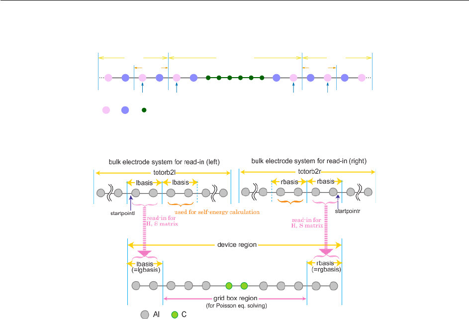
Chapter 11: Molecular Properties and Analysis 661
•$trans_method (Specifies the mode to calculated the electrode self-energies)
device region
lgbasis rgbasis
lbasis rbasis
latomlgatom ratom rgatom
Ag Au C
Figure 11.1: Illustration for the different regions of the molecular junction for Landauer calculation.
Figure 11.2: Illustration for the different regions of the molecular junction for NEGF calculation.
The $trans_model section provides the number of basis functions in the different regions (molecular model partition-
ing). There are no default values given for these parameters. The different regions are illustrated in Fig. 11.1 with a
six carbon atom chain based bridge used as an example of the Landauer calculation. The partitioning as well as the
scheme for the NEGF calculation is illustrated in Fig. 11.2. In these systems the electrodes are represented by a chain
of Au atoms. In this example of electrode wires, each single atom represents one layer.
The necessary parameters in the $trans_model section are as follows:
•trans_latom: INTEGER, atom index in the $molecule section where the central/bridge region starts (the first
atom in junction area).
•trans_ratom: INTEGER, atom index in the $molecule section where the central/bridge region ends (the last
atom in junction area).
•trans_lgatom: INTEGER, atom index where the repeat unit of the left electrode starts.
•trans_rgatom: INTEGER, atom index where the repeat unit of the right electrode ends.
See Fig. 11.1 for illustrations of the different regions, and the way the parameters define them. Atoms within num-
bers trans_lgatom,trans_lgatom+1, .., trans_latom-1 define the repeat unit of the left electrode (similarly for right
electrode).
Alternatively, the different regions can be provided with the atomic orbital (AO) index as follows:
•trans_lbasis: INTEGER, the number of basis functions appearing to the left of the device region (the index of
the first AO within the central region).
•trans_rbasis: INTEGER, the number of basis functions appearing to the right of the device region right electrode
(total number of basis functions minus this number equals last AO that is within the device).

Chapter 11: Molecular Properties and Analysis 662
•trans_lgbasis: INTEGER, the number of basis functions of the repeat unit of the left electrode.
•trans_rgbasis: INTEGER, the number of basis functions of the repeat unit of the right electrode.
For the NEGF calculation, trans_lbasis and trans_lgbasis must be the same number as shown in Fig. 11.2 (as for
trans_rbasis and trans_rgbasis.
Note: The assignment of trans_latom etc. has priority. If trans_latom is specified, then trans_lbasis is ignored.
Similarly for trans_latom and trans_lbasis.
For the example in Fig. 11.1, if there are a total of 18 atoms and the Au and Ag basis sets each contain 22 basis functions
per atom and the repeat unit includes a pair of Au Ag atoms, then the parameters should be given as follows (only the
first two columns are required, the rest are included for explanation):
trans_lbasis 88 No. of functions representing left electrode region (2×22 for Ag + 2×22 for Au)
trans_rbasis 88 No. of functions representing right electrode (2×22 for Ag + 2×22 for Au)
trans_lgbasis 44 Size of the repeating unit of the left electrode (22 for Ag + 22 for Au)
trans_rgbasis 44 Size of the repeating unit of the right electrode (22 for Ag + 22 for Au)
Or use the atom numbers corresponding to their position in the $molecule section:
trans_lgatom 3 Third atom is used to define the repeat unit of the left electrode
trans_latom 5 Fifth atom is the first atom of the junction
trans_ratom 14 Fourteenth atom is the last atom of the junction
trans_rgatom 16 Sixteenth atom is used to define the repeat unit of the right electrode
In this example, we have used for the same repeat unit for the left and right electrodes; this symmetry is not required.
Note: The order of atoms in the $molecule section is important and requires to following:
Repeating units (left) - Molecular Junction - Repeating units (right)
The atoms are provided first by the leftmost repeat unit with the left electrode then proceeds to the next repeat unit
up to the surface unit. Next the bridge atoms are provided followed by the right surface unit and the right electrode
region. The right electrode region starts with the surface layer and ends with the most distant layer within the bulk. The
atoms order within each electrode layer (the repeat units) must be consistent. The atoms order within the bridge region
(excluding the electrode repeat unit atoms) is arbitrary.
That is, the order of atoms in the molecule section has to adhere to the following:
1. atoms of the leftmost repeat unit
2. atoms of the next repeat unit
3. atoms of the left surface unit device
4. bridge atoms
5. atoms of the right surface unit
6. atoms of the next right electrode unit
7. atoms of the rightmost repeat unit
T-Chem allows for complete flexibility in determining the different regions of the electrode models. As a consequence,
incorrect setting of regions is not caught by the program and may produce transmission functions that are unphysical
(e.g. large values or even negative). Such errors can occur where the cluster model is partitioned (by mistake) within
the orbital space of an atom. Regions must always be defined between atomic layers. Each repeat unit atoms should be
always provided with the same internal order.
Note: At least a single repeat unit of the electrodes should be included in the bridge region. With the Landauer model,
if trans_readhs == 0, then at least one layer beyond the bridge region has to be included, an additional layer
(total of two or more) is required when trans_method != 0.

Chapter 11: Molecular Properties and Analysis 663
The necessary parameters in $trans_method section are listed as follows,
trans_mode
Mode of calculation.
INPUT SECTION: $trans_method
TYPE:
INTEGER
DEFAULT:
1 Landauer level.
OPTIONS:
3 A self-consistent Green’s function calculation with zero bias voltage (i.e. NEGF with zero
bias, which is used for preparation of full NEGF).
4 Full NEGF level
RECOMMENDATION:
For modes 3 and 4 SCF_ALGORITHM = NEGF must be set in in the $rem section.
trans_spin
Spin coupling scheme.
INPUT SECTION: $trans_method
TYPE:
INTEGER
DEFAULT:
0
OPTIONS:
0 For restricted spin calculations or closed-shell singlet states.
3 For unrestricted spin calculations or open-shell systems
RECOMMENDATION:
None
trans_method
Electrode surface GFs model.
INPUT SECTION: $trans_method
TYPE:
INTEGER
DEFAULT:
0
OPTIONS:
0 A wide band limit with a constant parameter trans_greens (default)
1 WBL using the Ke-Baranger-Yang TB at the Fermi energy.
2 WBL using the Lopez-Sancho TB at the Fermi energy.
3 Tight-binding (TB) following the procedure proposed by Ke-Baranger-Yang
4 TB following the procedure proposed by Lopez-Sancho (decimation).
RECOMMENDATION:
Only option 0 is available for the NEGF calculation at the current version.

Chapter 11: Molecular Properties and Analysis 664
trans_npoint
Number of grid points within the energy window of the transmission spectra calculation.
INPUT SECTION: $trans_method
TYPE:
INTEGER
DEFAULT:
300
OPTIONS:
nUser-specified number of points
RECOMMENDATION:
None
trans_readhs
Flag to read the Hamiltonian and overlap matrices for the bulk model.
INPUT SECTION: $trans_method
TYPE:
INTEGER
DEFAULT:
0 Use the current Hamiltonian and overlap matrices to parse the electrode integrals.
OPTIONS:
1 Use pre-calculated electrode Hamiltonian and overlap matrices.
RECOMMENDATION:
If set to 1, the following files are requred: FAmat2l.dat and Smat2l.dat (for left
electrode model), FAmat2r.dat and Smat2r.dat (for right electrode model). If both
electrodes are of the same type, may use symbolic links of these files to the same matrices.
(For unrestricted spin model, FBmat2l.dat and FBmat2r.dat are also necessary)
Note: NEGF requires trans_readhs to be set!
trans_htype
Determines the TB property on the relevant coupling terms.
INPUT SECTION: $trans_method
TYPE:
INTEGER
DEFAULT:
0
OPTIONS:
When trans_readhs = 0:
0 All coupling integrals between the junction and electrode functions are allowed as deter-
mined at the cluster model level (no screening imposed).
1 Only coupling between neighboring repeating units of the electrode model are allowed –
all terms of the repeating units elements that are beyond the neighboring unit are set to
zero.
2 Force both the TB coupling terms and the self-energy coupling terms to the same value as
determined by the electrode model. If trans_method != 0, the inequalities trans_lbasis
≥2×trans_lgbasis and trans_rbasis ≥2×trans_rgbasis must be satisfied.
When trans_readhs = 1:
2 Available using the pre-calculated electrode data.
3 The same way as 1 but using the pre-calculated electrode data. This is only for NEGF
calculation.
RECOMMENDATION:
None

Chapter 11: Molecular Properties and Analysis 665
Further options are summarized below:
trans_printdos (Integer):
Controls the printout of TDOS.
0 Default, no total DOS printing.
1 A TDOS (of the junction region) will be printed to TDOS.txt (closed shell).
trans_printiv (Integer):
Controls printout of calculated current.
0 Default, no current calculated and printed
1 Current will be printed to current.txt (closed shell) or currentA/B.txt (unrestricted or
open shell).
trans_ipoints (Integer):
Number of points for current calculation.
300 Default value.
trans_adjustefermi (Integer):
Flag to adjust the Fermi energy (FE) for trans_mode =3or4
0 Default, no adjustment. Fixed FE specified by trans_efermi (and trans_efermib) is used.
1 FE is chosen as midpoint of HOMO and LUMO levels
2 FE is adjusted so that charge neutrality is satisfied
3 FE is adjusted by combination way of 1 and 2, i.e. use 2 if maximum difference of density matrix in
the iteration is over 10−2and use 3 below that.
Options 1, 2, and 3 use the same FE for αand βspins. -1, -2, -3 are the same as 1, 2, 3, respectively, but allow for
different FEs for αand βspins.
trans_nvbias (Integer):
(Only for trans_mode = 4), number of points of bias voltage.
1 Default
The bias voltage values to be calculated are defined by dividing the range between trans_vstart and trans_vmax with
this number. For example, when trans_vstart = 0.0, trans_vmax = 1.0, and trans_nvbias = 5, the voltages are 0.0,
0.25, 0.50, 0.75, and 1.0. For the case of trans_nvbias = 1, the voltage to be calculated is trans_vmax.
trans_updatedmatlr (Integer):
(Only for trans_mode = 3), flag to update L, R, LC, RC blocks (i.e. except for center block) of density matrix during
SCF with zero bias. This is to prepare consistent density matrix with modified Hamiltonian matrix forced by read-in
bulk electrode data. Note that it may make it difficult or slow to converge.
0 No update.
1 Update every iteration step (default).
2 Mix the new density matrix with ratio of trans_mixing.
The following are parameters are set to a double precision value. The allowed values are set using trans_itodfac as
follows:
trans_itodfac (Integer):
Controls the accuracy for input parameters.
100 Default, the numbers can be of 0.0x precision.
1000 The input double numbers can be of 0.00x precision, etc.
trans_vstart (Double):
(Only for trans_mode = 4). Starting voltage bias (V). The bias voltage increases from trans_vstart to trans_vmax in
the NEGF calculation.
0.0 Default
trans_devsmear (Double):
Imaginary smearing (in eV) added to the real Hamiltonian in central region retarded GF evaluation.
0.01 Default, cannot be smaller than 1/trans_itodfac

Chapter 11: Molecular Properties and Analysis 666
trans_bulksmear (Double):
Imaginary smearing (in eV) added to the real Hamiltonian in electrodes GF evaluation.
0.01 Default, cannot be smaller than 1/trans_itodfac
trans_greens (Double):
Imaginary smearing/Broadening (in eV) added to the Green’s function.
0.07 Default, cannot be smaller than 1/trans_itodfac
trans_efermi (Double):
Fermi energy of the electrode (for αspin) (in eV) used for defining energy range in calculating current for T(E).
-5.0 Default
trans_efermib (Double):
Fermi energy for βspin (in eV). If this is not given, the same value of αspin is used.
trans_vmax (Double):
Maximum voltage bias (V).
1.0 Default
trans_gridoffset (Double):
(Only for trans_mode = 4), Offset distance (in Å) to define the grid box region for bias potential energy.
5.0 Default
The box size is defined by adding the offset distance with maximum and minimum x,yand zatomic coordinates for
each direction. The bias voltage V(r)on the grid points in the box is used for calculating correction term for the Fock
matrix (i.e. hi|V|ji). Note that this box is not for correcting electrostatic potential by solving Poisson equation. The
grid box region and its grid size for the Poisson equation is given by $plots block keyword (see also example later).
The same grid size is used for both boxes.
The following are parameters for when trans_mode = 3, 4:
trans_mixing (Double):
Mixing ratio of DIIS mixing method for updating the central block of density matrix in the NEGF iteration.
1.0 Default
trans_mixhistory (Integer):
The number of NEGF iteration steps in which the history of density matrix is stocked for the DIIS method.
40 Default
trans_dehcir (Double):
Grid size, dE (in eV), for integrating the Greens function on the half circle path on imaginary plane.
1.0 Default
trans_delpart (Double):
Grid size, dE (in eV), for integrating the Greens function on the path of the linear part on imaginary plane.
0.01 Default
trans_debwin (Double):
(For trans_mode = 4). Grid size, dE (in eV), for integration on the non-equilibrium term.
0.01 Default
trans_numres (Integer):
The number of poles at Fermi energy enclosed by closed contour on the imaginary plane.
100 Default
trans_peconv (Integer):
The convergence criteria of the iteration of the Poisson equation. The threshold is 10−nhartree of maximum energy
difference over the all grid points.
9 Default

Chapter 11: Molecular Properties and Analysis 667
trans_pemaxite (Integer):
Maximum iteration number of the Poisson equation.
1000 Default
trans_readesp (Integer):
Flag of read-in electrostatic potential energy. The data is printed in "ReadInESP/" directory with option of -1 or 0, and
read from the same directory name with option of 0 or 1.
-1 Print the read-in ESP data in "ReadInESP/" directory at the first step and stop calculation.
0 Print the read-in ESP data in "ReadInESP/" at the first step and continue calculation using it (default).
1 Read the pre-calculated read-in ESP data from "ReadInESP/" and continue calculation.
trans_restart (Integer):
Flag to restart reading the density matrix files, DAmat.dat (and DBmat.dat) from the "TransRestart/" directory.
0 No restart (default).
1 Read file of density matrix.
Note: The default energy window for transmission and current calculations is defined as:
trans_emin =trans_efermi -trans_vmax/2 and trans_emax =trans_efermi +trans_vmax/2
if trans_emin and trans_emax are not given.
The trans_emin and trans_emax values can be set to determine the energy window for calculating the transmission
function. If specified, these values will override the window defined by trans_efermi and trans_vmax values.
If higher accuracy parameters are set, trans_itodfac must be increased. For example for three digits accuracy (e.g.
trans_efermi = -5.341), then trans_itodfac = 1000 or higher must be used. (This parameter applies to all double
precision parameters.)
For trans_readhs = 1, the following parameters to parse precalculated Hamiltonian and overlap matrices have to be
provided:
•trans_totorb2 (Integer):
Total number of basis functions in the electrode models (if set, then same size is assumed for both electrodes)
(no default value).
•trans_totorb2l: Integer number, total number of basis functions in left electrode model (no default value).
•trans_totorb2r: Integer number, total number of basis functions in right electrode model (no default value).
•trans_startpoint: Integer number, start point (basis number) for reading the TB integrals. Note, the basis num-
ber, that is, index number of basis function starts from 0. (if set, then same size is assumed for both electrodes)
(default value 0).
•trans_startpointl: given as integer number, left start point (basis number) for reading the TB integrals. Note,
the basis number, that is, index number of basis function starts from 0. (default value 0).
•trans_startpointr: given as integer number, right start point (basis number) for reading the TB integrals. Note,
the basis number, that is, index number of basis function starts from 0. (no default value).

Chapter 11: Molecular Properties and Analysis 668
As an example of the Landauer calculation, the sample Q-CHEM input is given below.
Example 11.39 Quantum transport Landauer calculation applied to C6between two gold electrodes.
$molecule
0 1
Ag -11.0 0 0
Au -8.3 0 0
Ag -5.6 0 0
Au -2.9 0 0
Ag -0.2 0 0
Au 2.5 0 0
C 4.8 0 0
C 6.5 0 0
C 8.2 0 0
C 9.9 0 0
C 11.6 0 0
C 13.3 0 0
Au 15.6 0 0
Ag 18.3 0 0
Au 21.0 0 0
Ag 23.7 0 0
Au 26.4 0 0
Ag 29.1 0 0
$end
$rem
METHOD B3LYP
BASIS lanl2dz
ECP lanl2dz
GEOM_OPT_MAXCYC 200
INCDFT FALSE
MEM_STATIC 8000
MAX_SCF_CYCLES 400
MEM_TOTAL 32000
MOLDEN_FORMAT TRUE
SCF_CONVERGENCE 10
SCF_ALGORITHM diis
TRANS_ENABLE 1
$end
$trans-method
trans_spin 0
trans_npoints 300
trans_method 0
trans_readhs 0
trans_printdos 1
trans_efermi -6.50
trans_vmax 4.00
$end
$trans-model
trans_lgatom 3
trans_latom 5
trans_ratom 14
trans_rgatom 16
$end
A sample for unrestricted spin calculation can be found in the $QC/samples/tchem directory.
For NEGF calculations, note the followings concerning input etc:
•SCF_ALGORITHM = NEGF in $rem is necessary for NEGF calculation.

Chapter 11: Molecular Properties and Analysis 669
• The same numbers for trans_lgbasis and trans_lbasis, and also for trans_rgbasis and trans_rbasis must be
used.
• Only WBL method for evaluating self-energy is available for the NEGF in the current version (trans_method =
0)
•trans_htype = 3 and trans_readhs = 1 are required
•SYM_IGNORE = TRUE to keep the original input coordinates.
•MEM_TOTAL and MEM_STATIC may need to be set to ensure enough memory is available.
• The bias voltage of +V/2is added on the left electrode, and −V/2on the right electrode, where the bias potential
slope is along x-axis, i.e. the system structure must be built along xdirection.
• In the $plots section (when defining a grid box for the Poisson equation solving), the grid box region must cover
all atoms except for the left and right electrode parts defined in $trans_model. All integer index flags in $plots
can be 0.
• For calculations on bulk electrode, the same structure with the same orientation in xyz-Cartesian coordinate
system (but different size) must be used so as to reproduce the same overlap matrix at the used part.
• For better calculations, update of electrode relevant (non-center) blocks in the density matrix (trans_updatedmatlr
= 1) and Fermi energy to satisfy charge neutrality (trans_adjustefermi = 2 or 3) are recommended at zero bias
(trans_opt = 3) before performing a full NEGF calculation. However, these options may make it difficult or
slow to reach convergence.
• The criterion for convergence in the NEGF iterations is the maximum difference in density matrix elements, and
is not a energy threshold.
NEGF calculations depend on the following pre-calculated properties:
Step 1: Pre-calculations:
A: Hamiltonian and overlap matrices for the left and right bulk electrodes (required)
B: A converged junction electronic state by standard DFT (recommended)
C: Electrostatic potential of large electrode region (optional)
Step 2: Self-consistent Greens function calculation with zero bias:
Non zero bias cases should be calculated using density matrices calculated with zero bias voltage to obtain
converged density matrix. It is also recommend to evaluate the Fermi energy level within the NEGF scheme.
Step 3: NEGF calculations should be obtained by increasing the bias sequentially.

Chapter 11: Molecular Properties and Analysis 670
Examples of these steps applied to C2between two aluminium electrodes are given below.
Example 11.40 Step 1-A of the NEGF calculation, the pre-calculation of the bulk electrode. Flag keyword of printing
matrices must be set (i.e. trans_enable != 0).
$molecule
0 1
Al -15.04250 0.0 0.0
Al -12.30750 0.0 0.0
Al -9.572500 0.0 0.0
Al -6.837500 0.0 0.0
Al -4.102500 0.0 0.0
Al -1.367500 0.0 0.0
Al 1.367500 0.0 0.0
Al 4.102500 0.0 0.0
Al 6.837500 0.0 0.0
Al 9.572500 0.0 0.0
Al 12.30750 0.0 0.0
Al 15.04250 0.0 0.0
$end
$rem
UNRESTRICTED true
SYM_IGNORE true
MAX_SCF_CYCLES 500
EXCHANGE hf
CORRELATION none
ECP hwmb
BASIS hwmb
SCF_CONVERGENCE 4
$end
@@@
$molecule
read
$end
$rem
UNRESTRICTED true
SYM_IGNORE true
MAX_SCF_CYCLES 500
EXCHANGE b3lyp
CORRELATION none
ECP hwmb
BASIS hwmb
SCF_GUESS read
SCF_GUESS_MIX 3
SCF_CONVERGENCE 4
$end

Chapter 11: Molecular Properties and Analysis 671
@@@
$molecule
read
$end
$rem
UNRESTRICTED true
SYM_IGNORE true
MAX_SCF_CYCLES 500
EXCHANGE b3lyp
CORRELATION none
ECP hwmb
BASIS hwmb
SCF_GUESS read
SCF_GUESS_MIX 3
SCF_CONVERGENCE 7
TRANS_ENABLE -1
$end
$trans-method
trans_spin 2
$end
Example 11.41 Step 1-B of the NEGF calculation - the pre-calculation by the standard DFT. The same molecular
structure with the step 2 must be used
$molecule
0 1
Al -13.615 0.0 0.0
Al -10.880 0.0 0.0
Al -8.145 0.0 0.0
Al -5.410 0.0 0.0
Al -2.675 0.0 0.0
C -0.627 0.0 0.0
C 0.627 0.0 0.0
Al 2.675 0.0 0.0
Al 5.410 0.0 0.0
Al 8.145 0.0 0.0
Al 10.880 0.0 0.0
Al 13.615 0.0 0.0
$end
$rem
UNRESTRICTED true
SYM_IGNORE true
MAX_SCF_CYCLES 400
EXCHANGE b3lyp
CORRELATION none
BASIS hwmb
ECP hwmb
SCF_CONVERGENCE 5
$end

Chapter 11: Molecular Properties and Analysis 672
@@@
$molecule
read
$end
$rem
UNRESTRICTED true
SYM_IGNORE true
EXCHANGE b3lyp
CORRELATION none
BASIS hwmb
ECP hwmb
MAX_SCF_CYCLES 400
SCF_CONVERGENCE 6
SCF_GUESS read
SCF_GUESS_MIX 3
$end
Example 11.42 Step 2 of the NEGF calculation. As the preparation of this step, followings are necessary:
1. FAmat2l.dat,FAmat2r.dat,Smat2l.dat, and Smat2r.dat (also FBmat2l.dat and FBmat2r.dat
if the calculation is spin-unrestricted ) must be placed in the same directory of the Q-Chem input file by coping
or linking the output files of the step 1-A.
2. Restart directory of the standard DFT obtained in the step 1-B must be copied to here.
3. (Optional) Read-in electrostatic potential data in "ReadInESP/" directory must be placed if this option is used
(for trans_readesp = 1). This option can provide more bulk electrode electrostatic environment as the boundary
condition of Poisson equation solving (see the sample files in $QC/samples/tchem/) for more details).
$molecule
read
$end
$rem
JOBTYPE sp
UNRESTRICTED true
SYM_IGNORE true
MAXSCF 500
EXCHANGE b3lyp
CORRELATION none
BASIS hwmb
ECP hwmb
SCF_CONVERGENCE 4
SCF_ALGORITHM negf
SCF_GUESS read
MEM_TOTAL 16000
MEM_STATIC 4000
TRANS_ENABLE 1
$end
$plots
For NEGF (for Poisson equation)
190 -9.5 9.5
80 -4.0 4.0
80 -4.0 4.0
0000
0
$end

Chapter 11: Molecular Properties and Analysis 673
$trans-method
trans_opt 3
trans_spin 2
trans_npoints 500
trans_method 0
trans_printdos 1
trans_printiv 1
trans_adjustefermi 1
trans_vmax 1.0
trans_emin -6.5
trans_emax -2.5
trans_mixing 0.1
trans_mixhistory 50
trans_dehcir 1.0
trans_delpart 0.01
trans_numres 100
trans_peconv 8
trans_pemaxite 1000
trans_updatedmatlr 0
trans_readesp 0
trans_htype 3
trans_readhs 1
trans_totorb2 48
trans_startpointl 16
trans_startpointr 32
$end
$trans-model
trans_lbasis 8
trans_rbasis 8
trans_lgbasis 8
trans_rgbasis 8
$end
Example 11.43 Step 3 of the NEGF calculation. As the preparation of this step, followings are necessary:
1. In the same way as step 2, FAmat2l.dat,FAmat2r.dat,Smat2l.dat, and Smat2r.dat (also FBmat2l.dat
and FBmat2r.dat for spin-unrestricted calculations) must be placed.
2. Restart directory for Q-Chem generated in the step 2 must be copied to here (only coordinates are used).
3. Restart directory for density matrix "TransRestart/" must be created and DAmat.dat (and DBmat.dat for
spin-unrestricted) generated in the step 2 must be copied or linked in the directory.
4. Read-in electrostatic potential data in "ReadInESP/" directory used in the step 2 must be copied to here.
5. Put Fermi energy obtained in Step 2 (recommended).
$molecule
read
$end
$rem
UNRESTRICTED true
MAXSCF 500
SYM_IGNORE true
EXCHANGE b3lyp
ECP hwmb
SCF_CONVERGENCE 4
SCF_ALGORITHM negf
MEM_TOTAL 16000
MEM_STATIC 4000
TRANS_ENABLE 1
$end

Chapter 11: Molecular Properties and Analysis 674
$plots
For NEGF calculation
190 -9.5 9.5
80 -4.0 4.0
80 -4.0 4.0
0000
0
$end
$trans-method
trans_opt 4
trans_spin 2
trans_npoints 500
trans_method 0
trans_printdos 1
trans_printiv 1
trans_adjustefermi 0
trans_efermi -4.421836
trans_vmax 0.5
trans_emin -6.5
trans_emax -2.5
trans_mixing 0.2
trans_mixhistory 50
trans_dehcir 1.0
trans_delpart 0.01
trans_debwin 0.01
trans_numres 100
trans_peconv 8
trans_pemaxite 1000
trans_gridoffset 4.0
trans_updatedmatlr 0
trans_nvbias 6
trans_restart 1
trans_readesp 1
trans_htype 3
trans_readhs 1
trans_totorb2 48
trans_startpointl 16
trans_startpointr 32
$end
$trans-model
trans_lbasis 8
trans_rbasis 8
trans_lgbasis 8
trans_rgbasis 8
$end

Chapter 11: Molecular Properties and Analysis 675
References and Further Reading
[1] The MOLDEN program may be freely downloaded from www.cmbi.ru.nl/molden/molden.html.
[2] MACMOLPLT may be downloaded from https://brettbode.github.io/wxmacmolplt.
[3] NBO 5.0 manual: www.chem.wisc.edu/~nbo5.
[4] The VMD program may be downloaded from www.ks.uiuc.edu/Research/vmd.
[5] Ground-State Methods (Chapters 4and 6).
[6] Excited-State Calculations (Chapter 7).
[7] Basis Sets (Chapter 8).
[8] A. Adel and D. M. Dennison. Phys. Rev., 43:716, 1933. DOI: 10.1103/PhysRev.43.716.
[9] W. D. Allen, Y. Yamaguchi, A. G. Csázár, D. A. Clabo, Jr., R. B. Remington, and H. F. Schaefer III. Chem.
Phys., 145:427, 1990. DOI: 10.1016/0301-0104(90)87051-C.
[10] T. Bally and P. R. Rablen. J. Org. Chem, 76:4818, 2011. DOI: 10.1021/jo200513q.
[11] S. A. Bäppler, F. Plasser, M. Wormit, and A. Dreuw. Phys. Rev. A, 90:052521, 2014. DOI: 10.1103/Phys-
RevA.90.052521.
[12] V. Barone. J. Chem. Phys., 122:014108, 2005. DOI: 10.1063/1.1824881.
[13] A. D. Becke. J. Chem. Phys., 88:2547, 1988. DOI: 10.1063/1.454033.
[14] A. D. Becke. J. Chem. Phys., 119:2972, 2003. DOI: 10.1063/1.1589733.
[15] A. D. Becke and E. R. Johnson. J. Chem. Phys., 122:154104, 2005. DOI: 10.1063/1.1884601.
[16] E. J. Berquist and D. S. Lambrecht. A first principles approach for partitioning linear response properties into
additive and cooperative contributions. (preprint).
[17] N. A. Besley and J. A. Bryan. J. Phys. Chem. C, 112:4308, 2008. DOI: 10.1021/jp076167x.
[18] N. A. Besley and K. A. Metcalf. J. Chem. Phys., 126:035101, 2007. DOI: 10.1063/1.2426344.
[19] N. A. Besley, A. M. Lee, and P. M. W. Gill. Mol. Phys., 100:1763, 2002. DOI: 10.1080/00268970110111779.
[20] N. A. Besley, D. P. O’Neill, and P. M. W. Gill. J. Chem. Phys., 118:2033, 2003. DOI: 10.1063/1.1532311.
[21] R. C. Bochicchio. J. Mol. Struct. (Theochem), 429:229, 1998. DOI: 10.1016/S0166-1280(97)00357-6.
[22] B. M. Bode and M. S. Gordon. J. Mol. Graphics Mod., 16:133, 1998. DOI: 10.1016/S1093-3263(99)00002-9.
[23] S. F. Boys. Rev. Mod. Phys., 32:296, 1960. DOI: 10.1103/RevModPhys.32.296.
[24] S. F. Boys. In P.-O. Löwdin, editor, Quantum Theory of Atoms, Molecules, and the Solid State, page 253.
Academic, New York, 1966.
[25] C. M. Breneman and K. B. Wiberg. J. Comput. Chem., 11:361, 1990. DOI: 10.1002/jcc.540110311.
[26] A. Broo and S. Larsson. Chem. Phys., 148:103, 1990. DOI: 10.1016/0301-0104(90)89011-E.
[27] S. P. Brown, T. Schaller, U. P. Seelbach, F. Koziol, C. Ochsenfeld, F.-G. Klärner, and H. W. Spiess. Angew. Chem.
Int. Ed. Engl., 40:717, 2001. DOI: 10.1002/1521-3773(20010216)40:4<717::AID-ANIE7170>3.0.CO;2-X.
[28] P. Bultinck, C. Van Alsenoy, P. W. Ayers, and R. Carbó-Dorca. J. Chem. Phys., 126:144111, 2007. DOI:
10.1063/1.2715563.

Chapter 11: Molecular Properties and Analysis 676
[29] R. Burcl, N. C. Handy, and S. Carter. Spectrochim. Acta A, 59:1881, 2003. DOI: 10.1016/S1386-1425(02)00421-
3.
[30] T. Carrington, Jr. In P. v. R. Schleyer, N. L. Allinger, T. Clark, J. Gasteiger, P. A. Kollman, H. F. Schaefer III,
and P. R. Schreiner, editors, Encyclopedia of Computational Chemistry, page 3157. Wiley, Chichester, United
Kingdom, 1998.
[31] R. J. Cave and M. D. Newton. Chem. Phys. Lett., 249:15, 1996. DOI: 10.1016/0009-2614(95)01310-5.
[32] X. Cheng and R. P. Steele. J. Chem. Phys., 141:104105, 2014. DOI: 10.1063/1.4894507.
[33] D. M. Chipman. Theor. Chem. Acc., 76:73, 1989. DOI: 10.1007/BF00532125.
[34] J. Cioslowski and G. Liu. J. Chem. Phys., 105:4151, 1996. DOI: 10.1063/1.472285.
[35] D. A. Clabo, W. D. Allen, R. B. Remington, Y. Yamaguchi, and H. F. Schaefer III. Chem. Phys., 123:187, 1988.
DOI: 10.1016/0301-0104(88)87271-9.
[36] J. Contreras-García, E. R. Johnson, S. Keinan, B. Chaudret, J.-P. Piquemal, D. N. Beratan, and W. Yang. J. Chem.
Theory Comput., 7:625, 2011. DOI: 10.1021/ct100641a.
[37] S. Datta. Quantum transport: Atom to transistor. Cambridge University Press, Cambridge, 2005.
[38] M. de Wergifosse, V. Liégeois, and B. Champagne. Int. J. Quantum Chem., 114:900, 2014. DOI:
10.1002/qua.24685.
[39] M. Di Ventra. Electron transport in nanoscale systems. Cambridge University Press, Cambridge, 2008.
[40] R. Ditchfield. Mol. Phys., 27:789, 1974. DOI: 10.1080/00268977400100711.
[41] A. Dreuw and M. Head-Gordon. Chem. Rev., 105:4009, 2005. DOI: 10.1021/cr0505627.
[42] C. Edmiston and K. Ruedenberg. Rev. Mod. Phys., 35:457, 1963. DOI: 10.1103/RevModPhys.35.457.
[43] D. M. Elking, L. Perera, and L. G. Pedersen. Comput. Phys. Commun., 183:390, 2012. DOI:
10.1016/j.cpc.2011.10.003.
[44] A. Farazdel, M. Dupuis, E. Clementi, and A. Aviram. J. Am. Chem. Soc., 112:4206, 1990. DOI:
10.1021/ja00167a016.
[45] J. Gauss. Ber. Bunsenges. Phys. Chem., 99:1001, 1995. DOI: 10.1002/bbpc.199500022.
[46] A. Ghysels, V. Van Speybroeck, E. Pauwels, S. Catak, B. R. Brooks, D. Van Neck, and M. Waroquier. J. Comput.
Chem., 31:994, 2010. DOI: 10.1002/jcc.21386.
[47] P. M. W. Gill. Chem. Phys. Lett., 270:193, 1997. DOI: 10.1016/S0009-2614(97)00361-8.
[48] P. M. W. Gill, D. P. O’Neill, and N. A. Besley. Theor. Chem. Acc., 109:241, 2003. DOI: 10.1007/s00214-002-
0411-5.
[49] E. D. Glendening, J. K. Badenhoop, A. E. Reed, J. E. Carpenter, J. A. Bohmann, C. M. Morales, C. R. Landis,
and F. Weinhold, 2013.
[50] E. D. Glendening, C. R. Landis, and F. Weinhold. J. Comput. Chem., 34:1429, 2013. DOI: 10.1002/jcc.23266.
[51] M. W. D. Hanson-Heine. J. Chem. Phys., 143:164104, 2015. DOI: 10.1063/1.4934234.
[52] M. W. D. Hanson-Heine, M. W. George, and N. A. Besley. J. Chem. Phys., 136:224102, 2012. DOI:
10.1063/1.4727853.
[53] M. W. D. Hanson-Heine, F. S. Husseini, J. D. Hirst, and N. A. Besley. J. Chem. Theory Comput., 12:1905, 2016.
DOI: 10.1021/acs.jctc.5b01198.

Chapter 11: Molecular Properties and Analysis 677
[54] M. Häser, R. Ahlrichs, H. P. Baron, P. Weiss, and H. Horn. Theor. Chem. Acc., 83:455, 1992. DOI:
10.1007/BF01113068.
[55] M. Head-Gordon. Chem. Phys. Lett., 372:508, 2003. DOI: 10.1016/S0009-2614(03)00422-6.
[56] M. Head-Gordon, A. M. Graña, D. Maurice, and C. A. White. J. Phys. Chem., 99:14261, 1995. DOI:
10.1021/j100039a012.
[57] T. Helgaker and M. Jaszu´
nski K. Ruud. Chem. Rev., 99:293, 1990. DOI: 10.1021/cr960017t.
[58] T. Helgaker, M. Watson, and N.C. Handy. J. Chem. Phys., 113:9402, 2000. DOI: 10.1063/1.1321296.
[59] J. M. Herbert. The quantum chemistry of loosely-bound electrons. In A. L. Parill and K. Lipkowitz, editors,
Reviews in Computational Chemistry, volume 28, page 391. Wiley, 2015. DOI: 10.1002/9781118889886.ch8.
[60] J. M. Herbert, L. D. Jacobson, K. U. Lao, and M. A. Rohrdanz. Phys. Chem. Chem. Phys., 14:7679, 2012. DOI:
10.1039/c2cp24060b.
[61] S. Hirata, M. Nooijen, and R. J. Bartlett. Chem. Phys. Lett., 326:255, 2000. DOI: 10.1016/S0009-
2614(00)00772-7.
[62] J. O. Hirschfelder. J. Chem. Phys., 33:1462, 1960. DOI: 10.1063/1.1731427.
[63] F. L. Hirshfeld. Theor. Chem. Acc., 44:129, 1977. DOI: 10.1007/BF00549096.
[64] Z. C. Holden, R. M. Richard, and J. M. Herbert. J. Chem. Phys., 139:244108, 2013. DOI: 10.1063/1.4850655.
[65] C.-P. Hsu, Z.-Q. You, and H.-C. Chen. J. Phys. Chem. C, 112:1204, 2008. DOI: 10.1021/jp076512i.
[66] W. Humphrey, A. Dalke, and K. Schulten. J. Molec. Graphics, 14:33, 1996. DOI: 10.1016/0263-7855(96)00018-
5.
[67] C. R. Jacob and M. Reiher. J. Chem. Phys., 130:084106, 2009. DOI: 10.1063/1.3077690.
[68] C. R. Jacob, S. Luber, and M. Reiher. Chem. Eur. J, 15:13491, 2009. DOI: 10.1002/chem.200901840.
[69] C. R. Jacob, S. Luber, and M. Reiher. J. Phys. Chem. B, 113:6558, 2009. DOI: 10.1021/jp900354g.
[70] F. Jensen. J. Chem. Theory Comput., 2:1360, 2006. DOI: 10.1021/ct600166u.
[71] B. G. Johnson and J. Florián. Chem. Phys. Lett., 247:120, 1995. DOI: 10.1016/0009-2614(95)01186-9.
[72] B. G. Johnson, P. M. W. Gill, and J. A. Pople. J. Chem. Phys., 98:5612, 1993. DOI: 10.1063/1.464906.
[73] E. R. Johnson, S. Keinan, P. Mori-Sánchez, J. Contreras-García, A. J. Cohen, and W. Yang. J. Am. Chem. Soc.,
132:6498, 2010. DOI: 10.1021/ja100936w.
[74] P. Jørgensen, H. J. A. Jensen, and J. Olsen. J. Chem. Phys., 89:3654, 1988. DOI: 10.1063/1.454885.
[75] S. P. Karna and M. Dupuis. J. Comput. Chem., 12:487, 1991. DOI: 10.1002/jcc.540120409.
[76] T. Kato. Commun. Pure Appl. Math., 10:151, 1957. DOI: 10.1002/cpa.3160100201.
[77] H. F. King, R. E. Stanton, H. Kim, R. E. Wyatt, and R. G. Parr. J. Chem. Phys., 47:1936, 1967. DOI:
10.1063/1.1712221.
[78] P. P. Korambath, J. Kong, T. R. Furlani, and M. Head-Gordon. Mol. Phys., 100:1755, 2002. DOI:
10.1080/00268970110109466.
[79] J. Kussmann and C. Ochsenfeld. J. Chem. Phys., 127:054103, 2007. DOI: 10.1063/1.2749509.
[80] J. Kussmann and C. Ochsenfeld. J. Chem. Phys., 127:204103, 2007. DOI: 10.1063/1.2794033.
[81] A. W. Lange and J. M. Herbert. J. Am. Chem. Soc., 131:124115, 2009. DOI: 10.1021/ja808998q.

Chapter 11: Molecular Properties and Analysis 678
[82] V. I. Lebedev. Zh. Vychisl. Mat. Mat. Fix., 16:293, 1976. DOI: 10.1016/0041-5553(76)90100-2.
[83] V. I. Lebedev. Sibirsk. Mat. Zh., 18:132, 1977.
[84] V. I. Lebedev and D. N. Laikov. Dokl. Math., 366:741, 1999.
[85] A. M. Lee and P. M. W. Gill. Chem. Phys. Lett., 313:271, 1999. DOI: 10.1016/S0009-2614(99)00935-5.
[86] C. Y. Lin, A. T. B. Gilbert, and P. M. W. Gill. Theor. Chem. Acc., 120:23, 2008. DOI: 10.1007/s00214-007-
0292-8.
[87] J. Liu and J. M. Herbert. J. Chem. Phys., 143:034106, 2015. DOI: 10.1063/1.4926837.
[88] P.-O. Löwdin. J. Chem. Phys., 18:365, 1950. DOI: 10.1063/1.1747632.
[89] A. V. Marenich, S. V. Jerome, C. J. Cramer, and D. G. Truhlar. J. Chem. Theory Comput., 8:527, 2012. DOI:
10.1021/ct200866d.
[90] R. L. Martin. J. Chem. Phys., 118:4775, 2003. DOI: 10.1063/1.1558471.
[91] S. A. Mewes, F. Plasser, and A. Dreuw. J. Chem. Phys., 143:171101, 2015. DOI: 10.1063/1.4935178.
[92] S. A. Mewes, J.-M. Mewes, A. Dreuw, and F. Plasser. Phys. Chem. Chem. Phys., 18:2548, 2016. DOI:
10.1039/C5CP07077E.
[93] A. Miani, E. Cancès, P. Palmieri, A. Trombetti, and N. C. Handy. J. Chem. Phys., 112:248, 2000. DOI:
10.1063/1.480577.
[94] I. M. Mills. In K. N. Rao and C. W. Mathews, editors, Molecular Spectroscopy: Modern Research, chapter 3.2.
Academic Press, New York, 1972.
[95] C. W. Murray, G. J. Laming, N. C. Handy, and R. D. Amos. Chem. Phys. Lett., 199:551, 1992. DOI:
10.1016/0009-2614(92)85008-X.
[96] J. Neugebauer and B. A. Hess. J. Chem. Phys., 118:7215, 2003. DOI: 10.1063/1.1561045.
[97] M. D. Newton. Chem. Rev., 91:767, 1991. DOI: 10.1021/cr00005a007.
[98] H. H. Nielsen. Phys. Rev., 60:794, 1941. DOI: 10.1103/PhysRev.60.794.
[99] H. H. Nielsen. Rev. Mod. Phys., 23:90, 1951. DOI: 10.1103/RevModPhys.23.90.
[100] C. Ochsenfeld. Chem. Phys. Lett., 327:216, 2000. DOI: 10.1016/S0009-2614(00)00865-4.
[101] C. Ochsenfeld. Phys. Chem. Chem. Phys., 2:2153, 2000. DOI: 10.1039/b000174k.
[102] C. Ochsenfeld, C. A. White, and M. Head-Gordon. J. Chem. Phys., 109:1663, 1998. DOI: 10.1063/1.476741.
[103] C. Ochsenfeld, S. P. Brown, I. Schnell, J. Gauss, and H. W. Spiess. J. Am. Chem. Soc., 123:2597, 2001. DOI:
10.1021/ja0021823.
[104] C. Ochsenfeld, F. Koziol, S. P. Brown, T. Schaller, U. P. Seelbach, and F.-G. Klärner. Solid State Nucl. Mag., 22:
128, 2002. DOI: 10.1006/snmr.2002.0085.
[105] C. Ochsenfeld, J. Kussmann, and F. Koziol. Angew. Chem., 116:4585, 2004. DOI: 10.1002/ange.200460336.
[106] K. Ohta, G. L. Closs, K. Morokuma, and N. J. Green. J. Am. Chem. Soc., 108:1319, 1986. DOI:
10.1021/ja00266a045.
[107] J. Olsen, D. L. Yeager, and P. Jørgensen. J. Chem. Phys., 91:381, 1989. DOI: 10.1063/1.457471.
[108] R. T. Pack and W. B. Brown. J. Chem. Phys., 45:556, 1966. DOI: 10.1063/1.1727605.
[109] P. T. Panek and C. R. Jacob. ChemPhysChem, 15:3365, 2014. DOI: 10.1002/cphc.201402251.

Chapter 11: Molecular Properties and Analysis 679
[110] S. D. Peyerimhoff. In P. v. R. Schleyer, N. L. Allinger, T. Clark, J. Gasteiger, P. A. Kollman, H. F. Schaefer III,
and P. R. Schreiner, editors, Encyclopedia of Computational Chemistry, page 2646. Wiley, Chichester, United
Kingdom, 1998.
[111] J. Pipek and P. G. Mezey. J. Chem. Phys., 90:4916, 1989. DOI: 10.1063/1.456588.
[112] F. Plasser and H. Lischka. J. Chem. Theory Comput., 8:2777, 2012. DOI: 10.1021/ct300307c.
[113] F. Plasser, S. A. Bäppler, M. Wormit, and A. Dreuw. J. Chem. Phys., 141:024107, 2014. DOI:
10.1063/1.4885820.
[114] F. Plasser, M. Wormit, and A. Dreuw. J. Chem. Phys., 141:024106, 2014. DOI: 10.1063/1.4885819.
[115] F. Plasser, B. Thomitzni, S. A. Bäppler, J. Wenzel, D. R. Rehn, M. Wormit, and A. Dreuw. J. Comput. Chem.,
36:1609, 2015. DOI: 10.1002/jcc.23975.
[116] Felix Plasser. J. Chem. Phys., 144:194107, 2016.
[117] E. Proynov. J. Mol. Struct. (Theochem), 762:159, 2006. DOI: 10.1016/j.theochem.2005.08.037.
[118] E. Proynov, Y. Shao, and J. Kong. Chem. Phys. Lett., 493:381, 2010. DOI: 10.1016/j.cplett.2010.05.029.
[119] E. Proynov, F. Liu, Y. Shao, and J. Kong. J. Chem. Phys., 136:034102, 2012. DOI: 10.1063/1.3676726.
[120] E. Proynov, F. Liu, and J. Kong. Phys. Rev. A, 88:032510, 2013. DOI: 10.1103/PhysRevA.88.032510.
[121] V. A. Rassolov and D. M. Chipman. J. Chem. Phys., 104:9908, 1996. DOI: 10.1063/1.471719.
[122] V. A. Rassolov and D. M. Chipman. J. Chem. Phys., 105:1470, 1996. DOI: 10.1063/1.472009.
[123] V. A. Rassolov and D. M. Chipman. J. Chem. Phys., 105:1479, 1996. DOI: 10.1063/1.472010.
[124] Y. M. Rhee and M. Head-Gordon. J. Am. Chem. Soc., 130:3878, 2008. DOI: 10.1021/ja0764916.
[125] R. M. Richard and J. M. Herbert. J. Chem. Theory Comput., 7:1296, 2011. DOI: 10.1021/ct100607w.
[126] G. Schaftenaar and J. H. Noordik. J. Comput.-Aided Mol. Design, 14:123, 2000. DOI:
10.1023/A:1008193805436.
[127] A. P. Scott and L. Radom. J. Phys. Chem., 100:16502, 1996. DOI: 10.1021/jp960976r.
[128] H. Sekino and R. J. Bartlett. J. Chem. Phys., 85:976, 1986. DOI: 10.1063/1.451255.
[129] A. C. Simmonett, A. T. B. Gilbert, and P. M. W. Gill. Mol. Phys., 103:2789, 2005. DOI:
10.1080/00268970500187910.
[130] P. Sjoberg, J. S. Murray, T. Brinck, and P. Politzer. Can. J. Chem., 68:1440, 1990. DOI: 10.1139/v90-220.
[131] V. N. Staroverov and E. R. Davidson. Chem. Phys. Lett., 330:161, 2000. DOI: 10.1016/S0009-2614(00)01088-5.
[132] S. N. Steinmann and C. Corminbeoeuf. J. Chem. Theory Comput., 6:1990, 2010. DOI: 10.1021/ct1001494.
[133] A. J. Stone. Chem. Phys. Lett., 83:233, 1981. DOI: 10.1016/0009-2614(81)85452-8.
[134] A. J. Stone. J. Chem. Theory Comput., 1:1128, 2005. DOI: 10.1021/ct050190+.
[135] A. J. Stone and M. Alderton. Mol. Phys., 56:1047, 1985. DOI: 10.1021/ct050190+.
[136] J. E. Subotnik, Y. Shao, W. Liang, and M. Head-Gordon. J. Chem. Phys., 121:9220, 2004. DOI:
10.1063/1.1790971.
[137] J. E. Subotnik, S. Yeganeh, R. J. Cave, and M. A. Ratner. J. Chem. Phys., 129:244101, 2008. DOI:
10.1063/1.3042233.

Chapter 11: Molecular Properties and Analysis 680
[138] J. E. Subotnik, R. J. Cave, R. P. Steele, and N. Shenvi. J. Chem. Phys., 130:234102, 2009. DOI:
10.1063/1.3148777.
[139] J. E. Subotnik, J. Vura-Weis, A. Sodt, and M. A. Ratner. J. Phys. Chem. A, 114:8665, 2010. DOI:
10.1021/jp101235a.
[140] V. Sychrovský, J. Gräfenstein, and D. Cremer. J. Chem. Phys., 113:3530, 2000. DOI: 10.1063/1.1286806.
[141] A. Szabo and N. S. Ostlund. Modern Quantum Chemistry. Dover, 1996.
[142] K. Takatsuka, T. Fueno, and K. Yamaguchi. Theor. Chem. Acc., 48:175, 1978. DOI: 10.1007/BF00549017.
[143] A. J. W. Thom, E. J. Sundstrom, and M. Head-Gordon. Phys. Chem. Chem. Phys., 11:11297, 2009. DOI:
10.1039/b915364k.
[144] P. v. R. Schleyer, C. Maerker, A. Dransfield, H. Jiao, and N. J. R. van Eikema Hommes. J. Am. Chem. Soc., 118:
6317, 1996. DOI: 10.1021/ja960582d.
[145] E. F. Valeev, V. Coropceanu, D. A. da Silva Filho, S. Salman, and J.-L. Brédas. J. Am. Chem. Soc., 128:9882,
2006. DOI: 10.1021/ja061827h.
[146] D. E. P. Vanpoucke, P. Bultinck, and I. Van Driessche. J. Comput. Chem., 34:405, 2013. DOI: 10.1002/jcc.23088.
[147] A. A. Voityuk and N. Rösch. J. Chem. Phys., 117:5607, 2002. DOI: 10.1063/1.1502255.
[148] J. Vura-Weis, M. Wasielewski, M. D. Newton, and J. E. Subotnik. J. Phys. Chem. C, 114:20449, 2010. DOI:
10.1021/jp104783r.
[149] B. Wang, J. Baker, and P. Pulay. Phys. Chem. Chem. Phys., 2:2131, 2000. DOI: 10.1039/b000026o.
[150] F. Weinhold. In A. G. Kutateladze, editor, Computational Methods in Photochemistry, volume 13 of Molecular
and Supramolecular Photochemistry, page 393. Taylor & Francis, 2005.
[151] C. A. White, B. G. Johnson, P. M. W. Gill, and M. Head-Gordon. Chem. Phys. Lett., 230:8, 1994. DOI:
10.1016/0009-2614(94)01128-1.
[152] R. J. Whitehead and N. C. Handy. J. Mol. Spect., 55:356, 1975. DOI: 10.1016/0022-2852(75)90274-X.
[153] E. Wigner. Phys. Rev., 40:749, 1932. DOI: 10.1103/PhysRev.40.749.
[154] C. F. Williams and J. M. Herbert. J. Phys. Chem. A, 112:6171, 2008. DOI: 10.1021/jp802272r.
[155] E. B. Wilson and J. J. B. Howard. J. Chem. Phys., 4:260, 1936. DOI: 10.1063/1.1749833.
[156] K. Wolinski, J. F. Hinton, and P. Pulay. J. Am. Chem. Soc., 112:8251, 1990. DOI: 10.1021/ja00179a005.
[157] H. L. Woodcock, W. Zheng, A. Ghysels, Y. Shao, J. Kong, and B. R. Brooks. J. Chem. Phys., 129:214109, 2008.
DOI: 10.1063/1.3013558.
[158] Q. Wu and T. Van Voorhis. J. Chem. Phys., 125:164105, 2006. DOI: 10.1063/1.2360263.
[159] K. Yagi, K. Hirao, T. Taketsuga, M. W. Schmidt, and M. S. Gordon. J. Chem. Phys., 121:1383, 2004. DOI:
10.1063/1.1764501.
[160] Z.-Q. You and C.-P. Hsu. J. Chem. Phys., 133:074105, 2010. DOI: 10.1063/1.3467882.
[161] Z.-Q. You, Y.-C. Hung, and C.-P. Hsu. J. Phys. Chem. B, 119:7480, 2015. DOI: 10.1063/1.4936357.
[162] L. Y. Zhang, R. A. Friesner, and R. B. Murphy. J. Chem. Phys., 107:450, 1997. DOI: 10.1063/1.474406.
[163] W. J. Zheng and B. R. Brooks. Biophys. J., 88:3109, 2005. DOI: 10.1529/biophysj.104.058453.
Chapter 12
Molecules in Complex Environments:
Solvent Models, QM/MM and QM/EFP
Features, Density Embedding
12.1 Introduction
Q-CHEM has incorporated a number of methods for complex systems such as molecules in solutions, proteins, poly-
mers, molecular clusters, etc., summarized as follows:
• Implicit solvation models;
• QM/MM tools;
• EFP and QM/EFP approach (polarizable electrostatic embedding); and
• Density embedding methods.
12.2 Chemical Solvent Models
Ab initio quantum chemistry makes possible the study of gas-phase molecular properties from first principles. In liquid
solution, however, these properties may change significantly, especially in polar solvents. Although it is possible to
model solvation effects by including explicit solvent molecules in the quantum-chemical calculation (e.g. a super-
molecular cluster calculation, averaged over different configurations of the molecules in the first solvation shell), such
calculations are very computationally demanding. Furthermore, cluster calculations typically do not afford accurate
solvation energies, owing to the importance of long-range electrostatic interactions. Accurate prediction of solvation
free energies is, however, crucial for modeling of chemical reactions and ligand/receptor interactions in solution.
Q-CHEM contains several different implicit solvent models, which differ greatly in their level of sophistication. These
are generally known as self-consistent reaction field (SCRF) models, because the continuum solvent establishes a
“reaction field” (additional terms in the solute Hamiltonian) that depends upon the solute electron density, and must
therefore be updated self-consistently during the iterative convergence of the wave function. The simplest and oldest of
these models that is available in Q-CHEM is the Kirkwood-Onsager model,57,58,89 in which the solute molecule is placed
inside of a spherical cavity and its electrostatic potential is represented in terms of a single-center multipole expansion.
More sophisticated models, which use a molecule-shaped cavity and the full molecular electrostatic potential, include
the conductor-like screening model62 (COSMO) and the closely related conductor-like PCM (C-PCM),6,28,115 along

Chapter 12: Molecules in Complex Environments 682
Model Cavity Non- Supported
Construction Discretization Electrostatic Basis
Terms? Sets
Kirkwood-Onsager spherical point charges no all
Langevin Dipoles atomic spheres dipoles in no all
(user-definable) 3-d space
C-PCM atomic spheres point charges or user- all
(user-definable) smooth Gaussians specified
SS(V)PE/ atomic spheres point charges or user- all
IEF-PCM (user-definable) smooth Gaussians specified
COSMO predefined point charges none all
atomic spheres
Isodensity SS(V)PE isodensity contour point charges none all
SM8
predefined generalized
automatic
6-31G*
atomic spheres Born 6-31+G*
6-31+G**
SM12 predefined generalized automatic all
atomic spheres Born
SMD predefined point charges automatic all
atomic spheres
Table 12.1: Summary of implicit solvation models available in Q-CHEM, indicating how the solute cavity is con-
structed and discretized, whether non-electrostatic terms are (or can be) included, which basis sets are available for
use with each model, and whether analytic first and second derivatives are available for optimizations and frequency
calculations.
with the “surface and simulation of volume polarization for electrostatics” [SS(V)PE] model.20 The latter is also known
as the “integral equation formalism” (IEF-PCM).17,18
The C-PCM and IEF-PCM/SS(V)PE are examples of what are called “apparent surface charge” SCRF models, al-
though the term polarizable continuum models (PCMs), as popularized by Tomasi and coworkers,114 is now used
almost universally to refer to this class of solvation models. Q-CHEM employs a Switching/Gaussian or “SWIG” im-
plementation of these PCMs.42,67–70 This approach resolves a long-standing—though little-publicized—problem with
standard PCMs, namely, that the boundary-element methods used to discretize the solute/continuum interface may lead
to discontinuities in the potential energy surface for the solute molecule. These discontinuities inhibit convergence of
geometry optimizations, introduce serious artifacts in vibrational frequency calculations, and make ab initio molecular
dynamics calculations virtually impossible.67,68 In contrast, Q-CHEM’s SWIG PCMs afford potential energy surfaces
that are rigorously continuous and smooth. Unlike earlier attempts to obtain smooth PCMs, the SWIG approach largely
preserves the properties of the underlying integral-equation solvent models, so that solvation energies and molecular
surface areas are hardly affected by the smoothing procedure.
Other solvent models available in Q-CHEM include the “Langevin dipoles” model;35,36 as well as versions 8 and 12
of the SMxmodels, and the SMD model, developed at the University of Minnesota.80,81,84 SM8 and SM12 are based
upon the generalized Born method for electrostatics, augmented with atomic surface tensions intended to capture non-
electrostatic effects (cavitation, dispersion, exchange repulsion, and changes in solvent structure). Empirical corrections
of this sort are also available for the PCMs mentioned above, but within SM8 and SM12 these parameters have been
optimized to reproduce experimental solvation energies. SMD (where the “D” is for “density") combines IEF-PCM
with the non-electrostatic corrections, but because the electrostatics is based on the density rather than atomic point
charges, it is supported for arbitrary basis sets whereas SM8 and SM12 are not.
Table 12.1 summarizes the implicit solvent models that are available in Q-CHEM. Solvent models are invoked via the
SOLVENT_METHOD keyword, as shown below. Additional details about each particular solvent model can be found in
the sections that follow. In general, these methods are available for any SCF level of electronic structure theory, though
in the case of SM8 only certain basis sets are supported. Post-Hartree–Fock calculations can be performed by first
running an SCF + PCM job, in which case the correlated wave function will employ MOs and Hartree-Fock energy
levels that are polarized by the solvent.

Chapter 12: Molecules in Complex Environments 683
Energy Derivatives C-PCM SS(V)PE/ COSMO SM8 SM12 SMD
IEF-PCM
SCF energy gradient yes yes yes yes no yes
SCF energy Hessian yes no yes no no no
CIS/TDDFT energy gradient yes no — unsupported —
CIS/TDDFT energy Hessian yes no — unsupported —
MP2 & DH-DFT energy — unsupported —
derivatives
Coupled cluster methods — unsupported —
Table 12.2: Summary of analytic energy gradient and Hessian available with implicit solvent models.
Table 12.2 summarizes the analytical energy gradient and Hessian available with implicit solvent models. For unsup-
ported methods, finite difference methods may be used for performing geometry optimizations and frequency calcula-
tions.
Note: The job-control format for specifying implicit solvent models changed significantly starting in Q-CHEM ver-
sion 4.2.1. This change was made in an attempt to simply and unify the input notation for a large number of
different models.
SOLVENT_METHOD
Sets the preferred solvent method.
TYPE:
STRING
DEFAULT:
0
OPTIONS:
0 Do not use a solvation model.
ONSAGER Use the Kirkwood-Onsager model (Section 12.2.1).
PCM Use an apparent surface charge, polarizable continuum model
(Section 12.2.2).
ISOSVP Use the isodensity implementation of the SS(V)PE model
(Section 12.2.5).
COSMO Use COSMO (similar to C-PCM but with an outlying charge
correction;5,61 see Section 12.2.7).
SM8 Use version 8 of the Cramer-Truhlar SMxmodel (Section 12.2.8.1).
SM12 Use version 12 of the SMxmodel (Section 12.2.8.2).
SMD Use SMD (Section 12.2.8.3).
CHEM_SOL Use the Langevin Dipoles model (Section 12.2.9).
RECOMMENDATION:
Consult the literature. PCM is a collective name for a family of models and additional input
options may be required in this case, in order to fully specify the model. (See Section 12.2.2.)
Several versions of SM12 are available as well, as discussed in Section 12.2.8.2.
Before going into detail about each of these models, a few potential points of confusion warrant mention, with regards
to nomenclature. First, “PCM” refers to a family of models that includes C-PCM and SS(V)PE/IEF-PCM (the latter
two being completely equivalent18). One or the other of these models can be selected by additional job control variables
in a $pcm input section, as described in Section 12.2.2. COSMO is very similar to C-PCM but includes a correction for
that part of the solute’s electron density that penetrates beyond the cavity (the so-called “outlying charge”).5,61 This is
discussed in Section 12.2.7.
Two implementations of the SS(V)PE model are also available. The PCM implementation (which is requested by
setting SOLVENT_METHOD =PCM) uses a solute cavity constructed from atom-centered spheres, as with most other
PCMs. On the other hand, setting SOLVENT_METHOD =ISOSVP requests an SS(V)PE calculation in which the solute

Chapter 12: Molecules in Complex Environments 684
cavity is defined by an isocontour of the solute’s own electron density, as advocated by Chipman.20–22 This is an ap-
pealing, one-parameter cavity construction, although it is unclear that this construction alone is superior in its accuracy
to carefully-parameterized atomic radii,7at least not without additional, non-electrostatic terms included,91–94 which
are available in Q-CHEM’s implementation of the isodensity version of SS(V)PE (Section 12.2.6). Moreover, analytic
energy gradients are not available for the isodensity cavity construction, whereas they are available when the cavity is
constructed from atom-centered spheres. One additional subtlety, which is discussed in detail in Ref. 69, is the fact that
the PCM implementation of the equation for the SS(V)PE surface charges [Eq. (12.2)] uses an asymmetric Kmatrix.
In contrast, Chipman’s isodensity implementation uses a symmetrized Kmatrix. Although the symmetrized version is
somewhat more computationally efficient when the number of surface charges is large, the asymmetric version is better
justified, theoretically.69 (This admittedly technical point is clarified in Section 12.2.2 and in particular in Table 12.3.)
Regarding the accuracy of these models for solvation free energies (∆G298), SM8 achieves sub-kcal/mol accuracy for
neutral molecules, based on comparison to a large database of experimental values, although average errors for ions
are more like 4 kcal/mol.30 To achieve comparable accuracy with IEF-PCM/SS(V)PE, non-electrostatic terms must be
included.64,91,93 The SM12 model does not improve upon SM8 in any statistical sense,84 but does lift one important
restriction on the level of electronic structure that can be combined with these models. Specifically, the Generalized
Born model used in SM8 is based on a variant of Mulliken-style atomic charges, and is therefore parameterized only
for a few small basis sets, e.g., 6-31G*. SM12, on the other hand, uses a variety of charge schemes that are stable with
respect to basis-set expansion, and can therefore be combined with any level of electronic structure theory for the solute.
Like IEF-PCM, the SMD model is also applicable to any basis sets, and its accuracy is comparable to SM8 and SM12.81
Quantitative fluid-phase thermodynamics can also be obtained using Klamt’s COSMO-RS approach,59,65 where RS
stands for “real solvent”. The COSMO-RS approach is not included in Q-CHEM and requires the COSMOtherm
program, which is licensed separately through COSMOlogic,1but Q-CHEM can write the input files that are need by
COSMOtherm.
The following sections provide more details regarding theory and job control for the various implicit solvent models
that are available in Q-CHEM. In addition, recent review articles are available for PCM methods,114 SMx,30 and
COSMO.60 Formal relationships between various PCMs have been discussed in Refs. 21,69.
12.2.1 Kirkwood-Onsager Model
The simplest implicit solvation model available in Q-CHEM is the Kirkwood-Onsager model,57,58,89 wherein the solute
is placed inside of a spherical cavity that is surrounded by a homogeneous dielectric medium. This model is character-
ized by two parameters: the cavity radius, a, and the solvent dielectric constant, ε. The former is typically calculated
according to
a= (3Vm/4πNA)1/3(12.1)
where Vmis the solute’s molar volume, usually obtained from experiment (molecular weight or density120), and NA
is Avogadro’s number. It is also common to add 0.5 Å to the value of ain Eq. (12.1) in order to account for the first
solvation shell.123 Alternatively, ais sometimes selected as the maximum distance between the solute center of mass
and the solute atoms, plus the relevant van der Waals radii. A third option is to set 2a(the cavity diameter) equal to the
largest solute–solvent internuclear distance, plus the van der Waals radii of the relevant atoms. Unfortunately, solvation
energies are typically quite sensitive to the choice of a(and to the construction of the solute cavity, more generally).
Unlike older versions of the Kirkwood-Onsager model, in which the solute’s electron distribution was described entirely
in terms of its dipole moment, Q-CHEM’s version can use multipoles of arbitrarily high order, including the Born
(monopole) term for charged solutes,10 in order to describe the solute’s electrostatic potential. The solute–continuum
electrostatic interaction energy is then computed using analytic expressions for the interaction of the point multipoles
with a dielectric continuum.
Energies and analytic gradients for the Kirkwood-Onsager solvent model are available for Hartree-Fock, DFT, and
CCSD calculations. It is often advisable to perform a gas-phase calculation of the solute molecule first, which can
serve as the initial guess for a subsequent Kirkwood-Onsager implicit solvent calculation.

Chapter 12: Molecules in Complex Environments 685
The Kirkwood-Onsager SCRF is requested by setting SOLVENT_METHOD =ONSAGER in the $rem section (along
with normal job control variables for an energy or gradient calculation), and furthermore specifying several additional
options in a $solvent input section, as described below. Of these, the keyword CavityRadius is required. The $rem
variable CC_SAVEAMPL may save some time for CCSD calculations using the Kirkwood-Onsager model.
Note: SCRF and CCSD combo works only in CCMAN (with CCMAN2 = FALSE).
Note: The following three job control variables belong only in the $solvent section. Do not place them in the $rem
section. As with other parts of the Q-CHEM input file, this input section is not case-sensitive.
CavityRadius
Sets the radius of the spherical solute cavity.
INPUT SECTION: $solvent
TYPE:
FLOAT
DEFAULT:
No default.
OPTIONS:
aDesired cavity radius, in Ångstroms.
RECOMMENDATION:
Use Eq. (12.1).
Dielectric
Sets the dielectric constant of the solvent continuum.
INPUT SECTION: $solvent
TYPE:
FLOAT
DEFAULT:
78.39
OPTIONS:
εUse a (dimensionless) value of ε.
RECOMMENDATION:
As per required solvent; the default corresponds to water at 25◦C.
MultipoleOrder
Determines the order to which the multipole expansion of the solute charge density is
carried out.
INPUT SECTION: $solvent
TYPE:
INTEGER
DEFAULT:
15
OPTIONS:
`Include up to `th order multipoles.
RECOMMENDATION:
Use the default. The multipole expansion is usually converged by order `= 15.
Example 12.1 Onsager model applied at the Hartree-Fock level to H2O in acetonitrile

Chapter 12: Molecules in Complex Environments 686
$molecule
0 1
O 0.00000000 0.00000000 0.11722303
H -0.75908339 0.00000000 -0.46889211
H 0.75908339 0.00000000 -0.46889211
$end
$rem
METHOD HF
BASIS 6-31g**
SOLVENT_METHOD Onsager
$end
$solvent
CavityRadius 1.8 ! 1.8 Angstrom Solute Radius
Dielectric 35.9 ! Acetonitrile
MultipoleOrder 15 ! this is the default value
$end
Example 12.2 Kirkwood-Onsager SCRF applied to hydrogen fluoride in water, performing a gas-phase calculation
first.
$molecule
0 1
H 0.000000 0.000000 -0.862674
F 0.000000 0.000000 0.043813
$end
$rem
METHOD HF
BASIS 6-31G*
$end
@@@
$molecule
0 1
H 0.000000 0.000000 -0.862674
F 0.000000 0.000000 0.043813
$end
$rem
JOBTYPE FORCE
METHOD HF
BASIS 6-31G*
SOLVENT_METHOD ONSAGER
SCF_GUESS READ ! read vacuum solution as a guess
$end
$solvent
CavityRadius 2.5
$end
12.2.2 Polarizable Continuum Models
Clearly, the Kirkwood-Onsager model is inappropriate if the solute is very non-spherical. Nowadays, a more general
class of “apparent surface charge” SCRF solvation models are much more popular, to the extent that the generic
term “polarizable continuum model” (PCM) is typically used to denote these methods.114 Apparent surface charge
PCMs improve upon the Kirkwood-Onsager model in two ways. Most importantly, they provide a much more realistic
description of molecular shape, typically by constructing the “solute cavity” (i.e., the interface between the atomistic

Chapter 12: Molecules in Complex Environments 687
Model Literature Matrix KMatrix RScalar fε
Refs.
COSMO 62 S−fε1(ε−1)/(ε+ 1/2)
C-PCM 6,115 S−fε1(ε−1)/ε
IEF-PCM 18,20 S−(fε/2π)DAS −fε1−1
2πDA(ε−1)/(ε+ 1)
SS(V)PE 20,22 S−(fε/4π)DAS +SAD†−fε1−1
2πDA(ε−1)/(ε+ 1)
Table 12.3: Definition of the matrices in Eq. (12.2) for the various PCMs that are available in Q-CHEM. The matrix
Sconsists of Coulomb interactions between the cavity charges and Dis the discretized version of the matrix that
generates the outward-pointing normal electric field vector. (See Refs. 21,22,42 for detailed definitions.) The matrix
Ais diagonal and contains the surface areas of the cavity discretization elements, and 1is a unit matrix. At the level
of Eq. (12.2), COSMO and C-PCM differ only in the dielectric screening factor fε, although COSMO includes an
additional outlying charge correction that goes beyond Eq. (12.2).5,61
region and the dielectric continuum) from a union of atom-centered spheres, an aspect of the model that is discussed
in Section 12.2.2.2. In addition, the exact electron density of the solute (rather than a multipole expansion) is used to
polarize the continuum. Electrostatic interactions between the solute and the continuum manifest as an induced charge
density on the cavity surface, which is discretized into point charges for practical calculations. The surface charges are
determined based upon the solute’s electrostatic potential at the cavity surface, hence the surface charges and the solute
wave function must be determined self-consistently.
12.2.2.1 Formal Theory and Discussion of Different Models
The PCM literature has a long history114 and there are several different models in widespread use; connections between
these models have not always been appreciated.18,20,21,69 Chipman20,21 has shown how various PCMs can be formulated
within a common theoretical framework; see Ref. 42 for a pedagogical introduction. The PCM takes the form of a set
of linear equations,
Kq =Rv ,(12.2)
in which the induced charges qiat the cavity surface discretization points [organized into a vector qin Eq. (12.2)] are
computed from the values viof the solute’s electrostatic potential at those same discretization points. The form of the
matrices Kand Rdepends upon the particular PCM in question. These matrices are given in Table 12.3 for the PCMs
that are available in Q-CHEM.
The oldest PCM is the so-called D-PCM model of Tomasi and coworkers,87 but unlike the models listed in Table 12.3,
D-PCM requires explicit evaluation of the electric field normal to the cavity surface, This is undesirable, as evaluation
of the electric field is both more expensive and more prone to numerical problems as compared to evaluation of the
electrostatic potential. Moreover, the dependence on the electric field can be formally eliminated at the level of the
integral equation whose discretized form is given in Eq. (12.2).20 As such, D-PCM is essentially obsolete, and the
PCMs available in Q-CHEM require only the evaluation of the electrostatic potential, not the electric field.
The simplest PCM that continues to enjoy widespread use is the Conductor-Like Screening Model (COSMO) intro-
duced by Klamt and Schüürmann.62 Truong and Stefanovich115 later implemented the same model with a slightly
different dielectric scaling factor (fεin Table 12.3), and called this modification GCOSMO. The latter was imple-
mented within the PCM formalism by Barone and Cossi et al.,6,28 who called the model C-PCM (for “conductor-like”
PCM). In each case, the dielectric screening factor has the form
fε=ε−1
ε+x,(12.3)
where Klamt and Schüürmann proposed x= 1/2but x= 0 was used in GCOSMO and C-PCM. The latter value is
the correct choice for a single charge in a spherical cavity (i.e., the Born ion model), although Klamt and coworkers
suggest that x= 1/2is a better compromise, given that the Kirkwood-Onsager analytical result is x=`/(`+ 1) for an
`th-order multipole centered in a spherical cavity.5,62 The distinction is irrelevant in high-dielectric solvents; the x= 0

Chapter 12: Molecules in Complex Environments 688
and x= 1/2values of fεdiffer by only 0.6% for water at 25◦C, for example. Truong115 argues that x= 0 does a
better job of preserving Gauss’ Law in low-dielectric solvents, but more accurate solvation energies (at least for neutral
molecules, as compared to experiment) are sometimes obtained using x= 1/2(Ref. 6). This result is likely highly
sensitive to cavity construction, and in any case, both versions are available in Q-CHEM.
Whereas the original COSMO model introduced by Klamt and Schüürmann62 corresponds to Eq. (12.2) with Kand
Ras defined in Table 12.3, Klamt and coworkers later introduced a correction for outlying charge that goes beyond
Eq. (12.2).5,61 Klamt now consistently refers to this updated model as “COSMO”,60 and we shall adopt this nomencla-
ture as well. COSMO, with the outlying charge correction, is available in Q-CHEM and is described in Section 12.2.7.
In contrast, C-PCM consists entirely of Eq. (12.2) with matrices Kand Ras defined in Table 12.3, although it is
possible to modify the dielectric screening factor to use the x= 1/2value (as in COSMO) rather than the x= 0 value.
Additional non-electrostatic terms can be added at the user’s discretion, as discussed below, but there is no explicit
outlying charge correction in C-PCM. These and other fine-tuning details for PCM jobs are controllable via the $pcm
input section that is described in Section 12.2.3.
As compared to C-PCM, a more sophisticated treatment of continuum electrostatic interactions is afforded by the “sur-
face and simulation of volume polarization for electrostatics” [SS(V)PE] approach.20 Formally speaking, this model
provides an exact treatment of the surface polarization (i.e., the surface charge induced by the solute charge that is
contained within the solute cavity, which induces a surface polarization owing to the discontinuous change in dielec-
tric constant across the cavity boundary) but also an approximate treatment of the volume polarization (arising from
the aforementioned outlying charge). The “SS(V)PE” terminology is Chipman’s notation,20 but this model is for-
mally equivalent, at the level of integral equations, to the “integral equation formalism” (IEF-PCM) that was developed
originally by Cancès et al..17,113 Some difference do arise when the integral equations are discretized to form finite-
dimensional matrix equations,69 and it should be noted from Table 12.3 that SS(V)PE uses a symmetrized form of
the Kmatrix as compared to IEF-PCM. The asymmetric IEF-PCM is the recommended approach,69 although only
the symmetrized version is available in the isodensity implementation of SS(V)PE that is discussed in Section 12.2.5.
As with the obsolete D-PCM approach, the original version of IEF-PCM explicitly required evaluation of the normal
electric field at the cavity surface, but it was later shown that this dependence could be eliminated to afford the version
described in Table 12.3.18,20 This version requires only the electrostatic potential, and is thus preferred, and it is this
version that we designate as IEF-PCM. The C-PCM model becomes equivalent to SS(V)PE in the limit ε→ ∞,20,69
which means that C-PCM must somehow include an implicit correction for volume polarization, even if this was not
by design.61 For ε&50, numerical calculations reveal that there is essentially no difference between SS(V)PE and
C-PCM results.69 Since C-PCM is less computationally involved as compared to SS(V)PE, it is the PCM of choice
in high-dielectric solvents. The computational savings relative to SS(V)PE may be particularly significant for large
QM/MM/PCM jobs. For a more detailed discussion of the history of these models, see the lengthy and comprehensive
review by Tomasi et al..114 For a briefer discussion of the connections between these models, see Refs. 21,42,69.
12.2.2.2 Cavity Construction and Discretization
Construction of the cavity surface is a crucial aspect of PCMs, as computed properties are quite sensitive to the details
of the cavity construction. Most cavity constructions are based on a union of atom-centered spheres (see Fig. 12.1), but
there are yet several different constructions whose nomenclature is occasionally confused in the literature. Simplest and
most common is the van der Waals (vdW) surface consisting of a union of atom-centered spheres. Traditionally,8,112 and
by default in Q-CHEM, the atomic radii are taken to be 1.2 times larger than vdW radii extracted from crystallographic
data, originally by Bondi (and thus sometimes called “Bondi radii”).9This 20% augmentation is intended to mimic the
fact that solvent molecules cannot approach all the way to the vdW radius of the solute atoms, though it’s not altogether
clear that this is an optimal value. (The default scaling factor in Q-CHEM is 1.2 but can be modified by the user.) An
alternative to scaling the atomic radii is to add a certain fixed increment to each, representing the approximate size of
a solvent molecule (e.g., 1.4 Å for water) and leading to what is known as the solvent accessible surface (SAS). From
another point of view, the SAS represents the surface defined by the center of a spherical solvent molecule as it rolls
over the vdW surface, as suggested in Fig. 12.1. Both the vdW surface and the SAS possess cusps where the atomic
spheres intersect, although these become less pronounced as the atomic radii are scaled or augmented. These cusps
are eliminated in what is known as the solvent-accessible surface (SES), sometimes called the Connolly surface or the
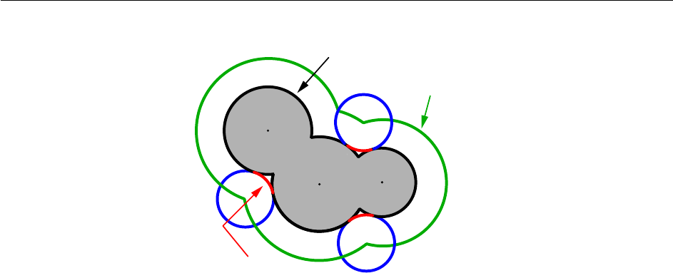
Chapter 12: Molecules in Complex Environments 689
van der Waals
surface
solvent
probe
solvent-
accessible
surface
re-entrant
surface
Figure 12.1: Illustration of various solute cavity surface definitions for PCMs.70 The union of atomic van der Waals
spheres (shown in gray) defines the van der Waals (vdW) surface, in black. Note that actual vdW radii from the
literature are sometimes scaled in constructing the vdW surface. If a probe sphere (representing the assumed size of a
solvent molecule) is rolled over the van der Waals surface, then its center point traces out the solvent accessible surface
(SAS), shown in green; the SAS is equivalent to a vdW surface where the atomic radii are increases by the radius of
the probe sphere. Finally, one can use the probe sphere to smooth out the sharp crevasses in the vdW surface using the
re-entrant surface elements shown in red, resulting in the solvent-excluded surface (SES).
“molecular surface". The SES uses the surface of the probe sphere at points where it is simultaneously tangent to two
or more atomic spheres to define elements of a “re-entrant surface” that smoothly connects the atomic (or “contact”)
surface.70
Having chosen a model for the cavity surface, this surface is discretized using atom-centered Lebedev grids71–73 of
the same sort that are used to perform the numerical integrations in DFT. (Discretization of the re-entrant facets of the
SES is somewhat more complicated but similar in spirit.70) Surface charges qiare located at these grid points and the
Lebedev quadrature weights can be used to define the surface area associated with each discretization point.67
A long-standing (though not well-publicized) problem with the aforementioned discretization procedure is that it fails
to afford continuous potential energy surfaces as the solute atoms are displaced, because certain surface grid points
may emerge from, or disappear within, the solute cavity, as the atomic spheres that define the cavity are moved. This
undesirable behavior can inhibit convergence of geometry optimizations and, in certain cases, lead to very large er-
rors in vibrational frequency calculations.67 It is also a fundamental hindrance to molecular dynamics calculations.68
Building upon earlier work by York and Karplus,125 Lange and Herbert67,68,70 developed a general scheme for imple-
menting apparent surface charge PCMs in a manner that affords smooth potential energy surfaces, even for ab initio
molecular dynamics simulations involving bond breaking.42,68 Notably, this approach is faithful to the properties of the
underlying integral equation theory on which the PCMs are based, in the sense that the smoothing procedure does not
significantly perturb solvation energies or cavity surface areas.67,68 The smooth discretization procedure combines a
switching function with Gaussian blurring of the cavity surface charge density, and is thus known as the “Switching/
Gaussian” (SWIG) implementation of the PCM.
Both single-point energies and analytic energy gradients are available for SWIG PCMs, when the solute is described
using molecular mechanics or an SCF (Hartree-Fock or DFT) electronic structure model, except that for the SES
cavity model only single-point energies are available. Analytic Hessians are available for the C-PCM model only. (As
usual, vibrational frequencies for other models will be computed, if requested, by finite difference of analytic energy
gradients.) Single-point energy calculations using correlated wave functions can be performed in conjunction with these
solvent models, in which case the correlated wave function calculation will use Hartree-Fock molecular orbitals that
are polarized in the presence of the continuum dielectric solvent (i.e., there is no post-Hartree–Fock PCM correction).

Chapter 12: Molecules in Complex Environments 690
Researchers who use these PCMs are asked to cite Refs. 68,69, which provide the details of Q-CHEM’s implementation,
and Ref. 70 if the SES is used. (We point the reader in particular to Ref. 68, which provides an assessment of the
discretization errors that can be anticipated using various PCMs and Lebedev grids; default grid values in Q-CHEM
were established based on these tests.) When publishing results based on PCM calculations, it is essential to specify
both the precise model that is used (see Table 12.3) as well as how the cavity was constructed.
For example, “Bondi radii multiplied by 1.2”, which is the Q-CHEM default, except for hydrogen, where the factor is
reduced to 1.1,99 as per usual. Radii for main-group elements that were not provided by Bondi are taken from Ref. 79.
Absent details such as these, PCM calculations will be difficult to reproduce in other electronic structure programs.
12.2.2.3 Nonequilibrium Solvation for Vertical Excitation, Ionization and Emission
In vertical excitation or ionization, the solute undergoes a sudden change in its charge distribution. Various micro-
scopic motions of the solvent have characteristic times to reach certain polarization response, and fast part of the
solvent response (electrons) can follow such a dynamic process while the remaining degrees of freedom (nuclei) re-
main unchanged as in the initial state. Such splitting of the solvent response gives rise to nonequilibrium solvation. In
the literature, two different approaches have been developed for describing nonequilibrium solvent effects: the linear
response (LR) approach14,26 and the state-specific (SS) approach.15,25,48,112 Both are implemented in Q-CHEM,127,at
the SCF level for vertical ionization and at the corresponding level (CIS, TDDFT or ADC, see Section 7.8.7) for ver-
tical excitation. A brief introduction to these methods is given below, and users of the nonequilibrium PCM features
are asked to cite Refs. 127 and 85. State-specific solvent-field equilibration for long-lived excited states to compute
e.g. emission energies is implemented for the ADC-suite of methods as described in section 7.8.7. Users of this
equilibrium-solvation PCM please cite and be referred to Ref. 86.
The LR approach considers the solvation effects as a coupling between a pair of transitions, one for solute and the
other for solvent. The transition frequencies when the interaction between the solute and solvent is turned on may
be determined by considering such an interaction as a perturbation. In the framework of TDDFT, the solvent/solute
interaction is given by45
ω0=ZdrZdr0Zdr00 Zdr000ρtr∗(r)1
|r−r0|+gXC(r,r0)
×χ∗(r0,r00, ω)1
|r00 −r000|+gXC(r00,r000)ρtr(r000),
(12.4)
where χis the charge density response function of the solvent and ρtr(r)is the solute’s transition density. This term
accounts for a dynamical correction to the transition energy so that it is related to the response of the solvent to the
charge density of the solute oscillating at the solute transition frequency (ω). Within a PCM, only classical Coulomb
interactions are taken into account, and Eq. (12.4) becomes
ω0
PCM =ZdrZdsρtr∗(r)
|r−s|Zds0Zdr0Q(s,s0, ε)ρtr(r0)
|s0−r0|,(12.5)
where Qis PCM solvent response operator for a generic dielectric constant, ε. The integral of Qand the potential of
the density ρtr gives the surface charge density for the solvent polarization.
The state-specific (SS) approach takes into account the capability of a part of the solvent degrees of freedom to respond
instantaneously to changes in the solute wave function upon excitation. Such an effect is not accounted for in the LR
approach. In SS, a generic solvated-solute excited state Ψiis obtained as a solution of a nonlinear Schrödinger equation
ˆ
Hvac +ˆ
Vslow
0+ˆ
Vfast
i|Ψii=ESS
i|Ψii(12.6)
that depends upon the solute’s charge distribution. Here ˆ
Hvac is the usual Hamiltonian for the solute in vacuum and the
reaction field operator ˆ
Vigenerates the electrostatic potential of the apparent surface charge density (Section 12.2.2.1),
corresponding to slow and fast polarization response. The solute is polarized self-consistently with respect to the
solvent’s reaction field. In case of vertical ionization rather than excitation, both the ionized and non-ionized states can

Chapter 12: Molecules in Complex Environments 691
be treated within a ground-state formalism. For vertical excitations, self-consistent SS models have been developed for
various excited-state methods,48,82 including both CIS and TDDFT.
In a linear dielectric medium, the solvent polarization is governed by the electric susceptibility, χ= [ε(ω)−1]/4π,
where ε(ω)is the frequency-dependent permittivity, In case of very fast vertical transitions, the dielectric response is
ruled by the optical dielectric constant, εopt =n2, where nis the solvent’s index of refraction. In both LR and SS,
the fast part of the solvent’s degrees of freedom is in equilibrium with the solute density change. Within PCM, the fast
solvent polarization charges for the SS excited state ican be obtained by solving the following equation:25
Kεopt qfast,SS
i=Rεopt vi+v(qslow
0).(12.7)
Here qfast,SS is the discretized fast surface charge. The dielectric constants in the matrices Kand R(Section 12.2.2.1)
are replaced with the optical dielectric constant, and viis the potential of the solute’s excited state density, ρi. The
quantity v(qslow
0)is the potential of the slow part of the apparent surface charges in the ground state, which are given
by
qslow
0=ε−εopt
ε−1q0.(12.8)
For LR-PCM, the solvent polarization is subjected to the first-order changes to the electron density (TDDFT linear
density response), and thus Eq. (12.7) becomes
Kεopt qfast,LR
i=Rεopt v(ρtr
i).(12.9)
The LR approach for CIS/TDDFT excitations and the self-consistent SS method (using the ground-state SCF) for
vertical ionizations are available in Q-CHEM. The self-consistent SS method for vertical excitations is not available,
because this method is problematic in the vicinity of (near-) degeneracies between excited states, such as in the vicinity
of a conical intersection. The fundamental problem in the SS approach is that each wave function Ψiis an eigenfunction
of a different Hamiltonian, since Eq. (12.6) depend upon the specific state of interest. To avoid the ordering and the
non-orthogonality problems, we compute the vertical excitation energy using a first-order, perturbative approximation
to the SS approach,16,19 in what we have termed the “ptSS” method.85 The zeroth-order excited-state wave function
can be calculated using various excited-state methods (currently available for CIS and TDDFT in Q-CHEM) with
solvent-relaxed molecular orbitals obtained from a ground-state PCM calculation. As mentioned previously, LR and
SS describe different solvent relaxation features in nonequilibrium solvation. In the perturbation scheme, we can
calculate the LR contribution using the zeroth-order transition density, in what we have called the "ptLR" approach.
The combination of ptSS and ptLR yields quantitatively good solvatochromatic shifts in combination with TDDFT but
not with the correlated variants of ADC, for which the pure ptSS approach was shown to be superior.85,127
The LR and SS approaches can also be used in the study of photon emission processes.49 An emission process can
be treated as a vertical excitation at a stationary point on the excited-state potential surface. The basic requirement
therefore is to prepare the solvent-relaxed geometry for the excited-state of interest. TDDFT/C-PCM analytic gradients
and Hessian are available.
Section 7.3.5 for computational details regarding excited-state geometry optimization with PCM. An emission process
is slightly more complicated than the absorption case. Two scenarios are discussed in literature, depending on the life-
time of an excited state in question. In the limiting case of ultra-fast excited state decay, when only fast solvent degrees
of freedom are expected to be equilibrated with the excited-state density. In this limit, the emission energy can be com-
puted exactly in the same way as the vertical excitation energy. In this case, excited state geometry optimization should
be performed in the nonequilibrium limit. The other limit is that of long-lived excited state, e.g., strongly fluorescent
species and phosphorescence. In the long-lived case, excited state geometry optimization should be performed with the
solvent equilibrium limit. Thus, the excited state should be computed using an equilibrium LR or SS approach, and the
ground state is calculated using nonequilibrium self-consistent SS approach. The latter approach is implemented for
the ADC-based methods as described in Section 7.8.7.
12.2.3 PCM Job Control
A PCM calculation is requested by setting SOLVENT_METHOD =PCM in the $rem section. As mentioned above, there
are a variety of different theoretical models that fall within the PCM family, so additional fine-tuning may be required,

Chapter 12: Molecules in Complex Environments 692
as described below.
12.2.3.1 $pcm section
Most PCM job control is accomplished via options specified in the $pcm input section, which allows the user to specify
which flavor of PCM will be used, which algorithm will be used to solve the PCM equations, and other options. The
format of the $pcm section is analogous to that of the $rem section:
$pcm
<Keyword> <parameter/option>
$end
Note: The following job control variables belong only in the $pcm section. Do not place them in the $rem section.
Theory
Specifies the which polarizable continuum model will be used.
INPUT SECTION: $pcm
TYPE:
STRING
DEFAULT:
CPCM
OPTIONS:
CPCM Conductor-like PCM with fε= (ε−1)/ε.
COSMO Original conductor-like screening model with fε= (ε−1)/(ε+ 1/2).
IEFPCM IEF-PCM with an asymmetric Kmatrix.
SSVPE SS(V)PE model, equivalent to IEF-PCM with a symmetric Kmatrix.
RECOMMENDATION:
The IEF-PCM/SS(V)PE model is more sophisticated model than either C-PCM or
COSMO, and probably more appropriate for low-dielectric solvents, but it is also more
computationally demanding. In high-dielectric solvents there is little difference between
these models. Note that the keyword COSMO in this context simply affects the dielectric
screening factor fε; to obtain the outlying charge correction suggested by Klamt,5,61 one
should use SOLVENT_METHOD =COSMO rather than SOLVENT_METHOD =PCM. (See
Section 12.2.7.)

Chapter 12: Molecules in Complex Environments 693
Method
Specifies which surface discretization method will be used.
INPUT SECTION: $pcm
TYPE:
STRING
DEFAULT:
SWIG
OPTIONS:
SWIG Switching/Gaussian method
ISWIG “Improved” Switching/Gaussian method with an alternative switching function
Spherical Use a single, fixed sphere for the cavity surface.
Fixed Use discretization point charges instead of smooth Gaussians.
RECOMMENDATION:
Use of SWIG is recommended only because it is slightly more efficient than the switching
function of ISWIG. On the other hand, ISWIG offers some conceptually more appealing
features and may be superior in certain cases. Consult Refs. 68,69 for a discussion of
these differences. The Fixed option uses the Variable Tesserae Number (VTN) algorithm
of Li and Jensen,74 with Lebedev grid points. VTN uses point charges with no switching
function or Gaussian blurring, and is therefore subject to discontinuities in geometry op-
timizations. It is not recommended, except to make contact with other calculations in the
literature.
SwitchThresh
Threshold for discarding grid points on the cavity surface.
INPUT SECTION: $pcm
TYPE:
INTEGER
DEFAULT:
8
OPTIONS:
nDiscard grid points when the switching function is less than 10−n.
RECOMMENDATION:
Use the default, which is found to avoid discontinuities within machine precision. In-
creasing nreduces the cost of PCM calculations but can introduce discontinuities in the
potential energy surface.
Construction of the solute cavity is an important part of the model and users should consult the literature in this capacity,
especially with regard to the radii used for the atomic spheres. The default values provided in Q-CHEM correspond
to the consensus choice that has emerged over several decades, namely, to use vdW radii scaled by a factor of 1.2.
The most widely-used set of vdW radii are those determined from crystallographic data by Bondi,9although the radius
for hydrogen was later adjusted to 1.1 Å,99 and radii for those main-group elements not addressed by Bondi were
provided later.79 This extended set of vdW is used by default in Q-CHEM, and for simplicity we call these “Bondi
radii” regardless of whether they come from Bondi’s original paper or the later work. Alternatively, atomic radii from
the Universal Force Field (UFF) are available.96 The main appeal of UFF radii is that they are defined for all atoms
of the periodic table, though the quality of these radii for PCM applications is unclear. Finally, the user may specify
his or her own radii for cavity construction using a $van_der_waals input section, the format for which is described
in Section 12.2.9. No scaling factor is applied to user-defined radii. Note that R= 0 is allowed for a particular
atomic radius, in which case the atom in question is not used to construct the cavity surface. This feature facilitates the
construction of “united atom” cavities,7in which the hydrogen atoms do not get their own spheres and the heavy-atom
radii are increased to compensate Finally, since the solvent molecules should not be able to penetrate all the way to the
atomic vdW radii of the solute, it is traditional either to scale the atomic radii (vdW surface construction) or else to
augment them with an assumed radius of a spherical solvent molecule (SAS construction), but not both.

Chapter 12: Molecules in Complex Environments 694
Radii
Specifies which set of atomic van der Waals radii will be used to define the solute cavity.
INPUT SECTION: $pcm
TYPE:
STRING
DEFAULT:
BONDI
OPTIONS:
BONDI Use the (extended) set of Bondi radii.
FF Use Lennard-Jones radii from a molecular mechanics force field.
UFF Use radii form the Universal Force Field.
READ Read the atomic radii from a $van_der_waals input section.
RECOMMENDATION:
Bondi radii are widely used. The FF option requires the user to specify an MM force field
using the FORCE_FIELD $rem variable, and also to define the atom types in the $molecule
section (see Section 12.3). This is not required for UFF radii.
vdwScale
Scaling factor for the atomic van der Waals radii used to define the solute cavity.
INPUT SECTION: $pcm
TYPE:
FLOAT
DEFAULT:
1.2
OPTIONS:
fUse a scaling factor of f > 0.
RECOMMENDATION:
The default value is widely used in PCM calculations, although a value of 1.0 might be
appropriate if using a solvent-accessible surface.
SASradius
Form a “solvent accessible” surface with the given solvent probe radius.
INPUT SECTION: $pcm
TYPE:
FLOAT
DEFAULT:
0.0
OPTIONS:
rUse a solvent probe radius of r, in Å.
RECOMMENDATION:
The solvent probe radius is added to the scaled van der Waals radii of the solute atoms. A
common solvent probe radius for water is 1.4 Å, but the user should consult the literature
regarding the use of solvent-accessible surfaces.

Chapter 12: Molecules in Complex Environments 695
SurfaceType
Selects the solute cavity surface construction.
INPUT SECTION: $pcm
TYPE:
STRING
DEFAULT:
VDW_SAS
OPTIONS:
VDW_SAS van der Waals or solvent-accessible surface
SES solvent-excluded surface
RECOMMENDATION:
The vdW surface and the SAS are each comprised simply of atomic spheres and thus
share a common option; the only difference is the specification of a solvent probe radius,
SASradius. For a true vdW surface, the probe radius should be zero (which is the de-
fault), whereas for the SAS the atomic radii are traditionally not scaled, hence vdwScale
should be set to zero (which is not the default). For the SES, only SWIG discretization is
available, but this can be used with any set of (scaled or unscaled) atomic radii, or with
radii that are augmented by SASradius.
Historically, discretization of the cavity surface has involved “tessellation” methods that divide the cavity surface
area into finite polygonal “tesserae”. (The GEPOL algorithm90 is perhaps the most widely-used tessellation scheme.)
Tessellation methods, however, suffer not only from discontinuities in the cavity surface area and solvation energy as a
function of the nuclear coordinates, but in addition they lead to analytic energy gradients that are complicated to derive
and implement. To avoid these problems, Q-CHEM’s SWIG PCM implementation67–69 uses Lebedev grids to discretize
the atomic spheres. These are atom-centered grids with icosahedral symmetry, and may consist of anywhere from 26 to
5294 grid points per atomic sphere. The default values used by Q-CHEM were selected based on extensive numerical
tests.68,69 The default for MM atoms (in MM/PCM or QM/MM/PCM jobs) is N= 110 Lebedev points per atomic
sphere, whereas the default for QM atoms is N= 302. (This represents a change relative to Q-CHEM versions earlier
than 4.2.1, where the default for QM atoms was N= 590.) These default values exhibit good rotational invariance
and absolute solvation energies that, in most cases, lie within ∼0.5–1.0 kcal/mol of the N→ ∞ limit,68 although
exceptions (especially where charged solutes are involved) can be found.69
Note: The acceptable values for the number of Lebedev points per sphere are N= 26, 50, 110, 194, 302, 434, 590,
770, 974, 1202, 1454, 1730, 2030, 2354, 2702, 3074, 3470, 3890, 4334, 4802, or 5294.
HPoints
The number of Lebedev grid points to be placed on H atoms in the QM system.
INPUT SECTION: $pcm
TYPE:
INTEGER
DEFAULT:
302
OPTIONS:
Acceptable values are listed above.
RECOMMENDATION:
Use the default for geometry optimizations. For absolute solvation energies, the user may
want to examine convergence with respect to N.

Chapter 12: Molecules in Complex Environments 696
HeavyPoints
The number of Lebedev grid points to be placed non-hydrogen atoms in the QM system.
INPUT SECTION: $pcm
TYPE:
INTEGER
DEFAULT:
302
OPTIONS:
Acceptable values are listed above.
RECOMMENDATION:
Use the default for geometry optimizations. For absolute solvation energies, the user may
want to examine convergence with respect to N.
MMHPoints
The number of Lebedev grid points to be placed on H atoms in the MM subsystem.
INPUT SECTION: $pcm
TYPE:
INTEGER
DEFAULT:
110
OPTIONS:
Acceptable values are listed above.
RECOMMENDATION:
Use the default for geometry optimizations. For absolute solvation energies, the user may
want to examine convergence with respect to N. This option applies only to MM/PCM
or QM/MM/PCM calculations.
MMHeavyPoints
The number of Lebedev grid points to be placed on non-hydrogen atoms in the MM
subsystem.
INPUT SECTION: $pcm
TYPE:
INTEGER
DEFAULT:
110
OPTIONS:
Acceptable values are listed above.
RECOMMENDATION:
Use the default for geometry optimizations. For absolute solvation energies, the user may
want to examine convergence with respect to N. This option applies only to MM/PCM
or QM/MM/PCM calculations.
Especially for complicated molecules, the user may want to visualize the cavity surface. This can be accomplished
by setting PrintLevel ≥2, which will trigger the generation of several .PQR files that describe the cavity surface.
(These are written to the Q-CHEM output file.) The .PQR format is similar to the common .PDB (Protein Data Bank)
format, but also contains charge and radius information for each atom. One of the output .PQR files contains the
charges computed in the PCM calculation and radii (in Å) that are half of the square root of the surface area represented
by each surface grid point. Thus, in examining this representation of the surface, larger discretization points are
associated with larger surface areas. A second .PQR file contains the solute’s electrostatic potential (in atomic units),
in place of the charge information, and uses uniform radii for the grid points. These .PQR files can be visualized using
various third-party software, including the freely-available Visual Molecular Dynamics (VMD) program,2,46 which is
particularly useful for coloring the .PQR surface grid points according to their charge, and sizing them according to
their contribution to the molecular surface area. (Examples of such visualizations can be found in Ref. 67.)

Chapter 12: Molecules in Complex Environments 697
PrintLevel
Controls the printing level during PCM calculations.
INPUT SECTION: $pcm
TYPE:
INTEGER
DEFAULT:
0
OPTIONS:
0 Prints PCM energy and basic surface grid information. Minimal additional printing.
1 Level 0 plus PCM solute-solvent interaction energy components and Gauss’ Law error.
2 Level 1 plus surface grid switching parameters and a .PQR file for visualization of
the cavity surface apparent surface charges.
3 Level 2 plus a .PQR file for visualization of the electrostatic potential at the surface
grid created by the converged solute.
4 Level 3 plus additional surface grid information, electrostatic potential and apparent
surface charges on each SCF cycle.
5 Level 4 plus extensive debugging information.
RECOMMENDATION:
Use the default unless further information is desired.
Finally, note that setting Method to Spherical in the $pcm input selection requests the construction of a solute cavity
consisting of a single, fixed sphere. This is generally not recommended but is occasionally useful for making contact
with the results of Born models in the literature, or the Kirkwood-Onsager model discussed in Section 12.2.1. In this
case, the cavity radius and its center must also be specified in the $pcm section. The keyword HeavyPoints controls
the number of Lebedev grid points used to discretize the surface.
CavityRadius
Specifies the solute cavity radius.
INPUT SECTION: $pcm
TYPE:
FLOAT
DEFAULT:
None
OPTIONS:
RUse a radius of R, in Ångstroms.
RECOMMENDATION:
None.
CavityCenter
Specifies the center of the spherical solute cavity.
INPUT SECTION: $pcm
TYPE:
FLOAT
DEFAULT:
0.0 0.0 0.0
OPTIONS:
x y z Coordinates of the cavity center, in Ångstroms.
RECOMMENDATION:
The format is CavityCenter followed by three floating-point values, delineated by spaces.
Uses the same coordinate system as the $molecule section.

Chapter 12: Molecules in Complex Environments 698
12.2.3.2 Examples
The following example shows a very basic PCM job. The solvent dielectric is specified in the $solvent section, which
is described below.
Example 12.3 A basic example of using the PCMs: optimization of trifluoroethanol in water.
$rem
JOBTYPE OPT
BASIS 6-31G*
METHOD B3LYP
SOLVENT_METHOD PCM
$end
$pcm
Theory CPCM
Method SWIG
Solver Inversion
HeavyPoints 194
HPoints 194
Radii Bondi
vdwScale 1.2
$end
$solvent
Dielectric 78.39
$end
$molecule
0 1
C -0.245826 -0.351674 -0.019873
C 0.244003 0.376569 1.241371
O 0.862012 -0.527016 2.143243
F 0.776783 -0.909300 -0.666009
F -0.858739 0.511576 -0.827287
F -1.108290 -1.303001 0.339419
H -0.587975 0.878499 1.736246
H 0.963047 1.147195 0.961639
H 0.191283 -1.098089 2.489052
$end
The next example uses a single spherical cavity and should be compared to the Kirkwood-Onsager job, Example 12.1

Chapter 12: Molecules in Complex Environments 699
on page 685.
Example 12.4 PCM with a single spherical cavity, applied to H2O in acetonitrile
$molecule
0 1
O 0.00000000 0.00000000 0.11722303
H -0.75908339 0.00000000 -0.46889211
H 0.75908339 0.00000000 -0.46889211
$end
$rem
METHOD HF
BASIS 6-31g**
SOLVENT_METHOD pcm
$end
$pcm
method spherical ! single spherical cavity with 590 discretization points
HeavyPoints 590
CavityRadius 1.8 ! Solute Radius, in Angstrom
CavityCenter 0.0 0.0 0.0 ! Will be at center of Standard Nuclear Orientation
Theory SSVPE
$end
$solvent
Dielectric 35.9 ! Acetonitrile
$end
Finally, we consider an example of a united-atom cavity. Note that a user-defined van der Waals radius is supplied only
for carbon, so the hydrogen radius is taken to be zero and thus the hydrogen atoms are not used to construct the cavity

Chapter 12: Molecules in Complex Environments 700
surface. (As mentioned above, the format for the $van_der_waals input section is discussion in Section 12.2.9).
Example 12.5 United-atom cavity construction for ethylene.
$comment
Benzene (in benzene), with a united-atom cavity construction
R = 2.28 A for carbon, R = 0 for hydrogen
$end
$molecule
0 1
C 1.38620 0.000000 0.000000
C 0.69310 1.200484 0.000000
C -0.69310 1.200484 0.000000
C -1.38620 0.000000 0.000000
C -0.69310 -1.200484 0.000000
C 0.69310 -1.200484 0.000000
H 2.46180 0.000000 0.000000
H 1.23090 2.131981 0.000000
H -1.23090 2.131981 0.000000
H -2.46180 0.000000 0.000000
H -1.23090 -2.131981 0.000000
H 1.23090 -2.131981 0.000000
$end
$rem
EXCHANGE hf
BASIS 6-31G*
SOLVENT_METHOD pcm
$end
$pcm
theory iefpcm ! this is a synonym for ssvpe
method swig
printlevel 1
radii read
$end
$solvent
dielectric 2.27
$end
$van_der_waals
1
6 2.28
1 0.00
$end
12.2.3.3 $solvent section
The solvent for PCM calculations is specified using the $solvent section, as documented below. In addition, the $solvent
section can be used to incorporate non-electrostatic interaction terms into the solvation energy. (The Theory keyword
in the $pcm section specifies only how the electrostatic interactions are handled.) The general form of the $solvent
input section is shown below. The $solvent section was used above to specify parameters for the Kirkwood-Onsager
SCRF model, and will be used again below to specify the solvent for SMxcalculations (Section 12.2.8); in each
case, the particular options that can be listed in the $solvent section depend upon the value of the $rem variable
SOLVENT_METHOD.
$solvent
NonEls <Option>

Chapter 12: Molecules in Complex Environments 701
NSolventAtoms <Number unique of solvent atoms>
SolventAtom <Number1> <Number2> <Number3> <SASradius>
SolventAtom <Number1> <Number2> <Number3> <SASradius>
...
<Keyword> <parameter/option>
...
$end
The keyword SolventAtom requires multiple parameters, whereas all other keywords require only a single parameter.
In addition to any (optional) non-electrostatic parameters, the $solvent section is also used to specify the solvent’s
dielectric constant. If non-electrostatic interactions are ignored, then this is the only keyword that is necessary in the
$solvent section. For nonequilibrium TDDFT/C-PCM calculations (Section 12.2.2.3), the optical dielectric constant
should be specified in the $solvent section as well.
Dielectric
The (static) dielectric constant of the PCM solvent.
INPUT SECTION: $solvent
TYPE:
FLOAT
DEFAULT:
78.39
OPTIONS:
εUse a dielectric constant of ε > 0.
RECOMMENDATION:
The static (i.e., zero-frequency) dielectric constant is what is usually called “the” dielectric
constant. The default corresponds to water at 25◦C.
OpticalDielectric
The optical dielectric constant of the PCM solvent.
INPUT SECTION: $solvent
TYPE:
FLOAT
DEFAULT:
1.78
OPTIONS:
ε∞Use an optical dielectric constant of ε∞>0.
RECOMMENDATION:
The default corresponds to water at 25◦C. Note that ε∞=n2, where nis the solvent’s
index of refraction.
The non-electrostatic interactions currently available in Q-CHEM are based on the work of Cossi et al.,27 and are
computed outside of the SCF procedure used to determine the electrostatic interactions. The non-electrostatic energy is
highly dependent on the input parameters and can be extremely sensitive to the radii chosen to define the solute cavity.
Accordingly, the inclusion of non-electrostatic interactions is highly empirical and probably needs to be considered on
a case-by-case basis. Following Ref. 27, the cavitation energy is computed using the same solute cavity that is used
to compute the electrostatic energy, whereas the dispersion/repulsion energy is computed using a solvent-accessible
surface.
The following keywords (in the $solvent section) are used to define non-electrostatic parameters for PCM calculations.

Chapter 12: Molecules in Complex Environments 702
NonEls
Specifies what type of non-electrostatic contributions to include.
INPUT SECTION: $solvent
TYPE:
STRING
DEFAULT:
None
OPTIONS:
Cav Cavitation energy
Buck Buckingham dispersion and repulsion energy from atomic number
LJ Lennard-Jones dispersion and repulsion energy from force field
BuckCav Buck + Cav
LJCav LJ + Cav
RECOMMENDATION:
A very limited set of parameters for the Buckingham potential is available at present.
NSolventAtoms
The number of different types of atoms.
INPUT SECTION: $solvent
TYPE:
INTEGER
DEFAULT:
None
OPTIONS:
NSpecifies that there are Ndifferent types of atoms.
RECOMMENDATION:
This keyword is necessary when NonEls = Buck, LJ, BuckCav, or LJCav. Methanol
(CH3OH), for example, has three types of atoms (C, H, and O).
SolventAtom
Specifies a unique solvent atom.
INPUT SECTION: $solvent
TYPE:
Various
DEFAULT:
None.
OPTIONS:
Input (TYPE) Description
Number1 (INTEGER): The atomic number of the atom
Number2 (INTEGER): How many of this atom are in a solvent molecule
Number3 (INTEGER): Force field atom type
SASradius (FLOAT): Probe radius (in Å) for defining the solvent accessible surface
RECOMMENDATION:
If not using LJ or LJCav, Number3 should be set to 0. The SolventAtom keyword is
necessary when NonEls = Buck, LJ, BuckCav, or LJCav.

Chapter 12: Molecules in Complex Environments 703
Temperature
Specifies the solvent temperature.
INPUT SECTION: $solvent
TYPE:
FLOAT
DEFAULT:
300.0
OPTIONS:
TUse a temperature of T, in Kelvin.
RECOMMENDATION:
Used only for the cavitation energy.
Pressure
Specifies the solvent pressure.
INPUT SECTION: $solvent
TYPE:
FLOAT
DEFAULT:
1.0
OPTIONS:
PUse a pressure of P, in bar.
RECOMMENDATION:
Used only for the cavitation energy.
SolventRho
Specifies the solvent number density
INPUT SECTION: $solvent
TYPE:
FLOAT
DEFAULT:
Determined for water, based on temperature.
OPTIONS:
ρUse a density of ρ, in molecules/Å3.
RECOMMENDATION:
Used only for the cavitation energy.
SolventRadius
The radius of a solvent molecule of the PCM solvent.
INPUT SECTION: $solvent
TYPE:
FLOAT
DEFAULT:
None
OPTIONS:
rUse a radius of r, in Å.
RECOMMENDATION:
Used only for the cavitation energy.

Chapter 12: Molecules in Complex Environments 704
The following example illustrates the use of the non-electrostatic interactions.
Example 12.6 Optimization of trifluoroethanol in water using both electrostatic and non-electrostatic PCM interac-
tions. OPLSAA parameters are used in the Lennard-Jones potential for dispersion and repulsion.
$rem
JOBTYPE OPT
BASIS 6-31G*
METHOD B3LYP
SOLVENT_METHOD PCM
FORCE_FIELD OPLSAA
$end
$pcm
Theory CPCM
Method SWIG
Solver Inversion
HeavyPoints 194
HPoints 194
Radii Bondi
vdwScale 1.2
$end
$solvent
NonEls LJCav
NSolventAtoms 2
SolventAtom 8 1 186 1.30
SolventAtom 1 2 187 0.01
SolventRadius 1.35
Temperature 298.15
Pressure 1.0
SolventRho 0.03333
Dielectric 78.39
$end
$molecule
0 1
C -0.245826 -0.351674 -0.019873 23
C 0.244003 0.376569 1.241371 22
O 0.862012 -0.527016 2.143243 24
F 0.776783 -0.909300 -0.666009 26
F -0.858739 0.511576 -0.827287 26
F -1.108290 -1.303001 0.339419 26
H -0.587975 0.878499 1.736246 27
H 0.963047 1.147195 0.961639 27
H 0.191283 -1.098089 2.489052 25
$end
12.2.3.4 Job control and Examples for Non-Equilibrium Solvation
The OpticalDielectric keyword in $solvent is always needed. The LR energy is automatically calculated while the
CIS/TDDFT calculations are performed with PCM, but it is turned off while the perturbation scheme is employed.

Chapter 12: Molecules in Complex Environments 705
ChargeSeparation
Partition fast and slow charges in solvent equilibrium state
INPUT SECTION: $pcm
TYPE:
STRING
DEFAULT:
No default.
OPTIONS:
Marcus Do slow-fast charge separation in the ground state.
Excited Do slow-fast charge separation in an excited-state.
RECOMMENDATION:
Charge separation is used in conjunction with the StateSpecific keyword in $pcm.
StateSpecific
Specifies which the state-specific method will be used.
INPUT SECTION: $pcm
TYPE:
Various
DEFAULT:
No default.
OPTIONS:
Marcus Run self-consistent SS method in the ground-state with a given slow polarization charges.
Perturb Perform ptSS and ptLR for vertical excitations.
iThe ith excited-state used for charge separation (for emission).
RECOMMENDATION:
NoneqGrad
Control whether perform excited state geometry optimization in equilibrium or nonequi-
librium.
INPUT SECTION: $pcm
TYPE:
NONE
DEFAULT:
No default.
OPTIONS:
RECOMMENDATION:
Specify it for nonequilibrium optimization otherwise equilibrium geometry optimization
will be performed.

Chapter 12: Molecules in Complex Environments 706
Example 12.7 LR-TDDFT/C-PCM low-lying vertical excitation energy
$molecule
0 1
C 0 0 0.0
O 0 0 1.21
$end
$rem
EXCHANGE B3LYP
CIS_N_ROOTS 10
CIS_SINGLETS TRUE
CIS_TRIPLETS TRUE
RPA TRUE
BASIS 6-31+G*
SOLVENT_METHOD PCM
$end
$pcm
Theory CPCM
Method SWIG
Solver Inversion
Radii Bondi
$end
$solvent
Dielectric 78.39
OpticalDielectric 1.777849
$end

Chapter 12: Molecules in Complex Environments 707
Example 12.8 PCM solvation effects on the vertical excitation energies of planar DMABN using the ptSS and ptLR
methods.
$molecule
0 1
C 0.000046 -0.000398 1.904953
C 1.210027 0.000379 1.186051
C 1.214640 -0.000065 -0.194515
C 0.000164 -0.000616 -0.933832
C -1.214349 -0.001557 -0.194687
C -1.209753 -0.001846 1.185775
H 2.151949 0.001377 1.722018
H 2.164371 0.000481 -0.709640
H -2.164082 -0.002008 -0.709781
H -2.151763 -0.002287 1.721615
C -0.000227 0.001061 3.325302
N -0.000475 0.002405 4.484321
N 0.000053 -0.000156 -2.297372
C -1.258656 0.001284 -3.036994
H -1.041042 0.001615 -4.102376
H -1.860897 -0.885647 -2.811117
H -1.859247 0.889133 -2.810237
C 1.258563 -0.000660 -3.037285
H 1.860651 0.886208 -2.810755
H 1.859362 -0.888604 -2.811461
H 1.040664 -0.000097 -4.102609
$end
$rem
EXCHANGE LRC-wPBEPBE
OMEGA 260
BASIS 6-31G*
CIS_N_ROOTS 10
RPA 2
CIS_SINGLETS 1
CIS_TRIPLETS 0
CIS_DYNAMIC_MEM TRUE
CIS_RELAXED_DENSITY TRUE
USE_NEW_FUNCTIONAL TRUE
SOLVENT_METHOD PCM
PCM_PRINT 1
$end
$pcm
NonEquilibrium
Theory IEFPCM
StateSpecific Perturb
$end
$solvent
Dielectric 35.688000 ! Acetonitrile
OpticalDielectric 1.806874
$end

Chapter 12: Molecules in Complex Environments 708
Example 12.9 Aqueous phenol ionization using state-specific nonequilibrium PCM
$molecule
0 1
C -0.189057 -1.215927 -0.000922
H -0.709319 -2.157526 -0.001587
C 1.194584 -1.155381 -0.000067
H 1.762373 -2.070036 -0.000230
C 1.848872 0.069673 0.000936
H 2.923593 0.111621 0.001593
C 1.103041 1.238842 0.001235
H 1.595604 2.196052 0.002078
C -0.283047 1.185547 0.000344
H -0.862269 2.095160 0.000376
C -0.929565 -0.042566 -0.000765
O -2.287040 -0.159171 -0.001759
H -2.663814 0.725029 0.001075
$end
$rem
EXCHANGE wPBE
CORRELATION PBE
LRC_DFT 1
OMEGA 300
BASIS 6-31+G*
SCF_CONVERGENCE 8
SOLVENT_METHOD PCM
PCM_PRINT 1
$end
$pcm
NonEquilibrium
$end
$solvent
Dielectric 78.39
OpticalDielectric 1.777849
$end
@@@
$molecule
1 2
read
$end
$rem
EXCHANGE wPBE
CORRELATION PBE
LRC_DFT 1
OMEGA 300
BASIS 6-31+G*
SCF_CONVERGENCE 8
SOLVENT_METHOD PCM
PCM_PRINT 1
SCF_GUESS READ
$end
$pcm
StateSpecific Marcus
$end
$solvent
Dielectric 78.39
OpticalDielectric 1.777849
$end

Chapter 12: Molecules in Complex Environments 709
Example 12.10 PCM solvation effects on the emission energy of twisted DMABN in acetonitrile.
$molecule
0 1
C -0.000002 -0.000003 1.894447
C 1.230178 0.000003 1.160765
C 1.244862 0.000001 -0.200360
C 0.000003 -0.000013 -0.917901
C -1.244845 -0.000000 -0.200354
C -1.230160 0.000000 1.160753
H 2.171128 0.000013 1.704064
H 2.180670 0.000009 -0.750140
H -2.180657 0.000006 -0.750120
H -2.171112 0.000006 1.704037
C -0.000023 -0.000002 3.293509
N -0.000011 -0.000001 4.459415
N -0.000008 -0.000005 -2.309193
C 0.000001 1.253881 -3.021235
H 0.000005 1.099076 -4.098660
H -0.882908 1.818975 -2.705815
H 0.882911 1.818967 -2.705805
C -0.000009 -1.253886 -3.021246
H 0.882917 -1.818966 -2.705849
H -0.882901 -1.818992 -2.705803
H -0.000038 -1.099071 -4.098670
$end
$rem
EXCHANGE LRC-wPBEPBE
OMEGA 280
BASIS 6-31G*
CIS_N_ROOTS 10
RPA 2
CIS_SINGLETS 1
CIS_TRIPLETS 0
CIS_DYNAMIC_MEM TRUE
CIS_RELAXED_DENSITY TRUE
USE_NEW_FUNCTIONAL TRUE
SOLVENT_METHOD PCM
PCM_PRINT 1
$end
$pcm
ChargeSeparation Excited
StateSpecific 1
$end
$solvent
Dielectric 35.688000 ! Acetonitrile
OpticalDielectric 1.806874
$end
@@@
$molecule
READ
$end
$rem
EXCHANGE LRC-wPBEPBE
OMEGA 280
BASIS 6-31G*
SCF_GUESS READ
SCF_CONVERGENCE 8
SOLVENT_METHOD PCM
PCM_PRINT 1
$end
$pcm
StateSpecific Marcus
$end
$solvent
Dielectric 35.688000 ! Acetonitrile
OpticalDielectric 1.806874
$end

Chapter 12: Molecules in Complex Environments 710
12.2.4 Linear-Scaling QM/MM/PCM Calculations
Recall that PCM electrostatics calculations require the solution of the set of linear equations given in Eq. (12.2), to
determine the vector qof apparent surface charges. The precise forms of the matrices Kand Rdepend upon the
particular PCM (Table 12.3), but in any case they have dimension Ngrid ×Ngrid, where Ngrid is the number of Lebedev
grid points used to discretize the cavity surface. Construction of the matrix K−1Raffords a numerically exact solution
to Eq. (12.2), whose cost scales as O(N3
grid)in CPU time and O(N2
grid)in memory. This cost is exacerbated by
smooth PCMs, which discard fewer interior grid points so that Ngrid tends to be larger, for a given solute, as compared
to traditional discretization schemes. For QM solutes, the cost of inverting Kis usually negligible relative to the cost
of the electronic structure calculation, but for the large values of Ngrid that are encountered in MM/PCM or QM/MM/
PCM jobs, the O(N3
grid)cost of inverting Kis often prohibitively expensive.
To avoid this bottleneck, Lange and Herbert42 have developed an iterative conjugate gradient (CG) solver for Eq. (12.2)
whose cost scales as O(N2
grid)in CPU time and O(Ngrid)in memory. A number of other cost-saving options are
available, including efficient pre-conditioners and matrix factorizations that speed up convergence of the CG iterations,
and a fast multipole algorithm for computing the electrostatic interactions.76 Together, these features lend themselves to
a solution of Eq. (12.2) whose cost scales as O(Ngrid)in both memory and CPU time, for sufficiently large systems.42
Currently, these options are available only for C-PCM, not for SS(V)PE/IEF-PCM.
Listed below are job control variables for the CG solver, which should be specified within the $pcm input section.
Researchers who use this feature are asked to cite the original SWIG PCM references68,69 as well as the reference for
the CG solver.42
Solver
Specifies the algorithm used to solve the PCM equations.
INPUT SECTION: $pcm
TYPE:
STRING
DEFAULT:
INVERSION
OPTIONS:
INVERSION Direct matrix inversion
CG Iterative conjugate gradient
RECOMMENDATION:
Matrix inversion is faster for small solutes because it needs to be performed only once in
a single-point calculation. However, the CG solver (which must be applied at each SCF
iteration) is recommended for large MM/PCM or QM/MM/PCM calculations.
CGThresh
The threshold for convergence of the conjugate gradient solver.
INPUT SECTION: $pcm
TYPE:
INTEGER
DEFAULT:
6
OPTIONS:
nConjugate gradient converges when the maximum residual is less than 10−n.
RECOMMENDATION:
The default typically affords PCM energies on par with the precision of matrix inversion
for small systems. For systems that have difficulty with SCF convergence, one should
increase nor try the matrix inversion solver. For well-behaved or very large systems, a
smaller nmight be permissible.

Chapter 12: Molecules in Complex Environments 711
DComp
Controls decomposition of matrices to reduce the matrix norm for the CG Solver.
INPUT SECTION: $pcm
TYPE:
INTEGER
DEFAULT:
1
OPTIONS:
0 Turns off matrix decomposition
1 Turns on matrix decomposition
3 Option 1 plus only stores upper half of matrix and enhances gradient evaluation
RECOMMENDATION:
None
PreCond
Controls the use of the pre-conditioner for the CG solver.
INPUT SECTION: $pcm
TYPE:
None
DEFAULT:
Off
OPTIONS:
No options. Specify the keyword to enable pre-conditioning.
RECOMMENDATION:
A Jacobi block-diagonal pre-conditioner is applied during the conjugate gradient algo-
rithm to improve the rate of convergence. This reduces the number of CG iterations,
at the expense of some overhead. Pre-conditioning is generally recommended for large
systems.
NoMatrix
Specifies whether PCM matrices should be explicitly constructed and stored.
INPUT SECTION: $pcm
TYPE:
None
DEFAULT:
Off
OPTIONS:
No options. Specify the keyword to avoid explicit construction of PCM matrices.
RECOMMENDATION:
Storing the PCM matrices requires O(N2
grid)memory. If this is prohibitive, the NoMatrix
option forgoes explicit construction of the PCM matrices, and instead constructs the ma-
trix elements as needed, reducing the memory requirement to O(Ngrid)at the expense of
additional computation.

Chapter 12: Molecules in Complex Environments 712
UseMultipole
Controls the use of the adaptive fast multipole method in the CG solver.
INPUT SECTION: $pcm
TYPE:
None
DEFAULT:
Off
OPTIONS:
No options. Specify the keyword in order to enable the fast multipole method.
RECOMMENDATION:
The fast multipole approach formally reduces the CPU time to O(Ngrid), but is only ben-
eficial for spatially extended systems with several thousand cavity grid points. Requires
the use of NoMatrix.
MultipoleOrder
Specifies the highest multipole order to use in the FMM.
INPUT SECTION: $pcm
TYPE:
INTEGER
DEFAULT:
4
OPTIONS:
nThe highest order multipole in the multipole expansion.
RECOMMENDATION:
Increasing the multipole order improves accuracy but also adds more computational ex-
pense. The default yields satisfactory performance in common QM/MM/PCM applica-
tions.
Theta
The multipole acceptance criterion.
INPUT SECTION: $pcm
TYPE:
FLOAT
DEFAULT:
0.6
OPTIONS:
nA number between zero and one.
RECOMMENDATION:
The default is recommended for general usage. This variable determines when the use
of a multipole expansion is valid. For a given grid point and box center in the FMM, a
multipole expansion is accepted when r/d ≤Theta, where dis the distance from the grid
point to the box center and ris the radius of the box. Setting Theta to one will accept all
multipole expansions, whereas setting it to zero will accept none. If not accepted, the grid
point’s interaction with each point inside the box is computed explicitly. A low Theta is
more accurate but also more expensive than a higher Theta.

Chapter 12: Molecules in Complex Environments 713
NBox
The FMM boxing threshold.
INPUT SECTION: $pcm
TYPE:
INTEGER
DEFAULT:
100
OPTIONS:
nThe maximum number of grid points for a leaf box.
RECOMMENDATION:
The default is recommended. This option is for advanced users only. The adaptive FMM
boxing algorithm divides space into smaller and smaller boxes until each box has less
than or equal to NBox grid points. Modification of the threshold can lead to speedup or
slowdown depending on the molecular system and other FMM variables.
A sample input file for the linear-scaling QM/MM/PCM methodology can be found in the $QC/samples directory,
under the name QMMMPCM_crambin.in. This sample involves a QM/MM description of a protein (crambin) in
which a single tyrosine side chain is taken to be the QM region. The entire protein is immersed in a dielectric using
C-PCM with SWIG discretization.
12.2.5 Isodensity Implementation of SS(V)PE
12.2.5.1 Basic Job Control
As discussed above, results obtained various types of PCMs are quite sensitive to the details of the cavity construction.
Q-CHEM’s implementation of PCMs, using Lebedev grids, simplifies this construction somewhat, but leaves the radii
of the atomic spheres as empirical parameters (albeit ones for which widely-used default values are provided). An
alternative implementation of the SS(V)PE solvation model is also available,22 which attempts to further eliminate
empiricism associated with cavity construction by taking the cavity surface to be a specified iso-contour of the solute’s
electron density. [We call this the isodensity implementation of SS(V)PE in Table 12.3, and it is based on Chipman’s
“symmetrized” form of the Kmatrix.22,69] In this case, the cavity surface is discretized by projecting a single-center
Lebedev grid onto the iso-contour surface. Unlike the PCM implementation discussed in Section 12.2.2, for which
point-group symmetry is disabled, this implementation of SS(V)PE supports full symmetry for all Abelian point groups.
The larger and/or the less spherical the solute molecule is, the more points are needed to get satisfactory precision in the
results. Further experience will be required to develop detailed recommendations for this parameter. Values as small
as 110 points are usually sufficient for diatomic or triatomic molecules. The default value of 1202 points is adequate to
converge the energy within 0.1 kcal/mol for solutes the size of mono-substituted benzenes.
Energy gradients are also not available for this implementation of SS(V)PE, although they are available for the im-
plementation described in Section 12.2.2 in which the cavity is constructed from atom-centered spheres. As with the
PCMs discussed in that section, the solute may be described using Hartree-Fock theory or DFT; post-Hartree–Fock
correlated wave functions can also take advantage of molecular orbitals that are polarized using SS(V)PE. Researchers
who use the isodensity SS(V)PE feature are asked to cite Ref. 20.
In related work, Pomogaeva and Chipman91–94 recently introduced a “composite method for implicit representation of
solvent” (CMIRS) that is based on SS(V)PE electrostatics but adds non-electrostatic terms. This model is available in
Q-CHEM 126 and is discussed in Section 12.2.6. In its current implementation, CMIRS requires an isodensity SS(V)PE
calculation, However, the current implementation computes the non-electrostatic interactions using the cavity and the
solute’s charge density generated from the isodensity SS(V)PE. To use the CMIRS model, an isodensity SS(V)PE
calculation must be requested (as described below), and the IDEFESR must be set to 1 in the $svp input section (see
Section 12.2.5.2).
An isodensity SS(V)PE calculation is requested by setting SOLVENT_METHOD =ISOSVP in the $rem section, in
addition to normal job control variables for a single-point energy calculation. Whereas the other solvation models

Chapter 12: Molecules in Complex Environments 714
described in this chapter use specialized input sections (e.g.,$pcm) in lieu of a slew of $rem variables, the isodensity
SS(V)PE code is an interface between Q-CHEM and a code written by Chipman,22 so some $rem variables are used for
job control of isodensity SS(V)PE calculations. These are listed below.
SVP_MEMORY
Specifies the amount of memory for use by the solvation module.
TYPE:
INTEGER
DEFAULT:
125
OPTIONS:
ncorresponds to the amount of memory in Mb.
RECOMMENDATION:
The default should be fine for medium size molecules with the default Lebedev grid, only in-
crease if needed.
SVP_PATH
Specifies whether to run a gas phase computation prior to performing the solvation procedure.
TYPE:
INTEGER
DEFAULT:
0
OPTIONS:
0 runs a gas-phase calculation and after
convergence runs the SS(V)PE computation.
1 does not run a gas-phase calculation.
RECOMMENDATION:
Running the gas-phase calculation provides a good guess to start the solvation stage and provides
a more complete set of solvated properties.
SVP_CHARGE_CONV
Determines the convergence value for the charges on the cavity. When the change in charges
fall below this value, if the electron density is converged, then the calculation is considered
converged.
TYPE:
INTEGER
DEFAULT:
7
OPTIONS:
nConvergence threshold set to 10−n.
RECOMMENDATION:
The default value unless convergence problems arise.
SVP_CAVITY_CONV
Determines the convergence value of the iterative isodensity cavity procedure.
TYPE:
INTEGER
DEFAULT:
10
OPTIONS:
nConvergence threshold set to 10−n.
RECOMMENDATION:
The default value unless convergence problems arise.

Chapter 12: Molecules in Complex Environments 715
SVP_GUESS
Specifies how and if the solvation module will use a given guess for the charges and cavity points.
TYPE:
INTEGER
DEFAULT:
0
OPTIONS:
0 No guessing.
1 Read a guess from a previous Q-CHEM solvation computation.
2 Use a guess specified by the $svpirf section from the input
RECOMMENDATION:
It is helpful to also set SCF_GUESS to READ when using a guess from a previous Q-CHEM run.
This last $rem variable requires specification of a $svpirf input section, the format for which is the following:
$svpirf
<# point> <x point> <y point> <z point> <charge> <grid weight>
<# point> <x normal> <y normal> <z normal>
$end
12.2.5.2 The $svp Input Section
More refined control over SS(V)PE jobs is obtained using a $svp input section. These are read directly by Chipman’s
SS(V)PE solvation module and therefore must be specified in the context of a FORTRAN namelist. The format is as
follows:
$svp
<KEYWORD>=<VALUE>, <KEYWORD>=<VALUE>,...
<KEYWORD>=<VALUE>
$end
For example, the section may look like this:
$svp
RHOISO=0.001, DIELST=78.39, NPTLEB=110
$end
The following keywords are supported in the $svp section:
DIELST
The static dielectric constant.
INPUT SECTION: $svp
TYPE:
FLOAT
DEFAULT:
78.39
OPTIONS:
real number specifying the constant.
RECOMMENDATION:
The default value 78.39 is appropriate for water solvent.

Chapter 12: Molecules in Complex Environments 716
IDEFESR
Specifies whether to request a CMIRS calculation.
INPUT SECTION: $svp
TYPE:
INTEGER
DEFAULT:
0
OPTIONS:
0 do not invoke a CMIRS calculation.
1 do invoke a CMIRS calculation.
RECOMMENDATION:
ISHAPE
A flag to set the shape of the cavity surface.
INPUT SECTION: $svp
TYPE:
INTEGER
DEFAULT:
0
OPTIONS:
0 use the electronic isodensity surface.
1 use a spherical cavity surface.
RECOMMENDATION:
Use the default surface.
RHOISO
Value of the electronic isodensity contour used to specify the cavity surface. (Only rele-
vant for ISHAPE = 0.)
INPUT SECTION: $svp
TYPE:
FLOAT
DEFAULT:
0.001
OPTIONS:
Real number specifying the density in electrons/bohr3.
RECOMMENDATION:
The default value is optimal for most situations. Increasing the value produces a smaller
cavity which ordinarily increases the magnitude of the solvation energy.
RADSPH
Sphere radius used to specify the cavity surface (Only relevant for ISHAPE=1.)
INPUT SECTION: $svp
TYPE:
FLOAT
DEFAULT:
Half the distance between the outermost atoms plus 1.4 Ångstroms.
OPTIONS:
Real number specifying the radius in bohr (if positive) or in Ångstroms (if negative).
RECOMMENDATION:
Make sure that the cavity radius is larger than the length of the molecule.

Chapter 12: Molecules in Complex Environments 717
INTCAV
A flag to select the surface integration method.
INPUT SECTION: $svp
TYPE:
INTEGER
DEFAULT:
0
OPTIONS:
0 Single center Lebedev integration.
1 Single center spherical polar integration.
RECOMMENDATION:
The Lebedev integration is by far the more efficient.
NPTLEB
The number of points used in the Lebedev grid for the single-center surface integration.
(Only relevant if INTCAV = 0.)
INPUT SECTION: $svp
TYPE:
INTEGER
DEFAULT:
1202
OPTIONS:
Valid choices are: 6, 18, 26, 38, 50, 86, 110, 146, 170, 194, 302, 350, 434, 590, 770,
974, 1202, 1454, 1730, 2030, 2354, 2702, 3074, 3470, 3890, 4334,
4802, or 5294.
RECOMMENDATION:
The default value has been found adequate to obtain the energy to within 0.1 kcal/mol for
solutes the size of mono-substituted benzenes.
NPTTHE, NPTPHI
The number of (θ,φ) points used for single-centered surface integration (relevant only if
INTCAV = 1.)
INPUT SECTION: $svp
TYPE:
INTEGER
DEFAULT:
8,16
OPTIONS:
θ,φspecifying the number of points.
RECOMMENDATION:
These should be multiples of 2 and 4 respectively, to provide symmetry sufficient for all
Abelian point groups. Defaults are too small for all but the tiniest and simplest solutes.

Chapter 12: Molecules in Complex Environments 718
LINEQ
Flag to select the method for solving the linear equations that determine the apparent point
charges on the cavity surface.
INPUT SECTION: $svp
TYPE:
INTEGER
DEFAULT:
1
OPTIONS:
0 use LU decomposition in memory if space permits, else switch to LINEQ = 2
1 use conjugate gradient iterations in memory if space permits, else use LINEQ = 2
2 use conjugate gradient iterations with the system matrix stored externally on disk.
RECOMMENDATION:
The default should be sufficient in most cases.
CVGLIN
Convergence criterion for solving linear equations by the conjugate gradient iterative
method (relevant if LINEQ = 1 or 2.)
INPUT SECTION: $svp
TYPE:
FLOAT
DEFAULT:
1.0E-7
OPTIONS:
Real number specifying the actual criterion.
RECOMMENDATION:
The default value should be used unless convergence problems arise.
Note that the single-center surface integration approach that is used to find the isodensity surface may fail for certain
very non-spherical solute molecules. The program will automatically check for this, aborting with a warning message if
necessary. The single-center approach succeeds only for what is called a “star surface”, meaning that an observer sitting
at the center has an unobstructed view of the entire surface. Said another way, for a star surface any ray emanating out
from the center will pass through the surface only once. Some cases of failure may be fixed by simply moving to a new
center with the ITRNGR parameter described below. But some surfaces are inherently non-star surfaces and cannot be
treated with this program until more sophisticated surface integration approaches are developed and implemented.

Chapter 12: Molecules in Complex Environments 719
ITRNGR
Translation of the cavity surface integration grid.
INPUT SECTION: $svp
TYPE:
INTEGER
DEFAULT:
2
OPTIONS:
0 No translation (i.e., center of the cavity at the origin
of the atomic coordinate system)
1 Translate to the center of nuclear mass.
2 Translate to the center of nuclear charge.
3 Translate to the midpoint of the outermost atoms.
4 Translate to midpoint of the outermost non-hydrogen atoms.
5 Translate to user-specified coordinates in Bohr.
6 Translate to user-specified coordinates in Ångstroms.
RECOMMENDATION:
The default value is recommended unless the single-center integrations procedure fails.
TRANX, TRANY, TRANZ
x,y, and zvalue of user-specified translation (only relevant if ITRNGR is set to 5 or 6).
INPUT SECTION: $svp
TYPE:
FLOAT
DEFAULT:
0, 0, 0
OPTIONS:
x,y, and zrelative to the origin in the appropriate units.
RECOMMENDATION:
None.
IROTGR
Rotation of the cavity surface integration grid.
INPUT SECTION: $svp
TYPE:
INTEGER
DEFAULT:
2
OPTIONS:
0 No rotation.
1 Rotate initial xyz axes of the integration grid to coincide
with principal moments of nuclear inertia (relevant if ITRNGR = 1)
2 Rotate initial xyz axes of integration grid to coincide with
principal moments of nuclear charge (relevant if ITRNGR = 2)
3 Rotate initial xyz axes of the integration grid through user-specified
Euler angles as defined by Wilson, Decius, and Cross.
RECOMMENDATION:
The default is recommended unless the knowledgeable user has good reason otherwise.

Chapter 12: Molecules in Complex Environments 720
ROTTHE ROTPHI ROTCHI
Euler angles (θ,φ,χ) in degrees for user-specified rotation of the cavity surface (relevant
if IROTGR = 3).
INPUT SECTION: $svp
TYPE:
FLOAT
DEFAULT:
0,0,0
OPTIONS:
θ,φ,χin degrees
RECOMMENDATION:
None.
IOPPRD
Specifies the choice of system operator form.
INPUT SECTION: $svp
TYPE:
INTEGER
DEFAULT:
0
OPTIONS:
0 Symmetric form.
1 Non-symmetric form.
RECOMMENDATION:
The default uses more memory but is generally more efficient, we recommend its use
unless there is shortage of memory available.
By default, Q-CHEM will check the validity of the single-center expansion by searching for the isodensity surface in
two different ways: first, working inwards from a large distance, and next by working outwards from the origin. If the
same result is obtained (within tolerances) using both procedures, then the cavity is accepted. If the two results do not
agree, then the program exits with an error message indicating that the inner isodensity surface is found to be too far
from the outer isodensity surface.
Some molecules, for example C60, can have a hole in the middle. Such molecules have two different “legal” isodensity
surfaces, a small inner one inside the “hole”, and a large outer one that is the desired surface for solvation. In such
cases, the cavity check described in the preceding paragraph causes the program to exit. To avoid this, one can consider
turning off the cavity check that works out from the origin, leaving only the outer cavity determined by working in
from large distances.
ICVICK
Specifies whether to perform cavity check
INPUT SECTION: $svp
TYPE:
INTEGER
DEFAULT:
1
OPTIONS:
0 no cavity check, use only the outer cavity
1 cavity check, generating both the inner and outer cavities and compare.
RECOMMENDATION:
Consider turning off cavity check only if the molecule has a hole and if a star (outer)
surface is expected.

Chapter 12: Molecules in Complex Environments 721
Solvent SolvRho A B C D Gamma
Benzene 0.0421 −0.00522 0.01294
Cyclohexane 0.0396 −0.00938 0.03184
DMSO 0.05279 −0.00951 0.044791 −162.07 4.1
CH3CN 0.03764 −0.008178 0.045278 −0.33914 1.3
Water 0.05 −0.006736 0.032698 −1249.6−21.405 3.7
Table 12.4: Optimized CMIRS parameters (from Ref. 126) using RHOISO = 0.0010 a.u. and, for ions, the proton
reference ∆Gvalue from Ref. 56.
12.2.6 Composite Method for Implicit Representation of Solvent (CMIRS)
Whereas PCMs, including sophisticated ones like SS(V)PE and IEF-PCM, account for long-range solute–solvent inter-
actions, an accurate model for free energies of solvation must also include a treatment of short-range, non-electrostatic
interactions. Various models decompose these interactions in different ways, but usually the non-electrostatic terms
attempt to model all or most of the following: solute–solvent dispersion (van der Waals) interactions, Pauli (exchange)
repulsion between solute and solvent, the work associated with forming the solute cavity within the dielectric medium
(the so-called “cavitation energy”), hydrogen-bonding and other specific interactions due to the molecular structure of
the solvent, and changes in the structure (and therefore the entropy) of the neat solvent upon introduction of the solute
Pomogaeva and Chipman91–94 have introduced an implicit solvation model that attempts to model these non-electrostatic
interactions alongside a PCM-style treatment of the bulk electrostatics. They call this approach the “composite method
for implicit representation of solvent” (CMIRS), and it consists first of a self-consistent treatment of solute–continuum
electrostatics using the SS(V)PE model (Section 12.2.5). To this electrostatics calculation, CMIRS adds a solute–
solvent dispersion term that is modeled upon the non-local VV09 van der Waals dispersion density functional,117 a
Pauli repulsion contribution that depends upon the tail of the solute’s electron density that extends beyond the solute
cavity, and a hydrogen-bonding correction based on the maximum and minimum values of the normal component of
the electric field generated by the solute at the cavity surface. The Gibbs free energy of solvation is thus modeled as
∆GCMIRS(ρs) =∆GSS(V)PE(ρs)+∆GDEFESR(ρs),(12.10)
where ∆GSS(V)PE is the continuum electrostatics contribution from the SS(V)PE model, which is based on a solute
cavity defined as an isocontour ρsof the solute’s charge density. The second term contains the short-range dispersion,
exchange, and "field-extremum short-range" (DEFESR) interactions:
∆GDEFESR =∆Gdisp + ∆Gexch + ∆GFESR .(12.11)
These terms are evaluated only once, using a converged charge density for the solute from a SS(V)PE calculation.
The CMIRS approach was implemented in Q-CHEM by Zhi-Qiang You and John Herbert.126 In the course of this
work, a serious error was discovered in the the original implementation of ∆Gdisp by Pomogaeva and Chipman, in the
GAMESS program. Although reparameterization of a corrected version of the model leads to only small changes in the
overall error statistics across a large database of experimental free energies of solvation, the apportionment between
energy components in Eq. (12.11) changes significantly.126 By request of Dan Chipman, the Q-CHEM implementation
is termed “CMIRS v. 1.1", reserving v. 1.0 for the original GAMESS implementation of Pomogaeva and Chipman.
The CMIRS model is independently parametrized for each solvent of interest, but uses no more than five empirical
parameters per solvent. It is presently available in Q-CHEM for water, acetonitrile, dimethyl sulfoxide, benzene,
and cyclohexane. Error statistics for ∆Gcompare very favorably to those of the SMxmodels that are described in
Section 12.2.8,e.g., mean unsigned errors <0.7kcal/mol in benzene and cyclohexane and <1.5kcal/mol in water.
The latter statistic includes challenging ionic solutes; errors for charge-neutral aqueous solutes are smaller still.126
The current implementation of CMIRS in Q-CHEM computes the electrostatic energy using Chipman’s isodensity
SS(V)PE module. The resulting isodensity cavity and the solute charge density are then employed in the calculation
of the DEFESR interactions. To request a CMIRS calculation, users must set IDEFESR =1in an isodensity SS(V)PE

Chapter 12: Molecules in Complex Environments 722
Solvent SolvRho A B C D Gamma
Benzene 0.0421 −0.00572 0.01116
Cyclohexane 0.0396 −0.00721 0.05618
DMSO 0.05279 −0.002523 0.011757 −817.93 4.3
CH3CN 0.03764 −0.003805 0.03223 −0.44492 1.2
Water 0.05 −0.006496 0.050833 −566.7−30.503 3.2
Table 12.5: Optimized CMIRS parameters (from Ref. 126) using RHOISO = 0.0005 a.u. and, for ions, the proton
reference ∆Gvalue from Ref. 56.
calculation (see Section 12.2.5.2). The solvent-dependent empirical parameters A,B,C,D,Gamma in the CMIRS
model need to be specified in the $pcm_nonels section. Three additional parameters are also required. One is the
damping parameter Delta in the dispersion equation. We recommend the parameter fixed at δ= 7 a.u. (about 3.7 Å), an
optimized value that only considers dispersion at intermolecular distances larger than van der Waals contact distance.
The second is solvent’s average electron density SolvRho. The last one is the number of Gauss–Laguerre points
GauLag_N for the integration over the solvent region in the exchange equation. We recommend 40 grid points for
efficient integration with accuracy. Optimized parameters for the supported solvents are listed in Tables 12.4 and 12.5
for two different values of ρs.126

Chapter 12: Molecules in Complex Environments 723
Example 12.11 CMIRS calculation for methane in the water solvent.
$rem
EXCHANGE = b3lyp5
BASIS = 6-31+g*
SCF_CONVERGENCE = 8
MEM_TOTAL = 4000
MEM_STATIC = 400
SYM_IGNORE = true
XC_GRID = 000096001202
$end
$molecule
0 1
C 0.000000 0.000005 0.000000
H 0.748558 0.801458 0.000000
H 0.506094 -0.972902 0.000000
H -0.627326 0.085706 0.895425
H -0.627326 0.085706 -0.895425
$end
@@@
$rem
EXCHANGE = b3lyp5
BASIS = 6-31+g*
SCF_CONVERGENCE = 8
MAX_SCF_CYCLES = 100
SOLVENT_METHOD = isosvp
SCF_GUESS = read
PCM_PRINT = 1
MEM_TOTAL = 4000
MEM_STATIC = 400
SVP_MEMORY = 1000
SYM_IGNORE = true
XC_GRID = 000096001202
$end
$molecule
read
$end
$svp
RHOISO=0.001, DIELST=78.36, NPTLEB=1202,
ITRNGR=2, IROTGR=2, IPNRF=1, IDEFESR=1
$end
$pcm_nonels
A -0.006736
B 0.032698
C -1249.6
D -21.405
Delta 7.0
Gamma 3.7
SolvRho 0.05
GauLag_N 40
$end

Chapter 12: Molecules in Complex Environments 724
12.2.7 COSMO
According to Table 12.3, COSMO and C-PCM appear to differ only in the dielectric screening factor, fεin Eq. (12.3).
Indeed, surface charges in either model are computed according to
q=−fεS−1v,(12.12)
and as discussed in Section 12.2.3 the user has the option to choose either the original value suggested by Klamt,61,62
fε= (ε−1)/(ε+ 1/2), or else fε= (ε−1)/ε as in, e.g., Refs. 28,69,115. More importantly, however, COSMO
differs from C-PCM in that the former includes a correction for outlying charge that goes beyond Eq. (12.12), whereas
C-PCM consists of nothing more than induced surface charges computed (self-consistently) according to Eq. (12.12)
Upon solution of Eq. (12.12), the outlying charge correction in COSMO5,61 is obtained by first defining a larger cavity
that is likely to contain essentially all of the solute’s electron density; in practice, this typically means using atomic
radii of 1.95 R, where Rdenotes the original atomic van der Waals radius that was used to compute q. (Note that
unlike the PCMs described in Sections 12.2.2 and 12.2.3, where the atomic radii have default values but a high degree
of user-controllability is allowed, the COSMO atomic radii are parameterized for this model and are fixed.) A new set
of charges, q0=−fε(S0)−1v0, is then computed on this larger cavity surface, and the charges on the original cavity
surface are adjusted to new values, q00 =q+q0. Finally, a corrected electrostatic potential on the original surface is
computed according to v00 =−fεSq00. It is this potential that is used to compute the solute–continuum electrostatic
interaction (polarization energy), Gpol =1
2Piq00
iv00
i. (For comparison, when the C-PCM approach described in
Section 12.2.2 is used, the electrostatic polarization energy is Gpol =1
2Piqivi, computed using the original surface
charges qand surface electrostatic potential v.) With this outlying charge correction, Q-CHEM’s implementation of
COSMO resembles the one in TURBOMOLE.100
A COSMO calculation is requested by setting SOLVENT_METHOD =COSMO in the $rem section, in addition to normal
job control variables. The keyword Dielectric in the $solvent section is used to set the solvent’s static dielectric
constant, as described above for other solvation models. COSMO calculations can also be used as a starting point
for COSMO-RS calculations,63,65 where “RS” stands for “real solvent”. The COSMO-RS approach is not included
in Q-CHEM and requires the COSMOtherm program, which is licensed separately through COSMOlogic.1Q-CHEM
users who are interested in COSMOtherm can request special versions of Q-CHEM for the generation of σ-surface
files that are needed by COSMOtherm.
12.2.8 SM8, SM12, and SMD Models
The SMxmodels developed by Cramer, Truhlar, and coworkers at the University of Minnesota are a class of implicit
solvation models that are designed to be “universal” in the sense that they can be applied to any solvent for which
a small of descriptors is known.30 (Note that the xin SMxis simply a version number; SM8, SM12, and SMD are
available in Q-CHEM.) In particular, the solvent descriptors are:
• dielectric constant
• refractive index
• bulk surface tension
• acidity on the Abraham scale
• basicity on the Abraham scale
• carbon aromaticity, which equals the fraction of non-hydrogenic solvent atoms that are aromatic carbon atoms
• electronegative halogenicity, which equals the fraction of non-hydrogenic solvent atoms that are F, Cl, or Br).
These models consist of a generalized Born treatment of continuum electrostatic interactions, along with non-electrostatic
interactions that are parameterized in terms of atomic surface tensions. The non-electrostatic interactions include cav-
itation, dispersion, and changes in solvent structure, and the treatment of these non-electrostatic effects is crucial to
obtaining accurate (free) energies of solvation.

Chapter 12: Molecules in Complex Environments 725
12.2.8.1 The SM8 Model
The SM8 model is described in detail in Ref. 80. It may be employed in conjunction with density functional theory
(with any density functional available in Q-CHEM) or with Hartree-Fock theory, but is intended for use only with the
6-31G*, 6-31+G*, and 6-31+G** basis sets, for reasons discussed below.
Bulk (continuum) electrostatic interactions in SM8 are described in terms of a generalized Born (GB) SCRF, using
a solute cavity constructed from atom-centered spheres. For the atoms H, C, N, O, F, Si, P, S, Cl, and Br, atomic
radii have been specifically optimized for use with SM8, whereas for other atoms the Bondi radius is used,9or else a
value of 2.0 Å for atoms not included in Bondi’s paper. Geometry-dependent radii are computed from these “intrinsic”
Coulomb radii via a de-screening approximation.80
In addition to GB electrostatics, there are several other contributions to the SM8 standard-state free energy of solvation.
The first of these is called the electronic-nuclear-polarization (ENP) energy, or simply the electronic polarization (EP)
energy if the solute geometry is assumed to be identical in the gas and solution phases. Another contribution to the
free energy of solvation comes from short-range interactions with solvent molecules in the first solvation shell, and is
sometimes called the cavitation/dispersion/solvent-structure (CDS) term. The CDS contribution to the solvation energy
is a sum of terms that are each proportional (with geometry-dependent proportionality constants called atomic surface
tensions) to the solvent-accessible surface areas (SASAs) of the individual solute atoms. The SASA of the solute
molecule is the area of a surface generated by the center of a spherical effective solvent molecule rolling on the van
der Waals surface of the solute molecule, as in the solvent-accessible surface that was mentioned in Section 12.2.2.
The SASA is computed using the Analytic Surface Area (ASA) algorithm of Ref. 77 and Bondi’s values for the van
der Waals radii,9or else a value of 2.0 Å if no Bondi radius is available. (Note that, as in the case of non-electrostatic
interactions in PCMs, this means that a different molecular surface is used for the bulk electrostatics as compared to the
non-electrostatic interactions.) The solvent probe radius used to generate the SASAs is set to 0.40 Å for all solvents.
Note that the solvent-structure part of the CDS term includes many aspects of solvent structure that are not described
by bulk electrostatics, for example, hydrogen bonding, exchange repulsion, and the variation of the effective dielectric
constant in the first solvation shell, relative to its bulk value. The semi-empirical nature of the CDS term also makes up
for errors due to (i) assuming fixed and model-dependent values of the intrinsic Coulomb radii, and (ii) any systematic
errors in the description of the solute–solvent electrostatic interactions using the GB approximation.
The final component of the SM8 solvation free energy is the concentration component. This is zero if the standard-state
concentration of the solute is the same in the gas and solution phases (e.g., if it is 1 mole/liter in the gas phase as well
as in the solution). Otherwise, this correction can be computed using ideal gas formulas, as discussed below.
SM8 does not require the user to assign molecular mechanics atom types to atoms or groups; all atomic surface tensions
in the theory are unique and continuous functions of the solute geometry, defined by the model and calculated internally
within Q-CHEM. In principle, SM8 can be used with any level of electronic structure theory so long as accurate partial
charges can be computed, but Q-CHEM’s implementation of SM8 specifically uses self-consistently polarized Charge
Model 4 (CM4) class IV charges.55 CM4 charges are obtained from Löwdin population analysis charges, via a mapping
whose parameters depend on the basis set (and only on the basis set, not on the density functional or anything else).
Basis sets supported for SM8 calculations in Q-CHEM are:
• 6-31G*
• 6-31+G*
• 6-31+G**
The charge mapping parameters are given in Ref. 55. Other basis sets should not be used in SM8 calculations.
The SM8 solvation free energy is output at T= 298 K for a standard-state concentration of 1 M in both the gas and
solution phase. However, solvation free energies in the literature are often tabulated using a standard state of P= 1 atm
for the gase. To convert 1 M-to1 M solvation free energies at 298 K to a standard state consisting of P= 1 atm for the
gas and a 1 M concentration in solution, add +1.89 kcal/mol to the computed solvation free energy.

Chapter 12: Molecules in Complex Environments 726
Solution-phase geometry optimizations can be carried out, but basis sets that use spherical harmonic dfunctions, or
angular momentum higher than d(f,g,etc.) are not supported. Since, by definition, the 6-31G*, 6-31+G*, and 6-
31+G** basis sets have Cartesian dshells, they are examples of basis sets that may be used for geometry optimization
with SM8. Solution-phase Hessian calculations can be carried out by numerical differentiation of analytical energy
gradients or by double differentiation of energies, although the former procedure is both more stable and more eco-
nomical. The analytic gradients of SM8 are based on the analytical derivatives of the polarization free energy and the
analytical derivatives of the CDS terms derived in Ref. 131.
An SM8 calculation is requested by setting SOLVENT_METHOD =SM8 in the $rem section, along with other job-
control variables appropriate for a Hartree-Fock or DFT calculation. Additional variables for SMxcalculations should
be listed in a $smx input section; for SM8, the only additional variable that is required is the name of the solvent:
Solvent
Sets the SMxsolvent
INPUT SECTION: $smx
TYPE:
STRING
DEFAULT:
water
OPTIONS:
Any name from the list of solvents given below.
RECOMMENDATION:
NONE
1,1,1-trichloroethane bromoethane m-ethylbenzoate
1,1,2-trichloroethane bromooctane m-ethylethanoate
1,1-dichloroethane butanal m-ethylmethanoate
1,2,4-trimethylbenzene butanoicacid m-ethylphenylketone
1,4-dioxane butanone m-ethylpropanoate
1-bromo-2-methylpropane butanonitrile m-ethylbutanoate
1-bromopentane butylethanoate m-ethylcyclohexane
1-bromopropane butylamine m-ethylformamide
1-butanol butylbenzene m-xylene
1-chloropentane carbon disulfide heptane
1-chloropropane carbon tetrachloride hexadecane
1-decanol chlorobenzene hexane
1-fluorooctane chlorotoluene nitrobenzene
1-heptanol cis-1,2-dimethylcyclohexane nitroethane
1-hexanol decalin nitromethane
1-hexene cyclohexane methylaniline
1-hexyne cyclohexanone nonane
1-iodobutane cyclopentane octane
1-iodopentene cyclopentanol pentane
1-iodopropane cyclopentanone o-chlorotoluene
1-nitropropane decane o-cresol
1-nonanol dibromomethane o-dichlorobenzene
1-octanol dibutyl ether o-nitrotoluene
1-pentanol dichloromethane o-xylene
1-pentene diethyl ether pentadecane
1-pentyne diethylsulfide pentanal
1-propanol diethylamine pentanoic acid
2,2,20trifluoroethanol diiodomethane pentylethanoate
2,2,4-trimethylpentane dimethyldisulfide pentylamine

Chapter 12: Molecules in Complex Environments 727
2,4-dimethylpentane dimethylacetamide perfluorobenzene
2,4-dimethylpyridine dimethylformamide phenyl ether
2,6-dimethylpyridine dimethylpyridine propanal
2-bromopropane dimethyl sulfoxide propanoic acid
2-chlorobutane dipropylamine propanonitrile
2-heptanone dodecane propylethanoate
2-hexanone E-1,2-dichloroethene propylamine
2-methylpentane E-2-pentene p-xylene
2-methylpyridine ethanethiol pyridine
2-nitropropane ethanol pyrrolidine
2-octanone ethylethanoate sec-butanol
2-pentanone ethylmethanoate t-butanol
2-propanol ethylphenyl ether t-butylbenzene
2-propen-1-ol ethylbenzene tetrachloroethene
3-methylpyridine ethylene glycol tetrahydrofuran
3-pentanone fluorobenzene tetrahyrothiophenedioxide
4-heptanone formamide tetralin
4-methyl-2-pentanone formic acid thiophene
4-methylpyridine hexadecyliodide thiophenol
5-nonanone hexanoic acid toluene
acetic acid iodobenzene trans-decalin
acetone iodoethane tribromomethane
acetonitrile iodomethane tributylphosphate
aniline isobutanol trichloroethene
anisole isopropyl ether trichloromethane
benzaldehyde isopropylbenzene triethylamine
benzene isopropyltoluene undecane
benzonitrile m-cresol water
benzyl alcohol mesitylene Z-1,2-dichloroethene
bromobenzene methanol other
The final choice, Solvent = “other”, requires an additional free-format file called “solvent_data” that should contain
the float-point values of the following solvent descriptors:
Dielec dielectric constant, ε, of the solvent
SolN index of refraction at optical frequencies at 293 K, nD
20
SolA Abraham’s hydrogen bond acidity, PαH
2
SolB Abraham’s hydrogen bond basicity, PβH
2
SolG γ=γm/γ0(default is 0.0), where γmis the macroscopic surface tension at air/solvent
interface at 298 K, and γ0is 1 cal mol−1Å−2(1 dyne/cm = 1.43932 cal mol−1Å−2)
SolC aromaticity, φ: the fraction of non-hydrogenic solvent atoms that are aromatic
carbon atoms
SolH electronegative “halogenicity”, ψ: the fraction of non-hydrogenic solvent atoms that are
F, Cl or Br
For a desired solvent, these values can be derived from experiment or from interpolation or extrapolation of data
available for other solvents. Solvent parameters for common organic solvents are tabulated in the Minnesota Solvent
Descriptor Database. The latest version of this database is available at:
http://comp.chem.umn.edu/solvation/mnsddb.pdf
The SM8 test suite contains the following representative examples:

Chapter 12: Molecules in Complex Environments 728
• single-point solvation energy and analytical gradient calculation for 2,2-dichloroethenyl dimethyl phosphate in
water at the M06-2X/6-31G* level;
• single-point solvation energy calculation for 2,2-dichloroethenyl dimethyl phosphate in benzene at the M06-2X/
6-31G* level;
• single-point solvation energy calculation for 2,2-dichloroethenyl dimethyl phosphate in ethanol at the M06-2X/
6-31G* level;
• single-point solvation energy calculation for 5-fluorouracil in water at the M06/6-31+G* level;
• single-point solvation energy calculation for 5-fluorouracil in octanol at the M06-L/6-31+G* level;
• single-point solvation energy and analytical gradient calculation for 5-fluorouracil in fluorobenzene at the M06-HF/
6-31+G** level;
• geometry optimization for protonated methanol CH3OH+
2in water at the B3LYP/6-31G* level;
• finite-difference frequency (with analytical gradient) calculation for protonated methanol CH3OH+
2in water at
the B3LYP/6-31G* level.
Users who wish to calculate solubilities can calculate them from the free energies of solvation by the method described
in Ref. 111. The present model can also be used with confidence to calculate partition coefficients (e.g., Henry’s Law
constants, octanol/water partition coefficients, etc.) by the method described in Ref. 29.
The user should note that the free energies of solvation calculated by the SM8 model in the current version of Q-CHEM
are all what may be called equilibrium free energies of solvation. The nonequilibrium algorithm required for vertical
excitation energies75 is not yet available in Q-CHEM. (Nonequilibrium versions of PCMs are available instead; see
Section 12.2.2.3.)
12.2.8.2 The SM12 Model
The SM12 model84 is also available in Q-CHEM. Similar to SM8, it employs (a) the generalized Born approximation
for the bulk electrostatic contribution to the free energy of solvation, and (b) the same formulas (with re-optimized
parameters) for CDS contributions. SM12 holds several advantages over SM8, and perhaps foremost among these
is that it uses CM5 charges,83 which are based on Hirshfeld population analysis, or else charges derived from the
electrostatic potential,11,104 for the bulk electrostatics term. These charges are stable with respect to extension of the
basis set, and thus SM12 can be used with larger basis sets whereas SM8 is limited to 6-31G*, 6-31+G*, and 6-31+G**,
due to instabilities in the Löwdin charges in larger basis sets. In addition, SM12 is parameterized using a more diverse
training set as compared to SM8, and is defined for the entire periodic table. However, the SM12 analytic gradient is
not available in Q-CHEM at present.
An SM12 calculation is requested by setting SOLVENT_METHOD =SM12 in the $rem section. The manner in which
the electrostatic term is computed is controlled by the Charges keyword in the $smx input section.

Chapter 12: Molecules in Complex Environments 729
Charges
Sets the type of atomic charges for the SM12 electrostatic term.
INPUT SECTION: $smx
TYPE:
STRING
DEFAULT:
CM5
OPTIONS:
CM5 Charge Model 5 charges83
MK Merz-Singh-Kollman charges104
CHELPG ChElPG charges11
RECOMMENDATION:
None. Merz-Singh-Kollman and ChElPG charges are fit to reproduce the molecular elec-
trostatic potential on the van der Waals surface or on a cubic grid, respectively, whereas
CM5 is an empirical model based on Hirshfeld population analysis.
Example 12.12 SM12CM5 calculation of the solvation free energy of water in the 1-octanol solvent.
$molecule
0 1
O 0.000000 0.125787 0.000000
H 0.758502 -0.503148 0.000000
H -0.758502 -0.503148 0.000000
$end
$rem
SCF_GUESS core
METHOD b3lyp
BASIS 6-31G*
SYM_IGNORE true
SOLVENT_METHOD sm12
$end
$smx
solvent 1octanol
charges chelpg
$end
12.2.8.3 The SMD Model
The SMD model81 is also available in Q-CHEM. Within this model, the electrostatic contribution to the free energy
solvation is described via the IEF-PCM model, where the CDS contributions follow the formulas as SM8 and SM12
with the parameters re-optimized to be compatible with the IEF-PCM electrostatics. Relative to SM8 or SM12, where
the electrostatic interactions are defined in terms of atomic point charges that are sensitive to the choice of basis set
(and therefore only certain basis sets are supported for use with these models), SMD can be used with any basis set.
An SMD energy or gradient calculation is requested by setting SOLVENT_METHOD =SMD in the $rem section. While
Q-CHEM users can vary the parameters for the IEF-PCM part of the SMD calculation, this should be done with caution
because a modified IEF-PCM electrostatics might be less compatible with CDS parameters and thus lead to less accurate

Chapter 12: Molecules in Complex Environments 730
results.
Example 12.13 SMD force calculation for tetrahydrofuran (THF) in the pentane solvent.
$molecule
0 1
C -0.361658 -0.986967 0.222366
C -1.331098 0.144597 -0.108363
O -0.592574 1.354183 0.036738
C 0.798089 1.070899 0.136509
C 0.964682 -0.396154 -0.256319
H -0.625676 -1.925862 -0.267011
H -0.333229 -1.158101 1.302753
H -1.697529 0.068518 -1.140448
H -2.193412 0.181620 0.562129
H 1.130199 1.238399 1.169839
H 1.348524 1.754318 -0.514697
H 1.050613 -0.489646 -1.343151
H 1.843065 -0.855802 0.199659
$end
$rem
JOBTYPE force
METHOD b3lyp
BASIS 6-31G*
SOLVENT_METHOD smd
$end
$smx
solvent pentane
$end
12.2.9 Langevin Dipoles Model
Q-CHEM provides the option to calculate molecular properties in aqueous solution and the magnitudes of the hydration
free energies by the Langevin dipoles (LD) solvation model developed by Jan Florián and Arieh Warshel35,36 at the
University of Southern California. In this model, a solute molecule is surrounded by a sphere of point dipoles, with
centers on a cubic lattice. Each of these “Langevin” dipoles changes its size and orientation in the electrostatic field of
the solute and the other Langevin dipoles. The electrostatic field from the solute is determined rigorously by the integra-
tion of its charge density, whereas for dipole–dipole interactions, a 12 Å cutoff is used. The Q-CHEM/CHEMSOL 1.0
implementation of the LD model is fully self-consistent in that the molecular quantum mechanical calculation takes
into account solute–solvent interactions. Further details on the implementation and parameterization of this model can
be found in the literature.35,36
The results of CHEMSOL calculations are printed in the standard output file. Below is a part of the output for a calcula-
tion on the methoxide anion (corresponding to the sample input given later on, and the sample file in the $QC/samples
directory).
Energy Component Value / kcal mol−1
LD Electrostatic energy −86.14
Hydrophobic energy 0.28
van der Waals energy −1.95
Bulk correction −10.07
Solvation free energy, ∆G(ILD) −97.87
Table 12.7: Results of the iterative Langevin Dipoles (ILD) solvation model, for aqueous methoxide.

Chapter 12: Molecules in Complex Environments 731
The total hydration free energy, ∆G(ILD) is calculated as a sum of several contributions. Note that the electrostatic part
of ∆Gis calculated by using the linear-response approximation35 and contains contributions from the polarization of
the solute charge distribution due to its interaction with the solvent. This results from the self-consistent implementation
of the Langevin dipoles model within Q-CHEM.
To perform an LD calculation in Q-CHEM, specify normal job-control variables for a Hartree-Fock or DFT calculation,
and set SOLVENT_METHOD =CHEM_SOL in the $rem section. Additional fine-tuning is accomplished using a set of
keywords in a $chem_sol input section. The remainder of this section summarizes these keywords.
EField
Determines how the solute charge distribution is approximated in evaluating the electro-
static field of the solute.
INPUT SECTION: $chem_sol
TYPE:
INTEGER
DEFAULT:
1
OPTIONS:
1 Exact solute charge distribution is used.
0 Solute charge distribution is approximated by Mulliken atomic charges.
RECOMMENDATION:
None. The Mulliken-based procedure is faster but less rigorous.
NGrids
Sets the number of grids used to calculate the average hydration free energy.
INPUT SECTION: $chem_sol
TYPE:
INTEGER
DEFAULT:
5∆Ghydr will be averaged over 5 different grids.
OPTIONS:
nUse ndifferent grids.
RECOMMENDATION:
None. The maximum allowed value of nis 20.
Print
Controls printing in the CHEMSOL part of the Q-CHEM output file.
INPUT SECTION: $chem_sol
TYPE:
INTEGER
DEFAULT:
0
OPTIONS:
0 Limited printout
1 Full printout
RECOMMENDATION:
None.

Chapter 12: Molecules in Complex Environments 732
ReadRadii
Read user-defined atomic radii from section $van_der_waals.
INPUT SECTION: $chem_sol
TYPE:
None
DEFAULT:
Off
OPTIONS:
No options. Specify the keyword to use user-defined atomic radii.
RECOMMENDATION:
None.
Accurate calculations of hydration free energies require a judicious choice of the solute–solvent boundary in terms
of atom-type dependent parameters. The default atomic van der Waals radii available in Q-CHEM were chosen to
provide reasonable hydration free energies for most solutes and basis sets. These parameters basically coincide with
the CHEMSOL 2.0 radii given in Ref. 36. The only difference between the Q-CHEM and CHEMSOL 2.0 atomic radii
stems from the fact that Q-CHEM parameter set uses radii for carbon and oxygen that are independent of the atom’s
hybridization state. User-defined atomic radii can be specified by declaring the option ReadRadii in the $chem_sol
input section, and then placing the radii in the $van_der_waals section. Two different (and mutually exclusive) formats
can be used, as shown below.
$van_der_waals
1
atomic_number vdW_radius
...
$end
$van_der_waals
2
sequential_atom_number vdW_radius
...
$end
The purpose of the second format is to permit the user to customize the radius of specific atoms, in the order that they
appear in the $molecule section, rather than simply by atomic numbers as in format 1. The radii of atoms that are not
listed in the $van_der_waals input will be assigned default values. The atomic radii that were used in the calculation

Chapter 12: Molecules in Complex Environments 733
are printed in the CHEMSOL part of the output file in the column denoted rp. All radii should be given in Ångstroms.
Example 12.14 A Langevin dipoles calculation on the methoxide anion. A customized value is specified for the radius
of the C atom.
$molecule
-1 1
C 0.0000 0.0000 -0.5274
O 0.0000 0.0000 0.7831
H 0.0000 1.0140 -1.0335
H 0.8782 -0.5070 -1.0335
H -0.8782 -0.5070 -1.0335
$end
$rem
METHOD hf
BASIS 6-31G
SCF_CONVERGENCE 6
SOLVENT_METHOD Chem_Sol
$end
$chem_sol
ReadRadii
$end
$van_der_waals
2
1 2.5
$end
12.2.10 Poisson Boundary Conditions
Each of the implicit solvation models described above is designed for isotropic, bulk solvation—conditions that can
be qualitatively described using a scalar dielectric constant, ε. For an anisotropic environment, such as a liquid/vapor
interface, a more general approach is to solve Poisson’s equation with a spatially-varying dielectric function,ε(r).
Such an approach can be used, for example, to model the air/water interface by describing certain regions of space
using ε= 1 (air) and other regions using ε= 78 (water).23,24 The atomistic region is described at the SCF level.
Construction of the dielectric function ε(r)is based on a solute cavity, somewhat analogous to the solute cavity in a
PCM calculation but where the dielectric changes smoothly (rather than abruptly) from ε= 1 inside the cavity (in the
atomistic QM region) to ε=εsolvent outside, in the continuum solvent. Options for modeling a liquid/vapor interface
are also available; see Section 12.2.10.3. In contrast to PCMs, which must approximate the “volume polarization” due
to penetration of the tails of the QM charge density beyond the solute cavity, this effect is described exactly under
Poisson boundary conditions. The price to be paid for lifting this approximation is that charge densities must be
discretized and integrated over three-dimensional space rather than simply a two-dimensional solute cavity surface.
Q-CHEM’s implementation of Poisson boundary conditions was introduced in Ref. 24 and refined in Ref. 23. Users of
this methodology are asked to cite at least Ref. 23.
12.2.10.1 Theory
The most general formulation of Poisson’s equation, for a dielectric function rather than a dielectric constant, is
ˆ
∇ · hε(r)ˆ
∇ϕtot(r)i=−4πρsol(r).(12.13)
The solute’s charge density will be separated into nuclear and electronic components,
ρsol(r) = ρnuc(r) + ρelec(r).(12.14)

Chapter 12: Molecules in Complex Environments 734
The total electrostatic potential ϕtot is comprised of the solute’s electrostatic potential ϕelec +ϕnuc, which is obtained
from the density in Eq. (12.14), plus the polarization potential induced in the medium:
ϕtot(r) = ϕelec(r) + ϕnuc(r) + ϕpol(r).(12.15)
To compute ρelec, the electronic contribution to the electrostatic potential in vacuum is first evaluated on a Cartesian
grid,
ϕelec(ri) =
Nbasis
X
µν
Pµν Dgµ(r)1
|r−ri|gν(r)E.(12.16)
Here Pis the one-electron density matrix, gµand gνare atom-centered Gaussian basis functions, and the integration is
over r. The electronic part of the solute’s charge density is then obtained from
ρelec(r) = −1
4πˆ
∇2ϕelec(r),(12.17)
where in practice the Laplacian of ϕelec is evaluated using an eighth-order finite difference scheme.23 The nuclear
charge density ρnuc is described classically,
ρnuc(r) = −
Natoms
X
A
Z
Aδ(r−RA),(12.18)
but to avoid numerical problems the nuclear charges are smeared out over one Cartesian grid voxel in practice. Opera-
tionally, this is achieved by adding ZA/dV to the grid point nearest RA, where dV is the volume of a Cartesian voxel.
The exact nuclear electrostatic potential in vacuum is computed according to
ϕnuc(r) = −1
4π
Natoms
X
A
Z
A
|r−RA|.(12.19)
The Dirac delta function in Eq. (12.18) has dimensions of (volume)−1and therefore incorporates the aforementioned
factor of dV −1
Having computed the electronic and nuclear charge densities and the electrostatic potentials in vacuum, one has in
hand an exact solution of Eq. (12.13) for the case where ε(r)=1. The induced polarization charge density and
corresponding electrostatic potential are then obtained iteratively, following closely the procedure outlined in Refs. 33
and 4. Equation (12.13) is rewritten to appear as Poisson’s equation in vacuum with an additional source charge density:
ˆ
∇2ϕtot(r) = −4π"ρsol(r)
ε(r)+ˆ
∇ln ε(r)·ˆ
∇ϕtot(r)
4π#
=−4πρsol(r) + ρpol(r),
(12.20)
where the polarization charge density is
ρpol(r) = ρiter(r) + 1−ε(r)
ε(r)ρsol(r).(12.21)
The iterative charge density ρiter(r)takes the form
ρ(k+1)
iter (r) = ˆ
∇ln ε(r)·ˆ
∇ϕ(k)
tot (r)
4π(12.22)
at iteration k+ 1. This function is nonzero only in transition regions where the dielectric is being interpolated from
vacuum to solvent. Note also that the second term in Eq. (12.21) vanishes wherever ε(r) = 1. The quantity ρiter(r)is
iterated to convergence by performing updates ρ(k)
iter(r)→ρ(k+1)
iter (r)using Eq. (12.22), taking ϕ(0)
tot(r)to be the solute’s
electrostatic potential in vacuum. Each time ρiter(r)is updated, a new polarization charge density is generated and
Eq. (12.20) is solved to obtain a new total electrostatic potential. To stabilize the iterative updates of ρiter(r), we use a
damping procedure
ρ(k+1)
iter (r) = η
4πˆ
∇ln ε(r)·ˆ
∇ϕ(k)
tot (r)+ (1 −η)ρ(k)
iter(r)
=ηρ(k+1)
iter + (1 −η)ρ(k)
iter(r)
(12.23)

Chapter 12: Molecules in Complex Environments 735
rather than using Eq. (12.22) as written. Following Refs. 33 and 4, we use η= 0.6.
Once the total charge density and electrostatic potential are iterated to self-consistency, the free energy of solvation,
Gpol =1
2Zdrϕpol(r)ρsol(r),(12.24)
is computed, where
ϕpol(r) = ϕtot(r)−ϕsol(r).(12.25)
Since ϕtot and ρtot are computed self-consistently at each SCF iteration, the polarization effects must be incorporated
into the Fock matrix. This is accomplished by adding the correction term ∆ˆ
F=δGpol/δρelec. The matrix form of this
correction in the atomic orbital basis is
∆Fµν =Zdrϕpol(r)gµ(r)gν(r).(12.26)
For additional details and a full description of the algorithm, see Ref. 23.
12.2.10.2 Nonequilibrium Solvation for Vertical Ionization
Nonequilibrium solvation within the framework of PCMs is discussed in Section 12.2.2.3, and that methodology85,127
has been adapted for vertical ionization processes in conjunction with Poisson boundary conditions.23,24 A state-specific
approach has been implemented that requires solution of a nonlinear Schrödinger equation, Eq. (12.6). For the reference
state, corresponding to i= 0 in Eq. (12.6), this is equivalent to solving Eq. (12.13) for the induced polarization potential
and computing the solvation free energy and Fock matrix correction according to Eqs. (12.24) and (12.26), respectively.
For the ionized state, denoted by a subscript i, the solvent polarization is partitioned into fast and slow components.
Within the Marcus partitioning scheme,127 Eq. (12.20) becomes23
−1
4πˆ
∇2ϕtot,i(r) = ρsol,i(r) + ρslow
pol,0(r) + ρfast
pol,i(r),(12.27)
where the fast polarization charge density of the ionized state, ρfast
pol,i, is given by
ρfast
pol,i(r) = ρiter,i(r) + 1−εopt(r)
εopt(r)ρsol,i(r) + ρslow
pol,0(r)(12.28)
and the fast polarization potential, ϕfast
pol,i, is
ϕfast
pol,i(r) = ϕtot,i(r)−ϕsol,i(r)−ϕslow
pol,0(r).(12.29)
Subscripts iand 0 refer to the ionized state and the reference state, respectively. The quantity εopt in Eq. (12.28) is the
solvent’s optical dielectric constant, and ρiter,i is computed using Eq. (12.23) but with a dielectric function constructed
using εopt and with ϕfast
tot,i substituted in place of ϕtot. For the Marcus partitioning scheme, the slow component of the
induced solvent polarization charge density is computed as the three-dimensional (volume charge rather than surface
charge) analogue of Eq. (12.8).
12.2.10.3 Job Control for the Poisson Equation Solver
A calculation using Poisson boundary conditions is requested by setting SOLVE_PEQ = TRUE in the $rem section. For
computational efficiency, solvent effects from the Poisson equation solver are not incorporated until the error in the
vacuum SCF calculation falls below a specified threshold, taken to be 10−3a.u. by default and controllable using the
$rem variable PEQ_SWITCH.
Note: When SOLVE_PEQ = TRUE, the keywords SYM_IGNORE and NO_REORIENT are also set to TRUE. Poisson’s
equation is discretized on a three-dimensional grid and the energy need not be rotationally invariant unless the
grid spacing is sufficiently small.

Chapter 12: Molecules in Complex Environments 736
SOLVE_PEQ
Perform a solvation free energy calculation on a Cartesian grid using Poisson equation boundary
conditions.
TYPE:
STRING
DEFAULT:
False
OPTIONS:
TRUE/FALSE
RECOMMENDATION:
None.
PEQ_SWITCH
Inclusion of solvent effects begins when the SCF error falls below 10−PEQ_SWITCH.
TYPE:
INTEGER
DEFAULT:
3
OPTIONS:
nCorresponding to 10−n
RECOMMENDATION:
Use the default unless solvent effects need to be incorporated earlier in the SCF procedure.
Further job control for the Poisson equation solver (PEqS) routines is set up in two sections: $peqs_grid and $peqs.
The former is used to define the Cartesian discretization grid, as follows:
$peqs_grid
DimX <Nx> <Xmin> <Xmax>
DimY <Ny> <Ymin> <Ymax>
DimZ <Nz> <Zmin> <Zmax>
$end
The Cartesian grid must be orthorhombic and Nx,Ny, and Nz refer to the number of grid points for the x,y, and z
axes.
Note: A fourth-order multigrid algorithm is used to accelerate convergence of the conjugate gradient PEqS routine
that solves Eq. (12.20).23 This requires that the number of grid points be odd, with the additional constraint
that the quantities Nx−1,Ny−1, and Nz−1must all be divisible by 8.
Values in the last two columns of the $peqs_grid section specify the minimum and maximum values of x,y, and
z, in units of Ångstroms. The length of the grid in the xdirection is Lx=xmax −xmin and the grid spacing is
∆x=Lx/(Nx−1). The volume element discussed in the context of Eq. (12.18) is dV = ∆x∆y∆z.
The $peqs section controls other aspects of a PEqS calculation, including construction of the solute cavity and other
required parameters for interfacial or nonequilibrium solvation. The format is:
$peqs
<Keyword> <parameter/option>
$end
Available keywords are described below.

Chapter 12: Molecules in Complex Environments 737
PEQMaxIter
Sets the maximum number of iterations used in the conjugate gradient solver.
INPUT SECTION: $peqs
TYPE:
INTEGER
DEFAULT:
500
OPTIONS:
User-defined.
RECOMMENDATION:
Use the default unless the calculation fails to converge.
PEQSolverThresh
The electrostatic potential is considered converged when the error falls below
10−PEQSolverThresh.
INPUT SECTION: $peqs
TYPE:
INTEGER
DEFAULT:
5
OPTIONS:
nCorresponding to 10−n
RECOMMENDATION:
Use the default unless a tighter convergence criterion is desired, at greater computational
cost.
PolarIterScale
Specifies the mixing parameter ηthat is used in Eq. (12.23) to stabilize iterative solution
for the polarization charge density.
INPUT SECTION: $peqs
TYPE:
FLOAT
DEFAULT:
0.6
OPTIONS:
ηDesired value of the mixing parameter (unit-less).
RECOMMENDATION:
Use the default, which was tested in Refs. 33 and 4, unless the calculation proves difficult
to converge.
BatchSize
Evaluate electrostatic potential integrals in batches over small parts of the Cartesian grid,
rather than computing all integrals in a single batch.
INPUT SECTION: $peqs
TYPE:
INTEGER
DEFAULT:
5000
OPTIONS:
nCorresponding to a batch size of ngrid points.
RECOMMENDATION:
For large grids (≥106grid points), a batch size n≈NxNyNz/5is recommended.

Chapter 12: Molecules in Complex Environments 738
SolventDielectric
Sets the dielectric value for the solvent.
INPUT SECTION: $peqs
TYPE:
FLOAT
DEFAULT:
78.39
OPTIONS:
εDesired value of ε(dimensionless).
RECOMMENDATION:
The default value corresponds to water at 25◦C.
OpticalDielectric
Sets the optical dielectric value of the solvent.
INPUT SECTION: $peqs
TYPE:
FLOAT
DEFAULT:
1.7778
OPTIONS:
εopt Desired value of εopt (dimensionless).
RECOMMENDATION:
The optical dielectric is equal to the square of the index of refraction. The default value
corresponds to water at 25◦C.
SoluteCavity
Specifies the type of solute cavity, which determines the form of the dielectric function
ε(r).
INPUT SECTION: $peqs
TYPE:
STRING
DEFAULT:
Vacuum
OPTIONS:
Vacuum Perform calculation in vacuum, ε(r)≡1.
RigidVDW Create a cavity using spherically symmetric error functions.
Spherical Create a single spherical cavity around the solute.
RECOMMENDATION:
None.
In conventional PCMs the solute cavity is a rigid two-dimensional surface constructed from a union of atomic spheres,
the radii of which are generally take to be equal to the van der Waals radius (rvdW) scaled by a factor of 1.2; see
Section 12.2.3.42 This cavity is rigid in the sense that once the atomic coordinates are specified, it remains unchanged
during the SCF cycles. (The isodensity cavity discussed in Section 12.2.5 is an exception, but is not available for
the PEqS method.) Furthermore, there is an abrupt and discontinuous change in the dielectric constant at the solute/
continuum boundary. A three-dimensional analogue of this cavity, using continuous and differentiable spherically-
symmetric error functions, has been implemented for PEqS calculations, following the procedure in Ref. 33. The
dielectric function, which depends parameterically on the nuclear positions RA, is
ε(r;{RA}) = εsolvent −1(Natoms
Y
A
h(dA,∆; |r−RA|)),(12.30)

Chapter 12: Molecules in Complex Environments 739
where
h(dA,∆; |r−RA|) = 1
21 + erf |r−RA| − dA
∆.(12.31)
Equation (12.30) smoothly interpolates between ε= 1 and ε=εsolvent, over a length scale of ≈4∆. The value of ∆is
specified using the RigidScale keyword. The quantity dAin Eqs. (12.30) and (12.31) sets radius of the atomic sphere
for atom A. By default, dA= 1.2rvdW but this can be controlled as described below.
RigidScale
Sets the length scale on which the error function employed in the rigid vdW cavity con-
struction interpolates the dielectric value from vacuum to solvent.
INPUT SECTION: $peqs
TYPE:
FLOAT
DEFAULT:
0.265 Å
OPTIONS:
∆Specifies the desired value (in Å); see Eq. (12.31).
RECOMMENDATION:
Use the default value, which was tuned in Ref. 33 so that errors in small-molecule solva-
tion energies were ≈1kcal/mol.
VDWType
Specifies details for the rigid vdW cavity construction.
INPUT SECTION: $peqs
TYPE:
STRING
DEFAULT:
Scaled
OPTIONS:
Unscaled dA=rvdW
Scaled dA=rvdW ×scale
Shifted dA= (rvdW +shift)×scale
RECOMMENDATION:
None. The values of scale and shif t are set with the VDWScale and VDWShift key-
words.
VDWScale
Sets the empirical scale factor applied to the atomic van der Waals radius.
INPUT SECTION: $peqs
TYPE:
FLOAT
DEFAULT:
1.2
OPTIONS:
scale Specifies the desired dimensionless scaling factor for the atomic vdW radii.
RECOMMENDATION:
Use the default value.

Chapter 12: Molecules in Complex Environments 740
VDWShift
Adjusts the center of the spherically-symmetric error functions when constructing the
rigid vdW cavity.
INPUT SECTION: $peqs
TYPE:
FLOAT
DEFAULT:
0.0 Ångstroms
OPTIONS:
shift Specifies the desired shift (in Å).
RECOMMENDATION:
None. If VDWType is set to Shifted, the vdW scale factor is set to 1.0 by default. This
can be adjusted using the VDWScale keyword.
Setting the SoluteCavity keyword to Spherical requests the construction of a spherical cavity around the solute, and
the dielectric is smoothly interpolated from vacuum to solvent using a hyperbolic tangent function:24
ε(r) = 1
2n(εsolvent + 1) + (εsolvent −1) tanhα(r−rmid)o.(12.32)
Here, rmid is the distance where the dielectric assumes the value ε(rmid)=(εsolvent + 1)/2. The value of rmid is taken
to be the sum of the sphere radius, R, and half of the interpolation length, L:rmid =R+L/2. The sphere radius
and interpolation length are controlled with the SphereRadius and InterpolLength keywords described below. The
parameter αcontrols the sharpness of the switching process, with α= 4/L by default.
SphereRadius
Sets the radius of the spherical solute cavity.
INPUT SECTION: $peqs
TYPE:
FLOAT
DEFAULT:
No default.
OPTIONS:
RDesired spherical cavity radius (in Å).
RECOMMENDATION:
None. See the Supporting Information of Ref. 24 for more information.
InterpolLength
Sets the length scale on which the dielectric is smoothly interpolated from vacuum to
solvent.
INPUT SECTION: $peqs
TYPE:
FLOAT
DEFAULT:
No default.
OPTIONS:
LDesired interpolation length (in Å).
RECOMMENDATION:
None.

Chapter 12: Molecules in Complex Environments 741
InterpolScale
For a given interpolation length (L), InterpolScale (α) sets the sharpness of the dielectric
transition from vacuum to solvent.
INPUT SECTION: $peqs
TYPE:
FLOAT
DEFAULT:
α=4/L
OPTIONS:
αDesired interpolation scale factor (in Å−1).
RECOMMENDATION:
Use the default unless a broader (smaller α) or narrower (larger α) transition region is
desired.
Interface
Perform a solvation calculation at a solvent/vacuum interface.
INPUT SECTION: $peqs
TYPE:
STRING
DEFAULT:
False
OPTIONS:
True Modify the dielectric function to simulate an interface between solvent and vacuum.
False Perform a solvation calculation in bulk solvent.
RECOMMENDATION:
The user will also need to specify the length scale on which the dielectric is smoothly
interpolated from the bulk solvent value to vacuum, and the location of the Gibbs dividing
surface (see below).
By setting Interface =True, the dielectric function on the Cartesian grid is further modified to mimic a solvent/vacuum
interface. First, the solute cavity is constructed as specified by the SoluteCavity keyword as discussed above. Then,
the dielectric function is smoothly interpolated in the zdirection across the Gibbs dividing surface (z≡zGDS) using
the following hyperbolic tangent switching function:23,24
ε(z) = 1
2n(εsolvent + 1) + (1 −εsolvent)tanhβ(z−zGDS)o.(12.33)
This interpolates the dielectric function over the interface length Linterface, centered at the Gibbs dividing surface,
z≡zGDS. Both of these values are controlled by the keywords InterfaceLength and GibbsDS, respectively. Similar
to the parameter αused in the spherical cavity construction, the parameter β= 4/Linterface controls the sharpness of
the interpolation across the Gibbs dividing surface.
InterfaceLength
Sets the length scale over which the dielectric function is smoothly transitioned from bulk
solvent to vacuum in the zdirection
INPUT SECTION: $peqs
TYPE:
FLOAT
DEFAULT:
None
OPTIONS:
Linterface Desired interface length (in Å).
RECOMMENDATION:
This sets the value β= 4/Linterface in Eq. (12.33). See the Supporting Information of
Ref. 24 for a full description of the solvent/vacuum interface construction.

Chapter 12: Molecules in Complex Environments 742
GibbsDS
Sets the location of the Gibbs dividing surface, in the zdirection.
INPUT SECTION: $peqs
TYPE:
FLOAT
DEFAULT:
None
OPTIONS:
zGDS Desired location of the Gibbs dividing surface (in Å).
RECOMMENDATION:
Consult the literature. One such way to determine this value is to compute a density profile
of the solvent as a function of zand set this location to be where the solvent density has
decreased to 50% of the bulk value. Usually zGDS ≈Linterface/2.
NonequilJob
Obtain the nonequilibrium free energy of solvation for a vertical ionization process.
INPUT SECTION: $peqs
TYPE:
STRING
DEFAULT:
False
OPTIONS:
True Compute the nonequilibrium free energy for a vertical ionization process.
False Compute the equilibrium solvation free energy.
RECOMMENDATION:
None.
NonequilPartition
Specifies the manner in which the solvent response is partitioned into fast and slow com-
ponents.
INPUT SECTION: $peqs
TYPE:
STRING
DEFAULT:
Marcus
OPTIONS:
Marcus Employ the Marcus partitioning scheme.
Pekar Employ the Pekar partitioning scheme.
RECOMMENDATION:
Use the default. Although the fast and slow solvation responses are different between the
two approaches, the total solvation free energy is the same,127 but the Pekar scheme is
computationally more expensive than the Marcus scheme.

Chapter 12: Molecules in Complex Environments 743
NonequilState
Specifies the state of interest for a nonequilibrium vertical ionization.
INPUT SECTION: $peqs
TYPE:
STRING
DEFAULT:
Reference
OPTIONS:
Reference The reference (initial) state, from which an electron will be removed.
Ionized The final (ionized) state.
RECOMMENDATION:
None. Both values will be needed in a compound input job, in order to compute the
nonequilibrium response to vertical ionization; see Example 17.
12.2.10.4 Examples
The following example computes the solvation free energy of a water molecule immersed in water. The Cartesian grid
is cubic with a side length of 15.0 Å and 73 grid points in each direction. A rigid vdW cavity is used based on scaled
vdW radii for the atomic spheres. The dielectric is not set, so takes the default value of 78.39.
Example 12.15 Free energy of solvation of water in water.
$rem
SCF_CONVERGENCE 5
THRESH 14
EXCHANGE wB97X-V
BASIS 6-31+G*
SOLVE_PEQ TRUE
PEQ_SWITCH 0
$end
$molecule
0 1
O 0.053004 -0.020947 -0.034784
H 0.003424 0.185855 0.910594
H -0.844842 0.146674 -0.358413
$end
$peqs
SOLUTECAVITY RIGIDVDW
$end
$peqs_grid
DimX 73 -7.50 7.50
DimY 73 -7.50 7.50
DimZ 73 -7.50 7.50
$end
The next example illustrates calculation of the solvation free energy of a water molecule at a water/vacuum interface,
with the Gibbs dividing surface placed at z= 0.50 Å. The length of the interface is set to Linterface = 2.75 Å and the
dielectric is interpolated from bulk solvent to vacuum in the positive zdirection across the Gibbs dividing surface. The

Chapter 12: Molecules in Complex Environments 744
Cartesian grid, solute cavity, and solvent dielectric are the same as in the previous example.
Example 12.16 Free energy of solvation of water at a water/vacuum interface.
$rem
SCF_CONVERGENCE 5
THRESH 14
EXCHANGE wB97X-V
BASIS 6-31+G*
SOLVE_PEQ TRUE
PEQ_SWITCH 0
$end
$molecule
0 1
O 0.053004 -0.020947 -0.034784
H 0.003424 0.185855 0.910594
H -0.844842 0.146674 -0.358413
$end
$peqs
SOLUTECAVITY RIGIDVDW
INTERFACE TRUE
INTERFACELENGTH 2.75
GIBBSDS 0.50
INTERFACEDIRECTION POSITIVE
$end
$peqs_grid
DimX 73 -7.50 7.50
DimY 73 -7.50 7.50
DimZ 73 -7.50 7.50
$end
The final example illustrates a nonequilibrium (NonEquilJob =True) solvation calculation for the vertical ionization
of H2O−in bulk water. This is a compound job that first calculates the equilibrium solvation free energy of the
anionic state (NonEquilState =Reference), then computes the nonequilibrium energy correction for the ionized state
(NonEquilState =Ionized). The two jobs are separated by “@@@”. The Cartesian grid and solvent dielectric are the
same as the previous examples, but the solute cavity is chosen to be spherical with a radius of 2.0 Å. The Marcus
scheme (NonEquilPartition =Marcus) is used to partition the solvent response into fast and slow components. Since
this is the default method, the NonEquilPartition keyword is omitted.
Example 12.17 Nonequilibrium free energy of solvation for the vertical ionization of H2O−

Chapter 12: Molecules in Complex Environments 745
$rem
SCF_CONVERGENCE 5
THRESH 14
EXCHANGE HF
BASIS 6-31++G*
SOLVE_PEQ TRUE
PEQ_SWITCH 0
$end
$molecule
-1 2
O 0.053004 -0.020947 -0.034784
H 0.003424 0.185855 0.910594
H -0.844842 0.146674 -0.358413
$end
$peqs
SOLUTECAVITY SPHERICAL
SPHERERADIUS 2.00
NONEQUILJOB TRUE
NONEQUILSTATE REFERENCE
$end
$peqs_grid
DimX 73 -7.50 7.50
DimY 73 -7.50 7.50
DimZ 73 -7.50 7.50
$end
@@@
$rem
SCF_CONVERGENCE 5
THRESH 14
EXCHANGE HF
BASIS 6-31++G*
SOLVE_PEQ TRUE
PEQ_SWITCH 0
$end
$molecule
0 1
O 0.053004 -0.020947 -0.034784
H 0.003424 0.185855 0.910594
H -0.844842 0.146674 -0.358413
$end
$peqs
SOLUTECAVITY SPHERICAL
SPHERERADIUS 2.00
NONEQUILJOB TRUE
NONEQUILSTATE IONIZED
$end
$peqs_grid
DimX 73 -7.50 7.50
DimY 73 -7.50 7.50
DimZ 73 -7.50 7.50
$end

Chapter 12: Molecules in Complex Environments 746
12.3 Stand-Alone QM/MM Calculations
Q-CHEM can perform hybrid quantum mechanics/molecular mechanics (QM/MM) calculations either as a stand-alone
program, which is described in this section, or in conjunction with the CHARMM package.47 See Section 12.4 for a
description of a latter approach.
12.3.1 Available QM/MM Methods and Features
Three modes of operation are available:
• MM calculations only (no QM)
• QM/MM calculations using a two-layer ONIOM model with mechanical embedding
• QM/MM calculations using the Janus model for electronic embedding
Q-CHEM can carry out purely MM calculations, wherein the entire molecular system is described by a MM force
field and no electronic structure calculation is performed. The MM force fields available at present are AMBER,119
CHARMM,37 and OPLSAA.52
As implemented in Q-CHEM, the ONIOM model116 is a mechanical embedding scheme that partitions a molecular
system into two subsystems (layers): an MM subsystem and a QM subsystem. The total energy of an ONIOM system
is given by
Etotal =EMM
total −EMM
QM +EQM
QM (12.34)
where EMM
total is the MM energy of the total system (i.e., QM + MM subsystems), EMM
QM is the MM energy of the QM
subsystem, and EQM
QM is the QM energy of the QM subsystem. MM energies are computed via a specified MM force
field, and QM energies are computed via a specified electronic structure calculation.
The advantage of the ONIOM model is its simplicity, which allows for straightforward application to a wide variety
of systems. A disadvantage of this approach, however, is that QM subsystem does not interact directly with the MM
subsystem. Instead, such interactions are incorporated indirectly, in the EMM
total contribution to the total energy. As a
result, the QM electron density is not polarized by the electrostatic charges of the MM subsystem.
If the QM/MM interface partitions the two subsystems across a chemical bond, a link atom (hydrogen) must be intro-
duced to act as a cap for the QM subsystem. Currently, Q-CHEM supports only carbon link atoms, of atom type 26, 35,
and 47 in the CHARMM27 force field.
The Janus model102 is an electronic embedding scheme that also partitions the system into MM and QM subsystems,
but is more versatile than the ONIOM model. The Janus model in Q-CHEM is based upon the “YinYang atom” model
of Shao and Kong.103 In this approach, the total energy of the system is simply the sum of the subsystem energies,
Etotal =EMM +EQM (12.35)
The MM subsystem energy, EMM, includes van der Waals interactions between QM and MM atoms but not QM/
MM Coulomb interactions. Rather, EQM includes the direct Coulomb potential between QM atoms and MM atoms
as external charges during the QM calculation, thus allowing the QM electron density to be polarized by the MM
atoms. Because of this, Janus is particularly well suited (as compared to ONIOM) for carrying out excited-state QM/
MM calculations, for excited states of a QM model system embedded within the electrostatic environment of the MM
system. Within a Janus calculation, Q-CHEM first computes EMM with the specified force field and then computes
EQM with the specified electronic structure theory.
When the Janus QM/MM partition cuts across a chemical bond, a YinYang atom103 is automatically introduced by
Q-CHEM. This atom acts as a hydrogen cap in the QM calculation, yet also participates in MM interactions. To retain
charge neutrality of the total system, the YinYang atom has a single electron and a modified nuclear charge in the QM

Chapter 12: Molecules in Complex Environments 747
calculation, equal to qnuclear = 1 + qMM (i.e., the charge of a proton plus the charge on the YinYang atom in the MM
subsystem).
Because this modified charge will affect the bond containing the YinYang atom, an additional repulsive Coulomb
potential is applied between the YinYang atom and its connecting QM atom to maintain a desirable bond length. The
additional repulsive Coulomb energy is added to EMM. The YinYang atom can be an atom of any kind, but it is highly
recommended to use carbon atoms as YinYang atoms.
Q-CHEM’s stand-alone QM/MM capabilities also include the following features:
• Analytic QM/MM gradients are available for QM subsystems described with density functional theory (DFT)
or Hartree-Fock (HF) electronic structure theory, allowing for geometry optimizations and QM/MM molecular
dynamics.
• Single-point QM/MM energy evaluations are available for QM subsystems described with most post-HF corre-
lated wave functions.
• Single-point QM/MM calculations are available for excited states of the QM subsystem, where the latter may
be described using CIS, TDDFT, or correlated wave function models. Analytic gradients for excited states are
available for QM/MM calculations if the QM subsystem is described using CIS.
• Single-point MM or QM/MM energy evaluations and analytic gradients are available using periodic boundary
conditions with Ewald summation.
• Implicit solvation for both Janus QM/MM calculations as well as MM-only calculations is available using the
Polarizable Continuum Models (PCMs) discussed in Section 12.2.2.
• Gaussian blurring of MM external charges is available for Janus QM/MM calculations.
• User-defined MM atoms types, MM parameters, and force fields.
12.3.2 Using the Stand-Alone QM/MM Features
12.3.2.1 $molecule section
To perform QM/MM calculations, the user must assign MM atom types for each atom in the $molecule section. The
format for this specification is modeled upon that used by the TINKER molecular modeling package,97 although the
TINKER program is not required to perform QM/MM calculations using Q-CHEM. Force field parameters and MM
atom type numbers used within Q-CHEM are identical to those used TINKER for the AMBER99, CHARMM27, and
OPLSAA force fields, and the format of the force field parameters files is also the same.
The $molecule section must use Cartesian coordinates to define the molecular geometry for internal QM/MM calcu-
lations; the Z-matrix format is not valid. MM atom types are specified in the $molecule section immediately after the
Cartesian coordinates on a line so that the general format for the $molecule section is
$molecule
<Charge> <Multiplicity>
<Atom> <X> <Y> <Z> <MM atom type>
...
$end
For example, one can define a TIP3P water molecule using AMBER99 atom types, as follows:
$molecule
0 1
O -0.790909 1.149780 0.907453 2001
H -1.628044 1.245320 1.376372 2002

Chapter 12: Molecules in Complex Environments 748
H -0.669346 1.913705 0.331002 2002
$end
When the input is specified as above, Q-CHEM will determine the MM bond connectivity based on the distances
between atoms; if two atoms are sufficiently close, they are considered to be bonded. Occasionally this approach can
lead to problems when non-bonded atoms are in close proximity of one another, in which case Q-CHEM might classify
them as bonded regardless of whether the appropriate MM bond parameters are available. To avoid such a scenario,
the user can specify the bonds explicitly by setting the $rem variable USER_CONNECT =TRUE, in which case the
$molecule section must have the following format
$molecule
<Charge> <Multiplicity>
<Atom> <X> <Y> <Z> <MM atom type> <Bond 1> <Bond 2> <Bond 3> <Bond 4>
...
$end
Each <Bond #> is the index of an atom to which <Atom> is bonded. Four bonds must be specified for each atom,
even if that atom is connected to fewer than four other atoms. (For non-existent bonds, use zero as a placeholder.)
Currently, Q-CHEM supports no more than four MM bonds per atom.
After setting USER_CONNECT =TRUE, a TIP3P water molecule in the AMBER99 force field could be specified as
follows:
$molecule
0 1
O -0.790909 1.149780 0.907453 2001 2 3 0 0
H -1.628044 1.245320 1.376372 2002 1 0 0 0
H -0.669346 1.913705 0.331002 2002 1 0 0 0
$end
Explicitly defining the bonds in this way is highly recommended.
12.3.2.2 $force_field_params section
In many cases, all atoms types (within both the QM and MM subsystems) will be defined by a given force field. In
certain cases, however, a particular atom type may not be defined in a given force field. For example, a QM/MM
calculation on the propoxide anion might consist of a QM subsystem containing an alkoxide functional group, for
which MM parameters do not exist. Even though the alkoxide moiety is described using quantum mechanics, van der
Waals parameters are nominally required for atoms within the QM subsystem, which interact with the MM atoms via
Lennard-Jones-type interactions.
In such cases, there are four possible options, the choice of which is left to the user’s discretion:
1. Use a similar MM atom type as a substitute for the missing atom type.
2. Ignore the interactions associated with the missing atom type.
3. Define a new MM atom type and associated parameters.
4. Define a new force field.
These options should be applied with care. Option 1 involves selecting an atom type that closely resembles the un-
defined MM atom. For example, the oxygen atom of an alkoxide moiety could perhaps use the MM atom type cor-
responding to the oxygen atom of a neutral hydroxyl group. Alternatively, the atom type could be ignored altogether
(option 2) by specifying MM atom type 0 (zero). Setting the atom type to zero should be accompanied with setting all

Chapter 12: Molecules in Complex Environments 749
four explicit bond connections to placeholders if USER_CONNECT =TRUE. An atom type of zero will cause all MM
energies involving that atom to be zero.
The third option in the list above requires the user to specify a $force_field_params section in the Q-CHEM input file.
This input section can be used to add new MM atom type definitions to one of Q-CHEM’s built-in force fields. At a
minimum, the user must specify the atomic charge and two Lennard-Jones parameters (radius and well depth, ), for
each new MM atom type. Bond, angle, and torsion parameters for stretches, bends, and torsions involving the new
atom type may also be specified, if desired. The format for the $force_field_params input section is
$force_field_params
NumAtomTypes <n>
AtomType -1 <Charge> <LJ Radius> <LJ Epsilon>
AtomType -2 <Charge> <LJ Radius> <LJ Epsilon>
...
AtomType -n <Charge> <LJ Radius> <LJ Epsilon>
Bond <a> <b> <Force constant> <Equilibrium Distance>
...
Angle <a> <b> <c> <Force constant> <Equilibrium Angle>
...
Torsion <a> <b> <c> <d> <Force constant> <Phase Angle> <Multiplicity>
...
$end
The first line in this input section specifies how many new MM atom types appear in this section (<n>). These are
specified on the following lines labeled with the AtomType tag. The atom type numbers are required to be negative
and to appear in the order −1,−2,−3,...,−n. The $molecule section for a water molecule, with user-defined MM
parameters for both oxygen and hydrogen, might appear as follows:
$molecule
0 1
O -0.790909 1.149780 0.907453 -1 2 3 0 0
H -1.628044 1.245320 1.376372 -2 1 0 0 0
H -0.669346 1.913705 0.331002 -2 1 0 0 0
$end
The remainder of each AtomType line in the $force_field_params section consists of a charge (in elementary charge
units), a Lennard-Jones radius (in Å), and a Lennard-Jones well depth (, in kcal/mol).
Each (optional) Bond line in the $force_field_params section defines bond-stretching parameters for a bond that con-
tains a new MM atom type. The bond may consist of both atoms <a> and <b> defined an AtomType line, or else
<a> may be defined with an AtomType line and <b> defined as a regular atom type for the force field. In the latter
case, the label for <b> should be the number of its general van der Waals type. For example, the atom type for a TIP3P
oxygen in AMBER99 is 2001, but its van der Waals type is 21, so the latter would be specified in the Bond line. The
remaining entries of each Bond line are the harmonic force constant, in kcal/mol/Å2, and the equilibrium distance, in
Å.
Similar to the Bond lines, each (optional) Angle line consists of one or more new atom types along with existing van
der Waals types. The central atom of the angle is <b>. The harmonic force constant (in units of kcal/mol/degree) and
equilibrium bond angle (in degrees) are the final entries in each Bond line.
Each (optional) Torsion line consists of one or more new MM atom types along with regular van der Waals types.
The connectivity of the four atoms that constitute the dihedral angle is <a>–<b>–<c>–<d>, and the torsional potential
energy function is
Etorsion(θ) = ktorsion[1 + cos(mθ −φ)] (12.36)
The force constant (ktorsion) is specified in kcal/mol and the phase angle (φ) in degrees. The multiplicity (m) is an
integer.

Chapter 12: Molecules in Complex Environments 750
12.3.2.3 User-Defined Force Fields
Option 4 in the list on page 748 is the most versatile, and allows the user to define a completely new force field. This
option is selected by setting FORCE_FIELD =READ, which tells Q-CHEM to read force field parameters from a text
file whose name is specified in the $force_field_params section as follows:
$force_field_params
Filename <path/filename>
$end
Here, <path/filename> is the full (absolute) path and name of the file that Q-CHEM will attempt to read for the
MM force field. For example, if the user has a file named MyForceField.prm that resides in the path /Users/me/parameters/,
then this would be specified as
$force_field_params
Filename /Users/me/parameters/MyForceField.prm
$end
Within the force field file, the user should first declare various rules that the force field will use, including how van der
Waals interactions will be treated, scaling of certain interactions, and the type of improper torsion potential. The rules
are declared in the file as follows:
RadiusRule <option>
EpsilonRule <option>
RadiusSize <option>
ImptorType <option>
vdw-14-scale <x>
chg-14-scale <x>
torsion-scale <x>
Currently, only a Lennard-Jones potential is available for van der Waals interactions. RadiusRule and EpsilonRule
control how to average σand , respectively, between atoms A and B in their Lennard-Jones potential. The op-
tions available for both of these rules are Arithmetic [e.g.,σAB = (σA+σB)/2] or Geometric [e.g.,σAB =
(σAσB)1/2]. RadiusSize has options Radius or Diameter, which specify whether the parameter σis the van
der Waals radius or diameter in the Lennard-Jones potential.
ImptorType controls the type of potential to be used for improper torsion (out-of-plane bending) energies, and has
two options: Trigonometric or Harmonic. These options are described in more detail below.
The scaling rules takes a floating point argument <x>. The vdw-14-scale and chg-14-scale rules only affect
van der Waals and Coulomb interactions, respectively, between atoms that are separated by three consecutive bonds
(atoms 1 and 4 in the chain of bonds). These interaction energies will be scaled by <x>. Similarly, torsion-scale
scales dihedral angle torsion energies.
After declaring the force field rules, the number of MM atom types and van der Waals types in the force field must be
specified using:
NAtom <n>
Nvdw <n>
where <n> is a positive integer.
Next, the atom types, van der Waals types, bonds, angles, dihedral angle torsion, improper torsions, and Urey-Bradley
parameters can be declared in the following format:
Atom 1 <Charge> <vdw Type index> <Optional description>
Atom 2 <Charge> <vdw Type index> <Optional description>
...

Chapter 12: Molecules in Complex Environments 751
Atom <NAtom> <Charge> <vdw Type index> <Optional description>
...
vdw 1 <Sigma> <Epsilon> <Optional description>
vdw 2 <Sigma> <Epsilon> <Optional description>
...
vdw <Nvdw> <Sigma> <Epsilon> <Optional description>
...
Bond <a> <b> <Force constant> <Equilibrium Distance>
...
Angle <a> <b> <c> <Force constant> <Equilibrium Angle>
...
Torsion <a> <b> <c> <d> <Force constant 1> <Phase Angle 1> <Multiplicity 1>
...
Improper <a> <b> <c> <d> <Force constant> <Equilibrium Angle> <Multiplicity>
...
UreyBrad <a> <b> <c> <Force constant> <Equilibrium Distance>
The parameters provided in the force field parameter file correspond to a basic MM energy functional of the form
EMM =ECoul +EvdW +Ebond +Eangle +Etorsion +Eimptor +EUreyBrad (12.37)
Coulomb and van der Waals interactions are computed for all non-bonded pairs of atoms that are at least three con-
secutive bonds apart (i.e., 1–4 pairs and more distant pairs). The Coulomb energy between atom types 1and 2is
simply
ECoul =fscale
q1q2
r12
(12.38)
where q1and q2are the respective charges on the atoms (specified with <Charge> in elementary charge units) and
r12 is the distance between the two atoms. For 1–4 pairs, fscale is defined with chg-14-scale but is unity for all
other valid pairs. The van der Waals energy between two atoms with van der Waals types aand b, and separated by
distance rab, is given by a “6-12” Lennard-Jones potential:
EvdW(rab) = fscale ab "σab
rab 12
−2σab
rab 6#(12.39)
Here, fscale is the scaling factor for 1–4 interactions defined with vdw-14-scale and is unity for other valid interac-
tions. The quantities ab and σab are the averages of the parameters of atoms aand bas defined with EpsilonRule
and RadiusRule, respectively (see above). The units of <Sigma> are Å , and the units of <Epsilon> are kcal/mol.
Hereafter, we refer to atoms’ van der Waals types with a, b, c, ... and atoms’ charges with 1,2, 3, ....
The bond energy is a harmonic potential,
Ebond(rab) = kbond(rab −req)2(12.40)
where kbond is provided by <Force Constant> in kcal/mol/Å2and req by <Equilibrium Distance> in Å.
Note that <a> and <b> in the Bond definition correspond to the van der Waals type indices from the vdw definitions,
not the Atom indices.
The bending potential between two adjacent bonds connecting three different atoms (<a>-<b>-<c>) is also taken to
be harmonic,
Eangle(θabc) = kangle(θabc −θeq)2(12.41)
Here, kangle is provided by <Force Constant> in kcal/mol/degrees and θeq by <Equilibrium Angle> in
degrees. Again, <a>,<b>, and <c> correspond to van der Waals types defined with vdw.
The energy dependence of the <a>-<b>-<c>-<d> dihedral torsion angle, where <a>,<b>,<c>, and <d> are van
der Waals types, is defined by
Etorsion(θabcd) = fscale X
m
kabcd[1 + cos(mθabcd −φ)] (12.42)

Chapter 12: Molecules in Complex Environments 752
Here, fscale is the scaling factor defined by torsion-scale. The force constant kabcd is defined with <Force
constant> in kcal/mol, and the phase angle φis defined with <Phase Angle> in degrees. The summation is
over multiplicities, m, and Q-CHEM supports up to three different values of mper dihedral angle. The force constants
and phase angles may depend on m, so if more than one multiplicity is used, then <Force constant> <Phase
Angle> <Multiplicity> should be specified for each multiplicity. For example, to specify a dihedral torsion
between van der Waals types 2–1–1–2, with multiplicities m= 2 and m= 3, we might have:
Torsion 2 1 1 2 2.500 180.0 2 1.500 60.0 3
Improper torsion angle energies for four atoms <a>-<b>-<c>-<d>, where <c> is the central atom, can be computed
in one of two ways, as controlled by the ImptorType rule. If ImptorType is set to Trigonometric, then the
improper torsion energy has a functional form similar to that used for dihedral angle torsions:
Eimptor(θabcd) = kabcd
Nequiv
[1 + cos(m θabcd −φ)] (12.43)
Here, θabcd is the out-of-plane angle of atom <c>, in degrees, and kabcd is the force constant defined with <Force
Constant>, in kcal/mol. The phase φand multiplicity mneed to be specified in the Improper declaration, although
the definition of an improper torsion suggests that these values should be set to φ= 0 and m= 2. The quantity Nequiv
accounts for the number of equivalent permutations of atoms <a>,<b>, and <d>, so that the improper torsion angle is
only computed once. If ImptorType is set to Harmonic, then in place of Eq. (12.43), the following energy function
is used:
Eimptor(θabcd) = kabcd
Nequiv
θ2
abcd (12.44)
The Urey-Bradley energy, which accounts for a non-bonded interaction between atoms <a> and <c> that are separated
by two bonds (i.e., a 1-3 interaction through <a>-<b>-<c>), is given by
EUreyBrad(rac) = kabc(rac −req)2(12.45)
The distance in Å between atoms <a> and <c> is rac, the equilibrium distance req is provided by <Equilibrium
Distance> in Å, and the force constant kabc is provided by <Force Constant> in kcal/mol/Å2.
A short example of a valid text-only file defining a force field for a flexible TIP3P water could be as follows:
//-- Force Field Example --//
// -- Rules -- //
RadiusRule Geometric
RadiusSize Radius
EpsilonRule Geometric
ImptorType Trigonometric
vdw-14-scale 1.0
chg-14-scale 0.8
torsion-scale 0.5
// -- Number of atoms and vdw to expect -- //
NAtom 2
Nvdw 2
// -- Atoms -- //
Atom 1 -0.8340 2 TIP3P Oxygen
Atom 2 0.4170 1 TIP3P Hydrogen
// -- vdw -- //
vdw 1 0.0000 0.0000 H parameters
vdw 2 1.7682 0.1521 O parameters

Chapter 12: Molecules in Complex Environments 753
// -- Bond -- //
Bond 1 2 553.0 0.9572
// -- Angle -- //
Angle 1 2 1 100.0 104.52
Lines that do not begin with one of the keywords will be ignored, and have been used here as comments.
12.3.2.4 $qm_atoms and $forceman sections
For QM/MM calculations (but not for purely MM calculations) the user must specify the QM subsystem using a
$qm_atoms input section, which assumes the following format:
$qm_atoms
<QM atom 1 index> <QM atom 2 index> . . .
...
<QM atom n index>
$end
Multiple indices can appear on a single line and the input can be split across multiple lines. Each index is an integer
corresponding to one of the atoms in the $molecule section, beginning at 1 for the first atom in the $molecule section.
Link atoms for the ONIOM model and YinYang atoms for the Janus model are not specified in the $qm_atoms section,
as these are inserted automatically whenever a bond connects a QM atom and an MM atom.
Q-Chem 4.2.2 and later versions also support, for example
$qm_atoms
18:31 35
$end
which specifies 15 QM atoms (atoms 18 through 31; atom 35).
For Janus QM/MM calculations, there are several ways of dealing with van der Waals interactions between the QM and
MM atoms. By default, van der Waals interactions are computed for all QM–MM and MM–MM atom pairs but not for
QM–QM atom pairs. In some cases, the user may prefer not to neglect the van der Waals interactions between QM–QM
atoms, or the user may prefer to neglect any van der Waals interaction that involves a QM atom. Q-CHEM allows the
user this control via two options in the $forceman section. To turn on QM–QM atom van der Waals interactions, the
user should include the following in their input:
$forceman
QM-QMvdw
$end
Similarly, to turn off all van der Waals interactions with QM atoms, the following should be included:
$forceman
NoQM-QMorQM-MMvdw
$end
12.3.2.5 Periodic Boundary Conditions
Periodic boundary conditions (using Ewald summation for the long-range Coulomb interactions) can be used in con-
junction with both MM-only calculations and QM/MM calculations. The approach is based off of the work of Nam
et al.88 and (independently) Riccardi et al.,98 as implemented in both the AMBER118 and CHARMM12,98 programs.

Chapter 12: Molecules in Complex Environments 754
These approaches use Mulliken charges to represent the periodic images of the wave function, and while suitable for
semi-empirical calculations with minimal basis sets, instabilities in the Mulliken charges for extended basis sets lead
to SCF convergence failure in the QM/MM-Ewald calculations.44 The implementation in Q-CHEM thus allows for the
use of ChElPG charges to represent the image wave functions, affording an algorithm that is stable in extended basis
sets.43,44
The efficiency of the Ewald summation is governed by the parameter, α, that controls the partition of the Coulomb
potential into short- and long-range components, and in the QM/MM-Ewald method there are separate values of αfor
the QM and MM portions of the calculations. Improper selection of αMM and/or αQM can greatly increase the com-
putational time, and the choices that are optimal for MM calculations need not be optimal for QM/MM calculations.44
The cost of the MM Ewald summation scales as O(NrecipNatoms), where Nrecip is the number of reciprocal-space
lattice vectors that is used for the k-space sum. The QM portion of the calculation scales as O(NrecipNQMNatoms),
where NQM is the number of QM atoms (whereas Natoms =NQM +NMM is the total number of atoms). The MM
Ewald parameter is thus selected to minimize the amount of work that is done in real space. The optimal value, which
is typically αMM ≈0.5Å−1, can be found by solving the equation44
αMM = 2C/L (12.46)
where
C=h−ln 10−SCF_CONVERGENCEi1/2(12.47)
and Lis the length of the simulation cell. (Only cubic simulation cells are available at present.) In contrast, the
parameter αQM should be selected to minimize the total number of vectors in both real and reciprocal space. The
optimal value, which is often αQM ≈0.1Å−1, is determined by solving the equation44
2CL3α3
QM
π3/2+α2
QML2
π1/2−αQML−2C= 0 .(12.48)
To perform an MM- or QM/MM-Ewald job, one must set MM_SUBTRACTIVE =TRUE and EWALD_ON =TRUE in the
$rem section, but otherwise job control is largely done through the $forceman section. The following variables must be
set for every type of Ewald calculation.
• The keyword Ewald will turn on Ewald summation.
• The keyword alpha should be followed by a value for the MM Ewald parameter and then the QM Ewald param-
eter. (The latter must be set even for MM-only jobs.)
•Box_length specifies the side length of the cubic simulation cell, in Å.
The following parameters are optional for further job control.
•Dielectric specifies a dielectric constant for the surrounding medium, which appears in the “dipole term” of
Ewald summation (Edipole in Ref. 44). If no value is set, the dielectric constant is set to infinity, corresponding
to “tin foil" boundary conditions.
• The keyword Ewald_SCF_thresh_on, followed by a real number, causes Q-CHEM to wait until the DIIS er-
ror falls below the specified value before adding the Ewald correction to the Fock matrix, thus obviating the
sometimes-costly Ewald correction in early SCF cycles. (The default value is 1.0, which turns on Ewald sum-
mation immediately in most cases)
A short example of a $forceman section using Ewald summation could be as follows:
$forceman
ewald
alpha 0.35 0.1
box_length 15.00

Chapter 12: Molecules in Complex Environments 755
dielectric 88.0
mm_read_scratch
ewald_scf_thresh_on 0.0001
$end
12.3.3 Additional Job Control Variables
A QM/MM job is requested by setting the $rem variables QM_MM_INTERFACE and FORCE_FIELD. Also required are
a$qm_atoms input section and appropriate modifications to the $molecule section, as described above. Additional job
control variables are detailed here.
QM_MM_INTERFACE
Enables internal QM/MM calculations.
TYPE:
STRING
DEFAULT:
NONE
OPTIONS:
MM Molecular mechanics calculation (i.e., no QM region)
ONIOM QM/MM calculation using two-layer mechanical embedding
JANUS QM/MM calculation using electronic embedding
RECOMMENDATION:
The ONIOM model and Janus models are described above. Choosing MM leads to no electronic
structure calculation. However, when using MM, one still needs to define the $rem variables
BASIS and EXCHANGE in order for Q-CHEM to proceed smoothly.
FORCE_FIELD
Specifies the force field for MM energies in QM/MM calculations.
TYPE:
STRING
DEFAULT:
NONE
OPTIONS:
AMBER99 AMBER99 force field
CHARMM27 CHARMM27 force field
OPLSAA OPLSAA force field
RECOMMENDATION:
None.
CHARGE_CHARGE_REPULSION
The repulsive Coulomb interaction parameter for YinYang atoms.
TYPE:
INTEGER
DEFAULT:
550
OPTIONS:
nUse Q = n×10−3
RECOMMENDATION:
The repulsive Coulomb potential maintains bond lengths involving YinYang atoms with the po-
tential V(r) = Q/r. The default is parameterized for carbon atoms.

Chapter 12: Molecules in Complex Environments 756
GAUSSIAN_BLUR
Enables the use of Gaussian-delocalized external charges in a QM/MM calculation.
TYPE:
LOGICAL
DEFAULT:
FALSE
OPTIONS:
TRUE Delocalizes external charges with Gaussian functions.
FALSE Point charges
RECOMMENDATION:
None
GAUSS_BLUR_WIDTH
Delocalization width for external MM Gaussian charges in a Janus calculations.
TYPE:
INTEGER
DEFAULT:
NONE
OPTIONS:
nUse a width of n×10−4Å.
RECOMMENDATION:
Blur all MM external charges in a QM/MM calculation with the specified width. Gaussian blur-
ring is currently incompatible with PCM calculations. Values of 1.0–2.0 Å are recommended in
Ref. 31.
MODEL_SYSTEM_CHARGE
Specifies the QM subsystem charge if different from the $molecule section.
TYPE:
INTEGER
DEFAULT:
NONE
OPTIONS:
nThe charge of the QM subsystem.
RECOMMENDATION:
This option only needs to be used if the QM subsystem (model system) has a charge that is
different from the total system charge.
MODEL_SYSTEM_MULT
Specifies the QM subsystem multiplicity if different from the $molecule section.
TYPE:
INTEGER
DEFAULT:
NONE
OPTIONS:
nThe multiplicity of the QM subsystem.
RECOMMENDATION:
This option only needs to be used if the QM subsystem (model system) has a multiplicity that is
different from the total system multiplicity. ONIOM calculations must be closed shell.

Chapter 12: Molecules in Complex Environments 757
USER_CONNECT
Enables explicitly defined bonds.
TYPE:
STRING
DEFAULT:
FALSE
OPTIONS:
TRUE Bond connectivity is read from the $molecule section
FALSE Bond connectivity is determined by atom proximity
RECOMMENDATION:
Set to TRUE if bond connectivity is known, in which case this connectivity must be specified in
the $molecule section. This greatly accelerates MM calculations.
MM_SUBTRACTIVE
Specifies whether a subtractive scheme is used in the ECoul, Eq. (12.38), portion of the calcula-
tion.
TYPE:
LOGICAL
DEFAULT:
FALSE
OPTIONS:
FALSE Only pairs that are not 1-2, 1-3, or 1-4 pairs are used.
TRUE All pairs are calculated, and then the pairs that are double counted (1-2, 1-3, and 1-4) are sub-
tracted out.
RECOMMENDATION:
When running QM/MM or MM calculations there is not recommendation. When running a QM/
MM Ewald calculation the value must be set to TRUE.
12.3.4 QM/MM Examples
• QM/MM Example 1
Features of this job:
–Geometry optimization using ONIOM mechanical embedding.
–MM region (water 1) described using OPLSAA.
–QM region (water 2) described using PBE0/6-31G*.
–$molecule input section contains user-defined MM bonds. A zero is used as a placeholder if there are no
more connections.

Chapter 12: Molecules in Complex Environments 758
Example 12.18 ONIOM optimization of water dimer.
$rem
METHOD pbe0
BASIS 6-31G*
QM_MM_INTERFACE oniom
FORCE_FIELD oplsaa
USER_CONNECT true
JOBTYPE opt
MOLDEN_FORMAT true
$end
$qm_atoms
456
$end
$molecule
0 1
O -0.790909 1.149780 0.907453 186 2 3 0 0
H -1.628044 1.245320 1.376372 187 1 0 0 0
H -0.669346 1.913705 0.331002 187 1 0 0 0
O 1.178001 -0.686227 0.841306 186 5 6 0 0
H 0.870001 -1.337091 1.468215 187 4 0 0 0
H 0.472696 -0.008397 0.851892 187 4 0 0 0
$end
• QM/MM Example 2
Features of this job:
–Janus electronic embedding with a YingYang link atom (the glycosidic carbon at the C10position of the
deoxyribose).
–MM region (deoxyribose) is described using AMBER99.
–QM region (adenine) is described using HF/6-31G*.
–The first 5 electronically excited states are computed with CIS. MM energy interactions between a QM
atom and an MM atom (e.g., van der Waals interactions, as well as angles involving a single QM atom) are
assumed to be the same in the excited states as in the ground state.
–$molecule input section contains user-defined MM bonds.
–Gaussian-blurred charges are used on all MM atoms, with a width set to 1.5 Å.

Chapter 12: Molecules in Complex Environments 759
Example 12.19 Excited-state single-point QM/MM calculation on deoxyadenosine.
$rem
METHOD cis
BASIS 6-31G*
QM_MM_INTERFACE janus
USER_CONNECT true
FORCE_FIELD amber99
GAUSSIAN_BLUR true
GAUSS_BLUR_WIDTH 15000
CIS_N_ROOTS 5
CIS_TRIPLETS false
MOLDEN_FORMAT true
PRINT_ORBITALS true
$end
$qm_atoms
18 19 20 21 22 23 24 25 26 27 28 29 30 31
$end
$molecule
0 1
O 0.000000 0.000000 0.000000 1244 2 9 0 0
C 0.000000 0.000000 1.440000 1118 1 3 10 11
C 1.427423 0.000000 1.962363 1121 2 4 6 12
O 1.924453 -1.372676 1.980293 1123 3 5 0 0
C 2.866758 -1.556753 0.934073 1124 4 7 13 18
C 2.435730 0.816736 1.151710 1126 3 7 8 14
C 2.832568 -0.159062 0.042099 1128 5 6 15 16
O 3.554295 1.211441 1.932365 1249 6 17 0 0
H -0.918053 0.000000 -0.280677 1245 1 0 0 0
H -0.520597 -0.885828 1.803849 1119 2 0 0 0
H -0.520597 0.885828 1.803849 1120 2 0 0 0
H 1.435560 0.337148 2.998879 1122 3 0 0 0
H 3.838325 -1.808062 1.359516 1125 5 0 0 0
H 1.936098 1.681209 0.714498 1127 6 0 0 0
H 2.031585 -0.217259 -0.694882 1129 7 0 0 0
H 3.838626 0.075227 -0.305832 1130 7 0 0 0
H 4.214443 1.727289 1.463640 1250 8 0 0 0
N 2.474231 -2.760890 0.168322 1132 5 19 27 0
C 1.538394 -2.869204 -0.826353 1136 18 20 28 0
N 1.421481 -4.070993 -1.308051 1135 19 21 0 0
C 2.344666 -4.815233 -0.582836 1134 20 22 27 0
C 2.704630 -6.167666 -0.619591 1140 21 23 24 0
N 2.152150 -7.057611 -1.455273 1142 22 29 30 0
N 3.660941 -6.579606 0.239638 1139 22 25 0 0
C 4.205243 -5.691308 1.066416 1138 24 26 31 0
N 3.949915 -4.402308 1.191662 1137 25 27 0 0
C 2.991769 -4.014545 0.323275 1133 18 21 26 0
H 0.951862 -2.033257 -1.177884 1145 19 0 0 0
H 2.449361 -8.012246 -1.436882 1143 23 0 0 0
H 1.442640 -6.767115 -2.097307 1144 23 0 0 0
H 4.963977 -6.079842 1.729564 1141 25 0 0 0
$end
• QM/MM Example 3
Features of this job:
–An MM-only calculation. BASIS and EXCHANGE need to be defined, in order to prevent a crash, but no
electronic structure calculation is actually performed.

Chapter 12: Molecules in Complex Environments 760
–All atom types and MM interactions are defined in $force_field_params using the CHARMM27 force field.
Atomic charges, equilibrium bond distances, and equilibrium angles have been extracted from a HF/6-
31G* calculation, but the force constants and van der Waals parameters are fictitious values invented for
this example.
–Molecular dynamics is propagated for 10 steps within a microcanonical ensemble (NVE), which is the only
ensemble available at present. Initial velocities are sampled from a Boltzmann distribution at 400 K.
Example 12.20 MM molecular dynamics with user-defined MM parameters.
$rem
BASIS sto-3g
METHOD hf
QM_MM_INTERFACE MM
FORCE_FIELD charmm27
USER_CONNECT true
JOBTYPE aimd
TIME_STEP 42
AIMD_STEPS 10
AIMD_INIT_VELOC thermal
AIMD_TEMP 400
$end
$molecule
-2 1
C 0.803090 0.000000 0.000000 -1 2 3 6 0
C -0.803090 0.000000 0.000000 -1 1 4 5 0
H 1.386121 0.930755 0.000000 -2 1 0 0 0
H -1.386121 -0.930755 0.000000 -2 2 0 0 0
H -1.386121 0.930755 0.000000 -2 2 0 0 0
H 1.386121 -0.930755 0.000000 -2 1 0 0 0
$end
$force_field_params
NumAtomTypes 2
AtomType -1 -0.687157 2.0000 0.1100
AtomType -2 -0.156422 1.3200 0.0220
Bond -1 -1 250.00 1.606180
Bond -1 -2 300.00 1.098286
Angle -2 -1 -2 50.00 115.870
Angle -2 -1 -1 80.00 122.065
Torsion -2 -1 -1 -2 2.500 180.0 2
$end
Further examples of QM/MM calculations can be found in the $QC/samples directory, including a QM/MM/PCM
example, QMMMPCM_crambin.in. This calculation consists of a protein molecule (crambin) described using a force
field, but with one tyrosine side chain described using electronic structure theory. The entire QM/MM system is placed
within an implicit solvent model, of the sort described in Section 12.2.2.
12.4 Q-CHEM/CHARMM Interface
Q-CHEM can be used a QM back-end for QM/MM calculations using CHARMM package.47 In this case, both software
packages are required to perform the calculations, but all the code required for communication between the programs
is incorporated in the released versions. Stand-alone QM/MM calculations are described in Section 12.3.
QM/MM jobs that use the CHARMM interface are controlled using the following $rem keywords:

Chapter 12: Molecules in Complex Environments 761
QM_MM
Turns on the Q-CHEM/CHARMM interface.
TYPE:
LOGICAL
DEFAULT:
FALSE
OPTIONS:
TRUE Do QM/MM calculation through the Q-CHEM/CHARMM interface.
FALSE Turn this feature off.
RECOMMENDATION:
Use the default unless running calculations with CHARMM.
QMMM_PRINT
Controls the amount of output printed from a QM/MM job.
TYPE:
LOGICAL
DEFAULT:
FALSE
OPTIONS:
TRUE Limit molecule, point charge, and analysis printing.
FALSE Normal printing.
RECOMMENDATION:
Use the default unless running calculations with CHARMM.
QMMM_CHARGES
Controls the printing of QM charges to file.
TYPE:
LOGICAL
DEFAULT:
FALSE
OPTIONS:
TRUE Writes a charges.dat file with the Mulliken charges from the QM region.
FALSE No file written.
RECOMMENDATION:
Use the default unless running calculations with CHARMM where charges on the QM region need
to be saved.
IGDEFIELD
Triggers the calculation of the electrostatic potential and/or the electric field at the positions of
the MM charges.
TYPE:
INTEGER
DEFAULT:
UNDEFINED
OPTIONS:
O Computes ESP.
1 Computes ESP and EFIELD.
2 Computes EFIELD.
RECOMMENDATION:
Must use this $rem when IGDESP is specified.

Chapter 12: Molecules in Complex Environments 762
GEOM_PRINT
Controls the amount of geometric information printed at each step.
TYPE:
LOGICAL
DEFAULT:
FALSE
OPTIONS:
TRUE Prints out all geometric information; bond distances, angles, torsions.
FALSE Normal printing of distance matrix.
RECOMMENDATION:
Use if you want to be able to quickly examine geometric parameters at the beginning and end of
optimizations. Only prints in the beginning of single point energy calculations.
QMMM_FULL_HESSIAN
Trigger the evaluation of the full QM/MM Hessian.
TYPE:
LOGICAL
DEFAULT:
FALSE
OPTIONS:
TRUE Evaluates full Hessian.
FALSE Hessian for QM-QM block only.
RECOMMENDATION:
None
LINK_ATOM_PROJECTION
Controls whether to perform a link-atom projection
TYPE:
LOGICAL
DEFAULT:
TRUE
OPTIONS:
TRUE Performs the projection
FALSE No projection
RECOMMENDATION:
Necessary in a full QM/MM Hessian evaluation on a system with link atoms
HESS_AND_GRAD
Enables the evaluation of both analytical gradient and Hessian in a single job
TYPE:
LOGICAL
DEFAULT:
FALSE
OPTIONS:
TRUE Evaluates both gradient and Hessian.
FALSE Evaluates Hessian only.
RECOMMENDATION:
Use only in a frequency (and thus Hessian) evaluation.

Chapter 12: Molecules in Complex Environments 763
GAUSSIAN_BLUR
Enables the use of Gaussian-delocalized external charges in a QM/MM calculation.
TYPE:
LOGICAL
DEFAULT:
FALSE
OPTIONS:
TRUE Delocalizes external charges with Gaussian functions.
FALSE Point charges
RECOMMENDATION:
None
SKIP_CHARGE_SELF_INTERACT
Ignores the electrostatic interactions among external charges in a QM/MM calculation.
TYPE:
LOGICAL
DEFAULT:
FALSE
OPTIONS:
TRUE No electrostatic interactions among external charges.
FALSE Computes the electrostatic interactions among external charges.
RECOMMENDATION:
None
Example 12.21 Do a basic QM/MM optimization of the water dimer. You need CHARMM to do this but this is the
Q-CHEM file that is needed to test the QM/MM functionality. These are the bare necessities for a Q-CHEM/CHARMM
QM/MM calculation.
$molecule
0 1
O -0.91126 1.09227 1.02007
H -1.75684 1.51867 1.28260
H -0.55929 1.74495 0.36940
$end
$rem
METHOD hf ! HF Exchange
BASIS cc-pvdz ! Correlation Consistent Basis
QM_MM true ! Turn on QM/MM calculation
JOBTYPE force ! Need this for QM/MM optimizations
$end
$external_charges
1.20426 -0.64330 0.79922 -0.83400
1.01723 -1.36906 1.39217 0.41700
0.43830 -0.06644 0.91277 0.41700
$end
The Q-CHEM/CHARMM interface is unique in that:
• The external point charges can be replaced with Gaussian-delocalized charges with a finite width.31 This is an
empirical way to include the delocalized character of the electron density of atoms in the MM region. This can
be important for the electrostatic interaction of the QM region with nearby atoms in the MM region.
• We allow the evaluation of the full QM/MM Hessian.124 When link atoms are inserted to saturate the QM region,
all Hessian elements associated with link atoms are automatically projected onto their QM and MM host atoms.

Chapter 12: Molecules in Complex Environments 764
• For systems with a large number of MM atoms, one can define blocks consisting of multiple MM atoms (i.e.,
mobile blocks) and efficiently evaluate the corresponding mobile-block Hessian (MBH) for normal mode analy-
sis.
12.5 Effective Fragment Potential Method
The Effective Fragment Potential (EFP) method is a computationally inexpensive way of modeling intermolecular
interactions in non-covalently bound systems. The EFP approach can be viewed as a QM/MM scheme with no empirical
parameters. Originally EFP was developed by Mark Gordon’s group,32,40 and was implemented in GAMESS.101 A
review of the EFP theory and applications can be found in Ref. 39,41. A related approach, also based on distributed
multipoles, is called XPol; it is described in Section 13.11.
A new implementation of the EFP method based on the libefp library by Dr. Ilya Kaliman (see https://libefp.
github.io) has been added to Q-CHEM.53,54 The new EFP module is called EFPMAN2. EFPMAN2 can run
calculations in parallel on shared memory multi-core computers and clusters of computers. EFPMAN2 is interfaced
with the CCMAN and CCMAN2 modules to allow coupled cluster and EOM-CC calculations with EFP. CIS and
TDDFT calculations with EFP are also available.
12.5.1 Theoretical Background
The total energy of the system consists of the interaction energy of the effective fragments (Eef−ef ) and the energy of
the ab initio (i.e., QM) region in the field of the fragments. The former includes electrostatics, polarization, dispersion
and exchange-repulsion contributions (the charge-transfer term, which might be important for description of the ionic
and highly polar species, is omitted in the current implementation):
Eef-ef =Eelec +Epol +Edisp +Eex-rep.(12.49)
The QM-EF interactions are computed as follows. The electrostatics and polarization parts of the EFP potential con-
tribute to the quantum Hamiltonian via one-electron terms,
H0
pq =Hpq +hp|ˆ
Velec +ˆ
Vpol|qi(12.50)
whereas dispersion and exchange-repulsion QM-EF interactions are treated as additive corrections to the total energy.
The electrostatic component of the EFP energy accounts for Coulomb interactions. In molecular systems with hydro-
gen bonds or polar molecules, this is the leading contribution to the total intermolecular interaction energy.13 An ac-
curate representation of the electrostatic potential is achieved by using multipole expansion (obtained from the Stone’s
distributed multipole analysis) around atomic centers and bond midpoints (i.e., the points with high electronic den-
sity) and truncating this expansion at octupoles.32,40,108,109 The fragment-fragment electrostatic interactions consist of
charge-charge, charge-dipole, charge-quadrupole, charge-octupole, dipole-dipole, dipole-quadrupole, and quadrupole-
quadrupole terms, as well as terms describing interactions of electronic multipoles with the nuclei and nuclear repulsion
energy.
Electrostatic interaction between an effective fragment and the QM part is described by perturbation ˆ
Velec of the ab
initio Hamiltonian (see Eq. (12.50)). The perturbation enters the one-electron part of the Hamiltonian as a sum of
contributions from the expansion points of the effective fragments. Contribution from each expansion point consists of
four terms originating from the electrostatic potential of the corresponding multipole (charge, dipole, quadrupole, and
octupole).
The multipole representation of the electrostatic density of a fragment breaks down when the fragments are too close.
The multipole interactions become too repulsive due to significant overlap of the electronic densities and the charge-
penetration effect. The magnitude of the charge-penetration effect is usually around 15% of the total electrostatic
energy in polar systems, however, it can be as large as 200% in systems with weak electrostatic interactions.106 To
account for the charge-penetration effect, the simple exponential damping of the charge-charge term is used.38,106 The

Chapter 12: Molecules in Complex Environments 765
charge-charge screened energy between the expansion points kand lis given by the following expression, where αk
and αlare the damping parameters associated with the corresponding expansion points:
Ech-ch
kl =1−(1 + αkRkl/2)e−αkRkl qkql/Rkl ,if αk=αl(12.51)
or =1−α2
l
α2
l−α2
k
e−αkRkl −α2
k
α2
k−α2
l
e−αlRkl qkql/Rkl ,if αk6=αl(12.52)
Damping parameters are included in the potential of each fragment, but QM-EFP electrostatic interactions are currently
calculated without damping corrections.
Alternatively, one can obtain the short-range charge-penetration energy using the spherical Gaussian overlap (SGO)
approximation:107
Epen
kl =−21
−2ln|Skl|1
2S2
kl
Rkl
(12.53)
where Skl is the overlap integral between localized MOs kand l, calculated for the exchange-repulsion term, Eq. (12.63).
This charge-penetration energy is calculated and printed separately from the rest of the electrostatic energy. Using
overlap-based damping generally results in a more balanced description of intermolecular interactions and is recom-
mended.
Polarization accounts for the intramolecular charge redistribution in response to external electric field. It is the ma-
jor component of many-body interactions responsible for cooperative molecular behavior. EFP employs distributed
polarizabilities placed at the centers of valence LMOs. Unlike the isotropic total molecular polarizability tensor, the
distributed polarizability tensors are anisotropic.
The polarization energy of a system consisting of an ab initio and effective fragment regions is computed as32
Epol =−1
2X
k
µk(Fmult,k +Fai,nuc,k) + 1
2X
k
¯µkFai,elec,k (12.54)
where µkand ¯µkare the induced dipole and the conjugated induced dipole at the distributed point k;Fmult,k is the
external field due to static multipoles and nuclei of other fragments, and Fai,elec,k and Fai,nuc,k are the fields due to
the electronic density and nuclei of the ab initio part, respectively.
The induced dipoles at each polarizability point kare computed as
µk=αkFtotal,k (12.55)
where αkis the distributed polarizability tensor at k. The total field Ftotal,k comprises from the static field and the
field due to other induced dipoles, Find
k, as well as the field due to nuclei and electronic density of the ab initio region:
Fai,total,k =Fmult,k +Find,k +Fai,elec,k +Fai,nuc,k (12.56)
As follows from the above equation, the induced dipoles on a particular fragment depend on the values of the induced
dipoles of all other fragments. Moreover, the induced dipoles on the effective fragments depend on the ab initio
electronic density, which, in turn, is affected by the field created by these induced dipoles through a one electron
contribution to the Hamiltonian:
ˆ
Vpol =−1
2X
k
x,y,z
X
a
(µk
a+ ¯µk
a)a
R3(12.57)
where Rand aare the distance and its Cartesian components between an electron and the polarizability point k. In
sum, the total polarization energy is computed self-consistently using a two level iterative procedure. The objectives
of the higher and lower levels are to converge the wave function and induced dipoles for a given fixed wave function,
respectively. In the absence of the ab initio region, the induced dipoles of the EF system are iterated until self-consistent
with each other.

Chapter 12: Molecules in Complex Environments 766
Self-consistent treatment of polarization accounts for many-body interaction effects. Polarization energy between EFP
fragments is augmented by gaussian-like damping functions with default parameter α=β= 0.6, applied to electric
field F:107
F=F0fdamp (12.58)
fdamp = 1.0−exp(−pαβr2)(1 + pαβr2)(12.59)
Dispersion provides a leading contribution to van der Waals and π-stacking interactions. The dispersion interaction is
expressed as the inverse Rdependence:
Edisp =X
n
C6R−6(12.60)
where coefficients C6are derived from the frequency-dependent distributed polarizabilities with expansion points lo-
cated at the LMO centroids, i.e., at the same centers as the polarization expansion points. The higher-order dispersion
terms (induced dipole-induced quadrupole, induced quadrupole/induced quadrupole, etc.) are approximated as 1/3of
the C6term.3
For small distances between effective fragments, dispersion interactions are corrected for charge penetration and elec-
tronic density overlap effect either with the Tang-Toennies damping formula110 with parameter b= 1.5,
Ckl
6→ 1−e−bR
6
X
k=0
(bR)k
k!!Ckl
6,(12.61)
or else using interfragment overlap (so-called overlap-based damping):107
Ckl
6→1−S2
kl 1−2 log |Skl|+ 2 log2|Skl|Ckl
6(12.62)
QM-EFP dispersion interactions are currently disabled.
Exchange-repulsion originates from the Pauli exclusion principle, which states that the wave function of two identical
fermions must be anti-symmetric. In traditional classical force fields, exchange-repulsion is introduced as a positive
(repulsive) term, e.g.,R−12 in the Lennard-Jones potential. In contrast, EFP uses a wave function-based formalism to
account for this inherently quantum effect. Exchange-repulsion is the only non-classical component of EFP and the
only one that is repulsive.
The exchange-repulsion interaction is derived as an expansion in the intermolecular overlap, truncated at the quadratic
term,50,51 which requires that each effective fragment carries a basis set that is used to calculate overlap and kinetic
one-electron integrals for each interacting pair of fragments. The exchange-repulsion contribution from each pair of
localized orbitals iand jbelonging to fragments Aand B, respectively, is:
Eexch
ij =−4r−2 ln |Sij |
π
S2
ij
Rij
(12.63)
−2Sij X
k∈A
FA
ikSkj +X
l∈B
FB
jl Sil −2Tij !(12.64)
+2S2
ij X
J∈B−ZJR−1
iJ + 2 X
l∈B
R−1
il +X
I∈A−ZIR−1
Ij + 2 X
k∈A
R−1
kj −R−1
ij !(12.65)
where i,j,kand lare the LMOs, Iand Jare the nuclei, Sand Tare the intermolecular overlap and kinetic energy
integrals, and Fis the Fock matrix element.
The expression for the Eexch
ij involves overlap and kinetic energy integrals between pairs of localized orbitals. In
addition, since Eq. (12.63) is derived within an infinite basis set approximation, it requires a reasonably large basis
set to be accurate [6-31+G* is considered to be the smallest acceptable basis set, 6-311++G(3df,2p) is recommended].
These factors make exchange-repulsion the most computationally expensive part of the EFP energy calculations of
moderately sized systems.

Chapter 12: Molecules in Complex Environments 767
Large systems require additional considerations. Since total exchange-repulsion energy is given by a sum of terms in
Eq. (12.63) over all the fragment pairs, its computational cost formally scales as O(N2)with the number of effective
fragments N. However, exchange-repulsion is a short-range interaction; the overlap and kinetic energy integrals decay
exponentially with the inter-fragment distance. Therefore, by employing a distance-based screening, the number of
overlap and kinetic energy integrals scales as O(N). Consequently, for large systems exchange-repulsion may become
less computationally expensive than the long-range components of EFP (such as Coulomb interactions).
The QM-EFP exchange-repulsion energy is currently disabled.
12.5.2 Excited-State Calculations with EFP
Interface of EFP with EOM-CCSD (both via CCMAN and CCMAN2), CIS, CIS(D), and TDDFT has been devel-
oped.66,105 In the EOM-CCSD/EFP calculations, the reference-state CCSD equations for the Tcluster amplitudes are
solved with the HF Hamiltonian modified by the electrostatic and polarization contributions due to the effective frag-
ments, Eq. (12.50). In the coupled-cluster calculation, the induced dipoles of the fragments are frozen at their HF
values.
The transformed Hamiltonian ¯
Heffectively includes Coulomb and polarization contributions from the EFP part. As ¯
H
is diagonalized in an EOM calculation, the induced dipoles of the effective fragments are frozen at their reference state
value, i.e., the EOM equations are solved with a constant response of the EFP environment. To account for solvent
response to electron rearrangement in the EOM target states (i.e., excitation or ionization), a perturbative non-iterative
correction is computed for each EOM root as follows. The one-electron density of the target EOM state (excited or
ionized) is calculated and used to re-polarize the environment, i.e., to recalculate the induced dipoles of the EFP part in
the field of an EOM state. These dipoles are used to compute the polarization energy corresponding to this state.
The total energy of the excited state with inclusion of the perturbative response of the EFP polarization is:
EEOM/EFP
IP =EEOM + ∆Epol (12.66)
where EEOM is the energy found from EOM-CCSD procedure and ∆Epol has the following form:
∆Epol =1
2X
k
x,y,z
X
ah−(µk
ex,a −µk
gr,a)(Fmult,k
a+Fnuc,k
a)(12.67)
+(˜µk
ex,aFai,k
ex,a −˜µk
gr,aFai,k
gr,a )−(µk
ex,a −µk
gr,a + ˜µk
ex,a −˜µk
gr,a)Fai,k
ex,ai(12.68)
where Fai
gr and Fai
ex are the fields due to the reference (HF) state and excited-state electronic densities, respectively. µk
gr
and ˜µk
gr are the induced dipole and conjugated induced dipole at the distributed polarizability point kconsistent with
the reference-state density, while µk
ex and ˜µk
ex are the induced dipoles corresponding to the excited state density.
The first two terms in Eq. (12.67) provide a difference of the polarization energy of the QM/EFP system in the excited
and ground electronic states; the last term is the leading correction to the interaction of the ground-state-optimized
induced dipoles with the wave function of the excited state.
The EOM states have both direct and indirect polarization contributions. The indirect term comes from the orbital
relaxation of the solute in the field due to induced dipoles of the solvent. The direct term given by Eq. (12.67) is the
response of the polarizable environment to the change in solute’s electronic density upon excitation. Note that the direct
polarization contribution can be very large (tenths of eV) in EOM-IP/EFP since the electronic densities of the neutral
and the ionized species are very different.
An important advantage of the perturbative EOM/EFP scheme is that it does not compromise multi-state nature of
EOM and that the electronic wave functions of the target states remain orthogonal to each other since they are obtained
with the same (reference-state) field of the polarizable environment. For example, transition properties between these
states can be calculated.
EOM-CC/EFP scheme works with any type of the EOM excitation operator Rkcurrently supported in Q-CHEM,i.e.,
spin-flipping (SF), excitation energies (EE), ionization potential (IP), electron affinity (EA) (see Section 7.7.13 for

Chapter 12: Molecules in Complex Environments 768
details). However, direct polarization correction requires calculation of one-electron density of the excited state, and
will be computed only for the methods with implemented one-electron properties.
Implementation of CIS/EFP, CIS(D)/EFP, and TDDFT/EFP methods is similar to the implementation of EOM/EFP.
Polarization correction as in Eq. 12.67 is calculated and added to the CIS or TDDFT excitation energies.
12.5.3 Extension to Macromolecules: Fragmented EFP Scheme
Macromolecules such as proteins or DNA present a large number of electronic structure problems (photochemistry,
redox chemistry, reactivity) that can be described within QM/EFP framework. EFP has been extended to deal with
such complex systems via the so-called fragmented EFP scheme (fEFP). The current Q-CHEM implementation allows
one to (i) compute interaction energy between a ligand and a macromolecule (both represented by EFP) and (ii) to
calculate the excitation energies, ionization potentials, electronic affinities of a QM moiety interacting with a fEFP
macromolecule using QM/EFP scheme (see Section 12.5.2). In the present implementation, the ligand cannot be
covalently bound to the macromolecule.
There are multiple ways to cut a large molecule into units depending on the position of the cut between two covalently
bound residues. An obvious way to cut a protein is to cut through peptide bonds such that each fragment represents
one amino acid. Alternatively, one can cut bonds between two atoms of the same nature (carbonyl and carbon-αor
carbon-αand the first carbon of the side chain). The user can choose the most appropriate way to cut.
Consider a protein (P) consisting of Namino acids, A1A2. . . AN, and is split into Nfragments (Ai). The fragments
can be saturated by either Hydrogen Link Atom104 (HLA) or by mono-valent groups of atoms from the neighboring
fragment(s), called Cap Link Atom (CLA) hereafter. If fragments are capped using the HLA scheme, the hydrogen is
located along the peptide bond axis and at the distance corresponding to the equilibrium bond length of a CH bond:
P=A1H+
N−1
X
i=2
HAiH+HAN(12.69)
In the CLA scheme, the cap has exactly the same geometry as the respective neighboring group. If the cuts are made
through peptide bonds (one fragment is one amino acid), the caps (Ci) are either an aldehyde to saturate the -N(H) end
of the fragment, or an amine to saturate the -C(=O) extremity of the fragment.
P=A1C2+
N−1
X
i=2
Ci−1AiCi+1 +CN−1AN(12.70)
Q-CHEM provides a two-step script, prefefp.pl, located in $QC/bin which takes a PDB file and breaks it into
capped fragments in the GAMESS format, such that the EFP parameters for these capped fragments can be generated, as
explained in Section 12.5.7. As the EFP parameters are generated for each capped fragment, the neighboring fragments
have duplicated parameter points (overlapping areas) in both the HLA and CLA schemes due to the overlapping caps.
Since multipole expansion points and polarizability expansion points are computed on each capped residue by the stan-
dard procedure, the multipole (and damping terms) and polarizabilities need to be removed (C∅) from the overlapping
areas.
Equations (12.69) and (12.70) become:
P=A1C∅+
N−1
X
i=2
C∅AiC∅+C∅AN(12.71)
The details concerning this removing procedure are presented in Section 12.5.7.
Once these duplicate parameters are removed from the EFP parameters of the capped fragments, the EFP-EFP and
QM-EFP calculations can be conducted as usual.
Currently, fEFP includes electrostatic and polarization contributions, which appear in EFP(ligand)/fEFP(macromolecule)
and in QM/fEFP calculations (note that the QM part is not covalently bound to the macromolecule). Consequently, the

Chapter 12: Molecules in Complex Environments 769
total interaction energy (Etot) between a ligand (L) and a protein (P) divided into fragments is:
Etot(P−L) = Eelec(P−L) + Epol(P−L)(12.72)
The electrostatics is an additive term; its contribution to fragment-fragment and ligand-fragment interaction is computed
as follows:
Eelec(P−L) =
N
X
i
Eelec C∅Ai=1C∅−L(12.73)
The polarization contribution in an EFP system (no QM) is:
Epol(P−L) = −1
2X
k∈P,L
µkFmult,k +1
2X
k∈P
µkFmult,k (12.74)
The first term is the polarization energy obtained upon convergence of the induced dipoles of the ligand (µk
efp(L)) and
all fragments (µk
fefp(Ai)). The system is thus fully polarized, all fragments (Aior L) are polarizing each other until
self-consistency.
µk
efp(L) = X
k∈Ai
αk(Fmult,k +Find,k)(12.75)
µk
fefp(Ai) = X
j6=iX
k∈L,Aj
αk(Fmult,k +Find,k)(12.76)
The second term of Eq. (12.74) is the polarization of the protein by itself; this value has to be subtracted once the
induced dipoles (Eq. 12.75) converged.
The LA scheme is available to perform QM/fEFP job. In this situation the fEFP has to include a macromolecule
(covalent bond between fragments). This scheme is not able yet to perform QM/fEFP/EFP in which a macromolecule
and solvent molecules would be described at the EFP level of theory.
In addition to the HLA and CLA schemes, Q-CHEM also features Molecular Fragmentation with Conjugated Caps ap-
proach (MFCC) which avoids the issue of overlapping of saturated fragments and was developed in 2003 by Zhang.129,130
The MFCC procedure consists of a summation over the interactions between a ligand and capped residues (CLA
scheme) and a subtraction over the interactions of merged caps (Ci+1Ci−1), the so-called “concaps”, with the ligand.
N−1concap fragments are actually used to subtract the overlapping effect.
P=A1C2+
N−1
X
i=2
Ci−1AiCi+1 +CN−1AN−
N−1
X
i
Ci+1Ci−1(12.77)
In this scheme the contributions due to overlapping caps simply cancel out and the EFP parameters do not need any
modifications, in contrast to the HLA or CLA procedures. However, the number of parameters that need to be generated
is larger (Ncapped fragments + N−1concaps).
The MFCC electrostatic interaction energy is given as the sum of the interaction energy between each capped fragment
(Ci−1AiCi+1) and the ligand minus the interaction energy between each concap (Ci−1Ci+1) and the ligand:
Eelec(P−L) =
N
X
i
Eelec Ci−1AiCi+1 −L−
N−1
X
i
Eelec Ci−1Ci+1 −L(12.78)
The main advantage of MFCC is that the multipole expansion obtained on each capped residue or concap are kept
during the Eelec(P−L)calculation. In the present implementation, there are no polarization contributions. The
MFCC scheme is not yet available for QM/fEFP.
12.5.4 Running EFP Jobs
The current version supports single point calculations in systems consisting of (i)ab initio and EFP regions (QM/
MM); or (ii) EFP region only. The ab initio region can be described by conventional quantum methods like HF,

Chapter 12: Molecules in Complex Environments 770
DFT, or correlated methods including methods for the excited states [CIS, CIS(D), TDDFT, EOM-CCSD methods].
Theoretical details on the interface of EFP with EOM-CCSD and CIS(D) can be found in Refs. 105 and 66.
Note: EFP provides both implicit (through orbital response) and explicit (as instantaneous response of the polarizable
EFP fragments) corrections to the electronic excited states. EFP-modified excitation energies are printed in the
property section of the output.
Electrostatic, polarization, exchange-repulsion, and dispersion contributions are calculated between EFs; only electro-
static and polarization terms are evaluated between ab initio and EF regions.
The ab initio region is specified by regular Q-CHEM input using $molecule and $rem sections. In calculations with no
QM part, the $molecule section should contain a dummy atom (for example, helium).
Positions of EFs are specified in the $efp_fragments section. Two geometry formats are available for fragments, Euler
angle format and XYZ format. In Euler angle format, each line in this section contains the information on an individual
fragment: fragment’s name and position, specified by center-of-mass coordinates (x,y,z) and the Euler rotation angles
(α,β,γ) relative to the fragment frame, i.e., the coordinates of the standard fragment provided in the fragment library.
The XYZ format is identical to the coordinate format used in GAMESS; i.e., the name of the fragment is provided on
the first line followed by three lines specifying names and x,y,z coordinates of first three atoms of the fragment.
When using EFPMAN2 you can also specify positions and orientations of the fragments using (x,y,z) coordinates of
the first three atoms of the fragment. To enable this feature use EFP_COORD_XYZ keyword. The format of input goes
as follows: for each fragment the first line should contain the name of the fragment and the following three lines should
specify coordinates of the three first atoms belonging to a fragment. The sample input can be found in the examples
section below.
12.5.5 Library of Fragments
The effective fragments are rigid and their potentials are generated from a set of ab initio calculations on each unique
isolated fragment. The EFP includes: (i) multipoles (produced by the Stone’s Distributed Multipolar Analysis) for
Coulomb and polarization terms; (ii) static polarizability tensors centered at localized molecular orbital (LMO) cen-
troids (obtained from coupled-perturbed Hartree-Fock calculations), which are used for calculations of polarization;
(iii) dynamic polarizability tensors centered on the LMOs that are generated by time-dependent HF calculations and
used for calculations of dispersion; and (iv) the Fock matrix, basis set, and localized orbitals needed for the exchange-
repulsion term. Additionally, the EF potential contains coordinates of atoms, coordinates of the points of multi-polar
expansion (typically, atoms and bond mid-points), coordinates of the LMO centroids, electrostatic and polarization
screening parameters, and atomic labels of the EF atoms.
Q-CHEM provides a library of standard fragments with precomputed effective fragment potentials. Currently the
library includes common organic solvents, nucleobases, and molecules from S22 and S66 datasets for non-covalent
interactions; see Table 12.8. EFP potentials in GAMESS format are supported by new EFPMAN2 module. They are
stored in $QCAUX/fraglib directory.
Note: The fragments from Q-CHEM fragment library have _L added to their names to distinguish them from user-
defined fragments.
The parameters for the standard fragments were computed as follows. The geometries of the solvent molecules were op-
timized by MP2/cc-pVTZ; geometries of nucleobases were optimized with RI-MP2/cc-pVTZ. Geometries of molecules
from S22 and S66 datasets are discussed in Ref. 34. The EFP parameters were obtained in GAMESS. To generate the
electrostatic multipoles and electrostatic screening parameters, analytic DMA procedure was used, with 6-31+G* basis
for non-aromatic compounds and 6-31G* for aromatic compounds and nucleobases. The rest of the potential, i.e., static
and dynamic polarizability tensors, wave function, Fock matrix, etc., were obtained using 6-311++G(3df,2p) basis set.

Chapter 12: Molecules in Complex Environments 771
Table 12.8: Standard fragments available in Q-CHEM
acetone ACETONE_L
acetonitrile ACETONITRILE_L
adenine ADENINE_L
ammonia AMMONIA_L
benzene BENZENE_L
carbon tetrachloride CCL4_L
cytosine C1 CYTOSINE_C1_L
cytosine C2a CYTOSINE_C2A_L
cytosine C2b CYTOSINE_C2B_L
cytosine C3a CYTOSINE_C3A_L
cytosine C3b CYTOSINE_C3B_L
dichloromethane DCM_L
dimethyl sulfoxide DMSO_L
guanine enol N7 GUANINE_EN7_L
guanine enol N9 GUANINE_EN9_L
guanine enol N9RN7 GUANINE_EN9RN7_L
guanine keton N7 GUANINE_KN7_L
guanine keton N9 GUANINE_KN9_L
methane METHANE_L
methanol METHANOL_L
phenol PHENOL_L
thymine THYMINE_L
toluene TOLUENE_L
water WATER_L
acetamide, S66, gas phase ACETAMIDE_L
acetamide, S66, H-bonded dimer ACETAMIDE_HB_L
acetic acid, S66, gas phase ACETICAC_L
acetic acid, S66, H-bonded dimer ACETICAC_HB_L
adenine, S22 stack dimer ADENINE_L
adenine, S22 WC dimer ADENINE_WC_L
2-aminopyridine, S22 AMINOPYRIDINE_L
cyclopentane, S66 CPENTANE_L
ethylene ETHENE_L
acetylene ETHYNE_L
formic acid, S22 H-bonded dimer FORMICAC_HB_L
formamide, S22 dimer FORMID_L
hydrogen cyanide HCN_L
indole, S22 INDOLE_L
methylamine, S66 MENH2_L
neopentane, S66 NEOPENTANE_L
O2O2_L
pentane, S66 PENTANE_L
peptide, S66 PEPTIDE_L
pyrazine PYRAZINE_L
pyridine, S66 PYRIDINE_L
2-pyridoxine, S22 PYRIDOXINE_L
thymine, S22 stack dimer THYMINE_L
thymine, S22 WC dimer THYMINE_WC_L
uracil, S66, gas phase URACIL_L
uracil, S66, H-bonded dimer URACIL_HB_L

Chapter 12: Molecules in Complex Environments 772
12.5.6 Calculation of User-Defined EFP Potentials
User-defined EFP parameters can be generated in MAKEFP job in GAMESS (see the GAMESS manual for details).
The EFP potential generation begins by determining an accurate structure for the fragment (EFP is the frozen-geometry
potential, so the fragment geometry will remain the same in all subsequent calculations). We recommend MP2/cc-
PVTZ level of theory.
12.5.6.1 Generating EFP Parameters in GAMESS
EFP parameters can be generated in GAMESS using MAKEFP job (RUNTYP=MAKEFP). For EFP parameters calcu-
lations, 6-311++G(3df,2p) basis set is recommended. Original Stone’s distributed multipole analysis (bigexp=0 in the
group $stone is recommended for non-aromatic compound; optionally, one may decrease the basis set to 6-31G* or
6-31+G* for generation of electrostatic multipoles and screening parameters. (To prepare such a “mixed" potential,
one has to run two separate MAKEFP calculations in larger and smaller bases, and combine the corresponding parts of
the potential). In aromatic compounds, one must either use numerical grid for generation of multipoles (bigexp=4.0)
or use 6-31G* basis with standard analytic DMA, which is recommended. The MAKEFP job produces (usually in the
scratch directory) the .efp file containing all the necessary EFP parameters. See the GAMESS manual for further details.
Below are examples of the RUNTYP=MAKEFP GAMESS input file for water and benzene.
GAMESS input example for water.
$contrl units=angs local=boys runtyp=makefp coord=cart icut=11 $end
$system timlim=99999 mwords=200 $end
$scf soscf=.f. diis=.t. conv=1.0d-06 $end
$basis gbasis=n311 ngauss=6 npfunc=2 ndfunc=3 nffunc=1
diffs=.t. diffsp=.t. $end
$stone
bigexp=0.0
$end
$damp ifttyp(1)=3,2 iftfix(1)=1,1 thrsh=500.0 $end
$dampgs
h3=h2
bo31=bo21
$end
$data
water h2o (geometry: mp2/cc-pvtz)
c1
o1 8.0 0.0000 0.0000 0.1187
h2 1.0 0.0000 0.7532 -0.4749
h3 1.0 0.0000 -0.7532 -0.4749
$end
GAMESS input example for benzene.
$contrl units=bohr local=boys runtyp=makefp coord=cart icut=11 $end
$system timlim=99999 mwords=200 $end
$scf soscf=.f. diis=.t. conv=1.0d-06 $end
$basis gbasis=n311 ngauss=6 npfunc=2 ndfunc=3 nffunc=1
diffs=.t. diffsp=.t. $end
$stone
bigexp=4.0

Chapter 12: Molecules in Complex Environments 773
$end
$damp ifttyp(1)=3,2 iftfix(1)=1,1 thrsh=500.0 $end
$dampgs
c6=c5
c2=c1
c3=c1
c4=c1
c5=c1
c6=c1
h8=h7
h9=h7
h10=h7
h11=h7
h12=h7
bo32=bo21
bo43=bo21
bo54=bo21
bo61=bo21
bo65=bo21
bo82=bo71
bo93=bo71
bo104=bo71
bo115=bo71
bo126=bo71
$end
$data
benzene c6h6 (geometry: mp2/cc-pvtz)
c1
c1 6.0 1.3168 -2.2807 0.0000
c2 6.0 2.6336 0.0000 0.0000
c3 6.0 1.3168 2.2807 0.0000
c4 6.0 -1.3168 2.2807 0.0000
c5 6.0 -2.6336 -0.0000 0.0000
c6 6.0 -1.3168 -2.2807 0.0000
h7 1.0 2.3386 -4.0506 0.0000
h8 1.0 4.6772 0.0000 0.0000
h9 1.0 2.3386 4.0506 0.0000
h10 1.0 -2.3386 4.0506 0.0000
h11 1.0 -4.6772 0.0000 0.0000
h12 1.0 -2.3386 -4.0506 0.0000
$end
12.5.7 fEFP Input Structure
A two-step script, prefefp.pl located in $QC/bin, allows users to break molecular structures from a PDB file into
the capped fragments in the GAMESS format, such that parameters for fEFP calculations can be generated.
To use the prefefp.pl scripts you need a PDB file, a MAP file, and a directory with all your .efp parameter files.
Run the following commands to: (1) obtain the Ninput file generating the NEFP parameters for the Ncapped
fragments, and (2) create the EFP input file in XYZ format.
perl prefp.pl 1 <PDB file> <MAP file>

Chapter 12: Molecules in Complex Environments 774
perl prefp.pl 2 <PDB file> <.efp path> <MAP file> <GMS input file name>
At the first step the script splits the biomolecule (PDB format) into Nfragments generating NGAMESS MAKEFP
input files with the help of a MAP file.
At the second step the .efp file from GAMESS MAKEFP is analyzed and is auto-edited using the same MAP file to
create the final EFP input (XYZ format).
The MAP file is required as an input for the script. It defines groups of atoms belonging to each EFP fragment both
for the MAKEFP calculation and for the consequent EFP jobs. Here is a description of the MAP file: Each fragment
described using section $RESIDUE followed by closing $end In this example the Lys2 is extracted cutting through the
peptidic bond, the cut bond is saturated with hydrogen atom. The explanation of each variable is given below.
$Residue
Name = lys2
PreAtoms = 14-35
NH = 14,12
CH = 34,36
PostAtoms = 14-35
Rescharge = +1
USEFP = lys2
$end
The four first lines are required for the first step of the script (GAMESS MAKEFP job); the next ones are necessary for
the actual EFP job.
Name: Residue name
PreAtoms: Atoms which belongs to the residue for GAMESS MAKEFP calculation.
CH, NH, or OH: In the case of broken bonds a hydrogen atom is added so that in X-Y bond (X belongs to the Lys2
residue and Y belongs to the previous or next residue) the Y atom is replaced by H along the X-Y axis. The default
equilibrium distance for the X-H bond is set to 1.08 Å for a C-H bond, to 1.00 Å for a N-H bond, and to 0.94 Å for a
O-H bond. It required to specify the atom number of the X and Y atoms.
PostAtoms: Atoms which belong to the residue after removing the overlapping fragment atoms or caps when the
HLA or the CLA scheme is used. This important step removes multipoles and polarizability expansion points of those
atoms according to the cutoff procedure (set by default to 1.3 Å and 1.2 Å for multipoles and polarizability expansion
points, respectively). Multipole expansion at duplicated points are eliminated but to maintain the net integer charge on
each amino acid the monopole expansion of the caps is redistributed on the natural fragment. This method is called
Expand-Remove-Redistribute. Concerning the polarizability expansion points, only one polarizability expansion point
is removed when a hydrogen atom saturates the dangling bond, whereas 6 or 5 polarizability points are removed when
the cap is an amine or an aldehyde, respectively.
ResCharge: The net charge of the residue after removing the overlapping fragment atoms (cfr. LA scheme).
USEFP: Name of the EFP fragment (and .efp file) to use with this fragment in the actual EFP calculation.
Note: In the MFCC scheme, the two first letters of the concap fragment have to be ’CC’.
Note: If the PostAtoms keyword is not present, the second script will generate an EFP job file without any modification
of the parameters, which is useful for the MFCC scheme.

Chapter 12: Molecules in Complex Environments 775
12.5.8 Input keywords
EFP_COORD_XYZ
Use coordinates of three atoms instead of Euler angles to specify position and orientation of the
fragments
TYPE:
LOGICAL
DEFAULT:
FALSE
OPTIONS:
TRUE FALSE
RECOMMENDATION:
None
EFP_DIRECT_POLARIZATION_DRIVER
Use direct solver for EFP polarization
TYPE:
LOGICAL
DEFAULT:
FALSE
OPTIONS:
TRUE FALSE
RECOMMENDATION:
Direct polarization solver provides stable convergence of induced dipoles which may otherwise
become problematic in case of closely lying or highly polar or charged fragments. The com-
putational cost of direct polarization versus iterative polarization becomes higher for systems
containing more than 10000 polarizable points.
EFP_ENABLE_LINKS
Enable fragment links in EFP region
TYPE:
LOGICAL
DEFAULT:
FALSE
OPTIONS:
TRUE FALSE
RECOMMENDATION:
None
EFP
Specifies that EFP calculation is requested
TYPE:
LOGICAL
DEFAULT:
FALSE
OPTIONS:
TRUE FALSE
RECOMMENDATION:
The keyword should be present if excited state calculation is requested

Chapter 12: Molecules in Complex Environments 776
EFP_FRAGMENTS_ONLY
Specifies whether there is a QM part
TYPE:
LOGICAL
DEFAULT:
FALSE QM part is present
OPTIONS:
TRUE Only MM part is present: all fragments are treated by EFP
FALSE QM part is present: do QM/MM EFP calculation
RECOMMENDATION:
None
EFP_INPUT
Specifies the format of EFP input
TYPE:
LOGICAL
DEFAULT:
FALSE Dummy atom (e.g., He) in $molecule section should be present
OPTIONS:
TRUE A format without dummy atom in $molecule section
FALSE A format with dummy atom in $molecule section
RECOMMENDATION:
None
FEFP_EFP
Specifies that fEFP_EFP calculation is requested to compute the total interaction energies be-
tween a ligand (the last fragment in the $efp_fragments section) and the protein (represented by
fEFP)
TYPE:
STRING
DEFAULT:
OFF
OPTIONS:
OFF disables fEFP
LA enables fEFP with the Link Atom (HLA or CLA) scheme (only electrostatics and polarization)
MFCC enables fEFP with MFCC (only electrostatics)
RECOMMENDATION:
The keyword should be invoked if EFP/fEFP is requested (interaction energy calculations). This
keyword has to be employed with EFP_FRAGMENT_ONLY =TRUE. To switch on/off electrostat-
ics or polarzation interactions, the usual EFP controls are employed.
FEFP_QM
Specifies that fEFP_QM calculation is requested to perform a QM/fEFPcompute computation.
The fEFP part is a fractionated macromolecule.
TYPE:
STRING
DEFAULT:
OFF
OPTIONS:
OFF disables fEFP_QM and performs a QM/EFP calculation
LA enables fEFP_QM with the Link Atom scheme
RECOMMENDATION:
The keyword should be invoked if QM/fEFP is requested. This keyword has to be employed with
efp_fragment_only false. Only electrostatics is available.

Chapter 12: Molecules in Complex Environments 777
EFP_ELEC
Controls fragment-fragment electrostatics in EFP
TYPE:
LOGICAL
DEFAULT:
TRUE
OPTIONS:
TRUE switch on electrostatics
FALSE switch off electrostatics
RECOMMENDATION:
None
EFP_POL
Controls fragment-fragment polarization in EFP
TYPE:
LOGICAL
DEFAULT:
TRUE
OPTIONS:
TRUE switch on polarization
FALSE switch off polarization
RECOMMENDATION:
None
EFP_DISP
Controls fragment-fragment dispersion in EFP
TYPE:
LOGICAL
DEFAULT:
TRUE
OPTIONS:
TRUE switch on dispersion
FALSE switch off dispersion
RECOMMENDATION:
None
EFP_EXREP
Controls fragment-fragment exchange repulsion in EFP
TYPE:
LOGICAL
DEFAULT:
TRUE
OPTIONS:
TRUE switch on exchange repulsion
FALSE switch off exchange repulsion
RECOMMENDATION:
None

Chapter 12: Molecules in Complex Environments 778
EFP_QM_ELEC
Controls QM-EFP electrostatics
TYPE:
LOGICAL
DEFAULT:
TRUE
OPTIONS:
TRUE switch on QM-EFP electrostatics
FALSE switch off QM-EFP electrostatics
RECOMMENDATION:
None
EFP_QM_POL
Controls QM-EFP polarization
TYPE:
LOGICAL
DEFAULT:
TRUE
OPTIONS:
TRUE switch on QM-EFP polarization
FALSE switch off QM-EFP polarization
RECOMMENDATION:
None
EFP_QM_DISP
Controls QM-EFP dispersion
TYPE:
LOGICAL
DEFAULT:
FALSE
OPTIONS:
TRUE switch on QM-EFP dispersion
FALSE switch off QM-EFP dispersion
RECOMMENDATION:
None
EFP_QM_EXREP
Controls QM-EFP exchange-repulsion
TYPE:
LOGICAL
DEFAULT:
FALSE
OPTIONS:
TRUE switch on QM-EFP exchange-repulsion
FALSE switch off QM-EFP exchange-repulsion
RECOMMENDATION:
None

Chapter 12: Molecules in Complex Environments 779
EFP_ELEC_DAMP
Controls fragment-fragment electrostatic screening in EFP
TYPE:
INTEGER
DEFAULT:
2
OPTIONS:
0 switch off electrostatic screening
1 use overlap-based damping correction
2 use exponential damping correction if screening parameters are provided in the EFP potential
RECOMMENDATION:
Overlap-based damping is recommended
EFP_DISP_DAMP
Controls fragment-fragment dispersion screening in EFP
TYPE:
INTEGER
DEFAULT:
2
OPTIONS:
0 switch off dispersion screening
1 use Tang-Toennies screening, with fixed parameter b= 1.5
2 use overlap-based damping
RECOMMENDATION:
None
EFP_POL_DAMP
Controls fragment-fragment polarization screening in EFP
TYPE:
INTEGER
DEFAULT:
1
OPTIONS:
0 switch off polarization screening
1 use Tang-Toennies screening
RECOMMENDATION:
None
EFP_QM_ELEC_DAMP
Controls QM-EFP electrostatics screening in EFP
TYPE:
INTEGER
DEFAULT:
0
OPTIONS:
0 switch off electrostatic screening
1 use overlap based damping correction
RECOMMENDATION:
None

Chapter 12: Molecules in Complex Environments 780
12.5.9 Examples
Example 12.22 Basic EFP-only calculation of benzene dimer in XYZ input format with new EFPMAN2 module. EFP
parameters are read from the fragment library ($QCAUX/fraglib).
$comment
Pure EFP energy computation on benzene dimer
$end
$molecule
0 1
He 5.0 5.0 5.0
$end
$rem
METHOD hf
BASIS 6-31G(d)
JOBTYPE sp
PURECART 2222
EFP_FRAGMENTS_ONLY true
EFP_DISP_DAMP 1
EFP_COORD_XYZ 1
$end
$efp_fragments
BENZENE_L
A01C -0.07088 -2.35729 1.06421
A02C 0.75298 -3.00688 0.16337
A03C 0.51391 -2.89905 -1.19436
BENZENE_L
A01C -1.72945 1.38131 -0.01219
A02C -0.47330 1.37787 -0.59037
A03C 0.65547 1.37017 0.20840
$end
Example 12.23 Basic EFP-only calculation of benzene dimer in Euler angle input format with new EFPMAN2 module.
EFP parameters are read from the fragment library ($QCAUX/fraglib).
$molecule
0 1
He 5.0 5.0 5.0
$end
$rem
METHOD hf
BASIS 6-31G(d)
JOBTYPE sp
PURECART 2222
EFP_FRAGMENTS_ONLY true
EFP_DISP_DAMP 1
$end
$efp_fragments
BENZENE_L -0.30448173 -2.24210052 -0.29383131 -0.642499 1.534222 -0.568147
BENZENE_L -0.60075437 1.36443336 0.78647823 3.137879 1.557344 -2.568550
$end

Chapter 12: Molecules in Complex Environments 781
Example 12.24 QM/MM computation of one water molecule in QM part and one water + two ammonia molecules in
EFP part. EFP parameters are read from the fragment library ($QCAUX/fraglib).
$molecule
0 1
O 0.0000 0.0000 0.2243
H -1.4233 0.0000 -0.8973
H 1.4233 0.0000 -0.8973
$end
$rem
METHOD hf
BASIS 6-31G(d)
JOBTYPE sp
PURECART 2222
EFP_DISP_DAMP 1
$end
$efp_fragments
WATER_L -2.12417561 1.22597097 -0.95332054 -2.902133 1.734999 -1.953647
AMMONIA_L 1.04358758 1.90477190 2.88279926 -1.105309 2.033306 -1.488582
AMMONIA_L -4.16795656 -0.98129149 -1.27785935 2.526442 1.658262 -2.742084
$end
Example 12.25 EOM-IP-CCSD/EFP calculation; CN radical hydrated by 6 waters.
$comment
EOM-IP/EFP; CN radical hydrated by 6 waters
all active orbitals and frozen core are tested
$end
$molecule
-1 1
C 1.004122 2.504092 -0.325463
N 0.816221 2.319773 0.780625
$end
$rem
BASIS 6-31+G*
METHOD eom-ccsd
EFP_FRAGMENTS_ONLY false
PURECART 2222
SCF_CONVERGENCE 8
IP_STATES 4
EFP 1
EOM_FAKE_IPEA true
CCMAN2 false
EFP_EXREP 0
$end
$efp_fragments
WATER_L 1.12736608 -1.43556954 -0.73517708 -1.45590530 2.99520330 0.11722720
WATER_L 1.25577919 0.62068648 -2.69876653 2.56168924 1.26470722 0.33910203
WATER_L 3.76006184 -1.03358049 0.45980636 -1.53852111 2.58787281 -1.98107746
WATER_L 4.81593067 2.87535152 -0.24524178 -1.86802100 0.73283467 -2.17837806
WATER_L 4.07402278 0.74020006 -1.92695949 2.21177738 1.69303397 -2.30505848
WATER_L 3.60104027 1.35547341 1.88776964 0.43895304 1.25442317 1.07742578
$end

Chapter 12: Molecules in Complex Environments 782
Example 12.26 QM/MM computation of one water molecule in the QM part and one water + two ammonia molecules
in the MM part. The EFP parameters will be taken from the EFP library ($QCAUX/fraglib).
$molecule
0 1
O1 0.47586 0.56326 0.53843
H2 0.77272 1.00240 1.33762
H3 0.04955 -0.23147 0.86452
$end
$rem
METHOD hf
BASIS 6-31G(d)
JOBTYPE sp
PURECART 2222
$end
$efp_fragments
WATER_L -2.12417561 1.22597097 -0.95332054 -2.902133 1.734999 -1.953647
AMMONIA_L 1.04358758 1.90477190 2.88279926 -1.105309 2.033306 -1.488582
AMMONIA_L -4.16795656 -0.98129149 -1.27785935 2.526442 1.658262 -2.742084
$end
Example 12.27 Excited states of formaldehyde with 6 EFP water molecules by CIS(D).
$molecule
0 1
C1 1.063245 2.026797 0.433887
O2 1.115445 1.079872 1.154242
H3 1.094466 3.039490 0.836046
H4 0.983660 1.924177 -0.645223
$end
$rem
BASIS 6-31+G*
EFP_FRAGMENTS_ONLY false
PURECART 2222
SCF_CONVERGENCE 8
METHOD cis(d)
EE_SINGLETS 2
EE_TRIPLETS 2
EFP 1
$end
$efp_fragments
WATER_L 1.45117729 -1.31271387 -0.39790305 -1.075756 2.378141 1.029199
WATER_L 1.38370965 0.22282733 -2.74327999 2.787663 1.446660 0.168420
WATER_L 4.35992117 -1.31285676 0.15919381 -1.674869 2.547933 -2.254831
WATER_L 4.06184149 2.79536141 0.05055916 -1.444143 0.750463 -2.291224
WATER_L 4.09898096 0.83731430 -1.93049301 2.518412 1.592607 -2.199818
WATER_L 3.96160175 0.71581837 2.05653146 0.825946 1.414384 0.966187
$end
12.6 Projector-Based Density Embedding
The exact density embedding method adapted from the method of Manby, Miller, and coworkers78 allows embedding
calculations to extend beyond electrostatic embedding. This embedding scheme allows for the fragmentation of a

Chapter 12: Molecules in Complex Environments 783
system into two interacting subsystems, which can be treated at two different levels of quantum mechanics (QM/QM),
for example coupled cluster embedded in DFT. This type of embedding fully accounts for polarization as well as
quantum mechanical exchange, as calculated from the super-molecular embedding density and the exchange correlation
functional used. The goal of this embedding theory is to perform, say, a DFT calculation on fragment 1 in the presence
of fragment 2.
12.6.1 Theory
Conventional super-molecular KS-DFT calculations contain several non-additive terms consisting of kinetic energies
and exchange-correlation effects. These non-additive terms are eliminated by applying a level-shift projection operator
to maintain orthogonality between fragments when performing a 1-in-2 energy calculation.
The process begins by performing a KS-DFT calculation on the full system, or super-molecule. The KS-DFT calcula-
tion is then repeated for fragment 1-in-2, which is fragment 1 in the presence of the localized MOs of fragment 2 taken
from the super-molecular full calculation. The Fock Matrix for this calculation is constructed as follows,
f(1) =h+J[γ(1) +γ(2)]−νxc[γ(1) +γ(2)] + µP(2) (12.79)
where P is the level-shift projection operator constructed as:
P(2)
αβ = [Sγ(2)S]αβ (12.80)
where γ(2) is the localized density of fragment 2, and S is the AO overlap matrix. Upon convergence, an energy
correction term is added to the final energy to account for the level-shift projection operator contribution to the Fock
Matrix energy. The correction term is calculated as the following:
Ecorrection =µ∗tr(γ(1)P(2))(12.81)
Once the KS-DFT energy of fragment 1-in-2 is computed, a post KS method can be applied to this converged density
to obtain the high-level QM additive energy of fragment 1. The same procedure can be repeated for fragment 2-in-1,
without continuing to a post-DFT method to yield the low-level QM additive energy of the fragment 2. These energies
are then summed to yield the total energy.
12.6.2 Job Control for Density Embedding Calculations
To use density embedding on a system, one must split the super-molecular system into two fragments indexed 1 and 2,
and set EMBEDMAN to 1. This is done through the standard Q-CHEM fragment input syntax. Two separate jobs must
be run to find the total energy of fragment 1-in-2 at a high level QM theory, and fragment 2-in-1 at a low level QM
theory. The order of the fragments in the $molecule section determines which fragment will undergo the high level QM.
The user must submit a separate job for the 2-in-1 low-level QM calculation, with the order of the fragments reversed
and EMBED_THEORY set to 0, which is the default value. The user must then add the final energies of the calculations
to determine the total QM/QM embedded energy.
For the current Q-CHEM implementation of density embedding, it is necessary to specify the basis as MIXED, which
requires to define the basis for each individual atom. When using CCSD(T), one should specify CCMAN2 as TRUE,
for Q-CHEM’s most updated coupled-cluster code. The current implementation of density embedding only works in
combination with the following settings: SCF_ALGORITHM =DIIS,INCFOCK =0, and PURECART =222. It is also
recommended that users disable symmetry for calculations with SYMMETRY =FALSE, and SYM_IGNORE =TRUE.
Refer to the sample input for correct job settings.

Chapter 12: Molecules in Complex Environments 784
EMBEDMAN
Turns density embedding on.
TYPE:
INTEGER
DEFAULT:
0
OPTIONS:
0 Do not use density embedding.
1 Turn on density embedding.
RECOMMENDATION:
Use EMBEDMAN for QM/QM density embedded calculations.
EMBED_THEORY
Specifies post-DFT method performed on fragment one.
TYPE:
INTEGER
DEFAULT:
0
OPTIONS:
0 No post HF method, only DFT on fragment one.
1 Perform CCSD(T) calculation on fragment one.
2 Perform MP2 calculation on fragment one.
RECOMMENDATION:
This should be 1 or 2 for the high-level QM calculation of fragment 1-in-2, and 0 for fragment
2-in-1 low-level QM calculation.
EMBED_MU
Specifies exponent value of projection operator scaling factor, µ[Eq. (12.79) and (12.81)].
TYPE:
INTEGER
DEFAULT:
7
OPTIONS:
nµ= 10n.
RECOMMENDATION:
Values of 2 - 7 are recommended. A higher value of µleads to better orthogonality of the
fragment MOs but µ > 107introduces numerical noise. µ < 102results in non-additive terms
becoming too large. Energy corrections are fairly insensitive to changes in µwithin the range of
102−107.
EMBED_THRESH
Specifies threshold cutoff for AO contribution used to determine which MOs belong to which
fragments
TYPE:
INTEGER
DEFAULT:
500
OPTIONS:
n Threshold =n/1000
RECOMMENDATION:
Acceptable values range from 0 to 1000. Should only need to be tuned for non-highly localized
MOs

Chapter 12: Molecules in Complex Environments 785
Example 12.28 Input for a CCSD(T)/PBE density embedding calculation of He-in-HF. The sum of the final energies
for these two jobs will yield the total QM/QM energy.
$molecule
0 1
--
0 1
He -4.63032 2.10289 -1.62399
--
0 1
F -8.00612 1.74605 -1.25581
H -7.40964 1.84462 -0.47756
$end
$rem
EXCHANGE PBE
CORRELATION PBE
BASIS mixed ! Must specify basis sets per atom in $basis section below
PURECART 222
MAX_SCF_CYCLES 100
SCF_ALGORITHM DIIS
INCFOCK 0
SYMMETRY false
SYM_IGNORE true
CC_SYMMETRY false
CCMAN2 true
EMBEDMAN 1 ! Turning density embedding on
EMBED_THEORY 1 ! Running CCSD(T) on fragment 1 in 2, or He in FH
EMBED_MU 7 ! Default value
EMBED_THRESH 500 ! Default value for assigning MOs to fragments
$end
$basis
he 1
6-31G
****
f 2
6-31G
****
h 3
6-31G
****
$end
@@@
$molecule
0 1
--
0 1
F -8.00612 1.74605 -1.25581
H -7.40964 1.84462 -0.47756
--
0 1
He -4.63032 2.10289 -1.62399
$end
$rem
EXCHANGE PBE
CORRELATION PBE
BASIS mixed
PURECART 222
MAXSCF 100
SCF_ALGORITHM DIIS
INCFOCK 0
SYMMETRY false
SYM_IGNORE true
EMBEDMAN 1
EMBED_THEORY 0 ! There will be no post-DFT calculations for HF-in-He
$end
$basis
f 1
6-31G
****
h 2
6-31G
****
he 3
6-31G
****
$end

Chapter 12: Molecules in Complex Environments 786
12.7 Frozen-Density Embedding Theory based methods
Frozen-Density Embedding Theory121,122 (FDET) provides a formal framework in which the whole system is described
by means of two independent quantities: the embedded wave function (interacting or not) and the density associated
with the environment. The total energy equation in frozen density embedding theory for a wave function in state I
embedded in a environment density ρBreads (for definitions see Table 12.9):
Etot
AB[ΨI
A, ρB] = hΨI
A|ˆ
HA|ΨI
Ai+Vnuc
B[ρI
A] + Jint[ρI
A, ρB] + Enad
xc [ρI
A, ρB]
+Tnad
s[ρI
A, ρB] + EHK
vB[ρB] + Vnuc
A[ρB](12.82)
The embedding operator ˆvemb, which is added to the Hamiltonian of subsystem A ˆ
HA, is given in the form of a
potential:
vemb[ρI
A, ρB, vB](r) = vB(r) + ZρB(r0)
|r−r0|dr+δEnad
xc,T [ρI
A, ρB]
δρI
A(r)(12.83)
The last term (non-electrostatic component) in equation 12.83 causes the embedding potential to be ρA-dependent,
which in return induces an inconsistency between the potential and the energy. In the canonical form of FDET (conven-
tional FDET) this inconsistency is addressed by performing macrocycles in which the embedding potential is repeatedly
constructed using the current (embedded) density ρcurr
A(r)after each cycle until self-consistency is reached.
In linearized FDET the non-additive energy functionals (for abbreviation denoted as Enad
xc,T [ρI
A, ρB]) are each ap-
proximated by a functional which is linear in ρA(r). The approximation is constructed as a Taylor expansion of the
non-additive energy functional at a reference density ρref
A(r)with the series being truncated after the linear term.
Enad
xc,T [ρI
A, ρB]≈Enad
xc,T [ρref
A, ρB] + ZρI
A(r)−ρref
A(r)δEnad
xc,T [ρref
A, ρB]
δρref
A(r)dr(12.84)
In contrast to conventional FDET, the embedding potential then becomes ρA-independent and macrocycles are no
longer necessary. Another consequence of the linearization is that orthogonality between states is maintained since the
same potential is used for all states.
12.7.1 FDE-ADC
FDE-ADC95 is a density embedding method based on the combination of the Algebraic Diagrammatic Construction
scheme for the polarization propagator (ADC, Section 7.8) and Frozen-Density Embedding Theory (FDET). In this
particular variant the subsystem A is represented by a wave function whereas subsystem B is described by a density.
The FDE-ADC method uses the linearized FDET approximation.128
12.7.1.1 FDE-ADC Job Control
The FDE-ADC job control is accomplished in two sections, $rem and $fde. Enabling FDE-ADC, specification of the
ADC method and other ADC job control parameters (thresholds, max. iterations etc.) should be set in the $rem section.
FDE-ADC also supports the excited state analysis (STATE_ANALYSIS) carried out by the LIBWFA module.
The fragments are specified via the fragment descriptors (see Section 13) in the $molecule section, whereas the first
fragment corresponds to the embedded species (A) while the second fragment represents the environment (B).
Note: The current implementation allows only for closed shell fragments.

Chapter 12: Molecules in Complex Environments 787
FDE
Turns density embedding on.
TYPE:
BOOLEAN
DEFAULT:
False
OPTIONS:
True Perform an FDE-ADC calculation.
False Don’t perform FDE-ADC calculation.
RECOMMENDATION:
Set the $rem variable FDE to TRUE to start a FDE-ADC calculation.
METHOD
Determines which FDE-ADC method should be used if FDE = True.
TYPE:
STRING
DEFAULT:
None
OPTIONS:
adc(2) Perform an FDE-ADC(2)-s calculation.
adc(2)-x Perform an FDE-ADC(2)-x calculation.
adc(3) Perform an FDE-ADC(3) calculation (potential constructed with MP(2) density).
cvs-adc(2) Perform an FDE-ADC(2)-s calculation of core excitations.
cvs-adc(2)-x Perform an FDE-ADC(2)-x calculation of core excitations.
cvs-adc(3) Perform an FDE-ADC(3) calculation of core excitations.
RECOMMENDATION:
None
The FDE-ADC job control with respect to embedding parameters is accomplished via options in the $fde input section.
The format of the $fde section requires key and value pairs separated by a space character:
$fde
<Keyword> <parameter>
$end
Note: The following job control variables belong only in the $fde section. Do not place them in the $rem section.
The super-molecular expansion (SE) uses the full basis set of the super-system for calculations on each fragment.
Because of the computational cost this option should only be used for small to medium sized super-systems. Note that
for visualization of orbitals or densities SE only supports the generation of volumetric data via MAKE_CUBE_FILES
(MOLDEN files are not supported, i.e. MOLDEN_FORMAT should be avoided).
The reassembling of density matrix95 (RADM) option allows for calculations on larger systems by only including
the basis functions of the embedded species for the ADC calculation. RADM introduces an approximation for the
construction of the embedding potential by using an artificially (but cheaply) constructed density matrix for subsystem
A. With RADM, all regular options for visualization are supported (MAKE_CUBE_FILES and MOLDEN_FORMAT).
The RADM option is the recommended choice for an FDE-ADC calculation.
Analogous to a regular DFT calculation in Q-CHEM(by using METHOD) the exchange-correlation functional combi-
nation can either be selected with one keyword XC_Func,or by defining X_Func and C_Func (similar to EXCHANGE
and CORRELATION).

Chapter 12: Molecules in Complex Environments 788
T_Func
Kinetic energy functional used for the construction of the embedding potential.
INPUT SECTION: $fde
TYPE:
STRING
DEFAULT:
None
OPTIONS:
TF Use Thomas-Fermi kinetic energy functional.
RECOMMENDATION:
None
XC_Func
Exchange-Correlation functional used for the construction of the embedding potential.
INPUT SECTION: $fde
TYPE:
STRING
DEFAULT:
None
OPTIONS:
All LDA/GGA exchange-correlation functionals available in Q-CHEM.
RECOMMENDATION:
Only use LDA or GGA-type functionals.
X_Func
Exchange functional used for the construction of the embedding potential.
INPUT SECTION: $fde
TYPE:
STRING
DEFAULT:
None
OPTIONS:
All LDA/GGA exchange functionals available in Q-CHEM.
RECOMMENDATION:
Only use LDA or GGA-type functionals. XC_Func and X_Func are mutually exclusive.
C_Func
Exchange-Correlation functional used for the construction of the embedding potential.
INPUT SECTION: $fde
TYPE:
STRING
DEFAULT:
None
OPTIONS:
All LDA/GGA correlation functionals available in Q-CHEM.
RECOMMENDATION:
Only use LDA or GGA-type functionals. XC_Func and C_Func are mutually exclusive.

Chapter 12: Molecules in Complex Environments 789
Expansion
Specifies which basis set expansion should be used.
INPUT SECTION: $fde
TYPE:
STRING
DEFAULT:
None
OPTIONS:
SE/super/supermolecular Supermolecular basis is used for both System A and B.
RADM Use RADM approximation (see above).
RECOMMENDATION:
SE should be used for testing purposes only since it is very expensive for large systems.
Use the RADM approximation for larger systems.
rhoB_method
Method to calculate the environment density (B).
INPUT SECTION: $fde
TYPE:
STRING
DEFAULT:
None
OPTIONS:
HF Use Hartree-Fock method.
DFT Use Density Functional Theory.
RECOMMENDATION:
If DFT is specified, the respective exchange-correlation functional has to defined using
the keyword XC_FUNC_B or X_FUNC_B and C_FUNC_B.
XC_Func_B
Exchange-Correlation functional used for the environment DFT calculation.
INPUT SECTION: $fde
TYPE:
STRING
DEFAULT:
None
OPTIONS:
All LDA/GGA/global-hybrid-GGA exchange-correlation functionals available in Q-CHEM.
RECOMMENDATION:
None
X_Func_B
Exchange functional used for the environment DFT calculation.
INPUT SECTION: $fde
TYPE:
STRING
DEFAULT:
None
OPTIONS:
All LDA/GGA exchange functionals available in Q-CHEM.
RECOMMENDATION:
XC_Func_B and X_Func_B are mutually exclusive.

Chapter 12: Molecules in Complex Environments 790
C_Func_B
Correlation functional used for the environment DFT calculation.
INPUT SECTION: $fde
TYPE:
STRING
DEFAULT:
None
OPTIONS:
All LDA/GGA correlation functionals available in Q-CHEM.
RECOMMENDATION:
XC_Func_B and C_Func_B are mutually exclusive.
PrintLevel
Print level for FDE-ADC output.
INPUT SECTION: $fde
TYPE:
INTEGER
DEFAULT:
0
OPTIONS:
0 minimum print level
1 extended print level
2 maximum print level
3 max. print level and additional text files (densities, etc.)
RECOMMENDATION:
None

Chapter 12: Molecules in Complex Environments 791
12.7.1.2 Examples
Example 12.29 Input for a FDE-ADC(2)/cc-pVDZ calculation in supermolecular expansion on CO embedded in one
water molecule.
$rem
SYM_IGNORE = true
METHOD = adc(2)
EE_STATES = 2
BASIS = cc-pvdz
FDE = true
MEM_STATIC = 1024
MEM_TOTAL = 16000
ADC_DAVIDSON_MAXITER = 100
ADC_DAVIDSON_CONV = 5
$end
$molecule
0 1
--
0 1
C -3.618090 1.376803 -0.020795
O -4.735683 1.525556 0.115023
--
0 1
O -7.956372 1.485406 0.116792
H -6.992316 1.421133 0.177470
H -8.105846 2.442220 0.111599
$end
$fde
T_Func TF
XC_Func PBE
expansion super
rhoB_method HF
$end
12.7.1.3 FDE-ADC output
In general the FDE-ADC output indicates all important stages of the FDE-ADC calculation, which are:
1. Generation of ρref
A,
2. Generation of ρB,
3. Construction of the embedding potential,
4. Start of FDE-ADC calculation and
5. Final FDE-ADC summary.
In the following table definitions of the terms printed to the output are collected. These quantities are printed for every
state, i.e. for every ρI
A(r). In addition, the non-electrostatic interactions with respect to the reference density ρref
A(r)
are printed at the top of the FDE-ADC summary.

Chapter 12: Molecules in Complex Environments 792
Subsystem Energies
Embedded system (A) hΨI
A|ˆ
HA+vlin
emb|ΨI
Ai
Environment (B) EB=EHK
vB[ρB]or EHF
Electrostatic Interactions
rho_A <-> rho_B Jint[ρA, ρB] = RR ρA(r)ρB(r0)
|r−r0|drdr0
rho_A <-> Nuc_B Vnuc
B[ρA] = RρA(r)vB(r)dr
rho_B <-> Nuc_A Vnuc
A[ρB] = RρB(r)vA(r)dr
Nuc_A <-> Nuc_B VNANB=PiPj
ZiZj
|Ri−Rj|
Non-Electrostatic Interactions
non-additive E_xc Enad
xc [ρI
A, ρB]
non-additive T_s Tnad
s[ρI
A, ρB]
integrated v_xc nad RρI
A(r)vnad
xc (r)dr
integrated v_T nad RρI
A(r)vnad
T(r)dr
Final FDE-ADC energies
Delta_Lin R(ρI
A(r)−ρref
A(r))vnad
xc,T (r)dr
Final Energy (A) Eemb
A[ΨI
A, ρB] = hΨI
A|ˆ
HA|ΨI
Ai+Jint[ρI
A, ρB] + Vnuc
B[ρI
A]
+Enad
xc,T [ρref
A, ρB]+∆lin[ρI
A, ρref
A, ρB] + Vnuc
A[ρB] + VNANB
Final Energy (A+B) Eemb
A[ΨI
A, ρB] + EB
Table 12.9: Definition of output terms.
References and Further Reading
[1] http://www.cosmologic.de/index.php.
[2] The VMD program may be downloaded from www.ks.uiuc.edu/Research/vmd.
[3] I. Adamovic and M. S. Gordon. Mol. Phys., 103:379, 2005. DOI: 10.1080/00268970512331317246.
[4] O. Andreussi, I. Dabo, and N. Marzari. J. Chem. Phys., 136:064102, 2012. DOI: 10.1063/1.3676407.
[5] K. Baldridge and A. Klamt. J. Chem. Phys., 106:6622, 1997. DOI: 10.1063/1.473662.
[6] V. Barone and M. Cossi. J. Phys. Chem. A, 102:1995, 1998. DOI: 10.1021/jp9716997.
[7] V. Barone, M. Cossi, and J. Tomasi. J. Chem. Phys., 107:3210, 1997. DOI: 10.1063/1.474671.
[8] R. Bonaccorsi, P. Palla, and J. Tomasi. J. Am. Chem. Soc., 106:1945, 1984. DOI: 10.1021/ja00319a008.
[9] A. Bondi. J. Phys. Chem., 68:441, 1964. DOI: 10.1021/j100785a001.
[10] M. Born. Z. Phys., 1:45, 1920. DOI: 10.1007/BF01881023.
[11] C. M. Breneman and K. B. Wiberg. J. Comput. Chem., 11:361, 1990. DOI: 10.1002/jcc.540110311.
[12] B. R. Brooks, C. L. Brooks III, A. D. Mackerell, Jr., L. Nilsson, R. J. Petrella, B. Roux, Y. Won, G. Archontis,
C. Bartels, S. Boresch, A. Caflisch, L. Caves, C. Qui, A. R. Dinner, M. Feig, S. Fischer, J. Gao, M. Hodoscek,
W. Im, K. Kuczera, T. Lazaridis, J. Ma, V. Ovchinnikov, E. Paci, R. W. Pastor, C. B. Post, J. Z. Pu, M. Schaefer,
B. Tidor, R. M. Venable, H. L. Woodcock, X. Wu, W. Yang, D. M. York, and M. Karplus. J. Comput. Chem.,
30:1545, 2009. DOI: 10.1002/jcc.21287.
[13] A. D. Buckingham. Q. Rev. Chem. Soc., 13:183, 1959. DOI: 10.1039/QR9591300183.
[14] R. Cammi and B. Mennucci. J. Chem. Phys., 110:9877, 1999. DOI: 10.1063/1.478861.

Chapter 12: Molecules in Complex Environments 793
[15] R. Cammi and J. Tomasi. Int. J. Quantum Chem. Symp., 29:465, 1995. DOI: 10.1002/qua.560560850.
[16] R. Cammi, S. Corni, B. Mennucci, and J. Tomasi. J. Chem. Phys., 122:104513, 2005. DOI: 10.1063/1.1867373.
[17] E. Cancès. J. Chem. Phys., 107:3032, 1997. DOI: 10.1063/1.474659.
[18] E. Cancès and B. Mennucci. J. Chem. Phys., 114:4744, 2001. DOI: 10.1063/1.1349091.
[19] M. Caricato, B. Mennucci, J. Tomasi, F. Ingrosso, R. Cammi, S. Corni, and G. Scalmani. J. Chem. Phys., 124:
124520, 2006. DOI: 10.1063/1.2183309.
[20] D. M. Chipman. J. Chem. Phys., 112:5558, 2000. DOI: 10.1063/1.481133.
[21] D. M. Chipman. Theor. Chem. Acc., 107:80, 2002. DOI: 10.1007/s00214-001-0302-1.
[22] D. M. Chipman and M. Dupuis. Theor. Chem. Acc., 107:90, 2002. DOI: 10.1007/s00214-001-0303-0.
[23] M. P. Coons and J. M. Herbert. J. Chem. Phys., 148:222834, 2018. DOI: 10.1063/1.5023916.
[24] M. P. Coons, Z.-Q. You, and J. M. Herbert. J. Am. Chem. Soc., 138:10879, 2016. DOI: 10.1021/jacs.6b06715.
[25] M. Cossi and V. Barone. J. Phys. Chem. A, 104:10614, 2000. DOI: 10.1021/jp000997s.
[26] M. Cossi and V. Barone. J. Chem. Phys., 115:4708, 2001. DOI: 10.1063/1.1394921.
[27] M. Cossi, B. Mennucci, and R. Cammi. J. Comput. Chem., 17:57, 1996. DOI: 10.1002/(SICI)1096-
987X(19960115)17:1<57::AID-JCC6>3.0.CO;2-#.
[28] M. Cossi, N. Rega, G. Scalmani, and V. Barone. J. Comput. Chem., 24:669, 2003. DOI: 10.1002/jcc.10189.
[29] C. J. Cramer and D. G. Truhlar. In M. R. Reddy and M. D. Erion, editors, Free Energy Calculations and Rational
Drug Design, page 63. Kluwer/Plenum, New York, 2001.
[30] C. J. Cramer and D. G. Truhlar. Acc. Chem. Res., 41:760, 2008. DOI: 10.1021/ar800019z.
[31] D. Das, K. P. Eurenius, E. M. Billings, P. Sherwood, D. C. Chatfield, M. Hodoscek, and B. R. Brooks. J. Chem.
Phys., 117:10534, 2002. DOI: 10.1063/1.1520134.
[32] P. N. Day, J. H. Jensen, M. S. Gordon, S. P. Webb, W. J. Stevens, M. Krauss, D. Garmer, H. Basch, and D. Cohen.
J. Chem. Phys., 105:1968, 1996. DOI: 10.1063/1.472045.
[33] G. Fisicaro, L. Genovese, O. Andreussi, N. Marzari, and S. Goedecker. J. Chem. Phys., 144:014103, 2016. DOI:
10.1063/1.4939125.
[34] J. C. Flick, D. Kosenkov, E. G. Hohenstein, C. D. Sherrill, and L. V. Slipchenko. J. Chem. Theory Comput., 8:
2835, 2012. DOI: 10.1021/ct200673a.
[35] J. Florián and A. Warshel. J. Phys. Chem. B, 101:5583, 1997. DOI: 10.1021/jp9705075.
[36] J. Florián and A. Warshel. J. Phys. Chem. B, 103:10282, 1999. DOI: 10.1021/jp992041r.
[37] N. Foloppe and A. D. MacKerell. J. Comput. Chem., 21:86, 2000. DOI: 10.1002/(SICI)1096-
987X(20000130)21:2<86::AID-JCC2>3.0.CO;2-G.
[38] M. A. Freitag, M. S. Gordon, J. H. Jensen, and W. J. Stevens. J. Chem. Phys., 112:7300, 2000. DOI:
10.1063/1.481370.
[39] D. Ghosh, D. Kosenkov, V. Vanovschi, C. F. Williams, J. M. Herbert, M. S. Gordon, M. W. Schmidt, L. V.
Slipchenko, and A. I. Krylov. J. Phys. Chem. A, 114:12739, 2010. DOI: 10.1021/jp107557p.
[40] M. S. Gordon, M. A. Freitag, P. Bandyopadhyay, J. H. Jensen, V. Kairys, and W. J. Stevens. J. Phys. Chem. A,
105:293, 2001. DOI: 10.1021/jp002747h.

Chapter 12: Molecules in Complex Environments 794
[41] M. S. Gordon, D. G. Fedorov, S. R. Pruitt, and L. V. Slipchenko. Chem. Rev., 112:632, 2012. DOI:
10.1021/cr200093j.
[42] J. M. Herbert and A. W. Lange. The polarizable continuum model for (bio)molecular electrostatics: Basic theory
and recent advances for macromolecules and simulations. In Q. Cui, P. Ren, and M. Meuwly, editors, Many-
Body Effects and Electrostatics in Multi-Scale Computations of Biomolecules, chapter 11, pages 363–416. Pan
Stanford, 2016.
[43] Z. C. Holden, M. P. Coons, and J. M. Herbert. Analytic gradients for periodic image charges derived from the
electrostatic potential and application to Ewald summation in QM/MM calculations. (in preparation).
[44] Z. C. Holden, R. M. Richard, and J. M. Herbert. J. Chem. Phys., 139:244108, 2013. DOI: 10.1063/1.4850655.
[45] C.-P. Hsu, G. R. Fleming, M. Head-Gordon, and T. Head-Gordon. J. Chem. Phys., 114:3065, 2001. DOI:
10.1063/1.1338531.
[46] W. Humphrey, A. Dalke, and K. Schulten. J. Molec. Graphics, 14:33, 1996. DOI: 10.1016/0263-7855(96)00018-
5.
[47] H. L. Woodcock III, M. Hodoscek, A. T. B. Gilbert, P. M. W. Gill, H. F. Schaefer III, and B. R. Brooks. J. Comput.
Chem., 28:1485, 2007. DOI: 10.1002/jcc.20587.
[48] R. Improta, V. Barone, G. Scalmani, and M. J. Frisch. J. Chem. Phys., 125:054103, 2006. DOI:
10.1063/1.2222364.
[49] R. Improta, G. Scalmani, M. J. Frisch, and V. Barone. J. Chem. Phys., 127:074504, 2007. DOI:
10.1063/1.2757168.
[50] J. H. Jensen and M. S. Gordon. Mol. Phys., 89:1313, 1996. DOI: 10.1080/00268979609482543.
[51] J. H. Jensen and M. S. Gordon. J. Chem. Phys., 108:4772, 1998. DOI: 10.1063/1.475888.
[52] W. L. Jorgensen, D. S. Maxwell, and J. Tirado-Rives. J. Am. Chem. Soc., 118:11225, 1996. DOI:
10.1021/ja9621760.
[53] I. A. Kaliman and L. V. Slipchenko. J. Comput. Chem., 34:2284, 2013. DOI: 10.1002/jcc.23375.
[54] I. A. Kaliman and L. V. Slipchenko. J. Comput. Chem., 36:129, 2015. DOI: 10.1002/jcc.23772.
[55] C. P. Kelly, C. J. Cramer, and D. G. Truhlar. J. Chem. Theory Comput., 1:1133, 2005. DOI: 10.1021/ct050164b.
[56] C. P. Kelly, C. J. Cramer, and D. G. Truhlar. J. Phys. Chem. B, 111:408, 2007. DOI: 10.1021/jp065403l.
[57] J. G. Kirkwood. J. Chem. Phys., 2:767, 1934. DOI: 10.1063/1.1749393.
[58] J. G. Kirkwood. J. Chem. Phys., 7:911, 1939. DOI: 10.1063/1.1750343.
[59] A. Klamt. J. Phys. Chem., 99:2225, 1995. DOI: 10.1021/j100007a062.
[60] A. Klamt. Wiley Interdiscip. Rev.: Comput. Mol. Sci., 1:699, 2011. DOI: 10.1002/wcms.56.
[61] A. Klamt and V. Jonas. J. Chem. Phys., 105:9972, 1996. DOI: 10.1063/1.472829.
[62] A. Klamt and G. Schüürmann. J. Chem. Soc. Perkin Trans. 2, page 799, 1993. DOI: 10.1039/P29930000799.
[63] A. Klamt, F. Eckert, and M. Hornig. J. Comput.-Aided Mol. Design, 15:355, 2001. DOI:
10.1023/A:1011111506388.
[64] A. Klamt, B. Mennucci, J. Tomasi, V. Barone, C. Curutchet, M. Orozco, and F. J. Luque. Acc. Chem. Res., 42:
489, 2009. DOI: 10.1021/ar800187p.
[65] A. Klamt, F. Eckert, and W. Arlt. Annu. Rev. Chem. Biomol. Eng., 1:101, 2010. DOI: 10.1146/annurev-
chembioeng-073009-100903.

Chapter 12: Molecules in Complex Environments 795
[66] D. Kosenkov and L. V. Slipchenko. J. Phys. Chem. A, 115:392, 2011. DOI: 10.1021/jp110026c.
[67] A. W. Lange and J. M. Herbert. J. Phys. Chem. Lett., 1:556, 2010. DOI: 10.1021/jz900282c.
[68] A. W. Lange and J. M. Herbert. J. Chem. Phys., 133:244111, 2010. DOI: 10.1063/1.3511297.
[69] A. W. Lange and J. M. Herbert. Chem. Phys. Lett., 509:77, 2011. DOI: 10.1016/j.cplett.2011.04.092.
[70] A. W. Lange, J. M. Herbert, B. J. Albrecht, and J. M. Herbert. Intrinsically smooth discretization of Connolly’s
solvent-excluded molecular surface. J. Chem. Theory Comput. (submitted).
[71] V. I. Lebedev. Zh. Vychisl. Mat. Mat. Fix., 16:293, 1976. DOI: 10.1016/0041-5553(76)90100-2.
[72] V. I. Lebedev. Sibirsk. Mat. Zh., 18:132, 1977.
[73] V. I. Lebedev and D. N. Laikov. Dokl. Math., 366:741, 1999.
[74] H. Li and J. H. Jensen. J. Comput. Chem., 25:1449, 2004. DOI: 10.1002/jcc.20072.
[75] J. Li, C. J. Cramer, and D. G. Truhlar. Int. J. Quantum Chem., 77:264, 2000. DOI: 10.1002/(SICI)1097-
461X(2000)77:1<264::AID-QUA24>3.0.CO;2-J.
[76] P. Li, H. Johnston, and R. Krasny. J. Comput. Phys., 228:3858, 2009. DOI: 10.1016/j.jcp.2009.02.022.
[77] D. A. Liotard, G. D. Hawkins, G. C. Lynch, C. J. Cramer, and D. G. Truhlar. J. Comput. Chem., 16:422, 1995.
DOI: 10.1002/jcc.540160405.
[78] F. R. Manby, M. Stella, J. D. Goodpaster, and T. F. Miller III. J. Chem. Theory Comput., 8:2564, 2012. DOI:
10.1021/ct300544e.
[79] M. Mantina, A. C. Chamberlin, R. Valero, C. J. Cramer, and D. G. Truhlar. J. Phys. Chem. A, 113:5806, 2009.
DOI: 10.1021/jp8111556.
[80] A. V. Marenich, R. M. Olson, C. P. Kelly, C. J. Cramer, and D. G. Truhlar. J. Chem. Theory Comput., 3:2011,
2007. DOI: 10.1021/ct7001418.
[81] A. V. Marenich, R. M. Olson, C. P. Kelly, C. J. Cramer, and D. G. Truhlar. J. Phys. Chem. B, 113:6378, 2009.
DOI: 10.1021/jp810292n.
[82] A. V. Marenich, C. J. Cramer, D. G. Truhlar, C. A. Guido, B. Mennucci, G. Scalmani, and M. J. Frisch. Chem.
Sci., 2:2143, 2011. DOI: 10.1039/c1sc00313e.
[83] A. V. Marenich, S. V. Jerome, C. J. Cramer, and D. G. Truhlar. J. Chem. Theory Comput., 8:527, 2012. DOI:
10.1021/ct200866d.
[84] A. V. Marenich, C. J. Cramer, and D. G. Truhlar. J. Chem. Theory Comput., 9:609, 2013. DOI:
10.1021/ct300900e.
[85] J.-M. Mewes, Z.-Q. You, M. Wormit, T. Kriesche, J. M. Herbert, and A. Dreuw. J. Phys. Chem. A, 119:5446,
2015. DOI: 10.1021/jp511163y.
[86] J.-M. Mewes, J. M. Herbert, and A. Dreuw. Phys. Chem. Chem. Phys., 19:1644, 2017. DOI:
10.1039/C6CP05986D.
[87] S. Miertuš, E. Scrocco, and J. Tomasi. Chem. Phys., 55:117, 1981. DOI: 10.1016/0301-0104(81)85090-2.
[88] K. Nam, J. Gao, and D. M. York. J. Chem. Theory Comput., 1:2, 2005. DOI: 10.1021/ct049941i.
[89] L. Onsager. J. Am. Chem. Soc., 58:1486, 1936. DOI: 10.1021/ja01299a050.
[90] J. L. Pascual-Ahuir, E. Silla, and I. Tu non. J. Comput. Chem., 15:1127, 1994. DOI: 10.1002/jcc.540151009.
[91] A. Pomogaeva and D. M. Chipman. J. Chem. Theory Comput., 7:3952, 2011. DOI: 10.1021/ct200575c.

Chapter 12: Molecules in Complex Environments 796
[92] A. Pomogaeva and D. M. Chipman. J. Phys. Chem. A, 117:5812, 2013. DOI: 10.1021/jp404624x.
[93] A. Pomogaeva and D. M. Chipman. J. Chem. Theory Comput., 10:211, 2014. DOI: 10.1021/ct400894j.
[94] A. Pomogaeva and D. M. Chipman. J. Phys. Chem. A, 119:5173, 2015. DOI: 10.1021/jp5098519.
[95] S. Prager, A. Zech, F. Aquilante, A. Dreuw, and T. A. Wesolowski. J. Chem. Phys., 144:204103, 2016. DOI:
10.1063/1.4948741.
[96] A. K. Rappé, C. J. Casewit, K. S. Colwell, W. A. Goddard III, and W. M. Skiff. J. Am. Chem. Soc., 114:10024,
1992. DOI: 10.1063/1.2137318.
[97] P. Ren and J. W. Ponder. J. Phys. Chem. B, 107:5933, 2003. DOI: 10.1021/jp027815+.
[98] D. Riccardi, P. Schaefer, and Q. Cui. J. Phys. Chem. B, 109:17715, 2005. DOI: 10.1021/jp0517192.
[99] R. S. Rowland and R. Taylor. J. Phys. Chem., 100:7384, 1996. DOI: 10.1021/jp953141+.
[100] A. Schäfer, A. Klamt, D. Sattle, J. C. W. Lohrenz, and F. Eckert. Phys. Chem. Chem. Phys., 2:2187, 2000. DOI:
10.1039/B000184H.
[101] M. W. Schmidt, K. K. Baldridge, J. A. Boatz, S. T. Elbert, M. S. Gordon, J. H. Jensen, S. Koseki, N. Matsunaga,
K. A. Nguyen, S. Su, T. L. Windus, M. Dupuis, and J. A. Montgomery, Jr. J. Comput. Chem., 14:1347, 1983.
DOI: 10.1002/jcc.540141112.
[102] H. M. Senn and W. Thiel. In Atomistic Approaches in Modern Biology, volume 268 of Topics in Current
Chemistry, page 173. 2007. DOI: 10.1007/128_2006_084.
[103] Y. Shao and J. Kong. J. Phys. Chem. A, 111:3661, 2007. DOI: 10.1021/jp067307q.
[104] U. C. Singh and P. A. Kollman. J. Comput. Chem., 7:718, 1986. DOI: 10.1002/jcc.540070604.
[105] L. V. Slipchenko. J. Phys. Chem. A, 114:8824, 2010. DOI: 10.1021/jp101797a.
[106] L. V. Slipchenko and M. S. Gordon. J. Comput. Chem., 28:276, 2007. DOI: 10.1002/jcc.20520.
[107] L. V. Slipchenko and M. S. Gordon. Mol. Phys., 107:999, 2009. DOI: 10.1080/00268970802712449.
[108] A. J. Stone. Chem. Phys. Lett., 83:233, 1981. DOI: 10.1016/0009-2614(81)85452-8.
[109] A. J. Stone and M. Alderton. Mol. Phys., 56:1047, 1985. DOI: 10.1021/ct050190+.
[110] K. T. Tang and J. P. Toennies. J. Chem. Phys., 80:3726, 1984. DOI: 10.1063/1.447150.
[111] J. D. Thompson, C. J. Cramer, and D. G. Truhlar. J. Chem. Phys., 119:1661, 2003. DOI: 10.1063/1.1579474.
[112] J. Tomasi and M. Persico. Chem. Rev., 94:2027, 1994. DOI: 10.1021/cr00031a013.
[113] J. Tomasi, B. Mennucci, and E. Cancès. J. Mol. Struct. (Theochem), 464:211, 1999. DOI: 10.1016/S0166-
1280(98)00553-3.
[114] J. Tomasi, B. Mennucci, and R. Cammi. Chem. Rev., 106:2999, 2005. DOI: 10.1021/cr9904009.
[115] T. N. Truong and E. V. Stefanovich. Chem. Phys. Lett., 240:253, 1995. DOI: 10.1016/0009-2614(95)00541-B.
[116] T. Vreven and K. Morokuma. Annu. Rep. Comp. Chem., 2:35, 2006. DOI: 10.1016/S1574-1400(06)02003-2.
[117] O. A. Vydrov and T. Van Voorhis. Phys. Rev. Lett., 103:063004, 2009. DOI: 10.1103/PhysRevLett.103.063004.
[118] R. C. Walker, M. F. Crowley, and D. A. Case. J. Comput. Chem., 29:1019, 2008. DOI: 10.1002/jcc.20857.
[119] J. Wang, P. Cieplak, and P. A. Kollman. J. Comput. Chem., 21:1049, 2000. DOI: 10.1002/1096-
987X(200009)21:12<1049::AID-JCC3>3.0.CO;2-F.

Chapter 12: Molecules in Complex Environments 797
[120] R. C. Weast, editor. CRC Handbook of Chemistry and Physics. Chemical Rubber Company, Boca Rotan, 70th
edition, 1989.
[121] T. A. Wesolowski. Phys. Rev. A, 77:012504, 2008. DOI: 10.1103/PhysRevA.77.012504.
[122] T. A. Wesolowski and A. Warshel. J. Phys. Chem., 97:8050, 1993. DOI: 10.1021/j100132a040.
[123] M. W. Wong, M. J. Frisch, and K. B. Wiberg. J. Am. Chem. Soc., 113:4776, 1991. DOI: 10.1021/ja00013a010.
[124] H. L. Woodcock, W. Zheng, A. Ghysels, Y. Shao, J. Kong, and B. R. Brooks. J. Chem. Phys., 129:214109, 2008.
DOI: 10.1063/1.3013558.
[125] D. M. York and M. Karplus. J. Phys. Chem. A, 103:11060, 1999. DOI: 10.1021/jp992097l.
[126] Z.-Q. You and J. M. Herbert. J. Chem. Theory Comput., 12:4338, 2016. DOI: 10.1021/acs.jctc.6b00644.
[127] Z.-Q. You, J.-M. Mewes, A. Dreuw, and J. M. Herbert. J. Chem. Phys., 143:204104, 2015. DOI:
10.1063/1.4936357.
[128] A. Zech, F. Aquilante, and T. A. Wesolowski. J. Chem. Phys., 143:164106, 2015. DOI: 10.1063/1.4933372.
[129] D. W. Zhang and J. Z. H. Zhang. J. Chem. Phys., 119:3599, 2003. DOI: 10.1063/1.1591727.
[130] D. W. Zhang, X. H. Chen, and J. Z. H. Zhang. J. Comput. Chem., 24:1846, 2003. DOI: 10.1002/jcc.10346.
[131] T. Zhu, J. Li, D. A. Liotard, C. J. Cramer, and D. G. Truhlar. J. Chem. Phys., 110:5503, 1999. DOI:
10.1063/1.478447.
Chapter 13
Fragment-Based Methods
13.1 Introduction
Molecular complexes and molecular clusters represent a broad class of systems with interesting chemical and physical
properties. Such systems can be naturally partitioned into fragments each representing a molecule or several molecules.
Q-CHEM contains a set of methods designed to use such partitioning either for physical or computational advantage.
Some of these methods (e.g. the ALMO-EDA method and its most recent updates/extensions) were developed and
implemented by Dr. Rustam Z. Khaliullin, Dr. Paul R. Horn, Dr. Yuezhi Mao, Dr. Jonathan Thirman, Dr. Daniel S.
Levine, and Qinghui Ge working with Prof. Martin Head-Gordon at the University of California–Berkeley. Other
methods [e.g., the XSAPT family of methods and TDDFT(MI)] were developed by Drs. Leif Jacobson, Ka Un Lao,
and Jie Liu working with Prof. John Herbert at Ohio State University.
The list of methods that use partitioning includes:
• Initial guess at the MOs as a superposition of the converged MOs on the isolated fragments (FRAGMO guess).32
• Constrained (locally-projected) SCF methods for molecular interactions (SCF MI methods) between both closed-
shell32 and open-shell23 fragments.
• Single Roothaan-step (RS) correction methods that improve FRAGMO and SCF MI description of molecular
systems.23,32
• Automated calculation of the BSSE with counterpoise correction method (full SCF and RS implementation).
• The original version the ALMO-EDA method (energy decomposition analysis based on absolutely localized
molecular orbitals), including the associated charge transfer analysis,23,33,34 and the analysis of intermolecular
bonding in terms of complementary occupied-virtual pairs (COVPs).23,34,35
• An improved version (“second generation”) of the ALMO-EDA method,21,22,24,25 including its extension to
single-bond interactions.47,48
• The “adiabatic" ALMO-EDA method that partitions the effects intermolecular interactions on molecular proper-
ties.55
• An extension of the ALMO-EDA to RI-MP2.72,73
• An extension of the ALMO-EDA to intermolecular interactions involving excited-state molecules (calculated by
CIS or TDDFT/TDA).11,13
• The variational explicit polarization (XPol) method, a self-consistent, charge-embedded, monomer-based SCF
calculation.16,27,78

Chapter 13: Fragment-Based Methods 799
• Symmetry-adapted perturbation theory (SAPT), a monomer-based method for computing intermolecular inter-
action energies and decomposing them into physically-meaningful components.30,71
• XPol+SAPT (XSAPT), which extends the SAPT methodology to systems consisting of more than two monomers.16,27,28
• Closed- and open-shell AO-XSAPT(KS)+D, a dispersion-corrected version of XSAPT in atomic orbital basis
that affords accurate intermolecular interaction energies at very low cost.39,40,42
• A stable and physically-motivated energy decomposition approach, SAPT/cDFT, in which cDFT is used to define
the charge-transfer component of the interaction energy and SAPT defines the electrostatic, polarization, Pauli
repulsion, and van der Waals contributions.43
• The electrostatically-embedded many-body expansion6,45,66,67 and the fragment molecular orbital method,7,36 for
decomposing large clusters into small numbers of monomers, facilitating larger calculations.
• The Ab Initio Frenkel Davydov Model,57,60 a low-order scaling, highly parallelizable approach to computing
excited state properties of liquids, crystals, and aggregates.
• TDDFT for molecular interactions [TDDFT(MI)], an excited-state extension of SCF MI that offers a reduced-cost
way to compute excited states in molecular clusters, crystals, and aggregates.17,51,52
• The ALMO-CIS and ALMO-CIS+CT models (also applicable to TDDFT) for computing a substantial number
of excited states in large molecular clusters.4,12
Another fragment-based approach, the Effective Fragment Potential (EFP) method,14 was developed by Prof. Lyudmila
Slipchenko at Purdue University and Prof. Anna Krylov at USC; this method is described in Section 12.5.
13.2 Specifying Fragments in the $molecule Section
To request any of the methods mentioned above one must specify how system is partitioned into fragments. All atoms
and all electrons in the systems should be assigned to a fragment. Each fragment must contain an integer number
of electrons. In the current implementation, both open and closed-shell fragments are allowed. In order to specify
fragments, the fragment descriptors must be inserted into the $molecule section of the Q-CHEM input file. A fragment
descriptor consists of two lines: the first line must start with two hyphens followed by optional comments, the second
line must contain the charge and the multiplicity of the fragment. At least two fragments must be specified. Fragment
descriptors in the $molecule section does not affect jobs that are not designed to use fragmentation.
Example 13.1 Fragment descriptors in the $molecule section.
$molecule
0 1
-- water molecule - proton donor
0 1
O1
H2 O1 0.96
H3 O1 0.96 H2 105.4
-- water molecule - proton acceptor
0 1
O4 O1 ROO H2 105.4 H3 0.0
X5 O4 2.00 O1 120.0 H2 180.0
H6 O4 0.96 X5 55.6 O1 90.0
H7 O4 0.96 X5 55.6 01 -90.0
ROO = 2.4
$end
Open shell systems must have a number of alpha electrons greater than the number of beta electrons. However, indi-
vidual fragments in the system can be made to contain excess beta electrons by specifying a negative multiplicity. For

Chapter 13: Fragment-Based Methods 800
instance, a multiplicity of −2indicates one excess beta electron, as in the second fragment of the following example.
Example 13.2 Open shell fragment descriptors in the $molecule section. The second fragment is made with a negative
multiplicity, so that overall the number of alpha and beta electrons match, yielding an approximate singlet state.
$molecule
0 1
-- An alpha spin H atom
0 2
H1
-- A beta spin H atom
0 -2
H2 H1 1.50
$end
13.3 FRAGMO Initial Guess for SCF Methods
An accurate initial guess can be generated for molecular systems by superimposing converged molecular orbitals on
isolated fragments. This initial guess is requested by specifying FRAGMO option for SCF_GUESS keyword and can be
used for both the conventional SCF methods and the locally-projected SCF methods. The number of SCF iterations
can be greatly reduced when FRAGMO is used instead of SAD. This can lead to significant time savings for jobs on
multi-fragment systems with large basis sets.33 Unlike the SAD guess, the FRAGMO guess is idempotent.
To converge molecular orbitals on isolated fragments, a child Q-CHEM job is executed for each fragment. $rem
variables of the child jobs are inherited from the $rem section of the parent job. If SCF_PRINT_FRGM is set to TRUE
the output of the child jobs is redirected to the output file of the parent job. Otherwise, the output is suppressed.
Additional keywords that control child Q-CHEM processes can be set in the $rem_frgm section of the parent input
file. This section has the same structure as the $rem section. Options in the $rem_frgm section override options of the
parent job. $rem_frgm is intended to specify keywords that control the SCF routine on isolated fragments. Please be
careful with the keywords in $rem_frgm section. $rem variables FRGM_METHOD,FRGM_LPCORR,JOBTYPE,BASIS,
PURECART,ECP are not allowed in $rem_frgm and will be ignored. $rem variables FRGM_METHOD,FRGM_LPCORR,

Chapter 13: Fragment-Based Methods 801
JOBTYPE, and SCF_GUESS are not inherited from the parent job.
Example 13.3 FRAGMO guess can be used with the conventional SCF calculations. $rem_frgm keywords in this
example specify that the SCF on isolated fragments does not have to be converged tightly. See also Example 12.2for
an open-shell fragment example.
$molecule
0 1
--
0 1
O -0.106357 0.087598 0.127176
H 0.851108 0.072355 0.136719
H -0.337031 1.005310 0.106947
--
0 1
O 2.701100 -0.077292 -0.273980
H 3.278147 -0.563291 0.297560
H 2.693451 -0.568936 -1.095771
--
0 1
O 2.271787 -1.668771 -2.587410
H 1.328156 -1.800266 -2.490761
H 2.384794 -1.339543 -3.467573
--
0 1
O -0.518887 -1.685783 -2.053795
H -0.969013 -2.442055 -1.705471
H -0.524180 -1.044938 -1.342263
$end
$rem
METHOD EDF1
BASIS 6-31(2+,2+)g(df,pd)
SCF_GUESS FRAGMO
SCF_PRINT_FRGM FALSE
$end
$rem_frgm
SCF_CONVERGENCE 2
THRESH 5
$end
The use of FRAGMO guess is also supported when GEN_SCFMAN =TRUE. It is extended to support more SCF
orbital types (R/U/RO/G). Meanwhile, users are allowed to read in the previously generated FRAGMO guess instead
of recalculating them if there is no difference between these jobs on the fragment level. This can be particularly useful
for scenarios such as scanning a potential energy curve for an intermolecular complex, or for restarting an EDA job.
This is controlled by the $rem variable FRAGMO_GUESS_MODE.

Chapter 13: Fragment-Based Methods 802
FRAGMO_GUESS_MODE
Decide what to do regarding to the FRAGMO guess in the present job.
TYPE:
INTEGER
DEFAULT:
0
OPTIONS:
0 Spawn fragment jobs sequentially and collect the results as the FRAGMO guess at the end.
1 Generate fragment inputs in folders “FrgX" under the scratch directory of the present job
and then terminate. Users can then take advantage of a queuing system to run these jobs
simultaneously using “FrgX" as their scratch folders (should be handled with scripting).
2 Read in the available fragment data.
RECOMMENDATION:
Consider using “1" if the fragment calculations are evenly expensive. Use “2" when FRAGMO
guess is pre-computed.

Chapter 13: Fragment-Based Methods 803
Example 13.4 FRAGMO guess for ROSCF calculation in GEN_SCFMAN. The first fragment is RO and the second
fragment is close-shell, while the super-system is computed with RO as well. The complex in the second job has a
modified interfragment distance so it can make use of the FRAGMO guess generated by the first job. Note that ROSCF
=TRUE is needed to treat the fragments and the super-system consistently.
$molecule
1 2
--
0 2
C1
H1 C1 1.09267
H2 C1 1.09267 H1 107.60335
H3 C1 1.09267 H2 107.60335 H1 115.692
--
1 1
Na C1 scan H3 111.28008 H2 -122.154
scan = 2.0
$end
$rem
METHOD b3lyp
BASIS 6-31g
GEN_SCFMAN true
UNRESTRICTED false
SCF_CONVERGENCE 8
ROSCF true
SCF_GUESS fragmo
THRESH 14
SYMMETRY false
SYM_IGNORE true
$end
@@@
$molecule
1 2
--
0 2
C1
H1 C1 1.09267
H2 C1 1.09267 H1 107.60335
H3 C1 1.09267 H2 107.60335 H1 115.692
--
1 1
Na C1 scan H3 111.28008 H2 -122.154
scan = 3.0
$end
$rem
METHOD b3lyp
BASIS 6-31g
GEN_SCFMAN true
UNRESTRICTED false
SCF_CONVERGENCE 8
ROSCF true
SCF_GUESS fragmo
FRAGMO_GUESS_MODE 2 !read in the available fragment data
THRESH 14
SYMMETRY false
SYM_IGNORE true
$end

Chapter 13: Fragment-Based Methods 804
13.4 Locally-Projected SCF Methods
Constrained locally-projected SCF is an efficient method for removing the SCF diagonalization bottleneck in calcu-
lations for systems of weakly interacting components such as molecular clusters and molecular complexes.23,32 The
method is based on the equations of the locally-projected SCF for molecular interactions (SCF MI).15,23,32,61,70 In the
SCF MI method, the occupied molecular orbitals on a fragment can be expanded only in terms of the atomic orbitals
of the same fragment. Such constraints produce non-orthogonal MOs that are localized on fragments and are called
absolutely-localized molecular orbitals (ALMOs). The ALMO approximation excludes charge-transfer from one frag-
ment to another. It also prevents electrons on one fragment from borrowing the atomic orbitals of other fragments to
compensate for incompleteness of their own AOs and, therefore, removes the BSSE from the interfragment binding
energies. The locally-projected SCF methods perform an iterative minimization of the SCF energy with respect to the
ALMOs coefficients. The convergence of the algorithm is accelerated with the locally-projected modification of the
DIIS extrapolation method.32
The ALMO approximation significantly reduces the number of variational degrees of freedom of the wave function.
The computational advantage of the locally-projected SCF methods over the conventional SCF method grows with both
basis set size and number of fragments. Although still cubic scaling, SCF MI effectively removes the diagonalization
step as a bottleneck in these calculations, because it contains such a small prefactor. In the current implementation, the
SCF MI methods do not speed up the evaluation of the Fock matrix and, therefore, do not perform significantly better
than the conventional SCF in the calculations dominated by the Fock build.
Two locally-projected schemes are implemented. One is based on the locally-projected equations of Stoll et al.,70 the
other uses the locally-projected equations of Gianinetti et al..15 These methods have comparable performance. The
Stoll iteration is only slightly faster than the Gianinetti iteration but the Stoll equations might be a little bit harder to
converge. The Stoll equations also produce ALMOs that are orthogonal within a fragment. The type of the locally-
projected SCF calculations is requested by specifying either STOLL or GIA for the FRGM_METHOD keyword.
Example 13.5 Locally-projected SCF method of Stoll
$molecule
0 1
--
-1 1
B 0.068635 0.164710 0.123580
F -1.197609 0.568437 -0.412655
F 0.139421 -1.260255 -0.022586
F 1.118151 0.800969 -0.486494
F 0.017532 0.431309 1.531508
--
+1 1
N -2.132381 -1.230625 1.436633
H -1.523820 -1.918931 0.977471
H -2.381590 -0.543695 0.713005
H -1.541511 -0.726505 2.109346
H -2.948798 -1.657993 1.873482
$end
$rem
METHOD BP86
BASIS 6-31(+,+)G(d,p)
FRGM_METHOD STOLL
$end
$rem_frgm
SCF_CONVERGENCE 2
THRESH 5
$end

Chapter 13: Fragment-Based Methods 805
13.4.1 Locally-Projected SCF Methods with Single Roothaan-Step Correction
Locally-projected SCF cannot quantitatively reproduce the full SCF intermolecular interaction energies for systems
with significant charge-transfer between the fragments (e.g., hydrogen bonding energies in water clusters). Good
accuracy in the intermolecular binding energies can be achieved if the locally-projected SCF MI iteration scheme
is combined with a charge-transfer perturbative correction.32 To account for charge-transfer, one diagonalization of
the full Fock matrix is performed after the locally-projected SCF equations are converged and the final energy is
calculated as infinite-order perturbative correction to the locally-projected SCF energy. This procedure is known as
single Roothaan-step (RS) correction.32,49,50 It is performed if FRGM_LPCORR is set to RS. To speed up evaluation
of the charge-transfer correction, second-order perturbative correction to the energy can be evaluated by solving the
linearized single-excitation amplitude equations. This algorithm is called the approximate Roothaan-step correction
and can be requested by setting FRGM_LPCORR to ARS.
Both ARS and RS corrected energies are very close to the full SCF energy for systems of weakly interacting fragments
but are less computationally expensive than the full SCF calculations. To test the accuracy of the ARS and RS meth-
ods, the full SCF calculation can be done in the same job with the perturbative correction by setting FRGM_LPCORR
to RS_EXACT_SCF or to ARS_EXACT_SCF. It is also possible to evaluate only the full SCF correction by setting
FRGM_LPCORR to EXACT_SCF.
The iterative solution of the linear single-excitation amplitude equations in the ARS method is controlled by a set of
NVO keywords described below.
Restrictions. Only single point HF and DFT energies can be evaluated with the locally-projected methods. Geometry
optimization can be performed using numerical gradients. Wave function correlation methods (MP2, CC, etc..) are
not implemented for the absolutely-localized molecular orbitals. SCF_ALGORITHM cannot be set to anything but DIIS,
however, all SCF convergence algorithms can be used on isolated fragments (set SCF_ALGORITHM in the $rem_frgm
section).
Example 13.6 Comparison between the RS corrected energies and the conventional SCF energies can be made by
calculating both energies in a single run.
$molecule
0 1
--
0 1
O -1.56875 0.11876 0.00000
H -1.90909 -0.78106 0.00000
H -0.60363 0.02937 0.00000
--
0 1
O 1.33393 -0.05433 0.00000
H 1.77383 0.32710 -0.76814
H 1.77383 0.32710 0.76814
$end
$rem
METHOD HF
BASIS AUG-CC-PVTZ
FRGM_METHOD GIA
FRGM_LPCORR RS_EXACT_SCF
$end
$rem_frgm
SCF_CONVERGENCE 2
THRESH 5
$end

Chapter 13: Fragment-Based Methods 806
13.4.2 Roothaan-Step Corrections to the FRAGMO Initial Guess
For some systems good accuracy for the intermolecular interaction energies can be achieved without converging
SCF MI calculations and applying either the RS or ARS charge-transfer correction directly to the FRAGMO initial
guess. Set FRGM_METHOD to NOSCF_RS or NOSCF_ARS to request the single Roothaan correction or approximate
Roothaan correction, respectively. To get a somewhat better energy estimate set FRGM_METHOD to NOSCF_DRS and
NOSCF_RS_FOCK. In the case of NOSCF_RS_FOCK, the same steps as in the NOSCF_RS method are performed fol-
lowed by one more Fock build and calculation of the proper SCF energy. In the case of the double Roothaan-step
correction, NOSCF_DRS, the same steps as in NOSCF_RS_FOCK are performed followed by one more diagonalization.
The final energy in the NOSCF_DRS method is evaluated as a perturbative correction, similar to the single Roothaan-step
correction.
Charge-transfer corrections applied directly to the FRAGMO guess are included in Q-CHEM to test accuracy and per-
formance of the locally-projected SCF methods. However, for some systems they give a reasonable estimate of the
binding energies at a cost of one (or two) SCF step(s).
13.4.3 Automated Evaluation of the Basis-Set Superposition Error
Evaluation of the basis-set superposition error (BSSE) is automated in Q-CHEM. To calculate BSSE-corrected binding
energies, specify fragments in the $molecule section and set JOBTYPE to BSSE. The BSSE jobs are not limited to
the SCF energies and can be evaluated for multi-fragment systems at any level of theory. Q-CHEM separates the
system into fragments as specified in the $molecule section and performs a series of jobs on (a) each fragment, (b) each
fragment with the remaining atoms in the system replaced by the ghost atoms, and (c) on the entire system. Q-CHEM
saves all calculated energies and prints out the uncorrected and the BSSE corrected binding energies. The $rem_frgm
section can be used to control calculations on fragments, however, make sure that the fragments and the entire system
are treated equally. It means that all numerical methods and convergence thresholds that affect the final energies (such
as SCF_CONVERGENCE,THRESH,PURECART,XC_GRID) should be the same for the fragments and for the entire
system. Avoid using $rem_frgm in the BSSE jobs unless absolutely necessary.
Important. It is recommended to include PURECART keyword in all BSSE jobs. GENERAL basis cannot be used for

Chapter 13: Fragment-Based Methods 807
the BSSE calculations in the current implementation. Use MIXED basis instead.
Example 13.7 Evaluation of the BSSE corrected intermolecular interaction energy
$molecule
0 1
--
0 1
O -0.089523 0.063946 0.086866
H 0.864783 0.058339 0.103755
H -0.329829 0.979459 0.078369
--
0 1
O 2.632273 -0.313504 -0.750376
H 3.268182 -0.937310 -0.431464
H 2.184198 -0.753305 -1.469059
--
0 1
O 0.475471 -1.428200 -2.307836
H -0.011373 -0.970411 -1.626285
H 0.151826 -2.317118 -2.289289
$end
$rem
JOBTYPE BSSE
METHOD MP2
BASIS 6-31(+,+)G(d,p)
GEN_SCFMAN FALSE
$end
13.5 The First-Generation ALMO-EDA and Charge-Transfer Analysis (CTA)
13.5.1 Energy Decomposition Analysis Based on Absolutely Localized Molecular Orbitals
The strength of intermolecular binding is inextricably connected to the fundamental nature of interactions between
the molecules. Intermolecular complexes can be stabilized through weak dispersive forces, electrostatic effects (e.g.,
charge–charge, charge–dipole, and charge–induced dipole interactions) and donor-acceptor type orbital interactions
such as forward and back-donation of electron density between the molecules. Depending on the extent of these in-
teractions, the intermolecular binding could vary in strength from just several kJ/mol (van der Waals complexes) to
several hundred kJ/mol (metal–ligand bonds in metal complexes). Understanding the contributions of various inter-
action modes enables one to tune the strength of the intermolecular binding to the ideal range by designing materials
that promote desirable effects. One of the most powerful techniques that modern first principles electronic structure
methods provide to study and analyze the nature of intermolecular interactions is the decomposition of the total molec-
ular binding energy into the physically meaningful components such as dispersion, electrostatic, polarization, charge
transfer, and geometry relaxation terms.
Energy decomposition analysis based on absolutely-localized molecular orbitals (ALMO-EDA) is implemented in
Q-CHEM,33 including the open shell generalization.23 In ALMO-EDA, the total intermolecular binding energy is
decomposed into the “frozen density” component (FRZ), the polarization (POL) term, and the charge-transfer (CT)
term. The “frozen density” term is defined as the energy change that corresponds to bringing infinitely separated
fragments together without any relaxation of their MOs. The FRZ term is calculated as a difference between the
FRAGMO guess energy and the sum of the converged SCF energies on isolated fragments. The polarization (POL)
energy term is defined as the energy lowering due to the intrafragment relaxation of the frozen occupied MOs on
the fragments. The POL term is calculated as a difference between the converged SCF MI energy and the FRAGMO
guess energy. Finally, the charge-transfer (CT) energy term is due to further interfragment relaxation of the MOs. It is
calculated as a difference between the fully converged SCF energy and the converged SCF MI energy.

Chapter 13: Fragment-Based Methods 808
The total charge-transfer term includes the energy lowering due to electron transfer from the occupied orbitals on one
molecule (more precisely, occupied in the converged SCF MI state) to the virtual orbitals of another molecule as well as
the further energy change caused by induction that accompanies such an occupied/virtual mixing. The energy lowering
of the occupied-virtual electron transfer can be described with a single non-iterative Roothaan-step correction starting
from the converged SCF MI solution. Most importantly, the mathematical form of the SCF MI(RS) energy expression
allows one to decompose the occupied-virtual mixing term into bonding and back-bonding components for each pair of
molecules in the complex. The remaining charge-transfer energy term (i.e., the difference between SCF MI(RS) energy
and the full SCF energy) includes all induction effects that accompany occupied-virtual charge transfer and is generally
small. This last term is called higher order (HO) relaxation. Unlike the RS contribution, the higher order term cannot be
divided naturally into forward and back-donation terms. The BSSE associated with each charge-transfer term (forward
donation, back-bonding, and higher order effects) can be corrected individually.
To perform energy decomposition analysis, specify fragments in the $molecule section and set JOBTYPE to EDA. For a
complete EDA job, Q-CHEM
• performs the SCF on isolated fragments (use the $rem_frgm section if convergence issues arise but make sure
that keywords in this section do not affect the final energies of the fragments),
• generates the FRAGMO guess to obtain the FRZ term,
• converges the SCF MI equations to evaluate the POL term,
• performs evaluation of the perturbative (RS or ARS) variational correction to calculate the forward donation and
back-bonding components of the CT term for each pair of molecules in the system,
• converges the full SCF procedure to evaluate the higher order relaxation component of the CT term.
The FRGM_LPCORR keyword controls evaluation of the CT term in an EDA job. To evaluate all of the CT components
mentioned above set this keyword to RS_EXACT_SCF or ARS_EXACT_SCF. If the HO term in not important then the
final step (i.e., the SCF calculation) can be skipped by setting FRGM_LPCORR to RS or ARS. If only the total CT term
is required then set FRGM_LPCORR to EXACT_SCF.
ALMO charge transfer analysis (ALMO-CTA) is performed together with ALMO EDA.34 The ALMO charge transfer
scale, ∆Q, provides a measure of the distortion of the electronic clouds upon formation of an intermolecular bond
and is such that all CT terms (i.e., forward-donation, back-donation, and higher order relaxation) have well defined
energetic effects (i.e., ALMO-CTA is consistent with ALMO-EDA).
To remove the BSSE from the CT term (both on the energy and charge scales), set EDA_BSSE to TRUE. Q-CHEM
generates an input file for each fragment with MIXED basis set to perform the BSSE correction. As with all jobs with
MIXED basis set and d or higher angular momentum basis functions on atoms, the PURECART keyword needs to be
initiated. If EDA_BSSE =TRUE then general basis sets (BASIS =GEN) cannot be used in the current implementation.
Please note that the energy of the geometric distortion of the fragments is not included into the total binding energy

Chapter 13: Fragment-Based Methods 809
calculated in an EDA job. The geometry optimization of isolated fragments must be performed to account for this term.
Example 13.8 Energy decomposition analysis of the binding energy between the water molecules in a tetramer.
ALMO-CTA results are also printed out.
$molecule
0 1
--
0 1
O -0.106357 0.087598 0.127176
H 0.851108 0.072355 0.136719
H -0.337031 1.005310 0.106947
--
0 1
O 2.701100 -0.077292 -0.273980
H 3.278147 -0.563291 0.297560
H 2.693451 -0.568936 -1.095771
--
0 1
O 2.271787 -1.668771 -2.587410
H 1.328156 -1.800266 -2.490761
H 2.384794 -1.339543 -3.467573
--
0 1
O -0.518887 -1.685783 -2.053795
H -0.969013 -2.442055 -1.705471
H -0.524180 -1.044938 -1.342263
$end
$rem
JOBTYPE EDA
METHOD EDF1
BASIS 6-31(+,+)g(d,p)
PURECART 1112
FRGM_METHOD GIA
FRGM_LPCORR RS_EXACT_SCF
EDA_BSSE TRUE
$end
Example 13.9 An open shell EDA example of Na+interacting with the methyl radical.
$molecule
1 2
--
0 2
C -1.447596 -0.000023 0.000019
H -1.562749 0.330361 -1.023835
H -1.561982 0.721445 0.798205
H -1.561187 -1.052067 0.225866
--
1 1
Na 1.215591 0.000036 -0.000032
$end
$rem
JOBTYPE EDA
METHOD B3LYP
BASIS 6-31G*
UNRESTRICTED TRUE
SCF_GUESS FRAGMO
FRGM_METHOD STOLL
FRGM_LPCORR RS_EXACT_SCF
EDA_BSSE TRUE
DIIS_SEPARATE_ERRVEC 1
$end

Chapter 13: Fragment-Based Methods 810
13.5.2 Analysis of Charge-Transfer Based on Complementary Occupied/Virtual Pairs
In addition to quantifying the amount and energetics of intermolecular charge transfer, it is often useful to have a
simple description of orbital interactions in intermolecular complexes. The polarized ALMOs obtained from the SCF
MI procedure and used as a reference basis set in the decomposition analysis do not directly show which occupied-
virtual orbital pairs are of most importance in forming intermolecular bonds. By performing rotations of the polarized
ALMOs within a molecule, it is possible to find a “chemist’s basis set” that represents bonding between molecules in
terms of just a few localized orbitals called complementary occupied-virtual pairs (COVPs). This orbital interaction
model validates existing conceptual descriptions of intermolecular bonding. For example, in the modified ALMO basis,
hydrogen bonding in water dimer is represented as an electron pair localized on an oxygen atom donating electrons to
the O–H σ-antibonding orbital on the other molecule,35 and the description of synergic bonding in metal complexes
agrees well with simple Dewar-Chatt-Duncanson model.5,34,53
Set EDA_COVP to TRUE to perform the COVP analysis of the CT term in an EDA job. COVP analysis is currently
implemented only for systems of two fragments. Set EDA_PRINT_COVP to TRUE to print out localized orbitals that
form occupied-virtual pairs. In this case, MOs obtained in the end of the run (SCF MI orbitals, SCF MI(RA) orbitals,
converged SCF orbitals) are replaced by the orbitals of COVPs. Each orbital is printed with the corresponding CT
energy term in kJ/mol (instead of the energy eigenvalues in hartrees). These energy labels make it easy to find corre-
spondence between an occupied orbital on one molecule and the virtual orbital on the other molecule. The examples
below show how to print COVP orbitals. One way is to set $rem variable PRINT_ORBITALS, the other is to set IANLTY
to 200 and use the $plots section in the Q-CHEM input. In the first case the orbitals can be visualized using MOLDEN
(set MOLDEN_FORMAT to TRUE), in the second case use VMD or a similar third party program capable of making 3D
plots.
Example 13.10 COVP analysis of the CT term. The COVP orbitals are printed in the Q-CHEM and MOLDEN formats.
$molecule
0 1
--
0 1
O -1.521720 0.129941 0.000000
H -1.924536 -0.737533 0.000000
H -0.571766 -0.039961 0.000000
--
0 1
O 1.362840 -0.099704 0.000000
H 1.727645 0.357101 -0.759281
H 1.727645 0.357101 0.759281
$end
$rem
JOBTYPE EDA
BASIS 6-31G
PURECART 1112
METHOD B3LYP
FRGM_METHOD GIA
FRGM_LPCORR RS_EXACT_SCF
EDA_COVP TRUE
EDA_PRINT_COVP TRUE
PRINT_ORBITALS 16
MOLDEN_FORMAT TRUE
$end

Chapter 13: Fragment-Based Methods 811
Example 13.11 COVP analysis of the CT term. Note that it is not necessary to run a full EDA job. It is suffice to
set FRGM_LPCORR to RS or ARS and EDA_COVP to TRUE to perform the COVP analysis. The orbitals of the most
significant occupied-virtual pair are printed into an ASCII file called plot.mo which can be converted into a cube file
and visualized in VMD.
$molecule
0 1
--
0 1
O -1.521720 0.129941 0.000000
H -1.924536 -0.737533 0.000000
H -0.571766 -0.039961 0.000000
--
0 1
O 1.362840 -0.099704 0.000000
H 1.727645 0.357101 -0.759281
H 1.727645 0.357101 0.759281
$end
$rem
BASIS 6-31G
PURECART 1112
METHOD B3LYP
FRGM_METHOD GIA
FRGM_LPCORR RS
IANLTY 200
EDA_COVP TRUE
EDA_PRINT_COVP TRUE
$end
$plots
MOs
80 -4.0 4.0
60 -3.0 3.0
60 -3.0 3.0
2 0 0 0
6 11
$end

Chapter 13: Fragment-Based Methods 812
13.6 Job Control for Locally-Projected SCF Methods
FRGM_METHOD
Specifies a locally-projected method.
TYPE:
STRING
DEFAULT:
NONE
OPTIONS:
STOLL Locally-projected SCF equations of Stoll are solved.
GIA Locally-projected SCF equations of Gianinetti are solved.
NOSCF_RS Single Roothaan-step correction to the FRAGMO initial guess.
NOSCF_ARS Approximate single Roothaan-step correction to the FRAGMO initial guess.
NOSCF_DRS Double Roothaan-step correction to the FRAGMO initial guess.
NOSCF_RS_FOCK Non-converged SCF energy of the single Roothaan-step MOs.
RECOMMENDATION:
STOLL and GIA are for variational optimization of the ALMOs. NOSCF options are for compu-
tationally fast corrections of the FRAGMO initial guess.
FRGM_LPCORR
Specifies a correction method performed after the locally-projected equations are converged.
TYPE:
STRING
DEFAULT:
NONE
OPTIONS:
ARS Approximate Roothaan-step perturbative correction.
RS Single Roothaan-step perturbative correction.
EXACT_SCF Full SCF variational correction.
ARS_EXACT_SCF Both ARS and EXACT_SCF in a single job.
RS_EXACT_SCF Both RS and EXACT_SCF in a single job.
RECOMMENDATION:
For large basis sets use ARS, use RS if ARS fails.
SCF_PRINT_FRGM
Controls the output of Q-CHEM jobs on isolated fragments.
TYPE:
LOGICAL
DEFAULT:
FALSE
OPTIONS:
TRUE The output is printed to the parent job output file.
FALSE The output is not printed.
RECOMMENDATION:
Use TRUE if details about isolated fragments are important.

Chapter 13: Fragment-Based Methods 813
EDA_BSSE
Calculates the BSSE correction when performing the energy decomposition analysis.
TYPE:
LOGICAL
DEFAULT:
FALSE
OPTIONS:
TRUE/FALSE
RECOMMENDATION:
Set to TRUE unless a very large basis set is used.
EDA_COVP
Perform COVP analysis when evaluating the RS or ARS charge-transfer correction. COVP anal-
ysis is currently implemented only for systems of two fragments.
TYPE:
LOGICAL
DEFAULT:
FALSE
OPTIONS:
TRUE/FALSE
RECOMMENDATION:
Set to TRUE to perform COVP analysis in an EDA or SCF MI(RS) job.
EDA_PRINT_COVP
Replace the final MOs with the CVOP orbitals in the end of the run.
TYPE:
LOGICAL
DEFAULT:
FALSE
OPTIONS:
TRUE/FALSE
RECOMMENDATION:
Set to TRUE to print COVP orbitals instead of conventional MOs.
NVO_LIN_MAX_ITE
Maximum number of iterations in the preconditioned conjugate gradient solver of the single-
excitation amplitude equations.
TYPE:
INTEGER
DEFAULT:
30
OPTIONS:
nUser–defined number of iterations.
RECOMMENDATION:
None.

Chapter 13: Fragment-Based Methods 814
NVO_LIN_CONVERGENCE
Target error factor in the preconditioned conjugate gradient solver of the single-excitation ampli-
tude equations.
TYPE:
INTEGER
DEFAULT:
3
OPTIONS:
nUser–defined number.
RECOMMENDATION:
Solution of the single-excitation amplitude equations is considered converged if the maximum
residual is less than 10−nmultiplied by the current DIIS error. For the ARS correction, nis auto-
matically set to 1 since the locally-projected DIIS error is normally several orders of magnitude
smaller than the full DIIS error.
NVO_METHOD
Sets method to be used to converge solution of the single-excitation amplitude equations.
TYPE:
INTEGER
DEFAULT:
9
OPTIONS:
nUser–defined number.
RECOMMENDATION:
This is an experimental option. Use the default.
NVO_UVV_PRECISION
Controls convergence of the Taylor series when calculating the Uvv block from the single-
excitation amplitudes. Series is considered converged when the maximum element of the term is
less than 10−n.
TYPE:
INTEGER
DEFAULT:
11
OPTIONS:
nUser–defined number.
RECOMMENDATION:
NVO_UVV_PRECISION must be the same as or larger than THRESH.
NVO_UVV_MAXPWR
Controls convergence of the Taylor series when calculating the Uvv block from the single-
excitation amplitudes. If the series is not converged at the nth term, more expensive direct
inversion is used to calculate the Uvv block.
TYPE:
INTEGER
DEFAULT:
10
OPTIONS:
nUser–defined number.
RECOMMENDATION:
None.

Chapter 13: Fragment-Based Methods 815
NVO_TRUNCATE_DIST
Specifies which atomic blocks of the Fock matrix are used to construct the preconditioner.
TYPE:
INTEGER
DEFAULT:
-1
OPTIONS:
n > 0If distance between a pair of atoms is more than nÅngstroms
do not include the atomic block.
-2 Do not use distance threshold, use NVO_TRUNCATE_PRECOND instead.
-1 Include all blocks.
0 Include diagonal blocks only.
RECOMMENDATION:
This option does not affect the final result. However, it affects the rate of the PCG algorithm
convergence. For small systems, use the default.
NVO_TRUNCATE_PRECOND
Specifies which atomic blocks of the Fock matrix are used to construct the preconditioner. This
variable is used only if NVO_TRUNCATE_DIST is set to −2.
TYPE:
INTEGER
DEFAULT:
2
OPTIONS:
nIf the maximum element in an atomic block is less than 10−ndo not include
the block.
RECOMMENDATION:
Use the default. Increasing nimproves convergence of the PCG algorithm but overall may slow
down calculations.
13.7 The Second-Generation ALMO-EDA Method
The ALMO-EDA method introduced in Section 13.5 is a very useful tool for unraveling the nature of intermolecular
interactions. Nevertheless, it has two major shortcomings: (i) Although the polarization (POL) energy is variationally
evaluated, it does not have a meaningful basis set limit. As the employed basis set becomes larger, the POL term
starts to be contaminated by charge transfer (CT) and loses its intended meaning. (ii) The frozen (FRZ) interaction is
a monolithic term in the original ALMO-EDA scheme. In practice, further decomposition of the FRZ term is often
desired. For example, if one wants to use ALMO-EDA as a tool for the development of empirical force fields, the
separation of the FRZ term into contributions from permanent electrostatics, Pauli repulsion and dispersion will be
helpful since they are usually modeled by distinct functional forms in classical force fields. These drawbacks have
been addressed recently, defining the second generation of the ALMO-EDA method (also referred to as “EDA2" in the
text below).21,24,25
13.7.1 Generalized SCFMI Calculations and Additional Features
The original definition of the ALMOs used in SCFMI calculations is based on the fragment-blocking structure of the
AO-to-MO transformation matrix, i.e., for a given fragment, the associated MOs can only be expanded by the AO
basis functions centered on the atoms that belong to the same fragment. Here we propose a generalized definition for
SCFMI calculations: given a set of basis vectors (G) in which each of them is tagged to a fragment but is allowed to
be spanned by any AO basis function, it defines the working basis of the SCFMI problem. Then, within this basis, the
locally projected SCF equations can be solved in a similar way, with the constraint that the MO coefficient matrix in the
working basis (G) is fragment-block-diagonal, while the MO coefficient matrix in the AO basis does not necessarily

Chapter 13: Fragment-Based Methods 816
retain the blocking structure. The basis vectors in Gcan be either non-orthogonal or orthogonal between fragments.
More details on the generalized SCFMI equations are available in ref. 21.
This generalized SCFMI scheme is implemented in GEN_SCFMAN (the original AO-block based scheme is available
in GEN_SCFMAN as well). It is used for the variational optimization of the polarized (but CT-forbidden) intermediate
state in “EDA2" (see Section 13.7.2). Another preferable feature of this generalized scheme is that the interfragment
linear dependency in Gcan be properly handled. Therefore, this scheme can be used to replace the original AO-block
based SCFMI without becoming ill-defined when interfragment linear dependency occurs. In contrast, the original
ALMO-EDA method that employs the AO-block based approach fails when the sum of the number of orbitals on each
fragment is not equal to the number of orbitals for the super-system (the latter is determined by the total number of
AO basis functions and BASIS_LIN_DEP_THRESH), which often happens when substantially large basis sets are used
or when the super-system comprises a large number of fragments.
SCFMI calculations based on the GEN_SCFMAN implementation are triggered by setting GEN_SCFMAN =TRUE
and FRGM_METHOD =STOLL or GIA (the other options of FRGM_METHOD are not allowed). A subset of supported
algorithms in GEN_SCFMAN are available for restricted (R) and unrestricted (U) SCFMI, including DIIS, GDM,
GDM_LS, and NEWTON_CG. While the DIIS algorithm iteratively solves for the locally-projected SCF equations,
the latter two methods use the energy derivatives with respect to the on-fragment orbital rotations to minimize the
energy until the gradient reaches zero. As for standard calculations using GEN_SCFMAN, internal stability analysis
is also available for R- and U-SCFMI, and one can set FD_MAT_VEC_PROD to TRUE if the analytical Hessian is not
available for the employed density functional.
As in the original implementation, perturbative corrections can be applied on top of the SCFMI solution to approach the
full SCF result, and this is still controlled by FRGM_LPCORR. Note that among the options introduced in Section 13.6,
only ARS and RS are allowed here since the exact SCF calculation is actually beyond the scope of SCFMI.
In addition, with this more general implementation users are allowed to specify some fragments to be frozen during
the SCFMI calculation, i.e., intrafragment relaxation does not occur on these fragments. This is achieved by specifying
the $rem variable SCFMI_FREEZE_SS. Such a calculation can be interpreted as an active fragment being embedded in
a frozen environment where the interaction between them is treated quantum mechanically.
SCFMI_MODE
Determine whether generalized SCFMI is used and also the property of the working basis.
TYPE:
INTEGER
DEFAULT:
0 (“1" is used by basic “EDA2" calculations).
OPTIONS:
0 AO-block based SCFMI (the original definition of ALMOs).
1 Generalized SCFMI with basis vectors that are non-orthogonal between fragments.
2 Generalized SCFMI with basis vectors that are orthogonal between fragments.
RECOMMENDATION:
None
SCFMI_FREEZE_SS
Keep the first several fragments unrelaxed in an SCFMI calculation.
TYPE:
INTEGER
DEFAULT:
0 (all fragments are active)
OPTIONS:
nFreeze the first nfragments.
RECOMMENDATION:
None

Chapter 13: Fragment-Based Methods 817
Example 13.12 Generalized SCFMI calculation for the water dimer with single Roothaan-step perturbative correction.
For this specific case, the result is identical to that given by AO-block based SCFMI (SCFMI_MODE = 0).
$molecule
0 1
--
0 1
O -1.551007 -0.114520 0.000000
H -1.934259 0.762503 0.000000
H -0.599677 0.040712 0.000000
--
0 1
O 1.350625 0.111469 0.000000
H 1.680398 -0.373741 -0.758561
H 1.680398 -0.373741 0.758561
$end
$rem
JOBTYPE sp
METHOD b3lyp
GEN_SCFMAN true
BASIS 6-31+G(d)
GEN_SCFMAN true
SCF_CONVERGENCE 8
THRESH 14
SYMMETRY false
SYM_IGNORE true
FRGM_METHOD stoll
FRGM_LPCORR rs
SCFMI_MODE 1 !gen scfmi (non-orthogonal)
$end
13.7.2 Polarization Energy with a Well-defined Basis Set Limit
The definition of polarization energy lowering in the original ALMO-EDA used the full AO space of each fragment as
the variational degrees of freedom. This is based on the assumption that the AO basis functions are fragment-ascribable
based on their atomic centers. However, this assumption becomes inappropriate when very large basis sets are used,
especially those with diffuse functions (e.g. def2-QZVPPD). In such scenarios, basis functions on a given fragment tend
to describe other fragments so that the “absolute localization" constraint becomes weaker and finally gets effectively
removed. This is why the original ALMO-EDA scheme does not have a well-defined basis set limit for its polarization
energy.
To overcome this problem, Horn and Head-Gordon proposed a new definition for the POL term in the ALMO-EDA
method based on fragment electrical response functions (FERFs).21 FERFs on a given fragment are prepared by solving
CPSCF equations after its SCF solution is found:
Hai,bj (∆µ)bj = (Mµ)ai,(13.1)
where His SCF orbital Hessian and Mµis a component (µ) of a multipole matrix with a certain order. The resulting
fragment response matrices ({∆µ}) are a set of nv×nomatrices. Then, a singular value decomposition (SVD) is
performed on ∆µ:
(∆µ)ai = (Lµ)ab(dµ)bj (RT
µ)ji,(13.2)
and the left vectors (not including the null vectors) will be used to construct a truncated virtual space, which is used to
define the variational degrees of freedom for the SCFMI problem:
Vµ=CvirLµ,(13.3)

Chapter 13: Fragment-Based Methods 818
where Cvir denotes the original virtual orbitals of the given fragment.
The basic spirit of using FERFs is to obtain a subset of virtuals that is most pertinent to the electrical polarization of
a given fragment, while the redundant variational degrees of freedom (which might be CT-like) are excluded. This
scheme is shown to give a well-defined basis set limit for the polarization energy that relies on the SCFMI calculation.
The multipole orders (dipole (D), quadrupole (Q), and octopole (O)) included on the RHS of eq. 13.2 decide the
span of FERFs on each fragment. Numerical experiments suggest that the inclusion of dipole- and quadrupole-type
responses is able to long-range induced electrostatics correctly and also gives a well-defined basis set limit, which is
thus recommended as the working basis of the SCFMI problem. The full span of the polarization subspace of fragment
Ais thus:
OA⊕span{Vµx,Vµy,Vµz} ⊕ span{VQ2,−2,VQ2,−1,VQ2,0,VQ2,1,VQ2,2}.(13.4)
Therefore, each occupied orbital will be paired with eight virtual orbitals (if the employed AO basis is large enough).
The polarization subspaces constructed as in eq. 13.4 are non-orthogonal between fragments. Therefore, it is named as
the “nDQ" model for polarization. There is another version of this method which enforces interfragment orthogonality
between the polarization subspaces and it is correspondingly termed as “oDQ" (or with other multipole orders). The
preparation of orthogonal FERFs is more complicated (see ref. 21 for the details) and usually gives less favorable
polarization energies. For most general cases, we recommend the use of the “nDQ" model. Calculations using FERFs
are performed using the generalized SCFMI procedure introduced in Section 13.7.1.
CHILD_MP
Compute FERFs for fragments and use them as the basis for SCFMI calculations.
TYPE:
BOOLEAN
DEFAULT:
FALSE
OPTIONS:
FALSE Do not compute FERFs (use the full AO span of each fragment).
TRUE Compute fragment FERFs.
RECOMMENDATION:
Use FERFs to compute polarization energy when large basis sets are used. In an “EDA2" calcu-
lation, this $rem variable is set based on the given option automatically.
CHILD_MP_ORDERS
The multipole orders included in the prepared FERFs. The last digit specifies how many mul-
tipoles to compute, and the digits in the front specify the multipole orders: 2: dipole (D); 3:
quadrupole (Q); 4: octopole (O). Multipole order 1 is reserved for monopole FERFs which can
be used to separate the effect of orbital contraction.46
TYPE:
INTEGER
DEFAULT:
0
OPTIONS:
21 D
232 DQ
2343 DQO
RECOMMENDATION:
Use 232 (DQ) when FERF is needed.

Chapter 13: Fragment-Based Methods 819
Example 13.13 Generalized SCFMI calculation for the water dimer using nDQ FERFs.
$molecule
0 1
--
0 1
O -1.551007 -0.114520 0.000000
H -1.934259 0.762503 0.000000
H -0.599677 0.040712 0.000000
--
0 1
O 1.350625 0.111469 0.000000
H 1.680398 -0.373741 -0.758561
H 1.680398 -0.373741 0.758561
$end
$rem
JOBTYPE sp
METHOD wb97x-v
GEN_SCFMAN true
BASIS 6-31+G(d)
GEN_SCFMAN true
SCF_ALGORITHM diis
SCF_CONVERGENCE 8
THRESH 14
SYMMETRY false
SYM_IGNORE true
SCF_FINAL_PRINT 1
FRGM_METHOD stoll
SCFMI_MODE 1 !nonortho gen scfmi
CHILD_MP true
CHILD_MP_ORDERS 232 !DQ
FD_MAT_VEC_PROD false
$end
13.7.3 Further Decomposition of the Frozen Interaction Energy
The frozen interaction energy in ALMO-EDA is defined as the energy difference between the unrelaxed frozen (Heitler-
London) wave function and the isolated fragments. In other literature (e.g. Ref. 20), this interaction is often decomposed
in a classical fashion:
∆Efrz = ∆Ecls
elec + ∆Ecls
pauli,(13.5)
where the contribution from permanent electrostatics is defined as the Coulomb interaction between isolated fragment
charge distributions:
∆Ecls
elec =X
A<B Zr1Zr2
ρtot
A(r1)1
r12
ρtot
B(r2)dr1dr2(13.6)
and the remainder constitutes the Pauli (or exchange) term. Such a decomposition (referred to as the classical decom-
position below) is associated with two issues: (i) the evaluation of permanent electrostatics makes use of the “pro-
molecule" state (whose density is the simple sum of monomer densities) rather than a properly anti-symmetrized wave
function; (ii) when dispersion-corrected density functionals are used, the Pauli term contains dispersion interaction and
thus loses its original meaning.
Horn et al. proposed a new scheme to further decompose the frozen term into contributions from permanent electro-
statics (ELEC), Pauli repulsion (PAULI) and dispersion (DISP):24
∆Efrz = ∆Eelec + ∆Epauli + ∆Edisp (13.7)

Chapter 13: Fragment-Based Methods 820
This approach is compatible with the use of all kinds of density functionals except double-hybrids, and all three com-
ponents of the FRZ term are computed with the antisymmetrized frozen wave function. The key step of this method is
the orthogonal decomposition of the 1PDM associated with the frozen wave function into contributions from individual
fragments: Pfrz =PA˜
PA. This is achieved by minimizing an objective function as follows:
Ω = X
A
EA[˜
PA]−EA[PA](13.8)
while interfragment orthogonality is enforced between ˜
PA’s. The readers are referred to Ref. 24 for more details about
the orthogonal decomposition.
The ELEC term is then defined as the Coulomb interaction between distorted fragment densities (˜ρA(r)):
∆Eelec =X
A<B Zr1Zr2
˜ρtot
A(r1)1
r12
˜ρtot
B(r2)dr1dr2.(13.9)
The DISP term is evaluated by subtracting the dispersion-free part of the total exchange-correlation (XC) interaction,
where an auxiliary “dispersion-free" (DF) XC functional is used in company with the primary XC functional:
∆Edisp = Exc[Pfrz]−X
A
Exc[˜
PA]!− EDF
xc [Pfrz]−X
A
EDF
xc [˜
PA]!.(13.10)
It is suggested that HF is an appropriate DFXC to be used for dispersion-corrected hybrid functionals (e.g. ωB97M-V,
B3LYP-D3), while revPBE is appropriate for semi-local functionals (e.g. B97M-V).
The remainder of the frozen interaction goes into the PAULI term, which includes the net repulsive interaction given
by eq. 13.8 and the “dispersion-free" part of the XC interaction:
∆Epauli =X
A
(EA[˜
PA]−EA[PA]) + EDF
xc [Pfrz]−X
A
EDF
xc [˜
PA]!.(13.11)
The PAULI term and the ELEC term can also be combined together and reported as the dispersion-free frozen (DFFRZ)
term if desired.
In Q-CHEM’s implementation of “EDA2", the classical frozen decomposition and the new scheme defined by eqs. 13.9–
13.11 are both calculated by default. The classical ELEC term only depends on monomer properties and the distances
between fragments, therefore, it can be particularly useful for scenarios such as force field development (as the reference
for permanent electrostatics). When the DISP term calculated by the new scheme is available, a modified classical Pauli
term54 is also reported, which is simply defined as
∆Emod
pauli = ∆Ecls
pauli −∆Edisp,(13.12)
i.e., the dispersion contribution is removed from the classical Pauli term computed using its original definition. Alter-
natively, this can also be achieved without performing the orthogonal decomposition, by setting CLS_DISP to TRUE.
This also evaluates the DISP term via eq. 13.10 except that undistorted monomer densities (PA’s) are used instead of
their distorted counterparts ( ˜
PA’s).
FRZ_ORTHO_DECOMP
Perform the decomposition of frozen interaction energy based on the orthogonal decomposition
of the 1PDM associated with the frozen wave function.
TYPE:
BOOLEAN
DEFAULT:
FALSE (automatically set to TRUE by EDA2 options 1–5)
OPTIONS:
FALSE Do not perform the orthogonal decomposition.
TRUE Perform the frozen energy decomposition using orthogonal fragment densities.
RECOMMENDATION:
Use default value automatically set by “EDA2". Note that users are allowed to turn off the orthog-
onal decomposition by setting FRZ_ORTHO_DECOMP to -1. Also, for calculations that involve
ECPs, it is automatically set to FALSE since unreasonable results will be produced otherwise.

Chapter 13: Fragment-Based Methods 821
FRZ_ORTHO_DECOMP_CONV
Convergence criterion for the minimization problem that gives the orthogonal fragment densities.
TYPE:
INTEGER
DEFAULT:
6
OPTIONS:
n10−n
RECOMMENDATION:
Use the default unless tighter convergence is preferred.
EDA_CLS_ELEC
Perform the classical decomposition of the frozen term.
TYPE:
BOOLEAN
DEFAULT:
FALSE (automatically set to TRUE by EDA2 options 1–5)
OPTIONS:
FALSE Do not compute the classical ELEC and PAULI terms.
TRUE Perform the classical decomposition.
RECOMMENDATION:
TRUE
EDA_CLS_DISP
Compute the DISP contribution without performing the orthogonal decomposition, which will
then be subtracted from the classical PAULI term.
TYPE:
BOOLEAN
DEFAULT:
FALSE
OPTIONS:
FALSE Use the DISP term computed with orthogonal decomposition (if available).
TRUE Use the DISP term computed using undistorted monomer densities.
RECOMMENDATION:
Set it to TRUE when orthogonal decomposition is not performed.
DISP_FREE_X
Specify the employed “dispersion-free" exchange functional.
TYPE:
STRING
DEFAULT:
HF
OPTIONS:
Exchange functionals (e.g. revPBE) or exchange-correlation functionals (e.g. B3LYP)
supported by Q-CHEM.
RECOMMENDATION:
HF is recommended for hybrid (primary) functionals (e.g.ωB97X-V) and revPBE for semi-local
ones (e.g.B97M-V). Other reasonable options (e.g. B3LYP for B3LYP-D3) can also be applied.

Chapter 13: Fragment-Based Methods 822
DISP_FREE_C
Specify the employed “dispersion-free" correlation functional.
TYPE:
STRING
DEFAULT:
NONE
OPTIONS:
Correlation functionals supported by Q-CHEM.
RECOMMENDATION:
Put the appropriate correlation functional paired with the chosen exchange functional (e.g. put
PBE if DISP_FREE_X is revPBE); put NONE if DISP_FREE_X is set to an exchange-correlation
functional.
13.7.4 Job Control for EDA2
The use of the FERF model for the evaluation of polarization energy and the further decomposition of the frozen term
define the second generation of the ALMO-EDA method. Meanwhile, under the same code structure, the original AO-
block based ALMO model and other related methods (such as the constrained relaxation of the frozen wave function22
which renders the frozen energy variationally computed, and the polMO model1that arguably gives a lower limit
to the polarization contribution) are also available. This entire set of methods implemented in Q-CHEM based on
GEN_SCFMAN (see Section 4.3) is referred to as “EDA2".
The job control for EDA2 is largely simplified by a series of preset options provided by the developers. The option
number is set through the EDA2 $rem variable (introduced below). Besides that, for the sake of flexibility, users are
allowed to overwrite the values of part of the preset $rem variables:
• Related to the isolated fragment calculations:
–EDA_CHILD_SUPER_BASIS: use the super-system basis for fragment calculations (default: FALSE).
–FRAGMO_GUESS_MODE: as introduced in Section 13.3 (default: 0).
• Related to the decomposition of the FRZ term:
–FRZ_ORTHO_DECOMP: it can be turned off by setting its value to -1 in the $rem section
(default: TRUE).
–FRZ_ORTHO_DECOMP_CONV: as introduced in Section 13.7.3 (default: 6).
–EDA_CLS_DISP: as introduced in Section 13.7.3 (default: FALSE).
–DISP_FREE_X: as introduced in Section 13.7.3 (default: HF).
–DISP_FREE_C: as introduced in Section 13.7.3 (default: NONE).
• Related to the evaluation of POL:
–CHILD_MP_ORDERS: as introduced in Section 13.7.2 (default: 232 (DQ)).
–SCFMI_FREEZE_SS: as introduced in Section 13.7.1 (default: 0).
• Related to the evaluation of CT and BSSE:
–EDA_NO_CT: skip the evaluation of the CT term in the EDA procedure
(default: FALSE (automatically turned on when SCFMI_FREEZE_SS =TRUE)).
–EDA_BSSE: use counterpoise-corrected monomer calculations to evaluate the BSSE
(default: FALSE).
–EDA_PCT_A: turn on perturbative charge transfer analysis (Roothaan step based).
–EDA_COVP: perform COVP analysis for charge transfer (see Section 13.5).

Chapter 13: Fragment-Based Methods 823
–EDA_PRINT_COVP: dump COVPs to the MO coefficient file (see Section 13.5). Note: EDA2 can automat-
ically generate the cubes for the dominant occupied-virtual pair for each pair of donor and acceptor when
EDA_PRINT_COVP is greater than 1.
EDA2
Switch on EDA2 and specify the option set number.
TYPE:
INTEGER
DEFAULT:
0
OPTIONS:
0 Do not run through EDA2.
1 Frozen energy decomposition + nDQ-FERF polarization
(the standard EDA2 option)
2 Frozen energy decomposition + (AO-block-based) ALMO polarization
(old scheme with the addition of frozen decomposition)
3 Frozen energy decomposition + oDQ-FERF polarization
(NOT commonly used)
4 Frozen wave function relaxation + Frozen energy decomposition + nDQ-FERF polarization
(NOT commonly used)
5 Frozen energy decomposition + polMO polarization
(NOT commonly used).
10 No preset. Completely controlled by user’s $rem input
(for developers only)
RECOMMENDATION:
Turn on EDA2 for Q-CHEM’s ALMO-EDA jobs unless CTA with the old scheme is desired.
Option 1 is recommended in general, especially when substantially large basis sets are employed.
The original ALMO scheme (option 2) can be used when the employed basis set is of small or
medium size (arguably no larger than augmented triple-ζ). The other options are rarely used for
routine applications.

Chapter 13: Fragment-Based Methods 824
Example 13.14 Energy decomposition analysis for the ammonia-borane complex. The FERF-nDQ model is used
for the POL term (as very large basis set is employed here), and decomposition of the frozen interaction energy is
performed (Hartree-Fock is employed as the DFXC functional by default).
$molecule
0 1
--
0 1
N 0.000000 0.000000 -0.727325
H 0.947371 0.000000 -1.091577
H -0.473685 -0.820448 -1.091577
H -0.473685 0.820448 -1.091577
--
0 1
B 0.000000 0.000000 0.930725
H -1.165774 0.000000 1.243063
H 0.582887 -1.009590 1.243063
H 0.582887 1.009590 1.243063
$end
$rem
JOBTYPE eda
EDA2 1
METHOD wB97M-V
BASIS def2-QZVPPD
SYMMETRY false
MEM_TOTAL 4000
MEM_STATIC 1000
THRESH 14
SCF_CONVERGENCE 8
XC_GRID 000099000590
NL_GRID 1
FD_MAT_VEC_PROD false
$end

Chapter 13: Fragment-Based Methods 825
Example 13.15 Energy decomposition analysis of the water dimer with a low-cost model chemistry. The original
ALMO model is used for the evaluation of polarization energy, and revPBE is chosen as the DFXC functional. Coun-
terpoise correction for the BSSE is applied.
$molecule
0 1
--
0 1
H1
O1 H1 0.95641
H2 O1 0.96500 H1 104.77306
--
0 1
O2 H2 dist O1 171.85474 H1 180.000
H3 O2 0.95822 H2 111.79807 O1 -58.587
H4 O2 0.95822 H2 111.79807 O1 58.587
dist = 2.0
$end
$rem
JOBTYPE eda
EDA2 2
METHOD b97m-v
BASIS def2-svpd
SCF_CONVERGENCE 8
THRESH 14
SYMMETRY false
DISP_FREE_X revPBE
DISP_FREE_C PBE
EDA_BSSE true
$end

Chapter 13: Fragment-Based Methods 826
Example 13.16 Performing perturbative CTA through EDA2. The automatic COVP generation is enabled by setting
EDA_PRINT_COVP = 2. The $plots section is still needed to set up the grid points (see Section 11.5) while there is no
need to specify how many and which orbitals to plot.
$molecule
0 1
--
0 1
O -1.521720 0.129941 0.000000
H -1.924536 -0.737533 0.000000
H -0.571766 -0.039961 0.000000
--
0 1
O 1.362840 -0.099704 0.000000
H 1.727645 0.357101 -0.759281
H 1.727645 0.357101 0.759281
$end
$rem
EDA2 2
JOBTYPE EDA
METHOD B3LYP
DFT_D D3_BJ
BASIS 6-31+G(d)
SYMMETRY FALSE
THRESH 14
SCF_CONVERGENCE 8
EDA_PCT_A TRUE !perturbative CT analysis
EDA_COVP TRUE
EDA_PRINT_COVP 2 !autogeneration of covp cube files
IANLTY 200
MAKE_CUBE_FILES TRUE
$end
$plots
MOs
80 -4.0 4.0
60 -3.0 3.0
60 -3.0 3.0
0000
$end
13.8 The MP2 ALMO-EDA Method
The previously described EDA methods are limited to SCF methods such as HF and DFT. However, for many systems,
it is preferable to use a wave function based correlation method. For this reason, the ALMO-EDA has been extended
to MP2.72,73 The MP2 ALMO-EDA is based on the first-generation ALMO-EDA. It provides an MP2 correction to the
FRZ, POL, and CT terms defined by the ALMO-EDA and also adds in a term corresponding to the London dispersion
force. This is done by defining a constrained intermediate MP2 wave function corresponding to each HF intermediate.
The current implementation is limited to only RI-MP2 rather than full MP2, and only works in the closed shell, spin
restricted case. Frozen core and spin scaling are also not yet supported. Attempting to use the EDA with a correlation
method other then RI-MP2 or with unrestricted orbitals will result in a crash. Frozen core and spin scaling settings will
be ignored with a warning by the EDA, but not by the final energy, leading to inconsistent results.
Though the MP2 EDA is based on the first generation ALMO-EDA, the code path and REM settings are shared with
the second generation ALMO-EDA. The MP2 ALMO-EDA does not define any new REM variables of its own. Rather,

Chapter 13: Fragment-Based Methods 827
running an EDA job with EDA2 and GEN_SCFMAN will trigger an MP2 ALMO-EDA when the correlation method
is RI-MP2. The correlation setting causes the SCF portion of the EDA to be switched back to the original scheme
and will also decompose the correlation energy. Most settings intended for the second generation ALMO-EDA are not
supported, but EDA_NO_CT and EDA_BSSE are. An example appears below.
Example 13.17 MP2 energy decomposition analysis of the water dimer.
$molecule
0 1
--
0 1
O -0.031783 -0.057754 0.000000
H -0.415035 0.819269 0.000000
H 0.919546 0.097478 0.000000
--
0 1
O 2.960796 0.171800 0.000000
H 3.290569 -0.313410 -0.758561
H 3.290569 -0.313410 0.758561
$end
$rem
JOBTYPE EDA
GEN_SCFMAN TRUE
EDA2 TRUE
FRGM_METHOD STOLL
EXCHANGE HF
CORRELATION RIMP2
SYMMETRY FALSE
BASIS aug-cc-pVTZ
AUX_BASIS rimp2-aug-cc-pVTZ
THRESH 14
SCF_CONVERGENCE 10
N_FROZEN_CORE 0
EDA_BSSE TRUE
USE_LIBQINTS 0
$end
13.9 The Adiabatic ALMO-EDA Method
Despite the huge success and usefulness of today’s most popular EDA methods, they still face some limitations in their
capabilities. For instance, EDAs are usually performed at complex geometries that are obtained from unconstrained
electronic structure calculations (e.g., optimized equilibrium geometries). For strongly interacting systems, close in-
termolecular contacts driven by POL and particularly CT often result in largely unfavorable FRZ interaction, which
offers little physical insights besides indicating obviously substantial intermolecular overlap. Another limitation is
that the conventional EDA methods often partitions a “single-point" interaction energy evaluated at a given geometry.
Therefore, the influence of FRZ, POL and CT on the structural and vibrational properties of an intermolecular complex
cannot be directly characterized.
Recently Mao et al. reformulated the original ALMO-EDA method in an adiabatic picture,55 where the term “adia-
batic" is borrowed from spectroscopy and indicates that energy differences are evaluated at relaxed geometry on each
potential energy surface (PES). In this scheme, the total binding energy (including monomer geometry distortions) is
repartitioned into adiabatic FRZ, POL and CT terms:
∆Ebind = ∆E(ad)
frz + ∆E(ad)
pol + ∆E(ad)
ct .(13.13)
The adiabatic frozen interaction energy is given by the difference between the energy minimum of the frozen PES (on
which the energy of each point is computed using the corresponding frozen wave function) and the sum of fully relaxed,

Chapter 13: Fragment-Based Methods 828
non-interacting fragment energies:
∆E(ad)
frz =E[P(frz)
frz ]−X
A
E(0)
A.(13.14)
Similarly, the adiabatic POL and CT terms can be obtained by performing geometry optimizations on the polarized
(SCFMI) and fully relaxed (unconstrained SCF) PESs:
∆E(ad)
pol =E[P(pol)
pol ]−E[P(frz)
frz ],(13.15)
∆E(ad)
ct =E[P(full)
full ]−E[P(pol)
pol ].(13.16)
With this method, the changes in monomer structures and intermolecular coordinates due to FRZ, POL and CT and the
accompanied energetics are provided. Moreover, at the energy minimum (or other stationary points) on each PES, the
other properties such as multipole points, vibrational frequencies and intensities can also be computed, therefore the
effect of different intermolecular interaction components on them can also be characterized.
The geometry optimization on the frozen PES is facilitated by the analytical gradient of the frozen wave function
energy implemented in Q-CHEM. As for the geometry optimization on the polarized PES, the nuclear gradient of the
SCFMI energy has the same form as that of the full SCF energy if the original ALMO model is used. These analytical
gradients can also be used for finite difference calculations of harmonic frequencies by setting IDERIV = 1. We note
that the analytical gradients of SCFMI calculations that use FERFs are not available yet, and SCFMI_MODE = 0 is
required for computing the forces on the frozen and polarized PESs. Also, the current implementation of this method
requires users to perform geometry optimization on the three PESs separately (see the example below) and evaluate the
energy components by taking several Q-CHEM outputs (including geometry optimizations for the monomers) together,
which is probably not so convenient. We look forward to extending the functionality of this method and improving its
implementation in the near future.
FRZ_GEOM
Compute forces on the frozen PES.
TYPE:
BOOLEAN
DEFAULT:
FALSE
OPTIONS:
FALSE Do not compute forces on the frozen PES.
TRUE Compute forces on the frozen PES.
RECOMMENDATION:
Set it to TRUE when optimized geometry or vibrational frequencies on the frozen PES are desired.
POL_GEOM
Compute forces on the polarized (converged SCFMI) PES.
TYPE:
BOOLEAN
DEFAULT:
FALSE
OPTIONS:
FALSE Do not compute forces on the polarized PES.
TRUE Compute forces on the polarized PES.
RECOMMENDATION:
Set it to TRUE when optimized geometry or vibrational frequencies on the polarized PES are
desired.

Chapter 13: Fragment-Based Methods 829
Example 13.18 Geometry optimization of the ammonia-borane complex on the fully relaxed, polarized, and frozen
potential energy surfaces successively.
$molecule
0 1
--
0 1
H 0.000000 0.000000 0.000000
H 0.000000 0.000000 1.629090
H 1.417687 0.000000 0.814543
N 0.473683 -0.370067 0.814542
--
0 1
N 3.494032 -1.531250 0.814538
H 3.967715 -1.901317 -0.000008
H 2.550028 -1.901319 0.814537
H 3.967715 -1.901317 1.629083
$end
$rem
JOBTYPE opt !optimization on the fully relaxed PES
GEN_SCFMAN true
METHOD wb97x-d
BASIS 6-31+g*
XC_GRID 1
THRESH 14
SCF_CONVERGENCE 9
SCF_GUESS fragmo
SYMMETRY false
SYM_IGNORE true
$end
@@@
$molecule
read
$end
$rem
JOBTYPE opt
POL_GEOM true !optimization on the polarized PES
GEN_SCFMAN true
METHOD wb97x-d
BASIS 6-31+g*
XC_GRID 1
THRESH 14
SCF_CONVERGENCE 9
SYMMETRY false
SYM_IGNORE true
SCFMI_MODE 0
$end

Chapter 13: Fragment-Based Methods 830
@@@
$molecule
read
$end
$rem
JOBTYPE opt
FRZ_GEOM true !optimization on the frozen PES
GEN_SCFMAN true
METHOD wb97x-d
BASIS 6-31+g*
XC_GRID 1
THRESH 14
SCF_CONVERGENCE 9
SYMMETRY false
SYM_IGNORE true
SCFMI_MODE 0
$end
Example 13.19 Geometry optimization of the CF3H···Cl−complex on the frozen PES followed by a calculation for
harmonic frequencies at the equilibrium geometry.
$molecule
-1 1
--
0 1
C 0.000000 0.000000 0.905509
H 0.000000 0.000000 -0.179815
F 1.250779 0.000000 1.406437
F -0.625389 -1.083207 1.406437
F -0.625389 1.083207 1.406437
--
-1 1
Cl 0.000000 0.000000 -2.664391
$end
$rem
JOBTYPE opt
FRZ_GEOM true
GEN_SCFMAN true
METHOD wb97X-V
BASIS def2-svpd
XC_GRID 000075000302
THRESH 14
SCF_CONVERGENCE 9
SYMMETRY false
SYM_IGNORE false
SCFMI_MODE 0
GEOM_OPT_TOL_GRADIENT 100
GEOM_OPT_TOL_DISPLACEMENT 100
GEOM_OPT_TOL_ENERGY 10
FD_MAT_VEC_PROD false
$end
@@@
$molecule
read
$end

Chapter 13: Fragment-Based Methods 831
$rem
JOBTYPE freq
FRZ_GEOM true
GEN_SCFMAN true
METHOD wb97X-V
BASIS def2-svpd
XC_GRID 000075000302
THRESH 14
SCF_CONVERGENCE 9
SYMMETRY false
SYM_IGNORE false
IDERIV 1
SCFMI_MODE 0
FD_MAT_VEC_PROD false
$end
13.10 ALMO-EDA Involving Excited-State Molecules
13.10.1 Theory
So far we have only covered EDA methods for intermolecular interactions between molecules in their ground states.
Since electronic excited states are associated with less strongly bound electrons, modified electrostatic multipole mo-
ments (due to electron transition), and often larger polarizabilities, effects imposed by other molecules can be even
larger as well as less chemically intuitive than those on ground states. Furthermore, there exist systems that are weakly
bound in the ground state but much more strongly bound in the electronic excited state (e.g. He2vs. He∗
2). Therefore,
it is very desirable to develop an interpretation tool that can be utilized to study these important phenomena that are
related to intermolecular interactions involving excited-state molecules.
Ge et al. recently extended the ALMO-EDA to treat exciplexes (where the excitation can be assigned to a single
molecule within a complex)13 and excimers (where multiple fragments contribute to the excitation)11 computed at the
CIS or TDDFT/TDA level of theory. Here we briefly overview the decomposition schemes. In the EDA for exciplexes,
one first defines the interaction energy in the excited state (∆E∗
INT) as
∆E∗
INT =E∗−E∗
frag (13.17)
where E∗=E+ωis the energy of the excited supersystem, and E∗
frag can be expressed as the sum of ground-state
fragment energies and the excitation energy of one of the fragments (without losing generality, this excited fragment is
denoted as fragment “1"):
E∗
frag =X
F
EF+ω1(13.18)
Therefore, we can rewrite the excited-state interaction as
∆E∗
INT = ∆EINT + ∆ωINT (13.19)
which contains contributions from the ground-state interaction energy (∆E=E−PFEF) and the excitation energy
(∆ωINT =ω−ω1). Then, as in the first-generation ALMO-EDA for ground states33, the excited-state interaction
energy can be separated into contributions from frozen interaction (FRZ), polarization (POL), and charge transfer
(CT):
∆E∗
INT = ∆E∗
FRZ + ∆E∗
POL + ∆E∗
CT (13.20)

Chapter 13: Fragment-Based Methods 832
Each term on the RHS of eq. 13.20 can be written in a similar form as eq. 13.19:
∆E∗
FRZ = ∆EFRZ +ωFRZ −ω1
= ∆EFRZ + ∆ωFRZ
∆E∗
POL = ∆EPOL +ωPOL −ωFRZ
= ∆EPOL + ∆ωPOL
∆E∗
CT = ∆ECT +ω−ωPOL
= ∆ECT + ∆ωCT
(13.21)
∆EFRZ,∆EPOL, and ∆ECT can be obtained by performing a ground-state ALMO-EDA for the supersystem. To
compute ∆ωFRZ,∆ωPOL, and ∆ωCT, one needs to define ωFRZ and ωPOL,i.e., excitation energies associated with
the frozen and polarized supersystem, respectively. The frozen intermediate state can be viewed as one excited fragment
embedded in the environment formed by other ground-state fragments, whose effects on the excited fragment are only
through the supersystem Fock matrix. The definition of the polarized intermediate state utilizes the ALMO-CIS model
(see Sec. 13.18), where both MOs and excitation amplitudes are fragment-localized. We also note that the frozen
contribution to the excited-state interaction energy, ∆E∗
FRZ, can be further partitioned into a classical electrostatics
term (Coulomb interactions between isolated fragment charge distributions) and a non-electrostatic term [mostly Pauli
repulsion if a non-dispersion-corrected model (e.g. CIS) is used]:
∆E∗
FRZ = ∆E∗
CLS-ELEC + ∆E∗
NON-ELEC (13.22)
Modifications are needed in order to extend this method to excimers, where different fragments are of degenerate or
near-degenerate excited states. In such cases, we choose Mreference fragment states as the initial basis. Denote the
sth excited state on fragment Ias the κth reference state (κ= 1,2, . . . , M). Similar to eqn. 13.18, we have
Eκ
frag =X
F
EF+ωs
I(13.23)
The corresponding frozen excited-state wavefunction is then constructed by embedding this excited fragment into the
environment formed by other fragments in their ground states:
|Φκ
FRZi=|Ψ1Ψ2···Ψs
I···ΨNi(13.24)
and the excited-state frozen interaction energy
∆Eκ
FRZ = ∆EFRZ + ∆ωκ
FRZ = ∆EFRZ + (ωκ
FRZ −ωs
I)(13.25)
With Mdegenerate or near-degenerate frozen excited states, a new intermediate state is then introduced to capture the
pure excitonic-splitting (EXSP) effect in the formation of excimers, which can be expressed as a linear combination of
the frozen states:
|Φκ
EXSPi=
M
X
κ0
cκκ0|Ψ1Ψ2···Ψs
I···ΨNi(13.26)
The associated excitation energy ωκ
EXSP and the corresponding linear combination coefficients can be obtained by
solving a secular equation in the basis of frozen states. As excitonic splitting is purely an excited-state phenomenon,
we have
∆Eκ
EXSP = ∆ωκ
EXSP =ωκ
EXSP −ωκ
FRZ (13.27)
Subsequently, polarization and charge transfer are handled in a similar way as in the excimer case:
∆Eκ
POL = ∆EPOL + ∆ωκ
POL = ∆EPOL + (ωκ
POL −ωκ
EXSP)
∆Eκ
CT = ∆ECT + ∆ωκ
CT = ∆ECT + (ωκ−ωκ
POL)(13.28)
One more complication compared to the EDA scheme for exciplexes is that since multiple (M) states are considered,
extra caution needs be paid to the state-ordering at different stages (EXSP, POL and CT). In order to locate the states of
interest (which can be most unambiguously identified at the EXSP stage) correctly during the entire EDA procedure, a
state-tracking algorithm based on a maximum-overlap criterion is employed. One is referred to ref. 11 for more details.

Chapter 13: Fragment-Based Methods 833
13.10.2 Job Control
The ALMO-EDA for intermolecular interactions involving excited-state molecules implemented in Q-CHEM 5.1 sup-
ports CIS and TDDFT within the Tamm-Dancoff approximation (TDA) for closed-shell systems, i.e., excited states
calculated by TDDFT and unrestricted systems are currently not supported. The EDA procedure is triggered by setting
EX_EDA to TRUE. The code first performs a customized ground-state calculation (using AO-based ALMOs) through
the “EDA2" driver. During the isolated fragment calculations in this EDA, the fragment excited states are also com-
puted after its ground-state SCF is converged, which is controlled by a new input section $frgm_cis_n_roots. The
format of this input section is as follows:
$frgm_cis_n_roots
frgm_idx1 nstates_to_calc nstates_as_exciton_basis
frgm_idx2 nstates_to_calc nstates_as_exciton_basis
...
$end
Here “nstates_to_calc" specifies the number of states to calculate for each fragment (the value of CIS_N_ROOTS for
each fragment calculation), and “nstates_as_exciton_basis" refers to the number of calculated fragment states that are
used to construct the EXSP state (whose sum gives Min eqn. 13.26). When the supersystem is considered as an
exciplex where the excitation is assigned to a specific fragment, only one row is needed in this section, and there is no
need to specify the number of states used as the basis for the EXSP state.
The other relevant rem variables includes CIS_N_ROOTS, which specifies the number of roots to calculate in the ALMO-
CIS/TDA and full CIS/TDA calculations, and EIGSLV_METH (see Sec. 13.18) that is set to 1 (using the Davidson
iterative solver) by default. Note that the number of states that the EDA is concerned with is controlled by the number
of isolated fragment states (the exciplex case) or the total number of states that are excitonically coupled (the excimer
case). In the latter case, CIS_N_ROOTS is usually set to a value that is larger than Mto ensure that all states of interest
are captured in the ALMO-CIS/TDA and full CIS/TDA calculations, as changes in state-ordering might occur.
EX_EDA
Perform an ALMO-EDA calculation with one or more fragments excited.
TYPE:
BOOLEAN
DEFAULT:
FALSE
OPTIONS:
TRUE Perform EDA with excited-state molecule(s) taken into account.
FALSE
RECOMMENDATION:
None

Chapter 13: Fragment-Based Methods 834
Example 13.20 EDA for the lowest two excited states of the formamide-water complex at the CIS/6-31+G(d) level of
theory. Both excited states are assigned to the formamide molecule and the system is regarded as an exciplex.
$molecule
0 1
--
0 1
C 1.1508059365 0.2982718924 0.0240277739
O 0.3545181649 1.2334803420 -0.0015882208
N 0.8104369587 -1.0072797234 0.0043506838
H 2.2327270535 0.4686363261 0.0666232655
H -0.1675092286 -1.2596328526 -0.0352400180
H 1.5210524537 -1.7122494331 0.0139809901
--
0 1
O -1.9693273428 -0.2999882700 -0.2293071572
H -1.3827632725 0.4697313642 -0.1375254289
H -2.7470364523 -0.0962178118 0.2907490329
$end
$rem
jobtype eda
ex_eda true
method hf
basis 6-31+g(d)
sym_ignore true
symmetry false
scf_convergence 8
cis_n_roots 2
cis_triplets false
thresh 12
$end
$frgm_cis_n_roots
1 2
$end
Example 13.21 EDA for the lowest two states (1s->2s) of the He∗
2excimer computed at the CIS/6-311(2+,2+)G
(customized) level of theory. For each He, eight excited states are calculated and only the lowest one is used to
construct the EXSP state, giving rise to two supersystem states.
$molecule
0 1
--
0 1
He 0.0 0.0 0.0
--
0 1
He 3.0 0.0 0.0
$end
$rem
jobtype eda
ex_eda true
method hf
basis gen !6-311(2+,2+)G
sym_ignore true
symmetry false
cis_n_roots 8
cis_triplets false
thresh 12
eigslv_meth 0 !direct
$end

Chapter 13: Fragment-Based Methods 835
$frgm_cis_n_roots
181
281
$end
$basis
He 0
S 3 1.000000
9.81243000E+01 2.87452000E-02
1.47689000E+01 2.08061000E-01
3.31883000E+00 8.37635000E-01
S 1 1.000000
8.74047000E-01 1.00000000E+00
S 1 1.000000
2.44564000E-01 1.00000000E+00
SP 1 1.000000
4.80000000E-02 1.00000000E+00 1.00000000E+00
SP 1 1.000000
1.44578313E-02 1.00000000E+00 1.00000000E+00
****
$end
13.11 The Explicit Polarization (XPol) Method
13.11.1 Theory
XPol is an approximate, fragment-based molecular orbital method that was developed as a “next-generation” force
field.10,77–79 The basic idea of the method is to treat a molecular liquid, solid, or cluster as a collection of fragments,
where each fragment is a molecule. Intra-molecular interactions are treated with a self-consistent field method (Hartree-
Fock or DFT), but each fragment is embedded in a field of point charges that represent electrostatic interactions with
the other fragments. These charges are updated self-consistently by collapsing each fragment’s electron density onto a
set of atom-centered point charges, using charge analysis procedures (Mulliken, Löwdin, or ChElPG, for example; see
Section 11.2.1). This approach incorporates many-body polarization, at a cost that scales linearly with the number of
fragments, but neglects the anti-symmetry requirement of the total electronic wave function. As a result, intermolecular
exchange-repulsion is neglected, as is dispersion since the latter is an electron correlation effect. As such, the XPol
treatment of polarization must be augmented with empirical, Lennard–Jones-type intermolecular potentials in order to
obtain meaningful optimized geometries, vibrational frequencies or dynamics.
The XPol method is based upon an ansatz in which the super-system wave function is written as a direct product of
fragment wave functions,
|Ψi=
Nfrag
Y
A|Ψ
Ai,(13.29)
where Nfrag is the number of fragments. We assume here that the fragments are molecules and that covalent bonds
remain intact. The fragment wave functions are anti-symmetric with respect to exchange of electrons within a fragment,
but not to exchange between fragments. For closed-shell fragments described by Hartree-Fock theory, the XPol total
energy is27,78
EXPol =X
A"2X
a
c†
ahA+JA−1
2KAca+EA
nuc#+Eembed.(13.30)
The term in square brackets is the ordinary Hartree-Fock energy expression for fragment A. Thus, cais a vector of
occupied MO expansion coefficients (in the AO basis) for the occupied MO a∈A;hAconsists of the one-electron
integrals; and JAand KAare the Coulomb and exchange matrices, respectively, constructed from the density matrix

Chapter 13: Fragment-Based Methods 836
for fragment A. The additional terms in Eq. (13.30),
Eembed =1
2X
AX
B6=AX
J∈B −2X
a
c†
aIJca+X
I∈A
LIJ !qJ,(13.31)
arise from the electrostatic embedding. The matrix IJis defined by its AO matrix elements,
(IJ)µν =*µ
1
~r −~
RJν+,(13.32)
and LIJ is given by
LIJ =ZI
~
RI−~
RJ.(13.33)
According to Eqs. (13.30) and (13.31), each fragment is embedded in the electrostatic potential arising from a set of
point charges, {qJ}, on all of the other fragments; the factor of 1/2in Eq. (13.31) avoids double-counting. Exchange
interactions between fragments are ignored, and the electrostatic interactions between fragments are approximated by
interactions between the charge density of one fragment and point charges on the other fragments.
Crucially, the vectors caare constructed within the ALMO ansatz,32 so that MOs for each fragment are represented in
terms of only those AOs that are centered on atoms in the same fragment. This choice affords a method whose cost
grows linearly with respect to Nfrag, and where basis set superposition error is excluded by construction. In compact
basis sets, the ALMO ansatz excludes inter- fragment charge transfer as well.
The original XPol method of Xie et al.77–79 uses Mulliken charges for the embedding charges qJin Eq. (13.31),
though other charge schemes could be envisaged. In non-minimal basis sets, the use of Mulliken charges is beset by
severe convergence problems,27 and Q-CHEM’s implementation of XPol offers the alternative of using either Löwdin
charges or ChElPG charges,3the latter being derived from the electrostatic potential as discussed in Section 11.2.1.
The ChElPG charges are found to be stable and robust, albeit with a somewhat larger computational cost as compared
to Mulliken or Löwdin charges.16,27 An algorithm to compute ChElPG charges using atom-centered Lebedev grids
rather than traditional Cartesian grids is available (see Section 11.2.1),19 which uses far fewer grid points and thus can
significantly improve the performance for the XPol/ChElPG method, where these charges must be iteratively updated.
Researchers who use Q-CHEM’s XPol code are asked to cite Refs. 27, and 16.
13.11.2 Supplementing XPol with Empirical Potentials
In order to obtain physical results, one must either supplement the XPol energy expression with either empirical inter-
molecular potentials or else with an ab initio treatment of intermolecular interactions. The latter approach is described
in Section 13.13. Here, we describe how to add Lennard-Jones or Buckingham potentials to the XPol energy, using the
$xpol_mm and $xpol_params sections described below.
The Lennard-Jones potential is
VLJ(Rij )=4ij "σij
Rij 12
−σij
Rij 6#,(13.34)
where Rij represents the distance between atoms iand j. This potential is characterized by two parameters, a well
depth ij and a length scale σij . Although quite common, the R−12 repulsion is unrealistically steep. The Buckingham
potential replaces this with an exponential function,
VBuck(Rij ) = ij "Ae−BRij
σij −Cσij
Rij 6#,(13.35)
Here, A,B, and Care additional (dimensionless) constants, independent of atom type. In both Eq. (13.34) and
Eq. (13.35), the parameters ij and σij are determined using the geometric mean of atomic well-depth and length-scale
parameters. For example,
σij =pσiσj.(13.36)

Chapter 13: Fragment-Based Methods 837
The atomic parameters σiand imust be specified using a $xpol_mm section in the Q-CHEM input file. The format is a
molecular mechanics-like specification of atom types and connectivities. All atoms specified in the $molecule section
must also be specified in the $xpol_mm section. Each line must contain an atom number, atomic symbol, Cartesian
coordinates, integer atom type, and any connectivity data. The $xpol_params section specifies, for each atom type, a
value for in kcal/mol and a value for σin Ångstroms. A Lennard-Jones potential is used by default; if a Buckingham
potential is desired, then the first line of the $xpol_params section should contain the string BUCKINGHAM followed
by values for the A,B, and Cparameters.
13.11.3 Job Control Variables for XPol
XPol calculations are enabled by setting the $rem variable XPOL to TRUE. These calculations can be used in com-
bination with Hartree-Fock theory and with most density functionals, a notable exception being that XPol is not yet
implemented for meta-GGA functionals (Section 5.3). Combining XPol with solvation models (Section 12.2) or ex-
ternal charges ($external_charges) is also not available. Analytic gradients are available when Mulliken or Löwdin
embedding charges are used, but not yet available for ChElPG embedding charges.
XPOL
Perform a self-consistent XPol calculation.
TYPE:
BOOLEAN
DEFAULT:
FALSE
OPTIONS:
TRUE Perform an XPol calculation.
FALSE Do not perform an XPol calculation.
RECOMMENDATION:
NONE
XPOL_CHARGE_TYPE
Controls the type of atom-centered embedding charges for XPol calculations.
TYPE:
STRING
DEFAULT:
QLOWDIN
OPTIONS:
QLOWDIN Löwdin charges.
QMULLIKEN Mulliken charges.
QCHELPG ChElPG charges.
RECOMMENDATION:
Problems with Mulliken charges in extended basis sets can lead to XPol convergence failure.
Löwdin charges tend to be more stable, and ChElPG charges are both robust and provide an
accurate electrostatic embedding. However, ChElPG charges are more expensive to compute,
and analytic energy gradients are not yet available for this choice.

Chapter 13: Fragment-Based Methods 838
XPOL_MPOL_ORDER
Controls the order of multipole expansion that describes electrostatic interactions.
TYPE:
STRING
DEFAULT:
CHARGES
OPTIONS:
GAS No electrostatic embedding; monomers are in the gas phase.
CHARGES Charge embedding.
DENSITY Density embedding.
RECOMMENDATION:
Should be set to GAS to do a dimer SAPT calculation (see Section 13.12).
XPOL_PRINT
Print level for XPol calculations.
TYPE:
INTEGER
DEFAULT:
1
OPTIONS:
NInteger print level
RECOMMENDATION:
Higher values prints more information
XPOL_OMEGA
Controls the range-separation parameter, ω, that is used in long-range-corrected DFT.
TYPE:
BOOLEAN
DEFAULT:
FALSE
OPTIONS:
TRUE Use different ωvalues for different fragments.
FALSE Use a single value of ωfor all fragments.
RECOMMENDATION:
If FALSE, the $rem variable OMEGA should be used to specify the single value of ω. If TRUE,
separate values for each fragment should be specified in an $lrc_omega input section. Values
in the $lrc_omega section have the same units as the $rem variable OMEGA, namely, ω=
OMEGA/1000, in atomic units.
13.11.4 Examples
XPol on its own is not a useful method (as it neglects all intermolecular interactions except for polarization), so the
two examples below demonstrate the use of XPol in conjunction with a Lennard-Jones and a Buckingham potential,

Chapter 13: Fragment-Based Methods 839
respectively.
Example 13.22 An XPol single point calculation on the water dimer using a Lennard-Jones potential.
$molecule
0 1
-- water 1
0 1
O -1.364553 .041159 .045709
H -1.822645 .429753 -.713256
H -1.841519 -.786474 .202107
-- water 2
0 1
O 1.540999 .024567 .107209
H .566343 .040845 .096235
H 1.761811 -.542709 -.641786
$end
$rem
METHOD HF
BASIS 3-21G
XPOL TRUE
XPOL_CHARGE_TYPE QLOWDIN
$end
$xpol_mm
1 O -1.364553 .041159 .045709 1 2 3
2 H -1.822645 .429753 -.713256 2 1
3 H -1.841519 -.786474 .202107 2 1
4 O 1.540999 .024567 .107209 1 5 6
5 H .566343 .040845 .096235 2 4
6 H 1.761811 -.542709 -.641786 2 4
$end
$xpol_params
1 0.16 3.16
2 0.00 0.00
$end

Chapter 13: Fragment-Based Methods 840
Example 13.23 An XPol single point calculation on the water dimer using a Buckingham potential.
$molecule
0 1
-- water 1
0 1
O -1.364553 .041159 .045709
H -1.822645 .429753 -.713256
H -1.841519 -.786474 .202107
-- water 2
0 1
O 1.540999 .024567 .107209
H .566343 .040845 .096235
H 1.761811 -.542709 -.641786
$end
$rem
METHOD HF
BASIS 3-21G
XPOL TRUE
XPOL_CHARGE_TYPE QLOWDIN
$end
$xpol_mm
1 O -1.364553 .041159 .045709 1 2 3
2 H -1.822645 .429753 -.713256 2 1
3 H -1.841519 -.786474 .202107 2 1
4 O 1.540999 .024567 .107209 1 5 6
5 H .566343 .040845 .096235 2 4
6 H 1.761811 -.542709 -.641786 2 4
$end
$xpol_params
BUCKINGHAM 500000.0 12.5 2.25
1 0.16 3.16
2 0.00 0.00
$end
13.12 Symmetry-Adapted Perturbation Theory (SAPT)
13.12.1 Theory
Symmetry-adapted perturbation theory (SAPT) is a theory of intermolecular interactions. When computing intermolec-
ular interaction energies one typically computes the energy of two molecules infinitely separated and in contact, then
computes the interaction energy by subtraction. SAPT, in contrast, is a perturbative expression for the interaction
energy itself. The various terms in the perturbation series are physically meaningful, and this decomposition of the in-
teraction energy can aid in the interpretation of the results. A brief overview of the theory is given below; for additional
technical details, the reader is referred to Jeziorski et al..29,30 Additional context can be found in a pair of more recent
review articles.18,71
In SAPT, the Hamiltonian for the A···Bdimer is written as
ˆ
H=ˆ
FA+ˆ
FB+ξˆ
WA+ηˆ
WB+ζˆ
V , (13.37)
where ˆ
WAand ˆ
WBare Møller-Plesset fluctuation operators for fragments Aand B, whereas ˆ
Vconsists of the inter-

Chapter 13: Fragment-Based Methods 841
molecular Coulomb operators. This part of the perturbation is conveniently expressed as
ˆ
V=X
i∈AX
j∈B
ˆv(ij)(13.38)
with
ˆv(ij) = 1
~ri−~rj+ˆvA(j)
NA
+ˆvB(i)
NB
+V0
NANB
.(13.39)
The quantity V0is the nuclear interaction energy between the two fragments and
ˆvA(j) = −X
I∈A
ZI
~rj−~
RI(13.40)
describes the interaction of electron j∈Bwith nucleus I∈A.
Starting from a zeroth-order Hamiltonian ˆ
H0=ˆ
FA+ˆ
FBand zeroth-order wave functions that are direct products of
monomer wave functions, |Ψ0i=|ΨAi|ΨBi, the SAPT approach is based on a symmetrized Rayleigh-Schrödinger
perturbation expansion29,30 with respect to the perturbation parameters ξ,η, and ζin Eq. (13.37). The resulting inter-
action energy can be expressed as29,30
Eint =∞
X
i=1
∞
X
j=0 E(ij)
pol +E(ij)
exch.(13.41)
Because it makes no sense to treat ˆ
WAand ˆ
WBat different orders of perturbation theory, there are only two indices in
this expansion: jfor the monomer fluctuations potentials and ifor the intermolecular perturbation. The terms E(ij)
pol are
known collectively as the polarization expansion, and these are precisely the same terms that would appear in ordinary
Rayleigh-Schrödinger perturbation theory, which is valid when the monomers are well-separated. The polarization
expansion contains electrostatic, induction and dispersion interactions, but in the symmetrized Rayleigh-Schrödinger
expansion, each term E(ij)
pol has a corresponding exchange term, E(ij)
exch, that arises from an anti-symmetrizer ˆ
AAB that
is introduced in order to project away the Pauli-forbidden components of the interaction energy that would otherwise
appear.30
The version of SAPT that is implemented in Q-CHEM assumes that ξ=η= 0, an approach that is usually called
SAPT0.18 Within the SAPT0 formalism, the interaction energy is formally expressed by the following symmetrized
Rayleigh-Schrödinger expansion:29,30
Eint(ζ) = hΨ0|ζˆ
Vˆ
AAB|Ψ(ζ)i
hΨ0|ˆ
AAB|Ψ(ζ)i,(13.42)
The anti-symmetrizer ˆ
AAB in this expression can be written as
ˆ
AAB =NA!NB!
(NA+NB)! ˆ
AAˆ
ABˆ
1 + ˆ
PAB +ˆ
P0,(13.43)
where ˆ
AAand ˆ
ABare anti-symmetrizers for the two monomers and ˆ
PAB is a sum of all one-electron exchange
operators between the two monomers. The operator ˆ
P0in Eq. (13.43) denotes all of the three-electron and higher-
order exchanges. This operator is neglected in what is known as the “single-exchange” approximation,29,30 which is
expected to be quite accurate at typical van der Waals and larger intermolecular separations, but sometimes breaks
down at smaller intermolecular separations.38
Only terms up to ζ= 2 in Eq. (13.42)—that is, second order in the intermolecular interaction—have been implemented
in Q-CHEM. It is common to relabel these low-order terms in the following way [cf. Eq. (13.41)]:
ESAPT0
int =E(1)
elst +E(1)
exch +E(2)
pol +E(2)
exch .(13.44)
The electrostatic part of the first-order energy correction is denoted E(1)
elst and represents the Coulomb interaction
between the two monomer electron densities.30 The quantity E(1)
exch is the corresponding first-order (i.e., Hartree-Fock)
exchange correction. Explicit formulas for these corrections can be found in Ref. 29. The second-order term from the

Chapter 13: Fragment-Based Methods 842
polarization expansion, denoted E(2)
pol in Eq. (13.44), consists of a dispersion contribution (which arises for the first time
at second order) as well as a second-order correction for induction. The latter can be written
E(2)
ind =E(2)
ind(A←B) + E(2)
ind(B←A),(13.45)
where the notation A←B, for example, indicates that the frozen charge density of Bpolarizes the density of A. In
detail,
E(2)
ind(A←B) = 2 X
ar
tar(wB)ra (13.46)
where
(wB)ar = (ˆvB)ar +X
b
(ar|bb)(13.47)
and tar = (wB)ar/(a−r). The second term in Eq. (13.45), in which Apolarizes B, is obtained by interchanging
labels.27 The second-order dispersion correction has a form reminiscent of the MP2 correlation energy:
E(2)
disp = 4 X
abrs
(ar|bs)(ra|sb)
a+b−r−s
.(13.48)
The induction and dispersion corrections both have accompanying exchange corrections (exchange-induction and
exchange-dispersion).29,30
The similarity between Eq. (13.48) and the MP2 correlation energy means that SAPT jobs, like MP2 calculations, can
be greatly accelerated using resolution-of-identity (RI) techniques, and an RI version of SAPT is available in Q-CHEM.
To use it, one must specify an auxiliary basis set. The same ones used for RI-MP2 work equally well for RI-SAPT,
but one should always select the auxiliary basis set that is tailored for use with the primary basis of interest, as in the
RI-MP2 examples in Section 6.6.1.
It is common to replace E(2)
ind and E(2)
exch−ind in Eq. (13.44) with their “response” (resp) analogues, which are the
infinite-order correction for polarization arising from a frozen partner density.29,30 Operationally, this substitution in-
volves replacing the second-order induction amplitudes, tar in Eq. (13.46), with amplitudes obtained from solution
of the coupled-perturbed Hartree-Fock equations.63 (The perturbation is simply the electrostatic potential of the other
monomer.) In addition, it is common to correct the SAPT0 binding energy for higher-order polarization effects by
adding a correction term of the form18,30
δEHF
int =EHF
int −E(1)
elst +E(1)
exch +E(2)
ind,resp +E(2)
exch−ind,resp(13.49)
to the interaction energy. Here, EHF
int is the counterpoise-corrected Hartree-Fock binding energy for A···B. Both the
response corrections and the δEHF
int correction are optionally available in Q-CHEM’s implementation of SAPT.
It is tempting to replace Hartree-Fock MOs and eigenvalues in the SAPT0 formulas with their Kohn-Sham counterparts,
as a low-cost means of introducing monomer electron correlation. The resulting procedure is known as SAPT(KS),75
and does offer an improvement on SAPT0 for some strongly hydrogen-bonded systems.16 Unfortunately, SAPT(KS)
results are generally in poor agreement with benchmark dispersion energies,16 owing to incorrect asymptotic behavior
of approximate exchange-correlation potentials.56 The dispersion energies can be greatly improved through the use
of long-range corrected (LRC) functionals in which the range-separation parameter, ω, is “tuned” so as to satisfy the
condition HOMO =−IP, where HOMO is the HOMO energy and “IP" represents the ionization potential.41 Monomer-
specific values of ω, tuned using the individual monomer IPs, substantially improve SAPT(KS) dispersion energies,
though the results are still not of benchmark quality.41 Other components of the interaction energy, however, can be
described quite accurately SAPT(KS) in conjunction with a tuned version of LRC-ωPBE.41 Use of monomer-specific
ωvalues is controlled by the variable XPOL_OMEGA in the $rem section, and individual values are entered via an
$lrc_omega input section. The omega values of monomers at geometries optimized at RIMP2/aug-cc-pVDZ using
LRC-ωPBE functional based on HOMO =−IP condition are listed in Table 13.1.
Finally, some discussion of basis sets is warranted. Typically, SAPT calculations are performed in the so-called dimer-
centered basis set (DCBS),76 which means that the combined A+Bbasis set is used to calculate the zeroth-order wave
functions for both Aand B. This leads to the unusual situation that there are more MOs than basis functions: one set

Chapter 13: Fragment-Based Methods 843
Monomer ωIP /a−1
0
adenine 0.271
2-aminopyridine 0.293
benzene 0.280
ethyne 0.397
ethene 0.359
methane 0.454
formamide 0.460
formic acid 0.412
water 0.502
HCN 0.452
indole 0.267
ammonia 0.440
phenol 0.292
pyrazine 0.367
2-pyridoxine 0.294
thymine 0.284
uracil 0.295
MeNH20.397
MeOH 0.438
AcNH20.453
AcOH 0.381
cyclopentane 0.420
neopentane 0.287
pentane 0.365
peptide 0.341
pyridine 0.316
F−0.480
Cl−0.372
SO2−
40.344
Li+2.006
Na+1.049
K+0.755
Table 13.1: Tuned values of the range separation parameter, ω.
of occupied and virtual MOs for each monomer, both expanded in the same (dimer) AO basis. As an alternative to the
DCBS, one might calculate |Ψ
Aiusing only A’s basis functions (similarly for B), in which case the SAPT calculation is
said to employ the monomer-centered basis set (MCBS).76 However, MCBS results are generally of poorer quality. As
an efficient alternative to the DCBS, Jacobson and Herbert27 introduced a projected (“proj”) or “pseudocanonicalized”
basis set, borrowing an idea from dual-basis MP2 calculations.69 In this approach, the SCF iterations are performed
in the MCBS but then Fock matrices for fragments Aand Bare constructed in the dimer (A+B) basis set and then
pseudocanonicalized, meaning that the occupied-occupied and virtual-virtual blocks of these matrices are diagonalized.
This procedure does not mix occupied and virtual orbitals, and thus leaves the fragment densities and zeroth-order
fragment energies unchanged. However, it does provide a larger set of virtual orbitals that extend over the partner
fragment. This larger virtual space is then used to evaluate the perturbative corrections. All three of these basis options
(MCBS, DCBS, and projected basis) are available in Q-CHEM.
13.12.2 Job Control for SAPT Calculations
Q-CHEM’s implementation of SAPT0 was designed from the start as a correction for XPol calculations, a functionality

Chapter 13: Fragment-Based Methods 844
that is described in Section 13.13. As such, a SAPT calculation is requested by setting both of the $rem variable SAPT
and XPOL to TRUE. (Alternatively, one may set RISAPT =TRUE to use the RI version of SAPT.) If one wishes to
perform a traditional SAPT calculation based on gas-phase SCF monomer wave functions rather than XPol monomer
wave functions, then the $rem variable XPOL_MPOL_ORDER should be set to GAS.
SAPT energy components are printed separately at the end of a SAPT job. If EXCHANGE =HF, then the calculation
corresponds to SAPT0, whereas a SAPT(KS) calculation is requested by specifying the desired density functional.
Note: (1) Meta-GGAs are not yet available for SAPT(KS) calculations when the projected (pseudocanonicalized)
basis set is used. SAPT(KS) calculations can be performed with meta-GGAs using the monomer or dimer
basis sets.
(2) Both closed- and open-shell (unrestricted) SAPT(KS) calculations are available.
(3) Frozen orbitals are not available for use with SAPT(KS).
Researchers who use Q-CHEM’s SAPT code are asked to cite Refs. 27 and 16.
SAPT
Requests a SAPT calculation.
TYPE:
BOOLEAN
DEFAULT:
FALSE
OPTIONS:
TRUE Run a SAPT calculation.
FALSE Do not run SAPT.
RECOMMENDATION:
If SAPT is set to TRUE, one should also specify XPOL =TRUE and XPOL_MPOL_ORDER =GAS.
RISAPT
Requests an RI-SAPT calculation
TYPE:
BOOLEAN
DEFAULT:
FALSE
OPTIONS:
TRUE Compute four-index integrals using the RI approximation.
FALSE Do not use RI.
RECOMMENDATION:
Set to TRUE if an appropriate auxiliary basis set is available, as RI-SAPT is much faster and
affords negligible errors (as compared to ordinary SAPT) if the auxiliary basis set is matched to
the primary basis set. (The former must be specified using AUX_BASIS.)
SAPT_ORDER
Selects the order in perturbation theory for a SAPT calculation.
TYPE:
STRING
DEFAULT:
SAPT2
OPTIONS:
SAPT1 First order SAPT.
SAPT2 Second order SAPT.
ELST First-order Rayleigh-Schrödinger perturbation theory.
RSPT Second-order Rayleigh-Schrödinger perturbation theory.
RECOMMENDATION:
SAPT2 is the most meaningful.

Chapter 13: Fragment-Based Methods 845
SAPT_EXCHANGE
Selects the type of first-order exchange that is used in a SAPT calculation.
TYPE:
STRING
DEFAULT:
S_SQUARED
OPTIONS:
S_SQUARED Compute first order exchange in the single-exchange (“S2") approximation.
S_INVERSE Compute the exact first order exchange.
RECOMMENDATION:
The single-exchange approximation is expected to be adequate except possibly at very short
intermolecular distances, and is somewhat faster to compute.
SAPT_BASIS
Controls the MO basis used for SAPT corrections.
TYPE:
STRING
DEFAULT:
MONOMER
OPTIONS:
MONOMER Monomer-centered basis set (MCBS).
DIMER Dimer-centered basis set (DCBS).
PROJECTED Projected (pseudocanonicalized) basis set.
RECOMMENDATION:
The DCBS is more costly than the MCBS and can only be used with XPOL_MPOL_ORDER =GAS
(i.e., it is not available for use with XPol). The PROJECTED choice is an efficient compromise
that is available for use with XPol.
SAPT_CPHF
Requests that the second-order corrections E(2)
ind and E(2)
exch−ind be replaced by their infinite-order
“response” analogues, E(2)
ind,resp and E(2)
exch−ind,resp.
TYPE:
BOOLEAN
DEFAULT:
FALSE
OPTIONS:
TRUE Evaluate the response corrections and use E(2)
ind,resp and E(2)
exch−ind,resp
FALSE Omit these corrections and use E(2)
ind and E(2)
exch−ind.
RECOMMENDATION:
Computing the response corrections requires solving CPHF equations for pair of monomers,
which is somewhat expensive but may improve the accuracy when the monomers are polar.
SAPT_DSCF
Request the δEHF
int correction
TYPE:
BOOLEAN
DEFAULT:
FALSE
OPTIONS:
TRUE Evaluate this correction.
FALSE Omit this correction.
RECOMMENDATION:
Evaluating the δEHF
int correction requires an SCF calculation on the entire (super)system. This
corrections effectively yields a “Hartree-Fock plus dispersion” estimate of the interaction energy.

Chapter 13: Fragment-Based Methods 846
SAPT_PRINT
Controls level of printing in SAPT.
TYPE:
INTEGER
DEFAULT:
1
OPTIONS:
NInteger print level
RECOMMENDATION:
Larger values generate additional output.
Example 13.24 Example showing a SAPT0 calculation using the RI approximation in a DCBS.
$rem
BASIS AUG-CC-PVDZ
AUX_BASIS RIMP2-AUG-CC-PVDZ
METHOD HF
RISAPT TRUE
XPOL TRUE
XPOL_MPOL_ORDER GAS ! gas-phase monomer wave functions
SAPT_BASIS DIMER
SYM_IGNORE TRUE
$end
$molecule
0 1
-- formamide
0 1
C -2.018649 0.052883 0.000000
O -1.452200 1.143634 0.000000
N -1.407770 -1.142484 0.000000
H -1.964596 -1.977036 0.000000
H -0.387244 -1.207782 0.000000
H -3.117061 -0.013701 0.000000
-- formamide
0 1
C 2.018649 -0.052883 0.000000
O 1.452200 -1.143634 0.000000
N 1.407770 1.142484 0.000000
H 1.964596 1.977036 0.000000
H 0.387244 1.207782 0.000000
H 3.117061 0.013701 0.000000
$end
13.13 The XPol+SAPT (XSAPT) Method
13.13.1 Theory
XPol+SAPT, or “XSAPT”, was introduced by Jacobson and Herbert16,27 (later significantly extended by Lao and
Herbert39,40,42,44) as a low-scaling, systematically-improvable method for intermolecular interactions that could be ap-
plicable to large systems. The original idea was to replace the need for empirical parameters in the XPol method with
on-the-fly evaluation of exchange-repulsion and dispersion interactions via pairwise-additive SAPT. Stated differently,
XSAPT uses XPol to evaluate many-body (non-pairwise-additive) polarization effects, but then assumes that disper-
sion and exchange-repulsion interactions are pairwise additive, and evaluates them via pairwise SAPT0 or SAPT(KS)
calculations. An overview of XSAPT-based methods can be found in Ref. 42.

Chapter 13: Fragment-Based Methods 847
The zeroth-order Hamiltonian for XSAPT is taken by the sum of fragment Fock operators defined by the XPol proce-
dure, and the perturbation is the usual SAPT intermolecular perturbation [Eq. (13.39)] less the intermolecular interac-
tions contained in the XPol fragment Fock operators. A standard SAPT0 correction is then computed for each pair of
monomers, using Eq. (13.44) in conjunction with the modified perturbation, to obtain dimer interaction energy EAB
int .
The total XSAPT energy is then
EXSAPT =X
A X
ah2A
a−c†
a(JA−1
2KA)cai+EA
nuc +X
B>A
EAB
int !.(13.50)
In this expression, we have removed the over-counting of two-electron interactions present in Hartree-Fock theory,
effectively taking the intrafragment perturbation to first order. The generalization to a Kohn-Sham description of the
monomers is straightforward, and is available in Q-CHEM.
The inclusion of many-body polarization within the zeroth-order Hamiltonian makes the subsequent SAPT corrections
less meaningful in terms of energy decomposition analysis. For instance, the first-order electrostatic correction in
XSAPT is not the total electrostatic energy, since the former corrects for errors in the approximate electrostatic treat-
ment at zeroth order (i.e., the electrostatic embedding). The dispersion correction may be less contaminated, since all
of the XSAPT modifications to the traditional SAPT perturbation are one-electron operators and therefore the pairwise
dispersion correction differs from its traditional SAPT analogue only insofar as the MOs are perturbed by the electro-
static embedding. This should be kept in mind when interpreting the output of an XSAPT calculation, although Lao
and Herbert40,42 later proposed a many-body energy decomposition scheme for XSAPT that extends traditional SAPT
energy decomposition to systems containing more than two monomers. (The aforementioned contamination prob-
lems are avoid through pairwise δHF
int corrections, comparing XSAPT results to traditional SAPT based on gas-phase
monomers.) An XSAPT calculation is requested by setting the $rem variables XPOL and SAPT equal to TRUE and also
setting XPOL_MPOL_ORDER =CHARGES.
Researchers who use Q-CHEM’s XPol+SAPT code are asked to cite Refs. 27 and 16. The latter contains a thorough
discussion of the theory; a briefer summary can be found in Ref. 28.
Example 13.25 Example showing an XPol+SAPT0 calculation using ChElPG charges and CPHF.
$rem
BASIS CC-PVDZ
METHOD HF
XPOL TRUE
XPOL_MPOL_ORDER CHARGES
XPOL_CHARGE_TYPE QCHELPG
SAPT TRUE
SAPT_CPHF TRUE
SYM_IGNORE TRUE
$end
$molecule
0 1
-- formic acid
0 1
C -1.888896 -0.179692 0.000000
O -1.493280 1.073689 0.000000
O -1.170435 -1.166590 0.000000
H -2.979488 -0.258829 0.000000
H -0.498833 1.107195 0.000000
-- formic acid
0 1
C 1.888896 0.179692 0.000000
O 1.493280 -1.073689 0.000000
O 1.170435 1.166590 0.000000
H 2.979488 0.258829 0.000000
H 0.498833 -1.107195 0.000000
$end

Chapter 13: Fragment-Based Methods 848
13.13.2 AO-XSAPT(KS)+aiD
As mentioned above, the dispersion components of the SAPT(KS) or XSAPT(KS) interaction energy are not of bench-
mark quality, even when tuned LRC functionals are employed.41 It happens that the dispersion and exchange-dispersion
terms are also the most expensive part of a SAPT0 or SAPT(KS) calculation, scaling as the fourth and fifth powers
of monomer size, respectively, whereas other terms are cubic scaling at worst. Both the efficiency and the accu-
racy of XSAPT(KS) calculations is thus improved if second-order dispersion (E(2)
disp +E(2)
exch−disp) is replaced by an
empirical atom–atom dispersion potential. Because the dispersion energy is well-defined (and separable) within the
SAPT formalism, it can be replaced by atom–atom dispersion potentials (of the −C6/R6−C8/R8− ··· variety)
without any double-counting problem (as there is in empirical dispersion corrections for DFT). Moreover, these dis-
persion potentials can be fit directly to ab initio dispersion energies from high-level SAPT calculations [SAPT(DFT)
and SAPT2+(3)], such that the dispersion potential, while it is classical in its form and does contain fitting parameters,
can reasonably said to be an ab initio dispersion potential. To distinguish this approach from DFT-D (Section 5.7.2),
which is more empirical and does have a potential double-counting problem, we now refer to this ab initio dispersion
correction as “+aiD”,44 although it was called simply “+D” in earlier work.39,40,42 The composite method is called
XSAPT(KS)+aiD; see Ref. 40 for an overview. A more efficient, atomic orbital (AO) implementation was reported
quite recently,44 extending the method to supramolecular complexes containing large monomers.
An XSAPT(KS)+aiD calculation is requested by setting SAPT_AO and SAPT_DISP_CORR equal to TRUE. There are
three versions of the ab initio the dispersion potential: “first generation" (+aiD1),39 second-generation (+aiD2),40 and
third-generation (+aiD3) version.42 The user can select amongst these using the SAPT_DISP_VERSION $rem variable.
Although all three versions exhibit similar performance for total interaction energies,42 only the +aiD2 and +aiD3 po-
tentials were fit directly to ab initio dispersion data (rather than being fit to reproduce interaction energies themselves),
and they do a much better job of reproducing individual energy components, as compared to +aiD1.40,42 The latter suc-
ceeds by error cancellation amongst the energy components and is not recommended. The difference between +aiD2
and +aiD3 is a larger training set for the latter, which was designed to afford better coverage of π-stacked systems. The
+aiD3 correction is the recommended one.
As with XPol, the XSAPT and XSAPT(KS)+aiD methods do not function with a solvation model or with external
changes. Only single-point energies are available, and frozen orbitals orbitals are not allowed. Both restricted and
unrestricted versions are available. Researchers who use XSAPT(KS)+aiD are asked to cite Ref. 39 for +aiD1, Ref. 40
for +aiD2, or Ref. 42 for +aiD3. The AO implementation of XSAPT is described in Ref. 44.
SAPT_AO
Request an atomic-orbital version of SAPT.
TYPE:
BOOLEAN
DEFAULT:
FALSE
OPTIONS:
TRUE Use the AO version of SAPT.
FALSE Use the MO version of SAPT.
RECOMMENDATION:
Use the AO version, which exhibits O(N3)scaling without significant memory bottlenecks.

Chapter 13: Fragment-Based Methods 849
SAPT_DISP_CORR
Request an empirical dispersion potential instead of calculating E(2)
disp and E(2)
exch-disp directly.
TYPE:
BOOLEAN
DEFAULT:
FALSE
OPTIONS:
TRUE Use a dispersion force field.
FALSE Calculate E(2)
disp and E(2)
exch-disp.
RECOMMENDATION:
Dispersion potentials combined with AO-SAPT reduces the scaling from O(N5)to O(N3)with
respect to monomer size, and second-order dispersion is not very accurate anyway.
SAPT_DISP_VERSION
Controls which dispersion potential is used for SAPT.
TYPE:
INTEGER
DEFAULT:
3
OPTIONS:
1 Use the “first generation” (+aiD1) dispersion potential.39
2 Use the “second generation” (+aiD2) dispersion potential.40
3 Use the “third generation” (+aiD3) dispersion potentials.42
RECOMMENDATION:
Use +aiD3. The second- and third-generation versions were parameterized using ab initio dis-
persion data and afford accurate energy components, in addition to accurate total interaction
energies. The third-generation version was parameterized using an expanded data set designed
to reduce some large errors observed for π-stacked complexes using +aiD2.

Chapter 13: Fragment-Based Methods 850
Example 13.26 AO-XSAPT(KS)+D3 calculation of water-water interaction.
$rem
SYM_IGNORE true
EXCHANGE gen
BASIS aug-cc-pVTZ
XPOL true ! must be set to true for sapt jobs too
XPOL_MPOL_ORDER charges
XPOL_CHARGE_TYPE qchelpg
XPOL_OMEGA true
XPOL_PRINT 3
SAPT_PRINT 3
SAPT true
SAPT_AO true
SAPT_ORDER 2 ! can be set to 1, ELST or RSPT
SAPT_BASIS projected ! monomer, dimer (if only 2 monomers), or projected
SAPT_DISP_CORR true
SAPT_DISP_VERSION 3
MEM_TOTAL 46000
MEM_STATIC 4000
AO2MO_DISK 35000
THRESH 12
SCF_CONVERGENCE 7
LRC_DFT true
CHELPG true
CHELPG_DX 5
CHELPG_HEAD 30
CHELPG_H 110
CHELPG_HA 590
$end
$xc_functional
x wPBE 1.0
c PBE 1.0
$end
$lrc_omega
502
502
$end
$molecule
0 1
--
0 1
O -1.551007 -0.114520 0.000000
H -1.934259 0.762503 0.000000
H -0.599677 0.040712 0.000000
--
0 1
O 1.350625 0.111469 0.000000
H 1.680398 -0.373741 -0.758561
H 1.680398 -0.373741 0.758561
$end

Chapter 13: Fragment-Based Methods 851
13.14 Energy Decomposition Analysis based on SAPT/cDFT
Many schemes for decomposing quantum chemical calculations of intermolecular interaction energies into physically
meaningful components can be found in the literature, but the definition of the charge-transfer (CT) contribution has
proven particularly vexing to define in a satisfactory way and typically depends strongly on the choice of basis set,43,68,74
because as virtual orbitals on monomer Astart to extend significantly over monomer Bas the basis set approaches
completeness, the distinction between polarization (excitations localized on A, introduced by the perturbing influence
of B) and CT (excitations from Ato B) becomes blurred.43 This ambiguity renders orbital-dependent definitions of
CT highly dependent on the choice of atomic orbital basis set. On the other hand, constrained density functional
theory (cDFT, Section 5.13), where a CT-free reference state can be defined based on “promolecule” densities, affords
a definition of CT that is scarcely dependent on the basis set and is in accord with chemical intuition in simple cases.43
For intermolecular interactions, the cDFT definition of CT can be combined with a definition of the remaining com-
ponents of the interaction energy (electrostatics, induction, Pauli repulsion, and van der Waals interactions) based on
symmetry-adapted perturbation theory (SAPT, Section 13.12). In traditional SAPT, the CT interaction energy resides
within the induction energy (also known as the polarization energy), which is therefore itself highly dependent upon
the basis set. However, using cDFT to define the CT component and subtracting this out of the SAPT induction en-
ergy, both the CT and the remaining induction energies are largely independent of basis set.43 SAPT/cDFT therefore
provides a stable and physically-motivated energy decomposition, which can be invoked by setting the $rem variable
SAPT_CDFT_EDA =TRUE in a SAPT calculation. A $cdft section must be set to specify the monomer charges and
spins for the cDFT calculation.
While the cDFT definition of CT exhibits only a very mild basis-set dependence, its quantitative details do depend
upon how the charge constraints in cDFT are defined relative to fragment populations (Section 5.13). For SAPT/cDFT,
both atomic Becke2and fragment-based Hirshfeld74 (FBH) charge partitioning methods are available. The former
involves construction of atomic cell functions that amount to smoothed Voronoi polyhedra centered about each atom.
A switching function defines the atomic cell of atom a, and falls rapidly from ≈1near the nucleus for atom a, to ≈0
near any other nucleus. Becke2defined atomic cell functions Pa(r)that are products of switching functions and that
can be used to define the cDFT integration weight for monomer Aby summing over atoms a∈A:
wBecke
A(r) = Pa∈APa(r)
PbPb(r).(13.51)
The sum in the denominator runs over all atoms in both monomers, Aand B. Becke populations, however, are rooted
in a somewhat arbitrarily-defined topology, based in part on assumed atomic radii, whereas FBH partitioning derives
physical significance from isolated monomer densities eρA(r)and eρB(r). The cDFT weight function for monomer A
is74
wFBH
A(r) = eρA(r)
eρA(r) + eρB(r),(13.52)
which is the same “stockholder” scheme used to define atomic Hirshfeld populations (Section 11.2.1), but applied here
to the entire monomer. In the language of cDFT, the denominator in this expression would be called the promolecule
density for the dimer A+B. In order to set a molecular fragment constraint, simply retain the existing syntax in the
$cdft input section (as described in Section 5.13) and specify all atoms within a given molecular fragment.
To perform SAPT/cDFT energy decomposition analysis, the user must request a normal SAPT calculation and in
addition set SAPT_CDFT_EDA =TRUE. Users of this method are asked to cite Ref. 43.

Chapter 13: Fragment-Based Methods 852
SAPT_CDFT_EDA
Request a SAPT/cDFT energy decomposition analysis
TYPE:
BOOLEAN
DEFAULT:
FALSE
OPTIONS:
TRUE Run a SAPT/cDFT calculation.
FALSE Do not run SAPT/cDFT.
RECOMMENDATION:
None
CDFT_POP
Sets the charge partitioning scheme for cDFT in SAPT/cDFT
TYPE:
STRING
DEFAULT:
FBH
OPTIONS:
FBH Fragment-Based Hirshfeld partitioning
BECKE Atomic Becke partitioning
RECOMMENDATION:
None

Chapter 13: Fragment-Based Methods 853
Example 13.27 Energy decomposition analysis for the water dimer using AO-SAPT+aiD3/cDFT.
$comment
a $cdft input section must be set to specify the monomer
charges and spins for the cDFT calculation.
$end
$rem
SYM_IGNORE true
EXCHANGE gen
BASIS aug-cc-pvdz
XPOL true ! must be set to true for sapt jobs too
XPOL_MPOL_ORDER gas ! gas or charges
XPOL_OMEGA true
XPOL_PRINT 3
SAPT_PRINT 3
SAPT true
SAPT_AO true
SAPT_ORDER 2 ! can be set to 1, ELST or RSPT
SAPT_BASIS dimer ! monomer, dimer (if only 2 monomers), or projected
SAPT_DISP_CORR true
SAPT_DISP_VERSION 3
LRC_DFT true
SAPT_CDFT_EDA true
CDFT_POP fbh ! Fragment-Based Hirshfeld (FBH) charge partitioning
$end
$xc_functional
x wPBE 1.0
c PBE 1.0
$end
$lrc_omega
500
500
$end
$cdft
0
113
0
113s
$end
$molecule
0 1
--
0 1
O -0.702196054 -0.056060256 0.009942262
H -1.022193224 0.846775782 -0.011488714
H 0.257521062 0.042121496 0.005218999
--
0 1
O 2.220871067 0.026716792 0.000620476
H 2.597492682 -0.411663274 0.766744858
H 2.593135384 -0.449496183 -0.744782026
$end

Chapter 13: Fragment-Based Methods 854
13.15 The Many-Body Expansion Method
13.15.1 Theory and Implementation Details
The many-body expansion (MBE) for a system of Nmonomers is given by
E=
N
X
I=1
EI+
N
X
I
N
X
J>I
∆EIJ +
N
X
I
N
X
J>I
N
X
K>J
∆EIJK +··· ,(13.53)
in which EIrepresents the energy of monomer I,∆EIJ =EIJ −EI−EJis a two-body correction for dimer
IJ, and ∆EIJK =EIJK −∆EIJ −∆EIK −∆EJK −EI−EJ−Ekis a three-body correction for trimer
IJK, etc. In a large system and/or a large basis set, truncation of this expression at the two- or three-body level
may dramatically reduce the amount of computer time that is required to compute the energy. Convergence of the
MBE can be accelerated by embedding the monomer (EI), dimer (EIJ ), trimer (EIJ K ), . . . calculations in some
representation of the electrostatic potential of the rest of the system. A simple means to do this is via atom-centered
point charges that could be obtained when the EIterms are calculated; this is the so-called electrostatically-embedded
many-body expansion (EE-MBE).6,45,66,67 Alternatively, since the monomer electron densities are available from the
EIterms as well, one could use these densities to compute the actual monomer–monomer Coulomb interactions, and
this forms the basis of the fragment molecular orbital (FMO) method.7,36 In particular, the “bodies” (fragments) cannot
be covalently bonded to one another, and therefore this is a method appropriate for non-covalent clusters of molecules.
Moreover, individual subsystem calculations have been parallelized across processors using MPI, hence the present
implementation is using the real power of the MBE. Analytic gradients are also available for MBE and EE-MBE, but
not FMO.
It is well known that the interaction energies of non-covalent clusters are usually overestimated (often substantially)
owing to basis-set superposition error (BSSE), which disappears only very slowly as the basis sets approach com-
pleteness. The widely used Boys–Bernardi counterpoise (CP) procedure corrects for this by computing all energies
(including cluster and monomers) using the cluster basis set. (Note, however, that basis-set extrapolation is still neces-
sary for high-quality binding energies; in (H2O)6, for example, a CP-corrected MP2/aug-cc-pVQZ calculation is still
≈1kcal/mol from the MP2 basis-set limit.64 Fortunately, the MBE allows for use of large basis sets in order to per-
form basis-set extrapolations in sizable clusters.64,65) Two low-cost CP corrections that are consistent with an n-body
expansion have been proposed: the many-body CP correction, MBCP(n),64,65 and the n-body Valiron-Mayer function
counterpoise correction, VMFC(n).31 The two approaches are equivalent for n= 2 but the MBCP(n) method requires
far fewer subsystem calculations starting at n= 3 and is thus significantly cheaper, while affording very similar results
as compared to VMFC(n).64,65
Q-CHEM’s implementation of the EE-MBE(n) approach (electrostatically-embedded n-body expansion) is designed
to use $mbe_charges section to specify embedding charges. As such, a MBE calculation is requested by setting
MANY_BODY_INT =TRUE. The variable MBE_EMBEDDING =CHARGES/GAS sets the MBE calculations with or
without using embedding charges. The variable MBE_ORDER sets the truncation order, n. As an alternative to point
charges, density embedding is also available, in which Coulomb interactions are computed between proper monomer
electron densities. The MBE with density embedding is equivalent to the original version of the fragment molecu-
lar orbital (FMO).36 (Many subsequent modifications to the FMO algorithm have been introduced7,8but are not yet
available in Q-CHEM. These include, in particular, the option to use point charges or approximate electron repulsion
integrals to compute the Coulomb interactions between distant monomers,9,62 which actually makes FMO more like
EE-MBE at long range.) This density-embedded version of FMO is available in Q-CHEM by setting XPOL =TRUE,
XPOL_MPOL_ORDER =DENSITY, and FRAG_MOL_ORB =TRUE. The variable FMO_ORDER sets the truncation or-
der, n. The MBE version of BSSE is requested by setting MANY_BODY_BSSE =MBCP or VMFC. The variable
MBE_BSSE_ORDER sets the truncation order, n.
Researchers who use Q-CHEM’s MBE code are asked to cite Ref. 45,66 and—if the MBCP(n) method is used—to cite
Ref. 64 as well.

Chapter 13: Fragment-Based Methods 855
13.15.2 Job Control and Examples
The following $rem variables control MBE jobs.
MANY_BODY_INT
Perform a MBE calculation.
TYPE:
BOOLEAN
DEFAULT:
FALSE
OPTIONS:
TRUE Perform a MBE calculation.
FALSE Do not perform a MBE calculation.
RECOMMENDATION:
NONE
MBE_ORDER
Controls the truncation order nfor MBE.
TYPE:
INTEGER
DEFAULT:
2
OPTIONS:
NOrder of MBE
RECOMMENDATION:
MBE can be performed up to fifth order.
MBE_EMBEDDING
Controls the type of MBE calculations.
TYPE:
STRING
DEFAULT:
GAS
OPTIONS:
GAS MBE without charge embedding.
CHARGES MBE with charge embedding.
RECOMMENDATION:
NONE.
MANY_BODY_BSSE
Controls the type of many-body BSSE corrections.
TYPE:
STRING
DEFAULT:
MBCP
OPTIONS:
MBCP Use many-body counterpoise correction.
VMFC Use Valiron-Mayer function counterpoise correction.
RECOMMENDATION:
NONE.

Chapter 13: Fragment-Based Methods 856
MBE_BSSE_ORDER
Controls the order of many-body BSSE corrections.
TYPE:
INTEGER
DEFAULT:
2
OPTIONS:
nOrder of many-body BSSE corrections
RECOMMENDATION:
MBCP and VMFC can be performed up to fourth order.
FRAG_MOL_ORB
Perform a FMO calculation.
TYPE:
BOOLEAN
DEFAULT:
FALSE
OPTIONS:
TRUE Perform a FMO calculation.
FALSE Do not perform a FMO calculation.
RECOMMENDATION:
NONE
FMO_ORDER
Controls the truncation order nfor FMO.
TYPE:
INTEGER
DEFAULT:
NONE
OPTIONS:
NOrder of FMO
RECOMMENDATION:
FMO can be performed up to third order.

Chapter 13: Fragment-Based Methods 857
Example 13.28 Example showing a 3-body EE-MBE calculation using TIP3P charges.
$rem
SYM_IGNORE true
METHOD B3LYP
BASIS cc-pVDZ
MANY_BODY_INT true
MBE_ORDER 3
MBE_EMBEDDING charges
THRESH 14
SCF_CONVERGENCE 7
$end
$molecule
0 1
--
0 1
O -1.126149 -1.748387 -0.423240
H -0.234788 -1.493897 -0.661862
H -1.062789 -2.681331 -0.218819
--
0 1
O -0.254210 1.611495 -1.293845
H -1.001520 1.163510 -1.690129
H -0.153399 2.411746 -1.809248
--
0 1
O 1.694541 -0.226287 1.705739
H 0.785920 0.073487 1.677909
H 2.047134 0.150917 2.511706
--
0 1
O -0.864533 0.522472 1.218817
H -0.694120 1.093542 0.469789
H -1.131418 -0.310426 0.829702
$end
$mbe_charges
-0.834
0.417
0.417
-0.834
0.417
0.417
-0.834
0.417
0.417
-0.834
0.417
0.417
$end

Chapter 13: Fragment-Based Methods 858
Example 13.29 Example showing a 3-body MBCP calculation.
$rem
SYM_IGNORE true
METHOD B3LYP
BASIS cc-pVDZ
MANY_BODY_BSSE mbcp
MBE_BSSE_ORDER 3
THRESH 14
SCF_CONVERGENCE 7
$end
$molecule
0 1
--
0 1
O -1.126149 -1.748387 -0.423240
H -0.234788 -1.493897 -0.661862
H -1.062789 -2.681331 -0.218819
--
0 1
O -0.254210 1.611495 -1.293845
H -1.001520 1.163510 -1.690129
H -0.153399 2.411746 -1.809248
--
0 1
O 1.694541 -0.226287 1.705739
H 0.785920 0.073487 1.677909
H 2.047134 0.150917 2.511706
--
0 1
O -0.864533 0.522472 1.218817
H -0.694120 1.093542 0.469789
H -1.131418 -0.310426 0.829702
$end

Chapter 13: Fragment-Based Methods 859
Example 13.30 Example showing a 3-body FMO calculation.
$rem
SYM_IGNORE true
METHOD B3LYP
BASIS cc-pVDZ
XPOL true
XPOL_MPOL_ORDER density
FRAG_MOL_ORB true
FMO_ORDER 3
THRESH 14
SCF_CONVERGENCE 7
$end
$molecule
0 1
--
0 1
O -1.126149 -1.748387 -0.423240
H -0.234788 -1.493897 -0.661862
H -1.062789 -2.681331 -0.218819
--
0 1
O -0.254210 1.611495 -1.293845
H -1.001520 1.163510 -1.690129
H -0.153399 2.411746 -1.809248
--
0 1
O 1.694541 -0.226287 1.705739
H 0.785920 0.073487 1.677909
H 2.047134 0.150917 2.511706
--
0 1
O -0.864533 0.522472 1.218817
H -0.694120 1.093542 0.469789
H -1.131418 -0.310426 0.829702
$end
13.16 Ab Initio Frenkel Davydov Exciton Model (AIFDEM)
13.16.1 Theory
A fairly old idea for describing the (potentially delocalized) excited states of molecular crystals, or more generally non-
covalent assemblies or aggregates of (weakly) electronically-coupled chromophores, is the so called Frenkel-Davydov
Exciton model. In such a model, a collective excitation of the entire aggregate is expressed as a linear combination of
excitations that are localized on molecular sites. The Ith excited state, |ΞIi, is thus written
|ΞIi=
sites
X
n
states
X
i
KIi
n|Ψi
niY
m6=n|Ψmi,(13.54)
where |Ψi
niis the ith excited state of the nth molecular fragment and |Ψmiis the ground-state wave function of the
mth fragment. Eigenstates and energies are found by constructing and diagonalizing the electronic Hamiltonian matrix
in this direct product, “exciton-site basis”.
In the ab initio Frenkel-Davydov exciton model (AIFDEM) developed by Morrison and Herbert,57,60 the ground-state
wave functions in Eq. (13.54) are single Slater determinants (obtained from SCF calculations on isolated fragments),

Chapter 13: Fragment-Based Methods 860
and the fragment excited-state wave functions are linear combinations of singly-excited determinants:
|Ψ∗
Ai=X
ia
Cia|Φia
Ai.(13.55)
The AIFDEM approach computes elements of the exact Hamiltonian,
hΨ∗
AΨ
BΨ
C. . . |ˆ
H|Ψ
AΨ∗
BΨ
C. . .i=X
iaσ X
kbτ
Cia
σCkb
τhΦia
AΦ
BΦ
C. . . |ˆ
H|Φ
AΦkb
BΦ
C. . .i.(13.56)
In particular, no dipole-coupling approximation is made (as is often invoked in simple exciton models). Such an
approximation may be valid for well-separated chromophores but likely less so for tightly-packed chromophores in a
molecular crystal. Overlap matrices
hΨ∗
AΨ
BΨ
C. . . |Ψ
AΨ∗
BΨ
C. . .i=X
iaσ X
kbτ
Cia
σCkb
τhΦia
AΦ
BΦ
C. . . |Φ
AΦkb
BΦ
C. . .i(13.57)
are also required because molecular orbitals located on different fragments are not orthogonal to one another. In
order to reduce the number of terms in Eqs. (13.56) and (13.57), the fragment excited states are transformed into the
natural transition orbital (NTO) basis (see Section 7.12.2) and then the corresponding orbitals transformation (Section
11.16.2.2) is used to compute matrix elements between non-orthogonal Slater determinants. The size of the exciton-
site basis is sufficiently small such that eigenvectors and energies of the exciton Hamiltonian can be printed and saved
to scratch files. Transition dipole moments between the ground state and the first ten excited states of the exciton
Hamiltonian are also computed.
The cost to compute each matrix element scales with the size of the supersystem (somewhere between quadratic and
quartic with monomer size), since all fragments must be included in the direct products. To reduce this scaling, a
physically-motivated charge embedding scheme was introduced57 that only treats the excited fragments, and neigh-
bors within a user-specified distance threshold, with full QM calculation, while the other ground state fragment in-
teractions are approximated by point charges. (The nature of the point charges is controlled by the $rem variable
XPOL_CHARGE_TYPE.) In general, inclusion of neighboring fragments in the QM part of the matrix element evalu-
ation does not seem to significantly improve the accuracy and diminishes the cost savings of the charge-embedding
procedure. Therefore, the minimal “ 0 Å” threshold, where only the excited fragments are described at a QM level, can
be considered optimal. Charge embedding with the minimal threshold affords an algorithm that scales as F2×O(n2−4
pair ),
where Fis the number of fragments and npair is the size of a pair of fragments.
The exciton-site basis can be expanded to include higher-lying fragment excited states which affords the wave function
increased variational flexibility, and can significantly improve the accuracy for polar systems and delocalized excited
states. The number of fragment excited states included in the basis is specified by the CIS_N_ROOTS keyword, which
must be ≥1. A cost effective means of including polarization effects is to use the XPol method to compute fragment
ground states, see Section 13.11 and associated job controls. Fragment excited states are then computed using the XPol-
polarized MOs. Charge transfer-type states of the form |Φ+
AΦ−
BΦ
C. . .i, where Φ±
Aare cationic or anionic determinants
from unrestricted SCF calculations on the isolated fragments, can also be included in the basis.
The exciton-site basis states are spin-adapted to form proper ˆ
S2eigenstates. Their multiplicity determines that of the
target excited state and this must be specified by setting CIS_SINGLETS or CIS_TRIPLETS to TRUE. The number of
terms included in Eqs. (13.56) and (13.57) can be rationally truncated at some fraction of the norm of the fragment
NTO amplitudes, in order to reduce cost at the expense of accuracy, although the approximation is controllable by
means of the truncation threshold. Computation time scales approximately quadratically with the number of terms
and a threshold of about 85% has been found to maintain acceptable accuracy for organic molecules with reasonable
cost. The fragment orbitals and excited states may be computed with any SCF and single-excitation theory, including
DFT and TDDFT, however the coupling matrix elements are always computed with a CIS-like Hamiltonian with no
DFT exchange-correlation. Both OpenMP and MPI parallel implementations are available; the former distributes two-
electron integral computation across cores in a node as in a traditional excited-state calculation, the latter can distribute
matrix element evaluations across hundreds of cores with minimal overhead.
Note: Symmetry should be turned off for AIFDEM calculations.

Chapter 13: Fragment-Based Methods 861
13.16.2 Job Control
AIFDEM
Perform an AIFDEM calculation.
TYPE:
LOGICAL
DEFAULT:
FALSE
OPTIONS:
FALSE Do not perform an AIFDEM calculation.
TRUE Perform an AIFDEM calculation.
RECOMMENDATION:
False
AIFDEM_NTOTHRESH
Controls the number of NTOs that are retained in the exciton-site basis states.
TYPE:
INTEGER
DEFAULT:
99
OPTIONS:
nThreshold percentage of the norm of fragment NTO amplitudes.
RECOMMENDATION:
A threshold of 85% gives a good trade-off of computational time and accuracy for organic
molecules.
AIFDEM_EMBED_RANGE
Specifies the size of the QM region for charge embedding
TYPE:
INTEGER
DEFAULT:
FULL_QM
OPTIONS:
FULL_QM No charge embedding.
0 Treat only excited fragments with QM.
nRange (Å) from excited fragments within which to treat other fragments with QM.
RECOMMENDATION:
Minimal, 0 Å, threshold maintains accuracy while significantly reducing computational time.
AIFDEM_CTSTATES
Include charge-transfer-like cation/anion pair states in the AIFDEM basis.
TYPE:
LOGICAL
DEFAULT:
FALSE
OPTIONS:
TRUE Include CT states.
FALSE Do not include CT states.
RECOMMENDATION:
None

Chapter 13: Fragment-Based Methods 862
Example 13.31 Example showing singlet excited state calculation, on (H2O)4. XPol is used to generate monomer
wave functions with ChElPG charges. Minimal QM charge embedding is used for the exciton model with three excited
states per fragment.
$rem
BASIS aug-cc-pvdz
EXCHANGE HF
CIS_N_ROOTS 3
CIS_TRIPLETS FALSE
XPOL TRUE
XPOL_CHARGE_TYPE QCHELPG
AIFDEM TRUE
AIFDEM_EMBED_RANGE 0
AIFDEM_NTOTHRESH 90
NTO_PAIRS 1
$end
$molecule
0 1
--H2O 0
0 1
O 1.74078 1.59716 -1.49814
H 2.22908 2.18316 -2.08914
H 0.88038 2.04726 -1.32684
--H2O 1
0 1
O 1.31998 -1.18934 -1.91734
H 1.49988 -0.22974 -1.89044
H 1.69058 -1.52594 -1.07704
--H2O 2
0 1
O -0.68982 2.59476 -0.72224
H -1.14372 3.37086 -1.07364
H -1.35592 1.84986 -0.78334
--H2O 3
0 1
O -1.27512 -1.77394 -1.69524
H -0.32252 -1.52884 -1.85604
H -1.53992 -2.30454 -2.45644
$end
13.16.3 Derivative Couplings
There are many chemical processes of interest where motion of nuclei induces electronic transitions, in a breakdown
of the Born-Oppenheimer approximation. In order to investigate such processes it is useful to calculate some quantity
that codifies the coupling of adiabatic electronic states dues to nuclear motion. In molecular electronic structure theory
this quantity is the nonadiabatic coupling (or “derivative coupling”) vector hΨI|(∂/∂x)|ΨJi, which describes how the
nuclear position derivative ∂/∂x couples adiabatic (Born-Oppenheimer) electronic states ΨIand ΨJ. In solid-state
physics these ideas are typically not discussed in terms of the Born-Oppenheimer approximation but rather in terms
of the so-called “Holstein” and “Peierls” exciton/phonon coupling constants (see below). Within the framework of
the AIFDEM, each of these quantities can be computed from a common intermediate H[x], which is the derivative of
the AIFDEM Hamiltonian matrix with respect to some nuclear coordinate x.58,59 Diagonal matrix elements H[x]
AA ≡
∂HAA/∂x describe how the exciton-site energies are modulated by nuclear motion and off-diagonal matrix elements
H[x]
AB ≡∂HAB /∂x describe how nuclear motion modifies the energy-transfer couplings.
Once H[x]has been constructed, then the nonadiabatic coupling vector between eigenstates ΨIand ΨJof the exciton

Chapter 13: Fragment-Based Methods 863
Hamiltonian is simply
hIJ =K†
IH[x]KJ.(13.58)
The Holstein (A=B) and Peierls (A6=B) coupling constants gABθ, expressed in dimensionless normal mode
coordinates, are59
gABθ = (2µθωθ)−1/2X
xe
H[x]
ABLxθ (13.59)
where the matrix Lis the transformation between Cartesians coordinates and normal (phonon) modes. The columns of
Lcontain the normalized Cartesian displacements of normal mode θ, whose frequency and effective mass are ωθand
µθ, respectively. The tilde on, e
H[x]
AB indicates that the matrix element derivatives have been orthogonalized (including
the derivative of the orthogonalization transformation).59
13.16.4 Job Control for AIFDEM Derivative Couplings
Analytic evaluation of H[x]and the analogous overlap derivative S[x]have been implemented in Q-CHEM.59 To com-
pute AIFDEM derivatives, request a standard AIFDEM job and set CIS_STATE_DERIV = 1. Currently, the AIFDEM
derivatives do not support charge embedding so the keyword AIFDEM_EMBED_RANGE must be omitted from these
jobs; this precludes the use of XPol wavefunctions for the fragments. Furthermore, only one excited state per fragment
is supported so the keyword CIS_N_ROOTS = 1. is required.
The derivatives of the AIFDEM Hamiltonian matrix and overlap matrix are printed in the output file in sets of the three
Cartesian coordinates that belong to a single atom. For convenience, the orthogonalized AIFDEM Hamiltonian matrix
elements are saved in the scratch directory, $QCSCRATCH/aifdem_deriv. These are organized such that the derivatives
for each unique matrix element are stored in individual files in the order of the atomic Cartesian coordinates. These
files can facilitate external calculation of exciton/phonon coupling constants.
Example 13.32
A basic AIFDEM derivative calculation on a chain of helium atoms.
$rem
basis = cc-pvdz
exchange = hf
aifdem = true
cis_n_roots = 1
cis_singlets = true
cis_triplets = false
cis_state_deriv = 1
nto_pairs = 1
mem_total = 1000
mem_static = 1000
max_cis_cycles = 200
max_scf_cycles = 200
thresh = 10
aifdem_ntothresh = 100
$end
$molecule
0 1
--frgm 0
0 1
He 0.0 0.0 0.0
He 0.0 0.0 1.4
--frgm 1
0 1
He 0.0 0.0 2.8
He 0.0 0.0 4.2
$end

Chapter 13: Fragment-Based Methods 864
13.17 TDDFT for Molecular Interactions
13.17.1 Theory
There exist a broad class of weakly interacting molecular complexes which give rise to interesting excited-state prop-
erties that are potentially very different from those of a single chromophore. The “TDDFT for molecular interactions"
or TDDFT(MI) method is designed for efficient excited-state calculations in such cases in (potentially large) systems
composed of weakly-interacting but electronically-coupled monomers.17,51 Such systems include molecular aggregates,
chromophores in explicit solvent, and even proteins, for which the traditional TDDFT method become prohibitively ex-
pensive. TDDFT(MI) starts from a ground-state SCF MI calculation, and the use of ALMOs is central to its efficiency.
In addition, the excitations are confined within monomer units and the explicit charge-transfer excitations are ignored,
significantly reduced the two-electron integrals cost. The method works by coupling together excitations computed
individually on different molecular fragments, and the number of excited states per fragment can be increased (at very
low cost) in order to increase the variational flexibility of this exciton-type basis. Thus, despite the localized nature of
the basis states, TDDFT(MI) is capable of describing collective excitations that are delocalized over multiple monomer
units, as for example in the case of organic semiconductors. In general, TDDFT(MI) reproduces full super-system
TDDFT excitation energies to within ∼0.2 eV, but with an order or magnitude reduction in total CPU time.51 Formally,
the cost of the method scales as O(N2
fragmentN2
rootsNx
sub-AO)where Nfragment is the number of monomers, Nroots is
the number of excited states per monomer, and Nsub-AO is the number of AOs on a dimer subsystem. The exponent x
(with 2≤x≤4) reflects the cost of forming the Fock-like matrices of a traditional TDDFT calculation.
An especially promising application of the TDDFT(MI) method is to study excitation energies of a single chromophore
in solution using a large number of explicit, quantum-mechanical solvent molecules. In such cases, the excitations are
localized on the single chromophore and we can introduce a local excitation approximation (LEA) to TDDFT(MI) in
which all of the Coulomb and exchange couplings between the solvent molecules and the chromophore are neglected.52
Following the ground-state SCF(MI) calculation, the cost of the TDDFT part of the calculation becomes essentially
the same as the cost of a TDDFT calculation on the gas-phase chromophore. In addition, this approach avoids the
appearance of, and mixing with, spurious charge-transfer-to-solvent states,17,52 of the sort that are known to arise in
TDDFT calculations with explicit solvent.26,37 Three versions of LEA-TDDFT(MI), named LEA0, LEA-Q and LEAc,
have been implemented in Q-CHEM.52 In the LEA0 method, ALMOs from the ground state SCF(MI) calculation are
used to perform the TDDFT calculation. In LEAc, a sub-block of the TDDFT(MI) working equation localized on chro-
mophore is extracted to calculate the excitation energies. Finally, LEA-Q is almost the same as LEAc except for some
transformations to eliminate the overlap matrices. These approaches have been applied to converge solvatochromatic
shifts for several aqueous chromophores.52
13.17.2 Job Control
In addition to the normal TDDFT job controls variables described in Section 7.3.3, there are several others to request
TDDFT(MI). Note that only single-point energies (not gradients) are available for this method.
TDDFT_MI
Perform an TDDFT(MI) calculation
TYPE:
LOGICAL
DEFAULT:
FALSE
OPTIONS:
FALSE Do not perform an TDDFT(MI) calculation
TRUE Perform an TDDFT(MI) calculation
RECOMMENDATION:
False

Chapter 13: Fragment-Based Methods 865
MI_ACTIVE_FRAGMENT
Sets the active fragment
TYPE:
INTEGER
DEFAULT:
NO DEFAULT
OPTIONS:
nSpecify the fragment on which the TDDFT calculation is to be performed, for LEA-TDDFT(MI).
RECOMMENDATION:
None
MI_LEA
Controls the LEA-TDDFT(MI) methods
TYPE:
INTEGER
DEFAULT:
NO DEFAULT
OPTIONS:
0 The LEA0 method
1 The LEA-Q method
2 The LEAc method
RECOMMENDATION:
1
13.18 The ALMO-CIS and ALMO-CIS+CT Methods
13.18.1 Theory
The ALMO-CIS4and ALMO-CIS+CT12 methods are local variants of configuration interaction singles (CIS), and
are formulated through the use of absolutely localized molecular orbitals (ALMOs). They share the same spirit with
the TDDFT(MI) method (Section 13.17), but were originally designed to target large numbers of excited states in
atomic/molecular clusters, such as the entire n= 2 band in helium clusters that contain hundreds of atoms.
In ALMO-CIS and ALMO-CIS+CT, we solve a truncated non-orthogonal CIS eigen-equation:
Aia,jbtjb =ωSia,jbtjb (13.60)
The use of ALMOs allows associating each MO index (i,a,jor b) to a fragment. In ALMO-CIS, approximation
is made such that only the amplitudes corresponding to intrafragment transitions are non-zero, i.e., tjb = 0 if the
occupied orbital jand the virtual orbital breside on two different fragments. The Hamiltonian and overlap matrix
are also truncated, with i(j) and a(b) belonging to the same fragment. This approximation excludes interfragment
charge transfer (CT) excitations entirely and sometimes may lead to insufficient accuracy. In ALMO-CIS+CT, the
CT effect is reintroduced by setting a distance cutoff rcut, so that transitions between neighboring fragments within a
distance smaller than rcut are allowed (i(j) and a(b) belonging to such a pair of fragments are also included in the
eigen-equation). In both ALMO-CIS and ALMO-CIS+CT, dimension of the eigenvalue problem scales linearly with
respect to system size, instead of having a quadratic scaling as in standard CIS. Because of the reduction of matrix
size, it is computationally feasible to explicitly build the Hamiltonian and diagonalize it to get a full band of eigenstates
for relatively large systems, and the overall scaling of ALMO-CIS/ALMO-CIS+CT is cubic, in contrast with the sixth
order scaling of standard CIS for a full-spectrum calculation.
Besides the full-spectrum calculations described above, use of the Davidson algorithm is also available for ALMO-CIS
and ALMO-CIS+CT, which targets a few lowest excited states. This implementation, unlike the original full-spectrum
version, also supports the local variants of TDDFT/TDA calculations that share the same working equation (eq. 13.60).

Chapter 13: Fragment-Based Methods 866
13.18.2 Job Control
In addition to the standard CIS job controls variables described in Section 7.2.8, there are several additional $rem
variables to specify for an ALMO-CIS/ALMO-CIS+CT calculation.
LOCAL_CIS
Invoke ALMO-CIS/ALMO-CIS+CT.
TYPE:
INTEGER
DEFAULT:
0
OPTIONS:
0 Regular CIS
1 ALMO-CIS/ALMO-CIS+CT without RI(slow)
2 ALMO-CIS/ALMO-CIS+CT with RI
RECOMMENDATION:
2 if ALMO-CIS is desired.
NN_THRESH
The distance cutoff for neighboring fragments (between which CT is enabled).
TYPE:
INTEGER
DEFAULT:
0
OPTIONS:
0 Do not include interfragment transitions (ALMO-CIS).
nInclude interfragment excitations between pairs of fragments the distances between whom
are smaller than nBohr (ALMO-CIS+CT).
RECOMMENDATION:
None
EIGSLV_METH
Control the method for solving the ALMO-CIS eigen-equation
TYPE:
INTEGER
DEFAULT:
0
OPTIONS:
0 Explicitly build the Hamiltonian then diagonalize (full-spectrum).
1 Use the Davidson method (currently only available for restricted cases).
RECOMMENDATION:
None

Chapter 13: Fragment-Based Methods 867
Example 13.33 ALMO-CIS+CT calculation (rcut = 10 a0) for all the n= 2 states of a helium dimer.
$molecule
0 1
--
0 1
He 2.8 0. 0.
--
0 1
He 0. 0. 0.
$end
$rem
basis gen
aux_basis rimp2-cc-pvdz
purecart 1111
method hf
sym_ignore true
symmetry false
frgm_method stoll
cis_n_roots 8
cis_triplets false
local_cis 2 ! use RI for ALMO-CIS
nn_thresh 10
$end
$rem_frgm
cis_n_roots 0
$end
$basis
****
HE 0
S 3 1.000000
3.84216340D+01 2.37660000D-02
5.77803000D+00 1.54679000D-01
1.24177400D+00 4.69630000D-01
S 1 1.000000
2.97964000D-01 1.00000000D+00
SP 1 1.000000
4.80000000D-02 1.00000000D+00 1.00000000D+00
****
$end

Chapter 13: Fragment-Based Methods 868
References and Further Reading
[1] R. J. Azar, P. R. Horn, E. J. Sundstrom, and M. Head-Gordon. J. Chem. Phys., 138:084102, 2013. DOI:
10.1063/1.4792434.
[2] A. D. Becke. J. Chem. Phys., 88:2547, 1988. DOI: 10.1063/1.454033.
[3] C. M. Breneman and K. B. Wiberg. J. Comput. Chem., 11:361, 1990. DOI: 10.1002/jcc.540110311.
[4] K. D. Closser, Q. Ge, Y. Mao, Y. Shao, and M. Head-Gordon. J. Chem. Theory Comput., 11:5791, 2015. DOI:
10.1021/acs.jctc.5b00703.
[5] E. A. Cobar, R. Z. Khaliullin, R. G. Bergman, and M. Head-Gordon. Proc. Natl. Acad. Sci. USA, 104:6963, 2007.
DOI: 10.1073/pnas.0610295104.
[6] E. E. Dahlke and D. G. Truhlar. J. Chem. Theory Comput., 3:46, 2007. DOI: 10.1021/ct600253j.
[7] D. G. Fedorov and K. Kitaura. J. Phys. Chem. A, 111:6904, 2007. DOI: 10.1021/jp0716740.
[8] D. G. Fedorov and K. Kitaura. In D. G. Fedorov and K. Kitaura, editors, The Fragment Molecular Orbital Method:
Practical Applications to Large Molecular Systems, chapter 2, page 5. CRC Press, Boca Rotan, FL, 2009.
[9] D. G. Fedorov, L. V. Slipchenko, and K. Kitaura. J. Phys. Chem. A, 114:8742, 2010. DOI: 10.1021/jp101724p.
[10] J. Gao. J. Chem. Phys., 109:2346, 1998. DOI: 10.1063/1.476802.
[11] Q. Ge and M. Head-Gordon. J. Chem. Theory Comput., 14:5156. DOI: 10.1021/acs.jctc.8b00537. 2018.
[12] Q. Ge, Y. Mao, A. F. White, E. Epifanovsky, K .D. Closser, and M. Head-Gordon. J. Chem. Phys., 146:044111,
2017. DOI: 10.1063/1.4973611.
[13] Q. Ge, Y. Mao, and M. Head-Gordon. J. Chem. Phys., 148:064105, 2018. DOI: 10.1063/1.5017510.
[14] D. Ghosh, D. Kosenkov, V. Vanovschi, C. F. Williams, J. M. Herbert, M. S. Gordon, M. W. Schmidt, L. V.
Slipchenko, and A. I. Krylov. J. Phys. Chem. A, 114:12739, 2010. DOI: 10.1021/jp107557p.
[15] E. Gianinetti, M. Raimondi, and E. Tornaghi. Int. J. Quantum Chem., 60:157, 1996. DOI: 10.1002/(SICI)1097-
461X(1996)60:1<157::AID-QUA17>3.0.CO;2-C.
[16] J. M. Herbert, L. D. Jacobson, K. U. Lao, and M. A. Rohrdanz. Phys. Chem. Chem. Phys., 14:7679, 2012. DOI:
10.1039/c2cp24060b.
[17] J. M. Herbert, X. Zhang, A. F. Morrison, and J. Liu. Acc. Chem. Res., 49:931, 2016. DOI:
10.1021/acs.accounts.6b00047.
[18] E. G. Hohenstein and C. D. Sherrill. Wiley Interdiscip. Rev.: Comput. Mol. Sci., 2:304, 2012. DOI:
10.1002/wcms.84.
[19] Z. C. Holden, R. M. Richard, and J. M. Herbert. J. Chem. Phys., 139:244108, 2013. DOI: 10.1063/1.4850655.
[20] M. Hopffgarten and G. Frenking. Wiley Interdiscip. Rev.: Comput. Mol. Sci., 2:43, 2012. DOI: 10.1002/wcms.71.
[21] P. R. Horn and M. Head-Gordon. J. Chem. Phys., 143:114111, 2015. DOI: 10.1063/1.4930534.
[22] P. R. Horn and M. Head-Gordon. J. Chem. Phys., 144:084118, 2016. DOI: 10.1063/1.4941849.
[23] P. R. Horn, E. J. Sundstrom, T. A. Baker, and M. Head-Gordon. J. Chem. Phys., 138:134119, 2013. DOI:
10.1063/1.4798224.
[24] P. R. Horn, Y. Mao, and M. Head-Gordon. J. Chem. Phys., 144:114107, 2016. DOI: 10.1063/1.4942921.
[25] P. R. Horn, Y. Mao, and M. Head-Gordon. Phys. Chem. Chem. Phys., 18:23067, 2016. DOI:
10.1039/C6CP03784D.

Chapter 13: Fragment-Based Methods 869
[26] C. M. Isborn, B. D. Mar, B. F. E. Curchod, I. Tavernelli, and T. J. Martínez. J. Phys. Chem. B, 117:12189, 2013.
DOI: 10.1021/jp4058274.
[27] L. D. Jacobson and J. M. Herbert. J. Chem. Phys., 134:094118, 2011. DOI: 10.1063/1.3560026.
[28] L. D. Jacobson, R. M. Richard, K. U. Lao, and J. M. Herbert. Annu. Rep. Comp. Chem., 9:25, 2013. DOI:
10.1016/B978-0-444-62672-1.00002-9.
[29] B. Jeziorski, R. Moszynski, A. Ratkiewicz, S. Rybak, K. Szalewicz, and H. L. Williams. SAPT: A program
for many-body symmetry-adapted perturbation theory calculations of intermolecular interaction energies. In
E. Clementi, editor, Methods and Techniques in Computational Chemistry: METECC-94, volume B, chapter 3,
page 79. STEF, Cagliari, 1993.
[30] B. Jeziorski, R. Moszynski, and K. Szalewicz. Chem. Rev., 94:1887, 1994. DOI: 10.1021/cr00031a008.
[31] M. Kamiya, S. Hirata, and M. Valiev. J. Chem. Phys., 128:074103, 2008. DOI: 10.1063/1.2828517.
[32] R. Z. Khaliullin, M. Head-Gordon, and A. T. Bell. J. Chem. Phys., 124:204105, 2006. DOI: 10.1063/1.2191500.
[33] R. Z. Khaliullin, E. A. Cobar, R. C. Lochan, A. T. Bell, and M. Head-Gordon. J. Phys. Chem. A, 111:8753, 2007.
DOI: 10.1021/jp073685z.
[34] R. Z. Khaliullin, A. T. Bell, and M. Head-Gordon. J. Chem. Phys., 128:184112, 2008. DOI: 10.1063/1.2912041.
[35] R. Z. Khaliullin, A. T. Bell, and M. Head-Gordon. Chem. Eur. J, 15:851, 2009. DOI: 10.1002/chem.200802107.
[36] K. Kitaura, E. Ikeo, T. Asada, T. Nakano, and M. Uebayasi. Chem. Phys. Lett., 313:701, 1999. DOI:
10.1016/S0009-2614(99)00874-X.
[37] A. Lange and J. M. Herbert. J. Chem. Theory Comput., 3:1680, 2007. DOI: 10.1021/ct700125v.
[38] K. U. Lao and J. M. Herbert. J. Phys. Chem. A, 116:3042, 2012. DOI: 10.1021/jp300109y.
[39] K. U. Lao and J. M. Herbert. J. Phys. Chem. Lett., 3:3241, 2012. DOI: 10.1021/jz301015p.
[40] K. U. Lao and J. M. Herbert. J. Chem. Phys., 139:034107, 2013. DOI: 10.1063/1.4813523.
[41] K. U. Lao and J. M. Herbert. J. Chem. Phys., 140:044108, 2014. DOI: 10.1063/1.4862644.
[42] K. U. Lao and J. M. Herbert. J. Phys. Chem. A, 119:235, 2015. DOI: 10.1021/jp5098603.
[43] K. U. Lao and J. M. Herbert. J. Chem. Theory Comput., 12:2569, 2016. DOI: 10.1021/acs.jctc.6b00155.
[44] K. U. Lao and J. M. Herbert. J. Chem. Theory Comput., 14:2955, 2018. DOI: 10.1021/acs.jctc.8b00058.
[45] K. U. Lao, K.-Y. Liu, R. M. Richard, and J. M. Herbert. J. Chem. Phys., 144:164105, 2016. DOI:
10.1063/1.4947087.
[46] D. S. Levine and M. Head-Gordon. J. Phys. Chem. Lett., 8:1967, 2017. DOI: 10.1021/acs.jpclett.7b00766.
[47] D. S. Levine and M. Head-Gordon. Proc. Natl. Acad. Sci. USA, 114:12649, 2017. DOI:
10.1073/pnas.1715763114.
[48] D. S. Levine, P. R. Horn, Y. Mao, and M. Head-Gordon. J. Chem. Theory Comput., 12:4812, 2016. DOI:
10.1021/acs.jctc.6b00571.
[49] W. Z. Liang and M. Head-Gordon. J. Phys. Chem. A, 108:3206, 2004. DOI: 10.1021/jp0374713.
[50] W. Z. Liang and M. Head-Gordon. J. Chem. Phys., 120:10379, 2004. DOI: 10.1063/1.1729870.
[51] J. Liu and J. M. Herbert. J. Chem. Phys., 143:034106, 2015. DOI: 10.1063/1.4926837.
[52] J. Liu and J. M. Herbert. J. Chem. Theory Comput., 12:157, 2016. DOI: 10.1021/acs.jctc.5b00828.

Chapter 13: Fragment-Based Methods 870
[53] R. C. Lochan, R. Z. Khaliullin, and M. Head-Gordon. Inorg. Chem., 47:4032, 2008. DOI: 10.1021/ic701625g.
[54] Y. Mao, O. Demerdash, M. Head-Gordon, and T. Head-Gordon. J. Chem. Theory Comput., 12:5422, 2016. DOI:
10.1021/acs.jctc.6b00764.
[55] Y. Mao, P. R. Horn, and M. Head-Gordon. Phys. Chem. Chem. Phys., 19:5944, 2017. DOI:
10.1039/C6CP08039A.
[56] A. J. Misquitta and K. Szalewicz. Chem. Phys. Lett., 357:301, 2002. DOI: 10.1016/S0009-2614(02)00533-X.
[57] A. F. Morrison and J. M. Herbert. J. Phys. Chem. Lett., 6:4390, 2015. DOI: 10.1021/acs.jpclett.5b02109.
[58] A. F. Morrison and J. M. Herbert. J. Phys. Chem. Lett., 8:1442, 2017. DOI: 10.1021/acs.jpclett.7b00230.
[59] A. F. Morrison and J. M. Herbert. J. Chem. Phys., 146:224110, 2017. DOI: 10.1063/1.4985607.
[60] A. F. Morrison, Z.-Q. You, and J. M. Herbert. J. Chem. Theory Comput., 10:5366, 2014. DOI:
10.1021/ct500765m.
[61] T. Nagata, O. Takahashi, K. Saito, and S. Iwata. J. Chem. Phys., 115:3553, 2001. DOI: 10.1063/1.1388039.
[62] T. Nakano, T. Kaminuma, T. Sato, K. Fukuzawa, Y. Akiyama, M. Uebayasi, and K. Kitaura. Chem. Phys. Lett.,
351:475, 2002. DOI: 10.1016/S0009-2614(01)01416-6.
[63] J. A. Pople, R. Krishnan, H. B. Schlegel, and J. S. Binkley. Int. J. Quantum Chem. Symp., 13:225, 1979. DOI:
10.1002/qua.560160825.
[64] R. M. Richard, K. U. Lao, and J. M. Herbert. J. Phys. Chem. Lett., 4:2674, 2013. DOI: 10.1021/jz401368u.
[65] R. M. Richard, K. U. Lao, and J. M. Herbert. J. Chem. Phys., 139:224102, 2013. DOI: 10.1063/1.4836637.
[66] R. M. Richard, K. U. Lao, and J. M. Herbert. J. Chem. Phys., 141:014108, 2014. DOI: 10.1063/1.4885846.
[67] R. M. Richard, K. U. Lao, and J. M. Herbert. Acc. Chem. Res., 47:2828, 2014. DOI: 10.1021/ar500119q.
[68] E. Ronca, L. Belpassi, and F. Tarantelli. ChemPhysChem, 15:2682, 2014. DOI: 10.1002/cphc.201402321.
[69] R. P. Steele, R. A. DiStasio, Jr., Y. Shao, J. Kong, and M. Head-Gordon. J. Chem. Phys., 125:074108, 2006. DOI:
10.1063/1.2234371.
[70] H. Stoll, G. Wagenblast, and H. Preuss. Theor. Chem. Acc., 57:169, 1980. DOI: 10.1007/BF00574903.
[71] K. Szalewicz. Wiley Interdiscip. Rev.: Comput. Mol. Sci., 2:254, 2012. DOI: 10.1002/wcms.86.
[72] J. Thirman and M. Head-Gordon. J. Chem. Phys., 143:084124, 2015. DOI: 10.1063/1.4929479.
[73] J. Thirman and M. Head-Gordon. J. Phys. Chem. A, 121:717, 2017. DOI: 10.1021/acs.jpca.6b11516.
[74] J. ˇ
Rezáˇ
c and A. de la Lande. J. Chem. Theory Comput., 11:528, 2015. DOI: 10.1021/ct501115m.
[75] H. L. Williams and C. F. Chabalowski. J. Phys. Chem. A, page 646, 2001. DOI: 10.1021/jp003883p.
[76] H. L. Williams, E. M. Mas, and K. Szalewicz. J. Chem. Phys., 103:7374, 1995. DOI: 10.1063/1.470309.
[77] W. Xie and J. Gao. J. Chem. Theory Comput., 3:1890, 2007. DOI: 10.1021/ct700167b.
[78] W. Xie, L. Song, D. G. Truhlar, and J. Gao. J. Chem. Phys., 128:234108, 2008. DOI: 10.1063/1.2936122.
[79] W. Xie, M. Orozco, D. G. Truhlar, and J. Gao. J. Chem. Theory Comput., 5:459, 2009. DOI: 10.1021/ct800239q.
Appendix A
Geometry Optimization with Q-CHEM
A.1 Introduction
Geometry optimization refers to the determination of stationary points, principally minima and transition states, on
molecular potential energy surfaces. It is an iterative process, requiring the repeated calculation of energies, gradients
and (possibly) Hessians at each optimization cycle until convergence is attained. The optimization step involves modi-
fying the current geometry, utilizing current and previous energy, gradient and Hessian information to produce a revised
geometry which is closer to the target stationary point than its predecessor was. The art of geometry optimization lies
in calculating the step h, the displacement from the starting geometry on that cycle, so as to converge in as few cycles
as possible.
There are four main factors that influence the rate of convergence. These are:
• Initial starting geometry.
• Algorithm used to determine the step h.
• Quality of the Hessian (second derivative) matrix.
• Coordinate system chosen.
The first of these factors is obvious: the closer the initial geometry is to the final converged geometry the fewer
optimization cycles it will take to reach it. The second factor is again obvious: if a poor step his predicted, this will
obviously slow down the rate of convergence. The third factor is related to the second: the best algorithms make use
of second derivative (curvature) information in calculating h, and the better this information is, the better will be the
predicted step. The importance of the fourth factor (the coordinate system) has been generally appreciated later on:
a good choice of coordinates can enhance the convergence rate by an order of magnitude (a factor of 10) or more,
depending on the molecule being optimized.
Q-CHEM includes a powerful suite of algorithms for geometry optimization written by Jon Baker and known col-
lectively as OPTIMIZE. These algorithms have been developed and perfected over the past ten years and the code is
robust and has been well tested. OPTIMIZE is a general geometry optimization package for locating both minima and
transition states. It can optimize using Cartesian, Z-matrix coordinates or delocalized internal coordinates. The last of
these are generated automatically from the Cartesian coordinates and are often found to be particularly effective. It also
handles fixed constraints on distances, angles, torsions and out-of-plane bends, between any atoms in the molecule,
whether or not the desired constraint is satisfied in the starting geometry. Finally it can freeze atomic positions, or any
x,y,zCartesian atomic coordinates.
OPTIMIZE is designed to operate with minimal user input. All that is required is the initial guess geometry, either
in Cartesian coordinates (e.g., from a suitable model builder such as HYPERCHEM) or as a Z-matrix, the type of

Appendix A: Geometry Optimization with Q-CHEM 872
stationary point being sought (minimum or transition state) and details of any imposed constraints. All decisions as to
the optimization strategy (what algorithm to use, what coordinate system to choose, how to handle the constraints) are
made by OPTIMIZE.
Note particularly, that although the starting geometry is input in a particular coordinate system (as a Z-matrix, for ex-
ample) these coordinates are not necessarily used during the actual optimization. The best coordinates for the majority
of geometry optimizations are delocalized internals, and these will be tried first. Only if delocalized internals fail for
some reason, or if conditions prevent them being used (e.g., frozen atoms) will other coordinate systems be tried. If
all else fails the default is to switch to Cartesian coordinates. Similar defaults hold for the optimization algorithm,
maximum step size, convergence criteria, etc. You may of course override the default choices and force a particu-
lar optimization strategy, but it is not normally necessary to provide OPTIMIZE with anything other than the minimal
information outlined above.
The heart of the OPTIMIZE package (for both minima and transition states) is Baker’s eigenvector-following (EF)
algorithm.1This was developed following the work of Cerjan and Miller,9and of Simons and co-workers.7,18 The
Hessian mode-following option incorporated into this algorithm is capable of locating transition states by walking
uphill from the associated minima. By following the lowest Hessian mode, the EF algorithm can locate transition states
starting from any reasonable input geometry and Hessian.
An additional option available for minimization is Pulay’s GDIIS algorithm,10 which is based on the well known DIIS
technique for accelerating SCF convergence.14 GDIIS must be specifically requested, as the EF algorithm is the default.
Although optimizations can be carried out in Cartesian or Z-matrix coordinates, the best choice, as noted above, is
usually delocalized internal coordinates. These coordinates were developed by Baker et al.,6and can be considered
as a further extension of the natural internal coordinates developed by Pulay et al.12,16 and the redundant optimization
method of Pulay and Fogarasi.15
OPTIMIZE incorporates a very accurate and efficient Lagrange multiplier algorithm for constrained optimization. This
was originally developed for use with Cartesian coordinates2,4and can handle constraints that are not satisfied in the
starting geometry. The Lagrange multiplier approach has been modified for use with delocalized internals;3this is
much more efficient and is now the default. The Lagrange multiplier code can locate constrained transition states as
well as minima.
A.2 Theoretical Background
Consider the energy, E(x0)at some point x0on a potential energy surface. We can express the energy at a nearby
point x=x0+hby means of the Taylor series
E(x0+h) = E(x0) + htdE(x0)
dx+1
2htd2E(x0)
dx1dx2h+··· (A.1)
If we knew the exact form of the energy functional E(x)and all its derivatives, we could move from the current point
x0directly to a stationary point, (i.e., we would know exactly what the step hought to be). Since we typically know
only the lower derivatives of E(x)at best, then we can estimate the step hby differentiating the Taylor series with
respect to h, keeping only the first few terms on the right hand side, and setting the left hand side, dE(x0+h)/dh, to
zero, which is the value it would have at a genuine stationary point. Thus
dE(x0+h)
dh=dE(x0)
dx+d2E(x0)
dx1dx2h+higher terms (ignored) (A.2)
from which
h=−H−1g(A.3)
where dE
dx≡g(gradient vector), d2E
dx1dx2≡H(Hessian matrix) (A.4)

Appendix A: Geometry Optimization with Q-CHEM 873
Equation (A.3) is known as the Newton-Raphson step. It is the major component of almost all geometry optimization
algorithms in quantum chemistry.
The above derivation assumed exact first (gradient) and second (Hessian) derivative information. Analytical gradients
are available for all methodologies supported in Q-CHEM; however analytical second derivatives are not. Furthermore,
even if they were, it would not necessarily be advantageous to use them as their evaluation is usually computationally
demanding, and, efficient optimizations can in fact be performed without an exact Hessian. An excellent compromise
in practice is to begin with an approximate Hessian matrix, and update this using gradient and displacement information
generated as the optimization progresses. In this way the starting Hessian can be “improved” at essentially no cost.
Using Eq. (A.3) with an approximate Hessian is called the quasi Newton-Raphson step.
The nature of the Hessian matrix (in particular its eigenvalue structure) plays a crucial role in a successful optimization.
All stationary points on a potential energy surface have a zero gradient vector; however the character of the stationary
point (i.e., what type of structure it corresponds to) is determined by the Hessian. Diagonalization of the Hessian
matrix can be considered to define a set of mutually orthogonal directions on the energy surface (the eigenvectors)
together with the curvature along those directions (the eigenvalues). At a local minimum (corresponding to a well in
the potential energy surface) the curvature along all of these directions must be positive, reflecting the fact that a small
displacement along any of these directions causes the energy to rise. At a transition state, the curvature is negative (i.e.,
the energy is a maximum) along one direction, but positive along all the others. Thus, for a stationary point to be a
transition state the Hessian matrix at that point must have one and only one negative eigenvalue, while for a minimum
the Hessian must have all positive eigenvalues. In the latter case the Hessian is called positive definite. If searching for
a minimum it is important that the Hessian matrix be positive definite; in fact, unless the Hessian is positive definite
there is no guarantee that the step predicted by Eq. (A.3) is even a descent step (i.e., a direction that will actually lower
the energy). Similarly, for a transition state search, the Hessian must have one negative eigenvalue. Maintaining the
Hessian eigenvalue structure is not difficult for minimization, but it can be a difficulty when trying to find a transition
state.
In a diagonal Hessian representation the Newton-Raphson step can be written
h=−X
iFi
biui(A.5)
where uiand biare the eigenvectors and eigenvalues of the Hessian matrix Hand Fi=ut
igis the component of g
along the local direction (eigenmode)ui. As discussed by Simons et al.,18 the Newton-Raphson step can be considered
as minimizing along directions uiwhich have positive eigenvalues and maximizing along directions with negative
eigenvalues. Thus, if the user is searching for a minimum and the Hessian matrix is positive definite, then the Newton-
Raphson step is appropriate since it is attempting to minimize along all directions simultaneously. However, if the
Hessian has one or more negative eigenvalues, then the basic Newton-Raphson step is not appropriate for a minimum
search, since it will be maximizing and not minimizing along one or more directions. Exactly the same arguments
apply during a transition state search except that the Hessian must have one negative eigenvalue, because the user has
to maximize along one direction. However, there must be only one negative eigenvalue. A positive definite Hessian is
a disaster for a transition state search because the Newton-Raphson step will then lead towards a minimum.
If firmly in a region of the potential energy surface with the right Hessian character, then a careful search (based on the
Newton-Raphson step) will almost always lead to a stationary point of the correct type. However, this is only true if the
Hessian is exact. If an approximate Hessian is being improved by updating, then there is no guarantee that the Hessian
eigenvalue structure will be retained from one cycle to the next unless one is very careful during the update. Updating
procedures that “guarantee” conservation of a positive definite Hessian do exist (or at least warn the user if the update
is likely to introduce negative eigenvalues). This can be very useful during a minimum search; but there are no such
guarantees for preserving the Hessian character (one and only one negative eigenvalue) required for a transition state.
In addition to the difficulties in retaining the correct Hessian character, there is the matter of obtaining a “correct”
Hessian in the first instance. This is particularly acute for a transition state search. For a minimum search it is pos-
sible to “guess” a reasonable, positive-definite starting Hessian (for example, by carrying out a molecular mechanics
minimization initially and using the mechanics Hessian to begin the ab initio optimization) but this option is usually
not available for transition states. Even if the user calculates the Hessian exactly at the starting geometry, the guess for

Appendix A: Geometry Optimization with Q-CHEM 874
the structure may not be sufficiently accurate, and the expensive, exact Hessian may not have the desired eigenvalue
structure.
Consequently, particularly for a transition state search, an alternative to the basic Newton-Raphson step is clearly
needed, especially when the Hessian matrix is inappropriate for the stationary point being sought.
One of the first algorithms that was capable of taking corrective action during a transition state search if the Hessian
had the wrong eigenvalue structure, was developed by Poppinger,13 who suggested that, instead of taking the Newton-
Raphson step, if the Hessian had all positive eigenvalues, the lowest Hessian mode be followed uphill; whereas, if there
were two or more negative eigenvalues, the mode corresponding to the least negative eigenvalue be followed downhill.
While this step should lead the user back into the right region of the energy surface, it has the disadvantage that the
user is maximizing or minimizing along one mode only, unlike the Newton-Raphson step which maximizes/minimizes
along all modes simultaneously. Another drawback is that successive such steps tend to become linearly dependent,
which degrades most of the commonly used Hessian updates.
A.3 Eigenvector-Following (EF) Algorithm
The work of Cerjan and Miller,9and later Simons and co-workers,7,18 showed that there was a better step than simply
directly following one of the Hessian eigenvectors. A simple modification to the Newton-Raphson step is capable of
guiding the search away from the current region towards a stationary point with the required characteristics. This is
h=−X
iFi
bi−λui(A.6)
in which λcan be regarded as a shift parameter on the Hessian eigenvalue bi. Scaling the Newton-Raphson step in
this manner effectively directs the step to lie primarily, but not exclusively (unlike Poppinger’s algorithm13), along one
of the local eigenmodes, depending on the value chosen for λ. References 7,9,18 all use the same basic approach of
Eq. (A.6) but differ in the means of determining the value of λ.
The EF algorithm1uses the rational function approach presented in Refs. 7, yielding an eigenvalue equation of the
form H g
gt0 h
1=λh
1(A.7)
from which a suitable λcan be obtained. Expanding Eq. (A.7) yields
(H−λ)h+g= 0 (A.8)
and
gth=λ(A.9)
In terms of a diagonal Hessian representation, Eq. (A.8) rearranges to Eq. (A.6), and substitution of Eq. (A.6) into the
diagonal form of Eq. (A.9) gives
λ=−X
i−F2
i
bi−λ(A.10)
which can be used to evaluate λiteratively.
The eigenvalues, λ, of the RFO equation Eq. (A.7) have the following important properties:7
• The (n+ 1) values of λbracket the neigenvalues of the Hessian matrix λi< bi< λi+1.
• At a stationary point, one of the eigenvalues, λ, of Eq. (A.7) is zero and the other neigenvalues are those of the
Hessian at the stationary point.
• For a saddle point of order m, the zero eigenvalue separates the mnegative and the (n−m)positive Hessian
eigenvalues.

Appendix A: Geometry Optimization with Q-CHEM 875
This last property, the separability of the positive and negative Hessian eigenvalues, enables two shift parameters to be
used, one for modes along which the energy is to be maximized and the other for which it is minimized. For a transition
state (a first-order saddle point), in terms of the Hessian eigenmodes, we have the two matrix equations
b1F1
F10 h1
1=λph1
1(A.11)
b2F2
...0.
.
.
0bnFn
F2··· Fn0
h2
.
.
.
hn
1
=λn
h2
.
.
.
hn
1
(A.12)
where it is assumed that we are maximizing along the lowest Hessian mode u1. Note that λpis the highest eigenvalue of
Eq. (A.11), which is always positive and approaches zero at convergence, and λnis the lowest eigenvalue of Eq. (A.12),
which it is always negative and again approaches zero at convergence.
Choosing these values of λgives a step that attempts to maximize along the lowest Hessian mode, while at the same
time minimizing along all the other modes. It does this regardless of the Hessian eigenvalue structure (unlike the
Newton-Raphson step). The two shift parameters are then used in Eq. (A.6) to give the final step
h=−F1
b1−λpu1+
n
X
i=2 Fi
bi−λnui(A.13)
If this step is greater than the maximum allowed, it is scaled down. For minimization only one shift parameter, λn,
would be used which would act on all modes.
In Eq. (A.11)) and Eq. (A.12) it was assumed that the step would maximize along the lowest Hessian mode, b1, and
minimize along all the higher modes. However, it is possible to maximize along modes other than the lowest, and
in this way perhaps locate transition states for alternative rearrangements/dissociations from the same initial starting
point. For maximization along the kth mode (instead of the lowest mode), Eq. (A.11) is replaced by
bkFk
Fk0 hk
1=λphk
1(A.14)
and Eq. (A.12) would now exclude the kth mode but include the lowest. Since what was originally the kth mode is the
mode along which the negative eigenvalue is required, then this mode will eventually become the lowest mode at some
stage of the optimization. To ensure that the original mode is being followed smoothly from one cycle to the next, the
mode that is actually followed is the one with the greatest overlap with the mode followed on the previous cycle. This
procedure is known as mode following. For more details and some examples, see Ref. 1.
A.4 Delocalized Internal Coordinates
The choice of coordinate system can have a major influence on the rate of convergence during a geometry optimization.
For complex potential energy surfaces with many stationary points, a different choice of coordinates can result in
convergence to a different final structure.
The key attribute of a good set of coordinates for geometry optimization is the degree of coupling between the individual
coordinates. In general, the less coupling the better, as variation of one particular coordinate will then have minimal
impact on the other coordinates. Coupling manifests itself primarily as relatively large partial derivative terms between
different coordinates. For example, a strong harmonic coupling between two different coordinates, iand j, results
in a large off-diagonal element, Hij , in the Hessian (second derivative) matrix. Normally this is the only type of
coupling that can be directly “observed” during an optimization, as third and higher derivatives are ignored in almost
all optimization algorithms.
In the early days of computational quantum chemistry geometry optimizations were carried out in Cartesian coordi-
nates. Cartesians are an obvious choice as they can be defined for all systems and gradients and second derivatives

Appendix A: Geometry Optimization with Q-CHEM 876
are calculated directly in Cartesian coordinates. Unfortunately, Cartesians normally make a poor coordinate set for
optimization as they are heavily coupled. Cartesians have been returning to favor later on because of their very general
nature, and because it has been clearly demonstrated that if reliable second derivative information is available (i.e., a
good starting Hessian) and the initial geometry is reasonable, then Cartesians can be as efficient as any other coordinate
set for small to medium-sized molecules.4,5Without good Hessian data, however, Cartesians are inefficient, especially
for long chain acyclic systems.
In the 1970s Cartesians were replaced by Z-matrix coordinates. Initially the Z-matrix was used simply as a means
of geometry input; it is far easier to describe a molecule in terms of bond lengths, bond angles and dihedral angles
(the natural way a chemist thinks of molecular structure) than to develop a suitable set of Cartesian coordinates. It
was subsequently found that optimization was generally more efficient in Z-matrix coordinates than in Cartesians,
especially for acyclic systems. This is not always the case, and care must be taken in constructing a suitable Z-matrix.
A good general rule is ensure that each variable is defined in such a way that changing its value will not change the
values of any of the other variables. A brief discussion concerning good Z-matrix construction strategy is given by
Schlegel.17
In 1979 Pulay et al. published a key paper, introducing what were termed natural internal coordinates into geom-
etry optimization.16 These coordinates involve the use of individual bond displacements as stretching coordinates,
but linear combinations of bond angles and torsions as deformational coordinates. Suitable linear combinations of
bends and torsions (the two are considered separately) are selected using group theoretical arguments based on local
pseudo-symmetry. For example, bond angles around an sp3hybridized carbon atom are all approximately tetrahedral,
regardless of the groups attached, and idealized tetrahedral symmetry can be used to generate deformational coordinates
around the central carbon atom.
The major advantage of natural internal coordinates in geometry optimization is their ability to significantly reduce the
coupling, both harmonic and anharmonic, between the various coordinates. Compared to natural internals, Z-matrix
coordinates arbitrarily omit some angles and torsions (to prevent redundancy), and this can induce strong anharmonic
coupling between the coordinates, especially with a poorly constructed Z-matrix. Another advantage of the reduced
coupling is that successful minimizations can be carried out in natural internals with only an approximate (e.g., diago-
nal) Hessian provided at the starting geometry. A good starting Hessian is still needed for a transition state search.
Despite their clear advantages, natural internals have only become used widely at a later stage. This is because,
when used in the early programs, it was necessary for the user to define them. This situation changed in 1992 with the
development of computational algorithms capable of automatically generating natural internals from input Cartesians.12
For minimization, natural internals have become the coordinates of first choice.4,12
There are some disadvantages to natural internal coordinates as they are commonly constructed and used:
• Algorithms for the automatic construction of natural internals are complicated. There are a large number of
structural possibilities, and to adequately handle even the most common of them can take several thousand lines
of code.
• For the more complex molecular topologies, most assigning algorithms generate more natural internal coor-
dinates than are required to characterize all possible motions of the system (i.e., the generated coordinate set
contains redundancies).
• In cases with a very complex molecular topology (e.g., multiply fused rings and cage compounds) the assigning
algorithm may be unable to generate a suitable set of coordinates.
The redundancy problem has been addressed in an excellent paper by Pulay and Fogarasi,15 who have developed a
scheme for carrying out geometry optimization directly in the redundant coordinate space.
Baker et al.6developed a set of delocalized internal coordinates that eliminate all of the above-mentioned difficulties.
Building on some of the ideas in the redundant optimization scheme of Pulay and Fogarasi,15 delocalized internals form
a complete, non-redundant set of coordinates which are as good as, if not superior to, natural internals, and which can
be generated in a simple and straightforward manner for essentially any molecular topology, no matter how complex.

Appendix A: Geometry Optimization with Q-CHEM 877
Consider a set of ninternal coordinates q= (q1, q2,...qn)tDisplacements ∆qin qare related to the corresponding
Cartesian displacements ∆xby means of the usual Wilson B-matrix,19
∆q=B∆x(A.15)
If any of the internal coordinates qare redundant, then the rows of the B-matrix will be linearly dependent.
Delocalized internal coordinates are obtained simply by constructing and diagonalizing the matrix G=BBt. Diag-
onalization of Gresults in two sets of eigenvectors; a set of m(typically 3N−6, where Nis the number of atoms)
eigenvectors with eigenvalues λ > 0, and a set of nm eigenvectors with eigenvalues λ= 0 (to numerical precision). In
this way, any redundancies present in the original coordinate set qare isolated (they correspond to those eigenvectors
with zero eigenvalues). The eigenvalue equation of Gcan thus be written
G(UR)=(UR)Λ 0
0 0 (A.16)
where Uis the set of non-redundant eigenvectors of G(those with λ > 0) and Ris the corresponding redundant set.
The nature of the original set of coordinates qis unimportant, as long as it spans all the degrees of freedom of the
system under consideration. We include in q, all bond stretches, all planar bends and all proper torsions that can be
generated based on the atomic connectivity. These individual internal coordinates are termed primitives. This blanket
approach generates far more primitives than are necessary, and the set qcontains much redundancy. This is of little
concern, as solution of Eq. (A.16) takes care of all redundancies.
Note that eigenvectors in both Uand Rwill each be linear combinations of potentially all the original primitives.
Despite this apparent complexity, we take the set of non-redundant vectors Uas our working coordinate set. Internal
coordinates so defined are much more delocalized than natural internal coordinates (which are combinations of a
relatively small number of bends or torsions) hence, the term delocalized internal coordinates.
It may appear that because delocalized internals are such a complicated mixing of the original primitive internals, they
are a poor choice for use in an actual optimization. On the contrary, arguments can be made that delocalized internals
are, in fact, the “best” possible choice, certainly at the starting geometry. The interested reader is referred to the original
literature for more details.6
The situation for geometry optimization, comparing Cartesian, Z-matrix and delocalized internal coordinates, and
assuming a “reasonable” starting geometry, is as follows:
• For small or very rigid medium-sized systems (up to about 15 atoms), optimizations in Cartesian and internal
coordinates (“good” Z-matrix or delocalized internals) should perform similarly.
• For medium-sized systems (say 15–30 atoms) optimizations in Cartesians should perform as well as optimiza-
tions in internal coordinates, provided a reliable starting Hessian is available.
• For large systems (30+ atoms), unless these are very rigid, neither Cartesian nor Z-matrix coordinates can com-
pete with delocalized internals, even with good quality Hessian information. As the system increases, and with
less reliable starting geometries, the advantage of delocalized internals can only increase.
There is one particular situation in which Cartesian coordinates may be the best choice. Natural internal coordinates
(and by extension delocalized internals) show a tendency to converge to low energy structures.4This is because steps
taken in internal coordinate space tend to be much larger when translated into Cartesian space, and, as a result, higher
energy local minima tend to be “jumped over”, especially if there is no reliable Hessian information available (which
is generally not needed for a successful optimization). Consequently, if the user is looking for a local minimum (i.e.,
a meta-stable structure) and has both a good starting geometry and a decent Hessian, the user should carry out the
optimization in Cartesian coordinates.

Appendix A: Geometry Optimization with Q-CHEM 878
A.5 Constrained Optimization
Constrained optimization refers to the optimization of molecular structures in which certain parameters (e.g., bond
lengths, bond angles or dihedral angles) are fixed. In quantum chemistry calculations, this has traditionally been
accomplished using Z-matrix coordinates, with the desired parameter set in the Z-matrix and simply omitted from
the optimization space. In 1992, Baker presented an algorithm for constrained optimization directly in Cartesian
coordinates.2Baker’s algorithm used both penalty functions and the classical method of Lagrange multipliers,11 and
was developed in order to impose constraints on a molecule obtained from a graphical model builder as a set of
Cartesian coordinates. Some improvements widening the range of constraints that could be handled were made in
1993.4Q-CHEM includes the latest version of this algorithm, which has been modified to handle constraints directly
in delocalized internal coordinates.3
The essential problem in constrained optimization is to minimize a function of, for example, nvariables F(x)subject
to a series of m constraints of the form Ci(x) = 0 fpr i=`, . . . , m. Assuming m < n, then perhaps the best way to
proceed (if this were possible in practice) would be to use the mconstraint equations to eliminate mof the variables,
and then solve the resulting unconstrained problem in terms of the n−mindependent variables. This is exactly what
occurs in a Z-matrix optimization. Such an approach cannot be used in Cartesian coordinates as standard distance and
angle constraints are non-linear functions of the appropriate coordinates. For example a distance constraint (between
atoms iand jin a molecule) is given in Cartesians by (Rij −R0) = 0, with
Rij =(xi−xj)2+ (yi−yj)2+ (zi−zj)21/2(A.17)
and R0the constrained distance. This obviously cannot be satisfied by elimination. What can be eliminated in Carte-
sians are the individual x,yand zcoordinates themselves and in this way individual atoms can be totally or partially
frozen.
Internal constraints can be handled in Cartesian coordinates by introducing the Lagrangian function
L(x, λ) = F(x)−
m
X
i=1
λiCi(x)(A.18)
which replaces the function F(x)in the unconstrained case. Here, the λiare the so-called Lagrange multipliers, one
for each constraint Ci(x). Differentiating Eq. (A.18) with respect to xand λaffords
dL(x, λ)
dxj
=dF (x)
dxj−
m
X
i=1
λidCi(x)
dxj(A.19)
dL(x, λ)
dλi
=−Ci(x)(A.20)
At a stationary point of the Lagrangian we have ˆ
∇L=0,i.e., all dL/dxj= 0 and all dL/dλi= 0. This latter
condition means that all Ci(x)=0and thus all constraints are satisfied. Hence, finding a set of values (x,λ) for which
ˆ
∇L=0will give a possible solution to the constrained optimization problem in exactly the same way as finding an x
for which g=ˆ
∇F=0gives a solution to the corresponding unconstrained problem.
The Lagrangian second derivative matrix, which is the analogue of the Hessian matrix in an unconstrained optimization,
is given by
ˆ
∇2L=
d2L(x, λ)
dxjdxk
d2L(x, λ)
dxjdλi
d2L(x, λ)
dxjdλi
d2L(x, λ)
dλjdλi
(A.21)

Appendix A: Geometry Optimization with Q-CHEM 879
where
d2L(x, λ)
dxjdxk
=d2F(x)
dxjdxk−
m
X
i=1
λid2Ci(x)
dxjdxk(A.22)
d2L(x, λ)
dxjdλi
=−dCi(x)
dxj(A.23)
d2L(x, λ)
dλjdλi
= 0 .(A.24)
Thus, in addition to the standard gradient vector and Hessian matrix for the unconstrained function F(x), we need
both the first and second derivatives (with respect to coordinate displacement) of the constraint functions. Once these
quantities are available, the corresponding Lagrangian gradient, given by Eq. (A.19), and Lagrangian second derivative
matrix, given by Eq. (A.21), can be formed, and the optimization step calculated in a similar manner to that for a
standard unconstrained optimization.2
In the Lagrange multiplier method, the unknown multipliers, λi, are an integral part of the parameter set. This means
that the optimization space consists of all nvariables xplus all mLagrange multipliers λ, one for each constraint.
The total dimension of the constrained optimization problem, nm, has thus increased by mcompared to the corre-
sponding unconstrained case. The Lagrangian Hessian matrix, ˆ
∇2L, has mextra modes compared to the standard
(unconstrained) Hessian matrix, ˆ
∇2F. What normally happens is that these additional modes are dominated by the
constraints (i.e., their largest components correspond to the constraint Lagrange multipliers) and they have negative
curvature (a negative Hessian eigenvalue). This is perhaps not surprising when one realizes that any motion in the
parameter space that breaks the constraints is likely to lower the energy.
Compared to a standard unconstrained minimization, where a stationary point is sought at which the Hessian matrix has
all positive eigenvalues, in the constrained problem we are looking for a stationary point of the Lagrangian function at
which the Lagrangian Hessian matrix has as many negative eigenvalues as there are constraints (i.e., we are looking for
an mth-order saddle point). For further details and practical applications of constrained optimization using Lagrange
multipliers in Cartesian coordinates; see Ref. 2.
Eigenvector following can be implemented in a constrained optimization in a similar way to the unconstrained case.
Considering a constrained minimization with mconstraints, then Eq. (A.11) is replaced by
b1F1
...0.
.
.
0bmFm
F1··· Fm0
h1
.
.
.
hm
1
=λp
h1
.
.
.
hm
1
(A.25)
and Eq. (A.12) by
bm+1 Fm+1
...0.
.
.
0bm+nFm+n
Fm+1 ··· Fm+n0
hm+1
.
.
.
hm+n
1
=λn
hm+1
.
.
.
hm+n
1
(A.26)
where now the biare the eigenvalues of ˆ
∇2L, with corresponding eigenvectors ui, and Fi=ut
iˆ
∇L. Here Eq. (A.25)
includes the mconstraint modes along which a negative Lagrangian Hessian eigenvalue is required, and Eq. (A.26)
includes all the other modes.
Equations (A.25) and (A.26) implement eigenvector following for a constrained minimization. Constrained transition
state searches can be carried out by selecting one extra mode to be maximized in addition to the mconstraint modes,
i.e., by searching for a saddle point of the Lagrangian function of order m+`.
It should be realized that, in the Lagrange multiplier method, the desired constraints are only satisfied at convergence,
and not necessarily at intermediate geometries. The Lagrange multipliers are part of the optimization space; they vary
just as any other geometrical parameter and, consequently the degree to which the constraints are satisfied changes from
cycle to cycle, approaching 100% satisfied near convergence. One advantage this brings is that, unlike in a standard
Z-matrix approach, constraints do not have to be satisfied in the starting geometry.

Appendix A: Geometry Optimization with Q-CHEM 880
Imposed constraints can normally be satisfied to very high accuracy, 10−6or better. However, problems can arise for
both bond and dihedral angle constraints near 0◦and 180◦and, instead of attempting to impose a single constraint, it
is better to split angle constraints near these limiting values into two by using a dummy atom,4exactly analogous to
splitting a 180◦bond angle into two 90◦angles in a Z-matrix.
Note: Exact 0◦and 180◦single angle constraints cannot be imposed, as the corresponding constraint normals, ˆ
∇Ci,
are zero, and would result in rows and columns of zeros in the Lagrangian Hessian matrix.
A.6 Delocalized Internal Coordinates
We do not give further details of the optimization algorithms available in Q-CHEM for imposing constraints in Cartesian
coordinates, as it is far simpler and easier to do this directly in delocalized internal coordinates.
At first sight it does not seem particularly straightforward to impose any constraints at all in delocalized internals,
given that each coordinate is potentially a linear combination of all possible primitives. However, this is deceptive,
and in fact all standard constraints can be imposed by a relatively simple Schmidt orthogonalization procedure. In this
instance consider a unit vector with unit component corresponding to the primitive internal (stretch, bend or torsion)
that one wishes to keep constant. This vector is then projected on to the full set, U, of active delocalized coordinates,
normalized, and then all n, for example, delocalized internals are Schmidt orthogonalized in turn to this normalized,
projected constraint vector. The last coordinate taken in the active space should drop out (since it will be linearly
dependent on the other vectors and the constraint vector) leaving n−1active vectors and one constraint vector.
In more detail, the procedure is as follows (taken directly from Ref. 6). The initial (usually unit) constraint vector Cis
projected on to the set Uof delocalized internal coordinates according to
Cproj =
n
X
k=1CCUkUkUk,(A.27)
where the summation is over all active coordinates Uk. The projected vector Cproj is then normalized and an n+l
dimensional vector space Vis formed, comprising the normalized, projected constraint vector together with all active
delocalized coordinates
V=Cproj,Uk(k= 1, . . . , n).(A.28)
This set of vectors is Schmidt orthogonalized according to the standard procedure,
e
Vk=αk Vk−
k−1
X
`=1VkVke
V`e
V`e
V`!,(A.29)
where the first vector is V1, is taken to be Cproj. The coefficient αkis a normalization factor. As noted above, the last
vector taken, Vn+1 ≡Uk, will drop out, leaving a fully orthonormal set of n−1active vectors and one constraint
vector.
After the Schmidt orthogonalization the constraint vector will contain all the weight in the active space of the primitive
to be fixed, which will have a zero component in all of the other n−1vectors. The fixed primitive has thus been isolated
entirely in the constraint vector which can now be removed from the active subspace for the geometry optimization step.
Extension of the above procedure to multiple constraints is straightforward. In addition to constraints on individual
primitives, it is also possible to impose combinatorial constraints. For example, if, instead of a unit vector, one started
the constraint procedure with a vector in which two components were set to unity, then this would impose a constraint
in which the sum of the two relevant primitives were always constant. In theory any desired linear combination of any
primitives could be constrained.
Note further that imposed constraints are not confined to those primitive internals generated from the initial atomic
connectivity. If we wish to constrain a distance, angle or torsion between atoms that are not formally connected, then
all we need to do is add that particular coordinate to our primitive set. It can then be isolated and constrained in exactly
the same way as a formal connectivity constraint.

Appendix A: Geometry Optimization with Q-CHEM 881
Everything discussed thus far regarding the imposition of constraints in delocalized internal coordinates has involved
isolating each constraint in one vector which is then eliminated from the optimization space. This is very similar
in effect to a Z-matrix optimization, in which constraints are imposed by elimination. This, of course, can only be
done if the desired constraint is satisfied in the starting geometry. We have already seen that the Lagrange multiplier
algorithm, used to impose distance, angle and torsion constraints in Cartesian coordinates, can be used even when the
constraint is not satisfied initially. The Lagrange multiplier method can also be used with delocalized internals, and its
implementation with internal coordinates brings several simplifications and advantages.
In Cartesians, as already noted, standard internal constraints (bond distances, angles and torsions) are somewhat com-
plicated non-linear functions of the x,yand zcoordinates of the atoms involved. A torsion, for example, which involves
four atoms, is a function of twelve different coordinates. In internals, on the other hand, each constraint is a coordinate
in its own right and is therefore a simple linear function of just one coordinate (itself).
If we denote a general internal coordinate by R, then the constraint function Ci(R)is a function of one coordinate, Ri,
and it and its derivatives can be written
Ci(Ri) = Ri−R0(A.30)
dCi(Ri)/dRi= 1; dCi(Ri)/dRj= 0 (A.31)
d2Ci(Ri)/dRidRj= 0 (A.32)
where R0is the desired value of the constrained coordinate, and Riis its current value. From Eq. (A.31) we see that
the constraint normals, dCi(R)/dRi, are simply unit vectors and the Lagrangian Hessian matrix, Eq. (A.21), can be
obtained from the normal Hessian matrix by adding mcolumns (and mrows) of, again, unit vectors.
A further advantage, in addition to the considerable simplification, is the handling of 0◦and 180◦dihedral angle
constraints. In Cartesian coordinates it is not possible to formally constrain bond angles and torsions to exactly 0◦
or 180◦because the corresponding constraint normal is a zero vector. Similar difficulties do not arise in internal
coordinates, at least for torsions, because the constraint normals are unit vectors regardless of the value of the constraint;
thus 0◦and 180◦dihedral angle constraints can be imposed just as easily as any other value. 180◦bond angles still
cause difficulties, but near-linear arrangements of atoms require special treatment even in unconstrained optimizations;
a typical solution involves replacing a near 180◦bond angle by two special linear co-planar and perpendicular bends,8
and modifying the torsions where necessary. A linear arrangement can be enforced by constraining the co-planar and
perpendicular bends.
One other advantage over Cartesians is that in internals the constraint coordinate can be eliminated once the constraint
is satisfied to the desired accuracy (the default tolerance is 10−6in atomic units: bohr and radians). This is not possible
in Cartesians due to the functional form of the constraint. In Cartesians, therefore, the Lagrange multiplier algorithm
must be used throughout the entire optimization, whereas in delocalized internal coordinates it need only be used until
all desired constraints are satisfied; as constraints become satisfied they can simply be eliminated from the optimization
space and once all constraint coordinates have been eliminated standard algorithms can be used in the space of the
remaining unconstrained coordinates. Normally, unless the starting geometry is particularly poor in this regard, con-
straints are satisfied fairly early on in the optimization (and at more or less the same time for multiple constraints), and
Lagrange multipliers only need to be used in the first half-dozen or so cycles of a constrained optimization in internal
coordinates.
A.7 GDIIS
Direct inversion in the iterative subspace (DIIS) was originally developed by Pulay for accelerating SCF convergence.14
Subsequently, Csaszar and Pulay used a similar scheme for geometry optimization, which they termed GDIIS.10 The
method is somewhat different from the usual quasi-Newton type approach and is included in OPTIMIZE as an alternative
to the EF algorithm. Tests indicate that its performance is similar to EF, at least for small systems; however there is
rarely an advantage in using GDIIS in preference to EF.

Appendix A: Geometry Optimization with Q-CHEM 882
In GDIIS, geometries xigenerated in previous optimization cycles are linearly combined to find the “best” geometry
on the current cycle
xn=
m
X
i=1
cixi(A.33)
where the problem is to find the best values for the coefficients ci.
If we express each geometry, xi, by its deviation from the sought-after final geometry, xf,i.e.,xf=xi+ei, where ei
is an error vector, then it is obvious that if the conditions
r=Xciei(A.34)
and Xci= 1 (A.35)
are satisfied, then the relation Xcixi=xf(A.36)
also holds.
The true error vectors eiare, of course, unknown. However, in the case of a nearly quadratic energy function they can
be approximated by
ei=−H−1gi(A.37)
where giis the gradient vector corresponding to the geometry xiand His an approximation to the Hessian matrix.
Minimization of the norm of the residuum vector r, Eq. (A.34), together with the constraint equation, Eq. (A.35), leads
to a system of m+llinear equations
B11 ··· B1m1
.
.
.....
.
..
.
.
Bm1··· Bmm 1
1··· 1 0
c1
.
.
.
cm
−λ
=
0
.
.
.
0
1
(A.38)
where Bij =hei|ejiis the scalar product of the error vectors eiand ej, and λis a Lagrange multiplier.
The coefficients cidetermined from Eq. (A.38) are used to calculate an intermediate interpolated geometry
x0
m+1 =Xcixi(A.39)
and its corresponding interpolated gradient
g0
m+1 =Xcigi(A.40)
A new, independent geometry is generated from the interpolated geometry and gradient according to
xm+1 =x0
m+1 −H−1g0
m+1 .(A.41)
Note: Convergence is theoretically guaranteed regardless of the quality of the Hessian matrix (as long as it is positive
definite), and the original GDIIS algorithm used a static Hessian (i.e., the original starting Hessian, often a
simple unit matrix, remained unchanged during the entire optimization). However, updating the Hessian at
each cycle generally results in more rapid convergence, and this is the default in OPTIMIZE.
Other modifications to the original method include limiting the number of previous geometries used in Eq. (A.33) and,
subsequently, by neglecting earlier geometries, and eliminating any geometries more than a certain distance from the
current geometry (default = 0.3 a.u.).

Appendix A: Geometry Optimization with Q-CHEM 883
References and Further Reading
[1] J. Baker. J. Comput. Chem., 7:385, 1986. DOI: 10.1002/jcc.540070402.
[2] J. Baker. J. Comput. Chem., 13:240, 1992. DOI: 10.1002/jcc.540130215.
[3] J. Baker. J. Comput. Chem., 18:1079, 1997. DOI: 10.1002/(SICI)1096-987X(199706)18:8<1079::AID-
JCC12>3.0.CO;2-8.
[4] J. Baker and D. Bergeron. J. Comput. Chem., 14:1339, 1993. DOI: 10.1002/jcc.540141111.
[5] J. Baker and W. J. Hehre. J. Comput. Chem., 12:606, 1991. DOI: 10.1002/jcc.540120510.
[6] J. Baker, A. Kessi, and B. Delley. J. Chem. Phys., 105:192, 1996. DOI: 10.1063/1.471864.
[7] A. Banerjee, N. Adams, J. Simons, and R. Shepard. J. Phys. Chem., 89:52, 1985. DOI: 10.1021/j100247a015.
[8] S. Califano. Vibrational States. Wiley, London, 1976.
[9] C. J. Cerjan and W. H. Miller. J. Chem. Phys., 75:2800, 1981. DOI: 10.1063/1.442352.
[10] P. Csaszar and P. Pulay. J. Mol. Struct. (Theochem), 114:31, 1984. DOI: 10.1016/S0022-2860(84)87198-7.
[11] R. Fletcher. Practial Methods of Optimization, volume 2. Wiley, New York, 1981.
[12] G. Fogarasi, X. Zhou, P. W. Taylor, and P. Pulay. J. Am. Chem. Soc., 114:8191, 1992. DOI: 10.1021/ja00047a032.
[13] D. Poppinger. Chem. Phys. Lett., 35:550, 1975. DOI: 10.1016/0009-2614(75)85665-X.
[14] P. Pulay. J. Comput. Chem., 3:556, 1982. DOI: 10.1002/jcc.540030413.
[15] P. Pulay and G. Fogarasi. J. Chem. Phys., 96:2856, 1992. DOI: 10.1063/1.462844.
[16] P. Pulay, G. Fogarasi, F. Pang, and J. E. Boggs. J. Am. Chem. Soc., 101:2550, 1979. DOI: 10.1021/ja00504a009.
[17] H. B. Schlegel. Theor. Chem. Acc., 66:333, 1984. DOI: 10.1007/BF00554788.
[18] J. Simons, P. Jørgensen, H. Taylor, and J. Ozment. J. Phys. Chem., 87:2745, 1983. DOI: 10.1021/j100238a013.
[19] E. B. Wilson, J. C. Decius, and P. C. Cross. Molecular Vibrations. McGraw-Hill, New York, 1955.
Appendix B
AOINTS
B.1 Introduction
Within the Q-CHEM program, an Atomic Orbital integrals (AOINTS) package has been developed which, while rela-
tively invisible to the user, is one of the keys to the overall speed and efficiency of the Q-CHEM program.
“Ever since Boys’ introduction of Gaussian basis sets to quantum chemistry in 1950, the calculation and handling of
the notorious two-electron repulsion integrals (ERIs) over Gaussian functions has been an important avenue of research
for practicing computational chemists. Indeed, the emergence of practically useful computer programs has been fueled
in no small part by the development of sophisticated algorithms to compute the very large number of ERIs that are
involved in calculations on molecular systems of even modest size”.17
The ERI engine of any competitive quantum chemistry software package will be one of the most complicated aspects
of the package as whole. Coupled with the importance of such an engine’s efficiency, a useful yardstick of a program’s
anticipated performance can be quickly measured by considering the components of its ERI engine. In recent times,
developers at Q-CHEM, Inc. have made significant contributions to the advancement of ERI algorithm technology (for
example, see Refs. 1,14–20,22,23), and it is not surprising that Q-CHEM’s AOINTS package is considered the most
advanced of its kind.
B.2 Historical Perspective
Prior to the 1950s, the most difficult step in the systematic application of Schrödinger wave mechanics to chemistry
was the calculation of the notorious two-electron integrals that measure the repulsion between electrons. Boys5showed
that this step can be made easier (although still time consuming) if Gaussian, rather than Slater, orbitals are used in the
basis set. Following the landmark paper of computational chemistry6(again due to Boys) programs were constructed
that could calculate all the ERIs that arise in the treatment of a general polyatomic molecule with sand porbitals.
However, the programs were painfully slow and could only be applied to the smallest of molecular systems.
In 1969, Pople constructed a breakthrough ERI algorithm, a hundred time faster than its predecessors. The algorithm
remains the fastest available for its associated integral classes and is now referred to as the Pople-Hehre axis-switch
method.29
Over the two decades following Pople’s initial development, an enormous amount of research effort into the construc-
tion of ERIs was documented, which built on Pople’s original success. Essentially, the advances of the newer algorithms
could be identified as either better coping with angular momentum (L) or, contraction (K); each new method increasing
the speed and application of quantum mechanics to solving real chemical problems.
By 1990, another barrier had been reached. The contemporary programs had become sophisticated and both academia
and industry had begun to recognize and use the power of ab initio quantum chemistry, but the software was struggling

Appendix B: AOINTS 885
with “dusty deck syndrome” and it had become increasingly difficult for it to keep up with the rapid advances in
hardware development. Vector processors, parallel architectures and the advent of the graphical user interface were all
demanding radically different approaches to programming and it had become clear that a fresh start, with a clean slate,
was both inevitable and desirable. Furthermore, the integral bottleneck had re-emerged in a new guise and the standard
programs were now hitting the N2wall. Irrespective of the speed at which ERIs could be computed, the unforgiving
fact remained that the number of ERIs required scaled quadratically with the size of the system.
The Q-CHEM project was established to tackle this problem and to seek new methods that circumvent the N2wall.
Fundamentally new approaches to integral theory were sought and the ongoing advances that have resulted3,7,12,30,33
have now placed Q-CHEM firmly at the vanguard of the field. It should be emphasized, however, that the O(N)
methods that we have developed still require short-range ERIs to treat interactions between nearby electrons, thus the
importance of contemporary ERI code remains.
The chronological development and evolution of integral methods can be summarized by considering a time line show-
ing the years in which important new algorithms were first introduced. These are best discussed in terms of the type of
ERI or matrix elements that the algorithm can compute efficiently.
1950 Boys 5ERIs with low Land low K
1969 Pople 29 ERIs with low Land high K
1976 Dupuis 13 Integrals with any Land low K
1978 McMurchie 25 Integrals with any Land low K
1982 Almlöf 4Introduction of the direct SCF approach
1986 Obara 26 Integrals with any Land low K
1988 Head-Gordon 20 Integrals with any Land low K
1991 Gill 16,17 Integrals with any Land any K
1994 White 33 J matrix in linear work
1996 Schwegler 30,31 HF exchange matrix in linear work
1997 Challacombe 7Fock matrix in linear work
B.3 AOINTS: Calculating ERIs with Q-CHEM
The area of molecular integrals with respect to Gaussian basis functions has recently been reviewed15 and the user
is referred to this review for deeper discussions and further references to the general area. The purpose of this short
account is to present the basic approach, and in particular, the implementation of ERI algorithms and aspects of interest
to the user in the AOINTS package which underlies the Q-CHEM program.
We begin by observing that all of the integrals encountered in an ab initio calculation, of which overlap, kinetic energy,
multipole moment, internuclear repulsion, nuclear-electron attraction and inter electron repulsion are the best known,
can be written in the general form
(ab|cd) = Zφa(r1)φb(r1)θ(r12)φc(r2)φd(r2)dr1dr2(B.1)
where the basis functions are contracted Gaussians (CGTF)
φa(r) = (x−Ax)ax(y−Ay)ay(z−Az)az
Ka
X
i=1
Dai e−αi|r−A|2(B.2)
and the operator θis a two-electron operator. Of the two-electron operators (Coulomb, CASE, anti-Coulomb and
delta-function) used in the Q-CHEM program, the most significant is the Coulomb, which leads us to the ERIs.
An ERI is the classical Coulomb interaction, θ(x)=1/x in Eq. (B.1), between two charge distributions referred to as
bras (ab|and kets |cd).

Appendix B: AOINTS 886
B.4 Shell-Pair Data
It is common to characterize a bra, a ket and a bra-ket by their degree of contraction and angular momentum. In
general, it is more convenient to compile data for shell-pairs rather than basis-function pairs. A shell is defined as that
sharing common exponents and centers. For example, in the case of a number of Pople derived basis sets, four basis
functions, encompassing a range of angular momentum types (i.e.,s,px,py,pzon the same atomic center sharing the
same exponents constitute a single shell.
The shell-pair data set is central to the success of any modern integral program for three main reasons. First, in
the formation of shell-pairs, all pairs of shells in the basis set are considered and categorized as either significant or
negligible. A shell-pair is considered negligible if the shells involved are so far apart, relative to their diffuseness, that
their overlap is negligible. Given the rate of decay of Gaussian basis functions, it is not surprising that most of the
shell-pairs in a large molecule are negligible, that is, the number of significant shell-pairs increases linearly with the
size of the molecule. Second, a number of useful intermediates which are frequently required within ERI algorithms
should be computed once in shell-pair formation and stored as part of the shell-pair information, particularly those
which require costly divisions. This prevents re-evaluating simple quantities. Third, it is useful to sort the shell-pair
information by type (i.e., angular momentum and degree of contraction). The reasons for this are discussed below.
Q-CHEM’s shell-pair formation offers the option of two basic integral shell-pair cutoff criteria; one based on the integral
threshold ($rem variable THRESH) and the other relative to machine precision.
Intelligent construction of shell-pair data scales linearly with the size of the basis set, requires a relative amount of CPU
time which is almost entirely negligible for large direct SCF calculations, and for small jobs, constitutes approximately
10% of the job time.
B.5 Shell-Quartets and Integral Classes
Given a sorted list of shell-pair data, it is possible to construct all potentially important shell-quartets by pairing of the
shell-pairs with one another. Because the shell-pairs have been sorted, it is possible to deal with batches of integrals
of the same type or class (e.g.,(ss|ss),(sp|sp),(dd|dd),etc.) where an integral class is characterized by both angular
momentum (L) and degree of contraction (K). Such an approach is advantageous for vector processors and for semi-
direct integral algorithms where the most expensive (high Kor Lintegral classes can be computed once, stored in
memory (or disk) and only less expensive classes rebuilt on each iteration.
While the shell-pairs may have been carefully screened, it is possible for a pair of significant shell-pairs to form a
shell-quartet which need not be computed directly. Three cases are:
• The quartet is equivalent, by point group symmetry, to another quartet already treated.
• The quartet can be ignored on the basis of cheaply computed ERI bounds19 on the largest quartet bra-ket.
• On the basis of an incremental Fock matrix build, the largest density matrix element which will multiply any of
the bra-kets associated with the quartet may be negligibly small.
Note: Significance and negligibility is always based on the level of integral threshold set by the $rem variable
THRESH.
B.6 Fundamental ERI
The fundamental ERI [ss|ss](0) ≡[0](0), which is the basis of all ERI algorithms, is usually represented as15
[0](0) =DADBDCDDZe−α|r1−A|2e−β|r1−B|21
r12 e−γ|r2−C|2e−δ|r2−D|2dr1dr2(B.3)

Appendix B: AOINTS 887
which can be reduced to a one-dimensional integral of the form
[0](0) =U(2 ϑ2)1/22
π1/2Z1
0
e−T u2du (B.4)
and can be efficiently computed using a modified Chebyshev interpolation scheme.18 Equation (B.4) can also be
adapted for the general case [0](m)integrals required for most calculations. Following the fundamental ERI, build-
ing up to the full bra-ket ERI (or intermediary matrix elements, see later) are the problems of angular momentum and
contraction.
Note: Square brackets denote primitive integrals and parentheses denote fully-contracted integrals.
B.7 Angular Momentum Problem
The fundamental integral is essentially an integral without angular momentum (i.e., it is an integral of the type [ss|ss]).
Angular momentum, usually depicted by L, has been problematic for efficient ERI formation, evident in the above time
line. Initially, angular momentum was calculated by taking derivatives of the fundamental ERI with respect to one of
the Cartesian coordinates of the nuclear center. This is an extremely inefficient route, but it works and was appropriate
in the early development of ERI methods. Recursion relations26,27 and the newly developed tensor equations1are the
basis for the modern approaches.
B.8 Contraction Problem
The contraction problem may be described by considering a general contracted ERI of s-type functions derived from
the STO-3G basis set. Each basis function has degree of contraction K= 3. Thus, the ERI may be written
(ss|ss) =
3
X
i=1
3
X
j=1
3
X
k=1
3
X
`=1
DAiDBj DCkDD`
×Ze−αi|r1−A|2e−βj|r1−B|21
r12 e−γk|r2−C|2e−δ`|r2−D|2dr1dr2
=
3
X
i=1
3
X
j=1
3
X
k=1
3
X
`=1
[sisj|sks`]
(B.5)
and requires 81 primitive integrals for the single ERI. The problem escalates dramatically for more highly contracted
sets (STO-6G, 6-311G) and has been the motivation for the development of techniques for shell-pair modeling,2in
which a second shell-pair is constructed with fewer primitives that the first, but introduces no extra error relative to the
integral threshold sought.
The Pople-Hehre axis-switch method29 is excellent for high contraction low angular momentum integral classes.
B.9 Quadratic Scaling
The success of quantitative modern quantum chemistry, relative to its primitive, qualitative beginnings, can be traced to
two sources: better algorithms and better computers. While the two technologies continue to improve rapidly, efforts
are heavily thwarted by the fact that the total number of ERIs increases quadratically with the size of the molecular
system. Even large increases in ERI algorithm efficiency yield only moderate increases in applicability, hindering the
more widespread application of ab initio methods to areas of, perhaps, biochemical significance where semi-empirical
techniques10,11 have already proven so valuable.
Thus, the elimination of quadratic scaling algorithms has been the theme of many research efforts in quantum chemistry
throughout the 1990s and has seen the construction of many alternative algorithms to alleviate the problem. Johnson

Appendix B: AOINTS 888
was the first to implement DFT exchange/correlation functionals whose computational cost scaled linearly with system
size.21 This paved the way for the most significant breakthrough in the area with the linear scaling CFMM algorithm33
leading to linear scaling DFT calculations.34 Further breakthroughs have been made with traditional theory in the form
of the QCTC7–9and ONX30,31 algorithms, while more radical approaches3,12 may lead to entirely new approaches to ab
initio calculations. Investigations into the quadratic Coulomb problem has not only yielded linear scaling algorithms,
but is also providing large insights into the significance of many molecular energy components.
Linear scaling Coulomb and SCF exchange/correlation algorithms are not the end of the story as the O(N3)diago-
nalization step has been rate limiting in semi-empirical techniques and, been predicted to become rate limiting in ab
initio approaches in the medium term.32 However, divide-and-conquer techniques24,35–37 and the recently developed
quadratically convergent SCF algorithm28 show great promise for reducing this problem.
B.10 Algorithm Selection
No single ERI algorithm is available to efficiently handle all integral classes; rather, each tends to have specific integral
classes where the specific algorithm outperforms the alternatives. The PRISM algorithm16 is an intricate collection of
pathways and steps in which the path chosen is that which is the most efficient for a given class. It appears that the
most appropriate path for a given integral class depends on the relative position of the contraction step (lowly contracted
bra-kets prefer late contraction, highly contracted bra-kets are most efficient with early contraction steps).
Careful studies have provided FLOP counts which are the current basis of integral algorithm selection, although care
must be taken to ensure that algorithms are not rate limited by MOPs.14 Future algorithm selection criteria will take
greater account of memory, disk, chip architecture, cache size, vectorization and parallelization characteristics of the
hardware, many of which are already exist within Q-CHEM.
B.11 More Efficient Hartree–Fock Gradient and Hessian Evaluations
Q-CHEM combines the Head-Gordon–Pople (HGP) method20 and the COLD prism method1for Hartree-Fock gradient
and Hessian evaluations. All two-electron four-center integrals are classified according to their angular momentum
types and degrees of contraction. For each type of integrals, the program chooses one with a lower cost. In practice,
the HGP method is chosen for most integral classes in a gradient or Hessian calculation, and thus it dominates the total
CPU time.
Recently the HGP codes within Q-CHEM were completely rewritten for the evaluation of the P IIxP term in the gradient
evaluation, and the P IIxy P term in the Hessian evaluation. Our emphasis is to improve code efficiency by reducing
cache misses rather than by reducing FLOP counts. Some timing results from a Hartree-Fock calculation on azt are
shown below.
B.12 User-Controllable Variables
AOINTS has been optimally constructed so that the fastest integral algorithm for ERI calculation is chosen for the given
integral class and batch. Thus, the user has not been provided with the necessary variables for overriding the program’s
selection process. The user is, however, able to control the accuracy of the cutoff used during shell-pair formation
(METECO) and the integral threshold (THRESH). In addition, the user can force the use of the direct SCF algorithm
(DIRECT_SCF) and increase the default size of the integrals storage buffer (INCORE_INTS_BUFFER).
Currently, some of Q-CHEM’s linear scaling algorithms, such as QCTC and ONX algorithms, require the user to specify
their use. It is anticipated that further research developments will lead to the identification of situations in which these,
or combinations of these and other algorithms, will be selected automatically by Q-CHEM in much the same way that
PRISM algorithms choose the most efficient pathway for given integral classes.

Appendix B: AOINTS 889
Basis Set AIX Linux
Gradient Evaluation: P IIxP Term
Old New New/Old Old New New/Old
3-21G 34 s 20 s 0.58 25 s 14 s 0.56
6-31G** 259 s 147 s 0.57 212 s 120 s 0.57
DZ 128 s 118 s 0.92 72 s 62 s 0.86
cc-pVDZ 398 s 274 s 0.69 308 s 185 s 0.60
Hessian Evaluation: P IIxy P term
Old New New/Old Old New New/Old
3-21G 294 s 136 s 0.46 238 s 100 s 0.42
6-31G** 2520 s 976 s 0.39 2065 s 828 s 0.40
DZ 631 s 332 s 0.53 600 s 230 s 0.38
cc-pVDZ 3202 s 1192 s 0.37 2715 s 866 s 0.32
Table B.1: AIX timings were obtained on an IBM RS/6000 workstation with AIX4 operating system, and Linux timings
on an Opteron cluster where the Q-CHEM executable was compiled with an Intel 32-bit compiler.
References and Further Reading
[1] T. R. Adams, R. D. Adamson, and P. M. W. Gill. J. Chem. Phys., 107:124, 1997. DOI: 10.1063/1.474359.
[2] R. D. Adamson. Shell-pair economisation. Master’s thesis, Massey University, Palmerston North, New Zealand,
1995.
[3] R. D. Adamson, J. P. Dombroski, and P. M. W. Gill. Chem. Phys. Lett., 254:329, 1996. DOI: 10.1016/0009-
2614(96)00280-1.
[4] J. Almlöf, K. Faegri, and K. Korsell. J. Comput. Chem., 3:385, 1982. DOI: 10.1002/jcc.540030314.
[5] S. F. Boys. Proc. Roy. Soc. Ser. A, 200:542, 1950. DOI: 10.1098/rspa.1950.0036.
[6] S. F. Boys, G. B. Cook, C. M. Reeves, and I. Shavitt. Nature, 178:1207, 1956. DOI: 10.1038/1781207a0.
[7] M. Challacombe and E. Schwegler. J. Chem. Phys., 106:5526, 1997. DOI: 10.1063/1.473575.
[8] M. Challacombe, E. Schwegler, and J. Almlöf. Technical report, 1996.
[9] M. Challacombe, E. Schwegler, and J. Almlöf. J. Chem. Phys., 104:4685, 1996. DOI: 10.1063/1.471163.
[10] M. J. S. Dewar. The Molecular Orbital Theory of Organic Chemistry. McGraw-Hill, New York, 1969.
[11] M. J. S. Dewar. Org. Mass. Spect., 28:305, 1993. DOI: 10.1002/oms.1210280407.
[12] J. P. Dombroski, S. W. Taylor, and P. M. W. Gill. J. Phys. Chem., 100:6272, 1996. DOI: 10.1021/jp952841b.
[13] M. Dupuis, J. Rys, and H. F. King. J. Chem. Phys., 65:111, 1976. DOI: 10.1063/1.432807.
[14] M. J. Frisch, B. G. Johnson, P. M. W. Gill, D. J. Fox, and R. H. Nobes. Chem. Phys. Lett., 206:225, 1993. DOI:
10.1016/0009-2614(93)85545-Y.
[15] P. M. W. Gill. Adv. Quantum Chem., 25:141, 1994. DOI: 10.1016/S0065-3276(08)60019-2.
[16] P. M. W. Gill and J. A. Pople. Int. J. Quantum Chem., 40:753, 1991. DOI: 10.1002/qua.560400605.
[17] P. M. W. Gill, M. Head-Gordon, and J. A. Pople. J. Phys. Chem., 94:5564, 1990. DOI: 10.1021/j100377a031.
[18] P. M. W. Gill, B. G. Johnson, and J. A. Pople. Int. J. Quantum Chem., 40:745, 1991. DOI:
10.1002/qua.560400604.

Appendix B: AOINTS 890
[19] P. M. W. Gill, B. G. Johnson, and J. A. Pople. Chem. Phys. Lett., 217:65, 1994. DOI: 10.1016/0009-
2614(93)E1340-M.
[20] M. Head-Gordon and J. A. Pople. J. Chem. Phys., 89:5777, 1988. DOI: 10.1063/1.455553.
[21] B. G. Johnson. Development, Implementation, and Performance of Efficient Methodologies for Density Functional
Calculations. PhD thesis, Carnegie Mellon University, Pittsburgh, PA, 1993.
[22] B. G. Johnson, P. M. W. Gill, and J. A. Pople. Chem. Phys. Lett., 206:229, 1993. DOI: 10.1016/0009-
2614(93)85546-Z.
[23] B. G. Johnson, P. M. W. Gill, and J. A. Pople. Chem. Phys. Lett., 206:239, 1993. DOI: 10.1016/0009-
2614(93)85547-2.
[24] T.-S. Lee, D. M. York, and W. Yang. J. Chem. Phys., 105:2744, 1996. DOI: 10.1063/1.472136.
[25] L. E. McMurchie and E. R. Davidson. J. Comput. Phys., 26:218, 1978. DOI: 10.1016/0021-9991(78)90092-X.
[26] S. Obara and A. Saika. J. Chem. Phys., 84:3963, 1986. DOI: 10.1063/1.450106.
[27] S. Obara and A. Saika. J. Chem. Phys., 89:1540, 1988. DOI: 10.1063/1.455717.
[28] C. Ochsenfeld and M. Head-Gordon. Chem. Phys. Lett., 270:399, 1997. DOI: 10.1016/S0009-2614(97)00402-8.
[29] J. A. Pople and W. J. Hehre. J. Comput. Phys., 27:161, 1978. DOI: 10.1016/0021-9991(78)90001-3.
[30] E. Schwegler and M. Challacombe. J. Chem. Phys., 105:2726, 1996. DOI: 10.1063/1.472135.
[31] E. Schwegler and M. Challacombe. J. Chem. Phys., 106:9708, 1996. DOI: 10.1063/1.473833.
[32] D. L. Strout and G. E. Scuseria. J. Chem. Phys., 102:8448, 1995. DOI: 10.1063/1.468836.
[33] C. A. White, B. G. Johnson, P. M. W. Gill, and M. Head-Gordon. Chem. Phys. Lett., 230:8, 1994. DOI:
10.1016/0009-2614(94)01128-1.
[34] C. A. White, B. G. Johnson, P. M. W. Gill, and M. Head-Gordon. Chem. Phys. Lett., 253:268, 1996. DOI:
10.1016/0009-2614(96)00175-3.
[35] W. Yang. Phys. Rev. A, 44:7823, 1991. DOI: 10.1103/PhysRevA.44.7823.
[36] W. Yang. Phys. Rev. Lett., 66:1438, 1991. DOI: 10.1103/PhysRevLett.66.1438.
[37] W. Yang and T.-S. Lee. J. Chem. Phys., 103:5674, 1995. DOI: 10.1063/1.470549.
Appendix C
Q-CHEM Quick Reference
C.1 Q-CHEM Text Input Summary
• Users are able to enter input sections in any order; see Table 3.1 for a complete list of input sections.
• Each input section must be terminated with $end.
• Not all input sections are required, but $rem and $molecule are compulsory.
• The entire Q-CHEM input is case-insensitive.
• Multiple jobs are separated by the string @@@ on a single line.
C.1.1 Keyword: $molecule
Four methods are available for inputing geometry information:
•Z-matrix (Ångstroms and degrees):
$molecule
[charge] [multiplicity]
[Z-matrix]
[blank line, if parameters are being used]
[Z-matrix parameters, if used]
$end
• Cartesian Coordinates (Ångstroms):
$molecule
[charge] [multiplicity]
[Cartesian coordinates]
[blank line, if parameter are being used]
[Coordinate parameters, if used]
$end
• Read from a previous calculation:
$molecule
read
$end

Appendix C: Q-CHEM Quick Reference 892
• Read from a file:
$molecule
read filename
$end
C.1.2 Keyword: $rem
See also the list of $rem variables at the end of this Appendix. The general format is:
$rem
REM_VARIABLE VALUE [optional comment]
$end
although specifying “REM_VARIABLE =VALUE” is also acceptable, i.e., the equals sign is ignored.
C.1.3 Keyword: $basis
The format for the user–defined basis section is as follows:
$basis
X0
L K scale
α1CLmin
1CLmin+1
1. . . CLmax
1
α2CLmin
2CLmin+1
2. . . CLmax
2
.
.
..
.
..
.
.....
.
.
αKCLmin
KCLmin+1
K. . . CLmax
K
****
$end
where
XAtomic symbol of the atom (atomic number not accepted)
LAngular momentum symbol (S, P, SP, D, F, G)
KDegree of contraction of the shell (integer)
scale Scaling to be applied to exponents (default is 1.00)
aiGaussian primitive exponent (positive real number)
CL
iContraction coefficient for each angular momentum (non–zero real numbers).
Atoms are terminated with **** and the complete basis set is terminated with the $end keyword terminator. No blank
lines can be incorporated within the general basis set input. Note that more than one contraction coefficient per line is
one required for compound shells like SP. As with all Q-CHEM input deck information, all input is case–insensitive.
C.1.4 Keyword: $comment
Note that the entire input deck is echoed to the output file, thus making the $comment keyword largely redundant.
$comment
User comments - copied to output file
$end

Appendix C: Q-CHEM Quick Reference 893
C.1.5 Keyword: $ecp
$ecp
For each atom that will bear an ECP
Chemical symbol for the atom
ECP name; the Lvalue for the ECP; number of core electrons removed
For each ECP component (in the order unprojected, ˆ
P0,ˆ
P1, , ˆ
PL−1
The component name
The number of Gaussians in the component
For each Gaussian in the component
The power of r; the exponent; the contraction coefficient
****
$end
Note: (1) All of the information in the $ecp block is case–insensitive.
(2) The Lvalue may not exceed 4. That is, nothing beyond Gprojectors is allowed.
(3) The power of r(which includes the Jacobian r2factor) must be 0, 1 or 2.
C.1.6 Keyword: $empirical_dispersion
$empirical_dispersion
S6 S6_value
D D_value
C6 element_1 C6_value_for_element_1 element_2 C6_value_for_element_2
VDW_RADII element_1 radii_for_element_1 element_2 radii_for_element_2
$end
Note: This section is only for values that the user wants to change from the default values recommended by Grimme.
C.1.7 Keyword: $external_charges
All input should be given in atomic units.
Update: While charges should indeed be listed in atomic units, the units for distances depend on the user input. If
the structure is specified in Ångstroms (the default), the coordinates for external charges should also be in Ångstroms.
If the structure is specified in atomic units, the coordinates for external charges should also be in atomic units. (See
INPUT_BOHR.)
$external_charges
x-coord1 y-coord1 z-coord1 charge1
x-coord2 y-coord2 z-coord2 charge2
$end

Appendix C: Q-CHEM Quick Reference 894
C.1.8 Keyword: $intracule
$intracule
int_type 0 Compute P(u)only
1 Compute M(v)only
2 Compute W(u, v)only
3 Compute P(u),M(v)and W(u, v)
4 Compute P(u)and M(v)
5 Compute P(u)and W(u, v)
6 Compute M(v)and W(u, v)
u_points Number of points, start, end.
v_points Number of points, start, end.
moments 0–4 Order of moments to be computed (P(u)only).
derivs 0–4 order of derivatives to be computed (P(u)only).
accuracy n(10−n)specify accuracy of intracule interpolation table (P(u)only).
$end
C.1.9 Keyword: $isotopes
Note that masses should be given in atomic units.
$isotopes
number_extra_loops tp_flag
number_of_atoms [temp pressure]
atom_number1 mass1
atom_number2 mass2
...
$end
C.1.10 Keyword: $multipole_field
Multipole fields are all in atomic units.
$multipole_field
field_component1 value1
field_component2 value2
...
$end
C.1.11 Keyword: $nbo
Refer to Chapter 11 and the NBO manual for further information. Note that the NBO $rem variable must be set to ON
to initiate the NBO package.
$nbo
[ NBO options ]
$end

Appendix C: Q-CHEM Quick Reference 895
C.1.12 Keyword: $occupied
$occupied
1 2 3 4 ... nalpha
1 2 3 4 ... nbeta
$end
C.1.13 Keyword: $opt
Note that units are in Ångstroms and degrees. Also see the summary in the next section of this Appendix.
$opt
CONSTRAINT
stre atom1 atom2 value
...
bend atom1 atom2 atom3 value
...
outp atom1 atom2 atom3 atom4 value
...
tors atom1 atom2 atom3 atom4 value
...
linc atom1 atom2 atom3 atom4 value
...
linp atom1 atom2 atom3 atom4 value
...
ENDCONSTRAINT
FIXED
atom coordinate_reference
...
ENDFIXED
DUMMY
idum type list_length defining_list
...
ENDDUMMY
CONNECT
atom list_length list
...
ENDCONNECT
$end
C.1.14 Keyword: $svp
$svp
<KEYWORD>=<VALUE>, <KEYWORD>=<VALUE>,...
<KEYWORD>=<VALUE>
$end
For example, the section may look like this:

Appendix C: Q-CHEM Quick Reference 896
$svp
RHOISO=0.001, DIELST=78.39, NPTLEB=110
$end
C.1.15 Keyword: $svpirf
$svpirf
<# point> <x point> <y point> <z point> <charge> <grid weight>
<# point> <x normal> <y normal> <z normal>
$end
C.1.16 Keyword: $plots
$plots
One comment line
Specification of the 3–D mesh of points on 3 lines:
Nxxmin xmax
Nyymin ymax
Nzzmin zmax
A line with 4 integers indicating how many things to plot:
NMO NRho NTrans NDA
An optional line with the integer list of MO’s to evaluate (only if NMO >0)
MO(1) MO(2) . . . MO(NMO)
An optional line with the integer list of densities to evaluate (only if NRho >0)
Rho(1) Rho(2) . . . Rho(NRho)
An optional line with the integer list of transition densities (only if NTrans >0)
Trans(1) Trans(2) . . . Trans(NTrans)
An optional line with states for detachment/attachment densities (if NDA >0)
DA(1) DA(2) . . . DA(NDA)
$end
C.1.17 Keyword: $localized_diabatization
$plots
One comment line.
One line with an an array of adiabatic states to mix together.
< adiabat1> < adiabat2> < adiabat3> . . .
$end
Note: We count adiabatic states such that the first excited state is < adiabat >= 1, the fifth is < adiabat >= 5, and
so forth.
C.1.18 Keyword: $van_der_waals
Note: All radii are given in Ångstroms.
$van_der_waals
1
atomic_number VdW_radius
$end

Appendix C: Q-CHEM Quick Reference 897
(alternative format)
$van_der_waals
2
sequential_atom_number VdW_radius
$end
C.1.19 Keyword: $xc_functional
$xc_functional
X exchange_symbol coefficient
X exchange_symbol coefficient
...
C correlation_symbol coefficient
C correlation_symbol coefficient
...
K coefficient
$end
C.2 Geometry Optimization with General Constraints
CONSTRAINT and ENDCONSTRAINT define the beginning and end, respectively, of the constraint section of $opt
within which users may specify up to six different types of constraints:
interatomic distances
Values in Ångstroms; value >0:
stre atom1 atom2 value
angles
Values in degrees, 0≤value ≤180;atom2 is the middle atom of the bend:
bend atom1 atom2 atom3 value
out–of–plane–bends
Values in degrees, −180 ≤value ≤180 atom2; angle between atom4 and the atom1–atom2–atom3 plane:
outp atom1 atom2 atom3 atom4 value
dihedral angles
Values in degrees, −180 ≤value ≤180; angle the plane atom1–atom2–atom3 makes with the plane atom2–atom3–
atom4:
tors atom1 atom2 atom3 atom4 value
coplanar bends
Values in degrees, −180 ≤value ≤180; bending of atom1–atom2–atom3 in the plane atom2–atom3–atom4:
linc atom1 atom2 atom3 atom4 value
perpendicular bends
Values in degrees, −180 ≤value ≤180; bending of atom1–atom2–atom3 perpendicular to the plane atom2–atom3–
atom4:
linp atom1 atom2 atom3 atom4 value
Absolute atom positions can be frozen with the FIXED section. The section starts with the FIXED keyword as the first
line and ends with the ENDFIXED keyword on the last. The format to fix a coordinate or coordinates of an atom is:
atom coordinate_reference

Appendix C: Q-CHEM Quick Reference 898
coordinate_reference can be any combination of up to three characters X,Yand Zto specify the coordinate(s) to be
fixed: X,Y,Z,XY,XZ,YZ,XYZ. The fixing characters must be next to each other. e.g.,
FIXED
2 XY
ENDFIXED
C.3 $rem Variable List
The general format of the $rem input for Q-CHEM text input files is simply as follows:
$rem
rem_variable rem_option [comment]
rem_variable rem_option [comment]
$end
This input is not case sensitive. The following sections contain the names and options of available $rem variables for
users. The format for describing each $rem variable is as follows:
REM_VARIABLE
A short description of what the variable controls
TYPE:
Defines the variable as either INTEGER, LOGICAL or STRING.
DEFAULT:
Describes Q-CHEM’s internal default, if any exists.
OPTIONS:
Lists options available for the user
RECOMMENDATION:
Gives a quick recommendation.
C.3.1 General
BASIS BASIS_LIN_DEP_THRESH
EXCHANGE CORRELATION
ECP JOBTYPE
METHOD PURECART
C.3.2 SCF Control
BASIS2 BASISPROJTYPE
DIIS_PRINT DIIS_SUBSPACE_SIZE
DIRECT_SCF INCFOCK
MAX_DIIS_CYCLES MAX_SCF_CYCLES
PSEUDO_CANONICAL SCF_ALGORITHM
SCF_CONVERGENCE SCF_FINAL_PRINT
SCF_GUESS SCF_GUESS_MIX
SCF_GUESS_PRINT SCF_PRINT
THRESH THRESH_DIIS_SWITCH
UNRESTRICTED VARTHRESH

Appendix C: Q-CHEM Quick Reference 899
C.3.3 DFT Options
CORRELATION EXCHANGE
FAST_XC INC_DFT
INCDFT_DENDIFF_THRESH INCDFT_GRIDDIFF_THRESH
INCDFT_DENDIFF_VARTHRESH INCDFT_GRIDDIFF_VARTHRESH
XC_GRID XC_SMART_GRID
C.3.4 Large Molecules
CFMM_ORDER DIRECT_SCF
EPAO_ITERATE EPAO_WEIGHTS
GRAIN INCFOCK
INTEGRAL_2E_OPR INTEGRALS_BUFFER
LIN_K MEM_STATIC
MEM_TOTAL METECO
OMEGA PAO_ALGORITHM
PAO_METHOD THRESH
VARTHRESH RI_J
RI_K ARI
ARI_R0 ARI_R1
C.3.5 Correlated Methods
AO2MO_DISK CD_ALGORITHM
CORE_CHARACTER CORRELATION
MEM_STATIC MEM_TOTAL
N_FROZEN_CORE N_FROZEN_VIRTUAL
PRINT_CORE_CHARACTER
C.3.6 Correlated Methods Handled by CCMAN and CCMAN2
Most of these $rem variables that start CC_.
These are relevant for CCSD and other CC methods (OD, VOD, CCD, QCCD, CCVB-SD, etc).
CC_CANONIZE CC_RESTART_NO_SCF
CC_T_CONV CC_DIIS_SIZE
CC_DIIS_FREQ CC_DIIS_START
CC_DIIS_MAX_OVERLAP CC_DIIS_MIN_OVERLAP
CC_RESTART CC_SAVEAMPL
These options are only relevant to methods involving orbital optimization (OOCD, VOD, QCCD, VQCCD):
CC_MP2NO_GUESS CC_MP2NO_GRAD
CC_DIIS CC_DIIS12_SWITCH
CC_THETA_CONV CC_THETA_GRAD_CONV
CC_THETA_STEPSIZE CC_RESET_THETA
CC_THETA_GRAD_THRESH CC_HESS_THRESH
CC_ED_CCD CC_QCCD_THETA_SWITCH
CC_PRECONV_T2Z CC_PRECONV_T2Z_EACH
CC_PRECONV_FZ CC_ITERATE_OV
CC_CANONIZE_FREQ CC_CANONIZE_FINAL

Appendix C: Q-CHEM Quick Reference 900
Properties and optimization:
CC_REF_PROP CC_REF_PROP_TE
CC_FULLRESPONSE
C.3.7 Perfect pairing, Coupled cluster valence bond, and related methods
CCVB_METHOD CCVB_GUESS
GVB_N_PAIRS GVB_LOCAL
GVB_ORB_MAX_ITER GVB_RESTART
GVB_ORB_CONV GVB_ORB_SCALE
GVB_AMP_SCALE GVB_DO_SANO
GVB_PRINT
C.3.8 Excited States: CIS, TDDFT, SF-XCIS and SOS-CIS(D)
CIS_CONVERGENCE CIS_GUESS_DISK
CIS_GUESS_DISK_TYPE CIS_N_ROOTS
CIS_RELAXED_DENSITY CIS_SINGLETS
CIS_STATE_DERIV CIS_TRIPLETS
MAX_CIS_CYCLES RPA
XCIS SPIN_FLIP_XCIS
C.3.9 Excited States: EOM-CC and CI Methods
Those are keywords relevant to EOM-CC and CI methods handled by CCMAN/CCMAN2. Most of these $rem vari-
ables that start CC_ and EOM_.
EOM_DAVIDSON_CONVERGENCE EOM_DAVIDSON_MAXVECTORS
EOM_DAVIDSON_THRESHOLD EOM_DAVIDSON_MAX_ITER
EOM_NGUESS_DOUBLES EOM_NGUESS_SINGLES
EOM_DOEXDIAG EOM_PRECONV_DOUBLES
EOM_PRECONV_SINGLES EOM_PRECONV_SD
EOM_IPEA_FILTER EOM_FAKE_IPEA
CC_REST_AMPL CC_REST_TRIPLES
CC_EOM_PROP CC_TRANS_PROP
CC_STATE_TO_OPT CC_EOM_PROP
CC_EOM_PROP_TE CC_FULLRESPONSE

Appendix C: Q-CHEM Quick Reference 901
C.3.10 Geometry Optimizations
CIS_STATE_DERIV FDIFF_STEPSIZE
GEOM_OPT_COORDS GEOM_OPT_DMAX
GEOM_OPTHESSIAN GEOM_OPT_LINEAR_ANGLE
GEOM_OPT_MAX_CYCLES GEOM_OPT_MAX_DIIS
GEOM_OPT_MODE GEOM_OPT_PRINT
GEOM_OPTSYMFLAG GEOM_OPT_PRINT
GEOM_OPTTOL_ENERGY GEOM_OPT_TOL_DISPLACEMENT
GEOM_OPT_TOL_ENERGY GEOM_OPT_TOL_GRADIENT
GEOMP_OPT_UPDATE IDERIV
JOBTYPE SCF_GUESS_ALWAYS
CC_STATE_TO_OPT
C.3.11 Vibrational Analysis
DORAMAN CPSCF_NSEG
FDIFF_STEPSIZE IDERIV
ISOTOPES JOBTYPE
VIBMAN_PRINT ANHAR
VCI FDIFF_DER
MODE_COUPLING IGNORE_LOW_FREQ
FDIFF_STEPSIZE_QFF
C.3.12 Reaction Coordinate Following
JOBTYPE RPATH_COORDS
RPATH_DIRECTION RPATH_MAX_CYCLES
RPATH_MAX_STEPSIZE RPATH_PRINT
RPATH_TOL_DISPLACEMENT
C.3.13 NMR Calculations
D_CPSCF_PERTNUM D_SCF_CONV_1
D_SCF_CONV_2 D_SCF_DIIS
D_SCF_MAX_1 D_SCF_MAX_2
JOBTYPE
C.3.14 Wave function Analysis and Molecular Properties
CHEMSOL CHEMSOL_EFIELD
CHEMSOL_NN CHEM_SOL_PRINT
CIS_RELAXED_DENSITY IGDESP
INTRACULE MAGNET
MULTIPOLE_ORDER NBO
POP_MULLIKEN PRINT_DIST_MATRIX
PRINT_ORBITALS READ_VDW
RESPONSE SOLUTE_RADIUS
SOLVENT_DIELECTRIC STABILITY_ANALYSIS
WAVEFUNCTION_ANALYSIS WRITE_WFN

Appendix C: Q-CHEM Quick Reference 902
C.3.15 Symmetry
CC_SYMMETRY
SYM_IGNORE SYMMETRY
SYMMETRY_DECOMPOSITION SYM_TOL
C.3.16 Printing Options
CC_PRINT CHEMSOL_PRINT
DIIS_PRINT GEOM_OPT_PRINT
MOM_PRINT PRINT_CORE_CHARACTER
PRINT_DIST_MATRIX PRINT_GENERAL_BASIS
PRINT_ORBITALS RPATH_PRINT
SCF_FINAL_PRINT SCF_GUESS_PRINT
SCF_PRINT VIBMAN_PRINT
WRITE_WFN
C.3.17 Resource Control
MEM_TOTAL MEM_STATIC
AO2MO_DISK CC_MEMORY
INTEGRALS_BUFFER MAX_SUB_FILE_NUM
DIRECT_SCF
C.4 Alphabetical Listing of $rem Variables

Appendix C: Q-CHEM Quick Reference 903
EIGSLV_METH
Control the method for solving the ALMO-CIS eigen-equation
TYPE:
INTEGER
DEFAULT:
0
OPTIONS:
0 Explicitly build the Hamiltonian then diagonalize (full-spectrum).
1 Use the Davidson method (currently only available for restricted cases).
RECOMMENDATION:
None
EX_EDA
Perform an ALMO-EDA calculation with one or more fragments excited.
TYPE:
BOOLEAN
DEFAULT:
FALSE
OPTIONS:
TRUE Perform EDA with excited-state molecule(s) taken into account.
FALSE
RECOMMENDATION:
None
LOCAL_CIS
Invoke ALMO-CIS/ALMO-CIS+CT.
TYPE:
INTEGER
DEFAULT:
0
OPTIONS:
0 Regular CIS
1 ALMO-CIS/ALMO-CIS+CT without RI(slow)
2 ALMO-CIS/ALMO-CIS+CT with RI
RECOMMENDATION:
2 if ALMO-CIS is desired.
NN_THRESH
The distance cutoff for neighboring fragments (between which CT is enabled).
TYPE:
INTEGER
DEFAULT:
0
OPTIONS:
0 Do not include interfragment transitions (ALMO-CIS).
nInclude interfragment excitations between pairs of fragments the distances between whom
are smaller than nBohr (ALMO-CIS+CT).
RECOMMENDATION:
None

Appendix C: Q-CHEM Quick Reference 904
FDIFF_STEPSIZE
Displacement used for calculating derivatives by finite difference.
TYPE:
INTEGER
DEFAULT:
1 Corresponding to 1.88973 ×10⁻⁵a.u.
OPTIONS:
nUse a step size of ntimes the default value.
RECOMMENDATION:
Use the default unless problems arise.
RESPONSE_POLAR
Control the use of analytic or numerical polarizabilities.
TYPE:
INTEGER
DEFAULT:
0 or −1 = 0 for HF or DFT, −1 for all other methods
OPTIONS:
0 Perform an analytic polarizability calculation.
−1 Perform a numeric polarizability calculation even when analytic 2nd derivatives are available.
RECOMMENDATION:
None
ADC_CVS
Activates the use of the CVS approximation for the calculation of CVS-ADC core-excited states.
TYPE:
LOGICAL
DEFAULT:
FALSE
OPTIONS:
TRUE Activates the CVS approximation.
FALSE Do not compute core-excited states using the CVS approximation.
RECOMMENDATION:
Set to TRUE, if to obtain core-excited states for the simulation of X-ray absorption spectra. In
the case of TRUE, the $rem variable CC_REST_OCC has to be defined as well.
ADC_C_C
Set the spin-opposite scaling parameter ccfor the ADC(2) calculation. The parameter value is
obtained by multiplying the given integer by 10−3.
TYPE:
INTEGER
DEFAULT:
1170 Optimized value cc= 1.17 for ADC(2)-s or
1000 cc= 1.0for ADC(2)-x
OPTIONS:
nCorresponding to n·10−3
RECOMMENDATION:
Use the default.

Appendix C: Q-CHEM Quick Reference 905
ADC_C_T
Set the spin-opposite scaling parameter cTfor an SOS-ADC(2) calculation. The parameter value
is obtained by multiplying the given integer by 10−3.
TYPE:
INTEGER
DEFAULT:
1300 Optimized value cT= 1.3.
OPTIONS:
nCorresponding to n·10−3
RECOMMENDATION:
Use the default.
ADC_C_X
Set the spin-opposite scaling parameter cxfor the ADC(2)-x calculation. The parameter value is
obtained by multiplying the given integer by 10−3.
TYPE:
INTEGER
DEFAULT:
1300 Optimized value cx= 0.9for ADC(2)-x.
OPTIONS:
nCorresponding to n·10−3
RECOMMENDATION:
Use the default.
ADC_DAVIDSON_CONV
Controls the convergence criterion of the Davidson procedure.
TYPE:
INTEGER
DEFAULT:
6Corresponding to 10−6
OPTIONS:
n≤12 Corresponding to 10−n.
RECOMMENDATION:
Use the default unless higher accuracy is required or convergence problems are encountered.
ADC_DAVIDSON_MAXITER
Controls the maximum number of iterations of the Davidson procedure.
TYPE:
INTEGER
DEFAULT:
60
OPTIONS:
nNumber of iterations
RECOMMENDATION:
Use the default unless convergence problems are encountered.

Appendix C: Q-CHEM Quick Reference 906
ADC_DAVIDSON_MAXSUBSPACE
Controls the maximum subspace size for the Davidson procedure.
TYPE:
INTEGER
DEFAULT:
5×the number of excited states to be calculated.
OPTIONS:
nUser-defined integer.
RECOMMENDATION:
Should be at least 2−4×the number of excited states to calculate. The larger the value the more
disk space is required.
ADC_DAVIDSON_THRESH
Controls the threshold for the norm of expansion vectors to be added during the Davidson pro-
cedure.
TYPE:
INTEGER
DEFAULT:
Twice the value of ADC_DAVIDSON_CONV, but at maximum 10−14.
OPTIONS:
n≤14 Corresponding to 10−n
RECOMMENDATION:
Use the default unless convergence problems are encountered. The threshold value 10−nshould
always be smaller than the convergence criterion ADC_DAVIDSON_CONV.
ADC_DIIS_ECONV
Controls the convergence criterion for the excited state energy during DIIS.
TYPE:
INTEGER
DEFAULT:
6 Corresponding to 10−6
OPTIONS:
nCorresponding to 10−n
RECOMMENDATION:
None
ADC_DIIS_MAXITER
Controls the maximum number of DIIS iterations.
TYPE:
INTEGER
DEFAULT:
50
OPTIONS:
nUser-defined integer.
RECOMMENDATION:
Increase in case of slow convergence.

Appendix C: Q-CHEM Quick Reference 907
ADC_DIIS_RCONV
Convergence criterion for the residual vector norm of the excited state during DIIS.
TYPE:
INTEGER
DEFAULT:
6 Corresponding to 10−6
OPTIONS:
nCorresponding to 10−n
RECOMMENDATION:
None
ADC_DIIS_SIZE
Controls the size of the DIIS subspace.
TYPE:
INTEGER
DEFAULT:
7
OPTIONS:
nUser-defined integer
RECOMMENDATION:
None
ADC_DIIS_START
Controls the iteration step at which DIIS is turned on.
TYPE:
INTEGER
DEFAULT:
1
OPTIONS:
nUser-defined integer.
RECOMMENDATION:
Set to a large number to switch off DIIS steps.
ADC_DO_DIIS
Activates the use of the DIIS algorithm for the calculation of ADC(2) excited states.
TYPE:
LOGICAL
DEFAULT:
FALSE
OPTIONS:
TRUE Use DIIS algorithm.
FALSE Do diagonalization using Davidson algorithm.
RECOMMENDATION:
None.

Appendix C: Q-CHEM Quick Reference 908
ADC_NGUESS_DOUBLES
Controls the number of excited state guess vectors which are double excitations.
TYPE:
INTEGER
DEFAULT:
0
OPTIONS:
nUser-defined integer.
RECOMMENDATION:
ADC_NGUESS_SINGLES
Controls the number of excited state guess vectors which are single excitations. If the number
of requested excited states exceeds the total number of guess vectors (singles and doubles), this
parameter is automatically adjusted, so that the number of guess vectors matches the number of
requested excited states.
TYPE:
INTEGER
DEFAULT:
Equals to the number of excited states requested.
OPTIONS:
nUser-defined integer.
RECOMMENDATION:
ADC_PRINT
Controls the amount of printing during an ADC calculation.
TYPE:
INTEGER
DEFAULT:
1 Basic status information and results are printed.
OPTIONS:
0 Quiet: almost only results are printed.
1 Normal: basic status information and results are printed.
2 Debug: more status information, extended information on timings.
...
RECOMMENDATION:
Use the default.
ADC_PROP_ES2ES
Controls the calculation of transition properties between excited states (currently only transition
dipole moments and oscillator strengths), as well as the computation of two-photon absorption
cross-sections of excited states using the sum-over-states expression.
TYPE:
LOGICAL
DEFAULT:
FALSE
OPTIONS:
TRUE Calculate state-to-state transition properties.
FALSE Do not compute transition properties between excited states.
RECOMMENDATION:
Set to TRUE, if state-to-state properties or sum-over-states two-photon absorption cross-sections
are required.

Appendix C: Q-CHEM Quick Reference 909
ADC_PROP_ES
Controls the calculation of excited state properties (currently only dipole moments).
TYPE:
LOGICAL
DEFAULT:
FALSE
OPTIONS:
TRUE Calculate excited state properties.
FALSE Do not compute state properties.
RECOMMENDATION:
Set to TRUE, if properties are required.
ADC_PROP_TPA
Controls the calculation of two-photon absorption cross-sections of excited states using matrix
inversion techniques.
TYPE:
LOGICAL
DEFAULT:
FALSE
OPTIONS:
TRUE Calculate two-photon absorption cross-sections.
FALSE Do not compute two-photon absorption cross-sections.
RECOMMENDATION:
Set to TRUE, if to obtain two-photon absorption cross-sections.
ADD_CHARGED_CAGE
Add a point charge cage of a given radius and total charge.
TYPE:
INTEGER
DEFAULT:
0 No cage.
OPTIONS:
0 No cage.
1 Dodecahedral cage.
2 Spherical cage.
RECOMMENDATION:
Spherical cage is expected to yield more accurate results, especially for small radii.
AFSSH
Adds decoherence approximation to surface hopping calculation.
TYPE:
INTEGER
DEFAULT:
0
OPTIONS:
0 Traditional surface hopping, no decoherence.
1 Use augmented fewest-switches surface hopping (AFSSH).
RECOMMENDATION:
AFSSH will increase the cost of the calculation, but may improve accuracy for some systems.
See Refs. 12,22,23 for more detail.

Appendix C: Q-CHEM Quick Reference 910
AIFDEM_CTSTATES
Include charge-transfer-like cation/anion pair states in the AIFDEM basis.
TYPE:
LOGICAL
DEFAULT:
FALSE
OPTIONS:
TRUE Include CT states.
FALSE Do not include CT states.
RECOMMENDATION:
None
AIFDEM_EMBED_RANGE
Specifies the size of the QM region for charge embedding
TYPE:
INTEGER
DEFAULT:
FULL_QM
OPTIONS:
FULL_QM No charge embedding.
0 Treat only excited fragments with QM.
nRange (Å) from excited fragments within which to treat other fragments with QM.
RECOMMENDATION:
Minimal, 0 Å, threshold maintains accuracy while significantly reducing computational time.
AIFDEM_NTOTHRESH
Controls the number of NTOs that are retained in the exciton-site basis states.
TYPE:
INTEGER
DEFAULT:
99
OPTIONS:
nThreshold percentage of the norm of fragment NTO amplitudes.
RECOMMENDATION:
A threshold of 85% gives a good trade-off of computational time and accuracy for organic
molecules.
AIFDEM
Perform an AIFDEM calculation.
TYPE:
LOGICAL
DEFAULT:
FALSE
OPTIONS:
FALSE Do not perform an AIFDEM calculation.
TRUE Perform an AIFDEM calculation.
RECOMMENDATION:
False

Appendix C: Q-CHEM Quick Reference 911
AIMD_FICT_MASS
Specifies the value of the fictitious electronic mass µ, in atomic units, where µhas dimensions
of (energy)×(time)2.
TYPE:
INTEGER
DEFAULT:
None
OPTIONS:
User-specified
RECOMMENDATION:
Values in the range of 50–200 a.u. have been employed in test calculations; consult Ref. 10 for
examples and discussion.
AIMD_INIT_VELOC
Specifies the method for selecting initial nuclear velocities.
TYPE:
STRING
DEFAULT:
None
OPTIONS:
THERMAL Random sampling of nuclear velocities from a Maxwell-Boltzmann
distribution. The user must specify the temperature in Kelvin via
the $rem variable AIMD_TEMP.
ZPE Choose velocities in order to put zero-point vibrational energy into
each normal mode, with random signs. This option requires that a
frequency job to be run beforehand.
QUASICLASSICAL Puts vibrational energy into each normal mode. In contrast to the
ZPE option, here the vibrational energies are sampled from a
Boltzmann distribution at the desired simulation temperature. This
also triggers several other options, as described below.
RECOMMENDATION:
This variable need only be specified in the event that velocities are not specified explicitly in a
$velocity section.
AIMD_LANGEVIN_TIMESCALE
Sets the timescale (strength) of the Langevin thermostat
TYPE:
INTEGER
DEFAULT:
none
OPTIONS:
nThermostat timescale,asn nfs
RECOMMENDATION:
Smaller values (roughly 100) equate to tighter thermostats but may inhibit rapid sampling. Larger
values (≥1000) allow for more rapid sampling but may take longer to reach thermal equilibrium.

Appendix C: Q-CHEM Quick Reference 912
AIMD_METHOD
Selects an ab initio molecular dynamics algorithm.
TYPE:
STRING
DEFAULT:
BOMD
OPTIONS:
BOMD Born-Oppenheimer molecular dynamics.
CURVY Curvy-steps Extended Lagrangian molecular dynamics.
RECOMMENDATION:
BOMD yields exact classical molecular dynamics, provided that the energy is tolerably con-
served. ELMD is an approximation to exact classical dynamics whose validity should be tested
for the properties of interest.
AIMD_MOMENTS
Requests that multipole moments be output at each time step.
TYPE:
INTEGER
DEFAULT:
0 Do not output multipole moments.
OPTIONS:
nOutput the first nmultipole moments.
RECOMMENDATION:
None
AIMD_NUCL_DACF_POINTS
Number of time points to use in the dipole auto-correlation function for an AIMD trajectory
TYPE:
INTEGER
DEFAULT:
0
OPTIONS:
0 Do not compute dipole auto-correlation function.
1≤n≤AIMD_STEPS Compute dipole auto-correlation function for last n
timesteps of the trajectory.
RECOMMENDATION:
If the DACF is desired, set equal to AIMD_STEPS.
AIMD_NUCL_SAMPLE_RATE
The rate at which sampling is performed for the velocity and/or dipole auto-correlation func-
tion(s). Specified as a multiple of steps; i.e., sampling every step is 1.
TYPE:
INTEGER
DEFAULT:
None.
OPTIONS:
1≤n≤AIMD_STEPS Update the velocity/dipole auto-correlation function
every nsteps.
RECOMMENDATION:
Since the velocity and dipole moment are routinely calculated for ab initio methods, this variable
should almost always be set to 1 when the VACF/DACF are desired.

Appendix C: Q-CHEM Quick Reference 913
AIMD_NUCL_VACF_POINTS
Number of time points to use in the velocity auto-correlation function for an AIMD trajectory
TYPE:
INTEGER
DEFAULT:
0
OPTIONS:
0 Do not compute velocity auto-correlation function.
1≤n≤AIMD_STEPS Compute velocity auto-correlation function for last n
time steps of the trajectory.
RECOMMENDATION:
If the VACF is desired, set equal to AIMD_STEPS.
AIMD_QCT_INITPOS
Chooses the initial geometry in a QCT-MD simulation.
TYPE:
INTEGER
DEFAULT:
0
OPTIONS:
0Use the equilibrium geometry.
nPicks a random geometry according to the harmonic vibrational wave function.
−nGenerates nrandom geometries sampled from
the harmonic vibrational wave function.
RECOMMENDATION:
None.
AIMD_QCT_WHICH_TRAJECTORY
Picks a set of vibrational quantum numbers from a random distribution.
TYPE:
INTEGER
DEFAULT:
1
OPTIONS:
nPicks the nth set of random initial velocities.
−nUses an average over nrandom initial velocities.
RECOMMENDATION:
Pick a positive number if you want the initial velocities to correspond to a particular set of
vibrational occupation numbers and choose a different number for each of your trajectories. If
initial velocities are desired that corresponds to an average over ntrajectories, pick a negative
number.

Appendix C: Q-CHEM Quick Reference 914
AIMD_SHORT_TIME_STEP
Specifies a shorter electronic time step for FSSH calculations.
TYPE:
INTEGER
DEFAULT:
TIME_STEP
OPTIONS:
nSpecify an electronic time step duration of n/AIMD_TIME_STEP_CONVERSION
a.u. If nis less than the nuclear time step variable TIME_STEP, the
electronic wave function will be integrated multiple times per nuclear time step,
using a linear interpolation of nuclear quantities such as the energy gradient and
derivative coupling. Note that nmust divide TIME_STEP evenly.
RECOMMENDATION:
Make AIMD_SHORT_TIME_STEP as large as possible while keeping the trace of the density ma-
trix close to unity during long simulations. Note that while specifying an appropriate duration
for the electronic time step is essential for maintaining accurate wave function time evolution,
the electronic-only time steps employ linear interpolation to estimate important quantities. Con-
sequently, a short electronic time step is not a substitute for a reasonable nuclear time step.
AIMD_STEPS
Specifies the requested number of molecular dynamics steps.
TYPE:
INTEGER
DEFAULT:
None.
OPTIONS:
User-specified.
RECOMMENDATION:
None.
AIMD_TEMP
Specifies a temperature (in Kelvin) for Maxwell-Boltzmann velocity sampling.
TYPE:
INTEGER
DEFAULT:
None
OPTIONS:
User-specified number of Kelvin.
RECOMMENDATION:
This variable is only useful in conjunction with AIMD_INIT_VELOC = THERMAL. Note that the
simulations are run at constant energy, rather than constant temperature, so the mean nuclear
kinetic energy will fluctuate in the course of the simulation.

Appendix C: Q-CHEM Quick Reference 915
AIMD_THERMOSTAT
Applies thermostatting to AIMD trajectories.
TYPE:
INTEGER
DEFAULT:
none
OPTIONS:
LANGEVIN Stochastic, white-noise Langevin thermostat
NOSE_HOOVER Time-reversible, Nosé-Hoovery chain thermostat
RECOMMENDATION:
Use either thermostat for sampling the canonical (NVT) ensemble.
AIMD_TIME_STEP_CONVERSION
Modifies the molecular dynamics time step to increase granularity.
TYPE:
INTEGER
DEFAULT:
1
OPTIONS:
nThe molecular dynamics time step is TIME_STEP/na.u.
RECOMMENDATION:
None
ANHAR_SEL
Select a subset of normal modes for subsequent anharmonic frequency analysis.
TYPE:
LOGICAL
DEFAULT:
FALSE Use all normal modes
OPTIONS:
TRUE Select subset of normal modes
RECOMMENDATION:
None
ANHAR
Performing various nuclear vibrational theory (TOSH, VPT2, VCI) calculations to obtain vibra-
tional anharmonic frequencies.
TYPE:
LOGICAL
DEFAULT:
FALSE
OPTIONS:
TRUE Carry out the anharmonic frequency calculation.
FALSE Do harmonic frequency calculation.
RECOMMENDATION:
Since this calculation involves the third and fourth derivatives at the minimum of the
potential energy surface, it is recommended that the GEOM_OPT_TOL_DISPLACEMENT,
GEOM_OPT_TOL_GRADIENT and GEOM_OPT_TOL_ENERGY tolerances are set tighter. Note
that VPT2 calculations may fail if the system involves accidental degenerate resonances. See the
VCI $rem variable for more details about increasing the accuracy of anharmonic calculations.

Appendix C: Q-CHEM Quick Reference 916
AO2MO_DISK
Sets the amount of disk space (in megabytes) available for MP2 calculations.
TYPE:
INTEGER
DEFAULT:
2000 Corresponding to 2000 Mb.
OPTIONS:
nUser-defined number of megabytes.
RECOMMENDATION:
Should be set as large as possible, discussed in Section 6.4.1.
ARI_R0
Determines the value of the inner fitting radius (in Ångstroms)
TYPE:
INTEGER
DEFAULT:
4 A value of 4 Å will be added to the atomic van der Waals radius.
OPTIONS:
nUser defined radius.
RECOMMENDATION:
For some systems the default value may be too small and the calculation will become unstable.
ARI_R1
Determines the value of the outer fitting radius (in Ångstroms)
TYPE:
INTEGER
DEFAULT:
5 A value of 5 Å will be added to the atomic van der Waals radius.
OPTIONS:
nUser defined radius.
RECOMMENDATION:
For some systems the default value may be too small and the calculation will become unstable.
This value also determines, in part, the smoothness of the potential energy surface.
ARI
Toggles the use of the atomic resolution-of-the-identity (ARI) approximation.
TYPE:
LOGICAL
DEFAULT:
FALSE ARI will not be used by default for an RI-JK calculation.
OPTIONS:
TRUE Turn on ARI.
RECOMMENDATION:
For large (especially 1D and 2D) molecules the approximation may yield significant improve-
ments in Fock evaluation time.

Appendix C: Q-CHEM Quick Reference 917
AUX_BASIS
Sets the auxiliary basis set to be used
TYPE:
STRING
DEFAULT:
No default auxiliary basis set
OPTIONS:
General, Gen User-defined. As for BASIS
Symbol Use standard auxiliary basis sets as in the table below
Mixed Use a combination of different basis sets
RECOMMENDATION:
Consult literature and EMSL Basis Set Exchange to aid your selection.
BASIS2
Sets the small basis set to use in basis set projection.
TYPE:
STRING
DEFAULT:
No second basis set default.
OPTIONS:
Symbol. Use standard basis sets as per Chapter 8.
BASIS2_GEN General BASIS2
BASIS2_MIXED Mixed BASIS2
RECOMMENDATION:
BASIS2 should be smaller than BASIS. There is little advantage to using a basis larger than a
minimal basis when BASIS2 is used for initial guess purposes. Larger, standardized BASIS2
options are available for dual-basis calculations (see Section 4.7).
BASISPROJTYPE
Determines which method to use when projecting the density matrix of BASIS2
TYPE:
STRING
DEFAULT:
FOPPROJECTION (when DUAL_BASIS_ENERGY=false)
OVPROJECTION (when DUAL_BASIS_ENERGY=true)
OPTIONS:
FOPPROJECTION Construct the Fock matrix in the second basis
OVPROJECTION Projects MOs from BASIS2 to BASIS.
RECOMMENDATION:
None
BASIS_LIN_DEP_THRESH
Sets the threshold for determining linear dependence in the basis set
TYPE:
INTEGER
DEFAULT:
6 Corresponding to a threshold of 10−6
OPTIONS:
nSets the threshold to 10−n
RECOMMENDATION:
Set to 5 or smaller if you have a poorly behaved SCF and you suspect linear dependence in you
basis set. Lower values (larger thresholds) may affect the accuracy of the calculation.

Appendix C: Q-CHEM Quick Reference 918
BASIS
Specifies the basis sets to be used.
TYPE:
STRING
DEFAULT:
No default basis set
OPTIONS:
General, Gen User defined ($basis keyword required).
Symbol Use standard basis sets as per Chapter 8.
Mixed Use a mixture of basis sets (see Chapter 8).
RECOMMENDATION:
Consult literature and reviews to aid your selection.
BOYSCALC
Specifies the Boys localized orbitals are to be calculated
TYPE:
INTEGER
DEFAULT:
0
OPTIONS:
0 Do not perform localize the occupied space.
1 Allow core-valence mixing in Boys localization.
2 Localize core and valence separately.
RECOMMENDATION:
None
BOYS_CIS_NUMSTATE
Define how many states to mix with Boys localized diabatization. These states must be specified
in the $localized_diabatization section.
TYPE:
INTEGER
DEFAULT:
0 Do not perform Boys localized diabatization.
OPTIONS:
2 to N where N is the number of CIS states requested (CIS_N_ROOTS)
RECOMMENDATION:
It is usually not wise to mix adiabatic states that are separated by more than a few eV or a typical
reorganization energy in solvent.
CAGE_CHARGE
Defines the total charge of the cage.
TYPE:
INTEGER
DEFAULT:
400 Add a cage charged +4e.
OPTIONS:
nTotal charge of the cage is n/100 a.u.
RECOMMENDATION:
None

Appendix C: Q-CHEM Quick Reference 919
CAGE_POINTS
Defines number of point charges for the spherical cage.
TYPE:
INTEGER
DEFAULT:
100
OPTIONS:
nNumber of point charges to use.
RECOMMENDATION:
None
CAGE_RADIUS
Defines radius of the charged cage.
TYPE:
INTEGER
DEFAULT:
225
OPTIONS:
nradius is n/100 Å.
RECOMMENDATION:
None
CALC_NAC
Whether or not non-adiabatic couplings will be calculated for the EOM-CC, CIS, and TDDFT
wave functions.
TYPE:
INTEGER
DEFAULT:
0 (do not compute NAC)
OPTIONS:
1 NYI for EOM-CC
2 Compute NACs using Szalay’s approach (this what needs to be specified for EOM-CC).
RECOMMENDATION:
Additional response equations will be solved and gradients for all EOM states and for summed
states will be computed, which increases the cost of calculations. Request only when needed and
do not ask for too many EOM states.
CALC_SOC
Whether or not the spin-orbit couplings between CC/EOM/ADC/CIS/TDDFT electronic states
will be calculated. In the CC/EOM-CC suite, by default the couplings are calculated between
the CCSD reference and the EOM-CCSD target states. In order to calculate couplings between
EOM states, CC_STATE_TO_OPT must specify the initial EOM state.
TYPE:
LOGICAL
DEFAULT:
FALSE (no spin-orbit couplings will be calculated)
OPTIONS:
FALSE, TRUE
RECOMMENDATION:
One-electron and mean-field two-electron SOCs will be computed by default. To enable full
two-electron SOCs, two-particle EOM properties must be turned on (see CC_EOM_PROP_TE).

Appendix C: Q-CHEM Quick Reference 920
CALC_SOC
Controls whether to calculate the SOC constants for EOM-CC, ADC, TDDFT/TDA and TDDFT.
TYPE:
LOGICAL
DEFAULT:
FALSE
OPTIONS:
FALSE Do not perform the SOC calculation.
TRUE Perform the SOC calculation.
RECOMMENDATION:
None
CCVB_GUESS
Specifies the initial guess for CCVB calculations
TYPE:
INTEGER
DEFAULT:
NONE
OPTIONS:
1 Standard GVBMAN guess (orbital localization via GVB_LOCAL + Sano procedure).
2 Use orbitals from previous GVBMAN calculation, along with SCF_GUESS = read.
3 Convert UHF orbitals into pairing VB form.
RECOMMENDATION:
Option 1 is the most useful overall. The success of GVBMAN methods is often dependent
on localized orbitals, and this guess shoots for these. Option 2 is useful for comparing results to
other GVBMAN methods, or if other GVBMAN methods are able to obtain a desired result more
efficiently. Option 3 can be useful for bond-breaking situations when a pertinent UHF solution
has been found. It works best for small systems, or if the unrestriction is a local phenomenon
within a larger molecule. If the unrestriction is non-local and the system is large, this guess will
often produce a solution that is not the global minimum. Any UHF solution has a certain number
of pairs that are unrestricted, and this will be output by the program. If GVB_N_PAIRS exceeds
this number, the standard GVBMAN initial-guess procedure will be used to obtain a guess for
the excess pairs
CCVB_METHOD
Optionally modifies the basic CCVB method
TYPE:
INTEGER
DEFAULT:
1
OPTIONS:
1 Standard CCVB model
3 Independent electron pair approximation (IEPA) to CCVB
4 Variational PP (the CCVB reference energy)
RECOMMENDATION:
Option 1 is generally recommended. Option 4 is useful for preconditioning, and for obtaining
localized-orbital solutions, which may be used in subsequent calculations. It is also useful for
cases in which the regular GVBMAN PP code becomes variationally unstable. Option 3 is a
simple independent-amplitude approximation to CCVB. It avoids the cubic-scaling amplitude
equations of CCVB, and also is able to reach the correct dissociation energy for any molecular
system (unlike regular CCVB which does so only for cases in which UHF can reach a correct dis-
sociate limit). However the IEPA approximation to CCVB is sometimes variationally unstable,
which we have yet to observe in regular CCVB.

Appendix C: Q-CHEM Quick Reference 921
CC_BACKEND
Used to specify the computational back-end of CCMAN2.
TYPE:
STRING
DEFAULT:
VM Default shared-memory disk-based back-end
OPTIONS:
XM libxm shared-memory disk-based back-end
CTF Distributed-memory back-end for MPI jobs
RECOMMENDATION:
Use XM for large jobs with limited memory or when the performance of the default disk-based
back-end is not satisfactory, CTF for MPI jobs
CC_CANONIZE_FINAL
Whether to semi-canonicalize orbitals at the end of the ground state calculation.
TYPE:
LOGICAL
DEFAULT:
FALSE unless required
OPTIONS:
TRUE/FALSE
RECOMMENDATION:
Should not normally have to be altered.
CC_CANONIZE_FREQ
The orbitals will be semi-canonicalized every ntheta resets. The thetas (orbital rotation angles)
are reset every CC_RESET_THETA iterations. The counting of iterations differs for active space
(VOD, VQCCD) calculations, where the orbitals are always canonicalized at the first theta-reset.
TYPE:
INTEGER
DEFAULT:
50
OPTIONS:
nUser-defined integer
RECOMMENDATION:
Smaller values can be tried in cases that do not converge.
CC_CANONIZE
Whether to semi-canonicalize orbitals at the start of the calculation (i.e. Fock matrix is diagonal-
ized in each orbital subspace)
TYPE:
LOGICAL
DEFAULT:
TRUE
OPTIONS:
TRUE/FALSE
RECOMMENDATION:
Should not normally have to be altered.

Appendix C: Q-CHEM Quick Reference 922
CC_CONVERGENCE
Overall convergence criterion for the coupled-cluster codes. This is designed to ensure at least n
significant digits in the calculated energy, and automatically sets the other convergence-related
variables (CC_E_CONV,CC_T_CONV,CC_THETA_CONV,CC_THETA_GRAD_CONV) [10−n].
TYPE:
INTEGER
DEFAULT:
6 Energies.
7 Gradients.
OPTIONS:
nCorresponding to 10−nconvergence criterion. Amplitude convergence is set
automatically to match energy convergence.
RECOMMENDATION:
Use the default
CC_DIIS12_SWITCH
When to switch from DIIS2 to DIIS1 procedure, or when DIIS2 procedure is required to generate
DIIS guesses less frequently. Total value of DIIS error vector must be less than 10−n, where n
is the value of this option.
TYPE:
INTEGER
DEFAULT:
5
OPTIONS:
nUser-defined integer
RECOMMENDATION:
None
CC_DIIS_FREQ
DIIS extrapolation will be attempted every n iterations. However, DIIS2 will be attempted every
iteration while total error vector exceeds CC_DIIS12_SWITCH. DIIS1 cannot generate guesses
more frequently than every 2 iterations.
TYPE:
INTEGER
DEFAULT:
2
OPTIONS:
NUser-defined integer
RECOMMENDATION:
None
CC_DIIS_MAX_OVERLAP
DIIS extrapolations will not begin until square root of the maximum element of the error overlap
matrix drops below this value.
TYPE:
DOUBLE
DEFAULT:
100 Corresponding to 1.0
OPTIONS:
abcde Integer code is mapped to abc ×10−de
RECOMMENDATION:
None

Appendix C: Q-CHEM Quick Reference 923
CC_DIIS_MIN_OVERLAP
The DIIS procedure will be halted when the square root of smallest element of the error overlap
matrix is less than 10−n, where nis the value of this option. Small values of the B matrix mean
it will become near-singular, making the DIIS equations difficult to solve.
TYPE:
INTEGER
DEFAULT:
11
OPTIONS:
nUser-defined integer
RECOMMENDATION:
None
CC_DIIS_SIZE
Specifies the maximum size of the DIIS space.
TYPE:
INTEGER
DEFAULT:
7
OPTIONS:
nUser-defined integer
RECOMMENDATION:
Larger values involve larger amounts of disk storage.
CC_DIIS_START
Iteration number when DIIS is turned on. Set to a large number to disable DIIS.
TYPE:
INTEGER
DEFAULT:
3
OPTIONS:
nUser-defined
RECOMMENDATION:
Occasionally DIIS can cause optimized orbital coupled-cluster calculations to diverge through
large orbital changes. If this is seen, DIIS should be disabled.
CC_DIIS
Specify the version of Pulay’s Direct Inversion of the Iterative Subspace (DIIS) convergence
accelerator to be used in the coupled-cluster code.
TYPE:
INTEGER
DEFAULT:
0
OPTIONS:
0 Activates procedure 2 initially, and procedure 1 when gradients are smaller
than DIIS12_SWITCH.
1 Uses error vectors defined as differences between parameter vectors from
successive iterations. Most efficient near convergence.
2 Error vectors are defined as gradients scaled by square root of the
approximate diagonal Hessian. Most efficient far from convergence.
RECOMMENDATION:
DIIS1 can be more stable. If DIIS problems are encountered in the early stages of a calculation
(when gradients are large) try DIIS1.

Appendix C: Q-CHEM Quick Reference 924
CC_DIRECT_RI
Controls use of RI and Cholesky integrals in conventional (undecomposed) form
TYPE:
LOGICAL
DEFAULT:
FALSE
OPTIONS:
FALSE use all integrals in decomposed format
TRUE transform all RI or Cholesky integral back to conventional format
RECOMMENDATION:
By default all integrals are used in decomposed format allowing significant reduction of mem-
ory use. If all integrals are transformed back (TRUE option) no memory reduction is achieved
and decomposition error is introduced, however, the integral transformation is performed signif-
icantly faster and conventional CC/EOM algorithms are used.
CC_DOV_THRESH
Specifies minimum allowed values for the coupled-cluster energy denominators. Smaller values
are replaced by this constant during early iterations only, so the final results are unaffected, but
initial convergence is improved when the HOMO-LUMO gap is small or when non-conventional
references are used.
TYPE:
INTEGER
DEFAULT:
0
OPTIONS:
abcde Integer code is mapped to abc ×10−de,e.g.,2502 corresponds to 0.25
RECOMMENDATION:
Increase to 0.25, 0.5 or 0.75 for non convergent coupled-cluster calculations.
CC_DO_DYSON_EE
Whether excited-state or spin-flip state Dyson orbitals will be calculated for EOM-IP/EA-CCSD
calculations with CCMAN.
TYPE:
LOGICAL
DEFAULT:
FALSE (the option must be specified to run this calculation)
OPTIONS:
TRUE/FALSE
RECOMMENDATION:
none
CC_DO_DYSON
CCMAN2: starts all types of Dyson orbitals calculations. Desired type is determined by request-
ing corresponding EOM-XX transitions CCMAN: whether the reference-state Dyson orbitals
will be calculated for EOM-IP/EA-CCSD calculations.
TYPE:
LOGICAL
DEFAULT:
FALSE (the option must be specified to run this calculation)
OPTIONS:
TRUE/FALSE
RECOMMENDATION:
none

Appendix C: Q-CHEM Quick Reference 925
CC_EOM_2PA
Whether or not the transition moments and cross-sections for two-photon absorption will be cal-
culated. By default, the transition moments are calculated between the CCSD reference and the
EOM-CCSD target states. In order to calculate transition moments between a set of EOM-CCSD
states and another EOM-CCSD state, the CC_STATE_TO_OPT must be specified for this state. If
2PA NTO analysis is requested, the CC_EOM_2PA value is redundant as long as CC_EOM_2PA
>0.
TYPE:
INTEGER
DEFAULT:
0 (do not compute 2PA transition moments)
OPTIONS:
1 Compute 2PA using the fastest algorithm (use ˜σ-intermediates for canonical
and σ-intermediates for RI/CD response calculations).
2 Use σ-intermediates for 2PA response equation calculations.
3 Use ˜σ-intermediates for 2PA response equation calculations.
RECOMMENDATION:
Additional response equations (6 for each target state) will be solved, which increases the cost
of calculations. The cost of 2PA moments is about 10 times that of energy calculation. Use the
default algorithm. Setting CC_EOM_2PA >0turns on CC_TRANS_PROP.
CC_EOM_PROP
Whether or not the non-relaxed (expectation value) one-particle EOM-CCSD target state prop-
erties will be calculated. The properties currently include permanent dipole moment, the second
moments hX2i,hY2i, and hZ2iof electron density, and the total hR2i=hX2i+hY2i+hZ2i
(in atomic units). Incompatible with JOBTYPE=FORCE, OPT, FREQ.
TYPE:
LOGICAL
DEFAULT:
FALSE (no one-particle properties will be calculated)
OPTIONS:
FALSE, TRUE
RECOMMENDATION:
Additional equations (EOM-CCSD equations for the left eigenvectors) need to be solved for
properties, approximately doubling the cost of calculation for each irrep. The cost of the
one-particle properties calculation itself is low. The one-particle density of an EOM-CCSD
target state can be analyzed with NBO or LIBWFA packages by specifying the state with
CC_STATE_TO_OPT and requesting NBO = TRUE and CC_EOM_PROP = TRUE.
CC_E_CONV
Convergence desired on the change in total energy, between iterations.
TYPE:
INTEGER
DEFAULT:
10
OPTIONS:
n10−nconvergence criterion.
RECOMMENDATION:
None

Appendix C: Q-CHEM Quick Reference 926
CC_FNO_THRESH
Initialize the FNO truncation and sets the threshold to be used for both cutoffs (OCCT and
POVO)
TYPE:
INTEGER
DEFAULT:
None
OPTIONS:
range 0000-10000
abcd Corresponding to ab.cd%
RECOMMENDATION:
None
CC_FNO_USEPOP
Selection of the truncation scheme
TYPE:
INTEGER
DEFAULT:
1 OCCT
OPTIONS:
0 POVO
RECOMMENDATION:
None
CC_FULLRESPONSE
Fully relaxed properties (including orbital relaxation terms) will be computed. The variable
CC_REF_PROP must be also set to TRUE.
TYPE:
LOGICAL
DEFAULT:
FALSE (no orbital response will be calculated)
OPTIONS:
FALSE, TRUE
RECOMMENDATION:
Not available for non UHF/RHF references and for the methods that do not have analytic gradi-
ents (e.g., QCISD).
CC_HESS_THRESH
Minimum allowed value for the orbital Hessian. Smaller values are replaced by this constant.
TYPE:
DOUBLE
DEFAULT:
102 Corresponding to 0.01
OPTIONS:
abcde Integer code is mapped to abc ×10−de
RECOMMENDATION:
None

Appendix C: Q-CHEM Quick Reference 927
CC_INCL_CORE_CORR
Whether to include the correlation contribution from frozen core orbitals in non iterative (2)
corrections, such as OD(2) and CCSD(2).
TYPE:
LOGICAL
DEFAULT:
TRUE
OPTIONS:
TRUE FALSE
RECOMMENDATION:
Use the default unless no core-valence or core correlation is desired (e.g., for comparison with
other methods or because the basis used cannot describe core correlation).
CC_ITERATE_ON
In active space calculations, use a “mixed” iteration procedure if the value is greater than 0.
Then if the RMS orbital gradient is larger than the value of CC_THETA_GRAD_THRESH, micro-
iterations will be performed to converge the occupied-virtual mixing angles for the current active
space. The maximum number of space iterations is given by this option.
TYPE:
INTEGER
DEFAULT:
0
OPTIONS:
nUp to noccupied-virtual iterations per overall cycle
RECOMMENDATION:
Can be useful for non-convergent active space calculations
CC_ITERATE_OV
In active space calculations, use a “mixed” iteration procedure if the value is greater than 0.
Then, if the RMS orbital gradient is larger than the value of CC_THETA_GRAD_THRESH, micro-
iterations will be performed to converge the occupied-virtual mixing angles for the current active
space. The maximum number of such iterations is given by this option.
TYPE:
INTEGER
DEFAULT:
0 No “mixed” iterations
OPTIONS:
nUp to noccupied-virtual iterations per overall cycle
RECOMMENDATION:
Can be useful for non-convergent active space calculations.
CC_MAX_ITER
Maximum number of iterations to optimize the coupled-cluster energy.
TYPE:
INTEGER
DEFAULT:
200
OPTIONS:
nup to niterations to achieve convergence.
RECOMMENDATION:
None

Appendix C: Q-CHEM Quick Reference 928
CC_MEMORY
Specifies the maximum size, in Mb, of the buffers for in-core storage of block-tensors in CCMAN
and CCMAN2.
TYPE:
INTEGER
DEFAULT:
50% of MEM_TOTAL. If MEM_TOTAL is not set, use 1.5 Gb. A minimum of
192 Mb is hard-coded.
OPTIONS:
nInteger number of Mb
RECOMMENDATION:
Larger values can give better I/O performance and are recommended for systems with large mem-
ory (add to your .qchemrc file. When running CCMAN2 exclusively on a node, CC_MEMORY
should be set to 75–80% of the total available RAM. )
CC_MP2NO_GRAD
If CC_MP2NO_GUESS is TRUE, what kind of one-particle density matrix is used to make the
guess orbitals?
TYPE:
LOGICAL
DEFAULT:
FALSE
OPTIONS:
TRUE 1 PDM from MP2 gradient theory.
FALSE 1 PDM expanded to 2nd order in perturbation theory.
RECOMMENDATION:
The two definitions give generally similar performance.
CC_MP2NO_GUESS
Will guess orbitals be natural orbitals of the MP2 wave function? Alternatively, it is possible to
use an effective one-particle density matrix to define the natural orbitals.
TYPE:
LOGICAL
DEFAULT:
FALSE
OPTIONS:
TRUE Use natural orbitals from an MP2 one-particle density matrix (see CC_MP2NO_GRAD).
FALSE Use current molecular orbitals from SCF.
RECOMMENDATION:
None
CC_ORBS_PER_BLOCK
Specifies target (and maximum) size of blocks in orbital space.
TYPE:
INTEGER
DEFAULT:
16
OPTIONS:
nOrbital block size of norbitals.
RECOMMENDATION:
None

Appendix C: Q-CHEM Quick Reference 929
CC_POL
Whether or not the static polarizability for the CCSD wave function will be calculated.
TYPE:
LOGICAL
DEFAULT:
FALSE (CCSD static polarizability will not be calculated)
OPTIONS:
FALSE, TRUE
RECOMMENDATION:
Static polarizabilities are expensive since they require solving three additional response equa-
tions. Do no request this property unless you need it.
CC_PRECONV_FZ
In active space methods, whether to pre-converge other wave function variables for fixed initial
guess of active space.
TYPE:
INTEGER
DEFAULT:
0
OPTIONS:
0 No pre-iterations before active space optimization begins.
nMaximum number of pre-iterations via this procedure.
RECOMMENDATION:
None
CC_PRECONV_T2Z_EACH
Whether to pre-converge the cluster amplitudes before each change of the orbitals in optimized
orbital coupled-cluster methods. The maximum number of iterations in this pre-convergence
procedure is given by the value of this parameter.
TYPE:
INTEGER
DEFAULT:
0 (FALSE)
OPTIONS:
0 No pre-convergence before orbital optimization.
nUp to niterations in this pre-convergence procedure.
RECOMMENDATION:
A very slow last resort option for jobs that do not converge.
CC_PRECONV_T2Z
Whether to pre-converge the cluster amplitudes before beginning orbital optimization in opti-
mized orbital cluster methods.
TYPE:
INTEGER
DEFAULT:
0 (FALSE)
10 If CC_RESTART,CC_RESTART_NO_SCF or CC_MP2NO_GUESS are TRUE
OPTIONS:
0 No pre-convergence before orbital optimization.
nUp to niterations in this pre-convergence procedure.
RECOMMENDATION:
Experiment with this option in cases of convergence failure.

Appendix C: Q-CHEM Quick Reference 930
CC_PRINT
Controls the output from post-MP2 coupled-cluster module of Q-CHEM
TYPE:
INTEGER
DEFAULT:
1
OPTIONS:
0−7higher values can lead to deforestation.. .
RECOMMENDATION:
Increase if you need more output and don’t like trees
CC_QCCD_THETA_SWITCH
QCCD calculations switch from OD to QCCD when the rotation gradient is below this threshold
[10−n]
TYPE:
INTEGER
DEFAULT:
210−2switchover
OPTIONS:
n10−nswitchover
RECOMMENDATION:
None
CC_REF_PROP_TE
Request for calculation of non-relaxed two-particle CCSD properties. The two-particle proper-
ties currently include hS2i. The one-particle properties also will be calculated, since the addi-
tional cost of the one-particle properties calculation is inferior compared to the cost of hS2i. The
variable CC_REF_PROP must be also set to TRUE.
TYPE:
LOGICAL
DEFAULT:
FALSE (no two-particle properties will be calculated)
OPTIONS:
FALSE, TRUE
RECOMMENDATION:
The two-particle properties are computationally expensive, since they require calculation and use
of the two-particle density matrix (the cost is approximately the same as the cost of an analytic
gradient calculation). Do not request the two-particle properties unless you really need them.

Appendix C: Q-CHEM Quick Reference 931
CC_REF_PROP
Whether or not the non-relaxed (expectation value) or full response (including orbital relaxation
terms) one-particle CCSD properties will be calculated. The properties currently include perma-
nent dipole moment, the second moments hX2i,hY2i, and hZ2iof electron density, and the total
hR2i=hX2i+hY2i+hZ2i(in atomic units). Incompatible with JOBTYPE=FORCE, OPT, FREQ.
TYPE:
LOGICAL
DEFAULT:
FALSE (no one-particle properties will be calculated)
OPTIONS:
FALSE, TRUE
RECOMMENDATION:
Additional equations need to be solved (lambda CCSD equations) for properties with the cost
approximately the same as CCSD equations. Use the default if you do not need properties. The
cost of the properties calculation itself is low. The CCSD one-particle density can be analyzed
with NBO package by specifying NBO=TRUE,CC_REF_PROP=TRUE and JOBTYPE=FORCE.
CC_RESET_THETA
The reference MO coefficient matrix is reset every n iterations to help overcome problems asso-
ciated with the theta metric as theta becomes large.
TYPE:
INTEGER
DEFAULT:
15
OPTIONS:
n n iterations between resetting orbital rotations to zero.
RECOMMENDATION:
None
CC_RESTART_NO_SCF
Should an optimized orbital coupled cluster calculation begin with optimized orbitals from
a previous calculation? When TRUE, molecular orbitals are initially orthogonalized, and
CC_PRECONV_T2Z and CC_CANONIZE are set to TRUE while other guess options are set to
FALSE
TYPE:
LOGICAL
DEFAULT:
FALSE
OPTIONS:
TRUE/FALSE
RECOMMENDATION:
None

Appendix C: Q-CHEM Quick Reference 932
CC_RESTART
Allows an optimized orbital coupled cluster calculation to begin with an initial guess for the
orbital transformation matrix U other than the unit vector. The scratch file from a previous run
must be available for the U matrix to be read successfully.
TYPE:
LOGICAL
DEFAULT:
FALSE
OPTIONS:
FALSE Use unit initial guess.
TRUE Activates CC_PRECONV_T2Z,CC_CANONIZE, and
turns off CC_MP2NO_GUESS
RECOMMENDATION:
Useful for restarting a job that did not converge, if files were saved.
CC_RESTR_AMPL
Controls the restriction on amplitudes is there are restricted orbitals
TYPE:
INTEGER
DEFAULT:
1
OPTIONS:
0 All amplitudes are in the full space
1 Amplitudes are restricted, if there are restricted orbitals
RECOMMENDATION:
None
CC_RESTR_TRIPLES
Controls which space the triples correction is computed in
TYPE:
INTEGER
DEFAULT:
0
OPTIONS:
0 Triples are computed in the full space
1 Triples are restricted to the active space
RECOMMENDATION:
None
CC_REST_AMPL
Forces the integrals, T, and Ramplitudes to be determined in the full space even though the
CC_REST_OCC and CC_REST_VIR keywords are used.
TYPE:
LOGICAL
DEFAULT:
TRUE
OPTIONS:
FALSE Do apply restrictions
TRUE Do not apply restrictions
RECOMMENDATION:
None

Appendix C: Q-CHEM Quick Reference 933
CC_REST_OCC
Sets the number of restricted occupied orbitals including active core occupied orbitals.
TYPE:
INTEGER
DEFAULT:
0
OPTIONS:
nRestrict nenergetically lowest occupied orbitals to correspond to the active core space.
RECOMMENDATION:
Example: cytosine with the molecular formula C4H5N3O includes one oxygen atom. To cal-
culate O 1s core-excited states, nhas to be set to 1, because the 1s orbital of oxygen is the
energetically lowest. To obtain the N 1s core excitations, the integer nhas to be set to 4, because
the 1s orbital of the oxygen atom is included as well, since it is energetically below the three 1s
orbitals of the nitrogen atoms. Accordingly, to simulate the C 1s spectrum of cytosine, nmust
be set to 8.
CC_REST_TRIPLES
Restricts R3amplitudes to the active space, i.e., one electron should be removed from the active
occupied orbital and one electron should be added to the active virtual orbital.
TYPE:
INTEGER
DEFAULT:
1
OPTIONS:
1 Applies the restrictions
RECOMMENDATION:
None
CC_REST_VIR
Sets the number of restricted virtual orbitals including frozen virtual orbitals.
TYPE:
INTEGER
DEFAULT:
0
OPTIONS:
nRestrict nvirtual orbitals.
RECOMMENDATION:
None
CC_SCALE_AMP
If not 0, scales down the step for updating coupled-cluster amplitudes in cases of problematic
convergence.
TYPE:
INTEGER
DEFAULT:
0 no scaling
OPTIONS:
abcd Integer code is mapped to abcd ×10−2,e.g.,90 corresponds to 0.9
RECOMMENDATION:
Use 0.9 or 0.8 for non convergent coupled-cluster calculations.

Appendix C: Q-CHEM Quick Reference 934
CC_STATE_TO_OPT
Specifies which state to optimize.
TYPE:
INTEGER ARRAY
DEFAULT:
None
OPTIONS:
[i,j] optimize the jth state of the ith irrep.
RECOMMENDATION:
None
CC_SYMMETRY
Activates point-group symmetry in the ADC calculation.
TYPE:
LOGICAL
DEFAULT:
TRUE If the system possesses any point-group symmetry.
OPTIONS:
TRUE Employ point-group symmetry
FALSE Do not use point-group symmetry
RECOMMENDATION:
None
CC_THETA_CONV
Convergence criterion on the RMS difference between successive sets of orbital rotation angles
[10−n].
TYPE:
INTEGER
DEFAULT:
5 Energies
6 Gradients
OPTIONS:
n10−nconvergence criterion.
RECOMMENDATION:
Use default
CC_THETA_GRAD_CONV
Convergence desired on the RMS gradient of the energy with respect to orbital rotation angles
[10−n].
TYPE:
INTEGER
DEFAULT:
7 Energies
8 Gradients
OPTIONS:
n10−nconvergence criterion.
RECOMMENDATION:
Use default

Appendix C: Q-CHEM Quick Reference 935
CC_THETA_GRAD_THRESH
RMS orbital gradient threshold [10−n] above which “mixed iterations” are performed in active
space calculations if CC_ITERATE_OV is TRUE.
TYPE:
INTEGER
DEFAULT:
2
OPTIONS:
n10−nthreshold.
RECOMMENDATION:
Can be made smaller if convergence difficulties are encountered.
CC_THETA_STEPSIZE
Scale factor for the orbital rotation step size. The optimal rotation steps should be approximately
equal to the gradient vector.
TYPE:
INTEGER
DEFAULT:
100 Corresponding to 1.0
OPTIONS:
abcde Integer code is mapped to abc ×10−de
If the initial step is smaller than 0.5, the program will increase step
when gradients are smaller than the value of THETA_GRAD_THRESH,
up to a limit of 0.5.
RECOMMENDATION:
Try a smaller value in cases of poor convergence and very large orbital gradients. For example,
a value of 01001 translates to 0.1
CC_TRANS_PROP
Whether or not the transition dipole moment (in atomic units) and oscillator strength for the
EOM-CCSD target states will be calculated. By default, the transition dipole moment is cal-
culated between the CCSD reference and the EOM-CCSD target states. In order to calculate
transition dipole moment between a set of EOM-CCSD states and another EOM-CCSD state,
the CC_STATE_TO_OPT must be specified for this state.
TYPE:
INTEGER
DEFAULT:
0 (no transition properties will be calculated)
OPTIONS:
1 (calculate transition properties between all computed EOM state and the reference state)
2 (calculate transition properties between all pairs of EOM states)
RECOMMENDATION:
NONE
Additional equations (for the left EOM-CCSD eigenvectors plus lambda CCSD equations in case if tran-
sition properties between the CCSD reference and EOM-CCSD target states are requested) need to be
solved for transition properties, approximately doubling the computational cost. The cost of the transition
properties calculation itself is low.

Appendix C: Q-CHEM Quick Reference 936
CC_T_CONV
Convergence criterion on the RMS difference between successive sets of coupled-cluster doubles
amplitudes [10−n]
TYPE:
INTEGER
DEFAULT:
8 energies
10 gradients
OPTIONS:
n10−nconvergence criterion.
RECOMMENDATION:
Use default
CC_Z_CONV
Convergence criterion on the RMS difference between successive doubles Z-vector amplitudes
[10−n].
TYPE:
INTEGER
DEFAULT:
8 Energies
10 Gradients
OPTIONS:
n10−nconvergence criterion.
RECOMMENDATION:
Use Default
CDFTCI_PRINT
Controls level of output from CDFT-CI procedure to Q-CHEM output file.
TYPE:
INTEGER
DEFAULT:
0
OPTIONS:
0 Only print energies and coefficients of CDFT-CI final states
1 Level 0 plus CDFT-CI overlap, Hamiltonian, and population matrices
2 Level 1 plus eigenvectors and eigenvalues of the CDFT-CI population matrix
3 Level 2 plus promolecule orbital coefficients and energies
RECOMMENDATION:
Level 3 is primarily for program debugging; levels 1 and 2 may be useful for analyzing the
coupling elements
CDFTCI_RESTART
To be used in conjunction with CDFTCI_STOP, this variable causes CDFT-CI to read already-
converged states from disk and begin SCF convergence on later states. Note that the same $cdft
section must be used for the stopped calculation and the restarted calculation.
TYPE:
INTEGER
DEFAULT:
0
OPTIONS:
nStart calculations on state n+ 1
RECOMMENDATION:
Use this setting in conjunction with CDFTCI_STOP.

Appendix C: Q-CHEM Quick Reference 937
CDFTCI_SKIP_PROMOLECULES
Skips promolecule calculations and allows fractional charge and spin constraints to be specified
directly.
TYPE:
BOOLEAN
DEFAULT:
FALSE
OPTIONS:
FALSE Standard CDFT-CI calculation is performed.
TRUE Use the given charge/spin constraints directly, with no promolecule calculations.
RECOMMENDATION:
Setting to TRUE can be useful for scanning over constraint values.
CDFTCI_STOP
The CDFT-CI procedure involves performing independent SCF calculations on distinct con-
strained states. It sometimes occurs that the same convergence parameters are not successful
for all of the states of interest, so that a CDFT-CI calculation might converge one of these dia-
batic states but not the next. This variable allows a user to stop a CDFT-CI calculation after a
certain number of states have been converged, with the ability to restart later on the next state,
with different convergence options.
TYPE:
INTEGER
DEFAULT:
0
OPTIONS:
nStop after converging state n(the first state is state 1)
0Do not stop early
RECOMMENDATION:
Use this setting if some diabatic states converge but others do not.
CDFTCI_SVD_THRESH
By default, a symmetric orthogonalization is performed on the CDFT-CI matrix before diago-
nalization. If the CDFT-CI overlap matrix is nearly singular (i.e., some of the diabatic states are
nearly degenerate), then this orthogonalization can lead to numerical instability. When comput-
ing S−1/2, eigenvalues smaller than 10−CDFTCI_SVD_THRESH are discarded.
TYPE:
INTEGER
DEFAULT:
4
OPTIONS:
nfor a threshold of 10−n.
RECOMMENDATION:
Can be decreased if numerical instabilities are encountered in the final diagonalization.

Appendix C: Q-CHEM Quick Reference 938
CDFTCI
Initiates a constrained DFT-configuration interaction calculation
TYPE:
LOGICAL
DEFAULT:
FALSE
OPTIONS:
TRUE Perform a CDFT-CI Calculation
FALSE No CDFT-CI
RECOMMENDATION:
Set to TRUE if a CDFT-CI calculation is desired.
CDFT_BECKE_POP
Whether the calculation should print the Becke atomic charges at convergence
TYPE:
LOGICAL
DEFAULT:
TRUE
OPTIONS:
TRUE Print Populations
FALSE Do not print them
RECOMMENDATION:
Use the default. Note that the Mulliken populations printed at the end of an SCF run will not
typically add up to the prescribed constraint value. Only the Becke populations are guaranteed
to satisfy the user-specified constraints.
CDFT_CRASHONFAIL
Whether the calculation should crash or not if the constraint iterations do not converge.
TYPE:
LOGICAL
DEFAULT:
TRUE
OPTIONS:
TRUE Crash if constraint iterations do not converge.
FALSE Do not crash.
RECOMMENDATION:
Use the default.
CDFT_LAMBDA_MODE
Allows CDFT potentials to be specified directly, instead of being determined as Lagrange multi-
pliers.
TYPE:
BOOLEAN
DEFAULT:
FALSE
OPTIONS:
FALSE Standard CDFT calculations are used.
TRUE Instead of specifying target charge and spin constraints, use the values
from the input deck as the value of the Becke weight potential
RECOMMENDATION:
Should usually be set to FALSE. Setting to TRUE can be useful to scan over different strengths of
charge or spin localization, as convergence properties are improved compared to regular CDFT(-
CI) calculations.

Appendix C: Q-CHEM Quick Reference 939
CDFT_POP
Sets the charge partitioning scheme for cDFT in SAPT/cDFT
TYPE:
STRING
DEFAULT:
FBH
OPTIONS:
FBH Fragment-Based Hirshfeld partitioning
BECKE Atomic Becke partitioning
RECOMMENDATION:
None
CDFT_POSTDIIS
Controls whether the constraint is enforced after DIIS extrapolation.
TYPE:
LOGICAL
DEFAULT:
TRUE
OPTIONS:
TRUE Enforce constraint after DIIS
FALSE Do not enforce constraint after DIIS
RECOMMENDATION:
Use the default unless convergence problems arise, in which case it may be beneficial to exper-
iment with setting CDFT_POSTDIIS to FALSE. With this option set to TRUE, energies should be
variational after the first iteration.
CDFT_PREDIIS
Controls whether the constraint is enforced before DIIS extrapolation.
TYPE:
LOGICAL
DEFAULT:
FALSE
OPTIONS:
TRUE Enforce constraint before DIIS
FALSE Do not enforce constraint before DIIS
RECOMMENDATION:
Use the default unless convergence problems arise, in which case it may be beneficial to experi-
ment with setting CDFT_PREDIIS to TRUE. Note that it is possible to enforce the constraint both
before and after DIIS by setting both CDFT_PREDIIS and CDFT_POSTDIIS to TRUE.
CDFT_THRESH
Threshold that determines how tightly the constraint must be satisfied.
TYPE:
INTEGER
DEFAULT:
5
OPTIONS:
N Constraint is satisfied to within 10−N.
RECOMMENDATION:
Use the default unless problems occur.

Appendix C: Q-CHEM Quick Reference 940
CDFT
Initiates a constrained DFT calculation
TYPE:
LOGICAL
DEFAULT:
FALSE
OPTIONS:
TRUE Perform a Constrained DFT Calculation
FALSE No Density Constraint
RECOMMENDATION:
Set to TRUE if a Constrained DFT calculation is desired.
CD_ALGORITHM
Determines the algorithm for MP2 integral transformations.
TYPE:
STRING
DEFAULT:
Program determined.
OPTIONS:
DIRECT Uses fully direct algorithm (energies only).
SEMI_DIRECT Uses disk-based semi-direct algorithm.
LOCAL_OCCUPIED Alternative energy algorithm (see 6.4.1).
RECOMMENDATION:
Semi-direct is usually most efficient, and will normally be chosen by default.
CFMM_ORDER
Controls the order of the multipole expansions in CFMM calculation.
TYPE:
INTEGER
DEFAULT:
15 For single point SCF accuracy
25 For tighter convergence (optimizations)
OPTIONS:
nUse multipole expansions of order n
RECOMMENDATION:
Use the default.
CHARGE_CHARGE_REPULSION
The repulsive Coulomb interaction parameter for YinYang atoms.
TYPE:
INTEGER
DEFAULT:
550
OPTIONS:
nUse Q = n×10−3
RECOMMENDATION:
The repulsive Coulomb potential maintains bond lengths involving YinYang atoms with the po-
tential V(r) = Q/r. The default is parameterized for carbon atoms.

Appendix C: Q-CHEM Quick Reference 941
CHELPG_DX
Sets the rectangular grid spacing for the traditional Cartesian ChElPG grid or the spacing between
concentric Lebedev shells (when the variables CHELPG_HA and CHELPG_H are specified as
well).
TYPE:
INTEGER
DEFAULT:
6
OPTIONS:
NCorresponding to a grid space of N/20, in Å.
RECOMMENDATION:
Use the default, which corresponds to the “dense grid” of Breneman and Wiberg,3, unless the
cost is prohibitive, in which case a larger value can be selected. Note that this default value is set
with the Cartesian grid in mind and not the Lebedev grid. In the Lebedev case, a larger value can
typically be used.
CHELPG_HA
Sets the Lebedev grid to use for non-hydrogen atoms.
TYPE:
INTEGER
DEFAULT:
NONE
OPTIONS:
NCorresponding to a number of points in a Lebedev grid (see Section 5.5.1.
RECOMMENDATION:
None.
CHELPG_HEAD
Sets the “head space”3(radial extent) of the ChElPG grid.
TYPE:
INTEGER
DEFAULT:
30
OPTIONS:
NCorresponding to a head space of N/10, in Å.
RECOMMENDATION:
Use the default, which is the value recommended by Breneman and Wiberg.3
CHELPG_H
Sets the Lebedev grid to use for hydrogen atoms.
TYPE:
INTEGER
DEFAULT:
NONE
OPTIONS:
NCorresponding to a number of points in a Lebedev grid.
RECOMMENDATION:
CHELPG_H must always be less than or equal to CHELPG_HA. If it is greater, it will automat-
ically be set to the value of CHELPG_HA.

Appendix C: Q-CHEM Quick Reference 942
CHELPG
Controls the calculation of CHELPG charges.
TYPE:
LOGICAL
DEFAULT:
FALSE
OPTIONS:
FALSE Do not calculate ChElPG charges.
TRUE Compute ChElPG charges.
RECOMMENDATION:
Set to TRUE if desired. For large molecules, there is some overhead associated with computing
ChElPG charges, especially if the number of grid points is large.
CHILD_MP_ORDERS
The multipole orders included in the prepared FERFs. The last digit specifies how many mul-
tipoles to compute, and the digits in the front specify the multipole orders: 2: dipole (D); 3:
quadrupole (Q); 4: octopole (O). Multipole order 1 is reserved for monopole FERFs which can
be used to separate the effect of orbital contraction.18
TYPE:
INTEGER
DEFAULT:
0
OPTIONS:
21 D
232 DQ
2343 DQO
RECOMMENDATION:
Use 232 (DQ) when FERF is needed.
CHILD_MP
Compute FERFs for fragments and use them as the basis for SCFMI calculations.
TYPE:
BOOLEAN
DEFAULT:
FALSE
OPTIONS:
FALSE Do not compute FERFs (use the full AO span of each fragment).
TRUE Compute fragment FERFs.
RECOMMENDATION:
Use FERFs to compute polarization energy when large basis sets are used. In an “EDA2" calcu-
lation, this $rem variable is set based on the given option automatically.
CHOLESKY_TOL
Tolerance of Cholesky decomposition of two-electron integrals
TYPE:
INTEGER
DEFAULT:
3
OPTIONS:
nCorresponds to a tolerance of 10−n
RECOMMENDATION:
2 - qualitative calculations, 3 - appropriate for most cases, 4 - quantitative (error in total energy
typically less than 1 µhartree)

Appendix C: Q-CHEM Quick Reference 943
CISTR_PRINT
Controls level of output.
TYPE:
LOGICAL
DEFAULT:
FALSE Minimal output.
OPTIONS:
TRUE Increase output level.
RECOMMENDATION:
None
CIS_AMPL_ANAL
Perform additional analysis of CIS and TDDFT excitation amplitudes, including generation of
natural transition orbitals, excited-state multipole moments, and Mulliken analysis of the excited
state densities and particle/hole density matrices.
TYPE:
LOGICAL
DEFAULT:
FALSE
OPTIONS:
TRUE Perform additional amplitude analysis.
FALSE Do not perform additional analysis.
RECOMMENDATION:
None
CIS_CONVERGENCE
CIS is considered converged when error is less than 10−CIS_CONVERGENCE
TYPE:
INTEGER
DEFAULT:
6 CIS convergence threshold 10−6
OPTIONS:
nCorresponding to 10−n
RECOMMENDATION:
None
CIS_DER_NUMSTATE
Determines among how many states we calculate non-adiabatic couplings. These states must be
specified in the $derivative_coupling section.
TYPE:
INTEGER
DEFAULT:
0
OPTIONS:
0 Do not calculate non-adiabatic couplings.
nCalculate n(n−1)/2pairs of non-adiabatic couplings.
RECOMMENDATION:
None.

Appendix C: Q-CHEM Quick Reference 944
CIS_DIABATH_DECOMPOSE
Decide whether or not to decompose the diabatic coupling into Coulomb, exchange, and one-
electron terms.
TYPE:
LOGICAL
DEFAULT:
FALSE Do not decompose the diabatic coupling.
OPTIONS:
TRUE
RECOMMENDATION:
These decompositions are most meaningful for electronic excitation transfer processes. Cur-
rently, available only for CIS, not for TDDFT diabatic states.
CIS_DYNAMIC_MEM
Controls whether to use static or dynamic memory in CIS and TDDFT calculations.
TYPE:
LOGICAL
DEFAULT:
FALSE
OPTIONS:
FALSE Partly use static memory
TRUE Fully use dynamic memory
RECOMMENDATION:
The default control requires static memory (MEM_STATIC) to hold a temporary array whose
minimum size is OV ×CIS_N_ROOTS. For a large calculation, one has to specify a large value
for MEM_STATIC, which is not recommended (see Chapter 2). Therefore, it is recommended to
use dynamic memory for large calculations.
CIS_GUESS_DISK_TYPE
Determines the type of guesses to be read from disk
TYPE:
INTEGER
DEFAULT:
Nil
OPTIONS:
0 Read triplets only
1 Read triplets and singlets
2 Read singlets only
RECOMMENDATION:
Must be specified if CIS_GUESS_DISK is TRUE.
CIS_GUESS_DISK
Read the CIS guess from disk (previous calculation).
TYPE:
LOGICAL
DEFAULT:
FALSE
OPTIONS:
FALSE Create a new guess.
TRUE Read the guess from disk.
RECOMMENDATION:
Requires a guess from previous calculation.

Appendix C: Q-CHEM Quick Reference 945
CIS_MOMENTS
Controls calculation of excited-state (CIS or TDDFT) multipole moments
TYPE:
LOGICAL
DEFAULT:
FALSE
OPTIONS:
FALSE Do not calculate excited-state moments.
TRUE Calculate moments for each excited state.
RECOMMENDATION:
Set to TRUE if excited-state moments are desired. (This is a trivial additional calculation.) The
MULTIPOLE_ORDER controls how many multipole moments are printed.
CIS_MULLIKEN
Controls Mulliken and Löwdin population analyses for excited-state particle and hole density
matrices.
TYPE:
LOGICAL
DEFAULT:
FALSE
OPTIONS:
FALSE Do not perform particle/hole population analysis.
TRUE Perform both Mulliken and Löwdin analysis of the particle and hole
density matrices for each excited state.
RECOMMENDATION:
Set to TRUE if desired. This represents a trivial additional calculation.
CIS_N_ROOTS
Sets the number of excited state roots to find
TYPE:
INTEGER
DEFAULT:
0 Do not look for any excited states
OPTIONS:
n n > 0Looks for nexcited states
RECOMMENDATION:
None
CIS_RELAXED_DENSITY
Use the relaxed CIS density for attachment/detachment density analysis.
TYPE:
LOGICAL
DEFAULT:
FALSE
OPTIONS:
FALSE Do not use the relaxed CIS density in analysis.
TRUE Use the relaxed CIS density in analysis.
RECOMMENDATION:
None

Appendix C: Q-CHEM Quick Reference 946
CIS_S2_THRESH
Determines whether a state is a singlet or triplet in unrestricted calculations.
TYPE:
INTEGER
DEFAULT:
120
OPTIONS:
nSets the hˆ
S2ithreshold to n/100
RECOMMENDATION:
For the default case, states with hˆ
S2i>1.2are treated as triplet states and other states are treated
as singlets.
CIS_SINGLETS
Solve for singlet excited states (ignored for spin unrestricted systems)
TYPE:
LOGICAL
DEFAULT:
TRUE
OPTIONS:
TRUE Solve for singlet states
FALSE Do not solve for singlet states.
RECOMMENDATION:
None
CIS_STATE_DERIV
Sets CIS state for excited state optimizations and vibrational analysis.
TYPE:
INTEGER
DEFAULT:
0 Does not select any of the excited states.
OPTIONS:
nSelect the nth state.
RECOMMENDATION:
Check to see that the states do not change order during an optimization, due to state crossings.
CIS_TRIPLETS
Solve for triplet excited states (ignored for spin unrestricted systems)
TYPE:
LOGICAL
DEFAULT:
TRUE
OPTIONS:
TRUE Solve for triplet states
FALSE Do not solve for triplet states.
RECOMMENDATION:
None

Appendix C: Q-CHEM Quick Reference 947
CM5
Controls running of CM5 population analysis.
TYPE:
LOGICAL
DEFAULT:
FALSE
OPTIONS:
TRUE Calculate CM5 populations.
FALSE Do not calculate CM5 populations.
RECOMMENDATION:
None
COMBINE_K
Controls separate or combined builds for short-range and long-range K
TYPE:
LOGICAL
DEFAULT:
FALSE
OPTIONS:
FALSE (or 0) Build short-range and long-range K separately (twice as expensive as a global hybrid)
TRUE (or 1) Build short-range and long-range K together (≈as expensive as a global hybrid)
RECOMMENDATION:
Most pre-defined range-separated hybrid functionals in Q-CHEM use this feature by default.
However, if a user-specified RSH is desired, it is necessary to manually turn this feature on.
COMPLEX_CCMAN
Requests complex-scaled or CAP-augmented CC/EOM calculations.
TYPE:
LOGICAL
DEFAULT:
FALSE
OPTIONS:
TRUE Engage complex CC/EOM code.
RECOMMENDATION:
Not available in CCMAN. Need to specify CAP strength or complex-scaling parameter in $com-
plex_ccman section.
COMPLEX_MIX
Mix a certain percentage of the real part of the HOMO to the imaginary part of the LUMO.
TYPE:
INTEGER
DEFAULT:
0
OPTIONS:
0–100 The mix angle = π·COMPLEX_MIX/100.
RECOMMENDATION:
It may help find the stable complex solution (similar idea as SCF_GUESS_MIX).

Appendix C: Q-CHEM Quick Reference 948
COMPLEX
Run an SCF calculation with complex MOs using GEN_SCFMAN.
TYPE:
BOOLEAN
DEFAULT:
FALSE
OPTIONS:
TRUE Use complex orbitals.
FALSE Use real orbitals.
RECOMMENDATION:
Set to TRUE if desired.
CORE_CHARACTER
Selects how the core orbitals are determined in the frozen-core approximation.
TYPE:
INTEGER
DEFAULT:
0
OPTIONS:
0 Use energy-based definition.
1-4 Use Mulliken-based definition (see Table 6.2 for details).
RECOMMENDATION:
Use the default, unless performing calculations on molecules with heavy elements.
CORE_IONIZE
Indicates how orbitals are specified for reduced excitation spaces.
TYPE:
INTEGER
DEFAULT:
1
OPTIONS:
1 all valence orbitals are listed in $solute section
2 only hole(s) are specified all other occupations same as ground state
RECOMMENDATION:
For MOM + TDDFT this specifies the input form of the $solute section. If set to 1 all occupied
orbitals must be specified, 2 only the empty orbitals to ignore must be specified.

Appendix C: Q-CHEM Quick Reference 949
CORRELATION
Specifies the correlation level of theory handled by CCMAN/CCMAN2.
TYPE:
STRING
DEFAULT:
None No Correlation
OPTIONS:
CCMP2 Regular MP2 handled by CCMAN/CCMAN2
MP3 CCMAN and CCMAN2
MP4SDQ CCMAN
MP4 CCMAN
CCD CCMAN and CCMAN2
CCD(2) CCMAN
CCSD CCMAN and CCMAN2
CCSD(T) CCMAN and CCMAN2
CCSD(2) CCMAN
CCSD(fT) CCMAN and CCMAN2
CCSD(dT) CCMAN
CCVB-SD CCMAN2
QCISD CCMAN and CCMAN2
QCISD(T) CCMAN and CCMAN2
OD CCMAN
OD(T) CCMAN
OD(2) CCMAN
VOD CCMAN
VOD(2) CCMAN
QCCD CCMAN
QCCD(T) CCMAN
QCCD(2) CCMAN
VQCCD CCMAN
VQCCD(T) CCMAN
VQCCD(2) CCMAN
RECOMMENDATION:
Consult the literature for guidance.
CPSCF_NSEG
Controls the number of segments used to calculate the CPSCF equations.
TYPE:
INTEGER
DEFAULT:
0
OPTIONS:
0 Do not solve the CPSCF equations in segments.
nUser-defined. Use nsegments when solving the CPSCF equations.
RECOMMENDATION:
Use the default.

Appendix C: Q-CHEM Quick Reference 950
CUBEFILE_STATE
Determines which excited state is used to generate cube files
TYPE:
INTEGER
DEFAULT:
None
OPTIONS:
nGenerate cube files for the nth excited state
RECOMMENDATION:
None
CUDA_RI-MP2
Enables GPU implementation of RI-MP2
TYPE:
LOGICAL
DEFAULT:
FALSE
OPTIONS:
FALSE GPU-enabled MGEMM off
TRUE GPU-enabled MGEMM on
RECOMMENDATION:
Necessary to set to 1 in order to run GPU-enabled RI-MP2
CUTOCC
Specifies occupied orbital cutoff.
TYPE:
INTEGER
DEFAULT:
50
OPTIONS:
0-200 CUTOFF = CUTOCC/100
RECOMMENDATION:
None
CUTVIR
Specifies virtual orbital cutoff.
TYPE:
INTEGER
DEFAULT:
0 No truncation
OPTIONS:
0-100 CUTOFF = CUTVIR/100
RECOMMENDATION:
None

Appendix C: Q-CHEM Quick Reference 951
DEUTERATE
Requests that all hydrogen atoms be replaces with deuterium.
TYPE:
LOGICAL
DEFAULT:
FALSE Do not replace hydrogens.
OPTIONS:
TRUE Replace hydrogens with deuterium.
RECOMMENDATION:
Replacing hydrogen atoms reduces the fastest vibrational frequencies by a factor of 1.4, which
allow for a larger fictitious mass and time step in ELMD calculations. There is no reason to
replace hydrogens in BOMD calculations.
DFPT_EXCHANGE
Specifies the secondary functional in a HFPC/DFPC calculation.
TYPE:
STRING
DEFAULT:
None
OPTIONS:
None
RECOMMENDATION:
See reference for recommended basis set, functional, and grid pairings.
DFPT_XC_GRID
Specifies the secondary grid in a HFPC/DFPC calculation.
TYPE:
STRING
DEFAULT:
None
OPTIONS:
None
RECOMMENDATION:
See reference for recommended basis set, functional, and grid pairings.
DFTVDW_ALPHA1
Parameter in XDM calculation with higher-order terms
TYPE:
INTEGER
DEFAULT:
83
OPTIONS:
10-1000
RECOMMENDATION:
None

Appendix C: Q-CHEM Quick Reference 952
DFTVDW_ALPHA2
Parameter in XDM calculation with higher-order terms.
TYPE:
INTEGER
DEFAULT:
155
OPTIONS:
10-1000
RECOMMENDATION:
None
DFTVDW_JOBNUMBER
Basic vdW job control
TYPE:
INTEGER
DEFAULT:
0
OPTIONS:
0 Do not apply the XDM scheme.
1 Add vdW as energy/gradient correction to SCF.
2 Add vDW as a DFT functional and do full SCF (this option only works with XDM6).
RECOMMENDATION:
None
DFTVDW_KAI
Damping factor kfor C6-only damping function
TYPE:
INTEGER
DEFAULT:
800
OPTIONS:
10–1000
RECOMMENDATION:
None
DFTVDW_METHOD
Choose the damping function used in XDM
TYPE:
INTEGER
DEFAULT:
1
OPTIONS:
1 Use Becke’s damping function including C6term only.
2 Use Becke’s damping function with higher-order (C8and C10) terms.
RECOMMENDATION:
None

Appendix C: Q-CHEM Quick Reference 953
DFTVDW_MOL1NATOMS
The number of atoms in the first monomer in dimer calculation
TYPE:
INTEGER
DEFAULT:
0
OPTIONS:
0–Natoms
RECOMMENDATION:
None
DFTVDW_PRINT
Printing control for VDW code
TYPE:
INTEGER
DEFAULT:
1
OPTIONS:
0 No printing.
1 Minimum printing (default)
2 Debug printing
RECOMMENDATION:
None
DFTVDW_USE_ELE_DRV
Specify whether to add the gradient correction to the XDM energy. only valid with Becke’s C6
damping function using the interpolated BR89 model.
TYPE:
LOGICAL
DEFAULT:
1
OPTIONS:
1 Use density correction when applicable.
0 Do not use this correction (for debugging purposes).
RECOMMENDATION:
None
DFT_C
Controls whether the DFT-C empirical BSSE correction should be added.
TYPE:
LOGICAL
DEFAULT:
FALSE
OPTIONS:
FALSE (or 0) Do not apply the DFT-C correction
TRUE (or 1) Apply the DFT-C correction
RECOMMENDATION:
NONE

Appendix C: Q-CHEM Quick Reference 954
DFT_D3_3BODY
Controls whether the three-body interaction in Grimme’s DFT-D3 method should be applied (see
Eq. (14) in Ref. 8).
TYPE:
LOGICAL
DEFAULT:
FALSE
OPTIONS:
FALSE (or 0) Do not apply the three-body interaction term
TRUE Apply the three-body interaction term
RECOMMENDATION:
NONE
DFT_D3_A1
The nonlinear parameter α1in Eqs. (5.27), (5.28), (5.29), and (5.30). Used in DFT-D3(BJ),
DFT-D3(CSO), DFT-D3M(0), DFT-D3M(BJ), and DFT-D3(op).
TYPE:
INTEGER
DEFAULT:
100000
OPTIONS:
nCorresponding to α1=n/100000.
RECOMMENDATION:
NONE
DFT_D3_A2
The nonlinear parameter α2in Eqs. (5.27) and (5.30). Used in DFT-D3(BJ), DFT-D3M(BJ), and
DFT-D3(op).
TYPE:
INTEGER
DEFAULT:
100000
OPTIONS:
nCorresponding to α2=n/100000.
RECOMMENDATION:
NONE
DFT_D3_POWER
The nonlinear parameter β6in Eq. (5.30). Used in DFT-D3(op). Must be greater than or equal to
6 to avoid divergence.
TYPE:
INTEGER
DEFAULT:
600000
OPTIONS:
nCorresponding to β6=n/100000.
RECOMMENDATION:
NONE

Appendix C: Q-CHEM Quick Reference 955
DFT_D3_RS6
The nonlinear parameter sr,6in Eqs. (5.26) and Eq. (5.29). Used in DFT-D3(0) and DFT-
D3M(0).
TYPE:
INTEGER
DEFAULT:
100000
OPTIONS:
nCorresponding to sr,6=n/100000.
RECOMMENDATION:
NONE
DFT_D3_RS8
The nonlinear parameter sr,8in Eqs. (5.26) and Eq. (5.29). Used in DFT-D3(0) and DFT-
D3M(0).
TYPE:
INTEGER
DEFAULT:
100000
OPTIONS:
nCorresponding to sr,8=n/100000.
RECOMMENDATION:
NONE
DFT_D3_S6
The linear parameter s6in eq. (5.25). Used in all forms of DFT-D3.
TYPE:
INTEGER
DEFAULT:
100000
OPTIONS:
nCorresponding to s6=n/100000.
RECOMMENDATION:
NONE
DFT_D3_S8
The linear parameter s8in Eq. (5.25). Used in DFT-D3(0), DFT-D3(BJ), DFT-D3M(0), DFT-
D3M(BJ), and DFT-D3(op).
TYPE:
INTEGER
DEFAULT:
100000
OPTIONS:
nCorresponding to s8=n/100000.
RECOMMENDATION:
NONE

Appendix C: Q-CHEM Quick Reference 956
DFT_D_A
Controls the strength of dispersion corrections in the Chai–Head-Gordon DFT-D scheme,
Eq. (5.24).
TYPE:
INTEGER
DEFAULT:
600
OPTIONS:
nCorresponding to a=n/100.
RECOMMENDATION:
Use the default.
DFT_D
Controls the empirical dispersion correction to be added to a DFT calculation.
TYPE:
LOGICAL
DEFAULT:
None
OPTIONS:
FALSE (or 0) Do not apply the DFT-D2, DFT-CHG, or DFT-D3 scheme
EMPIRICAL_GRIMME DFT-D2 dispersion correction from Grimme7
EMPIRICAL_CHG DFT-CHG dispersion correction from Chai and Head-Gordon5
EMPIRICAL_GRIMME3 DFT-D3(0) dispersion correction from Grimme (deprecated as
of Q-CHEM 5.0)
D3_ZERO DFT-D3(0) dispersion correction from Grimme et al.8
D3_BJ DFT-D3(BJ) dispersion correction from Grimme et al.9
D3_CSO DFT-D3(CSO) dispersion correction from Schröder et al.20
D3_ZEROM DFT-D3M(0) dispersion correction from Smith et al.21
D3_BJM DFT-D3M(BJ) dispersion correction from Smith et al.21
D3_OP DFT-D3(op) dispersion correction from Witte et al.25
D3 Automatically select the "best" available D3 dispersion correction
RECOMMENDATION:
Use the D3 option, which selects the empirical potential based on the density functional specified
by the user.
DH
Controls the application of DH-DFT scheme.
TYPE:
LOGICAL
DEFAULT:
FALSE
OPTIONS:
FALSE (or 0) Do not apply the DH-DFT scheme
TRUE (or 1) Apply DH-DFT scheme
RECOMMENDATION:
NONE

Appendix C: Q-CHEM Quick Reference 957
DIIS_ERR_RMS
Changes the DIIS convergence metric from the maximum to the RMS error.
TYPE:
LOGICAL
DEFAULT:
FALSE
OPTIONS:
TRUE, FALSE
RECOMMENDATION:
Use the default, the maximum error provides a more reliable criterion.
DIIS_PRINT
Controls the output from DIIS SCF optimization.
TYPE:
INTEGER
DEFAULT:
0
OPTIONS:
0 Minimal print out.
1 Chosen method and DIIS coefficients and solutions.
2 Level 1 plus changes in multipole moments.
3 Level 2 plus Multipole moments.
4 Level 3 plus extrapolated Fock matrices.
RECOMMENDATION:
Use the default
DIIS_SEPARATE_ERRVEC
Control optimization of DIIS error vector in unrestricted calculations.
TYPE:
LOGICAL
DEFAULT:
FALSE Use a combined αand βerror vector.
OPTIONS:
FALSE Use a combined αand βerror vector.
TRUE Use separate error vectors for the αand βspaces.
RECOMMENDATION:
When using DIIS in Q-CHEM a convenient optimization for unrestricted calculations is to sum
the αand βerror vectors into a single vector which is used for extrapolation. This is often
extremely effective, but in some pathological systems with symmetry breaking, can lead to
false solutions being detected, where the αand βcomponents of the error vector cancel ex-
actly giving a zero DIIS error. While an extremely uncommon occurrence, if it is suspected, set
DIIS_SEPARATE_ERRVEC = TRUE to check.
DIIS_SUBSPACE_SIZE
Controls the size of the DIIS and/or RCA subspace during the SCF.
TYPE:
INTEGER
DEFAULT:
15
OPTIONS:
User-defined
RECOMMENDATION:
None

Appendix C: Q-CHEM Quick Reference 958
DIP_SINGLETS
Sets the number of singlet DIP roots to find. Valid only for closed-shell references.
TYPE:
INTEGER/INTEGER ARRAY
DEFAULT:
0 Do not look for any singlet DIP states.
OPTIONS:
[i, j, k . . .]Find iDIP singlet states in the first irrep, jstates in the second irrep etc.
RECOMMENDATION:
None
DIP_STATES
Sets the number of DIP roots to find. For closed-shell reference, defaults into DIP_SINGLETS.
For open-shell references, specifies all low-lying states.
TYPE:
INTEGER/INTEGER ARRAY
DEFAULT:
0 Do not look for any DIP states.
OPTIONS:
[i, j, k . . .]Find iDIP states in the first irrep, jstates in the second irrep etc.
RECOMMENDATION:
None
DIP_TRIPLETS
Sets the number of triplet DIP roots to find. Valid only for closed-shell references.
TYPE:
INTEGER/INTEGER ARRAY
DEFAULT:
0 Do not look for any DIP triplet states.
OPTIONS:
[i, j, k . . .]Find iDIP triplet states in the first irrep, jstates in the second irrep etc.
RECOMMENDATION:
None
DIRECT_SCF
Controls direct SCF.
TYPE:
LOGICAL
DEFAULT:
Determined by program.
OPTIONS:
TRUE Forces direct SCF.
FALSE Do not use direct SCF.
RECOMMENDATION:
Use the default; direct SCF switches off in-core integrals.

Appendix C: Q-CHEM Quick Reference 959
DISP_FREE_C
Specify the employed “dispersion-free" correlation functional.
TYPE:
STRING
DEFAULT:
NONE
OPTIONS:
Correlation functionals supported by Q-CHEM.
RECOMMENDATION:
Put the appropriate correlation functional paired with the chosen exchange functional (e.g. put
PBE if DISP_FREE_X is revPBE); put NONE if DISP_FREE_X is set to an exchange-correlation
functional.
DISP_FREE_X
Specify the employed “dispersion-free" exchange functional.
TYPE:
STRING
DEFAULT:
HF
OPTIONS:
Exchange functionals (e.g. revPBE) or exchange-correlation functionals (e.g. B3LYP)
supported by Q-CHEM.
RECOMMENDATION:
HF is recommended for hybrid (primary) functionals (e.g.ωB97X-V) and revPBE for semi-local
ones (e.g.B97M-V). Other reasonable options (e.g. B3LYP for B3LYP-D3) can also be applied.
DORAMAN
Controls calculation of Raman intensities. Requires JOBTYPE to be set to FREQ
TYPE:
LOGICAL
DEFAULT:
FALSE
OPTIONS:
FALSE Do not calculate Raman intensities.
TRUE Do calculate Raman intensities.
RECOMMENDATION:
None
DSF_STATES
Sets the number of doubly spin-flipped target states roots to find.
TYPE:
INTEGER/INTEGER ARRAY
DEFAULT:
0 Do not look for any DSF states.
OPTIONS:
[i, j, k . . .]Find idoubly spin-flipped states in the first irrep, jstates in the second irrep etc.
RECOMMENDATION:
None

Appendix C: Q-CHEM Quick Reference 960
DUAL_BASIS_ENERGY
Activates dual-basis SCF (HF or DFT) energy correction.
TYPE:
LOGICAL
DEFAULT:
FALSE
OPTIONS:
Analytic first derivative available for HF and DFT (see JOBTYPE)
Can be used in conjunction with MP2 or RI-MP2
See BASIS, BASIS2, BASISPROJTYPE
RECOMMENDATION:
Use dual-basis to capture large-basis effects at smaller basis cost. Particularly useful with RI-
MP2, in which HF often dominates. Use only proper subsets for small-basis calculation.
D_CPSCF_PERTNUM
Specifies whether to do the perturbations one at a time, or all together.
TYPE:
INTEGER
DEFAULT:
0
OPTIONS:
0 Perturbed densities to be calculated all together.
1 Perturbed densities to be calculated one at a time.
RECOMMENDATION:
None
D_SCF_CONV_1
Sets the convergence criterion for the level-1 iterations. This preconditions the density for the
level-2 calculation, and does not include any two-electron integrals.
TYPE:
INTEGER
DEFAULT:
4 corresponding to a threshold of 10−4.
OPTIONS:
n < 10 Sets convergence threshold to 10−n.
RECOMMENDATION:
The criterion for level-1 convergence must be less than or equal to the level-2 criterion, otherwise
the D-CPSCF will not converge.
D_SCF_CONV_2
Sets the convergence criterion for the level-2 iterations.
TYPE:
INTEGER
DEFAULT:
4 Corresponding to a threshold of 10−4.
OPTIONS:
n < 10 Sets convergence threshold to 10−n.
RECOMMENDATION:
None

Appendix C: Q-CHEM Quick Reference 961
D_SCF_DIIS
Specifies the number of matrices to use in the DIIS extrapolation in the D-CPSCF.
TYPE:
INTEGER
DEFAULT:
11
OPTIONS:
n n = 0 specifies no DIIS extrapolation is to be used.
RECOMMENDATION:
Use the default.
D_SCF_MAX_1
Sets the maximum number of level-1 iterations.
TYPE:
INTEGER
DEFAULT:
100
OPTIONS:
nUser defined.
RECOMMENDATION:
Use the default.
D_SCF_MAX_2
Sets the maximum number of level-2 iterations.
TYPE:
INTEGER
DEFAULT:
30
OPTIONS:
nUser defined.
RECOMMENDATION:
Use the default.
EA_STATES
Sets the number of attached target states roots to find. By default, αelectron will be attached
(see EOM_EA_ALPHA).
TYPE:
INTEGER/INTEGER ARRAY
DEFAULT:
0 Do not look for any EA states.
OPTIONS:
[i, j, k . . .]Find iEA states in the first irrep, jstates in the second irrep etc.
RECOMMENDATION:
None

Appendix C: Q-CHEM Quick Reference 962
ECP
Defines the effective core potential and associated basis set to be used
TYPE:
STRING
DEFAULT:
No ECP
OPTIONS:
General, Gen User defined. ($ecp keyword required)
Symbol Use standard ECPs discussed above.
RECOMMENDATION:
ECPs are recommended for first row transition metals and heavier elements. Consul the reviews
for more details.
EDA2
Switch on EDA2 and specify the option set number.
TYPE:
INTEGER
DEFAULT:
0
OPTIONS:
0 Do not run through EDA2.
1 Frozen energy decomposition + nDQ-FERF polarization
(the standard EDA2 option)
2 Frozen energy decomposition + (AO-block-based) ALMO polarization
(old scheme with the addition of frozen decomposition)
3 Frozen energy decomposition + oDQ-FERF polarization
(NOT commonly used)
4 Frozen wave function relaxation + Frozen energy decomposition + nDQ-FERF polarization
(NOT commonly used)
5 Frozen energy decomposition + polMO polarization
(NOT commonly used).
10 No preset. Completely controlled by user’s $rem input
(for developers only)
RECOMMENDATION:
Turn on EDA2 for Q-CHEM’s ALMO-EDA jobs unless CTA with the old scheme is desired.
Option 1 is recommended in general, especially when substantially large basis sets are employed.
The original ALMO scheme (option 2) can be used when the employed basis set is of small or
medium size (arguably no larger than augmented triple-ζ). The other options are rarely used for
routine applications.
EDA_BSSE
Calculates the BSSE correction when performing the energy decomposition analysis.
TYPE:
LOGICAL
DEFAULT:
FALSE
OPTIONS:
TRUE/FALSE
RECOMMENDATION:
Set to TRUE unless a very large basis set is used.

Appendix C: Q-CHEM Quick Reference 963
EDA_CLS_DISP
Compute the DISP contribution without performing the orthogonal decomposition, which will
then be subtracted from the classical PAULI term.
TYPE:
BOOLEAN
DEFAULT:
FALSE
OPTIONS:
FALSE Use the DISP term computed with orthogonal decomposition (if available).
TRUE Use the DISP term computed using undistorted monomer densities.
RECOMMENDATION:
Set it to TRUE when orthogonal decomposition is not performed.
EDA_CLS_ELEC
Perform the classical decomposition of the frozen term.
TYPE:
BOOLEAN
DEFAULT:
FALSE (automatically set to TRUE by EDA2 options 1–5)
OPTIONS:
FALSE Do not compute the classical ELEC and PAULI terms.
TRUE Perform the classical decomposition.
RECOMMENDATION:
TRUE
EDA_COVP
Perform COVP analysis when evaluating the RS or ARS charge-transfer correction. COVP anal-
ysis is currently implemented only for systems of two fragments.
TYPE:
LOGICAL
DEFAULT:
FALSE
OPTIONS:
TRUE/FALSE
RECOMMENDATION:
Set to TRUE to perform COVP analysis in an EDA or SCF MI(RS) job.
EDA_PRINT_COVP
Replace the final MOs with the CVOP orbitals in the end of the run.
TYPE:
LOGICAL
DEFAULT:
FALSE
OPTIONS:
TRUE/FALSE
RECOMMENDATION:
Set to TRUE to print COVP orbitals instead of conventional MOs.

Appendix C: Q-CHEM Quick Reference 964
EE_SINGLETS
Controls the number of singlet excited states to calculate.
TYPE:
INTEGER/ARRAY
DEFAULT:
0 Do not perform an ADC calculation of singlet excited states
OPTIONS:
n > 0Number of singlet states to calculate for each irrep or
[n1, n2, ...]Compute n1states for the first irrep, n2states for the second irrep, ...
RECOMMENDATION:
Use this variable to define the number of excited states in case of restricted calculations of singlet
states. In unrestricted calculations it can also be used, if EE_STATES not set. Then, it has the same
effect as setting EE_STATES.
EE_STATES
Controls the number of excited states to calculate.
TYPE:
INTEGER/ARRAY
DEFAULT:
0 Do not perform an ADC calculation
OPTIONS:
n > 0Number of states to calculate for each irrep or
[n1, n2, ...]Compute n1states for the first irrep, n2states for the second irrep, ...
RECOMMENDATION:
Use this variable to define the number of excited states in case of unrestricted or open-shell calcu-
lations. In restricted calculations it can also be used, if neither EE_SINGLETS nor EE_TRIPLETS
is given. Then, it has the same effect as setting EE_SINGLETS.
EE_TRIPLETS
Controls the number of triplet excited states to calculate.
TYPE:
INTEGER/INTEGER ARRAY
DEFAULT:
0 Do not perform an ADC calculation of triplet excited states
OPTIONS:
n > 0Number of triplet states to calculate for each irrep or
[n1, n2, ...]Compute n1states for the first irrep, n2states for the second irrep, ...
RECOMMENDATION:
Use this variable to define the number of excited states in case of restricted calculations of triplet
states.
EFP_COORD_XYZ
Use coordinates of three atoms instead of Euler angles to specify position and orientation of the
fragments
TYPE:
LOGICAL
DEFAULT:
FALSE
OPTIONS:
TRUE FALSE
RECOMMENDATION:
None

Appendix C: Q-CHEM Quick Reference 965
EFP_DIRECT_POLARIZATION_DRIVER
Use direct solver for EFP polarization
TYPE:
LOGICAL
DEFAULT:
FALSE
OPTIONS:
TRUE FALSE
RECOMMENDATION:
Direct polarization solver provides stable convergence of induced dipoles which may otherwise
become problematic in case of closely lying or highly polar or charged fragments. The com-
putational cost of direct polarization versus iterative polarization becomes higher for systems
containing more than 10000 polarizable points.
EFP_DISP_DAMP
Controls fragment-fragment dispersion screening in EFP
TYPE:
INTEGER
DEFAULT:
2
OPTIONS:
0 switch off dispersion screening
1 use Tang-Toennies screening, with fixed parameter b= 1.5
2 use overlap-based damping
RECOMMENDATION:
None
EFP_DISP
Controls fragment-fragment dispersion in EFP
TYPE:
LOGICAL
DEFAULT:
TRUE
OPTIONS:
TRUE switch on dispersion
FALSE switch off dispersion
RECOMMENDATION:
None
EFP_ELEC_DAMP
Controls fragment-fragment electrostatic screening in EFP
TYPE:
INTEGER
DEFAULT:
2
OPTIONS:
0 switch off electrostatic screening
1 use overlap-based damping correction
2 use exponential damping correction if screening parameters are provided in the EFP potential
RECOMMENDATION:
Overlap-based damping is recommended

Appendix C: Q-CHEM Quick Reference 966
EFP_ELEC
Controls fragment-fragment electrostatics in EFP
TYPE:
LOGICAL
DEFAULT:
TRUE
OPTIONS:
TRUE switch on electrostatics
FALSE switch off electrostatics
RECOMMENDATION:
None
EFP_ENABLE_LINKS
Enable fragment links in EFP region
TYPE:
LOGICAL
DEFAULT:
FALSE
OPTIONS:
TRUE FALSE
RECOMMENDATION:
None
EFP_EXREP
Controls fragment-fragment exchange repulsion in EFP
TYPE:
LOGICAL
DEFAULT:
TRUE
OPTIONS:
TRUE switch on exchange repulsion
FALSE switch off exchange repulsion
RECOMMENDATION:
None
EFP_FRAGMENTS_ONLY
Specifies whether there is a QM part
TYPE:
LOGICAL
DEFAULT:
FALSE QM part is present
OPTIONS:
TRUE Only MM part is present: all fragments are treated by EFP
FALSE QM part is present: do QM/MM EFP calculation
RECOMMENDATION:
None

Appendix C: Q-CHEM Quick Reference 967
EFP_INPUT
Specifies the format of EFP input
TYPE:
LOGICAL
DEFAULT:
FALSE Dummy atom (e.g., He) in $molecule section should be present
OPTIONS:
TRUE A format without dummy atom in $molecule section
FALSE A format with dummy atom in $molecule section
RECOMMENDATION:
None
EFP_POL_DAMP
Controls fragment-fragment polarization screening in EFP
TYPE:
INTEGER
DEFAULT:
1
OPTIONS:
0 switch off polarization screening
1 use Tang-Toennies screening
RECOMMENDATION:
None
EFP_POL
Controls fragment-fragment polarization in EFP
TYPE:
LOGICAL
DEFAULT:
TRUE
OPTIONS:
TRUE switch on polarization
FALSE switch off polarization
RECOMMENDATION:
None
EFP_QM_DISP
Controls QM-EFP dispersion
TYPE:
LOGICAL
DEFAULT:
FALSE
OPTIONS:
TRUE switch on QM-EFP dispersion
FALSE switch off QM-EFP dispersion
RECOMMENDATION:
None

Appendix C: Q-CHEM Quick Reference 968
EFP_QM_ELEC_DAMP
Controls QM-EFP electrostatics screening in EFP
TYPE:
INTEGER
DEFAULT:
0
OPTIONS:
0 switch off electrostatic screening
1 use overlap based damping correction
RECOMMENDATION:
None
EFP_QM_ELEC
Controls QM-EFP electrostatics
TYPE:
LOGICAL
DEFAULT:
TRUE
OPTIONS:
TRUE switch on QM-EFP electrostatics
FALSE switch off QM-EFP electrostatics
RECOMMENDATION:
None
EFP_QM_EXREP
Controls QM-EFP exchange-repulsion
TYPE:
LOGICAL
DEFAULT:
FALSE
OPTIONS:
TRUE switch on QM-EFP exchange-repulsion
FALSE switch off QM-EFP exchange-repulsion
RECOMMENDATION:
None
EFP_QM_POL
Controls QM-EFP polarization
TYPE:
LOGICAL
DEFAULT:
TRUE
OPTIONS:
TRUE switch on QM-EFP polarization
FALSE switch off QM-EFP polarization
RECOMMENDATION:
None

Appendix C: Q-CHEM Quick Reference 969
EFP
Specifies that EFP calculation is requested
TYPE:
LOGICAL
DEFAULT:
FALSE
OPTIONS:
TRUE FALSE
RECOMMENDATION:
The keyword should be present if excited state calculation is requested
EMBEDMAN
Turns density embedding on.
TYPE:
INTEGER
DEFAULT:
0
OPTIONS:
0 Do not use density embedding.
1 Turn on density embedding.
RECOMMENDATION:
Use EMBEDMAN for QM/QM density embedded calculations.
EMBED_MU
Specifies exponent value of projection operator scaling factor, µ[Eq. (12.79) and (12.81)].
TYPE:
INTEGER
DEFAULT:
7
OPTIONS:
nµ= 10n.
RECOMMENDATION:
Values of 2 - 7 are recommended. A higher value of µleads to better orthogonality of the
fragment MOs but µ > 107introduces numerical noise. µ < 102results in non-additive terms
becoming too large. Energy corrections are fairly insensitive to changes in µwithin the range of
102−107.
EMBED_THEORY
Specifies post-DFT method performed on fragment one.
TYPE:
INTEGER
DEFAULT:
0
OPTIONS:
0 No post HF method, only DFT on fragment one.
1 Perform CCSD(T) calculation on fragment one.
2 Perform MP2 calculation on fragment one.
RECOMMENDATION:
This should be 1 or 2 for the high-level QM calculation of fragment 1-in-2, and 0 for fragment
2-in-1 low-level QM calculation.

Appendix C: Q-CHEM Quick Reference 970
EMBED_THRESH
Specifies threshold cutoff for AO contribution used to determine which MOs belong to which
fragments
TYPE:
INTEGER
DEFAULT:
500
OPTIONS:
n Threshold =n/1000
RECOMMENDATION:
Acceptable values range from 0 to 1000. Should only need to be tuned for non-highly localized
MOs
EOM_CORR
Specifies the correlation level.
TYPE:
STRING
DEFAULT:
None No correction will be computed
OPTIONS:
SD(DT) EOM-CCSD(dT), available for EE, SF, and IP
SD(FT) EOM-CCSD(fT), available for EE, SF, IP, and EA
SD(ST) EOM-CCSD(sT), available for IP
RECOMMENDATION:
None
EOM_DAVIDSON_CONVERGENCE
Convergence criterion for the RMS residuals of excited state vectors.
TYPE:
INTEGER
DEFAULT:
5 Corresponding to 10−5
OPTIONS:
nCorresponding to 10−nconvergence criterion
RECOMMENDATION:
Use the default. Normally this value be the same as EOM_DAVIDSON_THRESHOLD.
EOM_DAVIDSON_MAXVECTORS
Specifies maximum number of vectors in the subspace for the Davidson diagonalization.
TYPE:
INTEGER
DEFAULT:
60
OPTIONS:
nUp to nvectors per root before the subspace is reset
RECOMMENDATION:
Larger values increase disk storage but accelerate and stabilize convergence.

Appendix C: Q-CHEM Quick Reference 971
EOM_DAVIDSON_MAX_ITER
Maximum number of iteration allowed for Davidson diagonalization procedure.
TYPE:
INTEGER
DEFAULT:
30
OPTIONS:
nUser-defined number of iterations
RECOMMENDATION:
Default is usually sufficient
EOM_DAVIDSON_THRESHOLD
Specifies threshold for including a new expansion vector in the iterative Davidson diagonaliza-
tion. Their norm must be above this threshold.
TYPE:
INTEGER
DEFAULT:
00103 Corresponding to 0.00001
OPTIONS:
abcde Integer code is mapped to abc ×10−(de+2), i.e., 02505->2.5×10⁻⁶
RECOMMENDATION:
Use the default unless converge problems are encountered. Should normally be set to the same
values as EOM_DAVIDSON_CONVERGENCE, if convergence problems arise try setting to a value
slightly larger than EOM_DAVIDSON_CONVERGENCE.
EOM_EA_ALPHA
Sets the number of attached target states derived by attaching αelectron (Ms=1
2, default in EOM-
EA).
TYPE:
INTEGER/INTEGER ARRAY
DEFAULT:
0 Do not look for any EA states.
OPTIONS:
[i, j, k . . .]Find iEA states in the first irrep, jstates in the second irrep etc.
RECOMMENDATION:
None
EOM_EA_BETA
Sets the number of attached target states derived by attaching βelectron (Ms=−1
2, EA-SF).
TYPE:
INTEGER/INTEGER ARRAY
DEFAULT:
0 Do not look for any EA states.
OPTIONS:
[i, j, k . . .]Find iEA states in the first irrep, jstates in the second irrep etc.
RECOMMENDATION:
None

Appendix C: Q-CHEM Quick Reference 972
EOM_FAKE_IPEA
If TRUE, calculates fake EOM-IP or EOM-EA energies and properties using the diffuse orbital
trick. Default for EOM-EA and Dyson orbital calculations in CCMAN.
TYPE:
LOGICAL
DEFAULT:
FALSE (use proper EOM-IP code)
OPTIONS:
FALSE, TRUE
RECOMMENDATION:
None. This feature only works for CCMAN.
EOM_IPEA_FILTER
If TRUE, filters the EOM-IP/EA amplitudes obtained using the diffuse orbital implementation
(see EOM_FAKE_IPEA). Helps with convergence.
TYPE:
LOGICAL
DEFAULT:
FALSE (EOM-IP or EOM-EA amplitudes will not be filtered)
OPTIONS:
FALSE, TRUE
RECOMMENDATION:
None
EOM_IP_ALPHA
Sets the number of ionized target states derived by removing αelectron (Ms=−1
2).
TYPE:
INTEGER/INTEGER ARRAY
DEFAULT:
0 Do not look for any IP/αstates.
OPTIONS:
[i, j, k . . .]Find iionized states in the first irrep, jstates in the second irrep etc.
RECOMMENDATION:
None
EOM_IP_BETA
Sets the number of ionized target states derived by removing βelectron (Ms=1
2, default for
EOM-IP).
TYPE:
INTEGER/INTEGER ARRAY
DEFAULT:
0 Do not look for any IP/βstates.
OPTIONS:
[i, j, k . . .]Find iionized states in the first irrep, jstates in the second irrep etc.
RECOMMENDATION:
None

Appendix C: Q-CHEM Quick Reference 973
EOM_NGUESS_DOUBLES
Specifies number of excited state guess vectors which are double excitations.
TYPE:
INTEGER
DEFAULT:
0
OPTIONS:
nInclude nguess vectors that are double excitations
RECOMMENDATION:
This should be set to the expected number of doubly excited states, otherwise they may not be
found.
EOM_NGUESS_SINGLES
Specifies number of excited state guess vectors that are single excitations.
TYPE:
INTEGER
DEFAULT:
Equal to the number of excited states requested
OPTIONS:
nInclude nguess vectors that are single excitations
RECOMMENDATION:
Should be greater or equal than the number of excited states requested, unless .
EOM_POL
Whether or not the static polarizability for the EOM-CCSD wave function will be calculated.
TYPE:
LOGICAL
DEFAULT:
FALSE (EOM polarizability will not be calculated)
OPTIONS:
FALSE, TRUE
RECOMMENDATION:
Static polarizabilities are expensive since they require solving three additional response equa-
tions. Do no request this property unless you need it.
EOM_PRECONV_DOUBLES
When not zero, doubly excited vectors are converged prior to a full excited states calculation.
Sets the maximum number of iterations for pre-converging procedure
TYPE:
INTEGER
DEFAULT:
0
OPTIONS:
0 Do not pre-converge
N Perform N Davidson iterations pre-converging doubles.
RECOMMENDATION:
Occasionally necessary to ensure a doubly excited state is found. Also used in DSF calculations
instead of EOM_PRECONV_SINGLES

Appendix C: Q-CHEM Quick Reference 974
EOM_PRECONV_SD
When not zero, EOM vectors are pre-converged prior to a full excited states calculation. Sets the
maximum number of iterations for pre-converging procedure.
TYPE:
INTEGER
DEFAULT:
0
OPTIONS:
0 do not pre-converge
N perform N Davidson iterations pre-converging singles and doubles.
RECOMMENDATION:
Occasionally necessary to ensure that all low-lying states are found. Also, very useful in
EOM(2,3) calculations.
None
EOM_PRECONV_SINGLES
When not zero, singly excited vectors are converged prior to a full excited states calculation. Sets
the maximum number of iterations for pre-converging procedure.
TYPE:
INTEGER
DEFAULT:
0
OPTIONS:
0 do not pre-converge
1 pre-converge singles
RECOMMENDATION:
Sometimes helps with problematic convergence.
EOM_REF_PROP_TE
Request for calculation of non-relaxed two-particle EOM-CC properties. The two-particle prop-
erties currently include hS2i. The one-particle properties also will be calculated, since the addi-
tional cost of the one-particle properties calculation is inferior compared to the cost of hS2i. The
variable CC_EOM_PROP must be also set to TRUE. Alternatively, CC_CALC_SSQ can be used to
request hS2icalculation.
TYPE:
LOGICAL
DEFAULT:
FALSE (no two-particle properties will be calculated)
OPTIONS:
FALSE, TRUE
RECOMMENDATION:
The two-particle properties are computationally expensive since they require calculation and use
of the two-particle density matrix (the cost is approximately the same as the cost of an analytic
gradient calculation). Do not request the two-particle properties unless you really need them.

Appendix C: Q-CHEM Quick Reference 975
EOM_SHIFT
Specifies energy shift in EOM calculations.
TYPE:
INTEGER
DEFAULT:
0
OPTIONS:
ncorresponds to n·10−3hartree shift (i.e., 11000 = 11 hartree); solve for eigenstates around this
value.
RECOMMENDATION:
Not available in CCMAN.
EOM_USER_GUESS
Specifies if user-defined guess will be used in EOM calculations.
TYPE:
LOGICAL
DEFAULT:
FALSE
OPTIONS:
TRUE Solve for a state that has maximum overlap with a trans-n specified in $eom_user_guess.
RECOMMENDATION:
The orbitals are ordered by energy, as printed in the beginning of the CCMAN2 output. Not
available in CCMAN.
EPAO_ITERATE
Controls iterations for EPAO calculations (see PAO_METHOD).
TYPE:
INTEGER
DEFAULT:
0 Use non-iterated EPAOs based on atomic blocks of SPS.
OPTIONS:
nOptimize the EPAOs for up to niterations.
RECOMMENDATION:
Use the default. For molecules that are not too large, one can test the sensitivity of the results to
the type of minimal functions by the use of optimized EPAOs in which case a value of n= 500
is reasonable.
EPAO_WEIGHTS
Controls algorithm and weights for EPAO calculations (see PAO_METHOD).
TYPE:
INTEGER
DEFAULT:
115 Standard weights, use 1st and 2nd order optimization
OPTIONS:
15 Standard weights, with 1st order optimization only.
RECOMMENDATION:
Use the default, unless convergence failure is encountered.

Appendix C: Q-CHEM Quick Reference 976
ERCALC
Specifies the Edmiston-Ruedenberg localized orbitals are to be calculated
TYPE:
INTEGER
DEFAULT:
06000
OPTIONS:
aabcd
aa specifies the convergence threshold.
If aa > 3, the threshold is set to 10−aa. The default is 6.
If aa = 1, the calculation is aborted after the guess, allowing Pipek-Mezey
orbitals to be extracted.
bspecifies the guess:
0 Boys localized orbitals. This is the default
1 Pipek-Mezey localized orbitals.
cspecifies restart options (if restarting from an ER calculation):
0 No restart. This is the default
1 Read in MOs from last ER calculation.
2 Read in MOs and RI integrals from last ER calculation.
dspecifies how to treat core orbitals
0 Do not perform ER localization. This is the default.
1 Localize core and valence together.
2 Do separate localizations on core and valence.
3 Localize only the valence electrons.
4 Use the $localize section.
RECOMMENDATION:
ERCALC 1 will usually suffice, which uses threshold 10−6.
ER_CIS_NUMSTATE
Define how many states to mix with ER localized diabatization. These states must be specified
in the $localized_diabatization section.
TYPE:
INTEGER
DEFAULT:
0 Do not perform ER localized diabatization.
OPTIONS:
2 to N where N is the number of CIS states requested (CIS_N_ROOTS)
RECOMMENDATION:
It is usually not wise to mix adiabatic states that are separated by more than a few eV or a typical
reorganization energy in solvent.
ESP_TRANS
Controls the calculation of the electrostatic potential of the transition density
TYPE:
LOGICAL
DEFAULT:
FALSE
OPTIONS:
TRUE compute the electrostatic potential of the excited state transition density
FALSE compute the electrostatic potential of the excited state electronic density
RECOMMENDATION:
NONE

Appendix C: Q-CHEM Quick Reference 977
EXCHANGE
Specifies the exchange functional (or most exchange-correlation functionals for backwards com-
patibility).
TYPE:
STRING
DEFAULT:
No default
OPTIONS:
NAME Use EXCHANGE =NAME, where NAME is either:
1) One of the exchange functionals listed in Section 5.3.2
2) One of the XC functionals listed in Section 5.3.4 that is not marked with an
asterisk.
3) GEN, for a user-defined functional (see Section 5.3.6).
RECOMMENDATION:
In general, consult the literature to guide your selection. Our recommendations are indicated in
bold in Sections 5.3.4 and 5.3.2.
FAST_XC
Controls direct variable thresholds to accelerate exchange-correlation (XC) in DFT.
TYPE:
LOGICAL
DEFAULT:
FALSE
OPTIONS:
TRUE Turn FAST_XC on.
FALSE Do not use FAST_XC.
RECOMMENDATION:
Caution: FAST_XC improves the speed of a DFT calculation, but may occasionally cause the
SCF calculation to diverge.
FDE
Turns density embedding on.
TYPE:
BOOLEAN
DEFAULT:
False
OPTIONS:
True Perform an FDE-ADC calculation.
False Don’t perform FDE-ADC calculation.
RECOMMENDATION:
Set the $rem variable FDE to TRUE to start a FDE-ADC calculation.

Appendix C: Q-CHEM Quick Reference 978
FDIFF_DER
Controls what types of information are used to compute higher derivatives. The default uses a
combination of energy, gradient and Hessian information, which makes the force field calculation
faster.
TYPE:
INTEGER
DEFAULT:
3 for jobs where analytical 2nd derivatives are available.
0 for jobs with ECP.
OPTIONS:
0 Use energy information only.
1 Use gradient information only.
2 Use Hessian information only.
3 Use energy, gradient, and Hessian information.
RECOMMENDATION:
When the molecule is larger than benzene with small basis set, FDIFF_DER = 2 may be faster.
Note that FDIFF_DER will be set lower if analytic derivatives of the requested order are not
available. Please refers to IDERIV.
FDIFF_STEPSIZE_QFF
Displacement used for calculating third and fourth derivatives by finite difference.
TYPE:
INTEGER
DEFAULT:
5291 Corresponding to 0.1 bohr. For calculating third and fourth derivatives.
OPTIONS:
nUse a step size of n×10−5.
RECOMMENDATION:
Use the default, unless the potential surface is very flat, in which case a larger value should be
used.
FDIFF_STEPSIZE
Displacement used for calculating derivatives by finite difference.
TYPE:
INTEGER
DEFAULT:
100 Corresponding to 0.001 Å. For calculating second derivatives.
OPTIONS:
nUse a step size of n×10−5.
RECOMMENDATION:
Use the default except in cases where the potential surface is very flat, in which case a larger
value should be used. See FDIFF_STEPSIZE_QFF for third and fourth derivatives.
FD_MAT_VEC_PROD
Compute Hessian-vector product using the finite difference technique.
TYPE:
BOOLEAN
DEFAULT:
FALSE (TRUE when the employed functional contains NLC)
OPTIONS:
FALSE Compute Hessian-vector product analytically.
TRUE Use finite difference to compute Hessian-vector product.
RECOMMENDATION:
Set it to TRUE when analytical Hessian is not available.
Note: For simple R and U calculations, it can always be set to FALSE, which indicates that
only the NLC part will be computed with finite difference.

Appendix C: Q-CHEM Quick Reference 979
FEFP_EFP
Specifies that fEFP_EFP calculation is requested to compute the total interaction energies be-
tween a ligand (the last fragment in the $efp_fragments section) and the protein (represented by
fEFP)
TYPE:
STRING
DEFAULT:
OFF
OPTIONS:
OFF disables fEFP
LA enables fEFP with the Link Atom (HLA or CLA) scheme (only electrostatics and polarization)
MFCC enables fEFP with MFCC (only electrostatics)
RECOMMENDATION:
The keyword should be invoked if EFP/fEFP is requested (interaction energy calculations). This
keyword has to be employed with EFP_FRAGMENT_ONLY =TRUE. To switch on/off electrostat-
ics or polarzation interactions, the usual EFP controls are employed.
FEFP_QM
Specifies that fEFP_QM calculation is requested to perform a QM/fEFPcompute computation.
The fEFP part is a fractionated macromolecule.
TYPE:
STRING
DEFAULT:
OFF
OPTIONS:
OFF disables fEFP_QM and performs a QM/EFP calculation
LA enables fEFP_QM with the Link Atom scheme
RECOMMENDATION:
The keyword should be invoked if QM/fEFP is requested. This keyword has to be employed with
efp_fragment_only false. Only electrostatics is available.
FMO_ORDER
Controls the truncation order nfor FMO.
TYPE:
INTEGER
DEFAULT:
NONE
OPTIONS:
NOrder of FMO
RECOMMENDATION:
FMO can be performed up to third order.
FOA_FUNDGAP
Compute the frozen-orbital approximation of the fundamental gap.
TYPE:
Boolean
DEFAULT:
FALSE
OPTIONS:
FALSE Do not compute FOA derivative discontinuity and fundamental gap.
TRUE Compute and print FOA fundamental gap information. Implies KS_GAP_PRINT.
RECOMMENDATION:
Use in conjunction with KS_GAP_UNIT if true.

Appendix C: Q-CHEM Quick Reference 980
FOCK_EXTRAP_ORDER
Specifies the polynomial order Nfor Fock matrix extrapolation.
TYPE:
INTEGER
DEFAULT:
0 Do not perform Fock matrix extrapolation.
OPTIONS:
NExtrapolate using an Nth-order polynomial (N > 0).
RECOMMENDATION:
None
FOCK_EXTRAP_POINTS
Specifies the number Mof old Fock matrices that are retained for use in extrapolation.
TYPE:
INTEGER
DEFAULT:
0 Do not perform Fock matrix extrapolation.
OPTIONS:
MSave MFock matrices for use in extrapolation (M > N)
RECOMMENDATION:
Higher-order extrapolations with more saved Fock matrices are faster and conserve energy better
than low-order extrapolations, up to a point. In many cases, the scheme (N= 6, M= 12), in
conjunction with SCF_CONVERGENCE = 6, is found to provide about a 50% savings in compu-
tational cost while still conserving energy.
FOLLOW_ENERGY
Adjusts the energy window for near states
TYPE:
INTEGER
DEFAULT:
0
OPTIONS:
0 Use dynamic thresholds, based on energy difference between steps.
nSearch over selected state Eest ±n×10−6Eh.
RECOMMENDATION:
Use a wider energy window to follow a state diabatically, smaller window to remain on the
adiabatic state most of the time.
FOLLOW_OVERLAP
Adjusts the threshold for states of similar character.
TYPE:
INTEGER
DEFAULT:
0
OPTIONS:
0 Use dynamic thresholds, based on energy difference between steps.
nPercentage overlap for previous step and current step.
RECOMMENDATION:
Use a higher value to require states have higher degree of similarity to be considered the same
(more often selected based on energy).

Appendix C: Q-CHEM Quick Reference 981
FON_E_THRESH
DIIS error below which occupations will be kept constant.
TYPE:
INTEGER
DEFAULT:
4
OPTIONS:
n freeze occupations below DIIS error of 10−n
RECOMMENDATION:
This should be one or two numbers bigger than the desired SCF convergence threshold.
FON_NORB
Number of orbitals above and below the Fermi level that are allowed to have fractional occupan-
cies.
TYPE:
INTEGER
DEFAULT:
4
OPTIONS:
n number of active orbitals
RECOMMENDATION:
The number of valence orbitals is a reasonable choice.
FON_T_END
Final electronic temperature for FON calculation.
TYPE:
INTEGER
DEFAULT:
0
OPTIONS:
Any desired final temperature.
RECOMMENDATION:
Pick the temperature to either reproduce experimental conditions (e.g. room temperature) or as
low as possible to approach zero-temperature.
FON_T_METHOD
Selects cooling algorithm.
TYPE:
INTEGER
DEFAULT:
1
OPTIONS:
1 temperature is scaled by a factor in each cycle
2 temperature is decreased by a constant number in each cycle
RECOMMENDATION:
We have made slightly better experience with a constant cooling rate. However, choose constant
temperature when in doubt.

Appendix C: Q-CHEM Quick Reference 982
FON_T_SCALE
Determines the step size for the cooling.
TYPE:
INTEGER
DEFAULT:
90
OPTIONS:
n temperature is scaled by 0.01 ·nin each cycle (cooling method 1)
n temperature is decreased by n K in each cycle (cooling method 2)
RECOMMENDATION:
The cooling rate should be neither too slow nor too fast. Too slow may lead to final energies
that are at undesirably high temperatures. Too fast may lead to convergence issues. Reasonable
choices for methods 1 and 2 are 98 and 50, respectively. When in doubt, use constant tempera-
ture.
FON_T_START
Initial electronic temperature (in K) for FON calculation.
TYPE:
INTEGER
DEFAULT:
1000
OPTIONS:
Any desired initial temperature.
RECOMMENDATION:
Pick the temperature to either reproduce experimental conditions (e.g. room temperature) or as
low as possible to approach zero-temperature.
FORCE_FIELD
Specifies the force field for MM energies in QM/MM calculations.
TYPE:
STRING
DEFAULT:
NONE
OPTIONS:
AMBER99 AMBER99 force field
CHARMM27 CHARMM27 force field
OPLSAA OPLSAA force field
RECOMMENDATION:
None.
FRACTIONAL_ELECTRON
Add or subtract a fraction of an electron.
TYPE:
INTEGER
DEFAULT:
0
OPTIONS:
0 Use an integer number of electrons.
nAdd n/1000 electrons to the system.
RECOMMENDATION:
Use only if trying to generate E(N)plots. If n < 0, a fraction of an electron is removed from
the system.

Appendix C: Q-CHEM Quick Reference 983
FRAGMO_GUESS_MODE
Decide what to do regarding to the FRAGMO guess in the present job.
TYPE:
INTEGER
DEFAULT:
0
OPTIONS:
0 Spawn fragment jobs sequentially and collect the results as the FRAGMO guess at the end.
1 Generate fragment inputs in folders “FrgX" under the scratch directory of the present job
and then terminate. Users can then take advantage of a queuing system to run these jobs
simultaneously using “FrgX" as their scratch folders (should be handled with scripting).
2 Read in the available fragment data.
RECOMMENDATION:
Consider using “1" if the fragment calculations are evenly expensive. Use “2" when FRAGMO
guess is pre-computed.
FRAG_MOL_ORB
Perform a FMO calculation.
TYPE:
BOOLEAN
DEFAULT:
FALSE
OPTIONS:
TRUE Perform a FMO calculation.
FALSE Do not perform a FMO calculation.
RECOMMENDATION:
NONE
FRGM_LPCORR
Specifies a correction method performed after the locally-projected equations are converged.
TYPE:
STRING
DEFAULT:
NONE
OPTIONS:
ARS Approximate Roothaan-step perturbative correction.
RS Single Roothaan-step perturbative correction.
EXACT_SCF Full SCF variational correction.
ARS_EXACT_SCF Both ARS and EXACT_SCF in a single job.
RS_EXACT_SCF Both RS and EXACT_SCF in a single job.
RECOMMENDATION:
For large basis sets use ARS, use RS if ARS fails.

Appendix C: Q-CHEM Quick Reference 984
FRGM_METHOD
Specifies a locally-projected method.
TYPE:
STRING
DEFAULT:
NONE
OPTIONS:
STOLL Locally-projected SCF equations of Stoll are solved.
GIA Locally-projected SCF equations of Gianinetti are solved.
NOSCF_RS Single Roothaan-step correction to the FRAGMO initial guess.
NOSCF_ARS Approximate single Roothaan-step correction to the FRAGMO initial guess.
NOSCF_DRS Double Roothaan-step correction to the FRAGMO initial guess.
NOSCF_RS_FOCK Non-converged SCF energy of the single Roothaan-step MOs.
RECOMMENDATION:
STOLL and GIA are for variational optimization of the ALMOs. NOSCF options are for compu-
tationally fast corrections of the FRAGMO initial guess.
FRZ_GEOM
Compute forces on the frozen PES.
TYPE:
BOOLEAN
DEFAULT:
FALSE
OPTIONS:
FALSE Do not compute forces on the frozen PES.
TRUE Compute forces on the frozen PES.
RECOMMENDATION:
Set it to TRUE when optimized geometry or vibrational frequencies on the frozen PES are desired.
FRZ_ORTHO_DECOMP_CONV
Convergence criterion for the minimization problem that gives the orthogonal fragment densities.
TYPE:
INTEGER
DEFAULT:
6
OPTIONS:
n10−n
RECOMMENDATION:
Use the default unless tighter convergence is preferred.
FRZ_ORTHO_DECOMP
Perform the decomposition of frozen interaction energy based on the orthogonal decomposition
of the 1PDM associated with the frozen wave function.
TYPE:
BOOLEAN
DEFAULT:
FALSE (automatically set to TRUE by EDA2 options 1–5)
OPTIONS:
FALSE Do not perform the orthogonal decomposition.
TRUE Perform the frozen energy decomposition using orthogonal fragment densities.
RECOMMENDATION:
Use default value automatically set by “EDA2". Note that users are allowed to turn off the orthog-
onal decomposition by setting FRZ_ORTHO_DECOMP to -1. Also, for calculations that involve
ECPs, it is automatically set to FALSE since unreasonable results will be produced otherwise.

Appendix C: Q-CHEM Quick Reference 985
FSM_MODE
Specifies the method of interpolation
TYPE:
INTEGER
DEFAULT:
2
OPTIONS:
1 Cartesian
2 LST
RECOMMENDATION:
In most cases, LST is superior to Cartesian interpolation.
FSM_NGRAD
Specifies the number of perpendicular gradient steps used to optimize each node
TYPE:
INTEGER
DEFAULT:
Undefined
OPTIONS:
NNumber of perpendicular gradients per node
RECOMMENDATION:
Anything between 2 and 6 should work, where increasing the number is only needed for difficult
reaction paths.
FSM_NNODE
Specifies the number of nodes along the string
TYPE:
INTEGER
DEFAULT:
Undefined
OPTIONS:
Nnumber of nodes in FSM calculation
RECOMMENDATION:
N= 15. Use 10 to 20 nodes for a typical calculation. Reaction paths that connect multiple
elementary steps should be separated into individual elementary steps, and one FSM job run for
each pair of intermediates. Use a higher number when the FSM is followed by an approximate-
Hessian based transition state search (Section 10.2.2).
FSM_OPT_MODE
Specifies the method of optimization
TYPE:
INTEGER
DEFAULT:
Undefined
OPTIONS:
1 Conjugate gradients
2 Quasi-Newton method with BFGS Hessian update
RECOMMENDATION:
The quasi-Newton method is more efficient when the number of nodes is high.

Appendix C: Q-CHEM Quick Reference 986
FSSH_CONTINUE
Restart a FSSH calculation from a previous run, using the file 396.0. When this is enabled,
the initial conditions of the surface hopping calculation will be set, including the correct wave
function amplitudes, initial surface, and position/momentum moments (if AFSSH) from the final
step of some prior calculation.
TYPE:
INTEGER
DEFAULT:
0
OPTIONS:
0Start fresh calculation.
1Restart from previous run.
RECOMMENDATION:
None
FSSH_INITIALSURFACE
Specifies the initial state in a surface hopping calculation.
TYPE:
INTEGER
DEFAULT:
None
OPTIONS:
nAn integer between FSSH_LOWESTSURFACE and FSSH_LOWESTSURFACE +
FSSH_NSURFACES −1.
RECOMMENDATION:
None
FSSH_LOWESTSURFACE
Specifies the lowest-energy state considered in a surface hopping calculation.
TYPE:
INTEGER
DEFAULT:
None
OPTIONS:
nOnly states nand above are considered in a FSSH calculation.
RECOMMENDATION:
None
FSSH_NSURFACES
Specifies the number of states considered in a surface hopping calculation.
TYPE:
INTEGER
DEFAULT:
None
OPTIONS:
n n states are considered in the surface hopping calculation.
RECOMMENDATION:
Any states which may come close in energy to the active surface should be included in the surface
hopping calculation.

Appendix C: Q-CHEM Quick Reference 987
FTC_CLASS_THRESH_MULT
Together with FTC_CLASS_THRESH_ORDER, determines the cutoff threshold for included a
shell-pair in the dd class, i.e., the class that is expanded in terms of plane waves.
TYPE:
INTEGER
DEFAULT:
5 Multiplicative part of the FTC classification threshold. Together with
the default value of the FTC_CLASS_THRESH_ORDER this leads to
the 5×10⁻⁵threshold value.
OPTIONS:
nUser specified.
RECOMMENDATION:
Use the default. If diffuse basis sets are used and the molecule is relatively big then tighter FTC
classification threshold has to be used. According to our experiments using Pople-type diffuse
basis sets, the default 5×10⁻⁵value provides accurate result for an alanine5 molecule while
1×10⁻⁵threshold value for alanine10 and 5×10⁻⁶value for alanine15 has to be used.
FTC_CLASS_THRESH_ORDER
Together with FTC_CLASS_THRESH_MULT, determines the cutoff threshold for included a shell-
pair in the dd class, i.e., the class that is expanded in terms of plane waves.
TYPE:
INTEGER
DEFAULT:
5 Logarithmic part of the FTC classification threshold. Corresponds to 10−5
OPTIONS:
nUser specified
RECOMMENDATION:
Use the default.
FTC_SMALLMOL
Controls whether or not the operator is evaluated on a large grid and stored in memory to speed
up the calculation.
TYPE:
INTEGER
DEFAULT:
1
OPTIONS:
1 Use a big pre-calculated array to speed up the FTC calculations
0 Use this option to save some memory
RECOMMENDATION:
Use the default if possible and use 0 (or buy some more memory) when needed.
FTC
Controls the overall use of the FTC.
TYPE:
INTEGER
DEFAULT:
0
OPTIONS:
0 Do not use FTC in the Coulomb part
1 Use FTC in the Coulomb part
RECOMMENDATION:
Use FTC when bigger and/or diffuse basis sets are used.

Appendix C: Q-CHEM Quick Reference 988
GAUSSIAN_BLUR
Enables the use of Gaussian-delocalized external charges in a QM/MM calculation.
TYPE:
LOGICAL
DEFAULT:
FALSE
OPTIONS:
TRUE Delocalizes external charges with Gaussian functions.
FALSE Point charges
RECOMMENDATION:
None
GAUSS_BLUR_WIDTH
Delocalization width for external MM Gaussian charges in a Janus calculations.
TYPE:
INTEGER
DEFAULT:
NONE
OPTIONS:
nUse a width of n×10−4Å.
RECOMMENDATION:
Blur all MM external charges in a QM/MM calculation with the specified width. Gaussian blur-
ring is currently incompatible with PCM calculations. Values of 1.0–2.0 Å are recommended in
Ref. 6.
GEN_SCFMAN_ALGO_1
The first algorithm to be used in a hybrid-algorithm calculation.
TYPE:
STRING
DEFAULT:
0
OPTIONS:
All the available SCF_ALGORITHM options, including the GEN_SCFMAN additions (Section 4.3.1).
RECOMMENDATION:
None
GEN_SCFMAN_CONV_1
The convergence criterion given to the first algorithm. If reached, switch to the next algorithm.
TYPE:
INTEGER
DEFAULT:
0
OPTIONS:
n10−n
RECOMMENDATION:
None

Appendix C: Q-CHEM Quick Reference 989
GEN_SCFMAN_HYBRID_ALGO
Use multiple algorithms in an SCF calculation based on GEN_SCFMAN.
TYPE:
BOOLEAN
DEFAULT:
FALSE
OPTIONS:
FALSE Use a single SCF algorithm (given by SCF_ALGORITHM).
TRUE Use multiple SCF algorithms (to be specified).
RECOMMENDATION:
Set it to TRUE when the use of more than one algorithm is desired.
GEN_SCFMAN_ITER_1
Maximum number of iterations given to the first algorithm. If used up, switch to the next algo-
rithm.
TYPE:
INTEGER
DEFAULT:
50
OPTIONS:
User-defined
RECOMMENDATION:
None
GEN_SCFMAN
Use GEN_SCFMAN for the present SCF calculation.
TYPE:
BOOLEAN
DEFAULT:
TRUE
OPTIONS:
FALSE Use the previous SCF code.
TRUE Use GEN_SCFMAN.
RECOMMENDATION:
Set to FALSE in cases where features not yet supported by GEN_SCFMAN are needed.
GEOM_OPT_CHARAC_CONV
Overide the built-in convergence criterion for the Davidson solver.
TYPE:
INTEGER
DEFAULT:
0 (use the built-in default value 10−5)
OPTIONS:
nSet the convergence criterion to 10−n.
RECOMMENDATION:
Use the default. If it fails to converge, consider loosening the criterion with caution.

Appendix C: Q-CHEM Quick Reference 990
GEOM_OPT_CHARAC
Use the finite difference Davidson method to characterize the resulting energy mini-
mum/transition state.
TYPE:
BOOLEAN
DEFAULT:
FALSE
OPTIONS:
FALSE do not characterize the resulting stationary point.
TRUE perform a characterization of the stationary point.
RECOMMENDATION:
Set it to TRUE when the character of a stationary point needs to be verified, especially for a
transition structure.
GEOM_OPT_COORDS
Controls the type of optimization coordinates.
TYPE:
INTEGER
DEFAULT:
−1
OPTIONS:
0 Optimize in Cartesian coordinates.
1 Generate and optimize in internal coordinates, if this fails abort.
−1 Generate and optimize in internal coordinates, if this fails at any stage of the
optimization, switch to Cartesian and continue.
2 Optimize in Z-matrix coordinates, if this fails abort.
−2 Optimize in Z-matrix coordinates, if this fails during any stage of the
optimization switch to Cartesians and continue.
RECOMMENDATION:
Use the default; delocalized internals are more efficient.
GEOM_OPT_DMAX
Maximum allowed step size. Value supplied is multiplied by 10−3.
TYPE:
INTEGER
DEFAULT:
300 = 0.3
OPTIONS:
nUser-defined cutoff.
RECOMMENDATION:
Use the default.

Appendix C: Q-CHEM Quick Reference 991
GEOM_OPT_HESSIAN
Determines the initial Hessian status.
TYPE:
STRING
DEFAULT:
DIAGONAL
OPTIONS:
DIAGONAL Set up diagonal Hessian.
READ Have exact or initial Hessian. Use as is if Cartesian, or transform
if internals.
RECOMMENDATION:
An accurate initial Hessian will improve the performance of the optimizer, but is expensive to
compute.
GEOM_OPT_LINEAR_ANGLE
Threshold for near linear bond angles (degrees).
TYPE:
INTEGER
DEFAULT:
165 degrees.
OPTIONS:
nUser-defined level.
RECOMMENDATION:
Use the default.
GEOM_OPT_MAX_CYCLES
Maximum number of optimization cycles.
TYPE:
INTEGER
DEFAULT:
50
OPTIONS:
nUser defined positive integer.
RECOMMENDATION:
The default should be sufficient for most cases. Increase if the initial guess geometry is poor, or
for systems with shallow potential wells.
GEOM_OPT_MAX_DIIS
Controls maximum size of subspace for GDIIS.
TYPE:
INTEGER
DEFAULT:
0
OPTIONS:
0 Do not use GDIIS.
-1 Default size = min(NDEG, NATOMS, 4) NDEG = number of molecular
degrees of freedom.
nSize specified by user.
RECOMMENDATION:
Use the default or do not set ntoo large.

Appendix C: Q-CHEM Quick Reference 992
GEOM_OPT_MODE
Determines Hessian mode followed during a transition state search.
TYPE:
INTEGER
DEFAULT:
0
OPTIONS:
0 Mode following off.
nMaximize along mode n.
RECOMMENDATION:
Use the default, for geometry optimizations.
GEOM_OPT_PRINT
Controls the amount of OPTIMIZE print output.
TYPE:
INTEGER
DEFAULT:
3 Error messages, summary, warning, standard information and gradient print out.
OPTIONS:
0 Error messages only.
1 Level 0 plus summary and warning print out.
2 Level 1 plus standard information.
3 Level 2 plus gradient print out.
4 Level 3 plus Hessian print out.
5 Level 4 plus iterative print out.
6 Level 5 plus internal generation print out.
7 Debug print out.
RECOMMENDATION:
Use the default.
GEOM_OPT_SYMFLAG
Controls the use of symmetry in OPTIMIZE.
TYPE:
LOGICAL
DEFAULT:
TRUE
OPTIONS:
TRUE Make use of point group symmetry.
FALSE Do not make use of point group symmetry.
RECOMMENDATION:
Use the default.
GEOM_OPT_TOL_DISPLACEMENT
Convergence on maximum atomic displacement.
TYPE:
INTEGER
DEFAULT:
1200 ≡1200 ×10−6tolerance on maximum atomic displacement.
OPTIONS:
nInteger value (tolerance = n×10−6).
RECOMMENDATION:
Use the default. To converge GEOM_OPT_TOL_GRADIENT and one of
GEOM_OPT_TOL_DISPLACEMENT and GEOM_OPT_TOL_ENERGY must be satisfied.

Appendix C: Q-CHEM Quick Reference 993
GEOM_OPT_TOL_ENERGY
Convergence on energy change of successive optimization cycles.
TYPE:
INTEGER
DEFAULT:
100 ≡100 ×10−8tolerance on maximum (absolute) energy change.
OPTIONS:
nInteger value (tolerance = value n×10−8).
RECOMMENDATION:
Use the default. To converge GEOM_OPT_TOL_GRADIENT and one of
GEOM_OPT_TOL_DISPLACEMENT and GEOM_OPT_TOL_ENERGY must be satisfied.
GEOM_OPT_TOL_GRADIENT
Convergence on maximum gradient component.
TYPE:
INTEGER
DEFAULT:
300 ≡300 ×10−6tolerance on maximum gradient component.
OPTIONS:
nInteger value (tolerance = n×10−6).
RECOMMENDATION:
Use the default. To converge GEOM_OPT_TOL_GRADIENT and one of
GEOM_OPT_TOL_DISPLACEMENT and GEOM_OPT_TOL_ENERGY must be satisfied.
GEOM_OPT_UPDATE
Controls the Hessian update algorithm.
TYPE:
INTEGER
DEFAULT:
-1
OPTIONS:
-1 Use the default update algorithm.
0 Do not update the Hessian (not recommended).
1 Murtagh-Sargent update.
2 Powell update.
3 Powell/Murtagh-Sargent update (TS default).
4 BFGS update (OPT default).
5 BFGS with safeguards to ensure retention of positive definiteness
(GDISS default).
RECOMMENDATION:
Use the default.
GEOM_PRINT
Controls the amount of geometric information printed at each step.
TYPE:
LOGICAL
DEFAULT:
FALSE
OPTIONS:
TRUE Prints out all geometric information; bond distances, angles, torsions.
FALSE Normal printing of distance matrix.
RECOMMENDATION:
Use if you want to be able to quickly examine geometric parameters at the beginning and end of
optimizations. Only prints in the beginning of single point energy calculations.

Appendix C: Q-CHEM Quick Reference 994
GHF
Run a generalized Hartree-Fock calculation with GEN_SCFMAN.
TYPE:
BOOLEAN
DEFAULT:
FALSE
OPTIONS:
TRUE Run a GHF calculation.
FALSE Do not use GHF.
RECOMMENDATION:
Set to TRUE if desired.
GRAIN
Controls the number of lowest-level boxes in one dimension for CFMM.
TYPE:
INTEGER
DEFAULT:
-1 Program decides best value, turning on CFMM when useful
OPTIONS:
-1 Program decides best value, turning on CFMM when useful
1 Do not use CFMM
n≥8Use CFMM with nlowest-level boxes in one dimension
RECOMMENDATION:
This is an expert option; either use the default, or use a value of 1 if CFMM is not desired.
GVB_AMP_SCALE
Scales the default orbital amplitude iteration step size by n/1000 for IP/RCC. PP amplitude
equations are solved analytically, so this parameter does not affect PP.
TYPE:
INTEGER
DEFAULT:
1000 Corresponding to 100%
OPTIONS:
nUser-defined, 0–1000
RECOMMENDATION:
Default is usually fine, but in some highly-correlated systems it can help with convergence to use
smaller values.
GVB_DO_ROHF
Sets the number of Unrestricted-in-Active Pairs to be kept restricted.
TYPE:
INTEGER
DEFAULT:
0
OPTIONS:
nUser-Defined
RECOMMENDATION:
If nis the same value as GVB_N_PAIRS returns the ROHF solution for GVB, only works with
the UNRESTRICTED = TRUE implementation of GVB with GVB_OLD_UPP = 0 (its default value)

Appendix C: Q-CHEM Quick Reference 995
GVB_DO_SANO
Sets the scheme used in determining the active virtual orbitals in a Unrestricted-in-Active Pairs
GVB calculation.
TYPE:
INTEGER
DEFAULT:
2
OPTIONS:
0 No localization or Sano procedure
1 Only localizes the active virtual orbitals
2 Uses the Sano procedure
RECOMMENDATION:
Different initial guesses can sometimes lead to different solutions. Disabling sometimes can aid
in finding more non-local solutions for the orbitals.
GVB_GUESS_MIX
Similar to SCF_GUESS_MIX, it breaks alpha/beta symmetry for UPP by mixing the alpha HOMO
and LUMO orbitals according to the user-defined fraction of LUMO to add the HOMO. 100
corresponds to a 1:1 ratio of HOMO and LUMO in the mixed orbitals.
TYPE:
INTEGER
DEFAULT:
0
OPTIONS:
nUser-defined, 0≤n≤100
RECOMMENDATION:
25 often works well to break symmetry without overly impeding convergence.
GVB_LOCAL
Sets the localization scheme used in the initial guess wave function.
TYPE:
INTEGER
DEFAULT:
2 Pipek-Mezey orbitals
OPTIONS:
0 No Localization
1 Boys localized orbitals
2 Pipek-Mezey orbitals
RECOMMENDATION:
Different initial guesses can sometimes lead to different solutions. It can be helpful to try both
to ensure the global minimum has been found.
GVB_N_PAIRS
Alternative to CC_REST_OCC and CC_REST_VIR for setting active space size in GVB and va-
lence coupled cluster methods.
TYPE:
INTEGER
DEFAULT:
PP active space (1 occ and 1 virt for each valence electron pair)
OPTIONS:
nuser-defined
RECOMMENDATION:
Use the default unless one wants to study a special active space. When using small active spaces,
it is important to ensure that the proper orbitals are incorporated in the active space. If not, use
the $reorder_mo feature to adjust the SCF orbitals appropriately.

Appendix C: Q-CHEM Quick Reference 996
GVB_OLD_UPP
Which unrestricted algorithm to use for GVB.
TYPE:
INTEGER
DEFAULT:
0
OPTIONS:
0 Use Unrestricted-in-Active Pairs described in Ref. 17
1 Use Unrestricted Implementation described in Ref. 2
RECOMMENDATION:
Only works for Unrestricted PP and no other GVB model.
GVB_ORB_CONV
The GVB-CC wave function is considered converged when the root-mean-square orbital gradient
and orbital step sizes are less than 10−GVB_ORB_CONV. Adjust THRESH simultaneously.
TYPE:
INTEGER
DEFAULT:
5
OPTIONS:
nUser-defined
RECOMMENDATION:
Use 6 for PP(2) jobs or geometry optimizations. Tighter convergence (i.e. 7 or higher) cannot
always be reliably achieved.
GVB_ORB_MAX_ITER
Controls the number of orbital iterations allowed in GVB-CC calculations. Some jobs, particu-
larly unrestricted PP jobs can require 500–1000 iterations.
TYPE:
INTEGER
DEFAULT:
256
OPTIONS:
User-defined number of iterations.
RECOMMENDATION:
Default is typically adequate, but some jobs, particularly UPP jobs, can require 500–1000 itera-
tions if converged tightly.
GVB_ORB_SCALE
Scales the default orbital step size by n/1000.
TYPE:
INTEGER
DEFAULT:
1000 Corresponding to 100%
OPTIONS:
nUser-defined, 0–1000
RECOMMENDATION:
Default is usually fine, but for some stretched geometries it can help with convergence to use
smaller values.

Appendix C: Q-CHEM Quick Reference 997
GVB_POWER
Coefficient for GVB_IP exchange type amplitude regularization to improve the convergence of
the amplitude equations especially for spin-unrestricted amplitudes near dissociation. This is
the leading coefficient for an amplitude dampening term included in the energy denominator:
-(c/10000)(etp
ij −1)/(e1−1)
TYPE:
INTEGER
DEFAULT:
6
OPTIONS:
pUser-defined
RECOMMENDATION:
Should be decreased if unrestricted amplitudes do not converge or converge slowly at dissocia-
tion, and should be kept even valued.
GVB_PRINT
Controls the amount of information printed during a GVB-CC job.
TYPE:
INTEGER
DEFAULT:
0
OPTIONS:
nUser-defined
RECOMMENDATION:
Should never need to go above 0 or 1.
GVB_REGULARIZE
Coefficient for GVB_IP exchange type amplitude regularization to improve the convergence of
the amplitude equations especially for spin-unrestricted amplitudes near dissociation. This is the
leading coefficient for an amplitude dampening term −(c/10000)(etp
ij −1)/(e1−1)
TYPE:
INTEGER
DEFAULT:
0 For restricted
1 For unrestricted
OPTIONS:
cUser-defined
RECOMMENDATION:
Should be increased if unrestricted amplitudes do not converge or converge slowly at dissocia-
tion. Set this to zero to remove all dynamically-valued amplitude regularization.
GVB_REORDER_1
Tells the code which two pairs to swap first.
TYPE:
INTEGER
DEFAULT:
0
OPTIONS:
nUser-defined XXXYYY
RECOMMENDATION:
This is in the format of two 3-digit pair indices that tell the code to swap pair XXX with
YYY, for example swapping pair 1 and 2 would get the input 001002. Must be specified in
GVB_REORDER_PAIRS ≥1.

Appendix C: Q-CHEM Quick Reference 998
GVB_REORDER_2
Tells the code which two pairs to swap second.
TYPE:
INTEGER
DEFAULT:
0
OPTIONS:
nUser-defined XXXYYY
RECOMMENDATION:
This is in the format of two 3-digit pair indices that tell the code to swap pair XXX with
YYY, for example swapping pair 1 and 2 would get the input 001002. Must be specified in
GVB_REORDER_PAIRS ≥2.
GVB_REORDER_3
Tells the code which two pairs to swap third.
TYPE:
INTEGER
DEFAULT:
0
OPTIONS:
nUser-defined XXXYYY
RECOMMENDATION:
This is in the format of two 3-digit pair indices that tell the code to swap pair XXX with
YYY, for example swapping pair 1 and 2 would get the input 001002. Must be specified in
GVB_REORDER_PAIRS ≥3.
GVB_REORDER_4
Tells the code which two pairs to swap fourth.
TYPE:
INTEGER
DEFAULT:
0
OPTIONS:
nUser-defined XXXYYY
RECOMMENDATION:
This is in the format of two 3-digit pair indices that tell the code to swap pair XXX with
YYY, for example swapping pair 1 and 2 would get the input 001002. Must be specified in
GVB_REORDER_PAIRS ≥4.
GVB_REORDER_5
Tells the code which two pairs to swap fifth.
TYPE:
INTEGER
DEFAULT:
0
OPTIONS:
nUser-defined XXXYYY
RECOMMENDATION:
This is in the format of two 3-digit pair indices that tell the code to swap pair XXX with
YYY, for example swapping pair 1 and 2 would get the input 001002. Must be specified in
GVB_REORDER_PAIRS ≥5.

Appendix C: Q-CHEM Quick Reference 999
GVB_REORDER_PAIRS
Tells the code how many GVB pairs to switch around.
TYPE:
INTEGER
DEFAULT:
0
OPTIONS:
n0≤n≤5
RECOMMENDATION:
This allows for the user to change the order the active pairs are placed in after the orbitals are
read in or are guessed using localization and the Sano procedure. Up to 5 sequential pair swaps
can be made, but it is best to leave this alone.
GVB_RESTART
Restart a job from previously-converged GVB-CC orbitals.
TYPE:
LOGICAL
DEFAULT:
FALSE
OPTIONS:
TRUE/FALSE
RECOMMENDATION:
Useful when trying to converge to the same GVB solution at slightly different geometries, for
example.
GVB_SHIFT
Value for a statically valued energy shift in the energy denominator used to solve the coupled
cluster amplitude equations, n/10000.
TYPE:
INTEGER
DEFAULT:
0
OPTIONS:
nUser-defined
RECOMMENDATION:
Default is fine, can be used in lieu of the dynamically valued amplitude regularization if it does
not aid convergence.
GVB_SYMFIX
Should GVB use a symmetry breaking fix.
TYPE:
INTEGER
DEFAULT:
0
OPTIONS:
0 no symmetry breaking fix
1 symmetry breaking fix with virtual orbitals spanning the active space
2 symmetry breaking fix with virtual orbitals spanning the whole virtual space
RECOMMENDATION:
It is best to stick with type 1 to get a symmetry breaking correction with the best results coming
from CORRELATION=NP and GVB_SYMFIX = 1.

Appendix C: Q-CHEM Quick Reference 1000
GVB_SYMPEN
Sets the pre-factor for the amplitude regularization term for the SB amplitudes.
TYPE:
INTEGER
DEFAULT:
160
OPTIONS:
γUser-defined
RECOMMENDATION:
Sets the pre-factor for the amplitude regularization term for the SB amplitudes:
−(γ/1000)(e(c∗100)∗t2−1).
GVB_SYMSCA
Sets the weight for the amplitude regularization term for the SB amplitudes.
TYPE:
INTEGER
DEFAULT:
125
OPTIONS:
cUser-defined
RECOMMENDATION:
Sets the weight for the amplitude regularization term for the SB amplitudes:
−(γ/1000)(e(c∗100)∗t2−1).
GVB_TRUNC_OCC
Controls how many pairs’ occupied orbitals are truncated from the GVB active space.
TYPE:
INTEGER
DEFAULT:
0
OPTIONS:
nUser-defined
RECOMMENDATION:
This allows for asymmetric GVB active spaces removing the nlowest energy occupied orbitals
from the GVB active space while leaving their paired virtual orbitals in the active space. Only the
models including the SIP and DIP amplitudes (ie NP and 2P) benefit from this all other models
this equivalent to just reducing the total number of pairs.
GVB_TRUNC_VIR
Controls how many pairs’ virtual orbitals are truncated from the GVB active space.
TYPE:
INTEGER
DEFAULT:
0
OPTIONS:
nUser-defined
RECOMMENDATION:
This allows for asymmetric GVB active spaces removing the nhighest energy occupied orbitals
from the GVB active space while leaving their paired virtual orbitals in the active space. Only the
models including the SIP and DIP amplitudes (ie NP and 2P) benefit from this all other models
this equivalent to just reducing the total number of pairs.

Appendix C: Q-CHEM Quick Reference 1001
GVB_UNRESTRICTED
Controls restricted versus unrestricted PP jobs. Usually handled automatically.
TYPE:
LOGICAL
DEFAULT:
same value as UNRESTRICTED
OPTIONS:
TRUE/FALSE
RECOMMENDATION:
Set this variable explicitly only to do a UPP job from an RHF or ROHF initial guess. Leave this
variable alone and specify UNRESTRICTED = TRUE to access the new Unrestricted-in-Active-
Pairs GVB code which can return an RHF or ROHF solution if used with GVB_DO_ROHF
HESS_AND_GRAD
Enables the evaluation of both analytical gradient and Hessian in a single job
TYPE:
LOGICAL
DEFAULT:
FALSE
OPTIONS:
TRUE Evaluates both gradient and Hessian.
FALSE Evaluates Hessian only.
RECOMMENDATION:
Use only in a frequency (and thus Hessian) evaluation.
HFPT_BASIS
Specifies the secondary basis in a HFPC/DFPC calculation.
TYPE:
STRING
DEFAULT:
None
OPTIONS:
None
RECOMMENDATION:
See reference for recommended basis set, functional, and grid pairings.
HFPT
Activates HFPC/DFPC calculation.
TYPE:
LOGICAL
DEFAULT:
FALSE
OPTIONS:
Single-point energy only
RECOMMENDATION:
Use Dual-Basis to capture large-basis effects at smaller basis cost. See reference for recom-
mended basis set, functional, and grid pairings.

Appendix C: Q-CHEM Quick Reference 1002
HF_LR
Sets the fraction of Hartree-Fock exchange at r12 =∞.
TYPE:
INTEGER
DEFAULT:
No default
OPTIONS:
nCorresponding to HF_LR = n/1000
RECOMMENDATION:
None
HF_SR
Sets the fraction of Hartree-Fock exchange at r12 = 0.
TYPE:
INTEGER
DEFAULT:
No default
OPTIONS:
nCorresponding to HF_SR = n/1000
RECOMMENDATION:
None
HIRSHFELD_CONV
Set different SCF convergence criterion for the calculation of the single-atom Hirshfeld calcula-
tions
TYPE:
INTEGER
DEFAULT:
same as SCF_CONVERGENCE
OPTIONS:
nCorresponding to 10−n
RECOMMENDATION:
5
HIRSHFELD_READ
Switch to force reading in of isolated atomic densities.
TYPE:
LOGICAL
DEFAULT:
FALSE
OPTIONS:
TRUE Read in isolated atomic densities from previous Hirshfeld calculation from disk.
FALSE Generate new isolated atomic densities.
RECOMMENDATION:
Use the default unless system is large. Note, atoms should be in the same order with same basis
set used as in the previous Hirshfeld calculation (although coordinates can change). The previous
calculation should be run with the -save switch.

Appendix C: Q-CHEM Quick Reference 1003
HIRSHFELD_SPHAVG
Controls whether atomic densities should be spherically averaged in pro-molecule.
TYPE:
LOGICAL
DEFAULT:
TRUE
OPTIONS:
TRUE Spherically average atomic densities.
FALSE Do not spherically average.
RECOMMENDATION:
Use the default.
HIRSHFELD
Controls running of Hirshfeld population analysis.
TYPE:
LOGICAL
DEFAULT:
FALSE
OPTIONS:
TRUE Calculate Hirshfeld populations.
FALSE Do not calculate Hirshfeld populations.
RECOMMENDATION:
None
HIRSHITER_THRESH
Controls the convergence criterion of iterative Hirshfeld population analysis.
TYPE:
INTEGER
DEFAULT:
5
OPTIONS:
NCorresponding to the convergence criterion of N/10000, in e.
RECOMMENDATION:
Use the default, which is the value recommended in Ref. 4
HIRSHITER
Controls running of iterative Hirshfeld population analysis.
TYPE:
LOGICAL
DEFAULT:
FALSE
OPTIONS:
TRUE Calculate iterative Hirshfeld populations.
FALSE Do not calculate iterative Hirshfeld populations.
RECOMMENDATION:
None

Appendix C: Q-CHEM Quick Reference 1004
HIRSHMOD
Apply modifiers to the free-atom volumes used in the calculation of the scaled TS-vdW parame-
ters
TYPE:
INTEGER
DEFAULT:
4
OPTIONS:
0 Do not apply modifiers to the Hirshfeld volumes.
1 Apply built-in modifier to H.
2 Apply built-in modifier to H and C.
3 Apply built-in modifier to H, C and N.
4 Apply built-in modifier to H, C, N and O
RECOMMENDATION:
Use the default
IDERIV
Controls the order of derivatives that are evaluated analytically. The user is not normally required
to specify a value, unless numerical derivatives are desired. The derivatives will be evaluated
numerically if IDERIV is set lower than JOBTYPE requires.
TYPE:
INTEGER
DEFAULT:
Set to the order of derivative that JOBTYPE requires
OPTIONS:
2 Analytic second derivatives of the energy (Hessian)
1 Analytic first derivatives of the energy.
0 Analytic energies only.
RECOMMENDATION:
Usually set to the maximum possible for efficiency. Note that IDERIV will be set lower if analytic
derivatives of the requested order are not available.
IGDEFIELD
Triggers the calculation of the electrostatic potential and/or the electric field at the positions of
the MM charges.
TYPE:
INTEGER
DEFAULT:
UNDEFINED
OPTIONS:
O Computes ESP.
1 Computes ESP and EFIELD.
2 Computes EFIELD.
RECOMMENDATION:
Must use this $rem when IGDESP is specified.

Appendix C: Q-CHEM Quick Reference 1005
IGDESP
Controls evaluation of the electrostatic potential on a grid of points. If enabled, the output is in
an ASCII file, plot.esp, in the format x, y, z, esp for each point.
TYPE:
INTEGER
DEFAULT:
none no electrostatic potential evaluation
OPTIONS:
−2same as the option ’-1’, plus evaluate the ESP of $external_charges$
−1read grid input via the $plots section of the input deck
0Generate the ESP values at all nuclear positions
+nread ngrid points in bohr from the ASCII file ESPGrid
RECOMMENDATION:
None
IGNORE_LOW_FREQ
Low frequencies that should be treated as rotation can be ignored during
anharmonic correction calculation.
TYPE:
INTEGER
DEFAULT:
300 Corresponding to 300 cm−1.
OPTIONS:
nAny mode with harmonic frequency less than nwill be ignored.
RECOMMENDATION:
Use the default.
INCDFT_DENDIFF_THRESH
Sets the threshold for screening density matrix values in the IncDFT procedure.
TYPE:
INTEGER
DEFAULT:
SCF_CONVERGENCE + 3
OPTIONS:
nCorresponding to a threshold of 10−n.
RECOMMENDATION:
If the default value causes convergence problems, set this value higher to tighten the threshold.
INCDFT_DENDIFF_VARTHRESH
Sets the lower bound for the variable threshold for screening density matrix values in the IncDFT
procedure. The threshold will begin at this value and then vary depending on the error in the
current SCF iteration until the value specified by INCDFT_DENDIFF_THRESH is reached. This
means this value must be set lower than INCDFT_DENDIFF_THRESH.
TYPE:
INTEGER
DEFAULT:
0 Variable threshold is not used.
OPTIONS:
nCorresponding to a threshold of 10−n.
RECOMMENDATION:
If the default value causes convergence problems, set this value higher to tighten accuracy. If this
fails, set to 0 and use a static threshold.

Appendix C: Q-CHEM Quick Reference 1006
INCDFT_GRIDDIFF_THRESH
Sets the threshold for screening functional values in the IncDFT procedure
TYPE:
INTEGER
DEFAULT:
SCF_CONVERGENCE + 3
OPTIONS:
nCorresponding to a threshold of 10−n.
RECOMMENDATION:
If the default value causes convergence problems, set this value higher to tighten the threshold.
INCDFT_GRIDDIFF_VARTHRESH
Sets the lower bound for the variable threshold for screening the functional values in the IncDFT
procedure. The threshold will begin at this value and then vary depending on the error in the
current SCF iteration until the value specified by INCDFT_GRIDDIFF_THRESH is reached. This
means that this value must be set lower than INCDFT_GRIDDIFF_THRESH.
TYPE:
INTEGER
DEFAULT:
0 Variable threshold is not used.
OPTIONS:
nCorresponding to a threshold of 10−n.
RECOMMENDATION:
If the default value causes convergence problems, set this value higher to tighten accuracy. If this
fails, set to 0 and use a static threshold.
INCDFT
Toggles the use of the IncDFT procedure for DFT energy calculations.
TYPE:
LOGICAL
DEFAULT:
TRUE
OPTIONS:
FALSE Do not use IncDFT
TRUE Use IncDFT
RECOMMENDATION:
Turning this option on can lead to faster SCF calculations, particularly towards the end of the
SCF. Please note that for some systems use of this option may lead to convergence problems.
INCFOCK
Iteration number after which the incremental Fock matrix algorithm is initiated
TYPE:
INTEGER
DEFAULT:
1 Start INCFOCK after iteration number 1
OPTIONS:
User-defined (0 switches INCFOCK off)
RECOMMENDATION:
May be necessary to allow several iterations before switching on INCFOCK.

Appendix C: Q-CHEM Quick Reference 1007
INTEGRALS_BUFFER
Controls the size of in-core integral storage buffer.
TYPE:
INTEGER
DEFAULT:
15 15 Megabytes.
OPTIONS:
User defined size.
RECOMMENDATION:
Use the default, or consult your systems administrator for hardware limits.
INTEGRAL_2E_OPR
Determines the two-electron operator.
TYPE:
INTEGER
DEFAULT:
-2 Coulomb Operator.
OPTIONS:
-1 Apply the CASE approximation.
-2 Coulomb Operator.
RECOMMENDATION:
Use the default unless the CASE operator is desired.
INTERNAL_STABILITY_CONV
Convergence criterion for the Davidson solver (for the lowest eigenvalues).
TYPE:
INTEGER
DEFAULT:
4 (3 when FD_MAT_ON_VECS = TRUE)
OPTIONS:
nTerminate Davidson iterations when the norm of the residual vector is below 10−n.
RECOMMENDATION:
Use the default.
INTERNAL_STABILITY_DAVIDSON_ITER
Maximum number of Davidson iterations allowed in one stability analysis.
TYPE:
INTEGER
DEFAULT:
50
OPTIONS:
nPerform up to nDavidson iterations.
RECOMMENDATION:
Use the default.

Appendix C: Q-CHEM Quick Reference 1008
INTERNAL_STABILITY_ITER
Maximum number of new SCF calculations permitted after the first stability analysis is per-
formed.
TYPE:
INTEGER
DEFAULT:
0 (automatically set to 1 if INTERNAL_STABILITY = TRUE)
OPTIONS:
n n new SCF calculations permitted.
RECOMMENDATION:
Give a larger number if 1 is not enough (still unstable).
INTERNAL_STABILITY_ROOTS
Number of lowest Hessian eigenvalues to solve for.
TYPE:
INTEGER
DEFAULT:
2
OPTIONS:
nSolve for nlowest eigenvalues.
RECOMMENDATION:
Use the default.
INTERNAL_STABILITY
Perform internal stability analysis in GEN_SCFMAN.
TYPE:
BOOLEAN
DEFAULT:
FALSE
OPTIONS:
FALSE Do not perform internal stability analysis after convergence.
TRUE Perform internal stability analysis and generate the corrected MOs.
RECOMMENDATION:
Turn it on when the SCF solution is prone to unstable solutions, especially for open-shell species.
INTRACULE
Controls whether intracule properties are calculated (see also the $intracule section).
TYPE:
LOGICAL
DEFAULT:
FALSE
OPTIONS:
FALSE No intracule properties.
TRUE Evaluate intracule properties.
RECOMMENDATION:
None

Appendix C: Q-CHEM Quick Reference 1009
IP_STATES
Sets the number of ionized target states roots to find. By default, βelectron will be removed (see
EOM_IP_BETA).
TYPE:
INTEGER/INTEGER ARRAY
DEFAULT:
0 Do not look for any IP states.
OPTIONS:
[i, j, k . . .]Find iionized states in the first irrep, jstates in the second irrep etc.
RECOMMENDATION:
None
ISOTOPES
Specifies if non-default masses are to be used in the frequency calculation.
TYPE:
LOGICAL
DEFAULT:
FALSE
OPTIONS:
FALSE Use default masses only.
TRUE Read isotope masses from $isotopes section.
RECOMMENDATION:
None
JOBTYPE
Specifies the calculation.
TYPE:
STRING
DEFAULT:
Default is single-point, which should be changed to one of the following options.
OPTIONS:
OPT Equilibrium structure optimization.
TS Transition structure optimization.
RPATH Intrinsic reaction path following.
RECOMMENDATION:
Application-dependent.
KS_GAP_PRINT
Control printing of (generalized Kohn-Sham) HOMO-LUMO gap information.
TYPE:
Boolean
DEFAULT:
false
OPTIONS:
false (default) do not print gap information
true print gap information
RECOMMENDATION:
Use in conjunction with KS_GAP_UNIT if true.

Appendix C: Q-CHEM Quick Reference 1010
KS_GAP_UNIT
Unit for KS_GAP_PRINT and FOA_FUNDGAP (see Section 5.11)
TYPE:
INTEGER
DEFAULT:
0
OPTIONS:
0 (default) hartrees
1 eV
RECOMMENDATION:
none
LB94_BETA
Sets the βparameter for the LB94 XC potential
TYPE:
INTEGER
DEFAULT:
500
OPTIONS:
nCorresponding to β=n/10000.
RECOMMENDATION:
Use the default.
LINK_ATOM_PROJECTION
Controls whether to perform a link-atom projection
TYPE:
LOGICAL
DEFAULT:
TRUE
OPTIONS:
TRUE Performs the projection
FALSE No projection
RECOMMENDATION:
Necessary in a full QM/MM Hessian evaluation on a system with link atoms
LIN_K
Controls whether linear scaling evaluation of exact exchange (LinK) is used.
TYPE:
LOGICAL
DEFAULT:
Program chooses, switching on LinK whenever CFMM is used.
OPTIONS:
TRUE Use LinK
FALSE Do not use LinK
RECOMMENDATION:
Use for HF and hybrid DFT calculations with large numbers of atoms.

Appendix C: Q-CHEM Quick Reference 1011
LOBA_THRESH
Specifies the thresholds to use for LOBA
TYPE:
INTEGER
DEFAULT:
6015
OPTIONS:
aabb aa specifies the threshold to use for localization
bb specifies the threshold to use for occupation
Both are given as percentages.
RECOMMENDATION:
Decrease bb to see the smaller contributions to orbitals. Values of aa between 40 and 75 have
been shown to given meaningful results.
LOBA
Specifies the methods to use for LOBA
TYPE:
INTEGER
DEFAULT:
00
OPTIONS:
ab
aspecifies the localization method
0 Perform Boys localization.
1 Perform PM localization.
2 Perform ER localization.
bspecifies the population analysis method
0 Do not perform LOBA. This is the default.
1 Use Mulliken population analysis.
2 Use Löwdin population analysis.
RECOMMENDATION:
Boys Localization is the fastest. ER will require an auxiliary basis set.
LOBA 12 provides a reasonable speed/accuracy compromise.
LOCALFREQ_GROUP1
Select the number of modes to include in the first subset of modes to localize independently when
the keyword LOCALFREQ_GROUPS > 0.
TYPE:
INTEGER
DEFAULT:
NONE
OPTIONS:
nUser-specified integer.
RECOMMENDATION:
Modes will be included starting with the lowest frequency mode and then in ascending energy
order up to the defined value.

Appendix C: Q-CHEM Quick Reference 1012
LOCALFREQ_GROUPS
Select the number of groups of frequencies to be localized separately within a localized mode
calculation. The size of the groups are then controlled using the LOCALFREQ_GROUP1,
LOCALFREQ_GROUP2, and LOCALFREQ_GROUP3 keywords.
TYPE:
INTEGER
DEFAULT:
0 Localize all normal modes together.
OPTIONS:
1 Define one subset of modes to localize independently.
2 Define two subsets of modes to localize independently.
3 Define three subsets of modes to localize independently.
RECOMMENDATION:
None
LOCALFREQ_MAX_ITER
Controls the maximum number of mode localization sweeps permitted.
TYPE:
INTEGER
DEFAULT:
200
OPTIONS:
nUser-specified integer.
RECOMMENDATION:
None
LOCALFREQ_SELECT
Select a subset of normal modes for subsequent anharmonic frequency analysis.
TYPE:
LOGICAL
DEFAULT:
FALSE Use all normal modes.
OPTIONS:
TRUE Select a subset of normal modes.
RECOMMENDATION:
None
LOCALFREQ_THRESH
Mode localization is considered converged when the change in the localization criterion is less
than 10−LOCALFREQ_THRESH.
TYPE:
INTEGER
DEFAULT:
6
OPTIONS:
nUser-specified integer.
RECOMMENDATION:
None

Appendix C: Q-CHEM Quick Reference 1013
LOCALFREQ
Controls whether a vibrational mode localization calculation is performed.
TYPE:
INTEGER
DEFAULT:
0 Normal mode calculation.
OPTIONS:
1 Localized mode calculation with a Pipek-Mezey like criterion.
2 Localized mode calculation with a Boys like criterion.
RECOMMENDATION:
None
LOCAL_FREQ
Controls whether a vibrational mode localization calculation is performed.
TYPE:
INTEGER
DEFAULT:
0 Normal mode calculation.
OPTIONS:
1 Localized mode calculation with a Pipek-Mezey like criterion.
2 Localized mode calculation with a Boys like criterion.
RECOMMENDATION:
None
LOCAL_INTERP_ORDER
Controls the order of the B-spline
TYPE:
INTEGER
DEFAULT:
6
OPTIONS:
nAn integer
RECOMMENDATION:
The default value is sufficiently accurate
LOC_CIS_OV_SEPARATE
Decide whether or not to localized the “occupied” and “virtual” components of the localized dia-
batization function, i.e., whether to localize the electron attachments and detachments separately.
TYPE:
LOGICAL
DEFAULT:
FALSE Do not separately localize electron attachments and detachments.
OPTIONS:
TRUE
RECOMMENDATION:
If one wants to use Boys localized diabatization for energy transfer (as opposed to electron trans-
fer) , this is a necessary option. ER is more rigorous technique, and does not require this OV
feature, but will be somewhat slower.

Appendix C: Q-CHEM Quick Reference 1014
LOWDIN_POPULATION
Run Löwdin population analysis.
TYPE:
LOGICAL
DEFAULT:
FALSE
OPTIONS:
FALSE Do not calculate Löwdin populations.
TRUE Run Löwdin population analysis.
RECOMMENDATION:
None
LRC_DFT
Controls the application of long-range-corrected DFT
TYPE:
LOGICAL
DEFAULT:
FALSE
OPTIONS:
FALSE (or 0) Do not apply long-range correction.
TRUE (or 1) Add 100% long-range Hartree-Fock exchange to the requested functional.
RECOMMENDATION:
The $rem variable OMEGA must also be specified, in order to set the range-separation parameter.
MAGNET
Activate the magnetic property module.
TYPE:
LOGICAL
DEFAULT:
FALSE
OPTIONS:
FALSE (or 0) Don’t activate the magnetic property module.
TRUE (or 1) Activate the magnetic property module.
RECOMMENDATION:
None.
MANY_BODY_BSSE
Controls the type of many-body BSSE corrections.
TYPE:
STRING
DEFAULT:
MBCP
OPTIONS:
MBCP Use many-body counterpoise correction.
VMFC Use Valiron-Mayer function counterpoise correction.
RECOMMENDATION:
NONE.

Appendix C: Q-CHEM Quick Reference 1015
MANY_BODY_INT
Perform a MBE calculation.
TYPE:
BOOLEAN
DEFAULT:
FALSE
OPTIONS:
TRUE Perform a MBE calculation.
FALSE Do not perform a MBE calculation.
RECOMMENDATION:
NONE
MAX_CIS_CYCLES
Maximum number of CIS iterative cycles allowed.
TYPE:
INTEGER
DEFAULT:
30
OPTIONS:
nUser-defined number of cycles.
RECOMMENDATION:
Default is usually sufficient.
MAX_CIS_SUBSPACE
Maximum number of subspace vectors allowed in the CIS iterations
TYPE:
INTEGER
DEFAULT:
As many as required to converge all roots
OPTIONS:
nUser-defined number of subspace vectors
RECOMMENDATION:
The default is usually appropriate, unless a large number of states are requested for a large
molecule. The total memory required to store the subspace vectors is bounded above by 2nOV ,
where Oand Vrepresent the number of occupied and virtual orbitals, respectively. ncan be
reduced to save memory, at the cost of a larger number of CIS iterations. Convergence may be
impaired if nis not much larger than CIS_N_ROOTS.
MAX_DIIS_CYCLES
The maximum number of DIIS iterations before switching to (geometric) direct minimization
when SCF_ALGORITHM is DIIS_GDM or DIIS_DM. See also THRESH_DIIS_SWITCH.
TYPE:
INTEGER
DEFAULT:
50
OPTIONS:
1 Only a single Roothaan step before switching to (G)DM
n n DIIS iterations before switching to (G)DM.
RECOMMENDATION:
None

Appendix C: Q-CHEM Quick Reference 1016
MAX_RCA_CYCLES
The maximum number of RCA iterations before switching to DIIS when SCF_ALGORITHM is
RCA_DIIS.
TYPE:
INTEGER
DEFAULT:
50
OPTIONS:
N N RCA iterations before switching to DIIS
RECOMMENDATION:
None
MAX_SCF_CYCLES
Controls the maximum number of SCF iterations permitted.
TYPE:
INTEGER
DEFAULT:
50
OPTIONS:
n n > 0User-selected.
RECOMMENDATION:
Increase for slowly converging systems such as those containing transition metals.
MBDVDW
Flag to switch on the MBD-vdW method
TYPE:
INTEGER
DEFAULT:
0
OPTIONS:
0 Do not calculate MBD.
1 Calculate the MBD-vdW contribution to the energy.
2 Calculate the MBD-vdW contribution to the energy and the gradient.
RECOMMENDATION:
NONE
MBE_BSSE_ORDER
Controls the order of many-body BSSE corrections.
TYPE:
INTEGER
DEFAULT:
2
OPTIONS:
nOrder of many-body BSSE corrections
RECOMMENDATION:
MBCP and VMFC can be performed up to fourth order.

Appendix C: Q-CHEM Quick Reference 1017
MBE_EMBEDDING
Controls the type of MBE calculations.
TYPE:
STRING
DEFAULT:
GAS
OPTIONS:
GAS MBE without charge embedding.
CHARGES MBE with charge embedding.
RECOMMENDATION:
NONE.
MBE_ORDER
Controls the truncation order nfor MBE.
TYPE:
INTEGER
DEFAULT:
2
OPTIONS:
NOrder of MBE
RECOMMENDATION:
MBE can be performed up to fifth order.
MECP_METHODS
Determines which method to be used.
TYPE:
STRING
DEFAULT:
BRANCHING_PLANE
OPTIONS:
BRANCHING_PLANE Use the branching-plane updating method.
MECP_DIRECT Use the direct method.
PENALTY_FUNCTION Use the penalty-constrained method.
RECOMMENDATION:
The direct method is stable for small molecules or molecules with high symmetry. The
branching-plane updating method is more efficient for larger molecules but does not work
if the two states have different symmetries. If using the branching-plane updating method,
GEOM_OPT_COORDS must be set to 0 in the $rem section, as this algorithm is available in
Cartesian coordinates only. The penalty-constrained method converges slowly and is suggested
only if other methods fail.
MECP_OPT
Determines whether we are doing MECP optimizations.
TYPE:
LOGICAL
DEFAULT:
FALSE
OPTIONS:
TRUE Do MECP optimization.
FALSE Do not do MECP optimization.
RECOMMENDATION:
None.

Appendix C: Q-CHEM Quick Reference 1018
MECP_PROJ_HESS
Determines whether to project out the coupling vector from the Hessian when using branching
plane updating method.
TYPE:
LOGICAL
DEFAULT:
TRUE
OPTIONS:
TRUE
FALSE
RECOMMENDATION:
Use the default.
MECP_STATE1
Sets the first Born-Oppenheimer state for MECP optimization.
TYPE:
INTEGER/INTEGER ARRAY
DEFAULT:
None
OPTIONS:
[i,j] Find the jth excited state with the total spin i;j= 0 means the SCF ground state.
RECOMMENDATION:
iis ignored for restricted calculations; for unrestricted calculations, ican only be 0 or 1.
MECP_STATE2
Sets the second Born-Oppenheimer state for MECP optimization.
TYPE:
INTEGER/INTEGER ARRAY
DEFAULT:
None
OPTIONS:
[i,j] Find the jth excited state with the total spin i;j= 0 means the SCF ground state.
RECOMMENDATION:
iis ignored for restricted calculations; for unrestricted calculations, ican only be 0 or 1.
MEM_STATIC
Sets the memory for AO-integral evaluations and their transformations.
TYPE:
INTEGER
DEFAULT:
64 corresponding to 64 Mb.
OPTIONS:
nUser-defined number of megabytes.
RECOMMENDATION:
For RI-MP2 calculations, 150(ON +V)of MEM_STATIC is required. Because a number of
matrices with N2size also need to be stored, 32–160 Mb of additional MEM_STATIC is needed.

Appendix C: Q-CHEM Quick Reference 1019
MEM_TOTAL
Sets the total memory available to Q-CHEM, in megabytes.
TYPE:
INTEGER
DEFAULT:
2000 2 Gb
OPTIONS:
nUser-defined number of megabytes.
RECOMMENDATION:
Use the default, or set to the physical memory of your machine. The minimum requirement is
3X2.
METECO
Sets the threshold criteria for discarding shell-pairs.
TYPE:
INTEGER
DEFAULT:
2 Discard shell-pairs below 10−THRESH.
OPTIONS:
1 Discard shell-pairs four orders of magnitude below machine precision.
2 Discard shell-pairs below 10−THRESH.
RECOMMENDATION:
Use the default.
METHOD
Specifies the exchange-correlation functional.
TYPE:
STRING
DEFAULT:
No default
OPTIONS:
NAME Use METHOD =NAME, where NAME is either HF for Hartree-Fock theory or
else one of the DFT methods listed in Section 5.3.4.
RECOMMENDATION:
In general, consult the literature to guide your selection. Our recommendations for DFT are
indicated in bold in Section 5.3.4.
MGC_AMODEL
Choice of approximate cluster model.
TYPE:
INTEGER
DEFAULT:
Determines how the CC equations are approximated:
OPTIONS:
0 Local Active-Space Amplitude iterations (pre-calculate GVB orbitals with your method of choice
(RPP is good)).
7 Optimize-Orbitals using the VOD 2-step solver.
(Experimental-only use with MGC_AMPS = 2, 24 ,246)
8 Traditional Coupled Cluster up to CCSDTQPH.
9 MR-CC version of the Pair-Models. (Experimental)
RECOMMENDATION:
None

Appendix C: Q-CHEM Quick Reference 1020
MGC_AMPS
Choice of Amplitude Truncation
TYPE:
INTEGER
DEFAULT:
None
OPTIONS:
2≤n≤123456, a sorted list of integers for every amplitude
which will be iterated. Choose 1234 for PQ and 123456 for PH
RECOMMENDATION:
None
MGC_LOCALINTER
Pair filter on an intermediate.
TYPE:
LOGICAL
DEFAULT:
FALSE
OPTIONS:
Any nonzero value enforces the pair constraint on intermediates,
significantly reducing computational cost. Not recommended for ≤2 pair locality
RECOMMENDATION:
None
MGC_LOCALINTS
Pair filter on an integrals.
TYPE:
LOGICAL
DEFAULT:
FALSE
OPTIONS:
Enforces a pair filter on the 2-electron integrals, significantly
reducing computational cost. Generally useful. for more than 1 pair locality.
RECOMMENDATION:
None
MGC_NLPAIRS
Number of local pairs on an amplitude.
TYPE:
INTEGER
DEFAULT:
None
OPTIONS:
Must be greater than 1, which corresponds to the PP model. 2 for PQ, and 3 for PH.
RECOMMENDATION:
None

Appendix C: Q-CHEM Quick Reference 1021
MGEMM_THRESH
Sets MGEMM threshold to determine the separation between “large” and “small” matrix ele-
ments. A larger threshold value will result in a value closer to the single-precision result. Note
that the desired factor should be multiplied by 10000 to ensure an integer value.
TYPE:
INTEGER
DEFAULT:
10000 (corresponds to 1)
OPTIONS:
nUser-specified threshold
RECOMMENDATION:
For small molecules and basis sets up to triple-ζ, the default value suffices to not deviate too
much from the double-precision values. Care should be taken to reduce this number for larger
molecules and also larger basis-sets.
MI_ACTIVE_FRAGMENT
Sets the active fragment
TYPE:
INTEGER
DEFAULT:
NO DEFAULT
OPTIONS:
nSpecify the fragment on which the TDDFT calculation is to be performed, for LEA-TDDFT(MI).
RECOMMENDATION:
None
MI_LEA
Controls the LEA-TDDFT(MI) methods
TYPE:
INTEGER
DEFAULT:
NO DEFAULT
OPTIONS:
0 The LEA0 method
1 The LEA-Q method
2 The LEAc method
RECOMMENDATION:
1
MM_CHARGES
Requests the calculation of multipole-derived charges (MDCs).
TYPE:
LOGICAL
DEFAULT:
FALSE
OPTIONS:
TRUE Calculates the MDCs and also the traceless form of the multipole moments
RECOMMENDATION:
Set to TRUE if MDCs or the traceless form of the multipole moments are desired. The calculation
does not take long.

Appendix C: Q-CHEM Quick Reference 1022
MM_SUBTRACTIVE
Specifies whether a subtractive scheme is used in the ECoul, Eq. (12.38), portion of the calcula-
tion.
TYPE:
LOGICAL
DEFAULT:
FALSE
OPTIONS:
FALSE Only pairs that are not 1-2, 1-3, or 1-4 pairs are used.
TRUE All pairs are calculated, and then the pairs that are double counted (1-2, 1-3, and 1-4) are sub-
tracted out.
RECOMMENDATION:
When running QM/MM or MM calculations there is not recommendation. When running a QM/
MM Ewald calculation the value must be set to TRUE.
MODEL_SYSTEM_CHARGE
Specifies the QM subsystem charge if different from the $molecule section.
TYPE:
INTEGER
DEFAULT:
NONE
OPTIONS:
nThe charge of the QM subsystem.
RECOMMENDATION:
This option only needs to be used if the QM subsystem (model system) has a charge that is
different from the total system charge.
MODEL_SYSTEM_MULT
Specifies the QM subsystem multiplicity if different from the $molecule section.
TYPE:
INTEGER
DEFAULT:
NONE
OPTIONS:
nThe multiplicity of the QM subsystem.
RECOMMENDATION:
This option only needs to be used if the QM subsystem (model system) has a multiplicity that is
different from the total system multiplicity. ONIOM calculations must be closed shell.
MODE_COUPLING
Number of modes coupling in the third and fourth derivatives calculation.
TYPE:
INTEGER
DEFAULT:
2 for two modes coupling.
OPTIONS:
nfor nmodes coupling, Maximum value is 4.
RECOMMENDATION:
Use the default.

Appendix C: Q-CHEM Quick Reference 1023
MOLDEN_FORMAT
Requests a MOLDEN-formatted input file containing information from a Q-CHEM job.
TYPE:
LOGICAL
DEFAULT:
FALSE
OPTIONS:
TRUE Append MOLDEN input file at the end of the Q-CHEM output file.
RECOMMENDATION:
None.
MOM_METHOD
Determines the target orbitals with which to maximize the overlap on each SCF cycle.
TYPE:
INTEGER
DEFAULT:
3
OPTIONS:
3 Maximize overlap with the orbitals from the previous SCF cycle.
13 Maximize overlap with the initial guess orbitals.
RECOMMENDATION:
If appropriate guess orbitals can be obtained, then MOM_METHOD = 13 can provide more
reliable convergence to the desired solution.
MOM_PRINT
Switches printing on within the MOM procedure.
TYPE:
LOGICAL
DEFAULT:
FALSE
OPTIONS:
FALSE Printing is turned off
TRUE Printing is turned on.
RECOMMENDATION:
None
MOM_START
Determines when MOM is switched on to stabilize DIIS iterations.
TYPE:
INTEGER
DEFAULT:
0 (FALSE)
OPTIONS:
0 (FALSE) MOM is not used
nMOM begins on cycle n.
RECOMMENDATION:
Set to 1 if preservation of initial orbitals is desired. If MOM is to be used to aid convergence, an
SCF without MOM should be run to determine when the SCF starts oscillating. MOM should be
set to start just before the oscillations.

Appendix C: Q-CHEM Quick Reference 1024
MOPROP_CONV_1ST
Sets the convergence criteria for CPSCF and 1st order TDSCF.
TYPE:
INTEGER
DEFAULT:
6
OPTIONS:
n < 10 Convergence threshold set to 10−n.
RECOMMENDATION:
None
MOPROP_CONV_2ND
Sets the convergence criterion for second-order TDSCF.
TYPE:
INTEGER
DEFAULT:
6
OPTIONS:
n < 10 Convergence threshold set to 10−n.
RECOMMENDATION:
None
MOPROP_DIIS_DIM_SS
Specified the DIIS subspace dimension.
TYPE:
INTEGER
DEFAULT:
20
OPTIONS:
0 No DIIS.
nUse a subspace of dimension n.
RECOMMENDATION:
None
MOPROP_DIIS
Controls the use of Pulay’s DIIS in solving the CPSCF equations.
TYPE:
INTEGER
DEFAULT:
5
OPTIONS:
0 Turn off DIIS.
5 Turn on DIIS.
RECOMMENDATION:
None

Appendix C: Q-CHEM Quick Reference 1025
MOPROP_ISSC_PRINT_REDUCED
Specifies whether the isotope-independent reduced coupling tensor Kshould be printed in addi-
tion to the isotope-dependent J-tensor when calculating indirect nuclear spin-spin couplings.
TYPE:
LOGICAL
DEFAULT:
FALSE
OPTIONS:
FALSE Do not print K.
TRUE Print K.
RECOMMENDATION:
None
MOPROP_ISSC_SKIP_DSO
Specifies whether to skip the calculation of the diamagnetic spin-orbit contribution to the indirect
nuclear spin-spin coupling tensor.
TYPE:
LOGICAL
DEFAULT:
FALSE
OPTIONS:
FALSE Calculate diamagnetic spin-orbit contribution.
TRUE Skip diamagnetic spin-orbit contribution.
RECOMMENDATION:
None
MOPROP_ISSC_SKIP_FC
Specifies whether to skip the calculation of the Fermi contact contribution to the indirect nuclear
spin-spin coupling tensor.
TYPE:
LOGICAL
DEFAULT:
FALSE
OPTIONS:
FALSE Calculate Fermi contact contribution.
TRUE Skip Fermi contact contribution.
RECOMMENDATION:
None
MOPROP_ISSC_SKIP_PSO
Specifies whether to skip the calculation of the paramagnetic spin-orbit contribution to the indi-
rect nuclear spin-spin coupling tensor.
TYPE:
LOGICAL
DEFAULT:
FALSE
OPTIONS:
FALSE Calculate paramagnetic spin-orbit contribution.
TRUE Skip paramagnetic spin-orbit contribution.
RECOMMENDATION:
None

Appendix C: Q-CHEM Quick Reference 1026
MOPROP_ISSC_SKIP_SD
Specifies whether to skip the calculation of the spin-dipole contribution to the indirect nuclear
spin-spin coupling tensor.
TYPE:
LOGICAL
DEFAULT:
FALSE
OPTIONS:
FALSE Calculate spin-dipole contribution.
TRUE Skip spin-dipole contribution.
RECOMMENDATION:
None
MOPROP_MAXITER_1ST
The maximum number of iterations for CPSCF and first-order TDSCF.
TYPE:
INTEGER
DEFAULT:
50
OPTIONS:
nSet maximum number of iterations to n.
RECOMMENDATION:
Use the default.
MOPROP_MAXITER_2ND
The maximum number of iterations for second-order TDSCF.
TYPE:
INTEGER
DEFAULT:
50
OPTIONS:
nSet maximum number of iterations to n.
RECOMMENDATION:
Use the default.
MOPROP_PERTNUM
Set the number of perturbed densities that will to be treated together.
TYPE:
INTEGER
DEFAULT:
0
OPTIONS:
0 All at once.
nTreat the perturbed densities batch-wise.
RECOMMENDATION:
Use the default. For large systems, limiting this number may be required to avoid memory
exhaustion.

Appendix C: Q-CHEM Quick Reference 1027
MOPROP_RESTART
Specifies the option for restarting MOProp calculations.
TYPE:
INTEGER
DEFAULT:
0
OPTIONS:
0 Not a restart calculation.
1 Restart from a previous calculation using the same scratch directory.
RECOMMENDATION:
Need to also include "SCF_GUESS READ" and "SKIP_SCFMAN TRUE" to ensure the same
set of MOs.
MOPROP
Specifies the job number for MOProp module.
TYPE:
INTEGER
DEFAULT:
0 Do not run the MOProp module.
OPTIONS:
1 NMR chemical shielding tensors.
2 Static polarizability.
3 Indirect nuclear spin–spin coupling tensors.
100 Dynamic polarizability.
101 First hyperpolarizability.
102 First hyperpolarizability, reading First order results from disk.
103 First hyperpolarizability using Wigner’s 2n+ 1 rule.
104 First hyperpolarizability using Wigner’s 2n+ 1 rule, reading
first order results from disk.
RECOMMENDATION:
None
MRXC_CLASS_THRESH_MULT
Controls the of smoothness precision
TYPE:
INTEGER
DEFAULT:
1
OPTIONS:
im An integer
RECOMMENDATION:
A prefactor in the threshold for MRXC error control: im ×10−io

Appendix C: Q-CHEM Quick Reference 1028
MRXC_CLASS_THRESH_ORDER
Controls the of smoothness precision
TYPE:
INTEGER
DEFAULT:
6
OPTIONS:
io An integer
RECOMMENDATION:
The exponent in the threshold of the MRXC error control: im ×10−io
MRXC
Controls the use of MRXC.
TYPE:
INTEGER
DEFAULT:
0
OPTIONS:
0 Do not use MRXC
1 Use MRXC in the evaluation of the XC part
RECOMMENDATION:
MRXC is very efficient for medium and large molecules, especially when medium and large
basis sets are used.
MULTIPOLE_ORDER
Determines highest order of multipole moments to print if wave function analysis requested.
TYPE:
INTEGER
DEFAULT:
4
OPTIONS:
nCalculate moments to nth order.
RECOMMENDATION:
Use the default unless higher multipoles are required.
NBO
Controls the use of the NBO package.
TYPE:
INTEGER
DEFAULT:
0
OPTIONS:
0 Do not invoke the NBO package.
1 Do invoke the NBO package, for the ground state.
2 Invoke the NBO package for the ground state, and also each
CIS, RPA, or TDDFT excited state.
RECOMMENDATION:
None

Appendix C: Q-CHEM Quick Reference 1029
NL_CORRELATION
Specifies a non-local correlation functional that includes non-empirical dispersion.
TYPE:
STRING
DEFAULT:
None No non-local correlation.
OPTIONS:
None No non-local correlation
vdW-DF-04 the non-local part of vdW-DF-04
vdW-DF-10 the non-local part of vdW-DF-10 (also known as vdW-DF2)
VV09 the non-local part of VV09
VV10 the non-local part of VV10
RECOMMENDATION:
Do not forget to add the LSDA correlation (PW92 is recommended) when using vdW-DF-04,
vdW-DF-10, or VV09. VV10 should be used with PBE correlation. Choose exchange function-
als carefully: HF, rPW86, revPBE, and some of the LRC exchange functionals are among the
recommended choices.
NL_GRID
Specifies the grid to use for non-local correlation.
TYPE:
INTEGER
DEFAULT:
1
OPTIONS:
Same as for XC_GRID
RECOMMENDATION:
Use the default unless computational cost becomes prohibitive, in which case SG-0 may be used.
XC_GRID should generally be finer than NL_GRID.
NL_VV_B
Sets the parameter bin VV10. This parameter controls the short range behavior of the non-local
correlation energy.
TYPE:
INTEGER
DEFAULT:
No default
OPTIONS:
nCorresponding to b=n/100
RECOMMENDATION:
The optimal value depends strongly on the exchange functional used. b= 5.9is recommended
for rPW86. For further details see Ref. 24.

Appendix C: Q-CHEM Quick Reference 1030
NL_VV_C
Sets the parameter Cin VV09 and VV10. This parameter is fitted to asymptotic van der Waals
C6coefficients.
TYPE:
INTEGER
DEFAULT:
89 for VV09
No default for VV10
OPTIONS:
nCorresponding to C=n/10000
RECOMMENDATION:
C= 0.0093 is recommended when a semi-local exchange functional is used. C= 0.0089 is
recommended when a long-range corrected (LRC) hybrid functional is used. For further details
see Ref. 24.
NOCI_PRINT
Specify the debug print level of NOCI.
TYPE:
INTEGER
DEFAULT:
1
OPTIONS:
nPositive integer
RECOMMENDATION:
Increase this for additional debug information.
NOSE_HOOVER_LENGTH
Sets the chain length for the Nosé-Hoover thermostat
TYPE:
INTEGER
DEFAULT:
none
OPTIONS:
nChain length of nauxiliary variables
RECOMMENDATION:
Typically 3-6
NOSE_HOOVER_TIMESCALE
Sets the timescale (strength) of the Nosé-Hoover thermostat
TYPE:
INTEGER
DEFAULT:
none
OPTIONS:
nThermostat timescale, as nfs
RECOMMENDATION:
Smaller values (roughly 100) equate to tighter thermostats but may inhibit rapid sampling. Larger
values (≥1000) allow for more rapid sampling but may take longer to reach thermal equilibrium.

Appendix C: Q-CHEM Quick Reference 1031
NTO_PAIRS
Controls the writing of hole/particle NTO pairs for excited state.
TYPE:
INTEGER
DEFAULT:
0
OPTIONS:
NWrite NNTO pairs per excited state.
RECOMMENDATION:
If activated (N > 0), a minimum of two NTO pairs will be printed for each state. Increase the
value of Nif additional NTOs are desired.
NVO_LIN_CONVERGENCE
Target error factor in the preconditioned conjugate gradient solver of the single-excitation ampli-
tude equations.
TYPE:
INTEGER
DEFAULT:
3
OPTIONS:
nUser–defined number.
RECOMMENDATION:
Solution of the single-excitation amplitude equations is considered converged if the maximum
residual is less than 10−nmultiplied by the current DIIS error. For the ARS correction, nis auto-
matically set to 1 since the locally-projected DIIS error is normally several orders of magnitude
smaller than the full DIIS error.
NVO_LIN_MAX_ITE
Maximum number of iterations in the preconditioned conjugate gradient solver of the single-
excitation amplitude equations.
TYPE:
INTEGER
DEFAULT:
30
OPTIONS:
nUser–defined number of iterations.
RECOMMENDATION:
None.
NVO_METHOD
Sets method to be used to converge solution of the single-excitation amplitude equations.
TYPE:
INTEGER
DEFAULT:
9
OPTIONS:
nUser–defined number.
RECOMMENDATION:
This is an experimental option. Use the default.

Appendix C: Q-CHEM Quick Reference 1032
NVO_TRUNCATE_DIST
Specifies which atomic blocks of the Fock matrix are used to construct the preconditioner.
TYPE:
INTEGER
DEFAULT:
-1
OPTIONS:
n > 0If distance between a pair of atoms is more than nÅngstroms
do not include the atomic block.
-2 Do not use distance threshold, use NVO_TRUNCATE_PRECOND instead.
-1 Include all blocks.
0 Include diagonal blocks only.
RECOMMENDATION:
This option does not affect the final result. However, it affects the rate of the PCG algorithm
convergence. For small systems, use the default.
NVO_TRUNCATE_PRECOND
Specifies which atomic blocks of the Fock matrix are used to construct the preconditioner. This
variable is used only if NVO_TRUNCATE_DIST is set to −2.
TYPE:
INTEGER
DEFAULT:
2
OPTIONS:
nIf the maximum element in an atomic block is less than 10−ndo not include
the block.
RECOMMENDATION:
Use the default. Increasing nimproves convergence of the PCG algorithm but overall may slow
down calculations.
NVO_UVV_MAXPWR
Controls convergence of the Taylor series when calculating the Uvv block from the single-
excitation amplitudes. If the series is not converged at the nth term, more expensive direct
inversion is used to calculate the Uvv block.
TYPE:
INTEGER
DEFAULT:
10
OPTIONS:
nUser–defined number.
RECOMMENDATION:
None.

Appendix C: Q-CHEM Quick Reference 1033
NVO_UVV_PRECISION
Controls convergence of the Taylor series when calculating the Uvv block from the single-
excitation amplitudes. Series is considered converged when the maximum element of the term is
less than 10−n.
TYPE:
INTEGER
DEFAULT:
11
OPTIONS:
nUser–defined number.
RECOMMENDATION:
NVO_UVV_PRECISION must be the same as or larger than THRESH.
N_FROZEN_CORE
Sets the number of frozen core orbitals in a post-Hartree–Fock calculation.
TYPE:
INTEGER
DEFAULT:
FC
OPTIONS:
FC Frozen Core approximation (all core orbitals frozen).
nFreeze ncore orbitals (if set to 0, all electrons will be active).
RECOMMENDATION:
Correlated calculations calculations are more efficient with frozen core orbitals. Use default if
possible.
N_FROZEN_VIRTUAL
Sets the number of frozen virtual orbitals in a post-Hartree–Fock calculation.
TYPE:
INTEGER
DEFAULT:
0
OPTIONS:
nFreeze nvirtual orbitals.
RECOMMENDATION:
None
N_I_SERIES
Sets summation limit for series expansion evaluation of in(x).
TYPE:
INTEGER
DEFAULT:
40
OPTIONS:
n > 0
RECOMMENDATION:
Lower values speed up the calculation, but may affect accuracy.

Appendix C: Q-CHEM Quick Reference 1034
N_J_SERIES
Sets summation limit for series expansion evaluation of jn(x).
TYPE:
INTEGER
DEFAULT:
40
OPTIONS:
n > 0
RECOMMENDATION:
Lower values speed up the calculation, but may affect accuracy.
N_SOL
Specifies number of atoms included in the Hessian.
TYPE:
INTEGER
DEFAULT:
No default
OPTIONS:
User defined
RECOMMENDATION:
None
N_WIG_SERIES
Sets summation limit for Wigner integrals.
TYPE:
INTEGER
DEFAULT:
10
OPTIONS:
n < 100
RECOMMENDATION:
Increase nfor greater accuracy.
OCCUPATIONS
Activates pFON calculation.
TYPE:
INTEGER
DEFAULT:
0
OPTIONS:
0 Integer occupation numbers
1 Not yet implemented
2 Pseudo-fractional occupation numbers (pFON)
RECOMMENDATION:
Use pFON to improve convergence for small-gap systems.

Appendix C: Q-CHEM Quick Reference 1035
OCC_RI_K
Controls the use of the occ-RI-K approximation for constructing the exchange matrix
TYPE:
LOGICAL
DEFAULT:
False Do not use occ-RI-K.
OPTIONS:
True Use occ-RI-K.
RECOMMENDATION:
Larger the system, better the performance
OMEGA2
Sets the Coulomb attenuation parameter for the long-range component.
TYPE:
INTEGER
DEFAULT:
No default
OPTIONS:
nCorresponding to ω2 = n/1000, in units of bohr−1
RECOMMENDATION:
None
OMEGA_GDD_SCALING
Sets the empirical constant Cin ωGDD tuning procedure.
TYPE:
INTEGER
DEFAULT:
885
OPTIONS:
nCorresponding to C=n/1000.
RECOMMENDATION:
The quantity n= 885 was determined by Lao and Herbert in Ref. 16 using LRC-ωPBE and def2-
TZVPP augmented with diffuse functions on non-hydrogen atoms that are taken from Dunning’s
aug-cc-pVTZ basis set.
OMEGA_GDD
Controls the application of ωGDD tuning for long-range-corrected DFT
TYPE:
LOGICAL
DEFAULT:
FALSE
OPTIONS:
FALSE (or 0) Do not apply ωGDD tuning.
TRUE (or 1) Use ωGDD tuning.
RECOMMENDATION:
The $rem variable OMEGA must also be specified, in order to set the initial range-separation
parameter.

Appendix C: Q-CHEM Quick Reference 1036
OMEGA
Controls the degree of attenuation of the Coulomb operator.
TYPE:
INTEGER
DEFAULT:
No default
OPTIONS:
nCorresponding to ω=n/1000, in units of bohr−1
RECOMMENDATION:
None
OMEGA
Sets the Coulomb attenuation parameter for the short-range component.
TYPE:
INTEGER
DEFAULT:
No default
OPTIONS:
nCorresponding to ω=n/1000, in units of bohr−1
RECOMMENDATION:
None
OS_ROSCF
Run an open-shell singlet ROSCF calculation with GEN_SCFMAN.
TYPE:
BOOLEAN
DEFAULT:
FALSE
OPTIONS:
TRUE OS_ROSCF calculation is performed.
FALSE Do not run OS_ROSCF (it will run a close-shell RSCF calculation instead).
RECOMMENDATION:
Set to TRUE if desired.
PAO_ALGORITHM
Algorithm used to optimize polarized atomic orbitals (see PAO_METHOD)
TYPE:
INTEGER
DEFAULT:
0
OPTIONS:
0 Use efficient (and riskier) strategy to converge PAOs.
1 Use conservative (and slower) strategy to converge PAOs.
RECOMMENDATION:
None

Appendix C: Q-CHEM Quick Reference 1037
PAO_METHOD
Controls evaluation of polarized atomic orbitals (PAOs).
TYPE:
STRING
DEFAULT:
EPAO For local MP2 calculations Otherwise no default.
OPTIONS:
PAO Perform PAO-SCF instead of conventional SCF.
EPAO Obtain EPAOs after a conventional SCF.
RECOMMENDATION:
None
PARI_K
Controls the use of the PARI-K approximation in the construction of the exchange matrix
TYPE:
LOGICAL
DEFAULT:
FALSE Do not use PARI-K.
OPTIONS:
TRUE Use PARI-K.
RECOMMENDATION:
Use for basis sets aug-cc-pVTZ and larger.
PBHT_ANALYSIS
Controls whether overlap analysis of electronic excitations is performed.
TYPE:
LOGICAL
DEFAULT:
FALSE
OPTIONS:
FALSE Do not perform overlap analysis.
TRUE Perform overlap analysis.
RECOMMENDATION:
None
PBHT_FINE
Increases accuracy of overlap analysis.
TYPE:
LOGICAL
DEFAULT:
FALSE
OPTIONS:
FALSE
TRUE Increase accuracy of overlap analysis.
RECOMMENDATION:
None

Appendix C: Q-CHEM Quick Reference 1038
PEQ_SWITCH
Inclusion of solvent effects begins when the SCF error falls below 10−PEQ_SWITCH.
TYPE:
INTEGER
DEFAULT:
3
OPTIONS:
nCorresponding to 10−n
RECOMMENDATION:
Use the default unless solvent effects need to be incorporated earlier in the SCF procedure.
PHESS
Controls whether partial Hessian calculations are performed.
TYPE:
INTEGER
DEFAULT:
0 Full Hessian calculation
OPTIONS:
1 Partial Hessian calculation.
2 Vibrational subsystem analysis (massless).
3 Vibrational subsystem analysis (weighted).
RECOMMENDATION:
None
PH_FAST
Lowers integral cutoff in partial Hessian calculation is performed.
TYPE:
LOGICAL
DEFAULT:
FALSE Use default cutoffs
OPTIONS:
TRUE Lower integral cutoffs
RECOMMENDATION:
None
PIMC_ACCEPT_RATE
Acceptance rate for MC/PIMC simulations when Cartesian or normal-mode displacements are
used.
TYPE:
INTEGER
DEFAULT:
None
OPTIONS:
0<n<100 User-specified rate, given as a whole-number percentage.
RECOMMENDATION:
Choose acceptance rate to maximize sampling efficiency, which is typically signified by the
mean-square displacement (printed in the job output). Note that the maximum displacement is
adjusted during the warm-up run to achieve roughly this acceptance rate.

Appendix C: Q-CHEM Quick Reference 1039
PIMC_MCMAX
Number of Monte Carlo steps to sample.
TYPE:
INTEGER
DEFAULT:
None.
OPTIONS:
User-specified number of steps to sample.
RECOMMENDATION:
This variable dictates the statistical convergence of MC/PIMC simulations. For converged simu-
lations at least 105steps is recommended.
PIMC_MOVETYPE
Selects the type of displacements used in MC/PIMC simulations.
TYPE:
INTEGER
DEFAULT:
0
OPTIONS:
0 Cartesian displacements of all beads, with occasional (1%) center-of-mass moves.
1 Normal-mode displacements of all modes, with occasional (1%) center-of-mass moves.
2 Levy flights without center-of-mass moves.
RECOMMENDATION:
Except for classical sampling (MC) or small bead-number quantum sampling (PIMC),
Levy flights should be used. For Cartesian and normal-mode moves, the maximum
displacement is adjusted during the warm-up run to the desired acceptance rate (con-
trolled by PIMC_ACCEPT_RATE). For Levy flights, the acceptance is solely controlled by
PIMC_SNIP_LENGTH.
PIMC_NBEADSPERATOM
Number of path integral time slices (“beads”) used on each atom of a PIMC simulation.
TYPE:
INTEGER
DEFAULT:
None.
OPTIONS:
1 Perform classical Boltzmann sampling.
>1 Perform quantum-mechanical path integral sampling.
RECOMMENDATION:
This variable controls the inherent convergence of the path integral simulation. The one-
bead limit represents classical sampling and the infinite-bead limit represents exact quantum-
mechanical sampling. Using 32 beads is reasonably converged for room-temperature simulations
of molecular systems.

Appendix C: Q-CHEM Quick Reference 1040
PIMC_SNIP_LENGTH
Number of “beads” to use in the Levy flight movement of the ring polymer.
TYPE:
INTEGER
DEFAULT:
None
OPTIONS:
3≤n≤PIMC_NBEADSPERATOM User-specified length of snippet.
RECOMMENDATION:
Choose the snip length to maximize sampling efficiency. The efficiency can be estimated by the
mean-square displacement between configurations, printed at the end of the output file. This ef-
ficiency will typically, however, be a trade-off between the mean-square displacement (length of
statistical correlations) and the number of beads moved. Only the moved beads require recom-
puting the potential, i.e., a call to Q-CHEM for the electronic energy. (Note that the endpoints
of the snippet remain fixed during a single move, so n−2beads are actually moved for a snip
length of n. For 1 or 2 beads in the simulation, Cartesian moves should be used instead.)
PIMC_TEMP
Temperature, in Kelvin (K), of path integral simulations.
TYPE:
INTEGER
DEFAULT:
None.
OPTIONS:
User-specified number of Kelvin for PIMC or classical MC simulations.
RECOMMENDATION:
None.
PIMC_WARMUP_MCMAX
Number of Monte Carlo steps to sample during an equilibration period of MC/PIMC simulations.
TYPE:
INTEGER
DEFAULT:
None.
OPTIONS:
User-specified number of steps to sample.
RECOMMENDATION:
Use this variable to equilibrate the molecule/ring polymer before collecting production statistics.
Usually a short run of roughly 10% of PIMC_MCMAX is sufficient.
PLOT_SPIN_DENSITY
Requests the generation of spin densities, ραand ρβ.
TYPE:
LOGICAL
DEFAULT:
FALSE
OPTIONS:
FALSE Do not generate spin density cube files.
TRUE Generate spin density cube files.
RECOMMENDATION:
Set to TRUE if spin densities are desired in addition to total densities. Requires that
MAKE_CUBE_FILES be set to TRUE as well, and that one or more total densities is requested
in the $plots input section. The corresponding spin densities will then be generated also.

Appendix C: Q-CHEM Quick Reference 1041
POL_GEOM
Compute forces on the polarized (converged SCFMI) PES.
TYPE:
BOOLEAN
DEFAULT:
FALSE
OPTIONS:
FALSE Do not compute forces on the polarized PES.
TRUE Compute forces on the polarized PES.
RECOMMENDATION:
Set it to TRUE when optimized geometry or vibrational frequencies on the polarized PES are
desired.
POP_MULLIKEN
Controls running of Mulliken population analysis.
TYPE:
LOGICAL/INTEGER
DEFAULT:
TRUE (or 1)
OPTIONS:
FALSE (or 0) Do not calculate Mulliken populations.
TRUE (or 1) Calculate Mulliken populations.
2 Also calculate shell populations for each occupied orbital.
−1Calculate Mulliken charges for both the ground state and any CIS,
RPA, or TDDFT excited states.
RECOMMENDATION:
Leave as TRUE, unless excited-state charges are desired. Mulliken analysis is a trivial additional
calculation, for ground or excited states.
PRINT_CORE_CHARACTER
Determines the print level for the CORE_CHARACTER option.
TYPE:
INTEGER
DEFAULT:
0
OPTIONS:
0 No additional output is printed.
1 Prints core characters of occupied MOs.
2 Print level 1, plus prints the core character of AOs.
RECOMMENDATION:
Use the default, unless you are uncertain about what the core character is.
PRINT_DIST_MATRIX
Controls the printing of the inter-atomic distance matrix
TYPE:
INTEGER
DEFAULT:
15
OPTIONS:
0 Turns off the printing of the distance matrix
nPrints the distance matrix if the number of atoms in the molecule
is less than or equal to n.
RECOMMENDATION:
Use default unless distances are required for large systems

Appendix C: Q-CHEM Quick Reference 1042
PRINT_GENERAL_BASIS
Controls print out of built in basis sets in input format
TYPE:
LOGICAL
DEFAULT:
FALSE
OPTIONS:
TRUE Print out standard basis set information
FALSE Do not print out standard basis set information
RECOMMENDATION:
Useful for modification of standard basis sets.
PRINT_ORBITALS
Prints orbital coefficients with atom labels in analysis part of output.
TYPE:
INTEGER/LOGICAL
DEFAULT:
FALSE
OPTIONS:
FALSE Do not print any orbitals.
TRUE Prints occupied orbitals plus 5 virtual orbitals.
NVIRT Number of virtual orbitals to print.
RECOMMENDATION:
Use true unless more virtual orbitals are desired.
PRINT_RADII_GYRE
Controls printing of MO centroids and radii of gyration.
TYPE:
LOGICAL/INTEGER
DEFAULT:
FALSE
OPTIONS:
TRUE (or 1) Print the centroid and radius of gyration for each occupied MO and each density.
2 Print centroids and radii of gyration for the virtual MOs as well.
FALSE (or 0) Do not calculate these quantities.
RECOMMENDATION:
None
PROJ_TRANSROT
Removes translational and rotational drift during AIMD trajectories.
TYPE:
LOGICAL
DEFAULT:
FALSE
OPTIONS:
FALSE Do not apply translation/rotation corrections.
TRUE Apply translation/rotation corrections.
RECOMMENDATION:
When computing spectra (see AIMD_NUCL_DACF_POINTS, for example), this option can be
used to remove artificial, contaminating peaks stemming from translational and/or rotational
motion. Recommend setting to TRUE for all dynamics-based spectral simulations.

Appendix C: Q-CHEM Quick Reference 1043
PSEUDO_CANONICAL
When SCF_ALGORITHM =DM, this controls the way the initial step, and steps after subspace
resets are taken.
TYPE:
LOGICAL
DEFAULT:
FALSE
OPTIONS:
FALSE Use Roothaan steps when (re)initializing
TRUE Use a steepest descent step when (re)initializing
RECOMMENDATION:
The default is usually more efficient, but choosing TRUE sometimes avoids problems with orbital
reordering.
PURECART
INTEGER
TYPE:
Controls the use of pure (spherical harmonic) or Cartesian angular forms
DEFAULT:
2111 Cartesian h-functions and pure g, f, d functions
OPTIONS:
hgfd Use 1 for pure and 2 for Cartesian.
RECOMMENDATION:
This is pre-defined for all standard basis sets
QMMM_CHARGES
Controls the printing of QM charges to file.
TYPE:
LOGICAL
DEFAULT:
FALSE
OPTIONS:
TRUE Writes a charges.dat file with the Mulliken charges from the QM region.
FALSE No file written.
RECOMMENDATION:
Use the default unless running calculations with CHARMM where charges on the QM region need
to be saved.
QMMM_FULL_HESSIAN
Trigger the evaluation of the full QM/MM Hessian.
TYPE:
LOGICAL
DEFAULT:
FALSE
OPTIONS:
TRUE Evaluates full Hessian.
FALSE Hessian for QM-QM block only.
RECOMMENDATION:
None

Appendix C: Q-CHEM Quick Reference 1044
QMMM_PRINT
Controls the amount of output printed from a QM/MM job.
TYPE:
LOGICAL
DEFAULT:
FALSE
OPTIONS:
TRUE Limit molecule, point charge, and analysis printing.
FALSE Normal printing.
RECOMMENDATION:
Use the default unless running calculations with CHARMM.
QM_MM_INTERFACE
Enables internal QM/MM calculations.
TYPE:
STRING
DEFAULT:
NONE
OPTIONS:
MM Molecular mechanics calculation (i.e., no QM region)
ONIOM QM/MM calculation using two-layer mechanical embedding
JANUS QM/MM calculation using electronic embedding
RECOMMENDATION:
The ONIOM model and Janus models are described above. Choosing MM leads to no electronic
structure calculation. However, when using MM, one still needs to define the $rem variables
BASIS and EXCHANGE in order for Q-CHEM to proceed smoothly.
QM_MM
Turns on the Q-CHEM/CHARMM interface.
TYPE:
LOGICAL
DEFAULT:
FALSE
OPTIONS:
TRUE Do QM/MM calculation through the Q-CHEM/CHARMM interface.
FALSE Turn this feature off.
RECOMMENDATION:
Use the default unless running calculations with CHARMM.
RAS_ACT_DIFF
Sets the number of alpha vs. beta electrons
TYPE:
Integer
DEFAULT:
None
OPTIONS:
n user defined integer
RECOMMENDATION:
Set to 1 for an odd number of electrons or a cation, -1 for an anion. Only works with RASCI2.

Appendix C: Q-CHEM Quick Reference 1045
RAS_ACT_OCC
Sets the number of occupied orbitals to enter the RAS active space.
TYPE:
Integer
DEFAULT:
None
OPTIONS:
n user defined integer
RECOMMENDATION:
None. Only works with RASCI2
RAS_ACT_ORB
Sets the user-selected active orbitals (RAS2 orbitals).
TYPE:
INTEGER ARRAY
DEFAULT:
From RAS_OCC+1 to RAS_OCC+RAS_ACT
OPTIONS:
[i, j, k...]The number of orbitals must be equal to the RAS_ACT variable
RECOMMENDATION:
None. Only works with RASCI.
RAS_ACT_VIR
Sets the number of virtual orbitals to enter the RAS active space.
TYPE:
Integer
DEFAULT:
None
OPTIONS:
n user defined integer
RECOMMENDATION:
None. Only works with RASCI2.
RAS_ACT
Sets the number of orbitals in RAS2 (active orbitals).
TYPE:
INTEGER
DEFAULT:
None
OPTIONS:
nUser-defined integer, n > 0
RECOMMENDATION:
None. Only works with RASCI.

Appendix C: Q-CHEM Quick Reference 1046
RAS_AMPL_PRINT
Defines the absolute threshold (×102) for the CI amplitudes to be printed.
TYPE:
INTEGER
DEFAULT:
10 0.1 minimum absolute amplitude
OPTIONS:
nUser-defined integer, n≥0
RECOMMENDATION:
None. Only works with RASCI.
RAS_DO_HOLE
Controls the presence of hole excitations in the RAS-CI wave function.
TYPE:
LOGICAL
DEFAULT:
TRUE
OPTIONS:
TRUE Include hole configurations (RAS1 to RAS2 excitations)
FALSE Do not include hole configurations
RECOMMENDATION:
None. Only works with RASCI.
RAS_DO_PART
Controls the presence of particle excitations in the RAS-CI wave function.
TYPE:
LOGICAL
DEFAULT:
TRUE
OPTIONS:
TRUE Include particle configurations (RAS2 to RAS3 excitations)
FALSE Do not include particle configurations
RECOMMENDATION:
None. Only works with RASCI.
RAS_ELEC
Sets the number of electrons in RAS2 (active electrons).
TYPE:
INTEGER
DEFAULT:
None
OPTIONS:
nUser-defined integer, n > 0
RECOMMENDATION:
None. Only works with RASCI.

Appendix C: Q-CHEM Quick Reference 1047
RAS_FRAG_MO
Sets the number of atoms in each fragment.
TYPE:
INTEGER ARRAY
DEFAULT:
[NOcc,NAct,NVir] Number of orbitals within RAS1, RAS2 and RAS3 spaces
OPTIONS:
[i, j, k...]Defines sets of canonical MOs to be localized into nfragments
RECOMMENDATION:
Setting within RAS1, RAS2 and RAS3 spaces alleviates the computational cost of the localiza-
tion procedure. It might also result in improved fragment orbitals. Only works with RASCI.
RAS_FRAG_SETS
Sets the number of atoms in each fragment.
TYPE:
INTEGER ARRAY
DEFAULT:
[NOcc,NAct,NVir] Number of orbitals within RAS1, RAS2 and RAS3 spaces
OPTIONS:
[i, j, k...]Defines sets of canonical MOs to be localized into nfragments
RECOMMENDATION:
Setting within RAS1, RAS2 and RAS3 spaces alleviates the computational cost of the localiza-
tion procedure. It might also result in improved fragment orbitals. Only works with RASCI.
RAS_GUESS_CS
Controls the number of closed shell guess configurations in RAS-CI.
TYPE:
INTEGER
DEFAULT:
0
OPTIONS:
nImposes to start with nclosed shell guesses
RECOMMENDATION:
Only relevant for the computation of singlet states. Only works with RASCI.
RAS_NATORB_STATE
Allows to save the natural orbitals of a RAS-CI computed state.
TYPE:
INTEGER
DEFAULT:
0
OPTIONS:
iSaves the natural orbitals for the i-th state
RECOMMENDATION:
None. Only works with RASCI.

Appendix C: Q-CHEM Quick Reference 1048
RAS_NATORB
Controls the computation of the natural orbital occupancies.
TYPE:
LOGICAL
DEFAULT:
FALSE
OPTIONS:
TRUE Compute natural orbital occupancies for all states
FALSE Do not compute natural orbital occupancies
RECOMMENDATION:
None. Only works with RASCI.
RAS_NFRAG_ATOMS
Sets the number of atoms in each fragment.
TYPE:
INTEGER ARRAY
DEFAULT:
None
OPTIONS:
[i, j, k...]The sum of the numbers must be equal to the total number of atoms in the systems
RECOMMENDATION:
None. Only works with RASCI.
RAS_NFRAG
If n > 0activates the excitation analysis in RASCI
TYPE:
INTEGER
DEFAULT:
0
OPTIONS:
nNumber of fragments to be considered
RECOMMENDATION:
Only for RASCI. The printed information level is controlled by RAS_PRINT
RAS_N_ROOTS
Sets the number of RAS-CI roots to be computed.
TYPE:
INTEGER
DEFAULT:
None
OPTIONS:
n n > 0Compute nRAS-CI states
RECOMMENDATION:
None. Only works with RASCI2

Appendix C: Q-CHEM Quick Reference 1049
RAS_OCC
Sets the number of orbitals in RAS1
TYPE:
INTEGER
DEFAULT:
0
OPTIONS:
nUser-defined integer, n > 0
RECOMMENDATION:
These are the initial doubly occupied orbitals (RAS1) before including hole type of excitations.
The RAS1 space starts from the lowest orbital up to RAS_OCC, i.e. no frozen orbitals option
available yet. Only works with RASCI.
RAS_OMEGA
Sets the Coulomb range-separation parameter within the RAS-CI-srDFT method.
TYPE:
INTEGER
DEFAULT:
400 (ω= 0.4bohr−1)
OPTIONS:
nCorresponding to ω=n/1000, in units of bohr−1
RECOMMENDATION:
None. Range-separation parameter is typical indicated by ωor µ
RAS_PT2_PARTITION
Specifies the partitioning scheme in RASCI(2)
TYPE:
INTEGER
DEFAULT:
1 Davidson-Kapuy (DK) partitioning
OPTIONS:
2 Epstein-Nesbet (EN) partitioning
0 Do both DK and EN partitionings
RECOMMENDATION:
Only for RASCI if RAS_PT2 is set to true.
RAS_PT2_VSHIFT
Defines the energy level shift (×103au) in RASCI(2)
TYPE:
INTEGER
DEFAULT:
0
OPTIONS:
nUser-defined integer
RECOMMENDATION:
Only for RASCI if RAS_PT2 is set to true.

Appendix C: Q-CHEM Quick Reference 1050
RAS_PT2
Perform second-order perturbative correction to RAS-CI energy
TYPE:
LOGICAL
DEFAULT:
FALSE
OPTIONS:
TRUE Compute RASCI(2) energy corrections
FALSE Do not compute RASCI(2) energy corrections
RECOMMENDATION:
None. Only works with RASCI.
RAS_ROOTS
Sets the number of RAS-CI roots to be computed.
TYPE:
INTEGER
DEFAULT:
None
OPTIONS:
n n > 0Compute nRAS-CI states
RECOMMENDATION:
None. Only works with RASCI.
RAS_SPIN_MULT
Specifies the spin multiplicity of the roots to be computed
TYPE:
INTEGER
DEFAULT:
1 Singlet states
OPTIONS:
0 Compute any spin multiplicity
2n+ 1 User-defined integer, n≥0
RECOMMENDATION:
Only for RASCI, which at present only allows for the computation of systems with an even
number of electrons. Thus, RAS_SPIN_MULT only can take odd values.
RAS_SRDFT_COR
Define short-range correlation functional
TYPE:
STRING
DEFAULT:
No default
OPTIONS:
NAME Use RAS_SRDFT_COR =NAME, where NAME is
one of the short-range correlation functionals listed in Section 5.3.3
RECOMMENDATION:
None

Appendix C: Q-CHEM Quick Reference 1051
RAS_SRDFT_DAMP
Sets damping factor (α < 1) in the RAS-CI-srDFT method.
TYPE:
INTEGER
DEFAULT:
5000 (α= 0.5)
OPTIONS:
nCorresponding to α=n/10000
RECOMMENDATION:
Modify in case of convergence issues along the RAS-CI-srDFT iterations
RAS_SRDFT_EXC
Define short-range exchange functional
TYPE:
STRING
DEFAULT:
No default
OPTIONS:
NAME Use RAS_SRDFT_EXC =NAME, where NAME is
one of the short-range exchange functionals listed in Section 5.3.2
RECOMMENDATION:
None.
RAS_SRDFT
Perform short-range density functional RAS-CI calculation
TYPE:
LOGICAL
DEFAULT:
FALSE
OPTIONS:
TRUE Compute RASCI-srDFT states and energies
FALSE Do not perform a RASCI-srDFT calculation
RECOMMENDATION:
None. Only works with RASCI. RAS_SRDFT_EXC and RAS_SRDFT_COR need to be set.
RCA_PRINT
Controls the output from RCA SCF optimizations.
TYPE:
INTEGER
DEFAULT:
0
OPTIONS:
0 No print out
1 RCA summary information
2 Level 1 plus RCA coefficients
3 Level 2 plus RCA iteration details
RECOMMENDATION:
None

Appendix C: Q-CHEM Quick Reference 1052
RC_R0
Determines the parameter in the Gaussian weight function used to smooth the density at the
nuclei.
TYPE:
INTEGER
DEFAULT:
0
OPTIONS:
0 Corresponds the traditional delta function spin and charge densities
ncorresponding to n×10−3a.u.
RECOMMENDATION:
We recommend value of 250 for a typical spit valence basis. For basis sets with increased flexi-
bility in the nuclear vicinity the smaller values of r0also yield adequate spin density.
RDM_CG_CONVERGENCE
The minimum threshold for the conjugate gradient solver.
TYPE:
INTEGER
DEFAULT:
12
OPTIONS:
Nfor a threshold of 10−N
RECOMMENDATION:
Should be at least (RDM_EPS_CONVERGENCE+2).
RDM_CG_MAXITER
Maximum number of iterations for each conjugate gradient computations in the BPSDP algo-
rithm.
TYPE:
INTEGER
DEFAULT:
1000
OPTIONS:
N > 0
RECOMMENDATION:
Use default unless problems arise.
RDM_CONSTRAIN_SPIN
Indicates if the spin-constraints are enforced.
TYPE:
BOOLEAN
DEFAULT:
TRUE
OPTIONS:
TRUE Enforce spin-constraints.
FALSE Do not enforce spin-constraints.
RECOMMENDATION:
Use default.

Appendix C: Q-CHEM Quick Reference 1053
RDM_EPS_CONVERGENCE
The threshold for the error in the primal and dual constraints.
TYPE:
INTEGER
DEFAULT:
4
OPTIONS:
Nfor a threshold of 10−N
RECOMMENDATION:
Increase for gradient computations.
RDM_E_CONVERGENCE
The threshold for the primal-dual energy gap.
TYPE:
INTEGER
DEFAULT:
4
OPTIONS:
Nfor a threshold of 10−N
RECOMMENDATION:
Increase for gradient computations.
RDM_MAXITER
Maximum number of diagonalization steps in the BPSDP solver.
TYPE:
INTEGER
DEFAULT:
50000
OPTIONS:
N > 0
RECOMMENDATION:
Increase for computations that are difficult to converge.
RDM_MU_UPDATE_FREQUENCY
The number of v2RDM iterations after which the penalty parameter µis updated.
TYPE:
INTEGER
DEFAULT:
200
OPTIONS:
N > 0
RECOMMENDATION:
Change if convergence problems arise.

Appendix C: Q-CHEM Quick Reference 1054
RDM_OPTIMIZE_ORBITALS
Indicates if the molecular orbitals will be optimized.
TYPE:
BOOLEAN
DEFAULT:
TRUE
OPTIONS:
TRUE Optimize orbitals.
FALSE Do not optimize orbitals.
RECOMMENDATION:
Use default unless all orbitals are active.
RDM_ORBOPT_ENERGY_CONVERGENCE
The threshold for energy convergence during orbital optimization.
TYPE:
INTEGER
DEFAULT:
8
OPTIONS:
Nfor threshold of 10−N
RECOMMENDATION:
Tighten for gradient computations.
RDM_ORBOPT_FREQUENCY
The number of v2RDM iterations after which the orbital optimization routine is called.
TYPE:
INTEGER
DEFAULT:
500
OPTIONS:
N > 0
RECOMMENDATION:
Use default unless convergence problems arise.
RDM_ORBOPT_GRADIENT_CONVERGENCE
The threshold for the orbital gradient during orbital optimization.
TYPE:
INTEGER
DEFAULT:
4
OPTIONS:
Nfor threshold of 10−N
RECOMMENDATION:
Tighten for gradient computations.

Appendix C: Q-CHEM Quick Reference 1055
RDM_ORBOPT_MAXITER
The maximum number of orbital optimization steps each time the orbital optimization routine is
called.
TYPE:
INTEGER
DEFAULT:
20
OPTIONS:
N > 0
RECOMMENDATION:
Use default unless convergence problems arise.
RDM_POSITIVITY
Indicates positivity conditions enforced in the v2RDM optimization.
TYPE:
STRING
DEFAULT:
DQG
OPTIONS:
DQG, Two-electron conditions
DQGT1 Two-electron conditions plus the T1 partial three-electron conditions
DQGT2 Two-electron conditions plus the T2 partial three-electron conditions
DQGT1T2 Two-electron conditions plus the T1 and T2 partial three-electron conditions
RECOMMENDATION:
Use DQGT1T2 or DQGT2 for best accuracy, but such computations may become infeasible for
large active spaces.
RDM_PRINT
Controls the amount of printing.
TYPE:
INTEGER
DEFAULT:
0
OPTIONS:
0 Print minimal information.
1 Print information about all iterations.
RECOMMENDATION:
Use 1 to analyze convergence issues.
RDM_SOLVER
Indicates which solver to use for the v2RDM optimization.
TYPE:
STRING
DEFAULT:
VECTOR
OPTIONS:
VECTOR Picks the hand-tuned loop-based code.
BLOCK_TENSOR Picks the libtensor-based code.
RECOMMENDATION:
Use the default.

Appendix C: Q-CHEM Quick Reference 1056
RDM_TAU
Step-length parameter used in the BPSDP solver.
TYPE:
INTEGER
DEFAULT:
10
OPTIONS:
Nfor a value of 0.1 * N
RECOMMENDATION:
RDM_TAU should range between 10 and 16 for 1.0≤τ≤1.6.
RESPONSE
Activate the general response property module.
TYPE:
LOGICAL
DEFAULT:
FALSE
OPTIONS:
FALSE (or 0) Don’t activate the general response property module.
TRUE (or 1) Activate the general response property module.
RECOMMENDATION:
None.
RISAPT
Requests an RI-SAPT calculation
TYPE:
BOOLEAN
DEFAULT:
FALSE
OPTIONS:
TRUE Compute four-index integrals using the RI approximation.
FALSE Do not use RI.
RECOMMENDATION:
Set to TRUE if an appropriate auxiliary basis set is available, as RI-SAPT is much faster and
affords negligible errors (as compared to ordinary SAPT) if the auxiliary basis set is matched to
the primary basis set. (The former must be specified using AUX_BASIS.)
RI_J
Toggles the use of the RI algorithm to compute J.
TYPE:
LOGICAL
DEFAULT:
FALSE RI will not be used to compute J.
OPTIONS:
TRUE Turn on RI for J.
RECOMMENDATION:
For large (especially 1D and 2D) molecules the approximation may yield significant improve-
ments in Fock evaluation time when used with ARI.

Appendix C: Q-CHEM Quick Reference 1057
RI_K_GRAD
Turn on the nuclear gradient calculations
TYPE:
LOGICAL
DEFAULT:
FALSE Do not invoke occ-RI-K based gradient
OPTIONS:
TRUE Use occ-RI-K based gradient
RECOMMENDATION:
Use "RI_J false"
RI_K
Toggles the use of the RI algorithm to compute K.
TYPE:
LOGICAL
DEFAULT:
FALSE RI will not be used to compute K.
OPTIONS:
TRUE Turn on RI for K.
RECOMMENDATION:
For large (especially 1D and 2D) molecules the approximation may yield significant improve-
ments in Fock evaluation time when used with ARI.
ROKS_LEVEL_SHIFT
Introduce a level shift of N/100 hartree to aid convergence.
TYPE:
INTEGER
DEFAULT:
0
OPTIONS:
0 No shift
N level shift of N/100 hartree.
RECOMMENDATION:
Use in cases of problematic convergence.
ROKS
Controls whether ROKS calculation will be performed.
TYPE:
LOGICAL
DEFAULT:
FALSE
OPTIONS:
FALSE ROKS is not performed.
TRUE ROKS will be performed.
RECOMMENDATION:
Set to TRUE if ROKS calculation is desired. You should also set UNRESTRICTED = FALSE

Appendix C: Q-CHEM Quick Reference 1058
ROSCF
Run an ROSCF calculation with GEN_SCFMAN.
TYPE:
BOOLEAN
DEFAULT:
FALSE
OPTIONS:
FALSE Let Q-CHEM automatically decide if RO is needed.
TRUE Run an ROSCF calculation forcefully.
RECOMMENDATION:
No need to set this rem for standard calculations.
RPATH_COORDS
Determines which coordinate system to use in the IRC search.
TYPE:
INTEGER
DEFAULT:
0
OPTIONS:
0 Use mass-weighted coordinates.
1 Use Cartesian coordinates.
2 Use Z-matrix coordinates.
RECOMMENDATION:
Use the default.
RPATH_DIRECTION
Determines the direction of the eigenmode to follow. This will not usually be known prior to the
Hessian diagonalization.
TYPE:
INTEGER
DEFAULT:
1
OPTIONS:
1 Descend in the positive direction of the eigen mode.
-1 Descend in the negative direction of the eigen mode.
RECOMMENDATION:
It is usually not possible to determine in which direction to go a priori, and therefore both
directions will need to be considered.
RPATH_MAX_CYCLES
Specifies the maximum number of points to find on the reaction path.
TYPE:
INTEGER
DEFAULT:
20
OPTIONS:
nUser-defined number of cycles.
RECOMMENDATION:
Use more points if the minimum is desired, but not reached using the default.

Appendix C: Q-CHEM Quick Reference 1059
RPATH_MAX_STEPSIZE
Specifies the maximum step size to be taken (in 0.001 a.u.).
TYPE:
INTEGER
DEFAULT:
150 corresponding to a step size of 0.15 a.u..
OPTIONS:
nStep size = n/1000 a.u.
RECOMMENDATION:
None.
RPATH_PRINT
Specifies the print output level.
TYPE:
INTEGER
DEFAULT:
2
OPTIONS:
n
RECOMMENDATION:
Use the default, as little additional information is printed at higher levels. Most of the output
arises from the multiple single point calculations that are performed along the reaction pathway.
RPATH_TOL_DISPLACEMENT
Specifies the convergence threshold for the step. If a step size is chosen by the algorithm that is
smaller than this, the path is deemed to have reached the minimum.
TYPE:
INTEGER
DEFAULT:
5000 Corresponding to 0.005 a.u.
OPTIONS:
nUser-defined. Tolerance = n/1000000 a.u.
RECOMMENDATION:
Use the default. Note that this option only controls the threshold for ending the RPATH job
and does nothing to the intermediate steps of the calculation. A smaller value will provide
reaction paths that end closer to the true minimum. Use of smaller values without adjusting
RPATH_MAX_STEPSIZE, however, can lead to oscillations about the minimum.
RPA
Do an RPA calculation in addition to a CIS or TDDFT/TDA calculation.
TYPE:
LOGICAL/INTEGER
DEFAULT:
FALSE
OPTIONS:
FALSE Do not do an RPA calculation.
TRUE Do an RPA calculation.
2 Do an RPA calculation without running CIS or TDDFT/TDA first.
RECOMMENDATION:
None

Appendix C: Q-CHEM Quick Reference 1060
MAKE_CUBE_FILES
Requests generation of cube files for MOs, NTOs, or NBOs.
TYPE:
LOGICAL/STRING
DEFAULT:
FALSE
OPTIONS:
FALSE Do not generate cube files.
TRUE Generate cube files for MOs and densities.
NTOS Generate cube files for NTOs.
NBOS Generate cube files for NBOs.
RECOMMENDATION:
None
SAPT_AO
Request an atomic-orbital version of SAPT.
TYPE:
BOOLEAN
DEFAULT:
FALSE
OPTIONS:
TRUE Use the AO version of SAPT.
FALSE Use the MO version of SAPT.
RECOMMENDATION:
Use the AO version, which exhibits O(N3)scaling without significant memory bottlenecks.
SAPT_BASIS
Controls the MO basis used for SAPT corrections.
TYPE:
STRING
DEFAULT:
MONOMER
OPTIONS:
MONOMER Monomer-centered basis set (MCBS).
DIMER Dimer-centered basis set (DCBS).
PROJECTED Projected (pseudocanonicalized) basis set.
RECOMMENDATION:
The DCBS is more costly than the MCBS and can only be used with XPOL_MPOL_ORDER =GAS
(i.e., it is not available for use with XPol). The PROJECTED choice is an efficient compromise
that is available for use with XPol.
SAPT_CDFT_EDA
Request a SAPT/cDFT energy decomposition analysis
TYPE:
BOOLEAN
DEFAULT:
FALSE
OPTIONS:
TRUE Run a SAPT/cDFT calculation.
FALSE Do not run SAPT/cDFT.
RECOMMENDATION:
None

Appendix C: Q-CHEM Quick Reference 1061
SAPT_CPHF
Requests that the second-order corrections E(2)
ind and E(2)
exch−ind be replaced by their infinite-order
“response” analogues, E(2)
ind,resp and E(2)
exch−ind,resp.
TYPE:
BOOLEAN
DEFAULT:
FALSE
OPTIONS:
TRUE Evaluate the response corrections and use E(2)
ind,resp and E(2)
exch−ind,resp
FALSE Omit these corrections and use E(2)
ind and E(2)
exch−ind.
RECOMMENDATION:
Computing the response corrections requires solving CPHF equations for pair of monomers,
which is somewhat expensive but may improve the accuracy when the monomers are polar.
SAPT_DISP_CORR
Request an empirical dispersion potential instead of calculating E(2)
disp and E(2)
exch-disp directly.
TYPE:
BOOLEAN
DEFAULT:
FALSE
OPTIONS:
TRUE Use a dispersion force field.
FALSE Calculate E(2)
disp and E(2)
exch-disp.
RECOMMENDATION:
Dispersion potentials combined with AO-SAPT reduces the scaling from O(N5)to O(N3)with
respect to monomer size, and second-order dispersion is not very accurate anyway.
SAPT_DISP_VERSION
Controls which dispersion potential is used for SAPT.
TYPE:
INTEGER
DEFAULT:
3
OPTIONS:
1 Use the “first generation” (+aiD1) dispersion potential.13
2 Use the “second generation” (+aiD2) dispersion potential.14
3 Use the “third generation” (+aiD3) dispersion potentials.15
RECOMMENDATION:
Use +aiD3. The second- and third-generation versions were parameterized using ab initio dis-
persion data and afford accurate energy components, in addition to accurate total interaction
energies. The third-generation version was parameterized using an expanded data set designed
to reduce some large errors observed for π-stacked complexes using +aiD2.
SAPT_DSCF
Request the δEHF
int correction
TYPE:
BOOLEAN
DEFAULT:
FALSE
OPTIONS:
TRUE Evaluate this correction.
FALSE Omit this correction.
RECOMMENDATION:
Evaluating the δEHF
int correction requires an SCF calculation on the entire (super)system. This
corrections effectively yields a “Hartree-Fock plus dispersion” estimate of the interaction energy.

Appendix C: Q-CHEM Quick Reference 1062
SAPT_EXCHANGE
Selects the type of first-order exchange that is used in a SAPT calculation.
TYPE:
STRING
DEFAULT:
S_SQUARED
OPTIONS:
S_SQUARED Compute first order exchange in the single-exchange (“S2") approximation.
S_INVERSE Compute the exact first order exchange.
RECOMMENDATION:
The single-exchange approximation is expected to be adequate except possibly at very short
intermolecular distances, and is somewhat faster to compute.
SAPT_ORDER
Selects the order in perturbation theory for a SAPT calculation.
TYPE:
STRING
DEFAULT:
SAPT2
OPTIONS:
SAPT1 First order SAPT.
SAPT2 Second order SAPT.
ELST First-order Rayleigh-Schrödinger perturbation theory.
RSPT Second-order Rayleigh-Schrödinger perturbation theory.
RECOMMENDATION:
SAPT2 is the most meaningful.
SAPT_PRINT
Controls level of printing in SAPT.
TYPE:
INTEGER
DEFAULT:
1
OPTIONS:
NInteger print level
RECOMMENDATION:
Larger values generate additional output.
SAPT
Requests a SAPT calculation.
TYPE:
BOOLEAN
DEFAULT:
FALSE
OPTIONS:
TRUE Run a SAPT calculation.
FALSE Do not run SAPT.
RECOMMENDATION:
If SAPT is set to TRUE, one should also specify XPOL =TRUE and XPOL_MPOL_ORDER =GAS.

Appendix C: Q-CHEM Quick Reference 1063
SASF_RPA
Do an SA-SF-CIS/DFT calculation.
TYPE:
LOGICAL
DEFAULT:
FALSE
OPTIONS:
FALSE Do not do an SA-SF-CIS/DFT calculation.
TRUE Do an SA-SF-CIS/DFT calculation (requires ROHF ground state).
RECOMMENDATION:
None
SAVE_LAST_GPX
Save the last G[Px]when calculating dynamic polarizabilities in order to call the MOProp code
in a second run, via MOPROP =102.
TYPE:
INTEGER
DEFAULT:
0
OPTIONS:
0 False
1 True
RECOMMENDATION:
None
SCALE_NUCLEAR_CHARGE
Scales charge of each nuclei by a certain value. The nuclear repulsion energy is calculated for
the unscaled nuclear charges.
TYPE:
INTEGER
DEFAULT:
0 No scaling.
OPTIONS:
nA total positive charge of (1+n/100)e is added to the molecule.
RECOMMENDATION:
NONE
SCFMI_FREEZE_SS
Keep the first several fragments unrelaxed in an SCFMI calculation.
TYPE:
INTEGER
DEFAULT:
0 (all fragments are active)
OPTIONS:
nFreeze the first nfragments.
RECOMMENDATION:
None

Appendix C: Q-CHEM Quick Reference 1064
SCFMI_MODE
Determine whether generalized SCFMI is used and also the property of the working basis.
TYPE:
INTEGER
DEFAULT:
0 (“1" is used by basic “EDA2" calculations).
OPTIONS:
0 AO-block based SCFMI (the original definition of ALMOs).
1 Generalized SCFMI with basis vectors that are non-orthogonal between fragments.
2 Generalized SCFMI with basis vectors that are orthogonal between fragments.
RECOMMENDATION:
None
SCF_ALGORITHM
Algorithm used for converging the SCF.
TYPE:
STRING
DEFAULT:
DIIS Pulay DIIS.
OPTIONS:
DIIS Pulay DIIS.
DM Direct minimizer.
DIIS_DM Uses DIIS initially, switching to direct minimizer for later iterations
(See THRESH_DIIS_SWITCH,MAX_DIIS_CYCLES).
DIIS_GDM Use DIIS and then later switch to geometric direct minimization
(See THRESH_DIIS_SWITCH,MAX_DIIS_CYCLES).
GDM Geometric Direct Minimization.
RCA Relaxed constraint algorithm
RCA_DIIS Use RCA initially, switching to DIIS for later iterations (see
THRESH_RCA_SWITCH and MAX_RCA_CYCLES described
later in this chapter)
ROOTHAAN Roothaan repeated diagonalization.
RECOMMENDATION:
Use DIIS unless performing a restricted open-shell calculation, in which case GDM is rec-
ommended. If DIIS fails to find a reasonable approximate solution in the initial iterations,
RCA_DIIS is the recommended fallback option. If DIIS approaches the correct solution but
fails to finally converge, DIIS_GDM is the recommended fallback.
SCF_CONVERGENCE
SCF is considered converged when the wave function error is less that 10−SCF_CONVERGENCE.
Adjust the value of THRESH at the same time. (Starting with Q-CHEM 3.0, the DIIS error is
measured by the maximum error rather than the RMS error as in earlier versions.)
TYPE:
INTEGER
DEFAULT:
5 For single point energy calculations.
8 For geometry optimizations and vibrational analysis.
8 For SSG calculations, see Chapter 6.
OPTIONS:
User-defined
RECOMMENDATION:
Tighter criteria for geometry optimization and vibration analysis. Larger values provide more
significant figures, at greater computational cost.

Appendix C: Q-CHEM Quick Reference 1065
SCF_FINAL_PRINT
Controls level of output from SCF procedure to Q-CHEM output file at the end of the SCF.
TYPE:
INTEGER
DEFAULT:
0 No extra print out.
OPTIONS:
0 No extra print out.
1 Orbital energies and break-down of SCF energy.
2 Level 1 plus MOs and density matrices.
3 Level 2 plus Fock and density matrices.
RECOMMENDATION:
The break-down of energies is often useful (level 1).
SCF_GUESS_ALWAYS
Switch to force the regeneration of a new initial guess for each series of SCF iterations (for use
in geometry optimization).
TYPE:
LOGICAL
DEFAULT:
False
OPTIONS:
False Do not generate a new guess for each series of SCF iterations in an
optimization; use MOs from the previous SCF calculation for the guess,
if available.
True Generate a new guess for each series of SCF iterations in a geometry
optimization.
RECOMMENDATION:
Use the default unless SCF convergence issues arise
SCF_GUESS_MIX
Controls mixing of LUMO and HOMO to break symmetry in the initial guess. For unrestricted
jobs, the mixing is performed only for the alpha orbitals.
TYPE:
INTEGER
DEFAULT:
0 (FALSE) Do not mix HOMO and LUMO in SCF guess.
OPTIONS:
0 (FALSE) Do not mix HOMO and LUMO in SCF guess.
1 (TRUE) Add 10% of LUMO to HOMO to break symmetry.
nAdd n×10% of LUMO to HOMO (0<n<10).
RECOMMENDATION:
When performing unrestricted calculations on molecules with an even number of electrons, it is
often necessary to break alpha/beta symmetry in the initial guess with this option, or by specify-
ing input for $occupied.

Appendix C: Q-CHEM Quick Reference 1066
SCF_GUESS_PRINT
Controls printing of guess MOs, Fock and density matrices.
TYPE:
INTEGER
DEFAULT:
0
OPTIONS:
0 Do not print guesses.
SAD
1 Atomic density matrices and molecular matrix.
2 Level 1 plus density matrices.
CORE and GWH
1 No extra output.
2 Level 1 plus Fock and density matrices and, MO coefficients and
eigenvalues.
READ
1 No extra output
2 Level 1 plus density matrices, MO coefficients and eigenvalues.
RECOMMENDATION:
None
SCF_GUESS
Specifies the initial guess procedure to use for the SCF.
TYPE:
STRING
DEFAULT:
SAD Superposition of atomic densities (available only with standard basis sets)
GWH For ROHF where a set of orbitals are required.
FRAGMO For a fragment MO calculation
OPTIONS:
CORE Diagonalize core Hamiltonian
SAD Superposition of atomic density
SADMO Purified superposition of atomic densities (available only with standard basis sets)
GWH Apply generalized Wolfsberg-Helmholtz approximation
READ Read previous MOs from disk
FRAGMO Superimposing converged fragment MOs
RECOMMENDATION:
SAD or SADMO guess for standard basis sets. For general basis sets, it is best to use the BASIS2
$rem. Alternatively, try the GWH or core Hamiltonian guess. For ROHF it can be useful to
READ guesses from an SCF calculation on the corresponding cation or anion. Note that because
the density is made spherical, this may favor an undesired state for atomic systems, especially
transition metals. Use FRAGMO in a fragment MO calculation.

Appendix C: Q-CHEM Quick Reference 1067
SCF_MINFIND_INCREASEFACTOR
Controls how the height of the penalty function changes when repeatedly trapped at the same
solution
TYPE:
INTEGER
DEFAULT:
10100 meaning 1.01
OPTIONS:
abcde corresponding to a.bcde
RECOMMENDATION:
If the algorithm converges to a solution which corresponds to a previously located solution,
increase both the normalization N and the width lambda of the penalty function there. Then do a
restart.
SCF_MINFIND_INITLAMBDA
Control the initial width of the penalty function.
TYPE:
INTEGER
DEFAULT:
02000 meaning 2.000
OPTIONS:
abcde corresponding to ab.cde
RECOMMENDATION:
The initial inverse-width (i.e., the inverse-variance) of the Gaussian to place to fill solution’s well.
Measured in electrons(−1). Increasing this will repeatedly converging on the same solution.
SCF_MINFIND_INITNORM
Control the initial height of the penalty function.
TYPE:
INTEGER
DEFAULT:
01000 meaning 1.000
OPTIONS:
abcde corresponding to ab.cde
RECOMMENDATION:
The initial normalization of the Gaussian to place to fill a well. Measured in hartrees.
SCF_MINFIND_MIXENERGY
Specify the active energy range when doing Active mixing
TYPE:
INTEGER
DEFAULT:
00200 meaning 00.200
OPTIONS:
abcde corresponding to ab.cde
RECOMMENDATION:
The standard deviation of the Gaussian distribution used to select the orbitals for mixing (cen-
tered on the Fermi level). Measured in Hartree. To find less-excited solutions, decrease this
value

Appendix C: Q-CHEM Quick Reference 1068
SCF_MINFIND_MIXMETHOD
Specify how to select orbitals for random mixing
TYPE:
INTEGER
DEFAULT:
0
OPTIONS:
0 Random mixing: select from any orbital to any orbital.
1 Active mixing: select based on energy, decaying with distance from the Fermi level.
2 Active Alpha space mixing: select based on energy, decaying with distance from the
Fermi level only in the alpha space.
RECOMMENDATION:
Random mixing will often find very high energy solutions. If lower energy solutions are desired,
use 1 or 2.
SCF_MINFIND_NRANDOMMIXES
Control how many random mixes to do to generate new orbitals
TYPE:
INTEGER
DEFAULT:
10
OPTIONS:
nPerform nrandom mixes.
RECOMMENDATION:
This is the number of occupied/virtual pairs to attempt to mix, per separate density (i.e., for
unrestricted calculations both alpha and beta space will get this many rotations). If this is negative
then only mix the highest 25% occupied and lowest 25% virtuals.
SCF_MINFIND_RANDOMMIXING
Control how to choose new orbitals after locating a solution
TYPE:
INTEGER
DEFAULT:
00200 meaning .02 radians
OPTIONS:
abcde corresponding to a.bcde radians
RECOMMENDATION:
After locating an SCF solution, the orbitals are mixed randomly to move to a new position in
orbital space. For each occupied and virtual orbital pair picked at random and rotate between
them by a random angle between 0 and this. If this is negative then use exactly this number, e.g.,
−15708 will almost exactly swap orbitals. Any number<−15708 will cause the orbitals to be
swapped exactly.
SCF_MINFIND_READDISTTHRESH
The distance threshold at which to consider two solutions the same
TYPE:
INTEGER
DEFAULT:
00100 meaning 0.1
OPTIONS:
abcde corresponding to ab.cde
RECOMMENDATION:
The threshold to regard a minimum as the same as a read in minimum. Measured in electrons. If
two minima are closer together than this, reduce the threshold to distinguish them.

Appendix C: Q-CHEM Quick Reference 1069
SCF_MINFIND_RESTARTSTEPS
Restart with new orbitals if no minima have been found within this many steps
TYPE:
INTEGER
DEFAULT:
300
OPTIONS:
nRestart after nsteps.
RECOMMENDATION:
If the SCF calculation spends many steps not finding a solution, lowering this number may speed
up solution-finding. If the system converges to solutions very slowly, then this number may need
to be raised.
SCF_MINFIND_RUNCORR
Run post-SCF correlated methods on multiple SCF solutions
TYPE:
INTEGER
DEFAULT:
0
OPTIONS:
If this is set >0, then run correlation methods for all found SCF solutions.
RECOMMENDATION:
Post-HF correlation methods should function correctly with excited SCF solutions, but their
convergence is often much more difficult owing to intruder states.
SCF_MINFIND_WELLTHRESH
Specify what SCF_MINFIND believes is the basin of a solution
TYPE:
INTEGER
DEFAULT:
5
OPTIONS:
nfor a threshold of 10−n
RECOMMENDATION:
When the DIIS error is less than 10−n, penalties are switched off to see whether it has converged
to a new solution.
SCF_PRINT_FRGM
Controls the output of Q-CHEM jobs on isolated fragments.
TYPE:
LOGICAL
DEFAULT:
FALSE
OPTIONS:
TRUE The output is printed to the parent job output file.
FALSE The output is not printed.
RECOMMENDATION:
Use TRUE if details about isolated fragments are important.

Appendix C: Q-CHEM Quick Reference 1070
SCF_PRINT
Controls level of output from SCF procedure to Q-CHEM output file.
TYPE:
INTEGER
DEFAULT:
0 Minimal, concise, useful and necessary output.
OPTIONS:
0 Minimal, concise, useful and necessary output.
1 Level 0 plus component breakdown of SCF electronic energy.
2 Level 1 plus density, Fock and MO matrices on each cycle.
3 Level 2 plus two-electron Fock matrix components (Coulomb, HF exchange
and DFT exchange-correlation matrices) on each cycle.
RECOMMENDATION:
Proceed with care; can result in extremely large output files at level 2 or higher. These levels are
primarily for program debugging.
SCF_READMINIMA
Read in solutions from a previous SCF meta-dynamics calculation
TYPE:
INTEGER
DEFAULT:
0
OPTIONS:
nRead in nprevious solutions and attempt to locate them all.
−nRead in nprevious solutions, but only attempt to locate solution n.
RECOMMENDATION:
This may not actually locate all solutions required and will probably locate others too. The
SCF will also stop when the number of solutions specified in SCF_SAVEMINIMA are found.
Solutions from other geometries may also be read in and used as starting orbitals. If a solution
is found and matches one that is read in within SCF_MINFIND_READDISTTHRESH, its orbitals
are saved in that position for any future calculations. The algorithm works by restarting from the
orbitals and density of a the minimum it is attempting to find. After 10 failed restarts (defined by
SCF_MINFIND_RESTARTSTEPS), it moves to another previous minimum and attempts to locate
that instead. If there are no minima to find, the restart does random mixing (with 10 times the
normal random mixing parameter).
SCF_SAVEMINIMA
Turn on SCF meta-dynamics and specify how many solutions to locate.
TYPE:
INTEGER
DEFAULT:
0
OPTIONS:
0 Do not use SCF meta-dynamics
nAttempt to find ndistinct SCF solutions.
RECOMMENDATION:
Perform SCF Orbital meta-dynamics and attempt to locate ndifferent SCF solutions. Note that
these may not all be minima. Many saddle points are often located. The last one located will be
the one used in any post-SCF treatments. In systems where there are infinite point groups, this
procedure cannot currently distinguish between spatial rotations of different densities, so will
likely converge on these multiply.

Appendix C: Q-CHEM Quick Reference 1071
SET_QUADRATIC
Determines whether to include full quadratic response contributions for TDDFT.
TYPE:
LOGICAL
DEFAULT:
FALSE
OPTIONS:
TRUE Include full quadratic response contributions for TDDFT.
FALSE Use pseudo-wave function approach.
RECOMMENDATION:
The pseudo-wave function approach is usually accurate enough and is free of accidental singu-
larities. Consult Refs. 26 and 19 for additional guidance.
SET_STATE_DERIV
Sets the excited state index for analytical gradient calculation for geometry optimizations and
vibrational analysis with SOS-CIS(D0)
TYPE:
INTEGER
DEFAULT:
0
OPTIONS:
nSelect the nth state.
RECOMMENDATION:
Check to see that the states do no change order during an optimization. For closed-shell systems,
either CIS_SINGLETS or CIS_TRIPLETS must be set to false.
SFX_AMP_OCC_A
Defines a customer amplitude guess vector in SF-XCIS method.
TYPE:
INTEGER
DEFAULT:
0
OPTIONS:
nbuilds a guess amplitude with an α-hole in the nth orbital (requires SFX_AMP_VIR_B).
RECOMMENDATION:
Only use when default guess is not satisfactory.
SFX_AMP_VIR_B
Defines a user-specified amplitude guess vector in SF-XCIS method.
TYPE:
INTEGER
DEFAULT:
0
OPTIONS:
nbuilds a guess amplitude with a β-particle in the nth orbital (requires SFX_AMP_OCC_A).
RECOMMENDATION:
Only use when default guess is not satisfactory.

Appendix C: Q-CHEM Quick Reference 1072
SF_STATES
Controls the number of excited spin-flip states to calculate.
TYPE:
INTEGER
DEFAULT:
0 Do not perform a SF-ADC calculation
OPTIONS:
n > 0Number of states to calculate for each irrep or
[n1, n2, ...]Compute n1states for the first irrep, n2states for the second irrep, ...
RECOMMENDATION:
Use this variable to define the number of excited states in the case of a spin-flip calculation.
SF-ADC is available for ADC(2)-s, ADC(2)-x and ADC(3).
SKIP_CHARGE_SELF_INTERACT
Ignores the electrostatic interactions among external charges in a QM/MM calculation.
TYPE:
LOGICAL
DEFAULT:
FALSE
OPTIONS:
TRUE No electrostatic interactions among external charges.
FALSE Computes the electrostatic interactions among external charges.
RECOMMENDATION:
None
SKIP_CIS_RPA
Skips the solution of the CIS, RPA, TDA or TDDFT equations for wave function analysis.
TYPE:
LOGICAL
DEFAULT:
FALSE
OPTIONS:
TRUE / FALSE
RECOMMENDATION:
Set to true to speed up the generation of plot data if the same calculation has been run previously
with the scratch files saved.

Appendix C: Q-CHEM Quick Reference 1073
SOLVENT_METHOD
Sets the preferred solvent method.
TYPE:
STRING
DEFAULT:
0
OPTIONS:
0 Do not use a solvation model.
ONSAGER Use the Kirkwood-Onsager model (Section 12.2.1).
PCM Use an apparent surface charge, polarizable continuum model
(Section 12.2.2).
ISOSVP Use the isodensity implementation of the SS(V)PE model
(Section 12.2.5).
COSMO Use COSMO (similar to C-PCM but with an outlying charge
correction;1,11 see Section 12.2.7).
SM8 Use version 8 of the Cramer-Truhlar SMxmodel (Section 12.2.8.1).
SM12 Use version 12 of the SMxmodel (Section 12.2.8.2).
SMD Use SMD (Section 12.2.8.3).
CHEM_SOL Use the Langevin Dipoles model (Section 12.2.9).
RECOMMENDATION:
Consult the literature. PCM is a collective name for a family of models and additional input
options may be required in this case, in order to fully specify the model. (See Section 12.2.2.)
Several versions of SM12 are available as well, as discussed in Section 12.2.8.2.
SOLVE_PEQ
Perform a solvation free energy calculation on a Cartesian grid using Poisson equation boundary
conditions.
TYPE:
STRING
DEFAULT:
False
OPTIONS:
TRUE/FALSE
RECOMMENDATION:
None.
SOS_FACTOR
Sets the scaling parameter cT
TYPE:
INTEGER
DEFAULT:
1300000 corresponding to 1.30
OPTIONS:
n cT=n/1000000
RECOMMENDATION:
Use the default

Appendix C: Q-CHEM Quick Reference 1074
SOS_UFACTOR
Sets the scaling parameter cU
TYPE:
INTEGER
DEFAULT:
151 For SOS-CIS(D), corresponding to 1.51
140 For SOS-CIS(D0), corresponding to 1.40
OPTIONS:
n cU=n/100
RECOMMENDATION:
Use the default
SPIN_FLIP_XCIS
Do a SF-XCIS calculation.
TYPE:
LOGICAL
DEFAULT:
FALSE
OPTIONS:
FALSE Do not do an SF-XCIS calculation.
TRUE Do an SF-XCIS calculation (requires ROHF triplet ground state).
RECOMMENDATION:
None
SPIN_FLIP
Selects whether to perform a standard excited state calculation, or a spin-flip calculation. Spin
multiplicity should be set to 3 for systems with an even number of electrons, and 4 for systems
with an odd number of electrons.
TYPE:
LOGICAL
DEFAULT:
FALSE
OPTIONS:
TRUE/FALSE
RECOMMENDATION:
None
SRC_DFT
Selects form of the short-range corrected functional.
TYPE:
INTEGER
DEFAULT:
No default
OPTIONS:
1 SRC1 functional.
2 SRC2 functional.
RECOMMENDATION:
None

Appendix C: Q-CHEM Quick Reference 1075
SSG
Controls the calculation of the SSG wave function.
TYPE:
INTEGER
DEFAULT:
0
OPTIONS:
0 Do not compute the SSG wave function
1 Do compute the SSG wave function
RECOMMENDATION:
See also the UNRESTRICTED and DIIS_SUBSPACE_SIZE $rem variables.
SSS_FACTOR
Controls the strength of the same-spin component of PT2 correlation energy.
TYPE:
INTEGER
DEFAULT:
0
OPTIONS:
nCorresponding to css =n/106in Eq. (5.53).
RECOMMENDATION:
NONE
STABILITY_ANALYSIS
Performs stability analysis for a HF or DFT solution.
TYPE:
LOGICAL
DEFAULT:
FALSE
OPTIONS:
TRUE Perform stability analysis.
FALSE Do not perform stability analysis.
RECOMMENDATION:
Set to TRUE when a HF or DFT solution is suspected to be unstable.
STATE_ANALYSIS
Controls the analysis and export of excited state densities and orbitals (see 11.2.6 for details).
TYPE:
LOGICAL
DEFAULT:
FALSE
OPTIONS:
TRUE Perform excited state analyses.
FALSE No excited state analyses or export will be performed.
RECOMMENDATION:
Set to TRUE, if detailed analysis of the excited states is required or if density or orbital plots are
needed.

Appendix C: Q-CHEM Quick Reference 1076
STATE_FOLLOW
Turns on state following.
TYPE:
LOGICAL
DEFAULT:
FALSE
OPTIONS:
FALSE Do not use state-following.
TRUE Use state-following.
RECOMMENDATION:
None.
STS_ACCEPTOR
Define the acceptor molecular fragment.
TYPE:
STRING
DEFAULT:
0 No acceptor fragment is defined.
OPTIONS:
i-jAcceptor fragment is in the ith atom to the jth atom.
RECOMMENDATION:
Note no space between the hyphen and the numbers iand j.
STS_DONOR
Define the donor fragment.
TYPE:
STRING
DEFAULT:
0 No donor fragment is defined.
OPTIONS:
i-jDonor fragment is in the ith atom to the jth atom.
RECOMMENDATION:
Note no space between the hyphen and the numbers iand j.
STS_FCD
Control the calculation of FCD for ET couplings.
TYPE:
LOGICAL
DEFAULT:
FALSE
OPTIONS:
FALSE Do not perform an FCD calculation.
TRUE Include an FCD calculation.
RECOMMENDATION:
None

Appendix C: Q-CHEM Quick Reference 1077
STS_FED
Control the calculation of FED for EET couplings.
TYPE:
LOGICAL
DEFAULT:
FALSE
OPTIONS:
FALSE Do not perform a FED calculation.
TRUE Include a FED calculation.
RECOMMENDATION:
None
STS_FSD
Control the calculation of FSD for EET couplings.
TYPE:
LOGICAL
DEFAULT:
FALSE
OPTIONS:
FALSE Do not perform a FSD calculation.
TRUE Include a FSD calculation.
RECOMMENDATION:
For RCIS triplets, FSD and FED are equivalent. FSD will be automatically switched off and
perform a FED calculation.
STS_GMH
Control the calculation of GMH for ET couplings.
TYPE:
LOGICAL
DEFAULT:
FALSE
OPTIONS:
FALSE Do not perform a GMH calculation.
TRUE Include a GMH calculation.
RECOMMENDATION:
When set to true computes Mulliken-Hush electronic couplings. It yields the generalized
Mulliken-Hush couplings as well as the transition dipole moments for each pair of excited states
and for each excited state with the ground state.
STS_MOM
Control calculation of the transition moments between excited states in the CIS and TDDFT
calculations (including SF variants).
TYPE:
LOGICAL
DEFAULT:
FALSE
OPTIONS:
FALSE Do not calculate state-to-state transition moments.
TRUE Do calculate state-to-state transition moments.
RECOMMENDATION:
When set to true requests the state-to-state dipole transition moments for all pairs of excited
states and for each excited state with the ground state.

Appendix C: Q-CHEM Quick Reference 1078
SVP_CAVITY_CONV
Determines the convergence value of the iterative isodensity cavity procedure.
TYPE:
INTEGER
DEFAULT:
10
OPTIONS:
nConvergence threshold set to 10−n.
RECOMMENDATION:
The default value unless convergence problems arise.
SVP_CHARGE_CONV
Determines the convergence value for the charges on the cavity. When the change in charges
fall below this value, if the electron density is converged, then the calculation is considered
converged.
TYPE:
INTEGER
DEFAULT:
7
OPTIONS:
nConvergence threshold set to 10−n.
RECOMMENDATION:
The default value unless convergence problems arise.
SVP_GUESS
Specifies how and if the solvation module will use a given guess for the charges and cavity points.
TYPE:
INTEGER
DEFAULT:
0
OPTIONS:
0 No guessing.
1 Read a guess from a previous Q-CHEM solvation computation.
2 Use a guess specified by the $svpirf section from the input
RECOMMENDATION:
It is helpful to also set SCF_GUESS to READ when using a guess from a previous Q-CHEM run.
SVP_MEMORY
Specifies the amount of memory for use by the solvation module.
TYPE:
INTEGER
DEFAULT:
125
OPTIONS:
ncorresponds to the amount of memory in Mb.
RECOMMENDATION:
The default should be fine for medium size molecules with the default Lebedev grid, only in-
crease if needed.

Appendix C: Q-CHEM Quick Reference 1079
SVP_PATH
Specifies whether to run a gas phase computation prior to performing the solvation procedure.
TYPE:
INTEGER
DEFAULT:
0
OPTIONS:
0 runs a gas-phase calculation and after
convergence runs the SS(V)PE computation.
1 does not run a gas-phase calculation.
RECOMMENDATION:
Running the gas-phase calculation provides a good guess to start the solvation stage and provides
a more complete set of solvated properties.
SYMMETRY_DECOMPOSITION
Determines symmetry decompositions to calculate.
TYPE:
INTEGER
DEFAULT:
1
OPTIONS:
0 No symmetry decomposition.
1 Calculate MO eigenvalues and symmetry (if available).
2 Perform symmetry decomposition of kinetic energy and nuclear attraction
matrices.
RECOMMENDATION:
None
SYMMETRY
Controls the efficiency through the use of point group symmetry for calculating integrals.
TYPE:
LOGICAL
DEFAULT:
TRUE Use symmetry for computing integrals.
OPTIONS:
TRUE Use symmetry when available.
FALSE Do not use symmetry. This is always the case for RIMP2 jobs
RECOMMENDATION:
Use the default unless benchmarking. Note that symmetry usage is disabled for RIMP2, FFT,
and QM/MM jobs.
SYM_IGNORE
Controls whether or not Q-CHEM determines the point group of the molecule and reorients the
molecule to the standard orientation.
TYPE:
LOGICAL
DEFAULT:
FALSE Do determine the point group (disabled for RIMP2 jobs).
OPTIONS:
TRUE/FALSE
RECOMMENDATION:
Use the default unless you do not want the molecule to be reoriented. Note that symmetry usage
is disabled for RIMP2 jobs.

Appendix C: Q-CHEM Quick Reference 1080
SYM_TOL
Controls the tolerance for determining point group symmetry. Differences in atom locations less
than 10−SYM_TOL are treated as zero.
TYPE:
INTEGER
DEFAULT:
5 Corresponding to 10−5.
OPTIONS:
User defined.
RECOMMENDATION:
Use the default unless the molecule has high symmetry which is not being correctly identified.
Note that relaxing this tolerance too much may introduce errors into the calculation.
TAO_DFT_THETA_NDP
Controls the value of the fictitious temperature θin TAO-DFT.
TYPE:
INTEGER
DEFAULT:
3
OPTIONS:
n θ =m×10−n(hartrees), where mis the value of TAO_DFT_THETA
RECOMMENDATION:
NONE
TAO_DFT_THETA
Controls the value of the fictitious temperature θin TAO-DFT.
TYPE:
INTEGER
DEFAULT:
7
OPTIONS:
m θ =m×10−n(hartrees), where nis the value of TAO_DFT_THETA_NDP
RECOMMENDATION:
NONE
TAO_DFT
Controls whether to use TAO-DFT.
TYPE:
Boolean
DEFAULT:
false
OPTIONS:
false Do not use TAO-DFT
true Use TAO-DFT
RECOMMENDATION:
NONE

Appendix C: Q-CHEM Quick Reference 1081
TDDFT_MI
Perform an TDDFT(MI) calculation
TYPE:
LOGICAL
DEFAULT:
FALSE
OPTIONS:
FALSE Do not perform an TDDFT(MI) calculation
TRUE Perform an TDDFT(MI) calculation
RECOMMENDATION:
False
THRESH_DIIS_SWITCH
The threshold for switching between DIIS extrapolation and direct minimization of the SCF
energy is 10−THRESH_DIIS_SWITCH when SCF_ALGORITHM is DIIS_GDM or DIIS_DM. See
also MAX_DIIS_CYCLES
TYPE:
INTEGER
DEFAULT:
2
OPTIONS:
User-defined.
RECOMMENDATION:
None
THRESH_RCA_SWITCH
The threshold for switching between RCA and DIIS when SCF_ALGORITHM is RCA_DIIS.
TYPE:
INTEGER
DEFAULT:
3
OPTIONS:
N Algorithm changes from RCA to DIIS when Error is less than 10−N.
RECOMMENDATION:
None
THRESH
Cutoff for neglect of two electron integrals. 10−THRESH (THRESH ≤14).
TYPE:
INTEGER
DEFAULT:
8 For single point energies.
10 For optimizations and frequency calculations.
14 For coupled-cluster calculations.
OPTIONS:
nfor a threshold of 10−n.
RECOMMENDATION:
Should be at least three greater than SCF_CONVERGENCE. Increase for more significant figures,
at greater computational cost.

Appendix C: Q-CHEM Quick Reference 1082
TIME_STEP
Specifies the molecular dynamics time step, in atomic units (1 a.u. = 0.0242 fs).
TYPE:
INTEGER
DEFAULT:
None.
OPTIONS:
User-specified.
RECOMMENDATION:
Smaller time steps lead to better energy conservation; too large a time step may cause the job to
fail entirely. Make the time step as large as possible, consistent with tolerable energy conserva-
tion.
TRANS_ENABLE
To invoke the molecular transport code.
TYPE:
INTEGER
DEFAULT:
0 Do not perform transport calculations (default).
OPTIONS:
1 Perform transport calculations.
−1Print matrices needed for generating bulk model files.
RECOMMENDATION:
None
TRNSS
Controls whether reduced single excitation space is used.
TYPE:
LOGICAL
DEFAULT:
FALSE Use full excitation space.
OPTIONS:
TRUE Use reduced excitation space.
RECOMMENDATION:
None
TRTYPE
Controls how reduced subspace is specified.
TYPE:
INTEGER
DEFAULT:
1
OPTIONS:
1 Select orbitals localized on a set of atoms.
2 Specify a set of orbitals.
3 Specify a set of occupied orbitals, include excitations to all virtual orbitals.
RECOMMENDATION:
None

Appendix C: Q-CHEM Quick Reference 1083
TSVDW
Flag to switch on the TS-vdW method
TYPE:
INTEGER
DEFAULT:
0
OPTIONS:
0 Do not apply TS-vdW.
1 Apply the TS-vdW method to obtain the TS-vdW energy.
2 Apply the TS-vdW method to obtain the TS-vdW energy and corresponding gradients.
RECOMMENDATION:
Since TS-vdW is itself a form of dispersion correction, it should not be used in conjunction with
any of the dispersion corrections described in Section 5.7.2.
UNRESTRICTED
Controls the use of restricted or unrestricted orbitals.
TYPE:
LOGICAL
DEFAULT:
FALSE Closed-shell systems.
TRUE Open-shell systems.
OPTIONS:
FALSE Constrain the spatial part of the alpha and beta orbitals to be the same.
TRUE Do not Constrain the spatial part of the alpha and beta orbitals.
RECOMMENDATION:
Use the default unless ROHF is desired. Note that for unrestricted calculations on systems with
an even number of electrons it is usually necessary to break α/βsymmetry in the initial guess, by
using SCF_GUESS_MIX or providing $occupied information (see Section 4.4 on initial guesses).
USECUBLAS_THRESH
Sets threshold of matrix size sent to GPU (smaller size not worth sending to GPU).
TYPE:
INTEGER
DEFAULT:
250
OPTIONS:
n user-defined threshold
RECOMMENDATION:
Use the default value. Anything less can seriously hinder the GPU acceleration
USER_CONNECT
Enables explicitly defined bonds.
TYPE:
STRING
DEFAULT:
FALSE
OPTIONS:
TRUE Bond connectivity is read from the $molecule section
FALSE Bond connectivity is determined by atom proximity
RECOMMENDATION:
Set to TRUE if bond connectivity is known, in which case this connectivity must be specified in
the $molecule section. This greatly accelerates MM calculations.

Appendix C: Q-CHEM Quick Reference 1084
USE_LIBPT
Enable libpt for CCSD(T) calculations in CCMAN2.
TYPE:
LOGICAL
DEFAULT:
FALSE
OPTIONS:
TRUE FALSE
RECOMMENDATION:
libpt is now used by default in all real-valued CC/EOM-CC calculations
USE_MGEMM
Use the mixed-precision matrix scheme (MGEMM) if you want to make calculations in your
card in single-precision (or if you have a single-precision-only GPU), but leave some parts of the
RI-MP2 calculation in double precision)
TYPE:
LOGICAL
DEFAULT:
FALSE
OPTIONS:
FALSE MGEMM disabled
TRUE MGEMM enabled
RECOMMENDATION:
Use when having single-precision cards
USE_RVV10
Used to turn on the rVV10 NLC functional
TYPE:
LOGICAL
DEFAULT:
FALSE
OPTIONS:
FALSE Use VV10 NLC (the default for NL_CORRELATION)
TRUE Use rVV10 NLC
RECOMMENDATION:
Set to TRUE if the rVV10 NLC is desired.
VARTHRESH
Controls the temporary integral cut-off threshold. tmp_thresh = 10−VARTHRESH ×
DIIS_error
TYPE:
INTEGER
DEFAULT:
0 Turns VARTHRESH off
OPTIONS:
nUser-defined threshold
RECOMMENDATION:
3 has been found to be a practical level, and can slightly speed up SCF evaluation.

Appendix C: Q-CHEM Quick Reference 1085
VCI
Specifies the number of quanta involved in the VCI calculation.
TYPE:
INTEGER
DEFAULT:
0
OPTIONS:
User-defined. Maximum value is 10.
RECOMMENDATION:
The availability depends on the memory of the machine. Memory allocation for VCI calculation
is the square of 2(NVib +NVCI)/NVibNVCI with double precision. For example, a machine
with 1.5 Gb memory and for molecules with fewer than 4 atoms, VCI(10) can be carried out,
for molecule containing fewer than 5 atoms, VCI(6) can be carried out, for molecule containing
fewer than 6 atoms, VCI(5) can be carried out. For molecules containing fewer than 50 atoms,
VCI(2) is available. VCI(1) and VCI(3) usually overestimated the true energy while VCI(4)
usually gives an answer close to the converged energy.
VIBMAN_PRINT
Controls level of extra print out for vibrational analysis.
TYPE:
INTEGER
DEFAULT:
1
OPTIONS:
1 Standard full information print out.
If VCI is TRUE, overtones and combination bands are also printed.
3 Level 1 plus vibrational frequencies in atomic units.
4 Level 3 plus mass-weighted Hessian matrix, projected mass-weighted Hessian
matrix.
6 Level 4 plus vectors for translations and rotations projection matrix.
RECOMMENDATION:
Use the default.
WANG_ZIEGLER_KERNEL
Controls whether to use the Wang-Ziegler non-collinear exchange-correlation kernel in a SF-
DFT calculation.
TYPE:
LOGICAL
DEFAULT:
FALSE
OPTIONS:
FALSE Do not use non-collinear kernel.
TRUE Use non-collinear kernel.
RECOMMENDATION:
None

Appendix C: Q-CHEM Quick Reference 1086
WAVEFUNCTION_ANALYSIS
Controls the running of the default wave function analysis tasks.
TYPE:
LOGICAL
DEFAULT:
TRUE
OPTIONS:
TRUE Perform default wave function analysis.
FALSE Do not perform default wave function analysis.
RECOMMENDATION:
None
WIG_GRID
Specify angular Lebedev grid for Wigner intracule calculations.
TYPE:
INTEGER
DEFAULT:
194
OPTIONS:
Lebedev grids up to 5810 points.
RECOMMENDATION:
Larger grids if high accuracy required.
WIG_LEB
Use Lebedev quadrature to evaluate Wigner integrals.
TYPE:
LOGICAL
DEFAULT:
FALSE
OPTIONS:
FALSE Evaluate Wigner integrals through series summation.
TRUE Use quadrature for Wigner integrals.
RECOMMENDATION:
None
WIG_MEM
Reduce memory required in the evaluation of W(u, v).
TYPE:
LOGICAL
DEFAULT:
FALSE
OPTIONS:
FALSE Do not use low memory option.
TRUE Use low memory option.
RECOMMENDATION:
The low memory option is slower, so use the default unless memory is limited.

Appendix C: Q-CHEM Quick Reference 1087
WRITE_WFN
Specifies whether or not a wfn file is created, which is suitable for use with AIMPAC. Note that
the output to this file is currently limited to forbitals, which is the highest angular momentum
implemented in AIMPAC.
TYPE:
STRING
DEFAULT:
(NULL) No output file is created.
OPTIONS:
filename Specifies the output file name. The suffix .wfn will
be appended to this name.
RECOMMENDATION:
None
XCIS
Do an XCIS calculation in addition to a CIS calculation.
TYPE:
LOGICAL
DEFAULT:
FALSE
OPTIONS:
FALSE Do not do an XCIS calculation.
TRUE Do an XCIS calculation (requires ROHF ground state).
RECOMMENDATION:
None
XC_GRID
Specifies the type of grid to use for DFT calculations.
TYPE:
INTEGER
DEFAULT:
Functional-dependent; see Table 5.3.
OPTIONS:
0 Use SG-0 for H, C, N, and O; SG-1 for all other atoms.
nUse SG-nfor all atoms, n= 1,2, or 3
XY A string of two six-digit integers Xand Y, where Xis the number of radial points
and Yis the number of angular points where possible numbers of Lebedev angular
points, which must be an allowed value from Table 5.2 in Section 5.5.
−XY Similar format for Gauss-Legendre grids, with the six-digit integer Xcorresponding
to the number of radial points and the six-digit integer Yproviding the number of
Gauss-Legendre angular points, Y= 2N2.
RECOMMENDATION:
Use the default unless numerical integration problems arise. Larger grids may be required for
optimization and frequency calculations.

Appendix C: Q-CHEM Quick Reference 1088
XC_SMART_GRID
Uses SG-0 (where available) for early SCF cycles, and switches to the (larger) target grid speci-
fied by XC_GRID for final cycles of the SCF.
TYPE:
LOGICAL
DEFAULT:
FALSE
OPTIONS:
TRUE (or 1) Use the smaller grid for the initial cycles.
FALSE (or 0) Use the target grid for all SCF cycles.
RECOMMENDATION:
The use of the smart grid can save some time on initial SCF cycles.
XOPT_SEAM_ONLY
Orders an intersection seam search only, no minimization is to perform.
TYPE:
LOGICAL
DEFAULT:
FALSE
OPTIONS:
TRUE Find a point on the intersection seam and stop.
FALSE Perform a minimization of the intersection seam.
RECOMMENDATION:
In systems with a large number of degrees of freedom it might be useful to locate the seam first
setting this option to TRUE and use that geometry as a starting point for the minimization.
XOPT_STATE_1, XOPT_STATE_2
Specify two electronic states the intersection of which will be searched.
TYPE:
[INTEGER, INTEGER, INTEGER]
DEFAULT:
No default value (the option must be specified to run this calculation)
OPTIONS:
[spin, irrep, state]
spin = 0 Addresses states with low spin,
see also EE_SINGLETS or IP_STATES,EA_STATES.
spin = 1 Addresses states with high spin,
see also EE_TRIPLETS.
irrep Specifies the irreducible representation to which
the state belongs, for C2vpoint group symmetry
irrep = 1 for A1, irrep = 2 for A2,
irrep = 3 for B1, irrep = 4 for B2.
state Specifies the state number within the irreducible
representation, state = 1 means the lowest excited
state, state = 2 is the second excited state, etc..
0, 0, -1 Ground state.
RECOMMENDATION:
Only intersections of states with different spin or symmetry can be calculated at this time.

Appendix C: Q-CHEM Quick Reference 1089
XPOL_CHARGE_TYPE
Controls the type of atom-centered embedding charges for XPol calculations.
TYPE:
STRING
DEFAULT:
QLOWDIN
OPTIONS:
QLOWDIN Löwdin charges.
QMULLIKEN Mulliken charges.
QCHELPG ChElPG charges.
RECOMMENDATION:
Problems with Mulliken charges in extended basis sets can lead to XPol convergence failure.
Löwdin charges tend to be more stable, and ChElPG charges are both robust and provide an
accurate electrostatic embedding. However, ChElPG charges are more expensive to compute,
and analytic energy gradients are not yet available for this choice.
XPOL_MPOL_ORDER
Controls the order of multipole expansion that describes electrostatic interactions.
TYPE:
STRING
DEFAULT:
CHARGES
OPTIONS:
GAS No electrostatic embedding; monomers are in the gas phase.
CHARGES Charge embedding.
DENSITY Density embedding.
RECOMMENDATION:
Should be set to GAS to do a dimer SAPT calculation (see Section 13.12).
XPOL_OMEGA
Controls the range-separation parameter, ω, that is used in long-range-corrected DFT.
TYPE:
BOOLEAN
DEFAULT:
FALSE
OPTIONS:
TRUE Use different ωvalues for different fragments.
FALSE Use a single value of ωfor all fragments.
RECOMMENDATION:
If FALSE, the $rem variable OMEGA should be used to specify the single value of ω. If TRUE,
separate values for each fragment should be specified in an $lrc_omega input section. Values
in the $lrc_omega section have the same units as the $rem variable OMEGA, namely, ω=
OMEGA/1000, in atomic units.
XPOL_PRINT
Print level for XPol calculations.
TYPE:
INTEGER
DEFAULT:
1
OPTIONS:
NInteger print level
RECOMMENDATION:
Higher values prints more information

Appendix C: Q-CHEM Quick Reference 1090
XPOL
Perform a self-consistent XPol calculation.
TYPE:
BOOLEAN
DEFAULT:
FALSE
OPTIONS:
TRUE Perform an XPol calculation.
FALSE Do not perform an XPol calculation.
RECOMMENDATION:
NONE
Z_EXTRAP_ORDER
Specifies the polynomial order Nfor Z-vector extrapolation.
TYPE:
INTEGER
DEFAULT:
0 Do not perform Z-vector extrapolation.
OPTIONS:
NExtrapolate using an Nth-order polynomial (N > 0).
RECOMMENDATION:
None
Z_EXTRAP_POINTS
Specifies the number Mof old Z-vectors that are retained for use in extrapolation.
TYPE:
INTEGER
DEFAULT:
0 Do not perform response equation extrapolation.
OPTIONS:
MSave Mprevious Z-vectors for use in extrapolation (M > N)
RECOMMENDATION:
Using the default Z-vector convergence settings, a (M, N ) = (4,2) extrapolation was shown to
provide the greatest speedup. At this setting, a 2–3-fold reduction in iterations was demonstrated.
GEN_SCFMAN
Use GEN_SCFMAN for the present SCF calculation.
TYPE:
BOOLEAN
DEFAULT:
FALSE
OPTIONS:
FALSE Use the old SCF code.
TRUE Use GEN_SCFMAN.
RECOMMENDATION:
Setting to TRUE when features in GEN_SCFMAN are needed.
References and Further Reading
[1] K. Baldridge and A. Klamt. J. Chem. Phys., 106:6622, 1997. DOI: 10.1063/1.473662.

Appendix C: Q-CHEM Quick Reference 1091
[2] G. J. O. Beran, B. Austin, A. Sodt, and M. Head-Gordon. J. Phys. Chem. A, 109:9183, 2005. DOI:
10.1021/jp053780c.
[3] C. M. Breneman and K. B. Wiberg. J. Comput. Chem., 11:361, 1990. DOI: 10.1002/jcc.540110311.
[4] P. Bultinck, C. Van Alsenoy, P. W. Ayers, and R. Carbó-Dorca. J. Chem. Phys., 126:144111, 2007. DOI:
10.1063/1.2715563.
[5] J.-D. Chai and M. Head-Gordon. Phys. Chem. Chem. Phys., 10:6615, 2008. DOI: 10.1039/b810189b.
[6] D. Das, K. P. Eurenius, E. M. Billings, P. Sherwood, D. C. Chatfield, M. Hodoscek, and B. R. Brooks. J. Chem.
Phys., 117:10534, 2002. DOI: 10.1063/1.1520134.
[7] S. Grimme. J. Comput. Chem., 27:1787, 2006. DOI: 10.1002/jcc.20495.
[8] S. Grimme, J. Antony, S. Ehrlich, and H. Krieg. J. Chem. Phys., 132:154104, 2010. DOI: 10.1063/1.3382344.
[9] S. Grimme, S. Ehrlich, and L. Goerigk. J. Comput. Chem., 32:1456, 2011. DOI: 10.1002/jcc.21759.
[10] J. M. Herbert and M. Head-Gordon. J. Chem. Phys., 121:11542, 2004. DOI: 10.1063/1.1814934.
[11] A. Klamt and V. Jonas. J. Chem. Phys., 105:9972, 1996. DOI: 10.1063/1.472829.
[12] B. R. Landry and J. E. Subotnik. J. Chem. Phys., 137:22A513, 2012. DOI: 10.1063/1.4733675.
[13] K. U. Lao and J. M. Herbert. J. Phys. Chem. Lett., 3:3241, 2012. DOI: 10.1021/jz301015p.
[14] K. U. Lao and J. M. Herbert. J. Chem. Phys., 139:034107, 2013. DOI: 10.1063/1.4813523.
[15] K. U. Lao and J. M. Herbert. J. Phys. Chem. A, 119:235, 2015. DOI: 10.1021/jp5098603.
[16] K. U. Lao and J. M. Herbert. J. Chem. Theory Comput., 14:2955, 2018. DOI: 10.1021/acs.jctc.8b00058.
[17] K. V. Lawler, D. W. Small, and M. Head-Gordon. J. Phys. Chem. A, 114:2930, 2010. DOI: 10.1021/jp911009f.
[18] D. S. Levine and M. Head-Gordon. J. Phys. Chem. Lett., 8:1967, 2017. DOI: 10.1021/acs.jpclett.7b00766.
[19] Q. Ou, G. D. Bellchambers, F. Furche, and J. E. Subotnik. J. Chem. Phys., 142:064114, 2015. DOI:
10.1063/1.4906941.
[20] H. Schröder, A. Creon, and T. Schwabe. J. Chem. Theory Comput., 11:3163, 2015. DOI:
10.1021/acs.jctc.5b00400.
[21] D. G. Smith, L. A. Burns, K. Patkowski, and C. D. Sherrill. J. Phys. Chem. Lett., 7:2197, 2016. DOI:
10.1021/acs.jpclett.6b00780.
[22] J. E. Subotnik. J. Phys. Chem. A, 114:12083, 2011. DOI: 10.1021/jp206557h.
[23] J. E. Subotnik and N. Shenvi. J. Chem. Phys., 134:024105, 2011. DOI: 10.1063/1.3506779.
[24] O. A. Vydrov and T. Van Voorhis. J. Chem. Phys., 133:244103, 2010. DOI: 10.1063/1.3521275.
[25] J. Witte, N. Mardirossian, J. B. Neaton, and M. Head-Gordon. J. Chem. Theory Comput., 13:2043, 2017. DOI:
10.1021/acs.jctc.7b00176.
[26] X. Zhang and J. M. Herbert. J. Chem. Phys., 142:064109, 2015. DOI: 10.1063/1.4907376.
