Manual
User Manual:
Open the PDF directly: View PDF ![]() .
.
Page Count: 78
- 1 Presentation
- 2 About N2D2-IP
- 3 Performing simulations
- 4 INI file interface
- 4.1 Syntax
- 4.2 Template inclusion syntax
- 4.3 Global parameters
- 4.4 Databases
- 4.5 Stimuli data analysis
- 4.6 Environment
- 4.6.1 Built-in transformations
- AffineTransformation
- ApodizationTransformation
- ChannelExtractionTransformation
- ColorSpaceTransformation
- DFTTransformation
- DistortionTransformation
- EqualizeTransformation
- ExpandLabelTransformation
- FilterTransformation
- FlipTransformation
- GradientFilterTransformation
- LabelSliceExtractionTransformation
- MagnitudePhaseTransformation
- MorphologicalReconstructionTransformation
- MorphologyTransformation
- NormalizeTransformation
- PadCropTransformation
- RandomAffineTransformation
- RangeAffineTransformation
- RangeClippingTransformation
- RescaleTransformation
- ReshapeTransformation
- SliceExtractionTransformation
- ThresholdTransformation
- TrimTransformation
- WallisFilterTransformation
- 4.6.1 Built-in transformations
- 4.7 Network layers
- 4.7.1 Layer definition
- 4.7.2 Weight fillers
- 4.7.3 Weight solvers
- 4.7.4 Activation functions
- 4.7.5 Anchor
- 4.7.6 Conv
- 4.7.7 Deconv
- 4.7.8 Pool
- 4.7.9 Unpool
- 4.7.10 ElemWise
- 4.7.11 FMP
- 4.7.12 Fc
- 4.7.13 Rbf
- 4.7.14 Softmax
- 4.7.15 LRN
- 4.7.16 LSTM
- 4.7.17 Dropout
- 4.7.18 Padding
- 4.7.19 Resize
- 4.7.20 BatchNorm
- 4.7.21 Transformation
- 5 Tutorials

Commissariat à l’Energie Atomique et aux Energies Alternatives Département Architecture Conception et Logiciels Embarqués
Institut List | CEA Saclay Nano-INNOV | Bât. 861-PC142
91191 Gif-sur-Yvette Cedex - FRANCE
Tel. : +33 (0)1.69.08.49.67 | Fax : +33(0)1.69.08.83.95
www-list.cea.fr
Établissement Public à caractère Industriel et Commercial | RCS Paris B 775 685 019
Neural Network Design & Deployment
Olivier Bichler, David Briand, Victor Gacoin, Benjamin Bertelone, Thibault Allenet
Monday 21st January, 2019

Contents
1 Presentation 6
1.1 Databasehandling .................................... 6
1.2 Datapre-processing ................................... 6
1.3 Deepnetworkbuilding.................................. 7
1.4 Performancesevaluation................................. 8
1.5 Hardwareexports..................................... 8
1.6 Summary ......................................... 10
2 About N2D2-IP 11
3 Performing simulations 11
3.1 Obtaining the latest version of this manual . . . . . . . . . . . . . . . . . . . . . . 11
3.2 Minimum system requirements . . . . . . . . . . . . . . . . . . . . . . . . . . . . . 11
3.3 ObtainingN2D2 ..................................... 12
3.3.1 Prerequisites ................................... 12
Red Hat Enterprise Linux (RHEL) 6 . . . . . . . . . . . . . . . . . . . . . . 12
Ubuntu ...................................... 12
Windows ..................................... 13
3.3.2 Gettingthesources................................ 13
3.3.3 Compilation.................................... 13
3.4 Downloading training datasets . . . . . . . . . . . . . . . . . . . . . . . . . . . . . 14
3.5 Runthelearning ..................................... 14
3.6 Testalearnednetwork.................................. 14
3.6.1 Interpreting the results . . . . . . . . . . . . . . . . . . . . . . . . . . . . . 14
Recognitionrate ................................. 14
Confusionmatrix................................. 14
Memory and computation requirements . . . . . . . . . . . . . . . . . . . . 14
Kernels and weights distribution . . . . . . . . . . . . . . . . . . . . . . . . 14
Outputmapsactivity .............................. 15
3.7 Exportalearnednetwork ................................ 15
3.7.1 CexportN2D2 IP only ...................................... 17
3.7.2 CPP_OpenCL exportN2D2 IP only ................................ 18
3.7.3 CPP_TensorRT export .............................. 19
3.7.4 CPP_cuDNN export ................................ 20
3.7.5 C_HLS exportN2D2 IP only ................................... 20
4 INI file interface 21
4.1 Syntax........................................... 21
4.1.1 Properties..................................... 21
4.1.2 Sections...................................... 21
4.1.3 Casesensitivity.................................. 21
4.1.4 Comments..................................... 21
4.1.5 Quotedvalues................................... 21
4.1.6 Whitespace .................................... 21
4.1.7 Escapecharacters ................................ 21
4.2 Template inclusion syntax . . . . . . . . . . . . . . . . . . . . . . . . . . . . . . . . 22
4.2.1 Variable substitution . . . . . . . . . . . . . . . . . . . . . . . . . . . . . . . 22
4.2.2 Controlstatements................................ 22
block........................................ 23
for......................................... 23
2/78

if.......................................... 23
include ...................................... 23
4.3 Globalparameters .................................... 23
4.4 Databases......................................... 23
4.4.1 MNIST ...................................... 23
4.4.2 GTSRB ...................................... 23
4.4.3 Directory ..................................... 24
4.4.4 Other built-in databases . . . . . . . . . . . . . . . . . . . . . . . . . . . . . 26
CIFAR10_Database ................................ 26
CIFAR100_Database ............................... 26
CKP_Database .................................. 26
Caltech101_DIR_Database ........................... 26
Caltech256_DIR_Database ........................... 26
CaltechPedestrian_Database ......................... 27
Cityscapes_Database .............................. 27
Daimler_Database ................................ 27
DOTA_Database .................................. 28
FDDB_Database .................................. 28
GTSDB_DIR_Database .............................. 28
ILSVRC2012_Database .............................. 28
KITTI_Database ................................. 28
KITTI_Road_Database .............................. 29
KITTI_Object_Database ............................ 29
LITISRouen_Database .............................. 29
4.4.5 Dataset images slicing . . . . . . . . . . . . . . . . . . . . . . . . . . . . . . 29
4.5 Stimulidataanalysis................................... 29
4.5.1 Zero-mean and unity standard deviation normalization . . . . . . . . . . . . 30
4.5.2 Substracting the mean image of the set . . . . . . . . . . . . . . . . . . . . 30
4.6 Environment ....................................... 32
4.6.1 Built-in transformations . . . . . . . . . . . . . . . . . . . . . . . . . . . . . 33
AffineTransformation ............................. 34
ApodizationTransformation .......................... 34
ChannelExtractionTransformation ...................... 35
ColorSpaceTransformation .......................... 35
DFTTransformation ............................... 35
DistortionTransformationN2D2 IP only .......................... 36
EqualizeTransformationN2D2 IP only ............................ 36
ExpandLabelTransformationN2D2 IP only .......................... 36
FilterTransformation ............................. 36
FlipTransformation .............................. 37
GradientFilterTransformationN2D2 IP only ........................ 37
LabelSliceExtractionTransformationN2D2 IP only .................... 38
MagnitudePhaseTransformation ........................ 38
MorphologicalReconstructionTransformationN2D2 IP only ............... 38
MorphologyTransformationN2D2 IP only .......................... 39
NormalizeTransformation ........................... 39
PadCropTransformation ............................ 39
RandomAffineTransformationN2D2 IP only ......................... 40
RangeAffineTransformation .......................... 40
RangeClippingTransformationN2D2 IP only ........................ 40
RescaleTransformation ............................ 40
ReshapeTransformation ............................ 40
3/78

SliceExtractionTransformationN2D2 IP only ....................... 41
ThresholdTransformation ........................... 41
TrimTransformation .............................. 41
WallisFilterTransformationN2D2 IP only ......................... 41
4.7 Networklayers ...................................... 41
4.7.1 Layerdefinition.................................. 41
4.7.2 Weightfillers ................................... 42
ConstantFiller ................................. 43
HeFiller ..................................... 43
NormalFiller .................................. 43
UniformFiller .................................. 43
XavierFiller .................................. 43
4.7.3 Weightsolvers .................................. 44
SGDSolver_Frame ................................ 44
SGDSolver_Frame_CUDA ............................. 44
AdamSolver_Frame ................................ 45
AdamSolver_Frame_CUDA ............................ 45
4.7.4 Activationfunctions ............................... 45
Logistic ..................................... 45
LogisticWithLoss ................................ 45
Rectifier .................................... 46
Saturation .................................... 46
Softplus ..................................... 46
Tanh ........................................ 46
TanhLeCun .................................... 46
4.7.5 Anchor ...................................... 46
Configuration parameters (Frame models)................... 46
Outputsremapping ............................... 47
4.7.6 Conv ........................................ 48
Configuration parameters (Frame models)................... 50
Configuration parameters (Spike models) ................... 50
4.7.7 Deconv ...................................... 51
Configuration parameters (Frame models)................... 52
4.7.8 Pool ........................................ 53
Maxoutexample ................................. 53
Configuration parameters (Spike models) ................... 55
4.7.9 Unpool ...................................... 55
4.7.10 ElemWise ..................................... 56
Sum operation................................... 57
AbsSum operation................................. 57
EuclideanSum operation............................. 57
Prod operation .................................. 57
Max operation................................... 57
Examples ..................................... 57
4.7.11 FMP ........................................ 58
Configuration parameters (Frame models)................... 58
4.7.12 Fc ......................................... 58
Configuration parameters (Frame models)................... 58
Configuration parameters (Spike models) ................... 59
4.7.13 RbfN2D2 IP only ........................................ 59
Configuration parameters (Frame models)................... 60
4.7.14 Softmax ...................................... 60
4/78

4.7.15 LRN ........................................ 61
Configuration parameters (Frame models)................... 61
4.7.16 LSTM ....................................... 61
Global layer parameters (Frame_CUDA models) ............... 61
Configuration parameters (Frame_CUDA models) .............. 62
Currentrestrictions ............................... 62
Further development requirements . . . . . . . . . . . . . . . . . . . . . . . 63
Developmentguidance.............................. 64
4.7.17 Dropout ...................................... 64
Configuration parameters (Frame models)................... 64
4.7.18 Padding ...................................... 64
4.7.19 Resize ...................................... 64
Configuration parameters . . . . . . . . . . . . . . . . . . . . . . . . . . . . 65
4.7.20 BatchNorm .................................... 65
Configuration parameters (Frame models)................... 65
4.7.21 Transformation ................................. 65
5 Tutorials 67
5.1 Learning deep neural networks: tips and tricks . . . . . . . . . . . . . . . . . . . . 67
5.1.1 Choose the learning solver . . . . . . . . . . . . . . . . . . . . . . . . . . . . 67
5.1.2 Choose the learning hyper-parameters . . . . . . . . . . . . . . . . . . . . . 67
5.1.3 Convergence and normalization . . . . . . . . . . . . . . . . . . . . . . . . . 67
5.2 Building a classifier neural network . . . . . . . . . . . . . . . . . . . . . . . . . . . 67
5.3 Building a segmentation neural network . . . . . . . . . . . . . . . . . . . . . . . . 70
5.3.1 Facesdetection.................................. 71
5.3.2 Genderrecognition................................ 72
5.3.3 ROIsextraction.................................. 73
5.3.4 Datavisualization ................................ 73
5.4 Transcoding a learned network in spike-coding . . . . . . . . . . . . . . . . . . . . 74
5.4.1 Render the network compatible with spike simulations . . . . . . . . . . . . 74
5.4.2 Configure spike-coding parameters . . . . . . . . . . . . . . . . . . . . . . . 75
5/78

1 Presentation
The N2D2 platform is a comprehensive solution for fast and accurate Deep Neural Network (DNN)
simulation and full and automated DNN-based applications building. The platform integrates
database construction, data pre-processing, network building, benchmarking and hardware export
to various targets. It is particularly useful for DNN design and exploration, allowing simple and fast
prototyping of DNN with different topologies. It is possible to define and learn multiple network
topology variations and compare the performances (in terms of recognition rate and computationnal
cost) automatically. Export targets include CPU, DSP and GPU with OpenMP, OpenCL, Cuda,
cuDNN and TensorRT programming models as well as custom hardware IP code generation with
High-Level Synthesis for FPGA and dedicated configurable DNN accelerator IP1.
In the following, the first section describes the database handling capabilities of the tool,
which can automatically generate learning, validation and testing data sets from any hand made
database (for example from simple files directories). The second section briefly describes the data
pre-processing capabilites built-in the tool, which does not require any external pre-processing
step and can handle many data transformation, normalization and augmentation (for example
using elastic distortion to improve the learning). The third section show an example of DNN
building using a simple INI text configuration file. The fourth section show some examples of
metrics obtained after the learning and testing to evaluate the performances of the learned DNN.
Next, the fifth section introduces the DNN hardware export capabilities of the toolflow, which can
automatically generate ready to use code for various targets such as embedded GPUs or full custom
dedicated FPGA IP. Finally, we conclude by summarising the main features of the tool.
1.1 Database handling
The tool integrates everything needed to handle custom or hand made databases:
•Genericity: load image and sound, 1D, 2D or 3D data;
•
Associate a label for each data point (useful for scene labeling for example) or a single label
to each data file (one object/class per image for example), 1D or 2D labels;
•Advanced Region of Interest (ROI) handling:
Support arbitrary ROI shapes (circular, rectangular, polygonal or pixelwise defined);
Convert ROIs to data point (pixelwise) labels;
Extract one or multiple ROIs from an initial dataset to create as many corresponding
additional data to feed the DNN;
•
Native support of file directory-based databases, where each sub-directory represents a
different label. Most used image file formats are supported (JPEG, PNG, PGM...);
•Possibility to add custom datafile format in the tool without any change in the code base;
•Automatic random partitionning of the database into learning, validation and testing sets.
1.2 Data pre-processing
Data pre-processing, such as image rescaling, normalization, filtering... is directly integrated into
the toolflow, with no need for external tool or pre-processing. Each pre-processing step is called a
transformation.
The full sequence of transformations can be specified easily in a INI text configuration file. For
example:
; First step: convert the image to grayscale
[env.Transformation-1]
Type=ChannelExtractionTransformation
CSChannel=Gray
1Ongoing work
6/78

; Second step: rescale the image to a 29x29 size
[env.Transformation-2]
Type=RescaleTransformation
Width=29
Height=29
; Third step: apply histogram equalization to the image
[env.Transformation-3]
Type=EqualizeTransformation
; Fourth step (only during learning): apply random elastic distortions to the images to extent the
learning set
[env.OnTheFlyTransformation]
Type=DistortionTransformation
ApplyTo=LearnOnly
ElasticGaussianSize=21
ElasticSigma=6.0
ElasticScaling=20.0
Scaling=15.0
Rotation=15.0
Example of pre-processing transformations built-in in the tool are:
•Image color space change and color channel extraction;
•Elastic distortion;
•Histogram equalization (including CLAHE);
•
Convolutional filtering of the image with custom or pre-defined kernels (Gaussian, Gabor...);
•(Random) image flipping;
•(Random) extraction of fixed-size slices in a given label (for multi-label images)
•Normalization;
•Rescaling, padding/cropping, triming;
•Image data range clipping;
•(Random) extraction of fixed-size slices.
1.3 Deep network building
The building of a deep network is straightforward and can be done withing the same INI configuration
file. Several layer types are available: convolutional, pooling, fully connected, Radial-basis function
(RBF) and softmax. The tool is highly modular and new layer types can be added without
any change in the code base. Parameters of each layer type are modifiable, for example for the
convolutional layer, one can specify the size of the convolution kernels, the stride, the number of
kernels per input map and the learning parameters (learning rate, initial weights value...). For the
learning, the data dynamic can be chosen between 16 bits (with NVIDIA
®
cuDNN
2
), 32 bit and 64
bit floating point numbers.
The following example, which will serve as the use case for the rest of this presentation, shows
how to build a DNN with 5 layers: one convolution layer, followed by one MAX pooling layer,
followed by two fully connected layers and a softmax output layer.
; Specify the input data format
[env]
SizeX=24
SizeY=24
BatchSize=12
; First layer: convolutional with 3x3 kernels
[conv1]
Input=env
Type=Conv
2On future GPUs
7/78

KernelWidth=3
KernelHeight=3
NbOutputs=32
Stride=1
; Second layer: MAX pooling with pooling area 2x2
[pool1]
Input=conv1
Type=Pool
Pooling=Max
PoolWidth=2
PoolHeight=2
NbOutputs=32
Stride=2
Mapping.Size=1 ; one to one connection between convolution output maps and pooling input maps
; Third layer: fully connected layer with 60 neurons
[fc1]
Input=pool1
Type=Fc
NbOutputs=60
; Fourth layer: fully connected with 10 neurons
[fc2]
Input=fc1
Type=Fc
NbOutputs=10
; Final layer: softmax
[softmax]
Input=fc2
Type=Softmax
NbOutputs=10
WithLoss=1
[softmax.Target]
TargetValue=1.0
DefaultValue=0.0
The resulting DNN is shown in figure 1.
The learning is accelerated in GPU using the NVIDIA
®
cuDNN framework, integrated into
the toolflow. Using GPU acceleration, learning times can be reduced typically by two orders of
magnitude, enabling the learning of large databases within tens of minutes to a few hours instead
of several days or weeks for non-GPU accelerated learning.
1.4 Performances evaluation
The software automatically outputs all the information needed for the network applicative per-
formances analysis, such as the recognition rate and the validation score during the learning; the
confusion matrix during learning, validation and test; the memory and computation requirements
of the network; the output maps activity for each layer, and so on, as shown in figure 2.
1.5 Hardware exports
Once the learned DNN recognition rate performances are satisfying, an optimized version of the
network can be automatically exported for various embedded targets. An automated network
computation performances benchmarking can also be performed among different targets.
The following targets are currently supported by the toolflow:
•Plain C code (no dynamic memory allocation, no floating point processing);
8/78
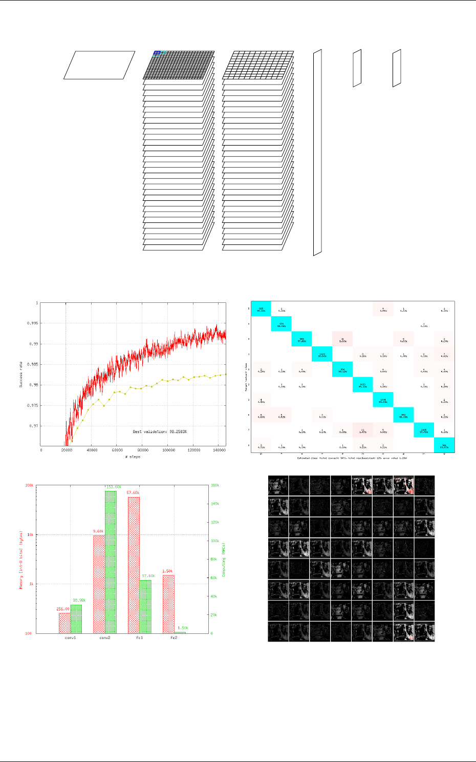
env
24x24
conv1
32 (22x22)
pool1
32 (11x11) Max
fc1
60
fc2
10
softmax
10
Figure 1: Automatically generated and ready to learn DNN from the INI configuration file example.
Recognition rate and validation score Confusion matrix
Memory and computation requirements Output maps activity
Figure 2: Example of information automatically generated by the software during and after learning.
•C code accelerated with OpenMP;
•C code tailored for High-Level Synthesis (HLS) with Xilinx®Vivado®HLS;
Direct synthesis to FPGA, with timing and utilization after routing;
9/78
Possibility to constrain the maximum number of clock cycles desired to compute the
whole network;
FPGA utilization vs number of clock cycle trade-off analysis;
•OpenCL code optimized for either CPU/DSP or GPU;
•Cuda kernels, cuDNN and TensorRT code optimized for NVIDIA®GPUs.
Different automated optimizations are embedded in the exports:
•
DNN weights and signal data precision reduction (down to 8 bit integers or less for custom
FPGA IPs);
•Non-linear network activation functions approximations;
•Different weights discretization methods.
The exports are generated automatically and come with a Makefile and a working testbench,
including the pre-processed testing dataset. Once generated, the testbench is ready to be compiled
and executed on the target platform. The applicative performance (recognition rate) as well as the
computing time per input data can then be directly mesured by the testbench.
OpenMP
OpenCL
CUDA
HLS FPGA
1
10
100
1000
10000
100000
Kpixels image / s
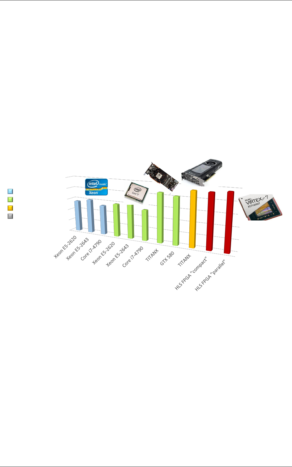
Figure 3: Example of network benchmarking on different hardware targets.
The figure 3 shows an example of benchmarking results of the previous DNN on different targets
(in log scale). Compared to desktop CPUs, the number of input image pixels processed per second
is more than one order of magnitude higher with GPUsand at least two orders of magnitude better
with synthesized DNN on FPGA.
1.6 Summary
The N2D2 platform is today a complete and production ready neural network building tool, which
does not require advanced knownledges in deep learning to be used. It is tailored for fast neural
network applications generation and porting with minimum overhead in terms of database creation
and management, data pre-processing, networks configuration and optimized code generation,
which can save months of manual porting and verification effort to a single automated step in the
tool.
10/78

2 About N2D2-IP
While N2D2 is our deep learning open-source core framework, some modules referred as "N2D2-IP"
in the manual, are only available through custom license agreement with CEA LIST.
If you are interested in obtaining some of these modules, please contact our business developer
for more information on available licensing options:
Sandrine VARENNE (Sandrine.VARENNE@cea.fr)
In addition to N2D2-IP modules, we can also provide our expertise to design specific solutions
for integrating DNN in embedded hardware systems, where power, latency, form factor and/or
cost are constrained. We can target CPU/DSP/GPU CoTS hardware as well as our own PNeuro
(programmable) and DNeuro (dataflow) dedicated hardware accelerator IPs for DNN on FPGA or
ASIC.
3 Performing simulations
3.1 Obtaining the latest version of this manual
Before going further, please make sure you are reading the latest version of this manual. It is located
in the manual sub-directory. To compile the manual in PDF, just run the following command:
cd manual && make
In order to compile the manual, you must have
pdflatex
and
bibtex
installed, as well as some
common LaTeX packages.
•
On Ubuntu, this can be done by installing the
texlive
and
texlive-latex-extra
software
packages.
•
On Windows, you can install the
MiKTeX
software, which includes everything needed and will
install the required LaTeX packages on the fly.
3.2 Minimum system requirements
•Supported processors:
ARM Cortex A15 (tested on Tegra K1)
ARM Cortex A53/A57 (tested on Tegra X1)
Pentium-compatible PC (Pentium III, Athlon or more-recent system recommended)
•Supported operating systems:
Windows
≥
7 or Windows Server
≥
2012, 64 bits with Visual Studio
≥
2015.2 (2015
Update 2)
GNU/Linux with GCC ≥4.4 (tested on RHEL ≥6, Debian ≥6, Ubuntu ≥14.04)
•At least 256 MB of RAM (1 GB with GPU/CUDA) for MNIST dataset processing
•At least 150 MB available hard disk space + 350 MB for MNIST dataset processing
For CUDA acceleration:
•CUDA ≥6.5 and CuDNN ≥1.0
•
NVIDIA GPU with CUDA compute capability
≥
3 (starting from Kepler micro-architecture)
•At least 512 MB GPU RAM for MNIST dataset processing
11/78

3.3 Obtaining N2D2
3.3.1 Prerequisites
Red Hat Enterprise Linux (RHEL) 6 Make sure you have the following packages installed:
•cmake
•gnuplot
•opencv
•opencv-devel (may require the rhel-x86_64-workstation-optional-6 repository channel)
Plus, to be able to use GPU acceleration:
•Install the CUDA repository package:
rpm -Uhv http://developer.download.nvidia.com/compute/cuda/repos/rhel6/x86_64/cuda-repo-
rhel6-7.5-18.x86_64.rpm
yum clean expire-cache
yum install cuda
•
Install cuDNN from the NVIDIA website: register to NVIDIA Developer and download the lat-
est version of cuDNN. Simply copy the header and library files from the cuDNN archive to the
corresponding directories in the CUDA installation path (by default:
/usr/local/cuda/include
and /usr/local/cuda/lib64, respectively).
•
Make sure the CUDA library path (e.g.
/usr/local/cuda/lib64
) is added to the
LD_LIBRARY_PATH
environment variable.
Ubuntu
Make sure you have the following packages installed, if they are available on your Ubuntu
version:
•cmake
•gnuplot
•libopencv-dev
•libcv-dev
•libhighgui-dev
Plus, to be able to use GPU acceleration:
•
Install the CUDA repository package matching your distribution. For example, for Ubuntu
14.04 64 bits:
wget http://developer.download.nvidia.com/compute/cuda/repos/ubuntu1404/x86_64/cuda-repo-
ubuntu1404_7.5-18_amd64.deb
dpkg -i cuda-repo-ubuntu1404_7.5-18_amd64.deb
•
Install the cuDNN repository package matching your distribution. For example, for Ubuntu
14.04 64 bits:
wget http://developer.download.nvidia.com/compute/machine-learning/repos/ubuntu1404/x86_64/
nvidia-machine-learning-repo-ubuntu1404_4.0-2_amd64.deb
dpkg -i nvidia-machine-learning-repo-ubuntu1404_4.0-2_amd64.deb
Note that the cuDNN repository package is provided by NVIDIA for Ubuntu starting from
version 14.04.
•Update the package lists: apt-get update
•Install the CUDA and cuDNN required packages:
apt-get install cuda-core-7-5 cuda-cudart-dev-7-5 cuda-cublas-dev-7-5 cuda-curand-dev-7-5
libcudnn5-dev
•Make sure there is a symlink to /usr/local/cuda:
ln -s /usr/local/cuda-7.5 /usr/local/cuda
•
Make sure the CUDA library path (e.g.
/usr/local/cuda/lib64
) is added to the
LD_LIBRARY_PATH
environment variable.
12/78

Windows On Windows 64 bits, Visual Studio ≥2015.2 (2015 Update 2) is required.
Make sure you have the following software installed:
•CMake (http://www.cmake.org/): download and run the Windows installer.
•dirent.h
C++ header (
https://github.com/tronkko/dirent
): to be put in the Visual
Studio include path.
•
Gnuplot (
http://www.gnuplot.info/
): the bin sub-directory in the install path needs to be
added to the Windows PATH environment variable.
•
OpenCV (
http://opencv.org/
): download the latest 2.x version for Windows and extract it
to, for example,
C:\OpenCV\
. Make sure to define the environment variable
OpenCV_DIR
to point
to
C:\OpenCV\opencv\build
. Make sure to add the bin sub-directory (
C:\OpenCV\opencv\build\x64
\vc12\bin) to the Windows PATH environment variable.
Plus, to be able to use GPU acceleration:
•
Download and install CUDA toolkit 8.0 located at
https://developer.nvidia.com/compute/
cuda/8.0/prod/local_installers/cuda_8.0.44_windows-exe:
rename cuda_8.0.44_windows-exe cuda_8.0.44_windows.exe
cuda_8.0.44_windows.exe -s compiler_8.0 cublas_8.0 cublas_dev_8.0 cudart_8.0 curand_8.0
curand_dev_8.0
•Update the PATH environment variable:
set PATH=%ProgramFiles%\NVIDIA GPU Computing Toolkit\CUDA\v8.0\bin;%ProgramFiles%\NVIDIA GPU
Computing Toolkit\CUDA\v8.0\libnvvp;%PATH%
•
Download and install cuDNN 8.0 located at
http://developer.download.nvidia.com/
compute/redist/cudnn/v5.1/cudnn-8.0-windows7-x64-v5.1.zip
(the following command
assumes that you have 7-Zip installed):
7z x cudnn-8.0-windows7-x64-v5.1.zip
copy cuda\include\*.* ^
"%ProgramFiles%\NVIDIA GPU Computing Toolkit\CUDA\v8.0\include\"
copy cuda\lib\x64\*.* ^
"%ProgramFiles%\NVIDIA GPU Computing Toolkit\CUDA\v8.0\lib\x64\"
copy cuda\bin\*.* ^
"%ProgramFiles%\NVIDIA GPU Computing Toolkit\CUDA\v8.0\bin\"
3.3.2 Getting the sources
Use the following command:
git clone git@github.com:CEA-LIST/N2D2.git
3.3.3 Compilation
To compile the program:
mkdir build
cd build
cmake .. && make
On Windows, you may have to specify the generator, for example:
cmake .. -G"Visual Studio 14"
Then open the newly created N2D2 project in Visual Studio 2015. Select "Release" for the build
target. Right click on ALL_BUILD item and select "Build".
13/78

3.4 Downloading training datasets
A python script located in the repository root directory allows you to select and automatically
download some well-known datasets, like MNIST and GTSRB (the script requires Python 2.x with
bindings for GTK 2 package):
./tools/install_stimuli_gui.py
By default, the datasets are downloaded in the path specified in the
N2D2_DATA
environment
variable, which is the root path used by the N2D2 tool to locate the databases. If the
N2D2_DATA
variable is not set, the default value used is
/local/$USER/n2d2_data/
(or
/local/n2d2_data/
if
the USER environment variable is not set) on Linux and C:\n2d2_data\ on Windows.
Please make sure you have write access to the
N2D2_DATA
path, or if not set, in the default
/local/$USER/n2d2_data/ path.
3.5 Run the learning
The following command will run the learning for 600,000 image presentations/steps and log the
performances of the network every 10,000 steps:
./n2d2 "mnist24_16c4s2_24c5s2_150_10.ini" -learn 600000 -log 10000
Note: you may want to check the gradient computation using the
-check
option. Note that it
can be extremely long and can occasionally fail if the required precision is too high.
3.6 Test a learned network
After the learning is completed, this command evaluate the network performances on the test data
set:
./n2d2 "mnist24_16c4s2_24c5s2_150_10.ini" -test
3.6.1 Interpreting the results
Recognition rate
The recognition rate and the validation score are reported during the learning
in the TargetScore_*/Success_validation.png file, as shown in figure 4.
Confusion matrix
The software automatically outputs the confusion matrix during learning,
validation and test, with an example shown in figure 5. Each row of the matrix contains the number
of occurrences estimated by the network for each label, for all the data corresponding to a single
actual, target label. Or equivalently, each column of the matrix contains the number of actual,
target label occurrences, corresponding to the same estimated label. Idealy, the matrix should be
diagonal, with no occurrence of an estimated label for a different actual label (network mistake).
The confusion matrix reports can be found in the simulation directory:
•TargetScore_*/ConfusionMatrix_learning.png;
•TargetScore_*/ConfusionMatrix_validation.png;
•TargetScore_*/ConfusionMatrix_test.png.
Memory and computation requirements
The software also report the memory and compu-
tation requirements of the network, as shown in figure 6. The corresponding report can be found in
the stats sub-directory of the simulation.
Kernels and weights distribution
The synaptic weights obtained during and after the learning
can be analyzed, in terms of distribution (weights sub-directory of the simulation) or in terms of
kernels (kernels sub-directory of the simulation), as shown in 7.
14/78
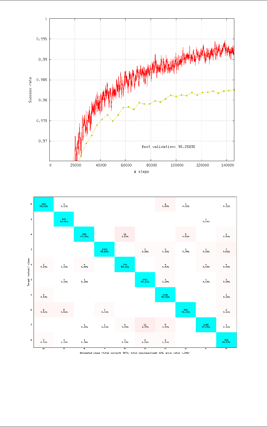
Figure 4: Recognition rate and validation score during learning.
Figure 5: Example of confusion matrix obtained after the learning.
Output maps activity
The initial output maps activity for each layer can be visualized in the
outputs_init sub-directory of the simulation, as shown in figure 8.
3.7 Export a learned network
15/78
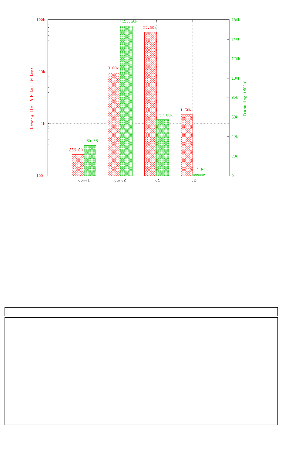
Figure 6: Example of memory and computation requirements of the network.
./n2d2 "mnist24_16c4s2_24c5s2_150_10.ini" -export CPP_OpenCL
Export types:
•CC export using OpenMP;
•C_HLS C export tailored for HLS with Vivado HLS;
•CPP_OpenCL C++ export using OpenCL;
•CPP_Cuda C++ export using Cuda;
•CPP_cuDNN C++ export using cuDNN;
•CPP_TensorRT C++ export using tensorRT 2.1 API;
•SC_Spike SystemC spike export.
Other program options related to the exports:
Option [default value] Description
-nbbits [8]
Number of bits for the weights and signals. Must be 8, 16, 32
or 64 for integer export, or -32, -64 for floating point export.
The number of bits can be arbitrary for the
C_HLS
export (for
example, 6 bits)
-calib [0]
Number of stimuli used for the calibration. 0 = no calibration
(default), -1 = use the full test dataset for calibration
-calib-passes [2]
Number of KL passes for determining the layer output values
distribution truncation threshold (0 = use the max. value,
no truncation)
-no-unsigned
If present, disable the use of unsigned data type in integer
exports
-db-export [-1]
Max. number of stimuli to export (0 = no dataset export, -1
= unlimited)
16/78
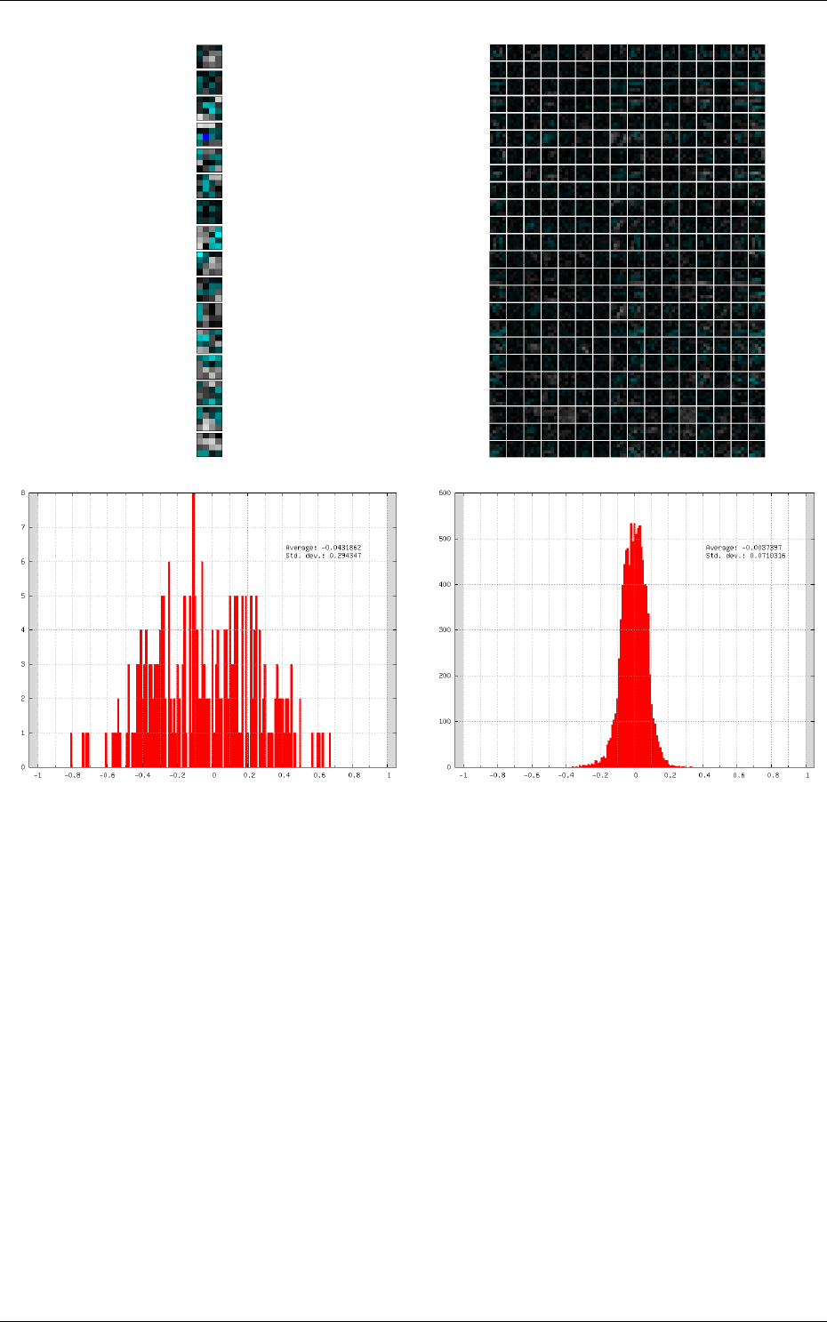
conv1 kernels conv2 kernels
conv1 weights distribution conv2 weights distribution
Figure 7: Example of kernels and weights distribution analysis for two convolutional layers.
3.7.1 CexportN2D2 IP only
Test the exported network:
cd export_C_int8
make
./bin/n2d2_test
The result should look like:
...
16 52 .0 0/ 17 62 ( avg = 93.757094%)
16 53 .0 0/ 17 63 ( avg = 93.760635%)
16 54 .0 0/ 17 64 ( avg = 93.764172%)
Te st ed 1764 s t i m u l i
S u c c e s s r a t e = 9 3.764 172%
P ro ce ss t ime pe r s t i m u l u s = 18 7. 548 186 u s ( 12 t h r e a d s )
Co nf us io n m a tri x :
−−−−−−−−−−−−−−−−−−−−−−−−−−−−−−−−−−−−−−−−−−−−−−−−−
| T \ E | 0 | 1 | 2 | 3 |
−−−−−−−−−−−−−−−−−−−−−−−−−−−−−−−−−−−−−−−−−−−−−−−−−
17/78
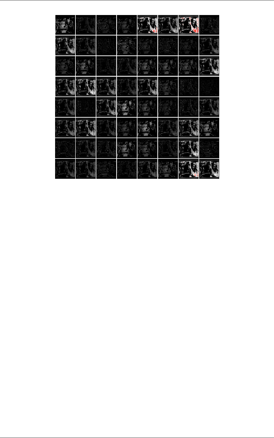
Figure 8: Output maps activity example of the first convolutional layer of the network.
| 0 | 329 | 1 | 5 | 2 |
| | 97.63% | 0.30% | 1.48% | 0.59% |
| 1 | 0 | 692 | 2 | 6 |
| | 0.00% | 98.86% | 0.29% | 0.86% |
| 2 | 11 | 27 | 609 | 55 |
| | 1.57% | 3.85% | 86.75% | 7.83% |
| 3 | 0 | 0 | 1 | 24 |
| | 0.00% | 0.00% | 4.00% | 96.00% |
−−−−−−−−−−−−−−−−−−−−−−−−−−−−−−−−−−−−−−−−−−−−−−−−−
T: T ar ge t E: Es t im a te d
3.7.2 CPP_OpenCL exportN2D2 IP only
The OpenCL export can run the generated program in GPU or CPU architectures. Compilation
features:
18/78

Preprocessor command [default value] Description
PROFILING [0]
Compile the binary with a synchronization be-
tween each layers and return the mean execution
time of each layer. This preprocessor option can
decrease performances.
GENERATE_KBIN [0]
Generate the binary output of the OpenCL kernel
.cl file use. The binary is store in the /bin folder.
LOAD_KBIN [0]
Indicate to the program to load an OpenCL ker-
nel as a binary from the /bin folder instead of a
.cl file.
CUDA [0]
Use the CUDA OpenCL SDK locate at
/usr/local/cuda
MALI [0]
Use the MALI OpenCL SDK locate at
/usr/MaliOpenCLSDKvXXX
INTEL [0]
Use the INTEL OpenCL SDK locate at
/opt/intel/opencl
AMD [1]
Use the AMD OpenCL SDK locate at
/opt/AM DAP P SDK −XXX
Program options related to the OpenCL export:
Option [default value] Description
-cpu
If present, force to use a CPU architecture to run the program
-gpu
If present, force to use a GPU architecture to run the program
-batch [1] Size of the batch to use
-stimulus [NULL]
Path to a specific input stimulus to test. For example: -
stimulus
/stimulus/env0000.pgm
command will test the file
env0000.pgm of the stimulus folder.
Test the exported network:
cd export_CPP_OpenCL_float32
make
./bin/n2d2_opencl_test -gpu
3.7.3 CPP_TensorRT export
The tensorRT 2.1 API export can run the generated program in NVIDIA GPU architecture. It use
CUDA and tensorRT 2.1 API library. The currently supported layers by the tensorRT 2.1 export
are : Convolutional, Pooling, Concatenation, Fully-Connected, Softmax and all activations type.
Custom layers implementation through the plugin factory and generic 8-bits calibrations inference
features are under development.
Program options related to the tensorRT 2.1 API export:
Option [default value] Description
-batch [1] Size of the batch to use
-dev [0] CUDA Device ID selection
-stimulus [NULL]
Path to a specific input stimulus to test. For example: -
stimulus
/stimulus/env0000.pgm
command will test the file
env0000.pgm of the stimulus folder.
-prof
Activates the layer wise profiling mechanism. This option
can decrease execution time performance.
-iter-build [1]
Sets the number of minimization build iterations done by
the tensorRT builder to find the best layer tactics.
19/78

Test the exported network with layer wise profiling:
cd export_CPP_TensorRT_float32
make
./bin/n2d2_tensorRT_test -prof
The results of the layer wise profiling should look like:
(19%) ∗∗∗∗ ∗∗∗∗∗ ∗∗∗∗∗ ∗∗∗∗∗ ∗∗∗∗∗∗∗∗∗∗∗∗∗∗ ∗∗∗∗∗ ∗∗ CONV1 + CONV1_ACTIVATION:
0. 02 194 67 ms
(05%) ∗∗∗∗∗∗∗∗∗∗∗∗ POOL1: 0.0 06 75 57 3 ms
(13%) ∗∗∗∗∗∗∗∗∗∗∗∗∗∗∗∗∗∗∗∗∗∗∗∗∗∗∗∗ CONV2 + CONV2_ACTIVATION: 0.0 15 90 89 ms
(05%) ∗∗∗∗∗∗∗∗∗∗∗∗ POOL2: 0.0 06 16 04 7 ms
(14%) ∗∗∗∗∗∗∗∗∗∗∗∗∗∗∗∗∗∗∗∗∗∗∗∗∗∗∗∗∗∗ CONV3 + CONV3_ACTIVATION: 0. 0 15 97 13 ms
(19%) ∗∗∗∗ ∗∗∗∗∗ ∗∗∗∗∗ ∗∗∗∗∗ ∗∗∗∗∗∗∗∗∗∗∗∗∗∗ ∗∗∗∗∗ ∗∗ FC1 + FC1_ACTIVATION : 0 .0 22 224 2 ms
(13%) ∗∗∗∗∗∗∗∗∗∗∗∗∗∗∗∗∗∗∗∗∗∗∗∗∗∗∗∗ FC2 : 0 .01 49 013 ms
(08%) ∗∗∗∗∗∗∗ ∗∗∗∗∗∗∗∗∗∗∗ SOFTMAX: 0 .0 10 0 63 3 ms
Average p r o f i l e d tensorRT p r o c es s ti me p er s t i m u l u s = 0.1 1 39 32 ms
3.7.4 CPP_cuDNN export
The cuDNN export can run the generated program in NVIDIA GPU architecture. It use CUDA
and cuDNN library. Compilation features:
Preprocessor command [default value] Description
PROFILING [0]
Compile the binary with a synchronization be-
tween each layers and return the mean execution
time of each layer. This preprocessor option can
decrease performances.
ARCH32 [0]
Compile the binary with the 32-bits architecture
compatibility.
Program options related to the cuDNN export:
Option [default value] Description
-batch [1] Size of the batch to use
-dev [0] CUDA Device ID selection
-stimulus [NULL]
Path to a specific input stimulus to test. For example: -
stimulus
/stimulus/env0000.pgm
command will test the file
env0000.pgm of the stimulus folder.
Test the exported network:
cd export_CPP_cuDNN_float32
make
./bin/n2d2_cudnn_test
3.7.5 C_HLS exportN2D2 IP only
Test the exported network:
cd export_C_HLS_int8
make
./bin/n2d2_test
Run the High-Level Synthesis (HLS) with Xilinx®Vivado®HLS:
vivado_hls -f run_hls.tcl
20/78

4 INI file interface
The INI file interface is the primary way of using N2D2. It is a simple, lightweight and user-friendly
format for specifying a complete DNN-based application, including dataset instanciation, data
pre-processing, neural network layers instanciation and post-processing, with all its hyperparameters.
4.1 Syntax
INI files are simple text files with a basic structure composed of sections, properties and values.
4.1.1 Properties
The basic element contained in an INI file is the property. Every property has a name and a value,
delimited by an equals sign (=). The name appears to the left of the equals sign.
name=value
4.1.2 Sections
Properties may be grouped into arbitrarily named sections. The section name appears on a line
by itself, in square brackets ([ and ]). All properties after the section declaration are associated
with that section. There is no explicit "end of section" delimiter; sections end at the next section
declaration, or the end of the file. Sections may not be nested.
[section]
a=a
b=b
4.1.3 Case sensitivity
Section and property names are case sensitive.
4.1.4 Comments
Semicolons (
;
) or number sign (
#
) at the beginning or in the middle of the line indicate a comment.
Comments are ignored.
; comment text
a=a # comment text
a="a ; not a comment" ; comment text
4.1.5 Quoted values
Values can be quoted, using double quotes. This allows for explicit declaration of whitespace,
and/or for quoting of special characters (equals, semicolon, etc.).
4.1.6 Whitespace
Leading and trailing whitespace on a line are ignored.
4.1.7 Escape characters
A backslash (\) followed immediately by EOL (end-of-line) causes the line break to be ignored.
21/78

4.2 Template inclusion syntax
Is is possible to recursively include templated INI files. For example, the main INI file can include
a templated file like the following:
[inception@inception_model.ini.tpl]
INPUT=layer_x
SIZE=32
ARRAY=2 ; Must be the number of elements in the array
ARRAY[0].P1=Conv
ARRAY[0].P2=32
ARRAY[1].P1=Pool
ARRAY[1].P2=64
If the inception_model.ini.tpl template file content is:
[{{SECTION_NAME}}_layer1]
Input={{INPUT}}
Type=Conv
NbOutputs={{SIZE}}
[{{SECTION_NAME}}_layer2]
Input={{SECTION_NAME}}_layer1
Type=Fc
NbOutputs={{SIZE}}
{% block ARRAY %}
[{{SECTION_NAME}}_array{{#}}]
Prop1=Config{{.P1}}
Prop2={{.P2}}
{% endblock %}
The resulting equivalent content for the main INI file will be:
[inception_layer1]
Input=layer_x
Type=Conv
NbOutputs=32
[inception_layer2]
Input=inception_layer1
Type=Fc
NbOutputs=32
[inception_array0]
Prop1=ConfigConv
Prop2=32
[inception_array1]
Prop1=ConfigPool
Prop2=64
The
SECTION_NAME
template parameter is automatically generated from the name of the including
section (before @).
4.2.1 Variable substitution
{{VAR}} is replaced by the value of the VAR template parameter.
4.2.2 Control statements
Control statements are between {% and %} delimiters.
22/78

block {%block ARRAY %} ... {%endblock %}
The
#
template parameter is automatically generated from the
{%block ... %}
template control
statement and corresponds to the current item position, starting from 0.
for {%for VAR in range([START, ]END])%} ... {%endfor %}
If START is not specified, the loop begins at 0 (first value of VAR). The last value of VAR is END-1.
if {%if VAR OP [VALUE] %} ... [{%else %}] ... {%endif %}
OP may be ==,!=,exists or not_exists.
include {%include FILENAME %}
4.3 Global parameters
Option [default value] Description
DefaultModel [Transcode]
Default layers model. Can be
Frame
,
Frame_CUDA
,
Transcode
or
Spike
DefaultDataType [Float32]
Default layers data type. Can be
Float16
,
Float32
or
Float64
SignalsDiscretization [0] Number of levels for signal discretization
FreeParametersDiscretization
[0]
Number of levels for weights discretization
4.4 Databases
The tool integrates pre-defined modules for several well-known database used in the deep learning
community, such as MNIST, GTSRB, CIFAR10 and so on. That way, no extra step is necessary to
be able to directly build a network and learn it on these database.
4.4.1 MNIST
MNIST (LeCun et al.,1998) is already fractionned into a learning set and a testing set, with:
•60,000 digits in the learning set;
•10,000 digits in the testing set.
Example:
[database]
Type=MNIST_IDX_Database
Validation=0.2 ; Fraction of learning stimuli used for the validation [default: 0.0]
Option [default value] Description
Validation [0.0] Fraction of the learning set used for validation
DataPath Path to the database
[$N2D2_DATA/mnist]
4.4.2 GTSRB
GTSRB (Stallkamp et al.,2012) is already fractionned into a learning set and a testing set, with:
•39,209 digits in the learning set;
•12,630 digits in the testing set.
Example:
23/78

[database]
Type=GTSRB_DIR_Database
Validation=0.2 ; Fraction of learning stimuli used for the validation [default: 0.0]
Option [default value] Description
Validation [0.0] Fraction of the learning set used for validation
DataPath Path to the database
[$N2D2_DATA/GTSRB]
4.4.3 Directory
Hand made database stored in files directories are directly supported with the
DIR_Database
module.
For example, suppose your database is organized as following (in the path specified in the
N2D2_DATA
environment variable):
•GST/airplanes: 800 images
•GST/car_side: 123 images
•GST/Faces: 435 images
•GST/Motorbikes: 798 images
You can then instanciate this database as input of your neural network using the following
parameters:
[database]
Type=DIR_Database
DataPath=${N2D2_DATA}/GST
Learn=0.4 ; 40% of images of the smallest category = 49 (0.4x123) images for each category will be
used for learning
Validation=0.2 ; 20% of images of the smallest category = 25 (0.2x123) images for each category
will be used for validation
; the remaining images will be used for testing
Each subdirectory will be treated as a different label, so there will be 4 different labels, named
after the directory name.
The stimuli are equi-partitioned for the learning set and the validation set, meaning that the
same number of stimuli for each category is used. If the learn fraction is 0.4 and the validation
fraction is 0.2, as in the example above, the partitioning will be the following:
Label ID Label name Learn set Validation set Test set
0airplanes 49 25 726
1car_side 49 25 49
2Faces 49 25 361
3Motorbikes 49 25 724
Total: 196 100 1860
Mandatory option
Option [default value] Description
DataPath Path to the root stimuli directory
Learn
If
PerLabelPartitioning
is true, fraction of images used for
the learning; else, number of images used for the learning,
regardless of their labels
LoadInMemory [0] Load the whole database into memory
Depth [1] Number of sub-directory levels to include. Examples:
24/78

Depth
= 0: load stimuli only from the current directory
(DataPath)
Depth
= 1: load stimuli from
DataPath
and stimuli contained
in the sub-directories of DataPath
Depth
< 0: load stimuli recursively from
DataPath
and all its
sub-directories
LabelName [] Base stimuli label name
LabelDepth [1]
Number of sub-directory name levels used to form the stimuli
labels. Examples:
LabelDepth = -1: no label for all stimuli (label ID = -1)
LabelDepth = 0: uses LabelName for all stimuli
LabelDepth
= 1: uses
LabelName
for stimuli in the current
directory (
DataPath
) and
LabelName
/sub-directory name for
stimuli in the sub-directories
PerLabelPartitioning [1]
If true, the stimuli are equi-partitioned for the learn/valida-
tion/test sets, meaning that the same number of stimuli for
each label is used
Validation [0.0]
If
PerLabelPartitioning
is true, fraction of images used for the
validation; else, number of images used for the validation,
regardless of their labels
Test [1.0-Learn-Validation]
If
PerLabelPartitioning
is true, fraction of images used for the
test; else, number of images used for the test, regardless of
their labels
ValidExtensions []
List of space-separated valid stimulus file extensions (if left
empty, any file extension is considered a valid stimulus)
LoadMore []
Name of an other section with the same options to load a
different DataPath
ROIFile []
File containing the stimuli ROIs. If a ROI file is specified,
LabelDepth should be set to -1
DefaultLabel []
Label name for pixels outside any ROI (default is no label,
pixels are ignored)
ROIsMargin [0]
Number of pixels around ROIs that are ignored (and not
considered as DefaultLabel pixels)
To load and partition more than one DataPath, one can use the LoadMore option:
[database]
Type=DIR_Database
DataPath=${N2D2_DATA}/GST
Learn=0.6
Validation=0.4
LoadMore=database.test
; Load stimuli from the "GST_Test" path in the test dataset
[database.test]
DataPath=${N2D2_DATA}/GST_Test
Learn=0.0
Test=1.0
; The LoadMore option is recursive:
; LoadMore=database.more
; [database.more]
; Load even more data here
25/78

4.4.4 Other built-in databases
CIFAR10_Database CIFAR10 database (Krizhevsky,2009).
Option [default value] Description
Validation [0.0] Fraction of the learning set used for validation
DataPath Path to the database
[
$N2D2_DATA
/cifar-10-batches-
bin]
CIFAR100_Database CIFAR100 database (Krizhevsky,2009).
Option [default value] Description
Validation [0.0] Fraction of the learning set used for validation
UseCoarse [0] If true, use the coarse labeling (10 labels instead of 100)
DataPath Path to the database
[$N2D2_DATA/cifar-100-binary]
CKP_Database
The Extended Cohn-Kanade (CK+) database for expression recognition (Lucey
et al.,2010).
Option [default value] Description
Learn Fraction of images used for the learning
Validation [0.0] Fraction of images used for the validation
DataPath Path to the database
[
$N2D2_DATA
/cohn-kanade-
images]
Caltech101_DIR_Database Caltech 101 database (Fei-Fei et al.,2004).
Option [default value] Description
Learn Fraction of images used for the learning
Validation [0.0] Fraction of images used for the validation
IncClutter [0]
If true, includes the BACKGROUND_Google directory of
the database
DataPath Path to the database
[$N2D2_DATA/
101_ObjectCategories]
Caltech256_DIR_Database Caltech 256 database (Griffin et al.,2007).
Option [default value] Description
Learn Fraction of images used for the learning
Validation [0.0] Fraction of images used for the validation
IncClutter [0]
If true, includes the BACKGROUND_Google directory of
the database
DataPath Path to the database
[$N2D2_DATA/
256_ObjectCategories]
26/78

CaltechPedestrian_Database Caltech Pedestrian database (Dollár et al.,2009).
Note that the images and annotations must first be extracted from the seq video data located in
the videos directory using the
dbExtract.m
Matlab tool provided in the "Matlab evaluation/labeling
code" downloadable on the dataset website.
Assuming the following directory structure (in the path specified in the
N2D2_DATA
environment
variable):
•CaltechPedestrians/data-USA/videos/... (from the setxx.tar files)
•CaltechPedestrians/data-USA/annotations/... (from the setxx.tar files)
•CaltechPedestrians/tools/piotr_toolbox/toolbox (from the Piotr’s Matlab Toolbox archive)
•CaltechPedestrians/*.m including dbExtract.m (from the Matlab evaluation/labeling code)
Use the following command in Matlab to generate the images and annotations:
cd([getenv(’N2D2_DATA’)’/CaltechPedestrians’])
addpath(genpath(’tools/piotr_toolbox/toolbox’)) % add the Piotr’s Matlab Toolbox in the Matlab
path
dbInfo(’USA’)
dbExtract()
Option [default value] Description
Validation [0.0] Fraction of the learning set used for validation
SingleLabel [1] Use the same label for "person" and "people" bounding box
IncAmbiguous [0]
Include ambiguous bounding box labeled "person?" using the
same label as "person"
DataPath Path to the database images
[$N2D2_DATA/
CaltechPedestrians/data-
USA/images]
LabelPath Path to the database annotations
[$N2D2_DATA/
CaltechPedestrians/data-
USA/annotations]
Cityscapes_Database Cityscapes database (Cordts et al.,2016).
Option [default value] Description
IncTrainExtra [0]
If true, includes the left 8-bit images - trainextra set (19,998
images)
UseCoarse [0]
If true, only use coarse annotations (which are the only
annotations available for the trainextra set)
SingleInstanceLabels [1]
If true, convert group labels to single instance labels (for
example, cargroup becomes car)
DataPath Path to the database images
[$N2D2_DATA/
Cityscapes/leftImg8bit] or
[
$CITYSCAPES_DATASET
] if defined
LabelPath []
Path to the database annotations (deduced from
DataPath
if
left empty)
Daimler_Database Daimler Monocular Pedestrian Detection Benchmark (Daimler Pedestrian).
27/78

Option [default value] Description
Learn [1.0] Fraction of images used for the learning
Validation [0.0] Fraction of images used for the validation
Test [0.0] Fraction of images used for the test
Fully [0]
When activate it use the test dataset to learn. Use only on
fully-cnn mode
DOTA_Database DOTA database (Xia et al.,2017).
Option [default value] Description
Learn Fraction of images used for the learning
DataPath Path to the database
[$N2D2_DATA/DOTA]
LabelPath Path to the database labels list file
[]
FDDB_Database
Face Detection Data Set and Benchmark (FDDB) (Jain and Learned-Miller,
2010).
Option [default value] Description
Learn Fraction of images used for the learning
Validation [0.0] Fraction of images used for the validation
DataPath Path to the images (decompressed originalPics.tar.gz)
[$N2D2_DATA/FDDB]
LabelPath Path to the annotations (decompressed FDDB-folds.tgz)
[$N2D2_DATA/FDDB]
GTSDB_DIR_Database GTSDB database (Houben et al.,2013).
Option [default value] Description
Learn Fraction of images used for the learning
Validation [0.0] Fraction of images used for the validation
DataPath Path to the database
[$N2D2_DATA/FullIJCNN2013]
ILSVRC2012_Database ILSVRC2012 database (Russakovsky et al.,2015).
Option [default value] Description
Learn Fraction of images used for the learning
DataPath Path to the database
[$N2D2_DATA/ILSVRC2012]
LabelPath Path to the database labels list file
[
$N2D2_DATA
/ILSVRC2012/synsets.txt]
KITTI_Database
The KITTI Database provide ROI which can be use for autonomous driving and
environment perception. The database provide 8 labeled different classes. Utilization of the KITTI
Database is under licensing conditions and request an email registration. To install it you have to
follow this link:
http://www.cvlibs.net/datasets/kitti/eval_tracking.php
and download
the left color images (15 GB) and the trainling labels of tracking data set (9 MB). Extract the
downloaded archives in your $N2D2_DATA/KITTI folder.
28/78

Option [default value] Description
Learn [0.8] Fraction of images used for the learning
Validation [0.2] Fraction of images used for the validation
KITTI_Road_Database
The KITTI Road Database provide ROI which can be used to road
segmentation. The dataset provide 1 labeled class (road) on 289 training images. The 290 test
images are not labeled. Utilization of the KITTI Road Database is under licensing conditions and
request an email registration. To install it you have to follow this link:
http://www.cvlibs.net/
datasets/kitti/eval_road.php
and download the "base kit" of (0.5 GB) with left color images,
calibration and training labels. Extract the downloaded archive in your
$N2D2_DATA/KITTI
folder.
Option [default value] Description
Learn [0.8] Fraction of images used for the learning
Validation [0.2] Fraction of images used for the validation
KITTI_Object_Database
The KITTI Object Database provide ROI which can be use for au-
tonomous driving and environment perception. The database provide 8 labeled different classes
on 7481 training images. The 7518 test images are not labeled. The whole database pro-
vide 80256 labeled objects. Utilization of the KITTI Object Database is under licensing con-
ditions and request an email registration. To install it you have to follow this link:
http:
//www.cvlibs.net/datasets/kitti/eval_object.php?obj_benchmark
and download the "lef
color images" (12 GB) and the training labels of object data set (5 MB). Extract the downloaded
archives in your $N2D2_DATA/KITTI_Object folder.
Option [default value] Description
Learn [0.8] Fraction of images used for the learning
Validation [0.2] Fraction of images used for the validation
LITISRouen_Database LITIS Rouen audio scene dataset (Rakotomamonjy and Gasso,2014).
Option [default value] Description
Learn [0.4] Fraction of images used for the learning
Validation [0.4] Fraction of images used for the validation
DataPath Path to the database
[$N2D2_DATA/data_rouen]
4.4.5 Dataset images slicing
It is possible to automatically slice images from a dataset, with a given slice size and stride, using
the .slicing attribute. This effectively increases the number of stimuli in the set.
[database.slicing]
ApplyTo=NoLearn
Width=2048
Height=1024
StrideX=2048
StrideY=1024
4.5 Stimuli data analysis
You can enable stimuli data reporting with the following section (the name of the section must
start with env.StimuliData):
29/78

[env.StimuliData-raw]
ApplyTo=LearnOnly
LogSizeRange=1
LogValueRange=1
The stimuli data reported for the full MNIST learning set will look like:
env . StimuliData−raw dat a :
Number of s t i m u l i : 60000
Data w i d t h r a n ge : [ 2 8 , 2 8 ]
Data h e i g h t ra ng e : [ 2 8 , 28 ]
Data c h a n n e l s r ang e : [ 1 , 1 ]
Val ue r a ng e : [ 0 , 2 5 5 ]
Value mean : 33. 3 18 4
Value s t d . de v . : 7 8.5 67 5
4.5.1 Zero-mean and unity standard deviation normalization
It it possible to normalize the whole database to have zero mean and unity standard deviation on
the learning set using a RangeAffineTransformation transformation:
; Stimuli normalization based on learning set global mean and std.dev.
[env.Transformation-normalize]
Type=RangeAffineTransformation
FirstOperator=Minus
FirstValue=[env.StimuliData-raw]_GlobalValue.mean
SecondOperator=Divides
SecondValue=[env.StimuliData-raw]_GlobalValue.stdDev
The variables
_GlobalValue.mean
and
_GlobalValue.stdDev
are automatically generated in the
[env.
StimuliData-raw]
block. Thanks to this facility, unknown and arbitrary database can be analysed
and normalized in one single step without requiring any external data manipulation.
After normalization, the stimuli data reported is:
env . StimuliData−n o r m a l i z e d d a t a :
Number of s t i m u l i : 60000
Data w i d t h r a n ge : [ 2 8 , 2 8 ]
Data h e i g h t ra ng e : [ 2 8 , 28 ]
Data c h a n n e l s r ang e : [ 1 , 1 ]
Value ra ng e : [ −0.4 2407 4 , 2 . 8 2 1 5 4 ]
Value mean : 2. 64 7 96 e −07
Value s t d . dev . : 1
Where we can check that the global mean is close to 0 and the standard deviation is 1 on the
whole dataset. The result of the transformation on the first images of the set can be checked in the
generated frames folder, as shown in figure 9.
4.5.2 Substracting the mean image of the set
Using the
StimuliData
object followed with an
AffineTransformation
, it is also possible to use the
mean image of the dataset to normalize the data:
[env.StimuliData-meanData]
ApplyTo=LearnOnly
MeanData=1 ; Provides the _MeanData parameter used in the transformation
[env.Transformation]
Type=AffineTransformation
FirstOperator=Minus
FirstValue=[env.StimuliData-meanData]_MeanData
The resulting global mean image can be visualized in env.StimuliData-meanData/meanData.bin.png
an is shown in figure 10.
After this transformation, the reported stimuli data becomes:
30/78
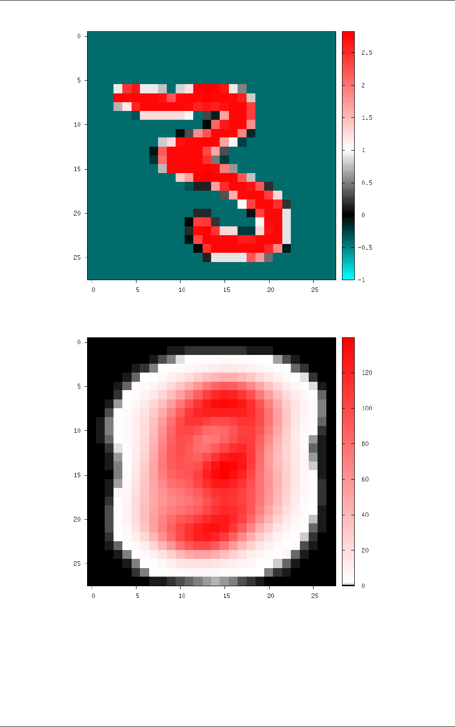
Figure 9: Image of the set after normalization.
Figure 10: Global mean image generated by StimuliData with the MeanData parameter enabled.
env . StimuliData−p r o c e s s e d d a ta :
Number of s t i m u l i : 60000
Data w i d t h r a n ge : [ 2 8 , 2 8 ]
Data h e i g h t ra ng e : [ 2 8 , 28 ]
Data c h a n n e l s r ang e : [ 1 , 1 ]
Value ra ng e : [ −139 .554 , 2 5 4 . 9 7 9 ]
31/78
Value mean : −3.45583 e −08
Value s t d . de v . : 66 .1 28 8
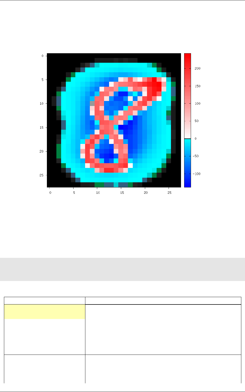
The result of the transformation on the first images of the set can be checked in the generated
frames folder, as shown in figure 11.
Figure 11: Image of the set after the
AffineTransformation
substracting the global mean image (keep in
mind that the original image value range is [0, 255]).
4.6 Environment
The environment simply specify the input data format of the network (width, height and batch
size). Example:
[env]
SizeX=24
SizeY=24
BatchSize=12 ; [default: 1]
Option [default value] Description
SizeX Environment width
SizeY Environment height
NbChannels [1]
Number of channels (applicable only if there is no
env.
ChannelTransformation[...])
BatchSize [1] Batch size
CompositeStimuli [0] If true, use pixel-wise stimuli labels
CachePath [] Stimuli cache path (no cache if left empty)
StimulusType [SingleBurst]
Method for converting stimuli into spike trains. Can be any
of SingleBurst,Periodic,JitteredPeriodic or Poissonian
DiscardedLateStimuli [1.0]
The pixels in the pre-processed stimuli with a value above
this limit never generate spiking events
32/78

PeriodMeanMin [50 TimeMs]
Mean minimum period
Tmin
, used for periodic temporal cod-
ings, corresponding to pixels in the pre-processed stimuli with
a value of 0 (which are supposed to be the most significant
pixels)
PeriodMeanMax [12 TimeS]
Mean maximum period
Tmax
, used for periodic temporal
codings, corresponding to pixels in the pre-processed stimuli
with a value of 1 (which are supposed to be the least signifi-
cant pixels). This maximum period may be never reached if
DiscardedLateStimuli is lower than 1.0
PeriodRelStdDev [0.1]
Relative standard deviation, used for periodic temporal cod-
ings, applied to the spiking period of a pixel
PeriodMin [11 TimeMs]
Absolute minimum period, or spiking interval, used for peri-
odic temporal codings, for any pixel
4.6.1 Built-in transformations
There are 6 possible categories of transformations:
•env.Transformation[...]
Transformations applied to the input images before channels creation;
•env.OnTheFlyTransformation[...]
On-the-fly transformations applied to the input images before
channels creation;
•env.ChannelTransformation[...] Create or add transformation for a specific channel;
•env.ChannelOnTheFlyTransformation[...]
Create or add on-the-fly transformation for a specific
channel;
•env.ChannelsTransformation[...]
Transformations applied to all the channels of the input
images;
•env.ChannelsOnTheFlyTransformation[...]
On-the-fly transformations applied to all the channels
of the input images.
Example:
[env.Transformation]
Type=PadCropTransformation
Width=24
Height=24
Several transformations can applied successively. In this case, to be able to apply multiple
transformations of the same category, a different suffix (
[...]
) must be added to each transformation.
The transformations will be processed in the order of appearance in the INI file
regardless of their suffix.
Common set of parameters for any kind of transformation:
Option [default value] Description
ApplyTo [All]
Apply the transformation only to the specified stimuli sets.
Can be:
LearnOnly: learning set only
ValidationOnly: validation set only
TestOnly: testing set only
NoLearn: validation and testing sets only
NoValidation: learning and testing sets only
NoTest: learning and validation sets only
All: all sets (default)
33/78

Example:
[env.Transformation-1]
Type=ChannelExtractionTransformation
CSChannel=Gray
[env.Transformation-2]
Type=RescaleTransformation
Width=29
Height=29
[env.Transformation-3]
Type=EqualizeTransformation
[env.OnTheFlyTransformation]
Type=DistortionTransformation
ApplyTo=LearnOnly ; Apply this transformation for the Learning set only
ElasticGaussianSize=21
ElasticSigma=6.0
ElasticScaling=20.0
Scaling=15.0
Rotation=15.0
List of available transformations:
AffineTransformation
Apply an element-wise affine transformation to the image with matrixes
of the same size.
Option [default value] Description
FirstOperator
First element-wise operator, can be
Plus
,
Minus
,
Multiplies
,
Divides
FirstValue First matrix file name
SecondOperator [Plus]
Second element-wise operator, can be
Plus
,
Minus
,
Multiplies
,
Divides
SecondValue [] Second matrix file name
The final operation is the following, with
A
the image matrix,
B1st
,
B2nd
the matrixes to
add/substract/multiply/divide and the element-wise operator :
f(A) = A
op1st B1st
op2nd B2nd
ApodizationTransformation Apply an apodization window to each data row.
Option [default value] Description
Size
Window total size (must match the number of data columns)
WindowName [Rectangular] Window name. Possible values are:
Rectangular: Rectangular
Hann: Hann
Hamming: Hamming
Cosine: Cosine
Gaussian: Gaussian
Blackman: Blackman
Kaiser: Kaiser
34/78

Gaussian window Gaussian window.
Option [default value] Description
WindowName
.Sigma
[0.4] Sigma
Blackman window Blackman window.
Option [default value] Description
WindowName
.Alpha
[0.16] Alpha
Kaiser window Kaiser window.
Option [default value] Description
WindowName
.Beta
[5.0]
Beta
ChannelExtractionTransformation Extract an image channel.
Option Description
CSChannel Blue
: blue channel in the BGR colorspace, or first channel of
any colorspace
Green
: green channel in the BGR colorspace, or second chan-
nel of any colorspace
Red
: red channel in the BGR colorspace, or third channel of
any colorspace
Hue: hue channel in the HSV colorspace
Saturation: saturation channel in the HSV colorspace
Value: value channel in the HSV colorspace
Gray: gray conversion
Y: Y channel in the YCbCr colorspace
Cb: Cb channel in the YCbCr colorspace
Cr: Cr channel in the YCbCr colorspace
ColorSpaceTransformation Change the current image colorspace.
Option Description
ColorSpace BGR: if the image is in grayscale, convert it in BGR
HSV
HLS
YCrCb
CIELab
CIELuv
DFTTransformation
Apply a DFT to the data. The input data must be single channel, the
resulting data is two channels, the first for the real part and the second for the imaginary part.
Option [default value] Description
TwoDimensional [1]
If true, compute a 2D image DFT. Otherwise, compute the
1D DFT of each data row
Note that this transformation can add zero-padding if required by the underlying FFT imple-
mentation.
35/78

DistortionTransformationN2D2 IP only
Apply elastic distortion to the image. This transformation is gener-
ally used on-the-fly (so that a different distortion is performed for each image), and for the learning
only.
Option [default value] Description
ElasticGaussianSize [15] Size of the gaussian for elastic distortion (in pixels)
ElasticSigma [6.0] Sigma of the gaussian for elastic distortion
ElasticScaling [0.0] Scaling of the gaussian for elastic distortion
Scaling [0.0] Maximum random scaling amplitude (+/-, in percentage)
Rotation [0.0] Maximum random rotation amplitude (+/-, in °)
EqualizeTransformationN2D2 IP only Image histogram equalization.
Option [default value] Description
Method [Standard]Standard: standard histogram equalization
CLAHE: contrast limited adaptive histogram equalization
CLAHE_ClipLimit [40.0] Threshold for contrast limiting (for CLAHE only)
CLAHE_GridSize [8]
Size of grid for histogram equalization (for
CLAHE
only). Input
image will be divided into equally sized rectangular tiles. This
parameter defines the number of tiles in row and column.
ExpandLabelTransformationN2D2 IP only Expand single image label (1x1 pixel) to full frame label.
FilterTransformation Apply a convolution filter to the image.
Option [default value] Description
Kernel Convolution kernel. Possible values are:
*: custom kernel
Gaussian: Gaussian kernel
LoG: Laplacian Of Gaussian kernel
DoG: Difference Of Gaussian kernel
Gabor: Gabor kernel
*kernel Custom kernel.
Option Description
Kernel.SizeX [0] Width of the kernel (numer of columns)
Kernel.SizeY [0] Height of the kernel (number of rows)
Kernel.Mat
List of row-major ordered coefficients of
the kernel
If both Kernel.SizeX and Kernel.SizeY are 0, the kernel is assumed to be square.
Gaussian kernel Gaussian kernel.
Option [default value] Description
Kernel.SizeX Width of the kernel (numer of columns)
Kernel.SizeY Height of the kernel (number of rows)
Kernel.Positive [1]
If true, the center of the kernel is positive
Kernel.Sigma [√2.0]Sigma of the kernel
36/78

LoG kernel Laplacian Of Gaussian kernel.
Option [default value] Description
Kernel.SizeX Width of the kernel (numer of columns)
Kernel.SizeY Height of the kernel (number of rows)
Kernel.Positive [1]
If true, the center of the kernel is positive
Kernel.Sigma [√2.0]Sigma of the kernel
DoG kernel Difference Of Gaussian kernel kernel.
Option [default value] Description
Kernel.SizeX Width of the kernel (numer of columns)
Kernel.SizeY Height of the kernel (number of rows)
Kernel.Positive [1]
If true, the center of the kernel is positive
Kernel.Sigma1 [2.0] Sigma1 of the kernel
Kernel.Sigma2 [1.0] Sigma2 of the kernel
Gabor kernel Gabor kernel.
Option [default value] Description
Kernel.SizeX Width of the kernel (numer of columns)
Kernel.SizeY Height of the kernel (number of rows)
Kernel.Theta Theta of the kernel
Kernel.Sigma [√2.0]Sigma of the kernel
Kernel.Lambda [10.0] Lambda of the kernel
Kernel.Psi [π/2.0] Psi of the kernel
Kernel.Gamma [0.5] Gamma of the kernel
FlipTransformation Image flip transformation.
Option [default value] Description
HorizontalFlip [0] If true, flip the image horizontally
VerticalFlip [0] If true, flip the image vertically
RandomHorizontalFlip [0] If true, randomly flip the image horizontally
RandomVerticalFlip [0] If true, randomly flip the image vertically
GradientFilterTransformationN2D2 IP only Compute image gradient.
37/78

Option [default value] Description
Scale [1.0] Scale to apply to the computed gradient
Delta [0.0] Bias to add to the computed gradient
GradientFilter [Sobel]
Filter type to use for computing the gradient. Possible
options are: Sobel,Scharr and Laplacian
KernelSize [3]
Size of the filter kernel (has no effect when using the
Scharr
filter, which kernel size is always 3x3)
ApplyToLabels [0]
If true, use the computed gradient to filter the image label and
ignore pixel areas where the gradient is below the
Threshold
.
In this case, only the labels are modified, not the image
InvThreshold [0]
If true, ignored label pixels will be the ones with a low
gradient (low contrasted areas)
Threshold [0.5] Threshold applied on the image gradient
Label [] List of labels to filter (space-separated)
GradientScale [1.0]
Rescale the image by this factor before applying the gradient
and the threshold, then scale it back to filter the labels
LabelSliceExtractionTransformationN2D2 IP only
Extract a slice from an image belonging to a given label.
Option [default value] Description
Width Width of the slice to extract
Height Height of the slice to extract
Label [-1]
Slice should belong to this label ID. If -1, the label ID is
random
MagnitudePhaseTransformation
Compute the magnitude and phase of a complex two channels
input data, with the first channel
x
being the real part and the second channel
y
the imaginary
part. The resulting data is two channels, the first one with the magnitude and the second one with
the phase.
Option [default value] Description
LogScale [0] If true, compute the magnitude in log scale
The magnitude is:
Mi,j =qx2
i,j +x2
i,j
If LogScale = 1, compute M0
i,j =log(1 + Mi,j ).
The phase is:
θi,j =atan2(yi,j, xi,j )
MorphologicalReconstructionTransformationN2D2 IP only
Apply a morphological reconstruction transfor-
mation to the image. This transformation is also useful for post-processing.
38/78

Option [default value] Description
Operation Morphological operation to apply. Can be:
ReconstructionByErosion
: reconstruction by erosion operation
ReconstructionByDilation
: reconstruction by dilation opera-
tion
OpeningByReconstruction
: opening by reconstruction operation
ClosingByReconstruction
: closing by reconstruction operation
Size Size of the structuring element
ApplyToLabels [0]
If true, apply the transformation to the labels instead of the
image
Shape [Rectangular]
Shape of the structuring element used for morphology opera-
tions. Can be Rectangular,Elliptic or Cross.
NbIterations [1]
Number of times erosion and dilation are applied for opening
and closing reconstructions
MorphologyTransformationN2D2 IP only
Apply a morphology transformation to the image. This transforma-
tion is also useful for post-processing.
Option [default value] Description
Operation Morphological operation to apply. Can be:
Erode: erode operation (=erode(src))
Dilate: dilate operation (=dilate(src))
Opening
: opening operation (
open
(
src
) =
dilate
(
erode
(
src
)))
Closing: closing operation (close(src) = erode(dilate(src)))
Gradient
: morphological gradient (=
dilate
(
src
)
−erode
(
src
))
TopHat: top hat (=src −open(src))
BlackHat: black hat (=close(src)−src)
Size Size of the structuring element
ApplyToLabels [0]
If true, apply the transformation to the labels instead of the
image
Shape [Rectangular]
Shape of the structuring element used for morphology opera-
tions. Can be Rectangular,Elliptic or Cross.
NbIterations [1] Number of times erosion and dilation are applied
NormalizeTransformation Normalize the image.
Option [default value] Description
Norm [MinMax] Norm type, can be:
L1: L1 normalization
L2: L2 normalization
Linf: Linf normalization
MinMax: min-max normalization
NormValue [1.0] Norm value (for L1,L2 and Linf)
Such that ||data||Lp=NormV alue
NormMin [0.0] Min value (for MinMax only)
Such that min(data) = N ormMin
NormMax [1.0] Max value (for MinMax only)
Such that max(data) = N ormMax
PerChannel [0] If true, normalize each channel individually
PadCropTransformation Pad/crop the image to a specified size.
39/78

Option [default value] Description
Width Width of the padded/cropped image
Height Height of the padded/cropped image
PaddingBackground [MeanColor] Background color used when padding. Possible values:
MeanColor: pad with the mean color of the image
BlackColor: pad with black
RandomAffineTransformationN2D2 IP only
Apply a global random affine transformation to the values of the
image.
Option [default value] Description
GainVar Random gain is in range ±GainVar
BiasVar [0.0] Random bias is in range ±BiasVar
RangeAffineTransformation Apply an affine transformation to the values of the image.
Option [default value] Description
FirstOperator First operator, can be Plus,Minus,Multiplies,Divides
FirstValue First value
SecondOperator [Plus] Second operator, can be Plus,Minus,Multiplies,Divides
SecondValue [0.0] Second value
The final operation is the following:
f(x)=(xo
op1st val1st)o
op2nd val2nd
RangeClippingTransformationN2D2 IP only Clip the value range of the image.
Option [default value] Description
RangeMin [min(data)] Image values below RangeMin are clipped to 0
RangeMax [max(data)]
Image values above
RangeMax
are clipped to 1 (or the maximum
integer value of the data type)
RescaleTransformation Rescale the image to a specified size.
Option [default value] Description
Width Width of the rescaled image
Height Height of the rescaled image
KeepAspectRatio [0] If true, keeps the aspect ratio of the image
ResizeToFit [1]
If true, resize along the longest dimension when
KeepAspectRatio is true
ReshapeTransformation Reshape the data to a specified size.
Option [default value] Description
NbRows New number of rows
NbCols [0] New number of cols (0 = no check)
NbChannels [0] New number of channels (0 = no change)
40/78

SliceExtractionTransformationN2D2 IP only Extract a slice from an image.
Option [default value] Description
Width Width of the slice to extract
Height Height of the slice to extract
OffsetX [0] X offset of the slice to extract
OffsetY [0] Y offset of the slice to extract
RandomOffsetX [0] If true, the X offset is chosen randomly
RandomOffsetY [0] If true, the Y offset is chosen randomly
RandomRotation [0] If true, extract randomly rotated slices
RandomRotationRange [0.0 360.0]
Range of the random rotations, in degrees, counterclockwise
(if RandomRotation is enabled)
AllowPadding [0]
If true, zero-padding is allowed if the image is smaller than
the slice to extract
ThresholdTransformation
Apply a thresholding transformation to the image. This transforma-
tion is also useful for post-processing.
Option [default value] Description
Threshold Threshold value
OtsuMethod [0]
Use Otsu’s method to determine the optimal threshold (if
true, the Threshold value is ignored)
Operation [Binary] Thresholding operation to apply. Can be:
Binary
BinaryInverted
Truncate
ToZero
ToZeroInverted
MaxValue [1.0]
Max. value to use with
Binary
and
BinaryInverted
operations
TrimTransformation Trim the image.
Option [default value] Description
NbLevels Number of levels for the color discretization of the image
Method [Discretize] Possible values are:
Reduce: discretization using K-means
Discretize: simple discretization
WallisFilterTransformationN2D2 IP only Apply Wallis filter to the image.
Option [default value] Description
Size Size of the filter
Mean [0.0] Target mean value
StdDev [1.0] Target standard deviation
PerChannel [0]
If true, apply Wallis filter to each channel individually (this
parameter is meaningful only if Size is 0)
4.7 Network layers
4.7.1 Layer definition
Common set of parameters for any kind of layer.
41/78
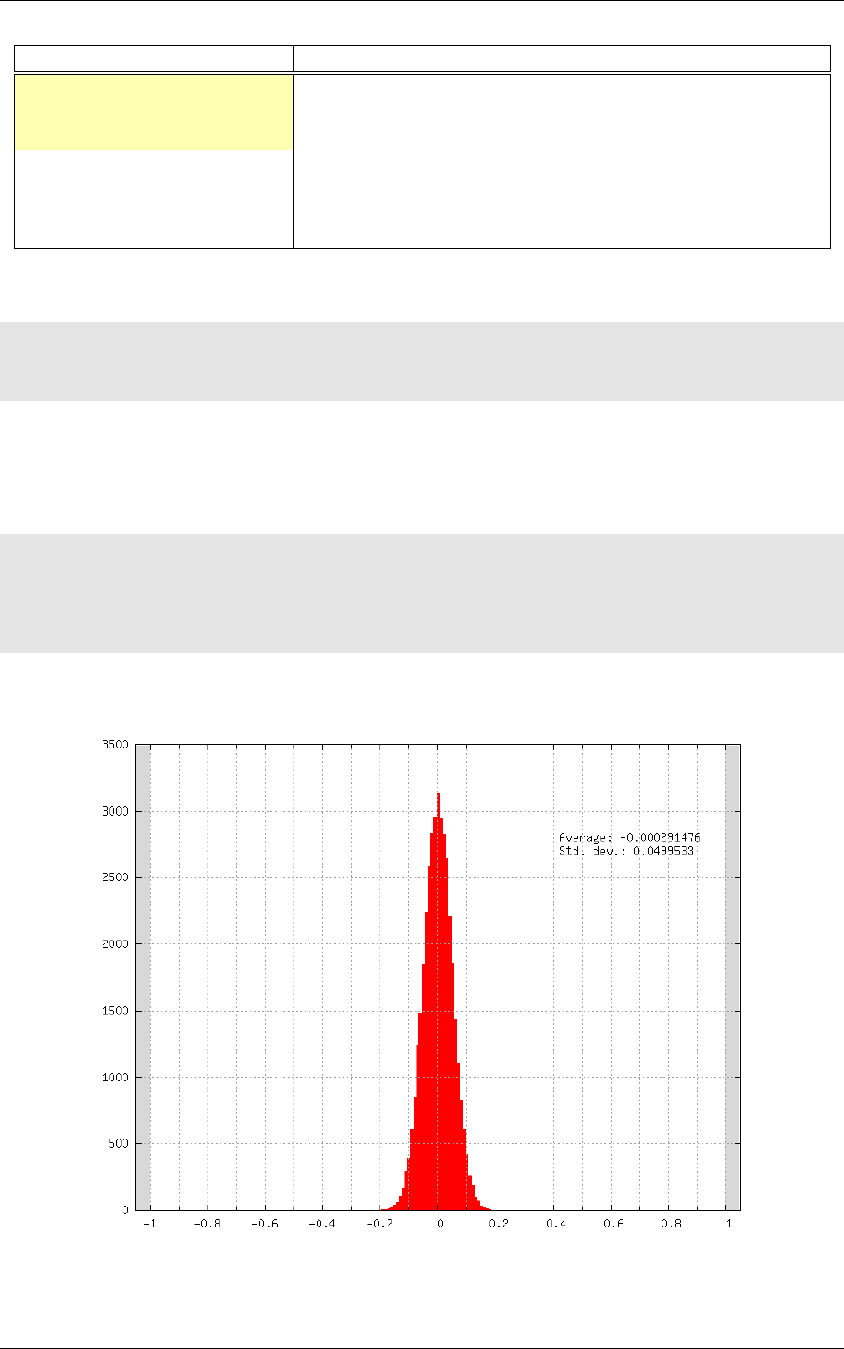
Option [default value] Description
Input
Name of the section(s) for the input layer(s). Comma sepa-
rated
Type Type of the layer. Can be any of the type described below
Model [DefaultModel] Layer model to use
DataType [DefaultDataType]
Layer data type to use. Please note that some layers may
not support every data type.
ConfigSection [] Name of the configuration section for layer
To specify that the back-propagated error must be computed at the output of a given layer
(generally the last layer, or output layer), one must add a target section named LayerName
.Target
:
...
[LayerName.Target]
TargetValue=1.0 ; default: 1.0
DefaultValue=0.0 ; default: -1.0
4.7.2 Weight fillers
Fillers to initialize weights and biases in the different type of layer.
Usage example:
[conv1]
...
WeightsFiller=NormalFiller
WeightsFiller.Mean=0.0
WeightsFiller.StdDev=0.05
...
The initial weights distribution for each layer can be checked in the weights_init folder, with
an example shown in figure 12.
Figure 12: Initial weights distribution of a layer using a normal distribution (
NormalFiller
) with a 0 mean
and a 0.05 standard deviation.
42/78

ConstantFiller Fill with a constant value.
Option Description
FillerName.Value Value for the filling
HeFiller
Fill with an normal distribution with normalized variance taking into account the
rectifier nonlinearity (He et al.,2015). This filler is sometimes referred as MSRA filler.
Option [default value] Description
FillerName
.VarianceNorm
[FanIn]
Normalization, can be FanIn,Average or FanOut
Use a normal distribution with standard deviation q2.0
n.
•n=fan-in with FanIn, resulting in V ar(W) = 2
fan-in
•n=(fan-in+fan-out)
2with Average, resulting in V ar(W) = 4
fan-in+fan-out
•n=fan-out with FanOut, resulting in V ar(W) = 2
fan-out
NormalFiller Fill with a normal distribution.
Option [default value] Description
FillerName.Mean [0.0] Mean value of the distribution
FillerName.StdDev [1.0] Standard deviation of the distribution
UniformFiller Fill with an uniform distribution.
Option [default value] Description
FillerName.Min [0.0] Min. value
FillerName.Max [1.0] Max. value
XavierFiller
Fill with an uniform distribution with normalized variance (Glorot and Bengio,
2010).
Option [default value] Description
FillerName
.VarianceNorm
[FanIn]
Normalization, can be FanIn,Average or FanOut
FillerName
.Distribution
[Uniform]
Distribution, can be Uniform or Normal
Use an uniform distribution with interval [−scale, scale], with scale =q3.0
n.
•n=fan-in with FanIn, resulting in V ar(W) = 1
fan-in
•n=(fan-in+fan-out)
2with Average, resulting in V ar(W) = 2
fan-in+fan-out
•n=fan-out with FanOut, resulting in V ar(W) = 1
fan-out
43/78

4.7.3 Weight solvers
SGDSolver_Frame SGD Solver for Frame models.
Option [default value] Description
SolverName
.LearningRate
[0.01]
Learning rate
SolverName.Momentum [0.0] Momentum
SolverName.Decay [0.0] Decay
SolverName
.
LearningRatePolicy [None]
Learning rate decay policy. Can be any of
None
,
StepDecay
,
ExponentialDecay,InvTDecay,PolyDecay
SolverName
.
LearningRateStepSize [1]
Learning rate step size (in number of stimuli)
SolverName
.LearningRateDecay
[0.1]
Learning rate decay
SolverName.Clamping [0] If true, clamp the weights and bias between -1 and 1
SolverName.Power [0.0] Polynomial learning rule power parameter
SolverName
.MaxIterations
[0.0]
Polynomial learning rule maximum number of iterations
The learning rate decay policies are the following:
•StepDecay
: every SolverName
.LearningRateStepSize
stimuli, the learning rate is reduced by a
factor SolverName.LearningRateDecay;
•ExponentialDecay
: the learning rate is
α
=
α0exp
(
−kt
), with
α0
the initial learning rate
SolverName
.LearningRate
,
k
the rate decay SolverName
.LearningRateDecay
and
t
the step
number (one step every SolverName.LearningRateStepSize stimuli);
•InvTDecay
: the learning rate is
α
=
α0/
(1 +
kt
), with
α0
the initial learning rate SolverName
.
LearningRate
,
k
the rate decay SolverName
.LearningRateDecay
and
t
the step number (one step
every SolverName.LearningRateStepSize stimuli).
•InvDecay
: the learning rate is
α
=
α0∗
(1 +
kt
)
−n
, with
α0
the initial learning rate Solver-
Name
.LearningRate
,
k
the rate decay SolverName
.LearningRateDecay
,
t
the current iteration
and nthe power parameter SolverName.Power
•PolyDecay
: the learning rate is
α
=
α0∗
(1
−k
t
)
n
, with
α0
the initial learning rate Solver-
Name
.LearningRate
,
k
the current iteration,
t
the maximum number of iteration SolverName
.
MaxIterations and nthe power parameter SolverName.Power
SGDSolver_Frame_CUDA SGD Solver for Frame_CUDA models.
44/78

Option [default value] Description
SolverName
.LearningRate
[0.01]
Learning rate
SolverName.Momentum [0.0] Momentum
SolverName.Decay [0.0] Decay
SolverName
.
LearningRatePolicy [None]
Learning rate decay policy. Can be any of
None
,
StepDecay
,
ExponentialDecay,InvTDecay
SolverName
.
LearningRateStepSize [1]
Learning rate step size (in number of stimuli)
SolverName
.LearningRateDecay
[0.1]
Learning rate decay
SolverName.Clamping [0] If true, clamp the weights and bias between -1 and 1
The learning rate decay policies are identical to the ones in the SGDSolver\_Frame solver.
AdamSolver_Frame Adam Solver for Frame models (Kingma and Ba,2014).
Option [default value] Description
SolverName
.LearningRate
[0.001]
Learning rate (stepsize)
SolverName.Beta1 [0.9]
Exponential decay rate of these moving average of the first
moment
SolverName.Beta2 [0.999]
Exponential decay rate of these moving average of the second
moment
SolverName.Epsilon [1.0e-8] Epsilon
AdamSolver_Frame_CUDA Adam Solver for Frame_CUDA models (Kingma and Ba,2014).
Option [default value] Description
SolverName
.LearningRate
[0.001]
Learning rate (stepsize)
SolverName.Beta1 [0.9]
Exponential decay rate of these moving average of the first
moment
SolverName.Beta2 [0.999]
Exponential decay rate of these moving average of the second
moment
SolverName.Epsilon [1.0e-8] Epsilon
4.7.4 Activation functions
Activation function to be used at the output of layers.
Usage example:
[conv1]
...
ActivationFunction=Rectifier
ActivationFunction.LeakSlope=0.01
ActivationFunction.Clipping=20
...
Logistic Logistic activation function.
LogisticWithLoss Logistic with loss activation function.
45/78

Rectifier Rectifier or ReLU activation function.
Option [default value] Description
ActivationFunction.LeakSlope
[0.0]
Leak slope for negative inputs
ActivationFunction.Clipping
[0.0]
Clipping value for positive outputs
Saturation Saturation activation function.
Softplus Softplus activation function.
Tanh Tanh activation function.
Computes y=tanh(αx).
Option [default value] Description
ActivationFunction.Alpha [1.0] αparameter
TanhLeCun Tanh activation function with an αparameter of 1.7159 ×(2.0/3.0).
4.7.5 Anchor
Anchor layer for Faster R-CNN or Single Shot Detector.
Option [default value] Description
Input
This layer takes one or two inputs. The total number of
input channels must be
ScoresCls
+ 4, with
ScoresCls
being
equal to 1 or 2.
Anchor[*]
Anchors definition. For each anchor, there must be two
space-separated values: the root area and the aspect ratio.
ScoresCls
Number of classes per anchor. Must be 1 (if the scores input
uses logistic regression) or 2 (if the scores input is a two-class
softmax layer)
FeatureMapWidth
[StimuliProvider.Width]
Reference width use to scale anchors coordinate.
FeatureMapHeight
[StimuliProvider.Height]
Reference height use to scale anchors coordinate.
Configuration parameters (Frame models)
Option [default value] Model(s) Description
PositiveIoU [0.7] all Frame
Assign a positive label for anchors whose IoU overlap
is higher than PositiveIoU with any ground-truth box
NegativeIoU [0.3] all Frame
Assign a negative label for non-positive anchors whose
IoU overlap is lower than
NegativeIoU
for all ground-
truth boxes
LossLambda [10.0] all Frame Balancing parameter λ
LossPositiveSample [128] all Frame
Number of random positive samples for the loss com-
putation
46/78

LossNegativeSample [128] all Frame
Number of random negative samples for the loss com-
putation
Usage example:
; RPN network: cls layer
[scores]
Input=...
Type=Conv
KernelWidth=1
KernelHeight=1
; 18 channels for 9 anchors
NbOutputs=18
...
[scores.softmax]
Input=scores
Type=Softmax
NbOutputs=[scores]NbOutputs
WithLoss=1
; RPN network: coordinates layer
[coordinates]
Input=...
Type=Conv
KernelWidth=1
KernelHeight=1
; 36 channels for 4 coordinates x 9 anchors
NbOutputs=36
...
; RPN network: anchors
[anchors]
Input=scores.softmax,coordinates
Type=Anchor
ScoresCls=2 ; using a two-class softmax for the scores
Anchor[0]=32 1.0
Anchor[1]=48 1.0
Anchor[2]=64 1.0
Anchor[3]=80 1.0
Anchor[4]=96 1.0
Anchor[5]=112 1.0
Anchor[6]=128 1.0
Anchor[7]=144 1.0
Anchor[8]=160 1.0
ConfigSection=anchors.config
[anchors.config]
PositiveIoU=0.7
NegativeIoU=0.3
LossLambda=1.0
Outputs remapping
Outputs remapping allows to convert scores and coordinates output feature
maps layout from another ordering that the one used in the N2D2
Anchor
layer, during weights
import/export.
For example, lets consider that the imported weights corresponds to the following output feature
maps ordering:
0 anchor[0].y
1 anchor[0].x
47/78

2 anchor[0].h
3 anchor[0].w
4 anchor[1].y
5 anchor[1].x
6 anchor[1].h
7 anchor[1].w
8 anchor[2].y
9 anchor[2].x
10 anchor[2].h
11 anchor[2].w
The output feature maps ordering required by the Anchor layer is:
0 anchor[0].x
1 anchor[1].x
2 anchor[2].x
3 anchor[0].y
4 anchor[1].y
5 anchor[2].y
6 anchor[0].w
7 anchor[1].w
8 anchor[2].w
9 anchor[0].h
10 anchor[1].h
11 anchor[2].h
The feature maps ordering can be changed during weights import/export:
; RPN network: coordinates layer
[coordinates]
Input=...
Type=Conv
KernelWidth=1
KernelHeight=1
; 36 channels for 4 coordinates x 9 anchors
NbOutputs=36
...
ConfigSection=coordinates.config
[coordinates.config]
WeightsExportFormat=HWCO ; Weights format used by TensorFlow
OutputsRemap=1:4,0:4,3:4,2:4
4.7.6 Conv
Convolutional layer.
Option [default value] Description
KernelWidth Width of the kernels
KernelHeight Height of the kernels
KernelDepth [] Depth of the kernels (implies 3D kernels)
OR
KernelSize [] Kernels size (implies 2D square kernels)
OR
KernelDims [] List of space-separated dimensions for N-D kernels
NbOutputs Number of output channels
SubSampleX [1] X-axis subsampling factor of the output feature maps
SubSampleY [1] Y-axis subsampling factor of the output feature maps
SubSampleZ [] Z-axis subsampling factor of the output feature maps
OR
48/78

SubSample [1] Subsampling factor of the output feature maps
OR
SubSampleDims []
List of space-separated subsampling dimensions for N-D
kernels
StrideX [1] X-axis stride of the kernels
StrideY [1] Y-axis stride of the kernels
StrideZ [] Z-axis stride of the kernels
OR
Stride [1] Stride of the kernels
OR
StrideDims [] List of space-separated stride dimensions for N-D kernels
PaddingX [0] X-axis input padding
PaddingY [0] Y-axis input padding
PaddingZ [] Z-axis input padding
OR
Padding [0] Input padding
OR
PaddingDims []
List of space-separated padding dimensions for N-D kernels
ActivationFunction [Tanh]
Activation function. Can be any of
Logistic
,
LogisticWithLoss
,
Rectifier,Softplus,TanhLeCun,Linear,Saturation or Tanh
WeightsFiller Weights initial values filler
[NormalFiller(0.0, 0.05)]
BiasFiller Biases initial values filler
[NormalFiller(0.0, 0.05)]
Mapping.NbGroups [] Mapping: number of groups
(mutually exclusive with all other Mapping.* options)
Mapping.ChannelsPerGroup [] Mapping: number of channels per group
(mutually exclusive with all other Mapping.* options)
Mapping.SizeX [1] Mapping canvas pattern default width
Mapping.SizeY [1] Mapping canvas pattern default height
Mapping.Size [1] Mapping canvas pattern default size
(mutually exclusive with Mapping.SizeX and Mapping.SizeY)
Mapping.StrideX [1] Mapping canvas default X-axis step
Mapping.StrideY [1] Mapping canvas default Y-axis step
Mapping.Stride [1] Mapping canvas default step
(mutually exclusive with
Mapping.StrideX
and
Mapping.StrideY
)
Mapping.OffsetX [0] Mapping canvas default X-axis offset
Mapping.OffsetY [0] Mapping canvas default Y-axis offset
Mapping.Offset [0] Mapping canvas default offset
(mutually exclusive with
Mapping.OffsetX
and
Mapping.OffsetY
)
Mapping.NbIterations [0]
Mapping canvas pattern default number of iterations (0
means no limit)
Mapping(in).SizeX [1] Mapping canvas pattern default width for input layer in
Mapping(in).SizeY [1] Mapping canvas pattern default height for input layer in
Mapping(in).Size [1] Mapping canvas pattern default size for input layer in
(mutually exclusive with Mapping(in).SizeX and
Mapping(in).SizeY)
Mapping(in).StrideX [1] Mapping canvas default X-axis step for input layer in
Mapping(in).StrideY [1] Mapping canvas default Y-axis step for input layer in
Mapping(in).Stride [1] Mapping canvas default step for input layer in
(mutually exclusive with Mapping(in).StrideX and
49/78

Mapping(in).StrideY)
Mapping(in).OffsetX [0] Mapping canvas default X-axis offset for input layer in
Mapping(in).OffsetY [0] Mapping canvas default Y-axis offset for input layer in
Mapping(in).Offset [0] Mapping canvas default offset for input layer in
(mutually exclusive with Mapping(in).OffsetX and
Mapping(in).OffsetY)
Mapping(in).NbIterations [0]
Mapping canvas pattern default number of iterations for
input layer in (0 means no limit)
WeightsSharing [] Share the weights with an other layer
BiasesSharing [] Share the biases with an other layer
Configuration parameters (Frame models)
Option [default value] Model(s) Description
NoBias [0] all Frame If true, don’t use bias
Solvers.*all Frame Any solver parameters
WeightsSolver.*all Frame
Weights solver parameters, take precedence over the
Solvers.* parameters
BiasSolver.*all Frame
Bias solver parameters, take precedence over the
Solvers.* parameters
WeightsExportFormat
[OCHW]
all Frame
Weights import/export format. Can be
OCHW
or
OCHW
,
with
O
the output feature map,
C
the input feature map
(channel),
H
the kernel row and
W
the kernel column, in
the order of the outermost dimension (in the leftmost
position) to the innermost dimension (in the rightmost
position)
WeightsExportFlip [0] all Frame If true, import/export flipped kernels
Configuration parameters (Spike models)
Experimental option (implementation may be wrong or susceptible to change)
Option [default value] Model(s) Description
IncomingDelay
[1
TimePs
;100 TimeFs]
all Spike Synaptic incoming delay wdelay
Threshold [1.0] Spike,Spike_RRAM Threshold of the neuron Ithres
BipolarThreshold [1] Spike,Spike_RRAM
If true, the threshold is also applied to the absolute
value of negative values (generating negative spikes)
Leak [0.0] Spike,Spike_RRAM Neural leak time constant τleak (if 0, no leak)
Refractory [0.0] Spike,Spike_RRAM Neural refractory period Trefrac
WeightsRelInit [0.0;0.05] Spike Relative initial synaptic weight winit
WeightsMinMean [1;0.1] Spike_RRAM Mean minimum synaptic weight wmin
WeightsMaxMean
[100;10.0]
Spike_RRAM Mean maximum synaptic weight wmax
WeightsMinVarSlope [0.0] Spike_RRAM OXRAM specific parameter
WeightsMinVarOrigin [0.0] Spike_RRAM OXRAM specific parameter
WeightsMaxVarSlope [0.0] Spike_RRAM OXRAM specific parameter
WeightsMaxVarOrigin [0.0] Spike_RRAM OXRAM specific parameter
50/78

WeightsSetProba [1.0] Spike_RRAM
Intrinsic SET switching probability
PSET
(upon receiv-
ing a SET programming pulse). Assuming uniform
statistical distribution (not well supported by experi-
ments on RRAM)
WeightsResetProba [1.0] Spike_RRAM
Intrinsic RESET switching probability
PRESET
(upon
receiving a RESET programming pulse). Assuming
uniform statistical distribution (not well supported by
experiments on RRAM)
SynapticRedundancy [1] Spike_RRAM
Synaptic redundancy (number of RRAM device per
synapse)
BipolarWeights [0] Spike_RRAM Bipolar weights
BipolarIntegration [0] Spike_RRAM Bipolar integration
LtpProba [0.2] Spike_RRAM
Extrinsic STDP LTP probability (cumulative with in-
trinsic SET switching probability PSET )
LtdProba [0.1] Spike_RRAM
Extrinsic STDP LTD probability (cumulative with
intrinsic RESET switching probability PRESET )
StdpLtp [1000 TimePs]Spike_RRAM STDP LTP time window TLT P
InhibitRefractory
[0
TimePs]
Spike_RRAM Neural lateral inhibition period Tinhibit
EnableStdp [1] Spike_RRAM
If false, STDP is disabled (no synaptic weight change)
RefractoryIntegration
[1]
Spike_RRAM
If true, reset the integration to 0 during the refractory
period
DigitalIntegration [0] Spike_RRAM
If false, the analog value of the devices is integrated,
instead of their binary value
4.7.7 Deconv
Deconvolutionlayer.
Option [default value] Description
KernelWidth Width of the kernels
KernelHeight Height of the kernels
KernelDepth [] Depth of the kernels (implies 3D kernels)
OR
KernelSize [] Kernels size (implies 2D square kernels)
OR
KernelDims [] List of space-separated dimensions for N-D kernels
NbOutputs Number of output channels
StrideX [1] X-axis stride of the kernels
StrideY [1] Y-axis stride of the kernels
StrideZ [] Z-axis stride of the kernels
OR
Stride [1] Stride of the kernels
OR
StrideDims [] List of space-separated stride dimensions for N-D kernels
PaddingX [0] X-axis input padding
PaddingY [0] Y-axis input padding
PaddingZ [] Z-axis input padding
OR
Padding [0] Input padding
51/78

OR
PaddingDims []
List of space-separated padding dimensions for N-D kernels
ActivationFunction [Tanh]
Activation function. Can be any of
Logistic
,
LogisticWithLoss
,
Rectifier,Softplus,TanhLeCun,Linear,Saturation or Tanh
WeightsFiller Weights initial values filler
[NormalFiller(0.0, 0.05)]
BiasFiller Biases initial values filler
[NormalFiller(0.0, 0.05)]
Mapping.NbGroups [] Mapping: number of groups
(mutually exclusive with all other Mapping.* options)
Mapping.ChannelsPerGroup [] Mapping: number of channels per group
(mutually exclusive with all other Mapping.* options)
Mapping.SizeX [1] Mapping canvas pattern default width
Mapping.SizeY [1] Mapping canvas pattern default height
Mapping.Size [1] Mapping canvas pattern default size
(mutually exclusive with Mapping.SizeX and Mapping.SizeY)
Mapping.StrideX [1] Mapping canvas default X-axis step
Mapping.StrideY [1] Mapping canvas default Y-axis step
Mapping.Stride [1] Mapping canvas default step
(mutually exclusive with
Mapping.StrideX
and
Mapping.StrideY
)
Mapping.OffsetX [0] Mapping canvas default X-axis offset
Mapping.OffsetY [0] Mapping canvas default Y-axis offset
Mapping.Offset [0] Mapping canvas default offset
(mutually exclusive with
Mapping.OffsetX
and
Mapping.OffsetY
)
Mapping.NbIterations [0]
Mapping canvas pattern default number of iterations (0
means no limit)
Mapping(in).SizeX [1] Mapping canvas pattern default width for input layer in
Mapping(in).SizeY [1] Mapping canvas pattern default height for input layer in
Mapping(in).Size [1] Mapping canvas pattern default size for input layer in
(mutually exclusive with Mapping(in).SizeX and
Mapping(in).SizeY)
Mapping(in).StrideX [1] Mapping canvas default X-axis step for input layer in
Mapping(in).StrideY [1] Mapping canvas default Y-axis step for input layer in
Mapping(in).Stride [1] Mapping canvas default step for input layer in
(mutually exclusive with Mapping(in).StrideX and
Mapping(in).StrideY)
Mapping(in).OffsetX [0] Mapping canvas default X-axis offset for input layer in
Mapping(in).OffsetY [0] Mapping canvas default Y-axis offset for input layer in
Mapping(in).Offset [0] Mapping canvas default offset for input layer in
(mutually exclusive with Mapping(in).OffsetX and
Mapping(in).OffsetY)
Mapping(in).NbIterations [0]
Mapping canvas pattern default number of iterations for
input layer in (0 means no limit)
WeightsSharing [] Share the weights with an other layer
BiasesSharing [] Share the biases with an other layer
Configuration parameters (Frame models)
Option [default value] Model(s) Description
52/78

NoBias [0] all Frame If true, don’t use bias
BackPropagate [1] all Frame If true, enable backpropogation
Solvers.*all Frame Any solver parameters
WeightsSolver.*all Frame
Weights solver parameters, take precedence over the
Solvers.* parameters
BiasSolver.*all Frame
Bias solver parameters, take precedence over the
Solvers.* parameters
WeightsExportFormat
[OCHW]
all Frame
Weights import/export format. Can be
OCHW
or
OCHW
,
with
O
the output feature map,
C
the input feature map
(channel),
H
the kernel row and
W
the kernel column, in
the order of the outermost dimension (in the leftmost
position) to the innermost dimension (in the rightmost
position)
WeightsExportFlip [0] all Frame If true, import/export flipped kernels
4.7.8 Pool
Pooling layer.
There are two CUDA models for this cell:
•Frame_CUDA
, which uses CuDNN as back-end and only supports one-to-one input to output
map connection;
•Frame_EXT_CUDA
, which uses custom CUDA kernels and allows arbitrary connections between
input and output maps (and can therefore be used to implement Maxout or both Maxout
and Pooling simultaneously).
Maxout example
In the following INI section, one implements a Maxout between each consecu-
tive pair of 8 input maps:
[maxout_layer]
Input=...
Type=Pool
Model=Frame_EXT_CUDA
PoolWidth=1
PoolHeight=1
NbOutputs=4
Pooling=Max
Mapping.SizeY=2
Mapping.StrideY=2
The layer connectivity is the following:
# input map
1
2
3
4
5
6
7
8
1 2 3 4
# output map
53/78

Option [default value] Description
Pooling Type of pooling (Max or Average)
PoolWidth Width of the pooling area
PoolHeight Height of the pooling area
PoolDepth [] Depth of the pooling area (implies 3D pooling area)
OR
PoolSize [] Pooling area size (implies 2D square pooling area)
OR
PoolDims [] List of space-separated dimensions for N-D pooling area
NbOutputs Number of output channels
StrideX [1] X-axis stride of the pooling area
StrideY [1] Y-axis stride of the pooling area
StrideZ [] Z-axis stride of the pooling area
OR
Stride [1] Stride of the pooling area
OR
StrideDims []
List of space-separated stride dimensions for N-D pooling
area
PaddingX [0] X-axis input padding
PaddingY [0] Y-axis input padding
PaddingZ [] Z-axis input padding
OR
Padding [0] Input padding
OR
PaddingDims []
List of space-separated padding dimensions for N-D pooling
area
ActivationFunction [Linear]
Activation function. Can be any of
Logistic
,
LogisticWithLoss
,
Rectifier,Softplus,TanhLeCun,Linear,Saturation or Tanh
Mapping.NbGroups [] Mapping: number of groups
(mutually exclusive with all other Mapping.* options)
Mapping.ChannelsPerGroup [] Mapping: number of channels per group
(mutually exclusive with all other Mapping.* options)
Mapping.SizeX [1] Mapping canvas pattern default width
Mapping.SizeY [1] Mapping canvas pattern default height
Mapping.Size [1] Mapping canvas pattern default size
(mutually exclusive with Mapping.SizeX and Mapping.SizeY)
Mapping.StrideX [1] Mapping canvas default X-axis step
Mapping.StrideY [1] Mapping canvas default Y-axis step
Mapping.Stride [1] Mapping canvas default step
(mutually exclusive with
Mapping.StrideX
and
Mapping.StrideY
)
Mapping.OffsetX [0] Mapping canvas default X-axis offset
Mapping.OffsetY [0] Mapping canvas default Y-axis offset
Mapping.Offset [0] Mapping canvas default offset
(mutually exclusive with
Mapping.OffsetX
and
Mapping.OffsetY
)
Mapping.NbIterations [0]
Mapping canvas pattern default number of iterations (0
means no limit)
Mapping(in).SizeX [1] Mapping canvas pattern default width for input layer in
Mapping(in).SizeY [1] Mapping canvas pattern default height for input layer in
Mapping(in).Size [1] Mapping canvas pattern default size for input layer in
(mutually exclusive with Mapping(in).SizeX and
Mapping(in).SizeY)
54/78

Mapping(in).StrideX [1] Mapping canvas default X-axis step for input layer in
Mapping(in).StrideY [1] Mapping canvas default Y-axis step for input layer in
Mapping(in).Stride [1] Mapping canvas default step for input layer in
(mutually exclusive with Mapping(in).StrideX and
Mapping(in).StrideY)
Mapping(in).OffsetX [0] Mapping canvas default X-axis offset for input layer in
Mapping(in).OffsetY [0] Mapping canvas default Y-axis offset for input layer in
Mapping(in).Offset [0] Mapping canvas default offset for input layer in
(mutually exclusive with Mapping(in).OffsetX and
Mapping(in).OffsetY)
Mapping(in).NbIterations [0]
Mapping canvas pattern default number of iterations for
input layer in (0 means no limit)
Configuration parameters (Spike models)
Option [default value] Model(s) Description
IncomingDelay
[1
TimePs
;100 TimeFs]
all Spike Synaptic incoming delay wdelay
value
4.7.9 Unpool
Unpooling layer.
Option [default value] Description
Pooling Type of pooling (Max or Average)
PoolWidth Width of the pooling area
PoolHeight Height of the pooling area
PoolDepth [] Depth of the pooling area (implies 3D pooling area)
OR
PoolSize [] Pooling area size (implies 2D square pooling area)
OR
PoolDims [] List of space-separated dimensions for N-D pooling area
NbOutputs Number of output channels
ArgMax
Name of the associated pool layer for the argmax (the pool
layer input and the unpool layer output dimension must
match)
StrideX [1] X-axis stride of the pooling area
StrideY [1] Y-axis stride of the pooling area
StrideZ [] Z-axis stride of the pooling area
OR
Stride [1] Stride of the pooling area
OR
StrideDims []
List of space-separated stride dimensions for N-D pooling
area
PaddingX [0] X-axis input padding
PaddingY [0] Y-axis input padding
55/78

PaddingZ [] Z-axis input padding
OR
Padding [0] Input padding
OR
PaddingDims []
List of space-separated padding dimensions for N-D pooling
area
ActivationFunction [Linear]
Activation function. Can be any of
Logistic
,
LogisticWithLoss
,
Rectifier,Softplus,TanhLeCun,Linear,Saturation or Tanh
Mapping.NbGroups [] Mapping: number of groups
(mutually exclusive with all other Mapping.* options)
Mapping.ChannelsPerGroup [] Mapping: number of channels per group
(mutually exclusive with all other Mapping.* options)
Mapping.SizeX [1] Mapping canvas pattern default width
Mapping.SizeY [1] Mapping canvas pattern default height
Mapping.Size [1] Mapping canvas pattern default size
(mutually exclusive with Mapping.SizeX and Mapping.SizeY)
Mapping.StrideX [1] Mapping canvas default X-axis step
Mapping.StrideY [1] Mapping canvas default Y-axis step
Mapping.Stride [1] Mapping canvas default step
(mutually exclusive with
Mapping.StrideX
and
Mapping.StrideY
)
Mapping.OffsetX [0] Mapping canvas default X-axis offset
Mapping.OffsetY [0] Mapping canvas default Y-axis offset
Mapping.Offset [0] Mapping canvas default offset
(mutually exclusive with
Mapping.OffsetX
and
Mapping.OffsetY
)
Mapping.NbIterations [0]
Mapping canvas pattern default number of iterations (0
means no limit)
Mapping(in).SizeX [1] Mapping canvas pattern default width for input layer in
Mapping(in).SizeY [1] Mapping canvas pattern default height for input layer in
Mapping(in).Size [1] Mapping canvas pattern default size for input layer in
(mutually exclusive with Mapping(in).SizeX and
Mapping(in).SizeY)
Mapping(in).StrideX [1] Mapping canvas default X-axis step for input layer in
Mapping(in).StrideY [1] Mapping canvas default Y-axis step for input layer in
Mapping(in).Stride [1] Mapping canvas default step for input layer in
(mutually exclusive with Mapping(in).StrideX and
Mapping(in).StrideY)
Mapping(in).OffsetX [0] Mapping canvas default X-axis offset for input layer in
Mapping(in).OffsetY [0] Mapping canvas default Y-axis offset for input layer in
Mapping(in).Offset [0] Mapping canvas default offset for input layer in
(mutually exclusive with Mapping(in).OffsetX and
Mapping(in).OffsetY)
Mapping(in).NbIterations [0]
Mapping canvas pattern default number of iterations for
input layer in (0 means no limit)
4.7.10 ElemWise
Element-wise operation layer.
Option [default value] Description
56/78

NbOutputs Number of output neurons
Operation Type of operation (Sum,AbsSum,EuclideanSum,Prod, or Max)
Weights [1.0]
Weights for the
Sum
,
AbsSum
, and
EuclideanSum
operation, in
the same order as the inputs
Shifts [0.0]
Shifts for the
Sum
and
EuclideanSum
operation, in the same
order as the inputs
ActivationFunction [Linear]
Activation function. Can be any of
Logistic
,
LogisticWithLoss
,
Rectifier,Softplus,TanhLeCun,Linear,Saturation or Tanh
Given Ninput tensors Ti, performs the following operation:
Sum operation Tout =PN
1(wiTi+si)
AbsSum operation Tout =PN
1(wi|Ti|)
EuclideanSum operation Tout =qPN
1(wiTi+si)2
Prod operation Tout =QN
1(Ti)
Max operation Tout =MAXN
1(Ti)
Examples Sum of two inputs (Tout =T1+T2):
[elemwise_sum]
Input=layer1,layer2
Type=ElemWise
NbOutputs=[layer1]NbOutputs
Operation=Sum
Weighted sum of two inputs, by a factor 0.5 for
layer1
and 1.0 for
layer2
(
Tout
= 0
.
5
×T1
+1
.
0
×T2
):
[elemwise_weighted_sum]
Input=layer1,layer2
Type=ElemWise
NbOutputs=[layer1]NbOutputs
Operation=Sum
Weights=0.5 1.0
Single input scaling by a factor 0.5 and shifted by 0.1 (Tout = 0.5×T1+ 0.1):
[elemwise_scale]
Input=layer1
Type=ElemWise
NbOutputs=[layer1]NbOutputs
Operation=Sum
Weights=0.5
Shifts=0.1
Absolute value of an input (Tout =|T1|):
[elemwise_abs]
Input=layer1
Type=ElemWise
NbOutputs=[layer1]NbOutputs
Operation=Abs
57/78

4.7.11 FMP
Fractional max pooling layer (Graham,2014).
Option [default value] Description
NbOutputs Number of output channels
ScalingRatio Scaling ratio. The output size is round input size
scaling ratio .
ActivationFunction [Linear]
Activation function. Can be any of
Logistic
,
LogisticWithLoss
,
Rectifier,Softplus,TanhLeCun,Linear,Saturation or Tanh
Configuration parameters (Frame models)
Option [default value] Model(s) Description
Overlapping [1] all Frame
If true, use overlapping regions, else use disjoint regions
PseudoRandom [1] all Frame
If true, use pseudorandom sequences, else use random
sequences
4.7.12 Fc
Fully connected layer.
Option [default value] Description
NbOutputs Number of output neurons
WeightsFiller Weights initial values filler
[NormalFiller(0.0, 0.05)]
BiasFiller Biases initial values filler
[NormalFiller(0.0, 0.05)]
ActivationFunction [Tanh]
Activation function. Can be any of
Logistic
,
LogisticWithLoss
,
Rectifier,Softplus,TanhLeCun,Linear,Saturation or Tanh
Configuration parameters (Frame models)
Option [default value] Model(s) Description
NoBias [0] all Frame If true, don’t use bias
BackPropagate [1] all Frame If true, enable backpropogation
Solvers.*all Frame Any solver parameters
WeightsSolver.*all Frame
Weights solver parameters, take precedence over the
Solvers.* parameters
BiasSolver.*all Frame
Bias solver parameters, take precedence over the
Solvers.* parameters
DropConnect [1.0] Frame
If below 1.0, fraction of synapses that are disabled with
drop connect
58/78

Configuration parameters (Spike models)
Option [default value] Model(s) Description
IncomingDelay
[1
TimePs
;100 TimeFs]
all Spike Synaptic incoming delay wdelay
Threshold [1.0] Spike,Spike_RRAM Threshold of the neuron Ithres
BipolarThreshold [1] Spike,Spike_RRAM
If true, the threshold is also applied to the absolute
value of negative values (generating negative spikes)
Leak [0.0] Spike,Spike_RRAM Neural leak time constant τleak (if 0, no leak)
Refractory [0.0] Spike,Spike_RRAM Neural refractory period Trefrac
TerminateDelta [0] Spike,Spike_RRAM Terminate delta
WeightsRelInit [0.0;0.05] Spike Relative initial synaptic weight winit
WeightsMinMean [1;0.1] Spike_RRAM Mean minimum synaptic weight wmin
WeightsMaxMean
[100;10.0]
Spike_RRAM Mean maximum synaptic weight wmax
WeightsMinVarSlope [0.0] Spike_RRAM OXRAM specific parameter
WeightsMinVarOrigin [0.0] Spike_RRAM OXRAM specific parameter
WeightsMaxVarSlope [0.0] Spike_RRAM OXRAM specific parameter
WeightsMaxVarOrigin [0.0] Spike_RRAM OXRAM specific parameter
WeightsSetProba [1.0] Spike_RRAM
Intrinsic SET switching probability
PSET
(upon receiv-
ing a SET programming pulse). Assuming uniform
statistical distribution (not well supported by experi-
ments on RRAM)
WeightsResetProba [1.0] Spike_RRAM
Intrinsic RESET switching probability
PRESET
(upon
receiving a RESET programming pulse). Assuming
uniform statistical distribution (not well supported by
experiments on RRAM)
SynapticRedundancy [1] Spike_RRAM
Synaptic redundancy (number of RRAM device per
synapse)
BipolarWeights [0] Spike_RRAM Bipolar weights
BipolarIntegration [0] Spike_RRAM Bipolar integration
LtpProba [0.2] Spike_RRAM
Extrinsic STDP LTP probability (cumulative with in-
trinsic SET switching probability PSET )
LtdProba [0.1] Spike_RRAM
Extrinsic STDP LTD probability (cumulative with
intrinsic RESET switching probability PRESET )
StdpLtp [1000 TimePs]Spike_RRAM STDP LTP time window TLT P
InhibitRefractory
[0
TimePs]
Spike_RRAM Neural lateral inhibition period Tinhibit
EnableStdp [1] Spike_RRAM
If false, STDP is disabled (no synaptic weight change)
RefractoryIntegration
[1]
Spike_RRAM
If true, reset the integration to 0 during the refractory
period
DigitalIntegration [0] Spike_RRAM
If false, the analog value of the devices is integrated,
instead of their binary value
4.7.13 RbfN2D2 IP only
Radial basis function fully connected layer.
59/78

Option [default value] Description
NbOutputs Number of output neurons
CentersFiller Centers initial values filler
[NormalFiller(0.5, 0.05)]
ScalingFiller Scaling initial values filler
[NormalFiller(10.0, 0.05)]
Configuration parameters (Frame models)
Option [default value] Model(s) Description
Solvers.*all Frame Any solver parameters
CentersSolver.*all Frame
Centers solver parameters, take precedence over the
Solvers.* parameters
ScalingSolver.*all Frame
Scaling solver parameters, take precedence over the
Solvers.* parameters
RbfApprox [None]Frame
Approximation for the Gaussian function, can be any
of: None,Rectangular or SemiLinear
4.7.14 Softmax
Softmax layer.
Option [default value] Description
NbOutputs Number of output neurons
WithLoss [0] Softmax followed with a multinomial logistic layer
GroupSize [0]
Softmax is applied on groups of outputs. The group size
must be a divisor of NbOutputs parameter.
The softmax function performs the following operation, with
ai
x,y
and
bi
x,y
the input and the
output respectively at position (x, y)on channel i:
bi
x,y =exp(ai
x,y)
N
P
j=0
exp(aj
x,y)
and
dai
x,y =
N
X
j=0 δij −ai
x,yaj
x,ydbj
x,y
When the
WithLoss
option is enabled, compute the gradient directly in respect of the cross-entropy
loss:
Lx,y =
N
X
j=0
tj
x,y log(bj
x,y)
60/78

In this case, the gradient output becomes:
dai
x,y =dbi
x,y
with
dbi
x,y =ti
x,y −bi
x,y
4.7.15 LRN
Local Response Normalization (LRN) layer.
Option [default value] Description
NbOutputs Number of output neurons
The response-normalized activity bi
x,y is given by the expression:
bi
x,y =ai
x,y
k+α
min(N−1,i+n/2)
P
j=max(0,i−n/2) aj
x,y2!β
Configuration parameters (Frame models)
Option [default value] Model(s) Description
N[5] all Frame Normalization window width in elements
Alpha [1.0e-4] all Frame
Value of the alpha variance scaling parameter in the
normalization formula
Beta [0.75] all Frame
Value of the beta power parameter in the normalization
formula
K[2.0] all Frame Value of the k parameter in normalization formula
4.7.16 LSTM
Long Short Term Memory Layer (Hochreiter and Schmidhuber,1997).
Global layer parameters (Frame_CUDA models)
Option [default value] Description
SeqLength
Maximum sequence length that the LSTM can take as an
input.
BatchSize
Number of sequences used for a single weights actualisation
process : size of the batch.
InputDim Dimension of every element composing a sequence.
HiddenSize Dimension of the LSTM inner state and output.
SingleBackpropFeeding [1] If disabled return the full output sequence.
Bidirectional [0] If enabled, build a bidirectional structure.
AllGatesWeightsFiller All Gates weights initial values filler.
61/78

AllGatesBiasFiller All Gates bias initial values filler.
WeightsInputGateFiller
Input gate previous layer and recurrent weights initial values
filler. Take precedence over AllGatesWeightsFiller parameter.
WeightsForgetGateFiller
Forget gate previous layer and recurrent weights initial values
filler. Take precedence over AllGatesWeightsFiller parameter.
WeightsCellGateFiller
Cell gate (or new memory) previous layer and recurrent
weights initial values filler. Take precedence over All-
GatesWeightsFiller parameter.
WeightsOutputGateFiller
Output gate previous layer and recurrent weights initial
values filler. Take precedence over AllGatesWeightsFiller
parameter.
BiasInputGateFiller
Input gate previous layer and recurrent bias initial values
filler. Take precedence over AllGatesBiasFiller parameter.
BiasRecurrentForgetGateFiller
Forget gate recurrent bias initial values filler. Take prece-
dence over AllGatesBiasFiller parameter. Often set to 1.0 to
show better convergence performance.
BiasPreviousLayerForgetGateFiller
Forget gate previous layer bias initial values filler. Take
precedence over AllGatesBiasFiller parameter.
BiasCellGateFiller
Cell gate (or new memory) previous layer and recurrent bias
initial values filler. Take precedence over AllGatesBiasFiller
parameter.
BiasOutputGateFiller Output gate previous layer and recurrent bias initial values
filler. Take precedence over AllGatesBiasFiller parameter.
HxFiller Recurrent previous state initialisation. Often set to 0.0
CxFiller
Recurrent previous LSTM inner state initialisation. Often
set to 0.0
Configuration parameters (Frame_CUDA models)
Option [default value] Model(s) Description
Solvers.*all Frame Any solver parameters
Dropout [0.0] all Frame
The probability with which the value from input would
be dropped.
InputMode [] all Frame
If enabled, drop the matrix multiplication of the input
data.
Algo [0] all Frame
Allow to choose different cuDNN implementation. Can
be 0 : STANDARD, 1 : STATIC, 2 : DYNAMIC. Case
1 and 2 aren’t supported yet.
Current restrictions :
•Only Frame_Cuda version is supported yet.
•
The implementation only support input sequences with a fixed length associated with a single
label.
•
CuDNN structures requires the input data to be ordered as [1, InputDim, BatchSize, Se-
qLength]. Depending on the use case (like sequential-MNIST), the input data would need to
62/78
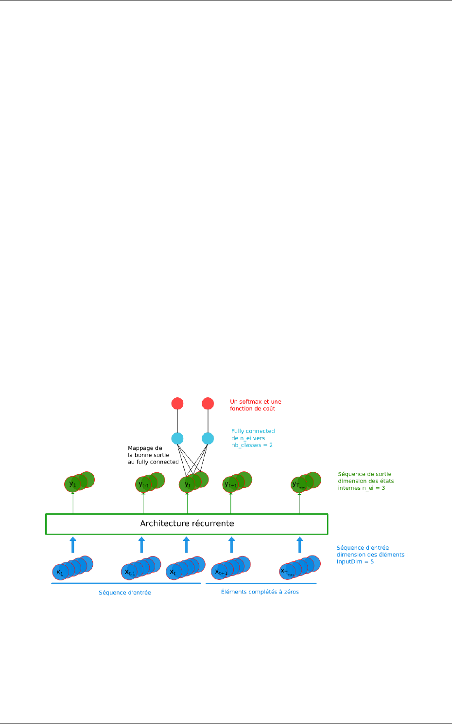
be shuffled between the stimuli provisder and the RNN in order to process batches of data.
No shuffling layer is yet operational. In that case, set batch to one for first experiments.
Further development requirements :
When it comes to RNN, two main factors needs to be considered to build proper interfaces :
1.
Whether the input data has a variable or a fixed length over the data base, that is to say
whether the input data will have a variable or fixed Sequence length. Of course the main
strength of a RNN is to process variable length data.
2.
Labelling granularity of the input data, that is to say wheteher every elements of a sequence
is labelled or the sequence itself has only one label.
For instance, let’s consider sentences as sequences of words in which every word would be part of a
vocabulary. Sentences could have a variable length and every element/word would have a label. In
that case, every relevant element of the output sequence from the recurrent structure is turned into
a prediction throught a fully connected layer with a linear activation fonction and a softmax.
On the opposite, using sequential-MNIST database, the sequence length would be the same re-
garding every image and there is only one label for an image. In that case, the last element of the
output sequence is the most relevant one to be turned into a prediction as it carries the information
of the entire input sequence.
To provide flexibility according to these factors, the first implementation choice is to set a
maximum sequence length emphSeqLength as an hyperparameter that the User provide. Variable
length senquences can be processed by padding the remaining steps of the input sequence.
Then two cases occur as the labeling granularity is scaled at each element of the sequence or scaled
at the sequence itself:
1.
The sequence itself has only one label : The model has a fixed size with one fully connected
Figure 13: RNN model : variable sequence length and labeling scaled at the sequence
mapped to the relevant element of the output sequence according to the input sequence.
2. Every elements of a sequence is labelled :
The model has a fixed size with one big fully connected (or Tmax fully connected) mapped to the
relevant elements of the output sequence according to the input sequence. The remaining elements
63/78
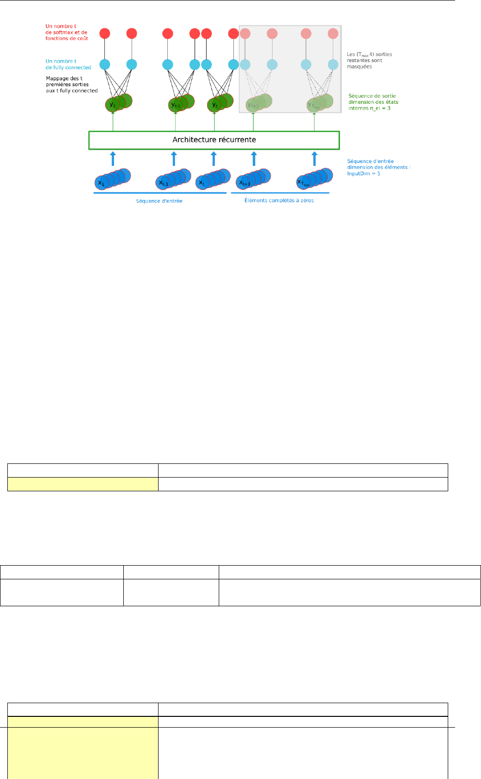
Figure 14: RNN model : variable sequence length and labeling scaled at each element of the sequence
need to be masked so it doesn’t influence longer sequences.
Development guidance :
•
Replace the inner local variables of LSTMCell_Frame_Cuda with a generic layer of shuffling
(on device) to enable the the process of data batch.
•
Develop some kind of label embedding within the layer to better articulate the labeling
granularity of the input data.
•Adapt structures to support the STATIC and DYNAMIC algorithm of cuDNN functions.
4.7.17 Dropout
Dropout layer (Srivastava et al.,2012).
Option [default value] Description
NbOutputs Number of output neurons
Configuration parameters (Frame models)
Option [default value] Model(s) Description
Dropout [0.5] all Frame
The probability with which the value from input would
be dropped
4.7.18 Padding
Padding layer.
Option [default value] Description
NbOutputs Number of output neurons
TopPadding Size of the top padding (positive or negative)
BottomPadding Size of the bottom padding (positive or negative)
LeftPadding Size of the left padding (positive or negative)
RightPadding Size of the right padding (positive or negative)
The padding layer allow to insert asymmetric padding for each layer axes.
4.7.19 Resize
Resize layer can be applied to change dimension of features maps or of stimuli provider.
Option [default value] Description
64/78

NbOutputs Number of output feature maps
OutputHeight Output height dimension
OutputWidth Output width dimension
Mode
Resize interpolation mode. Can be,
Bilinear
or
BilinearTF
(TensorFlow implementation)
Configuration parameters
Option [default value] Model(s) Description
AlignCorners [True] all Frame
Corner alignement mode if
BilinearTF
is used as inter-
polation mode
4.7.20 BatchNorm
Batch Normalization layer (Ioffe and Szegedy,2015).
Option [default value] Description
NbOutputs Number of output neurons
ActivationFunction [Tanh]
Activation function. Can be any of
Logistic
,
LogisticWithLoss
,
Rectifier,Softplus,TanhLeCun,Linear,Saturation or Tanh
ScalesSharing [] Share the scales with an other layer
BiasesSharing [] Share the biases with an other layer
MeansSharing [] Share the means with an other layer
VariancesSharing [] Share the variances with an other layer
Configuration parameters (Frame models)
Option [default value] Model(s) Description
Solvers.*all Frame Any solver parameters
ScaleSolver.*all Frame
Scale solver parameters, take precedence over the
Solvers.* parameters
BiasSolver.*all Frame
Bias solver parameters, take precedence over the
Solvers.* parameters
Epsilon [0.0] all Frame
Epsilon value used in the batch normalization formula.
If 0.0, automatically choose the minimum possible
value.
4.7.21 Transformation
Transformation layer, which can apply any transformation described in 4.6.1. Useful for fully CNN
post-processing for example.
65/78

Option [default value] Description
NbOutputs Number of outputs
Transformation Name of the transformation to apply
The Transformation options must be placed in the same section.
Usage example for fully CNNs:
[post.Transformation-thres]
Input=... ; for example, network’s logistic of softmax output layer
NbOutputs=1
Type=Transformation
Transformation=ThresholdTransformation
Operation=ToZero
Threshold=0.75
[post.Transformation-morpho]
Input=post.Transformation-thres
NbOutputs=1
Type=Transformation
Transformation=MorphologyTransformation
Operation=Opening
Size=3
66/78

5 Tutorials
5.1 Learning deep neural networks: tips and tricks
5.1.1 Choose the learning solver
Generally, you should use the SGD solver with a momemtum (typical value for the momentum:
0.9). It generalizes better, often significantly better, than adaptive methods like Adam (Wilson
et al.,2017).
Adaptive solvers, like Adam, may be used for fast exploration and prototyping, thanks to their
fast convergence.
5.1.2 Choose the learning hyper-parameters
To start a learning from scratch, a learning rate of 0.1 or 0.01 may be considered, for large batch
sizes (typically 256). Remind that if you scale the batch size (
N
) by a factor
k
, you should scale
the learning rate accordingly. A simple linear scaling rule is recommanded (Goyal et al.,2017).
Typical values for the SGDSolver are:
Solvers.LearningRate=0.1
Solvers.Decay=0.0001
Solvers.Momentum=0.9
5.1.3 Convergence and normalization
Deep networks (> 30 layers) and especially residual networks usually don’t converge without
normalization. Indeed, batch normalization is almost always used. ZeroInit is a method that can
be used to overcome this issue without normalization (Zhang et al.,2019).
5.2 Building a classifier neural network
For this tutorial, we will use the classical MNIST handwritten digit dataset. A driver module
already exists for this dataset, named MNIST_IDX_Database.
To instantiate it, just add the following lines in a new INI file:
[database]
Type=MNIST_IDX_Database
Validation=0.2 ; Use 20% of the dataset for validation
In order to create a neural network, we first need to define its input, which is declared with a
[sp]
section (sp for StimuliProvider). In this section, we configure the size of the input and the
batch size:
[sp]
SizeX=32
SizeY=32
BatchSize=128
We can also add pre-processing transformations to the StimuliProvider, knowing that the final
data size after transformations must match the size declared in the
[sp]
section. Here, we must
rescale the MNIST 28x28 images to match the 32x32 network input size.
[sp.Transformation_1]
Type=RescaleTransformation
Width=[sp]SizeX
Height=[sp]SizeY
Next, we declare the neural network layers. In this example, we reproduced the well-known
LeNet network. The first layer is a 5x5 convolutional layer, with 6 channels. Since there is only one
input channel, there will be only 6 convolution kernels in this layer.
67/78

[conv1]
Input=sp
Type=Conv
KernelWidth=5
KernelHeight=5
NbOutputs=6
The next layer is a 2x2 MAX pooling layer, with a stride of 2 (non-overlapping MAX pooling).
[pool1]
Input=conv1
Type=Pool
PoolWidth=2
PoolHeight=2
NbOutputs=[conv1]NbOutputs
Stride=2
Pooling=Max
Mapping.Size=1 ; One to one connection between input and output channels
The next layer is a 5x5 convolutional layer with 16 channels.
[conv2]
Input=pool1
Type=Conv
KernelWidth=5
KernelHeight=5
NbOutputs=16
Note that in LeNet, the
[conv2]
layer is not fully connected to the pooling layer. In N2D2, a
custom mapping can be defined for each input connection. The connection of
n
-th output map to
the inputs is defined by the
n
-th column of the matrix below, where the rows correspond to the
inputs.
Mapping(pool1)=\
1000111001111011\
1100011100111101\
1110001110010111\
0111001111001011\
0011100111101101\
0001110011110111
Another MAX pooling and convolution layer follow:
[pool2]
Input=conv2
Type=Pool
PoolWidth=2
PoolHeight=2
NbOutputs=[conv2]NbOutputs
Stride=2
Pooling=Max
Mapping.Size=1
[conv3]
Input=pool2
Type=Conv
KernelWidth=5
KernelHeight=5
NbOutputs=120
The network is composed of two fully-connected layers of 84 and 10 neurons respectively:
[fc1]
Input=conv3
Type=Fc
NbOutputs=84
68/78

[fc2]
Input=fc1
Type=Fc
NbOutputs=10
Finally, we use a softmax layer to obtain output classification probabilities and compute the
loss function.
[softmax]
Input=fc2
Type=Softmax
NbOutputs=[fc2]NbOutputs
WithLoss=1
In order to tell N2D2 to compute the error and the classification score on this softmax layer, one
must attach a N2D2 Target to this layer, with a section with the same name suffixed with
.Target
:
[softmax.Target]
By default, the activation function for the convolution and the fully-connected layers is the
hyperbolic tangent. Because the
[fc2]
layer is fed to a softmax, it should not have any activation
function. We can specify it by adding the following line in the [fc2] section:
[fc2]
...
ActivationFunction=Linear
In order to improve further the networks performances, several things can be done:
•Use ReLU activation functions.
In order to do so, just add the following in the
[conv1]
,
[conv2],[conv3] and [fc1] layer sections:
ActivationFunction=Rectifier
For the ReLU activation function to be effective, the weights must be initialized carefully, in
order to avoid dead units that would be stuck in the ]
− ∞,
0] output range before the ReLU
function. In N2D2, one can use a custom
WeightsFiller
for the weights initialization. For the
ReLU activation function, a popular and efficient filler is the so-called
XavierFiller
(see the
4.7.2 section for more information):
WeightsFiller=XavierFiller
•Use dropout layers.
Dropout is highly effective to improve the network generalization
capacity. Here is an example of a dropout layer inserted between the [fc1] and [fc2] layers:
[fc1]
...
[fc1.drop]
Input=fc1
Type=Dropout
NbOutputs=[fc1]NbOutputs
[fc2]
Input=fc1.drop ; Replaces "Input=fc1"
...
•Tune the learning parameters.
You may want to tune the learning rate and other learning
parameters depending on the learning problem at hand. In order to do so, you can add a
configuration section that can be common (or not) to all the layers. Here is an example of
configuration section:
[conv1]
...
ConfigSection=common.config
69/78

[...]
...
[common.config]
NoBias=1
WeightsSolver.LearningRate=0.05
WeightsSolver.Decay=0.0005
Solvers.LearningRatePolicy=StepDecay
Solvers.LearningRateStepSize=[sp]_EpochSize
Solvers.LearningRateDecay=0.993
Solvers.Clamping=1
For more details on the configuration parameters for the Solver, see section 4.7.3.
•Add input distortion. See for example the DistortionTransformation (section 4.6.1).
The complete INI model corresponding to this tutorial can be found in models/LeNet.ini.
In order to use CUDA/GPU accelerated learning, the default layer model should be switched to
Frame_CUDA
. You can enable this model by adding the following line at the top of the INI file (before
the first section):
DefaultModel=Frame_CUDA
5.3 Building a segmentation neural network
In this tutorial, we will learn how to do image segmentation with N2D2. As an example, we will
implement a face detection and gender recognition neural network, using the IMDB-WIKI dataset.
First, we need to instanciate the IMDB-WIKI dataset built-in N2D2 driver:
[database]
Type=IMDBWIKI_Database
WikiSet=1 ; Use the WIKI part of the dataset
IMDBSet=0 ; Don’t use the IMDB part (less accurate annotation)
Learn=0.90
Validation=0.05
DefaultLabel=background ; Label for pixels outside any ROI (default is no label, pixels are
ignored)
We must specify a default label for the background, because we want to learn to differenciate
faces from the background (and not simply ignore the background for the learning).
The network input is then declared:
[sp]
SizeX=480
SizeY=360
BatchSize=48
CompositeStimuli=1
In order to work with segmented data, i.e. data with bounding box annotations or pixel-wise
annotations (as opposed to a single label per data), one must enable the
CompositeStimuli
option in
the [sp] section.
We can then perform various operations on the data before feeding it to the network, like for
example converting the 3-channels RGB input images to single-channel gray images:
[sp.Transformation-1]
Type=ChannelExtractionTransformation
CSChannel=Gray
We must only rescale the images to match the networks input size. This can be done using
a
RescaleTransformation
, followed by a
PadCropTransformation
if one want to keep the images aspect
ratio.
70/78

[sp.Transformation-2]
Type=RescaleTransformation
Width=[sp]SizeX
Height=[sp]SizeY
KeepAspectRatio=1 ; Keep images aspect ratio
; Required to ensure all the images are the same size
[sp.Transformation-3]
Type=PadCropTransformation
Width=[sp]SizeX
Height=[sp]SizeY
A common additional operation to extend the learning set is to apply random horizontal mirror
to images. This can be achieved with the following FlipTransformation:
[sp.OnTheFlyTransformation-4]
Type=FlipTransformation
RandomHorizontalFlip=1
ApplyTo=LearnOnly ; Apply this transformation only on the learning set
Note that this is an on-the-fly transformation, meaning it cannot be cached and is re-executed
every time even for the same stimuli. We also apply this transformation only on the learning set,
with the ApplyTo option.
Next, the neural network can be described:
[conv1.1]
Input=sp
Type=Conv
...
[pool1]
...
[...]
...
[fc2]
Input=drop1
Type=Conv
...
[drop2]
Input=fc2
Type=Dropout
NbOutputs=[fc2]NbOutputs
A full network description can be found in the IMDBWIKI.ini file in the models directory of
N2D2. It is a fully-CNN network.
Here we will focus on the output layers required to detect the faces and classify their gender.
We start from the [drop2] layer, which has 128 channels of size 60x45.
5.3.1 Faces detection
We want to first add an output stage for the faces detection. It is a 1x1 convolutional layer with a
single 60x45 output map. For each output pixel, this layer outputs the probability that the pixel
belongs to a face.
[fc3.face]
Input=drop2
Type=Conv
KernelWidth=1
KernelHeight=1
NbOutputs=1
71/78

Stride=1
ActivationFunction=LogisticWithLoss
WeightsFiller=XavierFiller
ConfigSection=common.config ; Same solver options that the other layers
In order to do so, the activation function of this layer must be of type LogisticWithLoss.
We must also tell N2D2 to compute the error and the classification score on this softmax layer,
by attaching a N2D2 Target to this layer, with a section with the same name suffixed with
.Target
:
[fc3.face.Target]
LabelsMapping=${N2D2_MODELS}/IMDBWIKI_target_face.dat
; Visualization parameters
NoDisplayLabel=0
LabelsHueOffset=90
In this Target, we must specify how the dataset annotations are mapped to the layer’s output.
This can be done in a separate file using the
LabelsMapping
parameter. Here, since the output layer
has a single output per pixel, the target value can only be 0 or 1. A target value of -1 means that
this output is ignored (no error back-propagated). Since the only annotations in the IMDB-WIKI
dataset are faces, the mapping described in the IMDBWIKI_target_face.dat file is easy:
# background
background 0
# padding (*) is ignored (-1)
* -1
# not background = face
default 1
5.3.2 Gender recognition
We can also add a second output stage for gender recognition. Like before, it would be a 1x1
convolutional layer with a single 60x45 output map. But here, for each output pixel, this layer
would output the probability that the pixel represents a female face.
[fc3.gender]
Input=drop2
Type=Conv
KernelWidth=1
KernelHeight=1
NbOutputs=1
Stride=1
ActivationFunction=LogisticWithLoss
WeightsFiller=XavierFiller
ConfigSection=common.config
The output layer is therefore identical to the face’s output layer, but the target mapping is
different. For the target mapping, the idea is simply to ignore all pixels not belonging to a face and
affect the target 0 to male pixels and the target 1 to female pixels.
[fc3.gender.Target]
LabelsMapping=${N2D2_MODELS}/IMDBWIKI_target_gender.dat
; Only display gender probability for pixels detected as face pixels
MaskLabelTarget=fc3.face.Target
MaskedLabel=1
The content of the IMDBWIKI_target_gender.dat file would therefore look like:
# background
# ?-* (unknown gender)
# padding
default -1
72/78

# male gender
M-? 0 # unknown age
M-0 0
M-1 0
M-2 0
...
M-98 0
M-99 0
# female gender
F-? 1 # unknown age
F-0 1
F-1 1
F-2 1
...
F-98 1
F-99 1
5.3.3 ROIs extraction
The next step would be to extract detected face ROIs and assign for each ROI the most probable
gender. To this end, we can first set a detection threshold, in terms of probability, to select face
pixels. In the following, the threshold is fixed to 75% face probability:
[post.Transformation-thres]
Input=fc3.face
Type=Transformation
NbOutputs=1
Transformation=ThresholdTransformation
Operation=ToZero
Threshold=0.75
We can then assign a target of type
TargetROIs
to this layer that will automatically create the
bounding box using a segmentation algorithm.
[post.Transformation-thres.Target-face]
Type=TargetROIs
MinOverlap=0.33 ; Min. overlap fraction to match the ROI to an annotation
FilterMinWidth=5 ; Min. ROI width
FilterMinHeight=5 ; Min. ROI height
FilterMinAspectRatio=0.5 ; Min. ROI aspect ratio
FilterMaxAspectRatio=1.5 ; Max. ROI aspect ratio
LabelsMapping=${N2D2_MODELS}/IMDBWIKI_target_face.dat
In order to assign a gender to the extracted ROIs, the above target must be modified to:
[post.Transformation-thres.Target-gender]
Type=TargetROIs
ROIsLabelTarget=fc3.gender.Target
MinOverlap=0.33
FilterMinWidth=5
FilterMinHeight=5
FilterMinAspectRatio=0.5
FilterMaxAspectRatio=1.5
LabelsMapping=${N2D2_MODELS}/IMDBWIKI_target_gender.dat
Here, we use the fc3.gender.Target target to determine the most probable gender of the ROI.
5.3.4 Data visualization
For each Target in the network, a corresponding folder is created in the simulation directory, which
contains learning, validation and test confusion matrixes. The output estimation of the network for
each stimulus is also generated automatically for the test dataset and can be visualized with the
./test.py helper tool. An example is shown in figure 15.
73/78
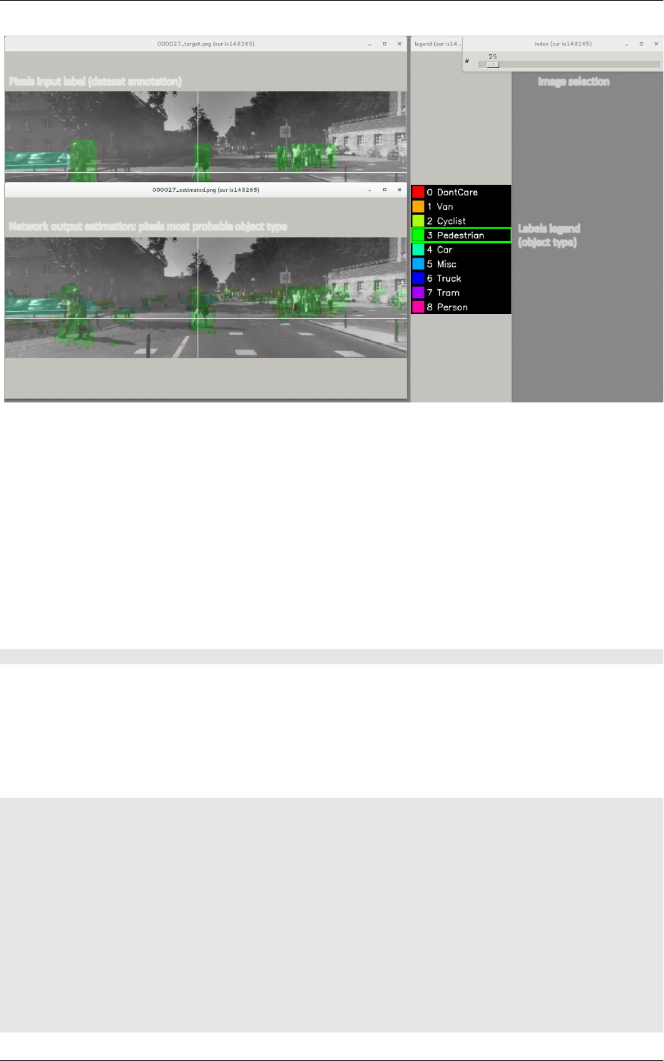
Image selection
Labels legend
(object type)
Network output estimation: pixels most probable object type
Pixels input label (dataset annotation)
Figure 15: Example of the target visualization helper tool.
5.4 Transcoding a learned network in spike-coding
N2D2 embeds an event-based simulator (historically known as ’Xnet’) and allows to transcode a
whole DNN in a spike-coding version and evaluate the resulting spiking neural network performances.
In this tutorial, we will transcode the LeNet network described in section 5.2.
5.4.1 Render the network compatible with spike simulations
The first step is to specify that we want to use a transcode model (allowing both formal and spike
simulation of the same network), by changing the DefaultModel to:
DefaultModel=Transcode_CUDA
In order to perform spike simulations, the input of the network must be of type Environment,
which is a derived class of StimuliProvider that adds spike coding support. In the INI model file, it
is therefore necessary to replace the
[sp]
section by an
[env]
section and replace all references of
sp
to env.
Note that these changes have at this point no impact at all on the formal coding simulations.
The beginning of the INI file should be:
DefaultModel=Transcode_CUDA
; Database
[database]
Type=MNIST_IDX_Database
Validation=0.2 ; Use 20% of the dataset for validation
; Environment
[env]
SizeX=32
SizeY=32
BatchSize=128
[env.Transformation_1]
Type=RescaleTransformation
74/78

Width=[env]SizeX
Height=[env]SizeY
[conv1]
Input=env
...
The dropout layer has no equivalence in spike-coding inference and must be removed:
...
[fc1.drop]
Input=fc1
Type=Dropout
NbOutputs=[fc1]NbOutputs
[fc2]
Input=fc1.drop
...
The softmax layer has no equivalence in spike-coding inference and must be removed as well.
The Target must therefore be attached to [fc2]:
...
[softmax]
Input=fc2
Type=Softmax
NbOutputs=[fc2]NbOutputs
WithLoss=1
[softmax.Target]
[fc2.Target]
...
The network is now compatible with spike-coding simulations. However, we did not specify at
this point how to translate the input stimuli data into spikes, nor the spiking neuron parameters
(threshold value, leak time constant...).
5.4.2 Configure spike-coding parameters
The first step is to configure how the input stimuli data must be coded into spikes. To this end, we
must attach a configuration section to the Environment. Here, we specify a periodic coding with
random initial jitter with a minimum period of 10 ns and a maximum period of 100 us:
[env]
...
ConfigSection=env.config
[env.config]
; Spike-based computing
StimulusType=JitteredPeriodic
PeriodMin=1,000,000 ; unit = fs
PeriodMeanMin=10,000,000 ; unit = fs
PeriodMeanMax=100,000,000,000 ; unit = fs
PeriodRelStdDev=0.0
The next step is to specify the neurons parameters, that will be common to all layers and can
therefore be specified in the
[common.config]
section. In N2D2, the base spike-coding layers use a
Leaky Integrate-and-Fire (LIF) neuron model. By default, the leak time constant is zero, resulting
to simple Integrate-and-Fire (IF) neurons.
Here we simply specify that the neurons threshold must be the unity, that the threshold is only
positive and that there is no incoming synaptic delay:
75/78

[common.config]
...
; Spike-based computing
Threshold=1.0
BipolarThreshold=0
IncomingDelay=0
Finally, we can limit the number of spikes required for the computation of each stimulus by
adding a decision delta threshold at the output layer:
[fc2]
...
ConfigSection=common.config,fc2.config
[fc2.Target]
[fc2.config]
; Spike-based computing
TerminateDelta=4
BipolarThreshold=1
The complete INI model corresponding to this tutorial can be found in models/LeNet_Spike.ini.
Here is a summary of the steps required to reproduce the whole experiment:
./n2d2 "$N2D2_MODELS/LeNet.ini" -learn 6000000 -log 100000
./n2d2 "$N2D2_MODELS/LeNet_Spike.ini" -test
The final recognition rate reported at the end of the spike inference should be almost identical
to the formal coding network (around 99% for the LeNet network).
Various statistics are available at the end of the spike-coding simulation in the stats_spike
folder and the stats_spike.log file. Looking in the stats_spike.log file, one can read the following
line towards the end of the file:
Read events per virtual synapse per pattern (average): 0.654124
This line reports the average number of accumulation operations per synapse per input stimulus
in the network. If this number if below 1.0, it means that the spiking version of the network is
more efficient than its formal counterpart in terms of total number of operations!
76/78

References
M. Cordts, M. Omran, S. Ramos, T. Rehfeld, M. Enzweiler, R. Benenson, U. Franke, S. Roth, and
B. Schiele. The cityscapes dataset for semantic urban scene understanding. In Proc. of the IEEE
Conference on Computer Vision and Pattern Recognition (CVPR), 2016.
P. Dollár, C. Wojek, B. Schiele, and P. Perona. Pedestrian detection: A benchmark. In CVPR,
2009.
L. Fei-Fei, R. Fergus, and P. Perona. Learning generative visual models from few training examples:
an incremental bayesian approach tested on 101 object categories. In IEEE. CVPR 2004,
Workshop on Generative-Model Based Vision, 2004.
X. Glorot and Y. Bengio. Understanding the difficulty of training deep feedforward neural networks.
In International conference on artificial intelligence and statistics, page 249–256, 2010.
P. Goyal, P. Dollár, R. B. Girshick, P. Noordhuis, L. Wesolowski, A. Kyrola, A. Tulloch, Y. Jia,
and K. He. Accurate, large minibatch SGD: training imagenet in 1 hour. CoRR, abs/1706.02677,
2017. URL http://arxiv.org/abs/1706.02677.
B. Graham. Fractional max-pooling. CoRR, abs/1412.6071, 2014.
G. Griffin, A. Holub, and P. Perona. Caltech-256 object category dataset, 2007.
K. He, X. Zhang, S. Ren, and J. Sun. Delving deep into rectifiers: Surpassing human-level
performance on imagenet classification. In Proceedings of the 2015 IEEE International Conference
on Computer Vision (ICCV), ICCV ’15, pages 1026–1034, 2015. doi: 10.1109/ICCV.2015.123.
S. Hochreiter and J. Schmidhuber. Long short-term memory. Neural Computation, 9(8):1735–1780,
1997. doi: 10.1162/neco.1997.9.8.1735.
S. Houben, J. Stallkamp, J. Salmen, M. Schlipsing, and C. Igel. Detection of traffic signs in
real-world images: The German Traffic Sign Detection Benchmark. In International Joint
Conference on Neural Networks, number 1288, 2013.
S. Ioffe and C. Szegedy. Batch normalization: Accelerating deep network training by reducing
internal covariate shift. CoRR, abs/1502.03167, 2015.
V. Jain and E. Learned-Miller. FDDB: A benchmark for face detection in unconstrained settings,
2010.
D. P. Kingma and J. Ba. Adam: A method for stochastic optimization. CoRR, abs/1412.6980,
2014. URL http://arxiv.org/abs/1412.6980.
A. Krizhevsky. Learning multiple layers of features from tiny images, 2009.
Y. LeCun, L. Bottou, Y. Bengio, and P. Haffner. Gradient-based learning applied to document
recognition. In Proceedings of the IEEE, volume 86, pages 2278–2324, 1998.
P. Lucey, J. F. Cohn, T. Kanade, J. Saragih, Z. Ambadar, and I. Matthews. The Extended Cohn-
Kanade Dataset (CK+): A complete dataset for action unit and emotion-specified expression.
2010.
A. Rakotomamonjy and G. Gasso. Histogram of gradients of time-frequency representations for
audio scene detection, 2014.
77/78

O. Russakovsky, J. Deng, H. Su, J. Krause, S. Satheesh, S. Ma, Z. Huang, A. Karpathy,
A. Khosla, M. Bernstein, A. C. Berg, and L. Fei-Fei. ImageNet Large Scale Visual Recog-
nition Challenge. International Journal of Computer Vision (IJCV), 115(3):211–252, 2015. doi:
10.1007/s11263-015-0816-y.
N. Srivastava, G. Hinton, A. Krizhevsky, I. Sutskever, and R. Salakhutdinov. Dropout: A simple
way to prevent neural networks from voverfitting. Journal of Machine Learning Research, 15:
1929–1958, 2012.
J. Stallkamp, M. Schlipsing, J. Salmen, and C. Igel. Man vs. computer: Benchmarking machine
learning algorithms for traffic sign recognition. Neural Networks, 2012. ISSN 0893-6080. doi:
10.1016/j.neunet.2012.02.016.
A. C. Wilson, R. Roelofs, M. Stern, N. Srebro, and B. Recht. The Marginal Value of Adaptive
Gradient Methods in Machine Learning. arXiv e-prints, art. arXiv:1705.08292, May 2017.
G. Xia, X. Bai, J. Ding, Z. Zhu, S. J. Belongie, J. Luo, M. Datcu, M. Pelillo, and L. Zhang. DOTA:
A large-scale dataset for object detection in aerial images. CoRR, abs/1711.10398, 2017. URL
http://arxiv.org/abs/1711.10398.
H. Zhang, Y. N. Dauphin, and T. Ma. Residual learning without normalization via better
initialization. In International Conference on Learning Representations, 2019. URL
https:
//openreview.net/forum?id=H1gsz30cKX.
78/78
