Manual
User Manual:
Open the PDF directly: View PDF ![]() .
.
Page Count: 44
- Citation, license, and obtaining the package
- Version history
- Capabilities and related reading and software
- Structure of DDE-BIFTOOL
- Delay differential equations
- System definition
- Data structures
- Point manipulation
- Branch manipulation
- Numerical methods
- Concluding comments
- Jacobians of tutorial examples !neuron! and !sddemo!
- Octave compatibility considerations
DDE-BIFTOOL v. 3.1.1 Manual —
Bifurcation analysis of delay differential
equations
J. Sieber, K. Engelborghs, T. Luzyanina, G. Samaey, D. Roose
April 5, 2017
Keywords
nonlinear dynamics, delay-differential equations, stability analysis, periodic solutions,
collocation methods, numerical bifurcation analysis, state-dependent delay.
1 Citation, license, and obtaining the package 1
2 Version history 2
2.1 Changes from 3.1 to 3.1.1 ................................... 2
2.2 Changes from 3.0 to 3.1 .................................... 2
2.3 Changes from 2.03 to 3.0 ................................... 3
3 Capabilities and related reading and software 3
4 Structure of DDE-BIFTOOL 5
5 Delay differential equations 6
5.1 Equations with constant delays ............................... 6
5.1.1 Steady states ...................................... 6
5.1.2 Periodic orbits ..................................... 7
5.1.3 Connecting orbits ................................... 7
5.2 Equations with state-dependent delays .......................... 7
6 System definition 9
6.1 Change from DDE-BIFTOOL v. 2.03 to v. 3.0 ....................... 9
6.2 Equations with constant delays ............................... 9
6.2.1 Right-hand side — sys_rhs ............................. 9
6.2.2 Delays — sys_tau .................................. 10
6.2.3 Jacobians of right-hand side — sys_deri (optional, but recommended) . . . 10
6.3 Equations with state-dependent delays .......................... 11
6.3.1 Right-hand side — sys_rhs ............................. 12
6.3.2 Delays — sys_tau and sys_ntau .......................... 12
6.3.3 Jacobian of right-hand side — sys_deri (optional, but recommended) . . . . 13
6.3.4 Jacobians of delays — sys_dtau (optional, but recommended) ......... 13
6.4 Extra conditions — sys_cond ................................ 14
6.5 Collecting user functions into a structure — call set_funcs ............... 14
i
7 Data structures 15
7.1 Problem definition (functions) structure .......................... 15
7.2 Point structures ........................................ 16
7.3 Stability structures ...................................... 18
7.4 Method parameters ...................................... 18
7.5 Branch structures ....................................... 19
7.6 Scalar measure structure ................................... 21
8 Point manipulation 21
9 Branch manipulation 24
10 Numerical methods 27
10.1 Determining systems ..................................... 27
10.2 Extra conditions ........................................ 29
10.3 Continuation .......................................... 30
10.4 Roots of the characteristic equation ............................. 31
10.5 Floquet multipliers ...................................... 33
11 Concluding comments 33
11.1 Existing extensions ...................................... 34
A Jacobians of tutorial examples neuron and sd_demo 38
B Octave compatibility considerations 42
ii

1. Citation, license, and obtaining the package
DDE-BIFTOOL was started by Koen Engelborghs as part of his PhD at the Computer Science
Department of the K.U.Leuven under supervision of Prof. Dirk Roose.
Citation
Scientific publications for which the package DDE-BIFTOOL has been used shall mention
usage of the package DDE-BIFTOOL, and shall cite the following publications to ensure proper
attribution and reproducibility:
•
K. Engelborghs, T. Luzyanina, and D. Roose. Numerical bifurcation analysis of delay differen-
tial equations using DDE-BIFTOOL, ACM Trans. Math. Softw. 28 (1), pp. 1-21, 2002.
•(this manual)
J. Sieber, K. Engelborghs, T. Luzyanina, G. Samaey, D. Roose . DDE-BIFTOOL v.
3.1.1 Manual — Bifurcation analysis of delay differential equations,
http://arxiv.org/abs/
1406.7144.
The implementation of normal forms for equilibria is based on
•
M. M. Bosschaert, B. Wage and Y. Kuznetsov: Description of the extension
ddebiftool nmfm
http://ddebiftool.sourceforge.net/nmfm_extension_description.pdf, 2015.
•
B. Wage: Normal form computations for Delay Differential Equations in DDE-BIFTOOL. Master
Thesis, Utrecht University (NL), supervised by Y.A. Kuznetsov (
http://dspace.library.uu.
nl/handle/1874/296912, 2014.
•
M. M. Bosschaert: Switching from codimension 2 bifurcations of equilibria in delay differential
equations. Master Thesis, Utrecht University (NL), supervised by Y.A. Kuznetsov,
http:
//dspace.library.uu.nl/handle/1874/334792, 2016.
All versions of this manual from v. 3.0 onward are available at
http://arxiv.org/abs/1406.7144
.
License The following terms cover the use of the software package DDE-BIFTOOL:
BSD 2-Clause license
Copyright (c) 2017, K.U. Leuven, Department of Computer Science, K. Engelborghs, T.
Luzyanina, G. Samaey. D. Roose, K. Verheyden, J. Sieber, B. Wage, D. Pieroux
All rights reserved.
Redistribution and use in source and binary forms, with or without modification,
are permitted provided that the following conditions are met:
1. Redistributions of source code must retain the above copyright notice, this
list of conditions and the following disclaimer.
2. Redistributions in binary form must reproduce the above copyright notice, this
list of conditions and the following disclaimer in the documentation and/or other
materials provided with the distribution.
THIS SOFTWARE IS PROVIDED BY THE COPYRIGHT HOLDERS AND CONTRIBUTORS "AS IS" AND
ANY EXPRESS OR IMPLIED WARRANTIES, INCLUDING, BUT NOT LIMITED TO, THE IMPLIED
WARRANTIES OF MERCHANTABILITY AND FITNESS FOR A PARTICULAR PURPOSE ARE DISCLAIMED.
IN NO EVENT SHALL THE COPYRIGHT HOLDER OR CONTRIBUTORS BE LIABLE FOR ANY DIRECT,
INDIRECT, INCIDENTAL, SPECIAL, EXEMPLARY, OR CONSEQUENTIAL DAMAGES (INCLUDING, BUT
NOT LIMITED TO, PROCUREMENT OF SUBSTITUTE GOODS OR SERVICES; LOSS OF USE, DATA, OR
PROFITS; OR BUSINESS INTERRUPTION) HOWEVER CAUSED AND ON ANY THEORY OF LIABILITY,
WHETHER IN CONTRACT, STRICT LIABILITY, OR TORT (INCLUDING NEGLIGENCE OR OTHERWISE)
ARISING IN ANY WAY OUT OF THE USE OF THIS SOFTWARE, EVEN IF ADVISED OF THE
POSSIBILITY OF SUCH DAMAGE.
1

Download
Upon acceptance of the above terms, one can obtain the package DDE-BIFTOOL
(version 3.1.1) from
https://sourceforge.net/projects/ddebiftool.
Versions up to 3.0 and resources on theoretical background continue to be available (under a different
license) on
http://twr.cs.kuleuven.be/research/software/delay/ddebiftool.shtml.
2. Version history
2.1. Changes from 3.1 to 3.1.1
•
Small bug fix: when changing focus on plot window during
br_contn
, the online plotting
no longer follows focus. This keeps the online bifurcation diagram in the same window. An
optional named argument
plotaxis
has been added to
br_contn
to explicitly set the plot
axes.
•
Added support for rotations (phase oscillators). Periodicity is enforced only up to multiples of
2
π
. Demo
../demos/phase_oscillator/html/phase_oscillator.html
shows how one can
track rotations. Demo was contributed by Azamat Yeldesbay.
• Demos showing detection and computation of Bodganov-Takens bifurcation in
../demos/Holling-Tanner/html/HollingTanner_demo.html
and cusp in
../demos/cusp/html/cusp_demo.html.
Contributed by M. M. Boschaert and Y. Kuznetsov.
•
A description of the mathematical formulas behind the normal form computations is now in
nmfm_extension_description.pdf, by M.Bossschaert, B. Wage, Y. Kuznetsov.
2.2. Changes from 3.0 to 3.1
Change of License and move to Sourceforge
D. Roose has permitted to change the license to a
Sourceforge-compliant BSD License. Thus, code and newest releases from version 3.1 onward are
now available from
https://sourceforge.net/projects/ddebiftool
. Older versions will con-
tinue to be available from
http://twr.cs.kuleuven.be/research/software/delay/ddebiftool.
shtml.
New feature: Normal form computation for bifurcations of equilibria
The new functionality is only
applicable for equations with constant delay. Normal form coefficients can be computed through
the extension
ddebiftool extra nmfm
. This extension is included in the standard DDE-BIFTOOL
archive, but the additional functions are kept in a separate folder. The following bifurcations are
currently supported.
• Hopf bifurcation (coefficient L1determining criticality),
•
generalized Hopf (Bautin) bifurcation (of codimension two, typically encountered along Hopf
curves)
•
Zero-Hopf interaction (Gavrilov-Guckenheimer bifurcation, of codimension two, typically
encountered along Hopf curves)
2

• Hopf-Hopf interaction (of codimension two, typically encountered along Hopf curves)
The extension comes with a demo
nmfm demo
. The demos
neuron
,
minimal demo
and
Mackey-Glass
illustrate the new functionality, too. Background theory is given in [46].
2.3. Changes from 2.03 to 3.0
New features
•Continuation of local periodic orbit bifurcations
for systems with constant or state-dependent
delay is now supported through the extension
ddebiftool extra psol
. This extension is
included in the standard DDE-BIFTOOL archive, but the additional functions are kept in a
separate folder.
•User-defined functions
specifying the right-hand side and delays (such as
sys_rhs
and
sys_tau
)
can have arbitrary names. These user functions (with arbitrary names) get collected in a struc-
ture
funcs
, which gets then passed on to the DDE-BIFTOOL routines. This interface is similar
to other functions acting on Matlab functions such as
fzero
or
ode45
. It enables users to add
extensions such as ddebiftool extra psol without changing the core routines.
•State-dependent delays
can now have arbitrary levels of nesting (for example, periodic orbits
of ˙
x(t) = µ−x(t−x(t−x(t−x(t)))) and their bifurcations can be tracked).
•Vectorization
Continuation of periodic orbits and their bifurcations benefits (moderately)
from vectorization of the user-defined functions.
•Utilities
Recurring tasks (such as branching off at bifurcations, defining initial pieces of
branches, or extracting the number of unstable eigenvalues) can now be performed more con-
veniently with some auxiliary functions provided in a separate folder
ddebiftool utilities
.
See ../demos/neuron/html/demo1_simple.html for a demonstration.
•Bugs fixed
Some bugs and problems have been fixed in the implementation of the heuristics
applied to choose the stepsize in the computation of eigenvalues of equilibria [45].
•Continuation of relative equilibiria and relative periodic orbits
and their local bifurcations for
systems with constant delay and rotational symmetry (saddle-node bifurcation, Hopf bi-
furcation, period-doubling, and torus bifurcation) is now supported through the extension
ddebiftool extra rotsym.
Extensions come with demos and separate documentation.
Change of user interface
Versions from 3.0 onward have a different the user interface for many
DDE-BIFTOOL functions than versions up to 2.03. They add one additional input argument
funcs
(this new argument comes always first). Since DDE-BIFTOOL v. 3.0 changed the user interface,
scripts written for DDE-BIFTOOL v. 2.0x or earlier will not work with versions later than 3.0. For
this reason version 2.03 will continue to be available. Users of both versions should ensure that only
one version is in the Matlab path at any time to avoid naming conflicts.
3. Capabilities and related reading and software
DDE-BIFTOOL consists of a set of routines running in Matlab
1
[
29
] or octave
2
, both widely used
environments for scientific computing. The aim of the package is to provide a tool for numerical
1http://www.mathworks.com
2http://www.gnu.org/software/octave
3

bifurcation analysis of steady state solutions and periodic solutions of differential equations with
constant delays (called DDEs) or state-dependent delays (here called sd-DDEs). It also allows users
to compute homoclinic and heteroclinic orbits in DDEs (with constant delays).
Capabilities DDE-BIFTOOL can perform the following computations:
• continuation of steady state solutions (typically in a single parameter);
•
approximation of the rightmost, stability-determining roots of the characteristic equation
which can further be corrected using a Newton iteration;
•
continuation of steady state folds and Hopf bifurcations (typically in two system parameters);
•
continuation of periodic orbits using orthogonal collocation with adaptive mesh selection
(starting from a previously computed Hopf point or an initial guess of a periodic solution
profile);
• approximation of the largest stability-determining Floquet multipliers of periodic orbits;
•
branching onto the secondary branch of periodic solutions at a period doubling bifurcation or
a branch point;
•
continuation of folds, period doublings and torus bifurcations (typically in two system param-
eters) using the extension ddebiftool extra psol;
•
computation of normal form coefficients for Hopf bifurcations and codimension-two bifurca-
tions along Hopf bifurcation curves (typically in two system parameters) using the extension
ddebiftool extra nmfm;
• continuation of connecting orbits (using the appropriate number of parameters).
All computations can be performed for problems with an arbitrary number of discrete delays. These
delays can be either parameters or functions of the state. (The only exception are computations of
connecting orbits, which support only problems with delays as parameters at the moment.)
A practical difference to AUTO or MatCont is that the package does not detect bifurcations
automatically because the computation of eigenvalues or Floquet multipliers may require more
computational effort than the computation of the equilibria or periodic orbits (for example, if the
system dimension is small but one delay is large). Instead the evolution of the eigenvalues can be
computed along solution branches in a separate step if required. This allows the user to detect and
identify bifurcations.
About this manual — related reading
This manual documents version 3.1.1. Earlier versions of the
manual for earlier versions of DDE-BIFTOOL continue to be available at the web addresses
versions ≥3.0 http://arxiv.org/abs/1406.7144
versions ≤2.03 http://twr.cs.kuleuven.be/research/software/delay/ddebiftool.shtml.
For readers who intend to analyse only systems with constant delays, the parts of the manual
related to systems with state-dependent delays can be skipped (sections 5.2,6.3). In the rest of this
manual we assume the reader is familiar with the notion of a delay differential equation and with
the basic concepts of bifurcation analysis for ordinary differential equations. The theory on delay
differential equations and a large number of examples are described in several books. Most notably
the early [
4
,
13
,
14
,
25
,
32
] and the more recent [
2
,
30
,
26
,
10
,
31
]. Several excellent books contain
introductions to dynamical systems and bifurcation theory of ordinary differential equations, see,
e.g., [1,6,23,33,40].
Turorial demos
The tutorial demos
demo1
and
sd demo
, providing a step-by-step walk-through
for the typical working mode with DDE-BIFTOOL are included as separate
html
files, published
directly from the comments in the demo code. See
../demos/index.html
for links to all demos,
many of which are extensively commented.
4
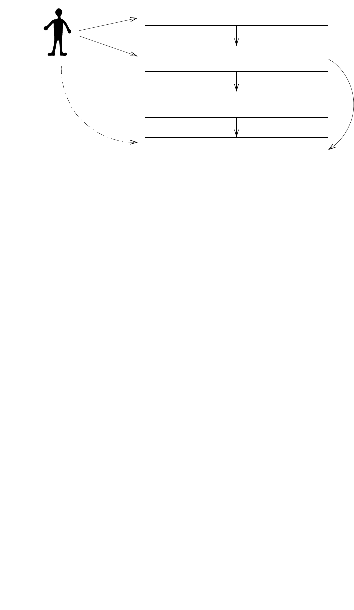
USER
Layer 0 : SYSTEM DEFINITION
Layer 2 : POINT MANIPULATION
Layer 1 : NUMERICAL METHODS
Layer 3 : BRANCH MANIPULATION
Figure 1:
The structure of DDE-BIFTOOL. Arrows indicate the calling (
−
) or writing (
·−
) of routines in a
certain layer.
Related software
A large number of packages exist for numerical continuation and bifurcation
analysis of systems of ordinary differential equations. Currently maintained packages are
AUTO url: http://sourceforge.net/projects/auto-07p using FORTRAN or C [12,11],
MatCont url: http://sourceforge.net/projects/matcont/ for Matlab [9,22], and
Coco url: http://sourceforge.net/projects/cocotools for Matlab [8].
For delay differential equations the package
knut url: http://gitorious.org/knut using C++
(formerly
PDDECONT
) is available as a stand-alone package (written in C++, but with a user interface
requiring no programming). This package was developed in parallel with DDE-BIFTOOL but
independently by R. Szalai [
44
,
38
]. For simulation (time integration) of delay differential equations
the reader is, e.g., referred to the packages ARCHI, DKLAG6, XPPAUT, DDVERK, RADAR and
dde23, see [
37
,
7
,
21
,
20
,
41
,
24
]. Of these, only XPPAUT has a graphical interface (and allows limited
stability analysis of steady state solutions of DDEs along the lines of [
35
]). TRACE-DDE is a Matlab
tool (with graphical interface) for linear stability analysis of linear constant-coefficient DDEs [5].
4. Structure of DDE-BIFTOOL
The structure of the package is depicted in figure 1. It consists of four layers.
Layer 0 contains the system definition and consists of routines which allow to evaluate the right
hand side
f
and its derivatives, state-dependent delays and their derivatives and to set or get the
parameters and the constant delays. It should be provided by the user and is explained in more
detail in section 6. All user-provided functions are collected in a single structure (called
funcs
in this
manual), and are passed on by the user as arguments to layer-3 or layer-2 functions.
Note that this
is a change in user interface between version 2.03 and version 3.0!
Layer 1 forms the numerical core of the package and is (normally) not directly accessed by the
user. The numerical methods used are explained briefly in section 10, more details can be found
in the papers [
35
,
18
,
17
,
16
,
19
,
34
,
39
] and in [
15
]. Its functionality is hidden by and used through
layers 2 and 3.
Layer 2 contains routines to manipulate individual points. Names of routines in this layer start
with ”
p
”. A point has one of the following five types. It can be a steady state point (abbreviated
5

stst
), steady state Hopf (abbreviated
hopf
) or fold (abbreviated
fold
) bifurcation point,
a periodic solution point (abbreviated
psol
) or a connecting orbit point (abbreviated
hcli
).
Furthermore, a point can contain additional information concerning its stability. Routines are
provided to compute individual points, to compute and plot their stability and to convert points
from one type to another.
Layer 3 contains routines to manipulate branches. Names of routines in this layer start with ”
br
”.
A branch is structure containing an array of (at least two) points, three sets of method parameters
and specifications concerning the free parameters. The
point
field of a branch contains an array
of points of the same type ordered along the branch. The
method
field contains parameters of the
computation of individual points, the continuation strategy and the computation of stability. The
parameter
field contains specification of the free parameters (which are allowed to vary along the
branch), parameter bounds and maximal step sizes. Routines are provided to extend a given branch
(that is, to compute extra points using continuation), to (re)compute stability along the branch and
to visualize the branch and/or its stability.
Layers 2 and 3 require specific data structures, explained in section 7, to represent points, stability
information, branches, to pass method parameters and to specify plotting information. Usage of these
layers is demonstrated through a step-by-step analysis of the demo systems
neuron
,
sd demo
and
hom demo
(see
../demos/index.html
). Descriptions of input/output parameters and functionality
of all routines in layers 2 and 3 are given in sections 8respectively 9.
5. Delay differential equations
This section introduces the mathematical notation that we refer to in this manual to describe the
problems solved by DDE-BIFTOOL.
5.1. Equations with constant delays
Consider the system of delay differential equations with constant delays (DDEs),
d
dtx(t) = f(x(t),x(t−τ1), . . . , x(t−τm),η), (1)
where
x(t)∈Rn
,
f:Rn(m+1)×Rp→Rn
is a nonlinear smooth function depending on a number of
parameters η∈Rp, and delays τi>0, i=1, . . . , m. Call τthe maximal delay,
τ=max
i=1,...,mτi.
The linearization of (1) around a solution x∗(t)is the variational equation, given by,
d
dty(t) = A0(t)y(t) +
m
∑
i=1
Ai(t)y(t−τi), (2)
where, using f≡f(x0,x1, . . . , xm,η),
Ai(t) = ∂f
∂xi(x∗(t),x∗(t−τ1), . . . , x∗(t−τm),η),i=0, . . . , m. (3)
5.1.1. Steady states
If x∗(t)corresponds to a steady state solution,
x∗(t)≡x∗∈Rn, with f(x∗,x∗, . . . , x∗,η) = 0,
6

then the matrices
Ai(t)
are constant,
Ai(t)≡Ai
, and the corresponding variational equation (2)
leads to a characteristic equation. Define the n×n-dimensional matrix ∆as
∆(λ) = λI−A0−
m
∑
i=1
Aie−λτi. (4)
Then the characteristic equation reads,
det(∆(λ)) = 0. (5)
Equation (5) has an infinite number of roots
λ∈C
which determine the stability of the steady state
solution
x∗
. The steady state solution is (asymptotically) stable provided all roots of the characteristic
equation (5) have negative real part; it is unstable if there exists a root with positive real part. It
is known that the number of roots in any right half plane
Re(λ)>γ
,
γ∈R
is finite, hence, the
stability is always determined by a finite number of roots.
Bifurcations occur whenever roots move through the imaginary axis as one or more parameters
are changed. Generically a fold bifurcation (or turning point) occurs when the root is real (that is,
equal to zero) and a Hopf bifurcation occurs when a pair of complex conjugate roots crosses the
imaginary axis.
5.1.2. Periodic orbits
A periodic solution x∗(t)is a solution which repeats itself after a finite time, that is,
x∗(t+T) = x∗(t), for all t.
Here
T>
0 is the period. The stability around the periodic solution is determined by the time
integration operator
S(T
, 0
)
which integrates the variational equation (2) around
x∗(t)
from time
t=
0 over the period. This operator is called the monodromy operator and its (infinite number of)
eigenvalues, which are independent of the starting moment
t=
0, are called the Floquet multipliers.
Furthermore, if
S(T
, 0
)k
is compact for
k>τ/T
. Thus, there are at most finitely many Floquet
multipliers outside of any ball around the origin of the complex plane.
For autonomous systems there is always a trivial Floquet multiplier at unity, corresponding to a
perturbation along the time derivative of the periodic solution. The periodic solution is exponen-
tially stable provided all multipliers (except the trivial one) have modulus smaller than unity, it is
exponenially unstable if there exists a multiplier with modulus larger than unity.
5.1.3. Connecting orbits
We call a solution x∗(t)of (1) at η=η∗aconnecting orbit if the limits
lim
t→−∞x∗(t) = x−, lim
t→+∞x∗(t) = x+, (6)
exist. For continuous
f
,
x−
and
x+
are steady state solutions. If
x−=x+
, the orbit is called
homoclinic, otherwise it is heteroclinic.
5.2. Equations with state-dependent delays
Consider the system of delay differential equations with state-dependent delays (sd-DDEs),
d
dtx(t) = f(x0,x1, . . . , xm,η),
xj=x(t−τj(x0, . . . , xj−1,η)(τ0=0, j=1, . . . , m),
(7)
7

where x(t)∈Rn, and
f:Rn(m+1)×Rp→Rn
τj:Rn j ×Rp→[0, ∞)
are smooth functions depending of their arguments. The right-hand side
f
depends on
m+
1 states
xj=x(t−τj)∈Rn
(
j=
0,
. . .
,
m
) and
p
parameters
η∈Rp
. The
j
th delay function
τj
depends on
all previously defined
j−
1 states
x(t−τi)∈Rn
(
i=
0,
. . .
,
j−
1) and
p
parameters
η∈Rp
. This
definition permits the user to formulate sd-DDEs with arbitrary levels of nesting in their function
arguments.
The linearization around a solution
(x∗(t)
,
η∗)
of
(7)
(the variational equation) with respect to
x
is given by (see [
27
], we are using the notation
x∗
0=x∗(t)
,
τ∗
j(t) = τj(x∗
0
,
. . .
,
x∗
j−1
,
η∗)
and
x∗
j=x∗(t−τ∗
j(t)) for j≥1)
d
dty(t) =
m
∑
j=0
Aj(t)Yk
Y0=y(t)
Yj=y(t−τ∗
j(t)) −(x∗)0(t−τj(t))
j−1
∑
k=0
Bk,j(t)Yk, (j=1 . . . m)
(8)
where (x∗)0(t) = dx∗(t)/dt, and
Aj(t) = ∂f
∂xj(x∗
0,x∗
1, . . . , x∗
m,η)∈Rn×n, (j=0, . . . , m),
Bj,k(t) = ∂τj
∂xk(x∗
0,x∗
1, . . . , x∗
j−1,η∗)∈R1×n, (k=0, . . . , j−1, j=1, . . . , m).
(9)
If
(x∗(t)
,
˜
τ∗(t))
corresponds to a steady state solution, then
x∗(t) = x∗
0=. . . =x∗
m≡x∗∈Rn
,
and τ∗
j(t)≡τj(x∗, . . . , x∗,η∗)for all j≥1, with
f(x∗,x∗, . . . , x∗,η∗) = 0
then the matrices
Ai(t)
are constant,
Ai(t)≡Ai
, and the vectors
Bi,j(t)
consist of zero elements only.
In this case, the corresponding variational equation
(8)
is a constant delay differential equation and
it leads to the characteristic equation (5), i.e. a characteristic equation with constant delays. Hence
the stability analysis of a steady state solution of (7) is similar to the stability analysis of (1).
Note that the right-hand side
f
, when considered as a functional mapping a history segment
into
Rn
is not locally Lipschitz continuous. This creates technical difficulties when considering
an sd-DDE of type
(7)
as an infinite-dimensional system, because the solution does not depend
smoothly on the initial condition (see Hartung et al [
27
] for a detailed review). However, periodic
boundary-value problems for
(7)
can be reduced to finite-dimensional systems of algebraic equations
that are as smooth as the coefficient functions
f
and
τj
[
43
]. This implies that all periodic orbits and
their bifurcations and stability as computed by DDE-BIFTOOL behave as expected. In particular,
branching off at Hopf bifurcations and period doubling works in the same way as for constant delays
(the proof for the Hopf bifurcation in sd-DDEs is also given in [43]).
Moreover, Mallet-Paret and Nussbaum [
36
] proved that the stability of the linear variational
equation
(8)
indeed reflects the local stability of the solution
(x∗(t)
,
˜
τ∗(t))
of
(7)
. For details on the
relevant theory and numerical bifurcation analysis of differential equations with state-dependent
delay see [34,27] and the references therein.
8

6. System definition
6.1. Change from DDE-BIFTOOL v. 2.03 to v. 3.0
Note that in DDE-BIFTOOL 3.1.1 all user-provided functions can be arbitrary function handles,
collected into a structure using the function
set_funcs
, explained in section 6.5. The only typical
mandatory functions for the user to provide are the right-hand side (
sys_rhs
) and the function
returning the delay indices (
sys_tau
). The names of the user functions can be arbitrary, and
user functions can be anonymous. This is a change from previous versions. See the tutorials in
../demos/index.html
for examples of usage, and the function description in section 6.5 for details.
6.2. Equations with constant delays
As an illustrative example we will use the following system of delay differential equations, taken
from [42], ˙
x1(t) = −κx1(t) + βtanh(x1(t−τs)) + a12 tanh(x2(t−τ2))
˙
x2(t) = −κx2(t) + βtanh(x2(t−τs)) + a21 tanh(x1(t−τ1)).(10)
This system models two coupled neurons with time delayed connections. It has two components
(
x1
and
x2
), three delays (
τ1
,
τ2
and
τs
), and four parameters (
κ
,
β
,
a12
and
a21
). The demo
neuron
(see
../demos/index.html
) walks through the bifurcation analysis of system
(10)
step by step to
demonstrate the working pattern for DDE-BIFTOOL.
To define a system, the user should provide the following Matlab functions, given in the following
paragraphs for system (10).
6.2.1. Right-hand side — sys_rhs
The right-hand side is a function of two arguments. For our example
(10)
, this would have the form
(giving the right-hand side the name neuron_sys_rhs)
neuron_sys_rhs=@(xx ,par )[...
-par (1)*xx (1 ,1)+ par (2)*tanh(xx (1 ,4))+ par (3)*tanh(xx (2 ,3));...
-par (1)*xx (2 ,1)+ par (2)*tanh(xx (2 ,4))+ par (4)*tanh(xx (1,2))];
% par =[\ kappa ,\ beta , a_ {12} , a_ {21} ,\ tau_1 ,\ tau_2 , \ tau_s ]
Listing 1: Definition for right-hand side of (10) as a variable.
Meaning of the arguments of the right-hand side function:
•xx ∈Rn×(m+1)contains the state variable(s) at the present and in the past,
•par ∈R1×pcontains the parameters, par =η.
The delays
τi
(
i=
1
. . .
,
m
) are considered to be part of the parameters (
τi=ηj(i)
,
i=
1,
. . .
,
m
). This
is natural since the stability of steady solutions and the position and stability of periodic solutions
depend on the values of the delays. Furthermore delays can occur both as a ‘physical’ parameter
and as delay, as in
˙
x=τx(t−τ)
. From these inputs the right hand side
f
is evaluated at time
t
.
Notice that the parameters have a specific order in par indicated in the comment line.
An alternative (vectorized) form would be
neuron_sys_rhs=@(xx ,p)[...
-p(1)*xx (1 ,1 ,:)+ p(2)*tanh(xx (1,4,:))+p(3)*tanh(xx (2 ,3 ,:));....
-p(1)*xx (2 ,1 ,:)+ p(2)*tanh(xx (2,4,:))+p(4)*tanh(xx (1,2,:))];
Listing 2:
Alternative definition of the right-hand side of
(10)
, vectorized for speed-up of periodic orbit compu-
tations.
9

Note the additional colon in argument
xx
and compare to Listing 1. The form shown in Listing 2
can be called in many points along a mesh simultaneously, speeding up the computations during
analysis of periodic orbits.
6.2.2. Delays — sys_tau
For constant delays another function is required which returns the position of the delays in the
parameter list. For our example, this is
neuron_tau =@()[5 6 7];
This function has no arguments for constant delays, and returns a row vector of indices into the
parameter vector.
6.2.3. Jacobians of right-hand side — sys_deri (optional, but recommended)
Several derivatives of the right hand side function
f
need to be evaluated during bifurcation analysis.
By default, DDE-BIFTOOL uses a finite-difference approximation, implemented in
df deriv.m
. For
speed-up or in case of convergence difficulties the user may provide the Jacobians of the right-hand
side analytically as a separate function. Its header is of the format
function J=sys_deri(xx ,par ,nx ,np ,v)
Arguments:
•xx ∈Rn×(m+1)
contains the state variable(s) at the present and in the past (as for the right-hand
side);
•par ∈R1×pcontains the parameters, par =η(as for the right-hand side);
•nx
(empty, one integer or two integers) index (indices) of
xx
with respect to which the right-
hand side is to be differentiated
•np
(empty or integer) whether right-hand side is to be differentiated with respect to parameters
•v
(empty or
Cn
) for mixed derivatives with respect to
xx
, only the product of the mixed
derivative with vis needed.
The result
J
is a matrix of partial derivatives of
f
which depends on the type of derivative requested
via nx and np multiplied with v(when nonempty), see table 1.
J
is defined as follows. Initialize
J
with
f
. If
nx
is nonempty take the derivative of
J
with respect
to those arguments listed in
nx
’s entries. Each entry of
nx
is a number between 0 and
m
based on
f≡f(x0
,
x1
,
. . .
,
xm
,
η)
. E.g., if
nx
has only one element take the derivative with respect to
xnx(1)
.
If it has two elements, take, of the result, the derivative with respect to
xnx(2)
and so on. Similarly,
if
np
is nonempty take, of the resulting
J
, the derivative with respect to
ηnp(i)
where
i
ranges over
all the elements of
np
, 1
≤i≤p
. Finally, if
v
is not an empty vector multiply the result with
v
. The
latter is used to prevent
J
from being a tensor if two derivatives with respect to state variables are
taken (when
nx
contains two elements). Not all possible combinations of these derivatives have to be
provided. In the current version,
nx
has at most two elements and
np
at most one. The possibilities
are further restricted as listed in table 1.
In the last row of table 1the elements of Jare given by,
Ji,j=∂
∂xnx(2) Anx(1)vi,j
=∂
∂xnx(2)
j n
∑
k=1
∂fi
∂xnx(1)
k
vk!,
with Alas defined in (3).
10

length(nx)length(np)v J
1 0 empty ∂f
∂xnx(1) =Anx(1) ∈Rn×n
0 1 empty ∂f
∂ηnp(1) ∈Rn×1
1 1 empty ∂2f
∂xnx(1)∂ηnp(1)
∈Rn×n
2 0 ∈Cn×1∂
∂xnx(2) Anx(1)v∈Cn×n
Table 1:
Results of the function
sys deri
depending on its input parameters
nx
,
np
and
v
using
f≡
f(x0,x1, . . . , xm,η).
The resulting routine is quite long, even for the small system
(10)
; see Listing 6in Appendix Afor a
printout of the function body. Furthermore, implementing so many derivatives is an activity prone to
a number of typing mistakes. Hence a default routine
df_deriv
is available which implements finite
difference formulas to approximate the requested derivatives (using several calls to the right-hand
side. It is, however, recommended to provide at least the first order derivatives with respect to the
state variables using analytical formulas. These derivatives occur in the determining systems for
fold and Hopf bifurcations and for connecting orbits, and in the computation of characteristic roots
and Floquet multipliers. All other derivatives are only necessary in the Jacobians of the respective
Newton procedures and thus influence only the convergence speed.
6.3. Equations with state-dependent delays
DDE-BIFTOOL also permits the delays to depend on parameters and the state. If at least one delay
is state-dependent then the format and semantics of the function specifying the delays,
sys_tau
,
is different from the format used for constant delays in section 6.2.2 (it now provides the values of
the delays). Note that for a system with only constant delays we recommend the use of the system
definitions as described in section 6.2 to reduce the computational effort.
As an illustrative example we will use the following system of delay differential equations,
d
dtx1(t) = 1
p1+x2(t)(1−p2x1(t)x1(t−τ3)x3(t−τ3) + p3x1(t−τ1)x2(t−τ2)),
d
dtx2(t) = p4x1(t)
p1+x2(t)+p5tanh(x2(t−τ5)) −1,
d
dtx3(t) = p6(x2(t)−x3(t)) −p7(x1(t−τ6)−x2(t−τ4))e−p8τ5,
d
dtx4(t) = x1(t−τ4)e−p1τ5−0.1,
d
dtx5(t) = 3(x1(t−τ2)−x5(t)) −p9,
(11)
11

function f=sd_rhs(xx ,par)
f(1 ,1)=(1/( par(1)+xx (2 ,1)))*(1 - par(2)*xx (1,1)*xx (1,4)*xx (3,4)+...
par(3)*xx (1,2)*xx (2,3));
f(2,1)=par(4)*xx (1,1)/(par(1)+xx (2,1))+par(5)*tanh(xx (2,6))-1;
f(3,1)=par(6)*( xx (2 ,1) - xx (3 ,1)) - par(7)*( xx (1,7)-...
xx (2 ,5))* exp ( - par (8)*xx (4 ,1));
f(4,1)=xx (1,5)*exp( - par(1)*xx (4 ,1)) -0.1;
f(5,1)=3*(xx (1 ,3) - xx (5 ,1)) - par(9);
end
Listing 3: Listing of right-hand side sys_rhs function for (11) function for (11), here called sd_rhs.
where
τ1,τ2are constant delays,
τ3=2+p5τ1x2(t)x2(t−τ1),
τ4=1−1
1+x1(t)x2(t−τ2),
τ5=x4(t),
τ6=x5(t).
This system has five components
(x1
,
. . .
,
x5)
, six delays
(τ1
,
. . .
,
τ6)
and eleven parameters
(p1
,
. . .
,
p11)
, where
p10 =τ1
and
p11 =τ2
. A step-by-step tutorial for analysis of sd-DDEs is
given in demo sd demo (see ../demos/index.html) of this system using (11).
To define a system with state-dependent delays, the user should provide the following Matlab
functions, given in the following sections for system (11).
6.3.1. Right-hand side — sys_rhs
The definition and functionality of this routine is equivalent to the one described in section 6.2.1.
Notice that the argument
xx
contains the state variable(s) at the present and in the past,
xx =
[x(t)x(t−τ1). . . . . . x(t−τm)]
. Possible constant delays (
τ1
and
τ2
in example
(11)
) are also
considered to be part of the parameters. See Listing 3for the right-hand side to be provided for
example (11).
6.3.2. Delays — sys_tau and sys_ntau
The format and semantics of the routines specifying the delays differ from the one described in
section 6.2.2. The user has to provide two functions:
function ntau=sys_ntau()
function tau=sys_tau (ind ,xx ,par)
The function
sys_ntau
has no arguments and returns the number of (constant and state-dependent)
delays. For the example (11), this could be the anonymous function @()6;.
The function sys_tau has the three arguments:
•ind (integer ≥1) indicates, which delay is to be returned;
•xx (n×ind-matrix) is the state: xx(:,1)=x(t),xx(:,k)=x(t−τk−1)for k=2 . . . ind;
•par (row vector) is the vector of system parameters
12

function tau=sd_tau(ind ,xx ,par)
if ind ==1
tau=par(10);
elseif ind ==2
tau=par(11);
elseif ind ==3
tau=2+par(5)*par(10)* xx (2,1)*xx (2,2);
elseif ind ==4
tau=1-1/(1+xx (2,3)*xx (1,1));
elseif ind ==5
tau=xx (4,1);
elseif ind ==6
tau=xx (5,1);
end
end
Listing 4: Listing of sys_tau function for (11), here called sd_tau.
The output is the value of
τind
, the
ind
’th delay. DDE-BIFTOOL calls
sys_tau m
times where
m=sys_ntau()
. In the first call
xx
is the
n×
1 vector,
x(t)
such that
τ1
may depend on
x(t)
and
par
.
After the first call to
sys_tau
, DDE-BIFTOOL computes
x(t−τ1)
. In the second call to
sys_tau xx
is a
n×
2 matrix, consisting of
[x(t)
,
x(t−τ1)]
such that the delay
τ2
may depend on
x(t)
,
x(t−τ1)
and
par
, etc. In this way, the user can define state-dependent point delays with arbitrary levels of
nesting. The delay function for the example (11) is given in Listing 4.
Note: order of delays
The order of the delays requested in
sys_tau
corresponds to the order in
which they appear in xx as passed to the functions sys_rhs and sys_deri.
Note: difference to section 6.2.2
When calling
sys_tau
for a constant delay, the value of the delay
is returned. This is in contrast with the definition of
sys_tau
in section 6.2.2, where the position in
the parameter list is returned.
6.3.3. Jacobian of right-hand side — sys_deri (optional, but recommended)
The definition and functionality of this routine is equivalent to the one described in section 6.2.3.
We do not present here the routine since it is quite long, see the Matlab code
sd deri.m
in the demo
example
sd demo
. If the user does not provide a function for the Jacobians the finite-difference
approximation (
df deriv.m
) will be used by default. However, as for constant delays, it is rec-
ommended to provide at least the first order derivatives with respect to the state variables using
analytical formulas.
6.3.4. Jacobians of delays — sys_dtau (optional, but recommended)
The routine of the format
function dtau=sd_dtau(ind ,xx ,par ,nx ,np )
supplies derivatives of all delays with respect to the state and parameters. Its functionality is similar
to the function sys_deri. Inputs:
•ind (integer ≥1) the number of the delay,
13

•par (n×ind matrix) is the state: xx(:,1)=x(t),xx(:,k)=x(t−τk−1)for k=2 . . . ind;
•nx
(empty, one integer or two integers) index (indices) of
xx
with respect to which the right-
hand side is to be differentiated;
•np
(empty or integer) whether right-hand side is to be differentiated with respect to parameters.
The result
dtau
is a scalar, vector or matrix of partial derivatives of the delay with number
ind
, which
depends on the type of derivative requested via
nx
and
np
, see table 2. The resulting routine is quite
long, even for the small system
(11)
; see Listing 7in Appendix Afor a printout of the function body.
If the user does not provide a
sys_dtau
function then the default routine
df_derit
will be used,
which implements finite difference formulas to approximate the requested derivatives (using several
calls to
sys_tau
), analogously to
df_deriv
. As in the case of
sys_deri
, it is recommended to provide
at least the first order derivatives with respect to the state variables using analytical formulas.
length(nx)length(np)dtau
1 0 ∂τind
∂xnx(1) ∈Rn
0 1 ∂τind
∂ ηnp(1)
∈R
1 1 ∂2τind
∂xnx(1) ∂ηnp(1)
∈Rn
2 0 ∂
∂xnx(2) ∂τind
∂xnx(1) ∈Rn×n
Table 2: Results of the function sys_dtau depending on its input parameters nx and np (ind=1, . . . , m).
6.4. Extra conditions — sys_cond
A system routine sys_cond with a header of the type
function [res ,p]= sys_cond(point )
can be used to add extra conditions during corrections and continuation, see section 10.2 for an
explanation of arguments and outputs.
6.5. Collecting user functions into a structure — call set_funcs
The user-provided functions are passed on as an additional argument to all routines of DDE-
BIFTOOL (similar to standard Matlab routines such as
ode45
). This was changed in DDE-BIFTOOL 3.0
from previous versions. The additional argument is a structure
funcs
containing all the handles to
all user-provided functions. In order to create this structure the user is recommended to call the
function set_funcs at the beginning of the script performing the bifurcation analysis:
function funcs =set_fun c s (...)
Its argument format is in the form of name-value pairs (in arbitrary order, similar to options at the
end of a call to
plot
). For the example
(10)
of a neuron, discussed in section 6.2 and in demo
neuron
(see ../demos/index.html), the call to set_funcs could look as follows:
14

funcs =set_func s (sys_rhs ,neuron_sys_rhs ,sys_tau ,@()[5,6,7],...
sys_deri ,@neuron_sys_deri);
Note that
neuron_sys_rhs
is a variable (a function handle pointing to an anonymous function
defined as in section 6.2.1), and
neuron sys deri.m
is the filename in which the function providing
the system derivatives are defined (see section 6.2.3). The delay function
sys_tau
is directly
specified as an anonymous function in the call to
set_funcs
(not needing to be defined in a separate
file or as a separate variable). If one does wish to not provide analytical derivatives, one may drop
the sys_deri pair (then a finite-difference approximation, implemented in df_deriv, is used):
funcs =set_func s (sys_rhs ,neuron_sys_rhs ,sys_tau ,@()[5 ,6 ,7]);
For the sd-DDE example (11), the call could look as follows:
funcs =set_func s (sys_rhs ,@sd_rhs ,sys_tau ,@sd_tau ,...
sys_ntau ,@()6 , sys_deri ,@sd_deri ,sys_dtau ,@sd_dtau );
Possible names to be used in the argument sequence equal the resulting field names in
funcs
(see
Table 3in section 7.1 later):
•sys_rhs
: handle of the user function providing the right-hand side, described in sec-
tions 6.2.1 and 6.3.1;
•sys_tau
: handle of the user function providing the indices of the delays in the parameter
vector for DDEs with constant delays, described in sections 6.2.2, or providing the values of
the delays for sd-DDEs as described in section 6.3.2;
•sys_ntau
(relevant for sd-DDEs only): handle of the user function providing the number of
delays in sd-DDEs as described in section 6.3.2;
•sys_deri
: handle of the user function providing the Jacobians of right-hand side, described
in sections 6.2.3 and 6.3.3;
•sys_dtau
(relevant for sd-DDEs only): handle of the user function providing the Jacobians
of delays (for sd-DDEs), described in section 6.2.3;
•x_vectorized
(logical, default
false
): if the functions in
sys_rhs
,
sys_deri
(if pro-
vided),
sys_tau
(for sd-DDEs) and
sys_dtau
(for sd-DDEs if provided) can be called with
3d arrays in their
xx
argument. Vectorization will speed up computations for periodic orbits
only.
An example for a necessary modification of the right-hand side to permit vectorization is given
for the neuron example in Listing 2. The output
funcs
is a structure containing all user-provided
functions and defaults for the Jacobians if they are not provided. This output is passed on as first
argument to all DDE-BIFTOOL routines during bifurcation analysis.
7. Data structures
In this section we describe the data structures used to define the problem, and to present individual
points, stability information, branches of points, method parameters and plotting information.
7.1. Problem definition (functions) structure
The user-provided functions described in Section 6get passed on to DDE-BIFTOOL’s routines
collected in a single argument
funcs
, a structure containing at least the fields listed in Table 3. Only
fields marked with
[!]
are mandatory (for sd-DDEs
sys_ntau
is mandatory, too). The user does
15

field content default
sys_rhs (mandatory) function handle
function in file
sys rhs.m
if found in current work-
ing folder
sys_ntau function handle @()0
sys_tau (mandatory) function handle
function in file
sys tau.m
if found in current work-
ing folder
sys_cond function handle @(p)dummy_cond
, a built-in routine that adds no
conditions
sys_deri function handle df_deriv
, coming with DDE-BIFTOOL and us-
ing finite-difference approximation
sys_dtau function handle df_derit
, coming with DDE-BIFTOOL and us-
ing finite-difference approximation
x_vectorized logical false
(tp_del ) logical
n/a (automatically determined from the number
of arguments expected by funcs.sys_tau)
(sys_deri_provided ) logical n/a (set automatically)
(sys_dtau_provided ) logical n/a (set automatically)
Table 3: Problem definition structure
containing (at least) the user-provided functions. Fields in brackets should
not normally be set or manually changed by the user. See also section 6.5.
usually not have to set the fields of this structure manually, but calls the routine
set_funcs
, which
returns the structure
funcs
to be passed on to other functions. The usage of
set_funcs
and the
meaning of the fields of its output are described in detail in section 6.5. See also the tutorial demos
neuron and sd demo (see ../demos/index.html for examples of usage.
7.2. Point structures
Table 4describes the structures used to represent a single steady state, fold, Hopf, periodic and
homoclinic/heteroclinic solution point.
A steady state solution is represented by the parameter values
η
(which contain also the constant
delay values, see section 6) and
x∗
. A fold bifurcation is represented by the parameter values
η
, its
position
x∗
and a null-vector of the characteristic matrix
∆(
0
)
. A Hopf bifurcation is represented by
the parameter values
η
, its position
x∗
, a frequency
ω
and a (complex) null-vector of the characteristic
matrix ∆(iω).
A periodic solution is represented by the parameter values
η
, the period
T
and a time-scaled
profile
x∗(t/T)
on a mesh in [0,1]. The mesh is an ordered collection of interval points
{
0
=t0<t1<
. . . <tL=
1
}
and representation points
ti+j
d
,
i=
0,
. . .
,
L−
1,
j=
1,
. . .
,
d−
1 which need to be chosen
in function of the interval points as
ti+j
d
=ti+j
d(ti+1−ti).
Warning: this assumption is not checked but needs to be fulfilled for correct results!
The profile is a
continuous piecewise polynomial on the mesh. More specifically, it is a polynomial of degree
d
on
each subinterval [ti,ti+1],i=0, . . . , L−1. Each of these polynomials is uniquely represented by its
16
field content
kind stst
parameter R1×p
xRn×1
stability empty or struct
(a) Steady state
field content
kind fold
parameter R1×p
xRn×1
vRn×1
stability empty or struct
(b) Steady state fold
field content
kind hopf
parameter R1×p
xRn×1
vCn×1
omega R
stability empty or struct
(c) Steady state Hopf
field content
kind psol
parameter R1×p
mesh [0, 1]1×(Ld+1)or empty
degree N0
profile Rn×(Ld+1)
period R+
0
stability empty or struct
(d) Periodic orbit
field content
kind hcli
parameter R1×p
mesh [0, 1]1×(Ld+1)or empty
degree N0
profile Rn×(Ld+1)
period R+
0
x1 Rn
x2 Rn
lambda_v Cs1
lambda_w Cs2
vCn×s1
wCn×s2
alpha Cs1
epsilon R
(e) Connecting orbit
Table 4: Point structures
: Field names and corresponding content for the point structures used to represent
steady state solutions, fold and Hopf points, periodic solutions and connecting orbits. Here,
n
is the
system dimension,
p
is the number of parameters,
L
is the number of intervals used to represent the
periodic solution,
d
is the degree of the polynomial on each interval,
s1
is the number of unstable modes
of x−and s2is the number of unstable modes of x+.
values at the points
{ti+j
d
}j=0,...,d
. Hence the complete profile is represented by its value at all the
mesh points,
x∗(ti+j
d
),i=0, . . . , L−1, j=0, . . . , d−1; and x∗(tL).
Because polynomials on adjacent intervals share the value at the common interval point, this
representation is automatically continuous (it is, however, not continuously differentiable). (As
indicated in table 4, the mesh may be empty, which indicates the use of an equidistant, fixed mesh.)
A connecting orbit is represented by the parameter values
η
, the period
T
, a time-scaled profile
x∗(t/T)
on a mesh in [0,1], the steady states
x−
and
x+
(fields
x1
and
x2
in the data structure),
the unstable eigenvalues of these steady states,
λ−
and
λ+
(fields
lambda_v
and
lambda_w
in
the data structure), the unstable right eigenvectors of
x−
(
v
), the unstable left eigenvectors of
x+
(
w
), the direction in which the profile leaves the unstable manifold, determined by
α
, and the
distance of the first point of the profile to
x−
, determined by
e
. For the mesh and profile, the same
remarks as in the case of periodic solutions hold.
The point structures are used as input to the point manipulation routines (layer 2) and are used
17

inside the branch structure (see further). The order of the fields in the point structures is important
(because they are used as elements of an array inside the branch structure). No such restriction holds
for the other structures (method, plot and branch) described in the rest of this section.
7.3. Stability structures
Most of the point structures contain a field
stability
storing eigenvalues or Floquet multipliers.
(The exception is the
hcli
structure for which stability does not really make sense.) During
bifurcation analysis the computation of stability is typically performed as a separate step, after
computation of the solution branches, because stability computation can easily be more expensive
than the solution finding. If no stability has been computed yet, the field
stability
is empty,
otherwise, it contains the computed stability information in the form described in Table 5.
field content
hR
l0 Cnl
l1 Cnc
n1 ({−1} ∪ N0)ncor empty
(a)
Structure in field
stability
for steady state,
fold and Hopf points of Table 4
field content
mu Cnm
(b)
Structure in field
stability
for periodic or-
bit points of Table 4
Table 5: Stability structures
for roots of the characteristic equation (in steady state, fold and Hopf structures)
(left) and for Floquet multipliers (in the periodic solutions structure) (right). Here,
nl
is the number of
approximated roots, ncis the number of corrected roots and nmis the number of Floquet multipliers.
For steady state, fold and Hopf points, approximations to the rightmost roots of the characteristic
equation are provided in field
l0
in order of decreasing real part. The steplength that was used to
obtain the approximations is provided in field
h
. Corrected roots are provided in field
l1
and
the number of Newton iterations applied for each corrected root in a corresponding field
n1
. If
unconverged roots are discarded,
n1
is empty and the roots in
l1
are ordered with respect to real
part; otherwise the order in
l1
corresponds to the order in
l0
and an element
−
1 in
n1
signals
that no convergence was reached for the corresponding root in
l0
and the last computed iterate is
stored in
l1
. The collection of uncorrected roots presents more accurate yet less robust information
than the collection of approximate roots, see section 10. For periodic solutions only approximations
to the Floquet multipliers are provided in a field
mu
(in order of decreasing modulus). As the
characteristic matrix is not analytically available, DDE-BIFTOOL does not offer an additional
correction.
7.4. Method parameters
To compute a single steady state, fold, Hopf, periodic or connecting orbit solution point, several
method parameters have to be passed to the appropriate routines. These parameters are collected
into a structure with the fields given in Table 6.
For the computation of periodic solutions, additional fields are necessary, marked with and asterisk
(∗) in Table 6. The meaning of the different fields in Table 6is explained in section 10.
Parameters controlling the pseudo-arclength continuation (using secant approximations for tan-
gents) are stored in a structure of the form given in Table 8. Similarly, for the approximation and
correction of roots of the characteristic equation respectively for the computation of the Floquet
multipliers method parameters are passed using a structure of the form given in table 7.
18
field content default value
newton_max_iterations N05,5,5,5,10
newton_nmon_iterations N1
halting_accuracy R+1e-10,1e-9,1e-9,1e-8,1e-8
minimal_accuracy R+
01e-8,1e-7,1e-7,1e-6,1e-6
extra_condition {0, 1}0
print_residual_info {0, 1}0
∗phase_condition {0, 1}1
∗collocation_parameters [0, 1]dor empty empty
∗adapt_mesh_before_correct N0
∗adapt_mesh_after_correct N3
Table 6: Point method structure
: fields and possible values. When different, default values are given in the order
stst
,
fold
,
hopf
,
psol
,
hcli
. Fields marked with and asterisk (
∗
) are needed and present for
points of type psol and hcli only.
7.5. Branch structures
A branch consists of an ordered array of points (all of the same type), and three method structures
containing point method parameters, continuation parameters respectively stability computation
field content default value
For steady state, fold and Hopf
lms_parameter_alpha Rktime_lms(bdf ,4)
lms_parameter_beta Rktime_lms(bdf ,4)
lms_parameter_rho R+
0time_saf(alpha,beta,0.01,0.01)
interpolation_order N04
minimal_time_step R+
00.01
maximal_time_step R+
00.1
max_number_of_eigenvalues N0100
minimal_real_part Ror empty empty
max_newton_iterations N6
root_accuracy R+
01e-6
remove_unconverged_roots {0, 1}1
delay_accuracy R−
0-1e-8
For periodic orbit
collocation_parameters [0, 1]dor empty empty
max_number_of_eigenvalues N100
minimal_modulus R+0.01
delay_accuracy R−
0-1e-8
Table 7: Stability method structures
: fields and possible values for the approximation and correction of roots
of the characteristic equation (top), or for the approximation Floquet multipliers (bottom). The LMS-
parameters are default set to the fourth order backwards differentiation LMS-method. The last row in
both parts is only used for sd-DDEs.
19
field content default value
steplength_condition {0, 1}1
plot {0, 1}1
prediction {1}1
steplength_growth_factor R+
01.2
plot_progress {0, 1}1
plot_measure struct or empty empty
halt_before_reject {0, 1}0
Table 8: Continuation method structure: fields and possible values.
field subfield content
point array of points (s. Table 4)
method point point method struct (s. Table 6)
stability stability method struct (s. Table 7)
continuation continuation method struct (s. Table 8)
parameter free Npf
min_bound [N R]pi
max_bound [N R]pa
max_step [N R]ps
Table 9: Branch structure
: fields and possible values. Here,
pf
is the number of free parameters;
pi
,
pa
and
ps
are
the number of minimal parameter values, maximal parameter values respectively maximal parameter
steplength values. If any of these values are zero, the corresponding subfield is empty.
parameters, see table 9.
The branch structure has three fields. One, called
point
, which contains an array of point
structures, one, called
method
, which is itself a structure containing three subfields and a third,
called
parameter
which contains four subfields. The three subfields of the method field are
again structures. The first, called
point
, contains point method parameters as described in Table
6. The second, called
stability
, contains stability method parameters as described in Table 7
and the third, called
continuation
, contains continuation method parameters as described in
Table 8. Hence the branch structure incorporates all necessary method parameters which are thus
automatically kept when saving a branch variable to file. The parameter field contains a list of free
parameter numbers which are allowed to vary during computations, and a list of parameter bounds
and maximal steplengths. Each row of the bound and steplength subfields consists of a parameter
number (first element) and the value for the bound or steplength limitation. Examples are given in
demo neuron (see ../demos/index.html).
A default, empty branch structure can be obtained by passing a list of free parameters and the
point kind (as
stst
,
fold
,
hopf
,
psol
or
hcli
) to the function
df_brnch
. A minimal
bound zero is then set for each constant delay if the function
sys_tau
is defined as in section 6.2
(i.e. for DDEs). The method contains default parameters (containing appropriate point, stability and
continuation fields) obtained from the function
df_mthod
with as only argument the type of solution
point.
20
field content meaning
field {parameter ,x,v,omega , . . . first field to select
profile ,period ,stability ...}from a point struct
subfield {’ ’, l0 ,l1 ,mu }empty string or 2nd field to select
row Nor {min ,max ,mean ,ampl ,all }row index
col Nor {min ,max ,mean ,ampl ,all }column index
func {,real ,imag ,abs }function to apply
Table 10: Measure structure: fields, content and meaning of a structure describing a measure of a point.
7.6. Scalar measure structure
After a branch has been computed some possibilities are offered to plot its content. For this a (scalar)
measure structure is used which defines what information should be taken and how it should be
processed to obtain a measure of a given point (such as the amplitude of the profile of a periodic
solution, etc. . . ); see Table 10. The result applied to a variable point is to be interpreted as
scalar_measure=func(point .field .subfield (row ,col ));
where
field
presents the field to select,
subfield
is empty or presents the subfield to select,
’row’ presents the row number or contains one of the functions mentioned in table 10. These functions
are applied columnwise over all rows. The function
all
specifies that the all rows should be
returned. The meaning of
col
is similar to
row
but for columns. To avoid ambiguity it is
required that either
row
or
col
contains a number or that both contain the function
all
. If
nonempty, the function ’func’ is applied to the result. Note that
func
can be a standard Matlab
function as well as a user written function. Note also that, when using the value
all
in the fields
col
and/or
row
it is possible to return a non-scalar measure (possibly but not necessarily further
processed by func ).
8. Point manipulation
Several of the point manipulation routines have already been used in the previous section. Here we
outline their functionality and input and output parameters. A brief description of parameters is
also contained within the source code and can be obtained in Matlab using the
help
command. Note
that a vector of zero elements corresponds to an empty matrix (written in Matlab as []).
function [point ,success]= p_correc(...
funcs ,point0 ,free_par ,step_cnd ,method ,adapt ,previous ,d_nr ,tz )
Function p_correc corrects a given point.
•funcs
: structure of user-defined functions, defining the problem (created, for example, using
set_funcs).
•point0: initial, approximate solution point as a point structure (see table 4).
•free_par: a vector of zero, one or more free parameters.
•step_cnd
: a vector of zero, one or more linear steplength conditions. Each steplength condition
is assumed fulfilled for the initial point and hence only the coefficients of the condition with
respect to all unknowns are needed. These coefficients are passed as a point structure (see
table 4). This means that for, e.g., a steady state solution point
p
the
i
-th steplength condition
enforces that
21

step_cnd(i). parameter *( p.parameter -point0.param e t e r ) +...
step_cnd(i).x*( p.x-point0.x)
is zero. Similar formulas hold for the other solution types.
•method: a point method structure containing the method parameters (see table 6).
•adapt
(optional): if zero or absent, do not use adaptive mesh selection (for periodic solutions);
if one, correct, use adaptive mesh selection and recorrect.
•previous
(optional): for periodic solutions and connecting orbits: if present and not empty,
minimize phase shift with respect to this point. Note that this argument should always be
present when correcting solutions for sd-DDEs, since in that case the argument
d_nr
always
needs to be specified. In the case of steady state, fold or Hopf-like points, one can just enter an
empty vector.
•d_nr
: (only for equations with state-dependent delays) if present, number of a negative state-
dependent delay.
•tz
: (only for equations with state-dependent delays and periodic solutions) if present, a
periodic solution is computed such that
τtz =
0 and d
τtz/
d
t=
0, where
τ
is a negative
state-dependent delay with number
d_nr
. For steady state solutions, a solution corresponding
to τ=0 is computed.
•point
: the result of correcting
point0
using the method parameters, steplength condition(s)
and free parameter(s) given. Stability information present in
point0
is not passed onto
point
.
If divergence occurred, point contains the final iterate.
•success
: nonzero if convergence was detected (that is, if the requested accuracy has been
reached).
function stability =p_stabil(funcs ,point ,method)
Function
p_stabil
computes stability of a given point by approximating its stability-determining
eigenvalues.
•funcs
: structure of user-defined functions, defining the problem (created, for example, using
set_funcs).
•point: a solution point as a point structure (see table 4).
•method: a stability method structure (see table 7).
•stability
: the computed stability of the point through a collection of approximated eigenval-
ues (as a structure described in table 5). For steady state, fold and Hopf points both approxi-
mations and corrections to the rightmost roots of the characteristic equation are provided. For
periodic solutions approximations to the dominant Floquet multipliers are computed.
function p_splot(point )
Function
p_splot
plots the characteristic roots respectively Floquet multipliers of a given point
(which should contain nonempty stability information). Characteristic root approximations and
Floquet multipliers are plotted using ’×’, corrected characteristic roots using ’∗’.
22
function stst_point =p_tostst(funcs ,point )
function fold_point =p_tofold(funcs ,point )
function hopf_point =p_tohopf(funcs ,point ,excludefreqs)
function [psol_point ,stepcond]= p_topsol(funcs ,point ,ampl ,degree ,nr_int)
function [psol_point ,stepcond]= p_topsol(funcs ,point ,ampl ,coll_points)
function [psol_point ,stepcond]= p_topsol(funcs ,hcli_ p oint )
function hcli_point =p_tohcli(funcs ,point )
The functions
p_tostst
,
p_tofold
,
p_tohopf
,
p_topsol
and
p_tohcli
convert a given point into an
approximation of a new point of the kind indicated by their name. They are used to switch from a
steady state point to a Hopf point or fold point, from a Hopf point to a fold point or vice versa, from a
(nearby double) Hopf point to the second Hopf point, from a Hopf point to the emanating branch of
periodic solutions, from a periodic solution near a period doubling bifurcation to the period-doubled
branch and from a periodic solution near a homoclinic orbit to this homoclinic orbit. The function
p_tostst is also capable of extracting the initial and final steady states from a connecting orbit.
The additional argument
excludefreqs
of function
p_tohopf
controls which Hopf frequency
is chosen if several are possible. Function
p_tohopf
calls
p_correc
with an initial guess for the
Hopf freqency equal to the eigenvalue closest to the imaginary axis. For each entry in the vector
excludefreqs
(of non-negative real numbers) the eigenvalue with imaginary part closest to this
entry will be removed from consideration. This becomes useful in systems with large delays. Then
equilibria have a large number of eigenvalues close to the imaginary axis, and correspondingly, the
system experiences many Hopf bifurcations over short parameter intervals. These Hopf bifurcations
can be picked up by calling p_tohopf repeatedly, and excluding frequencies one after another.
When starting a periodic solution branch from a Hopf point, an equidistant mesh is produced
with
nr_int
intervals and piecewise polynomials of degree
col_degree
and a steplength condition
stepcond
is returned which should be used (together with a corresponding free parameter) in
correcting the returned point. This steplength condition (normally) prevents convergence back to
the steady state solution (as a degenerate periodic solution of amplitude zero). When jumping to
a period-doubled branch, a period-doubled solution profile is produced using
coll_points
for
collocation points and a mesh which is the (scaled) concatenation of two times the original mesh. A
steplength condition is returned which (normally) prevents convergence back to the single period
branch.
When jumping from a homoclinic orbit to a periodic solution, the steplength condition prevents
divergence, by keeping the period fixed. When extracting the steady states from a connecting orbit,
an array is returned in which the first element is the initial steady state, and the second element is
the final steady state.
function rm_point=p_remesh(point ,new_degree ,new_mesh)
Function
p_remesh
changes the piecewise polynomial representation of a given periodic solution
point.
•point: initial point, containing old mesh, old degree and old profile.
•new_degree: new degree of piecewise polynomials.
•new_mesh
: mesh for new representation of periodic solution profile either as a (non-scalar)
row vector of mesh points (both interval and representation points, with the latter chosen
equidistant between the former, see section 7) or as the new number of intervals. In the latter
case the new mesh is adaptively chosen based on the old profile.
•rm_point
: returned point containing new degree, new mesh and an appropriately interpolated
(but uncorrected!) profile.
function tau_eva=p_tau (funcs ,point ,d_nr ,t)
23

Function p_tau evaluates state-dependent delay(s) with number(s) d_nr.
•funcs
: structure of user-defined functions, defining the problem (created, for example, using
set_funcs).
•point: a solution point as a point structure.
•d_nr: number(s) of delay(s) (in increasing order) to evaluate.
•t
(absent for steady state solutions and optional for periodic solutions): mesh (a time point or a
number of time points). If present, delay function(s) are evaluated at the points of
t
, otherwise
at the point.mesh (if point.mesh is empty, an equidistant mesh is used).
•tau_eva: evaluated values of delays (at t).
The following routines are used within branch routines but are less interesting for the general user.
function sc_measure =p_measur(p,measure)
Function p_measur computes the (scalar) measure measure of the given point p(see table 10).
function p=p_axpy(a,x,y)
Function
p_axpy
performs the axpy-operation on points. That is, it computes
p
=
ax
+
y
where
a
is a
scalar, and
x
and
y
are two point structures of the same type.
p
is the result of the operation on all
appropriate fields of the given points. If
x
and
y
are solutions on different meshes, interpolation is
used and the result is obtained on the mesh of
x
. Stability information, if present, is not passed onto
p.
function n=p_norm(point )
Function p_norm computes some norm of a given point structure.
function normalized_p=p_normlz(p)
Function
p_normlz
performs some normalization on the given point structure
p
. In particular, fold,
Hopf and connecting orbit determining eigenvectors are scaled to norm 1.
function [delay_nr ,tz ]= p_tsgn(point )
Function p_tsgn detects a first negative state-dependent delay.
•point: a solution point as a point structure.
•delay_nr: number of the first (and only the first !) detected negative delay τ.
•tz
(only for periodic solutions):
tz ∈[
0, 1
]
is a (time) point such that the delay function
τ(t)
has
its minimal value near this point. To compute
tz
, a refined mesh is used in the neighbourhood
of the minimum of the delay function. This point is later used to compute a periodic solution
such that τtz =0 and dτtz/dt=0.
9. Branch manipulation
Usage of most of the branch manipulation routines is illustrated in the demos
neuron
and
sd demo
(see
../demos/index.html
). Here we outline their functionality and input and output variables. As
for all routines in the package, a brief description of the parameters is also contained within the
source code and can be obtained in Matlab using the help command.
function [c_branch ,succ ,fail ,rjct]= br_contn(funcs ,branch ,max_tri e s )
The function br_contn computes (or rather extends) a branch of solution points.
24
•funcs
: structure of user-defined functions, defining the problem (created, for example, using
set_funcs).
•branch
: initial branch containing at least two points and computation, stability and contin-
uation method parameter structures and a free parameter structure as described in table
9.
•max_tries: maximum number of corrections allowed.
•c_branch
: the branch returned contains a copy of the initial branch plus the extra points
computed (starting from the end of the point array in the initial branch).
•succ: number of successful corrections.
•fail: number of failed corrections.
•rjct: number of rejected points.
Note also that successfully computed points are normalized using the procedure
p_normlz
(see
section 8).
function br_plot(branch ,x_measure ,y_measure ,lin e _ t yp e )
Function br_plot plots a branch (in the current figure).
•branch: branch to plot (see table 9).
•x_measure
: (scalar) measure to produce plotting quantities for the x-axis (see table 10). If
empty, the point number is used to plot against.
•y_measure
: (scalar) measure to produce plotting quantities for the y-axis (see table 10). If
empty, the point number is used to plot against.
•line_type (optional): line type to plot with.
function [x_measure ,y_measure ]= df_measr(stability ,branch)
function [x_measure ,y_measure ]= df_measr(stability ,par_list ,kind)
Function df_measr returns default measures for plotting.
•stability: nonzero if measures are required to plot stability information.
•branch: a given branch (see table 9) for which default measures should be constructed.
•par_list: a list of parameters for which default measures should be constructed.
•kind: a point type for which default measures should be constructed.
•x_measure
: default scalar measure to use for the x-axis.
x_measure
is chosen as the first
parameter which varies along the branch or as the first parameter of par_list.
•y_measure
: default scalar measure to use for the y-axis. If
stability
is zero, the following
choices are made for
y_measure
. For steady state solutions, the first component which varies
along the branch; for fold and Hopf bifurcations the first parameter value (different from the
one used for
x_measure
) which varies along the branch. For periodic solutions, the amplitude
of the fist varying component. If
stability
is nonzero,
y_measure
selects the real part of the
characteristic roots (for steady state solutions, fold and Hopf bifurcations) or the modulus of
the Floquet multipliers (for periodic solutions).
25
function st_branch =br_stabl(funcs ,branch ,skip ,recompute )
Function br_stabl computes stability information along a previously computed branch.
•funcs
: structure of user-defined functions, defining the problem (created, for example, using
set_funcs).
•branch: given branch (see table 9).
•skip
: number of points to skip between stability computations. That is, computations are
performed and stability field is filled in every skip+1-th point.
•recompute
: if zero, do not recompute stability information present. If nonzero, discard and
recompute old stability information present (for points which were not skipped).
•st_branch
: a copy of the given branch whose (non-skipped) points contain a non-empty
stability field with computed stability information (using the method parameters contained in
branch).
function t_branch=br_rvers(branch)
To continue a branch in the other direction (from the beginning instead of from the end of its point
array), br_rvers reverses the order of the points in the branches point array.
function recmp_branch=br_recmp(funcs ,branch ,p o int_numbe rs )
Function br_recmp recomputes part of a branch.
•funcs
: structure of user-defined functions, defining the problem (created, for example, using
set_funcs).
•branch: initial branch (see table 9).
•point_numbers
(optional): vector of one or more point numbers which should be recomputed.
Empty or absent if the complete point array should be recomputed.
•recmp_branch
: a copy of the initial branch with points who were (successfully) recomputed
replaced. If a recomputation fails, a warning message is given and the old value remains
present.
This routine can, e.g., be used after changing some method parameters within the branch method
structures.
function [col ,lengths]= br_measr(branch ,measure)
Function br_selec computes a measure along a branch.
•branch: given branch (see table 9).
•measure: given measure (see table 10).
•col
: the collection of measures taken along the branch (over its point array) ordered row-wise.
Thus, a column vector is returned if measure is scalar. Otherwise, col contains a matrix.
•lengths
: vector of lengths of the measures along the branch. If the measure is not scalar, it
is possible that its length varies along the branch (e.g. when plotting rightmost characteristic
roots). In this situation
col
is a matrix with number of columns equal to the maximal length
of the measures encountered. Extra elements of
col
are automatically put to zero by Matlab.
lengths can then be used to prevent plotting of extra zeros.
26
10. Numerical methods
This section contains short descriptions of the numerical methods for DDEs and the method
parameters used in DDE-BIFTOOL. More details on the methods can be found in the articles
[
35
,
18
,
17
,
16
,
19
,
39
] or in [
15
]. For details on applying these methods to bifurcation analysis of
sd-DDEs see [34].
10.1. Determining systems
Below we state the determining systems used to compute and continue steady state solutions,
steady state fold and Hopf bifurcations, periodic solutions and connecting orbits of systems of delay
differential equations.
For each determining system we mention the number of free parameters necessary to obtain
(generically) isolated solutions. In the package, the necessary number of free parameters is further
raised by the number of steplength conditions plus the number of extra conditions used. This choice
ensures the use of square Jacobians during Newton iteration. If, on the other hand, the number of
free parameters, steplength conditions and extra conditions are not appropriately matched Newton
iteration solves systems with a non-square Jacobian (for which Matlab uses an over- or under-
determined least squares procedure). If possible, it is better to avoid such a situation.
Steady state solutions
A steady state solution
x∗∈Rn
is determined from the following
n
-
dimensional determining system with no free parameters.
f(x∗,x∗, . . . , x∗,η) = 0. (12)
Steady state fold bifurcations
Fold bifurcations,
(x∗∈Rn
,
v∈Rn)
are determined from the follow-
ing 2n+1-dimensional determining system using one free parameter.
0=f(x∗,x∗, . . . , x∗,η)
0=∆(x∗,η, 0)v
0=cTv−1
(13)
(see
(4)
for the definition of the characteristic matrix
∆
). Here,
cTv−
1
=
0 presents a suitable
normalization of
v
. The vector
c∈Rn
is chosen as
c=v(0)/(v(0)Tv(0))
, where
v(0)
is the initial value
of v.
Steady state Hopf bifurcations
Hopf bifurcations,
(x∗∈Rn
,
v∈Cn
,
ω∈R)
are determined from
the following 2
n+
1-dimensional partially complex (and by this fact more properly called a 3
n+
2-
dimensional) determining system using one free parameter.
0=f(x∗,x∗, . . . , x∗,η)
0=∆(x∗,η, iω)v
0=cHv−1
(14)
27

Periodic solutions
Periodic solutions are found as solutions
(u(s)
,
s∈[
0, 1
]
;
T∈R)
of the following
(n(Ld +1) + 1-dimensional system with no free parameters.
˙
u(ci,j) = T f u(ci,j),uhci,j−τ1
Tmod [0,1], . . . , uhci,j−τm
Tmod [0,1],
i=0, . . . , L−1, j=1, . . . , d(15)
u(0) = u(1),
p(u) = 0.
Here the notation
t|mod [0,1]
refers to
t−max{k∈Z:k≤t}
, and
p
represents the integral phase
condition
Z1
0˙
u(s)∆u(s)ds=0, (16)
where uis the current solution and ∆uits correction. The collocation points are obtained as
ci,j=ti+cj(ti+1−ti),i=0, . . . , L−1, j=1, . . . , d,
from the interval points
ti
,
i=
0,
. . .
,
L−
1 and the collocation parameters
cj
,
j=
1,
. . .
,
d
. The
profile
u
is discretized as a piecewise polynomial as explained in section 7. This representation has a
discontinuous derivative at the interval points. If
ci,j
coincides with
ti
the right derivative is taken in
(15), if it coincides with
ti+1
the left derivative is taken. In other words the derivative taken at
ci,j
is
that of urestricted to [ti,ti+1].
Connecting orbits
Connecting orbits can be found as solutions of the following determining system
with
s+−s−+
1 free parameters, where
s+
and
s−
denote the number of unstable eigenvalues of
x+
and x−respectively.
˙
u(ci,j) =T f (u(ci,j),u(ci,j−τ1
T), . . . , u(ci,j−τm
T),η) = 0, (i=0, . . . , L−1, j=1, . . . , d)
u(˜
c) =x−+e
s−
∑
k=1
αkv−
keλ−
kT˜
c,˜
c<0
0=f(x−,x−,η)
0=f(x+,x+,η)(17)
0=∆(x−,λ−
k,η)v−
k
0=cH
kv−
k−1, (k=1, . . . , s−)
0=∆H(x+,λ+
k,η)w+
k
0=dH
kw+
k−1, (k=1, . . . , s+)
0=w2
k
H(u(1)−x+) +
G
∑
i=1
giw+
k
He−λ+
k(θi+τ)A1(x+,η)u(1+θi
T)−x+,(k=1, . . . , s+)
u(0) =x−+e
s−
∑
i=1
αkv−
k
1=
s−
∑
i=1
|αk|2
0=p(u,η)
Again, all arguments of
u
are taken modulo
[
0, 1
]
. We choose the same phase condition as for periodic
solutions and similar normalization of v−
kand w+k+as in (14).
28

Point method parameters
The point method parameters (see table 6) specify the following options.
•newton_max_iterations: maximum number of Newton iterations.
•newton_nmon_iterations
: during a first phase of
newton_nmon_iterations
+1 Newton iter-
ations the norm of the residual is allowed to increase. After these iterations, corrections are
halted upon residual increase.
•halting_accuracy
: corrections are halted when the norm of the last computed residual is less
than or equal to halting_accuracy is reached.
•minimal_accuracy
: a corrected point is accepted when the norm of the last computed residual
is less than or equal to minimal_accuracy.
•extra_condition
: this parameter is nonzero when extra conditions are provided in a routine
sys cond.m
which should border the determining systems during corrections. The routine
accepts the current point as input and produces an array of condition residuals and corre-
sponding condition derivatives (as an array of point structures) as illustrated below (§10.2).
•print_residual_info
: when nonzero, the Newton iteration number and resulting norm of
the residual are printed to the screen during corrections.
For periodic solutions and connecting orbits, the extra mesh parameters (see table 6) provide the
following information.
•phase_condition: when nonzero the integral phase condition (16) is used.
•collocation_parameters
: this parameter contains user given collocation parameters. When
empty, Gauss-Legendre collocation points are chosen.
•adapt_mesh_before_correct
: before correction and if the mesh inside the point is nonempty,
adapt the mesh every
adapt_mesh_before_correct
points. E.g.: if zero, do not adapt; if one,
adapt every point; if two adapt the points with odd point number.
•adapt_mesh_after_correct
: similar to
adapt_mesh_before_correct
but adapt mesh after
successful corrections and correct again.
10.2. Extra conditions
When correcting a point or computing a branch, it is possible to add one or more extra condi-
tions and corresponding free parameters to the determining systems presented earlier. These extra
conditions should be implemented using a function
sys_cond
and setting the method parame-
ter
extra_condition
to
1
(cf. table 6). The function
sys_cond
accepts the current point as input
and produces a residual and corresponding condition derivatives (as a point structure) per extra
condition.
As an example, suppose we want to compute a branch of periodic solutions of system
(10)
subject
to the following extra conditions
T=200,
0=a2
12 +a2
21 −1, (18)
that is, we wish to continue a branch with fixed period
T=
200 and parameter dependence
a2
12 +a2
21 =
1. The routine shown in Listing 5implements these conditions by evaluating and
returning each residual for the given point and the derivatives of the conditions w.r.t. all unknowns
(that is, w.r.t. to all the components of the point structure).
29

function [resi ,condi ]= sys_cond(point )
% kappa beta a12 a21 tau1 tau2 tau_s
if point .kind== psol
% fix period at 200:
resi(1)=point .period -200;
% d e ri vative of first c o nd it i on wrt unknowns :
condi (1)=p_axpy(0 , point ,[]);
condi (1).period=1;
% pa r a m et er condition :
resi(2)=point .parameter (3)^2+point .paramet e r (4)^2-1;
% d e ri vative of second condition wrt unknowns :
condi (2)=p_axpy(0 , point ,[]);
condi (2).paramet e r (3)=2*point .parameter (3);
condi (2).paramet e r (4)=2*point .parameter (4);
else
error (SYS_COND : po int is not psol . );
end
end
Listing 5: Implementation extra conditions (18) using a routine sys_cond.
10.3. Continuation
During continuation, a branch is extended by a combination of predictions and corrections. A new
point is predicted based on previously computed points using secant prediction over an appropriate
steplength. The prediction is then corrected using the determining systems
(12)
,
(13)
,
(14)
,
(15)
or
(17)
bordered with a steplength condition which requires orthogonality of the correction to the secant
vector. Hence one extra free parameter is necessary compared to the numbers mentioned in the
previous section.
The following continuation and steplength determination strategy is used. If the last point was
successfully computed, the steplength is multiplied with a given, constant factor greater than 1. If
corrections diverged or if the corrected point was rejected because its accuracy was not acceptable,
a new point is predicted, using linear interpolation, halfway between the last two successfully
computed branch points. If the correction of this point succeeds, it is inserted in the point array of
the branch (before the previously last computed point). If the correction of the interpolated point
fails again, the last successfully computed branch point is rejected (for fear of branch switch) and
the interpolation procedure is repeated between the (new) last two branch points. Hence, if, after a
failure, the interpolation procedure succeeds, the steplength is approximately divided by a factor
two. Test results indicate that this procedure is quite effective and proves an efficient alternative
to using only (secant) extrapolation with steplength control. The reason for this is mainly that the
secant extrapolation direction is not influenced by halving the steplength but it is by inserting a
newly computed point in between the last two computed points.
Continuation method parameters
The continuation method parameters (see table 8) have the fol-
lowing meaning.
•plot: if nonzero, plot predictions and corrections during continuation.
•prediction
: this parameter should be 1, indicating that secant prediction is used (being
currently the only alternative).
30

•steplength_growth_factor
: grow the steplength with this factor in every step except during
interpolation.
•plot_progress
: if nonzero, plotting is visible during continuation process. If zero, only the
final result is drawn.
•plot_measure
: if empty use default measures to plot. Otherwise
plot_measure
contains two
fields, ’x’ and ’y’, which contain measures (see table 10) for use in plotting during continuation.
•halt_before_reject
: If this parameter is nonzero, continuation is halted whenever (and
instead of) rejecting a previously accepted point based on the above strategy.
10.4. Roots of the characteristic equation
Roots of the characteristic equation are approximated using a linear multi-step (LMS-) method
applied to (2).
Consider the linear k-step formula
k
∑
j=0
αjyL+j=h
k
∑
j=0
βjfL+j. (19)
Here,
α0=
1,
h
is a (fixed) step size and
yj
presents the numerical approximation of
y(t)
at the
mesh point
tj:=jh
. The right hand side
fj:=f(yj
,
˜
y(tj−τ1)
,
. . .
,
˜
y(tj−τm))
is computed using
approximations
˜
y(tj−τ1)
obtained from
yi
in the past,
i<j
. In particular, the use of so-called
Nordsieck interpolation, leads to
˜
y(tj+eh) =
s
∑
l=−r
Pl(e)yj+l,e∈[0, 1). (20)
using
Pl(e):=
s
∏
k=−r,k6=l
e−k
l−k.
The resulting method is explicit whenever
β0=
0 and
min τi>sh
. That is,
yL+k
can then directly be
computed from (19) by evaluating
yL+k=−
k−1
∑
j=0
αjyL+j+h
k
∑
j=0
βjfL+j.
whose right hand side depends only on yj,j<L+k.
For the linear variational equation (2) around a steady state solution x∗(t)≡x∗we have
fj=A0yj+
m
∑
i=0
Ai˜
y(tj−τi)(21)
where we have omitted the dependency of
Ai
on
x∗
. The stability of the difference scheme (19), (21)
can be evaluated by setting
yj=µj−Lmin
,
j=Lmin
,
. . .
,
L+k
where
Lmin
is the smallest index used,
taking the determinant of (19) and computing the roots
µ
. If the roots of the polynomial in
µ
all have
modulus smaller than unity, the trajectories of the LMS-method converge to zero. If roots exist with
modulus greater than unity then trajectories exist which grow unbounded.
Since the LMS-method forms an approximation of the time integration operator over the time
step
h
, so do the roots
µ
approximate the eigenvalues of
S(h
, 0
)
. The eigenvalues of
S(h
, 0
)
are
exponential transforms of the roots λof the characteristic equation (5),
µ=exp(λh).
31

Hence, once µis found, λcan be extracted using,
Re(λ) = ln(|µ|)
h. (22)
The imaginary part of λis found modulo π/h, using
Im(λ)≡arcsin(Im(µ)
|µ|)
h(mod π
h). (23)
For small
h
, 0
<h
1, the smallest representation in (23) is assumed the most accurate one (that is,
we let arcsin map into [−π/2, π/2]).
The parameters
r
and
s
(from formula (20)) are chosen such that
r≤s≤r+
2 (see [
28
]). The
choice of his based on the related heuristic outlined in [19].
Approximations for the rightmost roots λobtained from the LMS-method using (22), (23) can be
corrected using a Newton process on the system,
0=∆(λ)v
0=cTv−1(24)
A starting value for
v
is the eigenvector of
∆(λ)
corresponding to its smallest eigenvalue (in modu-
lus).
Note that the collection of successfully corrected roots presents more accurate yet less robust
information than the set of uncorrected roots. Indeed, attraction domains of roots of equations like
(24) can be very small and hence corrections may diverge, or different roots may be corrected to a
single ’exact’ root thereby missing part of the spectrum. The latter does not occur when computing
the (full) spectrum of a discretization of S(h, 0).
Stability information is kept in the structure of table 5(left). The time step used is kept in field
h
.
Approximate roots are kept in field
l0
, corrected roots in field
l1
. If unconverged corrected roots are
discarded, field
n1
is empty. Otherwise, the number of Newton iterations used is kept for each root
in the corresponding position of
n1
. Here,
−
1 signals that convergence to the required accuracy was
not reached.
Stability method parameters
The stability method parameters (see table 7(top)) now have the
following meaning.
•lms_parameter_alpha
: LMS-method parameters
αj
ordered from past to present,
j=
0, 1,
. . .
,
k
.
•lms_parameter_beta
: LMS-method parameters
βj
ordered from past to present,
j=
0, 1,
. . .
,
k
.
•lms_parameter_rho
: safety radius
ρLMS,e
of the LMS-method stability region. For a precise
definition, see [15, §III.3.2].
•interpolation_order: order of the interpolation in the past, r+s=interpolation_order.
•minimal_time_step: minimal time step relative to maximal delay, h
τ≥minimal_time_step.
•maximal_time_step: maximal time step relative to maximal delay, h
τ≤minimal_time_step.
•max_number_of_eigenvalues: maximum number of rightmost eigenvalues to keep.
•minimal_real_part
: choose
h
such as the discretized system approximates eigenvalues with
Re(λ)≥minimal_real_part
well, discard eigenvalues with
Re(λ)<minimal_real_part
. If
h
is smaller than its minimal value, it is set to the minimal value and a warning is given. If
it is larger than its maximal value it is reduced to that number without warning. If minimal
and maximal value coincide,
h
is set to this value without warning. If
minimal_real_part
is
empty, the value minimal_real_part =1
τis used.
32
•max_newton_iterations
: maximum number of Newton iterations during the correction pro-
cess (24).
•root_accuracy: required accuracy of the norm of the residual of (24) during corrections.
•remove_unconverged_roots
: if this parameter is zero, unconverged roots are discarded (and
stability field n1 is empty).
•delay_accuracy
(only for state-dependent delays): if the value of a state-dependent delay is
less than delay_accuracy, the stability is not computed.
10.5. Floquet multipliers
Floquet multipliers are computed as eigenvalues of the discretized time integration operator
S(T
, 0
)
.
The discretization is obtained using the collocation equations
(15)
without the modulo operation (and
without phase and periodicity condition). From this system a discrete, linear map is obtained between
the variables presenting the segment
[−τ/T
, 0
]
and those presenting the segment
[−τ/T+
1, 1
]
. If
these variables overlap, part of the map is just a time shift.
Stability information is kept in the structure of table 5(right). Approximations to the Floquet
multipliers are kept in field mu.
Stability method parameters
The stability method parameters (see table 7(bottom)) have the fol-
lowing meaning.
•collocation_parameters
: user given collocation parameters or empty for Gauss-Legendre
collocation points.
•max_number_of_eigenvalues: maximum number of multipliers to keep.
•minimal_modulus: discard multipliers with |µ|<minimal_modulus.
•delay_accuracy
(only for state-dependent delays): if the value of a state-dependent delay is
less than delay_accuracy, the stability is not computed.
11. Concluding comments
The first aim of DDE-BIFTOOL is to provide a portable, user-friendly tool for numerical bifurcation
analysis of steady state solutions and periodic solutions of systems of delay differential equations
of the kinds (1) and (7). Part of this goal was fulfilled through choosing the portable, programmer-
friendly environment offered by Matlab. Robustness with respect to the numerical approximation is
achieved through automatic steplength selection in approximating the rightmost characteristic roots
and through collocation using piecewise polynomials combined with adaptive mesh selection.
Although the package has been successfully tested on a number of realistic examples, a word
of caution may be appropriate. First of all, the package is essentially a research code (hence we
accept no reliability) in a quite unexplored area of current research. In our experience up to now,
new examples did not fail to produce interesting theoretical questions (e.g., concerning homoclinic
or heteroclinic solutions) many of which remain unsolved today. Unlike for ordinary differential
equations, discretization of the state space is unavoidable during computations on delay equations.
Hence the user of the package is strongly advised to investigate the effect of discretization using
tests on different meshes and with different method parameters; and, if possible, to compare with
analytical results and/or results obtained using simulation.
Although there are no ’hard’ limits programmed in the package (with respect to system and/or
mesh sizes), the user will notice the rapidly increasing computation time for increasing system
33

dimension and mesh sizes. This is most notable in the stability and periodic solution computations.
Indeed, eigenvalues are computed from large sparse matrices without exploiting sparseness and the
Newton procedure for periodic solutions is implemented using direct methods. Nevertheless the
current version is sufficient to perform bifurcation analysis of systems with reasonable properties in
reasonable execution times. Furthermore, we hope future versions will include routines which scale
better with the size of the problem.
11.1. Existing extensions
•
Extension
debiftool extra psol
continues the three local codimension-one bifurcations of
periodic orbits, the fold bifurcation, the period doubling and the torus bifurcation for constant
and state-dependent delays.
•
Extension
debiftool extra rotsym
continues relative equilibria and relative periodic orbits
and their local codimension-one bifurcations for constant delays in systems with rotational sym-
metry (that is, there exists a matrix
A∈Rn×n
such that
AT=−A
and
exp(At)f(x0
,
. . .
,
xm) =
f(exp(At)x0, . . . , exp(At)xm)).
•
Extension
debiftool extra nmfm
computes normal form coefficients of Hopf bifurcations,
Hopf-Hopf interactions, generalized Hopf (Bautin) bifurcations, and zero-Hopf interactions
(Gavrilov-Guckenheimer bifurcations) for equations with constant delays.
Other possible future developments include
• a graphical user interface;
•
incorporation of the numerical core routines into a general continuation framework such as
Coco
[
8
] (which would permit the user to grow higher-dimensional solution families and wrap
other continuation algorithms around the core DDE routines),
•
the extension to other types of delay equations such as distributed delay and neutral functional
differential equations. See also Barton et al [
3
] for a demonstration of how to extend DDE-
BIFTOOL to neutral functional differential equations.
•
determination of more normal-form coefficients to detect other co-dimension-two bifurcations.
Acknowledgements
DDE-BIFTOOL v. 2.03 is a result of the research project OT/98/16, funded by the Research Council
K.U.Leuven; of the research project G.0270.00 funded by the Fund for Scientific Research - Flanders
(Belgium) and of the research project IUAP P4/02 funded by the programme on Interuniversity
Poles of Attraction, initiated by the Belgian State, Prime Minister’s Office for Science, Technology
and Culture. K. Engelborghs is a Postdoctoral Fellow of the Fund for Scientific Research - Flanders
(Belgium). J. Sieber’s contribution to the revision leading to version 3.0 was supported by EPSRC
grant EP/J010820/1.
References
[1]
J. Argyris, G. Faust, and M. Haase. An Exploration of Chaos — An Introduction for Natural Scientists
and Engineers. North Holland Amsterdam, 1994.
[2]
N. V. Azbelev, V. P. Maksimov, and L. F. Rakhmatullina. Introduction to the Theory of Functional
Differential Equations. Nauka, Moscow, 1991. (in Russian).
34
[3]
D.A.W. Barton, B. Krauskopf, and R.E. Wilson. Collocation schemes for periodic solutions of
neutral delay differential equations. Journal of Difference Equations and Applications, 12(11):1087–
1101, 2006.
[4]
R. Bellman and K. L. Cooke. Differential-Difference Equations, volume 6 of Mathematics in science
and engineering. Academic Press, 1963.
[5]
D. Breda, S. Maset, and R. Vermiglio. TRACE-DDE: a tool for robust analysis and characteristic
equations for delay differential equations. In J.J. Loiseau, W. Michiels, S.-I. Niculescu, and
R. Sipahi, editors, Topics in Time Delay Systems:Analysis, Algorithms, and Control, volume 388 of
Lecture Notes in Control and Information Sciences, pages 145–155, New York, 2009. Springer.
[6] S.-N. Chow and J. K. Hale. Methods of Bifurcation Theory. Springer-Verlag, 1982.
[7]
S. P. Corwin, D. Sarafyan, and S. Thompson. DKLAG6: A code based on continuously imbedded
sixth order Runge-Kutta methods for the solution of state dependent functional differential
equations. Applied Numerical Mathematics, 24(2–3):319–330, 1997.
[8]
H. Dankowicz and F. Schilder. Recipes for Continuation. Computer Science and Engineering.
SIAM, 2013.
[9]
A Dhooge, W Govaerts, and Y A Kuznetsov. MatCont: A Matlab package for numerical
bifurcation analysis of ODEs. ACM Transactions on Mathematical Software, 29(2):141–164, 2003.
[10]
O. Diekmann, S. A. van Gils, S. M. Verduyn Lunel, and H.-O. Walther. Delay Equations:
Functional-, Complex-, and Nonlinear Analysis, volume 110 of Applied Mathematical Sciences.
Springer-Verlag, 1995.
[11]
E J Doedel. Lecture notes on numerical analysis of nonlinear equations. In B Krauskopf, H M
Osinga, and J Gal
´
an-Vioque, editors, Numerical Continuation Methods for Dynamical Systems: Path
following and boundary value problems, pages 1–49. Springer-Verlag, Dordrecht, 2007.
[12]
E. J. Doedel, A. R. Champneys, T. F. Fairgrieve, Y. A. Kuznetsov, B. Sandstede, and X. Wang.
AUTO97: Continuation and bifurcation software for ordinary differential equations; available by FTP
from ftp.cs.concordia.ca in directory pub/doedel/auto.
[13]
R. D. Driver. Ordinary and Delay Differential Equations, volume 20 of Applied Mathematical Science.
Springer-Verlag, 1977.
[14]
L. E. El’sgol’ts and S. B. Norkin. Introduction to the Theory and Application of Differential Equations
with Deviating Arguments, volume 105 of Mathematics in science and engineering. Academic Press,
1973.
[15]
K. Engelborghs. Numerical Bifurcation Analysis of Delay Differential Equations. PhD thesis,
Department of Computer Science, Katholieke Universiteit Leuven, Leuven, Belgium, May 2000.
[16]
K. Engelborghs and E. Doedel. Stability of piecewise polynomial collocation for computing
periodic solutions of delay differential equations. Numerische Mathematik, 2001. Accepted.
[17]
K. Engelborghs, T. Luzyanina, K. J. in ´t Hout, and D. Roose. Collocation methods for the
computation of periodic solutions of delay differential equations. SIAM J. Sci. Comput., 22:1593–
1609, 2000.
[18]
K. Engelborghs and D. Roose. Numerical computation of stability and detection of Hopf
bifurcations of steady state solutions of delay differential equations. Advances in Computational
Mathematics, 10(3–4):271–289, 1999.
35
[19]
K. Engelborghs and D. Roose. On stability of LMS-methods and characteristic roots of delay
differential equations. SIAM J. Num. Analysis, 2001. Accepted.
[20]
W. H. Enright and H. Hayashi. A delay differential equation solver based on a continuous
Runge-Kutta method with defect control. Numer. Algorithms, 16:349–364, 1997.
[21]
B. Ermentrout. XPPAUT3.91 - The differential equations tool. University of Pittsburgh, Pittsburgh,
(http://www.pitt.edu/∼phase/) 1998.
[22]
W.J.F. Govaerts. Numerical Methods for Bifurcations of Dynamical Equilibria. Miscellaneous Titles
in Applied Mathematics Series. SIAM, 2000.
[23]
J. Guckenheimer and P. Holmes. Nonlinear Oscillations, Dynamical Systems and Bifurcations of
Vector Fields. Springer-Verlag New York, 1983.
[24] N. Guglielmi and E. Hairer. Stiff delay equations. Scholarpedia, 2(11):2850, 2007.
[25]
J. K. Hale. Theory of Functional Differential Equations, volume 3 of Applied Mathematical Sciences.
Springer-Verlag, 1977.
[26]
J. K. Hale and S. M. Verduyn Lunel. Introduction to Functional Differential Equations, volume 99
of Applied Mathematical Sciences. Springer-Verlag, 1993.
[27]
F. Hartung, T. Krisztin, H.-O. Walther, and J. Wu. Functional differential equations with state-
dependent delays: theory and applications. In P. Dr
´
abek, A. Ca
˜
nada, and A. Fonda, editors,
Handbook of Differential Equations:Ordinary Differential Equations, volume 3, chapter 5, pages
435–545. North-Holland, 2006.
[28]
T. Hong-Jiong and K. Jiao-Xun. The numerical stability of linear multistep methods for delay
differential equations with many delays. SIAM Journal of Numerical Analysis, 33(3):883–889, June
1996.
[29] The MathWorks Inc. MATLAB. Natick, Massachusetts, United States.
[30]
V. Kolmanovskii and A. Myshkis. Applied Theory of Functional Differential Equations, volume 85
of Mathematics and Its Applications. Kluwer Academic Publishers, 1992.
[31]
V. B. Kolmanovskii and A. Myshkis. Introduction to the theory and application of functional
differential equations, volume 463 of Mathematics and its applications. Kluwer Academic Publishers,
1999.
[32]
V. B. Kolmanovskii and V. R. Nosov. Stability of functional differential equations, volume 180 of
Mathematics in Science and Engineering. Academic Press, 1986.
[33]
Y. A Kuznetsov. Elements of Applied Bifurcation Theory, volume 112 of Applied Mathematical
Sciences. Springer-Verlag, New York, third edition, 2004.
[34]
T. Luzyanina, K. Engelborghs, and D. Roose. Numerical bifurcation analysis of differential
equations with state-dependent delay. Internat. J. Bifur. Chaos, 11(3):737–754, 2001.
[35]
T. Luzyanina and D. Roose. Numerical stability analysis and computation of Hopf bifurcation
points for delay differential equations. Journal of Computational and Applied Mathematics, 72:379–
392, 1996.
[36]
J. Mallet-Paret and R. D. Nussbaum. Stability of periodic solutions of state-dependent delay-
differential equations. Journal of Differential Equations, 250(11):4085 – 4103, 2011.
36
[37]
C. A. H. Paul. A user-guide to Archi - an explicit Runge-Kutta code for solving delay and
neutral differential equations. Technical Report 283, The University of Manchester, Manchester
Center for Computational Mathematics, December 1997.
[38]
D. Roose and R. Szalai. Continuation and bifurcation analysis of delay differential equations.
In B Krauskopf, H M Osinga, and J Gal
´
an-Vioque, editors, Numerical Continuation Methods for
Dynamical Systems:Path following and boundary value problems, pages 51–75. Springer-Verlag,
Dordrecht, 2007.
[39]
G. Samaey, K. Engelborghs, and D. Roose. Numerical computation of connecting orbits in delay
differential equations. Report TW 329, Department of Computer Science, K.U.Leuven, Leuven,
Belgium, October 2001.
[40]
R. Seydel. Practical Bifurcation and Stability Analysis — From Equilibrium to Chaos, volume 5 of
Interdisciplinary Applied Mathematics. Springer-Verlag Berlin, 2 edition, 1994.
[41]
L. F. Shampine and S. Thompson. Solving delay differential equations with dde23. Submitted,
2000.
[42]
L. P. Shayer and S. A. Campbell. Stability, bifurcation and multistability in a system of two
coupled neurons with multiple time delays. SIAM J. Applied Mathematics, 61(2):673–700, 2000.
[43]
J. Sieber. Finding periodic orbits in state-dependent delay differential equations as roots of
algebraic equations. Discrete and Continuous Dynamical Systems A, 32(8):2607–2651, 2012.
[44]
R. Szalai, G. St
´
ep
´
an, and S.J. Hogan. Continuation of bifurcations in periodic delay differential
equations using characteristic matrices. SIAM Journal on Scientific Computing, 28(4):1301–1317,
2006.
[45]
K. Verheyden, T. Luzyanina, and D. Roose. Efficient computation of characteristic roots of delay
differential equations using lms methods,. Journal of Computational and Applied Mathematics,
214:209–226, 2008.
[46]
Bram Wage. Normal form computations for delay differential equations in DDE-BIFTOOL.
Master’s thesis, Utrecht University, 2014. supervised by Y.A. Kuznetsov.
37

A. Jacobians of tutorial examples neuron and sd_demo
The meaning of input arguments to
sys_deri
is explained in section 6.2.3. The analysis of tutorial
example neuron is demonstrated in demo neuron step by step (see ../demos/index.html).
function J=neuron_sys_deri(xx ,par,nx ,np ,v)
%% Parameter vector
% par =[\ kappa , \ beta , a_ {12} , a_ {21} ,\ tau_1 ,\ tau_2 , \ tau_s ].
J=[];
if length(nx )==1 && isempty(np ) && isempty(v)
%% First - order derivative s wrt to state nx +1
if nx ==0 % deriv a t ive wrt x( t)
J(1 ,1)= - par(1);
J(2 ,2)= - par(1);
elseif nx ==1 % der iv at ive wrt x (t - tau 1 )
J(2,1)=par(4)*(1 - tanh(xx (1 ,2))^2);
J(2,2)=0;
elseif nx ==2 % der iv at ive wrt x (t - tau 2 )
J(1,2)=par(3)*(1 - tanh(xx (2 ,3))^2);
J(2,2)=0;
elseif nx ==3 % derivative wrt x(t - tau_s )
J(1,1)=par(2)*(1 - tanh(xx (1 ,4))^2);
J(2,2)=par(2)*(1 - tanh(xx (2 ,4))^2);
end
elseif isempty (nx ) && length(np )==1 && isempty(v)
%% First order deri v atives wrt paramet e rs
if np ==1 % derivative wrt kappa
J(1 ,1)= - xx (1,1);
J(2 ,1)= - xx (2,1);
elseif np ==2 % de r iv ative wrt beta
J(1,1)=tanh(xx (1,4));
J(2,1)=tanh(xx (2,4));
elseif np ==3 % de r iv ative wrt a12
J(1,1)=tanh(xx (2,3));
J(2,1)=0;
elseif np ==4 % de r iv ative wrt a21
J(2,1)=tanh(xx (1,2));
elseif np ==5 || np ==6 || np ==7 % derivative wrt tau
J=zeros (2,1);
end;
elseif length(nx )==1 && length(np )==1 && isempty(v)
%% Mixed state , parame t e r deri v atives
if nx ==0 % deriv a t ive wrt x( t)
if np ==1 % derivative wrt beta
J(1,1)=-1;
J(2,2)=-1;
else
J=zeros (2);
end;
elseif nx ==1 % der iv at ive wrt x (t - tau 1 )
if np ==4 % derivative wrt a21
J(2 ,1)=1 - tanh(xx (1,2))^2;
38
J(2,2)=0;
else
J=zeros (2);
end;
elseif nx ==2 % der iv at ive wrt x (t - tau 2 )
if np ==3 % derivative wrt a12
J(1 ,2)=1 - tanh(xx (2,3))^2;
J(2,2)=0;
else
J=zeros (2);
end;
elseif nx ==3 % derivative wrt x(t - tau_s )
if np ==2 % derivative wrt beta
J(1 ,1)=1 - tanh(xx (1,4))^2;
J(2 ,2)=1 - tanh(xx (2,4))^2;
else
J=zeros (2);
end;
end;
elseif length(nx )==2 && isempty(np ) && ~ isempty(v)
%% Second order derivativ e s wrt state variables
if nx (1)==0 % first d erivative wrt x (t)
J=zeros (2);
elseif nx (1)==1 % fi rst d erivati ve w rt x(t - tau 1 )
if nx (2)==1
th =tanh(xx (1 ,2));
J(2,1)=-2*par(4)*th *(1 - th *th )* v(1);
J(2,2)=0;
else
J=zeros (2);
end;
elseif nx (1)==2 % derivat iv e wrt x (t - t au2 )
if nx (2)==2
th =tanh(xx (2 ,3));
J(1,2)=-2*par(3)*th *(1 - th *th )* v(2);
J(2,2)=0;
else
J=zeros (2);
end
elseif nx (1)==3 % derivative wrt x(t - tau_s )
if nx (2)==3
th1 =tanh(xx (1,4));
J(1,1)=-2*par(2)*th1*(1 - th1*th1)* v(1);
th2 =tanh(xx (2,4));
J(2,2)=-2*par(2)*th2*(1 - th2*th2)* v(2);
else
J=zeros (2);
end
end
end
% Raise error if the requested derivati v e does not exist
39
if isempty(J)
error ([ SYS_DERI : requested d eriv at ive nx =% d , np =% d , ,...
size ( v )=% d could not be c om pu te d ! ],nx ,np ,size(v));
end
end
Listing 6: Jacobians of right-hand side neuron_sys_rhs in section 6.2.1 for neuron_sys_rhs.
The meaning of input arguments to
sys_dtau
is explained in section 6.3.4. The analysis of tutorial
example sd_demo is demonstrated step by step in demo sd demo (see ../demos/index.html).
function dtau=sd_dtau(ind ,xx ,par ,nx ,np )
% p1 p2 p3 p4 p5 p6 p7 p8 p9 p10 p11
dtau=[];
if length(nx )==1 && isempty(np )
%% first order deri v atives wrt state va r i a bl es :
if nx ==0 % deriv a t ive wrt x( t)
if ind ==3
dtau(1:5)=0;
dtau(2)=par (5)*par (10)* xx (2 ,2);
elseif ind ==4
dtau(1)=xx (2,3)/(1+xx (1 ,1)* xx (2,3))^2;
dtau(2:5)=0;
elseif ind ==5
dtau(1:5)=0;
dtau(4)=1;
elseif ind ==6
dtau(5)=1;
else
dtau(1:5)=0;
end;
elseif nx ==1 % der iv at ive wrt x (t - tau 1 )
if ind ==3
dtau(1:5)=0;
dtau(2)=par (5)*par (10)* xx (2 ,1);
else
dtau(1:5)=0;
end;
elseif nx ==2 % der iv at ive wrt x (t - tau 2 )
if ind ==4
dtau(1:5)=0;
dtau(2)=xx (1,1)/(1+xx (1 ,1)* xx (2,3))^2;
else
dtau(1:5)=0;
end;
else
dtau(1:5)=0;
end;
elseif isempty (nx ) && length(np )==1,
%% First order deri v atives wrt paramet e rs
if ind ==1 && np ==10
dtau=1;
elseif ind ==2 && np ==11
40

dtau=1;
elseif ind ==3 && np ==5
dtau=par (10)* xx (2 ,1)* xx (2 ,2);
elseif ind ==3 && np ==10
dtau=par (5)*xx (2 ,1)* xx (2 ,2);
else
dtau=0;
end;
elseif length(nx )==2 && isempty(np ) ,
%% Second order derivativ e s wrt state variables
dtau=zeros (5);
if ind ==3
if (nx (1)==0 && nx (2)==1) || ( nx (1)==1 && nx (2)==0)
dtau(2 ,2)= par (5)*par (10);
end
elseif ind ==4
if nx (1)==0 && nx (2)==0
dtau(1 ,1)= -2* xx (2 ,3)* xx (2,3)/(1+xx (1 ,1)* xx (2,2))^3;
elseif nx (1)==0 && nx (2)==2
dtau(1,2)=(1-xx (1 ,1)* xx (2 ,3))/(1+ xx (1 ,1)* xx (2,2))^3;
elseif nx (1)==2 && nx (2)==0
dtau(2,1)=(1-xx (1 ,1)* xx (2 ,3))/(1+ xx (1 ,1)* xx (2,2))^3;
elseif nx (1)==2 && nx (2)==2
dtau(2 ,2)= -2* xx (1 ,1)* xx (1,1)/(1+xx (1 ,1)* xx (2,2))^3;
end
end
elseif length(nx )==1 && length(np )==1,
%% Mixed state p a ra m et er deri v atives
dtau(1:5)=0;
if ind ==3
if nx ==0 && np ==5
dtau(2)=par (10)* xx (2 ,2);
elseif nx ==0 && np ==10
dtau(2)=par (5)*xx (2 ,2);
elseif nx ==1 && np ==5
dtau(2)=par (10)* xx (2 ,1);
elseif nx ==1 && np ==10
dtau(2)=par (5)*xx (2 ,1);
end
end
end
%% Otherwise raise error
% Raise error if the requested derivati v e does not exist
if isempty(dtau)
error ([ SYS_DTAU , delay % d: requested derivativ e ,...
nx =%d , np =% d does not exist ! ] , ind,nx ,np );
end
end
Listing 7: Jacobians of the delay function sd_tau in Listing 4for sd-DDE tutorial example (11).
41

B. Octave compatibility considerations
nargin incompatibility
The core DDE-BifTool code of version v2.0x was likely
octave
compatible.
The changes to 3.1.1, replacing function names by function handles, broke this compatibility initially,
because, for example, the call
nargin(sys_tau)
gives an error message in
octave
(version 3.2.3) if
sys_tau
is a function handle. To remedy this problem the additional field
tp_del
is attached to the
structure
funcs
defining the problem. The field
funcs.tp_del
is set in
set_funcs
(see Section 7.1
and Table 3).
As of version 3.8.1,
octave
also gives an error message when one loads function handles as created
using
set_funcs
from a data file. Function handles have to be re-created after a
clear
or a restart of
the session. For an up-to-date list of known differences in syntax and semantics between matlab and
octave see http://www.gnu.org/software/octave.
Output
The gradual updating of plots using
drawnow
slows down for the
gnuplot3
-based plot inter-
face of
octave
(as of version 3.2.3) as points get added to the plot. Setting the field
continuation.plot
to 0.5 (that is, less than 1 but larger than 0), prints the values on the screen instead of updating the
plot. The fltk-based plotting interface of octave does not appear to experience this slow-down.
Useful options to be set in octave:
•graphics_toolkit(fltk )
sets the graphics toolkit to the
fltk
-based interface (faster plot-
ting);
•page_output_immediately(true);
prints out the results of any
fprintf
or
disp
commands
immediately;
•page_screen_output(false); stops paging the terminal output.
3http://www.gnuplot.info/
42
