Manual
User Manual:
Open the PDF directly: View PDF ![]() .
.
Page Count: 32

Efficient Sparse Matrix-Vector Multiplication on CUDA
Nathan Bell∗and Michael Garland†
December 11, 2008
Abstract
The massive parallelism of graphics processing units (GPUs) offers tremendous performance in many
high-performance computing applications. While dense linear algebra readily maps to such platforms,
harnessing this potential for sparse matrix computations presents additional challenges. Given its role
in iterative methods for solving sparse linear systems and eigenvalue problems, sparse matrix-vector
multiplication (SpMV) is of singular importance in sparse linear algebra.
In this paper we discuss data structures and algorithms for SpMV that are efficiently implemented
on the CUDA platform for the fine-grained parallel architecture of the GPU. Given the memory-bound
nature of SpMV, we emphasize memory bandwidth efficiency and compact storage formats. We consider
a broad spectrum of sparse matrices, from those that are well-structured and regular to highly irregular
matrices with large imbalances in the distribution of nonzeros per matrix row. We develop methods to
exploit several common forms of matrix structure while offering alternatives which accommodate greater
irregularity.
On structured, grid-based matrices we achieve performance of 36 GFLOP/s in single precision and
16 GFLOP/s in double precision on a GeForce GTX 280 GPU. For unstructured finite-element matrices,
we observe performance in excess of 15 GFLOP/s and 10 GFLOP/s in single and double precision
respectively. These results compare favorably to prior state-of-the-art studies of SpMV methods on
conventional multicore processors. Our double precision SpMV performance is generally two and a half
times that of a Cell BE with 8 SPEs and more than ten times greater than that of a quad-core Intel
Clovertown system.
1 Introduction
Sparse matrix structures arise in numerous computational disciplines, and as a result, methods for efficiently
manipulating them are often critical to the performance of many applications. Sparse matrix-vector mul-
tiplication (SpMV) operations have proven to be of particular importance in computational science. They
represent the dominant cost in many iterative methods for solving large-scale linear systems and eigenvalue
problems that arise in a wide variety of scientific and engineering applications. The remaining part of
these iterative methods (e.g the conjugate gradient method [16]), typically reduce to dense linear algebra
operations that are readily handled by optimized BLAS [10] and LAPACK [1] implementations.
Modern NVIDIA GPUs are throughput-oriented manycore processors that offer very high peak compu-
tational throughput. Realizing this potential requires exposing large amounts of fine-grained parallelism and
structuring computations to exhibit sufficient regularity of execution paths and memory access patterns.
Recently, Volkov and Demmel [18] and Barrachina et al. [2] have demonstrated how to achieve significant
percentages of peak floating point throughput and bandwidth on dense matrix operations. Dense operations
are quite regular and are consequently often limited by floating point throughput. In contrast, sparse matrix
∗nbell@nvidia.com
†mgarland@nvidia.com
NVIDIA Technical Report NVR-2008-004, Dec. 2008.
c
2008 NVIDIA Corporation. All rights reserved.
1
__global__ void saxpy(int n, float a,
float *x, float *y)
{
// Determine element to process from thread index
int i = blockIdx.x*blockDim.x + threadIdx.x;
if( i<n ) y[i] += a*x[i];
}
__host__ void test_saxpy()
{
int n=64*1024, B=256, P=n/B;
saxpy<<<P, B>>>(n, 5.0, x, y);
// ... implicit global barrier between kernels ...
saxpy<<<P/2, B*2>>>(n, 5.0, x, y);
}
Launch kernel
saxpy()
across P blocks
Block 0 Block 1 Block P-1
GPU
SM
SM
SM
SM
SM
SM
SM
SM
SM
SM
SM
SM
SM
SM
SM
SM
SM
SM
SM
SM
SM
SM
SM
SM
SM
SM
SM
SM
SM
SM
Blocks are scheduled
onto multiprocessors
x :
128 bytes 128 bytes
Consecutive threads are
accessing consecutive words.
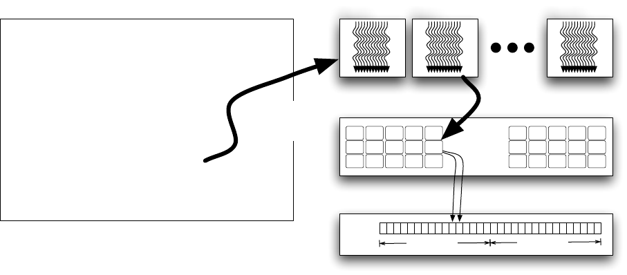
Figure 1: A saxpy kernel for computing y←ax +y. Each element of the vector yis processed by one thread.
operations are typically much less regular in their access patterns and consequently are generally limited
purely by bandwidth.
In this paper, we explore the design of efficient SpMV kernels for throughput-oriented processors like
the GPU. We implement these kernels in CUDA and analyze their performance on the GeForce GTX 280
GPU. Sparse matrices arising in different problems can exhibit a broad spectrum of regularity. We consider
data representations and implementation techniques that span this spectrum, from highly regular diagonal
matrices to completely unstructured matrices with highly varying row lengths.
Despite the irregularity of the SpMV computation, we demonstrate that it can be mapped quite suc-
cessfully onto the fine-grained parallel architecture employed by the GPU. For unstructured matrices, we
measure performance of roughly 10 GFLOP/s in double precision and around 15 GFLOP/s in single preci-
sion. Moreover, these kernels achieve a bandwidth of roughly 90 GBytes/s, or 63.5% of peak, which indicates
a relatively high level of efficiency on this bandwidth-limited computation.
2 Parallel Programming with CUDA
In the CUDA parallel programming model [13, 14], an application consists of a sequential host program
that may execute parallel programs known as kernels on a parallel device. A kernel is a SPMD (Single
Program Multiple Data) computation that is executed using a potentially large number of parallel threads.
Each thread runs the same scalar sequential program. The programmer organizes the threads of a kernel
into a grid of thread blocks. The threads of a given block can cooperate amongst themselves using barrier
synchronization and a per-block shared memory space that is private to that block.
We focus on the design of kernels for sparse matrix-vector multiplication. Although CUDA kernels may
be compiled into sequential code that can be run on any architecture supported by a C compiler, our SpMV
kernels are designed to be run on throughput-oriented architectures in general and the NVIDIA GPU in
particular. Broadly speaking, we assume that throughput-oriented architectures will provide both (1) some
form of SIMD thread execution and (2) vectorized or coalesced load/store operations.
A modern NVIDIA GPU is built around an array of SM multiprocessors [12], each of which supports up
to 1024 co-resident threads. A single multiprocessor is equipped with 8 scalar cores, 16384 32-bit registers,
and 16KB of high-bandwidth low-latency memory. Integer and single precision floating point operations
2

are performed by the 8 scalar cores, while a single shared unit is used for double precision floating point
operations.
Thread creation, scheduling, and management is performed entirely in hardware. High-end GPUs such
as the GeForce GTX 280 or Tesla C1060 contain 30 multiprocessors, for a total possible population of
30K threads. To manage this large population of threads efficiently, the GPU employs a SIMT (Single
Instruction Multiple Thread) architecture [12, 13] in which the threads of a block are executed in groups
of 32 called warps. A warp executes a single instruction at a time across all its threads. The threads of a
warp are free to follow their own execution path and all such execution divergence is handled automatically
in hardware. However, it is substantially more efficient for threads to follow the same execution path for the
bulk of the computation.
The threads of a warp are also free to use arbitrary addresses when accessing off-chip memory with
load/store operations. Accessing scattered locations results in memory divergence and requires the processor
to perform one memory transaction per thread. On the other hand, if the locations being accessed are
sufficiently close together, the per-thread operations can be coalesced for greater memory efficiency. Global
memory is conceptually organized into a sequence of 128-byte segments1. Memory requests are serviced for
16 threads (a half-warp) at a time. The number of memory transactions performed for a half-warp will be
the number of segments touched by the addresses used by that half-warp2. If a memory request performed
by a half-warp touches precisely 1 segment, we call this request fully coalesced, and one in which each thread
touches a separate segment we call uncoalesced. If only the upper or lower half of a segment is accessed, the
size of the transaction is reduced [14].
Figure 1 illustrates the basic structure of a CUDA program. The procedure saxpy() is a kernel entry
point, indicated by the use of the __global__ modifier. A call of the form saxpy<<<P,B>>> is a parallel kernel
invocation that will launch Pthread blocks of Bthreads each. These values can be set arbitrarily for each
distinct kernel launch, and an implicit global barrier between kernels guarantees that all threads of the first
kernel complete before any of the second are launched. When a kernel is invoked on the GPU, the hardware
scheduler launches thread blocks on available multiprocessors and continues to do so as long as the necessary
resources are available to do so. In this example, memory accesses to the vectors xand yare fully coalesced,
since threads with consecutive thread indices access contiguous words and the vectors are aligned by the
CUDA memory allocator.
Non-contiguous access to memory is detrimental to memory bandwidth efficiency and therefore the per-
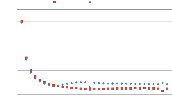
formance of memory-bound kernels. Consider the variation of the saxpy kernel given in Figure 2, which
permits a variable stride between elements. Any stride greater than one results in non-contiguous access
to the xand yvectors. Since larger strides result in a single warp touching more segments, we expect an
inverse relationship between stride and performance of the memory-bound saxpy kernel. Figure 3 confirms
this assumption, demonstrating that the effective memory bandwidth (and hence performance) decreases as
the stride increases from 1 to 33. Memory accesses with unit stride are more than ten times faster than
those with greater separation. Observe that performance of the double precision daxpy kernel follows a
similar relationship. Also note that, for large strides, the double precision kernel achieves roughly twice the
bandwidth of saxpy.
The relaxed coalescing rules of the GTX 200-series of processors largely mitigate the effect of alignment
on memory efficiency. For example, the rate of contiguous but unaligned memory access is roughly one-
tenth that of aligned access on the G80 architecture. However, on our target platform, unaligned access
is approximately 60% of the aligned case, a six-fold improvement over G80. Nevertheless, ensuring proper
memory alignment is key to achieving high SpMV performance.
3 Sparse Matrix Formats
There are a multitude of sparse matrix representations, each with different storage requirements, computa-
tional characteristics, and methods of accessing and manipulating entries of the matrix. Since, in the context
1Access granularities below 32 bits have different segment sizes [14].
2Earlier devices that do not support Compute Capability 1.2 have stricter coalescing requirements [14].
3
__ gl ob al __
void saxpy_with_stride(int n , float a , float * x , float * y , int stride)
{
int i = blockIdx.x *blockDim.x +threadIdx.x;
if (i < n )
y[i * st ride ] = a * x [i * stri de ] + y [ i * s tride ];
}
Figure 2: A saxpy kernel with variable stride.
0
20
40
60
80
100
120
140
0 5 10 15 20 25 30
GByte/s
Stride
Single Precision
Double Precision
Figure 3: Relationship between stride and memory bandwidth in the saxpy and daxpy kernels.
4
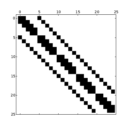
Figure 4: A 25-by-25 sparse matrix with 5 occupied diagonals. The matrix represents a finite-difference
approximation to the Laplacian operator on a 5-by-5 mesh.
of sparse matrix-vector multiplication, we are not concerned with modifying matrices, we will only consider
static sparse matrix formats, as opposed to those suitable for rapid insertion and deletion of elements.
The primary distinction among sparse matrix representations is the sparsity pattern, or the structure
of the nonzero entries, for which they are best suited. Although sparse formats tailored for highly specific
classes of matrices are the most computationally attractive, it is also important to consider general storage
schemes which efficiently store matrices with arbitrary sparsity patterns. In the remainder of this section we
summarize several sparse matrix representations and discuss their associated tradeoffs. Section 4 will then
describe CUDA kernels for performing SpMV operations with each sparse matrix format.
3.1 Diagonal Format
When nonzero values are restricted to a small number of matrix diagonals, the diagonal format (DIA) is
an appropriate representation [16]. Although not a general purpose format, the diagonal storage scheme
efficiently encodes matrices arising from the application of stencils to regular grids, a common discretization
method. Figure 4 illustrates the sparsity pattern of a 25-by-25 matrix with 5 occupied diagonals.
The diagonal format is formed by two arrays: data, which stores the nonzero values, and offsets, which
stores the offset of each diagonal from the main diagonal. By convention, the main diagonal corresponds to
offset 0, while i > 0 represents the i-th super-diagonal and i < 0 the i-th sub-diagonal. Figure 5 illustrates
the DIA representation of an example matrix with three occupied diagonals. In our implementation, data
is stored in column-major order so that its linearization in memory places consecutive elements within each
diagonal adjacently. Entries marked with the symbol ∗are used for padding and may store an arbitrary
value.
The benefits of the diagonal format are twofold. First, the row and column indices of each nonzero entry
are implicitly defined by their position within a diagonal and the corresponding offset of the diagonal. Implicit
indexing both reduces the memory footprint of the matrix and decreases the amount of data transferred
during a SpMV operation. Second, all memory access to data,x, and yis contiguous, which improves the
efficiency of memory transactions.
The downsides of the diagonal format are also evident. DIA allocates storage of values “outside” the
matrix and explicitly stores zero values that occur in occupied diagonals. Within the intended application
5
A=
1700
0280
5039
0604
data =
∗1 7
∗2 8
539
6 4 ∗
offsets =−201
Figure 5: Arrays data and offsets comprise the DIA representation of A.
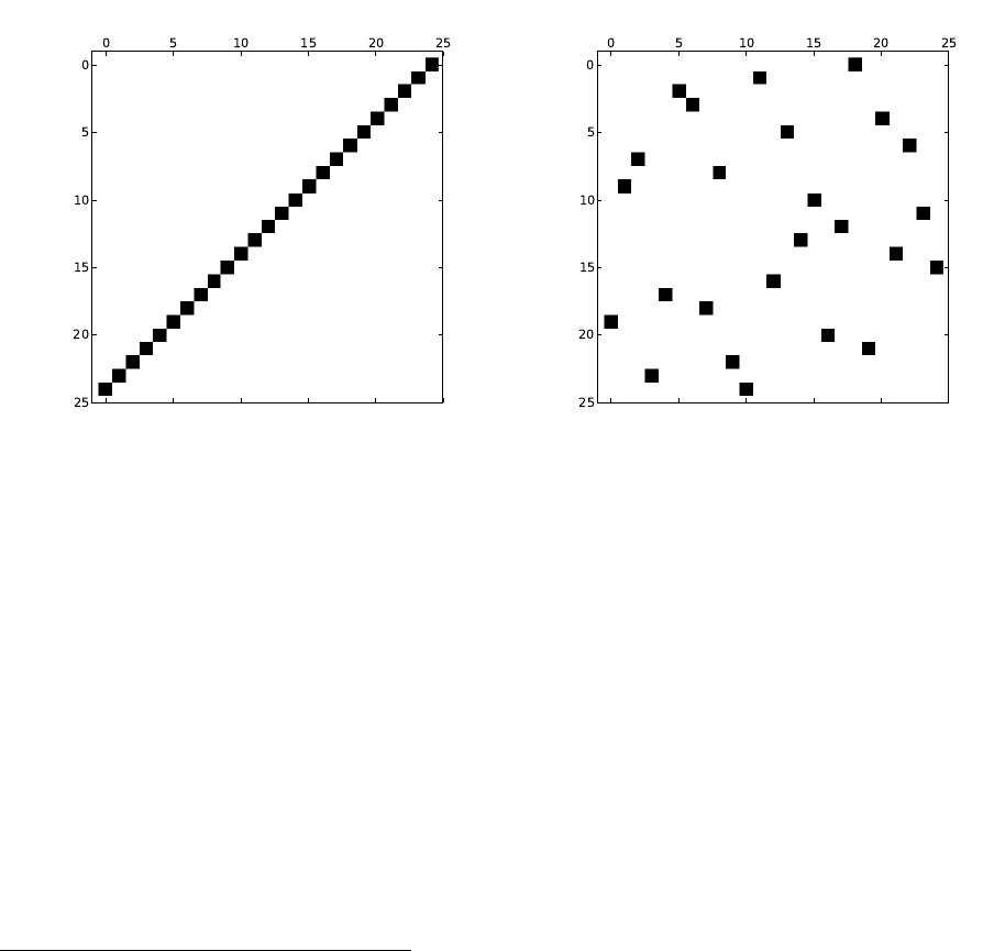
Figure 6: Sparsity patterns that are ill-suited to the sparse diagonal format.
area, i.e. stencils applied to regular grids, these are not problematic. However, it is important to note that
many matrices have sparsity patterns that are inappropriate for DIA, such as those illustrated in Figure 6.
3.2 ELLPACK Format
Another storage scheme that is well-suited to vector architectures is the ELLPACK (ELL) format3[7]. For
an M-by-Nmatrix with a maximum of Knonzeros per row, the ELLPACK format stores the nonzero values
in a dense M-by-Karray data, where rows with fewer than Knonzeros are zero-padded. Similarly, the
corresponding column indices are stored in indices, again with zero, or other some sentinel value used for
padding. ELL is more general than DIA since the nonzero columns need not follow any particular pattern.
Figure 7 illustrates the ELLPACK representation of an example matrix with a maximum of three nonzeros
per row. As in the DIA format, data and indices are stored in column-major order.
When the maximum number of nonzeros per row does not substantially differ from the average, the ELL
format is an efficient sparse matrix representation. Note that row indices are implicitly defined (like DIA),
3Also called the ITPACK format
6

A=
1700
0280
5039
0604
data =
1 7 ∗
2 8 ∗
539
6 4 ∗
indices =
0 1 ∗
1 2 ∗
023
1 3 ∗
Figure 7: Arrays data and indices comprise the ELL representation of A.
while column indices are stored explicitly. Aside from matrices defined by stencil operations on regular
grids (for which DIA is more appropriate), matrices obtained from semi-structured meshes and especially
well-behaved unstructured meshes meet this criterion. Figure 8 illustrates semi-structured and unstructured
meshes which are appropriate for the ELL storage scheme.
In practice, unstructured meshes do not always meet this requirement. Indeed, as Figure 9 illustrates, the
ratio between the maximum number of nonzeros per row and the average may be arbitrarily large. Clearly the
ELL format alone is an inappropriate choice for representing matrices obtained from such meshes. However,
a hybrid format that combines ELL with another, more general, storage scheme provides a useful alternative.
We discuss one such combination in Section 3.5.
3.3 Coordinate Format
The coordinate (COO) format4is a particularly simple storage scheme. The arrays: row,col, and data store
the row indices, column indices, and values, respectively, of the nonzero matrix entries. COO is a general
sparse matrix representation since, for an arbitrary sparsity pattern, the required storage is always propor-
tional to the number of nonzeros. Unlike DIA and ELL, both row and column indices are stored explicitly
in COO. Figure 10 illustrates the COO representation of an example matrix. In our implementation, the
row array is sorted, ensuring that entries with the same row index are stored contiguously.
3.4 Compressed Sparse Row Format
The compressed sparse row (CSR) format5is a popular, general-purpose sparse matrix representation. Like
the COO format, CSR explicitly stores column indices and nonzero values in arrays indices and data. A
third array of row pointers, ptr, takes the CSR representation. For an M-by-Nmatrix, ptr has length M+1
and stores the offset into the i-th row in ptr[i]. The last entry in ptr, which would otherwise correspond
to the (M+ 1)-st row, stores NNZ, the number of nonzeros in the matrix. Figure 11 illustrates the CSR
representation of an example matrix.
The CSR format may be viewed as a natural extension of the (sorted) COO representation discussed
in Section 3.3 with a simple compression scheme applied to the (often repeated) row indices. As a result,
converting between COO and CSR is straightforward and efficient. Aside from reducing storage, row pointers
facilitate fast querying of matrix values and allow other quantities of interest, such as the number of nonzeros
in a particular row (ptr[i+1] - ptr[i]), to be readily computed. For these reasons, the compressed row
format is commonly used for sparse matrix computations (e.g., sparse matrix-matrix multiplication) in
addition to sparse matrix-vector multiplication, the focus of this paper.
4Also called the triplet or IJV format.
5Also known as compressed row storage CRS
7
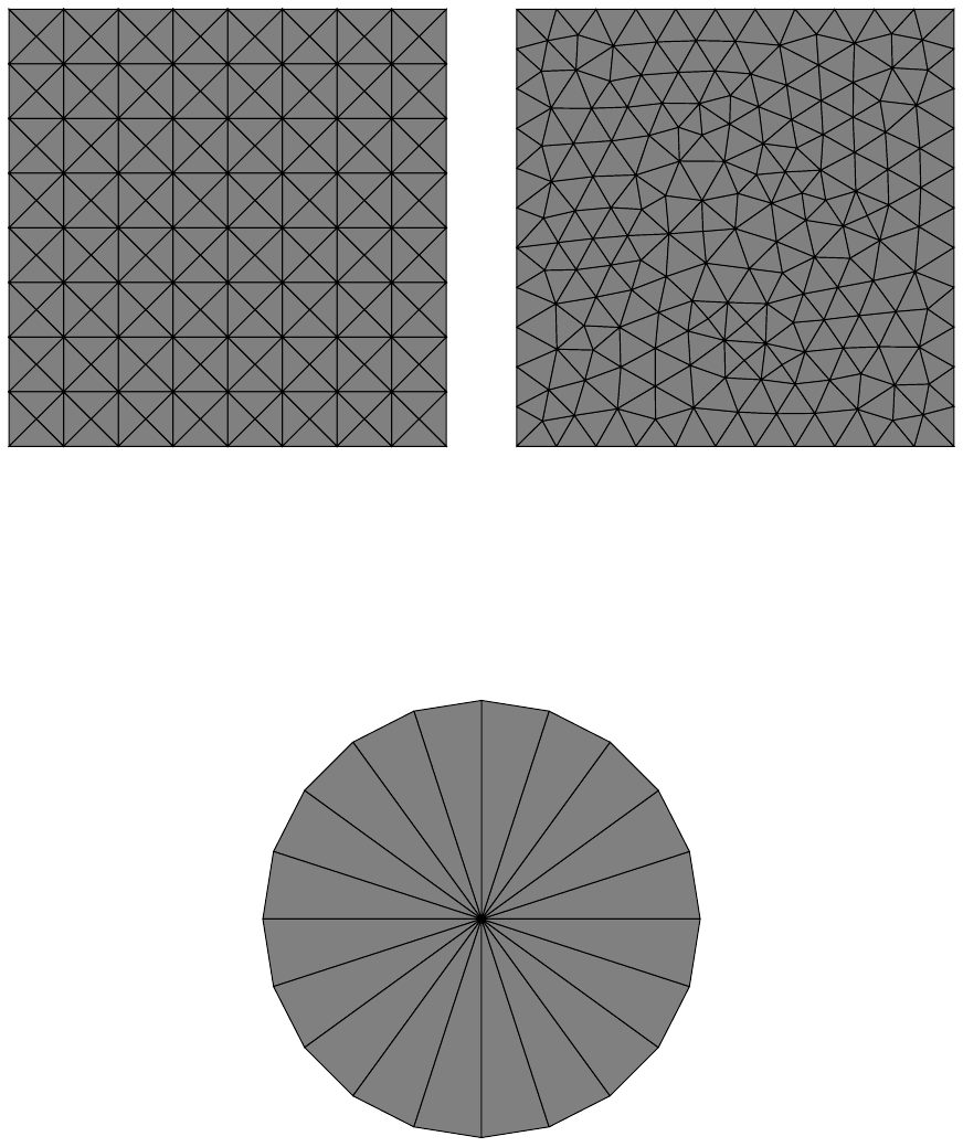
Figure 8: Example semi-structured (left) and unstructured (right) meshes whose vertex-edge connectivity is
efficiently encoded in ELL format. In each case the maximum vertex degree is not significantly greater than
the average degree.
Figure 9: The vertex-edge connectivity of the wheel is not efficiently encoded in ELL format. Since the
center vertex has high degree relative to the average degree, the vast majority of the entries in the data and
indices arrays of the ELL representation will be wasted.
8
A=
1700
0280
5039
0604
row =001122233
col =011202313
data =172853964
Figure 10: Arrays row,col, and data comprise the COO representation of A.
A=
1700
0280
5039
0604
ptr =02479
indices =011202313
data =172853964
Figure 11: Arrays ptr,indices, and data comprise the CSR representation of A.
9

3.5 Hybrid Format
While the ELLPACK format (cf. Section 3.2) is well-suited to vector architectures, its efficiency rapidly
degrades when the number of nonzeros per matrix row varies. In contrast, the storage efficiency of the
coordinate format (cf. Section 3.3) is invariant to the distribution of nonzeros per row. Furthermore, as we’ll
show in Section 4, this invariance extends to the cost of a sparse matrix-vector product using the coordinate
format. Since the best-case SpMV performance of ELL exceeds that of COO, a hybrid ELL/COO format,
which stores the majority of matrix entries in ELL and the remaining entries COO, is of substantial utility.
Consider a matrix that encodes the vertex connectivity of a planar triangle mesh in two dimensions.
While, as Figure 9 illustrates, the maximum vertex degree of such a mesh is arbitrarily large, the average
vertex degree is bounded by topological invariants. Therefore, the vast majority of vertices in a typical planar
triangle mesh will have approximately 6 neighbors, irrespective of the presence of vertices with exceptional
degree. Since similar properties hold for unstructured meshes in higher dimensions, it is worthwhile to
examine sparse matrix storage schemes that exploit this knowledge.
The purpose of the hybrid format is to store the typical number of nonzeros per row in the ELL data
structure and the remaining entries of exceptional rows in the COO format. Often the typical number of
nonzeros per row is known a priori, as in the case of planar meshes, and the ELL portion of the matrix is
readily extracted. However, in the general case this number must be determined directly from the input
matrix. Our implementation computes a histogram of the row sizes and determines the the largest number K
such that using Kcolumns per row in the ELL portion of the HYB matrix meets a certain objective measure.
Based on empirical results, we assume that the fully-occupied ELL format is roughly three times faster than
COO. Under this modeling assumption, it is profitable to add a K-th column to the ELL structure if at least
one third of the matrix rows contain K(or more) nonzeros. When the population of rows with Kor more
nonzero values falls below this threshold, the remaining nonzero values are placed into COO.
3.6 Packet Format
The packet format (PKT) is a novel sparse matrix representation designed for vector architectures. Tailored
for symmetric mesh-based matrices, such as those arising in FEM discretizations, the packet format first
decomposes the matrix into a given number of fixed-size partitions. Each partition is then stored in a
specialized packet data structure.
Figure 12 shows a triangle mesh with 11 vertices and partitioning of the vertices into two sets. The
objective of the partitioner is to minimize the edge cut: the total number of edges crossing between partitions.
In the context of the packet format, edges within a partition correspond to values that are cached in a low-
latency local memory, while the cut-edges correspond to values that must be fetched from off-chip memory.
Therefore, minimizing the edge cut reduces the number of high-latency memory accesses during a SpMV
operation.
Figure 13 illustrates the sparsity structure of the matrix associated with the mesh in Figure 12. Reordering
rows and columns by partition number ensures that most nonzeros lie in submatrices near the diagonal. Since
each submatrix contains only a small number of contiguous columns, the corresponding entries from the x
vector can be cached in local memory. Specifically, when performing the product A[i,j] * x[j], the value
of x[j] can be precached, and then fetched from low-latency local memory rather than high-latency main
memory. For now, we ignore the nonzero entries lying outside the diagonal submatrices and concentrate on
representing individual submatrices compactly.
In our implementation, the partition size is bounded by a constant determined by the available local
memory6. As a result, row and column indices within each diagonal submatrix are more compactly repre-
sented as local offsets from the first row and column of the submatrix. For example, the matrix entry (9,7)
within the second submatrix is stored as an offset of (3,2) from (6,6), the base index of the submatrix. We
represent the offset indices with 16-bit integers.
With submatrix indices stored as local offsets from a base index, the task remains to arrange these values
in a manner suitable for SIMT execution. We consider the case where each row of the submatrix is assigned
6At most 2,000 vertices per partition for single-precision and 1,000 for double-precision floating-point values
10
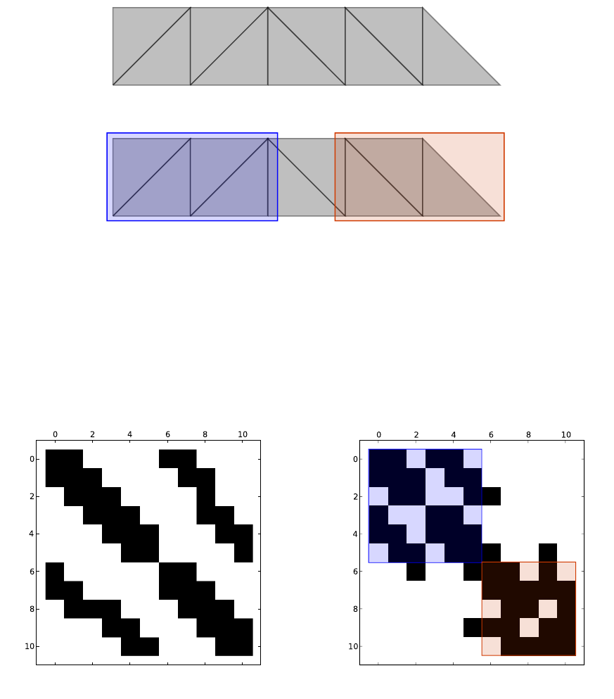
Figure 12: A sample triangle mesh with 11 vertices partitioned into two sets.
Figure 13: Reordering rows and columns by partition concentrates nonzeros into diagonal submatrices.
11
pkt0 =
(0,0) (0,1) (0,3) (0,4) ∗ ∗ ∗ ∗
(1,0) (1,1) (1,2) (1,4) (1,5) ∗∗∗
(2,1) (2,2) (2,5) (4,0) (4,1) (4,3) (4,4) (4,5)
(3,0) (3,3) (3,4) (5,1) (5,2) (5,4) (5,5) ∗
pkt1 =
(0,0) (0,1) (0,3) (4,1) (4,2) (4,3) (4,4)
(1,0) (1,1) (1,2) (1,3) (1,4) ∗ ∗
(2,1) (2,2) (2,4) ∗ ∗ ∗ ∗
(3,0) (3,1) (3,3) (3,4) ∗∗∗
Figure 14: Packet storage for the two diagonal submatrices in Figure 13. The first submatrix has base index
(0,0) while the second submatrix begins at (6,6). Rows of the pkt0 and pkt1 correspond to individual
thread lanes.
to a single thread, with a fixed number of threads associated to each packet. Under these assumptions,
data arrangement reduces to a packing problem: assign rows to threads such that the maximum work
assigned to any thread is minimized. Although this minimum multiprocessor scheduling problem is NP-hard
[11], we find that simple packing heuristics suffice for the domain of interest. Figure 14 illustrates packed
representations of the two submatrices in Figure 13 using four threads and a greedy least-occupied-bin-
first packing strategy. The nonzero values corresponding to each submatrix entry are stored in a similar
fashion, either in a separate array or together with the indices. In the complete data structure, packets
are concatenated together sequentially into an array of packets. In this example, the array [pkt0, pkt1]
combines the two packets. As with the DIA and ELL formats, the packet array is stored in column-major
order so concurrently executing threads access memory contiguously.
Like the coordinate portion of the hybrid ELL/COO format, nonzero matrix entries that lie outside the
diagonal submatrices may be stored in a separate data structure. Alternatively, these entries may be packed
in the same manner as the submatrix entries, albeit without the benefit of compressed indices. Since such
entries are relatively few in number, their handling has little impact on the overall performance.
Both ELL and PKT statically schedule work on a per-thread basis. In ELL the schedule is trivial: each
thread is assigned exactly one matrix row. The packet format is more general, allowing several rows to share
the same thread of execution. With a reasonable scheduling heuristic, this flexibility mitigates mild load
imbalances that are costly to store in ELL format.
In many ways the construction of the packet format resembles the strategy used in SpMV operations
on distributed memory systems. In either case, the matrix is partitioned into pieces based on the size of
the local memory store on each “node”. In our case, the individual multiprocessors on a single chip and
shared memory are the nodes and local store, while in distributed systems these are conventional computers
and their associated main memory. Although on different scales, the objective is to replace (relatively) high
latency communication with low latency memory access.
3.7 Other Formats
The formats discussed in this section represent only a small portion the complete space of sparse matrix
representations. Of these alternative formats, many are derived directly from one of the presented formats
(e.g., modified CSR [15]). Others, like CSR with permutation or the jagged diagonal format [6] are natural
generalizations of a basic format. Hybrid combinations of structured and unstructured formats, such as DIA
and CSR [15], are also useful.
12
__ gl ob al __ v oid
sp mv _d ia _k erne l ( con st int num_rows ,
const int num_cols ,
const int num_diags ,
const int * offsets ,
const float * data ,
const float * x ,
float * y )
{
int row = blockDim.x *blockIdx.x +threadIdx.x;
if ( ro w < n um_ ro ws ){
float dot = 0;
for (int n = 0; n < nu m_ di ag s ; n ++){
int col = row + offset s [ n];
float val = data [ n um _r ows * n + row ];
if ( col >= 0 && col < nu m_ co ls )
dot += val * x [ col ];
}
y [ row ] += do t;
}
}
Figure 15: SpMV kernel for the DIA sparse matrix format.
4 Sparse Matrix-Vector Multiplication
Sparse matrix-vector multiplication (SpMV) is arguably the most important operation in sparse matrix
computations. Iterative methods for solving large linear systems (Ax =b) and eigenvalue problems (Ax =
λx) generally require hundreds if not thousands of matrix-vector products to reach convergence. In this
paper, we consider the operation y=Ax +ywhere A is large and sparse and xand yare column vectors.
While not a true analog of the BLAS gemv operation (i.e., y=αAx+βy), our routines are easily generalized.
We choose this SpMV variant because it isolates the sparse component of the computation from the dense
component. Specifically, the number of floating point operations in y=Ax +yis always twice the number of
nonzeros in A(one multiply and one add per element), independent of the matrix dimensions. In contrast,
the more general form also includes the influence of the vector operation βy, which, when the matrix has
few nonzeros per row, will substantially skew performance.
In this section we describe SpMV implementations, or computational kernels, for the sparse matrix
formats introduced in Section 3. While the following CUDA code samples have been simplified for illustrative
purposes, the essence of the true implemention is maintained. For instance, the presented kernels ignore
range limits on grid dimensions e.g., gridDim.x ≤65535, which complicate the mapping of blocks and
threads to the appropriate indices. We refer interested readers to the source code which accompanies this
paper for further implementation details.
As discussed in Section 2, execution and memory divergence are the principal considerations. Therefore,
when mapping SpMV to the GPU, our task is to minimize the number of independent paths of execution
and leverage coalescing when possible. While these themes are broadly applicable, our primary focus is the
development of efficient kernels for CUDA-enabled devices. In particular, we target the GTX 200-series of
processors which support double precision floating point arithmetic [14].
4.1 DIA kernel
Parallelizing SpMV for the diagonal format is straightforward: one thread is assigned to each row of the
matrix. In Figure 15, each thread first computes a sequential thread index, row, and then computes the
(sparse) dot product between the corresponding matrix row and the xvector.
Recall from Section 3.1 that the data the array of the DIA format is stored in column-major order. As
13

data ∗ ∗ 561234789∗
Iteration 0 2 3
Iteration 1 0123
Iteration 2 012
Figure 16: Linearization of the DIA data array and the memory access pattern of the DIA SpMV kernel.
__ gl ob al __ v oid
sp mv _e ll _k erne l ( con st int num_rows ,
const int num_cols ,
const int num_cols_per_row ,
const int * indices ,
const float * data ,
const float * x ,
float * y )
{
int row = blockDim.x *blockIdx.x +threadIdx.x;
if ( ro w < n um_ ro ws ){
float dot = 0;
for (int n = 0; n < num_cols_per_row; n++){
int col = indi ce s [ n um _rows * n + row ];
float val = data [ n um _r ows * n + row ];
if ( va l != 0)
dot += val * x [ col ];
}
y [ row ] += do t;
}
}
Figure 17: SpMV kernel for the ELL sparse matrix format.
Figure 16 illustrates, this linearization of the DIA data array ensures that threads within the same warp
access memory contiguously. Since the DIA format for this matrix has three diagonals (i.e., num diags
= 3) the data array is accessed three times by each of the four executing threads. Given that consecutive
rows, and hence threads, correspond to consecutive matrix columns, threads within the same warp access
the xvector contiguously as well. As presented, memory accesses to data and xare contiguous, but not
generally aligned to any specific multi-word boundary. Fortunately, aligned access to data is easily achieved
by padding the columns of data (cf. Figure 5). Our implementation (not shown) uses this modification to
the standard DIA data structure. Additionally, our implementation of the DIA kernel accesses values in the
offsets array only once per block, as opposed to the per-thread access shown in Figure 15.
4.2 ELL Kernel
Figure 17 illustrates the ELL kernel which, like DIA, uses one thread per matrix row to parallelize the
computation. The structure of the ELL kernel is nearly identical to that of the DIA kernel, with the
exception that column indices are explicit in ELL and implicit in DIA. Therefore, the DIA kernel will
generally perform better than the ELL kernel on matrices that are efficiently stored in DIA format.
The memory access pattern of the ELL kernel, shown in Figure 16, resembles that of the DIA method.
Since data and indices of the ELL format are accessed in the same way we show only one access pattern.
As with DIA, our implementation used padding to align the ELL arrays appropriately. However, unlike DIA,
14
data 12567834∗ ∗ 9∗
indices 01011223∗ ∗ 3∗
Iteration 0 0123
Iteration 1 0123
Iteration 2 0123
Figure 18: Linearization of the ELL data and indices arrays and the memory access pattern of the ELL
SpMV kernel.
__ ho st __ void
sp mv _c sr _s eria l ( con st int num_rows ,
const int * ptr ,
const int * indices ,
const float * data ,
const float * x ,
float * y )
{
for (int row = 0; i < num_rows ; i++){
float dot = 0;
int r ow _s ta rt = pt r [ row ];
int r ow _e nd = p tr [ row +1] ;
for (int jj = ro w_ st ar t ; jj < ro w_ end ; jj ++)
do t += da ta [ j j ] * x [ in di ce s [ jj ]];
y [ row ] += do t;
}
}
Figure 19: Serial CPU SpMV kernel for the CSR sparse matrix format.
the ELL kernel does not necessarily access the xvector contiguously.
4.3 CSR kernel
Consider the serial CPU kernel for the CSR format shown in Figure 19. Since the (sparse) dot product
between a row of the matrix and xmay be computed independently of all other rows, the CSR SpMV
operation is easily parallelized. Figure 20 demonstrates a straightforward CUDA implementation, again
using one thread per matrix row. Several variants of this approach are documented in [13], which we refer
to as the scalar kernel.
While the scalar kernel exhibits fine-grained parallelism, its performance suffers from several drawbacks.
The most significant among these problems is the manner in which threads within a warp access the CSR
indices and data arrays. While the column indices and nonzero values for a given row are stored contigu-
ously in the CSR data structure, these values are not accessed simultaneously. Instead, each thread reads
the elements of its row sequentially, producing the pattern shown in Figure 21.
An alternative to the scalar method, which we call the vector kernel, assigns one warp to each matrix
row. An implementation of this described in Figure 22. The vector kernel can be viewed as an application of
the vector strip mining pattern to the sparse dot product computed for each matrix row. Unlike the previous
CUDA kernels, which all used one thread per matrix row, the CSR vector kernel requires coordination among
threads within the same warp. Specifically, a warp-wide parallel reduction is required to sum the per-thread
15
__ gl ob al __ v oid
spmv_csr_scalar_kernel(cons t int num_rows ,
const int * ptr ,
const int * indices ,
const float * data ,
const float * x ,
float * y )
{
int row = blockDim.x *blockIdx.x +threadIdx.x;
if ( ro w < n um_ ro ws ){
float dot = 0;
int r ow _s ta rt = pt r [ row ];
int r ow _e nd = p tr [ row +1] ;
for (int jj = ro w_ st ar t ; jj < ro w_ end ; jj ++)
do t += da ta [ j j ] * x [ in di ce s [ jj ]];
y [ row ] += do t;
}
}
Figure 20: SpMV kernel for the CSR sparse matrix format using one thread per matrix row.
indices 011202313
data 172853964
Iteration 0 0 1 2 3
Iteration 1 0 1 2 3
Iteration 2 2
Figure 21: CSR arrays indices and data and the memory access pattern of the scalar CSR SpMV kernel.
16
__ gl ob al __ v oid
spmv_csr_vector_kernel(cons t int num_rows ,
const int * ptr ,
const int * indices ,
const float * data ,
const float * x ,
float * y )
{
__ sh ar ed __ floa t val s [];
int t hr ea d_ id = b lo ck Di m. x *bl oc kI dx .x +threadIdx.x;// g lo ba l thread in de x
int w ar p_id = t hr ea d_id / 32; // global warp index
int l ane = th re ad _i d & (32 - 1); // th re ad i ndex within the warp
// one warp per row
int row = w arp _id ;
if ( ro w < n um_ ro ws ){
int r ow _s ta rt = pt r [ row ];
int r ow _e nd = p tr [ row +1] ;
// com pu te r un ni ng sum per thread
vals[threadIdx.x] = 0;
for (int jj = r ow _s ta rt + lane ; jj < row_end ; jj += 32)
vals[threadIdx.x] += d at a [ jj ] * x [ i nd ic es [ j j ]] ;
// par al le l r educt io n in shared me mo ry
if ( la ne < 16) v als [ threadIdx.x] += v als [ threadIdx.x + 1 6];
if ( la ne < 8) va ls [ threadIdx.x] += va ls [ threadIdx.x + 8];
if ( la ne < 4) va ls [ threadIdx.x] += va ls [ threadIdx.x + 4];
if ( la ne < 2) va ls [ threadIdx.x] += va ls [ threadIdx.x + 2];
if ( la ne < 1) va ls [ threadIdx.x] += va ls [ threadIdx.x + 1];
// fi rs t th re ad w ri te s the r es ul t
if ( la ne == 0)
y [ row ] += va ls [ threadIdx.x];
}
}
Figure 22: SpMV kernel for the CSR sparse matrix format using one 32-thread warp per matrix row.
results together.
The vector kernel accesses indices and data contiguously, and therefore overcomes the principal defi-
ciency of the scalar approach. Memory access in Figure 23 are labeled by warp index (rather than iteration
number) since the order in which different warps access memory is undefined and indeed, unimportant for
performance considerations. In this example, no warp iterates more than once while reading the CSR arrays
since no row has more than 32 nonzero values. Note that when a row consists of more than 32 nonzeros, the
order of summation differs from that of the scalar kernel.
Unlike DIA and ELL, the CSR storage format permits a variable number of nonzeros per row. While
CSR efficiently represents a broader class of sparse matrices, this additional flexibility introduces thread
divergence. For instance, when spmv csr scalar kernel is applied to a matrix with a highly variable
number of nonzeros per row, it is likely that many threads within a warp will remain idle while the thread
with the longest row continues iterating. Matrices whose distribution of nonzeros per row follows a power law
distribution are particularly troublesome for the scalar kernel. Since warps execute independently, this form
of thread divergence is less pronounced in spmv csr vector kernel. On the other hand, efficient execution
of the vector kernel demands that matrix rows contain a number of nonzeros greater than the warp size (32).
As a result, performance of the vector kernel is sensitive to matrix row size.
4.4 COO Kernel
Recall from Sections 3.1 and 3.2 that the DIA and ELL formats only represent specific sparsity patterns
efficiently. The CSR format is more general than DIA and ELL, however our CSR kernels suffer from thread
17

indices 011202313
data 172853964
Warp 0 0 0
Warp 1 1 1
Warp 2 222
Warp 3 3 3
Figure 23: CSR arrays indices and data and the memory access pattern of the vector CSR SpMV kernel.
divergence in the presence of matrix rows with variable numbers of nonzeros (scalar), or rows with few nonzero
elements (vector). It is desireable, then, to have a sparse matrix format and associated computational kernel
that is insensitive to sparsity structure. To satisfy these demands we have implemented a COO SpMV kernel
based on segmented reduction.
Note that spmv csr vector kernel (cf. Figure 22) uses a parallel warp-wide reduction to sum per-thread
results together. This approach implicitly relies on the fact that each warp processes only one row of the
matrix. In contrast, a segmented reduction allows warps to span multiple rows. Figure 24 describes our
warp-wide segmented reduction, which is the basis of our complete COO kernel (not shown).
Segmented reduction is a data-parallel operation, which like other primitives such as parallel prefix sum
(scan), facilitate numerous parallel algorithms [3]. Sengupta et al. [17] discuss efficient CUDA implementa-
tions of common parallel primitives, including an application of segmented scan to SpMV. Our COO kernel
is most closely related to the work of Blelloch et al. [4], which demonstrated structure-insensitive SpMV
performance the Cray C90 vector computer.
__ de vi ce __ v oid
segmented_reduction(c onst int lane , const int * rows , f loat * va ls )
{
// seg me nted red uc tion in sh ar ed memory
if ( l ane >= 1 && r ows [ threadIdx.x] == r ows [ threadIdx.x - 1] )
vals[threadIdx.x] += v als [ threadIdx.x - 1];
if ( l ane >= 2 && r ows [ threadIdx.x] == r ows [ threadIdx.x - 2] )
vals[threadIdx.x] += v als [ threadIdx.x - 2];
if ( l ane >= 4 && r ows [ threadIdx.x] == r ows [ threadIdx.x - 4] )
vals[threadIdx.x] += v als [ threadIdx.x - 4];
if ( l ane >= 8 && r ows [ threadIdx.x] == r ows [ threadIdx.x - 8] )
vals[threadIdx.x] += v als [ threadIdx.x - 8];
if ( l ane >= 16 && r ows [ threadIdx.x] == r ows [ threadIdx.x - 16] )
vals[threadIdx.x] += v als [ threadIdx.x - 16];
}
Figure 24: Parallel segmented reduction is the key component of the COO SpMV kernel.
Figure 25 illustrates the memory access pattern of the COO kernel. Here we have illustrated the case of
a single executing warp on a fictitious architecture with four threads per warp. We refer interested readers
to the source code which accompanies this paper for further implementation details.
4.5 HYB Kernel
Since the HYB format is simply the sum of its constituent ELL and COO parts, the HYB SpMV operation is
trivial to implement. Assuming that most nonzeros belong to the ELL portion, performance of HYB SpMV
operation will resemble that of the ELL kernel.
18
row 001122233
col 011202313
data 172853964
Iteration 0 0123
Iteration 1 0123
Iteration 2 0
Figure 25: COO arrays row,col, and data and the memory access pattern of the COO SpMV kernel.
__ de vi ce __ v oid
process_packet(c onst int work_per_thread ,
const int * index_packet ,
float * data_packet ,
const float * x_local ,
float * y_local)
{
for (int i = 0; i < wo rk_per_ th re ad ; i ++){
// of fs et i nto packet arrays
int pos = blockDim.x *i+threadIdx.x;
// r ow an d c olu mn i nd ic es ar e p ac ke d i n on e 32 - b it wo rd
int p acked_ ind ex = i ndex_array [ pos ];
// row and c ol um n s to re d in up pe r and lower half - words
int row = packed_index >> 16;
int c ol = p ac ked_in dex & 0 xF FFF ;
float v al = d at a_ ar ra y [ pos ];
y_ lo ca l [ row ] += va l * x _lo ca l [ col ];
}
}
Figure 26: A block of threads computes the matrix-vector product for a single packet. Here x local and
y local reside in shared memory for low-latency access.
4.6 PKT Kernel
As explained in Section 3.6, the PKT format is comprised by two parts, an array of compressed packets,
and a COO matrix containing a smaller number of nonzero values. Since the packet data structure contains
an explicit assignment of matrix rows onto a block of threads, processing packets is straightforward. The
CUDA code in Figure 26 details steps used to process a single packet using a thread block. Prior to calling
process packet, the PKT kernel must load the appropriate sections of the xand yvectors into the shared
memory arrays x local and y local respectively. After processing the packet, the results in y local must
be written back to y, which resides in global memory. By construction, memory accesses to the PKT data
structure, represented by index packet and data packet, are fully coalesced.
4.7 Caching
With the exception of the PKT kernel, which uses a shared memory cache, all SpMV kernels can benefit
from the texture cache present on all CUDA-capable devices. As shown in the results of Section 5, accessing
the xvector through the texture cache often improves performance considerably. In the cached variants of
our kernels, reads of the form x[j] are replaced with a texture fetch instruction tex1Dfetch(x tex, j),
19
Kernel Granularity Coalescing Bytes/FLOP (32-bit) Bytes/FLOP (64-bit)
DIA thread : row full 4 8
ELL thread : row full 6 10
CSR (scalar) thread : row rare 6 10
CSR (vector) warp : row partial 6 10
COO thread : nonzero full 8 12
HYB thread : row full 6 10
PKT thread : rows full 4 6
Table 1: Summary of SpMV kernel properties.
leaving the rest of the kernel unchanged.
4.8 Summary
Table 1 summarizes the salient features of our SpMV kernels. For the HYB and PKT entries, we have
assumed that only a small number of nonzero values are stored in their COO respective portions. As shown
in the column labeled “Granularity”, the COO kernel has the finest granularity (one thread per nonzero)
while PKT is the coarsest (several rows per thread). Recall that full utilization of the GPU requires many
thousands of active threads. Therefore, the finer granularity of the CSR (vector) and COO kernels is
advantageous when applied to matrices with a limited number of rows. Note that such matrices are not
necessarily small, as the number of nonzero entries per row is still arbitrarily large.
Except for the CSR kernels, all methods benefit from full coalescing when accessing the sparse matrix
format. As Figure 21 illustrates, the memory access pattern of the scalar CSR kernel seldom benefits from
coalescing. Warps of the vector kernel access the CSR structure in a contiguous but not generally aligned
fashion, which implies partial coalescing.
The rightmost columns of Table 1 reflect the computational intensity of the various kernels. As before,
we have neglected the COO portion of the HYB and PKT formats. In single precision arithmetic, the DIA
and PKT kernels generally have the lowest ratio of bytes per FLOP, and therefore the highest computational
intensity. Meanwhile, the COO format, which explicitly stores (uncompressed) row and column entries, has
the lowest intensity.
Note that these figures are only rough approximations to the true computational intensities, which are
matrix-dependent. Specifically, these estimates ignore accesses to the yvector, the ptr array of the CSR
format, the offset array of the DIA format, and the xvector used in the PKT kernel. Our matrix-specific
bandwidth results in Section 5 provide a more accurate empirical measurement of actual bandwidth usage.
5 Results
We have collected SpMV performance data on a broad collection of matrices representing numerous appli-
cation areas. Different classes of matrices highlight the strengths and weaknesses of the sparse formats and
their associated computational kernels. In this section we explore the effect of these performance tradeoffs
in terms of speed of execution, measured in GFLOP/s (billion floating point operations per second), and
memory bandwidth utilization, measured in GBytes/s (billion bytes per second).
We present results for both single (32-bit) and double precision (64-bit) floating point arithmetic. In
each case, we record performance with and without the caching applied to the xvector (cf. Section 4.7).
With cache enabled, the reported memory bandwidth figures are the effective bandwidth of the computation
using the same accounting as the results with no caching. Therefore, effective bandwidth is a hypothetical
measure of the memory bandwidth necessary to produce the observed performance in the absence of a cache.
Table 2 lists the software and hardware used in our performance study. All software components, including
source code for our implementations, are freely available and the matrices used in our study are available upon
20
GPU NVIDIA GeForce GTX 280
CPU Intel Core 2 Quad Q6600
Memory 2x2GB DDR2-800
Chipset NVIDIA 780i SLI
OS Ubuntu 8.04 (Linux 2.6.24-21 x86 64)
CUDA CUDA 2.1 Beta (2.1.1635-3065709)
Host Compiler GCC 4.2.4
Table 2: Test platform specifications.
Matrix Grid Diagonals Rows Columns Nonzeros
Laplace 3pt (1,000,000) 3 1,000,000 1,000,000 2,999,998
Laplace 5pt (1,000)25 1,000,000 1,000,000 4,996,000
Laplace 7pt (100)37 1,000,000 1,000,000 6,940,000
Laplace 9pt (1,000)29 1,000,000 1,000,000 8,988,004
Laplace 27pt (100)327 1,000,000 1,000,000 26,463,592
Table 3: Structured matrices used for performance testing.
request. The reported figures represent an average (arithmetic mean) of 500 SpMV operations. As described
in Section 4, the number of FLOPs for one sparse matrix-vector multiplication is precisely twice the number
of nonzeros in the matrix. Therefore, the rate of computation, which is reported in units of GFLOP/s, is
simply the number of FLOPs in a single matrix-vector product divided by the average computation time.
We do not include time spent transferring data between host and device memory. In the context of iterative
solvers, where such transfers would occur at most twice (at the beginning and end of iteration), transfer
overhead is amortized over a large number of SpMV operations, rendering it negligible.
5.1 Structured Matrices
We begin with a set of structured matrices that represent common stencil operations on regular one, two,
and three-dimensional grids. Our test set consists of standard discretizations of a Laplacian operator in
the corresponding dimension. Table 3 lists these matrices and the grid used to produce them. For instance
“Laplace 5pt” refers to the standard 5-point finite difference approximation to the two-dimensional Laplacian
operator. Note that the number of points in the stencil is precisely the number of occupied matrix diagonals,
and, aside from rows corresponding to points on the grid boundaries, it is also the number of nonzero entries
per matrix row.
5.1.1 Single Precision
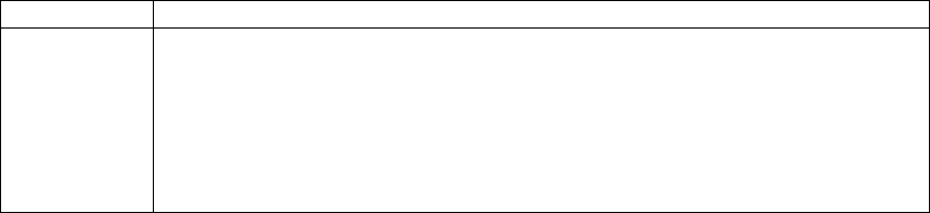
Figure 27 reports SpMV performance using single precision precision arithmetic. HYB results are excluded
from our structured matrix study as they are identical to the ELL figures. While the PKT kernel does not
use the texture cache, it is included among the cache-enabled kernels for comparison.
As expected, the DIA kernel offers the best performance in all cases. On the 27-point example, the DIA
kernel reaches 23.5 GFLOP/s without caching and 36.8 GFLOP/s with caching enabled, an improvement
of 56%. ELL performance is similar to DIA, although uniformly slower, owing to reduced computational
intensity associated with explicit column indices. Larger stencils, which offer greater opportunity for reuse,
see greater benefit from the use of caching with both DIA and ELL.
Despite a competitive computational intensity (cf. Table 1), PKT performance trails that of DIA and
ELL. This result is attributable in part to the relatively small size of the shared memory (16KB) which limits
the number of rows per packet (approximately 2000). In turn, the number of rows per packet paces a limit
21
0.0
5.0
10.0
15.0
20.0
25.0
30.0
35.0
40.0
Laplacian 3pt
Laplacian 5pt
Laplacian 7pt
Laplacian 9pt
Laplacian 27pt
GFLOP/s
Matrix
COO
CSR (scalar)
CSR (vector)
DIA
ELL
PKT
(a) Without Cache
0.0
5.0
10.0
15.0
20.0
25.0
30.0
35.0
40.0
Laplacian 3pt
Laplacian 5pt
Laplacian 7pt
Laplacian 9pt
Laplacian 27pt
GFLOP/s
Matrix
COO
CSR (scalar)
CSR (vector)
DIA
ELL
PKT
(b) With Cache
Figure 27: Performance results for structured matrices using single precision.
on the number of threads per packet while still maintaining several rows per thread. Our single precision
PKT results use 512 threads per packet, or roughly four rows per thread.
Although not competitive with DIA and ELL, the COO kernel exhibits steady performance across the
matrices in our study. As shown in Section 5.2, this quality is more important in the context of unstructured
matrices. The generality of the COO method is unnecessary for this set of highly regular, grid-based matrices.
Recall from Section 4.3 that the CSR (vector) kernel uses one 32-thread warp per matrix row. Since all
matrices in our study have fewer than 32 nonzeros per row, the vector kernel is underutilized. Indeed, when
the texture cache is enabled, the ratio of GFLOP/s to nonzeros per row only varies between 0.3285 and
0.3367. That performance scales linearly with the number of nonzeros per row indicates that COO (vector)
is entirely limited by poor thread utilization, as opposed to the available memory bandwidth. As a result,
the vector kernel is not competitive with DIA and ELL on the matrices considered.
Observe that CSR (scalar) kernel performance decreases as the number of diagonals increases. Given that
the number of nonzeros per row varies little, execution divergence of the scalar kernel is minimal. Instead,
memory divergence is the cause of the performance decline. The best performance is achieved when the
number of nonzeros per row is small, resulting in a modest degree of coalescing. However, as the number
of elements per row increases the likelihood of such fortuitous coalescing diminishes. Note that the typical
number of nonzeros per row is effectively the same as the stride in the saxpy kernels discussed in Section 2.
In either case, larger stride is detrimental to performance.
Although GFLOP/s is the primary metric for SpMV performance, it is also instructive to examine memory
bandwidth utilization. Figure 28 reports the observed memory bandwidth for each matrix and kernel in our
study. The maximum theoretical memory bandwidth of the GTX 280 is 141.7 GBytes/s, and without the
aid of caching, the DIA and ELL kernels deliver as much as 76% and 81% of this figure respectively. With
caching enabled, the maximum effective bandwidth of DIA is 155.1 GByte/s and 156.3 GByte/s for ELL.
Of course, these results reflect, in part, the internal memory bandwidth of the device.
5.1.2 Double Precision
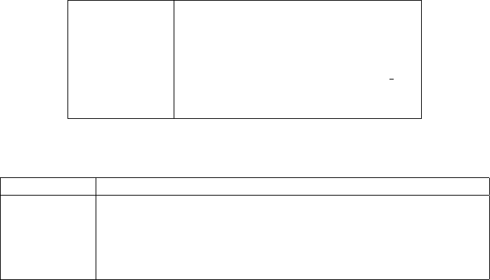
Double precision performance and bandwidth results are shown in Figures 29 and 30 respectively. Again the
DIA kernel offers the best performance in all cases, reaching 16.7 GFLOP/s on the 27-point example. The
ELL kernel runs at 13.5 GFLOP/s on the same matrix.
While the peak rate of double precision computation on the GTX 200-series GPU is an order of magnitude
less the single precision maximum, SpMV performance is bandwidth-limited, and therefore insensitive to
variations in peak floating point throughput. Indeed, DIA double precision (uncached) performance in the
27-point example is 44.2% that of the single precision result, which nearly matches the ratio of bytes per
22
0.0
20.0
40.0
60.0
80.0
100.0
120.0
140.0
160.0
180.0
Laplacian 3pt
Laplacian 5pt
Laplacian 7pt
Laplacian 9pt
Laplacian 27pt
GByte/s
Matrix
COO
CSR (scalar)
CSR (vector)
DIA
ELL
PKT
(a) Without Cache
0.0
20.0
40.0
60.0
80.0
100.0
120.0
140.0
160.0
180.0
Laplacian 3pt
Laplacian 5pt
Laplacian 7pt
Laplacian 9pt
Laplacian 27pt
GByte/s
Matrix
COO
CSR (scalar)
CSR (vector)
DIA
ELL
PKT
(b) With Cache
Figure 28: Bandwidth results for structured matrices using single precision.
0.0
2.0
4.0
6.0
8.0
10.0
12.0
14.0
16.0
18.0
Laplacian 3pt
Laplacian 5pt
Laplacian 7pt
Laplacian 9pt
Laplacian 27pt
GFLOP/s
Matrix
COO
CSR (scalar)
CSR (vector)
DIA
ELL
PKT
(a) Without Cache
0.0
2.0
4.0
6.0
8.0
10.0
12.0
14.0
16.0
18.0
Laplacian 3pt
Laplacian 5pt
Laplacian 7pt
Laplacian 9pt
Laplacian 27pt
GFLOP/s
Matrix
COO
CSR (scalar)
CSR (vector)
DIA
ELL
PKT
(b) With Cache
Figure 29: Performance results for structured matrices using double precision.
0.0
20.0
40.0
60.0
80.0
100.0
120.0
140.0
160.0
Laplacian 3pt
Laplacian 5pt
Laplacian 7pt
Laplacian 9pt
Laplacian 27pt
GByte/s
Matrix
COO
CSR (scalar)
CSR (vector)
DIA
ELL
PKT
(a) Without Cache
0.0
20.0
40.0
60.0
80.0
100.0
120.0
140.0
160.0
Laplacian 3pt
Laplacian 5pt
Laplacian 7pt
Laplacian 9pt
Laplacian 27pt
GByte/s
Matrix
COO
CSR (scalar)
CSR (vector)
DIA
ELL
PKT
(b) With Cache
Figure 30: Bandwidth results for structured matrices using double precision.
23

Matrix Rows Columns Nonzeros Nonzeros/Row
Dense 2,000 2,000 4,000,000 2000.0
Protein 36,417 36,417 4,344,765 119.3
FEM/Spheres 83,334 83,334 6,010,480 72.1
FEM/Cantilever 62,451 62,451 4,007,383 64.1
Wind Tunnel 217,918 217,918 11,634,424 53.3
FEM/Harbor 46,835 46,835 2,374,001 50.6
QCD 49,152 49,152 1,916,928 39.0
FEM/Ship 140,874 140,874 7,813,404 55.4
Economics 206,500 206,500 1,273,389 6.1
Epidemiology 525,825 525,825 2,100,225 3.9
FEM/Accelerator 121,192 121,192 2,624,331 21.6
Circuit 170,998 170,998 958,936 5.6
Webbase 1,000,005 1,000,005 3,105,536 3.1
LP 4,284 1,092,610 11,279,748 2632.9
Table 4: Unstructured matrices used for performance testing.
FLOP of the two kernels (50.0%) as listed in Table 1. For the ELL kernel, a similar analysis suggests
a relative performance of 60.0% (double precision to single precision) which again agrees with the 57.2%
observed.
Since the remaining kernels are not immediately bandwidth-limited, we cannot expect a direct corre-
spondence between relative performance and computational intensity. In particular, the CSR (scalar) kernel
retains 89.9% of its single precision performance, while computational intensity would suggest a 60.0% figure.
This anomaly is explained by the fact that uncoalesced double-word memory accesses are inherently more
efficient than uncoalesced single-word accesses on a memory bandwidth basis.
5.2 Unstructured Matrices
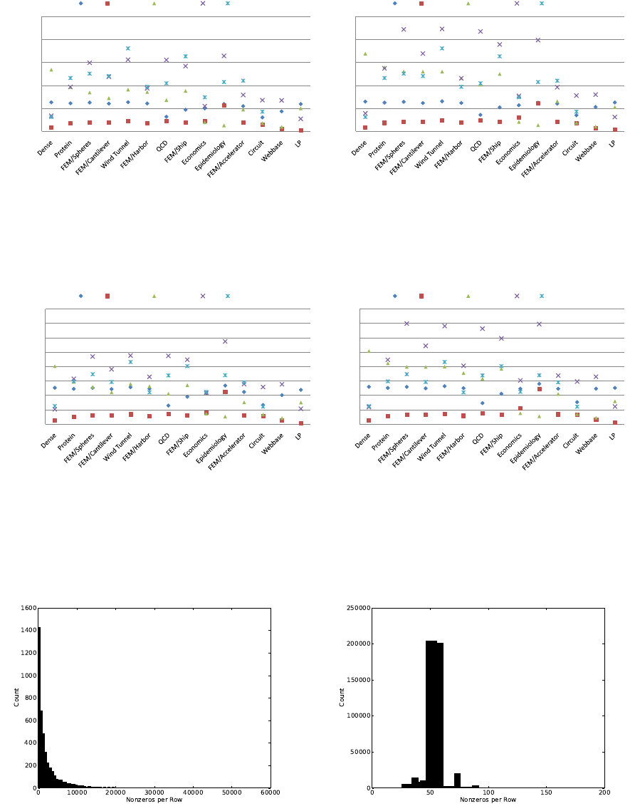
Our unstructured matrix performance study considers the same corpus of 14 matrices used by Williams et
al. [19] for benchmarking SpMV performance on several multicore processors. Table 4 lists these matrices
and summarizes their basic properties. Further details regarding the origin of each matrix are provided by
Williams et al. [19].
We have excluded the DIA and ELL formats from our unstructured performance study. Only the Epi-
demiology matrix is efficiently stored in ELL format, and none are efficiently stored in DIA. While most
nonzeros in the Epidemiology matrix are confined to three diagonals, the total number of occupied diagonals
is 769.
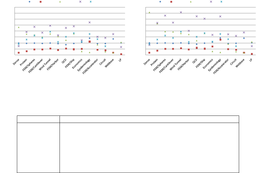
5.2.1 Single Precision
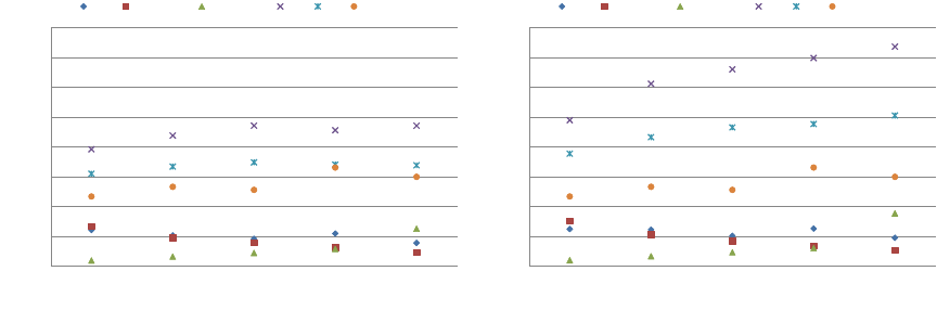
Single precision SpMV performance is reported in Figure 31. As before, we include the PKT measurements,
which do not use the texture cache, in both charts for comparison. Our implementation of the PKT format
extends only to matrices with symmetric nonzero patterns, so PKT results for the Webbase and LP matrices
are omitted.
Unstructured performance results are varied, with no single kernel or format outperforming all others.
The HYB format acheives the highest absolute performance, reaching 22.3 GFLOP/s in the FEM/Spheres
example and over 15.0 GFLOP/s in six of fourteen examples. The hybrid format exhibits the worst perfor-
mance in the LP matrix. As Figure 33 shows, the number of nonzeros per row varies widely in this example
from linear programming. In contrast, the distribution of nonzeros per row in the higher-performing Wind
Tunnel matrix is more compact. As a result, the only 45.4% of the LP matrix nonzeros are stored in the
ELL portion of the HYB data structure while fully 99.4% of the Wind Tunnel nonzeros reside there.
24
0.0
5.0
10.0
15.0
20.0
25.0
GFLOP/s
Matrix
COO
CSR (scalar)
CSR (vector)
HYB
PKT
(a) Without Cache
0.0
5.0
10.0
15.0
20.0
25.0
GFLOP/s
Matrix
COO
CSR (scalar)
CSR (vector)
HYB
PKT
(b) With Cache
Figure 31: Performance results for unstructured matrices using single precision.
0.0
20.0
40.0
60.0
80.0
100.0
120.0
140.0
160.0
GByte/s
Matrix
COO
CSR (scalar)
CSR (vector)
HYB
PKT
(a) Without Cache
0.0
20.0
40.0
60.0
80.0
100.0
120.0
140.0
160.0
GByte/s
Matrix
COO
CSR (scalar)
CSR (vector)
HYB
PKT
(b) With Cache
Figure 32: Bandwidth results for unstructured matrices using single precision.
Figure 33: Distribution of number of nonzeros per row for the LP (left) and Wind Tunnel (right) matrices.
25
0.0
2.0
4.0
6.0
8.0
10.0
12.0
14.0
16.0
GFLOP/s
Matrix
COO
CSR (scalar)
CSR (vector)
HYB
PKT
(a) Without Cache
0.0
2.0
4.0
6.0
8.0
10.0
12.0
14.0
16.0
GFLOP/s
Matrix
COO
CSR (scalar)
CSR (vector)
HYB
PKT
(b) With Cache
Figure 34: Performance results for unstructured matrices using double precision.
It is at first surprising that the HYB format does not perform well on the dense 2,000-by-2,000 matrix.
After all, this matrix is ideally suited to the ELL format underlying HYB. Recall from Section 2 that the
GTX 200-series processor supports 30K concurrently executing threads. However, the granularity of the ELL
kernel (one thread per row) implies that only 2,000 threads will be launched, significantly underutilizing the
device. For comparison, applying the HYB kernel to a dense matrix with 30K rows and 128 columns runs
at 30.83 GFLOP/s.
The CSR (vector) kernel is significantly faster than HYB on the 2,000 row dense matrix. Here the finer
granularity of the vector kernel (one warp per row), decomposes the SpMV operation into 64,000 distinct
threads of execution, which is more than sufficient to fill the device. As with the structured matrices
considered in Section 5.1, the vector kernel is sensitive to the number of nonzeros per matrix row. On the
seven examples with an average of 50 or more nonzeros per row, the vector kernel performs no worse than
12.5 GFLOP/s. Conversely, the matrices with fewer than four nonzeros per row, Epidemiology and Webbase,
contribute the worst results, at 1.3 and 1.0 GFLOP/s respectively.
Compared to the other kernels, COO performance is relatively stable across the test cases. The COO
kernel performs particularly well on the LP matrix, which proves especially challenging for the other methods.
Although LP is the only instance where COO exhibits the best performance, it is clearly a robust fallback
for pathological matrices.
The PKT method performs well on finite-element matrices and generally outperforms HYB on this class of
problems. However, HYB with caching proves to be a superior combination in all but the FEM/Accelerator
example. Therefore, in the cases considered, the texture cache is a viable alternative to explicit precaching
with shared memory.
With caching disabled, the memory bandwidth utilization of the HYB kernel (cf. Figure 32) exceeds 90
GByte/s, or 63.5% of the theoretical maximum, on several unstructured matrices. The bandwidth disparity
between structured and unstructured cases is primarily attributable to the lack of regular access to the x
vector. The texture cache mitigates this problem to a degree, improving performance by an average of 30%.
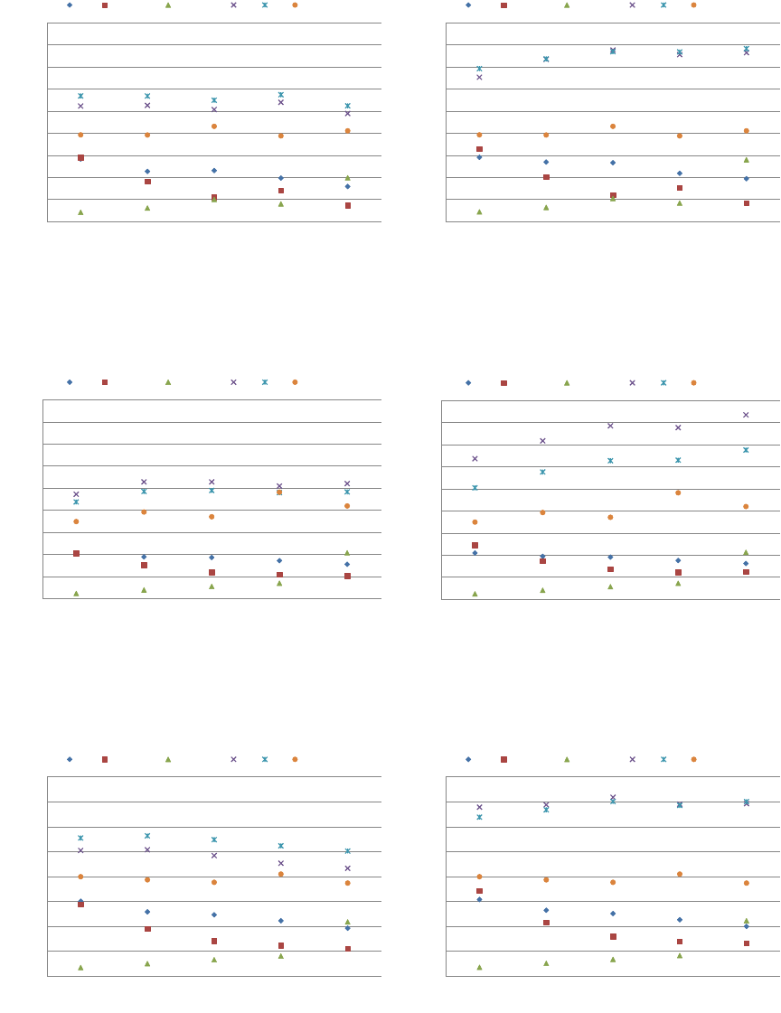
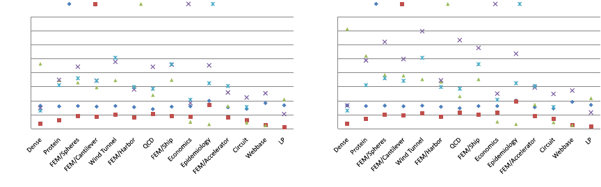
5.2.2 Double Precision
Together, our CSR and HYB kernels surpass the 10.0 GFLOP/s mark in half of the unstructured test cases
using double precision values. As shown in Figure 35, the CSR (vector) kernel achieves the highest absolute
performance at 14.2 GFLOP/s on the Dense matrix. Wind Tunnel and QCD represent best-case HYB
performance at 13.9 and 12.6 GFLOP/s respectively. Again, COO performance is stable, varying from a
minimum of 2.9 to a maximum 4.0 GFLOP/s, with most results close to the 3.3 GFLOP/s mark.
The relative performance between double and single precision performance follows the same pattern
discussed in Section 5.1.2. The median double precision HYB performance is 62.0% of the corresponding
26
0.0
20.0
40.0
60.0
80.0
100.0
120.0
140.0
160.0
GByte/s
Matrix
COO
CSR (scalar)
CSR (vector)
HYB
PKT
(a) Without Cache
0.0
20.0
40.0
60.0
80.0
100.0
120.0
140.0
160.0
GByte/s
Matrix
COO
CSR (scalar)
CSR (vector)
HYB
PKT
(b) With Cache
Figure 35: Bandwidth results for unstructured matrices using double precision.
Name Sockets Cores Clock (GHz) Description
Cell 1 8 (SPEs) 3.2 IBM QS20 Cell Blade (half)
Opteron 1 2 2.2 AMD Opteron 2214
Xeon 1 4 2.3 Intel Clovertown
Niagara 1 8 1.4 Sun Niagara2
Dual Cell 2 16 (SPEs) 3.2 IBM QS20 Cell Blade (full)
Dual Opteron 2 4 2.2 2 x AMD Opteron 2214
Dual Xeon 2 8 2.3 2 x Intel Clovertown
Table 5: Specifications for several multicore platforms.
single precision result. For CSR (vector), the median is 55.4%. The CSR (scalar) kernel retains 92.1% of its
single precision performance, again owing the relative bandwidth efficiency of divergent double-word memory
access to single-word accesses.
5.3 Performance Comparison
In this section we provide a comparison between our GPU SpMV results and SpMV results on a variety
of multicore architectures. The multicore results were obtained by Williams et al. [19], who also provide
complete descriptions of each platform. Table 5 summarizes the key features of each platform.
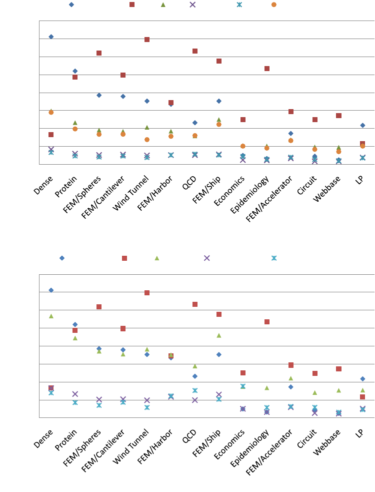
Figure 36 compares double precision SpMV performance of the CSR (vector) and HYB kernels to single
and dual socket multicore systems. Examining the single socket platforms we find that the GPU-based
methods offer the best performance in all 14 test cases, often by significant margins. Among the other
platforms, Cell is the clear winner. It is interesting to note that, like the GTX 200-series GPU, the peak
double precision floating point rate of this version of the Cell is a small fraction of its single precision
throughput. However, given the memory-bound nature of SpMV, the effective use of memory bandwidth is
of much greater importance.
The dual Cell platform is again the fastest of dual socket multicore processors, besting the GPU methods
on the FEM/Harbor matrix by a small margin (6.9 GFLOP/s to 7.0 GFLOP/s). In addition to increasing
the available memory bandwidth, the addition of a second processor increases the total cache size. As a
result, dual socket performance can exhibit super-linear speedup over single socket performance. This effect
is most pronounced in the dual socket Xeon platform with 16MB of total L2 cache. Hence, a relatively small
matrix like Economics runs four times faster. On the other hand, performance of the dual Xeon system does
not scale well on large matrices, such as Wind Tunnel (1.5x faster) and LP (1.3x faster).
27
0.0
2.0
4.0
6.0
8.0
10.0
12.0
14.0
16.0
GFLOP/s
Matrix
CSR (vector)
HYB
Cell
Opteron
Xeon
Niagara
0.0
2.0
4.0
6.0
8.0
10.0
12.0
14.0
16.0
GFLOP/s
Matrix
CSR (vector)
HYB
Dual Cell
Dual Opteron
Dual Xeon
Figure 36: CSR and HYB kernels compared to several single and dual processor multicore platforms.
28
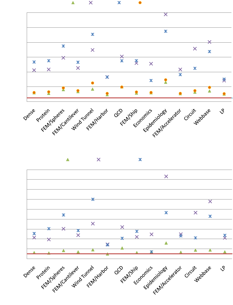
Figure 37 shows the ratio of the our best GPU kernel performance (either CSR (vector) or HYB) to the
performance of the single and dual-processor multicore systems. The median GPU performance advantages
over the single socket systems are: 2.47×for Cell, 10.32×for Opteron, 10.85×for Xeon, and 2.79×for
Niagara. For dual-processor platforms, the median GPU performance factors are: 1.41×for Cell, 4.96×for
Opteron, and 5.33×for Xeon.
6 Conclusion
We have demonstrated several efficient implementations of sparse matrix-vector multiplication (SpMV) in
CUDA. Our kernels exploit fine-grained parallelism to effectively utilize the computational resources of the
GPU. By tailoring the data access patterns of our kernels to the memory subsystem of the GTX 200-series
architecture, we harness a large fraction of the available memory bandwidth. In this section we provide a
summary our data structures and SpMV kernels and then close with a brief outline of areas of improvement
and topics for future work.
6.1 Results Summary
The DIA and ELL formats are well-suited to matrices obtained from structured grids and semi-structured
meshes. DIA is uniformly faster than ELL since both utilize memory bandwidth efficiently and DIA has
higher computational intensity. On the other hand, the use of explicit column indices makes ELL a more
flexible format.
CSR is a popular, general-purpose sparse matrix format which is convenient for many other sparse matrix
computations. A na¨ıve attempt to parallelize CSR SpMV using one thread per matrix row does not benefit
from memory coalescing, which consequently results in low bandwidth utilization and poor performance. On
the other hand, using a 32-thread warp to process each row ensures contiguous memory access, but leads
to a large proportion of idle threads when the number of nonzeros per row is smaller than the warp size.
Performance of the scalar method is rarely competitive with alternative choices, while the vector kernel excels
on matrices with large row sizes. However, both CSR kernels are subject to execution divergence caused by
variations in the distribution of nonzeros per row.
The COO SpMV kernel based on segmented reduction is robust with respect to variations in row sizes
and offers consistent performance. However, the COO format is verbose and has the worst computational
intensity of the formats considered. Furthermore, the segmented reduction operation more expensive than
alternative techniques that rely on a simpler decomposition of work into threads of execution. Nevertheless,
the COO kernel is reliable and complements the deficiencies of the other SpMV kernels.
The HYB format, a combination of the ELL and COO sparse matrix data structures, offers the speed of
ELL and the flexibility of COO. Often, unstructured matrices that are not efficiently stored in ELL format
alone and readily handled by HYB. In such matrices, rows with exceptional lengths contain a relatively small
number of the total matrix entries. As a result, HYB is generally the fastest format for a broad class of
unstructured matrices. While the PKT format is outperformed by HYB in a majority of cases considered,
further improvements are possible.
6.2 Future Work
We have not considered block formats, such as Block CSR or Variable-Block CSR [8] in this paper. Block
formats can deliver higher performance [5, 19], particularly for matrices arising in vector-valued problems.
A number of the techniques we have applied to scalar formats are compatible with block format extensions.
Special handling for the case of several vectors, so-called block vectors, is another standard optimization.
In the context of iterative methods for linear systems, this situation occurs when solving for several right-
hand-sides simultaneously (i.e. AX =Bwhere Bhas multiple columns). Furthermore, in the case of
eigensolvers such as the LOBPCG [9], it is not uncommon to utilize block vectors with ten or more columns.
29
0.00
4.00
8.00
12.00
16.00
20.00
24.00
Relative Performance
Matrix
Cell
Opteron
Xeon
Niagara
0.00
2.00
4.00
6.00
8.00
10.00
12.00
14.00
16.00
18.00
Relative Performance
Matrix
Dual Cell
Dual Opteron
Dual Xeon
Figure 37: Performance of the best GPU kernel relative to each of the multicore platforms.
30
Since the memory capacity and performance of any single device, GPU or otherwise, is fixed, it is nec-
essary to distribute large-scale computations over many devices. Effectively decomposing sparse matrix
computations over multiple GPUs presents additional challenges, not unlike those faced on distributed mem-
ory systems. Tackling these problems, either on a single node with multiple GPUs, or a networked collection
of GPU-equipped computers, is an important area of research.
We have only briefly explored the use of shared memory as an explicitly-managed cache. Possible ex-
tensions include more sophisticated variations of the packet format or prefetching values used in the CSR
kernels. Lastly, alternative packing schemes, such as combining the row, column, and value of a nonzero
matrix entry of the COO format into a single multi-word structure, are likely optimizations.
References
[1] E. Anderson, Z. Bai, C. Bischof, S. Blackford, J. Demmel, J. Dongarra, J. Du Croz, A. Greenbaum,
S. Hammarling, A. McKenney, and D. Sorensen. LAPACK Users’ Guide. Society for Industrial and
Applied Mathematics, Philadelphia, PA, third edition, 1999.
[2] Sergio Barrachina, Maribel Castillo, Francisco D. Igual, Rafael Mayo, and Enrique S. Quintana-Ort´ı.
Solving dense linear systems on graphics processors. In Proc. 14th Int’l Euro-Par Conference, volume
5168 of Lecture Notes in Computer Science, pages 739–748. Springer, August 2008.
[3] Guy E. Blelloch. Prefix sums and their applications. Technical Report CMU-CS-90-190, School of
Computer Science, Carnegie Mellon University, November 1990.
[4] Guy E. Blelloch, Michael A. Heroux, and Marco Zagha. Segmented operations for sparse matrix com-
putation on vector multiprocessors. Technical Report CMU-CS-93-173, School of Computer Science,
Carnegie Mellon University, August 1993.
[5] Luc Buatois, Guillaume Caumon, and Bruno L´evy. Concurrent number cruncher - a GPU implemen-
tation of a general sparse linear solver. International Journal of Parallel, Emergent and Distributed
Systems, to appear.
[6] E.F. DAzevedo, M.R. Fahey, and R.T. Mills. Vectorized sparse matrix multiply for compressed row
storage format. In International Conference on Computational Science (ICCS), pages 99–106. Springer,
2005.
[7] R. Grimes, D. Kincaid, and D. Young. ITPACK 2.0 User’s Guide. Technical Report CNA-150, Center
for Numerical Analysis, University of Texas, August 1979.
[8] Eun-Jin Im, Katherine Yelick, and Richard Vuduc. Sparsity: Optimization framework for sparse matrix
kernels. Int. J. High Perform. Comput. Appl., 18(1):135–158, 2004.
[9] Andrew V. Knyazev. Toward the optimal preconditioned eigensolver: Locally optimal block precondi-
tioned conjugate gradient method. SIAM Journal on Scientific Computing, 23(2):517–541, 2002.
[10] C. L. Lawson, R. J. Hanson, D. R. Kincaid, and F. T. Krogh. Basic Linear Algebra Subprograms for
Fortran Usage. ACM Transactions on Mathematical Software (TOMS), 5(3):308–323, 1979.
[11] J. K. Lenstra, D. B. Shmoys, and ´
E. Tardos. Approximation algorithms for scheduling unrelated parallel
machines. Math. Program., 46(3):259–271, 1990.
[12] Erik Lindholm, John Nickolls, Stuart Oberman, and John Montrym. NVIDIA Tesla: A unified graphics
and computing architecture. IEEE Micro, 28(2):39–55, Mar/Apr 2008.
[13] John Nickolls, Ian Buck, Michael Garland, and Kevin Skadron. Scalable parallel programming with
CUDA. Queue, 6(2):40–53, Mar/Apr 2008.
31
[14] NVIDIA Corporation. NVIDIA CUDA Programming Guide, June 2008. Version 2.0.
[15] Yousef Saad. SPARSKIT: A basic tool kit for sparse computations; Version 2, June 1994.
[16] Yousef Saad. Iterative Methods for Sparse Linear Systems. Society for Industrial Mathematics, 2003.
[17] Shubhabrata Sengupta, Mark Harris, Yao Zhang, and John D. Owens. Scan primitives for GPU com-
puting. In Graphics Hardware 2007, pages 97–106. ACM, August 2007.
[18] Vasily Volkov and James W. Demmel. Benchmarking GPUs to tune dense linear algebra. In Proc. 2008
ACM/IEEE Conference on Supercomputing, pages 1–11, November 2008.
[19] S. Williams, L. Oliker, R. Vuduc, J. Shalf, K. Yelick, and J. Demmel. Optimization of sparse matrix-
vector multiplication on emerging multicore platforms. In Proc. 2007 ACM/IEEE Conference on Su-
percomputing, 2007.
32
