Manual
User Manual:
Open the PDF directly: View PDF ![]() .
.
Page Count: 38
HAL (Hybrid Agent-based Library) Manual
Rafael Bravo, Mark Robertson-Tessi, Alexander Anderson
July 8, 2018
Integrated Mathematical Oncology Department
H. Lee Moffitt Cancer Center & Research Institute
12902 Magnolia Drive
Tampa, Florida, 33612.
rafael.bravo@moffitt.org, mark.robertsontessi@moffitt.org, alexander.anderson@moffitt.org
Abstract
The presented Hybrid Agent–based Library (HAL) is a Java Library made of simple, efficient, generic com-
ponents which can be used to model complex spatial systems. HAL’s components can broadly be classified
into: on and off lattice agent containers, finite difference diffusion fields, a gui building system, and additional
tools and utilities for computation and collecting data. These components were designed to operate indepe-
nently, but are standardized to make them easy to interface with one another. A complete example of how to
build a hybrid model (a spatial model with an interacting agent based component and PDE component, com-
monly used for oncology modeling) using HAL is included to showcase how modeling can be simplified using
our approach. HAL is a useful asset for researchers who wish to build efficient 2D and 3D hybrid models in
Java, while not starting entirely from scratch. It is available on github at https://github.com/torococo/HAL
under the MIT License. HAL requires at least Java 8 or later to run, and the java jdk version 1.8 or later to
compile the source code.
Contents
1 Setup 3
1.1 GettingJava............................................ 3
1.2 Getting the Framework Source Code . . . . . . . . . . . . . . . . . . . . . . . . . . . . . . . 3
1.3 GettingIntellijIDEA ....................................... 3
1.4 SettinguptheProject....................................... 3
2 Introduction 4
2.1 LearningJava ........................................... 4
2.2 UsingIntellijIDEA......................................... 4
2.3 UnderstandingHAL........................................ 5
2.4 SourceCodeOrganization..................................... 5
2.4.1 Examples ......................................... 5
2.4.2 LEARN_HERE ...................................... 5
2.4.3 Framework......................................... 5
2.5 Frameworkorganization...................................... 5
1
3 Grids and Agents 6
3.1 TypesofGrid ........................................... 6
3.2 TypesofAgent .......................................... 6
3.3 Grid and Agent Class Definition . . . . . . . . . . . . . . . . . . . . . . . . . . . . . . . . . . 7
3.4 GridConstructors ......................................... 7
3.5 Agent Initialization Functions . . . . . . . . . . . . . . . . . . . . . . . . . . . . . . . . . . . 8
3.6 GridIndexing ........................................... 8
3.6.1 SingleIndexing ...................................... 8
3.6.2 SquareIndexing ...................................... 8
3.6.3 PointIndexing....................................... 9
3.7 TypicalGridLoop ......................................... 9
3.8 TypeHeirarchy .......................................... 9
3.9 AgentFunctions.......................................... 10
3.10 Universal Grid Functions and Properties . . . . . . . . . . . . . . . . . . . . . . . . . . . . . 11
3.11 AgentGrid Method Descriptions . . . . . . . . . . . . . . . . . . . . . . . . . . . . . . . . . . 12
3.11.1 AgentGrid Agent Search Functions . . . . . . . . . . . . . . . . . . . . . . . . . . . . 12
3.12 PDEGrid Method Descriptions . . . . . . . . . . . . . . . . . . . . . . . . . . . . . . . . . . 13
3.13 Griddouble/Gridint/Gridlong Method Descriptions . . . . . . . . . . . . . . . . . . . . . . . . 15
4 Util.java 15
4.1 UtilArrayFunctions........................................ 15
4.2 Util Neigborhood Functions . . . . . . . . . . . . . . . . . . . . . . . . . . . . . . . . . . . . 16
4.3 UtilMathFunctions........................................ 16
4.4 UtilMiscFunctions ........................................ 17
4.5 UtilColorFunctions........................................ 17
4.6 Util MultiThread Function . . . . . . . . . . . . . . . . . . . . . . . . . . . . . . . . . . . . 18
4.7 Util Save and Load Functions . . . . . . . . . . . . . . . . . . . . . . . . . . . . . . . . . . . 18
5 Rand.java 19
6 Gui 19
6.1 Types of Gui and Method Descriptions . . . . . . . . . . . . . . . . . . . . . . . . . . . . . . 20
6.1.1 GridWindow ....................................... 20
6.1.2 UIWindow ........................................ 21
6.1.3 Vis2DOpenGL ...................................... 21
6.1.4 Vis3DOpenGL ...................................... 22
6.2 Types of GuiComponent and Method Descriptions . . . . . . . . . . . . . . . . . . . . . . . . 23
6.2.1 UIGrid ........................................... 23
6.2.2 UILabel .......................................... 23
6.2.3 UIButton ......................................... 23
6.2.4 UIBoolInput........................................ 23
6.2.5 UIIntInput ........................................ 23
6.2.6 UIDoubleInput ...................................... 23
6.2.7 UIStringInput ....................................... 23
6.2.8 UIComboBoxInput .................................... 23
6.2.9 UIFileChooserInput .................................... 24
7 Tools 24
7.1 Tools/FileIO ........................................... 24
7.2 Tools/SerializableModel ..................................... 25
7.3 Tools/ MultiwellExperiment . . . . . . . . . . . . . . . . . . . . . . . . . . . . . . . . . . . 25
2

8 Example: Competitive Release Model 25
8.1 Competitive Release Introduction . . . . . . . . . . . . . . . . . . . . . . . . . . . . . . . . . 25
8.2 MainFunction........................................... 29
8.3 ExampleModel Constructor and Properties . . . . . . . . . . . . . . . . . . . . . . . . . . . . 30
8.4 InitTumorFunction ........................................ 31
8.5 ModelStepFunction........................................ 32
8.6 CellStep Function and Cell Properties . . . . . . . . . . . . . . . . . . . . . . . . . . . . . . 33
8.7 DrawModelFunction ....................................... 34
8.8 Imports............................................... 35
8.9 ModelResults ........................................... 35
1 Setup
1.1 Getting Java
As pretty as HAL’s source code is, your going to need at least the Java8 JDK (Java Development Kit) installed
to do anything with it.
To check if the JDK is installed, open a command line/terminal/cmd window and enter
1j a v a −version
2j a v a c −version
If both of these commands print 1.8anything or later, you’re good to go. If not, get the latest Java JDK by
googling it or from the oracle website.
http://www.oracle.com/technetwork/java/javase/downloads/jdk9-downloads-3848520.html
You don’t need to download the demos and samples.
1.2 Getting the Framework Source Code
To download the framework java files, go to
https://github.com/torococo/AgentFramework
and click the clone or download button to get a zip file containing the source code along with the included
examples.
unzip this folder and put it somewhere easily accessible.
1.3 Getting Intellij IDEA
Intellij idea is my favorite ide for programming in Java, and it probably should be yours too (https://dzone.com/articles/why-
idea-better-eclipse). It can be downloaded here:
https://www.jetbrains.com/idea/download/
make sure you download the community edition, unless you really don’t know what to do with your grant
money.
1.4 Setting up the Project
1. Open Intellij Idea and click “create project from existing sources” (“file/ new/ project from existing sources”
from the main gui) and direct it to the unzipped AgentFramework Source code directory.
3
2. Continue through the rest of the setup, you can basically click next until it asks for the Java sdk:
•“/Library/ Java/ JavaVirtualMachines/” on mac.
•“C:\ Program Files\ Java\” on windows.
1. Once the setup is complete we will need to do one more step and add some libraries that allow for 2D and
3D OpenGL visualization:
2. open the Intellij IDEA main gui
3. go to “file/ project structure”
4. click the “libraries” tab
5. use the minus button to remove any pre-existing library setup
6. click the plus button, and direct the file browser to the “Framework/ lib” folder.
7. click apply or ok
This will setup the classes, sources, and native library locations that OpenGL needs. Try running the “Exam-
ples/Example3D” program in the examples folder to see that everything is working properly
If you think that the colorscheme that comes with Intellij leaves something to be desired, you’re not alone.
try “File/ import settings” and give it the NinjaTurtleScheme.jar file in the top level folder.
2 Introduction
2.1 Learning Java
If your already pretty familiar with programming, and want a quick, shallow description of the language syntax,
the first video on this list may be enough to get up to speed and jump into the framework:
https://www.youtube.com/results?search_query=learn+java
The resources are listed in order by popularity, just try some until you find one that jives well. For a more
textual perspective,
https://www.codecademy.com/learn/learn-java
http://www.learnjavaonline.org/
are some potential places to start.
2.2 Using Intellij IDEA
Some of the ways in which Intellij may make your life easier include:
•automatically importing classes as they are first mentioned in the code (right click on the class name and
intellij should offer to import it)
•debugging with the debugger (shocker) when necissary rather than relying on print statements alone
(https://www.youtube.com/watch?v=1bCgzjatcr4), HINT: while paused in the debugger right click on
anything and click “evaluate expression”
4
•using refactoring to rename variables, change function signatures, etc. without having to go hunting for
every place that the variable/function/class is mentioned. (right click on some code and check out the
“refactor” submenu)
•using “find usages” and “Go To Declaration” to move fluidly around your code base and to see how its pieces
connect together. (right clicking on things will get you there, see “find usages” and the “go to” submenu)
•using Shift-F10 to quickly run the currently open file, and learning other hotkeys to speed up your workflow.
•tapping Shift twice allows you to search the entire codebase for anything
•using fori, iter, and sout shortcuts to create a for loop, foreach loop, and print statment respectively
Don’t worry too much about learning all of these up front, but I suggest that you do check them out as you
become more comfortable with the platform.
2.3 Understanding HAL
Once you have a basic grasp of Java, I recommend skimming this manual as well as checking out the LEARN_HERE
folder. then look at the examples
2.4 Source Code Organization
At the top level, there are 3 folders which hold different framework parts. These are...
2.4.1 Examples
contains models that use the framework as a basis
2.4.2 LEARN_HERE
contains small examples that serve as tests of framework components
2.4.3 Framework
the top level framework source code folder, contains all of the following subfolders that hold various framework
components. Descriptions of the 7 subfolders contained within the framework folder are detailed below.
2.5 Framework organization
Grids this folder contains all of the Agent and Grid types that the framework supports. There are 2D and 3D,
stackable and unstackable, on-lattice and off-lattice agents and grids to contain them. The base classes
that the grids and agents extend are also in this folder.
Gui this folder contains the main UIWindow class, as well as many component classes that can be added to the
UI.
Tools this folder contains many useful tool classes, such as a FileIO wrapper, a genetic algorithm class, a multiwell
experiment runner, etc. as well as a Util class that is a container of generic static methods. It also contains
classes that are used internally by these tools.
5
Interfaces this folder contains interfaces that are used by the framework internally. It is useful to reference this
folder if a framework function takes a function interface argument, or implements an interface.
Extensions contains more specialized framework components that are created by extending the generic ones.
Lib contains outside libraries that have been integrated with the framework.
Util The only file directly on the top level, it’s full of goodies that can be broadly categorized into: color functions,
array functions, cellular automata neighborhood functions, and math functions.
The manual from here turns into a glossary that looks at the framework components in some detail (to the extent
that I bothered to write about them) and after that a simple but complete model example is provided.
Those looking to dive headfirst into modeling may want to first go to the LEARN_HERE folder for a hands
on approach, or check out the last section for an in depth explanation of a model and use the other chapters as
a reference. If you like reading dictionaries in your spare time then read this thing from end to end.
3 Grids and Agents
The bread and butter of the framework consists of different types of Grids and Agents. these are presented below.
3.1 Types of Grid
AgentGrid0D Holds nonspatial agents
AgentGrid1D Holds all 1D agents
AgentGrid2D Holds all 2D agents
AgentGrid3D Holds all 3D agents
PDEGrid1D facilitates modeling a single diffusible field in 1D
PDEGrid2D facilitates modeling a single diffusible field in 2D
PDEGrid3D facilitates modeling a single diffusible field in 3D
3.2 Types of Agent
Agent0D Nonspatial agents. this agent type is a member of AgentGrid0D grid type.
AgentSQ2Dunstackable “Square” agents in 2D. this agent type is bound to the AgentGrid2D lattice, and only
one AgentSQ2Dunstackable can occupy a given lattice position at a time.
AgentSQ2D “Square” agents in 2D. this agent type is bound to the AgentGrid2D lattice, however multiple
AgentSQ2Ds can occupy the same lattice position
AgentPT2D “Point” agents in 2D. this agent type is not bound to the AgentGrid2D lattice, and is free to move
continuously within the Grid, provided it does not try to cross the Grid boundaries.
AgentSQ2Dunstackable “Square” agents in 2D. this agent type is bound to the AgentGrid2D lattice, and only
one AgentSQ2Dunstackable can occupy a given lattice position at a time.
6

AgentSQ2D “Square” agents in 2D. this agent type is bound to the AgentGrid2D lattice, however multiple
AgentSQ2Ds can occupy the same lattice position
AgentPT2D “Point” agents in 2D. this agent type is not bound to the AgentGrid2D lattice, and is free to move
continuously within the Grid, provided it does not try to cross the Grid boundaries.
AgentSQ3Dunstackable “Square” agents in 3D (cube?). this agent type is bound to the AgentGrid3D lattice,
and only one AgentSQ3Dunstackable can occupy a given lattice position at a time (gotta love copy paste)
AgentSQ3D “Square” agents in 3D. this agent type is bound to the AgentGrid3D lattice, however multiple
AgentSQ3Ds can occupy the same lattice position
AgentPT3D “Point” agents in 3D. this agent type is not bound to the AgentGrid3D lattice, and is free to move
continuously within the Grid, provided it does not try to cross the Grid boundaries.
3.3 Grid and Agent Class Definition
for demonstration we will use bits of code from the CompetitiveReleaseModel example. It is a fairly simple yet
complete model, so it is a good place to begin learning the syntax of HAL. Grid classes and Agent classes used in
models will usually be created as extensions of the Grid and Agent classes shown above. This extension is done
with the following syntax:
Project specific AgentGrid definition syntax:
1p u b l i c c l a s s ExampleModel extends Grid2D<E xC ell > {
Project specific Agent class definition syntax:
1class ExampleCell extends AgentSQ2Dunstackable<ExModel> {
Note the <> after the base class name, in java this is called a generic type argument. This is how we tell the
Grid what kinds of Agent it will store, and how we tell the Agents what kind of Grid will store them. It is used
by the ExampleModel and ExampleCell to identify each other, so that their constituent functions can return the
proper type, and access each other’s variables and methods.
3.4 Grid Constructors
In order to create a class that extends any of the Grids, you must provide a constructor. let’s look at part of the
ExampleGrid constructor as an example
1public ExampleModel(int x,int y,Rand generator ) {
2super(x,y,ExampleCell .class) ;
the first line declares the constructor and arguments, the second line calls super, which is required since our
class extends a class with a constructor. Super is used to call the constructor of the base class. Into super we
pass what the AgentGrid2D needs for initialization: an x and y dimension, which define the size of the grid, and
ExampleCell.class, which is the class object of the ExampleCell. We pass the class object so that the ExampleGrid
can create ExampleCells for us, as described in the next section.
7

3.5 Agent Initialization Functions
a word of caution: DO NOT DEFINE A CONSTRUCTOR FOR YOUR AGENT CLASSES.
The AgentGrid that houses the agent will act as a “factory” for agents, and produce them with the NewAgent()
function. This will return an agent that is either newly constructed, or an agent that has died and is being recycled.
This returning of dead agents for reuse as new ones allows the model to run without tasking the garbage collector
with removing all of the dead agents. This will increase the speed and decrease the memory footprint of your
model. Instead of a constructor you should define some sort of initialization for your agents, which you do directly
after the call to NewAgent. An example from CompRelModel.java:
1for (int i= 0 ; i<h oo d S iz e ;i++) {
2i f (rng .Double ( ) < resistantProb) {
3NewAgentSQ(tumorNeighborhood [i] ) . t y pe =RESISTANT ;
4 } e l s e {
5NewAgentSQ(tumorNeighborhood [i] ) . t y pe =SENSITIVE ;
6 }
7 }
These lines of code come from the InitTumor function that the ExampleModel calls once at the beginning
of a simulation. We use a random number generator and an if-else statement to decide whether to create a
sensitive or resistant cell. since this type property is the only information individual cells store in this model,
setting it is all that is needed to initialize a new cell. We call the NewAgentSQ() function, and pass in an index
(“tumorNeighborhood” is an array of starting indices to setup the tumor) that marks where to place the new
agent.
3.6 Grid Indexing
There are 3 different ways to describe or index locations on framework grids:
3.6.1 Single Indexing
since the x dimension, y dimension, and possibly the z dimension values are Grid constants, every square or voxel
can be uniquely identified with a single integer index. Functions using this kind of indexing typically end with
the SQ (abbreviating Square) phrase at the end of the function name. Single indexing is done with the following
mappings:
In 2D: I(x, y) = x∗yDim +y
In 3D: I(x, y, z) = x∗yDim ∗zDim +y∗zDim +z
the agents/values in the grids are stored as a single array, so single indexing is actually the most efficient as
it requires no conversion.
3.6.2 Square Indexing
Similar to single indexing, square indexing uses a set of integers to refer to a specific square or voxel, as an (x,y)
or an (x,y,z) set. Functions using this kind of indexing typically end with the SQ (abbreviating Square) phrase at
the end of the function name.
8
3.6.3 Point Indexing
Uses a set of double values, to define continuous coordinates. Functions using this kind of indexing typically end
with the PT (abbreviating Point) phrase at the end of the function name. The integer flooring of a coordinate
set corresponds to the Square or Voxel that contains the point.
3.7 Typical Grid Loop
here we look at an example Loop or Run function. This is taken from the GOLGrid class, but all models will
usually follow a similar pattern.
1p u b l i c v o i d Run ( ) {
2for (int i= 0 ; i<runTicks ;i++) {
3for (GOLAgent a :this) {
4a.St ep ( ) ;
5 } ;
6 }
7 }
The outer for loop counts the ticks, meaning that we will run for a total of runTicks steps. The inner for loop
iterates over all the agents in the grid (“this” here is the grid that calls the Run function), and inside the loop we
call that agent’s Step function, which is defined in the GOLAgent class.
3.8 Type Heirarchy
in order to navigate the source code and see the full set of functions and properties of the framework components,
it is important to become familiar with the type heirarchy that the framework uses. Figure 1 summarizes this
heirarchy for 2D agents.
Figure 1:
AgentBase) AgentBaseSpatial) Agent2DBase) AgentSQ2Dunstackable)
AgentSQ2D)
AgentPT2D)
GridBase2D)
AgentGrid2D)
Grid2Ddouble) PDEGrid2D)
SphericalAgent2D)
Grid2Dint)
Grid2Dlong)
Grid2Dobject)
9
each node in the heirarchy names a class. each arrow denotes an extends relationship, eg. AgentBaseSpatial
extends AgentBase. The blue classes are abstract and cannot be used directly. The green classes are fully
implemented and can be used/extended further. classes later in the heirarchy keep all properties and methods
of the classes that they extend, which means that to see the full set of functions a class implements, one has
to look at all of the extended classes beneath that class as well. the method summaries included in this manual
can simplify this process somewhat as they show useful methods of the extended classes regardless of where they
come from in the class heirarchy.
3.9 Agent Functions
here we describe the builtin functions that the Agents expose to the user. (3D adds a z)
G: returns the grid that the agent belongs to (this is a permanent agent property, not a function)
Age(): returns the age of the agent, in ticks. Be sure to use IncTick on the AgentGrid appropriately for this
function to work.
BirthTick(): returns the tick on which the agent was born
Alive(): returns whether or not the agent currently exists on the grid
Isq(): returns the index of the square that the agent is currently on
Xsq(),Ysq(): returns the X or Y indices of the square that the agent is currently on.
Xpt(),Ypt(): returns the X or Y coordinates of the agent. If the Agent is on-lattice, these functions will return
the coordinates of the middle of the square that the agent is on.
MoveSQ(x,y),MoveSQ(i): moves the agent to the middle of the square at the indices/index specified
MovePT(x,y): moves the agent to the coordinates specified
MoveSafeSQ(x,y),MoveSafePT(x,y): Similar to the move functions, only it will automatically either apply
wraparound, or prevent moving along a partiular axis if movement would cause the agent to go out of
bounds.
Dispose(): removes the agent from the grid
SwapPoisition(otherAgent): swaps the positions of two agents. useful mostly for the AgentSQ2unstackable
and AgentSQ3unstackable classes, which don’t allow stacking of agents, making this maneuver otherwise
difficult.
MapHood(int[]neighborhood): This function takes a neighborhood (As generated by the neighborhood Util
functions, or using GenHood2D/GenHood3D), translates the neighborhood coordinates to be centered
around the agent, and computes the set of indices that the translated coordinates map to. The function
returns the number of valid locations it set, which if wraparound is disabled may be less than the full set of
coordinate pairs. this means that the passed in ret list will not be completely filled with valid entries. See
the CellStep function in the Complete Model example for more information.
MapEmptyHood(int[]neighborhood),MapOccupiedHood(int[]neighborhood): These functions are similar
to the the MapHood function, but they will only include valid empty or occupied indices, and skip the
others.
10
MapHood(int[]neighborhood,CoordsToBool): This function takes a neighborhood and another mapping func-
tion as argument, the mapping function should return a boolean that specifies whether coordinates map to
a valid location. the function will only include valid indices, and skip the others.
3.10 Universal Grid Functions and Properties
These functions and properties are shared by all of the different types of grids (3D adds a z):
xDim,yDim: the x or y dimension of the Grid
length: the total number of squares in the grid, equivalent to xDim*yDim
I(x,y): converts a set of coordinates to the index of the square at those coordinates.
ItoX(i),ItoY(i): converts an index of a square to that square’s X or Y coordinate
WrapI(x,y): returns the index of the square at the provided x,y coordinates, with wraparound.
In(x,y): returns whether the x and y coordinates provided are inside the Grid.
ConvXsq(x,otherGrid),ConvYsq(y,otherGrid): returns the index of the center of the square in otherGrid that
the coordinate maps to.
ConvXpt(x,otherGrid),ConvYpt(y,otherGrid): returns the provided coordinate scaled to the dimensions of the
otherGrid.
DispX(x1,x2),DispY(y1,y2): gets the displacement from the first coorinate to the second. using wraparound if
allowed over the given axis to find the shortest displacement.
Dist(x1,y1,x2,y2): gets the distance between two positions with or without grid wrap around (if wraparound is
enabled, the shortest distance taking this into account will be returned)
DistSquared(x1,y1,x2,y2): gets the distance squared between two positions with or without grid wrap around
(if wraparound is enabled, the shortest distance taking this into account will be returned) more efficient
than the Dist function above as it skips a square-root calculation.
ChangeGridsSQ(outsideAgent,x,y),ChangeGridsPT(outsideAgent,x,y): removes the agent from whichever
grid it is currently living on, and moves it to this grid. The age of the agent is also reset so that the agent
appears to be just born this timestep.
MapHood(int[]hood,centerX,centerY): This function takes a neighborhood centered around the origin, trans-
lates the set of coordinates to be centered around a particular central location, and computes which indices
the translated coordinates map to. The function returns the number of valid locations it set. this function
differs from HoodToIs and CoordsToIs in that it takes no ret[], MapHood instead puts the result of the
mapping back into the hood array.
MapHood(int[]hood,centerX,centerY,EvaluationFunction): This function is very similar to the previous def-
inition of MapHood, only it additionally takes as argument an EvaluationFunctoin. this function should
take as argument (i,x,y) of a location and return a boolean that decides whether that location should be
included as a valid one.
11
IncTick(): increments the internal grid tick counter by 1, used with the Age() and BirthTick() functions to get
age information about the agents on an AgentGrid. can otherwise be used as a counter with the other grid
types.
GetTick(): gets the current grid timestep.
ResetTick(): sets the tick to 0.
3.11 AgentGrid Method Descriptions
here we describe the builtin functions that the agent containing Grids expose to the user. Most functions that take
x,y arguments can alternatively take a single index argument. The Grid will use the index to find the appropriate
square. (3D adds a z)
NewAgentSQ(x,y),NewAgentSQ(i): returns a new agent, which will be placed at the center of the indicated
square. x,y, and i are assumed to be integers
NewAgentPT(x,y): returns a new agent, which will be placed at the coordinates specified. x and y are assumed
to be doubles
Pop(): returns the number of agents that are alive on the entire grid.
CleanAgents(): reorders the list of agents so that dead agents will no longer have to be iterated over. don’t call
this during the middle of iteration!
ShuffleAgents(): shuffles the list of agents, so that they will no longer be iterated over in the same order. don’t
call this during the middle of iteration!
CleanShuffIe(): Cleans the agent list and shuffles it. This function is often called at the end of a timestep. don’t
call this during the middle of iteration!
Reset(): disposes all agents, and resets the tick counter.
MapHoodEmpty(int[]coords,centerX,centerY): similar to the MapHood function, but will only include indices
of locations that are empty
MapHoodOccupied(int[]coords,centerX,centerY): similar to the MapHood function, but will only include
indices of locations that are occupied
RandomAgent(rand): returns a random living agent
3.11.1 AgentGrid Agent Search Functions
Several convinience methods have been added to make searching for agents easier.
GetAgent(x,y)GetAgent(i): Gets a single agent at the specified grid square, beware using this function with
stackable agents, as it will only return one of the stack of agents. This function is recommended for the
Unstackable Agents, as it tends to perform better than the other methods for single agent accesses.
GetAgentSafe(x,y): Same as GetAgent above, but if x or y are outside the domain, it will apply wrap around if
wrapping is enabled, or return null.
12
IterAgents(x,y),IterAgents(i): use in a foreach loop to iterate over all agents at a location. example: for(AGENT_TYPE
a : IterAgents(5,6)) will run a for loop over all agents at grid square (5,6) with the agent being stored as
the “a” variable. be sure to set AGENT_TYPE to the type of agent that lives of the grid that you are
iterating over.
IterAgentsSafe(x,y): Same as IterAgents above, but will apply wraparound if x,y fall outside the grid dimensions.
IterAgentsRad(xPT,yPT,rad): will iterate over all agents around the given coordinate pair that fall within
radius rad.
IterAgentsRadApprox(xPT,yPT,rad): will iterate over all agents around the given coordinate pair that at least
fall within radius rad, it is more efficient than IterAgentsRad, but it will also include some agents that fall
outside rad, so be sure to do an additional distance check inside the function.
IterAgentsHood(int[]hood,centerX,centerY): will iterate over all agents in the neighborhood as though it
were mapped to centerX,centerY position. note that this function won’t technically do the mapping. if the
neighborhood is already mapped, use IterAgentsHoodMapped instead.
IterAgentsHoodMapped(int[]hood,hoodLen): will iterate over all agents in the already mapped neighborhood.
be sure to supply the proper hood length.
IterAgentsRect(x,y,width,height): iterates over all agents in the rectangle defined by (x,y) as the lower left
corner, and (x+width,y+height) as the top right corner.
GetAgents(ArrayList<AgentType>,x,y)GetAgentsHood...: A variation of this function exists that matches
every IterAgents variant mentioned above. puts into the argument arraylist all agents found at the specified
location. call the clear function on the arraylist before passing it to GetAgents if you don’t want to append
to whatever agents were already added there.
RandomAgent(x,y,rand,EvalAgent)RandomAgentHood...: A variation of this function exists that matches
every IterAgents variant mentioned above. these functions are used to query a location and choose a
random agent from that area, an optional EvalAgent function (a function that takes an Agent and returns
a boolean) can be provided to ensure that the random agent satisfies the condition
PopAt(x,y),PopAt(i): returns the number of agents that occupy the specified position. this is more efficient
than using GetAgents and taking the length of the resulting arraylist.
3.12 PDEGrid Method Descriptions
The PDEGrid classes do not store agents. They are meant to be used to model Diffusible substances. PDEGrids
contain two fields (arrays) of double values: a current field, and a swap field. The intended usage of these fields is
that the values from the current timestep are stored in the current field while the swap field is used as a location
to write the result of diffusion. The Swap() function exchanges the identities of these fields, so that the current
field becomes the swap field and vice versa. Usually this will be called automatically at the end of a diffusion
computation. The functions included in the PDEGrid class are the following: (3D adds a z, 1D removes y)
GetField(): returns the “current field” double array which is usually used as the main field that agents interact
with
GetSwapField(): returns the “swap field” double array which is usually used as scratch to write the result of
diffusion.
13

Get(x,y),Set(x,y,val),Add(x,y,val),Mul(x,y,val): gets, sets, adds, or multiplies with a single value in the current
field at the position specified by the index argument. can also use an index to specify the position
GetSwap(x,y),SetSwap(x,y,val),AddSwap(x,y,val),MulSwap(x,y,val): gets, sets, adds, or multiplies a single
value in the swap field at the position specified by the index argument. can also use an index to specify the
position
SetAll(val),SetAll(val[])AddAll(val)MulAll(val): applies the Set/Get/Mul operations to all entries of the cur-
rent field
SetAllSwap(val),SetAllSwap(val[])AddAllSwap(val)MulAllSwap(val): applies the Set/Get/Mul operations
to all entries of the swap field
MaxDifInternal(): returns the maximum difference in any single lattice position between the current field and
the swap field. if the boolean scaled argument is set to true, then the difference will be scaled by the current
value.
BoundAll(min,max)BoundAllSwap(min,max): sets all values in the field so that they are between min and
max
Swap(): swaps the identities of the current and swap fields
SwapInc(): swaps and also increments the tick
Diffusion(nonDimDiffCoef,wrapX,wrapY): runs diffusion on the current field, putting the result into the swap
field, then swaps their identities, so that the now current field stores the result of diffusion. This form of the
function assumes either a reflective or wrapping boundary. the nonDimDiffCoef variable is the nondimen-
sionalized diffusion conefficient. If the dimensionalized diffusion coefficient is xthen nonDimDiffCoef can
be found by computing x∗SpaceStep
T imeStep2Note that if the nonDimDiffCoef exceeds 0.25, this diffusion method
will become numerically unstable.
Diffusion(nonDimDiffCoef,boundaryValue,wrapX,wrapY): has the same effect as the diffusion function with-
out the boundary value argument, except that at the boundaries the function assumes either a constant
value (which is the boundary value) or a wrapping bondary.
DiffusionADI(nonDimDiffCoef): runs diffusion on the current field using the ADI (alternating direction implicit)
method. ADI is numerically stable at any diffusion rate. However at high rates it may produce artifacts.
DiffusionADI(nonDimDiffCoef,boundaryValue): runs diffusion on the current field using the ADI (alternating
direction implicit) method. ADI is numerically stable at any diffusion rate. However at high rates it may
produce artifacts. adding a boundary value to the function call will caufse boundary conditions to be
imposed.
Advection(xVel,yVel): runs advection, which shifts the concentrations using a constant flow with the x and
y velocities passed. this signature of the function assumes wrap-around, so there can be no net flux of
concentrations.
Advection(xVel,yVel,bounaryValue): runs advection as described above with a boundary value, meaning that
the boundary value will advect in from the upwind direction, and the concentration will disappear in the
downwind direction.
GradientX(x,y),GradientY(x,y): returns the gradient of the diffusible along the specified axis
14
3.13 Griddouble/Gridint/Gridlong Method Descriptions
As an alternative to this class, it may be useful to simply employ a double/int/long array whose length is equal
to the length of the other associated grids. The I() function of any associated grids can be used to access values
in the double array with x,y or x,y,z coordinates.
GetField(): returns the field double array that the grid stores
Get(i),Get(x,y),Set(i),Set(x,y,val),Add(i),Add(x,y,val),Mul(i,val),Mul(x,y,val): gets, sets, adds, or multi-
plies with a single value in the field at the specified coordinates
SetAll(val),SetAll(val[])AddAll(val)MulAll(val): applies the Set/Get/Mul operations to all entries of the field
BoundAll(min,max)BoundAllSwap(min,max): sets all values in the field so that they are between min and
max
GradientX(x,y),GradientY(x,y): returns the gradient of the diffusible along the specified axis
4 Util.java
The Util class is one of the most ubiquitous classes in the framework, and contains all of the generic functions
that wouldn’t make sense to add to any particular object in the framework.
The list of utilities functions in the framework has only grown with time. the list presented here is not
exhaustive, so I recommend looking at the file itself if you feel something is missing, on top of that feel free to
ask for a new feature or better yet send me an implementation and I’ll most likely add it to the repository for
everyone to share.
4.1 Util Array Functions
A set of utilities for making array manipulation easier.
ArrToString(arr,delim): useful for collecting data or print statement debugging, returns the contents of an array
as a single string. entries are separated by the delimeter argument
IndicesArray(numEntries): generates an array of ascending indices starting with 0, up to nEntries.
Mean(arr): returns the mean of an array
Sum(arr): returns the sum of an array
Norm(arr): returns the euclidean norm of an array
NormSq(arr): returns the squared euclidian norm of an array, somewhat more efficient than Norm
SumTo1(arr): scales all entries in an array so that their sum is 1.
Normalize(arr): scales all entries in an array so that their norm is 1.
15
4.2 Util Neigborhood Functions
a set of utilities for generating neighborhoods. neighborhoods are lists of x,y index pairs, of the form [01,02, ...0n, x1, y1x2, y2...xn, yn]
in the third dimension these are [01,02, ...0n, x1, y1z1, x2, y2z2, ...xn, yn, zn]these arrays are useful when finding
the indices of the locations that make up the neighborhood around an agent when using Grid/Agent functions
such as MapHood. Neighborhood arrays are always padded with 0s at the beginning, for use with the MapHood
functions.
These functions should not be called over and over, as this would wastefully create arrays over and over.
instead the function should be called once and be stored by the grid.
GenHood2D(int[]coords),GenHood3D(int[]coords): generates a 2D/3D neighborhood array for use with the
MapHood functions. input should be an integer array of the form [x1, y1x2, y2...xn, yn]in 2D, or [x1, y1z1, x2, y2z2, ...xn, yn, zn]
in 3D.
VonNeumannHood(origin?),MooreHood(origin?): returns an array that contains the coordinates of the Von-
Neumann or Moore Neigbhorhood in 2D. the boolean argument specifies whether the center of these
neighborhood (0,0) should be included as part of the set of coordinates.
VonNeumannHood3D(origin?),MooreHood3D(origin?): returns an array that contains the coordinates of
the VonNeumann or Moore Neigbhorhood in 3D. the boolean argument specifies whether the center of
these neighborhood (0,0) should be included as part of the set of coordinates.
HexHoodEvenY(origin?),HexHoodOddY(origin?): to simulate a hex lattice on a Grid2D, the neighborhood
used for a given agent changes depending on the position of the agent. The hex hood changes depending
on whether the agent is on an even or odd Y position. These functions return an array that contains the
proper coordinates for a given case.
TriangleHoodSameParity(origin?),TriangleHoodDifParity(origin?): to simulate a triangle lattice on a Grid2D,
the neighborhood used for a given agent changes depending on the position of the agent. The Triangle
hood changes depending on whether the parity (“even-ness”) of the agents X and Y position match. These
functions return an array that contains the proper coordinates for a given case.
CircleHood(origin?,radius): generates a neighborhood of all squares within the radius of a starting position at
the middle of the (0,0) origin square. the boolean argument specifies wether (0,0) should be included in
the return array.
RectangleHood(origin?,radX,radY): generates a neighborhood of all squares whose x displacement is within
radX, and whose y displacement is within radY of a starting position at the middle of the (0,0) origin square.
the boolean argument specifies whether (0,0) should be included in the return array.
AlongLineCoords(x1,y1,x2,y2): returns an array of all squares that touch a line between the two starting
positions.
4.3 Util Math Functions
For all of the following functions, and throughout the framework, rn refers to a random number generator.
InfiniteLinesIntersection2D(x1,y1,x2,y2,x3,y3,x4,y4,double[]ret): computes the intersection of lines between
points 1 and 2, and points 3 and 4. puts the coordinates of the intersection point in ret. returns true if the
infinite lines intersect (if they are not parallel). returns false if the lines are parallel.
16
Bound(val,min,max): returns the value bounded by the min and max.
Rescale(val,min,max): assumes the starting value is in the 0-1 scale, and rescales it be in the min-max scale.
ModWrap(val,max): wraps the value provided so that it must be between 0 and max. used to implement
wraparound by the framework.
ProtonsToPh(protonConc): converts proton concentration to ph
PhToProtons(ph): converts ph to proton concentration
ProbScale(prob,duration): converts the probability that an even happens in unit time to the probability that
that same event happens in duration time.
Sigmoid(val,stretch,inflectionValue,minCap,maxCap): val is the value that the sigmoid function is being
applied to, the stretch argument stretchs or shrinks the sigmoid function along the x axis, the infectionValue
governs where the inflection point of the sigmoid is, minCap and maxCap bound the sigmoid along the y
axis.
4.4 Util Misc Functions
TimeStamp(): returns a timestamp string with format “YYYY_MM_DD_HH_MM_SS”
PWD(): returns the current working directory as a string
MemoryUsageStr(): returns a string with information about the current memory usage of the program.
QuickSort(sortMe,greatestToLeast): requires the passed sortMe class to implement the Sortable interface. the
passed boolean indicates whether the array should be sorted from greatest to least or least to greatest.
4.5 Util Color Functions
These functions generate integers that store RGBA (Red,Green,Blue,Alpha) color channels internally, 8 bits per
channel (integer values 0-255). These so-called “ColorInts” are intended to be used as arguments for the UIGrid,
GridWindow, Vis2DOpenGL, and Vis3DOpenGL to set the color of the pixels or objects being displayed. the RGB
components set the color, and the alpha component adds transparancy.
All of these functions (except the “Getters”) return a new ColorInt
RGB(r,g,b): sets the rgb color channels using the continous 0-1 range mapping. the alpha is always set to 1.
RGBA(r,g,b,a): sets the rgb and alpha channels using the continuous 0-1 range mapping.
RGB256(r,g,b): sets the rgb color channels using the discrete 0-255 range mapping. the alpha is always set to
1.
RGBA256(r,g,b,a): sets the rgb and alpha channels using the 0-255 range mapping.
GetRed(color),GetBlue(color),GetGreen(color),GetAlpha(color): returns the value of a single channel using
the continous 0-1 range mapping
GetRed256(color),GetBlue256(color),GetGreen256(color),GetAlpha256(color): returns the value of a sin-
gle channel using the discrete 0-255 range mapping
17
SetRed(color),SetGreen(color),SetBlue(color),SetAlpha(color): returns a new ColorInt with the one of its
channels changed compared to the argument passed in, uses the continuous 0-1 range mapping
SetRed256(color),SetGreen256(color),SetBlue256(color),SetAlpha256(color): returns a new ColorInt with
the one of its channels changed compared to the argument passed in, uses the discrete 0-255 range mapping
CategoricalColor(index): returns a categorical color from a nice mutually distinct set. Valid indices are 0-19.
the color order is (blue,red,green,yellow,purple,orange,cyan,pink,brown,light blue,light red,light green,light
yellow,light purple, light orange, light cyan,light pink, light brown, light gray, dark gray
HeatMapRGB(val),HeatMap???(val): returns a new colorInt using the heatmap color scale. values are distin-
guished in the 0-1 range. the heatmap color scale is black at 0, white at 1, and transitions between these by
changing one color channel at a time from none to full. the order that the channels are changed is dictated
by the order of the 3 letters at the end of the function name. the possible orders are RGB, RBG, GRB,
GBR, GRB and GBR
HeatMapRGB(val,min,max),HeatMap???(val): same as the above, but works to distinguish values in the
min-max range.
HSBColor(hue,saturation,brightness): returns a new colorInt using the HSB colorspace. values are distin-
guished in the continuous 0-1 range.
YCbCrColor(y,cb,cr): returns a new colorInt using the YCbCr colorspace. values are distinguished in the conti-
nous 0-1 range.
CbCrPlaneColor(x,y): returns a new colorInt using the CbCr plane at Y=0.5. a very nice colormap for distin-
guishing position in a 2 dimensional space. x,y are expected to be in the continuous 0-1 range.
4.6 Util MultiThread Function
Multithread(nRuns,nThreads,RunFun): A function so useful that it deserves its own section, the multithread
function creates a thread pool and launches a total of nRun threads, with nThreads running simultaneously
at a time. the RunFun that is passed in must be a void function that takes an integer argument. when the
function is called, this integer will be the index of that particular run in the lineup. This can be used to
assign the result of many runs to a single array, for example, if the array is written to once by each RunFun
at its run index. If you want to run many simulations simultaneously, this function is for you.
4.7 Util Save and Load Functions
NOTE:SerializableModel_Interface In order to save and load models, you must first have the model extend
the SerializableModel interface (this interface is defined in the Interfaces folder). this interface has one
method, called SetupConstructors. all you have to do in this method is call the AgentGrid function _Pas-
sAgentConstructor(AGENT.cass) once for each AgentGrid in your model, where AGENT is the type of agent
that the AgentGrid holds. see LEARN_HERE/Agents/SaveLoadModel for an example.
SaveState(model): Saves a model state to a byte array and returns it. The model must implement the Serial-
izableModel interface
SaveState(model,fileName): Saves a model state to a file with the name specified. creates a new file or
overwrites one if the file already exists. The model must implement the SerializableModel interface
18
LoadState(byte[]state): Loads a model form a byte array created with SaveState. The model must implement
the SerializableModel interface
LoadState(fileName): Loads a model from a file array created with SaveState. The model must implement the
SerializableModel interface
5 Rand.java
Int(bound): generates an integer in the uniformly distributed range 0 up to but not including the bound value.
Double(): generates a double in the range 0 to 1
Double(bound): generates a double in the uniformly distributed range 0 up to the bound value.
Long(bound): generates a long in the uniformly distributed range 0 up to but not including the bound value.
Bool(): generates a random boolean value, with equal probability of true and false.
Binomial(n,p): samples the binomial distribution, returns the number of heads with n weighted coin flips and
probability p of heads
Multinomial(double[]probs,n,Binomial,int[]ret,rn): fills the return array with the number of occurrences of
each event. n is the total number of occurrences to bin. Binomial is a class in the Tools folder.
Shuffle(arr,sampleSize,numberOfShuffles,rn): shuffles an array, sampleSize is how much of the complete array
should be involved in shuffling, and numberOfShuffles is the number of entries of the array that will be
shuffled. the shuffling results will always start from the beginning of the array up to numberOfShuffles.
Gaussian(mean,stdDev,rn): samples a gaussian with the mean and standard deviation given.
RandomVariable(double[]probs,rn): samples the distribution of probabilities (which should sum to 1, the
SumTo1 function comes in handy here) and returns the index of the probability bin that was randomly
chosen.
RandomPointOnSphereEdge(radius,double[]ret,rn): writes into ret the coordinates of a random point on a
sphere with given radius centered on (0,0,0)
RandomPointInSphere(radius,double[]ret,rn): writes into ret the coordinates of a random point of inside a
sphere with given radius centered on (0,0,0)
RandomPointOnCircleEdge(radius,double[]ret,rn): writes into ret the coordinates of a random point on the
edge of a circle with given radius ceneterd on (0,0)
RandomPointInCircle(radius,double[]ret,rn): writes into ret the coordinates of a random point on the edge
of a circle with given radius ceneterd on (0,0)
6 Gui
What fun is a model without being able to see and play with it in real time? The Gui classes allow you to easily
do this and works on top of the Java Swing gui system. (except the Vis2DOpenGL and Vis3DOpenGL, which are
built on lwjgl)
19
6.1 Types of Gui and Method Descriptions
Here we list the different guis that are provided by the framework and provide a summary of their functions
for a more complex look at how to use the gui system, check out the CSCCA and Polyp3D example models
in the ManualModels folder.
6.1.1 GridWindow
The simplest built-in Gui, it is nothing more than a UIGrid imbedded in a UIWindow. Recommended for first-time
users. All functions after Close() are also shared with the UIGrid class
GridWindow(title,xDim,yDim,scaleFactor,main?,active?): sets up a GridWindow, the pixel dimensions of
the created window will be: W idth =xDim ∗scaleF actor and Height =yDim ∗scaleF actor the main
boolean specifies whether the program should exit when the window is closed. the active boolean allows
easily toggling the objects on and off.
Clear(color): sets all pixels to a single color.
Close(): disposes of the GridWindow.
SetPix(x,y,color),SetPix(i,color): sets an individual pixel on the GridWindow. in the visualization the pixel will
take up scaleFactor*scaleFactor screen pixels.
SetPix(x,y,ColorIntGenerator),SetPix(i,ColorIntGenerator): same functionality as SetPix with a color argu-
ment, but instead takes a ColorIntGenerator function (a function that takes no arguments and returns an
int). the reason to use this method is that when the gui is inactivated the ColorIntGenerator function will
not be called, which saves the computation time of generating the color.
GetPix(x,y),GetPix(i): returns the pixel color at that location as a colorInt
TickPause(milliseconds): call this once per step of your model, and the function will ensure that your model
runs at the rate provided in milliseconds. the function will take the amount time between calls into account
to ensure a consistent tick rate.
PlotSegment(x1,y1,x2,y2,color,scaleX,scaleY): plots a line segment, connecting all pixels between the points
defined by (x1, y1) and (x2, y2) with the provided color. If you are using this function on a per-timestep
basis, I recommend setting individual pixels with SetPix, as it is more performant. the scaling variables
adjust the spatial scale of the points.
PlotLine(double[]xs,double[]ys,color,startPoint,endPoint,scaleX,scaleY): plots a line by drawing segments
between consecutive points. point iis defined by (xs[i], ys[i]). points are drawn starting at index startPoint,
and ending at index endPoint. the scaling variables adjust the spatial scale of the points.
PlotLine(double[]xys,color,startPoint,endPoint,scaleX,scaleY): plots a line by drawing segments between
consecutive points. points are expected in the coords format (x1, y1, x2, y2, x3, y3...). point iis defined by
(xys[i∗2], xys[i∗2 + 1]). points are drawn starting at index startPoint, and ending at index endPoint. the
scaling variables adjust the spatial scale of the points.
DrawStringSingleLine(string,xLeft,yTop,color,bkColor): draws a string onto the GuiWindow. each string
20
6.1.2 UIWindow
a container for Gui Components, which will be detailed below. the most supported of the gui types.
UIWindow(title,main?,CloseAction,active?): the title string is displayed in the top bar, the main boolean
specifies whether the program should exit when the window is closed. the active boolean allows easily
toggling the objects on and off.
AddCol(column,component): components are added to the gui from top to bottom in columns. when the
window is displayed, the rows and columns expand to fit the largest element in each.
RunGui(): once all components have been added, the RunGui function runs the gui and displays it to the screen.
GetBool(label): attempts to pull a boolean from the Param with the cooresponding label, works with the
UIBoolInput
GetInt(label): attempts to pull an integer from the Param with the cooresponding label, works with the UIIntIn-
put and UIComboBoxInput (returns the index of the chosen option)
GetDouble(label): attempts to pull a double from the Param with the cooresponding label, works with the
UIIntInput and UIDoubleInput
GetString(label): attempts to pull a string from the Param with the cooresponding label, works with all Param
types
Dispose(): disposes of the GridWindow.
TickPause(millis): call this once per step of your model, and the function will ensure that your model runs at
the rate provided in millis. the function will take the amount time between calls into account to ensure a
consistent tick rate.
6.1.3 Vis2DOpenGL
A window for visualizing 2D models, especially off lattice ones. I usually recommend using a UIGrid instead for
2D models.
Vis2DOpenGL(xPix,yPix,xDim,yDim,title,active?): creates a Vis2DOpenGL window. The dimensions on
screen are xPix by yPix. the xDim and yDim dimensions should match the model being drawn. the title
string is displayed on the top of the window, the active boolean allows easily disabling the Vis2DOpenGL
Show(): push the OpenGL display to the main gui
CheckClosed(): returns true if the close button has been clicked in the Gui
Close(): closes the Vis2DOpenGL. happens automatically when the main function finishes.
Circle(x,y,z,radius,color): Draws a circle. Currently this is the only builtin draw functionality along with the
FanShape function from which it is derived.
Line(x1,y1,x2,y2,color): Draws a line between 2 points
LineStrip(double[]xs,double[]ys,color): draws a set of connected line segments, xs and ys are expected to be
the same length.
21
LineStrip(double[]coords,color): draws a set of connected line segments, coords is expected to consist of
[x1,y1,x2,y2...] pairs of point coordinates.
TickPause(millis): call this once per step of your model, and the function will ensure that your model runs at
the rate provided in millis. the function will take the amount time between calls into account to ensure a
consistent tick rate.
6.1.4 Vis3DOpenGL
A window for visualizing 3D models.
Vis3DOpenGL(xPix,yPix,xDim,yDim,title,active?): creates a Vis3DOpenGL window. the dimensions on screen
are xPix by yPix. the xDim, yDim, and zDim dimensions should match the model being drawn. the title
string is displayed on the top of the window, the active boolean allows easily disabling the Vis3DOpenGL
CONTROLS: to move around inside an active Vis3DOpenGL window, click on the window, after which the
following controls apply:
•Esc Key: Get the mouse back
•Mouse Move: Change look direction
•W Key: Move forward
•S Key: Move backward
•D Key: Move right
•A Key: Move left
•Shift Key: Move up
•Space Key: Move down
•Q Key: Temporarily increase move speed
•E Key: Temporarily decrease move speed
Clear(color): usually called before anything else: clears the gui
Show(): push the OpenGL display to the main gui
CheckClosed(): returns true if the close button has been clicked in the Gui
Close(): closes the Vis3DOpenGL. happens automatically when the main function finishes.
Circle(x,y,z,radius,color): Draws a circle. Currently this is the only builtin draw functionality along with the
FanShape function from which it is derived.
CelSphere(x,y,z,radius,color): Draws a cool looking cel-shaded sphere, really several Circle function calls in a
row internally.
22
TickPause(millis): call this once per step of your model, and the function will ensure that your model runs at
the rate provided in millis. the function will take the amount time between calls into account to ensure a
consistent tick rate.
Line(x1,y1,z1,x2,y2,z2,color): Draws a line between 2 points
LineStrip(double[]xs,double[]ys,double[]zs,color): draws a set of connected line segments, xs and ys are ex-
pected to be the same length.
LineStrip(double[]coords,color): draws a set of connected line segments, coords is expected to consist of
[x1,y1,z1,x2,y2,z2...] triplets of point coordinates.
6.2 Types of GuiComponent and Method Descriptions
6.2.1 UIGrid
a grid of pixels that are each set individually. very fast and useful for displaying the contents of grids
UIGrid(gridW,gridH,scaleFactor,active?): sets up a UIGrid, the pixel dimensions of the created area will be:
W idth =xDim ∗scaleF actor and Height =yDim ∗scaleF actor. The active boolean allows easily
toggling the objects on and off. The functions that the UIGrid can execute are included above
6.2.2 UILabel
a label that displays text on the Gui and can be continuously updated. the UILabel’s on-screen size will remain
fixed at whatever size is needed to render the string first passed to it.
6.2.3 UIButton
a button that when clicked triggers an interrupting function
6.2.4 UIBoolInput
a button that can be set and unset, must be labeled. use the UIWindow Param functions to interact
6.2.5 UIIntInput
an input line that expects an integer, must be labeled. use the UIWindow Param functions to interact
6.2.6 UIDoubleInput
an input line that expects a double, must be labeled. use the UIWindow Param functions to interact
6.2.7 UIStringInput
an input line that takes any string, must be labeled. use the UIWindow Param functions to interact
6.2.8 UIComboBoxInput
a dropdown menu of text options, must be labeled. use the UIWindow Param functions to interact
23
6.2.9 UIFileChooserInput
a button that when clicked triggers a gui that facilitates choosing an existing file or creating one, must be labeled.
use the UIWindow Param functions to interact
7 Tools
7.1 Tools/ FileIO
An essential piece of the framework, the FileIO class facilitates easily writing to and reading from files. this is
important for collecting data from your models as well as systematically paramaterizing them. the API for the
FileIO object is discussed.
FileIO(filename,mode): the FileIO constructor expects a filename or path as a string, and a mode string, of
which there are 6 options:
•“r” creates a FileIO in read mode, this FileIO is able to read text files
•“w” creats a FileIO in write mode, this FileIO is able to write to a new text file
•“a” creates a FileIO in append mode, this FileIO is able to append to an existing text file or write to a new
file.
•“rb” creates a FileIO in read binary mode, this FileIO is able to read binary files
•“wb” creates a FileIO in write binary mode, this FileIO is able to write to binary files.
•“ab” creates a FileIO in append binary mode, this FileIO is able to append to an existing binary file or write
to a new file.
The functions in the next sections are split up based on which mode was used to open the FileIO
Close(): make sure to call this function when finished with the FileIO. the FileIO uses buffers internally to make
writing more efficient. without calling close the buffers may never be fully written out.
Read Mode Functions
Read(): returns an arraylist of Strings. each string is one line from the file
ReadLine(): returns the next line from the file as a string
ReadLineDelimit(delimeter),ReadLineIntDelimit(delimeter),etc: returns an array of strings,ints,or doubles,
etc. each entry is parsed using the delimeter.
ReadDelimit(delimeter),ReadIntDelimit(delimeter),etc: returns an arraylist of arrays of strings,ints,or dou-
bles, etc. each entry is parsed using the delimeter. each array is a line.
Write Mode Functions
Write(string): writes the string argument to a file
WriteDelimit(arr,delimit): writes the contents of the provided array to a file, entries are separated using the
delimeter.
24
ReadBinary Mode Functions
ReadBinBool(bool),ReadBinInt(int),ReadBinDouble(double),etc: read the next single value from the binary
file.
ReadBinBools(bool[]),ReadBinInts(int[]),ReadBinDoubles(double[]),etc: fills the array arugment with val-
ues read from the binary file.
WriteBinary Mode Functions
WriteBinBool(bool),WriteBinInt(int),WriteBinDouble(double),etc: writes a single value to the binary file.
WriteBinBools(bool[]),WriteBinInts(int[]),WriteBinDouble(double[]),etc: writes every entry in the array to
the binary file.
7.2 Tools/ SerializableModel
This is an incredibly useful interface that allows you to easily save and load entire model states! this is
done by having the model class file implement SerializableModel. the only function that must be setup by
default is the SetupConstructors function, in which you should go to all of your AgentGrids and call _Se-
tupAgentListConstructor(class) with the class object that that AgentGrid holds. For an example, check out
LEARN_HERE/Agents/SaveLoadModel.java
7.3 Tools/ MultiwellExperiment
The Multiwell experiment class can be used to run many models in parallel, and display them in a grid. For an
example, check out LEARN_HERE/Agents/MultiwellExample.java
8 Example: Competitive Release Model
To demonstrate how the aforementioned principles and components of HAL are applied, we now look at a simple
but complete example of a hybrid modeling experiment. We will be designing a model of pulsed therapy based
on a publication from our lab [1]. We also showcase the flexibility that the modular component approach brings
by displaying 3 different parameterizations of the same model side by side in a “multiwell experiment”.
8.1 Competitive Release Introduction
As in [1], the presented model assumes two competeing tumor-cell phenotypes: a rapidly dividing, drug-sensitive
phenotype and a slower dividing, drug-resistant phenotype. There is also a drug diffusible that enters the system
through the model edges and is consumed over time by the tumor cells.
Every tick (timestep), each cell has a probability of death and a probability of division. The division probability
is affected by phenotype and the availability of space. The death probability is affected by phenotype and the
local drug concentration.
An interesting outcome of the experiment is that pulsed therapy is better at managing the tumor than constant
therapy. The modular design of HAL allows us to test 3 different treatment conditions, each with an identical
starting tumor (No drug, constant drug, and pulsed drug) Under pulsed therapy the sensitive population is kept
25
in check, while still competing spatially with the resistant phenotype and preventing its expansion. The rest of
the section describes in detail how this abstract model is generated.
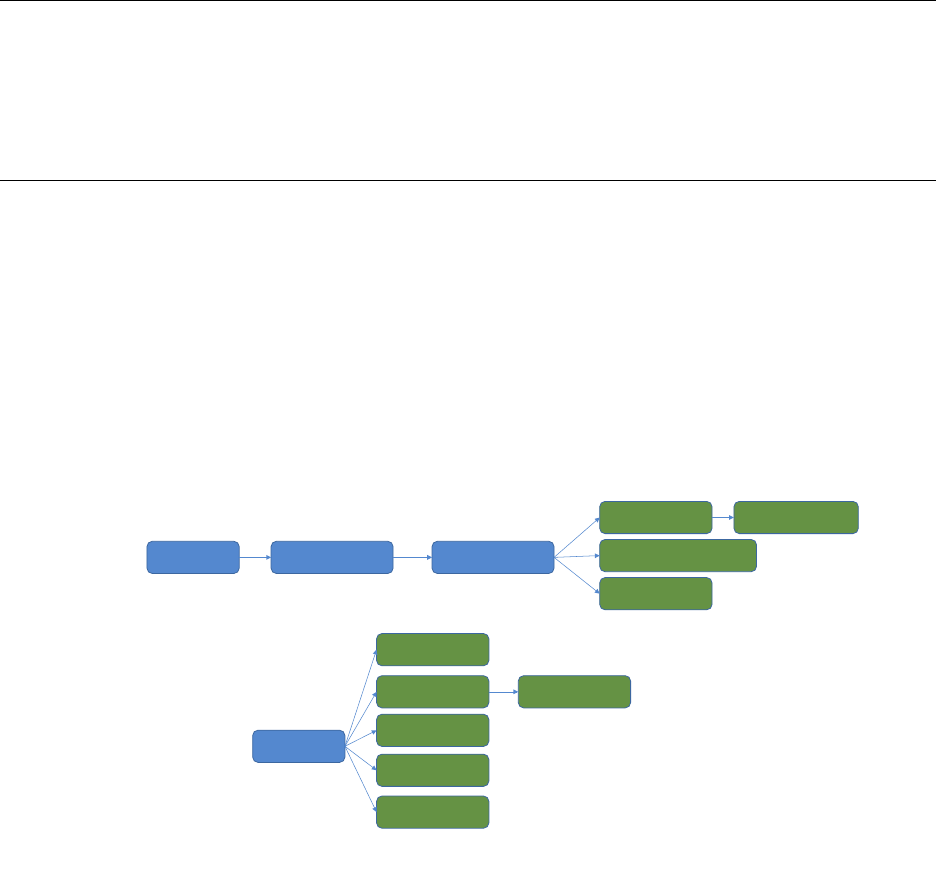
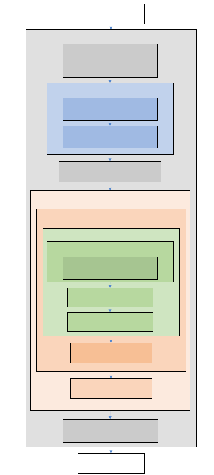
Figure 2 provides a high level look at the structure of the code. Table 1 provides a quick reference for the
built-in HAL functions in this example. Any functions that are used by the example but do not exist in the table
are defined within the example itself and explained in detail below the code. Those fluent in Java may be able to
understand the example just by reading the code and using the reference table.
Built-in framework functions and classes used in the code are highlighted in green to make identifying framework
components easier
26
Main%
For$each$Model:$
Grid%Constructor%
InitTumor%
Setup$constants,$
visualization,$$
and$file$output$
For$each$Time-Step:$
For$each$Model:$
ModelStep%
For$each$Cell:$
Close$visualization$$
and$file$output$
Record$populations$$
and$visualization$
CellStep%
DrawModel%
Drug$Diffusion$
Shuffle$Agents$
Program$Start$
Program$End$
Make$models$unique$
Figure 2: Example program flowchart. Yellow font indicates where funtions are first called.
27

Function Object Action
MapHood(
NEIGHBORHOOD, X, Y)
AgentGrid2D Finds all indices in the provided neighborhood, centered
around X,Y on the AgentGrid2D. Writes these indices into
the NEIGHBORHOOD argument, and returns the number
that were found.
NewAgentSQ( INDEX) AgentGrid2D Returns a new agent, placed at the center of the of the
square at the provided INDEX.
ShuffleAgents( RNG) AgentGrid2D Usually called after every timestep to: 1) remove dead
agents. 2) shuffle order of agents so next iteration is over a
new random order. 3) increment the grid timestep.
GetTick() AgentGrid2D Returns the current grid timestep.
ItoX( INDEX), ItoY(
INDEX)
AgentGrid2D Converts from a grid position INDEX to the x and y
components that point to the same grid position.
G AgentSQ2D Gets the grid that the agent occupies.
Isq() AgentSQ2D Gets the index of the grid square that the agent occupies.
MapEmptyHood(
NEIGHBORHOOD)
AgentSQ2D Finds all indices in the provided neighborhood, centered
around the agent, that do not have an agent occupying
them. Writes these indices into the HOOD argument, and
returns the number that were found.
Dispose() AgentSQ2D Removes the agent from the grid and from iteration.
Get( INDEX) PDEGrid2D Returns the concentration of the PDE field at the given
index.
Mul( INDEX, VALUE) PDEGrid2D Multiplies the concentration at the given INDEX by VALUE.
DiffusionADI( RATE) PDEGrid2D Applies diffusion using the ADI method with the rate
constant provided. a reflective boundary is assumed.
DiffusionADI( RATE,
BOUNDARY_COND)
PDEGrid2D Applies diffusion using the ADI method with the RATE
constant provided. the BOUNDARY_COND value diffuses
from the grid borders.
SetPix( INDEX, COLOR) GridWindow Sets the color of a pixel.
TickPause(
MILLISECONDS)
GridWindow Pauses the program between calls to TickPause. The
function automatically subtracts the time between calls from
MILLISECONDS to ensure a consistent framerate.
ToPNG( FILENAME) GridWindow Writes out the current state of the UIWindow to a PNG
image file.
Close() GridWindow Closes the GridWindow.
RGB( RED, GREEN,
BLUE)
Util Returns an integer with the requested color in RGB format.
This value can be used for visualization.
HeatMapRGB( VALUE) Util Maps the VALUE argument (assumed to be between 0 and
1) to a color in the heat colormap.
CircleHood(
INCLUDE_ORIGIN,
RADIUS)
Util Returns a set of coordinate pairs that define the
neighborhood of all squares whose centers are within the
RADIUS distance of the center (0,0) origin square. The
INCLUDE_ORIGIN argument specifies whether to include
the origin in this set of coordinates.
MooreHood(
INCLUDE_ORIGIN)
Util Returns a set of coordinate pairs that define a Moore
neighborhood around the (0,0) origin square. The
INCLUDE_ORIGIN boolean specifies whether we intend to
include the origin in this set of coordinates.
Write( STRING) FileIO Writes the STRING to the output file.
Close() FileIO Closes the output file.
Table 1: HAL functions used in the example. Each function is a method of a particular object, meaning that
when the function is called it can readily access properties that pertain to the object that it is called from.
28

8.2 Main Function
1p u b l i c s t a t i c v o i d main (String [ ] a r g s ) {
2// s e t t i n g up s t a r t i n g c on s t a n t s and d at a c o l l e c t i o n
3int x= 1 00 , y= 100 , v i s S c a l e = 5 , tumorRad = 10 , msPause = 0 ;
4d o u b l e resistantProb = 0 . 5 ;
5GridWindow win =new GridWindow(" C o m p e t i t i v e R e l e a s e " ,x∗3 , y,visScale ) ;
6F i l e I O popsOut =new F i l e I O (" p o p u l a t i o n s . c sv " ,"w" ) ;
7// s e t t i n g up mode l s
8ExampleModel [ ] mode l s =new ExampleModel [3];
9f o r (i n t i= 0 ; i<models .l e n g t h ;i++) {
10 models [i] = new ExampleModel(x,y,new Rand ( ) ) ;
11 models [i] . InitTumor(tumorRad ,resistantProb) ;
12 }
13 mode l s [0].DRUG_DURATION = 0 ; // no d rug
14 mode l s [1].DRUG_DURATION = 2 0 0 ; // c o n s t a n t d ru g
15 // Main r un l o o p
16 f o r (i n t t i c k = 0 ; t i c k < 10000; t i c k ++) {
17 win .TickPause(msPause) ;
18 for (i n t i= 0 ; i<m odels .length ;i++) {
19 models [i] . ModelStep(t i c k ) ;
20 models [i] . DrawModel(win ,i) ;
21 }
22 // d ata r e c o r d i n g
23 popsOut .Wr i te (models [0].Pop ( ) + " , " +models [1].Pop ( ) + " , " +models [2].Pop ( ) +
"\n" ) ;
24 i f ( ( t i c k ) % 100 == 0) {
25 win .ToPNG("ModelsTick" +t i c k +" . png " ) ;
26 }
27 }
28 // c l o s i n g d at a c o l l e c t i o n
29 popsOut .Close ( ) ;
30 win .Close ( ) ;
31 }
We first look at the main function for a bird’s-eye view of how the program is structured.
Note: Source code elements highlighted in green are already built into HAL.
3-4: Defines all of the constants that will be needed to setup the model and display.
5: Creates a GridWindow of RGB pixels for visualization and for generating timestep PNG images. x*3, y define
the dimensions of the pixel grid. X is multiplied by 3 so that 3 models can be visualized side by side in the
same window. The last argument is a scaling factor that specifies that each pixel on the grid will be viewed
as a 5x5 square of pixels on the screen.
6: Creates a file output object to write to a file called populations.csv
8: Creates an array with 3 entries to fill in with Models.
9-12: Fills the model list with models that are initialized identically. Each model will hold and update its own cells
and diffusible drug. See the Grid Definition and Constructor section and the InitTumor Function section for
more details.
13-14: Setting the DRUG_DURATION constant creates the only difference in the 3 models being compared.
In models[0] no drug is administered (the default value of DRUG_DURATION is 0). In models[1] drug is
29

administered constantly (DRUG_DURATION is set to equal DRUG_CYCLE). In models[2] drug will be
administered periodically. See the ExampleModel Constructor and Properties section for the default values.
16: Executes the main loop for 10000 timesteps. See the ModelStep Function for where the Model tick is
incremented.
17: Requires every iteration of the loop to take a minimum number of milliseconds. This slows down the execution
and display of the model and makes it easier for the viewer to follow.
18: Loops over all models to update them.
19: Advances the state of the agents and diffusibles in each model by one timestep. See the Model Step Function
for more details.
20: Draws the current state of each model to the window. See the Draw Model Function for more details.
23: Writes the population sizes of each model every timestep to allow the models to be compared.
24: Every 100 ticks, writes the state of the model as captured by the GridWindow to a PNG file.
29-30: After the main for loop has finished, the FileIO object and the visualization window are closed, and the
program ends.
8.3 ExampleModel Constructor and Properties
1p u b l i c c l a s s ExampleModel e x t e n d s AgentGrid2D<ExampleCell> {
2// model c o n s t a n t s
3p u b l i c f i n a l s t a t i c i n t RESISTANT =RGB( 0 , 1 , 0 ) , SENSITIVE =RGB( 0 , 0 , 1 ) ;
4p u b l i c d o u b l e DIV_PROB_SEN = 0 . 0 2 5 , DIV_PROB_RES = 0 . 0 1 , DEATH_PROB = 0 . 0 0 1 ,
5DRUG_DIFF_RATE = 2 , DRUG_UPTAKE = 0 . 9 1 , DRUG_TOXICITY = 0 . 2 , DRUG_BOUNDARY_VAL
= 1 . 0 ;
6p u b l i c i n t DRUG_START = 400 , DRUG_CYCLE = 200 , DRUG_DURATION = 4 0 ;
7// i n t e r n a l model o b j e c t s
8p u b l i c PDEGrid2D drug ;
9p u b l i c Rand r ng ;
10 p u b l i c i n t [ ] divHood =MooreHood(false) ;
11
12 p u b l i c ExampleModel(int x,i n t y,Rand generator) {
13 super(x,y,ExampleCell .c l a s s ) ;
14 rn g =generator ;
15 drug =new PDEGrid2D(x,y) ;
16 }
This section covers how the grid is defined and instantiated.
1: The ExampleModel class, which is user defined and specific to this example, is built by extending the generic
AgentGrid2D class. The extended grid class requires an agent type parameter, which is the type of agent
that will live on the grid. To meet this requirement, the <ExampleCell> type parameter is added to the
declaration.
3: Defines RESISTANT and SENSITIVE constants, which are created by the Util RGB function. These constants
serve as both colors for drawing and as labels for the different cell types.
30

4-5: Defines all constants that will be needed during the model run. These values can be reassigned after model
creation to facilitate testing different parameter settings. In the main function, the DRUG_DURATION
variable is modified for the Constant-Drug, and Pulsed Therapy experiment cases.
8: Declares that the model will contain a PDEGrid2D, which will hold the drug concentrations. The PDEGrid2D
can only be initialized when the x and y dimensions of the model are known, which is why we do not define
them until the constructor function.
9: Declares that the Grid will contain a Random number generator, but take it in as a constructor argument to
allow the modeler to seed it if desired.
10: Defines an array that will store the coordinates of a neighborhood generated by the MooreHood function.
The MooreHood function generates a set of coordinates that define the Moore Neighborhood, centered
around the (0,0) origin. The neighborhood is stored in the format [0102, ..., 0n, x1, y1, x2, y2, ..., xn, yn].
The leading zeros are written to when MapHood is called, and will store the indices that the neighborhood
maps to. See the CellStep function for more information.
12: Defines the model constructor, which takes as arguments the x and y dimensions of the world and a Random
number generator.
13: Calls the AgentGrid2D constructor with super, passing it the x and y dimensions of the world, and the
ExampleCell Class. This Class is used by the Grid to generate a new cell when the NewAgentSQ function
is called.
14-15: The random number generator argument is assigned and the drug PDEGrid2D is defined with matching
dimensions.
8.4 InitTumor Function
1p u b l i c v o id I n i t Tu mo r (i n t radius ,d o u b l e resistantProb) {
2// g e t a l i s t o f i n d i c e s t h a t f i l l a c i r c l e a t t h e c e n t e r o f t h e g r i d
3int [ ] tumorNeighborhood =CircleHood(t r u e ,r a d i u s ) ;
4int hoodSize =MapHood(tumorNeighborhood ,xDim / 2 , yDim / 2) ;
5f o r (i n t i= 0 ; i<hoodSize ;i++) {
6i f (rn g .Double ( ) < resistantProb) {
7NewAgentSQ(tumorNeighborhood [i] ) . t y p e =RESISTANT ;
8 } else {
9NewAgentSQ(tumorNeighborhood [i] ) . t y p e =SENSITIVE ;
10 }
11 }
12 }
The next segment of code is a function from the ExampleModel class that defines how the tumor is first seeded
after the ExampleModel is created.
1: The arguments passed to InitTumor function are the approximate radius of the circular tumor being created
and the probability that each created cell will be of the resistant phenotype.
3: Sets the circleCoords array using the built-in CircleHood function, which stores coordinates in the form
[01,02, ..., 0n, x1, y1, x2, y2, ...xn, yn]. These coordinate pairs define a neighborhood of all squares whose
centers are within the radius distance of the center (0,0) origin square. The leading 0s are used by the
31

MapHood function to store the mapping indices. The boolean argument specifies that the origin will be
included in this set of squares, thus making a completely filled circle of squares.
4: Uses the built-in MapHood function to map the neighborhood defined above to be centered around xDim/2,yDim/2
(the dimensions of the AgentGrid). The results of the mapping are written as indices to the beginning of
the tumorNeighborhood array. MapHood returns the number of valid indices found, and this will be the
size of the starting population.
5: Loops from 0 to hoodSize, allowing access to each mapped index in the tumorNeighborhood.
6: Samples a random number in the range (0 −1] and compares to the resistantProb argument to set whether
the cell should have the resistant phenotype or the sensitive phenotype.
7-9: Uses the built-in NewAgentSQ function to place a new cell at each tumorNeighborhood position. In the
same line we also specify that the type should be either resistant or sensitive, depending on the result of
the rng.Double() call.
8.5 ModelStep Function
1p u b l i c v o id ModelStep(i n t t i c k ) {
2ShuffleAgents(rng) ;
3f o r (E x a m p l e C e l l c e l l :t h i s ) {
4c e l l .CellStep ( ) ;
5 }
6int p e r i o d T i c k = ( t i c k −DRUG_START) % DRUG_CYCLE ;
7i f (periodTick > 0 && p e r i o d T i c k <DRUG_DURATION) {
8// d rug w i l l e n t e r t hr ou gh b o u n d a r i e s
9drug .DiffusionADI (DRUG_DIFF_RATE,DRUG_BOUNDARY_VAL) ;
10 } else {
11 // d rug w i l l n ot e n t e r t hr ou gh b o u n d a r i e s
12 drug .DiffusionADI (DRUG_DIFF_RATE) ;
13 }
14 }
This section looks at the main step function which is executed once per tick by the Model.
2: The ShuffleAgents function randomizes the order of iteration so that the agents are always looped through in
random order.
3-4: Iterates over every cell on the grid, and calls the CellStep function on every cell.
6: The GetTick function is a built-in function that returns the current Grid tick. The If statement logic checks if
the tick is past the drug start and if the tick is in the right part of the drug cycle to apply drug. (See the
Grid Definition and Constructor section for the values of the constants involved, the DRUG_DURATION
variable is set differently for each model in the Main Function)
7-9: If it is time to add drug to the model, the built-in DiffusionADI function is called. The default Diffusion
function uses the standard 2D Laplacian and is of the form: δC
δt =D∇2C, where D in this case is the
DRUG_DIFF_RATE. DiffusionADI uses the ADI method which is more stable and allows us to take larger
steps than the 2D Laplacian can support. The additional argument to the DiffusionADI equation specifies the
boundary condition value DRUG_BOUNDARY_VAL. This causes the drug to diffuse into the PDEGrid2D
from the boundary.
32

12: Without the second argument the DiffusionADI function assumes a reflective boundary, meaning that drug
concentration cannot escape or enter through the sides. Therefore the only way for the drug concentration
to decrease is via consumption by the Cells. See the CellStep function section, line 6, for more information.
8.6 CellStep Function and Cell Properties
1c l a s s ExampleCell e x t e n d s AgentSQ2Dunstackable<ExampleModel> {
2p u b l i c i n t type ;
3
4p u b l i c v o id CellStep ( ) {
5//Consumption of Drug
6G.drug .Mul (Isq ( ) , G.DRUG_UPTAKE) ;
7d o u b l e deathProb ,divProb ;
8// Chance of Death , d epen ds on r e s i s t a n c e and dr u g c o n c e n t r a t i o n
9i f (t h i s .t y p e == RESISTANT) {
10 deathProb =G.DEATH_PROB;
11 } else {
12 deathProb =G.DEATH_PROB +G.dru g .Get (I s q ( ) ) ∗G.DRUG_TOXICITY ;
13 }
14 i f (G.rn g .Double ( ) < deathProb) {
15 Dispose ( ) ;
16 r e t u r n ;
17 }
18 // Chance o f D i v i s i o n , d e pen ds on r e s i s t a n c e
19 i f (t h i s .t y p e == RESISTANT) {
20 divProb =G.DIV_PROB_RES;
21 } else {
22 divProb =G.DIV_PROB_SEN;
23 }
24 i f (G.rn g .Double ( ) < divProb) {
25 i n t options =MapEmptyHood(G.divHood) ;
26 i f (options > 0) {
27 G.NewAgentSQ(G.divHood [G.rn g .I n t (options) ] ) . t y p e =t h i s .type ;
28 }
29 }
30 }
31 }
We next look at how the Agent is defined and at the CellStep function that runs once per Cell per tick.
1: The ExampleCell class is built by extending the generic AgentSQ2Dunstackable class. The extended Agent
class requires the ExampleModel class as a type argument, which is the type of Grid that the Agent will
live on. To meet this requirement, we add the <EampleModel> type parameter to the extension.
2: Defines an internal int called type. each Cell holds a value for this field. If the value is RESISTANT, the
Cell is of the resistant phenotype, if the value is SENSITIVE, the cell is of the sensitive phenotype. The
RESISTANT and SENSITIVE constants are defined in the ExampleGrid as constants.
6: The G property is used to access the ExampleGrid object that the Cell lives on. G is used often with Agent
functions as the AgentGrid is expected to contain any information that is not local to the Cell itself. Here it
is used to get the drug PDEGrid2D. The drug concentration at the index that the Cell is currently occupying
(Isq()) is then multiplied by the drug uptake constant, thus modeling local drug consumption by the Cell.
7: Defines deathProb and divProb variables, these will be assigned different values depending on whether the
ExampleCell is RESISTANT or SENSITIVE.
33

9-12: If the cell is resistant the deathProb variable is set to the DEATH_PROB value alone, if the cell is sensitive,
an additional term is added to account for the probability of the cell dying from drug exposure, using the
concentration of drug at the cell’s position (Isq())
14-16: Samples a random number in the range (0 −1] and compares to deathProb to determine whether the cell
will die. If so, the built-in agent Dispose() function is called, which removes the agent from the grid, and
then return is called so that the dead cell will not divide.
19-22: Sets the divProb variable to either DIV_PROB_RES for resistant cells, or DIV_PROB_SEN for sensitive
cells.
24: Samples a random number in the range (0 −1] and compare to divProb to determine whether the cell will
divide.
25: If the cell will divide, the built-in MapEmptyHood function is used which displaces the divHood (the moore
neighborhood as defined in the Grid Definition and Constructor section) to be centered around the x and y
coordinates of the Cell, and writes the empty indices into the neighborhood. The MapEmptyHood function
will only map indices in the neighborhood that are empty. MapEmptyHood returns the number of valid
divison options found.
26-27: If there are one or more valid division options,a new daughter cell is created using the builitin NewAgentSQ
function and its starting location is chosen by randomly sampling the divHood array to pull out one if its
valid locations. Finally with the .type=this.type statement, the phenotype of the new daughter cell is set to
the phenotype of the pre-existing daughter that remains in place, thus maintaining phenotypic inheritance.
8.7 DrawModel Function
1p u b l i c v o id DrawModel(GridWindow vis ,int iModel) {
2f o r (i n t x= 0 ; x<xDim ;x++) {
3for (i n t y= 0 ; y<yDim ;y++) {
4E x a m p l e C e l l drawMe =GetAgent (x,y) ;
5i f (drawMe != null) {
6v i s .S e t P i x (x+iModel ∗xDim ,y,drawMe .type) ;
7 } else {
8v i s .S e t P i x (x+iModel ∗xDim ,y,HeatMapRGB(dru g .Get (x,y) ) ) ;
9 }
10 }
11 }
12 }
We next look at the DrawModel Function, which is used to display a summary of the model state on a GridWindow
object. DrawModel is called once for each model per timestep, see the Main Function section for more information.
2-3: Loops over every lattice position of the grid being drawn, xDim and yDim refer to the dimensions of the
model.
4: Uses the built-in GetAgent function to get the Cell that is at the x,y position.
5-6: If a cell exists at the requested position, the corresponding pixel on the GridWindow is set to the cel’s
phenotype color. to draw the models side by side, the pixel being drawn is displaced to the right by the
model index.
34

7-8: If there is no cell to draw, then the pixel color is set based on the drug concentration at the same index,
using the built-in heat colormap.
8.8 Imports
1package Examples ._6CompetitiveRelease ;
2import Framework .GridsAndAgents .AgentGrid2D ;
3import Framework .GridsAndAgents .PDEGrid2D ;
4import Framework .Gui .GridWindow ;
5import Framework .GridsAndAgents .AgentS Q 2Dunsta c kable ;
6import Framework .Gui .U I G r i d ;
7import Framework .Tools .F i l e I O ;
8import Framework .Rand ;
9im p or t s t a t i c Examples ._6CompetitiveRelease .ExampleModel .∗;
10 im p or t s t a t i c Framework .Util .∗;
The final code snippet looks at the imports that are needed. Any modern Java IDE should generate import
statements automatically.
1: The package statement is always needed and specifies where the file exists in the larger project structure
2-8: Imports all of the classes that we will need for the program.
9: Imports the static fields of the model so that we can use the type names defined there in the Agent class.
10: Imports the static functions of the Util file, which adds all of the Util functions to the current namespace, so
we can natively call them. Statically importing Util is recommended for every project.
8.9 Model Results
Table 2 displays the model visualization at tick 0, tick 400, tick 1100, tick 5500, and tick 10,000. The Figure
caption explores the notable trends visible in each image. Figure 3 displays the population sizes as recorded by
the FileIO object at the end of every timestep.
35
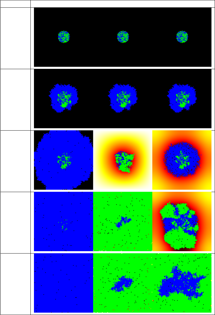
Timestep No Drug / Constant Drug / Pulsed Drug
0
400
1100
5500
10000
Table 2: Selected model visualization PNGs. Blue cells are drug sensitive, Green cells are drug resistant, back-
ground heatmap colors show drug concentration. At timestep 0 and timestep 400 (right before drug application
starts), all 3 models are identical. At tick 1100 the differences in treatment application show different effects:
when no drug is applied, the rapidly dividing sensitive cells quickly fill the domain, when drug is applied constantly,
the resistant cells overtake the tumor. Pulsed drug kills some sensitive cells, but leaves enough alive ot prevent
growth of the resistant cells. At tick 5500, the resistant cells have begun to emerge from the center of the pulsed
drug model. At tick 10000, all domains are filled. Interestingly, the sensitive cells are able to survive in the center
of the domain because drug is consumed by cells on the outside. This creates a drug-free zone in which the
sensitive cells outcompete the resistant cells.
36
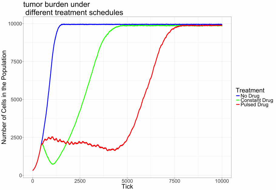
Figure 3: FileIO population output. This plot summarizes the changes in tumor burden over time for each model.
This plot was constructed in R using data accumulated in the program output csv file. Displayed using GGPlot
in R
This modeling example illustrates the power of HAL’s approach to model building. Writing relatively little
complex code, we setup a 3 model experiment with nontrivial dynamics along with methods to collect data and
visualize the models. We now briefly review the model results.
As can be seen in Figure 3 and Table 2, the pulsed therapy is the most effective at preventing tumor growth,
however the resistant cells ultimately succeed in breaking out of the tumor center and outcompeting the sensitive
cells on the fringes of the tumor. It may be possible to maintain a homeostatic population of sensitive and resistant
cells for longer by using a different pulsing schedule or possibly by using adaptive therapy. As the presented model
is primarily an example, we do not explore how to improve treatment further. For a more detailed exploration of
the potential of adaptive therapy for prolonging competitive release, see [1].
References
[1] Jill A Gallaher, Pedro M Enriquez-Navas, Kimberly A Luddy, Robert A Gatenby, and Alexander RA Anderson.
Adaptive vs continuous cancer therapy: Exploiting space and trade-offs in drug scheduling.
37
Acknowelgements
This work was possible through the generous support of NIH funding, Anderson and Tessi acknowledge NCI
U54CA193489, Anderson and Bravo acknowledge NCI UH2CA203781.
38
