Manual
User Manual:
Open the PDF directly: View PDF ![]() .
.
Page Count: 51

KA-TP-28-2018
PSI-PR-18-10
2HDECAY - A program for the Calculation of
Electroweak One-Loop Corrections to Higgs Decays
in the Two-Higgs-Doublet Model Including
State-of-the-Art QCD Corrections
Marcel Krause1∗
, Margarete M¨uhlleitner1†
, Michael Spira2‡
1Institute for Theoretical Physics, Karlsruhe Institute of Technology,
Wolfgang-Gaede-Str. 1, 76131 Karlsruhe, Germany.
2Paul Scherrer Institute,
CH-5232 Villigen PSI, Switzerland.
Abstract
We present the program package 2HDECAY for the calculation of the partial decay widths
and branching ratios of the Higgs bosons of a general CP-conserving 2-Higgs doublet model
(2HDM). The tool includes the full electroweak one-loop corrections to all two-body on-
shell Higgs decays in the 2HDM that are not loop-induced. It combines them with the
state-of-the-art QCD corrections that are already implemented in the program HDECAY. For
the renormalization of the electroweak sector an on-shell scheme is implemented for most
of the renormalization parameters. Exceptions are the soft-Z2-breaking squared mass scale
m2
12, where an MS condition is applied, as well as the 2HDM mixing angles αand β, for
which several distinct renormalization schemes are implemented. The tool 2HDECAY can be
used for phenomenological analyses of the branching ratios of Higgs decays in the 2HDM.
Furthermore, the separate output of the electroweak contributions to the tree-level partial
decay widths for several different renormalization schemes allows for an efficient analysis
of the impact of the electroweak corrections and the remaining theoretical error due to
missing higher-order corrections. The latest version of the program package 2HDECAY can be
downloaded from the URL https://github.com/marcel-krause/2HDECAY.
∗E-mail: marcel.krause@kit.edu
†E-mail: margarete.muehlleitner@kit.edu
‡E-mail: michael.spira@psi.ch
1 Introduction
The discovery of the Higgs particle, announced on 4 July 2012 by the LHC experiments ATLAS
[1] and CMS [2] marked a milestone for particle physics. It structurally completed the Standard
Model (SM) providing us with a theory that remains weakly interacting all the way up to the
Planck scale. While the SM can successfully describe numerous particle physics phenomena
at the quantum level at highest precision, it leaves open several questions. Among these are
e.g. the one for the nature of Dark Matter (DM), the baryon asymmetry of the universe or
the hierarchy problem. This calls for physics beyond the SM (BSM). Models beyond the SM
usually entail enlarged Higgs sectors that can provide candidates for Dark Matter or guarantee
successful baryogenesis. Since the discovered Higgs boson with a mass of 125.09 GeV [3] behaves
SM-like any BSM extension has to make sure to contain a Higgs boson in its spectrum that is in
accordance with the LHC Higgs data. Moreover, the models have to be tested against theoretical
and further experimental constraints from electroweak precision tests, B-physics, low-energy
observables and the negative searches for new particles that may be predicted by some of the
BSM theories.
The lack of any direct sign of new physics renders the investigation of the Higgs sector more
and more important. The precise investigation of the discovered Higgs boson may reveal indirect
signs of new physics through mixing with other Higgs bosons in the spectrum, loop effects due
to the additional Higgs bosons and/or further new states predicted by the model, or decays
into non-SM states or Higgs bosons, including the possibility of invisible decays. Due to the
SM-like nature of the 125 GeV Higgs boson indirect new physics effects on its properties are
expected to be small. Moreover, different BSM theories can lead to similar effects in the Higgs
sector. In order not to miss any indirect sign of new physics and to be able to identify the
underlying theory in case of discovery, highest precision in the prediction of the observables
and sophisticated experimental techniques are therefore indispensable. The former calls for the
inclusion of higher-order corrections at highest possible level, and theorists all over the world
have spent enormous efforts to improve the predictions for Higgs observables [4].
Among the new physics models supersymmetric (SUSY) extensions [5–17] certainly belong
to the best motivated and most thoroughly investigated models beyond the SM, and numerous
higher-order predictions exist for the production and decay cross sections as well as the Higgs
potential parameters, i.e. the masses and Higgs self-couplings [4]. The Higgs sector of the
minimal supersymmetric extension (MSSM) [17–20] is a 2-Higgs doublet model (2HDM) of type
II [21, 22]. While due to supersymmetry the MSSM Higgs potential parameters are given in
terms of gauge couplings this is not the case for general 2HDMs so that the 2HDM entails an
interesting and more diverse Higgs phenomenology and is also affected differently by higher-order
electroweak (EW) corrections. Moreover, 2HDMs allow for successful baryogenesis [23–41] and
in their inert version provide a Dark Matter candidate [42–56].
The situation with respect to EW corrections in non-SUSY models is not as advanced as
for SUSY extensions. While the QCD corrections can be taken over to those models with a
minimum effort from the SM and the MSSM by applying appropriate changes, this is not the
case for the EW corrections. Moreover, some issues arise with respect to renormalization. Thus,
only recently a renormalization procedure has been proposed by authors of this paper for the
mixing angles of the 2HDM that ensures explicitly gauge-independent decay amplitudes, [57,58].
Subsequent groups have confirmed this in different Higgs channels [59–62]. In [63] we completed
the renormalization of the 2HDM and calculated the higher-order corrections to Higgs-to-Higgs
decays. We have applied and extended this renormalization procedure in [64] to the next-to-
2

2HDM (N2HDM) which includes an additional real singlet. The computation of the (N)2HDM
EW corrections has shown that the corrections can become very large for certain areas of the
parameters space. There can be several reasons for this. The corrections can be parametrically
enhanced due to involved couplings that can be large [63–66]. This is in particular the case
for the trilinear Higgs self-couplings that in contrast to SUSY are not given in terms of the
gauge couplings of the theory and that are so far only weakly constrained by the LHC Higgs
data. The corrections can be large due to light particles in the loop in combination with not
too small couplings, e.g. light Higgs states of the extended Higgs sector. Also an inapt choice
of the renormalization scheme can artificially enhance loop corrections. Thus we found for our
investigated processes that process-dependent renormalization schemes or MS renormalization of
the scalar mixing angles can blow up the one-loop corrections due to an insufficient cancellation
of the large finite contributions from wave function renormalization constants [58,63]. Moreover,
counterterms can blow up in certain parameter regions because of small leading-order couplings,
e.g. in the 2HDM the coupling of the heavy non-SM-like CP-even Higgs boson to gauge bosons,
which in the limit of a light SM-like CP-even Higgs boson is almost zero. The same effects are
observed for supersymmetric theories where a badly chosen parameter set for the renormalization
can lead to very large counterterms and hence enhanced loop corrections, cf. Ref. [67] for a recent
analysis.
This discussion shows that the renormalization of the EW corrections to BSM Higgs ob-
servables is a highly non-trivial task. In addition, there may be no unique best renormalization
scheme for the whole parameter space of a specific model, and the user has to decide which
scheme to choose to obtain trustworthy predictions. With the publication of the new tool
2HDECAY we aim to give an answer to this problematic task.
The program 2HDECAY computes, for 14 different renormalization schemes, the EW correc-
tions to the Higgs decays of the 2HDM Higgs bosons into all possible on-shell two-particle final
states of the model that are not loop-induced. It is combined with the widely used Fortran
code HDECAY version 6.52 [68,69] which provides the loop-corrected decay widths and branching
ratios for the SM, the MSSM and 2HDM incorporating the state-of-the-art higher-order QCD
corrections including also loop-induced and off-shell decays. Through the combination of these
corrections with the 2HDM EW corrections 2HDECAY becomes a code for the prediction of the
2HDM Higgs boson decay widths at the presently highest possible level of precision. Addi-
tionally, the separate output of the leading order (LO) and next-to-leading order (NLO) EW
corrected decay widths allows to perform studies on the importance of the relative EW cor-
rections (as function of the parameter choices), comparisons with the relative EW corrections
within the MSSM or investigations on the most suitable renormalization scheme for specific
parameter regions. The comparison of the results for different renormalization schemes more-
over permits to estimate the remaining theoretical error due to missing higher-order corrections.
With this tool we contribute to the effort of improving the theory predictions for BSM Higgs
physics observables so that in combination with sophisticated experimental techniques Higgs
precision physics becomes possible and the gained insights may advance us in our understanding
of the mechanism of electroweak symmetry breaking (EWSB) and the true underlying theory.
The program package was developed and tested under Windows 10,openSUSE Leap 15.0
and macOS Sierra 10.12. It requires an up-to-date version of Python 2 or Python 3 (tested
with versions 2.7.14 and 3.5.0), the FORTRAN compiler gfortran and the GNU C compilers gcc
(tested for compatibility with versions 6.4.0 and 7.3.1) and g++. The latest version of the
package can be downloaded from
https://github.com/marcel-krause/2HDECAY .
3

The paper is organized as follows. The subsequent Sec. 2 forms the theoretical background
for our work. We briefly introduce the 2HDM, all relevant parameters and particles and set
our notation. We give a summary of all counterterms that are needed for the computation of
the EW corrections and state them explicitly. The relevant formulae for the computation of
the partial decay widths at one-loop level are presented and the combination of the electroweak
corrections with the QCD corrections already implemented in HDECAY is described. In Sec. 3, we
introduce 2HDECAY in detail, describe the structure of the program package and the input and
output file formats. Additionally, we provide installation and usage manuals. We conclude with
a short summary of our work in Sec. 4. As reference for the user, we list exemplary input and
output files in Appendices A and B, respectively.
2 One-Loop Electroweak and QCD Corrections in the 2HDM
In the following, we briefly set up our notation and introduce the 2HDM along with the input
parameters used in our parametrization. We give details on the EW one-loop renormalization
of the 2HDM. We discuss how the calculation of the one-loop partial decay widths is performed.
At the end of the section, we explain how the EW corrections are combined with the existing
state-of-the-art QCD corrections already implemented in HDECAY.
2.1 Introduction of the 2HDM
For our work, we consider a general CP-conserving 2HDM [21, 22] with a global discrete Z2
symmetry that is softly broken. The model consists of two complex SU(2)Ldoublets Φ1and
Φ2, both with hypercharge Y= +1. The electroweak part of the 2HDM can be described by
the Lagrangian
LEW
2HDM =LYM +LF+LS+LYuk +LGF +LFP .(2.1)
in terms of the Yang-Mills Lagrangian LYM and the fermion Lagrangian LFcontaining the
kinetic terms of the gauge bosons and fermions and their interactions, the Higgs Lagrangian
LS, the Yukawa Lagrangian Lyuk with the Higgs-fermion interactions, the gauge-fixing and the
Fadeev-Popov Lagrangian, LGF and LFP, respectively. Explicit forms of LYM and LFcan be
found e.g. in [70,71] and of the general 2HDM Yukawa Lagrangian e.g. in [22,72]. We do not give
them explicitly here. For the renormalization of the 2HDM, we follow the approach of Ref. [73]
and apply the gauge-fixing only after the renormalization of the theory, i.e. LGF contains only
fields that are already renormalized. For the purpose of our work we do not present LGF nor
LFP since their explicit forms are not needed in the following.
The scalar Lagrangian LSintroduces the kinetic terms of the Higgs doublets and their scalar
potential. With the the covariant derivative
Dµ=∂µ+i
2g
3
X
a=1
σaWa
µ+i
2g0Bµ,(2.2)
where Wa
µand Bµare the gauge bosons of the SU(2)Land U(1)Yrespectively, gand g0are the
corresponding coupling constants of the gauge groups and σaare the Pauli matrices, the scalar
Lagrangian is given by
LS=
2
X
i=1
(DµΦi)†(DµΦi)−V2HDM .(2.3)
4

The scalar potential of the CP-conserving 2HDM reads [22]
V2HDM =m2
11 |Φ1|2+m2
22 |Φ2|2−m2
12 Φ†
1Φ2+h.c.+λ1
2Φ†
1Φ12+λ2
2Φ†
2Φ22
+λ3Φ†
1Φ1Φ†
2Φ2+λ4Φ†
1Φ2Φ†
2Φ1+λ5
2Φ†
1Φ22+h.c..
(2.4)
Since we consider a CP-conserving model, the 2HDM potential can be parametrized by three
real-valued mass parameters m11,m22 and m12 as well as five real-valued dimensionless coupling
constants λi(i= 1, ..., 5). For later convenience, we define the frequently appearing combination
of three of these coupling constants as
λ345 ≡λ3+λ4+λ5.(2.5)
For m2
12 = 0, the potential V2HDM exhibits a discrete Z2symmetry under the simultaneous field
transformations Φ1→ −Φ1and Φ2→Φ2. This symmetry, implemented in the scalar potential
in order to avoid flavour-changing neutral currents (FCNC) at tree level, is softly broken by a
non-zero mass parameter m12.
After EWSB the neutral components of the Higgs doublets develop vacuum expectation
values (VEVs) which are real in the CP-conserving case. After expanding about the real VEVs
v1and v2, the Higgs doublets Φi(i= 1,2) can be expressed in terms of the charged complex
field ω+
iand the real neutral CP-even and CP-odd fields ρiand ηi, respectively as
Φ1= ω+
1
v1+ρ1+iη1
√2!,Φ2= ω+
2
v2+ρ2+iη2
√2!,(2.6)
where
v2=v2
1+v2
2≈(246.22 GeV)2(2.7)
is the SM VEV obtained from the Fermi constant GFand we define the ratio of the VEVs
through the mixing angle βas
tan β=v2
v1
(2.8)
so that
v1=vcβand v2=vsβ.(2.9)
Insertion of Eq. (2.6) in the kinetic part of the scalar Lagrangian in Eq. (2.3) yields after rotation
to the mass eigenstates the tree-level relations for the masses of the electroweak gauge bosons
m2
W=g2v2
4(2.10)
m2
Z=(g2+g02)v2
4(2.11)
m2
γ= 0 .(2.12)
The electromagnetic coupling constant eis connected to the fine-structure constant αem and to
the gauge boson coupling constants through the tree-level relation
e=√4παem =gg0
pg2+g02,(2.13)
5

which allows to replace g0in favor of eor αem. In our work, we use the fine-structure constant
αem as an independent input. Alternatively, one could use the tree-level relation to the Fermi
constant
GF≡√2g2
8m2
W
=αemπ
√2m2
W1−m2
W
m2
Z(2.14)
to replace one of the parameters of the electroweak sector in favor of GF. Since GFis used as
an input value for HDECAY, we present the formula here explicitly and explain the conversion
between the different parametrizations in Sec. 2.4.
Inserting Eq. (2.6) in the scalar potential in Eq. (2.4) leads to
V2HDM =1
2(ρ1ρ2)M2
ρρ1
ρ2+1
2(η1η2)M2
ηη1
η2+1
2ω±
1ω±
2M2
ωω±
1
ω±
2
+T1ρ1+T2ρ2+···
(2.15)
where the terms T1and T2and the matrices M2
ω,M2
ρand M2
ηare defined below. By requiring
the VEVs of Eq. (2.6) to represent the minimum of the potential, the minimum conditions for
the potential can be expressed as
∂V2HDM
∂ΦihΦji
= 0 .(2.16)
This is equivalent to the statement that the two terms linear in the CP-even fields ρ1and ρ2,
the tadpole terms,
T1
v1≡m2
11 −m2
12
v2
v1
+v2
1λ1
2+v2
2λ345
2(2.17)
T2
v2≡m2
22 −m2
12
v1
v2
+v2
2λ2
2+v2
1λ345
2,(2.18)
have to vanish at tree level:
T1=T2= 0 (at tree level) .(2.19)
The tadpole equations can be solved for m2
11 and m2
22 in order to replace these two parameters
by the tadpole parameters T1and T2.
The terms bilinear in the fields given in Eq. (2.15) define the scalar mass matrices
M2
ρ≡m2
12 v2
v1+λ1v2
1−m2
12 +λ345v1v2
−m2
12 +λ345v1v2m2
12 v1
v2+λ2v2
2+ T1
v10
0T2
v2!(2.20)
M2
η≡m2
12
v1v2−λ5 v2
2−v1v2
−v1v2v2
1+ T1
v10
0T2
v2!(2.21)
M2
ω≡m2
12
v1v2−λ4+λ5
2 v2
2−v1v2
−v1v2v2
1+ T1
v10
0T2
v2!,(2.22)
where Eqs. (2.17) and (2.18) have already been applied to replace the parameters m2
11 and m2
22
in favor of T1and T2. Keeping the latter explicitly in the expressions of the mass matrices is
6

crucial for the correct renormalization of the scalar sector, as explained in Sec. 2.2. By means
of two mixing angles αand βwhich define the rotation matrices1
R(x)≡cx−sx
sxcx,(2.23)
the fields ω+
i,ρiand ηiare rotated to the mass basis according to
ρ1
ρ2=R(α)H
h(2.24)
η1
η2=R(β)G0
A(2.25)
ω±
1
ω±
2=R(β)G±
H±,(2.26)
with the two CP-even Higgs bosons hand H, the CP-odd Higgs boson A, the CP-odd Goldstone
boson G0and the charged Higgs bosons H±as well as the charged Goldstone bosons G±. In
the mass basis, the diagonal mass matrices are given by
D2
ρ≡m2
H0
0m2
h(2.27)
D2
η≡m2
G00
0m2
A(2.28)
D2
ω≡m2
G±0
0m2
H±,(2.29)
with the diagonal entries representing the squared masses of the respective particles. The Gold-
stone bosons are massless,
m2
G0=m2
G±= 0 .(2.30)
The squared masses expressed in terms of the potential parameters and the mixing angle αcan
be cast into the form [66]
m2
H=c2
α−βM2
11 +s2(α−β)M2
12 +s2
α−βM2
22 (2.31)
m2
h=s2
α−βM2
11 −s2(α−β)M2
12 +c2
α−βM2
22 (2.32)
m2
A=m2
12
sβcβ−v2λ5(2.33)
m2
H±=m2
12
sβcβ−v2
2(λ4+λ5),with (2.34)
t2(α−β)=2M2
12
M2
11 −M2
22
,(2.35)
where we have introduced
M2
11 ≡v2c4
βλ1+s4
βλ2+ 2s2
βc2
βλ345(2.36)
M2
12 ≡sβcβv2−c2
βλ1+s2
βλ2+c2βλ345(2.37)
M2
22 ≡m2
12
sβcβ
+v2
8(1 −c4β) (λ1+λ2−2λ345).(2.38)
1Here and in the following, we use the short-hand notation sx≡sin(x), cx≡cos(x), tx≡tan(x) for conve-
nience.
7

u-type d-type leptons
I Φ2Φ2Φ2
II Φ2Φ1Φ1
lepton-specific Φ2Φ2Φ1
flipped Φ2Φ1Φ2
Table 1: The four Yukawa types of the Z2-symmetric 2HDM defined by the Higgs doublet that couples to each
kind of fermions.
2HDM type Y1Y2Y3Y4Y5Y6
Icα
sβ
sα
sβ−1
tβ
cα
sβ
sα
sβ−1
tβ
II −sα
cβ
cα
cβtβ−sα
cβ
cα
cβtβ
lepton-specific cα
sβ
sα
sβ−1
tβ−sα
cβ
cα
cβtβ
flipped −sα
cβ
cα
cβtβcα
sβ
sα
sβ−1
tβ
Table 2: Parametrization of the Yukawa coupling parameters in terms of six parameters Yi(i= 1, ..., 6) for each
2HDM type.
Inverting these relations, the quartic couplings λi(i= 1, ..., 5) can be expressed in terms of the
mass parameters m2
h,m2
H,m2
A,m2
H±and the CP-even mixing angle αas [66]
λ1=1
v2c2
βc2
αm2
H+s2
αm2
h−sβ
cβ
m2
12(2.39)
λ2=1
v2s2
βs2
αm2
H+c2
αm2
h−cβ
sβ
m2
12(2.40)
λ3=2m2
H±
v2+s2α
s2βv2m2
H−m2
h−m2
12
sβcβv2(2.41)
λ4=1
v2m2
A−2m2
H±+m2
12
sβcβ(2.42)
λ5=1
v2m2
12
sβcβ−m2
A.(2.43)
In order to avoid tree-level FCNC currents, as introduced by the most general 2HDM Yukawa
Lagrangian, one type of fermions is allowed to couple only to one Higgs doublet by imposing
a global Z2symmetry under which Φ1,2→ ∓Φ1,2. Depending on the Z2charge assignments,
there are four phenomenologically different types of 2HDMs summarized in Tab. 1. For the four
2HDM types considered in this work, all Yukawa couplings can be parametrized through six
different Yukawa coupling parameters Yi(i= 1, ..., 6) whose values for the different types are
presented in Tab. 2. They are introduced here for later convenience.
We conclude this section with an overview over the full set of independent parameters that
is used as input for the computations in 2HDECAY. Additionally to the parameters defined by
LEW
2HDM,HDECAY requires the electromagnetic coupling constant αem in the Thomson limit for
the calculation of the loop-induced decays into a photon pair and into Zγ, the strong coupling
constant αsfor the loop-induced decay into gluons and the QCD corrections as well as the total
decay widths of the Wand Zbosons, ΓWand ΓZ, for the computation of the off-shell decays into
massive gauge boson final states. In the mass basis of the scalar sector, the set of independent
8

parameters is given by
{GF, αs,ΓW,ΓZ, αem, mW, mZ, mf, Vij , tβ, m2
12, α, mh, mH, mA, mH±}.(2.44)
Here mfdenote the fermion masses of the strange, charm, bottom and top quarks and of the µ
and τleptons (f=s, c, b, t, µ, τ). All other fermion masses are assumed to be zero in HDECAY and
will also be assumed to be zero in our computation of the EW corrections to the decay widths.
The fermion and gauge boson masses are defined in accordance with the recommendations of the
LHC Higgs cross section working group [74]. The Vij denote the CKM mixing matrix elements.
All HDECAY decay widths are computed in terms of the Fermi constant GFexcept for processes
involving on-shell external photon vertices that are expressed by αem in the Thomson limit. In
the computation of the EW corrections, however, we require the on-shell masses mWand mZ
and the electromagnetic coupling at the Zboson mass scale, αem(m2
Z) (not to be confused with
the mixing angle αin the Higgs sector), as input parameters for our renormalization conditions.
We will come back to this point later.
Alternatively, the original parametrization of the scalar potential in the interaction basis can
be used2. In this case, the set of independent parameters is given by
{GF, αs,ΓW,ΓZ, αem, mW, mZ, mf, Vij , tβ, m2
12, λ1, λ2, λ3, λ4, λ5}.(2.45)
Actually, also the tadpole parameters T1and T2should be included in the two sets as inde-
pendent parameters of the Higgs potential. However, as described in Sec. 2.2, the treatment of
the minimum of the Higgs potential at higher orders requires special care, and in an alternative
treatment of the minimum conditions, the tadpole parameters disappear as independent param-
eters. In any case, after the renormalization procedure is completely performed, the tadpole
parameters vanish again and hence, do not count as input parameters for 2HDECAY.
2.2 Renormalization
We focus on the calculation of EW one-loop corrections to decay widths of Higgs particles in the
2HDM. Since the higher-order (HO) corrections of these decay widths are in general ultraviolet
(UV)-divergent, a proper regularization and renormalization of the UV divergences is required.
In the following, we briefly present the definition of the counterterms (CTs) needed for the
calculation of the EW one-loop corrections. For a thorough derivation and presentation of the
gauge-independent renormalization of the 2HDM, we refer the reader to [57, 58, 63].3
All input parameters that are renormalized for the calculation of the EW corrections (apart
from the mixing angles αand βand the soft-Z2-breaking scale m12) are renormalized in the
on-shell (OS) scheme. For the physical fields, we employ the conditions that any mixing of
fields with the same quantum numbers shall vanish on the mass shell of the respective particles
and that the fields are normalized by fixing the residue of their corresponding propagators at
their poles to unity. Mass CTs are fixed through the condition that the masses are defined
as the real parts of the poles of the renormalized propagators. These OS conditions suffice to
renormalize most of the parameters of the 2HDM necessary for our work. The renormalization
of the mixing angles αand βfollows an OS-motivated approach, as discussed in Sec. 2.2.4, while
m12 is renormalized via an MS condition as discussed in Sec. 2.2.6.
2HDECAY internally translates the parameters from the interaction to the mass basis, in terms of which the
decay widths are implemented.
3See also Refs. [59–61] for a discussion of the renormalization of the 2HDM. For recent works discussing
gauge-independent renormalization within multi-Higgs models, see [62, 75].
9

2.2.1 Tadpole Renormalization
As shown for the 2HDM for the first time in [57,58], the proper treatment of the tadpole terms at
one-loop order is crucial for the gauge-independent definition of the CTs of the mixing angles α
and β. This allows for the calculation of one-loop partial decay widths with a manifestly gauge-
independent relation between input variables and the physical observable. In the following, we
briefly repeat the different renormalization conditions for the tadpoles that can be employed in
the 2HDM.
The standard tadpole scheme is a commonly used renormalization scheme for the tadpoles
(cf. e.g. [71] for the SM or [66,76] for the 2HDM). While the tadpole parameters vanish at tree
level, as stated in Eq. (2.19), they are in general non-vanishing at higher orders in perturbation
theory. Since the tadpole terms, being the terms linear in the Higgs potential, define the
minimum of the potential, it is necessary to employ a renormalization of the tadpoles in such
a way that the ground state of the potential still represents the minimum at higher orders. In
the standard tadpole scheme, this condition is imposed on the loop-corrected potential. By
replacing the tree-level tadpole terms at one-loop order with the physical (i.e. renormalized)
tadpole terms and the tadpole CTs δTi,
Ti→Ti+δTi(i= 1,2) ,(2.46)
the correct minimum of the loop-corrected potential is obtained by demanding the renormalized
tadpole terms Tito vanish. This directly connects the tadpole CTs δTiwith the corresponding
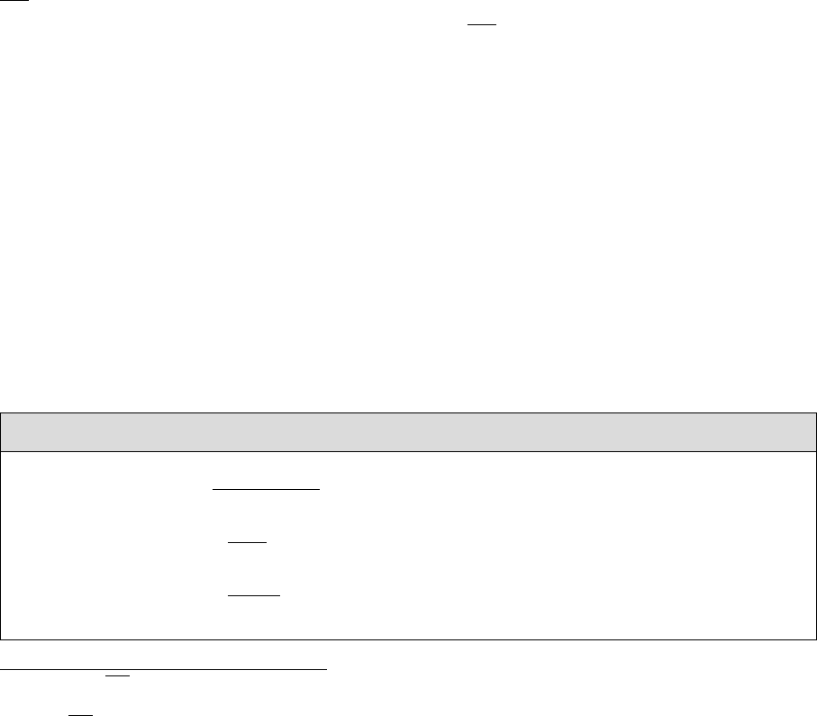
one-loop tadpole diagrams,
iδTH/h =
H/h
,(2.47)
where we switched the tadpole terms from the interaction basis to the mass basis by means of
the rotation matrix R(α), as indicated in Eq. (2.24). Since the tadpole terms explicitly appear
in the mass matrices in Eqs. (2.20)-(2.22), their CTs explicitly appear in the mass matrices at
one-loop order. The rotation from the interaction to the mass basis yields nine tadpole CTs in
total which depend on the two tadpole CTs δTH/h defined by the one-loop tadpole diagrams in
Eq. (2.47):
10

Tadpole renormalization (standard scheme)
δTHH =c3
αsβ+ s3
αcβ
vsβcβ
δTH−s2αsβ−α
vs2β
δTh(2.48)
δTHh =−s2αsβ−α
vs2β
δTH+s2αcβ−α
vs2β
δTh(2.49)
δThh =s2αcβ−α
vs2β
δTH−s3
αsβ−c3
αcβ
vsβcβ
δTh(2.50)
δTG0G0=cβ−α
vδTH+sβ−α
vδTh(2.51)
δTG0A=−sβ−α
vδTH+cβ−α
vδTh(2.52)
δTAA =cαs3
β+ sαc3
β
vsβcβ
δTH−sαs3
β−cαc3
β
vsβcβ
δTh(2.53)
δTG±G±=cβ−α
vδTH+sβ−α
vδTh(2.54)
δTG±H±=−sβ−α
vδTH+cβ−α
vδTh(2.55)
δTH±H±=cαs3
β+ sαc3
β
vsβcβ
δTH−sαs3
β−cαc3
β
vsβcβ
δTh(2.56)
Since the minimum of the potential is defined through the loop-corrected scalar potential, which
in general is a gauge-dependent quantity, the CTs defined through this minimum (e.g. the CTs
of the scalar or gauge boson masses) become manifestly gauge-dependent themselves. This is
no problem as long as all gauge dependences arising in a fixed-order calculation cancel against
each other. In the 2HDM, however, an improper renormalization condition for the mixing
angle CTs within the standard tadpole scheme can lead to uncanceled gauge dependences in the
calculation of partial decay widths. This is discussed in more detail in Sec. 2.2.4. Apart from the
appearance of the tadpole diagrams in Eqs. (2.48)-(2.56), and subsequently in the CTs and the
wave function renormalization constants (WFRCs) defined through these, the renormalization
condition in Eq. (2.47) ensures that all other appearances of tadpoles are canceled in the one-
loop calculation, i.e. tadpole diagrams in the self-energies or vertex corrections do not have to
be taken into account.
An alternative treatment of the tadpole renormalization was proposed by J. Fleischer and
F. Jegerlehner in the SM [77]. It was applied to the extended scalar sector of the 2HDM for
the first time in [57, 58] and is called alternative (FJ) tadpole scheme in the following. In this
alternative approach, the VEVs v1,2are considered as the fundamental quantities instead of
the tadpole terms. The proper VEVs are the renormalized all-order VEVs of the Higgs fields
which represent the true ground state of the theory and which are connected to the particle
masses and the couplings of the electroweak sector. Since the alternative approach relies on the
minimization of the gauge-independent tree-level scalar potential, the mass CTs defined in this
framework become manifestly gauge-independent quantities by themselves. Moreover, the alter-
native tadpole scheme connects the all-order renormalized VEVs directly to the corresponding
tree-level VEVs. Since the tadpoles are not the fundamental quantities of the Higgs minimum in
this framework, they do not receive CTs. Instead, CTs for the VEVs are introduced by replacing
11
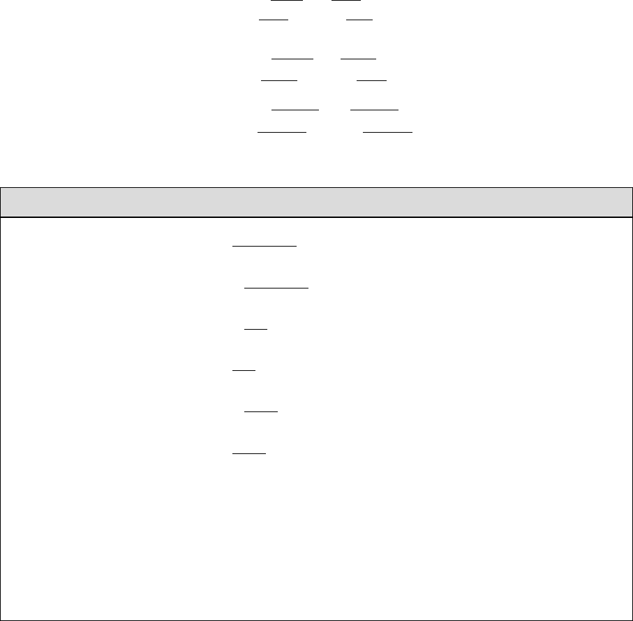
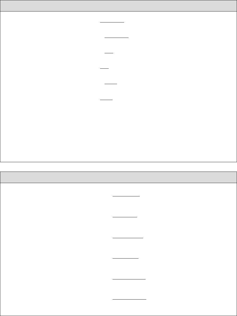
iΣtad(p2)≡+ +
H/h
iΣ(p2)≡+
Figure 1: Generic definition of the self-energies Σ and Σtad as function of the external momentum p2used in our
CT definitions of the 2HDM. While Σ is the textbook definition of the one-particle irreducible self-energy, the
self-energy Σtad additionally contains tadpole diagrams, indicated by the gray blob. For the actual calculation,
the full particle content of the 2HDM has to be inserted into the self-energy topologies depicted here.
the VEVs with the renormalized VEVs and their CTs,
vi→vi+δvi(2.57)
and by fixing the latter in such a way that it is ensured that the renormalized VEVs represent the
proper tree-level minima to all orders. At one-loop level, this leads to the following connection
between the VEV CTs in the interaction basis and the one-loop tadpole diagrams in the mass
basis,
δv1=−icα
m2
H
H
−−isα
m2
h
h
, δv2=−isα
m2
H
H
+−icα
m2
h
h
.(2.58)
The renormalization of the VEVs in the alternative tadpole scheme effectively shifts the VEVs
by tadpole contributions. As a consequence, tadpole diagrams have to be considered wherever
they can appear in the 2HDM. For the self-energies, this means that the fundamental self-
energies used to define the CTs are the ones defined as Σtad in Fig. 1 instead of the usual
one-particle irreducible self-energies Σ. Additionally, tadpole diagrams have to be considered
in the calculation of the one-loop vertex corrections to the Higgs decays. In summary, the
renormalization of the tadpoles in the alternative scheme leads to the following conditions:
Tadpole renormalization (alternative FJ scheme)
δTij = 0 (2.59)
Σ(p2)→Σtad(p2) (2.60)
Tadpole diagrams have to be considered in the vertex corrections.
12

2.2.2 Renormalization of the Gauge Sector
For the renormalization of the gauge sector, we introduce CTs and WFRCs for all parameters
and fields of the electroweak sector of the 2HDM by applying the shifts
m2
W→m2
W+δm2
W(2.61)
m2
Z→m2
Z+δm2
Z(2.62)
αem →αem +δαem ≡αem + 2αemδZe(2.63)
W±
µ→1 + δZW W
2W±
µ(2.64)
Z
γ→ 1 + δZZZ
2
δZZγ
2
δZγZ
21 + δZγγ
2!Z
γ,(2.65)
where for convenience, we additionally introduced the shift
e→e(1 + δZe) (2.66)
for the electromagnetic coupling constant by using Eq. (2.13). Applying OS conditions to the
gauge sector of the 2HDM leads to equivalent expressions for the CTs as derived in Ref. [71] for
the SM4, for the standard and alternative tadpole scheme, respectively,
Renormalization of the gauge sector (standard scheme)
δm2
W= Re ΣT
W W m2
W (2.67)
δm2
Z= Re ΣT
ZZ m2
Z (2.68)
Renormalization of the gauge sector (alternative FJ scheme)
δm2
W= Re hΣtad,T
W W m2
Wi(2.69)
δm2
Z= Re hΣtad,T
ZZ m2
Zi(2.70)
The WFRCs are the same in both tadpole schemes,
4In contrast to Ref. [71], however, we choose a different sign for the SU(2)Lterm of the covariant derivative,
which subsequently leads to a different sign in front of the second term of Eq. (2.71).
13

Renormalization of the gauge sector (standard and alternative FJ scheme)
δZe(m2
Z) = 1
2
∂ΣT
γγ p2
∂p2p2=0
+sW
cW
ΣT
γZ (0)
m2
Z−1
2∆α(m2
Z) (2.71)
δZW W =−Re "∂ΣT
W W p2
∂p2#p2=m2
W
(2.72)
δZZZ δZZγ
δZγZ δZγγ =
−Re ∂ΣT
ZZ (p2)
∂p2p2=m2
Z
2
m2
Z
ΣT
Zγ (0)
−2
m2
Z
Re hΣT
Zγ m2
Zi−Re ∂ΣT
γγ (p2)
∂p2p2=0
(2.73)
The superscript Tindicates that only the transverse parts of the self-energies are taken into
account. The CT for the electromagnetic coupling δZe(m2
Z) is defined at the scale of the Z
boson mass instead of the Thomson limit. For this, the additional term
∆α(m2
Z) = ∂Σlight,T
γγ (p2)
∂p2p2=0 −ΣT
γγ (m2
Z)
m2
Z
(2.74)
is required, where the transverse photon self-energy Σlight,T
γγ (p2) in Eq. (2.74) contains solely
light fermion contributions (i.e. contributions from all fermions apart from the tquark). This
ensures that the results of our EW one-loop computations are independent of large logarithms
due to light fermion contributions [71].
For later convenience, we additionally introduce the shift of the weak coupling constant
g→g+δg . (2.75)
Since gis not an independent parameter in our approach, cf. Eq. (2.13), the CT δg is not
independent either and can be expressed through the other CTs derived in this subsection as
δg
g=δZe(m2
Z) + 1
2(m2
Z−m2
W)δm2
W−m2
W
m2
Z
δm2
Z.(2.76)
14
2.2.3 Renormalization of the Scalar Sector
In the scalar sector of the 2HDM, the masses and fields of the scalar particles are shifted as
m2
H→m2
H+δm2
H(2.77)
m2
h→m2
h+δm2
h(2.78)
m2
A→m2
A+δm2
A(2.79)
m2
H±→m2
H±+δm2
H±(2.80)
H
h→1 + δZHH
2
δZHh
2
δZhH
21 + δZhh
2
H
h
(2.81)
G0
A→ 1 + δZG0G0
2
δZG0A
2
δZAG0
21 + δZAA
2!G0
A(2.82)
G±
H±→ 1 + δZG±G±
2
δZG±H±
2
δZH±G±
21 + δZH±H±
2!G±
H±.(2.83)
Applying OS renormalization conditions leads to the following CT definitions [57],
Renormalization of the scalar sector (standard scheme)
δZHh =2
m2
H−m2
h
RehΣHh(m2
h)−δTHhi(2.84)
δZhH =−2
m2
H−m2
h
RehΣHh(m2
H)−δTHhi(2.85)
δZG0A=−2
m2
A
RehΣG0A(m2
A)−δTG0Ai(2.86)
δZAG0=2
m2
A
RehΣG0A(0) −δTG0Ai(2.87)
δZG±H±=−2
m2
H±
RehΣG±H±(m2
H±)−δTG±H±i(2.88)
δZH±G±=2
m2
H±
RehΣG±H±(0) −δTG±H±i(2.89)
δm2
H= RehΣHH (m2
H)−δTHH i(2.90)
δm2
h= RehΣhh(m2
h)−δThhi(2.91)
δm2
A= RehΣAA(m2
A)−δTAAi(2.92)
δm2
H±= RehΣH±H±(m2
H±)−δTH±H±i(2.93)
15
Renormalization of the scalar sector (alternative FJ scheme)
δZHh =2
m2
H−m2
h
RehΣtad
Hh(m2
h)i(2.94)
δZhH =−2
m2
H−m2
h
RehΣtad
Hh(m2
H)i(2.95)
δZG0A=−2
m2
A
RehΣtad
G0A(m2
A)i(2.96)
δZAG0=2
m2
A
RehΣtad
G0A(0)i(2.97)
δZG±H±=−2
m2
H±
RehΣtad
G±H±(m2
H±)i(2.98)
δZH±G±=2
m2
H±
RehΣtad
G±H±(0)i(2.99)
δm2
H= RehΣtad
HH (m2
H)i(2.100)
δm2
h= RehΣtad
hh (m2
h)i(2.101)
δm2
A= RehΣtad
AA(m2
A)i(2.102)
δm2
H±= RehΣtad
H±H±(m2
H±)i(2.103)
Renormalization of the scalar sector (standard and alternative FJ scheme)
δZHH =−Re "∂ΣHH p2
∂p2#p2=m2
H
(2.104)
δZhh =−Re "∂Σhh p2
∂p2#p2=m2
h
(2.105)
δZG0G0=−Re "∂ΣG0G0p2
∂p2#p2=0
(2.106)
δZAA =−Re "∂ΣAA p2
∂p2#p2=m2
A
(2.107)
δZG±G±=−Re "∂ΣG±G±p2
∂p2#p2=0
(2.108)
δZH±H±=−Re "∂ΣH±H±p2
∂p2#p2=m2
H±
(2.109)
with the tadpole CTs in the standard scheme defined in Eqs. (2.48)-(2.56).
16
2.2.4 Renormalization of the Scalar Mixing Angles
In the following, we describe the renormalization of the scalar mixing angles αand βin the
2HDM. In our approach, we perform the rotation from the interaction to the mass basis,
cf. Eqs. (2.24)-(2.26), before renormalization so that the mixing angles need to be renormal-
ized. At one-loop level, the bare mixing angles are replaced by their renormalized values and
counterterms as
α→α+δα (2.110)
β→β+δβ . (2.111)
The renormalization of the mixing angles in the 2HDM is a non-trivial task and several different
schemes have been proposed in the literature. In the following, we only briefly present the
definition of the mixing angle CTs in all different schemes that are implemented in 2HDECAY and
refer to [57, 58] for details on the derivation of these schemes. It was shown in [57, 78] that an
MS condition for δα and δβ can lead to one-loop corrections that are orders of magnitude larger
than the LO result5. We therefore do not implement MS conditions for the mixing angle CTs
in 2HDECAY.
KOSY scheme. The KOSY scheme (denoted by the authors’ initials) was suggested in [66].
It combines the standard tadpole scheme with the definition of the counterterms through off-
diagonal wave function renormalization constants. As shown in [57, 58], the KOSY scheme not
only implies a gauge-dependent definition of the mixing angle CTs but also leads to explicitly
gauge-dependent decay amplitudes. The CTs are derived by temporarily switching from the
mass to the gauge basis. Since βdiagonalizes both the charged and CP-odd sector not all
scalar fields can be defined OS at the same time, unless a systematic modification of the SU (2)
relations is performed which we do not do here. We implemented two different CT definitions
where δβ is defined through the CP-odd or the charged sectors, indicated by superscripts oand
c, respectively. The KOSY scheme is implemented in 2HDECAY both in the standard and in the
alternative FJ scheme as a benchmark scheme for comparison with other schemes, but for actual
computations, we do not recommend to use it due to the explicit gauge dependence of the decay
amplitudes. In the KOSY scheme, the mixing angle CTs are defined as
Renormalization of δα and δβ: KOSY scheme (standard scheme)
δα =1
2(m2
H−m2
h)Re ΣHh(m2
H)+ΣHh(m2
h)−2δTHh(2.112)
δβo=−1
2m2
A
Re ΣG0A(m2
A)+ΣG0A(0) −2δTG0A(2.113)
δβc=−1
2m2
H±
Re ΣG±H±(m2
H±)+ΣG±H±(0) −2δTG±H±(2.114)
5In [59], an MS condition for the scalar mixing angles in certain processes led to corrections that are numerically
well-behaving due to a partial cancellation of large contributions from tadpoles. In the decays considered in our
work, an MS condition of δα and δβ in general leads to very large corrections, however.
17
Renormalization of δα and δβ: KOSY scheme (alternative FJ scheme)
δα =1
2(m2
H−m2
h)Re hΣtad
Hh(m2
H)+Σtad
Hh(m2
h)i(2.115)
δβo=−1
2m2
A
Re hΣtad
G0A(m2
A)+Σtad
G0A(0)i(2.116)
δβc=−1
2m2
H±
Re hΣtad
G±H±(m2
H±)+Σtad
G±H±(0)i(2.117)
p∗-pinched scheme. One possibility to avoid gauge-dependent mixing angle CTs was
suggested in [57, 58]. The main idea is to maintain the OS-based definition of δα and δβ of
the KOSY scheme, but instead of using the usual gauge-dependent off-diagonal WFRCs, the
WFRCs are defined through pinched self-energies in the alternative FJ scheme by applying the
pinch technique (PT) [79–86]. As worked out for the 2HDM for the first time in [57, 58], the
pinched scalar self-energies are equivalent to the usual scalar self-energies in the alternative FJ
scheme, evaluated in Feynman-’t Hooft gauge (ξ= 1), up to additional UV-finite self-energy
contributions Σadd
ij (p2). The mixing angle CTs depend on the scale where the pinched self-
energies are evaluated. In the p∗-pinched scheme, we follow the approach of [87] in the MSSM,
where the self-energies Σtad
ij (p2) are evaluated at the scale
p2
∗≡m2
i+m2
j
2.(2.118)
At this scale, the additional contributions Σadd
ij (p2) vanish. Using the p∗-pinched scheme at
one-loop level yields explicitly gauge-independent partial decay widths. The mixing angle CTs
are defined as
Renormalization of δα and δβ:p∗-pinched scheme (alternative FJ scheme)
δα =1
m2
H−m2
h
Re Σtad
Hh m2
H+m2
h
2ξ=1
(2.119)
δβo=−1
m2
A
Re Σtad
G0Am2
A
2ξ=1
(2.120)
δβc=−1
m2
H±
Re Σtad
G±H±m2
H±
2ξ=1
(2.121)
OS-pinched scheme. In order to allow for the analysis of the effects of different scale
choices of the mixing angle CTs, we implemented another OS-motivated scale choice, which is
18

called the OS-pinched scheme. Here, the additional terms do not vanish and are given by [57]
Σadd
Hh (p2) = αemm2
Zsβ−αcβ−α
8πm2
W1−m2
W
m2
Zp2−m2
H+m2
h
2B0(p2;m2
Z, m2
A)−B0(p2;m2
Z, m2
Z)
+ 2m2
W
m2
ZB0(p2;m2
W, m2
H±)−B0(p2;m2
W, m2
W)(2.122)
Σadd
G0A(p2) = αemm2
Zsβ−αcβ−α
8πm2
W1−m2
W
m2
Zp2−m2
A
2B0(p2;m2
Z, m2
H)−B0(p2;m2
Z, m2
h)(2.123)
Σadd
G±H±(p2) = αemsβ−αcβ−α
4π1−m2
W
m2
Zp2−m2
H±
2B0(p2;m2
W, m2
H)−B0(p2;m2
W, m2
h).(2.124)
The mixing angle CTs in the OS-pinched scheme are then defined as
Renormalization of δα and δβ: OS-pinched scheme (alternative FJ scheme)
δα =
RehΣtad
Hh(m2
H)+Σtad
Hh(m2
h)ξ=1 + Σadd
Hh (m2
H)+Σadd
Hh (m2
h)i
2m2
H−m2
h(2.125)
δβo=−
RehΣtad
G0A(m2
A)+Σtad
G0A(0)ξ=1 + Σadd
G0A(m2
A)+Σadd
G0A(0)i
2m2
A
(2.126)
δβc=−
RehΣtad
G±H±(m2
H±)+Σtad
G±H±(0)ξ=1 + Σadd
G±H±(m2
H±)+Σadd
G±H±(0)i
2m2
H±
(2.127)
Process-dependent schemes. The definition of the mixing angle CTs through observables,
like e.g. partial decay widths of Higgs bosons, was proposed for the MSSM in [88, 89] and for
the 2HDM in [90]. This scheme leads to explicitly gauge-independent partial decay widths
per construction. Moreover, the connection of the mixing angle CTs with physical observables
allows for a more physical interpretation of the unphysical mixing angles αand β. However,
as it was shown in [57, 58], process-dependent schemes can in general lead to very large one-
loop corrections. We implemented three different process-dependent schemes for δα and δβ in
2HDECAY. The schemes differ in the processes that are used for the definition of the CTs. In
all cases we have chosen leptonic Higgs boson decays. For these, the QED corrections can be
separated in a UV-finite way from the rest of the EW corrections and therefore be excluded
from the counterterm definition. This is necessary to avoid the appearance of infrared (IR)
divergences in the CTs [89]. The NLO corrections to the partial decay widths of the leptonic
decay of a Higgs particle φiinto a pair of leptons fj,fkcan then be cast into the form
ΓNLO,weak
φifjfk= ΓLO
φifjfk1 + 2Re hFVC
φifjfk+FCT
φifjfki ,(2.128)
where FVC
φifjfkand FCT
φifjfkare the form factors of the vertex corrections and the CT, respectively,
and the superscript weak indicates that in the vertex corrections IR-divergent QED contributions
are excluded. The form factor FCT
φifjfkcontains either δα or δβ or both simultaneously as well
19
as other CTs that are fixed as described in the other subsections of Sec. 2.2. Employing the
renormalization condition
ΓLO
φifjfk≡ΓNLO,weak
φifjfk(2.129)
for two different decays then allows for a process-dependent definition of the mixing angle CTs.
For more details on the calculation of the CTs in process-dependent schemes in the 2HDM,
we refer to [57, 58]. In 2HDECAY, we have chosen the following three different combinations of
processes as definition for the CTs,
1. δβ is first defined by A→τ+τ−and δα is subsequently defined by H→τ+τ−.
2. δβ is first defined by A→τ+τ−and δα is subsequently defined by h→τ+τ−.
3. δβ and δα are simultaneously defined by H→τ+τ−and h→τ+τ−.
Employing these renormalization conditions yields the following definitions of the mixing angle
CTs6:
Renormalization of δα and δβ: process-dependent scheme 1 (both schemes)
δα =−Y5
Y4FVC
Hτ τ +δg
g+δmτ
mτ−δm2
W
2m2
W
+Y6δβ +δZHH
2+Y4
Y5
δZhH
2+δZL
ττ
2(2.130)
+δZR
ττ
2
δβ =−Y6
1 + Y2
6FVC
Aττ +δg
g+δmτ
mτ−δm2
W
2m2
W
+δZAA
2−1
Y6
δZG0A
2+δZL
ττ
2+δZR
ττ
2(2.131)
Renormalization of δα and δβ: process-dependent scheme 2 (both schemes)
δα =Y4
Y5FVC
hττ +δg
g+δmτ
mτ−δm2
W
2m2
W
+Y6δβ +δZhh
2+Y5
Y4
δZHh
2+δZL
ττ
2(2.132)
+δZR
ττ
2
δβ =−Y6
1 + Y2
6FVC
Aττ +δg
g+δmτ
mτ−δm2
W
2m2
W
+δZAA
2−1
Y6
δZG0A
2+δZL
ττ
2+δZR
ττ
2(2.133)
Renormalization of δα and δβ: process-dependent scheme 3 (both schemes)
δα =Y4Y5
Y2
4+Y2
5FVC
hττ − FVC
Hτ τ +δZhh
2−δZHH
2+Y5
Y4
δZHh
2−Y4
Y5
δZhH
2(2.134)
δβ =−1
Y6(Y2
4+Y2
5)(Y2
4+Y2
5)δg
g+δmτ
mτ−δm2
W
2m2
W
+δZL
ττ
2+δZR
ττ
2(2.135)
+Y4Y5δZHh
2+δZhH
2+Y2
4δZhh
2+FVC
hττ +Y2
5δZHH
2+FVC
Hτ τ
6While the definition of the CTs is generically the same for both tadpole schemes, their actual analytic forms
differ in both schemes since some of the CTs used in the definition differ in the two schemes, as well.
20

Note that for the process-dependent schemes, decays have to be chosen that are experimentally
accessible. This may not be the case for certain parameter configurations, in which case the user
has to choose, if possible, the decay combination that leads to large enough decay widths to be
measurable.
2.2.5 Renormalization of the Fermion Sector
The masses mf, where fgenerically stands for any fermion of the 2HDM, the CKM matrix
elements Vij (i, j = 1,2,3), the Yukawa coupling parameters Yk(k= 1, ..., 6) and the fields
of the fermion sector are replaced by the renormalized quantities and the respective CTs and
WFRCs as
mf→mf+δmf(2.136)
Vij →Vij +δVij (2.137)
Yk→Yk+δYk(2.138)
fL
i→ δij +δZf,L
ij
2!fL
j(2.139)
fR
i→ δij +δZf,R
ij
2!fR
j,(2.140)
where we use Einstein’s sum convention in the last two lines. The superscripts Land Rdenote
the left- and right-chiral component of the fermion fields, respectively. The Yukawa coupling
parameters Yiare not independent input parameters, but functions of αand β,cf. Tab. 2. Their
one-loop counterterms are therefore given in terms of δα and δβ defined in Sec. 2.2.4 by the
following formulae which are independent of the 2HDM type,
δY1=Y1−Y2
Y1
δα +Y3δβ(2.141)
δY2=Y2Y1
Y2
δα +Y3δβ(2.142)
δY3=1 + Y2
3δβ (2.143)
δY4=Y4−Y5
Y4
δα +Y6δβ(2.144)
δY5=Y5Y4
Y5
δα +Y6δβ(2.145)
δY6=1 + Y2
6δβ . (2.146)
Before presenting the renormalization conditions of the mass CTs and WFRCs, we shortly
discuss the renormalization of the CKM matrix. In [71] the renormalization of the CKM matrix
is connected to the renormalization of the fields, which in turn are renormalized in an OS
approach, leading to the definition (i, j, k = 1,2,3)
δVij =1
4hδZu,L
ik −δZu,L†
ik Vkj −Vik δZd,L
kj −δZd,L†
kj i ,(2.147)
where the superscripts uand ddenote up-type and down-type quarks, respectively. This def-
inition of the CKM matrix CTs leads to uncanceled explicit gauge dependences when used in
21
the calculation of EW one-loop corrections, however, [91–96]. Since the CKM matrix is ap-
proximately a unit matrix [97], the numerical effect of this gauge dependence is typically very
small, but the definition nevertheless introduces uncanceled explicit gauge dependences into the
partial decay widths, which should be avoided. In our work, we follow the approach of Ref. [95]
and use pinched fermion self-energies for the definition of the CKM matrix CT. An analytic
analysis shows that this is equivalent with defining the CTs in Eq. (2.147) in the Feynman-’t
Hooft gauge.
Apart from the CKM matrix CT, all other CTs of the fermion sector are defined through
OS conditions. The resulting forms of the CTs are analogous to the ones presented in [71] and
given by
Renormalization of the fermion sector (standard scheme)
δmf,i =mf,i
2Re Σf,L
ii (m2
f,i)+Σf,R
ii (m2
f,i) + 2Σf,S
ii (m2
f,i)(2.148)
δZf,L
ij =2
m2
f,i −m2
f,j
Rem2
f,j Σf,L
ij (m2
f,j ) + mf,imf,j Σf,R
ij (m2
f,j ) (2.149)
+ (m2
f,i +m2
f,j )Σf,S
ij (m2
f,j ),(i6=j)
δZf,R
ij =2
m2
f,i −m2
f,j
Rem2
f,j Σf,R
ij (m2
f,j ) + mf,imf,j Σf,L
ij (m2
f,j ) (2.150)
+ 2mf,imf,j Σf,S
ij (m2
f,j ),(i6=j)
Renormalization of the fermion sector (alternative FJ scheme)
δmf,i =mf,i
2Re Σf,L
ii (m2
f,i)+Σf,R
ii (m2
f,i) + 2Σtad,f,S
ii (m2
f,i)(2.151)
δZf,L
ij =2
m2
f,i −m2
f,j
Rem2
f,j Σf,L
ij (m2
f,j ) + mf,imf,j Σf,R
ij (m2
f,j ) (2.152)
+ (m2
f,i +m2
f,j )Σtad,f,S
ij (m2
f,j ),(i6=j)
δZf,R
ij =2
m2
f,i −m2
f,j
Rem2
f,j Σf,R
ij (m2
f,j ) + mf,imf,j Σf,L
ij (m2
f,j ) (2.153)
+ 2mf,imf,j Σtad,f,S
ij (m2
f,j ),(i6=j)
22

Renormalization of the fermion sector (standard and alternative FJ scheme)
δVij =1
4hδZu,L
ik −δZu,L†
ik Vkj −Vik δZd,L
kj −δZd,L†
kj iξ=1 (2.154)
δZf,L
ii =−RehΣf,L
ii (m2
f,i)i−m2
f,iRe "∂Σf,L
ii (p2)
∂p2+∂Σf,R
ii (p2)
∂p2+ 2∂Σf,S
ii (p2)
∂p2#p2=m2
f,i
(2.155)
δZf,R
ii =−RehΣf,R
ii (m2
f,i)i−m2
f,iRe "∂Σf,L
ii (p2)
∂p2+∂Σf,R
ii (p2)
∂p2+ 2∂Σf,S
ii (p2)
∂p2#p2=m2
f,i
(2.156)
where as before, the superscripts Land Rdenote the left- and right-chiral parts of the self-
energies, while the superscript Sdenotes the scalar part.
2.2.6 Renormalization of the Soft-Z2-Breaking Parameter m2
12
The last remaining parameter of the 2HDM that needs to be renormalized is the soft-Z2-breaking
parameter m2
12. As before, we replace the bare parameter by the renormalized one and its
corresponding CT,
m2
12 →m2
12 +δm2
12 .(2.157)
In order to fix δm2
12 in a physical way, one could use a process-dependent scheme analogous to
Sec. 2.2.4 for the scalar mixing angles. Since m2
12 only appears in trilinear Higgs couplings, a
Higgs-to-Higgs decay width would have to be chosen as observable that fixes the CT. However,
as discussed in [63], a process-dependent definition of δm2
12 can lead to very large one-loop
corrections in Higgs-to-Higgs decays. We therefore employ an MS condition in 2HDECAY to fix
the CT. This is done by calculating the off-shell decay process h→hh at one-loop order and by
extracting all UV-divergent terms, i.e. all terms proportional to
∆≡1
ε−γE+ ln(4π),(2.158)
that are left in the amplitude after all parameters apart from m2
12 are renormalized. Here, γEis
the Euler-Mascheroni constant and εthe dimensional shift when switching from 4 to D= 4 −2ε
dimensions in the framework of dimensional regularization [98–100]. This fixes the CT of m2
12
to
Renormalization of m2
12 (standard and alternative FJ scheme)
δm2
12 =αemm2
12
16πm2
W1−m2
W
m2
Zh8m2
12
s2β−2m2
H±−m2
A+s2α
s2β
(m2
H−m2
h)−3(2m2
W+m2
Z)
+X
u
3m2
u
1
s2
β−X
d
6m2
dY3−Y3−1
t2β−X
l
2m2
lY6−Y6−1
t2βi∆ (2.159)
23
ALO
φX1X2
φ
p1
p2
X1
p3
X2
AVC
φX1X2
φ
p1
p2
X1
p3
X2
ACT
φX1X2
φ
p1
p2
X1
p3
X2
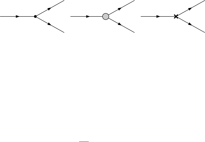
Figure 2: Decay amplitudes at LO and NLO. The LO decay amplitude ALO
φX1X2simply consists of the trilinear
coupling of the three particles φ1,X1and X2, while the one-loop amplitude is given by the sum of the genuine
vertex corrections AVC
φX1X2, indicated by a grey blob, and the vertex counterterm ACT
φX1X2which also includes
all WFRCs necessary to render the NLO amplitude UV-finite. We do not show corrections on the external legs
since in the decays we consider, they vanish either due to OS renormalization conditions or due to Slavnov-Taylor
identities. In the case of the alternative tadpole scheme, the vertex corrections AVC
φX1X2also in general contain
tadpole diagrams.
where the sum indices u,dand lindicate a summation over all up-type and down-type quarks
and charged leptons, respectively. The result in Eq. (2.159) is in agreement with the formula
presented in [76].
Choosing to renormalize m2
12 in an MS scheme automatically leads to a dependence of the
partial decay widths of the Higgs-to-Higgs decays on the renormalization scale µR. This scale
should be chosen appropriately in order to avoid the appearance of large logarithms in the EW
one-loop corrections. A typical choice of µRis e.g. the mass scale of the decaying Higgs boson.
In 2HDECAY, the scale µRcan either be set to a global fixed value for all decay channels or it can
be chosen equal to the mass of the decaying Higgs boson of the respective decay channel.
2.3 Electroweak Decay Processes at LO and NLO
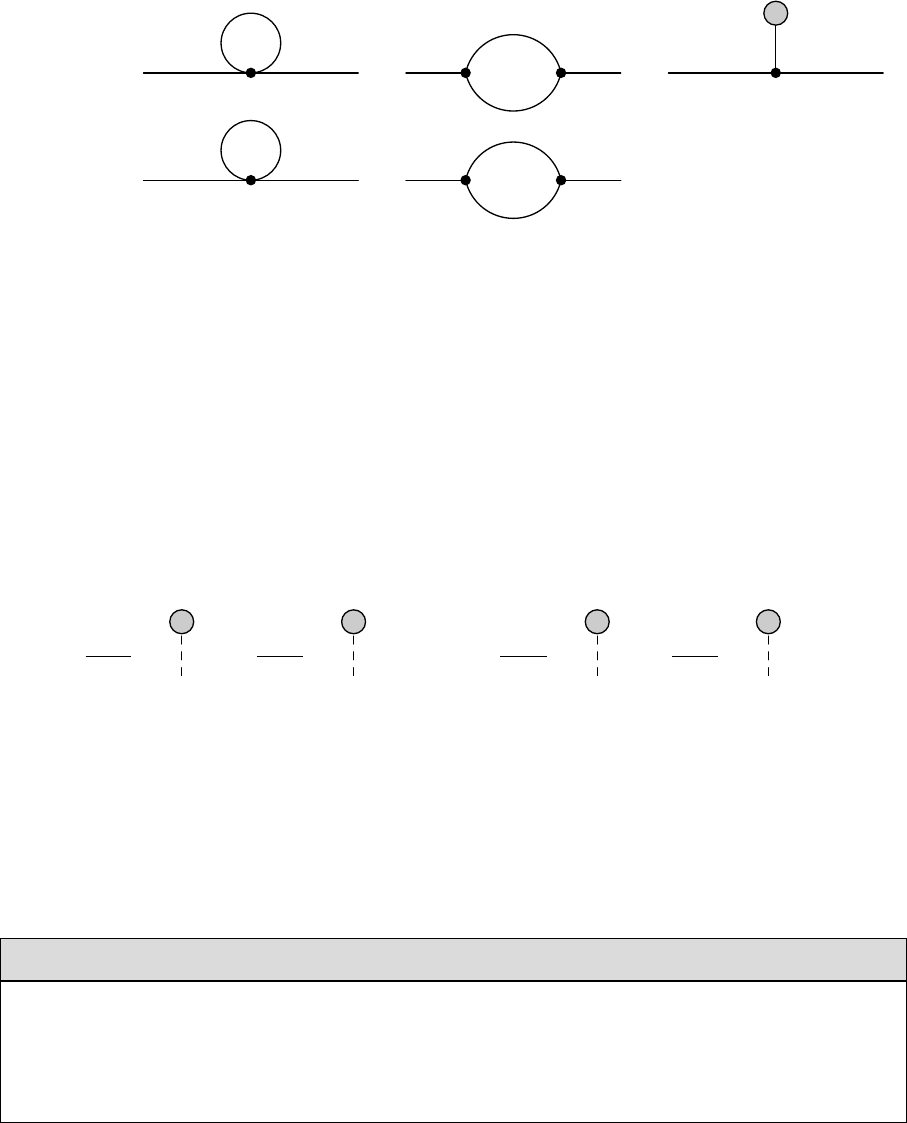
Figure 2 shows the topologies that contribute to the tree-level and one-loop corrected decay of a
scalar particle φwith four-momentum p1into two other particles X1and X2with four-momenta
p2and p3, respectively. We emphasize that for the EW corrections, we restrict ourselves to OS
decays, i.e. we demand
p2
1≥(p2+p3)2,(2.160)
with p2
i=m2
i(i= 1,2,3) where midenote the masses of the three particles. Moreover, we
do not calculate EW corrections to loop-induced Higgs decays, which are of two-loop order. In
particular, we do not provide EW corrections to Higgs boson decays into two-gluon, two-photon
or Zγ final states. Note, however, that the decay widths implemented in HDECAY include also
loop-induced decay widths as well as off-shell decays into heavy-quark, massive gauge boson,
neutral Higgs pair as well as Higgs and gauge boson final states. We come back to this point in
Sec. 2.4. The LO and NLO partial decay widths were calculated by first generating all Feynman
diagrams and the corresponding amplitudes for all decay modes that exist for the 2HDM, shown
topologically in Fig. 2, with help of the tool FeynArts 3.9 [101]. To that end, we used the
2HDM model file that is implemented in FeynArts, but modified the Yukawa couplings to
implement all four 2HDM types. Diagrams that account for NLO corrections on the external
legs were not calculated since for all decay modes that we considered, they either vanish due
to OS renormalization conditions or due to Slavnov-Taylor identities. All amplitudes were then
calculated analytically with FeynCalc 8.2.0 [102,103], together with all self-energy amplitudes
needed for the CTs.
24

The LO partial decay width is obtained from the LO amplitude ALO
φX1X2, while the NLO
amplitude is given by the sum of all amplitudes stemming from the vertex correction and the
necessary CTs as defined in Sec. 2.2,
A1loop
φX1X2≡ AVC
φX1X2+ACT
φX1X2.(2.161)
By introducing the K¨all´en phase space function
λ(x, y, z)≡px2+y2+z2−2xy −2xz −2yz , (2.162)
the LO and NLO partial decay widths can be cast into the form
ΓLO
φX1X2=Sλ(m2
1, m2
2, m2
3)
16πm3
1X
d.o.f. ALO
φX1X2
2(2.163)
ΓNLO
φX1X2= ΓLO
φX1X2+Sλ(m2
1, m2
2, m2
3)
8πm3
1X
d.o.f.
Re hALO
φX1X2∗A1loop
φX1X2i+ ΓφX1X2+γ,(2.164)
where the symmetry factor Saccounts for identical particles in the final state and the sum
extends over all degrees of freedom of the final-state particles, i.e. over spins or polarizations.
The partial decay width ΓφX1X2+γaccounts for real corrections that are necessary for removing
IR divergences in all decays that involve charged particles in the initial or final state. For this,
we implemented the results given in [104] for generic one-loop two-body partial decay widths.
Since the involved integrals are analytically solvable for two-body decays [71], the IR corrections
that are implemented in 2HDECAY are given in analytic form as well and do not require numerical
integration. Additionally, since the implemented integrals account for the full phase-space of the
radiated photon, i.e. both the “hard” and “soft” parts, our results do not depend on arbitrary
cuts in the photon phase-space.
In the following, we present all decay channels for which the EW corrections were calculated
at one-loop order:
•h/H/A →f¯
f(f=u, d, c, s, t, b, e, µ, τ)
•h/H →V V (V=W±, Z)
•h/H →V S (V=Z, W ±,S=A, H±)
•h/H →SS (S=A, H±)
•H→hh
•H±→V S (V=W±,S=h, H, A)
•H+→f¯
f(f=u, c, t, νe, νµ, ντ,¯
f=¯
d, ¯s, ¯
b, e+, µ+, τ+)
•A→V S (V=Z, W ±,S=h, H, H±)
All analytic results of these decay processes are stored in subdirectories of 2HDECAY. For a
consistent connection with HDECAY,cf. also Sec. 2.4, not all of these decay processes are used
for the calculation of the decay widths and branching ratios, however. Decays containing pairs
of first-generation fermions are neglected, i.e. in 2HDECAY, the EW corrections of the following
processes are not used for the calculation of the partial decay widths and branching ratios:
h/H/A →f¯
f(f=u, d, e) and H+→f¯
f(f¯
f=u¯
d, νee+). The reason is that they are
overwhelmed by the Dalitz decays Φ →f¯
f(0)γ(Φ = h, H, A, H±) that are induced e.g. by
off-shell γ∗→f¯
fsplitting.
25

2.4 Link to HDECAY, Calculated Higher-Order Corrections and Caveats
The EW one-loop corrections to the Higgs decays in the 2HDM derived in this work are com-
bined with HDECAY version 6.52 [68, 69]7in form of the new tool 2HDECAY. The Fortran code
HDECAY provides the LO and QCD corrected decay widths. As outlined in Sec. 2.2.2 the EW
corrections use αem at the Zboson mass scale as input parameter instead of GFas used in
HDECAY. For a consistent combination of the EW corrected decay widths with the HDECAY im-
plementation in the GFscheme we would have to convert between the {αem, mW, mZ}and the
{GF, mW, mZ}scheme including 2HDM higher-order corrections in the conversion formulae.
Since these conversion formulae are not implemented yet, we chose a pragmatic approximate
solution:
In the configuration of 2HDECAY with OMIT ELW2=0 being set (cf. the input file format de-
scribed in Sec. 3.5), the EW corrections to the decay widths are calculated automatically. This
setting also overwrites the value that the user chooses for the input 2HDM. If e.g. the user does
not choose the 2HDM by setting 2HDM=0 but at the same time chooses OMIT ELW2=0 in order
to calculate the EW corrections, then a warning is printed and 2HDM=1 is automatically set
internally. In this configuration, the value of GFgiven in the input file of 2HDECAY is ignored
by the part of the program that calculates the EW corrections. Instead, αem(m2
Z), given in line
26 of the input file, is taken as independent input. This αem(m2
Z) is used for the calculation of
all electroweak corrections. Subsequently, for the consistent combination with the decay widths
of HDECAY computed in terms of the Fermi constant GF, the latter decay widths are adapted to
the input scheme of the EW corrections by rescaling the HDECAY decay widths with Gcalc
F/GF,
where Gcalc
Fis calculated by means of the tree-level relation Eq. (2.14) as a function of αem(m2
Z).
We expect the differences between the observables within these two schemes to be small.
On the other hand, if OMIT ELW2=1 is set, no EW corrections are computed and 2HDECAY
reduces to the original program code HDECAY, including (where applicable) the QCD corrections
in the decay widths, the off-shell decays and the loop-induced decays. In this case, the value
of GFgiven in line 27 of the input file is used as input parameter instead of being calculated
through the input value of αem(m2
Z), and no rescaling with Gcalc
Fis performed. We note in
particular that therefore the QCD corrected decay widths, printed out separately by 2HDECAY,
will be different in the two input options OMIT ELW2=0 and OMIT ELW2=1.
Another comment is at order in view of the fact that we implemented EW corrections to OS
decays only, while HDECAY also features the computation of off-shell decays. More specifically,
HDECAY includes off-shell decays into final states with an off-shell top-quark t∗,i.e. φ→t∗¯
t
(φ=h, H, A), H+→t∗+¯
d, ¯s, ¯
b, into gauge and Higgs boson final states with an off-shell gauge
boson, h/H →Z∗A, A →Z∗h/H, φ →H−W+∗, H+→φW +∗, and into neutral Higgs pairs
with one off-shell Higgs boson that is assumed to predominantly decay into the b¯
bfinal state,
h/H →AA∗,H→hh∗. The top quark total width within the 2HDM, required for the off-
shell decays with top final states, is calculated internally in HDECAY. In 2HDECAY, we combine
the EW and QCD corrections in such a way that HDECAY still computes the decay widths of
off-shell decays, while the electroweak corrections are added only to OS decay channels. It is
important to keep this restriction in mind when performing the calculation for large varieties
of input data. If e.g. the lighter Higgs boson his chosen to be the SM-like Higgs boson, then
the OS decay h→W+W−would be kinematically forbidden while the heavier Higgs boson
decay H→W+W−might be OS. In such cases, 2HDECAY calculates the EW NLO corrections
only for the latter decay channel, while the LO (and QCD decay widths where applicable) are
7The program code for HDECAY can be downloaded from the URL http://tiger.web.psi.ch/hdecay/.
26

IELW2=0 QCD-corrected QCD&EW-corrected
on-shell and ΓHD,QCD Gcalc
F
GFΓHD,QCD[1 + δEW]Gcalc
F
GF
non-loop induced
off-shell or ΓHD,QCD Gcalc
F
GFΓHD,QCD Gcalc
F
GF
loop-induced
Table 3: The QCD-corrected and the QCD&EW-corrected decay widths as calculated by 2HDECAY for IELW2=0.
The label QCD is in the sense that the QCD corrections are included where applicable.
calculated for both. The same is true for any other decay channel for which we implemented
EW corrections but which are off-shell in certain input scenarios.
For the combination of the QCD and EW corrections finally, we assume that these corrections
factorize. We denote by δQCD and δEW the relative QCD and EW corrections, respectively. Here
δQCD is normalized to the LO width ΓHD,LO, calculated internally by HDECAY. This means for
example in the case of quark pair final states that the LO width includes the running quark
mass in order to improve the perturbative behaviour. The relative EW corrections δEW on the
other hand are obtained by normalization to the LO width with on-shell particle masses. With
these definitions the QCD and EW corrected decay width into a specific final state, ΓQCD&EW,
is given by
ΓQCD&EW =Gcalc
F
GF
ΓHD,LO[1 + δQCD][1 + +δEW]≡Gcalc
F
GF
ΓHD,QCD[1 + δEW].(2.165)
We have included the rescaling factor Gcalc
F/GFwhich is necessary for the consistent connection
of our EW corrections with the decay widths obtained from HDECAY, as outline above.
QCD&EW-corrected branching ratios: The program code will provide the branching ratios
calculated originally by HDECAY, which, however, for OMIT ELW2=0 are rescaled by Gcalc
F/GF.
They include all loop decays, off-shell decays and QCD corrections where applicable. We sum-
marize these branching ratios under the name ’QCD-corrected’ branching ratios and call their
associated decay widths ΓHD,QCD, keeping in mind that the QCD corrections are included only
where applicable. Furthermore, the EW and QCD corrected branching ratios will be given out.
Here, we add the EW corrections to the decay widths calculated internally by HDECAY where
possible, i.e. for non-loop induced and OS decay widths. We summarize these branching ratios
under the name ’QCD&EW-corrected’ branching ratios and call their associated decay widths
ΓQCD&EW. In Table 3 we summarize all details and caveats on their calculation that we de-
scribed here above. All these branching ratios are written to the output file carrying the suffix
’ BR’ with its filename, see also end of section 3.5 for details.
NLO EW-corrected decay widths: For IELW2 =0, we additionally give out the LO and the
EW-corrected NLO decay widths as calculated by the new addition to HDECAY. Here the LO
widths do not include any running of the quark masses in the case of quark final states, but
are obtained for OS masses. They can hence differ quite substantially from the LO widths
as calculated in the original HDECAY version. These LO and EW-corrected NLO widths are
computed in the {αem, mW, mZ}scheme and therefore obviously do not need the inclusion of
the rescaling factor Gcalc
F/GF. The decay widths are written to the output file carrying the suffix
’ EW’ with its filename. While the widths given out here are not meant to be applied in Higgs
observables as they do not include the important QCD corrections, the study of the NLO EW-
corrected decay widths for various renormalization schemes, as provided by 2HDECAY, allows to
27

analyze the importance of the EW corrections and estimate the remaining theoretical error due
to missing higher-order EW corrections. The decay widths can also be used for phenomenological
studies like e.g. the comparison with the EW-corrected decay widths in the MSSM in the limit of
large supersymmetric particle masses, or the investigation of specific 2HDM parameter regions
at LO and NLO as e.g. the alignment limit, the non-decoupling limit or the wrong-sign limit.
Caveats: We would like to point out to the user that it can happen that the EW-corrected
decay widths become negative because of too large negative EW corrections compared to the
LO width. There can be several reasons for this: (i) The LO width may be very small in parts
of the parameter space due to suppressed couplings. For example the decay of the heavy Higgs
boson Hinto massive vector bosons is very small in the region where the lighter hbecomes
SM-like and takes over almost the whole coupling to massive gauge bosons. If the NLO EW
width is not suppressed by the same power of the relevant coupling or if at NLO there are
cancellations between the various terms that remove the suppression, the NLO width can largely
exceed the LO width. (ii) The EW corrections are artificially enhanced due to a badly chosen
renormalization scheme, cf. Refs. [58, 63, 64] for investigations on this subject. The choice of a
different renormalization scheme may cure this problem, but of course raises also the question for
the remaining theoretical error due to missing higher-order corrections. (iii) The EW corrections
are parametrically enhanced due to involved couplings that are large, because of small coupling
parameters in the denominator or due to light particles in the loop, see also Refs. [58, 63,64] for
discussions. This would call for the resummation of EW corrections beyond NLO to improve
the behaviour. It is obvious that the EW corrections should not be trusted in case of extremely
large positive or negative corrections and rather be discarded, in particular in the comparison
with experimental observables, unless some of the suggested measures are taken to improve the
behaviour.
3 Program Description
In the following, we describe the system requirements needed for compiling and running 2HDECAY,
the installation procedure and the usage of the program. Additionally, we describe the input
and output file formats in detail.
3.1 System Requirements
The Python/FORTRAN program code 2HDECAY was developed under Windows 10 and openSUSE
Leap 15.0. The supported operating systems are:
•Windows 7 and Windows 10 (tested with Cygwin 2.10.0)
•Linux (tested with openSUSE Leap 15.0)
•macOS (tested with macOS Sierra 10.12)
In order to compile and run 2HDECAY on Windows, you need to install Cygwin first (together
with the packages cURL,find,gcc,g++ and gfortran, which also are required to be installed
on Linux and macOS). For the compilation, the GNU C compilers gcc (tested with versions 6.4.0
and 7.3.1), g++ and the FORTRAN compiler gfortran are required. Additionally, an up-to-date
version of Python 2 or Python 3 is required (tested with versions 2.7.14 and 3.5.0). For an
optimal performance of 2HDECAY, we recommend that the program is installed on a solid state
drive (SSD) with high reading and writing speeds.
28

3.2 License
2HDECAY is released under the GNU General Public License (GPL) (GNU GPL-3.0-or-later).
2HDECAY is free software, which means that anyone can redistribute it and/or modify it under
the terms of the GNU GPL as published by the Free Software Foundation, either version 3 of
the License, or any later version. 2HDECAY is distributed without any warranty. A copy of the
GNU GPL is included in the LICENSE.md file in the root directory of 2HDECAY.
3.3 Download
The latest version of the program as well as a short quick-start documentation is given at
https://github.com/marcel-krause/2HDECAY. To obtain the code either the repository is cloned
or the zip archive is downloaded and unzipped to a directory of the user’s choice, which here
and in the following will be referred to as $2HDECAY. The main folder of 2HDECAY consists of
several subfolders:
BuildingBlocks Contains the analytic electroweak one-loop corrections for all decays con-
sidered, as well as the real corrections and CTs needed to render the decay widths UV-
and IR-finite.
Documentation Contains this documentation.
HDECAY This subfolder contains a modified version of HDECAY 6.52 [68, 69], needed for the
computation of the LO and (where applicable) QCD corrected decay widths. HDECAY
also provides off-shell decay widths and the loop-induced decay widths into gluon and
photon pair final states and into Zγ.HDECAY is furthermore used for the computation of
the branching ratios.
Input In this subfolder, at least one or more input files can be stored that shall be used
for the computation. The format of the input file is explained in Sec. 3.5. In the Github
repository, the Input folder contains an exemplary input file which is printed in App. A.
Results All results of a successful run of 2HDECAY are stored as output files in this subfolder
under the same name as the corresponding input files in the Input folder, but with the
file extension .in replaced by .out and a suffix “ BR” and “ EW” for the branching
ratios and electroweak partial decay widths, respectively. In the Github repository, the
Results folder contains two exemplary output files which are given in App. B.
The main folder $2HDECAY itself also contains several files:
2HDECAY.py Main program file of 2HDECAY. It serves as a wrapper file for calling HDECAY in
order to convert the charm and bottom quark masses from the MS input values to the
corresponding OS values and to calculate the LO widths, QCD corrections, off-shell and
loop-induced decays, the branching ratios as well as electroweakCorrections for the
calculation of the EW one-loop corrections.
Changelog.md Documentation of all changes made in the program since version
2HDECAY 1.0.0.
CommonFunctions.py Function library of 2HDECAY, providing functions frequently used in
the different files of the program.
29

Config.py Main configuration file. If LoopTools is not installed automatically by the in-
staller of 2HDECAY, the paths to the LoopTools executables and libraries have to be set
manually in this file.
constants.F90 Library for all constants used in 2HDECAY.
counterterms.F90 Definition of all fundamental CTs necessary for the EW one-loop renor-
malization of the Higgs boson decays. The CTs defined in this file require the analytic
results saved in the BuildingBlocks subfolder.
electroweakCorrections.F90 Main file for the calculation of the EW one-loop corrections
to the Higgs boson decays. It combines the EW one-loop corrections to the decay widths
with the necessary CTs and IR corrections and calculates the EW contributions to the
tree-level decay widths that are then combined with the QCD corrections in HDECAY.
getParameters.F90 Routine to read in the input values given by the user in the input files
that are needed by 2HDECAY.
LICENSE.md Contains the full GNU General Public License (GNU GPL-3.0-or-later) agree-
ment under which 2HDECAY is published.
README.md Provides an overview over basic information about the program as well as a
quick-start guide.
setup.py Main setup and installation file of 2HDECAY. For a guided installation, this file
should be called after downloading the program.
3.4 Installation
We highly recommend to use the automatic installation script setup.py that is part of the
2HDECAY download. The script guides the user through the installation and asks what com-
ponents should be installed. For an installation under Windows, the user should open the
configuration file $2HDECAY/Config.py and check that the path to the Cygwin executable in
line 36 is set correctly before starting the installation. In order to initiate the installation, the
user navigates to the $2HDECAY folder and executes the following in the command-line shell:
python setup . py
The script first asks the user if LoopTools should be downloaded and installed. By entering y,
the installer downloads the LoopTools version that is specified in the $2HDECAY/Config.py file
in line 37 and starts the installation automatically. LoopTools is then installed in a subdirectory
of 2HDECAY. Further information about the installation of the program can be found in [105].
If the user already has a working version of LoopTools on the system, this step of the
installation can be skipped. In this case, the user has to open the file $2HDECAY/Config.py in
an editor and change the lines 33-35 to the absolute path of the LoopTools root directory and to
the LoopTools executables and libraries on the system. Additionally, line 32 has to be changed
to
useRelativeLoopToolsPath = False
30

Line Input name Allowed values and meaning
6OMIT ELW2 0: electroweak corrections (2HDM) are calculated
1: electroweak corrections (2HDM) are neglected
92HDM 0: considered model is not the 2HDM
1: considered model is the 2HDM
56 PARAM 1: 2HDM Higgs masses and α(lines 64-68) are given as input
2: 2HDM potential parameters (lines 70-74) are given as input
57 TYPE 1: 2HDM type I
2: 2HDM type II
3: 2HDM lepton-specific
4: 2HDM flipped
58 RENSCHEM 0: all renormalization schemes are calculated
1-14: only the chosen scheme (cf. Tab. 6) is calculated
Table 4: Input parameters for the basic control of 2HDECAY. The line number corresponds to the line of the input
file where the input value can be found. In order to calculate the EW corrections for the 2HDM, the input
parameter OMIT ELW2 has to be set to 0. In this case, the given input value of 2HDM is ignored and 2HDM=1 is set
automatically, independent of the chosen input value. All input values presented in this table have to be entered
as integer values.
This step is important if LoopTools is not installed automatically with the install script, since
otherwise, 2HDECAY will not be able to find the necessary executables and libraries for the
calculation of the EW one-loop corrections.
As soon as LoopTools is installed (or alternatively, as soon as paths to the LoopTools
libraries and executables on the user’s system are being set manually in $2HDECAY/Config.py),
the installation script asks whether it should automatically create the makefile and the main
EW corrections file electroweakCorrections.F90 and whether the program shall be compiled.
For an automatic installation, the user should type yfor all these requests to compile the main
program as well as to compile the modified version of HDECAY that is included in 2HDECAY. The
compilation may take several minutes to finish. At the end of the installation the user has the
choice to ’make clean’ the installation. This is optional.
In order to test if the installation was successful, the user can type
python 2HDECAY. py
in the command-line shell, which runs the main program. The exemplary input file provided by
the default 2HDECAY version is used for the calculation. In the command window, the output
of several steps of the computation should be printed, but no errors. If the installation was
successful, 2HDECAY terminates with no errors and the existing output files in $2HDECAY/Results
are overwritten by the newly created ones, which, however, are equivalent to the exemplary
output files that are provided with the program.
3.5 Input File Format
The format of the input file is adopted from HDECAY [68, 69], with minor modifications to ac-
count for the EW corrections that are implemented. The file has to be stored as a text-only
file in UTF-8 format. Since 2HDECAY is a program designed for the calculation of higher-order
corrections solely for the 2HDM, only a subset of input parameters in comparison to the orig-
inal HDECAY input file is actually used (e.g. SUSY-related input parameters are not needed for
31

2HDECAY). The input file nevertheless contains the full set of input parameters from HDECAY
to make 2HDECAY fully backwards-compatible, i.e. HDECAY 6.52 is fully contained in 2HDECAY.
The input file contains two classes of input parameters. The first class are input values that
control the main flow of the program (e.g. whether corrections for the SM or the 2HDM are
calculated). The control parameters relevant for 2HDECAY are shown in Tab. 4, together with
their line numbers in the input file, their allowed values and the meaning of the input values.
In order to choose the 2HDM as the model that is considered, the input value 2HDM = 1 has
to be chosen. By setting OMIT ELW2 = 0, the EW and QCD corrections are calculated for the
2HDM, whereas for OMIT ELW2 = 1, only the QCD corrections are calculated. The latter choice
corresponds to the corrections for the 2HDM that are already implemented in HDECAY 6.52. If
the user sets OMIT ELW2 = 0 in the input file, then 2HDM = 1 is automatically set internally, in-
dependent of the input value of 2HDM that the user provides. The input value PARAM determines
which parametrization of the Higgs sector shall be used. For PARAM = 1, the Higgs boson masses
and mixing angle αare chosen as input, while for PARAM = 2, the Higgs potential parameters
λiare used as input. As described at the end of Sec. 2.1, however, it should be noted that
the EW corrections in 2HDECAY are in both cases parametrized through the Higgs masses and
mixing angle. Hence, if PARAM = 2 is chosen, the masses and mixing angle are calculated as
functions of λiby means of Eqs. (2.31)-(2.35). The input value TYPE sets the type of the 2HDM,
as described in Sec. 2.1, and RENSCHEM determines the renormalization schemes that are used
for the calculation. By setting RENSCHEM = 0, the EW corrections to the Higgs boson decays
are calculated for all 14 implemented renormalization schemes. This allows for analyses of the
renormalization scheme dependence and for an estimate of the effects of missing higher-order
EW corrections, but this setting has the caveat of increasing the computation time and output
file size rather significantly. A specific integer value of RENSCHEME between 1 and 14 sets the
renormalization scheme to the chosen one. An overview of all implemented schemes and their
identifier values between 1 and 14 is presented in Tab. 6. All input values of the first class must
be entered as integers.
The second class of input values in the input file are the physical input parameters shown
in Tab. 5, together with their line numbers in the input file, their allowed input values and the
meaning of the input values. This is the full set of input parameters needed for the calculation
of the electroweak and QCD corrections. All other input parameters present in the input file
that are not shown in Tab. 5 are neglected for the calculation of the QCD and EW corrections
in the 2HDM. We want to emphasize again that depending on the choice of PARAM (cf. Tab. 4),
either the Higgs masses and mixing angle αor the Higgs potential parameters λiare chosen
as independent input, but never both simultaneously, i.e. if PARAM = 1 is chosen, then the
input values for λiare ignored, while for PARAM = 2, the input values of the Higgs masses and
αare ignored and instead calculated by means of Eqs. (2.31)-(2.35). All input values of the
second class are entered in FORTRAN double-precision format, i.e. valid input formats are e.g. MT
= 1.732e+02 or MHH = 258.401D0. Due to the MS renormalization of m2
12, the partial decay
widths of Higgs-to-Higgs decays depend on the renormalization scale µR, which should be chosen
appropriately to avoid artificially enhanced corrections. The input value INSCALE of µRcan be
entered either as a double-precision number or it can be expressed in terms of the mass scale MIN
of the decaying Higgs boson, i.e. setting e.g. INSCALE=MIN sets µR=m1for each decay channel,
where m1is the mass of the decaying Higgs boson in the respective channel. Note finally, that the
input masses for the Wand Zgauge bosons must be the on-shell values for consistency with the
renormalization conditions applied in the EW corrections. The amount of input files that can be
stored in the input folder is not limited. The input files can have arbitrary non-empty names and
32

Line Input name Name in Sec. 2 Allowed values and meaning
18 ALS(MZ) αs(mZ) strong coupling constant (at mZ)
19 MSBAR(2) ms(2 GeV) s-quark MS mass at 2 GeV in GeV
20 MCBAR(3) mc(3 GeV) c-quark MS mass at 3 GeV in GeV
21 MBBAR(MB) mb(mb)b-quark MS mass at mbin GeV
22 MT mtt-quark pole mass in GeV
23 MTAU mττ-lepton pole mass in GeV
24 MMUON mµµ-lepton pole mass in GeV
25 1/ALPHA α−1
em(0) inverse fine-structure constant (Thomson limit)
26 ALPHAMZ αem(mZ) fine-structure constant (at mZ)
29 GAMW ΓWpartial decay width of the Wboson
30 GAMZ ΓZpartial decay width of the Zboson
31 MZ mZZboson on-shell mass in GeV
32 MW mWWboson on-shell mass in GeV
33-41 Vij Vij CKM matrix elements (i∈ {u, c, t},j∈ {d, s, b})
60 TGBET2HDM tβratio of the VEVs in the 2HDM
61 M 12^2 m2
12 squared soft-Z2-breaking scale in GeV2
62 INSCALE µRrenormalization scale in GeV or in terms of MIN
64 ALPHA H αCP-even Higgs mixing angle in radians
65 MHL mhlight CP-even Higgs boson mass in GeV
66 MHH mHheavy CP-even Higgs boson mass in GeV
67 MHA mACP-odd Higgs boson mass in GeV
68 MH+- mH±charged Higgs boson mass in GeV
70-74 LAMBDAi λiHiggs potential parameters [see Eq. (2.4)]
Table 5: Shown are all relevant physical input parameters of 2HDECAY that are necessary for the calculation of
the QCD and EW corrections. The line number corresponds to the line of the input file where the input value
can be found. Depending on the chosen value of PARAM (cf. Tab. 4), either the Higgs masses and mixing angle α
(lines 64-68) or the 2HDM potential parameters (lines 70-74) are chosen as input, but never both simultaneously.
The value INSCALE is entered either as a double-precision number or as MIN, representing the mass scale of the
decaying Higgs boson. All other input values presented in this table are entered as double-precision numbers.
filename extensions8. The output files are saved in the $2HDECAY/Results subfolder under the
same name as the corresponding input files, but with their filename extension replaced by .out.
For each input file, two output files are generated. The output file containing the branching
ratios is indicated by the filename suffix ’ BR’, while the output file containing the electroweak
partial decay widths is indicated by the filename suffix ’ EW’.
3.6 Structure of the Program
As briefly mentioned in Sec. 3.3, the main program 2HDECAY combines the already existing
QCD corrections from HDECAY with the full EW one-loop corrections. Depicted in Fig. 3 is the
flowchart of 2HDECAY which shows how the QCD and EW corrections are combined by the main
wrapper file 2HDECAY.py. First, the wrapper file generates a list of all input files that the user
8On some systems, certain filename extensions should be avoided when naming the input files, as they are
reserved for certain types of files (e.g. under Windows, the .exe file extension is automatically connected to
executables by the operating system, which can under certain circumstances lead to runtime problems when trying
to read the file). Choosing text file extensions like .in,.out,.dat or .txt should in general be unproblematic.
33

Input ID Tadpole scheme δα δβ Gauge-indep. Γ
1 standard KOSY KOSY (odd) 7
2 standard KOSY KOSY (charged) 7
3 alternative (FJ) KOSY KOSY (odd) 7
4 alternative (FJ) KOSY KOSY (charged) 7
5 alternative (FJ) p∗-pinched p∗-pinched (odd) 3
6 alternative (FJ) p∗-pinched p∗-pinched (charged) 3
7 alternative (FJ) OS-pinched OS-pinched (odd) 3
8 alternative (FJ) OS-pinched OS-pinched (charged) 3
9 standard proc.-dep. 1 proc.-dep. 1 3
10 alternative (FJ) proc.-dep. 1 proc.-dep. 1 3
11 standard proc.-dep. 2 proc.-dep. 2 3
12 alternative (FJ) proc.-dep. 2 proc.-dep. 2 3
13 standard proc.-dep. 3 proc.-dep. 3 3
14 alternative (FJ) proc.-dep. 3 proc.-dep. 3 3
Table 6: Overview over all renormalization schemes for the mixing angles αand βthat are implemented in
2HDECAY. By setting RENSCHEM in the input file, cf. Tab. 4, equal to the Input ID the renormalization scheme is
chosen. In case of 0 the results for all renormalization schemes are given out. The definition of the CTs δα and
δβ in each scheme is explained in Sec. 2.2.4. The crosses and check marks in the column for gauge independence
indicate whether the chosen scheme in general yields explicitly gauge-independent partial decay widths or not.
provides in $2HDECAY/Input. The user can provide an arbitrary non-zero amount of input files
with arbitrary filenames, as described in Sec. 3.5. For any input file in the list, the wrapper
file first calls HDECAY in a so-called minimal run, technically by calling HDECAY in the subfolder
$2HDECAY/HDECAY with an additional flag “1”:
run 1
With this flag, HDECAY reads the selected input file from the input file list and uses the input
values only to convert the MS values of the c- and b-quark masses, as given in the input file, to
the corresponding pole masses, but no other computations are performed at this step.
The wrapper file then calls the subprogram electroweakCorrections, which reads the
selected input file as well as the OS values of the quark masses. With these input values, the
full EW one-loop corrections are calculated for all decays that are kinematically allowed, as
described in Sec. 2.3, and the value of Gcalc
Fat the Zmass is calculated, as described in Sec. 2.4.
Subsequently, a temporary new input file is created, which consists of a copy of the selected input
file with the calculated OS quark masses, the calculated value of Gcalc
Fand all EW corrections
being appended.
Lastly, the wrapper file calls HDECAY without the minimal flag. In this configuration, HDECAY
reads the temporary input file and calculates the LO widths and QCD corrections to the de-
cays. Moreover, the program calculates off-shell decay widths as well as the loop-induced de-
cays to final-state pairs of gluons or photons and Zγ. Furthermore, the branching ratios are
calculated by HDECAY. The results of these computations are consistently combined with the
electroweak corrections, as described in Sec. 2.4. The results are saved in an output file in the
$2HDECAY/Results subfolder.
The wrapper file repeats these steps for each file in the input file list until the end of the list
is reached.
34
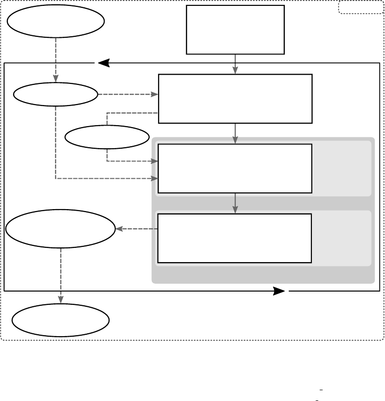
2HDECAY.py
$2HDECAY
HDECAY (minimal run)
$2HDECAY/HDECAY
List of input files
$2HDECAY/Input
mc(OS), mb(OS)
selectedFile.in
EW 1-loop
LO
loop-corrected
selectedFile_BR.out
electroweakCorrections
$2HDECAY
HDECAY
$2HDECAY/HDECAY
List of output files
$2HDECAY/Results
Iterate over all input files
2HDECAY
QCD
off-shell
loop-induced
LO
selectedFile_EW.out
Figure 3: Flowchart of 2HDECAY. The main wrapper file 2HDECAY.py generates a list of input files, provided by the
user in the subfolder $2HDECAY/Input, and iterates over the list. For each selected input file in the list, the wrapper
calls HDECAY and the subprogram electroweakCorrections. The computed branching ratios including the EW
and QCD corrections as described in the text are written to the output file with suffix ’ BR’, the calculated LO
and NLO EW-corrected partial decay widths are given out in the output file with suffix ’ EW’. For further details,
we refer to the text.
3.7 Usage
Before running the program, the user should check that all input files for which the computation
shall be performed are stored in the subfolder $2HDECAY/Input. The input files have to be
formatted exactly as described in 3.5 or otherwise the input values are not read in correctly and
the program might crash with a segmentation error. The exemplary input file printed in App. A
that is part of the 2HDECAY repository can be used as a template for generating other input files
in order to avoid formatting problems.
The user should check the output subfolder $2HDECAY/Results for any output files of previ-
ous runs of 2HDECAY. These previously created output files are overwritten if in a new run input
files with the same names as the already stored output files are used. Hence, the user is advised
to create backups of the output files before starting a new run of 2HDECAY.
In order to run the program, open a terminal, navigate to the $2HDECAY folder and execute
the following command:
35
python 2HDECAY. py
If 2HDECAY was installed correctly according to Sec. 3.4 and if the input files have the correct
format, the program should now compute the EW and/or QCD corrections according to the
flowchart shown in Fig. 3. Several intermediate results and information about the computation
are printed in the terminal. As soon as the computation for all input files is done, 2HDECAY is
terminated and the resulting output files can be found in the $2HDECAY/Results subfolder.
3.8 Output File Format
For each input file, two output files with the suffices ’ QCD’ and ’ EW’ for the branching
ratios and electroweak partial decay widths, respectively, are generated in an SLHA format, as
described in Sec. 2.4. The SLHA output format [106–108] in its strict and original sense has
only been designed for supersymmetric models. We have modified the format to account for the
EW corrections that are implemented in 2HDECAY in the 2HDM. As a reference for the following
description, exemplary output files are given in App. B. These modified SLHA output files are
only generated if OMIT ELW2=0 is set in the input file, i.e. only if the electroweak corrections to
the 2HDM decays are taken into account. In the following we describe the changes that we have
applied.
The first block BLOCK DCINFO contains basic information about the program itself, while the
subsequent three blocks SMINPUTS,2HDMINPUTS and VCKMIN contain the input parameters used
for the calculation that were already described in Sec. 3.5. As explained in Sec. 2.4, the value
of GFprinted in the output file is not necessarily the same as the one given in the input file if
OMIT ELW2=0 is set, since in this case, GFis calculated from the input value αem(m2
Z) instead,
and this value is then given out. These four blocks are given out in both output files.
In the output file containing the branching ratios, indicated by the suffix ’ BR’, subsequently
two blocks follow for each Higgs boson (h, H, A and H±). They are called DECAY QCD and DECAY
QCD&EW. The block DECAY QCD contains the total decay width and the branching ratios of the
decays of the respective Higgs boson, as implemented in HDECAY. These are in particular the
LO (loop-induced for the gg,γγ and Zγ final states) decay widths including the relevant and
state-of-the art QCD corrections where applicable (cf. [68, 69] for further details). For decays
into heavy quarks, massive vector bosons, neutral Higgs pairs as well as gauge and Higgs boson
final states also off-shell decays are computed if necessary. We want to emphasize again that
the partial and total decay widths differ from the ones of the original HDECAY version if OMIT
ELW2=0 is set, as for consistency with the computed EW corrections in this case the HDECAY
decay widths are rescaled by Gcalc
F/GF, as explained in Sec. 2.4. If OMIT ELW2=1 is set, no EW
corrections are computed and the HDECAY decay widths are computed with GFas in the original
HDECAY version.
The block DECAY QCD&EW contains the total decay width and branching ratios of the re-
spective Higgs boson including both the QCD corrections (provided by HDECAY) and the EW
corrections (computed by 2HDECAY) to the LO decay widths. Note that the LO decay widths are
also computed by 2HDECAY. As an additional cross-check, we internally compare the respective
HDECAY LO decay width (rescaled by Gcalc
F/GFand calculated with OS masses for this compar-
ison) with the one computed by 2HDECAY. If they differ (which they should not), a warning is
printed on the screen. As described in Sec. 2.4, we emphasize again that the EW corrections
are calculated and included only for OS decay channels that are kinematically allowed and for
non-loop-induced decays. Therefore, some of the branching ratios given out may be QCD-, but
36

not EW-corrected. The total decay width given out in this block is the sum of all accordingly
computed partial decay widths.
The last block at the end of the file with the branching ratios contains the QCD-corrected
branching ratios of the top-quark calculated in the 2HDM. It is required for the computation of
the Higgs decays into final states with an off-shell top.
In the output file with the EW corrected NLO decay widths, indicated by the suffix ’ EW’,
the first four blocks described above are instead followed by the two blocks LO DECAY WIDTH
and NLO DECAY WIDTH for each Higgs boson (h, H, A and H±). In these blocks, the partial
decay widths at LO and including the one-loop EW corrections are given out, respectively.
These values are particularly useful for studies of the relative size of the EW corrections and for
studying the renormalization scheme dependence of the EW corrections. This allows for a rough
estimate of the remaining theoretical error due to missing higher-order EW corrections. Since
the EW corrections are calculated only for OS decays and additionally only for decays that are
not loop-induced, these two blocks do not contain all final states written out in the blocks DECAY
QCD and DECAY QCD&EW. Hence, depending on the input values that are chosen, it can happen
that the two blocks DECAY QCD and DECAY QCD&EW contain decays that are not printed out in
the blocks LO DECAY WIDTH and NLO DECAY WIDTH, since for the calculation of the branching
ratios, off-shell and loop-induced decays are considered by HDECAY as well.
4 Summary
We have presented the program package 2HDECAY for the calculation of the Higgs boson decays in
the 2HDM. The tool computes the NLO EW corrections to all 2HDM Higgs boson decays into OS
final states that are not loop-induced. The user can choose among 14 different renormalization
schemes that have been specified in the manual. They are based on different renormalization
schemes for the mixing angles αand β, an MS condition for the soft-Z2-breaking scale m2
12 and
an OS scheme for all other counterterms and wave function renormalization constants of the
2HDM necessary for calculating the EW corrections. The EW corrections are combined with the
state-of-the-art QCD corrections obtained from HDECAY. The EW&QCD-corrected total decay
widths and branching ratios are given out in an SLHA-inspired output file format. Moreover,
the tool provides separately an SLHA-inspired output for the LO and EW NLO partial decay
widths to all OS and non-loop-induced decays. This separate output enables e.g. an efficient
analysis of the size of the EW corrections in the 2HDM or the comparison with the relative EW
corrections in the MSSM as a SUSY benchmark model. The implementation of several different
renormalization schemes additionally allows for the investigation of the numerical effects of the
different schemes and an estimate of the residual theoretical uncertainty due to missing higher-
order EW corrections. Being fast, our new tool enables efficient phenomenological studies of
the 2HDM Higgs sector at high precision. The latter is necessary to reveal indirect new physics
effects in the Higgs sector and to identify the true underlying model in case of the discovery
of additional Higgs bosons. This brings us closer to our goal of understanding electroweak
symmetry breaking and deciphering the physics puzzle in fundamental particle physics.
Acknowledgments
The authors thank David Lopez-Val and Jonas M¨uller for independently cross-checking some
of the analytic results derived for this work. The authors express gratitude to David Lopez-Val
for his endeavors on debugging the early alpha versions of 2HDECAY and to Stefan Liebler and
37
Florian Staub for helpful discussions. MK and MM acknowledge financial support from the
DFG project Precision Calculations in the Higgs Sector - Paving the Way to the New Physics
Landscape (ID: MU 3138/1-1).
A Exemplary Input File
In the following, we present an exemplary input file 2hdecay.in as it is included in the subfolder
$2HDECAY/Input in the 2HDECAY repository. The first integer in each line represents the line
number and is not part of the actual input file, but printed here for convenience. The meaning
of the input parameters is specified in Sec. 3.5. In comparison to the input file format of the
unmodified HDECAY program [68, 69], the lines 6, 26, 28, 58 and 62 are new, but the rest of the
input file format is unchanged. We want to emphasize again that the value GFCALC in the input
file is overwritten by the program and thus not an input value that is provided by the user, but
it is calculated by 2HDECAY internally. The sample 2HDM parameter point has been checked
against all relevant theoretical and experimental constraints. In particular it features a SM-like
Higgs boson with a mass of 125.09 GeV which is given by the lightest CP-even neutral Higgs
boson h. For details on the applied constraints, we refer to Refs. [38, 109].
1 SLHAIN = 1
2 SLHAOUT = 1
3 COUPVAR = 1
4 HIGGS = 5
5 OMIT ELW = 1
6 OMIT ELW2= 0
7 SM4 = 0
8 FERMPHOB = 0
9 2HDM = 1
10 MODEL = 1
11 TGBET = 5. 0 7 4 03 e+01
12 MABEG = 4 .67 9 6 7 e+02
13 MAEND = 4. 6 7 967 e+02
14 NMA = 1
15 ∗∗∗∗∗∗∗∗∗∗∗∗∗∗∗∗∗∗∗∗∗ hMSSM (MODEL = 10) ∗∗∗∗∗∗∗∗∗∗∗∗∗∗∗∗∗∗∗∗∗∗∗∗∗∗∗∗∗∗∗∗∗
16 MHL = 1 2 5 . D0
17 ∗∗∗∗∗∗∗∗∗∗∗∗∗∗∗∗∗∗∗∗∗∗∗∗∗∗∗∗∗∗∗∗∗∗∗∗∗∗∗∗∗∗∗∗∗∗∗∗∗∗∗∗∗∗∗∗∗∗∗∗∗∗∗∗∗∗∗∗∗∗∗∗∗∗
18 ALS(MZ) = 1. 1 8 000 e−01
19 MSBAR( 2 ) = 9 . 500 00 e −02
20 MCBAR( 3 ) = 0 . 986 00 e+00
21 MBBAR(MB)= 4 . 1 8000 e+00
22 MT = 1. 7 3 200 e+02
23 MTAU = 1 .77 6 8 2 e+00
24 MMUON = 1 .0 56 583715 e−01
25 1/ALPHA = 1. 3 7 0 36 e+02
26 ALPHAMZ = 7.754222173973729 e −03
27 GF = 1.16 6 3 7 8 7 e−05
28 GFCALC = 0.00000000 0
29 GAMW = 2. 0 8 500 e+00
30 GAMZ = 2. 4 9 520 e+00
31 MZ = 9. 1 1 876 e+01
32 MW = 8. 0 385 e+01
33 VTB = 9 . 9 910 e −01
34 VTS = 4. 0 40 e−02
35 VTD = 8 . 6 7 e −03
36 VCB = 4 . 1 2 e −02
38

37 VCS = 9 .7344 e−01
38 VCD = 2 . 25 2 e −01
39 VUB = 3 . 5 1 e −03
40 VUS = 2. 2 534 e−01
41 VUD = 9 . 7 42 7 e −01
42 ∗∗∗∗∗∗∗∗∗∗∗∗∗∗∗∗∗∗∗∗∗ 4TH GENERATION ∗∗∗∗∗∗∗∗∗∗∗∗∗∗∗∗∗∗∗∗∗∗∗∗∗∗∗∗∗∗∗∗∗∗∗∗∗
43 SCENARIO FOR ELW. CORRECTIONS TO H −>GG (EVERYTHING IN GEV) :
44 GG ELW = 1 : MTP = 500 MBP = 450 MNUP = 375 MEP = 450
45 GG ELW = 2 : MBP = MNUP = MEP = 600 MTP = MBP+50∗(1+LOG(M H/115) /5)
46
47 GG ELW = 1
48 MTP = 5 0 0 . D0
49 MBP = 4 5 0 . D0
50 MNUP = 3 7 5 . D0
51 MEP = 4 5 0 . D0
52 ∗∗∗∗∗∗∗∗∗∗∗∗∗∗∗∗∗∗∗∗∗∗∗∗∗∗ 2 Higgs Doublet Model ∗∗∗∗∗∗∗∗∗∗∗∗∗∗∗∗∗∗∗∗∗∗∗∗∗
53 TYPE: 1 ( I ) , 2 ( I I ) , 3 ( l e p t o n −s p e c i f i c ) , 4 ( f l i p p e d )
54 PARAM: 1 ( masses ) , 2 ( l ambda i )
55
56 PARAM = 1
57 TYPE = 1
58 RENSCHEM = 7
59 ∗∗∗∗∗∗∗∗∗∗∗∗∗∗∗∗∗∗∗∗
60 TGBET2HDM= 4 .23 6 3 5D0
61 M 12ˆ2 = 28 5 0 5.5D0
62 INSCALE = MIN
63 ∗∗∗∗∗∗∗∗∗∗∗∗∗∗∗∗∗∗∗∗ PARAM=1:
64 ALPHA H = −0.189345D0
65 MHL = 12 5 . 09D0
66 MHH = 381 . 7 67D0
67 MHA = 350 . 6 65D0
68 MH+−= 414. 1 1 4D0
69 ∗∗∗∗∗∗∗∗∗∗∗∗∗∗∗∗∗∗∗∗ PARAM=2:
70 LAMBDA1 = 6. 3 6 8 67437753008670 0D0
71 LAMBDA2 = 0. 2 3 5 57024007235097 0D0
72 LAMBDA3 = 1. 7 8 0 41649084762170 0D0
73 LAMBDA4 = −1.52623758540479430D0
74 LAMBDA5 = 0. 0 7 4 59276471755285 6D0
75 ∗∗∗∗∗∗∗∗∗∗∗∗∗∗∗∗∗∗∗∗∗∗∗∗∗∗∗∗∗∗∗∗∗∗∗∗∗∗∗∗∗∗∗∗∗∗∗∗∗∗∗∗∗∗∗∗∗∗∗∗∗∗∗∗∗∗∗∗∗∗∗∗∗∗
76 SUSYSCALE= 2 .22 4 4 9 e+03
77 MU = −1.86701 e+03
78 M2 = −2.39071 e+02
79 MGLUINO = 7 .32 7 5 4 e+02
80 MSL1 = 1. 4 9 5 52 e+03
81 MER1 = 1. 6 2 210 e+03
82 MQL1 = 9 . 303 7 9 e+01
83 MUR1 = 2 .77 0 2 9 e+03
84 MDR1 = 1 . 7 648 1 e+03
85 MSL = 1 . 977 1 4 e+03
86 MER = 9 .29 6 7 8 e+02
87 MSQ = 2 . 6812 4 e+03
88 MUR = 1 . 8 593 9 e+03
89 MDR = 2 .28 2 3 5 e+03
90 AL = −4.62984 e+03
91 AU = 5. 3 1 164 e+03
92 AD = 2 . 544 3 0 e+03
93 ON−SHELL = 0
94 ON−SH−WZ = 0
39

95 IPOLE = 0
96 OFF−SUSY = 0
97 INDIDEC = 0
98 NF−GG = 5
99 IGOLD = 0
100 MPLANCK = 2. 4 0 000 e+18
101 MGOLD = 1. 0 0 0 00 e−13
102 ∗∗∗∗∗∗∗∗∗∗∗∗∗∗∗∗∗∗∗ VARIATION OF HIGGS COUPLINGS ∗∗∗∗∗∗∗∗∗∗∗∗∗∗∗∗∗∗∗∗∗∗∗∗∗
103 ELWK = 1
104 CW = 1 . D0
105 CZ = 1 . D0
106 Ctau = 1 . D0
107 Cmu = 1 . D0
108 Ct = 1 . D0
109 Cb = 1 . D0
110 Cc = 1 . D0
111 Cs = 1 . D0
112 Cgaga = 0 . D0
113 Cgg = 0 . D0
114 CZga = 0 . D0
115 ∗∗∗∗∗∗∗∗∗∗∗∗∗∗∗∗∗∗∗∗∗ 4TH GENERATION ∗∗∗∗∗∗∗∗∗∗∗∗∗∗∗∗∗∗∗∗∗∗∗∗∗∗∗∗∗∗∗∗∗∗∗∗∗
116 Ctp = 0 . D0
117 Cbp = 0 . D0
118 Cnup = 0 . D0
119 Cep = 0 . D0
B Exemplary Output Files
In the following, we present exemplary output files 2hdecay BR.out and 2hdecay EW.out as
they are generated from the sample input file 2hdecay.in and included in the subfolder
$2HDECAY/Results in the 2HDECAY repository. The suffices “ BR” and “ EW” stand for the
branching ratios and electroweak partial decay widths, respectively. The first integer in each
line represents the line number and is not part of the actual output file, but printed here for
convenience. The output file format is explained in detail in Sec. 3.8. The exemplary output file
was generated for a specific choice of the renormalization scheme, i.e. we have set RENSCHEM =
7in line 58 of the input file, cf. App. A. For RENSCHEM = 0, the output file becomes considerably
longer, since the electroweak corrections are calculated for all 14 implemented renormalization
schemes.
B.1 Exemplary Output File for the Branching Ratios
The exemplary output file 2hdecay BR.out contains the branching ratios without and with the
electroweak corrections. The content of the file is presented in the following.
1#
2 BLOCK DCINFO # Decay Program i n f o r m a t i o n
3 1 2HDECAY # de cay c a l c u l a t o r
4 2 1 . 0 . 0 # v e r s i o n number
5#
6 BLOCK SMINPUTS # Sta nd ar d Model i n p u t s
7 2 1.19596488E−05 # G F [ GeVˆ −2]
8 3 1.18000000E−01 # a l p h a S (M Z) ˆMSbar
9 4 9.1187 6 0 0 0E+01 # M Z on−s h e l l mass
10 5 4.1800 0 0 0 0E+00 # mb(mb) ˆMSbar
40

11 6 1.7320 0 0 0 0E+02 # mt p o l e mass
12 7 1.7768 2 0 0 0E+00 # mtau p o l e mass
13 8 4.8414 1 2 9 7E+00 # mb p o l e mass
14 9 1.4314 1 2 9 7E+00 # mc p o l e mass
15 10 1.05658372E−01 # muon mass
16 11 8 .03850000E+01 # M W on−s h e l l mass
17 12 2 .08500000E+00 # W boson t o t a l wid t h
18 13 2 .49520000E+00 # Z boson t o t a l w i dth
19 #
20 BLOCK 2HDMINPUTS # 2HDM i n p u t s
21 1 1 # 2HDM parametrization
22 2 1 # 2HDM t y p e
23 3 4.2363 5 0 0 0E+00 # t an ( b e t a )
24 4 2.8505 5 0 0 0E+04 # M 12ˆ2
25 5 −1.89345000E−01 # alpha
26 6 1.2509 0 0 0 0E+02 # M h
27 7 3.8176 7 0 0 0E+02 # M H
28 8 3.5066 5 0 0 0E+02 # M A
29 9 4.1411 4 0 0 0E+02 # M CH
30 10 6 .53022117E+00 # LAMBDA1 c a l c . from masses / a l pha
31 11 2.41545678E−01 # LAMBDA2 c a l c . from masses / a lp ha
32 12 1 .82557826E+00 # LAMBDA3 c a l c . from masses / a l pha
33 13 −1.56495189E+00 # LAMBDA4 c a l c . from masses / a l pha
34 14 7.64848730E−02 # LAMBDA5 c a l c . from masses / a lp ha
35 15 7 # r e n o r m a l i z a t i o n scheme EW c o r r s
36 16 MIN # i n p u t s c a l e
37 #
38 BLOCK VCKMIN # CKM mixin g
39 1 9.9910 0 0 0 0E−01 # V tb
40 1 4.0400 0 0 0 0E−02 # V t s
41 1 8.6700 0 0 0 0E−03 # V td
42 1 4.1200 0 0 0 0E−02 # V cb
43 1 9.7344 0 0 0 0E−01 # V cs
44 1 2.2520 0 0 0 0E−01 # V cd
45 1 3.5100 0 0 0 0E−03 # V ub
46 1 2.2534 0 0 0 0E−01 # V us
47 1 9.7427 0 0 0 0E−01 # V ud
48 #
49 # PDG Width QCD Only
50 DECAY QCD 25 4.2307 9 7 6 7E−03 # h decays wit h QCD c o r r e c t i o n s o nl y
51 # BR NDA ID1 ID2
52 5.94057260E−01 2 5 −5# BR( h −>b bb )
53 6.38910135E−02 2 −15 15 # BR( h −>t a u+ tau−)
54 2.26195956E−04 2 −13 13 # BR( h −>mu+ mu−)
55 2.24336368E−04 2 3 −3# BR( h −>s sb )
56 2.90834784E−02 2 4 −4# BR( h −>c cb )
57 7.77041237E−02 2 21 21 # BR( h −>g g )
58 2.19287204E−03 2 22 22 # BR( h −>gam gam )
59 1.50138640E−03 2 22 23 # BR( h −>Z gam )
60 2.05453788E−01 2 24 −24 # BR( h −>W+ W−)
61 2.56655457E−02 2 23 23 # BR( h −>Z Z )
62 #
63 # PDG Width QCD and EW
64 DECAY QCD&EW 25 4 . 1 0 9 0 2 403E−03 # h decays wit h QCD and EW c o r r e c t i o n s
65 7 # Reno r m a l izati o n Scheme Number
66 # BR NDA ID1 ID2
67 5.85629854E−01 2 5 −5# BR( h −>b bb )
68 6.30484763E−02 2 −15 15 # BR( h −>t a u+ tau−)
41
69 2.18338629E−04 2 −13 13 # BR( h −>mu+ mu−)
70 2.25852423E−04 2 3 −3# BR( h −>s sb )
71 2.90980943E−02 2 4 −4# BR( h −>c cb )
72 8.00069367E−02 2 21 21 # BR( h −>g g )
73 2.25785925E−03 2 22 22 # BR( h −>gam gam )
74 1.54588098E−03 2 22 23 # BR( h −>Z gam )
75 2.11542547E−01 2 24 −24 # BR( h −>W+ W−)
76 2.64261611E−02 2 23 23 # BR( h −>Z Z )
77 #
78 # PDG Width QCD Only
79 DECAY QCD 35 1.9177 0 6 4 1E−01 # H decays w ith QCD c o r r e c t i o n s o nly
80 # BR NDA ID1 ID2
81 1.19192593E−03 2 5 −5# BR(H −>b bb )
82 1.58161473E−04 2 −15 15 # BR(H −>tau+ tau−)
83 5.59342612E−07 2 −13 13 # BR(H −>mu+ mu−)
84 4.49422613E−07 2 3 −3# BR(H −>s sb )
85 5.83220675E−05 2 4 −4# BR(H −>c cb )
86 5.20107902E−01 2 6 −6# BR(H −>t t b )
87 4.07509451E−03 2 21 21 # BR(H −>g g )
88 1.78393866E−05 2 22 22 # BR(H −>gam gam )
89 1.07062881E−05 2 22 23 # BR(H −>Z gam )
90 1.35039668E−01 2 24 −24 # BR(H −>W+ W−)
91 6.26636468E−02 2 23 23 # BR(H −>Z Z )
92 1.21461206E−10 2 36 36 # BR(H −>A A )
93 2.76517470E−01 2 25 25 # BR(H −>h h )
94 1.58255247E−04 2 23 36 # BR(H −>Z A )
95 #
96 # PDG Width QCD and EW
97 DECAY QCD&EW 35 2 . 0 8 6 1 4 540E−01 # H decays w ith QCD and EW c o r r e c t i o n s
98 7 # Reno r m a l izati o n Scheme Number
99 # BR NDA ID1 ID2
100 1.04478374E−03 2 5 −5# BR(H −>b bb )
101 1.31703579E−04 2 −15 15 # BR(H −>t a u+ tau−)
102 4.55027271E−07 2 −13 13 # BR(H −>mu+ mu−)
103 3.85379375E−07 2 3 −3# BR(H −>s sb )
104 4.95282635E−05 2 4 −4# BR(H −>c cb )
105 4.69367675E−01 2 6 −6# BR(H −>t t b )
106 3.74606433E−03 2 21 21 # BR(H −>g g )
107 1.63990036E−05 2 22 22 # BR(H −>gam gam )
108 9.84184384E−06 2 22 23 # BR(H −>Z gam )
109 1.29180073E−01 2 24 −24 # BR(H −>W+ W−)
110 7.16362911E−02 2 23 23 # BR(H −>Z Z )
111 1.11654218E−10 2 36 36 # BR(H −>A A )
112 3.24671322E−01 2 25 25 # BR(H −>h h )
113 1.45477444E−04 2 23 36 # BR(H −>Z A )
114 #
115 # PDG Width QCD Only
116 DECAY QCD 36 4.2715 2 7 3 7E−01 # A decays w ith QCD c o r r e c t i o n s o nly
117 # BR NDA ID1 ID2
118 7.25746347E−04 2 5 −5# BR(A −>b bb )
119 9.71815207E−05 2 −15 15 # BR(A −>t a u+ tau−)
120 3.43658327E−07 2 −13 13 # BR(A −>mu+ mu−)
121 2.60392190E−07 2 3 −3# BR(A −>s sb )
122 3.66923493E−05 2 4 −4# BR(A −>c cb )
123 9.60042117E−01 2 6 −6# BR(A −>t t b )
124 9.61480220E−03 2 21 21 # BR(A −>g g )
125 3.96441723E−05 2 22 22 # BR(A −>gam gam )
126 6.57435803E−06 2 22 23 # BR(A −>Z gam )
42

127 2.94366379E−02 2 23 25 # BR(A −>Z h )
128 #
129 # PDG Width QCD and EW
130 DECAY QCD&EW 36 4 . 2 4 4 3 3 777E−01 # A decay s w it h QCD and EW c o r r e c t i o n s
131 7 # Reno r m a l izati o n Scheme Number
132 # BR NDA ID1 ID2
133 6.82493672E−04 2 5 −5# BR(A −>b bb )
134 8.62127699E−05 2 −15 15 # BR(A −>t a u+ tau−)
135 2.97643093E−07 2 −13 13 # BR(A −>mu+ mu−)
136 2.37952864E−07 2 3 −3# BR(A −>s sb )
137 3.32024128E−05 2 4 −4# BR(A −>c cb )
138 9.69089576E−01 2 6 −6# BR(A −>t t b )
139 9.67639546E−03 2 21 21 # BR(A −>g g )
140 3.98981363E−05 2 22 22 # BR(A −>gam gam )
141 6.61647394E−06 2 22 23 # BR(A −>Z gam )
142 2.03850692E−02 2 23 25 # BR(A −>Z h )
143 #
144 # PDG Width QCD Only
145 DECAY QCD 37 9.8520 2 0 6 1E−01 # H+ d ecays with QCD c o r r e c t i o n s on ly
146 # BR NDA ID1 ID2
147 6.37168323E−07 2 4 −5# BR(H+ −>c bb )
148 4.97594276E−05 2 −15 16 # BR(H+ −>t a u+ nu tau )
149 1.75959317E−07 2 −13 14 # BR(H+ −>mu+ nu mu )
150 4.40906799E−09 2 2 −5# BR(H+ −>u bb )
151 6.72128061E−09 2 2 −3# BR(H+ −>u s b )
152 8.82535052E−07 2 4 −1# BR(H+ −>c db )
153 1.66151916E−05 2 4 −3# BR(H+ −>c sb )
154 9.68313852E−01 2 6 −5# BR(H+ −>t bb )
155 1.58162332E−03 2 6 −3# BR(H+ −>t sb )
156 7.28404834E−05 2 6 −1# BR(H+ −>t db )
157 2.81079832E−02 2 24 25 # BR(H+ −>W+ h )
158 4.73997465E−05 2 24 35 # BR(H+ −>W+ H )
159 1.80821952E−03 2 24 36 # BR(H+ −>W+ A )
160 #
161 # PDG Width QCD and EW
162 DECAY QCD&EW 37 9 . 4 8 0 1 7 110E−01 # H+ d e ca ys w ith QCD and EW c o r r e c t i o s
163 7 # Reno r m a l izati o n Scheme Number
164 # BR NDA ID1 ID2
165 5.93596259E−07 2 4 −5# BR(H+ −>c bb )
166 4.70821612E−05 2 −15 16 # BR(H+ −>t a u+ nu tau )
167 1.62670592E−07 2 −13 14 # BR(H+ −>mu+ nu mu )
168 3.64051049E−09 2 2 −5# BR(H+ −>u bb )
169 6.54232264E−09 2 2 −3# BR(H+ −>u s b )
170 8.52909834E−07 2 4 −1# BR(H+ −>c db )
171 1.60586860E−05 2 4 −3# BR(H+ −>c sb )
172 9.63902996E−01 2 6 −5# BR(H+ −>t bb )
173 1.57661387E−03 2 6 −3# BR(H+ −>t sb )
174 7.29483674E−05 2 6 −1# BR(H+ −>t db )
175 3.24542779E−02 2 24 25 # BR(H+ −>W+ h )
176 4.92589505E−05 2 24 35 # BR(H+ −>W+ H )
177 1.87914498E−03 2 24 36 # BR(H+ −>W+ A )
178 #
179 # PDG Width
180 DECAY 6 1.3357 0 5 9 9E+00 # t o p decays
181 # BR NDA ID1 ID2
182 1.00000000E+00 2 5 24 # BR( t −>b W+ )
In the following, we make some comments on the output files that partly pick up hints and
43

caveats made in the main text of the manual. First of all, notice that indeed the branching
ratios of the lightest CP-even Higgs boson hare SM-like. All branching ratios presented in the
blocks DECAY QCD can be compared to the ones generated by the program code HDECAY version
6.52. The user will notice that the partial widths related to the branching ratios generated by
2HDECAY and HDECAY, respectively, differ by the rescaling factor Gcalc
F/GF= 1.026327, which is
applied in 2HDECAY for the consistent combination of the EW-corrected decay widths with the
decay widths generated by HDECAY. The comparison furthermore shows an additional difference
between the decay widths for the heavy CP-even Higgs boson Hinto massive vector bosons,
Γ(H→V V ) (V=W, Z), of around 2%. The reason is that HDECAY throughout computes
these decay widths using the double off-shell formula while 2HDECAY uses the on-shell formula
for Higgs boson masses above the threshold. Let us also note some phenomenological features
of the chosen parameter point. The Hboson with a mass of 382 GeV is heavy enough to decay
on-shell into W W and ZZ, and also into the 2-Higgs boson final state hh. It decays off-shell
into AA and the gauge plus Higgs boson final state ZA with branching ratios of O(10−10) and
O(10−4), respectively. The pseudoscalar with a mass of 351 GeV decays on-shell into the gauge
plus Higgs boson final state Zh with a branching ratio at the per cent level. The charged Higgs
boson has a mass of 414 GeV allowing it to decay on-shell in the gauge plus Higgs boson final
state W+hwith a branching ratio at the per cent level. It decays off-shell into the final states
W+Hand W+Awith branching ratios of O(10−5) and O(10−3), respectively.
B.2 Exemplary Output File for the Electroweak Partial Decay Widths
The exemplary output file 2hdecay EW.out contains the LO and electroweak NLO partial decay
widths. The content of the file is presented in the following.
1#
2 BLOCK DCINFO # Decay Program i n f o r m a t i o n
3 1 2HDECAY # de cay c a l c u l a t o r
4 2 1 . 0 . 0 # v e r s i o n number
5#
6 BLOCK SMINPUTS # Sta nd ar d Model i n p u t s
7 2 1.19596488E−05 # G F [ GeVˆ −2]
8 3 1.18000000E−01 # a l p h a S (M Z) ˆMSbar
9 4 9.1187 6 0 0 0E+01 # M Z p o l e mass
10 5 4.1800 0 0 0 0E+00 # mb(mb) ˆMSbar
11 6 1.7320 0 0 0 0E+02 # mt p o l e mass
12 7 1.7768 2 0 0 0E+00 # mtau p o l e mass
13 8 4.8414 1 2 9 7E+00 # mb p o l e mass
14 9 1.4314 1 2 9 7E+00 # mc p o l e mass
15 10 1.05658372E−01 # muon mass
16 11 8 .03850000E+01 # M W mass
17 12 2 .08500000E+00 # W boson t o t a l wid t h
18 13 2 .49520000E+00 # Z boson t o t a l w i dth
19 #
20 BLOCK 2HDMINPUTS # 2HDM i n p u t s
21 1 1 # 2HDM parametrization
22 2 1 # 2HDM t y p e
23 3 4.2363 5 0 0 0E+00 # t an ( b e t a )
24 4 2.8505 5 0 0 0E+04 # M 12ˆ2
25 5 −1.89345000E−01 # alpha
26 6 1.2509 0 0 0 0E+02 # M h
27 7 3.8176 7 0 0 0E+02 # M H
28 8 3.5066 5 0 0 0E+02 # M A
44

29 9 4.1411 4 0 0 0E+02 # M CH
30 10 6 .53022117E+00 # LAMBDA1 c a l c . from masses / a l pha
31 11 2.41545678E−01 # LAMBDA2 c a l c . from masses / a lp ha
32 12 1 .82557826E+00 # LAMBDA3 c a l c . from masses / a l pha
33 13 −1.56495189E+00 # LAMBDA4 c a l c . from masses / a l pha
34 14 7.64848730E−02 # LAMBDA5 c a l c . from masses / a lp ha
35 15 7 # r e n o r m a l i z a t i o n scheme EW c o r r s
36 16 MIN # i n p u t s c a l e
37 #
38 BLOCK VCKMIN # CKM mixin g
39 1 9.9910 0 0 0 0E−01 # V tb
40 1 4.0400 0 0 0 0E−02 # V t s
41 1 8.6700 0 0 0 0E−03 # V td
42 1 4.1200 0 0 0 0E−02 # V cb
43 1 9.7344 0 0 0 0E−01 # V cs
44 1 2.2520 0 0 0 0E−01 # V cd
45 1 3.5100 0 0 0 0E−03 # V ub
46 1 2.2534 0 0 0 0E−01 # V us
47 1 9.7427 0 0 0 0E−01 # V ud
48 #
49 # PDG
50 LO DECAY WIDTH 25 # h non−z e ro LO d ec ay w i d t h s o f on−s h e l l and non−loop
induced decays
51 # WIDTH NDA ID1 ID2
52 5.97381239E−03 2 5 −5# GAM( h −>b bb )
53 2.70309951E−04 2 −15 15 # GAM( h −>tau+ tau−)
54 9.56989322E−07 2 −13 13 # GAM( h −>mu+ mu−)
55 2.32096231E−06 2 3 −3# GAM( h −>s sb )
56 5.26515301E−04 2 4 −4# GAM( h −>c cb )
57 #
58 # PDG
59 NLO DECAY WIDTH 25 # h non−z e r o NLO EW d ec ay w i d t h s o f on−s h e l l and non−loop
induced decays
60 7 # Reno r m a l izati o n Scheme Number
61 # WIDTH NDA ID1 ID2
62 5.71956373E−03 2 5 −5# GAM( h −>b bb )
63 2.59067704E−04 2 −15 15 # GAM( h −>tau+ tau−)
64 8.97158672E−07 2 −13 13 # GAM( h −>mu+ mu−)
65 2.26939232E−06 2 3 −3# GAM( h −>s sb )
66 5.11617771E−04 2 4 −4# GAM( h −>c cb )
67 #
68 # PDG
69 LO DECAY WIDTH 35 # H non−z e r o LO d ec ay w i d t h s o f on−s h e l l and non−loop
induced decays
70 # WIDTH NDA ID1 ID2
71 6.74992142E−04 2 5 −5# GAM(H −>b bb )
72 3.03307270E−05 2 −15 15 # GAM(H −>tau+ tau−)
73 1.07265491E−07 2 −13 13 # GAM(H −>mu+ mu−)
74 2.60148127E−07 2 3 −3# GAM(H −>s sb )
75 5.90563953E−05 2 4 −4# GAM(H −>c cb )
76 6.42270681E−02 2 6 −6# GAM(H −>t t b )
77 2.58966436E−02 2 24 −24 # GAM(H −>W+ W−)
78 1.20170477E−02 2 23 23 # GAM(H −>Z Z )
79 5.30279324E−02 2 25 25 # GAM(H −>h h )
80 #
81 # PDG
82 NLO DECAY WIDTH 35 # H non−z e r o NLO EW d ec ay w i d t h s o f on−s h e l l and non−loop
induced decays
45

83 7 # Reno r m a l izati o n Scheme Number
84 # WIDTH NDA ID1 ID2
85 6.43633010E−04 2 5 −5# GAM(H −>b bb )
86 2.74752816E−05 2 −15 15 # GAM(H −>tau+ tau−)
87 9.49253048E−08 2 −13 13 # GAM(H −>mu+ mu−)
88 2.42670344E−07 2 3 −3# GAM(H −>s sb )
89 5.45568867E−05 2 4 −4# GAM(H −>c cb )
90 6.30522048E−02 2 6 −6# GAM(H −>t t b )
91 2.69488415E−02 2 24 −24 # GAM(H −>W+ W−)
92 1.49443719E−02 2 23 23 # GAM(H −>Z Z )
93 6.77311584E−02 2 25 25 # GAM(H −>h h )
94 #
95 # PDG
96 LO DECAY WIDTH 36 # A non−z e r o LO d ec ay w i d t h s o f on−s h e l l and non−loop
induced decays
97 # WIDTH NDA ID1 ID2
98 9.24277129E−04 2 5 −5# GAM(A −>b bb )
99 4.15113526E−05 2 −15 15 # GAM(A −>tau+ tau−)
100 1.46794595E−07 2 −13 13 # GAM(A −>mu+ mu−)
101 3.56016986E−07 2 3 −3# GAM(A −>s s b )
102 8.08237531E−05 2 4 −4# GAM(A −>c cb )
103 1.84002229E−01 2 6 −6# GAM(A −>t t b )
104 1.25739404E−02 2 23 25 # GAM(A −>Z h )
105 #
106 # PDG
107 NLO DECAY WIDTH 36 # A non−z e r o NLO EW d ec ay w i d t h s o f on−s h e l l and non−loop
induced decays
108 7 # Reno r m a l izati o n Scheme Number
109 # WIDTH NDA ID1 ID2
110 8.63659833E−04 2 5 −5# GAM(A −>b bb )
111 3.65916116E−05 2 −15 15 # GAM(A −>tau+ tau−)
112 1.26329782E−07 2 −13 13 # GAM(A −>mu+ mu−)
113 3.23266311E−07 2 3 −3# GAM(A −>s s b )
114 7.26707905E−05 2 4 −4# GAM(A −>c cb )
115 1.84554001E−01 2 6 −6# GAM(A −>t t b )
116 8.65211194E−03 2 23 25 # GAM(A −>Z h )
117 #
118 # PDG
119 LO DECAY WIDTH 37 # H+ non−z er o LO d ec ay w i d t h s o f on−s h e l l and no−loop
induced decays
120 # WIDTH NDA ID1 ID2
121 2.01499994E−06 2 4 −5# GAM(H+ −>c bb )
122 4.90230906E−05 2 −15 16 # GAM(H+ −>t a u+ nu tau )
123 1.73355482E−07 2 −13 14 # GAM(H+ −>mu+ nu mu )
124 1.34490261E−08 2 2 −5# GAM(H+ −>u bb )
125 2.13488662E−08 2 2 −3# GAM(H+ −>u sb )
126 4.84069114E−06 2 4 −1# GAM(H+ −>c db )
127 9.08443168E−05 2 4 −3# GAM(H+ −>c s b )
128 9.50609568E−01 2 6 −5# GAM(H+ −>t bb )
129 1.55272618E−03 2 6 −3# GAM(H+ −>t s b )
130 7.15105580E−05 2 6 −1# GAM(H+ −>t db )
131 2.76920430E−02 2 24 25 # GAM(H+ −>W+ h )
132 #
133 # PDG
134 NLO DECAY WIDTH 37 # H+ non−z e r o NLO EW dec ay w i d t h s o f on−s h e l l an non−loop
induced decays
135 7 # Reno r m a l izati o n Scheme Number
136 # WIDTH NDA ID1 ID2
46

137 1.80635406E−06 2 4 −5# GAM(H+ −>c bb )
138 4.46346944E−05 2 −15 16 # GAM(H+ −>t a u+ nu tau )
139 1.54214504E−07 2 −13 14 # GAM(H+ −>mu+ nu mu )
140 1.06855576E−08 2 2 −5# GAM(H+ −>u bb )
141 1.99961142E−08 2 2 −3# GAM(H+ −>u sb )
142 4.50162585E−06 2 4 −1# GAM(H+ −>c db )
143 8.44876595E−05 2 4 −3# GAM(H+ −>c s b )
144 9.10563486E−01 2 6 −5# GAM(H+ −>t bb )
145 1.48938859E−03 2 6 −3# GAM(H+ −>t s b )
146 6.89134176E−05 2 6 −1# GAM(H+ −>t db )
147 3.07672108E−02 2 24 25 # GAM(H+ −>W+ h )
The inspection of the output file shows that the EW corrections reduce the hdecay widths,
and the relative NLO EW corrections, ∆EW = (ΓEW −ΓLO)/ΓLO, range between -6.3 and -2.2%
for the decays Γ(h→µ+µ−) and Γ(h→s¯s), respectively. Regarding H, the corrections can
both enhance and reduce the decay widths. The relative corrections range between -11.5 and
27.7% for the decays Γ(H→µ+µ−) and Γ(H→hh), respectively. The relative corrections to
the Adecay widths vary between -31.2 and 0.3% for the decays Γ(A→Zh) and Γ(A→t¯
t),
respectively. And those for the H±decays between -20.6 and 11.1% for the decays Γ(H+→u¯
b)
and Γ(H+→W+h), respectively. The EW corrections (for the renormalization scheme number
7) of the chosen parameter point can hence be sizeable. Finally, note also that only LO and
NLO EW-corrected decay widths are given out for on-shell and non-loop induced decays.
References
[1] ATLAS, G. Aad et al., Phys. Lett. B716, 1 (2012), arXiv:1207.7214.
[2] CMS, S. Chatrchyan et al., Phys. Lett. B716, 30 (2012), arXiv:1207.7235.
[3] ATLAS, CMS, G. Aad et al., Phys. Rev. Lett. 114, 191803 (2015), arXiv:1503.07589.
[4] LHC Higgs Cross Section Working Group, D. de Florian et al., (2016), arXiv:1610.07922.
[5] Yu. A. Golfand and E. P. Likhtman, JETP Lett. 13, 323 (1971), [Pisma Zh. Eksp. Teor.
Fiz. 13, 452 (1971)].
[6] D. Volkov and V. Akulov, Phys. Lett. B46, 109 (1973).
[7] J. Wess and B. Zumino, Nucl. Phys. B70, 39 (1974).
[8] P. Fayet, Nucl. Phys. B90, 104 (1975).
[9] P. Fayet and S. Ferrara, Phys. Rept. 32, 249 (1977).
[10] P. Fayet, Phys. Lett. 64B, 159 (1976).
[11] P. Fayet, Phys. Lett. 69B, 489 (1977).
[12] H. P. Nilles, Phys. Rept. 110, 1 (1984).
[13] H. E. Haber and G. L. Kane, Phys. Rept. 117, 75 (1985).
[14] M. Sohnius, Phys. Rept. 128, 39 (1985).
47
[15] J. Gunion and H. E. Haber, Nucl. Phys. B272, 1 (1986).
[16] J. Gunion and H. E. Haber, Nucl. Phys. B278, 449 (1986).
[17] J. F. Gunion, H. E. Haber, G. L. Kane, and S. Dawson, Front. Phys. 80, 1 (2000).
[18] S. P. Martin, Adv. Ser. Direct. High Energy Phys. 21, 1 (2010), hep-ph/9709356.
[19] S. Dawson, p. 261 (1997), hep-ph/9712464.
[20] A. Djouadi, Phys. Rept. 459, 1 (2008), hep-ph/0503173.
[21] T. D. Lee, Phys. Rev. D8, 1226 (1973).
[22] G. C. Branco et al., Phys. Rept. 516, 1 (2012), arXiv:1106.0034.
[23] L. D. McLerran, M. E. Shaposhnikov, N. Turok, and M. B. Voloshin, Phys. Lett. B256,
451 (1991).
[24] N. Turok and J. Zadrozny, Nucl. Phys. B358, 471 (1991).
[25] A. G. Cohen, D. B. Kaplan, and A. E. Nelson, Phys. Lett. B263, 86 (1991).
[26] N. Turok and J. Zadrozny, Nucl. Phys. B369, 729 (1992).
[27] K. Funakubo, A. Kakuto, and K. Takenaga, Prog. Theor. Phys. 91, 341 (1994), hep-
ph/9310267.
[28] A. T. Davies, C. D. froggatt, G. Jenkins, and R. G. Moorhouse, Phys. Lett. B336, 464
(1994).
[29] J. M. Cline, K. Kainulainen, and A. P. Vischer, Phys. Rev. D54, 2451 (1996), hep-
ph/9506284.
[30] J. M. Cline and P.-A. Lemieux, Phys. Rev. D55, 3873 (1997), hep-ph/9609240.
[31] L. Fromme, S. J. Huber, and M. Seniuch, JHEP 11, 038 (2006), hep-ph/0605242.
[32] J. M. Cline, K. Kainulainen, and M. Trott, JHEP 11, 089 (2011), arXiv:1107.3559.
[33] G. C. Dorsch, S. J. Huber, and J. M. No, JHEP 10, 029 (2013), arXiv:1305.6610.
[34] K. Fuyuto and E. Senaha, Phys. Lett. B747, 152 (2015).
[35] G. C. Dorsch, S. J. Huber, K. Mimasu, and J. M. No, Phys. Rev. Lett. 113, 211802
(2014), arXiv:1405.5537.
[36] G. C. Dorsch, S. J. Huber, K. Mimasu, and J. M. No, Phys. Rev. D93, 115033 (2016),
arXiv:1601.04545.
[37] G. C. Dorsch, S. J. Huber, T. Konstandin, and J. M. No, JCAP 1705, 052 (2017),
arXiv:1611.05874.
[38] P. Basler, M. Krause, M. Muhlleitner, J. Wittbrodt, and A. Wlotzka, JHEP 02, 121
(2017), arXiv:1612.04086.
48
[39] G. C. Dorsch, S. J. Huber, K. Mimasu, and J. M. No, JHEP 12, 086 (2017),
arXiv:1705.09186.
[40] P. Basler, M. Muhlleitner, and J. Wittbrodt, JHEP 03, 061 (2018), arXiv:1711.04097.
[41] P. Basler and M. Muhlleitner, (2018), arXiv:1803.02846.
[42] N. G. Deshpande and E. Ma, Phys. Rev. D18, 2574 (1978).
[43] R. Barbieri, L. J. Hall, and V. S. Rychkov, Phys. Rev. D74, 015007 (2006), hep-
ph/0603188.
[44] L. Lopez Honorez, E. Nezri, J. F. Oliver, and M. H. G. Tytgat, JCAP 0702, 028 (2007),
hep-ph/0612275.
[45] E. M. Dolle and S. Su, Phys. Rev. D80, 055012 (2009), arXiv:0906.1609.
[46] L. Lopez Honorez and C. E. Yaguna, JHEP 09, 046 (2010), arXiv:1003.3125.
[47] M. Gustafsson, S. Rydbeck, L. Lopez-Honorez, and E. Lundstrom, Phys. Rev. D86,
075019 (2012), arXiv:1206.6316.
[48] B. Swiezewska, Phys. Rev. D88, 055027 (2013), arXiv:1209.5725, [Erratum: Phys. Rev.
D88, no.11, 119903 (2013)].
[49] B. Swiezewska and M. Krawczyk, Phys. Rev. D88, 035019 (2013), arXiv:1212.4100.
[50] A. Arhrib, Y.-L. S. Tsai, Q. Yuan, and T.-C. Yuan, JCAP 1406, 030 (2014),
arXiv:1310.0358.
[51] M. Klasen, C. E. Yaguna, and J. D. Ruiz-Alvarez, Phys. Rev. D87, 075025 (2013),
arXiv:1302.1657.
[52] T. Abe, R. Kitano, and R. Sato, Phys. Rev. D91, 095004 (2015), arXiv:1411.1335, [Erra-
tum: Phys. Rev. D96, no.1, 019902 (2017)].
[53] M. Krawczyk, D. Sokolowska, P. Swaczyna, and B. Swiezewska, JHEP 09, 055 (2013),
arXiv:1305.6266.
[54] A. Goudelis, B. Herrmann, and O. St˚al, JHEP 09, 106 (2013), arXiv:1303.3010.
[55] N. Chakrabarty, D. K. Ghosh, B. Mukhopadhyaya, and I. Saha, Phys. Rev. D92, 015002
(2015), arXiv:1501.03700.
[56] A. Ilnicka, M. Krawczyk, and T. Robens, Phys. Rev. D93, 055026 (2016),
arXiv:1508.01671.
[57] M. Krause, On the Renormalization of the Two-Higgs-Doublet Model, Master’s thesis,
KIT, Karlsruhe, ITP, 2016.
[58] M. Krause, R. Lorenz, M. Muhlleitner, R. Santos, and H. Ziesche, JHEP 09, 143 (2016),
arXiv:1605.04853.
[59] A. Denner, L. Jenniches, J.-N. Lang, and C. Sturm, JHEP 09, 115 (2016),
arXiv:1607.07352.
49
[60] L. Altenkamp, S. Dittmaier, and H. Rzehak, JHEP 09, 134 (2017), arXiv:1704.02645.
[61] A. Denner, S. Dittmaier, and J.-N. Lang, (2018), arXiv:1808.03466.
[62] M. Fox, W. Grimus, and M. L¨oschner, Int. J. Mod. Phys. A33, 1850019 (2018),
arXiv:1705.09589.
[63] M. Krause, M. Muhlleitner, R. Santos, and H. Ziesche, Phys. Rev. D95, 075019 (2017),
arXiv:1609.04185.
[64] M. Krause, D. Lopez-Val, M. Muhlleitner, and R. Santos, JHEP 12, 077 (2017),
arXiv:1708.01578.
[65] S. Kanemura, S. Kiyoura, Y. Okada, E. Senaha, and C. P. Yuan, Phys. Lett. B558, 157
(2003), hep-ph/0211308.
[66] S. Kanemura, Y. Okada, E. Senaha, and C. P. Yuan, Phys. Rev. D70, 115002 (2004),
hep-ph/0408364.
[67] G. B´elanger, V. Bizouard, F. Boudjema, and G. Chalons, Phys. Rev. D96, 015040 (2017),
arXiv:1705.02209.
[68] A. Djouadi, J. Kalinowski, and M. Spira, Computer Physics Communications 108, 56
(1998).
[69] A. Djouadi, J. Kalinowski, M. Muhlleitner, and M. Spira, (2018), arXiv:1801.09506.
[70] M. E. Peskin and D. V. Schroeder, An Introduction to quantum field theory (Addison-
Wesley, Reading, USA, 1995).
[71] A. Denner, Fortsch. Phys. 41, 307 (1993), arXiv:0709.1075.
[72] M. Aoki, S. Kanemura, K. Tsumura, and K. Yagyu, Phys. Rev. D80, 015017 (2009),
arXiv:0902.4665.
[73] R. Santos and A. Barroso, Phys. Rev. D56, 5366 (1997), hep-ph/9701257.
[74] A. Denner et al., (2015), LHCHXSWG-INT-2015-006.
[75] W. Grimus and M. L¨oschner, (2018), arXiv:1807.00725.
[76] S. Kanemura, M. Kikuchi, and K. Yagyu, Nucl. Phys. B896, 80 (2015), arXiv:1502.07716.
[77] J. Fleischer and F. Jegerlehner, Phys. Rev. D 23, 2001 (1981).
[78] R. Lorenz, Full One-Loop Electroweak Corrections to the Decays H+→W+h/H in the
Two-Higgs-Doublet Model, Master’s thesis, KIT, Karlsruhe, ITP, 2015.
[79] D. Binosi, J. Phys. G30, 1021 (2004), hep-ph/0401182.
[80] D. Binosi and J. Papavassiliou, Phys. Rept. 479, 1 (2009), arXiv:0909.2536.
[81] J. M. Cornwall and J. Papavassiliou, Phys. Rev. D40, 3474 (1989).
[82] J. Papavassiliou, Phys. Rev. D41, 3179 (1990).
50
[83] G. Degrassi and A. Sirlin, Phys. Rev. D46, 3104 (1992).
[84] J. Papavassiliou, Phys. Rev. D50, 5958 (1994), hep-ph/9406258.
[85] N. J. Watson, Phys. Lett. B349, 155 (1995), hep-ph/9412319.
[86] J. Papavassiliou and A. Pilaftsis, Phys. Rev. Lett. 75, 3060 (1995), hep-ph/9506417.
[87] J. R. Espinosa and Y. Yamada, Phys. Rev. D67, 036003 (2003), hep-ph/0207351.
[88] J. A. Coarasa Perez, D. Garcia, J. Guasch, R. A. Jimenez, and J. Sola, Eur. Phys. J. C2,
373 (1998), hep-ph/9607485.
[89] A. Freitas and D. Stockinger, Phys. Rev. D66, 095014 (2002), hep-ph/0205281.
[90] R. Santos, A. Barroso, and L. Brucher, Phys. Lett. B391, 429 (1997), hep-ph/9608376.
[91] P. Gambino, P. A. Grassi, and F. Madricardo, Phys. Lett. B454, 98 (1999), hep-
ph/9811470.
[92] A. Barroso, L. Brucher, and R. Santos, Phys. Rev. D62, 096003 (2000), hep-ph/0004136.
[93] B. A. Kniehl, F. Madricardo, and M. Steinhauser, Phys. Rev. D62, 073010 (2000), hep-
ph/0005060.
[94] A. Pilaftsis, Phys. Rev. D65, 115013 (2002), hep-ph/0203210.
[95] Y. Yamada, Phys. Rev. D64, 036008 (2001), hep-ph/0103046.
[96] K. P. O. Diener and B. A. Kniehl, Nucl. Phys. B617, 291 (2001), hep-ph/0109110.
[97] K. Olive and P. D. Group, Chinese Physics C 38, 090001 (2014).
[98] J. F. Ashmore, Lettere al Nuovo Cimento (1971-1985) 4, 289 (1972).
[99] C. G. Bollini and J. J. Giambiagi, Nuovo Cim. B12, 20 (1972).
[100] G. ’t Hooft and M. Veltman, Nuclear Physics B 44, 189 (1972).
[101] T. Hahn, Comput. Phys. Commun. 140, 418 (2001), hep-ph/0012260.
[102] R. Mertig, M. B¨ohm, and A. Denner, Computer Physics Communications 64, 345 (1991).
[103] V. Shtabovenko, R. Mertig, and F. Orellana, Comput. Phys. Commun. 207, 432 (2016),
arXiv:1601.01167.
[104] M. D. Goodsell, S. Liebler, and F. Staub, Eur. Phys. J. C77, 758 (2017), arXiv:1703.09237.
[105] T. Hahn and M. Prez-Victoria, Computer Physics Communications 118, 153 (1999).
[106] P. Z. Skands et al., JHEP 07, 036 (2004), hep-ph/0311123.
[107] B. C. Allanach et al., Comput. Phys. Commun. 180, 8 (2009), arXiv:0801.0045.
[108] F. Mahmoudi et al., Comput. Phys. Commun. 183, 285 (2012), arXiv:1008.0762.
[109] M. Muhlleitner, M. O. P. Sampaio, R. Santos, and J. Wittbrodt, JHEP 08, 132 (2017),
arXiv:1703.07750.
51
