Manual 2019 03 27
User Manual:
Open the PDF directly: View PDF ![]() .
.
Page Count: 23
MANUAL
for DFTBparaopt
Version 1.0
Van Quan Vuong
March 27, 2019
Contents
1 An Introduction to DFTB Parameterization 3
1.1 DFTB ......................................... 3
1.2 Electronic Parameters ................................. 4
1.3 Repulsive Potentials .................................. 5
1.4 Scoring Function ................................... 5
1.5 Genetic Algorithm .................................. 6
2 Overview and Installation of DFTBparaopt 7
2.1 Overview ....................................... 7
2.2 Installation ...................................... 7
3 Manual for REPOPT 9
3.1 Required Inputs .................................... 9
3.1.1 $system: ................................... 9
3.1.2 $genetic_algorithm: ............................. 10
3.2 Optional Inputs .................................... 11
3.2.1 $element_types: ............................... 12
3.2.2 $repulsive_potentials: ............................ 12
3.2.3 $compounds: ................................. 13
3.2.4 $definition_reactions: ............................. 14
3.2.5 $reactions: .................................. 14
3.3 Output ......................................... 15
3.4 Tips .......................................... 15
4 Manual for EREPOPT 16
4.1 Input .......................................... 16
4.1.1 $system: ................................... 16
4.1.2 $genetic_algorithm: ............................. 17
4.1.3 $element_type: ................................ 18
4.1.4 $d3: ...................................... 18
4.1.5 $vorbes: .................................... 18
4.2 Output ......................................... 18
4.3 Tips .......................................... 18
5 Utility Tools 19
5.1 Convert repopt-output to skf-files .......................... 19
5.2 Plot Repulsive Potentials ............................... 20
6 Tutorials 21
1

Chapter 1
An Introduction to DFTB
Parameterization
1.1 DFTB
Expansion from DFT
E[ρ0(r) + ∆ρ(r)] =
occ
∑
i
hψi|H0|ψiiEBS
−1
2Z Z ρ0(r0)ρ0(r)
|r−r0|dr0dr −Zvxc[ρ0(r)]ρ0(r)dr
+Exc[ρ0(r)] + ENN
≈1
2∑
a,b
Vrep
ab (Rab) = Erep
+1
2Z Z 1
|r−r0|+δ2Exc[ρ(r)]
δ ρ(r0)δ ρ(r)ρ0(r0)ρ0(r)∆ρ(r0)∆ρ(r)dr0drE2nd
+1
6Z Z Z δ3Exc[ρ(r)]
δ ρ(r00)δ ρ (r0)δ ρ(r)ρ0(r00)ρ0(r0)ρ0(r)
∆ρ(r00)∆ρ(r0)∆ρ(r)dr00dr0dr
E3rd
+. . . .
(1.1)
None Consistent-Charge (NCC)-DFTB
ENCC−DFT B =
occ
∑
i
hψi|H0|ψii+Erep.(1.2)
Eigenvalue problem:
AO
∑
ν
cνi(H0
µν −εiSµν ) = 0.(1.3)
Hamiltonian matrix elements, H0
µν :
H0
µν =
φµ−1
2∇2+V[ρ0
a+ρ0
b]φνif a6=b
εfree atom if a=b,µ=ν
0 if a=b,µ6=ν.
(1.4)
3

Self-Consistent-Charge (SCC)-DFTB
ESCC−DF T B =
occ
∑
i
hψi|H0|ψii+Erep+1
2∑
a,b
γab(Rab)∆qa∆qb.(1.5)
Eigenvalue problem:
AO
∑
ν
cνi(Hµν −εiSµν) = 0,(1.6)
Hamiltonian, Hµν :
Hµν =H0
µν +1
2Sµν ∑
c
(γac +γbc)∆qc.(1.7)
Mulliken charge, ∆q :
∆qa=1
2∑
i
ni∑
µ∈a
∑
ν
(cµicνiSµν +cνicµiSν µ )−q0
a,(1.8)
∆qcdepends on MO coefficients ⇒must be solved iteratively.
1.2 Electronic Parameters
• Minimal basis set:
Pure atomic orbitals (AOs) are too diffuse
• Electron density ρo:
ρis more compressed in molecule
⇒"−1
2∇2+ve f f [ρatom]+ r
ro!2#φµ=εµφµ(1.9)
Free variables:
Minimal AO basis set ⇒rw f
o
Electron density ρo⇒rdens
o
4

1.3 Repulsive Potentials
Repulsive Potentials Erep: sum of two-center repulsions,
Erep =1
2∑
A,B
VAB(|RA−RB|),(1.10)
Where,
VAB(RAB) =
e−a1∗RAB+a2+a3,RAB <RAB,0,
∑4
i=0aAB,n,i(RAB −RAB,n)i,RAB,n≤RAB <RAB,n+1;4 ≤n≤6
0,RAB,cut−o f f ≤RAB,
(1.11)
Free variables: RAB,nand aAB,n,i.
1.4 Scoring Function
fscore =∑
i∈equi
Wat,iEre f
at,i−EDFT B
at,i+∑
i∈bar
Wbar,iEre f
bar,i−EDFT B
bar,i
+∑
i∈equi
Wf,i∑
j∈3NiFDFT B
i,j+∑
i∈pert
Wf,i∑
j∈3NiFre f
i,j−FDFT B
i,j,
(1.12)
Wat,i,Wbar,i,Wf,i: Weight factors
Eat : Atomization energies
Ebar: Proton transfer barriers
N: Number of atoms
F: Forces
5
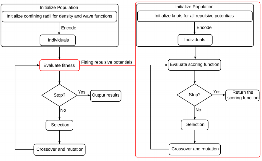
1.5 Genetic Algorithm
Initialize confining radii for density and wave functions
Individuals
Encode
Evaluate fitness
Crossover and mutation
Selection
Stop? Output results
Initialize Population
Yes
No
Fitting repulsive potentials
Evaluate scoring function
Crossover and mutation
Selection
Stop? Return the
scoring function
Yes
No
6
Chapter 2
Overview and Installation of
DFTBparaopt
2.1 Overview
DFTBparaopt[2] is a package to automatically optimize electronic, repulsive, and dispersion pa-
rameters for Density-Functional based Tight-Binding (DFTB) method. The package includes two
main programs: (1) repopt for optimization of only repulsive potentials and (2) erepopt for opti-
mization of all DFTB parameters. erepopt uses repopt for the repulsive potentials fitting. Cur-
rently, repopt is stable released version 1.0. On the other hand, erepopt is still in the beta-
development version. In addition, the package also provide some tools to analyze or evaluate new
DFTB parameters.
Most of the codes were written in C++. The code required two libraries: galib247 and eigen3. A
part of the repulsive fitting (repopt) uses some piece of code from a semi-automatic erepfit program
originally developed by Michael Gaus.[1] This manual was prepared using same style of DFTB+
manual, making it looks similar to DFTB+ manual. ¨^¨^¨^
2.2 Installation
To get the code:
git clone https://github.com/v2quan89/dftbparaopt.git
or download compressed file
wget https://github.com/v2quan89/DFTBparaopt.tar.gz
Note, both links may not work at this moment. You can send an email to v2quan89@gmail.com if
the links do not work. Then, extract DFTBparaopt.tar.gz using
tar -xzvf DFTBparaopt.tar.gz
Change to directory DFTBparaopt and type “./install.sh”. Currently, DFTBparaopt was tested for
two compilers: GNU(g++) and INTEL(icpc). For MAC OS, you need a “GNU” compiler instead
of “GNU” connecting with clang.
You can choose the compiler by setting $CXX=“g++” or $CXX=“icpc” in the “install.sh” file.
To compile “erepopt”, a MPI library is also required. The install.sh script will try to get all the
7
required library and compile the code. You might have to adjust some flags in the makefile.
After the compilation, if you use bash, you can add following command to you “.bashrc” or run it
before using DFTBparaopt,
source path-to-DFTBparaopt-directory/DFTBparaopt_on.rc
8

Chapter 3
Manual for REPOPT
“repopt” is a program to optimize DFTB repulsive potentials. To run the program, type:
repopt rep.inp
where repopt is program name and rep.inp is name of the input file. The input file is organized
in “block” sections. Each section begins with “$blockname:” and end with “$end:”. ‘#’ is the
comment character. Everything after ‘#’ will be skipped.
3.1 Required Inputs
The general “block” format of required sections is showed as following
$blockname:
keyword_1 value_1
. . . . . .
keyword_n value_n
$end
Following input block must be presented in all kind of running job.
3.1.1 $system:
Keyword Type Range Default
dftb_version string dftb+
idecompose integer 1:7 6
ilmsfit integer 1:4 4
nreplicate integer ≥1 1
dftb_version Executable dftb-program
idecompose Select decomposition method from EIGEN library:
1 => ldlt
2 => partialPivLu
3 => fullPivLu
4 => householderQr
9

5 => colPivHouseholderQr
6 => fullPivHouseholderQr
7 => completeOrthogonalDecomposition
Please check the website for more information.
ilmsfit Select regression method from EIGEN library:
1 => householderQr
2 => colPivHouseholderQr
3 => fullPivHouseholderQr
4 => bdcSvd
Please check the website for more information.
nreplicate Number of the fitting will be replicated. nreplicate should be 1. Larger than 1 only
for testing purpose to measure the effect of decomposition and regression methods on the
computing time.
Example:
$system:
dftb_version dftb+
idecompose 6
ilmsfit 4
nreplicate 1
$end:
3.1.2 $genetic_algorithm:
Keyword Type Range Default
ga bool 0|1 1
runtest bool 0|1 0
score_type integer 1|2|4 2
read_spline bool 0|1 1
popsizemax integer ≥1 1000
preserved_num integer ≥0 100
destroy_num integer ≥0 10
popsizemin integer ≥1 2
ngen integer ≥0 1000
pmut integer 0.0:1.0 0.02
pcross integer 0.0:1.0 0.90
grid_update bool 0|1 0
ga switch on or off genetic algorithm
runtest switch on or off testing job
score_type set scoring function to:
1 => sum of absolute deviation
2 => sum of squared deviation
10

4 => sum of quartic deviation
read_spline how “grid” input file would be used:
0 => only read the cutoff and count the number of knots from “grid” input file
1 => use all knots in the “grid” input file as initial guess
popsizemax set the initial and maximum population size for GA.
preserved_num set the number of best individuals would be kept from “n-1” to “n” generation.
destroy_num set the number individuals be removed every generation. If greater than 0, the
population size will be reduced generation by generation.
popsizemin set the final and minimum population size for GA. popsizemin is used only if de-
stroy_num≥1.
ngen set the number of generation for GA.
pmut set the mutation probability for GA.
pcross set the crossover probability for GA.
grid_update How “grid” input file would be updated:
0 => leave the “grid” input file untouched.
1 => the “grid” input file is updated at the end of the GA optimization using the best found
knots.
Example:
$genetic_algorithm:
ga 1
runtest 0
score_type 2
read_spline 1
popsizemax 1000
preserved_num 100
destroy_num 10
popsizemin 2
ngen 1000
pmut 0.02
pcross 0.90
grid_update 0
$end:
3.2 Optional Inputs
The general “block” format of required sections is showed as following
11

$blockname:
entry_name_1 option_1_1 . . . option_1_m
. . . . . . . . . . . .
entry_name_n option_n_1 . . . option_n_m
$end
Following input blocks in optional, depending on the desired job.
3.2.1 $element_types:
String Real(a.u.)
element_name_1 atomic_energy_1
. . . . . .
element_name_n atomic_energy_n
element_name name of fitting element, must be two lower case letters characters long. The
underscore character ‘_’ is added if element name has only one character.
atomic_energy Atomic energy in a.u. for the corresponding fitting element.
Note: if element_name is provided, atomic_energy must be provided also. atomic_energy (can
be calculated by DFT) is needed to fit atomization energy. If element_name is not listed, the
atomic_energy will be optimized. You can interpret the meaning of atomic_energy as: If atomic_energy
is provided, the absolute atomization energy will be fitted (by fitting atomization energy). If
atomic_energy is optimized (not provided), the relative atomization energy (reaction energy) will
be fitted (by optimization of the atomic energy). This methodology was proposed by Gaus et al.
in the 3ob parameterization strategy for obtaining repulsive potentials, and their optimized atomic
energies (used to generate the 3ob repulsives) were published in their supporting information.[?]
Example:
$element_types:
h_ -0.256789
c_ -0.456789
$end:
3.2.2 $repulsive_potentials:
string Real(Å) string Real(Å) integer integer 0|1
name_1 min_r knot-vector min_step spline order smooth negative?
. . . . . . . . . . . . . . . . . . . . .
name_n min_r knot-vector min_step spline order smooth negative?
name name of fitting potential
min_r limit the small knot. The small knot must larger than or equal to shortest bond length
min(Rbond ) - min_r
12

knot-vector name of the file containing division points in the format (in Å):
knot_1
...
knot_n
cutoff
The number of knot will be counted from the not-vector
min_step set the smallest difference between knot
spline order the order of spline function to be used (currently only support 4th order)
smooth smoothing level of that potential
0 => constrain on potential energy
1 => constrain on the first derivative of energy
2 => constrain on the second derivative of energy
3 => constrain on the third derivative of energy
negative? and allowance the potential to be attractive or not.
0 => repulsive potential energy must be always positive 1 => repulsive potential energy can
be negative
Example:
$repulsive_potentials:
h_h_ 0.2 grids/hh.grdx 0.05 4 2 0
c_h_ 0.3 grids/ch.grdx 0.05 4 2 1
c_c_ 0.3 grids/cc.grdx 0.30 4 2 1
$end
3.2.3 $compounds:
string Real(kcal/mol) string Real string 0|string integer
structure1 Eat eweight fweight dftbinp forceinput placeholder
. . . . . . . . . . . . . . . . . . . . .
structuren Eat eweight fweight dftbinp forceinput placeholder
list of filenames for geometries of the fitting molecular.
name file name for geometry, the files need to be in xyz-format
Eat reference atomization energy of the molecule. The atomization energy is defined as:
Eat =−Etot +
Natom
∑
i=1
Eatom
i
eweight weights for energy equations
fweight weights for force equations
dftbinp input-file to run a single point energy and force calculation using the dftb
13

forceinput for an equilibrium structure, should be a “0”, otherwise a reference force file can be
specified which is formatted as (in a.u.):
Ref_Force-Atom_1_X Ref_Force-Atom_1_Y Ref_Force-Atom_1_Z
...
Ref_Force-Atom_n_X Ref_Force-Atom_n_Y Ref_Force-Atom_n_Z
placeholder for developement only, must be ‘0’ for now
Example:
$compounds:
path/h2.xyz 109.9 1 1 path/dftb_inp1.hsd 0 0
path/ch4.xyz 420.1 1 1 path/dftb_inp2.hsd 0 0
path/h3cch3.xyz 712.0 1 1 path/dftb_inp2.hsd 0 0
path/h2_d0.1.xyz 000.0 0 1 path/dftb_inp2.hsd path/hh_d0.1.frc 0
$end
3.2.4 $definition_reactions:
For specifying reaction equations
string string string
abbreviation filename dftbinp
. . . . . . . . .
abbreviation filename dftbinp
abbreviation abbrev name for a geometry
filename file name for the geometry, the files need to be in xyz-format
dftbinp input-file to run a single point energy calculation using the DFTB
Example:
$definition_reactions:
h2 path/h2.xyz path/dftb_inp1.hsd
ch4 path/ch4.xyz path/dftb_inp2.hsd
h3cch3 path/h3cch3.xyz path/dftb_inp2.hsd
$end
3.2.5 $reactions:
integer string integer string string Real(kcal/mol) Real
coeff abbreviation . . . coeff abbreviation -> reactionenergy reaweight
. . . . . . . . . . . . . . . -> . . . . . .
coeff abbreviation . . . coeff abbreviation -> reactionenergy reaweight
14

coeff reaction coefficient
if positive => reactant
if negative => product
abbreviation defined in the $definition_reactions: block
reactionenergy reaction energy
reaweight weight for reaction energy equations
Example:
$reactions:
+1 h3cch3 +1 h2 -2 ch4 -> -18.33 1.0
$end
3.3 Output
The output of a successful repopt contains:
scoring function scoring function as a function of generation
input interpreted input, a list of all distances appearing within the reference geometries sorted by
atom type pair.
technical information a list of number of fitting equation, number of free variables. . .
summary of fitting summary of the MSE, MUE, and RMS
residual in detail residuals for each equation predicted by the fitted parameters in comparison to
the reference are listed.
fitted atomic energies fitted atomic energies if they are optimized
repulsive potentials the repulsive potentials are given in a format of the “Spline” format.
If there is no error, repopt ends with a statement “repopt normal termination”. Any warnings
concerning the fit will appear after #ga end!.
3.4 Tips
15

Chapter 4
Manual for EREPOPT
“erepopt” is a program to optimize all DFTB parameters simultaneously. To run the program, type:
erepopt erep.inp
where erepopt is program name and erep.inp is name of the input file. The input file is organized
in “block” sections. Each section begins with “$blockname:” and end with “$end:”. ‘#’ is the
comment character. Everything after ‘#’ will be skipped.
4.1 Input
4.1.1 $system:
Keyword Type Range Default
nthreads integer ≥11
dftbversion string dftb+
skgen string skgen
onecent string hfatom_spin
twocent string sktwocnt_lr
gasrepfit string repopt
power integer ≥22
dgrid Real ≥0.00.1
ngrid integer ≥1120
grids string grids
rep.in string rep4e.in
libdir string libskf4e
scratchfolder string /dev/shm
skfclean bool 0|1 0
outfile string gaserepfit.log
popinitialfile string pop.initial.dat
popfinalfile string pop.final.dat
Example:
16

$system:
nthreads 1
dftbversion dftb+
skgen skgen
onecent hfatom_spin
twocent sktwocnt_lr
gasrepfit repopt
power 2
dgrid 0.1
ngrid 120
grids grids
rep.in rep4e.in
libdir libskf4e
scratchfolder /dev/shm
skfclean 0
outfile gaserepfit.log
popinitialfile pop.initial.dat
popfinalfile pop.final.dat
$end
4.1.2 $genetic_algorithm:
Keyword Type Range Default
ga bool 0|1 1
runtest bool 0|1 0
fit_type integer 1|2|4 2
popsize integer ≥1 1000
preserved_num integer ≥0 100
ngen integer ≥0 1000
pmut integer 0.0:1.0 0.02
pcross integer 0.0:1.0 0.90
readr bool 0|1 1
restart bool 0|1 1
Example:
$genetic_algorithm:
ga 1
runtest 0
fit_type 0
popsize 32
preserved_num 3
ngen 30
pmut 0.05
pcross 0.9
readr 1
restart 0
$end:
17

4.1.3 $element_type:
Example:
$element_types:
H 11 0 2.9 2.9 2.9 1 2.9 2.9 2.9 1
O 111 1 2.7 2.8 2.9 1 2.7 2.8 2.9 1 2.7 2.8 2.9 1
N 111 1 3.0 3.2 3.4 1 3.0 3.2 3.4 1 3.0 3.2 3.4 1
C 111 1 3.6 3.8 4.0 1 3.6 3.8 4.0 1 3.6 3.8 4.0 1
$end
4.1.4 $d3:
Example:
$d3:
s6 1.00 1.00 1.00 2
s8 1.40 1.40 1.40 1
a1 0.48 0.48 0.48 2
a2 4.70 4.70 4.70 1
$end:
4.1.5 $vorbes:
Example:
$vorbes:
N 2S -0.83 -0.82 -0.81 3
$end:
4.2 Output
4.3 Tips
18
Chapter 5
Utility Tools
In the following section, some utility tools will be explained. These tools were originally developed
by Michael Gaus and were later modified by the author.
5.1 Convert repopt-output to skf-files
The bash-scripts rep2XabSpl and xabSpl2spl are available in the “utils” directory as well as the
C++ program ord2abSpl which is called by the xabSpl2spl script.
rep2XabSpl Usage: rep2XabSpl repout-output-file
The rep2XabSpl extracts the Spline of repulsive potentials from the output-file and writes it
in separate files. The ending of the files are XabSpl.
xabSpl2spl Usage: xabSpl2spl XabSpl-file skf-electronic-file 1
The xabSpl2spl script combines one XabSpl file with skf-electronic-file into the final skf-file.
ord2abSpl called by the xabSpl2spl
For a short description of all options run rep2XabSpl or xabSpl2spl without any arguments.
Example
# doing the rep fitting
repopt rep.in >rep.out
# extract Spline for H-H
rep2XabSpl rep.out
mv h_h_.4abSpl hh.4abSpl
# create the final skf-files
xabSpl2spl hh.4abSpl hh_elec.skf 1
Under utils folder, a script named combine.sh can do all jobs at once.
19
5.2 Plot Repulsive Potentials
SplineAnsch is a script to plot repulsive potentials and its derivatives. The script requires gnuplot
and gv ghostscript interpreter.
Usage
one skf file: SplineAnsch -a rmin:rmax file1.skf
two skf file: SplineAnsch -a rmin:rmax -v file1.skf file2.skf
Note: any files in the XabSpl or spl format can be also be used. You can find all options by running
SplineAnsch without arguments.
Example
# to plot new cc.skf zoom in on a range of 2.0-5.0 (a.u.).
SplineAnsch -a 2.0:5.0 cc.skf
# to compare the new cc.skf with cc.skf from mio set.
SplineAnsch -a 2.0:5.0 -v cc_mio.spl cc.4abSpl
20
Chapter 6
Tutorials
For repopt, there are two examples rep1.in and rep2.in under the examples folder. It is straight
forward to run these examples:
# cd to the examples folder and type
repopt rep1.in >& rep1.out
repopt rep2.in >& rep2.out
For erepopt, the exmamples are under construction.
21
Bibliography
[1] Michael Gaus, Chien-Pin Chou, Henryk Witek, and Marcus Elstner. Automatized Parametriza-
tion of SCC-DFTB Repulsive Potentials: Application to Hydrocarbons. J. Phys. Chem. A,
113(43):11866–11881, 2009. 7
[2] Van Quan Vuong, Jissy Akkarapattiakal Kuriappan, Maximilian Kubillus, Julian J. Kranz, Thilo
Mast, Thomas A Niehaus, Stephan Irle, and Marcus Elstner. Parametrization and Benchmark of
Long-Range Corrected DFTB2 for Organic Molecules. J. Chem. Theory Comput., 14(1):115–
125, 2018. 7
22
