Jenetics Manual 4.4.0
User Manual:
Open the PDF directly: View PDF ![]() .
.
Page Count: 139 [warning: Documents this large are best viewed by clicking the View PDF Link!]
- Fundamentals
- Advanced topics
- Internals
- Modules
- Examples
- Build
- Bibliography

JENETICS
LIBRARY USER’S MANUAL 4.4
Franz Wilhelmstötter

Franz Wilhelmstötter
franz.wilhelmstoetter@gmail.com
http://jenetics.io
4.4.0—2019/02/19
This work is licensed under a Creative Commons Attribution-ShareAlike 3.0 License. To view
a copy of this license, visit http://creativecommons.org/licenses/by-sa/3.0/ or send a
letter to Creative Commons, 444 Castro Street, Suite 900, Mountain View, California, 94041,
USA.

Contents
1 Fundamentals 1
1.1 Introduction.............................. 1
1.2 Architecture.............................. 4
1.3 Baseclasses.............................. 5
1.3.1 Domainclasses ........................ 6
1.3.1.1 Gene ........................ 6
1.3.1.2 Chromosome . . . . . . . . . . . . . . . . . . . . 7
1.3.1.3 Genotype...................... 8
1.3.1.4 Phenotype . . . . . . . . . . . . . . . . . . . . . 11
1.3.1.5 Population . . . . . . . . . . . . . . . . . . . . . 11
1.3.2 Operation classes . . . . . . . . . . . . . . . . . . . . . . . 12
1.3.2.1 Selector....................... 12
1.3.2.2 Alterer ....................... 16
1.3.3 Engineclasses......................... 22
1.3.3.1 Fitness function . . . . . . . . . . . . . . . . . . 22
1.3.3.2 Engine ....................... 23
1.3.3.3 EvolutionStream . . . . . . . . . . . . . . . . . . 25
1.3.3.4 EvolutionResult . . . . . . . . . . . . . . . . . . 26
1.3.3.5 EvolutionStatistics . . . . . . . . . . . . . . . . . 27
1.3.3.6 Engine.Evaluator . . . . . . . . . . . . . . . . . . 29
1.4 Nutsandbolts ............................ 30
1.4.1 Concurrency ......................... 30
1.4.1.1 Basic configuration . . . . . . . . . . . . . . . . 30
1.4.1.2 Concurrency tweaks . . . . . . . . . . . . . . . . 31
1.4.2 Randomness ......................... 32
1.4.3 Serialization.......................... 35
1.4.4 Utility classes . . . . . . . . . . . . . . . . . . . . . . . . . 36
2 Advanced topics 39
2.1 Extending Jenetics ......................... 39
2.1.1 Genes ............................. 39
2.1.2 Chromosomes......................... 40
2.1.3 Selectors............................ 42
2.1.4 Alterers ............................ 43
2.1.5 Statistics ........................... 43
2.1.6 Engine............................. 44
2.2 Encoding ............................... 45
2.2.1 Realfunction......................... 45
ii

CONTENTS CONTENTS
2.2.2 Scalar function . . . . . . . . . . . . . . . . . . . . . . . . 46
2.2.3 Vector function . . . . . . . . . . . . . . . . . . . . . . . . 47
2.2.4 Affine transformation . . . . . . . . . . . . . . . . . . . . 47
2.2.5 Graph............................. 49
2.3 Codec ................................. 51
2.3.1 Scalarcodec.......................... 52
2.3.2 Vectorcodec ......................... 53
2.3.3 Matrixcodec ......................... 53
2.3.4 Subsetcodec ......................... 54
2.3.5 Permutation codec . . . . . . . . . . . . . . . . . . . . . . 55
2.3.6 Mappingcodec ........................ 56
2.3.7 Composite codec . . . . . . . . . . . . . . . . . . . . . . . 57
2.4 Problem................................ 58
2.5 Validation............................... 59
2.6 Termination.............................. 60
2.6.1 Fixed generation . . . . . . . . . . . . . . . . . . . . . . . 61
2.6.2 Steadyfitness......................... 62
2.6.3 Evolution time . . . . . . . . . . . . . . . . . . . . . . . . 64
2.6.4 Fitness threshold . . . . . . . . . . . . . . . . . . . . . . . 65
2.6.5 Fitness convergence . . . . . . . . . . . . . . . . . . . . . 66
2.6.6 Population convergence . . . . . . . . . . . . . . . . . . . 67
2.6.7 Gene convergence . . . . . . . . . . . . . . . . . . . . . . . 68
2.7 Reproducibility............................ 68
2.8 Evolution performance . . . . . . . . . . . . . . . . . . . . . . . . 69
2.9 Evolution strategies . . . . . . . . . . . . . . . . . . . . . . . . . 70
2.9.1 (µ, λ)evolution strategy . . . . . . . . . . . . . . . . . . . 70
2.9.2 (µ+λ)evolution strategy . . . . . . . . . . . . . . . . . . 71
2.10 Evolution interception . . . . . . . . . . . . . . . . . . . . . . . . 71
3 Internals 73
3.1 PRNGtesting............................. 73
3.2 Randomseeding ........................... 74
4 Modules 77
4.1 io.jenetics.ext .......................... 78
4.1.1 Data structures . . . . . . . . . . . . . . . . . . . . . . . . 78
4.1.1.1 Tree......................... 78
4.1.1.2 Parentheses tree . . . . . . . . . . . . . . . . . . 79
4.1.1.3 Flattree ...................... 80
4.1.2 Genes ............................. 81
4.1.2.1 BigInteger gene . . . . . . . . . . . . . . . . . . 81
4.1.2.2 Treegene...................... 81
4.1.3 Operators........................... 81
4.1.4 Weasel program . . . . . . . . . . . . . . . . . . . . . . . 82
4.1.5 Modifying Engine ...................... 84
4.1.5.1 ConcatEngine ................... 85
4.1.5.2 CyclicEngine ................... 86
4.1.5.3 AdaptiveEngine .................. 86
4.1.6 Multi-objective optimization . . . . . . . . . . . . . . . . 88
4.1.6.1 Pareto efficiency . . . . . . . . . . . . . . . . . . 88
iii

CONTENTS CONTENTS
4.1.6.2 Implementing classes . . . . . . . . . . . . . . . 89
4.1.6.3 Termination . . . . . . . . . . . . . . . . . . . . 92
4.2 io.jenetics.prog .......................... 93
4.2.1 Operations .......................... 93
4.2.2 Program creation . . . . . . . . . . . . . . . . . . . . . . . 94
4.2.3 Program repair . . . . . . . . . . . . . . . . . . . . . . . . 95
4.2.4 Program pruning . . . . . . . . . . . . . . . . . . . . . . . 96
4.3 io.jenetics.xml .......................... 96
4.3.1 XMLwriter.......................... 96
4.3.2 XMLreader.......................... 97
4.3.3 Marshalling performance . . . . . . . . . . . . . . . . . . . 98
4.4 io.jenetics.prngine ........................ 99
5 Examples 104
5.1 Onescounting............................. 104
5.2 Realfunction ............................. 106
5.3 Rastriginfunction .......................... 108
5.4 0/1Knapsack.............................110
5.5 Traveling salesman . . . . . . . . . . . . . . . . . . . . . . . . . . 112
5.6 Evolvingimages ...........................115
5.7 Symbolic regression . . . . . . . . . . . . . . . . . . . . . . . . . . 118
5.8 DTLZ1 ................................120
6 Build 123
Bibliography 127
iv

List of Figures
1.2.1 Evolution workflow . . . . . . . . . . . . . . . . . . . . . . . . . . 4
1.2.2 Evolution engine model . . . . . . . . . . . . . . . . . . . . . . . 4
1.2.3Packagestructure........................... 5
1.3.1Domainmodel ............................ 6
1.3.2 Chromosome structure ........................ 8
1.3.3 Genotype structure.......................... 8
1.3.4 Row-major Genotype vector .................... 9
1.3.5 Column-major Genotype vector................... 10
1.3.6 Genotype scalar............................ 11
1.3.7 Fitness proportional selection . . . . . . . . . . . . . . . . . . . . 13
1.3.8 Stochastic-universal selection . . . . . . . . . . . . . . . . . . . . 15
1.3.9 Single-point crossover . . . . . . . . . . . . . . . . . . . . . . . . 19
1.3.102-pointcrossover ........................... 19
1.3.113-pointcrossover ........................... 19
1.3.12Partially-matched crossover . . . . . . . . . . . . . . . . . . . . . 20
1.3.13Uniform crossover . . . . . . . . . . . . . . . . . . . . . . . . . . 20
1.3.14Line crossover hypercube . . . . . . . . . . . . . . . . . . . . . . 21
1.4.1Evaluationbatch ........................... 30
1.4.2Blocksplitting ............................ 34
1.4.3Leapfrogging ............................. 35
1.4.4 Seq classdiagram........................... 37
2.2.1 Undirected graph and adjacency matrix . . . . . . . . . . . . . . 49
2.2.2 Directed graph and adjacency matrix . . . . . . . . . . . . . . . . 50
2.2.3 Weighted graph and adjacency matrix . . . . . . . . . . . . . . . 51
2.3.1 Mapping codec types . . . . . . . . . . . . . . . . . . . . . . . . . 56
2.6.1 Fixed generation termination . . . . . . . . . . . . . . . . . . . . 62
2.6.2 Steady fitness termination . . . . . . . . . . . . . . . . . . . . . . 63
2.6.3 Execution time termination . . . . . . . . . . . . . . . . . . . . . 64
2.6.4 Fitness threshold termination . . . . . . . . . . . . . . . . . . . . 65
2.6.5 Fitness convergence termination: NS= 10,NL= 30 ....... 67
2.6.6 Fitness convergence termination: NS= 50,NL= 150 ....... 68
2.8.1 Selector-performance (Knapsack) . . . . . . . . . . . . . . . . . . 69
4.0.1Modulegraph............................. 77
4.1.1Exampletree ............................. 78
4.1.2 Parentheses tree syntax diagram . . . . . . . . . . . . . . . . . . 79
4.1.3 Example FlatTree .......................... 81
4.1.4 Single-node crossover . . . . . . . . . . . . . . . . . . . . . . . . . 82
v

LIST OF FIGURES LIST OF FIGURES
4.1.5 Engine concatenation ........................ 85
4.1.6 Cyclic Engine ............................. 86
4.1.7 Adaptive Engine ........................... 87
4.1.8Circlepoints ............................. 89
4.1.9 Maximizing Pareto front . . . . . . . . . . . . . . . . . . . . . . . 90
4.1.10Minimizing Pareto front . . . . . . . . . . . . . . . . . . . . . . . 91
4.3.1 Genotype write performance . . . . . . . . . . . . . . . . . . . . . 99
4.3.2 Genotype read performance . . . . . . . . . . . . . . . . . . . . . 100
5.2.1Realfunction .............................106
5.3.1 Rastrigin function . . . . . . . . . . . . . . . . . . . . . . . . . . 108
5.6.1 Evolving images UI . . . . . . . . . . . . . . . . . . . . . . . . . . 116
5.6.2 Evolving Mona Lisa images..................... 117
5.7.1 Symbolic regression polynomial . . . . . . . . . . . . . . . . . . . 120
5.8.1 Pareto front DTLZ1 . . . . . . . . . . . . . . . . . . . . . . . . . 122
vi

Chapter 1
Fundamentals
Jenetics
is an advanced
Genetic Algorithm
,
Evolutionary Algorithm
and
Genetic Programming
library, respectively, written in modern day Java.
It is designed with a clear separation of the several algorithm concepts, e. g.
Gene
,
Chromosome
,
Genotype
,
Phenotype
, population and fitness
Function
.
Jenetics
allows you to minimize or maximize a given fitness function without
tweaking it. In contrast to other GA implementations, the library uses the
concept of an evolution stream (EvolutionStream) for executing the evolution
steps. Since the
EvolutionStream
implements the Java
Stream
interface, it
works smoothly with the rest of the Java Stream API. This chapter describes
the design concepts and its implementation. It also gives some basic examples
and best practice tips.1
1.1 Introduction
Jenetics
is a library, written in Java
2
, which provides an genetic algorithm (GA)
and genetic programming (GP) implementation. It has no runtime dependencies
to other libraries, except the Java 8 runtime. Although the library is written in
Java 8, it is compilable with Java 9, 10 and 11.
Jenetics
is available on Maven
central repository
3
and can be easily integrated into existing projects. The very
clear structuring of the different parts of the GA allows an easy adaption for
different problem domains.
This manual is not an introduction or a tutorial for genetic and/or evolu-
tionary algorithms in general. It is assumed that the reader has a knowledge
about the structure and the functionality of genetic algorithms. Good in-
troductions to GAs can be found in [
29
], [
21
], [
28
], [
20
], [
22
] or [
33
]. For
genetic programming you can have a look at [18] or [19].
1
The classes described in this chapter reside in the
io.jenetics.base
module or
io:jenetics:jenetics:4.4.0 artifact, respectively.
2
The library is build with and depends on Java SE 8:
http://www.oracle.com/technetwork/
java/javase/downloads/index.html
3https://mvnrepository.com/artifact/io.jenetics/jenetics
: If you are using Gradle,
you can use the following dependency string: »io.jenetics:jenetics:4.4.0«.
1

1.1. INTRODUCTION CHAPTER 1. FUNDAMENTALS
To give you a first impression on how to use
Jenetics
, lets start with a
simple »Hello World« program. This first example implements the well known
bit-counting problem.
1import i o . j e n e t i c s . BitChromosome ;
2import i o . j e n e t i c s . BitGene ;
3import i o . j e n e t i c s . Genotype ;
4import i o . j e n e t i c s . en gi n e . Engine ;
5import i o . j e n e t i c s . e n g i n e . E v o l u t i o n R e s u l t ;
6import i o . j e n e t i c s . u t i l . Fac tory ;
7
8public f i n a l c l as s HelloWorld {
9// 2 . ) D e f i n i t i o n of th e f i t n e s s f u n c t io n .
10 pr iv at e s t a t i c in t eval (final Genotype<BitGene> gt ) {
11 return gt . getChromosome ( )
12 . as ( BitChromosome . c l a s s )
13 . bitCount () ;
14 }
15
16 pub li c s t a t i c void main ( final S t r i n g [ ] a r g s ) {
17 // 1 . ) De fin e the ge notyp e ( f a c t o ry ) s u i t a b l e
18 // f o r th e problem .
19 final Factory<Genotype<BitGene>> g t f =
20 Genotype . o f ( BitChromosome . o f ( 1 0 , 0 . 5 ) ) ;
21
22 // 3 . ) C r ea te t he e x e c u t i o n e nv ir on me nt .
23 final Eng ine<BitGene , I n t e g e r > e n g i n e = En gin e
24 . b u i l d e r ( He lloW orld : : ev al , g t f )
25 . b u i l d ( ) ;
26
27 // 4 . ) S t a r t t he e x e c u t i o n ( e v o l u t i o n ) and
28 // c o l l e c t the r e s u l t .
29 final Genotype<BitGene> r e s u l t = e n g i n e . s tr ea m ( )
30 . l i m i t ( 1 0 0 )
31 . c o l l e c t ( E v o l u t i o n R e s u l t . t oB es tG en ot yp e ( ) ) ;
32
33 System . out . p r i n t l n ( " H e l l o World : \ n\ t " + r e s u l t ) ;
34 }
35 }
Listing 1.1: »Hello World« GA
In contrast to other GA implementations,
Jenetics
uses the concept of an
evolution stream (
EvolutionStream
) for executing the evolution steps. Since
the
EvolutionStream
implements the Java
Stream
interface, it works smoothly
with the rest of the Java Stream API. Now let’s have a closer look at listing 1.1
and discuss this simple program step by step:
1.
The probably most challenging part, when setting up a new evolution
Engine
, is to transform the problem domain into an appropriate
Genotype
(factory) representation.
4
In our example we want to count the number
of ones of a
BitChromosome
. Since we are counting only the ones of one
chromosome, we are adding only one
BitChromosome
to our
Genotype
.
In general, the
Genotype
can be created with 1 to
n
chromosomes. For a
detailed description of the genotype’s structure have a look at section 1.3.1.3
on page 8.
2.
Once this is done, the fitness function, which should be maximized, can
be defined. Utilizing language features introduced in Java 8, we simply
4Section 2.2 on page 45 describes some common problem encodings.
2

1.1. INTRODUCTION CHAPTER 1. FUNDAMENTALS
write a private static method, which takes the genotype we defined and
calculate it’s fitness value. If we want to use the optimized bit-counting
method,
bitCount()
, we have to cast the
Chromosome<BitGene>
class
to the actual used
BitChromosome
class. Since we know for sure that we
created the
Genotype
with a
BitChromosome
, this can be done safely. A
reference to the
eval
method is then used as fitness function and passed
to the Engine.build method.
3.
In the third step we are creating the evolution
Engine
, which is responsible
for changing, respectively evolving, a given population. The Engine is highly
configurable and takes parameters for controlling the evolutionary and the
computational environment. For changing the evolutionary behavior, you
can set different alterers and selectors (see section 1.3.2 on page 12). By
changing the used
Executor
service, you control the number of threads,
the
Engine
is allowed to use. An new
Engine
instance can only be created
via its builder, which is created by calling the Engine.builder method.
4.
In the last step, we can create a new
EvolutionStream
from our
Engine
.
The
EvolutionStream
is the model (or view) of the evolutionary process.
It serves as a »process handle« and also allows you, among other things,
to control the termination of the evolution. In our example, we simply
truncate the stream after 100 generations. If you don’t limit the stream, the
EvolutionStream
will not terminate and run forever. The final result, the
best
Genotype
in our example, is then collected with one of the predefined
collectors of the EvolutionResult class.
As the example shows,
Jenetics
makes heavy use of the
Stream
and
Collector
classes of Java 8. Also the newly introduced lambda expressions and the
functional interfaces (SAM types) play an important roll in the library design.
There are many other GA implementations out there and they may slightly
differ in the order of the single execution steps.
Jenetics
uses an classical
approach. Listing 1.2 shows the (imperative) pseudo-code of the
Jenetics
genetic algorithm steps.
1P0←Pinitial
2F(P0)
3while !f inished do
4g←g+ 1
5Sg←selectS(Pg−1)
6Og←selectO(Pg−1)
7Og←alter(Og)
8Pg←filter[gi≥gmax](Sg) + f ilter[gi≥gmax](Og)
9F(Pg)
Listing 1.2: Genetic algorithm
Line (1) creates the initial population and line (2) calculates the fitness value
of the individuals. The initial population is created implicitly before the first
evolution step is performed. Line (4) increases the generation number and line (5)
and (6) selects the survivor and the offspring population. The offspring/survivor
fraction is determined by the
offspringFraction
property of the
Engine-
.Builder
. The selected offspring are altered in line (7). The next line combines
the survivor population and the altered offspring population—after removing
the died individuals—to the new population. The steps from line (4) to (9) are
repeated until a given termination criterion is fulfilled.
3
1.2. ARCHITECTURE CHAPTER 1. FUNDAMENTALS
1.2 Architecture
The basic metaphor of the
Jenetics
library is the Evolution Stream, implemented
via the Java 8 Stream API. Therefore it is no longer necessary (and advised)
to perform the evolution steps in an imperative way. An evolution stream is
powered by—and bound to—an Evolution Engine, which performs the needed
evolution steps for each generation; the steps are described in the body of the
while-loop of listing 1.2 on the previous page.
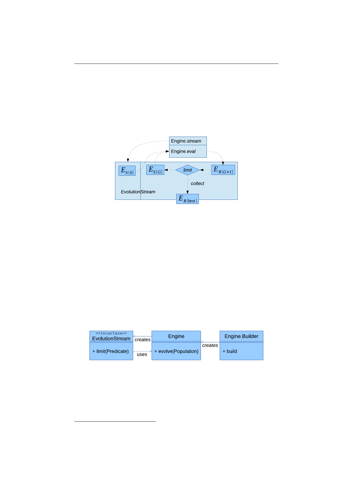
Figure 1.2.1: Evolution workflow
The described evolution workflow is also illustrated in figure 1.2.1, where
ES(i)
denotes the
EvolutionStart
object at generation
i
and
ER(i)
the
Evo-
lutionResult
at the
ith
generation. Once the evolution
Engine
is created, it
can be used by multiple
EvolutionStreams
, which can be safely used in different
execution threads. This is possible, because the evolution
Engine
doesn’t have
any mutable global state. It is practically a stateless function,
fE
: P
→
P,
which maps a start population, P, to an evolved result population. The
Engine
function,
fE
, is, of course, non-deterministic. Calling it twice with the same
start population will lead to different result populations.
The evolution process terminates, if the
EvolutionStream
is truncated and
the
EvolutionStream
truncation is controlled by the
limit
predicate. As
long as the predicate returns true, the evolution is continued.
5
At last, the
EvolutionResult
is collected from the
EvolutionStream
by one of the available
EvolutionResult collectors.
Figure 1.2.2: Evolution engine model
Figure 1.2.2 shows the static view of the main evolution classes, together
with its dependencies. Since the
Engine
class itself is immutable, and can’t
be changed after creation, it is instantiated (configured) via a builder. The
Engine
can be used to create an arbitrary number of
EvolutionStream
s. The
EvolutionStream
is used to control the evolutionary process and collect the final
5
See section 2.6 on page 60 for a detailed description of the available termination strategies.
4
1.3. BASE CLASSES CHAPTER 1. FUNDAMENTALS
result. This is done in the same way as for the normal
java.util.stream.-
Stream
classes. With the additional
limit(Predicate)
method, it is possible
to truncate the
EvolutionStream
if some termination criteria is fulfilled. The
separation of
Engine
and
EvolutionStream
is the separation of the evolution
definition and evolution execution.
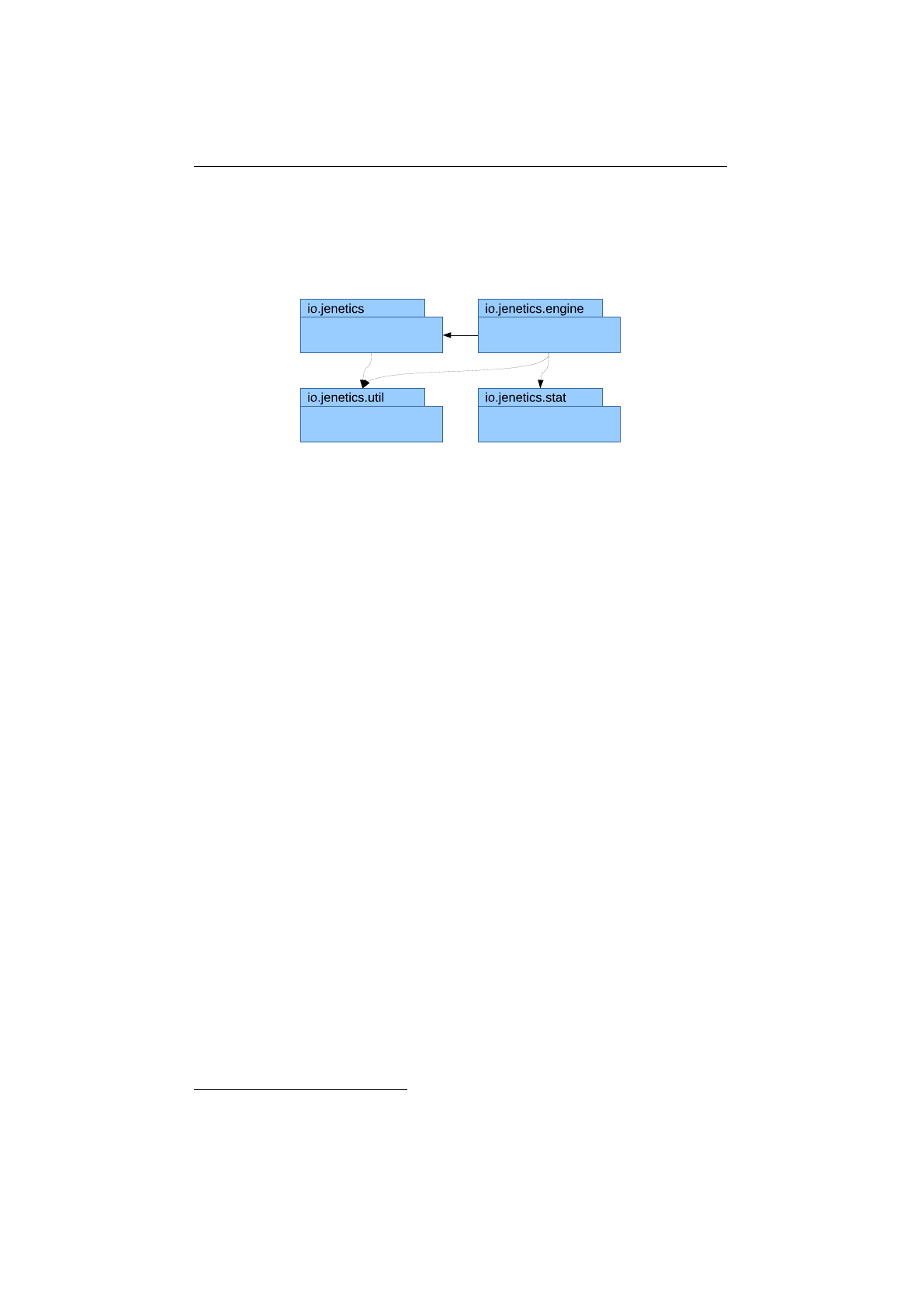
Figure 1.2.3: Package structure
In figure 1.2.3 the package structure of the library is shown and it consists of
the following packages:
io.jenetics
This is the base package of the
Jenetics
library and contains all
domain classes, like
Gene
,
Chromosome
or
Genotype
. Most of this types
are immutable data classes and doesn’t implement any behavior. It also
contains the
Selector
and
Alterer
interfaces and its implementations.
The classes in this package are (almost) sufficient to implement an own
GA.
io.jenetics.engine
This package contains the actual GA implementation
classes, e. g.
Engine
,
EvolutionStream
or
EvolutionResult
. They
mainly operate on the domain classes of the io.jenetics package.
io.jenetics.stat
This package contains additional statistics classes which are
not available in the Java core library. Java only includes classes for calcu-
lating the sum and the average of a given numeric stream (e. g.
Double-
SummaryStatistics
). With the additions in this package it is also possible
to calculate the variance, skewness and kurtosis—using the
DoubleMoment-
Statistics
class. The
EvolutionStatistics
object, which can be cal-
culated for every generation, relies on the classes of this package.
io.jenetics.util
This package contains the collection classes (
Seq
,
ISeq
and
MS
eq) which are used in the public interfaces of the
Chromosome
and
Geno-
type
. It also contains the
RandomRegistry
class, which implements the
global PRNG lookup, as well as helper
IO
classes for serializing
Genotype
s
and whole populations.
1.3 Base classes
This chapter describes the main classes which are needed to setup and run an
genetic algorithm with the
Jenetics6
library. They can roughly divided into
three types:
6
The documentation of the whole API is part of the download package or can be viewed
online: http://jenetics.io/javadoc/jenetics/4.4/index.html.
5
1.3. BASE CLASSES CHAPTER 1. FUNDAMENTALS
Domain classes
This classes form the domain model of the evolutionary algo-
rithm and contain the structural classes like
Gene
and
Chromosome
. They
are directly located in the io.jenetics package.
Operation classes
This classes operates on the domain classes and includes the
Alterer
and
Selector
classes. They are also located in the
io.jenetics
package.
Engine classes
This classes implements the actual evolutionary algorithm and
reside solely in the io.jenetics.engine package.
1.3.1 Domain classes
Most of the domain classes are pure data classes and can be treated as value
objects
7
. All
Gene
and
Chromosome
implementations are immutable as well as
the Genotype and Phenotype class.
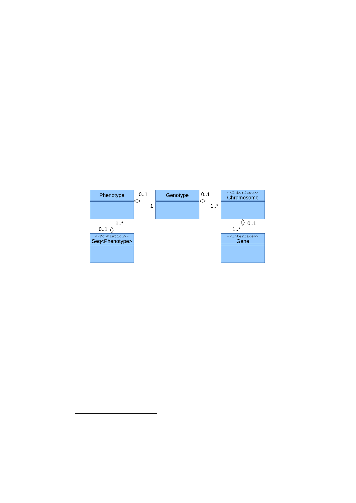
Figure 1.3.1: Domain model
Figure 1.3.1 shows the class diagram of the domain classes. All domain
classes are located in the
io.jenetics
package. The
Gene
is the base of the
class structure.
Gene
s are aggregated in
Chromosome
s. One to n
Chromosome
s
are aggregated in
Genotype
s. A
Genotype
and a fitness
Function
form the
Phenotype, which are collected into a population Seq.
1.3.1.1 Gene
Gene
s are the basic building blocks of the
Jenetics
library. They contain the
actual information of the encoded solution, the allele. Some of the implemen-
tations also contains domain information of the wrapped allele. This is the
case for all
BoundedGene
, which contain the allowed minimum and maximum
values. All
Gene
implementations are final and immutable. In fact, they are all
value-based classes and fulfill the properties which are described in the Java API
documentation[24].8
Beside the container functionality for the allele, every
Gene
is its own factory
and is able to create new, random instances of the same type and with the same
constraints. The factory methods are used by the
Alterer
s for creating new
7https://en.wikipedia.org/wiki/Value_object
8
It is also worth reading the blog entry from Stephen Colebourne:
http://blog.joda.org/
2014/03/valjos-value-java-objects.html
6

1.3. BASE CLASSES CHAPTER 1. FUNDAMENTALS
Gene
s from the existing one and play a crucial role by the exploration of the
problem space.
1public i n t e r f a c e Gene<A, G extends Gene<A, G>>
2extends Factory<G>, V e r i f i a b l e
3{
4public A g e t A l l e l e ( ) ;
5public G new In st anc e ( ) ;
6public G new I ns t an c e (A a l l e l e ) ;
7public boolean isValid () ;
8}
Listing 1.3: Gene interface
Listing 1.3 shows the most important methods of the
Gene
interface. The
isValid
method, introduced by the
Verifiable
interface, allows the gene to
mark itself as invalid. All invalid genes are replaced with new ones during the
evolution phase.
The available
Gene
implementations in the
Jenetics
library should cover a
wide range of problem encodings. Refer to chapter 2.1.1 on page 39 for how to
implement your own Gene types.
1.3.1.2 Chromosome
A
Chromosome
is a collection of
Gene
s which contains at least one
Gene
. This
allows to encode problems which requires more than one
Gene
. Like the
Gene
interface, the
Chromosome
is also it’s own factory and allows to create a new
Chromosome from a given Gene sequence.
1public i n t e r f a c e Chromosome<G extends Gene <?, G>>
2extends Factory<Chromosome<G>>, I t e r a b l e <G>, V e r i f i a b l e
3{
4public Chromosome<G> ne w In s ta n ce ( ISeq<G> ge n e s ) ;
5public G getGene ( int i n de x ) ;
6public ISeq<G> to Seq ( ) ;
7public Stream<G> stream ( ) ;
8public in t l e n g t h ( ) ;
9}
Listing 1.4: Chromosome interface
Listing 1.4 shows the main methods of the
Chromosome
interface. This are the
methods for accessing single
Gene
s by index and as an
ISeq
respectively, and
the factory method for creating a new
Chromosome
from a given sequence of
Gene
s. The factory method is used by the
Alterer
classes which were able to
create altered Chromosome from a (changed) Gene sequence.
Most of the
Chromosome
implementations can be created with variable length.
E. g. the
IntegerChromosome
can be created with variable length, where the
minimum value of the length range is included and the maximum value of the
length range is excluded.
1IntegerChromosome chromosome = IntegerChromosome . of (
20 , 1_000 , I ntRa nge . o f ( 5 , 9 )
3) ;
The factory method of the
IntegerChromosome
will now create chromosome
instances with a length between
[rangemin, rangemax)
, equally distributed. Fig-
ure 1.3.2 on the following page shows the structure of a
Chromosome
with variable
length.
7
1.3. BASE CLASSES CHAPTER 1. FUNDAMENTALS
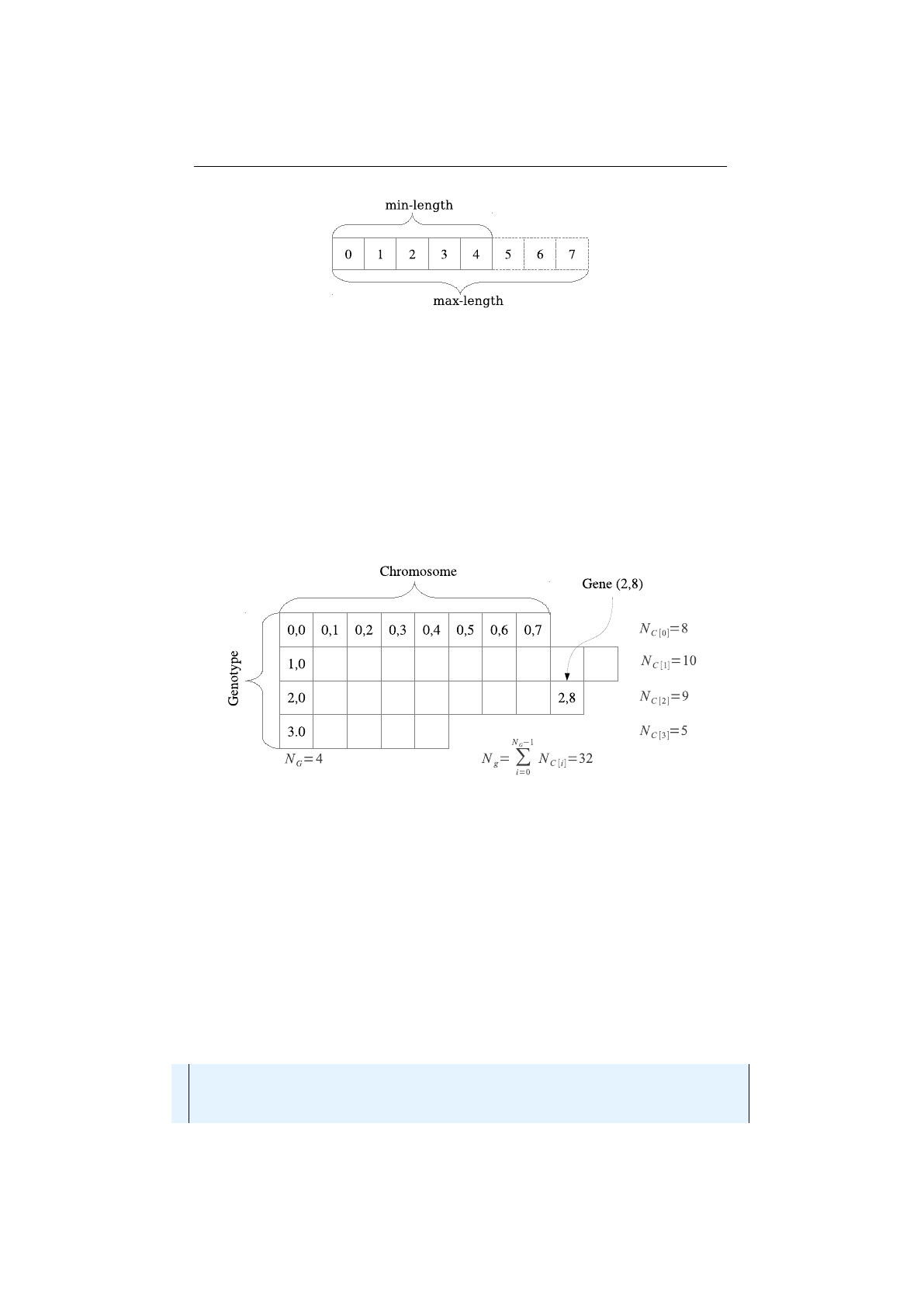
Figure 1.3.2: Chromosome structure
1.3.1.3 Genotype
The central class, the evolution
Engine
is working with, is the
Genotype
. It
is the structural and immutable representative of an individual and consists
of one to
nChromosome
s. All
Chromosome
s must be parameterized with the
same
Gene
type, but it is allowed to have different lengths and constraints. The
allowed minimal- and maximal values of a
NumericChromosome
is an example
of such a constraint. Within the same chromosome, all numeric gene alleles must
lay within the defined minimal- and maximal values.
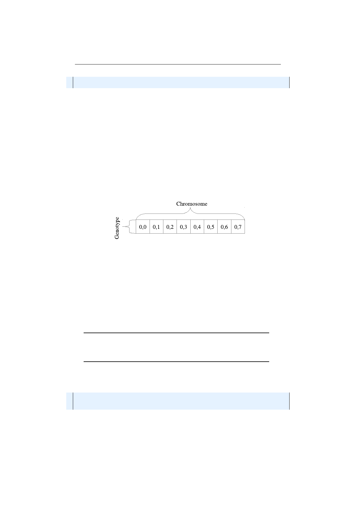
Figure 1.3.3: Genotype structure
Figure 1.3.3 shows the
Genotype
structure. A
Genotype
consists of
NG
Chromosome
s and a
Chromosome
consists of
NC[i]Gene
s (depending on the
Chromosome
). The overall number of
Gene
s of a
Genotype
is given by the sum
of the
Chromosome
’s
Gene
s, which can be accessed via the
Genotype.gene-
Count() method:
Ng=
NG−1
X
i=0
NC[i](1.3.1)
As already mentioned, the
Chromosome
s of a
Genotype
doesn’t have to have
necessarily the same size. It is only required that all genes are from the same
type and the
Gene
s within a
Chromosome
have the same constraints; e. g. the
same min- and max values for numerical Genes.
1Genotype<DoubleGene> g en ot yp e = Genotype . o f (
2DoubleChromosome . o f ( 0 . 0 , 1 . 0 , 8) ,
3DoubleChromosome . o f ( 1 . 0 , 2 . 0 , 1 0) ,
4DoubleChromosome . o f ( 0 . 0 , 1 0 . 0 , 9) ,
8
1.3. BASE CLASSES CHAPTER 1. FUNDAMENTALS
5DoubleChromosome . o f ( 0 . 1 , 0 . 9 , 5)
6) ;
The code snippet in the listing above creates a
Genotype
with the same structure
as shown in figure 1.3.3 on the preceding page. In this example the
DoubleGene
has been chosen as Gene type.
Genotype vector
The
Genotype
is essentially a two-dimensional composition
of
Gene
s. This makes it trivial to create
Genotype
s which can be treated
as a
Gene
matrices. If its needed to create a vector of
Gene
s, there are two
possibilities to do so:
1. creating a row-major or
2. creating a column-major
Genotype
vector. Each of the two possibilities have specific advantages and
disadvantages.
Figure 1.3.4: Row-major Genotype vector
Figure 1.3.4 shows a
Genotype
vector in row-major layout. A
Genotype
vector of length
n
needs one
Chromosome
of length
n
. Each
Gene
of such a vector
obeys the same constraints. E. g., for
Genotype
vectors containing
Numeric-
Gene
s, all
Gene
s must have the same minimum and maximum values. If the
problem space doesn’t need to have different minimum and maximum values, the
row-major
Genotype
vector is the preferred choice. Beside the easier
Genotype
creation, the available
Recombinator
alterers are more efficient in exploring the
search domain.
If the problem space allows equal
Gene
constraint, the row-major
Genotype
vector encoding should be chosen. It is easier to create and the available
Recombinator classes are more efficient in exploring the search domain.
The following code snippet shows the creation of a row-major
Genotype
vector. All
Alterer
s derived from the
Recombinator
do a fairly good job in
exploring the problem space for row-major Genotype vector.
1Genotype<DoubleGene> g en ot yp e = Genotype . o f (
2DoubleChromosome . o f ( 0 . 0 , 1 . 0 , 8)
3) ;
The column-major
Genotype
vector layout must be chosen when the problem
space requires components (
Gene
s) with different constraints. This is almost the
9
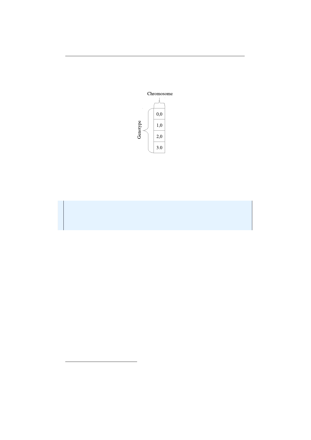
1.3. BASE CLASSES CHAPTER 1. FUNDAMENTALS
only reason for choosing the column-major layout. The layout of this
Genotype
vector is shown in 1.3.5. For a vector of length
n
,
nChromosome
s of length one
are needed.
Figure 1.3.5: Column-major Genotype vector
The code snippet below shows how to create a
Genotype
vector in column-
major layout. It’s a little more effort to create such a vector, since every
Gene
has to be wrapped into a separate
Chromosome
. The
DoubleChromosome
in the
given example has length of one, when the length parameter is omitted.
1Genotype<DoubleGene> g en ot yp e = Genotype . o f (
2DoubleChromosome . o f ( 0 . 0 , 1 . 0 ) ,
3DoubleChromosome . o f ( 1 . 0 , 2 . 0 ) ,
4DoubleChromosome . o f ( 0 . 0 , 1 0 . 0 ) ,
5DoubleChromosome . o f ( 0 . 1 , 0 . 9 )
6) ;
The greater flexibility of a column-major
Genotype
vector has to be payed with
a lower exploration capability of the
Recombinator
alterers. Using
Crossover
alterers will have the same effect as the
SwapMutator
, when used with row-major
Genotype vectors. Recommended alterers for vectors of NumericGenes are:
•MeanAlterer9,
•LineCrossover10 and
•IntermediateCrossover11
See also 2.3.2 on page 53 for an advanced description on how to use the predefined
vector codecs.
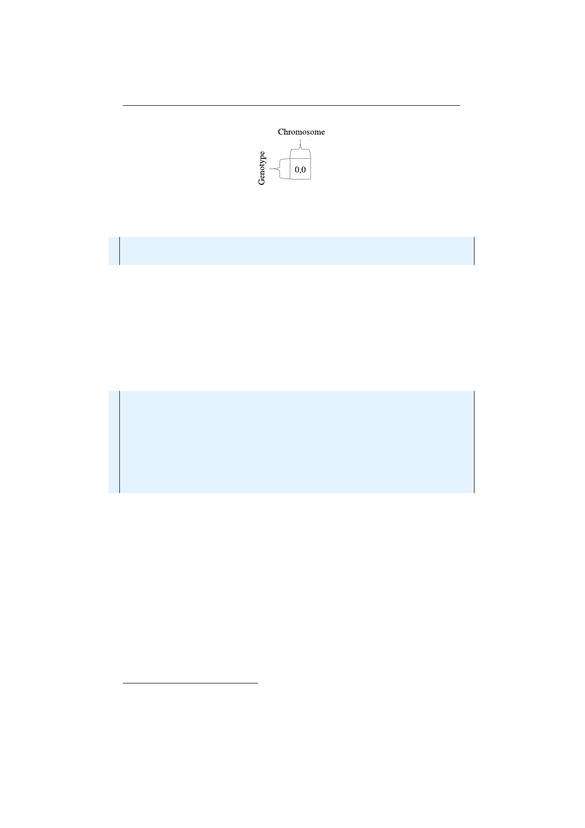
Genotype scalar
A very special case of a
Genotype
contains only one
Chro-
mosome
with length one. The layout of such a
Genotype
scalar is shown in 1.3.6
on the next page. Such
Genotype
s are mostly used for encoding real function
problems.
How to create a
Genotype
for a real function optimization problem, is shown
in the code snippet below. The recommended
Alterer
s are the same as for
column-major
Genotype
vectors:
MeanAlterer
,
LineCrossover
and
Inter-
mediateCrossover.
9See 1.3.2.2 on page 21.
10See 1.3.2.2 on page 21.
11See 1.3.2.2 on page 21.
10
1.3. BASE CLASSES CHAPTER 1. FUNDAMENTALS
Figure 1.3.6: Genotype scalar
1Genotype<DoubleGene> g en ot yp e = Genotype . o f (
2DoubleChromosome . o f ( 0 . 0 , 1 . 0 )
3) ;
See also 2.3.1 on page 52 for an advanced description on how to use the predefined
scalar codecs.
1.3.1.4 Phenotype
The
Phenotype
is the actual representative of an individual and consists of
the
Genotype
and the fitness
Function
, which is used to (lazily) calculate the
Genotype
’s fitness value.
12
It is only a container which forms the environment
of the
Genotype
and doesn’t change the structure. Like the
Genotype
, the
Phenotype is immutable and can’t be changed after creation.
1public f i n a l c l as s Phenotype<
2Gextends Gene <?, G>,
3Cextends Comparable<? super C>
4>
5implements Comparable<Phenotype<G, C>>
6{
7public C g e t F i t n e s s ( ) ;
8public Genotype<G> getGenot ype ( ) ;
9public long getAge(long currentGeneration) ;
10 public void evaluate () ;
11 }
Listing 1.5: Phenotype class
Listing 1.5 shows the main methods of the
Phenotype
. The
fitness
property
will return the actual fitness value of the
Genotype
, which can be fetched with
the
getGenotype
method. To make the runtime behavior predictable, the fitness
value is evaluated lazily. Either by querying the
fitness
property or through
the call of the
evaluate
method. The evolution
Engine
is calling the evaluate
method in a separate step and makes the fitness evaluation time available
through the
EvolutionDurations
class. Additionally to the fitness value, the
Phenotype
contains the generation when it was created. This allows to calculate
the current age and the removal of overaged individuals from the population.
1.3.1.5 Population
There is no special class which represents a population. It’s just a collection
of phenotypes. As collection class, the
Seq
interface is used. The own
Seq
12
Since the fitness
Function
is shared by all
Phenotype
s, calls to the fitness
Function
must
be idempotent. See section 1.3.3.1 on page 22.
11

1.3. BASE CLASSES CHAPTER 1. FUNDAMENTALS
implementations allows to express the mutability state of the population at the
type level and makes the coding more reliable. For a detailed description of this
collection classes see section 1.4.4 on page 36.
1.3.2 Operation classes
Genetic operators are used for creating genetic diversity (
Alterer
) and selecting
potentially useful solutions for recombination (
Selector
). This section gives an
overview about the genetic operators available in the
Jenetics
library. It also
contains some theoretical information, which should help you to choose the right
combination of operators and parameters, for the problem to be solved.
1.3.2.1 Selector
Selectors are responsible for selecting a given number of individuals from the
population. The selectors are used to divide the population into survivors
and offspring. The selectors for offspring and for the survivors can be chosen
independently.
The selection process of the
Jenetics
library acts on
Phenotype
s and indi-
rectly, via the fitness function, on
Genotype
s. Direct
Gene
- or population
selection is not supported by the library.
1Engine<DoubleGene , Double> e n gi ne = Engine . b u i l d e r ( . . . )
2. offspringFraction (0.7)
3. survivorsSelector(new R ou l et t e Wh e el S e le c to r <>() )
4. offspringSelector(new To u rnamentS e lector <>() )
5. b u i l d ( ) ;
The
offspringFraction
,
fO∈
[0
,
1], determines the number of selected off-
spring
NOg=kOgk=rint (kPgk · fO)(1.3.2)
and the number of selected survivors
NSg=kSgk=kPgk−kOgk.(1.3.3)
The Jenetics library contains the following selector implementations:
•TournamentSelector
•TruncationSelector
•MonteCarloSelector
•ProbabilitySelector
•RouletteWheelSelector
•LinearRankSelector
•ExponentialRankSelector
•BoltzmannSelector
•StochasticUniversalSelector
•EliteSelector
Beside the well known standard selector implementation the
Probability-
Selector is the base of a set of fitness proportional selectors.
12
1.3. BASE CLASSES CHAPTER 1. FUNDAMENTALS
Tournament selector
In tournament selection the best individual from a
random sample of
s
individuals is chosen from the population
Pg
. The samples are
drawn with replacement. An individual will win a tournament only if the fitness
is greater than the fitness of the other
s−
1competitors. Note that the worst
individual never survives, and the best individual wins in all the tournaments it
participates. The selection pressure can be varied by changing the tournament
size
s
. For large values of
s
, weak individuals have less chance of being selected.
Compared with fitness proportional selectors, the tournament selector is often
used in practice because of its lack of stochastic noise. Tournament selectors are
also independent to the scaling of the genetic algorithm fitness function.
Truncation selector
In truncation selection individuals are sorted according
to their fitness and only the
n
best individuals are selected. The truncation
selection is a very basic selection algorithm. It has it’s strength in fast selecting
individuals in large populations, but is not very often used in practice; whereas
the truncation selection is a standard method in animal and plant breeding. Only
the best animals, ranked by their phenotypic value, are selected for reproduction.
Monte Carlo selector
The Monte Carlo selector selects the individuals from
a given population randomly. Instead of a directed search, the Monte Carlo
selector performs a random search. This selector can be used to measure the
performance of a other selectors. In general, the performance of a selector should
be better than the selection performance of the Monte Carlo selector. If the
Monte Carlo selector is used for selecting the parents for the population, it will
be a little bit more disruptive, on average, than roulette wheel selection.[29]
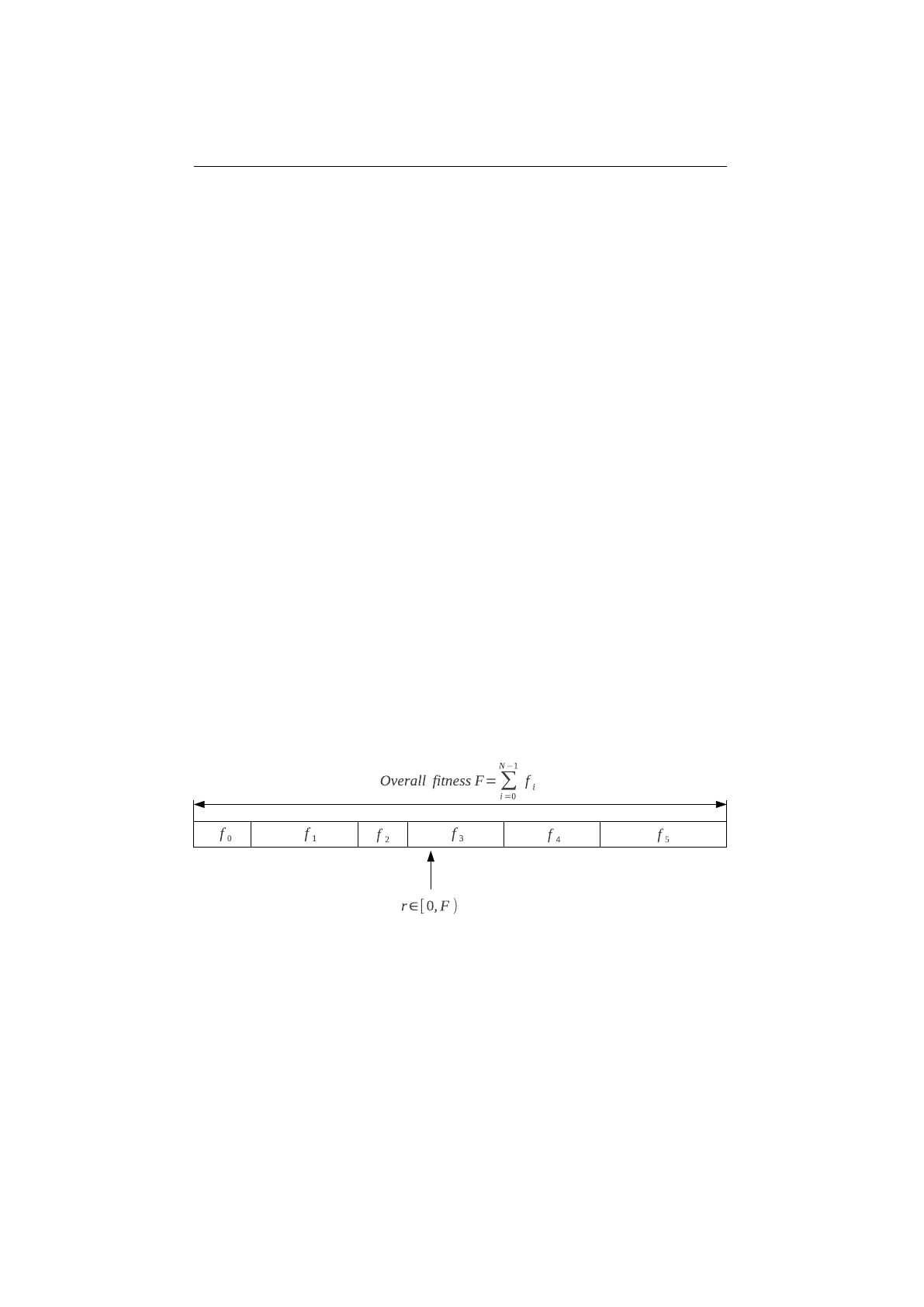
Probability selectors
Probability selectors are a variation of fitness propor-
tional selectors and selects individuals from a given population based on it’s
selection probability
P(i)
. Fitness proportional selection works as shown in
Figure 1.3.7: Fitness proportional selection
figure 1.3.7. An uniform distributed random number
r∈[0, F )
specifies which
individual is selected, by argument minimization:
i←argmin
n∈[0,N)(r <
n
X
i=0
fi),(1.3.4)
where
N
is the number of individuals and
fi
the fitness value of the
ith
individual.
The probability selector works the same way, only the fitness value
fi
is replaced
13

1.3. BASE CLASSES CHAPTER 1. FUNDAMENTALS
by the individual’s selection probability
P
(
i
). It is not necessary to sort the
population. The selection probability of an individual
i
follows a binomial
distribution
P(i, k) = n
kP(i)k(1 −P(i))n−k(1.3.5)
where
n
is the overall number of selected individuals and
k
the number of
individual
i
in the set of selected individuals. The runtime complexity of the
implemented probability selectors is
O(n+ log (n))
instead of
O(n2)
as for the
naive approach: A binary (index) search is performed on the summed probability
array.
Roulette-wheel selector
The roulette-wheel selector is also known as fitness
proportional selector and
Jenetics
implements it as probability selector. For
calculating the selection probability
P(i)
, the fitness value
fi
of individual
i
is
used.
P(i) = fi
PN−1
j=0 fj
(1.3.6)
Selecting
n
individuals from a given population is equivalent to play
n
times
on the roulette-wheel. The population don’t have to be sorted before selecting
the individuals. Notice that equation 1.3.6 assumes that all fitness values are
positive and the sum of the fitness values is not zero. To cope with negative
fitnesses, an adapted formula is used for calculating the selection probabilities.
P0(i) = fi−fmin
PN−1
j=0 (fj−fmin),(1.3.7)
where
fmin = min
i∈[0,N){fi,0}
As you can see, the worst fitness value
fmin
, if negative, has now a selection
probability of zero. In the case that the sum of the corrected fitness values is
zero, the selection probability of all fitness values will be set 1
N.
Linear-rank selector
The roulette-wheel selector will have problems when
the fitness values differ very much. If the best chromosome fitness is 90%, its
circumference occupies 90% of roulette-wheel, and then other chromosomes have
too few chances to be selected.[
29
] In linear-ranking selection the individuals
are sorted according to their fitness values. The rank
N
is assigned to the best
individual and the rank 1 to the worst individual. The selection probability
P(i)
of individual iis linearly assigned to the individuals according to their rank.
P(i) = 1
Nn−+n+−n−i−1
N−1.(1.3.8)
Here
n−
N
is the probability of the worst individual to be selected and
n+
N
the
probability of the best individual to be selected. As the population size is held
constant, the condition
n+
= 2
−n−
and
n−≥
0must be fulfilled. Note that
all individuals get a different rank, respectively a different selection probability,
even if they have the same fitness value.[5]
14
1.3. BASE CLASSES CHAPTER 1. FUNDAMENTALS
Exponential-rank selector
An alternative to the weak linear-rank selector
is to assign survival probabilities to the sorted individuals using an exponential
function:
P(i)=(c−1) ci−1
cN−1,(1.3.9)
where
c
must within the range
[0,1)
. A small value of
c
increases the probability
of the best individual to be selected. If
c
is set to zero, the selection probability of
the best individual is set to one. The selection probability of all other individuals
is zero. A value near one equalizes the selection probabilities. This selector sorts
the population in descending order before calculating the selection probabilities.
Boltzmann selector
The selection probability of the Boltzmann selector is
defined as
P(i) = eb·fi
Z,(1.3.10)
where
b
is a parameter which controls the selection intensity and
Z
is defined as
Z=
n
X
i=1
efi.(1.3.11)
Positive values of
b
increases the selection probability of individuals with high
fitness values and negative values of
b
decreases it. If
b
is zero, the selection
probability of all individuals is set to 1
N.
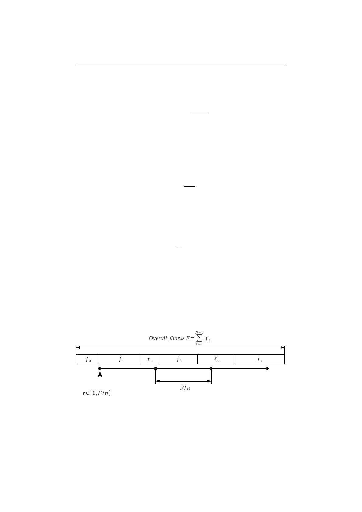
Stochastic-universal selector
Stochastic-universal selection[
1
] (SUS) is a
method for selecting individuals according to some given probability in a way
that minimizes the chance of fluctuations. It can be viewed as a type of roulette
game where we now have
p
equally spaced points which we spin. SUS uses
a single random value for selecting individuals by choosing them at equally
spaced intervals. Weaker members of the population (according to their fitness)
have a better chance to be chosen, which reduces the unfair nature of fitness-
proportional selection methods. The selection method was introduced by James
Baker.[
2
] Figure 1.3.8 shows the function of the stochastic-universal selection,
Figure 1.3.8: Stochastic-universal selection
where
n
is the number of individuals to select. Stochastic universal sampling
ensures a selection of offspring, which is closer to what is deserved than roulette
wheel selection.[29]
15

1.3. BASE CLASSES CHAPTER 1. FUNDAMENTALS
Elite selector
The
EliteSelector
copies a small proportion of the fittest
candidates, without changes, into the next generation. This may have a dramatic
impact on performance by ensuring that the GA doesn’t waste time re-discovering
previously refused partial solutions. Individuals that are preserved through
elitism remain eligible for selection as parents of the next generation. Elitism is
also related with memory: remember the best solution found so far. A problem
with elitism is that it may causes the GA to converge to a local optimum, so pure
elitism is a race to the nearest local optimum. The elite selector implementation of
the
Jenetics
library also lets you specify the selector for the non-elite individuals.
1.3.2.2 Alterer
The problem encoding/representation determines the bounds of the search space,
but the
Alterer
s determine how the space can be traversed:
Alterer
s are
responsible for the genetic diversity of the
EvolutionStream
. The two
Alterer
hierarchies used in Jenetics are:
1. mutation and
2. recombination (e. g. crossover).
First we will have a look at the mutation
— There are two distinct
roles mutation plays in the evolution process:
1. Exploring the search space
: By making small moves, mutation allows
a population to explore the search space. This exploration is often slow
compared to crossover, but in problems where crossover is disruptive this
can be an important way to explore the landscape.
2. Maintaining diversity
: Mutation prevents a population from converging
to a local minimum by stopping the solution to become to close to one
another. A genetic algorithm can improve the solution solely by the
mutation operator. Even if most of the search is being performed by
crossover, mutation can be vital to provide the diversity which crossover
needs.
The mutation probability,
P(m)
, is the parameter that must be optimized. The
optimal value of the mutation rate depends on the role mutation plays. If
mutation is the only source of exploration (if there is no crossover), the mutation
rate should be set to a value that ensures that a reasonable neighborhood of
solutions is explored.
The mutation probability,
P(m)
, is defined as the probability that a specific
gene, over the whole population, is mutated. That means, the (average) number
of genes mutated by a mutator is
ˆµ=NP·Ng·P(m)(1.3.12)
where
Ng
is the number of available genes of a genotype and
NP
the population
size (revere to equation 1.3.1 on page 8).
16

1.3. BASE CLASSES CHAPTER 1. FUNDAMENTALS
Mutator
The mutator has to deal with the problem, that the genes are
arranged in a 3
D
structure (see chapter 1.3.1.3). The mutator selects the gene
which will be mutated in three steps:
1. Select a genotype G[i]from the population with probability PG(m),
2.
select a chromosome
C
[
j
]from the selected genotype
G
[
i
]with probability
PC(m)and
3.
select a gene
g
[
k
]from the selected chromosome
C
[
j
]with probability
Pg(m).
The needed sub-selection probabilities are set to
PG(m) = PC(m) = Pg(m) = 3
pP(m).(1.3.13)
Gaussian mutator
The Gaussian mutator performs the mutation of number
genes. This mutator picks a new value based on a Gaussian distribution around
the current value of the gene. The variance of the new value (before clipping to
the allowed gene range) will be
ˆσ2=gmax −gmin
42
(1.3.14)
where
gmin
and
gmax
are the valid minimum and maximum values of the number
gene. The new value will be cropped to the gene’s boundaries.
Swap mutator
The swap mutator changes the order of genes in a chromosome,
with the hope of bringing related genes closer together, thereby facilitating the
production of building blocks. This mutation operator can also be used for
combinatorial problems, where no duplicated genes within a chromosome are
allowed, e. g. for the TSP.
The second alterer type is the recombination
— An enhanced genetic
algorithm (EGA) combine elements of existing solutions in order to create a new
solution, with some of the properties of each parents. Recombination creates a
new chromosome by combining parts of two (or more) parent chromosomes. This
combination of chromosomes can be made by selecting one or more crossover
points, splitting these chromosomes on the selected points, and merge those
portions of different chromosomes to form new ones.
1void recombi n e ( final ISeq<Phenotype<G, C>> pop ) {
2// S e l e c t t he Genotypes f o r c r o s s o v e r .
3final Random random = RandomRegistry . getRandom ( ) ;
4f i n a l i nt i 1 = random . n e x t I n t ( pop . l e n g t h ( ) ) ;
5f i n a l i nt i 2 = random . n e x t I n t ( pop . l e n g t h ( ) ) ;
6final Phenotype<G, C> pt1 = pop . g et ( i 1 ) ;
7final Phenotype<G, C> pt2 = pop . g et ( i 2 ) ;
8final Genotype<G> gt 1 = p t1 . getGeno typ e ( ) ;
9final Genotype<G> gt 2 = p t2 . getGeno typ e ( ) ;
10
11 // Choosin g th e Chromosome f o r c r o s s o v e r .
12 f i n a l i nt chIn d e x =
17

1.3. BASE CLASSES CHAPTER 1. FUNDAMENTALS
13 random . n ex t I n t ( min ( g t1 . l e n g t h ( ) , g t 2 . l e n g t h ( ) ) ) ;
14 final MSeq<Chromosome<G>> c1 = gt 1 . toSeq ( ) . copy ( ) ;
15 final MSeq<Chromosome<G>> c2 = gt 2 . toSeq ( ) . copy ( ) ;
16 final MSeq<G> ge ne s1 = c1 . g e t ( chI n d ex ) . t oSeq ( ) . copy ( ) ;
17 final MSeq<G> ge ne s2 = c2 . g e t ( chI n d ex ) . t oSeq ( ) . copy ( ) ;
18
19 // Perform t he c r o s s o v e r .
20 c r o s s o v e r ( genes1 , ge ne s2 ) ;
21 c1 . s e t ( c hI nd ex , c1 . g e t ( c hI nd ex ) . n e wI n st a n ce ( g e n e s 1 . t o I S e q ( ) ) ) ;
22 c2 . s e t ( c hI nd ex , c2 . g e t ( c hI nd ex ) . n e wI n st a n ce ( g e n e s 2 . t o I S e q ( ) ) ) ;
23
24 // C re at in g two new Phenotypes and r e p l a c e t he o l d one .
25 MSeq<Phenotype<G, C>> r e s u l t = pop . copy ( ) ;
26 r e s u l t . s e t ( i 1 , pt 1 . n e w In s t an c e ( g t 1 . ne w I ns t a nc e ( c 1 . t o I S e q ( ) ) ) ) ;
27 r e s u l t . s e t ( i 2 , pt 2 . n e w In s t an c e ( g t 1 . ne w I ns t a nc e ( c 2 . t o I S e q ( ) ) ) ) ;
28 }
Listing 1.6: Chromosome selection for recombination
Listing 1.6 on the preceding page shows how two chromosomes are selected for
recombination. It is done this way for preserving the given constraints and to
avoid the creation of invalid individuals.
Because of the possible different
Chromosome
length and/or
Chromosome
constraints within a
Genotype
, only
Chromosome
s with the same
Genotype position are recombined (see listing 1.6 on the previous page).
The recombination probability,
P
(
r
), determines the probability that a given
individual (genotype) of a population is selected for recombination. The (mean)
number of changed individuals depend on the concrete implementation and
can be vary from
P
(
r
)
·NG
to
P
(
r
)
·NG·OR
, where
OR
is the order of the
recombination, which is the number of individuals involved in the
combine
method.
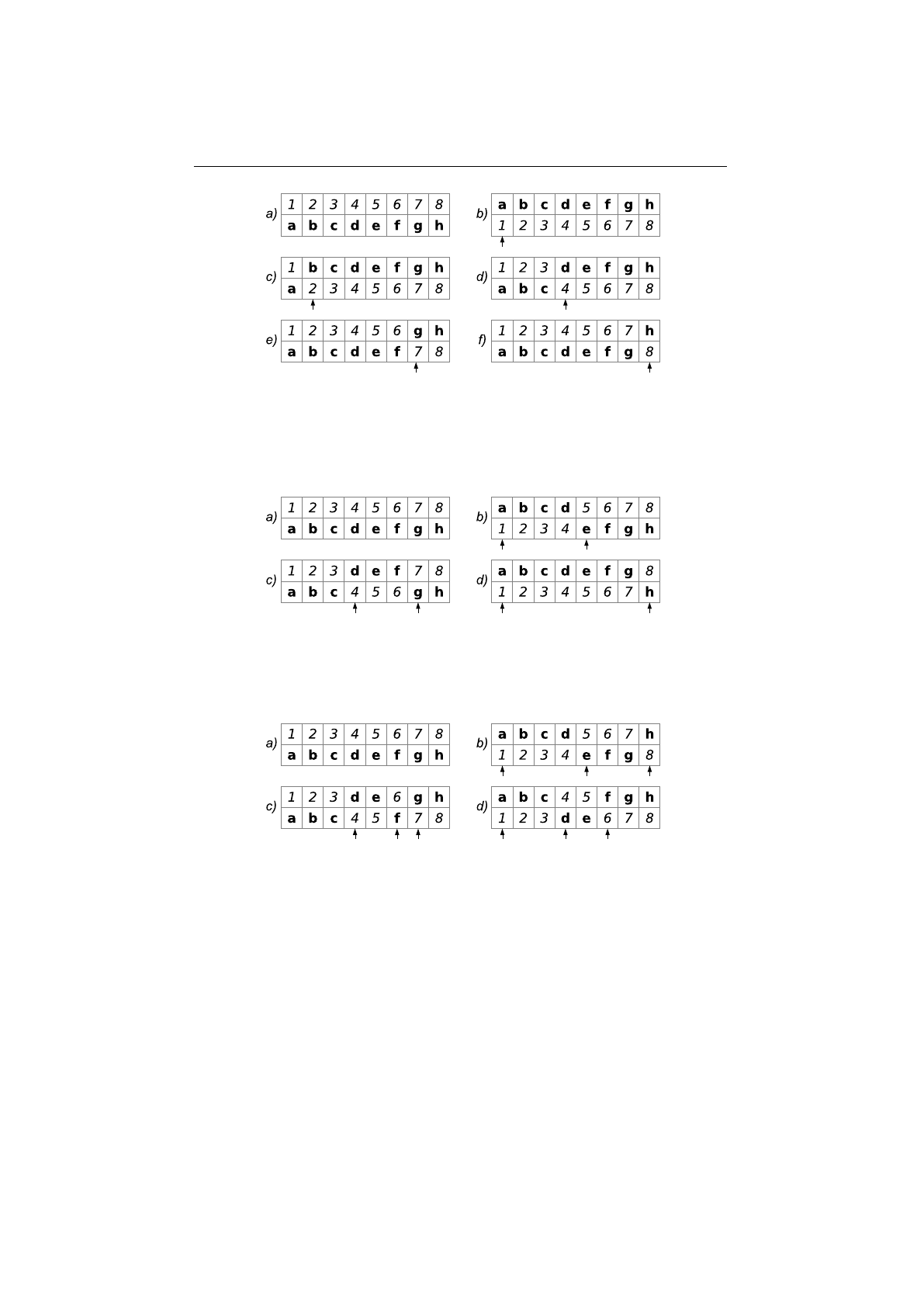
Single-point crossover
The single-point crossover changes two children chro-
mosomes by taking two chromosomes and cutting them at some, randomly
chosen, site. If we create a child and its complement we preserve the total
number of genes in the population, preventing any genetic drift. Single-point
crossover is the classic form of crossover. However, it produces very slow mixing
compared with multi-point crossover or uniform crossover. For problems where
the site position has some intrinsic meaning to the problem single-point crossover
can lead to smaller disruption than multiple-point or uniform crossover.
Figure 1.3.9 shows how the
SinglePointCrossover
class is performing the
crossover for different crossover points. Sub-figure a) shows the two chromosomes
chosen for crossover. The examples in sub-figures b) to f) illustrates the crossover
results for indexes 0,1,3,6and 7.
Multi-point crossover
If the
MultiPointCrossover
class is created with
one crossover point, it behaves exactly like the single-point crossover. The figures
in 1.3.10 shows how the multi-point crossover works with two crossover points.
Figure a) shows the two chromosomes chosen for crossover, b) shows the crossover
18
1.3. BASE CLASSES CHAPTER 1. FUNDAMENTALS
Figure 1.3.9: Single-point crossover
result for the crossover points at index 0and 4,c) uses crossover points at index
3and 6and d) at index 0and 7.
Figure 1.3.10: 2-point crossover
Figure 1.3.11 you can see how the crossover works for an odd number of
crossover points.
Figure 1.3.11: 3-point crossover
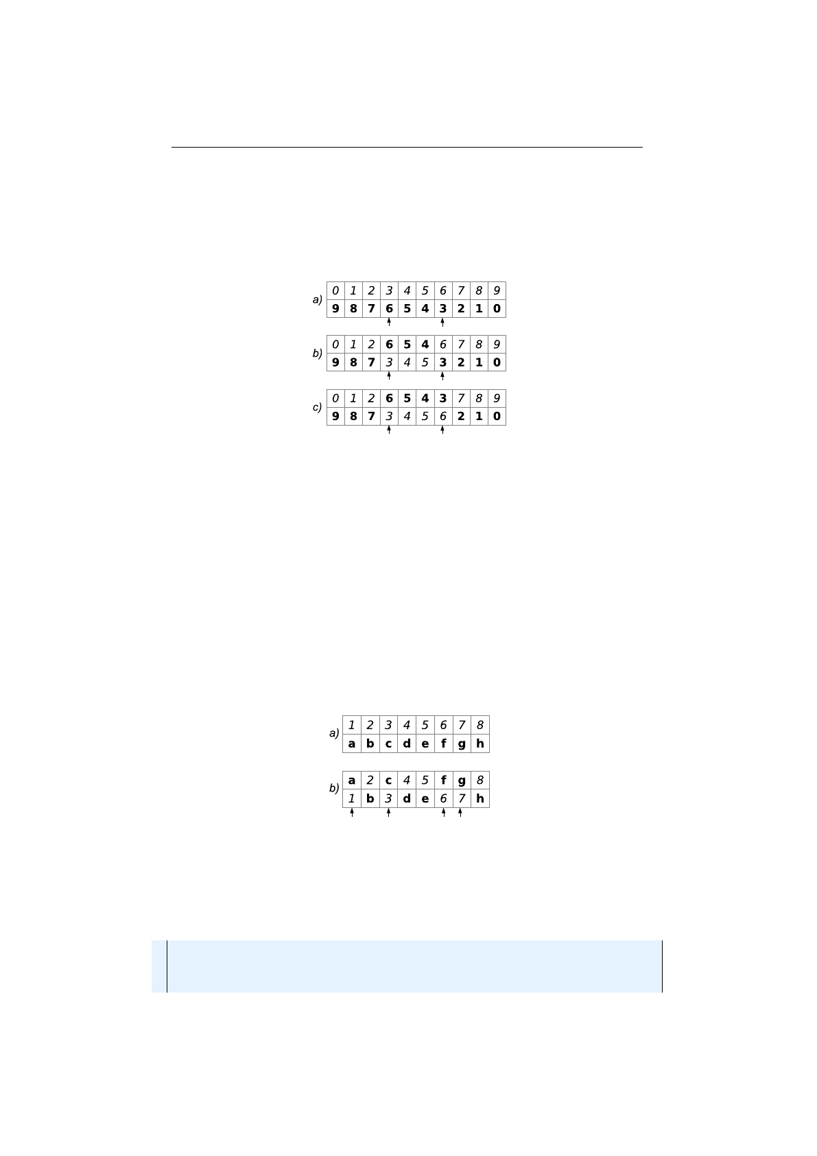
Partially-matched crossover
The partially-matched crossover guarantees
that all genes are found exactly once in each chromosome. No gene is duplicated
by this crossover strategy. The partially-matched crossover (PMX) can be applied
usefully in the TSP or other permutation problem encodings. Permutation
encoding is useful for all problems where the fitness only depends on the ordering
of the genes within the chromosome. This is the case in many combinatorial
optimization problems. Other crossover operators for combinatorial optimization
are:
19
1.3. BASE CLASSES CHAPTER 1. FUNDAMENTALS
•order crossover
•cycle crossover
•edge recombination crossover
•edge assembly crossover
The PMX is similar to the two-point crossover. A crossing region is chosen
by selecting two crossing points (see figure 1.3.12 a)).
Figure 1.3.12: Partially-matched crossover
After performing the crossover we–normally–got two invalid chromosomes
(figure 1.3.12 b)). Chromosome 1contains the value 6 twice and misses the value
3. On the other side chromosome 2contains the value 3 twice and misses the
value 6. We can observe that this crossover is equivalent to the exchange of the
values 3
→
6, 4
→
5 and 5
→
4. To repair the two chromosomes we have to apply
this exchange outside the crossing region (figure 1.3.12 b)). At the end figure
1.3.12 c) shows the repaired chromosome.
Uniform crossover
In uniform crossover, the genes at index
i
of two chro-
mosomes are swapped with the swap-probability,
pS
. Empirical studies shows
that uniform crossover is a more exploitative approach than the traditional
exploitative approach that maintains longer schemata. This leads to a better
search of the design space with maintaining the exchange of good information.[
8
]
Figure 1.3.13: Uniform crossover
Figure 1.3.13 shows an example of a uniform crossover with four crossover
points. A gene is swapped, if a uniformly created random number, r∈[0,1], is
smaller than the swap-probability,
pS
. The following code snippet shows how
these swap indexes are calculated, in a functional way.
1final Random random = RandomRegistry . getRandom ( ) ;
2f i n a l i nt l e n g t h = 8 ;
3f i n a l double ps = 0 . 5 ;
4f i n a l i nt [ ] i n d e x e s = In tRan ge . ra ng e ( 0 , l e n g t h )
20
1.3. BASE CLASSES CHAPTER 1. FUNDAMENTALS
5. f i l t e r ( i −> random . nextDouble ( ) < ps )
6. toA rray ( ) ;
Mean alterer
The Mean alterer works on genes which implement the
Mean
interface. All numeric genes implement this interface by calculating the arithmetic
mean of two genes.
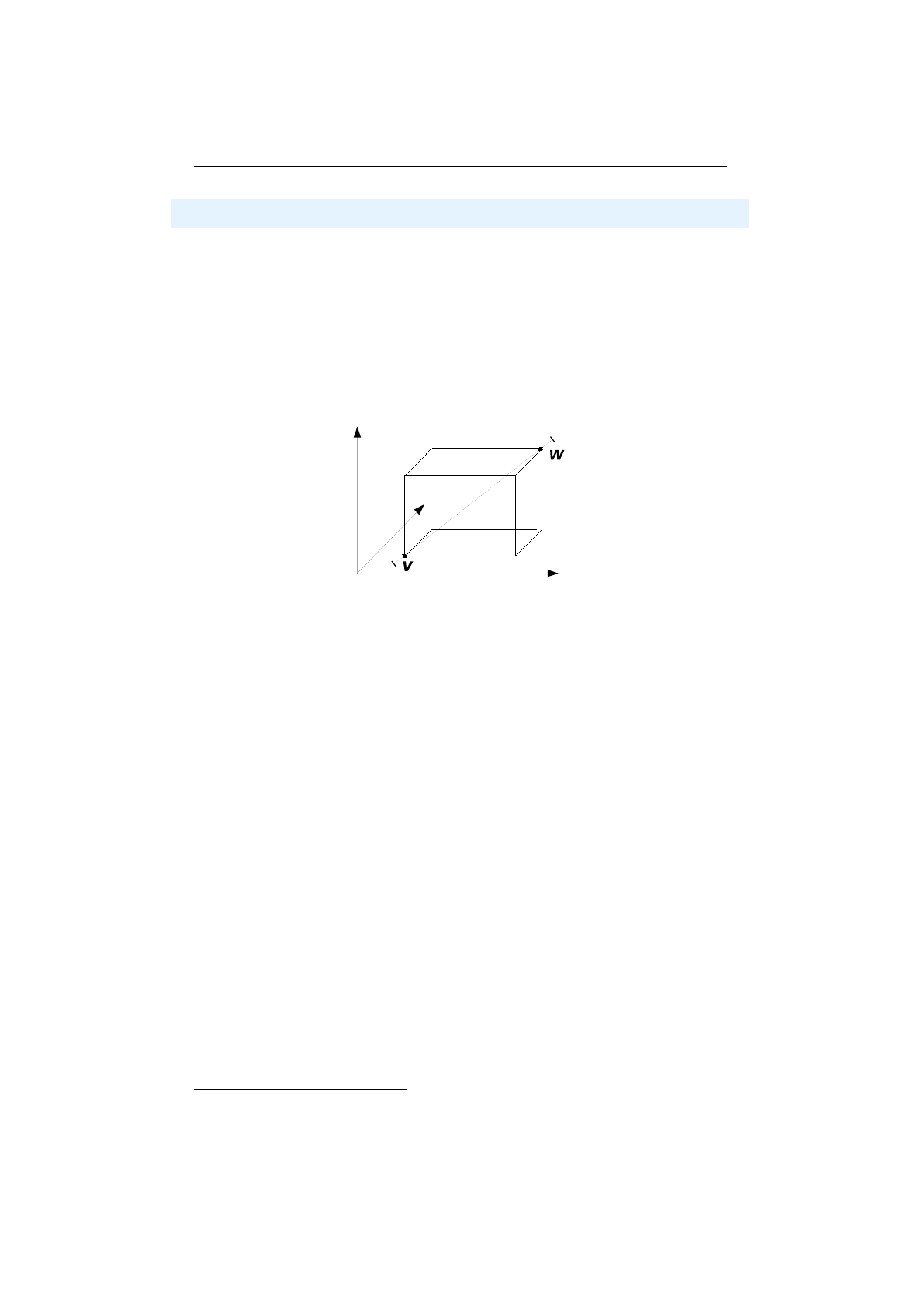
Line crossover
The line crossover
13
takes two numeric chromosomes and
treats it as a real number vector. Each of this vectors can also be seen as a point
in
Rn
. If we draw a line through this two points (chromosome), we have the
possible values of the new chromosomes, which all lie on this line.
Figure 1.3.14: Line crossover hypercube
Figure 1.3.14 shows how the two chromosomes form the two three-dimensional
vectors (black circles). The dashed line, connecting the two points, form the
possible solutions created by the line crossover. An additional variable,
p
,
determines how far out along the line the created children will be. If
p
= 0 then
the children will be located along the line within the hypercube. If
p >
0, the
children may be located on an arbitrary place on the line, even outside of the
hypercube.This is useful if you want to explore unknown regions, and you need
a way to generate chromosomes further out than the parents are.
The internal random parameters, which define the location of the new
crossover point, are generated once for the whole vector (chromosome). If
the
LineCrossover
generates numeric genes which lie outside the allowed min-
imum and maximum value, it simply uses the original gene and rejects the
generated, invalid one.
Intermediate crossover
The intermediate crossover is quite similar to the
line crossover. It differs in the way on how the internal random parameters
are generated and the handling of the invalid–out of range–genes. The internal
random parameters of the
IntermediateCrossover
class are generated for each
gene of the chromosome, instead once for all genes. If the newly generated gene
is not within the allowed range, a new one is created. This is repeated, until a
valid gene is built.
The crossover parameter,
p
, has the same properties as for the line crossover.
If the chosen value for
p
is greater than 0, it is likely that some genes must be
created more than once, because they are not in the valid range. The probability
13
The line crossover, also known as line recombination, was originally described by Heinz
Mühlenbein and Dirk Schlierkamp-Voosen.[23]
21

1.3. BASE CLASSES CHAPTER 1. FUNDAMENTALS
for gene re-creation rises sharply with the value of
p
. Setting
p
to a value greater
than one, doesn’t make sense in most of the cases. A value greater than 10
should be avoided.
1.3.3 Engine classes
The executing classes, which perform the actual evolution, are located in the
io.jenetics.engine
package. The evolution stream (
EvolutionStream
) is the
base metaphor for performing an GA. On the
EvolutionStream
you can define
the termination predicate and than collect the final
EvolutionResult
. This
decouples the static data structure from the executing evolution part. The
EvolutionStream
is also very flexible, when it comes to collecting the final
result. The
EvolutionResult
class has several predefined collectors, but you
are free to create your own one, which can be seamlessly plugged into the existing
stream.
1.3.3.1 Fitness function
The fitness
Function
is also an important part when modeling an genetic
algorithm. It takes a
Genotype
as argument and returns, at least, a
Comparable
object as result—the fitness value. This allows the evolution
Engine
, respectively
the selection operators, to select the offspring- and survivor population. Some
selectors have stronger requirements to the fitness value than a
Comparable
,
but this constraints is checked by the Java type system at compile time.
Since the fitness Function is shared by all Phenotypes, calls to the fitness
Function has to be idempotent. A fitness Function is idempotent if, whenever
it is applied twice to any Genotype, it returns the same fitness value as if it
were applied once. In the simplest case, this is achieved by Functions which
doesn’t contain any global mutable state.
The following example shows the simplest possible fitness
Function
. This
Function simply returns the allele of a 1x1float Genotype.
1pu bl ic c l a s s Main {
2static Double i d e n t i t y ( final Genotype<DoubleGene> gt ) {
3return gt . getGene ( ) . g e t A l l e l e ( ) ;
4}
5
6pub li c s t a t i c void main ( final S t r i n g [ ] a r g s ) {
7// C re at e f i t n e s s f u n c t i o n from method r e f e r e n c e .
8Function<Genotype<DoubleGene >, Double>> f f 1 =
9Main : : i d e n t i t y ;
10
11 // C re at e f i t n e s s f u n c t i o n from lambda e x p r e s s i o n .
12 Function<Genotype<DoubleGene >, Double>> f f 2 = gt −>
13 gt . getGene ( ) . g e t A l l e l e ( ) ;
14 }
15 }
The first type parameter of the
Function
defines the kind of
Genotype
from
which the fitness value is calculated and the second type parameter determines
the return type, which must be, at least, a Comparable type.
22

1.3. BASE CLASSES CHAPTER 1. FUNDAMENTALS
1.3.3.2 Engine
The evolution
Engine
controls how the evolution steps are executed. Once the
Engine is created, via a
Builder
class, it can’t be changed. It doesn’t contain
any mutable global state and can therefore safely used/called from different
threads. This allows to create more than one
EvolutionStreams
from the
Engine and execute them in parallel.
1public f i n a l c l as s Engine<
2Gextends Gene <?, G>,
3Cextends Comparable<? super C>
4>
5implements Fu nc ti on <E v o l u t i o n S t a r t <G, C> ,
6E v o l ut i o n R e s u l t <G, C>>,
7E vo l u ti o nS t r ea m ab l e <G, C>
8{
9// The e v o l u t i o n f u n ct i on , pe r fo rm s one e v o l u t i o n st e p .
10 E v ol u ti o nR e su l t <G, C> e v o l v e (
11 ISeq<Phenotype<G, C>> p o pu la ti o n ,
12 long g e n e r a t i o n
13 ) ;
14
15 // E v o l ut i on st re am f o r " no rm al " e v o l u t i o n e x e c u t i o n .
16 E vo lu ti o nS tr e am <G, C> st r ea m ( ) ;
17
18 // E v ol ut io n i t e r a t o r f o r e x t e r n a l e v o l u t i o n i t e r a t i o n .
19 I t e r a t o r <E vo lu ti on Re su lt <G, C>> i t e r a t o r ( ) ;
20 }
Listing 1.7: Engine class
Listing 1.7 shows the main methods of the
Engine
class. It is used for performing
the actual evolution of a give population. One evolution step is executed by
calling the
Engine.evolve
method, which returns an
EvolutionResult
object.
This object contains the evolved population plus additional information like
execution duration of the several evolution sub-steps and information about the
killed and as invalid marked individuals. With the
stream
method you create a
new
EvolutionStream
, which is used for controlling the evolution process—see
section 1.3.3.3 on page 25. Alternatively it is possible to iterate through the
evolution process in an imperative way (for whatever reasons this should be
necessary). Just create an
Iterator
of
EvolutionResult
object by calling the
iterator method.
As already shown in previous examples, the
Engine
can only be created
via its
Builder
class. Only the fitness
Function
and the
Chromosome
s, which
represents the problem encoding, must be specified for creating an Engine
instance. For the rest of the parameters default values are specified. This are
the Engine parameters which can configured:
alterers
A list of
Alterer
s which are applied to the offspring population, in
the defined order. The default value of this property is set to
Single-
PointCrossover<>(0.2) followed by Mutator<>(0.15).
clock
The
java.time.Clock
used for calculating the execution durations. A
Clock
with nanosecond precision (
System.nanoTime()
) is used as default.
executor
With this property it is possible to change the
java.util.concur-
rent.Executor
engine used for evaluating the evolution steps. This prop-
erty can be used to define an application wide
Executor
or for controlling
23

1.3. BASE CLASSES CHAPTER 1. FUNDAMENTALS
the number of execution threads. The default value is set to
ForkJoin-
Pool.commonPool().
evaluator
This property allows you to replace the evaluation strategy of the
Phenotype
’s fitness function. Normally, each fitness value is evaluated
concurrently, but independently from each other. In some configuration
it is necessary, for performance reason, to evaluate the fitness values of a
population at once. This is then performed by the
Engine.Evaluator
or
Engine.GenotypeEvaluator interface.
fitnessFunction
This property defines the fitness
Function
used by the evo-
lution Engine. (See section 1.3.3.1 on page 22.)
genotypeFactory
Defines the
Genotype Facto
ry used for creating new indi-
viduals. Since the
Genotype
is its own
Fact
ory, it is sufficient to create a
Genotype, which then serves as template.
genotypeValidator
This property lets you override the default implementation
of the
Genotype.isValid
method, which is useful if the
Genotype
validity
not only depends on valid property of the elements it consists of.
maximalPhenotypeAge
Set the maximal allowed age of an individual (Pheno-
type). This prevents super individuals to live forever. The default value is
set to 70.
offspringFraction
Through this property it is possible to define the fraction of
offspring (and survivors) for evaluating the next generation. The fraction
value must within the interval [0
,
1]. The default value is set to 0
.
6.
Additionally to this property, it is also possible to set the
survivorsFrac-
tion
,
survivorsSize
or
offspringSize
. All this additional properties
effectively set the offspringFraction.
offspringSelector
This property defines the
Selector
used for selecting the
offspring population. The default values is set to
TournamentSelect-
or<>(3).
optimize
With this property it is possible to define whether the fitness
Function
should be maximized of minimized. By default, the fitness
Function
is
maximized.
phenotypeValidator
This property lets you override the default implementa-
tion of the
Phenotype.isValid
method, which is useful if the
Phenotype
validity not only depends on valid property of the elements it consists of.
populationSize
Defines the number of individuals of a population. The evolu-
tion
Engine
keeps the number of individuals constant. That means, the
population of the
EvolutionResult
always contains the number of entries
defined by this property. The default value is set to 50.
selector
This method allows to set the
offspringSelector
and
survivors-
Selector in one step with the same selector.
survivorsSelector
This property defines the
Selector
used for selecting the
survivors population. The default values is set to
TournamentSelec-
tor<>(3).
24

1.3. BASE CLASSES CHAPTER 1. FUNDAMENTALS
individualCreationRetries
The evolution
Engine
tries to create only valid
individuals. If a newly created
Genotype
is not valid, the
Engine
creates
another one, till the created
Genotype
is valid. This parameter sets the
maximal number of retries before the
Engine
gives up and accept invalid
individuals. The default value is set to 10.
mapper
This property lets you define an mapper, which transforms the final
EvolutionResult
object after every generation. One usage of the mapper
is to remove duplicate individuals from the population. The
Evolution-
Result.toUniquePopulation()
method provides such a de-duplication
mapper.
The
EvolutionStream
s created by the
Engine
class are unlimited. Such streams
must be limited by calling the available
EvolutionStream.limit
methods. Al-
ternatively, the
Engine
instance itself can be limited with the
Engine.limit
methods. This limited
Engine
s no longer creates infinite
EvolutionStream
s,
they are truncated by the limit predicate defined by the
Engine
. This feature is
needed when you are concatenating evolution
Engine
s (see section 4.1.5.1 on
page 85).
1final E v ol u t i on S t r e am a b l e <DoubleGene , Doubl e> e n g i n e =
2Engine . b u i l d e r ( problem )
3. m ini mi zi ng ( )
4. b u i l d ( )
5. l i m i t ( ( ) −> Limits . bySteadyFitness(10) ) ;
As shown in the example code above, one important difference between the
Engine.limit
and the
EvolutionStream.limit
method is, that the limit me-
thod of the
Engine
takes a limiting
Predicate Supplier
instead of the the
Predicate
itself. The reason for this is that some
Predicate
s has to maintain
internal state to work properly. This means, every time the
Engine
creates a
new stream, it must also create a new limiting Predicate.
1.3.3.3 EvolutionStream
The EvolutionStream controls the execution of the evolution process and can
be seen as a kind of execution handle. This handle can be used to define
the termination criteria and to collect the final evolution result. Since the
EvolutionStream
extends the Java
Stream
interface, it integrates smoothly
with the rest of the Java Stream API.14
1public i n te r fa c e Evo l utionStr e am<
2Gextends Gene <?, G>,
3Cextends Comparable<? super C>
4>
5extends Stream<E v ol ut io nR es ul t <G, C>>
6{
7public Evoluti o n Stream <G, C>
8l i m i t ( Pr ed i ca te <? super E v ol u ti o nR e su lt <G, C>> pr oce ed ) ;
9}
Listing 1.8: EvolutionStream class
14
It is recommended to make yourself familiar with the Java Stream API.
A good introduction can be found here:
http://winterbe.com/posts/2014/07/31/
java8-stream-tutorial-examples/
25

1.3. BASE CLASSES CHAPTER 1. FUNDAMENTALS
Listing 1.8 on the preceding page shows the whole
EvolutionStream
interface.
As it can be seen, it only adds one additional method. But this additional
limit
method allows to truncate the
EvolutionStream
based on a
Predicate
which
takes an
EvolutionResult
. Once the
Predicate
returns
false
, the evolution
process is stopped. Since the
limit
method returns an
EvolutionStream
, it
is possible to define more than one
Predicate
, which both must be fulfilled to
continue the evolution process.
1Eng in e<DobuleGene , Double> e n g i n e = . . .
2E vo lu t io nS t re a m<DoubleGene , Double> s t re am = e n g i n e . s tr ea m ( )
3. l i m i t ( p r e d i c a t e 1 )
4. l i m i t ( p r e d i c a t e 2 )
5. l i m i t ( 1 0 0 ) ;
The
EvolutionStream
, created in the example above, will be truncated if one
of the two predicates is
false
or if the maximal allowed generations, of 100,
is reached. An
EvolutionStream
is usually created via the
Engine.stream()
method. The immutable and stateless nature of the evolution
Engine
allows to
create more than one EvolutionStream with the same Engine instance.
The generations of the
EvolutionStream
are evolved serially. Calls of the
EvolutionStream
methods (e. g.
limit
,
peek
, ...) are executed in the
thread context of the created
Stream
. In a typical setup, no additional
synchronization and/or locking is needed.
In cases where you appreciate the usage of the
EvolutionStream
but need a
different
Engine
implementation, you can use the
EvolutionStream.of
factory
method for creating an new EvolutionStream.
1static <G extends Gene <? , G>, C extends Comparable<? super C>>
2Evo lut io nSt re am <G, C> o f (
3S u p p l i e r <E v o l u t i o n S t a r t <G, C>> s t a r t ,
4Function <? super E v o l u t i o n S t a r t <G, C> , E v o l u t io n R e s u l t <G, C>> f
5) ;
This factory method takes a start value, of type
EvolutionStart
, and an
evolution
Function
. The evolution
Function
takes the start value and returns
an
EvolutionResult
object. To make the runtime behavior more predictable,
the start value is fetched/created lazily at the evolution start time.
1final S u p p l i e r <E v o l u t i o n S t a r t <DoubleGene , Double>> s t a r t = . . .
2final Evoluti o n Stream <DoubleGene , Double> stream =
3Ev ol ut io nS tr ea m . o f ( s t a r t , new MySpecialEngine () ) ;
1.3.3.4 EvolutionResult
The
EvolutionResult
collects the result data of an evolution step into an
immutable value class. This class is the type of the stream elements of the
EvolutionStream, as described in section 1.3.3.3 on the previous page.
1public f i n a l c l as s EvolutionResult<
2Gextends Gene <?, G>,
3Cextends Comparable<? super C>
4>
5implements Comparable<E vo lu ti on Re s ul t <G, C>>
26

1.3. BASE CLASSES CHAPTER 1. FUNDAMENTALS
6{
7IS eq <Ph enot ype<G, C>> g e t P o p u l a t i o n ( ) ;
8long g et Ge ne ra ti o n ( ) ;
9}
Listing 1.9: EvolutionResult class
Listing 1.3.3.4 on the preceding page shows the two most important properties,
the
population
and the
generation
the result belongs to. This are also the
two properties needed for the next evolution step. The
generation
is, of
course, incremented by one. To make collecting the
EvolutionResult
object
easier, it also implements the
Comparable
interface. Two
EvolutionResult
s
are compared by its best Phenotype.
The
EvolutionResult
classes has three predefined factory methods, which
will return Collectors usable for the EvolutionStream:
toBestEvolutionResult()
Collects the best
EvolutionResult
of a
Evolu-
tionStream according to the defined optimization strategy.
toBestPhenotype()
This collector can be used if you are only interested in the
best Phenotype.
toBestGenotype()
Use this collector if you only need the best
Genotype
of the
EvolutionStream.
The following code snippets shows how to use the different
EvolutionStream
collectors.
1// C o l l e c t i n g t h e b e s t E v o l u t i o n R e s u l t o f t he Ev o lu t io n St r ea m .
2Ev ol ut io nRe su lt <DoubleGene , Double> r e s u l t = stream
3. c o l l e c t ( E v o l u t i o n R e s u l t . t o B e s t E v o l u t i o n R e s u l t ( ) ) ;
4
5// C o l l e c t i n g t he be s t Phenotype o f t he E vol ut ion St rea m .
6Phenotype<DoubleGene , Double> r e s u l t = s t r e am
7. c o l l e c t ( E v o l u t i o n R e s u l t . t oB es t Ph en ot y pe ( ) ) ;
8
9// C o l l e c t i n g t he be s t Genotype o f t he E vo lut io nSt re am .
10 Genotype<DoubleGene> r e s u l t = stream
11 . c o l l e c t ( E v o l u t i o n R e s u l t . t oB es tG en ot yp e ( ) ) ;
1.3.3.5 EvolutionStatistics
The
EvolutionStatistics
class allows you to gather additional statistical
information from the
EvolutionStream
. This is especially useful during the
development phase of the application, when you have to find the right parametriza-
tion of the evolution
Engine
. Besides other informations, the
Evolution-
Statistics
contains (statistical) information about the fitness, invalid and
killed
Phenotypes
and runtime information of the different evolution steps.
Since the
EvolutionStatistics
class implements the
Consumer<Evolution-
Result<?, C>>
interface, it can be easily plugged into the
EvolutionStream
,
adding it with the peek method of the stream.
1Eng in e<DoubleGene , Double> e n g i n e = . . .
2E v o l u t i o n S t a t i s t i c s <?, Double> s t a t i s t i c s =
3EvolutionStatistics .ofNumber() ;
4e n g i n e . s tr e am ( )
5. l i m i t ( 1 0 0 )
27

1.3. BASE CLASSES CHAPTER 1. FUNDAMENTALS
6. peek ( s t a t i s t i c s )
7. c o l l e c t ( to B e s tG enotype ( ) ) ;
Listing 1.10: EvolutionStatistics usage
Listing 1.10 on the previous page shows how to add the the
EvolutionStatistics
to the
EvolutionStream
. Once the algorithm tuning is finished, it can be re-
moved in the production environment.
There are two different specializations of the EvolutionStatistics object
available. The first is the general one, which will be working for every kind
of
Gene
s and fitness types. It can be created via the
EvolutionStatistics.-
ofComparable()
method. The second one collects additional statistical data for
numeric fitness values. This can be created with the
EvolutionStatistics.-
ofNumber() method.
1+---------------------------------------------------------------------------+
2| Time st at is t ic s |
3+---------------------------------------------------------------------------+
4| Se le ct ion : sum = 0 .0 4 65 3 827 800 0 s ; mean =0 . 00 3 878 189 833 s |
5| Alte ri ng : sum =0.0 8 61 5 54 5 70 0 0 s; mean =0 . 00 7 17 9 62 1 41 7 s |
6| Fitne ss c alc ul ati on : sum =0 .02 290 1 60 6 00 0 s ; mean =0. 001 9 08 4 67 1 67 s |
7| Overall e xe c ut io n : sum = 0.1 4 72 9 80 6 70 0 0 s; mean =0 .01 2 27 4 83 8 91 7 s |
8+---------------------------------------------------------------------------+
9| Evo lu ti on st at is t ic s |
10 +---------------------------------------------------------------------------+
11 | Ge ne rat io ns : 12 |
12 | Al te re d : su m =7 ,331; m ean = 61 0.9 166 66 66 7 |
13 | Kil le d : sum =0 ; me an =0 .00 000 000 0 |
14 | In va li ds : sum =0; mean =0 .00 000 000 0 |
15 +---------------------------------------------------------------------------+
16 | Pop ul ati on s tat is tic s |
17 +---------------------------------------------------------------------------+
18 | Age : ma x =1 1; m ea n = 1. 95 10 00 ; var = 5. 545 19 0 |
19 | Fi tn es s : |
20 | min = 0.000000000000 |
21 | max = 481.748227114537 |
22 | mean = 384.430345078660 |
23 | var = 13 0 06. 1 32 5 373 0 15 2 8 |
24 +---------------------------------------------------------------------------+
A typical output of an number
EvolutionStatistics
object will look like the
example above.
The
EvolutionStatistics
object is a simple for inspecting the
Evolution-
Stream
after it is finished. It doesn’t give you a
live
view of the current evolution
process, which can be necessary for long running streams. In such cases you
have to maintain/update the statistics yourself.
1pu bl ic c l a s s TSM {
2// The l o c a t i o n s to v i s i t .
3s t a t i c f i n a l ISeq<Point> POINTS = I Seq . of ( . . . ) ;
4
5// The per muta tio n c ode c .
6s t a t i c f i n a l Codec<ISeq<Point >, EnumGene<Point>>
7CODEC = Codecs . ofP e rm ut ati on (POINTS) ;
8
9// The f i t n e s s f u n c t i o n ( i n the proble m domain ) .
10 s t a t i c double d i s t ( final ISeq<Point> p ) { . . . }
11
12 // The e v o l u t i o n e n gi ne .
13 s t a t i c f i n a l Engine<EnumGene<Point >, Double> ENGINE = Engine
14 . b u i l d e r (TSM : : d i s t , CODEC)
15 . o p t i m i z e ( O pt im iz e . MINIMUM)
16 . b u i l d ( ) ;
17
28

1.3. BASE CLASSES CHAPTER 1. FUNDAMENTALS
18 // Best phenotype found so f a r .
19 static Phenotype<EnumGene<P oin t >, Double> b e s t = nul l ;
20
21 // You w i l l be i nf orm ed on new r e s u l t s . This a ll o w s t o
22 // r e a c t on new b e s t p he no ty pe s , e . g . l o g i t .
23 pr iv at e s t a t i c void update(
24 final Ev ol ut ion Re su lt <EnumGene<Point >, Double> r e s u l t
25 ) {
26 i f ( b e s t == n u ll | |
27 b e s t . compareTo ( r e s u l t . g et B es tP h en ot y pe ( ) ) < 0 )
28 {
29 b e s t = r e s u l t . ge tB es tP h en ot y pe ( ) ;
30 System . out . p r i n t ( r e s u l t . ge tG ene rat io n ( ) + " : " ) ;
31 System . out . p r i n t l n ( " Found b e s t ph eno ty pe : " + b e s t ) ;
32 }
33 }
34
35 // Find the s o l u t i o n .
36 pub li c s t a t i c void main ( final S t r i n g [ ] a r g s ) {
37 final ISeq<Point> r e s u l t = CODEC. decode (
38 ENGINE . stream ( )
39 . peek (TSM : : update )
40 . l i m i t ( 1 0 )
41 . c o l l e c t ( E v o l u t i o n R e s u l t . t oB es tG en ot yp e ( ) )
42 ) ;
43 System . out . p r i n t l n ( r e s u l t ) ;
44 }
45 }
Listing 1.11: Live evolution statistics
Listing 1.11 on the preceding page shows how to implement a manual statistics
gathering. The update method is called whenever a new
EvolutionResult
is
has been calculated. If a new best
Phenotype
is available, it is stored and logged.
With the
TSM::update
method, which is called on every finished generation,
you have a live view on the evolution progress.
1.3.3.6 Engine.Evaluator
This interface allows to define different strategies for evaluating the fitness
functions of a given population. Usually, it is not necessary to override the
default evaluation strategy. It is helpful if you have performance problems when
the fitness function is evaluated serially—or in small concurrent batches, as it
is implemented by the default strategy. In this case, the
Engine.Evaluator
interface can be used to calculate the fitness function for a population in one
batch.
1public i n te r fa c e E v aluat or<
2Gextends Gene <?, G>,
3Cextends Comparable<? super C>
4> {
5IS eq<Phenotype<G, C>> e v a l u a t e ( Seq<Phenotype<G, C>> pop ) ;
6}
Listing 1.12: Engine.Evaluator interface
The implementer is free to do the evaluation in place, or create new Phenotype
instance and return the newly created one.
29
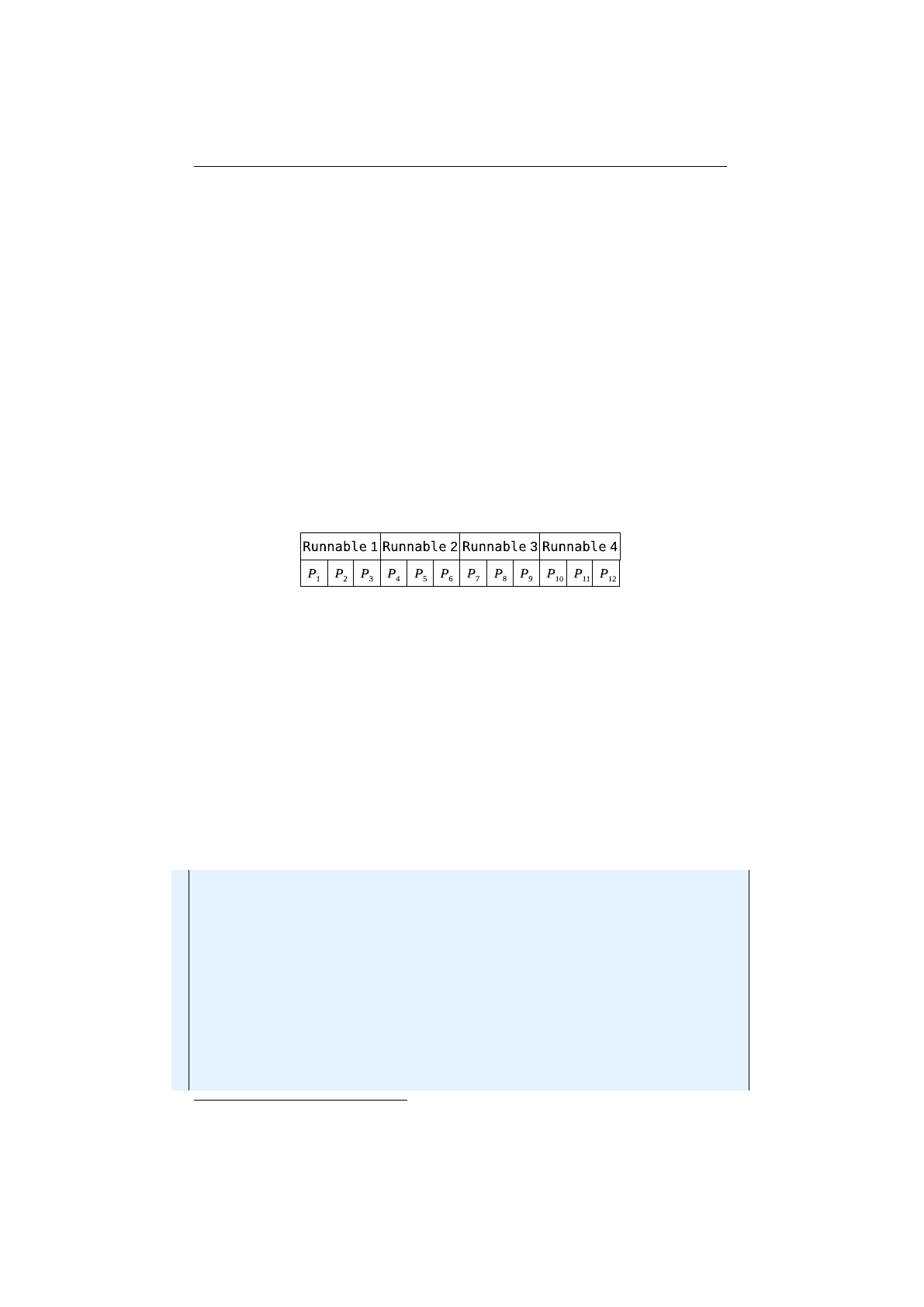
1.4. NUTS AND BOLTS CHAPTER 1. FUNDAMENTALS
A second use case for the
Evaluator
interface is, when the fitness value also
depends on the current composition of the population. E. g. it is possible to
normalize the population’s fitness values.
1.4 Nuts and bolts
1.4.1 Concurrency
The
Jenetics
library parallelizes independent task whenever possible. Especially
the evaluation of the fitness function is done concurrently. That means that the
fitness function must be thread safe, because it is shared by all phenotypes of a
population. The easiest way for achieving thread safety is to make the fitness
function immutable and re-entrant.
Since the number of individuals of one population, which determines the
number of fitness functions to be evaluated, is usually much higher then the
number of available CPU cores, the fitness evaluation is done in batches. This
reduces the evaluation overhead, for lightweight fitness functions.
Figure 1.4.1: Evaluation batch
Figure 1.4.1 shows an example population with 12 individuals. The evaluation
of the phenotype’s fitness functions are evaluated in batches with three elements.
For this purpose, the individuals of one batch are wrapped into a
Runnable
object. The batch size is automatically adapted to the available number of CPU
cores. It is assumed that the evaluation cost of one fitness function is quite small.
If this assumption doesn’t hold, you can configure the the maximal number
of batch elements with the
io.jenetics.concurrency.maxBatchSize
system
property15.
1.4.1.1 Basic configuration
The used
Executor
can be defined when building the evolution
Engine
object.
1import j a v a . u t i l . c o n c u r r e n t . Ex ec ut o r ;
2import j a v a . u t i l . c o n c u r r e n t . Ex e c u to r s ;
3
4pu bl ic c l a s s Main {
5pr iv at e s t a t i c Double e v a l ( final Genotype<DoubleGene> gt ) {
6// c a l c u l a t e and r e t u r n f i t n e s s
7}
8
9pub li c s t a t i c void main ( final S t r i n g [ ] a r g s ) {
10 // C r e a t in g an f i x e d s i z e E x e c u t o r S e r v i c e
11 final E x e c u t o r S e r v i c e e x e c u t o r = E x ec u t or s
12 . newF ix ed Th re ad Poo l ( 1 0 )
13 final Factory<Genotype<DoubleGene>> g t f = . . .
14 final Eng in e<DoubleGene , Double> e n g i n e = E ng ine
15 . b u i l d e r ( Main : : ev al , g t f )
15See section 1.4.1.2 on the following page.
30

1.4. NUTS AND BOLTS CHAPTER 1. FUNDAMENTALS
16 // Us in g 10 t h r e a d s f o r e v o l v i n g .
17 . e x e c u t o r ( e x e c u t o r )
18 . b u i l d ( )
19 ...
20 }
21 }
If no
Executor
is given,
Jenetics
uses a common
ForkJoinPool16
for concur-
rency.
Sometimes it might be useful to run the evaluation
Engine
single-threaded,
or even execute all operations in the main thread. This can be easily achieved
by setting the appropriate Executor.
1final Engine<DoubleGene , Double> e n gi ne = Engine . b u i l d e r ( . . . )
2// Doing t he Eng in e o p e r a t i o n s i n t he main t h re a d
3. e x e c u t o r ( ( E xe c ut or ) Ru nnab le : : run )
4. b u i l d ( )
The code snippet above shows how to do the
Engine
operations in the main
thread. Whereas the snippet below executes the
Engine
operations in a single
thread, other than the main thread.
1final Engine<DoubleGene , Double> e n gi ne = Engine . b u i l d e r ( . . . )
2// Doing t he Eng in e o p e r a t i o n s i n a s i n g l e th r ea d
3. e x e c u t o r ( E x ec u t or s . n e wS in g le T hr ea d Ex ec u to r ( ) )
4. b u i l d ( )
Such a configuration can be useful for performing reproducible (performance)
tests, without the uncertainty of a concurrent execution environment.
1.4.1.2 Concurrency tweaks
Jenetics
uses different strategies for minimizing the concurrency overhead, de-
pending on the configured
Executor
. For the
ForkJoinPool
, the fitness evalua-
tion of the population is done by recursively dividing it into sub-populations using
the abstract
RecursiveAction
class. If a minimal sub-population size is reached,
the fitness values for this sub-population are directly evaluated. The default value
of this threshold is five and can be controlled via the
io.jenetics.concurrency-
.splitThreshold
system property. Besides the
splitThreshold
, the size of
the evaluated sub-population is dynamically determined by the
ForkJoinTask-
.getSurplusQueuedTaskCount()
method.
17
If this value is greater than three,
the fitness values of the current sub-population are also evaluated immediately.
The default value can be overridden by the
io.jenetics.concurrency.max-
SurplusQueuedTaskCount system property.
$ java -Dio.jenetics.concurrency.splitThreshold=1 \
-Dio.jenetics.concurrency.maxSurplusQueuedTaskCount=2 \
-cp jenetics-4.4.0.jar:app.jar \
com.foo.bar.MyJeneticsApp
16https://docs.oracle.com/javase/8/docs/api/java/util/concurrent/ForkJoinPool.
html
17
Excerpt from the Javadoc: Returns an estimate of how many more locally queued tasks
are held by the current worker thread than there are other worker threads that might steal
them. This value may be useful for heuristic decisions about whether to fork other tasks. In
many usages of
ForkJoinTasks
, at steady state, each worker should aim to maintain a small
constant surplus (for example, 3) of tasks, and to process computations locally if this threshold
is exceeded.
31

1.4. NUTS AND BOLTS CHAPTER 1. FUNDAMENTALS
You may want to tweak this parameters, if you realize a low CPU utilization
during the fitness value evaluation. Long running fitness functions could lead
to CPU under-utilization while evaluating the last sub-population. In this case,
only one core is busy, while the other cores are idle, because they already finished
the fitness evaluation. Since the workload has been already distributed, no
work-stealing is possible. Reducing the
splitThreshold
can help to have a
more equal workload distribution between the available CPUs. Reducing the
maxSurplusQueuedTaskCount
property will create a more uniform workload for
fitness function with heavily varying computation cost for different genotype
values.
The fitness function shouldn’t acquire locks for achieving thread safety. It
is also recommended to avoid calls to blocking methods. If such calls are
unavoidable, consider using the
ForkJoinPool.managedBlock
method.
Especially if you are using a
ForkJoinPool
executor, which is the default.
If the Engine is using an
ExecutorService
, a different optimization strategy
is used for reducing the concurrency overhead. The original population is divided
into a fixed number
18
of sub-populations, and the fitness values of each sub-
population are evaluated by one thread. For long running fitness functions, it is
better to have smaller sub-populations for a better CPU utilization. With the
io.jenetics.concurrency.maxBatchSize
system property, it is possible to
reduce the sub-population size. The default value is set to
Integer.MAX_VALUE
.
This means, that only the number of CPU cores influences the batch size.
$ java -Dio.jenetics.concurrency.maxBatchSize=3 \
-cp jenetics-4.4.0.jar:app.jar \
com.foo.bar.MyJeneticsApp
Another source of under-utilized CPUs are lock contentions. It is therefore
strongly recommended to avoid locking and blocking calls in your fitness function
at all. If blocking calls are unavoidable, consider using the managed block
functionality of the ForkJoinPool.19
1.4.2 Randomness
In general, GAs heavily depends on pseudo random number generators (PRNG)
for creating new individuals and for the selection- and mutation-algorithms.
Jenetics
uses the Java
Random
object, respectively sub-types from it, for gen-
erating random numbers. To make the random engine pluggable, the
Random
object is always fetched from the
RandomRegistry
. This makes it possible to
change the implementation of the random engine without changing the client
code. The central
RandomRegistry
also allows to easily change
Random
engine
even for specific parts of the code.
18
The number of sub-populations actually depends on the number of available CPU cores,
which are determined with Runtime.availableProcessors().
19
A good introduction on how to use managed blocks, and the motivation behind it, is given
in this talk: https://www.youtube.com/watch?v=rUDGQQ83ZtI
32

1.4. NUTS AND BOLTS CHAPTER 1. FUNDAMENTALS
The following example shows how to change and restore the
Random
object.
When opening the
with
scope, changes to the
RandomRegistry
are only visible
within this scope. Once the
with
scope is left, the original
Random
object is
restored.
1L i s t <Genotype<DoubleGene>> g e no t y p e s =
2RandomRegistry . with (new Random ( 1 2 3 ) , r −> {
3Genotype . o f ( DoubleChromosome . o f ( 0 . 0 , 1 0 0 . 0 , 1 0) )
4. i n s t a n c e s ( )
5. l i m i t ( 1 0 0 )
6. c o l l e c t ( C o l l e c t o r s . t o L i s t ( ) )
7}) ;
With the previous listing, a random, but reproducible, list of genotypes is created.
This might be useful while testing your application or when you want to evaluate
the EvolutionStream several times with the same initial population.
1Eng in e<DoubleGene , Double> e n g i n e = . . . ;
2// C re at e a new e v o l u t i o n s tre am w ith th e g iv e n
3// i n i t i a l gen ot yp es .
4Pheno type<DoubleGene , Double> b e s t = e n g i n e . s tr ea m ( g e n o t y pe s )
5. l i m i t ( 1 0 )
6. c o l l e c t ( E v o l u t i o n R e s u l t . t oB es t Ph en ot y pe ( ) ) ;
The example above uses the generated genotypes for creating the
Evolution-
Stream
. Each created stream uses the same starting population, but will, most
likely, create a different result. This is because the stream evaluation is still
non-deterministic.
Setting the PRNG to a Random object with a defined seed has the effect,
that every evolution stream will produce the same result—in an single
threaded environment.
The parallel nature of the GA implementation requires the creation of streams
ti,j
of random numbers which are statistically independent, where the streams
are numbered with
j
= 1
,
2
,
3
, ..., p
,
p
denotes the number of processes. We expect
statistical independence between the streams as well. The used PRNG should
enable the GA to play fair, which means that the outcome of the GA is strictly
independent from the underlying hardware and the number of parallel processes
or threads. This is essential for reproducing results in parallel environments
where the number of parallel tasks may vary from run to run.
The Fair Play property of a PRNG guarantees that the quality of the
genetic algorithm (evolution stream) does not depend on the degree of
parallelization.
When the
Random
engine is used in an multi-threaded environment, there
must be a way to parallelize the sequential PRNG. Usually this is done by
taking the elements of the sequence of pseudo-random numbers and distribute
them among the threads. There are essentially four different parallelizations
techniques used in practice: Random seeding,Parameterization,Block splitting
and Leapfrogging.
33
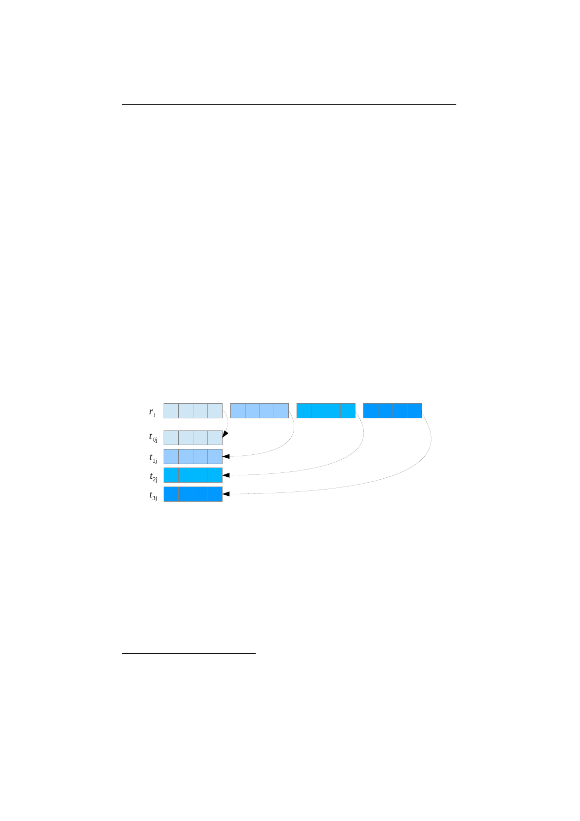
1.4. NUTS AND BOLTS CHAPTER 1. FUNDAMENTALS
Random seeding
Every thread uses the same kind of PRNG but with a
different seed. This is the default strategy used by the
Jenetics
library. The
RandomRegistry
is initialized with the
ThreadLocalRandom
class from the
ja-
va.util.concurrent
package. Random seeding works well for the most prob-
lems but without theoretical foundation.
20
If you assume that this strategy is
responsible for some non-reproducible results, consider using the
LCG64Shift-
Random PRNG instead, which uses block splitting as parallelization strategy.
Parameterization
All threads uses the same kind of PRNG but with different
parameters. This requires the PRNG to be parameterizable, which is not the
case for the Random object of the JDK. You can use the
LCG64ShiftRandom
class if you want to use this strategy. The theoretical foundation for these
method is weak. In a massive parallel environment you will need a reliable set
of parameters for every random stream, which are not trivial to find.
Block splitting
With this method each thread will be assigned a non-over-
lapping contiguous block of random numbers, which should be enough for the
whole runtime of the process. If the number of threads is not known in advance,
the length of each block should be chosen much larger then the maximal expected
number of threads. This strategy is used when using the LCG64ShiftRandom.-
ThreadLocal
class.This class assigns every thread a block of 2
56 ≈
7
,
2
·
10
16
random numbers.After 128 threads, the blocks are recycled, but with changed
seed.
Figure 1.4.2: Block splitting
Leapfrog
With the leapfrog method each thread
t∈[0, P )
only consumes the
Pth
random number and jump ahead in the random sequence by the number of
threads,
P
. This method requires the ability to jump very quickly ahead in the
sequence of random numbers by a given amount. Figure 1.4.3 on the next page
graphically shows the concept of the leapfrog method.
LCG64ShiftRandom21
The
LCG64ShiftRandom
class is a port of the
trng::-
lcg64_shift
PRNG class of the TRNG
22
library, implemented in C++.[
4
]
20
This is also expressed by Donald Knuth’s advice: »Random number generators should not
be chosen at random.«
21
The
LCG64ShiftRandom
PRNG is part of the
io.jenetics.prngine
module (see section 4.4
on page 99).
22http://numbercrunch.de/trng/
34
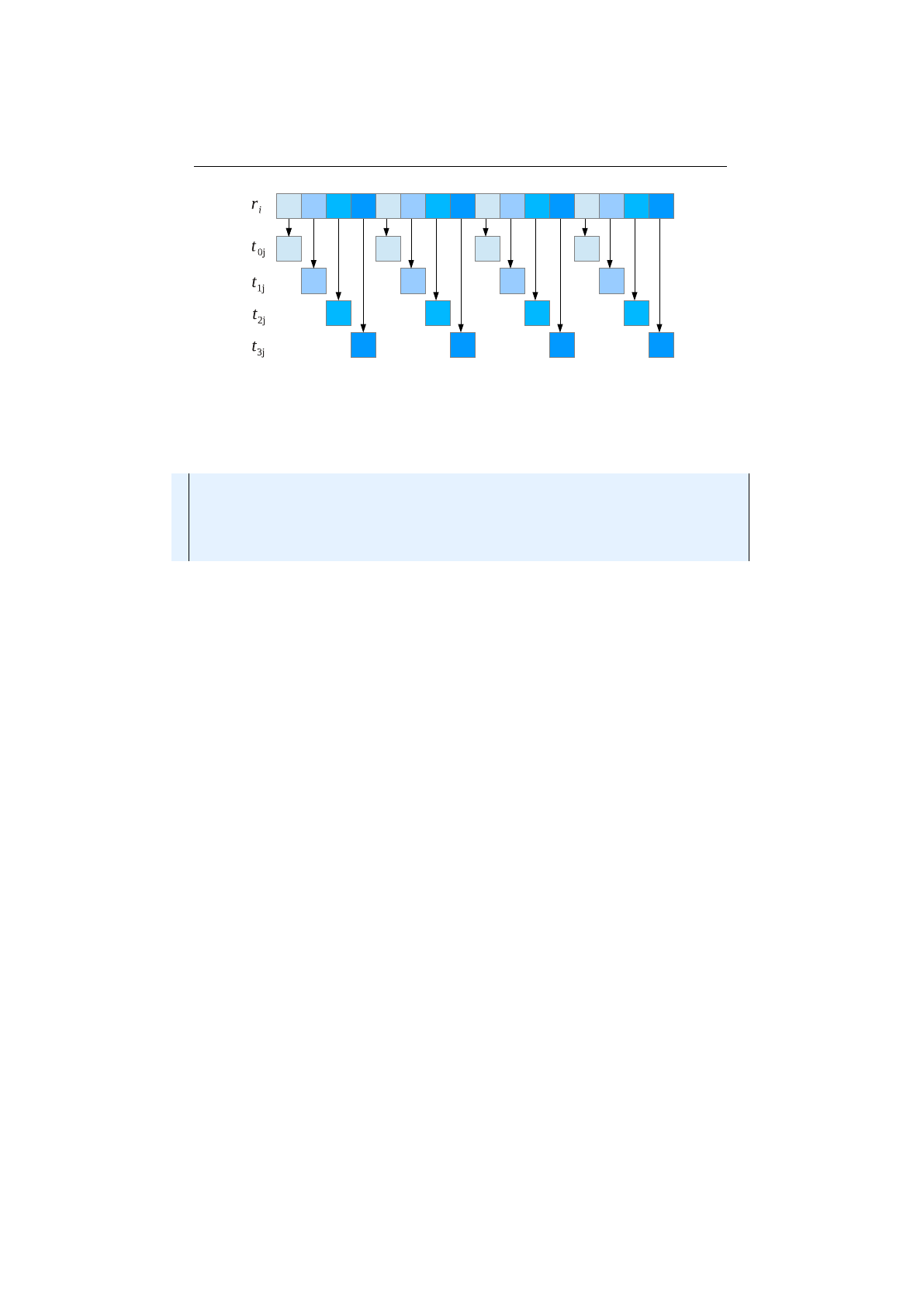
1.4. NUTS AND BOLTS CHAPTER 1. FUNDAMENTALS
Figure 1.4.3: Leapfrogging
It implements additional methods, which allows to implement the block split-
ting—and also the leapfrog—method.
1pu bl ic c l a s s LCG64ShiftRandom extends Random {
2public void s p l i t ( f i n a l int p , f i n a l i nt s ) ;
3public void jump( f i n a l long s t e p ) ;
4public void jump2 ( f i n a l int s ) ;
5...
6}
Listing 1.13: LCG64ShiftRandom class
Listing 1.13 shows the interface used for implementing the block splitting and
leapfrog parallelizations technique. This methods have the following meaning:
split
Changes the internal state of the PRNG in a way that future calls to
nextLong()
will generated the
sth
sub-stream of
pth
sub-streams.
s
must
be within the range of
[0, p −1)
. This method is used for parallelization
via leapfrogging.
jump
Changes the internal state of the PRNG in such a way that the engine
jumps
s
steps ahead. This method is used for parallelization via block
splitting.
jump2
Changes the internal state of the PRNG in such a way that the engine
jumps 2
s
steps ahead. This method is used for parallelization via block
splitting.
1.4.3 Serialization
Jenetics
supports serialization for a number of classes, most of them are located
in the
io.jenetics
package. Only the concrete implementations of the
Gene
and the
Chromosome
interfaces implements the
Serializable
interface. This
gives a greater flexibility when implementing own Genes and Chromosomes.
•BitGene
•BitChromosome
•CharacterGene
•CharacterChromosome
•IntegerGene
•IntegerChromosome
•LongGene
•LongChomosome
35

1.4. NUTS AND BOLTS CHAPTER 1. FUNDAMENTALS
•DoubleGene
•DoubleChromosome
•EnumGene
•PermutationChromosome
•Genotype
•Phenotype
With the serialization mechanism you can write a population to disk and load
it into an new
EvolutionStream
at a later time. It can also be used to transfer
populations to evolution engines, running on different hosts, over a network link.
The
IO
class, located in the
io.jenetics.util
package, supports native Java
serialization.
1// C r e a t i n g r e s u l t p o p u l a t i o n .
2Ev ol ut io nRe su lt <DoubleGene , Double> r e s u l t = stream
3. l i m i t ( 1 0 0 )
4. c o l l e c t ( t o B e s t E v o l u t i o n R e s u l t ( ) ) ;
5
6// W ri t in g th e p o p u l a t i o n t o d i s k .
7final F i l e f i l e = new File(" p o p u l a t i o n . o b j " ) ;
8IO . o b j e c t . w r i t e ( r e s u l t . g e t P o p u l a t i o n ( ) , f i l e ) ;
9
10 // R ead in g t he p o p u l a t i o n fro m d i s k .
11 IS eq <Phe notype<G, C>> p o p u l a t i o n =
12 ( I Se q<Phenotype<G, C>>)IO . o b j e c t . re ad ( f i l e ) ;
13 Evoluti o nStream <DoubleGene , Double> stream = Engine
14 . b u i l d ( f f , g t f )
15 . stream ( p op u la ti on , 1) ;
1.4.4 Utility classes
The
io.jenetics.util
and the
io.jenetics.stat
package of the library con-
tains utility and helper classes which are essential for the implementation of the
GA.
io.jenetics.util.Seq
Most notable are the
Seq
interfaces and its implemen-
tation. They are used, among others, in the
Chromosome
and
Genotype
classes
and holds the
Gene
s and
Chromosome
s, respectively. The
Seq
interface itself
represents a fixed-sized, ordered sequence of elements. It is an abstraction over
the Java build-in array-type, but much safer to use for generic elements, because
there are no casts needed when using nested generic types.
Figure 1.4.4 on the next page shows the
Seq
class diagram with their most
important methods. The interfaces
MSeq
and
ISeq
are mutable, respectively
immutable specializations of the basis interface. Creating instances of the
Seq
interfaces is possible via the static factory methods of the interfaces.
1// C r ea t e " d i f f e r e n t " s e q u e n c e s .
2final Seq<I n t e g e r > a1 = Seq . o f ( 1 , 2 , 3 ) ;
3final MSeq<I n t e g e r > a2 = MSeq . o f ( 1 , 2 , 3 ) ;
4final IS eq<I n t e g e r > a3 = MSeq . o f ( 1 , 2 , 3 ) . t o I Se q ( ) ;
5final MSeq<I n t e g e r > a4 = a3 . co py ( ) ;
6
7// The ’ e q u a l s ’ method p er fo r m s e lemen t−w is e com p arison .
8a s s e r t ( a1 . e qu al s ( a2 ) && a1 != a2 ) ;
9a s s e r t ( a2 . e qu al s ( a3 ) && a2 != a3 ) ;
10 a s s e r t ( a3 . e qu al s ( a4 ) && a3 != a4 ) ;
36
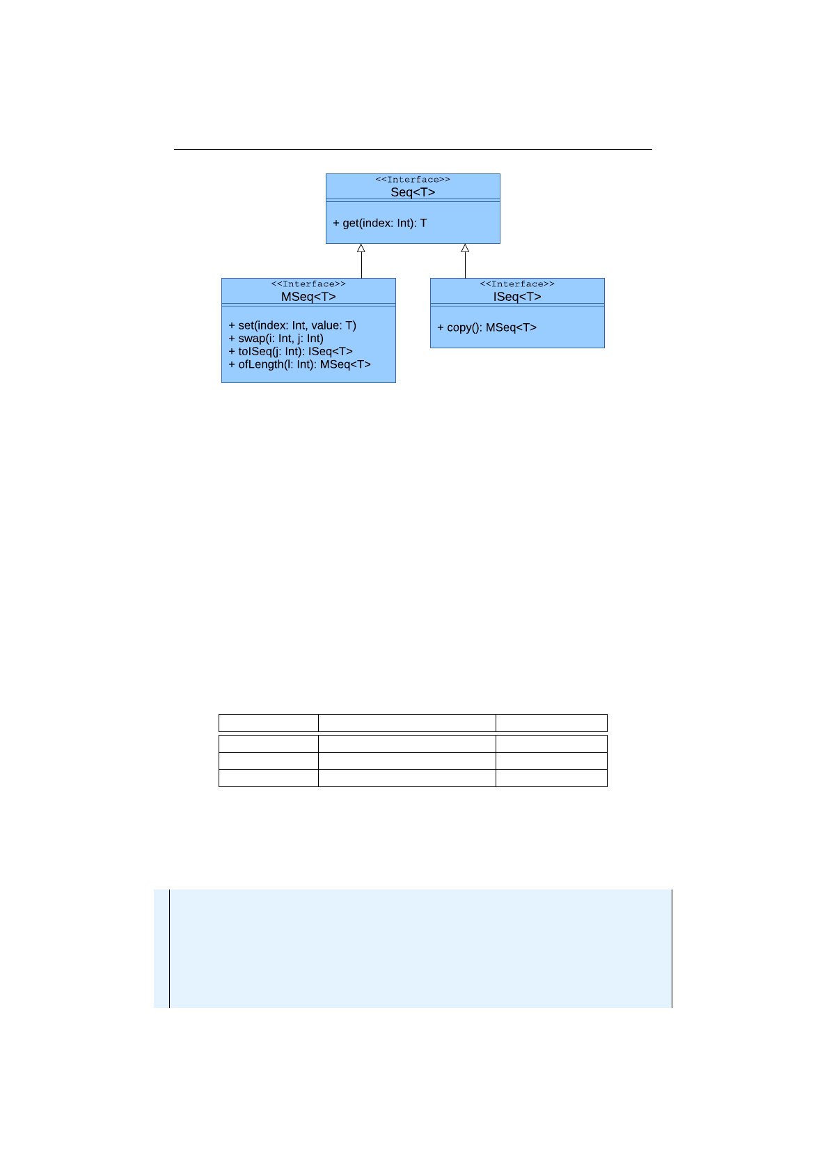
1.4. NUTS AND BOLTS CHAPTER 1. FUNDAMENTALS
Figure 1.4.4: Seq class diagram
How to create instances of the three
Seq
types is shown in the listing above.
The
Seq
classes also allows a more functional programming style. For a full
method description refer to the Javadoc.
io.jenetics.stat
This package contains classes for calculating statistical
moments. They are designed to work smoothly with the Java Stream API and
are divided into mutable (number) consumers and immutable value classes, which
holds the statistical moments. The additional classes calculate the
•minimum,
•maximum,
•sum,
•mean,
•variance,
•skewness and
•kurtosis value.
Numeric type Consumer class Value class
int IntMomentStatistics IntMoments
long LongMomentStatistics LongMoments
double DoubleMomentStatistics DoubleMoments
Table 1.4.1: Statistics classes
Table 1.4.1 contains the available statistical moments for the different numeric
types. The following code snippet shows an example on how to collect double
statistics from an given DoubleGene stream.
1// C o l l e c t i n g in t o an s t a t i s t i c s o b j ec t .
2DoubleChromosome chromosome = . . .
3Do ubl eM om en t St at is ti c s s t a t i s t i c s = chromosome . s t re a m ( )
4. c o l l e c t ( D o ub le Mo m en tS ta ti s ti cs
5. t oD ou bl eM ome nt St at is ti cs ( v −> v . do ubl eV alu e ( ) ) ) ;
6
7// C o l l e c t i n g i nt o an moments o b j e ct .
8DoubleMoments moments = chromosome . stream ( )
9. c o l l e c t ( DoubleMoments . toDoubleMoments ( v −> v . d ou bl eV alu e ( ) ) ) ;
37

1.4. NUTS AND BOLTS CHAPTER 1. FUNDAMENTALS
The
stat
package also contains a class for calculating the quantile
23
of a stream
of double values. It’s implementing algorithm, which is described in [
15
], calcu-
lates—or estimates—the quantile value on the fly, without storing the consumed
double values. This allows to use the
Quantile
class even for very large num-
ber of double values. How to calculate the first quartile of a given, random
DoubleStream is shown in the code snipped below.
1final Qu an til e q u a r t i l e = new Qu an ti le ( 0 . 2 5 ) ;
2new Random () . do ub les (10 _000 ) . fo rE a ch ( q u a r t i l e ) ;
3f i n a l double v a lu e = q u a r t i l e . g etV al u e ( ) ;
Be aware, that the calculated quartile is just an estimation. For a sufficient
accuracy, the stream size should be sufficiently large (size 100).
23https://en.wikipedia.org/wiki/Quantile
38

Chapter 2
Advanced topics
This section describes some advanced topics for setting up an evolution
Engine
or
EvolutionStream
. It contains some problem encoding examples and how to
override the default validation strategy of the given Genotypes. The last section
contains a detailed description of the implemented termination strategies.
2.1 Extending Jenetics
The
Jenetics
library was designed to give you a great flexibility in transforming
your problem into a structure that can be solved by an GA. It also comes with
different implementations for the base data-types (genes and chromosomes) and
operators (alterers and selectors). If it is still some functionality missing, this
section describes how you can extend the existing classes. Most of the extensible
classes are defined by an interface and have an abstract implementation which
makes it easier to extend it.
2.1.1 Genes
Gene
s are the starting point in the class hierarchy. They hold the actual
information, the alleles, of the problem domain. Beside the classical bit-gene,
Jenetics
comes with gene implementations for numbers (
double
-,
int
- and
long values), characters and enumeration types.
For implementing your own gene type you have to implement the
Gene
interface with three methods: (1) the
getAllele
() method which will return the
wrapped data, (2) the
newInstance
method for creating new, random instances
of the gene—must be of the same type and have the same constraint—and (3)
the
isValid()
method which checks if the gene fulfill the expected constraints.
The gene constraint might be violated after mutation and/or recombination. If
you want to implement a new number-gene, e. g. a gene which holds complex
values, you may want extend it from the abstract
NumericGene
class. Every
Gene
extends the
Serializable
interface. For normal genes there is no more
work to do for using the Java serialization mechanism.
39

2.1. EXTENDING JENETICS CHAPTER 2. ADVANCED TOPICS
The custom
Gene
s and
Chromosome
s implementations must use the
Random
engine available via the
RandomRegistry.getRandom
method
when implementing their factory methods. Otherwise it is not possible
to seamlessly change the
Random
engine by using the
RandomRegistry-
.setRandom method.
If you want to support your own allele type, but want to avoid the effort of
implementing the
Gene
interface, you can alternatively use the
AnyGene
class. It
can be created with
AnyGene.of(Supplier, Predicate)
. The given
Supplier
is responsible for creating new random alleles, similar to the
newInstance
method in the
Gene
interface. Additional validity checks are performed by the
given Predicate.
1c l a s s LastMonday {
2// C re at es new random ’ Loca lDate ’ o b j e c t s .
3pr iv at e s t a t i c L oc alDat e nextMonday ( ) {
4final Random random = RandomRegistry . getRandom ( ) ;
5LocalDate
6. o f ( 2 0 15 , 1 , 5 )
7. p lus We ek s ( random . n e x t I n t ( 1 0 0 0 ) ) ;
8}
9
10 // Do some a d d i t i o n a l v a l i d i t y c heck .
11 pr iv at e s t a t i c boolean isValid(final Loc a lDate da t e ) { . . . }
12
13 // C re at e a new gene from th e random ’ S u p p l i e r ’ and
14 // v a l i d a t i o n ’ P re di c at e ’ .
15 private f i n a l AnyGene<LocalDate> gene = AnyGene
16 . o f ( LastMonday : : nextMonday , LastMonday : : i s V a l i d ) ;
17 }
Listing 2.1: AnyGene example
Example listing 2.1 shows the (almost) minimal setup for creating user defined
Gene
allele types. By convention, the
Random
engine, used for creating the
new
LocalDate
objects, must be requested from the
RandomRegistry
. With
the optional validation function,
isValid
, it is possible to reject
Genes
whose
alleles doesn’t conform some criteria.
The simple usage of the
AnyGene
has also its downsides. Since the
AnyGene
instances are created from function objects, serialization is not supported by
the
AnyGene
class. It is also not possible to use some
Alterer
implementations
with the AnyGene, like:
•GaussianMutator,
•MeanAlterer and
•PartiallyMatchedCrossover
2.1.2 Chromosomes
A new gene type normally needs a corresponding chromosome implementation.
The most important part of a chromosome is the factory method
newInstance
,
which lets the evolution
Engine
create a new
Chromosome
instance from a
40

2.1. EXTENDING JENETICS CHAPTER 2. ADVANCED TOPICS
sequence of
Gene
s. This method is used by the
Alterer
s when creating new,
combined
Chromosome
s. It is allowed, that the newly created chromosome has
a different length than the original one. The other methods should be self-
explanatory. The chromosome has the same serialization mechanism as the gene.
For the minimal case it can extends the Serializable interface.1
Just implementing the Serializable interface is sometimes not enough. You
might also need to implement the
readObject
and
writeObject
methods
for a more concise serialization result. Consider using the serialization proxy
pattern, item 90, described in Effective Java [6].
Corresponding to the
AnyGene
, it is possible to create chromosomes with
arbitrary allele types with the AnyChromosome.
1pu bl ic c l a s s LastMonday {
2// The used problem Codec .
3pr iv at e s t a t i c f i n a l Codec<LocalDate , AnyGene<LocalDate>>
4CODEC = Codec . o f (
5Genotype . o f ( AnyChromosome . o f ( LastMonday : : nextMonday ) ) ,
6gt −> gt . getGene ( ) . g e t A l l e l e ( )
7) ;
8
9// C re at es new random ’ Loca lDate ’ o b j e c t s .
10 pr iv at e s t a t i c L oc alDat e nextMonday ( ) {
11 final Random random = RandomRegistry . getRandom ( ) ;
12 LocalDate
13 . o f ( 2 0 15 , 1 , 5 )
14 . p lus We ek s ( random . n e x t I n t ( 1 0 0 0 ) ) ;
15 }
16
17 // The f i t n e s s f u n c t i o n : f i n d a monday a t the end o f the month .
18 pr iv at e s t a t i c in t fitness(final Loc a lDate da t e ) {
19 return da te . getDayOfMonth ( ) ;
20 }
21
22 pub li c s t a t i c void main ( final S t r i n g [ ] a r g s ) {
23 final Eng ine<AnyGene<L oca lD ate >, I n t e g e r > e n g i n e = E ngi ne
24 . b u i l d e r ( LastMonday : : f i t n e s s , CODEC)
25 . offspringSelector(new Ro u l e t te W h e e l Se l e c t o r <>() )
26 . b u i l d ( ) ;
27
28 final Phenotype<AnyGene<Lo ca lDa te >, I n t e g e r > b e s t =
29 e n g i n e . s tr e am ( )
30 . l i m i t ( 5 0 )
31 . c o l l e c t ( E v o l u t i o n R e s u l t . t oB es t Ph en ot y pe ( ) ) ;
32
33 System . out . p r i n t l n ( be s t ) ;
34 }
35 }
Listing 2.2: AnyChromosome example
Listing 2.2 shows a full usage example of the
AnyGene
and
AnyChromosome
class.
The example tries to find a Monday with a maximal day of month. An interesting
detail is, that an
Codec2
definition is used for creating new
Genotypes
and
1http://www.oracle.com/technetwork/articles/java/javaserial-1536170.html
2See section 2.3 on page 51 for a more detailed Codec description.
41

2.1. EXTENDING JENETICS CHAPTER 2. ADVANCED TOPICS
for converting them back to
LocalDate
alleles. The convenient usage of the
AnyChromosome
has to be payed by the same restriction as for the
AnyGene
:
no serialization support for the chromosome and not usable for all
Alterer
implementations.
2.1.3 Selectors
If you want to implement your own selection strategy you only have to implement
the Selector interface with the select method.
1@FunctionalInterface
2public i n te r fa c e Selector<
3Gextends Gene <?, G>,
4Cextends Comparable<? super C>
5> {
6public ISeq<Phenotype<G, C>> s e l e c t (
7Seq<Phenotype<G, C>> po pu l a t io n ,
8int count ,
9Optimize opt
10 ) ;
11 }
Listing 2.3: Selector interface
The first parameter is the original
population
from which the sub-population
is selected. The second parameter,
count
, is the number of individuals of the
returned sub-population. Depending on the selection algorithm, it is possible
that the sub-population contains more elements than the original one. The
last parameter,
opt
, determines the optimization strategy which must be used
by the selector. This is exactly the point where it is decided whether the GA
minimizes or maximizes the fitness function.
Before implementing a selector from scratch, consider to extend your selector
from the
ProbabilitySelector
(or any other available
Selector
implementa-
tion). It is worth the effort to try to express your selection strategy in terms of
selection property
P(i)
. Another way for re-using existing
Selector
implemen-
tation is by composition.
1pu bl ic c l a s s EliteSelector<
2Gextends Gene <?, G>,
3Cextends Comparable<? super C>
4>
5implements Selector<G, C>
6{
7private f i n a l TruncationSelector<G, C>
8_ e l i t e = new TruncationSelector <>();
9
10 private f i n a l To urnament S elector <G, C>
11 _r e st = new Tou r namentSe l ector <>(3) ;
12
13 public E l i t e S e l e c t o r ( ) {
14 }
15
16 @Override
17 public ISeq<Phenotype<G, C>> s e l e c t (
18 final Seq<Phenotype<G, C>> p o pu la t i o n ,
19 f i n a l i nt count ,
20 final Optimize opt
21 ) {
22 ISeq<Phenotype<G, C>> r e s u l t ;
42

2.1. EXTENDING JENETICS CHAPTER 2. ADVANCED TOPICS
23 i f ( p o p u l a t i o n . isEmpt y ( ) | | c ou nt <= 0 ) {
24 r e s u l t = I Seq . empty ( ) ;
25 }else {
26 f i n a l i nt e c = min ( count , _ eli te Co un t ) ;
27 r e s u l t = _ e l i t e . s e l e c t ( po pu la t i o n , ec , opt ) ;
28 r e s u l t = r e s u l t . append (
29 _r e st . s e l e c t ( po p u l at io n , max( 0 , c ou n t −e c ) , opt )
30 ) ;
31 }
32 return r e s u l t ;
33 }
34 }
Listing 2.4: Elite selector
Listing 2.4 on the preceding page shows how an elite selector could be imple-
mented by using the existing
Truncation
- and
TournamentSelector
. With
elite selection, the quality of the best solution in each generation monotoni-
cally increases over time.[
3
] Although this is not necessary, since the evolution
Engine
/
Stream
doesn’t throw away the best solution found during the evolution
process.
2.1.4 Alterers
For implementing a new alterer class it is necessary to implement the
Alterer
interface. You might do this if your new
Gene
type needs a special kind of
alterer not available in the Jenetics project.
1@FunctionalInterface
2public i n te r fa c e Alterer<
3Gextends Gene <?, G>,
4Cextends Comparable<? super C>
5> {
6public A l t e r e r R e s u l t <G, C> a l t e r (
7Seq<Phenotype<G, C>> po pu l a t io n ,
8long g e n e r a t i o n
9) ;
10 }
Listing 2.5: Alterer interface
The first parameter of the
alter
method is the population which has to be al-
tered. The second parameter is the
generation
of the newly created individuals
and the return value is the number of genes that has been altered.
To maximize the range of application of an
Alterer
, it is recommended
that they can handle Genotypes and Chromosomes with variable length.
2.1.5 Statistics
During the developing phase of an application which uses the
Jenetics
library,
additional statistical data about the evolution process is crucial. Such data can
help to optimize the parametrization of the evolution Engine. A good starting
point is to use the
EvolutionStatistics
class in the
io.jenetics.engine
package (see listing 1.10 on page 27). If the data in the
EvolutionStatistics
43

2.1. EXTENDING JENETICS CHAPTER 2. ADVANCED TOPICS
class doesn’t fit your needs, you simply have to write your own statistics class.
It is not possible to derive from the existing
EvolutionStatistics
class. This
is not a real restriction, since you still can use the class by delegation. Just
implement the Java Consumer<EvolutionResult<G, C>> interface.
2.1.6 Engine
The evolution
Engine
itself can’t be extended, but it is still possible to create an
EvolutionStream
without using the
Engine
class.
3
Because the
Evolution-
Stream
has no direct dependency to the
Engine
, it is possible to use an different,
special evolution Function.
1public f i n a l c l as s SpecialEngine {
2// The Genotype f a c t o r y .
3pr iv at e s t a t i c f i n a l Factory<Genotype<DoubleGene>> GTF =
4Genotype . o f ( DoubleChromosome . o f ( 0 , 1 ) ) ;
5
6// The f i t n e s s f u n c t i o n .
7pr iv at e s t a t i c Double f i t n e s s ( final Genotype<DoubleGene> gt ) {
8return gt . getGene ( ) . g e t A l l e l e ( ) ;
9}
10
11 // C re at e new e v o l u t i o n s t a r t o b j e c t .
12 pr iv at e s t a t i c E v o l u t i o n S t a r t <DoubleGene , Double>
13 start(f i n a l in t p o p u l a t i o n S i z e , f i n a l long g e n e r a t i o n ) {
14 final IS eq <Phe notyp e<DoubleGene , Double>> p o p u l a t i o n = GTF
15 . i n s t a n c e s ( )
16 . map( g t −> Phenotype
17 . o f ( gt , g e n e r a t i o n , S p e c i a l E n g i n e : : f i t n e s s ) )
18 . l i m i t ( p o p u l a t i o n S i z e )
19 . c o l l e c t ( IS e q . t o I S e q ( ) ) ;
20
21 return E v o l u t i o n S t a r t . o f ( p o pu l a ti o n , g e n e r a t i o n ) ;
22 }
23
24 // The s p e c i a l e v o l u t i o n f u n c t i o n .
25 pr iv at e s t a t i c E vo lu t io nR e su lt <DoubleGene , Double>
26 evolve( final E v o l u t i o n S t a r t <DoubleGene , Double> s t a r t ) {
27 return ...; // Add im ple me n ta tio n !
28 }
29
30 pub li c s t a t i c void main ( final S t r i n g [ ] a r g s ) {
31 final Genotype<DoubleGene> b e s t = E v ol u ti on St r ea m
32 . o f ( ( ) −> s t a r t ( 5 0 , 0 ) , S p e c i a l E n g i n e : : e v o l v e )
33 . limit (Limits . bySteadyFitness (10))
34 . l i m i t ( 1 0 0 )
35 . c o l l e c t ( E v o l u t i o n R e s u l t . t oB es tG en ot yp e ( ) ) ;
36
37 System . out . p r i n t l n ( " Bes t Genotype : " + b e s t ) ) ;
38 }
39 }
Listing 2.6: Special evolution engine
Listing 2.6 shows a complete implementation stub for using an own special
evolution Function.
3
Also refer to section 1.3.3.3 on page 25 on how to create an
EvolutionStream
from an
evolution Function.
44

2.2. ENCODING CHAPTER 2. ADVANCED TOPICS
2.2 Encoding
This section presents some encoding examples for common problems. The
encoding should be a complete and minimal expression of a solution to the
problem. An encoding is complete if it contains enough information to represent
every solution to the problem. An minimal encoding contains only the information
needed to represent a solution to the problem. If an encoding contains more
information than is needed to uniquely identify solutions to the problem, the
search space will be larger than necessary.
Whenever possible, the encoding should not be able to represent infeasible
solutions. If a genotype can represent an infeasible solution, care must be taken
in the fitness function to give partial credit to the genotype for its »good« genetic
material while sufficiently penalizing it for being infeasible. Implementing a
specialized
Chromosome
, which won’t create invalid encodings can be a solution
to this problem. In general, it is much more desirable to design a representation
that can only represent valid solutions so that the fitness function measures only
fitness, not validity. An encoding that includes invalid individuals enlarges the
search space and makes the search more costly. A deeper analysis of how to
create encodings can be found in [27] and [26].
Some of the encodings represented in the following sections has been imple-
mented by
Jenetics
, using the
Codec4
interface, and are available through static
factory methods of the io.jenetics.engine.Codecs class.
2.2.1 Real function
Jenetics
contains three different numeric gene and chromosome implementations,
which can be used to encode a real function, f:R→R:
•IntegerGene/Chromosome,
•LongGene/Chromosome and
•DoubleGene/Chromosome.
It is quite easy to encode a real function. Only the minimum and maximum
value of the function domain must be defined. The
DoubleChromosome
of length
1 is then wrapped into a Genotype.
1Genotype . o f (
2DoubleChromosome . o f ( min , max , 1 )
3) ;
Decoding the double value from the Genotype is also straight forward. Just
get the first gene from the first chromosome, with the
getGene()
method, and
convert it to a double.
1s t a t i c double toDouble ( final Genotype<DoubleGene> gt ) {
2return gt . getGene ( ) . d ou ble Va lue ( ) ;
3}
When the
Genotype
only contains scalar chromosomes
5
, it should be clear, that
it can’t be altered by every
Alterer
. That means, that none of the
Crossover
4See section 2.3 on page 51.
5Scalar chromosomes contains only one gene.
45

2.2. ENCODING CHAPTER 2. ADVANCED TOPICS
alterers will be able to create modified
Genotype
s. For scalars the appropriate
alterers would be the MeanAlterer,GaussianAlterer and Mutator.
Scalar
Chromosome
s and/or
Genotype
s can only be altered by
MeanAlterer
,
GaussianAlterer
and
Mutator
classes. Other alterers
are allowed, but will have no effect on the Chromosomes.
2.2.2 Scalar function
Optimizing a function
f(x1, ..., xn)
of one or more variable whose range is
one-dimensional, we have two possibilities for the Genotype encoding.[
31
] For
the first encoding we expect that all variables,
xi
, have the same minimum
and maximum value. In this case we can simply create a
Genotype
with a
Numeric Chromosome of the desired length n.
1Genotype . o f (
2DoubleChromosome . o f ( min , max , n )
3) ;
The decoding of the
Genotype
requires a cast of the first
Chromosome
to a
DoubleChromosome
. With a call to the
DoubleChromosome.toArray()
method
we return the variables (x1, ..., xn)as double[] array.
1s t a t i c double [] toScalars ( final Genotype<DoubleGene> g t ) {
2return gt . getChromosome ( ) . as ( DoubleChromosome . c l a s s ) . t oArray ( ) ;
3}
With the first encoding you have the possibility to use all available alterers,
including all Crossover alterer classes.
The second encoding must be used if the minimum and maximum value of
the variables
xi
can’t be the same for all
i
. For the different domains, each
variable
xi
is represented by a
Numeric Chromosome
with length one. The final
Genotype will consist of nChromosomes with length one.
1Genotype . o f (
2DoubleChromosome . o f ( min1 , max1 , 1) ,
3DoubleChromosome . o f ( min2 , max2 , 1) ,
4...
5DoubleChromosome . o f ( minn , maxn , 1 )
6) ;
With the help of the new Java Stream API, the decoding of the
Genotype
can
be done in a view lines. The
DoubleChromosome
stream, which is created from
the chromosome
Seq
, is first mapped to
double
values and then collected into
an array.
1s t a t i c double [] toScalars ( final Genotype<DoubleGene> g t ) {
2return gt . s tream ( )
3. mapToDouble ( c −> c . getGene ( ) . do ubl eV alu e ( ) )
4. toA rray ( ) ;
5}
As already mentioned, with the use of scalar chromosomes we can only use the
MeanAlterer,GaussianAlterer or Mutator alterer class.
If there are performance issues in converting the
Genotype
into a
double[]
array, or any other numeric array, you can access the
Gene
s directly via the
46

2.2. ENCODING CHAPTER 2. ADVANCED TOPICS
Genotype.get(i, j)
method and than convert it to the desired numeric value,
by calling intValue(),longValue() or doubleValue().
2.2.3 Vector function
A function
f(X1, ..., Xn)
, of one to
n
variables whose range is
m
-dimensional, is
encoded by
mDoubleChromosome
s of length
n
.[
32
] The domain–minimum and
maximum values–of one variable Xiare the same in this encoding.
1Genotype . o f (
2DoubleChromosome . o f ( min1 , max1 , m) ,
3DoubleChromosome . o f ( min2 , max2 , m) ,
4...
5DoubleChromosome . o f ( minn , maxn , m)
6) ;
The decoding of the vectors is quite easy with the help of the Java Stream API. In
the first
map
we have to cast the
Chromosome<DoubleGene>
object to the actual
DoubleChromosome
. The second
map
then converts each
DoubleChromosome
to
a
double[]
array, which is collected to an 2-dimensional
double[n][m]
array
afterwards.
1s t a t i c double [ ] [ ] t o V e c t o r s ( final Genotype<DoubleGene> g t ) {
2return gt . s tream ( )
3. map( dc −> dc . as ( DoubleChromosome . c l a s s ) . toArra y ( ) )
4. toArray(double [ ] [ ] : : new) ;
5}
For the special case of
n
= 1, the decoding of the
Genotype
can be simplified to
the decoding we introduced for scalar functions in section 2.2.2.
1s t a t i c double [ ] to Ve ct o r ( final Genotype<DoubleGene> g t ) {
2return gt . getChromosome ( ) . as ( DoubleChromosome . c l a s s ) . t oArray ( ) ;
3}
2.2.4 Affine transformation
An affine transformation
6 7
is usually performed by a matrix multiplication
with a transformation matrix—in a homogeneous coordinates system
8
. For a
transformation in R2, we can define the matrix A9:
A=
a11 a12 a13
a21 a22 a23
001
.(2.2.1)
A simple representation can be done by creating a
Genotype
which contains
two DoubleChromosomes with a length of 3.
1Genotype . o f (
2DoubleChromosome . o f ( min , max , 3 ) ,
3DoubleChromosome . o f ( min , max , 3 )
4) ;
6https://en.wikipedia.org/wiki/Affine_transformation
7http://mathworld.wolfram.com/AffineTransformation.html
8https://en.wikipedia.org/wiki/Homogeneous_coordinates
9https://en.wikipedia.org/wiki/Transformation_matrix
47

2.2. ENCODING CHAPTER 2. ADVANCED TOPICS
The drawback with this kind of encoding is, that we will create a lot of invalid
(non-affine transformation matrices) during the evolution process, which must
be detected and discarded. It is also difficult to find the right parameters for
the min and max values of the DoubleChromosomes.
A better approach will be to encode the transformation parameters instead
of the transformation matrix. The affine transformation can be expressed by the
following parameters:
•sx– the scale factor in xdirection
•sy– the scale factor in ydirection
•tx– the offset in xdirection
•ty– the offset in ydirection
•θ– the rotation angle clockwise around origin
•kx– shearing parallel to xaxis
•ky– shearing parallel to yaxis
This parameters can then be represented by the following Genotype.
1Genotype . o f (
2// S c a l e
3DoubleChromosome . o f ( sxMin , sxMax ) ,
4DoubleChromosome . o f ( syMin , syMax ) ,
5// Translation
6DoubleChromosome . o f ( txMin , txMax ) ,
7DoubleChromosome . o f ( tyMin , tyMax ) ,
8// Ro ta t io n
9DoubleChromosome . o f ( thMin , thMax ) ,
10 // Shear
11 DoubleChromosome . o f ( kxMin , kxMax ) ,
12 DoubleChromosome . o f ( kyMin , kxMax )
13 )
This encoding ensures that no invalid
Genotype
will be created during the
evolution process, since the crossover will be only performed on the same kind of
chromosome (same chromosome index). To convert the
Genotype
back to the
transformation matrix A, the following equations can be used [14]:
a11 =sxcos θ+kxsysin θ
a12 =sykxcos θ−sxsin θ
a13 =tx
a21 =kysxcos θ+sysin θ(2.2.2)
a22 =sycos θ−sxkysin θ
a23 =ty
This corresponds to an transformation order of T·Sh·Sc·R:
1 0 tx
0 1 ty
0 0 1
·
1kx0
ky1 0
0 0 1
·
sx0 0
0sy0
0 0 1
·
cos θ−sin θ0
sin θcos θ0
0 0 1
.
In Java code, the conversion from the
Genotype
to the transformation matrix,
will look like this:
48
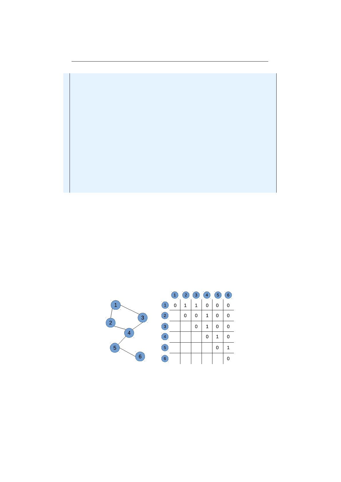
2.2. ENCODING CHAPTER 2. ADVANCED TOPICS
1s t a t i c double [ ] [ ] toM a tri x ( final Genotype<DoubleGene> gt ) {
2f i n a l double sx = gt . g e t (0 , 0) . doubl eVal u e () ;
3f i n a l double sy = gt . g e t (1 , 0) . doubl eVal u e () ;
4f i n a l double tx = gt . ge t (2 , 0) . doub leVal ue ( ) ;
5f i n a l double ty = gt . ge t (3 , 0) . doub leVal ue ( ) ;
6f i n a l double th = g t . g et ( 4 , 0 ) . d ou bl eV al u e ( ) ;
7f i n a l double kx = gt . g e t (5 , 0) . doub leVa l ue ( ) ;
8f i n a l double ky = gt . g e t (6 , 0) . doub leVa l ue ( ) ;
9
10 f i n a l double cos_th = co s ( th ) ;
11 f i n a l double si n_th = s i n ( th ) ;
12 f i n a l double a11 = co s_ th ∗s x + kx∗sy ∗sin_th ;
13 f i n a l double a12 = co s_ th ∗kx∗sy −sx ∗sin_th ;
14 f i n a l double a21 = co s_ th ∗ky∗sx + sy ∗sin_th ;
15 f i n a l double a22 = co s_ th ∗s y −ky∗sx ∗sin_th ;
16
17 return new double [][] {
18 {a11 , a12 , tx } ,
19 {a21 , a22 , ty } ,
20 { 0 . 0 , 0 . 0 , 1 . 0 }
21 } ;
22 }
For the introduced encoding all kind of alterers can be used. Since we have one
scalar DoubleChromosome, the rotation angle θ, it is recommended also to add
aMeanAlterer or GaussianAlterer to the list of alterers.
2.2.5 Graph
A graph can be represented in many different ways. The most known graph
representation is the adjacency matrix. The following encoding examples uses
adjacency matrices with different characteristics.
Undirected graph
In an undirected graph the edges between the vertices
have no direction. If there is a path between nodes
i
and
j
, it is assumed that
there is also path from jto i.
Figure 2.2.1: Undirected graph and adjacency matrix
Figure 2.2.1 shows an undirected graph and its corresponding matrix rep-
resentation. Since the edges between the nodes have no direction, the values
of the lower diagonal matrix are not taken into account. An application which
49
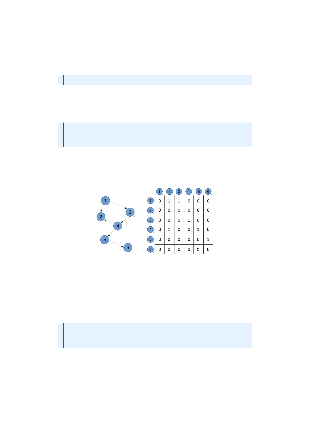
2.2. ENCODING CHAPTER 2. ADVANCED TOPICS
optimizes an undirected graph has to ignore this part of the matrix.10
1f i n a l i nt n = 6 ;
2final Genotype<BitGene> g t = Genotype . o f ( BitChromosome . o f ( n ) , n ) ;
The code snippet above shows how to create an adjacency matrix for a graph
with
n
= 6 nodes. It creates a genotype which consists of
nBitChromosome
s of
length
n
each. Whether the node
i
is connected to node
j
can be easily checked by
calling
gt.get(i-1, j-1).booleanValue()
. For extracting the whole matrix
as int[] array, the following code can be used.
1f i n a l i nt [ ] [ ] a r r a y = gt . toSe q ( ) . stream ( )
2. map( c −> c . toSe q ( ) . stream ( )
3. mapToInt ( BitGene : : o r d i n a l )
4. toA rray ( ) )
5. toArray( int [ ] [ ] : : new) ;
Directed graph
A directed graph (digraph) is a graph where the path between
the nodes have a direction associated with them. The encoding of a directed
graph looks exactly like the encoding of an undirected graph. This time the
whole matrix is used and the second diagonal matrix is no longer ignored.
Figure 2.2.2: Directed graph and adjacency matrix
Figure 2.2.2 shows the adjacency matrix of a digraph. This time the whole
matrix is used for representing the graph.
Weighted directed graph
A weighted graph associates a weight (label) with
every path in the graph. Weights are usually real numbers. They may be
restricted to rational numbers or integers.
The following code snippet shows how the
Genotype
of the matrix is created.
1f i n a l i nt n = 6 ;
2f i n a l double min = −1;
3f i n a l double max = 2 0 ;
4final Genotype<DoubleGene> g t = Genotype
5. o f ( DoubleChromosome . o f ( min , max , n ) , n ) ;
10
This property violates the minimal encoding requirement we mentioned at the beginning
of section 2.2 on page 45. For simplicity reason this will be ignored for the undirected graph
encoding.
50
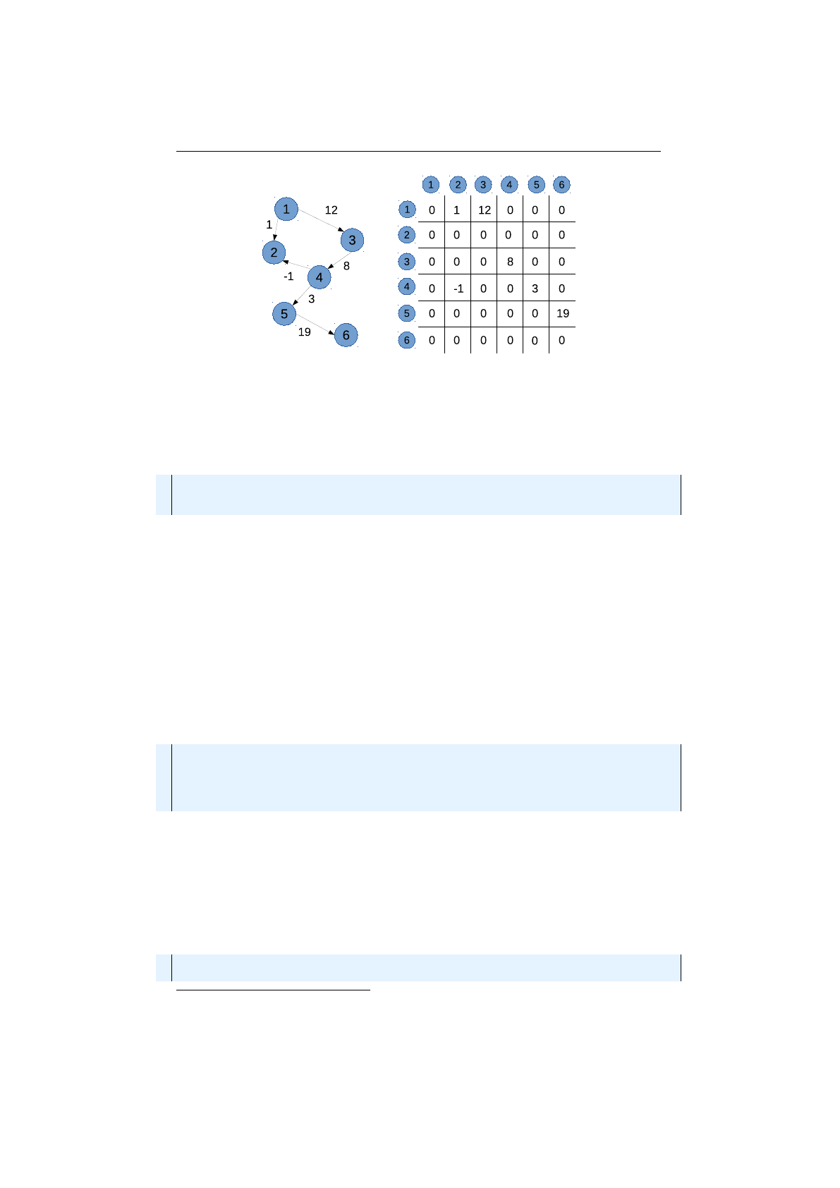
2.3. CODEC CHAPTER 2. ADVANCED TOPICS
Figure 2.2.3: Weighted graph and adjacency matrix
For accessing the single matrix elements, you can simply call
Genotype.get(i,
j).doubleValue()
. If the interaction with another library requires a
double-
[][] array, the following code can be used.
1f i n a l double [ ] [ ] ar r ay = gt . stream ( )
2. map( dc −> dc . as ( DoubleChromosome . c l a s s ) . toArra y ( ) )
3. toArray(double [ ] [ ] : : new) ;
2.3 Codec
The
Codec
interface—located in the
io.jenetics.engine
package—narrows
the gap between the fitness Function, which should be maximized/minimized,
and the
Genotype
representation, which can be understand by the evolution
Engine
. With the
Codec
interface it is possible to implement the encodings of
section 2.2 on page 45 in a more formalized way.
Normally, the
Engine
expects a fitness function which takes a
Genotype
as
input. This
Genotype
has then to be transformed into an object of the problem
domain. The usage
Codec
interface allows a tighter coupling of the
Genotype
definition and the transformation code.11
1public i n t e r f a c e Codec<T, G extends Gene <? , G>> {
2public Fa cto ry<Genotype<G>> e nc od ing ( ) ;
3public Fu nc tio n<Genotype<G>, T> d ec od er ( ) ;
4public defaul t T decode ( final Genotype<G> gt ) { . . . }
5}
Listing 2.7: Codec interface
Listing 2.7 shows the
Codec
interface. The
encoding()
method returns the
Genotype
factory, which is used by the
Engine
for creating new
Genotypes
.
The decoder
Function
, which is returned by the
decoder()
method, transforms
the
Genotype
to the argument type of the fitness
Function
. Without the
Codec
interface, the implementation of the fitness Function is polluted with code, which
transforms the
Genotype
into the argument type of the actual fitness
Function
.
1s t a t i c double eval(final Genotype<DoubleGene> gt ) {
2f i n a l double x = g t . getGene ( ) . d ou ble Va lue ( ) ;
11
Section 2.2 on page 45 describes some possible encodings for common optimization
problems.
51

2.3. CODEC CHAPTER 2. ADVANCED TOPICS
3// Do some c a l c u l a t i o n with ’ x ’ .
4return ...
5}
The
Codec
for the example above is quite simple and is shown below. It is not
necessary to implement the
Codec
interface, instead you can use the
Codec.of
factory method for creating new Codec instances.
1final DoubleRange domain = DoubleRange . of (0 , 2∗PI ) ;
2final Codec<Double , DoubleGene> c od ec = Codec . o f (
3Genotype . o f ( DoubleChromosome . o f ( domain ) ) ,
4gt −> gt . getChromosome ( ) . getGene ( ) . g e t A l l e l e ( )
5) ;
When using a
Codec
instance, the fitness
Function
solely contains code from
your actual problem domain—no dependencies to classes of the
Jenetics
library.
1s t a t i c double eval(f i n a l double x ) {
2// Do some c a l c u l a t i o n with ’ x ’ .
3return ...
4}
Jenetics
comes with a set of standard encodings, which are created via static
factory methods of the
io.jenetics.engine.Codecs
class. The following sub-
sections shows some of the implementation of this methods.
2.3.1 Scalar codec
Listing 2.8 shows the implementation of the
Codecs.ofScalar
factory method—for
Integer scalars.
1static Codec<I n t e g e r , In t eg er G en e > o f S c a l a r ( In tRa ng e domain ) {
2return Codec . o f (
3Genotype . o f ( IntegerChromosome . o f ( domain ) ) ,
4gt −> gt . getChromosome ( ) . getGene ( ) . g e t A l l e l e ( )
5) ;
6}
Listing 2.8: Codec factory method: ofScalar
The usage of the
Codec
, created by this factory method, simplifies the imple-
mentation of the fitness
Function
and the creation of the evolution
Engine
.
For scalar types, the saving, in complexity and lines of code, is not that big, but
using the factory method is still quite handy. The following listing demonstrates
the interaction between Codec, fitness Function and evolution Engine.
1c l a s s Main {
2// F i t n e s s f u nc t i o n d i r e c t l y t a ke s an ’ i n t ’ v al ue .
3s t a t i c double fitness(int arg ) {
4return ...;
5}
6pub li c s t a t i c void main ( S t r i n g [ ] a r gs ) {
7final Eng in e<I n te g er G en e , Doub le> e n g i n e = E ngi ne
8. b u i l d e r ( Main : : f i t n e s s , o f S c a l a r ( IntRange . o f ( 0 , 10 0) ) )
9. b u i l d ( ) ;
10 ...
11 }
12 }
52

2.3. CODEC CHAPTER 2. ADVANCED TOPICS
2.3.2 Vector codec
In listing 2.9, the
ofVector
factory method returns a
Codec
for an
int[]
array.
The
domain
parameter defines the allowed range of the
int
values and the
length defines the length of the encoded int array.
1static Codec<int [ ] , In t eg e rG e ne > o f V e c t o r (
2IntRange domain ,
3int length
4) {
5return Codec . o f (
6Genotype . o f ( Int ege rC hr omo so me . o f ( domain , l e n g t h ) ) ,
7gt −> gt . getChromosome ( )
8. as ( IntegerChromosome . c l a s s )
9. toA rray ( )
10 ) ;
11 }
Listing 2.9: Codec factory method: ofVector
The usage example of the vector
Codec
is almost the same as for the scalar
Codec
. As additional parameter, we need to define the length of the desired
array and we define our fitness function with an int[] array.
1c l a s s Main {
2// F i t n e s s f u nc t i o n d i r e c t l y t a ke s an ’ i n t [ ] ’ ar ra y .
3s t a t i c double fitness(int [ ] a r g s ) {
4return ...;
5}
6pub li c s t a t i c void main ( S t r i n g [ ] a r gs ) {
7final Eng in e<I n te g er G en e , Doub le> e n g i n e = E ngi ne
8. builder(
9Main : : f i t n e s s ,
10 o f V e c t o r ( In tR an ge . o f ( 0 , 1 0 0) , 1 0) )
11 . b u i l d ( ) ;
12 ...
13 }
14 }
2.3.3 Matrix codec
In listing 2.10, the
ofMatrix
factory method returns a
Codec
for an
int[][]
matrix. The
domain
parameter defines the allowed range of the
int
values and
the rows and cols defines the dimension of the matrix.
1static Codec<int [ ] [ ] , Inte gerG e ne > of M a tr ix (
2IntRange domain ,
3int rows ,
4int c o l s
5) {
6return Codec . o f (
7Genotype . o f (
8IntegerChromosome . o f ( domain , c o l s ) . i n s t a n c e s ( )
9. l i m i t ( rows )
10 . c o l l e c t ( IS e q . t o I S e q ( ) )
11 ) ,
12 gt −> gt . stre am ( )
13 . map( ch −> ch . s tream ( )
14 . mapToInt ( I n te g e r G en e : : i n t V a l u e )
15 . toA rray ( ) )
16 . toArray( int [ ] [ ] : : new)
53

2.3. CODEC CHAPTER 2. ADVANCED TOPICS
17 ) ;
18 }
Listing 2.10: Codec factory method: ofMatrix
2.3.4 Subset codec
There are currently two kinds of subset codecs you can choose from: finding
subsets with variable size and with fixed size.
Variable-sized subsets
A Codec for variable-sized subsets can be easily
implemented with the use of a BitChromosome, as shown in listing 2.11.
1static <T> Codec<ISeq <T>, BitGene> o fS ubS et ( IS eq <T> b a s i c S e t ) {
2return Codec . o f (
3Genotype . o f ( BitChromosome . o f ( b a s i c S e t . l en g t h ( ) ) ) ,
4gt −> gt . getChromosome ( )
5. as ( BitChromosome . c l a s s ) . on es ( )
6. mapToObj ( b a s i c S e t )
7. c o l l e c t ( IS e q . t o I S e q ( ) )
8) ;
9}
Listing 2.11: Codec factory method: ofSubSet
The following usage example of subset
Codec
shows a simplified version of the
Knapsack problem (see section 5.4 on page 110). We try to find a subset, from
the given basic
SET
, where the sum of the values is as big as possible, but smaller
or equal than 20.
1c l a s s Main {
2// The b a s i c s e t fr om wh ere t o c ho o s e an ’ o pt i m al ’ s u b s e t .
3f i n a l s t a t i c I Seq <I n t e g e r > SET =
4ISe q . o f ( 1 , 2 , 3 , 4 , 5 , 6 , 7 , 8 , 9 , 1 0) ;
5
6// F i t n e s s f u nc t i o n d i r e c t l y t a ke s an ’ i n t ’ v al ue .
7s t a t i c i nt f i t n e s s ( ISe q<I n t e g e r > s u b s e t ) {
8a s s e r t ( s ub s e t . s i z e ( ) <= SET . s i z e ( ) ) ;
9f i n a l i nt s i z e = s u b s e t . stream ( ) . c o l l e c t (
10 C o l l e c t o r s . summingInt ( I n t e g e r : : i nt Va lu e ) ) ;
11 return s i z e <= 20 ? s i z e : 0 ;
12 }
13 pub li c s t a t i c void main ( S t r i n g [ ] a r gs ) {
14 final Eng in e<BitG ene , D ouble> e n g i n e = E ng in e
15 . b u i l d e r ( Main : : f i t n e s s , ofS ub Se t (SET) )
16 . b u i l d ( ) ;
17 ...
18 }
19 }
Fixed-size subsets
The second kind of subset codec allows you to find the
best subset of a given, fixed size. A classical usage for this encoding is the Subset
sum problem12:
Given a set (or multi-set) of integers, is there a non-empty subset whose sum is
zero? For example, given the set
{−7,−3,−2,5,8}
, the answer is yes because
the subset {−3,−2,5}sums to zero. The problem is NP-complete.13
12https://en.wikipedia.org/wiki/Subset_sum_problem
13https://en.wikipedia.org/wiki/NP-completeness
54

2.3. CODEC CHAPTER 2. ADVANCED TOPICS
1pu bl ic c l a s s SubsetSum
2implements Problem<IS eq<I n t e g e r >, EnumGene<I n t e g e r >, I n t e g e r >
3{
4private f i n a l I Se q<I n t e g e r > _ b a si c S et ;
5private f i n a l int _ s iz e ;
6
7public SubsetSum ( IS eq<I n t e g e r > b a s i c S e t , int s i z e ) {
8_ ba si cS et = b a s i c S e t ;
9_s i ze = s i z e ;
10 }
11
12 @Override
13 public Fu nc tio n<ISe q<I n t e g e r >, I n t e g e r > f i t n e s s ( ) {
14 return s u b s e t −> abs (
15 s ub s et . stream ( ) . mapToInt ( I n t e g e r : : i nt V al u e ) . sum ( ) ) ;
16 }
17
18 @Override
19 public Codec<ISe q<I n t e g e r >, EnumGene<I n t e g e r >> c od ec ( ) {
20 return Codecs . of Sub Se t ( _ basi c Set , _ si z e ) ;
21 }
22 }
2.3.5 Permutation codec
This kind of codec can be used for problems where optimal solution depends on
the order of the input elements. A classical example for such problems is the
Knapsack problem (chapter 5.5 on page 112).
1static <T> Codec<T [ ] , EnumGene<T>> of P er mu tat io n (T . . . a l l e l e s ) {
2return Codec . o f (
3Genotype . o f ( PermutationChromosome . o f ( a l l e l e s ) ) ,
4gt −> gt . getChromosome ( ) . s tream ( )
5. map( EnumGene : : g e t A l l e l e )
6. t oA rr ay ( l e n g t h −> (T [ ] ) Array . newI nst anc e (
7a l l e l e s [ 0 ] . g e t C l a s s ( ) , l e n gt h ) )
8) ;
9}
Listing 2.12: Codec factory method: ofPermutation
Listing 2.12 shows the implementation of a permutation codec, where the order
of the given alleles influences the value of the fitness function. An alternate
formulation of the traveling salesman problem is shown in the following listing.
It uses the permutation codec in listing 2.12 and uses
io.jenetics.jpx.Way-
Points, from the JPX14 project, for representing the city locations.
1pu bl ic c l a s s TSM {
2// The l o c a t i o n s to v i s i t .
3s t a t i c f i n a l ISeq<WayPoint> POINTS = ISe q . o f ( . . . ) ;
4
5// The per muta tio n c ode c .
6s t a t i c f i n a l Codec<ISeq<WayPoint>, EnumGene<WayPoint>>
7CODEC = Codecs . ofP e rm ut ati on (POINTS) ;
8
9// The f i t n e s s f u n c t i o n ( i n the proble m domain ) .
10 s t a t i c double d i s t ( final ISeq<WayPoint> path ) {
11 return path . stream ( )
12 . c o l l e c t ( Geoid .DEFAULT. toTourLength ( ) )
14https://github.com/jenetics/jpx
55
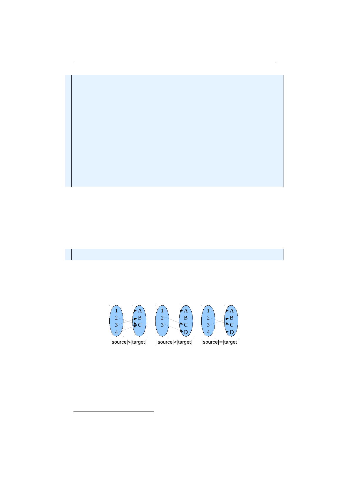
2.3. CODEC CHAPTER 2. ADVANCED TOPICS
13 . t o ( Length . Unit .METER) ;
14 }
15
16 // The e v o l u t i o n e n gi ne .
17 s t a t i c f i n a l Engine<EnumGene<WayPoint >, Double> ENGINE = Engine
18 . b u i l d e r (TSM : : d i s t , CODEC)
19 . o p t i m i z e ( O pt im iz e . MINIMUM)
20 . b u i l d ( ) ;
21
22 // Find the s o l u t i o n .
23 pub li c s t a t i c void main ( final S t r i n g [ ] a r g s ) {
24 final ISeq<WayPoint> r e s u l t = CODEC. decode (
25 ENGINE . stream ( )
26 . l i m i t ( 1 0 )
27 . c o l l e c t ( E v o l u t i o n R e s u l t . t oB es tG en ot yp e ( ) )
28 ) ;
29
30 System . out . p r i n t l n ( r e s u l t ) ;
31 }
32 }
2.3.6 Mapping codec
This codec is a variation of the permutation codec. Instead of permuting the
elements of a given array, it permutes the mapping of elements of a source set to
the elements of a target set. The code snippet below shows the method of the
Codecs
class, which creates a mapping codec from a given source- and target
set.
1pub li c s t a t i c <A, B> Codec<Map<A, B>, EnumGene<I n t e g e r >>
2ofMapping ( ISeq <? extends A> s our ce , ISeq <? extends B> t a r g e t ) ;
It is not necessary that the source and target set are of the same size. If
|source|>
|target|
, the returned mapping function is surjective, if
|source|<|target|
, the
mapping is injective and if
|source|
=
|target|
, the created mapping is bijective.
In every case the size of the encoded
Map
is
|target|
. Figure 2.3.1 shows the
described different mapping types in graphical form.
Figure 2.3.1: Mapping codec types
With
|source|
=
|target|
, you will create a codec for the assignment problem.
The problem is defined by a number of workers and a number of jobs. Every
worker can be assigned to perform any job. The cost for a worker may vary
depending on the worker-job assignment. It is required to perform all jobs by
assigning exactly one worker to each job and exactly one job to each worker in
such a way which optimizes the total assignment costs.
15
The costs for such
15https://en.wikipedia.org/wiki/Assignment_problem
56

2.3. CODEC CHAPTER 2. ADVANCED TOPICS
worker-job assignments are usually given by a matrix. Such an example matrix
is shown in table 2.3.1.
Job 1 Job 2 Job 3 Job 4
Worker 1 13 4 7 6
Worker 2 1 11 5 4
Worker 3 6 7 3 8
Worker 4 1 3 5 9
Table 2.3.1: Worker-job cost
If your worker-job cost can be expressed by a matrix, the Hungarian algo-
rithm
16
can find an optimal solution in
On3
time. You should consider this
deterministic algorithm before using a GA.
2.3.7 Composite codec
The composite
Codec
factory method allows to combine two or more
Codec
s
into one. Listing 2.13 shows the method signature of the factory method, which
is implemented directly in the Codec interface.
1static <G extends Gene <? , G>, A, B, T> Codec<T, G> o f (
2final Codec<A, G> codec1 ,
3final Codec<B, G> codec2 ,
4final Bi Function<A, B, T> de co de r
5) { . . . }
Listing 2.13: Composite Codec factory method
As you can see from the method definition, the combining
Codecs
and the
combined Codec have the same Gene type.
Only
Codec
s which the same
Gene
type can be composed by the combining
factory methods of the Codec class.
The following listing shows a full example which uses a combined
Codec
. It
uses the subset
Codec
, introduced in section 2.3.4 on page 54, and combines it
into a Tuple of subsets.
1c l a s s Main {
2s t a t i c f i n a l IS eq <I n t e g e r > SET =
3ISe q . o f ( 1 , 2 , 3 , 4 , 5 , 6 , 7 , 8 , 9) ;
4
5// R e s ul t ty pe o f th e combined ’ Codec ’ .
6s t a t i c f i n a l c l a s s Tuple<A, B> {
7final A first ;
8final B se con d ;
9Tuple ( final A f i r s t , final B seco n d ) {
10 this . f i r s t = f i r s t ;
11 this . second = second ;
12 }
13 }
14
16https://en.wikipedia.org/wiki/Hungarian_algorithm
57

2.4. PROBLEM CHAPTER 2. ADVANCED TOPICS
15 s t a t i c i nt f i t n e s s ( Tuple<ISe q<I n t e g e r >, IS eq<I n t e g e r >> a r g s ) {
16 return a r g s . f i r s t . stream ( )
17 . mapToInt ( I n t e g e r : : i n tV al ue )
18 . sum ( ) −
19 a r g s . s ec o nd . s tr ea m ( )
20 . mapToInt ( I n t e g e r : : i n tV al ue )
21 . sum ( ) ;
22 }
23
24 pub li c s t a t i c void main ( S t r i n g [ ] a r gs ) {
25 // Combined ’ Codec ’ .
26 final Codec<Tuple<IS eq<I n t e g e r >, I Seq <I n t e g e r >>, BitGene>
27 c od ec = Codec . o f (
28 Codecs . of Sub Se t (SET) ,
29 Codecs . of Sub Se t (SET) ,
30 Tuple : : new
31 ) ;
32
33 final Eng ine<BitGene , I n t e g e r > e n g i n e = Eng ine
34 . b u i l d e r ( Main : : f i t n e s s , co de c )
35 . b u i l d ( ) ;
36
37 final Phenotype<BitGene , I n t e g e r > pt = e n g i n e . st re am ( )
38 . l i m i t ( 1 0 0 )
39 . c o l l e c t ( E v o l u t i o n R e s u l t . t oB es t Ph en ot y pe ( ) ) ;
40
41 // Use t he c o de c f o r c o n v e r t i n g t he r e s u l t ’ Genotype ’ .
42 final Tuple<I Se q<I n t e g e r >, IS eq<I n t e g e r >> r e s u l t =
43 cod ec . d ec od er ( ) . ap ply ( pt . getGenoty pe ( ) ) ;
44 }
45 }
If you have to combine more than one Codec into one, you have to use the
second, more general, combining function:
Codec.of(ISeq<Codec<?, G>>,-
Function<Object[], T>)
. The example above shows how to use the general
combining function. It is just a little bit more verbose and requires explicit casts
for the sub-codec types.
1final Codec<T ri p l e <Long , Long , Long>, LongGene>
2cod ec = Codec . o f ( ISeq . of (
3Codecs . o f S c a l a r ( LongRange . o f ( 0 , 100 ) ) ,
4Codecs . o f S c a l a r ( LongRange . o f ( 0 , 1000 ) ) ,
5Codecs . o f S c a l a r ( LongRange . o f ( 0 , 1000 0) ) ) ,
6v a l u e s −> {
7final Long f i r s t = ( Long ) v a l u e s [ 0 ] ;
8final Long s ec on d = ( Long ) v a l u e s [ 1 ] ;
9final Long t h i r d = ( Long ) v a l u e s [ 2 ] ;
10 return new T ri pl e <>( f i r s t , s econ d , t h i r d ) ;
11 }
12 ) ;
2.4 Problem
The
Problem
interface is a further abstraction level, which allows to bind the
problem encoding and the fitness function into one data structure.
1public i nt e rf a c e Problem<
2T,
3Gextends Gene <?, G>,
4Cextends Comparable<? super C>
58

2.5. VALIDATION CHAPTER 2. ADVANCED TOPICS
5> {
6public Function<T, C> f i t n e s s ( ) ;
7public Codec<T, G> c od ec ( ) ;
8}
Listing 2.14: Problem interface
Listing 2.14 on the previous page shows the
Problem
interface. The generic
type
T
represents the native argument type of the fitness function and
C
the
Comparable
result of the fitness function.
G
is the
Gene
type, which is used by
the evolution Engine.
1// D e f i n i t i o n o f th e Ones co un ti ng problem .
2final Problem<IS eq<BitGen e >, BitGene , I n t e g e r > ONES_COUNTING =
3Problem . of (
4// F i t n e s s F unc ti on<I Se q<BitGene >, I n t e g e r >
5genes −> ( int ) g ene s . s tream ( )
6. f i l t e r ( BitGene : : g e t B i t ) . count ( ) ,
7Codec . o f (
8// Genotype Factory<Genotype<BitGene>>
9Genotype . o f ( BitChromosome . o f ( 2 0 , 0 . 1 5 ) ) ,
10 // Genotype c o n v e r s i o n
11 // Function<Genotype<BitGene >, <BitGene>>
12 gt −> gt . getChromosome ( ) . toSe q ( )
13 )
14 ) ;
15
16 // Engine c r e a t i o n f o r Problem s o l v i n g .
17 final Eng ine<BitGene , I n t e g e r > e n g i n e = Eng ine
18 . b u l d e r (ONES_COUNTING)
19 . p o p u l a t i o n S i z e ( 1 5 0)
20 . s u r v i v o r s S e l e c t o r ( newTournamentSelector <>(5) )
21 . offspringSelector(new Ro u l e t te W h e e l Se l e c t o r <>() )
22 . a l t e r e r s (
23 new Mutator < >(0.03) ,
24 new S i n g l e P o i n t C r o s s o v e r < >( 0.125) )
25 . b u i l d ( ) ;
The listing above shows how a new
Engine
is created by using a predefined
Problem
instance. This allows the complete decoupling of problem and
Engine
definition.
2.5 Validation
A given problem should usually encoded in a way, that it is not possible for
the evolution
Engine
to create invalid individuals (
Genotypes
). Some possible
encodings for common data-structures are described in section 2.2 on page 45.
The
Engine
creates new individuals in the altering step, by rearranging (or
creating new)
Genes
within a
Chromosome
. Since a
Genotype
is treated as
valid if every single
Gene
in every
Chromosome
is valid, the validity property of
the Genes determines the validity of the whole Genotype.
The
Engine
tries to create only valid individuals when creating the initial
population and when it replaces
Genotype
s which has been destroyed by the
altering step. Individuals which has exceeded its lifetime are also replaced by new
valid ones. To guarantee the termination of the
Genotype
creation, the Engine
is parameterized with the maximal number of retries (
individualCreationRe-
59

2.6. TERMINATION CHAPTER 2. ADVANCED TOPICS
tr
ies)
17
. If the described validation mechanism doesn’t fulfill your needs, you
can override the validation mechanism by creating the
Engine
with an external
Genotype validator.
1final Predicate<? super Genotype<DoubleGene>> v a l i d a t o r = gt −> {
2// Implement advanced Genotype c heck .
3boolean v a l i d = . . . ;
4return v a l i d ;
5} ;
6final Engine<DoubleGene , Double> e n gi ne = Engine . b u i l d e r ( g tf , f f )
7. l i m i t ( 1 0 0 )
8. g e n o t y p e V a l i d a t o r ( v a l i d a t o r )
9. individualCreationRetries (15)
10 . b u i l d ( ) ;
Having the possibility to replace the default validation check is a nice thing, but
it is better to not create invalid individuals in the first place. For achieving this
goal, you have two possibilities:
1. Creating an explicit Genotype factory and
2. implementing new Gene/Chromosome/Alterer classes.
Genotype factory
The usual mechanism for defining an encoding is to create a
Genotype
prototype
18
. Since the
Genotype
implements the
Factory
interface,
an prototype instance can easily passed to the
Engine.builder
method. For a
more advanced
Genotype
creation, you only have to create an explicit
Genotype
factory.
1final Factory<Genotype<DoubleGene>> g t f = ( ) −> {
2// Implement y our advanced Genotype f a c t o r y .
3Genotype<DoubleGene> ge notyp e = . . . ;
4return genotype ;
5} ;
6final Engine<DoubleGene , Double> e n gi ne = Engine . b u i l d e r ( g tf , f f )
7. l i m i t ( 1 0 0 )
8. individualCreationRetries (15)
9. b u i l d ( ) ;
With this method you can avoid that the
Engine
creates invalid individuals
in the first place, but it is still possible that the alterer step will destroy your
Genotypes.
Gene/Chromosome/Alterer
Creating your own
Gene
,
Chromosome
and
Alt-
erer
classes is the most heavy-weighted possibility for solving the validity
problem. Refer to section 2.1 on page 39 for a more detailed description on how
to implement this classes.
2.6 Termination
Termination is the criterion by which the evolution stream decides whether to
continue or truncate the stream. This section gives a deeper insight into the
different ways of terminating or truncating the evolution stream, respectively.
17See section 1.3.3.2 on page 23.
18https://en.wikipedia.org/wiki/Prototype_pattern
60

2.6. TERMINATION CHAPTER 2. ADVANCED TOPICS
The
EvolutionStream
of the
Jenetics
library offers an additional method for
limiting the evolution. With the
limit(Predicate<EvolutionResult<G,C>>)
method it is possible to use more advanced termination strategies. If the predicate,
given to the
limit
function, returns false, the evolution stream is truncated.
EvolutionStream.limit(r -> true) will create an infinite evolution stream.
All termination strategies described in the following sub-sections are part of
the library and can be created by factory methods of the
io.jenetics.engine-
.Limits
class. The termination strategies where tested by solving the Knapsack
problem
19
(see section 5.4 on page 110) with 250 items. This makes it a real
problem with a search-space size of 2250 ≈1075 elements.
The predicate given to the
EvolutionStream.limit
function must return
false for truncating the evolution stream. If it returns true, the evolution is
continued.
Population size: 150
Survivors selector: TournamentSelector<>(5)
Offspring selector: RouletteWheelSelector<>()
Alterers: Mutator<>(0.03) and
SinglePointCrossover<>(0.125)
Fitness scaler: Identity function
Table 2.6.1: Knapsack evolution parameters
Table 2.6.1 shows the evolution parameters used for the termination tests.
To make the tests comparable, all test runs uses the same evolution parameters
and the very same set of knapsack items. Each termination test was repeated
1,000 times, which gives us enough data to draw the given candlestick diagrams.
Some of the implemented termination strategy needs to maintain an internal
state. This strategies can’t be re-used in different evolution streams. To be on
the safe side, it is recommended to always create a
Predicate
instance for each
stream. Calling
Stream.limit(Limits.byTerminationStrategy )
will always
work as expected.
2.6.1 Fixed generation
The simplest way for terminating the evolution process, is to define a maximal
number of generations on the
EvolutionStream
. It just uses the existing
limit
method of the Java Stream interface.
1f i n a l long MAX_GENERATIONS = 1 0 0 ;
2E vo lu t io nS t re a m<DoubleGene , Double> s t re am = e n g i n e . s tr ea m ( )
3. l i m i t (MAX_GENERATIONS) ;
This kind of termination method should always be applied—usually additional
with other evolution terminators—, to guarantee the truncation of the evolution
stream and to define an upper limit of the executed generations.
19
The actual implementation used for the termination tests can be found in the Github repos-
itory:
https://github.com/jenetics/jenetics/blob/master/jenetics.example/src/main/
java/io/jenetics/example/Knapsack.java
61
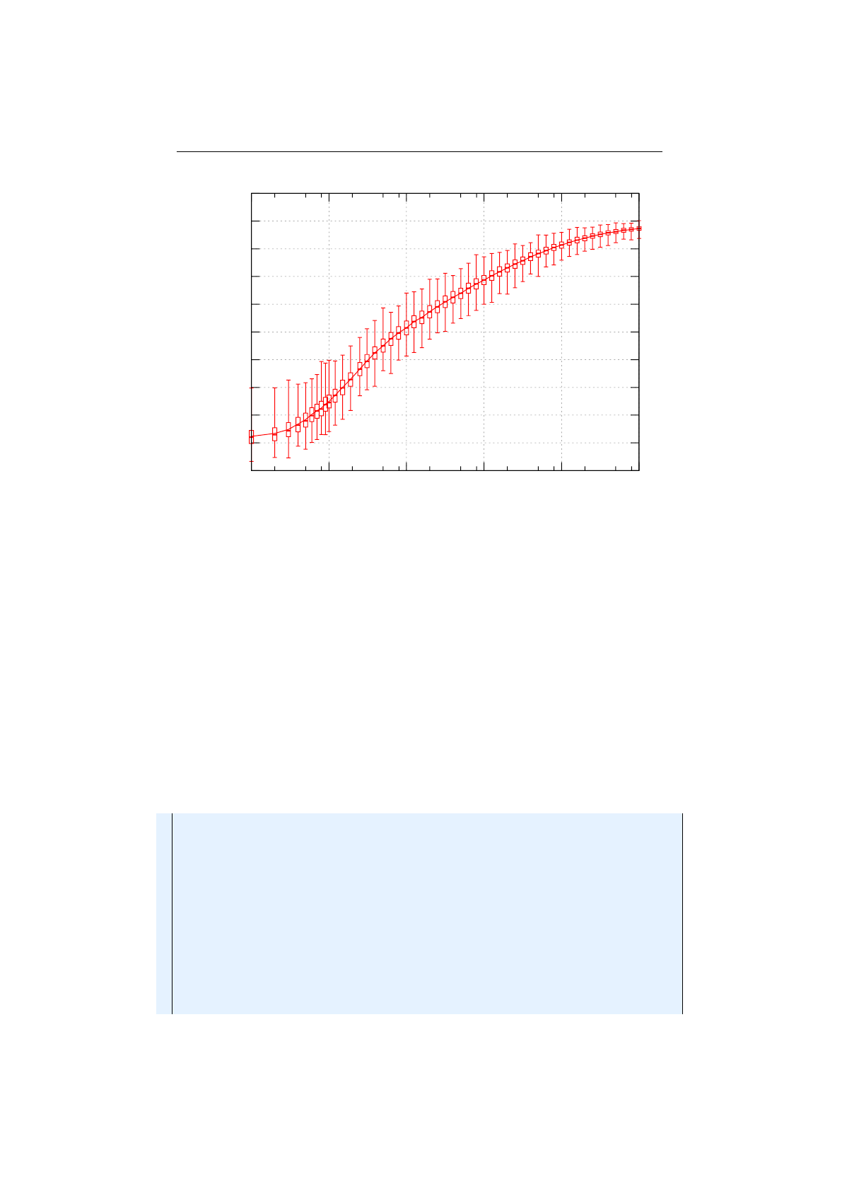
2.6. TERMINATION CHAPTER 2. ADVANCED TOPICS
6.5
7.0
7.5
8.0
8.5
9.0
9.5
10.0
10.5
11.0
11.5
100101102103104105
Fitness
Generation
Figure 2.6.1: Fixed generation termination
Figure 2.6.1 shows the best fitness values of the used Knapsack problem after
a given number of generations, whereas the candle-stick points represents the
min,25
th
percentile,median,75
th
percentile and max fitness after 250 repetitions
per generation. The solid line shows for the mean of the best fitness values. For
a small increase of the fitness value, the needed generations grows exponentially.
This is especially the case when the fitness is approaching to its maximal value.
2.6.2 Steady fitness
The steady fitness strategy truncates the evolution stream if its best fitness
hasn’t changed after a given number of generations. The predicate maintains an
internal state, the number of generations with non increasing fitness, and must
be newly created for every evolution stream.
1f i n a l c la s s SteadyFitnessLimit<C extends Comparable<? super C>>
2implements P re d ic a te <E vo lu ti on Re su lt <? , C>>
3{
4private f i n a l int _generations ;
5private boolean _proceed = true ;
6private int _ st ab le = 0 ;
7private C _ f i t n e s s ;
8
9public SteadyFitnessLimit ( f i n a l i nt generations) {
10 _ ge ne ra ti on s = g e n e r a t i o n s ;
11 }
12
13 @Override
14 public boolean t e s t ( final E v o l u ti o n R e s u lt <? , C> e r ) {
15 i f ( ! _proceed ) return f a l s e ;
62
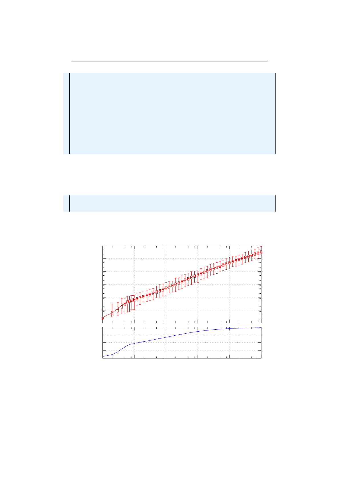
2.6. TERMINATION CHAPTER 2. ADVANCED TOPICS
16 i f ( _ f i t n e s s == n u l l ) {
17 _ f i t n e s s = e r . g e t B e s t F i t n e s s ( ) ;
18 _ st ab le = 1 ;
19 }else {
20 final Optimize opt = r e s u l t . g etO pt imi ze ( ) ;
21 i f ( opt . compare ( _ f i t n e s s , er . g e t B e s t F i t n e s s ( ) ) >= 0 ) {
22 _proceed = ++_ s t ab le <= _g e ne r at i o n s ;
23 }else {
24 _ f i t n e s s = e r . g e t B e s t F i t n e s s ( ) ;
25 _ st ab le = 1 ;
26 }
27 }
28 return _proceed ;
29 }
30 }
Listing 2.15: Steady fitness
Listing 2.15 on the preceding page shows the implementation of the
Limits-
.bySteadyFitness(int)
in the
io.jenetics.engine
package. It should give
you an impression of how to implement own termination strategies, which possible
holds and internal state.
1Eng in e<DobuleGene , Double> e n g i n e = . . .
2E vo lu t io nS t re a m<DoubleGene , Double> s t re am = e n g i n e . s tr ea m ( )
3. limit (Limits . bySteadyFitness (15)) ;
The steady fitness terminator can be created by the
bySteadyFitness
factory
method of the
io.jenetics.engine.Limits
class. In the example above, the
evolution stream is terminated after 15 stable generations.
100
101
102
103
104
105
106
Total generation
7.0
8.0
9.0
10.0
11.0
100101102103104105
Fitness
Steady generation
Figure 2.6.2: Steady fitness termination
Figure 2.6.2 shows the actual total executed generation depending on the
desired number of steady fitness generations. The variation of the total generation
63
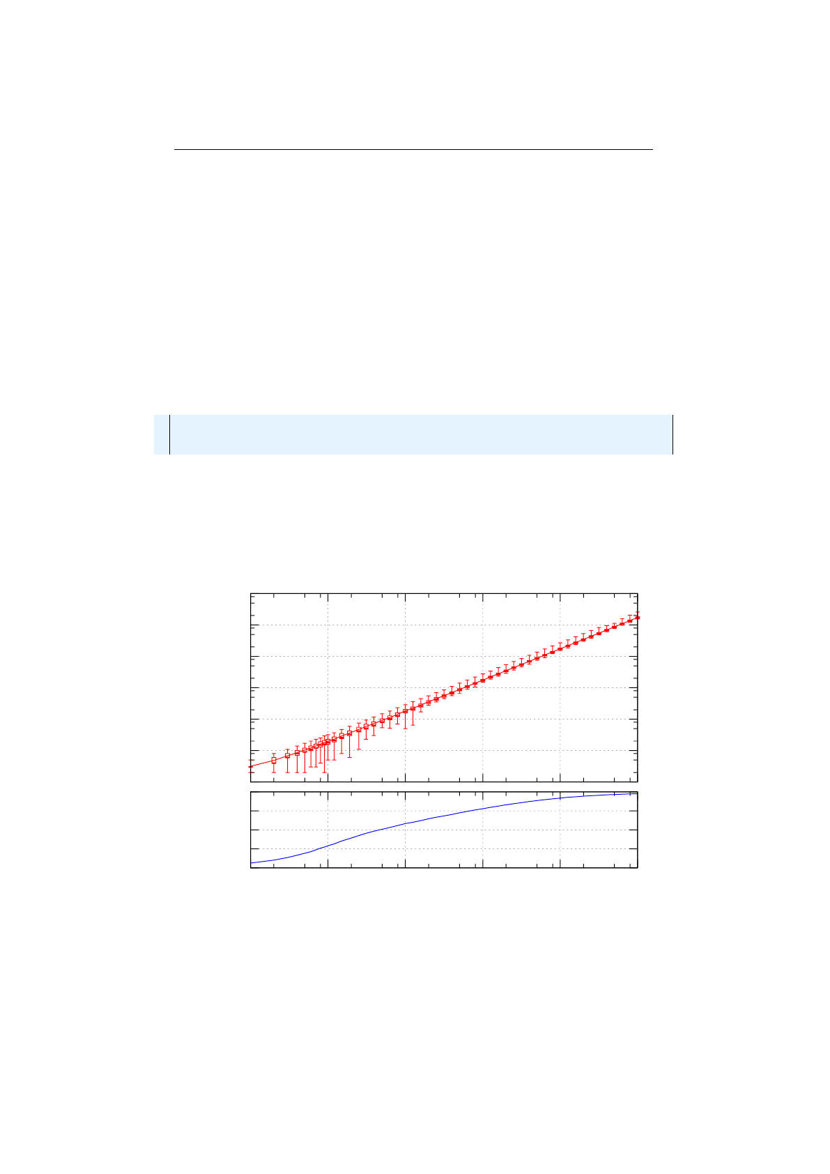
2.6. TERMINATION CHAPTER 2. ADVANCED TOPICS
is quite big, as shown by the candle-sticks. Though the variation can be quite
big—the termination test has been repeated 250 times for each data point—, the
tests showed that the steady fitness termination strategy always terminated, at
least for the given test setup. The lower diagram give an overview of the fitness
progression. Only the mean values of the maximal fitness is shown.
2.6.3 Evolution time
This termination strategy stops the evolution when the elapsed evolution time
exceeds an user-specified maximal value. The evolution stream is only truncated
at the end of an generation and will not interrupt the current evolution step.
An maximal evolution time of zero ms will at least evaluate one generation. In
an time-critical environment, where a solution must be found within a maximal
time period, this terminator let you define the desired guarantees.
1Eng in e<DobuleGene , Double> e n g i n e = . . .
2E vo lu t io nS t re a m<DoubleGene , Double> s t re am = e n g i n e . s tr ea m ( )
3. l i m i t ( L i m i t s . byExecutionTime ( Dur a tion . o f M i l l i s ( 5 0 0 ) ) ;
In the code example above, the
byExecutionTime(Duration)
method is used for
creating the termination object. Another method,
byExecutionTime(Duration,
Clock)
, lets you define the
java.time.Clock
, which is used for measure the
execution time.
Jenetics
uses the nano precision clock
io.jenetics.util.-
NanoClock
for measuring the time. To have the possibility to define a different
Clock implementation is especially useful for testing purposes.
100
101
102
103
104
105
106
Total generation
7.0
8.0
9.0
10.0
11.0
100101102103104105
Fitness
Execution time [ms]
Figure 2.6.3: Execution time termination
Figure 2.6.3 shows the evaluated generations depending on the execution
time. Except for very small execution times, the evaluated generations per time
64
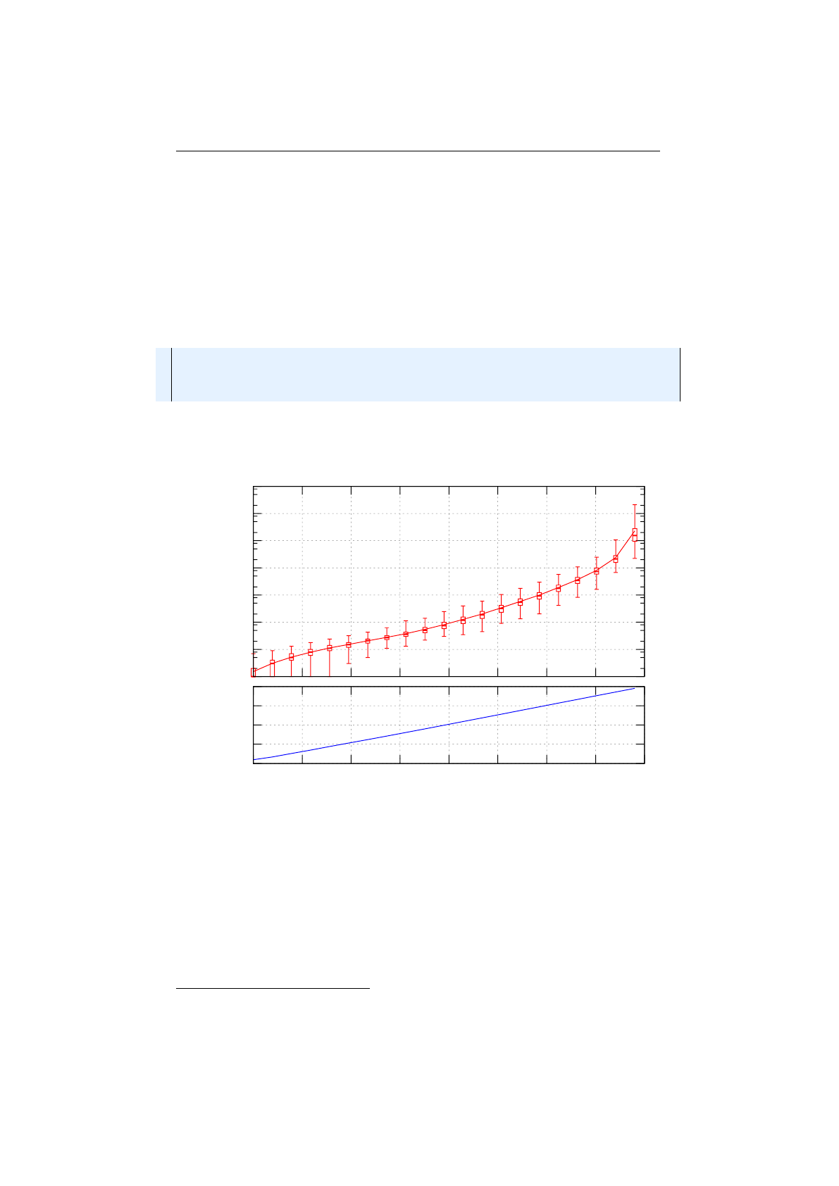
2.6. TERMINATION CHAPTER 2. ADVANCED TOPICS
unit stays quite stable.
20
That means that a doubling of the execution time will
double the number of evolved generations.
2.6.4 Fitness threshold
A termination method that stops the evolution when the best fitness in the
current population becomes less than the user-specified fitness threshold and the
objective is set to minimize the fitness. This termination method also stops the
evolution when the best fitness in the current population becomes greater than
the user-specified fitness threshold when the objective is to maximize the fitness.
1Eng in e<DobuleGene , Double> e n g i n e = . . .
2E vo lu t io nS t re a m<DoubleGene , Double> s t re am = e n g i n e . s tr ea m ( )
3. l i m i t ( Li mit s . by Fi tn es s Th re sh ol d ( 1 0 . 5 )
4. l i m i t ( 5 0 0 0 ) ;
When limiting the evolution stream by a fitness threshold, you have to have a
knowledge about the expected maximal fitness. If there is no such knowledge, it
is advisable to add an additional fixed sized generation limit as safety net.
100
101
102
103
104
105
106
107
Total generation
7.0
8.0
9.0
10.0
11.0
7.0 7.5 8.0 8.5 9.0 9.5 10.0 10.5 11.0
Fitness
Fitness threshold
Figure 2.6.4: Fitness threshold termination
Figure 2.6.4 shows executed generations depending on the minimal fitness
value. The total generations grows exponentially with the desired fitness value.
This means, that this termination strategy will (practically) not terminate, if
the value for the fitness threshold is chosen to high. And it will definitely not
terminate if the fitness threshold is higher than the global maximum of the
fitness function. It will be a perfect strategy if you can define some good enough
fitness value, which can be easily achieved.
20
While running the tests, all other CPU intensive process has been stopped. The measuring
started after a warm-up phase.
65

2.6. TERMINATION CHAPTER 2. ADVANCED TOPICS
2.6.5 Fitness convergence
In this termination strategy, the evolution stops when the fitness is deemed as
converged. Two filters of different lengths are used to smooth the best fitness
across the generations. When the best smoothed fitness of the long filter is
less than a specified percentage away from the best smoothed fitness from the
short filter, the fitness is deemed as converged.
Jenetics
offers a generic version
fitness-convergence predicate and a version where the smoothed fitness is the
moving average of the used filters.
1pub li c s t a t i c <N extends Number & Comparable <? super N>>
2P re d ic a te <E vo lu ti on Re su lt <? , N>> by Fi tne ssC onv erg enc e (
3f i n a l i nt shortFilterSize ,
4f i n a l i nt longFilterSize ,
5final B iP r ed i ca te <DoubleMoments , DoubleMoments> p ro ce ed
6) ;
Listing 2.16: General fitness convergence
Listing 2.16 shows the factory method which creates the generic fitness con-
vergence predicate. This method allows to define the evolution termination
according to the statistical moments of the short- and long fitness filter.
1pub li c s t a t i c <N extends Number & Comparable <? super N>>
2P re d ic a te <E vo lu ti on Re su lt <? , N>> by Fi tne ssC onv erg enc e (
3f i n a l i nt shortFilterSize ,
4f i n a l i nt longFilterSize ,
5f i n a l double epsilon
6) ;
Listing 2.17: Mean fitness convergence
The second factory method (shown in listing 2.17) creates a fitness convergence
predicate, which uses the moving average
21
for the two filters. The smoothed
fitness value is calculated as follows:
σF(N) = 1
N
N−1
X
i=0
F[G−i](2.6.1)
where
N
is the length of the filter,
F[i]
the fitness value at generation
i
and
G
the current generation. If the condition
|σF(NS)−σF(NL)|
δ< (2.6.2)
is fulfilled, the evolution stream is truncated. Where δis defined as follows:
δ=max (|σF(NS)|,|σF(NL)|) if 6= 0
1 otherwise .(2.6.3)
1Eng in e<DobuleGene , Double> e n g i n e = . . .
2E vo lu t io nS t re a m<DoubleGene , Double> s t re am = e n g i n e . s tr ea m ( )
3. l i m i t ( Li mi ts . by Fi tn es sC on ve rg en ce ( 1 0 , 30 , 10E−4) ;
For using the fitness convergence strategy you have to specify three parameter.
The length of the short filter,
NS
, the length of the long filter,
NL
and the
relative difference between the smoothed fitness values, .
21https://en.wikipedia.org/wiki/Moving_average
66
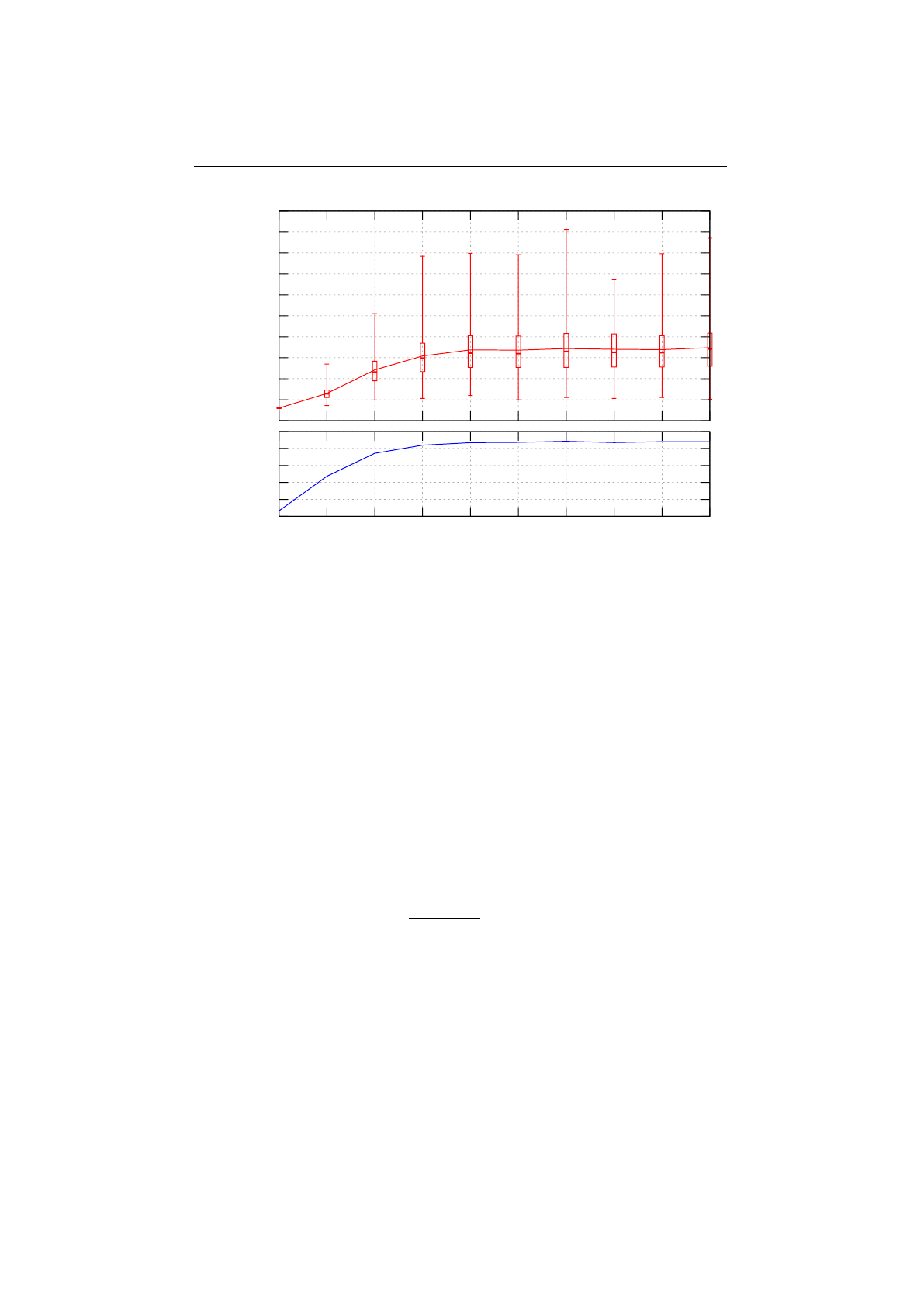
2.6. TERMINATION CHAPTER 2. ADVANCED TOPICS
0
50
100
150
200
250
300
350
400
450
500
NS= 10
NL= 30
Total generation
8.4
8.6
8.8
9.0
9.2
9.4
10-10
10-9
10-8
10-7
10-6
10-5
10-4
10-3
10-2
10-1
Fitness
Epsilon
Figure 2.6.5: Fitness convergence termination: NS= 10,NL= 30
Figure 2.6.5 shows the termination behavior of the fitness convergence termi-
nation strategy. It can be seen that the minimum number of evolved generations
is the length of the long filter, NL.
Figure 2.6.6 on the next page shows the generations needed for terminating
the evolution for higher values of the NSand NLparameters.
2.6.6 Population convergence
This termination method that stops the evolution when the population is deemed
as converged. A population is deemed as converged when the average fitness
across the current population is less than a user-specified percentage away from
the best fitness of the current population. The population is deemed as converged
and the evolution stream is truncated if
fmax −¯
f
δ< , (2.6.4)
where
¯
f=1
N
N−1
X
i=0
fi,(2.6.5)
fmax = max
i∈[0,N){fi}(2.6.6)
and
δ=max |fmax|,¯
fif 6= 0
1 otherwise .(2.6.7)
Ndenotes the number of individuals of the population.
67
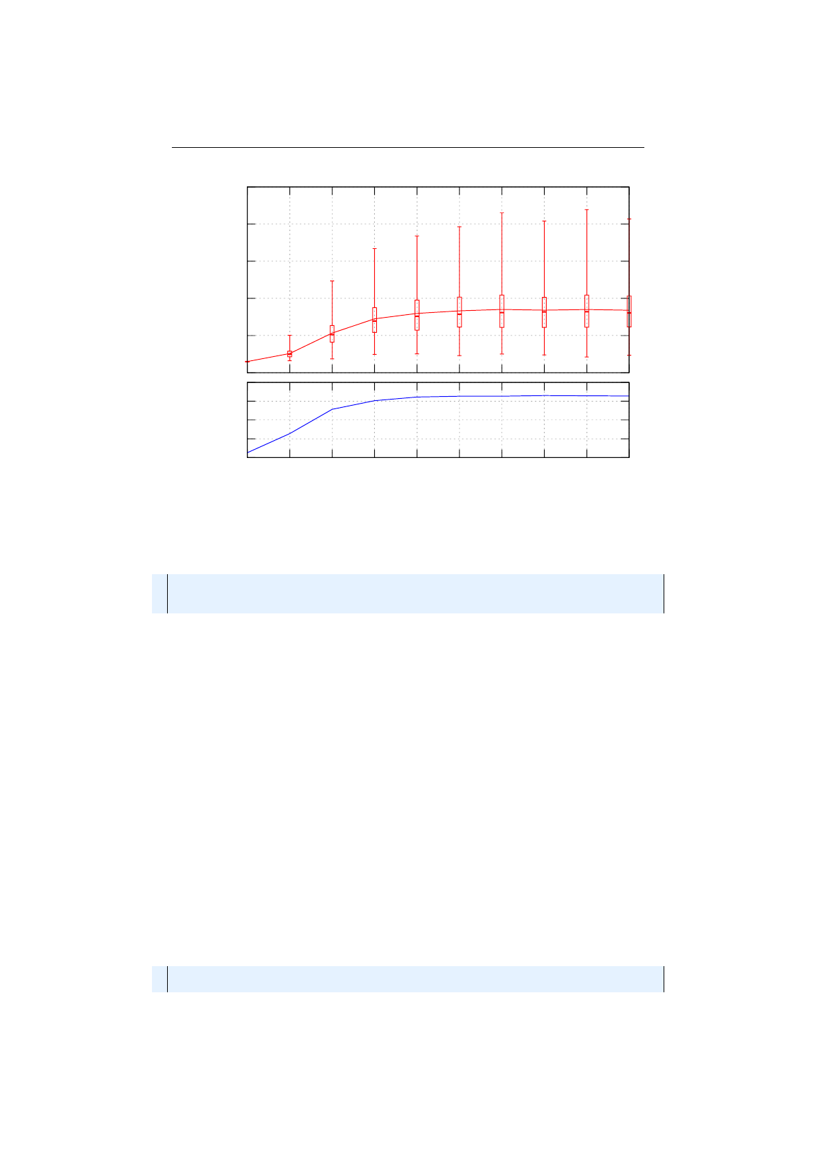
2.7. REPRODUCIBILITY CHAPTER 2. ADVANCED TOPICS
0
500
1000
1500
2000
2500
NS= 50
NL= 150
Total generation
9.2
9.4
9.6
9.8
10.0
10-10
10-9
10-8
10-7
10-6
10-5
10-4
10-3
10-2
10-1
Fitness
Epsilon
Figure 2.6.6: Fitness convergence termination: NS= 50,NL= 150
1Eng in e<DobuleGene , Double> e n g i n e = . . .
2E vo lu t io nS t re a m<DoubleGene , Double> s t re am = e n g i n e . s tr ea m ( )
3. l i m i t ( Li mi ts . byPo pula t ion C onve rgen ce ( 0 . 1 ) ;
The evolution stream in the example above will terminate, if the difference
between the population’s fitness mean value and the maximal fitness value of
the population is less then 10%.
2.6.7 Gene convergence
This termination strategy is different, in the sense that it takes the genes or
alleles, respectively, for terminating the evolution stream. In the gene convergence
termination strategy the evolution stops when a specified percentage of the genes
of a genotype are deemed as converged. A gene is treated as converged when the
average value of that gene across all of the genotypes in the current population
is less than a given percentage away from the maximum allele value across the
genotypes.
2.7 Reproducibility
Some problems can be define with different kinds of fitness functions or encodings.
Which combination works best can’t usually be decided a priori. To choose one,
some testing is needed.
Jenetics
allows you to setup an evolution
Engine
in a
way that will produce the very same result on every run.
1final Eng in e<DoubleGene , Double> e n g i n e =
2En gi ne . b u i l d e r ( f i t n e s s F u n c t i o n , co dec )
68
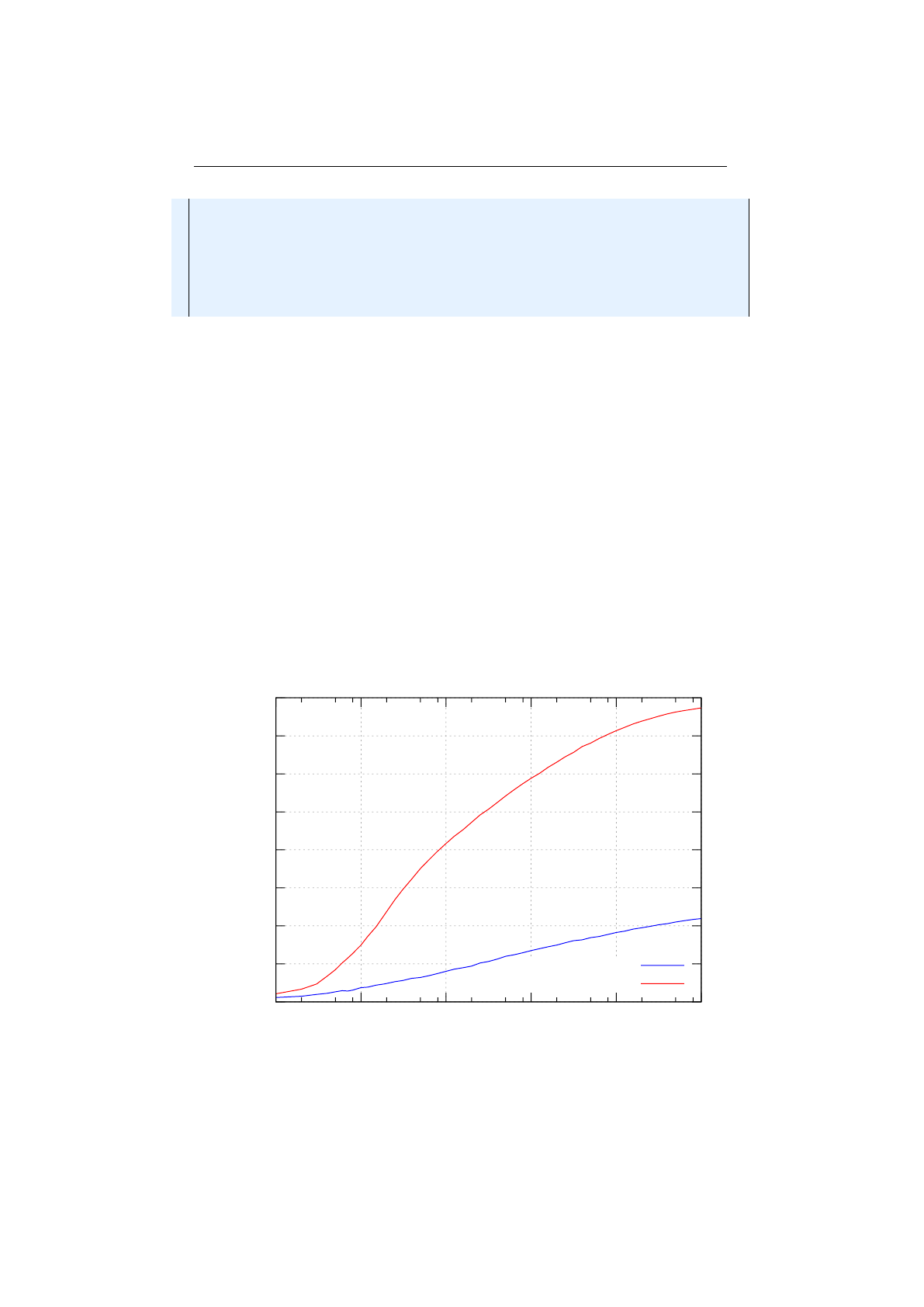
2.8. EVOLUTION PERFORMANCE CHAPTER 2. ADVANCED TOPICS
3. e x e c u t o r ( Run nabl e : : ru n )
4. b u i l d ( ) ;
5final Ev ol ut io nR esu lt <DoubleGene , Double> r e s u l t =
6RandomRegistry . with (new Random ( 4 5 6 ) , r −>
7e n g i n e . s tr e am ( p o p u l a t i o n )
8. l i m i t ( 1 0 0 )
9. c o l l e c t ( E v o l u t i o n R e s u l t . t o B e s t E v o l u t i o n R e s u l t ( ) )
10 ) ;
Listing 2.18: Reproducible evolution Engine
Listing 2.18 on the preceding page shows the basic setup of such a reproducible
evolution
Engine
. Firstly, you have to make sure that all evolution steps are exe-
cuted serially. This is done by configuring a single threaded executor. In the sim-
plest case the evolution is performed solely on the main thread—
Runnable::run
.
If the evolution
Engine
uses more than one worker thread, the reproducibility
is no longer guaranteed. The second step configures the random engine, the
evolution
Engine
is working with. Just wrap the evolution stream execution in a
RandomRegistry::with
block. Additionally you can start the evolution stream
with a predefined, initial population. Once you have setup the
Engine
, you can
vary the fitness function and the codec and compare the results.
2.8 Evolution performance
This section contains an empirical proof, that evolutionary selectors deliver
significantly better fitness results than a random search. The
MonteCarlo-
Selector is used for creating the comparison (random search) fitness values.
7.0
7.5
8.0
8.5
9.0
9.5
10.0
10.5
11.0
100101102103104105
Fitness
Generation
MonteCarloSelector
Evolutionary-Selector
Figure 2.8.1: Selector-performance (Knapsack)
69

2.9. EVOLUTION STRATEGIES CHAPTER 2. ADVANCED TOPICS
Figure 2.8.1 on the previous page shows the evolution performance of the
Selector22
used by the examples in section 2.6 on page 60. The lower blue
line shows the (mean) fitness values of the Knapsack problem when using the
MonteCarloSelector
for selecting the survivors and offspring population. It
can be easily seen, that the performance of the real evolutionary
Selector
s is
much better than a random search.
2.9 Evolution strategies
Evolution Strategies, ES, were developed by Ingo Rechenberg and Hans-Paul
Schwefel at the Technical University of Berlin in the mid 1960s.[
30
] It is a
global optimization algorithm in continuous search spaces and is an instance
of an Evolutionary Algorithm from the field of Evolutionary Computation. ES
uses truncation selection
23
for selecting the individuals and usually mutation
24
for changing the next generation. This section describes how to configure the
evolution Engine of the library for the (µ, λ)- and (µ+λ)-ES.
2.9.1 (µ, λ)evolution strategy
The
(µ, λ)
algorithm starts by generating
λ
individuals randomly. After eval-
uating the fitness of all the individuals, all but the
µ
fittest ones are deleted.
Each of the
µ
fittest individuals gets to produce
λ
µ
children through an ordinary
mutation. The newly created children just replaces the discarded parents.[20]
To summarize it:
µ
is the number of parents which survive, and
λ
is the
number of offspring, created by the
µ
parents. The value of
λ
should be a multiple
of
µ
. ES practitioners usually refer to their algorithm by the choice of
µ
and
λ
.
If we set µ= 5 and λ= 5, then we have a (5,20)-ES.
1final Eng in e<DoubleGene , Double> e n g i n e =
2Engine . b u i l d e r ( f i t n e s s , co de c )
3. p o p u l a t i o n S i z e ( lambda )
4. survivorsSize (0)
5. offspringSelector(new TruncationSelector<>(mu))
6. a l t e r e r s (new Mutator <>(p ) )
7. b u i l d ( ) ;
Listing 2.19: (µ, λ)Engine configuration
Listing 2.19 shows how to configure the evolution Engine for
(µ, λ)
-ES. The
population size is set to
λ
and the survivors size to zero, since the best parents are
not part of the final population. Step three is configured by setting the offspring
selector to the
TruncationSelector
. Additionally, the
TruncationSelector
is parameterized with
µ
. This lets the
TruncationSelector
only select the
µ
best individuals, which corresponds to step two of the ES.
There are mainly three levers for the
(µ, λ)
-ES where we can adjust explo-
ration versus exploitation:[20]
22
The termination tests are using a
TournamentSelector
, with tournament-size 5, for se-
lecting the survivors, and a RouletteWheelSelector for selecting the offspring.
23See 1.3.2.1 on page 13.
24See 1.3.2.2 on page 17.
70

2.10. EVOLUTION INTERCEPTION CHAPTER 2. ADVANCED TOPICS
•Population size λ
: This parameter controls the sample size for each
population. For the extreme case, as
λ
approaches
∞
, the algorithm would
perform a simple random search.
•Survivors size of µ
: This parameter controls how selective the ES is.
Relatively low
µ
values pushes the algorithm towards exploitative search,
because only the best individuals are used for reproduction.25
•Mutation probability p
: A high mutation probability pushes the al-
gorithm toward a fairly random search, regardless of the selectivity of
µ.
2.9.2 (µ+λ)evolution strategy
In the
(µ+λ)
-ES, the next generation consists of the selected best
µ
parents
and the
λ
new children. This is also the main difference to
(µ, λ)
, where the
µ
parents are not part of the next generation. Thus the next and all successive
generations are
µ
+
λ
in size.[
20
]
Jenetics
works with a constant population
size and it is therefore not possible to implement an increasing population size.
Besides this restriction, the
Engine
configuration for the
(µ+λ)
-ES is shown
in listing 2.20.
1final Eng in e<DoubleGene , Double> e n g i n e =
2Engine . b u i l d e r ( f i t n e s s , co de c )
3. p o p u l a t i o n S i z e ( lambda )
4. survivorsSize(mu)
5. selector(new TruncationSelector<>(mu))
6. a l t e r e r s (new Mutator <>(p ) )
7. b u i l d ( ) ;
Listing 2.20: (µ+λ)Engine configuration
Since the selected
µ
parents are part of the next generation, the
survivorsSize
property must be set to
µ
. This also requires to set the survivors selector to the
TruncationSelector
. With the
selector(Selector)
method, both selectors,
the selector for the survivors and for the offspring, can be set. Because the
best parents are also part of the next generation, the
(µ+λ)
-ES may be more
exploitative than the
(µ, λ)
-ES. This has the risk, that very fit parents can defeat
other individuals over and over again, which leads to a prematurely convergence
to a local optimum.
2.10 Evolution interception
Once the
EvolutionStream
is created, it will continuously create
Evolution-
Result
objects, one for every generation. It is not possible to alter the results,
although it is tempting to use the
Stream.map
method for this purpose. The
problem with the
map
method is, that the altered
EvolutionResult
will not be
fed back to the Engine when evolving the next generation.
25
As you can see in listing 2.19 on the preceding page, the survivors size (reproduction pool
size) for the
(µ, λ)
-ES must be set indirectly via the
TruncationSelector
parameter. This is
necessary, since for the
(µ, λ)
-ES, the selected best
µ
individuals are not part of the population
of the next generation.
71

2.10. EVOLUTION INTERCEPTION CHAPTER 2. ADVANCED TOPICS
1private E vo l ut i on Re s ul t <DoubleGene , Double>
2mapping ( E vo lu ti onR es ult <DoubleGene , Double> r e s u l t ) { . . . }
3
4final Genotype<DobuleGene> r e s u l t = e n g i n e . st re am ( )
5. map( this : : mapping )
6. l i m i t ( 1 0 0 )
7. c o l l e c t ( to B e s tG enotype ( ) ) ;
Doing the
EvolutionResult
mapping as shown in the code snippet above, will
only change the results for the operations after the mapper definition. The
evolution processing of the
Engine
is not affected. If we want to intercept the
evolution process, the mapping must be defined when the Engine is created.
1final Eng in e<DobuleGene , Double> e n g i n e = E ng ine . b u i l d ( p ro bl em )
2. mapping( this : : mapping )
3. b u i l d ( ) ;
The code snippet above shows the correct way for intercepting the evolution
stream. The mapper given to the
Engine
will change the stream of
Evolution-
Results and the will also feed the altered result back to the evolution Engine.
Distinct population
This kind of intercepting the evolution process is very
flexible.
Jenetics
comes with one predefined stream interception method, which
allows to remove duplicate individuals from the resulting population.
1final Eng in e<DobuleGene , Double> e n g i n e = E ng ine . b u i l d ( p ro bl em )
2. mapping ( E v o l u t i o n R e s u l t . t o U ni q u eP o p ul a ti o n ( ) )
3. b u i l d ( ) ;
Despite the de-duplication, it is still possible to have duplicate individuals.
This will be the case when domain of the possible
Genotype
s is not big enough
and the same individual is created by chance. You can control the number of
Genotype
creation retries using the
EvolutionResult.toUniquePopulation(-
int)
method, which allows you to define the maximal number of retries if an
individual already exists.
72

Chapter 3
Internals
This section contains internal implementation details which doesn’t fit in one of
the previous sections. They are not essential for using the library, but would give
the user a deeper insight in some design decisions, made when implementing the
library. It also introduces tools and classes which where developed for testing
purpose. This classes are not exported and not part of the official API.
3.1 PRNG testing
Jenetics
uses the
dieharder1
(command line) tool for testing the randomness
of the used PRNGs.
dieharder
is a random number generator (RNG) testing
suite. It is intended to test generators, not files of possibly random numbers.
Since
dieharder
needs a huge amount of random data, for testing the quality
of a RNG, it is usually advisable to pipe the random numbers to the
dieharder
process:
$ cat /dev/urandom | dieharder -g 200 -a
The example above demonstrates how to stream a raw binary stream of bits to
the
stdin
(raw) interface of
dieharder
. With the
DieHarder
class, which is
part of the
io.jenetics-.prngine.internal
package, it is easily possible to
test PRNGs extending the
java.util.Random
class. The only requirement is,
that the PRNG must be default-constructible and part of the classpath.
$ java -cp io.jenetics.prngine-1.0.1.jar \
io.jenetics.prngine.internal.DieHarder \
<random-engine-name> -a
Calling the command above will create an instance of the given random engine
and stream the random data (bytes) to the raw interface of
dieharder
process.
1#=============================================================================#
2# Te st ing : < random - engi ne - name > (20 15 -07 -11 2 3:4 8) #
3#=============================================================================#
4#=============================================================================#
5# Li nu x 3.19 .0 - 22 - ge ne ri c ( amd 64 ) #
6# java ve rs io n " 1 .8 .0 _4 5 " #
1From Robert G. Brown:http://www.phy.duke.edu/~rgb/General/dieharder.php
73

3.2. RANDOM SEEDING CHAPTER 3. INTERNALS
7# J av a ( TM ) S E R un ti me E nv i ro n me nt ( b ui l d 1 .8 .0 _ 45 - b 14 ) #
8# J av a H ot Sp o t ( TM ) 64 - B it S er ve r VM ( b ui ld 25 .4 5 - b 02 ) #
9#=============================================================================#
10 #=============================================================================#
11 # dieharder ver si on 3 .31 .1 C op yr ig ht 20 03 Rob ert G. B row n #
12 #=============================================================================#
13 rn g_ na me | ran ds / s ec on d | Seed |
14 s td in _i np u t_ ra w | 1. 36 e + 07 | 15 8 34 96 49 6 |
15 #=============================================================================#
16 te st _n am e | n tup | t sa mp le s | p sa mpl es | p - v al ue | A sse ssm en t
17 #=============================================================================#
18 di eh ard _b irt hd ays | 0| 100| 1 00 |0 .63 37 207 8| PASS ED
19 di eh ard _o per m5 | 0| 1 00 00 00| 10 0|0 .4 296 50 82| PASS ED
20 di eh ard _r ank _32 x3 2 | 0| 400 00| 1 00| 0. 951 59 38 0| PA SS ED
21 diehard_rank_6x8| 0| 100000| 100|0.70376799| PASSED
22 ...
23 Preparing to r un te st 209. n tup le = 0
24 da b_ mo nob it 2 | 12| 6 50 00 00 0| 1| 0. 76 563 78 0| PA SSED
25 #=============================================================================#
26 # S um m ar y : P AS SE D =112 , W EA K =2 , FA IL ED =0 #
27 # 235 ,031 .49 2 MB of ra ndo m data c re ated wit h 41. 394 MB / sec #
28 #=============================================================================#
29 #=============================================================================#
30 # Runtime: 1:34:37 #
31 #=============================================================================#
In the listing above, a part of the created
dieharder
report is shown. For test-
ing the
LCG64ShiftRandom
class, which is part of the
io.jenetics.prngine
module, the following command can be called:
$ java -cp io.jenetics.prngine-1.0.1.jar \
io.jenetics.prngine.internal.DieHarder \
io.jenetics.prngine.LCG64ShiftRandom -a
Table 3.1.1 shows the summary of the
dieharder
tests. The full report is part
of the source file of theLCG64ShiftRandom class.2
Passed tests Weak tests Failed tests
110 4 0
Table 3.1.1: LCG64ShiftRandom quality
3.2 Random seeding
The PRNGs
3
, used by the
Jenetics
library, needs to be initialized with a proper
seed value before they can be used. The usual way for doing this, is to take the
current time stamp.
1pub li c s t a t i c long s ee d ( ) {
2return System . nanoTime ( ) ;
3}
Before applying this method throughout the whole library, I decided to perform
some statistical tests. For this purpose I treated the
seed()
method itself as
PRNG and analyzed the created long values with the
DieHarder class
. The
2https://github.com/jenetics/prngine/blob/master/prngine/src/main/java/io/
jenetics/prngine/LCG64ShiftRandom.java
3See section 1.4.2 on page 32.
74
3.2. RANDOM SEEDING CHAPTER 3. INTERNALS
seed()
method has been wrapped into the
io.jenetics.prngine.internal.-
NanoTimeRandom
class. Assuming that the
dieharder
tool is in the search path,
calling
$ java -cp io.jenetics.prngine-1.0.1.jar \
io.jenetics.prngine.internal.DieHarder \
io.jenetics.prngine.internal.NanoTimeRandom -a
will perform the statistical tests for the nano time random engine. The statistical
quality is rather bad: every single test failed. Table 3.2.1 shows the summary of
the dieharder report.4
Passed tests Weak tests Failed tests
0 0 114
Table 3.2.1: Nano time seeding quality
An alternative source of entropy, for generating seed values, would be the
/dev/random
or
/dev/urandom
file. But this approach is not portable, which
was a prerequisite for the Jenetics library.
The next attempt tries to fetch the seeds from the JVM, via the
Object.-
hashCode()
method. Since the hash code of an Object is available for every
operating system and most likely »randomly« distributed.
1pub li c s t a t i c long s ee d ( ) {
2return ( ( long )new Obje ct ( ) . hashCode ( ) << 32 ) |
3new O bj ec t ( ) . hashCode ( ) ;
4}
This seed method has been wrapped into the
ObjectHashRandom
class and
tested as well with
$ java -cp io.jenetics.prngine-1.0.1.jar \
io.jenetics.prngine.internal.DieHarder \
io.jenetics.prngine.internal.ObjectHashRandom -a
Table 3.2.2 shows the summary of the
dieharder
report
5
, which looks better
than the nano time seeding, but 86 failing tests was still not very satisfying.
Passed tests Weak tests Failed tests
28 0 86
Table 3.2.2: Object hash seeding quality
After additional experimentation, a combination of the nano time seed and
the object hash seeding seems to be the right solution. The rational behind this
was, that the PRNG seed shouldn’t rely on a single source of entropy.
4
The detailed test report can be found in the source of the NanoTimeRandom
class.
https://github.com/jenetics/prngine/blob/master/prngine/src/main/java/io/
jenetics/prngine/internal/NanoTimeRandom.java
5
Full report:
https://github.com/jenetics/prngine/blob/master/prngine/src/main/
java/io/jenetics/prngine/internal/ObjectHashRandom.java
75

3.2. RANDOM SEEDING CHAPTER 3. INTERNALS
1pub li c s t a t i c long s ee d ( ) {
2return mix ( System . nanoType ( ) , obj ec tHa sh Se ed ( ) ) ;
3}
4
5pr iv at e s t a t i c long mix ( f i n a l long a , f i n a l long b ) {
6long c = a^b ;
7c ^= c << 1 7 ;
8c ^= c >>> 3 1 ;
9c ^= c << 8 ;
10 return c ;
11 }
12
13 pr iv at e s t a t i c long o bj ec tH ash Se ed ( ) {
14 return ( ( long )new Obje ct ( ) . hashCode ( ) << 32 ) |
15 new O bj ec t ( ) . hashCode ( ) ;
16 }
Listing 3.1: Random seeding
The code in listing 3.1 shows how the nano time seed is mixed with the object
seed. The
mix
method was inspired by the mixing step of the
lcg64_shift6
random engine, which has been reimplemented in the
LCG64ShiftRandom
class.
Running the tests with
$ java -cp io.jenetics.prngine-1.0.1.jar \
io.jenetics.prngine.internal.DieHarder \
io.jenetics.prngine.internal.SeedRandom -a
leads to the statistics summary7, which is shown in table 3.2.3.
Passed tests Weak tests Failed tests
112 2 0
Table 3.2.3: Combined random seeding quality
The statistical performance of this seeding is better, according to the
die-
harder
test suite, than some of the real random engines, including the default
Java
Random
engine. Using the proposed
seed()
method is in any case prefer-
able to the simple System.nanoTime() call.
Open questions
•How does this method perform on operating systems other than Linux?
•How does this method perform on other JVM implementations?
6
This class is part of the TRNG library:
https://github.com/rabauke/trng4/blob/
master/src/lcg64_shift.hpp
7
Full report:
https://github.com/jenetics/prngine/blob/master/prngine/src/main/
java/io/jenetics/prngine/internal/SeedRandom.java
76
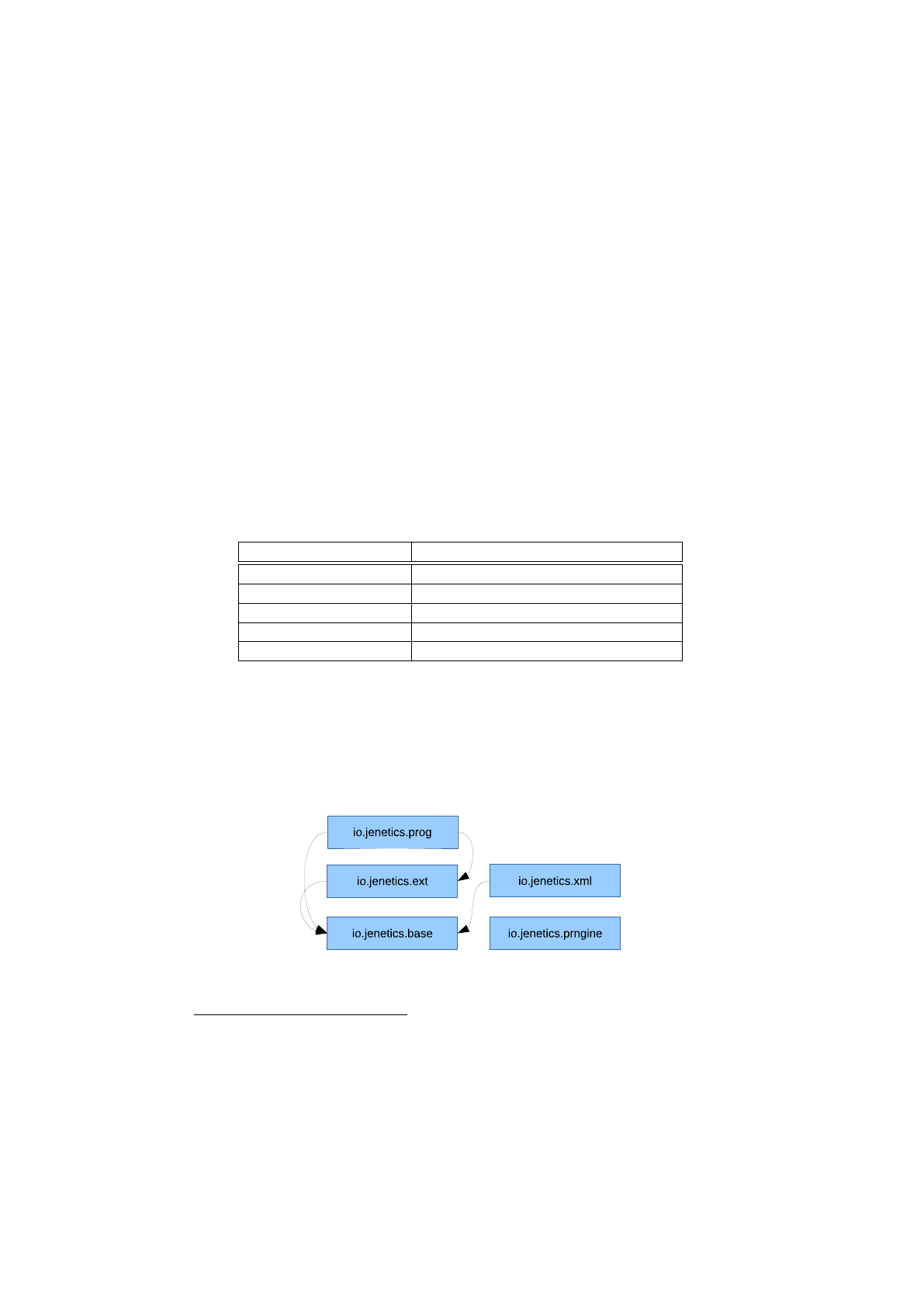
Chapter 4
Modules
The
Jenetics
library has been split up into several modules, which allows to keep
the base EA module as small as possible. It currently consists of the modules
shown in table 4.0.1, including the Jenetics base module.1
Module Artifact
io.jenetics.base io.jenetics:jenetics:4.4.0
io.jenetics.ext io.jenetics:jenetics.ext:4.4.0
io.jenetics.prog io.jenetics:jenetics.prog:4.4.0
io.jenetics.xml io.jenetics:jenetics.xml:4.4.0
io.jenetics.prngine io.jenetics:prngine:1.0.1
Table 4.0.1: Jenetics modules
With this module split the code is easier to maintain and doesn’t force the user
to use parts of the library he or she isn’t using, which keep the
io.jenetics-
.base
module as small as possible. The additional
Jenetics
modules will be
described in this chapter. Figure 4.0.1 shows the dependency graph of the
Jenetics modules.
Figure 4.0.1: Module graph
1
The used module names follow the recommended naming scheme for the JPMS automatic
modules: http://blog.joda.org/2017/05/java-se-9-jpms-automatic-modules.html.
77
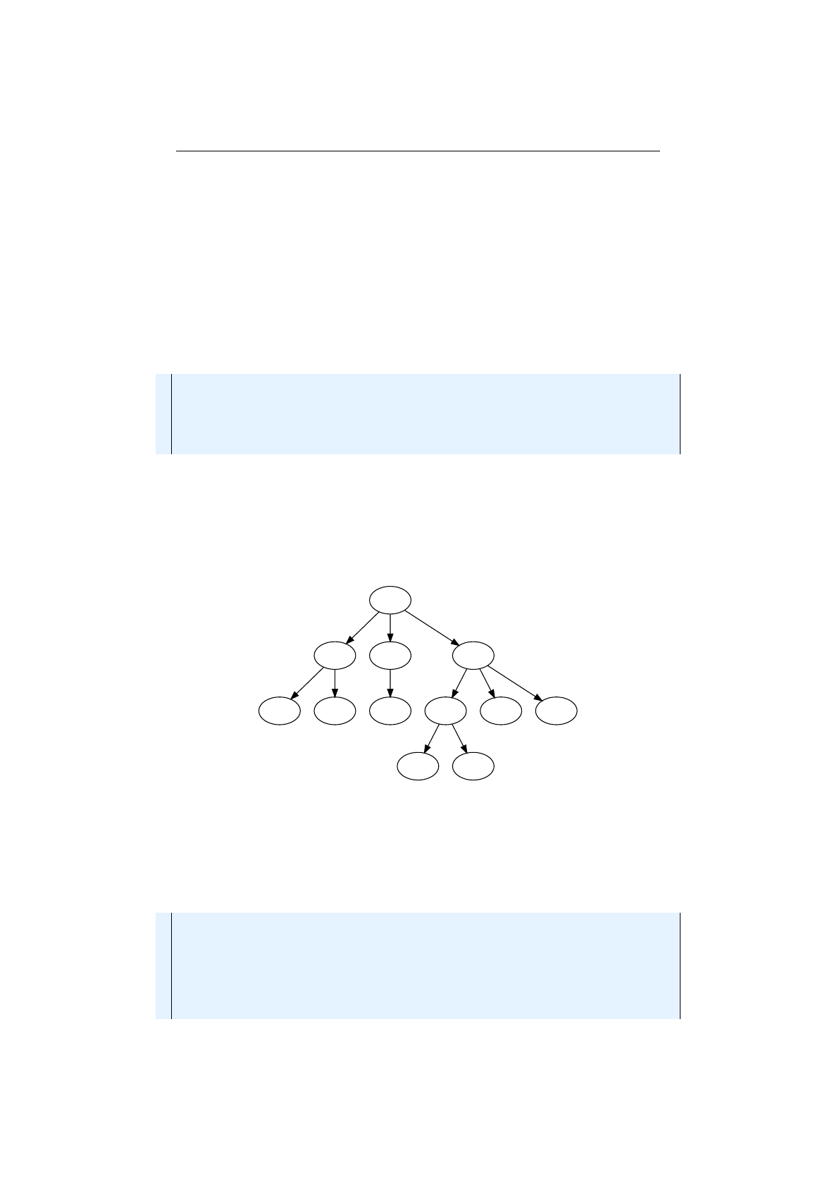
4.1. IO.JENETICS.EXT CHAPTER 4. MODULES
4.1 io.jenetics.ext
The
io.jenetics.ext
module implements additional non-standard genes and
evolutionary operations. It also contains data structures which are used by this
additional genes and operations.
4.1.1 Data structures
4.1.1.1 Tree
The
Tree
interface defines a general tree data type, where each tree node can
have an arbitrary number of children.
1public i n t e r f a c e Tree<V, T extends Tree<V, T>> {
2public V getValue () ;
3public Optio nal <T> ge tP ar en t ( ) ;
4public T g e t C h i l d ( int i n de x ) ;
5public in t c hi ld Co un t ( ) ;
6}
Listing 4.1: Tree interface
Listing 4.1 shows the
Tree
interface with its basic abstract tree methods. All
other needed tree methods, e. g. for node traversal and search, are implemented
with default methods, which are derived from this four abstract tree methods. A
mutable default implementation of the
Tree
interface is given by the
TreeNode
class.
0
1 2 3
456789
10 11
Figure 4.1.1: Example tree
To illustrate the usage of the
TreeNode
class, we will create a
TreeNode
instance from the tree shown in figure 4.1.1. The example tree consists of 12
nodes with a maximal depth of three and a varying child count from one to
three.
1final TreeNode<I n t e g e r > t r e e = TreeNode . o f ( 0 )
2. a t t a c h ( TreeNode . o f ( 1 )
3. a t t a c h ( 4 , 5 ) )
4. a t t a c h ( TreeNode . o f ( 2 )
5. a t t a c h ( 6 ) )
6. a t t a c h ( TreeNode . o f ( 3 )
7. a t t a c h ( TreeNode . o f ( 7 )
8. a t t a c h ( 1 0 , 1 1) )
78
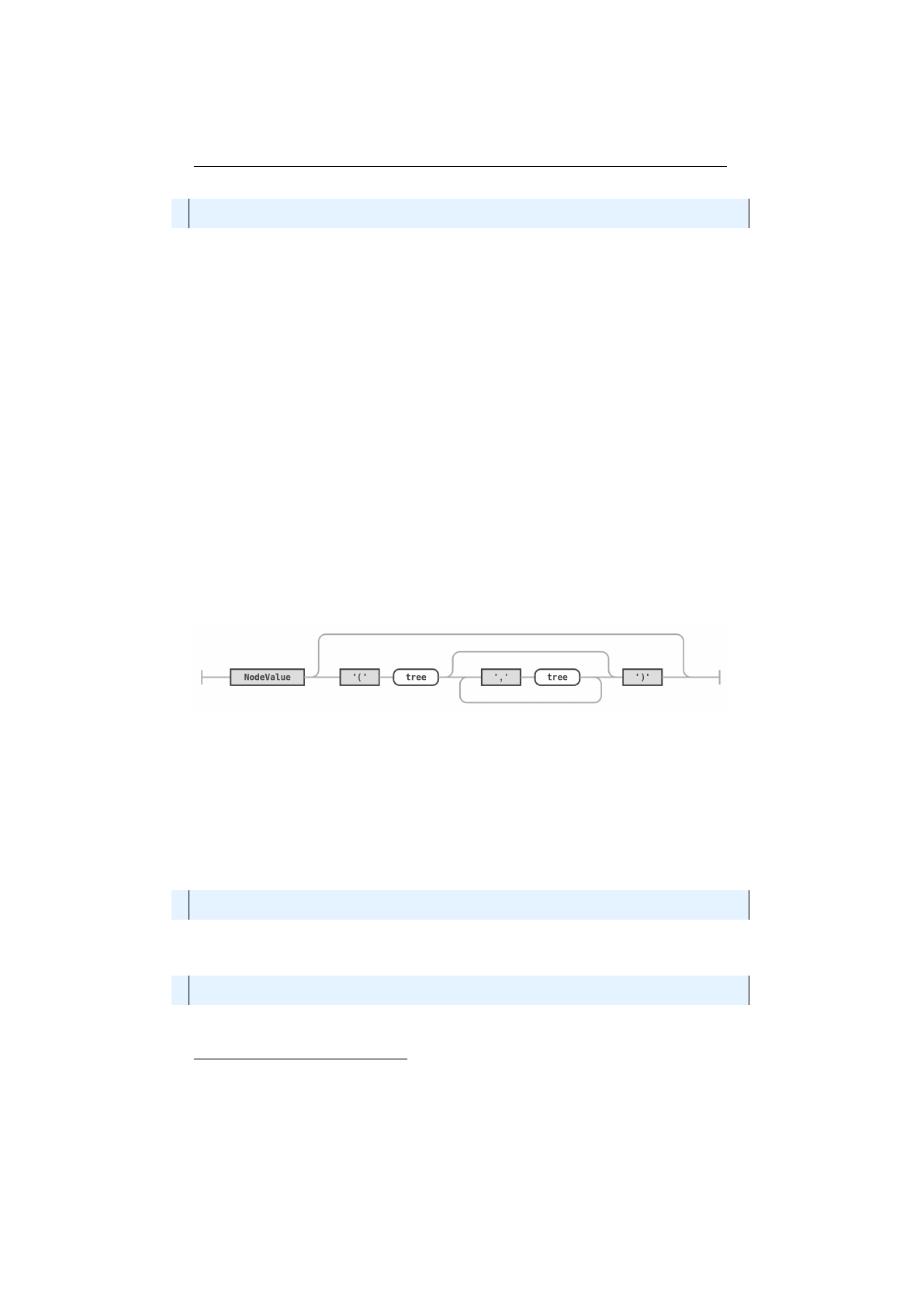
4.1. IO.JENETICS.EXT CHAPTER 4. MODULES
9. a t t a c h ( 8 )
10 . a t t a c h ( 9 ) ) ;
Listing 4.2: Example TreeNode
Listing 4.2 on the preceding page shows the
TreeNode
representation of the
given example tree. New children are added by using the
attach
method. For
full Tree method list have a look at the Javadoc documentation.
4.1.1.2 Parentheses tree
A parentheses tree
2
is a serialized representation of a tree and is a simplified
form of the Newick tree format
3
. The parentheses tree representation of the tree
in figure 4.1.1 on the previous page will look like the following string:
0(1(4,5),2(6),3(7(10,11),8,9))
As you can see, nodes on the same tree level are separated by a comma, ’
,
’. New
tree levels are created with an opening parentheses ’
(
’ and closed with a closing
parentheses ’
)
’. No additional spaces are inserted between the separator character
and the node value. Any spaces in the parentheses tree string will be part of the
node value. Figure 4.1.2 shows the syntax diagram of the parentheses tree. The
NodeValue
in the diagram is the string representation of the
Tree.getValue()
object.
Figure 4.1.2: Parentheses tree syntax diagram
To get the parentheses tree representation, you just have to call
Tree.to-
ParenthesesTree()
. This method uses the
Object.toString()
method for
serializing the tree node value. If you need a different string representation
you can use the
Tree.toParenthesesTree(Function<? super V, String>)
method. A simple example, on how to use this method, is shown in the code
snippet below.
1final Tree<Path , ?> t r e e = . . . ;
2final S t r i n g s t r i n g = t r e e . t o P a r e n t h e s e s S t r i n g ( Path : : ge tFileName ) ;
If the string representation of the tree node value contains one of the protected
characters, ’,’, ’(’ or ’)’, they will be escaped with a ’\’ character.
1final Tree<S tr in g , ?> t r e e = TreeNode . o f ( " ( r o o t ) " )
2. a t t a c h ( ","," ( " ,")")
The tree in the code snippet above will be represented as the following parentheses
string:
2https://www.i-programmer.info/programming/theory/3458-parentheses-are-trees.
html
3http://evolution.genetics.washington.edu/phylip/newicktree.html
79

4.1. IO.JENETICS.EXT CHAPTER 4. MODULES
\(root\)(\„\(,\))
Serializing a tree into parentheses form is just one part of the story. It is also
possible to read back the parentheses string as tree object. The
TreeNode-
.parse(String)
method allows you to parse a tree string back to a
TreeNode<-
String>
object. If you need to create a tree with the original node type, you
can call the
parse
method with an additional string mapper function. How you
can parse a given parentheses tree string is shown in the code below.
1final Tree<I n t e g e r , ?> t r e e = TreeNode . p a r s e (
2" 0 ( 1 ( 4 , 5 ) , 2 ( 6 ) , 3 ( 7 ( 1 0 , 1 1 ) , 8 , 9 ) ) " ,
3I n t e g e r : : p a r s e I n t
4) ;
The
TreeNode.parse
method will throw an
IllegalArgumentException
if it
is called with an invalid tree string.
4.1.1.3 Flat tree
The main purpose for the
Tree
data type in the
io.jenetics.ext
module is
to support hierarchical
TreeGene
s, which are needed for genetic programming
(see section 4.2 on page 93). Since the chromosome type is essentially an array,
a mapping from the hierarchical tree structure to a 1-dimensional array is
needed.
4
For general trees with arbitrary child count, additional information
needs to be stored for a bijective mapping between tree and array. The
FlatTree
interface extends the Tree node with a
childOffset()
method, which returns
the absolute start index of the tree’s children.
1public i n te r fa c e F l atTre e<V, T extends FlatT r ee<V, T>>
2extends Tree<V, T>
3{
4public in t childOffset () ;
5public defa u l t IS eq <T> f l a t t e n e d N o d e s ( ) { . . . } ;
6}
Listing 4.3: FlatTree interface
Listing 4.3 shows the additional child offset needed for reconstructing the tree
from the flattened array version. When flattening an existing tree, the nodes are
traversed in breadth first order.
5
For each node the absolute array offset of the
first child is stored, together with the child count of the node. If the node has
no children, the child offset is set to −1.
Figure 4.1.3 on the next page illustrates the flattened example tree shown in
figure 4.1.1 on page 78. The curved arrows denotes the child offset of a given
parent node and the curly braces denotes the child count of a given parent node.
1final TreeNode<I n t e g e r > t r e e = . . . ;
2final IS eq<F la tTr ee Nod e<I n t e g e r >> n od es = F latT re eNod e . o f ( t r e e )
3. flattenedNodes () ;
4a s s e r t Tree . e qu al s ( t r ee , nodes . ge t ( 0 ) ) ;
5
6final TreeNode<I n t eg e r > u n f l a t t e n e d = TreeNode . o f ( no des . g et ( 0 ) ) ;
7a s s e r t t r e e . e q u a l s ( u n f l a t t e n e d ) ;
8a s s e r t u n f l a t t e n e d . e qu a l s ( t r e e ) ;
4
There exists mapping schemes for perfect binary trees, which allows a bijective mapping
from tree to array without additional storage need:
https://en.wikipedia.org/wiki/Binary_
tree#Arrays
. For general trees with arbitrary child count, such simple mapping doesn’t exist.
5https://en.wikipedia.org/wiki/Breadth-first_search
80

4.1. IO.JENETICS.EXT CHAPTER 4. MODULES
Figure 4.1.3: Example FlatTree
The code snippet above shows how to flatten a given integer tree and convert it
back to a regular tree. The first element of the flattened tree node sequence is
always the root node.
Since the
TreeGene
and the
ProgramGene
are implementing the
FlatTree
interface, it is helpful to know and understand the used tree
to array mapping.
4.1.2 Genes
4.1.2.1 BigInteger gene
The
BigIntegerGene
implements the
NumericGene
interface and can be used
when the range of the existing
LongGene
or
DoubleGene
is not enough. Its
allele type is a
BigInteger
, which can store arbitrary-precision integers. There
also exists a corresponding BigIntegerChromosome.
4.1.2.2 Tree gene
The
TreeGene
interface extends the
FlatTree
interface and serves as basis for
the
ProgramGene
, used for genetic programming. Its tree nodes are stored in
the corresponding
TreeChromosome
. How the tree hierarchy is flattened and
mapped to an array is described in section 4.1.1.3 on the previous page.
4.1.3 Operators
Simulated binary crossover
The
SimulatedBinaryCrossover
performs the
simulated binary crossover (SBX) on
NumericChromosome
s such that each posi-
tion is either crossed contracted or expanded with a certain probability. The
probability distribution is designed such that the children will lie closer to their
parents as is the case with the single point binary crossover. It is implemented
as described in [11].
Single-node crossover
The
SingleNodeCrossover
class works on
TreeCh-
romosome
s. It swaps two, randomly chosen, nodes from two tree chromosomes.
Figure 4.1.4 on the following page shows how the single-node crossover works. In
this example node 3of the first tree is swapped with node
h
of the second tree.
81
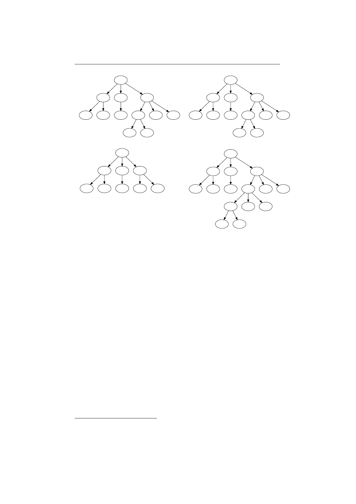
4.1. IO.JENETICS.EXT CHAPTER 4. MODULES
0
1 2 3
456789
10 11
a
b c d
e f g h i j
k l
3←→ h
0
12h
456kl
a
b c d
e f g 3 i j
7 8 9
10 11
Figure 4.1.4: Single-node crossover
4.1.4 Weasel program
The Weasel program
6
is thought experiment from Richard Dawkins, in which
he tries to illustrate the function of genetic mutation and selection.
7
For this
reason he chooses the well known example of typewriting monkeys.
I don’t know who it was first pointed out that, given enough time, a
monkey bashing away at random on a typewriter could produce all
the works of Shakespeare. The operative phrase is, of course, given
enough time. Let us limit the task facing our monkey somewhat.
Suppose that he has to produce, not the complete works of Shake-
speare but just the short sentence»Methinks it is like a weasel«, and
we shall make it relatively easy by giving him a typewriter with a
restricted keyboard, one with just the 26 (uppercase) letters, and a
space bar. How long will he take to write this one little sentence?[
9
]
The search space of the 28 character long target string is 27
28 ≈
10
40
. If the
monkey writes 1
,
000
,
000 different sentences per second, it would take about 10
26
years (in average) writing the correct one. Although Dawkins did not provide
the source code for his program, a »Weasel« style algorithm could run as follows:
1. Start with a random string of 28 characters.
2. Make ncopies of the string (reproduce).
6https://en.wikipedia.org/wiki/Weasel_program
7The classes are located in the io.jenetics.ext module.
82

4.1. IO.JENETICS.EXT CHAPTER 4. MODULES
3. Mutate the characters with an mutation probability of 5%.
4.
Compare each new string with the target string »METHINKS IT IS LIKE
A WEASEL«, and give each a score (the number of letters in the string
that are correct and in the correct position).
5.
If any of the new strings has a perfect score (28), halt. Otherwise, take
the highest scoring string, and go to step 2.
Richard Dawkins was also very careful to point out the limitations of this
simulation:
Although the monkey/Shakespeare model is useful for explaining the
distinction between single-step selection and cumulative selection, it is
misleading in important ways. One of these is that, in each generation
of selective »breeding«, the mutant »progeny« phrases were judged
according to the criterion of resemblance to a distant ideal target,
the phrase METHINKS IT IS LIKE A WEASEL. Life isn’t like that.
Evolution has no long-term goal. There is no long-distance target, no
final perfection to serve as a criterion for selection, although human
vanity cherishes the absurd notion that our species is the final goal of
evolution. In real life, the criterion for selection is always short-term,
either simple survival or, more generally, reproductive success.[9]
If you want to write a Weasel program with the
Jenetics
library, you need to
use the special WeaselSelector and WeaselMutator.
1pu bl ic c l a s s WeaselProgram {
2pr iv at e s t a t i c f i n a l S t r i n g TARGET =
3"METHINKS IT IS LIKE A WEASEL" ;
4
5pr iv at e s t a t i c in t s c o r e ( final Genotype<CharacterGene> g t ) {
6final Ch ar Seq uen ce s o u r c e =
7( CharSequence ) gt . getChromosome ( ) ;
8return I nt St re am . ra n ge ( 0 , TARGET. l e n g t h ( ) )
9. map( i −> s o u r c e . ch arA t ( i ) == TARGET. c ha rAt ( i ) ? 1 : 0)
10 . sum ( ) ;
11 }
12
13 pub li c s t a t i c void main ( final S t r i n g [ ] a r g s ) {
14 final CharSeq c h a r s = C harSeq . o f ( "A−Z " ) ;
15 final Factory<Genotype<CharacterGene>> g t f = Genotype . o f (
16 new C haracter Chro mosome ( c h ar s , TARGET. l e n g t h ( ) )
17 ) ;
18 final Eng ine<C ha rac ter Gen e , I n t e g e r > e n g i ne = E ng in e
19 . b u i l d e r ( WeaselProgram : : s co re , g t f )
20 . p o p u l a t i o n S i z e ( 1 5 0)
21 . selector(new WeaselSelector <>())
22 . offspringFraction (1)
23 . a l t e r e r s (new WeaselMutator <>(0.05) )
24 . b u i l d ( ) ;
25 final Phenotype<Ch ara cte rGe ne , I n t e g e r > r e s u l t = e n g i n e
26 . stream ( )
27 . l i m i t ( b y F it n e s s T hr e s ho l d (TARGET. l e n g t h ( ) −1) )
28 . peek ( r −> System . out . p r i n t l n (
29 r . getTotalGenerations () + " : " +
30 r . getBestPhenotype () ) )
31 . c o l l e c t ( toBestPh e notype ( ) ) ;
32 System . out . p r i n t l n ( r e s u l t ) ;
83

4.1. IO.JENETICS.EXT CHAPTER 4. MODULES
33 }
34 }
Listing 4.4: Weasel program
Listing 4.4 on the previous page shows how-to implement the
WeaselProgram
with
Jenetics
. Step (1) and (2) of the algorithm is done implicitly when the
initial population is created. The third step is done by the
WeaselMutator
, with
mutation probability of 0.05. Step (4) is done by the WeaselSelector together
with the configured offspring-fraction of one. The evolution stream is limited by
the
Limits.byFitnessThreshold
, which is set to
scoremax −
1. In the current
example this value is set to TARGET.length() - 1 = 27.
11: [ U BN HL JUS RCO XR L FI YLA WRD CCN Y ] -- > 6
22: [ U BN HL JUS RCO XR L FI YLA WWD CCN Y ] -- > 7
33: [ U BQ HL JUS RCO XR L FI YLA WWE CCN Y ] -- > 8
45: [ U BQ HL JUS RCO XR L FI CLA WWE CCN L ] -- > 9
56: [W QHLJUS RCOXR LFICLA WEGCNL] --> 10
67: [W QHLJKS RCOXR LFIHLA WEGCNL] --> 11
78: [W QHLJKS RCOXR LFIHLA WEGSNL] --> 12
89: [ W QH LJ KS RCOXR LFIS A W EGSNL ] - -> 13
910: [M Q HL JKS RC OX R L FIS A WEGS NL ] -- > 14
10 11: [ M EQHLJ KS RCOXR LFIS A W EG SNL ] - -> 15
11 12: [ M EQHIJ KS ICOXR LFIN A W EG SNL ] - -> 17
12 14: [ M EQHIN KS ICOXR LFIN A W EG SNL ] - -> 18
13 16: [ M ETHIN KS ICOXR LFIN A W EG SNL ] - -> 19
14 18: [ M ETHIN KS IMOXR LFKN A W EG SNL ] - -> 20
15 19: [ M ETHIN KS IMOXR LIKN A W EG SNL ] - -> 21
16 20: [ M ETHIN KS IMOIR LIKN A W EG SNL ] - -> 22
17 23: [ M ETHIN KS IMOIR LIKN A W EG SEL ] - -> 23
18 26: [ M ETHIN KS IMOIS LIKN A W EG SEL ] - -> 24
19 27: [ M ETHIN KS IM IS L IKN A WEHS EL ] -- > 25
20 32: [ M ETHIN KS IT IS L IKN A WEHS EL ] -- > 26
21 42: [ M ETHIN KS IT IS L IKN A WEAS EL ] -- > 27
22 46: [ M ETHIN KS IT IS L IKE A WEAS EL ] -- > 28
The (shortened) output of the Weasel program (listing 4.4 on the preceding
page) shows, that the optimal solution is reached in generation 46.
4.1.5 Modifying Engine
The current design of
Engine
allows to created multiple independent evolution
streams from a single Engine instance. One drawback of this approach is, that
the evolution stream runs with the same evolution parameters until the stream is
truncated. It is not possible to change the stream’s
Engine
configuration during
the evolution process. For this purpose, the
EvolutionStreamable
interface has
been introduced. It is similar to the Java
Iterable
interface and abstracts the
EvolutionStream creation.
1public i n te r fa c e EvolutionStreamable<
2Gextends Gene <?, G>,
3Cextends Comparable<? super C>
4> {
5Evoluti o nStream <G, C>
6s tr ea m ( S u p p l i e r <E v o l u t i o n S t a r t <G, C>> s t a r t ) ;
7
8Evo lu ti on St re am <G, C> s tream ( E v o l u t i o n I n i t <G> i n i t ) ;
9
10 E vo l u ti o nS t r ea m ab l e <G, C>
11 l i m i t ( S u p p l i e r <P r e d i c a t e <? super E v ol u t i on R e s ul t <G, C>>> p )
12 }
Listing 4.5: EvolutionStreamable interface
84
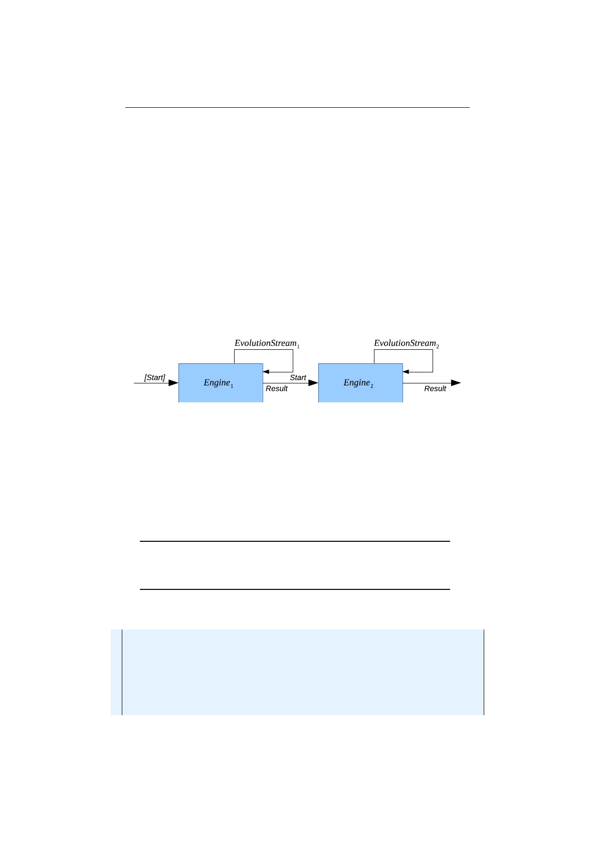
4.1. IO.JENETICS.EXT CHAPTER 4. MODULES
Listing 4.5 on the previous page shows the main methods of the
Evolution-
Streamable
interface. The existing
stream
methods take an initial value,
which allows to concatenate different engines. With the
limit
method it
is possible to limit the size of the created
EvolutionStream
instances. The
io.jenetics.ext
module contains additional classes which allows to concate-
nate evolution
Engines
with different configurations, which will then create one
varying EvolutionStream. This additional Engine classes are:
1. ConcatEngine,
2. CyclicEngine and
3. AdaptiveEngine.
4.1.5.1 ConcatEngine
The
ConcatEngine
class allows to create more than one
Engine
s, with different
configurations, and combine it into one EvolutionStreamable (Engine).
Figure 4.1.5: Engine concatenation
Figure 4.1.5 shows how the
EvolutionStream
of two concatenated
Engine
s
works. You can create the first partial
EvolutionStream
with an optional start
value. If the first
EvolutionStream
stops, it’s final
EvolutionResult
is used
as start value of the second evolution stream, created by the second evolution
Engine
. It is important that the evolution
Engine
s used for concatenation are
limited. Otherwise the created
EvolutionStream
will only use the first
Engine
,
since it is not limited.
The concatenated evolution Engines must be limited (by calling
Engine.limit
), otherwise only the first
Engine
is used executing the
resulting EvolutionStream.
The following code sample shows how to create an
EvolutionStream
from
two concatenate Engines. As you can see, the two Engines are limited.
1final Engine<DoubleGene , Double> e n g i n e 1 = . . . ;
2final Engine<DoubleGene , Double> e n g i n e 2 = . . . ;
3
4final Genotype<DoubleGene> r e s u l t =
5ConcatEngine . of (
6e n g in e 1 . l i m i t ( 5 0 ) ,
7en gi n e2 . l i m i t ( ( ) −> Limits . bySteadyFitness (30) ))
8. stream ( )
9. c o l l e c t ( E v o l u t i o n R e s u l t . t oB es tG en ot yp e ( ) ) ;
85
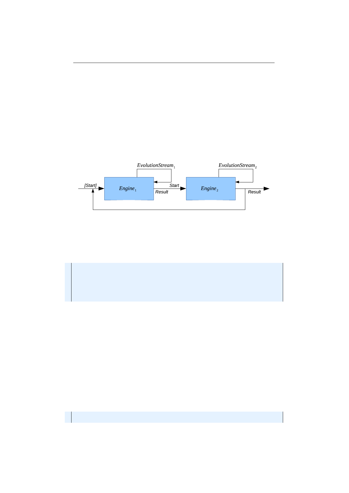
4.1. IO.JENETICS.EXT CHAPTER 4. MODULES
A practical use case for the
Engine
concatenation is, when you want to do a
broader exploration of the search space at the beginning and narrow it with the
following
Engine
s. In such a setup, the first
Engine
would be configured with a
Mutator
with a relatively big mutation probability. The mutation probabilities
of the following Engines would then be gradually reduced.
4.1.5.2 CyclicEngine
The
CyclicEngine
is similar to the
ConcatEngine
. Where the
ConcatEngine
stops the evolution, when the stream of the last engine terminates, the
Cyclic-
Engine
continues with a new stream from the first
Engine
. The evolution flow
of the CyclicEngine is shown in figure 4.1.6.
Figure 4.1.6: Cyclic Engine
Since the
CyclicEngine
creates unlimited streams, although the participating
Engine
s are all creating limited streams, the resulting
EvolutionStream
must
be limited as well. The code snippet below shows the creation and execution of
acyclic EvolutionStream.
1final Genotype<DoubleGene> r e s u l t =
2CyclicEngine . of (
3e n g in e 1 . l i m i t ( 5 0 ) ,
4en gi n e2 . l i m i t ( ( ) −> Limits . bySteadyFitness (15) ))
5. stream ( )
6. limit (Limits . bySteadyFitness (50))
7. c o l l e c t ( E v o l u t i o n R e s u l t . t oB es tG en ot yp e ( ) ) ;
The reason for using a cyclic
EvolutionStream
is similar to the reason for using a
concatenated
EvolutionStream
. It allows you to do a broad search, followed by
a narrowed exploration. This cycle is then repeated until the limiting predicate
of the outer stream terminates the evolution process.
4.1.5.3 AdaptiveEngine
The
AdaptiveEngine
is the most flexible method for creating
EvolutionStream
s.
Instead of defining a fixed set
Engine
s, which then creates the
EvolutionStream
,
you define a function which creates an
Engine
, depending on last
EvolutionRe-
sult
of the previous
EvolutionStream
. You can see the evolution flow of the
AdaptiveEngine in figure 4.1.7 on the following page.
From the implementation perspective, the
AdaptiveEngine
requires a little
bit more code. The additional flexibility isn’t for free, as you can see in the code
example below.
1pub li c s t a t i c void main ( final S t r i n g [ ] a r g s ) {
2final Problem<double [ ] , DoubleGene , Double> problem = . . . ;
86
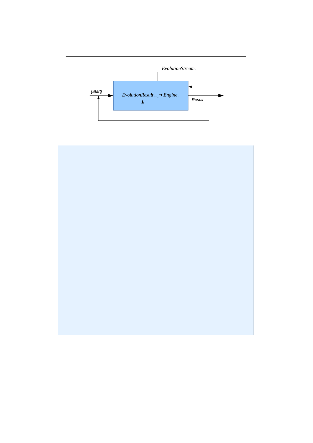
4.1. IO.JENETICS.EXT CHAPTER 4. MODULES
Figure 4.1.7: Adaptive Engine
3// En gin e . B u i l d e r t e m pl a t e .
4final En gi ne . Bu i ld er <DoubleGene , Double> b ld = Eng in e
5. b u i l d e r ( problem )
6. m ini mi zi ng ( ) ;
7
8final Genotype<DoubleGene> r e s u l t =
9AdaptiveE ngine .< DoubleGene , Double>o f ( r −> e n g i n e ( r , b l d ) )
10 . stream ( )
11 . limit (Limits . bySteadyFitness (50))
12 . c o l l e c t ( E v o l u t i o n R e s u l t . t oB es tG en ot yp e ( ) ) ;
13 }
14
15 static E v ol u t i on S t r e am a b l e <DoubleGene , Doubl e> e n g i n e (
16 final Ev ol ut io nR es ul t <DoubleGene , Double> r e s u l t ,
17 final Engine . Bu il de r<DoubleGene , Double> b u i l d e r
18 ) {
19 return var ( r e s u l t ) < 0 . 2
20 ? b u i l d e r . copy ( )
21 . a l t e r e r s (new Mutator < >(0.75) )
22 . b u i l d ( )
23 . l i m i t ( 5)
24 : b u i l d e r . copy ( )
25 . a l t e r e r s (
26 new Mutator < >(0.05) ,
27 new MeanAlterer <>())
28 . selector(new R o u l e tt e W h e e lS e l e c t or <>() )
29 . b u i l d ( )
30 . limit (Limits . bySteadyFitness (25)) ;
31 }
32
33 s t a t i c double var ( final E v o l ut i o n R e su l t <DoubleGene , Double> e r ) {
34 return e r != n u l l
35 ? e r . g e t P o p u l a t i o n ( ) . st re am ( )
36 . map( Phenotype : : g e t F i t n e s s )
37 . c o l l e c t ( toDoubleMoments ( ) )
38 . g e t V a r i a n c e ( )
39 : 0 . 0 ;
40 }
The example tries to broaden the search, once the variance of the population’s
fitness values are below a given threshold. When implementing the
Engine
creation function, you have to be aware, that the
EvolutionResult
for the first
Engine is null.
87

4.1. IO.JENETICS.EXT CHAPTER 4. MODULES
4.1.6 Multi-objective optimization
A Multi-objective Optimization Problem (MOP) can be defined as the problem
of finding
a vector of decision variables which satisfies constraints and optimizes
a vector function whose elements represent the objective functions.
These functions form a mathematical description of performance
criteria which are usually in conflict with each other. Hence, the
term »optimize« means finding such a solution which would give the
values of all the objective functions acceptable to the decision maker.
[25]
There are several ways for solving multiobjective problems. An excellent theo-
retical foundation is given in [
7
]. The algorithms implemented by
Jenetics
are
based in therms of Pareto optimality as described in [13], [10] and [17].
4.1.6.1 Pareto efficiency
Pareto efficiency is named after the Italian economist and political scientist
Vilfredo Pareto8. He used the concept in his studies of economic efficiency and
income distribution. The concept has been applied in different academic fields
such as economics, engineering, and the life sciences. Pareto efficiency says that
an allocation is efficient if an action makes some individual better off and no
individual worse off. In contrast to single-objective optimization, where usually
only one optimal solution exits, the multi-objective optimization creates a set of
optimal solutions. The optimal solutions are also known as the Pareto front or
Pareto set.
Definition. (Pareto efficiency
[
7
]
):
A solution
x
is said to be Pareto op-
timal iff there is no
x0
for which
v
=
(f1(x0), ..., fk(x0))
dominates
u
=
(f1(x), ..., fk(x)).
The definition says that
x∗
is Pareto optimal if there exists no feasible vector
x
which would decrease some criterion without causing a simultaneous increase
in at least one other criterion.
Definition. (Pareto dominance
[
7
]
):
A vector
u
=
(u1, ..., uk)
is said to
dominate
another vector
v
=
(v1, ..., vk)
(denoted by
uv
) iff
u
is partially
greater than v, i.e., ∀i∈ {1, ..., k},ui≥vi∧ ∃i∈ {1, ..., k}:ui> vi.
After this two basic definitions, lets have a look at a simple example. Fig-
ure 4.1.8 on the next page shows some points of a two-dimensional solution
space. For simplicity, the points will all lie within a circle with radius 1and
center point of (1,1).
Figure 4.1.9 on page 90 shows the Pareto front of a maximization problem.
This means we are searching for solutions tries to maximize the
x
and
y
coordinate
at the same time.
Figure 4.1.10 on page 91 shows the Pareto front if we try to minimize the
x
and ycoordinate at the same time.
8https://en.wikipedia.org/wiki/Vilfredo_Pareto
88
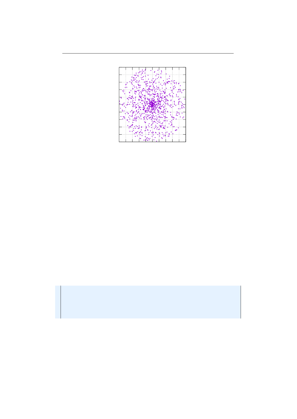
4.1. IO.JENETICS.EXT CHAPTER 4. MODULES
0
0.2
0.4
0.6
0.8
1
1.2
1.4
1.6
1.8
2
0 0.2 0.4 0.6 0.8 1 1.2 1.4 1.6 1.8 2
Figure 4.1.8: Circle points
4.1.6.2 Implementing classes
The classes, used for solving multi-objective problems, reside in the
io.jenetics-
.ext.moea
package. Originally, the
Jenetics
library focuses on solving single-
objective problems. This drives the design decision to force the return value of
the fitness function to be
Comparable
. If the result type of the fitness function
is a vector, it is no longer clear how to make the results comparable.
Jenetics
chooses to use the Pareto dominance relation (see section 4.1.6.1 on the preceding
page). The Pareto dominance relation,
, defines a strict partial order, which
means is
1. irreflexive: uu,
2. transitive: uv∧vw⇒uwand
3. asymmetric: uv⇒vu.
The
io.jenetics.ext.moea
package contains the classes needed for doing multi-
objective optimization. One of the central types is the
Vec
interface, which
allows you wrap a vector of any element type into a Comparable.
1public i n t e r f a c e Vec<T> extends Comparable<Vec<T>> {
2public T data ( ) ;
3public in t l e n g t h ( ) ;
4public ElementComparator<T> c omparato r ( ) ;
5public Element Dista nce<T> d i s t a n c e ( ) ;
6public Comparator<T> dominance ( ) ;
7}
Listing 4.6: Vec interface
Listing 4.6 shows the necessary methods of the
Vec
interface. This methods are
sufficient to do all the optimization calculations. The
data()
method returns the
underlying vector type, like
double[]
or
int[]
. With the
ElementComparator
,
which is returned by the
comparator()
method, it is possible to compare single
elements of the vector type
T
. This is similar to the
ElementDistance
function,
89
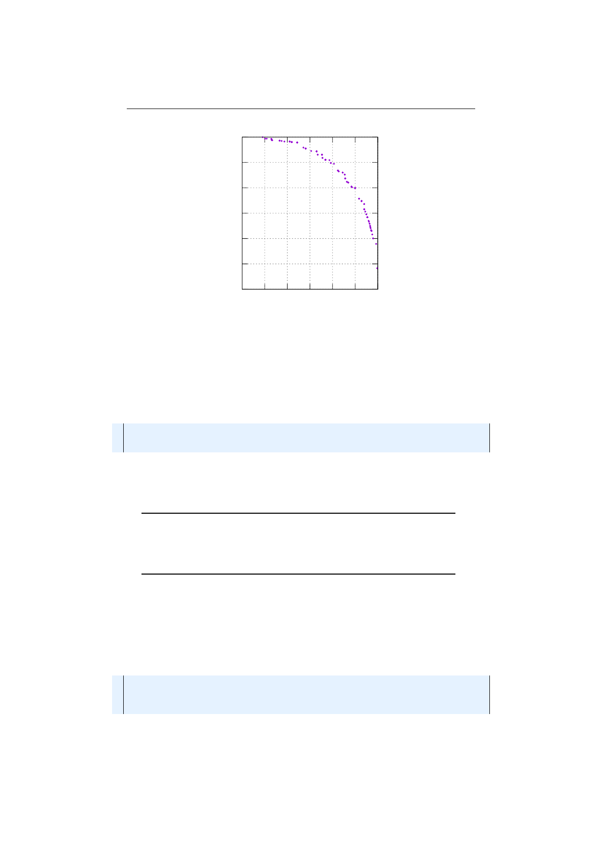
4.1. IO.JENETICS.EXT CHAPTER 4. MODULES
0.8
1
1.2
1.4
1.6
1.8
2
0.8 1 1.2 1.4 1.6 1.8 2
Figure 4.1.9: Maximizing Pareto front
returned by the
distance()
method, which calculates the distance of two
vector elements. The last method,
dominance()
, returns the Pareto dominance
comparator,
. Since it is quite a bothersome to implement all this needed
methods, the
Vec
interface comes with a set of factory methods, which allows to
create Vec instance for some primitive array types.
1final Vec<int[] > i v e c = Vec . o f ( 1 , 2 , 3) ;
2final Vec<long [ ] > l v e c = Vec . o f (1L , 2L , 3L ) ;
3final Vec<double [] > dvec = Vec . of ( 1 . 0 , 2 . 0 , 3 . 0 ) ;
For efficiency reason, the primitive arrays are not copied, when the
Vec
instance
is created. This lets you, theoretically, change the value of a created
Vec
instance,
which will lead to unexpected results.
Although the
Vec
interface extends the
Comparable
interface, it violates its
general contract. It only implements the Pareto dominance relation, which
defines a partial order. So, trying to sort a list of
Vec
objects, might lead
to an exception (thrown by the sorting method) at runtime.
The second difference to the single-objective setup is the
EvolutionResult
collector. In the single-objective case, we will only get one best result, which
is different in the multi-object optimization. As we have seen in section 4.1.6.1
on page 88, we no longer have only one result, we have a set of Pareto optimal
solutions. There is a predefined collector in the
io.jenetics.ext.moea
package,
MOEA.toParetoSet(IntRange)
, which collects the Pareto optimal
Phenotypes
into an ISeq.
1final ISeq<Phenotype<DoubleGene , Vec<double[]>>> paretoSet =
2e n g i n e . s tr e am ( )
3. l i m i t ( 1 0 0 )
4. c o l l e c t (MOEA. t o P a r e t o S e t ( I ntR an ge . o f ( 3 0 , 5 0 ) ) ) ;
90
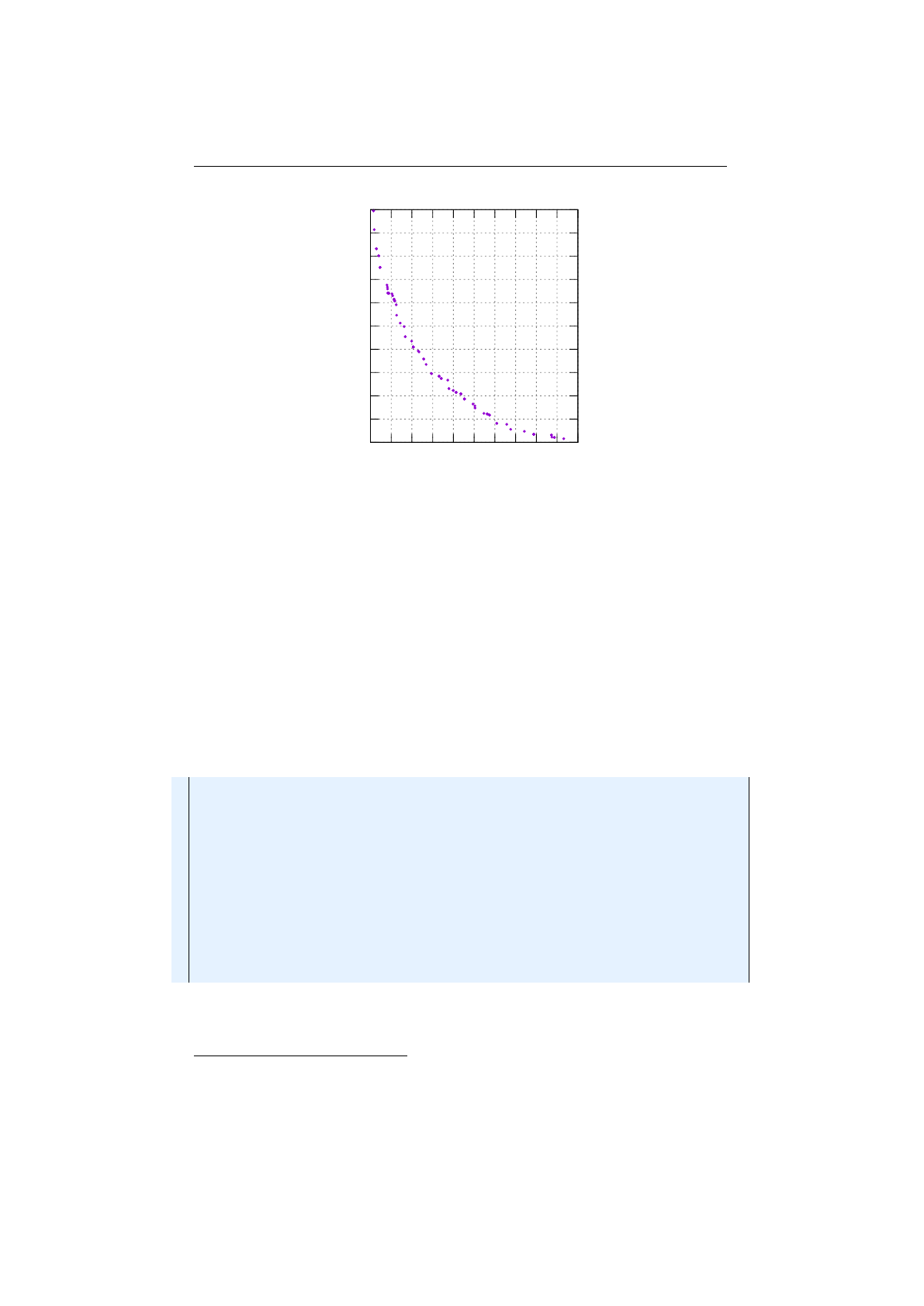
4.1. IO.JENETICS.EXT CHAPTER 4. MODULES
0
0.1
0.2
0.3
0.4
0.5
0.6
0.7
0.8
0.9
1
0 0.1 0.2 0.3 0.4 0.5 0.6 0.7 0.8 0.9 1
Figure 4.1.10: Minimizing Pareto front
Since there exists a potential infinite number of Pareto optimal solutions, you
have to define desired number set elements. This is done with an
IntRange
object, where you can specify the minimal and maximal set size. The example
above will return a Pareto size which size in the range of
[30,50)
. For reducing the
Pareto set size, the distance between two vector elements is taken into account.
Points which lie very close to each other are removed. This leads to a result,
where the Pareto optimal solutions are, more or less, evenly distributed over the
whole Pareto front. The crowding-distance
9
measure is used for calculating the
proximity of two points and it is described in [7] and [13].
Till now we have described the multi-objective result type (
Vec
) and the final
collecting of the Pareto optimal solution. So lets create a simple multi-objective
problem and an appropriate Engine.
1final Problem<double [ ] , DoubleGene , Vec<double[]>> problem =
2Problem . of (
3v−> Vec . o f ( v [ 0 ] ∗c os ( v [ 1 ] ) + 1 , v [ 0 ] ∗si n ( v [ 1 ] ) + 1 ) ,
4Co de cs . o f V e c t o r (
5DoubleRange . o f ( 0 , 1 ) ,
6DoubleRange . of (0 , 2∗PI )
7)
8) ;
9
10 final Engine<DoubleGene , Vec<double[] >> e n g i n e =
11 Engine . b u i l d e r ( problem )
12 . offspringSelector(new To ur na me nt Se le ct or <>(4) )
13 . s u r v i v o r s S e l e c t o r ( UFTournamentSelector . ofVec ( ) )
14 . b u i l d ( ) ;
The fitness function in the example problem above will create 2D-points which will
all lies within a circle with a center of
(1,1)
. In figure 4.1.9 on the previous page
you can see how the resulting solution will look like. There is almost no difference
9
The crowding distance value of a solution provides an estimate of the density of solutions
surrounding that solution. The crowding distance value of a particular solution is the av-
erage distance of its two neighboring solutions.
https://www.igi-global.com/dictionary/
crowding-distance/42740.
91

4.1. IO.JENETICS.EXT CHAPTER 4. MODULES
in creating an evolution Engine for single- or multi-objective optimization. You
only have to take care to choose the right Selector. Not all
Selector
s will
work for multi-objective optimization. This include all
Selector
s which needs
a
Number
fitness type and where the population needs to be sorted
10
. The
Selector which works fine in a multi-objective setup is the
TournamentSelector
.
Additionally you can use one of the special MO selectors:
NSGA2Selector
and
UFTournamentSelector.
NSGA2 selector
This selector selects the first elements of the population,
which has been sorted by the Crowded-comparison operator (equation 4.1.1),
n
,
as described in [10]
i
njif (irank < jrank )∨((irank =jrank )∧idist > jdist),(4.1.1)
where
irank
denotes the non-domination rank of individual
i
and
idist
the crowd-
ing distance of individual i.
Unique fitness tournament selector
The selection of unique fitnesses lifts
the selection bias towards over-represented fitnesses by reducing multiple solutions
sharing the same fitness to a single point in the objective space. It is therefore no
longer required to assign a crowding distance of zero to individual of equal fitness
as the selection operator correctly enforces diversity preservation by picking
unique points in the objective space. [13]
Since the multi-objective optimization (MOO) classes are an extensions to
the existing evolution
Engine
, the implementation doesn’t exactly follow an
established algorithm, like NSGA2 or SPEA2. The results and performance,
described in the relevant papers, are therefore not directly comparable. See
listing 1.2 on page 3 for comparing the Jenetics evolution flavor.
4.1.6.3 Termination
Most of the existing termination strategies, implemented in the
Limits
class,
presumes a total order of the fitness values. This assumption holds for single-
objective optimization problems, but not for multi-objective problems. Only
termination strategies which doesn’t rely on the total order of the fitness value,
can be safely used. The following termination strategies can be used for multi-
objective problems:
•Limits.byFixedGeneration,
•Limits.byExecutionTime and
•Limits.byGeneConvergence.
All other strategies doesn’t have a well defined termination behavior.
10
Since the
relation doesn’t define a total order, sorting the population will lead to an
IllegalArgumentException at runtime.
92

4.2. IO.JENETICS.PROG CHAPTER 4. MODULES
4.2 io.jenetics.prog
In artificial intelligence, genetic programming (GP) is a technique whereby com-
puter programs are encoded as a set of genes that are then modified (evolved) us-
ing an evolutionary algorithm (often a genetic algorithm).
11
The
io.jenetics-
.prog
module contains classes which enables the
Jenetics
library doing GP. It
introduces a
ProgramGene
and
ProgramChromosome
pair, which serves as the
main data-structure for genetic programs. A
ProgramGene
is essentially a tree
(AST12) of operations (Op) stored in a ProgramChromosome.13
4.2.1 Operations
When creating own genetic programs, it is not necessary to derive own classes
from the
ProgramGene
or
ProgramChromosome
. The intended extension point
is the Op interface.
The extension point for own GP implementations is the Op interface. There
is in general no need for extending the ProgramChromosome class.
1public i n t e r f a c e Op<T> {
2public S t r i n g name ( ) ;
3public in t a r i t y ( ) ;
4public T a pp ly (T [ ] a r g s ) ;
5}
Listing 4.7: GP Op interface
The generic type of the
Op
interface (see listing 4.7) enforces the data-type
constraints for the created program tree and makes the implementation a strongly
typed GP. Using the
Op.of
factory method, a new operation is created by defining
the desired operation function.
1final Op<Double> add = Op . o f ( "+" , 2 , v −> v [ 0 ] + v [ 1 ] ) ;
2final Op<S t r i n g > c o n c a t = Op. o f ( "+" , 2 , v −> v [ 0 ] + v [ 1 ] ) ;
A new
ProgramChromosome
is created with the operations suitable for our
problem. When creating a new
ProgramChromosome
, we must distinguish two
different kind of operations:
1.
Non-terminal operations have an arity greater than zero, which means they
take at least one argument. This operations need to have child nodes, where
the number of children must be equal to the arity of the operation of the
parent node. Non-terminal operations will be abbreviated to operations.
2.
Terminal operations have an arity of zero and from the leaves of the
program tree. Terminal operations will be abbreviated to terminals.
The
io.jenetics.prog
module comes with three predefined terminal opera-
tions: Var,Const and EphemeralConst.
11https://en.wikipedia.org/wiki/Genetic_programming
12https://en.wikipedia.org/wiki/Abstract_syntax_tree
13
When implementing the GP module, the emphasis was to not create a parallel world of
genes and chromosomes. It was an requirement, that the existing Alterer and Selector classes
could also be used for the new GP classes. This has been achieved by flattening the AST of a
genetic program to fit into the 1-dimensional (flat) structure of a chromosome.
93

4.2. IO.JENETICS.PROG CHAPTER 4. MODULES
Var
The
Var
operation defines a variable of a program, which is set from
outside when it is evaluated.
1final Var<Double> x = Var . o f ( "x" , 0) ;
2final Var<Double> y = Var . o f ( "y" , 1) ;
3final Var<Double> z = Var . o f ( "z" , 2) ;
4final IS eq <Op<Double>> t e r m i n a l s = I Se q . o f ( x , y , z ) ;
The terminal operations defined in the listing above can be used for defining
a program which takes a 3-dimensional vector as input parameters,
x
,
y
, and
z
, with the argument indices 0,1, and 2. If you have again a look at the
apply
method of the operation interface, you can see that this method takes an
object array of type
T
. The variable
x
will return the first element of the input
arguments, because it has been created with index 0.
Const
The
Const
operation will always return the same, constant, value when
evaluated.
1final Const<Double> one = Const . o f ( 1 . 0 ) ;
2final Const<Double> p i = Const . o f ( " PI " , Math . PI ) ;
We can create a constant operation in to flavors: with a value only and with a
dedicated name. If a constant has a name, the symbolic name is used, instead of
the value, when the program tree is printed.
EphemeralConst
An ephemeral constant is a terminal operation, which encap-
sulates a value that is generated at run time from the
Supplier
it is created
from. Ephemeral constants allows you to have terminals that don’t have all the
same values. To create an ephemeral constant that takes its random value in
[0,1) you will write the following code.
1final Op<Double> rand1 = EphemeralConst
2. o f ( RandomRegistry . getRandom ( ) : : ne xtDouble ) ;
3final Op<Double> rand2 = EphemeralConst
4. o f ( "R" , RandomRegistry . getRandom ( ) : : nextDouble ) ;
The ephemeral constant value is determined when it is inserted in the tree and
never changes until it is replaced by another ephemeral constant.
4.2.2 Program creation
The
ProgramChromosome
comes with some factory methods, which lets you
easily create program trees with a given depth and a given set of operations and
terminals.
1f i n a l i nt depth = 5 ;
2final IS eq <Op<Double>> o p e r a t i o n s = I Se q . o f ( . . . ) ;
3final IS eq <Op<Double>> t e r m i n a l s = I Se q . o f ( . . . ) ;
4final ProgramChromosome<Double> program = ProgramChromosome
5. o f ( depth , o p e r a t i o n s , t e r m i n a l s ) ;
The code snippet above will create a perfect program tree
14
of depth 5. All non-
leaf nodes will contain operations, randomly selected from the given operations,
whereas all leaf nodes are filled with operations from the terminals.
14
All leafs of a perfect tree have the same depth and all internal nodes have degree
Op.arity
.
94

4.2. IO.JENETICS.PROG CHAPTER 4. MODULES
The created program tree is perfect, which means that all leaf nodes have
the same depth. If new trees needs to be created during evolution, they
will be created with the depth,operations and terminals defined by the
template program tree.
The evolution
Engine
used for solving GP problems is created the same
way as for normal GA problems. Also the execution of the
EvolutionStream
stays the same. The first
Gene
of the collected final
Genotype
represents the
evolved program, which can be used to calculate function values from arbitrary
arguments.
1final Eng in e<ProgramGene<Double >, Do uble> e n g i n e = E ng in e
2. b u i l d e r ( Main : : e r ro r , program )
3. m ini mi zi ng ( )
4. a l t e r e r s (
5new SingleNodeCrossover <>() ,
6new Mutator <>() )
7. b u i l d ( ) ;
8
9final ProgramGene<Double> p rogr am = e n g i n e . s tr ea m ( )
10 . l i m i t ( 3 0 0 )
11 . c o l l e c t ( E v o l u t i o n R e s u l t . t oB es tG en ot yp e ( ) )
12 . getGene ( ) ;
13 f i n a l double r e s u l t = program . e v a l ( 3 . 4 ) ;
For a complete GP example have a look at the examples in chapter 5.7 on
page 118.
4.2.3 Program repair
The specialized crossover class,
SingleNodeCrossover
, for a
TreeGene
guar-
antees that the program tree after the alter operation is still valid. It obeys
the tree structure of the gene. General alterers, not written for
ProgramGene
of
TreeGene
classes, will most likely destroy the tree property of the altered
chromosome. There are essentially two possibility for handling invalid tree
chromosomes:
1.
Marking the chromosome as invalid. This possibility is easier to achieve,
but would also to lead to a large number of invalid chromosomes, which
must be recreated. When recreating invalid chromosomes we will also loose
possible solutions.
2.
Trying to repair the invalid chromosome. This is the approach the
Jenetics
library has chosen. The repair process reuses the operations in a
Program-
Chromosome and rebuilds the tree property by using the operation arity.
Jenetics
allows the usage of arbitrary Alterer implementations. Even alterers
not implemented for ProgramGenes. Genes destroyed by such alterer are
repaired.
95

4.3. IO.JENETICS.XML CHAPTER 4. MODULES
4.2.4 Program pruning
When you are solving symbolic regression problems, the mathematical expression
trees, created during the evolution process, can become quite big. From the
diversity point of view, this might be not that bad, but it comes with additional
computation cost. With the
MathTreePruneAlterer
you are able to simplify
some portion of the population in each generation.
1final Eng in e<ProgramGene<Double >, Do uble> e n g i n e = E ng in e
2. b u i l d e r ( Main : : e r ro r , program )
3. m ini mi zi ng ( )
4. a l t e r e r s (
5new SingleNodeCrossover <>() ,
6new Mutator <>() ,
7new MathTreePruneAlterer <>(0.5))
8. b u i l d ( ) ;
In the example above, half of the expression trees are simplified in each generation.
If you want to prune the final result, you can do this with the
MathExpr.simplify
method.
1final ProgramGene<Double> p rogr am = e n g i n e . s tr ea m ( )
2. l i m i t ( 3 0 0 0 )
3. c o l l e c t ( E v o l u t i o n R e s u l t . t oB es tG en ot yp e ( ) )
4. getGene ( ) ;
5
6final TreeNode<Op<Double>> ex p r = MathExpr . s i m p l i f y ( program ) ;
The algorithm used for pruning the expression tree, currently only uses some
basic mathematical identities, like
x
+ 0 =
x
,
x·
1 =
x
or
x·
0=0. More
advanced simplification algorithms may be implemented in the future. The
MathExpr
helper class can also be used for creating mathematical expression
trees from the usual textual representation.
1final MathExpr expr = MathExpr
2. p a r s e ( " 5∗z + 6∗x + s i n ( y ) ^3 + (1 + s i n ( z ∗5) / 4) /6 " ) ;
3f i n a l double v a lu e = e xp r . e v a l ( 5 . 5 , 4 , 2 . 3 ) ;
The variables in an expression string are sorted alphabetically. This means, that
the expression is evaluated with
x
= 5
.
5,
y
= 4 and
z
= 2
.
3, which leads to a
result value of 44.19673085074048.
4.3 io.jenetics.xml
The
io.jenetics.xml
module allows to write and read chromosomes and geno-
types to and from XML. Since the existing JAXB marshaling is part of the
deprecated
javax.xml.bind
module the
io.jenetics.xml
module is now the
recommended for XML marshalling of the
Jenetics
classes. The XML mar-
shalling, implemented in this module, is based on the Java
XMLStreamWriter
and XMLStreamReader classes of the java.xml module.
4.3.1 XML writer
The main entry point for writing XML files is the typed XML
Writer
interface.
Listing 4.8 on the following page shows the interface of the XMLWriter.
96

4.3. IO.JENETICS.XML CHAPTER 4. MODULES
1@FunctionalInterface
2public i n te r fa c e Writer<T> {
3public void w r i t e ( XMLStreamWriter xml , T data )
4throws XMLStreamException ;
5
6pub li c s t a t i c <T> W ri ter <T> a t t r ( S t r i n g name ) ;
7pub li c s t a t i c <T> W ri ter <T> a t t r ( S t r i n g name , O bj ec t va l ue ) ;
8pub li c s t a t i c <T> W rit er<T> t e x t ( ) ;
9
10 pub li c s t a t i c <T> Writer<T>
11 elem ( S t r i n g name , Write r <? super T> . . . c h i l d r e n ) ;
12
13 pub li c s t a t i c <T> Writer<I t e r a b l e <T>>
14 ele m s ( Writer <? super T> w r i t e r ) ;
15 }
Listing 4.8: XMLWriter interface
Together with the static
Writer
factory method, it is possible to define arbitrary
writers through composition. There is no need for implementing the
Writer
interface. A simple example will show you how to create (compose) a Writer
class for the
IntegerChromosome
. The created XML should look like the given
example above.
1<int - c hr om oso me le ng th = " 3" >
2< mi n > -2 14 74 83 648 < / mi n >
3< max > 214 74 836 47 </ max >
4<alleles>
5< all ele > -187 876 243 9 </ all ele >
6< a ll el e > -9 57 34 65 95 < / al le le >
7< all ele > -8 8668 137 </ al lel e >
8</alleles>
9< / in t - c hr o m os o m e >
The following writer will create the desired XML from an integer chromosome.
As the example shows, the structure of the XML can easily be grasp from the
XML writer definition and vice versa.
1final Writer<IntegerChromosome> w r i t e r =
2elem( " i n t −chromosome " ,
3a t t r ( " l e n g t h " ) . map( ch −> ch . l e n g t h ( ) ) ,
4elem( " min " , W ri te r .< I n t e g e r >t e x t ( ) . map( ch −> ch . getMin ( ) ) ) ,
5elem( "max" , W ri te r .< I n t e g e r >t e x t ( ) . map( ch −> ch . getMax ( ) ) ) ,
6elem( " a l l e l e s " ,
7ele m s ( " a l l e l e " , W ri te r .< I n t e g e r >t e x t ( ) )
8. map( ch −> ch . t oS eq ( ) . map( g −> g . g e t A l l e l e ( ) ) )
9)
10 ) ;
4.3.2 XML reader
Reading and writing XML files uses the same concepts. For reading XML there
is an abstract
Reader
class, which can be easily composed. The main method
of the Reader class can be seen in listing 4.9.
1pu bl ic a bs tra ct c l a s s Reader<T> {
2public abstract T re ad ( final XMLStreamReader xml )
3throws XMLStreamException ;
4}
Listing 4.9: XMLReader class
97

4.3. IO.JENETICS.XML CHAPTER 4. MODULES
When creating a XML
Reader
, the structure of the XML must be defined in a
similar way as for the XML
Writer
. Additionally, a factory function, which will
create the desired object from the extracted XML data, is needed. A
Reader
,
which will read the XML representation of an
IntegerChromosome
can be seen
in the following code snippet below.
1final Reader<Int egerChrom os om e> r e a d e r =
2elem(
3( Ob je ct [ ] v ) −> {
4f i n a l i nt l e n g t h = ( int ) v [ 0 ] ;
5f i n a l i nt min = ( int ) v [ 1 ] ;
6f i n a l i nt max = ( int ) v [ 2 ] ;
7final L i s t <I n t e g e r > a l l e l e s = ( L i s t <I n t e g e r >)v [ 3 ] ;
8a s s e r t a l l e l e s . s i z e ( ) == l e n g t h ;
9return IntegerChromosome . of (
10 a l l e l e s . s t re a m ( )
11 . map( v a lu e −> In te g er G en e . o f ( va lu e , min , max)
12 . toArray ( In te ge rG e ne [ ] : : new)
13 ) ;
14 } ,
15 " i nt −chromosome " ,
16 a t t r ( " l e n g t h " ) . map( I n t e g e r : : p a r s e I n t ) ,
17 elem( " min " , t e x t ( ) . map( I n t e g e r : : p a r s e I n t ) ) ,
18 elem( "max" , t e x t ( ) . map ( I n t e g e r : : p a r s e I n t ) ) ,
19 elem( " a l l e l e s " ,
20 ele m s ( elem ( " allele " , t e x t ( ) . map( I n t e g e r : : p a r s e I n t ) ) )
21 )
22 ) ;
4.3.3 Marshalling performance
Another important aspect when doing marshalling, is the space needed for the
marshaled objects and the time needed for doing the marshalling. For the
performance tests a genotype with a varying chromosome count is used. The
used genotype template can be seen in the code snippet below.
1final Genotype<DoubleGene> g en ot yp e = Genotype . o f (
2DoubleChromosome . o f ( 0 . 0 , 1 . 0 , 1 00 ) ,
3chromosomeCount
4) ;
Table 4.3.1 shows the required space of the marshaled genotypes for different
marshalling methods: (a) Java serialization, (b) JAXB
15
serialization and (c)
XMLWriter.
Chromosome count Java serialization JAXB XML writer
1 0.0017 MiB 0.0045 MiB 0.0035 MiB
10 0.0090 MiB 0.0439 MiB 0.0346 MiB
100 0.0812 MiB 0.4379 MiB 0.3459 MiB
1000 0.8039 MiB 4.3772 MiB 3.4578 MiB
10000 8.0309 MiB 43.7730 MiB 34.5795 MiB
100000 80.3003 MiB 437.7283 MiB 345.7940 MiB
Table 4.3.1: Marshaled object size
15
The JAXB marshalling has been removed in version 4.0. It is still part of the table for
comparison with the new XML marshalling.
98
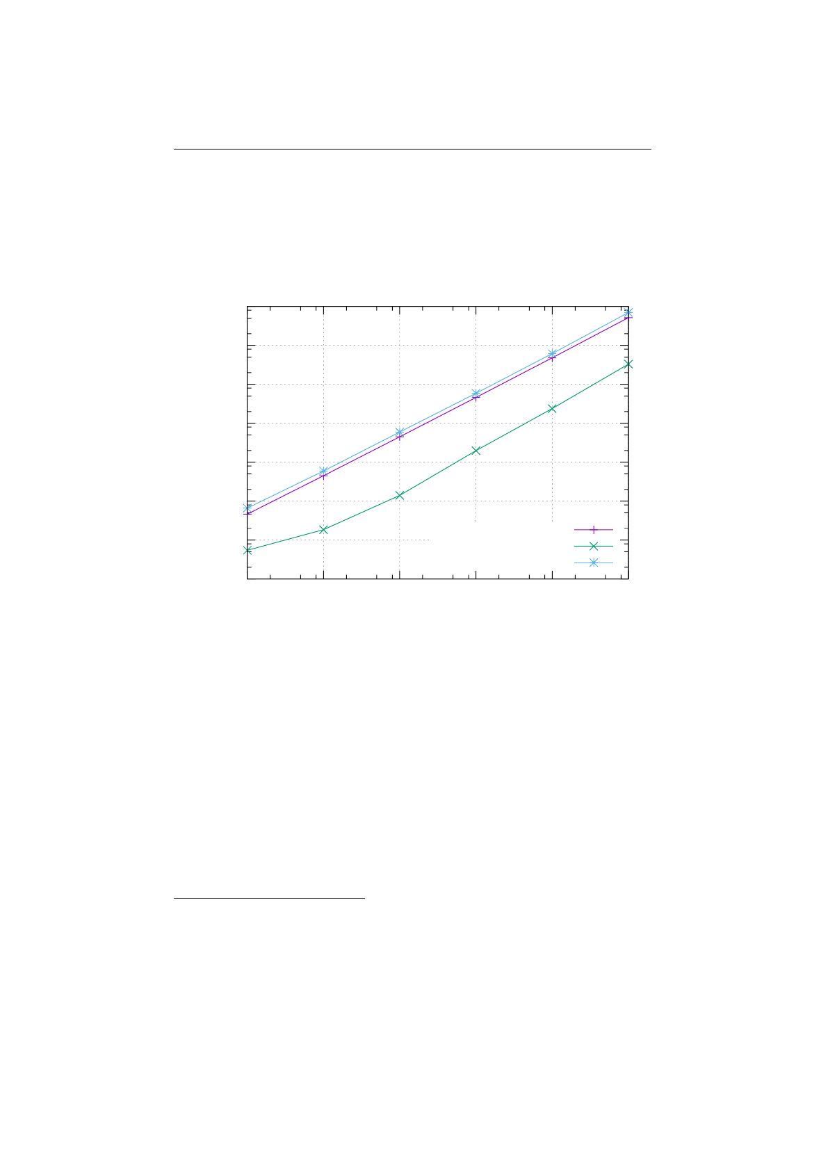
4.4. IO.JENETICS.PRNGINE CHAPTER 4. MODULES
Using the Java serialization will create the smallest files and the XML
Writer
of the
io.jenetics.xml
module will create files roughly 75% the size of the
JAXB serialized genotypes. The size of the marshaled also influences the write
performance. As you can see in diagram 4.3.1 the Java serialization is the fastest
marshalling method, followed by the JAXB marshalling. The XML
Writer
is
the slowest one, but still comparable to the JAXB method.
100
101
102
103
104
105
106
107
100101102103104105
Marshalling time [µs]
Chromosome count
JAXB
Java serialization
XML writer
Figure 4.3.1: Genotype write performance
For reading the serialized genotypes, we will see similar results (see dia-
gram 4.3.2 on the following page). Reading Java serialized genotypes has the
best read performance, followed by JAXB and the XML Reader. This time the
difference between JAXB and the XML Reader is hardly visible.
4.4 io.jenetics.prngine
The
prngine16
module contains pseudo-random number generators for sequen-
tial and parallel Monte Carlo simulations
17
. It has been designed to work
smoothly with the
Jenetics
GA library, but it has no dependency to it. All
PRNG implementations of this library extends the Java Random class, which
makes it easily usable in other projects.
16
This module is not part of the
Jenetics
project directly. Since it has no dependency to
any of the
Jenetics
modules, it has been extracted to a separate GitHub repository (
https:
//github.com/jenetics/prngine) with an independent versioning.
17https://de.wikipedia.org/wiki/Monte-Carlo-Simulation
99
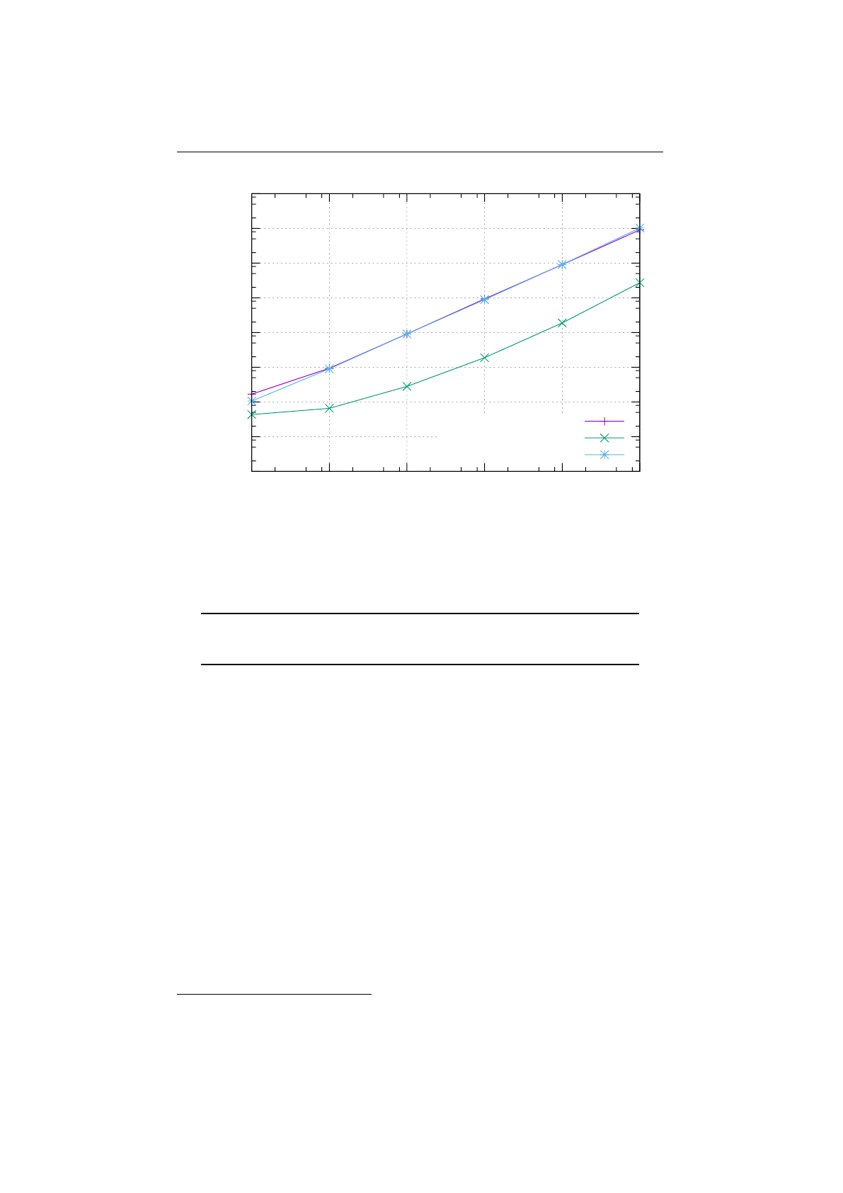
4.4. IO.JENETICS.PRNGINE CHAPTER 4. MODULES
100
101
102
103
104
105
106
107
108
100101102103104105
Marshalling time [µs]
Chromosome count
JAXB
Java serialization
XML reader
Figure 4.3.2: Genotype read performance
The pseudo random number generators of the
io.jenetics.prngine
mod-
ule are not cryptographically strong PRNGs.
The
io.jenetics.prngine
module consists of the following PRNG imple-
mentations:
KISS32Random
Implementation of an simple PRNG as proposed in Good Practice
in (Pseudo) Random Number Generation for Bioinformatics Applications
(JKISS32, page 3) David Jones, UCL Bioinformatics Group.[
16
] The period
of this PRNG is ≈2.6·1036.
KISS64Random
Implementation of an simple PRNG as proposed in Good Practice
in (Pseudo) Random Number Generation for Bioinformatics Applications
(JKISS64, page 10) David Jones, UCL Bioinformatics Group.[
16
] The
PRNG has a period of ≈1.8·1075.
LCG64ShiftRandom
This class implements a linear congruential PRNG with
additional bit-shift transition. It is a port of the trng::lcg64_shift PRNG
class of the TRNG library created by Heiko Bauke.18
MT19937_32Random
This is a 32-bit version of Mersenne Twister pseudo random
number generator.19
18https://github.com/jenetics/trng4
19https://en.wikipedia.org/wiki/Mersenne_Twister
100

4.4. IO.JENETICS.PRNGINE CHAPTER 4. MODULES
MT19937_64Random
This is a 64-bit version of Mersenne Twister pseudo random
number generator.
XOR32ShiftRandom
This generator was discovered and characterized by George
Marsaglia [Xorshift RNGs]. In just three XORs and three shifts (generally
fast operations) it produces a full period of 2
32 −
1on 32 bits. (The missing
value is zero, which perpetuates itself and must be avoided.)20
XOR64ShiftRandom
This generator was discovered and characterized by George
Marsaglia [Xorshift RNGs]. In just three XORs and three shifts (generally
fast operations) it produces a full period of 2
64 −
1on 64 bits. (The missing
value is zero, which perpetuates itself and must be avoided.)
All implemented PRNGs has been tested with the
dieharder
test suite. Ta-
ble 4.4.1 shows the statistical performance of the implemented PRNGs, including
the Java
Random
implementation. Beside the
XOR32ShiftRandom
class, the
j.u.Random
implementation has the poorest performance, concerning its statis-
tical performance.
PRNG Passed Weak Failed
KISS32Random 108 6 0
KISS64Random 109 5 0
LCG64ShiftRandom 110 4 0
MT19937_32Random 113 1 0
MT19937_64Random 111 3 0
XOR32ShiftRandom 101 4 9
XOR64ShiftRandom 107 7 0
j.u.Random 106 4 4
Table 4.4.1: Dieharder results
The second important performance measure for PRNGs is the number of
random number it is able to create per second.
21
Table 4.4.2 on the following
page shows the PRN creation speed for all implemented generators. The slowest
random engine is the
j.u.Random
class, which is caused by the synchronized
implementations. When the only the creation speed counts, the
j.u.c.Thread-
LocalRandom is the random engine to use.
20http://digitalcommons.wayne.edu/jmasm/vol2/iss1/2/
21
Measured on a Intel(R) Core(TM) i7-6700HQ CPU @ 2.60GHz with Java(TM) SE Runtime
Environment (build 1.8.0_102-b14)—Java HotSpot(TM) 64-Bit Server VM (build 25.102-b14,
mixed mode)—, using the JHM micro-benchmark library.
101
4.4. IO.JENETICS.PRNGINE CHAPTER 4. MODULES
PRNG 106int/s 106float/s 106long/s 106double/s
KISS32Random 189 143 129 108
KISS64Random 128 124 115 124
LCG64ShiftRandom 258 185 261 191
MT19937_32Random 140 115 92 82
MT19937_64Random 148 120 148 120
XOR32ShiftRandom 227 161 140 120
XOR64ShiftRandom 225 166 235 166
j.u.Random 91 89 46 46
j.u.c.TL Random 264 224 268 216
Table 4.4.2: PRNG speed
102

Appendix

Chapter 5
Examples
This section contains some coding examples which should give you a feeling
of how to use the
Jenetics
library. The given examples are complete, in the
sense that they will compile and run and produce the given example output.
Running the examples delivered with the
Jenetics
library can be started with
the run-examples.sh script.
$ ./jenetics.example/src/main/scripts/run-examples.sh
Since the script uses JARs located in the build directory you have to build it
with the jar Gradle target first; see section 6 on page 123.
5.1 Ones counting
Ones counting is one of the simplest model-problem. It uses a binary chromosome
and forms a classic genetic algorithm
1
. The fitness of a
Genotype
is proportional
to the number of ones.
1import s t a t i c i o . j e n e t i c s . e n g i n e . E v o l u t i o n R e s u l t . t oB e st Ph en o ty pe ;
2import s t a t i c i o . j e n e t i c s . e n gi ne . L im i ts . by S t e a d y Fi t ne s s ;
3
4import i o . j e n e t i c s . BitChromosome ;
5import i o . j e n e t i c s . BitGene ;
6import i o . j e n e t i c s . Genotype ;
7import i o . j e n e t i c s . Mutator ;
8import i o . j e n e t i c s . Phenotype ;
9import io . jenetics . RouletteWheelSelector ;
10 import i o . j e n e t i c s . S i n g l e P o i n t C r o s s o v e r ;
11 import i o . j e n e t i c s . en gi n e . Engine ;
12 import i o . j e n e t i c s . en gi ne . E v o l u t i o n S t a t i s t i c s ;
13
14 pu bl ic c l a s s OnesCounting {
15
16 // This method c a l c u l a t e s th e f i t n e s s f o r a g i ve n gen o type .
17 pr iv at e s t a t i c I n t e g e r count ( final Genotype<BitGene> gt ) {
18 return gt . getChromosome ( )
19 . as ( BitChromosome . c l a s s )
20 . bitCount () ;
1
In the classic genetic algorithm the problem is a maximization problem and the fitness
function is positive. The domain of the fitness function is a bit-chromosome.
104

5.1. ONES COUNTING CHAPTER 5. EXAMPLES
21 }
22
23 pub li c s t a t i c void main ( S t r i n g [ ] a r gs ) {
24 // C o nf ig ur e and b u i ld th e e v o l u t i o n e n gi ne .
25 final Eng ine<BitGene , I n t e g e r > e n g i n e = Eng ine
26 . builder(
27 OnesCounting : : count ,
28 BitChromosome . o f ( 2 0 , 0 . 1 5 ) )
29 . p o p u l a t i o n S i z e ( 5 0 0)
30 . selector(new R o u l e tt e W h e e lS e l e c t or <>() )
31 . a l t e r e r s (
32 new Mutator < >(0.55) ,
33 new S i n g l e P o i n t C r o s s o v e r < >(0. 06) )
34 . b u i l d ( ) ;
35
36 // Cr eat e e v o l u t i o n s t a t i s t i c s consumer .
37 final E v o l u t i o n S t a t i s t i c s <I nt eg e r , ?>
38 s t a t i s t i c s = E v o l u t i o n S t a t i s t i c s . ofNumber ( ) ;
39
40 final Phenotype<BitGene , I n t e g e r > b e s t = e n g in e . s tr ea m ( )
41 // Tru ncate t he e v o l u t i o n stream a f t e r 7 " s te ad y "
42 // generations .
43 . limit ( bySteadyFitness (7) )
44 // The e v o l u t i o n w i l l s to p a f t e r maximal 100
45 // generations .
46 . l i m i t ( 1 0 0 )
47 // Update t he e v a l u a t i o n s t a t i s t i c s a f t e r
48 // each g e n e r a t i o n
49 . peek ( s t a t i s t i c s )
50 // C o l l e c t ( r ed uc e ) th e e v o l u t i o n str eam to
51 // i t s b e s t p he no ty pe .
52 . c o l l e c t ( toBestPh e notype ( ) ) ;
53
54 System . out . p r i n t l n ( s t a t i s t i c s ) ;
55 System . out . p r i n t l n ( be s t ) ;
56 }
57 }
The genotype in this example consists of one
BitChromosome
with a ones
probability of 0.15. The altering of the offspring population is performed by
mutation, with mutation probability of 0.55, and then by a single-point crossover,
with crossover probability of 0.06. After creating the initial population, with the
ga.setup()
call, 100 generations are evolved. The tournament selector is used
for both, the offspring- and the survivor selection—this is the default selector.
2
1+---------------------------------------------------------------------------+
2| Time st at is t ic s |
3+---------------------------------------------------------------------------+
4| Se le ct ion : sum = 0 .0 1 65 8 014 400 0 s ; mean =0 . 00 1 381 678 667 s |
5| Alte ri ng : sum =0.0 9 69 0 41 5 90 0 0 s ; mean =0 . 00 8 07 5 34 6 58 3 s |
6| Fitne ss c alc ul ati on : sum =0 .02 289 431 8 00 0 s ; mean =0. 001 907 8 59 8 33 s |
7| Overall e xe c ut io n : sum = 0.1 365 7 53 2 30 0 0 s; mean =0 .01 1 38 1 27 6 91 7 s |
8+---------------------------------------------------------------------------+
9| Evo lu ti on st at is t ic s |
10 +---------------------------------------------------------------------------+
11 | Ge ne rat io ns : 12 |
12 | Al te re d : su m =4 0 ,487 ; m ean =3 37 3. 916 66 66 67 |
13 | Kil le d : sum =0 ; me an =0 .00 000 000 0 |
14 | In va li ds : sum =0; mean =0 .00 000 000 0 |
15 +---------------------------------------------------------------------------+
16 | Pop ul ati on s tat is tic s |
17 +---------------------------------------------------------------------------+
2
For the other default values (population size, maximal age, ...) have a look at the Javadoc:
http://jenetics.io/javadoc/jenetics/4.4/index.html
105
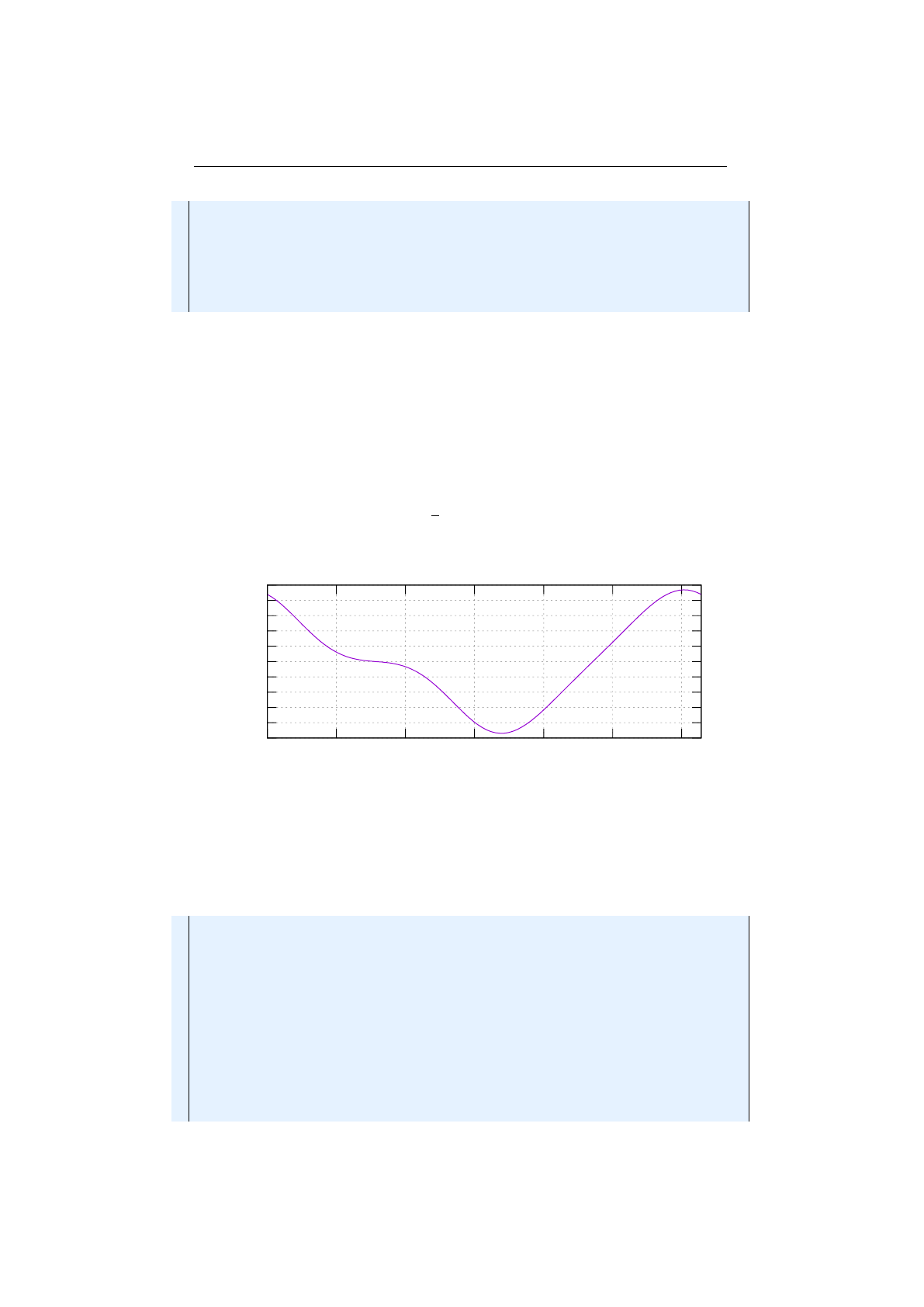
5.2. REAL FUNCTION CHAPTER 5. EXAMPLES
18 | Age : ma x =9; m ea n = 0. 80 86 67 ; va r = 1. 44 62 99 |
19 | Fi tn es s : |
20 | min = 1.000000000000 |
21 | max = 18 . 00 0 000 000 000 |
22 | mean = 1 0 .0 5 08 3 33 3 33 3 3 |
23 | var = 7.839555898205 |
24 | std = 2. 7 99 9 20 6 94 9 85 |
25 +---------------------------------------------------------------------------+
26 [0 0 001 1 01| 1 1 11 0 1 11 | 1 11 1 1 11 1 ] -- > 18
The given example will print the overall timing statistics onto the console. In
the Evolution statistics section you can see that it actually takes 15 generations
to fulfill the termination criteria—finding no better result after 7 consecutive
generations.
5.2 Real function
In this example we try to find the minimum value of the function
f(x) = cos 1
2+ sin (x)·cos (x).(5.2.1)
-1
-0.8
-0.6
-0.4
-0.2
0
0.2
0.4
0.6
0.8
1
0123456
y
x
Figure 5.2.1: Real function
The graph of function 5.2.1, in the range of
[0,2π]
, is shown in figure 5.2.1
and the listing beneath shows the GA implementation which will minimize the
function.
1import s t a t i c j av a . l an g . Math . PI ;
2import s t a t i c j av a . l an g . Math . co s ;
3import s t a t i c j av a . la ng . Math . s i n ;
4import s t a t i c i o . j e n e t i c s . e n g i n e . E v o l u t i o n R e s u l t . t oB e st Ph en o ty pe ;
5import s t a t i c i o . j e n e t i c s . e n gi ne . L im i ts . by S t e a d y Fi t ne s s ;
6
7import i o . j e n e t i c s . DoubleGene ;
8import i o . j e n e t i c s . MeanAlterer ;
9import i o . j e n e t i c s . Mutator ;
10 import i o . j e n e t i c s . Optimize ;
11 import i o . j e n e t i c s . Phenotype ;
12 import i o . j e n e t i c s . en gi n e . Codecs ;
13 import i o . j e n e t i c s . en gi n e . Engine ;
14 import i o . j e n e t i c s . en gi ne . E v o l u t i o n S t a t i s t i c s ;
106

5.2. REAL FUNCTION CHAPTER 5. EXAMPLES
15 import i o . j e n e t i c s . u t i l . DoubleRange ;
16
17 pu bl ic c l a s s RealFunction {
18
19 // The f i t n e s s f u n c t i o n .
20 pr iv at e s t a t i c double fitness (f i n a l double x ) {
21 return co s ( 0 . 5 + s i n ( x ) ) ∗c os ( x ) ;
22 }
23
24 pub li c s t a t i c void main ( final S t r i n g [ ] a r g s ) {
25 final Eng in e<DoubleGene , Double> e n g i n e = E ng ine
26 // C re at e a new b u i l d e r with the gi ve n f i t n e s s
27 // f u n c t i o n and chromosome .
28 . builder(
29 Rea l Fun ctio n : : f i t n e s s ,
30 Codecs . o f S c a l a r ( DoubleRange . o f ( 0 . 0 , 2 . 0∗PI ) ) )
31 . p o p u l a t i o n S i z e ( 5 0 0)
32 . o p t i m i z e ( O pt im iz e . MINIMUM)
33 . a l t e r e r s (
34 new Mutator < >(0.03) ,
35 new M ean Alt ere r < >(0.6) )
36 // B ui ld an e v o l u t i o n e ng i ne with the
37 // d e f i n e d pa ra me te r s .
38 . b u i l d ( ) ;
39
40 // Cr eat e e v o l u t i o n s t a t i s t i c s consumer .
41 final EvolutionStatistics<Double , ?>
42 s t a t i s t i c s = E v o l u t i o n S t a t i s t i c s . ofNumber ( ) ;
43
44 final Pheno type<DoubleGene , Double> b e s t = e n g i n e . s tr ea m ( )
45 // Tru ncate t he e v o l u t i o n stream a f t e r 7 " s te ad y "
46 // generations .
47 . limit ( bySteadyFitness (7) )
48 // The e v o l u t i o n w i l l s to p a f t e r maximal 100
49 // generations .
50 . l i m i t ( 1 0 0 )
51 // Update t he e v a l u a t i o n s t a t i s t i c s a f t e r
52 // each g e n e r a t i o n
53 . peek ( s t a t i s t i c s )
54 // C o l l e c t ( r ed uc e ) th e e v o l u t i o n str eam to
55 // i t s b e s t p he no ty pe .
56 . c o l l e c t ( toBestPh e notype ( ) ) ;
57
58 System . out . p r i n t l n ( s t a t i s t i c s ) ;
59 System . out . p r i n t l n ( be s t ) ;
60 }
61 }
The GA works with 1
×
1
DoubleChromosomes
whose values are restricted
to the range [0,2π].
1+---------------------------------------------------------------------------+
2| Time st at is t ic s |
3+---------------------------------------------------------------------------+
4| Se le ct io n : sum =0 .0 644 064 560 00 s; mea n =0 .00 306 697 409 5 s |
5| Al te ri ng : sum =0 .0 7015 838 200 0 s ; mean =0 .0 033 40 87 533 3 s |
6| Fitne ss c alc ul ati on : sum =0 .05 045 264 7 00 0 s ; mean =0. 002 402 507 0 00 s |
7| Overall e xe c ut io n : sum = 0.1 6 98 3 51 5 40 0 0 s; mean =0 .00 8 08 7 38 8 28 6 s |
8+---------------------------------------------------------------------------+
9| Evo lu ti on st at is t ic s |
10 +---------------------------------------------------------------------------+
11 | Ge ne rat io ns : 21 |
12 | Al te re d : su m =3 ,897; mean =1 85 .5 714 285 71 |
13 | Kil le d : sum =0 ; me an =0 .00 000 000 0 |
14 | In va li ds : sum =0; mean =0 .00 000 000 0 |
107
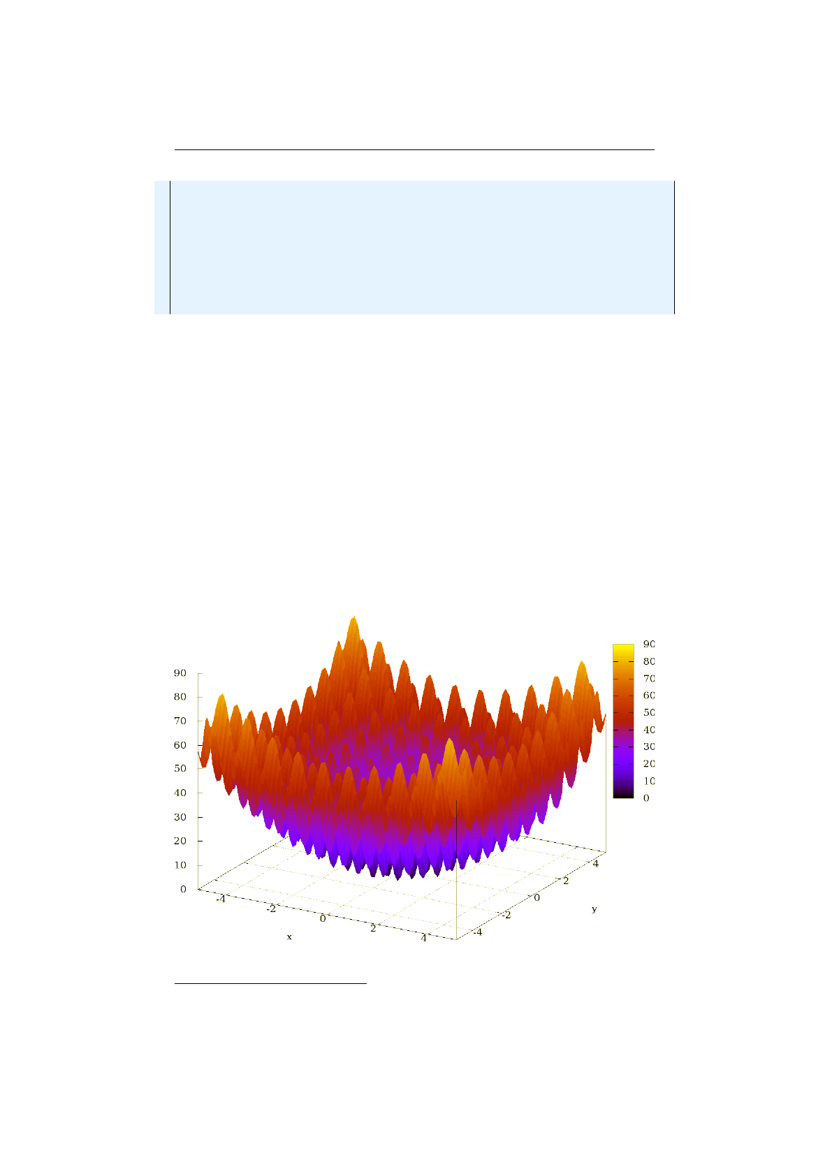
5.3. RASTRIGIN FUNCTION CHAPTER 5. EXAMPLES
15 +---------------------------------------------------------------------------+
16 | Pop ul ati on s tat is tic s |
17 +---------------------------------------------------------------------------+
18 | Age : ma x =9; m ea n = 1. 10 43 81 ; va r = 1. 96 26 25 |
19 | Fi tn es s : |
20 | min = -0.938171897696 |
21 | max = 0.936310125279 |
22 | mean = - 0. 89 785658366 5 |
23 | var = 0.027246274838 |
24 | std = 0. 1 65 0 64 4 56 6 17 |
25 +---------------------------------------------------------------------------+
26 [[ [ 3. 3 8 91 2 5 78 2 657 3 14] ] ] -- > -0 .9 38 171 89 769 56 66 1
The GA will generated an console output like above. The exact result of the
function–for the given range–will be 3
.
389
,
125
,
782
,
8907
,
939
...
You can also see,
that we reached the final result after 19 generations.
5.3 Rastrigin function
The Rastrigin function
3
is often used to test the optimization performance of
genetic algorithm.
f(x) = An +
n
X
i=1 x2
i−Acos (2πxi).(5.3.1)
As the plot in figure 5.3.1 shows, the Rastrigin function has many local minima,
which makes it difficult for standard, gradient-based methods to find the global
minimum. If
A
= 10 and
xi∈[−5.12,5.12]
, the function has only one global
minimum at x=0with f(x)=0.
Figure 5.3.1: Rastrigin function
3https://en.wikipedia.org/wiki/Rastrigin_function
108

5.3. RASTRIGIN FUNCTION CHAPTER 5. EXAMPLES
The following listing shows the
Engine
setup for solving the Rastrigin func-
tion, which is very similar to the setup for the real-function in section 5.2 on
page 106. Beside the different fitness function, the
Codec
for
double
vectors is
used, instead of the double scalar Codec.
1import s t a t i c j av a . l an g . Math . PI ;
2import s t a t i c j av a . l an g . Math . co s ;
3import s t a t i c i o . j e n e t i c s . e n g i n e . E v o l u t i o n R e s u l t . t oB e st Ph en o ty pe ;
4import s t a t i c i o . j e n e t i c s . e n gi ne . L im i ts . by S t e a d y Fi t ne s s ;
5
6import i o . j e n e t i c s . DoubleGene ;
7import i o . j e n e t i c s . MeanAlterer ;
8import i o . j e n e t i c s . Mutator ;
9import i o . j e n e t i c s . Optimize ;
10 import i o . j e n e t i c s . Phenotype ;
11 import i o . j e n e t i c s . en gi n e . Codecs ;
12 import i o . j e n e t i c s . en gi n e . Engine ;
13 import i o . j e n e t i c s . en gi ne . E v o l u t i o n S t a t i s t i c s ;
14 import i o . j e n e t i c s . u t i l . DoubleRange ;
15
16 pu bl ic c l a s s RastriginFunction {
17 pr iv at e s t a t i c f i n a l double A = 1 0 ;
18 pr iv at e s t a t i c f i n a l double R = 5 . 1 2 ;
19 pr iv at e s t a t i c f i n a l i nt N = 2 ;
20
21 pr iv at e s t a t i c double fitness (f i n a l double [ ] x ) {
22 double value = A∗N;
23 for (int i = 0 ; i < N; ++i ) {
24 v al u e += x [ i ] ∗x [ i ] −A∗c os ( 2 . 0 ∗PI∗x [ i ] ) ;
25 }
26
27 return value ;
28 }
29
30 pub li c s t a t i c void main ( final S t r i n g [ ] a r g s ) {
31 final Eng in e<DoubleGene , Double> e n g i n e = E ng ine
32 . builder(
33 R a s t r i g i n F u n c t i o n : : f i t n e s s ,
34 // Codec f o r ’ x ’ v e c t o r .
35 Co de cs . o f V e c t o r ( Doubl eRange . o f (−R, R) , N) )
36 . p o p u l a t i o n S i z e ( 5 0 0)
37 . o p t i m i z e ( O pt im iz e . MINIMUM)
38 . a l t e r e r s (
39 new Mutator < >(0.03) ,
40 new M ean Alt ere r < >(0.6) )
41 . b u i l d ( ) ;
42
43 final EvolutionStatistics<Double , ?>
44 s t a t i s t i c s = E v o l u t i o n S t a t i s t i c s . ofNumber ( ) ;
45
46 final Pheno type<DoubleGene , Double> b e s t = e n g i n e . s tr ea m ( )
47 . limit ( bySteadyFitness (7) )
48 . peek ( s t a t i s t i c s )
49 . c o l l e c t ( toBestPh e notype ( ) ) ;
50
51 System . out . p r i n t l n ( s t a t i s t i c s ) ;
52 System . out . p r i n t l n ( be s t ) ;
53 }
54 }
The console output of the program shows, that
Jenetics
finds the optimal
solution after 38 generations.
109

5.4. 0/1 KNAPSACK CHAPTER 5. EXAMPLES
1+---------------------------------------------------------------------------+
2| Time st at is t ic s |
3+---------------------------------------------------------------------------+
4| Se le ct ion : sum = 0 .2 0 91 8 513 400 0 s ; mean =0 . 00 5 504 871 947 s |
5| Alte ri ng : sum =0.2 9 51 0 20 4 40 0 0 s; mean =0 . 00 7 76 5 84 3 26 3 s |
6| Fitne ss c alc ul ati on : sum =0 .17 687 9 93 7 00 0 s ; mean =0. 004 654 7 35 1 84 s |
7| Overall e xec ut io n : sum = 0 .6 6 45 1 72 5 600 0 s ; mean =0 . 01 7 48 7 29 6 21 1 s |
8+---------------------------------------------------------------------------+
9| Evo lu ti on st at is t ic s |
10 +---------------------------------------------------------------------------+
11 | Ge ne rat io ns : 38 |
12 | Al te re d : su m =7 ,549; mean =1 98 .6 578 947 37 |
13 | Kil le d : sum =0 ; me an =0 .00 000 000 0 |
14 | In va li ds : sum =0; mean =0 .00 000 000 0 |
15 +---------------------------------------------------------------------------+
16 | Pop ul ati on s tat is tic s |
17 +---------------------------------------------------------------------------+
18 | Age : ma x =8; m ea n = 1. 10 02 11 ; va r = 1. 81 40 53 |
19 | Fi tn es s : |
20 | min = 0.000000000000 |
21 | max = 63 . 672 604 047 475 |
22 | mean = 3.484157452128 |
23 | var = 71 . 047 475 139 018 |
24 | std = 8. 4 28 9 66 4 33 6 16 |
25 +---------------------------------------------------------------------------+
26 [[ [ -1. 32 2 61 685 88 424 14 3 E -9] ,[ -1 .0 96 96 49 71 40 4292 E -9]] ] - -> 0.0
5.4 0/1 Knapsack
In the Knapsack problem
4
a set of items, together with it’s size and value, is
given. The task is to select a disjoint subset so that the total size does not
exceed the knapsack size. For solving the 0/1 knapsack problem we define a
BitChromosome
, one bit for each item. If the
ith
bit is set to one the
ith
item is
selected.
1import s t a t i c i o . j e n e t i c s . e n g i n e . E v o l u t i o n R e s u l t . t oB e st Ph en o ty pe ;
2import s t a t i c i o . j e n e t i c s . e n gi ne . L im i ts . by S t e a d y Fi t ne s s ;
3
4import ja v a . u t i l . Random ;
5import j av a . u t i l . f u n c t i o n . F un ct ion ;
6import ja va . u t i l . stream . C o l l e c t o r ;
7import ja v a . u t i l . stream . Stream ;
8
9import i o . j e n e t i c s . BitGene ;
10 import i o . j e n e t i c s . Mutator ;
11 import i o . j e n e t i c s . Phenotype ;
12 import io . jenetics . RouletteWheelSelector ;
13 import i o . j e n e t i c s . S i n g l e P o i n t C r o s s o v e r ;
14 import i o . j e n e t i c s . To urna ment Sele ctor ;
15 import i o . j e n e t i c s . en gi n e . Codecs ;
16 import i o . j e n e t i c s . en gi n e . Engine ;
17 import i o . j e n e t i c s . en gi ne . E v o l u t i o n S t a t i s t i c s ;
18 import i o . j e n e t i c s . u t i l . IS eq ;
19 import i o . j e n e t i c s . u t i l . RandomRegistry ;
20
21 // The main c l a s s .
22 pu bl ic c l a s s Knapsack {
23
24 // This c l a s s r e p r e s e n t s a knaps ack item , with a s p e c i f i c
25 // " s i z e " and " v alu e " .
26 f i n a l s t a t i c c l a s s Item {
27 public f i n a l double s i z e ;
4https://en.wikipedia.org/wiki/Knapsack_problem
110

5.4. 0/1 KNAPSACK CHAPTER 5. EXAMPLES
28 public f i n a l double value ;
29
30 Item ( f i n a l double s i z e , f i n a l double value ) {
31 this . s i z e = s i z e ;
32 this . value = value ;
33 }
34
35 // Cr eat e a new random knapsack it e m .
36 static Item random ( ) {
37 final Random r = RandomRegistry . getRandom ( ) ;
38 return new Item (
39 r . nex tDoubl e ( ) ∗1 00 ,
40 r . nex tDoubl e ( ) ∗100
41 ) ;
42 }
43
44 // C o l l e c t o r f o r summing up t he kn apsack i te ms .
45 static C o l l e c t o r <Item , ? , Item> toSum ( ) {
46 return C o l l e c t o r . o f (
47 ( ) −>new double [ 2 ] ,
48 ( a , b ) −> {a [ 0 ] += b . s i z e ; a [ 1 ] += b . val u e ; } ,
49 ( a , b ) −> {a [ 0 ] += b [ 0 ] ; a [ 1 ] += b [ 1 ] ; return a ; } ,
50 r−>new Item ( r [ 0 ] , r [ 1 ] )
51 ) ;
52 }
53 }
54
55 // C r ea t in g t he f i t n e s s f u n ct io n .
56 static Function<ISeq<Item >, Double>
57 fitness(f i n a l double s i z e ) {
58 return items −> {
59 final Item sum = ite m s . stream ( ) . c o l l e c t ( Item . toSum ( ) ) ;
60 return sum . s i z e <= s i z e ? sum . va lu e : 0 ;
61 } ;
62 }
63
64 pub li c s t a t i c void main ( final S t r i n g [ ] a r g s ) {
65 f i n a l i nt n it em s = 1 5 ;
66 f i n a l double k s s i z e = ni t ems ∗1 0 0 . 0 / 3 . 0 ;
67
68 final ISeq<Item> i t e ms =
69 Stream . g e n e r a t e ( Item : : random )
70 . l i m i t ( n ite ms )
71 . c o l l e c t ( IS e q . t o I S e q ( ) ) ;
72
73 // C o nf ig ur e and b u i ld th e e v o l u t i o n e n gi ne .
74 final Eng in e<BitG ene , D ouble> e n g i n e = E ng in e
75 . b u i l d e r ( f i t n e s s ( k s s i z e ) , Codecs . o fSu bS et ( i te ms ) )
76 . p o p u l a t i o n S i z e ( 5 0 0)
77 . survivorsSelector(new T ou rn ame nt Se le ct or <>(5) )
78 . offspringSelector(new Ro u l e t te W h e e l Se l e c t o r <>() )
79 . a l t e r e r s (
80 new Mutator < >(0.115) ,
81 new S i n g l e P o i n t C r o s s o v e r < >(0. 16) )
82 . b u i l d ( ) ;
83
84 // Cr eat e e v o l u t i o n s t a t i s t i c s consumer .
85 final EvolutionStatistics<Double , ?>
86 s t a t i s t i c s = E v o l u t i o n S t a t i s t i c s . ofNumber ( ) ;
87
88 final Pheno type<Bi tGene , Do uble> b e s t = e n g i n e . s t re am ( )
89 // Tru ncate t he e v o l u t i o n stream a f t e r 7 " s te ad y "
111

5.5. TRAVELING SALESMAN CHAPTER 5. EXAMPLES
90 // generations .
91 . limit ( bySteadyFitness (7) )
92 // The e v o l u t i o n w i l l s to p a f t e r maximal 100
93 // generations .
94 . l i m i t ( 1 0 0 )
95 // Update t he e v a l u a t i o n s t a t i s t i c s a f t e r
96 // each g e n e r a t i o n
97 . peek ( s t a t i s t i c s )
98 // C o l l e c t ( r ed uc e ) th e e v o l u t i o n str eam to
99 // i t s b e s t p he no ty pe .
100 . c o l l e c t ( toBestPh e notype ( ) ) ;
101
102 System . out . p r i n t l n ( s t a t i s t i c s ) ;
103 System . out . p r i n t l n ( be s t ) ;
104 }
105 }
The console out put for the Knapsack GA will look like the listing beneath.
1+---------------------------------------------------------------------------+
2| Time st at is t ic s |
3+---------------------------------------------------------------------------+
4| Se le ct ion : sum = 0 .0 4 44 6 597 800 0 s ; mean =0 . 00 5 558 247 250 s |
5| Alte ri ng : sum =0.0 6 73 8 52 1 10 0 0 s; mean =0 .00 8 42 3 15 1 37 5 s |
6| Fitne ss c alc ul ati on : sum =0 .03 720 818 9 00 0 s ; mean =0. 004 651 0 23 6 25 s |
7| Overall e xe cut io n : sum = 0.1 2646 853 900 0 s ; mean = 0.0 158 085 673 75 s |
8+---------------------------------------------------------------------------+
9| Evo lu ti on st at is t ic s |
10 +---------------------------------------------------------------------------+
11 | Ge ne rat io ns : 8 |
12 | Al te re d : su m =4 ,842; m ean = 60 5.2 500 00 00 0 |
13 | Kil le d : sum =0 ; me an =0 .00 000 000 0 |
14 | In va li ds : sum =0; mean =0 .00 000 000 0 |
15 +---------------------------------------------------------------------------+
16 | Pop ul ati on s tat is tic s |
17 +---------------------------------------------------------------------------+
18 | Age : ma x =7; m ea n = 1. 38 75 00 ; va r = 2. 78 00 39 |
19 | Fi tn es s : |
20 | min = 0.000000000000 |
21 | max = 542.363235999342 |
22 | mean = 436.098248628661 |
23 | var = 11 4 31. 8 01 2 918 1 23 9 0 |
24 | std = 106.919601999878 |
25 +---------------------------------------------------------------------------+
26 [01111011|10111101] --> 542.3632359993417
5.5 Traveling salesman
The Traveling Salesman problem
5
is one of the classical problems in computa-
tional mathematics and it is the most notorious NP-complete problem. The goal
is to find the shortest distance, or the path, with the least costs, between
N
different cities. Testing all possible path for
N
cities would lead to
N
!checks to
find the shortest one.
The following example uses a path where the cities are lying on a circle. That
means, the optimal path will be a polygon. This makes it easier to check the
quality of the found solution.
1import s t a t i c j av a . l an g . Math . PI ;
2import s t a t i c j av a . l an g . Math . co s ;
3import s t a t i c j av a . l an g . Math . hypot ;
4import s t a t i c j av a . la ng . Math . s i n ;
5https://en.wikipedia.org/wiki/Travelling_salesman_problem
112

5.5. TRAVELING SALESMAN CHAPTER 5. EXAMPLES
5import s t a t i c j av a . l an g . System . out ;
6import s t a t i c j av a . u t i l . Ob je c t s . r eq u ir e N o n N u ll ;
7import s t a t i c i o . j e n e t i c s . e n g i n e . E v o l u t i o n R e s u l t . t oB e st Ph en o ty pe ;
8import s t a t i c i o . j e n e t i c s . e n gi ne . L im i ts . by S t e a d y Fi t ne s s ;
9
10 import ja v a . u t i l . Random ;
11 import j av a . u t i l . f u n c t i o n . F un ct ion ;
12 import ja v a . u t i l . stream . In t Strea m ;
13
14 import i o . j e n e t i c s . EnumGene ;
15 import i o . j e n e t i c s . Optimize ;
16 import i o . j e n e t i c s . P a r t i a l l y M a t c h e d C r o s s o v e r ;
17 import i o . j e n e t i c s . Phenotype ;
18 import i o . j e n e t i c s . SwapMutator ;
19 import i o . j e n e t i c s . en gi n e . Codec ;
20 import i o . j e n e t i c s . en gi n e . Codecs ;
21 import i o . j e n e t i c s . en gi n e . Engine ;
22 import i o . j e n e t i c s . en gi ne . E v o l u t i o n S t a t i s t i c s ;
23 import i o . j e n e t i c s . en gi n e . Problem ;
24 import i o . j e n e t i c s . u t i l . IS eq ;
25 import i o . j e n e t i c s . u t i l . MSeq ;
26 import i o . j e n e t i c s . u t i l . RandomRegistry ;
27
28 pu bl ic c l a s s TravelingSalesman
29 implements Problem<ISeq<double [ ] > , EnumGene<double [ ] > , Double>
30 {
31
32 private f i n a l ISeq<double [] > _p oints ;
33
34 // C re at e new TSP problem i n s t a n c e w ith g iv en way p o i n t s .
35 public TravelingSalesman(ISeq<double [ ] > p o i n t s ) {
36 _po in ts = r e qu ir eN on N ul l ( p o i n t s ) ;
37 }
38
39 @Override
40 public Function<ISeq<double [ ] > , Double> f i t n e s s ( ) {
41 return p−> I nt St re am . ra n ge ( 0 , p . l e n g t h ( ) )
42 . mapToDouble ( i −> {
43 f i n a l double [ ] p1 = p . g e t ( i ) ;
44 f i n a l double [ ] p2 = p . ge t ( ( i + 1)%p . s i z e ( ) ) ;
45 return hypot ( p1 [ 0 ] −p2 [ 0 ] , p1 [ 1 ] −p2 [ 1 ] ) ; })
46 . sum ( ) ;
47 }
48
49 @Override
50 public Codec<ISeq<double [ ] > , EnumGene<double[]>> co de c ( ) {
51 return Codecs . ofP erm ut at i on ( _po ints ) ;
52 }
53
54 // Cr eat e a new TSM example problem with th e g i v e n number
55 // o f s t o p s . A l l s t o p s l i e on a c i r c l e with t he g i v e n r a d i u s .
56 pub li c s t a t i c TravelingSalesman of ( int st o p s , double r a d i u s ) {
57 final MSeq<double [ ] > p o i n t s = MSeq . of Le ng th ( s t o p s ) ;
58 f i n a l double d e l t a = 2 . 0∗PI / s t o p s ;
59
60 for (int i = 0 ; i < s t o p s ; ++i ) {
61 f i n a l double a lp ha = d e l t a ∗i ;
62 f i n a l double x = co s ( a lph a ) ∗r a d i u s + r a d i u s ;
63 f i n a l double y = s i n ( a lp ha ) ∗r a d i u s + r a d i u s ;
64 p o i n t s . s e t ( i , new double [ ] { x , y }) ;
65 }
66
113

5.5. TRAVELING SALESMAN CHAPTER 5. EXAMPLES
67 // S h u f f l i n g o f t h e c r e a t e d p o i n t s .
68 final Random random = RandomRegistry . getRandom ( ) ;
69 for (int j = p o i n t s . l e n g t h ( ) −1 ; j > 0 ; −−j ) {
70 f i n a l i nt i = random . n e x t I n t ( j + 1 ) ;
71 f i n a l double [ ] tmp = p o i n t s . ge t ( i ) ;
72 p o i n t s . s e t ( i , p o i n t s . g e t ( j ) ) ;
73 p o i n t s . s e t ( j , tmp ) ;
74 }
75
76 return new T r a v e l in g S a le s m a n ( p o i n t s . t o I S e q ( ) ) ;
77 }
78
79 pub li c s t a t i c void main ( S t r i n g [ ] a r gs ) {
80 int s t o p s = 2 0 ; double R = 1 0 ;
81 double minPath Length = 2 . 0 ∗stops∗R∗s i n ( PI / s t o p s ) ;
82
83 T ra v el i ng S al e sm a n tsm = T ra ve l in g Sa l es m an . o f ( s to ps , R) ;
84 Engine<EnumGene<double [ ] > , Do uble> e n g i n e = E ngi ne
85 . b u i l d e r ( tsm )
86 . o p t i m i z e ( O pt im iz e . MINIMUM)
87 . maximalPhenotypeAge (11)
88 . p o p u l a t i o n S i z e ( 5 0 0)
89 . a l t e r e r s (
90 new SwapMutator < >(0.2) ,
91 new P a rt ia ll yM at ch ed Cr os so ve r < >(0.35) )
92 . b u i l d ( ) ;
93
94 // Cr eat e e v o l u t i o n s t a t i s t i c s consumer .
95 EvolutionStatistics<Double , ?>
96 s t a t i s t i c s = E v o l u t i o n S t a t i s t i c s . ofNumber ( ) ;
97
98 Phenotype<EnumGene<double [ ] > , Double> b e s t =
99 e n g i n e . s tr e am ( )
100 // Tru ncate t he e v o l u t i o n stream a f t e r 25 " s te a dy "
101 // generations .
102 . limit ( bySteadyFitness (25) )
103 // The e v o l u t i o n w i l l s to p a f t e r maximal 250
104 // generations .
105 . l i m i t ( 2 5 0 )
106 // Update t he e v a l u a t i o n s t a t i s t i c s a f t e r
107 // each g e n e r a t i o n
108 . peek ( s t a t i s t i c s )
109 // C o l l e c t ( r ed uc e ) th e e v o l u t i o n str eam to
110 // i t s b e s t p he no ty pe .
111 . c o l l e c t ( toBestPh e notype ( ) ) ;
112
113 out . p r i n t l n ( s t a t i s t i c s ) ;
114 out . p r i n t l n ( "Known min p ath l e n g t h : " + minPathLength ) ;
115 out . p r i n t l n ( " Found min pat h l e n g t h : " + b es t . g e t F i t n e s s ( ) ) ;
116 }
117
118 }
The Traveling Salesman problem is a very good example which shows you
how to solve combinatorial problems with an GA.
Jenetics
contains several
classes which will work very well with this kind of problems. Wrapping the base
type into an
EnumGene
is the first thing to do. In our example, every city has
an unique number, that means we are wrapping an
Integer
into an
EnumGene
.
Creating a genotype for integer values is very easy with the factory method
of the
PermutationChromosome
. For other data types you have to use one of
the constructors of the permutation chromosome. As alterers, we are using a
114

5.6. EVOLVING IMAGES CHAPTER 5. EXAMPLES
swap-mutator and a partially-matched crossover. These alterers guarantees that
no invalid solutions are created—every city exists exactly once in the altered
chromosomes.
1+---------------------------------------------------------------------------+
2| Time st at is t ic s |
3+---------------------------------------------------------------------------+
4| Se le ct io n : sum =0 .0 774 512 970 00 s; mea n =0 .00 061 961 037 6 s |
5| Alte ri ng : sum =0.2 0 53 5 16 8 80 0 0 s; mean =0 .00 1 64 2 81 3 50 4 s |
6| Fitne ss c alc ul ati on : sum =0 .09 712 722 5 00 0 s ; mean =0. 000 777 017 8 00 s |
7| Overall e xe c ut io n : sum = 0.3 713 0 44 6 40 0 0 s; mean =0 .00 2 97 0 43 5 71 2 s |
8+---------------------------------------------------------------------------+
9| Evo lu ti on st at is t ic s |
10 +---------------------------------------------------------------------------+
11 | Ge ne rat io ns : 125 |
12 | Al te re d : su m =177 ,20 0; m ean =1 41 7. 600 000 00 0 |
13 | Kil le d : sum = 17 3; mean = 1. 384 000 000 |
14 | In va li ds : sum =0; mean =0 .00 000 000 0 |
15 +---------------------------------------------------------------------------+
16 | Pop ul ati on s tat is tic s |
17 +---------------------------------------------------------------------------+
18 | Age : ma x =1 1; m ea n = 1. 67 78 72 ; var = 5. 617 29 9 |
19 | Fi tn es s : |
20 | min = 62 . 573 786 016 0 92 |
21 | max = 344.248763720487 |
22 | mean = 144.636749974591 |
23 | var = 50 8 2.9 4 72 4 78 7 895 3 |
24 | std = 71 . 294 791 169 3 34 |
25 +---------------------------------------------------------------------------+
26 Kno wn m in pa th l en gt h : 6 2.5 73 78 60 16 09 235
27 Fou nd m in pa th l en gt h : 6 2.5 73 78 60 16 09 235
The listing above shows the output generated by our example. The last line
represents the phenotype of the best solution found by the GA, which represents
the traveling path. As you can see, the GA has found the shortest path, in
reverse order.
5.6 Evolving images
The following example tries to approximate a given image by semitransparent
polygons.
6
It comes with an Swing UI, where you can immediately start your
own experiments. After compiling the sources with
$ ./gradlew jar
you can start the example by calling
$ ./jrun io.jenetics.example.image.EvolvingImages
Figure 5.6.1 on the following page show the GUI after evolving the default
image for about 4,000 generations. With the »Open« button it is possible to load
other images for polygonization. The »Save« button allows to store polygonized
images in PNG format to disk. At the button of the UI, you can change some of
the GA parameters of the example:
Population size The number of individual of the population.
Tournament size
The example uses a
TournamentSelector
for selecting the
offspring population. This parameter lets you set the number of individual
used for the tournament step.
6
Original idea by Roger Johansson
http://rogeralsing.com/2008/12/07/
genetic-programming-evolution-of-mona-lisa.
115
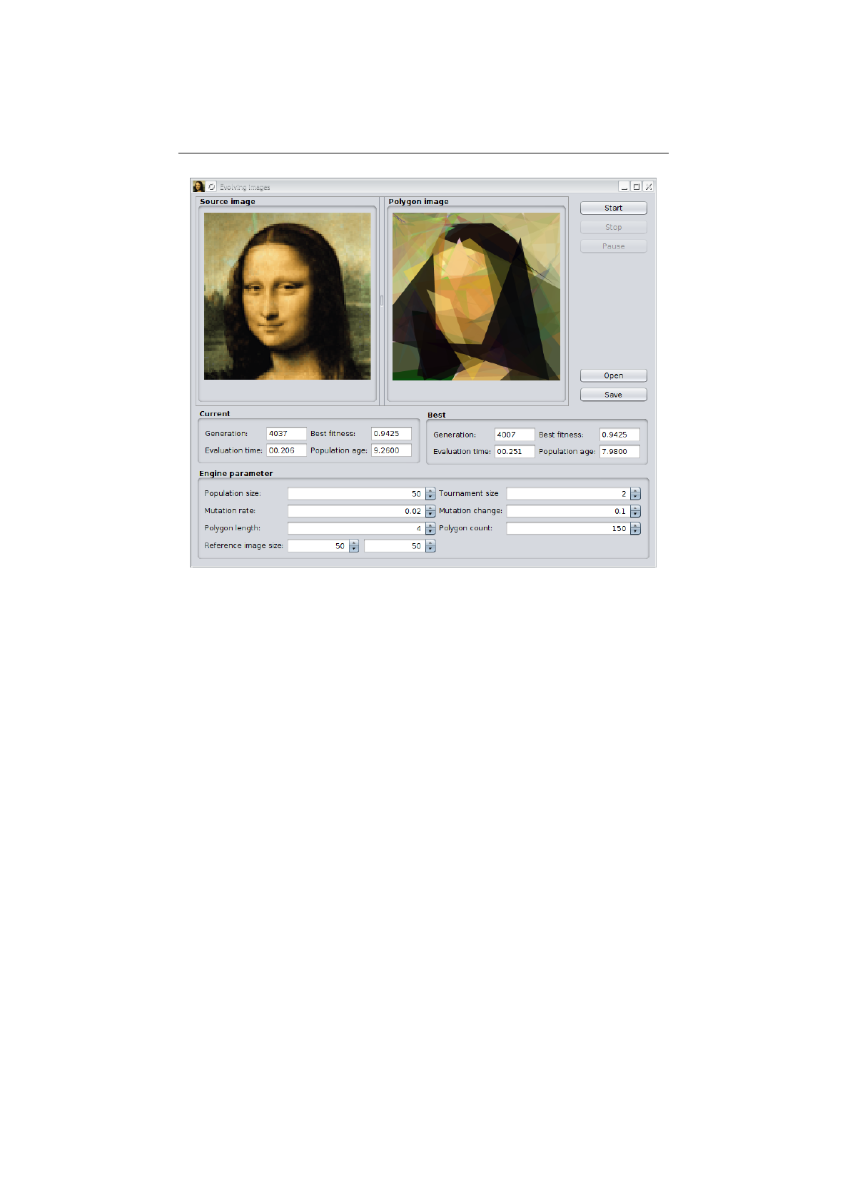
5.6. EVOLVING IMAGES CHAPTER 5. EXAMPLES
Figure 5.6.1: Evolving images UI
Mutation rate
The probability that a polygon component (color or vertex
position) is altered.
Mutation magnitude
In case a polygon component is going to be mutated,
its value will be randomly modified in the uniform range of [−m, +m].
Polygon length The number of edges (or vertices) of the created polygons.
Polygon count The number of polygons of one individual (Genotype).
Reference image size
To improve the processing speed, the fitness of a given
polygon set (individual) is not calculated with the full sized image. Instead
an scaled reference image with the given size is used. A smaller reference
image will speed up the calculation, but will also reduce the accuracy.
It is also possible to run and configure the Evolving Images example from the
command line. This allows to do long running evolution experiments and save
polygon images every
n
generations—specified with the
--image-generation
parameter.
$ ./jrun io.jenetics.example.image.EvolvingImages evolve \
--engine-properties engine.properties \
--input-image monalisa.png \
--output-dir evolving-images \
116
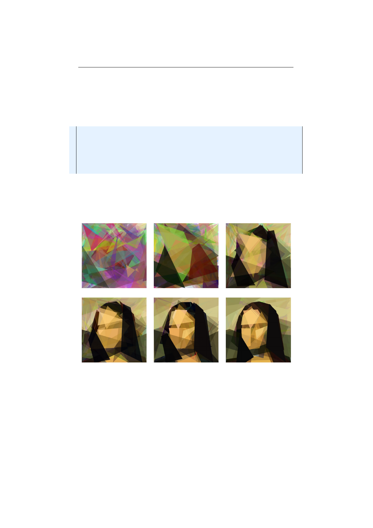
5.6. EVOLVING IMAGES CHAPTER 5. EXAMPLES
--generations 10000 \
--image-generation 100
Every command line argument has proper default values, so that it is possible
to start it without parameters. Listing 5.1 shows the default values for the GA
engine if the --engine-properties parameter is not specified.
1p o p u l a t i o n _ s i z e =50
2tournament_size=3
3mutation_ r ate =0.025
4mutation_multitude=0.15
5polygon_length=4
6polygon_count=250
7refe renc e _ima g e_wi dth =60
8reference_image_height=60
Listing 5.1: Default engine.properties
For a quick start, you can simply call
$ ./jrun io.jenetics.example.image.EvolvingImages evolve
a)100generations b)102generations c)103generations
d)104generations e)105generations f)106generations
Figure 5.6.2: Evolving Mona Lisa images
The images in figure 5.6.2 shows the resulting polygon images after the given
number of generations. They where created with the command line version of
the program using the default engine.properties file (listing 5.1):
$ ./jrun io.jenetics.example.image.EvolvingImages evolve \
--generations 1000000 \
--image-generation 100
117

5.7. SYMBOLIC REGRESSION CHAPTER 5. EXAMPLES
5.7 Symbolic regression
Symbolic regression is a specific type of regression analyses, where the search
space consists of mathematical expressions. The task is to find a model, which
fits a given data-set in terms of accuracy and simplicity. In a classical approach,
you will try to optimize the parameters of a predefined function type, e. g. a
polynomial of grade
n
. If the type of mathematical function is not known in
advance, GP can be used finding a function, which is composed out of a given
set of primitives.
Symbolic regression involves finding a mathematical expression, in
symbolic form, that provides a good, best, or perfect fit between a
given finite sampling of values of the independent variables and the
associated values of the dependent variables.[18]
The following example shows how to setup and solve a symbolic regression
problem with the help of GP and
Jenetics
. The data set used for the example
was created with the polynomial, 4
x3−
3
x2
+
x
. This allows us to check the
quality of the function found by the GP. Setting up a GP requires a little bit
more effort then the setup of a GA. First, you have to define the set of atomic
mathematical operations, the GP is working with. This operations influences the
search space and is a kind of a priori knowledge put into the GP. As second step
you have to define the terminal operations. Terminals are either constants or
variables. The number of variables defines the domain dimension of the fitness
function.
1import s t a t i c j av a . l an g . Math . pow ;
2
3import ja v a . u t i l . Arrays ;
4
5import i o . j e n e t i c s . Genotype ;
6import i o . j e n e t i c s . Mutator ;
7import i o . j e n e t i c s . en gi n e . Codec ;
8import i o . j e n e t i c s . en gi n e . Engine ;
9import i o . j e n e t i c s . e n g i n e . E v o l u t i o n R e s u l t ;
10 import i o . j e n e t i c s . u t i l . IS eq ;
11 import i o . j e n e t i c s . u t i l . RandomRegistry ;
12
13 import i o . j e n e t i c s . e xt . S i ng l eN o de C ro s s ov e r ;
14
15 import i o . j e n e t i c s . prog . ProgramChromosome ;
16 import i o . j e n e t i c s . prog . ProgramGene ;
17 import i o . j e n e t i c s . prog . op . EphemeralConst ;
18 import i o . j e n e t i c s . prog . op . MathOp ;
19 import i o . j e n e t i c s . prog . op . Op;
20 import i o . j e n e t i c s . prog . op . Var ;
21
22 pu bl ic c l a s s Sy m bo l ic R e g r e s s i on {
23
24 // Sample data c r e a t e d wi th 4∗x^3 −3∗x ^2 + x
25 s t a t i c f i n a l double [ ] [ ] SAMPLES = new double [][] {
26 {−1.0 , −8.00 00} ,
27 {−0.9 , −6.24 60} ,
28 {−0.8 , −4.76 80} ,
29 {−0.7 , −3.54 20} ,
30 {−0.6 , −2.54 40} ,
31 {−0.5 , −1.75 00} ,
32 {−0.4 , −1.13 60} ,
118

5.7. SYMBOLIC REGRESSION CHAPTER 5. EXAMPLES
33 {−0.3 , −0.67 80} ,
34 {−0.2 , −0.35 20} ,
35 {−0.1 , −0.13 40} ,
36 { 0 . 0 , 0 . 0 0 0 0 } ,
37 { 0 . 1 , 0 . 0 7 4 0 } ,
38 { 0 . 2 , 0 . 1 1 2 0 } ,
39 { 0 . 3 , 0 . 1 3 8 0 } ,
40 { 0 . 4 , 0 . 1 7 6 0 } ,
41 { 0 . 5 , 0 . 2 5 0 0 } ,
42 { 0 . 6 , 0 . 3 8 4 0 } ,
43 { 0 . 7 , 0 . 6 0 2 0 } ,
44 { 0 . 8 , 0 . 9 2 8 0 } ,
45 { 0 . 9 , 1 . 3 8 6 0 } ,
46 { 1 . 0 , 2. 0 0 00 }
47 } ;
48
49 // D e f i n i t i o n o f t he o p e r a t i o n s .
50 s t a t i c f i n a l ISeq<Op<Double>> OPERATIONS = IS e q . o f (
51 MathOp .ADD,
52 MathOp . SUB,
53 MathOp .MUL
54 ) ;
55
56 // D e f i n i t i o n o f t he t e r m i n a l s .
57 s t a t i c f i n a l ISeq<Op<Double>> TERMINALS = I Se q . o f (
58 Var . o f ( "x" , 0) ,
59 EphemeralConst . of (() −> ( double ) RandomRegistry
60 . getRandom ( ) . n e x t I n t ( 1 0 ) )
61 ) ;
62
63 s t a t i c double error(final ProgramGene<Double> program ) {
64 return Arrays . s t r ea m (SAMPLES)
65 . mapToDouble ( sampl e −>
66 pow ( sample [ 1 ] −program . e v a l ( sample [ 0 ] ) , 2) +
67 program . s i z e ( ) ∗0.00001)
68 . sum ( ) ;
69 }
70
71 s t a t i c f i n a l Codec<ProgramGene<Double >, ProgramGene<Double>>
72 CODEC = Codec . o f (
73 Genotype . o f ( ProgramChromosome . o f (
74 5 ,
75 ch −> ch . g e tR o o t ( ) . s i z e ( ) <= 50 ,
76 OPERATIONS,
77 TERMINALS
78 ) ) ,
79 Genotype : : getGene
80 ) ;
81
82 pub li c s t a t i c void main ( final S t r i n g [ ] a r g s ) {
83 final Eng in e<ProgramGene<Double >, Do uble> e n g i n e = E ng in e
84 . b u i l d e r ( S ym bo li cR eg r es s io n : : e rr o r , CODEC)
85 . m ini mi zi ng ( )
86 . a l t e r e r s (
87 new SingleNodeCrossover <>() ,
88 new Mutator <>() )
89 . b u i l d ( ) ;
90
91 final ProgramGene<Double> p rogr am = e n g i n e . s tr ea m ( )
92 . l i m i t ( 1 0 0 )
93 . c o l l e c t ( E v o l u t i o n R e s u l t . t oB es tG en ot yp e ( ) )
94 . getGene ( ) ;
119
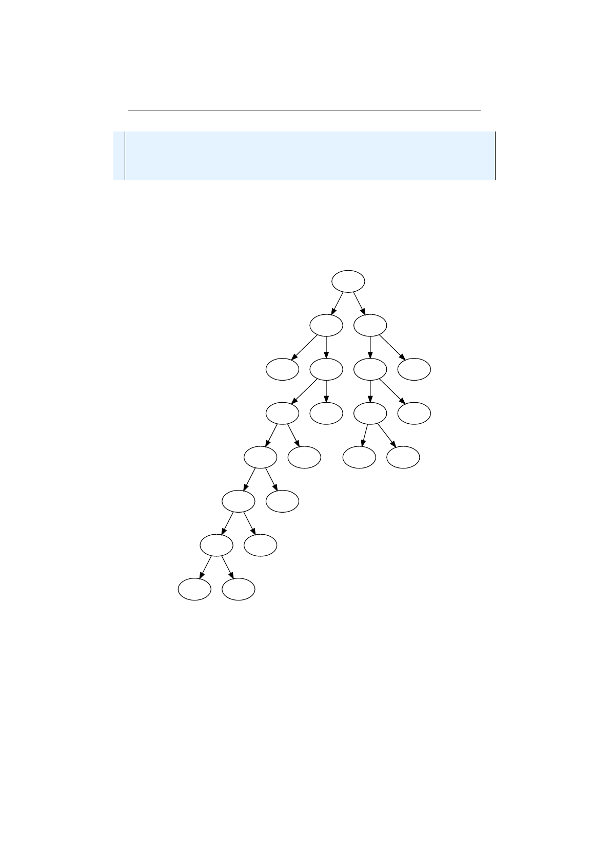
5.8. DTLZ1 CHAPTER 5. EXAMPLES
95
96 System . out . p r i n t l n ( program . t o P a r e n t h e s e s S t r i n g ( ) ) ;
97 }
98
99 }
The fitness function calculates the summed error between the expected
function value and the actual function value. An additional term is added to the
error, which penalizes expression trees which grow to big. The factor 0
.
00001
is an empirical value, found after some test runs. One output of a GP run is
shown in figure 5.7.1. If we simplify this program tree, we will get exactly the
polynomial which created the sample data.
sub
add mul
x mul add x
mul x add x
add x x x
add x
add x
x x
Figure 5.7.1: Symbolic regression polynomial
5.8 DTLZ1
Deb, Thiele, Laumanns and Zitzler have proposed a set of generational MOPs
for testing and comparing MOEAs. This suite of benchmarks attempts to define
generic MOEA test problems that are scalable to a user defined number of
objectives. Because of the last names of its creators, this test suite is known as
DTLZ (Deb-Thiele-Laumanns-Zitzler). [7]
120

5.8. DTLZ1 CHAPTER 5. EXAMPLES
DTLZ1 is an M-objective problem with linear Pareto-optimal front: [12]
f1(x) = 1
2x1x2· · · xM−1(1 + g(xM)) ,
f2(x) = 1
2x1x2· · · (1 −xM−1) (1 + g(xM)) ,
.
.
.
fM−1(x) = 1
2x1(1 −x2) (1 + g(xM)) ,
fM(x) = 1
2(1 −x1) (1 + g(xM)) ,
∀i∈[1, ..n] : 0 ≤xi≤1
The functional
g(xM)
requires
|xM|
=
k
variables and must take any function
with g≥0. Typically gis defined as:
g(xM) = 100 "|xM|+x−1
22
−cos 20πx−1
2#.
In the above problem, the total number of variables is
n
=
M
+
k−
1. The
search space contains 11
k−
1local Pareto-optimal fronts, each of which can
attract an MOEA.
1import s t a t i c j av a . l an g . Math . PI ;
2import s t a t i c j av a . l an g . Math . co s ;
3import s t a t i c j av a . l an g . Math . pow ;
4
5import i o . j e n e t i c s . DoubleGene ;
6import i o . j e n e t i c s . Mutator ;
7import i o . j e n e t i c s . Phenotype ;
8import i o . j e n e t i c s . To urna ment Sele ctor ;
9import i o . j e n e t i c s . en gi n e . Codecs ;
10 import i o . j e n e t i c s . en gi n e . Engine ;
11 import i o . j e n e t i c s . en gi n e . Problem ;
12 import i o . j e n e t i c s . u t i l . DoubleRange ;
13 import i o . j e n e t i c s . u t i l . IS eq ;
14 import i o . j e n e t i c s . u t i l . IntRange ;
15
16 import i o . j e n e t i c s . e xt . S i m u la t e d Bi na r y C ro ss o ve r ;
17 import i o . j e n e t i c s . e xt . moea .MOEA;
18 import i o . j e n e t i c s . e xt . moea . NSGA2Selector ;
19 import i o . j e n e t i c s . e xt . moea . Vec ;
20
21 pu bl ic c l a s s DTLZ1 {
22 pr iv at e s t a t i c f i n a l i nt VARIABLES = 4 ;
23 pr iv at e s t a t i c f i n a l i nt OBJECTIVES = 3 ;
24 pr iv at e s t a t i c f i n a l i nt K = VARIABLES −OBJECTIVES + 1 ;
25
26 s t a t i c f i n a l Problem<double [ ] , DoubleGene , Vec<double[]>>
27 PROBLEM = Problem . o f (
28 DTLZ1 : : f ,
29 Co de cs . o f V e c t o r ( Doubl eRange . o f ( 0 , 1 . 0 ) , VARIABLES)
30 ) ;
31
32 static Vec<double [] > f ( f i n a l double [ ] x ) {
33 double g = 0 . 0 ;
34 for (int i = VARIABLES −K; i < VARIABLES; i ++) {
121
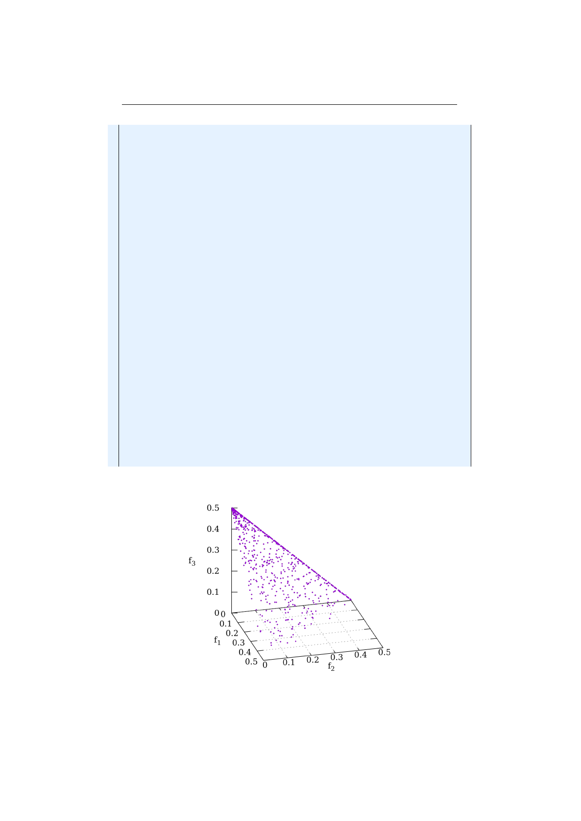
5.8. DTLZ1 CHAPTER 5. EXAMPLES
35 g += pow ( x [ i ] −0 . 5 , 2 . 0 ) −c o s ( 2 0 . 0 ∗PI ∗( x [ i ] −0 . 5 ) ) ;
36 }
37 g = 100.0∗(K + g ) ;
38
39 f i n a l double [ ] f = new double [ OBJECTIVES ] ;
40 for (int i = 0 ; i < OBJECTIVES; ++i ) {
41 f [ i ] = 0 . 5 ∗( 1 . 0 + g ) ;
42 for (int j = 0 ; j < OBJECTIVES −i−1 ; ++j ) {
43 f [ i ] ∗= x [ j ] ;
44 }
45 i f ( i != 0 ) {
46 f [ i ] ∗= 1 −x [ OBJECTIVES −i−1 ] ;
47 }
48 }
49
50 return Vec . o f ( f ) ;
51 }
52
53 s t a t i c f i n a l Engine<DoubleGene , Vec<double[]>> ENGINE =
54 Engine . b u i l d e r (PROBLEM)
55 . p o p u l a t i o n S i z e ( 1 0 0)
56 . a l t e r e r s (
57 new SimulatedBinaryCrossover <>(1) ,
58 new Mutator <>(1.0/VARIABLES) )
59 . offspringSelector(new To ur na me nt Se le ct or <>(5) )
60 . s u r v i v o r s S e l e c t o r ( NSGA2Selector . ofVec ( ) )
61 . m ini mi zi ng ( )
62 . b u i l d ( ) ;
63
64 pub li c s t a t i c void main ( final S t r i n g [ ] a r g s ) {
65 final ISeq<Vec<double[]>> f r o n t = ENGINE . stream ( )
66 . l i m i t ( 2 5 0 0 )
67 . c o l l e c t (MOEA. t o P a r e t o S e t ( I ntR an ge . o f ( 1 0 0 0 , 1 10 0 ) ) )
68 . map( Phenotype : : g e t F i t n e s s ) ;
69 }
70
71 }
The listing above shows the encoding of the DTLZ1 problem with the
Jenetics
library. Figure 5.8.1 shows the Pareto-optimal front of the DTLZ1 optimization.
Figure 5.8.1: Pareto front DTLZ1
122

Chapter 6
Build
For building the
Jenetics
library from source, download the most recent, stable
package version from
https://github.com/jenetics/jenetics/releases
and
extract it to some build directory.
$ unzip jenetics-<version>.zip -d <builddir>
<version>
denotes the actual
Jenetics
version and
<builddir>
the actual build
directory. Alternatively you can check out the latest version from the Git
master
branch.
$ git clone https://github.com/jenetics/jenetics.git \
<builddir>
Jenetics
uses Gradle
1
as build system and organizes the source into sub-projects
(modules).2Each sub-project is located in it’s own sub-directory.
Published projects
•jenetics
: This project contains the source code and tests for the
Jenetics
base-module.
•jenetics.ext
: This module contains additional non-standard GA opera-
tions and data types. It also contains classes for solving multi-objective
problems (MOEA).
•jenetics.prog
: The modules contains classes which allows to do genetic
programming (GP). It seamlessly works with the existing
Evolution-
Stream and evolution Engine.
•jenetics.xml
: XML marshalling module for the
Jenetics
base data struc-
tures.
1http://gradle.org/downloads
2
If you are calling the
gradlew
script (instead of
gradle
), which are part of the downloaded
package, the proper Gradle version is automatically downloaded and you don’t have to install
Gradle explicitly.
123

CHAPTER 6. BUILD
•prngine
: PRNGine is a pseudo-random number generator library for
sequential and parallel Monte Carlo simulations. Since this library has no
dependencies to one of the other projects, it has its own repository
3
with
independent versioning.
Non-published projects
•jenetics.example
: This project contains example code for the base-
module.
•jenetics.doc: Contains the code of the web-site and this manual.
•jenetics.tool
: This module contains classes used for doing integration
testing and algorithmic performance testing. It is also used for creating
GA performance measures and creating diagrams from the performance
measures.
For building the library change into the
<builddir>
directory (or one of the
module directory) and call one of the available tasks:
•compileJava
: Compiles the
Jenetics
sources and copies the class files to
the <builddir>/<module-dir>/build/classes/main directory.
•jar
: Compiles the sources and creates the JAR files. The artifacts are
copied to the <builddir>/<module-dir>/build/libs directory.
•test
: Compiles and executes the unit tests. The test results are printed
onto the console and a test-report, created by TestNG, is written to
<builddir>/<module-dir> directory.
•javadoc
: Generates the API documentation. The Javadoc is stored in the
<builddir>/<module-dir>/build/docs directory.
•clean
: Deletes the
<builddir>/build/*
directories and removes all gen-
erated artifacts.
For building the library from the source, call
$ cd <build-dir>
$ gradle jar
or
$ ./gradlew jar
if you don’t have the the Gradle build system installed—calling the the Gradle
wrapper script will download all needed files and trigger the build task afterwards.
3https://github.com/jenetics/prngine
124

CHAPTER 6. BUILD
External library dependencies
The following external projects are used for
running and/or building the Jenetics library.
•TestNG
◦Version:6.14.3
◦Homepage:http: // testng. org/ doc/ index. html
◦License:Apache License, Version 2.0
◦Scope:test
•Apache Commons Math
◦Version:3.6.1
◦Homepage
:
http: // commons. apache. org/ proper/ commons-math/
◦Download
:
http: // tweedo. com/ mirror/ apache/ commons/ math/
binaries/ commons-math3-3. 6. 1-bin. zip
◦License:Apache License, Version 2.0
◦Scope:test
•EqualsVerifier
◦Version:2.5.2
◦Homepage:http: // jqno. nl/ equalsverifier/
◦Download
:
https: // github. com/ jqno/ equalsverifier/ releases
◦License:Apache License, Version 2.0
◦Scope:test
•Java2Html
◦Version:5.0
◦Homepage:http: // www. java2html. de/
◦Download:http: // www. java2html. de/ java2html_ 50. zip
◦License:GPL orCPL1.0
◦Scope:javadoc
•Gradle
◦Version: 5.2.1
◦Homepage:http: // gradle. org/
◦Download
:
http: // services. gradle. org/ distributions/ gradle-5.
2. 1-bin. zip
◦License:Apache License, Version 2.0
◦Scope:build
Maven Central
The whole
Jenetics
package can also be downloaded from
the Maven Central repository http://repo.maven.apache.org/maven2:
125

CHAPTER 6. BUILD
pom.xml snippet for Maven
<dependency>
<groupId>io.jenetics</groupId>
<artifactId>module-name </artifactId>
<version>4.4.0</version>
</dependency>
Gradle
’io.jenetics:module-name :4.4.0’
License The library itself is licensed under theApache License, Version 2.0.
Copyright 2007-2019 Franz Wilhelmstötter
Licensed under the Apache License, Version 2.0 (the "License");
you may not use this file except in compliance with the License.
You may obtain a copy of the License at
http://www.apache.org/licenses/LICENSE-2.0
Unless required by applicable law or agreed to in writing, software
distributed under the License is distributed on an "AS IS" BASIS,
WITHOUT WARRANTIES OR CONDITIONS OF ANY KIND, either express or implied.
See the License for the specific language governing permissions and
limitations under the License.
126

Bibliography
[1]
Thomas Back. Evolutionary Algorithms in Theory and Practice. Oxford
Univiversity Press, 1996.
[2]
James E. Baker. Reducing bias and inefficiency in the selection algorithm.
Proceedings of the Second International Conference on Genetic Algorithms
and their Application, pages 14–21, 1987.
[3]
Shumeet Baluja and Rich Caruana. Removing the genetics from the standard
genetic algorithm. pages 38–46. Morgan Kaufmann Publishers, 1995.
[4]
Heiko Bauke. Tina’s random number generator library.
https://github.com/rabauke/trng4/blob/master/doc/trng.pdf, 2011.
[5]
Tobias Blickle and Lothar Thiele. A comparison of selection schemes used
in evolutionary algorithms. Evolutionary Computation, 4:361–394, 1997.
[6]
Joshua Bloch. Effective Java. Addison-Wesley Professional, 3rd edition,
2018.
[7]
David A. Van Veldhuizen Carlos A. Coello Coello, Gary B. Lamont. Evo-
lutionary Algorithms for Solving Multi-Objective Problems. Genetic and
Evolutionary Computation. Springer, Berlin, Heidelberg, 2nd edition, 2007.
[8]
P.K. Chawdhry, R. Roy, and R.K. Pant. Soft Computing in Engineering
Design and Manufacturing. Springer London, 1998.
[9]
Richard Dawkins. The Blind Watchmaker. New York: W. W. Norton &
Company, 1986.
[10]
K. Deb, A. Pratap, S. Agarwal, and T. Meyarivan. A fast and elitist
multiobjective genetic algorithm: Nsga-ii. Trans. Evol. Comp, 6(2):182–197,
April 2002.
[11]
Kalyanmoy Deb and Hans-Georg Beyer. Self-adaptive genetic algorithms
with simulated binary crossover. COMPLEX SYSTEMS, 9:431–454, 1999.
[12]
Kalyanmoy Deb, Lothar Thiele, Marco Laumanns, and Eckart Zitzler.
Scalable test problems for evolutionary multi-objective optimization. Number
112 in TIK-Technical Report. ETH-Zentrum, ETH-Zentrum Switzerland,
July 2001.
127

BIBLIOGRAPHY BIBLIOGRAPHY
[13]
Félix-Antoine Fortin and Marc Parizeau. Revisiting the nsga-ii crowding-
distance computation. In Proceedings of the 15th Annual Conference on
Genetic and Evolutionary Computation, GECCO ’13, pages 623–630, New
York, NY, USA, 2013. ACM.
[14]
J.F. Hughes and J.D. Foley. Computer Graphics: Principles and Practice.
The systems programming series. Addison-Wesley, 2014.
[15]
Raj Jain and Imrich Chlamtac. The p2 algorithm for dynamic calculation
of quantiles and histograms without storing observations. Commun. ACM,
28(10):1076–1085, October 1985.
[16]
David Jones. Good practice in (pseudo) random number generation for
bioinformatics applications, May 2010.
[17]
Abdullah Konak, David W. Coit, and Alice E. Smith. Multi-objective
optimization using genetic algorithms: A tutorial. Rel. Eng. & Sys. Safety,
91(9):992–1007, 2006.
[18]
John R. Koza. Genetic Programming: On the Programming of Computers
by Means of Natural Selection. MIT Press, Cambridge, MA, USA, 1992.
[19]
John R. Koza. Introduction to genetic programming: Tutorial. In Proceed-
ings of the 10th Annual Conference Companion on Genetic and Evolutionary
Computation, GECCO ’08, pages 2299–2338, New York, NY, USA, 2008.
ACM.
[20]
Sean Luke. Essentials of Metaheuristics. Lulu, second edition, 2013. Avail-
able for free at http://cs.gmu.edu/∼sean/book/metaheuristics/.
[21]
Zbigniew Michalewicz. Genetic Algorithms + Data Structures = Evolution.
Springer, 1996.
[22]
Melanie Mitchell. An Introduction to Genetic Algorithms. MIT Press,
Cambridge, MA, USA, 1998.
[23]
Heinz Mühlenbein and Dirk Schlierkamp-Voosen. Predictive models for the
breeder genetic algorithm i. continuous parameter optimization. 1(1):25–49.
[24]
Oracle. Value-based classes. https://docs.oracle.com/javase/8/docs/api/-
java/lang/doc-files/ValueBased.html, 2014.
[25]
A. Osyczka. Multicriteria optimization for engineering design. Design
Optimization, page 193–227, 1985.
[26]
Charles C. Palmer and Aaron Kershenbaum. An approach to a problem in
network design using genetic algorithms. Networks, 26(3):151–163, 1995.
[27]
Franz Rothlauf. Representations for Genetic and Evolutionary Algorithms.
Springer, 2 edition, 2006.
[28]
Daniel Shiffman. The Nature of Code. The Nature of Code, 1 edition, 12
2012.
[29]
S. N. Sivanandam and S. N. Deepa. Introduction to Genetic Algorithms.
Springer, 2010.
128

BIBLIOGRAPHY BIBLIOGRAPHY
[30]
W. Vent. Rechenberg, ingo, evolutionsstrategie — optimierung technischer
systeme nach prinzipien der biologischen evolution. 170 s. mit 36 abb.
frommann-holzboog-verlag. stuttgart 1973. broschiert. Feddes Repertorium,
86(5):337–337, 1975.
[31]
Eric W. Weisstein. Scalar function. http://mathworld.wolfram.com/-
ScalarFunction.html, 2015.
[32]
Eric W. Weisstein. Vector function. http://mathworld.wolfram.com/-
VectorFunction.html, 2015.
[33]
Darrell Whitley. A genetic algorithm tutorial. Statistics and Computing,
4:65–85, 1994.
129

Index
0/1 Knapsack, 110
2-point crossover, 19
3-point crossover, 19
AdaptiveEngine, 86
Allele, 6, 39
Alterer, 16, 43
AnyChromosome, 41
AnyGene, 40
Apache Commons Math, 125
Architecture, 4
Assignment problem, 56
Base classes, 5
BigIntegerGene, 81
Block splitting, 34
Boltzmann selector, 15
Build, 123
Gradle, 123
gradlew, 123
Chromosome, 7, 8, 40
recombination, 18
scalar, 45
variable length, 7
Codec, 51
Composite, 57
Mapping, 56
Matrix, 53
Permutation, 55
Scalar, 52
Subset, 54
Vector, 53
Compile, 124
Composite codec, 57
ConcatEngine, 85
Concurrency, 30
configuration, 30
maxBatchSize, 32
maxSurplusQueuedTaskCount, 31
splitThreshold, 31
tweaks, 31
Crossover
2-point crossover, 19
3-point crossover, 19
Intermediate crossover, 21
Line crossover, 21
Multiple-point crossover, 18
Partially-matched crossover, 19,
20
Simulated binary crossover, 81
Single-point crossover, 18, 19
Uniform crossover, 20
CyclicEngine, 86
Dieharder, 73
Directed graph, 50
Distinct population, 72
Domain classes, 6
Domain model, 6
Download, 123
DTLZ1, 120
Elite selector, 16, 43
Elitism, 16, 43
Encoding, 45
Affine transformation, 47
Directed graph, 50
Graph, 49
Real function, 45
Scalar function, 46
Undirected graph, 49
Vector function, 47
Weighted graph, 50
Engine, 23, 44
Evaluator, 29
reproducible, 69
Engine classes, 22
Ephemeral constant, 94
ES, 69
Evolution
Engine, 23
130

INDEX INDEX
interception, 72
performance, 69
reproducible, 69
Stream, 4, 22, 25
Evolution strategy, 69
(µ+λ)-ES, 71
(µ, λ)-ES, 70
Evolution time, 64
Evolution workflow, 4
EvolutionResult, 26
interception, 72
mapper, 25, 72
EvolutionStatistics, 27
EvolutionStream, 25
EvolutionStreamable, 84
Evolving images, 115, 116
Examples, 104
0/1 Knapsack, 110
Evolving images, 115, 116
Ones counting, 104
Rastrigin function, 108
Real function, 106
Traveling salesman, 112
Exponential-rank selector, 15
Fitness convergence, 66
Fitness function, 22
Fitness threshold, 65
Fixed generation, 61
FlatTree, 80
Gaussian mutator, 17
Gene, 6, 39
validation, 7
Gene convergence, 68
Genetic algorithm, 3
Genetic programming, 93, 118
Const, 94
Operations, 93
Program creation, 94
Program pruning, 96
Program repair, 95
Var, 94
Genotype, 8
scalar, 10, 45
Validation, 24
vector, 9
Git repository, 123
GP, 93, 118
Gradle, 123, 125
gradlew, 123
Graph, 49
Hello World, 2
Installation, 123
Interception, 72
Internals, 73
io.jenetics.ext, 78
io.jenetics.prngine, 99
io.jenetics.prog, 93
io.jenetics.xml, 96
Java property
maxBatchSize, 32
maxSurplusQueuedTaskCount, 31
splitThreshold, 31
Java2Html, 125
LCG64ShiftRandom, 34, 74
Leapfrog, 34
License, i, 126
Linear-rank selector, 14
Mapping codec, 56
Matrix codec, 53
Mean alterer, 21
Modifying Engine, 84
Modules, 77
io.jenetics.ext, 78
io.jenetics.prngine, 99
io.jenetics.prog, 93
io.jenetics.xml, 96
Mona Lisa, 117
Monte Carlo selector, 13, 69
MOO, 88
Multi-objective optimization, 88
Multiple-point crossover, 18
Mutation, 16
Mutator, 17
NSGA2 selector, 92
Ones counting, 104
Operation classes, 12
Package structure, 5
Parentheses tree, 79
Pareto dominance, 88
Pareto efficiency, 88
Partially-matched crossover, 19, 20
131

INDEX INDEX
Permutation codec, 55
Phenotype, 11
Validation, 24
Population, 6
unique, 25
Population convergence, 67
PRNG, 32
Block splitting, 34
LCG64ShiftRandom, 34
Leapfrog, 34
Parameterization, 34
Random seeding, 34
PRNG testing, 73
Probability selector, 13
Problem, 58
Quantile, 38
Random, 32
Engine, 32
LCG64ShiftRandom, 34
Registry, 32
seeding, 74
testing, 73
Random seeding, 34
Randomness, 32
Rastrigin function, 108
Real function, 106
Recombination, 17
Reproducibility, 69
Roulette-wheel selector, 14
SBX, 81
Scalar chromosome, 45
Scalar codec, 52
Scalar genotype, 45
Seeding, 74
Selector, 12, 42
Elite, 43
Seq, 36
Serialization, 35
Simulated binary crossover, 81
Single-node crossover, 81
Single-point crossover, 18, 19
Source code, 123
Statistics, 37, 43
Steady fitness, 62
Stochastic-universal selector, 15
Subset codec, 54
Swap mutator, 17
Symbolic regression, 118
Termination, 60
Evolution time, 64
Fitness convergence, 66
Fitness threshold, 65
Fixed generation, 61
Gene convergence, 68
Population convergence, 67
Steady fitness, 62
TestNG, 125
Tournament selector, 13
Traveling salesman, 112
Tree, 78
TreeGene, 81
Truncation selector, 13
Undirected graph, 49
Uniform crossover, 20
Unique fitness tournament selector,
92
Unique population, 72
Validation, 7, 24, 59
Vec, 89
Vector codec, 53
Weasel program, 82
WeaselMutator, 83
WeaselSelector, 83
Weighted graph, 50
132
