Manual SPECFEM3D Cartesian
User Manual:
Open the PDF directly: View PDF ![]() .
.
Page Count: 118 [warning: Documents this large are best viewed by clicking the View PDF Link!]
- Contents
- 1 Introduction
- 2 Getting Started
- 3 Mesh Generation
- 4 Creating the Distributed Databases
- 5 Running the Solver xspecfem3D
- 6 Kinematic and dynamic fault sources
- 7 Adjoint Simulations
- 8 Doing tomography based on the sensitivity kernels obtained
- 9 Performing full waveform inversion (FWI) or source inversions
- 10 Noise Cross-correlation Simulations
- 11 Gravity integral calculations for the gravity field of an Earth model
- 12 Graphics
- 13 Running through a Scheduler
- 14 Changing the Model
- 15 Post-Processing Scripts
- 16 Information for developers of the code, and for people who want to learn how the technique works
- Notes & Acknowledgments
- Copyright
- Bibliography
- A Reference Frame Convention
- B Channel Codes of Seismograms
- C Troubleshooting
- D License
User Manual
COMPUTATIONAL INFRASTRUCTURE FOR GEODYNAMICS (CIG)
Version 3.0
CNRS (FRANCE)
PRINCETON UNIVERSITY (USA)
ETH ZÜRICH (SWITZERLAND)
SPECFEM 3D
Cartesian
g
→
SPECFEM3D
Cartesian
User Manual
© CNRS (France), Princeton University (USA),
and ETH Zürich (Switzerland)
Version 3.0
June 15, 2018
1
Authors
The SPECFEM3D package was first developed by Dimitri Komatitsch and Jean-Pierre Vilotte at Institut de Physique
du Globe (IPGP) in Paris, France from 1995 to 1997 and then by Dimitri Komatitsch and Jeroen Tromp at Harvard
University and Caltech, USA, starting in 1998. The story started on April 4, 1995, when Prof. Yvon Maday from
CNRS and University of Paris, France, gave a lecture to Dimitri Komatitsch and Jean-Pierre Vilotte at IPG about
the nice properties of the Legendre spectral-element method with diagonal mass matrix that he had used for other
equations. We are deeply indebted and thankful to him for that. That followed a visit by Dimitri Komatitsch to OGS
(Istituto Nazionale di Oceanografia e di Geofisica Sperimentale) in Trieste, Italy, in February 1995 to meet with Géza
Seriani and Enrico Priolo, who introduced him to their 2D Chebyshev version of the spectral-element method with a
non-diagonal mass matrix. We are deeply indebted and thankful to them for that.
Since then it has been developed and maintained by a development team: in alphabetical order, Michael Afanasiev,
Jean-Paul (Pablo) Ampuero, Étienne Bachmann, Kangchen Bai, Piero Basini, Céline Blitz, Alexis Bottero, Ebru Boz-
da˘
g, Emanuele Casarotti, Joseph Charles, Min Chen, Paul Cristini, Clément Durochat, Percy Galvez, Hom Nath
Gharti, Dominik Göddeke, Vala Hjörleifsdóttir, Sue Kientz, Dimitri Komatitsch, Jesús Labarta, Nicolas Le Goff,
Pieyre Le Loher, Matthieu Lefebvre, Qinya Liu, Youshan Liu, David Luet, Yang Luo, Alessia Maggi, Federica
Magnoni, Roland Martin, René Matzen, Dennis McRitchie, Matthias Meschede, Peter Messmer, David Michéa, Vadim
Monteiller, Surendra Nadh Somala, Masaru Nagaso, Tarje Nissen-Meyer, Daniel Peter, Kevin Pouget, Max Rietmann,
Elliott Sales de Andrade, Brian Savage, Bernhard Schuberth, Anne Sieminski, James Smith, Leif Strand, Carl Tape,
Jeroen Tromp, Brice Videau, Jean-Pierre Vilotte, Zhinan Xie, Chang-Hua Zhang, Hejun Zhu.
The cover graphic of the manual was created by Santiago Lombeyda from Caltech’s Center for Advanced Com-
puting Research (CACR), USA, with free satellite clipart pictures from http://www.4vector.com and http:
//www.clker.com added to it.
The code is released open-source under the GNU version 3 license, see the license at the end of this manual.

2
Current and past main participants or main sponsors of the SPECFEM project
(in no particular order)
Contents
Contents 3
1 Introduction 6
1.1 Citation .................................................. 8
1.2 Support .................................................. 10
2 Getting Started 11
2.1 Adding OpenMP support in addition to MPI ............................... 14
2.2 Compiling on an IBM BlueGene ..................................... 14
2.3 Visualizing the subroutine calling tree of the source code ........................ 15
2.4 Using the ADIOS library for I/O ..................................... 16
2.5 Becoming a developer of the code, or making small modifications in the source code ......... 17
3 Mesh Generation 18
3.1 Meshing with CUBIT ........................................... 18
3.1.1 Creating the Mesh with CUBIT ................................. 19
3.1.2 Exporting the Mesh with run_cubit2specfem3d.py ................... 20
3.1.3 Partitioning the Mesh with xdecompose_mesh ........................ 24
3.2 Meshing with xmeshfem3D ....................................... 25
4 Creating the Distributed Databases 30
4.1 Main parameter file Par_file ..................................... 30
4.2 Choosing the time step DT ........................................ 36
5 Running the Solver xspecfem3D 39
5.1 Note on the viscoelastic model used ................................... 45
6 Kinematic and dynamic fault sources 47
6.1 Mesh Generation with Split Nodes .................................... 47
6.2 CUBIT-Python Scripts for Faults ..................................... 49
6.3 Examples ................................................. 50
6.4 Sign Convention for Fault Quantities ................................... 50
6.5 Input Files ................................................. 51
6.6 Setting the Kelvin-Voigt Damping Parameter .............................. 53
6.7 Output Files ............................................... 54
6.8 Post-processing and Visualization .................................... 55
7 Adjoint Simulations 56
7.1 Adjoint Simulations for Sources Only (not for the Model) ........................ 56
7.2 Adjoint Simulations for Finite-Frequency Kernels (Kernel Simulation) ................. 57
3
CONTENTS 4
8 Doing tomography based on the sensitivity kernels obtained 59
8.1 Tomographic full waveform inversion (FWI) / imaging using the sensitivity kernels obtained ..... 59
8.1.1 Principle ............................................. 59
8.1.2 Computation of the gradient based on the adjoint method .................... 60
8.2 Tomographic tools ............................................ 62
8.2.1 Summing kernels ......................................... 63
8.2.2 Smoothing and post-processing ................................. 65
8.2.3 Model updating .......................................... 66
8.3 OLD VERSION OF THE SECTION, WILL SOON BE IMPROVED AND ENRICHED ....... 67
9 Performing full waveform inversion (FWI) or source inversions 68
10 Noise Cross-correlation Simulations 69
10.1 Input Parameter Files ........................................... 69
10.2 Noise Simulations: Step by Step ..................................... 70
10.2.1 Pre-simulation .......................................... 70
10.2.2 Simulations ............................................ 71
10.2.3 Post-simulation .......................................... 72
10.3 Example .................................................. 72
11 Gravity integral calculations for the gravity field of an Earth model 73
12 Graphics 74
12.1 Meshes .................................................. 74
12.2 Movies .................................................. 74
12.2.1 Movie Surface and Shakemaps .................................. 75
12.2.2 Movie Volume .......................................... 76
12.3 Finite-Frequency Kernels ......................................... 77
13 Running through a Scheduler 80
14 Changing the Model 81
14.1 Using external tomographic Earth models ................................ 81
14.2 External (an)elastic Models ........................................ 83
14.3 Anisotropic Models ............................................ 84
14.4 Using external SEP models ........................................ 84
15 Post-Processing Scripts 85
15.1 Process Data and Synthetics ....................................... 85
15.1.1 Data processing script process_data.pl .......................... 85
15.1.2 Synthetics processing script process_syn.pl ........................ 86
15.1.3 Script rotate.pl ....................................... 86
15.2 Collect Synthetic Seismograms ...................................... 86
15.3 Clean Local Database ........................................... 87
15.4 Plot Movie Snapshots and Synthetic Shakemaps ............................. 87
15.4.1 Script movie2gif.gmt.pl .................................. 87
15.4.2 Script plot_shakemap.gmt.pl ............................... 87
15.5 Map Local Database ........................................... 87
16 Information for developers of the code, and for people who want to learn how the technique works 88
Notes & Acknowledgments 90
Copyright 91
Bibliography 92
Chapter 1
Introduction
FIRST ANNOUNCEMENT: SPECFEM3D can now perform full waveform inversion (FWI), i.e. invert for
models in an iterative fashion, and it can also perform source inversions in a constant model; please refer to
the two new directories, inverse_problem_for_model and inverse_problem_for_source, and the
README files they contain. For FWI inversions for the model, also refer to the new examples provided in
directory EXAMPLES.
SECOND ANNOUNCEMENT: SPECFEM3D can now perform coupling with an external code (DSM,
AxiSEM or FK) based on a database of displacement vectors and traction vectors on the outer edges of the
mesh created once and for all (see Monteiller et al. [2013,2015], Wang et al. [2016], Tong et al. [2014a,b], and if
you use that feature of the code please cite at least one of these papers).
To use coupling with FK, just use the set of parameters that is in the DATA/Par_file input file of the code:
#———————————————————–
#
# Coupling with an injection technique (DSM, AxiSEM, or FK)
#
#———————————————————–
COUPLE_WITH_INJECTION_TECHNIQUE = .false.
INJECTION_TECHNIQUE_TYPE = 3 # 1 = DSM, 2 = AxiSEM, 3 = FK
MESH_A_CHUNK_OF_THE_EARTH = .false.
TRACTION_PATH = ./DATA/AxiSEM_tractions/3/
FKMODEL_FILE = FKmodel
RECIPROCITY_AND_KH_INTEGRAL = .false. # does not work yet
That part (coupling with FK) is actively maintained and works fine. See e.g. http://komatitsch.free.fr/
preprints/GRL_Ping_Tong_2014.pdf for some examples. There is also an example that is provided with
the code: specfem3d/EXAMPLES/small_example_coupling_FK_specfem.
Regarding coupling with DSM, that part is not actively maintained any more, but it is still included in the code, you may
have to test it again and make minor adjustments if needed. The necessary tools are in directory specfem3d/EXTERNAL_PACKAGES_coupled_with_SPECFEM3D/DSM_for_SPECFEM3D
, and there is a README file in specfem3d/EXTERNAL_PACKAGES_coupled_with_SPECFEM3D that should be
more or less up-to-date (there are about four steps to follow in total, the first one being creating the database of DSM
tractions and displacements on the edges of the coupling box).
See e.g. http://komatitsch.free.fr/preprints/GJI1_Vadim_2013.pdf and http://komatitsch.
free.fr/preprints/GJI2_Vadim_2015.pdf for some examples.
THIRD ANNOUNCEMENT: SPECFEM3D can now perform gravity field calculations in addition (or in-
stead of) seismic wave propagation only. See flag GRAVITY_INTEGRALS in file setup/constants.h.in.
Please also refer to http://komatitsch.free.fr/preprints/GJI_Martin_gravimetry_2017.pdf.
And yes, that is the reason why I added a falling apple on the cover of the manual :-). Note that SPECFEM3D
can also model transient gravity perturbations induced by earthquake rupture, as developed and explained in
Harms et al. [2015]. These are two different things, and both are implemented and avaible in SPECFEM3D. To
6
CHAPTER 1. INTRODUCTION 7
use the second feature, please refer to doc/how_to/README_gravity_perturbation.txt.
The software package SPECFEM3D Cartesian simulates seismic wave propagation at the local or regional scale
and performs full waveform imaging (FWI) or adjoint tomography based upon the spectral-element method (SEM).
The SEM is a continuous Galerkin technique [Tromp et al.,2008,Peter et al.,2011], which can easily be made discon-
tinuous [Bernardi et al.,1994,Chaljub,2000,Kopriva et al.,2002,Chaljub et al.,2003,Legay et al.,2005,Kopriva,
2006,Wilcox et al.,2010,Acosta Minolia and Kopriva,2011]; it is then close to a particular case of the discontinuous
Galerkin technique [Reed and Hill,1973,Lesaint and Raviart,1974,Arnold,1982,Johnson and Pitkäranta,1986,
Bourdel et al.,1991,Falk and Richter,1999,Hu et al.,1999,Cockburn et al.,2000,Giraldo et al.,2002,Rivière and
Wheeler,2003,Monk and Richter,2005,Grote et al.,2006,Ainsworth et al.,2006,Bernacki et al.,2006,Dumbser and
Käser,2006,De Basabe et al.,2008,de la Puente et al.,2009,Wilcox et al.,2010,De Basabe and Sen,2010,Étienne
et al.,2010], with optimized efficiency because of its tensorized basis functions [Wilcox et al.,2010,Acosta Minolia
and Kopriva,2011]. In particular, it can accurately handle very distorted mesh elements [Oliveira and Seriani,2011].
In fluids, when gravity is turned off, SPECFEM3D uses the classical linearized Euler equation; thus if you
have sharp local variations of density in the fluid (highly heterogeneous fluids in terms of density) or if density
becomes extremely small in some regions of your model (e.g. for upper-atmosphere studies), before using the
code please make sure the linearized Euler equation is a valid approximation in the case you want to study,
and/or see if you should turn gravity on. For more details on that see e.g. Jensen et al. [2011].
It has very good accuracy and convergence properties [Maday and Patera,1989,Seriani and Priolo,1994,Deville
et al.,2002,Cohen,2002,De Basabe and Sen,2007,Seriani and Oliveira,2008,Ainsworth and Wajid,2009,2010,
Melvin et al.,2012]. The spectral element approach admits spectral rates of convergence and allows exploiting hp-
convergence schemes. It is also very well suited to parallel implementation on very large supercomputers [Komatitsch
et al.,2003,Tsuboi et al.,2003,Komatitsch et al.,2008,Carrington et al.,2008,Komatitsch et al.,2010b] as well as
on clusters of GPU accelerating graphics cards [Komatitsch,2011,Michéa and Komatitsch,2010,Komatitsch et al.,
2009,2010a]. Tensor products inside each element can be optimized to reach very high efficiency [Deville et al.,2002],
and mesh point and element numbering can be optimized to reduce processor cache misses and improve cache reuse
[Komatitsch et al.,2008]. The SEM can also handle triangular (in 2D) or tetrahedral (in 3D) elements [Wingate and
Boyd,1996,Taylor and Wingate,2000,Komatitsch et al.,2001,Cohen,2002,Mercerat et al.,2006] as well as mixed
meshes, although with increased cost and reduced accuracy in these elements, as in the discontinuous Galerkin method.
Note that in many geological models in the context of seismic wave propagation studies (except for instance for
fault dynamic rupture studies, in which very high frequencies or supershear rupture need to be modeled near the fault,
see e.g. Benjemaa et al. [2007,2009], de la Puente et al. [2009], Tago et al. [2010]) a continuous formulation is
sufficient because material property contrasts are not drastic and thus conforming mesh doubling bricks can efficiently
handle mesh size variations [Komatitsch and Tromp,2002a,Komatitsch et al.,2004,Lee et al.,2008,2009a,b].
For a detailed introduction to the SEM as applied to regional seismic wave propagation, please consult Peter et al.
[2011], Tromp et al. [2008], Komatitsch and Vilotte [1998], Komatitsch and Tromp [1999], Chaljub et al. [2007] and
in particular Lee et al. [2009b,a,2008], Godinho et al. [2009], van Wijk et al. [2004], Komatitsch et al. [2004]. A
detailed theoretical analysis of the dispersion and stability properties of the SEM is available in Cohen [2002], De
Basabe and Sen [2007], Seriani and Oliveira [2007], Seriani and Oliveira [2008] and Melvin et al. [2012].
Effects due to lateral variations in compressional-wave speed, shear-wave speed, density, a 3D crustal model,
topography and bathymetry are included. The package can accommodate full 21-parameter anisotropy (see Chen
and Tromp [2007]) as well as lateral variations in attenuation [Savage et al.,2010]. Adjoint capabilities and finite-
frequency kernel simulations are included [Tromp et al.,2008,Peter et al.,2011,Liu and Tromp,2006,Fichtner et al.,
2009a,Virieux and Operto,2009].
The SEM was originally developed in computational fluid dynamics [Patera,1984,Maday and Patera,1989] and
has been successfully adapted to address problems in seismic wave propagation. Early seismic wave propagation ap-
plications of the SEM, utilizing Legendre basis functions and a perfectly diagonal mass matrix, include Cohen et al.
[1993], Komatitsch [1997], Faccioli et al. [1997], Casadei and Gabellini [1997], Komatitsch and Vilotte [1998] and
CHAPTER 1. INTRODUCTION 8
Komatitsch and Tromp [1999], whereas applications involving Chebyshev basis functions and a non-diagonal mass
matrix include Seriani and Priolo [1994], Priolo et al. [1994] and Seriani et al. [1995]. In the Legendre version that
we use in SPECFEM the mass matrix is purposely slightly inexact but diagonal (but can be made exact if needed, see
Teukolsky [2015]), while in the Chebyshev version it is exact but non diagonal.
Beware that, in a spectral-element method, some spurious modes (that have some similarities with classical
so-called "Hourglass modes" in finite-element techniques, although in the SEM they are not zero-energy modes)
can appear in some (but not all) cases in the spectral element in which the source is located. Fortunately, they
do not propagate away from the source element. However, this means that if you put a receiver in the same
spectral element as a source, the recorded signals may in some cases be wrong, typically exhibiting some spu-
rious oscillations, which are often even non causal. If that is the case, an easy option is to slightly change the
mesh in the source region in order to get rid of these Hourglass-like spurious modes, as explained in Duczek
et al. [2014], in which this phenomenon is described in details, and in which practical solutions to avoid it are
suggested.
All SPECFEM3D software is written in Fortran2003 with full portability in mind, and conforms strictly to the
Fortran2003 standard. It uses no obsolete or obsolescent features of Fortran. The package uses parallel programming
based upon the Message Passing Interface (MPI) [Gropp et al.,1994,Pacheco,1997].
SPECFEM3D won the Gordon Bell award for best performance at the SuperComputing 2003 conference in
Phoenix, Arizona (USA) (see Komatitsch et al. [2003] and www.sc-conference.org/sc2003/nrfinalaward.
html). It was a finalist again in 2008 for a run at 0.16 petaflops (sustained) on 149,784 processors of the ‘Jaguar’
Cray XT5 system at Oak Ridge National Laboratories (USA) [Carrington et al.,2008]. It also won the BULL Joseph
Fourier supercomputing award in 2010.
It reached the sustained one petaflop performance level for the first time in February 2013 on the Blue Waters Cray
supercomputer at the National Center for Supercomputing Applications (NCSA), located at the University of Illinois
at Urbana-Champaign (USA).
This new release of the code includes Convolution or Auxiliary Differential Equation Perfectly Matched absorbing
Layers (C-PML or ADE-PML) [Martin et al.,2008b,c,Martin and Komatitsch,2009,Martin et al.,2010,Komatitsch
and Martin,2007]. It also includes support for GPU graphics card acceleration [Komatitsch,2011,Michéa and Ko-
matitsch,2010,Komatitsch et al.,2009,2010a].
The next release of the code will use the PT-SCOTCH parallel and threaded version of SCOTCH for mesh parti-
tioning instead of the serial version.
SPECFEM3D Cartesian includes coupled fluid-solid domains and adjoint capabilities, which enables one to ad-
dress seismological inverse problems, but for linear rheologies only so far. To accommodate visco-plastic or non-linear
rheologies, the reader can refer to the GeoELSEsoftware package [Casadei and Gabellini,1997,Stupazzini et al.,
2009].
1.1 Citation
You can find all the references below in BIBT
EXformat in file doc/USER_MANUAL/bibliography.bib.
If you use SPECFEM3D Cartesian for your own research, please cite at least one of the following articles:
Numerical simulations in general
Forward and adjoint simulations are described in detail in Tromp et al. [2008], Peter et al. [2011], Vai et al.
[1999], Komatitsch et al. [2009,2010a], Chaljub et al. [2007], Madec et al. [2009], Komatitsch et al. [2010b],
Carrington et al. [2008], Tromp et al. [2010a], Komatitsch et al. [2002], Komatitsch and Tromp [2002a,b,1999]
or Komatitsch and Vilotte [1998]. Additional aspects of adjoint simulations are described in Tromp et al. [2005],
Liu and Tromp [2006], Tromp et al. [2008], Liu and Tromp [2008], Tromp et al. [2010a], Peter et al. [2011].
CHAPTER 1. INTRODUCTION 9
Domain decomposition is explained in detail in Martin et al. [2008a], and excellent scaling up to 150,000
processor cores is shown for instance in Carrington et al. [2008], Komatitsch et al. [2008], Martin et al. [2008a],
Komatitsch et al. [2010a], Komatitsch [2011],
GPU computing
Computing on GPU graphics cards for acoustic or seismic wave propagation applications is described in detail
in Komatitsch [2011], Michéa and Komatitsch [2010], Komatitsch et al. [2009,2010a].
If you use this new version, which has non blocking MPI for much better performance for medium or large runs,
please cite at least one of these six articles, in which results of non blocking MPI runs are presented: Peter et al.
[2011], Komatitsch et al. [2010a,b], Komatitsch [2011], Carrington et al. [2008], Martin et al. [2008a].
If you use the C-PML absorbing layer capabilities of the code, please cite at least one article written by the
developers of the package, for instance:
•Xie et al. [2014],
•Xie et al. [2016].
If you use the UNDO_ATTENUATION option of the code in order to produce full anelastic/viscoelastic sensitivity
kernels, please cite at least one article written by the developers of the package, for instance (and in particular):
•Komatitsch et al. [2016].
More generally, if you use the attenuation (anelastic/viscoelastic) capabilities of the code, please cite at least one article
written by the developers of the package, for instance:
•Komatitsch et al. [2016],
•Blanc et al. [2016].
If you use the kernel capabilities of the code, please cite at least one article written by the developers of the package,
for instance:
•Tromp et al. [2008],
•Peter et al. [2011],
•Liu and Tromp [2006],
•Morency et al. [2009].
If you work on geophysical applications, you may be interested in citing some of these application articles as well,
among others:
Southern California simulations
Komatitsch et al. [2004], Krishnan et al. [2006a,b].
If you use the 3D southern California model, please cite Süss and Shaw [2003] (Los Angeles model), Lovely
et al. [2006] (Salton Trough), and Hauksson [2000] (southern California). The Moho map was determined by
Zhu and Kanamori [2000]. The 1D SoCal model was developed by Dreger and Helmberger [1990].
Anisotropy
Chen and Tromp [2007], Ji et al. [2005], Chevrot et al. [2004], Favier et al. [2004], Ritsema et al. [2002], Tromp
and Komatitsch [2000].
Attenuation
Savage et al. [2010], Komatitsch and Tromp [2002a,1999].
Topography
Lee et al. [2009b,a,2008], Godinho et al. [2009], van Wijk et al. [2004].
The corresponding BibT
EX entries may be found in file doc/USER_MANUAL/bibliography.bib.
CHAPTER 1. INTRODUCTION 10
1.2 Support
This material is based upon work supported by the USA National Science Foundation under Grants No. EAR-0406751
and EAR-0711177, by the French CNRS, French INRIA Sud-Ouest MAGIQUE-3D, French ANR NUMASIS under
Grant No. ANR-05-CIGC-002, and European FP6 Marie Curie International Reintegration Grant No. MIRG-CT-
2005-017461. Any opinions, findings, and conclusions or recommendations expressed in this material are those of the
authors and do not necessarily reflect the views of the USA National Science Foundation, CNRS, INRIA, ANR or the
European Marie Curie program.
Chapter 2
Getting Started
To download the SPECFEM3D_Cartesian software package, type this:
git clone --recursive --branch devel https://github.com/geodynamics/specfem3d.git
Note: for people who would like to run the package on Windows rather than on Unix machines, you can in-
stall Docker or VirtualBox (installing a Linux in VirtualBox in that latter case) and run it easily from inside that.
We recommend that you add ulimit -S -s unlimited to your .bash_profile file and/or limit stacksize
unlimited to your .cshrc file to suppress any potential limit to the size of the Unix stack.
Then, to configure the software for your system, run the configure shell script. This script will attempt to guess
the appropriate configuration values for your system. However, at a minimum, it is recommended that you explicitly
specify the appropriate command names for your Fortran compiler (another option is to define FC, CC and MPIF90 in
your .bash_profile or your .cshrc file):
./configure FC=gfortran CC=gcc
If you want to run in parallel, i.e., using more than one processor core, then you would type
./configure FC=gfortran CC=gcc MPIFC=mpif90 --with-mpi
You can replace the GNU compilers above (gfortran and gcc) with other compilers if you want to; for instance for
Intel ifort and icc use FC=ifort CC=icc instead.
Note that MPI must be installed with MPI-IO enabled because parts of SPECFEM3D perform I/Os through MPI-
IO.
Before running the configure script, you should probably edit file flags.guess to make sure that it contains
the best compiler options for your system. Known issues or things to check are:
Intel ifort compiler See if you need to add -assume byterecl for your machine. In the case of that
compiler, we have noticed that initial release versions sometimes have bugs or issues that can lead to wrong
results when running the code, thus we strongly recommend using a version for which at least one service
pack or update has been installed. In particular, for version 17 of that compiler, users have reported
problems (making the code crash at run time) with the -assume buffered_io option; if you notice
problems, remove that option from file flags.guess or change it to -assume nobuffered_io and
try again.
IBM compiler See if you need to add -qsave or -qnosave for your machine.
Mac OS You will probably need to install XCODE.
When compiling on an IBM machine with the xlf and xlc compilers, we suggest running the configure script
with the following options:
./configure FC=xlf90_r MPIFC=mpif90 CC=xlc_r CFLAGS="-O3 -q64" FCFLAGS="-O3 -q64" -with-scotch-dir=...
11
CHAPTER 2. GETTING STARTED 12
If you have problems configuring the code on a Cray machine, i.e. for instance if you get an error message
from the configure script, try exporting these two variables: MPI_INC=$CRAY_MPICH2_DIR/include and
FCLIBS=" ", and for more details if needed you can refer to the utils/Cray_compiler_information
directory.
On SGI systems, flags.guess automatically informs configure to insert ‘‘TRAP_FPE=OFF” into the gen-
erated Makefile in order to turn underflow trapping off.
You can add -enable-vectorization to the configuration options to speed up the code in the fluid (acous-
tic) and elastic parts. This works fine if (and only if) your computer always allocates a contiguous memory block
for each allocatable array; this is the case for most machines and most compilers, but not all. To disable this feature,
use option -disable-vectorization. For more details see github.com/geodynamics/specfem3d/issues/81 . To
check if that option works fine on your machine, run the code with and without it for an acoustic/elastic model and
make sure the seismograms are identical.
Note that we use CUBIT (now called Trelis) to create meshes of hexahedra, but other packages can be used as well,
for instance GiD from http://gid.cimne.upc.es or Gmsh from http://geuz.org/gmsh [Geuzaine and
Remacle,2009]. Even mesh creation packages that generate tetrahedra, for instance TetGen from http://tetgen.
berlios.de, can be used because each tetrahedron can then easily be decomposed into four hexahedra as shown
in the picture of the TetGen logo at http://tetgen.berlios.de/figs/Delaunay-Voronoi-3D.gif;
while this approach does not generate hexahedra of optimal quality, it can ease mesh creation in some situations and
it has been shown that the spectral-element method can very accurately handle distorted mesh elements [Oliveira and
Seriani,2011].
The SPECFEM3D Cartesian software package relies on the SCOTCH library to partition meshes created with
CUBIT. METIS [Karypis and Kumar,1998a,c,b] can also be used instead of SCOTCH if you prefer, by editing
file src/decompose_mesh/decompose_mesh.F90 and uncommenting the flag USE_METIS_INSTEAD_OF_SCOTCH.
You will also then need to install and compile Metis version 4.0 (do *NOT* install Metis version 5.0, which has in-
compatible function calls) and edit src/decompose_mesh/Makefile.in and uncomment the METIS link flag
in that file before running configure.
The SCOTCH library [Pellegrini and Roman,1996] provides efficient static mapping, graph and mesh partitioning
routines. SCOTCH is a free software package developed by François Pellegrini et al. from LaBRI and INRIA in
Bordeaux, France, downloadable from the web page https://gforge.inria.fr/projects/scotch/. In
case no SCOTCH libraries can be found on the system, the configuration will bundle the version provided with the
source code for compilation. The path to an existing SCOTCH installation can to be set explicitly with the option
--with-scotch-dir. Just as an example:
./configure FC=ifort MPIFC=mpif90 --with-scotch-dir=/opt/scotch
If you use the Intel ifort compiler to compile the code, we recommend that you use the Intel icc C compiler to compile
Scotch, i.e., use:
./configure CC=icc FC=ifort MPIFC=mpif90
When compiling for GPU cards i.e. using CUDA, you can use:
./configure -with-cuda
for CUDA version 4, or
./configure -with-cuda=cuda5
for CUDA version 5, or
./configure -with-cuda=cuda6
for CUDA version 6, or
./configure -with-cuda=cuda8
for CUDA version 8.
Before CUDA version 5, one version supported basically one new architecture and needed a different kind of
compilation. Since version 5, the compilation has stayed the same, but newer versions supported newer architectures.
However at the moment, we still have one version linked to one specific architecture:
- CUDA 4 for Fermi, - CUDA 5 for Tesla K20 - CUDA 6 for Tesla K80 - CUDA 8 for Pascal P100.
CHAPTER 2. GETTING STARTED 13
So even if you have the new CUDA toolkit version 8, but you want to run on say a K20 GPU, then you would still
configure with:
./configure -with-cuda=cuda5
The compilation should work and the cuda5 setting chooses the right architecture (-gencode=arch=compute_35,code=sm_35
for K20 cards).
So, type
./configure -with-cuda=cuda8
for Pascal P100 boards.
When compiling the SCOTCH source code, if you get a message such as: "ld: cannot find -lz", the Zlib com-
pression development library is probably missing on your machine and you will need to install it or ask your system
administrator to do so. On Linux machines the package is often called "zlib1g-dev" or similar. (thus "sudo apt-get
install zlib1g-dev" would install it)
To compile a serial version of the code for small meshes that fits on one compute node and can therefore be run
serially, run configure with the --without-mpi option to suppress all calls to MPI.
A summary of the most important configuration variables follows.
F90 Path to the Fortran compiler.
MPIF90 Path to MPI Fortran.
MPI_FLAGS Some systems require this flag to link to MPI libraries.
FLAGS_CHECK Compiler flags.
The configuration script automatically creates for each executable a corresponding Makefile in the src/ subdi-
rectory. The Makefile contains a number of suggested entries for various compilers, e.g., Portland, Intel, Absoft,
NAG, and Lahey. The software has run on a wide variety of compute platforms, e.g., various PC clusters and machines
from Sun, SGI, IBM, Compaq, and NEC. Select the compiler you wish to use on your system and choose the related
optimization flags. Note that the default flags in the Makefile are undoubtedly not optimal for your system, so we
encourage you to experiment with these flags and to solicit advice from your systems administrator. Selecting the right
compiler and optimization flags can make a tremendous difference in terms of performance. We welcome feedback
on your experience with various compilers and flags.
Now that you have set the compiler information, you need to select a number of flags in the constants.h file
depending on your system:
LOCAL_PATH_IS_ALSO_GLOBAL Set to .false. on most cluster applications. For reasons of speed, the (par-
allel) distributed database generator typically writes a (parallel) database for the solver on the local disks of the
compute nodes. Some systems have no local disks, e.g., BlueGene or the Earth Simulator, and other systems
have a fast parallel file system, in which case this flag should be set to .true.. Note that this flag is not used
by the database generator or the solver; it is only used for some of the post-processing.
The package can run either in single or in double precision mode. The default is single precision because for almost
all calculations performed using the spectral-element method using single precision is sufficient and gives the same
results (i.e. the same seismograms); and the single precision code is faster and requires exactly half as much memory.
Select your preference by selecting the appropriate setting in the constants.h file:
CUSTOM_REAL Set to SIZE_REAL for single precision and SIZE_DOUBLE for double precision.
In the precision.h file:
CUSTOM_MPI_TYPE Set to MPI_REAL for single precision and MPI_DOUBLE_PRECISION for double precision.
On many current processors (e.g., Intel, AMD, IBM Power), single precision calculations are significantly faster; the
difference can typically be 10% to 25%. It is therefore better to use single precision. What you can do once for the
physical problem you want to study is run the same calculation in single precision and in double precision on your
system and compare the seismograms. If they are identical (and in most cases they will), you can select single preci-
sion for your future runs.
If your compiler has problems with the use mpi statements that are used in the code, use the script called
replace_use_mpi_with_include_mpif_dot_h.pl in the root directory to replace all of them with include
’mpif.h’ automatically.

CHAPTER 2. GETTING STARTED 14
2.1 Adding OpenMP support in addition to MPI
NOTE FROM JULY 2013: OpenMP support is maybe / probably not maintained any more. Thus the section below is
maybe obsolete.
OpenMP support can be enabled in addition to MPI. However, in many cases performance will not improve because
our pure MPI implementation is already heavily optimized and thus the resulting code will in fact be slightly slower.
A possible exception could be IBM BlueGene-type architectures.
To enable OpenMP, uncomment the OpenMP compiler option in two lines in file src/specfem3D/Makefile.in
(before running configure) and also uncomment the #define USE_OPENMP statement in file
src/specfem3D/specfem3D.F90.
The DO-loop using OpenMP threads has a SCHEDULE property. The OMP_SCHEDULE environment variable can
set the scheduling policy of that DO-loop. Tests performed by Marcin Zielinski at SARA (The Netherlands) showed
that often the best scheduling policy is DYNAMIC with the size of the chunk equal to the number of OpenMP threads,
but most preferably being twice as the number of OpenMP threads (thus chunk size = 8 for 4 OpenMP threads etc).
If OMP_SCHEDULE is not set or is empty, the DO-loop will assume generic scheduling policy, which will slow down
the job quite a bit.
2.2 Compiling on an IBM BlueGene
More recent installation instruction for IBM BlueGene, from April 2013:
Edit file flags.guess and put this for FLAGS_CHECK:
-g -qfullpath -O2 -qsave -qstrict -qtune=qp -qarch=qp -qcache=auto -qhalt=w
-qfree=f90 -qsuffix=f=f90 -qlanglvl=95pure -Q -Q+rank,swap_all -Wl,-relax
The most relevant are the -qarch and -qtune flags, otherwise if these flags are set to “auto” then they are wrongly
assigned to the architecture of the frond-end node, which is different from that on the compute nodes. You will need
to set these flags to the right architecture for your BlueGene compute nodes, which is not necessarily “qp”; ask your
system administrator. On some machines if is necessary to use -O2 in these flags instead of -O3 due to a compiler bug
of the XLF version installed. We thus suggest to first try -O3, and then if the code does not compile or does not run
fine then switch back to -O2. The debug flags (-g, -qfullpath) do not influence performance but are useful to get at
least some insights in case of problems.
Before running configure, select the XL Fortran compiler by typing module load bgq-xl/1.0 or module
load bgq-xl (another, less efficient option is to load the GNU compilers using module load bgq-gnu/4.4.6
or similar).
Then, to configure the code, type this:
./configure FC=bgxlf90_r MPIFC=mpixlf90_r CC=bgxlc_r LOCAL_PATH_IS_ALSO_GLOBAL=true
In order for the SCOTCH domain decomposer to compile, on some (but not all) Blue Gene systems you may need
to run configure with CC=gcc instead of CC=bgxlc_r.
Older installation instruction for IBM BlueGene, from 2011:
To compile the code on an IBM BlueGene, Laurent Léger from IDRIS, France, suggests the following: compile the
code with
FLAGS_CHECK="-O3 -qsave -qstrict -qtune=auto -qarch=450d -qcache=auto \
-qfree=f90 -qsuffix=f=f90 -g -qlanglvl=95pure -qhalt=w -Q \
-Q+rank,swap_all -Wl,-relax"
Option "-Wl,-relax" must be added on many (but not all) BlueGene systems to be able to link the binaries xmeshfem3D
and xspecfem3D because the final link step is done by the GNU ld linker even if one uses FC=bgxlf90_r,

CHAPTER 2. GETTING STARTED 15
MPIFC=mpixlf90_r and CC=bgxlc_r to create all the object files. On the contrary, on some BlueGene systems
that use the native AIX linker option "-Wl,-relax" can lead to problems and must be suppressed from flags.guess.
Also, AR=ar, ARFLAGS=cru and RANLIB=ranlib are hardwired in all Makefile.in files by default, but to
cross-compile on BlueGene/P one needs to change these values to AR=bgar, ARFLAGS=cru and RANLIB=bgranlib.
Thus the easiest thing to do is to modify all Makefile.in files and the configure script to set them automatically
by configure. One then just needs to pass the right commands to the configure script:
./configure --prefix=/path/to/SPECFEM3DG_SP --host=Babel --build=BGP \
FC=bgxlf90_r MPIFC=mpixlf90_r CC=bgxlc_r AR=bgar ARFLAGS=cru \
RANLIB=bgranlib LOCAL_PATH_IS_ALSO_GLOBAL=false
This trick can be useful for all hosts on which one needs to cross-compile.
On BlueGene, one also needs to run the xcreate_header_file binary file manually rather than in the Makefile:
bgrun -np 1 -mode VN -exe ./bin/xcreate_header_file
2.3 Visualizing the subroutine calling tree of the source code
Packages such as Doxywizard can be used to visualize the calling tree of the subroutines of the source code.
Doxywizard is a GUI front-end for configuring and running Doxygen.
To do your own call graphs, you can follow these simple steps below.
0. Install Doxygen and graphviz (the two are usually in the package manager of classic Linux distribution).
1. Run in the terminal : doxygen -g, which creates a Doxyfile that tells doxygen what you want it to do.
2. Edit the Doxyfile. Two Doxyfile-type files have been already committed in the directory
specfem3d/doc/Call_trees:
•Doxyfile_truncated_call_tree will generate call graphs with maximum 3 or 4 levels of tree
structure,
•Doxyfile_complete_call_tree will generate call graphs with complete tree structure.
The important entries in the Doxyfile are:
PROJECT_NAME
OPTIMIZE_FOR_FORTRAN Set to YES
EXTRACT_ALL Set to YES
EXTRACT_PRIVATE Set to YES
EXTRACT_STATIC Set to YES
INPUT From the directory specfem3d/doc/Call_trees, it is "../../src/"
FILE_PATTERNS In SPECFEM case, it is *.f90* *.F90* *.c* *.cu* *.h*
HAVE_DOT Set to YES
CALL_GRAPH Set to YES
CALLER_GRAPH Set to YES
DOT_PATH The path where is located the dot program graphviz (if it is not in your $PATH)
RECURSIVE This tag can be used to turn specify whether or not subdirectories should be searched for input
files as well. In the case of SPECFEM, set to YES.
EXCLUDE Here, you can exclude:

CHAPTER 2. GETTING STARTED 16
../../src/specfem3D/older_not_maintained_partial_OpenMP_port
../../src/decompose_mesh/scotch
../../src/decompose_mesh/scotch_5.1.12b
DOT_GRAPH_MAX_NODES to set the maximum number of nodes that will be shown in the graph. If the
number of nodes in a graph becomes larger than this value, doxygen will truncate the graph, which is
visualized by representing a node as a red box. Minimum value: 0, maximum value: 10000, default value:
50.
MAX_DOT_GRAPH_DEPTH to set the maximum depth of the graphs generated by dot. A depth value of 3
means that only nodes reachable from the root by following a path via at most 3 edges will be shown.
Using a depth of 0 means no depth restriction. Minimum value: 0, maximum value: 1000, default value:
0.
3. Run : doxygen Doxyfile, HTML and LaTeX files created by default in html and latex subdirectories.
4. To see the call trees, you have to open the file html/index.html in your browser. You will have many
informations about each subroutines of SPECFEM (not only call graphs), you can click on every boxes / sub-
routines. It show you the call, and, the caller graph of each subroutine : the subroutines called by the concerned
subroutine, and the previous subroutines who call this subroutine (the previous path), respectively. In the case
of a truncated calling tree, the boxes with a red border indicates a node that has more arrows than are shown (in
other words: the graph is truncated with respect to this node).
Finally, some useful links:
• a good and short summary for the basic utilisation of Doxygen:
http://www.softeng.rl.ac.uk/blog/2010/jan/30/callgraph-fortran-doxygen/,
• to configure the diagrams :
http://www.stack.nl/~dimitri/doxygen/manual/diagrams.html,
• the complete alphabetical index of the tags in Doxyfile:
http://www.stack.nl/~dimitri/doxygen/manual/config.html,
• more generally, the Doxygen manual:
http://www.stack.nl/~dimitri/doxygen/manual/index.html.
2.4 Using the ADIOS library for I/O
Regular POSIX I/O can be problematic when dealing with large simulations one large clusters (typically more than
10,000 processes). SPECFEM3D use the ADIOS library Liu et al. [2013] to deal transparently take advantage of
advanced parallel file system features. To enable ADIOS, the following steps should be done:
1. Install ADIOS (available from https://www.olcf.ornl.gov/center-projects/adios/). Make
sure that your environment variables reference it.
2. You may want to change ADIOS related values in the constants.h.in file. The default values probably
suit most cases.
3. Configure using the -with-adios flag.
ADIOS is currently only usable for meshfem3D generated mesh (i.e. not for meshes generated with CUBTI). Addi-
tional control parameters are discussed in section 4.1.
CHAPTER 2. GETTING STARTED 17
2.5 Becoming a developer of the code, or making small modifications in the
source code
If you want to develop new features in the code, and/or if you want to make small changes, improvements, or bug
fixes, you are very welcome to contribute. To do so, i.e. to access the development branch of the source code with
read/write access (in a safe way, no need to worry too much about breaking the package, there is a robot called
BuildBot that is in charge of checking and validating all new contributions and changes), please visit this Web page:
https://github.com/geodynamics/specfem3d/wiki/Using-Hub.
To visualize the call tree (calling tree) of the source code, you can see the Doxygen tool available in directory
doc/call_trees_of_the_source_code.
Chapter 3
Mesh Generation
The first step in running a spectral-element simulation consists of constructing a high-quality mesh for the region
under consideration. We provide two possibilities to do so: (1) relying on the external, hexahedral mesher CUBIT, or
(2) using the provided, internal mesher xmeshfem3D. In the following, we explain these two approaches.
3.1 Meshing with CUBIT
CUBIT is a meshing tool suite for the creation of finite-element meshes for arbitrarily shaped models. It has been
developed and maintained at Sandia National Laboratories and can be purchased for a small academic institutional
fee at http://cubit.sandia.gov. Our experience showed that using CUBIT greatly facilitates and speeds up
the generation and preparation of hexahedral, conforming meshes for a variety of geophysical models with increasing
complexity.
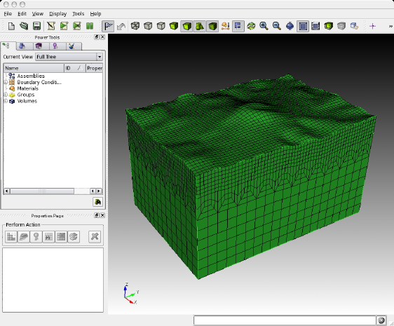
Figure 3.1: Example of the graphical user interface of CUBIT. The hexahedral mesh shown in the main display consists
of a hexahedral discretization of a single volume with topography.
The basic steps in creating a load-balanced, partitioned mesh with CUBIT are:
1. setting up a hexahedral mesh with CUBIT,
18
CHAPTER 3. MESH GENERATION 19
2. exporting the CUBIT mesh into a SPECFEM3D Cartesian file format and
3. partitioning the SPECFEM3D Cartesian mesh files for a chosen number of cores.
Examples are provided in the SPECFEM3D Cartesian package in the subdirectory EXAMPLES/. We strongly encour-
age you to contribute your own example to this package by contacting the CIG Computational Seismology Mailing
List (cig-seismo@geodynamics.org).
3.1.1 Creating the Mesh with CUBIT
For the installation and handling of the CUBIT meshing tool suite, please refer to the CUBIT user manual and docu-
mentation. In order to give you a basic understanding of how to use CUBIT for our purposes, examples are provided
in the SPECFEM3D Cartesian package in the subdirectory EXAMPLES/:
homogeneous_halfspace Creates a single block model and assigns elastic material parameters.
layered_halfspace Combines two different, elastic material volumes and creates a refinement layer between
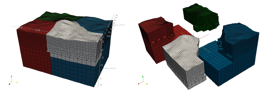
the two. This example can be compared for validation against the solutions provided in subdirectory
VALIDATION_3D_SEM_SIMPLER_LAYER_SOURCE_DEPTH/.
waterlayered_halfspace Combines an acoustic and elastic material volume as in a schematic marine survey
example.
tomographic_model Creates a single block model whose material properties will have to be read in from a
tomographic model file during the databases creation by xgenerate_databases.
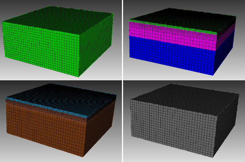
Figure 3.2: Screenshots of the CUBIT examples provided in subdirectory EXAMPLES/: homogeneous halfspace
(top-left), layered halfspace (top-right), water layered halfspace (bottom-left) and tomographic model (bottom-right).
In each example subdirectory you will find a README file, which explains in a step-by-step tutorial the workflow
for the example. Please feel free to contribute your own example to this package by contacting the CIG Computational
CHAPTER 3. MESH GENERATION 20
Seismology Mailing List (cig-seismo@geodynamics.org).
In some cases, to re-create the meshes for the examples given, just type
claro ./create_mesh.py
or similar from the command line (claro is the command to run CUBIT from the command line).
IMPORTANT: In order to correctly set up GEOCUBIT and run the examples, please read the file called EXAMPLES/README;
in particular, please make sure you correctly set up the Python paths as indicated in that file.
Concerning the script create_mesh.py, you may find the option use_explicit which chooses how to
assign the material properties for the volume (or domain):
(1) one way is to explicitly assign block attributes to the block of the corresponding volume, by commands like:
cubit.cmd(’block ’+str(id_block)+’ attribute index 2 2800’) # vp
This is done when using use_explicit = 1 in the script. The final command:
cubit2specfem3d.export2SPECFEM3D(’MESH/’)
will then create the corresponding MESH/nummaterial_velocity_file for all such defined block vol-
umes/domains.
(2) the other option with use_explicit = 0 is to let GEOCUBIT deal with a dummy entry and then overwrite
the nummaterial_velocity_file at the end with a corresponding command section:
f = open(nummaterial_velocity_file,’w’)
This second way is chosen by default because GEOCUBIT can handle partitions for several processes and
glues everything together automatically. Thus, it adds some more sophistication when the model gets more
complicated than just this single volume example.
You will find out by experimenting what is easier for your case.
3.1.2 Exporting the Mesh with run_cubit2specfem3d.py
Once the geometric model volumes in CUBIT are meshed, you prepare the model for exportation with the definition
of material blocks and boundary surfaces. Thus, prior to exporting the mesh, you need to define blocks specify-
ing the materials and absorbing boundaries in CUBIT. This process could be done automatically using the script
run_cubit2specfem3d.py if the mesh meets some conditions or manually, following the block convention:
material_name Each material should have a specific block defined by a unique name. The name convention of the
material is to start with either ’elastic’ or ’acoustic’. It must be then followed by a unique identifier, e.g. ’elastic
1’,’elastic 2’, etc. The additional attributes to the block define the material description.
For an elastic material:
material_id An integer value which is unique for this material.
Vp P-wave speed of the material (given in m/s).
Vs S-wave speed of the material (given in m/s).
rho density of the material (given in kg/m3).
Qquality factor to use in case of a simulation with attenuation turned on. It should be between 1 and 9000.
In case no attenuation information is available, it can be set to zero. You can either specify a single
Q value, in which case it will be assumed to be pure shear attenuation Qµ, or two separate values for
bulk and shear attenuation, Qκand Qµrespectively. Note that Qmu is always equal to Qs, but Qkappa
is in general not equal to Qp. To convert one to the other see doc/note_on_Qkappa_versus_Qp.pdf and
utils/attenuation/conversion_from_Qkappa_Qmu_to_Qp_Qs_from_Dahlen_Tromp_959_960.f90.
CHAPTER 3. MESH GENERATION 21
Please note that your Vp- and Vs-speeds are given for a reference frequency. To change this refer-
ence frequency, you change the value of ATTENUATION_f0_REFERENCE in the main constants file
constants.h found in subdirectory src/shared/. The code uses a constant Qquality factor,
write(IMAIN,*) "but approximated based on a series of Zener standard linear solids (SLS). The approxima-
tion is thus performed in a given frequency band determined based on that ATTENUATION_f0_REFERENCE
reference frequency.
anisotropic_flag Flag describing the anisotropic model to use in case an anisotropic simulation should be con-
ducted. See the file model_aniso.f90 in subdirectory src/generate_databases/ for an im-
plementation of the anisotropic models. In case no anisotropy is available, it can be set to zero.
Note that this material block has to be defined using all the volumes which belong to this elastic material. For
volumes belonging to another, different material, you will need to define a new material block.
For an acoustic material:
material_id An integer value which is unique for this material.
Vp P-wave speed of the material (given in m/s).
0S-wave speed of the material is ignored.
rho density of the material (given in kg/m3).
face_topo Block definition for the surface which defines the free surface (which can have topography). The name of
this block must be ’face_topo’, the block has to be defined using all the surfaces which constitute the complete
free surface of the model.
face_abs_xmin Block definition for the faces on the absorbing boundaries, one block for each surface with x=Xmin.
face_abs_xmax Block definition for the faces on the absorbing boundaries, one block for each surface with x=Xmax.
face_abs_ymin Block definition for the faces on the absorbing boundaries, one block for each surface with y=Ymin.
face_abs_ymax Block definition for the faces on the absorbing boundaries, one block for each surface with y=Ymax.
face_abs_bottom Block definition for the faces on the absorbing boundaries, one block for each surface with z=bottom.
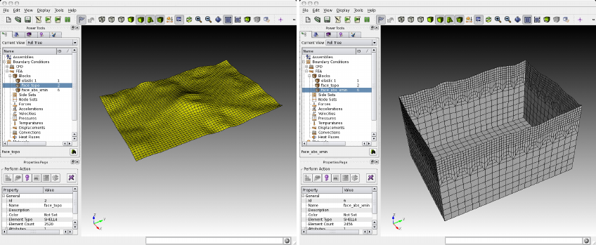
Figure 3.3: Example of the block definitions for the free surface ’face_topo’ (left) and the absorbing boundaries,
defined in a single block ’face_abs_xmin’ (right) in CUBIT.
Optionally, instead of specifying for each surface at the boundaries a single block like mentioned above, you
can also specify a single block for all boundary surfaces and name it as one of the absorbing blocks above, e.g.
’face_abs_xmin’.
CHAPTER 3. MESH GENERATION 22
After the block definitions are done, you export the mesh using the script cubit2specfem3d.py provided in
each of the example directories (linked to the common script CUBIT_GEOCUBIT/cubit2specfem3d.py). If the
export was successful, you should find the following files in a subdirectory MESH/:
absorbing_cpml_file (only needed in case of C-PML absorbing conditions) Contains on the first line the total
number of C-PML spectral elements in the mesh, and then on the following line the list of all these C-PML
elements with two numbers per line: first the spectral element number, and then a C-PML flag indicating to
which C-PML layer(s) that element belongs, according to the following convention:
• Flag = 1 : element belongs to a X CPML layer only (either in Xmin or in Xmax),
• Flag = 2 : element belongs to a Y CPML layer only (either in Ymin or in Ymax),
• Flag = 3 : element belongs to a Z CPML layer only (either in Zmin or in Zmax),
• Flag = 4 : element belongs to a X CPML layer and also to a Y CPML layer,
• Flag = 5 : element belongs to a X CPML layer and also to a Z CPML layer,
• Flag = 6 : element belongs to a Y CPML layer and also to a Z CPML layer,
• Flag = 7 : element belongs to a X, to a Y and to a Z CPML layer, i.e., it belongs to a CPML corner.
Note that it does not matter whether an element belongs to a Xmin or to a Xmax CPML, the flag is the same in
both cases; the same is true for Ymin and Ymax, and also Zmin and Zmax.
When you have an existing CUBIT (or similar) mesh stored in SPECFEM3D format, i.e., if you have exist-
ing nodes_coords_file and mesh_file files but do not know how to assign CPML flags to them, we
have created a small serial Fortran program that will do that automatically for you, i.e., which will create the
absorbing_cpml_file for you. That program is:
utils/CPML/convert_external_layers_of_a_given_mesh_to_CPML_layers.f90,
and a small Makefile is provided in that directory (utils/CPML).
IMPORTANT: it is your responsibility to make sure that in the input CUBIT (or similar) mesh that this code will
read in SPECFEM3D format from files nodes_coords_file and mesh_file you have created layers of
elements that constitute a layer of constant thickness aligned with the coordinate grid axes (X, Y and/or Z), so
that this code can assign CPML flags to them. This code does NOT check that (because it cannot, in any easy
way). The mesh inside these CPML layers does not need to be structured nor regular, any non-structured mesh
is fine as long as it has flat PML inner and outer faces, parallel to the axes, and thus of a constant thickness. The
thickness can be different for the X, Y and Z sides. But for X it must not vary, for Y it must not vary, and for Z
it must not vary. If you do not know the exact thickness, you can use a slightly LARGER value in this code (say
2% to 5% more) and this code will fix that and will adjust it; never use a SMALLER value otherwise this code
will miss some CPML elements.
Note: in a future release we will remove the constraint of having CPML layers aligned with the coordinate
axes; we will allow for meshes that are titled by any constant angle in the horizontal plane. However this is not
implemented yet.
Note: in the case of fluid-solid layers in contact, the fluid-solid interface currently needs to be flat and horizontal
inside the CPML layer (i.e., bathymetry should become flat and horizontal when entering the CPML); this
(small) constraint will probably remain in the code for a while because it makes fluid-solid matching inside the
CPML much easier.
materials_file Contains the material associations for each element. The format is:
element_ID material_ID
where element_ID is the element identifier and material_ID is a unique identifier, positive (for materials
taken from this list of materials, i.e. for which each spectral element has constant material properties taken from
this list) or negative (for tomographic models, i.e. for spectral element whose real velocities and density will be
assigned later by calling an external function to define model variations, for instance in the case of tomographic
models; in such a case, material properties can vary inside each spectral element, i.e. be different at each of its
Gauss-Lobatto-Legendre grid points).
CHAPTER 3. MESH GENERATION 23
nummaterial_velocity_file Defines the material properties.
• For classical materials (i.e., spectral elements for which the velocity and density model will not be assigned
by calling an external function to define for instance a tomographic model), the format is:
domain_ID material_ID rho vp vs Qkappa Qmu anisotropy_flag
where domain_ID is 1 for acoustic and 2 for elastic or viscoelastic materials, material_ID a
unique identifier, rho the density in kg m−3,vp the P-wave speed in m s−1,vs the S-wave speed in
m s−1,Qthe quality factor and anisotropy_flag an identifier for anisotropic models. Note that
both Qkappa and Qmu are ignored by the code unless ATTENUATION is set. If you want a model
with no Qmu attenuation, both set ATTENUATION to .false. in the Par_file and set Qmu to
9999 here. If you want a model with no Qkappa attenuation, set Qkappa to 9999 here. Note that
Qmu is always equal to Qs, but Qkappa is in general not equal to Qp. To convert one to the other see
doc/note_on_Qkappa_versus_Qp.pdf and utils/attenuation/conversion_from_Qkappa_Qmu_to_Qp_Qs_from_Dahlen_Tromp_959_960.f90.
• For tomographic velocity models, please read Chapter 14 and Section 14.1 ‘Using external tomographic
Earth models’ for further details.
nodes_coords_file Contains the point locations in Cartesian coordinates of the mesh element corners.
mesh_file Contains the mesh element connectivity. The hexahedral elements can have 8 or 27 nodes.
See picture doc/mesh_numbering_convention/numbering_convention_27_nodes.jpg to see
in which (standard) order the points must be cited. In the case of 8 nodes, just include the first 8 points.
free_or_absorbing_surface_file_zmax Contains the free surface connectivity or
the surface connectivity of the absorbing boundary surface at the top (Zmax),
depending on whether the top surface is defined as free or absorbing (STACEY_INSTEAD_OF_FREE_SURFACE
in DATA/Par_file).
You should put both the surface of acoustic regions and of elastic regions in that file; that is, list all the element
faces that constitute the surface of the model in that file.
absorbing_surface_file_xmax Contains the surface connectivity of the absorbing boundary surface at Xmax
(also needed in the case of C-PML absorbing conditions, in order for the code to be able to impose Dirichlet
conditions on their outer edge).
absorbing_surface_file_xmin Contains the surface connectivity of the absorbing boundary surface at Xmin
(also needed in the case of C-PML absorbing conditions, in order for the code to be able to impose Dirichlet
conditions on their outer edge).
absorbing_surface_file_ymax Contains the surface connectivity of the absorbing boundary surface at Ymax
(also needed in the case of C-PML absorbing conditions, in order for the code to be able to impose Dirichlet
conditions on their outer edge).
absorbing_surface_file_ymin Contains the surface connectivity of the absorbing boundary surface at Ymin
(also needed in the case of C-PML absorbing conditions, in order for the code to be able to impose Dirichlet
conditions on their outer edge).
absorbing_surface_file_bottom Contains the surface connectivity of the absorbing boundary surface at the bottom
(Zmin)
(also needed in the case of C-PML absorbing conditions, in order for the code to be able to impose Dirichlet
conditions on their outer edge).
These mesh files are needed as input files for the partitioner xdecompose_mesh to load-balance the mesh. Please
see the next section for further details.
In directory "CUBIT_GEOCUBIT/" we provide a script that can help doing the above tasks of exporting a CUBIT
mesh to SPECFEM3D format automatically for you: "run_cubit2specfem3d.py". Just edit them to indicate the path to
your local installation of CUBIT and also the name of the *.cub existing CUBIT mesh file that you want to export to
SPECFEM3D format. These scripts will do the conversion for you automatically except assigning material properties
CHAPTER 3. MESH GENERATION 24
to the different mesh layers. To do so, you will then need to edit the file called "nummaterial_velocity_file" that will
have just been created and change it from the prototype created:
0 1 vol1 --> syntax: #material_domain_id #material_id #rho #vp #vs #Q_kappa #Q_mu #anisotropy
0 2 vol2 --> syntax: #material_domain_id #material_id #rho #vp #vs #Q_kappa #Q_mu #anisotropy
(where "vol1" and "vol2" here represent the volume labels that you have set while creating the mesh in CUBIT) to for
instance
2 1 1500 2300 1800 9999.0 9999.0 0
2 2 1600 2500 20000 9999.0 9999.0 0
Checking the mesh quality
The quality of the mesh may be inspected more precisely based upon the serial code in the file check_mesh_quality_
CUBIT_Abaqus.f90 located in the directory src/check_mesh_quality_CUBIT_Abaqus/. Running this
code is optional because no information needed by the solver is generated.
Prior to running and compiling this code, you have to export your mesh in CUBIT to an ABAQUS (.inp) format.
For example, export mesh block IDs belonging to volumes in order to check the quality of the hexahedral elements.
You also have to determine a number of parameters of your mesh, such as the number of nodes and number of
elements and modify the header of the check_mesh_quality_CUBIT_Abaqus.f90 source file in directory
src/check_mesh_quality_CUBIT_Abaqus/.
Then, in the main directory, type
make xcheck_mesh_quality
and use
./bin/xcheck_mesh_quality
to generate an OpenDX output file (DX_mesh_quality.dx) that can be used to investigate mesh quality, e.g. skewness
of elements, and a Gnuplot histogram (mesh_quality_histogram.txt) that can be plotted with gnuplot (type ‘gnuplot
plot_mesh_quality_histogram.gnu’). The histogram is also printed to the screen. Analyze that skewness histogram of
mesh elements to make sure no element has a skewness above approximately 0.75, otherwise the mesh is of poor quality (and if even
a single element has a skewness value above 0.80, then you must definitely improve the mesh). If you want to start designing your
own meshes, this tool is useful for viewing your creations. You are striving for meshes with elements with ‘cube-like’ dimensions,
e.g., the mesh should contain no very elongated or skewed elements.
3.1.3 Partitioning the Mesh with xdecompose_mesh
The SPECFEM3D Cartesian software package performs large scale simulations in a parallel ’Single Process Multiple
Data’ way. The spectral-element mesh created with CUBIT needs to be distributed on the processors. This partitioning
is executed once and for all prior to the execution of the solver so it is referred to as a static mapping.
An efficient partitioning is important because it leverages the overall running time of the application. It amounts
to balance the number of elements in each slice while minimizing the communication costs resulting from the place-
ment of adjacent elements on different processors. decompose_mesh depends on the SCOTCH library [Pellegrini
and Roman,1996], which provides efficient static mapping, graph and mesh partitioning routines. SCOTCH is a free
software package developed by François Pellegrini et al. from LaBRI and INRIA in Bordeaux, France, downloadable
from the web page https://gforge.inria.fr/projects/scotch/.
In most cases, the configuration with ./configure FC=ifort should be sufficient. During the configuration
process, the script tries to find existing SCOTCH installations. In case your system has no pre-existing SCOTCH in-
stallation, we provide the source code of SCOTCH, which is released open source under the French CeCILL-C version
1 license, in directory src/decompose_mesh/scotch_5.1.12b. This version gets bundled with the compila-
tion of the SPECFEM3D Cartesian package if no libraries could have been found. If this automatic compilation of
the SCOTCH libraries fails, please refer to file INSTALL.txt in that directory to see further details how to compile it
on your system. In case you want to use a pre-existing installation, make sure you have correctly specified the path
of the SCOTCH library when using the option --with-scotch-dir with the ./configure script. In the fu-
ture you should be able to find more recent versions at http://www.labri.fr/perso/pelegrin/scotch/
CHAPTER 3. MESH GENERATION 25
scotch_en.html.
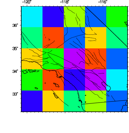
Figure 3.4: Example of a mesh partitioning onto four cores. Each single core partition is colored differently. The
executable xdecompose_mesh can equally distribute the mesh on any arbitrary number of cores. Domain decom-
position is explained in detail in Martin et al. [2008a], and excellent scaling up to 150,000 processor cores in shown
for instance in Carrington et al. [2008], Komatitsch et al. [2008], Martin et al. [2008a], Komatitsch et al. [2010a],
Komatitsch [2011].
When you are ready to compile, in the main directory type
make xdecompose_mesh
If all paths and flags have been set correctly, the executable bin/xdecompose_mesh should be produced.
The partitioning is done in serial for now (in the next release we will provide a parallel version of that code). It
needs to be run in the main directory because it expects the ./DATA/Par_file. The synopsis is:
./bin/xdecompose_mesh nparts input_directory output_directory
where
•nparts is the number of partitions, i.e., the number of cores for the parallel simulations,
•input_directory is the directory which holds all the files generated by the Python script cubit2specfem3d.py
explained in the previous Section 3.1.2, e.g. ./MESH/, and
•output_directory is the directory for the output of this partitioner which stores ACII-format files named
like proc******_Database for each partition. These files will be needed for creating the distributed
databases, and have to reside in the directory LOCAL_PATH specified in the main Par_file, e.g. in directory
./OUTPUT_FILES/DATABASES_MPI. Please see Chapter 4for further details.
Note that all the files generated by the Python script cubit2specfem3d.py must be placed in the input_directory
folder before running the program.
3.2 Meshing with xmeshfem3D
In case you successfully ran the configuration script, you are also ready to compile the internal mesher. This is an
alternative to CUBIT for the mesh generation of relatively simple models.
In the main directory, type
make xmeshfem3D
CHAPTER 3. MESH GENERATION 26
Figure 3.5: For parallel computing purposes, the model block is subdivided in NPROC_XI ×NPROC_ETA slices of
elements. In this example we use 52= 25 processors.
If all paths and flags have been set correctly, the mesher should now compile and produce the executable bin/xmeshfem3D.
Please note that xmeshfem3D must be called directly from the main directory, as most of the binaries of the package.
Input for the mesh generation program is provided through the parameter file Mesh_Par_file, which resides
in the subdirectory DATA/meshfem3D_files/. (to see how to use it, see the EXAMPLES specific to the internal
mesher in directory EXAMPLES/meshfem3D_examples/. Before running the mesher, a number of parameters
need to be set in the Mesh_Par_file. This requires a basic understanding of how the SEM is implemented, and we
encourage you to read Komatitsch and Vilotte [1998], Komatitsch and Tromp [1999] and Komatitsch et al. [2004].
The mesher and the solver use UTM coordinates internally, therefore you need to define the zone number for the
UTM projection (e.g., zone 11 for Los Angeles). Use decimal values for latitude and longitude (no minutes/seconds).
These values are approximate; the mesher will round them off to define a square mesh in UTM coordinates. When run-
ning benchmarks on rectangular models, turn the UTM projection off by using the flag SUPPRESS_UTM_PROJECTION,
in which case all ‘longitude’ parameters simply refer to the xaxis, and all ‘latitude’ parameters simply refer to the
yaxis. To run the mesher for a global simulation, the following parameters need to be set in the Mesh_Par_file:
LATITUDE_MIN Minimum latitude in the block (negative for South).
LATITUDE_MAX Maximum latitude in the block.
LONGITUDE_MIN Minimum longitude in the block (negative for West).
LONGITUDE_MAX Maximum longitude in the block.
DEPTH_BLOCK_KM Depth of bottom of mesh in kilometers.
UTM_PROJECTION_ZONE UTM projection zone in which your model resides, only valid when SUPPRESS_UTM_PROJECTION
is .false.. Use a negative zone number for the Southern hemisphere: the Northern hemisphere corresponds
to zones +1 to +60, the Southern hemisphere to zones -1 to -60.
We use the WGS84 (World Geodetic System 1984) reference ellipsoid for the UTM projection. If you pre-
fer to use the Clarke 1866 ellipsoid, edit file src/shared/utm_geo.f90, uncomment that ellipsoid and
recompile the code.
From http://en.wikipedia.org/wiki/Universal_Transverse_Mercator_coordinate_
system:
CHAPTER 3. MESH GENERATION 27
The Universal Transverse Mercator coordinate system was developed by the United States Army Corps of
Engineers in the 1940s. The system was based on an ellipsoidal model of Earth. For areas within the contiguous
United States the Clarke Ellipsoid of 1866 was used. For the remaining areas of Earth, including Hawaii, the
International Ellipsoid was used. The WGS84 ellipsoid is now generally used to model the Earth in the UTM
coordinate system, which means that current UTM northing at a given point can be 200+ meters different from
the old one. For different geographic regions, other datum systems (e.g.: ED50, NAD83) can be used.
SUPPRESS_UTM_PROJECTION set to be .false. when your model range is specified in geographical coordi-
nates, and needs to be .true. when your model is specified in Cartesian coordinates. UTM PROJECTION
ZONE IN WHICH YOUR SIMULATION REGION RESIDES.
INTERFACES_FILE File which contains the description of the topography and of the interfaces between the dif-
ferent layers of the model, if any. The number of spectral elements in the vertical direction within each layer is
also defined in this file.
NEX_XI The number of spectral elements along one side of the block. This number must be 8 ×a multiple of
NPROC_XI defined below. Based upon benchmarks against semi-analytical discrete wavenumber synthetic
seismograms [Komatitsch et al.,2004], determined that a NEX_XI = 288 run is accurate to a shortest period of
roughly 2 s. Therefore, since accuracy is determined by the number of grid points per shortest wavelength, for
any particular value of NEX_XI the simulation will be accurate to a shortest period determined by
shortest period (s) = (288/NEX_XI)×2.(3.1)
The number of grid points in each orthogonal direction of the reference element, i.e., the number of Gauss-
Lobatto-Legendre points, is determined by NGLLX in the constants.h file. We generally use NGLLX = 5,
for a total of 53= 125 points per elements. We suggest not to change this value.
NEX_ETA The number of spectral elements along the other side of the block. This number must be 8 ×a multiple of
NPROC_ETA defined below.
NPROC_XI The number of processors or slices along one side of the block (see Figure 3.5); we must have NEX_XI =
8×c×NPROC_XI, where c≥1is a positive integer.
NPROC_ETA The number of processors or slices along the other side of the block; we must have NEX_ETA =
8×c×NPROC_ETA, where c≥1is a positive integer.
USE_REGULAR_MESH set to be .true. if you want a perfectly regular mesh or .false. if you want to add
doubling horizontal layers to coarsen the mesh. In this case, you also need to provide additional information by
setting up the next three parameters.
NDOUBLINGS The number of horizontal doubling layers. Must be set at least to 1if USE_REGULAR_MESH is set to
.true.. Multiple mesh doublings can be chosen, for which each an NZ_DOUBLING_** entry must be given.
By default, we only provide two possible entries in the Mesh_Par_file. For higher numbers of doubling
layers, additional entries must be added.
NZ_DOUBLING_1 The position of the first doubling layer (only interpreted if USE_REGULAR_MESH is set to
.true.).
NZ_DOUBLING_2 The position of the second doubling layer (only interpreted if USE_REGULAR_MESH is set to
.true. and if NDOUBLINGS is set to 2). Doubling layers must be at least 2layers apart. The layer count
starts from the bottom layer. More entries must be listed by the user if NDOUBLINGS is larger than 2.
CREATE_ABAQUS_FILES Set this flag to .true. to save Abaqus FEA (www.simulia.com) mesh files for
subsequent viewing. Turning the flag on generates files in the LOCAL_PATH directory. See Section 12.1 for a
discussion of mesh viewing features.
CREATE_DX_FILES Set this flag to .true. to save OpenDX (www.opendx.org) mesh files for subsequent
viewing.
CHAPTER 3. MESH GENERATION 28
LOCAL_PATH Directory in which the partitions generated by the mesher will be written. Generally one uses a
directory on the local disk of the compute nodes, although on some machines these partitions are written on a
parallel (global) file system (see also the earlier discussion of the LOCAL_PATH_IS_ALSO_GLOBAL flag in
Chapter 2).
The mesher generates the necessary partitions in parallel, one set for each of the NPROC_XI ×NPROC_ETA
slices that constitutes the mesh (see Figure 3.5). After the mesher finishes, you can log in to one of the compute
nodes and view the contents of the LOCAL_PATH directory to see the files generated by the mesher. These files
will be needed for creating the distributed databases, and have to reside in the directory LOCAL_PATH specified
in the main Par_file, e.g. in directory OUTPUT_FILES/DATABASES_MPI. Please see Chapter 4for
further details.
NMATERIALS The number of different materials in your model. In the following lines, each material needs to be
defined as:
material_ID rho vp vs Q anisotropy_flag domain_ID
where
•Q: quality factor (0=no attenuation) for shear attenuation Qµ
•anisotropy_flag : 0=no anisotropy / 1,2,.. check with implementation in aniso_model.f90
•domain_id : 1=acoustic / 2=elastic
NREGIONS The number of regions in the mesh. In the following lines, because the mesh is regular or ’almost regular’,
each region is defined as:
NEX_XI_BEGIN NEX_XI_END NEX_ETA_BEGIN NEX_ETA_END NZ_BEGIN NZ_END material_ID
The INTERFACES_FILE parameter of Mesh_Par_File defines the file which contains the settings of the topog-
raphy grid and of the interfaces grids. Topography is defined as a set of elevation values on a regular 2D grid. It is
also possible to define interfaces between the layers of the model in the same way. The file needs to define several
parameters:
• The number of interfaces, including the topography. This needs to be set at the first line. Then, from the bottom
to the top of the model, you need to define the grids with:
•SUPPRESS_UTM_PROJECTION flag as described previously,
• number of points along xand ydirection (NXI and NETA),
• minimal xand ycoordinates (LONG_MIN and LAT_MIN),
• spacing between points along xand y(SPACING_XI and SPACING_ETA) and
• the name of the file which contains the elevation values (in y.xincreasing order).
At the end of this file, you simply need to set the number of spectral elements in the vertical direction for each layer.
We provide a few models in the EXAMPLES/ directory.
Finally, depending on your system, you might need to provide a file that tells MPI what compute nodes to use for
the simulations. The file must have a number of entries (one entry per line) at least equal to the number of processors
needed for the run. A sample file is provided in the file mymachines. This file is not used by the mesher or solver,
but is required by the go_mesher and go_solver default job submission scripts. See Chapter 13 for information
about running the code on a system with a scheduler, e.g., LSF.
Now that you have set the appropriate parameters in the Mesh_Par_file and have compiled the mesher, you
are ready to launch it! This is most easily accomplished based upon the go_mesher script. When you run on a
PC cluster, the script assumes that the nodes are named n001, n002, etc. If this is not the case, change the tr -d
CHAPTER 3. MESH GENERATION 29
‘n’ line in the script. You may also need to edit the last command at the end of the script that invokes the mpirun
command. See Chapter 13 for information about running the code on a system with a scheduler, e.g., LSF.
Mesher output is provided in the OUTPUT_FILES directory in output_mesher.txt; this file provides lots
of details about the mesh that was generated. Please note that the mesher suggests a time step DT to run the solver
with. The mesher output file also contains a table about the quality of the mesh to indicate possible problems with
the distortions of elements. Alternatively, output can be directed to the screen instead by uncommenting a line in
constants.h:
! uncomment this to write messages to the screen
! integer, parameter :: IMAIN = ISTANDARD_OUTPUT
To control the quality of the mesh, check the standard output (either on the screen or in the OUTPUT_FILES directory
in output_mesher.txt) and analyze the skewness histogram of mesh elements to make sure no element has a
skewness above approximately 0.75, otherwise the mesh is of poor quality (and if even a single element has a skewness
value above 0.80, then you must definitely improve the mesh). To draw the skewness histogram on the screen, type
gnuplot plot_mesh_quality_histogram.gnu.
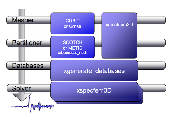
Chapter 4
Creating the Distributed Databases
After using xmeshfem3D or xdecompose_mesh, the next step in the workflow is to compile xgenerate_
databases. This program is going to create all the missing information needed by the SEM solver.
Figure 4.1: Schematic workflow for a SPECFEM3D Cartesian simulation. The executable
xgenerate_databases creates the GLL mesh points and assigns specific model parameters.
In the main directory, type
make xgenerate_databases
Input for the program is provided through the main parameter file Par_file, which resides in the subdirectory
DATA. Please note that xgenerate_databases must be called directly from the main directory, as most of the
binaries of the package.
4.1 Main parameter file Par_file
Before running xgenerate_databases, a number of parameters need to be set in the main parameter Par_file
located in the subdirectory DATA:
SIMULATION_TYPE is set to 1 for forward simulations, 2 for adjoint simulations (see Section 7.2) and 3 for kernel
simulations (see Section 12.3).
30
CHAPTER 4. CREATING THE DISTRIBUTED DATABASES 31
SAVE_FORWARD is only set to .true. for a forward simulation with the last frame of the simulation saved, as
part of the finite-frequency kernel calculations (see Section 12.3). For a regular forward simulation, leave
SIMULATION_TYPE and SAVE_FORWARD at their default values.
UTM_PROJECTION_ZONE UTM projection zone in which your model resides, only valid when SUPPRESS_UTM_PROJECTION
is .false..
SUPPRESS_UTM_PROJECTION set to be .false. when your model range is specified in the geographical coor-
dinates, and needs to be .true. when your model is specified in a cartesian coordinates. UTM PROJECTION
ZONE IN WHICH YOUR SIMULATION REGION RESIDES.
NPROC The number of MPI processors, each one is assigned one slice of the whole mesh.
NSTEP The number of time steps of the simulation. This controls the length of the numerical simulation, i.e., twice
the number of time steps requires twice as much CPU time. This feature is not used at the time of generat-
ing the distributed databases but is required for the solver, i.e., you may change this parameter after running
xgenerate_databases.
DT The length of each time step in seconds. This feature is not used at the time of generating the distributed databases
but is required for the solver. Please see also Section 4.2 for further details.
NGNOD The number of nodes for 2D and 3D shape functions for hexahedra. We use either 8-node mesh elements
(bricks) or 27-node elements. If you use the internal mesher, the only option is 8-node bricks (27-node elements
are not supported). CUBIT does not support HEX27 elements either (it can generate them, but they are flat,
i.e. identical to HEX8). To generate HEX27 elements with curvature properly taken into account, you can use
Gmsh http://geuz.org/gmsh/
MODEL Must be set to one of the following:
Models defined by mesh parameters:
default Uses model parameters as defined by meshing procedures described in the previous Chapter 3.
1D models with real structure:
1D_prem Isotropic version of the spherically symmetric Preliminary Reference Earth Model (PREM)
[Dziewo´
nski and Anderson,1981].
1D_socal A standard isotropic 1D model for Southern California.
1D_cascadia Isotropic 1D profile for the Cascadia region.
Fully 3D models:
aniso For a user-specified fully anisotropic model. Parameters are set up in routines located in file
model_aniso.f90 in directory src/generate_databases/. See Chapter 14 for a discus-
sion on how to specify your own 3D model.
external For a user-specified isotropic model which uses externally defined model parameters. Uses
external model definitions set up in routines located in file model_external_values.f90 in
directory src/generate_databases/. Please modify these generic template routines to use
your own model definitions.
gll For a user-specified isotropic model which uses external binary files for vp,vsand ρ. Binary
files are given in the same format as when outputted by the xgenerate_databases executable
when using option SAVE_MESH_FILES. These binary files define the model parameters on all GLL
points which can be used for iterative inversion procedures. Note that for simulation setups with
attenuation, it will also read in the external binary mesh files for Qκand Qµ. Note that Qmu is
always equal to Qs, but Qkappa is in general not equal to Qp. To convert one to the other see
doc/note_on_Qkappa_versus_Qp.pdf and utils/attenuation/conversion_from_Qkappa_Qmu_to_Qp_Qs_from_Dahlen_Tromp_959_960.f90.
salton_trough A 3D Vpmodel for Southern California. Users must provide the corresponding data
file regrid3_vel_p.bin in directory DATA/st_3D_block_harvard/.
CHAPTER 4. CREATING THE DISTRIBUTED DATABASES 32
tomo For a user-specified 3D isotropic model which uses a tomographic model file tomographic_model.xyz
in directory DATA. See Section 14.1, for a discussion on how to specify your own 3D tomographic
model.
APPROXIMATE_OCEAN_LOAD Set to .true. if the effect of the oceans on seismic wave propagation should be
incorporated based upon the (rough) approximate treatment discussed in Komatitsch and Tromp [2002b]. This
feature is inexpensive from a numerical perspective, both in terms of memory requirements and CPU time.
This approximation is accurate at periods of roughly 20 s and longer. At shorter periods the effect of water
phases/reverberations is not taken into account, even when the flag is on. If you want to model the effect of
a fluid-solid model at short periods, then set this flag to .false. and mesh the fluid layer explicitly in your
mesher, so that it is computed accurately and without this approximation.
TOPOGRAPHY This feature is only effective if APPROXIMATE_OCEAN_LOAD is set to .true.. Set to .true. if
topography and bathymetry should be read in based upon the topography file specified in the main constants file
constants.h found in subdirectory src/shared/ to evaluate elevations. If not set, elevations will be read
from the numerical mesh.
ATTENUATION Set to .true. if attenuation should be incorporated. Turning this feature on increases the memory
requirements significantly (roughly by a factor of 1.5), and is numerically fairly expensive. See Komatitsch
and Tromp [1999,2002a] for a discussion on the implementation of attenuation based upon standard linear
solids. Please note that the Vp- and Vs-velocities of your model are given for a reference frequency. To
change this reference frequency, you change the value of ATTENUATION_f0_REFERENCE in the main con-
stants file constants.h found in subdirectory src/shared/. The code uses a constant Qquality factor,
write(IMAIN,*) "but approximated based on a series of Zener standard linear solids (SLS). The approximation
is thus performed in a given frequency band determined based on that ATTENUATION_f0_REFERENCE refer-
ence frequency. Note that Qmu is always equal to Qs, but Qkappa is in general not equal to Qp. To convert one to
the other see doc/note_on_Qkappa_versus_Qp.pdf and utils/attenuation/conversion_from_Qkappa_Qmu_to_Qp_Qs_from_Dahlen_Tromp_959_960.f90.
ANISOTROPY Set to .true. if you want to use an anisotropy model. Please see the file model_aniso.f90 in
subdirectory src/generate_databases/ for the current implementation of anisotropic models.
TOMOGRAPHY_PATH Directory in which the tomography files are stored for using external tomographic Earth mod-
els (please read Chapter 14 and Section 14.1 ‘Using external tomographic Earth models’ for further details.).
USE_OLSEN_ATTENUATION Set to .true. if you want to use the attenuation model that scaled from the S-wave
speed model using Olsen’s empirical relation (see Olsen et al. [2003]).
OLSEN_ATTENUATION_RATIO Determines the Olsen’s constant in Olsen’s empirical relation (see Olsen et al.
[2003]).
PML_CONDITIONS Set to .true. to turn on C-PML boundary conditions for a regional simulation. Both fluids
and elastic solids are supported. Note that xmeshfem3d generated meshes do not support C-PML yet.
PML_INSTEAD_OF_FREE_SURFACE Set to .true. to turn on C-PML boundary conditions on the top surface
instead of the usual free surface.
f0_FOR_PML Determines the dominant frequency that will be used in the calculation of PML damping profiles; This
should be set to the same (or similar) dominant frequency as that of the source that you will use in your
simulation. It is VERY IMPORTANT to do that, otherwise the PML absorbing conditions can become
unstable. If you plan to use a Dirac source, then use the dominant frequency of the source wavelet with which
you plan to convolve your seismograms later on in post-processing.
STACEY_ABSORBING_CONDITIONS Set to .true. to turn on Clayton-Enquist absorbing boundary conditions
(see Komatitsch and Tromp [1999]). In almost all cases it is much better to use CPML absorbing layers (see the
options above) and leave this flag to .false..
STACEY_INSTEAD_OF_FREE_SURFACE Set to .true. to turn on absorbing boundary conditions on the top
surface which by default constitutes a free surface of the model.
CHAPTER 4. CREATING THE DISTRIBUTED DATABASES 33
BOTTOM_FREE_SURFACE When STACEY_ABSORBING_CONDITIONS is set to .true. : absorbing conditions
are defined in xmin, xmax, ymin, ymax and zmin this option BOTTOM_FREE_SURFACE can be set to .true.
to make zmin free surface instead of absorbing condition.
CREATE_SHAKEMAP Set this flag to .true. to create a ShakeMap®, i.e., a peak ground velocity map of the
maximum absolute value of the two horizontal components of the velocity vector.
MOVIE_SURFACE Set to .false., unless you want to create a movie of seismic wave propagation on the Earth’s
surface. Turning this option on generates large output files. See Section 12.2 for a discussion on the generation
of movies. This feature is only relevant for the solver.
MOVIE_TYPE Set this flag to 1 to show the top surface (tomography + oceans) only, to 2 to show all external faces
of the mesh (i.e. topography + vertical edges + bottom) in shakemaps and surface movies.
MOVIE_VOLUME Set to .false., unless you want to create a movie of seismic wave propagation in the Earth’s
interior. Turning this option on generates huge output files. See Section 12.2 for a discussion on the generation
of movies. This feature is only relevant for the solver.
SAVE_DISPLACEMENT Set this flag to .true. if you want to save the displacement instead of velocity for the
movie frames.
USE_HIGHRES_FOR_MOVIES Set this flag to .true. if you want to save the values at all the NGLL grid points
for the movie frames.
NTSTEP_BETWEEN_FRAMES Determines the number of timesteps between movie frames. Typically you want to
save a snapshot every 100 timesteps. The smaller you make this number the more output will be generated! See
Section 12.2 for a discussion on the generation of movies. This feature is only relevant for the solver.
HDUR_MOVIE Determines the half duration of the source time function for the movie simulations. When this parame-
ter is set to be 0, a default half duration that corresponds to the accuracy of the simulation is provided. Otherwise,
it adds this half duration to the half duration specified in the source file CMTSOLUTION, thus simulates longer
periods to make the movie images look smoother.
SAVE_MESH_FILES Set this flag to .true. to save ParaView (www.paraview.org) mesh files for subsequent
viewing. Turning the flag on generates large (distributed) files in the LOCAL_PATH directory. See Section 12.1
for a discussion of mesh viewing features.
LOCAL_PATH Directory in which the distributed databases will be written. Generally one uses a directory on
the local disk of the compute nodes, although on some machines these databases are written on a parallel
(global) file system (see also the earlier discussion of the LOCAL_PATH_IS_ALSO_GLOBAL flag in Chap-
ter 2). xgenerate_databases generates the necessary databases in parallel, one set for each of the NPROC
slices that constitutes the mesh (see Figure 3.4 and Figure 3.5). After the executable finishes, you can log in to
one of the compute nodes and view the contents of the LOCAL_PATH directory to see the (many) files generated
by xgenerate_databases. Please note that the LOCAL_PATH directory should already contain the output
files of the partitioner, i.e. from xdecompose_mesh or xmeshfem3D.
NTSTEP_BETWEEN_OUTPUT_INFO This parameter specifies the interval at which basic information about a run is
written to the file system (timestamp*files in the OUTPUT_FILES directory). If you have access to a fast
machine, set NTSTEP_BETWEEN_OUTPUT_INFO to a relatively high value (e.g., at least 100, or even 1000
or more) to avoid writing output text files too often. This feature is not used at the time of meshing. One can set
this parameter to a larger value than the number of time steps to avoid writing output during the run.
NTSTEP_BETWEEN_OUTPUT_SEISMOS This parameter specifies the interval at which synthetic seismograms are
written in the LOCAL_PATH directory. If a run crashes, you may still find usable (but shorter than requested)
seismograms in this directory. On a fast machine set NTSTEP_BETWEEN_OUTPUT_SEISMOS to a relatively
high value to avoid writing to the seismograms too often. This feature is only relevant for the solver.
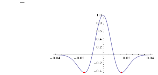
CHAPTER 4. CREATING THE DISTRIBUTED DATABASES 34
USE_FORCE_POINT_SOURCE Turn this flag on to use a (tilted) FORCESOLUTION force point source instead of a
CMTSOLUTION moment-tensor source. When the force source does not fall exactly at a grid point, the solver
interpolates the force between grid points using Lagrange interpolants. This can be useful e.g. for oil industry
foothills simulations in which the source is a vertical force, normal force, tilted force, or an impact etc. Note
that in the FORCESOLUTION file, you will need to edit the East, North and vertical components of an arbitrary
(not necessarily unitary, the code will normalize it automatically) direction vector of the force vector; thus refer
to Appendix Afor the orientation of the reference frame. This vector is made unitary internally in the solver
and thus only its direction matters here; its norm is ignored and the norm of the force used is the factor force
source times the source time function.
When using this option, by default the code can locate the force source anywhere between mesh points in order to
honor its exact location; this is more precise than using the closest GLL mesh point, but it is also a bit slower. If
needed, you can change that default behavior and force the code to use the closest GLL mesh point instead by set-
ting flag USE_BEST_LOCATION to .false. instead of .true. in file src/shared/constants.h.in
and running the configure script again and recompiling the code.
USE_RICKER_TIME_FUNCTION Turn this flag on to use a Ricker source time function, i.e., the second derivative
of a Gaussian, instead of the source time functions set by default to represent a (tilted) FORCESOLUTION force
point source or a CMTSOLUTION moment-tensor source. Note that we use the standard definition of a Ricker,
for a dominant frequency f0:Ricker(t) = (1 −2at2)e−at2, with a=π2f2
0, whose Fourier transform is thus:
1
2
√πω2
a3/2e−ω2
4aThis gives the wavelet of Figure 4.2. Originally, if a CMTSOLUTION moment-tensor source is
Figure 4.2: We use the standard definition of a Ricker (i.e., second derivative of a Gaussian). Image taken from
http://subsurfwiki.org.
used, a (pseudo) Heaviside step function with a very short half duration is defined for elastic cases to represent
the permanent slip on the fault while in the acoustic case a Gaussian source time function with a similarly short
half duration is defined to physically describe actions within the fluid. Otherwise, if a FORCESOLUTION force
source is used, a (pseudo) Dirac delta source time function is defined by default. Any other source-time function
may then be obtained by convolution.
PRINT_SOURCE_TIME_FUNCTION Turn this flag on to print information about the source time function in the file
OUTPUT_FILES/plot_source_time_function.txt. This feature is only relevant for the solver.
NUMBER_OF_SIMULTANEOUS_RUNS adds the ability to run several calculations (several earthquakes) in an embarrassingly-
parallel fashion from within the same run; this can be useful when using a very large supercomputer to compute
many earthquakes in a catalog, in which case it can be better from a batch job submission point of view to start
fewer and much larger jobs, each of them computing several earthquakes in parallel.
To turn that option on, set parameter NUMBER_OF_SIMULTANEOUS_RUNS to a value greater than 1. To
implement that, we create NUMBER_OF_SIMULTANEOUS_RUNS MPI sub-communicators, each of them be-
ing labeled my_local_mpi_comm_world, and we use them in all the routines in "src/shared/parallel.f90",
except in MPI_ABORT() because in that case we need to kill the entire run.
When that option is on, of course the number of processor cores used to start the code in the batch system must
be a multiple of NUMBER_OF_SIMULTANEOUS_RUNS, all the individual runs must use the same number
CHAPTER 4. CREATING THE DISTRIBUTED DATABASES 35
of processor cores, which as usual is NPROC in the Par_file, and thus the total number of processor cores
to request from the batch system should be NUMBER_OF_SIMULTANEOUS_RUNS *NPROC. All the runs to
perform must be placed in directories called run0001, run0002, run0003 and so on (with exactly four digits).
Imagine you have 10 independent calculations to do, each of them on 100 cores; you have three options:
1/ submit 10 jobs to the batch system
2/ submit a single job on 1000 cores to the batch, and in that script create a sub-array of jobs to start 10 jobs,
each running on 100 cores (see e.g. http://www.schedmd.com/slurmdocs/job_array.html)
3/ submit a single job on 1000 cores to the batch, start SPECFEM3D on 1000 cores, create 10 sub-communicators,
cd into one of 10 subdirectories (called e.g. run0001, run0002,... run0010) depending on the sub-communicator
your MPI rank belongs to, and run normally on 100 cores using that sub-communicator.
The option NUMBER_OF_SIMULTANEOUS_RUNS implements 3/.
BROADCAST_SAME_MESH_AND_MODEL if we perform simultaneous runs in parallel, if only the source and re-
ceivers vary between these runs but not the mesh nor the model (velocity and density) then we can also read the
mesh and model files from a single run in the beginning and broadcast them to all the others; for a large number
of simultaneous runs for instance when solving inverse problems iteratively this can DRASTICALLY reduce
I/Os to disk in the solver (by a factor equal to NUMBER_OF_SIMULTANEOUS_RUNS), and reducing I/Os is
crucial in the case of huge runs. Thus, always set this option to .true. if the mesh and the model are the same for
all simultaneous runs. In that case there is no need to duplicate the mesh and model file database (the content of
the DATABASES_MPI directories) in each of the run0001, run0002,... directories, it is sufficient to have one in
run0001 and the code will broadcast it to the others).
USE_FAILSAFE_MECHANISM if one or a few of these simultaneous runs fail, kill all the runs or let the others finish
using a fail-safe mechanism (in most cases, should be set to true).
TODO / future work to do: currently the BROADCAST_SAME_MESH_AND_MODEL option assumes to have the
(master) mesh files in run0001/DATABASES_MPI or run0001/OUTPUT_FILES/DATABASES_MPI.
However, for adjoint runs you still need a DATABASES_MPI/ folder in each of the sub-runs directories, e.g.
run0002/DATABASES_MPI, etc. to store the forward wavefields, kernels etc. of each sub-run. This would
not be needed for forward simulations.
TODO / future work to do: the sensitivity kernel summing and smoothing tools in directory src/tomography are
currently not ported to this new option to do many runs simultaneously, only the solver (src/specfem3d) is. Thus
these tools should work, but in their current version will need to be run for each simulation result independently.
More precisely, the current kernel summing and smoothing routines work fine, with the exception that you need
to move out the mesh files (and also the parameters). This works because these routines consider multiple runs
by design. You simply have to provide them the directories where the kernels are.
GPU_MODE Turn this flag on to use GPUs.
ADIOS_ENABLED Turn this flag on to enable ADIOS. If set to .false., subsequent ADIOS parameters will not
be considered.
ADIOS_FOR_DATABASES Turn this flag on to use ADIOS for xmeshfem3D output and xgenerate_database input.
ADIOS_FOR_MESH Turn this flag on to use ADIOS for generated databases.
ADIOS_FOR_FORWARD_ARRAYS Turn this flag on to read and write forward arrays using ADIOS.
ADIOS_FOR_KERNELS Turn this flag on to produce ADIOS kernels that can later be visualized with the ADIOS
version of combine_vol_data.
The present version of SPECFEM can handle fully saturated porous simulations, Christina Morency implemented
Biot equation. But the code cannot calculate partially saturated cases in its state. Christina Morency is presently
working on a dual porosity, dual permeability formulation, type Pride and Berryman, for an other project, but it will
not be available for some time.
CHAPTER 4. CREATING THE DISTRIBUTED DATABASES 36
The way we prescribe material property for porous material in SPECFEM3D is as follow: We use a file name
"nummaterial_poroelastic_file", which is located in the directory MESH/, the format is as follow:
rhos rhof phi c kxx kxy kxz kyy kyz kzz Ks Kf Kfr etaf mufr
where
rho_s = solid density,
rho_f = fluid density,
phi = porosity,
tort = tortuosity,
kxx = xx component of permeability tensor,
kxy = xy,yx components of permeability tensor,
kyy = yy component of permeability tensor,
kxz = xz,zx components of permeability tensor,
kzz = zz component of permeability tensor,
kappa_s = solid bulk modulus,
kappa_f = fluid bulk modulus,
kappa_fr = frame bulk modulus,
eta_f = fluid viscosity,
mu_fr = frame shear modulus.
Using an external mesh (for instance coming from CUBIT/TRELIS), poroelastic materials have the ID number 3,
while 1 is acoustic and 2 is elastic (see the example in the package: EXAMPLES/homogeneous_poroelastic).
If you use PML, the mesh elements that belong to the PML layers can be acoustic or elastic, but not viscoelastic nor
poroelastic. Then, when defining your model, you should define these absorbing elements as either acoustic or elastic.
In you forget to do that, the code will fix the problem by automatically converting the viscoelastic or poroelastic PML
elements to elastic. This means that strictly speaking the PML layer will not be perfectly matched any more, since the
physical model will change from viscoelastic or poroelastic to elastic at the entrance of the PML, but in practice this
is sufficient and produces only tiny / negligible spurious reflections.
If you use PML and an external mesh (created using an external meshing tool such as CUBIT/TRELIS or similar),
try to have elements inside the PML as regular as possible, i.e. ideally non-deformed cubes obtained by ‘extrusion’
of regular surface mesh elements meshing the outer edges of the computational domain without PML; by doing
so, the PMLs obtained will be far more stable in time (PML being weakly unstable from a mathematical point of
view, very deformed mesh elements inside the PMLs can trigger instabilities much more quickly). We have two
utilities in directory utils/CPML that do that automatically and that are very fast. To stabilize PMLs it also
helps to add a transition layer of geometrically-regular non-PML elements, in which attenuation is also turned off (i.e.
Qκ=Qµ= 9999 in that layer), as in the red layer of Figure 4.3. Our tools in directory utils/CPML implement that
transition layer automatically.
If you use PML and an external tomographic velocity and density model, you should be careful because mathe-
matically a PML cannot handle heterogeneities along the normal to the PML edge inside the PML layer. This comes
from the fact that the damping profile that is defined assumes a constant velocity and density model along the normal
direction.
Thus, you need to modify your velocity and density model in order for it to be 1D inside the PML, as shown in
Figure 4.4.
This applies to the bottom layer as well; there you should make sure that your model is 1D and thus constant along
the vertical direction.
To summarize, only use a 3D velocity and density model inside the physical region, and in all the PML layers
extend it by continuity from its values along the inner PML edge.
4.2 Choosing the time step DT
The parameter DT sets the length of each time step in seconds. The value of this parameter is crucial for the stability
of the spectral-element simulation. Your time step DT will depend on the minimum ratio between the distance hof
neighboring mesh points and the wave speeds vdefined in your model. The condition for the time step ∆tis:
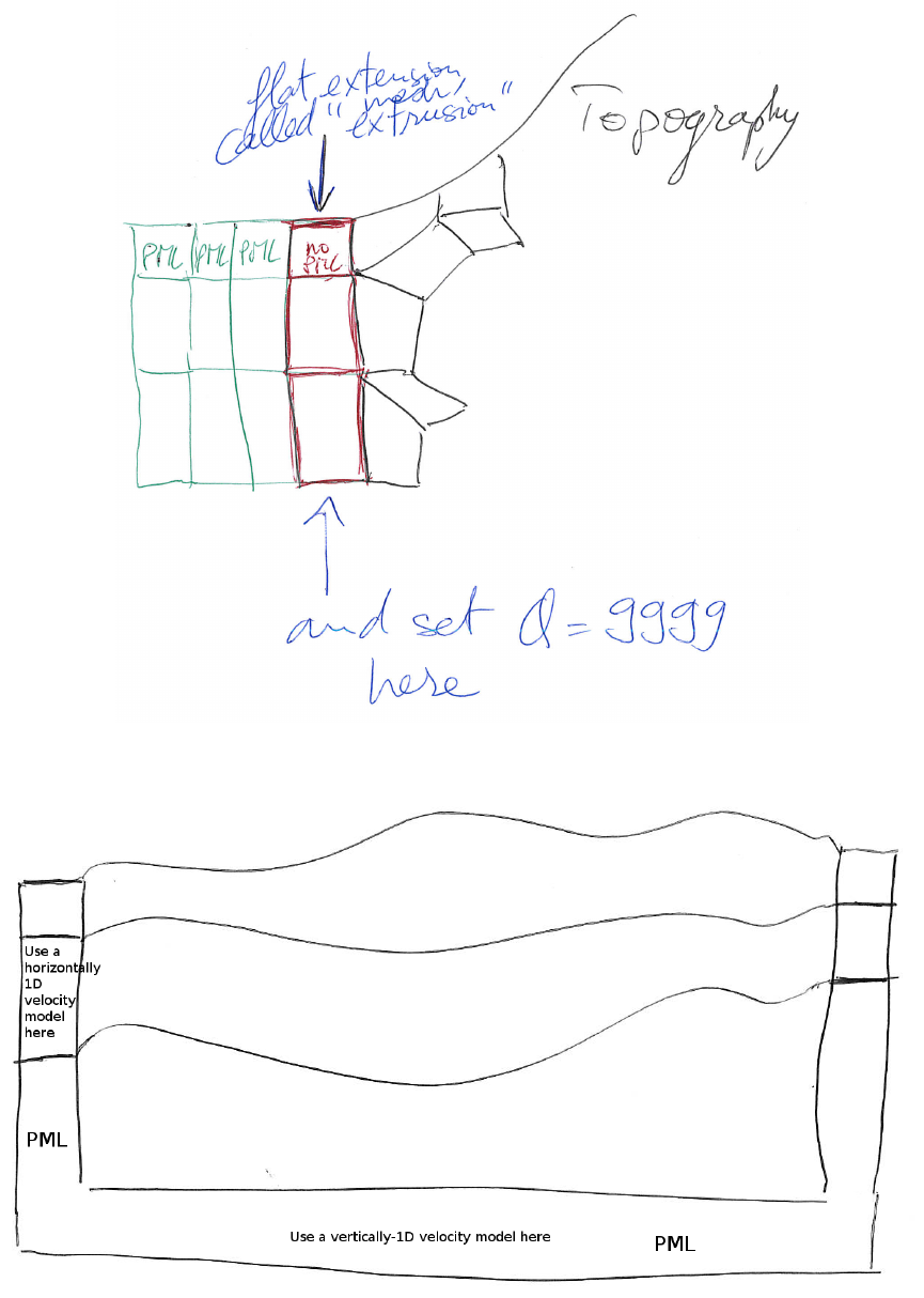
CHAPTER 4. CREATING THE DISTRIBUTED DATABASES 37
Figure 4.3: Mesh extrusion for PML (green elements) and a non-PML stabilization layer (red elements).
Figure 4.4: How to modify your external 3D velocity and density model in order to use PML. Such a modification is
not needed when using Stacey absorbing boundary conditions (but such conditions are significantly less efficient).
CHAPTER 4. CREATING THE DISTRIBUTED DATABASES 38
∆t<C minΩ(h/v )
where Cis the so-called Courant number and Ωdenotes the model volume. The distance hdepends on the mesh
element size and the number of GLL points NGLL specified in the main constants file constants.h located in the
src/shared/ subdirectory. The wave speed vis determined based on your model’s P- (or S-) wave speed values.
The database generator xgenerate_databases, as well as the internal mesher xmeshfem3D, are trying to
evaluate the value of ∆tfor empirically chosen Courant numbers C∼0.3. If you used the mesher xmeshfem3D
to generate your mesh, you should set the value suggested in OUTPUT_FILES/output_mesher.txt file, which
is created after the mesher completed. In case you used CUBIT to create the mesh, you might use an arbitrary value
when running xgenerate_databases and then use the value suggested in the
OUTPUT_FILES/output_mesher.txt file after the database generation completed. Note that the implemented
Newmark time scheme uses this time step globally, thus your simulations become more expensive for very small mesh
elements in high wave-speed regions. Please be aware of this restriction when constructing your mesh in Chapter 3.
Chapter 5
Running the Solver xspecfem3D
Now that you have successfully generated the databases, you are ready to compile the solver. In the main directory,
type
make xspecfem3D
Please note that xspecfem3D must be called directly from the main directory, as most of the binaries of the package.
The solver needs three input files in the DATA directory to run:
Par_file the main parameter file which was discussed in detail in the previous Chapter 4,
CMTSOLUTION or FORCESOLUTION the earthquake source parameter file or the force source parameter file, and
STATIONS the stations file.
Most parameters in the Par_file should be set prior to running the databases generation. Only the following
parameters may be changed after running xgenerate_databases:
• the simulation type control parameters: SIMULATION_TYPE and SAVE_FORWARD
• the time step parameters NSTEP and DT
• the absorbing boundary control parameter PML_CONDITIONS on condition that the
PML_INSTEAD_OF_FREE_SURFACE flag remains unmodified after running the databases generation.
• the movie control parameters MOVIE_SURFACE,MOVIE_VOLUME, and NTSTEPS_BETWEEN_FRAMES
• the ShakeMap® option CREATE_SHAKEMAP
• the output information parameters MOVIE_TYPE,NTSTEP_BETWEEN_OUTPUT_INFO and
NTSTEP_BETWEEN_OUTPUT_SEISMOS
• the PRINT_SOURCE_TIME_FUNCTION flags
Any other change to the Par_file implies rerunning both the database generator xgenerate_databases and
the solver xspecfem3D.
For any particular earthquake, the CMTSOLUTION file that represents the point source may be obtained directly
from the Harvard Centroid-Moment Tensor (CMT) web page (www.seismology.harvard.edu). It looks like
the example shown in Fig. 5.1. The CMTSOLUTION file should be edited in the following way:
• Set the latitude or UTM xcoordinate, longitude or UTM ycoordinate, depth of the source (in km). Re-
mark: In principle in the international CMTSOLUTION format in geophysics the depth is given in kilome-
ters; however for users in other fields (non-destructive testing, medical imaging, near-surface studies...) who
may prefer to give the position of the source (rather than its depth from the surface), or for people who
use FORCESOLUTION to describe the source rather than CMTSOLUTION, we provide an option called
39
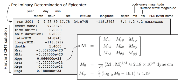
CHAPTER 5. RUNNING THE SOLVER XSPECFEM3D 40
Figure 5.1: CMTSOLUTION file based on the format from the Harvard CMT catalog. Mis the moment tensor, M0is
the seismic moment, and Mwis the moment magnitude.
USE_SOURCES_RECEIVERS_Z in the Par_file, and if so that position is read from CMTSOLUTION in me-
ters rather than kilometers (and again, it is then the true position in the mesh, not the depth). When option
USE_SOURCES_RECEIVERS_Z in the Par_file is on, this remark applies to the position of the receivers as
well.
• Set the time shift parameter equal to 0.0(the solver will not run otherwise.) The time shift parameter
would simply apply an overall time shift to the synthetics, something that can be done in the post-processing
(see Section 15.1).
• For point-source simulations (see finite sources, page 41) we recommend setting the source half-duration pa-
rameter half duration equal to zero, which corresponds to simulating a step source-time function, i.e.,
a moment-rate function that is a delta function. If half duration is not set to zero, the code will use a
Gaussian (i.e., a signal with a shape similar to a ‘smoothed triangle’, as explained in Komatitsch and Tromp
[2002a] and shown in Fig 5.2) source-time function with half-width half duration. We prefer to run the
solver with half duration set to zero and convolve the resulting synthetic seismograms in post-processing
after the run, because this way it is easy to use a variety of source-time functions (see Section 15.1). Ko-
matitsch and Tromp [2002a] determined that the noise generated in the simulation by using a step source time
function may be safely filtered out afterward based upon a convolution with the desired source time function
and/or low-pass filtering. Use the serial code convolve_source_timefunction.f90 and the script
convolve_source_timefunction.csh for this purpose, or alternatively use signal-processing software
packages such as SAC (www.llnl.gov/sac). Type
make xconvolve_source_timefunction
to compile the code and then set the parameter hdur in convolve_source_timefunction.csh to the
desired half-duration.
• The zero time of the simulation corresponds to the center of the triangle/Gaussian, or the centroid time of the
earthquake. The start time of the simulation is t=−1.5∗half duration (the 1.5 is to make sure the
moment rate function is very close to zero when starting the simulation). To convert to absolute time tabs, set
tabs =tpde +time shift +tsynthetic
where tpde is the time given in the first line of the CMTSOLUTION,time shift is the corresponding value
from the original CMTSOLUTION file and tsynthetic is the time in the first column of the output seismogram.
If you know the earthquake source in strike/dip/rake format rather than in CMTSOLUTION format, use the C
code SPECFEM3D_GLOBE/utils/strike_dip_rake_to_CMTSOLUTION.c to convert it. The conversion
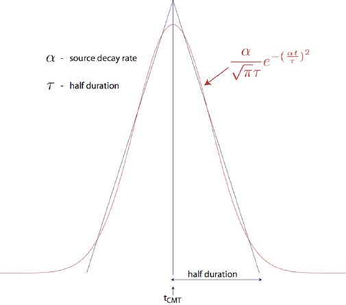
CHAPTER 5. RUNNING THE SOLVER XSPECFEM3D 41
Figure 5.2: Comparison of the shape of a triangle and the Gaussian function actually used.
formulas are given for instance in Aki and Richards [1980]. Note that the Aki and Richards [1980] convention is
slightly different from the Harvard CMTSOLUTION convention (the sign of some components is different). The C
code outputs both.
Centroid latitude and longitude should be provided in geographical coordinates. The code converts these coordi-
nates to geocentric coordinates [Dahlen and Tromp,1998]. Of course you may provide your own source representa-
tions by designing your own CMTSOLUTION file. Just make sure that the resulting file adheres to the Harvard CMT
conventions (see Appendix A). Note that the first line in the CMTSOLUTION file is the Preliminary Determination of
Earthquakes (PDE) solution performed by the USGS NEIC, which is used as a seed for the Harvard CMT inversion.
The PDE solution is based upon P waves and often gives the hypocenter of the earthquake, i.e., the rupture initiation
point, whereas the CMT solution gives the ‘centroid location’, which is the location with dominant moment release.
The PDE solution is not used by our software package but must be present anyway in the first line of the file.
To simulate a kinematic rupture, i.e., a finite-source event, represented in terms of Nsources point sources, provide
aCMTSOLUTION file that has Nsources entries, one for each subevent (i.e., concatenate Nsources CMTSOLUTION files
to a single CMTSOLUTION file). At least one entry (not necessarily the first) must have a zero time shift, and
all the other entries must have non-negative time shift. Each subevent can have its own half duration, latitude,
longitude, depth, and moment tensor (effectively, the local moment-density tensor).
Note that the zero in the synthetics does NOT represent the hypocentral time or centroid time in general, but the
timing of the center of the source triangle with zero time shift (Fig 5.3).
Although it is convenient to think of each source as a triangle, in the simulation they are actually Gaussians (as
they have better frequency characteristics). The relationship between the triangle and the gaussian used is shown in
Fig 5.2. For finite fault simulations it is usually not advisable to use a zero half duration and convolve afterwards,
since the half duration is generally fixed by the finite fault model.
The FORCESOLUTION file should be edited in the following way:
• Set the time shift parameter equal to 0.0(the solver will not run otherwise.) The time shift parameter
would simply apply an overall time shift to the synthetics, something that can be done in the post-processing
(see Section 15.1).
• Set the f0 parameter (the dominant frequency) of the Ricker source time function (i.e., the second derivative of
a Gaussian) when USE_RICKER_TIME_FUNCTION is turned on in the main parameter file Par_file. In
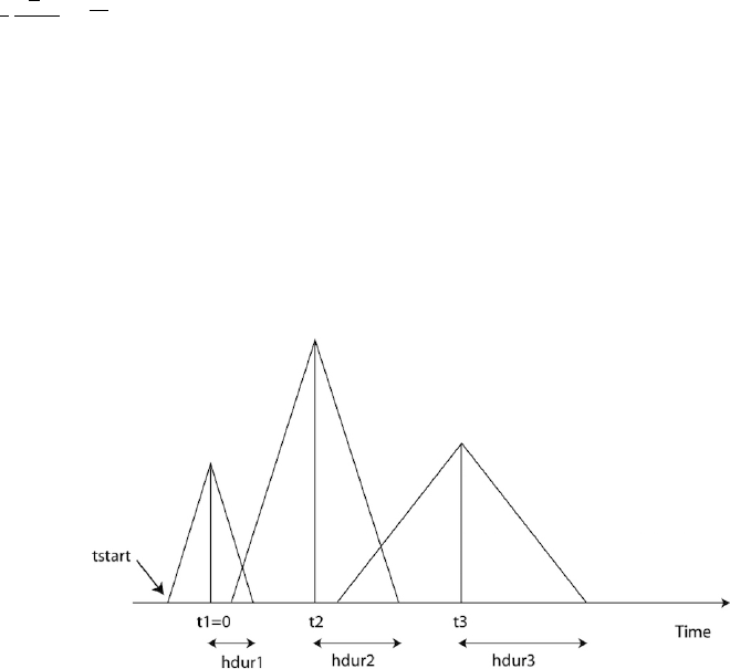
CHAPTER 5. RUNNING THE SOLVER XSPECFEM3D 42
case that the solver uses a (pseudo) Dirac delta source time function to represent a force point source, a very
short duration of five time steps is automatically set by default. Note that we use the standard definition of a
Ricker, for a dominant frequency f0:Ricker(t) = (1 −2at2)e−at2, with a=π2f2
0, whose Fourier transform is
thus: 1
2
√πω2
a3/2e−ω2
4aThis gives the wavelet of Figure 4.2.
• Set the latitude or UTM xcoordinate, longitude or UTM ycoordinate, depth of the source (in km).
• Set the magnitude of the force source.
• Set the components of a (non-unitary) direction vector for the force source in the East/North/Vertical basis (see
Appendix A for the orientation of the reference frame).
Where necessary, set a FORCESOLUTION file in the same way you configure a CMTSOLUTION file with Nsources
entries, one for each subevent (i.e., concatenate Nsources FORCESOLUTION files to a single FORCESOLUTION file).
At least one entry (not necessarily the first) must have a zero time shift, and all the other entries must have non-
negative time shift. Each subevent can have its own half latitude, longitude, depth, half duration and force
parameters.
Figure 5.3: Example of timing for three sources. The center of the first source triangle is defined to be time zero. Note
that this is NOT in general the hypocentral time, or the start time of the source (marked as tstart). The parameter time
shift in the CMTSOLUTION file would be t1(=0), t2, t3 in this case, and the parameter half duration would
be hdur1, hdur2, hdur3 for the sources 1, 2, 3 respectively.
In addition to inbuild source time function, the solver can also use an external source time function defined by the
user. This option can be activated by setting EXTERNAL_SOURCE_FILE to true in Par_File and by adding the
name of the file containing the source time function at the end of FORCESOLUTION or CMTSOLUTION files. The
source time function file must contain the value of the time step on its first line, and then a single column with the
amplitude of the source time function for all the time steps. The time step must be exactly the same as that used for
the simulation. Note when the EXTERNAL_SOURCE_FILE is set to false then the line with the external source time
function file must not appear in the files FORCESOLUTION and CMTSOLUTION otherwise the solver will exit with
an error. When using an external source file, you can still set up the source location and directivity as in the default
case. In the FORCESOLUTION file: you set "latorUTM", "longorUTM" and "depth" to define the position of your
point source. Then if you want to define a directivity, then change the following lines: "component dir vect source E",
"component dir vect source N" and "component dir vect source Z_UP". What you are doing is simply that you define
the source position and directivity the same way as in the default case, but in addition you are specifying the path to
read in a non-default source time function from an external file.
The solver can calculate seismograms at any number of stations for basically the same numerical cost, so the user
is encouraged to include as many stations as conceivably useful in the STATIONS file, which looks like this:
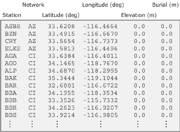
CHAPTER 5. RUNNING THE SOLVER XSPECFEM3D 43
Figure 5.4: Sample STATIONS file. Station latitude and longitude should be provided in geo-
graphical coordinates. The width of the station label should be no more than 32 characters (see
MAX_LENGTH_STATION_NAME in the constants.h file), and the network label should be no more than 8 char-
acters (see MAX_LENGTH_NETWORK_NAME in the constants.h file).
Each line represents one station in the following format:
Station Network Latitude(degrees) Longitude(degrees) Elevation(m) burial(m)
The solver xspecfem3D filters the list of stations in file DATA/STATIONS to exclude stations that are not
located within the region given in the Par_file (between LATITUDE_MIN and LATITUDE_MAX and between
LONGITUDE_MIN and LONGITUDE_MAX). The filtered file is called DATA/STATIONS_FILTERED.
Elevation and burial are generally applicable to geographical regions. Burial is measured down from the top
surface. For other problems in other fields (ultrasonic testing, medical imaging etc...), it may be confusing. We
generally follow either of the following procedures for those kind of problems:
Procedure 1 (mostly for geophysics, when the top surface is a free surface (topography) and the five other edges
of the mesh are absorbing surfaces):
====================================================================================================================================================
- Put the origin on the top of the model.
- Let’s say you want to place two receivers at (x1,y1,z1) and (x2,y2,z2). Your STATIONS file should look like:
BONE GR y1 x1 0.00 -z1
BONE GR y2 x2 0.00 -z2
Procedure 2 (useful for other application domains, in which using the absolute Zposition of the sources and re-
ceivers is more standard than using their depth from the surface):
==================================================================================================================================================================================
- In principle in the international CMTSOLUTION format in geophysics the depth is given in kilometers; however
for users in other fields (non-destructive testing, medical imaging, near-surface studies...) who may prefer to give
the position of the source (rather than its depth from the surface), or for people who use FORCESOLUTION to de-
scribe the source rather than CMTSOLUTION, we provide an option called USE_SOURCES_RECEIVERS_Z in the
Par_file, and if so that position is read from CMTSOLUTION in meters rather than kilometers (and again, it is then
the true position in the mesh, not the depth). When option USE_SOURCES_RECEIVERS_Z in the Par_file is on, this
remark applies to the position of the receivers as well.
CHAPTER 5. RUNNING THE SOLVER XSPECFEM3D 44
- Let’s say you want to place two receivers at (x1,y1,z1) and (x2,y2,z2). Your STATIONS file should then look like:
BONE GR y1 x1 0.00 z1
BONE GR y2 x2 0.00 z2
The option USE_SOURCES_RECEIVERS_Z set to .true. will then discard the elevation and set burial as the z
coordinate.
Third column is Y and Fourth is X due to the latitude/longitude convention.
You can replace the station name "BONE" with any word of length less than 32, and the network name "GR" with any
word of length less than 8.
You can always plot OUTPUT_FILES/sr.vtk file in ParaView to check the source/receiver locations after your simu-
lation.
Solver output is provided in the OUTPUT_FILES directory in the output_solver.txt file. Output can be
directed to the screen instead by uncommenting a line in constants.h:
! uncomment this to write messages to the screen
! integer, parameter :: IMAIN = ISTANDARD_OUTPUT
On PC clusters the seismogram files are generally written to the local disks (the path LOCAL_PATH in the Par_file)
and need to be gathered at the end of the simulation.
While the solver is running, its progress may be tracked by monitoring the ‘timestamp*’ files in the OUTPUT_FILES/
directory. These tiny files look something like this:
Time step # 10000
Time: 108.4890 seconds
Elapsed time in seconds = 1153.28696703911
Elapsed time in hh:mm:ss = 0 h 19 m 13 s
Mean elapsed time per time step in seconds = 0.115328696703911
Max norm displacement vector U in all slices (m) = 1.0789589E-02
The timestamp*files provide the Mean elapsed time per time step in seconds, which may be used
to assess performance on various machines (assuming you are the only user on a node), as well as the Max norm
displacement vector U in all slices (m). If something is wrong with the model, the mesh, or the source,
you will see the code become unstable through exponentially growing values of the displacement and fluid potential
with time, and ultimately the run will be terminated by the program. You can control the rate at which the timestamp
files are written based upon the parameter NTSTEP_BETWEEN_OUTPUT_INFO in the Par_file.
Having set the Par_file parameters, and having provided the CMTSOLUTION (or the FORCESOLUTION)
and STATIONS files, you are now ready to launch the solver! This is most easily accomplished based upon the
go_solver script (See Chapter 13 for information about running through a scheduler, e.g., LSF). You may need to
edit the last command at the end of the script that invokes the mpirun command. The runall script compiles and
runs both xgenerate_databases and xspecfem3D in sequence. This is a safe approach that ensures using the
correct combination of distributed database output and solver input.
It is important to realize that the CPU and memory requirements of the solver are closely tied to choices about
attenuation (ATTENUATION) and the nature of the model (i.e., isotropic models are cheaper than anisotropic models).
We encourage you to run a variety of simulations with various flags turned on or off to develop a sense for what is
involved.
For the same model, one can rerun the solver for different events by simply changing the CMTSOLUTION or
FORCESOLUTION file, or for different stations by changing the STATIONS file. There is no need to rerun the
xgenerate_databases executable. Of course it is best to include as many stations as possible, since this does
not add to the cost of the simulation.
We have also added the ability to run several calculations (several earthquakes) in an embarrassingly-parallel
fashion from within the same run; this can be useful when using a very large supercomputer to compute many earth-
quakes in a catalog, in which case it can be better from a batch job submission point of view to start fewer and
CHAPTER 5. RUNNING THE SOLVER XSPECFEM3D 45
much larger jobs, each of them computing several earthquakes in parallel. To turn that option on, set parameter
NUMBER_OF_SIMULTANEOUS_RUNS to a value greater than 1 in file setup/constants.h.in before configuring and
compiling the code. When that option is on, of course the number of processor cores used to start the code in the
batch system must be a multiple of NUMBER_OF_SIMULTANEOUS_RUNS, all the individual runs must use the same
number of processor cores, which as usual is NPROC in the input file DATA/Par_file, and thus the total number
of processor cores to request from the batch system should be NUMBER_OF_SIMULTANEOUS_RUNS ×NPROC.
All the runs to perform must be placed in directories called run0001,run0002,run0003 and so on (with exactly
four digits) and you must create a link from the root directory of the code to the first copy of the executable programs
by typing ln -s run0001/bin bin.
5.1 Note on the viscoelastic model used
The model used is a constant Q, thus with no dependence on frequency (Q(f)= constant). See e.g. Blanc et al. [2016].
However in practice for technical reasons it is approximated based on the sum of different Generalized Zener body
mechanisms and thus the code outputs the band in which the approximation is very good, outside of that range it can
be less accurate. The logarithmic center of that frequency band is the ATTENUATION_f0 parameter defined (in Hz)
in input file DATA/Par_file.
Regarding attenuation (viscoelasticity), in the Par_file you need to select the number of standard linear solids (N_SLS)
to use to mimic a constant Qquality factor. Using N_SLS = 3 is always safe. If (and only if) you know what you
are doing, you can try to reduce that in order to reduce the cost of the simulations. Figure 5.5 shows values that
you can consider using (again, if and only if you know what you are doing). That table has been created by Zhinan
Xie using a comparison between results obtained with a truly-constant Qand results obtained with its approximation
based on N_SLS standard linear solids. The comparison is performed using the time-frequency misfit and goodness-
of-fit criteria proposed by Kristeková et al. [2009]. The table is drawn for a dimensionless parameter representing the
distance of propagation.
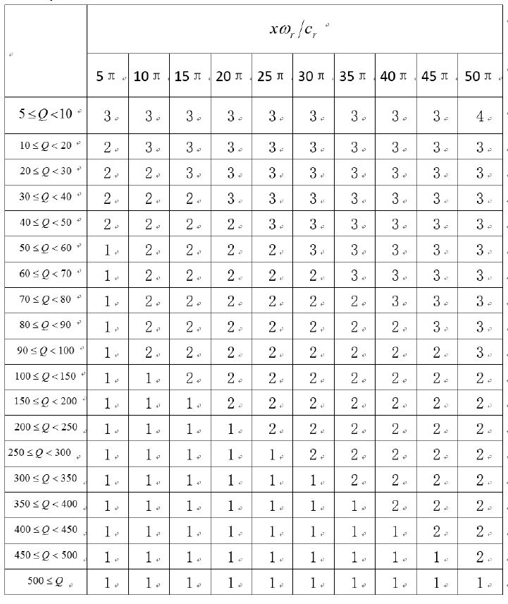
CHAPTER 5. RUNNING THE SOLVER XSPECFEM3D 46
Figure 5.5: Table showing how you can select a value of N_SLS smaller than 3, if and only if you know what you are
doing.
Chapter 6
Kinematic and dynamic fault sources
SPECFEM3D can handle finite fault sources of two kinds:
1. Kinematic: the spatio-temporal distribution of slip rate is prescribed along the fault surface
2. Dynamic: a friction law and initial stresses are prescribed on the fault, a spontaneous rupture process is com-
puted.
6.1 Mesh Generation with Split Nodes
Faults need to be handled in a special way during mesh generation. A fault surface must lie at the interface between
elements (the mesh must honor the fault surfaces). Moreover, a fault is made of two surfaces in contact. Each of these
two surfaces needs a separate set of nodes. This approach is known as "split nodes". Currently faults can only be run
with xdecompose_mesh and CUBIT.xmeshfem3D is not yet ready to handle faults.
To facilitate the mesh generation with split nodes in CUBIT, we need to separate the two fault surfaces by a small
distance, effectively creating a tiny opening of the fault (Figure 6.1,6.2). Note that the opening distance should not
be too small especially in single precision simulations (For example, if your fault is at y=y0plane, then the opening
distance should be at least 10−6y0since single precision can ensure precision within only 7 digits). Note that only the
interior of the fault must be opened, its edges must remain closed (except the edge on the free surface). The fault is
automatically closed later by SPECFEM3D.
Here is an example CUBIT script to generate a mesh with split nodes for a buried vertical strike-slip fault:
reset
brick x 10 y 10 z 10
webcut volume all with plane xplane
webcut volume all with plane yplane
webcut volume all with plane xplane offset 3
webcut volume all with plane zplane offset 3
webcut volume all with plane zplane offset -3
imprint all
merge all
unmerge surf 160
mesh vol all
set node constraint off
node in surf 168 move X 0 Y 0.01 Z 0
node in surf 160 move X 0 Y -0.01 Z 0
The CUBIT scripts (*.jou and *.py) in the directory EXAMPLES generate more complicated meshes. The *.py files
are Python scripts that execute CUBIT commands and use the CUBIT-python interface for SPECFEM3D (see next
section). The Python language allows to define and manipulate variables to parameterize the mesh. Alternatively, the
Python script can call a CUBIT journal file (*.jou), which looks like the example above. Variables can be defined and
manipulated there using the APREPRO language built in CUBIT.
47
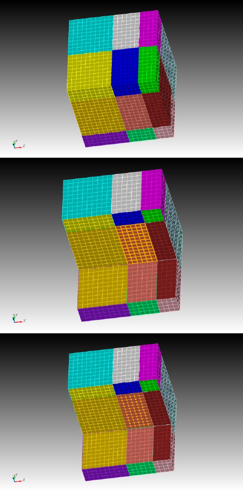
CHAPTER 6. KINEMATIC AND DYNAMIC FAULT SOURCES 48
Figure 6.1: Screenshots of the CUBIT example for the embedded fault with split nodes: The entire mesh is decom-
posed into several volumes bounding the fault (top), the fault surface 168 is shown as orange squares (middle) and
split nodes of the fault shown as orange dots(bottom). Note that only interior nodes of the fault are split while those
on the edges of the fault surface are touching each other.
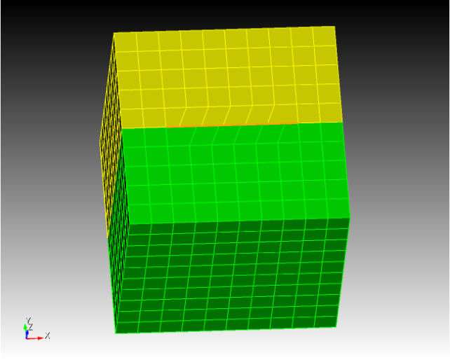
CHAPTER 6. KINEMATIC AND DYNAMIC FAULT SOURCES 49
Figure 6.2: Screenshots of a CUBIT example showing split nodes for a fault reaching the surface. Surface trace of the
fault is shown in orange. Note that the edges of the fault are not split while the interior nodes are offset by a small
distance on either side of the fault
Note that you should avoid gaps in the list of indices of mesh objects with the following CUBIT command:
compress ids hex face edge node
(otherwise you will get a segmentation fault during domain decomposition)
6.2 CUBIT-Python Scripts for Faults
The mesh generated in CUBIT needs to be processed and exported in a format compatible with SPECFEM3D. This is
achieved in the Python scripts by calling the Python-CUBIT interface functions defined in the CUBIT directory:
1. Function define_bc (or boundary_definition.py) must be called to set up the absorbing boundaries database
2. Function fault_input must be called once for each fault to set up the fault database
3. Function cubit2specfem3d.export2SPECFEM3D must be called at the very end of the script to export the
mesh in a SPECFEM3D format.
The functions in #1 and #3 are for the bulk and are documented in Section 3.1.2. We focus here on #2:
Function: fault_input
Purpose: export a fault mesh database from CUBIT to a SPECFEM3D-compliant file
Syntax: fault_input(id_fault, ids_surf_1, ids_surf_2)
Inputs:
• id_fault integer index assigned to the fault. (The user must number all the faults, starting at 1, with unit incre-
ments)
CHAPTER 6. KINEMATIC AND DYNAMIC FAULT SOURCES 50
• ids_surf_1 list of CUBIT ids of all surfaces that form side 1 of the fault.
• ids_surf_2 list of CUBIT ids of all surfaces that form side 2 of the fault. (The user must decide which side of
the fault is side 1. This choice affects the sign conventions of fault quantities as explained in Section 6.4).
Outputs: file fault_file_X.dat, where X is the fault id (id_fault).
Example: For the example in Section 6.1:
A1 = [168]
A2 = [160]
fault_input(1,A1,A2)
6.3 Examples
The package includes examples, the SCEC benchmark problems:
• TPV5, a planar vertical strike-slip fault
• TPV14 and TPV15, vertical strike-slip fault system with a fault branch
• TPV102 and TPV103, rate-and-state benchmarks
• TPV22 and TPV23, step-over benchmarks
• TPV16, heterogenous initial stress
and
• Splay fault models from Wendt et al. (2009)
Read the documents in the directory EXAMPLES/*/description. They contain a description of the example and
additional instructions to run it. Visualize the results with the Matlab scripts in the directory EXAMPLES/∗/post
6.4 Sign Convention for Fault Quantities
During mesh generation, the fault is defined by two surfaces in contact. Let’s denote as "side 1" the SECOND surface
declared by the user in the call to the python function "fault_input", and the FIRST surface as "side 2". The local
coordinate system on the fault is defined as the right-handed coordinate system defined by (strike, dip, normal), where
"normal" is the normal vector outgoing from side 1, "dip" is parallel to the along-dip direction pointing downwards,
and "strike" is the horizontal along-strike vector such that the system is right-handed. In places where the fault plane
is horizontal, we define the alone strike direction to be (1,0,0).
Slip is defined as displacement on side 2 minus displacement on side 1. In the local coordinate system on the fault,
positive along-strike slip is right-lateral and positive along-dip slip is thrust if side 1 is on the hanging wall (normal
faulting if side 1 is on the foot wall).
Traction is defined as the stress induced on side 1 by side 2, which is the stress tensor times the normal vector
outgoing from side 1. In the local coordinate system on the fault, the normal traction is negative in compression,
positive along-strike traction generates right-lateral slip and positive along-dip traction generates thrust slip if side 1 is
on the hanging wall (normal faulting if side 1 is on the foot wall).
CHAPTER 6. KINEMATIC AND DYNAMIC FAULT SOURCES 51
6.5 Input Files
Three additional input files are required in the DATA/ directory for dynamic and kinematic faults. They are Par_file_faults,
FAULT_STATIONS and input_file.txt or rsf_hete_input_file.txt(optional). If the former does not exist, the
code assumes that there are no faults.
DATA/Par_file_faults contains parameters of the fault. The first part of this file has a strict format:
Line 1: Number of faults (NF)
Lines 2 to NF+1: Kelvin Voigt damping (in seconds) for each fault. (See below how to set this parameter)
Line NF+2: Type of simulation (1=dynamic , 2 = kinematic)
Line NF+3: Number of time steps between updates of the time series outputs at selected fault points (see
DATA/FAULT_STATIONS), usually a large number (100s or 1000s). Note that the sampling rate of
the time series is usually much higher.
Line NF+4: Number of time steps between fault snapshot outputs (quantities at every fault point exported
at regular times), usually a large number (100s or 1000s).
Line NF+5: Slip velocity threshold below which frictional healing is set (friction coefficient is reset to
its static value). If this value is negative healing is disabled.
Line NF+6: Slip velocity threshold to define the rupture front. Only used for outputs.
The rest of this file is made of namelist input blocks (see "namelist" in a Fortran 9x manual). The input
for each fault has the following sequence (arguments in [brackets] are optional):
&RUPTURE_SWITCHES / RATE_AND_STATE ,TPV16 ,HETE_RSF ,TPV10X
&BEGIN_FAULT /
&STRESS_TENSOR Sigma = σxx,σyy ,σzz ,σxy ,σxz,σyz /
&INIT_STRESS S1, S2, S3 [,n1, n2, n3] /
followed by (n1+n2+n3) &DIST2D blocks
&SWF mus, mud, dc [, nmus, nmud, ndc] /
&RSF V0,f0,a,b,L,V_init,theta_init,C,StateLaw [ nV0,nf0,na,nb,nL,nV_init,ntheta_init,nC ] /
followed by (nV0+nf0+na+nb+nL+nV_init+ntheta_init+nC) &DIST2D blocks
&RUPTURE_SWITCHES input block sets some switches in the simulation process.
RATE_AND_STATE = .TRUE. use rate and state friction,=.FALSE. use slip weakening
friction
TPV16 =.TRUE turn on heterogeneity fault property input for slip weakening friction from
DATAinput_file.txt, =.FALSE. turn off such feature
HETE_RSF =.TRUE. turn on heterogeneity fault property input for rate and state friction
using input from DATArsf_hete_input_filr.txt, =.FALSE. turn off such feature
TPV10X =.TRUE. turn on some ad hoc features for TPV101-104 simulations, a rate strength-
ening layer surrounding the rate weakening region. =.FALSE. turn off such feature
&STRESS_TENSOR input block sets the initial fault stresses by projecting a uniform regional stress
field onto the fault plane.So that the tractions τ=σ:nwhile nis the local norm of the fault
plane. Sigma = σxx,σyy ,σzz ,σxy ,σxz,σyz (in Pa)
&INIT_STRESS input block sets the initial fault stresses relative to the foot-wall side of the fault. Initial
stresses are composed of a constant background value possibly overwritten in prescribed
regions by heterogeneous distributions (see &DIST2D blocks below):

CHAPTER 6. KINEMATIC AND DYNAMIC FAULT SOURCES 52
S1 = constant background value of along-strike shear stress (positive in the usual strike di-
rection)
S2 = constant background value of along-dip shear (positive is down-dip, normal faulting)
S3 = constant background value of normal stress (negative in compression)
n1 = number of heterogeneous items for along-strike shear stress [default is 0]
n2 = number of heterogeneous items for along-dip shear stress [default is 0]
n3 = number of heterogeneous items for normal stress [default is 0]
&SWF input block sets the slip-weakening friction parameters of the fault:
mus = constant background value of static friction coefficient
mud = constant background value of dynamic friction coefficient
dc = constant background value of critical slip-weakening distance
C= constant background value of cohesion (in Pa)
nmus = number of heterogeneous items for static friction coefficient [default is 0]
nmud = number of heterogeneous items for dynamic friction coefficient [default is 0]
ndc = number of heterogeneous items for critical slip-weakening distance [default is 0]
nC = number of heterogeneous items for cohesion
&RSF input block sets the rate and state friction parameters of the fault:
We refer to the well known rate and state friction formula:
µ=f0+a∗log(v
v0
) + b∗log(v0
θL))
V0 = constant background value of V0
f0 = constant background value of f0
a= constant background value of a
b= constant background value of b
L= constant background value of L
V_init = constant background value of along strike right lateral slip rate at time 0
theta_init = constant background value of state variable θat time 0
C= constant background value of cohesion (in Pa)
StateLaw = 1 or 2. 1 for aging law , 2 for slip law with strong dynamic weakening.
n** = number of heterogeneous items for quantity **
&DIST2D input blocks modify (overwrite) the value of a fault parameter by a heterogeneous spatial
distribution:
&DIST2D shapeval=’square’, val, xc, yc, zc, l /
sets a constant value (val) within a cube with center (xc,yc,zc) and edge size l.
&DIST2D shapeval=’rectangle’, val, xc, yc, zc, lx, ly, lz /
sets a constant value (val) within a rectangular prism with center (xc,yc,zc) and edge sizes
(lx,ly,lz).
&DIST2D shapeval=’rectangle −taper’, val, valh, xc, yc, zc, lx, ly, lz /
sets a vertical linear gradient within a rectangular prism with center (xc,yc,zc) and edge sizes
(lx,ly,lz). Values vary linearly as a function of vertical position z between value val at z =
zc-lz/2 and value valh at z = zc+lz/2 .
&DIST2D shapeval=’circular’, val, xc, yc, zc, r /
sets a constant value (val) within a sphere with center (xc,yc,zc) and radius r.
CHAPTER 6. KINEMATIC AND DYNAMIC FAULT SOURCES 53
DATA/FAULT_STATIONS Stations in the fault plane.
Line 1 : number of stations.
Line 2 to end: 5 columns: X, Y, Z (-depth), station name, fault-id
The fault-id identifies the fault that contains the station. It is the index of appearance in the faults list after
line 2 of Par_file_faults
DATA/input_file.txt Heterogeneous stresses and friction for linear slip weakening friction parameters are docu-
mented in page 10 of
EXAMPLES/tpv16/description/TPV16_17_Description_v03.pdf
To activate this feature, in Par_file_faults name list &RUPTURE_SWITCHES, set TPV16=.TRUE..
DATA/rsf_hete_input_file.txt Heterogeneous stresses and friction input for rate and state friction. To activate this
feature, in Par_file_faults name list &RUPTURE_SWITCHES, set RSF_HETE=.TRUE.. The format
of DATA/rsf_hete_input_file.txt is as such, in the first line there are four integers that are sequentially
documenting the number of divisions along strike, number of divisions along dip, cell size along strike
, cell size along dip. Then the following N (N=NumberOfDivisionsAlongStrike * NumberOfDivision-
sAlongDip) lines will document the stress and friction properties on the grid. There are a total of 13
columns.
1. Column1 = Along strike distance(m)
2. Column2 = Along dip distances(m) The distance should be negative for points at depth
3. Column3 = Normal stress(Pa)
4. Column4 = Horizontal right-lateral shear stress(Pa)
5. Column5 = Vertical up-dip shear stress(Pa)
6. Column6 = V0value in RSF(m/s)
7. Column7 = f0value in RSF
8. Column8 = a value in RSF
9. Column9 = b value in RSF
10. Column10 = L value in RSF
11. Column11 = Initial slip velocity(m/s)
12. Column12 = State variable θ
13. Column13 = Cohesion(Pa)
Note that the input grid file do not have to coincide with the mesh. For each fault node on the mesh, they
will use the value from the nearest node on the input grid.
6.6 Setting the Kelvin-Voigt Damping Parameter
The purpose of the Kelvin-Voigt viscosity in the dynamic fault solver is to damp spurious oscillations generated by
the fault slip at frequencies that are too high to be resolved by the mesh. The viscosity eta (in seconds) depends on
the size of the elements on the fault. Here is how to set it:
1. Determine the average linear size of the elements on the fault plane, h_fault. Usually this value is prescribed
by the user during mesh generation. Otherwise it can be found by inspection of the mesh inside the CUBIT
GUI.
2. Use the Matlab function utils/critical_timestep.mto compute
dtc_fault =critical_timestep cp,h_fault,ngll.
This is the critical time step in an elastic medium for a hypothetical element of cubic shape with size equal to
h_fault.

CHAPTER 6. KINEMATIC AND DYNAMIC FAULT SOURCES 54
3. Set eta in Par_file_faults to (0.1 to 0.3)×dtc_fault. A larger eta damps high-frequencies more aggres-
sively but it might also affect lower frequencies and rupture speed.
Viscosity reduces numerical stability: the critical timestep in a simulation with Kelvin-Voigt damping needs to be
smaller than that in a purely elastic simulation. Here is how to set the time step accordingly:
1. Run a test simulation without viscosity (eta=0 and only a few time steps)
2. Look for the "maximum suggested time step" in OUTPUT_FILES/output_mesher.txt. This is the criti-
cal timestep of a purely elastic simulation, dtc_bulk.
3. Reset the timestep of the simulation with a Kelvin-Voigt material to a value smaller than
dtc_kv =eta p1 + dtc_bulk2/eta2−1
Note that in general dtc_bulk is smaller than dtc_fault, because elements off the fault might be smaller or more
distorted than element faces on the fault.
6.7 Output Files
Several output files are saved in OUTPUT_FILES/:
1. Seismograms for each station on the fault plane given in DATA/FAUL_STATIONS. One output file is generated
for each station, named after the station. The files are ascii and start with a header (22 lines long) followed by a
data block with the following format, one line per time sample:
Column 1 = Time (s)
Column 2 = horizontal right-lateral slip (m)
Column 3 = horizontal right-lateral slip rate (m/s)
Column 4 = horizontal right-lateral shear stress (MPa)
Column 5 = vertical up-dip slip (m)
Column 6 = vertical up-dip slip rate (m/s)
Column 7 = vertical up-dip shear stress (MPa)
Column 8 = normal stress (MPa)
The stresses are relative to the footwall side of the fault (this convention controls their sign, but not their ampli-
tude). Slip is defined as displacement of the hanging wall relative to the footwall.
2. Seismograms at stations in the bulk (out of the fault plane) given in DATA/STATIONS.
3. Rupture time files are named Rupture_time_FAULT-id. One file is generated for each fault. The files are ascii
and start with a header (12 lines long) followed by a data block with the following format, one line per fault
node:
Column 1 = horizontal coordinate, distance along strike (m)
Column 2 = vertical coordinate, distance down-dip (m)
Column 3 = rupture time (s)
4. Fault quantities (slip, slip rate, stresses, etc) at regular times are stored in binary data files called Snapshot#it#.bin,
where #it# is the timestep number. These can be read in Matlab with the function utils/FSEM3D_snapshot.m
CHAPTER 6. KINEMATIC AND DYNAMIC FAULT SOURCES 55
6.8 Post-processing and Visualization
Some Matlab functions for post-processing and visualization are included in directory utils. The functions are inter-
nally documented (see their matlab help).
FSEM3D_snapshot reads a fault data snapshot
The directories EXAMPLES/*/post contain additional Matlab scripts to generate figures specific to each example.
Chapter 7
Adjoint Simulations
Adjoint simulations are generally performed for two distinct applications. First, they can be used in point source
moment-tensor inversions, or source imaging for earthquakes with large ruptures such as the Lander’s earthquake
[Wald and Heaton,1994]. Second, they can be used to generate finite-frequency sensitivity kernels that are a critical
part of tomographic inversions based upon 3D reference models [Tromp et al.,2005,Liu and Tromp,2006,Tromp
et al.,2008,Liu and Tromp,2008]. In either case, source parameter or velocity structure updates are sought to mini-
mize a specific misfit function (e.g., waveform or traveltime differences), and the adjoint simulation provides a means
of computing the gradient of the misfit function and further reducing it in successive iterations. Applications and
procedures pertaining to source studies and finite-frequency kernels are discussed in Sections 7.1 and 7.2, respec-
tively. The two related parameters in the Par_file are SIMULATION_TYPE (1, 2 or 3) and the SAVE_FORWARD
(boolean).
7.1 Adjoint Simulations for Sources Only (not for the Model)
When a specific misfit function between data and synthetics is minimized to invert for earthquake source parameters,
the gradient of the misfit function with respect to these source parameters can be computed by placing time-reversed
seismograms at the receivers as virtual sources in an adjoint simulation. Then the value of the gradient is obtained
from the adjoint seismograms recorded at the original earthquake location.
1. Prepare the adjoint sources
(a) First, run a regular forward simulation (SIMULATION_TYPE = 1 and SAVE_FORWARD = .false.).
You can automatically set these two variables using the utils/change_simulation_type.pl script:
utils/change_simulation_type.pl -f
and then collect the recorded seismograms at all the stations given in DATA/STATIONS.
(b) Then select the stations for which you want to compute the time-reversed adjoint sources and run the
adjoint simulation, and compile them into the DATA/STATIONS_ADJOINT file, which has the same
format as the regular DATA/STATIONS file.
• Depending on what type of misfit function is used for the source inversion, adjoint sources need to
be computed from the original recorded seismograms for the selected stations and saved in a sub-
directory called SEM/ in the root directory of the code, with the format NT.STA.BX?.adj, where
NT,STA are the network code and station name given in the DATA/STATIONS_ADJOINT file, and
BX? represents the component name of a particular adjoint seismogram. Please note that the band
code can change depending on your sampling rate (see Appendix Bfor further details).
• The adjoint seismograms are in the same format as the original seismogram (NT.STA.BX?.sem?),
with the same start time, time interval and record length.
(c) Notice that even if you choose to time reverse only one component from one specific station, you still need
to supply all three components because the code is expecting them (you can set the other two components
to be zero).
56
CHAPTER 7. ADJOINT SIMULATIONS 57
(d) Also note that since time-reversal is done in the code itself, no explicit time-reversing is needed for the
preparation of the adjoint sources, i.e., the adjoint sources are in the same forward time sense as the original
recorded seismograms.
2. Set the related parameters and run the adjoint simulation
In the DATA/Par_file, set the two related parameters to be SIMULATION_TYPE = 2 and SAVE_FORWARD
= .false.. More conveniently, use the scripts utils/change_simulation_type.pl to modify the
Par_file automatically (change_simulation_type.pl -a). Then run the solver to launch the ad-
joint simulation.
3. Collect the seismograms at the original source location
After the adjoint simulation has completed successfully, collect the seismograms from LOCAL_PATH.
• These adjoint seismograms are recorded at the locations of the original earthquake sources given by the
DATA/CMTSOLUTION file, and have names of the form NT.S?????.S??.sem for the six-component
strain tensor (SNN,SEE,SZZ,SNE,SNZ,SEZ) at these locations, and
NT.S?????.BX?.sem for the three-component displacements (BXN,BXE,BXZ) recorded at these lo-
cations.
•S????? denotes the source number; for example, if the original CMTSOLUTION provides only a point
source, then the seismograms collected will start with S00001.
• These adjoint seismograms provide critical information for the computation of the gradient of the misfit
function.
7.2 Adjoint Simulations for Finite-Frequency Kernels (Kernel Simulation)
Finite-frequency sensitivity kernels are computed in two successive simulations (please refer to Liu and Tromp [2006]
and Tromp et al. [2008] for details).
1. Run a forward simulation with the state variables saved at the end of the simulation
Prepare the CMTSOLUTION and STATIONS files, set the parameters SIMULATION_TYPE = 1 and SAVE_FORWARD =
.true. in the Par_file (change_simulation_type -F), and run the solver.
• Notice that attenuation is not implemented yet for the computation of finite-frequency kernels; therefore
set ATTENUATION = .false. in the Par_file.
• We also suggest you modify the half duration of the CMTSOLUTION to be similar to the accuracy of the
simulation (see Equation 3.1) to avoid too much high-frequency noise in the forward wavefield, although
theoretically the high-frequency noise should be eliminated when convolved with an adjoint wavefield with
the proper frequency content.
• This forward simulation differs from the regular simulations (SIMULATION_TYPE = 1 and SAVE_FORWARD
= .false.) described in the previous chapters in that the state variables for the last time step of the simulation,
including wavefields of the displacement, velocity, acceleration, etc., are saved to the LOCAL_PATH to be used for
the subsequent simulation.
• For regional simulations, the files recording the absorbing boundary contribution are also written to the
LOCAL_PATH when SAVE_FORWARD = .true..
2. Prepare the adjoint sources
The adjoint sources need to be prepared the same way as described in the Section 1.
• In the case of travel-time finite-frequency kernel for one source-receiver pair, i.e., point source from
the CMTSOLUTION, and one station in the STATIONS_ADJOINT list, we supply a sample program
in utils/adjoint_sources/traveltime/xcreate_adjsrc_traveltime to cut a certain
portion of the original displacement seismograms and convert it into the proper adjoint source to compute
the finite-frequency kernel.

CHAPTER 7. ADJOINT SIMULATIONS 58
xcreate_adjsrc_traveltime t1 t2 ifile[0-5] E/N/Z-ascii-files [baz]
where t1 and t2 are the start and end time of the portion you are interested in, ifile denotes the
component of the seismograms to be used (0 for all three components, 1 for East, 2 for North, and 3
for vertical, 4 for transverse, and 5 for radial component), E/N/Z-ascii-files indicate the three-
component displacement seismograms in the right order, and baz is the back-azimuth of the station. Note
that baz is only supplied when ifile = 4 or 5.
• Similarly, a sample program to compute adjoint sources for amplitude finite-frequency kernels may be
found in utils/adjoint_sources/amplitude and used in the same way as described for travel-
time measurements
xcreate_adjsrc_amplitude t1 t2 ifile[0-5] E/N/Z-ascii-files [baz]
3. Run the kernel simulation
With the successful forward simulation and the adjoint source ready in the SEM/ directory, set SIMULATION_TYPE
= 3 and SAVE_FORWARD = .false. in the Par_file (you can use change_simulation_type.pl
-b), and rerun the solver.
• The adjoint simulation is launched together with the back reconstruction of the original forward wavefield
from the state variables saved from the previous forward simulation, and the finite-frequency kernels are
computed by the interaction of the reconstructed forward wavefield and the adjoint wavefield.
• The back-reconstructed seismograms at the original station locations are saved to the LOCAL_PATH at the
end of the kernel simulations, and can be collected to the local disk.
• These back-constructed seismograms can be compared with the time-reversed original seismograms to
assess the accuracy of the backward reconstruction, and they should match very well.
• The arrays for density, P-wave speed and S-wave speed kernels are also saved in the LOCAL_PATH with
the names proc??????_rho(alpha,beta)_kernel.bin, where proc?????? represents the
processor number, rho(alpha,beta) are the different types of kernels.
4. Run the anisotropic kernel simulation
Instead of the kernels for the isotropic wave speeds, you can also compute the kernels for the 21 independent
components CIJ , I, J = 1, ..., 6(using Voigt’s notation) of the elastic tensor in the cartesian coordinate system.
This is done by setting ANISOTROPIC_KL = .true. in constants.h before compiling the package. The
definition of the parameters CIJ in terms of the corresponding components cijkl, ijkl, i, j, k, l = 1,2,3of the
elastic tensor in cartesian coordinates follows Chen and Tromp [2007]. The 21 anisotropic kernels are saved in
the LOCAL_PATH in one file with the name of proc??????_cijkl_kernel.bin (with proc??????
the processor number). The output kernels correspond to absolute perturbations δCIJ of the elastic parameters
and their unit is in s/GP a/km3. For consistency, the output density kernels with this option turned on are for a
perturbation δρ (and not δρ
ρ) and their unit is in s / (kg/m3) / km3. These ‘primary’ anisotropic kernels can then
be combined to obtain the kernels for different parameterizations of anisotropy. This can be done, for example,
when combining the kernel files from slices into one mesh file (see Section 12.3).
If ANISOTROPIC_KL = .true. by additionally setting ANISOTROPIC_KL = .true. in constants.h
the package will save anisotropic kernels parameterized as velocities related to transverse isotropy based on the
the Chen and Tromp parameters Chen and Tromp [2007]. The kernels are saved as relative perturbations for
horizontal and vertical P and S velocities, αv, αh, βv, βh. Explicit relations can be found in appendix B. of
Sieminski et al. [2007]
The anisotropic kernels are only currently available for CPU mode.
In general, the three steps need to be run sequentially to assure proper access to the necessary files. If the simulations
are run through some cluster scheduling system (e.g., LSF), and the forward simulation and the subsequent kernel
simulations cannot be assigned to the same set of computer nodes, the kernel simulation will not be able to access the
database files saved by the forward simulation. Solutions for this dilemma are provided in Chapter 13. Visualization
of the finite-frequency kernels is discussed in Section 12.3.

Chapter 8
Doing tomography, i.e., updating the model
based on the sensitivity kernels obtained
ANNOUNCEMENT (June 2017): See also the next chapter (Chapter 9) about
how to perform full waveform inversion (FWI) or source inversions.
UNDER CONSTRUCTION (July 2015). New content will be added soon.
8.1 Tomographic full waveform inversion (FWI) / imaging using the sensi-
tivity kernels obtained
One of the fundamental reasons for computing sensitivity kernels (Section 7.2) is to use them within a tomographic
inversion, i.e., perform imaging. In other words, use recorded seismograms, make measurements with synthetic
seismograms, and use the misfit between the two to iteratively improve the model described by (at least) Vp,Vs, and ρ
as a function of space.
As explained for instance in Monteiller et al. [2015], full waveform inversion means that one considers the observed
seismograms (possibly filtered) as the basic observables that one wants to fit. One thus searches for the model that
minimizes the mean squared difference between observed and synthetic seismograms. In other words, the goal is to
find a structural model that can explain a larger portion of seismological records, and not simply the phase of a few
seismic arrivals.
Whatever misfit function you use for the tomographic inversion (you can find several examples in Tromp et al.
[2008] and Tromp et al. [2005]), you will weigh the sensitivity kernels with measurements. Furthermore, you will use
as many measurements (stations, components, time windows) as possible per event; hence, we call these composite
kernels “event kernels”, which are volumetric fields representing the gradient of the misfit function with respect to
one of the variables (e.g.,Vs). The basic features of an adjoint-based tomographic inversion were illustrated in Tromp
et al. [2008] and Tape et al. [2007] using a conjugate-gradient algorithm. Other, more powerful techniques such as the
Limited-Memory Broyden-Fletcher-Goldfarb-Shanno (L-BFGS) method can now be used, as illustrated for instance
in Monteiller et al. [2015].
8.1.1 Principle
We want to minimize the classical waveform misfit function:
χ(m) =
N
X
s=1
M
X
r=1 ZT
0
1
2ku(xr,xs;t)−d(xr,xs;t)k2dt. (8.1)
This functional quantifies the L2difference between the observed waveforms d(xr,xs;t)at receivers xr,r= 1, ..., M
produced by sources at xs,s= 1, ..., N, and the corresponding synthetic seismograms u(xr,xs;t)computed in model
59

CHAPTER 8. DOING TOMOGRAPHY BASED ON THE SENSITIVITY KERNELS OBTAINED 60
m. While this misfit function is indeed classical, it is worth mentioning that in the case of noisy real data other norms
could be used, since in the oil industry for instance it is known that the L1norm (Crase et al. [1990], Brossier et al.
[2010]), hybrid L1−L2norms (Bube and Langan [1997]), Hubert norm (Ha et al. [2009]), Student-t distribution
(Aravkin et al. [2011], Jeong et al. [2015]) etc... can be more robust that the L2norm used here in the context of
synthetic data with no noise. In the vicinity of m, the misfit function can be expanded into a Taylor series:
χ(m+δm)≈χ(m) + g(m)·δm+δm·H(m)·δm,(8.2)
where g(m)is the gradient of the waveform misfit function:
g(m) = ∂χ(m)
∂m,(8.3)
and H(m)the Hessian:
H(m) = ∂2χ(m)
∂m2.(8.4)
In the following, for simplicity the dependence of the gradient and Hessian on the model will be implicitly assumed
and omitted in the notations. The nearest minimum of χin (8.2) with respect to the model perturbation δmis reached
for
δm=−H−1·g.(8.5)
The local minimum of (8.1) is thus given by perturbing the model in the direction of the gradient preconditioned by
the inverse Hessian.
8.1.2 Computation of the gradient based on the adjoint method
A direct method to compute the gradient is to take the derivative of (8.1) with respect to model parameters:
∂χ(m)
∂m=−
N
X
s=1
M
X
r=1 ZT
0
∂u(xr,xs;t)
∂m·[u(xr,xs;t)−d(xr,xs;t)] dt . (8.6)
This equation can be reformulated as the matrix-vector product:
g=−J∗·δd,(8.7)
where J∗is the adjoint of the Jacobian matrix of the forward problem that contains the Fréchet derivatives of the
data with respect to model parameters, and δdis the vector that contains the data residuals. The determination of
Jwould require computing the Fréchet derivatives for each time step in the time window considered and for all the
source-station pairs, which is completely prohibitive on current supercomputers (let us note that this situation may
change one day). However, it is possible to obtain this gradient without computing the Jacobian matrix explicitly. The
approach to determine the gradient without computing the Fréchet derivatives was introduced in nonlinear optimization
by Chavent [1974] working with J. L. Lions, and later applied to seismic exploration problems by Bamberger et al.
[1977], Bamberger et al. [1982], Lailly [1983] and Tarantola [1984]. The idea is to resort to the adjoint state, which
corresponds to the wavefield emitted and back-propagated from the receivers [e.g., Tromp et al.,2005,2008,Plessix,
2006,Fichtner et al.,2006].
Let us give an outline of the theory to compute the gradient based on the adjoint method, and refer the reader to
e.g. Tromp et al. [2005] and Tromp et al. [2008] for further details. The perturbation of the misfit function can be
expressed as:
δχ(m) =
N
X
s=1
M
X
r=1 ZT
0
[u(xr,xs;t)−d(xr,xs;t)] ·δu(xr,xs;t)dt , (8.8)
where δuis the perturbation of displacement given by the first-order Born approximation [e.g., Hudson,1977]:
δu(xr,xs;t) = −Zt
0ZVδρ(x)G(xr,x;t−t0)·∂2
t0u(x,xs;t0)
+∇G(xr,x;t−t0) : δc(x) : ∇u(x;t0)] d3xdt0.(8.9)
CHAPTER 8. DOING TOMOGRAPHY BASED ON THE SENSITIVITY KERNELS OBTAINED 61
In this expression, Gis the Green’s tensor, δρ the perturbation of density, δc the perturbation of the fourth-order
elasticity tensor, and a colon denotes a double tensor contraction operation. Inserting (8.9) into (8.8) we obtain
δχ(m) = −
N
X
s=1
M
X
r=1 ZT
0
[u(xr,xs;t)−d(xr,xs;t)] Zt
0ZVδρ(x)G(xr,x;t−t0)·∂2
t0u(x,xs;t0)
+∇G(xr,x;t−t0) : δc(x) : ∇u(x, t0)] d3xdt0dt . (8.10)
Defining the waveform adjoint source for each source xs
f†(x,xs;t) =
M
X
r=1
[u(xr,xs;T−t)−d(xr,xs;T−t)] δ(x−xr),(8.11)
and the corresponding adjoint wavefield
u†(x,xs;t) = Zt0
0ZV
G(x,x0;t0−t)·f†(x0,xs;t)d3x0dt , (8.12)
the perturbation of the misfit function may be expressed as:
δχ(m) = −
N
X
s=1 ZVZT
0δρ u†(x,xs;T−t)·∂2
tu(x,xs;t)
+∇u†(x,xs;T−t) : δc:∇u(x,xs;t)d3xdt . (8.13)
At this point, we make some assumptions on the nature of the elasticity tensor. A general fourth-order elasticity tensor
is described by 21 elastic parameters, a very large number that makes its complete characterization way beyond the
reach of any tomographic approach. For the time being, let us thus consider isotropic elasticity tensors, described by
the two Lamé parameters λand µ:
cijkl =λδij δkl +µ(δik δjl +δilδjk).(8.14)
In this case, (8.13) can be written as:
δχ(m) = −
N
X
s=1 ZV
[Kρ(x,xs)δln ρ(x) + Kλ(x,xs)δln λ(x)
+Kµ(x,xs)δln µ(x)] d3x,(8.15)
where ln() is the natural logarithm and where the Fréchet derivatives with respect to the density and Lamé parameters
are given by:
Kρ(x,xs) = −ZT
0
ρ(x)u†(x,xs;T−t)·∂2
tu(x,xs;t)dt (8.16)
Kλ(x,xs) = −ZT
0
λ(x)∇ · u†(x,xs;T−t)∇ · u(x,xs;t)dt (8.17)
Kµ(x,xs) = −2ZT
0
µ(x)(x)∇u†(x,xs;T−t) : ∇u(x,xs;t)dt . (8.18)
Since the propagation of seismic waves mainly depends on compressional wave speed αand shear wave speed β, but
also because these seismic velocities are easier to interpret, tomographic models are usually described based on these
two parameters. With this new parametrization, the perturbation of the misfit function may be written as:
δχ(m) = −
N
X
s=1 ZVK0
ρ(x,xs)δln ρ(x) + K0
α(x,xs)δln α(x)
+K0
β(x,xs)δln β(x)d3x,(8.19)

CHAPTER 8. DOING TOMOGRAPHY BASED ON THE SENSITIVITY KERNELS OBTAINED 62
where
K0
ρ(x,xs) = Kρ(x,xs) + Kλ(x,xs) + Kµ(x,xs)(8.20)
K0
α(x,xs)=2λ+ 2µ
λKλ(x,xs)(8.21)
K0
β(x,xs)=2Kµ−4µ
λKλ(x,xs).(8.22)
As can be seen from these expressions, the principle of the adjoint-state method is to correlate two wavefields: the
direct (i.e. forward) field that propagates from the source to the receivers, and the adjoint field that propagates from
all the receivers backward in time. The same approach can be followed for any type of seismic observable (phase,
amplitude, envelope, time series...), provided the appropriate adjoint source is used [Tromp et al.,2005,2008]. For
example, for the cross-correlated traveltime of a seismic phase, the adjoint source is defined as the velocity of that
synthetic phase weighted by the travel-time residual.
Computing the gradient based on the adjoint-state method requires performing two simulations per source (forward
and adjoint fields) regardless of the type of observable. However, to define the adjoint field one must know the adjoint
source, and that source is computed from the results of the forward simulation. One must therefore perform the forward
simulation before the adjoint simulation. A straightforward solution for time-domain methods would be to store the
whole forward field to disk at each time step during the forward run and then read it back during the adjoint simulation
to calculate the interaction of these two fields. In 2-D this is feasible but in the 3-D case for very short seismic periods
and without lossy compression, downsampling, or a large amount of disk or memory checkpointing [e.g., Fichtner
et al.,2009b,Rubio Dalmau et al.,2014,Cyr et al.,2015] the amount of disk storage required would currently be too
large.
However let us note again that this situation will change in the future. In the mean time, a standard possible
solution is to perform three simulations per source [Tromp et al.,2008,Peter et al.,2011], i.e., perform the forward
calculation twice, once to compute the adjoint sources and once again at the same time as the adjoint simulation to
correlate the two fields and sum their interaction on the fly over all the time steps. Doing so for an elastic Earth, one
only needs a small amount of disk storage to store the last time step of the forward run, which is then used as an initial
condition to redo the forward run backwards, as well as the field on the outer edges of the mesh for each time steps in
order to be able to undo the absorbing boundary conditions.
8.2 Tomographic tools
Besides the ability to compute adjoint sensitivity kernels, the SPECFEM3D package provides a number of tools
useful for post-processing kernels, gradients and conducting tomographic model updates. The tomographic and post-
processing tools can be compiled by typing in the main directory:
make tomography
make postprocess
You can modify specific settings affecting, e.g., the (isotropic) parameterization or directory setup structure in file
setup/constants_tomography.h. The compiled binaries can be found in directory bin/.
The iterative inversion workflow may comprise three main steps for which tools are provided:
1. Summing event kernels, e.g. Kα,β,ρ, to build the misfit gradient g(m)
2. Smoothing and post-processing of the gradient g(m)
3. Updating the model mi+1 =mi+δm.
Please note that the tomographic routines are very similar for both SPECFEM3D_Cartesian and SPECFEM3D_GLOBE
versions. Some differences occur, e.g., when reading in mesh files and when the maximum of the gradient is taken for
the update step length. Also note that currently only the binary database format is supported, no ADIOS file format
support is implemented yet. In future, we plan to extend and merge these into the same set of tools within a common
SPECFEM function library.
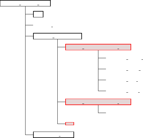
CHAPTER 8. DOING TOMOGRAPHY BASED ON THE SENSITIVITY KERNELS OBTAINED 63
8.2.1 Summing kernels
For summing different event kernels, the executables xsum_kernels and xsum_preconditioned_kernels
can be used. The binaries sum up either a set of isotropic or transversely isotropic kernel files, depending on the setting
in file setup/constants_tomography.h. The following parameterizations can be chosen:
- isotropic kernels Kα,β,ρ or
- isotropic bulk kernels Kc,β,ρ, or
- transversely isotropic bulk kernels Kc,βv,βh,η.
The tools for summing event kernels can be used in parallel, using the same number of processes (NPROC) as the
forward/kernel simulations. The summation tools use the following input/output format (see Fig. 8.1 for the default
directory structure):
-Input: Input is provided by a list of event directories, given in file kernels_list.txt (default setting for
KERNEL_FILE_LIST in constants_tomography.h). The file lists all event kernel directories which
should be summed together. All event directories have to be located in directory INPUT_KERNELS/, which
can be setup as links to all individual event kernel directories.
-Output: The summed kernels will be stored in corresponding kernel files in output directory OUTPUT_SUM/.
TOMO ROOT DIR
bin
kernels list.txt
INPUT KERNELS
event1 DATABASES MPI
proc*** alpha kernel.bin
proc*** beta kernel.bin
proc*** rho kernel.bin
proc*** hess kernel.bin
event2 DATABASES MPI
....
....
OUTPUT SUM
Figure 8.1: Example directory structure when using tomographic tools for summation. Event directory names (red)
can be chosen freely with corresponding name entries in file kernels_list.txt
Kernel summation: As example with a total of 4 MPI processes
mpirun -np 4 ./bin/xsum_kernels
adds sensitivity kernels Kfrom different events together, i.e. outputs gwhere
g=
N
X
i
Ki
for events i= 1, .., N as specified in file kernel_list.txt.

CHAPTER 8. DOING TOMOGRAPHY BASED ON THE SENSITIVITY KERNELS OBTAINED 64
Kernel Summation with Preconditioning: As example with a total of 4 MPI processes
mpirun -np 4 ./bin/xsum_preconditioned_kernels
adds sensitivity kernels Ktogether from different events and "preconditions" the sum by dividing with the sum
of the corresponding approximate Hessians ˜
H, i.e. outputs gwhere
g=1
X
i
˜
HiX
i
Ki
In this case, the factor 1
X
i
˜
Hiacts as preconditioner, approximating the inverse of the Hessian H−1.
Kernel names: The summation tool will look for kernels with following names:
- for an isotropic model parameterization, kernel names are:
## Cartesian version
proc***_alpha_kernel.bin
proc***_beta_kernel.bin
proc***_rho_kernel.bin
## GLOBE version
proc***_reg1_alpha_kernel.bin
proc***_reg1_beta_kernel.bin
proc***_reg1_rho_kernel.bin
- for an isotropic bulk model parameterization, kernel names are:
## Cartesian version
proc***_bulk_kernel.bin
proc***_bulk_beta_kernel.bin
proc***_rho_kernel.bin
## GLOBE version
proc***_reg1_bulk_kernel.bin
proc***_reg1_bulk_beta_kernel.bin
proc***_reg1_rho_kernel.bin
- for a transversely isotropic model parameterization, kernel names are:
## Cartesian version
proc***_bulk_c_kernel.bin
proc***_bulk_betav_kernel.bin
proc***_bulk_betah_kernel.bin
proc***_eta_kernel.bin
## GLOBE version
proc***_reg1_bulk_c_kernel.bin
proc***_reg1_bulk_betav_kernel.bin
proc***_reg1_bulk_betah_kernel.bin
proc***_reg1_eta_kernel.bin
Note that these event kernels are stored after a kernel simulation (SIMULATION_TYPE = 3) in the LOCAL_PATH
directory, which by default points to directory DATABASES_MPI/. Isotropic kernels will be created by de-
fault. To create transversely isotropic kernels, you set ANISOTROPIC_KL and SAVE_TRANSVERSE_KL to
.true. in the parameter file DATA/Par_file.
- for preconditioning, the approximate Hessian kernels taken for summation are:
## Cartesian version
proc***_hess_kernel.bin
## GLOBE version
proc***_reg1_hess_kernel.bin
These Hessian kernels approximate the diagonal elements of the Hessian matrix and can be used as precondi-
tioner in a gradient optimization scheme. To create these kernels, you have to set APPROXIMATE_HESS_KL
to .true. in the parameter file DATA/Par_file.
For SPECFEM3D_GLOBE, by default only kernels in the crust/mantle region ("reg1") will be considered for sum-
mation. You can change the default by setting parameter REG in file constants_tomography.h to the region of
interest.

CHAPTER 8. DOING TOMOGRAPHY BASED ON THE SENSITIVITY KERNELS OBTAINED 65
Note that although we provide the preconditioned summation here, we recommend to smooth first both, the
summed kernels and summed approximate Hessians, before inverting the summed Hessian and applying it as pre-
conditioner to the gradient. From experience, we prefer doing
g=1
Fsmooth N
X
i
˜
Hi!Fsmooth X
i
Ki!
rather than
g=Fsmooth
1
N
X
i
˜
HiX
i
Ki
.
Due to the large sensitivity kernel values close to source and receiver locations, the inverse of the thresholded summed
Hessian becomes better balanced in the former.
8.2.2 Smoothing and post-processing
For additional smoothing and post-processing of kernels, gradients, or models, we provide tools useful for gradient
and model preparation. These additional tools for post-processing sensitivity kernels are provided together with the
main package. For compilation of these tools, you type in the main directory:
make postprocess
The following tools are provided:
-xsmooth_sem is used for smoothing with a gaussian function.
-xclip_sem is used to threshold a kernel, gradient or model, clipping to a minimum and maximum value.
-xcombine_sem is used to combine different event kernels, gradient or model files, summing all individually
specified files together (similar to xsum_kernels but more flexible).
The post-processing tools are primarily intented to be used to process kernel files. They can be used though on any
scalar field of dimension (NGLLX,NGLLY,NGLLZ,NSPEC). The tools are parallel programs – they must be invoked
with mpirun or other appropriate utility. Operations are performed in embarrassingly-parallel fashion.
Smoothing: To smooth a kernel, gradient or model file, use
mpirun -np NPROC bin/xsmooth_sem SIGMA_H SIGMA_V KERNEL_NAME INPUT_DIR OUPUT_DIR
with command line arguments: SIGMA_H horizontal smoothing radius, SIGMA_V vertical smoothing radius,
KERNEL_NAME kernel name, e.g. alpha_kernel,INPUT_DIR directory from which kernels are read,
OUTPUT_DIR directory to which smoothed kernels are written.
Smooths kernels by convolution with a Gaussian. Writes the resulting smoothed kernels to OUTPUT_DIR.
Files written to OUTPUT_DIR have the suffix ’smooth’ appended, e.g. proc***alpha_kernel.bin be-
comes proc***alpha_kernel_smooth.bin.
Clipping: Values in a kernel, gradient or model binary file can be clipped with a minimum/maximum threshold value
using
mpirun -np NPROC bin/xclip_sem MIN_VAL MAX_VAL KERNEL_NAMES INPUT_FILE OUTPUT_DIR
CHAPTER 8. DOING TOMOGRAPHY BASED ON THE SENSITIVITY KERNELS OBTAINED 66
with command line arguments: MIN_VAL threshold below which array values are clipped, MAX_VAL thresh-
old above which array values are clipped, KERNEL_NAMES one or more kernel names separated by commas,
INPUT_DIR directory from which arrays are read, OUTPUT_DIR directory to which clipped array are written.
For each name in KERNEL_NAMES, reads kernels from INPUT_DIR, applies thresholds, and writes the result-
ing clipped kernels to OUTPUT_DIR.
KERNEL_NAMES is a comma-delimited list of kernel names, e.g. alphav_kernel,alphah_kernel.
For example, in this case type
mpirun -np 4 ./bin/xclip_sem -0.1 0.1 alphav_kernel,alphah_kernel DIR1/ DIR1/
to clip the corresponding kernels in directory DIR1 to be in range [−0.1,0.1].
Files written to OUTPUT_DIR have the suffix ’clip’ appended, e.g. proc***alpha_kernel.bin becomes
proc***alpha_kernel_clip.bin
Combining: To combine kernel values from different kernel directories, you can use
mpirun -np NPROC bin/xcombine_sem KERNEL_NAMES INPUT_FILE OUTPUT_DIR
with command line arguments: KERNEL_NAMES one or more kernel names separated by commas, INPUT_FILE
text file containing list of kernel directories, OUTPUT_PATH directory to which summed kernels are written.
For each name in KERNEL_NAMES, sums kernels from directories specified in INPUT_FILE. Writes the re-
sulting sums to OUTPUT_DIR.
INPUT_FILE is a text file containing a list of absolute or relative paths to kernel directories, one directory per
line.
KERNEL_NAMES is a comma-delimited list of kernel names, e.g. alpha_kernel,beta_kernel,rho_kernel.
8.2.3 Model updating
We provide (simple) tools for updating the current model miusing a gradient gand steplength α:, i.e.
mi+i=mi+δm
with
δm=−αg.
The following tomographic tools are provided:
-xadd_model_iso can be used to update isotropic model files with a (summed & smoothed) gradient. The
gradient files are given for isotropic parameters or isotropic bulk parameters.
Note that instead of using the density kernels Kρfor model updates, setting USE_RHO_SCALING to .true.
will ignore the density kernel and use density perturbations scaled from isotropic Vspertubations.
Isotropic model update: The program xadd_model_iso can be used to update isotropic model files with (smoothed
& summed) event kernels:
mpirun -np 4 bin/xadd_model_iso step_factor [INPUT-KERNELS-DIR/] [OUTPUT-MODEL-DIR/]
with command line arguments: step_factor the step length to scale the gradient, e.g. 0.03 for a ±3% update,
INPUT-KERNELS-DIR/ (optional) directory which holds summed kernels (e.g. proc***alpha_kernel.bin,..,
by default directory INPUT_GRADIENT/ is used), OUTPUT-MODEL-DIR/ (optional) directory which will
hold new model files (e.g. proc***vp_new.bin,.., by default directory OUTPUT_MODEL/ is used).
The gradients are given for isotropic parameters (alpha,beta,rho) or (bulk_c,beta,rho).
The algorithm uses a steepest descent method with a step length determined by the given maximum update
percentage.
By default, the directory and file setup used is:
CHAPTER 8. DOING TOMOGRAPHY BASED ON THE SENSITIVITY KERNELS OBTAINED 67
- directory INPUT_MODEL/ contains:
proc***_vs.bin
proc***_vp.bin
proc***_rho.bin
- directory INPUT_GRADIENT/ contains:
proc***_bulk_c_kernel_smooth.bin
proc***_bulk_beta_kernel_smooth.bin
proc***_rho_kernel_smooth.bin
or
proc***_alpha_kernel_smooth.bin
proc***_beta_kernel_smooth.bin
proc***_rho_kernel_smooth.bin
depending on the model parameterization.
- directory topo/ contains:
proc***_external_mesh.bin
for the Cartesian version, and
proc***_solver_data.bin
for the GLOBE version.
The new model files are stored in directory OUTPUT_MODEL/ as
proc***_vp_new.bin
proc***_vs_new.bin
proc***_rho_new.bin
Note that additional post-processing and model update tools are provided for the SPECFEM3D_GLOBE version
and will be provided for the Cartesian version as well in future.
8.3 OLD VERSION OF THE SECTION, WILL SOON BE IMPROVED
AND ENRICHED
There are many other versions of gradient-based inversion algorithms that could alternatively be used (see e.g. Virieux
and Operto [2009], Monteiller et al. [2015] for a list). The tomographic inversion of Tape et al. [2009,2010] used
SPECFEM3D_Cartesian as well as several additional components which are also stored on the CIG svn server, de-
scribed next.
The directory containing external utilities for tomographic inversion using SPECFEM3D Cartesian (or other pack-
ages that evaluate misfit functions and gradients) is in directory utils/ADJOINT_TOMOGRAPHY_TOOLS/:
flexwin/ -- FLEXWIN algorithm for automated picking of time windows
measure_adj/ -- reads FLEXWIN output file and makes measurements,
with the option for computing adjoint sources
iterate_adj/ -- various tools for iterative inversion
(requires pre-computed "event kernels")
This directory also contains a brief README file indicating the role of the three subdirectories, flexwin [Maggi et al.,
2009], measure_adj, and iterate_adj. The components for making the model update are there; however, there
are no explicit rules for computing the model update, just as with any optimization problem. There are options for
computing a conjugate gradient step, as well as a source subspace projection step.
The best single file to read is probably: ADJOINT_TOMO/iterate_adj/cluster/README.
Chapter 9
Performing full waveform inversion (FWI)
or source inversions
ANNOUNCEMENT: SPECFEM3D can now perform full waveform inver-
sion (FWI), i.e. invert for models in an iterative fashion, and it can also per-
form source inversions in a constant model; please refer to the two new direc-
tories, inverse_problem_for_model and inverse_problem_for_source,
and the README files they contain. For FWI inversions for the model, also
refer to the new examples provided in directory EXAMPLES.
68
Chapter 10
Noise Cross-correlation Simulations
Besides earthquake simulations, SPECFEM3D Cartesian includes functionality for seismic noise tomography as well.
In order to proceed successfully in this chapter, it is critical that you have already familiarized yourself with procedures
for meshing (Chapter 3), creating distributed databases (Chapter 4), running earthquake simulations (Chapters 5) and
adjoint simulations (Chapter 7). Also, make sure you read the article ‘Noise cross-correlation sensitivity kernels’
[Tromp et al.,2010b], in order to understand noise simulations from a theoretical perspective.
10.1 Input Parameter Files
As usual, the three main input files are crucial: Par_file,CMTSOLUTION and STATIONS. Unless otherwise spec-
ified, those input files should be located in directory DATA/.
CMTSOLUTION is required for all simulations. At a first glance, it may seem unexpected to have it here, since the
noise simulations should have nothing to do with the earthquake – CMTSOLUTION. However, for noise simulations, it
is critical to have no earthquakes. In other words, the moment tensor specified in CMTSOLUTION must be set to zero
manually!
STATIONS remains the same as in previous earthquake simulations, except that the order of receivers listed in
STATIONS is now important. The order will be used to determine the ‘master’ receiver, i.e., the one that simultane-
ously cross correlates with the others.
Par_file also requires careful attention. A parameter called NOISE_TOMOGRAPHY has been added which
specifies the type of simulation to be run. NOISE_TOMOGRAPHY is an integer with possible values 0, 1, 2 and 3. For
example, when NOISE_TOMOGRAPHY equals 0, a regular earthquake simulation will be run. When it is 1/2/3, you
are about to run step 1/2/3 of the noise simulations respectively. Should you be confused by the three steps, refer to
Tromp et al. [2010b] for details.
Another change to Par_file involves the parameter NSTEP. While for regular earthquake simulations this
parameter specifies the length of synthetic seismograms generated, for noise simulations it specifies the length of
the seismograms used to compute cross correlations. The actual cross correlations are thus twice this length, i.e.,
2 NSTEP −1. The code automatically makes the modification accordingly, if NOISE_TOMOGRAPHY is not zero.
There are other parameters in Par_file which should be given specific values. For instance, since the first
two steps for calculating noise sensitivity kernels correspond to forward simulations, SIMULATION_TYPE must be
1 when NOISE_TOMOGRAPHY equals 1 or 2. Also, we have to reconstruct the ensemble forward wavefields in adjoint
simulations, therefore we need to set SAVE_FORWARD to .true. for the second step, i.e., when NOISE_TOMOGRAPHY
equals 2. The third step is for kernel constructions. Hence SIMULATION_TYPE should be 3, whereas SAVE_FORWARD
must be .false..
69
CHAPTER 10. NOISE CROSS-CORRELATION SIMULATIONS 70
Finally, for most system architectures, please make sure that LOCAL_PATH in Par_file is in fact local, not
globally shared. Because we have to save the wavefields at the earth’s surface at every time step, it is quite problematic
to have a globally shared LOCAL_PATH, in terms of both disk storage and I/O speed.
10.2 Noise Simulations: Step by Step
Proper parameters in those parameter files are not enough for noise simulations to run. We have more parameters to
specify: for example, the ensemble-averaged noise spectrum, the noise distribution etc. However, since there are a few
‘new’ files, it is better to introduce them sequentially. In this section, standard procedures for noise simulations are
described.
10.2.1 Pre-simulation
• As usual, we first configure the software package using:
./configure FC=ifort MPIFC=mpif90
Use the following if SCOTCH is needed:
./configure FC=ifort MPIFC=mpif90 --with-scotch-dir=/opt/scotch
• Next, we need to compile the source code using:
make xgenerate_databases
make xspecfem3D
• Before we can run noise simulations, we have to specify the noise statistics, e.g., the ensemble-averaged noise
spectrum. Matlab scripts are provided to help you to generate the necessary file:
EXAMPLES/noise_tomography/NOISE_TOMOGRAPHY.m (main program)
EXAMPLES/noise_tomography/PetersonNoiseModel.m
In Matlab, simply run:
NOISE_TOMOGRAPHY(NSTEP, DT, Tmin, Tmax, NOISE_MODEL)
DT is given in Par_file, but NSTEP is NOT the one specified in Par_file.Instead, you have to feed
2 NSTEP −1to account for the doubled length of cross correlations.Tmin and Tmax correspond to the
period range you are interested in, whereas NOISE_MODEL denotes the noise model you will be using (’NLNM’
for New Low Noise Model or ’NHNM’ for New High Noise Model). Details can be found in the Matlab script.
After running the Matlab script, you will be given the following information (plus a figure in Matlab):
*************************************************************
the source time function has been saved in:
..../S_squared (note this path must be different)
S_squared should be put into directory:
./NOISE_TOMOGRAPHY/ in the SPECFEM3D Cartesian package
In other words, the Matlab script creates a file called S_squared, which is the first ‘new’ input file we en-
counter for noise simulations.
One may choose a flat noise spectrum rather than Peterson’s noise model. This can be done easily by modifying
the Matlab script a little.
CHAPTER 10. NOISE CROSS-CORRELATION SIMULATIONS 71
• Create a new directory in the SPECFEM3D Cartesian package, name it as ./NOISE_TOMOGRAPHY/. We will
add some parameter files later in this folder.
• Put the Matlab-generated-file S_squared in ./NOISE_TOMOGRAPHY/.
That’s to say, you will have a file ./NOISE_TOMOGRAPHY/S_squared in the example provided in the
SPECFEM3D Cartesian package.
• Create a file called ./NOISE_TOMOGRAPHY/irec_master_noise. Note that this file is located in direc-
tory ./NOISE_TOMOGRAPHY/ as well. In general, all noise simulation related parameter files go into that
directory. irec_master_noise contains only one integer, which is the ID of the ‘master’ receiver. For ex-
ample, if this file contains 5, it means that the fifth receiver listed in DATA/STATIONS becomes the ‘master’.
That’s why we mentioned previously that the order of receivers in DATA/STATIONS is important.
Note that in some simulations, the DATA/STATIONS might contain receivers which are outside of our computa-
tional domains. Therefore, the integer in irec_master_noise is actually the ID in DATA/STATIONS_FILTERED
(which is generated by bin/xgenerate_databases).
• Create a file called ./NOISE_TOMOGRAPHY/nu_master. This file holds three numbers, forming a (unit)
vector. It describes which component we are cross-correlating at the ‘master’ receiver, i.e., ˆναin Tromp et al.
[2010b]. The three numbers correspond to E/N/Z components respectively. Most often, the vertical component
is used, and in those cases the three numbers should be 0, 0 and 1.
• Describe the noise direction and distributions in src/specfem3d/noise_tomography.f90. Search for
a subroutine called noise_distribution_direction in noise_tomography.f90. It is actually
located at the very beginning of noise_tomography.f90. The default assumes vertical noise and a uniform
distribution across the whole free surface of the model. It should be quite self-explanatory for modifications.
Should you modify this part, you have to re-compile the source code.
10.2.2 Simulations
With all of the above done, we can finally launch our simulations. Again, please make sure that the LOCAL_PATH in
DATA/Par_file is not globally shared. It is quite problematic to have a globally shared LOCAL_PATH, in terms
of both disk storage and speed of I/O (we have to save the wavefields at the earth’s surface at every time step).
As discussed in Tromp et al. [2010b], it takes three steps/simulations to obtain one contribution of the ensemble
sensitivity kernels:
• Step 1: simulation for generating wavefields
SIMULATION_TYPE = 1
NOISE_TOMOGRAPHY = 1
SAVE_FORWARD (not used, can be either .true. or .false.)
• Step 2: simulation for ensemble forward wavefields
SIMULATION_TYPE = 1
NOISE_TOMOGRAPHY = 2
SAVE_FORWARD = .true.
• Step 3: simulation for ensemble adjoint wavefields and sensitivity kernels
SIMULATION_TYPE = 3
NOISE_TOMOGRAPHY = 3
SAVE_FORWARD = .false.
Note Step 3 is an adjoint simulation, please refer to previous chapters on how to prepare adjoint sources and
other necessary files, as well as how adjoint simulations work.
CHAPTER 10. NOISE CROSS-CORRELATION SIMULATIONS 72
It is better to run the three steps continuously within the same job on a cluster, otherwise you have to collect the
saved surface movies from the old nodes to the new nodes. This process varies from cluster to cluster and thus cannot
be discussed here. Please ask your cluster administrator for information/configuration of the cluster you are using.
10.2.3 Post-simulation
After those simulations, you have all stuff you need, either in the OUTPUT_FILES/ or in the directory specified by
LOCAL_PATH in DATA/Par_file (which are most probably on local nodes). Collect whatever you want from the
local nodes to your workstation, and then visualize them. This process is the same as what you may have done for
regular earthquake simulations. Refer to other chapters if you have problems.
Simply speaking, two outputs are the most interesting: the simulated ensemble cross correlations and one contri-
bution of the ensemble sensitivity kernels.
The simulated ensemble cross correlations are obtained after the second simulation (Step 2). Seismograms in
OUTPUT_FILES/ are actually the simulated ensemble cross correlations. Collect them immediately after Step 2,
or the Step 3 will overwrite them. Note that we have a ‘master’ receiver specified by irec_master_noise, the
seismogram at one station corresponds to the cross correlation between that station and the ‘master’. Since the seis-
mograms have three components, we may obtain cross correlations for different components as well, not necessarily
the cross correlations between vertical components.
One contribution of the ensemble cross-correlation sensitivity kernels are obtained after Step 3, stored in the
DATA/LOCAL_PATH on local nodes. The ensemble kernel files are named the same as regular earthquake kernels.
You need to run another three simulations to get the other contribution of the ensemble kernels, using different
forward and adjoint sources given in Tromp et al. [2010b].
10.3 Example
In order to illustrate noise simulations in an easy way, one example is provided in EXAMPLES/noise_tomography/.
See EXAMPLES/noise_tomography/README for explanations.
Note, however, that they are created for a specific workstation (CLOVER@PRINCETON), which has at least 4
cores with ‘mpif90’ working properly.
If your workstation is suitable, you can run the example in EXAMPLES/noise_tomography/ using:
./pre-processing.sh
Even if this script does not work on your workstation, the procedure it describes is universal. You may review
the whole process described in the last section by following the commands in pre-processing.sh, which should
contain enough explanations for all the commands.
Chapter 11
Gravity integral calculations for the gravity
field of an Earth model
SPECFEM can now compute the gravity field as well as its derivatives (i.e., gravity gradiometry) generated by any
given 3D Earth model at a given elevation, i.e., on a given observation surface. That feature is still experimental but
should work just fine.
To see how it is implemented and to use it, type this in the root directory of the code:
grep -i GRAVITY_INTEGRALS src/*/*
73
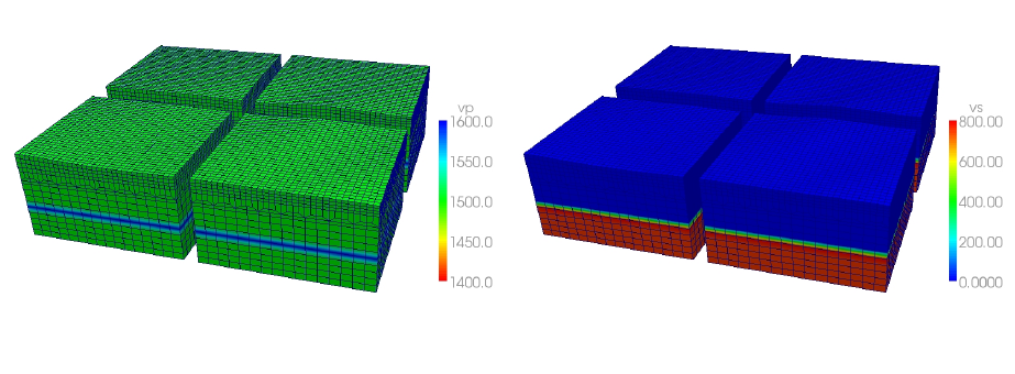
Chapter 12
Graphics
12.1 Meshes
In case you used the internal mesher xmeshfem3D to create and partition your mesh, you can output mesh files in
ABAQUS (.INP) and DX (.dx) format to visualize them. For this, you must set either the flag CREATE_DX_FILES
or CREATE_ABAQUS_FILES to .true. in the mesher’s parameter file Mesh_Par_file prior to running the
mesher (see Chapter 3.2 for details). You can then use AVS (www.avs.com) or OpenDX (www.opendx.org) to
visualize the mesh and MPI partition (slices).
Figure 12.1: Visualization using Paraview of VTK files created by xgenerate_databases showing P- and S-
wave velocities assigned to the mesh points. The mesh was created by xmeshfem3D for 4 processors.
You have also the option to visualize the distributed databases produced by xgenerate_databases using
Paraview (www.paraview.org). For this, you must set the flag SAVE_MESH_FILES to .true. in the main
parameter file Par_file (see Chapter 4.1 for details). This will create VTK files for each single partition. You can
then use Paraview (www.paraview.org) to visualized these partitions.
To visualize seismograms with Paraview, you should turn off the flag SU_FORMAT, and turn on the use binary
seismograms flag. This will generate .bin files, that you can open with Paraview. You have to select the way you open
it ("raw"), and specify the dimensions of the file (NSTEP and NREC).
12.2 Movies
To make a surface or volume movie of the simulation, set parameters MOVIE_SURFACE,MOVIE_VOLUME,MOVIE_TYPE,
and NTSTEP_BETWEEN_FRAMES in the Par_file. Turning on the movie flags, in particular MOVIE_VOLUME,
74

CHAPTER 12. GRAPHICS 75
produces large output files. MOVIE_VOLUME files are saved in the LOCAL_PATH directory, whereas MOVIE_SURFACE
output files are saved in the OUTPUT_FILES directory. We save the displacement field if the parameter SAVE_DISPLACEMENT
is set, otherwise the velocity field is saved. The look of a movie is determined by the half-duration of the source. The
half-duration should be large enough so that the movie does not contain frequencies that are not resolved by the
mesh, i.e., it should not contain numerical noise. This can be accomplished by selecting a CMT HALF_DURATION
> 1.1 ×smallest period (see figure 5.1). When MOVIE_SURFACE = .true., the half duration of each source in the
CMTSOLUTION file is replaced by
p(HALF_DURATION2+HDUR_MOVIE2)
NOTE: If HDUR_MOVIE is set to 0.0, the code will select the appropriate value of 1.1 ×smallest period. As
usual, for a point source one can set half duration in the CMTSOLUTION file to be 0.0 and HDUR_MOVIE = 0.0
in the Par_file to get the highest frequencies resolved by the simulation, but for a finite source one would keep all
the half durations as prescribed by the finite source model and set HDUR_MOVIE = 0.0.
12.2.1 Movie Surface and Shakemaps
When running xspecfem3D with the MOVIE_SURFACE flag turned on, the code outputs moviedata??????
files in the OUTPUT_FILES directory. There are several flags in the main parameter file Par_file that control the
output of these movie data files, please see section 4.1 for more details. Especially, the following parameters affect the
output:
•SAVE_DISPLACEMENT: to save displacement instead of velocity,
•NTSTEP_BETWEEN_FRAMES: to set the timesteps between frames,
•USE_HIGHRES_FOR_MOVIES: to save values at all GLL point instead of element edges.
You can also output shakemaps independant of the MOVIE_SURFACE flag. Shakemaps show the peak-ground val-
ues of the simulation. For creating shakemaps (at the end of the simulation), you would set the parameter CREATE_SHAKEMAP
to .true.. For shakemaps, both the parameters MOVIE_TYPE and USE_HIGHRES_FOR_MOVIES affect the output. The
following setting has an additional affect:
•MOVIE_TYPE: if set to 1, the horizontal peak-ground values of displacement/velocity/acceleration are output. if
set to 2, the maximum length of the particle displacement/velocity/acceleration vector is output. Please be aware
that these peak-ground values can differ from each other.
The movie and shakemap output files are in a custom binary format, but there is a program provided to convert the
output into more user friendly formats:
xcreate_movie_shakemap_AVS_DX_GMT From create_movie_shakemap_AVS_DX_GMT.f90, it out-
puts data in ASCII, OpenDX, or AVS format (also readable in ParaView). Before compiling the code, make sure
you have the file surface_from_mesher.h in the OUTPUT_FILES/ directory. This file will be created
by the solver run. Then type
make xcreate_movie_shakemap_AVS_DX_GMT
and run the executable xcreate_movie_shakemap_AVS_DX_GMT in the main directory. It will create
visualization files in your format of choice. The code will prompt the user for input parameters.
The SPECFEM3D Cartesian code is running in near real-time to produce animations of southern California earth-
quakes via the web; see Southern California ShakeMovie®(www.shakemovie.caltech.edu).
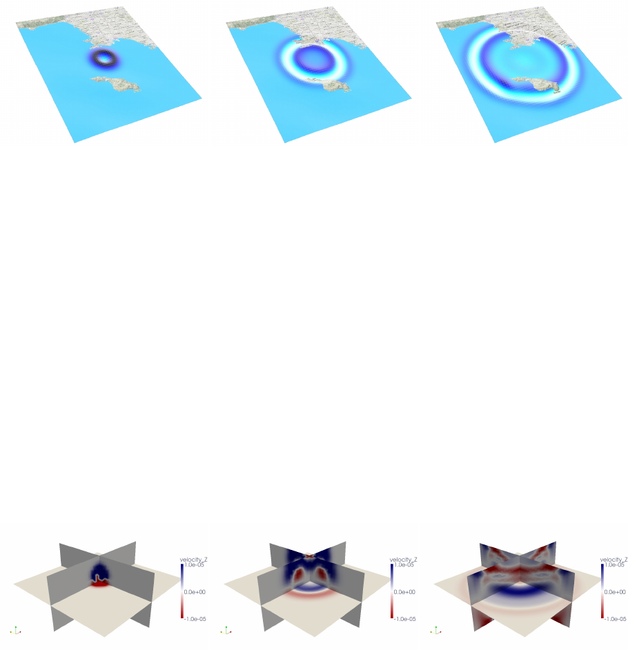
CHAPTER 12. GRAPHICS 76
Figure 12.2: Visualization using AVS files created by xcreate_movie_shakemap_AVS_DX_GMT showing
movie snapshots of vertical velocity components at different times.
12.2.2 Movie Volume
When running xspecfem3D with the MOVIE_VOLUME flag turned on, the code outputs several files in LOCAL_PATH
specified in the main Par_file, e.g. in directory OUTPUT_FILES/DATABASES_MPI. The output is saved by each
processor at the time interval specified by NTSTEP_BETWEEN_FRAMES. For all domains, the velocity field is output to
files:
proc??????_velocity_X_it??????.bin
proc??????_velocity_Y_it??????.bin
proc??????_velocity_Z_it??????.bin
For elastic domains, the divergence and curl taken from the velocity field, i.e. ∇ · vand ∇ × v, get stored as well:
proc??????_div_it??????.bin
proc??????_curl_X_t??????.bin
proc??????_curl_Y_it??????.bin
proc??????_curl_Z_it??????.bin
The files denoted proc??????_div_glob_it??????.bin and proc??????_curl_glob_it??????.bin are stored
on the global points only, all the other arrays are stored on all GLL points. Note that the components X/Y/Z can change
to E/N/Z according to the SUPPRESS_UTM_PROJECTION flag (see also Appendix Aand B).
Figure 12.3: Paraview visualization using movie volume files (converted by xcombine_vol_data and
mesh2vtu.pl) and showing snapshots of vertical velocity components at different times.
To visualize these files, we use an auxiliary program combine_vol_data.f90 to combine the data from all
slices into one mesh file. To compile it in the root directory, type:
make xcombine_vol_data
which will create the executable bin/xcombine_vol_data. To output the usage of this executable, type
./bin/xcombine_vol_data
without arguments.
xcombine_vol_data will combine the data on the different processors (located in OUTPUT_FILES/DATABASES_MPI),
for a given quantity and a given iteration, to one file. For example, if you want to combine velocity_Z, for the
iteration 400 on 4 processors, i.e. if you want to combine these files :
CHAPTER 12. GRAPHICS 77
proc000000_velocity_Z_it000400.bin
proc000001_velocity_Z_it000400.bin
proc000002_velocity_Z_it000400.bin
proc000003_velocity_Z_it000400.bin
You have to go in the directory of the concerned example (where are the directories DATA,OUTPUT_FILES, etc.).
Then, you can launch xcombine_vol_data, specifying the path where it is located. As an example, if the DATA
and OUTPUT_FILES directories of the concerned example are in the root specfem3d directory, xcombine_vol_data
is in ./bin, and you have to type:
./bin/xcombine_vol_data 0 3 velocity_Z_it000400 ./OUTPUT_FILES/DATABASES_MPI ./OUTPUT_FILES 0
Here, 0is the number of the first processor, 3the number of the last one, velocity_Z_it000400 the name
of the files we want to combine without the prefix proc000000*_,./OUTPUT_FILES/DATABASES_MPI the
directory where the files are located, ./OUTPUT_FILES the directory where the combined file will be stored, and 0
is the parameter to create a low-resolution mesh file (1for a high-resolution).
When compiling the code, you will get two executables related to this: xcombine_vol_data, and xcombine_vol_data_vtk.
Use the executable that has the _vtk extension if you want to directly create VTK files. If you use the executable that
does not have the _vtk extension, then the output mesh file will have a name of the form velocity_Z_it000400.mesh.
You will then have to convert the .mesh file into the VTU (Unstructured grid file) format which can be viewed in
ParaView.
For this task, you can use and modify the script mesh2vtu.pl located in directory utils/Visualization/Paraview,
for example:
mesh2vtu.pl -i velocity_Z_it000400.mesh -o velocity_Z_it000400.vtu
Notice that this Perl script uses a program mesh2vtu in the utils/Visualization/Paraview/mesh2vtu
directory, which further uses the VTK (http://www.vtk.org) run-time library for its execution. Therefore, make
sure you have them properly set in the script according to your system.
Then, to do a movie with several iterations, you have to repeat this process for each iteration you want to put in
your movie.
12.3 Finite-Frequency Kernels
The finite-frequency kernels computed as explained in Section 7.2 are saved in the LOCAL_PATH at the end of the
simulation. Therefore, we first need to collect these files on the front end, combine them into one mesh file, and
visualize them with some auxiliary programs.
1. Create slice files
We will only discuss the case of one source-receiver pair, i.e., the so-called banana-doughnut kernels. Although
it is possible to collect the kernel files from all slices on the front end, it usually takes up too much storage space
(at least tens of gigabytes). Since the sensitivity kernels are the strongest along the source-receiver great circle
path, it is sufficient to collect only the slices that are along or close to the great circle path.
A Perl script slice_number.pl located in directory utils/Visualization/Paraview/ can help to
figure out the slice numbers that lie along the great circle path. It applies to meshes created with the internal
mesher xmeshfem3D.
(a) On machines where you have access to the script, copy the Mesh_Par_file, and output_solver
files, and run:
slice_number.pl Mesh_Par_file output_solver.txt slice_file
which will generate a slices_file.
(b) For cases with multiple sources and multiple receivers, you need to provide a slice file before proceeding
to the next step.
CHAPTER 12. GRAPHICS 78
2. Collect the kernel files
After obtaining the slice files, you can collect the corresponding kernel files from the given slices.
(a) You can use or modify the script utils/copy_basin_database.pl to accomplish this:
utils/copy_database.pl slice_file lsf_machine_file filename [jobid]
where lsf_machine_file is the machine file generated by the LSF scheduler, filename is the kernel name
(e.g., rho_kernel,alpha_kernel and beta_kernel), and the optional jobid is the name of the subdirectory
under LOCAL_PATH where all the kernel files are stored.
(b) After executing this script, all the necessary mesh topology files as well as the kernel array files are col-
lected to the local directory of the front end.
3. Combine kernel files into one mesh file
We use an auxiliary program combine_vol_data.f90 to combine the kernel files from all slices into one
mesh file.
(a) Compile it in the root directory:
make xcombine_vol_data
./bin/xcombine_vol_data slice_list filename input_dir output_dir high/low-resolution
where input_dir is the directory where all the individual kernel files are stored, and output_dir is
where the mesh file will be written.
(b) Use 1 for a high-resolution mesh, outputting all the GLL points to the mesh file, or use 0 for low resolution,
outputting only the corner points of the elements to the mesh file.
(c) The output mesh file will have the name filename_rho(alpha,beta).mesh
4. Convert mesh files into .vtu files
(a) We next convert the .mesh file into the VTU (Unstructured grid file) format which can be viewed
in ParaView. For this task, you can use and modify the script mesh2vtu.pl located in directory
utils/Visualization/Paraview/, for example:
mesh2vtu.pl -i file.mesh -o file.vtu
(b) Notice that this Perl script uses a program mesh2vtu in the utils/Visualization/Paraview/mesh2vtu
directory, which further uses the VTK (http://www.vtk.org/) run-time library for its execution.
Therefore, make sure you have them properly set in the script according to your system.
5. Copy over the source and receiver .vtk file
In the case of a single source and a single receiver, the simulation also generates the file sr.vtk located in
the OUTPUT_FILES/ directory to describe the source and receiver locations, which can also be viewed in
Paraview in the next step.
6. View the mesh in ParaView
Finally, we can view the mesh in ParaView (www.paraview.org).
(a) Open ParaView.
(b) From the top menu, File →Open data, select file.vtu, and click the Accept button.
• If the mesh file is of moderate size, it shows up on the screen; otherwise, only the bounding box is
shown.
(c) Click Display Tab →Display Style →Representation and select wireframe of surface to display it.
(d) To create a cross-section of the volumetric mesh, choose Filter →cut, and under Parameters Tab, choose
Cut Function →plane.
(e) Fill in center and normal information given by the global_slice_number.pl script (either from the
standard output or from normal_plane.txt file).
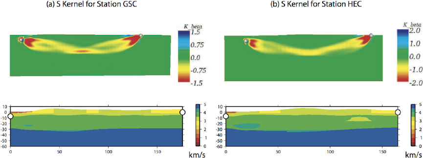
CHAPTER 12. GRAPHICS 79
(f) To change the color scale, go to Display Tab →Color →Edit Color Map and reselect lower and upper
limits, or change the color scheme.
(g) Now load in the source and receiver location file by File →Open data, select sr.vtk, and click the
Accept button. Choose Filter →Glyph, and represent the points by ‘spheres’.
(h) For more information about ParaView, see the ParaView Users Guide (www.paraview.org/files/
v1.6/ParaViewUsersGuide.PDF).
Figure 12.4: (a) Top Panel: Vertical source-receiver cross-section of the S-wave finite-frequency sensitivity kernel Kβ
for station GSC at an epicentral distance of 176 km from the September 3, 2002, Yorba Linda earthquake. Lower
Panel: Vertical source-receiver cross-section of the 3D S-wave speed model used for the spectral-element simulations
[Komatitsch et al.,2004]. (b) The same as (a) but for station HEC at an epicentral distance of 165 km [Liu and Tromp,
2006].
Chapter 13
Running through a Scheduler
The code is usually run on large parallel machines, often PC clusters, most of which use schedulers, i.e., queuing or
batch management systems to manage the running of jobs from a large number of users. The following considerations
need to be taken into account when running on a system that uses a scheduler:
• The processors/nodes to be used for each run are assigned dynamically by the scheduler, based on availability.
Therefore, in order for the xgenerate_databases and the xspecfem3D executables (or between succes-
sive runs of the solver) to have access to the same database files (if they are stored on hard drives local to the
nodes on which the code is run), they must be launched in sequence as a single job.
• On some systems, the nodes to which running jobs are assigned are not configured for compilation. It may
therefore be necessary to pre-compile both the xgenerate_databases and the xspecfem3D executables.
• One feature of schedulers/queuing systems is that they allow submission of multiple jobs in a “launch and
forget” mode. In order to take advantage of this property, care needs to be taken that output and intermediate
files from separate jobs do not overwrite each other, or otherwise interfere with other running jobs.
Examples of job scripts can be found in the utils/Cluster/ directory and can straightforwardly be modified and adapted
to meet more specific running needs.
80
Chapter 14
Changing the Model
In this section we explain how to change the velocity model used for your simulations. These changes involve con-
tributing specific subroutines that replace existing subroutines in the SPECFEM3D Cartesian package. Note that
SPECFEM3D Cartesian can handle Earth models with material properties that vary within each spectral element.
14.1 Using external tomographic Earth models
To implement your own external tomographic model(s), you must provide your own external tomography file(s), and
choose between two possible options:
(1) set in the Par_file the model parameter MODEL = tomo,
or for more user control:
(2) set in the Par_file the model parameter MODEL = default, define the negative material_ID identi-
fier for each element in the file MESH/materials_file and use the following format in the file MESH/nummaterial_velocity_file
when using CUBIT to construct your mesh (see also section 3.1.2):
domain_ID material_ID tomography elastic file_name 1
where:
domain_ID is 1 for acoustic or 2 for elastic materials,
material_ID a negative, unique identifier (i.e., -1,-2,...),
tomography keyword for tomographic material definition,
elastic keyword for elastic material definition,
file_name the name of the tomography file and 1 a positive unique identifier.
The external tomographic model is represented by a grid of points with assigned material properties and homoge-
neous resolution along each spatial direction x, y and z. The ASCII file file_name that describe the tomography
should be located in the TOMOGRAPHY_PATH directory, set in the Par_file. The format of the file, as read from
model_tomography.f90 located in the src/generate_databases directory, looks like Figure 14.1, start-
ing with a header information where
ORIG_X,END_X are, respectively, the coordinates of the initial and final tomographic grid points along the x direction
(in the mesh units, e.g., m);
ORIG_Y,END_Y respectively the coordinates of the initial and final tomographic grid points along the y direction (in
the mesh units, e.g., m);
ORIG_Z,END_Z respectively the coordinates of the initial and final tomographic grid points along the z direction (in
the mesh units, e.g., m);
SPACING_X,SPACING_Y,SPACING_Z the spacing between the tomographic grid points along the x, y and z
directions, respectively (in the mesh units, e.g., m);
81
CHAPTER 14. CHANGING THE MODEL 82
NX,NY,NZ the number of grid points along the spatial directions x, y and z, respectively; NX is given by [(END_X -
ORIG_X)/SPACING_X]+1; NY and NZ are the same as NX, but for the y and z directions, respectively;
VP_MIN,VP_MAX,VS_MIN,VS_MAX,RHO_MIN,RHO_MAX the minimum and maximum values of the wave speed
vp and vs (in m s−1) and of the density rho (in kg m−3); these values could be the actual limits of the
tomographic parameters in the grid or the minimum and maximum values to which we force the cut of velocity
and density in the model.
After the first four lines, the tomography file file_name lists the data record where all tomographic grid points are
listed with the corresponding values of vp,vs and rho (and optionally Qpand Qs), scanning the grid along the x
coordinate (from ORIG_X to END_X with step of SPACING_X) for each given y (from ORIG_Y to END_Y, with step
of SPACING_Y) and each given z (from ORIG_Z to END_Z, with step of SPACING_Z).
Each data record line provides the velocity model values in a format like:
# data record format: purely isotropic model
x y z vp vs rho
..
or
# data record format: anelastic isotropic model
x y z vp vs rho Qp Qs
..
where x,y,zare the grid point position, vp,vs and rho the P- and S-wave speeds and density, and Qp and Qs the
quality factors for P- and S-wave speeds. The quality factors are optional and can be omitted for purely elastic models
(the tomography routine will recognize both formats). Internally, the quality factors will be converted to bulk and
shear attenuation values, Qκand Qµrespectively [Anderson and Hart,1978]. Note that Qmu is always equal to Qs,
but Qkappa is in general not equal to Qp. To convert one to the other see doc/note_on_Qkappa_versus_Qp.pdf and
utils/attenuation/conversion_from_Qkappa_Qmu_to_Qp_Qs_from_Dahlen_Tromp_959_960.f90. For simulations with
attenuation, please note that the Vp- and Vs-velocities of your model are given for a reference frequency. To change
this reference frequency, you change the value of ATTENUATION_f0_REFERENCE in the main constants file
constants.h found in subdirectory src/shared/.
The code uses a constant Qquality factor, write(IMAIN,*) "but approximated based on a series of Zener stan-
dard linear solids (SLS). The approximation is thus performed in a given frequency band determined based on that
ATTENUATION_f0_REFERENCE reference frequency.
The user can implement his own interpolation algorithm for the tomography model by changing the routine
model_tomography.f90 located in the src/generate_databases/ directory. Moreover, for models that
involve both fully defined materials and a tomography description, the nummaterial_velocity_file has mul-
tiple lines each with the corresponding suitable format described above.
Example: External tomography file with variable discretization intervals
The example in Figure 14.1 is for an external tomography file with uniform spacing in the x,y, and zdirections. (Note
that ∆x,∆y, and ∆zneed not be the same as in the example.) In that example, the nummaterial_velocity_file
is
2 -1 tomography elastic tomography_model.xyz 1
and the file tomography_model.xyz will need to reside in DATA/. All entries in the second column of materials_file
will be -1, which means that each element in the mesh will be interpolated according to the values in tomography_model.xyz.
In some cases it may be desirable to have an external tomography model that is described in more than one file.
For example, in cases like southern California, the length scale of variation in the structure of the wave speed model
is much shorter in the sedimentary basin models within the upper 15 km. Therefore one might want to use an external
tomography file that is sampled with, say, ∆x= 1000 m, ∆y= 1000 m, and ∆z= 250 m in the uppermost 15 km,
and then use ∆x= 2000 m, ∆y= 2000 m, and ∆z= 1000 m below a depth of 15 km. If these intervals are chosen
appropriately, then it will result in a pair of external tomography file that is much smaller than the alternative of having
a single file with the fine discretization. In this case nummaterial_velocity_file is
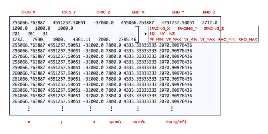
CHAPTER 14. CHANGING THE MODEL 83
Figure 14.1: Tomography file file_name that describes an external, purely elastic Earth model. The coordinates
x, y and z of the grid, their limits ORIG_X, ORIG_Y, ORIG_Z, END_X, END_Y, END_Z and the grid spacings
SPACING_X, SPACING_Y, SPACING_Z should be in the units of the constructed mesh (e.g., UTM coordinates in
meters).
2 -1 tomography elastic file_above_15km.xyz 1
2 -2 tomography elastic file_below_15km.xyz 1
and the files file_above_15km.xyz and file_below_15km.xyz will need to reside in DATA/. All entries
in the second column of materials_file will need to be either -1 or -2, depending on whether the element is
above or below 15 km depth. In this sense, the construction of the mesh and the discretization of the external model
will generally be done in tandem.
Other more complicated discretizations can be used following the same procedure. (In particular, there is no limit
on the number of different external files that are used.)
14.2 External (an)elastic Models
To use your own external model, you can set in the Par_file the model parameter MODEL = external. Three-
dimensional acoustic and/or (an)elastic (attenuation) models may then be superimposed onto the mesh based upon
your subroutine in model_external_values.f90 located in directory src/generate_databases. The
call to this routine would be as follows
call model_external_values(xmesh, ymesh, zmesh, &
rho, vp, vs, qkappa_atten, qmu_atten, iflag_aniso, idomain_id)
Input to this routine consists of:
xmesh,ymesh,zmesh location of mesh point
Output to this routine consists of:
rho,vp,vs isotropic model parameters for density ρ(kg/m3), vp(m/s) and vs(m/s)
qkappa_atten,qmu_atten Bulk and shear wave quality factor: 0< Qκ,µ <9000. Note that Qmu is always
equal to Qs, but Qkappa is in general not equal to Qp. To convert one to the other see doc/note_on_Qkappa_versus_Qp.pdf
and utils/attenuation/conversion_from_Qkappa_Qmu_to_Qp_Qs_from_Dahlen_Tromp_959_960.f90.
CHAPTER 14. CHANGING THE MODEL 84
iflag_aniso anisotropic model flag, 0indicating no anisotropy or 1using anisotropic model parameters as defined
in routine file model_aniso.f90
idomain_id domain identifier, 1for acoustic, 2for elastic, 3for poroelastic materials.
Note that the resolution and maximum value of anelastic models are truncated. This speeds the construction of the
standard linear solids during the meshing stage. To change the resolution, currently at one significant figure following
the decimal, or the maximum value (9000), consult shared/constants.h.
14.3 Anisotropic Models
To use your anisotropic models, you can either set in the Par_file the model parameter ANISOTROPY to .true.
or set the model parameter MODEL = aniso. Three-dimensional anisotropic models may be superimposed on the
mesh based upon the subroutine in file model_aniso.f90 located in directory src/generate_databases.
The call to this subroutine is of the form
call model_aniso(iflag_aniso, rho, vp, vs, &
c11,c12,c13,c14,c15,c16,c22,c23,c24,c25,c26, &
c33,c34,c35,c36,c44,c45,c46,c55,c56,c66)
Input to this routine consists of:
iflag_aniso flag indicating the type of the anisotropic model, i.e. 0for no superimposed anisotropy, 1or 2for
generic pre-defined anisotropic models.
rho,vp,vs reference isotropic model parameters for density ρ,vpand vs.
Output from the routine consists of the following non-dimensional model parameters:
c11,..,c66 21 dimensionalized anisotropic elastic parameters.
You can replace the model_aniso.f90 file by your own version provided you do not change the call structure of
the routine, i.e., the new routine should take exactly the same input and produce the required relative output.
14.4 Using external SEP models
Stanford Exploration Project (SEP) models consists of two files per variables, one header file (.H) and one binary file
(.H@). Among other information, the header file indicates, for each dimension, the offset (o1,o2 and o3 fields),
the spatial step size (d1,d2 and d3 fields) and the number of samples (n1,n2 and n3) necessary to read the linked
binary file (in field).
SEP model reading occurs during database generation. It it the user responsibility to ensure that proper interfaces
between acoustic and elastic domains are set up during the meshing phase. For more information, refer to section 3.2.
In DATA/Par_file,MODEL should be set to sep, and SEP_MODEL_DIRECTORY should point to wherever
your sep model files reside.
Note that in order not to overload the parameter file, SEP header files should be named vp.H,vs.H and rho.H.
The in field in these binary files can be any path as long as it is relative to the previously set SEP_MODEL_DIRECTORY.
We also assume that any dimensional value inside SEP header files is given in meters and that binary files are single
precision floating point numbers stored in little endian format. There is currently only support for vp,vs and rho
variables.
An example demonstrating the use SEP models is given in: EXAMPLES/meshfem3D_examples/sep_bathymetry.
Chapter 15
Post-Processing Scripts
Several post-processing scripts/programs are provided in the utils/ directory, and most of them need to be adjusted
when used on different systems, for example, the path of the executable programs. Here we only list a few of the
available scripts and provide a brief description, and you can either refer to the related sections for detailed usage or,
in a lot of cases, type the script/program name without arguments for its usage.
15.1 Process Data and Synthetics
In many cases, the SEM synthetics are calculated and compared to data seismograms recorded at seismic stations.
Since the SEM synthetics are accurate for a certain frequency range, both the original data and the synthetics need to
be processed before a comparison can be made.
For such comparisons, the following steps are recommended:
1. Make sure that both synthetic and observed seismograms have the correct station/event and timing information.
2. Convolve synthetic seismograms with a source time function with the half duration specified in the CMTSOLUTION
file, provided, as recommended, you used a zero half duration in the SEM simulations.
3. Resample both observed and synthetic seismograms to a common sampling rate.
4. Cut the records using the same window.
5. Remove the trend and mean from the records and taper them.
6. Remove the instrument response from the observed seismograms (recommended) or convolve the synthetic
seismograms with the instrument response.
7. Make sure that you apply the same filters to both observed and synthetic seismograms. Preferably, avoid filtering
your records more than once.
8. Now, you are ready to compare your synthetic and observed seismograms.
We generally use the following scripts provided in the utils/seis_process/ directory:
15.1.1 Data processing script process_data.pl
This script cuts a given portion of the original data, filters it, transfers the data into a displacement record, and picks
the first P and S arrivals. For more functionality, type ‘process_data.pl’ without any argument. An example of
the usage of the script:
process_data.pl -m CMTSOLUTION -s 1.0 -l 0/4000 -i -f -t 40/500 -p -x bp DATA/1999.330*.BH?.SAC
85
CHAPTER 15. POST-PROCESSING SCRIPTS 86
which has resampled the SAC files to a sampling rate of 1 seconds, cut them between 0 and 4000 seconds, transfered
them into displacement records and filtered them between 40 and 500 seconds, picked the first P and S arrivals, and
added suffix ‘bp’ to the file names.
Note that all of the scripts in this section actually use the SAC and/or IASP91 to do the core operations; therefore
make sure that the SAC and IASP91 packages are installed properly on your system, and that all the environment
variables are set properly before running these scripts.
15.1.2 Synthetics processing script process_syn.pl
This script converts the synthetic output from the SEM code from ASCII to SAC format, and performs similar opera-
tions as ‘process_data.pl’. An example of the usage of the script:
process_syn.pl -m CMTSOLUTION -h -a STATIONS -s 1.0 -l 0/4000 -f -t 40/500 -p -x bp SEM/*.BX?.semd
which will convolve the synthetics with a triangular source-time function from the CMTSOLUTION file, convert the
synthetics into SAC format, add event and station information into the SAC headers, resample the SAC files with a
sampling rate of 1 seconds, cut them between 0 and 4000 seconds, filter them between 40 and 500 seconds with the
same filter used for the observed data, pick the first P and S arrivals, and add the suffix ‘bp’ to the file names.
More options are available for this script, such as adding time shift to the origin time of the synthetics, convolving
the synthetics with a triangular source time function with a given half duration, etc. Type process_syn.pl without
any argument for a detailed usage.
In order to convert between SAC format and ASCII files, useful scripts are provided in the subdirectories
utils/sac2000_alpha_convert/ and utils/seis_process/asc2sac/.
15.1.3 Script rotate.pl
The original data and synthetics have three components: vertical (BHZ resp. BXZ), north (BHN resp. BXN) and east
(BHE resp. BXE). However, for most seismology applications, transverse and radial components are also desirable.
Therefore, we need to rotate the horizontal components of both the data and the synthetics to the transverse and radial
direction, and rotate.pl can be used to accomplish this:
rotate.pl -l 0 -L 180 -d DATA/*.BHE.SAC.bp
rotate.pl -l 0 -L 180 SEM/*.BXE.semd.sac.bp
where the first command performs rotation on the SAC data obtained through Seismogram Transfer Program (STP)
(http://www.data.scec.org/STP/stp.html), while the second command rotates the processed SEM syn-
thetics.
15.2 Collect Synthetic Seismograms
The forward and adjoint simulations generate synthetic seismograms in the OUTPUT_FILES/ directory by de-
fault. For the forward simulation, the files are named like NT.STA.BX?.semd for two-column time series, or
NT.STA.BX?.semd.sac for ASCII SAC format, where NT and STA are the network code and station name, and
BX? stands for the component name. Please see the Appendix Aand Bfor further details.
The adjont simulations generate synthetic seismograms with the name NT.S?????.S??.sem (refer to Section
7.1 for details). The kernel simulations output the back-reconstructed synthetic seismogram in the name NT.STA.BX?.semd,
mainly for the purpose of checking the accuracy of the reconstruction. Refer to Section 7.2 for further details.
You do have further options to change this default output behavior, given in the main constants file constants.h
located in src/shared/ directory:
SEISMOGRAMS_BINARY set to .true. to have seismograms written out in binary format.
WRITE_SEISMOGRAMS_BY_MASTER Set to .true. to have only the master process writing out seismograms.
This can be useful on a cluster, where only the master process node has access to the output directory.
CHAPTER 15. POST-PROCESSING SCRIPTS 87
USE_OUTPUT_FILES_PATH Set to .false. to have the seismograms output to LOCAL_PATH directory spec-
ified in the main parameter file DATA/Par_file. In this case, you could collect the synthetics onto the
frontend using the collect_seismo_lsf_multi.pl script located in the utils/Cluster/lsf/ di-
rectory. The usage of the script would be e.g.:
collect_seismo.pl machines DATA/Par_file
where machines is a file containing the node names and DATA/Par_file the parameter file used to extract
the LOCAL_PATH directory used for the simulation.
15.3 Clean Local Database
After all the simulations are done, the seismograms are collected, and the useful database files are copied to the
frontend, you may need to clean the local scratch disk for the next simulation. This is especially important in the case
of kernel simulation, where very large files are generated for the absorbing boundaries to help with the reconstruction
of the regular forward wavefield. A sample script is provided in utils/:
cleanbase.pl machines
where machines is a file containing the node names.
15.4 Plot Movie Snapshots and Synthetic Shakemaps
15.4.1 Script movie2gif.gmt.pl
With the movie data saved in OUTPUT_FILES/ at the end of a movie simulation (MOVIE_SURFACE=.true.), you
can run the ‘create_movie_shakemap_AVS_DX_GMT’ code to convert these binary movie data into GMT xyz files for futher
processing. A sample script movie2gif.gmt.pl is provided to do this conversion, and then plot the movie snapshots in GMT,
for example:
movie2gif.gmt.pl -m CMTSOLUTION -g -f 1/40 -n -2 -p
which for the first through the 40th movie frame, converts the moviedata files into GMT xyz files, interpolates them
using the ’nearneighbor’ command in GMT, and plots them on a 2D topography map. Note that ‘-2’ and ‘-p’ are
both optional.
15.4.2 Script plot_shakemap.gmt.pl
With the shakemap data saved in OUTPUT_FILES/ at the end of a shakemap simulation
(CREATE_SHAKEMAP=.true.), you can also run ‘create_movie_shakemap_AVS_DX_GMT’ code to con-
vert the binary shakemap data into GMT xyz files. A sample script plot_shakemap.gmt.pl is provided to do
this conversion, and then plot the shakemaps in GMT, for example:
plot_shakemap.gmt.pl data _dir type(1,2,3) CMTSOLUTION
where type=1 for a displacement shakemap, 2for velocity, and 3for acceleration.
15.5 Map Local Database
A sample program remap_database is provided to map the local database from a set of machines to another set of
machines. This is especially useful when you want to run mesher and solver, or different types of solvers separately
through a scheduler (refer to Chapter 13).
run_lsf.bash --gm-no-shmem --gm-copy-env remap_database old_machines 150
where old_machines is the LSF machine file used in the previous simulation, and 150 is the number of processors
in total.
Chapter 16
Information for developers of the code, and
for people who want to learn how the
technique works
You can get a very simple 1D version of a demo code (there is one in Fortran and one in Python):
git clone --recursive https://github.com/geodynamics/specfem1d.git
We also have simple 3D demo source codes that implement the SEM in a single, small program, in directory
utils/small_SEM_solvers_in_Fortran_and_C_without_MPI_to_learn of the specfem3d package. They are useful to
learn how the spectral-element method works, and how to write or modify a code to implement it. Also useful to test
new ideas by modifying these simple codes to run some tests. We also have a similar, even simpler, demo source code
for the 2D case in directory
utils/small_SEM_solver_in_Fortran_without_MPI_to_learn of the specfem2d package.
For information on how to contribute to the code, i.e., for how to make your modifications, additions or improvements
part of the official package, see https://github.com/geodynamics/specfem3d/wiki .
88
Notes & Acknowledgments
In order to keep the software package thread-safe in case a multithreaded implementation of MPI is used, developers
should not add modules or common blocks to the source code but rather use regular subroutine arguments (which can
be grouped in “derived types” if needed for clarity).
The Gauss-Lobatto-Legendre subroutines in gll_library.f90 are based in part on software libraries from
the Massachusetts Institute of Technology, Department of Mechanical Engineering (Cambridge, Massachusetts, USA).
The non-structured global numbering software was provided by Paul F. Fischer (Brown University, Providence, Rhode
Island, USA, now at Argonne National Laboratory, USA).
OpenDX (http://www.opendx.org) is open-source based on IBM Data Explorer, AVS (http://www.
avs.com) is a trademark of Advanced Visualization Systems, and ParaView (http://www.paraview.org) is
an open-source visualization platform.
Please e-mail your feedback, questions, comments, and suggestions to the CIG Computational Seismology Mailing
List (cig-seismo@geodynamics.org).
90

Copyright
Main historical authors: Dimitri Komatitsch and Jeroen Tromp
CNRS, France and Princeton University, USA
© October 2017
This program is free software; you can redistribute it and/or modify it under the terms of the GNU General Public
License as published by the Free Software Foundation (see Appendix D).
Please note that by contributing to this code, the developer understands and agrees that this project and contribution
are public and fall under the open source license mentioned above.
Evolution of the code:
MPI v. 3.0, December 2014: many developers. Convolutional PML, LDDRK time scheme, bulk attenuation sup-
port, simultaneous MPI runs, ADIOS file I/O support, new seismogram names, Deville routines for additional GLL
degrees, tomography tools, unit/regression test framework, improved CUDA GPUs performance, additonal GEOCU-
BIT support, better make compilation, git versioning system.
MPI v. 2.1, July 2012: Max Rietmann, Peter Messmer, Daniel Peter, Dimitri Komatitsch, Joseph Charles, Zhinan
Xie: support for CUDA GPUs, better CFL stability for the Stacey absorbing conditions.
MPI v. 2.0, November 2010: Dimitri Komatitsch, Nicolas Le Goff, Roland Martin and Pieyre Le Loher, University
of Pau, France, Daniel Peter, Jeroen Tromp and the Princeton group of developers, Princeton University, USA, and
Emanuele Casarotti, INGV Roma, Italy: support for CUBIT meshes decomposed by SCOTCH; much faster solver
using Michel Deville’s inlined matrix products.
MPI v. 1.4 Dimitri Komatitsch, University of Pau, Qinya Liu and others, Caltech, September 2006: better adjoint
and kernel calculations, faster and better I/Os on very large systems, many small improvements and bug fixes.
MPI v. 1.3 Dimitri Komatitsch, University of Pau, and Qinya Liu, Caltech, July 2005: serial version, regular mesh,
adjoint and kernel calculations, ParaView support.
MPI v. 1.2 Min Chen and Dimitri Komatitsch, Caltech, July 2004: full anisotropy, volume movie.
MPI v. 1.1 Dimitri Komatitsch, Caltech, October 2002: Zhu’s Moho map, scaling of Vswith depth, Hauksson’s
regional model, attenuation, oceans, movies.
MPI v. 1.0 Dimitri Komatitsch, Caltech, USA, May 2002: first MPI version based on global code.
Dimitri Komatitsch, IPG Paris, France, December 1996: first 3-D solver for the CM-5 Connection Machine, par-
allelized on 128 processors using Connection Machine Fortran.
91
Bibliography
C. A. Acosta Minolia and D. A. Kopriva. Discontinuous Galerkin spectral element approximations on moving meshes.
J. Comput. Phys., 230(5):1876–1902, 2011. doi: 10.1016/j.jcp.2010.11.038.
M. Ainsworth and H. Wajid. Dispersive and dissipative behavior of the spectral element method. SIAM Journal on
Numerical Analysis, 47(5):3910–3937, 2009. doi: 10.1137/080724976.
M. Ainsworth and H. Wajid. Optimally blended spectral-finite element scheme for wave propagation and nonstandard
reduced integration. SIAM Journal on Numerical Analysis, 48(1):346–371, 2010. doi: 10.1137/090754017.
M. Ainsworth, P. Monk, and W. Muniz. Dispersive and dissipative properties of discontinuous Galerkin finite element
methods for the second-order wave equation. Journal of Scientific Computing, 27(1):5–40, 2006. doi: 10.1007/
s10915-005-9044-x.
K. Aki and P. G. Richards. Quantitative seismology, theory and methods. W. H. Freeman, San Francisco, USA, 1980.
700 pages.
D. L. Anderson and R. S. Hart. Qof the earth. J. Geophys. Res., 83(B12), 1978.
A. Aravkin, T. van Leeuwen, and F. Herrmann. Robust full-waveform inversion using the Student’s t-distribution. In
SEG Technical Program Expanded Abstracts 2011, pages 2669–2673, 2011. doi: 10.1190/1.3627747.
D. N. Arnold. An interior penalty finite element method with discontinuous elements. SIAM Journal on Numerical
Analysis, 19(4):742–760, 1982. doi: 10.1137/0719052.
A. Bamberger, G. Chavent, and P. Lailly. Une application de la théorie du contrôle à un problème inverse sismique.
Ann. Geophys., 33:183–200, 1977.
A. Bamberger, G. Chavent, C. Hemons, and P. Lailly. Inversion of normal incidence seismograms. Geophysics, 47(5):
757–770, 1982.
M. Benjemaa, N. Glinsky-Olivier, V. M. Cruz-Atienza, J. Virieux, and S. Piperno. Dynamic non-planar crack rupture
by a finite volume method. Geophys. J. Int., 171(1):271–285, 2007. doi: 10.1111/j.1365-246X.2006.03500.x.
M. Benjemaa, N. Glinsky-Olivier, V. M. Cruz-Atienza, and J. Virieux. 3D dynamic rupture simulation by a finite
volume method. Geophys. J. Int., 178(1):541–560, 2009. doi: 10.1111/j.1365-246X.2009.04088.x.
M. Bernacki, S. Lanteri, and S. Piperno. Time-domain parallel simulation of heterogeneous wave propagation on
unstructured grids using explicit, nondiffusive, discontinuous Galerkin methods. J. Comput. Acoust., 14(1):57–81,
2006.
C. Bernardi, Y. Maday, and A. T. Patera. A new nonconforming approach to domain decomposition: the Mortar
element method. In H. Brezis and J. L. Lions, editors, Nonlinear partial differential equations and their applications,
Séminaires du Collège de France, pages 13–51, Paris, 1994. Pitman.
E. Blanc, D. Komatitsch, E. Chaljub, B. Lombard, and Z. Xie. Highly accurate stability-preserving optimization of
the Zener viscoelastic model, with application to wave propagation in the presence of strong attenuation. Geophys.
J. Int., 205(1):427–439, 2016. doi: 10.1093/gji/ggw024.
92
BIBLIOGRAPHY 93
F. Bourdel, P.-A. Mazet, and P. Helluy. Resolution of the non-stationary or harmonic Maxwell equations by a discon-
tinuous finite element method: Application to an E.M.I. (electromagnetic impulse) case. In Proceedings of the 10th
international conference on computing methods in applied sciences and engineering, pages 405–422, Commack,
NY, USA, 1991. Nova Science Publishers.
R. Brossier, S. Operto, and J. Virieux. Which data residual norm for robust elastic frequency-domain full waveform
inversion? Geophysics, 75(3):R37–R46, 2010.
K. P. Bube and R. T. Langan. Hybrid L1/L2minimization with applications to tomography. Geophysics, 62(4):
1183–1195, 1997. doi: 10.1190/1.1444219.
L. Carrington, D. Komatitsch, M. Laurenzano, M. Tikir, D. Michéa, N. Le Goff, A. Snavely, and J. Tromp. High-
frequency simulations of global seismic wave propagation using SPECFEM3D_GLOBE on 62 thousand processor
cores. In Proceedings of the SC’08 ACM/IEEE conference on Supercomputing, pages 60:1–60:11, Austin, Texas,
USA, Nov. 2008. IEEE Press. doi: 10.1145/1413370.1413432. Article #60, Gordon Bell Prize finalist article.
F. Casadei and E. Gabellini. Implementation of a 3D coupled Spectral Element solver for wave propagation and
soil-structure interaction simulations. Technical report, European Commission Joint Research Center Report
EUR17730EN, Ispra, Italy, 1997.
E. Chaljub. Modélisation numérique de la propagation d’ondes sismiques en géométrie sphérique : application à la
sismologie globale (Numerical modeling of the propagation of seismic waves in spherical geometry: application to
global seismology). PhD thesis, Université Paris VII Denis Diderot, Paris, France, 2000.
E. Chaljub, Y. Capdeville, and J. P. Vilotte. Solving elastodynamics in a fluid-solid heterogeneous sphere: a parallel
spectral-element approximation on non-conforming grids. J. Comput. Phys., 187(2):457–491, 2003.
E. Chaljub, D. Komatitsch, J. P. Vilotte, Y. Capdeville, B. Valette, and G. Festa. Spectral element analysis in seismol-
ogy. In R.-S. Wu and V. Maupin, editors, Advances in wave propagation in heterogeneous media, volume 48 of
Advances in Geophysics, pages 365–419. Elsevier - Academic Press, London, UK, 2007.
G. Chavent. Identification of function parameters in partial differential equations. In R. E. Goodson and M. Polis,
editors, Identification of parameter distributed systems, pages 31–48. American Society of Mechanical Engineers,
1974.
M. Chen and J. Tromp. Theoretical and numerical investigations of global and regional seismic wave propagation
in weakly anisotropic earth models. Geophys. J. Int., 168(3):1130–1152, 2007. doi: 10.1111/j.1365-246X.2006.
03218.x.
S. Chevrot, N. Favier, and D. Komatitsch. Shear wave splitting in three-dimensional anisotropic media. Geophys. J.
Int., 159(2):711–720, 2004. doi: 10.1111/j.1365-246X.2004.02432.x.
B. Cockburn, G. E. Karniadakis, and C.-W. Shu. Discontinuous Galerkin Methods: Theory, Computation and Appli-
cations. Springer-Verlag, Heidelberg, Germany, 2000.
G. Cohen. Higher-order numerical methods for transient wave equations. Springer-Verlag, Berlin, Germany, 2002.
349 pages.
G. Cohen, P. Joly, and N. Tordjman. Construction and analysis of higher-order finite elements with mass lumping for
the wave equation. In R. Kleinman, editor, Proceedings of the second international conference on mathematical
and numerical aspects of wave propagation, pages 152–160. SIAM, Philadelphia, Pennsylvania, USA, 1993.
E. Crase, A. Pica, M. Noble, J. McDonald, and A. Tarantola. Robust elastic non-linear waveform inversion: application
to real data. Geophysics, 55:527–538, 1990.
E. C. Cyr, J. N. Shadid, and T. Wildey. Towards efficient backward-in-time adjoint computations using data compres-
sion techniques. Comput. Methods Appl. Mech. Eng., 288:24–44, 2015. doi: 10.1016/j.cma.2014.12.001.
F. A. Dahlen and J. Tromp. Theoretical Global Seismology. Princeton University Press, Princeton, New-Jersey, USA,
1998. 944 pages.
BIBLIOGRAPHY 94
J. D. De Basabe and M. K. Sen. Grid dispersion and stability criteria of some common finite-element methods for
acoustic and elastic wave equations. Geophysics, 72(6):T81–T95, 2007. doi: 10.1190/1.2785046.
J. D. De Basabe and M. K. Sen. Stability of the high-order finite elements for acoustic or elastic wave propagation
with high-order time stepping. Geophys. J. Int., 181(1):577–590, 2010. doi: 10.1111/j.1365-246X.2010.04536.x.
J. D. De Basabe, M. K. Sen, and M. F. Wheeler. The interior penalty discontinuous Galerkin method for elastic wave
propagation: grid dispersion. Geophys. J. Int., 175(1):83–93, 2008. doi: 10.1111/j.1365-246X.2008.03915.x.
J. de la Puente, J. P. Ampuero, and M. Käser. Dynamic rupture modeling on unstructured meshes using a discontinuous
Galerkin method. J. Geophys. Res., 114:B10302, 2009. doi: 10.1029/2008JB006271.
M. O. Deville, P. F. Fischer, and E. H. Mund. High-Order Methods for Incompressible Fluid Flow. Cambridge
University Press, Cambridge, United Kingdom, 2002. 528 pages.
D. S. Dreger and D. V. Helmberger. Broadband modeling of local earthquakes. Bull. seism. Soc. Am., 80:1162–1179,
1990.
S. Duczek, S. Liefold, D. Schmicker, and U. Gabbert. Wave propagation analysis using high-order finite element
methods: Spurious oscillations excited by internal element eigenfrequencies. Technische Mechanik, 34:51–71,
2014.
M. Dumbser and M. Käser. An arbitrary high-order discontinuous Galerkin method for elastic waves on un-
structured meshes-II. The three-dimensional isotropic case. Geophys. J. Int., 167(1):319–336, 2006. doi:
10.1111/j.1365-246X.2006.03120.x.
A. M. Dziewo´
nski and D. L. Anderson. Preliminary reference Earth model. Phys. Earth planet. Inter., 25(4):297–356,
1981.
V. Étienne, E. Chaljub, J. Virieux, and N. Glinsky. An hp-adaptive discontinuous Galerkin finite-element method for
3-D elastic wave modelling. Geophys. J. Int., 183(2):941–962, 2010. doi: 10.1111/j.1365-246X.2010.04764.x.
E. Faccioli, F. Maggio, R. Paolucci, and A. Quarteroni. 2D and 3D elastic wave propagation by a pseudo-spectral
domain decomposition method. J. Seismol., 1:237–251, 1997.
R. S. Falk and G. R. Richter. Explicit finite element methods for symmetric hyperbolic equations. SIAM Journal on
Numerical Analysis, 36(3):935–952, 1999. doi: 10.1137/S0036142997329463.
N. Favier, S. Chevrot, and D. Komatitsch. Near-field influences on shear wave splitting and traveltime sensitivity
kernels. Geophys. J. Int., 156(3):467–482, 2004. doi: 10.1111/j.1365-246X.2004.02178.x.
A. Fichtner, H.-P. Bunge, and H. Igel. The adjoint method in seismology: I. Theory. Phys. Earth planet. Inter., 157
(1-2):86–104, 2006. doi: 10.1016/j.pepi.2006.03.016.
A. Fichtner, H. Igel, H.-P. Bunge, and B. L. N. Kennett. Simulation and inversion of seismic wave propagation on
continental scales based on a spectral-element method. Journal of Numerical Analysis, Industrial and Applied
Mathematics, 4(1-2):11–22, 2009a.
A. Fichtner, B. L. N. Kennett, H. Igel, and H. P. Bunge. Full seismic waveform tomography for upper-mantle structure
in the Australasian region using adjoint methods. Geophys. J. Int., 179(3):1703–1725, 2009b.
C. Geuzaine and J. F. Remacle. Gmsh: a three-dimensional finite element mesh generator with built-in pre- and
post-processing facilities. Int. J. Numer. Methods Eng., 79(11):1309–1331, 2009.
F. X. Giraldo, J. S. Hesthaven, and T. Warburton. Nodal high-order discontinuous Galerkin methods for the spherical
shallow water equations. J. Comput. Phys., 181(2):499–525, 2002. doi: 10.1006/jcph.2002.7139.
L. Godinho, P. A. Mendes, A. Tadeu, A. Cadena-Isaza, C. Smerzini, F. J. Sánchez-Sesma, R. Madec, and D. Ko-
matitsch. Numerical simulation of ground rotations along 2D topographical profiles under the incidence of elastic
plane waves. Bull. seism. Soc. Am., 99(2B):1147–1161, 2009. doi: 10.1785/0120080096.
BIBLIOGRAPHY 95
W. Gropp, E. Lusk, and A. Skjellum. Using MPI, portable parallel programming with the Message-Passing Interface.
MIT Press, Cambridge, USA, 1994.
M. J. Grote, A. Schneebeli, and D. Schötzau. Discontinuous Galerkin finite element method for the wave equation.
SIAM Journal on Numerical Analysis, 44(6):2408–2431, 2006. doi: 10.1137/05063194X.
T. Ha, W. Chung, and C. Shin. Waveform inversion using a back-propagation algorithm and a Huber function norm.
Geophysics, 74(3):R15–R24, 2009. doi: 10.1190/1.3112572.
J. Harms, J.-P. Ampuero, M. Barsuglia, E. Chassande-Mottin, J.-P. Montagner, S. N. Somala, and B. F. Whiting.
Transient gravity perturbations induced by earthquake rupture. Geophys. J. Int., 201(3):1416–1425, 2015. doi:
10.1093/gji/ggv090.
E. Hauksson. Crustal structure and seismicity distribution adjacent to the Pacific and North America plate boundary
in Southern California. J. Geophys. Res., 105:13875–13903, 2000.
F. Q. Hu, M. Y. Hussaini, and P. Rasetarinera. An analysis of the discontinuous Galerkin method for wave propagation
problems. J. Comput. Phys., 151(2):921–946, 1999. doi: 10.1006/jcph.1999.6227.
J. A. Hudson. Scattered waves in the coda of P.J. Geophys. Res., 43:359–374, 1977.
F. B. Jensen, W. A. Kuperman, M. Porter, and H. Schmidt. Computational Ocean Acoustics. Springer-Verlag, Berlin,
Germany, 2nd edition, 2011. 794 pages.
W. Jeong, M. Kang, S. Kim, D.-J. Min, and W.-K. Kim. Full waveform inversion using Student’s tdistribution: a
numerical study for elastic waveform inversion and simultaneous-source method. Pure Appl. Geophys., 172(6):
1491–1509, 2015. doi: 10.1007/s00024-014-1020-7.
C. Ji, S. Tsuboi, D. Komatitsch, and J. Tromp. Rayleigh-wave multipathing along the west coast of North America.
Bull. seism. Soc. Am., 95(6):2115–2124, 2005. doi: 10.1785/0120040180.
C. Johnson and J. Pitkäranta. An analysis of the discontinuous Galerkin method for a scalar hyperbolic equation.
Math. Comp., 46:1–26, 1986. doi: 10.1090/S0025-5718-1986-0815828-4.
G. Karypis and V. Kumar. A fast and high-quality multilevel scheme for partitioning irregular graphs. SIAM Journal
on Scientific Computing, 20(1):359–392, 1998a.
G. Karypis and V. Kumar. Multilevel k-way partitioning scheme for irregular graphs. Journal of Parallel and Dis-
tributed Computing, 48(1):96–129, 1998b.
G. Karypis and V. Kumar. A parallel algorithm for multilevel graph partitioning and sparse matrix ordering. Journal
of Parallel and Distributed Computing, 48:71–85, 1998c.
D. Komatitsch. Méthodes spectrales et éléments spectraux pour l’équation de l’élastodynamique 2D et 3D en milieu
hétérogène (Spectral and spectral-element methods for the 2D and 3D elastodynamics equations in heterogeneous
media). PhD thesis, Institut de Physique du Globe, Paris, France, 1997. 187 pages.
D. Komatitsch. Fluid-solid coupling on a cluster of GPU graphics cards for seismic wave propagation. C. R. Acad.
Sci., Ser. IIb Mec., 339:125–135, 2011. doi: 10.1016/j.crme.2010.11.007.
D. Komatitsch and R. Martin. An unsplit convolutional Perfectly Matched Layer improved at grazing incidence for
the seismic wave equation. Geophysics, 72(5):SM155–SM167, 2007. doi: 10.1190/1.2757586.
D. Komatitsch and J. Tromp. Introduction to the spectral-element method for 3-D seismic wave propagation. Geophys.
J. Int., 139(3):806–822, 1999. doi: 10.1046/j.1365-246x.1999.00967.x.
D. Komatitsch and J. Tromp. Spectral-element simulations of global seismic wave propagation-I. Validation. Geophys.
J. Int., 149(2):390–412, 2002a. doi: 10.1046/j.1365-246X.2002.01653.x.
D. Komatitsch and J. Tromp. Spectral-element simulations of global seismic wave propagation-II. 3-D models, oceans,
rotation, and self-gravitation. Geophys. J. Int., 150(1):303–318, 2002b. doi: 10.1046/j.1365-246X.2002.01716.x.
BIBLIOGRAPHY 96
D. Komatitsch and J. P. Vilotte. The spectral-element method: an efficient tool to simulate the seismic response of 2D
and 3D geological structures. Bull. seism. Soc. Am., 88(2):368–392, 1998.
D. Komatitsch, R. Martin, J. Tromp, M. A. Taylor, and B. A. Wingate. Wave propagation in 2-D elastic media
using a spectral element method with triangles and quadrangles. J. Comput. Acoust., 9(2):703–718, 2001. doi:
10.1142/S0218396X01000796.
D. Komatitsch, J. Ritsema, and J. Tromp. The spectral-element method, Beowulf computing, and global seismology.
Science, 298(5599):1737–1742, 2002. doi: 10.1126/science.1076024.
D. Komatitsch, S. Tsuboi, C. Ji, and J. Tromp. A 14.6 billion degrees of freedom, 5 teraflops, 2.5 terabyte earthquake
simulation on the Earth Simulator. In Proceedings of the SC’03 ACM/IEEE conference on Supercomputing, pages
4–11, Phoenix, Arizona, USA, Nov. 2003. ACM. doi: 10.1145/1048935.1050155. Gordon Bell Prize winner article.
D. Komatitsch, Q. Liu, J. Tromp, P. Süss, C. Stidham, and J. H. Shaw. Simulations of ground motion in the Los
Angeles basin based upon the spectral-element method. Bull. seism. Soc. Am., 94(1):187–206, 2004. doi: 10.1785/
0120030077.
D. Komatitsch, J. Labarta, and D. Michéa. A simulation of seismic wave propagation at high resolution in the inner
core of the Earth on 2166 processors of MareNostrum. Lecture Notes in Computer Science, 5336:364–377, 2008.
D. Komatitsch, D. Michéa, and G. Erlebacher. Porting a high-order finite-element earthquake modeling application to
NVIDIA graphics cards using CUDA. Journal of Parallel and Distributed Computing, 69(5):451–460, 2009. doi:
10.1016/j.jpdc.2009.01.006.
D. Komatitsch, G. Erlebacher, D. Göddeke, and D. Michéa. High-order finite-element seismic wave propagation
modeling with MPI on a large GPU cluster. J. Comput. Phys., 229(20):7692–7714, 2010a. doi: 10.1016/j.jcp.2010.
06.024.
D. Komatitsch, L. P. Vinnik, and S. Chevrot. SHdiff/SVdiff splitting in an isotropic Earth. J. Geophys. Res., 115(B7):
B07312, 2010b. doi: 10.1029/2009JB006795.
D. Komatitsch, Z. Xie, E. Bozda˘
g, E. Sales de Andrade, D. Peter, Q. Liu, and J. Tromp. Anelastic sensitivity kernels
with parsimonious storage for adjoint tomography and full waveform inversion. Geophys. J. Int., 206(3):1467–1478,
2016. doi: 10.1093/gji/ggw224.
D. A. Kopriva. Metric identities and the discontinuous spectral element method on curvilinear meshes. Journal of
Scientific Computing, 26(3):301–327, 2006. doi: 10.1007/s10915-005-9070-8.
D. A. Kopriva, S. L. Woodruff, and M. Y. Hussaini. Computation of electromagnetic scattering with a non-conforming
discontinuous spectral element method. Int. J. Numer. Methods Eng., 53(1):105–122, 2002. doi: 10.1002/nme.394.
S. Krishnan, C. Ji, D. Komatitsch, and J. Tromp. Case studies of damage to tall steel moment-frame buildings in
Southern California during large San Andreas earthquakes. Bull. seism. Soc. Am., 96(4A):1523–1537, 2006a. doi:
10.1785/0120050145.
S. Krishnan, C. Ji, D. Komatitsch, and J. Tromp. Performance of two 18-story steel moment-frame buildings in
Southern California during two large simulated San Andreas earthquakes. Earthquake Spectra, 22(4):1035–1061,
2006b. doi: 10.1193/1.2360698.
M. Kristeková, J. Kristek, and P. Moczo. Time-frequency misfit and goodness-of-fit criteria for quantitative compari-
son of time signals. Geophys. J. Int., 178(2):813–825, 2009. doi: 10.1111/j.1365-246X.2009.04177.x.
P. Lailly. The seismic inverse problem as a sequence of before-stack migrations. In J. B. Bednar, R. Redner, E. Robin-
son, and A. Weglein, editors, Proceedings of the Conference on Inverse Scattering, Theory and Application Ex-
panded Abstracts, pages 206–220, Philadelphia, PA, USA, 1983. Society of Industrial and Applied Mathematics.
S. J. Lee, H. W. Chen, Q. Liu, D. Komatitsch, B. S. Huang, and J. Tromp. Three-dimensional simulations of seismic
wave propagation in the Taipei basin with realistic topography based upon the spectral-element method. Bull. seism.
Soc. Am., 98(1):253–264, 2008. doi: 10.1785/0120070033.
BIBLIOGRAPHY 97
S. J. Lee, Y. C. Chan, D. Komatitsch, B. S. Huang, and J. Tromp. Effects of realistic surface topography on seismic
ground motion in the Yangminshan region of Taiwan based upon the spectral-element method and LiDAR DTM.
Bull. seism. Soc. Am., 99(2A):681–693, 2009a. doi: 10.1785/0120080264.
S. J. Lee, D. Komatitsch, B. S. Huang, and J. Tromp. Effects of topography on seismic wave propagation: An example
from northern Taiwan. Bull. seism. Soc. Am., 99(1):314–325, 2009b. doi: 10.1785/0120080020.
A. Legay, H. W. Wang, and T. Belytschko. Strong and weak arbitrary discontinuities in spectral finite elements. Int. J.
Numer. Methods Eng., 64(8):991–1008, 2005. doi: 10.1002/nme.1388.
P. Lesaint and P. A. Raviart. On a finite-element method for solving the neutron transport equation (Proc. Symposium,
Mathematical Research Center). In U. of Wisconsin-Madison, editor, Mathematical aspects of finite elements in
partial differential equations, volume 33, pages 89–123, New York, USA, 1974. Academic Press.
Q. Liu and J. Tromp. Finite-frequency kernels based on adjoint methods. Bull. seism. Soc. Am., 96(6):2383–2397,
2006. doi: 10.1785/0120060041.
Q. Liu and J. Tromp. Finite-frequency sensitivity kernels for global seismic wave propagation based upon adjoint
methods. Geophys. J. Int., 174(1):265–286, 2008. doi: 10.1111/j.1365-246X.2008.03798.x.
Q. Liu, J. Logan, Y. Tian, H. Abbasi, N. Podhorszki, J. Y. Choi, S. Klasky, R. Tchoua, J. Lofstead, R. Oldfield,
M. Parashar, N. Samatova, K. Schwan, A. Shoshani, M. Wolf, K. Wu, and W. Yu. Hello ADIOS: the challenges and
lessons of developing leadership class I/O frameworks. Concurrency and Computation: Practice and Experience,
pages n/a–n/a, 2013. doi: 10.1002/cpe.3125.
P. Lovely, J. Shaw, Q. Liu, and J. Tromp. A structural model of the Salton Trough and its implications for seismic
hazard. Bull. seism. Soc. Am., 96:1882–1896, 2006.
Y. Maday and A. T. Patera. Spectral-element methods for the incompressible Navier-Stokes equations. In State of the
art survey in computational mechanics, pages 71–143, 1989. A. K. Noor and J. T. Oden editors.
R. Madec, D. Komatitsch, and J. Diaz. Energy-conserving local time stepping based on high-order finite elements for
seismic wave propagation across a fluid-solid interface. Comput. Model. Eng. Sci., 49(2):163–189, 2009.
A. Maggi, C. Tape, M. Chen, D. Chao, and J. Tromp. An automated time-window selection algorithm for seismic
tomography. Geophys. J. Int., 178:257–281, 2009.
R. Martin and D. Komatitsch. An unsplit convolutional perfectly matched layer technique improved at grazing inci-
dence for the viscoelastic wave equation. Geophys. J. Int., 179(1):333–344, 2009. doi: 10.1111/j.1365-246X.2009.
04278.x.
R. Martin, D. Komatitsch, C. Blitz, and N. Le Goff. Simulation of seismic wave propagation in an asteroid based upon
an unstructured MPI spectral-element method: blocking and non-blocking communication strategies. Lecture Notes
in Computer Science, 5336:350–363, 2008a.
R. Martin, D. Komatitsch, and A. Ezziani. An unsplit convolutional perfectly matched layer improved at grazing
incidence for seismic wave equation in poroelastic media. Geophysics, 73(4):T51–T61, 2008b. doi: 10.1190/1.
2939484.
R. Martin, D. Komatitsch, and S. D. Gedney. A variational formulation of a stabilized unsplit convolutional perfectly
matched layer for the isotropic or anisotropic seismic wave equation. Comput. Model. Eng. Sci., 37(3):274–304,
2008c. doi: 10.3970/cmes.2008.037.274.
R. Martin, D. Komatitsch, S. D. Gedney, and E. Bruthiaux. A high-order time and space formulation of the unsplit
perfectly matched layer for the seismic wave equation using Auxiliary Differential Equations (ADE-PML). Comput.
Model. Eng. Sci., 56(1):17–42, 2010. doi: 10.3970/cmes.2010.056.017.
T. Melvin, A. Staniforth, and J. Thuburn. Dispersion analysis of the spectral-element method. Quarterly Journal of
the Royal Meteorological Society, 138(668):1934–1947, 2012. doi: 10.1002/qj.1906.
BIBLIOGRAPHY 98
E. D. Mercerat, J. P. Vilotte, and F. J. Sánchez-Sesma. Triangular spectral-element simulation of two-dimensional
elastic wave propagation using unstructured triangular grids. Geophys. J. Int., 166(2):679–698, 2006.
D. Michéa and D. Komatitsch. Accelerating a 3D finite-difference wave propagation code using GPU graphics cards.
Geophys. J. Int., 182(1):389–402, 2010. doi: 10.1111/j.1365-246X.2010.04616.x.
P. Monk and G. R. Richter. A discontinuous Galerkin method for linear symmetric hyperbolic systems in inhomoge-
neous media. Journal of Scientific Computing, 22-23(1-3):443–477, 2005. doi: 10.1007/s10915-004-4132-5.
V. Monteiller, S. Chevrot, D. Komatitsch, and N. Fuji. A hybrid method to compute short period synthetic seismograms
of teleseismic body waves in a 3-D regional model. Geophys. J. Int., 192(1):230–247, 2013. doi: 10.1093/gji/
ggs006.
V. Monteiller, S. Chevrot, D. Komatitsch, and Y. Wang. Three-dimensional full waveform inversion of short-period
teleseismic wavefields based upon the SEM-DSM hybrid method. Geophys. J. Int., 202(2):811–827, 2015. doi:
10.1093/gji/ggv189.
C. Morency, Y. Luo, and J. Tromp. Finite-frequency kernels for wave propagation in porous media based upon adjoint
methods. Geophys. J. Int., 179:1148–1168, 2009. doi: 10.1111/j.1365-246X.2009.04332.
S. P. Oliveira and G. Seriani. Effect of element distortion on the numerical dispersion of spectral-element methods.
Communications in Computational Physics, 9(4):937–958, 2011.
K. B. Olsen, S. M. Day, and C. R. Bradley. Estimation of Qfor long-period (>2 sec) waves in the Los Angeles basin.
Bull. seism. Soc. Am., 93(2):627–638, 2003.
P. S. Pacheco. Parallel programming with MPI. Morgan Kaufmann Press, San Francisco, USA, 1997.
A. T. Patera. A spectral element method for fluid dynamics: Laminar flow in a channel expansion. J. Comput. Phys.,
54(3):468–488, 1984. doi: 10.1016/0021-9991(84)90128-1.
F. Pellegrini and J. Roman. SCOTCH: A software package for static mapping by dual recursive bipartitioning of
process and architecture graphs. Lecture Notes in Computer Science, 1067:493–498, 1996.
D. Peter, D. Komatitsch, Y. Luo, R. Martin, N. Le Goff, E. Casarotti, P. Le Loher, F. Magnoni, Q. Liu, C. Blitz,
T. Nissen-Meyer, P. Basini, and J. Tromp. Forward and adjoint simulations of seismic wave propagation on fully
unstructured hexahedral meshes. Geophys. J. Int., 186(2):721–739, 2011. doi: 10.1111/j.1365-246X.2011.05044.x.
R. E. Plessix. A review of the adjoint-state method for computing the gradient of a functional with geophysical
applications. Geophys. J. Int., 167(2):495–503, 2006.
E. Priolo, J. M. Carcione, and G. Seriani. Numerical simulation of interface waves by high-order spectral modeling
techniques. J. Acoust. Soc. Am., 95(2):681–693, 1994.
W. H. Reed and T. R. Hill. Triangular mesh methods for the neutron transport equation. Technical Report LA-UR-73-
479, Los Alamos Scientific Laboratory, Los Alamos, USA, 1973.
J. Ritsema, L. A. Rivera, D. Komatitsch, J. Tromp, and H. J. van Heijst. The effects of crust and mantle heterogeneity
on PP/P and SS/S amplitude ratios. Geophys. Res. Lett., 29(10):1430, 2002. doi: 10.1029/2001GL013831.
B. Rivière and M. F. Wheeler. Discontinuous finite element methods for acoustic and elastic wave problems. Contem-
porary Mathematics, 329:271–282, 2003.
F. Rubio Dalmau, M. Hanzich, J. de la Puente, and N. Gutiérrez. Lossy data compression with DCT transforms. In
Proceedings of the EAGE Workshop on High Performance Computing for Upstream, page HPC30, Chania, Crete,
Greece, 2014. doi: 10.3997/2214-4609.20141939.
B. Savage, D. Komatitsch, and J. Tromp. Effects of 3D attenuation on seismic wave amplitude and phase measure-
ments. Bull. seism. Soc. Am., 100(3):1241–1251, 2010. doi: 10.1785/0120090263.
BIBLIOGRAPHY 99
G. Seriani and S. P. Oliveira. Optimal blended spectral-element operators for acoustic wave modeling. Geophysics,
72(5):SM95–SM106, 2007. doi: 10.1190/1.2750715.
G. Seriani and S. P. Oliveira. Dispersion analysis of spectral-element methods for elastic wave propagation. Wave
Motion, 45:729–744, 2008. doi: 10.1016/j.wavemoti.2007.11.007.
G. Seriani and E. Priolo. A spectral element method for acoustic wave simulation in heterogeneous media. Finite
Elements in Analysis and Design, 16:337–348, 1994.
G. Seriani, E. Priolo, and A. Pregarz. Modelling waves in anisotropic media by a spectral element method. In
G. Cohen, editor, Proceedings of the third international conference on mathematical and numerical aspects of wave
propagation, pages 289–298. SIAM, Philadephia, PA, 1995.
A. Sieminski, Q. Liu, J. Trampert, and J. Tromp. Finite-frequency sensitivity of body waves to anisotropy based upon
adjoint methods. Geophys. J. Int., 171:368–389, 2007. doi: 10.1111/j.1365-246X.2007.03528.x.
M. Stupazzini, R. Paolucci, and H. Igel. Near-fault earthquake ground-motion simulation in the grenoble valley by a
high-performance spectral element code. Bull. Seismol. Soc. Am., 99(1):286–301, 2009.
M. P. Süss and J. H. Shaw. P wave seismic velocity structure derived from sonic logs and industry reflection data in
the Los Angeles basin, California. J. Geophys. Res., 108(B3):2170, 2003. doi: 10.1029/2001JB001628.
J. Tago, V. M. Cruz-Atienza, V. Étienne, J. Virieux, M. Benjemaa, and F. J. Sánchez-Sesma. 3D dynamic rupture with
anelastic wave propagation using an hp-adaptive Discontinuous Galerkin method. In Abstract S51A-1915 presented
at 2010 AGU Fall Meeting, San Francisco, California, USA, Dec. 2010.
C. Tape, Q. Liu, and J. Tromp. Finite-frequency tomography using adjoint methods - Methodology and examples using
membrane surface waves. Geophys. J. Int., 168(3):1105–1129, 2007. doi: 10.1111/j.1365-246X.2006.03191.x.
C. Tape, Q. Liu, A. Maggi, and J. Tromp. Adjoint tomography of the southern California crust. Science, 325:988–992,
2009.
C. Tape, Q. Liu, A. Maggi, and J. Tromp. Seismic tomography of the southern California crust based on spectral-
element and adjoint methods. Geophys. J. Int., 180:433–462, 2010.
A. Tarantola. Inversion of seismic reflection data in the acoustic approximation. Geophysics, 49:1259–1266, 1984.
M. A. Taylor and B. A. Wingate. A generalized diagonal mass matrix spectral element method for non-quadrilateral
elements. Appl. Num. Math., 33:259–265, 2000.
S. A. Teukolsky. Short note on the mass matrix for Gauss-Lobatto grid points. J. Comput. Phys., 283:408–413, 2015.
doi: 10.1016/j.jcp.2014.12.012.
P. Tong, C.-W. Chen, D. Komatitsch, P. Basini, and Q. Liu. High-resolution seismic array imaging based on a SEM-FK
hybrid method. Geophys. J. Int., 197(1):369–395, 2014a. doi: 10.1093/gji/ggt508.
P. Tong, D. Komatitsch, T.-L. Tseng, S.-H. Hung, C.-W. Chen, P. Basini, and Q. Liu. A 3-D spectral-element and
frequency-wave number hybrid method for high-resolution seismic array imaging. Geophys. Res. Lett., 41(20):
7025–7034, 2014b. doi: 10.1002/2014GL061644.
J. Tromp and D. Komatitsch. Spectral-element simulations of wave propagation in a laterally homogeneous Earth
model. In E. Boschi, G. Ekström, and A. Morelli, editors, Problems in Geophysics for the New Millennium, pages
351–372. INGV, Roma, Italy, 2000.
J. Tromp, C. Tape, and Q. Liu. Seismic tomography, adjoint methods, time reversal and banana-doughnut kernels.
Geophys. J. Int., 160(1):195–216, 2005. doi: 10.1111/j.1365-246X.2004.02453.x.
J. Tromp, D. Komatitsch, and Q. Liu. Spectral-element and adjoint methods in seismology. Communications in
Computational Physics, 3(1):1–32, 2008.
BIBLIOGRAPHY 100
J. Tromp, D. Komatitsch, V. Hjörleifsdóttir, Q. Liu, H. Zhu, D. Peter, E. Bozda˘
g, D. McRitchie, P. Friberg, C. Trabant,
and A. Hutko. Near real-time simulations of global CMT earthquakes. Geophys. J. Int., 183(1):381–389, 2010a.
doi: 10.1111/j.1365-246X.2010.04734.x.
J. Tromp, Y. Luo, S. Hanasoge, and D. Peter. Noise cross-correlation sensitivity kernels. Geophys. J. Int., 183:
791–819, 2010b. doi: 10.1111/j.1365-246X.2010.04721.x.
S. Tsuboi, D. Komatitsch, C. Ji, and J. Tromp. Broadband modeling of the 2002 Denali fault earthquake on the Earth
Simulator. Phys. Earth planet. Inter., 139(3-4):305–313, 2003. doi: 10.1016/j.pepi.2003.09.012.
R. Vai, J. M. Castillo-Covarrubias, F. J. Sánchez-Sesma, D. Komatitsch, and J. P. Vilotte. Elastic wave propagation
in an irregularly layered medium. Soil Dynamics and Earthquake Engineering, 18(1):11–18, 1999. doi: 10.1016/
S0267-7261(98)00027-X.
K. van Wijk, D. Komatitsch, J. A. Scales, and J. Tromp. Analysis of strong scattering at the micro-scale. J. Acoust.
Soc. Am., 115(3):1006–1011, 2004. doi: 10.1121/1.1647480.
J. Virieux and S. Operto. An overview of full-waveform inversion in exploration geophysics. Geophysics, 74(6):
WCC1–WCC26, 2009. doi: 10.1190/1.3238367.
D. J. Wald and T. H. Heaton. Spatial and temporal distribution of slip for the 1992 Landers, California earthquake.
Bull. seism. Soc. Am., 84:668–691, 1994.
Y. Wang, S. Chevrot, V. Monteiller, D. Komatitsch, F. Mouthereau, G. Manatschal, M. Sylvander, J. Diaz, M. Ruiz,
F. Grimaud, S. Benahmed, H. Pauchet, and R. Martin. The deep roots of the western Pyrenees revealed by full
waveform inversion of teleseismic Pwaves. Geology, 44(6):475–478, 2016. doi: 10.1130/G37812.1.
L. C. Wilcox, G. Stadler, C. Burstedde, and O. Ghattas. A high-order discontinuous Galerkin method for wave
propagation through coupled elastic-acoustic media. J. Comput. Phys., 229(24):9373–9396, 2010. doi: 10.1016/j.
jcp.2010.09.008.
B. A. Wingate and J. P. Boyd. Spectral element methods on triangles for geophysical fluid dynamics problems. In
A. V. Ilin and L. R. Scott, editors, Proceedings of the Third International Conference on Spectral and High-order
Methods, pages 305–314, Houston, Texas, 1996. Houston J. Mathematics.
Z. Xie, D. Komatitsch, R. Martin, and R. Matzen. Improved forward wave propagation and adjoint-based sensitivity
kernel calculations using a numerically stable finite-element PML. Geophys. J. Int., 198(3):1714–1747, 2014. doi:
10.1093/gji/ggu219.
Z. Xie, R. Matzen, P. Cristini, D. Komatitsch, and R. Martin. A perfectly matched layer for fluid-solid problems:
Application to ocean-acoustics simulations with solid ocean bottoms. J. Acoust. Soc. Am., 140(1):165–175, 2016.
doi: 10.1121/1.4954736.
L. Zhu and H. Kanamori. Moho depth variation in southern California from teleseismic receiver functions. J. Geophys.
Res., 105:2969–2980, 2000.
Appendix A
Reference Frame Convention
The code uses the following convention for the Cartesian reference frame:
• the xaxis points East
• the yaxis points North
• the zaxis points up
Note that this convention is different from both the Aki and Richards [1980] convention and the Harvard Centroid-
Moment Tensor (CMT) convention. The Aki & Richards convention is
• the xaxis points North
• the yaxis points East
• the zaxis points down
and the Harvard CMT convention is
• the xaxis points South
• the yaxis points East
• the zaxis points up
Source and receiver locations
The SPECFEM3D Cartesian software code internally uses Cartesian coordinates. The given locations for sources and
receiver locations thus may get converted. Sources and receiver locations are read in from the CMTSOLUTION (or
FORCESOLUTION) and STATIONS files. Note that e.g. the CMTSOLUTION and FORCESOLUTION files denotes
the location by "longitude/latitude/depth". We read in longitude as xcoordinate, latitude as ycoordinate.
In case the flag SUPPRESS_UTM_PROJECTION is set to .false. in the main parameter file (see Chapter 4),
the x/ycoordinates have to be given in degrees and are converted to Cartesian coordinates using a UTM conversion
with the specified UTM zone.
The value for depth (given in km in CMTSOLUTION and FORCESOLUTION) or burial depth (given in min
STATIONS) is evaluated with respect to the surface of the mesh at the specified x/ylocation to find the corresponding z
coordinate. It is possible to use this depth value directly as zcoordinate by changing the flag USE_SOURCES_RECVS_Z
to .true. in the file constants.h located in the src/shared/ subdirectory.
101
APPENDIX A. REFERENCE FRAME CONVENTION 102
Seismogram outputs
The seismogram output directions are given in Cartesian x/y/zdirections and not rotated any further. Changing flags
in constants.h in the src/shared/ subdirectory only rotates the seismogram outputs if receivers are forced to
be located at the surface (RECVS_CAN_BE_BURIED_EXT_MESH set to .false.) and the normal to the surface
at the receiver location should be used (EXT_MESH_RECV_NORMAL set to .true.) as vertical. In this case, the
outputs are rotated to have the vertical component normal to the surface of the mesh, xand ydirections are somewhat
arbitrary orthogonal directions along the surface.
For the labeling of the seismogram channels, see Appendix B. Additionally, we add labels to the synthetics using
the following convention: For a receiver station located in an
elastic domain:
•semd for the displacement vector
•semv for the velocity vector
•sema for the acceleration vector
acoustic domain:
(please note that receiver stations in acoustic domains must be buried. This is due to the free surface condition
which enforces a zero pressure at the surface.)
•semd for the displacement vector
•semv for the velocity vector
•sema for pressure which will be stored in the vertical component Z. Note that pressure in the acoustic
media is isotropic and thus the pressure record would be the same in the other two component directions.
We therefore use the other two seismogram components to store the acoustic potential in component X(or
N) and the first time derivative of the acoustic potential in component Y(or E).
The seismograms are by default written out in ASCII-format to the OUTPUT_FILES/ subdirectory by each parallel
process. You can change this behavior by changing the following flags in the constants.h file located in the
src/shared/ subdirectory:
SEISMOGRAMS_BINARY set to .true. to have seismograms written out in binary format.
WRITE_SEISMOGRAMS_BY_MASTER Set to .true. to have only the master process writing out seismograms.
This can be useful on a cluster, where only the master process node has access to the output directory.
USE_OUTPUT_FILES_PATH Set to .false. to have the seismograms output to LOCAL_PATH directory speci-
fied in the main parameter file DATA/Par_file.
Appendix B
Channel Codes of Seismograms
Seismic networks, such as the Global Seismographic Network (GSN), generally involve various types of instruments
with different bandwidths, sampling properties and component configurations. There are standards to name chan-
nel codes depending on instrument properties. IRIS (http://www.iris.edu) uses SEED format for channel
codes, which are represented by three letters, such as LHN,BHZ, etc. In older versions of the SPECFEM3D Carte-
sian package, a common format was used for the channel codes of all seismograms, which was BHE/BHN/BHZ
for three components. To avoid confusion when comparison are made to observed data, we are now using the
FDSN convention (http://www.fdsn.org/) for SEM seismograms. In the following, we give a brief expla-
nation of the FDSN convention used by IRIS, and how it is adopted in SEM seismograms. Please visit http:
//www.iris.edu/manuals/SEED_appA.htm for further information.
Band code: The first letter in the channel code denotes the band code of seismograms, which depends on the
response band and the sampling rate of instruments. The list of band codes used by IRIS is shown in Figure B.1.
The sampling rate of SEM synthetics is controlled by the resolution of simulations rather than instrument properties.
However, for consistency, we follow the FDSN convention for SEM seismograms governed by their sampling rate.
For SEM synthetics, we consider band codes for which dt ≤1s. IRIS also considers the response band of instru-
ments. For instance, short-period and broad-band seismograms with the same sampling rate correspond to different
band codes, such as S and B, respectively. In such cases, we consider SEM seismograms as broad band, ignoring
the corner period (≥10 s) of the response band of instruments (note that at these resolutions, the minimum period
in the SEM synthetics will be less than 10 s). Accordingly, when you run a simulation the band code will be chosen
depending on the resolution of the synthetics, and channel codes of SEM seismograms will start with either L,M,B,
H,Cor F, shown by red color in the figure.
Instrument code: The second letter in the channel code corresponds to instrument codes, which specify the
family to which the sensor belongs. For instance, Hand Lare used for high-gain and low-gain seismometers, respec-
tively. The instrument code of SEM seismograms will always be X, as assigned by FDSN for synthetic seismograms.
Orientation code: The third letter in channel codes is an orientation code, which generally describes the phys-
ical configuration of the components of instrument packages. SPECFEM3D Cartesian uses the traditional orientation
code E/N/Z (East-West, North-South, Vertical) for three components when a UTM projection is used. If the UTM
conversion is suppressed, i.e. the flag SUPPRESS_UTM_PROJECTION is set to .true., then the three components
are labelled X/Y/Z according to the Cartesian reference frame.
EXAMPLE: The sampling rate is given by DT in the main parameter file Par_file located in the DATA/ subdirec-
tory. Depending on the resolution of your simulations, if you choose a sampling rate greater than 0.01 s and less than
1s, a seismogram recording displacements on the vertical component of a station ASBS (network AZ) will be named
AZ.ASBS.MXZ.semd.sac, whereas it will be AZ.ASBS.BXZ.semd.sac, if the sampling rate is greater than
0.0125 and less equal to 0.1 s.
103

APPENDIX B. CHANNEL CODES OF SEISMOGRAMS 104
Band
code
Band type
Sampling rate (sec)
Corner
period
(sec)
F
...
> 0.0002 to <= 0.001
≥ 10 sec
G
...
> 0.0002 to <= 0.001
< 10 sec
D
...
> 0.001 to <= 0.004
< 10 sec
C
...
> 0.001 to <= 0.004
≥ 10 sec
E
Extremely Short Period
<= 0.0125
< 10 sec
S
Short Period
<= 0.1 to > 0.0125
< 10 sec
H
High Broad Band
<= 0.0125
>= 10 sec
B
Broad Band
<= 0.1 to > 0.0125
>= 10 sec
M
Mid Period
< 1 to > 0.1
L
Long Period
1
V
Very Long Period
10
U
Ultra Long Period
100
R
Extremely Long Period
1000
P
On the order of 0.1 to 1 day
<= 100000 to > 10000
T
On the order of 1 to 10 days
<= 1000000 to > 100000
Q
Greater than 10 days
> 1000000
A
Administrative Instrument Channel
variable
NA
O
Opaque Instrument Channel
variable
NA
Figure B.1: The band code convention is based on the sampling rate and the response band of instruments. Please visit
http://www.iris.edu/manuals/SEED_appA.htm for further information. Grey rows show the relative
band-code range in SPECFEM3D Cartesian, and the band codes used to name SEM seismograms are denoted in red.
Appendix C
Troubleshooting
FAQ
configuration fails:
Examine the log file ’config.log’. It contains detailed informations. In many cases, the paths to these specific
compiler commands F90, CC and MPIF90 will not be correct if ‘./configure‘ fails.
Please make sure that you have a working installation of a Fortran compiler, a C compiler and an MPI imple-
mentation. You should be able to compile this little program code:
program main
include ’mpif.h’
integer, parameter :: CUSTOM_MPI_TYPE = MPI_REAL
integer ier
call MPI_INIT(ier)
call MPI_BARRIER(MPI_COMM_WORLD,ier)
call MPI_FINALIZE(ier)
end
compilation fails stating:
...
obj/program_generate_databases.o: In function ‘MAIN__’:
program_generate_databases.f90:(.text+0x14): undefined reference to ‘_gfortran_set_std’
...
Make sure you’re pointing to the right ’mpif90’ wrapper command.
Normally, this message will appear when you are mixing two different Fortran compilers. That is, using e.g.
gfortran to compile non-MPI files and mpif90, wrapper provided for e.g. ifort, to compile MPI-files.
fix: e.g. specify > ./configure FC=gfortran MPIF90=/usr/local/openmpi-gfortran/bin/mpif90
after executing xmeshfem3D I’ve got elements with skewness of 81% percent, what does this mean: Look at the
skewness table printed in the output_mesher.txt file after executing xmeshfem3D for the example given
in EXAMPLES/meshfem3D_examples/simple_model/:
...
histogram of skewness (0. good - 1. bad):
0.0000000E+00 - 5.0000001E-02 27648 81.81818 %
5.0000001E-02 - 0.1000000 0 0.0000000E+00 %
...
The first line means that you have 27,648 elements with a skewness value between 0 and 0.05 (which means the
element is basically not skewed, just plain regular hexahedral element). The total number of elements you have
in this mesh is (see in the output_mesher.txt file a bit further down):
105
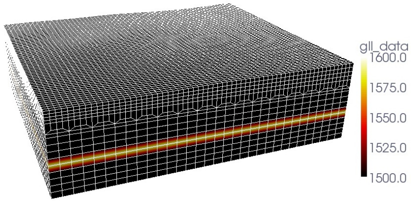
APPENDIX C. TROUBLESHOOTING 106
...
total number of elements in entire mesh: 33792
...
which gives you that: 27,648 / 33,792 ∼81.8 % of all elements are not skewed, i.e. regular elements. a fantastic
value :)
The histogram lists for this mesh also some stronger skewed elements, for example the worst ones belong to:
...
0.6000000 - 0.6500000 2048 6.060606 %
...
about 6 % of all elements have distortions with a skewness value between 0.6 and 0.65. The skewness values
give you a hint of how good your mesh is. In an ideal world, you would want to have no distortions, just
like the 81% from above. Those elements give you the best approximate values by the GLL quadrature used
in the spectral-element method. However, having weakly distorted elements is still fine and the solutions are
still accurate enough. So empirically, values up to around 0.7 are tolerable, above that you should consider
remeshing...
To give you an idea why some of the elements are distorted, see the following figure C.1 of the mesh you obtain
in the example EXAMPLES/meshfem3D_examples/simple_model/.
Figure C.1: Paraview visualization using the mesh vtk-files for the example given in
EXAMPLES/meshfem3D_examples/simple_model/.
You will see that the mesh contains a doubling layer, where we stitch elements together such that the size of two
elements will transition to the size of one element (very useful to keep the ratio of wavespeed / element_size
about constant). Those elements in this doubling layer have higher skewness values and make up those 6 % in
the histogram.
the code gives following error message "need at least one receiver": This means that no stations given in the input
file DATA/STATIONS could be located within the dimensions of the mesh. This can happen for example when
the mesh was created with the in-house mesher xmeshfem3D while using the Universal Transverse Mercator
(UTM) projection but the simulation with xspecfem3D was suppressing this projection from latitude/longitude
to x/y/z coordinates.
In such cases, try to change your DATA/Par_file and set e.g.:
APPENDIX C. TROUBLESHOOTING 107
SUPPRESS_UTM_PROJECTION = .false.
to be the same in Mesh_Par_file and Par_file. This flag should be identical when using the in-house
mesher xmeshfem3D,xgenerate_databases and xspecfem3D together to run simulations.
The flag determines if the coordinates you specify for your source and station locations are given as lat/lon de-
grees and must be converted to UTM coordinates. As an example, if you use .false. within Mesh_Par_file
then you create a mesh with xmeshfem3D using the UTM projection from lat/lon as input format to UTM pro-
jected coordinates to store the mesh point positions, which is fine. The error then may occur if in the Par_file
you have this set to .true. so that the xgenerate_databases and xspecfem3D suppress the UTM pro-
jection and assume that all coordinates you use now for source and receiver locations are given in meters (that
is, converted) already. So it won’t find the specified locations in the used mesh. As a solutions, just change
the flag in Par_file to be the same as in Mesh_Par_file and rerun xgenerate_databases and
xspecfem3D to make sure that your simulation works fine.
I get the following error message "forward simulation became unstable and blew up": In most cases this means
that your time step size DT is chosen too big. Look at your files output_mesher.txt or output_solver.txt
created in the folder OUTPUT_FILES. In these output files, find the section:
...
*********************************************
*** Verification of simulation parameters ***
*********************************************
...
*** Minimum period resolved = 4.308774
*** Maximum suggested time step = 6.8863556E-02
...
then change DT in the DATA/Par_file to be somewhere close to the maximum suggested time step. In the
example above:
DT = 0.05d0
would (most probably) work fine. It could be also bigger than the 0.068 s suggested. This depends a bit on the
distortions of your mesh elements. The more regular they are, the bigger you can choose DT. Just play with this
value a bit and see when the simulation becomes stable ...
Appendix D
License
GNU GENERAL PUBLIC LICENSE
Version 3, 29 June 2007
Copyright © 2007 Free Software Foundation, Inc. http://fsf.org/
Everyone is permitted to copy and distribute verbatim copies of this
license document, but changing it is not allowed.
Preamble
The GNU General Public License is a free, copyleft license for software and other kinds of works.
The licenses for most software and other practical works are designed to take away your freedom to share and
change the works. By contrast, the GNU General Public License is intended to guarantee your freedom to share
and change all versions of a program–to make sure it remains free software for all its users. We, the Free Software
Foundation, use the GNU General Public License for most of our software; it applies also to any other work released
this way by its authors. You can apply it to your programs, too.
When we speak of free software, we are referring to freedom, not price. Our General Public Licenses are designed
to make sure that you have the freedom to distribute copies of free software (and charge for them if you wish), that
you receive source code or can get it if you want it, that you can change the software or use pieces of it in new free
programs, and that you know you can do these things.
To protect your rights, we need to prevent others from denying you these rights or asking you to surrender the rights.
Therefore, you have certain responsibilities if you distribute copies of the software, or if you modify it: responsibilities
to respect the freedom of others.
For example, if you distribute copies of such a program, whether gratis or for a fee, you must pass on to the
recipients the same freedoms that you received. You must make sure that they, too, receive or can get the source code.
And you must show them these terms so they know their rights.
Developers that use the GNU GPL protect your rights with two steps: (1) assert copyright on the software, and (2)
offer you this License giving you legal permission to copy, distribute and/or modify it.
For the developers’ and authors’ protection, the GPL clearly explains that there is no warranty for this free software.
For both users’ and authors’ sake, the GPL requires that modified versions be marked as changed, so that their problems
will not be attributed erroneously to authors of previous versions.
Some devices are designed to deny users access to install or run modified versions of the software inside them,
although the manufacturer can do so. This is fundamentally incompatible with the aim of protecting users’ freedom to
change the software. The systematic pattern of such abuse occurs in the area of products for individuals to use, which
is precisely where it is most unacceptable. Therefore, we have designed this version of the GPL to prohibit the practice
for those products. If such problems arise substantially in other domains, we stand ready to extend this provision to
those domains in future versions of the GPL, as needed to protect the freedom of users.
Finally, every program is threatened constantly by software patents. States should not allow patents to restrict
development and use of software on general-purpose computers, but in those that do, we wish to avoid the special
108
APPENDIX D. LICENSE 109
danger that patents applied to a free program could make it effectively proprietary. To prevent this, the GPL assures
that patents cannot be used to render the program non-free.
The precise terms and conditions for copying, distribution and modification follow.
TERMS AND CONDITIONS
0. Definitions.
“This License” refers to version 3 of the GNU General Public License.
“Copyright” also means copyright-like laws that apply to other kinds of works, such as semiconductor masks.
“The Program” refers to any copyrightable work licensed under this License. Each licensee is addressed as
“you”. “Licensees” and “recipients” may be individuals or organizations.
To “modify” a work means to copy from or adapt all or part of the work in a fashion requiring copyright
permission, other than the making of an exact copy. The resulting work is called a “modified version” of the
earlier work or a work “based on” the earlier work.
A “covered work” means either the unmodified Program or a work based on the Program.
To “propagate” a work means to do anything with it that, without permission, would make you directly or sec-
ondarily liable for infringement under applicable copyright law, except executing it on a computer or modifying
a private copy. Propagation includes copying, distribution (with or without modification), making available to
the public, and in some countries other activities as well.
To “convey” a work means any kind of propagation that enables other parties to make or receive copies. Mere
interaction with a user through a computer network, with no transfer of a copy, is not conveying.
An interactive user interface displays “Appropriate Legal Notices” to the extent that it includes a convenient and
prominently visible feature that (1) displays an appropriate copyright notice, and (2) tells the user that there is
no warranty for the work (except to the extent that warranties are provided), that licensees may convey the work
under this License, and how to view a copy of this License. If the interface presents a list of user commands or
options, such as a menu, a prominent item in the list meets this criterion.
1. Source Code.
The “source code” for a work means the preferred form of the work for making modifications to it. “Object
code” means any non-source form of a work.
A “Standard Interface” means an interface that either is an official standard defined by a recognized standards
body, or, in the case of interfaces specified for a particular programming language, one that is widely used
among developers working in that language.
The “System Libraries” of an executable work include anything, other than the work as a whole, that (a) is
included in the normal form of packaging a Major Component, but which is not part of that Major Component,
and (b) serves only to enable use of the work with that Major Component, or to implement a Standard Interface
for which an implementation is available to the public in source code form. A “Major Component”, in this
context, means a major essential component (kernel, window system, and so on) of the specific operating system
(if any) on which the executable work runs, or a compiler used to produce the work, or an object code interpreter
used to run it.
The “Corresponding Source” for a work in object code form means all the source code needed to generate,
install, and (for an executable work) run the object code and to modify the work, including scripts to control
those activities. However, it does not include the work’s System Libraries, or general-purpose tools or generally
available free programs which are used unmodified in performing those activities but which are not part of the
work. For example, Corresponding Source includes interface definition files associated with source files for the
work, and the source code for shared libraries and dynamically linked subprograms that the work is specifically
designed to require, such as by intimate data communication or control flow between those subprograms and
other parts of the work.
The Corresponding Source need not include anything that users can regenerate automatically from other parts
of the Corresponding Source.
The Corresponding Source for a work in source code form is that same work.
APPENDIX D. LICENSE 110
2. Basic Permissions.
All rights granted under this License are granted for the term of copyright on the Program, and are irrevocable
provided the stated conditions are met. This License explicitly affirms your unlimited permission to run the un-
modified Program. The output from running a covered work is covered by this License only if the output, given
its content, constitutes a covered work. This License acknowledges your rights of fair use or other equivalent,
as provided by copyright law.
You may make, run and propagate covered works that you do not convey, without conditions so long as your
license otherwise remains in force. You may convey covered works to others for the sole purpose of having
them make modifications exclusively for you, or provide you with facilities for running those works, provided
that you comply with the terms of this License in conveying all material for which you do not control copyright.
Those thus making or running the covered works for you must do so exclusively on your behalf, under your
direction and control, on terms that prohibit them from making any copies of your copyrighted material outside
their relationship with you.
Conveying under any other circumstances is permitted solely under the conditions stated below. Sublicensing is
not allowed; section 10 makes it unnecessary.
3. Protecting Users’ Legal Rights From Anti-Circumvention Law.
No covered work shall be deemed part of an effective technological measure under any applicable law fulfill-
ing obligations under article 11 of the WIPO copyright treaty adopted on 20 December 1996, or similar laws
prohibiting or restricting circumvention of such measures.
When you convey a covered work, you waive any legal power to forbid circumvention of technological measures
to the extent such circumvention is effected by exercising rights under this License with respect to the covered
work, and you disclaim any intention to limit operation or modification of the work as a means of enforcing,
against the work’s users, your or third parties’ legal rights to forbid circumvention of technological measures.
4. Conveying Verbatim Copies.
You may convey verbatim copies of the Program’s source code as you receive it, in any medium, provided
that you conspicuously and appropriately publish on each copy an appropriate copyright notice; keep intact all
notices stating that this License and any non-permissive terms added in accord with section 7 apply to the code;
keep intact all notices of the absence of any warranty; and give all recipients a copy of this License along with
the Program.
You may charge any price or no price for each copy that you convey, and you may offer support or warranty
protection for a fee.
5. Conveying Modified Source Versions.
You may convey a work based on the Program, or the modifications to produce it from the Program, in the form
of source code under the terms of section 4, provided that you also meet all of these conditions:
(a) The work must carry prominent notices stating that you modified it, and giving a relevant date.
(b) The work must carry prominent notices stating that it is released under this License and any conditions
added under section 7. This requirement modifies the requirement in section 4 to “keep intact all notices”.
(c) You must license the entire work, as a whole, under this License to anyone who comes into possession of a
copy. This License will therefore apply, along with any applicable section 7 additional terms, to the whole
of the work, and all its parts, regardless of how they are packaged. This License gives no permission to
license the work in any other way, but it does not invalidate such permission if you have separately received
it.
(d) If the work has interactive user interfaces, each must display Appropriate Legal Notices; however, if the
Program has interactive interfaces that do not display Appropriate Legal Notices, your work need not make
them do so.
A compilation of a covered work with other separate and independent works, which are not by their nature
extensions of the covered work, and which are not combined with it such as to form a larger program, in or
APPENDIX D. LICENSE 111
on a volume of a storage or distribution medium, is called an “aggregate” if the compilation and its resulting
copyright are not used to limit the access or legal rights of the compilation’s users beyond what the individual
works permit. Inclusion of a covered work in an aggregate does not cause this License to apply to the other parts
of the aggregate.
6. Conveying Non-Source Forms.
You may convey a covered work in object code form under the terms of sections 4 and 5, provided that you also
convey the machine-readable Corresponding Source under the terms of this License, in one of these ways:
(a) Convey the object code in, or embodied in, a physical product (including a physical distribution medium),
accompanied by the Corresponding Source fixed on a durable physical medium customarily used for soft-
ware interchange.
(b) Convey the object code in, or embodied in, a physical product (including a physical distribution medium),
accompanied by a written offer, valid for at least three years and valid for as long as you offer spare parts
or customer support for that product model, to give anyone who possesses the object code either (1) a copy
of the Corresponding Source for all the software in the product that is covered by this License, on a durable
physical medium customarily used for software interchange, for a price no more than your reasonable cost
of physically performing this conveying of source, or (2) access to copy the Corresponding Source from a
network server at no charge.
(c) Convey individual copies of the object code with a copy of the written offer to provide the Corresponding
Source. This alternative is allowed only occasionally and noncommercially, and only if you received the
object code with such an offer, in accord with subsection 6b.
(d) Convey the object code by offering access from a designated place (gratis or for a charge), and offer
equivalent access to the Corresponding Source in the same way through the same place at no further
charge. You need not require recipients to copy the Corresponding Source along with the object code. If
the place to copy the object code is a network server, the Corresponding Source may be on a different
server (operated by you or a third party) that supports equivalent copying facilities, provided you maintain
clear directions next to the object code saying where to find the Corresponding Source. Regardless of what
server hosts the Corresponding Source, you remain obligated to ensure that it is available for as long as
needed to satisfy these requirements.
(e) Convey the object code using peer-to-peer transmission, provided you inform other peers where the object
code and Corresponding Source of the work are being offered to the general public at no charge under
subsection 6d.
A separable portion of the object code, whose source code is excluded from the Corresponding Source as a
System Library, need not be included in conveying the object code work.
A “User Product” is either (1) a “consumer product”, which means any tangible personal property which is
normally used for personal, family, or household purposes, or (2) anything designed or sold for incorporation
into a dwelling. In determining whether a product is a consumer product, doubtful cases shall be resolved in
favor of coverage. For a particular product received by a particular user, “normally used” refers to a typical or
common use of that class of product, regardless of the status of the particular user or of the way in which the
particular user actually uses, or expects or is expected to use, the product. A product is a consumer product
regardless of whether the product has substantial commercial, industrial or non-consumer uses, unless such uses
represent the only significant mode of use of the product.
“Installation Information” for a User Product means any methods, procedures, authorization keys, or other
information required to install and execute modified versions of a covered work in that User Product from
a modified version of its Corresponding Source. The information must suffice to ensure that the continued
functioning of the modified object code is in no case prevented or interfered with solely because modification
has been made.
If you convey an object code work under this section in, or with, or specifically for use in, a User Product, and
the conveying occurs as part of a transaction in which the right of possession and use of the User Product is
transferred to the recipient in perpetuity or for a fixed term (regardless of how the transaction is characterized),
the Corresponding Source conveyed under this section must be accompanied by the Installation Information.
APPENDIX D. LICENSE 112
But this requirement does not apply if neither you nor any third party retains the ability to install modified
object code on the User Product (for example, the work has been installed in ROM).
The requirement to provide Installation Information does not include a requirement to continue to provide sup-
port service, warranty, or updates for a work that has been modified or installed by the recipient, or for the User
Product in which it has been modified or installed. Access to a network may be denied when the modifica-
tion itself materially and adversely affects the operation of the network or violates the rules and protocols for
communication across the network.
Corresponding Source conveyed, and Installation Information provided, in accord with this section must be in
a format that is publicly documented (and with an implementation available to the public in source code form),
and must require no special password or key for unpacking, reading or copying.
7. Additional Terms.
“Additional permissions” are terms that supplement the terms of this License by making exceptions from one
or more of its conditions. Additional permissions that are applicable to the entire Program shall be treated as
though they were included in this License, to the extent that they are valid under applicable law. If additional
permissions apply only to part of the Program, that part may be used separately under those permissions, but the
entire Program remains governed by this License without regard to the additional permissions.
When you convey a copy of a covered work, you may at your option remove any additional permissions from
that copy, or from any part of it. (Additional permissions may be written to require their own removal in certain
cases when you modify the work.) You may place additional permissions on material, added by you to a covered
work, for which you have or can give appropriate copyright permission.
Notwithstanding any other provision of this License, for material you add to a covered work, you may (if
authorized by the copyright holders of that material) supplement the terms of this License with terms:
(a) Disclaiming warranty or limiting liability differently from the terms of sections 15 and 16 of this License;
or
(b) Requiring preservation of specified reasonable legal notices or author attributions in that material or in the
Appropriate Legal Notices displayed by works containing it; or
(c) Prohibiting misrepresentation of the origin of that material, or requiring that modified versions of such
material be marked in reasonable ways as different from the original version; or
(d) Limiting the use for publicity purposes of names of licensors or authors of the material; or
(e) Declining to grant rights under trademark law for use of some trade names, trademarks, or service marks;
or
(f) Requiring indemnification of licensors and authors of that material by anyone who conveys the material
(or modified versions of it) with contractual assumptions of liability to the recipient, for any liability that
these contractual assumptions directly impose on those licensors and authors.
All other non-permissive additional terms are considered “further restrictions” within the meaning of section
10. If the Program as you received it, or any part of it, contains a notice stating that it is governed by this
License along with a term that is a further restriction, you may remove that term. If a license document contains
a further restriction but permits relicensing or conveying under this License, you may add to a covered work
material governed by the terms of that license document, provided that the further restriction does not survive
such relicensing or conveying.
If you add terms to a covered work in accord with this section, you must place, in the relevant source files, a
statement of the additional terms that apply to those files, or a notice indicating where to find the applicable
terms.
Additional terms, permissive or non-permissive, may be stated in the form of a separately written license, or
stated as exceptions; the above requirements apply either way.
8. Termination.
APPENDIX D. LICENSE 113
You may not propagate or modify a covered work except as expressly provided under this License. Any attempt
otherwise to propagate or modify it is void, and will automatically terminate your rights under this License
(including any patent licenses granted under the third paragraph of section 11).
However, if you cease all violation of this License, then your license from a particular copyright holder is
reinstated (a) provisionally, unless and until the copyright holder explicitly and finally terminates your license,
and (b) permanently, if the copyright holder fails to notify you of the violation by some reasonable means prior
to 60 days after the cessation.
Moreover, your license from a particular copyright holder is reinstated permanently if the copyright holder
notifies you of the violation by some reasonable means, this is the first time you have received notice of violation
of this License (for any work) from that copyright holder, and you cure the violation prior to 30 days after your
receipt of the notice.
Termination of your rights under this section does not terminate the licenses of parties who have received copies
or rights from you under this License. If your rights have been terminated and not permanently reinstated, you
do not qualify to receive new licenses for the same material under section 10.
9. Acceptance Not Required for Having Copies.
You are not required to accept this License in order to receive or run a copy of the Program. Ancillary prop-
agation of a covered work occurring solely as a consequence of using peer-to-peer transmission to receive a
copy likewise does not require acceptance. However, nothing other than this License grants you permission
to propagate or modify any covered work. These actions infringe copyright if you do not accept this License.
Therefore, by modifying or propagating a covered work, you indicate your acceptance of this License to do so.
10. Automatic Licensing of Downstream Recipients.
Each time you convey a covered work, the recipient automatically receives a license from the original licensors,
to run, modify and propagate that work, subject to this License. You are not responsible for enforcing compliance
by third parties with this License.
An “entity transaction” is a transaction transferring control of an organization, or substantially all assets of one,
or subdividing an organization, or merging organizations. If propagation of a covered work results from an
entity transaction, each party to that transaction who receives a copy of the work also receives whatever licenses
to the work the party’s predecessor in interest had or could give under the previous paragraph, plus a right to
possession of the Corresponding Source of the work from the predecessor in interest, if the predecessor has it or
can get it with reasonable efforts.
You may not impose any further restrictions on the exercise of the rights granted or affirmed under this License.
For example, you may not impose a license fee, royalty, or other charge for exercise of rights granted under
this License, and you may not initiate litigation (including a cross-claim or counterclaim in a lawsuit) alleging
that any patent claim is infringed by making, using, selling, offering for sale, or importing the Program or any
portion of it.
11. Patents.
A “contributor” is a copyright holder who authorizes use under this License of the Program or a work on which
the Program is based. The work thus licensed is called the contributor’s “contributor version”.
A contributor’s “essential patent claims” are all patent claims owned or controlled by the contributor, whether
already acquired or hereafter acquired, that would be infringed by some manner, permitted by this License,
of making, using, or selling its contributor version, but do not include claims that would be infringed only
as a consequence of further modification of the contributor version. For purposes of this definition, “control”
includes the right to grant patent sublicenses in a manner consistent with the requirements of this License.
Each contributor grants you a non-exclusive, worldwide, royalty-free patent license under the contributor’s
essential patent claims, to make, use, sell, offer for sale, import and otherwise run, modify and propagate the
contents of its contributor version.
In the following three paragraphs, a “patent license” is any express agreement or commitment, however denomi-
nated, not to enforce a patent (such as an express permission to practice a patent or covenant not to sue for patent
APPENDIX D. LICENSE 114
infringement). To “grant” such a patent license to a party means to make such an agreement or commitment not
to enforce a patent against the party.
If you convey a covered work, knowingly relying on a patent license, and the Corresponding Source of the
work is not available for anyone to copy, free of charge and under the terms of this License, through a publicly
available network server or other readily accessible means, then you must either (1) cause the Corresponding
Source to be so available, or (2) arrange to deprive yourself of the benefit of the patent license for this particular
work, or (3) arrange, in a manner consistent with the requirements of this License, to extend the patent license to
downstream recipients. “Knowingly relying” means you have actual knowledge that, but for the patent license,
your conveying the covered work in a country, or your recipient’s use of the covered work in a country, would
infringe one or more identifiable patents in that country that you have reason to believe are valid.
If, pursuant to or in connection with a single transaction or arrangement, you convey, or propagate by procuring
conveyance of, a covered work, and grant a patent license to some of the parties receiving the covered work
authorizing them to use, propagate, modify or convey a specific copy of the covered work, then the patent
license you grant is automatically extended to all recipients of the covered work and works based on it.
A patent license is “discriminatory” if it does not include within the scope of its coverage, prohibits the exercise
of, or is conditioned on the non-exercise of one or more of the rights that are specifically granted under this
License. You may not convey a covered work if you are a party to an arrangement with a third party that is in
the business of distributing software, under which you make payment to the third party based on the extent of
your activity of conveying the work, and under which the third party grants, to any of the parties who would
receive the covered work from you, a discriminatory patent license (a) in connection with copies of the covered
work conveyed by you (or copies made from those copies), or (b) primarily for and in connection with specific
products or compilations that contain the covered work, unless you entered into that arrangement, or that patent
license was granted, prior to 28 March 2007.
Nothing in this License shall be construed as excluding or limiting any implied license or other defenses to
infringement that may otherwise be available to you under applicable patent law.
12. No Surrender of Others’ Freedom.
If conditions are imposed on you (whether by court order, agreement or otherwise) that contradict the conditions
of this License, they do not excuse you from the conditions of this License. If you cannot convey a covered work
so as to satisfy simultaneously your obligations under this License and any other pertinent obligations, then as
a consequence you may not convey it at all. For example, if you agree to terms that obligate you to collect a
royalty for further conveying from those to whom you convey the Program, the only way you could satisfy both
those terms and this License would be to refrain entirely from conveying the Program.
13. Use with the GNU Affero General Public License.
Notwithstanding any other provision of this License, you have permission to link or combine any covered work
with a work licensed under version 3 of the GNU Affero General Public License into a single combined work,
and to convey the resulting work. The terms of this License will continue to apply to the part which is the
covered work, but the special requirements of the GNU Affero General Public License, section 13, concerning
interaction through a network will apply to the combination as such.
14. Revised Versions of this License.
The Free Software Foundation may publish revised and/or new versions of the GNU General Public License
from time to time. Such new versions will be similar in spirit to the present version, but may differ in detail to
address new problems or concerns.
Each version is given a distinguishing version number. If the Program specifies that a certain numbered version
of the GNU General Public License “or any later version” applies to it, you have the option of following the
terms and conditions either of that numbered version or of any later version published by the Free Software
Foundation. If the Program does not specify a version number of the GNU General Public License, you may
choose any version ever published by the Free Software Foundation.
If the Program specifies that a proxy can decide which future versions of the GNU General Public License can
be used, that proxy’s public statement of acceptance of a version permanently authorizes you to choose that
version for the Program.
APPENDIX D. LICENSE 115
Later license versions may give you additional or different permissions. However, no additional obligations are
imposed on any author or copyright holder as a result of your choosing to follow a later version.
15. Disclaimer of Warranty.
THERE IS NO WARRANTY FOR THE PROGRAM, TO THE EXTENT PERMITTED BY APPLICABLE
LAW. EXCEPT WHEN OTHERWISE STATED IN WRITING THE COPYRIGHT HOLDERS AND/OR
OTHER PARTIES PROVIDE THE PROGRAM “AS IS” WITHOUT WARRANTY OF ANY KIND, EITHER
EXPRESSED OR IMPLIED, INCLUDING, BUT NOT LIMITED TO, THE IMPLIED WARRANTIES OF
MERCHANTABILITY AND FITNESS FOR A PARTICULAR PURPOSE. THE ENTIRE RISK AS TO THE
QUALITY AND PERFORMANCE OF THE PROGRAM IS WITH YOU. SHOULD THE PROGRAM PROVE
DEFECTIVE, YOU ASSUME THE COST OF ALL NECESSARY SERVICING, REPAIR OR CORRECTION.
16. Limitation of Liability.
IN NO EVENT UNLESS REQUIRED BY APPLICABLE LAW OR AGREED TO IN WRITING WILL ANY
COPYRIGHT HOLDER, OR ANY OTHER PARTY WHO MODIFIES AND/OR CONVEYS THE PRO-
GRAM AS PERMITTED ABOVE, BE LIABLE TO YOU FOR DAMAGES, INCLUDING ANY GENERAL,
SPECIAL, INCIDENTAL OR CONSEQUENTIAL DAMAGES ARISING OUT OF THE USE OR INABIL-
ITY TO USE THE PROGRAM (INCLUDING BUT NOT LIMITED TO LOSS OF DATA OR DATA BEING
RENDERED INACCURATE OR LOSSES SUSTAINED BY YOU OR THIRD PARTIES OR A FAILURE OF
THE PROGRAM TO OPERATE WITH ANY OTHER PROGRAMS), EVEN IF SUCH HOLDER OR OTHER
PARTY HAS BEEN ADVISED OF THE POSSIBILITY OF SUCH DAMAGES.
17. Interpretation of Sections 15 and 16.
If the disclaimer of warranty and limitation of liability provided above cannot be given local legal effect accord-
ing to their terms, reviewing courts shall apply local law that most closely approximates an absolute waiver of
all civil liability in connection with the Program, unless a warranty or assumption of liability accompanies a
copy of the Program in return for a fee.
END OF TERMS AND CONDITIONS
How to Apply These Terms to Your New Programs
If you develop a new program, and you want it to be of the greatest possible use to the public, the best way to
achieve this is to make it free software which everyone can redistribute and change under these terms.
To do so, attach the following notices to the program. It is safest to attach them to the start of each source file
to most effectively state the exclusion of warranty; and each file should have at least the “copyright” line and a
pointer to where the full notice is found.
<one line to give the program’s name and a brief idea of what it does.>
Copyright (C) <textyear> <name of author>
This program is free software: you can redistribute it and/or modify
it under the terms of the GNU General Public License as published by
the Free Software Foundation, either version 3 of the License, or
(at your option) any later version.
This program is distributed in the hope that it will be useful,
but WITHOUT ANY WARRANTY; without even the implied warranty of
MERCHANTABILITY or FITNESS FOR A PARTICULAR PURPOSE. See the
GNU General Public License for more details.
You should have received a copy of the GNU General Public License
along with this program. If not, see <http://www.gnu.org/licenses/>.
Also add information on how to contact you by electronic and paper mail.
If the program does terminal interaction, make it output a short notice like this when it starts in an interactive
mode:
APPENDIX D. LICENSE 116
<program> Copyright (C) <year> <name of author>
This program comes with ABSOLUTELY NO WARRANTY; for details type ‘show w’.
This is free software, and you are welcome to redistribute it
under certain conditions; type ‘show c’ for details.
The hypothetical commands show w and show c should show the appropriate parts of the General Public
License. Of course, your program’s commands might be different; for a GUI interface, you would use an “about
box”.
You should also get your employer (if you work as a programmer) or school, if any, to sign a “copyright
disclaimer” for the program, if necessary. For more information on this, and how to apply and follow the GNU
GPL, see http://www.gnu.org/licenses/.
The GNU General Public License does not permit incorporating your program into proprietary programs. If
your program is a subroutine library, you may consider it more useful to permit linking proprietary applications
with the library. If this is what you want to do, use the GNU Lesser General Public License instead of this
License. But first, please read http://www.gnu.org/philosophy/why-not-lgpl.html.
