Manual Get Homologues Est
User Manual:
Open the PDF directly: View PDF ![]() .
.
Page Count: 37
- Description
- Requirements and installation
- User manual
- A few examples
- Extracting coding sequences (CDS) from transcripts
- Clustering orthologous transcripts from FASTA files, one per strain
- Producing a nucleotide-based pangenome matrix
- Estimating protein domain enrichment of some sequence clusters
- Making and annotating a non-redundant pangenome matrix
- Annotating a sequence cluster
- A step-by-step protocol with barley assembled transcripts
- Frequently asked questions (FAQs)
- Credits and references

Contents
1 Description 3
2 Requirements and installation 3
2.1 Perl modules ................................................. 4
2.2 Required binaries ............................................... 4
2.3 Optional software dependencies ....................................... 5
3 User manual 8
3.1 Input data ................................................... 8
3.2 Program options ................................................ 9
3.3 Accompanying scripts ............................................ 14
4 A few examples 16
4.1 Extracting coding sequences (CDS) from transcripts ............................. 16
4.2 Clustering orthologous transcripts from FASTA files, one per strain ..................... 18
4.3 Producing a nucleotide-based pangenome matrix .............................. 23
4.4 Estimating protein domain enrichment of some sequence clusters ...................... 24
4.5 Making and annotating a non-redundant pangenome matrix ......................... 26
4.6 Annotating a sequence cluster ........................................ 28
5 A step-by-step protocol with barley assembled transcripts 30
6 Frequently asked questions (FAQs) 33
7 Credits and references 37
2
1 Description
This document describes GET HOMOLOGUES-EST, a fork of get homologues for clustering homologous gene/transcript
sequences of strains/populations of the same species. This algorithm has been designed and tested with plant transcripts
and CDS sequences, and uses BLASTN to compare DNA sequences. The main tasks for which this was conceived are:
•Finding and translating coding regions (CDSs) within raw transcripts.
•Clustering transcripts/CDS nucleotide sequences in homologous (possibly orthologous) groups, on the grounds of
DNA sequence similarity.
•Definition of pan- and core-transcriptomes by calculation of overlapping sets of CDSs.
The core algorithms of get homologues-est have been adapted from get homologues, and are therefore explained in
manual get homologues.pdf. This document focuses mostly on EST-specific options.
When obtaining twin DNA and peptide CDS files, the output of GET HOMOLOGUES-EST can be used to drive
phylogenomics and population genetics analyses with the kin pipeline GET PHYLOMARKERS.
This table lists features developed for get homologues-est which were not available in the original get homologues
release, although most have been backported.
name description
transcripts2cds.pl Script to extract coding sequences CDS from raw transcripts by combining Transdecoder
and BLASTX.
redundant isoform calling get homologues-est can handle redundant isoforms which otherwise will degrade clustering
performance.
ANI matrices get homologues-est can compute Average Nucleotide Identity (ANI) matrices which sum-
marize the genetic distance among input genotypes.
make nr pangenome matrix.pl Produces a non-redundant pangenome matrix by comparing all nucleotide/peptide clusters
to each other.
pfam enrich.pl Script to test whether a set of sequence clusters are enriched in some Pfam domains.
annotate cluster.pl Produces a multiple alignment view of the supporting local BLAST alignments of se-
quences in a cluster. It can also annotate Pfam domains and find private sequence variants
private to an arbitrary group of sequences.
Table 1: List of novel scripts/features in get homologues-est.
2 Requirements and installation
get homologues-est.pl is a Perl5 program bundled with a few binary files. The software has been tested on 64-bit Linux
boxes, and on Intel MacOSX 10.11.1 systems. Therefore, a Perl5 interpreter is needed to run this software, which is
usually installed by default on these operating systems.
In order to install and test this software please follow these steps:
1. Unpack the software with: $ tar xvfz get_homologues_X.Y.tgz
2. $ cd get_homologues_X.Y
3. $ ./install.pl
Please follow the indications in case some required part is missing.
4. Type $ ./get_homologues-est.pl -v which will tell exactly which features are available.
5. Test the main Perl script, named get_homologues-est.pl, with the included sample input folder
sample_transcripts_fasta by means of the instruction:
$ ./get_homologues-est.pl -d sample_transcripts_fasta . You should get an output similar to the con-
tents of file sample_transcripts_output.txt.
3

6. Optionally modify your $PATH environment variable to include get homologues-est.pl. Please copy the following
lines to the .bash_profile or .bashrc files, found in your home directory, replacing [INSTALL_PATH] by the
full path of the installation folder:
export GETHOMS=[INSTALL_PATH]/get_homologues_X.Y
export PATH=${GETHOMS}/:${PATH}
This change will be effective in a new terminal or after running: $ source ~/.bash_profile
The rest of this section might be safely skipped if installation went fine, it was written to help solve installation
problems.
2.1 Perl modules
A few Perl core modules are required by the get homologues-est.pl script, which should be already installed on your sys-
tem: Cwd, FindBin, File::Basename, File::Spec, File::Temp, FileHandle, List::Util, Getopt::Std, Benchmark and Storable.
In addition, the Bio::Seq,Bio::SeqIO,Bio::Graphics and Bio::SeqFeature::Generic modules from the Bioperl collec-
tion, and modules Parallel::ForkManager,URI::Escape are also required, and have been included in the get homologues-
est bundle for your convenience.
Should this version of BioPerl fail in your system (as diagnosed by install.pl) it might be necessary to install it from
scratch. However, before trying to download it, you might want to check whether it is already living on your system, by
typing on the terminal:
$ perl -MBio::Root::Version -e ’print $Bio::Root::Version::VERSION’
If you get a message Can’t locate Bio/Root/Version... then you need to actually install it, which can some-
times become troublesome due to failed dependencies. For this reason usually the easiest way of installing it, provided
that you have root privileges, it is to use the software manager of your Linux distribution (such as synaptic/apt-get in
Ubuntu, yum in Fedora or YaST in openSUSE). If you prefer the terminal please use the cpan program with administrator
privileges (sudo in Ubuntu):
$ cpan -i C/CJ/CJFIELDS/BioPerl-1.6.1.tar.gz
This form should be also valid:
$ perl -MCPAN -e ’install C/CJ/CJFIELDS/BioPerl-1.6.1.tar.gz’
Please check this tutorial if you need further help.
2.2 Required binaries
In order to properly read (optionally) compressed input files, get homologues-est requires gunzip and bunzip2, which
should be universally installed on most systems.
The Perl script install.pl, already mentioned in section 2, checks whether the included precompiled binaries for hmmer,
MCL and BLAST are in place and ready to be used by get homologues-est. This includes also COGtriangles, which is
used only by prokaryotic get homologues. However, if any of these binaries fails to work in your system, perhaps due a
different architecture or due to missing libraries, it will be necessary to obtain an appropriate version for your system or
to compile them with your own compiler.
In order to compile MCL the GNU gcc compiler is required, although it should most certainly already be installed on
your system. If not, you might install it by any of the alternatives listed in section 2.1. For instance, in Ubuntu this works
well: $ sudo apt-get install gcc . The compilation steps are as follows:
$ cd bin/mcl-14-137;
$ ./configure‘;
$ make
To compile COGtriangles the GNU g++ compiler is required. You should obtain it by any of the alternatives listed in
section 2.1. The compilation would then include several steps:
$cd bin/COGsoft;
$cd COGlse; make;
$cd ../COGmakehash;make;
$cd ../COGreadblast;make;
$cd ../COGtriangles;make
4

Regarding BLAST, get homologues-est uses BLAST+ binaries, which can be easily downloaded from the NCBI
FTP site. The packed binaries are blastp and makeblastdb from version ncbi-blast-2.2.27+. If these do not work
in your machine or your prefer to use older BLAST versions, then it will be necessary to edit file lib/phyTools.pm.
First, environmental variable $ENV{’BLAST_PATH’} needs to be set to the right path in your system (inside subroutine
sub set_phyTools_env).
Variables $ENV{’EXE_BLASTP’} and $ENV{’EXE_FORMATDB’} also need to be changed to the appropriate BLAST bi-
naries, which are respectively blastall and formatdb.
2.3 Optional software dependencies
It is possible to make use of get homologues-est on a computer farm or high-performance computing cluster managed by
gridengine. In particular we have tested this feature with versions GE 6.0u8, 6.2u4, 2011.11p1 invoking the program with
option -m cluster. For this command to work it might be necessary to edit the get homologues-est.pl file and add the
right path to set global variable $SGEPATH. To find out the installation path of your SGE installation you might try the
next terminal command: $ which qsub
In case you have access to a multi-core computer you can follow the next steps to set up your own Grid Engine cluster
and speed up your calculations:
# updated 02032017
# 1) go to http://arc.liv.ac.uk/downloads/SGE/releases ,
# create user ’sgeadmin’ and download the latest binary packages
# (Debian-like here) matching your architecture (amd64 here):
wget -c http://arc.liv.ac.uk/downloads/SGE/releases/8.1.9/sge-common_8.1.9_all.deb
wget -c http://arc.liv.ac.uk/downloads/SGE/releases/8.1.9/sge_8.1.9_amd64.deb
wget -c http://arc.liv.ac.uk/downloads/SGE/releases/8.1.9/sge-dbg_8.1.9_amd64.deb
sudo useradd sgeadmin
sudo dpkg -i sge-common_8.1.9_all.deb
sudo dpkg -i sge_8.1.9_amd64.deb
sudo dpkg -i sge-dbg_8.1.9_amd64.deb
sudo apt-get install -f
# 2) set hostname to anything but localhost by editing /etc/hosts so that
# the first line is something like this (localhost or 127.0.x.x IPs not valid):
# 172.1.1.1 yourhost
# 3) install Grid Engine server with defaults except cluster name (’yourhost’)
# and admin user name (’sgeadmin’):
sudo su
cd /opt/sge/
chown -R sgeadmin sge
chgrp -R sgeadmin sge
./install_qmaster
# 4) install Grid Engine client with all defaults:
./install_execd
exit
# 5) check the path to your sge binaries, which can be ’lx-amd64’
ls /opt/sge/bin
# 6) Set relevant environment variables in /etc/bash.bashrc [can also be named /etc/basrhc]
# or alternatively in ~/.bashrc for a given user
export SGE_ROOT=/opt/sge
5

export PATH=$PATH:"$SGE_ROOT/bin/lx-amd64"
# 7) Optionally configure default all.q queue:
qconf -mq all.q
# 8) Add your host to list of admitted hosts:
qconf -as yourhost
For cluster-based operations three bundled Perl scripts are invoked:
_cluster_makeHomolog.pl,_cluster_makeInparalog.pl and _cluster_makeOrtholog.pl .
It is also possible to invoke Pfam domain scanning from get homologues-est. This option requires the bundled binary
hmmscan, which is part of the HMMER3 package, whose path is set in file lib/phyTools.pm (variable $ENV{’EXE_HMMPFAM’}).
Should this binary not work in your system, a fresh install might be the solution, say in /your/path/hmmer-3.1b2/. In
this case you’ll have to edit file lib/phyTools.pm and modify the relevant:
if( ! defined($ENV{’EXE_HMMPFAM’}) )
{
$ENV{’EXE_HMMPFAM’} = ’/your/path/hmmer-3.1b2/src/hmmscan --noali --acc --cut_ga ’;
}
The Pfam HMM library is also required and the install.pl script should take care of it. However, you can manually
download it from the appropriate Pfam FTP site. This file needs to be decompressed, either in the default db folder or
in any other location, and then it should be formatted with the program hmmpress, which is also part of the HMMER3
package. A valid command sequence could be:
$ cd db;
$ wget ftp://ftp.sanger.ac.uk/pub/databases/Pfam/current_release/Pfam-A.hmm.gz .;
$ gunzip Pfam-A.hmm.gz;
$ /your/path/hmmer-3.1b2/src/hmmpress Pfam-A.hmm
Finally, you’ll need to edit file lib/phyTools.pm and modify the relevant line to:
if( ! defined($ENV{"PFAMDB"}) ){ $ENV{"PFAMDB"} = "db/Pfam-A.hmm"; }
In order to reduce the memory footprint of get homologues-est it is possible to take advantage of the Berkeley DB
database engine, which requires Perl core module DB File, which should be installed on all major Linux distributions.
The accompanying script transcripts2cds.pl should work out of the box, but the more efficient transcripts2cdsCPP.pl
requires the installation of module Inline::CPP, which in turn requires Inline::C and g++, the GNU C++ compiler. The
installation of these modules is known to be troublesome in some systems, but the standard way should work in most
cases:
$ yum -y install gcc-c++ perl-Inline-C perl-Inline-CPP # Redhat and derived distros
$ sudo apt-get -y install g++ # Ubuntu/Debian-based distros, and then cpan below
$ cpan -i Inline::C Inline::CPP # will require administrator privileges (sudo)
This script may optionally use Diamond instead of BLASTX. The bundled linux binary should work out of the box;
in case the macOS binary does not work in your system you might have to re-compile it with:
cd bin/diamond-0.8.25/
build_simple.sh
cd ../../..
Similarly, in order to take full advantage of the accompanying script parse pangenome matrix.pl, particularly for op-
tion -p, the installation of module GD is recommended. An easy way to install them, provided that you have administrator
privileges, is with help from the software manager of your Linux distribution (such as synaptic/apt-get in Ubuntu, yum in
Fedora or YaST in openSUSE).
This can usually be done on the terminal as well, in different forms:
6

$ sudo apt-get -y install libgd-gd2-perl # Ubuntu/Debian-based distros
$ yum -y install perl-GD # Redhat and derived distros
$ zypper --assume-yes install perl-GD # SuSE
$ cpan -i GD # will require administrator privileges (sudo)
$ perl -MCPAN -e ’install GD’ # will require administrator privileges (sudo)
The installation of perl-GD on macOSX systems is known to be troublesome.
The accompanying scripts compare clusters.pl,plot pancore matrix.pl,parse pangenome matrix.pl,
plot matrix heatmap.sh,hcluster pangenome matrix.sh require the installation of the statistical software R, which usually
is listed by software managers in all major Linux distributions. In some cases (some SuSE versions and some Redhat-like
distros) it will be necessary to add a repository to your package manager. R can be installed from the terminal:
$ sudo apt-get -y install r-base r-base-dev # Ubuntu/Debian-based distros
$ yum -y install R # RedHat and derived distros
$ zypper --assume-yes R-patched R-patched-devel # Suse
Please visit CRAN to download and install R on macOSX systems, which is straightforward.
In addition to R itself, plot matrix heatmap.sh and hcluster pangenome matrix.sh require some R packages to run,
which can be easily installed from the R command line with:
> install.packages(c("ape", "gplots", "cluster", "dendextend, "factoextra"), dependencies=TRUE)
Finally, the script compare clusters.pl might require the installation of program PARS from the PHYLIP suite, which
should be already bundled with your copy of get homologues.
7

3 User manual
This section describes the available options for the get homologues-est software.
3.1 Input data
This program takes input sequences in FASTA format, which might be GZIP- or BZIP2-compressed, contained in a
directory or folder containing several files with extension ’.fna’, which can have twin .faa files with translated amino
acid sequences for the corresponding CDSs. File names matching the tag ’flcdna’ are handled as full-length transcripts,
and this information will be used downstream in order to estimate coverage. Global variable $MINSEQLENGTH controls
the minimum length of sequences to be considered; the default value is 20.
8
3.2 Program options
Typing $ ./get_homologues-est.pl -h on the terminal will show the basic options:
-v print version, credits and checks installation
-d directory with input FASTA files (.fna , optionally .faa), (use of pre-clustered sequences
1 per sample, or subdirectories (subdir.clusters/subdir_) ignores -c)
with pre-clustered sequences (.faa/.fna ). Files matching
tag ’flcdna’ are handled as full-length transcripts.
Allows for files to be added later.
Creates output folder named ’directory_est_homologues’
Optional parameters:
-o only run BLASTN/Pfam searches and exit (useful to pre-compute searches)
-i cluster redundant isoforms, including those that can be (min overlap, default: -i 40,
concatenated with no overhangs, and perform use -i 0 to disable)
calculations with longest
-c report transcriptome composition analysis (follows order in -I file if enforced,
with -t N skips clusters occup<N [OMCL],
ignores -r,-e)
-R set random seed for genome composition analysis (optional, requires -c, example -R 1234)
-s save memory by using BerkeleyDB; default parsing stores
sequence hits in RAM
-m runmode [local|cluster] (default: -m local)
-n nb of threads for BLASTN/HMMER/MCL in ’local’ runmode (default=2)
-I file with .fna files in -d to be included (takes all by default, requires -d)
Algorithms instead of default bidirectional best-hits (BDBH):
-M use orthoMCL algorithm (OMCL, PubMed=12952885)
Options that control sequence similarity searches:
-C min %coverage of shortest sequence in BLAST alignments (range [1-100],default: -C 75)
-E max E-value (default: -E 1e-05 , max=0.01)
-D require equal Pfam domain composition (best with -m cluster or -n threads)
when defining similarity-based orthology
-S min %sequence identity in BLAST query/subj pairs (range [1-100],default: -S 1 [BDBH|OMCL])
-b compile core-transcriptome with minimum BLAST searches (ignores -c [BDBH])
Options that control clustering:
-t report sequence clusters including at least t taxa (default: t=numberOfTaxa,
t=0 reports all clusters [OMCL])
-L add redundant isoforms to clusters (optional, requires -i)
-r reference transcriptome .fna file (by default takes file with
least sequences; with BDBH sets
first taxa to start adding genes)
-e exclude clusters with inparalogues (by default inparalogues are
included)
-F orthoMCL inflation value (range [1-5], default: -F 1.5 [OMCL])
-A calculate average identity of clustered sequences, (optional, creates tab-separated matrix,
uses blastn results [OMCL])
-z add soft-core to genome composition analysis (optional, requires -c [OMCL])
The only required option is -d, which indicates an input folder, as seen in section 3.1. It is important to remark that
in principle only files with extensions .fna / .fa / .fasta and optionally .faa are considered when parsing the -d
directory. By using .faa input files protein sequences can be used to scan Pfam domains and included in output clusters.
The use of an input folder or directory (-d) is recommended as it allows for new files to be added there in the future,
reducing the computing required for updated analyses. For instance, if a user does a first analysis with 5 input genomes
9
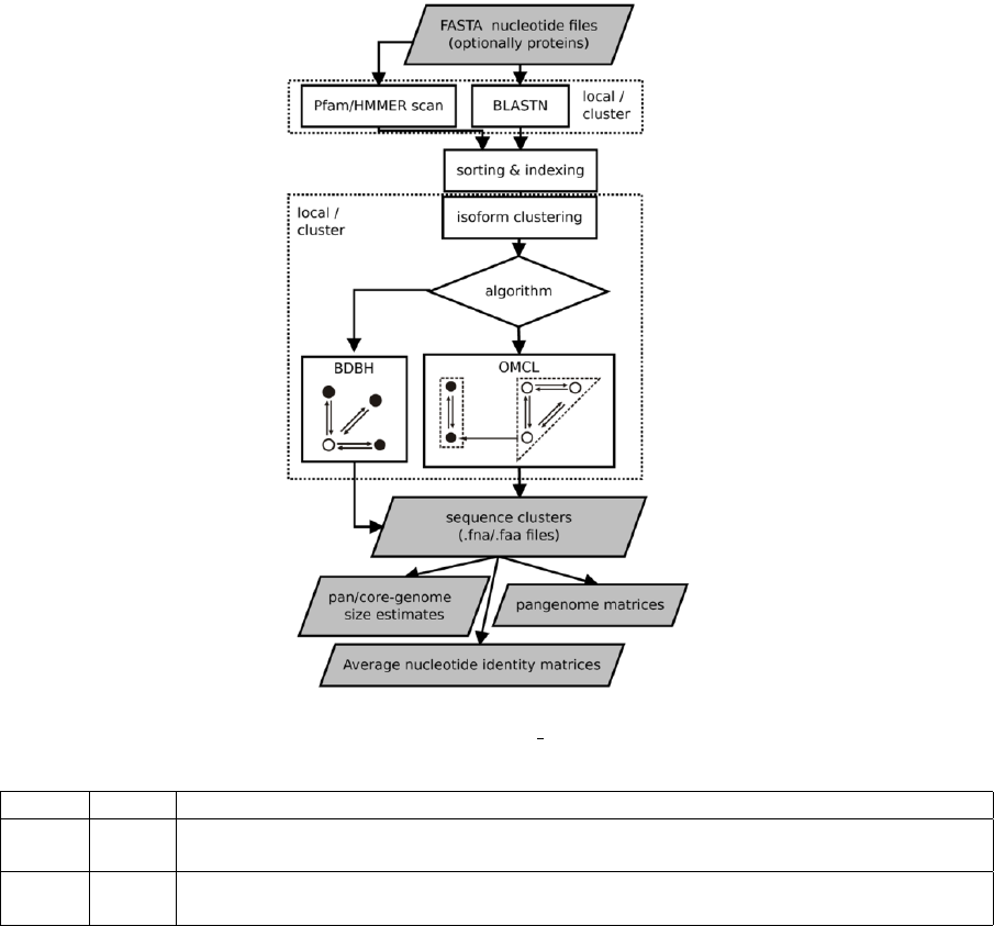
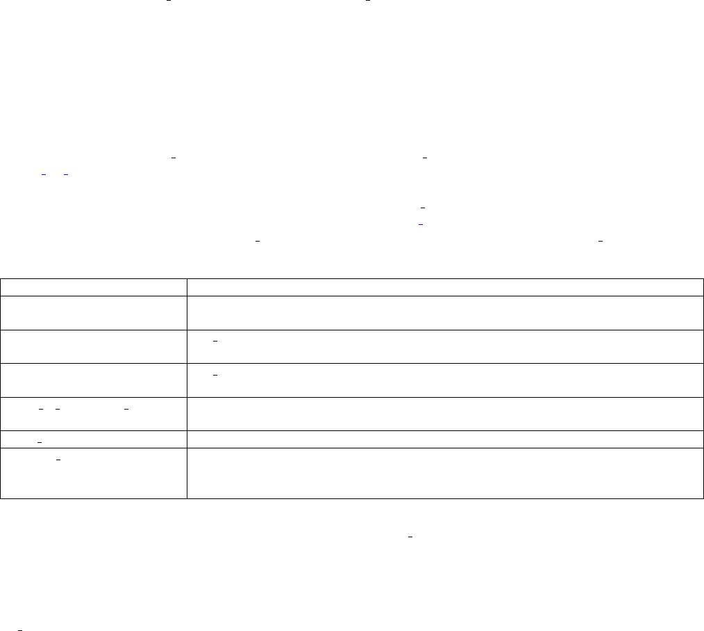
Figure 1: Flowchart of get homologues-est.
name option
BDBH default Starting from a reference genome, keep adding genomes stepwise while storing the se-
quence clusters that result of merging the latest bidirectional best hits.
OMCL -M OrthoMCL v1.4, uses the Markov Cluster Algorithm to group sequences, with inflation
(-F) controlling cluster granularity, as described in PubMed=12952885.
Table 2: List of available clustering algorithms. Note that the COG triangles algorithm is not supported.
today, it is possible to check how the resulting clusters would change when adding an extra 10 genomes tomorrow, by
copying these new 10 .fna input files to the pre-existing -d folder, so that all previous BLASTN searches are re-used.
All remaining flags are options that can modify the default behavior of the program, which is to use the bidirectional
best hit algorithm (BDBH) in order to compile clusters of potential orthologous DNA sequences, taking the smallest
genome as a reference. By default nucleotide sequences are used to guide the clustering, thus relying on BLASTN
searches.
Perhaps the most important optional parameter would be the choice of clustering algorithm (Table 2):
The remaining options are now reviewed:
•Apart from showing the credits, option -v can be helpful after installation, for it prints the enabled features of the
program.
•-o is ideally used to submit to a computer cluster the required BLAST (and Pfam) searches, preparing a job for
posterior analysis on a single computer.
•-i can be used to filter out short, redundant isoforms which overlap, with no overhangs, for a minimun length. By
default this is set to $MINREDOVERLAP=40 as in PubMed=12651724. This EST-specific feature can be turned off
by setting -i 0. Redundant isoforms will not be output unless -L is set.
10
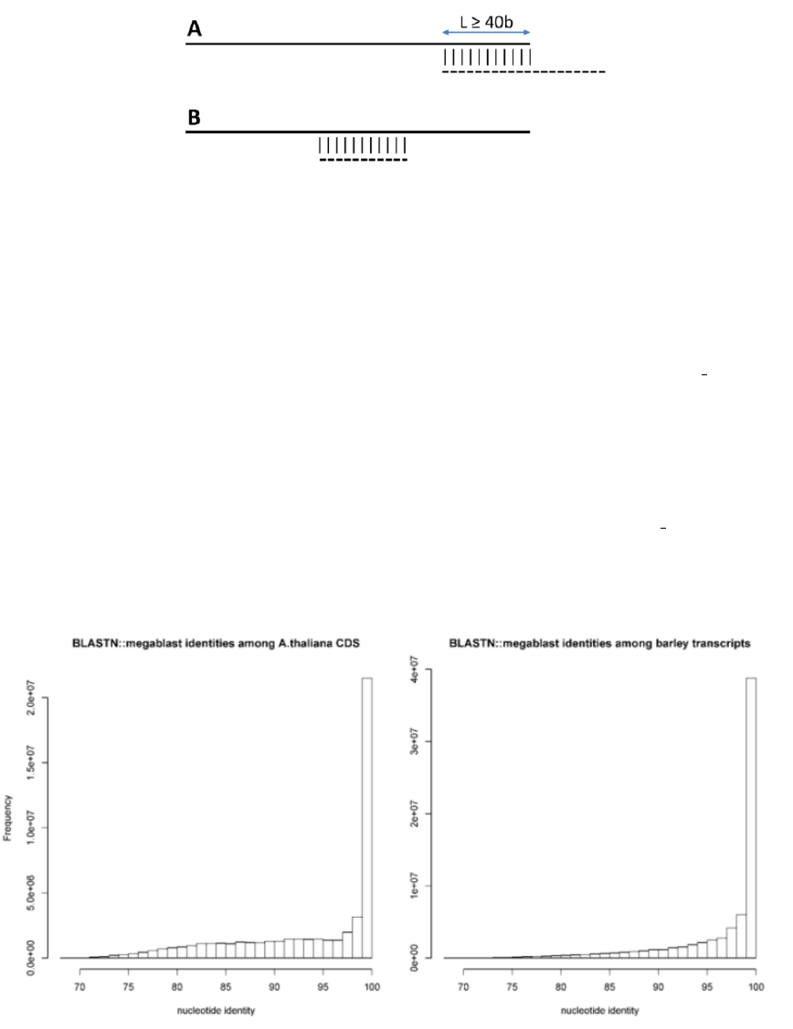
Figure 2: Redundant isoforms (dashed) are optionally removed from an input sequence set if they overlap a longer
sequence over a length ≥40 (A) or when they are completely matched (B). In either case a 100% sequence identity is
required. By calling option -L all redundant isoforms are included in the output.
•-c is used to request a pan- and core-genome analysis of the input sequences, which will be output as tab-separated
files. The number of samples for the genome composition analysis is set to 20 by default, but this can be edited
at the header of get_homologues-est.pl (check the $NOFSAMPLESREPORT variable). As get homologues-est is
meant to be used primarily for the study of transcripts/CDSs of the same species, it uses appropriate thresholds
to define new accessory genes ($MIN_PERSEQID_HOM_EST=70,$MIN_COVERAGE_HOM_EST=50), which mean that
genes/transcripts added to the pool must be ≥70% identical in sequence to any previous sequence with cover ≥50%
in order to be called homologous; otherwise they are handled as novel sequences. This low coverage is set in order
to allow transcripts with retained/unprocessed introns to be matched. The default identity value was chosen to match
the fact that BLASTN::megablast hardly reports hits with lower identities in our tests with barley transcripts and
A.thaliana CDS sequences. Note that these default values are different to those set in get homologues for peptide
sequences. When combined with flag -t (see below), the composition analysis will disregard clusters reported in a
selected number of strains. This feature can be used to filter out singletons or artifacts which might arise from de
novo assembled transcriptomes.
Figure 3: Histograms of % identity reported by BLASTN among Arabidopsis thaliana CDS sequences (left) and Hordeum
vulgare (right) transcripts. Note that the default BLASTN algorithm (megablast) hardly reports alignments with identities
<70%. Plots were computed from 51,110,547 and 70,653,179 alignments, respectively.
•-R takes a number that will be used to seed the random generator used with option -c. By using the same seed in
different -c runs the user ensures that genomes are sampled in the same order.
11
•-s can be used to reduce the memory footprint, provided that the Perl module BerkeleyDB is in place. This option
usually makes get homologues-est slower, but for very large datasets or in machines with little memory resources
this might be the only way to complete a job.
•-m allows the choice of runmode, which can be either -m local (the default) or -m cluster. In the second case
global variable $SGEPATH might need to be appropriately set, as explained in manual get homologues.pdf, as well
as $QUEUESETTINGS, that specificies for instance a particular queue name for your cluster jobs.
•-n sets the number of threads/CPUs to dedicate to each BLAST/HMMER/mcl job run locally, which by default is
2.
•-I list_file.txt allows the user to restrict a get homologues-est job to a subset of FASTA files included in the
input -d folder. This flag can be used in conjunction with -c to control the order in which genomes are considered
during pan- and core-transcriptome analyses. Taking the sample_RNAseq folder, a valid list_file.txt could
contain these lines:
Esterel.trinity.fna.bz2
Franka.trinity.fna.bz2
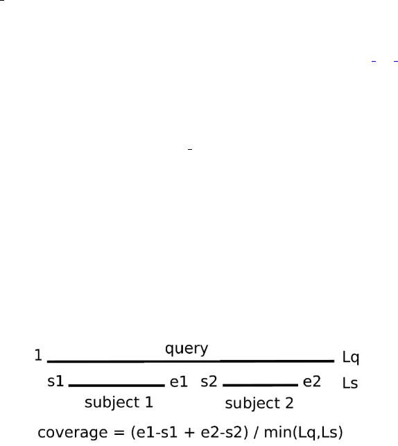
•option -C sets the minimum percentage of coverage required to call two sequences best hits. As EST/transcripts are
frequently truncated, by default coverage is calculated with respect to the shortest sequence in the pair, unless both
of them come from a full-length collection (see 3.1).
Figure 4: Coverage illustrated with the alignment of sequence ’query’ to two aligned fragments of sequence ’subject’. Lq
and Ls are the lengths of both sequences, and s1,e1,s2,e2 and Lq are alignment coordinates.
•-E sets the maximum expectation value (E-value) for BLASTN alignments. This value is by default set to 1e-05.
•-D is an extra restriction for calling best hits, that should have identical Pfam domain compositions. Note that this
option requires scanning all input sequences for Pfam domains, and this task requires extra computing time, ideally
on a computer cluster (-m cluster). While for BDBH domain filtering is done at the time bidirectional best hits
are called, this processing step is performed only after the standard OMCL algorithms have completed, to preserve
the algorithm features.
•-S can be passed to require a minimum % sequence identity for two sequences to be called best hits. The default
value is set to 95%, as in PubMed=21572440.
•-b reduces the number of pairwise BLAST searches performed while compiling core-genomes with algorithm
BDBH, reducing considerably memory and run-time requirements (for Ggenomes, 3G searches are launched in-
stead of the default G2). It comes at the cost of being less exhaustive in finding inparalogues, but in our bacterial
benchmarks this potential, undesired effect was negligible.
•-t is used to control which sequence clusters should be reported. By default only clusters which include at least one
sequence per genome are output. However, a value of -t 2 would report all clusters containing sequences from at
least 2 taxa. A especial case is -t 0, which will report all clusters found, even those with sequences from a single
genome.
•-r allows the choice of any input sequence set (of course included in -d folder) as the reference, instead of the
default smaller one. If possible, resulting clusters are named using CDS/transcript names from this genome, which
can be used to select well annotated species for this purpose.
12
•-e excludes clusters with inparalogues, defined as sequences with best hits in its own genome. This option might
be helpful to rule out clusters including several sequences from the same species, which might be of interest for
users employing these clusters for primer design, for instance.
•-F is the inflation value that governs Markov Clustering in OMCL runs, as explained in PubMed=12952885. As
a rule of thumb, low inflation values (-F 1)result in the inclusion of more sequences in fewer groups, whilst large
values produce more, smaller clusters (-F 4).
•-A tells the program to produce a tab-separated file with average % sequence identity values among pairs of
genomes, computed from sequences in the final set of clusters (see also option -t ). By default these identi-
ties are derived from BLASTN alignments, and hence correspond to nucleotide sequence identities, to produce
genomic average nucleotide sequence identities (ANI).
•-z can be called when performing a genome composition analysis with clustering algorithm OMCL. In addition to
the core- and pan-genome tab-separated files mentioned earlier (see option -c), this flag requests a soft-core report,
considering all sequence clusters present in a fraction of genomes defined by global variable $SOFTCOREFRACTION,
with a default value of 0.95. This choice produces a composition report more robust to assembly or annotation errors
than the core-genome.
13

3.3 Accompanying scripts
The following Perl and shell scripts are included in each release to assist in the interpretation of results generated by
get homologues-est.pl. See examples of use in manual get homologues.pdf manual get homologues.pdf:
•compare clusters.pl primarily calculates the intersection between cluster sets, which can be used to select clusters
supported by different algorithms or settings. This script can also produce pangenome matrices and Venn diagrams.
•parse pangenome matrix.pl is a script that can be used to analyze pan-genome sets, in order to find transcripts/genes
present in a group A of strains which are absent in set B. This script can also be used for calculating and plotting
cloud, shell and core genome compartments.
•make nr pangenome matrix.pl is provided to post-process pangenome matrices in case the user wishes to remove
redundant clusters, using either nucleotide or protein sequence identity cut-offs.
•plot pancore matrix.pl, a Perl script to plot pan/soft/core-genome sampling results and to fit regression curves with
help from Rfunctions.
•check BDBHs.pl is a script that can be used, after a previous get homologues-est run, to find out the bidirectional
best hits of a sequence identifier chosen by the user. It can also retrieve the Pfam annotations of a sequence and its
reciprocal best hits.
•add pancore matrices.pl can be used to add pan/core-matrices produced by previous get homologues.est -c -R runs
on the same set of genomes, with the aim of combining clusters.
•annotate cluster.pl produces a multiple alignment view of the supporting local BLAST alignments of sequences
in a cluster. It can also annotate Pfam domains and find private sequence variants private to an arbitrary group of
sequences.
•plot matrix heatmap.sh calculates ordered heatmaps with attached row and column dendrograms from tab-separated
numeric matrices, which can be presence/absence pangenomic matrices or similarity / identity matrices as those
produced by get homologues-est with flag -A.
•hcluster pangenome matrix.sh generates a distance matrix out of a tab-separated presence/absence pangenome ma-
trix, which is then used to call R functions hclust() and heatmap.2() in order to produce a heatmap.
•pfam enrich.pl calculates the enrichment of a set of sequence clusters in terms of Pfam domains, by using Fisher’s
exact test.
Apart from these, auxiliar transcripts2cds.pl script is bundled to assist in the analysis of transcripts. In particular, this
script can be used to annotate potential Open Reading Frames (ORFs) contained within raw transcripts, which might be
truncated or contain introns. This script uses TransDecoder, BLASTX and SWISSPROT, which should be installed by
running: ./install.pl
Ths program supports the following options:
usage: ./transcripts2cds.pl [options] <input FASTA file(s) with transcript nucleotide sequences>
-h this message
-p check only ’plus’ strand (optional, default both strands)
-l min length for CDS (optional, default=50 amino acid residues)
-g genetic code to use during translation (optional, default=1, example: -g 11)
-d run blastx against selected protein FASTA database file (default=swissprot, example: -d db.faa)
-E max E-value during blastx search (default=1e-05)
-n number of threads for BLASTX jobs (default=2)
-X use diamond instead of blastx (optional, much faster for many sequences)
-G show available genetic codes and exit
The main output of this script are two files, as shown in section 4.1, which contain inferred nucleotide and peptide
CDS sequences. These FASTA files contain in each header the evidence supporting each called CDS, which can be
blastx,transdecoder or a combination of both, giving precedence to blastx in case of conflict. Note that we
14

have observed that the output of TransDecoder might change if a single sequence is analyzed alone, in contrast to the
analysis of a batch of sequences. The next table shows the rules and evidence codes used by this script in order to call
CDS sequences by merging BLASTX (1) and TransDecoder (2) predictions. The rules are mutually exclusive and are
tested hierarchically from top to bottom. Sequences from 1 and 2 with less than 90 consecutive matches (30 amino
acid residues) are considered to be non-overlapping (last rule). Note that the occurrence of mismatches are checked as a
control:
graphical summary evidence description
1---------- blastx no transdecoder
2---------- transdecoder no blastx
1---------- blastx.transdecoder inferred CDS overlap with no
2----------- mismatches and are concatenated
1---------- transdecoder.blastx inferred CDS overlap with no
2----------- mismatches and are concatenated
1----------------- blastx<transdecoder blastx CDS includes transdecoder CDS
2-----------
1---------- transdecoder<blastx transdecoder CDS includes blastx CDS
2------------------
1--------C-- blastx-mismatches blastx CDS is returned as sequences
2---T------ have mismatches
1----- blastx-noover blastx CDS is returned as transdecoder
2--- CDS does not overlap
Our benchmarks suggest that 78 to 92% of deduced CDS sequences match the correct peptide sequences. :
evidence Arabidopsis thaliana [Col-0] n Hordeum vulgare [Haruna Nijo] n
blastx 0.787 960 0.654 1,657
transdecoder 0.914 8,194 0.662 9,026
blastx.transdecoder 0.930 4,678 0.843 5,939
transdecoder.blastx 0.959 15,700 0.859 8,903
blastx<transdecoder 0.620 324 0.674 218
transdecoder<blastx 0.966 6,581 0.872 11,999
blastx-mismatches 0 1 0
blastx-noover 0.232 835 0.426 2,211
overall 0.923 0.783
Table 3: Fraction of correct peptide sequences in deduced CDS obtained by combining BLASTX and TransDecoder.
The results obtained with DIAMOND instead of BLASTX are very similar:
15

evidence Arabidopsis thaliana [Col-0] n Hordeum vulgare [Haruna Nijo] n
blastx 0.800 929 0.655 1,598
transdecoder 0.914 8,166 0.663 8,980
blastx.transdecoder 0.929 4,685 0.844 5,951
transdecoder.blastx 0.958 15,698 0.859 8,890
blastx<transdecoder 0.615 325 0.671 216
transdecoder<blastx 0.967 6,583 0.872 11,999
blastx-mismatches 0 0
blastx-noover 0.270 833 0.452 2,190
Table 4: Fraction of correct peptide sequences in deduced CDS obtained by combining DIAMOND and TransDecoder.
4 A few examples
This section presents typical ways of running get homologues-est.pl and the accompanying scripts with provided sample
input data. Please check file manual get homologues.pdf for more examples, particularly for the auxiliary scripts, which
are not explained in this document.
4.1 Extracting coding sequences (CDS) from transcripts
This example takes the provided sample file sample_transcripts.fna to demonstrate how to annotate coding se-
quences contained in those sequences by calling transcripts2cds.pl. Note that transcripts2cdsCPP.pl is signif-
icantly faster, but requires an optional Perl module (see 2.3).
This is an optional pre-processing step which you might not want to do, as the software should be able to properly
handle any nucleotides sequences suitable for BLASTN. However, coding sequences have the advantage that can be
translated to amino acids and thus used to scan Pfam domains further down in the analysis (see option -D).
A simple command would be, which will discard sequences less than 50b long, and will aligned them to SWISSPROT
proteins in order to annotate coding regions. In case of overlap, Transdecoder-defined and BLASTX-based coding regions
are combined provided that a $MINCONOVERLAP=90 overlap, with no mismatches, is found; otherwise the latter are given
higher priority:
./transcripts2cdsCPP.pl -n 10 sample_transcripts.fna
The output should look like this (contained in file sample_transcripts_output.txt):
# ./transcripts2cdsCPP.pl -p 0 -m -d /path/get_homs-est/db/swissprot -E 1e-05 -l 50 -g 1 -n 10 -X 0
# input files(s):
# sample_transcripts.fna
## processing file sample_transcripts.fna ...
# running transdecoder...
# parsing transdecoder output (_sample_transcripts.fna_l50.transdecoder.cds.gz) ...
# running blastx...
# parsing blastx output (_sample_transcripts.fna_E1e-05.blastx.gz) ...
# calculating consensus sequences ...
# input transcripts = 9
# transcripts with ORFs = 7
# transcripts with no ORFs = 2
# output files: sample_transcripts.fna_l50_E1e-05.transcript.fna ,
# sample_transcripts.fna_l50_E1e-05.cds.fna ,
# sample_transcripts.fna_l50_E1e-05.cds.faa ,
# sample_transcripts.fna_l50_E1e-05.noORF.fna
The resulting CDS files can then be analyzed with get homologues-est.pl.
Apart from the listed output files, which include translated protein sequences, temporary files are stored in the working
directory, which of course can be removed, but will be re-used if the same job is re-run later, such as
_sample_transcripts.fna_E1e-05.blastx.gz,
16

_sample_transcripts.fna_l50.transdecoder.cds.gz or
_sample_transcripts.fna_l50.transdecoder.pep.gz.
By default the script uses BLASTX (in combination with Transdecoder), which might take quite some time to process
large numbers of sequences. For this reason the DIAMOND algorithm is also available (upon calling option -X), which in
our benchmarks showed comparable performance and was several orders of magnitude faster when using multiple CPU
cores.
CDS sequences can be deduced for a collection of transcriptomes and put in the same folder, so that they can all be an-
alyzed together with get homologues-est.pl. Such files support calling option -D, which will annotate Pfam domains con-
tained in those sequences, and can then also be used to calculate enrichment as explained in manual get homologues.pdf.
17
4.2 Clustering orthologous transcripts from FASTA files, one per strain
This example takes the sample input folder sample_transcripts_fasta, which contains automatically assembled
transcripts (Trinity) of three Hordeum vulgare strains (barley), plus a set of full-length cDNA collection of cultivar Haruna
Nijo, to show to produce clusters of transcripts.
The next command uses the OMCL algorithm to cluster sequences, produces a composition report, including the soft-
core, and finally computes an Average Nucleotide Identity matrix on the produced clusters. Note that redundant isoforms
are filtered, keeping only the longest one (you can turn this feature off with -i 0):
$ ./get_homologues-est.pl -d sample_transcripts_fasta -M -c -z -A
The output should look like this (contained in file sample_transcripts_output.txt):
# results_directory=/path/sample_transcripts_fasta_est_homologues
# parameters: MAXEVALUEBLASTSEARCH=0.01 MAXPFAMSEQS=250 BATCHSIZE=100
# checking input files...
# Esterel.trinity.fna.bz2 5892 median length = 506
# Franka.trinity.fna.bz2 6036 median length = 523
# Hs_Turkey-19-24.trinity.fna.bz2 6204 median length = 476
# flcdnas_Hnijo.fna.gz 28620 [full length sequences] median length = 1504
# 4 genomes, 46752 sequences
# taxa considered = 4 sequences = 46752 residues = 63954041
# mask=Esterel_alltaxa_algOMCL_e0_ (_algOMCL)
[...]
# re-using previous isoform clusters
# 42 sequences
# 65 sequences
# 61 sequences
# 2379 sequences
# creating indexes, this might take some time (lines=2.08e+05) ...
# construct_taxa_indexes: number of taxa found = 4
# number of file addresses/BLAST queries = 4.4e+04
# genome composition report (samples=20,permutations=24,seed=0)
# genomic composition parameters: MIN_PERSEQID_HOM=70 MIN_COVERAGE_HOM=50 SOFTCOREFRACTION=0.95
[...]
# file=sample_transcripts_fasta_est_homologues/core_genome_algOMCL.tab
genomes mean stddev | samples
0 8559 6614 | 4665 4665 4665 ...
1 1113 737 | 496 432 2007 ...
2 255 101 | 84 308 347 ...
3 66 0 | 66 66 66 ...
# file=sample_transcripts_fasta_est_homologues/soft-core_genome_algOMCL.tab
genomes mean stddev | samples
0 8559 6614 | 4665 4665 4665 ...
1 3491 2311 | 2428 2195 8108 ...
2 2170 1017 | 765 3460 2145 ...
3 645 101 | 816 592 553 ...
18
# looking for valid sequence clusters (n_of_taxa=4)...
# number_of_clusters = 66
# cluster_list = sample_transcripts_fasta_est_homologues/Esterel_alltaxa_algOMCL_e0_.cluster_list
# cluster_directory = sample_transcripts_fasta_est_homologues/Esterel_alltaxa_algOMCL_e0_
# average_nucleotide_identity_matrix_file = # [...]/Esterel_alltaxa_algOMCL_e0_Avg_identity.tab
Notice that both core and soft-core sampling experiments are reported, considering sequences found in all strains and
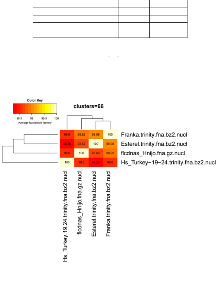
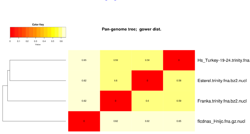
in 95% strains, respectively. The produced Average Nucleotide Identity matrix looks like this:
genomes Esterel Franka HsTurkey flcdnasHnijo
Esterel 100 98.29 98.04 99.33
Franka 98.29 100 98.25 98.90
HsTurkey 98.04 98.25 100 98.41
flcdnasHnijo 98.33 98.90 98.41 100
Provided that optional R modules described in manual get homologues.pdf are installed, this matrix can be plotted
with the following command:
./plot_matrix_heatmap.sh -i sample_[...]/Esterel_alltaxa_algOMCL_e0_Avg_identity.tab \
-t "clusters=66" -k "Average Nucleotide Identity" -o pdf -m 28 -v 35 -H 9 -W 10
Figure 5: Heatmap of Average Nucleotide Identity.
19
If the previous command is changed by adding option -t -2 only transcripts present in at least two strains will be
considered, which are output in folder:
sample_transcripts_fasta_est_homologues/Esterel_2taxa_algOMCL_e0_
This second command produces a significantly different pan-genome composition matrix, which changes from:
# file=sample_transcripts_fasta_est_homologues/pan_genome_algOMCL.tab
genomes mean stddev | samples
0 8559 6614 | 4665 4665 4665 ...
1 14830 6425 | 8937 9002 21292 ...
2 21384 4866 | 13004 24283 23358 ...
3 26380 468 | 27019 26209 25652 ...
to
# file=sample_transcripts_fasta_est_homologues/pan_genome_2taxa_algOMCL.tab
genomes mean stddev | samples
0 2860 1172 | 2262 2262 2262 ...
1 4270 490 | 4110 3828 4196 ...
2 4953 424 | 5475 4767 4294 ...
3 4954 424 | 5475 4768 4296 ...
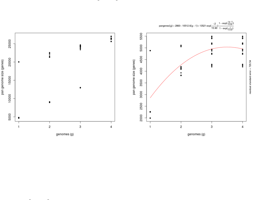
Both matrices can be plotted with script plot pancore matrix.pl, with a command such as:
./plot_pancore_matrix.pl -i sample_transcripts_fasta_est_homologues/pan_genome_algOMCL.tab -f pan
Figure 6: Pan-transcriptome size estimates (-t 0, left) and (-t 2, right) based on random samples of 4 transcriptome sets.
As the left example illustrates, four strains are usually not enough to fit a Tettelin-like function.
The next figure shows a similar analysis but now using genomic data instead of transcript sets. The example shows
pan-genome size estimates of Whole Genome Sequence assemblies of 19 Arabidopsis thaliana ecotypes, downloaded
from http://mus.well.ox.ac.uk/19genomes/sequences/CDS and described in PubMed=21874022.
Script plot pancore matrix.pl can also be called with flag -a:
./plot_pancore_matrix.pl -i sample_transcripts_fasta_est_homologues/pan_genome_algOMCL.tab \
-f pan -a snapshots+
20
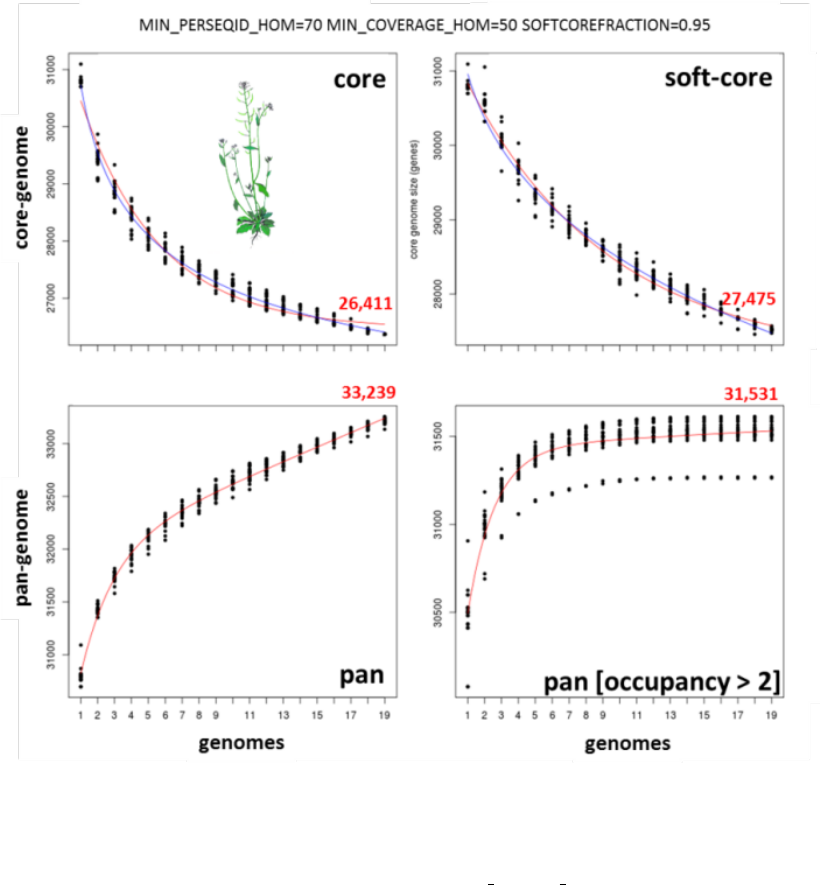
Figure 7: Core-genome, soft-core-genome and pan-genome CDS composition analysis of WGS assemblies of 19
A.thaliana ecotypes. Note that the pan-genome simulation was done with all clusters (left) and with all clusters found
in at least three genomes (right), illustrating the effect of option -t 3, which might be useful to remove low confidence
sequences. Red numbers correspond to fitted values generated by plot pancore matrix.pl.
This will create and store a in folder snapshots/ a series of GIF images that can be used to animate pan-genome
simulations. The next Figure show some of this snapshots:
21
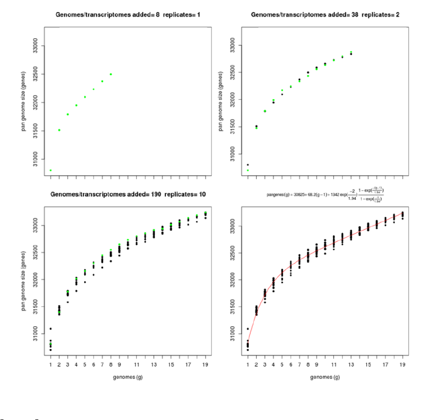
Figure 8: Four snapshots of the pan-genome simulation carried out in the previous figure, generated by
plot pancore matrix.pl.
22
4.3 Producing a nucleotide-based pangenome matrix
The clusters obtained in the previous section with option -t 2 can be used to compile a pangenome matrix without sin-
gletons with this command:
./compare_clusters.pl -d sample_[...]/Esterel_2taxa_algOMCL_e0_ -o outdir -n -m
# number of input cluster directories = 1
# parsing clusters in sample_transcripts_fasta_est_homologues/Esterel_2taxa_algOMCL_e0_ ...
# cluster_list in place, will parse it (sample_[...]/Esterel_2taxa_algOMCL_e0_.cluster_list)
# number of clusters = 5241
# intersection output directory: outdir
# intersection size = 5241 clusters
# intersection list = outdir/intersection_t0.cluster_list
# pangenome_file = outdir/pangenome_matrix_t0.tab
# pangenome_phylip file = outdir/pangenome_matrix_t0.phylip
If the optional R modules described in manual get homologues.pdf are installed, such a pangenome matrix can be
used to hierarchically cluster strains with this command:
./hcluster_pangenome_matrix.sh -i outdir/pangenome_matrix_t0.tab
Figure 9: Hierarchical grouping of strains based on pangenome matrix.
23
4.4 Estimating protein domain enrichment of some sequence clusters
This example uses data from the barley benchmark, the test_barley/ folder, which contains instructions to download
sequences from: http://floresta.eead.csic.es/plant-pan-genomes
After completing the downloads, the folder will contain FASTA files with nucleotide sequences of 14 de-novo assem-
bled transcriptomes and transcripts/cDNA sequences annotated in reference accessions Morex and Haruna Nijo. CDS can
be extracted as explained in Section 5and then Pfam domains can be annotated as follows:
$ ./get_homologues-est.pl -d cds -D -o -m cluster
These annotations will serve to calculate background domain frequencies.
Once this is completed, we can compute ”control” clusters with this command:
$ ./get_homologues-est.pl -d cds -M -m cluster
which we will then place in a folder called clusters_cds:
compare_clusters.pl -d cds_est_homologues/Alexis_0taxa_algOMCL_e0_ \
-o clusters_cds -m -n+
In order to call accessory sequences with more confidence we will use only non-cloud clusters (occupancy >2), which
we do with this command:
$ ./get_homologues-est.pl -d cds -M -t 3 -m cluster
The output should include the next lines:
# number_of_clusters = 34248
# cluster_list = cds_est_homologues/Alexis_3taxa_algOMCL_e0_.cluster_list
# cluster_directory = cds_est_homologues/Alexis_3taxa_algOMCL_e0_
We should be now in position to compile the pan-genome matrix corresponding to these clusters:
./compare_clusters.pl -d cds_est_homologues/Alexis_3taxa_algOMCL_e0_ \
-o clusters_cds_t3 -m -n
which should produce:
# number of clusters = 34248
# intersection output directory: clusters_cds_t3
# intersection size = 34248 clusters
# intersection list = clusters_cds_t3/intersection_t0.cluster_list
# pangenome_file = clusters_cds_t3/pangenome_matrix_t0.tab
# pangenome_phylip file = clusters_cds_t3/pangenome_matrix_t0.phylip
We should now interrogate the pan-genome matrix, for instance looking for clusters found in one genotype (A) but
not in others (B):
./parse_pangenome_matrix.pl -m clusters_cds_t3/pangenome_matrix_t0.tab \
-A cds/SBCC073.list -B cds/ref.list -g
You should obtain a list of 4348 accessory clusters:
# matrix contains 34248 clusters and 16 taxa
# taxa included in group A = 1
# taxa included in group B = 2
# finding genes present in A which are absent in B ...
# file with genes present in set A and absent in B (4348):
clusters_cds_t3/pangenome_matrix_t0__pangenes_list.txt
24
Finally, we will now estimate whether these clusters are enriched in any Pfam domain, producing also a single FASTA
file with the tested sequences:
./pfam_enrich.pl -d cds_est_homologues -c clusters_cds -n -t greater \
-x clusters_cds_t3/pangenome_matrix_t0__pangenes_list.txt -e -p 0.05 \
-r SBCC073 -f SBCC073_accessory.fna
The output should be:
# 39400 sequences extracted from 113222 clusters
# total experiment sequence ids = 4818
# total control sequence ids = 39400
# parse_Pfam_freqs: set1 = 562 Pfams set2 = 3718 Pfams
# created FASTA file: SBCC073_accessory.fna
# sequences=4818 mean length=353.8 , seqs/cluster=1.11
# fisher exact test type: ’greater’
# multi-testing p-value adjustment: fdr
# adjusted p-value threshold: 1
# total annotated domains: experiment=1243 control=19192
#PfamID counts(exp) counts(ctr) freq(exp) freq(ctr) p-value p-value(adj) description
PF00009 0 20 0.000e+00 1.042e-03 1.000e+00 1.000e+00 Elongation factor Tu GTP binding domain
PF00010 0 32 0.000e+00 1.667e-03 1.000e+00 1.000e+00 Helix-loop-helix DNA-binding domain
...
PF00665 13 31 1.046e-02 1.615e-03 1.418e-06 1.318e-03 Integrase core domain
PF07727 28 61 2.253e-02 3.178e-03 3.033e-13 1.128e-09 Reverse transcriptase (RNA-dep DNA pol)
PF00931 44 201 3.540e-02 1.047e-02 1.750e-10 3.253e-07 NB-ARC domain
PF13976 14 19 1.126e-02 9.900e-04 2.744e-09 3.401e-06 GAG-pre-integrase domain
25

4.5 Making and annotating a non-redundant pangenome matrix
The script make_nr_pangenome_matrix.pl produces a non-redundant pangenome matrix by comparing all clusters to
each other, taking the median sequence in each cluster. By default nucleotide sequences are compared, but if the original
input of get homologues-est comprised both DNA and protein sequences, the user can also choose peptide sequences to
compute redundancy, which probably make more sense in terms of protein function. On the contrary, it would seem more
appropriate to use DNA sequences to measure diversity.
In this example a DNA-based non-redundant pangenome matrix is computed with BLASTN assuming that sequences
might be truncated (option -e) and using 10 processor cores and a coverage cutoff of 50%:
./make_nr_pangenome_matrix.pl -m outdir/pangenome_matrix_t0.tab -n 10 -e -C 50
# input matrix contains 5241 clusters and 4 taxa
# filtering clusters ...
# 5241 clusters with taxa >= 1 and sequence length >= 0
# sorting clusters and extracting median sequence ...
# running makeblastdb with outdir/pangenome_matrix_t0_nr_t1_l0_e1_C50_S90.fna
# parsing blast result! (outdir/pangenome_matrix_t0_nr_t1_l0_e1_C50_S90.blast , 0.37MB)
# parsing file finished
# 5172 non-redundant clusters
# created: outdir/pangenome_matrix_t0_nr_t1_l0_e1_C50_S90.fna
# printing nr pangenome matrix ...
# created: outdir/pangenome_matrix_t0_nr_t1_l0_e1_C50_S90.tab
Note that the previous command can be modified to match external reference sequences, for instance from Swissprot,
or pre-computed clusters, such as groups of orthologous sequences, so that the resulting matrix contains cross-references
to those external clusters, and their annotations. In either case, both input clusters and reference sequences must be of the
same type: either nucleotides or peptides.
The next example shows how a set of clusters produced by get homologues-est can be matched to some nucleotide
reference sequences, in this case annotated rice cDNAs:
./make_nr_pangenome_matrix.pl -m outdir/pangenome_matrix_t0.tab -n 10 -e -C 50 -f oryza.fna
This is the produced output:
# input matrix contains 5241 clusters and 4 taxa
# filtering clusters ...
# 5241 clusters with taxa >= 1 and sequence length >= 0
# sorting clusters and extracting median sequence ...
# re-using previous BLAST output outdir/pangenome_matrix_t0_nr_t1_l0_e1_C50_S90.blast
# parsing blast result! (outdir/pangenome_matrix_t0_nr_t1_l0_e1_C50_S90.blast , 0.34MB)
# parsing file finished
# 5172 non-redundant clusters
# created: outdir/pangenome_matrix_t0_nr_t1_l0_e1_C50_S90.fna
# 66339 reference sequences parsed in oryza.fna
# parsing blast result! (outdir/pangenome_matrix_t0_nr_t1_l0_e1_C50_S90_ref.blast , 0.37MB)
# parsing file finished
26

# matching nr clusters to reference (%alignment coverage cutoff=50) ...
# printing nr pangenome matrix ...
# created: outdir/pangenome_matrix_t0_nr_t1_l0_e1_C50_S90_ref_c50_s50.tab
# NOTE: matrix can be transposed for your convenience with:
perl -F’\t’ -ane ’$r++;for(1 .. @F){$m[$r][$_]=$F[$_-1]}; \
$mx=@F;END{for(1 .. $mx){for $t(1 .. $r){print"$m[$t][$_]\t"}print"\n"}}’ \
outdir/pangenome_matrix_t0_nr_t1_l0_e1_C50_S90_ref_c50_s50.tab
The suggested perl command can be invoked to tranpose the matrix, which now contains rows such as these:
non-redundant Franka.bz2.nucl Esterel.bz2.nucl flcdnas_Hnijo.gz.nucl ... redundant reference
1_TR2804-c0_g1_i1.fna 1 1 0 0 NA LOC_Os09g07300.1 cDNA|BIG, putative, expressed
2_TR1554-c0_g1_i1.fna 0 2 1 0 NA LOC_Os03g53280.1 cDNA|WD domain containing protein
6_TR3918-c0_g1_i1.fna 0 1 1 0 NA NA
...
Pangenome matrices with more than 4 taxa can be plotted with help from script parse pangenome matrix.pl, as ex-
plained in manual get homologues.pdf.
27
4.6 Annotating a sequence cluster
After analyzing pan-genome or pan-transcriptome clusters it might be interesting to find out what kind of proteins they
enconde, or we might just want to double-check the BLAST matches that support a produced cluster. The script anno-
tate cluster.pl does just that, and be used with both nucleotide and peptide clusters. It can be called like this:
./annotate_cluster.pl -f outdir/1004_TR425-c0_g2_i1.fna -o 1004_TR425-c0_g2_i1.aln.fna -D
And will produce this output:
# DEFBLASTNTASK=megablast DEFEVALUE=10
# MINBLUNTBLOCK=100 MAXSEQNAMELEN=60
# MAXMISMCOLLAP=0 MAXGAPSCOLLAP=2
# ./annotate_cluster.pl -f outdir/1004_TR425-c0_g2_i1.fna -r \
# -o 1004_TR425-c0_g2_i1.aln.fna -P 1 -b 0 -D 1 -c 0 -A -B
# total sequences: 3 taxa: 2
# Pfam domains: PF10602,PF01399,
# Pfam annotation: 26S proteasome subunit RPN7;PCI domain;
# aligned sequences: 3 width: 1595
# alignment sites: SNP=3 parsimony-informative=0 (outdir/1004_TR425-c0_g2_i1.fna)
# taxa included in alignment: 2
# alignment file: 1004_TR425-c0_g2_i1.aln.fna
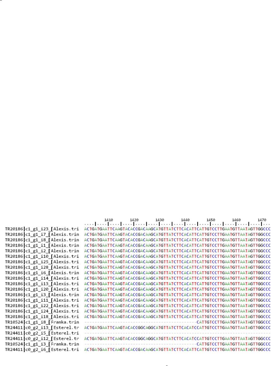
If option -b is enforced a blunt-end alignment is produced, which might be useful for further analyses. In either case,
the produced FASTA alignment file will contain Pfam domains in each header, in addition to the relevant BLAST scores:
>TR425|c0_g2_i1_[Esterel.trinity.fna.bz2] bits E-value N qy ht 1:1595 Pfam:..
CCTGCTGGTGCATTTTTTTACAAACAGTTGGCACAGAGTATTTGTTGCTAATTGTGTTCGTTTTCTTGAA...
Figure 10: Fragment of alignment produced by annotate cluster.pl, rendered with BioEdit.
28
Finally, option -c can be invoked to collapse aligned sequences from the same species or taxon. This might be
useful when working with clusters of transcript isoforms, which are often redundant and broken in possibly overlapping
fragments. Taking the same example cluster, we could try to collapse isoforms with overlaps ≥30 residues like this:
./annotate_cluster.pl -f outdir/1004_TR425-c0_g2_i1.fna -o 1004_TR425-c0_g2_i1.aln.fna -D -c 30
Note that by default the script does not tolerate mismatches between sequences to be collapsed, but that behaviour can
be relaxed by editing the value of variable $MAXMISMCOLLAP=0 at the top of the script. Instead, as BLASTN-placed gaps
in identical sequences can often move, by default two such gaps are accepted (see variable MAXGAPSCOLLAP=2).
By default, the script annotate_cluster.pl looks for the longest sequences and aligns all other cluster sequences
to it with BLASTN (megablast). The user can also pass an external, reference sequence to guide cluster alignment (see
option -r). However, in either case, clusters of transcripts often contain a fraction of BLASTN hits that do not match
the longest/reference sequence; instead, they align towards the 5’ or 3’ of other sequences of the clusters and are thus not
included in the produced multiple sequence alignment (MSA):
----------------- <= longest/reference sequence
-------------
-------------
-----------
------------
.... <= sequences not included in MSA
..
29
5 A step-by-step protocol with barley assembled transcripts
This section describes the steps required to proceed with the analysis of barley transcripts with folder test_barley,
which you should get with the software. The following commands are to be pasted in your terminal:
## set get_homologues path if not already in $PATH
export GETHOMS=~/soft/github/get_homologues/
cd test_barley
## 1) prepare sequences
cd seqs
# download all transcriptomes
wget -c -i wgetlist.txt
# extract CDS sequences (this takes several hours)
# choose cdsCPP.sh if dependency Inline::CPP is available in your system
# the script will use 20 CPU cores, please adapt it to your system
./cds.sh
# clean and compress
#rm -f _* *noORF* *transcript*
#gzip *diamond*
# put cds sequences aside
mv *cds.f*gz ../cds
cd ..
# check lists of accessions are in place (see HOWTO.txt there)
ls cds/*list
## 2) cluster sequences and start the analyses
# calculate protein domain frequencies (Pfam)
$GETHOMS/get_homologues-est.pl -d cds -D -m cluster -o &> log.cds.pfam
# alternatively, if not running in a SGE cluster, taking for instance 20 CPUs
$GETHOMS/get_homologues-est.pl -d cds -D -n 20 -o &> log.cds.pfam
# calculate ’control’ cds clusters
$GETHOMS/get_homologues-est.pl -d cds -M -t 0 -m cluster &> log.cds
# get non-cloud clusters
$GETHOMS/get_homologues-est.pl -d cds -M -t 3 -m cluster &> log.cds.t3
# clusters for dN/dS calculations
$GETHOMS/get_homologues-est.pl -d cds -e -M -t 4 -m cluster &> log.cds.t4.e
# leaf clusters and pangenome growth simulations with soft-core
$GETHOMS/get_homologues-est.pl -d cds -c -z \
-I cds/leaf.list -M -t 3 -m cluster &> log.cds.leaf.t3.c
# produce pan-genome matrix and allocate clusters to occupancy classes
# all occupancies
30
$GETHOMS/compare_clusters.pl -d cds_est_homologues/Alexis_0taxa_algOMCL_e0_ \
-o clusters_cds -m -n &> log.compare_clusters.cds
# excluding cloud clusters, the most unreliable in our benchmarks
$GETHOMS/compare_clusters.pl -d cds_est_homologues/Alexis_3taxa_algOMCL_e0_ \
-o clusters_cds_t3 -m -n &> log.compare_clusters.cds.t3
$GETHOMS/parse_pangenome_matrix.pl -m clusters_cds_t3/pangenome_matrix_t0.tab -s \
&> log.parse_pangenome_matrix.cds.t3
# make pan-genome growth plots
$GETHOMS/plot_pancore_matrix.pl -i cds_est_homologues/core_genome_leaf.list_algOMCL.tab \
-f core_both &> log.core.plots
$GETHOMS/plot_pancore_matrix.pl -i cds_est_homologues/pan_genome_leaf.list_algOMCL.tab \
-f pan &> log.pan.plots
## 3) annotate accessory genes
# find [-t 3] SBCC073 clusters absent from references
$GETHOMS/parse_pangenome_matrix.pl -m clusters_cds_t3/pangenome_matrix_t0.tab \
-A cds/SBCC073.list -B cds/ref.list -g &> log.acc.SBCC073
mv clusters_cds_t3/pangenome_matrix_t0__pangenes_list.txt \
clusters_cds_t3/SBCC073_pangenes_list.txt
# how many SBCC073 clusters are there?
perl -lane ’if($F[0] =~ /SBCC073/){ foreach $c (1 .. $#F){ if($F[$c]>0){ $t++ } }; print $t }’ \
clusters_cds_t3/pangenome_matrix_t0.tab
# find [-t 3] Scarlett clusters absent from references
$GETHOMS/parse_pangenome_matrix.pl -m clusters_cds_t3/pangenome_matrix_t0.tab \
-A cds/Scarlett.list -B cds/ref.list -g &> log.acc.Scarlett
mv clusters_cds_t3/pangenome_matrix_t0__pangenes_list.txt \
clusters_cds_t3/Scarlett_pangenes_list.txt
# find [-t 3] H.spontaneum clusters absent from references
$GETHOMS/parse_pangenome_matrix.pl -m clusters_cds_t3/pangenome_matrix_t0.tab \
-A cds/spontaneum.list -B cds/ref.list -g &> log.acc.spontaneum
mv clusters_cds_t3/pangenome_matrix_t0__pangenes_list.txt \
clusters_cds_t3/spontaneum_pangenes_list.txt
# Pfam enrichment tests
# core
$GETHOMS/pfam_enrich.pl -d cds_est_homologues -c clusters_cds -n \
-x clusters_cds_t3/pangenome_matrix_t0__core_list.txt -e -p 1 \
-r SBCC073 > SBCC073_core.pfam.enrich.tab
$GETHOMS/pfam_enrich.pl -d cds_est_homologues -c clusters_cds -n \
-x clusters_cds_t3/pangenome_matrix_t0__core_list.txt -e -p 1 \
-r SBCC073 -t less > SBCC073_core.pfam.deplet.tab
# accessory
$GETHOMS/pfam_enrich.pl -d cds_est_homologues -c clusters_cds -n \
-x clusters_cds_t3/SBCC073_pangenes_list.txt -e -p 1 -r SBCC073 \
-f SBCC073_accessory.fna > SBCC073_accessory.pfam.enrich.tab
31
$GETHOMS/pfam_enrich.pl -d cds_est_homologues -c clusters_cds -n \
-x clusters_cds_t3/Scarlett_pangenes_list.txt -e -p 1 -r Scarlett \
-f Scarlett_accessory.fna > Scarlett_accessory.pfam.enrich.tab
$GETHOMS/pfam_enrich.pl -d cds_est_homologues -c clusters_cds -n \
-x clusters_cds_t3/spontaneum_pangenes_list.txt -e -p 1 -r Hs_ \
-f spontaneum_accessory.fna > spontaneum_accessory.pfam.enrich.tab
# note that output files contain data such as the mean length of sequences
# get merged stats for figure
perl suppl_scripts/_add_Pfam_domains.pl > accessory_stats.tab
perl -lane ’print if($F[0] >= 5 || $F[1] >= 5 || $F[2] >= 5)’ \
accessory_stats.tab > accessory_stats_min5.tab
Rscript suppl_scripts/_plot_heatmap.R
32
6 Frequently asked questions (FAQs)
Please see also the FAQs in manual get homologues.pdf.
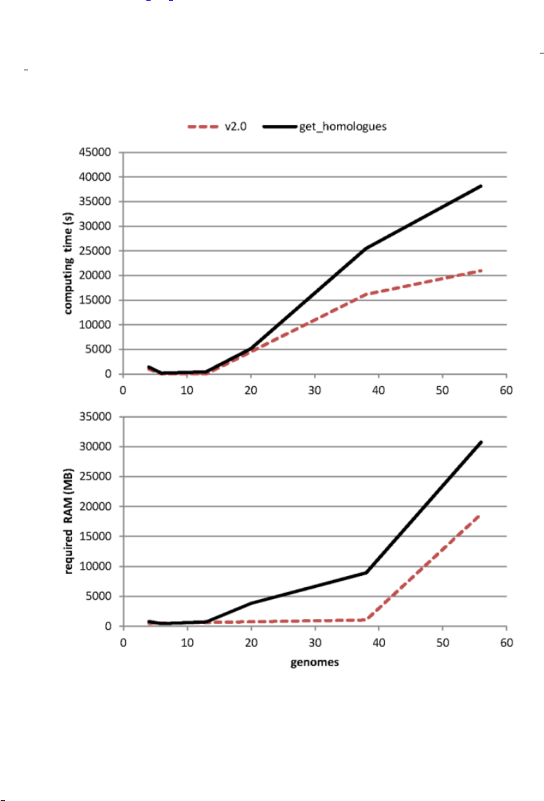
•What’s the performance gain of v2?
After evolving parts of the original code base, and fixing some bugs (see CHANGES.txt), both get homologues.pl
and get homologues-est.pl have significantly improved their performance, as can be seen in the figure, which com-
bines data from the original benchmark and new data generated after v2 was in place.
Figure 11: Computing time and RAM requirements of the original algorithm (OMCL, measured on 6 sequence sets) as
compared to the updated v2 code (measured on 3 three sets).
•What are the main caveats when clustering transcripts/CDS sequences?
get homologues-est.pl has been mainly tested with plant sequences, using both CDS sets from whole-genome anno-
tations and also transcripts from expression experiments. The main problems we have found so far are split genes,
frequent artifacts in genome assemblies, incomplete genes which lack exons, for the same previous reasons, and
retained introns, which are common among plant transcripts. These three common situations are illustrated in the
figure.
•What are those chimeras warnings produced when running transcripts2cds?
33
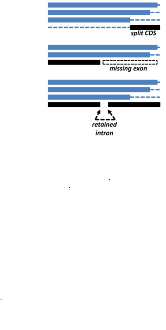
Figure 12: Common problems faced when clustering transcripts/CDS sequences.
When subroutine transcripts::parseblastxcdssequencesreadsBLAST X/DIAMONDresultscheckswhethersecondaryalignmentstothesameproteinsequenceareinthesamestrandastheprimaryalignment.IncaseswereasecondorthirdBLAST HSPo f thesamehitis f oundontheoppositestrand,thatwarningisprintedtoalerttheuser.
•Why have you not implemented the COG algorithm in the get homologues-est.pl?
We have left the COG algorithm out of get homologues-est.pl as it will take some more work to integrate it with redundant
isoform calling, which is important for EST datasets. However, it should be possible to do it.
•The number of clusters produced with -C 75 -S 85 does not match the pangenome/pantranscriptome size estimated
with option -c
The reason for these discrepancies is that these are fundamentally different analyses. While the default runmode simply
groups sequences trying to put in the same cluster isoforms of orthologues and very close inparalogues, a genome compo-
sition analysis performs a simulation in order to estimate how many novel sequences are added by genomes/transcriptomes
sampled in random order. In terms of code, there are a couple of key global variables set in lib/marfil_homology.pm,
lines 135-138, which control how a gene/transcript is compared to previously processed sequences in order to call it novel:
$MIN_PERSEQID_HOM_EST = 70.0;
$MIN_COVERAGE_HOM_EST = 50.0;
These values are equivalent to say that any sequence with coverage ≥50% and identity ≥70% to previous genes/transcripts
will be considered simply a homologue and won’t be accumulated to the growing pangenome/pantranscriptome. You
might want to change these values to increase or relax the stringency and to match the parameters set to produce your
clusters.
•Can get homologues-est.pl be used to analyze non-coding sequences?
In principle the software should work with any type of nucleotide sequences. For instance, the next figure shows how it
can used to analyze conserved non-coding sequences among Brachypodium distachyon and rice, with a median BLASTN
alignment length of 32.
•I produced 2 different parsimony trees with compare clusters.pl, is there a way to merge them and add bootstrap values?
34
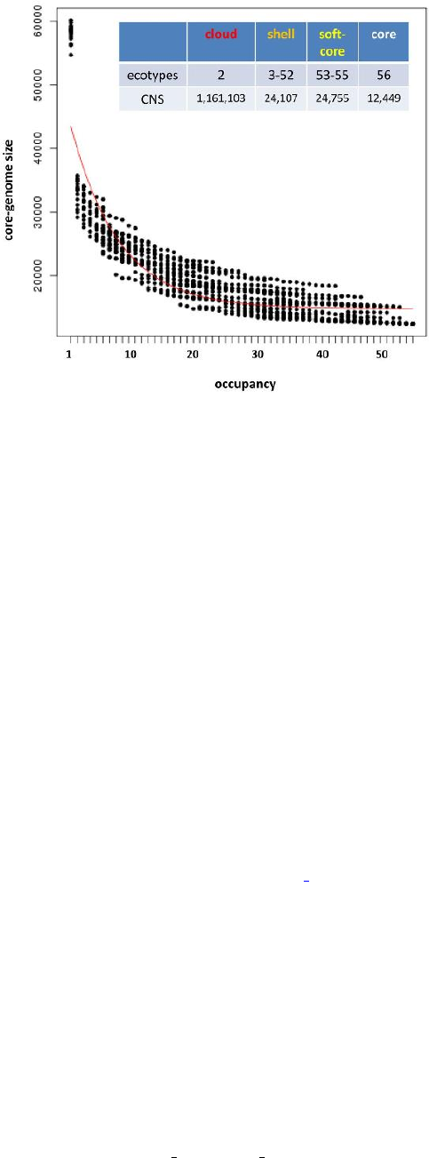
Figure 13: Core-genome composition analysis of conserved non-coding sequences (CNS) from 56 Brachypodium dis-
tachyon ecotypes and rice.
The two trees are equally parsimonious, that is, have the same parsimony score but different topologies. One possibility
to combine them into one topology is to compute either the majority rule consensus (mjr) tree, for example with consense
from the PHYLIP package, or represent a network consensus with a program such as splitstree.
Regarding the bootstrapping, you could write some R code (or in any other language) to randomly sample the columns
in the pangenome matrix with replacement to construct a new, bootstrapped matrix with the same number of columns as
the original one. You should generate 100 or 500 of these matrices and then run pars on each one of them. Then run
consense to obtain the mjr consensus tree and associated split frequencies (bootstrap support values for each bipartition).
An easy way of achieving this would be with R’s boot package (see example).
Another option is to call seqboot from the PHYLIP package to generate N bootstrap pseudo-replicates of the matrix.
Rename the resulting file as infile and call pars to read the file, using the option m no_of_pseudoreplicates to run
the standard (Fitch) parsimony analysis on each of the bootstraped matrices. PHYLIP pars will generate an outtree file
containing as many trees as bootstraped matrices found in infile. Rename outtree to intree and call consense to generate
the default majority rule consensus tree. This tree is only a cladogram (only topology, no branch lengths). The node labels
correspond to the number of bootstrap pseudoreplicates in which that particular bipartition was found.
•How can I produce a maximum likelihood (ML) tree with bootstrap values from a pangenome matrix?
We recommend script estimate_pangenome_trees.sh from the GET PHYLOMARKERS pipeline.
Another alternative is to use the .fasta version of the pangenome matrix produced by script ./compare_clusters.pl -m ,
next to the .tab and .phy files. This FASTA file can be analyzed with ML software such as IQ-TREE (PubMed=25371430)
both online or in the terminal with a command such as:
path_to_iqtree -s pangenome_matrix_t0.fasta -st BIN -m TEST -bb 1000 -alrt 1000
This will produce an optimal ML tree after selecting a binary substitution model with both bootstrap and aLRT support
values.
•Is there a way to plot ANI matrices of soft-core clusters?
Let’s say you have 20 genomes, then 95% of them are exaclty 19 taxa, which is the minimum occupancy that defines
soft-core clusters (see global variable $SOFTCOREFRACTION). You should then compute the ANI matrix as follows:
./get_homologues.pl -d your_data -a ’CDS’ -A -M -t 19
And then plot the resulting matrix with script hcluster pangenome matrix.sh.
35

•When I use the hcluster pangenome matrix.sh script the trees in the output of the newick file and the heatmap differ. Is
there a reason for this?
The difference in the topologies of the NJ trees and the row-dendrogram of the heatmaps differ because the heatmaps are
ordered bi-dimensionally. That is, the heatmap plot shows only the row-dendrogram, but the matrix is ordered also by
columns. The NJ tree is computed from the distance matrix that you indicate the program to calculate for you (ward.D2
is the default).
•I ran get homologues with fasta files of 78 genomes; is there a way to export a 78 x 78 matrix of the number of homologues
shared between each genome?
If you did your analysis requesting cluster of all occupancies (-t 0) then you can get what you want in two steps. First,
you must produce a pangenome matrix with compare_clusters -d ... -m. Now it is possible to request an intersec-
tion pangenome matrix (pangenome_matrix_t0__intersection.tab) which contains the number of sequence clus-
ters shared by any two pairs of genomes with parse_pangenome_matrix.pl -m pangenome_matrix_t0.tab -s -x.
Note that these clusters might contain several inparalogues of the same species.
•How can I use get homologues to produce clusters for GET PHYLOMARKERS?
You should use option -e and make sure that your input FASTA nucleotide files have twin files with matching peptide
sequences. Then, in GET PHYLOMARKERS make sure to set option -f EST.
36

7 Credits and references
get homologues-est.pl is designed, created and maintained at the Laboratory of Computational Biology at Estaci´
on Ex-
perimental de Aula Dei/CSIC in Zaragoza (Spain) and at the Center for Genomic Sciences of Universidad Nacional
Aut´
onoma de M´
exico (CCG/UNAM).
The code was written mostly by Bruno Contreras-Moreira and Pablo Vinuesa, but it also includes code and binaries
from OrthoMCL v1.4 (algorithm OMCL, -M), NCBI Blast+,MVIEW,DIAMOND and BioPerl 1.5.2.
Other contributors: Carlos P Cantalapiedra, Roland Wilhelm.
We ask the reader to cite the main reference describing the get homologues software,
•Contreras-Moreira B, Cantalapiedra CP, Garcia Pereira MJ, Gordon S, Vogel JP, Igartua E, Casas AM and Vinuesa P
(2017) Analysis of plant pan-genomes and transcriptomes with GETHOMOLOGUES−EST,aclusteringsolution f orsequenceso f thesamespecies.Front.PlantSci.10.3389/f pls.2017.00184
and also the original papers describing the included algorithms and databases, accordingly:
•Li L, Stoeckert CJ Jr, Roos DS (2003) OrthoMCL: identification of ortholog groups for eukaryotic genomes.
Genome Res. 13(9):2178-89.
•Altschul SF, Madden TL, Schaffer AA, Zhang J, Zhang Z, Miller W and Lipman DJ (1997) Gapped BLAST and
PSI-BLAST: a new generation of protein database search programs. Nucl. Acids Res. 25(17): 3389-3402.
•Stajich JE, Block D, Boulez K, Brenner SE, Chervitz SA, Dagdigian C, Fuellen G, Gilbert JG, Korf I, Lapp H,
Lehvslaiho H, Matsalla C, Mungall CJ, Osborne BI, Pocock MR, Schattner P, Senger M, Stein LD, Stupka E,
Wilkinson MD, Birney E. (2002) The Bioperl toolkit: Perl modules for the life sciences. Genome Res. 12(10):1611-
8.
•hmmscan :: search sequence(s) against a profile database HMMER 3.1b2 (Feb 2015) http://hmmer.org Copyright
(C) 2015 Howard Hughes Medical Institute. Freely distributed under the GNU General Public License (GPLv3).
•Finn RD, Coggill P, Eberhardt RY, Eddy SR, Mistry J, Mitchell AL, Potter SC, Punta M, Qureshi M, Sangrador-
Vegas A, Salazar GA, Tate J, Bateman A. (2016) The Pfam protein families database: towards a more sustainable
future. Nucleic Acids Res. 44(D1):D279-85
•Haas BJ, Papanicolaou A, Yassour M et al. (2013) De novo transcript sequence reconstruction from RNA-seq using
the Trinity platform for reference generation and analysis. Nat Protoc. 8(8):1494-512.
•Brown NP, Leroy C, Sander C (1998) MView: A Web compatible database search or multiple alignment viewer.
Bioinformatics. 14 (4):380-381.
•Buchfink B, Xie C, Huson DH (2015) Fast and sensitive protein alignment using DIAMOND. Nat Methods.
12(1):59-60
If you use the accompanying scripts the following references should also be cited:
•R Core Team (2013) R: A Language and Environment for Statistical Computing. http://www.R-project.org R
Foundation for Statistical Computing, Vienna, Austria, ISBN3-900051-07-0
37
