Manual Giswater3 Eng
User Manual:
Open the PDF directly: View PDF ![]() .
.
Page Count: 142 [warning: Documents this large are best viewed by clicking the View PDF Link!]
GISWATER 3
USER MANUAL
Version 3.1.103
October 2018

Giswater 3 User Manual
2
PREAMBLE
The Giswater 3 User Manual aims to answer questions regarding the installation and execution of the
Giswater program. This document covers all the necessary information that users and interested parties
know how to install, configure and operate with Giswater 3.
The software has been licensed under the GNU-GLP 3 license (https://www.gnu.org/licenses/gpl-3.0).
The index gives information about the list of available elements and is structured in two main blocks such as:
installation and use
Gratefulness
This manual and the Giswater 3 code has been funded by different water companies in Catalonia, which
have opted to share the development of a software product that can meet both their present and future
needs in the world of Geographic Information Systems. With this objective, the development of the Giswater
program has been carried out, of which you have the manual in your hands.
A deep appreciation to the water companies that have made it possible:
Aigües de Banyoles, SA
Aigües de Castellbisbal, SA
Aigües de Figueres, SA
Aigües de Girona, Salt i Sarriá de Ter, SA
Aigües de Vic, SA
Consorci d’Aigües de Tarragona
Proveïments d’Aigua, SA
Aigües de Mataró, SA
Sabemsa
Aigües de Blanes, SA
Aigües del Prat, SA
Granollers, April 23, 2018
Document licensed under Creative Commons license
CC-BY-SA

Giswater 3 User Manual
3
INDEX
1. INTRODUCTION ............................................................................................................................................ 5
1.1 What is Giswater? ................................................................................................................................. 5
1.2 What is the goal of this user’s guide? ................................................................................................. 6
1.3 Suggested system architecture ........................................................................................................... 6
2. INSTALATION AND START UP .................................................................................................................. 10
2.1 Installation prerequisites. ................................................................................................................... 10
2.2 Download and configuration of PostgreSQL.................................................................................... 11
2.3 Download and configuration of Giswater. ........................................................................................ 12
2.3.1 Toolbar of the main menu. ......................................................................................................... 13
2.3.2 Giswater configuration ............................................................................................................... 14
2.3.3 Connection configuration. .......................................................................................................... 14
2.3.4 Creation of Giswater project template in a database .............................................................. 15
2.3.5 Basic configuration of a project template ............................................................................ 16
2.4. Creation of new example project (sample) ...................................................................................... 19
2.5 Creation of project starting from scratch ......................................................................................... 20
2.6 Configuration of QGIS ......................................................................................................................... 21
3. BASIC WORK RULES ................................................................................................................................. 23
3.1 Project types ........................................................................................................................................ 23
3.2 Available elements .............................................................................................................................. 25
3.3 General conditions of working with database .................................................................................. 27
3.4 Map zones ............................................................................................................................................ 28
3.5 Working in a corporative environment .............................................................................................. 28
3.6 Default values ...................................................................................................................................... 29
3.6.1 User’s values ............................................................................................................................... 29
3.6.2 System values ............................................................................................................................. 30
3.7 Topology rules ..................................................................................................................................... 30
3.7.1 Arc-node behavior ....................................................................................................................... 30
3.7.2 Link-vnode behavior ................................................................................................................... 30
3.7.3 Double geometry elements ........................................................................................................ 32
3.7.4 State’s topology .......................................................................................................................... 32
3.8 Summary of work rules applied to the insertion of NODES ............................................................ 33
4. WORKING ENVIRONMENT IN QGIS .......................................................................................................... 34
4.1 Graphic interface ................................................................................................................................. 35
4.2 Table of Contents ................................................................................................................................ 36
4.2.1 Inventory of assets (INVENTORY) ............................................................................................. 36
4.2.1.1 Catalogs .................................................................................................................................. 36
4.2.1.2 Map zones .............................................................................................................................. 38
4.2.1.3 Network elements (Network) .................................................................................................. 39
4.2.1.4 Others ..................................................................................................................................... 45
4.2.1.5 Topology analysis ................................................................................................................... 46
4.2.2 Operations and management (O&M) ......................................................................................... 47
4.2.3 EPANET ........................................................................................................................................ 49
4.2.4 SWMM ........................................................................................................................................... 50
4.2.5 Masterplan .................................................................................................................................... 52
4.2.5.1 Planification sectors (psectors)............................................................................................... 54
4.2.5.2 Managing prices of network elements .................................................................................... 54
4.2.6 System .......................................................................................................................................... 56
4.2.7 Basemap ....................................................................................................................................... 61
5. GISWATER PLUGIN ............................................................................................................................... 62
5.1 Installation and configuration of Giswater plugin ....................................................................... 62
5.2 Toolbars of a plugin ............................................................................................................................ 63
5.2.1 Basics ........................................................................................................................................... 63
5.2.2 Operations and management ..................................................................................................... 70
5.2.3 Edition .......................................................................................................................................... 84
5.2.4 Hydraulic model ........................................................................................................................ 101
5.2.5 Masterplan .................................................................................................................................. 106
5.2.6 Administration ........................................................................................................................... 115
6. HOW TO DIGITALIZE THE NETWORK .................................................................................................... 121

Giswater 3 User Manual
4
7. EXPORT – IMPORT OF THE HYDRAULIC MODEL ................................................................................ 128
7.1 Process characteristics .................................................................................................................... 128
7.1.1 Main characteristics for watter supply networks (WS) ......................................................... 128
7.1.1.1 Working by sectors ............................................................................................................... 128
7.1.1.2 Demand scenarios ................................................................................................................ 129
7.1.1.3 Transformation of nodes into arcs ........................................................................................ 129
7.1.1.4 Possibility of multipump ........................................................................................................ 130
7.1.1.5 Using different state types of valves ..................................................................................... 130
7.1.2 Main characteristics for urban drainage networks (UD) ....................................................... 131
7.1.2.1 Working by sectors ............................................................................................................... 131
7.1.2.2 Management of hydrology scenarios ................................................................................... 131
7.1.2.3 Integration of the standard form catalog of SWMM .............................................................. 132
7.1.2.4 Flow regulators ..................................................................................................................... 134
8. REAL-TIME MATHEMATICAL MODEL (RTC) FOR WS .......................................................................... 135
9. OTHER CONSIDERATIONS ..................................................................................................................... 138
9.1 Good practice .................................................................................................................................... 138
9.2 Management and use of the QGIS composer ................................................................................. 138
9.3 Control and verification of projects and schemas ......................................................................... 139
Giswater 3 User Manual
5
1. INTRODUCTION
Welcome to Giswater, the first open source software for water cicle management (water supply and urban
drainage).
This user’s guide will help you start working with Giswater.
1.1 What is Giswater?
Giswater is an open source application for management and exploitation of hydraulic infrastructure elements
in both water supply and urbain drainage. It’s accesible using database and graphic representation using any
kind of geographic information system (GIS).
At the same time, Giswater can act as a driver connecting spatial database with tools used for hydraulic
analysis.
Currently the third version of Giswater software is available for users. Many improvements have been made,
comparing with previous versions, not only graphically but also in usability and capabilities.
As presented on image 1, Giswater is located between the applications, which used all together allow a solid
and global management in relation to water supply and urban drainage models.
The central element of the set is the database, where all the information and most of the functionalities of
each Giswater project is located. Giswater uses PostgreSQL database, which together with its PostGIS
extension allows to conveniently link it with the next application of the set: QGIS.
QGIS is the geographic information system software on which the development of the Giswater project has
been based. QGIS is related through PostGIS to the database, showing organized spatial data and always
taking into account all the rules, relationships and processes established in the database.
The central point of the project (Database - GIS) also allows to connect with SCADA, in order to update in
real time, the information that comes directly from the physical elements of the network. In this way, Giswater
Image 1: Schema of the applications used by Giswater with a database in its central point.
Giswater 3 User Manual
6
is also a global management system that allows its users to always work with data that is updated
automatically.
Apart from the data management through GIS software there is also the possibility of working with Giswater
data in web and mobile environment. This functionality is separate from the usual desktop use, since it is
only for customers that require it, and it is managed from the BMAPS platform.
1.2 What is the goal of this user’s guide?
The most important goal of this guide is to provide the user a document which will help to carry out any task
with Giswater, from the initial installation process of the necessary programs to the most complex
management operations.
The improvements made in the version 3.0 will be reflected throughout the manual and the purpose of those
improvemnets, together with the instructions of how to make use of them, will be explained in the best
possible way.
1.3 Suggested system architecture
The suggested system is composed of three machines that act as a server, and two clients. Heavy clients
which use QGIS as a GIS engine, and thin clients, which use Google Chrome as a GIS engine.
Given the architecture of the system on image 2, it is necessary to install different technologies in different
machines that are listed below.
Image 2: Suggested system architecture with three servers.
Giswater 3 User Manual
7
▪ DATABASE SERVER (DB)
First, it’s necessary to install the database of the new corporate GIS, in this case PostgreSQL
(https://www.postgres.org) and its spatial extension, PostGIS (https://www.postgis.net).
The operating system can be either LINUX or WINDOWS. In relation to terms of speed,
performance, customization and reliability we recommend a machine (virtualized or not) with
operating system DEBIAN 9 or higher. However, there is no problem if that it is a Windows machine
with a current operating system. This decision depends entirely to the preference of the personnel of
IT department of a company.
What needs to be kept in mind is that depending on the number of users and records in the
organization, it is highly recommended to install the database in a highly available environment with
the aim that simultaneous queries, especially those that consume a large amount of resources, can
be attended without high penalties.
Considering the fact that the database usually works with the disk to recover or display information, it
is essential that the machine has a solid hard disk (SSD) as well as a controller with enough
bandwidth to access the information in a massive and fast way. From now on, the architecture of
virtualization and the software layer that manages it, will mostly depend on the number of users and
the volume of managed data.
▪ WEB SERVER
The web server is another piece of the project’s architecture. This server is the one that needs a
lower number of resources since it simply has to publish the information provided by the database. In
this part of the system, the determining factor is no longer the speed or capacity of the system, but
its safety.
For this purpose, it is necessary to install all the required technologies to provide security, reliability
and performance to the web environment. There are shown on image 3:
Image 3: All the technologies that should be installed in order to use Giswater with the most relialibity.

Giswater 3 User Manual
8
Unlike the previous server, this has to be obligatorily a LINUX in DEBIAN distribution, version 9.
▪ PUBLICATION SERVE
Because of security reasons, an additional server is defined specifically for publication. The functions
of this server are:
1) Publish the corporate data, so that the production database is never exposed in case of a hacking
attack. A determined process (nocturnal, in real time) will be responsible for keeping updated the
data on this server.
2) Enable web writing options, if they are operative. All the inserts from the outside will be made in
this database, and then a determined process (nocturnal, in real time) will be responsible for
accessing this machine in order to collect the necessary data and place it where necessary.
The firewall is generated using this intermediate machine. It allows that the access to the corporate
information is beeing protected from the outside in both write and read mode.
▪ FILE SERVER
The file server
1
must be a centralized repository of all documents that have to be managed by the
system (photographs, files, plans, administrative documentation, etc.). The architecture and
technology of this server depends on what is used in a company and it is recommended to develop a
specific connection device for each case.
Topics such as publishing the files on network or not, serving an URL or folder routes are the
decisions on which depends the final architecture of the system and the reuse or not of the current
file server organization.
So that the Giswater project could work, the only files that have to be served, and which are the part
of the architecture of the project and to which all the users need to have access in a READING
MODE, are files located in a corporate plugin folder:
o Giswater plugin
o Time manager
o Table manager
o Folder used for sharing QGIS projects
▪ HEAVY GIS CLIENT MACHINES (QGIS)
As presented in the image 2 there are two types of client machines. The one with the highest
requirements is the one with QGIS as a GIS client. In this case it is necessary to have at least the
following software:
o QGIS (https://www.qgis.org) – last stable LTR
o Notepad++ ( https://notepad-plus-plus.org)
o JRE (http://www.oracle.com/technetwork/java/javase/downloads)
o Giswater (https://www.giswater.org/descarga)
1
File server doesn’t have to be a spetial, separated machine. It can be any file server used by a company or a folder located on a
database server, shared with all the network.

Giswater 3 User Manual
9
In case that a hydraulic model compatible with Giswater is necessary, the EPA software can be
downloaded from the Giswater website:
o EPA SWMM (https://www.giswater.org/descarga)
o EPA NET (https://www.giswater.org/descarga)
In order to have a better user experience with the GIS software, it is recommended to have an office
suite installed, as well as a PDF reader.
▪ GIS THIN CLIENT MACHINES (CHROME)
There is also a second type of client machines that are used as a GIS thin client in the internet
browser, which will perform the functions of WebAPP. In this case it is only necessary to have
installed Google Chrome itself.
The development is only certified and validated with the use of the Google Chrome browser and any
other browser - Mozilla Firefox, Opera or Internet Explorer may have some dysfunctions and its
usage is not recommended.

Giswater 3 User Manual
10
2. INSTALATION AND START UP
In this second section of the user’s guide you will find all the necessary steps that must be done before
starting working in the Giswater environment, from the pre-installation requirements of the software’s
configuration, through the creation of new projects (real or example), to testing the functionalities of Giswater.
2.1 Installation prerequisites.
In relation to section 1.3, where the suggested system’s architecture was presented, in this part the details of
the tree servers, of which the system is composed, will be commented
On the data server side, the performance depends mostly on the number of users and the volume of data.
As an order of magnitude and for companies with one or two people who edit data and between five to eight
who consult, with a relatively small network data volume respect the volume of dedicated staff, a machine
with four cores and a minimum of 32 GB of RAM has to be enough. Regarding hard drive, the two elements
to keep in mind are capacity and speed.
In the case of larger organizations, it would be necessary to analyze the available server technology and the
type of virtualizations that are used in order to adjust the needs to the reality of the service and verify
whether the system is sufficient or needs to be resized.
If the machine is only used as a PostgreSQL server (and the basic functions of OS), the disk space
consumed by the database is not very high. It is also important to know that the hard disk is used for more
functions than just to store the PostgreSQL data in a binary format. Specifically, this use also includes
1. Basic functions of OS support.
2. Help through temporary files to PostgreSQL processes.
3. Storage of specific Giswater files.
It is recommened to initially allocate about 100 GB for storage. Regarding the access speed of the disk,
which is a particularly relevant issue, the fact of having a solid hard drive (SSD) can greatly favor the benefits
to end users with a controller that guarantees the fastest possible access to data.
On the side of the web server, less features are required and therefore, always taking into account the size
of the company mentioned above, with a two-core machine (recommended having four) and a minimum of
16 GB of RAM would be sufficient. In any case, this will depend on the concurrence and the use on the web
side.
What should be highlighted in this case is the importance of a disk to store the field photographs, which are
made and than managed by a MongoDB database. For this purpose, the size of the disk which does not
need to be solid, should be adjusted to the usage of daily capture of photographs on the web.
On the file server side and regarding the storage of specific Giswater files, it is recommended to use the
same PostgreSQL machine to host a folder, read only, with shared network access for normal users in which
they could find a plugin repositor, the original QGIS projects and also the primal installation files.
In this GIS directory the templates of the QGIS projects (subfolder templates) will be stored. This directory
will also be configured as a path for QGIS client plugins (subfolder plugins) which will be installed on the
client’s machines. In the plugin’s subfolder will be installes all those add-ons that are of interest to the
organization.
About other data types (QGIS projects, cartography base layers, attached documents, etc.) It’s not
recommended to use the same machine. The best option is to use the shared network unit with which the
data is usually worked (to take advantage of the organized backup system).
Giswater 3 User Manual
11
Configuring this folder with the plugins on all client users with read-only permissions ensures that all QGIS
users have the same plugins installed and makes it much easier to update them.
On the client side the machines must have some processing capacity (i7 processors are recommended)
with a minimum of 18 GB of memory. The operating system must be Windows 7 or higher. In case you want
to carry out an intensive resource consumption with the generation of high-intensity geoprocesses, it is
recommended to use a client machine with greater features such as a multicuore of 16-32 GB of RAM and a
solid hard disk.
2.2 Download and configuration of PostgreSQL
PostgreSQL is an open source database with enormous potential, which will be used to store all the data
with which Giswater works. Thanks to its geospatial extension PostGIS allows a very comfortable relation
with GIS, especially QGIS. This extension contains of over 1000 geospatial functions, which maks it one of
the most powerful GIS software available, although PostgreSQL is not a specific GIS program.
There are different versions of PostgreSQL available for download. To work with Giswater it is recommended
to download any versión higher than 9.5, with which the programs are 100% compatible.
The download and installation are very simple and can be done from https://www.postgresql.org/download.
Together with the database, a database administration program is installed, pgAdmin
(https://www.pgadmin.org/download/ to download it), which will be used to manage the database in a visually
way, easy for user. Using pgAdmin it’s possible to modify the tables, views and rules of the database, as well
as consult all the information and manage it.
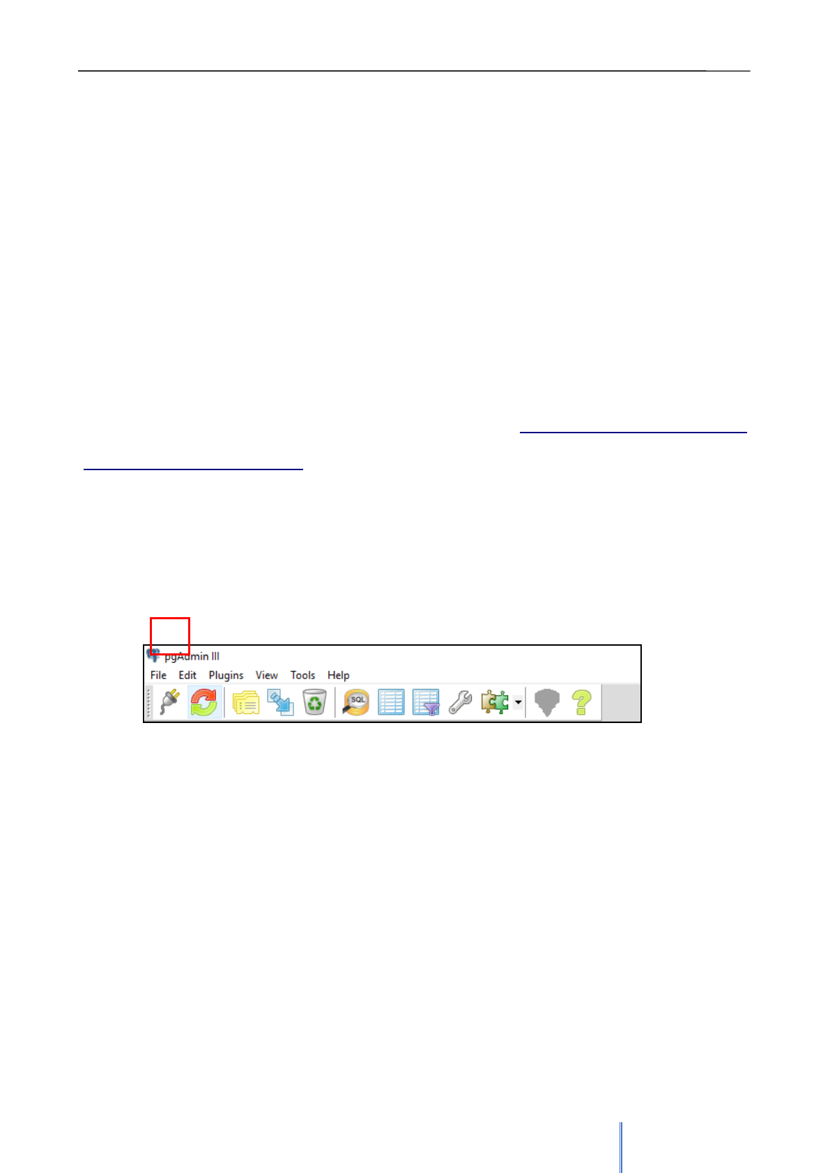
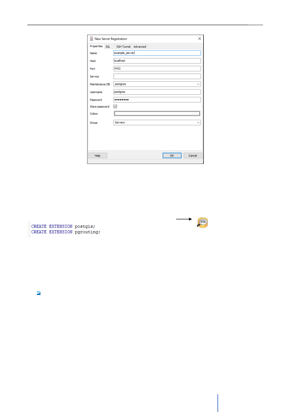
Once both programs are installed, after opening pgAdmin the first thing that needs to be done is adding a
new connection.
It’s necessary to
fill in the listed fields in
order to créate a new connection:
▪ Name: connection name
▪ Host: it can be a localhost or a connection with another server
▪ Port: port
▪ Service: related to a service configured in a file pg_service.conf. (Opcional)
▪ Maintenance DB: existing database to which the new connection is related
▪ Username: user’s name. The first user should be ‘postgres’
▪ Password: password, which for a postgres user is also ‘postgres’.
Giswater 3 User Manual
12
Once the new connection is created, the first ‘public’ scheme is automatically created in a database. Next,
the PostGIS extension must be added, in order to have all the GIS functionalities available, as well as the
pgRouting extension, which adds routing and network analysis functions to the database. pgRouting is
essential for some of the Giswater tools such as the cutting polygon and the longitudinal profiles.
By clicking the SQL command button, we can write our first query
2.3 Download and configuration of Giswater.
Giswater is composed by an application, which acts as a driver used for the configuration, creation and
management of the different projects in the database, and a plugin based on QGIS for the exploitation of
network elements.
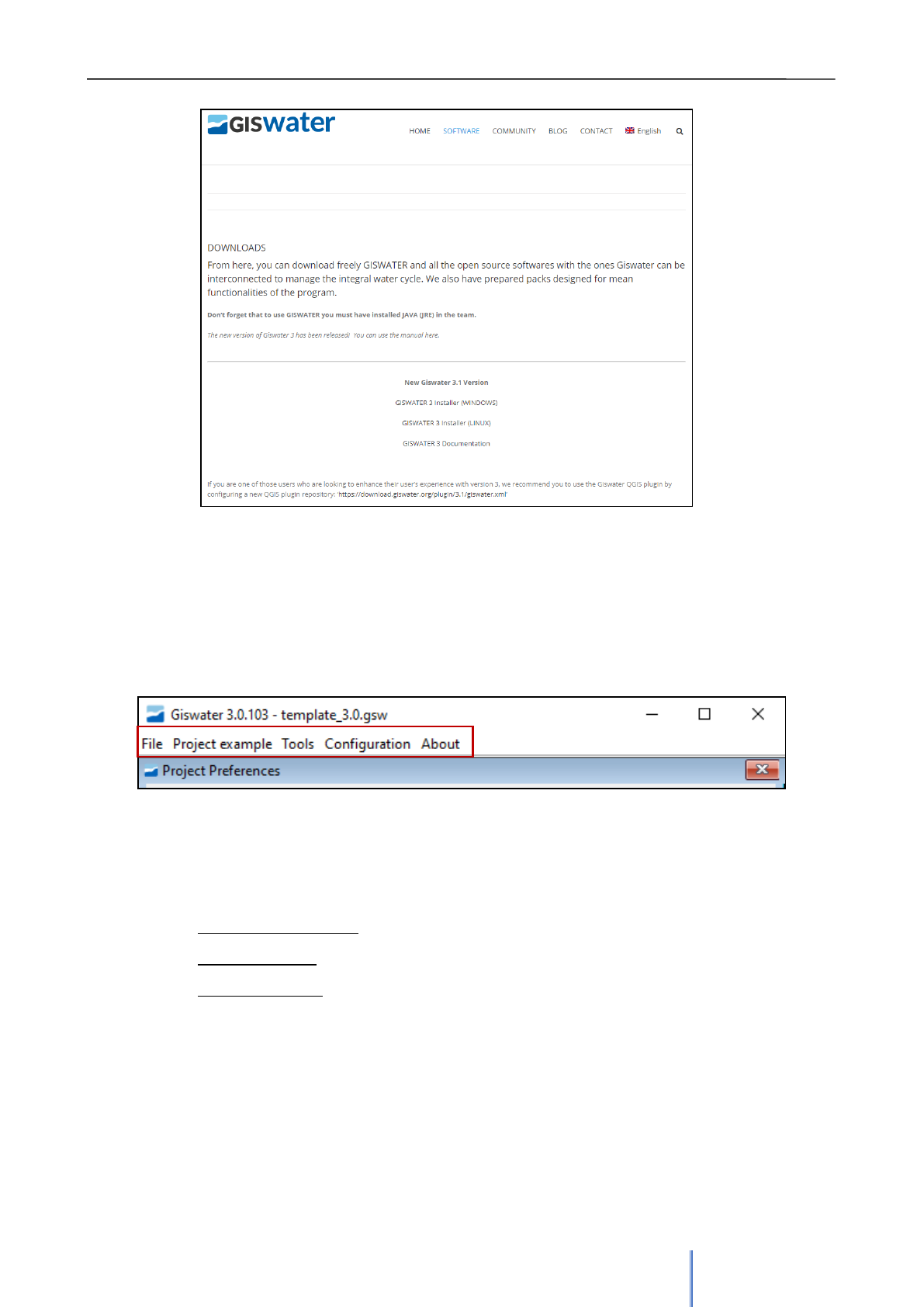
To download Giswater use the link: https://www.giswater.org/downloads/?lang=en
The website of Giswater has available to download the latest version 3.0 as well as previous versions of the
program.
Apart from the download tab, on the website you can also consult information about the product, the benefits
of open source programs, the community of experts that develop Giswater or obtain materials and tutorials to
learn how to use it.
Image 4: Add new connection to Postgres using pgAdmin.
Giswater 3 User Manual
13
Once installed, open Giswater and start the configuration and creation of the new project.
2.3.1 Toolbar of the main menu.
Toolbar of the main menu of Giswater consists of the following submenús continuación:
▪ File: Allows to manage the configuration preferences defined by user and save or restore the
database schema.
▪ Project example: Automatic creation of sample projects included in Giswater.
▪ Tools: Tools realte to the database:
o Database administrator: Allows to open the database management program.
o SQL file launcher: Allows to execute SQL scripts in the database.
o Developer toolbox: Allows to update a database schema.
▪ Configuration: Allows to manage different parameters of the program.
▪ About: Relatied to other aspects of Giswater, like welcome, community or license.
Image 5: Giswater website, where you can download both Giswater software and QGIS plugin. Previos
versions are also available.
Giswater 3 User Manual
14
2.3.2 Giswater configuration
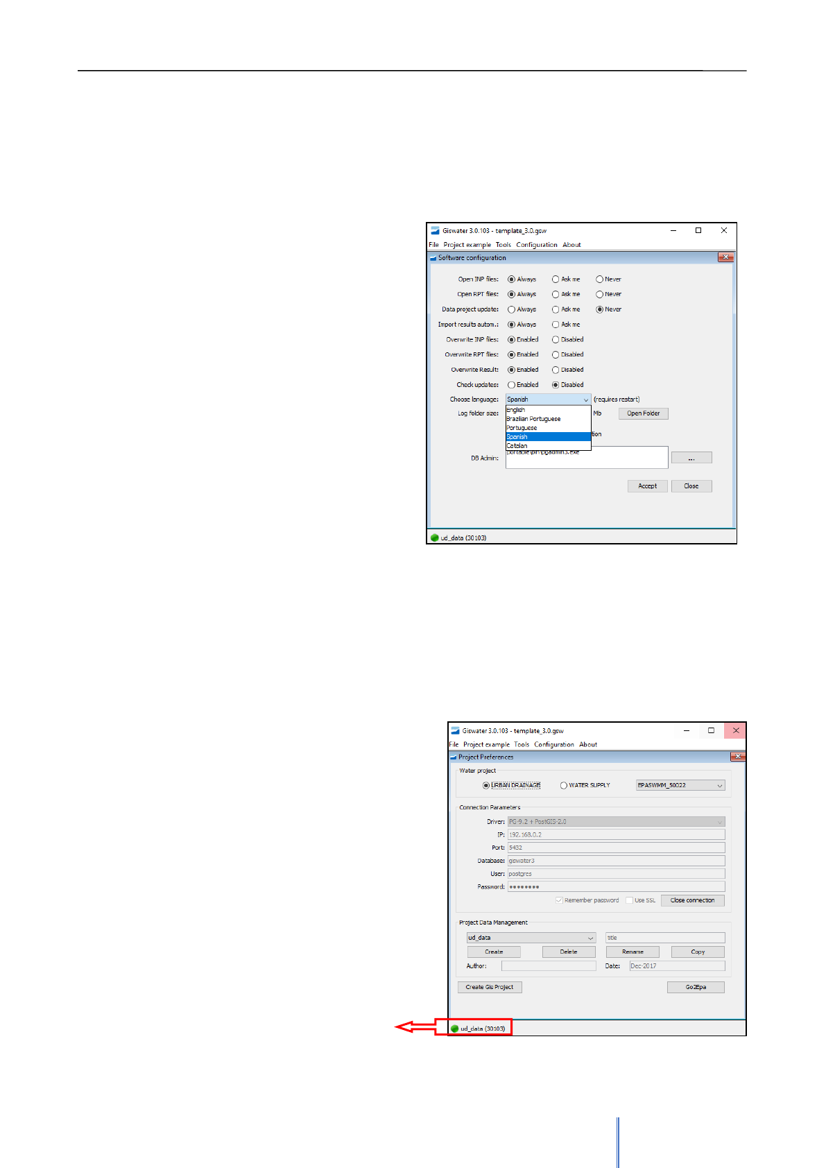
It’s possible to parametrize the basic options of the program using the menu Configuration, such as:
Open INP files: Allows to configurate when the INP files are opened.
Open RPT files: Allows to configurate when the RPT files
are opened.
Data Project update: Allows automatic updated in case of
bugs.
Import result autom.: Allows automatic import of the
simulation results.
Overwrite INP files: Allows to overwrite the INP files.
Overwrite RPT files: Allows to overwrite the RPT files.
Overwrite Result: Allows to store more than one result in a
database (it’s recommended to enable the option).
Check updates: Allows to check whether new versions of
software are available (it’s recommended to enable the
option).
Choose language: Allows to choose the language of the
project and user’s interface.
Log folder size: Escoger la capacidad de la carpeta log.
DB Admin: Configuration of the path where the executable
file of ‘pgAdmin’ is located in order to access the database.
2.3.3 Connection configuration.
As a first step with Giswater, before creation of the data schema, is creation of the connection to the
database on which all the data will be stored. To do this, in the 'Project preferences' menu, in the 'Connetion
Parameters' section, the parameters of the connection needs to be configured:
Driver: Driver versión of the database connection.
IP: IP address of the connection (may be localhost)
Port: Port enabled to access the connection.
Database: Name of the database.
User: Database user’s name.
Password: User’s password.
Green color indicates
that the connection is
correct
Image 6: Initial configuration of the software.
Image 7: Project preferences and management.
Giswater 3 User Manual
15
2.3.4 Creation of Giswater project template in a database
Once the connection to the database is configured, everything is ready to create a working scheme with the
predefined template of all the tables, views and functions that act in the database. This template is the basic
element of Giswater, because it represents the logical skeleton of the project and all the relationships that
allow its correct operation. Within the template there are some tables with the data incorporated by default
(system) and other tables and views with different data for each project.
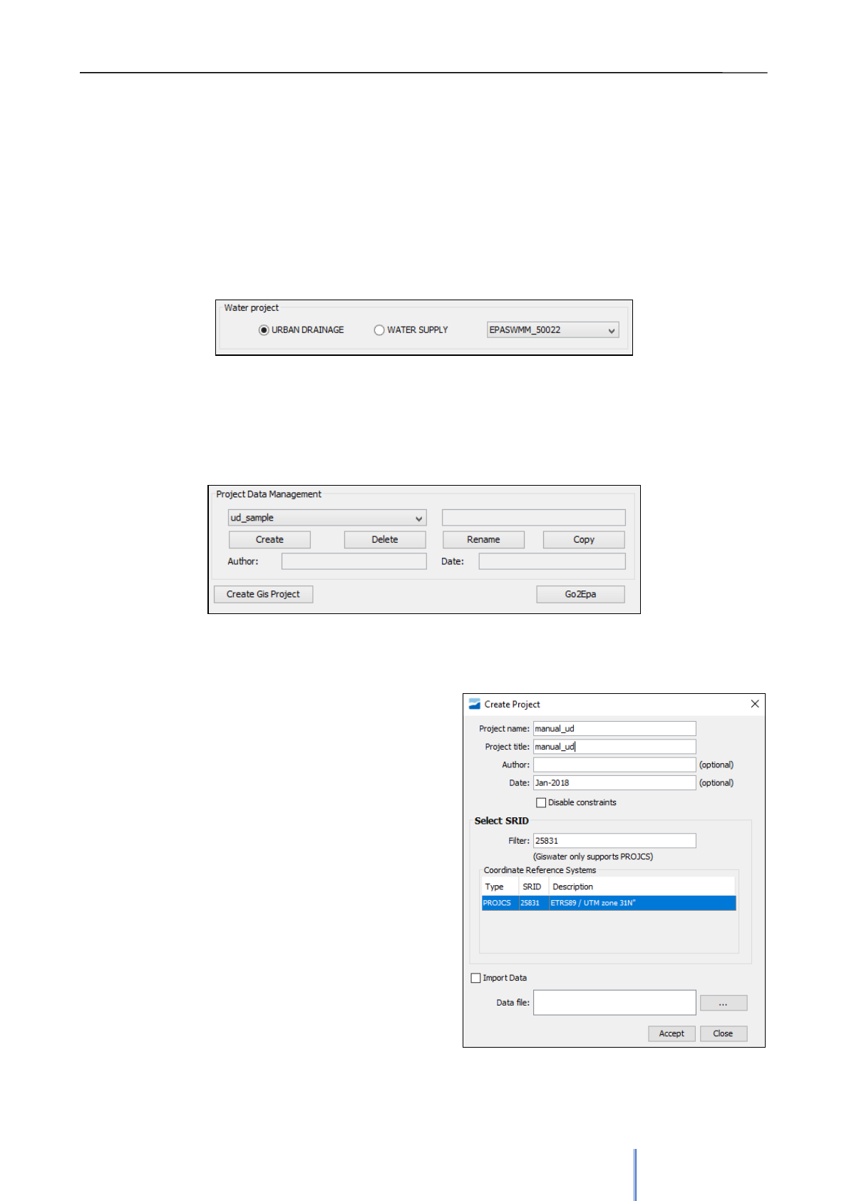
So as to create the template the following steps have to be executed:
a) Select the project type (Urban Drainage o Water Suply)
b) In the menu Project Data Management, click the button ‘Create’, in order to créate a new data
schema (template of tables, views, functions, etc.).
Project name: Name of database schema.
Project title: Project title.
Author: Author of the project.
Date: Creat date.
Select SRID: Selector of Spatial Reference ID.
Import data: Allows to import a file with project creation
parameters.
Once the data project has been created, it can be deleted,
renamed or a copied using the buttons of Giswate. It’s
possible to verify if it has been created correctly by
opening pgAdmin and the corresponding schema
(manual_ud for this example). There must exists all the
tables related to Giswater, although most of them empty.
Image 8: Creation of a project in a database.

Giswater 3 User Manual
16
2.3.5 Basic configuration of a project template
There are many types of tables within all those created in the previous section. There are some that are
already filled by default, others that will be filled in as elements of the network are created and there are
tables that can be customized by the users, depending on their needs and those of their network.
The basic tables that match the main generic elements of any Giswater project are of great importance and
must be taken into account in order to explain this section. They are the following:
Arc
Node
Connec
Gully (only for UD)
These four tables are empty and will only be filled when the project has geospatial elements of the
corresponding type. The important thing is that they have many restrictions and relationships with other
tables that must be fulfilled.
Below are the tables that, from the beginning, should be filled in by the user so that Giswater works correctly.
1- Creation of new, personalized network elements
cat_feature
node_type
arc_type
connec_type
gully_type (only for UD)
These tables are used as an intermediate catalog for all the elements of the different types.
Each element that is created must necessarily be part of an element type (feature_type), which can
be node, arc, connec or gully, and in addition to another type within each of the above, specified in
the table sys_feature_type (no modifiable by users). There are 24 records for water supply projects
(ws) and 17 for sanitation (ud).
Each user can customize the cat_feature table with specific elements that are necessary for their
network, provided they are related to one of the sys_feature_type fields (for example, TANK or
FOUNTAIN) and one of the existing feature_type (for example, NODE or CONNEC).
The following tables that must be filled in are those of element types related to only one feature_type
(node_type, arc_type, connec_type and gully_type). The id of the cat_feature table must match the id
of * _type tables, which, obviously, will only have elements of their specific type. The * _type tables
connect with the individual management tables of each element type, as well as with those that act
on the hydraulic models (inp).
To finish the hierarchy of the tables that determine the existing elements, the catalog tables must be
filled in by relating each new element, with name to the user's liking, with any of the types specified
in the higher hierarchy tables (see section 4.2.1.1).
Giswater 3 User Manual
17
2- Custom value domains
man_type_category
man_type_fluid
man_type_function
man_type_location
In these tables the specific information about the type of category, fluid, function or location related to
the different types of basic elements (arc, node connec, gully) is defined. Each of the tables has the
following fields:
id
serial
Automatic id (primary key)
*_type
varchar (50)
Field to put in the information that will be used in arc/node/connec/gully
table
feature_type
varchar (30)
Element type to which the value is assigned
featurecat_id
varchar (30)
Allows to detail to which kind of element is assigned the value
observ
varchar (150)
Field for additional information
*category/fluid/function/location
To give an example of the use of these tables, we could define a domain catalog of custom values
for a tank in addition to what would correspond to it by node.
These fields are managed by the database through foreign keys to guarantee the consistency and
uniqueness of the information. The foreign key has special characteristics to govern this system of
different values depending on the source table. One of the most important properties is the duplicity
of the foreign key. This means, that to give an example for the node table, and regarding the type of
fluid, the double key is managed so that only those values of fluid_type in the table man_fluid_type
that meet the condition of having the field feature_type = 'NODE' will be available in the
node.fluid_type field.
The double foreign key guarantees that the information is consistent at all times, avoiding insertions
that do not comply with this criterion and spreading changes in case of renewing or eliminating value
domains.
3- Verification values
value_verified
This table is used to customize the verified field that is present in all the tables of the basic elements.
Each user, depending on their needs, can add verification values in order to improve the accuracy of
their data.
Some examples of verification values could be: to review, verified, pending confirmation, etc.
4- Condiguration of tables embed in forms
config_client_forms
This table is used to customize the visibility of all the tables embedded in the forms and aims to
customize which fields are visible, how wide they are and which is the alias of the column.

Giswater 3 User Manual
18
The relation shoulf be configurated and its appearance is detailed in the attached table
project_type
location_type
table
utils
basic toolbar
v_ui_workcat_x_feature_end
utils
basic toolbar
v_ui_workcat_x_feature
utils
om toolbar
v_ui_om_visit
utils
om toolbar
om_psector
utils
edit toolbar
doc
utils
edit toolbar
element
utils
epa toolbar
v_ui_rpt_cat_result
utils
plan toolbar
plan_psector
utils
plan toolbar
v_ui_om_result_cat
utils
node form
v_ui_scada_x_node
utils
node form
v_ui_scada_x_node_values
utils
node form
v_ui_element_x_node
utils
node form
v_ui_om_visit_x_node
utils
node form
v_ui_doc_x_node
utils
arc form
v_ui_element_x_arc
utils
arc form
v_ui_om_visit_x_arc
utils
arc form
v_ui_doc_x_arc
utils
connec form
v_ui_doc_x_connec
utils
connec form
v_ui_element_x_connec
utils
connec form
v_ui_om_visit_x_connec
utils
connec form
v_rtc_hydrometer_x_connec
ws
om toolbar
v_ui_anl_mincut_result_cat
ws
node form
v_ui_node_x_relations
ws
connec form
v_ui_mincut_hydrometer
ud
node form
v_ui_node_x_connection_downstream
ud
node form
v_ui_node_x_connection_upstream
ud
gully form
v_ui_doc_x_gully
ud
gully form
v_ui_om_visit_x_gully
ud
gully form
v_ui_element_x_gully
On the other hand, the configuration table has the listed columns:
id serial, location_type, project_type, table_id, column_id, column_index, status, width, alias,
dev1_status, dev2_status, dev3_status, dev_alias, donde para la configuración del cliente QGIS
solo se debe actuar sobre los campos:
status: true/false if it would be show or not in the forms
alias: the name of the columna shown in the
width: the width of the shown field
Fields dev1_status, dev2_status, dev3_status and dev_alias are created for users using mobile
devices.

Giswater 3 User Manual
19
5- Creation of personalized attributes
man_addfields_parameter
This table, as its name indicates, is intended to add fields to any project element that are not created
by default in Giswater. This allows users to customize the fields according to the requirements of
each user. In this way if at any time there is a neccessity of linking any type of information to an
element it’s possible to do it through this table.
There are three more tables related to man_addfields_parameter:
- man_addfields_cat_datatype: catalog of data types (integer, text, boolean ...)
- man_addfields_cat_widgettype: catalog of widget types displayed in the form (QCheckBox,
QComboBox, QTextEdit ...)
- man_addfields_value: table where the values are stored for each type of parameter added by the
user.
The information contained in the fields of these tables can not be displayed in the attribute table of
the element, but it will be seen in the corresponding form and in the addfields tables.
6- Configuration of visit, inspection and planification functionalities.
om_visit_parameter
The table om_visit_parameter allows to add fields for each type of inspection that can be done in the
water network. Any type of visit can be defined (for example, inspection or rehabilitation) to meet the
needs of the user. However, the visit must also be related to an existing element type.
plan_psector
It’s required to insert at least one planification sector before starting to work. This zone will work as
default sector for new planified elements.
2.4. Creation of new example project (sample)
To facilitate the first steps with Giswater and have a complete data model that serves as a reference source,
Giswater has incorporated two example schemes, for both urban drainage 'ud_sample', and water supply
networks 'ws_sample'.
Having a complete data model, apart from serving as a query source to see how the data is structured within
each of the tables, will allow to start with an environment and practice with all the features that contains the
Giswater plugin.
In order to créate the sample project click Project example on the main menu toolbar.
Image 9: With the database connection opened, it’s posible to create a sample data
schema to practise Giswater functionalities.
Giswater 3 User Manual
20
After clicking on selected type of project, the program warns about the characteristics of the example project
and asks whether we wish to continue. Click Yes and the project will be created. In the case of having
created the urban drainage example, a new scheme with the name 'ud_sample' will appear in a database; If
the created example is a water supply network, the created scheme will be called 'ws_sample'.
Finally, create a new QGIS project to visualize and start working with the example data. When clicking OK
button, the sample QGIS project will be created which will allow to start working with the sample data.
The generated project is specifically created to work with the tables of the database, as well as designed
with a symbology that allows to visualize the project data in the most comfortable way possible.
2.5 Creation of project starting from scratch
If what we want is to start our project from scratch, with the real data of our network, we must take into
account the vital layers so that at least the Giswater plugin would be activated once we are inside the QGIS
project.
Si lo que queremos es empezar nuestro proyecto desde cero, con los datos reales de nuestra red, debemos
tener en cuenta las capas vitales para que como mínimo se active el plugin de Giswater una vez estemos
dentro del proyecto GIS.
The essential layers required by the plugun are the ones which call the views:
▪ v_edit_arc – view of all elements in table arc
▪ v_edit_node – view of all elements in table node
▪ v_edit_connec – view of all elements in table connec
▪ v_edit_gully (only UD) – view of all elements in table gully
Moreover, the listed tables have to be loaded:
▪ version – table that stores the information about different versions of programs (Giswater y
PostgreSQL), schema creation date, the default language or EPSG.
▪ exploitation – value of exploitation to which belongs the network. There should be defined at least
one exploitation so that the plugin activates itself. It’s also neccessary to filter the data showed in a
project using the expl_id
Once the information is in the tables of the created database (manual_ud), you can proceed to create a
QGIS project to finally visualize the information in a specific software of Geographic Information Systems.
Giswater 3 User Manual
21
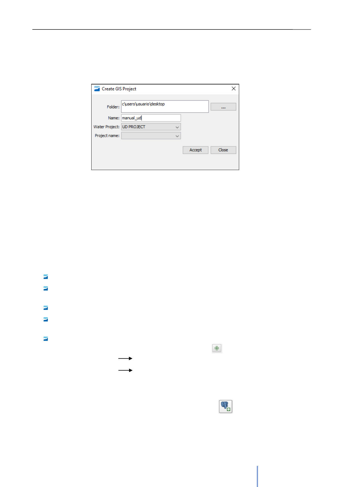
Within Project Preferences of Giswater and with the connection opened to manual_ud, click directly on the
'Create Gis Project' button. This will open the menu shown below where the following parameters are
configured: Location where the QGIS file will be saved, file name, project type (choose between UD and WS)
and the database schema with which it will be linked.
Once all the parameters have been defined, the project will be created. QGIS project links all the tables and
views of the data template created in section 2.3.4 with the information filled in at the beginning of this
section.
2.6 Configuration of QGIS
When opening the QGIS project for the first time, a series of parameters necessary to work with Giswater
must be configured. These requirements are the following:
Create a PostGIS connection to the database where the data schema is located
To work comfortably and quickly with rasters, it’s recommended to extend the cache memory of
QGIS to 1GB and 1 year, through the menu 'Settings / Options / Network'.
Choose open form if a single entity is selected
Install plugins recommended to improve the QGIS user experience: Reloader, Table manager, Time
manager
Set two variables within the project properties (Project / Project Properties / Variables). To add
variables to those that appear by default, there is the button
1. project_type ud/ws (depending on the project type)
2. expl_id value of the exploitation with which the project works
How to configure the connection between QGIS and PostGIS
1) Open QGIS and click oni con Add PostGIS layers
2) Click on button New and introduce the connection parameters.
Image 10: It’s posible to créate a QGIS project for an opened
database connection using button Create Gis Project.
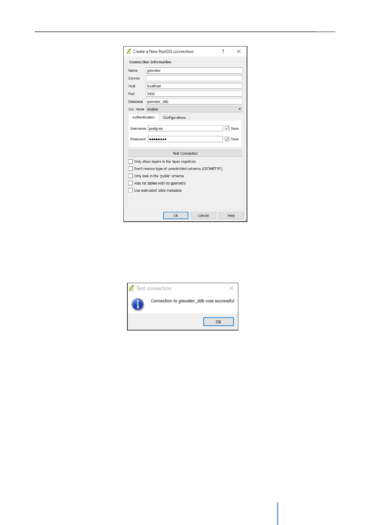
Giswater 3 User Manual
22
3) Once the parameters have been entered, click on ‘Test Connection’ button. If everything is correct the
following message will be shown:
4) Click on OK. In this momento the connection is saved and will be available on the listo of connections.
Once connected it’s possible to see the list of all tables, with or without geometry, availables in the database
and add it to the project if neccessary
Image 11: Connection form between QGIS and
PostGIS. Thanks to this it’s posible to import layers
from database.

Giswater 3 User Manual
23
3. BASIC WORK RULES
Once the software installation, the necessary configuration and the creation of data schemas and projects
has been completed, the user must become familiar with the basic rules of working with Giswater. Apart from
those already mentioned in the previous sections, which were indispensables for preparation process now
it’s time to make an approximation of the tool operation, its characteristics and capabilities, with special
emphasis on the rules of how to work with the data in a safe way.
One of the main advantages of working combining a database with GIS is the great capacity that can be
acquired in terms of robustness of the data thanks to the existence of primary and foreign keys, topological
rules or the possibility of managing the data edition.
In this section the main rules and knowledge, which need to be taken into account while working with
Giswater, will be presented.
3.1 Project types
There are two very different types of projects in the world of Giswater, which have great similarities in terms
of the structurin and categorization of data, but which at the same time should not be confused by user. It’s
always important to know if you are working on:
Water Supply
Project related to the drinking water supply network of a territory. The data represent all the
elements that are necessary for this type of network, starting with the pipes (arc elements) and
following with the valves (node elements), that are found along the network among many other
elements. Giswater aims to represent as accurately as possible the reality of a water supply system,
so it covers all possibilities that may occur in the system.
The main tools are used to regulate and manage water flows, pressures or planning supply to
customers depending on the moment. In relation to this there are sets of tables that allow the
monitoring of the flows thanks to SCADA systems or the management of real visits to the elements
of the network.
Urban Drainage
Project related to the sanitation and drainage network of urban waters in a territory. As in WS
projects, the aim is to represent the network in the most realistic way possible. Here the main
elements are the conduits in which the wastewater circulates. There are elements that coincide with
the water supply projects, but mosto of them are characteristic only for drainage networks, such as
the gullies or the sewage treatment plants.
Some of the most prominent tools of this type of project are related to the direction of wastewater
circulation, either upstream or downstream. In this sense, Giswater allows to represent a profile of
the conduits with relevant information about them,
This guide is unique for both types of project, although individualized manuals for each of them could
perfectly exist. It has been worked to unify it in order to have all the information of Giswater in a single
document, but the intention is that within this manual the user can quickly differentiate if the content of a
section is specific to a WS project, a UD project or it is common section.
Giswater 3 User Manual
24
To accomplish this goal, all sections of the document that are specific to a project type will be marked with a
color: blue for WS and yellow for UD. All the sections presented so far have been common, but from now on
the differences between projects will be shown.
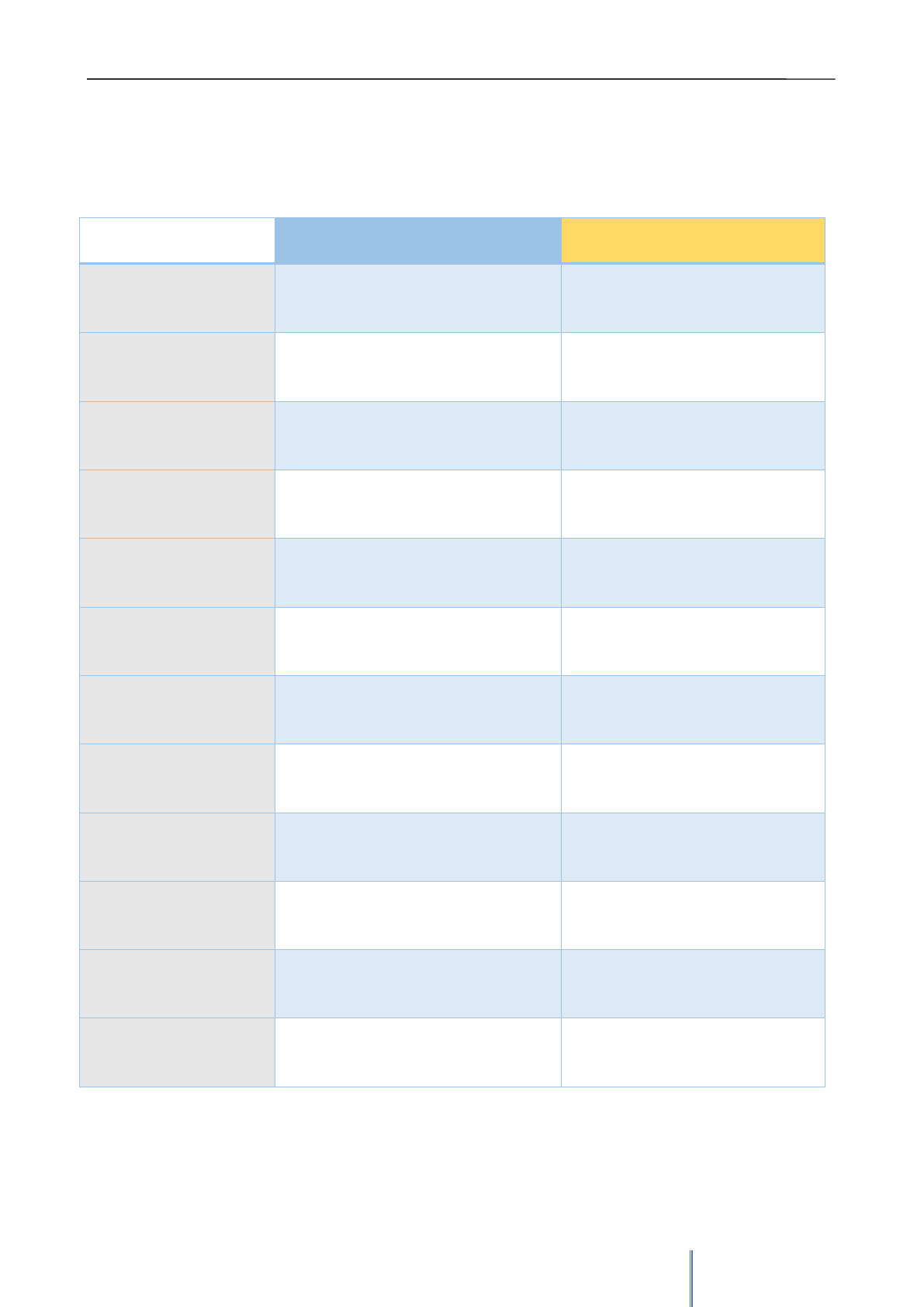
The following table compares some of the highlights of both types of projects:
WS
UD
Existing elements
Node / Arc / Connec / Element
Node / Arc / Connec / Gully / Element
Parent nodes
Nodes can be related to a parent node
The option doesn’t exist
Elements belonging to arc
Connec and unconnected nodes can
belong to an arc
Connec and gullies can belong to an
arc
Node type
The field doesn’t exist in node table, it’s
controled by node catalog
Existe campo de gobierno de tipo de
nodo
Arc Type
The field doesn’t exist in arc table, it’s
controled by arc catalog
Existe campo de gobierno de tipo de
arco
Connec Type
The field doesn’t exist in connec table, it’s
controled by connec catalog
Existe campo de gobierno de tipo de
connec, así como también de tipo de
gully
Specific tools
Minimum cut (mincut)
Longitudinal profile,
upstream and downstream
Topologic review
Incoherent nodes with arcs (T, X)
Sink nodes, possible flow regulators,
high outlets, counter slope and
intersected arcs.
Sector
Macrosector exists
Macrosector exists
Exploitation
Macroexploitation exists
Doesn’t exist any superior entity
Elevation calculations and
arc direction
The direction depends on digitalization
The direction of arcs depends on the
geometric slopes, elevation calculated
based on a dynamic decision tree
Structural inspection
Standard event
Specific events for structural
inspection according to UNE-EN
13508-2
Giswater 3 User Manual
25
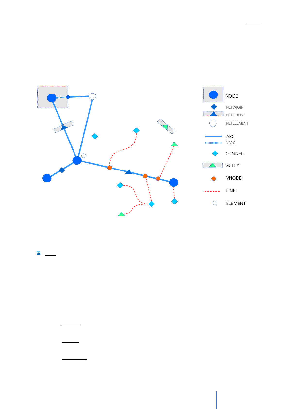
3.2 Available elements
One of the most attractive and representative features of Giswater is the large number of elements that can
be represented in the work environment, a fact that allows a very tight representation of reality.
In this section the functionality of the main existing elements, which are visually represented in image 12, will
be introduced. Most of the elements are represented here, although later we will see that there are more.
Node
One of the main element types of the network. It is always governed by topological rules. The node-
type elements have been divided into a multitude of categories, differentiated for WS and UD
projects. They are always represented as points, although some may have associated polygons that
represent their real perimeter when needed.
Nodes are always placed between two arcs; therefore, they break these arcs in different entities.
Most elements exert specific functions to break (such as flow reductions or check valves), although
there are nodes that would not normally break arcs, in some special cases they must exercise this
function. They are those that are represented in the image:
▪ Netwjoin: is a water connection (connec) that by its dimensions or other characteristics is a
part of the network and is located on top of an arc.
▪ Netgully: is a gully that by its dimensions or other characteristics is a part of the network and
is located on top of an arc.
▪ Netelement: is any element that does not usually connect to the network but due to its
characteristics must be placed on top of an arc and cut into two.
Image 12: Schematic representation of different elements in Giswater.
Giswater 3 User Manual
26
Arc
Arcs, together with nodes, are the main elements of the network. They are located between two
nodes and represent the conduits and pipes of the network. There are not as many types of arcs
as there are of nodes, although they are also categorized and all their characteristics (such as
diameter, material, roughness ...) can be added in their attribute table to differentiate them better.
In the image the operation of a Varc (virtual arcs) is presented. They connect the network
topologically between arcs and nodes when in reality an arc reaches a polygon and therefore
does not really exist inside it as an arc. They are usually short stretches. This is necessary for
the topology rules to work correctly in the Giswater network.
Connec
Connections, the elements that connect the network with buildings or other elements such as
fountains. They are point elements, although to link the connections with the rest of the network,
links and virtual nodes are used.
Gully
Gullies that are not placed on top of the arcs, but are located at a certain distance from the
network. The ones located on top of arc are netgullies and are represented as nodes. They are
also point elements, like connections, and can be related to the network through links and virtual
nodes.
Vnode
Virtual nodes are nodes which, like the virtual arcs, do not exist in reality but must exist in the
Giswater network so that it works correctly. Virtual nodes are always placed on top of arcs, but,
unlike the nodes, they never divide the arcs into two parts.
The function of these elements is to place on the network gullies and connections that are at a
certain distance from arcs. They are point elements that, as has been said, are represented over
the closest arc from the connec or gully
Link
Links are linear elements that relate gullies and connections with their virtual nodes located over
the nearest arc, therefore, they exert the function of connecting the separated elements with the
network.
Element
This category is available for other types of point elements not connected to the network, which
the user can customize himself. It can be network accessories or any other element that is
necessary for a representation with the highest possible degree of reality.
In addition to all these main elements, there are some other elements that do not have any topology but are
interesting to visualize on the map:
Address: within this group there are all those elements related to the representation of the
territory of the network. The layers of street axis, municipal boundary, perimeter of buildings and
portals are available.
Pond / Pool: they represent the presence of pools and ponds in the territory. Although they are
also related to the use of water, these elements do not connect with the network, but may be
interesting as an additional source of information

Giswater 3 User Manual
27
Dimensions: Finally, we must mention the layer that represents the dimensions. This table will
only be filled when the user uses the specific tool to measure distances between elements. It’s
used as a complement to the network to see in detail the created dimensions.
3.3 General conditions of working with database
In order to work correctly with databases that contain a big amount of information, a series of basic rules
must be followed so that the data has consistency and the usability of the database could be maximized.
Most of these rules have to do with the relationships between tables, which share a large number of columns
and fields. In relation to this we must take into account foreign keys that allow the information of one table to
be a part of another table.
In addition, it is also essential to understand the functionality of primary keys, the columns that restrict the
repetition of fields.
Image 13 represents the creation script of the sector table, that the primary key of the table is sector_id,
which means that the content of this column can not be repeated in any case. This table also has a foreign
key, which refers to macrosector table and specifically to the macrosector_id field. What does this mean?
That before inserting a value of macrosector_id in a table sector the same value must be created in the table
macrosector. To give an example, if in the macrosector_id column of the macrosector table we only have
data 1 and 2, to fill the same column in the sector table we can only choose one of these two numbers.
This makes the relationships between tables narrow and many fields have restrictions when adding
information for it to be correct. Besides the use of keys, in some tables there are also restrictions of the
check type, which limit the possibility of adding data in certain fields only with the established values. The
check restrictions are only found where necessary, since they are tables that require specific values for the
system to work correctly and therefore can not be modified.
As already mentioned in section 2.3.5, the use of hierarchical catalogs to categorize the elements is very
important and this functionality can only be developed through the use of foreign keys. To add elements in a
catalog, they must always be related to some type of higher hierarchy element.
Image 13: Script of creation of a table sector with references of primary and
foreign key.

Giswater 3 User Manual
28
3.4 Map zones
To know how far the water supply and drainage networks reach, Giswater establishes different typr of zones
that limit the territories. Each of these zones has specific characteristics and there are certain relationships
between them, managed, as explained in the previous section, with foreign keys.
Image 14 allows to understand what is the role of each zone and with which other elements of the network is
related to.
The main zones are Sector and Exploitation, they act as heads of the rest of the map zones, each one within
their activity. Sectors are delimited with hydraulic coherence as their only condition and may have large
differences in the extension. A single sector can, for example, represent a single street or represent a whole
municipality depending on the needs of each managing entity. The only indispensable thing is to have one or
more water inlets and one or more water outlets in each sector. On the other hand, exploitations are more
related to the territory and are formed by macrodmas and dmas.
All the main elements of the project must be located within sector and exploitation. As it is represented in the
image, some elements are related just to exploitation and only subcatchment must be indispensable within a
sector. In no case an element can be unrelated to any of the areas on the map.
3.5 Working in a corporative environment
In an administration department or a company dedicated to water management the employees never work
on the same issues nor, usually, a single employee is in charge of the entire water management process. To
allow working on different tasks at the same time Giswater environment can be categorized by different types
of work depending on the tables or views that user usually needs. Both Giswater and PostgreSQL database
Image 14: Schema represents different zones and the elements of the network that are related to them.
Giswater 3 User Manual
29
allow the introduction of different work roles, to facilitate the use of tools within a corporate environment
where users work simultaneously.
The aim of roles is to improve security, preventing users without permission from modifying data likely to
generate errors, as well as allowing a customization of some aspects of the project depending on each user
with a different role.
The roles availables are:
Role type
ROLE NAME IN GISWATER
DESCRIPTION
Consult
role_basic
Allows to visualize and consult
information without its
modification
Operations and
management
role_om
Allows to modify the data in tables
related to visits and revisions
Edition
role_edit
Allows to edit data in most of the
tables that has geometry
Hydraulic models
role_epa
Allows to modify data related to
hydraulic models
Budget and planning
role_masterplan
Allows to modify data in tables
related to budget and planning
Administrator
role_admin
Has all the permissions to edit
data
All roles with a higher hierarchy automatically acquire lower role permissions, that’s why they are sorted
according to the importance and permissions they have.
3.6 Default values
Giswater has the option of adding default values to parameters that are mandatory or highly recommended.
It facilitates the work of users at the process of inserting data in the different tables and views of the project.
By means of different commands, when a new element is inserted and user has defined default values for
the related fields, they are automatically filled in with that established value. The value set by default must
always be of the same type as the field to be filled, otherwise the insertion will be erroneous.
3.6.1 User’s values
User’s default values are those that are managed through the config_param_user table. Usually these values
are used during the data insertion process.
The corresponding parameters can be added within config_param_user. A clear example of the default value
that can be used would be that of municipality, in case of having only one, the value of muni_id field could be
automatically inserted.
The use of default values can be useful in the insertion of new elements. In the case of the map zones, it
must be remembered that the default value prevails over the geometry of the area that Giswater
automatically captures. For example, if a new element is to be inserted within the perimeter of a sector = 3,

Giswater 3 User Manual
30
the program will capture that the sector would be 3, but if we have a default value of sector = 2, the element
will be inserted with sector = 2.
It’s also possible to manage the default values using Giswater plugin configuration tool.
3.6.2 System values
The default system values are only modifiable by users with administration role. They are related to the
configuration of tables and are usually used to manage the parameters of the different topological rules,
which are described in the following section. Section 5.2.6 points out information with respect to the default
system values, since they can be modifiable from the plugin Configuration tool.
3.7 Topology rules
The definition of geospatial topology says: "The topology expresses the spatial relationships between
characteristics of vectors (points, polylines and polygons) connected or adjacent in GIS." Once the meaning
is known, we will see some of the main topological characteristics that are important for the use of Giswater
in its GIS branch.
3.7.1 Arc-node behavior
The relationship between arcs and nodes is probably the most important at the topological level within
Giswater, partly because of the large number of elements that come into play. In order for the program to
work properly, it is necessary to fulfill these topological rules. The program itself shows messages to the user
when an important rule is about to be broken.
The Giswater plugin has a specific tool that allows detecting certain topological errors related to the arcs and
nodes. Later we will see how this tool is used, but in this section, we will explain the topological rules that are
emphasized:
▪ Orphan nodes: nodes that are not connected to any arc
▪ Duplicated nodes: nodes that are located exactly at the same place and that’s why the produce the
incoherence in the system
▪ Topological consistency of nodes: there are some specific topological rules of Giswater, which take
into account the type of node. For example, there are types of nodes that must have connection with
three different arcs, if not, they will be marked as erroneous.
▪ Arcs with the same start and end node: the arcs must always be placed between two different nodes
(with different id), therefore, an arc that starts and ends at the same node is incorrect. This can be
configured from the config table and the samenode_init_end_control field, where if we have the
value TRUE the program will not allow arcs with the same start and end node; if we have FALSE,
these arcs will be accepted.
▪ Arc without start or end node: Arcs disconnected from one of their ends.
3.7.2 Link-vnode behavior
Link is a graphical connection between elements of the map. The properties that it has are the direction of
digitization, the node to which it belongs (feature) and the exit node (exit), as well as the userdefined_geom
field (boolean value that allows to identify if the geometry is customized by the user or not) . In this sense,
what a link does is to connect an input element with an output element, which can be directly the network
(arc by node or by virtual node) or with an intermediate element (other connec or gully), that at its once they
are directly connected to the network or to other connec or gully.

Giswater 3 User Manual
31
In case the output element is an arc or a node, the arc_id will be automatically assigned as the parent
section of the link element, otherwise the arc_id will not be assigned automatically by the tool and the user
must manually attribute the arc_id of the father stretch.
On the other hand, if the output element is neither node, nor connec, nor gully, a node called virtual node
(Vnode) is created. In the case that vnode is close to an arc, by adhesion it is inserted over it.
Spetial features:
1) Regarding its feature node (which is upstream), the link acts as if it belongs to this feature, which means:
▪ The visibility of the map, ie link takes the value of dma, sector and exploitation from its
feature.
▪ The default state value, when inserting a new link manually or automatically, is the same as feature’s
state.
▪ If the feature element (connec or gully) is deleted, the link is deleted too (feature is considered to be
functioning as an integrated unit and not dissociated from its link).
▪ The attributes of the link, such as length, diameter or material, are represented and displayed in the
data model of the feature to which it belongs.
▪ It is possible to have more than one link for a feature node (as they can have different states 0, 1 or
2, and user can modify it as he wishes).
2) Regarding the exit point exit (the one that is downstream), there is no more relevance but simply topology,
which means that:
Respecto su punto de salida exit (el que se encuentra aguas abajo), ya no hay pertinencia sino simplemente
topología, con lo cual:
▪ No status, nor visibility with the downstream elements is managed.
▪ Topology is managed (if the exit point moves, link moves as well).
▪ If an output element of a link is deleted, link will not be deleted until it’s disconnected previously.
▪ If the output element is a connec or a gully, the arc_id value of the parent arc is copied from the exit
element.
▪ If the vnode is updated to one arc or another, the arc_id field of the feature node is always updated.
Attention: if the vnode update disconnects the link from arc, the arc_id of the feature node will
automatically be NULL.
3) In case of using the tool of automatic connection of connec or gully to the network (connect_to_network):
▪ The tool will create, if necessary, a vnode. In case this vnode already exists, the same will be used to
connect the link. The vnodes created by the tool have the value of vnode_type field AUTO. Those
created by the user have the vnode_type of CUSTOM.

Giswater 3 User Manual
32
▪ The link created by the tool is always the shortest distance between the connec or gully and the
network (using the layers v_edit_node, v_edit_arc, with which the state, exploitation and planning
sectors decide what is shown in these two layers).
▪ Created link has as a default value of the field userdefined_geom set as FALSE. In case of a link
drawn or updated by the user, the userdefined_geom field changes its value to TRUE.
▪ If the values of userdefined_geom is TRUE, the automatic tool won’t redesign the link, preventing the
'destruction' of custom geometries.
4) As the link is an element that connects two other elements, if you want to update the geometry of it, for
example, intermediate vertices, it is possible to do as long as the extreme vertices are not updated, in which
case it will not be possible. If you want to reconnect different elements you must proceed with the deletion of
the link and then creation of another.
3.7.3 Double geometry elements
Giswater makes use of double-geometric elements. This means that a single element is formed by two
different geometries, in this case they are always points that belong to a polygon.
Only some of the elements of the network have this particularity. They are types of elements that can have
much larger measurements than those that are represented with a simple point and therefore it’s interesting
to visualize them as a polygon around the point.
Double geometry elements for WS
▪ Tank, Register, Fountain
▪ Double geometry elements for UD
▪ Storage, Chamber, Wwtp, Netgully, Gully
When adding a new node of one of the listed types, a square polygon will be immediately created around the
point element. The main topological rules of this relationship are:
- If the node is moved, the associated polygon will move to the new position of the node.
- If a new polygon is drawn, with the perimeter that the user wants and around a node of the
same type, the new perimeter directly replaces the old one.
- It’s impossible to draw a new polygon without a node of the same type being inside it
- If a node with double-geometry is deleted, the associated polygon will also be eliminated. On
the other hand, if the polygon can be deleted without modifying the node.
- If a node with double-geometry is deleted, the associated polygon will also be eliminated. On
the other hand, the polygon can be deleted without modifying the node.
To work with this type of double-geometric elements it’s important to set a configuration that manages it. You
can enable or disable this function in the config table, insert_double_geometry field. If it’s enabled
(recommended), the buffer_value field assigns a default value of the side length of the polygon square. As
already said, this square can be edited to have a desired shape.
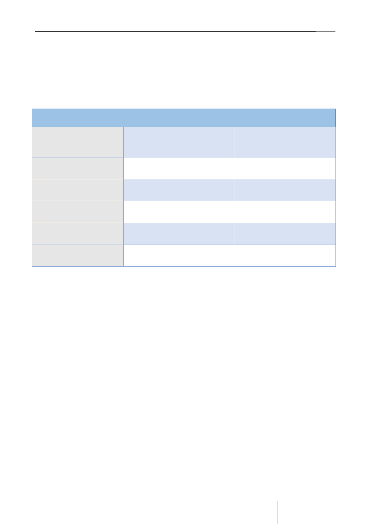
3.7.4 State’s topology
To end the section of topological rules, we must also take into account some of the conditions in relation to
the states of the elements. In the following table all types of modifications (insert or update) between arc and
node elements are presented. It is worth reminding, that the available states are:
Giswater 3 User Manual
33
0 = Obsolete 1 = On Service 2 = Planified
From the element
Tot he element
Result
Comment
Type
TG_OP
State
Type
State
NODE
INSERT/
UPDATE
0
Node
0,1,2
OK
State 0 doesn’t have topology
Arc
0,1,2
OK
State 0 doesn’t have topology
1
Node
0
OK
State 0 doesn’t have topology
1
KO
Only one node with state 1 can be
located in the same place
2
OK
It’s possible to located node with state
1 over a node with state 2
2
Node
0
OK
State 0 doesn’t have topology
1
OK
It’s possible to located node with state
2 over a node with state 1
2
KO
ARC
INSERT/
UPDATE
0
Node
0,1,2
OK
1
Node
0
KO
1
OK
2
KO
2
Node
0
KO
1
OK
2
OK
If an arc belongs to the same psector
as a node
The type of state that has the most restrictive conditions is the planned one. Operating with elements in state
= 2 is only possible for users with the role of masterplan or higher and it must be kept in mind that the
management of these elements can break the topology.
First of all, it’s necessary to have at least one record in the plan_psector table, which is used to manage the
planning. It is also essential to set a default value for psector. Arcs and nodes will be inserted with this
default value in the specific tables: plan_arc_x_psector and plan_node_x_psector. It’s important to check the
state and doable fields.
All elements, whether nodes or arcs, which have on service state (1) and the user changes them manually to
Planified, will be automatically introduced in the default psector that is currently available. Although this
change is allowed by the topological rules, it should not be usual to pass a On Service element into Planified.
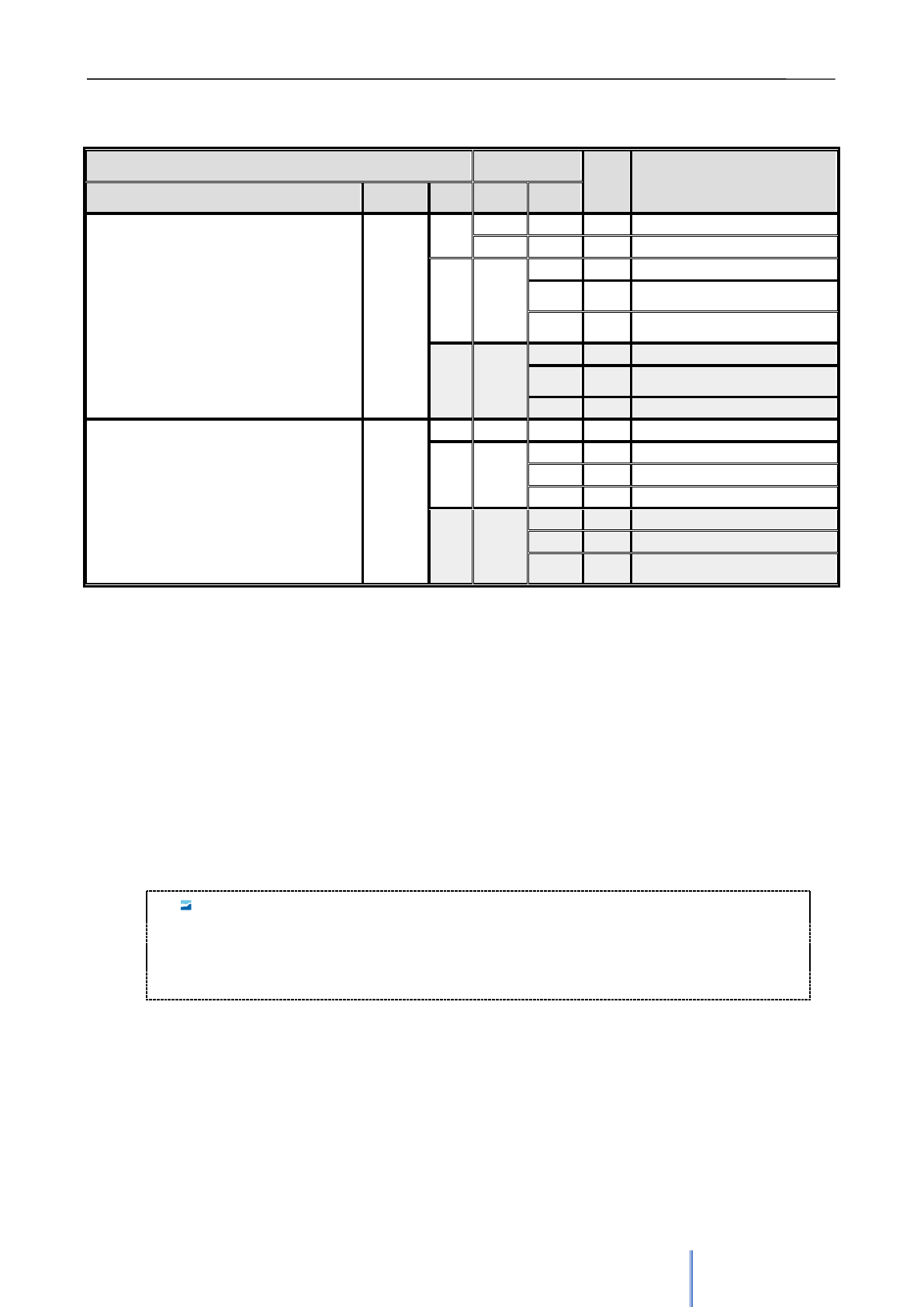
NOTE 01 ADDITIONAL TOPOLOGY INFORMATION: some of the parameters referred
to the topology must be configured and customized according to the needs of the user. To perform
such processes, you must use the plugin Configuration tool. The parameters related to the topology
will be explained in detail in section 5.6.2 of the manual, as well as the operation of the tool.
3.8 Summary of work rules applied to the insertion of NODES
To finish this section of basic work rules, an example scheme is presented to summarize all the work rules
that need to be followed in the process of inserting a new node element. In the diagram, the mandatory
insertion fields are defined and arrows visualize the steps to follow in order to conduct the process correctly.
The case in which the insertion is not possible is also presented.
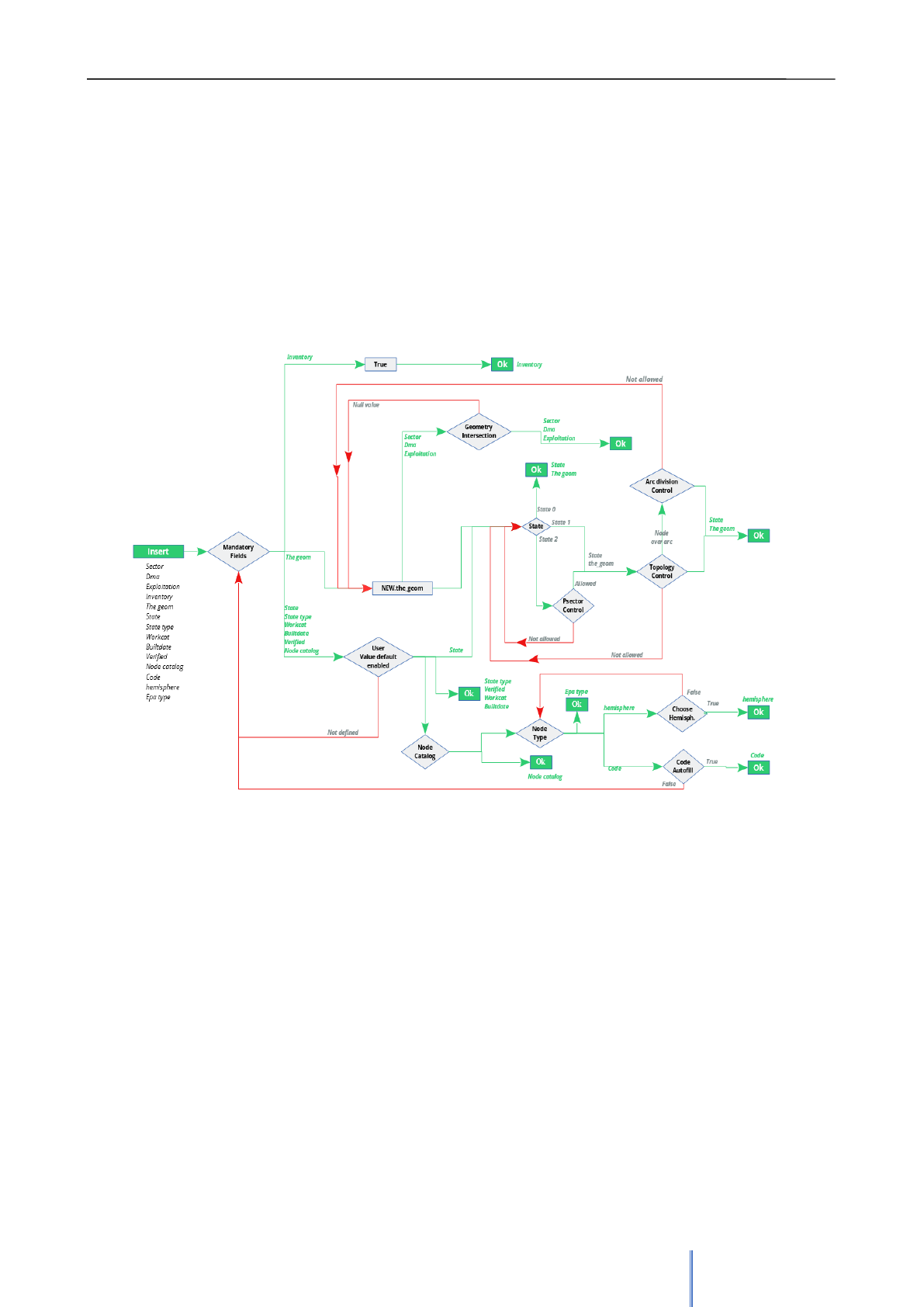
Giswater 3 User Manual
34
Field the_geom is one of the most important fields and in this case the rules related to it are easy to
understand. When inserting a new element, the geometry of it must be placed inside the geometry of a
sector, dma and exploitation, otherwise the insertion will be erroneous.
If the state is 2, as mentioned recently, there must be at least one psector defined in a project, otherwise the
insertion will be incorrect. For elements with status "on service" (1), the topological rules explained in section
3.7.1 must be fulfilled.
The other mandatory fields may have defined default values or being entered directly by the user. The
hierarchies and keys for the catalogs of elements must be respected, which means that trying inserting a
node that does not belong to the catalogs, we won’t succeed.
Image 15: Summary schema of the steps that need to be followed in the process of insertion of a node type element. The green
lines represent successful steps; the red lines show the different scenarios in which the insertion will not be correct.
Giswater 3 User Manual
35
4. WORKING ENVIRONMENT IN QGIS
While all GIS systems are compatible with the Giswater tool, the same does not apply to the plugin, since it
has been programmed as a complement to QGIS. Thus, all the available functionalities will be executed from
the QGIS environment.
4.1 Graphic interface
Any user that requires the use of Giswater plugin must be familiar with geographic information systems
(GIS).
Once the user has created a new data project, with the Giswater tool, as explained in sections 2.3.4, 2.4 and
2.5, he is already in a position to open the QGIS project and start working with it. In this manual the example
project for water supply (ws_sample) will be used.
The main parts of the QGIS environment in relation to Giswater and its plugin are shown below.
Toolbar of Giswater
plugin
ToC with the personalized Giswater project
Canvas to visualize
and edit the spatial
information
Image 16: General visualization of the screen with project of Giswater opened in QGIS. Note the complement toolbar and the
customization of the table of contents.
Giswater 3 User Manual
36
4.2 Table of Contents
ToC (Table of Contents) is where all the necessary tables and views of the database are loaded. To have the
information well structured, this topic has been divided into seven large groups that will also facilitate the
management of roles (depending on the permissions, the user is be able to manage certain tables, which by
default belong to a group). These groups are: Inventory of assets, Operations and maintenance, Analysis
EPANET, Masterplan, System tables, Additional tables and Base maps.
In this section all the tables and views that are loaded in QGIS are described, in order to facilitate the user
understanding of the complex network of tables that Giswater is composed of. Each table has a variable
number of fields with information related to what the table represents. As the amount of information in this
section would be very large, most of the definitions of tables and fields are presented in the annex of the
manual. However, the user will find below enough information to understand the purpose of each group of
tables.
NOTE 02 Usually the name that a layer receives inside the ToC is not exactly the same as it it in
the database. Although in some cases it may coincide, it’s important to know that they are mostly
different. If inside QGIS the user has doubts about the table referenced by a layer, he can place
the mouse over the name of the layer and the following information will appear:
dbname, host, port, user, sslmode, key, srid, type, table (referring to the scheme and table)
In the section 4.2 the layers are named by their name in QGIS and for greater understanding the
name of the database table is added in parentheses.
4.2.1 Inventory of assets (INVENTORY)
This group contains the information about the network assets inventory and it’s divided into five subgroups:
Catalogs, Map zones, Network elements, Others and Topology analysis.
4.2.1.1 Catalogs
Working with catalogs is one of the main characteristics of Giswater, and it’is possible thanks to the
database environment.
In fact, before starting working with the project it’s necessary to fill in at least arc and node catalog to be able
to introduce a simple record in the arc and node layers.
The function of catalogs is multiple. Among other characteristics, they allow to standardize inserted values,
add economic value for every elemento of the network or characterize the properties of the elements for
further use in the hydraulic model.
It’s interesting to know that there are four types of catalogs:
• Topological elements: given that the network is based on the arc-node topology, the catalogs of
elements are the most important ones (node catalog and arc catalog).
• Other elements of the network: The elements that complement the network sucha as connecs or
elements which have their own catalogs.
Giswater 3 User Manual
37
• Management: As a complement to the network catalogs, there are other tables in the database
that also act as catalogs, such as the catalogs of: soil, constructors, work records, owners,
pavement.
• Hydraulic model: Catalogs that are necessary for the construction of a high quality hydraulic
model. In this sense there is a rugosities catalog, which allows to differentiate roughness
according to the age of the material.
List of the common catalogs (in brackets the name of the table in database)
▪ CATALOG OF NODE’S MATERIALS (cat_mat_node)
▪ CATALOG OF ARC’S MATERIALS (cat_mat_arc)
▪ CATALOG OF NODES (cat_node)
▪ CATALOG OF ARCS (cat_arc)
▪ CATALOG OF CONNECS (cat_connec)
▪ CATALOG OF ELEMENT’S MATERIALS (cat_mat_element)
▪ CATALOG OF ELEMENTS (cat_element)
▪ CATALOG OF OWNERS (cat_owner)
▪ CATALOG OF SOILS (cat_soil)
▪ CATALOG OF PAVEMENTS (cat_pavement)
▪ CATALOG OF WORK RECORDS (cat_work)
▪ CATALOG OF BUILDERS (cat_builder)
List of catalogs specifics for WS project
▪ CATALOG OF RUGOSITY (inp_cat_mat_roughness)
▪ CATALOG OF PRESSURE ZONES (cat_press_zone)
NOTE 03 Only for WS projects. When a new material is inserted in the catalog of materials for
arcs, this new material is also automatically inserted as a record in the rugosity catalog
(inp_cat_mat_roughness) but without period or roughness values.
List of catalogs specifics for UD project
▪ CATALOG OF ARC’S SHAPES (cat_arc_shape)
▪ CATALOG OF HYDROLOGY (cat_hydrology)
▪ CATALOG OF GULLIES (cat_grate)
Pre-dependencies
Before starting to work with catalogs, the system tables that typify the different elements of the network must
be filled in (see section 2.3.5):
node_type (in case of node catalog)
arc_type (in case of arc catalog)
connec_type (in case of connec catalog)
gully_type (in case of gullies catalog for UD)
Those tables are not present in the QGIS project, that’s why they should be filled in directly in a database
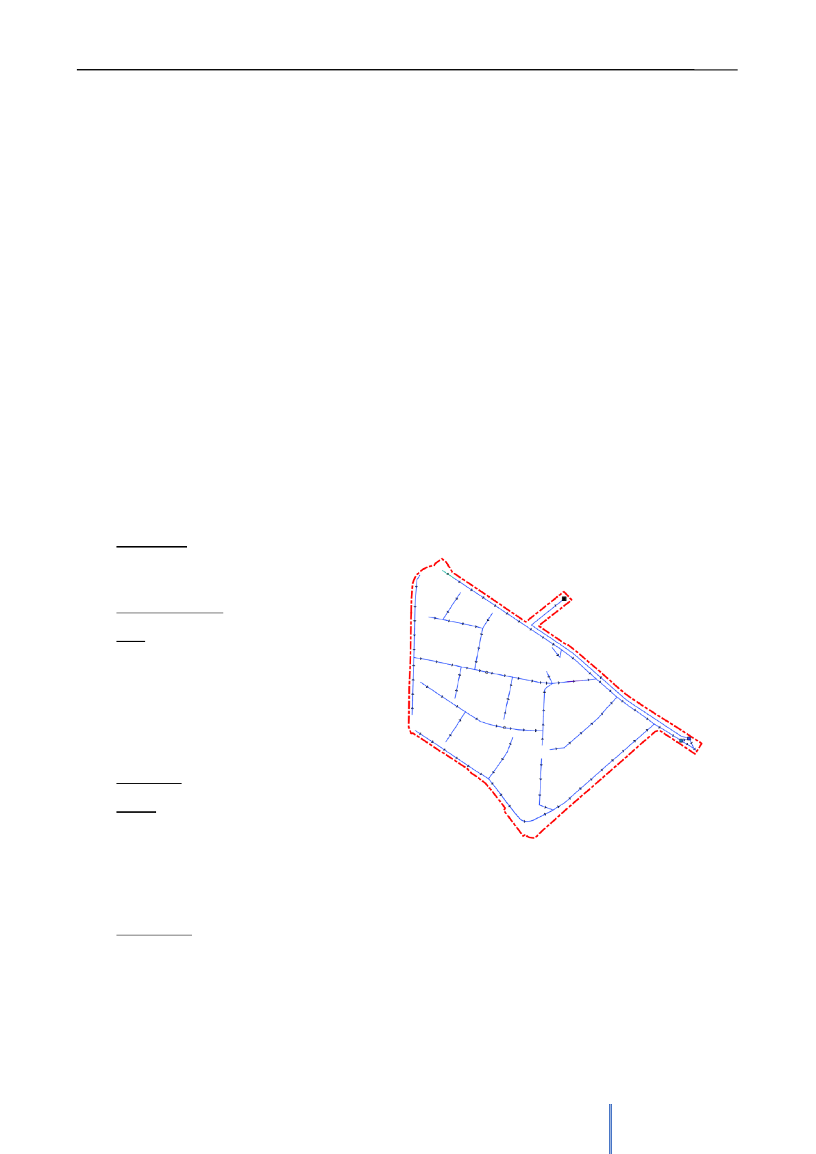
Giswater 3 User Manual
38
Post-dependencies
The catalogs generate many dependencies, in fact, they must be filled before starting to work since their
records will be requested in many system tables.
In addition, it should be noted that the catalogs also have dependencies between each other. In this sense,
before filling the arc and node catalogs, the previous catalogs that are node materials and arc materials must
be filled.
4.2.1.2 Map zones
The second group of layers of the assets inventory is the one related to the zones of the map. As its name
very well indicates, this group of layers represents and delimits the different territorial zones of the map,
already defined in section 3.4 of this manual.
All the layers in this group have polygonal geometry - except for macroexploitation, which only appears in a
table format for WS projects. It’s a very important group of layers, since one of the basic rules of the project
is the necessity of every element of the network to be within one of the different zones.
Exploitation is essential to start any project. As mentioned before, it’s highly recommended to add an
exploitation value in the properties of the project, using a variable. Thus, the project will be directly related to
an exploitation, the area of the map that, in general, will cover a larger area.
The map zones of Giswater are:
▪ Exploitation: exploitation area, usually
related to a management area of one or
more users.
▪ Macroexploitation: group of exploitations.
▪ Dma: in case of WS it’s district metering
areas, área used to register the water
usage. For UD it’s district management
areas, management areas of sanitation
network. In both cases they can be
delimited according to the needs of the
user and always with a coherence of use.
▪ Macrodma: group of dmas.
▪ Sector: sectors are related to the correct
functioning of the hydraulic model and
therefore they must be consistent with the
water inlets and outlets of it. They are
delimited according to this coherence as
the user considers appropriate.
▪ Macrosector: group of sectores.
Image 17: Representation of one of the map zones, specifically of
a sector that exists in the ws_sample project.
Giswater 3 User Manual
39
4.2.1.3 Network elements (Network)
This group contains of all those layers reffered to network elements which have geometry, that is, they are
represented graphically on the map.
Once the corresponding catalogs have been completed, the construction of thr network can be started by
editing these layers. Always following the order marked by the topological rules, as explained in section 3.7.
The elements of the network are divided into four groups according to its category and geometry type:
• Group of elements node
• Group of elements arc
• Group of elements connec y gully (for ws only connec)
• Group of elements polygon
Each network element has its own editable view, which is what is visualized in QGIS. This editable view has
attributes that come from the editable view of the corresponding element (node, arc, connec, gully).
The basic sequence of steps that make the data of each element is the following (example for junction):
node v_node v_edit_man_junction
JOIN man_junction (id) = v_node (id)
To take advantage of the use of GIS, each element has its own associated style that is displayed in the
graphical interface of QGIS. The styles are represented according to the specific type of element (to find out
which are they consult the table sys_feature_cat).
In the case of network elements, the differences between project types are quite big. There are very few
elements that coincide in both water supply and urban drainage; that is why no table in this group will be
described as a common.
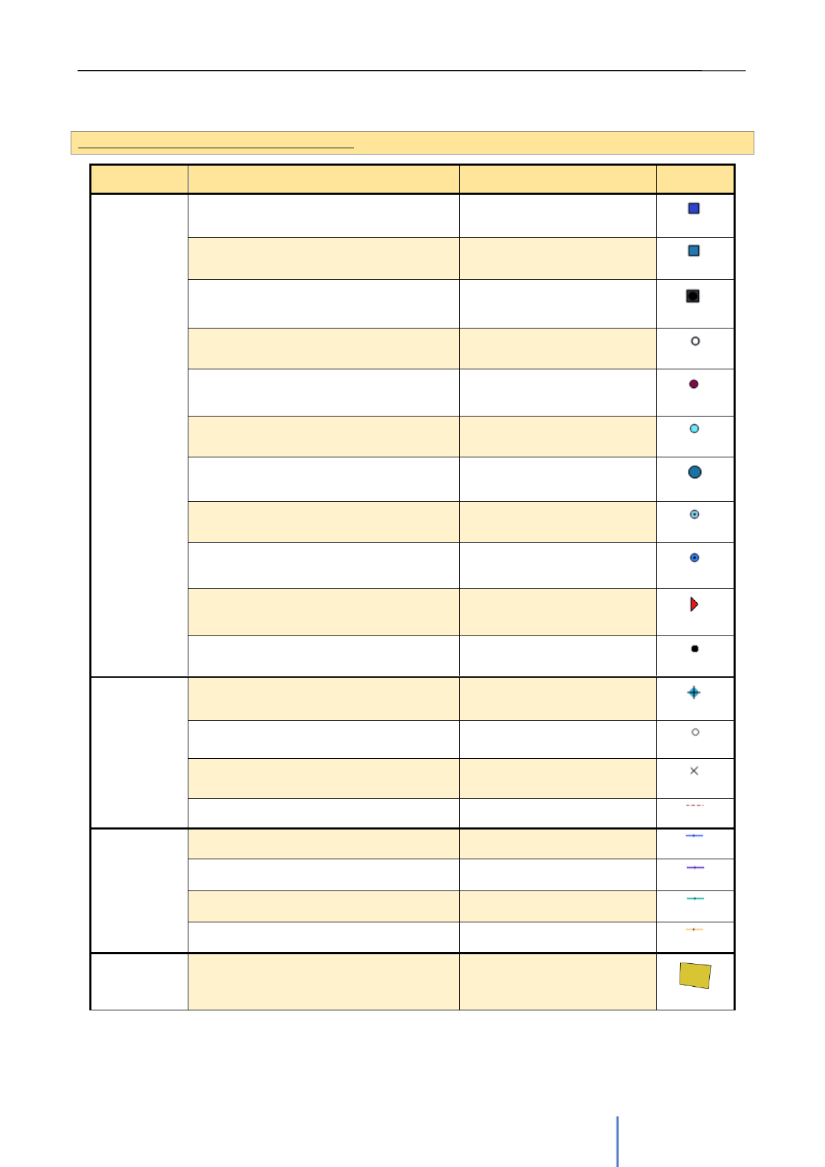
Giswater 3 User Manual
40
Table of all the elemnts present in UD project
Group
Element (name of thetable)
Description
Style
Node
Storage (v_edit_man_storage)
Storage
Chamber (v_edit_man_chamber)
Chamber
Wwtp (v_edit_man_wwtp)
Wastewater Treatment Plant
Netgully (v_edit_man_netgully)
Topological gully
Netelement (v_edit_man_netelement)
Topological element
Manhole (v_edit_man_manhole)
Manhole
Netinit (v_edit_man_netinit)
Network initiation
Wjump (v_edit_man_wjump)
Water jump
Junction (v_edit_man_junction)
Junction without register
Outfall (v_edit_man_outfall)
Outfall
Valve (v_edit_man_valve)
Valve
Connec &
Gully
Connec (v_edit_man_connec)
Connec
Gully (v_edit_man_gully)
Gully
Vnode (v_edit _vnode)
Connection to network
Link (v_edit_link)
Element of graphic connection
Arc
Conduit (v_edit_man_conduit)
Conduit
Siphon (v_edit_man_siphon)
Siphon
Waccel (v_edit_man_waccel)
Water accelerator
Varc (v_edit_man_varc)
Fictional conduit
Polygon
Gully polygon (v_edit_man_gully_pol)
Polygonal element for gully
Giswater 3 User Manual
41
Netgully polygon (v_edit_man_netgully_pol)
Polygonal element for
topological gully
Wwtp polygon (v_edit_man_wwtp_pol)
Polygonal element for
wastewater treatment plant
Chamber polygon (v_edit_man_chamber_pol)
Polygonal element for chamber
Storage polygon (v_edit_man_storage_pol)
Polygonal element for storage
Table of all elements present in WS project
Group
Element (name of the table)
Description
Style
Node
Wtp (v_edit_man_wtp)
Water treatment plant
Source (v_edit_man_source)
Source
Waterwell (v_edit_man_waterwell)
Waterwell
Tank (v_edit_man_tank)
Tank
Netsamplepoint (v_edit_man_netsamplepoint)
Topological sample point
Netelement (v_edit_man_netelement)
Topological elemento
Flexunion (v_edit_man_flexunion)
Flexible union
Expantank (v_edit_man_expansiontank)
Expansion tank
Register (v_edit_man_register)
Register
Pump (v_edit_man_pump)
Pump station
Hydrant (v_edit_man_hydrant)
Hydrant
Manhole (v_edit_man_manhole)
Manhole
Meter (v_edit_man_meter)
Meter
Reduction (v_edit_man_reduction)
Reduction
Giswater 3 User Manual
42
Filter (v_edit_man_filter)
Filter
Junction (v_edit_man_junction)
Junction
Valve (v_edit_man_valve)
Valve
Netwjoin (v_edit_man_netwjoin)
Topological water connection
Arc
Varc (v_edit_man_varc)
Fictional pipe
Pipe (v_edit_man_pipe)
Pipe
Connec
Link (v_edit_link)
Element of graphical
connection
Vnode (v_edit_vnode)
Connection to network
Greentap (v_edit_man_greentap)
Irrigation connection
Wjoin (v_edit_man_wjoin)
Water connection
Fountain (v_edit_man_fountain)
Fountain
Tap (v_edit_man_tap)
Tap
Polygon
Fountain polygon (v_edit_man_fountain_pol)
Polygonal element for
fountain
Register polygon (v_edit_man_register_pol)
Polygonal element for
register
Tank polygon (v_edit_man_tank_pol)
Polygonal element for tank
Forms of the elements
In addition to the visual style of each of the elements, they also have an associated form, designed one by
one according to their specific fields. The forms are opened when the user clicks an item using the
information button in QGIS and use different tabs to display the information according to their category:
▪ Name of the elemento: information related to the element's own attributes. In the tables located in
the annex of the manual you can check the fields of each element, which are shown in this tab of the
form. It’s also distributed in different sections.
o Numeric information: (only for arc elements) parameters related to geometries,
dimensions, lengths, etc.
o Basic information: basic information common between most of the elements, for example
construction date, code, soil, elevation and depth, etc.

Giswater 3 User Manual
43
o Scecific information: information specific for each type of element
o Additional information: additional information. Contains the information about the address
and other optionally information.
o Feature graphic design: Relatef to the visualization of the element. Position of the label, icon
as svg.
▪ Connections: (only for node type elements) shows a table of all the elements connected to the
node, distinguishing those which are upstream from the downstream
▪ Relations: shows a table of elements that are linked only to this element. They are usually not
connected to the network, and the main element must be large enough to contain its related
elements. The possible relationship, depending on the type of project and the type of element, is:
o Arc can be related to node and connec
o Node can be related to node
o Arc can be related to connec and gully
▪ Element: in this tab other elements are shown, not connected to the network, which are linked to the
element that we are visualizing. From the form itself you can link, unlink and add elements of this
type.
▪ Hydrometer: (only for connec type elements) relates connections with hydrometers and can show
their values, connect or unconnect them.
▪ Document: this tab shows the documents related to the visualized element. It’s possible to link,
unlink or créate a new document as well as filter them by date or document type.
▪ O&M: this tab shows the events related to the visualized element. Every event is a parto of a visit,
which can be consulted using the button located in a form. It’s also possible to add visit, show fotos
and documents related to the events.
▪ Scada: (only for node type elements) tab show the values coming from the SCADA system.
▪ Cost: (only for node and arc type elements) allows to calculate the costo f the visualized element.
For nodes, only two parameters come into play (price per unit or price per meter depth). For arc
there are many more variables that are necessary at the time of calculating the price and all are
specified in this last section of the form.
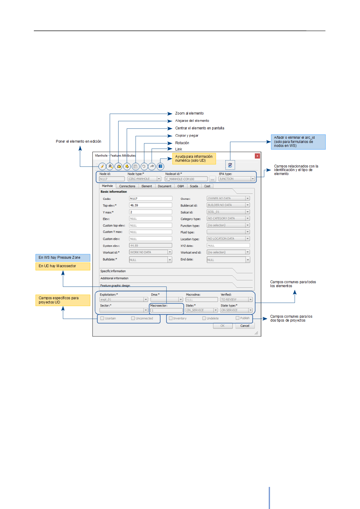
Giswater 3 User Manual
44
Sections of the form
In the following image the different parts of a form are presented. The reference is made to the different parts
for each type of project, although the sample form is a manhole element of a UD project. The central part of
the form, where the information that varies depending on the tab that is activated, is not described in the
image, since in the previous section explains it in details.
In order to help users, understand some of the fields, the image 19 presents graphically the most important
parameters like depth, dimensions and slope for the urban drainage project (UD).
Imagen 18: Form of a node element, type Manhole. Most of the element’s
forms are similar to the presente done, which shows the distribution of the
atributes and tabs.
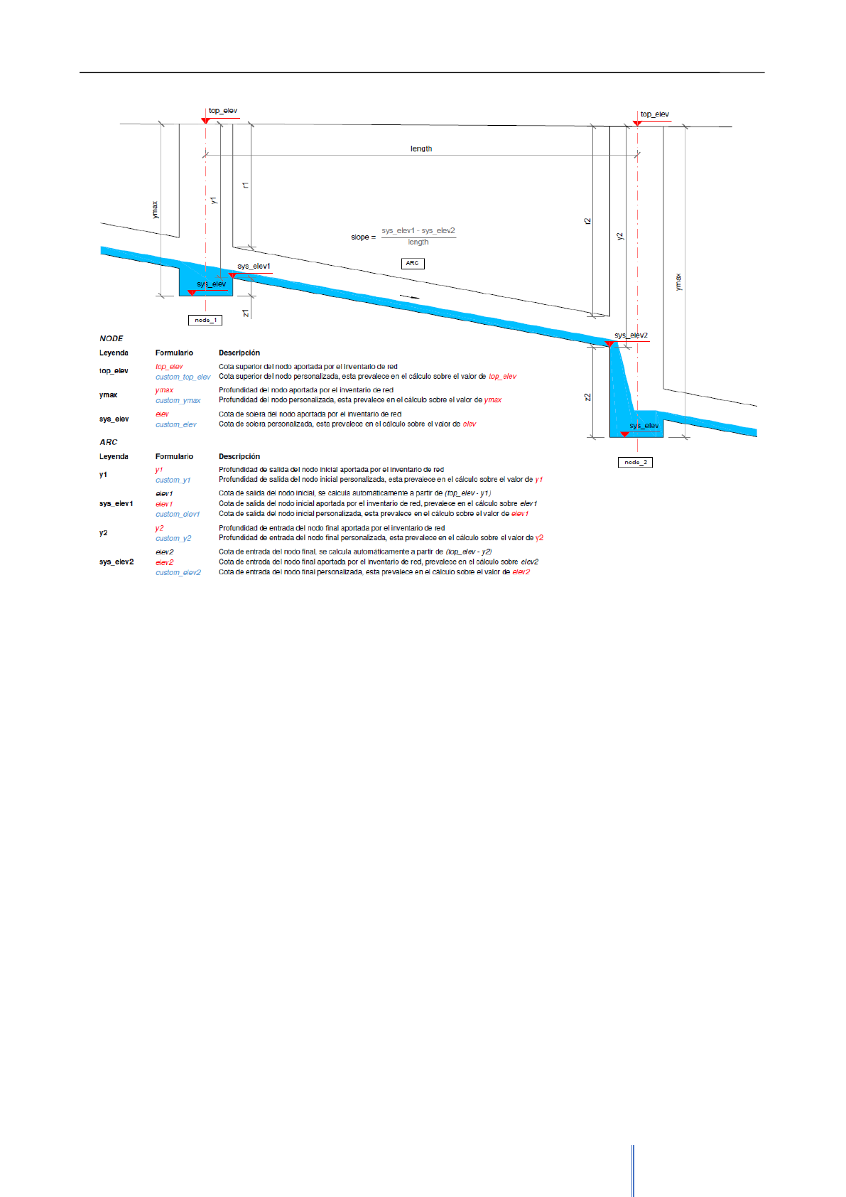
Giswater 3 User Manual
45
4.2.1.4 Others
The elements that are not strictly a part of the water supply or sanitation network, but do have a visual
representation on the QGIS map, which means they have geometry, are in this group. The data of these
elements is not indispensable for the use of the hydraulic models incorporated Giswater, but its an
information that can have interest in other aspects, and, therefore, it’s also necessary to get to know its
characteristics.
Common elements
▪ Dimensioning (v_edit_dimensions): this table is filled in when the user uses the plugin tool that
allows to calculate distances and dimensions between different points within the QGIS map. The
distance is represented by a line and a label with the numerical information in meters. It also shows
the depth in case of associating a value of it.
▪ Samplepoint (v_edit_samplepoint): layer with information about sample points. These are the points
where the water quality is analyzed. It has a field that relates the sampling point with a laboratory
▪ Element (v_edit_element): can be any other type of element that needs to be defined first in the
element catalog. These may or may not be linked with other network elements. They allow to add
extra information in relation to some characteristic.
Image 19: Schema helps understand the information that should be put in the fields related to elevation, dimensions, depth of node
and arc elements of urban drainage projects (UD).
Giswater 3 User Manual
46
Specific elements of WS project
▪ Pond (v_edit_pond): represents ponds located in the exploitation
▪ Pool (v_edit_pool): represents pools located in the exploitation
4.2.1.5 Topology analysis
This last group of layers in the asset inventory represent the tables that are filled when the user uses
topology tools, which are located in the Toolbox.
Most types of topological analysis have a specific layer to represent their results on the map, since it’s not
possible to have elements with different geometries in the same layer.
Because of that, the following layers are present in the QGIS project, each with a different symbology and
depending on the type of project:
Common layers of the topologic analysis:
▪ Arc with same start-end node (v_anl_arc_point) : point layer that represents nodes which are
the result of arc with the same start and end node analysis
▪ Arc without start-end node (v_anl_arc_x_node_point) : point layer that represents nodes which
are the result of arc without start or end node analysis
▪ Arc without start-end node (v_anl_arc_x_node) : line layer that represents arcs which are the
result of arc without start or end node analysis
▪ Connec analysis (v_anl_connec) : view that represents the results of different topologic
analysis related to connec.
Layers of topologic analysis related to UD projects:
▪ Arc analysis (v_anl_arc): view that represents the results of different topologic analysis related to
arc. It has a field context which allows to symbolize it in function of the conducted process:
o Arc insersection
o Arc inverted
o Arc with same start-end nodes
▪ Node analysis (v_anl_node): view that represents the results of different topologic analysis related
to node. It has a field context which allows to symbolize it in function of the conducted process:
o Node duplicated
o Node orphan
o Node topological consistency
o Node exit upper intro
Giswater 3 User Manual
47
o Node flow regulator
o Node sink
Layers of topologic analysis related to WS project
▪ Arc with same start-end nodes (v_anl_arc) : line layer that represents the results of the
analysis of arcs with the same start and end node
▪ Node analysis (v_anl_node): view that represents the results of different topologic analysis related
to node. It has a field context which allows to symbolize it in function of the conducted process:
o Node duplicated
o Node orphan
o Node topological consistency
4.2.2 Operations and management (O&M)
The second group of layers in the ToC of the QGIS Giswater projectis the operations and management
(O&M). Unlike the previous group (inventory of assets), which has a large number of layers, this one is
reduced to a simple group of 2 or 3 layers depending on the type of project and the inventory of visits,
common fot both types of projects.
The layers of operations and management are:
Visits (v_edit_om_visit)
In this layer all the completed visits made to the network are found and visualized by means of specific
elements on the map. Each visit has a start and end date, as well as an identifier of the user who made the
visit. Each visit can contain different events and in the same way each event can have several photographs
to illustrate the event. Events are not found in this same layer, but they are related to visits with foreign keys.
Minimum cut process (mincut)
The mincut layers propose to the users the valves that should be closed in case of wanting to do some type
of operation on any element of the network. Based on the different states and attributes of the elements, the
cutting polygon will be different. There are several parameters that come into play when using this tool.
Mainly we must take into account the state (state) and exploitation (exploitation) of the elements that are
displayed on the screen, because the tool will use only the visible elements.
NOTE 04 It is important to remember that the mother tables of the project (node, arc,
connec) contain all the information of elements of each type, but these elements are visualized in
QGIS using views (v_edit_node, v_edit_arc, v_edit_connec), which performs a filter in function of
which the item appears on the screen or not. If the user decides that he does not want to see the
obsolete elements (using the status selector), the view will not contain the information of the
obsolete elements, but the information is still in mother tables.

Giswater 3 User Manual
48
Since obsolete elements don’t have topology (they are not connected to the network), it’s recommended that
they are not visible when the tool is used. The elements with state ‘on service’ can be used without any
problems to make the cutting polygon. Also, the planned elements can be a part of a mincut polygon but it’s
necessary to be careful with those elements as they can be placed on top of other elements on service and
cause errors in the process.
The layers that are loaded in the QGIS map are those related to the results of the mincut polygon according
to its geometry and type of element, with its own symbology:
▪ Mincut result valve (v_anl_mincut_result_valve): Results of the minimum cut polygon representing
valves. The proposed field establishes whether a valve should be closed or not.
▪ Mincut result arc (v_anl_mincut_result_arc): Results of the minimum cut polygon representing arcs.
▪ Mincut result node (v_anl_mincut_result_node): Results of the minimum cut polygon representing
nodes.
▪ Mincut result connec (v_anl_mincut_result_connec): Results of the minimum cut polygon
representing connecs.
Flowtrace
The flowtrace layers show elements of the network that are upstream or downstream from the selected
element. The layer updates its fields each time user performs a new operation to know the affected elements
and these are represented on the map, using a specific symbology, so they can be easily consulted. As in
the tool of the mincut, also in this case all the elements that are visible on the map come into play (they are
within the editable views of node, arc, connec).
The use of this tool is relevant in two different cases:
▪ Data structuring: if there are arcs that go in the wrong direction, it’s easy to detect them using
flowtrace process, because they will cut the network in an unusual point so its direction can be
modified and thus correct the error.
▪ Consulting: it allows to visualize all the elements that are upstream or downstream of a specific
element.
There are 2 layers and 4 different symbologies:
▪ Flowtrace arc (v_anl_flow_arc): represents the arc type elements for the flow tracking tool. It shows
arcs that are upstream (flow trace) or downstream (flow exit) from the selected element.
o Flow exit
o Flow trace
▪ Flowtrace node (v_anl_flow_node): represents the node type elements for the flow tracking tool. It
shows nodes that are upstream (flow trace) or downstream (flow exit) from the selected element.
o Flow exit
o Flow trace
In the section 5.2.2 the details of using this tool with plugin is explained.
Giswater 3 User Manual
49
Giswater database contains many other tables related to the section O&M, but these are not found in the
homonymous group of QGIS, as they are used in other ToC groups or for various program processes. The
purpose of the operations and management tables is to do an inventory and schedule the visits made by
technicians to the real supply or sanitation network in order to control, calculate or do any type of
rehabilitation or repair in the network.
4.2.3 EPANET
The third group of layers found in the ToC is the one related to the hydraulic model (EPANET). The behavior
of this group is based on the program with the same name, public domain and developed by the United
States Environmental Protection Agency (EPA).
This is an exclusive group for water supply projects (WS), however, the sanitation projects have their
exclusive group with similar characteristics (SWMM), which will be described in section 4.2.4.
NOTE 05 EPANET performs simulations of hydraulic behavior and water quality in
pressure distribution networks. EPANET determines the flow that circulates through the
pipes, the pressure of each node, the water levels in the tanks and the concentrations of
different chemical components that are in the network during a determined period of time. It
can be used for a multitude of applications in analysis of distribution systems. The EPANET
parameters found within Giswater are the same as those of the EPANET program itself; to
have more information you can consult the user manual of this program.
The layers of the EPANET group are divided into two groups:
▪ Input data: all the layers with data necessary for correct work of hydraulic model. There are different
groups within Input data according to the nature of the data and the type of geometry:
o Node: formed by geometric layers of node type and related tables.
o Arc: formed by geometric layers of arc type and related tables.
o Controls & Rules: tables of different rules and contols related to data.
o Options: tables of options related to hydraulic model.
o Tags y Labels
▪ Output result: these are all the layers that store the results, once the hydraulic model has been
done. They allow the results to be quickly visualized within the QGIS map and compared with older
results. The results (tables with the prefix rpt) are divided into:
o Node minimum values
o Node maximum values
o Arc maximum values
o Energy usage y Hydraulic status
In chapter 7 of this manual it’s shown how to implement the hydraulic model of the network through the
layers and tables that that are part of this group.
Giswater 3 User Manual
50
4.2.4 SWMM
Storm Water Management Model (SWMM) is the third group of layers that can be found in the ToC of urbain
drainage project (UD). It is the "brother" of EPANET, also developed by the EPA, but whose use and
applications are obviously different.
NOTE 06 The SWMM water management model is a rainfall simulator, which can be used
for a single event or to carry out a continuous simulation in an extended period. The
program allows to simulate both the quantity and the quality of the evacuated water,
especially urban sewers. It can be divided into the runoff module, catchment areas where
the rain falls, and transport module, the route of these waters through the system of the
network. Its main function is to estimate the quality of the water, its precipitated quantities
and show the different results over time. The EPANET parameters found within Giswater are
the same as those of the EPANET program itself; to have more information you can consult
the user manual of this program.
The layers of SWMM are structured, like EPANET, in layers and tables of entry and exit, adding an
intermediate group that will allow the user to establish which sectors and hydrological basins come into play
when making the hydraulic model:
▪ Input data: input data for SWMM model. As there are a lot of parameters, they are grouped
according to their nature:
o Climatology: in this group data related to the weather, that may influence the water flow
before it reaches the network, can be introduced.
o Hydrology: referred to data related to water flow that enters naturally into network (runoff),
such as rainfall, aquifers, infiltrations or thaw. There are two layers with geometry:
Raingage: represents rain gauges as point elements
Subcatchment: represents subcatchments as polygons
o Hydraulics: in this group there are different elements of the network that are necessary to
make the model. They are divided into nodes and arcs, each of them related to other tables
without geometry that contain additional information.
Node: elments such as Junction, Outfall, Divider y Storage. The additional tables
refer to external contributions of flow that goes directly to the network. There are
three types od them:
➢ Inflows – series of flow values that go directly into the nodes defined by the
user. They are used in case of absence of runoff data.
➢ Dwf (Dry weather inflows) – continuous flow inputs that reflect the
contributions that sewage flow makes to the network. They can be
considered as reference flows of conduits.
➢ RDII (Rainfall-Derived Infiltration/Inflow) –flows from rainwater that are
introduced into the network due to direct contributions in the connections
with the wells, collectors of pumps or in case of breaks in pipes or bad
connections of the elements.
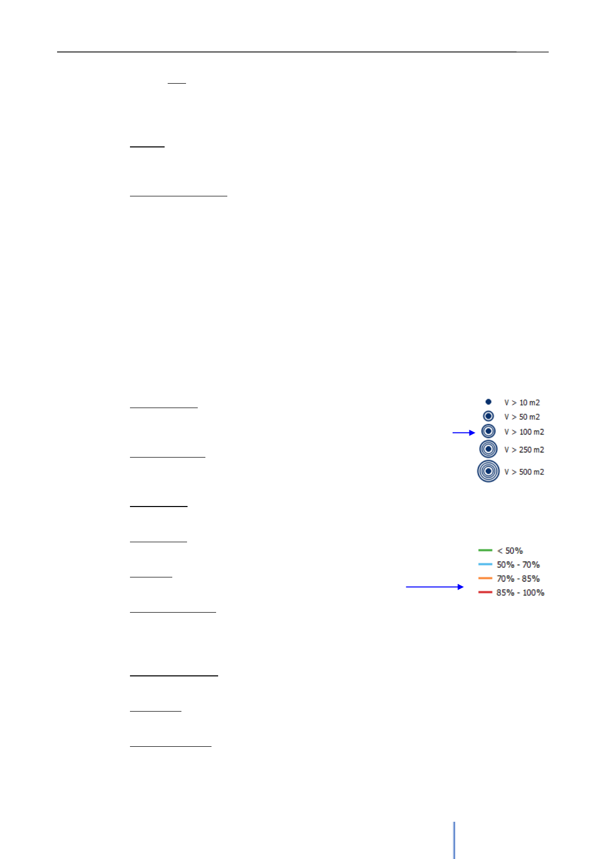
Giswater 3 User Manual
51
Arc: elements such as Conduit and Virtual arc. There are tables referring to the
cross sections, which describe how the bottom level of a pipe varies and flow
regulators which are devices used to control and derive the flows within the system.
The orifices, weirs, outlets and pumps can exert the regulation function.
o Quality: this group of tables, without geometry, allows to introduce data related to land uses
and pollutants present in the water. Land uses are only used to consider the phenomena of
accumulation and carry-over of pollutants in the catchments.
o Curves & Timeseries: Curves allow to establish the relationship between two quantities (in a
similar way to a graph) so that this data is easily introduced into the network by assigning
curves to the elements of the system. Time series are used to describe certain properties of
some project objects that vary over time.
▪ Input selected feature: this group is used, in case of having several sectors or hydrological
catchments, to select with which of them the user wants to work. This is one of the tools that
Giswater adds to the own uses of the SWMM program. If specific zone to make the hydraulic model
is selected, in this group of layers will be shown node and arc elements that come into play, which
will be all those that are within the selected area.
▪ Output result: group of model results allows to visualize through elements symbolized on the map
and data tables, the results of the SWMM hydraulic model. As in EPANET, it’s also possible to
compare results with another model previously made.
The possible results of the model, ordered in the same way as the QGIS ToC as described below:
o Node flooding: it shows all the water that overflows a node, during the
time it has been overflowed, the maximum flow during the flood, as well as
the different volumes of water on m2. It is represented in QGIS in this way:
o Node surcharge: overload occurs when water rises above the crown of the
highest conduit. It shows the data referred to hours of overload and
maximum and minimum values.
o Node inflow: represents the total flow input, both laterally and through links. Shows total,
temporary and maximum values.
o Node depth: average and maximum depth of water. Maximum hydraulic height (HGL) and
maximum depth time.
o Arc flow: this layer represents the percentages of water flow in the
network conduits. They are symbolized in QGIS as follows:
o Conduit surcharge: in this layer the overload of conduits is represented. Only those arcs with
one or more non-zero entries can be displayed. A conduit will be considered overloaded
when the slope of the HGL exceeds the slope of the conduit. Data about overload times will
be shown in one or both nodes linked to the arc.
o Pumping summary: different data referred to the operation of the pumps, such as maximum
and average flow pumped, energy consumed, percentages of operation times, etc.
o Flow class: classification of different categories of flows related to the arcs, for example, if
they are dry in one of their nodes or if the level of flow is critical
o Arc pollutant load: relationship between arcs and pollutants
Giswater 3 User Manual
52
o Outfall flow/load: flows of outfall. Percentage of discharge time, maximum and average
discharge flow, total discharge volume, etc.
o Subcatchment runoff: total values of precipitation, evaporation,
infiltration, depth and volume of the escape of the subcatchment. It’s
represented by a break coefficient.
o Storage volume: data reffered to the deposit. Maximum and average
volume in the installation, percentage used, times of use and maximum outflow of the
deposit
o Subcatchment washoff: total mass of each pollutant that leaves the subcatchemnt
o LID performance: They are the performances that have been obtained through the
application of LID (Low Impact Development) techniques.
The rest of the tables found in this group do not have geometry, but they also provide data related to
results of the hydraulic model such as quality and quantity of infiltration, instability indexes, surface
water values, among others.
4.2.5 Masterplan
This fourth group of tables and layers found in QGIS ToC is used to perform budget calculations of the
network. It’s one of the main tools of Giswater that has big potential, since its use allows to realize in a very
simple way different valorization of the water network and allows to systematize this process so that once all
the necessary data is available the calculation is be practically automatic. This means a considerable saving
of time and work for the users responsible for carrying out such calculations.
For both WS and UD projects, the group structure is the same, but the data has some differences, since the
nature of the projects is different. As throughout the manual, when any of the explanations is exclusive for a
type of project, its membership will be specified.
There are two clearly differentiated parts within the Masterplan group:
▪ Calculation of the heritage value of the elements: in these layers the price is calculated for each
element of every state (obsolete, on service or planned). All data is inserted into two views
(v_plan_result_node and v_plan_result_arc) depending on the type of element.
▪ Calculation of values of the planning sectors (psector): prices are calculated only for the planned
elements. Each group of elements planned for a network modification must be inserted into a
planned sector or psector. The objective of this group is to know the price a planned operation on the
network before carrying it out
The first step of all is to assign prices to the elements of the network, to the materials, to the possible
combinations of variables and, in short, to all the parameters that may have cost to create the budget. In the
catalogs there are many of these values, which are transferred directly to the elements. The rest of the prices
should be included in the three tables of the Asset unitary price group:
▪ Simple price: in this table the simple prices for each parameter are shown. Most of these are
imported from the database and calculations of ITeC (Institute of Construction Technology). The unit
field specifies the way to calculate the price (per unit, per cubic meter, etc.)
▪ Compost price: shows variable prices, since the price of certain elements can not be calculated with
a simple price, as it’s made up of more than one part. Here we describe what the price refers to and
the its id is related to the following table.
Giswater 3 User Manual
53
▪ Value compost price: contains the id's of the two previous tables. The compost_id can be repeated,
since a composite element will consist of more than one simple element (simple_id). The column
value represents the percentage of simple element that composes the compound element. By
relating these fields it is possible to calculate the total prices.
NOTE 07 The elements can be assessed in cubic meters (m3), units (u) or
meters (m). The cost_unit field governs whether an item is valued in one way or another and it
can be found in the different catalogs. It’s important to know what types of element are specific
for each form of valorization and what is the other field that gives the information to respect.
For UD (unit / element / measurement field)
-m3 / Storage y Chamber / man_storage y man_chamber.max_volume
- m / any other / node.ymax
- u / any other / el propio elemento
For WS (unit / element / measurement field)
-m3 / Tank / man_tank.vmax
- u / Pump / man_pump.pump_number
- m / any other / node.depth
- u / any other / el propio elemento
To calculate the heritage value, there is only one table inside the group of input data:
▪ Arc_x_pavement: this table has, as its only objective, to establish the percentages of types of
pavement that has a evry arc. Obviously, an arc can have 100% of its length in the same pavement,
but in oposite case when they vary along the arc, this table will be used to specify what percentage
covers each type. As the pavements - which are found in the pavement catalog (cat_pavement) -
have different prices per square meter, the fact of knowing the percentages used in each arc of the
network will finally allow to establish very precisely the heritage values.
ATTENTION: When you insert a new arc, the records are automatically inserted in the
plan_arc_x_pavement table, without pavement values and percentages, but in this way all the arcs
will be prepared to add the values of pavements.
Once the price and pavement tables have all the necessary data, it’s time to fill in the tables of results of the
patrimonial value. The importance of having complete data must be taken into account. Some data are taken
from different tables. Some come directly from the tables of the elements (arc, node) and must be correctly
filled in for a right calculation. All columns are required and all parameters are necessary.
There are two tables that has the results of the calculation of the heritage value. Remember that it’s possible
to display the data related to elements in any state type, whether it’s obsolete, on service or planned:
▪ Plan result node: contains the data of the calculation of the heritage value of each node and is
represented in QGIS as a punctual element with colors depending on the final value.
▪ Plan result arc: contains the data of the calculation of the heritage value of each arc and is
represented in QGIS as a line element with colors depending on the final value.

Giswater 3 User Manual
54
4.2.5.1 Planification sectors (psectors)
Psectors, planification sectors, are areas with planned actions that affect different elements represented in
the QGIS map. Obviously, if they are planned elements, their state must be planified (2).
The importance of this group of tables and layers is that it’s usually difficult to calculate the value and price of
operations of adding new elements to the network. Through these planning sectors it is be possible to obtain
the execution price of the entire work, as well as the detailed prices of each element.
Tables and layers that are part of the section are detailed below:
▪ Input data
o Plan psector (v_edit_plan_psector): geometrically represents the existing planning sectors. It
contains additional data, such as priority or some fields of percentages such as gexpenses
(added contract costs) and vat (VAT cost).
▪ Output data
o Plan psector cost (v_plan_psector): has the same geometry as the previous layer, but the
result of all cost calculations for the elements, that make up each planning sector is added. In
this layer the final values of the different prices can be found:
€ pem ----------------- material execution price
€ pec ------------------ contract execution price (pam + gexpenses)
€ pec_vat ------------ pec + VAT
€ pca ------------------ price for administration
o Plan psector x node cost (v_plan_psector_x_node): this layer represents the node-type
elements of the planning sectors. The total cost of each element appears in its attribute table. It
can be symbolized according to the cost.
o Plan psector x node arc (v_plan_psector_x_arc): this layer represents the arc-type elements of
the planning sectors. The total cost of each element appears in its attribute table. It can be
symbolized according to the cost.
o Plan psector x other (v_plan_psector_x_other): in this table, without geometry, the prices of
other parameters that also participate in the planning are added.
4.2.5.2 Managing prices of network elements
In masterplan, in addition to planning the network sectors, two types of prices that the network can have are
also managed. There are prices of reconstruction and rehabilitation.
To be able to have a reconstruction price assigned, it is necessary to have completely filled the fields of the
catalogs provided for it, so the first thing to do is to fill them in. Figure 20 shows a pipeline with its respective
measurements, specifying all the parameters that come into play when calculating prices.
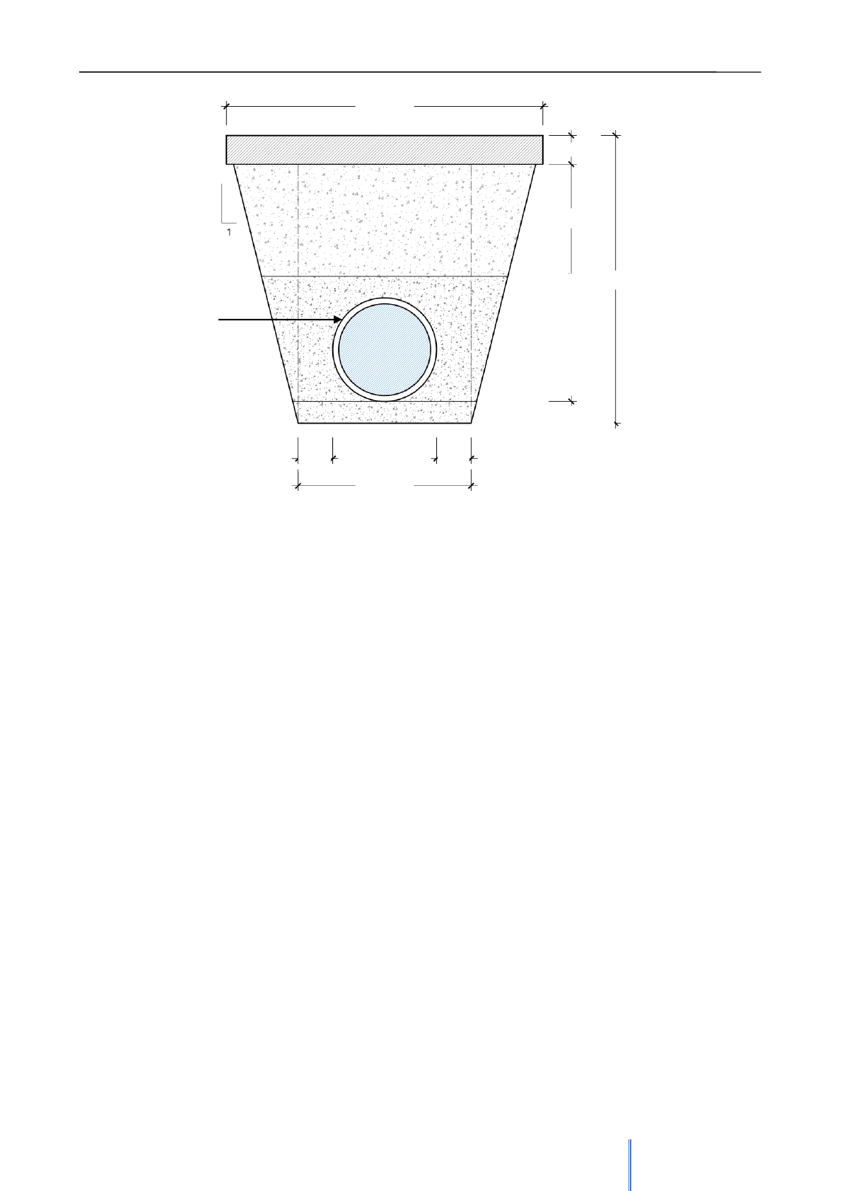
Giswater 3 User Manual
55
The fields that affect the calculation of patrimonial value are:
From arc catalog (cat_arc):
z1 (m)
z2 (m)
width (m) – Total width. Width + bulk*2
area (m2)
estimated_depth (m)
bulk (UD (m) WS (mm)) - thickness of the conduit’s wall
cost_unit – Measurement units
cost - Price of the type of arc. Related with price tables.
m2bottom_cost - Price of the type of soil. Related with price tables.
m3protec_cost - Price of protection. Related with price tables.
From pavement catalog (cat_pavement)
thickness (m) – thickness of the pavement
m2_cost - Price of the square meter of the pavement. Related with price tables.
From soil catalog (cat_soil)
y_param – Inclination of the slope of the trench
b (m) - Distance between the Conduit and the trench limit
trenchlining (%) - Percentage of intivation of the soil type
m3exc_cost - Excavation price. Related with price tables.
m3fill_cost – Filling Price. Related with price tables.
area
y_param
estimated depth
bulk
b
b
z1
z2
width
Image 20: Conduit’s section with its measurement parameters.

Giswater 3 User Manual
56
m3excess_cost - Excess transportation price. Related with price tables.
m2trenchl_cost – Intivation price. Related with price tables.
From node catalog (cat_node):
estimated_y
cost_unit – Measurement units
cost – Price of the node type. Related with price tables.
Once the work is done, the only part left is to link the elements with its catalogs:
ARC in: cat_arc (arc.arccat_id), cat_pavement (plan_arc_x_pavement) y cat_soil (arc.soilcat_id)
NODE in: cat_node (node.nodecat_id)
On the other hand, in order to assign a rehabilitation price, given the disparity of costs and cases,
each operator must build its own rehabilitation algorithm, with which the option is ready, but is
disabled as a series value.
4.2.6 System
The tables of system ARE TABLES THAT SHOULD BE MANIPULATED BY EXPERT PERSONNEL since
changes of the in this tables can cause that the system will stop working. In those tables the information that
is necessary for the correct functioning of Giswater is located, but they will rarely have to be viewed directly,
since there are tables with information that is shown in other places of the project. Even so, it’s important to
know its existence, objectives and usability.
Unlike the previous version of Giswater, now the group of system layers has a large number of tables with
different types of information, which are divided into subgroups according to the type of role they are
adjusted to.
▪ Basic
This group contains some of the most important layers of the project, because if they are not within the
ToC the program won’t work. These are the editable views of node, arc, connec and gully elements (the
last one only in UD projects). Through these views the rest of the layers that contain the geometric
elements can be seen, therefore there are considered as "mother" views of the project. Its symbology
coincides with that of each type of element in the group of network elements (section 4.2.1.3).
In addition to these views, the Basic subgroup also contains tables with information regarding
hydrometers and scada data and catalogs or other external tables.
▪ Edit
This subgroup also has relevant information stored in the tables, all without geometry. Some of them
contain data with values that will be used in different Giswater tools, but there are others that deserve a
more detailed explanation of their behavior:
o Project version (version): This table is the most important of Giswater project. It is used for a
multitude of system tasks and it must be kept in mind that in the QGIS project there must always be
one and only one for the plugin to activate.
o Node type (node_type): The table characterizes the different types of node that the project can
have. The list of types of nodes that the system permits - field type, from now on 'system node type' -
is not modifiable or extensible. What user can do is create as many node type elements as he wants
– field id, from now on 'custom node type' - with the same system node type attribute, as long as this
attribute is in the system.

Giswater 3 User Manual
57
It’s important to know, that:
▪ Each 'system node type' has a defined data model, different from the others. If user
wants to create a new record of node type, he must first analyze which of the
different data models implemented in the system nodes is more adjusted to the new
'node custom type'.
▪ For each 'custom node type' a default value of type of element in the hydraulic model
can be defined. This default value is REQUIRED, but for each network element can
be modified at any time by hydraulic engineers.
▪ 'Custom node type' allows to customize the names of the elements in the selected
language. This allows that, although the system always works with the 'system node
type' this will always be transparent for the user who will never see the 'system node
type' but will always work with the 'custom node type'.

Giswater 3 User Manual
58
o Arc type (arc_type): The table arc_type La tabla arc_type characterizes the different types of arc
that are present in the project.
Exactly as for node_type, It’s important to know, that:
▪ Each 'system arc type' can have a defined data model, different than the others.
▪ For each 'custom arc type' a default value of type of element in the hydraulic model
can be defined. This default value is REQUIRED, but for each network element can
be modified at any time by hydraulic engineers.
▪ 'Custom arc type' allows to customize the names of the elements in the selected
language. This allows that, although the system always works with the 'system arc
type' this will always be transparent for the user who will never see the 'system arc
type' but will always work with the 'custom arc type'.
o Connec type (connec_type): the table characterizes the different types of connec that the project
can have. The list of types of connecs that the system permits - field type, from now on 'system
connec type' - is not modifiable or extensible. What user can do is create as many connec type
elements as he wants – field id, from now on 'custom connec type' - with the same system connec
type attribute, as long as this attribute is in the system.
It’s important to know, that:
▪ Each 'system connec type' has a defined data model, different from the others. If
user wants to create a new record of connec type, he must first analyze which of the
different data models implemented in the system connec is more adjusted to the
new ‘connec custom type'.
▪ For each 'custom connec type' a default value of type of element in the hydraulic
model can be defined. This default value is REQUIRED, but for each network
element can be modified at any time by hydraulic engineers.
▪ 'Custom connec type' allows to customize the names of the elements in the selected
language. This allows that, although the system always works with the 'system
connec type' this will always be transparent for the user who will never see the
'system connec type' but will always work with the 'custom connec type'.
o Gully type (gully_type): the table characterizes the different types of gully that the project can have.
The list of types of gullies that the system permits - field type, from now on 'system gully type' - is not
modifiable or extensible. What user can do is create as many gully type elements as he wants – field
id, from now on 'custom gully type' - with the same system gully type attribute, as long as this
attribute is in the system.
It’s important to know, that:
▪ Each 'system gully type' has a defined data model, different from the others. If user
wants to create a new record of gully type, he must first analyze which of the
different data models implemented in the system gully is more adjusted to the new
‘gully custom type'.
▪ For each 'custom gully type' a default value of type of element in the hydraulic model
can be defined. This default value is REQUIRED, but for each network element can
be modified at any time by hydraulic engineers.
▪ 'Custom gully type' allows to customize the names of the elements in the selected
language. This allows that, although the system always works with the 'system gully
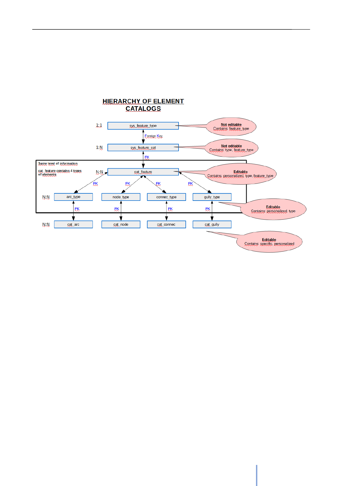
Giswater 3 User Manual
59
type' this will always be transparent for the user who will never see the 'system gully
type' but will always work with the 'custom gully type'.
It is important to know the functioning of the catalogs, their relations through foreign keys and other
restrictions in order to maintain consistency of the project. In image 21, the hierarchy of elements’ catalogs
is represented.
In addition to all the tables described, in the Edit subgroup there are tables:
▪ man_type_function
▪ man_type_location
▪ man_type_category
▪ man_type_fluid
These four tables are used to add specific information for each element. Its use is explained in point 2 of
section 2.3.5.
O&M
This subgroup contains tables with additional information about the operations and management group, such
as visit parameters or types of visits. There is also the layer with polygonal geometry that represents the
planning sector related to the om that is selected at the moment (current).
Image 21: Schema representing the hierarchy of tables related to principal elements of
Giswater.

Giswater 3 User Manual
60
EPA Y SWMM
This subgroup contains tables with additional information related to the EPANET and SWMM layers. Most
are containers of values that will be used during the calculations of the hydraulic model. Its data comes by
default with the creation of the working scheme with Giswater, that is why those are tables that should not be
modified by the user.
Masterplan
Contains tables related to the Masterplan section. There is a table with the relation of the different types of
price units (m3, u, kg ...) and another one with the polygonal geometry that represents the planning sector
that is selected at the moment (current).
Utils
The last subgroup aims to store other system tables that do not have any specific relationship with other
subgroups. Here there is located audit_cat_table, a table that is used in some Giswater functionality and that
at the same time can help the user to understand the rest of the tables of the entire project. Audit_cat_table
contains the following information for each of the tables and views in the database schema:
▪ Id
▪ Context
▪ Description
▪ Role and criticality in the system
▪ Number of rows that the table must have in the system
▪ Role and criticality in QGIS (different than the one from the system)
▪ Message in QGIS
▪ Numeric sequence that filles in the field id.
This audit information can be very helpful when the user has doubts about the nature of a table and also
about its need to be loaded in QGIS or in the system (database). In this sense, the criticality field represents
this need. It has values from 0 to 3, with 3 being the maximum criticality, because if a table with criticality 3 is
not loaded in the database or in QGIS (depending on which one has that criticality), the project will not be
able to work or it will not work correctly.
The criticality 3 for QGIS is only present in four tables:
Version
v_edit_arc
v_edit_node
v_edit_connec
With these tables the program could begin to be used, although with some possibilities well below the real
ones. Layers with criticality of QGIS = 2 are highly recommended to be loaded in the program, since their
presence is important and if they are not found many of the features of Giswater could not be used. Layers
with criticality of QGIS = 1 must also be loaded for proper functioning of all tools, although their non-
existence in the project would not be especially tragic either. If any experienced user knows that any of these
layers will not affect his use of the program, he could eliminate it from the ToC. Finally, the tables with
criticality of QGIS = 0 should not be loaded in the project, as their presence is not necessary for the uses of
Giswater. That table should not be eliminated from the system, even if ll the tables have been created with a
specific objective and function.
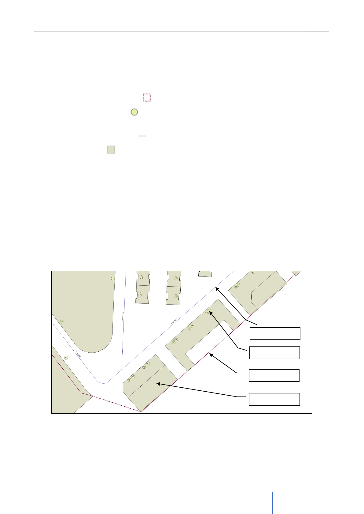
Giswater 3 User Manual
61
4.2.7 Basemap
The last group of layers of the ToC of Giswater is the one with base maps, which is the cartography that can
be used as reference for the rest of the elements and that represents some part of the territory. The
incorporation of these layers to the project is very important, since it adds information that most users is used
to see and therefore, they find it easier to identify to work with it. The base cartography is composed of:
▪ Municipality (ext_municipality) : polygon layer that marks the limits of municipality
▪ Address (v_ext_address) : punctual layer that represents the portals, each one with its number
and relationship with the street to which it belongs
▪ Streetaxis (v_ext_streetaxis) : linear layer that represents the street axes within the municipality
▪ Plot (v_ext_plot) : polygonal layer that represents the different areas of the buildings and
constructions that exist in the municipality.
There are different foreign keys between the street tables that give consistency to the data and restrict
possible errors. The ext_address table has field muni_id which is relates it to ext_municipality table and field
streetaxis_id relates it to ext_streetaxis table. At the same time, the ext_streetaxis is also related to
municipality by the field muni_id. In case of existing many municipalities, each streetaxis can be related only
to one municipality.
The origin of the data referring to base cartography has nothing to do with Giswater, but must come from
other sources, hence the prefix ext in the layers, such as cadastral data. These layers, depite their external
origin, are completely integrated into Giswater project and have more functionalities besides the simple
cartographic representation of the elements. They must have specific structure, which can be seen in the
annex of this manual. These functionalities will be reflected in section 5.2, but its most important function is
searching the specific location.
In the same way, if a user wishes to, more external layers related to the base map of the area can be added
into the group to visualize other elements or anything that one wants to represent. In this case, any layer that
is added will be completely external to Giswater and will have no relationship with other tables. Examples of
layers that can be added are a topography raster or an orthophoto.
Image 22: Example of the elements that are present in the Basemap group.
Municipality
Plot
Address
Streetaxis
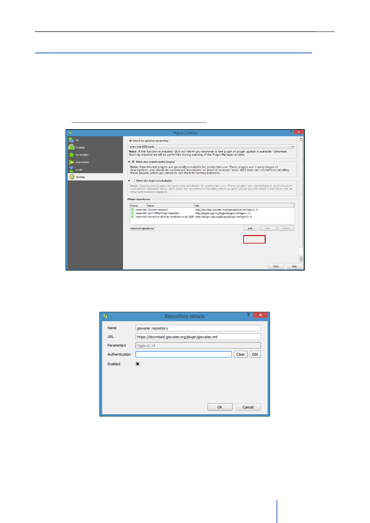
Giswater 3 User Manual
62
5. GISWATER PLUGIN
5.1 Installation and configuration of Giswater plugin
In order to install and connect Giswater plugin with QGIS, it’s necessary to configure a new repository, which
1. Open QGIS and access plugins’ repository (Plugins > Mange and install plugins).
2. Enter the tab ‘Settings’ and add a new repositoryo.
'https://download.giswater.org/plugin/giswater.xml'
3. Introduce the name that will identify the repository and the URL.
4. Find and install Giswater plugin, from tab ‘All‘.
Image 23: To add the plugin of Giswater to QGIS it needs to be shown on the list of plugin repositories.
Image 24: The repository is added manually, using a URL.
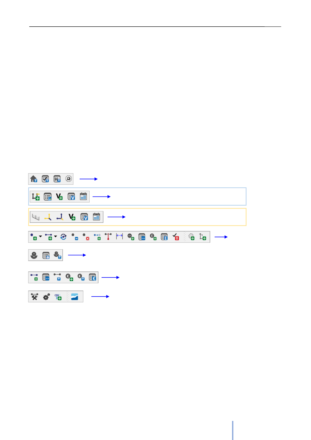
Giswater 3 User Manual
63
Warning: So that the Giswater plugin starts to work user must previously create a connection to the database, where
the data schema is located, using PostGIS.
If after installing plugin and establishing the connection to the database, it doesn’t appear directly in the toolbar,
access the menu 'View / Toolbars' and add it.
In case of having more than one QGIS project open, the behavior of the plugin may present instabilities, so it’is
recommended not to use the plugin with more than one open QGIS project at a time.
5.2 Toolbars of a plugin
One of the biggest and most notable improvements of the 3rd versión of Giswater can be found in the plugin
tools. Not only the new capabilities have been added, but also the existing tools have been improved.
Giswater plugin is a part of the software with which the user should become more familiar, since most of the
actions that he wants to carry out can be done using the tools available in the plugin.
Giswater currently has up to 38 tools available, divided into different toolbars that must be associated with
the six roles that exist in Giswater.
Those toolbars are:
Later on, the functionality and the objective that each one of the tools has is detailed.
5.2.1 Basics
This group of three consulting tools is related to the basic role of Giswater. They are tools that allow to select
and consult the data, but still without the capacity to modify it. Even so, its use is very important, since the
fact of selecting one or another parameter, for example, the states of the elements, will modify the behavior
of other tools.
Edition toolbar
Planification toolbar
Utility toolbar
Basic consult toolbar
Operations and management toolbar for UD
Operations and management toolbar for WS
Hydraulic model toolbar
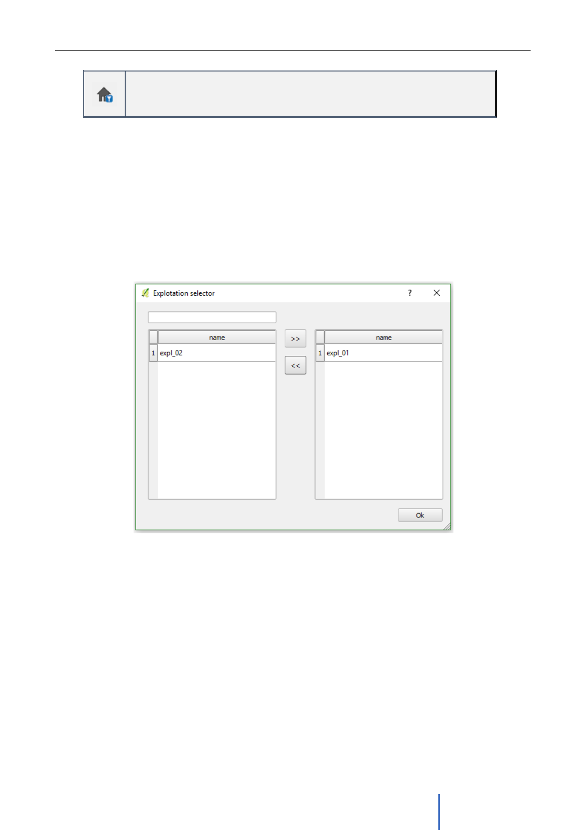
Giswater 3 User Manual
64
Exploitation selector
Allows to visualize or not different exploitations – role_basic
The exploitation selector, as its name indicates, is a tool that allows to choose the exploitation
that will be visualized. When we talk about visualization it doesn’t mean that the data of the
exploitations that are hidden are eliminated, they are simply not visible in the graphical
interface of QGIS.
The use of this tool is very simple: in the form appear two lists which contain the exploitations
of the network. Those that are placed on the list on the left won’t be displayed and those on
the right will. To move an exploitation from one list to another it has to be selected by clicking
on it and moved from one side to the other using the arrows, that are located between the two
lists.
In the form in image 25, exploitation 1 (expl_01) and all its data would be displayed in QGIS,
unlike the data of expl_02, which will be hidden until the values of selector are modified again.
The box that is located above the list on the left allows to search among the different
exploitations that are not visible.
ATTENTION: When an exploitation is selected in the selector, all the sectors that intersect that
exploitation are displayed automatically.
Image 25: Form of exploitation selector tool. On the left there are listed those that won’t
be visualized, on the right those that will be visible on the map.
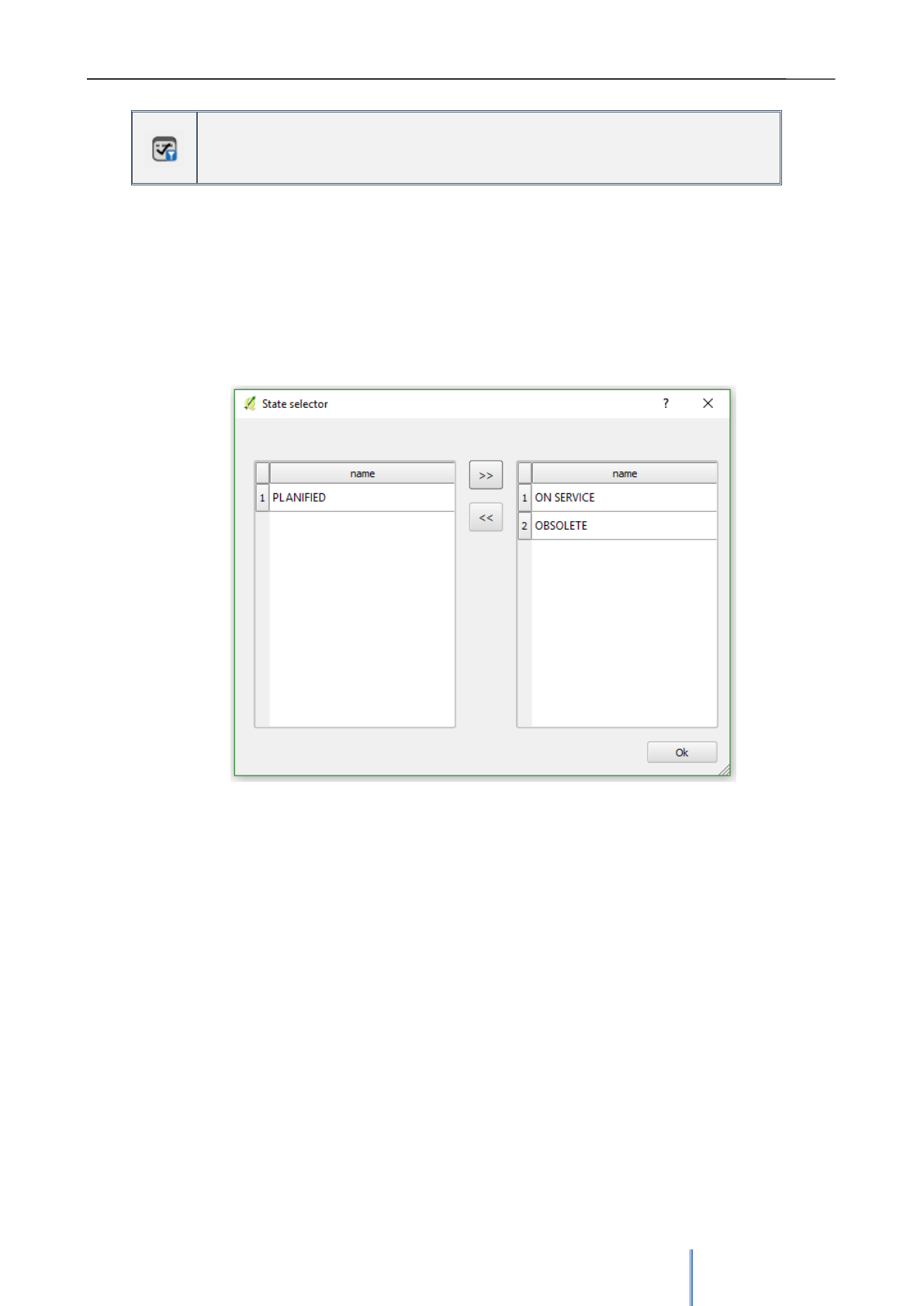
Giswater 3 User Manual
65
State selector
Allows to visualize the elements in function of their state – role_basic
In the same way as the exploitation selector, the state selector allows to visualize the elements
of the network depending on their state. The states have been previously defined and those
are: OBSOLETE, ON SERVICE and PLANNIFIED.
This tool has the same performance as the previous one, the different states can be moved
between two lists using the arrows located between them.
In the form of the image 26, the elements with state on service and obsolete have been
selected and will be visible for the user. The plannified elements will be hidden. When using
this tool, it must be beared in mind, that the elements that are displayed on the map will be the
same and only ones that will be used by other tools that require those elements of the
network.
Image 26: Form of state selector tool. On the left there are listed states that won’t be
visualized, on the right those that will be visible on the map.
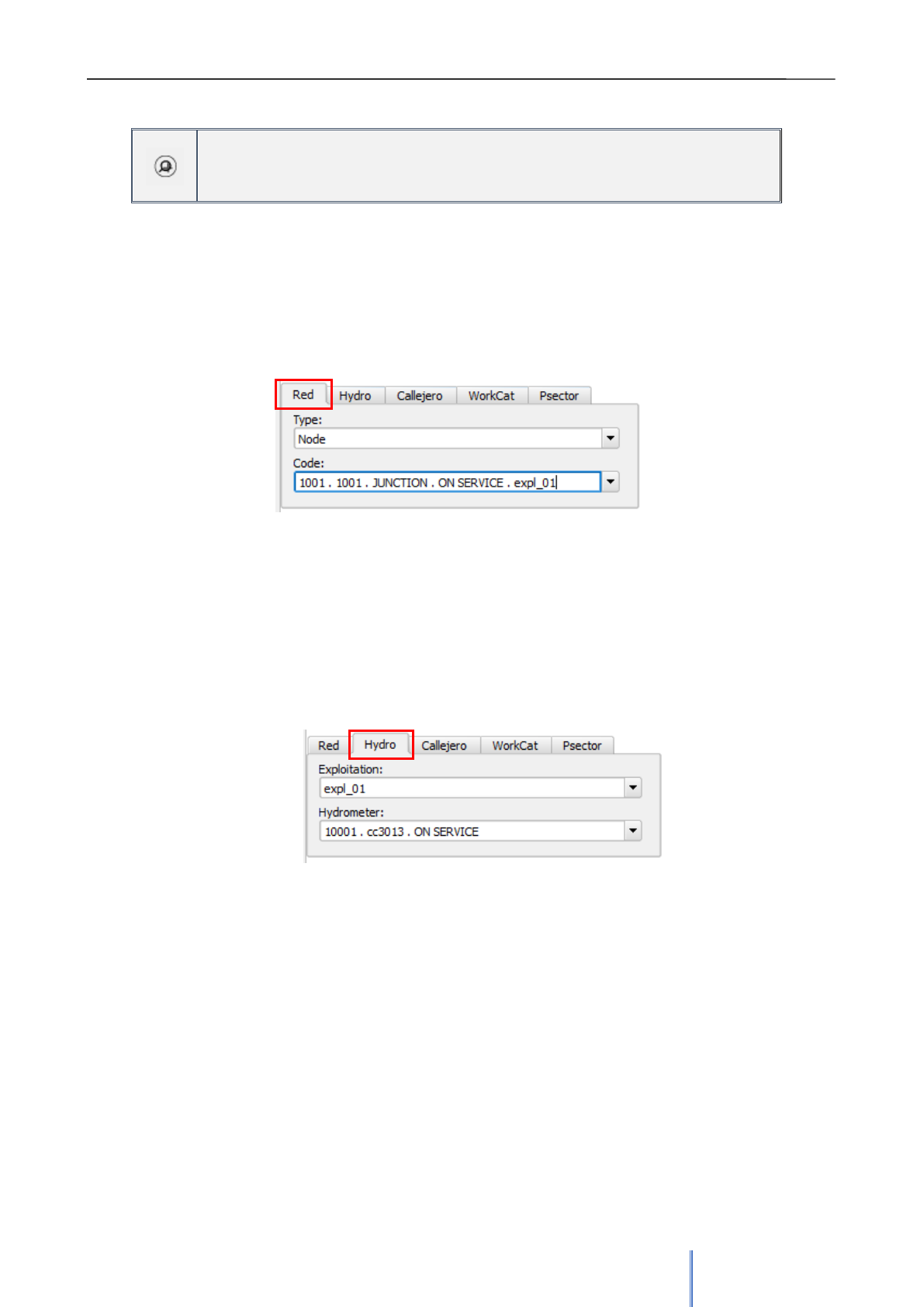
Giswater 3 User Manual
66
Searcher
Allows to search for the elements of the network and addresses – role_basic
The Giswater search engine allows to search and select elements of the network or the
address. There are five different tabs within the search engine, each with different seeking
parameters.
We will see tab by tab the use of the searcher:
▪ Network: allows to search for specific elements of the network. First the type of
element must be selected, later in the drop-down list, all the available ones will be
filtered showing their code, id, type, state and exploitation. When selecting one of
them, the element will be zoomed and centered in the middle of the screen. Searcher
acts with the project system layers, which is a reason to have them always loaded in
the project.
▪ Hydrometer: it allows to search for hydrometers, which must always be related to
connecs. In the first drop-down list the exploitation must be selected. Then, it’s posible
to search among all the hydrometers of that exploitation. The
hydrometer_customer_code, connec_customer_code and hydrometer state will be
displayed. When selecting a record, the tool will automatically open the hydrometer
form and zoom in to the corresponding connec. All the parameters that are used in
this browser tab are customizable by the user in the config_param_system table.
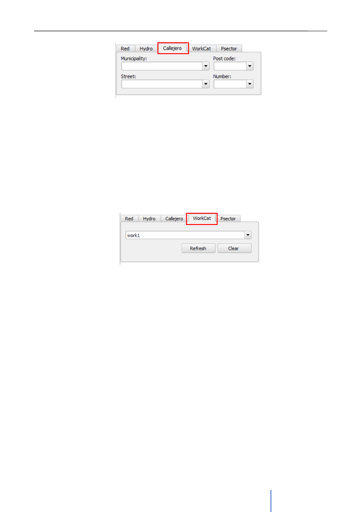
Giswater 3 User Manual
67
▪ Address: the third tab of searcher is related to the street map, loaded in the last group
of Giswater layers (base map). It allows to search for municipalities, streets or specific
portal numbers. To use it, the fields of the ext_municipality, ext_streetaxis and
ext_address tables must be correctly filled out. After opening the Municipality drop-
down list, and choosing municipality the map will be automatically zoomed in to its
limits. It is also possible to make a similar selection by postal code. Next step, is
choosing a street of the municipality in the Street drop-down list. By selecting a street,
the map will zoom in to its extension. Finally, with the street selected, the street
number may be chosen from a Number drop-down list. By clicking on a specific
number the map will zoom in to the selected element, centering it on the screen.
▪ WorkCat (work records): it allows to filter the elements of type node, arc, connec,
gully and element according to the work record to which they belong. In the drop down
list user can choose a record and after clicking on it, a window containing two tables
will automatically open. On the left side the elements that have assigned the selected
record as a start work (installation of an element) will appear. In the table on the right,
those which have it as an end work record will be displayed. Clicking on any row of
the table will open the specific form of the element. In the lower part of each table a
summary of the table is presented, showing the total number of elements of the same
type as well as the total length of the arcs that are part of the selected work file.
▪ In addition, in this window it’s possible to export the information presented in the
tables into csv file. To do it’s necessary to set the save path and click Export to csv
button.
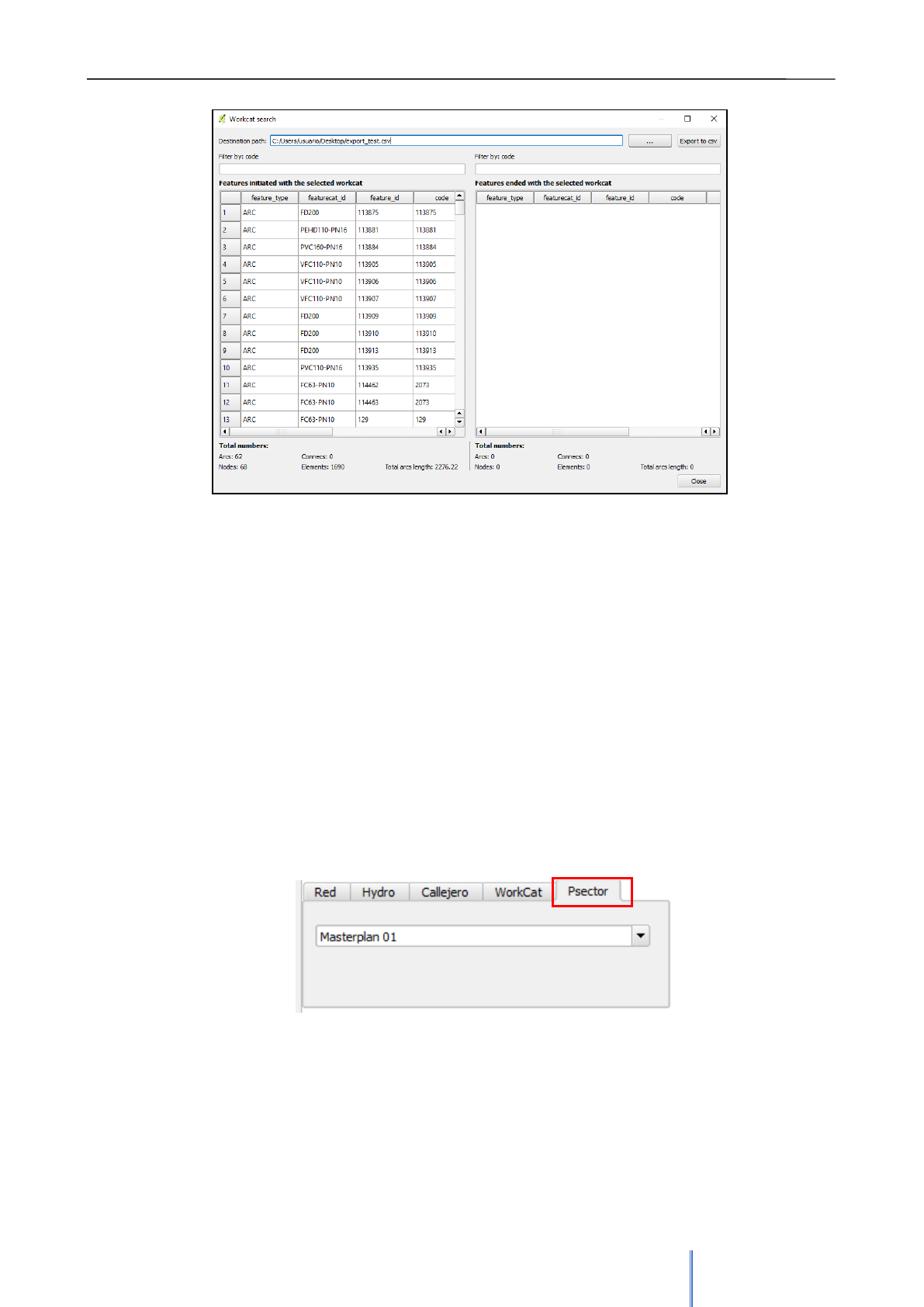
Giswater 3 User Manual
68
In QGIS project there is loaded a layer (v_ui_workcat_polygon), which as the name
implies, has polygonal geometry. This polygon is drawn dynamically around the
elements of the map that have a specific work record. After selecting one of them
using WorkCat search tool, the map will zoom in to the polygon of the work record. It
allows to see how big area was covered by this action.
Below the drop-down list that allows to find the work record there are two buttons,
Refresh and Clear. The first one is used to refresh the information of a work record, so
in case of adding a new element with a specific workcat_id it must be clicked in order
to regenerate the polygon and add to it the geometry of the new element. The second
button, Clear, allows to eliminate the visualization of a polygon from the QGIS
interface, simply so that it does not obstruct the use and representation of the rest of
the elements. To visualize it again it’s necessary to use again the searcher.
▪ Psector: The last tab of the search engine allows to look for the different planification
sectors generated in the project. The use is very simple: select one of the psectores
from the drop-down list. When clicking, the form associated with the corresponding
psector will open automatically, there will be the possibility to edit the information, see
the linked elements, add prices or documents, etc. The search engine also zooms to
the geometry of the specific psector.
Image 27: Form of searching by work record (workcat_id). Allows to export the
information into csv file.
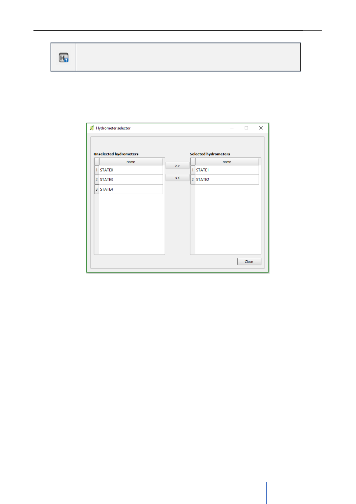
Giswater 3 User Manual
69
Hydrometer’s state selector
Allows to visualize or not the hydrometers in function of its state – role_basic
The last tool of the basic bar is used to select the hydrometers according to their state. Like
the spatial elements, the hydrometers also have a state, which the user defines and manages
from the tables ext_rtc_hydrometer_state (to define new states) and ext_rtc_hydrometer (to
add a certain state to the selected hydrometer).
The method of use of this tool is the same as that of exploitation and state selectors presented
before. Remember that the hydrometers are shown in a tab of the connec or gully type
elements to which they are linked to.
Using this tool will only show the information related to the hydrometers that have the selected
states. This will happen in the tabs of the elements’ forms and in the hydrometer seeker.
The objective of this selector is to facilitate the management of hydrometers, since it’s a table
that can have a huge amount of data and therefore its management can be dificult.
Image 28: Selected states are showed in the columna on the right.
Giswater 3 User Manual
70
5.2.2 Operations and management
This group of tools is designed to perform or simulate actions on the actual network of water supply or urbain
drainage. Some of them will be used directly from the location of the element in the field, to report
information on its status, others from the office. One way or another they are focused on the actual use of the
elements.
This O&M toolbar of the plugin is the only one where there are big differences between WS and UD projects.
There are some tools that are only for water supply and others that are exclusive for urban drainage. As
usual, a clear distinction will be made when detailing the operations.
However, there are several common tools in this toolbar, such as those related to the management of visits
and events. The visits to elements are made by a worker in the field, who can add the information directly to
the tables specially designed for this function through a mobile device.
Minimum cut polygon
Allows to create a new mincut polygon – role_om
Mincut polygon functionality is surely one of the most important functionalities that a drinking
water network manager needs to operate with day to day. In this section it will be explained
how the internal work logic of the database is developed.
The mincut polygon propagates flows from the elements that supply water to the network and
then proposes the valves that should be closed in case of wanting to leave a specific point
without water supply.
First of all, there are several previous aspects about the data that are strictly necessary for
the tool to work correctly:
1. Pgrouting library is used for this process.
2. All nodes and arcs must have filled in fields state and state_type. The type of state must
be one that is in use. This can be seen in the value_state_type table in the is_operative
field, which must be TRUE. In case of FALSE the element will not enter into the process
of the mincut polygon.
3. The network traceability is made from the node_1 and node_2 of the elements type arc,
that’s why the network must have topology.
4. The identifiers (id) of arcs and nodes must be integer.
5. Table man_valve should have values in fields closed y broken, which by default have
value FALSE.
6. Mincut polygon works in the context of the exploitation system defined by the user in the
table anl_mincut_inlet_x_exploitation. In this table the nodes that contribute water to the
system (usually they are source or tank) together with the information to which
exploitation they belong must defined.
7. The type of valves that participate in the mincut polygon must be configured. This can
be done from the table anl_mincut_selector_valve or using the plugin. Usually they are
only the shutoff valves.
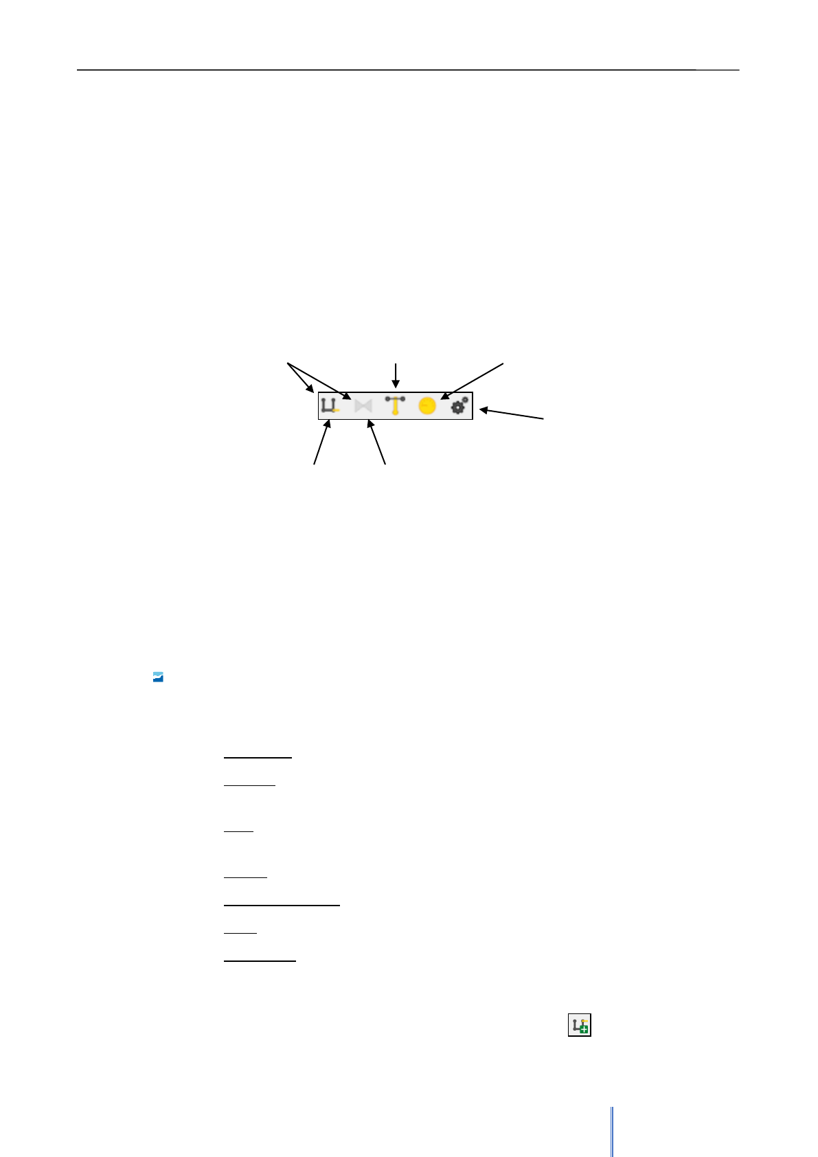
Giswater 3 User Manual
71
8. For mincut there are three different types of states (not to be confused with the states of
the elements of the network). These are defined in the table anl_mincut_cat_state and
are:
▪ Planified id=0
▪ In Progress id=1
▪ Finished id=2
Once all the mentioned aspects are controlled the tool can be used. Clicking on the button
opens the mincut form, where, in the first place pay attention to the top menu. Here it’s
possible to distinguish the mincut types and the configuration of the tool. In the configuration
the types of valves that enter into process can be selected.
As shoed in image 28 there are three types of mincut polygon. The one with the most
developed functionality is number 1, which proposes the valves to be closed in order to
leave a specific location without water supply
How to use the tree types of mincut:
Network mincut – Class 1
To make a mincut polygon of type 1 the form must be filled (image 30) with the
parameters:
▪ Work order: work record (optional).
▪ Location: location of the point that won’t have (made from fields municipality,
post code, street and number).
▪ Type: may be demo, real or test, depending on whether the water cut is
actually going to take place or is just a test to see what would be the results
▪ Cause: Accidental o plannified.
▪ Start and end date: forecast dates of the process
▪ User: name of the user assigned to this task.
▪ Description: additional information in text format for the specific case.
Now the state of mincut polygon will be Planified. The state is automatically modified
depending on the process. At this moment it’s time to click the button that will allow
to choose the point of the network where the water will be cut.
Configuration
Automatic valve mincut
Manual closing of
valves.
1- Network mincut
2- Connec mincut
3- Hydrometer mincut
Image 29: Toolbar of mincut form. It’s posible to select the type of proccess that will be
performed.
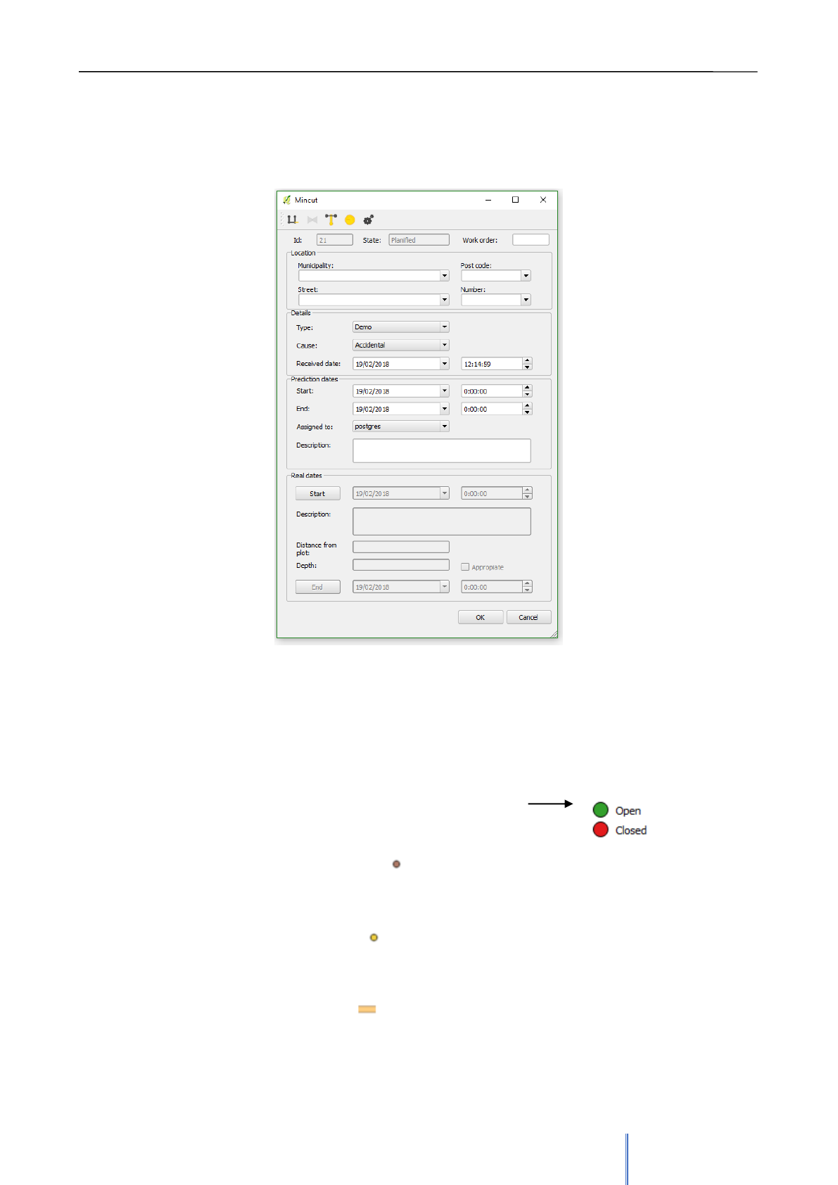
Giswater 3 User Manual
72
The cursor must be placed over the desired point, which can be located either on an
arc or a node. When clicking, the mincut polygon will be automatically made,
showing the valves that will have to be closed and all the elements that will be
affected (sections, nodes and connections).
To offer this information mincut has different tables where the results are stored
depending on the type of element:
▪ Mincut result valve: represents all valves of the network depending on
whether they should be opened or closed
▪ Mincut result connec: represents all the connecs of the network that
will be affected by the mincut
▪ Mincut result node: represents all the nodes of the network that will be
affected by the mincut
▪ Mincut result arc: represents all the arcs of the network that will be
affected by the mincut
Image 30: Form of mincut polygon, same for all the
mincut types. It has different functions and fields that
are activated depending on the state of the process.
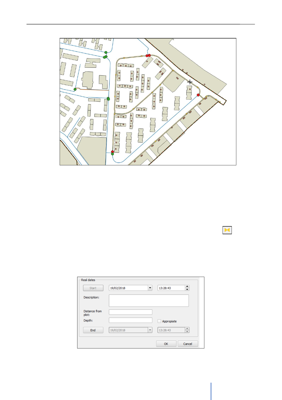
Giswater 3 User Manual
73
All these tables store the information of the element and the identifier of the mincut
polygon and allow to clearly visualize on the map the affectation of the process, as
shown in image 30.
At this moment the second button of the mincut toolbar is activated, which will allow,
optionally, to choose a valve that for whatever reason will not be able to be closed. It
can be done by clicking on the button and choosing the valve. After that the results of
the process will be recalculated taking into account the modification.
With the completed polygon and knowing that all the marked valves can be
effectively closed, it’s time for the second part of the form, which is called Real dates.
When clicking on Start, the rest of the fields will be activated, the start date and time
will be set automatically and the status of the process will change into In Progress.
It’s possible to add an additional description of the process and fiil in the other fields
such as building distance or depth.
Image 31: View of the map showing the results of the mincut process. The symbology shows the
valves to close, as well as arcs, nodes and connecs affected by it.
Image 32: Fields of form are activated when the true process of field
work starts.
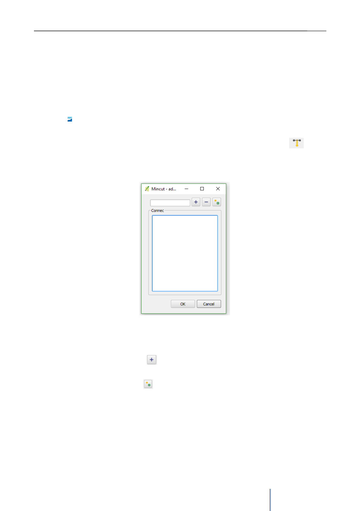
Giswater 3 User Manual
74
If it’s a test mincut usually the duration will be very short, as the important part is the
range of theprocess. On the other hand, if the mincut is real, the steps are clicking
OK and leaving the process in this state until, when the time comes, clicking End to
finish and change the state to Finished. Clicking End opens another small form to
specify, if necessary, the location and dates of the process. By clicking OK in this last
form, this cutting polygon will be permanently closed and stored without the
possibility of editing it again.
Connec mincut – Class 2
To perform a type 2 mincut, in the same way as in 1, the form must be filled in with
the location, dates and mincut details. Then, clickin the button will start the
process:
At this moment a small form is opened that will allow to select the connections to
which the water supply will be cut (Imagen 32).
There are two ways of selection:
▪ With the button the connection can be added through its connec_id,
which will be filtered in the container of values that are in the form.
▪ With the button many connections can be added at the same time. All
the connections that are inside the rectangle that is drawn on the map are
going to be inserted in the mincut.
Button (-) allows to unselect the connections.
Once selected, by clicking OK these elements will be stored as connections to be cut
for the mincut that is in process and they will be able to be visualized in the map
through the Mincut result connec layer.
Imagen 33: Form to choose the
connecs that will be affected by the
mincut process.

Giswater 3 User Manual
75
In the same way as for the Network mincut, at this moment the state may be
modified. It can be left as planned, it can be started and left as in progress or
finished.
Although this type of mincut polygon does not provide as much information as type
1, it is also important when planning network operations in cases where valves do
not have to be closed, but the connecs will be.
Hydrometer mincut – Class 3
This last type of mincut polygon is very similar to the previous one, but with an
added level of detail. In this case, the hydrometers that are going to be closed are
identified. It is useful for cases in which not all the hydrometers of a connection must
be closed.
The flow of use is the same as in the previous case, but in this case the selection
form has two filters: one for connecs and another for the hydrometers that are
related to the connecs.
Since the hydrometers do not have geometry, it will not be possible to visualize the
results on the map, but they will be stored in the Mincut result hydrometer table.
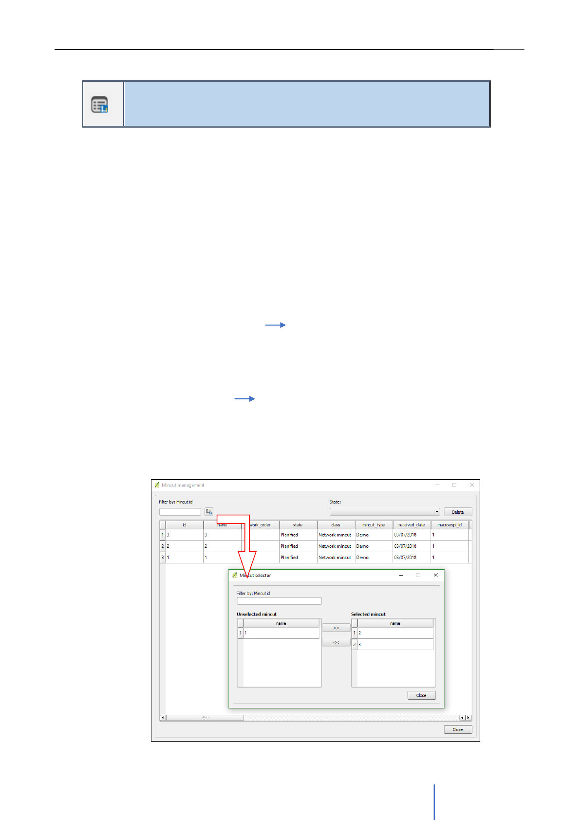
Giswater 3 User Manual
76
Mincut manager
Allows to manage the existing mincut polygons – role_om
The mincut polygon manager complements the mincut tool. The objective of this tool is to
store the different mincut polygons made in the project and allow to recover and visualize
again the data refelated to the existing polygons.
After clicking the button a form opens. In the part there is a table where the polygons already
made are displayed in rows, whatever their state (plannified, in process or completed). Each
row presents the mincut polygon information: type, dates, street, cause, start element, etc. The
capabilities of the tool are the following:
▪ Filter by id
▪ Filter by mincut state
▪ Delete selected mincut
▪ Open selected mincut When opening a micut polygon first the form
will be shown and in case when it’s not finalized, it is possible edit the data.
At the same time, the results tables of mincut will be updated with the data of
the selected process and therefore it will possible to see them again on the
map.
▪ Mincut selector Next to the filter by mincut_id button there is a
button that opens the mincut selector. After clicking, a selector will appear,
allowing to see on the screen different mincut polygons at the same time.
Important thing is that having different polygons in the selector, the tables
where the data is stored will also have more information differentiated by the
mincut_id.
Image 34: For of mincut menager with opened mincut selector form.
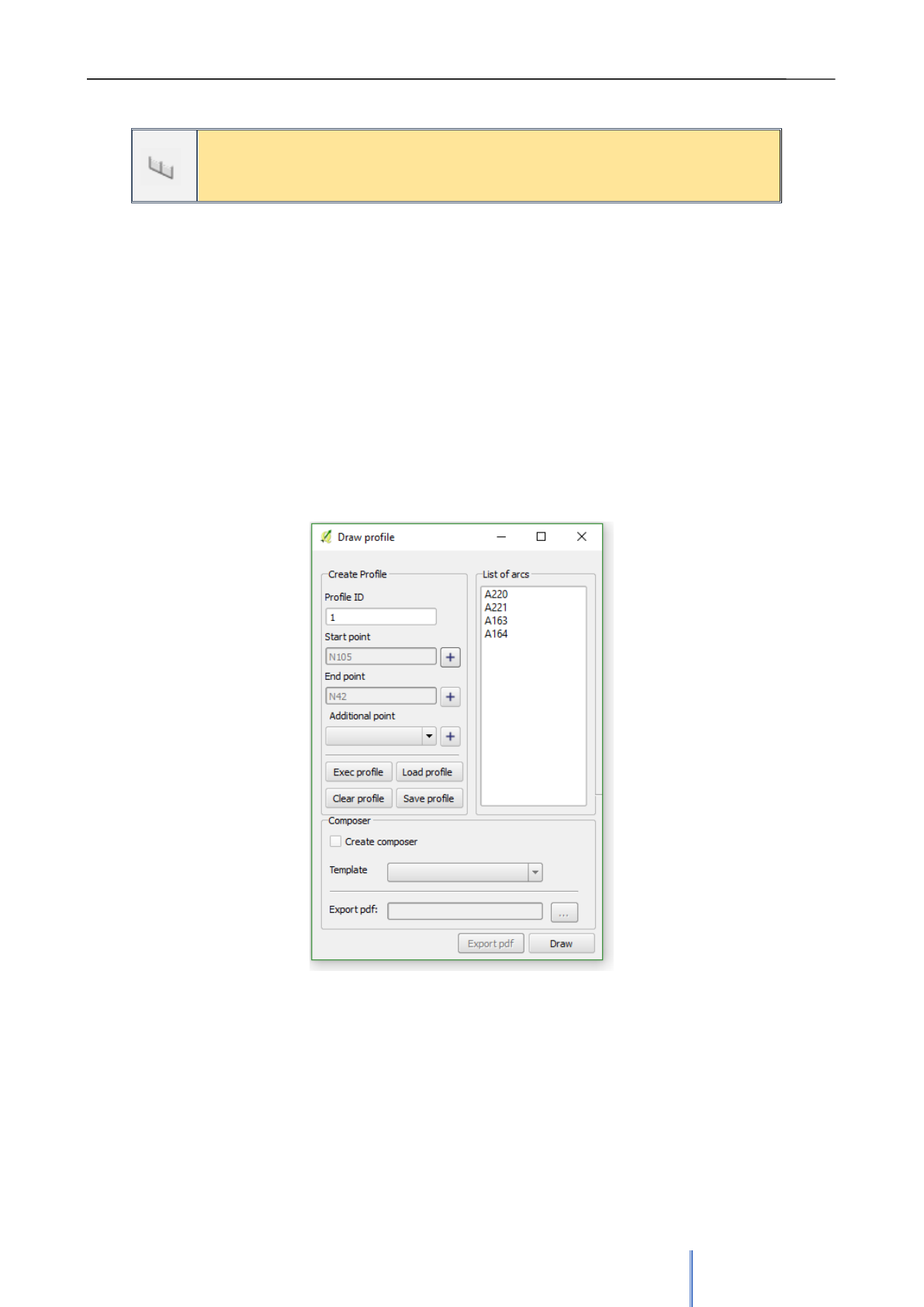
Giswater 3 User Manual
77
Longitudinal profile
Allows to draw or load longitudinal profile – role_om
The longitudinal profiles are technical representations of a part of the urban water drainage
system. This tool automatically creates longitudinal profiles of the area that user wants. To
choose which elements should be represented, the user must select a start node and a final
node. The longitudinal profile will represent all the arcs and nodes that are between these two
nodes (including themselves). In addition, there is an option of selecting an additional node
which, in case the initial and final nodes have two possible routes, will mark the direction by
which the profile should be drawn.
Clicking the button that starts the tool will open a form like the one in image 34. Here the user
must establish a profile id, as well as the start and end nodes. With the [+] button it can be
choosen from the map by placing the cursor over the desired node. Once values of these
nodes are set, by clicking Exec profile, the arcs that are inside the selection will appear
automatically in the list on the right. Next step is clicking Draw button to create the desired
longitudinal profile. The Clear profile button deletes selected data.
The example longitudinal profile shows the nodes and arcs that are between nodes N105 and
N42. The representation is a graphic type with a table of dimensions in the lower part. It shows
the following data:
• Elevation and maximum elevation of node
• Y max of node
• Diameter, slope and length of arc
Image 35: Form to créate a longitudinal profile.
Allows to select start and en nodes and draw a
complete profile.
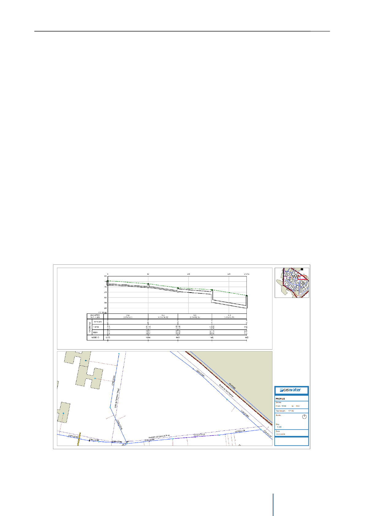
Giswater 3 User Manual
78
This is a very useful tool to obtain a graphic representation of the network in a very simple
way. It should be remembered that if any of the essential fields for drawing the profile is
empty, the tool has customizable default values in the config_param_system table. These
values are:
• top_elev (node) / sys_elev (node)
• ymax (node)
• geom1 (cat_arc)
• z1 / z2 (cat_arc)
• cat_geom1(cat_node)
• sys_elev1 / sys_elev2 (arc)
• y1 / y2 (arc)
• slope (arc)
In addition to drawing a new longitudinal profile, the tool allows to load an existing one. In
order to keep a profile in a database it must be saved using Save profile button. All that is
saved can be displayed again by clicking Load profile in a main form of a tool.
In order to prepare the profile to print it or export to pdf mark Create Composer, select one of
the templates that are incorporated with Giswater and click Draw. The Composer of QGIS will
be opened with the longitudinal profile represented in a personalized style. In addition to the
longitudinal profile, the part of the map with the elements that make up the profile are shown, a
general situation map and additional profile information: start and end nodes, length, scale and
date (Image 36).
Image 36: Example of a QGIS personalized composer, that shows a longitudinal profile together with a map of its
location.
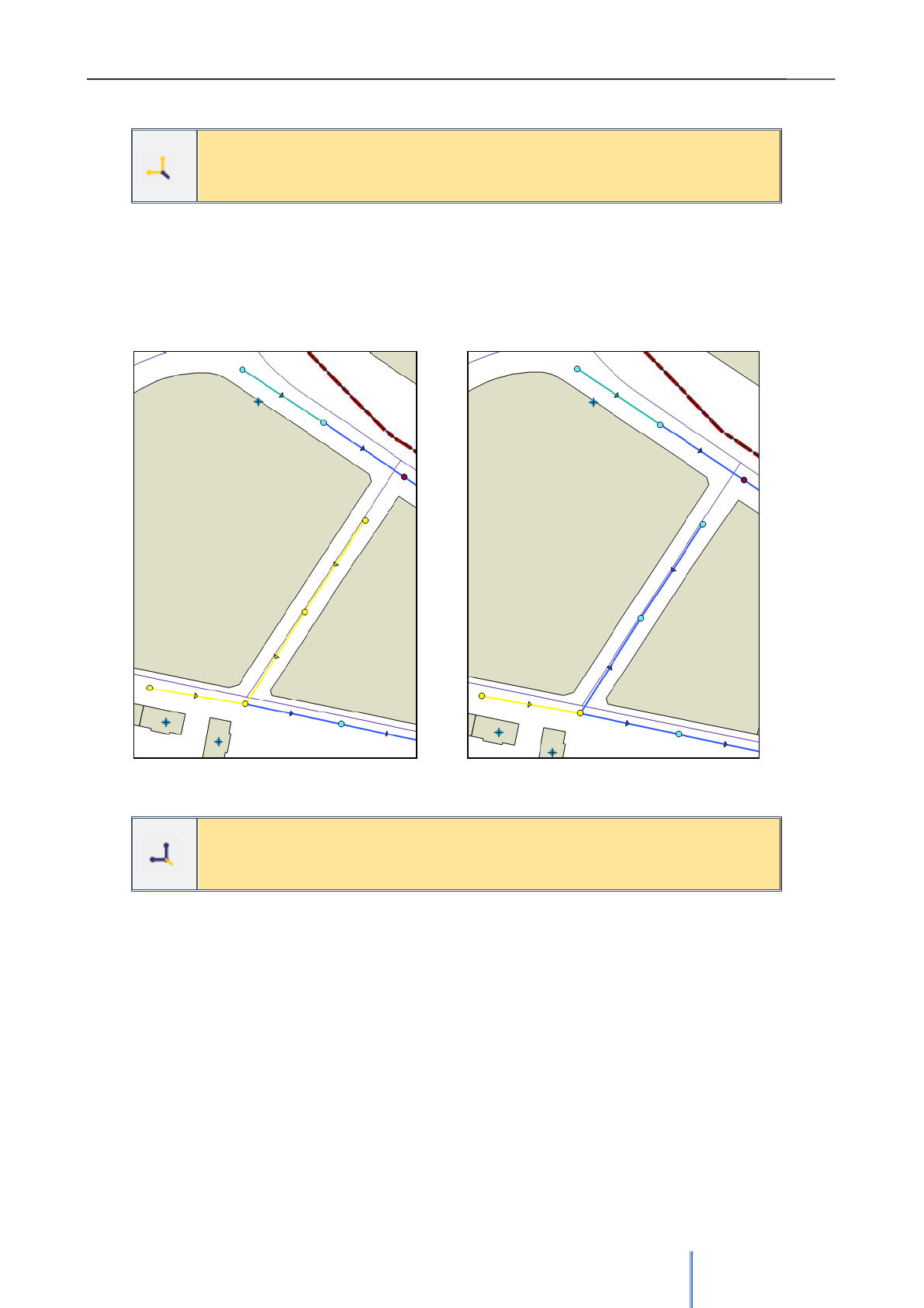
Giswater 3 User Manual
79
Upstream
Shows the elements located upstream – role_om
This tool, specific for sanitation projects, allows to select a specific node of the network and
show all the elements that are upstream of the chosen node. To show these elements, the
tool selects all of them (by painting yellow) and it is possible to visualize them both in the
graphical interface and in the attribute tables (where they are also selected).
Downstream
Shows the elements located downstream – role_om
This is the same process as the previous tool (upstream), but this time selected elements are
located downstream from the selected node.
In order to make this selection, the tool searches in the nodes contiguous with the selected
one checking its maximum height and in case when it is higher (for upstream) or lower (for
downstream) it selects it and continues the search until the end of the network. One of the
objectives of this tool is to help find errors in the network, since the elements upstream or
downstream must have a coherence of heights so that water flows through the conduits. If the
top_elev field of a node that should be upstream is smaller than its predecessor, the tool will
stop and the node will not be selected. This can be understood more easily in image 37. On
the right the section that should be upstream is not selected, therefore, there might be a
problem with heights. In the one on the left all data is correcte and all the network elements
are selected.
Image 37: Elements located upstream from the selected node. On the right the error is show, because of the
inverse direction of one of the arcs and that’s why it’s not detected as upstream.
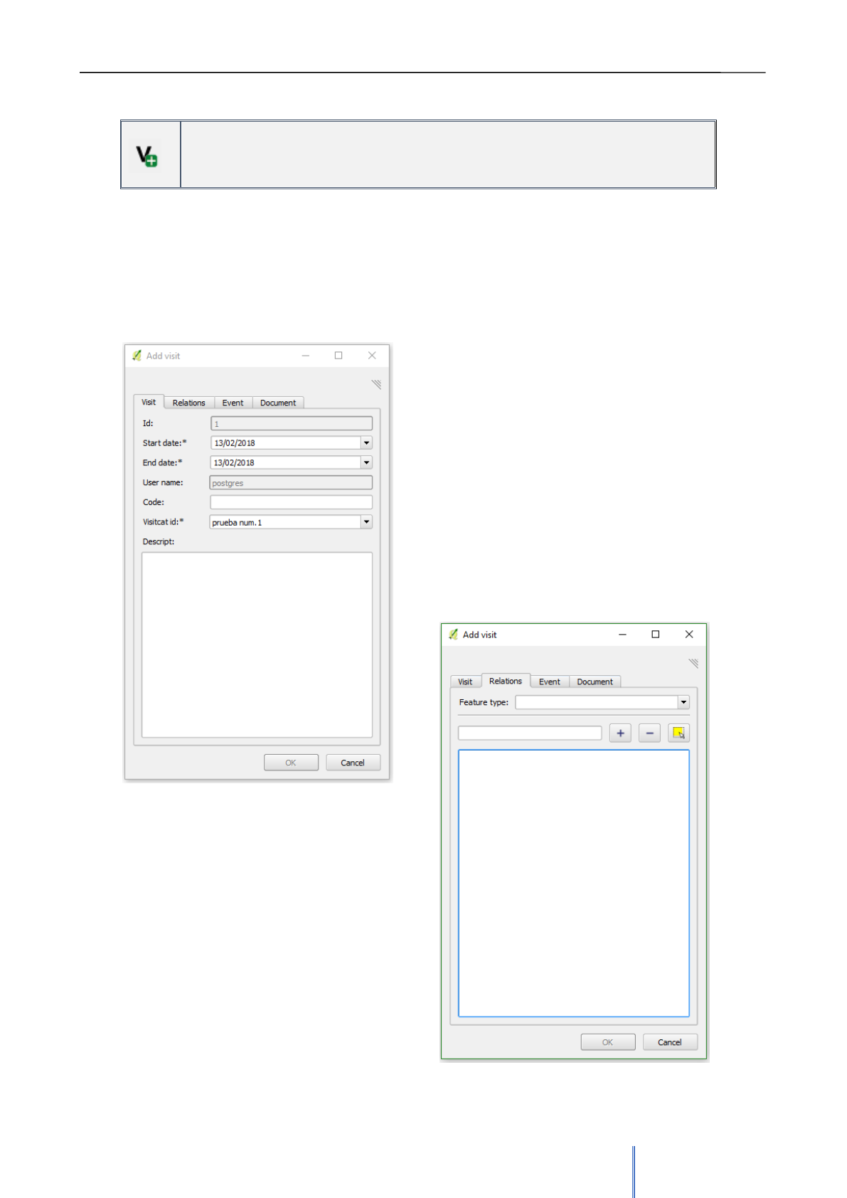
Giswater 3 User Manual
80
Add multiple visit
Allows creating a new visit and its relations – role_om
The visits with which Giswater works aim to make an inventory of the different moments in
which some element or section of the network has been visited in reality. Keep in mind that a
visit is the superior of a series of related parameters: a visit may contain multiple events,
which, in turn, may contain multiple documents
After clicking Add visit tool, a form with four different tabs appears. In the first one there is a
place to fill in the data of the new visit that is
going to be created. Before doing that, it is
necessary to have at least one value in the visits
catalog (om_visit_cat), since each visit must be
related to a value in this table. Only visits in
active status will be available. When inserting
start and end dates, there is a possibility to link
the selector_date table to automatically obtain
the dates that are inserted (Image 38).
The second tab of the form refers to the
relationships between elements and the visit.
The link between creating visit and new
elements can be added using the tools in this
tab. It allows to select the type of element and
add it by using id or by selecting directly from
the map. (Image 39).
Image 38: For of creating a new visit. In the first
tab all the basic data is located.
Image 39: Form of creating a visit. In the second
tab the relation between visit and elements of
the network is created. It is filtered by
feature_type.
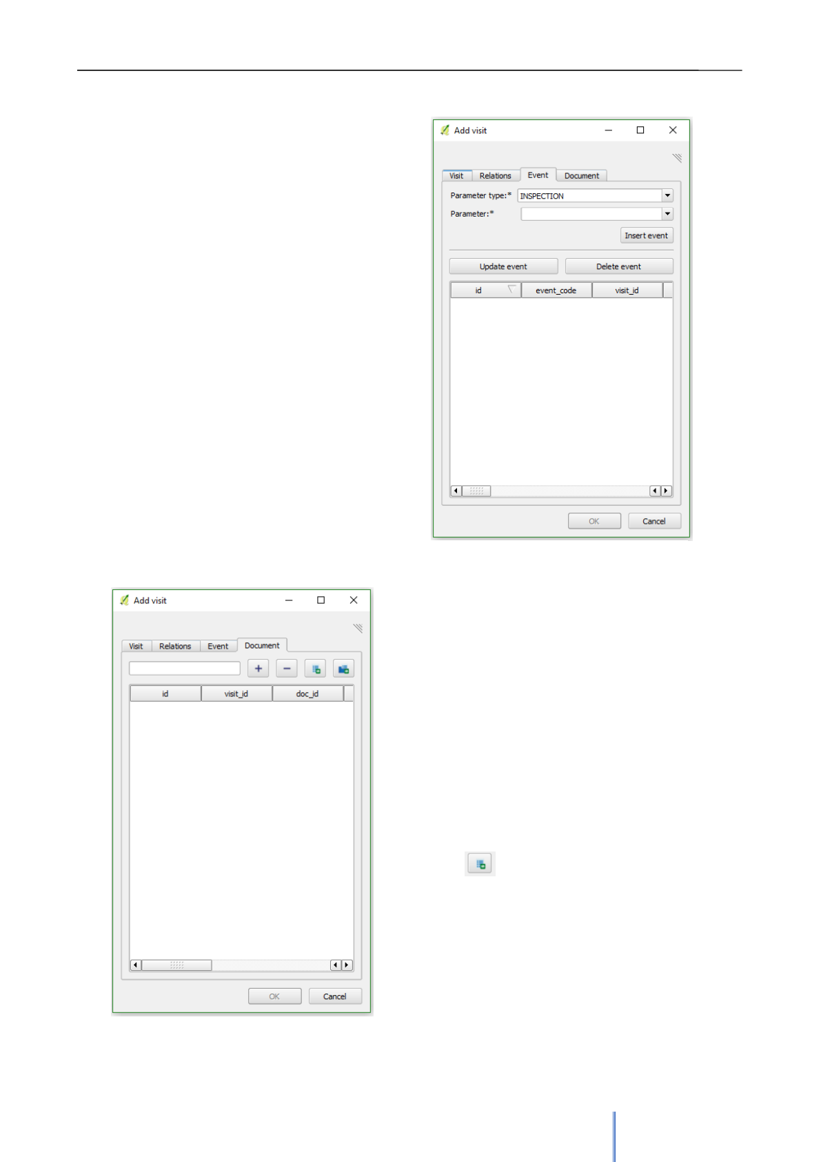
Giswater 3 User Manual
81
The third tab relates the visit with events (Image 40). As has been said, different events can be
part of the same visit. These could be defined as
actions taken during the visit, such as repairing a
crack or cleaning a section of pipe. To insert an
event at least one value in the parameter tables
must be present (in the database they are called
om_visit_parameter and
om_visit_paramter_type). The parameters
depend on the type of event and the type of
element on which it is carried out. There are
three types of events by default:
Standard events (event_standard) has fields like
parameter, value and comment (optional text
field).
Standard events of urban drainage
(event_ud_arc_standard), have two fields more
to manage the position inside the arc at which
the event takes place.
Rehabilitation events of urban drainage
(event_ud_arc_rehabit), especially indicated to
identify structural pathologies that must be
rehabilitated.
All generic element forms have the ability to add
an image to the event or view the gallery of
available images. In the case of multiple visits,
this option will not be operative since it is not
possible to add or view photographs in a multiple
visit.
Finally, in the last tab of the form, visits can be
related to documents (Image 41). These are
external documents in ‘common’ formats such as
pdf, doc or csv. In the text space it is possible to
filter existing documents and link them to the visit.
In case the user wishes to add a new document at
this moment, it is possible to do so by clicking the
button:
This performs the same function as the Add
Document plugin tool, which will be explained
later.
The other button allows to open the URL of the
selected document.
Image 40: Form of inserting the visit. The third
tab relates events with the visit.
Imagen 41: The last tab that allows to related
documents to the visit.
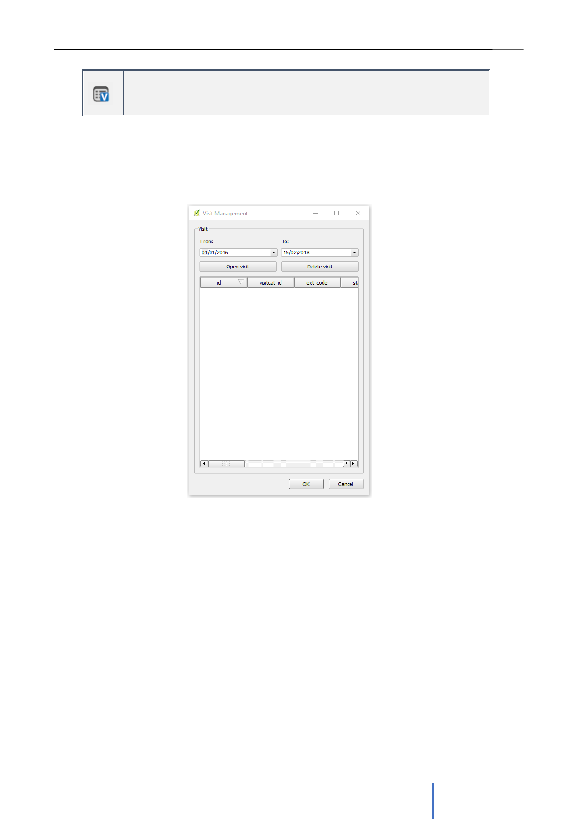
Giswater 3 User Manual
82
Visit manager
Allows to manage the existing visits – role_om
When opening the visit manager, a form with a table containing all the visits made and some
of their data is shown. This tool allows to select a visit and open or delete it. The user is also
allowed to filter visits by date
Image 42: Form of visit manager. Here all the
available visits are shown and might be filtered
by date.
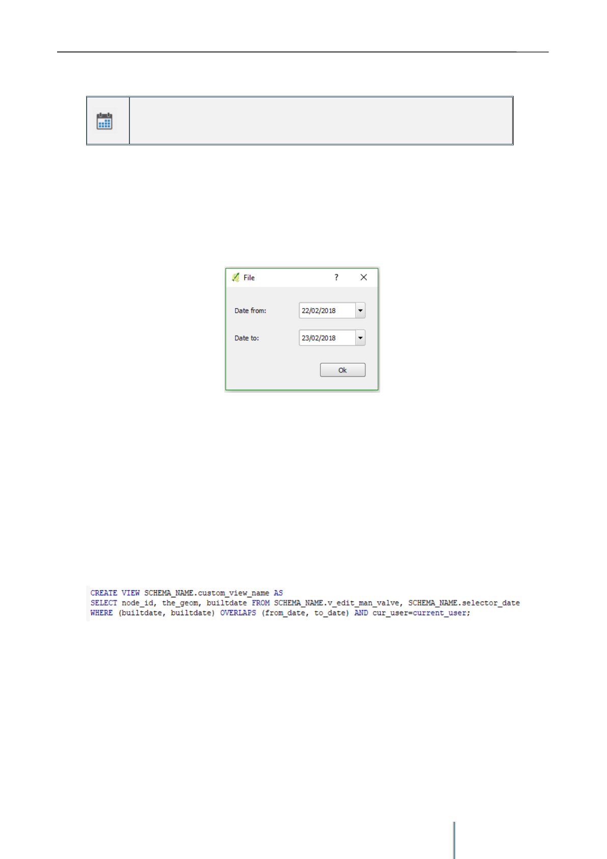
Giswater 3 User Manual
83
Date selector
Allows to set the dates– role_om
This tool allows to establish the values for the dates of operations and management.
After clicking on it, a small form opens where it’s possible to select a start date and a final
date, which will be used later for other processes. This information is stored in the
selector_date table and will be replaced as the user uses this tool and modify the values. The
table allows only one set of date type values for each user, so that the same user can not have
several dates available.
The purpose of this tool is to simplify the use of dates of visits. If a user wants to create a view
related to operations and management, he can filter the date fields using those in the
selector_date table, and it will be very easy to update the values and use them as default
dates. It is designed to establish values such as the following month or this week and use
them in different scenarios.
To give an example of the usability of the tool, a query that generates a customized view that
can be updated from the date selector is presented below. This view shows the valves, their
geometry and their construction date:
To visualize the result thos view must be loaded in QGIS project. This view will be filtered
automatically depending on the value that is put in the date selector. For example, if selected
dates are from the beginning of 2010 until the present year, the view will only show the valves
with a date of registration (field builtdate) between these dates.
To sum up, any table that has date values can be filtered through this tool, thus achieving a
very simple method of representing information according to the needs of the user, who can
customize the view.
Imagen 43: Date selector. Dates inserted in
this form will be used to set the dates of
other processes.

Giswater 3 User Manual
84
5.2.3 Edition
The toolbar related to editing the network is the largest one. These tools are intended to facilitate the
insertion, elimination or modification of existing data, especially in relation to geospatial elements. This
includes basic tools for adding nodes or arcs, moving elements or connecting them together, as well as
another block of tools to establish relationships with documents or additional elements.
.
Insert node
Allows to insert a new node element – role_edit
It’s a basic tool that allows to add a new node-type element to the network, both for water
supply and sanitation projects. To perform the insertion there are two options:
1. Click on an arrow on the side of a button and select from the list an element to insert.
2. Use the keyboard shortcut to select the element type to insert. The shortcuts must be
previously configured in order to use this function. To do so, it’s necessary to fill in the
shortcut_key field of the sys_feature_cat table with a letter.
Once the node type is selected the next step is to place the element on a map by clicking the
desired location. It is important to remember that many times a node will be inserted on top of
an arc or another existing node. Snapping makes this task easy, but the important thing is that
when inserting a node on top of an arc it will be broken in two parts to maintain the topological
coherence of the network. Here the rules of the state topology come back into play (3.7.4): if
the state of the arc is the same as the state of a node (except for obsolete elements), the node
will be inserted and the arc will be divided; if the states of the elements are different, the node
will be inserted, but without breaking the arc.
Clicking on the place of nodes insertation will automatically open the form related to it. Here
the information referring to the new element can be added. Fields with (*) are mandatory and
therefore must always be filled in; however, to facilitate the fast insertion of elements, some of
these fields can be filled in automatically thanks to the functionality of Giswater. The
exploitation, dma and sector of the new element will be captured directly in case the new
element is situated within the limits of these zone layers.
The rest of the fields must be filled in manually or using some of the default values, which
must have been previously configured.
Finally clicking OK will finish the edition and the new element will be inserted.
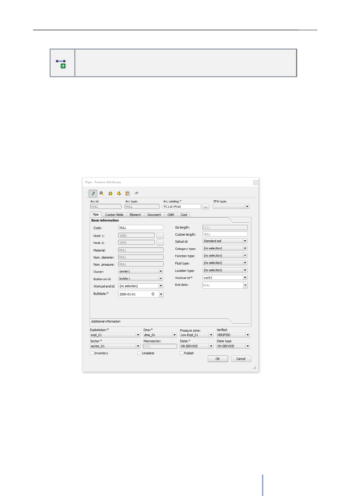
Giswater 3 User Manual
85
Insert arc
Allows to insert new arc element – role_edit
This tool allows add a new arc to the network. The flow of using it is exactly the same as of
insertion of a node, with the exception that in the case of arcs it must be drawn between two
nodes. In case of not doing so, the insertion will be erroneous, since the topological rules says
that an arc has to have nodes at its ends. To draw an arc the first step is to click on the starting
point and then draw different sections in desired direction until clicking again with the right
button to finish the arc.
Once the insertion form of the arc opens it’s important to know the differences that exist in
some fields, since the arcs have specific attributes such as the length or the codes of the
nodes. The other mandatory fields have the same usability as in the case of nodes.
Finally, by clicking OK the edition is closed and arc is inserted.
Image 44: General arc form, arc type Pipe. Most of the forms of elements are
very similar, with some of the presented diferrences.
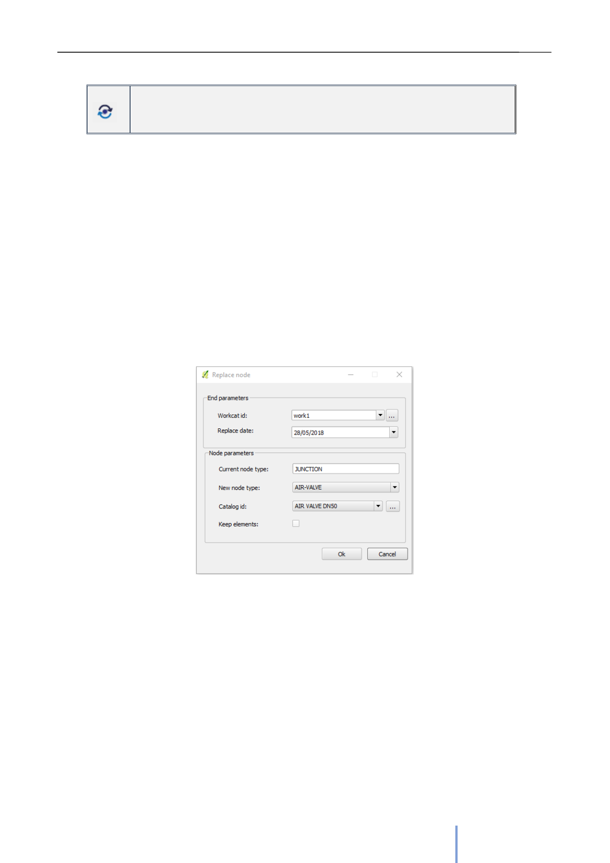
Giswater 3 User Manual
86
Replace node
Replaces an node with a new one and changes its state – role_edit
The replace node tool aims to change an existing node to a new one. To do this, Giswater
changes the state of existing node to obsolete and replaces it with a new node with the state
on service. User can choose the type of node with which he wants to replace the previous one
as well as modify its data.
When the tool button is clicked the cursor changes its appearance and allows to select the
node that is about to be replaced. Once clicked on the item, a form opens where the work
record of the elimination and creation of the elements must be chosen. If the work record
doesn’t exist in the cat_work table, there is a possibility to generate one directly from this tool
by clicking the button […].
In the second part of the form there are the parameters of a node; here the current node type
is displayed. At this time the new node type must be selected together with its specific catalog
(a drop-down list that refers to the cat_node table). If Keep elements checkbox is marked, the
elements and documents related to the old node will be saved for the new one.
In order to check the result of this tool, it can be done using state selector. That will allow to
see one node in a state on service (1) and another in an obsolete state (0).
This is a very useful tool because it facilitates the process of replacing elements in the
network, without having to worry about the topology since its position is exactly the same.
Image 45: Form of replace node tool. In this example a
filter is replaced by the air valve.
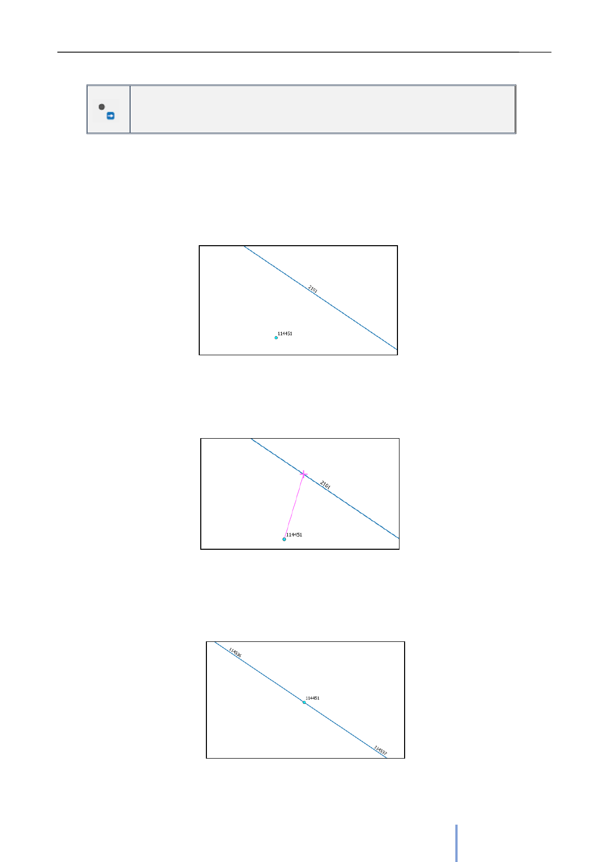
Giswater 3 User Manual
87
Divide arc
Allows to divide an arc into two by placing a node over it – role_edit
This tool allows to place nodes that are disconnected from the network on top of arcs. In this
process the arc will be divided into two parts, which inherit the data from the old arc, but with
new identifiers. It can only be done one by one.
The image 46 represents an arc that is a part of a network and a disconnected node. To move
this node and place it over the arc, so that it becomes a part of the network, this tool must be
used.
Clicking the tool button and selecting the node 114451. Gives the possibility to draw an
imaginary line to the arc that will be broken and where node will be placed. (Image 47)
Finally, in image 48, node 114451 has been moved towards the arc and had divided it into two
parts, one with id 114536 and the other 114537. The old arc with id 2101 has been removed.
Image 46: Node 114451 is disconnected from the
network and can be connected using divide arc tool.
Image 47: The tool allows to move the node over the
arc.
Image 48: Node connected to the network.

Giswater 3 User Manual
88
Arc fusion
Allows to join two arcs in one, eliminationg the existing node – role_edit
This tool does exactly the opposite of the previous one; It allows eliminate a node that divides
pipes and thus join two arcs into one.
One of the requirements of this tool is that the arcs must be of the same type and belong to
the same catalog, that is, the arccat_id attribute must be the same to be able to join them. The
node can only be related to two arcs so that the process performs correctly.
It’s important to keep in mind that if the node to eliminate has a TRUE value in the undelete
field, it won’t be possible to eliminate it. To do so this value needs to be changed to FALSE.
Knowing this, the flow of the tool is very simple: with the active tool cursor needs to be placed
over the node that is going to be removed and after clicking it, a window will open warning
about the elimination of the node. In case of accepting this node will be deleted and the two
arcs with which it was related will automatically join in one with new id.
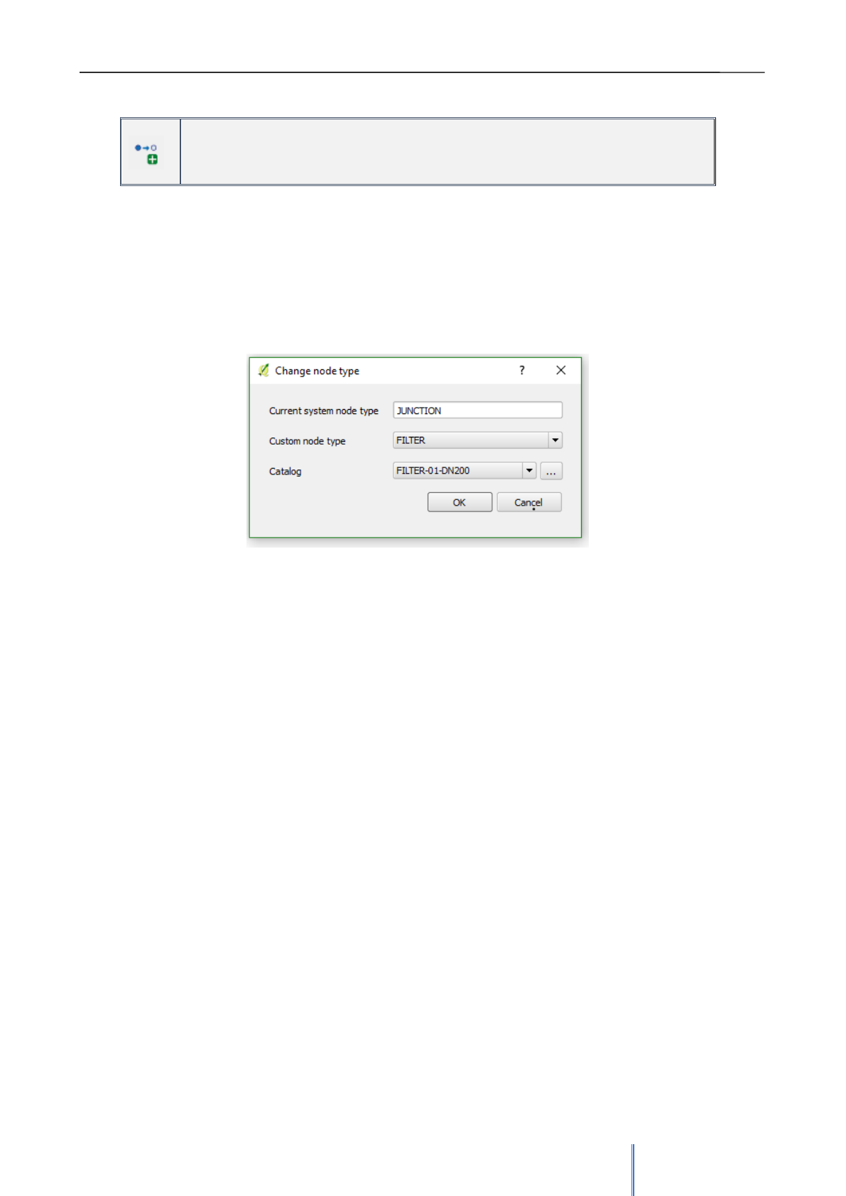
Giswater 3 User Manual
89
Change node type
Allows to change the type of existing node – role_edit
The change node type tool allows to select an existing node and automatically modify its type
and catalog.
To use this tool, click its button and then select the node which will be changed. After
selecting, the modification form will open, where the current node type is shown and whereit’s
possible to select the type by which it will be changed (Image 49). The catalog of nodes will
filter according to the selected type of node. After clicking OK, the change will be made,
without modifying the rest of the element's data
The usefulness of this tool lies in the fact that it allows modifying the type of node, a parameter
that in the forms of the elements is not editable, in a very simple, convenient and fast way;
without the need even to put into edition the selected node.
The Replace node tool and Change node type are very similar. Replace node deletes the old
element and inserts one again, with a new identifier. In contrast to Change node type which
maintains the identifier and does not deregister any element, it simply modifies its type.
Imagen 49: Form of the change node type tool.
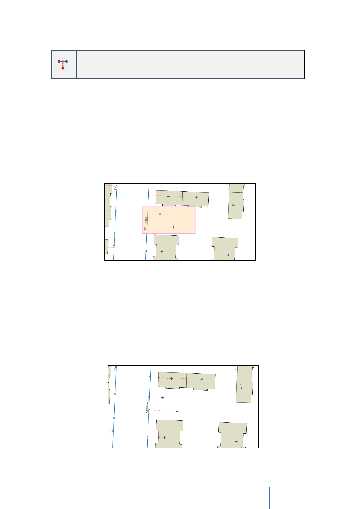
Giswater 3 User Manual
90
Connect to network
Allows to connect one or many connecs to the network – role_edit
As we already mentioned, the connections are related with the network, specifically to the
arcs, by means of links, which draw a straight line between the connec and the nearest
network arc, where a virtual union node is located. The tool connect to network automates the
process of creating these links and vnodes.
The objective of the tool is to connect to the network all connections that have no link. The tool
allows to insert during one process as many links as the userwants, which makes it a very
powerful tool and very easy to use.
By clicking the button to start the tool, the cursor changes its appearance and allows to draw a
rectangle, within which the connections we want to connect to the network must be placed
(Image 50).
.
At this moment the connecs will be painted yellow (selected), but it’s still possible to draw
another rectangle to select more connecs if needed, because those that are already selected
will not be lost. It’s important to know that to deselect connecs shortcut of Shift + Ctrl keys can
be used together with drawing a rectangle that will act in the opposite way to the selection.
Once all the connections are selected, clicking on the right button of the mouse will start the
process. First a message will appear indicating the number of selected connections. After
clicking OK, links will be automatically drawn from the connections to the network and at the
intersection point the virtual nodes will be inserted (Image 51).
Image 50: Only the connecs inside the selection rectangle will be
connected.
Image 51: Connecs already connected to the network with a link.
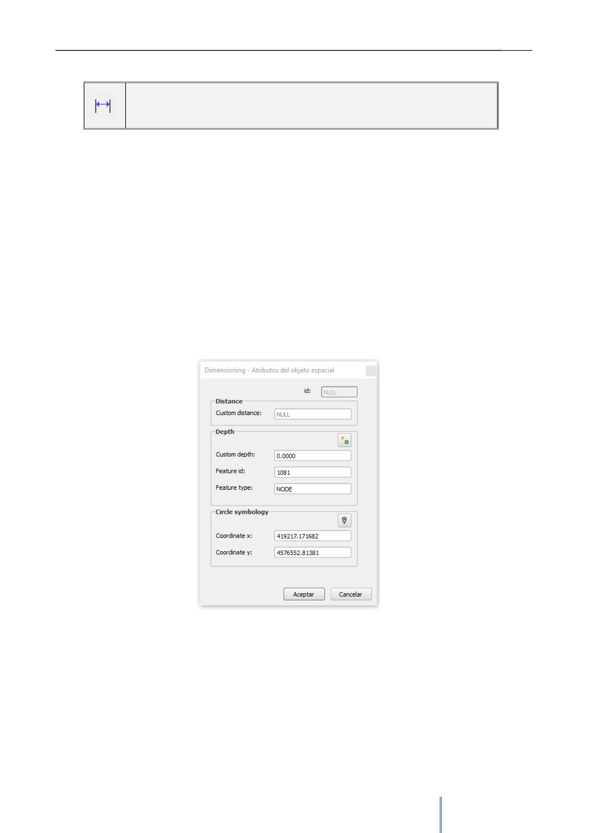
Giswater 3 User Manual
91
Dimensioning
Allows to calculate and show the distance between elements – role_edit
The purpose of the dimensioning tool is to offer the possibility of calculating distances within
the map, either in relation to elements of the network or with elements of the base map. It is
also possible to use the tool in spaces of the map where there is no layer.
As has been already said in previous sections, the dimensions are a linear geometry layer that
is represented on the map by means of a view (v_edit_dimensions). This allows that the
stored values can be represented on the map, offering additional information which may be
valuable for networks with a particularly accurate digitization
How to use this tool? Clicking the button activates it and mouse cursor changes. The
dimension is drawn as any other line, beggining by clicking on the point where it’s supposed to
start, finishing by clicking at the end point and terminating the process using right button of the
mouse. In case of making dimension with more than one segment, drawing lines can be
continued by clicking the left button.
Once the line is finished, the form opens, where more data may be introduced.
If the distance of the created dimension is known to the user, it can be introduced into Custom
distance field, in case of leaving it blank the tool will calculate the distance from the map. If the
depth of created dimensioning is known, field Custom depth should be filled. Otherwise, there
is an option of selecting a node or connec and using its depth. In addition, the tool stores the
id and the selected element type.
Image 52: Form of dimensioning, where data related
to depth and distance may be introduced together
with the coordinates of a circle symbology.
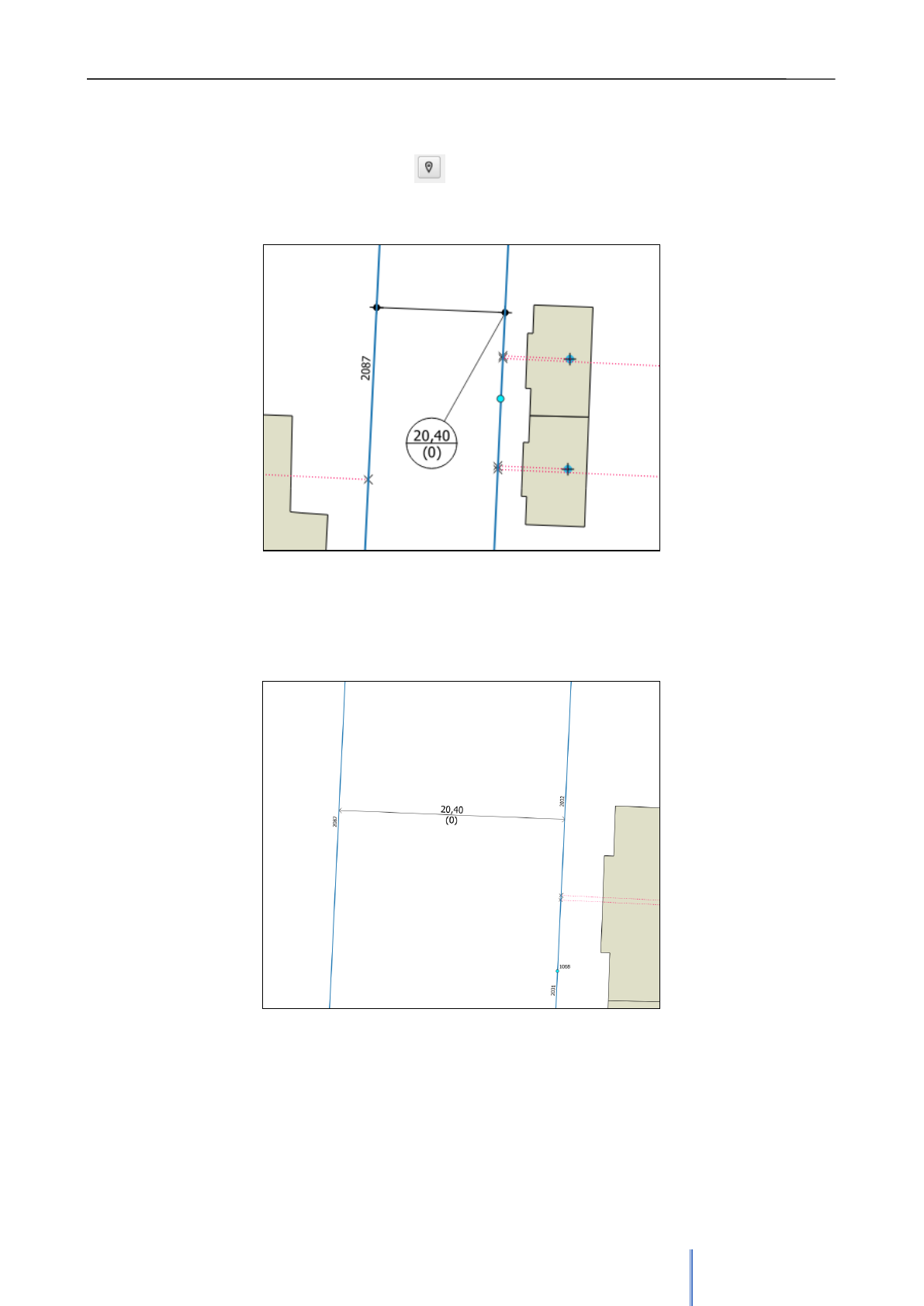
Giswater 3 User Manual
92
The tool offers different symbologies depending on the zoom of the project. The dimension
data can be displayed as a label of a line or in a circle. Using the button below the coordinates
of the circle location can be captured.
In images 53 and 54 the examples of the different types of dimensioning symbology according
to the project's zoom is presented.
Image 53: Example of circle symbology. In the top part of the circle
the distance is shown, above the depth. This type of symbology is
programmed for small scales.
Image 54: Example of line symbology of the dimension (same case
as in image 55). This type of symbology is programmed for big
scales.
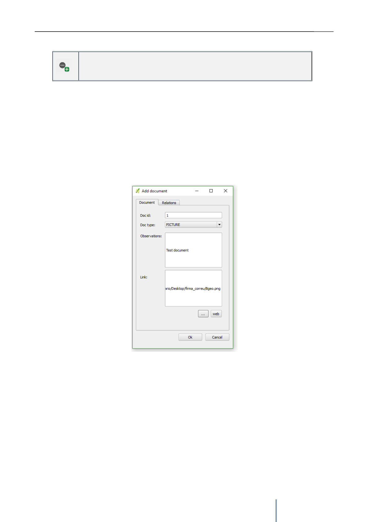
Giswater 3 User Manual
93
Add document
Allows to relate a document with network elements– role_edit
Many times, the elements of the network will be able to have linked information stored in
external documents. As presented in other sections, this is possible with Giswater, since the
element forms have a specific tab where a document can be created and linked with it.
This tool aims to link documents with one or more elements of the network, which can be
opened and visible directly from the plugin and its forms.
Clicking on the tool button automatically opens the form to add a new document (Image 56).
Here the data of the document: id, type, observations and the link with the path to the file or
website must be enter.
Next, in the Relations tab, all the elements with which the new document will be related can be
selected. Nodes, arcs and connecs must be added separately. They can be selected in the
usual ways: with the buttons (+) and (-) they are added and deleted in the list of elements, by
means of the id, or using the selector on the map, creating a rectangle to select different
elements at the same time.
In the example of the image 56, the document that is being added in this process is linked to
the node with node_id 1019.
Image 55: First tab of creat document tool
where the basic information is added.
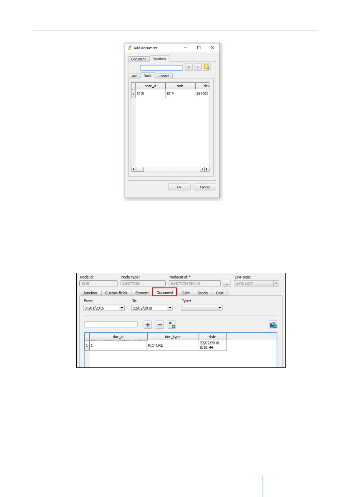
Giswater 3 User Manual
94
To verify the correct linkage of the document with the node, the form of the Junction (node_id
1019) can be opened, where, in the Document tab, the linked document with doc_id 1 should
be present. The document may be opened by double clicking on the row (Image 57 ).
This example showed relation to only one element, but the proces of relating it to many is the
same.
Imagen 56: Second tab of the tool form, where
document is being linked to the elements of
the network.
Imagen 57: Form of element to which a document was added. It’s possible to check whether
the link is correct.
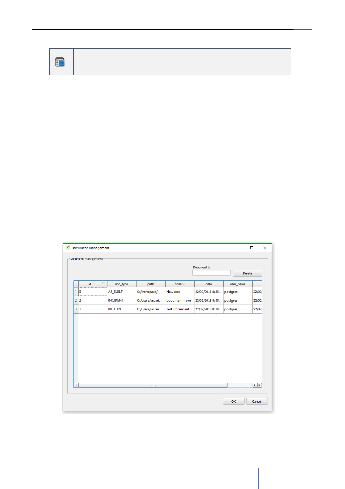
Giswater 3 User Manual
95
Document manager
Allows to see all the documents related to the network– role_edit
The document manager is a tool used to inventory, visualize, filter and delete all the
documents that have been linked to any element of the network.
In the form that opens after clicking on the tool a table with all the available documents is
displayed. The table shows the following data:
▪ Id
▪ Document type
▪ Path
▪ Observations
▪ Date
▪ User that added the document
A document may be oppened using a double click on a row.
In the top section of a form a filter is located, which allows to list the documents in function of
its id. On the right from the filter there is a button that allows to eliminate a selected document.
Image 58: Form of document manager. Here all the documents related to the network are visible.
Form allows to filter, show and delete them.
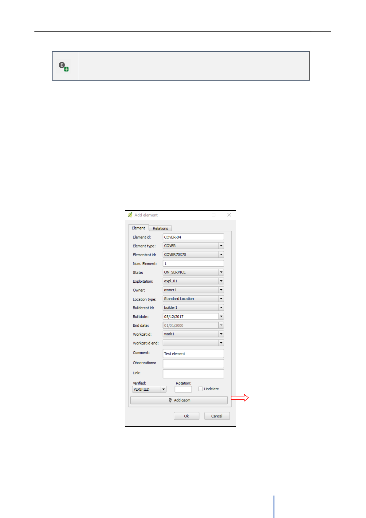
Giswater 3 User Manual
96
Add element
Allows to relate an element with other network elements – role_edit
This tool is very similar to Add document, since they share the same objective of linking
something with the elements of the network. The difference in this case is found in the type of
object that is related; If an external document has been added before, now other elements will
be linked with the elements of the network. In section 3.2 has been defined what elements are
and that they have their own catalog, therefore, if a new element is added it must be related to
any of those defined in the catalog of elements (cat_element).
Clicking on the button to start the tool will open the form to add a new element (Image 59).
Here the data of the new element must be entered. Many fields are selectable in different
drop-down lists. There is also a possibility to add the geometry of the element
Once the data is entered, in the Relations tab, new element must be linekd with the other
elements of the network (arc, node, connec). To do this exactly the same steps as those of the
Add Document tool must be followed.
Button to add
geometry
Image 59: Form of adding a new elementa and relating
it to an existing elemento f the network.
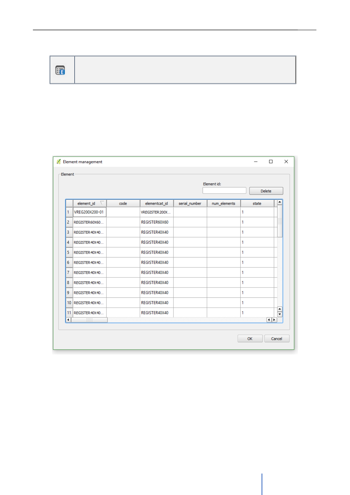
Giswater 3 User Manual
97
Element manager
Allows to see all the elements related to the network – role_edit
The element manager, like all the management tools presented before, serves as an inventory
of the elements found in the project. It allows to see all these elements and their attributes.
Double clicking on a selected item opens its specific form. In addition, there is an option to
filter by the element_id field and delete elements with the Delete button.
Image 60: Form of element manager. Allows to filter, show and delete elements.
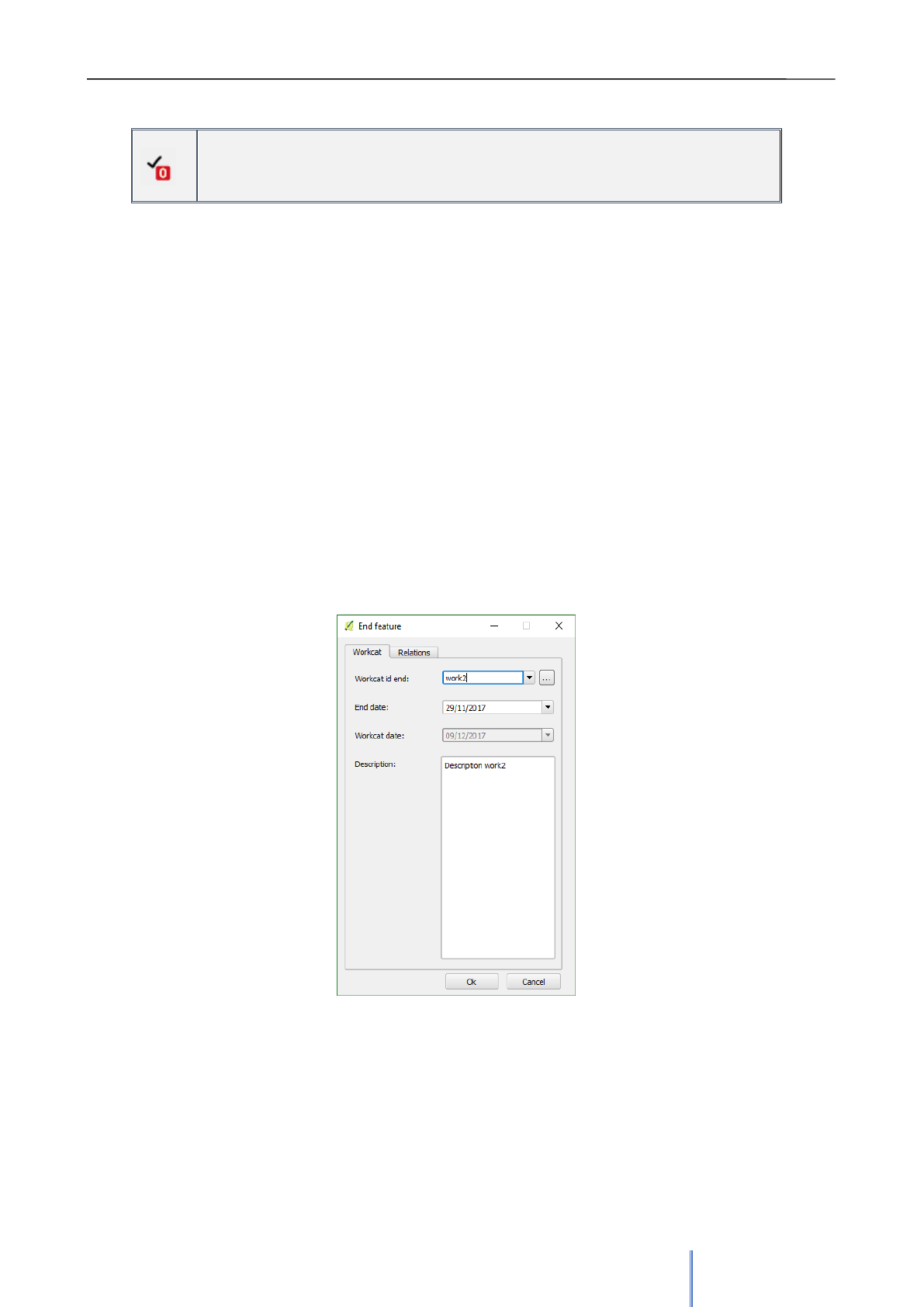
Giswater 3 User Manual
98
End feature
Changes state to obsolete – role_edit
This tool aims to remove elements from the network, that is, change its status to obsolete. To
do this, the elements must be on service. It is also necessary to take into account the topology
rules when deleting elements, since it will not be possible to do so if, for example, the selected
node is connected to other arcs. To ‘end’ the element it must be disconnected from the
network.
In this case, Giswater permits an exception. Users are allowed to disconnect arcs that have
associated connec-type elements, so that the arc will be disengaged and the related connecs
will lose their link with the arc. This allows to facilitate the editing of the network in cases
where it’s necessary to cancel an arc and losing the relationship with the connec is not
important. By way of prevention, the program will always show a list of all the elements that
will be disconnected before proceeding.
When clicking on the tool button, the form to remove the item will open. First, it’s necessary to
fill in some data of the ‘end’, such as the date or the work record (a new one can be created at
this point). The next step is to relate the ‘end’ with one or more elements. In the Relations tab
all the elements that will be canceled should be selected. Once chosen, clicking OK will carry
out the state change.
It’s important to remember that the ‘ended’ elements will become obsolete, which does not
mean that they will be eliminated. These will be equally visible if the obsolete elements are
visible in the state selector.
Image 61: Form of end feature. In the
tab Relations it’s posible to link one or
many elements that will have their state
changed to 0.
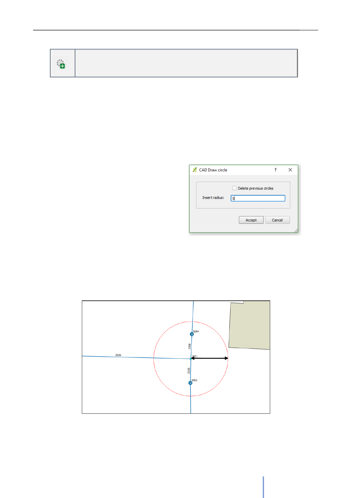
Giswater 3 User Manual
99
Create a circle
Allows to draw a circle in selected position – role_edit
Draw a circle is the first of the two CAD tools that Giswater has. There are grouped within
editing role, although they are in a small bar separated from the rest of the editing tools.
The objective of this tool is to draw a circle around a specific point with a radius set by the
user. This circle should serve to draw support points when digitizing the network.
To facilitate the use of this tool it’s neccessary to have configured the snapping of QGIS, since
it will only be possible to draw circles using as reference elements configured in the snapping
After clicking the tool button will change the cursor shape. That’s the moment of choosing the
location of the center of a circle on the map. Next,
the program will show the option to set a radius for
this circle. Once entered the value and clicked
Accept the circle will be created automatically.
This circle and the rest of the elements that are
generated with the tool will be stored in an
auxiliary view of the database
(v_edit_cad_auxcircle). If the view already
contains too many unnecessary elements it’s
possible to eliminate them by clicking Delete
previous circles checkbox and the view will empty
at the end of the insertion of the new circle.
Knowing the radius of the circle and using its geometry as a reference, thanks to the snapping,
inserting reference points that help drawing new elements in exact locations is possible.
5 m.
Image 62: Form in which the radius of a circle
should be entered.
Image 63: Example of a circle generated with the tool. In the form, showed on the
previous image, the value radius 5 was introduced.
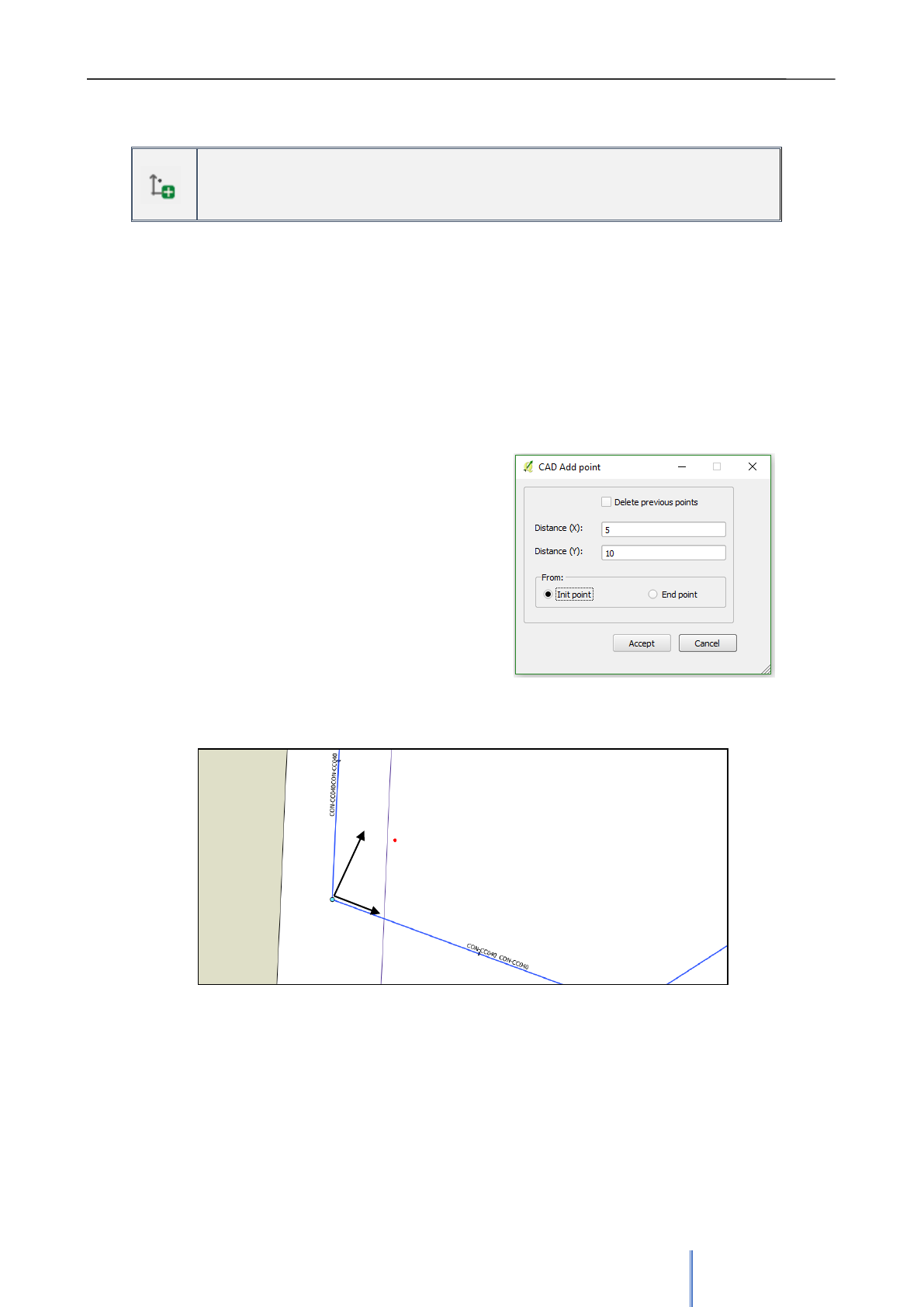
Giswater 3 User Manual
100
Add point using relative coordinates
Allows to draw a point in defined distance from another element – role_edit
The second CAD tool of the Giswater plugin is the one that allows inserting a point element at
a distance (x, y) relative to another point on the map. The point of support generated should
serve as a reference to draw new arcs and nodes of the network.
To add a new relative point using this tool, after clicking the button first step is to mark two
points on the map, either above other elements or in empty points. The imaginary line joining
these two points will serve as a reference to introduce the relative point. Once selected, a form
will open whith the fields to set the distances.
The X distance is the position where the support point will be located respecting the x
coordinate of the beginning of the imaginary line. The
Y distance is the position where the support point will
be located respecting the y coordinate of the
beginning of the imaginary line. Using the two
distances the element will be placed. Both values
admit negative numbers, because only then placing
points in all direction is possible.
In the section From there are two options available:
Init point the distances will be taken from the point
which was clicked as first and End point, the
distances will be relative to the second selected
point.
All the support points created in a project are stored in an auxiliary view, in the same way as in
the other CAD tool. In this case the view is called v_edit_cad_auxpoint and itt can be found in
the BASEMAP group of the ToC.
5 m
10 m
Image 64: Form of adding point using
relative coordinates.
Image 65: Example of a relativo point located 5 meters of x distance and 10 meters of y
distance from the Junction node. That’s where the first click was made, the second one was
made above, on the horizontal arc in order to follow the same direction.
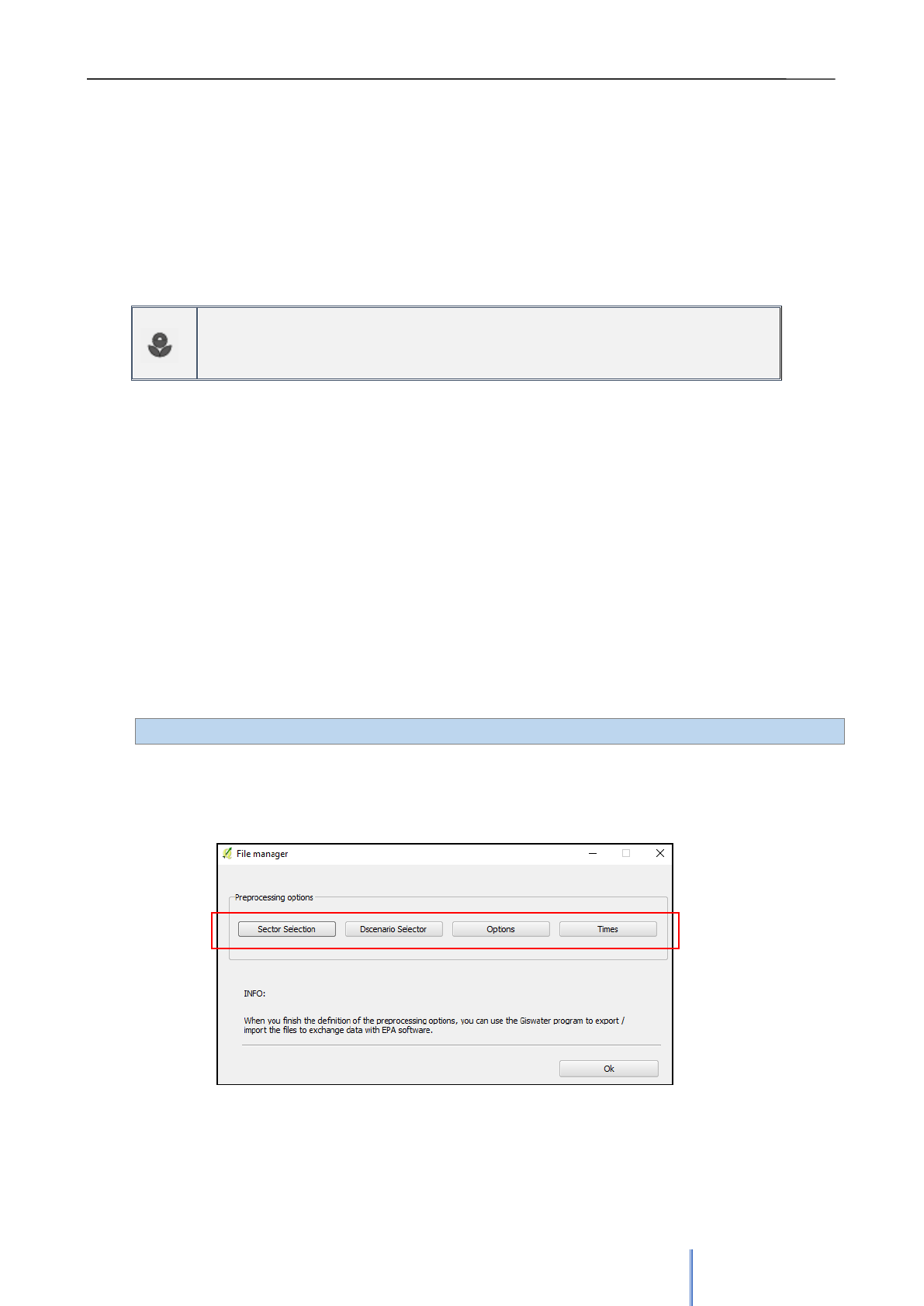
Giswater 3 User Manual
101
5.2.4 Hydraulic model
The group of tools related to the hydraulic model is the one used by users specialized in the management of
hydraulic behavior in the distribution or sanitation networks. In addition to knowing the use of the four tools
that make up the group, users should also be very clear about the data that is necessary for the models to
work properly. These data are described in sections 4.2.3 and 4.2.4. The characteristics and specific
operations of the hydraulic model are explained in detail in section 7 of this manual.
Go 2 EPA
Allows to export and import hydraulic model of the network – role_epa
Go 2 EPA is the group's main tool for exporting the hydraulic model. Its objective is to obtain
the results of this model, by filling in the corresponding tables and views, so that they can be
automatically visualized in QGIS through a specific symbology.
Before using the tool, it is necessary to enter the mandatory data in the tables of EPANET
(WS) or SWMM (UD) group, depending on the type of project. The tool has many similarities
between both types, although there are parameters that are only specific for one type or
another.
The process will be done in two parts, since the first one is done with the plugin and there are
differences between both types of project, and the second with the Giswater driver, this being
the same for both water supply and urban drainage projects.
FIRST PART - SPECIFIC
The operation of the tool in WS projects
When clicking the tool, main form opens, which has four buttons, designed to define
parameters prior to the process (Image 66). First, there is the sector selector, which allows to
choose which sector / s will or will not be a part of the hydraulic model that will be carried out
Imagen 66: Main form of Go 2 EPA tool with the options prior tothe process maked
in red.
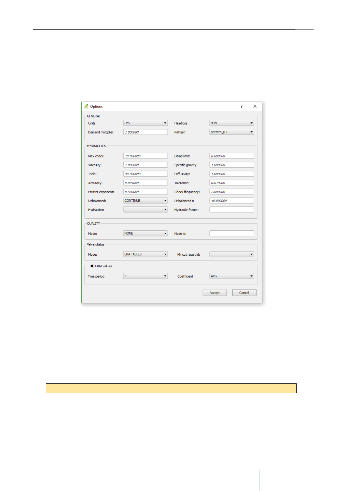
Giswater 3 User Manual
102
The second button is the selector of demand scenarios (7.1.1.2), which allows selecting a
specific demand scenario, previously defined, to act on the exportation of the model. The
performance is the same in all tools of 'selector' type, allowing to move different scenarios
from one column to another.
The Options button, the third one, is where the user can define different variables related to
the hydraulic model.
All these fields are very similar to those used by EPANET program, therefore, the user in
charge of this process, knowing the hydraulic operation, should already know how to fill in or
modify the data.
Finally, with the Times button parameters related to the temporary variables can be defined.
The operation of the tool in UD project:
The tool is considered the same for both WS and UD, but, as already mentioned, the data,
processes and results are different. If the project is related to urban drainage, then the form of
the tool will be a little different. In the options buttons prior to the process, instead of the
demand scenarios selector, there is a hydrology selector, defined in the table cat_hydrology.
Image 67: Form of Options section of Go 2 EPA tool. All the data and configuration of
the model should be introduced here.
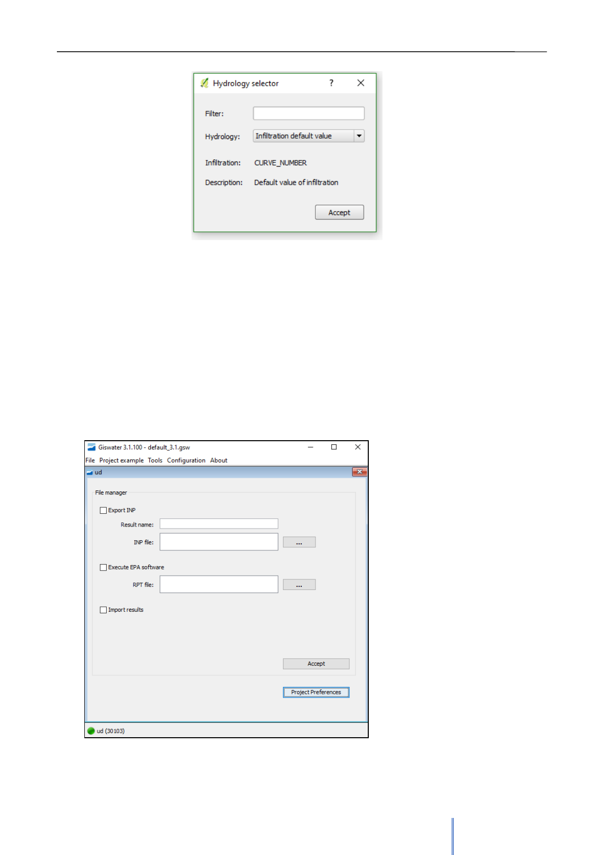
Giswater 3 User Manual
103
In reference to the Options, these are very similar to those of the SWMM program, therefore,
knowing these, it’s easy to fill in the form correctly. The Times tab, like in WS, allows to
establish certain values of the time variables, which will be specific for the drainage data,
much more related to the climatology.
SECOND PART - COMMON
The second part of the export / import process of the hydraulic model is carried out after the
first one, that is, once the database has the hydraulic data and the options of the specific part
correctly configured.
At this time, it is necessary to reuse the Giswater program, where Go2Epa button is located.
In the page that will open
after clicking the button, the
name for the corresponding
export must be defined. It’s
also necessary to establish
the routes in the computer
where the inp and rpt files,
generated at the end of the
process, will be stored.
Image 68: Hydrology selector, which has the
information related to the infiltration.
Image 69: Driver of Giswater allows to establish the paths where the files
related to hydraulic model will be saved. In order to go to this page, click
Go2Epa button located in Project preferences.
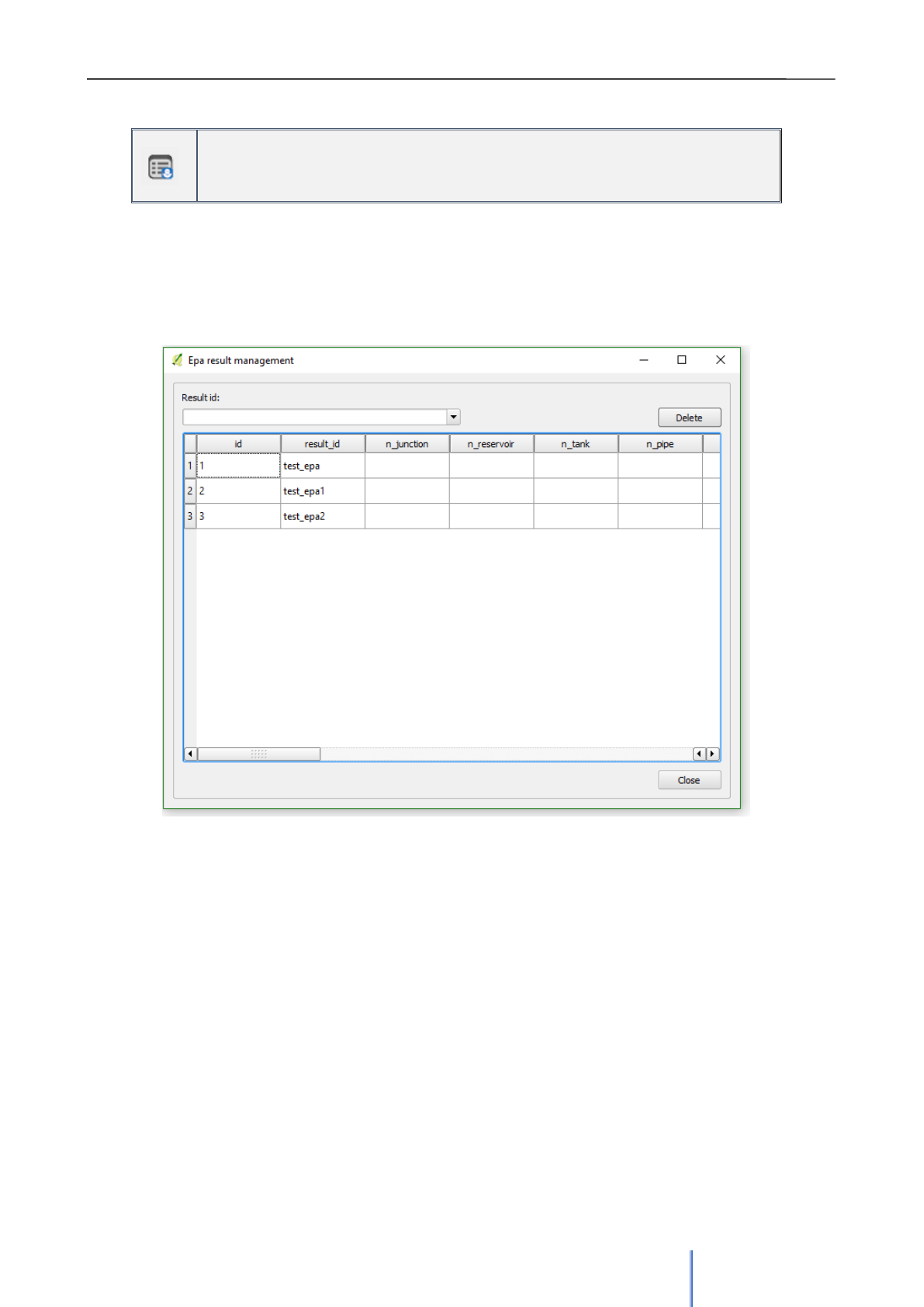
Giswater 3 User Manual
104
Epa result manager
Allows to manage all the different results of carried out models– role_epa
The EPA Result Manager tool allows to visualize the data of the different results of the import
and export processes of the hydraulic model.
The form of the tool shows, for each row, different data of each one of the model's results. As
always, filtering based on the result_id field is possible and rows can be eliminated using a
Delete button.
Image 70: Form of the EPA result manager. All the resutts of the exportation of hydraulic model are
shown in the table. They can be filtered, showed and deleted.
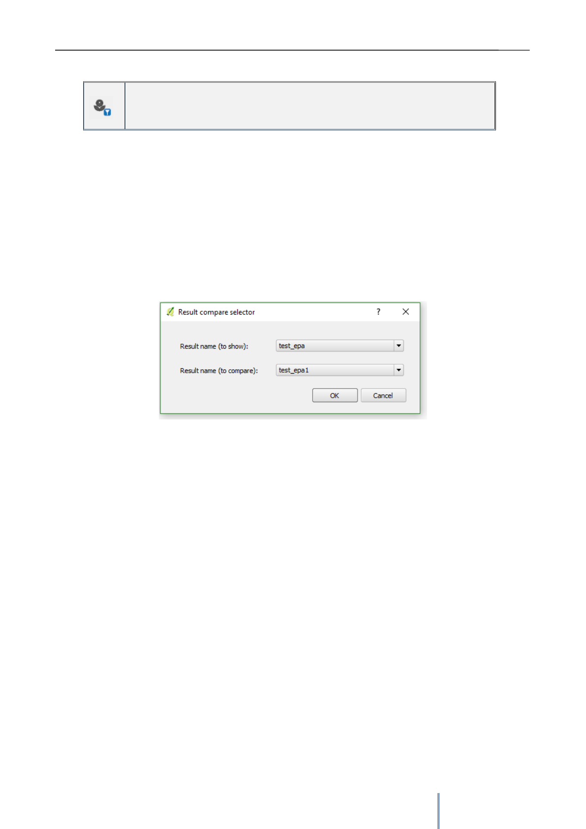
Giswater 3 User Manual
105
EPA Result selector
Allows to choose the results to visualize them in QGIS – role_epa
This tool is used to establish the results of the hydraulic model that will be displayed in QGIS
at that particular moment. The data of the chosen result will be the ones that fill in the different
views present in the project, so that it is possible to see results of old processes, sectors or
specific scenarios.
One of the highlights of the information management regarding the hydraulic model that
Giswater does is the possibility of using data from two different results at the same time; first
main one and another that serves to compare and visualize the existing differences.
With this tool it is also possible to select the result with which the main one will be compared,
so that the data will appear in the comparison tables. These results will have the same style as
the main ones, therefore, it will be possible to play with both groups and compare results.
The functioning of this tool is very simple: select the main result in the first combo box, which
will show all available results. In the second combo box select the result that will serve as a
comparison. Clicking the OK button will update the data and can be used.
Image 71: Form of EPA result selector tool with two simple filters. First is
a list of main results, that will be displayed in the QGIS layers created for
this purpose. Second are the result for comparing, which also have its
layers in the QGIS and are easy to visualize and compare.
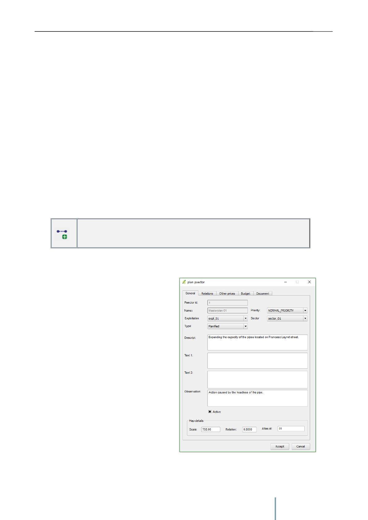
Giswater 3 User Manual
106
5.2.5 Masterplan
The planning tools are specially designed for users in charge of issues related to budgets (both at the level of
individual elements and of actions with multiple effects) and the management of planned sectors of the
network. For the correct functioning of this group of tools, the project and its data must be specially
configured and with great accuracy.
As already explained in section 4.2.5, referring to the tables related to planning, the first step of all is to fill in
the price data of the elements. Prices should be inserted in the Simple Price, Compost Price and Value
Compost Price tables and these will be linked to the elements present in the results tables of their category:
▪ Plan result node
▪ Plan result arc
▪ Plan psector x node cost
▪ Plan psector x arc cost
If in the planning operations an economic planning will be carried out, it is necessary to fill all the prices of
the fields of the tables that are related to it. For more information, see section 4.2.5.
The different tools that make up the masterplan group are be explained below:
This tool aims to permit user to create a new planning sector and assign the elements with
which it will be related, as well as show the cost details of the set of operations that would be
necessary to carry out the project.
First, when the tool starts, the psector form
appears (Image 72). This form is similar to
the one that each specific element of the
network has, but referring to an entire
sector of the map and therefore to several
elements.
In the initial tab the basic data of the
psector must be enterd: name, priority,
exploitation and sector to which it belongs,
type and other observations.
At the moment, after clicking OK, the
planning sector will be created. At the
beginning it will appear without geometry,
but at the moment it begins to have
relations with elements, a polygonal,
rectangular geometry will be automatically
generated around the linked elements
.
New psector
Allows to créate a new sector of planification – role_master
Image 72: Form to add a new planification sector. In the first
tab all basic data can be added.
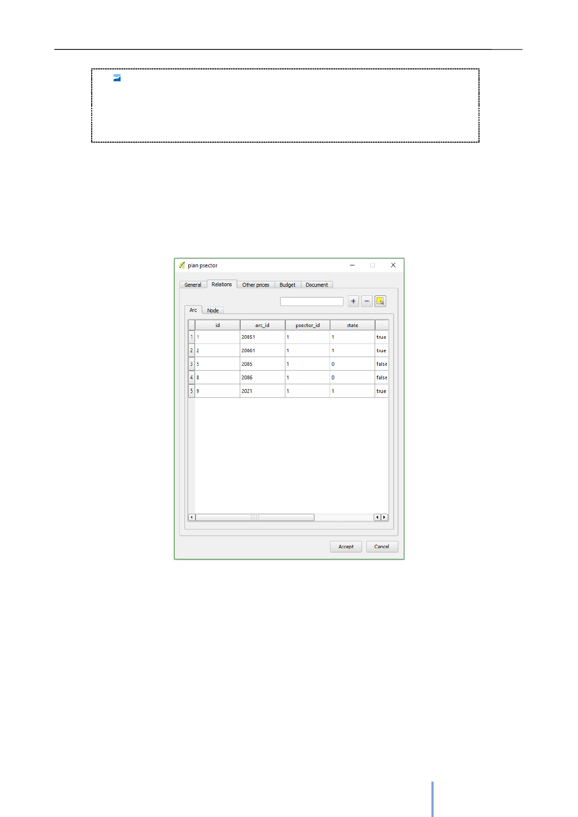
Giswater 3 User Manual
107
NOTE 08 It is very important to always generate at least one planning
sector when user starts working with Giswater, since all elements with a planned
state must belong to one. Without any planning sector it will not be possible to work
with these elements and the program may show errors.
In order to link the network elements with a psector there are two ways:
▪ When inserting a new item with planned status. It will be directly linked to the planning
sector that is selected as default at the time.
▪ Using the Relations tab of the form (Image 73) elements (arc and node) that will be
part of the psector can be selected.
In this tab the information of the related elements will appear. It is important to look at the
state and doable fields. State refers to the state within the psector, it is not the state of the
element in the network. Elements with state 1 will be displayed and those with state = 0 won’t.
Doable is used to establish whether or not the item will enter into budget calculations: TRUE
will enter, FALSE will not enter. In many cases, the planning sectors need to incorporate
existing elements in the network, which should not be used to calculate the price. The
objective of this field is to allow such calculations. Those two fields will be filled automatically
depending on the state_type of the linked element.
Image 73: The second tab of form is used to relate the elements
of the network to the planification sector. They are located in two
subtabs – arc and node.
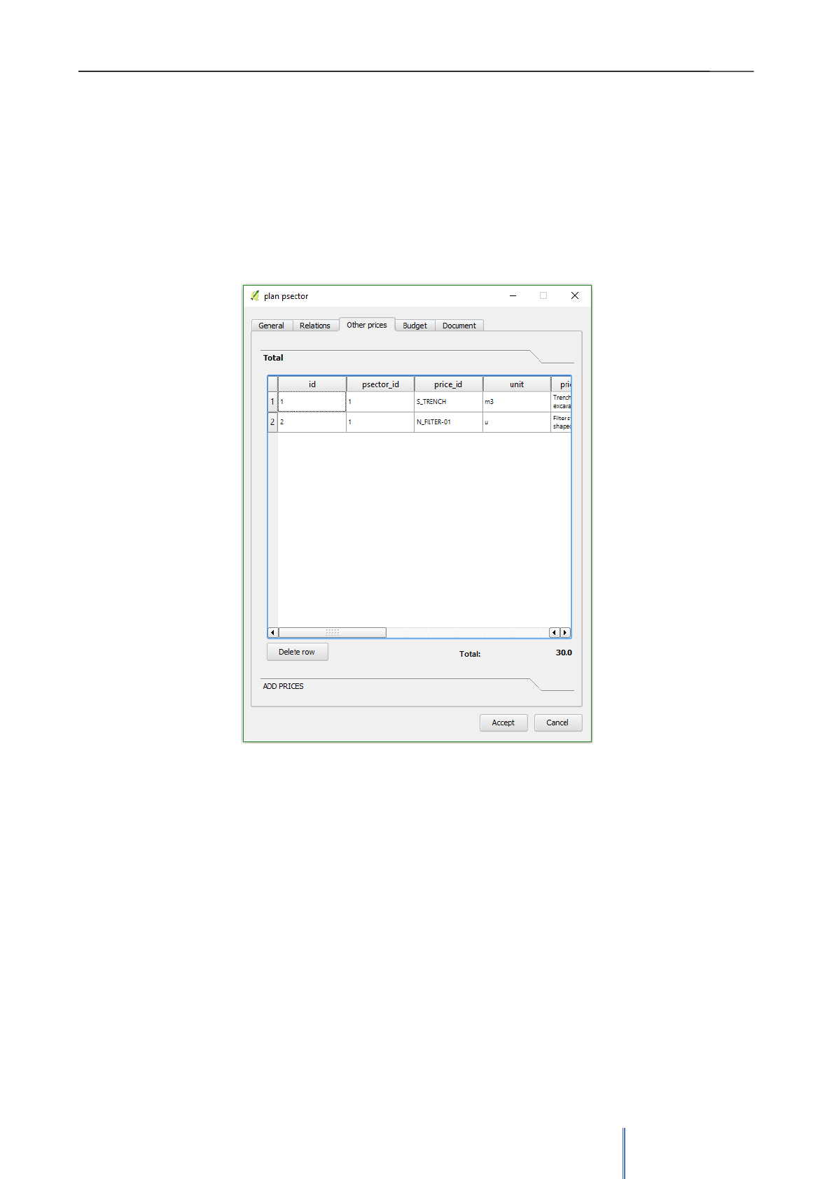
Giswater 3 User Manual
108
The third tab of the form is used to add to the budget of the planning sector the prices of any
other parameters that are required to develop the work, apart from the value of the elements of
the network. For example, the user can add prices for the transport of waste, excavation or
any work that is necessary.
Selecting any of the prices and linking it with the total budget of the planning sector can be
done by clicking on the lower part of the form with name ADD PRICES. The prices available in
the price_compost table are shown here. All prices that are necessary for this budget can be
added from here.
Tab Budget allows to see a budget summary of the planning sector. Here, the prices of the
planned operations are detailed and presented in groups:
▪ Total value of arcos
▪ Total value of nodos
▪ Total value of other parameters
▪ General expenses (+19%)
▪ VAT (+21%)
▪ Others
With the sum of all these groups of prices the total budget of the project is generated.
Image 74: Tab Other prices allows to link the costs not related
directly with the network elements to the planification sector.
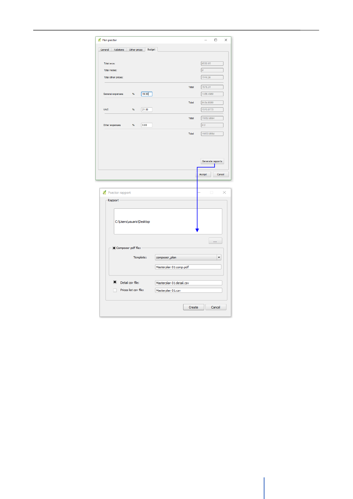
Giswater 3 User Manual
109
In the lower part of the form there is the Generate rapports button, which allows creating
external files with the information about psector. There are three options to generate reports,
each of them individually selectable based on the interest of user. The file in pdf format that
can be generated by the QGIS composer can use templates that the user loaded into the
project. Keep in mind that the template must be well configured so that the process could work
properly.
The last tab, added in version 3.1 of the plugin, allows to link documents to a psector. These
can be created from the existing form or link.
Image 75: The last tab of the form shows the total Budget of
the psector. It’s possible to create personalized reports with
the data of psectors using the Generate rapports.
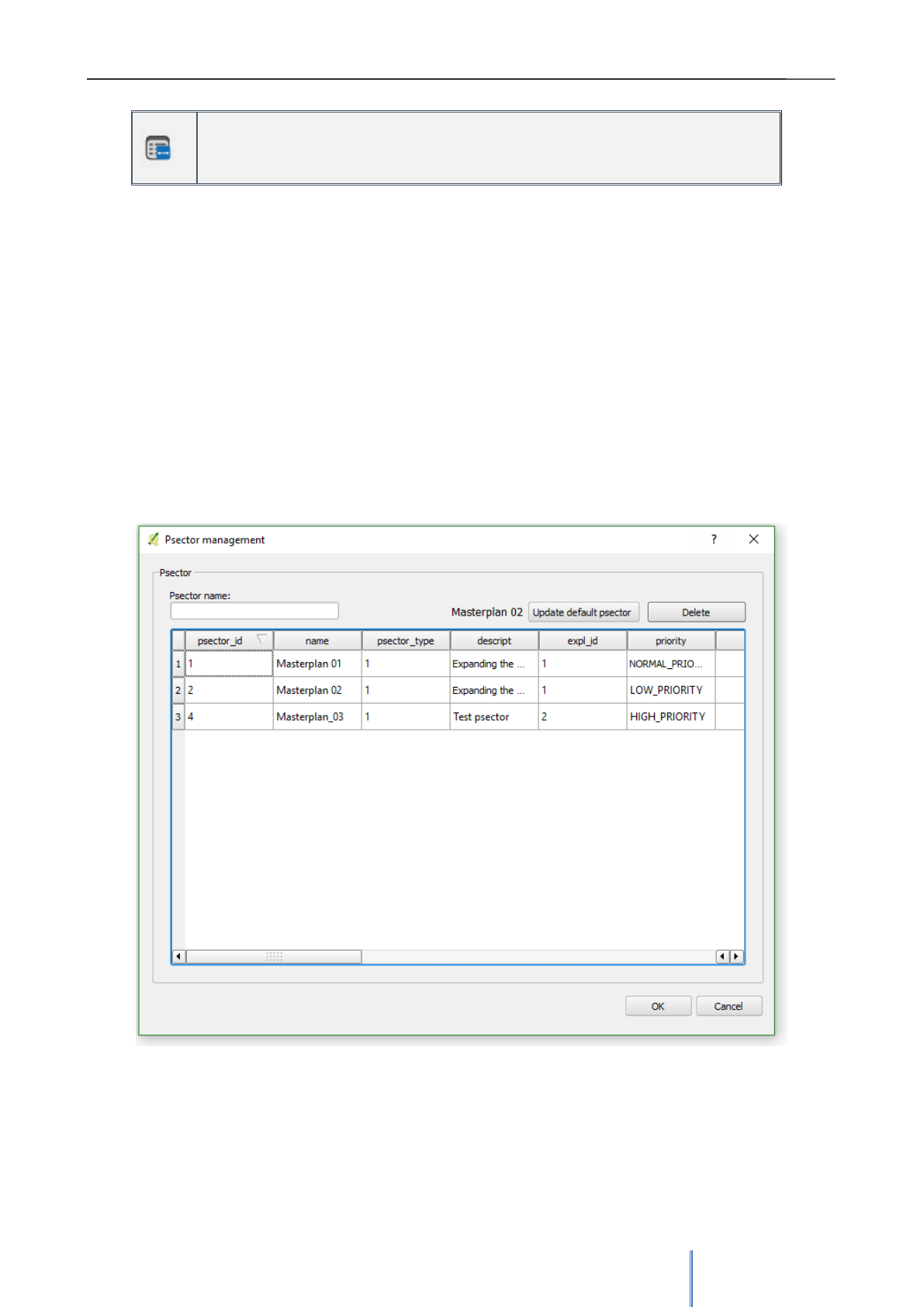
Giswater 3 User Manual
110
Psector manager
Allows to manager the planification sectors– role_master
The planning sector manager is a tool that allows to inventory, visualize, filter and eliminate
existing psectors. In addition, it shows the planning sector which is selected as default at the
moment and allows to change it by another one. The default psector is an important
parameter, since all the planified elements that are inserted will be linked to it.
In the form, that opens after clicking on the tool button, a table with all the existing sectors and
its data is presented.
It is possible to open the selected psector form with double click on the row. Unlike other
Giswater management tools, this is the only way to open the psector form, therefore, it’s
very important to remember that while working on planification.
In the upper part of the form there is a filter, current default psector, button for changing the
default psector and button to deleting the planification
Image 76: Form of psector manager. All existing psectors in the project are displayed here. The tool allows you
to filter according to the identifier, update the psector that will be used as default, delete data or open a specific
form, where the user can view the related elements and associated budgets
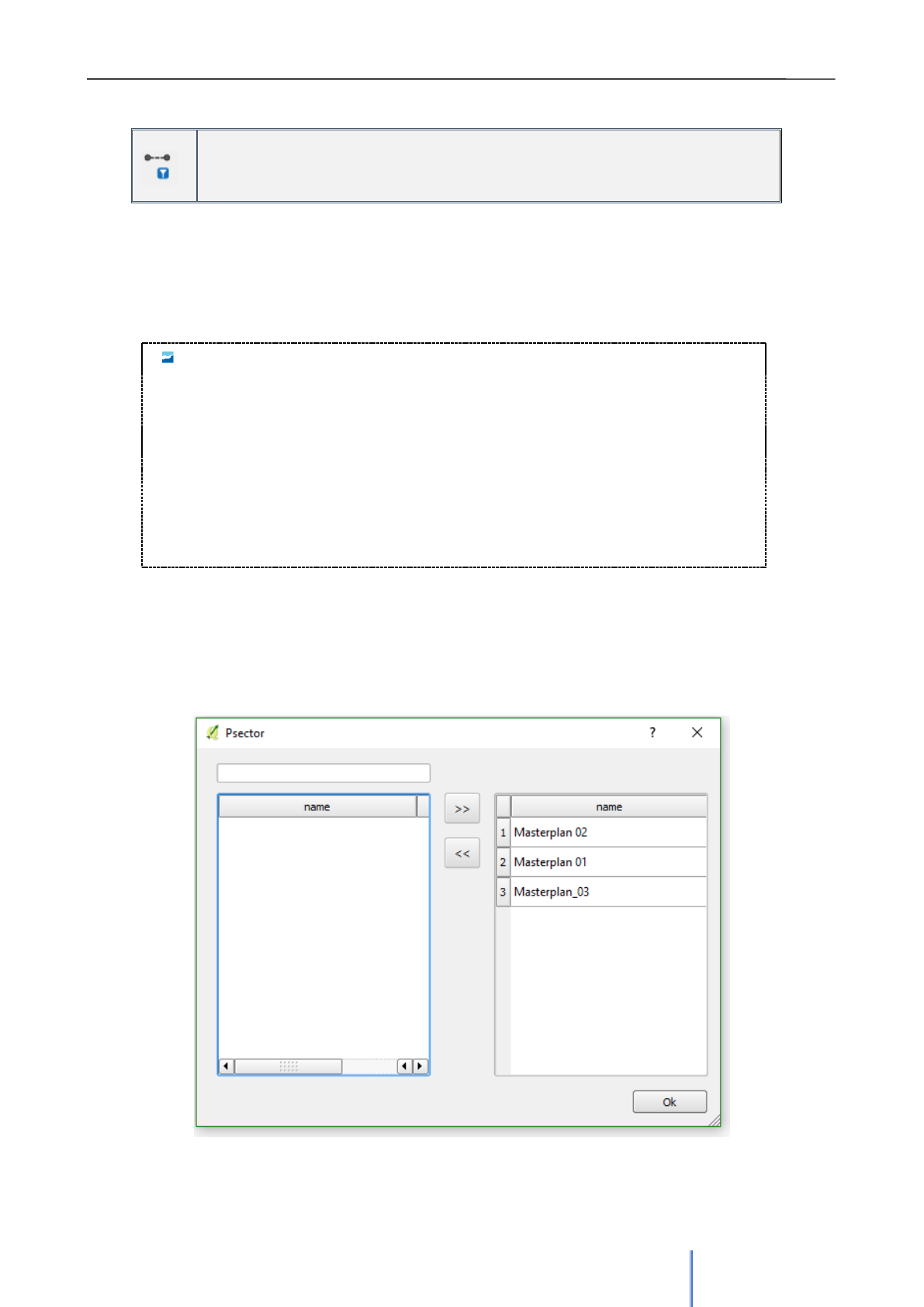
Giswater 3 User Manual
111
Psector selector
Allows to visualize or not the selected planification sectors– role_master
This tool, like the others of the type 'Selector', allows to choose which sectors of planning will
be seen on the screen at the moment. It aims to facilitate the management of these psectors,
since seeing all their geometries at the same time can be inconvenient for user.
NOTE 09 The use of this tool coincides, in part, with the state selector. Users who
have the right to use both tools should know that, even if the planned elements are
desactivated in the state selector, with this tool the planned ones of the selected
psectors will be displayed. In a contrary way, even if they do not have a selected
psector, the planned elements can be viewed from the status selector. The
difference is found in the fact that with the selector of psector the elements with
state on service linked to the specific psector are hidden to show only the planned
ones.
The usage of the tool is very simple. With the form opened, all the planning sectors that are on
the right side will be visualized. The sectors that are not going to be displayed at this time
should be on the list on the left. The change of columns is done by the arrows that are
between them.
Image 77: Form of planification sector selector.
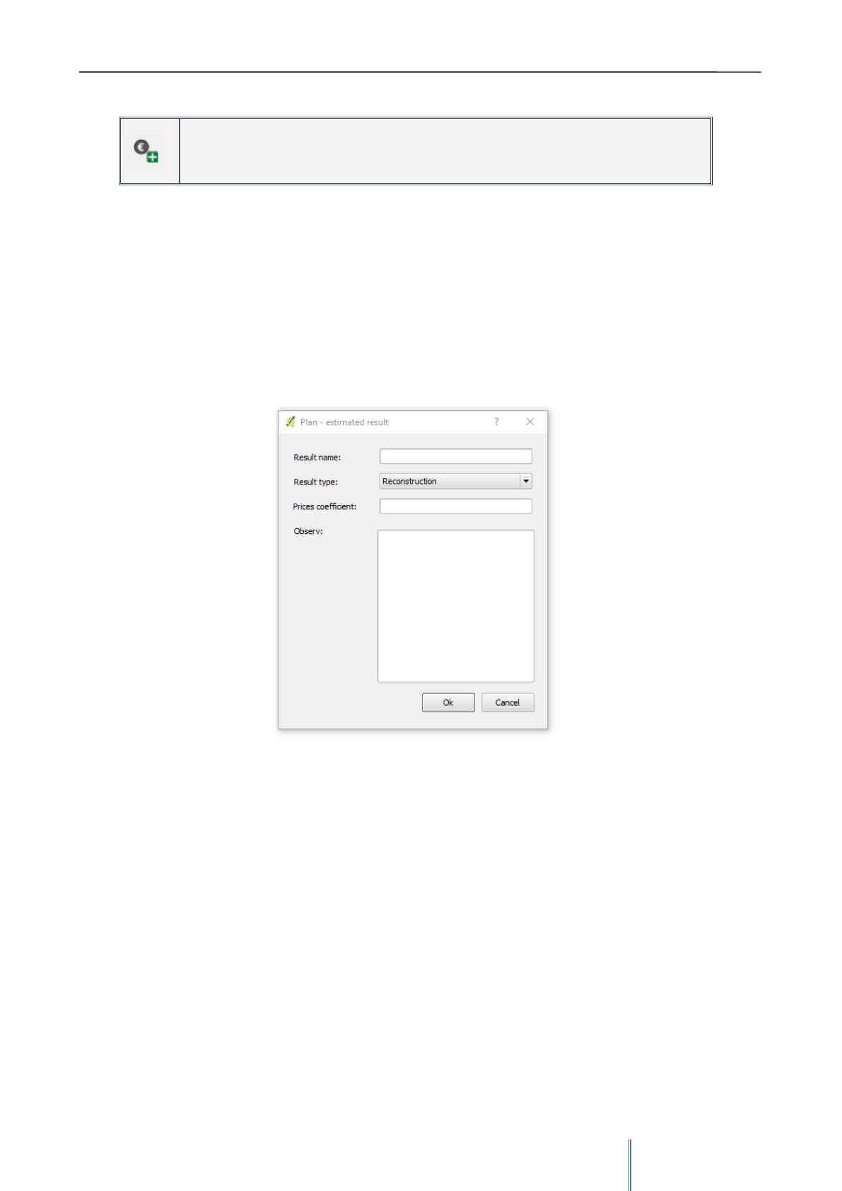
Giswater 3 User Manual
112
New network cost
Allows to generate new costs of the network – role_master
This tool allows to generate cost calculations of the network elements that are active (state =
1).
The only process that is carried out is establishing a new link between the active elements
(state = 1), which already have their prices listed in the catalogs, and the current price base.
There are two types of prices - rehabilitation and reconstruction.
The only thing to comment about the form are that prices that can have a multiplying
coefficient, depending on what the report is intended for.
The form also supports a text field for any kind of observations.
Image 78: Form to add a new cost of the network.
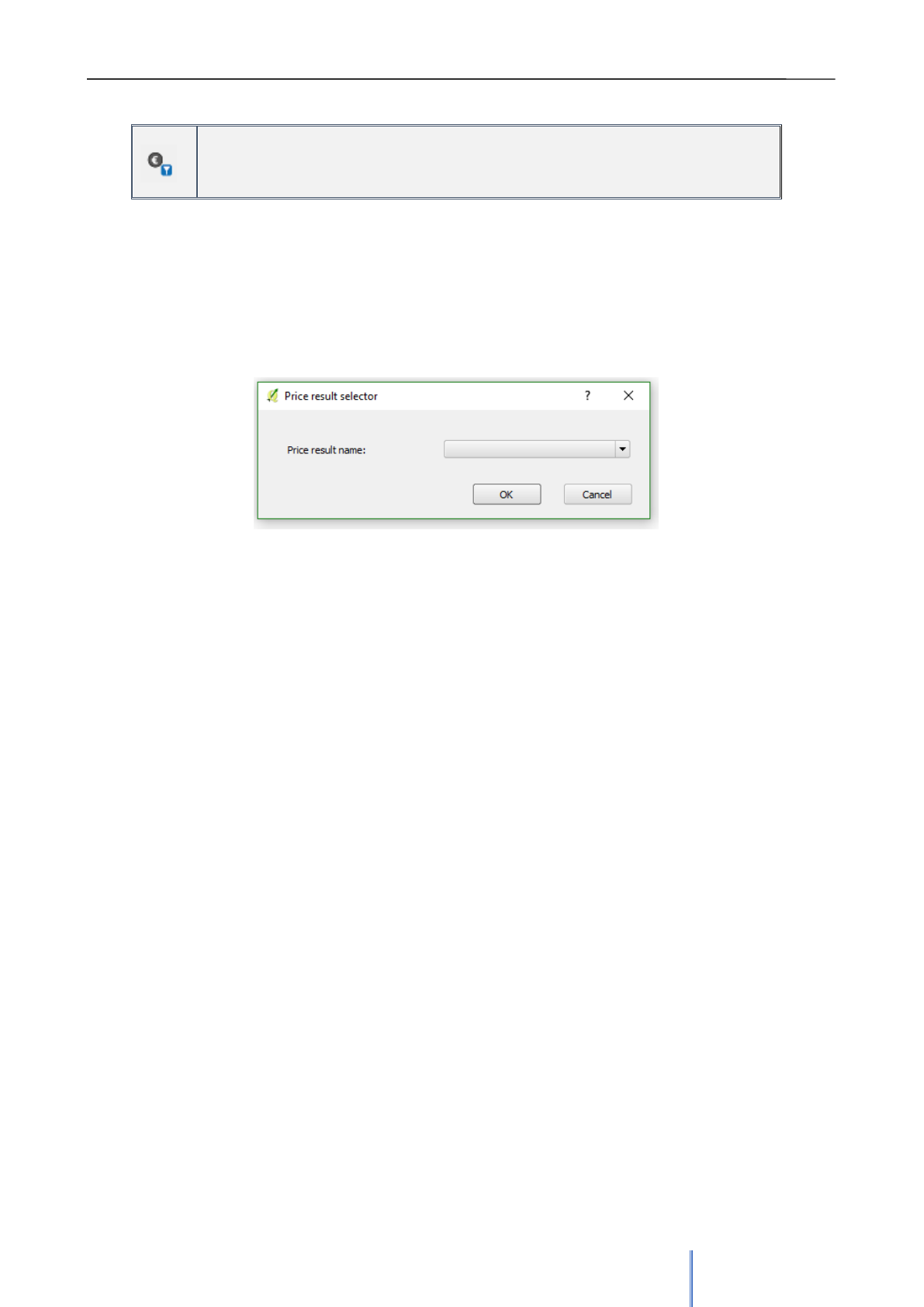
Giswater 3 User Manual
113
Estimate result selector
Allows to select the result and work with it – role_master
This tool, like the others of the type 'Selector', allows to choose which network cost calculation
results (only those of rehabilitation type) will be displayed on the screen at the moment.
Selecting the network cost result as active result is used to replace the value shown in the
views of 'v_plan_result_node' and 'v_plan_result_arc'. This value of interest is the one that will
be displayed in the QGIS interface.
Image 79: Estimate result selector. The selection can be made
using drop-down list.
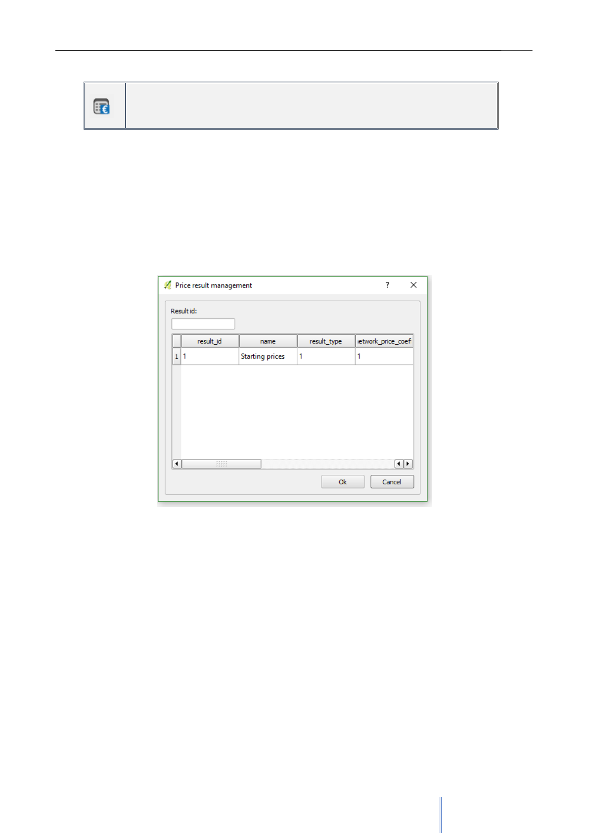
Giswater 3 User Manual
114
Network cost manager
Allows to manage different results of the costs– role_master
Network cost manager is a tool that allows to inventory, visualize, filter and eliminate the
different calculated network costs.
In the form that opens after clicking the tool button ther table with all the results is presented. It
shows the data of each of the results.
It is possible to open the information relatef to the selected result by double clicking on the
row.
In the upper part of the form it can be filtered according to the result identifier.
Image 80: Form of network cost manager. All the costs are showed here
and can be filtered or opened.
.
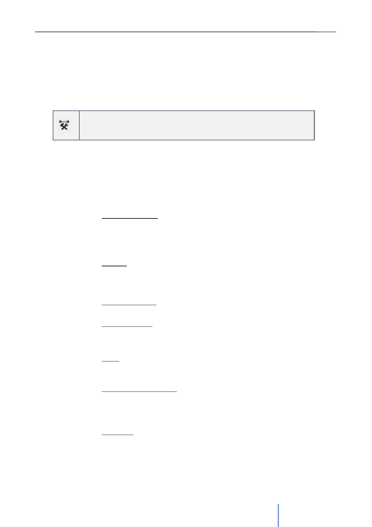
Giswater 3 User Manual
115
5.2.6 Administration
This last group of tools of the Giswater plugin is formed by tools that can be used for project management
tasks. It is a heterogeneous group, with very different functionalities focused on general processes, unlike
the rest of the toolbars that had much more specific role. Here there are tools that allow control, topology
check, value management, data import and also Giswater's structural functionalities.
Topo tools
Allows to use different tools of control and topology – role_admin
The toolbox aims to offer a multitude of functions that may be useful when checking if the
certain parameters of the project are correct. The different functions offer different answers:
some insert data in tables and others represent new geometries within a layer.
The tool is divided into three tabs:
- Edit
▪ Check Project /data: two functions. The first reads the layers loaded in the
project and warns if doesn’t find important layers that must be loaded. The
second controls that the default values defined by user are consistent, which
means, that the inserted values can be used in the required field and won’t
generate errors.
▪ Topology: these functions analyze different topological rules of the network.
When activating any of these parameters, if there are elements that do not
comply with the rules, their values will be inserted in the corresponding
layers of the Topology analysis group.
▪ Check mincut data: checks if all the data related to mincut polygon are
correct. Solo para WS.
▪ Check profile tool: checks if all the data related to longitudinal profile are
correct. Solo para UD.
- Master
▪ Prices: two functions. One controls that the data needed to calculate
reconstruction prices is complete and the other does the same for
rehabilitations. The result is shown in the table audit_check_data.
▪ Advanced topology review: are advanced topology functions, designed for
the realization of revisions of the network. They allow to visualize possible
errors respect the topological rules.
- Admin
▪ Check data: function that controls the number of rows that each table of the
project should have. It reads all the tables and its number of rows and
compares it with the values that are defined as the minimum. The results are
stored in the table audit_check_project and show the number of rows each
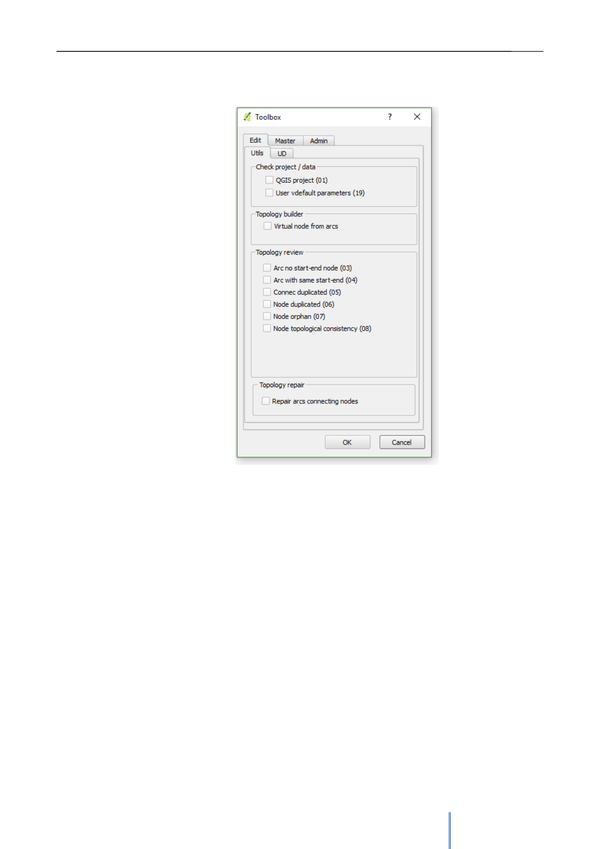
Giswater 3 User Manual
116
table should have and the actual number it has; in case the number is
correct the enabled field will be TRUE, otherwise it will be FALSE.
Image 81: Topo tools has many options divided
into tabs. Both projects have their specific subtabs
- WS and UD which appear depending on the type
of the project.
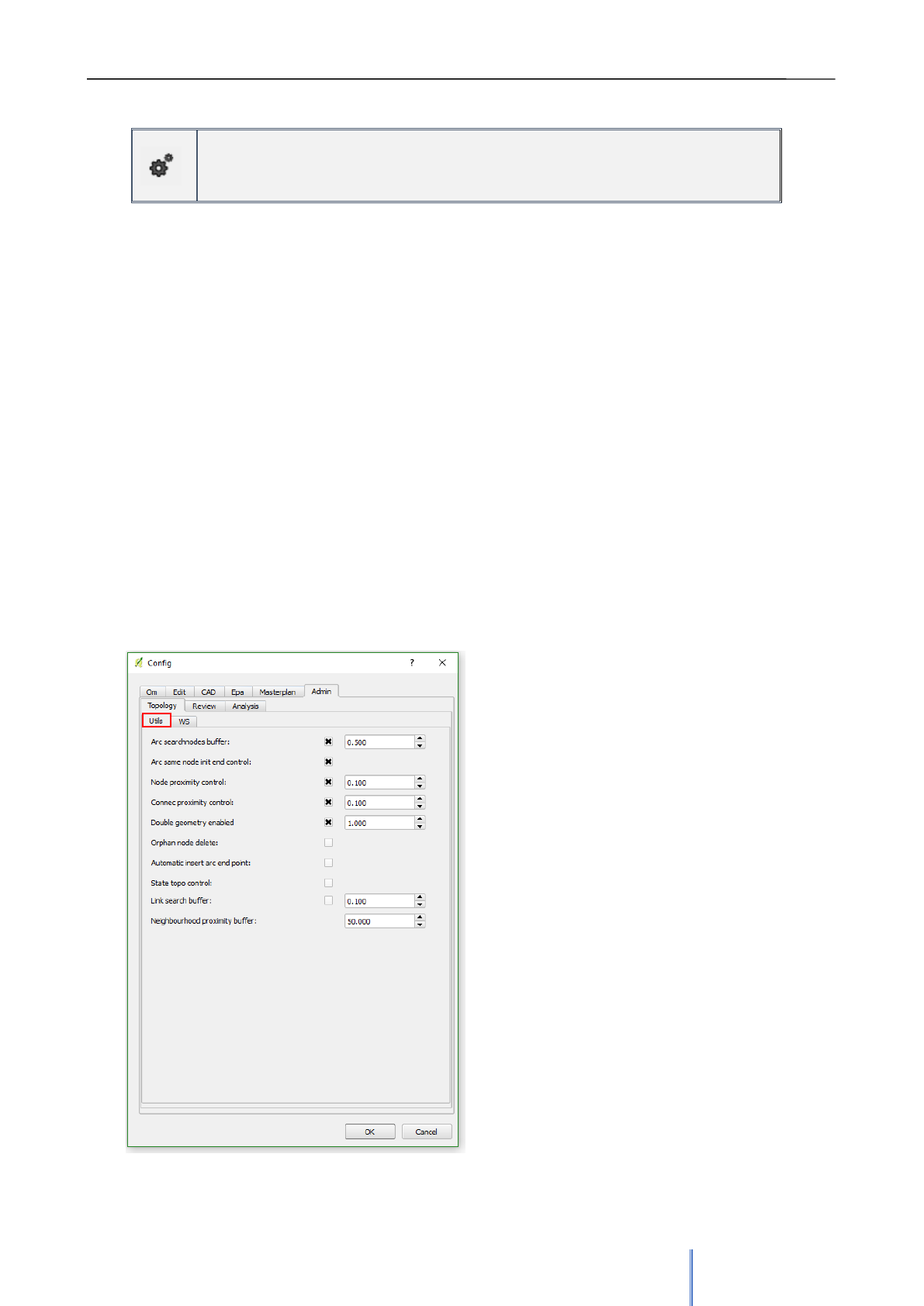
Giswater 3 User Manual
117
Config
Allows to define default values of the project – role_admin
Configuration assistant for the behavior of the plugin. It allows to define different parameters
that are used in other tools and processes of the project. It is a tool of enormous importance
and the one that all users should know well, since its use is recurrent and essential for the
operation of Giswater.
The form of the tool is divided into six different tabs. Within the tabs there is another
subdivision depending on whether the parameters are common (Utils) or specific for WS or
UD projects.
The operation is the same for all the tabs: each parameter has a checkbox next to its value.
The user can set the value he considers appropriate, following the filters that each parameter
has. If the checkbox is checked, the value of the parameter will be active and stored in one of
the database configuration tables. If the checkbox is not checked, the value of the parameter
will not be used anywhere.
Within the toolbox both default values configurable by the user and system values can be
found. They can be modified or chosen by the user in the way that has been explained in the
section 3.6. Many of the values that can be configurable with the tool are easily recognizable,
for example, those of the Edit tab. On the other hand, there are some that are more complex
and require an explanation, such as those referring to topology:
Arc searchnodes buffer: sets the tolerance
when connecting ends of the arc to the
nearest node.
Arc same node init end control: Controls
the arcs with the same start and end node.
Node/connec proximity control: allows or
not the insertion of very close nodes /
connecs, with defined tolerance value
Double geometry enabled: allows the
automatic insertion of double geometry
elements and controls the area that the
generated polygon will occupy.
Orphan node delete: Deletes unconnected
nodes
Automatic insert arc end point: Insert a
node automatically at the end of the created
arc. It’s possible to choose the type of the
inserted node.
Image 82: Form of config, topology tab.
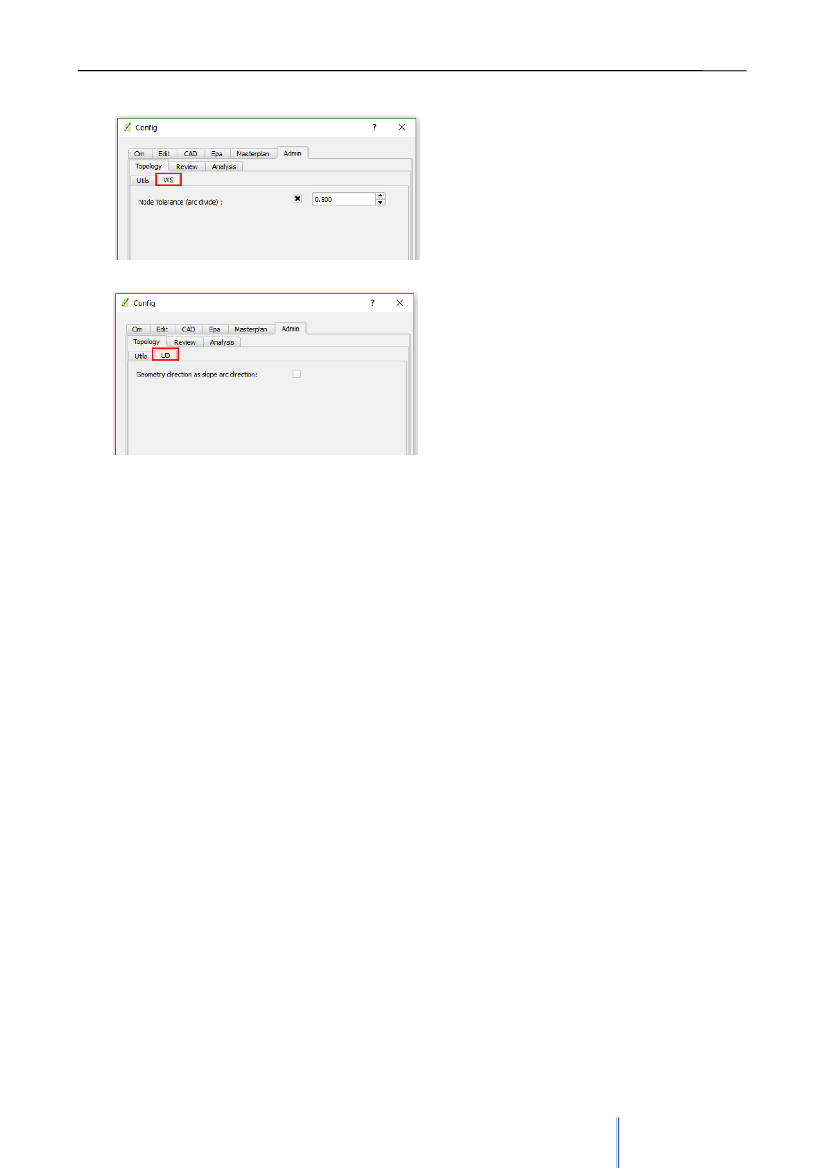
Giswater 3 User Manual
118
State topocontrol: Activate or desactivate state
topology control
Link serach buffer: allows to establish a
tolerance to perform a buffer relative to a
link.
Neighbourhood proximity buffer: allows to
establish a tolerance when making a buffer
that looks for elements considered as
neighbors.
Node tolerance (arc divide): establishes a
tolerance at the moment of breaking arcs.
Geometry direction as slope arc
direction: controls whether the direction of
the geometry is the same as the slope of the
section.
In the tab related to the configuration of the CAD tools there is just one parameter, which allows
choosing which of the ToC layers will be used as the base layer. This layer is the only one that
QGIS will allow to snap while drawing. In case of not having this parameter set, the
management of the layers that will allow the snapping will be managed from the own
configuration of QGIS.
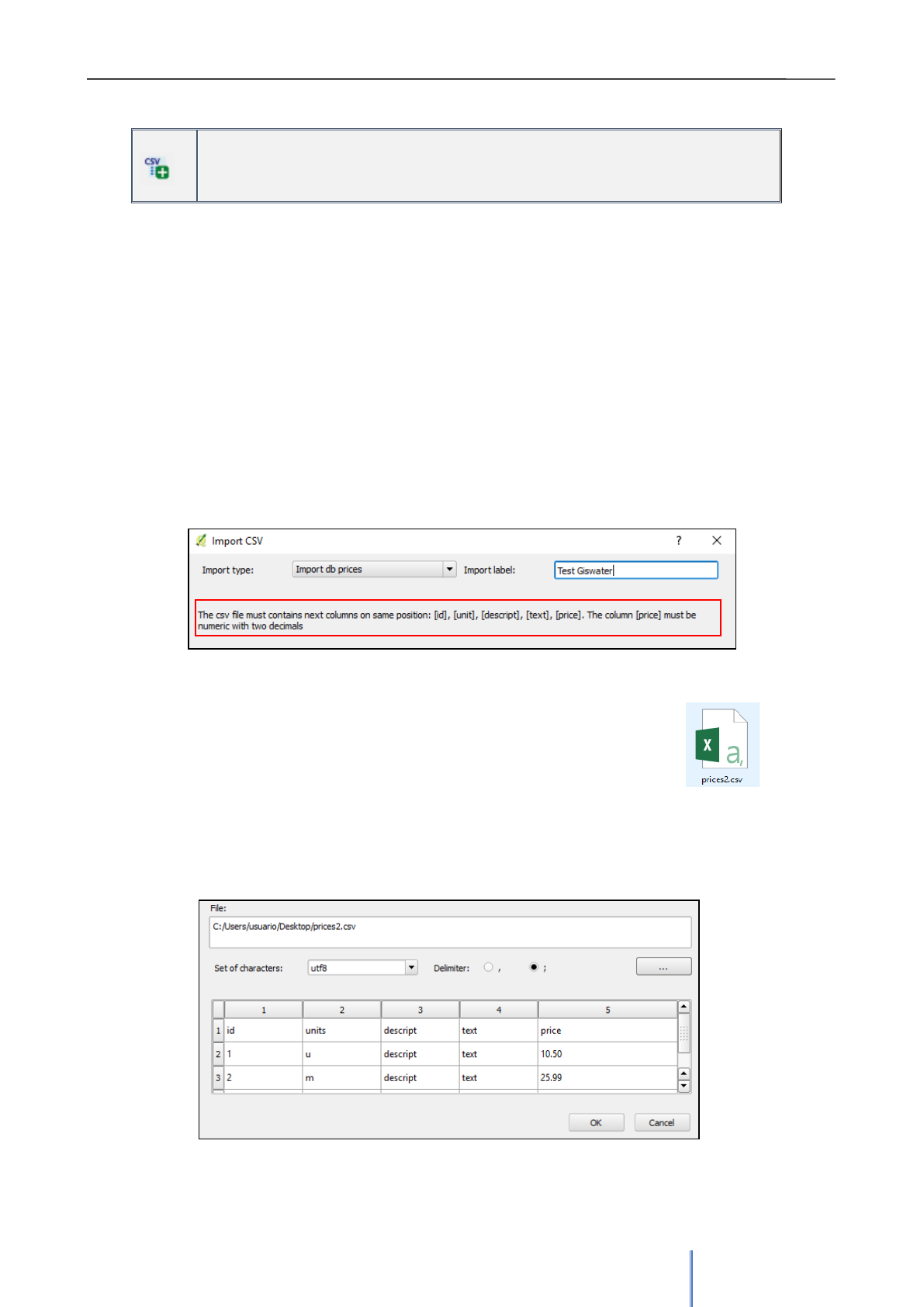
Giswater 3 User Manual
119
Import CSV
Allows to importa n external csv file into database - role_admin
It’s very common to have data related to the network that is in table format, such as xls or csv.
Giswater incorporates this tool in its plugin to provide the possibility of directly importing the
data in a csv file into the schema tables.
To show the functionality of the tool, an example of importing a price table, which will be
incorporated directly into the price_simple table will be presented. The program has a specially
designed function to perform such a process. It’s important to know that each type of csv
import files must have a specific function.
How the tool is used to incorporate new simple prices into our database:
1- A .csv must be ready to import. This means that it must meet the requirements of the tool
and the Giswater function, otherwise the data will not be incorporated correctly. These
requirements can be checked by opening the tool and, at the top, selecting an Import type,
in this case it’s Import db prices.
The forms show the position and order of the fields: id, unit, description,
text, price (numeric with two decimals).
2- Within the form, with Import db prices selected, set a value for Import label, which will be
the name that will receive the prices of the import and will be included in the catalog of
simple prices (Price_cat_simple). For this example, it will be: Test Giswater.
Image 83: The form of import csv explains how the csv file should be prepared in order to
import it. In this case the name of all the imported prices will be Test Giswater.
Image 84: With the file path added, the table will show a preview of the data.
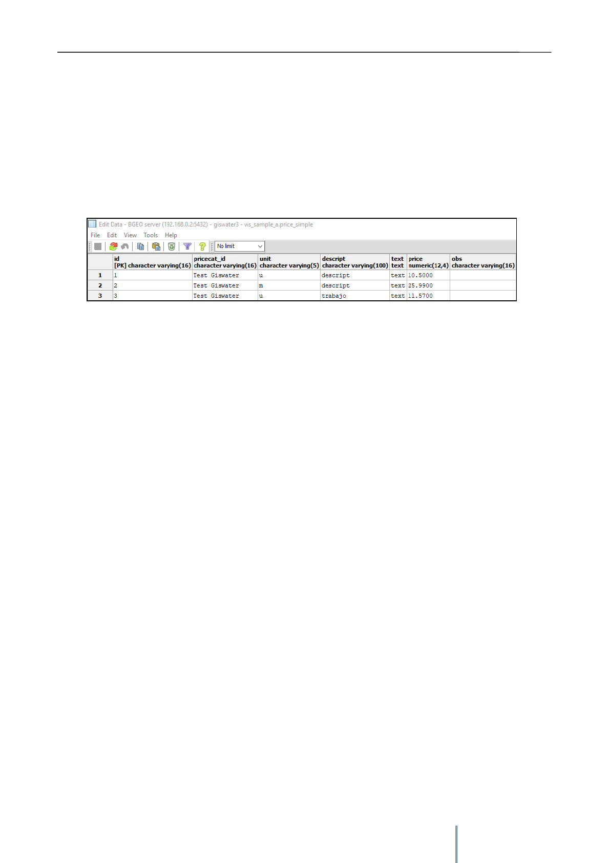
Giswater 3 User Manual
120
3- Add the file path, here prices2.csv and select the encoding and the delimiter, which can be
'comma' or 'semicolon'. The table below shows a preview of how the data will be inserted
(Image 84).
4- Click OK to start the process.
5- The function is parameterized so that the data of the correctly structured file could be
incorporated directly into the price_simple table, so that the columns of this table coincide
with those of the import. As presented on image 85, the data is perfectly added to the
table, with all its records and with the price catalog (pricecat_id) as Test Giswater, which
is selected from the price_cat_simple table where it was just added.
As the result of the process, the information from .csv file is inserted into specific tables of the
database. The data located in the price_simple table are available for use in other Giswater
tools and processes, for example while making budget calculations with Masterplan
operations.
Apart from linking the price tables, the tool includes other specific functionalities to import csv
files that refer to:
- Import addfields: to link custom fields directly to the man_addfields_value table. To
do so, the table must have id of the element, the parameter (referring to the custom
field) and the value to assign.
- Import elements: useful for linking elements associated with arcs, nodes or
connecs. To perform an import a specific table for each type of element is required.
That means, in order to link elements with nodes a csv that has only the information
about node type elements in neccessary. The table should contain the id of the
topological element, the catalog of the associated element, observations, additional
comments and number of elements. When performing the operation, the element
and element_x_ * tables, which link the elements associated with the topological
elements (node, arc, connec), are automatically filled in.
- Import visit table: useful to link visits to any type of network element. There are
specific functionalities in the Import type drop-down list, for each type of element, so
the visits can be linked only to nodes, arcs or connecs depending on the selected
type and the csv file.
Image 85: The data from csv file inserted into the Price_simple table. The inserted values can be used in other
functions of Giswater.
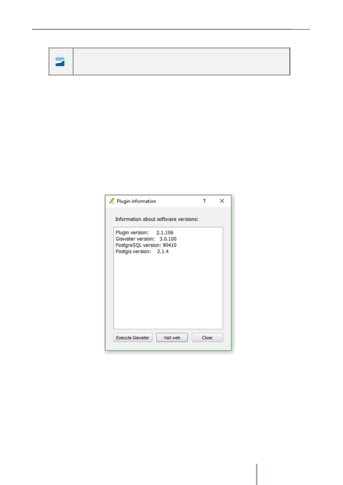
Giswater 3 User Manual
121
Giswater
Shows the information about Fiswater and allows to open the software driver – role_admin
The last tool of Giswater plugin is the one that provides information about the versions of the
different drivers from which the whole project is supported:
▪ The plugin itself
▪ Giswater
▪ PostgreSQL
▪ PostGIS
Apart from this information, the tool also allows to run the Giswater driver in the same way that
it could be done from the icon located on the computer. In this way all the functionality (section
2.3) of Giswater (creation of new schemes, configuration of connections, renaming projects,
etc.) is incorporated into the QGIS plugin itself.
The last function of this tool is a link to visit a website of Giswater.
Image 86: Form of Giswater tool. From here the software
driver or Giswater website can be opened.
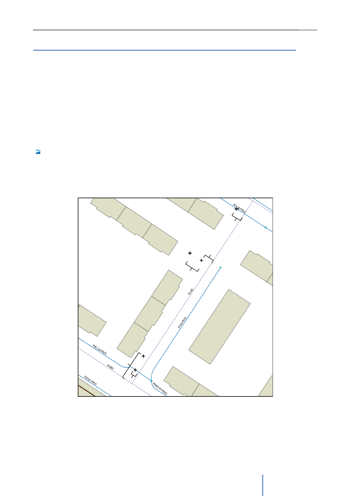
Giswater 3 User Manual
122
6. HOW TO DIGITALIZE THE NETWORK
Once all the tools of the Giswater plugin are known, it’s timeto use the full potential of the program and start
working with the water network. It is considered appropriate and interesting to dedicate a section to present
the correct steps to digitize the parts of the network, because it’s one of the most common processes for
those in charge of managing it.
Users who are more experienced in the use of GIS may not need to read this section, but it can also serve
them as a small guide to develop a task of great precision.
To digitize, the plugin tools can be used, especially those associated with role_edit, but other parameters
must be taken into account so that the insertion of new elements is correct and accurate. Next, it will be
explained in detail which are the steps that must be followed, in chronological or to digitize new elements,
both linear and punctual:
Example of digitalization of a new arc
By means of a practical example, carried out in one of the sample projects of Giswater, it will be
explained how a new section of the network can be generated. It will consist of the insertion of 5 new
nodes and 4 arcs. All these new elements must be placed in a specific position, as represented in the
image 87, simulating a real work.
2 m
12 m
2 m
4 m
2 m
Image 87: The elements that will be inserted in this example should be located in the
places showed in the image, where the distance between the elements is determined.
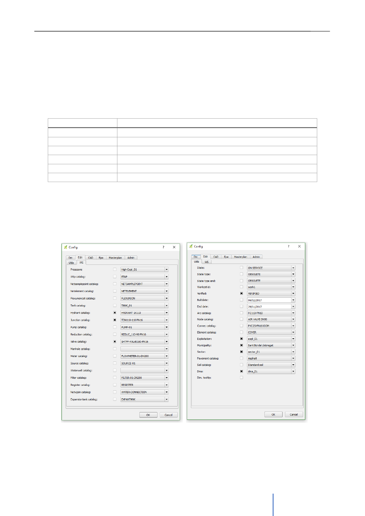
Giswater 3 User Manual
123
The elements represented in the image refer to the nodes, which will consist of 3 junctions (Junction),
located at the intersections of arcs, a valve and a hydrant. The arcs will be all pipes (Pipe), which will be
drawn in a straight line connecting the nodes.
Process
1. Before creating any element, it is very important to know what are the mandatory fields for each
type of element, so that, if they are not filled in during insertion, it will not be completed. The
following table specifies these fields and how they can be filled in, since Giswater offers different
methods to facilitate the insertion of data. In the form itself the mandatory fields are marked with a *.
Field
¿In case in leaving it NULL (empty), how is it filled in?
Node/Arc catalog
Default value (one for each element)
Municipality
Default value, if not the value is captured from geometry
Exploitation
Default value, if not the value is captured from geometry
Dma
Value is captured from geometry, if not it uses default value
Sector
Value is captured from geometry, if not it uses default value
State
Default value, if not the first value from value_state table
2. It is important to configure default values, since many times the insertions of new elements will be
made in the same municipality, exploitation, dma and sector. The default values will allow to work
faster. For this example, using the configuration tool, the default values for Hydrant catalog, Junction
catalog, Valve catalog, Verified (field not mandatory but recommended), Exploitation, Municipality,
Sector and Dma will be set. The state will be entered manually each time.
3. To digitize with a higher degree of precision, as in the case of this example, before entering any
element it’s important to draw support points which will help with placing the nodes in the specific
Image 88: In the form of Configuration the value default for this example are marked. They can be updated
as many times as user wants.
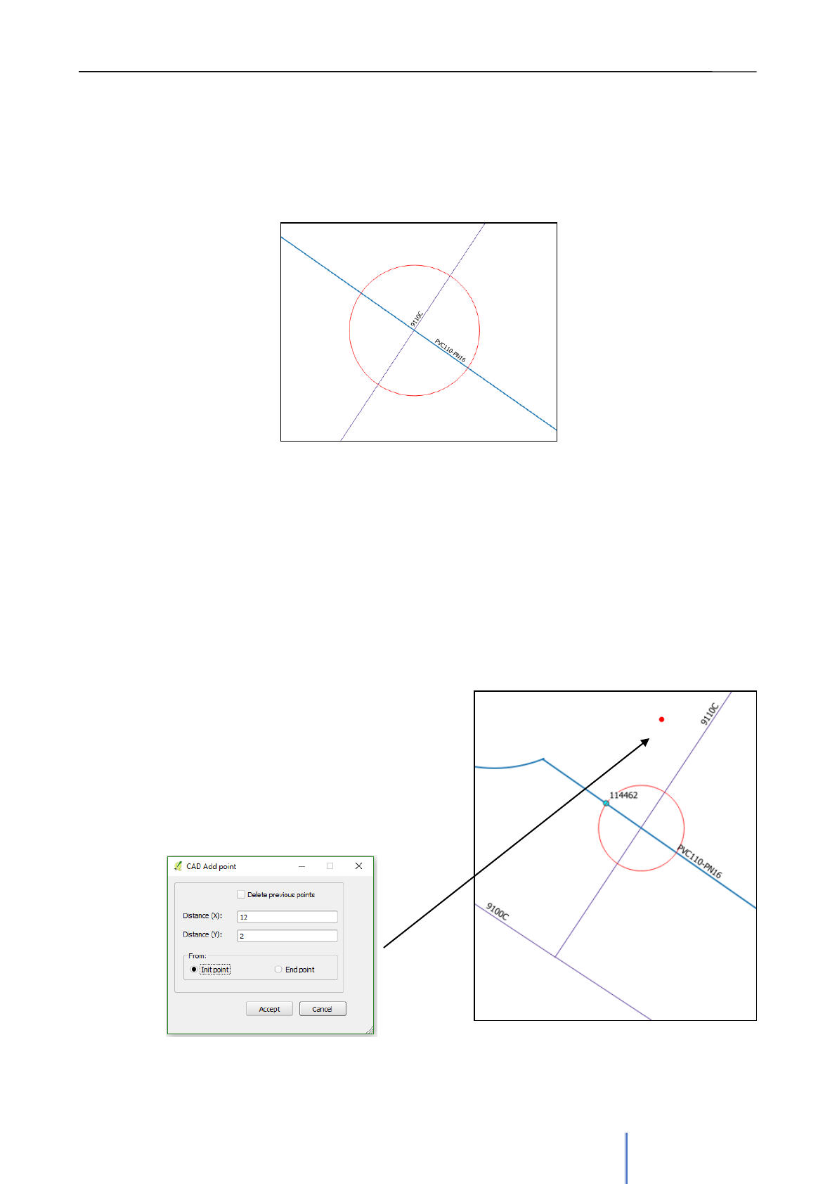
Giswater 3 User Manual
124
location. To draw these support points there are different options: the CAD tools of the Giswater
plugin or other tools incorporated into QGIS, such as the 'advanced digitization tools'.
4. To draw the first support point, which must be 2 meters from the intersection between the street
9110C and arc PVC110-PN16, the 'Create Circle' plugin tool will be used. With the snapping
activated, place the cursor over the intersection and click. The radius of the circle must be 2 meters
5. At the intersection of the circle line with the Pipe layer is where the first Junction element is going to
be placed. Using the keyboard shortcut (J) the new element just above the intersection can be
inserted. If the process is correct, the program should show a window telling that this node is about
to break an arc. Since many values are established as default, the only thing that needs to be
indicated in the form is state. In this case, ON SERVICE, together with the status type as ON
SERVICE.
6. With the first element already introduced, the second support point needs to be placed. It will serve
to mark the location of a new valve. This should be 12 meters from the beginning of the street 9110C
and 2 meters to the left.
7. With the tool 'Add relative point', mark the first point
at the beginning of 9110C street of the Streetaxis
layer and another at a certain distance on the same
line. That’s how a point 12 meters from the beginning
(x) and 2 meters towards the outside (y) can be
drawn.
Image 89: The circle of 2 meters radius will be used to
place the node in the exact location.
Image 90: The second node is located over the red point, generated using ‘Add relative point’.
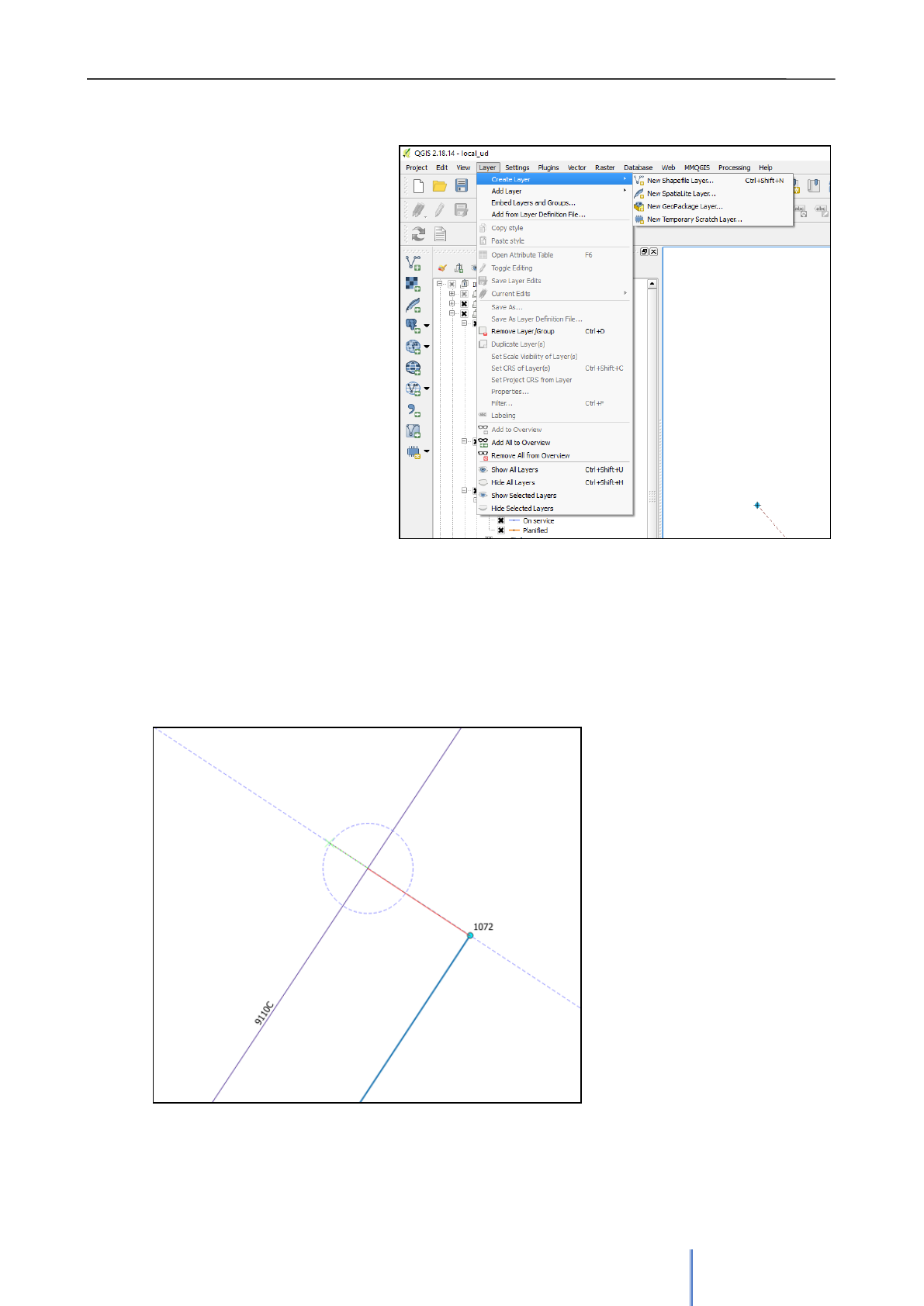
Giswater 3 User Manual
125
8. Just over this support point is
where the new valve should be
placed. As before, the only values
that need to be filled in manually
are the state and type of state. The
rest are configured by default.
9. To draw the next support point (in
this case it will be a line), use the
QGIS tools. With the advanced
digitizing panel, it is possible to
draw a line perpendicular to node
1072 and which, at the same time,
is 2 meters from the street 9110C.
10. The first step is to generate a new
temporary scratch layer (Image
90). It must be a linear layer, with
the same EPSG as the project
has. Once created, put the layer in
edition and click on 'Add spatial
object'.
11. With the advanced digitizing panel active, first select the node from which the new line should start.
Then click on the 'Perpendicular' button and select the arc that will serve as a reference to draw the
perpendicular line, in this case the Pipe showed in image 92. That thin auxiliary line is drawn
perpendicular to the desired node. Now, click on the street axis, thus establishing the first part of the
line. Without stopping the
edition, establish a radius
of 2 meters in the field
where it says 'd', taking
into account that the
cursor must be located
above the axis of the
street. Click again on the
auxiliary line, now just
above the intersection with
the 2 meter circle
generated. Once the red
line reaches where the
desired point, click the
right button of the mouse
to finish the support line.
Image 91: From Layer in main menu a temporary scratch layer can be
added.
Image 92: Using the panel of advanced digitizing posible to draw a
perpedicular line to another element at the desired distance. The red line
represents an arc that will be saved in the temporal table. The left side of
the circle also has the line slightly painted red.
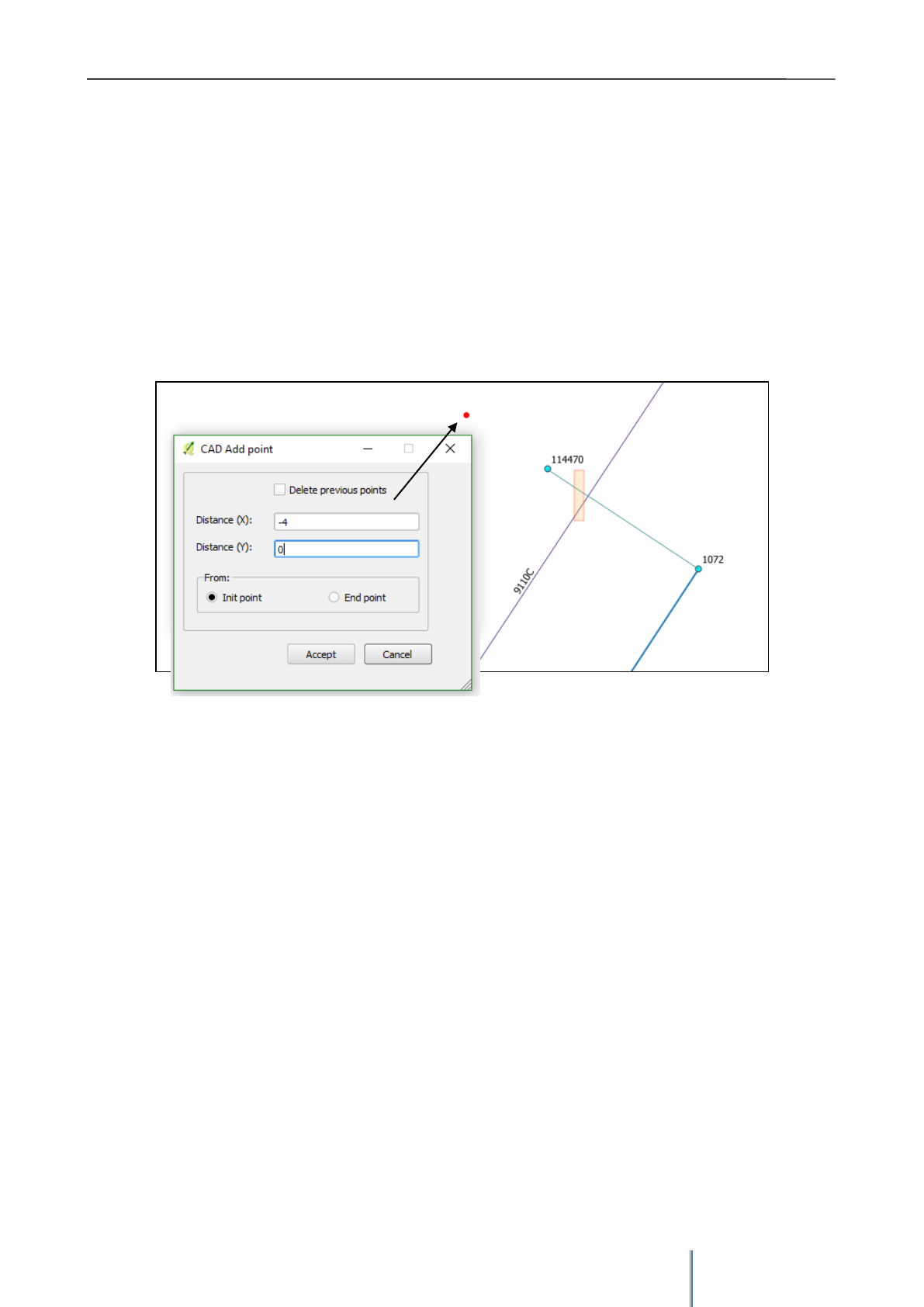
Giswater 3 User Manual
126
12. Using this line, the third node of the example can be placed. In this case a union of type 'T'. In the
same way as in previous cases, insert the new element just at the limit of the support line, knowing
that it is exactly where it should be: two meters from the street axis, perpendicular to the other
pipeline and at the same height as the union that ends this pipe.
13. The next step is tolocate the hydrant, which must be 4 meters from the union that was just generated
and at the same height. Since the support line is still visible on the map, use it again to locate the
new support point. Knowing that this must be at the same height as the line, introduce a point of
support using tool 'Add relative point'.
14. With this tool mark a point on the node 114470 and another one on the support line of the temporal
layer. The 'x' must be -4 and 'y' must be 0. In section from select the Init point as the start point of the
relative element.
15. Place the hydrant just over the added support point. As always, with the default values configured,
only the status of the node must be added.
16. Now, four out of five nodes that were planned at the beginning of the example are added. To insert
the last union, which will break the arc FC110-PN10, use the same method as in the first union of the
example: draw a circle with a radius of 2 meters at the intersection of the arc and the street axis.
17. Insert a unión element, checking that the arc was divided into two.
18. Drawing nodes is finishef. At this moment those nodes need to be connect using arcs. The insertion
process is very simple.
19. At the beginning of the example, only the default values for node-type elements were established.
Now it’s important to add the default value for the arc catalog as well, in this case FC110-PN10, so
the insertion will be faster.
20. To add the first pipe, using the keyboard shortcut 'P', choose the start node and the final node,
clicking with the left mouse button to set it and with the right button to finish the line.
Image 93: the tool Add relative point can be used to place the point as the determined distance from another
element. The temporal line is selected by the rectangle for its better visualization.
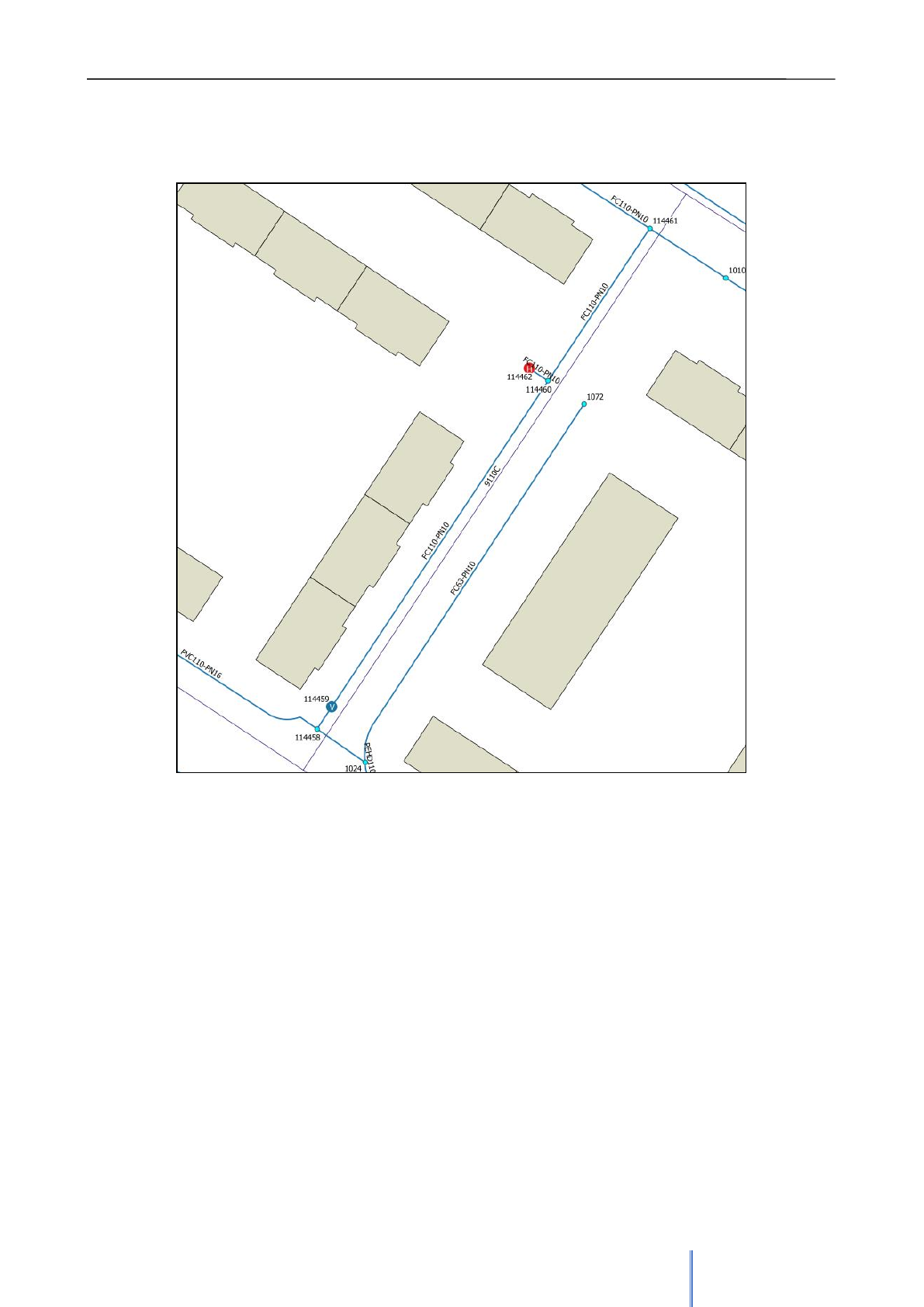
Giswater 3 User Manual
127
21. Repeat the process of inserting pipeline elements to join all the nodes created during this example,
so that the network connects from one side to the other. The final result can be seen in image 94
Image 94: The new network section, planned in image 87. Inserted nodes and arcs connect the
already existing sections of the network with the new ones. The new elements are placed exactly
where it was planned, so that the representation of the real network has the maximum possible
precision.
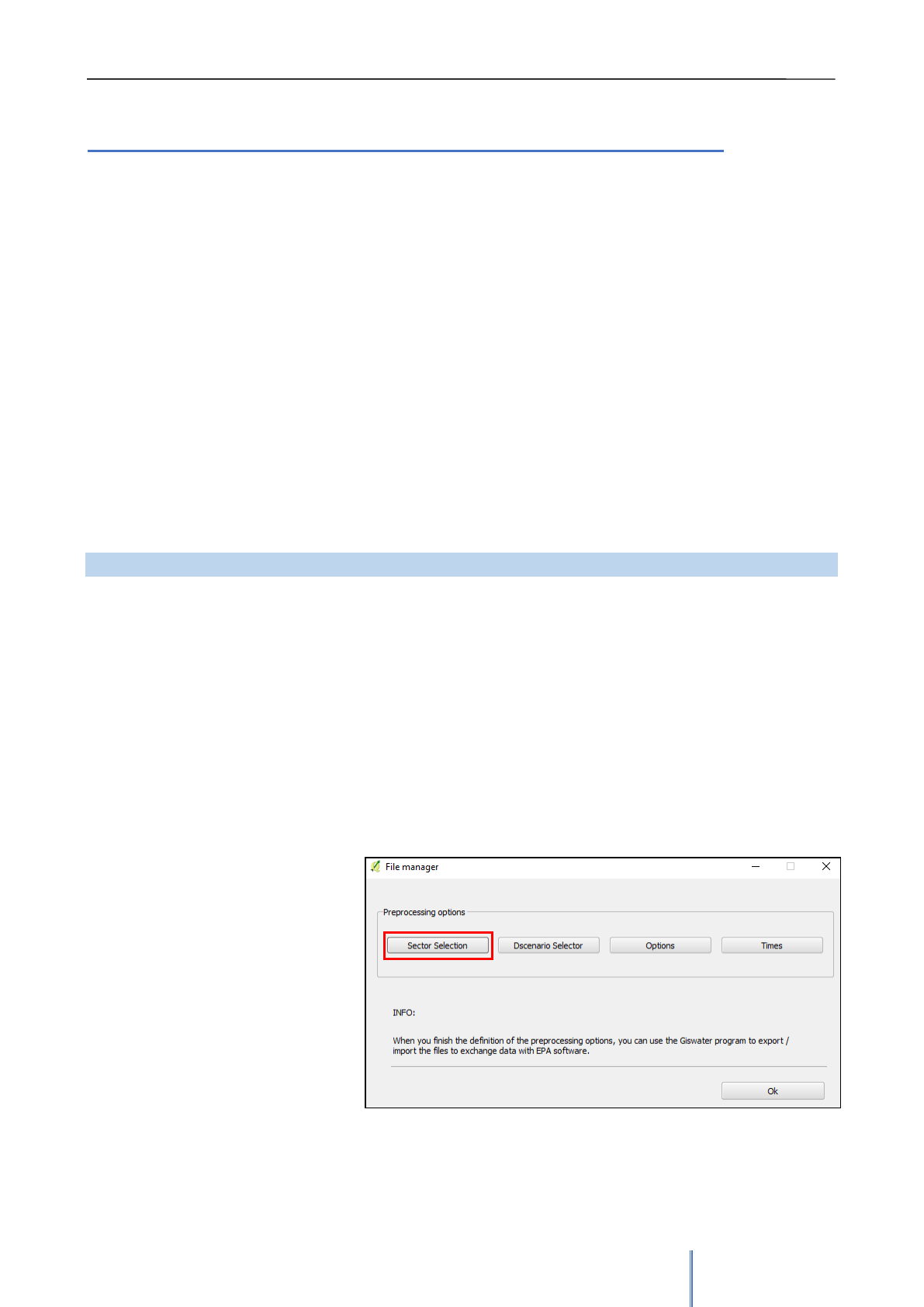
Giswater 3 User Manual
128
7. EXPORT – IMPORT OF THE HYDRAULIC MODEL
7.1 Process characteristics
The process of export-import of a hydraulic model is done almost exactly as in version 1.1 of Giswater (the
driver remains intact) but have introduced a number of improvements, which are list below:
1. The elements can be sent to a model according to their status (STATE) that can be on service,
obsolete or plannified, with the only condition that they have hydraulic coherence. For example, the
case that’s not possible to happen, in a sector there is only a deposit with on service state, and only
planned elements are sent to hydraulic model.
2. In case of WS projects it is possible to configure the roughness according to the age of the pipe. To
do so, use the inp_cat_roughness table and assign the age to the element. If the construction date is
not assigned to the element, it will be considered new for the purpose of capturing the roughness
value.
3. In case of WS, a new concept of elements appeared that is called nodarcos. Nodarcos are those
elements that in inventory management are flow regulating nodes, such as valves or pumps, but in
the hydraulic model they must be arcs, since a flow regulator is always a conceptual element ‘arc'
that regulates flow between two different nodes.
7.1.1 Main characteristics for watter supply networks (WS)
In order to perform the hydraulic model, it’s necessary to have complete and accurate data for each of the
elements and parameters of the model. To understand everything required in each of the hydraulic model
tables, the EPANET manual is available. It specifies in a very exact and detailed way all those necessary
concepts.
7.1.1.1 Working by sectors
The work by sectors allows to filter and send to the hydraulic model only those elements that belong to a
specific sector, or send several sectors at the same time. As specified in section 4.2.1.2 of this manual, the
field 'sector_id' stores the data of the hydraulic sector to which the element belongs, and subsequently
through the table ‘inp_selector_sector’ filters those elements that belong to the selected sectors.
It should be noted that the sectors selected for export to the hydraulic model must have hydraulic coherence,
that is, for WS there must be a water
reserve, which supplies the system
(RESERVOIR, TANK) and at least
one point of consumption.
Image 95: It’s possible to open the sector selector from the form of the tool
Go2EP.
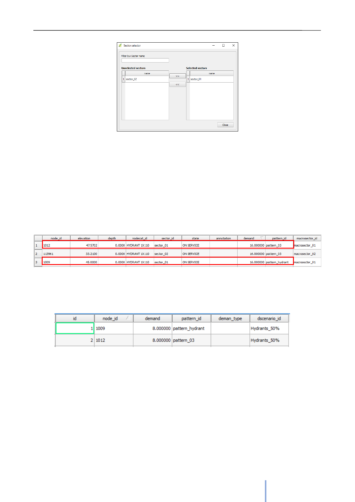
Giswater 3 User Manual
129
7.1.1.2 Demand scenarios
In case of WS networks, exist demand scenarios. The demand scenarios allow to define different demand
hypotheses on the consumption elements (JUNCTION).
In a normal case, the relationship between consumption point and demand value is 1: 1 and the main value
of demand, together with the consumption pattern 'pattern_id' are defined in the table 'inp_junction', as it is
shown in the following image.
Using the 'inp_demand' table user can apply an alternative demand to the main demand of the consumption
node and change the demand pattern. First of all, the new scenario is created in the catalog table
'cat_scenario' and later the node element is linked to the new demand and to the scenario to which it
belongs, as shown below.
7.1.1.3 Transformation of nodes into arcs
Giswater solves this duality using the elements called 'nodarco'. Elements that by their characteristics in the
inventory are nodes, but due to their behavior of flow regulator in the hydraulic model must be arcs. This
'nodarco' element is defined on user‘s demand in the system table (node_type).
All those elements that are labeled as SHORTIPE / VALVE / PUMP, are 'nodarco' type elements, and
therefore their model information is stored in the tables:
- inp_shortpipe
- inp_valve
Image 96: Sector selector for hydraulic model.
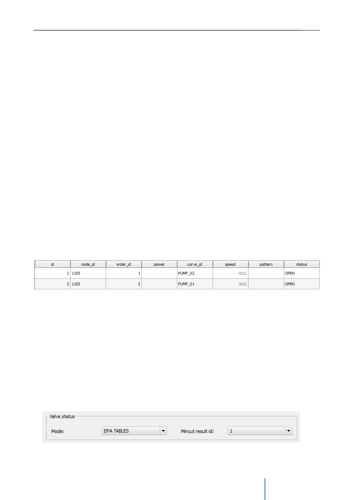
Giswater 3 User Manual
130
- inp_pump
For a 'nodarco' element to be valid, it must comply with the rule of having 1 or 2 extreme arcs, otherwise the
node will not be valid and will not become an arc.
The transformation process from NODE to ARC:
- A new ARC type geometry of 0.5 meters legth or less is generated (suffix _n2a)
- Two new JUNCTION nodes are generated (suffixes n2a1 'initial node' and n2a2 'final node')
- The arc geometries of the existing arcs are 'trimmed' and reconnected to the new nodes to
accommodate the new arch
- The attributes of the JUNCTION elements are inherited from the parent node.
- The attributes of the ARC elements are inherited from one of the two extreme arcs (material,
diameter, etc.)
7.1.1.4 Possibility of multipump
When representing a pump inside Giswater, there is a possibility that the relation between the element and
its behavior in the hydraulic model is not 1:1, but that it contains more than one pump and therefore
generates a 1: n relation with the element,
Every flow regulator labeled as PUMP stores its information in the 'inp_pump' table, which must be
completed with the parameters that regulate the operation of that pump, thus, by default, the relationship that
is generated between the node and the number of pumps is 1: 1.
Using the 'inp_pump_additional' table, Giswater allows to manage more than one pump for a single pump
element. In this table the id of the parent node, the pump number defined in that node, respecting the total
number of additional pumps and the working parameters of each of the additional pumps must be indicated,
as shown in the following example:
The example shows two additional pumps of the node '1105'. It means that this node, when exported to the
hydraulic model, will be transformed into three pump-type arcs each with their own working parameters.
7.1.1.5 Using different state types of valves
The management of the valve status in a supply network is usually dynamic, depending on the needs of the
user its’ state may be one or another to perform the hydraulic simulation of the model. This change in the
status is due to changes in the inventory (broken valve, valve out of service, etc ...) or specific changes in
their status when generating a mincut polygon.
Thus, it can be said that the valves may have different status depending on the table in which the data is
stored: 'inp_shorpipe', 'man_valve' or 'anl_result_mincut_valve'.
Using the button 'Options' inside the form of export to the hydraulic model, user can choose the state of the
valves that will be used in said simulation.
-
Image 97: Part of the form related to the state of valves.
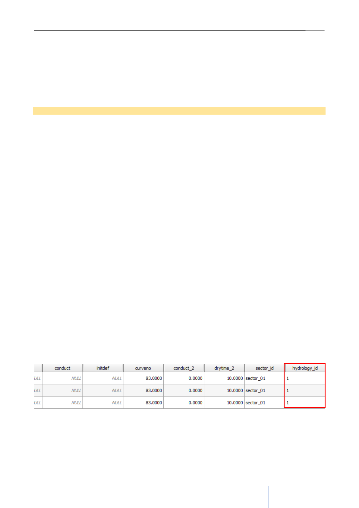
Giswater 3 User Manual
131
EPA TABLE: Those, which state is ‘On service’ o ‘Plannified’ in the layer ‘inp_shortpipe’
- INVENTORY VALUES: Those, which state is ‘On service’ o ‘Plannified’ in the layer ‘man_valve’
- MINCUT RESULT: Those valves that have been affected depending on the results generated by the
mincut polygon. At the same time, user will be able to choose, using the 'Mincut result id' drop-down
list, the results of the mincut polygon that he wishes to model.
7.1.2 Main characteristics for urban drainage networks (UD)
In order to perform the hydraulic model, it’s necessary to have complete and accurate data for each of the
elements and parameters of the model. To understand everything required in each of the hydraulic model
tables, the SWMM manual is available. It specifies in a very exact and detailed way all those necessary
concepts.
7.1.2.1 Working by sectors
The work by sectors allows to filter and send to the hydraulic model only those elements that belong to a
specific sector, or send several sectors at the same time. As specified in section 4.2.1.2 of this manual, the
field 'sector_id' stores the data of the hydraulic sector to which the element belongs, and subsequently
through the table 'inp_selector_sector' filters those elements belonging to the selected sectors.
It should be noted that the sector or sectors selected for export to the hydraulic model must have hydraulic
coherence. For UD networks the minimum requirements would be an entry point of water into the system,
either rain, through the application of a rain in the SUBCATCHMENTS or, through wastewater (DWF), and a
point of exit of the system (OUTFALL).
7.1.2.2 Management of hydrology scenarios
In case of UD networks, exist hydrology scenarios. The hydrology scenarios allow to define different
hypotheses about the method of infiltration, surface runoff, groundwater, de-icing, etc... applied to the
drainage sub-basins (SUBCATCHMENTS).
Using the catalog 'cat_hydrology' it’s possible to define a catalog element referring to the data of water flows
that enter naturally into the system, indicating the identifier, a name and the infiltration method.
The infiltration methods recognizable by SWMM are: curve number, Green-Ampt or Horton equation.
Once the hydrology catalog is defined, each subcatchment needs to be related to the hydrology catalog to
which it belongs, through the inp_subcatchment table, fields hydrology_id..
This relation allows calculation of different hypotheses applied to the same subcatchment and allows, using
the hydrology selector, to select those that should be used for the simulation.
It is important to note that the filled fields that refer to the infiltration method in the inp_subcatchment table
must be recognizable by the hydrology catalog that is imputed to them.

Giswater 3 User Manual
132
7.1.2.3 Integration of the standard form catalog of SWMM
Giswater integrates in its system a variety of geometric sections accepted by SWMM. There are available in
a conduits catalog of UD network. Using the arc catalog table, the different types of conduits are defined,
filling in the following obligatory fields: id, matcat_id, shape and geom fields, necessary to define the shape
of an arc.
In order to know what data should be put in these fields, consult the catalog of SWMM sections. It-s also
important to know how this catalog and the domain table of values of normalized sections work
(cat_arc_shape).
The table cat_arc_shape is composed by the following fields:
- Id: name of the form (in selected language) of the catalog (it’s the value that acts as domain
values of the cat_arc_shape field).
- Epa: name that receives the form in SWMM (see section catalog of SWMM).
- tsect_id: in case of open irregular shapes, label of the set of values in the inp_transects table
that define the irregular geometry according to the HEC format.
- curve_id: in case of forms not included in the catalog of the attached document, name of the
curve defined in the inp_curve table that defines the pairs of values that make up the detail of
form of this section.
- image: system field with the name of the png file that is stored in the Giswater plugin folder
(plugins / giswater / png) and that is called when an info is done on an arc type element and the
cost tab is clicked.
- descript: auxiliary field the description of the section.
- active: boolean field that allows to control if the form is active in the catalog or has been
unsubscribed and is not selectable
Taking into account the previous information and consulting the SWMM section catalog, the geom* fields can
be filled in depending on the choosen form.
Two examples of the relation between the cat_arc_shape table and the arc catalog cat_arc are presen ted
below:
In case of creating circular conduits, called, as 'Round' this translates into:
For the table cat_arc_shape,
cat_arc_shape.id = Round
cat_arc_shape.epa = 'CIRCULAR'
cat_arc_shape.image = 'ud_section_circular.png'
And in the table cat_arc,
cat_arc.shape = ‘Round’
cat_arc.geom1 = Value of the internal diameter of arc expressed in meters.
In case of creating rectangular conduits, called, as ‘Rectangular’ this translates into:
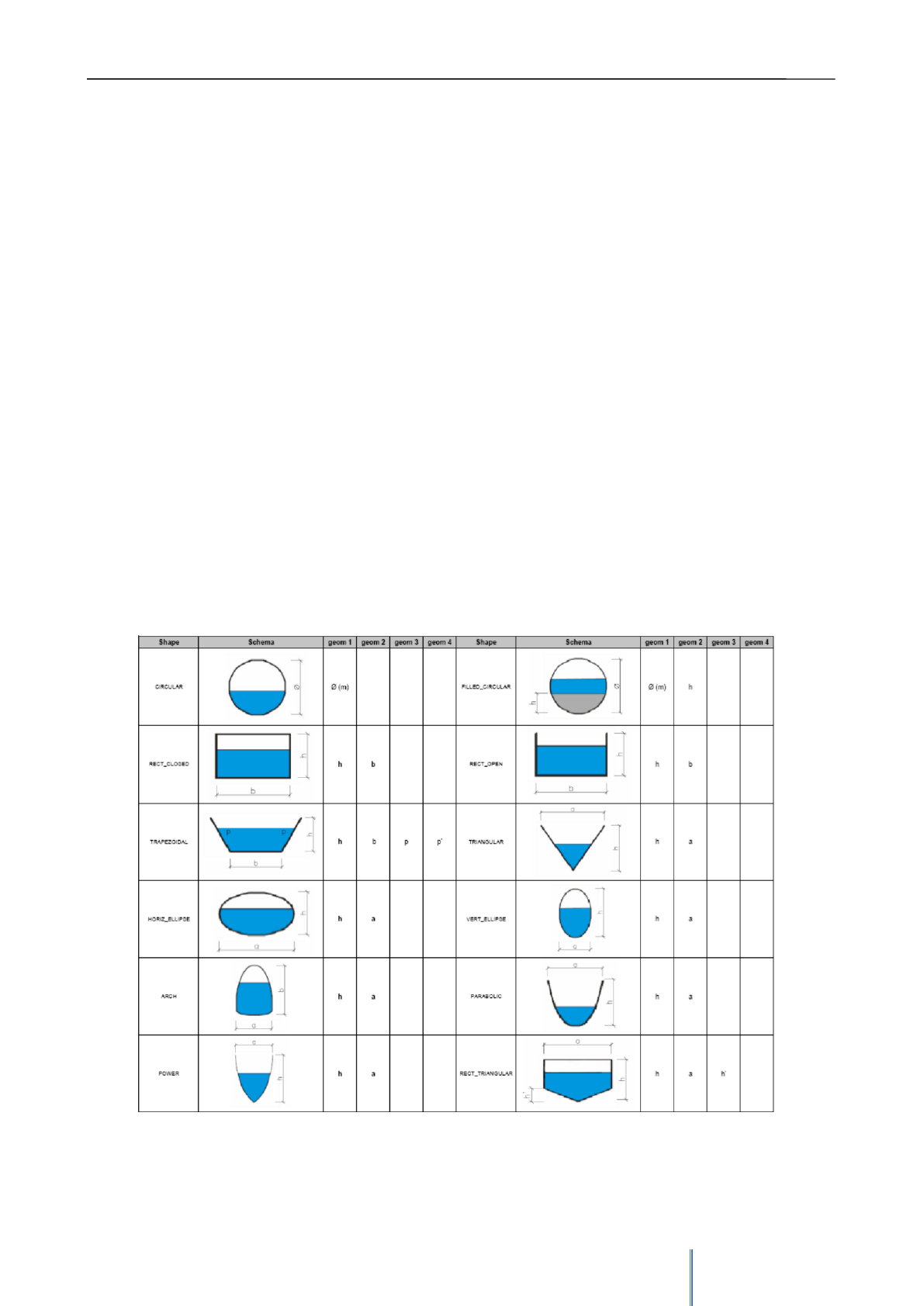
Giswater 3 User Manual
133
For the table cat_arc_shape,
cat_arc_shape.id = 'Rectangular'
cat_arc_shape.epa = 'RECT_CLOSED'
cat_arc_shape.image = 'ud_section_rect_closed.png'
And in the table cat_arc,
cat_arc.shape = 'Rectangular'
cat_arc.geom1 = Value of the vertical dimension of arc expressed in meters
cat_arc.geom2 = Value of the horizontal dimension of arc expressed in meters
In reality the table cat_arc_shape is already filled in with all the standardized forms of SWMM, so expanding
this catalog according to the needs of user is quite easy to understand and proceed.
THREE BASIC RULES need to be fulfilled:
1) The value of cat_arc_shape.id can be customized by user, but the value of cat_arc_shape.epa must
always be normalized to one of the values of the SWMM section catalog.
2) All the measurements (cat_arc.geom*) are interior and should be expressed in meters.
3) Values of cat_arc.geom1 always correspond to the vertical dimension of the element, just as the values of
cat_arc.geom2 always correspond to the horizontal dimension of the element
For the other cases, consult the SWMM section catalog.
Image 98: Table with different SWMM sections available in Giswater as a method of arc shape inventory.

Giswater 3 User Manual
134
7.1.2.4 Flow regulators
For the management of different flow controllers, version 3.0 of Giswater maintains the same logic as the
previous versions where virtual arcs can be assigned to an EPA element.
In this sense, there are two types of virtual arcs, those that enter into the node (which would be the
prolongation of the driving that precedes it) and those that leave the node (which would be the flow
regulators).
In the first case, the virtual arc is simply a flow propagator, which apart from the characteristics of the
element must have indicated the direction it drains (node 2). In this way, when carrying out the export to the
hydraulic model, what Giswater does is joining this virtual arc with its predecessor, converting the two into a
single one.
At the same time, if the add_length field value is true, the length of the virtual arc will be added at the time of
merging, but if we have it in false, the length of that element will not be added
In a practical case, the virtual arcs which are propagators of flow, would be applied to nodes of big
dimensions like deposits or cameras. Its arcs arrive to them but do not connect with the center, but remain at
its perimeter. The connection section between these two points would be a virtual_arc.
In the second case the virtual arc behaves as a flow regulator. The flow regulators are structures or devices
used to control and derive the flows within the transportation system. The flow control elements that SWMM
can model are the ones listed below, together with the information in which tables there are stored:
- Orifice, tabla: inp_flwreg_orifice
- Weirs, tabla: inp_flwreg_weir
- Outlets, tabla: inp_flwreg_outlet
- Pump, table: inp_flwreg_pump
At the moment of introducing a new flow regulator, the following parameters must be defined in the tables
mentioned above: source node, target arc, ordinal regulation (in case of introducing more than one regulator
between that node and that arc with that type of regulation), and finally the different parameters that control
that regulator.
In the particular case when there is a virtual arc just after the node, the field exit_conduit must not be the
arc_id of the virtual arc but must be the arc_id of the conduit that receives the flow, since the operation of
merging the virtual arcs with the conduit is coupled with the arc_id of the conduit.
If more than one regulator coexists between a given node and arc, at the time of export, the system draws
for SWMM as many arcs as regulators.
Important aspects related to flw_length parameter:
- The parameter flw_length is the length of the flow regulator.
- If there is more than one flow regulator between the node and arc, the system will take the
maximum value.
- The length of the flow regulator is important in case of orifices or weirs and refers to the
distance downstream of it, in which normal flow conditions in the pipeline can not be assumed,
ie it is an ineffective length of the pipeline. downstream conduit.

Giswater 3 User Manual
135
8. REAL-TIME MATHEMATICAL MODEL (RTC) FOR WS
Giswater 3 is pre-configured to simulate flow data in real time for the water supply projects (WS). It allows to
calibrate with real data the obtained model results. For this purpose, the working workflow of real drinking
water network data is as follows:
First thing to comment is that the commercial management system should be integrated into the GIS and
that can be done using this table proposal:
CREATE TABLE hydrometer(
id bigint PRIMARY KEY,
code text,
connec_id integer,
muni_id integer,
plot_code integer,
priority_id integer,
catalog_id integer,
category_id integer,
state_id integer,
hydro_number text,
hydro_man_date date,
crm_number text,
customer_name text,
address1 text,
address2 text,
address3 text,
address2_1 text,
address2_2 text,
address2_3 text,
m3_volume integer,
start_date date,
end_date date,
update_date date);
CREATE TABLE hydrometer_x_data (
"id" bigserial PRIMARY KEY,
"hydrometer_id" bigserial NOT NULL,
"m3value" float,
"value_date" date,
"period_id" integer);
CREATE TABLE hydro_cat_catalog(
"id" int8 PRIMARY KEY,
"code" character varying(16),
"hydro_type" character varying(100),
"madeby" character varying(100),
"class" character varying(100),
"flow" character varying(100),
"dnom" character varying(100),
"observ" text);
CREATE TABLE hydro_cat_type(
"id" integer PRIMARY KEY,
"code" character varying(16) NOT NULL,
"observ" character varying(100));

Giswater 3 User Manual
136
CREATE TABLE hydro_cat_category(
"id" integer PRIMARY KEY,
"code" character varying(16) NOT NULL,
"observ" character varying(100));
CREATE TABLE hydro_val_state(
"id" integer PRIMARY KEY,
"code" character varying(16) NOT NULL,
"observ" character varying(100));
CREATE TABLE hydro_cat_period(
"id" integer PRIMARY KEY,
"code" character varying(16) NOT NULL,
"observ" character varying(100));
CREATE TABLE hydro_cat_priority(
"id" integer PRIMARY KEY,
"code" character varying(16) NOT NULL,
"observ" character varying(100));
Using a script for connecting to the CRM, these tables can be filled either with the real time data, or with data
obtained through process of loading and updating during the night. Once the tables are filled in, it’s
neccessary to relate that information using the tables and views of Giswater rtc_ * with their corresponding
correlation.
LAYERS NECESSARY FOR REAL TIME MAPPING OF SCADA VALUES
ext_rtc_hydrometer_x_value: shows the current value of hydrometers (for remote reading)
ext_rtc_scada_x_value: shows the current value of scada
LAYERS FOR INFORMATIONAL ONLY
ext_cat_scada: scada catalog, optional
rtc_scada_x_dma: Scada x dma with the flow sign, optional
rtc_scada_x_sector: Scada x sector with the flow sign, optional
ext_rtc_scada_x_data: Valores hitorical values of scada (deprecated)
Hydrometers:
rtc_hydrometer: commercial table of inserted hydrometers
rtc_hydrometer_x_connec: table with the relation between hydrometers and connecs
Scada:
ext_rtc_scada: Tableof all registered SCADAS
rtc_scada_node: table with relation between scada and nodes
RTC Calculation:
ext_cat_period: Period catalog
IMPORTANT: periods of SCADA should be the same as COMMERCIAL periods
ext_rtc_hydrometer_x_data: Hydrometers’ values used for the real time calculation
IMPORTANT: periods of SCADA should be the same as COMMERCIAL periods
ext_rtc_dma_period: Total values of dma per period
IMPORTANT: periods of SCADA should be the same as COMMERCIAL periods

Giswater 3 User Manual
137
IMPORTANT: The minimum, maximum, average values refer to the measurement interval (5 minutes, 10
minutes, etc), but the same for all three tables. These values will allow to calculate the maximum, minimum
and loss values.
On the other hand, the total period value can be compared with the total value of the hydrometers period and
establish the loss ratio for the dma.
The calculation options are available in the options form (CRM group VALUES) where
it is necessary to activate the option of CRM (check box of CRM values enabled). From there it’s possible to
select the calculation period from among all available (Time period) and the coefficient, maximum, minimum,
average value, with which it is intended to simulate within this calculation period (Coefficient)
To show in GIS:
All SCADA field data (flow rate & pressures) of the DMCs can be consulted using rtc_scada_value.
The information of the commercial data bank of monthly hydrometers’ consumption of can be consulted
using rtc_hydrometer_value.
In order to make an EPANET calculation:
In the table ext_cat_period different periods are defined and stored, from which an aggregate query of all the
data of the SCADA and the HYDROMETER can be made.
With the information of specific period defined in rtc_period, the values for the different DMAs are recorded in
the table ext_rtc_dma_period, thus obtaining for a given period:
- Contour flows: maximum, minimum and average (difference between the incoming and outgoing flows
measured by the macro-meters)
- Total monthly flow.
These data are compared with the aggregate values of all consumers within the DMA for a given period of
time (cat_period) and also with the previous ones to establish the loss coefficient. Based on the coefficient of
losses and the maximum / minimum factors based on the values of ext_rtc_dma_period, the compensated
values can be sent to EPANET:
Note: The aggregation of flow values for each hydrometer is done in the following way:
1- The reading of the total hydrometer value of the selected period is made
2- The coefficient of losses that is recorded in the DMA is applied
3- The maximum / minimum coefficient is applied, depending on user’s choice
4- The different hydrometer values of a single connec are added
5- The different values of all the connec for a single arc are added
6- The 50% division of the flow values for a given arc between its extreme nodes is performed.
7- The sum of all values received by each node from its different arcs is calculated.
8- The information is sent to the hydraulic model, overwriting the estimated values that the nodes have.
In case that a node has an estimated value, but has no real value, the model will be made using the
estimated value.
Image 99: Part of the form of the tool Go 2 EPA, which incorporates the values of CRM.
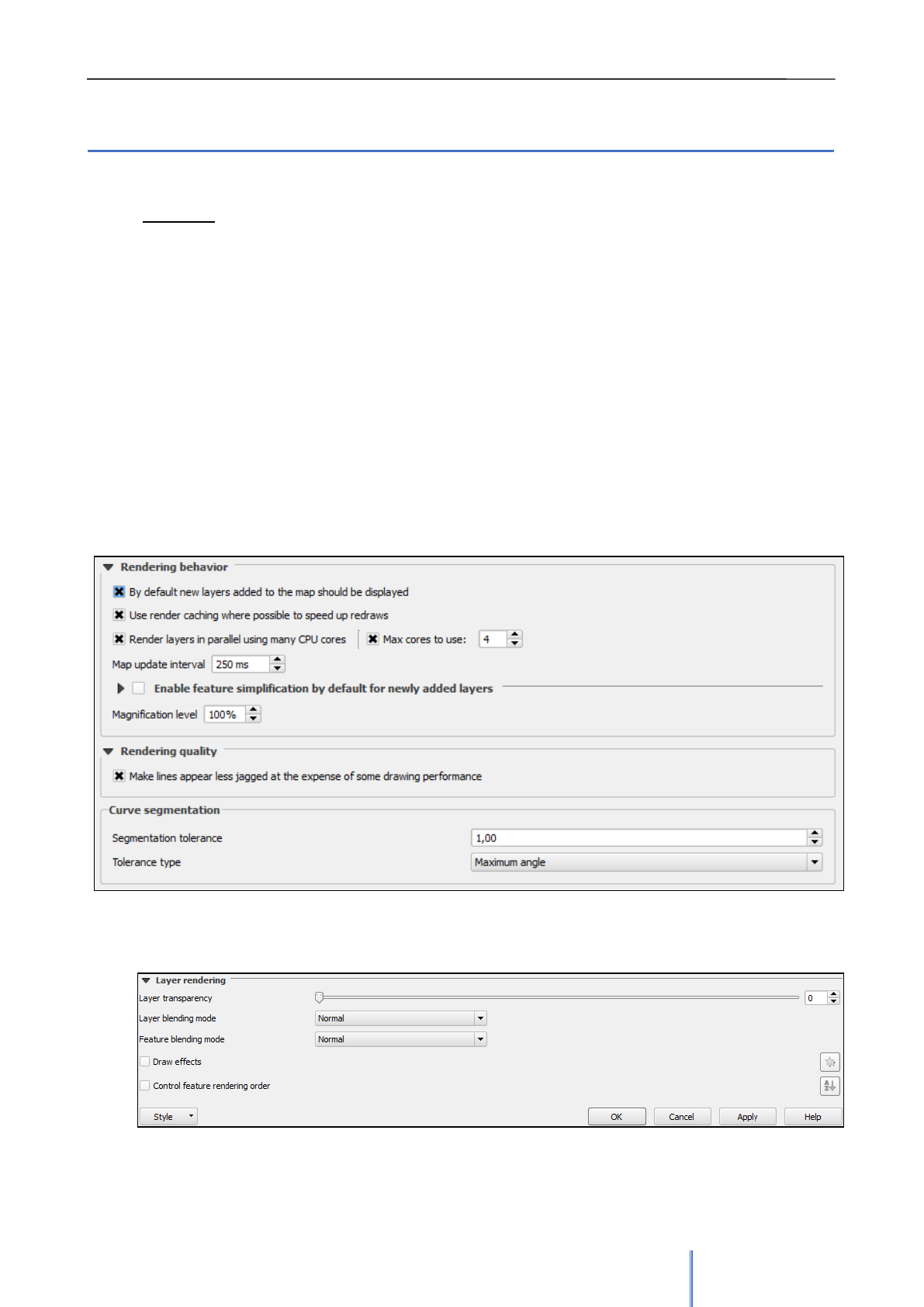
Giswater 3 User Manual
138
9. OTHER CONSIDERATIONS
9.1 Good practice
• Rendering
1) Only the visible information is being renderized:
It’s important to study the performance and take the decision (activate).
It’s crucial in order to gain the speed of the project.
>5000 only arcs
<5000 tanks
<2000 everything
<1500 connecs
<1000 links
<500 virtuals
2) Good QGIS configuration
Open: Settings > Options > Rendering. The configuration that is displayed in image 100
would be a correct example for layer rendering.
E
E
Each layer also should be controlled: Layer propertie > Style > Layer rendering
9.2
Man
Image 100: Example of the configuration neccessary to good performance of rendering.
Image 101: Correct settings of layer rendering
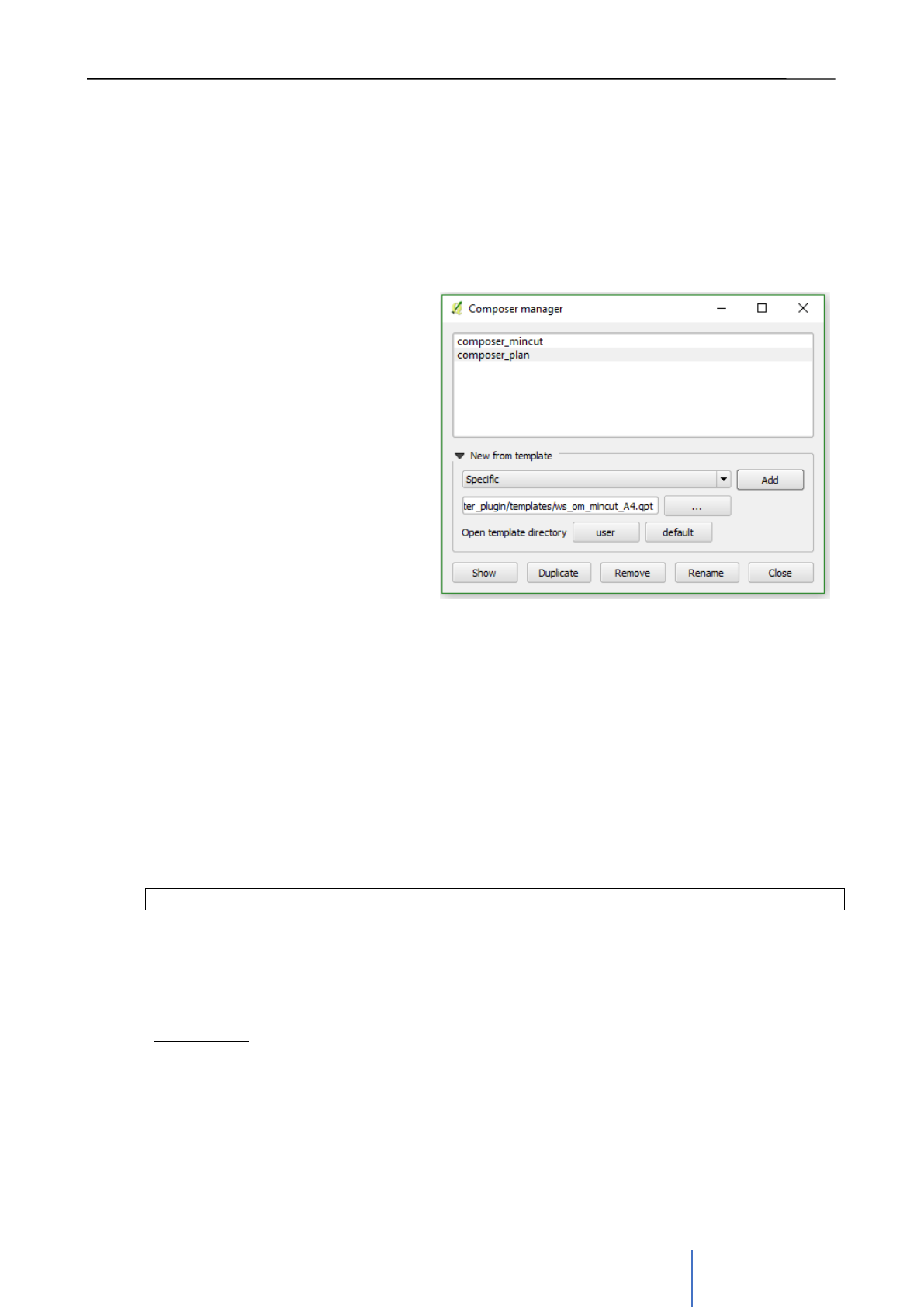
Giswater 3 User Manual
139
agement and use of the QGIS composer
Giswater offers different templates to generate plans and maps of some part of the project. As already
mentioned in previous sections, some of the tools directly incorporate the generation of plans using the
composer templates. As examples, the tools of the longitudinal profile, the mincut polygon or the planning
sectors generate plans directly
The Giswater plugin folder has a subfolder called templates that contains several qpt files, QGIS templates,
that the user can call from the composer manager and add them to the project. Initially in this folder there are
templates to make plans of the longitudinal
profile, mincut polygon and the planning sectors
(om and plan) for both A3 and A4 format.
However, each user can generate their own
templates for the composer, so that any
generated plan can have the desired
appearance. For less experienced users, a good
way to generate your own template is to copy
some of the existing ones in Giswater and modify
some of its parts.
9.3 Control and verification of projects and schemas
As seen throughout the manual, the Giswater data schemas are complex and have a large number of tables,
views and layers with dependencies between them, which can be difficult to understand at the beginning.
All Giswater data schema incorporates a "group" of tables and functions that allow the user to control
different parameters, perform certain actions or verify processes, always in relation to the management of
tables and the data they contain. The purpose of these audit tables is to provide users with help tools in the
management and editing processes of Giswater.
- Audit check project
Shows in QGIS if the project is missing some important layer to load.
Description: This function reads the tables present in QGIS project and compares them with the
existing ones in the table audit_cat_table. Those that in this table have the field qgis_criticity
greater than 0 should be loaded in the project, because their presence is necessary for the proper
functioning of the tools of Giswater.
How it’s used: It’s activated alone. Each time the QGIS project is opened, the function reads the
loaded layers and, in case of finding any with criticality greater than 0 that is not loaded, warnes the
user showing the list of missing layers.
Image 102: Composers management form. Those linked to the
QGIS project are represented here. In the templates folder there
are more templates unlinked with the project
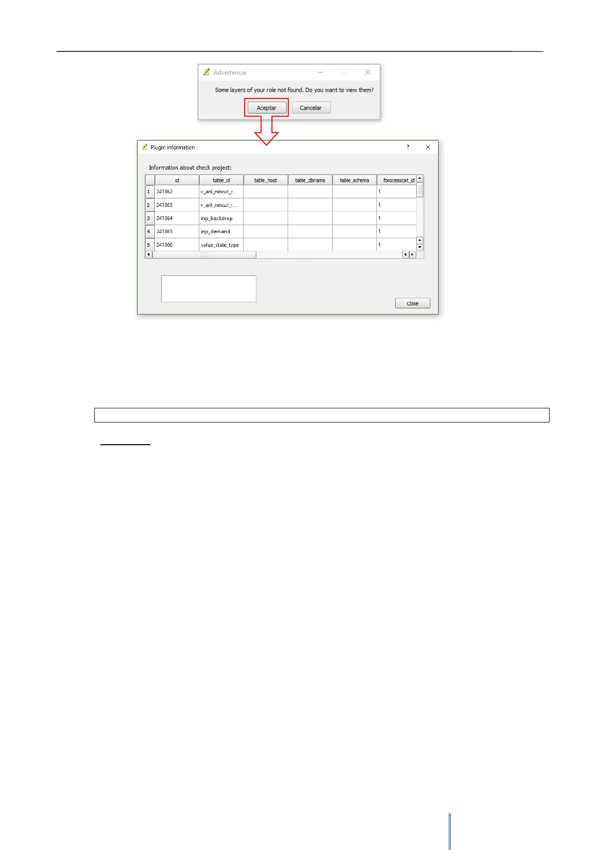
Giswater 3 User Manual
140
- Audit check data
It informs if there are important fields for budget that have value null
Description: shows if some of the important columns for budget planning are empty. Acts on the
following tables:
• fprocesscat_id = 15 – For the processes in which the value NULL affects the calculation of
reconstruction results:
- Table: cat_arc Columns: active, cost, m2bottom_cost, m3protec_cost
- Table: cat_node Columns: active, cost, cost_unit, estimated_depth, estimated_depth, estimated_y
- Table: cat_connec Columns: active, cost_m1, cost_m3
- Table: cat_pavement Columns: thickness, m2_cost
- Table: cat_soil Columns: y_param, b, m3exc_cost, m3fill_cost, m3excess_cost, m2trenchl_cost
- Table: cat_grate Columns: active, cost_ut
- Table: arc Columns: (compares arcs in state other than obsolete with the registers in table
plan_arc_x_pavement)
- Table: plan_arc_x_pavement Columnas: pavcat_id
• fprocesscat_id = 16 - For the processes in which the value NULL affects the calculation of
rehabilitation results
For each of these tables, the function counts all the active rows and, at the same time, the rows for
the particular columns that are not null. If when comparing both values there are less rows of the
concrete column than of total active rows, it means that there will be NULL values in the column.
Image 103: The function audit_check_project acts every time the project is
opened. In case of finding the layers that should be loaded, but are not, shows
the list of those layers.
List with missing
tables
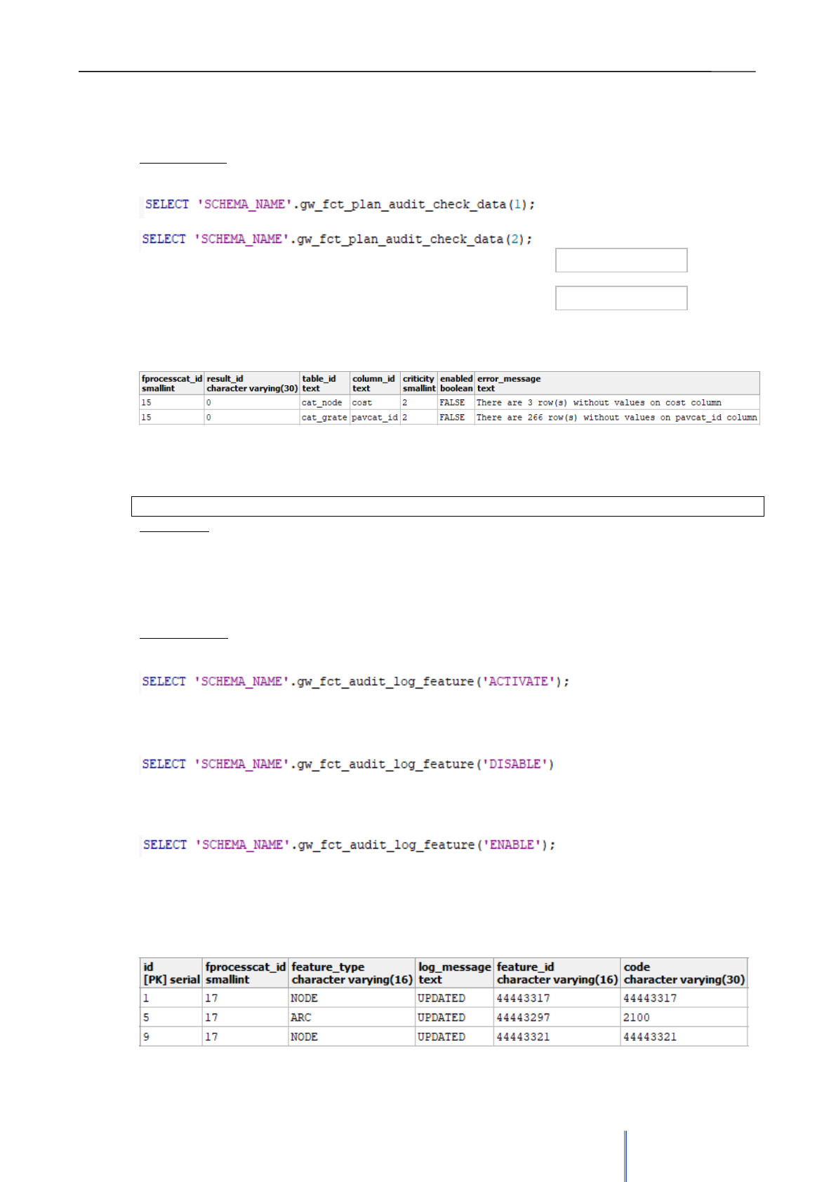
Giswater 3 User Manual
141
Finally, the function stores in the table audit_check_data a row with information regarding the table,
the column and the number of rows with NULL values that it has found.
How it’s used: the functionality can be activated the Toolbox tool all writing the following SQL query
in Postgres:
This will automatically fill in the table audit_check_data showing rows
with null values related to the column and specific table. The final
objective of this function is to provide the user with the
necessary information if he has all the data filled in order to perform the reconstruction (15) or
rehabilitation (16) calculations.
- Audit log feature
Saves in a table all the modifications made to the data of the
Description: this function allows managing changes, both deletion and modification of data, for all
types of project elements: node, arc, connec, gully and element. In this way it’s possible to control
all changes and rectify them in case of commiting an error. The table of the database
audit_log_feature stores in rows every change made in the data, differentiating through a column if
it is an UPDATE or DELETE operation.
How it’s used: this functionality is disabled by default, because it stores a large amount of data for
no reason. It can be activated using the following SQL query in Postgres:
At this moment all the neccessary triggers and the function will be activa. It’s possible to
desactivate it using the folowing query:
If the triggers have already been created and have been deactivated once, they must not be
created again to reactivate them. They can be reactivated using the following query:
If the function is active, with each modification made in the data of an element, a new row will be
stored in the table audit_log_feature with all the information of the element before the modification.
For example, if the code field of a node is changed from 2100 to 2150, the code 2100 will be
saved, since the 2150 will be the one that will remain in the element’s table.
Reconstruction
Rehabilitation
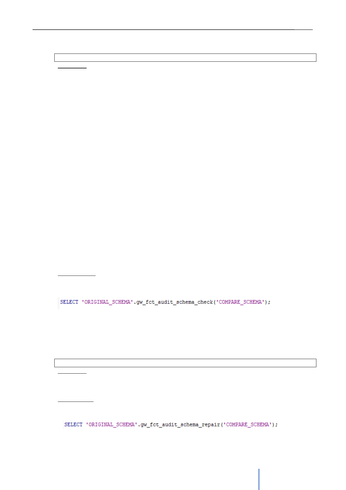
Giswater 3 User Manual
142
- Audit schema check
It allows to compare the information of two different schemes by creating views
Description: This function aims to offer all the necessary information in order to compare two
different data schemas. This can be functional in cases where modifications have been made and it
is not known exactly what they were. If there is a scheme that is known to be correctly filled in,
comparing both schemes can be useful to obtain information about the modifications made in one
of the two.
To show such information, the function generates different views in the scheme where it is called,
what we will call the original scheme. The other will be the comparison scheme. The views
generated are the following:
• v_audit_schema_column: reads all the columns of the tables and views of the original
schema
• v_audit_schema_table: reads all the tables and views of the original schema
• v_audit_schema_catalog_compare_table: shos the tables of the original schema that are not
present in the audit_cat_table.
• v_audit_schema_foreign_column: reads all the columns of the tables and views of the
comparison schema
• v_audit_schema_foreign_compare_column: shows all the columns present in one schema
but not in the other
• v_audit_schema_foreign_compare_table: shows all the tables present in one schema but not
in the other
With all the information of the views, the user can easily know what are the differences in the
architecture of the schemes, not the data itself, and can act accordingly.
How it’s used: the use of this function is very simple and must be done through a query in the
database by writing the name of the original scheme in front of the function and the name of the
comparison scheme below, as follows:
ATTENTION: the original scheme and the comparison one must be in the same database so that
the function can compare its information.
- Audit schema repair
Allows to repair a scheme with the information from another one
Description: This tool can be used to repair a scheme based on the information of another scheme.
Unlike the audit_schema_check function, this directly modifies the working scheme by adding
tables, columns and different inherited rules of the scheme with which it is compared.
How it’s used: the function must be called directly with a query in the database, basically in the
same way as the previous function, only changing the name of the function.
