Manual Osloctm3
User Manual:
Open the PDF directly: View PDF ![]() .
.
Page Count: 145 [warning: Documents this large are best viewed by clicking the View PDF Link!]
Oslo CTM3
v1.0
User manual
Amund Søvde Haslerud
CICERO Center for International Climate Research
November 6, 2018

Oslo CTM3 user manual November 6, 2018
Abstract
This manual contains a description of the Oslo CTM3
and how to set up simulations. Information about emis-
sions, which type of simulation you want do, with which
components etc. are described, but most of all, this man-
ual attempts to document the different processes and the
source code of the Oslo CTM3.
Contents
1 Oslo CTM3 manual 5
1.1 Historical background . . . . . . . . . . . 5
1.2 Version numbering . . . . . . . . . . . . . 5
1.3 Oslo CTM3 vs the UCI CTM . . . . . . . 5
1.4 Limitations to Oslo CTM3 . . . . . . . . . 6
2 Get started 6
2.1 How to get the model – SVN . . . . . . . 6
2.2 User manual . . . . . . . . . . . . . . . . . 6
2.3 Source code directory . . . . . . . . . . . 6
2.4 Model grid . . . . . . . . . . . . . . . . . 6
2.4.1 Degraded resolution . . . . . . . . 7
2.5 Oslo CTM3 vs Oslo CTM2 . . . . . . . . 7
2.6 Variable names . . . . . . . . . . . . . . . 8
2.7 Setting up the model . . . . . . . . . . . . 8
2.7.1 Makefile ............... 9
2.7.2 Main program – pmain . . . . . . 9
2.7.3 Input file – LxxCTM.inp ...... 9
2.7.4 Tracer list – tracer_list.d ..... 10
2.7.5 Emissions list –
Ltracer_emis_xxxx.inp ...... 10
2.7.6 Meteorological data . . . . . . . . 11
2.7.7 Restart file . . . . . . . . . . . . . 11
2.7.8 Other input data . . . . . . . . . . 12
2.7.9 Surface CH4 . . . . . . . . . . . . 12
2.7.10 Transport options . . . . . . . . . 13
2.8 Compiling . . . . . . . . . . . . . . . . . . 13
2.9 Running the model . . . . . . . . . . . . . 13
2.9.1 Model crashes . . . . . . . . . . . . 13
2.10 Publishing & documenting . . . . . . . . . 13
2.10.1 Publishing in journals . . . . . . . 13
2.10.2 Documenting changes . . . . . . . 13
3 Source code introduction 14
3.1 The core source . . . . . . . . . . . . . . . 14
3.1.1 The parameter files . . . . . . . . . 14
3.1.2 Global variable files . . . . . . . . 14
3.1.3 Main program . . . . . . . . . . . 14
3.1.4 Core diagnostics . . . . . . . . . . 14
3.2 The Oslo core source . . . . . . . . . . . . 14
3.2.1 Important variables . . . . . . . . 14
3.2.2 Application variables . . . . . . . . 15
3.2.3 Dummies . . . . . . . . . . . . . . 15
4 Program structure 15
4.1 Main structure – pmain.f90 ........ 15
4.1.1 Main loops . . . . . . . . . . . . . 15
4.1.2 Sub-stepping loop . . . . . . . . . 16
4.1.3 Internal chemistry loop . . . . . . 16
4.1.4 Important notes . . . . . . . . . . 16
4.2 The C-code preprocessing system . . . . . 17
4.3 Parallelisation of the Oslo CTM3 . . . . . 17
4.3.1 OpenMP . . . . . . . . . . . . . . 17
4.3.2 Parallel IJ-blocks (MP-blocks) . . 17
4.3.3 Parallel layers . . . . . . . . . . . . 18
4.3.4 OpenMP and advection . . . . . . 18
4.3.5 Writing parallelized code . . . . . 18
4.3.6 How many CPUs and IJ-blocks? . 18
4.4 Module based programming . . . . . . . . 20
5 Programming guidelines 20
5.1 Comment your code! . . . . . . . . . . . . 20
5.2 Change existing code? . . . . . . . . . . . 20
5.3 Accessing variables in Fortran90 free format 20
5.4 Adding a new subroutine . . . . . . . . . 20
5.5 Adding new components . . . . . . . . . . 20
5.6 Efficient code . . . . . . . . . . . . . . . . 21
5.7 Unit conversion . . . . . . . . . . . . . . . 21
5.7.1 Mass to concentration . . . . . . . 21
5.7.2 Mass to mixing ratio . . . . . . . . 21
5.7.3 vmr to mmr . . . . . . . . . . . . . 21
5.7.4 Concentration to mixing ratio . . . 21
5.8 Keep pmain clean . . . . . . . . . . . . . . 22
5.9 Precision of numbers . . . . . . . . . . . . 22
5.10 Stay away from C-code . . . . . . . . . . . 22
5.11 Looping in Fortran . . . . . . . . . . . . . 22
5.12 Implicit none . . . . . . . . . . . . . . . . 23
6 Transport 23
6.1 Secondary Order Moments . . . . . . . . . 23
6.2 Advection . . . . . . . . . . . . . . . . . . 23
6.2.1 Horizontal advection . . . . . . . . 23
6.2.2 Vertical advection . . . . . . . . . 23
6.3 Convection . . . . . . . . . . . . . . . . . 24
6.4 Boundary layer mixing . . . . . . . . . . . 25
6.4.1 NBLX=1: Prather scheme . . . . . 25
6.4.2 NBLX=5: Holtslag . . . . . . . . . 25
6.4.3 Other schemes . . . . . . . . . . . 25
7 Wet and dry scavenging 25
7.1 Wet scavenging . . . . . . . . . . . . . . . 25
7.1.1 Large scale scavenging . . . . . . . 26
7.1.2 Convective scavenging . . . . . . . 26
7.1.3 Theory on Henry’s law . . . . . . . 27
7.1.4 Hard-coded Henry coefficients . . . 28
7.2 Dry deposition . . . . . . . . . . . . . . . 28
7.2.1 Historical note . . . . . . . . . . . 28
7.2.2 The new dry deposition scheme . . 29
7.2.3 Technical description: gaseous
species................ 29
7.2.4 Technical description: aerosols . . 33
7.2.5 Soil uptake of CH4......... 33
7.2.6 Inside or outside chemistry? . . . . 33
7.2.7 UCI dry deposition . . . . . . . . . 34
7.3 Uptake on aerosols . . . . . . . . . . . . . 34
8 Emissions 34
8.1 Emissions treatment . . . . . . . . . . . . 34
8.1.1 Emissions in chemistry . . . . . . . 34
8.1.2 Emissions as a process . . . . . . . 34
8.2 Important about NOx . . . . . . . . . . . 34
8.3 How to set up emissions . . . . . . . . . . 34
8.4 Emission datasets . . . . . . . . . . . . . . 35
8.4.1 Monthly & annual emissions . . . 36
8.4.2 Diurnal scaling . . . . . . . . . . . 36
8.4.3 Vertical distribution of 2D emissions 37
8.4.4 Short term variations . . . . . . . 37
8.5 Forest fires emissions . . . . . . . . . . . . 38
8.6 Biogenic emissions: MEGAN . . . . . . . 39
8.6.1 Modifications to MEGAN code . . 39
8.6.2 MEGAN total emissions . . . . . . 40
8.7 Aircraft emissions . . . . . . . . . . . . . . 40
8.8 Lightning emissions . . . . . . . . . . . . . 40
8.8.1 Horizontal distribution – OAS2015 40
2

Oslo CTM3 user manual November 6, 2018
8.8.2 Horizontal distribution – GMD2012 42
8.8.3 Horizontal distribution – AP2002 . 43
8.8.4 Horizontal distribution – UCI2015 43
8.8.5 Horizontal distribution – other . . 43
8.8.6 Vertical distribution . . . . . . . . 43
8.8.7 Lightning scaling factors . . . . . . 43
8.9 CH4emissions . . . . . . . . . . . . . . . 44
8.10 Emission diagnoses . . . . . . . . . . . . . 44
8.11 Pre-defined datasets . . . . . . . . . . . . 44
8.11.1 CEDS . . . . . . . . . . . . . . . . 44
8.11.2 ECLIPSE . . . . . . . . . . . . . . 45
8.11.3 EDGAR v4.2 . . . . . . . . . . . . 45
8.11.4 Lamarque/IPCC . . . . . . . . . . 45
8.11.5 HTAP . . . . . . . . . . . . . . . . 45
8.11.6 RETRO . . . . . . . . . . . . . . . 45
8.11.7 POET . . . . . . . . . . . . . . . . 45
8.11.8 CH4emissions Bousquet . . . . . . 45
8.11.9 Volcanic emissions . . . . . . . . . 45
8.11.10 Soil emissions . . . . . . . . . . . . 45
8.11.11 Biomass burning . . . . . . . . . . 45
9 QSSA chemical integrator 45
9.1 Long-lived species . . . . . . . . . . . . . 46
9.2 Short-lived species . . . . . . . . . . . . . 46
9.3 Species of intermediate lifetime . . . . . . 46
10 Tropospheric chemistry 46
10.1 Non-transported species . . . . . . . . . . 46
10.2 Tropospheric domain . . . . . . . . . . . . 46
10.3 Without stratospheric chemistry; O3,
NOx and HNO3............... 46
10.4 Box version of tropospheric chemistry code 48
11 Stratospheric chemistry 48
11.1 Technical information . . . . . . . . . . . 48
11.2 Stratospheric H2O ............. 48
11.3 Microphysics . . . . . . . . . . . . . . . . 49
11.4 Heterogeneous chemistry . . . . . . . . . . 50
11.5 Input files needed . . . . . . . . . . . . . . 50
11.6 Upper boundary / Chemistry in LPAR? . 50
11.7Linoz..................... 50
12 Photochemistry 50
12.1 Solar flux . . . . . . . . . . . . . . . . . . 51
12.2 Cloud cover . . . . . . . . . . . . . . . . . 51
12.2.1 Average cloud cover . . . . . . . . 51
12.2.2 Random cloud cover . . . . . . . . 51
12.3 Aerosols in fast-JX . . . . . . . . . . . . . 52
12.4 Generating cross sections . . . . . . . . . 52
12.5 Generating scattering properties . . . . . 52
12.5.1 FJ_phase . . . . . . . . . . . . . . 53
12.5.2 Mishchenko spher.f . . . . . . . . . 54
13 Sulphur module 54
13.1 Sulphur emissions . . . . . . . . . . . . . . 55
13.2 SO4scattering and absorption . . . . . . . 55
14 Black carbon and organic matter 55
14.1 BC/OM emissions . . . . . . . . . . . . . 55
14.2 BC/OM deposition . . . . . . . . . . . . . 56
14.3 BC/OM wet scavenging . . . . . . . . . . 56
14.4 BC/OM scattering and absorption . . . . 56
14.5 BC on snow – BCsnow . . . . . . . . . . . 56
14.6 Secondary organic aerosols . . . . . . . . . 57
15 Mineral dust 57
15.1 Get DUST running . . . . . . . . . . . . . 57
15.2 Dust size bins . . . . . . . . . . . . . . . . 58
15.3 Dust sources . . . . . . . . . . . . . . . . 58
15.3.1 Input files needed . . . . . . . . . . 58
15.3.2 Technical . . . . . . . . . . . . . . 58
15.3.3 Wind speed variability . . . . . . . 59
15.4 Dust sinks . . . . . . . . . . . . . . . . . . 59
15.4.1 Gravitational settling . . . . . . . 59
15.4.2 Wet scavenging . . . . . . . . . . . 59
15.5 DUST scattering and absorption . . . . . 59
15.6 Things to watch out for . . . . . . . . . . 60
15.7 Dust budgets . . . . . . . . . . . . . . . . 60
15.8 Additional notes . . . . . . . . . . . . . . 60
15.9 Into the future . . . . . . . . . . . . . . . 60
16 Sea salt 60
16.1 Sea salt production . . . . . . . . . . . . . 60
16.2 Technical information . . . . . . . . . . . 61
16.2.1 Wet scavenging . . . . . . . . . . . 61
16.3 SALT scattering and absorption . . . . . . 61
16.4 Salt budgets . . . . . . . . . . . . . . . . . 61
17 Nitrate 61
17.1 Nitrate physics – modes . . . . . . . . . . 61
17.2 Nitrate tracers . . . . . . . . . . . . . . . 62
17.3 Sea salt in the nitrate model . . . . . . . 62
17.4 Nitrate emissions . . . . . . . . . . . . . . 62
17.5 Remaining problems . . . . . . . . . . . . 62
17.6 Box version . . . . . . . . . . . . . . . . . 63
18 M7 63
19 Secondary organic aerosols (SOA) 63
19.1 SOA precursor tracers . . . . . . . . . . . 63
19.2 SOA tracers . . . . . . . . . . . . . . . . . 63
19.3 SOA sources and sinks . . . . . . . . . . . 63
20 Physics 64
20.1 Tropopause height . . . . . . . . . . . . . 64
20.1.1 PVU based tropopause . . . . . . . 64
20.1.2 Lapse rate based tropopause . . . 64
20.1.3 Lapse rate based on E90 tracer . . 64
20.2 Potential vorticity . . . . . . . . . . . . . 64
20.3 Equivalent latitude . . . . . . . . . . . . . 64
20.4 Boundary layer height . . . . . . . . . . . 65
20.5 Land surface types . . . . . . . . . . . . . 65
20.6 Leaf area index . . . . . . . . . . . . . . . 65
20.7 Roughness length . . . . . . . . . . . . . . 66
21 Diagnostics 66
21.1 Core diagnostics . . . . . . . . . . . . . . 66
21.1.1 3D averages . . . . . . . . . . . . . 66
21.1.2 Process diagnostics / budget diag-
nostics................ 67
21.1.3 e90 tracer . . . . . . . . . . . . . . 67
21.1.4 Stratosphere-Troposphere-Exchange 67
21.2 Oslo CTM3 diagnostics . . . . . . . . . . 69
21.2.1 Chemical production and loss . . . 69
21.2.2 CH4and N2O burdens and lifetimes 69
21.2.3 OH and CH4lifetimes . . . . . . . 69
21.2.4 Atmospheric burdens . . . . . . . . 69
21.2.5 Atmospheric lifetimes . . . . . . . 69
21.2.6 Time series of vertical profiles . . . 69
21.2.7 Satellite vertical profiles . . . . . . 70
21.2.8 O3column ............. 70
21.2.9 3-hourly output . . . . . . . . . . . 71
21.2.10 Snapshots on θ-levels . . . . . . . . 71
21.2.11 Emission tendencies . . . . . . . . 71
A Description of model files 71
3

Oslo CTM3 user manual November 6, 2018
A.1 UCI core source files . . . . . . . . . . . . 71
A.1.1 cmn_precision.f90 ......... 71
A.1.2 cmn_size.F90 ............ 71
A.1.3 cmn_parameters.f90 ........ 71
A.1.4 cmn_ctm.f90 ............ 71
A.1.5 cmn_chem.f90 ........... 71
A.1.6 cmn_diag.f90 ............ 72
A.1.7 cmn_fjx.f90 ............. 72
A.1.8 cmn_met.f90 ............ 72
A.1.9 cmn_sfc.f90 ............. 72
A.1.10 averages.f90 ............. 72
A.1.11 budgets.f90 ............. 72
A.1.12 cloudjx.f90 ............. 73
A.1.13 convection.f90 ............ 73
A.1.14 fastjx.f90 .............. 73
A.1.15 grid.f90 ............... 73
A.1.16 initialize.f90 ............. 73
A.1.17 lightning.f90 ............. 73
A.1.18 metdata_ecmwf.f90 ......... 73
A.1.19 metdata_ecmwf_uioformat.f90 . . 74
A.1.20 omp.f90 ............... 74
A.1.21 pbl_mixing.f90 ........... 74
A.1.22 pmain.f90 .............. 74
A.1.23 regridding.f90 ............ 74
A.1.24 source_uci.f90 ........... 74
A.1.25 scavenging_largescale_uci.f90 . . . 74
A.1.26 spectral_routines.f ......... 74
A.1.27 steflux.f90 .............. 75
A.1.28 stt_save_load.f90 ......... 75
A.1.29 utilities.f90 ............. 75
A.1.30 p-cloud2.f .............. 76
A.1.31 p-dyn0.f ............... 76
A.1.32 p-dyn0-v2.f ............. 76
A.1.33 p-dyn2.f ............... 76
A.1.34 p-dyn2-v2.f ............. 76
A.1.35 p-linoz.f ............... 76
A.1.36 p-vect3.f ............... 76
A.1.37 p-phot_oc.f ............. 76
A.2 Oslo source files . . . . . . . . . . . . . . . 77
A.2.1 cmn_oslo.f90 ............ 77
A.2.2 aerosols2fastjx.f90 ......... 78
A.2.3 bcoc_oslo.f90 ............ 78
A.2.4 caribic2.f90 ............. 78
A.2.5 ch4routines.f90 ........... 78
A.2.6 chem_oslo.f90 ........... 79
A.2.7 chem_oslo_rates.f90 ........ 79
A.2.8 cnv_oslo.f90 ............ 79
A.2.9 dateconv.f90 ............. 79
A.2.10 drydeposition_oslo.f90 ....... 79
A.2.11 diagnostics_general.f90 . . . . . . 79
A.2.12 diagnostics_scavenging.f90 . . . . 80
A.2.13 dust_oslo.f90 ............ 80
A.2.14 emisdep4chem_oslo.f90 . . . . . . 80
A.2.15 emissions_aircraft.f90 ....... 81
A.2.16 emissions_megan.f90 ....... 81
A.2.17 emissions_ocean.f90 ........ 82
A.2.18 emissions_oslo.f90 ......... 82
A.2.19 emissions_volcanoes.f90 . . . . . . 82
A.2.20 emisutils_oslo.f90 ......... 82
A.2.21 eqsam_v03d.f90 ........... 83
A.2.22 fallingaerosols.f90 .......... 83
A.2.23 gmdump3hrs.f90 .......... 83
A.2.24 hippo.f90 .............. 83
A.2.25 input_oslo.f90 ........... 83
A.2.26 main_oslo.f90 ........... 83
A.2.27 ncutils.f90 .............. 83
A.2.28 nitrate.f90 .............. 84
A.2.29 pchemc_ij.f90 ............ 84
A.2.30 pchemc_str_ij.f90 ......... 84
A.2.31 physics_oslo.f90 .......... 84
A.2.32 psc_microphysics.f90 ........ 84
A.2.33 qssa_integrator.f90 ......... 85
A.2.34 satelliteprofiles_mls.f90 ...... 85
A.2.35 seasalt.f90 .............. 85
A.2.36 seasaltprod.f90 ........... 85
A.2.37 soa_oslo.f90 ............ 85
A.2.38 strat_aerosols.f90 ......... 85
A.2.39 strat_h2o.f90 ............ 85
A.2.40 strat_loss.f90 ............ 86
A.2.41 strat_o3noy_clim.f90 ....... 86
A.2.42 stratchem_oslo.f90 ......... 86
A.2.43 sulphur_oslo.f90 .......... 86
A.2.44 troccinox_xxx.f90 .......... 86
A.2.45 tropchem_oslo.f90 ......... 86
A.2.46 utilities_oslo.f90 .......... 86
A.2.47 verticalprofiles_stations2.f90 . . . 87
A.3 DUST source code . . . . . . . . . . . . . 87
A.4 Oslo dummy files . . . . . . . . . . . . . . 87
B SVN – Subversion 87
B.1 Repository structure . . . . . . . . . . . . 87
B.2 Checkout . . . . . . . . . . . . . . . . . . 87
B.3 Status .................... 88
B.4 Conflicts & resolve . . . . . . . . . . . . . 88
B.5 Adding a file . . . . . . . . . . . . . . . . 88
B.6 Deleting a file . . . . . . . . . . . . . . . . 88
B.7 Committing changes . . . . . . . . . . . . 89
B.8 Go back to previous version . . . . . . . . 89
B.9 Diff...................... 89
B.10Log...................... 89
B.11Help ..................... 89
B.12 Branching . . . . . . . . . . . . . . . . . . 89
C Technical notes 89
C.1 AIRmass .................. 89
C.2 Calculation of layer heights . . . . . . . . 90
C.3 Calculation of relative humidity . . . . . . 90
C.4 How Makefile works . . . . . . . . . . . . 90
C.5 DUST map . . . . . . . . . . . . . . . . . 90
C.5.1 Libraries needed to run the map
module ............... 91
D Future work/revisions 91
D.1 Optimisation . . . . . . . . . . . . . . . . 91
D.2 Dry deposition update . . . . . . . . . . . 91
D.3 New chemistry solver . . . . . . . . . . . . 91
D.4 Uptake and conversion on aerosols . . . . 91
D.5 J-values ................... 91
D.6 Aerosol sedimentation . . . . . . . . . . . 91
D.7 PSC microphysics . . . . . . . . . . . . . . 91
D.8 Upper and lower boundary conditions . . 92
D.9 Lightning factors . . . . . . . . . . . . . . 92
E Compiler options and optimisation 92
E.1 Linux .................... 92
E.1.1 intel – ifort . . . . . . . . . . . . . 92
E.1.2 portland – pgf90 . . . . . . . . . . 92
F HPC 93
F.1 slurm interactively . . . . . . . . . . . . . 93
F.2 Checking your run . . . . . . . . . . . . . 94
G External libraries 94
G.1 netCDF ................... 94
G.2 HDF..................... 94
4

Oslo CTM3 user manual November 6, 2018
H Meteorological data 94
H.1 ECMWF meteorological data . . . . . . . 95
H.1.1 File format . . . . . . . . . . . . . 95
H.1.2 Available fields . . . . . . . . . . . 95
H.1.3 Producing openIFS data . . . . . . 95
H.1.4 Producing IFS data . . . . . . . . 96
H.2 Meteorological fields in the Oslo CTM3 . 97
H.2.1 Convective mass flux . . . . . . . . 97
H.3 GCM meteorological data . . . . . . . . . 97
H.3.1 Read-in routine . . . . . . . . . . . 97
I Trouble shooting 97
J Chemical reactions 98
J.1 Photolytic reactions . . . . . . . . . . . . 98
J.2 Bi-molecular reactions . . . . . . . . . . . 99
J.3 Tri-molecular reactions . . . . . . . . . . . 102
J.4 Instantaneous reactions . . . . . . . . . . 102
J.5 Thermal decomposition reactions . . . . . 102
J.6 Heterogeneous reactions . . . . . . . . . . 102
K Peer-reviewed papers 103
K.1 2017 – 6 papers . . . . . . . . . . . . . . . 103
K.2 2016 – 11 papers . . . . . . . . . . . . . . 103
K.3 2015 – 5 papers . . . . . . . . . . . . . . . 103
K.4 2014 – 11 papers . . . . . . . . . . . . . . 104
K.5 2013 – 20 papers . . . . . . . . . . . . . . 104
K.6 2012 – 8 papers . . . . . . . . . . . . . . . 105
K.7 2011 – 16 papers . . . . . . . . . . . . . . 105
K.8 2010 – 4 papers . . . . . . . . . . . . . . . 105
K.9 2009 – 13 papers . . . . . . . . . . . . . . 105
K.10 2008 – 4 papers . . . . . . . . . . . . . . . 106
K.11 2007 – 10 papers . . . . . . . . . . . . . . 106
K.12 2006 – 13 papers . . . . . . . . . . . . . . 106
K.13 2005 – 5 papers . . . . . . . . . . . . . . . 107
K.14 2004 – 4 papers . . . . . . . . . . . . . . . 107
K.15 2003 – 10 papers . . . . . . . . . . . . . . 107
K.16 2002 – 4 papers . . . . . . . . . . . . . . . 107
K.17 2001 – 4 papers . . . . . . . . . . . . . . . 107
K.18 Oslo CTM1 – 12 papers . . . . . . . . . . 108
L Contact information 108
Acknowledgements 108
References 108
Index 132
1 Oslo CTM3 manual
The Oslo CTM3 is a three dimensional global chemical
transport model (CTM), and this manual explains how
to use it. This manual also describes the model, and is
meant as a thorough description of the model.
Generally, the use of the model is described in Section 2–
5, while the rest is describing the different processes and
the model code.
The Oslo CTM3 is available through a repository, as will
be explained in the coming sections.
First, some starting info about the Oslo CTM3.
1.1 Historical background
Oslo CTM3 is developed at the Department of Geo-
sciences at the University of Oslo (UiO), and later at
the CICERO Center for International Climate Research.
It is described by Søvde et al. (2012) and is an updated
version of the Oslo CTM2, which was based on a CTM
from University of California, Irvine (UCI), developed
by Michael Prather & Xin Zhu (January 1996, p-code
1.0/96), and where the chemical modules developed at
the UiO were included.
In roughly a decade the two models diverged substan-
tially; the Oslo CTM2 grew with additional chem-
istry/aerosol packages, while the UCI group developed
and improved the efficiency of the transport. In order to
save CPU hour requirements, the UCI group (Prather et
al.) updated their CTM to improve the structure, paral-
lelisation and transport in 2007. Due to the large CPU
requirements for the Oslo CTM2, it was decided to imple-
ment the new UCI structure in the Oslo model, earning
the name Oslo CTM3.
By the end of 2007, the Oslo CTM2 was very messy, so
the update of the core structure also initiated a clean-up
of the Oslo CTM2 code.
1.2 Version numbering
The Oslo CTM3 documented by Søvde et al. (2012) is to
be considered version v0.1, while the current version is
v1.0. Version numbering is not directly related to reposi-
tory revision numbers, however, in the Oslo CTM3 repos-
itory, the version documented by Søvde et al. (2012) was
r143.
There are numerous small changes from version v0.1 to
v1.0, e.g. that the aerosol packages have undergone some
revisions, and the scavenging tables have been modified.
1.3 Oslo CTM3 vs the UCI CTM
During the first five years of Oslo CTM3 development,
the basic idea of the Oslo CTM3 was to keep the UCI
model core untouched, only adding modules we want and
thereby staying away from interfering too much with the
core.
However, in 2015, the UCI CTM had already diverged
some bit from the starting point of Oslo CTM3, be-
ing partly rewritten to use modules instead of common
blocks. So I decided to rewrite the Oslo CTM3 into For-
tran90. This was done for all files except the transport
routines, which are the basis for the transport model.
Keeping those intact may be wise in case of future UCI
updates. However, all the common blocks are now gone.
The model driver (pmain) is kept clean and short; the
Oslo CTM2 philosophy that all goes into pmain is left
for good!
So far the Oslo CTM3 changes have been large enough
so it is not possible to use the UCI chemistry just by
operating a switch. The original UCI code files are avail-
able through the UCI group, and will not be available in
5

Oslo CTM3 user manual November 6, 2018
CTM3. I do, however, have their older codes if update
history is needed.
1.4 Limitations to Oslo CTM3
Oslo CTM3 is a good tool to study the atmospheric pro-
cesses. However, care should be taken when comparing
model results with observations. Even a high resolution
in the Oslo CTM3 is actually fairly coarse, so a perfect fit
with observations, especially close to the Earth surface,
should not be expected.
The Oslo CTM3 is primarily set up to study current me-
teorology, so when using it in pre-industrial conditions
you have to make assumptions.
2 Get started
The Oslo CTM3 is currently available through a SVN
repository (see Section 2.1), and to get access to the
model you have to have a user account at the Depart-
ment of Geosciences or at CICERO, and you have to be
member of the unix group gf-ozone. This will change
eventually.
I have planned to eventually make the Oslo CTM3 open
source, but that is yet for the future.
When you are well into the model, you may need
some utilities or programs (for generating e.g. input
files). Such CTM-files may not be part of the SVN,
and may otherwise be located at /div/amoc/d4-4/oslo-
ctm/archive_ctm/.
Part of the SVN, though, are some tools for post process-
ing. More of this later.
In this Section you will find a short description of how
to download the model from the SVN repository, a short
model overview and how to get it running.
2.1 How to get the model – SVN
The Oslo CTM3 is available through the UiO central sub-
version system (SVN). To access the code you have to be
member of the group gf-ozone.
SVN is a version control system, and if you are unfamiliar
with it, the SVN book offers a fairly good introduction
to it: http://svnbook.red-bean.com/.
To use SVN you need to have SVN installed/loaded. Con-
tact your IT services if you need help on this.
Important SVN commands are checkout,add,delete,
commit,status,diff,resolve (for versions prior to 1.5
it is called resolved), merge.
You will find more about SVN in the SVN book, and
a short summary in Appendix B. The repository struc-
ture is described in Section B.1, where you will also see
that there also are some plotting utilities and other tools
available.
Fetching the code
The code is located in a repository, and you get it by
typing (in shell scripts, ’\’ allows you to write a command
on several lines; you should skip character that and write
everything on one line):
svn checkout \
svn+ssh://svn.uio.no/svnroot/osloctm3/ctm3f90 \
<name of dir to put the code>
After doing this, you have a copy of the code in the di-
rectory you specified. In the .svn directory the original
revision files are also available, but you will not use those
directly; .svn is for SVN to use.
If you don’t specify the name of directory where the
code will be copied to, it will get the repository name,
i.e. ctm3f90.
Update an existing code
If one of the experienced users tell you to update your
code, just go to your directory and execute the command:
svn update
Note that if you have modified a file that needs update,
you may experience a conflict, i.e. SVN does not under-
stand how to merge the changes. If you are unfamiliar
with this, ask the experienced users.
2.2 User manual
The Oslo CTM3 user manual (this document) is avail-
able as a pdf file (manual_osloctm3.pdf) in the model
directory. The L
A
T
E
X source code is located in a separate
repository.
2.3 Source code directory
When you have downloaded the source code, you find
that it contains several files and some directories. The
transport source codes, i.e. the UCI heritage of the model,
are located at the top level of the directory. Most of
the files have the extension .f90, except for a few of the
transport subroutines which have extension .f.
All the specific Oslo chemistry/physics files are put in the
directory OSLO. You can find more about the directory
structure in Appendix B.1, and in Appendix A you can
find more information on the files.
2.4 Model grid
As already noted, the Oslo CTM3 is a global model. It
is divided into grid boxes to cover the atmosphere and
hence has a certain resolution. When you specify a reso-
lution, there are three numbers to keep in mind, at least
for ECMWF meteorology data. The truncation number
is given by ’T’ (e.g. T159), indicating the spectral reso-
lution of the native model (e.g. ECMWF IFS). The ver-
tical resolution is given by ’L’ (L60). A forecast model
6

Oslo CTM3 user manual November 6, 2018
can have both gridded data and spectral data, in differ-
ent resolutions, so to define the gridded data there is the
’N’ number (N80). At ECMWF the T and N numbers
are closely connected. See Appendix H for more.
In the Oslo CTM3 the spatial resolution is controlled by
the following parameters:
•IPAR: Number of grid boxes in the zonal (east-west)
direction. IPARW is the zonal resolution of the me-
teorological input data and differs from IPAR if you
run with “degraded” horizontal resolution (see Sec-
tion 2.4.1 for more on degradation of resolution).
•JPAR: Number of grid boxes in the meridional
(north-south) direction. JPARW is the meridional res-
olution of the meteorological input data and differs
from JPAR if you run with degraded horizontal reso-
lution (see Section 2.4.1 for more on degradation of
resolution).
•LPAR: Number of grid boxes in the vertical. If you
collapse layers, the vertical resolution of the mete-
orological input data is LPARW (see Section 2.4.1 for
more on collapsing layers).
There are several variables describing the grid. The hor-
izontal grid is set up at model start, with grid center
longitudes defined in:
•XGRD(IPAR): Radians.
•XDGRD(IPAR): Degrees.
And grid center latitudes:
•YGRD(JPAR): Radians.
•YDGRD(JPAR): Degrees.
The grid edges are defined similarly by:
•XEDG(IPAR+1): Eastern edge longitude of grid box
(radians).
•XDEDG(IPAR+1): Eastern edge longitude of grid box
(degrees).
•YEDG(JPAR+1): Southern edge latitude of grid box
(radians).
•YDEDG(JPAR+1): Southern edge latitude of grid box
(degrees).
The vertical grid, however, is not fixed throughout
a model run. It depends on the meteorological input
data, more specifically the pressure. For a model layer L,
the pressure at the grid box bottom is given by
pb(L) = ηa(L) + ηb(L)ps(1)
where psis surface pressure in hPa and ηa
(ETAA(LPAR+1), units of hPa) and ηb(ETAB(LPAR+1),
unitless) are hybrid sigma coordinates. If you collapse
layers, the original sigma coordinates are given by
ETAAW(LPARW+1)) and ETABW(LPARW+1).
The grid box center pressure of a level Lis halfway be-
tween the edges of the box:
pc(L) = 1
2[ηa(L) + ηa(L+ 1)
+ (ηb(L) + ηb(L+ 1)) ∗ps](2)
The height of grid box bottoms are given by the array
ZOFLE(LPAR+1,IPAR,JPAR). Surface values of this vari-
able act as topography, and are calculated from a 2D
annual mean surface pressure field pm:
Zs= 16000 log 10 1013.25hPa
pm(3)
The height levels above the surface (i.e. for the vertical
range 2:LPAR+1 of ZOFLE) are calculated from the thick-
ness of each layer, based on temperature (T), specific
humidity (q) and pressure at grid box edges (pb).
∆Z(L) = −29.27T(L) [1 −0.6q(L)]
·log pb(L+ 1)
pb(L)(4)
Although Zsis the topography in meters, this quantity is
mainly used for diagnostics. Physical processes generally
use ZOFLE to find layer thickness, while it is the surface
pressure that defines the topography. See Appendix C.2
for some more info.
2.4.1 Degraded resolution
The Oslo CTM3 can be run with lower resolution than
the meteorological input data. It is possible to collapse as
many layers as you like, however, Makefile allows for only
one automatic set-up, collapsing layer 1–3 and 4–5 into
two layers. See Section 2.7.1 for Makefile user settings.
While this is standard treatment by the UCI group, the
Oslo CTM3 has so far not been used in this fashion.
A newer feature to Oslo CTM3 is that the horizontal res-
olution may be degraded, combining e.g. 4 boxes into one.
This means that the model can read e.g. 1.125◦x 1.125◦
meteorological data, and convert them to 2.25◦x 2.25◦
resolution, but still using the native resolution for calcu-
lating cloud properties. The Makefile settings are:
•HWINDOW=HORIGINAL: Use native resolution.
•HWINDOW=HTWO: Combine 2 x 2 native boxes.
•HWINDOW=HFOUR: Combine 4 x 4 native boxes.
Also described in Section 2.7.1.
2.5 Oslo CTM3 vs Oslo CTM2
Skip this part if you are not familiar with Oslo CTM2.
The structure of the model has changed substantially
since Oslo CTM2. In the Oslo CTM2 all tracers were lo-
cated in the tracer array STT, whereas in Oslo CTM3 only
the transported tracers are in STT. Therefore also MTC is
now only for the transported species. Other variables
have also been changed to separate the transported and
non-transported species. The non-transported species
are stored in XSTT, and will be further explained in Sec-
tion 3.
The parallel structure has changed, and most processes
(chemistry, boundary layer mixing, emissions, etc.) are
now integrated columnwise instead of through a latitude
band. Horizontal transport, however, is calculated layer
by layer (see Section 6). Section 3 describes the source
code more closely.
Input files and diagnostics
The diagnostics have changed, as well as the names of the
input files. The input files are described in Section 2.7,
while diagnostics are described in Section 21.
C-code
The C-coding in the Oslo CTM2 has been removed, and
7

Oslo CTM3 user manual November 6, 2018
replaced with dummy calls and logical switches. This will
be explained thoroughly in this manual.
Changes in chemistry
There are some changes in the tracer list since
Oslo CTM2:
•Tracer number 2 (NOX), the sum of NOx compo-
nents (NO, NO2, NO3, 2xN2O5+PAN) is only set
in the tropospheric chemistry for stability. There is
no need to transport NOX since all its components
are transported.
•Tracer number 3 (NOZ), the sum of NO3and N2O5is
removed. It is now set in the tropospheric chemistry,
as was done already in the stratospheric chemistry.
NOZ is treated in chemistry to create stability, and
does not need to be transported as long as NO3and
N2O5are transported.
•Tracer number 26 (CH2O2OH) was transported but
not used. It is removed.
•Tracer number 45 (O3NO) is set inside the tropo-
spheric chemistry from O3and NO, also for stability.
It was not transported, not used in the stratosphere,
and the diagnose was not useful, therefore it was re-
moved.
•Tracer number 47 (DMS) is not in use in the tropo-
spheric chemistry, and is removed. It is used in the
sulphur scheme where it has a new number (which
is 71).
NPAR
In contrast to the Oslo CTM2 the STT now only handles
the transported species, given by NPAR. Non-transported
species are treated as a separate array XSTT, of which
there are NOTRPAR. See Section 3.1 for more on this.
Convective activity
The convectivity files used for lightning emission in
Oslo CTM2 are not needed in the Oslo CTM3. This
is because the lightning routine is now more consistent
with the meteorological data, not using the Price et al.
(1997) dataset.
In the Oslo CTM3 we calculate a somewhat similar con-
vective activity at each time step and scale it against
a climatological mean. This mean is specific for a cer-
tain meteorological dataset, and is sensitive for resolu-
tion. An important difference to the Oslo CTM2 is that
the Oslo CTM2 divided the annual amount following the
monthly totals of Price et al. (1997), whereas Oslo CTM3
more physically follows only the meteorological condi-
tions. It could be noted that Murray et al. (2012) ar-
gue that Northern Hemisphere summer lightning produce
more NOx than elsewhere and at other seasons, but this
is not included in Oslo CTM3. See Section 8.8 for more
on lightning emissions.
fast-JX
The Fast-J2 (Bian and Prather, 2002) applied in the
Oslo CTM2 has been replaced by fast-JX in the
Oslo CTM3. There are some differences in the photo-
chemistry, e.g. slight differences in cross sections.
Source code documentation
In the process of cleaning up the Oslo code, also the
source code comments have been revised and improved.
See Section 5 for programming guidelines.
Variable names
There are several variable names that have been renamed
from Oslo CTM2 to Oslo CTM3. The new variable names
are more self-explaining.
A good example of a changed variable name is the
tropopause level, which is now called LMTROP, since it is
the “LM of the troposphere”. In the old model its name
was LMSTRT, which was somewhat misleading.
Another is the max number of component IDs, which has
been changed from IREPMX to TRACER_ID_MAX.
The tracer mapping from chemical id to transport num-
ber has changed name from MTC to trsp_idx. Similarly,
the mapping the other way is changed from IDMTC to
chem_idx.
TMMVV, the conversion factor from mass mixing ratio
to volume mixing ratio, is called TMASSMIX2MOLMIX.
There are also mappings the other way, namely
TMOLMIX2MASSMIX.
Old variable names are not listed in the index list, so
if you wonder where to find the old variable, ask the
experienced users.
Other differences
In the Oslo CTM2 the whole tracer array (STT) was often
converted from one unit to another unit, just to access
a few tracers in the correct units. This is no longer pos-
sible, and should be avoided.
Other differences are noted when necessary in the other
sections.
2.6 Variable names
Most of the model variable names referred to in this man-
ual are listed in the index list at the end of the manual,
under “variables”. If you cannot find the variable names
there, they are probably not mentioned here, and you
have to look in the model files. A good place to start
is the global variables in the files called cmn_* (cmn for
common files instead of common blocks).
If you look for a variable and do not find it in the indexed
list, you may also do a text search in this document; the
variable may not have been included in the index list.
2.7 Setting up the model
This section will explain the steps to get the model run-
ning, and will describe some important files.
You need to know the
•Makefile
•pmain.f90
•input file (LxxCTM.inp), which lists some important
flags and input file names.
•tracer list (tracer_list.d)
•wet scavenging list (scavenging_wet.dat), which lists
how to treat wet scavenging of tracers.
•dry scavenging list (scavenging_dry.dat), which lists
how UCI treats dry deposition of tracers. NOT used
for Oslo chemistry! Oslo chemistry uses the file dry-
dep.ctm, located in the directory Input_CTM3.
•meteorological data
8

Oslo CTM3 user manual November 6, 2018
•other input data, e.g. how to treat CH4at the sur-
face (and possibly how to initialize the tracer array
STT).
2.7.1 Makefile
The first file you need to know, is the Makefile. In Make-
file you can set user options, i.e. which modules or pack-
ages to apply, which resolution to use and some compiler
options. Your choices are:
•OPTS: Optimize (O,A) or debug (D).
•HNATIVE: Horizontal resolution of meteorological
data, e.g. T42, T159.
•VNATIVE: Vertical resolution of meteorological data,
most likely L60, but old files exist in e.g. L40.
•HWINDOW: Model degradation of horizontal resolu-
tion. Setting it to HORIGINAL, the model uses native
resolution, and with HTWO it combines 2 x 2 native
grid boxes. A third option is HFOUR.
•COLLAPSE: Collapse layer 1-3 and 4-5 into two layers.
•OSLOCHEM: Turn on Oslo chemistry/physics. For
Oslo CTM3 you would most likely never turn this
off.
•TROPCHEM: Oslo tropospheric chemistry (Section 10).
•STRATCHEM: Oslo stratospheric chemistry (Sec-
tion 11).
•SULPHUR: Sulphur chemistry and sulphate (Sec-
tion 13).
•BCOC: Black and organic carbon package (Sec-
tion 14).
•NITRATE: Nitrate package (Section 17).
•SEASALT: Sea salt package (Section 16).
•DUST: Mineral dust package (Section 15).
•SOA: Secondary organic aerosols package (Sec-
tion 19).
•E90: Turn on to use e90 tracer for STE flux calcula-
tions (Section 21.1.4) and to produce the tropopause
LSTRATAIR_E90 (not yet used to distinguish tropo-
spheric and stratospheric chemistry).
•LINOZ: Turn on to use Linoz O3for STE calculations.
Oslo CTM3 has not yet been set up to use Linoz to
replace stratospheric chemistry.
•LIT: Can be used for generating lightning factors.
Explanation is given in Makefile.
•EMISDEP_TREATMENT: Defines whether to treat
emissions and deposition as separate pro-
cesses (EMISDEP_TREATMENT :=U) or as re-
spectively production and loss in chemistry
(EMISDEP_TREATMENT :=O).
•FC: Fortran compiler (ifort,pgf90,openf90 ...) See
Appendix E for more on the compiler options.
Makefile does not use a dependency generator, so if you
add files to be compiled you have to add dependency rules
at the end of Makefile. How to do this is described closer
in Appendix C.4.
The Makefile tokens set up the compilation and is used
for setting model parameters. The file cmn_size.F90 is
the only file (except the mineral dust code) containing
C-style code, and thereby needs to be preprocessed by
the Fortran compiler.
See Section 2.8 if you don’t know how to compile.
If you want to run non-standard resolutions, you need to
check that the cmn_size.F90 has the necessary parame-
ters.
See Appendix C.4 for more on Makefile.
2.7.2 Main program – pmain
The main program is located in pmain.f90. It is described
in Section 4. You should know the structure of pmain.f90,
and how it works. When you need to work on the tracer
arrays, you should also know how the parallel regions
work.
2.7.3 Input file – LxxCTM.inp
There is one input file for each resolution, and it is typi-
cally called LxxCTM.inp. The first part of the file is to set
up the run, with information about the date, time steps,
meteorological fields, and physical processes (boundary
layer mixing, dry and wet deposition schemes).
The second part lists some input file names, e.g. the
tracer list file (tracer_list.d), while the third part covers
information about the diagnostics (covered in Section 21).
The important parameters to set are
•IYEAR: Reference year.
•NDAYI: Day of year to begin CTM run.
•NDAYE: Day at end of CTM run (finishes at end of
day NDAYE-1).
•LCLDQMD: Use mid-point of quadrature cloud cover
independent cloud atmospheres (ICA) (for fast-JX,
Section 12.2).
•LCLDQMN: Mean quadrature cloud cover ICAs (for
fast-JX).
•LCLDRANA: Random selected from all cloud cover
ICAs (for fast-JX; default treatment).
•LCLDRANQ: Random selected from 4 mean quadrature
cloud cover ICAs (for fast-JX).
•RANSEED: The seed number to create random num-
bers. Ensures that the random cloud properties are
the same in two runs).
•NROPSM: Number of operator split steps per meteo-
rological time step. Default is 1 hour, i.e. NROPSM=3.
Note that the meteorological steps per day (NRMETD)
is hard coded into the model because it is necessary
for e.g. the diagnostic tools.
•NRCHEM: Number of chemical sub steps per operator
split step. Default is NRCHEM=1.
•LJCCYC: Flag for calculating J-values every internal
chemical cycling step. See Section 12 for more.
•LMTSOM: Second order moment limiter. Should be 2
(monotonic), but can also be set to 1 () and 3
(min/max). Do not change this unless you know
what you are doing.
•CFLLIM: Global CFL limit for divergence, i.e. max
allowed amount taken from a grid box in advection.
This value should be set to 0.95, and you should not
need to change it. With the Oslo CTM2 there were
a few instances where certain meteorological data
would cause the model to crash because 0.95 was
too high, this behaviour has so far not been seen in
Oslo CTM3.
9

Oslo CTM3 user manual November 6, 2018
Next, there is a section for meteorological data, specifying
which type of data and where to read them:
•metTYPE: Possible types are ECMWF_oIFS for
OpenIFS generated locally at CICERO/UIO,
and ECMWF_IFS for the IFS data generated at
ECMWF/UIO.
•metCYCLE: The cycle of the ECMWF IFS/OpenIFS
model.
•metREVNR: The revision number of the ECMWF
IFS/OpenIFS model.
•LLPYR: Allow for leap year.
•LFIXMET: Annually recycle met fields.
•JMPOLAR: Defines if polar grid box has same latitudi-
nal size as other grid boxes (JMPOLAR=0) or half size
(JMPOLAR=1). Should be 0 for ECMWF data.
•GM0000: I-coord of Greenwich Meridian. For
ECMWF GM0000=1.5, meaning that Greenwich
(0◦E) is in the middle of grid box 1 (so that 1 is
left edge and 2 is right edge). Other meteorological
data may have different grids.
After this, the hybrid sigma coordinates are listed. Note
that if you collapse layers (COLLAPSE in Makefile), the
LMMAP must match this. So if you collapse layers 1–3, the
LMMAP of the first 3 entries must be 1. Native level 4 will
then have LMMAP=2. Traditionally, the Oslo CTM3 had
always been run in native vertical resolution, while UCI-
CTM is often run with collapsed layers near the surface.
Next:
•PFZON: Allows polar latitudes to combine grid boxes
horizontally. However, this is not applied in
Oslo CTM3. Entries should therefore be 1 (there
are 25 entries).
•NBLX: Boundary layer scheme (Section 6.4). Default
should be 5.
•NDPX: Dry deposition scheme (Section 7.2). Only
simple UCI scheme is available, but it is modi-
fied/overwritten for the Oslo CTM3.
•NSCX: Scavenging scheme for large scale scavenging
(Section 7.1.1). Should be set to 1.
Then input filenames for annual mean pressure and vege-
tation are listed, followed by more tracer specific param-
eters, e.g. how to start the model:
•LCONT: Start from restart file (T) or not (F).
•START_AVG: If LCONT = F, this index specifies how
else to initialize the tracer field. START_AVG=0:
STT=0,START_AVG=1: start from Oslo CTM3 aver-
age file.
A chemistry run initialised to zero (LCONT=F and
START_AVG=0) will crash, probably reporting negative
stratospheric NOxor NOy.
In this tracer specific section, the filenames of the tracer
list (Section 2.7.4), scavenging lists and emission list (Sec-
tion 2.7.5) are given.
Note that the tracer list is read immediately after it is
defined. This is to allow for checking against included
tracers, e.g. by different diagnostics.
Lastly, there are several settings and flag calendars for
diagnostics.
•JDO_C: When to save restart files.
•JDO_T: When to do tendencies.
With the tendency tracer flags you specify which tracers
to diagnose. Note that these are transport numbers, not
component IDs.
Then we have:
•JDO_A: When to do averages.
•JDO_X: When to do STE calculations.
And finally the UCI time series output. This is not the
same as the Oslo CTM3 time series (Section 21.2.6), and
is not used.
Future update
Using transport numbers to define output is problematic,
because you need to keep track of the order of compo-
nents. In the future this will be changed to component
names.
2.7.4 Tracer list – tracer_list.d
The tracer list (tracer_list.d) lists all tracers needed in
the simulation. Names and molecular weights are listed,
as well as some diagnostic flags that are not yet in use.
The list is divided into two parts: the first lists the
transported and the second lists the non-transported
species. The total listed numbers of transported and
non-transported species must match NPAR and NOTRPAR
in cmn_size.F90.
When read into the model, the tracer names are found in
the variables TNAME for transported species and XTNAME
for non-transported species.
There may be a tracer list available for your choices, and
they are located in the directory tables. You may have
to make your own tracer list, depending on which appli-
cations you include.
It can be mentioned that eventually, the non-transported
array should be removed, but this is left for future work.
Where is the tracer list specified?
The path and file name of the tracer list is specified in
the input file LxxCTM.inp.
2.7.5 Emissions list – Ltracer_emis_xxxx.inp
This file contains all emission information needed for the
Oslo CTM3 to run; information on forest fires, lightning,
2D and 3D monthly emissions. The files are located in
the directory tables. You may want to build your own
list; just save it under a different name. There are files
for different main inventories, such as CEDS, ECLIPSE,
RETRO and Lamarque, listed in the subdirectory EMIS-
SION_LISTS.
The most recent dataset is CEDS (CMIP6) version from
May 2017.
Important 1:
You should keep good track of the emission inputs you use
in different model runs; they are important to be able to
reproduce the simulations. For simplicity, the whole list
10

Oslo CTM3 user manual November 6, 2018
is printed to standard out, before reading the file again
and doing the actual read-in of emission datasets.
Important 2:
There is not really a default/preferred emission dataset
yet, so you have to ask the experienced users about which
you should use. It will probably be best to use the newest
emission estimates. There are several datasets for anthro-
pogenic emissions, but fewer for natural emissions. Nat-
ural emissions will often have to be taken from several
datasets.
Important 3:
If you want to include CH4emissions instead of using
the standard fixed surface concentrations, you have to
do some changes to the code and input files. To do this
correctly, you must read Section 8.9.
Important 4:
If you want to build your own emission list, please read
Section 8.3.
File names of emission files are listed along with scaling
for each component which the file applies for. Also a few
short term variations can be specified.
Note that the whole path for the emission files should
be given in the emission list (Ltracer_emis_xxxx.inp), so
you don’t have to link to the emission directory.
Emission data can usually be found in a directory avail-
able for all users. However, when you start using the
Oslo CTM3, you should ask us where to find the data.
See Section 8 for further information on the emissions
and the scaling possibilities.
2.7.6 Meteorological data
Traditionally, the Oslo CTM3 has been driven by me-
teorological data from the ECMWF Integrated Forecast
System (IFS) model, in both 40-layer and 60-layer ver-
sions. In 2015, the ECMWF openIFS model was applied
to generate new data locally at CICERO/UIO, covering
a larger time period. This model is in principle similar
to the IFS model.
You define which meteorological data to use in the file
LxxCTM.inp. First you need to specify the dataset:
•metTYPE: Which type of data. ECMWF_oIFSnc4 is
openIFS data in netCDF4 format. ECMWF_oIFS is
openIFS data in the UIO format. ECMWF_oIFS is the
older IFS data in the UIO format.
•metCYCLE: The cycle number of the model used to
generate meteorological data.
•metREVNR: The revision number of the cycle version.
Note that the Oslo CTM3 is only set up for these datasets
so far. When other data is used, a new read-in routine
must be made, and then the cycle and revision numbers
can still be used to define the model version.
Next you define the path where the meteorological data
is located, MET_ROOT. The Oslo CTM3 will use metTYPE,
metCYCLE,metREVNR and metTYPE to make the full path
of file names. This is carried out in the INPUT routine in
file initialize.f90.
When you start using the Oslo CTM3, you should ask
current users where to find the data.
Important
The openIFS meteorological data was updated from bi-
nary files to netCDF4 files late 2015. You can find
more about the meteorological data and the data for-
mats in Appendix H. If you need to run the old for-
mat, there is a separate read-in available, called met-
data_ecmwf_uioformat.f90. The Oslo CTM3 should give
you a hint about this if you specify an old metTYPE.
Important for older meteorology data
The old format will eventually be phased out. The new
format has greater flexibility e.g. to read a field from the
next time step and interpolate temporally between them.
If that is included at some point, it will be difficult to use
the binary files.
If you get very strange results in the first time steps, you
may have chosen the wrong resolution data. Reading 60-
layer data in a L40 model run, may not proceed past the
end of the file. But a L60 run will try to read past the
end of file of 40-layer data, and the model will crash.
2.7.7 Restart file
A restart file contains tracer distributions for all species
in a simulation, as well as the moments for all the trans-
ported species. It allows you to continue a run without
loss of tracer information, and while some aerosol pack-
ages can be started from zero, chemical components usu-
ally requires initial values.
There are several versions of read-in routines avail-
able. The standard read-in reads netCDF4 files,
and is called load_restart_file, located in the
file stt_save_load.f90. It is called from subroutine
SETUP_SPECIES in the file initialize.f90, which is is called
from pmain.f90.
In the restart file, transported species have prefix STT_,
and for these species there are also moments available,
having prefixes SUT_,SVT_,SWT_,SUU_,SVV_,SWW_,SUV_,
SUW_,SVW_. Non-transported species have prefix XSTT_.
The read-in will interpolate horizontally if the model res-
olution differs from the file resolution, but note that in
such cases only two moments are used: SWT and SWW_.
A possibility for vertical interpolation should be included
eventually.
The read-in assumes the restart file is called restart.nc,
but note that it is possible to read several restart files.
As long as the read in flag MODE is set correctly, only the
uninitialised fields will then be set.
Complementary, there is a routine to save the restart files,
called save_restart_file,
As a new user, you should regularly check that you actu-
ally use the restart file you think you use.
Traditionally you can also restart from a monthly aver-
age, but this needs more spin-up. There is yet no routine
for reading average netCDF files.
11

Oslo CTM3 user manual November 6, 2018
2.7.8 Other input data
There are some additional data you need for running
the Oslo CTM3. The model reads these data from
the directory Input_CTM3, so you need to link to
that directory. On the Abel cluster this is located
at /work/projects/cicero/ctm_input/Input_CTM3, and
the data consists of
•2d-data for the stratospheric module (boundary con-
dition data).
•Background aerosol surface area densities for the
stratospheric module.
•CH4surface mixing ratios.
•Dry deposition values.
2d-data
Stratospheric chemistry includes a number of species
which have long tropospheric lifetimes, and thus is set
as fixed mixing ratios in the model levels closest to the
surface. At the top of the model, i.e. upper stratosphere,
the model lacks information on how much is transported
upwards (into the mesosphere) and also on mixing ratios
to be transported downwards (from the mesosphere).
Species having very long lifetimes and are destroyed in
the mesosphere, they may build up in the stratosphere if
the flux out is not considered. Likewise, if a component is
produced in the mesosphere and transported downwards,
it would not be included as a source for the stratosphere.
Traditionally, upper boundary conditions have been set
for many species, mimicking this, while doing chemistry
up to the next-to-uppermost layer (LPAR-1).
These boundary conditions are taken from simulations
done with the Oslo 2D model, and are just called the 2d-
data. The data are read from the directory Input_CTM3,
so you have to link this directory to where you run the
model.
While such a method may hinder build-up of some
species, it is for other species not an ideal solution.
•Firstly; the uppermost level of the 2D model is
about 55 km, well below the L60 top level. The
mixing ratios are therefore scaled to the L60 ver-
tical grid using the uppermost mixing ratio gradient
of the 2d-data (see Section 11.6 for more). Using
2d-data may perhaps be OK for L40, but not for
L60.
•Secondly; depending on the tracer, it may effectively
act as either a sink or a source. This may not be
what was intended.
•A third obstacle is that upper boundary conditions
must match the simulated year. Removing it will
make modelling e.g. pre-industrial and future at-
mospheres easier.
•Finally, the Oslo 2D model can no longer be run
because its input files are nowhere to be found. The
2D data are therefore not available for years after
2011.
One solution is to use e.g. WACCM to produce bound-
ary conditions. Another, perhaps better, solution is to do
chemistry all the way p to the model top, so that there
is a fixed lid on top of the model. If a flux out or in
is needed, it should be parameterised as a separate pro-
cess. I am currently trying to revise this (started
January 2015).
The 2d-data are read from original Oslo 2D files, so-called
sr-files, and interpolation to model resolution is carried
out on-line.
Stratospheric background aerosols
Background aerosol surface area density is impor-
tant for the heterogeneous chemistry in the strato-
sphere. These data are also located in the directory In-
put_CTM3/backaer_monthly/.
These data were compiled by David Considine and Larry
Thomason at NASA LaRC, based on SAGE II, SAGE
I and SAM II satellites. Data was prepared by the ap-
proach of Thomason et al. (1997), and a description can
be found in the backaer_monthly/ directory.
The data are read from the original resolution and inter-
polated on-line to the model resolution.
Only year 1979 to 1999 are available, where 1979 is used
for all years prior to 1979 and 1999 for all years after
1999.
Dry deposition
Dry deposition velocities are read from the file dry-
dep.ctm, which is found in the Input_CTM3 directory.
A new dry deposition scheme is under way, and will re-
place this method or most species. See Section 7.2 for
more.
2.7.9 Surface CH4
Due to its long lifetime, CH4is usually fixed at the model
surface. This is the default treatment in Oslo CTM3.
The files containing this input data are located in the
Input_CTM3 directory. Surface volume mixing ratios
were calculated in the project HYMN, where CH4emis-
sions were included, and monthly averages for 2003, 2004
and 2005 are available for Oslo CTM3. Currently we
use 2003 monthly values, however, these values should
be scaled to match observed values for the year you are
simulating. This can be done by a separate routine, scal-
ing the HYMN 2003 dataset to marine global annual CH4
observed by ESRL Global Monitoring Division (see Sec-
tion A.2.5).
Important 1
For pre-industrial simulations, these will have to be scaled
or updated.
To match these surface values, it is possible to also set
the whole 3D tracer field from the HYMN results.
Important 2
As noted above, the fixed CH4field from HYMN can be
scaled to observed values. If you use a CH4field from
a different year, you can make a similar scaling routine
(see Appendix A.2.5).
Not so important
Also available are RETRO surface values, as zonal means
for different years.
CH4emissions
The Oslo CTM3 can also be run with CH4surface emis-
sions. Currently the possible set-up is a combination
of anthropogenic emissions and natural emissions and
soil uptake provided by Bousquet (project GAME). If
12

Oslo CTM3 user manual November 6, 2018
you want to include CH4emissions, you must read Sec-
tion 8.9.
2.7.10 Transport options
Transport is explained in Section 6, however, there are
two things worth mentioning before you start.
In the input file (LxxCTM.inp), you specify the duration
of the operator split time step, i.e. the duration of each
process. Default is NROPSM=3, which means 60 minutes
when there are 8 meteorological time steps during the day
(this is default in Oslo CTM3). This is not the time step
used in the transport routine; this is further explained in
Section 6. The operator split time step is the duration of
each process before the next is started.
It is possible to run the Oslo CTM3 with as short operator
split time step as wanted. Halving the value to NROPSM=6
will improve the polar vortex gradients, and should be
used when studying the polar stratosphere (Søvde et al.,
2012).
In addition, it is possible to use a more accurate treat-
ment of the polar cap transport. The improved transport
improves cross-polar gradients and should also be con-
sidered for polar stratosphere studies. How to implement
the more accurate transport is explained in the horizontal
transport section in pmain.
2.8 Compiling
When the Makefile is set up, it can be compiled e.g. using
gmake. Just type gmake and hit enter. Note that parallel
compiling (e.g. gmake -j8) is faster.
When you change global parameters you need to re-
compile the whole program, it is wise to first clean up
the object files:
gmake clean
This cleans all the files generated by gmake during a com-
pilation.
You can also check the contents of Makefile by
gmake check.
2.9 Running the model
You start the model by typing
./osloctm3 < LxxCTM.inp
where Lxx is the vertical resolution you compiled with (in-
cluding possible info on how layers are collapsed). Usu-
ally, Oslo CTM3 uses L60CTM.inp. You use the same
input file for all horizontal resolutions. Horizontal reso-
lution is set in Makefile.
Oslo CTM3 is parallelized using OpenMP (see Sec-
tion 4.3), and for most machines you need to spec-
ify the number of threads in an environment variable
(OMP_NUM_THREADS). This can be handled automatically
by a job script, or you may have to specify yourself. You
can e.g. use 16 CPUs by running:
OMP_NUM_THREADS=16 ./osloctm3 < LxxCTM.inp
Note that this will print to screen. To print to a log file,
use
OMP_NUM_THREADS=16 ./osloctm3 < LxxCTM.inp > results.log
Add the standard &at the end to make the program run
in the background.
2.9.1 Model crashes
As a new user you will probably experience that the
model crashes when you try to run the model for the
first time.
A couple of diagnostics require certain tracers to be in-
cluded, and if they are not, the model will crash. These
are:
•satprofs_master
•vprofs_master
•caribic2_master
•trocciXXX_master
To solve this, you may either change the list of tracers
in their corresponding files, or you may comment out the
calls to the routines. The latter is done in the routine
nops_diag in diagnostics_general.f90.
Note that the calls are by default commented out, so you
have to put them back if you need them.
You should also check out the Appendix I for trouble
shooting.
2.10 Publishing & documenting
Not only should we publish research in peer-reviewed
journals, we should also document changes in the
Oslo CTM3, at least if the changes are introduced to
the repository.
2.10.1 Publishing in journals
When you publish results from the Oslo CTM3, please
let the Oslo CTM3 users know of it!
I have included a list of papers in Appendix K.
Contact info is found in Appendix L.
2.10.2 Documenting changes
If you upgrade the Oslo CTM3 (other than small bug
fixes) please write up a description document, including
the main effects.
13

Oslo CTM3 user manual November 6, 2018
3 Source code introduction
This section provides a short description of the model
source code, which is mainly written in Fortran90 with
file extension -.f90. However, there are a few files written
in fixed form with extension -.f. The latter comprise the
most important transport files inherited from UCI, and
were not converted to make possible future updates from
UCI easier.
Oslo CTM3 is free from common blocks. All variables
are defined in modules.
Model source code files are generally divided into core
files and files needed for Oslo chemistry and aerosols mod-
ules. The Oslo files are located in the directory OSLO.
Model parameters and variables are found in the cmn-
files, see Section 3.1.2.
Note that several modules also contain their own global
variables.
See Section 4 for program structure and Section 5 for
programming guidelines.
3.1 The core source
The model core consists of the files (routines, variables,
parameters) necessary to run the model with transport
only, e.g. meteorological variables and tracer distribution
variables. The core source is located in the main direc-
tory, and are based on the files inherited from UCI.
The global variable cmn-files are placed in several files,
described in Section 3.1.2.
Essential to the model is the tracer distribution of the
transported species, named STT, which is a 4D array of
model grid size (see Section 2.4 for grid description) times
the number of transported components (NPAR). See Sec-
tion 3.2 for how to handle the non-transported species.
Inside the parallelisation loops, the tracer field (STT) is
moved into local arrays (BTT), which have a different
structure. We will call this a B-array (or private array),
and its structure will be explained in Section 4.3.
The second order moments scheme also transports the
first and second order moments, i.e. 9 moments for each
of the transported species. These moments are named
SUT,SVT,SWT,SUU,SVV,SWW,SUV,SUW, and SVW, and are
described in Section 6. Also the moments are transformed
into B-arrays in the parallel region.
3.1.1 The parameter files
Central to the model core is the parameter file
cmn_size.F90, which sets the model resolution (i.e. ar-
ray sizes) through the parameters IPAR,JPAR,LPAR,NPAR,
etc.
This file uses the Makefile tokens to include chunks of
code defined by the C-code (such as #ifdef). All pa-
rameters are set automatically when compiling with well
known user choices in Makefile.
Among the parameters are also logical switches for each
of the chemistry or aerosol modules, such as
•LOSLOCTROP: Use Oslo tropospheric module.
•LOSLOCSTRAT: Use Oslo stratospheric module.
•LSULPHUR: Use Oslo sulphur module.
•LBCOC: Use BCOC module.
Makefile was described in Section 2.7.1.
3.1.2 Global variable files
The global variable files (common files) are:
•cmn_precision.f90: Defines precision parameters.
•cmn_size.F90: Parameters for grid sizes and also
logical parameters needed for the run.
•cmn_ctm.f90: Transport variables and more.
•cmn_chem.f90: Emission variables and other vari-
ables related to chemistry.
•cmn_fjx.f90: Variables for fast-JX (photochem-
istry).
•cmn_met.f90: Meteorological variables.
•cmn_sfc.f90: Surface (2-dimensional) variables.
•cmn_diag.f90: Diagnostic variables.
•cmn_parameters.f90: Parameters.
•OSLO/cmn_oslo.f90: Variables for Oslo chemistry
and aerosols.
3.1.3 Main program
The main program is located in pmain.f90. It is described
in Section 4.
3.1.4 Core diagnostics
The main diagnostics are baked into the model core, and
also have a few B-arrays. Such B-arrays bring their diag-
nostics back to the upper level, where they usually are put
out every operator split time step, or e.g. accumulated for
averaged values. The diagnostics will be described fur-
ther in Section 21.
3.2 The Oslo core source
The Oslo core comprises the files and variables necessary
to run the model with Oslo packages. The files are located
in the directory OSLO.
Variables are generally located inside modules or in
cmn_oslo.f90, whereas the subroutines are mostly lo-
cated in modules.
3.2.1 Important variables
In chemistry, each component has a chemical id, and
these ids must be mapped to transport number. This
is done in the variable trsp_idx maps the transported
species (chemical IDs) into their transport number –
i.e. into their place in the STT array. In the same way
Xtrsp_idx maps the non-transported species into their
place in the non-transported tracer array XSTT. The sizes
14

Oslo CTM3 user manual November 6, 2018
of the mapping arrays are set by the maximum number
of chemical IDs (TRACER_ID_MAX in cmn_size.F90).
Similarly, two other index arrays map the other way;
chem_idx (size NPAR) and Xchem_idx (size NOTRPAR), re-
spectively.
These can be found in the files cmn_ctm.f90 and
cmn_oslo.f90, respectively.
XSTT is located in cmn_oslo.f90.
Note that if you have no non-transported species, the
array size will of e.g. Xchem_idx will be zero. This means
that before trying to access this array, you need to check
if NOTRPAR is greater than zero, otherwise the program
may stop.
To diagnose the non-transported species, a 3D av-
erage field is also defined (XSTTAVG). This average
field follows the Oslo CTM3 core average treat-
ment. Note that these arrays are reverse-indexed
(LPAR, NOTRPAR, IPAR, JPAR) to reduce striding, since
they are only accessed in the IJ-blocks. They keep this
structure when written to the restart file and to average
files.
Important
The use of non-transported species should be out-phased
and replaced by some steady-state considerations, but
this will be left for later.
3.2.2 Application variables
Variables that are only used by a specific application are
in general defined in their respective modules or files.
3.2.3 Dummies
To be able to turn off an application, most ap-
plications have some dummy routines, located in
OSLO/DUMMIES. See Section 4.1.4 for more.
4 Program structure
To get an overview of how the Oslo CTM3 works and
how it is structured, it is best to look into the main driver
pmain (pmain.f90).
4.1 Main structure – pmain.f90
The main program (pmain.f90) controls the main loops
and calls to do the calculations. Its general structure
is outlined in Table 1, with the important loop vari-
ables NDAY,NMET,NOPS, and NSUB. They are all defined
in pmain, and are thus not global variables.
4.1.1 Main loops
NDAY is the day counter, looping through each day (from
NDAYI to NDAYE-1, see Section 2.7.3). These variables are
Table 1: The general structure of the main program.
<initialize model>
!// MAIN LOOP
do NDAY = NDAYI,NDAYE-1
<do daily stuff>
!// METEOROLOGICAL LOOP
do NMET = 1,NRMETD
<update meteorology etc>
!// OPERATOR SPLIT LOOP
do NOPS = 1,NROPSM
!// SUB LOOP
do NSUB = 1, LCM
!// do master calls
<chemistry>
<transport>
<diagnostics>
end do
<diagnostics after every NOPS>
end do
<diagnostics after every NMET>
end do
<daily diagnostics>
end do
therefore defined in pmain (not global). Things that need
to be done on daily basis will be placed in this loop. Daily
diagnostics, however, should be placed at the end of the
day.
NMET is the meteorological time step. For ECMWF IFS
data, the meteorological data is stored 8 times per day
(00UTC, 03UTC, ...). The number of meteorological
time steps is set by the NRMETD parameter defined in
cmn_size.F90. It should be noted that some ERA-40
data are also available. These are also ECMWF data,
but given 4 times per day. The Oslo CTM3 is not set up
to use them, however, if you want to use ERA-40, you
should change the number of meteorological time steps
NRMETD. A less optimal method is to read the data ev-
ery second NMET and not changing NRMETD. I would not
recommend this, but if you insist, remember in read-in
to change the time step used for scaling the accumulated
data.
NOPS is the operator splitting time step, with a duration
of DTOPS. Operator splitting means that the operations
are done in sequence, with a certain time step. There
number of such sequences per meteorological time step
is given by NROPSM. For a short enough time step the
operations should be close to reality, and the solution
should converge when further shortening the time step.
Keep in mind that the order of the processes may be
important. Note that the meteorology is kept constant
through the meteorological step, no matter how many
15

Oslo CTM3 user manual November 6, 2018
Table 2: Examples of sub-stepping (NSUB) with un-
even time steps.
Example 1:NADV=1 and NRCHEM=4, with NLCM=4:
Step What is done Time duration
1 CHEM ADV 15min / 60min
2 CHEM 15min
3 CHEM 15min
4 CHEM 15min
1 CHEM ADV etc...
Example 2:NADV=3 and NRCHEM=4, with NLCM=12:
Step What is done Time duration’s
1 CHEM ADV 15min / 20min
2
3
4 CHEM 15min
5 ADV 20min
6
7 CHEM 15min
8
9 ADV 20min
10 CHEM 15min
11
12
1 CHEM ADV etc...
operator split time steps are used.
Within each NOPS, there is a sub-stepping loop where
chemistry and transport are done asynchronously if their
time steps differ. This will be explained next.
4.1.2 Sub-stepping loop
During one operator split loop (for each NOPS) advec-
tion is done NADV times (calculated based on numerical
stability), while chemistry and boundary layer mixing
are done NRCHEM times. NRCHEM is set by the user in
LxxCTM.inp, with a default value of 1. See section 4.1.3
for more on this variable. The corresponding time steps
are DTADV=DTOPS/NADV and DTCHM=DTOPS/NRCHEM, respec-
tively.
Operations are in general done in sequence (operator
splitting), but when time steps DTADV and DTCHM differ
the result is an asynchronous stepping. The sequence of
operations is solved by looping through the least common
multiple (NLCM) and do advection and chemistry accord-
ingly. This is done by NSUB in Table 1. Figuratively, this
can be shown by some examples, given in Table 2.
It follows from these examples, that when NADV and
NRCHEM are larger than 1, the operations are done more
frequently than once per NOPS, and should therefore be
closer to reality.
Note that the processes in general do not start at the
same hours and minutes, but are asynchronous: Exam-
ple 2 in Table 2 shows this. The processes are car-
ried out using different time steps (DTADV=DTOPS/3 vs
DTCHM=DTOPS/4), so that at NSUB=5, chemistry has al-
ready been calculated (4–6) when advection is calculated
(5–9)
Both chemistry and advection is done in the first NSUB, so
that in Example 1, chemistry is done for 60 minutes con-
secutively (4 times of 15 min), starting at step 2, before
the next advection.
4.1.3 Internal chemistry loop
Considerable CPU time is used to go in and out of the B-
array parallel region. The reason for this is that advection
needs two types of parallel coding (IJ-block, Section 4.3.2
and layer parallelisation, Section 4.3.3). If the processes
that only need IJ-block parallelisation (e.g. chemistry) is
carried out more often, the time spent on moving in and
out of the B-arrays will increase.
It is therefore preferable to set NRCHEM as low as possi-
ble. However, the number of operator splits is usually 3,
which for NRCHEM=1 will give a time step of one hour for
each of the processes (emissions, boundary layer mixing,
chemistry and deposition). This may be a little too long
in the boundary layer, where mixing is relatively fast.
Traditionally, the Oslo CTM2 solved this by looping
boundary layer mixing and chemistry with a time step
of 15 min. We adopt this in Oslo CTM3, introducing
an internal loop over emissions, boundary layer mix-
ing, chemistry and deposition in pmain. The looping
is carried out CHMCYCLES times per NOPS; for NRCHEM=1,
CHMCYCLES=4, for NRCHEM=2,CHMCYCLES=2 and otherwise
CHMCYCLES=1.
Note that the chemical section (emissions, boundary layer
mixing, chemistry and deposition) is still calculated for
one NRCHEM before advection is calculated.
Future update
I think it would be a good idea to let NRCHEM change ac-
cording to NADV; in T42 resolution, we often have NADV=1,
but also encounter larger values, especially in higher res-
olutions. The code should be modified to be able to ac-
count for this.
4.1.4 Important notes
Do not mess with pmain.f90!
pmain.f90 is supposed to be very short and easy to grasp.
As few as possible calls should be made from pmain, and
the calls should preferably be to master routines (e.g. di-
agnostics or chemistry).
Keep the model clean of C-code!
If you do not know what C-code may do in the Fortran
code, all is well. Or you can check Section 4.2. C-code
should not be necessary to include or exclude parts of
code. It makes the code very difficult to read, at least for
large chunks of code. Even if one programmer introduces
a new small chunk of C-code, experience has shown that
this practice will grow. If you insist on using them in
your subroutines or modules, keep the existing code free
of C-code.
In the model core, there is only one file containing C-
code, and that is cmn_size.F90, which is the basis for
16

Oslo CTM3 user manual November 6, 2018
Makefile to generate important parameters. (In the Oslo
core, the DUST code also contain some C-code.)
Instead of C-code, dummy routines should be used in the
model code. The time spent on calling a routine which in
worst case does nothing (see Section 4.2), is very minute
compared to spending time on a messy program code.
The compiler will in most cases remove the call to an
empty routine, removing calling overhead by inlining the
code (which is empty). See the files in OSLO/DUMMIES
for dummy examples.
4.2 The C-code preprocessing system
The C-code preprocessing system is a way to include or
exclude chunks of code from being compiled. The pre-
processor will look for specified tokens, e.g. DO_THIS. In
the preprocessing the code located between the statement
#ifdef DO_THIS and #endif will then be compiled. The
C-compiler will make a temporary file which will be com-
piled by the Fortran compiler.
Files containing such C-code will typically only be located
in files with extensions -.F or -.F90.
We will avoid C-code in the model, except in
cmn_size.F90, where the tokens are coupled to settings
in Makefile.
4.3 Parallelisation of the Oslo CTM3
The Oslo CTM3 is parallelized using OpenMP. The gen-
eral parallelisation is done in pmain.f90 and is carried
out in two different ways, which will be described in Sec-
tion 4.3.2 and 4.3.3:
1. Over IJ-blocks: Applies for chemistry, boundary
layer mixing, convection and vertical advection.
2. Over vertical layers: Horizontal advection only.
In addition some other routines outside parallel regions
are parallelized, e.g. emission interpolation.
Here I go through the basics of these parallel regions and
how they are set up to work most efficiently.
4.3.1 OpenMP
The OpenMP code can easily be located by the !$OMP at
the beginning of a line of code. It is followed by differ-
ent specifications, e.g. !$OMP PARALLEL. One of the im-
portant issues is to understand the meaning of PRIVATE
variables; they are private to each thread/CPU. SHARED
variables are shared. By default, as a safety measure, you
have to define all variables inside a parallel region (not
necessary for parameters, which cannot be changed).
If you want to learn more about OpenMP, see
http://openmp.org/. Also, the Fortran company provides
a tutorial on their web page http://www.fortran.com/.
Figure 1: Default IJ-block structure for T42 horizon-
tal resolution, where one block covers half the zonal
direction and one latitude band.
4.3.2 Parallel IJ-blocks (MP-blocks)
Most processes are either independent of neighboring grid
boxes, or they depend on the grid box above or below.
In the Oslo CTM3 these processes are treated column-
wise, and the columns are grouped together in blocks of
a certain horizontal extent.
In this way the model domain (IPARxJPARxLPAR) is split
into blocks (so-called IJ-blocks or MP-blocks) benefi-
cial for parallel work: IPAR is divided into MPIPAR sec-
tions, and JPAR into MPJPAR sections, while LPAR is un-
changed. This creates MPIPAR x MPJPAR blocks of size
(LPAR,IDBLK,JDBLK) which are fed into the parallelisa-
tion (IDBLK=IPAR/MPIPAR and JDBLK=JPAR/MPJPAR).
Useful related parameters are IDGRD=IPARW/IPAR and
JDGRD=JPARW/JPAR, giving the number of grid boxes com-
bined in each direction. Total number of grid boxes com-
bined is NDGRD.
For the IJ-blocks, the transported 4D arrays (STT, and
moments) are split into temporary private arrays (B-
arrays) available for each processor, where the spatial
size is (LPAR,IDBLK,JDBLK). The index order has been
“reversed” (i.e. the LPAR first instead of last) to mini-
mize striding when working vertically. See Section 5.11
for more on striding.
Due to the IJ-block array structure, the loops will pro-
duce less striding for long zonal blocks. Depending on
the resolution, the choice of MPIPAR and MPJPAR must be
tested to find which is faster. For the older T42 and for
newer 2x2 combined T159 horizontal resolutions the de-
fault is MPIPAR=2 and MPJPAR=JPAR, so that the IJ-blocks
cover half of the zonal direction (1:IPAR/2), and one lat-
itude band, as shown in Figure 1.
It may, however, be that other configurations are bet-
ter when transporting few tracers. For other resolutions
there are other block sizes (defined in cmn_size.F90).
A more thorough discussion on the IJ-block sizes is in-
cluded in Section 4.3.6.
In pmain.f90, the parallel index Mloops through the num-
ber of IJ-blocks, and is passed on to subroutines where
it is usually named MP. The global indices are accessi-
ble by using the variables MPBLKIB,MPBLKIE,MPBLKJB
and MPBLKJE (all of size MPBLK). Their names MPBLKIB
and MPBLKIE are somewhat self-explaining; the first con-
tains the zonal beginning point of all IJ-blocks (i.e. the
global zonal indices), while the latter contains the end
17

Oslo CTM3 user manual November 6, 2018
Table 3: Looping through an IJ-block and accessing
global and private variables, for component N.
!// Loop over latitudes in IJ-block
do J = MPBLKJB(MP),MPBLKJE(MP)
!// IJ-block index JJ
JJ = J - MPBLKJB(MP) + 1
!// Loop over longitudes
do I = MPBLKIB(MP),MPBLKIE(MP)
!// IJ-block index II
II = I - MPBLKIB(MP) + 1
!// Corresponding local/global
!// indices
BTT(L,N,II,JJ) = STT(I,J,L,N)
enddo
enddo
points. Similarly, MPBLKJB and MPBLKJE are the starting
and end points in the meridional direction. For a given
IJ-block (which have parallel index MP), the first global
zonal index therefore is given by MPBLKIB(MP) and ends
at MPBLKIE(MP), while the first global meridional index
is given by MPBLKJB(MP) and ends at MPBLKJE(MP).
A typical IJ-block loop is outlined in Table 3, and
you should understand how it works and why the
reverse-ordered B-arrays provide less striding (see Sec-
tion 5.11 for more on striding). For global in-
dices I,J the local/private indices for IJ-block num-
ber MP are given by II = I - MPBLKIB(MP) + 1 and
JJ = J - MPBLKJB(MP) + 1.
A mapping from global indices I,J to IJ-block num-
ber and local indices can be found in the variable
all_mp_indices:
(II,JJ,MP) = all_mp_indices(1:3,I,J)
4.3.3 Parallel layers
Horizontal advection, i.e. transport between neighboring
grid boxes, have no need for information about boxes
above or below. Hence, this process carried out layer by
layer, and a processor calculates transport of all tracers
for one layer, before being assigned (by OpenMP) a new
layer to transport.
It is also possible to do the transport component by com-
ponent, so that each processor work on each species,
transporting them layer by layer. Although this was done
in Oslo CTM2, it is not done now. The experience of the
UCI group was that looping over layers is faster. Note
also that studies with few tracers would limit effective use
of the number of CPUs, if parallelisation is done over
components.
4.3.4 OpenMP and advection
The important consequences of the advection treatment
(Section 4.3.2 and 4.3.3) is that advection works both
Table 4: Computational efficiency when increasing
the number of CPUs for T42L60 resolution. Timings
are given in wall clock hours, for pure transport of
32 and 64 tracers, T42L60 resolution, meteorological
data for January 2005
T42L60_32 T42L60_64
4 CPUs 1.72 –
8 CPUs 0.92 1.95
16 CPUs 0.57 1.08
32 CPUs 0.46 0.67
8:4 0.53 –
16:8 0.62 0.55
32:16 0.81 0.62
in IJ-block and layers and therefore need to go in and
out of IJ-blocks for each transported time step. It means
that increasing the number of operator split steps, also
increases the time spent shuffling data in and out of B-
arrays; transport may be better resolved, but it will be
slightly more time consuming.
4.3.5 Writing parallelized code
When you write a new module, be sure to parallelize it!
For most processes or applications, it would be wise to
use the IJ-block structure, and therefore assign global
arrays in reverse order (LPAR,IPAR,JPAR), or even better
by blocks (LPAR,IDBLK,JDBLK,MPBLK).
If your application works in the horizontal (this is less
likely), parallelisation should be layerwise, and global ar-
rays should not be reverse order but have the usual struc-
ture (IPAR,JPAR,LPAR).
Example: If you use 4 processes and your unparallelized
application uses 5 seconds per time step (assuming one
hour), it will contribute with ∼12 hours of computing
time when simulating one year. Effectively parallelized,
you could possibly divide this by the numbers of proces-
sors, so that in using 4 CPUs you save 9 hours of real
computing time.
4.3.6 How many CPUs and IJ-blocks?
The more done in parallel, the more efficient and faster
will the program be. The Oslo CTM3 is better paral-
lelized than the Oslo CTM2, however, there are a few
things you should be aware of when it comes to the choice
of CPU numbers and how it relates to the number of IJ-
blocks.
The number of IJ-blocks (set up in cmn_size.F90 should
be close to a multiple of the number of CPUs, since the
amount of work done in a column should be approxi-
mately the same for all columns. However, this may not
be true; the vertical transport (such ad convection and
advection) may have a large impact on the time spent in
an IJ-block.
It is more difficult to do such a choice for the horizon-
tal transport, since the amount of work done differ from
layer to layer (shorter time step for larger wind speeds).
18

Oslo CTM3 user manual November 6, 2018
Table 5: Computational efficiency for different
choices of IJ-block sizes, for 64 tracers in T42N32L60
resolution. Timings are for one day of transport
(1 January 2005), given in wall clock seconds.
Pure transport (average for 4 tests per case).
MPIPAR/MPJPAR 16 CPU 32 CPU
1/16 120.8 112.0
1/32 122.0 71.4
2/16 119.6 72.5
1/64 116.7 69.6
2/32 115.0 69.3
2/64 110.8 68.0
Full chemistry (average for 3 tests per case).
MPIPAR/MPJPAR 16 CPU 32 CPU
1/32 256.3 151.7
2/32 245.9 144.8
2/64 245.0 145.0
However, the time spent in horizontal transport is rela-
tively small, so a good choice for the number of CPUs
will be a multiple of the number of IJ-blocks. As will
be explained, the number of IJ-blocks should be at least
twice as large as the number of CPUs.
Since the time spent in each block may differ, it can be
assumed that OpenMP should use a dynamic schedule.
To make that efficient, the number of blocks must be
larger than the number of CPUs. But there is also the
possibility that too many CPUs may give larger overhead.
I will discuss this further below.
Timing tests of pure transport are included in Table 4,
showing that transporting 32 tracers on 8 CPUs and
switching to 16 CPUs saves ∼40 % time, while switch-
ing from 16 to 32 only saves 20 %. However, transporting
64 tracers and switching from 16 to 32 CPUs also saves
about 40 %. Hence, the number of IJ-blocks should be at
least twice as large as the number of CPUs.
The number of IJ-blocks and how they are defined also af-
fect how efficient the parallel code will be. For the setting
MPIPAR=1 and MPJPAR=JPAR/2, each block will cover the
whole zonal direction (1:IPAR) and two latitude bands.
Table 5 shows a few tests carried out for meteorologic
data of 1 January 2005, in T42N32L60 horizontal resolu-
tion, comparing CPU timings for different IJ-block sizes.
Based on Table 4, the number of blocks should be at least
twice the number of CPUs.
It should be easily recognized that the number of IJ-
blocks should be at least as large as the number of CPUs,
since most work is done in the IJ-blocks used in paral-
lelization. 16 IJ-blocks on 32 CPUs was only slightly
faster than on 16 CPUs because horizontal transport is
parallelized over 60 model layers, where the main im-
provement was.
Due to e.g. read access limits, the timings varied slightly.
Therefore, each test was done 4 times, and the values pre-
sented in Table 5 are averages. It seems that MPIPAR=2
and MPJPAR=JPAR is fastest for T42N32L60 transport, fol-
lowed closely by MPIPAR=2 and MPJPAR=JPAR/2.
Adding chemistry makes the array sizes larger, and rela-
tively more work is done in the IJ-blocks. One-day tests
with full tropospheric and stratospheric chemistry show
that on 16 CPUs, MPIPAR=2 and MPJPAR=JPAR saves about
10 s per day, compared to MPIPAR=1 and MPJPAR=JPAR/2.
Note that 10 s per day amounts to ∼1 hour of comput-
ing time for one year. For T42N32L60, the configura-
tion MPIPAR=2 and MPJPAR=JPAR/2 seems to be almost
as fast as MPIPAR=2 and MPJPAR=JPAR on 16 CPUs, and
slightly faster on 32 CPUs. As the default IJ-block size
for T42N32L60 we set MPIPAR=2 and MPJPAR=JPAR.
Using a different date, where the meteorological condi-
tions impose a shorter time step (10 Jan in this case),
indicates that IJ-blocks spanning more than 2 meridional
boxes, e.g. MPIPAR=2 and MPJPAR=JPAR/4, seem to make
transport slower.
Higher resolutions
For higher resolutions, the recommendation is a bit more
difficult. Based on the transport tests, using MPIPAR=1
and MPJPAR=JPAR, was the fastest choice. Adding chem-
istry and more species will increase the memory use and
potentially change this. In fact, tests done in 2018 sug-
gested MPIPAR=8 and MPJPAR=JPAR as a better option.
Important
However, the OpenMP scheduling has until 2018 been
static (the default scheduling). This means that every
CPU know which IJ-block it will calculate, and is likely
not beneficial if the computing time differs for each block
(which it often does). Therefore, the use of dynamic
scheduling should be used. It adds some overhead, but
is generally faster unless the number of IJ-blocks is very
high compared to the number of CPUs used. The differ-
ence between static and dynamic scheduling for 1280 IJ-
blocks in T159N80L60 resolution was about 12 %. Thus,
the default value for T159N80L60 is set to MPIPAR=8 and
MPJPAR=JPAR, i.e. 1280 IJ-blocks.
Also when combining 2x2 grid boxes, dynamic was
clearly beneficial, saving 10–20 % for MPIPAR=2 and
MPJPAR=JPAR. It is not clear whether MPIPAR=2 is faster
than MPIPAR=4 for dynamic scheduling, but with static
scheduling MPIPAR=4 is worse. As default, we keep the
MPIPAR=2 and MPJPAR=JPAR and use dynamic scheduling
for 2x2 combination of grid boxes.
The main lesson is: The number of IJ-blocks should be
close to a multiple (2/4/8) of CPUs. This should make
sure that CPUs are not partially idle during computa-
tion. E.g. when using 80 IJ-blocks for T159N80L60 on
32 CPUs, half of the CPUs will on average do 3 IJ-blocks,
while the rest does 2.
As noted, vertical transport may change this slightly if
time steps differ greatly in different IJ-blocks. However,
a multiple of the number of CPUs seems to be the best
choice.
Keep in mind that machines sometimes are set up with
hyperthreading, telling you it has more CPUs than it
actually has. The Oslo CTM3 has even shown slower
performance when the number of CPUs requested is
higher than the number of physical CPUs (but within
the threaded number).
In essence, when using other resolutions, you should
check different choices of IJ-blocks to find which is faster.
19

Oslo CTM3 user manual November 6, 2018
If you plan to use only one processor (serial run), you
should still use several IJ-blocks. E.g. one global IJ-block
will be large and not very efficient, since the whole global
arrays will have to be re-arranged. Remember also that
the efficiency is greatly reduced in a serial run, since the
re-arranging of the structure is time consuming and car-
ried out by one processor only.
4.4 Module based programming
The model code has evolved from being partially For-
tran90 to being fully Fortran90 in 2015. Common blocks
are no longer used, as they are marked obsolete by the
Fortran company.
When you add new packages, you should program them
as modules. It is more flexible, and allows combining
fixed format code with free format code. Another advan-
tage is that you can define which parts of a module you
want to access. You access the whole module with
use <module>
where <module> is the name of the module. This state-
ment must be placed before the implicit none state-
ment.
However, you get a better code, which is easier to read
and search or debug, when you specify the variables and
subroutines to use:
use <module>, only: <variables, subroutines>
where <variables, subroutines> is the list of needed
variables and/or subroutines, separated by commas.
If you include a module A, which again includes a module
B, you have indirectly access to all variables and routines
in B. By using the only statement, this can be restricted.
For programming guidelines on how to make your sub-
routines optimal for the Oslo CTM3, see Section 5.
5 Programming guidelines
Think structure! If you do not understand the structure
of the model (Section 4), you will probably end up with
a very messy and inefficient code.
A messy code may solve your problem, but should never
be added to the Oslo CTM3 repository!
5.1 Comment your code!
Comment your code! Others should understand your
code (and yourself included after putting the code away
for a while). If you do simplifications or approximations,
include a comment about why.
Comment so that a newbeginner should understand
quickly. Never include comments that are not under-
standable, such as “be careful”.
You should at least describe the following:
•Each module at the top of the file; its purpose and
what it contains.
•Each subroutine, its purpose and variables, includ-
ing the units of variables.
•All calculations. Include exact references if possible;
if no reference is available, write why you do what
you do. Write a description that can be included in
this manual at a later stage.
5.2 Change existing code?
You should try to stay away from the existing core code
except for making master calls at the top level (pmain) or
in master routines themselves. If you think you need to
do changes (especially big changes) in the existing code,
check with the experienced programmers to find out if
there may be better ways.
5.3 Accessing variables in Fortran90
free format
The Fortran90 free format is much easier to read than the
fixed F77 style format, and is more elegant. E.g., there is
no limit on the number of characters used on each line.
You can access variables from other modules in this way:
use cmn_size, only: IPAR
5.4 Adding a new subroutine
When you add a new subroutine it should be included in
a module. Global variables or parameters should also be
specified in this module, or possibly in common modules.
Still, there may be some very very few occasions, where it
may be necessary to add arrays to the core or the existing
chemistry files, but it should generally be avoided.
When adding a new file, you need to include it in Make-
file. How to do this is explained in Appendix C.4.
5.5 Adding new components
When you add components, you need to make sure to
change the number of tracers in cmn_size.F90, so that
Makefile selects the right numbers in compiling. Also
make sure the tracer list (tracer_list.d) has the correct
tracer numbers, names and molecular masses.
The default length of tracer names (TMASS and (XTMASS)
is 10, set by TNAMELEN in cmn_size.F90. If you need
longer names, you have to modify TNAMELEN.
Scavenging parameters are located in the file scaveng-
ing_wet.dat and scavenging_dry.dat.
20

Oslo CTM3 user manual November 6, 2018
5.6 Efficient code
Think parallel! Whether you add processes or diagnos-
tics, the work should be done in parallel regions.
Diagnostics may be a little tricky, since they often require
access to the global arrays. In this case, try to keep the
arrays small, and do calculations in the parallel regions.
The goal is to do as little as possible outside of the parallel
regions (see Section 4.3.5).
If you need to convert a few tracers to another unit, you
should only convert the ones you need. See Section 5.7
for more information on this.
5.7 Unit conversion
The tracer arrays are given in mass (kg) per grid box, and
when you need another unit you should create a tempo-
rary array and convert it on the fly, avoiding routines
converting the whole tracer array.
All tracers are, however, converted before chemistry, and
put into the local array ZC_LOCAL (also stratospheric com-
ponents before doing tropospheric chemistry). There is
probably not much/anything to gain by only converting
the tropospheric components for tropospheric chemistry
and vice versa for stratospheric chemistry, but it may
be revised at a later stage. However, only the tropo-
spheric column is converted before tropospheric chem-
istry (1:LMTROP(I,J)), and only the stratospheric column
before stratospheric chemistry (LMTROP(I,J)+1:LPAR).
The conversion routines are located in utilities_oslo.f90.
Next follows descriptions of the conversions, you will
probably need them.
5.7.1 Mass to concentration
The unit of concentration is molec/cm3. Conversion from
mass (mt) to concentration (ct) involves the molecular
mass (unit g/mol) and volume (m3). The conversion is
done by
ct=mt
10−3NA
MtV(5)
where NAis the Avogadro’s number (6.022149 ×
1023molec/mol), Mtis the molecular mass (or weight) of
the tracer (g/mol), and Vis the grid box volume (m3).
The factor 10−3is a combination of converting mtfrom
kg to g and volume from m3to cm3.
Converting the other way;
mt=ct
103MtV
NA
(6)
Mtis given in TMASS for transported species and XTMASS
for non-transported species. Remember that they are
indexed after transported and non-transported numbers,
not tracer IDs, so to get the correct molecular masses you
need the index arrays trsp_idx and/or Xtrsp_idx.
5.7.2 Mass to mixing ratio
By the term mixing ratio, the atmospheric chemistry
community often mean mole/number mixing ratio, which
as I will show is the same as volume mixing ratio for an
ideal gas. In the aerosol field, however, mass mixing ratio
is more common.
Mass mixing ratio (mmr) unit is kg/kg, i.e. mass of tracer
(mt) divided by the mass of air (ma). On the other
hand, mole (or number) mixing ratio is the number of
tracer molecules (nt) divided by molecules of air (na).
For an ideal gas, concentration is ct=ntNA/V , and
ca=naNA/V , so the mixing ratio by volume is ct/ca.
For a specific tracer, the relationship between mole (nt)
and mass (mt) is:
nt=mt
Mt
(7)
Thus, the conversion from mmr to vmr only involves
the tracer mass (mt), air mass (ma) and the molecular
weights of the tracer (Mt) and air (Ma):
vmr =nt
na
=
mt
Mt
ma
Ma
=mt
ma
Ma
Mt
(8)
The number Ma/Mtis available as TMASSMIX2MOLMIX
for transported species and XTMASSMIX2MOLMIX for non-
transported species.
Note also that mt/mais the mass mixing ratio mmr.
Converting back to mass:
mt=vmr ×ma
Mt
Ma
(9)
Mt/Mais available as the variable TMOLMIX2MASSMIX
for transported species and XTMOLMIX2MASSMIX for
non-transported species, so to convert to mass mix-
ing ratio you multiply with TMOLMIX2MASSMIX (or
XTMOLMIX2MASSMIX) and then multiply with the air mass.
5.7.3 vmr to mmr
The conversion from mass mixing ratio (mmr) to volume
mixing ratio (vmr) is very short and easy. Given tracer
mass (mt), tracer moles (nt), air mass (ma), air moles
(na) and the molecular weights of the tracer (Mt) and
air (Ma):
mmr =mt
ma
=ntMt
naMa
=vmr ×Mt
Ma
(10)
In other words: multiply volume mixing ratio
by TMOLMIX2MASSMIX (or XTMOLMIX2MASSMIX for non-
transported tracers).
5.7.4 Concentration to mixing ratio
You should not need this conversion, but I include it in
case you are interested. For an ideal gas the volume mix-
ing ratio equals molecules of tracer divided by molecules
21

Oslo CTM3 user manual November 6, 2018
of air, i.e. concentration of tracer divided by concentra-
tion of air:
vmr =ct
ca
(11)
cais the concentration of air – i.e. air density
(molec/cm3), while ctis the tracer concentration. The
air density is given as AIRMOLEC_IJ, a global field on IJ-
block structure (LPAR,IDBLK,JDBLK,MPBLK) which is up-
dated in the B-region at each meteorological time step.
Equation (11) can also be derived from Equation (6) and
(8):
vmr =ct
103MaV
maNA
=ct
ca
(12)
Back to concentration:
ct=vmr 10−3maNA
MaV
=vmr ×ca(13)
5.8 Keep pmain clean
As noted in Section 4.1.4, you should not make large
changes in pmain.f90. It is supposed to be very short and
easy to grasp. Only simple master calls should be made
from pmain (which is possible; write master routines!).
5.9 Precision of numbers
Variables should in general be defined as double preci-
sion, although there are some exceptions. The precision
parameters are set in cmn_precision.f90, and you should
follow the existing code. Do not use the old real*8
method.
There are several definitions for precision:
•r8 is double precision.
•r4 is single precision.
•rMom is the precision of the second order moments
(standard is single precision).
•rAvg is the precision of average diagnostic arrays.
•rTnd is the precision of budget tendency arrays.
Most computers work faster on double precision than on
single precision, so you should use double precision for
floating point numbers. Only for very large arrays a gain
can be achieved by using single precision, since it may
reduce the number of cache misses. See Section 6.1 for
an example of this.
5.10 Stay away from C-code
From the start, the goal has been to keep the Oslo CTM3
free of C-code! Write dummy routines instead; if you
need an example, take a look in the directory OSLO vs
OSLO/DUMMIES while you study the Makefile.
The only C-code allowed should be in the file
cmn_size.F90 (and of course the DUST code which I
have not updated).
Table 6: Correct traversing of an array in Fortran.
do J=1,JPAR
do I=1,IPAR
ARR(I,J) = ...
enddo
enddo
Table 7: A very bad choice of C-looping in Fortran.
Do not do this in Fortran.
do I=1,IPAR
do J=1,JPAR
do L=1,LPAR
do N=1,NPAR
ARR(I,J,L,N) = ...
enddo
enddo
enddo
enddo
5.11 Looping in Fortran
Multidimensional arrays should be traversed in the natu-
ral ascending storage order, which is column-major order
for Fortran. This means that the leftmost index varies
most rapidly with a stride of one. For a loop through the
array ARR(IPAR,JPAR), the correct traversing is shown in
Table 6.
If you want to set the whole array (e.g. initialize it), use
ARR(:,:) = 0.
not just ARR = 0., which is possible: It makes the
code easier to read. If you want to initialize only
grid boxes I = 10 to 20 and J = 4 to 10, you can use
ARR(10:20,4:10) = 0.. The compiler will chose the
most efficient way to handle this.
If you are accustomed to C programming, you should
note that C uses row-major order, where the rightmost
index varies most rapidly. If you put your 3D or 4D
array from C coding into Fortran, it will be very ineffec-
tive, striding at every step: If the array is of dimension
(IPAR,JPAR,LPAR,NPAR), and you loop through it C-wise,
for every step of N(from 1to NPAR) it must jump (stride)
over IPARxJPARxLPAR memory locations to get to the next
N(see Table 7). You must not do this in Fortran!
There are of course times when this needs to be violated,
for example when rearranging arrays into temporary ar-
rays, with different structures (see e.g. Section 4.3). In
cases where the temporary array is smaller, the largest ar-
rays should be traversed in column-major order, to keep
the memory jumps as small as possible. Sometimes it
may be difficult to decide which way to loop.
22

Oslo CTM3 user manual November 6, 2018
5.12 Implicit none
Always use implicit programming, starting each subrou-
tine with implicit none. Explicit programming is very
difficult to debug if necessary, and should be avoided.
6 Transport
Transport of atmospheric species is done by large scale
advection, convection and turbulent mixing. The latter is
most important in the boundary layer. The basis for the
Oslo CTM3 transport is the Secondary Order Moments
scheme introduced by Prather (1986), which was later
re-structured and documented in Prather et al. (2008).
6.1 Secondary Order Moments
In addition to transporting mean grid box values, the
first and second order moments are also transported. The
first order moments carry information about the slope be-
tween grid boxes, while the second order moments carry
information about the curvature (the slope of the slope).
The 3 first order moments are SUT,SVT and SWT, and the
6 second order moments are called SUU,SVV,SWW,SUV,
SUW and SVW). In result, there are 9 moments that need
to be transported.
The moment array sizes are (IPAR,JPAR,LPAR,NPAR), and
their units are the same as for the mean grid value
(i.e. kg/grid box). This may be somewhat counter-
intuitive, but is explained in Prather (1986).
The horizontal mass fluxes due to advection is stored in
two arrays, one for zonal divergence (ALFA) and one for
meridional (BETA).
ALFA(I,J,L) ==> [I,J,L] ==> ALFA(I+1,J,L)
BETA(I,J,L) ==> [I,J,L] ==> BETA(I,J+1,L)
Their units are kg/s. See p-dyn0.f for more.
It is easy to see that transporting 10 variables per com-
ponent will require a lot of CPU power, and that the
memory requirements also are relatively large. The mass
amounts carried by the moments are small compared to
the gridbox tracer average (STT), and can therefore be
stored in single precision (defined by rMom). However,
in the 1D transport subroutine, everything is carried out
in double precision (r8). Overall, this makes the code
faster, due to reduced code size and hence reduced cache
misses. It could be mentioned that conversion from sin-
gle to double precision takes some extra time, but the
gain in a reduced code size is much larger. Comparison
with double precision moments has been done, finding
that single precision do introduce some noise, but very
small.
6.2 Advection
Advection is carried out through the use of Secondary
Order Moments scheme, as described by Prather et al.
(2008). The transport papers are available for free at his
web page1.
The global time step is based upon a Lifshitz criterion,
which in our case is a divergence criterion (Prather et al.,
2008). The transporting routine – qvect3 – has an in-
ternal CFL criteria / time stepping. The latter allows
a shorter time step at high latitudes where the grid boxes
are smaller compared to low latitudes.
Note that the Lifshitz criterion and internal CFL cri-
terion may not handle very rigorous deep convection
well. Testing meteorological data from an earth system
model indicates this, giving negative air mass after ver-
tical transport if the number of advection steps is not
increased. I have included a crude fix for this in the rou-
tine CFLADV in p-dyn0.f – if you run into this problem,
you may try that solution.
One of the major improvements from Oslo CTM2 is that
polar grid boxes are no longer combined in transport (the
so-called extended polar zones).
There is, however, one important update from the 2008
description. In Søvde et al. (2012), the treatment of hor-
izontal transport at the polar caps was updated (see Sec-
tion 6.2.1).
6.2.1 Horizontal advection
The horizontal advection is carried out layer by layer, so
that each CPU works on a whole layer. The routines are
DYN2UL and DYN2VL, located in p-dyn2.f.
In Prather et al. (2008), the polar cap treatment of hor-
izontal transport was to combine the polar boxes Iand
I+IPAR/2, for meridional transport, while maintaining
the gradients. This did not work well, and was updated
in 2011 to allow for a more accurate treatment, which are
described in Søvde et al. (2012).
For meridional transport, the two pie-shaped boxes on
opposite sides of the poles are no longer combined, and
the V-flux across the pole is zeroed and instead added to
the U-flux (transport around the pole point). To avoid
short transport time steps due to small masses in the
polar-pie grid boxes, the default treatment in Oslo CTM3
is to combine boxes 1:2 and JPAR-1:JPAR, for a given I,
and maintain the moments. An optional, more accurate
treatment, is to skip the combining of boxes, but that is
more time consuming due to a shorter global time step re-
quired in transport. The latter treatment improves cross-
polar gradients, and should be considered when studying
e.g. frozen-in anti-cyclones or O3holes.
To use this optional treatment involves using the files
p-dyn0-v2.f and p-dyn2-v2.f instead of the standard p-
dyn0.f and p-dyn2.f, and is explained in detail in the hor-
izontal transport section of pmain.f90.
6.2.2 Vertical advection
The vertical advection is carried out column by column.
Large scale advection is computed from the continuity
1http://www.ess.uci.edu/∼prather/
23

Oslo CTM3 user manual November 6, 2018
equation, as the global field GAMA. In the IJ-blocks it is put
into the field GAMAB. Both advection and subsidence due
to convection (GAMACB) are transported together. I.e. ver-
tical advection must be calculated after convection (Sec-
tion 6.3).
As the advection routine qvect3 needs the transport pipe
to be of even number length, care must be taken when
using degraded vertical resolution (L37/ or L57) (to get
a transport pipe of even length).
There are two possible ways to create even length trans-
port pipes, and for very short arrays (e.g. 19 layers) this
may also improve the speed of the vertical advection:
•For each component, stack some columns on top of
each other, to be transported as a longer pipe.
•Stack several components from the same column in
the longer pipe.
The number of stacked columns or components is given
by IMDIV in cmn_size.F90, and is therefore chosen auto-
matically by Makefile.
Due to the model structure, stacking two components
from the same column works better than stacking two
columns, since the minimum time step needed in the pipe
may differ in two columns: Combining different columns
means that the column with the shortest time step forces
the other columns to take a shorter time step. E.g. con-
vection may cause this, since it can vary much from col-
umn to column.
Due to the structure of the B-arrays, this stacking of
columns also strides more than for tracer stacking, al-
though that may not be a big problem for computers to
handle.
For L60/L40 resolution, the fastest vertical advection is
achieved by no stacking at all. For special meteorological
conditions using IMDIV=1 halved the operator splitting
time step compared to IMDIV=4.
Stacking components has, however, a small disadvantage;
If NPAR is not divisible with IMDIV, the remaining part
of the transport pipe will have to be filled with dummy
tracers. The cost of this is small. Choosing IMDIV=2
ensures the least number of dummies.
At some point the cost of creating a long pipe will be
larger than the gain of using fewer pipes, reducing the ef-
ficiency of this method. For L60 and L40 we use IMDIV=1,
while for L37 and L57 we use a pipe with 2 components,
for both T42 and 1x1 horizontal resolution.
6.3 Convection
Convective transport is calculated as a separate process,
and the subsidence due to convection is calculated as
a mass flux (GAMACB). GAMACB is treated together with the
large scale vertical advection GAMA in the same transport
routine (DYN2W_OC).
The wet removal of gases due to convective rain is de-
scribed in Section 7.1.2, whereas the transport is de-
scribed here.
Convective transport is calculated using mass fluxes of
updrafts and downdrafts. The ECMWF IFS convective
scheme is based on Tiedtke (1989), so we use the same
reference for the Oslo CTM3 convection.
Two important processes that occur in convection are en-
trainment and detrainment. They can be separated into
(1) turbulent exchange through cloud edges and (2) or-
ganized exchanges. For updrafts the entrainment can be
noted
Eup =E(1)
up +E(2)
up (14)
and detrainment
Dup =D(1)
up +D(2)
up (15)
If you look at the IFS documentations, you will see that
the parameterisations change from cycle to cycle. In gen-
eral
E(1)
up =fD(1)
up (16)
where fmay be unity or parameterized. E(1)
up is propor-
tional to the incoming mass flux and inverse proportional
to the cloud radii:
E(1)
up =f0.2
Rup
Mup
ρ(17)
where ρis the air density. In this equation we locate the
fractional entrainment (m−1) as:
ε(1)
up =0.2
Rup
(18)
See the IFS documentation for more on this and on equa-
tions for E(2)
up and for detrainment.
Important
While the detrainment rates are given as [s−1] in the
IFS documentation, the meteorological fields available
(archived data) are mass flux per height, i.e. accumulated
[kg/(m3s)].
Available mass flux fields in the meteorological data are
•Updraft mass flux (CWETE)
•Downdraft mass flux (CWETD)
•Updraft detrainment rate
•Downdraft detrainment rate
The detrainment rates are converted to entrainment mass
fluxes CENTU for updrafts and CENTD for downdrafts. See
Appendix H.2.1 for some details on this.
For a given grid box, the Oslo CTM3 treatment of convec-
tion due to updrafts consists of three parts, considering
•Mass flux in at bottom and out on top.
•Entrainment into updrafts from ambient air.
•Entrainment or detrainment to balance the net up-
draft mass fluxes and entrainment.
It can be noted that the organized entrainment in the
IFS model takes place in the lowest part of the cloud,
below the level of strongest vertical ascent (explained in
IFS documentation). This information is lost for our use,
but the balancing due to net flux will retrieve some of the
lost information.
In the convective routine the entrainment CENTU is re-
trieved as ENT_U and mass flux CWETE as FLUX_E. For
a given layer L, with short notation, they are related as
FE(L) + EU(L)−DU(L) = FE(L+ 1) (19)
24

Oslo CTM3 user manual November 6, 2018
where FEis the mass flux from bottom of the given level,
EUis air entrained and DUis the detrained air at the
same level (positive if detrained). In this way we allow
detrainment to act as a vent as the air is rising, possi-
bly increasing the mixing with the surrounding air in the
process (detrainment will leave polluted mass at lower
levels, transporting less to the plume top).
The detrainment DU(L)is positive when air leaves the
convective plume and is lost to the surroundings. From
Eq. (19) we have:
DU(L) = −FE(L+ 1) + (FE(L) + EU(L)) (20)
However, it may be that this results in a negative DU,
which means that an additional amount of ambient air
needs to be entrained from the surroundings to balance
the mass fluxes.
Downdrafts are explained in Appendix H.2.1.
6.4 Boundary layer mixing
The boundary layer mixing scheme is selected by the flag
NBLX in LxxCTM.inp. In the UCI code only the Prather
scheme is available, but in the Oslo CTM3 the Holtslag
scheme has been included from qcode 55.
The boundary layer is mixed each chemical time step,
before chemistry.
It is important to notice that boundary layer height (BLH)
is usually an instantaneous field, which may be problem-
atic during morning hours when photochemistry becomes
effective – especially for thin boundary layer heights.
A method for solving this is included, namely interpolat-
ing the BLH linearly in time between the current and the
next meteorological time step (BLH_CUR and BLH_NEXT,
respectively). The routine is called set_blh_ij, and is
called from pmain, in the CCYC-loop. To do this, each
IJ-block counts its elapsed seconds of the meteorological
time step, in the variable nmetTimeIntegrated defined in
pmain.
Important
This means that when using the time interpolation, BLH
should be used with care in other routines.
Except from the boundary layer mixing routine, BLH is
put out in several routines (vertical profiles and such),
outside the IJ-block. These routines put out values in-
terpolated to each NOPS (if BLH_NEXT is available).
6.4.1 NBLX=1: Prather scheme
The Prather bulk scheme uses e-folding time assuming
full mixing in 3 hours. The scheme is set up to be applied
to collapsed bottom layers (layer 1 consists of layer 1:3
and layer 2 of 4:5). The bulk scheme should in principle
be applicable to the full resolution, but it may be too fast
or slow.
It has been tested in the UCI CTM to do well compared
with other boundary layer schemes, although much sim-
pler. Some boundary layer parameters are still calcu-
lated.
The Oslo CTM3 dry deposition used diffusitivities
(PBL_KEDDY) for the lowermost model level, which were
only calculated in the Holtslag method. A separate cal-
culation of PBL_KEDDY has been included in the Prather
scheme.
6.4.2 NBLX=5: Holtslag
The Holtslag et al. (1990) k-profile scheme has been
retrieved from the previous version of the UCI model
(qcode 55). The boundary layer height needs to be dou-
bled due to catch the whole boundary layer. In L40,
a maximum of 9000 m was used, but for L60 this had to
be lowered to 8000 m.
ZBL = min(BLH(i,J)*2.d0,8000.d0)
6.4.3 Other schemes
No other schemes are available, but qcode 55 also had
code for H&R (NBLX=2), Louis (NBLX=3) and M-Y2.5
(NBLX=4).
7 Wet and dry scavenging
Dry deposition is the process where gases are deposited
on the ground, i.e. either through gravitational settling
of by uptake processes in the soil or in plants. Thus it
applies only to the lowermost model level.
Wet deposition, or scavenging, is when gases or aerosols
are removed by precipitation.
7.1 Wet scavenging
Wet scavenging is usually divided into three types:
•Rainout: Used for aerosols when they act as cloud
condensation nuclei (CCN) and fall out as rain.
•Washout: Gases/aerosols are deposited on rain
drops. This is the usual mechanism for scavenging
gases.
•Sweepout: When the rain droplets collect molecules
or aerosols. Sometimes called impact washout.
In Oslo CTM3 we treat washout for both gases and
aerosols, since the meteorology (rain) is prescribed: We
do not calculate the precipitation from CCN. But the
large scale scavenging scheme does also calculate sweep-
out of species with mass limited washout (i.e. species
which easily stick to water, such as HNO3and some
aerosols), called impact washout in the code.
It should be noted that the washout process is treated
differently for large scale and convective precipitation.
The wet scavenging parameters are found in the file
scavenging_wet.dat, as listed in Tables 32–34. It dif-
fers from the original UCI file, which is also available
in scavng55.dat for the interested reader. In general, the
scavenging follows Henry’s law, so coefficients for this are
25

Oslo CTM3 user manual November 6, 2018
listed. How to specify more sophisticated effective expres-
sions is explained in Section 7.1.4. The settings apply in
general to the large scale wet scavenging, but there are
a few options that only apply for convective scavenging.
The wet scavenging list contains parameters for convec-
tive scavenging and large scale scavenging – where some
are specific for either convective or large scale, but most
apply for both. Here follows a list of the parameters,
which are also described at the end of the scavenging
list.
•SOLU: Fraction of grid box available for wet scav-
enging. Applies for both convective and large scale
scavenging. For convective scavenging, this must be
accompanied by setting the flag CHN
•CHN: Defines treatment of convective scavenging,
with the possibility to switch off liquid or ice large
scale scavenging. Options are listed at the bottom
of the scavenging file, and the most used flags are
0, 1 or 3. Large scale scavenging is treated unless
stated otherwise:
0 No convective scavenging.
1 Fraction dissolved is calculated from Henry co-
efficients, either using Henry’s law or mass-
limited. This fraction is multiplied with QFRAC
to get the fraction removed by scavenging (Sec-
tion 7.1.2–7.1.3).
2 Not in use.
3 Assumes fully dissolved tracer, so that QFRAC
gives the fraction removed.
4 Removes fraction given by SOLU and not QFRAC.
In other words: Everything is removed for
SOLU=1. Should be used with care!
5 Same as (3), but large scale scavenging is
turned off.
6 Same as (3), but large scale scavenging on liq-
uid is turned off. Large scale ice scavenging is
included (if defined by ISCVFR).
7 Convective removal only if minimum temper-
ature in convective plume is lower than 258 K.
Large scale ice scavenging is included, but not
liquid scavenging.
8 Convective removal only if minimum temper-
ature in convective plume is lower than 258 K
and maximum temperature in plume is lower
than 273 K. Large scale ice scavenging is in-
cluded, but not liquid scavenging.
•TCHENA: First part of Henry expression, i.e. Henry
coefficient at 298 K.
•TCHENB: Exponential part of Henry expression, i.e.
the temperature coefficient.
•TCKAQA: Flag for denoting that Henry expression
should be modified by hard-coded settings. See 7.1.4
for more.
•TCKAQB: Zero is removal according to Henry expres-
sion, non-zero is mass (or kinetically) limited re-
moval, which is used for highly soluble species.
•ISCVFR: Fraction of gridbox available for large-scale
ice scavenging.
•IT: Ice treatment when ISCVFR>0.
0 No scavenging below 258 K.
1 For temperatures below 258 K use Kärcher and
Voigt (2006).
2 Use same treatment as for 258 K – 273 K, i.e.
with retention coefficient.
3 No removal for T<258 K, but set retention co-
efficient to 1 instead of 0.5.
4 Standard treatment (Henry’s law or kinetically
limited) below 258 K (as in option 2), but set
retention coefficient to 1 instead of 0.5.
7.1.1 Large scale scavenging
The large scale scavenging master routine located in
WASHOUT0. While the model in principle can use a sim-
plified scheme (WASHOUT1), it has been disabled for
Oslo CTM3; we only use the more sophisticated version
by Neu and Prather (2012) (WASHOUT2), which scavenge
separately by liquid and ice precipitation. It is still pos-
sible to choose the simple scheme by changing the pa-
rameter NSCX in the input file LxxCTM.inp, but the data
needed is not read into the model. If you need that data,
you can find it in scavng55.dat.
The WASHOUT2 is a simple cloud model, dividing each grid
box layer in four parts:
•Cloud core, with rain coming in from above. De-
pending on how much rains out, rain may evaporate
or be formed.
•Cloudy, with no rain coming in, but rain may form.
•Clear sky with rain from above.
•Clear sky with no rain.
Fractional areas are calculated and may change e.g. due
to evaporation. A constant evaporation rate is used.
More details are explained by Neu and Prather (2012).
For some species, such as HNO3and some aerosols, up-
take on ice may be important. Uptake on ice is con-
trolled by a non-zero ice scavenging fraction ISCVFR in
the scavenging list, denoting how much of the grid box is
available for ice scavenging. For 258 K < T < 273 K, the
uptake is generally calculated using Henry’s law and the
table-specified Henry’s law coefficients, modified by a re-
tention coefficient. This is because Henry expressions are
not given for temperatures below 0◦C, and currently the
retention coefficient is set to 0.5 (Neu and Prather, 2012).
Mass limited ice removal of species is calculated assum-
ing a Henry coefficient of typically 108, which will yield
the species completely dissolved, even if the retention co-
efficient is 0.5.
Note that the retention coefficient can possibly be over-
written by the IT flags. In the future, it could be that the
retention coefficient could become part of the scavenging
table.
Uptake of HNO3on ice can also occur below 258 K, and
follows Kärcher and Voigt (2006) when IT is set to 1.
Other options are also available.
7.1.2 Convective scavenging
Convective scavenging is adopted from the Oslo CTM2,
and does not separate between ice and liquid water; all
is treated as rain. It differs from the UCI method, which
is rather crude. The routines are called from CONVW_OC
and are located in cnv_oslo.f90.
If you need to do changes in that file, be certain that you
understand the units used; rain, liquid water and mass
26

Oslo CTM3 user manual November 6, 2018
fluxes are kg/s. Note that these values are accumulated
in the meteorological data files, and then converted. En-
trainment into updrafts is originally not flux, and is de-
scribed in Section 6.3.
Convection forms an elevator (or plume) transporting
mass upwards. To calculate the convective scavenging
we need to know how much of a tracer that is solved in
the liquid water of the elevator (elev_mass_lw), which is
described at the end of this section. The elev_mass_lw
also covers the rain in the elevator.
The fraction of rain to liquid water in the elevator is called
QFRAC. Given an amount of tracer solved in the elevator
liquid water, the fraction QFRAC is subject for removal.
Calculation is done using the mass fluxes from the me-
teorological data. At the lowest level of entrainment, we
entrain air and humidity from the surroundings, to form
the base of the elevator. It is then lifted according to the
mass fluxes, and assuming adiabatic lifting, the elevator
temperature cools and eventually water will condense.
The condensed water goes into elev_mass_lw. Entrain-
ment or detrainment is then calculated, before we remove
the net rain out of the box. We do not consider net rain
into the box to increase elev_mass_lw; with our simpli-
fied elevator, this unfortunately not possible.
Eventually we reach the elevator top (determined by the
mass fluxes) and we have the following data for each level
of the elevator: Amount of liquid water, volume of eleva-
tor and volume fraction of liquid water (droplets) in the
elevator, which is called LW_VOLCONC (e.g. volume concen-
tration). LW_VOLCONC is used in calculating the amount
of tracer solved in the elevator. Some species are dis-
solved completely (e.g. HNO3) and others are dissolved
according to Henry’s law (Section 7.1.3).
In the scavenging list, the parameters SOLU and CHN de-
fines whether or not each tracer is washed out by con-
vection. These data are stored in the model arrays
TCWETL(NPAR) and TCCNVHENRY(NPAR), respectively. CHN
controls how to calculate the fraction of tracer removed.
Options are listed at the bottom of the scavenging file,
and also in the previous Section.
The use of Henry’s law to find the fraction of tracer dis-
solved in the elevator is described in the next Section.
7.1.3 Theory on Henry’s law
Looking at the convective scavenging code, you find
a fraction of dissolved tracer on the form
fdissolved =HHLWvolconc
HHLWvolconc + 1 (21)
A similar expression can be found in the large scale scav-
enging routine (subroutine HENRYS, although it is dif-
ferent below 273 K). I will explain the background of this
equation here.
First of all, there are several data on Henry coefficients;
usually they are given at 298 K, together with a temper-
ature coefficient. Another possibility, as in Sander et al.
(2011), coefficients are given for the expression:
ln H(T) = A+B
T+Cln T(22)
Coefficient Cis rarely used, and while Bis used by the
Oslo CTM3, I stress that this A-coefficient differs from
the model definition: Oslo CTM3 applies the well used
van’t Hoff’s temperature extrapolation from 298 K. This
extrapolation assumes that Henry’s law varies as
dln H
d T =∆Hsol
RT 2(23)
where ∆Hsol is the solution enthalpy. ∆Hsol is assumed
constant (a fairly good approximation), so that the ex-
pression can be re-arranged and integrated between tem-
peratures T1and T2:
H(T2) = H(T1) exp h∆Hsol
R1
T1−1
T2i (24)
The temperature dependence
∆Hsol
R=−dln H
d(1
T)(25)
is the Bcoefficient given e.g. by Sander et al. (2011) and
also used in the Oslo CTM3. Hence, using T2= 298 K,
the model finds the Henry expression at any temperature:
H(T) = H(298 K) exp hB1
T−1
298 K i (26)
This means that the A-coefficient used in the model (in
scavenging table), is in fact H(298 K).
The following explanation applies to the convective scav-
enging, where LWvolconc is calculated. In the routine
for large scale scavenging, LWvolconc is not explicitly cal-
culated, which is why Eq. (21) differs slightly in that
routine. However, the basics behind it is the same.
Important notice
When Eq. (21) is used and LWvolconc is calculated, as
in the convective routine, H(T)has to be modified to
get the correct units, i.e. we have to multiply it by R T ,
where R= 0.08206 atm L mol−1K−1.
Deriving Eq. (21)
Henry’s law coefficient for any gas is defined as
Pgas =kHX(27)
where Pgas is the partial pressure of the gas above the
solution, and Xis the molar fraction of the dissolved gas
in the solution;
X=naq
naq +nsolvent
(28)
where naq is the number of moles solved, and nsolvent
is the number of moles of the solvent (i.e. water in our
case).
Assuming ideal solution, we can change to concentration
by dividing by volume of the solution, and get:
X=Caq
Caq +Csolvent
(29)
As long as Henry’s law applies, i.e. the species is not
highly soluble, we always have Caq Csolvent, and can
approximate to:
X=Caq
Csolvent
(30)
Since the concentration of the solvent (water) is approx-
imately constant, we arrive at the other common form of
Henry’s law:
Pgas =kCaq (31)
27

Oslo CTM3 user manual November 6, 2018
Units for k: [atm L(solvent)/mol], and for Pgas: [atm].
If kis high, it means the component prefers thermody-
namically to be in gas phase.
We are interested in calculating Caq from Pgas, so we
introduce
HST AR = 1/k (32)
with units [mol/(atm L(solvent))], so that
Caq =HST ARPgas (33)
If we want to apply the calculations to molar concentra-
tion (mol/L), we have to change some units:
Pgas =CgRT (34)
given correct units of R, i.e. [atm L /(mol K):
•J = kgm2/s2= Pa m3
•R = 8.31451J/(mol K) / 101325Pa/atm
x 1000 L/m3= 0.0820578 atm L/(mol K)
Henry’s law therefore implies that the concentration in
the solution is proportional to the atmospheric concen-
tration:
Caq =HST ARRT Cg=HHCg(35)
where HHhas the units [mol/L(solvent) / (mol/L(air))].
We want the mass fraction of the dissolved gas, which
equals the molar fraction fdissolved.
fdissolved =naq
naq +ng
(36)
The volumes have units [m3], while the number concen-
tration of tracer in air, Cg, has units [mol/L(air)]. Hence,
we get the moles of tracer in gas phase:
ng=CgVelevator_air
103L(air)
m3(air) (37)
Caq has units [mol/L(solvent)], and the number of moles
in the solution is
naq =CaqVelevator_solvent (38)
·103L(solvent)/m3(solvent)
As already explained, the solvent is liquid water. The
volume of the solvent is given by the liquid water con-
tent, and is calculated in elevator fractions as volume
concentration, i.e. volume of liquid water in elevator to
total elevator volume. As can be found in the source code
comments, the volume of liquid water is
Velevator_solvent =mass of liquid water
ρ(39)
where ρis the density of water (which is 103kg/m3). The
liquid water volume concentration is then
LWvolconc =Velevator_solvent
Velevator_air
(40)
Using Equation (38) and (40), the moles of gas dissolved
in water is
naq =CaqLWvolconcVelevator_air (41)
·103L(solvent)/m3(solvent) (42)
The mass fraction dissolved in the droplets (mass fraction
equals mole fraction in this case), which is subject to
washout, is therefore
fdissolved =naq
naq +ng
=CaqLWvolconc
CaqLWvolconc +Cg
(43)
and by Equation (35) we get
fdissolved =HHLWvolconc
HHLWvolconc + 1 (44)
In the Oslo CTM3 code this fraction is called
DISSOLVEDFRAC.
When the retention coefficient is used in large scale scav-
enging, it is multiplied by HHin Equation (44).
7.1.4 Hard-coded Henry coefficients
Some tracers have empirical Henry constants, which need
to be hard-coded. This is specified by a non-zero TCKAQA
in the scavenging list scavenging_wet.dat.
The hard coding is done in the routine getHstar in scav-
enging_largescale_uci.f90, called by either the large scale
scavenging routine or the convective scavenging routine.
7.2 Dry deposition
Deposition velocities are stored in VDEP of size
(NPAR,IPAR,JPAR), thus allowing for possible deposition
of any transported tracer.
VDEP is given in units [m/s], and is set in subroutine
setdrydep in the file drydeposition_oslo.f90, which is
called from pmain.
Important 1
When these deposition velocities are to be used in QSSA,
they have to be divided by the height of the lower-
most layer, to get the unit [s−1]. This is carried out
e.g. before chemistry (MASTER_OSLO) and in subroutine
bcoc_master.
Important 2
Inspired by CTM2-tests done by others, I started in 2013–
2014 to make an update of the dry deposition scheme.
However, I never got to finish it. Early 2018, I got a
small opportunity to look at it again, and made some
small changes, so the new scheme may be tested properly.
The Oslo CTM2 parameterisation, which is the standard
scheme, is explained very briefly in Section 7.2.1, while
the new scheme is described in Section 7.2.2–7.2.3.
7.2.1 Historical note
In the Oslo CTM3 (Søvde et al., 2012) and its predecessor
Oslo CTM2 dry deposition has been parameterised based
on Wesely (1989), not by calculating the deposition ve-
locities from equations, but rather by using seasonal day
and night averaged deposition velocities for different land
28

Oslo CTM3 user manual November 6, 2018
use types. However, some velocities seem to rather come
from Hough (1991).
Using 5 land-use types (water, forest, grass, tun-
dra/desert and ice/snow) in each gridbox, a mean ve-
locity was then defined. Day and night was defined by
using the solar zenith angle (subroutine SOLARZ), giving
day if less than 90◦. Winter was defined as temperatures
below 273.15 K for grid boxes containing land masses.
Ocean gridboxes containing sea ice use ice/snow values,
but a distinction on season was not necessary because
the summer and winter values are equal. However, snow
cover was taken into account, reducing uptake when snow
thickness was about 1 m (10 cm water equivalents) in for-
est and 10 cm (1 cm water equivalents) on grass/tundra.
The old UCI read-in is disabled, but a short note about
it is given in Section 7.2.7.
7.2.2 The new dry deposition scheme
The dry deposition parameterisation is in the process of
being updated to follow the method of the EMEP model
(Simpson et al., 2012). It is a more physical approach
and is described in detail in Section 7.2.3.
The EMEP method is used for the gaseous species O3,
H2O2, NO2, PAN, SO2, NH3, HCHO, CH3CHO. CO has
a very small uptake and is not included in the EMEP
treatment, so we keep the old Oslo CTM2 parameterisa-
tion.
Some of the aerosol deposition rates follow the EMEP
aerosol parameterisation, namely BC/OC aerosols, sul-
phur aerosols (SO4and MSA), and secondary organic
aerosols (SOA). Other aerosol modules have their own
parameterisations which are described in their own sec-
tions of this manual.
My first tests showed that the new parameterisation im-
proved the ability to reproduce measured surface O3.
Generally, the largest impacts can be found for O3,
HNO3, SO2and NH3, but also for SO4due to changes in
SO2.
However, the 2018 version of the new scheme uses a more
physically correct value of the stomatal conductance, cal-
culated by the MEGANv2.10 module. It is also possible
to use a climatology of stomatal conductance, but I would
not recommend it.
Tropospheric burden of O3and HNO3increased by 5–8 %
and 5–10 %, respectively. A ∼20 % decrease was found
for tropospheric SO2and SO4, while NH3tropospheric
burden decreased by 20–30 %. The other species do
not change much (0–3 %). Interestingly, NO2decreases
slightly during winter but increases more during summer,
showing that secondary effects coming from chemistry are
also important.
7.2.3 Technical description: gaseous species
Typically, deposition uptake follows an electric circuit
analogy, where the deposition velocity vi
dfor species i
is
vi
d=1
Ra+Ri
b+Ri
c
(45)
where Rais the aerodynamical resistance between the
surface and the top of the vegetation canopy (i.e. the
altitude z0, called roughness length), Ri
bis the quasi-
laminar layer resistance to the gas and Ri
cis the canopy
resistance (often called surface resistance and sometimes
denoted ri
s).
Rais the same for all gases, depending only on the sur-
face/air properties. Ri
band Ri
care different for all gases,
and the latter also vary from vegetation type to vegeta-
tion type.
The inverse of a resistance is called conductance, which
is denoted G:
G=1
R(46)
Conductance is in essence the same as velocity. This is
important to keep in mind when calculating an average
deposition value in a gridbox.
If Eq. (45) is the gridbox average, then the Rs are grid
box effective averages. This must be kept in mind when
calculating grid box averages of Ri
c, which depend on
land-use types; then we need to calculate resistances for
all vegetation types and do a proper weighting to get the
gridbox average.
To do this weighting we recognise that a molecule can
only choose one land type; it will not take the least resis-
tance of several land-use types.
As an example, assume we have 2 land-use types with
gridbox fractions being 50 % each, with resistances R1=
1s/m and R2= 10000 s/m. A molecule is located above
one of these surfaces and cannot choose where to go. This
means that several land-use types, e.g. forest and grass,
cannot occupy the same area when the area is infinitesi-
mally small (approaches zero).
Each of these two areas would have their respective ve-
locities vi= 1/Ri, i.e. v1= 1 m/s and v2= 10−4m/s.
The small velocity will remove little, but if the big veloc-
ity would remove almost everything, it would in this case
remove half of the species in the whole gridbox.
Then it is easy to see that the gridbox effective average
Ris found by
1
R=f1·1
R1
+f2·1
R2
(47)
which is actually the average conductance
G=f1·G1+f2·G2(48)
giving v≈0.5m/s. If v= 1 m/s would remove all in the
gridbox, v= 0.5m/s removes half, as expected.
Had we used (f1∗R1+f2∗R2) as the average resistance,
the velocity would be 0.0002 m/s, which is clearly not
what we want.
Hence, it is the velocities (or conductances) which have
to be weighted according to land-use fractions, to get
a gridbox mean velocity.
The new dry deposition scheme calculates Ra,Ri
band Ri
c
following Simpson et al. (2012), which will be referred to
29

Oslo CTM3 user manual November 6, 2018
as EMEP2012. Main gases included are O3, SO2, NH3,
NO2, H2O2and HNO3, but in addition I have included
NO, HCHO and CH3CHO which to some extent are also
subject to dry deposition.
As already noted, dry deposition of CO is still treated
with the old scheme. This is because it is not available
through EMEP2012. In general, CO dry deposition is so
small that models tend to exclude it. It is set to 0.03 cm/s
over vegetated areas Conrad and Seiler (1985), and it is
reduced when there is snow.
Aerosols are not part of the new update and follows the
old deposition treatment, using fixed deposition velocities
or calculated separately as in the sea salt or mineral dust
modules.
Important
To use this treatment, both the nitrate and sulphur mod-
ules should be included. They are needed for calculation
of SO2deposition which is again needed to calculate dry
deposition velocities for other gases. Note that Søvde
et al. (2012) concluded that these modules should be in-
cluded anyway; doing so does not increase computing
time by much. Still, if sulphur and nitrate are not in-
cluded, a monthly model climatology of the parameters
asn and a24h
sn is needed.
However, this climatology has not yet been produced, so
if you try to run the model without sulphur and nitrate
modules, the program will stop.
Aerodynamical resistance Ra
The aerodynamical resistance (Ra) in EMEP2012 is not
well defined in Simpson et al. (2012). They first assess
friction velocity u∗by using stability functions (Eq. (52)
in EMEP2012):
u∗=VH(z)k
ln z−d
z0−Ψmz−d
z0−Ψmz0
L(49)
Here, VH(z)is the wind speed at their reference height z
and Ψmrepresents the integrated stability equations for
momentum, dis a constant (typically 0.7 m), and Lis the
Obukhov length. However, they do not list the equation
for Ra.
A somewhat similar expression is found for Rain the
earlier EMEP version (EMEP2003, Simpson et al., 2003),
namely
Ra=1
k u∗hln z−d
z0−Ψhz−d
z0−Ψhz0
Li
(50)
However, for certain values of z,z0and L, Eq. (50) can
produce a negative Ra, which is wrong. This also applies
to the u∗calculation of EMEP2012.
Therefore we use a different approach in Oslo CTM3,
namely the method of Monteith (1973). Sensible heat
flux (SHF ) between surface and air is given by
SHF =ρcp
T0−Tz
Ra,H
(51)
where ρis air density, cpthe specific heat at constant
pressure, T0is the surface temperature, Tzis the tem-
perature at reference height z, and the aerodynamic re-
sistance Ra,H is the diffusion resistance to sensible heat
transfer between surface and the reference height z. In
Oslo CTM3 it is assumed that Ra=Ra,H .
Sensible heat flux can also be written
SHF =−ρcpKH
∂T
∂z (52)
and momentum flux using the wind uprofile
MF =−ρu2
∗=ρKM
∂u
∂z (53)
where KHand KMare the respective eddy diffusitivities.
When KM=KH, Eq. (52) and (53) gives
SHF =−ρcp
∂T
∂u u2
∗(54)
which in finite differences between surface and reference
height zcan be written
SHF =ρcp(T0−Tz)u2
∗
uz
(55)
where Tzand uzare temperature and wind speed at
height z. From Eq. (51) we get the Monteith (1973) equa-
tion for Ra,H :
Ra,H =uz
u2
∗
(56)
This is what we use for Rain Oslo CTM3, and as ref-
erence height we use the midpoint of the surface model
level. This level is about 16 m thick, so the reference
height is about 8 m. This is possible because both uz
and u∗are available from the meteorological data.
Quasi-laminar layer resistance Rb
Ri
bis species specific, and is defined differently over land
and ocean. When a gridbox contain both land and ocean,
a weighted mean Ri
bis calculated using the respective
land and ocean conductances.
Over land we use
Ri
b=2
k u∗Sci
P r 2/3
(57)
where P r is the Prandtl number (0.72) and Sciis the
Schmidt number for gas i, defined as:
Sci=ν
Di
(58)
Here νis the kinetic viscosity of air and Diis the molec-
ular diffusivity for gas i. If you look at the code, you will
see that the ScH2O= 0.6as well as DH2O= 0.21 ·10−4
are defined, and that Sciis found from
Sci=ScH2O
DH2O
Di
(59)
where DH2O/Diis listed in Table 8.
Over sea we use
Ri
b=1
k u∗
ln z0
Di
k u∗(60)
with minimum limit of 10 s/m and maximum of 1000 s/m.
z0is available from monthly mean ISLSCP2/FASIR but
have zero value over ocean. Hence, a different approach
is taken to find z0over water; assuming different ap-
proaches over calm and rough ocean, separated by wind
30

Oslo CTM3 user manual November 6, 2018
Table 8: Values of DH2O/Diand fi
0and Hi
∗.
Species i DH2O/Difi
0Hi
∗[M/atm]
O31.6 1.0 10−2
SO21.9 0.0 105
NO21.6 0.1 10−2
H2O21.4 1.0 105
HCHO 1.3 0.0 6·103
NO 1.3 0.0 2·10−3
CH3CHO 1.6 15.0 0.0
speed of 3 m/s. Calm sea follows e.g. Hinze (1975) or
Garratt (1992), but with a slightly higher coefficient:
z0,w,calm = min 2·10−3,0.135 ν
u∗(61)
where νis kinematic viscosity for air, calculated from
surface pressure (Psfc), temperature (2-meter tempera-
ture T2M) and gas constant for air (Rair):
ν=6.2·10−8T2M
Psf c
T2MRair
(62)
Here the numerator is absolute viscosity and the denom-
inator is air density.
Rough sea follows the method of Wu (1980), which is the
Charnock (1955) method with slightly higher coefficient.
z0,w,rough = min 2·10−3,0.018 u2
∗
g(63)
In addition, there is a maximum roughness length limit
of 2 mm imposed on both cases. However, the calculated
z0,w is usually so small that the limits on Eq. (60) kicks
in, so in practice z0,w could very often have been zero in
this parameterisation.
Surface resistance Rc
Surface resistance (Ri
c) consists of both stomatal and
non-stomatal resistances. To find the gridbox average
we use conductances, as explained earlier:
Gi
c=LAI ·Gsto +Gi
ns (64)
where LAI is the leaf area index (zero for non-vegetated
surfaces), Gsto is the stomatal conductance and Gi
ns is
the non-stomatal conductance.
This is the so-called big leaf assumption, where Gsto
is leaf stomatal conductance. It is fetched from the
MEGANv2.10 module (see Section 8.6), for each of the
vegetation types. An average is calculated to use in the
dry deposition scheme. The LAI used, is the Oslo CTM3
field taken from ISLSCP2/FASIR.
It is also possible to use a monthly mean Gsto, and
there are fields available from the LPJ group (provided
through HYMN project). These are, as far as I under-
stand, canopy stomatal conductances, which should not
be multiplied by LAI.
Stomatal conductance
Note that EMEP2012 calculate Gsto from a maximum
stomatal conductance gsto multiplied by functions to take
temperature, light, etc. into account. However, when
using Gsto from MEGAN, the light dependency is already
taken into account. For monthly means, a light scaling is
necessary. Both requires a temperature scaling.
The light scaling for monthly conductances can be
done using the photosynthetically active radiation (PAR)
available through the meteorological data, multiplying
Gsto at each time step (and grid box) with PAR and
dividing by some max or mean value. To avoid precal-
culation of mean PAR for each month, I have decided to
use 500 W/m2:
Gsto(t) = Gsto
P AR(t)
500 (65)
I will let others decide whether 500 is a suitable value.
Temperature scaling is done using minimum, optimal and
maximum temperatures, however, for simplicity, I have
not done this for each canopy type. I picked average val-
ues from Simpson et al. (2012). Not the best for tropical
forests, so feel free to revise it.
fT2=T2m−Tmin
Topt −Tmin Tmax −T2m
tmax −Topt
Tmax−Topt
Topt−Tmin (66)
The values used are Tmin = 2◦C, Topt = 22◦C, Tmax =
37◦C, and T2mis 2-meter temperature given by the me-
teorological data (of course also given in ◦C).
Non-stomatal conductance
In the new scheme, non-stomatal conductance is calcu-
lated specifically for O3, SO2, HNO3and NH3. For other
species, an interpolation between O3and SO2values are
carried out.
– O3–
The non-stomatal conductance for O3consists of two
terms, one depending on vegetation type and one de-
pending on the soil/surface. For land-type Nof Nmax
types, we can write:
GO3
ns (N) = SAI(N)
rext
+1
Rinc(N) + RO3
gs (N)(67)
SAI(N)is the surface area index for vegetation type N,
which is LAI plus some value representing cuticles and
other surfaces, having external leaf resistance of rext =
2000FTs/m, where FTis a temperature correction factor
for temperatures below −1◦C. Note that FThas an upper
limit of 2, hence has a range of 1–2:
FT= exp(−0.2(1 + Ts)) ; 1 ≤FT≤2(68)
We assume that Tsin this equation is the surface temper-
ature, i.e. 2-meter temperature T2M. Temperature unit
is ◦C.
In general we have that SAI =LAI for all land types,
but there are three exceptions. The first two exceptions
are forest and wetlands, for which we set SAI =LAI +1.
The last exception is for cropland; during the first part
of the growth season SAI =LAI ·5/3.5while for the
second part SAI =LAI + 1.5. In winter, cropland act
as a non-vegetated surface with SAI = 0.
The two parts of growth seasons are simply defined:
NH: day 90–140 and 141–270.
SH: day 272–322 and 323–452 (i.e. day 87).
In this way, vegetation affects the conductance also by
being there, not only by uptake through the stomata.
31

Oslo CTM3 user manual November 6, 2018
Table 9: Land-use properties in the new dry deposi-
tion treatment.
Vegetation ˆ
RO3
cˆ
RSO2
cSAI h [m]
1 Forest 200 – LAI+1 20∗
2 Crops 200 – 0.4
3 Moorland 400 – LAI 0.7
4 Grassland 1000 – LAI 0.4
5 Wetland 400 50 LAI+1 0.5
6 Tundra 400 500 LAI 0
7 Desert 2000 1000 0 0
8 Water 2000 1 0 0
9 Urban 400 400 0 0
10 Snow/ice 2000 1000 0 0
–: Calculated, see text.
∗: 20 m up to 60 N/S, 6 m from 75 N/S.
Interpolated 60–75 ˙
N/S.
: Season dependent, see text.
Rinc is the in-canopy resistance, defined for each vege-
tated land-type Nas
Rinc(N) = b SAI(N)h(N)
u∗
(69)
where h(N)is the canopy height and b= 14 s−1is an em-
pirical constant. The in-canopy resistance is not affected
by temperature or snow in EMEP2012, and is of course
zero for non-vegetated surfaces.
The term RO3
gs (N)is found from tabulated values of
all land-types ( ˆ
RO3
gs ), corrected by FTand snow cover
fsnow(N):
1
RO3
ns (N)=1−fsnow(N)
ˆ
RO3
ns (N)+fsnow(N)
RO3
snow
(70)
Note that EMEP2012 uses 2fsnow with a range of [0,1].
This is explained weirdly in Zhang et al. (2003), but we
stick to using fsnow with range [0,1].
Table 9 lists all land-use types and according values of
h(N),SAI(N),ˆ
RO3
ns (N)and ˆ
RSO2
ns (N). Forest vegetation
height is assumed to be 20 m up to 60 degrees latitude,
and 6 m poleward of 75 degrees. From latitudes 60–75
a linear interpolation is carried out.
Snow cover
Snow cover does complicate the treatment slightly, be-
cause it depends on the land-type category: While
e.g. 10 cm of snow may be enough to cover grass, it is not
enough to cover forest. So we calculate a snow cover frac-
tion using the snow depth SDavailable through the mete-
orological data (note that this is given in meter equivalent
water, so we multiply by 10 to get snow depth in meter):
fsnow(N) = SD
SD,max
=10 SD
0.1h(N)(71)
This is carried out for each land-type, under the simple
assumption that SD,max = 0.1h(N), where h(N)is the
canopy height for the given land-type N. For O3we
assuming RO3
snow = 2000 s/m as in EMEP2012, constant
for all temperatures.
From the equations above, we see that this means that
both the SAI-term and Rinc are unaffected by tempera-
ture and snow.
Adding it up
For each land-use type Nwe now calculate GO3
ns (N)ac-
cording to Eq. (67) using the land-type specific SAI,
Rinc and ˆ
RO3
gs corrected by FTand fsnow. Then we
make a gridbox average using the according land-type
fractions (fL):
GO3
ns,tot =
Nmax
X
N=0
GO3
ns (N)·fL(N)(72)
Finally, we have the gridbox average RO3
c:
RO3
c=1
LAI ·Gsto +GO3
ns,tot
(73)
– NH3–
RNH3
cis treated separately using the molar ratio of
SO2/NH3:
asn =[SO2]
[NH3](74)
An upper limit of 10 is assumed, and this limit is also
used for [NH3]=0. Using the 2 m temperature (T2M) we
have that for T2M>0◦C:
RNH3
c=β F1(T2M, RH)F2(asn)(75)
where β= 1/22 is a normalising factor, and
F1= 10 log10(T2M+ 2) exp 100 −RH
7(76)
where RH is relative humidity in percent, and
F2= 10−1.1099 asn+1.6769 (77)
See Simpson et al. (2012) for references.
If you run the Oslo CTM3 without the nitrate and sul-
phur modules, asn should be read from a monthly model
climatology.
– SO2–
The EMEP2012 treatment is based on an empirical for-
mula for vegetated surfaces, using the 24 hour mean mo-
lar ratio of SO2/NH3(a24h
sn ):
RSO2
ns = 11.84 exp(1.1a24h
sn )f−1.67
RH (78)
Here a24h
sn is limited to 3, and fRH is fractional humid-
ity (0–1). Minimum and maximum limits of 10 s/m and
1000 s/m, respectively, are imposed, and if fRH = 0 we
assume maximum value.
Additionally, there is a temperature dependent limit for
SO2, using the 2 m temperature (T2M):
RSO2
ns = 500 s/m for T2M≤ −5◦C and
RSO2
ns = 100 s/m for −5◦C< T2M≤0◦C.
For non-vegetated land surfaces, tabulated values
ˆ
RSO2
ns (N)are used (Table 9, modified with FTsimilarly
as explained for O3:
1
RSO2
ns (N)=1−fsnow(N)
ˆ
RSO2
ns (N)+fsnow(N)
RSO2
snow
(79)
Here we have
RSO2
snow = 70 T2M≤+1◦C
= 70 ·(2 −T2M)−1◦C≤T2M<+1◦C
= 700 T2M≤ −1◦C (80)
32

Oslo CTM3 user manual November 6, 2018
The total conductance is then
GSO2
ns,tot =
Nmax
X
N=0
1
RSO2
ns (N)fL(N)(81)
and because RSO2
cdoes not have a SAI term:
RSO2
c=1
GSO2
ns,tot
(82)
If you run the Oslo CTM3 without the nitrate and sul-
phur modules, a24h
sn should be read from a monthly model
climatology.
– HNO3–
The surface resistance of HNO3is generally very small,
but is reduced at cold temperatures. We follow
EMEP2012, but with a minimum value of 1 s/m instead
of 10:
RHN O3
ns = max(1,−2T2M)(83)
– Other gases –
Other gases (except CO; see below) are interpolated using
conductances from O3and SO2;
Gi
ns,tot = 10−5Hi
∗GSO2
ns,tot +fi
0GO3
ns,tot (84)
where Hi
∗and fi
0are taken from tables in Wesely (1989),
also listed in Table 8. From these we find the surface
resistance for gas i:
Ri
c=1
Gi
ns,tot
(85)
There is no need of doing this calculation for each land-
use type, as the interpolation itself introduces uncertain-
ties, and because there are so little data available on non-
stomatal resistances, this simpler scaling is acceptable
(EMEP Report 1/2003).
In Oslo CTM3, this method is applied for PAN, H2O2,
NO2, NO, HCHO and CH3CHO.
– CO –
CO uptake is very small and the Oslo CTM2 parameter-
isation, namely a fixed deposition rate of 0.03 cm/s over
forest and grass lands.
Note on stability scaling
The old deposition scheme adjusted dry deposition veloc-
ities according to stability, following:
vd,adj =vd
1 + vdz
Kz
(86)
where zis the mid-point of the surface layer and Kzthe
eddy coefficient calculated by the boundary layer mixing
routine. Physically, it is the mixing of the surface level
that is reduced, and it is carried out for species using the
old treatment at the end of setdrydep, and the unit is
still [m/s].
This scaling is not used for the EMEP parameterisation,
which already takes stability into account through u∗and
other meteorological variables.
7.2.4 Technical description: aerosols
The sea salt (Section 16) and mineral dust (Section 15)
modules have their own deposition routines. For BC/OC,
sulphate and SOA, however, we use the EMEP treatment
(Simpson et al., 2012). They give the dry deposition ve-
locity vdas
Vd
u∗
=(a1:L≥0
a1FNh1 + −a2
L2/3i:L < 0(87)
where FN= 3 for fine-nitrate and ammonium, and FN=
1for all other aerosols. Simpson et al. (2012) limit this
to 1/L < −0.04 m−1, which means that for −25 < L < 0
we use L=−25 in Eq. (87).
The parameters a1and a2are
a1=0.002 non-forest
max(0.002,0.008 SAI
10 )forest (88)
a2= 300 m (89)
In principle, a1could differ from dry to wet surfaces. This
is not yet taken into account for sulphate, MSA, nitrate
and SOA. For BC/OC, however, we have calculated our
own parameters based on mean values of Oslo CTM2 for
water, land and ice surfaces, as well as the annual mean
friction velocity (u∗):
a1,L =Vland
u∗
(90)
a1,W =Vwater
u∗
(91)
a1,I =Vice
u∗
(92)
The V-values are defined in the BC/OC module (Sec-
tion 14) as 0.025 cm/s, with the exception of hydrophilic
aerosols over wet surfaces which use 0.2 cm/s.
7.2.5 Soil uptake of CH4
If CH4emissions are included (Section 8.9), a soil sink
also has to be included: CH4is taken up in soils by
microbacteria, and this process can be modelled as dry
deposition. In Oslo CTM3, this requires a deposition ve-
locity, which currently is calculated from two datasets;
soil uptake in kg/s from a dataset provided by Bousquet
(Section 8.9), and CH4mass in the surface gridboxes of
T42L60 resolution, calculated during the HYMN project.
The routines taking care of this are located in the file
ch4routines.f90.
7.2.6 Inside or outside chemistry?
There are two ways to treat deposition in the Oslo CTM3;
the Oslo way and the UCI core method.
In the UCI core method, tracers are removed by deposi-
tion as a separate process in the operator split loop. This
allows for better control over diagnostics.
The Oslo method is to treat dry deposition as a loss
term in chemistry, along with treating emissions as source
terms. You define the method you need in the user spec-
ified section of Makefile. This is described in Section 8;
remember that this also moves emissions into chemistry.
33

Oslo CTM3 user manual November 6, 2018
Note that e.g. mineral dust and sea salt modules have
their own deposition calculations.
The two methods should be tested thoroughly against
each other.
7.2.7 UCI dry deposition
It is in principle possible to use the UCI CTM deposition
scheme, which is very simple, listing deposition velocities
for 3 different soil types (listed in the old scavenge list
scavng55.dat).
7.3 Uptake on aerosols
A third option for scavenging of gases is uptake on
aerosols. This may involve reactions which release prod-
ucts back to the atmosphere, and is thus sometimes re-
ferred to as heterogeneous reactions.
Currently, there is only tropospheric uptake of N2O5,
producing HNO3, and uptake of HO2and RO2. In the
stratosphere there are a few other aerosol uptake pro-
cesses.
The tropospheric uptake is in the process of being revised.
8 Emissions
Emissions can largely be divided into surface, lightning
and aircraft emissions. Surface emissions can further be
divided into anthropogenic, biomass burning (often dis-
tributed vertically), natural biogenic, natural oceanic and
natural soil emissions.
How emissions are treated in Oslo CTM3 is explained in
Section 8.1, before a short note on NOx. How to set up
different emission sets and include new sets are described
in Section 8.3.
Different types of emissions are explained in the following
sections.
Note that emissions are always stored with units of kg/s.
When used as chemical production terms, the units are
converted to molecules/cm3/s.
8.1 Emissions treatment
Emissions can be treated in two ways in the Oslo CTM3.
•Inside chemistry as a chemical source (Oslo method,
Section 8.1.1).
•As a separate process (UCI method, Section 8.1.2).
The choice of approach is set in Makefile, by the vari-
able EMISDEP_TREATMENT. The default choice is the Oslo
treatment until extensive testing has been carried out.
8.1.1 Emissions in chemistry
In the traditional Oslo chemistry method, the emissions
are treated as chemical source terms (and deposition as
a sink). This method aims to combine several of the
operator split processes in one.
One advantage of this treatment is a quasi steady state
between sources and sinks, so that parts of what is emit-
ted is also lost (when a sink is present). This method
will give smoother time series, since the sources and sinks
compete in the calculation.
At the moment this is the default treatment in
Oslo CTM3.
8.1.2 Emissions as a process
The other approach is the UCI method
(EMISDEP_TREATMENT :=U in Makefile), treating emis-
sions as a separate process (routine SOURCE). Emissions
are put directly into the tracer array (as mass, kg),
before they are mixed in boundary layer mixing and
then the chemistry is calculated. For this method, the
emissions may impose a large change in the concentra-
tions, causing a larger adjustment in the chemistry. It is
important to do boundary layer mixing after emissions
to reduce the artificial impact in the surface layer.
With this method it is possible to better diagnose every
step of the operator split processes. This is useful for
evaluating the model and its resolution (e.g. time step vs
convergence).
After extensive testing is carried out, this may eventually
become the default emission treatment in Oslo CTM3.
Important
Note that e.g. sea salt has separate production routines,
using QSSA. This will have to be revised if you want
sea salt production as a separate process (see also Sec-
tion 16.2). Probably less straight-forward is to change
the mineral dust production from DEAD treatment to
a separate source.
8.2 Important about NOx
NOx is treated as a family in the Oslo chemistry. Tradi-
tionally this NOx family was also transported, but since
all its components are transported there is no longer need
for the family to be transported, and hence not emitted.
8.3 How to set up emissions
The emissions are listed in the file
Ltracer_emis_xxxx.inp, where xxxx is e.g. eclipse_V5.
You will find some information at the top of the file,
followed by a section with flags and data for special
emissions (e.g. aircraft emissions). After this the 2D and
3D monthly emissions are listed separately.
Next, there’s a section containing static fields used in
the model to generate other relevant emissions, e.g. emis-
sions that are be updated more frequently. The section is
34

Oslo CTM3 user manual November 6, 2018
named STV for short term variation. Examples are DMS
emissions, volcanic emissions and dust emissions.
Finally, there is a section for biomass burning, denoted
’BBB’.
The emission datasets are described in next Sections,
however, here is a short how-to.
It is important to make sure you include all categories
you need; and that sources are not covered by different
datasets at the same time:
•aircraft emissions
•anthropogenic emissions
•biomass burning emissions
•lightning emissions
•natural biogenic emissions
•natural oceanic emissions
•natural soil emissions
•volcanic emissions
Some datasets are given for one year only, e.g. 2000, while
others are given for different years. If you want to inter-
polate between the datasets, the easiest way is to include
both datasets in the Ltracer_emis_xxxx.inp and apply
weightings for each dataset. E.g. for 2001 you can in-
clude 0.8 of the 2000 dataset and 0.2 of the 2005 dataset.
You should also be aware that some datasets, such as
ECLIPSE, include agricultural waste burning as anthro-
pogenic emissions, while it is also present in the GFED
biomass burning datasets. You need to apply only one
of these. This will be explained in the subsections of
Section 8.11.
For each section in the emission list, the read-in structure
is shown first, with a more detailed explanation at the
bottom of the file. An example from the 2D section is
shown in Table 10.
The different variables to set are described at the bottom
of the file:
•ID: Tag referring to the format to read. When in-
cluding a new set with a new structure, a new read-
in code has to be included.
•SCALE: Scaling factor which applies for the whole
dataset.
•RES: String describing the resolution; 1x1 for 1 de-
gree, HLF for 0.5 degree, and ZP1 for 0.1 degree.
•MONTH: The month the dataset applies for. 99 is all
months.
•YEAR: The year the dataset applies for. 9999 is all
years.
•CAT: The category for the dataset. This is used for
diagnostics only, summing up emissions for each cat-
egory.
•TYPE: Defines whether the field should be scaled with
area or not. 0when field is not per area, 1when field
is 1/cm2and 2when field is 1/m2.
•UNIT: To define the unit of the dataset, so correct
scaling is applied in the emission routines. If per
area, it is combined with non-zero TYPE.1for kg/s,
2for moelc/s, 3for kg/y, and 4for kg/month.
•DIURN: Flags a dataset for diurnal variation. See
Section 8.4.2 for more. 0for no diurnal variation, 1
for RETRO local hour variations, 2for +50 % from
8 am to 7 pm and -50 % from 8 pm to 7 am. DIURN=3:
Scaling with Tand daylight, DIURN=4: Scaling with
daylight, DIURN=5: Heating degree day (HDD) scal-
ing.
•VERT: Flags whether 2D dataset should be dis-
tributed vertically on the lowermost model lev-
els (altitudes about 0-16m/16-41m/41-77m/77-
128m). Several options are available, although
none are documented yet. They should be
documented as soon as possible. VERT=1:
0.25/0.125/0.125/0.5 (typical power/industrial com-
bustion), VERT=2: 0.6/0.2/0.2/0.0 (typical residen-
tial heating), VERT=3: 0.3/0.4/0.3/0.0 (typical ship
emissions).
•DATASET_NAME: The name of the dataset on file,
needed for e.g. netCDF files.
•SCENYEAR: The year to extract data for – used for
read-ins where the file contains several years of data.
If the file only contain data for a specific year, this
is not used.
•SPECIES: the component for which the dataset is to
be applied. If species differ from what the dataset
applies for, a scaling factor may be needed to ac-
count for differences in molecular masses (SCALING).
•SCALING: Scaling factor for SPECIES, for the given
dataset. Use this for taking different molecular
weights into account, e.g. as shown for NO in Ta-
ble 10.
Important: The scaling of components must take
into account differences in molecular weights. How-
ever, if the emission dataset is given in molecules,
such a scaling should not be included. See the two
NO/NO2 examples in Table 10.
8.4 Emission datasets
As already mentioned, there are several emission in-
ventories available, and most are listed in the direc-
tory tables/EMISSION_LISTS. Usually, the natural and
anthropogenic emissions are separated into different
datasets. E.g. natural biogenic, oceanic and soil emis-
sions may be taken from POET (Granier et al., 2005;
Olivier et al., 2003). Biogenic emissions may rather
be taken from more recent MEGAN datasets, but note
that MEAGAN does not comprise oceanic emissions,
nor soil emissions of NOx. Recently, a newer MEGAN
dataset has become available, the so-called MEGAN-
MACC (Sindelarova1 et al., 2014). Anthropogenic emis-
sion datasets are e.g. CEDS, RETRO, Lamarque et al.
(2010), EDGARv4.2 or ECLIPSE.
You specify which emission datasets to include in the
emission list Ltracer_emis_xxxx.inp. See Section 8.3 for
a description on this.
All these emissions are read by the routine emis_input in
emissions_oslo.f90. Any dataset can in principle be used,
although you may have to include new read-in routines.
There are currently no studies on which dataset is the
best, and how they affect the model results. Generally,
the newer datasets should be better because they are
more up-to-date. However, some datasets lack seasonal
variation, which could be important for your study.
Note that some specific components need more
specific/hard-coded parameterisations, like forest fires
35

Oslo CTM3 user manual November 6, 2018
Table 10: Structure of the emission file Ltracer_emis_xxxx.inp. Note how NO and NO2are scaled when
data is given as kg or molecules.
-2D-- 2D emissions -------------------------------------------------------
filename / description (See detailed description below)
ID SCALE RES MONTH YEAR CAT TYPE UNIT DIURN VERT DATASET_NAME SCENYEAR
SPECIES SCALING (’xxx’ to close dataset)
’/full_path/some_emission_file_of_anthropogenic_CO_2000_0.5x0.5.nc’
601 1.0000d+00 HLF 99 9999 AGR 2 0 1 0 ’emiss_agr’ 0000
CO 1.d0
xxx 0 To close this data set
’/full_path/some_emission_file_of_anthropogenic_NO_2000_0.5x0.5.nc’
601 1.0000d+00 HLF 99 9999 AGR 2 0 1 0 ’emiss_agr’ 0000
NO 0.96d0
NO2 0.0613333333d0 # NO on file: 0.04*46/30
xxx 0 To close this data set
’/work/projects/cicero/ctm_input/EMIS/RETROEMIS_NEW/soils.nox.nc’ 0000
601 1.0000d+00 1x1 99 9999 BIO 1 1 0 0 ’bio’
NO 0.96d0 # molecules on file, no need to scale NO2/NO
NO2 0.04d0
xxx 0 To close this data set
(Section 8.5) and aircraft emissions (Section 8.7).
Such emissions are updated by update_emis in emis-
sions_oslo.f90.
8.4.1 Monthly & annual emissions
The monthly and annual emissions can be
2D or 3D. 2D fields are stored in the array
E2DS(IPAR,JPAR,NE2DS,ETPAR), where NE2DS is usu-
ally 1, but can be 6 if you want moments included
(described below). ETPAR is the max number of tables,
and there is a counter for the actual number of tables
used, NE2TBL.
If you have emissions as a separate process (UCI method),
and if the emissions are on a higher resolution than the
model resolution and you want higher accuracy for where
emissions are put out, it is possible to include moments
in the 2D emissions. To do this you have to hard-code
NE2DS=6 in cmn_size.F90). This is only for experienced
users. It is probably wise to leave out moments for hori-
zontal resolutions higher than T159.
When treating emissions inside chemistry, the moments
cannot be included (NE2DS=1).
There can be max E3PAR 3D fields, and they are given
in E3DSNEW(LPAR,IPAR,JPAR,E3PAR), which is changed
from the UCI core due to striding in the original
E3DS(IPAR,JPAR,LPAR,E3PAR). The counter for used
fields is NE3TBL.
Forest fires are treated separately (Section 8.5) and
there are also some other short term variations based on
monthly or annual data (Section 8.4.4).
The Oslo CTM3 should in general be modified to read
monthly emissions each month, to save memory require-
ments.
8.4.2 Diurnal scaling
Diurnal variations can be imposed on the 2D
monthly/annual datasets. This is done by setting the
DIURN flag in Ltracer_emis_xxxx.inp. The DIURN flag
is described below, and Ltracer_emis_xxxx.inp in Sec-
tion 8.3).
The DIURN can either scale to local hour or by a 2D field.
Local hour scaling emits more during certain hours than
at other, presently with an hourly temporal resolution.
Scaling the dataset to a 2D field usually means that it is
scaled by meteorological properties such as temperature.
These scalings need reference fields, e.g. on monthly basis.
Available diurnal variations
When the flag DIURN is set for a dataset listed in
Ltracer_emis_xxxx.inp, a diurnal variation is applied to
the dataset. Currently the possibilities are
•DIURN=0: No diurnal variation.
•DIURN=1: RETRO variations (TNO2).
•DIURN=2: +50 % from 8 am to 7 pm and -50 % from
8 pm to 7 am.
•DIURN=3: Scaling with Tand daylight.
•DIURN=4: Scaling with daylight.
•DIURN=5: Heating degree day (HDD) scaling.
If you need other scalings, inclusion of new ones should
be rather straightforward once you know the system.
DIURN=1 and DIURN=2 can in principle be set up to work
on 3D fields, but is currently not used.
Local hour scalings
These are found in the variable E2LocHourSCALE and
of size 24,NECAT,NE2LocHourVARS and are defined in
cmn_oslo.f90 and set in emisutils_oslo.f90, routine
set_diurnal_scalings
RETRO variations
2Nederlandse Organisatie voor Toegepast Natuurweten-
schappelijk Onderzoek
36

Oslo CTM3 user manual November 6, 2018
DIURN=1 sets the RETRO variations (TNO3). There is
one scaling per category.
Note that these work for pre-defined categories.
+50 % −50 %
DIURN=2 sets +50 % from 8 am to 7 pm and -50 % from
8 pm to 7 am.
Variations with Tand daylight
Some species, typically naturally emitted isoprene and
monoterpenes, are emitted only during daytime, whereas
the emission files are usually monthly or annual means.
In Oslo CTM3 we have the possibility to scale surface
emissions so that they are emitted only during daytime.
In addition, it is possible to scale according to temper-
ature, i.e. daytime temperature. In other words, these
are more complex diurnal scalings than the local hour
predefined scaling.
Monthly-based daylight scaling
The daylight scaling is a 2D field of the fraction of day-
light hours during the month, which we denote fday. It is
possible to modify this to a daily basis, but the monthly
basis was chosen to match monthly emissions.
For each hour we check if there is daylight, and scale up
the emissions E:
Eday =E/fday (93)
During night there is consequently no emissions, except
that when there is polar night, i.e. no daylight during
a day, we set fday = 1. This is of minor importance for
species such as isoprene and monoterpenes, which should
have very small emissions during the polar night. You
set this option by DIURN=4 in the emission list.
Monthly-based day-temperature scaling
Another surface scaling field is based on temperature and
daylight for the years 1997–2010 using our T42L60 me-
teorological data (ECMWF IFS cycle 36r1).
This method is based upon Guenther et al. (1995), who
described the effect of temperature on emissions of VOCs.
They found that the emissions Ecould be described by
variation around a standard emission Esat a standard
temperature Ts:
E=EsfT(94)
fT=exp C1(T−Ts)
RTsT
1 + exp C2(T−Tm)
RTsT(95)
Three empirical constants are used here: Tm= 314 K,
C1= 95000 and C2= 230000.
Using fTin Eq. (95), a standard temperature Ts= 303 K,
and 3-hourly surface temperatures from our 1997–2010
meteorology, we have computed climatological monthly
means of fT, namely fT clim. When applied to a monthly
emission inventory, we calculate Esfrom Eq. (94), using
fT clim. Since Esis the climatological emissions at the
standard temperature, we can each hour in the model
scale with fTusing Tat that time step.
Note that this method is also taking only daylight into
account, as described above, except in polar night, where
3Nederlandse Organisatie voor Toegepast Natuurweten-
schappelijk Onderzoek
temperature scaling is carried out using temperatures for
the whole day/night. You set this option by DIURN=3 in
the emission list.
Heating degree day (HDD) scaling
HDD is defined as a difference temperature in Kelvin:
HDD = max(0,288.15 −Tsf c)(96)
Weighting the surface temperature Tsf c by the time steps
of the meteorological data (3 hr), HDD has been summed
up on monthly and annual basis, giving the fraction of
monthly to annual HDD. This is done for specific years.
To be applied monthly on annual data of units kg/s, this
fraction has to be converted to a scaling by multiplying
with 12; the sum of the 12 scalings for a grid box should
not be 1, but 12, because we are scaling up or down
annual mean kg/s and applying it for different months.
This is so far only set up on a monthly basis, but could
in principle be updated every meteorological time step.
Stohl et al. (2013), however, found that using a monthly
variation was a good approximation.
8.4.3 Vertical distribution of 2D emissions
For 2D emission datasets, it is possible to distribute
the emissions into four of the lowermost model layers.
These layers roughly cover surface–16 m, 16–41 m, 41–
77 m and 77–128 m (the actual thickness depends on sur-
face pressure, temperature and specific humidity, see Ap-
pendix C.2).
The distributions are not documented yet, but were used
in Oslo CTM2:
•VERB=0: All in surface layer.
•VERB=1: 0.25/0.125/0.125/0.5, typical for power and
industrial combustion.
•VERB=2: 0.6/0.2/0.2/0.0, typical for residential heat-
ing.
•VERB=3: 0.3/0.4/0.3/0.0, typical for ships.
Defined in cmn_oslo.f90, there are NE2vertVARS distri-
butions, and the distributions are stored in the variable
E2vertSCALE.
8.4.4 Short term variations
Some emissions are not given on monthly or annual basis,
but depend strongly on e.g. wind or temperature. Exam-
ples are DMS from ocean and sea spray. Organic matter
from sea spray is also difficult to retrieve from a separate
monthly dataset.
The STV section of the emission list allows inclusion of
some of these datasets.
DMS from ocean
DMS is emitted continuously from ocean water, and those
emissions are parameterized using climatological concen-
trations of DMS for each month, combined with winds
from the meteorological data. See Section 13.1 for more.
The concentration is read into DMSseaconc, and has units
of nM (nanoMolar), i.e. nmole/L. The units are then con-
verted to kg/m and multiplied with a velocity based on
37

Oslo CTM3 user manual November 6, 2018
Table 11: Biomass burning variables used by the Oslo CTM3. Default FF_TYPE is 9 (or 8 if daily fractions
are not available).
Variable Option Description
FF_TYPE 4 GFEDv4 monthly (code 567)
5 CEDS monthly (code 568)
51 CEDS monthly (code 574), distributed according to
model level thickness in the boundary layer.
6 GFEDv4 monthly (code 569), distributed according to air mass in the
boundary layer.
7 GFEDv4 daily (code 570), distributed according to air mass in the
boundary layer.
8 GFEDv4 monthly (code 571), distributed according to
model level thickness in the boundary layer.
9 GFEDv4 daily (code 572), distributed according to
model level thickness in the boundary layer. DEFAULT.
FF_YEAR 9999 Use current meteorological year (MYEAR), or specify which year to use.
FF_PATH Path to where emissions are.
the wind speed. This is carried out in the SOURCE routine
or in emis4chem_oslo when using emissions as produc-
tion terms in chemistry.
Organic matter from ocean
The emission of organic matter from ocean follows Gantt
et al. (2015), based on chlorophyll A and sea spray.
Sea spray is taken from the sea salt module if it is in-
cluded. Several schemes are available, as described in
Section 16.1, using the flag SeaSaltScheme. If the sea
salt module is not included, this sea spray is calculated
by the organic matter emission routine, using its own flag
SeaSaltScheme.
Oslo CTM3 use Chlorophyll A from MODIS, where
monthly data for the years 2003–2014 are available. A cli-
matology for the same years have been generated, and the
user specifies whether to use the climatology or not in the
emission list.
The MODIS monthly mean data are fetched from
https://oceancolor.gsfc.nasa.gov/cgi/l3 where you down-
load the files V*.L3b_MO_CHL.nc by clicking on the
lower right corner of each thumbnail. The files are hdf5,
even if the extension is .nc. Before 2015, the files were
hdf4, with different names.
I have stored the original files at /div/amoc/d4-4/oslo-
ctm//modis_chlorophyllA/.
Files (both hdf5 and hdf4) are converted to netcdf us-
ing IDL program read_chla.pro (located in the utilities
directory) which applies the program readl3bin_nc.pro.
The climatology is generated from netCDF files using the
IDL program chla_avg.pro.
DUST emissions
Emissions of mineral dust should be defined in the STV
section, as explained in Section 15.3.1.
8.5 Forest fires emissions
Several species are affected by forest fires, and emissions
may be updated more frequently than each month. Due
to this, the forest fires need to be coded separately.
It is recommended to use daily GFEDv4 emissions, dis-
tributed in the boundary layer, using the format code 572
in the emission list, i.e. daily emissions. If daily emis-
sions are not available (years prior to 2003), you should
use monthly emissions (code 571). Some other options
for GFEDv4 are described below.
The code defines FF_TYPE, while the year defines FF_YEAR
and the path defines FF_PATH. See Table 11.
A diurnal cycle is further added, according to Roberts
et al. (2009), putting increasing daytime emissions by
90 % (7–19 local hours) and reducing nighttime emissions
to 10 %.
An alternative dataset to GFEDv4 is monthly CEDS
biomass burning, which you set up with the old vertical
profile (code 568) and the altitude weighted boundary
layer profile (code 574).
You find the inputs to the emission list in
Ltracer_emis_biomassburning.dat in EMIS-
SION_LISTS. The list includes scaling factors for
different species.
Historically, the biomass burning emissions have been dis-
tributed in the vertical by a distribution from RETRO.
This should be left behind, as it is not very physical.
We rather distribute the emissions within the boundary
layer. The old profile probably put too much above the
boundary layer, so with the new method, over-shooting
is reduced.
If over-shooting is needed, you should make a distribution
on the emission strength in the emission dataset, and for
the strongest sources (e.g. defined by 90-percentile) select
the grid boxes where over-shooting may occur.
Two test options are included, distributing emissions ac-
cording to air mass in the boundary layer (air mass
weighted), namely code 570 (FF_TYPE=6, monthly emis-
sions) and 571 (FF_TYPE=7, daily emissions). These put
emissions a bit closer to the surface than the altitude-
weighted profile.
The read-in is called from update_emis (in emis-
38

Oslo CTM3 user manual November 6, 2018
sions_oslo.f90, and there you can see which routines are
called for the different choices.
Note that the daily fractions require the monthly field
to be read every day (for the future, consider storing it).
The daily fractions have to be applied prior to regridding.
The species emitted are listed in the BBB section of the
emission list, and are typically CO, NOx, hydrocarbons,
NH3, SO2and black and organic carbon. The emissions
are distributed vertically based on RETRO vertical dis-
tribution.
The number of components treated is given as NEFIR,
with an upper limit of EPAR_FIR. Their transport
numbers are given in ECOMP_FIR(EPAR_FIR) and emis-
sions are stored in the array EMIS_FIR with dimension
(EPAR_FIR_LM,EPAR_FIR,IDBLK,JDBLK,MPBLK). The ar-
ray structure makes it easy to use with very little striding.
Note that the read-in from file is placed outside the par-
allel region of the model, because the interpolation is par-
allelized.
Other variables used for determining species and file
names, which are read from emission list, are:
•FF_CNAMES: Emitted component.
•FF_BNAMES: Component name used in file name.
•FF_SCALE: Scaling factor.
•FF_PARTITIONS: Partition factors (GFED only).
Forest fire partitions
It is possible to turn off specific partitions of the GFEDv4
data. There are six partitions:
•agriculture
•deforestation
•forest
•peat
•savanna
•woodland
The turning off is done by hard-coding the flags
partitions in the routine gfed4_rd_*, the read-in lo-
cated in emisutils_oslo.f90.
One example where you have to do this, is for ECLIPSE
emissions of black carbon, where you have to turn off
agricultural waste burning (AWB), because it is included
in the ECLIPSE dataset. See Section 14 for more.
8.6 Biogenic emissions: MEGAN
The emission model MEGAN, version 2.10 (Guenther
et al., 2012), is included in the Oslo CTM3. You turn
it on by including it in the emission list (STV section),
as in Table 12.
Turn off other biogenic emissions! Make sure that
other biogenic emission datasets are not included in the
2D section of the emission list. Also NOx from soil emis-
sions should be turned off.
The MEGAN model uses leaf area index (LAI) and rough-
ness length (ZOI). See Section 20.6 and Section 20.7, re-
spectively.
Here will follow a description of MEGAN and the changes
done for Oslo CTM3.
8.6.1 Modifications to MEGAN code
The MEGANv2.10 code has been adopted to Oslo CTM3,
in other words stripped and cleaned up to fit the
Oslo CTM3 structure. Input to MEGAN is through
megan_tables.dat, found in the tables/ directory.
Here is a list of the tables (in appearing order):
1. Megan original species (20 of them). Note that soil
NOx is included, even if it is not described by (Guen-
ther et al., 2012).
2. Canopy types, or plant function types (PFTs).
There are 16 of these, listed in Table 13, and
stored in the variable landSurfTypeFrac. See also
Section 20.5.
3. Canopy Characteristics, listed in Table 13.
4. Emission factors for the 20 MEGAN species for
each canopy type. This is Table 2 in Guenther
et al. (2012).
5. Emission factors for each specified species (151 of
those). In the MEGAN original, these should sum
up to 1 for each of the 20 species. Note that while
MEGAN originally does not take molecular masses
into account, we have to do this at least for NO and
NO2. This is explained in the text.
Molecular weight: MEGAN does take into account
possible differences in molecular weights of the 20 species
when speciation to 150 species is done. This means that
it calculates a total mass for each of the 20 species, and
then distributes the masses on each component.
This may be problematic when species of very different
molecular weights are lumped together. E.g. if we want
to emit NO as 4 % NO2or some other fraction as NH3,
it would distribute the total mass of NO, not considering
that NH3is lighter or NO2heavier.
Taking the molecular weight of the 20-species into ac-
count would solve this, but is clearly not what was in-
tended in MEGAN.
NO, NO2and NH3: I have therefore kept the MEGAN
method, but for NO the speciation factors have to take
into account the difference in molecular weights. These
are thus scaled so that 4 % of NO is emitted as NO2.
The total atmospheric source of NOx is 6 Tg(N) from
soil, based on towards a mechanistic model of global soil
nitric oxide emissions: implementation and space based
constraints (2012), assuming a total source of 7.5 Tg(N)
combined with canopy uptake of 20 %. Inclusion of NO2
makes it 151 speciated species in total.
Emission factors for the 20-species NO have been in-
creased to match WRF factors. This increase is more
than conversion from N to NO. This gave an annual total
of 4.93 Tg(NO) for year 2000. We use the speciated fac-
tors to scale up to 12.85 Tg(NO)/year (i.e. 6 Tg(N)/year).
Putting 4 % on NO2, we get speciated factors for NO =
2.50 and NO2= 0.16 (taking conversion of NO to NO2
into account).
NH3is also emitted from soils, and is scaled to match
39

Oslo CTM3 user manual November 6, 2018
Table 12: Turn on the online MEGAN biogenic emissions by including this in the STV section of the
emission list.
-STV- Used for short time variations; only one species per field ------------
’Indata_CTM3/MEGAN/’
557 1.00000d+00 HLF 99 9999 BIO 0 -1 0 ’---’ 9999
--- #This section defines the use of MEGAN and sets path to MEGAN datasets
GEIA totals of 7.32 Tg(NH3) (4.36 from crops and 2.96
as natural vegetation). Our value of 4.93 Tg(NO)/year
is used to estimate the NH3speciation factor, i.e. 2.620.
Since MEGAN operates on mass, this scale will get us
the mass we need for NH3(unlike NO2where molecular
masses are taken into account, converting NO to NO2on
the way into the atmosphere.
The sum of speciation factors for nitrogen components is
thus larger than one.
Global scaling factor: The global scaling factor Cce
is set to 0.466, to match the total isoprene emissions in
MEGAN-MACC (Sindelarova1 et al., 2014) for year 2000
(i.e. 572 Tg/yr), using 1982–1998 climatology of LAI and
z0. The scaling factor was originally 0.56 in the MEGAN
code, whereas e.g. CLM uses 0.4 (Guenther et al., 2012).
DI initialised: The Palmer severity drought index (DI)
was never initialised, and is set to zero. In the original
MEGAN code it was allocated and that supposedly set
it to zero also.
STRESS components: Some of the 150 species (e.g.
ethane) were assigned to 20-component number 19, but
named ’STRESS’, which is component 20. This was cor-
rected, giving about 50% lower emissions due to the dif-
ferent emission factors.
8.6.2 MEGAN total emissions
The emissions of Oslo CTM3 species com-
ing from MEGAN are diagnosed following
the BUDGETS calendar, and put in files
emis_accumulated_3d_megan_*.nc, similar to reg-
ular emission tendencies.
Table 14 lists the Oslo CTM3 MEGAN emissions for year
2000, matching the values in Guenther et al. (2012) fairly
well. While our isoprene is somewhat higher, other com-
ponents are lower than in Guenther et al. (2012), mainly
due to different input datasets (LAI, roughness length,
temperature, photosynthetic active radiation). Note that
CH3OH was included in this process – it was not ac-
counted for in earlier versions of Oslo CTM3.
8.7 Aircraft emissions
Aircraft emission routines are located in emis-
sions_aircraft.f90. You define which scenario (AirScen)
to use in Ltracer_emis_xxxx.inp, along with the path
to aircraft emissions (AirEmisPath). If you add new
emissions, the read-in will have to be updated. As for
other gaseous species, the emissions are added to the
global emission arrays.
There is no plume chemistry yet, as we have left the NILU
plume parameterisation behind, but this can eventually
be included.
Aircraft emissions of H2O are treated as a separate tracer,
since H2O is not transported in the troposphere, and de-
pending on your setup, maybe not in the stratosphere.
This separate aircraft H2O tracer is given the tracer num-
ber 148, and must be transported. It is removed below
400 hPa according to Danilin et al. (1998), by assuming
a lifetime of 1 hour.
8.8 Lightning emissions
Lightning is a major contributor to NOx in the atmo-
sphere, assumed to amount to 5±3Tg(N)/year (Shu-
mann and Huntrieser, 2007). As will be described below,
we use a climatological value of ∼5 Tg(N)/year, i.e. the
emissions will vary somewhat from year to year due to
different meteorology.
To properly parameterise lightning emissions, a horizon-
tal (geographical) distribution of lightning strikes must
be used, and then a vertical distribution must be applied.
In general, lightning flash rates in Oslo CTM3 are con-
nected to the horizontal distribution of convection, thus
depending on the meteorological dataset you use. To con-
vert to observed flash rates we need scaling factors, and
these will differ for different meteorological data (also for
different cycles or resolutions). A step-by-step recipe on
how to calculate these scaling factors is explained in Sec-
tion 8.8.7, but first you should understand the horizontal
and vertical distributions.
The horizontal distribution of lightning NOx (L-NOx)
was updated in 2011 by Chris D. Holmes at UCI, and
was documented in Søvde et al. (2012). However, it was
locked to the T42 resolution, and had to be updated in
order to properly use higher resolutions. The current
version is documented below as OAS2015 (Section 8.8.1),
while the GMD version is documented as GMD2012 (Sec-
tion 8.8.2). In addition, I have listed here also the 2015
version of UCI (UCI2015) and another method (AP2002).
8.8.1 Horizontal distribution – OAS2015
The Price et al. (1997) equations for flash rates over land
and ocean are the basis for Oslo CTM3 L-NOx:
f(~x, t) = fL(~x, t) = sLPL(~x, t)over land
fO(~x, t) = sOPO(~x, t)over ocean (97)
where PLand POare the Price et al. (1997) equations
for a given location ~x and time t, but without scaling
factors. sLand sOare scaling factors, however, the Price
40

Oslo CTM3 user manual November 6, 2018
Table 13: Canopy types (PFTs) and canopy charac-
teristics used in MEGAN.
# Canopy type
1 Needleleaf evergreen temperate tree
2 Needleleaf evergreen boreal tree
3 Needleleaf deciduous boreal tree
4 Broadleaf evergreen tropical tree
5 Broadleaf evergreen temperate tree
6 Broadleaf deciduous tropical tree
7 Broadleaf deciduous temperate tree
8 Broadleaf deciduous boreal tree
9 Broadleaf evergreen temperate shrub
10 Broadleaf deciduous temperate shrub
11 Broadleaf deciduous boreal shrub
12 Cool/Arctic C3 grass
13 C3 grass (cool)
14 C4 grass (warm)
15 Crop 1 (Corn)
16 Crop 2 (Other crops)
# Canopy characteristics
1 canopy depth (height above ground is
canopy height minus canopy depth)
2 leaf width
3 leaf length
4 canopy height
5 scattering coefficient for PPFD
6 scattering coefficient for near IR
7 reflection coefficient for diffuse PPFD
8 reflection coefficient for diffuse near IR
9 clustering coefficient (accounts for leaf
clumping influence on mean projected leaf
area in the direction of the suns beam) use
0.85 for default, corn=0.4-0.9; Pine=0.6-
1.0; oak=0.53-0.67; tropical rainforest=1.1
10 leaf IR emissivity
11 leaf stomata and cuticle factor: 1=hypos-
tomatous, 2=amphistomatous, 1.25=hy-
postomatous but with some transpiration
through cuticle
12 daytime temperature lapse rate (K m-1)
13 nighttime temperature lapse rate (K m-1)
14 warm (>283K) canopy total humidity
change (Pa)
15 cool (>= 283K) canopy total humidity
change (Pa)
16 normalized canopy depth where wind is
negligible
17 canopy transparency (included in
MEGAN3)
et al. (1997) scaling factors will most likely not be suitable
when using the global meteorological fields in the model.
Therefore, we generate our own scaling factors, so that
the flash rates calculated from meteorological data match
what is observed. These will be described below. PLand
POare:
PL(~x, t) = H(~x, t)4.92 over land
PO(~x, t) = H(~x, t)1.73 over ocean (98)
Table 14: MEGAN annual emissions in Oslo CTM3,
for year 2000.
Species Tg/yr
Isoprene 572.27
CO 92.74
Formaldehyde (CH2O) 4.94
Methanol (CH3OH) 127.95
Ethane (C2H4) 29.52
Propane (C3H6) 13.90
Acetone 36.09
α-pinene 58.87
β-pinene 18.57
Limonene 10.67
Ocimene 15.22
D3carene 7.37
Myrcene 7.68
Sabinene 8.22
Terpinolene 1.11
Terpinene 2.10
Terpene Alcohol 4.14
Sesquiterpenes 21.36
Terpinene-ketone 2.87
Toluene++ (Tolmatic) 1.53
Acetaldehyde (CH3CHO) 24.43
Dimethylbenzene++ (C6HXR) 1.48
Dimethylsulfide (DMS) 1.45
NO 12.62
NO20.81
NH37.30
Total VOC+CO 1064.45
His the cloud top height (km), which we represent by
the height of the uppermost grid box having convective
updraft mass flux coming into it.
Scaling factors
After PLand POare calculated, they need to be scaled
to match observations. I.e. we need to find sLand sO.
In this process, we also use the scaling factors to change
units from flashes per minute (as in Price et al., 1997)
to annual fraction of flashes per second (the reason will
become evident in the next paragraphs).
Modelled total annual unscaled flashes for land and
ocean, respectively, are then
ftot,L =P~x,t PL∆t
ftot,O =P~x,t PO∆t(99)
where ∆tis the model time step, which for Oslo CTM3
means the meteorological time step.
In other words, PL·ftot,L ·∆tthrough the year sums up
to 1 and PO·ftot,O ·∆tthrough the year sums up to 1.
Taking the observed fraction of ocean/land flashes into
account, we get total scaling factors:
sL=
fL,obs
fO,obs +fL,obs
ftot,L
(100)
sO=
fO,obs
fO,obs +fL,obs
ftot,O
(101)
41

Oslo CTM3 user manual November 6, 2018
For each time step, we can now calculate POand PL,
and multiply them with sOand sL, respectively, to
get the annual fraction of flashes per second. Multi-
ply by the time step and climatological annual emission
(e.g. 5 Tg(N)/year) and we have the amount emitted dur-
ing the time step, over land and ocean separately.
Because a climatological value is assumed for the emis-
sion (e.g. 5 Tg(N)/year), the scaling factors should also be
generated for several years, to make climatological scaling
factors.
Scaling factors for IFS cy36r1
For IFS cy36r1, the scaling factors are calculated using
T42L60 meteorology, years 1997–2010, to get a clima-
tological mean. For T159L60 resolution, only one year
(2007) is calculated and used together with the same year
from T42L60, to scale the T42L60 climatological factors.
Scaling factors for OpenIFS cy38r1
OpenIFS cy38r1 is only generated in T159L60, and the
scaling factors are calculated as a mean of 1995–2005.
When combining grid boxes 2 x 2, only the year 2005 has
been used.
Observed flash rates are taken from Cecil et al. (2014),
where the average flash rate over land is 36.9 fl s−1and
9.1 fl s−1over ocean, using the HRAC dataset (LISOT-
DHRAC, 2014). A climatological flash rate of 46 s−1im-
plies an average production rate of 3.45 kg(N) per flash,
or 246 mol/flash. An IDL program calculating these val-
ues is given by lightning_lisotd.pro in the IDL utilities.
Flash filter criteria
The challenge is to sort out which convective plumes that
produce lightning. If no filtering is carried out, small flash
rates can be found even in shallow convection. Based on
some of the UCI2015 method and also my own testing,
these are the best criteria I have found:
•Convective mass flux is filtered before use: If sev-
eral intervals of fluxes are found, only the thickest
interval is used. Intervals of one or two layers are
disregarded.
•Convective mass flux below about 1200 m is disre-
garded to filter away some shallow convection. This
is calculated for each time step, but it can be noted
that prior to 2018, the layer was hard coded to layer
12 – based on average ECMWF 60-layer data. To
be more flexible with other meteorology, this was
changed to be calculated on the fly.
•Convective mass flux must reach at least 500 hPa.
•Entrainment into updrafts must be non-zero above
500 hPa.
•Maximum temperature in the cloud must be higher
than 270.5 K.
•Minimum temperature in the cloud must be lower
than 243 K.
Typically, a cloud needs both liquid and ice phase par-
ticles to produce lightning, so it is usually assumed that
minimum cloud/updraft temperature must be lower than
233 K and maximum temperature must be higher than
273 K. To allow for some uncertainty around this, we
include two scaling factors taking the temperature into
account.
•The first considers minimum temperature, linearly
increasing from 0 at 243 K to 1 at 233 K.
•The second considers maximum temperature, lin-
early increasing from 0 at 270.5 K to 1 at 280.5 K.
Note
As will be described next, GMD2012 use cloud fraction
to make grid averages. However, cloud fraction is an
instant meteorological field, while convective mass flux
is accumulated. To combine them is inconsistent, since
cloud fraction may be zero even if there were convective
flux during the accumulated period. Hence this approach
cannot be used.
8.8.2 Horizontal distribution – GMD2012
The GMD2012 L-NOx method documented by Søvde
et al. (2012) uses the Price and Rind (1992) equations
and measurements by Optical Transient Detector (OTD,
Christian et al. (1999a)) and Lightning Imaging Sensor
(LIS, Christian et al. (1999b)). The difference to the
OAS2015 scheme is the filtering of convective instances
producing lightning.
•There must be convective flux in the grid box col-
umn.
•The grid box average updraft velocity at ∼850 hPa
must be larger than 0.01 m s−1.
•The surface temperature must be higher than 273 K
while cloud top temperature must be lower than
233 K.
In addition, the cloud fraction was used. Convective
vertical fluxes and the clouds that contain them occupy
a small fraction of the horizontal area of a model grid
square. Therefore, lightning also occupies a small frac-
tion, a, of the model grid area. The grid-averaged light-
ning flash rate ( ¯
f) is then
¯
f(~x, t) = a(~x, t)f(~x, t).(102)
where a, the area fraction experiencing lightning, is esti-
mated as a weighted average of the cloud fractions in the
column:
a(~x, t) = Plt
l=1 fc,lwl
Plt
l=1 wl
(103)
Here, fc,l is the cloudy fraction at level l,wlis the wet
convective mass flux at level l, and ltis the model level
at the cloud top.
The observed flash rate values used here was 35 s−1for
land and 11 s−1for ocean, as given by OTD-LIS observa-
tions during 1998–2005.
The grid box average flash rates are next constrained
to match the climatological averages of 35 s−1for land
and 11 s−1for ocean, as given by OTD-LIS observations
during 1998–2005. This is done by scaling factors βland
βofor land and ocean, respectively, which in Oslo CTM3
also converts units from 1/min to 1/s. The final scaled
box average flash rate is:
¯
fscaled(~x, t) = βl¯
f(~x, t)over land
βo¯
f(~x, t)over ocean (104)
The average flash frequencies for our meteorological data
1999–2009 (ECMWF cycle 36r1, resolution T42L60), im-
ply that βl= 6 and βo= 210. Søvde et al. (2012) pre-
sented the factors βl= 0.10 and βo= 3.50, but these
42

Oslo CTM3 user manual November 6, 2018
were calculated using the original units of the Price and
Rind (1992) equations (flashes/minute) and were there-
fore a factor 1/60 smaller.
Compared to the Price and Rind (1992) coefficients, the
gridbox average flash rates are thus scaled up by about
6 over land and 200 over ocean to match observed flash
rates.
As for the OAS2015 method, scaling factors need to
be generated, thereby converting to fraction of annual
flashes.
8.8.3 Horizontal distribution – AP2002
There are other possible parameterisation, e.g. Allen and
Pickering (2002), where the cloud-to-ground (CG) flash
frequency (LFcg) is calculated from the mass flux (M)
at 440 hPa. Hence, the convective plumes must reach
440 hPa, and the equation is
LFcg =A
A30 (a+bM +cM2+dM 3+eM4)(105)
where the coefficients a-eare different for land and water,
and:
0< M < 9.6kg/(m2min) (106)
Ais the grid box area, while A30 is grid box area at
30 degrees latitude (actually it was the area of a specific
size, but this will be of no consequence since we scale the
flash rates to match observations).
To account for intra-cloud lightning, CG fraction can be
found from the cold-cloud thickness (∆Z, Price and Rind,
1993), i.e. the depth (km) of the cloud above the freezing
level. In the model, it is calculated between cloud top and
the midpoint of the highest layer where the temperature
exceeds 273 K.
fCG =1
A∆z4B∆z3+C∆z2+D∆z+E+ 1 (107)
In Eq. (107) it is assumed that ∆zis never smaller than
5.5 km. In addition, if ∆z > 14 km, fCG is set to 0.02,
acting as an asymptotic value. A= 0.021,B=−0.648,
C= 7.493,D=−36.54,E= 63.09.
The total flash rate for this scheme is then:
f=LFCG
fCG
(108)
This method has been briefly tested in Oslo CTM3, but
I found the seasonal variation of globally averaged flash
rate to misplace when minimum and maximum occur,
ans also it was very noisy. While the annual horizontal
flash rate distribution was not too bad, the variation was
also very large. This method would therefore probably
not be used, but it is included in the source code anyway.
8.8.4 Horizontal distribution – UCI2015
The 2015 method of UCI is explained in the lightning
source code and will not be mentioned here. I have de-
cided not to use it, because it has a very weak flash rate
seasonal cycle, and the distribution is not documented
anywhere. It is also not very physical when it comes to
filtering the convective lightning events.
8.8.5 Horizontal distribution – other
The parameterisation described by Grewe et al. (2001)
could be an option for Oslo CTM3, but this method is
rather similar to the current approach.
8.8.6 Vertical distribution
Many CTMs distribute L-NOx vertically by using the
vertical profiles of Pickering et al. (1998). Those profiles
have recently been revised by Ott et al. (2010), where the
“C-shaped” emission profile is replaced by a “backward-
C” shaped profile, and is now the default distribution in
the Oslo CTM3.
The vertical distribution (Ott et al., 2010) needs different
geographic regions to be defined, and these are taken from
Allen et al. (2010). The vertical profiles are scaled to
match the height of the convective plumes, as found in
the meteorological data.
When the Oslo CTM3 was in its early start, UCI CTM
used a different vertical distribution, namely by Stockwell
et al. (1999). This treatment placed lightning emissions
too low in the atmosphere, and should not be used.
8.8.7 Lightning scaling factors
To match the lightning frequency in Eq. (97) to observed
values, we need to find sOand sL(Eq. (101–100). To
find proper values, at least a whole year of meteorological
data should be applied. Preferably, several years should
be used, to create a climatological mean.
This calculation is already done in the lightning subrou-
tine lightning.f90. Accumulated flash rates for land and
ocean are calculated using the original Price and Rind
(1992) equations scaled to grid box averages, i.e. Eq. (97),
and from these the scaling factors are calculated. Run-
ning average values are printed to screen at the last me-
teorological time step of each day, average scaling factors
are printed to screen. When you start a simulation at
day 1, the annual average scaling factor is thus found at
day 365.
The quickest way to generate scaling factors is to set
LIT=:Y in Makefile, and use a stripped pmain.f90 which
only reads meteorological data and calculates lightning.
When you have a new meteorological dataset, you should
let the model run through these calculations, and use the
new factors to replace scaleLand and scaleOcean.
If you have one year of e.g. T159L60 and T42L60, and
know the scaling factors for one of them, you may prob-
ably obtain suitable scaling factors without using the cli-
matological values mentioned above, but instead calcu-
late for one year of both datasets.
Alternative method
To make more specific calculations on the rates,
e.g. standard deviations, you can also specify
getFlashFiles=.true. in lightning.f90, to produce
files containing the 3-hourly flash rates for both land
and ocean. These files can be read using the IDL
43

Oslo CTM3 user manual November 6, 2018
program lightning_flashrate.pro or the Fortran program
lightning_flashrate.f90, found in the repository utilities.
These files get rather big, and the IDL program may be
very slow for high resolutions.
8.9 CH4emissions
Traditionally, CTMs have used fixed surface fields
of CH4, because of its relatively long lifetime in the
atmosphere. It is now possible to rather run the
Oslo CTM3 with emissions of CH4. Whereas several
emission datasets include anthropogenic CH4emissions
(e.g. EDGARv4.2 and ECLIPSE), natural emissions are
often not available. There is also soil uptake to be ac-
counted for, a process that is not well quantified. Our
current natural CH4source is generated by Bousquet
for the GAME project, providing emissions from biomass
burning, wetlands and oceans, and uptake by soil. This
dataset also contain anthropogenic sources, which is not
used in the Oslo CTM3.
What to remember when using CH4emissions (also
described in the README file in model directory):
•LOLD_TREATMENT=.false. in strat_h2o.f90.
•Transport stratospheric H2O, H2and H2Os;
this requires NPAR_STRAT to be increased by 3
and NOTRPAR_STRAT to be decreased by 2 in
cmn_size.F90. This means that in the tracer_list.d
file you have to to move H2and H2Os to the trans-
ported section. And you have to add tracer number
114 H2O.
•Increase JPPJ in cmn_size.F90, and add H2O in
ratj_oc.d. The entry is listed at the bottom of the
file.
•Add H2O in FJX_spec.dat; entry at the bottom of
the file. You must also increase the first number on
the second line of the file by 1; if this is 62, you
change it to 63.
•Scale the CH4emissions up or down to match steady
state. Or run the model until steady state is reached.
•Include appropriate CH4emissions in the emission
file.
•If CH4dataset includes agricultural emissions, you
need to turn off GFED emissions from that sector.
This is done by the partitions variable in emisu-
tils_oslo.f90.
Stratospheric H2O
When calculating CH4emissions, stratospheric H2O
must also be calculated. The old treatment, using the
sum of H2, 2 x CH4and a fixed sum of these two and
H2O, will not hold when CH4is allowed to increase or
decrease. That would require the sum of the three species
is allowed to vary (on short time scales, at least).
So when CH4emissions are included, we also calculate
gaseous H2O in the stratosphere. It has a tropospheric
source, due to upward transport, which is parameterized
assuming tropopause H2O to be 3.7 ppm, but limited to
the saturation value (which is controlled by temperature).
Emission files
Anthropogenic emissions of CH4are available from sev-
eral datasets, e.g. EDGAR v4.2 and CEDS. See ta-
bles/EMISSION_LISTS for options.
Natural CH4emissions are taken from Bousquet data,
given in a file called fch4.ref.mask11.nc. Its natural
sources are the fields biomass burning (bbur), wetlands
(wetlands) and other sources (other). The Oslo CTM3
also reads the field soils in the deposition routine, to
calculate surface dry deposition (see Section 7.2.5). Note
that when biomass burning is included from the Bousquet
data, the GFED data should not be used.
Important note
The CH4emissions must probably be scaled up or down
to match the total loss in the model. If you are not
familiar with this approach, ask the experienced users.
Total CH4loss is written to standard out every month,
and the emitted CH4should match this when in steady
state.
8.10 Emission diagnoses
The emissions of each species are accumulated in the ar-
ray DIAGEMIS_IJ. From this array, the daily accumulated
global totals are found in the subroutine tnd_emis_daily
in diagnostics_general.f90. At the dates specified by the
diagnostics/budget calendar in LxxCTM.inp file, the fol-
lowing are done (subroutine tnd_emis2file):
•Globally accumulated emissions of each species since
last printout are written to standard output (i.e. re-
sult file).
•The horizontal distribution of the ac-
cumulated emissions are written to files
emis_maps_YYYYMMDD.dta. If emissions
are located at several model levels, they are all
written to file.
•Daily accumulated emission totals are written to
file emis_daily_totals_YYYY.dta. These are only
written at the days specified by the budget calendar.
If emissions are treated as a separate process, most of
this diagnostic is unnecessary. However, since we treat
emissions as production terms in chemistry, this diagnose
must be included to assess what is actually emitted.
8.11 Pre-defined datasets
Here you can find some info on the different pre-
defined collections of emission files. Generally, these
can be found through the ECCAD (Emissions of atmo-
spheric Compounds & Compilation of Ancillary Data)
web page http://eccad.sedoo.fr/. Emission lists can be
found in the directory tables and the subdirectory EMIS-
SION_LISTS. These latter lists have to be combined into
a total emission list in tables. Some lists of both anthro-
pogenic and natural emissions are already generated; see
the tables/Ltracer_emis.inp-files.
Keep in mind which year the files are defined for! This is
usually given by their file names.
8.11.1 CEDS
Lists for CEDS anthropogenic emissions can be found at
Ltracer_emis_ceds.dat.
44

Oslo CTM3 user manual November 6, 2018
These are the CMIP6 emission datasets, but note that
I have generated new files for the anthropogenic emis-
sions. This is because the CEDS format is ill suited for
extracting separate sectors.
CEDS has monthly variation.
8.11.2 ECLIPSE
Lists for ECLIPSE anthropogenic emissions
can be found at Ltracer_emis_eclipse5.dat and
Ltracer_emis_eclipse4.dat.
ECLIPSE includes the agricultural waste burning, which
is usually a part of biomass burning. This means that
when including GFED biomass burning, you have to skip
that partition. This is hard-coded in the GFED routine,
through the variable partitions,
ECLIPSE has no monthly variation; it is annual mean
only.
8.11.3 EDGAR v4.2
EDGAR v4.2 anthropogenic emissions are available, and
can be found in Ltracer_emis_edgar42.dat. This file con-
tains CH4emissions, so if you use fixed surface CH4, you
cannot include those entries.
EDGARv4.2 has no monthly variation; it is annual mean.
8.11.4 Lamarque/IPCC
Lamarque et al. (2010) anthropogenic emissions
Ltracer_emis_lamarque.dat.
The Lamarque dataset has a monthly variation.
8.11.5 HTAP
More information can be found at the HTAP web
page http://htap.org/. HTAP emissions are given on
a monthly time scale, and are based on EDGAR data.
Ltracer_emis_htap.dat.
8.11.6 RETRO
RETRO anthropogenic emissions, combined with POET
natural emissions (Granier et al., 2005; Olivier et al.,
2003), can be found in Ltracer_emis_retro.dat in ta-
bles/EMISSION_LISTS/.
This dataset has a monthly variation.
8.11.7 POET
POET provided datasets of natural emissions from ocean.
tables/EMISSION_LISTS/Ltracer_emis_ocean.dat.
8.11.8 CH4emissions Bousquet
Through the project GAME, a dataset of CH4emis-
sions, based on Bousquet et al. (2011) was generated:
Ltracer_emis_ch4_bousquet.dat.
Keep in mind that this dataset also includes biomass
burning, so you must make sure CH4is not included in
GFED.
The dataset contains several sources of CH4, however, we
have never used the anthropogenic part. Also soil sink is
given.
Dataset has monthly variation for year 1984 – 2009.
8.11.9 Volcanic emissions
Volcanic emissions of SO2was provided by both AERO-
COM and later HTAP: Ltracer_emis_volcanoes.dat.
Note that HTAP emissions are based on volcanic events,
so make sure the emissions actually cover your simulation
period.
8.11.10 Soil emissions
Soil emissions for some species: Ltracer_emis_soils.dat.
8.11.11 Biomass burning
Lists for biomass burning (CEDS and GFEDv4) emis-
sions can be found at Ltracer_emis_biomassburning.dat.
9 QSSA chemical integrator
The numerical integration of chemical kinetics is done ap-
plying the Quasi Steady State Approximation (QSSA) in-
troduced by Hesstvedt et al. (1978), using three different
integration methods depending on the chemical lifetime
of the species, to save computing time.
For a given integration time step ∆t, the definition of the
three methods are
•Long-lived: Loss <0.1/∆t
•Short-lived: Loss >10/∆t
•Intermediate: 0.1/∆t≤Loss ≤10/∆t
The change of a tracer concentration depends on the pro-
duction and loss terms
dC
dt =P−LC (109)
where Cis tracer concentration [molec/cm3], Pis pro-
duction [molec/(cm3s)] and Lis loss rate [1/s].
Re-arranging, we get
dC
P−LC =dt (110)
which can be integrated using the kernel rule:
−1
Ldln(P−LC) = dt (111)
45

Oslo CTM3 user manual November 6, 2018
Integrating from (C1, t1) to (C2, t2), we have
P−LC2
P−LC1
=e−(t2−t1)L(112)
Setting ∆t=t2−t1and solving for C2we get
C2=P
L+ (C1−P
L)e−L∆t(113)
9.1 Long-lived species
Long-lived species have small Land we can approximate
exp (−L∆t)≈1−L∆t(114)
and using this, Equation (113) becomes
C2=C1+ ( P
L−C1)L∆t(115)
9.2 Short-lived species
Short-lived species have larger Land we can approximate
exp (−L∆t)≈0(116)
and get
C2=P
L(117)
However, for P= 0, short-lived species are treated like
intermediate species.
9.3 Species of intermediate lifetime
Species of intermediate lifetime and short-lived species
without production terms are integrated using the full
Equation (113).
10 Tropospheric chemistry
The tropospheric chemistry routine is in principle a 1D
model, looping through a column. It is turned on by set-
ting TROPCHEM :=Y in the user specified section of Make-
file.
The tropospheric chemistry was first introduced in the
CTM-1 (Berntsen and Isaksen, 1997), and in its general
form it contains 46 components given in Table 15. Orig-
inally there were 51 species, but 2 were not used (nr 26:
CH2O2OH and nr 47: DMS, which has a new number
in sulphur scheme) and are removed in the Oslo CTM3.
Also the NOX and NOZ families used to be unnecessarily
transported, so they have been put solely into the chem-
istry. O3NO (O3–NO) is also treated in chemistry only
(commented in Section 2.5).
Transporting a species with lifetime much shorter the
transport time step (usually 15 minutes for boundary
layer mixing/chemistry) may seem inconsistent, because
the species may have changed a lot during transport.
Therefore, some tracers have not been transported in
Oslo CTM3, listed with a No in the Table 15. See Sec-
tion 10.1 for more on this.
Some species in Table 15 are labeled Maybe, indicating
that they may be left out of transport. I advise against
this. Species should either be transported or set from
some steady state initial value in the chemistry routines.
Tropospheric water vapor is set from meteorological data
and is kept fixed for the whole meteorological time step.
10.1 Non-transported species
One issue that has to be resolved in the Oslo CTM3 is
that non-transported species should not be used as his-
toric values: After other species have been transported,
the non-transported species should not be used in chem-
istry for the same grid box. Instead some initial steady
state value should be calculated before chemistry. Then
the array of non-transported species could be removed or
kept as a diagnostic tool.
Be sure that if the species labeled Maybe in Table 15
are removed from transport, you should set initial values
in the chemistry. These will have to be hard coded to
some steady state expression/value, and should never be
from a non-transported array.
It can be argued that transporting very short-lived
species (labeled No in Table 15) makes little sense, since
the tracer concentration will have changed before getting
to a new location. However, we still keep some tracers
in the non-transported array. I mention again that his-
torical values of the non-transported tracers are of little
value, and in worst case erratic. For OH this may not be
a big problem, due to the iteration to get a stable value,
although the old value is used for some calculations before
the new value is calculated.
10.2 Tropospheric domain
When running tropospheric chemistry, you may or may
not include stratospheric chemistry (see Section 11 for
stratospheric chemistry).
If you run without stratospheric chemistry, tropospheric
chemistry is calculated up to a certain altitude, but when
running full chemistry (stratospheric chemistry included)
it stops at the actual tropopause level for each column.
The tropopause level for a grid box is defined by the
global array LMTROP (see Section 20.1).
It is also possible to use the e90-tracer to define strato-
spheric air (Section 21.1.3), either as a 3D field or
by selecting the uppermost tropospheric grid box as
tropopause. The program code is not set up for a 3D
definition.
10.3 Without stratospheric chem-
istry; O3, NOx and HNO3
O3, NOx and HNO3are very important in the strato-
sphere, and are transported down into the troposphere.
46

Oslo CTM3 user manual November 6, 2018
Table 15: The components of the tropospheric chemistry application. The table gives order of magnitude
estimates of the lifetime of the components. If the lifetime is short, there is no need for transport.
Nr Component name Remarks Approximate Transport Wet dep.
lifetime
1 O3Ozone ∼months Yes Yes
4 HNO3Nitric acid ∼weeks Yes Yes
5 PANX PAN + CH3COO2Yes No
6 CO Yes No
7 C2H4Ethane [CH2CH2] Yes No
8 C2H6Ethane [CH3CH3] Yes No
9 C3H6Propane [CH3CHCH2] Yes No
10 C4H10 Butane [CH3CH2CH2CH3] Yes No
11 C6H14 Dimethylbutane Yes No
12 C6HXR m-Xylene/1,3-Dimethylbenzene [C8H10] Yes No
13 CH2O Formaldehyde Yes Yes
14 CH3CHO acetaldehyde Yes Yes
15 H2O2hydrogenperoxide Yes Yes
16 CH3O2H methyl hydroperoxide Yes Yes
17 HO2NO2Peroxynitric acid Yes Yes
18 CH3COY Bi-acetyl [CH3COCOCH3] Yes No
19 C3COX Methylethyl ketone (2-butanone), Yes No
CH3COC2H5
20 ISORPRENE Isoprene/2-methylbuta-1,3-diene [C5H8] Yes No
21 HO2short Maybe No
22 CH3O2methyldioxy radical short No No
23 C2H5O2ethyldioxy radical short No No
24 C4H9O2butyldioxy radical short No No
25 C6H13O2short No No
27 CH3COB RO2from C4H10+OH, CH3COCH(O2)CH3Yes No
28 CH3CXX CH3CH(O2)CH2OH Yes No
29 AR1 RO2from C6HXR + OH short Maybe No
30 AR2 Ketone from AR1 Yes No
31 AR3 RO2from AR3 short Maybe No
32 ISOR1 RO2from ISOPRENE + OH short Maybe No
33 ISOK methylvinylketone + methacrolein (ketones) Yes Yes
34 ISOR3 RO2from ISOK short Maybe No
35 HCOHCO Glyoxal Yes No
36 RCOHCO Methyl glyoxal, CH3COCHO Yes No
37 CH3X Peroxyacetyl radical, CH3COO2Yes No
38 O(3P) short No No
39 O(1D) short No No
40 OH short No No
41 NO3Yes No
42 N2O5Yes No
43 NO Yes No
44 NO2Yes No
46 CH4Methane ∼years Yes No
48 C3H8Propane Yes No
49 C3H7O2Propyl peroxide; from (propane+OH)+O2Yes No
50 Acetone CH3COCH3Yes No
51 C3COD Propyldioxy, 2-oxo-propyldioxy, Yes No
CH3COCH2(O2)
52 CH3OH Methanol Included 2018 Yes Yes
In Oslo CTM2 a flux of O3was set in the upper-
most model layer (the SynOz approach, McLinden et al.
(2000)), but this is only possible for L40 vertical resolu-
tion. We have left this behind, and now use a climatol-
ogy calculated from a full-chemistry T42L60 simulation
for the years 2000–2008.
For each model latitude band (for each J), tropo-
spheric chemistry is calculated up to a few levels above
max(LMTROP(:,J)). The number of levels added are con-
trolled by the parameter LVS2ADD2TC in cmn_oslo.f90.
Above this, O3is set from the model climatology.
The climatology of O3also affects DO3 used in calculation
of photochemical reaction rates (Section 12).
Above max(LMTROP(:,J))+LVS2ADD2TC we also set HNO3
and NOx species based on climatologies. For consistency,
47

Oslo CTM3 user manual November 6, 2018
these are from the same T42L60 simulation as the O3
climatology. This is carried out to improve important
UTLS NOx chemistry.
The old Oslo CTM2 method is still available, but should
not be used. It was based on observed mixing ratio
(µ) correlations of NOy with O3, assuming 40% to be
NOx=NO and 60% to be HNO3:
µHN O3= 0.0024µO3
µNO = 0.0016µO3
The routines are shortly described in Appendix A.2.41.
10.4 Box version of tropospheric
chemistry code
A box version of the tropospheric chemistry code
was produced by Alf Grini and it is available in
the Oslo CTM3 tool box at /div/amoc/d4-4/oslo-
ctm/archive_ctm/box_models/.
This directory includes some matlab scripts which will
plot the concentration daily cycles. The box can be
a good educational tool, and has been used in a bach-
elor level atmospheric chemistry course.
A user manual for the box application is available as tex-
file in the photochem_box/manual-directory.
11 Stratospheric chemistry
The stratospheric application is turned on by setting
STRATCHEM :=Y in the user specified section of Makefile.
Species treated in the stratospheric chemistry are listed
in Table 16. As for tropospheric chemistry there are some
non-transported species, which should either be changed
into transported species or set inside chemistry. E.g. H2
must be transported when stratospheric H2O is calcu-
lated (Section 11.2), but should otherwise be a static
field.
The stratospheric chemistry was originally based on the
Oslo 2D model (Stordal et al., 1985), later included in the
stratospheric 3D model Oslo SCTM-1 (Rummukainen,
1996; Rummukainen et al., 1999) before included in the
Oslo CTM2 (Gauss, 2003; Søvde et al., 2008).
11.1 Technical information
The stratospheric master routine is called from the chem-
istry master routine in main_oslo.f90. Working on an
IJ-block (Section 4.3.2), it loops first through the lati-
tudes and longitudes of the IJ-block, calling the chem-
istry (OSLO_CHEM_STR_IJ) column-wise.
Reaction rates dependent on temperature and pressure
are defined as arrays of length LPAR, but only the strato-
spheric values are calculated, i.e. from LMTROP+1 to LPAR
(even though chemistry is not currently calculated in
LPAR). Although the tropospheric part of the arrays are
not used, this approach is faster than allocating the ar-
rays on the fly. In addition, the arrays are small and
minimal in numbers. Also heterogeneous reaction rates
are calculated in this way.
11.2 Stratospheric H2O
In general H2O is not transported in the Oslo CTM3;
tropospheric H2O is set from the meteorological data,
while stratospheric H2O is calculated from the sum of
Table 16: The components of the stratospheric ap-
plication. Trsp. denotes transport or not.
Nr Component Remarks Trsp.
101 MCF CH3CCl3Yes
102 HCFC22 CHF2Cl Yes
103 CFC11 CCl3F Yes
104 CFC12 CCl2F2Yes
105 CCl4Yes
106 CH3Cl Yes
107 N2O Yes
108 Clx Yes
109 NOx_str Yes
110 SO O3+ O(3P) + O(1D) Yes
- NO - Cl - Br
111 HCl Yes
112 Cly Yes
113 H2No/Yes
114 H2O May be used
115 SH H + OH + H2O2Yes
116 CH3Br Yes
117 H1211 CF2ClBr Yes
118 H1301 CF3Br Yes
119 Bry Yes
120 H2402 CF2BrCF2Br No
121 F113 CF2ClCFCl2Yes
122 F114 CF2ClCF2Cl Yes
123 F115 CF3CF2Cl Yes
124 HNO3s Solid HNO3Yes
125 H2Os Solid H2O Yes
126 HCls Not in use
127 HCFC123 CF3CHCl2Yes
128 HCFC141 CF3FCl2Yes
129 HCFC142 CF3CF2Cl Yes
130 H No
131 HNO2Not in use
132 Cl No
133 ClO Yes
134 OHCl Yes
135 ClONO2Yes
136 Cl2Yes
137 OClO Yes
138 HBr Yes
139 Br Yes
140 BrO Yes
141 BrONO2Yes
142 OHBr Yes
143 Br2Yes
144 ClOO Yes
145 Cl2O2Yes
146 BrCl Yes
147 NOy_str Yes
48

Oslo CTM3 user manual November 6, 2018
potential hydrogen, denoted sumH2, as:
H2O=sumH2−2CH4−H2(118)
where sumH2= 7.72 ppmv (Zöger et al., 1999). The old
sum was 6.97 ppmv, which was slightly low, although the
difference did not change the chemistry much.
Note that this value has to be lowered if you simulate
pre-industrial times..
It is also possible to transport H2O and calcu-
late H2O in the stratospheric chemistry, by setting
LOLD_H2OTREATMENT=.false. in strat_h2o.f90. If you
want to do this, you need to
•Set LOLD_H2OTREATMENT=.false..
•Transport H2O (component 114), H2(113) and solid
H2O (125), i.e. in cmn_size.F90 you must add 3
(113, 114 and 125) to NPAR_STRAT and remove 2 from
NOTRPAR_STRAT (113 and 125).
•Include cross section information for fast-JX in
FJX_spec.dat, put them after Acet-b (H2O values
can be found in FJX_spec_h2o.dat).
•Add 1 to the first two numbers in the header of
FJX_spec.dat, i.e. change 62 to 63.
•Also add H2O in ratj_oc.d.
•In cmn_size.F90 you must add 1 to JPPJ.
Tropospheric source of stratospheric H2O
H2O is transported throughout the model domain. How-
ever, we only calculate H2O chemistry in the strato-
sphere. In the troposphere, H2O is set from the meteo-
rological data. Consequently, our H2O tracer is a purely
stratospheric tracer, with a tropospheric source. The tro-
pospheric source is set before transport, and is calculated
assuming a mixing ratio of 3.7 ppm at the tropopause, but
limited to saturation mixing ratios.
To avoid large values coming up, the tropospheric values
are set in the tropopause level and 4 levels below it. From
there and down to the surface, a very small value is set.
In this treatment, H2O mixing ratio in the uppermost
model layer is assumed to be the same as in the layer
below (routine strat_h2o_ubc2 in strat_h2o.f90).
Important
This new H2O treatment is better than the old version,
which should eventually be abandoned. It should be ap-
plicable also for pre-industrial simulations, assuming the
tropopause mixing ratio has not changed much. However,
tropopause temperatures may indeed have changed, but
the largest contribution to changes in stratospheric H2O
from pre-industrial times is due to increased CH4.
Further testing is needed before using the new treatment
widely.
11.3 Microphysics
The microphysics scheme calculates the formation and
evolution of polar stratospheric clouds (PSCs). It is a col-
umn model, which fits very well into the IJ-block struc-
ture. The microphysics are explained in detail by Søvde
et al. (2008), but will be included here as well.
You can turn off PSC heterogeneous chemistry by the
logical LPSC in psc_microphysics.f90, where you also can
turn off heterogeneous chemistry on stratospheric back-
ground aerosols (LAEROSOL).
Particles are calculated for NBsize bins, originally set
to 40, but since early 2018 the default is 15 bins to save
computing time (sedimentation is done for each bin). Us-
ing 15 bins covering the same radius range only changes
total O3column by up to 0.2 %, also in O3hole con-
ditions (year 2016 have been tested). If you experience
larger errors in the O3hole conditions, you may consider
increasing NB.
The calculated surface area densities PSC1 and PSC2 are
given in global fields of size (LPAR,IPAR,JPAR). These
are used to calculate reaction rates in the stratospheric
chemistry master routine.
An important aspect of this microphysics is that sulfuric
acid (H2SO4) is needed in the calculations. As long as
H2SO4is not calculated as a species in the stratosphere,
it is computed from an existing background aerosol dis-
tribution (see Section 11.4), assuming some content of
H2SO4(see Søvde et al. (2008) for more). As explained
in the following text, the background aerosol surface area
may be modified by the microphysics scheme, and to keep
the consistency, the amount of sulfuric acid is always com-
puted from the original satellite data.
Important
The PSC microphysics module limits calculations to
an altitude of 30 km. This is to reduce the number of un-
necessary calculations. However, it means that for other
aerosols, the satellite based surface aerosol density will
be used. It could be that using the PSC microphysics
above 30 km could alter possible aerosols there.
Formation
Given an amount of HNO3, H2SO4and H2O, the com-
position of a ternary solution is calculated according to
Carslaw et al. (1995). This includes HNO3freezing on ice
assuming 3 K supercooling below TICE from Marti and
Mauersberger (1993):
TICE =2663.5
12.537 −log10 pH2O
(119)
with pH2Oin Pa.
The formed particle is treated as background aerosols
(temporarily overwriting the background aerosol satellite
data) unless the temperature is below TNAT given by
Hanson and Mauersberger (1988) for pressures in Torr:
log pHN O3=m(T) log pH2O+b(T)(120)
m(T) = −2.7836 −0.00088T
b(T) = 38.9855 −11397
T+ 0.009179T
At equilibrium we have T=TNAT . Below this tem-
perature the particle is treated as supercooled ternary
solution (STS, also known as PSC1b).
Further, this ternary solution is assumed to be liquid until
freezing at a temperature
TF RZ =−9384
log10 (pHNO3pH2O)−39 (121)
where the pressures are in Torr. This expression is close
to the freezing temperature SAT:MixH reported by Fox
49

Oslo CTM3 user manual November 6, 2018
et al. (1995), of a mixture of SAT (H2SO4·4H2O) and
HNO3·H2SO4·5H2O. TF RZ is in general 3-6K lower than
TNAT , in agreement with several studies (e.g. Voigt et al.,
2005).
The particle is then assumed to be nitric acid trihydrate
(NAT, or PSC1a). Once formed, the NAT will stay NAT
until it melts at the temperature reported by Zhang et al.
(1993):
TMELT =3236
11.502 −log10 pH2O
(122)
where pH2Ois in Torr.
Søvde et al. (2011b) let the NAT particles grow, also let-
ting the volume of PSCs grow without a limit, whereas
the original treatment in Søvde et al. (2008) used a vol-
ume limit as in the routine it was based on. We keep this
limit in Oslo CTM3 because otherwise the particle area
density will grow too large. This was never an issue in
the Antarctic, but made too large PSCs when modelling
the 2011 Arctic spring.
Sedimentation
Sedimentation is done according to Kasten (1968) for
each size bin in the log-normal size distributions.
11.4 Heterogeneous chemistry
In Oslo CTM3 stratosphere, heterogeneous chemistry
comprises reactions on PSCs and background aerosols.
The reaction rates depend on the surface area density
of the particles, which are either given by monthly av-
eraged satellite data or calculated by the microphysics
scheme (see Section 11.3).
11.5 Input files needed
The stratospheric module needs information about
stratospheric background aerosols and also boundary
conditions for the species treated only in the strato-
sphere (surface conditions to simulate emissions, and up-
per boundary conditions to simulate interaction with the
atmosphere above).
The data are located in the directory Input_CTM3:
•Climatological background aerosol data are given
in the directory backaer_monthly (described in Sec-
tion 2.7.8).
•Boundary conditions generated from the Oslo 2D
model are located in the directory 2d_data. Note
that the last year of data is for 2011 due to the
Oslo 2D model being discontinued. See also next
Section for upper boundary alternatives.
You also need to have the correct tracer list tracer_list.d,
with the correct number of species, which you can find in
the directory tables/.
11.6 Upper boundary / Chemistry in
LPAR?
So far, the Oslo CTM3 and Oslo CTM2 have not calcu-
lated chemistry at the top model layer (LPAR). This may
be revised in the future.
The use of Oslo 2D data as upper boundary conditions
must be revised! The uppermost level of the 2D model is
about 55km, well below the L60 top level. Using 2d-data
is OK for L40, but not ideal for L60. However, in lack of
other boundary conditions we scale the 2D data to L60
using the uppermost mixing ratio gradient.
The best solution is to do chemistry for all species in
LPAR. However, it can be tricky for some tracers if a flux
in or out is needed, such as species with long strato-
spheric lifetimes where the mesosphere provides an im-
portant sink. Although a bit tricky, that should rather
be parameterised.
Using another model (e.g. WACCM) or observations as
upper boundary condition is better than using Oslo 2D
results. However, any fixed upper boundary will possi-
bly act as a sink or source, and the upper boundary will
depend on whether pre-industrial, current or future at-
mosphere is modelled.
If chemistry is to be calculated in LPAR, this must be
done:
•Reaction rates dependent on temperature and pres-
sure must be calculated in LPAR (in subroutine
TCRATE_TP_IJ_STR and TCRATE_HET_IJ).
•The routine updating the upper boundary
must be removed (update_strat_boundaries in
stratchem_oslo.f90).
•Climatological O3, temperature and mass for layer
LPAR, used in photoj must be removed. Can also be
removed from set_atm in fastjx.f90.
11.7 Linoz
Linoz v2 (McLinden et al., 2000) is included in the file
p-linoz.f. However, the Oslo CTM3 is not set up to use
this instead of stratospheric chemistry, only as part of the
STE diagnostic tool (Section 21.1.4).
However, all UCI Linoz codes are present, so setting it up
as an alternative stratosphere should be rather straight-
forward.
12 Photochemistry
The photodissociation rates (J-values) are calculated on-
line using the fast-JX method, version 6.7c (Prather,
2012). fast-JX calculates dissociation rates in the tropo-
sphere and stratosphere. When treating only the tropo-
sphere, there are 20 values calculated, and for the strato-
spheric application there are 49. The parameter name
for this is JPPJ and is automatically set in cmn_size.F90.
The reactions are listed in ratj_oc.d.
You can set up the model to calculate J-values every
chemical time step (NRCHEM), or to calculate only once
every step of the operator split (NOPS). This is controlled
in the input file (see Section 2.7.3) using the parameter
LJCCYC (J-values constant in the chemistry cycle). Each
parallel block (IJ-block) calculates its J-values, and stores
them in the array JVAL_IJ, which is a global B-like array
50

Oslo CTM3 user manual November 6, 2018
of size (JPPJ,LPAR,IDBLK,JDBLK,MPBLK). This minimises
the striding necessary for each parallel block.
The master routine is jvalues_oslo, where J-values
for each column is calculated by the driver jv_column,
and stored in the global JVAL_IJ. These subroutines
are located in main_oslo.f90 (see Appendix A.1.37
and A.2.26).
The driver calls the fast-JX routine PHOTOJ located in the
file p-phot_oc.f.
The fast-JX uses the ozone column to calculate radia-
tive properties. To account for the atmosphere above the
model, a climatology is applied. This is carried out in
the subroutine SET_ATM in fastjx.f90.
SET_ATM provides information about what is above the
model top (above ETAA(LPAR+1)) as
•TOPT: Temperature
•TOPM: Mass
•TOP3: O3 concentration
In addition we have computed the values for layer LPAR
(between ETAA(LPAR) and ETAA(LPAR+1)), since a clima-
tology is thought to be more reliable than the 2D upper
boundary conditions. These arrays are LPART,LPARM and
LPAR3.
Important input to the J-values are cloud cover and
aerosol distribution, since they have important scatter-
ing properties, and these will be addressed next. First
a short note about solar flux.
12.1 Solar flux
The solar flux is listed at the top of the table
FJX_spec.dat, named SOL#/cm2/s. It is the average of
solar low (11 Nov 1994) and 80 % of solar high (29 Mar
1992). The values apply for the wave lengths given in the
same file. The values are from the Solar-Spectral Irradi-
ance Monitor (SUSIM).
The solar low and solar max values are found in the file
FJX_solminmax.dat. It is possible to include an interpo-
lation between these based on observed solar cycle. See
fastjx.f90 and search for FLmin or FLmax to find out more.
I am not completely sure that a linear interpolation be-
tween min and max is correct for all wave length bins,
but it is the easiest way to do this at the moment.
Solar flux can be found at Natural Resources
Canada, http://www.spaceweather.gc.ca/solarflux/sx-5-
en.php, and when I tested this I made 7-month running
mean of the fraction of maximum flux (i.e. 1 is max and
0 is solar min). A file can be found in the tables direc-
tory: solflux_7month_running_mean_1990_2016.dat.
You have to specify FLscale (see fastjx.f90) fits the num-
ber of years in this file.
Note that including the solar cycle will only affect pho-
tochemistry. This effect is not so large as the effect of
changed atmospheric temperatures, which is already in-
cluded in the meteorological data.
12.2 Cloud cover
If no clouds are found in a model column, the J-values
in a model column are calculated straight-forward; only
one calculation is necessary. Clouds, however, makes the
calculations more complicated.
In a given model column, there may be different types
of clouds with different cloud fractions, which may over-
lap or not. Using the cloud cover in the meteorological
data, there are several ways to calculate the cloud optical
properties used for J-values in fast-JX.
How to treat the clouds in fast-JX is defined in the
LxxCTM.inp-files, where you can set a random cloud
cover treatment; so if you set all to false, the result will
be the classic average cloud cover as in Oslo CTM2. The
default treatment is LCLDRANA.
The treatment of overlapping clouds is described by Neu
et al. (2007), and is also described shortly below.
12.2.1 Average cloud cover
Average cloud cover means that clouds covering a frac-
tion of a gridbox is averaged to a cloud covering the whole
grid box. E.g. a convective cloud with optical depth of 20
covering 20 % of the grid box, will be treated as a cloud
covering the whole grid box by an optical depth of 4. Neu
et al. (2007) showed that this is not a good approxima-
tion.
12.2.2 Random cloud cover
Clouds with cloud fraction (CF) less than 1 does not cover
the whole grid box. They may be located at different
places and they may overlap. There are two main types
of treating this overlap; random and maximum-random
overlap (Neu et al., 2007).
In the Oslo CTM3 the calculations are carried out
over NDGRD=IDGRDxJDGRD columns of cloud properties.
IDGRD=IPARW/IPAR, and similarly for JDGRD; in other
words they will be 1 for non-degraded horizontal resolu-
tion. NDGRD is therefore the number of native columns
covered by a column in a degraded run. For non-
degraded, NDGRD=1. For a degraded-grid simulation
where each column covers several native columns, the
native information from the meteorological data is used.
For each column the clouds are grouped into maximum-
overlapping clouds: Clouds from neighboring levels are
expected to be closely connected and assumed to form
a maximum-overlap group.
For each maximum-overlap group, the number of possible
combinations of columns are calculated. These are the
independent cloud atmospheres, ICAs). In this process,
as described by Neu et al. (2007), the total number of
ICAs has been reduced by grouping cloud fractions into
bins (there are CBIN_ of them (set in cmn_fjx.f90).
For each ICA the total column optical depth (TOD) is
calculated. How the TOD values are treated depends on
your random scheme choice. The TOD values are the
51

Oslo CTM3 user manual November 6, 2018
basis for creating 4 quadrature atmospheres (QA), which
are defined by optical depths:
•QA(1): 0-0.5 (clear sky)
•QA(2): 0.5-4 (cirrus hazy)
•QA(3): 4-30 (stratus)
•QA(4): >30 (cumulus)
For further reading see Neu et al. (2007). As a general
user, your choices are to set the LxxCTM.inp switches,
which are:
LCLDQMD
Use mid-point of quadrature cloud cover ICAs. This is
the original method published by the UCI group (Neu
et al., 2007). It generates all the possible max-ran over-
lap cloud profiles, then sorts them in order of increasing
optical depth (OD), and breaks those into 4 groups based
on the standard breakpoints defined above.
Next, each group (may be less than 4) has a fractional
area, from which the mid-point of that area is picked to
find the ICA that is used.
This is the most expensive because it sorts a large number
of ICAs and then results on average in 2.5 to 2.8 calls to
fast-JX per time step.
LCLDQMN
Mean quadrature cloud cover ICAs. Generates all max-
ran ICAs and then averages them into the four quadra-
ture bins. No sorting by OD, but still used up to 4 ICAs
per step.
LCLDRANA
Random selected from all cloud cover ICAs. This is the
cheapest and fastest - it picks a random number (frac-
tional area = 0–1) and then generates the ICAs until
it reaches that fractional area and selects that ICA. No
sorting and only 1 call to fast-JX per time step. This is
the default.
LCLDRANQ
Random selected from 4 mean quadrature cloud cover
ICAs. Generates the ICAs and up to 4 quad atmospheres
(as for LCLDQMN), but then picks one of the 4 based on
a random number.
12.3 Aerosols in fast-JX
fast-JX can handle different aerosol types, usually fetched
from the tracer array (STT), but can also be set from cli-
matologies. The arrays and routines used for this is found
in aerosols2fastjx.f90, where climatologies from previous
simulations also can be read in.
You can turn off the effect of aerosols on fast-JX with
the switch LJV_AEROSOL in aerosols2fastjx.f90. Here you
also define which aerosols that can affect fast-JX. If you
do a simulation without these aerosols, fast-JX will skip
them also, unless a climatology is read in.
Aerosols may grow in size due to relative humidity (RH),
and the optical properties for such aerosols are treated
slightly different than for dry aerosols. The properties
are listed in the files tables/FJX_scat.dat for aerosols in-
dependent of RH and tables/FJX_UMaer.dat for RH-
dependent. These files will be further described in Sec-
tion 12.5.
Using this module requires initialisation (separate routine
in the module) and then to set the aerosol path arrays
before fast-JX. This is done in main_oslo.f90.
Each aerosol type to include must be given a match-
ing entry in the files listing optical properties (ta-
bles/FJX_scat.dat or tables/FJX_UMaer.dat). The
scattering properties themselves are described in the re-
spective aerosol sections.
If climatologies are used, they are given as monthly means
of aerosol paths and are interpolated linearly in time,
between two monthly means, at 00UTC every day.
If you change or add aerosol types, you may need to do
changes in this module.
12.4 Generating cross sections
A program is available on Prather’s web page, that allows
you to generate cross sections. You only need to write
your own small subroutine, which should be fairly easy
after looking at the existing ones. You will need to look
up JPL (Sander et al., 2006, 2011) or IUPAC (Atkinson
et al., 2010) to get the data needed. You can also find
a version of this program in the utilities repository (see
Appendix B.1).
12.5 Generating scattering properties
When an aerosol is taken into account by fast-JX, its
scattering and extinction properties are needed. You
find pre-calculated values for aerosols independent on hu-
midity in the file FJX_scat.dat, while scattering proper-
ties for aerosols depending on humidity can be found in
FJX_UMaer.dat.
There are several ways to generate these numbers. The
original one is by the program FJ_phase.
The better option is, however, a method by Mishchenko.
It is better documented and also works better for produc-
ing humidity dependent parameters for FJX_UMaer.dat.
See Section 12.5.2 for more.
Both methods can be found in the utilities repository (see
Section B.1 to find where).
An entry in the FJX_scat.dat is shown in Table 17.
An aerosol entry in FJX_UMaer.dat consists of 21 lines
covering optical parameters for relative humidity 0% to
95 % with increments of 5, and finally adding 99%. For
6 wavelengths, 200 nm, 300 nm, 400 nm, 550 nm, 600 nm
and 1000 nm, 3 optical variables are stored: single scat-
tering albedo, asymmetry parameter (g) and the extinc-
tion coefficient (Qext).
Size bins / Monodisperse particles
Some aerosols are assumed to have fixed size, as for dust
and sea salt, so that several tracers make up the size
distribution. Separate properties may then be calcu-
lated assuming monodisperse aerosols, as explained in
the Mishchenko code.
52

Oslo CTM3 user manual November 6, 2018
Table 17: A typical entry of FJX_scat.dat, where w0is the single scattering albedo, and w1–w7are the
terms 1–7 in the Legendre expansion of the phase function (the first term w0is always 1 and is omitted in
the list).
15 S-Vol LOGN:r=.080 s=.800 n=1.514/.../1.435 reff=0.386___G=.0721_rho=1.630
200 2.5935 1.0000 2.092 2.914 2.880 3.295 3.185 3.430 3.379
300 2.6669 1.0000 2.121 2.861 2.792 2.936 2.733 2.703 2.568
400 2.5588 1.0000 2.144 2.813 2.711 2.695 2.425 2.257 2.069
600 2.1893 1.0000 2.149 2.713 2.547 2.362 2.018 1.740 1.499
999 1.4540 1.0000 2.118 2.537 2.277 1.951 1.555 1.229 0.972
λ Qext w0ω1ω2ω3ω4ω5ω6ω7
12.5.1 FJ_phase
This is the generator I got from UCI, originating from
Hansen and Travis (1974). The process is as follows:
•Compile mie.for.
•mie < mie.in > mie.out
•Compile leg_mieout.for.
•leg_mieout < mie.out > leg.out; leg.out con-
tains the Legendre expansion, plus phase function
vs. angle. The FJX_scat.dat values are found in
the file fort.7.
You may also do the following:
•Compile rd_mieout.for.
•rd_mieout < mie.out; Look at stdout and check
summary of aerosol distributions.
mie.in
The mie.in file consists of these parameters:
NSTEPS
The NSTEPS are set up to feed into the Legendre fitter
that is the second part of the code, do not change these
unless you want more forward peak resolution. It breaks
the solution at the scattering phase angle into sections of
different resolution (more at the forward and backward
peak as noted).
NSD
Size distribution type. All are described in Hansen and
Travis (1974).
1 Two-parameter Gamma function.
2 Bi-modal Gamma function.
3 Log-normal.
4 Power law.
IPART and NG
IPART and NG are for the integration over the size dis-
tribution (R). This is obscure, but historical in a way I
haven’t fully figured out. The size distribution is broken
into IPART segments and each segment is then integrated
over R in the range from RBOT to RBOT + RDIV us-
ing NG (96 in this case) Gauss-point quadrature. Thus
the NG*IPART is the effective number of R’s used to
integrate the scattering.
A, B, C
The parameters A, B and C depends on the size distri-
bution.
NSD=1; Gamma function
n(r) = constant r(1/B−3) exp(−r/(AB)) (123)
where the constant is given in the fortran program and
A=effective radius
B=effective variance
This probably comes from Deirmendjian’s modified
GAMMA (pure GAMMA when γ= 1)
n(r) = arαexp(−brγ)(124)
N=a/γb[−(α+1)/γ]Γ[(α+ 1)/γ](125)
The mode radius is rc:
rγ
c=α/(γ∗b)(126)
where
α=dimensionless integer
b=has units of 1/radius
Lacis’s GAMMA: (NSD=1)
A= (α+ 3)/b =reff (127)
⇒1/b =reff /(α+ 3)
B= 1/(α+ 3) (128)
rc=A∗B∗(1/B −3) = A∗(1 −3∗B)(129)
rc=rmode =reff ∗α/(α+ 3) (130)
NSD=2; bi-modal Gamma distribution
n(r) = 1
2
r1/B−3exp[−r
AB ]
(AB)(1/B−2)Γ[1/B −2]
+1
2
r1/B−3exp[−r
CB ]
(CB)(1/B−2)Γ[1/B −2] (131)
Here we have
A=effective radius of mode 1
B=effective variance
C=effective radius of mode 2
NSD=3; Log-normal distribution
n(r) = 1
√2πσg
1
rexp −(ln r−ln rg)2
2σ2
g(132)
53

Oslo CTM3 user manual November 6, 2018
Table 18: A typical entry of mie.in.
NSTEPS=04 NUMSD=01 NG=192IPART=10 NSIZEP=0 MIESPR=0 MIEOUT=3 SIZLIM=1.0D-09
STEP= 0.05 FROM=00.00 TO= 2.00
STEP= 0.10 FROM= 2.00 TO= 8.00
STEP= 0.25 FROM= 8.00 TO=10.00
STEP= 0.25 FROM=10.00 TO=90.00
NSD=3 A= 0.080 B= 0.800 C= 0.000 RR1= 0.00 RR2= 2.50
WAVL= 0.200 NR=1.460 NI=0.000
WAVL= 0.300 NR=1.460 NI=0.000
WAVL= 0.400 NR=1.460 NI=0.000
WAVL= 0.600 NR=1.460 NI=0.000
WAVL= 0.999 NR=1.460 NI=0.000
where
A=rg
B= ln(σg)
NSD=4; Power-law
For a6= 1 we have
n(r) = (a−1)r(a−1)
1r(a−1)
2
r(a−1)
2−r(a−1)
1
r−a
=1−a
r(1−a)
2−r(1−a)
1
r−afor r1≤r≤r2
(133)
= 0 otherwise (134)
and for a= 1
n(r) = r
ln r2/r1
for r1≤r≤r2(135)
= 0 otherwise (136)
where
A=a
C=r2
B=r1
12.5.2 Mishchenko spher.f
There are several codes for scattering available online at
Mike Mishchenko’s web page at GISS. His code for spher-
ical aerosols is given in the spher.f, and is clearly based
on the same source as FJ_phase, the work of Hansen and
Travis (1974). This program is very well documented in
the program file.
As already noted, you can find this code in the utilities of
the SVN repository (Section B.1), and a modified version
for the Oslo CTM3 can be found in the file spher_ctm3.f.
If you use the original program, you will have to hard-
code the parameters and run the program for each wave-
length you need.
The modified spher_ctm3.f loops over the wave lengths
used in the Oslo CTM3, and may also loop over relative
humidity.
RH-dependent or -independent
For RH-dependent aerosols, we set
LRHDEPENDENT=.true., otherwise to false. When
Table 19: The components of the sulphate applica-
tion.
Nr Component name Wet dep
71 DMS (dimethyl-sulfidea) Yes
72 SO2Yes
73 SO4Yes
74 H2S No
75 MSA (methanesulfonic acidb) Yes
a(CH3)2S
bCH3SO3H
.true., the program will loop through RH from 0% with
increments of 5.
If RH-dependent, look for results in umdata.dat, and for
RH-independent in scatdata.dat.
What to change
Refractive indices are listed in ASMRR and ASMRI, and ap-
ply for wave lengths given in ASLAM. You have to define
size distributions and how the radius grow due to RH.
See the file to find out more.
13 Sulphur module
The tropospheric sulphur chemistry is turned on by set-
ting SULPHUR :=Y in the user specified section of Makefile.
It is documented by Berglen et al. (2004).
To run this application you need to include at least the
tropospheric chemistry module. The scheme needs 5 ad-
ditional tracers, which are listed in Table 19. They need
to be transported, and 4 of them are subject to wet de-
position.
Originally two additional species included in the tracer
array; CS2and OCS (carbonyl sulfide). However, they
were calculated (no chemistry, no transport), so they are
left out. They are not included because they are not
important in the troposphere, but they do play a role in
the stratosphere. When including sulphur chemistry in
the stratosphere, these should be included.
54

Oslo CTM3 user manual November 6, 2018
13.1 Sulphur emissions
For SO2emissions it is usually assumed that 2.5% is emit-
ted as sulphate, to account for oxidation. There are
several datasets available for anthropogenic emissions.
Biomass burning is usually from the Global Forest fires
Emissions Database, with a vertical distribution from
RETRO. Volcanic emissions are usually taken from AE-
ROCOM or HTAP. Note that HTAP emissions are based
on volcanic events, so make sure the emissions actually
cover your simulation period.
No information is available on H2S emissions from vege-
tation and soil, but they could be as described by Berglen
et al. (2004).
DMS from ocean is parameterized as in Nightingale et al.
(2000), where the DMS ocean concentration for each
month is taken from Kettle and Andreae (2000), a cli-
matology based on observations. The Kettle climatology
for DMS was updated in 2010 by Lana et al. (2011), and
this field is now also available. The updated climatology
should be tested before it is used extensively. Also see
Section 8.4.4.
In the Oslo CTM3 this climatology is given in the vari-
able DMSseaconc, and is converted from units of nM
(i.e. nmole/L) to kg/m. This is further converted to a flux
using the parameterisation of Nightingale et al. (2000),
based on wind speed from the meteorological data. The
flux calculation is carried out in the SOURCE or emis4chem
routine.
13.2 SO4scattering and absorption
Sulphate aerosols have optical properties that can be
taken into account when calculating photochemical re-
action rates.
Particles are assumed to be of log-normal size distribu-
tion, with dry radius of 0.05 µm and σ= 2, and will grow
due to relative humidity according to Fitzgerald (1975).
Optical properties are found in FJX_UMaer.dat, in the
entry GM_SO4. Refractive indices used for calculating
these data are for ammonium sulphate according to Toon
et al. (1976), and the value at 200 nm is set to be equal
to 300 nm, in lack of measurements below 300 nm.
14 Black carbon and organic
matter
The black carbon and organic matter (BC/OM) appli-
cation (Berntsen et al., 2006) is turned on by setting
BCOC :=Y in the user specified section of Makefile.
This application is a stand-alone part of the Oslo CTM3
and needs the 14 tracers listed in Table 20.
Both water-soluble and insoluble species are emitted from
different sources into the atmosphere (Section 14.1). The
species are subject for deposition on the Earth surface
(dry deposition, Section 14.2), and water soluble particles
are also subject to wash-out.
Table 20: The components of the black carbon
(BC) and organic matter (OM) application. All
are transported. Wet scavenging is done for hy-
drophilic BC/OM, but also for 20 % of hydrophobic
BC aerosols on large scale ice precipitation. Most are
numbered ’1’ to allow for more size bins or particle
types.
Nr Component Remarks
230 omBB1fob Insoluble OM biomass burn 1.
231 omBB1fil Soluble OM biomass burn 1.
232 omFF1fob Insoluble OM fossil fuel 1.
233 omFF1fil Soluble OM fossil fuel 1.
234 omBF1fob Insoluble OM biofuel 1.
235 omBF1fil Soluble OM biofuel 1.
236 omOCNfob Insoluble OM from ocean.
237 omOCNfil Soluble OM from ocean.
240 bcBB1fob Insoluble BC biomass burn 1.
241 bcBB1fil Soluble BC biomass burn 1.
242 bcFF1fob Insoluble BC fossil fuel 1.
243 bcFF1fil Soluble BC fossil fuel 1.
244 bcBF1fob Insoluble BC biofuel 1.
245 bcBF1fil Soluble BC biofuel 1.
Further, the insoluble species are transformed to soluble
species after given aging times. The aging times are de-
pendent on latitude and season, based on a simulation
with the M7 application in the Oslo CTM2 (Skeie et al.,
2011a; Lund and Berntsen, 2012). These are read from
file in bcoc_chetinit in bcoc_oslo.f90 , and stored in the
array CHET. Input data is T42, which is interpolated to
the model resolution.
BC can be deposited on snow, thereby changing the
albedo of snow. A module for calculating BC on snow
(Rypdal et al., 2009; Skeie et al., 2011a) is included in
Oslo CTM3 (BCsnow, Section 14.5).
14.1 BC/OM emissions
The main sources of black carbon and organic matter
comes from:
•Fossil fuel emissions
•Biofuel emissions
•Biomass burning
In addition, organic matter is emitted from the ocean,
which is explained below.
Several datasets are available for the non-oceanic anthro-
pogenic emissions, such as Bond et al. (2007). How-
ever, other inventories have recently become available,
e.g. from the project ECLIPSE. Traditionally, fossil fuel
and biofuel have been combined to one dataset, although
recently it has become necessary to separate them.
Biomass burning is taken from Global Fire Emissions
Database, which are distributed vertically according to
the RETRO vertical distribution.
Organic matter released from the ocean follows Gantt
et al. (2015), and is calculated in the file emis-
sions_ocean.f90.
55

Oslo CTM3 user manual November 6, 2018
Important 1
The is method is based on sea spray production, but the
Oslo CTM3 sea spray function is not necessarily the same
as in Gantt et al. (2015). You should make sure the
Oslo CTM3 does what you want it to.
If the SALT module (Section 16) is included, sea spray is
retrieved from that module. If SALT is not included, sea
salt production is calculated separately.
In the emissions_ocean.f90 file, you can specify which
sea spray scheme to use (parameter SeaSaltScheme; it
may not be the same as used by the SALT module (it
has a parameter with the same name).
However, the actual schemes are listed in Section 16.1,
and can be found in the file seasaltprod.f90.
Important 2
Note that when using ECLIPSE emissions, you have to
turn off agricultural waste burning (AWB) in GFED.
This is done by hard-coding the flags partitions in the
GFED read-in routine emisutils_oslo.f90.
14.2 BC/OM deposition
All BC/OM tracers are dry deposited at the surface. The
dry deposition velocities are simple; they consist of three
constant values for each component, and applies for sea,
land and ice. The land fraction controls when to use land
or sea, while snow cover and ice cover (also sea ice) con-
trols when to use deposition on ice. Generally the depo-
sition rate is 0.025 cm/s, except for hydrophilic BC/OM
over water, which is assumed to be 0.2 cm/s.
As for all Oslo CTM3 dry deposition velocities, these
are modified due to the stability of the meteorological
conditions. When deposited on the ground, the particles
are lost to the model. However, the BCsnow module (if
included) will keep track of the amount of BC deposited
on snow (Section 14.5).
The hydrophilic aerosols are also washed out by rain, as
will be described next.
14.3 BC/OM wet scavenging
BC and OM aerosols are scavenged by rain (Section 7.1),
and as most aerosols they are assumed to be dissolved
completely – i.e. mass limited removal. However, the re-
moval on large scale ice precipitation is reduced, assum-
ing that 20 % of the grid box is available for scavenging.
The 20 % is somewhat arbitrary, but stems from the fact
that these aerosols are scavenged by collision processes in
rain, but in ice they are removed mainly by acting as ice
nuclei (Browse et al., 2012). As will be explained below,
we also apply the 20 % on large scale ice for hydropho-
bic BC/OC, and hydrophobic BC is also fully subject to
convective wet scavenging.
Although Browse et al. (2012) suggested there should
be no large scale wet scavenging for temperatures below
258 K, we also assume that 20 % of the grid box aerosols
can be subject for large scale ice scavenging. Convective
scavenging is assumed to be rain, having no such limit.
Most models seem to overestimate the stratospheric
amount of BC, suggesting that tropospheric loss mech-
anisms are missing. Stratospheric loss processes are not
very effective, covering gravitational settling and coagu-
lation to mixed aerosols (e.g. together with sulphate).
As a possible tropospheric loss mechanism it has been
suggested that hydrophobic BC is probably activated
more quickly in convective rain, because of the large mix-
ing going on within convective plumes. In principle there
are two ways of parameterising this; either by calculating
the aging time on-line, or to scavenge hydrophobic BC
directly in convective rain.
We have chosen the second option, and we assume the
wet scavenging to be similar to hydrophilic BC (but not
for OM). The first option would require a microphysical
parameterisation, and could in principle be taken from
the M7 application not yet included in Oslo CTM3. An-
other possibility is to build a simpler scheme based on
available model variables and tracers, such as sulphate
and temperature. We have not yet looked into this.
14.4 BC/OM scattering and absorp-
tion
Black carbon (soot) and organic matter have some optical
properties that can be taken into account. Properties
depend on whether the aerosols are of fossil fuel origin
(FF), biofuel (BF), or comes from biomass burning (BB).
BCFF
Dry aerosols, log-normal size distribution with radius
0.012 µm, standard deviation σ= 2. Refractive in-
dices are from soot (World Climate Research Programme,
1986). Hydrophilic BCFF is assumed to have 50 % larger
extinction coefficient, giving two entries in FJX_scat.dat:
31 GM_BCFF_PHOB and 32 GM_BCFF_PHIL.
BCBB and OCBB
Dry aerosols, bi-log-normal size distribution, with radii
r1= 0.08 and r2= 0.16 µm, standard deviations σ1= 1.5
and σ1= 1.25, and Γ=0.25/0.75. Refractive in-
dices are from the SAFARI campaign (Haywood et al.,
2003b; Myhre et al., 2003a). Entry in FJX_scat.dat is
33 GM_BCOCBB
OCFF
Dependent on relative humidity. Log-normal size distri-
bution with radius 0.5 µm, and σ= 2. Refractive indices
are from ammonium sulphate (Toon et al., 1976), and
the value at 200 nm is set to be equal to 300 nm, in lack
of measurements below 300 nm. Growth due to humidity
follows Peng et al. (2001). Entry in FJX_UMaer.dat is
labeled GM_OCFF.
14.5 BC on snow – BCsnow
The BCsnow module was first introduced by Rypdal et al.
(2009) and later used by Skeie et al. (2011a). It diagnoses
the amount of BC deposited on snow; it does not allow
the deposited BC to get back into the atmosphere. When
snow evaporates or melts, the BC is assumed to deposit
on the ground and is thereby lost. Technically, it is a sim-
ple parameterisation for generating snow layers based on
56

Oslo CTM3 user manual November 6, 2018
meteorological data, using snowfall and dry deposition
values to account for the BC.
You turn this on by setting the logical parameter
LBCsnow=.true. in bcoc_oslo.f90.
How it works
There are two processes depositing BC on snow: dry de-
position and wet scavenging. During each operator split
time step, dry deposition is diagnosed by the BCOM mas-
ter routine (variables bcsnow_dd_ffc,bcsnow_dd_bfc
and bcsnow_dd_bio), while a separate routine in
pmain diagnoses wet scavenging based on the private
arrays BTT and BTTBCK (variables bcsnow_prec_ffc,
bcsnow_prec_bfc and bcsnow_prec_bio).
The parameter ILMM defines the maximum number of
snow layers allowed. Snow is built in BSNOWL, while BC
layers are built in BBCFFC,BBCBFC and BBCBIO. These four
variables are of size (ILMM,IDBLK,JDBLK,MPBLK).
When initializing from zero, the first snow layer is fetched
from the meteorological data snow depth, but with maxi-
mum of 0.2 m water equivalents (≈2 m snow). Next, snow
layers are produced by the amount of snowfall. This pro-
cess is carried out after wet scavenging, by the BCsnow
master routine bcsnow_master, before a few other pro-
cesses/adjustments are taken into account:
•bcsnow_collect_ij: Collects BC deposited on snow.
•bcsnow_evapmelt_ij: Calculates evaporation and
melting of snow.
•bcsnow_seaice_ij: Adjustment for sea ice.
•bcsnow_adjustment_ij: Other adjustments.
Collection
When BC is collected, it is always assumed that the up-
permost layer is very thin (1 cm of snow, or 0.1 cm of
water equivalents). This is to account for dry deposition
being deposited only on the snow layer surface. If there
is snowfall, both dry deposited and wet scavenged BC is
first added to the uppermost thin layer. If there has been
snowfall during the last 24 hours, the uppermost layer is
merged with the layer below, i.e. building a thicker layer.
Finally, a new thin layer, with the same BC concentra-
tion, is made for the next round. Note, however, that the
new thin layer is formed only if the current top layer is
thicker than a threshold value, set to be 1.1 cm of snow.
This is to avoid generating extremely thin layers.
Evaporation and melting
Evaporation and melting is treated as one process (sum of
the meteorological fields). The levels below the topmost
layer will be processed first, and when a layer is evap-
orated (fully or partially), its corresponding fraction of
BC is merged with the topmost layer. The topmost layer
is not affected until all layers below have disappeared.
Note that evaporation can be negative, and this is treated
as extra snowfall, adding to the topmost snow layer.
Sea-ice treatment
The ECMWF meteorological data does not include snow
depth, snow melt and evaporation on sea ice. We param-
eterise this as a linear reduction of the snow layer (on sea
ice coverage larger than 30 %) between spring and sum-
mer. Snow layers are not allowed if sea ice coverage is
less than 30 %.
Further adjustments
It may be that the snow layers generated from snowfall
does not correspond fully with the snow depth given in
the meteorological data. This is adjusted for here, but
only for land surface, not for sea.
14.6 Secondary organic aerosols
Secondary organic aerosols (SOA) are part of the or-
ganic matter, and when running the stand-alone BCOM
code, organic carbon may comprise both primary organic
aerosols (POA or POM), and SOA. If, however, a more
sophisticated SOA scheme is applied (see Section 19), the
organic carbon species of the BCOM module act as POA
only.
15 Mineral dust
The Dust Entrainment and Deposition (DEAD) Model
(Zender et al., 2003) has been coupled to the Oslo CTM3.
You include it by setting DUST =:Y in Makefile.
Based on wind and surface properties, it calculates the
vertical (upward) flux of mineral dust (i.e. production),
and based on observed size distributions (source modes)
of mineral dust, the flux is distributed onto the model
size bins. The DEAD module also calculates gravita-
tional settling and deposition at the surface, although
this can be implemented with other settling parame-
terisations. Washout is carried out in the Oslo CTM3
washout (see Section 15.4.2). It is, however, possible to
let DEAD take care of washout, but this option is dis-
abled in Oslo CTM3.
The DEAD code for the Oslo CTM3 is located in the di-
rectory OSLO/DEAD_COLUMN, and the DUST mas-
ter routines connecting it to the Oslo CTM3 can be
found in the master module dust_oslo.f90 in OSLO. The
original Oslo CTM2 files are located in the directory
OSLO/DEAD_COLUMN/dead_ctm2.
15.1 Get DUST running
The dust application can be run alone with two or more
dust tracers. The number of tracers must be set in
cmn_size.F90 (NPAR_DUST). Default is 8 tracers, as ex-
plained in Section 15.2.
DUST tracer names must be DUST01, DUST02, etc,
and can be placed anywhere in the tracer list; they do
not need to be listed after each other. But it is wise
to declare them in increasing order, representing increas-
ing size bins: The routines will not consider the num-
bering, but assign the first dust tracer to the smallest
bin and the last to the largest bin. A separate array
(dust_trsp_idx) keeps track of the transport numbers
of the DUST species.
If you need to change the size distribution, see Sec-
tion 15.2.
57

Oslo CTM3 user manual November 6, 2018
15.2 Dust size bins
In the standard set-up of Oslo CTM3, mineral dust is
calculated using 8 size bins with diameters ranging log-
normally from 0.06 µm to 50 µm. The diameter size pa-
rameters are set in dstpsd.F90:dmt_min and dmt_max.
The dust source is controlled by the observed source
modes described next. In principle, it should not be nec-
essary to change the size range, and probably not the
number of bins. If you want to do changes to the model
size bins, this is done in cmn_size.F90 (NPAR_DUST). You
also have to change the properties used in fast-JX.
15.3 Dust sources
Mineral dust is produced by wind blowing across surfaces
where mineral dust occur. Information on earth surface
is read from the DUST input file dst_Txxx.nc, and the
user can select a mobilisation map and a matching scaling
factor. This is described in Section 15.3.1 for more.
How the production is technically done, is described in
Section 15.3.2.
DEAD can use mean winds or it can use a probability
density function for wind speed. This treatment is dis-
cussed in Section 15.3.3.
15.3.1 Input files needed
DEAD reads time invariant (static) and time variant sur-
face fields from the file dst_Txxx.nc, where xxx should
match the native metdata resolution (only either T159
or T42 are available). The files are located in the direc-
tory OSLO/DEAD_COLUMN/dustinput, and you need
to copy the correct file to the directory where you run
the model.
Such input files can be generated with the map module
written by Charlie, see Appendix C.5 for more on map.
Note that this program has not been compiled and used
since around 2005.
Mobilisation/erodibility dataset
Several fields are read from dst_Txxx.nc, but there is
only one field where the user can make a choice, namely
which mobilisation dataset/map to read. This field is
also referred as the erodibility or erodibility factor.
There are several erodibility maps available, as listed
in the left column of Table 22, but not all should be
used. The standard field for Oslo CTM3 should be
bsn_mds_sqr, as found by Grini et al. (2005), but it seems
Oslo CTM2 has used mbl_bsn_fct ever since, which is
what Oslo CTM3 has inherited.
It should be noted that in the DEAD code, the erodi-
bility map is called mbl_bsn_fct (file dsttidbs.F90), even
though another map is used. This is somewhat unfortu-
nate, but I didn’t want to change the variable names in
dst_Txxx.nc.
Fudge factor
In addition, the user much define a global scaling fac-
tor (fudge factor) that should match the mobilisation
dataset. You specify this with the EFAC number in the
STV section of Ltracer_emis_xxxx.inp, as shown in Ta-
ble 21.
The fudge factor is used to scale dust production up or
down, to get a certain annual total of emissions. The
fudge factor is somewhat resolution dependent, so you
need to make sure you use the correct value (check an-
nual total production). What you specify for EFAC in
the STV section of Ltracer_emis_xxxx.inp, is stored
in flx_mss_fdg_fct0 in dstcst.F90, and used later in
dstmbl.F90.
Note that the fudge factors are not well tested in
Oslo CTM3, and if ’N/A’ is listed in Table 22, you should
use it with care.
15.3.2 Technical
DEAD calculates first the horizontal flux of mineral dust,
which is not what is transported horizontally in the
model, but the basis for calculating the vertical flux,
i.e. the mobilisation of dust. From observed source
size modes of dust, the vertical flux is next partitioned
into the model size bins, using the overlap fraction
ovr_src_snk_frc, i.e. the fraction of each source mode
going into each model size bin.
There are currently 3 source modes (dst_src_nbr
in dstgrd.F90), given by parameters in the routine
dst_psd_src_ini in dstpsd.F90:
•mss_frc_srcx: Mass fraction.
•dmt_vma_srcx: Mass median diameter [m].
•gsd_anl_srcx: Geometric standard deviation.
These are the parameters you need to change if you want
a different size distribution of the emissions.
The overlap fraction is thus a matrix of size
(dst_src_nbr,DST_NBR), giving the fraction of size distri-
bution iin source modes that overlap with model bin j.
There are two methods available for calculating the
fluxes:
1 Horizontal flux from White (1979) in subroutine
flx_mss_hrz_slt_ttl_Whi79_get in dstmblutl.F90.
Vertical flux from Marticorena and Bergametti
(1995) in routine flx_mss_vrt_dst_ttl_MaB95_get
(same file).
2 Follows Alfaro and Gomes (2001). Should be
checked against a more recent version of
DEAD before use.
Option 1 is default, and to use Option 2 you have to
include the appropriate DUST token (AlG01) in Makefile.
Depending on your bins and distributions, the model bins
may or may not cover all sizes given by the defined source
bins. If the i-th source is completely bracketed by model
bins, then
j=dst_nbr
X
j=1
ovr_src_snk_frc(i, j) = 1 (137)
and similarly, if the j-th model bin completely brackets
58

Oslo CTM3 user manual November 6, 2018
Table 21: Defining fudge factor and mobilisation dataset in the STV section of Ltracer_emis_xxxx.inp.
’DEAD_Mineral_Dust_FudgeFactor_and_Mobilisation_Dataset_Name’
556 1.4686d-04 HLF 99 9999 NAT 0 -1 0 ’bsn_mds_sqr’
--- #This section sets mobilisation map name and fudge factor for DUST
Table 22: Mobilisation dataset and fudge factors:
Your choices must be set in Ltracer_emis_xxxx.inp,
and it is important that the fudge factor matches
the mobilisation dataset. The factors were made for
Oslo CTM2, and are to some extent resolution de-
pendent, so you have to check the annual total pro-
duction to find the correct factor for your runs.
Mobilisation dataset fudge factor
bsn_mds_sqr (pdf winds) 1.4686×10⁻⁴
bsn_mds_lnr (pdf winds) 1.0780×10⁻⁴
bsn_mds_lnr (mean winds) 2.5046×10⁻⁴
mbl_bsn_fct (pdf winds) 2.1994×10⁻⁴
area_acm_fct (pdf winds) N/A
the sources, then:
i=dst_src_nbr
X
i=1
ovr_src_snk_frc(i, j) = 1 (138)
The part of the sources bins being smaller or larger than
the model size bin range will not be accounted for.
Note that inputs for calculating the overlap fraction are
generic median diameters of log-normal distributions.
Thus, if the routine is called with number median di-
ameters it will compute the overlap factors for number
concentration, and if it is called with mass median diam-
eters then it will compute the overlap factors for mass.
For the default Option 1, this is done in
ovr_src_snk_frc_get in psdlgn.F90, called from
dst_psd_ini in dstpsd.F90. This fraction is converted
to mass (ovr_src_snk_mss). If you use Option 2, the
overlap (ovr_src_snk_mss) is updated each time step in
dst_mbl in dstmbl.F90.
Scaling the fluxes
After horizontal fluxes are calculated, they are scaled lin-
early with:
•Bare ground fraction.
•Erodibility map/mobilisation factor.
•Fudge factor.
15.3.3 Wind speed variability
Dust is formed due to wind at the surface, and although
the grid box wind is given from the meteorological data,
the actual wind will vary around the mean wind. Be-
cause the dust production is sensitive to the wind speed,
the inclusion of wind speed variability may be important.
By default we apply a variability of 5 steps (parameter
wnd_mdp_nbr in dstmbl.F90), so that the calculation of
dust production (i.e. the flux from the surface) is done
for 5 wind speeds; the mean wind, two lower and two
higher wind speeds, before being weighted properly to
form the total dust flux.
For a grid value of 10 m/s and wnd_mdp_nbr=5, the dust
flux will be calculated for winds of approximately 6, 8,
10, 12 and 14 m/s, and then weighted to one flux.
You can turn this off by setting the variable
wnd_mdp_nbr=1 in dstmbl.F90. It is also possible to in-
crease this number.
15.4 Dust sinks
Mineral dust can be removed by precipitation and by
gravitational settling.
15.4.1 Gravitational settling
Currently, DEAD handles the gravitational settling, but
this should probably be revised when a second order mo-
ment routine is available. The fall velocity is calculated
from Stokes theory, and at the surface the velocity is ad-
justed due to turbulent mixing.
15.4.2 Wet scavenging
Dust tracers are washed out as regular tracers, following
the parameters listed in the file scavenging_wet.dat. All
dust tracers are assumed to be soluble, as they gener-
ally are good cloud condensation nuclei. They are also
removed by ice.
If you include more DUST tracers, make sure they are de-
fined to be wet scavenged in the file scavenging_wet.dat.
15.5 DUST scattering and absorption
Mineral dust have optical properties that can be taken
into account when calculating photochemical reaction
rates.
The dust bins (8 by default) are assumed to logarithmi-
cally span the diameter range of 0.06 µm to 50 µm, so
that the size of aerosols in each bin are monodisperse
(no variation of diameter in each bin). However, within
each bin, the mass weighted diameter is calculated, based
on the bin sizes and mass median diameter (dmt_vma in
routine dst_psd_ini in dstpsd.F90) and standard devia-
tion of the distribution (gsd_anl, same location). Default
value for dmt_vma is 2.524 µm, with a standard deviation
gsd_anl of 2. These numbers are supposedly taken from
Shettle (1984), but I could not manage to find it. Zender
has probably a copy if you need it.
59

Oslo CTM3 user manual November 6, 2018
Particle density is assumed to be 2.6 g/cm3, and refrac-
tive indices are taken from the SHADE campaign (Hay-
wood et al., 2003a; Myhre et al., 2003b).
Mineral dust does not swell with increased humidity, so
the scattering and absorbing properties are listed in the
file FJX_scat.dat, having entries GM_DUST1 to GM_DUST8.
Important
If you change either the size of the bins, or the
mass median diameter (dmt_vma) or standard deviation
(gsd_anl_dfl), you have to re-compute the table values
for GM_DUST in FJX_scat.dat.
15.6 Things to watch out for
Oslo CTM3 and DEAD are since 2015 fully consistent in
resolution parameters.
Note that DEAD has level 1 on the top (i.e. the top of
the atmosphere has index 1). The transformation is taken
care of in the subroutines in dust_oslo.f90.
In the DEAD file blmutl.F90 two fixes have been added.
The first is to make sure the displacement height is never
higher than 70 % of the midpoint height. The second
is to make sure that roughness height is never higher
than 70 cm, which seemed to give problems in iterations
for some grid points at some specific times (that is: the
energy budget for the first layer did not converge).
15.7 Dust budgets
The dust module outputs a file called ctm3dstbudget.nc
which is the budget for dust. The file contains 5 tempo-
rally averaged fields, which are average fluxes (kg/m2/s)
of dust for different processes, and one average for the
burden (kg/m2):
•Convective wet deposition [kg/m2/s]
•Large scale wet deposition [kg/m2/s]
•Dry deposition [kg/m2/s]
•Production [kg/m2/s]
•Total burden [kg/m2]
The time span for the average is defined as for the
SALT module; using the core budget tendencies calendar
(“BUDGET tendencies calendar” flags in LxxCTM.inp).
Also grid area is put out.
By default, the budget terms are summed up over all
dust tracers, but you can also put out budget terms
for each of the tracers. The latter is done by setting
LDUSTDIAG3D=.true in dust_oslo.f90.
3D averages of dust mass is put out as usual by the core
diagnostics. For dust, it makes more sense to talk about
mass mixing ratio (kg/kg) since the dust is not molecules
as such.
15.8 Additional notes
The original DEAD model available from Zender was
coded to be parallelized over latitudes, and had to be re-
structured for the column treatment in Oslo CTM3; to
run the original DEAD model as a column model (with
parameters PLON=PLAT=1) does not fit the treatment of in-
put data for a global model. So the code was re-organized
to yield a purely column treatment.
Important
If you include more DUST tracers, make sure they are de-
fined to be wet scavenged in the file scavenging_wet.dat.
The DEAD version implemented is 1.3.2. There are,
however, newer versions available; check the web site4
for information. If an update is needed, check the new
version against the code we use. Be certain that you
keep the column treatment of the Oslo CTM3; if neces-
sary, you can compare the new version to the old code in
OSLO/DEAD_COLUMN/dead_ctm2.
15.9 Into the future
The DEAD model included should be updated to a more
recent version.
16 Sea salt
The sea salt application was introduced by Grini et al.
(2002). It is an independent application which can be
included in any transport model.
In the Oslo CTM3, the salt code is located in the file
seasalt.f90. It is primarily based on Fitzgerald (1975).
Sea salt production, however, is located in a separate
module seasaltprod.f90, because it is used to calculate
emissions of organic matter from ocean.
16.1 Sea salt production
The sea salt production, or flux, is found
in the array seasalt_flux, and is of size
(NPAR_SALT, IDBLK, JDBLK, MPBLK) and has units
kg/s.
The flux is calculated from the winds, and hence car-
ried out every meteorological time step, by the subrou-
tine seasalt_emis. Several methods are available, set by
SeaSaltScheme in seasalt.f90:
1 Monahan et al. (1986) for small particles, as sug-
gested by Gong et al. (1997), and Smith et al. (1993)
for large particles. This is the default heritage from
Oslo CTM2.
2 Mårtensson et al. (2003).
3 Gantt et al. (2015), i.e. Gong (2003) with sea surface
temperature adjustment as in Jaeglé et al. (2011).
4 Witek et al. (2016), i.e. Sofiev et al. (2011) with-
out salinity effects, using sea surface temperature
adjustment as in Jaeglé et al. (2011).
Seasalt flux is used to calculate emissions of organic mat-
ter from ocean, in emissions_ocean.f90. Also see Sec-
tion 14.1 for some more info.
4http://dust.ess.uci.edu/dead/
60

Oslo CTM3 user manual November 6, 2018
16.2 Technical information
The salt aerosols are divided into bins, and there is one
tracer field for each bin. The tracer names are SALT01,
SALT02, etc. They do not need to be listed after each
other, but should be (it is wise to keep the tracers close
to each other in the transport array). The tracers should
be listed in increasing order (01, 02, 03, ...) since the size
bins will be assigned from small to large, using the names
encountered in the tracer list.
The QSSA solver is used to integrate sea salt (for each
bin). The production terms are surface emissions (only
in the lowermost layer) and gravitational settling from
the layer above (except for the top layer). The loss term
includes gravitational settling to layers below (all layers
except lowest layer) and dry deposition (lowest layer).
Hence surface layer dry deposition differs from gravita-
tional settling.
So far the emissions and dry deposition are treated as
production and loss terms in the QSSA solver. This may
be non-compatible with the UCI emission treatment, and
may need to be revised.
Water makes the sea salt particles grow to larger sizes.
However, this water is not transported. The growth is
calculated locally each time step, depending on the local
relative humidity, and the information on how large the
aerosols are are used to adjust their falling velocity and
their dry deposition velocity.
16.2.1 Wet scavenging
Sea salt aerosols are assumed to be absolutely soluble
and are removed in the convective and stratiform pre-
cipitation processes in the Oslo CTM3. Wet scavenging
parameters are set in the file scavenging_wet.dat.
Important
If you include more SALT tracers, make sure they are de-
fined to be wet scavenged in the file scavenging_wet.dat.
16.3 SALT scattering and absorption
Sea salt have optical properties that can be taken into
account when calculating photochemical reaction rates.
For dry aerosols, the 8 size bins are assumed to logarith-
mically span the diameter range of 0.03 µm to 25 µm, so
that the size of aerosols in each bin are monodisperse (no
variation of diameter in each bin).
Salt particles will grow due to relative humidity, and op-
tical properties are found in FJX_UMaer.dat, where the
entries are GM_SALT1 to GM_SALT8. The growth follows
Fitzgerald (1975), and refractive indices used for calcu-
lating these data are taken from Shettle and Fenn (1979)
and Rothman et al. (2003).
16.4 Salt budgets
The SALT module produces averages of the salt bud-
get, on the same days as the core budget tendencies
does; it uses the “BUDGET tendencies calendar” flags
in LxxCTM.inp. The routine is called from pmain after
core tendencies have been processed, and the netCDF
output file is called ctm3sltbudget.nc.
Several processes are diagnosed:
•Production [kg/m2/s]
•Dry deposition [kg/m2/s]
•Large scale wet deposition [kg/m2/s]
•Total burden [kg/m2]
•Convective wet deposition [kg/m2/s]
By default, the budget terms are summed up over all
sea salt tracers, but you can also put out budget terms
for each of the tracers. The latter is done by setting
LSALTDIAG3D=.true in seasalt.f90.
In the netCDF file you find all the information you need,
including grid area, the time span of accumulation, etc.
17 Nitrate
Aerosol nitrate can be simulated with the equilibrium
module developed by Metzger et al. (2002). In the
Oslo CTM3 it needs to be run together with tropospheric
chemistry (Section 10), sulphate module (Section 13) and
the SALT module (Section 16). These must be turned on
in the user section in Makefile.
The nitrate master routine is located in the file ni-
trate_oslo.f90, and it works on IJ-blocks, calling the Met-
zger program as a column model.
Note that the nitrate module is not used in the
stratosphere. When stratospheric chemistry is in-
cluded, the nitrate module is applied up to the
tropopause height (maxval(LMTROP(I,J))). When strato-
spheric chemistry is turned off, nitrate is calculated up
to the maximum tropopause height of the latitude band
(maxval(LMTROP(:,J))) plus a few layers (LVS2ADD2TC).
In the stratosphere nitrate species are converted to
HNO3, and therefore also added to NOy. This strato-
spheric loss was not included in CTM2.
The Metzger program takes into account sulphate, to-
tal HNO3(i.e. HNO3(gas) + NO3(aerosol)), total NH3
(i.e. NH3(gas) + NH4(aerosol)). The basic principles for
gas/aerosol partitioning in Metzger’s program are:
•All sulphate exists as aerosols.
•The most stable form of sulphate is Na2SO4.
•The next most stable form of sulphate is
(NH4)2SO4.
•The most stable for of aerosol ammonium is
(NH4)2)SO4.
•Nitrate can exist in aerosols if neutralized by NH3.
•Nitrate only exists in aerosols if it is cold (due to
the Clausius Clapeyron equation).
17.1 Nitrate physics – modes
In nature, condensation/evaporation drives the partition-
ing of HNO3. In the equilibrium-module, however, there
is no way to follow the path from gas to aerosol. What
61

Oslo CTM3 user manual November 6, 2018
is found is the partitioning with lowest Gibbs energy of
the mixture we put in.
The equilibrium routine will predict Na2SO4aerosols if
both Na+and SO2−
4are in the mixture. However, since
both SO2−
4and Na+are non-volatile, given a mixture
of NaCl, H2SO4, HNO3and NH3the equilibrium model
could predict aerosol Na2SO4and otherwise gaseous com-
ponents.
However, if sulphates are small aerosols (accumulation
mode) and NaCl are large aerosols (coarse mode), the
only way Na can mix with SO4is through coagulation
and not through condensation.
To treat this right, we make the (simple) assumption that
sulphate exists as a “fine” mode, and sea salt as a “coarse”
mode. We calculate chemical equilibrium for both modes.
For the first mode, we calculate chemical equilibrium for
the mixture of NH3, HNO3and H2SO4, which will nor-
mally predict aerosol (NH4)2SO4. If any excess NH3is
present and if it is cold enough, aerosol NH4NO3will be
predicted.
For the coarse mode, equilibrium between the leftover
from the first equilibrium (HNO3and NH3) and NaCl
is calculated. Normally this will transfer a large part of
HNO3to the aerosol phase, creating NaNO3. The “small”
mode should have the chance to reach equilibrium first;
because of their higher surface to mass ratio, they reach
equilibrium much quicker than the larger ones.
To make things simple, aerosols are assumed meta-stable
in the Oslo CTM3, so that we don’t need to take into
account particle history.
17.2 Nitrate tracers
As noted, the nitrate application depends on tropospheric
chemistry, sulphate and sea salt applications. The new
tracers needed for this simulation are given in Table 23.
Wet scavenging of NH3is based on Henry’s law, assumed
not to be taken up in ice, while the aerosols are assumed
to be mass limited uptake (see Section 7.1.1).
H2Ofine and H2Ocoarse are not used in the Oslo CTM3,
since H2O is not transported. They are only used as diag-
nostics, and are therefore left out until transport is neces-
sary; they are calculated privately in the nitrate module
nitrate_oslo.f90.
17.3 Sea salt in the nitrate model
Sea salt is crucial to the nitrate application. The stand-
alone sea salt application is treated in mass space and
does not need a specific molar mass. However, when ni-
trate is included it is important that you put the correct
molecular mass to the sea salt tracers (which is 58 g/mol),
because the equilibrium model evaluates how much of the
Cl in NaCl which can be replaced with NO3.
Note that after this has been evaluated, sea salt is trans-
ported as NaCl again. This might seem inconsistent since
strictly speaking, they may contain some NaNO3. How-
ever, this is not important since NaNO3is more stable
than NaCl and if we have NO−
3available it will replace
the Cl−in the next time step also. The reaction happen-
ing is:
NaCl(aq) +HNO3(g) →NaNO3(aq) +HCl(g)
However, the fact that we set [Cl−] = [Na+] as input to
the equilibrium calculations does not really change the
output since HCl is the first gas to evaporate anyway.
If HNO3is available, it will replace Cl−until [NO−
3] =
[Na+]. Thus the important thing is to keep track of Na+,
which we do in the sea salt tracers.
17.4 Nitrate emissions
The nitrate application needs emissions of NH3. Differ-
ent datasets are available, e.g. GEIA (Bouwman et al.,
1997) which has traditionally been used in Oslo CTM2.
However, newer sets are also available, e.g. from Lamar-
que et al. (2010). While the latter covers only anthro-
pogenic emissions, the GEIA data covers both anthro-
pogenic and natural emissions, given on 1x1 resolution
on an annual basis. Following Adams et al. (1999), we
impose a monthly variation on three datasets by weight-
ing emissions by the number of daylight hours during the
year: Domestic animals, fertilizers, and crops sources.
The GEIA dataset is rather old, so it should probably be
updated.
The Oslo CTM2 emissions were summed up in one file,
which made them less flexible. Therefore, the format
is updated, and the GEIA datasets are available on
a netCDF file, scaled to kg(NH3)/s for 12 months. Three
of them are scaled with sunlit hours as described above.
All original files are available in /div/amoc/d4-4/oslo-
ctm/archive_ctm/input_files/, in the subdirectory emis-
sions/NH3_GEIA. Here you also find the program sum-
data_as.f, which does the scalings (the original file scaled
all datasets with sunlit hours). While producing monthly
totals in separate files, it also produces a file that the
IDL program make_geia_netcdf.pro uses to make the
netCDF file.
Emissions files can be found in the emission direc-
tories, and must be included in the emission list
Ltracer_emis_xxxx.inp.
17.5 Remaining problems
The dry deposition of NH3is set to some numbers found
in an old paper by Sorteberg and Hov (1996). There
seems to be agreement that drydep velocities of NH3
should exceed velocities of NH+
4, but it is unclear by how
much. The new dry deposition scheme (Section 7.2) may
improve this.
Based on the first nitrate studies with Oslo CTM2, it
seems that the amount of NO3fine aerosol is heavily de-
pendent on how efficiently NH3is mixed up to altitudes
where it is cold enough to form NH4NO3. At ground it
is usually quite warm, while at higher altitudes aqueous
production of H2SO4makes aerosols too acidic to form
NH4NO3.
62

Oslo CTM3 user manual November 6, 2018
Table 23: Tracers included in the nitrate model. H2Ofine and H2Ocoarse are only used in diagnostics, and
are therefore left out until transport is necessary; they are calculated privately in the nitrate module.
Nr Component name Remarks Approximate Transport Wet dep.
lifetime
61 NH3 Gas, emitted weeks Yes Yes
62 NH4fine weeks Yes Yes
63 NH4coarse days Yes Yes
64 NO3fine weeks Yes Yes
65 NO3coarse days Yes Yes
– H2Ofine Aerosol water adjusts rapidly short — —
to ambient RH
– H2Ocoarse short — —
A scientific analysis of the Oslo CTM3 should perhaps in-
clude sensitivity to vertical mixing, since the first CTM2
results seem to indicate that NH3/NH+
4is not mixed to
cold enough layers, and the cold layers thus stay acidic
due to high sulphate production there.
17.6 Box version
A box version of the nitrate code exists in the
Oslo CTM3 tool box at /div/amoc/d4-4/oslo-
ctm/archive_ctm/box_models/.
18 M7
M7 is not yet implemented, and there is no plan yet to
do so.
19 Secondary organic aerosols
(SOA)
Secondary organic aerosols (SOA) was implemented in
Oslo CTM2 by Hoyle et al. (2007), and utilised later in
e.g. Hoyle et al. (2009a).
Several precursor hydrocarbons are included (Sec-
tion 19.1). The precursors also react within the tro-
pospheric gas phase chemistry, oxidised by OH, O3and
NO3, forming SOA gas phase components (Section 19.2).
A separate module calculates SOA from an equilibrium
approach, as explained in Hoyle et al. (2007).
Stochiometric coefficients are used for the chemical prod-
ucts, based on a two-product model (Hoffmann et al.,
1997), and the partitioning (or separation) between the
gas and aerosol phases is calculated assuming equilibrium
and using partitioning coefficients (Hoyle et al., 2007).
Importantly, in Oslo CTM3 we do the separation in both
the troposphere and the stratosphere, but the chemical
conversion from precursors is only carried out in the tro-
posphere. Stratospheric separation was not treated in
Oslo CTM2.
19.1 SOA precursor tracers
The SOA precursor VOCs are listed in Table 24. In
addition, the Oslo CTM3 component C6HXR has been
split in three, namely C6HXR_SOA for trimethyl-benzenes,
Benzene for benzene and Tolmatic for toluene and other
aromatics.
Table 24: The secondary organic aerosol precur-
sor components. Bottom three replaces the usual
C6HXR in Oslo CTM3.
Nr Component Remarks
280 Apine α-Pinene
281 Bpine β-Pinene
282 Limon Limonene
283 Myrcene Myrcene
284 Sabine Sabinene
285 D3carene ∆3-Carene
286 Ocimene Ocimene
287 Trpolene Terpinolene
288 Trpinene α- and γ-Terpinene
289 TrpAlc Terpinoid alcohols
290 Sestrp Sesquiterpenes
291 Trp_Ket Terpenoid ketones
192 Benzene Benzene
193 Tolmatic Toluene and
other aromatics
12 C6HXR_SOA Trimethyl-benzenes and
xylene (replaces C6HXR)
19.2 SOA tracers
The SOA tracers are several gas components SOAGASxy,
where xis the class number (1–8), and yis the oxidis-
ing component (1–3, O3, OH, NO3). Similarly, there are
aerosol components SOAAERxy. These components have
component IDs between 150 and 191. See Hoyle et al.
(2007) for more information.
19.3 SOA sources and sinks
The SOA precursors are emitted from the earth surface,
using a rather old dataset, which should be updated.
63

Oslo CTM3 user manual November 6, 2018
These precursors, and also isoprene, are emitted assum-
ing emissions only at daytime and scaled to sunlight, as
described in Section 8.4.4.
SOA are produced or lost according to the separation
method, which is based on temperature; i.e. the separa-
tion can be either production or loss.
SOA gases and the precursor gases are assumed to have
a stratospheric lifetime of 1 month, assuming the SOA
are converted into species not treated in the model.
Oslo CTM2 used a lifetime of 1 week, which was con-
sidered too short and hence upped in Oslo CTM3. See
strat_loss.f90 for more. SOA aerosols are subject to grav-
itational settling (also treated in stratloss_loss.f90), and
if you run the Oslo CTM3 without stratospheric chem-
istry, the 1 month lifetime also applies for the aerosols.
20 Physics
Based on the meteorological data, some physical proper-
ties may be calculated. These include tropopause height,
equivalent latitude, potential vorticity, etc. The physics
routines are located in the physics module, which can be
found in the file physics_oslo.f90 in the OSLO directory.
Also see Appendix C, where e.g. airmass, layer thickness
and relative humidity is calculated.
20.1 Tropopause height
In Oslo CTM3, several routines need to distinguish
between tropospheric and stratospheric air. This is
typically done by finding the tropopause, which is 2-
dimensional, or it can be done in 3D.
The chemistry is so far set up to use a 2D tropopause
to select when to use the tropospheric module and when
to use the stratospheric module. Some diagnostics such
as STE flux uses 3D fields to separate tropospheric from
stratospheric air.
In any case there are several ways to calculate the
tropopause. The 3D representation is explained in Sec-
tion 21.1.4, while the 2D representation is described here.
As noted above, the routine can be found in the file
physics_oslo.f90.
What we call the tropopause (2D) is defined as the up-
permost layer of the troposphere, and is therefore named
LMTROP (historically, LM was often used as parameter in-
stead of LPAR).
20.1.1 PVU based tropopause
First, the tropopause level is not allowed to have poten-
tial temperature higher than 380 K (Holton et al., 1995).
The uppermost layer having potential temperature below
380 K is called L380K.
Traversing downwards from L380K, the tropopause (top
layer of troposphere) is defined at the level where the
PVU (106PV) is lower than 2.5 PVU (Holton et al., 1995),
but not lower than 5 km (a somewhat arbitrary value, not
often encountered). If the maximum PVU is lower than
this limit (typical for low latitudes) the tropopause is
defined at L380K; the upper-most level where potential
temperature is lower than 380 K.
Sometimes the minimum (absolute value) PVU in a col-
umn can be greater than 2.5 (e.g. in the polar vortex). In
that case, two options remains; if there exists an altitude
of minimum absolute PVU, it is chosen as tropopause.
If PVU decrease monotonically with depth (i.e. down-
wards), the tropopause is set to a default minimum height
of 5 km.
The routine is called tp_pvu_ij and you set this option
using TP_TYPE=1 in cmn_oslo.f90.
20.1.2 Lapse rate based tropopause
The tropopause can also be found traversing upwards un-
til the level where the lapse rate (calculated between the
current level and the next)
−dT/dz =−TL+1 −TL
zL+1 −zL
(139)
goes below 2 K/km.
It assumes a minimum tropopause height of 5 km, and
a maximum height given by 50 hpa (top of grid box must
have larger pressure than this).
The routine is called tp_dtdz_ij, and you set this option
using TP_TYPE=2 in cmn_oslo.f90.
20.1.3 Lapse rate based on E90 tracer
The tropopause defined by the E90 tracer (Prather et al.,
2011) can be used if the E90 tracer is included. It is the
uppermost level where the 3D LSTRATAIR_E90 is .false.
(i.e. tropospheric air), as given by the variable LPAUZTOP.
The routine is called tp_e90_ij, and you set this option
using TP_TYPE=3 in cmn_oslo.f90.
20.2 Potential vorticity
Potential vorticity (PV) is available in the L60 meteo-
rological data, but only in a few L40 data sets. If not
available, PV will be calculated from the meteorological
data (temperature, wind and pressure). A routine for
this is available in physics_oslo.f90.
20.3 Equivalent latitude
In the physics module (in the file physics_oslo.f90) we
also calculate equivalent latitude. Equivalent latitude is
calculated from PVU according to Nash et al. (1996),
based upon the fact that PV is assumed to be conserved
on potential temperature (θ) surfaces. All necessary pa-
rameters and variables are defined in the physics module.
How it is done
We define NTHE θlevels in the parameter pvthe(NTHE),
and we interpolate PV onto each of those levels. Then
64

Oslo CTM3 user manual November 6, 2018
we find equivalent latitudes for all horizontal grid boxes
for those θsurfaces.
The calculation of equivalent latitude is carried out for
each hemisphere separately. Max absolute PV is in the
polar vortex, and is therefore assumed to be the pole
in equivalent latitudes. Minimum is at Equator. The
PV span is divided into bins, and the area covering each
binned value of PV is calculated. Depending on the area
containing each PV, each grid box is assigned an equiva-
lent latitude. See the routine for equations and descrip-
tion.
Remember that equivalent latitude is only useful in the
uppermost troposphere and in the stratosphere, which
should be reflected in the pvthe values.
How to use the data
For a given grid box, find the potential temperature and
interpolate equivalent latitude from the closest θlevels in
pvthe.
20.4 Boundary layer height
The routine set_blh_ij sets BLH from the boundary layer
height at the current and next meteorological time step
(BLH_CUR and BLH_NEXT, respectively). This is interpo-
lated linearly in time, and we interpolate halfway into
the time step ∆tchem2 of the CCYC-loop. The weight-
ing fraction of current and next fields are then
fnext =nmetTimeIntegrated +∆tchem2
2
∆tmet (140)
fcur = 1 −fnext (141)
where nmetTimeIntegrated is the elapsed time of the me-
teorological time step, and ∆tmet is the meteorological
time step.
For diagnostic output which are done every NOPS, the
weighting is done to get BLH at each NOPS:
fnext =NOPS −1
NROPSM (142)
fcur = 1 −fnext (143)
Both BLH_CUR and BLH_NEXT needs to be set when read-
ing meteorological data. If BLH_NEXT cannot be found, it
should be set to the same as BLH_CUR.
20.5 Land surface types
The Oslo CTM3 needs information about land surface
types, also called land use types or plant functional types
(PFT). These are used e.g. for dry deposition scheme or
in the biogenic emission routines.
Prior to the inclusion of online biogenic emissions (see
Section 8.6), a MODIS dataset was used. Now we use
the PFT field from the Community Land Model (CLM),
giving vegetation information for 16 types for all years
since 1860. Specifics of the PFTs are listed in Table 25
and Table 26.
The land surface type fractions for a grid point I,J are
stored in landSurfTypeFrac(:,I,J). You define which
year to apply in the input file, stored in LANDUSE_YEAR.
If you set 9999, the meteorological year will be used.
The variable LANDUSE_IDX sets the dataset you want, 2 is
MODIS and 3 is CLM.
Table 25: CLM-PFTs.
# Name
1 Needleleaf evergreen temperate tree
2 Needleleaf evergreen boreal tree
3 Needleleaf deciduous boreal tree
4 Broadleaf evergreen tropical tree
5 Broadleaf evergreen temperate tree
6 Broadleaf deciduous tropical tree
7 Broadleaf deciduous temperate tree
8 Broadleaf deciduous boreal tree
9 Broadleaf evergreen temperate shrub
10 Broadleaf deciduous temperate shrub
11 Broadleaf deciduous boreal shrub
12 Cool/Arctic C3 grass
13 C3 grass (cool)
14 C4 grass (warm)
15 Crop 1 (Corn)
16 Crop 2 (Other crops)
17 Barren land
Table 26: MODIS-PFTs.
# Name
1 Evergreen Needleleaf Forests
2 Evergreen Broadleaf Forests
3 Deciduous Needleleaf Forests
4 Deciduous Broadleaf Forests
5 Mixed Forests
6 Closed Shrublands
7 Open Shrublands
8 Woody Savannas
9 Savannas
10 Grasslands
11 Permanent Wetlands
12 Croplands
13 Urban and Built-Up
14 Cropland/Natural Vegetation Mosaic
15 Permanent Snow and Ice
16 Barren or Sparsely Vegetated
17 Unclassified
20.6 Leaf area index
The leaf area index (LAI) in Oslo CTM3 is actually green
leaf area index, but we still call it LAI. It is taken from
ISLSCP2, FASIR adjusted, in 0.25 degree resolution, (Si-
etse et al., 2010). The field is interpolated to Oslo CTM3
resolution.
The path to the file is set in the input file, along with
the year to apply, LAI_YEAR. Only year 1982 to 1998 are
available, so for general model studies we use the clima-
tological mean of these, set by LAI_YEAR=0000 If you set
9999, the meteorological year will be used (if available).
65

Oslo CTM3 user manual November 6, 2018
20.7 Roughness length
The roughness length (ZOI) is taken from ISLSCP2,
FASIR adjusted, in 0.25 degree resolution, (Sietse et al.,
2010). The field is interpolated to Oslo CTM3 resolution.
The path to the file is set in the input file, along with
the year to apply, ZOI_YEAR. Only year 1982 to 1998 are
available, so for general model studies we use the clima-
tological mean of these, set by LAI_YEAR=0000 If you set
9999, the meteorological year will be used (if available).
21 Diagnostics
In the Oslo CTM3 we try to do all processes in parallel
regions (private arrays), and this also applies for the di-
agnostics. This is done either by creating private arrays
for diagnostics, which are then put back to global arrays
at the end of the parallel region, or by letting the paral-
lel region work directly on its part of a global array – in
that case the global array should be set up for IJ-block
structure (see Section 4.3.2 for more on that).
21.1 Core diagnostics
The simplest diagnostics is the 3D averages, but the core
can also diagnose each process.
The process diagnostics can be calculated in 2D (zonal
means or layers), for pre-defined boxes, and in addition
time series can be produced. The core diagnostics are
controlled by flags in the input file LxxCTM.inp.
21.1.1 3D averages
Averages of all species are calculated. The 3D aver-
age in the Oslo CTM2 was monthly averages. In the
Oslo CTM3, however, you are more free to set the tem-
poral span of the average.
In the file LxxCTM.inp you can set flags for when to
calculate averages (AVERAGES calendar JDO_A). The
shortest time span is one day, and the time span is the
period since the last average calculation. Setting the flags
to 1generates the files, while setting it higher than 1also
prints some data to screen.
Since mid-2017, The file format for averages is netCDF4,
and the file name is avgsavFROMDATE_TODATE.nc,
where FROMDATE and TODATE are on the form YYYYMMDD.
Hourwise, the accumulation starts at 00UTC on
FROMDATE, and runs until 00UTC on TODATE (00UTC on
TODATE is thus taken into account in the next average).
Note that the program will stop if the avgsav-file already
exist. This is to prevent results from being overwritten.
The plan is that only selected species (listed in input file)
will be written to 3D averages, to save space.
All variables put to file are described in the file, and they
are:
The variable dimensions on file:
•lat: Latitudinal dimension
•lon: Longitudinal dimension
•lev: Vertical dimension
•ilat: lat+1
•ilon: lon+1
•ilev: lev+1
•tname_len: Length of character strings in TNAME
•date_size: 6 (year, month, date, hour, minutes, sec-
onds)
The fixed (not average) variables are:
•lon: Longitudes at grid box center. Unit is degrees
East.
•lat: Latitudes at grid box center. Unit is degrees
North.
•lev: Pressure at mass-weighted grid box center
(mean of pressures at upper and lower edges), as-
suming surface at 1000hPa. Unit is hPa.
•ilon: Longitude at at eastern edges of grid boxes.
Unit is degrees East.
•ilat: Latitudes at southern edges of grid boxes. Unit
is degrees North.
•ilev: Pressure at lower edge of grid box, assuming
surface at 1000hPa. Unit is hPa.
•ihya: Sigma hybrid coordinate A, called ETAA in
Oslo CTM3. Unit is hPa.
•ihyb: Sigma hybrid coordinate B, called ETAB in
Oslo CTM3. Unitless.
•IPARW: Meteorological data native longitudinal
resolution.
•JPARW: Meteorological data native latitudinal res-
olution.
•LPARW: Meteorological data vertical resolution.
•NRAVG: Number of time steps accumulated.
•START_TIME: Start time
[YYYY,MM,DD,hh,mm,ss] for accumulating
data.
•END_TIME: End time [YYYY,MM,DD,hh,mm,ss]
for accumulating data.
•START_DAY: Start day for accumulating data
(model counter NDAY).
•END_DAY: End day for accumulating data (model
counter NDAY).
•VERSION: Output file version number.
•NPAR: Number of transported species in simulation.
•NOTRPAR: Number of non-transported species in
simulation.
•tracer_idx: ID numbers for species used in
Oslo CTM3(chem_idx and Xchem_idx).
•tracer_molweight: Molecular weight for trans-
ported species. Unit is g/mol.
•tracer_name: Tracer/species names.
•tracer_transported: Flag if tracer was transported
(1) or not (0).
•gridarea: Grid box area. Unit is m2.
The averaged variables are:
•Psfc: Surface pressure. Unit is hPa.
•AIR: Grid box air masses. Unit is kg.
•volume: Grid box air volumes. Unit is m3.
•air_density: Grid box air density. Unit is
molec/cm3.
•temperature: Grid box temperature: Unit is K.
•height: Height of grid box bottom, so it is of size
LPAR+1, and it has reverse order (ilev,lon,lat).
•LMTROP: Uppermost model level in troposphere.
•H2O_all: H2O from metdata Q, but overwritten in
the stratosphere by calculated H2O when available.
•Q: Specific humidity retrieved from meteorological
data. Unit is kg(H2O)/kg(air).
•Tracers: All included tracers. Units are kg of
species.
66

Oslo CTM3 user manual November 6, 2018
21.1.2 Process diagnostics / budget diagnos-
tics
All processes are diagnosed. However, when the Oslo
treatment of emissions and deposition is used, those pro-
cesses will not be diagnosed well, as they are part of the
chemistry. However, they are diagnosed separately.
Budget diagnostics of different processes are controlled by
the BUDGET tendencies calendar (JDO_T) in the input
file.
21.1.3 e90 tracer
Prather et al. (2011) presented a tracer that with given
surface emissions and an e-folding atmospheric lifetime
of 90 days, will follow the observed tropopause closely at
about 90 ppbv.
This is used to set the 3D logical variable LSTRATAIR_E90,
where .true. is stratospheric air. It uses a specific vol-
ume mixing ratio for the E90 tracer, given by E90VMR_TP
(Prather et al., 2011).
You can turn this tracer on in Makefile.
The e90 tracer is so far used for flux calculations (Sec-
tion 21.1.4), but could in the future also be used for se-
lecting tropospheric or stratospheric chemistry scheme,
either as a 3D field or by selecting the uppermost tropo-
spheric grid box as tropopause, similar to the PVU-based
tropopause. Note that the program code is not set up for
a 3D definition.
21.1.4 Stratosphere-Troposphere-Exchange
In Oslo CTM3 the stratosphere-troposphere-exchange
(STE) calculation follows Hsu et al. (2005), and requires
that the e90 tracer is included (Section 21.1.3). STE is
calculated based on the calculated O3, with the possibil-
ity to also calculate STE for a Linoz O3tracer.
During a certain time period in Oslo CTM3
(e.g. a month), STE of O3is calculated as a resid-
ual of column mass budgets between the model surface
and a certain O3isopleth (Hsu et al., 2005). Below the
given isopleth and for the given time period, this can be
written
dM
dt tot
=dM
dt chem −S+Fs→t−Fh,t→t(144)
where dMt
dt tot is the total change in O3,dMt
dt chem is
the corresponding chemical tendency of O3and Sis sink
processes such as dry deposition at the surface and wet
scavenging. Fs→tis the STE to be inferred (both hori-
zontal and vertical), and Fh,t→tis the horizontal flux of
O3from tropospheric air to tropospheric air (positive out
of the column). The latter is found by comparing the vol-
ume mixing ratio of the flux to the isopleth values, and
account for values lower than the isopleth (i.e. the partly
tropospheric air in a gridbox). The calculation of Fh,t→t
is explained at the end of this Section.
For post-processing, it is also worth noting that Fh,t→t
and dMt
dt tot may need to be filtered to reduce noisy plots
– see the end of this Section for more on that.
Back to Eq (144), the left-hand side is thus diagnosed
as the change from the beginning to the end of the time
period, while the right-hand side terms (except Fs→t) are
summed up for all time steps during the time period.
Note that this is the same treatment as used by Stevenson
et al. (2006); but instead of separating the Pand Lterms
for tropospheric O3(which is somewhat arbitrary and
often based on a concept of odd-oxygen) we diagnose the
sum P−Las (dM/dt)chem in Eq (144) and the deposition
Das S. Assuming no tropospheric trend, as in Stevenson
et al. (2006), means that (dM/dt)tot +Ft→t= 0 in our
equation.
The use of the 120 ppb O3surface for calculating STE
may be problematic in very polluted regions, e.g. in
biomass burning areas. This has been solved by forc-
ing the diagnose to assume all air below 4 km altitude
to be tropospheric, and between 30 S and 30 N air is as-
sumed to be tropospheric all the way to the tropopause.
Similarly, the use of 150 ppb may confuse stratospheric
O3-hole air with tropospheric air if O3is below 150 ppb.
A better diagnose is probably to use a surface indepen-
dent of O3, such as the e90-stratosphere definition, as
basis for Eq (144). This is included in the CTM3, found
to produce approximately similar STE as the 120 ppb O3
surface (Søvde et al., 2012). Also for this diagnose air
below 4 km is assumed tropospheric.
An additional possibility is to use Linoz O3tracer for
STE calculations. The Linoz tracer is turned on with
a separate option in Makefile, and this tracer needs to
be called O3LINOZ. It should be noted that CTM3 is not
set up to use Linoz instead of the stratospheric chemistry
module, only as an STE diagnostic. See Section 11.7 for
more.
How often STE is to be diagnosed, is set in the input file,
by the flags in JDO_X calendar. The whole STE budget
is written to file ste_YYYYMMDD_YYYYMMDD.nc,
where the first date is the start time (00UTC) of STE
calculation and the latter date is the end of the calcula-
tion (also at 00UTC).
To summarize, STE can be calculated when strato-
spheric O3is present, either through CTM3 stratospheric
chemistry or by Linoz. Also, you have to include the
e90 tracer in the Makefile settings.
Calculation of Fh,t→tusing e90-tracer
This is also explained in detail in the source code (ste-
flux.f90). This flux is called QFU and QFV in Oslo CTM3,
and in the source code you find them in steflux.f90
and also in p-vect3.f. These variables give the tracer
mass transported from one grid box to the next, and
also the first moments For Uthese are QFU(:,:,1) and
QFU(:,:,2), respectively. Similarly, QFV(:,:,1) and
QFV(:,:,2), are for V).
In the STE diagnose, we need to keep track of the flux
from tropospheric to tropospheric grid boxes, i.e. Fh,t→t.
To decide whether the air is tropospheric, stratospheric
or both, we apply the mean flux of the e90 tracer out of
the grid box (Q0F_E90) and the first moment (Q1F_E90).
Figuratively, Q0F_E90 and Q1F_E90 set up a trapezoid,
with left top point at
hL=|Q0F,E90|+|Q1F,E90|(145)
67

Oslo CTM3 user manual November 6, 2018
and right top point at
hR=|Q0F,E90| − |Q1F,E90|(146)
The signs in front of the moments are opposite of the
original CHEMFLUX routine, where the O3gradient is
used: e90 and O3has opposite gradients.
Stratospheric air is found when the mass mixing ratio
of the e90-tracer is smaller than the tropopause value,
called F0in the routine, and we do this comparison for
the mass mixing ratio in the flux:
Tropospheric air
Mass in left corner of trapezoid is higher than the strato-
spheric limit F0∗abs(QU), where QU is air flux:
F0|QU|<|Q0F,E90| − |Q1F,E90|(147)
Stratospheric air
Mass in right corner of trapezoid is lower than the strato-
spheric limit:
F0|QU| ≥ |Q0F,E90|+|Q1F,E90|(148)
Partly tropospheric and partly stratospheric air
We need to locate the tropopause first. Having the range
of the trapezoid x-axis [0,1], the tropopause lies within,
at a point X.Xis therefore the fraction of tropospheric
air, and lies between hLin Eq. (145) and hRin Eq. (146):
|Q0F,E90|+|Q1F,E90| − 2X|Q1F,E90|=F0|QU|(149)
Rearranging:
X=−F0|QU| − |Q0F,E90| − |Q1F,E90|
2|Q1F,E90|(150)
The stratospheric fraction is therefore (perhaps more eas-
ily) derived by looking from right to left on the trapezoid:
Xf= (1 −X) = F0|QU| − |Q0F,E90|+|Q1F,E90|
2|Q1F,E90|(151)
To avoid dividing by zero, we limit the divisor (|Q1F,E90|)
by 10−10|Q0F,E90|.
Again: Note that when using |Q0F|and |Q1F|for O3
to calculate the tropospheric fraction, Xfis effectively
the tropospheric fraction because its gradient is opposite
of E90.
Having the stratospheric fraction Xf, and the tropo-
spheric fraction X= (1 −Xf), we calculate the O3flux
at X, which we call Y.
Y=|Q0F,O3| − |Q1F,O3|+ (1 −Xf) 2 |Q1F,O3|(152)
The basis for this equation is that the O3gradient and
E90 gradient have opposite signs, so we interpolate the
O3flux linearly from the left corner of the O3trapezoid
(tropospheric part), to the tropopause value at X.
Having the flux (|Q0F,O3| − |Q1F,O3|) at the left corner
of the O3trapezoid and Yat the point (1−Xf), we
integrate over the trapezoid, i.e. finding the area bound
by x= [0,1−Xf]and y= [|Q0F,O3|−|Q1F,O3|, Y ]to find
the tropospheric part of the flux:
Fh,t→t= (|Q0F,O3| − |Q1F,O3|+Y)(1 −Xf)/2(153)
Why integrate? While Q0F,O3is the mean flux out of the
box, we use the moments and find the flux (i.e the grid
box mass transported to the neighbor box) at both ends
of the trapezoid. The total mass transported equals the
area of the trapezoid.
Filters
The calculation of STE may result in a noisy figure when
plotted as a map. To reduce the noise, UCI uses a 1–2–1
filter (0.25:0.5:0.25 weights) for Fh,t→tand for dMt
dt tot,
given in Table 27.
I am not totally confident in this method, but in any
case, it should be done in post-processing data, not for
calculating the global STE in Oslo CTM3. Hence, this is
not included in the netCDF output file.
Table 27: UCI filter method for Fh,t→tand dMt
dt tot
when calculating STE.
!// For hflx, do 1-2-1 filtering twice:
do k = 1, 2
do j = 1, jpar
do i = 1, ipar
ib = mod(i, ipar) + 1
ia = mod(i-2+ipar, ipar) + 1
hflx(i,j) = 0.25 * hflx(ib,j)
+ 0.50 * hflx(i,j)
+ 0.25 * hflx(ia,j)
end do
end do
!// Skip polar-most boxes:
do j = 6, jpar - 5
do i = 1, ipar
hflx(i,j) = 0.25 * hflx(i,j-1)
+ 0.50 * hflx(i,j)
+ 0.25 * hflx(i,j+1)
end do
end do
end do
!// For dm, do 1-2-1 filtering once:
do j = 1, jpar
do i = 1, ipar
ib = mod(i, ipar) + 1
ia = mod(i-2+ipar, ipar) + 1
dm(i,j) = 0.25 * dm(ia,j)
+ 0.50 * dm(i,j)
+ 0.25 * dm(ib,j)
end do
end do
!// Do all but polar boxes first:
do j = 2, jpar-1
do i = 1, ipar
dm(i,j) = 0.25 * dm(i,j-1)
+ 0.50 * dm(i,j)
+ 0.25 * dm(i,j+1)
end do
end do
!// Override polar boxes:
do i = 1, ipar
dm(i,jpar) = dm(i,jpar-1)
dm(i,1) = dm(i,2)
end do
68

Oslo CTM3 user manual November 6, 2018
21.2 Oslo CTM3 diagnostics
There are several diagnostics developed for the
Oslo CTM2 that are inherited by the Oslo CTM3.
The diagnoses are generally located in the files diagnos-
tics_general.f90. However, there are also some scaveng-
ing diagnostics given in diagnostics_scavenging.f90.
21.2.1 Chemical production and loss
Production and loss terms for selected species are accu-
mulated during chemistry routines. Only some species
are included in this diagnose so far, namely CH4, N2O
and a few others. The routine doing the summing is
save_PL.
If you need to include more diagnostics, look for CHEMLOSS
and CHEMPROD in the chemistry routines.
These budget terms, along with the tracer burdens, can
be put out in the routine chembud_output.
Note that some species are difficult to diagnose, such as
O3, which is calculated by the use of the Oxfamily con-
cept.
The diagnosed losses are used to calculate lifetimes, as
will be described in Section 21.2.2.
21.2.2 CH4and N2O burdens and lifetimes
When running the Oslo CTM3 with full chemistry, the
burdens and lifetimes of N2O and CH4are calculated out.
The diagnoses can be found in diagnostics_general.f90.
Average burden of N2O and CH4are diagnosed in
ch4n2o_burden, while chemical loss is summed up in
ch4_loss3 and n2o_loss3.
Calculations are done between the surface and
•the model tropopause level.
•200 hPa.
•the 150 ppbv O3surface.
•the model top.
Instant, monthly means and running monthly means are
printed to standard out. This is done in the routine
report_ch4n2o, called from REPORTS_CHEMISTRY.
Note that while CH4is lost only to OH in the tropo-
sphere, it is also lost to O(1D) and Cl in the stratosphere,
reducing the lifetime compared to a pure OH diagnostic.
See also Section 21.2.3 for atmospheric OH and additional
CH4lifetime calculations.
Also note that even though all the loss terms may be diag-
nosed from chemistry, the lifetime concept may not hold
if there are large sources. If you include CH4emissions,
the method may not give the correct lifetime. However,
we assume minimal impact on the loss and hence report
the calculated lifetime anyway.
21.2.3 OH and CH4lifetimes
The routine sumup_burden_and_lifetimes calculates at-
mospheric OH in different ways:
•OH-average CH4-kernel, Eq. (154), from surface to
model top.
•OH-average CH4-kernel from surface to LMTROP (not
printed by default).
•OH-average CH4-kernel from surface to 200 hPa (not
printed by default).
•OH-average CO-kernel, Eq. (155), from surface to
model top.
•Spivakovsky et al. (2000)
•Lawrence et al. (2001)
Summing up throughout the domains listed above.
CH4kernel:
OHCH4=PmakOH+CH4[OH]
PmakOH+CH4
(154)
where mais air mass (kg), and [OH] is concentration
(molecules/cm3) and kOH+CH4is the reaction rate for
OH + CH4.
CO kernel:
OHCO =PmakOH+CO [OH]
PmakOH+CO
(155)
Instantaneous and running averages are reported by
report_burden_and_lifetime, which is called from
REPORTS_CHEMISTRY.
Lifetimes using the CH4kernel and the Lawrence method
are printed to standard out.
21.2.4 Atmospheric burdens
The routine diag_burden_snapshot, called from
REPORTS_CHEMISTRY, puts out instantaneous tropo-
spheric and stratospheric burdens of selected species.
This is done for each meteorological time step, and
currently only O3. Other species can be included easily.
Generally it is not very useful to print instantaneous bur-
den that often, so I have restricted it to O3so far.
21.2.5 Atmospheric lifetimes
It is possible to add calculation of other chemical life-
times; if you want to do that, you should follow the
method for CH4and N2O.
Note also that aerosol packages generally have their own
calculations of lifetimes.
21.2.6 Time series of vertical profiles
Time series of vertical profiles, for given stations, are in-
cluded. The code can be found in the file verticalpro-
files_stations2.f90 in the OSLO directory. Species are
diagnosed at the beginning of each NOPS (i.e. for every
hour in standard settings), for each station grid box.
Using the station location (latitude and longitude), this
routine linearly interpolates horizontally from the 4 clos-
est grid boxes.
69
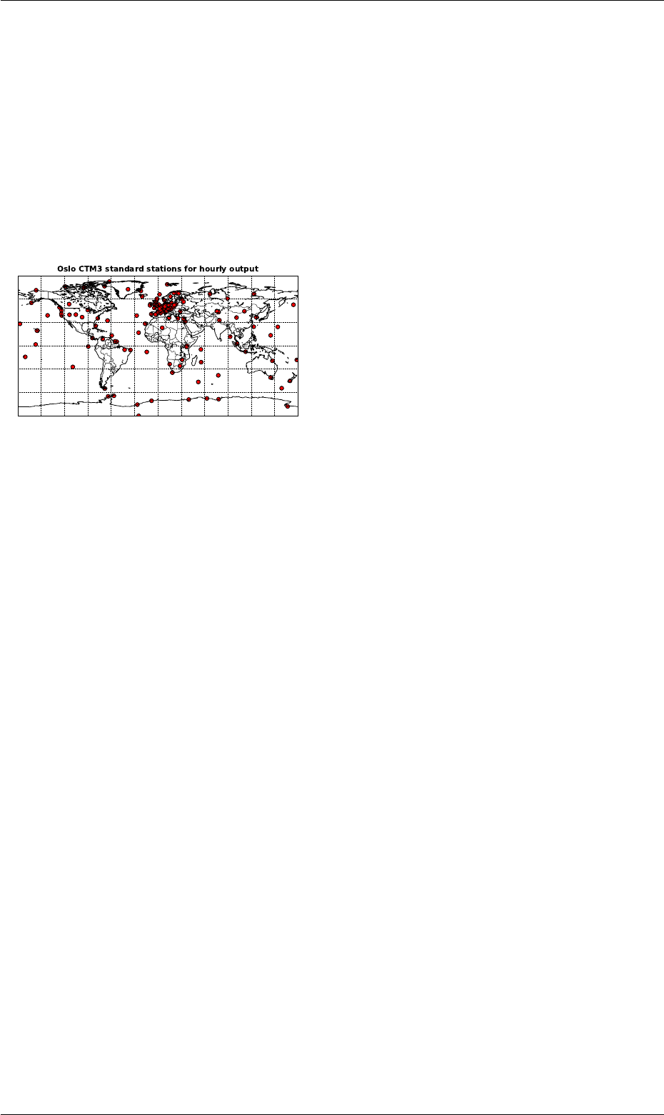
Oslo CTM3 user manual November 6, 2018
An IDL program for reading this output is available in
the SVN repository (see Section B).
You specify species to diagnose in the file verticalpro-
files_stations2.f90. Some meteorological components are
also diagnosed, e.g. temperature, pressure, model grid
height, air mass, equivalent latitude, etc.
As input the program reads a file station-
list_verticalprofiles.dat at model start, while output is
done at the beginning of each day (i.e. after start day),
in the file hourly_station_vprof_YYYYMMDD.dta.
The stations used in the standard output are shown in
Figure 2.
Figure 2: Map of stations included in the standard
output for vertical profiles.
List of output data for each daily file:
•year: Year.
•month: Month of year.
•date: Date of month.
•LPAR: Number of vertical layers.
•ntracer: Number of tracers diagnosed.
•nrofstations: Number of stations.
•NTHE: Number of θ-levels for equivalent latitude.
•actual_diag: Number of NOPS steps diagnosed, i.e.
NROPSM * NRMETD.
•etaa: Sigma coordinate A (ηa) for all levels.
•etab: Sigma coordinate B (ηb) for all levels.
•stt_components: Tracer ID numbers diagnosed.
•mole_mass: Molecular mass of tracers.
•pvthe: Theta levels for equivalent latitude.
List of output data for each station:
•locname: Station name.
•loccode: Station 3-char code.
•lat: Latitude.
•lon: Longitude.
•alt: Altitude.
•ii: CTM zonal grid box index.
•jj: CTM meridional grid box index.
•nb_ii: Zonal neighbor grid box index.
•nb_jj: Meridional neighbor grid box index.
•nb_xfrac: Fractional distance to zonal neighbor.
•nb_yfrac: Fractional distance to meridional neigh-
bor.
•areaxy: Grid box area [m2] (interpolated).
For all diagnostic steps, the following data are stored:
•psfc: Surface pressure [hPa].
•BLH: Boundary layer height [m].
•mass: Tracer masses [kg/grid box].
•h2o: H2O mass [kg/grid box].
•temperature: Temperature [K].
•airmass: Air mass [kg/grid box].
•zoflev: Height of grid box bottoms [m].
•eqlat: Equivalent latitude on theta levels.
•PVU: Potential vorticity units.
•tph_pres: Tropopause pressure [hPa].
21.2.7 Satellite vertical profiles
A routine for putting out vertical profiles at given loca-
tions and times, e.g. satellite positions, are included in the
file satelliteprofiles_mls.f90. In this file you define which
tracers to put out. Some meteorological components are
also diagnosed, e.g. temperature, pressure, model grid
height, air mass, equivalent latitude, etc. Using the satel-
lite profile location (latitude and longitude), this routine
linearly interpolates horizontally from the 4 closest grid
boxes. In the future, it may be better to save data for all
columns and do interpolation in post-processing. Due to
the large amount of data per file, this is not done now.
Since each profile is taken between some start time of
NOPS and start time of NOPS+1, output is given for both
NOPS and NOPS+1, allowing temporal interpolation as well.
List of output data for each daily file:
•year: Year.
•month: Month of year.
•date: Date of month.
•LPAR: Number of vertical layers.
•ntracer: Number of tracers diagnosed.
•nsatprofs: Number of profiles.
•NTHE: Number of θ-levels for equivalent latitude.
•etaa: Sigma coordinate A (ηa).
•etab: Sigma coordinate B (ηb).
•stt_components: Tracer ID numbers diagnosed.
•mole_mass: Molecular mass of tracers.
•pvthe: Theta levels for equivalent latitude.
List of output data for each profile:
•time: Time of observation.
•time_sec: CTM NOPS times before and after.
•lat: Latitude.
•lon: Longitude.
•ii: CTM zonal grid box index.
•jj: CTM meridional grid box index.
•nb_ii: Zonal neighbor grid box index.
•nb_jj: Meridional neighbor grid box index.
•nb_xfrac: Fractional distance to zonal neighbor.
•nb_yfrac: Fractional distance to meridional neigh-
bor.
•areaxy: Grid box area [m2] (interpolated).
For the two closest NOPS steps, the following data are
stored:
•psfc: Surface pressure [hPa].
•BLH: Boundary layer height [m].
•mass: Tracer masses [kg/grid box].
•H2O: H2O mass [kg/grid box].
•temperature: Temperature [K].
•airmass: Air mass [kg/grid box].
•zoflev: Height of grid box bottoms [m].
•eqlat: Equivalent latitude on theta levels.
•PVU: Potential vorticity units.
•tph_pres: Tropopause pressure.
21.2.8 O3column
Tropospheric and total columns of O3are diagnosed
in the subroutine du_columns in the file diagnos-
tics_general.f90. It is called from mp_diag, which does
diagnoses in each IJ-block.
The columns are diagnosed every meteorological time
step (NMET) and are stored once every day. This is carried
out in the routine write_ducolumns.
70

Oslo CTM3 user manual November 6, 2018
21.2.9 3-hourly output
Oslo CTM3 has the possibility of putting out 3-hourly
instantaneous fields, mostly O3and aerosols. These are
e.g. used for RF calculations.
You turn this diagnose on by setting LDUMP3HRS=.true.
at the top of the file gmdump3hrs.f90, and the main rou-
tine is dump3hrs.
If you want to add other components than O3, this is
of course possible. When you understand the code, it
should be easy to implement.
21.2.10 Snapshots on θ-levels
In the routine write_snapshot_the, located in diagnos-
tics_general.f90, you can put out instantaneous mixing
ratios of selected species, interpolated to the potential
temperature (θ) levels defined in the physics routine, see
Section 20.3. The number of θ-levels (pvthe) are given
by NTHE.
Routine puts out data every hour, and the default species
put out are O3and N2O, along with PVU and equivalent
latitude.
Routine can put out data for only one hemisphere or
both. See the source code for how to change it.
The routine is called from nops_diag, but is commented
out by default. A second routine, write_snapshot, is also
available, putting out gridbox mass of selected species on
model levels.
21.2.11 Emission tendencies
When emissions are treated as production terms in chem-
istry, i.e. in standard Oslo chemistry, the total emitted
per day is calculated for all species, in tnd_emis_daily.
This is explained in Section 8.10.
A Description of model files
Here the source files are described. Generally, files inher-
ited from UCI are placed in the main directory, while the
OSLO chemistry and physics are placed in the directory
OSLO. The files in the main directory is often referred to
as the core files, and will be described next.
A.1 UCI core source files
The Oslo CTM3 started out based on the UCI CTM ver-
sion 5.6d, but was later updated to 6.1b, before most of
the UCI code was restructured into Fortran90 free for-
mat, and all common blocks were abandoned. In this
process I renamed most of the files. Future core update
should be fairly straight-forward for a somewhat experi-
enced user.
This Section describes the core files necessary to run the
Oslo CTM3. If you want to go back and see the UCI
codes, you should contact UCI.
First the global variable files (common files) are listed,
then the core files are listed alphabetically.
A.1.1 cmn_precision.f90
This file defines the precision of the Oslo CTM3 floating
point variables. Several are used:
r8 Double precision. Most variables use this.
r4 Single precision.
rMom Precision of the second order moments. By default
this is single precision.
rAvg Precision of the global average arrays. By default
this is single precision.
rTnd Precision of the global tendency arrays. By default
this is single precision.
A.1.2 cmn_size.F90
Contains the array size parameters and flags. Exam-
ples are IPAR,IPARW,JPAR,JPARW,LPAR,LPARW,MPIPAR,
MPJPAR,NRMETD,NPAR, etc.
A.1.3 cmn_parameters.f90
Contains chemical and physical parameters, such as the
Earth radius (A0), Avogadro’s number (AVOGNR), Appar-
ent molecular weight of dry air (M_AIR), gas constants
(R_AIR,R_UNIV,R_ATM), and many more. These are all
listed in Table 28.
A.1.4 cmn_ctm.f90
Defines the main arrays for the transport model, such as
STT and the moments (SUT,SVT,SWT,SUU,SVV,SWW,SUV,
SUW,SVW).
Also grid info such as longitude (XGRD,XDGRD,XEDG,
XDEDG), latitude (YGRD,YDGRD,YEDG,YDEDG), and sigma
hybrid coordinates (ETAA,ETAAW ETAB,ETABW) are defined
here.
A.1.5 cmn_chem.f90
Defines the main arrays for emissions and chemistry, such
as E3DSNEW(LPAR,IPAR,JPAR,E3PAR) and the tables map-
ping species to emission datasets:
•NE2TBL: Total number of 2D emission datasets.
•NM2TBL: Table of months the emissions apply for.
•NY2TBL: Table of months the emissions apply for.
•E2DS: All 2D emission datasets.
•E2LTBL: Table mapping species to 2D emission
datasets.
•E2STBL: Table of scaling factors for the mapping of
each species and 2D emission datasets.
Similar arrays exist for 3D emissions.
71

Oslo CTM3 user manual November 6, 2018
Table 28: Parameters defined in cmn_parameters.f90.
Name Value Description
A0 6371000 Earth radius [m]
G0 9.80665 Gravitational constant [m/s2]
CPI 3.141592653589793 π
C2PI 2*CPI 2π
CPI180 CPI/180 Conversions to radians
ZPI180 1/CPI180 Conversions from radians
atm2Pa 101325 Conversion from atmospheres to Pa
Pa2atm 1/atm2Pa Conversion from Pa to atm
J2kcal 4186.8 Numbers of kcal in a J
M_AIR 28.97 Molecular mass for air [g/mol]
R_UNIV 8.31446 Universal gas constant [J/(K mol)] = [m3*Pa/(K mol)]
R_ATM R_UNIV * Pa2atm Gas constant in [m3*atm/(K mol)] (∼8.205e-5)
R_AIR R_UNIV / M_AIR * 1000 Specific gas constant for air [J/(K kg)] (∼287)
R_H2O R_UNIV / 18.01528 * 1000 Specific gas constant for water vapor [J/(K kg)] (∼461)
AVOGNR 6.022149e23 Avogadro’s number [molecules/mol]
BOLTZMANN 1.38063e-23 Boltzmann’s const [J/(K molecules)]
KBOLTZ 1.e4 * BOLTZMANN Boltzmann’s const [mb cm3/(K molecules)]
cp_air 1004 Specific heat of dry air at constant pressure [J/(K kg)
Lv_0C 2.501e6 Latent heat of vaporization at 0◦C [J/kg]
dLv_dT -0.00237e6 Gradient of Lv between 0C and 100C [(J/kg)/K]
(Table C-5 in Stull, 1988)
TK_0C 273.15 Temperature [K] at 0◦C
es_0C 611.2 Saturation vapor pressure of H2O at 0◦C [Pa]
secDay 86400 Seconds in a day
secYear 31536000 Seconds in a year
MINTEMP 150 Minimum temperature allowed in chemistry
MAXTEMP 350 Maximum temperature allowed in chemistry
TEMPRANGE MAXTEMP - MINTEMP Temperature range.
LDEBUG .true. Global flag for including more extensive debugging.
Here you also find the tracer name TNAME, tracer molecu-
lar weight TMASS, and other variables such as conversion
factors TMASSMIX2MOLMIX and TMOLMIX2MASSMIX.
The variables are generally well described in the source
code.
A.1.6 cmn_diag.f90
Defines arrays for diagnostics, such as STTAVG,AIRAVG,
JDO_A.
A.1.7 cmn_fjx.f90
Defines fast-JX parameters and arrays.
A.1.8 cmn_met.f90
Defines meteorological arrays.
A.1.9 cmn_sfc.f90
Defines surface variables such as land surface type
(landSurfTypeFrac), land-sea mask (LSMASK), and dry
deposition velocity (VDEP).
A.1.10 averages.f90
Contains routines for summing up 3D averages.
•AVG_WRT_NC4: Write core 3D averages (the avgsav-
files), including XSTT averages, surface pressure av-
erages (which is 2D), and some meteorological aver-
ages.
•AVG_ADD2: Add to 3D averages.
•AVG_CLR2: Clear 3D averages.
•AVG_P1: Write 1D averages to screen.
•AVG_WRT2: Only included for history. See
AVG_WRT_NC4. Write core 3D averages (the avgsav-
files), including XSTT averages, surface pressure av-
erages (which is 2D), and several meteorological av-
erages.
A.1.11 budgets.f90
Contains routines for summing up tendency budgets.
•TBGT_G: Clear budget arrays.
•TBGT_L: Accumulate budgets layerwise.
•TBGT_IJ: Accumulate budgets in IJ-block.
•TBGT_P0: 0D print to screen.
•TBGT_P1: 1D print to screen.
•TBGT_P2: 2D print to screen.
72

Oslo CTM3 user manual November 6, 2018
A.1.12 cloudjx.f90
Routines for treating cloud-J. Currently set up for cloud2
as used by fast-JX 6.7c, but will be updated when fast-JX
7.3c is included.
•cloud_init: Initialise cloud-J.
•RANSET: Set random number. Random seed is
RANSEED, which is set in LxxCTM.inp.
Some important variables for cloud2:
•LCLDAVG:
•LCLDQMD:
•LCLDQMN:
•LCLDRANA:
•LCLDRANA:
A.1.13 convection.f90
This is the f90 version of the UCI p-cnvw.f. It has
been modified to Oslo CTM3, calculating elevator frac-
tions, and also the Henry coefficients used in convective
washout. A new convective wet loss variable is included;
CNV_WETL(LPAR,NPAR).
•CONVW_OSLO: The main routine.
•ADJFLX2: Adjust convective fluxes so that no more
than a fraction of the grid box mass is moved each
time step.
•ADJFLX Old version of ADJFLX2.
•QCNVW2_OSLO: Column model calculating convective
transport, and also convective scavenging by up-
drafts.
•QCNVW2: UCI routine kept for history.
•SCAV_UPD: UCI routine kept for history.
A.1.14 fastjx.f90
Contains routines for fastJX, except the main driver
which is so far located in p-phot_oc.f. That will change
when fast-JX is updated to 7.3.
•RD_XXX: Reads FJX_spec.dat.
•RD_MIE: Reads FJX_scat.dat.
•RD_JS: Reads ratj_oc.d file.
•RD_O1D: Reads O1D entry of ratj_oc.d file.
•SET_ATM: Reads O3and temperature climatologies
to use above the model domain. It can possibly be
used in the stratosphere when stratospheric chem-
istry in not included, but Oslo CTM3 uses its own
climatology for that. Sets e.g. TOPT,TOPM,TOP3.
Changes compared to UCI p-phot.f file
In the subroutine PHOT_IN a small piece of ASAD code
was removed. Some other ASAD variables has been re-
moved.
Also, the subroutine SET_ATM had to be modified to in-
clude climatology data for the uppermost layer (LPAR3,
LPART and LPARM).
A.1.15 grid.f90
Routines for setting up model grid.
•SET_GRID: Sets up global grid, such as latitude, lon-
gitude, area of grid boxes, etc.
•LABELG: For printing grid info to screen.
•DIAGBLK: Finds grid box start/end indices for box
diagnose.
•DIAG_LTSTN: Finds grid box indices for station diag-
nose.
•DIAG_LTGL: Finds grid box indices for local time sta-
tion diagnose.
•GAUSST2: Calculate Gaussian quadrature points and
weights.
•DBLDBL: Define longitude and latitude of horizontally
degraded grid.
•AIRSET: Sets up 3D air mass.
•SURF_IN: Reads land fraction datasets.
•gridICAO: Not used. I think this finds grid for some
ICAO emission data.
A.1.16 initialize.f90
Routines for initializing the Oslo CTM3.
•INPUT: Reads LxxCTM.inp.
•SETUP_SPECIES: Reads restart file.
•SETUP_UNF_OUTPUT: Opens unformatted output files
(UCI heritage).
•report_zeroinit: Reports which tracers are initial-
ized to zero (i.e. not read from file).
A.1.17 lightning.f90
Contains routines for calculating lightning NOx (L-NOx)
emissions. There are several methods for doing this, as
described in Section 8.8.
•getScaleFactors: Sets scaling factors based on
which meteorological dataset is used.
•LIGHTNING_OAS2015: Default method for calculating
L-NOx.
•LIGHTNING_GMD2012: L-NOx as described by Søvde
et al. (2012).
•LIGHTNING_UCI2015: L-NOx as used by UCI-CTM
in 2015. I do not recommend using this.
•LIGHTDIST: Sets up vertical distribution of L-NOx.
•filterLNC: Filter convective mass fluxes to reduce
noise in L-NOx horizontal distribution.
•distland: Finds grid boxes that are land or have
land in 300 km proximity. Test routine to make land
near-land lightning behaving like land. Not used.
•LIGHTNING_ALLEN2002: L-NOx as described by
Allen and Pickering (2002). Not evaluated.
A.1.18 metdata_ecmwf.f90
Read-in for ECMWF IFS meteorological data on
netCDF4 format.
•update_metdata: Updates meteorological data.
•fluxfilter2: Filter convective mass fluxes; removes
noise.
•data2mpblocks: Puts globally gridded (IPAR,JPAR)
data into IJ-block (IDBLK,JDBLK,MPBLK).
•gotData: Prints info to standard out.
•skipData: Prints info to standard out.
73

Oslo CTM3 user manual November 6, 2018
A.1.19 metdata_ecmwf_uioformat.f90
Traditional read-in for ECMWF IFS meteorological data
on UIO binary format.
A.1.20 omp.f90
Routines for switching between global and IJ-block struc-
tures. Slightly modified compared to UCI routines,
e.g. looping is changed to reduce striding.
•MPSPLIT: Split global arrays into IJ-block arrays.
•MPBIND: Convert back to global arrays.
•get_iijjmp: From global indices I,J, find IJ-block
indices II,JJ,MP. Not really necessary because of
the array all_mp_indices and the next routine:
•get_all_mpind: Sets up array all_mp_indices to
map global indices to IJ-block indices.
all_mp_indices(1,I,J)=II
all_mp_indices(2,I,J)=JJ
all_mp_indices(3,I,J)=MP
A.1.21 pbl_mixing.f90
Routines for calculating planetary boundary layer (PBL)
mixing. This is the f90 version of the UCI file p-pbl.f, but
modified to use the scheme by Holtslag et al. (1990).
•CNVBDL: Main routine for calculating PBL mixing.
•BULK: Prather bulk scheme.
•get_keddy_L1: Calculates diffusivity in the lower-
most model layer, as done in the routine KPROF.
•KPROF2: Calculates diffusivity of heat used in PBL
closure, as used by the Holtslag et al. (1990) scheme.
Should be used instead of KPROF, since unnecessary
calculations have been removed.
•KPROF: Calculates diffusitivities used in PBL closure,
as used by the Holtslag et al. (1990) scheme.
•PHIM: Calculates similarity theory stability correc-
tion for momentum.
•PHIH: Calculates similarity theory stability correc-
tion for heat.
•TRIDIAG: Solves tri-diagonal system.
•INTERP: Mass weighted interpolation routine to de-
termine PBL profiles from similarity. Ekman solu-
tion.
•QXZON: Combines mass boxes into extended zones.
•QZONX: Divides one extended zone into equal-mass
boxes.
A.1.22 pmain.f90
The main program pmain.f90 has been modified for
the Oslo CTM3. Input routines are changed and also
some calls to master routines. There is also an internal
chemistry loop of max 15 minutes for the processes mix-
ing/emissions/chemistry/deposition. This is to reduce
the large changes imposed by emissions and deposition.
For large deposition values, all of a tracer can be removed
at the surface if the time step is too long. For a 16 m layer,
a deposition velocity of 1.77 cm/s will remove everything
in 15 minutes. Linoz calls has been removed.
See Section 4.1.3 for more.
A.1.23 regridding.f90
Routines for regridding data.
•E_GRID: Regridding of 2D horizontal field. Field
must not be per area, i.e. concentrations and mix-
ing ratios must be multiplied by area before inter-
polation, and divided by new area afterwards. Han-
dles emission dataset which include moments (usu-
ally not used in Oslo CTM3). XBEDG and XDEDG may
have shift at dateline. YBEDG and YDEDG must start
at 90S.
•E_GRID_Y: Regridding of array in meridional direc-
tion.
•TRUNG8: Convert double precision (r8) field from na-
tive resolution to degraded horizontal resolution.
•TRUNG4: Convert single precision (r4) field from na-
tive resolution to degraded horizontal resolution.
A.1.24 source_uci.f90
•SOURCE: Routine for adding emissions to emission
array each time step, when treated as a separate
process (i.e. not as production term in chemistry).
Not tested with Oslo chemistry.
When treated as chemistry production term, the
routine emis4chem in emisdep4chem_oslo.f90 is
used (see Appendix A.2.14).
A.1.25 scavenging_largescale_uci.f90
Large scale scavenging as described in Section 7.1.1.
Some modifications from Oslo CTM3 are implemented.
•WASHO: Master routine calling WASH1 or WASH2.
•WASH1: Simple UCI wet scavenging routine. Kept
for history; should not be used.
•WASH2: Routine by Neu and Prather (2012), partly
modified for Oslo CTM3.
•DISGAS: Calculates the mass of tracer dissolved in
aqueous phase. Uses the flag IT258K to define how
to use Henry’s law.
•HENRYS: Use Henry’s law to calculate mass dissolved
in aqueous phase. No dissolved tracer below 258 K,
and uses retention coefficient between 258 K and
273 K.
•HENRYSallT: Same as HENRYS, but uses retention co-
efficient also below 258 K.
•RAINGAS: Calculates tracer (kg) picked up by new
rain.
•WASHGAS: Calculates tracer picked up by falling pre-
cipitation (kg) and also evaporated from precipita-
tion (kg).
•DIAMEMP: Empirical fit of precipitation diameter to
cloud water density and rain rate, following Field
and Heymsfield (2003).
•GAMMAX: Calculates gamma using ln gamma algo-
rithm.
•WETSET_CTM3: Initialises and sets wet scavenging pa-
rameters for Oslo CTM3.
A.1.26 spectral_routines.f
Spectral routines, not collected as module. These are
purely inherited from UCI/Oslo CTM2.
74

Oslo CTM3 user manual November 6, 2018
•SPE2GP: Converts spectral field to gridded field.
•ZD2UV: Converts spectral fields of vorticity and diver-
gence to gridded field of zonal wind (U) and merid-
ional wind (V).
•UVCOEF: Used by ZD2UV to calculate spectral coeffi-
cients.
•FFT_99: Multiple fast real periodic transform of
length N performed by removing redundant oper-
ations from complex transform length N.
•FFT_RPASS: Performs one pass-thru data as part of
multiple FFT (FFT_99).
•FFT_DDSS: Calculate constant arrays needed for eval-
uating spectral coefficients for Uand Vfrom vorticity
and divergence.
•FFT_SET: Computes factors of N and trigonometric
functions needed by FFT_99
•LEGGEN: Calculate Legendre functions.
•GAUSST: Old routine for calculating Gaussian
quadrature points and weights. Use GAUSST2
(grid.f90) instead.
A.1.27 steflux.f90
Routines for calculating stratosphere-troposphere ex-
change (STE) as explained in Section 21.1.4. This is the
f90 version of UCI code p-chemflux.f.
•CHEMFLUX: Saves the horizontal flux of specified
tracer (usually O3) in the troposphere, but only for
tropospheric to tropospheric boxes.
•CHEMFLUX_E90: Finds horizontal fluxes within the
troposphere based on e90-tracer.
•dumpuvflux: Accumulates horizontal fluxes into 3D
arrays. Accumulates over time period defined by
flux calendar (JDO_X).
•DUMPTRMASS: Accumulates tropospheric mass of
tracer (O3).
•DUMPTRMASS_E90: Accumulates tropospheric mass of
tracer (O3) based on e90 tracer.
•SAVETRMASS: Saves daily average mass of tracer (O3).
•STEBGT_CLR: Clears STE diagnostics.
•STEBGT_WRITE: Writes STE budget to netCDF4 file.
•ctm3_pml: Calculates tendency (production minus
loss; PML) below predefined O3surfaces.
•ctm3_o3scav: Calculates net scavenged O3below
predefined O3surfaces.
•chemflux_setup: Set up STE diagnostics.
A.1.28 stt_save_load.f90
Contains routines to save and load STT from restart files.
•load_restart_file: Restart from netCDF4 files
saved by save_restart_file. Setting argument
MODE to zero will read the main restart file (also set-
ting AIR), while non-zero will read additional fields
from specified files. This has to be hard-coded in the
subroutine SETUP_SPECIES in the file initialize.f90.
•getField_and_interpolate: This routine is bound
to load_restart_file, and reads a 3D field from
a netCDF4 file, with ncid as file id and var_id as
variable id. If resolution on file differs from model
resolution, the field is interpolated to model resolu-
tion. Vertical interpolation is not possible yet.
•save_restart_file: Saves netCDF4 restart file.
Contains variables necessary for restarting a run, as
well as useful variables for other purposes. Trans-
ported species have prefix STT_, and for these species
there are also moments available, having prefixes
SUT_,SVT_,SWT_,SUU_,SVV_,SWW_,SUV_,SUW_,
SVW_. Non-transported species have prefix XSTT_.
•OSLO_CON_RUN: Restart from files saved by
OC_CON_SAV. Setting argument MODE to zero will
read the main restart file, while non-zero will read
additional fields from any specified file. Must match
model resolution.
•OSLO_CON_SAV: Old routine for saving restart file; in-
stant fields, component by component. Called based
on input file flag JDO_C. The restart file also contains
grid info to use when e.g. interpolating to other res-
olutions. Should not be used.
•restart_from_CTM3avg: Starts from Oslo CTM3
avgsavDDDDD.dta files, version 7. Reads the file
avgsav_input (no extension), so you must rename
the input file accordingly. Must match model reso-
lution.
•restart_from_CTM3avg_T42: Same as
restart_from_CTM3avg, but reads T42 resolu-
tion avgsavDDDDD files and interpolates to current
resolution. It reads the file avgsav_input (no
extension).
•OSLO_CON_RUN42: Reads Oslo CTM3 T42 resolution
restart file, and interpolates to current resolution.
Works on sav-files version 1 and 2.
•OSLO_CON_RUNxx: Reads any Oslo CTM3 resolution
restart file, and interpolates to current resolution.
Requires that the sav-file is version 2 or higher. Will
stop if model resolution is the same as on file, be-
cause not all moments are used.
•OSLO_RESTARTFILE_INFO: Retrieves resolution info
from the old binary restart files.
A.1.29 utilities.f90
Various utilities for Oslo CTM3. More utilities are given
in utilities_oslo.f90.
•write_log: Writes start and end of model to screen.
•model_info: Prints info about run to screen.
•calendar: Calculates day counters, but also some
info about next time step, such as JYEAR_NEXT,
JMON_NEXT,JDAY_NEXT,JDATE_NEXT.
•is_leap: Calculates whether a year is leap year or
not.
•get_soldecdis: Calculates solar declination and
distance to Sun. Same as originally found in
CALENDR.
•CALENDR_OLD: Old routine to calculate day counters
and also solar declination and distance to Sun. Not
used.
•CALENDL: Looks up calendar and checks for flags.
•LOCSZA: Calculates cosine of local solar zenith angle,
and the solar flux factor.
•LCM: Calculates the least common multiple of two
numbers.
•ctmExitC: Exit routine printing message.
•ctmExitL: Exit routine printing message and label.
•ctmExitIJL: Exit routine printing message and
I,J,L.
•get_free_fileid: Finds a free file id number.
75

Oslo CTM3 user manual November 6, 2018
•get_dinm: Returns the number of days in months,
depending on whether year is leap year or not.
•CFRMIN: Set minimum limit on cloud fraction.
•CIWMIN: Set minimum limit on in-cloud water and
ice ratios (kg/kg).
•check_btt: Checks BTT array for negatives and
NaNs. Allows tracer id 110 (sum of oxygen, SO)
to be negative.
•adjust_moments: Scales down moments if BTT has
been reduced during a process (if it is smaller than
BTTBCK).
A.1.30 p-cloud2.f
Routines for calculating cloud2. Will be updated when
cloud-J is included.
•CLOUD: Calculates cloud properties.
•QUADCA: Generates 4 quadrature independent col-
umn atmospheres (ICAs).
•OD_LIQ: Sets effective radius and extinction for liq-
uid clouds.
•CLDQUAD: Generates independent ICAs from max-
random overlap criteria.
•QUADMD: Sort ICAs in order of increasing optical
depth. Calculates weights.
•ICANR: Evaluate number of ICAs.
•HEAPSRT: Heap sort.
A.1.31 p-dyn0.f
Sets up atmospheric variables after they have been read
from file.
•DYN0: Sets up advective fields.
•EPZ_UV: Redistributes Uand Vfluxes to smooth over
extended polar zones.
•EPZ_TQ: Average temperature (T) and specific hu-
midity (Q) over extended polar zones.
•EPZ_P: Average surface pressure (P) over extended
polar zones.
•PFILTER: Global filter to smooth pressure errors.
Also adjusts the horizontal fluxes accordingly.
•CFLADV: Calculates global Lifshitz (not CFL) time
step limiter for advection step. NADV is the number
of global advection steps.
A.1.32 p-dyn0-v2.f
Same as p-dyn0.f, but for more accurate polar cap treat-
ment.
A.1.33 p-dyn2.f
Contains advection subroutines.
•DYN2UL: Zonal advection.
•DYN2VL: Meridional advection.
•DYN2W_OC: Vertical advection.
•QLIMIT2: Quick SOM limiter only for LIM=2
(pos+mono) in the X direction.
•POLES1: Combine polar-pie box with next lower lat-
itude (J=1,2 and J=JM-1,JM) using SOM.
•POLES2: Split extended polar-pie box back into two
(J=1,2 and J=JM-1,JM). Use SOM to split, need to
know final air mass in J=1 and J=JM.
A.1.34 p-dyn2-v2.f
Same as p-dyn2.f, but for more accurate polar cap treat-
ment. Does not use POLES1 and POLES2. Calls from
pmain.f90 needs to be modified (described in pmain.f90).
A.1.35 p-linoz.f
Linoz is available in Oslo CTM3, but only for STE calcu-
lation (Section 21.1.4). Here are the available routines,
but note that some are not used because Linoz is only
used for STE.
•LNZ_INIT: Read/init Linoz data and other strat
chem tables from pratmo box model.
•LNZ_SET: Set up Linoz (and other stratosphere) table
data for each day/month/year.
•LNZ_SETO3: Initialize Linoz O3(N=N_LZ) based on
supplied climatology.
•LNZ_PML: Linoz = linearize P-L for stratospheric
ozone based on tables from the PRATMO model
using climatological T, O3, Month.
•INT_LAT: Interpolate from pratmo standard tables
(85S to 85N) to CTM J-grid.
•INT_MID: Interpolation routine, using grid box mid-
point.
•INT_SOM: Interpolation routine using moments.
•DECAY: Simple e-fold decay of species throughout the
model domain. Not used; Oslo CTM3 uses its
own routine.
•TPAUSEB: Defines the tropopause level based on
Linoz O3.Not used; rather use TPAUSEB_E90.
•TPAUSEG:Not used; rather use TPAUSE_E90.
A.1.36 p-vect3.f
The second order moment 1D transport routine QVECT3.
A.1.37 p-phot_oc.f
Contains the column model for fast-JX, used by the main
driver jv_column in main_oslo.f90.
•PHOTOJ: Column model for J-values. T,O3 and mass
is also set from climatology in the uppermost layer
(TTJ,DDJ and ZZJ for L1_-1).
•OPTICL: Sets cloud fast-JX properties at the std 5
wavelengths (200, 300, 400, 600, 999nm).
•OPTICA: Sets aerosol fast-JX properties at the std 5
wavelengths (200, 300, 400, 600, 999nm).
•OPTICM: Sets fast-JX properties for Mie scattering.
•SOLARZ: Solar zenith angle.
•SPHERE2: Calculation of spherical geometry.
•EXTRAL: Adds sub-layers (JXTRA) to thick
cloud/aerosol layers.
•FLINT: Three point linear interpolation function.
•JRATET: Interpolates J-values.
•JP_ATM: Print out atmosphere used in J-value calc
•OPMIE: Mie scattering code.
•MIESCT: Mie scattering, used by OPMIE.
•LEGND0: Calculates ordinary Legendre functions.
•BLKSLV: Sets up and solves the block tri-diagonal
system.
•GEN_ID: Generates coefficient matrices for the block
tri-diagonal system.
•:
76

Oslo CTM3 user manual November 6, 2018
A.2 Oslo source files
The Oslo source files are located in the directory OSLO.
A.2.1 cmn_oslo.f90
Defines variables needed for Oslo chemistry, which are
not part of the transport code. It may be that some of
these variables should have been in the other cmn-files.
Physical variables:
•LMTROP(IPAR,JPAR): The uppermost level of tropo-
sphere. Stratosphere starts at LMTROP+1.
•NEW_TP: Switch used to diagnose the calculated
tropopause.
•PARTAREA(LPAR,IPAR,JPAR): Background aerosol
surface area density. Be aware that the indexing
has changed since Oslo CTM2.
Convective washout variables:
•TCCNVHENRY(NPAR): Flag to decide which Henry con-
stant to use for convective wash out.
•LELEVTEMP(2,IDBLK,JDBLK,MPBLK): Flag for con-
vective plume/elevator temperatures. If minimum
plume temperature is below 258 K the first entry
is 1, and if maximum temperature is below 273.15 K
the second entry is 1. Otherwise these flags are 0.
•QFRAC Fraction of elevator convective precipitation
/ elevator liquid water volume.
•LW_VOLCONC Convective elevator liquid water volume
concentration.
Air values:
•AIRMOLEC_IJ(LPAR,IDBLK,JDBLK,MPBLK): Air den-
sity.
•DV_IJ(LPAR,IDBLK,JDBLK,MPBLK): Gridbox vol-
ume.
Tracer related variables:
•trsp_idx(TRACER_ID_MAX): Mapping from chemical
ID to transport number.
•chem_idx(NPAR) Inverse mapping for trsp_idx
(from transport number to chemical ID).
•Xtrsp_idx(TRACER_ID_MAX) Mapping from chemi-
cal ID to non-transported number (place in XSST).
•Xchem_idx(NOTRPAR) Reverse mapping for
Xtrsp_idx.
•XTNAME(NOTRPAR) Name array for non-transported
tracers.
•XTMASS(NOTRPAR) Tracer mass for non-transported
tracers.
•XTMASSMIX2MOLMIX(NOTRPAR) Conversion from
kg/kg to mole/mole (i.e. M_AIR/XTMASS).
•XTMOLMIX2MASSMIX(NOTRPAR) Conversion from
mole/mole to kg/kg (i.e. XTMASS/M_AIR).
•XSTT(LPAR,NOTRPAR,IPAR,JPAR): The non-
transported tracer distribution.
•XSTTAVG(LPAR,NOTRPAR,IPAR,JPAR): The diagnos-
tic (avgsav) array of the non-transported tracers.
Chemical variables:
•JVAL_IJ(JPPJ,LPAR,IDBLK,JDBLK,MPBLK): J-
values.
•STT_2D_LB: Lower boundary conditions for tracers.
•STT_2D_LT: Upper boundary conditions for tracers.
•TROPCHEMnegO3(LPAR,MPBLK): Counting number of
negative O3occurring in the troposphere (I have
only found this in the surface layer).
•PR42HET(IPAR,JPAR): Aerosol surface conversion of
N2O5to HNO3.
•CH4FIELD(IPAR,JPAR): Surface field for CH4set
each month. Not used when CH4emissions are
turned on.
Emission variables:
•EMIS_IJ(LPAR,NPAR,IDBLK,JDBLK,MPBLK): Emis-
sions for Oslo chemistry treatment as production in
chemistry, i.e. units [molec/(cm3s)].
•DIAGEMIS_IJ: Diagnose emissions accumulated (kg)
over time span defined by budget calendar (JDO_T).
•emisTotalsDaily(NPAR,366): Diagnose daily accu-
mulated emissions (kg).
•emisTotalsOld(NPAR): Used for the daily accumu-
lated emissions diagnose.
•METHANEMIS: Logical specifying whether CH4emis-
sions are to be used or not.
•NECAT: Number of emission categories to diagnose
(only used for diagnostics).
•ECATNAMES(NECAT): 3-character names for each
emission category. So far the RETRO categories
are used.
•E2CTBL(ETPAR): Mapping category number to emis-
sion table.
•E2LocHourTBL(ETPAR): Table mapping 2D emission
table to diurnal variation index. See Section 8.4.2.
•NE2LocHourVARS: Number of local hour scalings.
•E2LocHourSCALE(24,NECAT,NE2LocHourVARS): Lo-
cal hour scalings.
•E22dTBL(ETPAR): Table mapping 2D emission table
to horizontal 2D variation index. See Section 8.4.2.
•NE22dVARS: Number of horizontal 2D types.
•E22dSCALE(IDBLK,JDBLK,MPBLK,NE22dVARS): 2D
scalings.
•E2L2dTBL(NE22dVARS): Keep track of 2D scalings
used.
•E2vertTBL(ETPAR): Table mapping 2D emissions to
vertical distributions.
•NE2vertVARS: Number of vertical distributions.
•NE2vertLVS: Number of vertical levels for the distri-
butions.
•E2vertSCALE(NE2vertLVS,NE2vertVARS): The ver-
tical scalings.
Forest fires variables:
•FF_TYPE: Type of forest fires emissions.
•FF_YEAR: Year of forest fires dataset.
•FF_PATH: Path of forest fires, set in
Ltracer_emis_xxxx.inp.
•NEFIR: Number of components with forest fires emis-
sions. Must not be larger than EPAR_FIR.
•EPAR_FIR: Max number of components with forest
fires emissions.
•EPAR_FIR_LM: Vertical CTM layers covered.
•ECOMP_FIR(EPAR_FIR): Components emitted.
•EMIS_FIR: The forest fires emission array of size
(EPAR_FIR_LM,EPAR_FIR,IDBLK,JDBLK,MPBLK).
Global diagnose variables:
•DIAGEMIS_IJ: Diagnose emissions accumulated (kg)
over time span defined by budget calendar (JDO_T).
77

Oslo CTM3 user manual November 6, 2018
•emisTotalsDaily(NPAR,366): Diagnose daily accu-
mulated emissions (kg).
•emisTotalsOld(NPAR): Used for the daily accumu-
lated emissions diagnose.
•CONVWASHOUT(LPAR,NPAR,IDBLK,JDBLK,MPBLK): Di-
agnose tracer removed by convective scavenging
(kg), accumulated over time span defined by bud-
get calendar (JDO_T).
•dobson_snapshot(IPAR,JPAR,24): Snapshots of to-
tal O3column each hour (DU).
•dobson_snapshot_ts(IPAR,JPAR,24): Snapshots of
tropospheric O3column each hour (DU).
•TEMPAVG: Temperature average, accumulated over
time span defined by budget calendar (JDO_T).
•H2OAVG: H2O average, accumulated over time span
defined by budget calendar (JDO_T).
•QAVG: Specific humidity average, accumulated over
time span defined by budget calendar (JDO_T).
•AMAVG: Air density average, accumulated over time
span defined by budget calendar (JDO_T).
•LMTROPAVG: Average level of tropopause height
(LMTROP), accumulated over time span defined by
budget calendar (JDO_T).
•SCAV_LS: Accumulated amount (kg) removed by
large scale scavenging.
•SCAV_CN: Accumulated amount (kg) removed by
convective scavenging.
•SCAV_DD: Accumulated amount (kg) removed by dry
deposition.
•SCAV_BRD: Accumulated burden to be used for cal-
culating average burden.
•SCAV_DIAG(NPAR,4,366): Daily accumulated val-
ues. Last entry is average burden.
•SCAV_MAP_WLS: Total (kg) scavenged by large scale
scavenging at the surface.
•SCAV_MAP_WCN: Total (kg) scavenged by convective
scavenging at the surface.
•SCAV_MAP_DRY: Total (kg) scavenged by dry deposi-
tion at the surface.
Help variables:
•DINM: Number of days in month, changes depending
on leap year or not.
•ZEROINIT: Flag to keep track of initialised compo-
nents.
•XZEROINIT: Flag to keep track of initialised non-
transported components.
•RESULTDIR: Can be used to put results in a specified
directory.
•dustbinsradii: Radius of dust bins. Only set if
mineral dust module is included.
A.2.2 aerosols2fastjx.f90
Routine for handling tropospheric aerosols in fast-JX.
•initialize_tropaerosols: Initialize arrays.
•set_aer4fjx: Calculate the path of each aerosols,
to be used in fast-JX calculations.
•get_tropaerosols: Reads monthly model climatol-
ogy for specified aerosols. Not fully implemented.
•update_tropaerosols: Sets the climatological val-
ues of aerosols, interpolates temporally between two
monthly climatologies.
•set_aer4fjx_ctm2: Sets simple BC profile as in
CTM2.
A.2.3 bcoc_oslo.f90
Routines for treating the BCOM module (Section 14).
•bcoc_init: Initializes the BCOM; indices are set
and dry deposition is set.
•bcoc_master: Master routine for calculating BCOC.
Loops through IJ-blocks and their columns and in-
tegrates aerosol masses using QSSA.
•bcoc_setdrydep: Puts deposition rates into VDEP.
It is called from the routine setdrydep. Stability is
treated in the latter after VDEP has been set.
•bcoc_chetinit: Initialize latitude dependent aging
times.
•bcsnow_init: Initialize BCsnow.
•bcsnow_diagwetrm: Diagnose BC removed by wet
scavenging and deposited on snow.
•bcsnow_save_restart: Save restart file for BCsnow
diagnostics.
•bcsnow_status: Print status of BCsnow.
•bcsnow_check_snow (private): Debug routine for
BCsnow.
•bcsnow_getspringsummer (private): Get dates for
spring and summer to be used in melting calcula-
tions.
•bcsnow_nmet_output: Puts BCsnow data to file ev-
ery NMET.
•bcsnow_nmet_output_nc: Puts BCsnow data to
netCDF file every NMET.
•bcsnow_collect_ij (private): Collects diagnosed
amount of BC deposited on snow, from wet scaveng-
ing and dry deposition, thus building snow layers.
•bcsnow_meltevap_ij (private): Calculates evapora-
tion.
•bcsnow_seaice_ij (private): Corrects calculations
over sea ice.
•bcsnow_adjustment_ij (private): Adjusts calcu-
lated snow depth to snow depth from meteorological
data.
•bcsnow_master: BCsnow master routine.
A.2.4 caribic2.f90
Routines for producing vertical profiles at CARIBIC
measurement locations and times. CARIBIC input is
available from 2005. Called from nops_diag in diagnos-
tics_general.f90.
•get_new_events (private): Find observations for
this day.
•caribic_output (private): Produces output for the
given NOPS and the previous NOPS.
•caribic_data_to_file (private): Write collected
flight path data to file.
•caribic2_master: Process profiles. Called outside
parallel region.
A.2.5 ch4routines.f90
Routines for treating CH4as fixed at surface or as emis-
sions. To choose type of constant surface data, use
CH4TYPE at the top of this file. To use emissions, set
flag METHANEMIS in cmn_oslo.f90.
•update_ch4surface: Updates surface mixing ratios.
This is mainly done from pmain.
78

Oslo CTM3 user manual November 6, 2018
•ch4surface_hymn (private): Reads surface data
from HYMN, given for years 2003-2005. This is
standard.
•ch4surface_scale_hymn (private): Scales HYMN
2003 dataset to marine global annual CH4ob-
served by ESRL Global Monitoring Division
http://www.esrl.noaa.gov/gmd/ccgg/trends_ch4/
•ch4surface_poet (private): Reads surface data
from POET.
•ch4surface_retro (private): Reads surface data
from RETRO.
•READCH4 (private): Carries out the actual read-in for
POET data.
•set_ch4_stt: Sets 3D CH4, i.e. in the STT array, to
values found in HYMN.
•updateSOILUPTAKEbousquet: Updates soil uptake
each month, according to the Bousquet data.
•read_ch4sfc4soiluptake (private): Reads HYMN
surface data [kg], to convert Bousquet data from
[kg/s] to [1/s].
•read_ch4bousquet (private): Reads the Bousquet
data. Can read any year in dataset, but standard is
to read 2003, matching the HYMN surface data for
2003.
•ch4drydep_bousquet: Calculates the dry deposition
velocity of CH4to be used in Oslo CTM3.
•reportsfcch4: Reports global average surface mix-
ing ratio of CH4.
•setch4sfc: Set CH4at surface to keep it constant.
A.2.6 chem_oslo.f90
This is where Oslo chemistry master routine will be lo-
cated in the future. For now tropospheric chemistry is
in tropchem_oslo.f90 and stratospheric chemistry is in
stratchem_oslo.f90.
A.2.7 chem_oslo_rates.f90
Routines for setting up chemistry reaction rates.
•TCRATE_CONST2: Constant rates and rates depend-
ing only on temperature. The latter are stored in
intervals of 1 K. Rates used in the troposphere are
listed first, then the rates only used in the strato-
sphere are listed.
•set_pr42het: Sets aerosol surface uptake reac-
tion for hydrolysis of N2O5in the troposphere.
This aerosol climatology is an annual mean height-
latitude distribution from (Dentener and Crutzen,
1993), and should be revised.
•getRQAER (private): Find removal rate by aerosol
(RQAER), only dependent upon land/sea and vertical
variation. Crude approximation, should be revised.
•TCRATE_TP_IJ_TRP: Rates dependent on tempera-
ture and pressure in troposphere.
•TCRATE_TP_IJ_STR: Stratospheric rates dependent
on temperature and pressure.
•TCRATE_onAER: Gaseous uptake and heterogeneous
chemistry on aerosols. Includes new and old param-
eterisations. Tropospheric chemistry.
•TCRATE_HET_IJ: Heterogeneous chemistry reactions
in the stratosphere.
A.2.8 cnv_oslo.f90
Oslo wet removal due to convective rain is treated in two
steps:
1. Calculating the fraction of convective rain to cloud
water in the elevator (QFRAC).
2. Calculating the fraction of tracer in cloud water
(DISSOLVEDFRAC).
See Section 6.3 for details. The subroutines in this file
are:
•elevator_fractions: Calculates QFRAC and
LW_VOLCONC. Called from CONVW_OC.
•liquid_fractions: Calculates DISSOLVEDFRAC and
returns CNV_WETL. Called from CONVW_OC.
•wf_henry (private): Calculates Henry coefficients,
possibly modified by hard coding.
A.2.9 dateconv.f90
Routines for date conversion, used e.g. by caribic2.f90.
•itau2idate: Calculate date from given time in sec-
onds relative to reference year.
•idate2itau: Calculate time in seconds since 1 Jan
1995.
•julianday: Calculate julian day from given date.
•calendardate: Calculate date from given julian day.
A.2.10 drydeposition_oslo.f90
Sets up dry deposition velocities.
•drydepinit: Reads drydep.ctm from directory In-
put_CTM3.
•update_drydepvariables: Sets up special drydep
treatments, e.g. soil uptake of CH4and variables
for the new dry deposition treatment. Called from
subroutine oc_update_chemistry.
•setdrydep: Sets drydeposition velocities each time
step, in subroutine oc_main.
•get_ctm2dep (private): Calculate old (CTM2)
treatment dry deposition rates.
•get_vdep2 (private): Calculate new dry deposition
velocities.
•get_STC (private): Get monthly mean stomatal con-
ductances.
•get_PARMEAN (private): Get monthly mean photo-
synthetically active radiation (PAR).
•get_asm24h (private): Get 24-hour mean of asn vari-
able for new dry deposition treatment. I.e. daily
mean of the molar ratio of SO2and NH3. Uses all
NOPS steps to calculate daily mean.
A.2.11 diagnostics_general.f90
Oslo chemistry diagnostics. Scavenging diagnos-
tics are located in diagnostics_scavenging.f90 (Ap-
pendix A.2.12).
Variables (private):
•o3lim: O3mixing ratio used to find tropopause level
tp_o3, based on where O3>o3lim.
•tp_o3: From surface upwards, this is the uppermost
level where O3<o3lim.
79

Oslo CTM3 user manual November 6, 2018
•preslim: Pressure limit for hPa-based tropopause
tp_hpa.
•tp_hpa: From surface upwards, this is the upper-
most level where p <100hPa.
•Plus several variables to get running averages of tro-
pospheric OH concentration and CH4lifetime.
Subroutines:
•diag_ohch4n2o_init: Initializes the lifetime diag-
nostics.
•init_lifetime (private): Initialize CH4and N2O
accumulated losses and burdens.
•du_columns: Calculate tropospheric and total O3
columns each meteorological time step.
•write_ducolumns: Write the columns to file dob-
son_nmet.nc.
•init_daily_diag: Daily initialisations in the begin-
ning of the day.
•daily_diag_output: Daily output carried out at the
end of the day.
•nops_diag: Diagnoses for each NOPS, before parallel
loop.
•mp_diag: Diagnoses for each IJ-block.
•TBGT_2FILE: Processes 2D tendency budgets and
dumps to file.
•REPORTS_CHEMISTRY: Print out different kinds of re-
ports.
•sumup_burden_and_lifetimes: Sum up OH bur-
den and CH4lifetime for different tropopause defi-
nitions, for a given IJ-block.
•report_burden_and_lifetime (private): Print out
the burdens and lifetimes.
•diag_burden_snapshot (private): Print out burden
at specific times.
•write_snapshot: Writes out snapshots of selected
species/metdata for hemisphere or global. Mass
space is put out.
•write_snapshot_the: Writes out snapshots of se-
lected species on potential temperature surfaces.
Put out as mixing ratio. See Section 21.2.10.
•ch4n2o_burden2: Sums up burden of CH4and N2O.
•ch4_loss3: Sums up monthly chemical loss of CH4.
•n2o_loss3: Sums up monthly chemical loss of N2O.
•ocdiags_tpset: Sets tropopause for burden and
lifetime diagnostics.
•report_negO3: Print out the number of negative O3
reported by tropospheric chemistry routine.
•tnd_emis_daily (private): Saves accumulated
emissions for each species per day, in array
emisTotalsDaily.
•tnd_emis2file: Writes the daily emission totals
to file emis_daily_totals_YYYY.nc. Writ-
ing follows the budget calendar, and is called
from pmain. Also writes accumulated emis-
sions in 3D following the tendency calendar, to file
emis_accumulated_3d_YYYYMMDD_YYYYMMDD.nc.
•save_chemPL: Accumulate chemistry losses, convert
to units [kg].
•chembud_output: Write chemistry budgets to file.
Burden, CHEMLOSS and CHEMPROD, all in units
kg/gridbox. Only for selected species. Also see Sec-
tion 21.2.1.
A.2.12 diagnostics_scavenging.f90
Routines for diagnosing dry and wet scavenging.
•scav_diag_init: Initialises separate diagnostics for
wet scavenging and dry deposition.
•scav_diag_put_ddep: Accumulates kg of tracer de-
posited by dry deposition.
•scav_diag_brd: Accumulates burden of tracers each
meteorological time step to generate averages.
•scav_diag_ls: Diagnose large scale scavenging.
•scav_diag_cn: Diagnose convective scavenging.
•scav_diag_collect_daily: Collect daily scavenged
tracer masses and also the average tracer burden.
•scav_diag_2fileA: Write daily totals of scav-
enged tracer, plus their burdens, to file scaveng-
ing_daily_totals_YYYY.nc. Scavenging includes
wet removal (large scale and convective) and dry
deposition.
•scav_diag_2fileB: Write 2D daily totals of
scavenged tracer (i.e. maps) to file scaveng-
ing_daily_2d_YYYYMMDD.nc. Scavenging in-
cludes wet removal (large scale and convective) and
dry deposition.
A.2.13 dust_oslo.f90
Routines for treating the DUST module (Section 15).
•dust_init: Initializes the DUST.
•dustinput_met: Special input for dust calculations.
•SWradbdg_get (private): calculate approximate so-
lar radiation in and out at the surface. Not used
when available from meteorological data.
•psadjust (private): Adjust Ps, account for advec-
tion.
•dust_globalupdate: Update global DUST parame-
ters.
•oro_set (private): Set orography.
•plevs0 (private): Get pressure, temperature and
height properties for DUST.
•dust_master: Master routine for calculating DUST.
Calls column solver for DUST.
•dust_column (private): Column treatment of
DUST; calls DEAD routines to solve DUST in the
column.
•dustbdg2d: Writes dust budget to file.
•dist_set_ssrd: Sets meteorological variable SSRD
in dust code.
•dist_set_strd: Sets meteorological variable STRD
in dust code.
•dist_set_SWVL1: Sets meteorological variable
SWVL1 in dust code.
•dustbdg2file: Puts out dust budget to netCDF file.
A.2.14 emisdep4chem_oslo.f90
Routines to treat get emissions and deposition values and
convert them for use in chemistry as production and loss
terms, respectively.
•emis4chem: Routine similar to the core
SOURCE, fetching all emissions from the emis-
sions array (as kg/s). The output array is
EMIS_IJ(LPAR,NPAR,IDBLK,JDBLK,MPBLK).
80

Oslo CTM3 user manual November 6, 2018
•getEMISX: Fetches the column emissions for all
chemical IDs, converts from kg/s to molec/(cm3s)
and puts them into EMISX(TRACER_ID_MAX,LPAR).
Called from chemistry master routine where column
values are retrieved.
•getVDEP_oslo: Converts VDEP(NPAR,IPAR,JPAR)
[m/s] to VDEP_OSLO(TRACER_ID_MAX) [1/s] to use as
loss term in chemistry. See Section 7.2 for more.
A.2.15 emissions_aircraft.f90
Routines for reading and updating aircraft emissions.
Possible datasets cover TradeOff, React4C and Quantify.
In the Ltracer_emis_xxxx.inp, you specify AirScen to
define the dataset, and AirEmisPath to define the path
to where aircraft emissions are in general.
Emissions are interpolated to the model resolution. Old
routines are also available for having the possibility to
read old resolution specific emission data. Emissions are
read into a separate array, which is used either in SOURCE
or in emis4chem.
•aircraft_emis_master: Master routine for treating
aircraft emissions.
•aircraft_set_species: Defines which species to
emit.
•aircraft_emis_update (private): Read data from
file.
•aircraft_emis_vinterp (private): Vertical interpo-
lation.
•ac_interp (private): Interpolation routine used
byaircraft_emis_vinterp.
•read_original_res (private): Read original (e.g.
1x1 degree) data.
•read_tradeoff_original (private): Read original
TradeOff data.
•read_react4c_original (private): Read original
React4C data.
•read_quantify_original (private): Read Quantify
data.
•readmass_qfyAIR_month (private): Routine to do
the netCDF reading of Quantify data, called by
read_quantify_original.
•read_ceds_original: (private): Read CEDS data.
•get_xyedges (private): Get grid box info for inter-
polation.
•aircraft_zero_400hpa (private): Below 400 hPa,
zero out the aircraft tracers (H2O). This is done by
assuming 1 hour lifetime. Setting to zero may cause
negative tracers due to moments not being zeroed.
It should be possible to include a diurnal variation for
aircraft emissions, but it has not been implemented yet.
A.2.16 emissions_megan.f90
Contains routines for calculating MEGANv2.10 emissions
(Guenther et al., 2012). Oslo CTM3 routines are:
•megan_report: reports daily totals of MEGAN.
Should not be included as default.
•add_meganBiogenic: Adds MEGAN emissions to
species in Oslo CTM3.
•megan_get_co2: Reads file to get monthly CO2for
isoprene activity factor.
•megan_input: Reads input table ta-
bles/megan_tables.dat.
•megan_update_metdata: Updates meteorological
data needed in MEGAN (e.g. accumulated rain).
Also sets monthly CO2.
•megan_emis: Main routine for calculating emissions.
•getWP: Get wilting point for soil.
•megan_emis2file: Puts emitted amounts to file fol-
lowing the BUDGETS calendar. See Section 8.6.2.
MEGAN routines adjusted to Oslo CTM3:
•GAMMA_AGE: Calculate leaf age activity.
•GAMMA_CANOPY: Calculate activity from canopy.
•DIstomata: Calculate drought-induced effect on
stomata (range 0–1) based on the Palmer Severity
Drought Index. Note that MEGAN sets the drought
index to zero as default.
•Ea1t99: Temperature dependence activity factor for
emission type 1 (e.g. isoprene, MBO).
•Ealti99: Calculate light independent algorithms.
•Ea1p99: Not sure what this does.
•WaterVapPres: Convert water mixing ratio (kg/kg)
to water vapor pressure.
•Stability: Temperature lapse rate in canopy, using
canopy characteristics and solar input.
•GaussianIntegration: Gaussian distribution.
•SolarFractions: Calculate transmission, the frac-
tion of photosynthetic photon flux density (PPFD)
that is diffuse, and fraction of solar rad that is
PPFD.
•WeightSLW: Calculates a Gaussian weighting func-
tion for LAI in the canopy layers.
•CanopyRad: Canopy light environment model.
•CalcExtCoeff: Calculates extinction coefficient.
•CalcRadComponents: Radiative calculations.
•CanopyEB: Canopy energy balance model for esti-
mating leaf temperature.
•LeafEB: Leaf energy balance.
•ConvertHumidityPa2kgm3: Convert Pa to kg/m3.
•ResSC: Leaf stomatal resistance. Not well refer-
enced.
•LeafIROut: IR thermal radiation energy output by
leaf.
•LHV: Calculate latent heat of vaporisation from Stull
(1988), p.641.
•LeafLE: Latent energy term in energy balance.
•LeafBLC: Boundary layer conductance.
•LeafH: Convective energy term in energy balance
(W/m2heat flux from both sides of leaf).
•SvdTk: Calculate saturation vapor density.
•CalcEccentricity: Calculate eccentricity.
•UnexposedLeafIRin: Calculate IR into leaf that is
not exposed to the sky.
•ExposedLeafIRin: Calculate IR into leaf that is ex-
posed to the sky.
•SOILNOX: Calculation of soil NOx based on Yienger
and II (1995).
•FERTLZ_ADJ: Computes fertilizer adjustment factor
for soil NOx.
•GROWSEASON: Computes day of growing season for
soil NOx.
•prec_adj: Calculates precipitation pulse adjust-
ment factor for soil NOx.
•getPulseType: Computes the pulse type from a
rainfall rate (Yienger and II, 1995).
•precipfact: Computes a precipitation adjustment
factor.
81

Oslo CTM3 user manual November 6, 2018
A.2.17 emissions_ocean.f90
Routines for treating emissions from ocean. Also sea
spray routines will be placed here eventually.
•emissions_ocean_organiccarbon_init: Initialise
variables for using oceanic emissions.
•emissions_ocean_getChlA: Fetches chlorophyll A
for specified month. Uses MODIS chlorophyll A,
which has been binned into 0.5x0.5 degree grid. Uses
meteorological year for years 2003–2012, and other-
wise a climatology of those years.
•emissions_ocean_organiccarbon: Calculate emis-
sions of oceanic organic carbon aerosols (POA), fol-
lowing Gantt et al. (2015). If sea salt module is
included, use sea salt production rate, otherwise cal-
culate it separately (slightly different method for
now). This routine only depend on meteorological
variables, and is called from update_emis_ii (emis-
sions_oslo.f90).
•emissions_ocean_total: Print out current total
POA flux as [Tg/yr].
•add_oceanOCemis: Routine to add oceanic carbon
emissions. Called from either emis4chem_oslo or
SOURCE.
A.2.18 emissions_oslo.f90
Routine for reading in emissions, and master routine for
short term variations.
•emis_input: Reads in emission data based on
Ltracer_emis_xxxx.inp.
•update_emis: Updates short term varia-
tions/emissions globally.
•update_emis_ij: Update short term emissions in an
IJ-block.
•emis_prop (private): Set properties for input data.
•emis_unit (private): Unit conversions for datasets.
•emis_check2dscal (private): Check 2D scaling flag
and keep track of which ones are used.
A.2.19 emissions_volcanoes.f90
Variables and routines for volcanic emissions.
Variables:
•volc_emis_so2: Emissions of SO2for each event.
•volc_elev: Elevation of the volcano.
•volc_cch: Cloud column height, i.e. the height of
the cloud rising from the volcano. When equal to the
elevation, the volcano is non-eruptive, i.e. gassing
from the surface.
•volc_ii: IJ-array zonal index of event.
•volc_jj: IJ-array meridional index of event.
•volc_mp: IJ-array number.
•volc_event_start(31,12): Keeps track of first
event for each day, through the year.
•volc_event_end(31,12): Keeps track of last event
for each day, through the year.
Subroutines:
•init_volcPATH: Initialize file path and year for vol-
canic emissions.
•read_volcEMIS: Master routine for reading volcanic
emissions.
•read_volcEMIS_HTAP: Reads HTAP volcanic emis-
sions (1979–2010).
•read_volcEMIS_ACOM: Reads AEROCOM volcanic
emissions.
•add_volcEMIS: Adds volcanic SO2emissions to emis-
sion array.
A.2.20 emisutils_oslo.f90
Routines used by emissions_oslo.f90. When including
new types of emissions/datasets, new read-in routines
should be placed here.
•reademis_2d: Controls the read-in of 2D emission
data and its interpolations. This is where you will
find info on the 2D format codes used in the emission
file Ltracer_emis_xxxx.inp.
•reademis_3d: Controls the read-in of 3D emission
data and its interpolations. This is where you will
find info on the 3D format codes used in the emission
file Ltracer_emis_xxxx.inp.
•reademis_stv: Controls the read-in and interpo-
lation of 2D fields used for short term variations
(see Section 8.4.4). This is where you will find info
on the STV format codes used in the emission file
Ltracer_emis_xxxx.inp.
•emisinterp2d (private): Interpolates 2D field and
designates dataset numbers.
•emis_setscalings: Set scaling for tracers using dif-
ferent datasets.
•scale_area (private): Scales with dataset by grid
box area.
•get_xyedges: Calculate grid box properties.
•set_diurnal_scalings: Sets simple diurnal scal-
ings. These are e.g. from TNO/RETRO or such
as 50 % up in daytime and 50 % down during night.
•emis_setscaling_2dfields: Reads scaling data to
use for 2D scaling, e.g. daylight temperatures or
heating-degree-days.
•emis_diag: Accumulates the emissions of each
species into DIAGEMIS_IJ.
•ctm2_rdmolec2 (private): Reads CTM2 POET for-
mat.
•iiasa_read2d (private): Reads IIASA 2D data as
in CTM2.
•gfed_read3d: Reads GFED 3D data. Not used in
the GFED emissions now; this routine was used to
read monthly emissions into the core emission array.
•volc_read1 (private): Reads volcanic emissions.
•read_retrobbh (private): Reads the vertical distri-
bution of forest fires.
•read_bcoc_bond_2d: Reads Tami Bond data version
4 and 5.
•read_aerocom_2d: Reads ascii data from AERO-
COM.
•gfed4_rd: Reads monthly GFEDv4 data along with
partitioning.
•gfed4_init: Reads emission factors from GFEDv4.
•gfed4_rd_novert: Reads monthly GFEDv4 emis-
sions for distributing according to boundary layer
height.
•gfed4_rd_novert_daily: Reads monthly GFEDv4
emissions along with daily fraction of emissions per
month.
82

Oslo CTM3 user manual November 6, 2018
A.2.21 eqsam_v03d.f90
Subroutine eqsam_v03d_sub is the main nitrate (eqsam)
driver, based on Metzger et al. (2002).
A.2.22 fallingaerosols.f90
Contains routines for calculating gravitational settling of
aerosol using second order moments transport. Not used
yet.
•aerosolsettling: Master routine.
•readkasten1968: Reads aerosol fall speeds of Kas-
ten (1968).
•getGAMAAER: The vertical velocity of particles are
found based on their radius. Assumes fixed radius
for the whole IJ-block.
•GRAV_SETN: Routine for SOM transport of a tracer
downwards.
•fallspeed: Purpose: Given size and density of par-
ticle, and column thermodynamic profile, compute
terminal fall speed. Based on DEAD/DUST code.
•turbfallspeed: Purpose: Given size and density of
particle, and column thermodynamic profile, com-
pute Based on DEAD/DUST code.
•getGAMAAER_NS: Same as getGAMAAER but handles
different radii and vertical properties.
A.2.23 gmdump3hrs.f90
Routine for dumping selected components to netCDF file
every 3 hours. Turn on this diagnose by setting its flag
LDUMP3HRS=.true..
•dump3hrs: Dumps the components.
•gm_dump_nc (private): Does the writing to netCDF
files. Converts from kg/gridbox to kg/m3.
A.2.24 hippo.f90
Routines for producing vertical profiles at HIPPO mea-
surement locations and times. Called from nops_diag in
diagnostics_general.f90.
•get_new_events (private): Find observations for
this day.
•hippo_output (private): Produces output for the
given NOPS and the previous NOPS.
•hippo_data_to_file private): Write collected flight
path data to file.
•hippo_master: Process profiles. Called outside par-
allel region.
A.2.25 input_oslo.f90
Subroutines to initialize the Oslo CTM3.
•clear_oslo_variables: Clear arrays used by chem-
istry (e.g. trsp_idx). Called by routine INPUT.
•init_oslo: Initialize Oslo chemistry. Tracer related
data is read, and constant chemical reaction rates
are set. Dry deposition parameters are read and
some diagnostics are also initialized.
•info_oslo (private): Print out info about Oslo
chemistry.
•info_qssa (private): Print out info about QSSA
solver.
•read_tracer_list (private): Read tracer list, ini-
tialize Oslo chemistry.
•tracer_specific_input (private): Read in the
tracer-specific run instructions and data sets. Based
on UCI CHEM_IN, but set up for Oslo chemistry.
•set_resultdir (private): Sets a result directory if
defined.
•read_lsmask: Reads the land-sea mask LSMASK.
A.2.26 main_oslo.f90
The module main_oslo comprises the master subroutine
for chemistry and aerosol packages.
•master_oslo: Master routine to control Oslo chem-
istry. Processes for each IJ-block is called separately.
•jvalues_oslo (private): Collects J-values in the IJ-
block.
•jv_column (private): Sets photolysis rates in the col-
umn. Based on UCI subroutine PHOTOL.
•update_chemistry: Update chemistry, e.g. bound-
ary conditions.
A.2.27 ncutils.f90
Contains netCDF utilities.
•readnc_3d_from4d: Read netCDF file containing
4D fields (DIM1,DIM2,DIM3,DIM4), and returns
3D-field for a DIM4 entry.
•readnc_2d_from3d: Read netCDF file containing
3D fields (DIM1,DIM2,DIM3), and returns 2D-field
for a DIM3 entry.
•readnc_1d: Opens a netCDF file and returns a 1D
field of specified size from the file.
•readnc_1d_from2d: Opens a netCDF file and ex-
tracts a 1D from a 2D field on file. Specifying an
entry of DIM2, a 1D array is returned from the 2D
array (DIM1,DIM2).
•get_netcdf_var_1d: Reads 1D variable from
netCDF file. Array is allocated in this routine, and
must be deallocated after use.
•get_netcdf_var_2d: Reads 2D variable from
netCDF file. Array is allocated in this routine, and
must be deallocated after use.
•get_netcdf_var_3d: Reads 3D variable from
netCDF file. Array is allocated in this routine, and
must be deallocated after use.
•get_netcdf_var_4d: Reads 4D variable from
netCDF file. Array is allocated in this routine, and
must be deallocated after use.
•get_netcdf_att_char: Reads attribute data for
variable from netCDF file.
•get_netcdf_var_dims: Reads dimensions of vari-
able from netCDF file.
•get_netcdf_r4var_1d_from_2d: Returns single
precision (r4) 1D array from a 2D netCDF field.
Used for reading meteorological data on netCDF for-
mat.
•get_netcdf_r4var_2d_from_3d: Returns single
precision (r4) 2D array from a 3D netCDF field.
Used for reading meteorological data on netCDF for-
mat.
83

Oslo CTM3 user manual November 6, 2018
•get_netcdf_r4var_3d_from_4d: Returns single
precision (r4) 3D array from a 4D netCDF field.
Used for reading meteorological data on netCDF for-
mat.
•handle_err: Handle netCDF errors. This routine
does not print out much helpful information.
•handle_error: Handle netCDF errors slightly bet-
ter than handle_err.
A.2.28 nitrate.f90
Nitrate routines. Note that the nitrate equilibrium model
is located in its own file eqsam_v03d.f90.
•nitrate_init: Initialise nitrate module.
•nitrate_master: Nitrate master routine.
A.2.29 pchemc_ij.f90
The tropospheric 1D chemical integrator, integrating the
chemistry in the tropospheric column.
The Oslo chemistry was originally set up to use emis-
sions as production terms and deposition as loss terms.
This is still default, and is controlled by the user settings
in Makefile (Section 2.7.1). Note that treating them in
chemistry, the lightning and aircraft emissions are also
included in the emission array. See Section A.2.14 for
more.
A.2.30 pchemc_str_ij.f90
The stratospheric 1D chemical integrator, integrating the
chemistry in the stratospheric column.
A.2.31 physics_oslo.f90
The module physics_oslo contains subroutines for do-
ing physical calculations in the Oslo CTM3. Parameters
and variables are
•NTHE: number of theta levels to calculate equivalent
latitudes.
•pvthe: Potential vorticity on the theta levels.
•theqlat: Equivalent latitude on the theta levels.
The subroutines are
•update_physics: Updates physical variables such as
tropopause level.
•defineTP: Defines the tropopause level, based on the
parameter TP_TYPE=1 in cmn_oslo.f90. Default for
the Oslo CTM3 is a PVU-based tropopause:
•tp_pvu_ij (private): Calculates the tropopause
level from PVU and potential temperature
(TP_TYPE=1).
•tp_dtdz_ij (private): Not tested. Calculate the
tropopause level using lapse rate (TP_TYPE=2).
•tp_e90_ij (private): Not tested. Uses tropopause
level from E90 tracer, i.e. as given in LPAUZTOP
(TP_TYPE=3).
•tp_03_150 (private): Not in use. Tropopause based
on where O3< 150ppbv.
•get_pvu: If the meteorological data do not provide
PV, it may be calculated from the winds in this
routine.
•ijlw2lij: Converts a field of size
(IPARW,JPARW,LPARW) to the possibly degraded
and vertically collapsed (LPAR,IPAR,JPAR).
•theta_pv: Interpolate PV to pre-defined theta lev-
els.
•theta_eqlat: Calculates equivalent latitudes for
pre-defined theta levels.
•IJLfield2ThetaLvs: Interpolates standard IJL-
field to θ-levels.
•metdata_ij: Sets arrays of air molecular density
AIRMOLEC_IJ and box volume DV_IJ. They are used
in converting to concentration.
•check_lmtrop (private): If E90 tracer needs to be
initialised, LMTROP must be defined. If LMTROP is
calculated from E90-tropopause, it must be set in
another fashion, and for this the PVU tropopause is
used. Only carried out at the first time step.
A.2.32 psc_microphysics.f90
Variables and routines to calculate formation and evolu-
tion of PSCs. Some important variables:
•N_B: The number of PSC particle bins. Originally set
to 40, but since early 2018 the default is 15 bins to
save computing time (sedimentation is done for each
bin). Using 15 bins covering the same radius range
only changes total O3column by up to 0.2 %, also
in O3hole conditions (year 2016 have been tested).
If you model O3loss specifically, you might want to
consider increasing NB.
•LAEROSOL: Flag to include aerosol heterogeneous
chemistry (in stratosphere).
•LPSC: Flag to include PSC1 heterogeneous chem-
istry.
•LPSC2: Flag to include PSC2 heterogeneous chem-
istry. Requires LPSC=.true..
•PSC1: PSC1 surface area density.
•PSC2: PSC2 surface area density.
•VOLA: Volume of frozen aerosols.
•SAT: Flags when STS have frozen to NAT.
•SPS_PARTAREA: Surface area density of aerosols after
PSC modification
And subroutines:
•oslochem_psc: Master routine.
•get_psc12_sad: Get column values of PSC1, PSC2
and SAD.
•get_mw: Fetches coefficients for mass to concentra-
tion conversion.
•PSC_1d_07: Column model for PSC surface area cal-
culation.
•CARS: Carslaw routine.
•H2O_SAT: Calculate saturation concentration of
H2O.
•WSED: Get falling speed of aerosols.
•sedimentation: Sedimentation routine.
•SED: Old sedimentation routine
•AM_BIN: Calculate H2O in binary solution.
•X_CARS: Used by AM_BIN.
•HENRIC: Calculate Henry’s law constants.
•RHO_S_CAR: Calculate density of H2SO4in binary
solution.
84

Oslo CTM3 user manual November 6, 2018
•RHO_N_CAR: Calculate density of HNO3in binary so-
lution.
•LOGN: Get log-normal distribution.
•MOM: Calculate moments of distribution.
•DIS_LN: Routine for calling LOGN and MOM.
•sps_SURF: Calculate H2SO4mixing ratio from
aerosol surface area density.
•sps_WSASAS: Get H2SO4mass fraction in a solution
with plane surface, and in equilibrium with ambient
water vapor pressure.
•sps_ROSAS: Get density of the sulphuric acid solu-
tion.
•PSC_diagnose: Simple diagnostic of PSCs.
•set_psc_constants: Initializes the PSC constants.
•getTnat: Calculate TNAT, the freezing tempera-
ture of NAT.
A.2.33 qssa_integrator.f90
Routine for integrating chemistry.
•qssa: Integrates chemistry.
•qssastr: Same as qssa, but allows negative pro-
duction due to the treatment of the sum of oxygen
(SO).
A.2.34 satelliteprofiles_mls.f90
Routines for diagnosing satellite profile measurements.
Called from nops_diag in diagnostics_general.f90.
•get_satprofiles_mls (private): Get profiles for
specified time step.
•initialize_satprofiles_mls (private): Initialize.
•satprofs_mls_to_file (private): Write to file.
•satprofs_mls_master: Control the other routines.
A.2.35 seasalt.f90
Routines for treating the SALT module (Section 16).
•seasalt_init: Initializes the SALT.
•seasalt_master: Master routine for calculating
SALT.
•dry2wet (private): Calculate the density and diam-
eter of wet sea salt particles.
•growth_factor (private): Calculate growth factor.
•falling (private): Gravitational settling.
•drydeppart (private): Dry deposition.
•addtogether (private): Add the parts together.
•saltbdg2file: Puts out salt budget to netCDF file.
A.2.36 seasaltprod.f90
Contains different sea salt production routines. They are
used by both the SALT application and the BCOC ap-
plication.
•seasalt_production: The standard Oslo CTM3 sea
salt production, using small particles as in Monahan
et al. (1986) as suggested by Gong et al. (1997), and
large particles as in Smith et al. (1993).
•seasalt_production_maartenson03: Sea salt pro-
duction following Mårtensson et al. (2003).
•seasalt_production_gantt15: Sea salt production
following Gantt et al. (2015), i.e. parameterisation
of Gong (2003) with sea surface temperature adjust-
ment as in Jaeglé et al. (2011).
A.2.37 soa_oslo.f90
Routines for calculating secondary organic aerosols
(SOA).
•soa_init: Initialise SOA.
•soa_setdrydep: Set dry deposition for SOA.
•SOA_v9_separate: Master routine for calculating
SOA separation, i.e. the amount in gas phase and
in aerosol phase.
•FINDM0 (private): Find concentration of total or-
ganic aerosol.
•FM0: Used by FINDM0.
•soa_diag_drydep: Diagnose SOA drydep.
•soa_diag_separate: Diagnose changes in SOA due
to separation routine.
•soa_diag2file_nc4: Writes SOA diagnostics to
netCDF4 files, one for 3D for all SOA species
(soa_budgets_*), and one for daily global totals
(soa_dailybudgets_YYYY).
•soa_nopsdiag: SOA diagnoses each NOPS.
•soa_diag_lsscav: Diagnose SOA large scale scav-
enging.
A.2.38 strat_aerosols.f90
Routines for setting stratospheric aerosols, i.e. the vari-
able PARTAREA. Aerosol dataset was made by Considine
at NASA.
•update_strat_backaer: Update background
aerosols by adjusting to meteorology.
•update_ba: Update background aerosols. Done ev-
ery month.
•ctm2_set_partarea: Adjust satellite data to meteo-
rology, mainly pressure. Assumes that SAD data are
means on geographical latitude (i.e. not equivalent
latitude).
•ctm2_set_partarea5: If a zonal mean dataset uses
equivalent latitudes, it is possible to interpolate
those to the model by using the model equivalent
latitude. This routine tries to do that, but is not in
use.
•meri_interpol: Interpolate linearly in latitude.
A.2.39 strat_h2o.f90
Module for H2O treatment in the stratosphere. Also sets
H2O in the troposphere.
Variables and parameters:
•sumH2: Sum of H2+2CH4+H2O in the stratosphere,
as volume mixing ratio.
•LOLD_H2OTREATMENT: .true. means H2O is calculated
from the sumH2 (old treatment). .false. means H2O
is calculated in the chemistry, and requires H2, H2O
and H2Os to be transported.
•str_h2o: Array containing stratospheric H2O when
calculating from the sum.
•d_h2o: Sedimented ice from PSC microphysics.
Subroutines:
•set_trop_h2o_b4trsp_clim: Sets tropospheric
H2O values before transport based on model clima-
tology.
85

Oslo CTM3 user manual November 6, 2018
•reset_trop_h2o: Resets tropospheric H2O to values
from specific humidity.
•set_strat_h2o_b4chem: For old treatment, this cal-
culates H2O from sumH2.
•set_d_h2o: Sets d_h2o, called from PSC micro-
physics.
•strat_h2o_init: Initialize arrays for H2O treat-
ment. Will overwrite a possible stored field if H2O
is transported.
•strat_h2o_ubc: Set upper boundary conditions for
H2O.
•strat_h2o_ubc2: Set upper boundary conditions for
H2O and H2using same mixing ratio as layer below.
•strat_h2o_max: Report max H2O in the strato-
sphere.
•zc_strh2o: Put H2O into ZC_LOCAL before chem-
istry if H2O is not transported.
•set_h2_eurohydros: Sets H2based on monthly
means from the EUROHYDROS project.
•strat_h2o_init_clim: Initialise tropopause mixing
ratio of H2used as climatology.
A.2.40 strat_loss.f90
Subroutines:
•stratloss_oslo: Stratospheric loss of tracers not
handled by stratospheric chemistry routine.
A.2.41 strat_o3noy_clim.f90
When calculating only tropospheric chemistry, the
module strat_o3noy_clim sets up stratospheric O3,
NOx and HNO3.
•read_o3clim: Reads netCDF file with climatologies
of O3, HNO3, PANX, HO2NO2, NO3, N2O5, NO
and NO2, based on a Oslo CTM2 T42L60 simu-
lation. Reads monthly mean for current and next
month.
•get_strato3noy_clim: Main routine for non-
parallel region. Called 00UTC each day.
•stratO3_interp (private): Interpolates linearly in
time between two monthly means of climatology,
called from get_strato3noy_clim once each day.
•update_stratO3: Sets O3from time interpolated
monthly mean climatology. Routine works in paral-
lel over IJ-blocks!
•stratNOY_interp (private): Interpolates NOy com-
ponents linearly in time between two monthly means
of climatology, called from get_strato3noy_clim
once each day.
•update_stratNOX (private): Sets NOx and HNO3
similar to Oslo CTM2. Should not be used.
•update_stratNOX2 (private): Inert stratospheric
NOx and HNO3are scaled to the NOx and HNO3
values used in Oslo CTM2. Should not be used.
•update_stratNOY (private): Updates stratospheric
NOx and HNO3based on the climatology.
•update_strato3ctm2 (private): Old CTM2 routine
for L40. Updates stratospheric O3in the upper-
most layer assuming an influx of O3. HNO3and
NO are set in the stratospheric domain, based on
O3. Should be replaced with an interpolation to
L60 climatology.
A.2.42 stratchem_oslo.f90
The module stratchem_oslo sets up the strato-
spheric chemistry and calls OSLO_CHEM_STR located in
pchemc_str_ij.f90.
•oslochem_strat: Master routine for stratospheric
chemistry.
•read_oslo2d2: Reads original output from Oslo
2D model and interpolates on the fly. Data are
read in STT_2D_LT for upper layer (T for top) and
STT_2D_LB for bottom (B).
•update_strat_boundaries: Updates BTT from
STT_2D_LT at surface and STT_2D_LB at model top.
•set_fam_in_trop: Sums up stratospheric families in
the troposphere.
A.2.43 sulphur_oslo.f90
Contains a few variables, and also the ocean concentra-
tion of DMS, in the variable DMSseaconc.
•TCRATE_CONST_S: Sets constant reaction rates for
sulphur chemistry.
•TCRATE_TP_S_IJ: Calculates heterogeneous reaction
rates for sulphur chemistry.
A.2.44 troccinox_xxx.f90
Routines for producing vertical profiles at TROCCI-
NOX2 measurement locations and times, from January
2005 to early March 2005. ’xxx’ is ’fal’ for Falcon, ’geo’
for Geophysica and ’ban’ for Bandeirante. These files
are practically identical, and routines are: Called from
nops_diag in diagnostics_general.f90.
•get_new_events:
•flight_output:
•flight_data_to_file:
•troccixxx_master:
A.2.45 tropchem_oslo.f90
The module tropchem_oslo takes care of the tropo-
spheric chemistry calls in the IJ-block. It calls OSLO_CHEM
located in pchemc_ij.f90.
•oslochem_trop: Master routine for tropospheric
chemistry.
A.2.46 utilities_oslo.f90
Contains utilities for the Oslo CTM3, mainly related to
Oslo chemistry.
•gotoZC_IJ: Put BTT into a local column array for all
tracers, indexed by tracer IDs.
•backfromZC_IJ: Convert local tracer array back to
BTT.
•ZC_MASS2CONC: Convert local tracer array from mass
to concentration.
•ZC_CONC2MASS: Convert local tracer array back to
mass.
•troe: Old routine to calculate reaction rates for
three body reactions.
86

Oslo CTM3 user manual November 6, 2018
•rate3b: Calculate reaction rates for three-body re-
actions. Used in both troposphere and stratosphere.
•get_chmcycles: Find number of internal loops
(CHMCYCLES) for chemistry/boundary layer mixing.
•US76_Atmosphere: Compute properties of the 1976
standard atmosphere.
•h2o_sat: Calculate saturation concentration of H2O
at a given temperature.
•source_e90: Calculate source for e90 tracer.
•decay_e90: Calculate decay for e90 tracer.
•init_e90: Initialise e90 tracer.
•tpause_e90: Find tropopause based on e90 tracer.
•tpauseb_e90: Find tropopause in IJ-block based on
e90 tracer.
•tpauseb_o3: Find tropopause in IJ-block based on
Linoz O3isopleths.
•SZA_PN: Calculates solar zenith angle and also
whether it is polar night (PN), i.e. when sun does
not go above the horizon.
•stringUpCase: Changes a string to upper case let-
ters (English alphabet only).
A.2.47 verticalprofiles_stations2.f90
Routines for diagnosing vertical profiles at stations.
Called from nops_diag in diagnostics_general.f90.
•vprof_stations (private): Get profiles for specified
time step.
•initialize_stations (private): Initialize.
•vprofs_to_file (private): Write to file.
•vprofs_master: Control the other routines.
A.3 DUST source code
The mineral DUST code is located in the directory
OSLO/DEAD_COLUMN.
A.4 Oslo dummy files
When the Oslo CTM3 is compiled without Oslo chem-
istry, i.e. run in transport mode only, the Oslo modules
used by the core source are replaced with dummy mod-
ules in Makefile. The code is designed so that there are
very few such files, and further development should also
keep such files at a minimum. The files are located in the
directory OSLO/DUMMIES.
B SVN – Subversion
The Oslo CTM3 is available through the UiO central sub-
version system (SVN). To access the code you have to be
member of the group gf-ozone.
SVN is a version control system, and a good introduc-
tion is the SVN book, available at http://svnbook.red-
bean.com/.
To use SVN you need to have SVN installed/loaded. If
it is not installed on the computer, it could be available
as a module which you can usually load it with
module load svn
Important SVN commands are checkout,add,
delete/remove,commit,status,diff.
For version 1.5 you also have resolve, which differs from
previous versions using resolved. You can find documen-
tation of earlier versions on the SVN book home page.
B.1 Repository structure
Only the Oslo CTM3 code, i.e. the ctm3f90 of SVN, is
described in this manual. But there are other tools avail-
able through SVN, given in different directories of the
repository. One of the most important ones is utilities.
When you are experienced enough to use branches and
tags, you have separate directories for them.
ctm3f90/ (Oslo CTM3 code)
MANUAL/ (this manual)
LATEX/ (latex code manual)
OSLO/ (Oslo chemistry code)
DEAD_COLUMN/ (Dust code)
DUMMIES/ (Dummy routines)
tables/ (tables)
PMEAN/ (to generate annual mean sfcP)
tmp/ (where .o-files end up)
mod/ (where .mod-files end up)
branches/
tags/
utilities/
generateOpenIFS/
fast_jx/
scattering/
fj_phase/
mishchenko/
xsection/
fortran/
ec2netcdf4/
generate_ctm3_restart/
idl/
matlab/
ctm2/ (old CTM2 code)
trunk/ ("old" Oslo CTM3 code)
MANUAL/ (this manual)
OSLO/ (Oslo chemistry code)
DEAD_COLUMN/ (Dust code)
DUMMIES/ (Dummy routines)
ROUTINES_NOT_USED/ (Old routines)
UCI_Q56D/ (original UCI code)
UCI_Q60A/ (original UCI code)
tables/ (tables)
PMEAN/ (to generate annual mean sfcP)
tmp/ (for compilation)
B.2 Checkout
The Oslo CTM3 code is located in a repository, and you
get it by typing:
svn checkout \
svn+ssh://svn.uio.no/svnroot/osloctm3/ctm3f90 \
<name of dir to put the code>
87

Oslo CTM3 user manual November 6, 2018
You can write this on one line in the command window;
the backslash allows you to write a command on several
lines. The code is now available in your working directory.
In the .svn directory the original revision files are also
available.
If you don’t specify the name of directory where the code
will be copied to, it will be named ctm3f90.
Similarly you can fetch the utilities or any other di-
rectory from the repository, just swap “ctm3f90” with the
directory you want. For example, if you only want this
manual, use ctm3f90/MANUAL.
B.3 Status
SVN can check your working directory files against the
original revision of the repository. It does not check the
repository itself! The status tells you whether the file has
changed or not.
svn status <file or path>
If a file is specified, only that file is checked. If a direc-
tory is specified (no specified path or file means current
directory) all files in the directory are checked.
The status returns a letter for each file specified:
•? File does not exist in repository.
•A File is scheduled for addition.
•D File is scheduled for removal.
•C File is in conflict with repository.
•M File is locally modified.
Important
The current version (i.e. the latest repository version)
may have changed even though the file status reports the
file to be unchanged. Adding an option to the command
allows you to see which files that have newer versions in
the repository (marked by *):
svn status -u <file or path>
You can also add a verbose option -v.
B.4 Conflicts & resolve
Conflicts occur when you try to update your files, and
SVN does not know how to implement your changes into
the repository. This must then be resolved before you
can commit the changes. Resolving can be carried out
immediately or be postponed, which is usually the best
way.
SVN version 1.4 and older
If you use svn older than version 1.5, you solve a conflict
by doing changes to the file and then type:
svn resolved <file in conflict>
SVN version 1.5 and newer
When getting a conflict for a file, several files are gener-
ated, their file names being the original file name + an
extension:
•.mine Your working copy based on revision XX.
•.rXX Revision which your working copy was based
on.
•.rYY The new file in the repository.
For version 1.5 and newer, the command is resolve, and it
takes several options. You can decide to use your version
svn resolve --accept mine-full \
<file in conflict>
This can also be done by manually correcting the conflicts
in the file, followed by
svn resolve --accept working \
<file in conflict>
Other possibilities are to accept the repository version
(no changes will be committed)
svn resolve --accept theirs-full \
<file in conflict>
For resolving conflicts, see Chapter 2 in the SVN book.
B.5 Adding a file
When adding a new file or directory you must first update
to the most recent repository version, and then you write
svn add <the new file>
which schedules the file for the repository. Then you can
commit the file:
svn commit <the new file>
B.6 Deleting a file
If you want to delete a file, simply use the delete or
remove commands, e.g.
svn delete <remove-file>
which schedules the file for removal, and also removes
your local copy. It will be deleted in the repository when
you do the commit:
svn commit <remove-file>
Remember to have the last repository version before
deleting files.
You can also delete directories in the same way. In that
case, however, the local directory is probably not removed
until you commit the changes.
88

Oslo CTM3 user manual November 6, 2018
B.7 Committing changes
Not everybody should be allowed to commit changes.
A moderator should approve your work before it is com-
mitted.
When it has been agreed that your modified files are to
be included to the repository, you first need to make sure
the file is otherwise updated:
svn update
Then you can commit the changes, unless there are con-
flicts;
svn commit -m ‘‘msg’’
where “msg” is a message to tag the changes. Instead
of a message you can send in a file where you describe
the changes. This is done by -F <filename> instead of
-m ‘‘msg’’.
If you only want to commit some of the changed files, use
svn commit <files to commit> -m ‘‘msg’’
B.8 Go back to previous version
If you commit and want to go back to another version,
here is what you have to do. Say you want to go back to
revision r203, then you write:
svn merge -r HEAD:r203 .
You may have to give password several times. Probably,
also svn merge -c r203 works. Then, your working copy
is updated to r203 and you have to commit it:
svn commit -m ‘‘msg’’
B.9 Diff
Diff will give you the differences between your working
copy and the revision of the repository it is updated to,
i.e. what is located in the .svn directory. It does not check
the repository!
If you want to compare with other revisions, use the op-
tion -r revision_number; this will check the repository.
The revision number can take several forms, which you
should find in the SVN book. The useful revision is usu-
ally the latest, and the best solution for this is probably:
svn diff -r revision <file>
where revision may be the wanted revision number, or it
may be some date format e.g. {YYYY-MM-DD} or {HH:MM}
(must include parentheses). See the SVN book for more.
B.10 Log
The changes you specify with -m when you commit will
be stored in a log. You access the log by
svn log
to get all changes reported, or by
svn log <file>
to get changes for a specific file.
B.11 Help
You find out more about the SVN commands by typing
svn help <command>
B.12 Branching
When you start working on a large modification to the
Oslo CTM3, it is wise to create a branch containing your
code. SVN will keep track of your files as before, but it
will not affect the trunk – only the branch. Later, when
the branch is working well, the branch may be merged
into the trunk.
Read the SVN book to find out more on this.
C Technical notes
In this Appendix some technicalities are described,
e.g. how the atmosphere is set up.
C.1 AIR mass
The air mass (AIR) is calculated from the pressure, in the
routine AIRSET.
Since pressure is force (mg0) per area, we find the mass
of each grid box from the pressure difference ∆pbetween
grid box top and bottom, and the grid box area A:
m=∆pA
g0
(156)
This air mass is then the wet air (AIRWET), and dry air
is calculated by using the specific humidity (model field
Q):
md=m(1 −Q)(157)
When initializing from a restart file, AIR is also initialized
from that file.
89

Oslo CTM3 user manual November 6, 2018
C.2 Calculation of layer heights
The height of a layer Lis calculated by the hypsometric
equation
∆z(L) = RdTv(L)
g0
ln p(L)
p(L+ 1) (158)
where pis the pressure array for the grid box bottom
edges, starting at the surface. The model variable is
called ZOFLE.
By using specific humidity, the virtual temperature can
be calculated:
Tv=T(1 −Q)(159)
UCI assumes 0.5% mixing ratio, giving q= 0.005, and in-
stead of calculating Tv, they calculate the corresponding
average gas constant
R=Rd(1 −q) + Rvq≈288 (160)
and use temperature directly. You find this value where
they multiply with 29.36 ≈288/g0. This is not done in
the Oslo CTM3; we use Qfrom the meteorological data.
C.3 Calculation of relative humidity
Relative humidity is not available as meteorological field.
But it can be calculated from specific humidity (Q). Note
that when ECMWF reduced Gaussian fields are interpo-
lated, e.g. from T319 to T42, temperature and specific
humidity are treated differently. Temperature interpola-
tion takes altitude into account. Thus, in regions of steep
mountains, the calculated relative humidity may become
unrealistically high. It may also be that the conversion
from reduced Gaussian grid to regular grid may produce
some of the same inconsistencies.
However, the openIFS meteorological data is produced
in T159N80L60 resolution, so no conversion to coarser
resolution is done.
Specific humidity is defined as
Q=%v
%=%v
%a+%v
(161)
where %vis density of water vapor and %ais density of
dry air.
From the equation of state, we have densities expressed
by pressure pand temperature T:
%a=pa
RaT(162)
%v=pv
RvT(163)
From Eq. (161) we see that
%v(1 −Q) = %aQ(164)
and from Eq. (162-162) we get
Ra
Rd
pv(1 −Q) = paQ(165)
With the usual approximation that papv, so that
p'pa, denoting Ra/Rv=ε:
pv=pQ
ε(1 −Q)(166)
For temperature in Kelvin, saturation water vapor pres-
sure (ew(T)) is given by
ew(T) = 611.2 exp( 17.67 (T−273.15)
T−29.65 )(167)
giving relative humidity
RH =pv
ew
(168)
Relative humidity with respect to ice is another matter,
and requires that you calculate ei(T)instead of ew(T).
C.4 How Makefile works
The code is compiled with GNU make; just write gmake
(or make) in the code directory). It reads the Makefile
and sets up the list of source files and compiles them. All
object files are put into the temporary directory tmp/.
The compilation will be faster by using the option -j,
e.g. gmake -j8.
When you add a file to the code, you need to include some
information about it in Makefile. This may be a little
tricky, so I will go through the steps here.
Adding a new file
Say you add a file to the OSLO directory, called my-
file.f90. Then follow these two steps:
Step 1
Add the file to the source list in Makefile: Locate the
OSLO_SRC variable and add the file name there.
Step 2
Add dependencies; which objects does your file depend
on, and which of the existing files depend on your file.
These are listed at the bottom of Makefile. If your file
depend on cmn_size.f90, you add
$(filter %myfile.o, $(ALL_OBJ)): \
$(filter %cmn_size.o, $(ALL_OBJ))
In the same way you must add %myfile.o to the file using
your file.
Try to keep the files in alphabetic order in the dependency
listing. You only need to list module files and common
files, not regular subroutine files since those are checked
only at the last program linking (but you may still include
dependencies if you like).
Adding a new directory
Follow the structure of OSLO_PATH and OSLO_SRC and cre-
ate your similar directory MY_PATH and list MY_SRC.
The path must be added to ALL_DIRS and perhaps
INCLUDES. At the end of the source listing, add MY_SRC
to ALL_SRC (as is done for OSLO_PATH).
C.5 DUST map
Input files for the DUST application (Section 15) can be
generated with the map module written by Charlie Zen-
der. It is located in the directory /div/amoc/d4-4/oslo-
ctm/archive_ctm/ctm_tools/map. If you want a newer
90

Oslo CTM3 user manual November 6, 2018
version of map you have to contact Zender who develops
map.
The map-module takes several 1x1 or 0.25 x 0.25 degree
files and interpolates them to the desired resolution.
Commands to generate datasets are given in the bds.sh
file in the map-directory.
Having the correct input file, it is important to decide
what kind of erodibility factor you want to use. The pro-
gram bds.F90 contains commands to set the right erodi-
bility factor using the ncap command. See Section 15 for
more on erodibility factor.
All input data needed for running map
are available on /div/amoc/d4-4/oslo-
ctm/archive_ctm/input_files/data.
C.5.1 Libraries needed to run the map mod-
ule
The map module needs several libraries, also written
by Charlie Zender. These libraries are in general non-
standard Fortran codes, and are not compiled.
If you want to compile the libraries from scratch (for ex-
ample on Linux, SGI or HP-UX), you have to compile
Charlies f-module (available on /div/amoc/d4-4/oslo-
ctm/archive_ctm/ctm_tools/libraries/zender_f), Char-
lie’s c-module (similarly on zender_c). In theory: get
the files and write gmake, in practice, this might cause
some pain...
You should have all the compiled library files in one di-
rectory, with write access to the directory (you need to
write to this directory when running the map module).
After you have the libraries, you need to set the environ-
ment variable MY_LIB_DIR to be this directory.
All Charlie’s programs use the environment variable
NETCDF_INC and NETCDF_LIB, so you might want to set
those before you start doing anything else. See Ap-
pendix G.1 for paths to netCDF libraries.
D Future work/revisions
During my (Amund) 15-ish years of working with this
model, here are some of the changes I think are needed
for the Oslo CTM3.
D.1 Optimisation
The parallel region for chemistry spends a lot of
time moving data from regular arrays (e.g. size
IPAR,JPAR,LPAR,NPAR) to private arrays (e.g. size
LPAR,NPAR,IDBLK,JDBLK).
I think the following should be changed:
•Tshould be converted to T_LIJ.
•GAMA should be converted to LIJ, which could make
GAMAB unnecessary.
•Diagnostic array STTTND should be converted.
•It should be considered to convert all transport ar-
rays also, and do layerwise conversion for horizontal
transport. This is a large job and will make the
Oslo CTM3 quite different to work with (if you are
used to how it is today).
D.2 Dry deposition update
The dry deposition is very crude and should be updated.
I have included a first try of the EMEP dry deposition
scheme (Section 7.2) and would suggest a proper testing
of that.
D.3 New chemistry solver
Ideally, the chemistry routine should cover both tropo-
sphere and stratosphere, but this may be a lot of work
with current schemes. The best solution, which makes
the Oslo CTM3 more flexible (e.g. diagnosing production
and loss terms), is to use the kinetic preprosessor (KPP).
Using KPP would make it easier to diagnose chemical
production and loss terms.
Tropospheric heterogeneous reactions should be revised,
as well as uptake and conversion on tropospheric aerosols.
Sulfur chemistry should be included in the stratosphere.
Probably a microphysics scheme for sulfur aerosols should
be included.
D.4 Uptake and conversion on
aerosols
Uptake of species and conversion on tropospheric aerosols
should be revised. I have started this work, it can be
found in aerosols2fastjx.f90, see Section 12.3.
D.5 J-values
FastJX 7.3 should be implemented. Not very important,
though. If not updating to 7.3, OpenMP should be con-
sidered included in CLOUD and then tested saved time
in T159. Will not save a lot, since it is called only every
NMET.
D.6 Aerosol sedimentation
Sedimentation of aerosols should probably be done
as separate process, probably using the moments.
A first try is given in subroutine aerosolsettling in
fallingaerosols.f90. This will require that gravitational
settling in the DUST module will have to be turned off.
D.7 PSC microphysics
I think it should be considered to replace PSC micro-
physics (Section 11.3) with an even more detailed scheme,
91

Oslo CTM3 user manual November 6, 2018
without the current assumptions which are somewhat un-
explained (nonphysical?).
At least, the current 40 size bins makes the code rather
slow. Using kess bins may be an option; tests have shown
that 15 bins may be enough and would save some com-
putational time.
D.8 Upper and lower boundary con-
ditions
The upper and lower boundary conditions must be re-
vised: They are taken from the Oslo 2D model, which is
outdated and not possible to run. The last year available
is 2011. For upper boundary, a zero flux or other treat-
ment may be considered, otherwise such fields could be
generated using e.g.WACCM.
It should be noted that the Oslo 2D model actually uses
zero flux conditions, i.e. it could be possible also in
Oslo CTM3. But it could lead to a larger drift – may
want to have UBC unchanged from year to year. Zero
flux is that no tracer leaves UB; we could do chemistry
in LPAR or set mixrat(LPAR) = mixrat(LPAR-1). For
long-lived species we could use mixing ratio gradient, but
I’m not sure why this would be better than doing chem-
istry.
D.9 Lightning factors
Note that scaling factors for lightning may not have been
produced for all different resolutions and meteorological
data.
E Compiler options and optimi-
sation
In Makefile, there are three main choices when it comes
to optimisation: OPTS=D for debug options, OPTS=O for
O2 optimisation, and OPTS=A (denoting more aggressive
optimisation) for O3 and a few more additions. O2 is
typically judged to be “safe”, whereas O3 may cause small
inaccuracies to speed up the code. I have never found O3
to fail, and recommend using OPTS=A.
Depending on the machine structure, there are different
compilers available, and they have different options.
E.1 Linux
On Linux machines the usual compilers are intel and
portland.
E.1.1 intel – ifort
For more information, see manual pages for ifort (man
ifort).
Standard options
•-auto: Cause all local variables to be allocated on
the run time stack. Default if OpenMP.
•-fpp: Enable use of C preprocessor really only
needed for .F90 files and not .f90 files, but doesn’t
harm compilation of .f files.
•-ftz: Set abnormally low values to zero; i.e. values
below 10−34 will be zero if real*4 is used.
•-mcmodel=large: Allow for large executable file as
we will get with many components and high resolu-
tion (medium can be set to large).
•-shared-intel: Libraries provided by intel are
linked dynamically (old intel versions: i-dynamic).
Debug options
•-mp: Maintain floating point precision. This will
reduce optimisations!
•-check bounds: Check array bounds.
•-check uninit: Check whether variables are used
without being initialised first.
•-traceback: Should trace back the error to a spe-
cific line in the code.
•-openmp: Enable OpenMP.
Optimizing options
•-inline-forceinline: Inline code (see O2 option).
•-O2: Including global code scheduling5, software
pipelining6, predication, and speculation7. It also
enables inlining8and removes unreferenced vari-
ables.
•-openmp: Enable OpenMP.
•-mp1: As -mp, it tries to maintain floating point
precision, but disables fewer optimisations than -mp
(see below).
Aggressive optimizing options
As for Optimizing options, but instead of -O2, use
•-O3: Enables -O2 optimisations plus more aggressive
optimisations, such as prefetching9, scalar replace-
ment10 , and loop transformations. Enables optimi-
sations for maximum speed, but does not guarantee
higher performance unless loop and memory access
transformations take place.
In addition use
•-fno-alias: Specifies that aliasing should not be
assumed in the program.
•-fomit-frame-pointer: Disables use of EBP as
a general purpose register so it can be used as a stack
frame pointer.
E.1.2 portland – pgf90
For more information, see manual pages for pgf90 (man
pgf90 or pgf90 -help).
Standard options
5Schedule instruction so that hardware is effectively used
6Makes the processor work all the time, avoids waiting
7E.g. guesses results of if-tests and starts calculations in
advance
8Include subroutines directly into code
9Grabs code and starts calculating instead of waiting for
the calculation to arrive
10Checks if any calculation can be replaced by constants
92

Oslo CTM3 user manual November 6, 2018
•-mcmodel=medium: Allow for large executable file.
Necessary to run the Oslo CTM3.
Debug options
•-Mbounds: Check array bounds.
•-g: Generate symbolic debug information.
Optimizing options
•-O2: Including global code scheduling.
•-mp: Enable OpenMP.
•-Minline: Pass options to the function inliner.
•-Mprefetch: Pass options to the function inliner.
Aggressive optimizing options
As for Optimizing options, but instead of -O2, use
•-O3: Enables -O2 optimisations plus more aggressive
optimisations.
•-mp: Enable OpenMP.
•-Minline=reshape: Pass options to the function in-
liner. Also reshape arrays that would hinder normal
inlining.
•-Mprefetch: Add (don’t add) prefetch instructions
for those processors that support them.
•-Munroll: Unroll loops.
F HPC
You will probably use a high performance computing
(HPC) facility to run the model. These usually require
that you submit a simulation to a queue system, using
a job script.
Some smaller systems may not have queues, but use the
traditional nohup command. Queue systems usually also
have a possibility to run jobs interactively, meaning that
you can log on to a computer and run the model in your
terminal window. This is the typical choice for testing
your program.
You will have to find a suitable computer or cluster to
run the model.
Some computing clusters use the slurm queue system. An
example can be found in the job file example c3run.job in
your working directory, or the example given in Table 29
and 30.
Basically, the script consists of four steps: First is the set-
ting of number of CPUs and memory usage, second copy-
ing and linking to work (scratch) directory, then running
the model and copying the results to somewhere else.
Directory names can be modified, as well as the copying
and linking statements.
It is vital to set the stack size properties, also when you
do not use a queue system.
F.1 slurm interactively
To run the model interactively, use qlogin. You will
also need to specify the account, CPUs etc (see top of
Table 29).
Table 29: Job script for USIT HPC, part 1.
#!/bin/bash
# Job name:
#SBATCH --job-name=testscript
# Project:
#SBATCH --account=account_name
# Wall clock limit:
#SBATCH --time=1:0:0
# Max memory usage:
#SBATCH --mem-per-cpu=2000M
# Possibly use hugemem nodes
####SBATCH --partition=hugemem
# Number of cores:
#SBATCH --ntasks-per-node=8
# Number of nodes:
#SBATCH --nodes=1
# Work disk space
#SBATCH --tmp=60G
# Set up job environment
source /site/bin/jobsetup
# ------------------------------
# No need to change this section
# Must set large stack size (unlimited)
ulimit -s unlimited
# Set ulimit also to unlimited
ulimit unlimited
# Print out information about ulimit
ulimit -a
# allocate specified memory to each thread
export THREAD_STACKSIZE=100m
# ifort: KMP_STACKSIZE
export KMP_STACKSIZE=$THREAD_STACKSIZE
# number of OpenMP threads (number of CPUs)
export OMP_NUM_THREADS= \
$SLURM_NTASKS_PER_NODE
You need to be a bit careful when setting the memory
per CPU; the total (number of CPUs times memory per
CPU) should not exceed what is available on a node.
It may be that the cluster also have some nodes with
more memory than this, possibly defined by an option
such as hugemem (see top of Table 29).
To have an idea on the total memory required to run the
model, use the UNIX command size:
size osloctm3
and look at the number bss, which for T42L60 with
tropospheric and stratospheric chemistry is typically be-
tween 5 GB and 9 GB depending on which modules you
include.
While running your program interactively, you can also
use the command top to see the virtual memory used by
your program.
Interactively 8 CPUs
93

Oslo CTM3 user manual November 6, 2018
Table 30: Job script for USIT HPC, part 2.
# the PID number (if you want it)
export PID=‘date +"%d%m%y".$$‘
# ---------------------------
# Do changes here
# Model dir
export MODELDIR=$HOME/WHERE_THE_MODEL_IS
# Scenario name (use e.g. job name)
export SCEN=$SLURM_JOB_NAME
# Result directory at $HOME
export RESULTDIR=$HOME/DONE.$SCEN
# Copy or link files to work directory:
cp $MODELDIR/myprogram $SCRATCH/
# Go to work directory
cd $SCRATCH
# Run command (using $SCEN)
./myprogram > results.$SCEN
# Make the result directory
mkdir $RESULTDIR
# Copy files to result directory
cp results* $RESULTDIR/
# Done
qlogin --account=ACCOUNT_NAME \
--ntasks-per-node=8 \
--mem-per-cpu=2000M
--nodes=1
If your specified amount of memory is too low, or the de-
fined stack size is too low, the program may stop. The lat-
ter will usually only produce a segmentation fault, while
the first may produce better info.
Given that the program stops with a segmentation fault,
try setting:
ulimit -s unlimited
If that does not help, try to increase the thread stack
size:
export THREAD_STACKSIZE=300m
export KMP_STACKSIZE=$THREAD_STACKSIZE
These should be set in job scripts, but may be too low
for some applications.
Remember the UNIX command size to get an idea on
the total memory required.
F.2 Checking your run
You can check your run using the command squeue.
If you want more info than standard output, you can
e.g. use (put everything on one line):
squeue -o ’%.8i %16j %8u %.1t %.10M %.4C %.5D
%R’ -S ’-t’ -u USER
where USER is your user name.
To check end time (put everything on one line):
squeue -o ’%.8i %16j %8u %9a %.1t %.19e %.10M %.4C %.5D
%.7m %R’ -S ’-t’ -u USER
To check time and time left (put everything on one line):
squeue -o ’%.8i %12j %8u %7a %.1t %.10M %.10L %.3C %.3D
%R’ -S ’-e’ -u USER
G External libraries
So far the only external libraries needed to run the
Oslo CTM3 is netCDF.
G.1 netCDF
To run the model, you need the netCDF libraries, and
their path should be exported as environment variables
NETCDF_INC and NETCDF_LIB. This is done in Makefile,
and the paths are given here for different machines.
Abel
Use module load netcdf.intel or similar for other com-
pilers. This sets environment variables used by Makefile.
G.2 HDF
No need for HDF, but if you are considering it, here is
a note: Using both HDF and netCDF may not work un-
less they are compiled with the same of compiler version.
H Meteorological data
So far the Oslo CTM3 only reads ECMWF data produced
at UiO, but can be set up to use data from any GCM, as
long as the required meteorological fields are available.
Until 2015, the meteorological data were produced with
the Integrated Forecast System (IFS) model at the
ECMWF computing facilities. During 2015, the openIFS
model was installed at the UiO computing facility Abel.
This allowed production of more years of data.
The openIFS data are available in netCDF4 format, and
also as old UiO binary format for some years. Standard
read-in is netcdf4.
94

Oslo CTM3 user manual November 6, 2018
Table 31: Resolutions available from the ECMWF,
taken from http://www.ecmwf.int/
Spectral Grid Degrees IPAR JPAR
T42 N32 2.8125 128 64
T63 N48 1.875 192 96
T106 N80 1.125 320 160
T159 N80 1.125 320 160
T319 N160 0.5625 640 320
T511 N256 0.351 1024 512
T799 N400 0.225 1600 800
T1023 N512 0.176 2048 1024
At CICERO, the data are stored at /div/pdo/metdata/,
and as the catalog names indicate, there are data from
different cycles of IFS, and also data from the openIFS
model.
Note that the data must be copied to the computer sys-
tem where the Oslo CTM3 is to be run. At CICERO we
have put most of what is needed at /div/amoc/d4-4/oslo-
ctm/ and /work/projects/cicero/ctm_input.
H.1 ECMWF meteorological data
The IFS/openIFS data are 36-hour forecasts, with
12 hours spin-up, starting from reanalyses fields at
12 UTC the day before. Since cycle 36r1, the reanalyses
have been from ERA-Interim, but before that the IFS
model was started from operational analyses.
Typical ECMWF horizontal resolutions are listed in Ta-
ble 31. We use T159/N80 in openIFS, while the older
IFS cycle 36r1 used T319/N160. The IFS and openIFS
models are usually run in Gaussian reduced grids, but at
least the IFS model has previously been used to put out
data on regular grids.
Conversion from reduced Gaussian grid to regular Gaus-
sian grid is done with the GRIB API, either at the
ECMWF or locally.
H.1.1 File format
Until 2015, the meteorological data were provided in a bi-
nary little-endian format, the UiO binary format.
Since late 2015, the meteorological data are available in
netCDF4 format, which is now the standard read-in for
Oslo CTM3.
You define which format to use by the metTYPE in
LxxCTM.inp:
•ECMWF_oIFSnc4: OpenIFS generated in netCDF4
format.
•ECMWF_oIFS: OpenIFS generated in UiO binary for-
mat.
•ECMWF_IFS: IFS data generated in UiO binary for-
mat.
However, to use the UiO binary format you need to
use a different read-in, which can be found in met-
data_ecmwf_uioformat.f90. The Oslo CTM3 should tell
you if that is the case.
UiO binary format
The UiO binary format provides data in 3 files per day:
•Files EC*.b01: Spectral data.
•Files EC*.b02: 3D data on Gaussian grid.
•Files EC*.b03: Surface (2D) data.
All data for one meteorological time step is written before
the next time step is written, allowing a sequential read.
This is rather quick, since when continuing read-in for
a time step always continues where you left off in the
previous time step. Spectral data are converted using
a fast Fourier transform.
netCDF4 format
In the netCDF4 format, all meteorological fields are given
on one file per meteorological time step. This means that
there are 8 files per day; 2790 files per year. They have
therefore been grouped in directories for each month.
This is the quickest way to access all data for a time step,
so the netCDF will not have to locate a part of a 3D or
4D array, but can access the fields almost sequential.
H.1.2 Available fields
The meteorological fields, including their names, details
and ID numbers (the UiO format IDs) are given in Ta-
ble 35–37 (tables located after references). The netCDF4
files also contain info about the grid, which are also listed
in the tables.
IFS and openIFS generally use the local table 2 ver-
sion 128 for naming and numbering of output variables.
The UiO format IDs generally follow this table, with the
exception of the extra fields put out.
ECMWF uses GRIB output format, so their result files
have to be converted to our format. This is done locally
at CICERO/UiO, and currently involves creating UiO bi-
nary format files, which are then converted to netCDF4.
A short description on how to do this is described in Ap-
pendix H.1.3.
H.1.3 Producing openIFS data
At Abel, the openIFS model was set up in 2015. As
the IFS model before it, it includes a special branch that
diagnoses the convective mass fluxes and 3D precipitation
fluxes (convective and large scale).
To run the openIFS model, it must be compiled, and at
Abel it can be loaded using module:
module load openifs
In the openifs/38r1v04/ directory (or openifs/40r1v1/ for
cycle 40r1), located in /cluster/software/VERSIONS/,
you find the subdirectory osloctm. In principle this
should be copied to your own suitable directory, but in
my opinion the files should be slightly modified. Such
modified files can be found in the repository directory
utilities/generateOpenIFS.
There are four job scripts that you will use, and one input
file:
•getEIdata.job
95

Oslo CTM3 user manual November 6, 2018
•runInterpolation.job
•runOpenIFS.job
•runECgrib2CTM.job
•initrun
The scripts should be run separately, although it is pos-
sible to let one start the next. That has been tested and
may cause problems.
In initrun, you define the resolution and date to retrieve.
It should look like this for T159L60N80 resolution:
# Experiment id (has to stay the same from
# interpolation to running openIFS.
EXPVER=b0z5
# Resolution
RESOL=159
# Number of vertical levels
LEVELS=60
# reduced GG to regular GG
NGG=80
# for openIFS l_2 if higher resolution is used
GRID_TYPE="l_2"
# start date YYYYMMDD
SDATE=20150801
# end date YYYYMMDD
EDATE=20150831
# TIME is given as a list of times separated
# by / i.e. 00/12
TIME=12
# TIMESTEP timestep to run openIFS
TIMESTEP=1200.0
# FCLENGTH is the FORECAST LENGTH (hours) to
# run openIFS
FCLENGTH=36
EXPVER is experiment version you may alter, however, it
has to stay the same from interpolation to running the
OpenIFS.
TIME is the start hour of the run, which is noon. If you
specify other values also, you will get more data. This is
not necessary.
To use coarser resolution such as RESOL=42, you need to
set GRID_TYPE=_2.
The job scripts needs an environment variable WORKDIR,
which on Abel is your work directory. These are set up
when you load openIFS using module.
Retrieve analyses from ECMWF
To retrieve restart fields for openIFS, you must
have a registered account at ECMWF, see soft-
ware.ecmwf.int/wiki/display/OIFS/ for more on this.
The getEIdata.job will put retrieved reanalysis fields in
the directory $WORKDIR/EI/. Retrieving one month
of data usually takes less than one hour. It is wise to
download several months of data before doing the next
steps.
Important
ECMWF wants you to download no more than one month
of data in each job.
Interpolate to specified resolution
I have set up runInterpolation.job to use 12 CPUs on one
node, since I found it most effective (less queue, still fairly
fast).
Interpolated fields will be located in the directory
$WORKDIR/$RESOL/.
Interpolating one month of data usually takes less than
15 minutes. I suggest running at least 3 months at a time.
Run the openIFS
I have set up runOpenIFS.job to use 16 CPUs on one
node, since I found it most effective. Running one month
usually takes about 2 hours. 32 CPUs on several nodes is
usually not much faster; it is very often slower.
Output will be located in the directory
$WORKDIR/$RESOL/.
Convert to UiO binary format
runECgrib2CTM.job runs on 1 CPU, and takes a bit of
time. It reads GRIB files and converts to UiO binary
format.
Output will be located in the directory
$WORKDIR/OSLOCTM/$RESOL.
Processing one month usually takes about 2–3 hours.
Note that the file day number changes from openIFS to
CTM fields, which is because the openIFS was started at
noon and we only use data for the next day.
Convert to netCDF4
In the repository utilities, there is a fortran program
available which converts UiO binary format to netCDF4.
The program is available at utilities/fortran/ec2netcdf4/,
and at the top of the source code you find info on how to
compile it.
You must specify where the UiO binary files are. After
compiling the program, you run it using
ec2ncdf4 YYYY
where YYYY is the year to process. Output data will be
placed in the directory where you run the program.
H.1.4 Producing IFS data
Since 2015 we started using the openIFS model for pro-
ducing meteorological data, but here is a very short de-
scription of how IFS retrieval worked.
The IFS model is run through web interface at the
ECMWF, where you select the wanted resolution.
After that the archived data are retrieved in the same
or lower resolution (it is interpolated at ECMWF). Note
that the native resolution usually is reduced Gaussian,
and we need to specify we need regular Gaussian data.
This is a user choice in the retrieval of data from the
MARS archive at ECMWF.
The files retrieved from ECMWF are on GRIB format,
from which the UiO binary format files are retrieved lo-
cally at UiO.
96

Oslo CTM3 user manual November 6, 2018
H.2 Meteorological fields in the
Oslo CTM3
The Oslo CTM3 puts the meteorological data into arrays,
where some are used directly, and others are converted
to the suitable units. As already explained, the variable
names are listed and described in Table 35–37 (tables
located after references).
Some meteorological fields are described more closely
here.
H.2.1 Convective mass flux
The updraft mass flux (CWETE) and downdraft mass flux
(CWETD, which is negative downwards) is given on half-
levels, meaning they are values valid at the bottom of
each grid box.
Their original units are accumulated kg/(m2s), and since
the flux up or down at the surface it is always zero, the
first level stored is for layer 2.
Conversion to kg/s is done by dividing by the time span
(3 hours for ECMWF IFS and openIFS) and multiplying
with grid box area.
More special is the entrainment into updrafts CENTU and
into downdrafts CENTD. These are built from detrainment
rates, which are given as accumulated kg/(m2s) per grid
height, so the units are accumulated [kg/(m3s)]. Detrain-
ment rates are given for full-levels, i.e. grid center values.
To convert to detrainment fluxes, these rates are multi-
plied with grid height and area and divided by the time
span. Entrainment (E) is build from the mass flux (F)
in at bottom and out of top and detrainment (D) by
considering incoming versus outgoing air:
F(L) + E(L) = F(L+ 1) + D(L)(169)
Another way to look at this is similarly to the IFS docu-
mentation dF
dz dz =E(L)−D(L)(170)
which gives the same result
F(L+ 1) −F(L) = E(L)−D(L)(171)
Equation (169) applies for downdrafts as well, since
the downdraft mass fluxes are negative (total mass in:
−F(L+ 1) + E, total mass out: −F(L)−D).
H.3 GCM meteorological data
If you want to set up the model to use meteorological
data from a GCM, you need the correct hybrid coordi-
nates, and you need to make a new routine reading the
data. Note that if the GCM puts out spectral data, the
Oslo CTM3 routines for converting to grided data may
not be suitable, so it may be best to use gridded data
directly.
Also note that for the boundary layer heightBLH, the re-
trieval of the next time step value (BLH_NEXT) may be
difficult if the data are structured in a bad way (but not
impossible, of course).
H.3.1 Read-in routine
There is no read-in available for other meteorological
data, so you have to make your own. Use the ECMWF
read-in as starting point.
I Trouble shooting
When you log on to the computers, you may experience
a few problems. Do not hesitate to ask the experienced
Oslo CTM3 users about this, they have probably been
there!
One of the first problem you will run into is the compiling.
You choose the compiler in Makefile, and it is typically
intel.
The compilers may not be loaded by default, you may
need to load them manually. Ask the experienced users
or see the user manual for the computing facility.
The next problem is probably that the model crashes, so
you should look up Appendix F for environment variables
you need to set; OMP_NUM_THREADS and KMP_STACKSIZE
(for intel). And you also need to set
ulimit -s unlimited
If the program says “OpenMP cannot create thread”, it
is often a stack size problem, but it can also be prob-
lems with arrays not declared correctly (e.g. in arguments
etc.). Look in parallel regions first.
Also, the program may just say “Segmentation fault” if
you have set the KMP_STACKSIZE too low.
-O3 floating point exception
If you compile a loop where one index of the loop is zero
(set by parameter), the compiling may fail in the Op-
timizer loop nesting. Can usually be solved by better
programming on the loop.
To stop when array is out of bounds
You force the program to stop at array out of bounds by
setting the environment variable
export F90_BOUNDS_CHECK_ABORT=YES
Strange things happen
If suddenly very strange messages occur when compiling,
there may have been e.g. updates to compilers. Clear the
compilation (gmake clean) and compile all from start.
Negative mass after mp-splitting
This is not trivial. Locate the call to check_btt in pmain
and insert similar calls after each process.
If you are using non-ECMWF meteorological data, it may
be that convection creates a very large GAMACB (vertical
subsidence due to convective updrafts), so that vertical
advection (DYN2W_OC) transports too much out of a grid
box (Lifshitz-criterion may not be well defined). This
may mean that the convective mass flux is not good. To
continue using the meteorological data as is, a solution
97

Oslo CTM3 user manual November 6, 2018
is to increase the number of advection steps NADV. See
Section 6.2 for a possible work-around.
J Chemical reactions
Reactions taken into account in the Oslo CTM3 are listed
here, separated into photolytic reactions, bi-molecular re-
actions, tri-molecular reactions, and heterogeneous reac-
tions.
Listed are the JPL (Sander et al., 2006) reaction numbers,
that consist of a letter followed by number (e.g. A1),
and the IUPAC (Atkinson et al., 2010) numbers which
use more letters to describe the reaction. The numbering
should be evident once you look at JPL/IUPAC.
If reaction data are provided by both JPL and IUPAC ,
the number in italics is not used. In the tables below, the
JPL/IUPAC values are listed as ’Reference’ or ’Ref.’.
Sometime during 2015-2016, I changed the reaction
names in Oslo CTM3 so that reaction of A + B is called
r_a_b. They are listed in the file chem_oslo_rates.f90.
J.1 Photolytic reactions
Tropospheric chemistry module
Reaction Reference
Ox
O3+ hν−→ O2+ O(3P) A1/
O3+ hν−→ O2+ O(1D) A2/
HOx
H2O2+ hν−→ 2OH B3/
NOx
NO2+ hν−→ NO + O(3P) C1/PNOx4
NO3+ hν−→ NO2+ O(3P) C2a/PNOx5
N2O5+ hν−→ NO2+ NO3C5/PNOx7
HNO3+ hν−→ NO2+ OH C7/PNOx2
HO2NO2+ hν−→ NO2+ HO2C8a+b/PNOx3
Organic
CH2O+hν−→ H + HCO D1/P1
CH2O+hν−→ H2+ CO D1/P1
CH3CHO + hν−→ CHO + CH3D2/P3
CH3O2H+hν−→ OH + CH3O D7/P12
CH3COCH2CH3+ hν−→
CH3CO + C2H5O2/P8
CH3COCOCH3+ hν−→ 2 CH3CO use D18/P6
HCOHCO + hν−→ CO + CH2O D17/P4
CH3COHCO + hν−→
CO + CH3CHO D18/P6
CH3COCH3+ hν−→
CH3CO + CH3/0.7P8
Stratospheric chemistry module
98

Oslo CTM3 user manual November 6, 2018
Reaction Reference
Ox
O3+ hν−→ O2+ O(3P) A2/POx1
O3+ hν−→ O2+ O(1D) A2/POx1
O2+ hν−→ 2 O(3P) A1/POx2
HOx
H2O+hν−→ OH + H B2/PHOx1
H2O2+ hν−→ 2OH B3/PHOx2
NOx
NO + hν−→ N + O N/A
NO2+ hν−→ NO + O(3P) C1/PNOx4
NO3+ hν−→ NO2+ O(3P) C2a/PNOx5
NO3+ hν−→ NO + O2C2b/PNOx5
N2O+hν−→ N2 + O(1D) C3/PNOx6
N2O5+ hν−→ NO2+ NO3C5/PNOx7
HNO3+ hν−→ NO2+ OH C7/PNOx2
HO2NO2+ hν−→ NO2+ HO2C8a/PNOx3
HO2NO2+ hν−→ NO3+ OH C8b/PNOx3
Organic
CH2O+hν−→ H + HCO D1/P1
CH2O+hν−→ H2+ CO D1/P1
CH3O2H+hν−→ CH3O + OH N/A
ClOx
Cl2+ hν−→ Cl + Cl F1/PCl11
ClO + hν−→ Cl + O(3P) F2/
OClO + hν−→ O(3P) + ClO F4/PCl3
Cl2O2+ hν−→ ClOO + Cl F7/PCl5
OHCl + hν−→ OH + Cl F14a/PCl2
ClONO2+ hν−→ Cl + NO3F18/PCl10
CF2Cl2(CFC12) + hν−→ Clx /PCl15
CFCl3(CFC11) + hν−→ Clx PCl16
CHF2Cl (HCFC22)+ hν−→ Clx / PCl14
CH3Cl + hν−→ Clx /PCl12
CH3CCl3+ hν−→ Clx /PCl20
CF3CHCl2(HCFC123) + hν−→ Clx F42/PCl22
CF2ClCFCl2(CFC113) + hν−→ Clx /PCl23
CF2ClCF2Cl (CFC114)+ hν−→ Clx /PCl24
CF3CF2Cl (CFC115) + hν−→ Clx /PCl25
CH3CFCl2(HCFC141b) + hν−→ Clx F45/PCl19
CH3CF2Cl (HCFC142b) + hν−→ Clx F46/PCl18
BrOx
Br2+ hν−→ Br + Br G1/PBr9
HBr + hν−→ H + Br G2/PBr1
BrO + hν−→ Br + O G3/PBr3
OHBr + hν−→ OH + Br G6/PBr2
BrONO2+ hν−→ BrO + NO2G9/PBr7
BrCl + hν−→ Br + Cl G10/PBr8
CH3Br + hν−→ Bry G12/PBr10
CF2ClBr (Halon-1211) + hν−→ Bry G25/PBr12
CF3Br (Halon-1301) + hν−→ Bry G26/PBr11
J.2 Bi-molecular reactions
Tropospheric chemistry module
Reaction Ref.
O(1D)
O(1D) + O2−→ O(3P) + O2A3
O(1D) + H2O−→ 2OH A6
O(1D) + N2−→ O(3P) + N2A7
HOx
O3+ OH −→ O2+ HO2B6
OH + H2−→ H2O + H B7
OH + HO2−→ H2O+O2B10
OH + H2O2−→ H2O + HO2B11
O3+ HO2−→ OH + 2O2B12
HO2+ HO2−→ H2O2+ O2B13
HO2+ HO2+ M −→
H2O2+ O2+ M B13
NOx
O(3P) + NO2−→ NO + O2C1
OH + HNO3−→ NO3+ H2O C9
NO + HO2−→ NO2+ OH C12
OH + HO2NO2−→
NO2+ O2+ HO2C10/R4017
O3+ NO −→ NO2+ O2C20
NO + NO3−→ 2NO2C21
O3+ NO2−→ NO3+ O2C22
NO2+ NO3−→
NO + NO2+ O2C23
Organic
O3+ C2H4−→ HCHO D8
+ 0.12HO2+ 0.44CO
O3+ C3H6−→ 0.25HO2Ox_VOC6/
+ 0.5(HCHO + CH3CHO)
+ 0.15OH + 0.03CH3O
+ 0.31CH3+ 0.07CH4
+ 0.4CO
OH + CH4−→ CH3+ H2O D11
OH + C2H6−→ D21
C2H5O2+ H2O
OH + CH3OH −→ JPL17
CH3O/CH2OH + H2O
−→ 0.15 (CH3+ HO2+ H2O)
−→ 0.85 (CH2O + HO2+ H2O)
99

Oslo CTM3 user manual November 6, 2018
OH + C3H8−→ D22/HOx_VOC6
C3H7O2+ H2O
OH + C4H10 −→ /HOx_VOC7
C4H9O2+ H2O
OH + C6H14 −→
C6H13O2+ H2O NA
OH + m-Xylene −→ 0.6AR1 NA
OH + Isoprene −→ ISOR1 HOx_VOC8
OH + HCHO −→ CHO + H2O D14
CH3O2+ HO2−→ D35
CH3O2H+O2
CHO + O2−→ HO2+ CO D44
CH3O+O2−→ HO2+ HCHO D46
CH3O2+ CH3O2−→ D50
0.4(2CH3O+O2)
+ 0.6HCHO
OH + CH3O2H−→ D16
CH3O2+ H2O
OH + CH3O2H−→ D16
HCHO + OH + H2O
OH + AR2 −→ AR3 NA
OH + CH3COCH2CH3−→ HOx_VOC20
CH3COCH(O2)CH3
OH + ISOK −→ HOx_VOC2/
ISOR2
OH + HCOHCO −→ HOx_VOC16
fa45 (CHO + CO)
+ fb45 (CH3CO)
+ fc45 (2CO + HO2)
OH + RCOHCO −→ HOx_VOC18
CH3CO + CO
OH + CH3COCH3−→ HOx_VOC19
H2O + CH3COCH2
O3
−→CH3COCH2(O2)
OH + CH3CHO −→ HOx_VOC12
CH3CO + H2O
OH + PAN −→ HCHO + NO2HOx_VOC44
+ CO2+ H2O
NO + CH3O2−→ D51
fa48 (NO2+ CH3O)
NO + C2H5O2−→ fa49(NO2
+ (1−fb49)(HCHO + CH3)D57/ROO_2
+ fb49(HO2+ CH3CHO))
NO + C3H7O2−→ fa50(NO2
+ (1-fb50(CH3CHO + CH3O2)ROO_4
+ fb50(HO2+ CH3COCH3))
NO + C4H9O2−→ fa51(NO2use ROO_4
+ (1−fb51(CH3CHO
+ C2H5O2)
+ fb51(HO2
+ CH3COCH2CH3))
NO + C6H13O2−→ fa52(NO2use ROO_4
+ C4H9O2+ CH3CHO)
NO + AR1 −→ NO2+ HO2use D51
+ AR2 + RCOHCO
NO + AR3 −→ NO2+ HO2use D51
+ HCOHCO + RCOHCO
NO + ISOR1 −→ fa55(NO2+ HO2use D51
+ ISOK + HCHO)
1.5NO + ISOR2 −→ use D51
1.5NO2+ 0.67HO2
+ 0.43HCHO + 0.67RCOHCO
+ 0.33CH3CO + 0.33CH3CHO
NO + CH3COCH(O2)CH3−→ use D51
fa57 (NO2+ HO2
+ CH3COCOCH3)
NO + CH3COCH2(O2)−→ use D51
NO2+ HO2+ CH3COCHO
NO + CH3CH(O2)CH2OH −→ use D51
NO2+ HCHO
+ CH3CHO + HO2
NO3+ CH3CHO −→ D41
HNO3+ CH3CO
CH3CO + O2−→ R_Oxygen11
CH3COO2
CH3COO2+ NO −→ CH3D59
+ NO2+ CO2
CH3COO2+ CH3O2−→ D52/ROO_23
CH3O + CH3+ CO2+ O2
CH3COO2+ CH3O2−→ D52/ROO_23
HCHO + CH3COOH + O2
CH3O2+ C2H5O2−→ ROO_41
0.5(CH3O
+ (1-fb68)(HCHO + CH3)
+ fb68 (HO2+ CH3CHO))
+ 0.25(HCHO + CH3CHO)
CH3O2+ C3H7O2−→ 0.5(CH3O use ROO_41
+ (1−fb69)(CH3CHO
+ CH3O2)
+ fb69(HO2+ CH3COCH3))
+ 0.25(HCHO + CH3COCH3)
CH3O2+ C4H9O2−→ 0.5(CH3O use ROO_41
+ (1−fb70)(CH3CHO
+ C2H5O2)
+ fb70(HO2+
CH3COCH2CH3))
+ 0.25(HCHO
+ CH3COCH2CH3)
CH3O2+ C6H13O2−→ use ROO_41
CH3O + CH3CHO + C4H9O2
CH3O2+ CH3COCH2(O2)−→ ROO_24
CH3O + CH3COCHO
+ HCHO + HO2
CH3O2+ CH3CH(O2)CH2OH −→ use ROO_41
CH3O + CH3CHO
+ HCHO + HO2
CH3O2+ CH3COCH(O2)CH3−→ ?
CH3O + HO2+ CH3COCOCH3
CH3O2+ ISOR1 −→ use ROO_41
HCHO + CH3O + HO2+ ISOK
CH3O2+ ISOR2 −→ use ROO_41
RCOHCO + CH3O + HO2
HO2+ CH3O(O2)−→ HOx_VOC54
CH3O2H+O2
HO2+ C2H5O2−→ CH3O2H D36
HO2+ C3H7O2−→ CH3O2H D36
HO2+ C4H9O2−→ CH3O2H D36
HO2+ C6H13O2−→ CH3O2H D36
HO2+ CH3COCH2(O2)−→ D36/HOx_VOC57
CH3O2H
HO2+ CH3CH(O2)CH2OH −→ use D36
CH3O2H
HO2+ CH3COCH(O2)CH3−→ use D36
CH3O2H
HO2+ ISOR1 −→ CH3O2H use D36
HO2+ ISOR2 −→ CH3O2H use D36
100

Oslo CTM3 user manual November 6, 2018
Stratospheric chemistry module Reaction Ref.
Ox
O(3P) + O3−→ O2+ O2A1
O(1D)
O(1D) + N2O−→ N2+ O2A8
O(1D) + N2O−→ NO + NO A7
O(1D) + H2O−→ OH + OH A6
O(1D) + CH4−→ OH + CH3A11,B
O(1D) + CH4−→ HCHO + H2A11
O(1D) + H2−→ OH + H A5
O(1D) + N2−→ O(3P) + N2A7
O(1D) + O2−→ O(3P) + O2A3
O(1D) + HCl −→ Cl + OH A12
O(1D) + CFCl3−→ Clx A19
O(1D) + CF2Cl2−→ Clx A20
O(1D) + CHCl2CF3−→ Clx A42
O(1D) + CH3CCl2F−→ Clx A36
O(1D) + CH3CClF2−→ Clx A37
HOx
O(3P) + OH −→ O2+ H B1
O(3P) + HO2−→ OH + O2B2
H+O3−→ OH + O2B4
H + HO2−→ 2OH B5
H + HO2−→ O+H2O B5
H + HO2−→ H2+ O2B5
OH + O3−→ HO2+ O2B6
OH + H2−→ H2O + H B7
OH + OH −→ H2O + O(3P) B9
OH + HO2−→ H2O+O2B10
OH + H2O2−→ H2O + HO2B11
HO2+ O3−→ OH + 2O2B12
HO2+ HO2−→ H2O2+ O2B13
HO2+ HO2+ M −→ B13
H2O2+ O2+ M
NOx
O(3P) + NO2−→ NO + O2C1
OH + HNO3−→ H2O + NO3C9
OH + HO2NO2−→ C10
O2+ H2O + NO2
NO + HO2−→ NO2+ OH C12
N+O2−→ NO + O(3P) C16
N + NO −→ N2+ O(3P) C18
O3+ NO −→ NO2+ O2C20
NO + NO3−→ 2NO2C21
O3+ NO2−→ NO3+ O2C22
NO2+ NO3−→ C23
NO + NO2+ O2
Organic
O(3P) + HCHO −→ HCO + OH D4
OH + CH4−→ CH3+ H2O D11
OH + HCHO −→ H2O + HCO D14
OH + CH3OH −→ JPL17
CH3O/CH2OH + H2O
−→ CH2O + HO2+ H2O
OH + CH3O2H−→ D16
0.7 (CH3O2+ H2O)
OH + CH3O2H−→ D16
0.3 (CH2O+OH+H2O)
HO2+ CH3O2−→ CH3OOH + O2D35
CH3O2+ NO −→ CH3O + NO2D51
ClOx
O(3P) + ClO −→ Cl + O2F1
O(3P) + OClO −→ ClO + O2F2
O(3P) + HCl −→ OH + Cl F4
O(3P) + ClONO2−→ NO3+ ClO F6
OH + ClO −→ HO2+ Cl F10
OH + ClO −→ HCl + O2F10
OH + HCl −→ H2O + Cl F12
OH + OHCl −→ H2O + ClO F13
OH + ClONO2−→ OHCl + NO3F15
OH + CH3Cl −→ Clx F16
OH + CHF2Cl −→ Clx F22
OH + CH3CCl3−→ Clx F26
OH + CH3CCl2F−→ Clx F27
OH + CH3CClF2−→ Clx F28
OH + CHCl2CF3−→ Clx F33
HO2+ Cl −→ HCl + O2F45
HO2+ Cl −→ OH + ClO F45
HO2+ ClO −→ OHCl + O2F46
101

Oslo CTM3 user manual November 6, 2018
NO + OClO −→ NO2+ ClO F48
Cl + O3−→ ClO + O2F52
Cl + H2−→ HCl + H F53
Cl + H2O2−→ HCl + HO2F54
Cl + CH4−→ HCl + CH3F59
Cl + HCHO −→ HCl + HCO JPL17
Cl + CH3OH −→ JPL17
CH2OH + HCl
−→ CH2O + HO2+ HCl
Cl + ClONO2−→ 2Cl + NO3F85
ClO + NO −→ NO2+ Cl F111
ClO + CO −→ Cl + CO2F114
BrOx
O(3P) + BrO −→ Br + O2G1
O(3P) + HBr −→ OH + Br G2
OH + Br2−→ OHBr + Br G5
OH + BrO −→ HBr + O2G6
OH + BrO −→ Br + HO2G6
OH + HBr −→ H2O + Br G7
OH + CH3Br −→ Bry G8
HO2+ Br −→ HBr + O2G24
HO2+ BrO −→ OHBr +O2G25
Br + O3−→ BrO + O2G31
Br + H2O2−→ HBr + HO2G32
Br + HCHO −→ HBr + CHO G34
BrO + O3−→ Br + 2O2G38
BrO + NO −→ NO2+ Br G39
BrO + ClO −→ Br + OClO G41
BrO + ClO −→ Br + ClOO G41
BrO + ClO −→ BrCl + O2G41
BrO + BrO −→ 2Br + O2G42
BrO + BrO −→ Br2+ O2G42
J.3 Tri-molecular reactions
Tropospheric chemistry module
Reaction Ref.
Ox
O(3P) + O2+ M −→ O3+ M
HOx
OH+OH+M−→
H2O2B2
HO2+ HO2+ M −→
H2O2+ O2+ M See bi-molecular
NOx
OH + NO2+ M −→ HNO3+ M C4
NO2+ HO2+ M −→ C5
HO2NO2+ M
NO2+ NO3+ M −→ C6
N2O5+ M
HO2NO2+ M −→ NOx17
HO2+ NO2+ M
N2O5+ M −→ NOx32
NO2+ NO3+ M
Organic
OH+CO+O2−→ HOx_VOC10
HO2+ CO2
OH + C2H4+ M −→ D5
CH3+ HCHO + M
OH + C3H6+ M −→ /HOx_VOC5
CH3CH(O2)CH2OH + M
CH3+ O2+ M −→ D3/R_Oxygen1
CH3O2+ M
CH3COO2+ NO2+ M −→ D12
PAN + M
PAN + M −→ ROO_15
CH3COO2+ NO2+ M
Stratospheric chemistry module
Reaction Ref.
Ox
O(3P) + O2+ M −→ O3+ M A1
HOx
H+O2+ M −→ HO2+ M B1
OH+OH+M−→ B2
H2O + O(3P) + M
NOx
O(3P) + NO2+ M −→ NO3+ M C2
OH + NO2+ M −→ HNO3+ M C4
NO2+ HO2+ M −→ HO2NO2+ M C5
NO2+ NO3+ M −→ N2O5+ M C6
Organic
OH+CO+O2−→ HOx_VOC10
HO + CO2
ClOx
Cl + O2+ M −→ ClOO + M F1
ClO + NO2+ M −→ ClONO2+ M F8
ClO + ClO + M −→ Cl2O2+ M F10
BrOx
BrO + NO2+ M −→ BrONO2+ M G2
J.4 Instantaneous reactions
Stratospheric chemistry module
Reaction Ref.
CH3+ O2−→ CH3O2D42/R_Oxygen1
HCO + O2−→ CO + HO2D44/R_Oxygen10
CH3O+O2−→ CH2O + HO2D46/R_O1
J.5 Thermal decomposition reactions
Stratospheric chemistry module
Reaction JPL Ref.
HO2NO2−→ HO2+ NO2T3-1.2
N2O5−→ NO2+ NO3T3-1.4
ClOO −→ Cl + O2T3-1.11
Cl2O2−→ ClO + ClO T3-1.14
J.6 Heterogeneous reactions
Tropospheric chemistry module
Reaction Ref./CTM
N2O5+ aq(aerosol) −→ 2HNO3(aq) NA/PR42HET
102

Oslo CTM3 user manual November 6, 2018
Stratospheric chemistry module
See the code in chem_oslo_rates.f90 for full references.
Reaction CTM
On PSCs
N2O5+ HCl (s) −→ ClNO2+ HNO3(s) ACPAR
N2O5+ H2O (s) −→ 2HNO3(s) ADPAR
ClONO2+ HCl (s) −→ Cl2+ HNO3(s) BCPAR
ClONO2+ H2O (s) −→ HOCl + HNO3(s) BDPAR
HOCl + HCl (s) −→ Cl2+ H2O (s) ECPAR
BrONO2+ H2O (s) −→ OHBr + HNO3(s) FDPAR
BrONO2+ HCl (s) −→ BrCl + HNO3(s) FCPAR
OHBr + HCl (s) −→ BrCl + H2O (s) GCPAR
ClONO2+ HBr (s) −→ BrCl + H2O (s) BHPAR
On sulfuric aerosols
N2O5+ HCl −→ ClNO2+ HNO3ACPARBK
N2O5+ H2O−→ 2HNO3ADPARBK
ClONO2+ HCl −→ Cl2+ HNO3BCPARBK
ClONO2+ H2O−→ HOCl + HNO3BDPARBK
HOCl + HCl −→ Cl2+ H2O ECPARBK
BrONO2+ H2O−→ OHBr + HNO3FDPARBK
BrONO2+ HCl −→ BrCl + HNO3FCPARBK
OHBr + HCl −→ BrCl + H2O GCPARBK
For reactions on PSCs, the species marked (s) stay on the
particle.
K Peer-reviewed papers
Here you find the peer-reviewed papers of
Oslo CTM3 and Oslo CTM2. and a few older
Oslo CTM1 papers at the end.
K.1 2017 – 6 papers
Regional temperature change potentials for short-
lived climate forcing based on radiative forcing from
multiple models (Aamaas et al., 2017).
Investigation of global particulate nitrate from the
AeroCom phase III experiment (Bian et al., 2017).
Emission metrics for quantifying regional climate im-
pacts of aviation (Lund et al., 2017a).
Sensitivity of black carbon concentrations and cli-
mate impact to aging and scavenging in OsloCTM2-
M7 (Lund et al., 2017b).
Multi-model simulations of aerosol and ozone radia-
tive forcing due to anthropogenic emission changes
during the period 1990-2015 (Myhre et al., 2017).
Aerosols at the poles: an AeroCom Phase II multi-
model evaluation (Sand et al., doi:10.5194/acp-17-
12197-2017).
K.2 2016 – 11 papers
Regional emission metrics for short-lived climate
forcing from multiple models (Aamaas et al., 2016).
Atmospheric methane evolution the last 40 years
(Dalsøren et al., 2016).
What controls the vertical distribution of aerosol?
Relationships between process sensitivity in
HadGEM3-UKCA and inter-model variation
from AeroCom Phase II (Kipling et al., 2016).
Evaluation of the aerosol vertical distribution in
global aerosol models through comparison against
CALIOP measurements: AeroCom phase II results
(Koffi et al., 2016).
Evaluation of observed and modelled aerosol lifetimes
using radioactive tracers of opportunity and an en-
semble of 19 global models (Kristiansen et al., 2016).
Extensive release of methane from Arctic seabed west
of Svalbard during summer 2014 does not influence
the atmosphere (Myhre et al., 2016).
Comparison of aerosol optical properties above
clouds between POLDER and AeroCom models over
the South East Atlantic Ocean during the fire season
(Peers et al., 2016).
Radiative forcing from aircraft emissions of NOx:
model calculations with CH4 surface flux boundary
condition (Pitari et al., 2016).
Multi-model evaluation of short-lived pollutant dis-
tributions over East Asia during summer 2008
(Quennehen et al., 2016).
The effect of future ambient air pollution on human
premature mortality to 2100 using output from the
ACCMIP model ensemble (Silva et al., 2016).
Global and regional radiative forcing from 20 % re-
ductions in BC, OC and SO4 - an HTAP2 multi-
model study (Stjern et al., 2016).
K.3 2015 – 5 papers
AMAP Assessment 2015: Methane as an Arctic
climate forcing (Arctic Monitoring and Assessment
Programme (AMAP), 2015).
Current model capabilities for simulating black car-
bon and sulfate concentrations in the Arctic atmo-
sphere: a multi-model evaluation using a comprehen-
sive measurement data set (Eckhardt et al., 2015).
Impact of coupled NOx-aerosol aircraft emissions on
ozone photochemistry and radiative forcing (Pitari
et al., 2015).
Measuring and Modeling the Lifetime of Nitrous Ox-
ide including its Variability (Prather et al., 2015).
Evaluating the climate and air quality impacts of
short-lived pollutants (Stohl et al., 2015).
103

Oslo CTM3 user manual November 6, 2018
K.4 2014 – 11 papers
Forty-seven years of weekly atmospheric black car-
bon measurements in the Finnish Arctic: Decrease
in black carbon with declining emissions (Dutkiewicz
et al., 2014).
Climate penalty for shifting shipping to the Arctic
(Fuglestvedt et al., 2014).
How shorter black carbon lifetime alters its climate
effect (Hodnebrog et al., 2014).
Atmospheric Ozone and Methane in a Changing Cli-
mate (Isaksen et al., 2014).
An AeroCom assessment of black carbon in Arctic
snow and sea ice (Jiao et al., 2014).
Climate impacts of short-lived climate forcers versus
CO2 from biodiesel: A case of the EU on-road sector
(Lund et al., 2014a).
Global and regional climate impacts of black carbon
and co-emitted species from the on-road diesel sector
(Lund et al., 2014b).
Modelled black carbon radiative forcing and atmo-
spheric lifetime in AeroCom Phase II constrained by
aircraft observations (Samset et al., 2014).
Aircraft emission mitigation by changing route alti-
tude: A multi-model estimate of aircraft NOx emis-
sion impact on O3 photochemistry (Søvde et al.,
2014).
The AeroCom evaluation and intercomparison of or-
ganic aerosol in global models (Tsigaridis et al.,
2014).
The influence of future non-mitigated road transport
emissions on regional ozone exceedences at global
scale (Williams et al., 2014).
K.5 2013 – 20 papers
Evaluation of ACCMIP outgoing longwave radiation
from tropospheric ozone using TES satellite observa-
tions (Bowman et al., 2013).
Environmental impacts of shipping in 2030 with a
particular focus on the Arctic region (Dalsøren et al.,
2013).
Reducing CO2 from shipping - do non-CO2 effects
matter? (Eide et al., 2013).
Ozone Variations Derived by a Chemical Transport
Model (Eleftheratos et al., 2013).
Elemental carbon measurements in European Arctic
snow packs (Forsström et al., 2013).
Improvements to the retrieval of tropospheric NO2
from satellite stratospheric correction using SCIA-
MACHY limb/nadir matching and comparison to
Oslo CTM2 simulations (Hilboll et al., 2013).
Global Warming Potentials and Radiative Efficien-
cies of Halocarbons and Related Compounds: A
Comprehensive Review (Hodnebrog et al., 2013).
Future methane, hydroxyl, and their uncertainties:
key climate and emission parameters for future pre-
dictions (Holmes et al., 2013).
Multi-model mean nitrogen and sulfur deposition
from the Atmospheric Chemistry and Climate Model
Intercomparison Project (ACCMIP): evaluation of
historical and projected future changes (Lamarque
et al., 2013a).
The Atmospheric Chemistry and Climate Model In-
tercomparison Project (ACCMIP): overview and de-
scription of models, simulations and climate diagnos-
tics (Lamarque et al., 2013b).
Evaluation of preindustrial to present-day black car-
bon and its albedo forcing from Atmospheric Chem-
istry and Climate Model Intercomparison Project
(ACCMIP) (Lee et al., 2013).
Radiative forcing of the direct aerosol effect from Ae-
roCom Phase II simulations (Myhre et al., 2013).
Preindustrial to present-day changes in tropospheric
hydroxyl radical and methane lifetime from the At-
mospheric Chemistry and Climate Model Intercom-
parison Project (ACCMIP) (Naik et al., 2013).
Comparison of spheroidal carbonaceous particle
(SCP) data with modelled atmospheric black carbon
concentration and deposition, and airmass sources in
northern Europe, 1850-2010 (Ruppel et al., 2013).
Black carbon vertical profiles strongly affect its ra-
diative forcing uncertainty (Samset et al., 2013).
Radiative forcing in the ACCMIP historical and fu-
ture climate simulations (Shindell et al., 2013).
Global premature mortality due to anthropogenic
outdoor air pollution and the contribution of past
climate change (Silva et al., 2013).
Tropospheric ozone changes, radiative forcing and at-
tribution to emissions in the Atmospheric Chemistry
and Climate Model Inter-comparison Project (AC-
CMIP) (Stevenson et al., 2013).
Analysis of present day and future OH and methane
lifetime in the ACCMIP simulations (Voulgarakis
et al., 2013).
Pre-industrial to end 21st century projections of tro-
pospheric ozone from the Atmospheric Chemistry
and Climate Model Intercomparison Project (AC-
CMIP) (Young et al., 2013).
104

Oslo CTM3 user manual November 6, 2018
K.6 2012 – 8 papers
Future air quality in Europe: a multi-model assess-
ment of projected exposure to ozone (Colette et al.,
2012).
Global air quality and climate (Fiore et al., 2012).
Future impact of traffic emissions on atmospheric
ozone and OH based on two scenarios (Hodnebrog
et al., 2012).
Attribution of the Arctic ozone column deficit in
March 2011 (Isaksen et al., 2012).
Application of the CALIOP Layer Product to eval-
uate the vertical distribution of aerosols estimated
by global models: Part 1. AeroCom phase I results
(Koffi et al., 2012).
Parameterization of black carbon aging in the
OsloCTM2 and implications for regional transport
to the Arctic (Lund and Berntsen, 2012).
The chemical transport model Oslo CTM3 (Søvde
et al., 2012).
Short-lived climate forcers from current shipping and
petroleum activities in the Arctic (Ødemark et al.,
2012).
K.7 2011 – 16 papers
Inferring absorbing organic carbon content from
AERONET data (Arola et al., 2011).
Observed and Modelled record ozone decline over the
Arctic during winter/spring 2011 (Balis et al., 2011).
Air quality trends in Europe over the past decade: a
first multi-model assessment (Colette et al., 2011).
A note on the comparison between total ozone from
Oslo CTM2 and SBUV satellite data (Eleftheratos
et al., 2011).
Future impact of non-land based traffic emissions on
atmospheric ozone and OH - an optimistic scenario
and a possible mitigation strategy (Hodnebrog et al.,
2011).
A review of the anthropogenic influence on biogenic
secondary organic aerosol (Hoyle et al., 2011a).
Representation of tropical deep convection in atmo-
spheric models - Part 2: Tracer transport (Hoyle
et al., 2011b).
Global dust model intercomparison in AeroCom
phase I (Huneeus et al., 2011).
Strong atmospheric chemistry feedback to climate
warming from Arctic methane emissions (Isaksen
et al., 2011).
Radiative forcing due to changes in ozone and
methane caused by the transport sector (Myhre
et al., 2011).
Representation of tropical deep convection in atmo-
spheric models - Part 1: Meteorology and compari-
son with satellite observations (Russo et al., 2011).
Vertical dependence of black carbon, sulphate and
biomass burning aerosol radiative forcing (Samset
and Myhre, 2011).
Black carbon in the atmosphere and snow, from pre-
industrial times until present (Skeie et al., 2011a).
Anthropogenic radiative forcing time series from pre-
industrial times until 2010 (Skeie et al., 2011b).
The HNO3 forming branch of the HO2 + NO reac-
tion: pre-industrial-to-present trends in atmospheric
species and radiative forcings (Søvde et al., 2011a).
Estimation of Arctic Ozone Loss in the Winter
2006/07 using a Chemical Transport Model and Data
Assimilation (Søvde et al., 2011b).
K.8 2010 – 4 papers
Direct radiative effect of aerosols emitted by trans-
port: from road, shipping and aviation (Balkanski
et al., 2010).
Impacts of the Large Increase in International
Ship Traffic 2000-2007 on Tropospheric Ozone and
Methane (Dalsøren et al., 2010).
Transport impacts on atmosphere and climate: Avi-
ation (Lee et al., 2010).
Transport impacts on atmosphere and climate: Land
transport (Uherek et al., 2010).
K.9 2009 – 13 papers
Effect of emission changes in southeast Asia on global
hydroxyl and methane levels (Dalsøren et al., 2009b).
Update on emissions and environmental impacts
from the international fleet of ships: the contribu-
tion from major ship types and ports (Dalsøren et al.,
2009a).
Transport impacts on atmosphere and climate: Ship-
ping (Eyring et al., 2009).
The impact of traffic emissions on atmospheric ozone
and OH: results from QUANTIFY (Hoor et al.,
2009).
Anthropogenic influence on SOA and the resulting
radiative forcing (Hoyle et al., 2009a).
Present-day contribution of anthropogenic emissions
105

Oslo CTM3 user manual November 6, 2018
from China to the global burden and radiative forcing
of aerosol and ozone (Hoyle et al., 2009b).
Atmospheric composition change: Climate-
Chemistry interactions (Isaksen et al., 2009).
Evaluation of black carbon estimations in global
aerosol models (Koch et al., 2009).
Modelled radiative forcing of the direct aerosol ef-
fect with multi-observation evaluation (Myhre et al.,
2009b).
Consistency Between Satellite-Derived and Modeled
Estimates of the Direct Aerosol Effect (Myhre, 2009).
Modelling of chemical and physical aerosol properties
during the ADRIEX aerosol campaign (Myhre et al.,
2009a).
The influence of foreign vs. North American emis-
sions on surface ozone in the US (Reidmiller et al.,
2009).
Costs and global impacts of black carbon abatement
strategies (Rypdal et al., 2009).
K.10 2008 – 4 papers
Climate forcing from the transport sectors (Fu-
glestvedt et al., 2009).
Modeling of the solar radiative impact of biomass
burning aerosols during the Dust and Biomass burn-
ing Experiment (DABEX) (Myhre et al., 2008).
European surface ozone in the extreme summer 2003
(Solberg et al., 2008).
Evaluation of the chemical transport model Oslo
CTM2 with focus on Arctic winter ozone depletion
(Søvde et al., 2008).
K.11 2007 – 10 papers
Sulphate trends in Europe: are we able to model the
recent observed decrease? (Berglen et al., 2007).
Environmental impacts of the expected increase in
sea transportation, with a particular focus on oil and
gas scenarios for Norway and Northwest Russia (Dal-
søren et al., 2007).
Changes in Nitrogen Dioxide and Ozone over South-
east and East Asia between Year 2000 and 2030 with
Fixed Meteorology (Gauss et al., 2007).
Climate impact of supersonic air traffic: An approach
to optimize a potential future supersonic fleet - Re-
sults from the EU-project SCENIC (Grewe et al.,
2007).
Secondary organic aerosol in the global aerosol -
chemical transport model Oslo CTM2 (Hoyle et al.,
2007).
A Study of Tropospheric Ozone over China with a
3-D Global CTM Model (Liu et al., 2007).
Comparison of the radiative properties and direct ra-
diative effect of aerosols from a global aerosol model
and remote sensing data over ocean (Myhre et al.,
2007a).
Aerosol-cloud interaction inferred from MODIS satel-
lite data and global aerosol models (Myhre et al.,
2007b).
Aircraft pollution: A futuristic view (Søvde et al.,
2007).
The effect of harmonized emissions on aerosol proper-
ties in global models - an AeroCom experiment (Tex-
tor et al., 2007).
K.12 2006 – 13 papers
Abatement of Greenhouse Gases: Does Location
Matter? (Berntsen et al., 2006).
CTM study of changes in tropospheric hydroxyl dis-
tribution 1990-2001 and its impact on methane (Dal-
søren and Isaksen, 2006).
Nitrogen and sulfur deposition on regional and global
scales: A multimodel evaluation (Dentener et al.,
2006a).
The Global Atmospheric Environment for the Next
Generation (Dentener et al., 2006b).
Impact of aircraft NOx emissions on the atmosphere
- tradeoffs to reduce the impact (Gauss et al., 2006a).
Radiative forcing since preindustrial times due to
ozone change in the troposphere and the lower strato-
sphere (Gauss et al., 2006b).
An AeroCom initial assessment - optical properties in
aerosol component modules of global models (Kinne
et al., 2006).
Modelling of nitrate and ammonium-containing
aerosols in presence of sea salt (Myhre et al., 2006).
Multi-model ensemble simulations of tropospheric
NO2 compared with GOME retrievals for the year
2000 (van Noije et al., 2006).
Radiative forcing by aerosols as derived from the
AeroCom present-day and pre-industrial simulations
(Schulz et al., 2006).
Multimodel simulations of carbon monoxide: Com-
parison with observations and projected near-future
changes (Shindell et al., 2006).
Multimodel ensemble simulations of present-day and
106

Oslo CTM3 user manual November 6, 2018
near-future tropospheric ozone (Stevenson et al.,
2006).
Analysis and quantification of the diversities of
aerosol life cycles within AeroCom (Textor et al.,
2006).
K.13 2005 – 5 papers
Response of climate to regional emissions of ozone
precursors: sensitivities and warming potentials
(Berntsen et al., 2005).
An evaluation of the performance of chemistry trans-
port models - Part 2: Detailed comparison with two
selected campaigns (Brunner et al., 2005).
Model simulations of dust sources and transport in
the global atmosphere: Effects of soil erodibility and
wind speed variability (Grini et al., 2005).
Tropospheric ozone changes at unpolluted and
semipolluted regions induced by stratospheric ozone
changes (Isaksen et al., 2005).
Radiative effect of surface albedo change from
biomass burning (Myhre et al., 2005).
K.14 2004 – 4 papers
A global model of the coupled sulfur/oxidant chem-
istry in the troposphere: The sulfur cycle (Berglen
et al., 2004).
Roles of saltation, sandblasting, and wind speed vari-
ability on mineral dust aerosol size distribution dur-
ing the Puerto Rican Dust Experiment (PRIDE)
(Grini and Zender, 2004).
NOx change over China and its influences (Liu et al.,
2004).
Uncertainties in the Radiative Forcing Due to Sulfate
Aerosols (Myhre et al., 2004).
K.15 2003 – 10 papers
An evaluation of the performance of chemistry trans-
port models by comparison with research aircraft ob-
servations. Part 1: Concepts and overall model per-
formance (Brunner et al., 2003).
Emission from international sea transportation and
environmental impact (Endresen et al., 2003).
Impact of H2O emissions from cryoplanes and
kerosene aircraft on the atmosphere (Gauss et al.,
2003a).
Radiative forcing in the 21st century due to ozone
changes in the troposphere and the lower strato-
sphere (Gauss et al., 2003b).
Impact of aircraft NOx emission on NOx and ozone
over China (Liu et al., 2003a).
The possible influences of the increasing anthro-
pogenic emissions in India on tropospheric ozone and
OH (Liu et al., 2003b).
Modeling the radiative impact of mineral dust during
the Saharan Dust Experiment (SHADE) campaign
(Myhre et al., 2003b).
Modeling the solar radiative impact of aerosols from
biomass burning during the Southern African Re-
gional Science Initiative (SAFARI-2000) experiment
(Myhre et al., 2003a).
Fresh air in the 21st century? (Prather et al., 2003).
Chemical transport model ozone simulations for
spring 2001 over the western Pacific: Comparisons
with TRACE-P lidar, ozonesondes, and Total Ozone
Mapping Spectrometer columns (Wild et al., 2003).
K.16 2002 – 4 papers
Modeling the Annual Cycle of Sea Salt in the Global
3D Model Oslo CTM2: Concentrations, Fluxes, and
Radiative Impact (Grini et al., 2002).
Impacts of NOx emissions from subsonic aircraft in a
global three-dimensional chemistry transport model
including plume processes (Kraabøl et al., 2002).
Model intercomparison of the transport of aircraft-
like emissions from sub- and supersonic aircraft
(Rogers et al., 2002).
Photochemical Activity and Solar Ultraviolet Radi-
ation (PAUR) Modulation Factors: An overview of
the project (Zerefos et al., 2002).
K.17 2001 – 4 papers
Atmospheric degradation and global warming poten-
tials of three perfluoroalkenes (Acerboni et al., 2001).
Chemistry-transport model comparison with ozone
observations in the midlatitude lowermost strato-
sphere (Bregman et al., 2001).
Model calculations of present and future levels of
ozone and ozone precursors with a global and a re-
gional model (Jonson et al., 2001).
Sulphate particles from subsonic aviation: impact
on upper tropospheric and lower stratospheric ozone
(Pitari et al., 2001).
107

Oslo CTM3 user manual November 6, 2018
K.18 Oslo CTM1 – 12 papers
NOx Emissions from Aircraft: Its Impact on the
Global Distribution of CH4 and O3 and on Radia-
tive Forcing (Isaksen et al., 2001).
Time evolution of tropospheric ozone and its radia-
tive forcing (Berntsen et al., 2000).
Trend analysis of O3 and CO in the period 1980-
1996: A three-dimensional model study (Karlsdóttir
et al., 2000).
Radiative forcing due to changes in tropospheric
ozone in the period 1980 to 1996 (Myhre et al., 2000).
Effects of lightning and convection on changes in tro-
pospheric ozone due to NOx emissions from aircraft
(Berntsen et al., 1999).
Influence of Asian emissions on the composition of air
reaching the north western United States (Berntsen
et al., 1999).
3-D global simulations of tropospheric CO distribu-
tions: Results of the GIM/IGAC intercomparison
1997 exercise (Kanakidou et al., 1999).
Estimation of the direct radiative forcing due to sul-
fate and soot aerosols (Myhre et al., 1998).
Global distribution of sulphate in the troposphere: A
three-dimensional model study (Restad et al., 1998).
Effects of anthropogenic emissions on tropospheric
ozone and its radiative forcing (Berntsen et al., 1997).
A global three-dimensional chemical transport
model: 2. Nitrogen oxides and nonmethane hydro-
carbon results (Jaffe et al., 1997).
A global three-dimensional chemical transport model
for the troposphere: 1. Model description and CO
and Ozone results (Berntsen and Isaksen, 1997).
L Contact information
CICERO
P.O. Box 1129 Blindern
N-0318 Oslo
Norway
e-mail: post@cicero.oslo.no
web: http://www.cicero.oslo.no/
The easiest way of getting in touch with us is to
send an e-mail to CICERO or to the Oslo CTM3
user mailing list.
Oslo CTM3 mail list: oslo-ctm@geo.uio.no
Acknowledgements
Parts of this manual was written during my time at
the Department of Geosciences at the University of
Oslo, although considerable amount of it, including
revisions, have been written on my spare time or dur-
ing model development in projects at CICERO.
Thanks to Alf Grini for starting the Oslo CTM2 man-
ual; some sections in this manual are based on his
work. Also thanks to EGU for L
A
T
EX bibliography
style.
I (Amund) left CICERO and Oslo CTM3 in February
2018, and hope this manual will be a good tool for
future users of Oslo CTM3.
References
Aamaas, B., Berntsen, T. K., Fuglestvedt, J. S.,
Shine, K. P., and Bellouin, N.: Regional emission
metrics for short-lived climate forcers from multi-
ple models, Atmos. Chem. Phys., 16, 7451–7468,
doi:10.5194/acp-16-7451-2016, 2016.
Aamaas, B., Berntsen, T. K., Fuglestvedt, J. S.,
Shine, K. P., and Collins, W. J.: Regional tem-
perature change potentials for short-lived climate
forcers based on radiative forcing from multiple
models, Atmos. Chem. Phys., 17, 10 795–10 809,
doi:10.5194/acp-17-10795-2017, 2017.
Acerboni, G., Beukes, J., Jensen, N., Hjorth, J.,
Myhre, G., Nielsen, C., and Sundet, J.: At-
mospheric degradation and global warming po-
tentials of three perfluoroalkenes, Atmospheric
Environment, 35, 4113–4123, doi:10.1016/S1352-
2310(01)00209-6, 2001.
Adams, P. J., Seinfeld, J. H., and Koch, D. M.:
Global concentrations of tropospheric sulfate, ni-
trate, and ammonium aerosol simulated in a gen-
eral circulation model, J. Geophys. Res., 104,
13 791–13 823, doi:10.1029/1999JD900083, 1999.
Alfaro, S. C. and Gomes, L.: Modeling min-
eral aerosol production by wind erosion: Emis-
sion intensities and aerosol size distributions in
source areas, J. Geophys. Res., 106, 18 075–18 084,
doi:10.1029/2000JD900339, 2001.
Allen, D., Pickering, K., Duncan, B., and Da-
mon, M.: Impact of lightning NO emissions
on North American photochemistry as deter-
mined using the Global Modeling Initiative
(GMI) model, J. Geophys. Res., 115, D22 301,
doi:10.1029/2010JD014062, 2010.
Allen, D. J. and Pickering, K. E.: Evaluation of light-
ning flash rate parameterizations for use in a global
chemical transport model, J. Geophys. Res., 107,
4711, doi:10.1029/2002JD002066, 2002.
108

Oslo CTM3 user manual November 6, 2018
Arctic Monitoring and Assessment Programme
(AMAP): AMAP Assessment 2015: Methane as
an Arctic climate forcer, Oslo, Norway, vii+139 pp,
available online, iSBN 978-82-7971-091-2, 2015.
Arola, A., Schuster, G., Myhre, G., Kazadzis,
S., Dey, S., and Tripathi, S. N.: Infer-
ring absorbing organic carbon content from
AERONET data, Atmos. Chem. Phys., 11, 215–
225, doi:10.1080/01431161003698401, 2011.
Atkinson, R., Baulch, D. L., Cox, R. A., Crow-
ley, J. N., Hampson, R. F., Hynes, R. G.,
Jenkin, M. E., Rossi, M. J., and Troe,
J.: Evaluated kinetic and photochemical data
for atmospheric chemistry, http://www.iupac-
kinetic.ch.cam.ac.uk/, see also http://www.atmos-
chem-phys.net/special_issue8.html, 2010.
Balis, D., Isaksen, I. S. A., Zerefos, C., Zyrichi-
dou, I., Eleftheratos, K., Tourpali, K., Bo-
jkov, R., Rognerud, B., Stordal, F., Søvde,
O. A., and Orsolini, Y.: Observed and modelled
record ozone decline over the Arctic during win-
ter/spring 2011, Geophys. Res. Lett., 38, L23 801,
doi:10.1029/2011GL049259, 2011.
Balkanski, Y., Myhre, G., Gauss, M., Rädel, G.,
Highwood, E. J., and Shine, K. P.: Direct radiative
effect of aerosols emitted by transport: from road,
shipping and aviation, Atmos. Chem. Phys., 10,
4477–4489, doi:10.5194/acp-10-4477-2010, 2010.
Berglen, T. F., Berntsen, T. K., Isaksen, I. S. A.,
and Sundet, J. K.: A global model of the cou-
pled sulfur/oxidant chemistry in the troposphere:
The sulfur cycle, J. Geophys. Res., 109, D19 310,
doi:10.1029/2003JD003948, 2004.
Berglen, T. F., Myhre, G., Isaksen, I. S. A., Vestreng,
V., and Smith, S. J.: Sulphate trends in Eu-
rope: are we able to model the recent observed de-
crease?, Tellus B, 59, 773–786, doi:10.1111/j.1600-
0889.2007.00289.x, 2007.
Berntsen, T. and Isaksen, I. S. A.: A global
3-D chemical transport model for the tropo-
sphere, 1, Model description and CO and Ozone
results, J. Geophys. Res., 102, 21 239–21 280,
doi:10.1029/97JD01140, 1997.
Berntsen, T., Isaksen, I., Myhre, G., Fuglestvedt, J.,
Stordal, F., Larsen, T., Freckleton, R., and Shine,
K.: Effects of anthropogenic emissions on tropo-
spheric ozone and its radiative forcing, J. Geophys.
Res., 102, 28 101–28 126, doi:10.1029/97JD02226,
1997.
Berntsen, T., Myhre, G., Stordal, F., and Isaksen, I.:
Time evolution of tropospheric ozone and its ra-
diative forcing, J. Geophys. Res., 105, 8915–8930,
doi:10.1029/1999JD901139, 2000.
Berntsen, T., Fuglestvedt, J., Myhre, G., Stordal,
F., and Berglen, T. F.: Abatement of Greenhouse
Gases: Does Location Matter?, Climatic Change,
74, 377–411, doi:10.1007/s10584-006-0433-4, 2006.
Berntsen, T. K., Karlsdóttir, S., and Jaffe, D. A.:
Influence of Asian emissions on the composi-
tion of air reaching the north western United
States, Geophys. Res. Lett., 26, 2171–2174,
doi:10.1029/1999GL900477, 1999.
Berntsen, T. K., Fuglestvedt, J. S., Joshi, M. M.,
Shine, K. P., Stuber, N., Ponater, M., Sausen,
R., Hauglustaine, D. A., and Li, L.: Re-
sponse of climate to regional emissions of ozone
precursors: sensitivities and warming poten-
tials, Tellus B, 57, 283–304, doi:10.1111/j.1600-
0889.2005.00152.x, 2005.
Bian, H., Chin, M., Hauglustaine, D. A., Schulz, M.,
Myhre, G., Bauer, S. E., Lund, M. T., Karydis,
V. A., Kucsera, T. L., Pan, X., Pozzer, A., Skeie,
R. B., Steenrod, S. D., Sudo, K., Tsigaridis, K.,
Tsimpidi, A. P., and Tsyro, S. G.: Investigation of
global particulate nitrate from the AeroCom phase
III experiment, Atmos. Chem. Phys., 17, 12 911–
12 940, doi:10.5194/acp-17-12911-2017, 2017.
Bian, H. S. and Prather, M. J.: Fast-J2: Accurate
simulation of stratospheric photolysis in global
chemical models, J. of Atmos. Chem., 41, 281–296,
doi:10.1023/A:1014980619462, 2002.
Bond, T. C., Bhardwaj, E., Dong, R., Jogani, R.,
Jung, S., Roden, C., Streets, D. G., Fernandes, S.,
and Trautmann, N.: Historical emissions of black
and organic carbon aerosol from energy-related
combustion, 1850-2000, Global Biogeochemical
Cycles, 12, GB2018, doi:10.1029/2006GB002840,
2007.
Bousquet, P., Ringeval, B., Pison, I., Dlugokencky,
E. J., Brunke, E.-G., Carouge, C., Chevallier, F.,
Fortems-Cheiney, A., Frankenberg, C., Hauglus-
taine, D. A., Krummel, P. B., Langenfelds, R. L.,
Ramonet, M., Schmidt, M., Steele, L. P., Szopa,
S., Yver, C., Viovy, N., and Ciais, P.: Source attri-
bution of the changes in atmospheric methane for
2006-2008, Atmos. Chem. Phys., 11, 3689–3700,
doi:10.5194/acp-11-3689-2011, 2011.
Bouwman, A. F., Lee, D. S., Asman, W. A. H., Den-
tener, F. J., Hoek, K. W. V. D., and Olivier, J.
G. J.: A global high-resolution emission inventory
for ammonia, Global Biogeochem. Cycles, 11, 561–
587, doi:10.1029/97GB02266, 1997.
Bowman, K., Shindell, D., Worden, H., Lamarque,
J. F., Young, P. J., Stevenson, D., Qu, Z., de la
Torre, M., Bergmann, D., Cameron-Smith, P.,
Collins, W. J., Doherty, R., Dalsøren, S., Falu-
vegi, G., Folberth, G., Horowitz, L., Josse, B., Lee,
Y. H., MacKenzie, I., Myhre, G., Nagashima, T.,
Naik, V., Plummer, D., Rumbold, S. T., Skeie,
R. B., Strode, S. A., Sudo, K., Szopa, S., Voulgar-
akis, A., Zeng, G., Kulawik, S. S., Aghedo, A. M.,
109

Oslo CTM3 user manual November 6, 2018
and Worden, J. R.: Evaluation of ACCMIP out-
going longwave radiation from tropospheric ozone
using TES satellite observations, Atmos. Chem.
Phys., 13, 4057–4072, doi:10.5194/acp-13-4057-
2013, 2013.
Bregman, A., Krol, M. C., Teyssedre, H., Nor-
ton, W. A., Iwi, A., Chipperfield, M., Pitari,
G., Sundet, J. K., and Lelieveld, J.: Chemistry-
transport model comparion with ozone obser-
vation in the midlatitude lowermost strato-
sphere, J. Geophys. Res., 106, 17 479–17 489,
doi:10.1029/2000JD900752, 2001.
Browse, J., Carslaw, K. S., Arnold, S. R., Pringle,
K., and Boucher, O.: The scavenging processes
controlling the seasonal cycle in Arctic sulphate
and black carbon aerosol, Atmos. Chem. Phys., 12,
6775–6798, doi:10.5194/acp-12-6775-2012, 2012.
Brunner, D., Staehelin, J., Rogers, H. L., Köh-
ler, M. O., Pyle, J. A., Hauglustaine, D., Jour-
dain, L., Berntsen, T. K., Gauss, M., Isaksen, I.
S. A., Meijer, E., van Velthoven, P., Pitari, G.,
Mancini, E., Grewe, V., and Sausen, R.: An eval-
uation of the performance of chemistry transport
models by comparison with research aircraft ob-
servations. Part 1: Concepts and overall model
performance, Atmos. Chem. Phys., 3, 1609–1631,
doi:10.5194/acp-3-1609-2003, 2003.
Brunner, D., Staehelin, J., Rogers, H. L., Köhler,
M. O., Pyle, J. A., Hauglustaine, D. A., Jour-
dain, L., Berntsen, T. K., Gauss, M., Isaksen, I.
S. A., Meijer, E., van Velthoven, P., Pitari, G.,
Mancini, E., Grewe, V., and Sausen, R.: An eval-
uation of the performance of chemistry transport
models - Part 2: Detailed comparison with two
selected campaigns, Atmos. Chem. Phys., 5, 107–
129, doi:10.5194/acp-5-107-2005, 2005.
Carslaw, K., Luo, B., and Peter, T.: An an-
alytic expression for the composition of aque-
ous HNO3+H2SO4 stratospheric aerosols includ-
ing gas phase removal of HNO3, Geophys. Res.
Letters, 22, 1877–1880, doi:10.1029/95GL01668,
1995.
Cecil, D. J., Buechler, D. E., and Blakeslee,
R. J.: Gridded lightning climatology from
TRMM-LIS and OTD: Dataset description,
Atmospheric Research, 135-136, 404–414,
doi:10.1016/j.atmosres.2012.06.028, 2014.
Charnock, H.: Wind stress on a water sur-
face, Q.J.R. Meteorol. Soc., 81, 639–640,
doi:10.1002/qj.49708135027, 1955.
Christian, H. J., Blakeslee, R. J., Boccippio, D. J.,
Boeck, W. L., Buechler, D. E., Driscoll, K. T.,
Goodman, S. J., Hall, J. M., Mach, D. A., and
Stewart, M. F.: Global Frequency and Distribu-
tion of Lightning as Observed by the Optical Tran-
sient Dector (OTD), in: Proceedings of the 11th
International Conference on Atmospheric Electric-
ity, Guntersville, Alabama, pp. 726–729, 1999a.
Christian, H. J., Blakeslee, R. J., Goodman, S. J.,
Mach, D. A., Stewart, M. F., Buechler, D. E.,
Koshak, W. J., Hall, J. M., Boeck, W. L., Driscoll,
K. T., and Bocippio, D. J.: The Lightning Imag-
ing Sensor, in: Proceedings of the 11th Inter-
national Conference on Atmospheric Electricity,
Guntersville, Alabama, pp. 746–749, 1999b.
Colette, A., Granier, C., Hodnebrog, Ø., Jakobs, H.,
Maurizi, A., Nyiri, A., Bessagnet, B., D’Angiola,
A., D’Isidoro, M., Gauss, M., Meleux, F.,
Memmesheimer, M., Mieville, A., Rouïl, L., Russo,
F., Solberg, S., Stordal, F., and Tampieri, F.: Air
quality trends in Europe over the past decade: a
first multi-model assessment, Atmos. Chem. Phys.,
11, 11 657–11 678, doi:10.5194/acp-11-11657-2011,
2011.
Colette, A., Granier, C., Hodnebrog, Ø., Jakobs,
H., Maurizi, A., Nyiri, A., Rao, S., Amann, M.,
Bessagnet, B., D’Angiola, A., Gauss, M., Heyes,
C., Klimont, Z., Meleux, F., Memmesheimer, M.,
Mieville, A., Rouïl, L., Russo, F., Schucht, S.,
Simpson, D., Stordal, F., Tampieri, F., and Vrac,
M.: Future air quality in Europe: a multi-model
assessment of projected exposure to ozone, Atmos.
Chem. Phys., 12, 10 613–10 630, doi:10.5194/acp-
12-10613-2012, 2012.
Conrad, R. and Seiler, W.: Influence of Temperature,
Moisture, and Organic Carbon on the Flux of H2
and CO Between Soil and Atmosphere: Field Stud-
ies in Subtropical Regions, J. Geophys. Res., 90,
5699–5709, doi:10.1029/JD090iD03p05699, 1985.
Dalsøren, S. B. and Isaksen, I. S. A.: CTM
study of changes in tropospheric hydroxyl
distribution 1990-2001 and its impact on
methane, Geophys. Res. Lett., 33, L23 811,
doi:10.1029/2006GL027295, 2006.
Dalsøren, S. B., Endresen, Ø., Isaksen, I. S. A.,
Gravir, G., and Sørgård, E.: Environmental im-
pacts of the expected increase in sea transporta-
tion, with a particular focus on oil and gas scenar-
ios for Norway and Northwest Russia, J. Geophys.
Res., 112, D02 310, doi:10.1029/2005JD006927,
2007.
Dalsøren, S. B., Eide, M. S., Endresen, Ø., Mjelde,
A., Gravir, G., and Isaksen, I. S. A.: Update on
emissions and environmental impacts from the in-
ternational fleet of ships: the contribution from
major ship types and ports, Atmos. Chem. Phys.,
9, 2171–2194, doi:10.5194/acp-9-2171-2009, 2009a.
Dalsøren, S. B., Isaksen, I. S. A., Li, L., and
Richter, A.: Effect of emission changes in south-
east Asia on global hydroxyl and methane lev-
els, Tellus B, 61, 588–601, doi:10.1111/j.1600-
0889.2009.00429.x, 2009b.
110

Oslo CTM3 user manual November 6, 2018
Dalsøren, S. B., Eide, M. S., Myhre, G., Endresen,
Ø., Isaksen, I. S. A., and Fuglestvedt, J. S.:
Impacts of the Large Increase in International
Ship Traffic 2000-2007 on Tropospheric Ozone and
Methane, Environ. Sci. Technol., 44, 2482–2489,
doi: 10.1021/es902628e, 2010.
Dalsøren, S. B., Samset, B. H., Myhre, G., Cor-
bett, J. J., Minjares, R., Lack, D., and Fu-
glestvedt, J. S.: Environmental impacts of ship-
ping in 2030 with a particular focus on the Arc-
tic region, Atmos. Chem. Phys., 13, 1941–1955,
doi:10.5194/acp-13-1941-2013, 2013.
Dalsøren, S. B., Myhre, C. L., Myhre, G., Gomez-
Pelaez, A. J., Søvde, O. A., Isaksen, I. S. A.,
Weiss, R. F., and Harth, C. M.: Atmospheric
methane evolution the last 40 years„ Atmos.
Chem. Phys., 16, 3099–3126, doi:10.5194/acp-16-
3099-2016, 2016.
Danilin, M. Y., Fahey, D. W., Schumann, U.,
Prather, M. J., Penner, J. E., Ko, M. K. W.,
Weisenstein, D. K., Jackman, C. H., Pitari, G.,
Köhler, I., Sausen, R., Weaver, C. J., Douglass,
A. R., Connell, P. S., Kinnison, D. E., Dentener,
F. J., Fleming, E. L., Berntsen, T. K., Isaksen,
I. S. A., Haywood, J. M., and Kärcher, B.: Avia-
tion fuel tracer simulation: Model intercomparison
and implications, Geophys. Res. Lett., 25, 3947,
doi:10.1029/1998GL900058, 1998.
Dentener, F. and Crutzen, P.: Reaction of NO on
Tropospheric Aerosols: Impact on the Global Dis-
tributions of NO, O, and OH, J. Geophys. Res.,
98, 7149–7163, doi:10.1029/92JD02979, 1993.
Dentener, F., Drevet, J., Lamarque, J. F., Bey,
I., Eickhout, B., Fiore, A. M., Hauglustaine, D.,
Horowitz, L. W., Krol, M., Kulshrestha, U. C.,
Lawrence, M., Galy-Lacaux, C., Rast, S., Shin-
dell, D., Stevenson, D., Noije, T. V., Atherton,
C., Bell, N., Bergman, D., Butler, T., Cofala,
J., Collins, B., Doherty, R., Ellingsen, K., Gal-
loway, J., Gauss, M., Montanaro, V., Müller, J. F.,
Pitari, G., Rodriguez, J., Sanderson, M., Solmon,
F., Strahan, S., Schultz, M., Sudo, K., Szopa, S.,
and Wild, O.: Nitrogen and sulfur deposition on
regional and global scales: A multimodel evalu-
ation, Global Biogeochem. Cycles, 20, GB4003,
doi:10.1029/2005GB002672, 2006a.
Dentener, F., Stevenson, D., Ellingsen, K., van Noije,
T., Schultz, M., Amann, M., Atherton, C., Bell,
N., Bergmann, D., Bey, I., Bouwman, L., But-
ler, T., Cofala, J., Collins, B., Drevet, J., Do-
herty, R., Eickhout, B., Eskes, H., Fiore, A.,
Gauss, M., Hauglustaine, D., Horowitz, L., Isak-
sen, I. S. A., Josse, B., Lawrence, M., Krol, M.,
Lamarque, J. F., Montanaro, V., Müller, J. F.,
Peuch, V. H., Pitari, G., Pyle, J., Rast, S., Ro-
driguez, J., Sanderson, M., Savage, N. H., Shin-
dell, D., Strahan, S., Szopa, S., Sudo, K., Din-
genen, R. V., Wild, O., and Zeng, G.: The
Global Atmospheric Environment for the Next
Generation, Environ. Sci. Technol., 40, 3586–3594,
doi:10.1021/es0523845, 2006b.
Dutkiewicz, V. A., DeJulio, A. M., Ahmed, T.,
Laing, J., Hopke, P. K., Skeie, R. B., Viisanen,
Y., Paatero, J., and Husain, L.: Forty-seven years
of weekly atmospheric black carbon measurements
in the Finnish Arctic: Decrease in black carbon
with declining emissions, J. Geophys. Res., 119,
7667–7683, doi:10.1002/2014JD021790, 2014.
Eckhardt, S., Quennehen, B., Olivié, D. J. L.,
Berntsen, T. K., Cherian, R., Christensen, J. H.,
Collins, W., Crepinsek, S., Daskalakis, N., Flan-
ner, M., Herber, A., Heyes, C., Hodnebrog, Ø.,
Huang, L., Kanakidou, M., Klimont, Z., Langner,
J., Law, K. S., Lund, M. T., Mahmood, R.,
Massling, A., Myriokefalitakis, S., Nielsen, I. E.,
Nøjgaard, J. K., Quaas, J., Quinn, P. K., Raut, J.-
C., Rumbold, S. T., Schulz, M., Sharma, S., Skeie,
R. B., Skov, H., Uttal, T., von Salzen, K., and
Stohl, A.: Current model capabilities for simulat-
ing black carbon and sulfate concentrations in the
Arctic atmosphere: a multi-model evaluation using
a comprehensive measurement data set, Atmos.
Chem. Phys., 15, 9413–9433, doi:10.5194/acp-15-
9413-2015, 2015.
Eide, M. S., Dalsøren, S. B., Endresen, Ø., Sam-
set, B., Myhre, G., Fuglestvedt, J., and Berntsen,
T.: Reducing CO2 from shipping - do non-CO2 ef-
fects matter?, Atmos. Chem. Phys., 13, 4183–4201,
doi:10.5194/acp-13-4183-2013, 2013.
Eleftheratos, K., Zerefos, C., Gerasopoulos, E., Isak-
sen, I., Rognerud, B., Dalsøren, S., and Varot-
sos, C.: A note on the comparison between total
ozone from Oslo CTM2 model and SBUV satellite
data, International Journal of Remote Sensing, 32,
2535–2545, doi:10.1080/01431161003698401, 2011.
Eleftheratos, K., Isaksen, I., Zerefos, C., Nas-
tos, P., Tourpali, K., and Rognerud, B.: Ozone
Variations Derived by a Chemical Transport
Model, Water, Air, & Soil Pollution, 224, 1585,
doi:10.1007/s11270-013-1585-2, 2013.
Endresen, Ø., Sørgård, E., Sundet, J. K., Dalsøren,
S. B., Isaksen, I. S. A., Berglen, T. F., and Gravir,
G.: Emission from international sea transportation
and environmental impact, J. Geophys. Res., 108,
4560„ doi:10.1029/2002JD002898, 2003.
Eyring, V., Isaksen, I. S., Berntsen, T., Collins,
W. J., Corbett, J. J., Endresen, O., Grainger,
R. G., Moldanova, J., Schlager, H., and Steven-
son, D. S.: Transport impacts on atmosphere and
climate: Shipping, Atmospheric Environment, 44,
4735–4771, doi:10.1016/j.atmosenv.2009.04.059,
2009.
Field, P. R. and Heymsfield, A. J.: Aggregation
and Scaling of Ice Crystal Size Distributions,
111

Oslo CTM3 user manual November 6, 2018
J. Atmos. Sci., 60, 544–560, doi:10.1175/1520-
0469(2003)060%3C0544:AASOIC%3E2.0.CO;2,
2003.
Fiore, A. M., Naik, V., Spracklen, D. V., Steiner, A.,
Unger, N., Prather, M., Bergmann, D., Cameron-
Smith, P. J., Cionni, I., Collins, W. J., Dal-
søren, S., Eyring, V., Folberth, G. A., Ginoux,
P., Horowitz, L. W., Josse, B., Lamarque, J.-
F., MacKenzie, I. A., Nagashima, T., O’Connor,
F. M., Righi, M., Rumbold, S. T., Shindell,
D. T., Skeie, R. B., Sudo, K., Szopa, S., Take-
mura, T., and Zeng, G.: Global air quality
and climate, Chem. Soc. Rev., 41, 6663–6683,
doi:10.1039/C2CS35095E, 2012.
Fitzgerald, J. W.: Approximation formula for
the equilibrium size of an aerosol particle
as a function of its dry size and compo-
sition and the ambient relative humidity, J.
Appl. Meteor., 14, 1044–1049, doi:10.1175/1520-
0450(1975)014<1044:AFFTES>2.0.CO;2, 1975.
Forsström, S., Isaksson, E., Skeie, R. B., Ström, J.,
Pedersen, C. A., Hudson, S. R., Berntsen, T. K.,
Lihavainen, H., Godtliebsen, F., and Gerland, S.:
Elemental carbon measurements in European Arc-
tic snow packs, J. Geophys. Res., 118, 13 614–
13 627, doi:10.1002/2013JD019886, 2013.
Fox, L. E., Worsnop, D. R., Zahniser, M. S.,
and Wofsy, S. C.: Metastable Phases in Po-
lar Stratospheric Aerosols, Science, 267, 351,
doi:10.1126/science.267.5196.351, 1995.
Fuglestvedt, J., Berntsen, T., Myhre, G., Rypdal,
K., and Skeie, R. B.: Climate forcing from the
transport sectors, Proc. Natl. Acad. Sci., 105, 454–
458, doi:10.1073/pnas.0702958104, 2009.
Fuglestvedt, J. S., Dalsøren, S. B., Samset, B. H.,
Berntsen, T., Myhre, G., Hodnebrog, Ø., Eide,
M. S., and Bergh, T. F.: Climate penalty for shift-
ing shipping to the Arctic, Environ. Sci. Technol.,
48, 13 273–13 279, doi:10.1021/es502379d, 2014.
Gantt, B., Johnson, M. S., Crippa, M., Prévôt,
A. S. H., and Meskhidze, N.: Implementing ma-
rine organic aerosols into the GEOS-Chem model,
Geosci. Model Dev., 8, 619–629, doi:10.5194/gmd-
8-619-2015, 2015.
Garratt, J. R.: The Atmospheric Boundary Layer,
Cambridge University Press, 1992.
Gauss, M.: Impact of aircraft emissions and ozone
changes in the 21st century: 3-D model studies,
Ph.D. thesis, University of Oslo, Department of
Geophysics, Section of Meteorology and Oceanog-
raphy, PB. 1022 Blindern, 0315 Oslo, Norway,
ISSN 1501-7710, No. 304, 2003.
Gauss, M., Isaksen, I. S. A., Wong, S., and Wang,
W. C.: Impact of H2O emissions from cryoplanes
and kerosene aircraft on the atmosphere, J. Geo-
phys. Res., 108, 4304, doi:10.1029/2002JD002623,
2003a.
Gauss, M., Myhre, G., Pitari, G., Prather, M. J.,
Isaksen, I. S. A., Berntsen, T. K., Brasseur, G. P.,
Dentener, F. J., Derwent, R. G., Hauglustaine,
D. A., Horowitz, L. W., Jacob, D. J., John-
son, M., Law, K. S., Mickley, L. J., Müller, J.-
F., Plantevin, P.-H., Pyle, J. A., Rogers, H. L.,
Stevenson, D. S., Sundet, J. K., van Weele, M.,
and Wild, O.: Radiative forcing in the 21st century
due to ozone changes in the troposphere and the
lower stratosphere, J. Geophys. Res., 108, 4292,
doi:10.1029/2002JD002624, 2003b.
Gauss, M., Isaksen, I. S. A., Lee, D. S., and Søvde,
O. A.: Impact of aircraft NOx emissions on the
atmosphere - tradeoffs to reduce the impact, At-
mos. Chem. Phys., 6, 1529–1548, doi:10.5194/acp-
6-1529-2006, 2006a.
Gauss, M., Myhre, G., Isaksen, I. S. A., Grewe, V.,
Pitari, G., Wild, O., Collins, W. J., Dentener,
F. J., Ellingsen, K., Gohar, L. K., Hauglustaine,
D. A., Iachetti, D., Lamarque, J.-F., Mancini, E.,
Mickley, L. J., Prather, M. J., Pyle, J. A., Sander-
son, M. G., Shine, K. P., Stevenson, D. S., Sudo,
K., Szopa, S., and Zeng, G.: Radiative forcing
since preindustrial times due to ozone change in
the troposphere and the lower stratosphere, At-
mos. Chem. Phys., 6, 575–599, doi:10.5194/acp-6-
575-2006, 2006b.
Gauss, M., Ellingsen, K., Isaksen, I. S. A., Den-
tener, F. J., Stevenson, D. S., Amann, M.,
and Cofala, J.: Changes in Nitrogen Dioxide
and Ozone over Southeast and East Asia be-
tween Year 2000 and 2030 with Fixed Meteo-
rology, Terr. Atmos. Ocean. Sci., 18, 475–492,
doi:10.3319/TAO.2007.18.3.475(EA), 2007.
Gong, S. L.: A parameterization of sea-salt aerosol
source function for sub- and super-micron parti-
cles, Global Biogeochem. Cycles, 17, 1097–1103,
doi:10.1029/2003GB002079, 2003.
Gong, S. L., Barrie, L. A., and Blanchet, J.-P.: Mod-
eling sea-salt aerosols in the atmosphere: 1. Model
development, J. Geophys. Res., 102, 3805–3818,
doi:10.1029/96JD02953, 1997.
Granier, C., Lamarque, J. F., Mieville, A.,
Muller, J. F., Olivier, J., Orlando, J., Pe-
ters, J., Petron, G., Tyndall, G., and Wal-
lens, S.: POET, a database of surface emis-
sions of ozone precursors, available on internet
at http://www.aero.jussieu.fr/projet/ACCENT/
POET.php, 2005.
Grewe, V., Brunner, D., Dameris, M., Grenfell, J. L.,
Hein, R., Shindell, D., and Staehelin, J.: Ori-
gin and variability of upper tropospheric nitro-
gen oxides and ozone at northern mid-latitudes,
112

Oslo CTM3 user manual November 6, 2018
Atmos. Env., 35, 3421–3433, doi:10.1016/S1352-
2310(01)00134-0, 2001.
Grewe, V., Stenke, A., Ponater, M., Sausen, R.,
Pitari, G., Iachetti, D., Rogers, H., Dessens, O.,
Pyle, J., Isaksen, I. S. A., Gulstad, L., Søvde,
O. A., Marizy, C., and Pascuillo, E.: Climate
impact of supersonic air traffic: An approach to
optimize a potential future supersonic fleet - Re-
sults from the EU-project SCENIC, Atmos. Chem.
Phys., 7, 5129–5145, doi:10.5194/acp-7-5129-2007,
2007.
Grini, A. and Zender, C. S.: Roles of saltation, sand-
blasting, and wind speed variability on mineral
dust aerosol size distribution during the Puerto Ri-
can Dust Experiment (PRIDE), J. Geophys. Res.,
109, D07 202, doi:10.1029/2003JD004233, 2004.
Grini, A., Myhre, G., Sundet, J. K., and Isak-
sen, I. S. A.: Modeling the annual cycle of sea
salt in the global 3-D model Oslo CTM-2, Jour-
nal of Climate, 15, 1717–1730, doi:10.1175/1520-
0442(2002)015<1717:MTACOS>2.0.CO;2, 2002.
Grini, A., Myhre, G., Zender, C., and Isaksen, I.
S. A.: Model simulation of dust sources and trans-
port in the global atmosphere. Effects of soil erodi-
bility and wind speed variability, J. Geophys. Res.,
110, D02 205, doi:10.1029/2004JD005037, 2005.
Guenther, A., Hewitt, C. N., Erickson, D., Fall, R.,
Geron, C., Graedel, T., Harley, P., Klinger, L.,
Lerdau, M., Mckay, W. A., Pierce, T., Scholes, B.,
Steinbrecher, R., Tallamraju, R., Taylor, J., and
Zimmerman, P.: A global model of natural volatile
organic compound emissions, J. Geophys. Res.,
100, 8873–8892, doi:10.1029/94JD02950, 1995.
Guenther, A. B., Jiang, X., Heald, C. L.,
Sakulyanontvittaya, T., Duhl, T., Emmons,
L. K., and Wang, X.: The Model of Emis-
sions of Gases and Aerosols from Nature ver-
sion 2.1 (MEGAN2.1): an extended and up-
dated framework for modeling biogenic emissions,
Geoscientific Model Development, 5, 1471–1492,
doi:10.5194/gmd-5-1471-2012, 2012.
Hansen, J. E. and Travis, L. D.: Light scattering in
planetary atmospheres, Space Science Reviews, 16,
527–610, doi:10.1007/BF00168069, 1974.
Hanson, D. R. and Mauersberger, K.: Laboratory
studies of the nitric acid trihydrate: Implications
for the south polar stratosphere, Geophys. Res.
Lett., 15, 855–858, doi:10.1029/GL015i008p00855,
1988.
Haywood, J., Francis, P., Osborne, S., Glew, M.,
Loeb, N., Highwood, E., Tanré, D., Myhre, G.,
Formenti, P., and Hirst, E.: Radiative proper-
ties and direct radiative effect of Saharan dust
measured by the C-130 aircraft during SHADE:
1. Solar spectrum, J. Geophys. Res., 108, 8577,
doi:10.1029/2002JD002687, 2003a.
Haywood, J. M., Osborne, S. R., Francis, P. N.,
Keil, A., Formenti, P., Andreae, M. O., and Kaye,
P. H.: The mean physical and optical proper-
ties of regional haze dominated by biomass burn-
ing aerosol measured from the C-130 aircraft dur-
ing SAFARI 2000, J. Geophys. Res., 108, 8473,
doi:10.1029/2002JD002226, 2003b.
Hesstvedt, E., Hov, Ö., and Isaksen, I. S. A.: Quasi
steady-state approximation in air pollution mod-
elling: Comparison of two numerical schemes for
oxidant prediction, Int. Journal of Chem. Kinetics,
X, 971–994, doi:10.1002/kin.550100907, 1978.
Hilboll, A., Richter, A., Rozanov, A., Hodnebrog,
Ø., Heckel, A., Solberg, S., Stordal, F., and Bur-
rows, J. P.: Improvements to the retrieval of tro-
pospheric NO2 from satellite stratospheric correc-
tion using SCIAMACHY limb/nadir matching and
comparison to Oslo CTM2 simulations, Atmos.
Meas. Tech., 6, 565–584, doi:10.5194/amt-6-565-
2013, 2013.
Hinze, J. O.: Turbulence, McGraw-Hill, New York,
1975.
Hodnebrog, Ø., Berntsen, T. K., Dessens, O., Gauss,
M., Grewe, V., Isaksen, I. S. A., Koffi, B., Myhre,
G., Olivié, D., Prather, M. J., Pyle, J. A.,
Stordal, F., Szopa, S., Tang, Q., van Velthoven, P.,
Williams, J. E., and Ødemark, K.: Future impact
of non-land based traffic emissions on atmospheric
ozone and OH – an optimistic scenario and a pos-
sible mitigation strategy, Atmos. Chem. Phys.,
11, 11 293–11 317, doi:10.5194/acp-11-11293-2011,
2011.
Hodnebrog, Ø., Berntsen, T. K., Dessens, O., Gauss,
M., Grewe, V., Isaksen, I. S. A., Koffi, B., Myhre,
G., Olivié, D., Prather, M. J., Stordal, F., Szopa,
S., Tang, Q., van Velthoven, P., and Williams,
J. E.: Future impact of traffic emissions on at-
mospheric ozone and OH based on two scenarios,
Atmospheric Chemistry and Physics, 12, 12 211–
12 225, doi:10.5194/acp-12-12211-2012, 2012.
Hodnebrog, Ø., Etminan, M., Fuglestvedt, J. S.,
Marston, G., Myhre, G., Nielsen, C. J., Shine,
K. P., and Wallington, T. J.: Global Warming
Potentials and Radiative Efficiencies of Halocar-
bons and Related Compounds: A Comprehen-
sive Review, Reviews of Geophysics, 51, 300–378,
doi:10.1002/rog.20013, 2013.
Hodnebrog, Ø., Myhre, G., and Samset, B. H.:
How shorter black carbon lifetime alters its cli-
mate effect, Nature Communications, 5, 5065,
doi:10.1038/ncomms6065, 2014.
Hoffmann, T., Odum, J. R., Bowman, F., Collins,
D., Klockow, D., Flagan, R. C., and Seinfeld, J. H.:
Formation of Organic Aerosols from the Oxidation
of Biogenic Hydrocarbons, J. Atmos. Chem., 26,
189–222, doi:10.1023/A:1005734301837, 1997.
113

Oslo CTM3 user manual November 6, 2018
Holmes, C. D., Prather, M. J., Søvde, O. A., and
Myhre, G.: Future methane, hydroxyl, and their
uncertainties: key climate and emission parame-
ters for future predictions, Atmos. Chem. Phys.,
13, 285–302, doi:10.5194/acp-13-285-2013, 2013.
Holton, J. R., Haynes, P. H., McIntyre, M. E.,
Douglass, A. R., Rood, R. B., and Pfister, L.:
Stratosphere-Troposphere Exchange, Rev. Geo-
phys., 33, 403–439, doi:10.1029/95RG02097, 1995.
Holtslag, A. A. M., DeBruijn, E. I. F., and Pan,
H.-L.: A High resolution air mass transformation
model for short-range weather forecasting, Mon.
Wea. Rev., 118, 1561–1575, doi:10.1175/1520-
0493(1990)118<1561:AHRAMT>2.0.CO;2, 1990.
Hoor, P., Borken-Kleefeld, J., Caro, D., Dessens, O.,
Endresen, O., Gauss, M., Grewe, V., Hauglus-
taine, D., Isaksen, I. S. A., Jöckel, P., Lelieveld,
J., Myhre, G., Meijer, E., Olivie, D., Prather,
M., Poberaj, C. S., Shine, K. P., Staehelin, J.,
Tang, Q., van Aardenne, J., van Velthoven, P.,
and Sausen, R.: The impact of traffic emis-
sions on atmospheric ozone and OH: results from
QUANTIFY, Atmos. Chem. Phys., 9, 3113–3136,
doi:10.5194/acp-9-3113-2009, 2009.
Hough, A. M.: Development of a two-dimensional
global tropospheric model: Model chem-
istry, J. Geophys. Res., 96, 7325–7362,
doi:10.1029/90JD01327, 1991.
Hoyle, C. R., Berntsen, T. K., Myhre, G., and
Isaksen, I. S. A.: Secondary organic aerosol
in the global aerosols-chemical transport model
Oslo CTM2, Atmos. Chem. Phys., 7, 5675–5694,
doi:10.5194/acp-7-5675-2007, 2007.
Hoyle, C. R., Myhre, G., Berntsen, T. K., and Isak-
sen, I. S. A.: Anthropogenic influence on SOA
and the resulting radiative forcing, Atmos. Chem.
Phys., 9, 2715–2728, doi:10.5194/acp-9-2715-2009,
2009a.
Hoyle, C. R., Myhre, G., and Isaksen, I. S. A.:
Present-day contribution of anthropogenic emis-
sions from China to the global burden and radia-
tive forcing of aerosol and ozone, Tellus B, 61, 618–
624, doi:10.1111/j.1600-0889.2009.00424.x, 2009b.
Hoyle, C. R., Boy, M., Donahue, N. M., Fry, J. L.,
Glasius, M., Guenther, A., Hallar, A. G., Hartz,
K. H., Petters, M. D., Petäjä, T., Rosenoern,
T., and Sullivan, A. P.: A review of the an-
thropogenic influence on biogenic secondary or-
ganic aerosol, Atmos. Chem. Phys., 11, 321–343,
doi:10.5194/acp-11-321-2011, 2011a.
Hoyle, C. R., Marécal, V., Russo, M. R., Allen,
G., Arteta, J., Chemel, C., Chipperfield, M. P.,
D’Amato, F., Dessens, O., Feng, W., Hamilton,
J. F., Harris, N. R. P., Hosking, J. S., Lewis,
A. C., Morgenstern, O., Peter, T., Pyle, J. A.,
Reddmann, T., Richards, N. A. D., Telford, P. J.,
Tian, W., Viciani, S., Volz-Thomas, A., Wild, O.,
Yang, X., and Zeng, G.: Representation of tropi-
cal deep convection in atmospheric models - Part 2:
Tracer transport, Atmos. Chem. Phys., 11, 8103–
8131, doi:10.5194/acpd-10-8103-2011, 2011b.
Hsu, J., Prather, M. J., and Wild, O.: Diagnosing
the stratosphere-to-troposphere flux of ozone in a
chemistry transport model, J. Geophys. Res., 110,
D19 305, doi:10.1029/2005JD006045, 2005.
Huneeus, N., Schulz, M., Balkanski, Y., Griesfeller,
J., Prospero, J., Kinne, S., Bauer, S., Boucher,
O., Chin, M., Dentener, F., Diehl, T., Easter,
R., Fillmore, D., Ghan, S., Ginoux, P., Grini, A.,
Horowitz, L., Koch, D., Krol, M. C., Landing, W.,
Liu, X., Mahowald, N., Miller, R., Morcrette, J.-J.,
Myhre, G., Penner, J., Perlwitz, J., Stier, P., Take-
mura, T., and Zender, C. S.: Global dust model in-
tercomparison in AeroCom phase I, Atmos. Chem.
Phys., 11, 7781–7816, doi:10.5194/acp-11-7781-
2011, 2011.
Isaksen, I., Granier, C., Myhre, G., Berntsen, T.,
Dalsøren, S., Gauss, M., Klimont, Z., Benes-
tad, R., Bousquet, P., Collins, W., Cox, T.,
Eyring, V., Fowler, D., Fuzzi, S., Jöckel, P.,
Laj, P., Lohmann, U., Maione, M., Monks, P.,
Prevot, A., Raes, F., Richter, A., Rognerud,
B., Schulz, M., Shindell, D., Stevenson, D.,
Storelvmo, T., Wang, W.-C., van Weele, M.,
Wild, M., and Wuebbles, D.: Atmospheric
composition change: Climate-Chemistry interac-
tions, Atmospheric Environment, 43, 5138–5192,
doi:10.1016/j.atmosenv.2009.08.003, 2009.
Isaksen, I. S. A., Berntsen, T. K., and Wang,
W.-C.: NOx Emissions from Aircraft: Its
Impact on the Global Distribution of CH4
and O3 and on Radiative Forcing, Terr.
Atmos. Ocean. Sci., 12, 63–78, pdf on-
line:http://tao.cgu.org.tw/pdf/v121p063.pdf,
2001.
Isaksen, I. S. A., Zerefos, C., Kourtidis, K., Meleti,
C., Dalsøren, S. B., Sundet, J. K., Grini, A., Zanis,
P., and Balis, D.: Tropospheric ozone changes at
unpolluted and semipolluted regions induced by
stratospheric ozone changes, J. Geophys. Res., 110,
D02 302, doi:10.1029/2004JD004618, 2005.
Isaksen, I. S. A., Gauss, M., Myhre, G., Anthony,
K. M. W., and Ruppel, C.: Strong atmospheric
chemistry feedback to climate warming from Arc-
tic methane emissions, Global Biogeochem. Cycles,
25, GB2002, doi:10.1029/2010GB003845, 2011.
Isaksen, I. S. A., Zerefos, C., Wang, W.-C., Balis,
D., Eleftheratos, K., Rognerud, B., Stordal,
F., Berntsen, T. K., LaCasce, J. H., Søvde,
O. A., Olivié, D., Orsolini, Y. J., Zyrichidou,
I., Prather, M., and Tuinder, O. N. E.: At-
tribution of the Arctic ozone column deficit in
March 2011, Geophys. Res. Lett., 39, L24 810,
doi:10.1029/2012GL053876, 2012.
114

Oslo CTM3 user manual November 6, 2018
Isaksen, I. S. A., Berntsen, T. K., Dalsøren, S. B.,
Eleftheratos, K., Orsolini, Y., Rognerud, B.,
Stordal, F., Søvde, O. A., Zerefos, C., and
Holmes, C. D.: Atmospheric Ozone and Methane
in a Changing Climate, Atmosphere, 5, 518–535,
doi:10.3390/atmos5030518, 2014.
Jaeglé, L., Quinn, P. K., Bates, T. S., Alexander,
B., and Lin, J.-T.: Global distribution of sea salt
aerosols: new constraints from in situ and remote
sensing observations, Atmos. Chem. Phys., 2011.
Jaffe, D., Berntsen, T., and Isaksen, I. S. A.:
A global three-dimensional chemical transport
model: 2. Nitrogen oxides and nonmethane hy-
drocarbon results, J. Geophys. Res., 102, 21 281–
21 296, doi:10.1029/96JD03400, 1997.
Jiao, J., Flanner, M. G., Balkanski, Y., Bauer, S. E.,
Bellouin, N., Berntsen, T. K., Bian, H., Carslaw,
K. S., Chin, M., Luca, N. D., Diehl, T., Ghan,
S. J., Iversen, T., Kirkevåg, A., Koch, D., Liu, X.,
Mann, G. W., Penner, J. E., Pitari, G., Schulz, M.,
Seland, Ø., Skeie, R. B., Steenrod, S. D., Stier, P.,
Takemura, T., Tsigaridis, K., van Noije, T., Yun,
Y., and Zhang, K.: An AeroCom assessment of
black carbon in Arctic snow and sea ice, Atmos.
Chem. Phys., 14, 2399–2417, doi:10.5194/acp-14-
2399-2014, 2014.
Jonson, J. E., Sundet, J. K., and Tarrason, L.: Model
calculations of present and future levels of ozone
and ozone precursors with a global and a regional
model, Atmospheric Environment, 35, 525–537,
doi:10.1016/S1352-2310(00)00314-9, 2001.
Kanakidou, M., Dentener, F., Brasseur, G.,
Berntsen, T., Collins, W., Hauglustaine, D. A.,
Howling, S., Isaksen, I. S. A., Krol, M., Lawrence,
M., Muller, J., Poisson, N., Roelofs, G., Wang,
Y., and Wauben, W.: 3-D global simulations
of tropospheric CO distributions: Results of
the GIM/IGAC intercomparison 1997 exercise,
Chemosphere: Global Change Science, 1, 263–282,
doi:10.1016/S1465-9972(99)00029-X, 1999.
Kärcher, B. and Voigt, C.: Formation of
nitric acid/water ice particles in cirrus
clouds, Geophys. Res. Lett., 33, L08 806,
doi:10.1029/2006GL025927, 2006.
Karlsdóttir, S., Isaksen, I. S. A., Myhre, G., and
Berntsen, T. K.: Trend analysis of O3 and CO
in the period 1980-1996: A three-dimensional
model study, J. Geophys. Res., 105, 28 907–28 933,
doi:10.1029/2000JD900374, 2000.
Kasten, F.: Falling speed of aerosol particles, J.
Appl. Meteorol., 7, 944–947, doi:10.1175/1520-
0450(1968)007<0944:FSOAP>2.0.CO;2, 1968.
Kettle, A. J. and Andreae, M. O.: Flux of dimethyl-
sulfide from the oceans: A comparison of updated
data sets and flux models, J. Geophys. Res., 105,
26 793–26 808, doi:10.1029/2000JD900252, 2000.
Kinne, S., Schulz, M., Textor, C., Guibert, S., Balka-
nski, Y., Bauer, S. E., Berntsen, T., Berglen, T. F.,
Boucher, O., Chin, M., Collins, W., Dentener, F.,
Diehl, T., Easter, R., Feichter, J., Fillmore, D.,
Ghan, S., Ginoux, P., Gong, S., Grini, A., Hen-
dricks, J., Herzog, M., Horowitz, L., Isaksen, I.,
Iversen, T., Kirkevåg, A., Kloster, S., Koch, D.,
Kristjansson, J. E., Krol, M., Lauer, A., Lamar-
que, J. F., Lesins, G., Liu, X., Lohmann, U.,
Montanaro, V., Myhre, G., Penner, J., Pitari, G.,
Reddy, S., Seland, O., Stier, P., Takemura, T.,
and Tie, X.: An AeroCom initial assessment - op-
tical properties in aerosol component modules of
global models, Atmos. Chem. Phys., 6, 1815–1834,
doi:10.5194/acp-6-1815-2006, 2006.
Kipling, Z., Stier, P., Johnson, C. E., Mann, G. W.,
Bellouin, N., Bauer, S. E., Bergman, T., Chin,
M., Diehl, T., Ghan, S. J., Iversen, T., Kirkevåg,
A., Kokkola, H., Liu, X., Luo, G., van Noije, T.,
Pringle, K. J., von Salzen, K., Schulz, M., Seland,
Ø., Skeie, R. B., Takemura, T., Tsigaridis, K., and
Zhang, K.: What controls the vertical distribution
of aerosol? Relationships between process sensitiv-
ity in HadGEM3-UKCA and inter-model variation
from AeroCom Phase II, Atmos. Chem. Phys., 16,
2221–2241, doi:10.5194/acp-16-2221-2016, 2016.
Koch, D., Schulz, M., Kinne, S., McNaughton,
C., Spackman, J. R., Balkanski, Y., Bauer, S.,
Berntsen, T., Bond, T. C., Boucher, O., Chin, M.,
Clarke, A., De Luca, N., Dentener, F., Diehl, T.,
Dubovik, O., Easter, R., Fahey, D. W., Feichter,
J., Fillmore, D., Freitag, S., Ghan, S., Ginoux,
P., Gong, S., Horowitz, L., Iversen, T., Kirkevåg,
A., Klimont, Z., Kondo, Y., Krol, M., Liu, X.,
Miller, R., Montanaro, V., Moteki, N., Myhre, G.,
Penner, J. E., Perlwitz, J., Pitari, G., Reddy, S.,
Sahu, L., Sakamoto, H., Schuster, G., Schwarz,
J. P., Seland, Ø., Stier, P., Takegawa, N., Take-
mura, T., Textor, C., van Aardenne, J. A., and
Zhao, Y.: Evaluation of black carbon estimations
in global aerosol models, Atmos. Chem. Phys., 9,
9001–9026, doi:10.5194/acp-9-9001-2009, 2009.
Koffi, B., Schulz, M., Bréon, F.-M., Griesfeller, J.,
Winker, D., Balkanski, Y., Bauer, S., Berntsen,
T., Chin, M., Collins, W. D., Dentener, F., Diehl,
T., Easter, R., Ghan, S., Ginoux, P., Gong, S.,
Horowitz, L. W., Iversen, T., Kirkevåg, A., Koch,
D., Krol, M., Myhre, G., Stier, P., and Take-
mura, T.: Application of the CALIOP Layer Prod-
uct to evaluate the vertical distribution of aerosols
estimated by global models: Part 1. AeroCom
phase I results, J. Geophys. Res., 117, D10 201,
doi:10.1029/2011JD016858, 2012.
Koffi, B., Schulz, M., Bréon, F.-M., Dentener, F.,
Steensen, B. M., Griesfeller, J., Winker, D., Balka-
nski, Y., Bauer, S. E., Bellouin, N., Berntsen, T.,
Bian, H., Chin, M., Diehl, T., Easter, R., Ghan,
S., Hauglustaine, D. A., Iversen, T., Kirkevåg,
A., Liu, X., Lohmann, U., Myhre, G., Rasch,
115

Oslo CTM3 user manual November 6, 2018
P., Seland, Ø., Skeie, R. B., Steenrod, S. D.,
Stier, P., Tackett, J., Takemura, T., Tsigaridis,
K., Vuolo, M. R., Yoon, J., and Zhang, K.:
Evaluation of the aerosol vertical distribution in
global aerosol models through comparison against
CALIOP measurements: AeroCom phase II re-
sults, J. Geophys. Res. Atmos., 121, 7254–7283,
doi:10.1002/2015JD024639, 2016.
Kraabøl, A. G., Berntsen, T. K., Sundet, J. K.,
and Stordal, F.: Impacts of NOx emis-
sions from subsonic aircraft in a global three-
dimensional chemistry transport model including
plume processes, J. Geophys. Res., 107, 4655,
doi:10.1029/2001JD001019, 2002.
Kristiansen, N. I., Stohl, A., Olivié, D. J. L.,
Croft, B., Søvde, O. A., Klein, H., Christoudias,
T., Kunkel, D., Leadbetter, S. J., Lee, Y. H.,
Zhang, K., Tsigaridis, K., Bergman, T., Evan-
geliou, N., Wang, H., Ma, P.-L., Easter, R. C.,
Rasch, P. J., Liu, X., Pitari, G., Genova, G. D.,
Zhao, S. Y., Balkanski, Y., Bauer, S. E., Faluvegi,
G. S., Kokkola, H., Martin, R. V., Pierce, J. R.,
Schulz, M., Shindell, D., Tost, H., and Zhang,
H.: Evaluation of observed and modelled aerosol
lifetimes using radioactive tracers of opportunity
and an ensemble of 19 global models, Atmos.
Chem. Phys., 16, 3525–3561, doi:10.5194/acp-16-
3525-2016, 2016.
Lamarque, J.-F., Bond, T. C., Eyring, V., Granier,
C., Heil, A., Klimont, Z., Lee, D., Liousse, C.,
Mieville, A., Owen, B., Schultz, M. G., Shindell,
D., Smith, S. J., Stehfest, E., Van Aardenne, J.,
Cooper, O. R., Kainuma, M., Mahowald, N., Mc-
Connell, J. R., Naik, V., Riahi, K., and van Vu-
uren, D. P.: Historical (1850-2000) gridded anthro-
pogenic and biomass burning emissions of reac-
tive gases and aerosols: methodology and appli-
cation, Atmospheric Chemistry and Physics, 10,
7017–7039, doi:10.5194/acp-10-7017-2010, 2010.
Lamarque, J.-F., Dentener, F., McConnell, J.,
Ro, C.-U., Shaw, M., Vet, R., Bergmann, D.,
Cameron-Smith, P., Dalsoren, S., Doherty, R.,
Faluvegi, G., Ghan, S. J., Josse, B., Lee, Y. H.,
MacKenzie, I. A., Plummer, D., Shindell, D. T.,
Skeie, R. B., Stevenson, D. S., Strode, S., Zeng, G.,
Curran, M., Dahl-Jensen, D., Das, S., Fritzsche,
D., and Nolan, M.: Multi-model mean nitrogen
and sulfur deposition from the Atmospheric Chem-
istry and Climate Model Intercomparison Project
(ACCMIP): evaluation of historical and projected
future changes, Atmos. Chem. Phys., 13, 7997–
8018, doi:10.5194/acp-13-7997-2013, 2013a.
Lamarque, J.-F., Shindell, D. T., Josse, B., Young,
P. J., Cionni, I., Eyring, V., Bergmann, D.,
Cameron-Smith, P., Collins, W. J., Doherty, R.,
Dalsoren, S., Faluvegi, G., Folberth, G., Ghan,
S. J., Horowitz, L. W., Lee, Y. H., MacKenzie,
I. A., Nagashima, T., Naik, V., Plummer, D.,
Righi, M., Rumbold, S. T., Schulz, M., Skeie,
R. B., Stevenson, D. S., Strode, S., Sudo, K.,
Szopa, S., Voulgarakis, A., and Zeng, G.: The
Atmospheric Chemistry and Climate Model In-
tercomparison Project (ACCMIP): overview and
description of models, simulations and climate
diagnostics, Geosci. Model Dev., 6, 179–206,
doi:10.5194/gmd-6-179-2013, 2013b.
Lana, A., Bell, T. G., Simó, R., Vallina, S. M.,
Ballabrera-Poy, J., Kettle, A. J., Dachs, J., Bopp,
L., Saltzman, E. S., Stefels, J., Johnson, J. E.,
and Liss, P. S.: An updated climatology of surface
dimethlysulfide concentrations and emission fluxes
in the global ocean, Global Biogeochem. Cycles,
25, GB1004, doi:10.1029/2010GB003850, 2011.
Lawrence, M. G., Jöckel, P., and von Kuhlmann,
R.: What does the global mean OH concen-
tration tell us?, Atmos. Chem. Phys., 1, 37–49,
doi:10.5194/acp-1-37-2001, 2001.
Lee, D. S., Pitari, G., Grewe, V., Gierens, K.,
Penner, J. E., Petzold, A., Prather, M. J.,
Schumann, U., Bais, A., Berntsen, T., Ia-
chetti, D., Lim, L. L., and Sausen, R.: Trans-
port impacts on atmosphere and climate: Avia-
tion, Atmospheric Environment, 44, 4678–4734,
doi:10.1016/j.atmosenv.2009.06.005, 2010.
Lee, Y. H., Lamarque, J.-F., Flanner, M. G., Jiao, C.,
Shindell, D. T., Berntsen, T., Bisiaux, M. M., Cao,
J., Collins, W. J., Curran, M., Edwards, R., Falu-
vegi, G., Ghan, S., Horowitz, L. W., McConnell,
J. R., Ming, J., Myhre, G., Nagashima, T., Naik,
V., Rumbold, S. T., Skeie, R. B., Sudo, K., Take-
mura, T., Thevenon, F., Xu, B., and Yoon, J.-H.:
Evaluation of preindustrial to present-day black
carbon and its albedo forcing from Atmospheric
Chemistry and Climate Model Intercomparison
Project (ACCMIP), Atmos. Chem. Phys., 13,
2607–2634, doi:10.5194/acp-13-2607-2013, 2013.
LISOTDHRAC: LIS/OTD 0.5 Degree High
Resolution Annual Climatology (HRAC),
doi:10.5067/LIS/LIS-OTD/DATA301, 2014.
Liu, L., Sundet, J. K., Liu, Y., Berntsen, T. K.,
and Isaksen, I. S. A.: A Study of Tropospheric
Ozone over China with a 3-D Global CTM
Model, Terr. Atmos. Ocean. Sci., 18, 515–545,
doi:10.3319/TAO.2007.18.3.515(EA), 2007.
Liu, Y., Isaksen, I. S. A., Sundet, J. K., Xi-
uji, Z., and Jianzhong, M.: Impact of aircraft
NOx emission on NOx and ozone over China,
Advances in Atmospheric Sciences, 20, 565–574,
doi:10.1007/BF02915499, 2003a.
Liu, Y., Weiliang, L., Xiuji, Z., Isaksen, I. S. A.,
Sundet, J. K., and Jinhai, H.: The possible
influences of the increasing anthropogenic emis-
sions in India on tropospheric ozone and OH,
Advances in Atmospheric Sciences, 20, 968–977,
doi:10.1007/BF02915520, 2003b.
116

Oslo CTM3 user manual November 6, 2018
Liu, Y., Isaksen, I. S. A., Sundet, J. K., He, J., and
Yan, P.: NOx change over China and its influences,
Advances in Atmospheric Sciences, 21, 132–140,
doi:10.1007/BF02915687, 2004.
Lund, M. T. and Berntsen, T.: Parameterization of
black carbon aging in the OsloCTM2 and implica-
tions for regional transport to the Arctic, Atmos.
Chem. Phys., 12, 6999–7014, doi:10.5194/acp-12-
6999-2012, 2012.
Lund, M. T., Berntsen, T., and Fuglestvedt, J. S.:
Climate impacts of short-lived climate forcers ver-
sus CO2 from biodiesel: A case of the EU on-road
sector, Environ. Sci. Technol., 48, 14 445–14 454,
doi:10.1021/es505308g, 2014a.
Lund, M. T., Berntsen, T. K., Heyes, C.,
Klimont, Z., and Samset, B. H.: Global
and regional climate impacts of black carbon
and co-emitted species from the on-road diesel
sector, Atmospheric Environment, 98, 50–58,
doi:10.1016/j.atmosenv.2014.08.033, 2014b.
Lund, M. T., Aamaas, B., Berntsen, T., Bock, L.,
Burkhardt, U., Fuglestvedt, J. S., and Shine, K. P.:
Emission metrics for quantifying regional climate
impacts of aviation, Earth Syst. Dynam., 8, 547–
563, doi:10.5194/esd-8-547-2017, 2017a.
Lund, M. T., Berntsen, T. K., and Samset,
B. H.: Sensitivity of black carbon concentrations
and climate impact to aging and scavenging in
OsloCTM2-M7, Atmos. Chem. Phys., 17, 6003–
6022, doi:10.5194/acp-17-6003-2017, 2017b.
Marti, J. and Mauersberger, K.: A survey and new
measurements of ice vaopr pressure at tempera-
tures between 170 and 250K, Geophys. Res. Lett.,
20, 363–366, doi:10.1029/93GL00105, 1993.
Marticorena, B. and Bergametti, G.: Modeling the
atmospheric dust cycle: 1. Design of a soil-derived
dust emission scheme, J. Geophys. Res., 100,
16 415–16 430, doi:10.1029/95JD00690, 1995.
McLinden, C. A., Olsen, S. C., Hannegan, B. J.,
Wild, O., Prather, M. J., and Sundet, J.: Strato-
sphere ozone in 3-D models: A simple chemistry
and the cross-tropopause flux, J. Geophys. Res.,
105, 14 653–14 666, doi:10.1029/2000JD900124,
2000.
Metzger, S., Dentener, F., Pandis, S., and Lelieveld,
J.: Gas/aerosol partitioning: 1. A computation-
ally efficient model, J. Geophys. Res., 107, 4312,
doi:10.1029/2001JD001102, 2002.
Monahan, E. G., Spiel, D. E., and Davidson, K. L.:
A Model of Marine Aerosol Generation Via White-
caps and Wave Disruption, in Oceanic Whitecaps
and Their Role in Air-Sea Exchange Processes,
Springer Netherlands, 167-174, doi:10.1007/978-
94-009-4668-2_16, 1986.
Monteith, J. L.: Principles of Enviromental Physics,
Edward Arnold, London, 1973.
Mårtensson, E. M., Nilsson, E. D., de Leeuw, G.,
Cohen, L. H., and Hansson, H.-C.: Laboratory
simulations and parameterization of the primary
marine aerosol production, J. Geophys. Res., 108,
4297, doi:10.1029/2002JD002263, 2003.
Murray, L. T., Jacob, D. J., Logan, J. A., Hud-
man, R. C., and Koshak, W. J.: Optimized re-
gional and interannual variability of lightning in
a global chemical transport model constrained by
LIS/OTD satellite data, J. Geophys. Res., 117,
D20 307, doi:10.1029/2012JD017934, 2012.
Myhre, C. L., Ferré, B., Platt, S. M., Silyakova, A.,
Hermansen, O., Allen, G., Pisso, I., Schmidbauer,
N., Stohl, A., Pitt, J., Jansson, P., Greinert, J.,
Percival, C., Fjaeraa, A. M., O’Shea, S. J., Gal-
lagher, M., Breton, M. L., Bower, K. N., Baugui-
tte, S. J. B., Dalsøren, S., Vadakkepuliyambatta,
S., Fisher, R. E., Nisbet, E. G., Lowry, D., Myhre,
G., Pyle, J. A., Cain, M., and Mienert, J.: Exten-
sive release of methane from Arctic seabed west of
Svalbard during summer 2014 does not influence
the atmosphere, Geophys. Res. Lett., 43, 4624–
4631, doi:10.1002/2016GL068999, 2016.
Myhre, G.: Consistency Between Satellite-
Derived and Modeled Estimates of the Di-
rect Aerosol Effect, Science, 325, 153–154,
doi:10.1126/science.1176991, 2009.
Myhre, G., Stordal, F., Restad, K., and Isaksen,
I. S. A.: Estimation of the direct radiative forc-
ing due to sulfate and soot aerosols, Tellus B,
50, 463–477, doi:10.1034/j.1600-0889.1998.t01-4-
00005.x, 1998.
Myhre, G., Karlsdóttir, S., Isaksen, I., and
Stordal, F.: Radiative forcing due to changes
in tropospheric ozone in the period 1980 to
1996, J. Geophys. Res., 105, 28 935–28 942,
doi:10.1029/2000JD900187, 2000.
Myhre, G., Berntsen, T. K., Haywood, J. M., Sun-
det, J. K., Holben, B. N., Johnsrud, M., and
Stordal, F.: Modeling the solar radiative impact of
aerosols from biomass burning during the South-
ern African Regional Science Initiative (SAFARI-
2000) experiment, J. Geophys. Res., 108, 8501,
doi:10.1029/2002JD002313, 2003a.
Myhre, G., Grini, A., Haywood, J. M., Stordal, F.,
Chatenet, B., Tanré, D., Sundet, J. K., and Isak-
sen, I. S.: Modeling the radiative impact of min-
eral dust during the Saharan Dust Experiment
(SHADE) campaign, J. Geophys. Res., 108, 8579,
doi:10.1029/2002JD002566, 2003b.
Myhre, G., Stordal, F., Berglen, T. F., Sundet,
J. K., and Isaksen, I. S. A.: Uncertainties in
the Radiative Forcing Due to Sulfate Aerosols,
J. Atmos. Sci., 61, 485–498, doi:10.1175/1520-
0469(2004)061<0485:UITRFD>2.0.CO;2, 2004.
117

Oslo CTM3 user manual November 6, 2018
Myhre, G., Govaerts, Y., Haywood, J. M.,
Berntsen, T. K., and Lattanzio, A.: Ra-
diative effect of surface albedo change from
biomass burning, Geophys. Res. Lett., 32, L20 812,
doi:10.1029/2005GL022897, 2005.
Myhre, G., Grini, A., and Metzger, S.: Modelling
of nitrate and ammonium-containing aerosols in
presence of sea salt, Atmos. Chem. Phys., 6, 4809–
4821, doi:10.5194/acp-6-4809-2006, 2006.
Myhre, G., Bellouin, N., Berglen, T. F., Berntsen,
T. K., Boucher, O., Grini, A., Isaksen, I. S. A.,
Johnsrud, M., Mishchenko, M. I., Stordal, F., and
Tanré, D.: Comparison of the radiative proper-
ties and direct radiative effect of aerosols from a
global aerosol model and remote sensing data over
ocean, Tellus B, 597, 115–129, doi:10.1111/j.1600-
0889.2006.00226.x, 2007a.
Myhre, G., Stordal, F., Johnsrud, M., Kaufman,
Y. J., Rosenfeld, D., Storelvmo, T., Kristjans-
son, J. E., Berntsen, T. K., Myhre, A., and
Isaksen, I. S. A.: Aerosol-cloud interaction in-
ferred from MODIS satellite data and global
aerosol models, Atmos. Chem. Phys., 7, 3081–
3101, doi:10.5194/acp-7-3081-2007, 2007b.
Myhre, G., Hoyle, C. R., Berglen, T. F., Johnson,
B. T., and Haywood, J. M.: Modeling of the so-
lar radiative impact of biomass burning aerosols
during the Dust and Biomass burning Experi-
ment (DABEX), J. Geophys. Res., 113, D00C16,
doi:10.1029/2008JD009857, 2008.
Myhre, G., Berglen, T. F., Hoyle, C., Christopher,
S., Coe, H., Crosier, J., Formenti, P., Haywood,
J., Johnsrud, M., Jones, T., Loeb, N., Osborne,
S., and Remer, L.: Modelling of chemical and
physical aerosol properties during the ADRIEX
aerosol campaign, Q.J.R. Meteorol. Soc., 135, 53–
66, doi:10.1002/qj.350, 2009a.
Myhre, G., Berglen, T. F., Johnsrud, M., Hoyle,
C. R., Berntsen, T. K., Christopher, S. A., Fa-
hey, D. W., Isaksen, I. S. A., Jones, T. A., Kahn,
R. A., Loeb, N., Quinn, P., Remer, L., Schwarz,
J. P., and Yttri, K. E.: Modelled radiative forcing
of the direct aerosol effect with multi-observation
evaluation, Atmos. Chem. Phys., 9, 1365–1392,
doi:10.5194/acp-9-1365-2009, 2009b.
Myhre, G., Shine, K., Rädel, G., Gauss, M., Isak-
sen, I., Tang, Q., Prather, M., Williams, J.,
van Velthoven, P., Dessens, O., Koffi, B., Szopa,
S., Hoor, P., Grewe, V., Borken-Kleefeld, J.,
Berntsen, T., and Fuglestvedt, J.: Radiative forc-
ing due to changes in ozone and methane caused by
the transport sector, Atmospheric Environment,
45, 387–394, doi:10.1016/j.atmosenv.2010.10.001,
2011.
Myhre, G., Samset, B. H., Schulz, M., Balkanski,
Y., Bauer, S., Berntsen, T. K., Bian, H., Bellouin,
N., Chin, M., Diehl, T., Easter, C., Feichter, J.,
Ghan, S. J., Hauglustaine, D., Iversen, T., Kinne,
S., Kirkevåg, A., Lamarque, J. F., Lin, G., Liu,
X., Lund, M. T., Luo, G., Ma, X., van Noije, T.,
Penner, J., Rasch, R. P. J., Ruiz, A., Seland, Ø.,
Skeie, R. B., Stier, P., Takemura, T., Tsigaridis,
K., Wang, Z., Xu, L., Yu, H., Yu, F., Yoon, J.-H.,
Zhang, K., Zhang, H., and Zhou, C.: Radiative
forcing of the direct aerosol effect from AeroCom
Phase II simulations, Atmos. Chem. Phys., 13,
1853–1877, doi:10.5194/acp-13-1853-2013, 2013.
Myhre, G., Aas, W., Cherian, R., Collins, W., Falu-
vegi, G., Flanner, M., Forster, P., Hodnebrog,
Ø., Klimont, Z., Lund, M. T., Mülmenstädt, J.,
Myhre, C. L., Olivié, D., Prather, M., Quaas,
J., Samset, B. H., Schnell, J. L., Schulz, M.,
Shindell, D., Skeie, R. B., Takemura, T., and
Tsyro, S.: Multi-model simulations of aerosol and
ozone radiative forcing due to anthropogenic emis-
sion changes during the period 1990-2015, Atmos.
Chem. Phys., 17, 2709–2720, doi:10.5194/acp-17-
2709-2017, 2017.
Naik, V., Voulgarakis, A., Fiore, A. M., Horowitz,
L. W., Lamarque, J.-F., Lin, M., Prather, M. J.,
Young, P. J., Bergmann, D., Cameron-Smith,
P. J., Cionni, I., Collins, W. J., Dalsøren, S. B.,
Doherty, R., Eyring, V., Faluvegi, G., Folberth,
G. A., Josse, B., Lee, Y. H., MacKenzie, I. A.,
Nagashima, T., van Noije, T. P. C., Plummer,
D. A., Righi, M., Rumbold, S. T., Skeie, R., Shin-
dell, D. T., Stevenson, D. S., Strode, S., Sudo, K.,
Szopa, S., and Zeng, G.: Preindustrial to present-
day changes in tropospheric hydroxyl radical and
methane lifetime from the Atmospheric Chem-
istry and Climate Model Intercomparison Project
(ACCMIP), Atmos. Chem. Phys., 13, 5277–5298,
doi:10.5194/acp-13-5277-2013, 2013.
Nash, E., P Newman, J. R., and Schoeberl, M.: An
objective determination of the polar vortex using
Ertel’s potential vorticity, J. Geophys. Res., 101,
9471–9478, doi:10.1029/96JD00066, 1996.
Neu, J. L. and Prather, M. J.: Toward a more phys-
ical representation of precipitation scavenging in
global chemistry models: cloud overlap and ice
physics and their impact on tropospheric ozone,
Atmospheric Chemistry and Physics, 12, 3289–
3310, doi:10.5194/acp-12-3289-2012, 2012.
Neu, J. L., Prather, M. J., and Penner, J. E.:
Global Atmospheric Chemistry: Integrating over
Fractional Cloud Cover, J. Geophys. Res., 112,
D11 306, doi:10.1029/2006JD008007, 2007.
Nightingale, P. D., Malin, G., Law, C. S., Wat-
son, A. J., Liss, P. S., Liddicoat, M. I., Boutin,
J., and Upstill-Goddard, R. C.: In Situ Eval-
uation of Air-Sea Gas Exchange Parameteriza-
tions Using Novel Conservative and Volatile Trac-
ers, Global Biogeochem. Cycles, 14, 373–387,
doi:10.1029/1999GB900091, 2000.
118

Oslo CTM3 user manual November 6, 2018
Ødemark, K., Dalsøren, S. B., Samset, B. H.,
Berntsen, T. K., Fuglestvedt, J. S., and Myhre,
G.: Short-lived climate forcers from current ship-
ping and petroleum activities in the Arctic, Atmos.
Chem. Phys., 12, 1979–1993, doi:10.5194/acp-12-
1979-2012, 2012.
Olivier, J., Peters, J., Granier, C., Petron, G.,
Müller, J. F., and Wallens, S.: Present and fu-
ture emissions of atmospheric compounds, POET
report #2, EU report EV K2-1999-00011, 2003.
Ott, L. E., Pickering, K. E., Stenchikov, G. L.,
Allen, D. J., DeCaria, A. J., Ridley, B., Lin, R.-F.,
Lang, S., and Tao, W.-K.: Production of lightning
NOx and its vertical distribution calculated from
three-dimensional cloud-scale chemical transport
model simulations, J. Geophys. Res., 115, D04 301,
doi:10.1029/2009JD011880, 2010.
Peers, P., Bellouin, N., Waquet, F., Ducos, F.,
Goloub, P., Mollard, J., Myhre, G., Skeie, R. B.,
Takemura, T., Tanré, D., Thieuleux, F., and
Zhang, K.: Comparison of aerosol optical proper-
ties above clouds between POLDER and AeroCom
models over the South East Atlantic Ocean during
the fire season, Geophys. Res. Lett., 43, 3991–4000,
doi:10.1002/2016GL068222, 2016.
Peng, C., Chan, M. N., and Chan, C. K.: The Hygro-
scopic Properties of Dicarboxylic and Multifunc-
tional Acids: Measurements and UNIFAC Pre-
dictions, Environ. Sci. Technol., 35, 4495–4501,
doi:10.1021/es0107531, 2001.
Pickering, K. E., Wang, Y. S., Tao, W. K., Price, C.,
and Muller, J. F.: Vertical distributions of light-
ning NOx for use in regional and global chemical
transport models, J. Geophys. Res., 103, 31 203–
31 216, doi:10.1029/98JD02651, 1998.
Pitari, G., Mancini, E., Bregman, A., Rogers, H.,
Sundet, J., Grewe, V., and Dessens, O.: Sulphate
particles from subsonic aviation: impact on upper
tropospheric and lower stratospheric ozone, Phys.
Chem. Earth, 26, 563–569, doi:10.1016/S1464-
1917(01)00048-4, 2001.
Pitari, G., Iachetti, D., Genova, G. D., Luca,
N. D., Søvde, O. A., Hodnebrog, Ø., Lee,
D. S., and Lim, L. L.: Impact of coupled NOx-
aerosol aircraft emissions on ozone photochemistry
and radiative forcing, Atmosphere, 6, 751–782,
doi:10.3390/atmos6060751, 2015.
Pitari, G., Cionni, I., Genova, G. D., Søvde, O. A.,
and Lim, L.: Radiative forcing from aircraft
emissions of NOx: model calculations with CH4
surface flux boundary condition, Meteorologische
Zeitschrift, doi:10.1127/metz/2016/0776, 2016.
Prather, M.: Fast-JX version 6.7c, available
at: ftp://halo.ess.uci.edu/public/prather/Fast-J/,
2012.
Prather, M., Gauss, M., Berntsen, T., Isaksen, I.,
Sundet, J., Bey, I., Brasseur, G., Dentener, F.,
Derwent, R., Stevenson, D., Grenfell, L., Hauglus-
taine, D., Horowitz, L., Jacob, D., Mickley, L.,
Lawrence, M., von Kuhlmann, R., Muller, J.-F.,
Pitari, G., Rogers, H., Johnson, M., Pyle, J., Law,
K., van Weele, M., and Wild, O.: Fresh air in
the 21st century?, Geophys. Res. Lett., 30, 1100,
doi:10.1029/2002GL016285, 2003.
Prather, M. J.: Numerical advection by conservation
of second-order moments, J. Geophys. Res., 91,
6671–6681, doi:10.1029/JD091iD06p06671, 1986.
Prather, M. J., Zhu, X., Strahan, S. E., Steen-
rod, S. D., and Rodriguez, J. M.: Quantify-
ing errors in trace species transport modeling,
Proc. Natl. Acad. Sci. USA, 105, 19 617–19 621,
doi:10.1073/pnas.0806541106, 2008.
Prather, M. J., Zhu, X., Tang, Q., Hsu, J., and
Neu, J. L.: An atmospheric chemist in search of
the tropopause, J. Geophys. Res., 116, D04 304,
doi:10.1029/2010JD014939, 2011.
Prather, M. J., Hsu, J., DeLuca, N. M., Jackman,
C. H., Oman, L. D., Douglass, A. R., Fleming,
E. L., Strahan, S. E., Steenrod, S. D., Søvde, O. A.,
Isaksen, I. S. A., Froidevaux, L., and Funke, B.:
Measuring and Modeling the Lifetime of Nitrous
Oxide including its Variability, J. Geophys. Res.,
120, 5693–5705, doi:10.1002/2015JD023267, 2015.
Price, C. and Rind, D.: A Simple Lightning Pa-
rameterization for Calculating Global Lightning
Distributions, J. Geophys. Res., 97, 9919–9933,
doi:10.1029/92JD00719, 1992.
Price, C. and Rind, D.: What determines the
cloud-to-ground lightning fraction in thunder-
storms, Geophys. Res. Lett., 20, 463–466, doi:
10.1029/93GL00226, 1993.
Price, C., Penner, J., and Prather, M.: NOx from
lightning 1. Global distribution based on light-
ning physics, J. Geophys. Res., 102, 5929–5941,
doi:10.1029/96JD03504, 1997.
Quennehen, B., Raut, J.-C., Law, K. S., Daskalakis,
N., Ancellet, G., Clerbaux, C., Kim, S.-W., Lund,
M. T., Myhre, G., Olivié, D. J. L., Safieddine, S.,
Skeie, R. B., Thomas, J. L., Tsyro, S., Bazureau,
A., Bellouin, N., Hu, M., Kanakidou, M., Klimont,
Z., Kupiainen, K., Myriokefalitakis, S., Quaas, J.,
Rumbold, S. T., Schulz, M., Cherian, R., Shimizu,
A., Wang, J., Yoon, S.-C., and Zhu, T.: Multi-
model evaluation of short-lived pollutant distribu-
tions over East Asia during summer 2008, Atmos.
Chem. Phys., 16, 10 765–10 792, doi:10.5194/acp-
16-10765-2016, 2016.
Reidmiller, D. R., Fiore, A. M., Jaffe, D. A.,
Bergmann, D., Cuvelier, C., Dentener, F. J., Dun-
can, B. N., Folberth, G., Gauss, M., Gong, S.,
Hess, P., Jonson, J. E., Keating, T., Lupu, A.,
119

Oslo CTM3 user manual November 6, 2018
Marmer, E., Park, R., Schultz, M. G., Shindell,
D. T., Szopa, S., Vivanco, M. G., Wild, O., and Zu-
ber, A.: The influence of foreign vs. North Amer-
ican emissions on surface ozone in the US, At-
mos. Chem. Phys., 9, 5027–5042, doi:10.5194/acp-
9-5027-2009, 2009.
Restad, K., Isaksen, I. S. A., and Berntsen, T. K.:
Global distribution of sulphate in the troposphere:
A three-dimensional model study, Atmospheric
Environment, 32, 3593–3609, doi:10.1016/S1352-
2310(98)00081-8, 1998.
Roberts, G., Wooster, M. J., and Lagoudakis,
E.: Annual and diurnal african biomass burning
temporal dynamics, Biogeosciences, 6, 849–866,
doi:10.5194/bg-6-849-2009, 2009.
Rogers, H., Teyssedre, H., Pitari, G., Grewe, V., van
Veltoven, P., and Sundet, J. K.: Model intercom-
parison of the transport of aircraft-like emissions
from sub- and supersonic aircraft, Meteorol. Z., 11,
151–159, doi:10.1127/0941-2948/2002/0011-0151,
2002.
Rothman, L. S., Barbe, A., Benner, D. C., Brown,
L. R., Camy-Peyrete, C., Carleer, M. R., Chance,
K., Clerbaux, C., Dana, V., Devi, V. M., Fayt,
A., Flaud, J.-M., Gamache, R. R., Goldman, A.,
Jacquemart, D., Jucks, K. W., Lafferty, W. J.,
Mandin, J.-Y., Massie, S. T., Nemtchinov, V.,
Newnham, D. A., Perrin, A., Rinsland, C. P.,
Schroeder, J., Smith, K. M., Smith, M. A. H.,
Tang, K., Toth, R. A., Auwera, J. V., Varanasi,
P., and Yoshino, K.: The HITRAN molecular
spectroscopic database: edition of 2000 includ-
ing updates through 2001, Journal of Quantita-
tive Spectroscopy & Radiative Transfer, 82, 5–44,
doi:10.1016/S0022-4073(03)00146-8, 2003.
Rummukainen, M.: Modeling stratospheric chem-
istry in a global three-dimensional chemical trans-
port model, SCTM-1. Model development, Finnish
Meteorological Institute Contributions, 19, 1996.
Rummukainen, M., Isaksen, I. S. A., Rognerud,
B., and Stordal, F.: A global model tool for
three-dimensional multiyear stratospheric chem-
istry simulations: Model description and first
results, J. Geophys. Res., 104, 26 437–26 456,
doi:10.1029/1999JD900407, 1999.
Ruppel, M., Lund, M. T., Grythe, H., Rose, N. L.,
Weckström, J., and Korhola, A.: Comparison of
spheroidal carbonaceous particle (SCP) data with
modelled atmospheric black carbon concentration
and deposition, and airmass sources in north-
ern Europe, 1850-2010, Advances in Meteorology,
2013, 393 926, doi:10.1155/2013/393926, 2013.
Russo, M. R., Marécal, V., Hoyle, C. R., Arteta,
J., Chemel, C., Chipperfield, M. P., Dessens, O.,
Feng, W., Hosking, J. S., Telford, P. J., Wild, O.,
Yang, X., and Pyle, J. A.: Representation of trop-
ical deep convection in atmospheric models - Part
1: Meteorology and comparison with satellite ob-
servations, Atmos. Chem. Phys., 11, 2765–2786,
doi:10.5194/acp-11-2765-2011, 2011.
Rypdal, K., Rive, N., Berntsen, T. K., Klimont,
Z., Mideksa, T. K., Myhre, G., and Skeie,
R. B.: Costs and global impacts of black car-
bon abatement strategies, Tellus B, 61, 625–641,
doi:10.1111/j.1600-0889.2009.00430.x, 2009.
Samset, B. H. and Myhre, G.: Vertical dependence
of black carbon, sulphate and biomass burning
aerosol radiative forcing, Geophys. Res. Lett., 38,
L24 802, doi:10.1029/2011GL049697, 2011.
Samset, B. H., Myhre, G., Schulz, M., Balkanski,
Y., Bauer, S., Berntsen, T. K., Bian, H., Bel-
louin, N., Diehl, T., Easter, R. C., Ghan, S. J.,
Iversen, T., Kinne, S., Kirkevåg, A., Lamarque, J.-
F., Lin, G., Liu, X., Penner, J., Seland, Ø., Skeie,
R. B., Stier, P., Takemura, T., Tsigaridis, K., and
Zhang, K.: Black carbon vertical profiles strongly
affect its radiative forcing uncertainty, Atmos.
Chem. Phys., 13, 2423–2434, doi:10.5194/acp-13-
2423-2013, 2013.
Samset, B. H., Myhre, G., Herber, A., Kondo, Y.,
Li, S.-M., Moteki, N., Koike, M., Oshima, N.,
Schwarz, J. P., Balkanski, Y., Bauer, S. E., Bel-
louin, N., Berntsen, T. K., Bian, H., Chin, M.,
Diehl, T., Easter, R. C., Ghan, S. J., Iversen,
T., Kirkevåg, A., Lamarque, J.-F., Lin, G., Liu,
X., Penner, J. E., Schulz, M., Seland, Ø., Skeie,
R. B., Stier, P., Takemura, T., Tsigaridis, K., and
Zhang, K.: Modelled black carbon radiative forc-
ing and atmospheric lifetime in AeroCom Phase
II constrained by aircraft observations, Atmos.
Chem. Phys., 14, 12 465–12 477, doi:10.5194/acp-
14-12465-2014, 2014.
Sand, M., Samset, B. H., Balkanski, Y., Bauer, S.,
Bellouin, N., Berntsen, T. K., Bian, H., Chin,
M., Diehl, T., Easter, R., Ghan, S. J., Iversen,
T., Kirkevåg, A., Lamarque, J.-F., Lin, G., Liu,
X., Luo, G., Myhre, G., van Noije, T., Penner,
J. E., Schulz, M., Seland, Ø., Skeie, R. B., Stier,
P., Takemura, T., Tsigaridis, K., Yu, F., Zhang,
K., and Zhang, H.: Aerosols at the Poles: An Ae-
roCom Phase II multi-model evaluation, Atmos.
Chem. Phys., 17, 12 197–12 218, doi:10.5194/acp-
17-12197-2017.
Sander, S. P., Finlayson-Pitts, B. J., Friedl, R. R.,
Golden, D. M., Huie, R. E., Keller-Rudek, H.,
Kolb, C. E., Kurylo, M. J., Molina, M. J., Moort-
gat, G. K., Orkin, V. L., Ravishankara, A. R., and
Wine, P. H.: Chemical Kinetics and Photochemi-
cal Data for Use in Atmospheric Studies, Evalua-
tion No. 15, Tech. Rep. 06-2, Jet Propulsion Lab-
oratory, Pasadena, California Institute of Technol-
ogy, http://jpldataeval.jpl.nasa.gov/, 2006.
Sander, S. P., Abbatt, J., Barker, J. R., Burkholder,
J. B., Friedl, R. R., Golden, D. M., Huie,
120

Oslo CTM3 user manual November 6, 2018
R. E., Kolb, C. E., Kurylo, M. J., Moort-
gat, G. K., Orkin, V. L., and Wine, P. H.:
Chemical Kinetics and Photochemical Data for
Use in Atmospheric Studies, Evaluation No.
17, Tech. Rep. 10-06, Jet Propulsion Labora-
tory, Pasadena, California Institute of Technology,
http://jpldataeval.jpl.nasa.gov/, 2011.
Schulz, M., Textor, C., Kinne, S., Balkanski, Y.,
Bauer, S., Berntsen, T., Berglen, T., Boucher, O.,
Dentener, F., Guibert, S., Isaksen, I. S. A., Iversen,
T., Koch, D., Kirkevåg, A., Liu, X., Montanaro,
V., Myhre, G., Penner, J. E., Pitari, G., Reddy, S.,
Seland, Ø., Stier, P., and Takemura, T.: Radiative
forcing by aerosols as derived from the AeroCom
present-day and pre-industrial simulations, Atmos.
Chem. Phys., 6, 5225–5246, doi:10.5194/acp-6-
5225-2006, 2006.
Shettle, E. P.: Optical and radiative properties of a
desert aerosol model, in: IRS ’84: Current Prob-
lems in Atmospheric Radiation: Proceedings of
the International Radiation Symposium, Perugia,
Italy, 21-28 August 1984, edited by Fiocco, G.,
Studies in geophysical optics and remote sensing,
pp. 74–77, A. Deepak Pub., Hampton, Va., USA,
1984.
Shettle, E. P. and Fenn, R. W.: Models for the
aerosols of the lower atmosphere and the effects of
humidity variations on their optical properties, En-
vironmental Research Papers, p. 676, aFGL-TR-
79-0214, 1979.
Shindell, D. T., Faluvegi, G., Stevenson, D. S.,
Krol, M. C., Emmons, L. K., Lamarque, J.-F.,
Pétron, G., Dentener, F. J., Ellingsen, K., Schultz,
M. G., Wild, O., Amann, M., Atherton, C. S.,
Bergmann, D. J., Bey, I., Butler, T., Cofala, J.,
Collins, W. J., Derwent, R. G., Doherty, R. M.,
Drevet, J., Eskes, H. J., Fiore, A. M., Gauss, M.,
Hauglustaine, D. A., Horowitz, L. W., Isaksen, I.
S. A., Lawrence, M. G., Montanaro, V., Müller,
J.-F., Pitari, G., Prather, M. J., Pyle, J. A.,
Rast, S., Rodriguez, J. M., Sanderson, M. G.,
Savage, N. H., Strahan, S. E., Sudo, K., Szopa,
S., Unger, N., van Noije, T. P. C., and Zeng,
G.: Multimodel simulations of carbon monoxide:
Comparison with observations and projected near-
future changes, J. Geophys. Res., 111, D19 306,
doi:10.1029/2006JD007100, 2006.
Shindell, D. T., Lamarque, J.-F., Schulz, M., Flan-
ner, M., Jiao, C., Chin, M., Young, P., Lee, Y. H.,
Rotstayn, L., Mahowald, N., Milly, G., Faluvegi,
G., Balkanski, Y., Collins, W. J., Conley, A. J.,
Dalsøren, S. B., Easter, R., Ghan, S., Horowitz,
L., Liu, X., Myhre, G., Nagashima, T., Naik,
V., Rumbold, S., Skeie, R., Sudo, K., Szopa,
S., Takemura, T., Voulgarakis, A., Yoon, J.-H.,
and Lo, F.: Radiative forcing in the ACCMIP
historical and future climate simulations, Atmos.
Chem. Phys., 13, 2939–2974, doi:10.5194/acp-13-
2939-2013, 2013.
Shumann, U. and Huntrieser, H.: The global
lightning-induced nitrogen oxides source, Atmos.
Chem. Phys., 7, 3823–3907, doi:10.5194/acp-7-
3823-2007, 2007.
Sietse, O. L., Hall, F. G., Collatz, G. J., Mee-
son, B. W., Los, S. O., Colstoun, E. B. D.,
and Landis, D. R.: ISLSCP II FASIR-adjusted
NDVI Biophysical Parameter Fields, 1982-1998,
ORNL DAAC, Oak Ridge, Tennessee, USA.,
doi:10.3334/ORNLDAAC/970, 2010.
Silva, R. A., West, J. J., Lamarque, J.-F., Shindell,
D. T., Collins, W. J., Dalsøren, S., Faluvegi, G.,
Folberth, G., Horowitz, L. W., Nagashima, T.,
Naik, V., Rumbold, S. T., Sudo, K., Takemura,
T., Bergmann, D., Cameron-Smith, P., Cionni, I.,
Doherty, R. M., Eyring, V., Josse, B., MacKenzie,
I. A., Plummer, D. S., Righi, M., Stevenson, D. S.,
Strode, S., Szopa, S., and Zeng, G.: The effect of
future ambient air pollution on human premature
mortality to 2100 using output from the ACCMIP
model ensemble, Atmos. Chem. Phys., 2016, 9847–
9862, doi:10.5194/acp-16-9847-2016, 2016.
Silva, R. A. S., West, J. J., Zhang, Y., Anen-
berg, S. C., Lamarque, J.-F., Shindell, D. T.,
Collins, W. J., Dalsoren, S., Faluvegi, G., Fol-
berth, G., Horowitz, L. W., Nagashima, T., Naik,
V., Rumbold, S., Skeie, R., Sudo, K., Takemura,
T., Bergmann, D., Cameron-Smith, P., Cionni, I.,
Doherty, R. M., Eyring, V., Josse, B., MacKen-
zie, I. A., Plummer, D., Righi, M., Stevenson,
D. S., Strode, S., Szopa, S., and Zeng, G.: Global
premature mortality due to anthropogenic out-
door air pollution and the contribution of past
climate change, Environ. Res. Lett., 8, 034 005,
doi:10.1088/1748-9326/8/3/034005, 2013.
Simpson, D., Tuovinen, J.-P., Emberson, L., and
Ashmore, M. R.: Characteristics of an ozone
deposition module II: Sensitivity analysis, Wa-
ter, Air, and Soil Pollution, 143, 123–137,
doi:10.1023/A:1022890603066, 2003.
Simpson, D., Benedictow, A., Berge, H., Bergström,
R., Emberson, L. D., Fagerli, H., Flechard, C. R.,
Hayman, G. D., Gauss, M., Jonson, J. E., Jenkin,
M. E., Nyíri, A., Richter, C., Semeena, V. S.,
Tsyro, S., Tuovinen, J.-P., Valdebenito, Á., and
Wind, P.: The EMEP MSC-W chemical transport
model - technical description, Atmospheric Chem-
istry and Physics, 12, 7825–7865, doi:10.5194/acp-
12-7825-2012, 2012.
Sindelarova1, K., Granier, C., Bouarar, I., Guen-
ther, A., Tilmes, S., Stavrakou, T., Müller, J.-
F., Kuhn, U., Stefani, P., and Knorr, W.: Global
data set of biogenic VOC emissions calculated by
the MEGAN model over the last 30 years, Atmos.
Chem. Phys., 14, 9317–9341, doi:10.5194/acp-14-
9317-2014, 2014.
121

Oslo CTM3 user manual November 6, 2018
Skeie, R. B., Berntsen, T., Myhre, G., Pedersen,
C. A., Ström, J., Gerland, S., and Ogren, J. A.:
Black carbon in the atmosphere and snow, from
pre-industrial times until present, Atmos. Chem.
Phys., 11, 6809–6836, doi:10.5194/acp-11-6809-
2011, 2011a.
Skeie, R. B., Berntsen, T. K., Myhre, G., Tanaka, K.,
Kvalevåg, M. M., and Hoyle, C. R.: Anthropogenic
radiative forcing time series from pre-industrial
times until 2010, Atmos. Chem. Phys., 11, 11 827–
11 857, doi:10.5194/acp-11-11827-2011, 2011b.
Smith, M. H., Park, P. M., and Consterdine, I. E.:
Marine aerosol concentration and estimated fluxes
over sea, Q.J.R. Meteorol. Soc., 119, 809–824,
doi:10.1002/qj.49711951211, 1993.
Sofiev, M., Soares, J., Prank, M., de Leeuw, G.,
and Kukkonen, J.: A regional-to-global model
of emission and transport of sea salt particles in
the atmosphere, J. Geophys. Res., 116, D21 302,
doi:10.1029/2010JD014713, 2011.
Solberg, S., Coddeville, P., De Backer, H., C. Forster,
Ø. H., Orsolini, Y., Uhse, K., Isaksen, I. S. A., and
Søvde, A.: European surface ozone in the extreme
summer 2003, J. Geophys. Res., 113, D07 307,
doi:10.1029/2007JD009098, 2008.
Sorteberg, A. and Hov, Ö.: Two parametrizations
of the dry deposition exchange for SO2 and NH3
in a numerical model, Atm. Env., 30, 1823–1840,
doi:10.1016/1352-2310(95)00381-9, 1996.
Søvde, O. A., Gauss, M., Isaksen, I. S. A., Pitari,
G., and Marizy, C.: Aircraft pollution - A fu-
turistic view, Atmos. Chem. Phys., 7, 3621–3632,
doi:10.5194/acp-7-3621-2007, 2007.
Søvde, O. A., Gauss, M., Smyshlyaev, S. P., and Isak-
sen, I. S. A.: Evaluation of the chemical transport
model Oslo CTM2 with focus on Arctic winter
ozone depletion, J. Geophys. Res., 113, D09 304,
doi:10.1029/2007jd009240, 2008.
Søvde, O. A., Hoyle, C. R., Myhre, G., and Isaksen,
I. S. A.: The HNO3forming branch of the HO2
+ NO reaction: pre-industrial-to-present trends
in atmospheric species and radiative forcings, At-
mospheric Chemistry and Physics, 11, 8929–8943,
doi:10.5194/acp-11-8929-2011, 2011a.
Søvde, O. A., Orsolini, Y. J., Jackson, D. R., Stordal,
F., Isaksen, I. S. A., and Rognerud, B.: Estimation
of Arctic O3 loss during winter 2006/2007 using
data assimilation and comparison with a chemical
transport model, Q.J.R. Meteorol. Soc., 137, 118–
128, doi:10.1002/qj.740, 2011b.
Søvde, O. A., Prather, M. J., Isaksen, I. S. A.,
Berntsen, T. K., Stordal, F., Zhu, X., Holmes,
C. D., and Hsu, J.: The chemical transport model
Oslo CTM3, Geosci. Model Dev., 5, 1441–1469,
doi:10.5194/gmd-5-1441-2012, 2012.
Søvde, O. A., Matthes, S., Skowron, A., Iachetti,
D., Lim, L., Owen, B., Hodnebrog, Ø., Di Gen-
ova, G., Pitari, G., Lee, D. S., Myhre, G., and
Isaksen, I. S. A.: Aircraft emission mitigation
by changing route altitude: A multi-model esti-
mate of aircraft NOx emission impact on O3 pho-
tochemistry, Atmospheric Environment, 95, 468–
479, doi:10.1016/j.atmosenv.2014.06.049„ 2014.
Spivakovsky, C. M., Logan, J. A., Montzka, S. A.,
Balkanski, Y. J., Foreman-Fowler, M., Jones, D.
B. A., Horowitz, L. W., Fusco, A. C., Bren-
ninkmeijer, C. A. M., Prather, M. J., Wofsy, S. C.,
and McElroy, M. B.: Three-dimensional climato-
logical distribution of tropospheric OH: Update
and evaluation, J. Geophys. Res., 105, 8931–8980,
doi:10.1029/1999JD901006, 2000.
Stevenson, D. S., Dentener, F. J., Schultz, M. G.,
Ellingsen, K., van Noije, T. P. C., Wild, O.,
Zeng, G., Amann, M., Atherton, C. S., Bell, N.,
Bergmann, D. J., Bey, I., Butler, T., Cofala, J.,
Collins, W. J., Derwent, R. G., Doherty, R. M.,
Drevet, J., Eskes, H. J., Fiore, A. M., Gauss, M.,
Hauglustaine, D. A., Horowitz, L. W., Isaksen, I.
S. A., Krol, M. C., Lamarque, J.-F., Lawrence,
M. G., Montanaro, V., Muller, J.-F., Pitari, G.,
Prather, M. J., Pyle, J. A., Rast, S., Rodriguez,
J. M., Sanderson, M. G., Savage, N. H., Shindell,
D. T., Strahan, S. E., Sudo, K., and Szopa, S.:
Multimodel ensemble simulations of present-day
and near-future tropospheric ozone, J. Geophys.
Res., 111, D08 301, doi:10.1029/2005JD006338,
2006.
Stevenson, D. S., Young, P. J., Naik, V., Lamar-
que, J.-F., Shindell, D. T., Voulgarakis, A., Skeie,
R. B., Dalsøren, S. B., Myhre, G., Berntsen,
T. K., Folberth, G. A., Rumbold, S. T., Collins,
W. J., MacKenzie, I. A., Doherty, R. M., Zeng,
G., van Noije, T. P. C., Strunk, A., Bergmann,
D., Cameron-Smith, P., Plummer, D. A., Strode,
S. A., Horowitz, L., Lee, Y., Szopa, S., Sudo,
K., Nagashima, T., Josse, B., Cionni, I., Righi,
M., Eyring, V., Conley, A., Bowman, K. W.,
Wild, O., and Archibald, A.: Tropospheric
ozone changes, radiative forcing and attribution
to emissions in the Atmospheric Chemistry and
Climate Model Inter-comparison Project (AC-
CMIP), Atmos. Chem. Phys., 13, 3063–3085,
doi:10.5194/acp-13-3063-2013, 2013.
Stjern, C. W. S., Samset, B. H., Myhre, G., Bian,
H., Chin, M., Davila, Y., Dentener, F., Emmons,
L., Flemming, J., Haslerud, A. S., Henze, D., Jon-
son, J. E., Kucsera, T., Lund, M. T., Schulz, M.,
Sudo, K., Takemura, T., , and Tilmes, S.: Global
and regional radiative forcing from 20 % reduc-
tions in BC, OC and SO4 - an HTAP2 multi-
model study, Atmos. Chem. Phys., 16, 13 579–
13 599, doi:10.5194/acp-16-13579-2016, 2016.
Stockwell, D. Z., Giannakopoulos, C., Plantevin, P.-
H., Carver, G. D., Chipperfield, M. P., Law, K. S.,
122

Oslo CTM3 user manual November 6, 2018
Pyle, J. A., Shallcross, D. E., and Wang, K.-Y.:
Modelling NOx from lightning and its impact on
global chemical fields, Atmospheric Environment,
33, 4477–4493, doi:10.1016/S1352-2310(99)00190-
9, 1999.
Stohl, A., Klimont, Z., Eckhardt, S., Kupiainen, K.,
Shevchenko, V. P., Kopeikin, V. M., and Novi-
gatsky, A. N.: Black carbon in the Arctic: the
underestimated role of gas flaring and residen-
tial combustion emissions, Atmospheric Chemistry
and Physics, 13, 8833–8855, doi:10.5194/acp-13-
8833-2013, 2013.
Stohl, A., Aamaas, B., Amann, M., Baker, L. H., Bel-
louin, N., Berntsen, T. K., Boucher, O., Cherian,
R., Collins, W., Daskalakis, N., Dusinska, M., Eck-
hardt, S., Fuglestvedt, J. S., Harju, M., Heyes,
C., Hodnebrog, Ø., Hao, J., Im, U., Kanakidou,
M., Klimont, Z., Kupiainen, K., Law, K. S., Lund,
M. T., Maas, R., MacIntosh, C. R., Myhre, G.,
Myriokefalitakis, S., Olivié, D. J., Quaas, J., Quen-
nehen, B., Raut, J.-C., Rumbold, S., Samset,
B. H., Schulz, M., Seland, Ø., Shine, K. P., Skeie,
R. B., Wang, S., Yttri, K. E., and Zhu, T.: Evalu-
ating the climate and air quality impacts of short-
lived pollutants, Atmos. Chem. Phys., 15, 10 529–
10 566, doi:10.5194/acp-15-10529-2015, 2015.
Stordal, F., Isaksen, I. S. A., and Horntvedt,
K.: A diabatic circulation two-dimensional
model with photochemistry: Simulations of
ozone and long-lived tracers with surface
sources, J. Geophys. Res., 90, 5757–5776,
doi:10.1029/JD090iD03p05757, 1985.
Stull, R. B.: An Introduction to Boundary
Layer Meteorology, Kluwer Academic Publishers,
doi:10.1007/978-94-009-3027-8, 1988.
Textor, C., Schulz, M., Guibert, S., Kinne, S., Balka-
nski, Y., Bauer, S., Berntsen, T., Berglen, T.,
Boucher, O., Chin, M., Dentener, F., Diehl, T.,
Easter, R., Feichter, H., Fillmore, D., Ghan, S.,
Ginoux, P., Gong, S., Grini, A., Hendricks, J.,
Horowitz, L., Huang, P., Isaksen, I., Iversen, I.,
Kloster, S., Koch, D., Kirkevåg, A., Kristjansson,
J. E., Krol, M., Lauer, A., Lamarque, J. F., Liu,
X., Montanaro, V., Myhre, G., Penner, J., Pitari,
G., Reddy, S., Seland, Ø., Stier, P., Takemura, T.,
and Tie, X.: Analysis and quantification of the di-
versities of aerosol life cycles within AeroCom, At-
mos. Chem. Phys., 6, 1777–1813, doi:10.5194/acp-
6-1777-2006, 2006.
Textor, C., Schulz, M., Guibert, S., Kinne, S., Balka-
nski, Y., Bauer, S., Berntsen, T., Berglen, T.,
Boucher, O., Chin, M., Dentener, F., Diehl, T.,
Feichter, J., Fillmore, D., Ginoux, P., Gong, S.,
Grini, A., Hendricks, J., Horowitz, L., Huang, P.,
Isaksen, I. S. A., Iversen, T., Kloster, S., Koch,
D., Kirkevåg, A., Kristjansson, J. E., Krol, M.,
Lauer, A., Lamarque, J. F., Liu, X., Montanaro,
V., Myhre, G., Penner, J. E., Pitari, G., Reddy,
M. S., Seland, Ø., Stier, P., Takemura, T., and
Tie, X.: The effect of harmonized emissions on
aerosol properties in global models - an AeroCom
experiment, Atmos. Chem. Phys., 7, 4489–4501,
doi:10.5194/acp-7-4489-2007, 2007.
Thomason, L. W., Poole, L. R., and Deshler,
T.: A global climatology of stratospheric aerosol
surface area density deduced from Stratospheric
Aerosol and Gas Experiment II measurements:
1984-1994, J. Geophys. Res., 102, 8967–8976,
doi:10.1029/96JD02962, 1997.
Tiedtke, M.: A Comprehensive Mass Flux
Scheme for Cumulus Parameterisation
on Large Scale Models, Mon. Weather
Rev., 117, 1779–1800, doi:10.1175/1520-
0493(1989)117<1779:ACMFSF>2.0.CO;2, 1989.
Toon, O. B., Pollack, J. B., and Khare, B. N.: The
optical constants of several atmospheric aerosol
species, ammonium sulphate, aluminium oxide,
and sodium chloride, J. Geophys. Res., 81, 5733–
5748, doi:10.1029/JC081i033p05733, 1976.
towards a mechanistic model of global soil nitric ox-
ide emissions: implementation, S. and space based
constraints: Hudman, R. C. and N. E. Moore and
A. K. Mebust and R. V. Martin and A. R. Rus-
sell and L. C. Valin and R. C. Cohen, Atmos.
Chem. Phys., 12, 7779–7795, doi:10.5194/acp-12-
7779-2012, 2012.
Tsigaridis, K., Daskalakis, N., Kanakidou, M.,
Adams, P. J., Artaxo, P., Bahadur, R., Balka-
nski, Y., Bauer, S. E., Bellouin, N., Benedetti,
A., Bergman, T., Berntsen, T. K., Beukes, J. P.,
Bian, H., Carslaw, K. S., Chin, M., Curci, G.,
Diehl, T., Easter, R. C., Ghan, S. J., Gong, S. L.,
Hodzic, A., Hoyle, C. R., Iversen, T., Jathar,
S., Jimenez, J. L., Kaiser, J. W., Kirkevåg, A.,
Koch, D., Kokkola, H., Lee, Y. H., Lin, G., Liu,
X., Luo, G., Ma, X., Mann, G. W., Mihalopou-
los, N., Morcrette, J.-J., Müller, J.-F., Myhre,
G., Myriokefalitakis, S., Ng, N. L., O’Donnell, D.,
Penner, J. E., Pozzoli, L., Pringle, K. J., Russell,
L. M., Schulz, M., Sciare, J., Seland, Ø., Shindell,
D. T., Sillman, S., Skeie, R. B., Spracklen, D.,
Stavrakou, T., Steenrod, S. D., Takemura, T., Ti-
itta, P., Tilmes, S., Tost, H., van Noije, T., van
Zyl, P. G., von Salzen, K., Yu, F., Wang, Z.,
Wang, Z., Zaveri, R. A., Zhang, H., Zhang, K.,
Zhang, Q., and Zhang, X.: The AeroCom eval-
uation and intercomparison of organic aerosol in
global models, Atmos. Chem. Phys., 14, 10 845–
10 895, doi:10.5194/acp-14-10845-2014, 2014.
Uherek, E., Halenka, T., Borken-Kleefeld, J., Balka-
nski, Y., Berntsen, T., Borrego, C., Gauss, M.,
Hoor, P., Juda-Rezler, K., Lelieveld, J., Melas,
D., Rypdal, K., and Schmid, S.: Transport im-
pacts on atmosphere and climate: Land trans-
port, Atmospheric Environment, 44, 4772–4816,
doi:10.1016/j.atmosenv.2010.01.002, 2010.
123

Oslo CTM3 user manual November 6, 2018
van Noije, T. P. C., Eskes, H. J., Dentener, F. J.,
Stevenson, D. S., Ellingsen, K., Schultz, M. G.,
Wild, O., Amann, M., Atherton, C. S., Bergmann,
D. J., Bey, I., Boersma, K. F., Butler, T., Co-
fala, J., Drevet, J., Fiore, A. M., Gauss, M.,
Hauglustaine, D. A., Horowitz, L. W., Isaksen, I.
S. A., Krol, M. C., Lamarque, J.-F., Lawrence,
M. G., Martin, R. V., Montanaro, V., Müller, J.-
F., Pitari, G., Prather, M. J., Pyle, J. A., Richter,
A., Rodriguez, J. M., Savage, N. H., Strahan,
S. E., Sudo, K., Szopa, S., and van Roozendael,
M.: Multi-model ensemble simulations of tropo-
spheric NO2 compared with GOME retrievals for
the year 2000, Atmos. Chem. Phys., 6, 2943–2979,
doi:10.5194/acp-6-2943-2006, 2006.
Voigt, C., Schlager, H., Luo, B. P., Dörnbrack, A.,
Roiger, A., Stock, P., Curtius, J., Vössing, H., Bor-
rmann, ., Davies, S., Konopka, P., Schiller, C.,
Shur, G., and Peter, T.: Nitric Acid Trihydrate
(NAT) formation at low NAT supersaturation in
Polar Stratospheric Clouds (PSCs), Atmos. Chem.
Phys., 5, 1371–1380, doi:10.5194/acp-5-1371-2005,
2005.
Voulgarakis, A., Naik, V., Lamarque, J.-F., Shin-
dell, D. T., Young, P. J., Prather, M. J., Wild,
O., Field, R. D., Bergmann, D., Cameron-Smith,
P., Cionni, I., Collins, W. J., Dalsøren, S. B., Do-
herty, R. M., Eyring, V., Faluvegi, G., Folberth,
G. A., Horowitz, L. W., Josse, B., McKenzie, I. A.,
Nagashima, T., Plummer, D. A., Righi, M., Rum-
bold, S. T., Stevenson, D. S., Strode, S. A., Sudo,
K., Szopa, S., and Zeng, G.: Analysis of present
day and future OH and methane lifetime in the
ACCMIP simulations, Atmos. Chem. Phys., 13,
2563–2587, doi:10.5194/acp-13-2563-2013, 2013.
Wesely, M. L.: Parameterization of surface resis-
tances to gaseous dry deposition in regional-scale
numerical models, Atmospheric Environment, 23,
1293–1304, 1989.
White, B. R.: Soil transport by winds on Mars,
J. Geophys. Res.: Solid Earth, 84, 4643–4651,
doi:10.1029/JB084iB09p04643, 1979.
Wild, O., Sundet, J. K., Prather, M. J., Isaksen, I.
S. A., Akimoto, H., Browell, E. V., and Oltmans,
S. J.: Chemical transport model ozone simulations
for spring 2001 over the western Pacific: Compar-
isons with TRACE-P lidar, ozonesondes, and To-
tal Ozone Mapping Spectrometer columns, J. Geo-
phys. Res., 108, 8826, doi:10.1029/2002JD003283,
2003.
Williams, J. E., Hodnebrog, Ø., van Velthoven,
P. F. J., Berntsen, T. K., Dessens, O., Gauss,
M., Grewe, V., Isaksen, I. S. A., Olivié, D.,
Prather, M. J., and Tang, Q.: The influence
of future non-mitigated road transport emis-
sions on regional ozone exceedences at global
scale, Atmospheric Environment, 89, 633–641,
doi:10.1016/j.atmosenv.2014.02.041, 2014.
Witek, M. L., Diner, D. J., and Garay, M. J.: Satel-
lite assessment of sea spray aerosol productivity:
Southern Ocean case study, J. Geophys. Res. At-
mos., 121, 872/894, doi:10.1002/2015JD023726,
2016.
World Climate Research Programme: A preliminary
cloudless standard atmosphere for radiation com-
putation, Tech. Rep. WCP-112, WMO/TD No. 24,
World Climate Research Programme, 1986.
Wu, J.: Wind-Stress coefficients over Sea sur-
face near Neutral Conditions - A Revisit, J.
Phys. Oceanogr., 10, 727–740, doi:10.1175/1520-
0485(1980)010<0727:WSCOSS>2.0.CO;2, 1980.
Yienger, J. J. and II, H. L.: Empirical model
of global soil-biogenic NOx emissions, Jour-
nal of Geophysical Research, 100, 11 447–11 464,
doi:10.1029/95JD00370, 1995.
Young, P. J., Archibald, A. T., Bowman, K. W.,
Lamarque, J.-F., Naik, V., Stevenson, D. S.,
Tilmes, S., Vougarakis, A., Wild, O., Bergmann,
D., Cameron-Smith, P., Cionni, I., Collins, W. J.,
Dalsøren, S. B., Doherty, R. M., Eyring, V., Falu-
vegi, G., Horowitz, L. W., Josse, B., Lee, Y. H.,
MacKenzie, I. A., Nagashima, T., Plummer, D. A.,
Righi, M., Rumbold, S. T., Skeie, R. B., Shin-
dell, D. T., Strode, S. A., Sudo, K., Szopa, S.,
and Zeng, G.: Pre-industrial to end 21st cen-
tury projections of tropospheric ozone from the
Atmospheric Chemistry and Climate Model In-
tercomparison Project (ACCMIP), Atmos. Chem.
Phys., 13, 2063–2090, doi:10.5194/acp-13-2063-
2013, 2013.
Zender, C. S., Bian, H., and Newman, D.:
Mineral Dust Entrainment And Deposition
(DEAD) model: Description and 1990s dust
climatology, J. Geophys. Res., 108, 4416,
doi:10.1029/2002JD002775. Errata: Equation 1b
parenthetical expression (1-0.858...) should be
squared. Equation 10 final factor (1+u*t/u*)
should be squared., 2003.
Zerefos, C. S., Kourtidis, K. A., Melas, D., Balis, D.,
Zanis, P., Katsaros, L., Mantis, H. T., Repapis, C.,
Isaksen, I., Sundet, J., Herman, J., Bhartia, P. K.,
and Calpini, B.: Photochemical Activity and So-
lar Ultraviolet Radiation (PAUR) Modulation Fac-
tors: An overview of the project, J. Geophys. Res.,
107, 8134, doi:10.1029/2000JD000134, 2002.
Zhang, L., Brook, J. R., and Vet, R.: A revised pa-
rameterization for gaseous dry deposition in air-
quality models, Atmos. Chem. Phys., 3, 2067–
2082, doi:10.1054/acp-3-2067-2003, 2003.
Zhang, R., Wooldridge, P. J., Abbatt, J. P. D., and
Molina, M. J.: Physical chemistry of the sulfu-
ric acid/water binary system at low temperatures:
stratospheric implications, J. Phys. Chem., 97,
7351 – 7358, doi:10.1021/j100130a038, 1993.
124

Oslo CTM3 user manual November 6, 2018
Zöger, M., Engel, A., McKenna, D. S., Schiller, C.,
Schmidt, U., and Woyke, T.: Balloon-borne in situ
measurements of stratospheric H2O, CH4 and H2
at midlatitudes, J. Geophys. Res., 104, 1817–1825,
doi:10.1029/1998JD100024, 1999.
125

Oslo CTM3 user manual November 6, 2018
Table 32: Oslo CTM3 v1.0 wet deposition parameters (Haslerud August 2017).
Tracer SOLU CHN TCHENA TCHENB TCKAQA TCKAQB ISCVFR IT
O3 1.00 1 1.1d-02 2400 0 0 0.0d-00 0
OH 1.00 0 2.5d+01 5300 0 0 0.0d-00 0
HO2 1.00 1 4.0d+03 5900 0 0 0.0d-00 0
NO 1.00 0 1.9d-03 1400 0 0 0.0d-00 0
NO3 1.00 1 2.0d+00 2000 0 0 0.0d-00 0
NO2 1.00 0 1.2d-02 2500 0 0 0.0d-00 0
N2O5 1.00 1 2.1d+00 3400 0 0 0.0d-00 0
HONO 1.00 0 4.9d+01 4800 0 0 0.0d-00 0
HNO3 1.00 3 2.1d+05 8700 1 1 1.0d-00 1
HO2NO2 1.00 1 1.2d+04 6900 0 0 0.0d-00 0
H2O2 1.00 1 7.1d+04 6800 0 1 0.0d-00 0
CH4 1.00 0 1.4d-03 1600 0 0 0.0d-00 0
CH3O2 1.00 1 2.0d+03 6600 0 0 0.0d-00 0
CH3O2H 1.00 1 3.1d+02 5200 0 0 0.0d-00 0
CH2O 1.00 1 3.2d+03 6800 1 0 0.0d-00 0
CO 1.00 0 9.5d-04 1300 0 0 0.0d-00 0
O2 1.00 0 1.3d-03 1500 0 0 0.0d-00 0
N2 1.00 0 6.1d-04 1300 0 0 0.0d-00 0
C2H6 1.00 0 1.9d-03 2300 0 0 0.0d-00 0
C2H5O2 1.00 1 2.2d+03 7200 0 0 0.0d-00 0
EtOOH 1.00 0 3.4d+02 6000 0 0 0.0d-00 0
CH3CHO 1.00 1 1.4d+01 5600 0 0 0.0d-00 0
MeCO3 1.00 0 1.0d-01 0 0 0 0.0d-00 0
PANX 1.00 1 2.9d+00 5900 0 0 0.0d-00 0
Alkane 1.00 0 1.2d-03 3100 0 0 0.0d-00 0
ROHOO 1.00 0 0.0d+00 0 0 0 0.0d-00 0
Alkene 1.00 0 7.4d-03 3400 0 0 0.0d-00 0
Aromatic 1.00 0 1.5d-01 4000 0 0 0.0d-00 0
ISOPRENE 1.00 0 1.3d-02 0 0 0 0.0d-00 0
MVKMACR 1.00 0 2.1d+01 7800 0 0 0.0d-00 0
ISOK 1.00 1 1.3d+01 7800 0 0 0.0d-00 0
H2S 1.00 0 8.7d-02 2100 0 0 0.0d-00 0
DMS 1.00 0 4.8d-01 3100 0 0 0.0d-00 0
Me2SO 1.00 0 5.0d+04 0 0 0 0.0d-00 0
Me2SO2 1.00 0 5.0d+04 0 0 0 0.0d-00 0
MeSO3H 1.00 0 1.0d+08 0 0 0 0.0d-00 0
MSA 1.00 3 5.0d+04 0 0 0 0.0d-00 0
SO2 1.00 1 1.2d+00 3020 1 0 0.0d-00 0
SO3 1.00 0 1.0d+08 0 0 0 0.0d-00 0
SO4 1.00 3 1.0d+08 0 0 1 0.1d-00 0
SF6 1.00 0 2.4d-04 2400 0 0 0.0d-00 0
Rn 1.00 0 9.3d-03 2600 0 0 0.0d-00 0
omBB1fil 1.00 3 1.0d+08 0 0 1 0.1d-00 4
omFF1fil 1.00 3 1.0d+08 0 0 1 0.1d-00 4
omBF1fil 1.00 3 1.0d+08 0 0 1 0.1d-00 4
omOCNfil 1.00 3 1.0d+08 0 0 1 0.1d-00 4
omBB1fob 1.00 6 1.0d+08 0 0 1 0.2d-00 4
omFF1fob 1.00 6 1.0d+08 0 0 1 0.2d-00 4
omBF1fob 1.00 6 1.0d+08 0 0 1 0.2d-00 4
omOCNfob 1.00 6 1.0d+08 0 0 1 0.2d-00 4
bcBB1fil 1.00 3 1.0d+08 0 0 1 0.1d-00 4
bcFF1fil 1.00 3 1.0d+08 0 0 1 0.1d-00 4
bcBF1fil 1.00 3 1.0d+08 0 0 1 0.1d-00 4
bcBB1fob 1.00 6 1.0d+08 0 0 1 0.2d-00 4
bcFF1fob 1.00 6 1.0d+08 0 0 1 0.2d-00 4
bcBF1fob 1.00 6 1.0d+08 0 0 1 0.2d-00 4
126

Oslo CTM3 user manual November 6, 2018
Table 33: Oslo CTM3 v1.0 wet deposition parameters continued for sea salt, mineral dust and nitrate.
Tracer SOLU CHN TCHENA TCHENB TCKAQA TCKAQB ISCVFR IT
SALT01 1.00 3 1.0d+08 0 0 1 0.1d-00 0
SALT02 1.00 3 1.0d+08 0 0 1 0.1d-00 0
SALT03 1.00 3 1.0d+08 0 0 1 0.1d-00 0
SALT04 1.00 3 1.0d+08 0 0 1 0.1d-00 0
SALT05 1.00 3 1.0d+08 0 0 1 0.1d-00 0
SALT06 1.00 3 1.0d+08 0 0 1 0.1d-00 0
SALT07 1.00 3 1.0d+08 0 0 1 0.1d-00 0
SALT08 1.00 3 1.0d+08 0 0 1 0.1d-00 0
DUST01 1.00 3 1.0d+08 0 0 1 0.5d-00 4
DUST02 1.00 3 1.0d+08 0 0 1 0.5d-00 4
DUST03 1.00 3 1.0d+08 0 0 1 0.5d-00 4
DUST04 1.00 3 1.0d+08 0 0 1 0.5d-00 4
DUST05 1.00 3 1.0d+08 0 0 1 0.5d-00 4
DUST06 1.00 3 1.0d+08 0 0 1 0.5d-00 4
DUST07 1.00 3 1.0d+08 0 0 1 0.5d-00 4
DUST08 1.00 3 1.0d+08 0 0 1 0.5d-00 4
HNO3s 1.00 3 2.1d+05 8700 1 1 1.0d-00 1
NH3 1.00 1 3.3d+06 0 0 0 0.0d-00 0
NH4fine 1.00 3 1.0d+08 0 0 1 0.1d-00 0
NH4coarse 1.00 3 1.0d+08 0 0 1 0.1d-00 0
NO3fine 1.00 3 1.0d+08 0 0 1 0.1d-00 0
NO3coarse 1.00 3 1.0d+08 0 0 1 0.1d-00 0
127

Oslo CTM3 user manual November 6, 2018
Table 34: Oslo CTM3 v1.0 wet deposition parameters continued for SOA species.
Tracer SOLU CHN TCHENA TCHENB TCKAQA TCKAQB ISCVFR IT
SOAGAS11 1.00 1 1.0d+05 12 0 0 1.0d-00 0
SOAGAS21 1.00 1 1.0d+05 12 0 0 1.0d-00 0
SOAGAS31 1.00 1 1.0d+05 12 0 0 1.0d-00 0
SOAGAS41 1.00 1 1.0d+05 12 0 0 1.0d-00 0
SOAGAS51 1.00 1 1.0d+05 12 0 0 1.0d-00 0
SOAGAS12 1.00 1 1.0d+05 12 0 0 1.0d-00 0
SOAGAS22 1.00 1 1.0d+05 12 0 0 1.0d-00 0
SOAGAS32 1.00 1 1.0d+05 12 0 0 1.0d-00 0
SOAGAS42 1.00 1 1.0d+05 12 0 0 1.0d-00 0
SOAGAS52 1.00 1 1.0d+05 12 0 0 1.0d-00 0
SOAGAS13 1.00 1 1.0d+05 12 0 0 1.0d-00 0
SOAGAS23 1.00 1 1.0d+05 12 0 0 1.0d-00 0
SOAGAS33 1.00 1 1.0d+05 12 0 0 1.0d-00 0
SOAGAS43 1.00 1 1.0d+05 12 0 0 1.0d-00 0
SOAGAS53 1.00 1 1.0d+05 12 0 0 1.0d-00 0
SOAGAS61 1.00 1 1.0d+05 12 0 0 1.0d-00 0
SOAGAS62 1.00 1 1.0d+05 12 0 0 1.0d-00 0
SOAGAS71 1.00 1 1.0d+04 12 0 0 1.0d-00 0
SOAGAS72 1.00 1 1.0d+03 12 0 0 1.0d-00 0
SOAGAS81 1.00 1 1.0d+03 12 0 0 1.0d-00 0
SOAGAS82 1.00 1 1.0d+03 12 0 0 1.0d-00 0
Apine 1.00 1 2.3d-02 0 0 0 1.0d-00 0
Bpine 1.00 1 2.3d-02 0 0 0 1.0d-00 0
Sabine 1.00 1 2.3d-02 0 0 0 1.0d-00 0
D3carene 1.00 1 2.3d-02 0 0 0 1.0d-00 0
Trp_Ket 1.00 1 2.3d-02 0 0 0 1.0d-00 0
Limon 1.00 1 7.0d-02 0 0 0 1.0d-00 0
Trpolene 1.00 1 6.7d-02 0 0 0 1.0d-00 0
Trpinene 1.00 1 6.7d-02 0 0 0 1.0d-00 0
Myrcene 1.00 1 5.4d+01 0 0 0 1.0d-00 0
Ocimene 1.00 1 5.4d+01 0 0 0 1.0d-00 0
TrpAlc 1.00 1 5.4d+01 0 0 0 1.0d-00 0
Sestrp 1.00 1 4.9d-02 0 0 0 1.0d-00 0
SOAAER11 0.80 3 1.0d+08 0 0 1 2.0d-01 4
SOAAER21 0.80 3 1.0d+08 0 0 1 2.0d-01 4
SOAAER31 0.80 3 1.0d+08 0 0 1 2.0d-01 4
SOAAER41 0.80 3 1.0d+08 0 0 1 2.0d-01 4
SOAAER51 0.80 3 1.0d+08 0 0 1 2.0d-01 4
SOAAER12 0.80 3 1.0d+08 0 0 1 2.0d-01 4
SOAAER22 0.80 3 1.0d+08 0 0 1 2.0d-01 4
SOAAER32 0.80 3 1.0d+08 0 0 1 2.0d-01 4
SOAAER42 0.80 3 1.0d+08 0 0 1 2.0d-01 4
SOAAER52 0.80 3 1.0d+08 0 0 1 2.0d-01 4
SOAAER13 0.80 3 1.0d+08 0 0 1 2.0d-01 4
SOAAER23 0.80 3 1.0d+08 0 0 1 2.0d-01 4
SOAAER33 0.80 3 1.0d+08 0 0 1 2.0d-01 4
SOAAER43 0.80 3 1.0d+08 0 0 1 2.0d-01 4
SOAAER53 0.80 3 1.0d+08 0 0 1 2.0d-01 4
SOAAER61 0.80 3 1.0d+08 0 0 1 2.0d-01 4
SOAAER62 0.80 3 1.0d+08 0 0 1 2.0d-01 4
SOAAER71 0.80 3 1.0d+08 0 0 1 2.0d-01 4
SOAAER72 0.80 3 1.0d+08 0 0 1 2.0d-01 4
SOAAER81 0.80 3 1.0d+08 0 0 1 2.0d-01 4
SOAAER82 0.80 3 1.0d+08 0 0 1 2.0d-01 4
128

Oslo CTM3 user manual November 6, 2018
Table 35: ECMWF meteorological fields in netCDF4 files and in UiO binary files. Units, whether field is
instantaneous or accumulated (I/A). If field is used in Oslo CTM3, it has a CTM name. Also lists the UiO
index and file where data is found: spectral (SP), gridded 3D (GG) or gridded 2D (surface, SFC).
Field CTM UiO UiO
name name Description Unit I/A ID file
lon XDGRD†Longitude at grid center degree East — — —
lat YDGRD†Latitude at grid center degree North — — —
ilon XDEDG†Longitude at interstices degree East — — —
ilat YDEDG†Latitude at interstices degree North — — —
hyai ETAA†Hybrid sigma coordinate A at interstices hPa — — —
hybi ETAB†Hybrid sigma coordinate B at interstices 0–1 — — —
data_date — Date and UTC hour for data — — — —
given as YYYYMMDDHH
time_span — Time span of accumulated period s — — —
i.e. meteorological time step
†Field is not read, but is calculated or read from other input.
temperature T Temperature K I 130 SPE
U U Horizontal wind at grid center∗m/s*cos(lat) I — —
Unit is converted in CTM: kg/s
V V Meridional wind at interstices∗m/s*cos(lat) I — —
Unit is converted in CTM: kg/s
∗In UiO format, U and V are calculated from vorticity and divergence:
Vorticity, relative∗s−1I 138 SPE
Divergence∗s−1I 155 SPE
qhum Q Specific humidity kg/kg I 133 GG
lwc CLDLWC Cloud liquid water content kg/kg I 246 GG
iwc CLDIWC Cloud ice water content kg/kg I 247 GG
cfr CLDFR Cloud cover (0–1) I 248 GG
cflxu — Mass flux into updrafts kg m−2s−1A 212 GG
(1/2-levels starting first level above sfc)
CWETE Unit is converted in CTM: kg s−1
cflxd — Mass flux into downdrafts kg m−2s−1A 213 GG
(1/2-levels starting first level above sfc)
CWETD Unit is converted in CTM: kg s−1
cdetu Mass flux detrainment into updrafts kg m−3s−1A 214 GG
CDETU Unit is converted in CTM: kg s−1
cdetd Mass flux detrainment into downdrafts kg m−3s−1A 215 GG
CDETD Unit is converted in CTM: kg s−1
convrain — Convective precipitation kg m−2s−1A 217 GG
(half-levels starting at surface)
PRECCNV Unit is converted in CTM: kg s−1
lsrain — Large scale precipitation kg m−2s−1A 218 GG
(half-levels starting at surface)
PRECLS Unit is converted in CTM: kg s−1
PV — Potential Vorticity K m2kg−1s−1I 60 GG
PVU Unit is converted to PVU in CTM: 106PV
Some derived 3D fields in Oslo CTM3
— CENTU Mass flux entrainment into updrafts kg s−1
Calculated from CWETE and CDETU.
— CENTD Mass flux entrainment into downdrafts kg s−1
Calculated from CWETD and CDETD.
— ZOFLE Height of grid box interstices (bottom) m
129

Oslo CTM3 user manual November 6, 2018
Table 36: Meteorological fields (continued).
Field CTM UiO UiO
name name Description Unit I/A ID file
U10M SFU 10 metre U wind component m s−1I 165 SFC
V10M SFV 10 metre V wind component m s−1I 166 SFC
U10G — 10 metre wind gust m s−1I 49 SFC
TDEW2M — 2 metre dewpoint temperature K I 168 SFC
to calculate specific humidity SFQ
T2M SFT 2 metre temperature K I 167 SFC
BLD — Boundary layer dissipation W m−2A 145 SFC
BLH BLH_CUR Boundary layer height m I 159 SFC
for current time step
BLH BLH_NEXT Boundary layer height m I 159 SFC
for next time step
BLH Boundary layer height m I 159 SFC
Set from BLH_CUR and BLH_NEXT
CHNK — Charnock parameter — I 148 SFC
CAPE — Convective available potential energy J kg−1I 59 SFC
CONVPREC — Convective precipitation m A 143 SFC
DUVRS — Downward UV radiation at the surface W m−2A 57 SFC
EWSS EWSS East-West surface stress N m−2A 180 SFC
E — Evaporation m of water A 182 SFC
SA SA Forecast surface albedo 0–1 I 243 SFC
FLZOH — Forecast ln(surface roughness for heat) ln(m) I 245 SFC
FSR — Forecast surface roughness m I 244 SFC
ZSFC — Surface Geopotential m2s−2I 129 SFC
GWD — Gravity wave dissipation W m−2s A 197 SFC
HCC — High cloud cover 0–1 I 188 SFC
ISTL1 — Ice surface temperature layer 1 K I 35 SFC
ISTL2 — Ice surface temperature layer 2 K I 36 SFC
ISTL3 — Ice surface temperature layer 3 K I 37 SFC
ISTL4 — Ice surface temperature layer 4 K I 38 SFC
LSM — Land-sea mask 0–1 I 172 SFC
LSPF — Large-scale precipitation fraction 0–1 A 50 SFC
LSPREC LSPREC Large-scale precipitation m A 142 SFC
LGWS — Latitudinal component of gravity wave stress N m−2A 195 SFC
LZOH — ln(surface roughness length for heat) ln(m) I 234 SFC
LCC — Low cloud cover 0–1 I 186 SFC
MX2T — Maximum temperature at 2 m K I 201 SFC
MSLP — Mean sea level pressure Pa I 151 SFC
MCC — Medium cloud cover 0–1 I 187 SFC
MGWS — Meridional component of gravity wave stress N m−2A 196 SFC
MN2T — Minimum temperature at 2m K I 202 SFC
NSSS NSSS North-South surface stress N m−2A 181 SFC
PAR PAR Photosynthetically active radiation W m−2A 58 SFC
at the surface
RO — Runoff m A 205 SFC
SSTK — Sea surface temperature-Kelvin K I 34 SFC
CI CI Sea-ice cover 0–1 I 31 SFC
SRC — Skin reservoir content m of water I 198 SFC
SKT — Skin temperature K I 235 SFC
ASN — Snow albedo 0–1 I 32 SFC
RSN — Snow density kg m−3I 33 SFC
SD SD Snow depth m of water I 141 SFC
equivalent
ES ES Snow evaporation m of water A 44 SFC
SF SF Snowfall (conv. + strat.) m of water A 144 SFC
equivalent
SMLT SMLT Snowmelt m of water A 45 SFC
STL1∗— Soil temperature level 1 K I 139 SFC
∗Erroneously called SLT1 on netCDF files
STL2 — Soil temperature level 2 K I 170 SFC
STL3 — Soil temperature level 3 K I 183 SFC
STL4 — Soil temperature level 4 K I 236 SFC
SUND — Sunshine duration 1 A 189 SFC
130

Oslo CTM3 user manual November 6, 2018
Table 37: Meteorological fields (continued).
Field CTM UiO UiO
name name Description Unit I/A ID file
SLHF SLH Surface latent heat flux W m−2A 147 SFC
SNSRCS — Surface net solar radiation, clear sky W m−2A 210 SFC
SNTRCS — Surface net thermal radiation, clear sky W m−2A 211 SFC
pres_sfc P Surface pressure hPa I 152 SPE
UiO format: ln(Pa)
SSHF SHF Surface sensible heat flux W m−2A 146 SFC
SSR — Surface solar radiation W m−2A 176 SFC
SSRD SSRD∗∗ Surface solar radiation downwards W m−2A 169 SFC
STR — Surface thermal radiation W m−2A 177 SFC
STRD STRD∗∗ Surface thermal radiation downwards W m−2A 177 SFC
TSN — Temperature of snow layer K I 238 SFC
TSRC — Top net solar radiation, clear sky W m−2A 208 SFC
TTRC — Top net thermal radiation, clear sky W m−2A 209 SFC
TSR — Top solar radiation W m−2A 178 SFC
TTR — Top thermal radiation W m−2A 179 SFC
TCC — Total cloud cover 0–1 I 164 SFC
TCIW — Total column ice water kg m−2I 79 SFC
TCLW — Total column liquid water kg m−2I 78 SFC
TCW — Total column water kg m−2I 136 SFC
TCWV — Total column water vapor kg m−2I 137 SFC
SWVL1 SWVL1∗∗ Volumetric soil water layer 1 m m−3I 39 SFC
SWVL2 — Volumetric soil water layer 2 m m−3I 40 SFC
SWVL3 — Volumetric soil water layer 3 m m−3I 41 SFC
SWVL4 — Volumetric soil water layer 4 m m−3I 42 SFC
∗∗ These are available only in DUST code.
Some derived 2D fields in Oslo CTM3
— SFQ Specific humidity at surface kg/kg I — —
— USTR Friction velocity m/s I — —
131
Index
2d-data, 12, 50
about the manual, 5
acknowledgements, 108
adding a subroutine, 20
advection, 23
horizontal, 23
vertical, 23
aerosol uptake, 34
aerosols
BCOC, see BCOM
DUST, see DUST
M7, see M7
nitrate, see nitrate
SALT, see SALT
SOA, see SOA
sulphate, see sulphur module
aging times, 55
air density, 22
arrays out of bounds, 97
author, 108
average cloud cover, 51
avgsav-files, 72
B-array, 14
background aerosols
stratosphere, 12
BCOM, 55
absorption, 56
aging times, 55
BC on snow, 55, 56
BCsnow, 55, 56
deposition, 56
emissions, 55
scattering, 56
secondary organic aerosols, 57
SOA, 57
wet deposition, 56
wet scavenging, 56
black carbon module, see BCOM
boundary layer mixing, 25, 65
Holtslag scheme, 25
important, 25
Prather scheme, 25
C-code, 16
C-code preprocessing system, 17
CFL criteria, 23
CH4
3D initialisation, 12
CH4fixed at surface, 12
checking simulation, 94
chemistry, 46, 48
integrator, 45
qssa, 45
stratospheric, 48
tropospheric, 46
cloud cover, 51
average, 51
random overlap, 51
cloud2, 76
cmn_size.F90, see source code
code
big changes in existing code?, 20
where is it?, 6, 87
common blocks, 14
compiler options, 92
compilers
ifort, see intel
intel, 92
-O2, 92
-O3, 92
-auto, 92
-check bounds, 92
-check uninit, 92
-fno-alias, 92
-fomit-frame-pointer, 92
-fpp, 92
-ftz, 92
-inline-forceinline, 92
-mcmodel=medium, 92
-mp, 92
-mp1, 92
-openmp, 92
-shared-intel, 92
-traceback, 92
pfg90, see portland
portland, 92
-Mbounds, 93
-Minline, 93
-Mprefetch, 93
-Munroll, 93
-O2, 93
-O3, 93
-g, 93
-mcmodel=medium, 93
-mp, 93
compiling, 13
gmake, 13
gmake check, 13
problems, 13
contact information, 108
convection, 24
detrainment rate, 24
units, 24
downdraft mass flux, 24
fractional entrainment, 24
updraft mass flux, 24
convective activity files, 8
CPUs: how many to use?, 18
crashing, 13
CTM2 vs CTM3, 7
degraded resolution, 7
dependency generator, 9
detrainment
flux, 97
into updrafts, 97
132

Oslo CTM3 user manual November 6, 2018
into downdrafts, 97
rate, 24, 97
detrainment rate
units, 24
diagnostics, 66
3-hourly output, 71
3D averages, 66
core, 66
3D averages, 66
e90 tracer, 67
process diagnostics, 67
STE, 67
stratosphere-troposphere-exchange, 67
e90 tracer, 67
general, 79
Oslo CTM3, 69
3-hourly output, 71
burden, 69
burden CH4, 69
burden N2O, 69
CH4lifetime, 69
chemical loss, 69
chemical production, 69
emission tendencies, 71
lifetimes, 69
OH, 69
ozone column, 70
satellite profiles, 70
snapshots on θ-levels, 71
time series, 69
vertical profiles, 69, 70
processes, 67
scavenging, 80
STE, 67
stratosphere-troposphere-exchange, 67
documenting changes, 13
downdraft mass flux, 24
downloading the Oslo CTM3, 6
dry deposition, 28
aerodynamical resistance (Ra), 30
input data, 12
inside chemistry, 33
non-stomatal conductance, 31
outside chemistry, 33
quasi-laminar layer resistance (Rb), 30
stability scaling, 33
stomatal conductance, 31
surface resistance (Rc), 31
technical description: aerosols, 33
technical description: gaseous species, 29
technical description: historical note, 28
UCI, 34
VDEP, 28, 81
VDEP_OSLO, 81
DUST, 57
absorption, 59
changing size bins, 58
changing size distribution, 58
DEAD, 57
version, 60
dmt_max, 58
dmt_min, 58
erodibility, 58
erodibility factor, 58
fudge factor, 58
input files, 58
map, 90
libraries needed, 91
mobilisation dataset, 58
mobilisation map, 58
NPAR_DUST, 58
production, technical, 58
running the application, 57
scattering, 59
sinks, 59
size bins, 58
source modes, 58
sources, 58
things to watch out for, 60
wind speed variability, 59
dust module, see DUST
ec2nc4.f90, 96
emission lists, 44
emissions, 34
aircraft emissions, 40
annual, 36
biogenic, 34
biogenic emissions, 39
biomass burning, 45
CEDS, 44
CH4emissions, 44
Bousquet, 45
chemical production, 34
datasets, 44
daylight variations, 37
diagnose, 77
DIURN, 35, 36
diurnal scaling, 36
diurnal variations, 36
DMS, 55
DMS from ocean, 37
dust, 38
ECLIPSE, 45, 56
EDGAR v4.2, 45
emission datasets, 35
forest fires, 38, see forest fires
partitions, 39
HDD, 37
heating degree day, 37
HTAP, 45
in chemistry, 34
interpolate between datasets, 35
Lamarque, 45
lightning, 40
local hour variations, 36
MEGAN, 39
input tables, 39
monthly, 36
NOx, 34
oceanic, 34
organic matter from ocean, 38
POET, 45
133

Oslo CTM3 user manual November 6, 2018
RETRO, 45
SCALING, 35
SCENYEAR, 35
separate process, 34
setting up, 34
short term variations, 36, 37
soil, 34, 45
SPECIES, 35
sulphur module, 55
temperature variations, 37
tendency, 44
treatment, 34
UNIT, 35
variables, 77
VERT, 35
vertical distribution of 2D, 37
volcanic, 45
emissions list, Ltracer_emis.inp, 10
entrainment
into downdrafts, 24
into updrafts, 24
mass flux, 24
equivalent latitude, 64
ERA-40, 15
F90_BOUNDS_CHECK_ABORT, 97
Fast-J2, 50
fast-JX, 50, 76
cloud cover, 51
average, 51
random overlap, 51
driver, 51
PHOTOJ, 51
quadrature atmospheres, 52
solar flux, 51
files, see source code
forest fires, 38, 77
variables, 77
free format, 20
including cmn-files, 20
fudge factor, 58
full chemistry, 46
full-levels, 97
functions
AM_BIN, 84
CalcEccentricity, 81
ConvertHumidityPa2kgm3, 81
DIstomata, 81
Ea1p99, 81
Ealt99, 81
Ealti99, 81
ExposedLeafIRin, 81
FERTLZ_ADJ, 81
get_free_fileid, 75
getPulseType, 81
getTnat, 85
H2O_SAT, 84
HENRIC, 84
julianday, 79
LeafBLC, 81
LeafH, 81
LeafIROut, 81
LeafLE, 81
LHV, 81
PHIH, 74
PHIM, 74
prec_adj, 81
precipfact, 81
rate3b, 87
ResSC, 81
RHO_N_CAR, 85
RHO_S_CAR, 84
sps_ROSAS, 85
Stability, 81
SvdTk, 81
troe, 86
UnexposedLeafIRin, 81
WaterVapPres, 81
WSED, 84
X_CARS, 84
get started, 6
get the model, 6
get the user manual, 6
repository structure, 87
SVN, 6
global variables, 14
cmn_chem.f90, 14
cmn_ctm.f90, 14
cmn_diag.f90, 14
cmn_fjx.f90, 14
cmn_met.f90, 14
cmn_oslo.f90, 14
cmn_parameters.f90, 14
cmn_precision.f90, 14
cmn_sfc.f90, 14
cmn_size.F90, 14
gmake, 13
clean, 13
grid, 6
half-levels, 97
heating degree day, 37
height of layer, 90
heterogeneous chemistry, 12, 34, 49, 50
history, 5
hybrid coordinates, 7, 10
hybrid sigma coordinates, 7, 10
ICA, 76
ICA, independent column atmosphere, 9
ICA, independent column atmosphere, 51
ice scavenging, 26
ifort, see compilers
IFS, 15
IJ-blocks, 17, 48
(I,J) to (II,JJ,MP), 18
indices, 18
implicit none, 23
independent column atmosphere (ICA), 9, 51
independent column atmospheres, 76
indexing
reverse order, 18
input data, 12
134

Oslo CTM3 user manual November 6, 2018
intel compiler, see compilers
interactive run, 93
interactive run:on 8 CPUs, 93
interactive run:program size, 93
internal chemistry loop, 16
LAI, 39, 65
land surface types, 65
leaf area index, LAI, 39, 65
libraries, 94
hdf, 94
netCDF, 94
netCDF on Abel, 94
lightning emissions, 40
horizontal distribution, 40, 42
horizontal distribution AP2002, 43
horizontal distribution other, 43
horizontal distribution UCI2015, 43
scaling factors, 43
vertical distribution, 43
linking to input data?, 12
Linoz
O3LINOZ, 67
longitude, 71
loops in Fortran, 22
Ltracer_emis.inp, 10
M7, 63
main loop, 15
Makefile, 9
BCOC, 9
COLLAPSE, 9
compiler options and optimisation, 92
DUST, 9
E90, 9
EMISDEP_TREATMENT, 9, 34
FC, 9
HNATIVE, 9
HWINDOW, 9
LINOZ, 9
LIT, 9
NITRATE, 9
OPTS, 9
OSLOCHEM, 9
SEASALT, 9
SOA, 9
STRATCHEM, 9
SULPHUR, 9
TROPCHEM, 9
VNATIVE, 9
meteorological data, 11, 15, 94
available fields, 95
convective mass flux, 97
Convert to netCDF4, 96
ec2nc4.f90, 96
ECMWF, 95
ECMWF IFS, 15
ERA-40, 15
file format, 95
GCM, 97
metTYPE, 11
netCDF4 format, 95
Oslo CTM3, 97
producing IFS data, 96
producing openIFS data, 95
Convert to netCDF4, 96
Convert to UiO binary, 96
Interpolate, 96
Retrieve reanalyses, 96
Run openIFS, 96
Read-in routine, 97
UiO binary format, 95
meteorological fields, 94
meteorological loop, 15
metTYPE, 11
mineral dust
budgets, 60
diagnostics, 60
future work, 60
mineral dust module, see DUST
model crashes, 13
model grid, 6
model setup, 8
modules, 20
common block, 20
use, 20
moments, see second order moments
negative mass, 97
after mp-splitting, 97
nitrate, 61
emissions, 62
modes, 61
physics, 61
remaining problems, 62
seasalt, 62
tracers, 62
nitrate application
box version, 63
nitrate module, see nitrate
OMP, 17
OpenMP, 17
operator split loop, 15
operator splitting, 15
organic matter module, see BCOM
Oslo 2D, 12
OsloCTM2 vs OsloCTM3, 7
out of bounds: stop, 97
parallelisation, 17
access to global indices, 18
access to IJ-block indices, 18
advection, 18
CPUs: how many to use?, 18
IDBLK, 17
IJ-blocks, 17
JDBLK, 17
layers, 18
MPBLKIB/MPBLKIE, 18
MPBLKJB/MPBLKJE, 18
MPIPAR, 17, 19
MPJPAR, 17, 19
serial run, 20
135

Oslo CTM3 user manual November 6, 2018
writing parallelized code, 18
parameters, see variables, see variables
file cmn_size.F90, 14
PBL_KEDDY, 25
pfg90, see compilers
PFTs, 65
photochemistry, 50
JVAL_IJ, 50
photosynthetic photon flux density, PPFD, 81
physics, 64
BLH temporal interpolation, 65
equivalent latitude, 64
land surface types, 65
leaf area index, 65
potential vorticity, 64
roughness length, 66
tropopause height, 64
e90 tracer, 64
lapse rate, 64
PVU, 64
plant functional types, PFTs, 65
pmain.f90, 15
C-code, 16, 22
important notes, 16
internal chemistry loop, 16
main loop, 15
messing with pmain.f90, 16, 22
meteorological loop, 15
operator split loop, 15
sub-stepping loop, 16
polar stratospheric clouds, 49
NAT, 50
PSC1a, 50
PSC1b, 49
STS, 49
TF RZ , 49
TICE , 49
TNAT , 49
portland compiler, see compilers
potential vorticity, 64
PPFD, 81
pre-industrial emissions, 12
pre-industrial simulation, 49
pre-industrial surface, 12
precision
r4, 22
r8, 22
rAvg, 22
rMom, 22, 23
rTnd, 22
preprocessing system, 17
PRIVATE, 17
programming guidelines, 20
accessing variables, 20
adding a subroutine, 20
adding components, 20
change existing code, 20
column major order, 22
comments, 20
concentration to volume mixing ratio, 21
double precision, 22
efficient code, 21
implicit none, 23
initializing arrays, 22
looping in Fortran, 22
mass to concentration, 21
mass to volume mixing ratio, 21
row major order, 22
striding, 22
unit conversion, 21
use r8, 22
vmr to mmr, 21
publishing, 13
qssa, 45
quadrature atmospheres, 52
r4, 22
r8, 22
random cloud cover, 51
rAvg, 22
relative humidity, 90
resolution
degraded, 7
restart file, 11
retention coefficient, 26, 28, 74
reverse order, 18
revise this, 91
rMom, 22, 23
roughness length, z0, 66
roughness length, ZOI, 39
rTnd, 22
running the model, 13
crash, 13
SALT, 60
absorption, 61
budgets, 61
diagnostics, 61
flux, 60
production, 60
scattering, 61
technical information, 61
tracer names, 61
salt module, see SALT
scavenging, 25
CHN, 27
convective, 26
ice scavenging, 26
large scale, 26
LW_VOLCONC, 27
QFRAC, 27
retention coefficient, 26, 28
SOLU, 27
uptake on aerosols, 34
wet scavenging, 25
scavenging parameters, 20
sea salt module, see SALT
second order moments, 14
secondary order moments, 23
units, 23
secondary organic aerosols, 57
segmentation fault, 94
136

Oslo CTM3 user manual November 6, 2018
serial run, 20
setup, 8
emissions list, 10
input data, 12
linking to input data?, 12
Ltracer_emis.inp, emissions list, 10
main input file, 9
Makefile, 9
meteorological data, 11
pmain, 9, 14
pre-industrial CH4, 12
resolution, 7
restart file, 11
surface CH4, 12
surface CH4emissions, 12
tracer list, 10
tracer_list.d, tracer list, 10
transport options, 13
SHARED, 17
sigma coordinates, 7, 10
SOA, 57, 63
solar flux, 51
source code, 14
chem_oslo_rates.f90, 98
cmn_ctm.f90, 15
core, 14, 71
averages.f90, 72
budgets.f90, 72
cloudjx.f90, 73
cmn_chem.f90, 71
cmn_ctm.f90, 71
cmn_diag.f90, 72
cmn_fjx.f90, 72
cmn_met.f90, 72
cmn_oslo.f90, 14
cmn_parameters.f90, 71
cmn_precision.f90, 71
cmn_sfc.f90, 72
cmn_size.F90, 14–16, 20, 71
convection.f90, 73
fastjx.f90, 50, 73
grid.f90, 73
initialize.f90, 11, 73, 75
lightning.f90, 43, 73
metdata_ecmwf.f90, 73
metdata_ecmwf_uioformat.f90, 74
omp.f90, 74
p-cloud2.f, 76
p-dyn0-v2.f, 23, 76
p-dyn0.f, 23, 76
p-dyn2-v2.f, 23
p-dyn2.f, 23, 76
p-linoz.f, 76
p-phot_oc.f, 76
p-vect3.f, 76
pbl_mixing.f90, 74
pmain.f90, 74
regridding.f90, 74
scavenging_largescale_uci.f90, 74
source_uci.f90, 74
spectral_routines.f, 74
steflux.f90, 75
stt_save_load.f90, 11, 75
utilities.f90, 75
core diagnostics, 14
directory, 6
oslo, 14, 77
aerosols2fastjx.f90, 52, 78, 91
bcoc_oslo.f90, 55, 78
caribic2.f90, 78
ch4routines.f90, 33, 78
chem_oslo.f90, 79
chem_oslo_rates.f90, 79
cmn_oslo.f90, 15, 77
cnv_oslo.f90, 26, 79
dateconv.f90, 79
diagnostics_general.f90, 13, 69, 70, 79
diagnostics_scavenging.f90, 69, 80
drydeposition_oslo.f90, 28, 79
dstpsd.F90, 58
dust_oslo.f90, 57, 80
emisdep4chem_oslo.f90, 80
emissions_aircraft.f90, 40, 81
emissions_megan.f90, 81
emissions_ocean.f90, 55, 60, 82
emissions_oslo.f90, 82
emissions_volcanoes.f90, 82
emisutils_oslo.f90, 39, 82
eqsam_v03d.f90, 83
fallingaerosols.f90, 83
gmdump3hrs.f90, 71, 83
hippo.f90, 83
input_oslo.f90, 83
main_oslo.f90, 83
ncutils.f90, 83
nitrate.f90, 84
nitrate_oslo.f90, 61, 62
pchemc_ij.f90, 84
pchemc_str_ij.f90, 84
physics_oslo.f90, 64, 84
psc_microphysics.f90, 84
qssa_integrator.f90, 85
satelliteprofiles_mls.f90, 70, 85
scavenging_largescale_uci.f90, 28
seasalt.f90, 60, 85
seasaltprod.f90, 56, 60, 85
soa_oslo.f90, 85
strat_aerosols.f90, 85
strat_h2o.f90, 44, 85
strat_loss.f90, 86
strat_o3noy_clim.f90, 86
stratchem_oslo.f90, 50, 86
sulphur_oslo.f90, 86
troccinox_xxx.f90, 86
tropchem_oslo.f90, 86
utilities_oslo.f90, 21, 86
verticalprofiles_stations2.f90, 69, 87
repository, 5, 6
repository (SVN), 87
where is it?, 6, 87
STE, 67
filters, 68
137

Oslo CTM3 user manual November 6, 2018
output file, 67
stop when out of bounds, 97
stratosphere-troposphere-exchange, see STE
stratospheric chemistry, 48
2d-data, 12, 50
chemistry in LPAR?, 50
H2O treatment, 48
heterogeneous chemistry, 50
input files, 50
Linoz, 50
microphysics, 49
sum of H2, 49
technical information, 48
striding, 18, 22
sub-stepping loop, 16
subroutine
emis4chem, 55
subroutines, 76
ac_interp, 81
add_meganBiogenic, 81
add_oceanOCemis, 82
add_volcEMIS, 82
addtogether, 85
ADJFLX2, 73
adjust_moments, 76
aerosolsettling, 83, 91
aircraft_emis_master, 81
aircraft_emis_update, 81
aircraft_emis_vinterp, 81
aircraft_set_species, 81
aircraft_zero_400hpa, 81
AIRSET, 73, 89
AVG_ADD2, 72
AVG_CLR2, 72
AVG_P1, 72
AVG_WRT2, 72
AVG_WRT_NC4, 72
backfromZC_IJ, 86
bcoc_chetinit, 55, 78
bcoc_init, 78
bcoc_master, 78
bcoc_setdrydep, 78
bcsnow_adjustment_ij, 78
bcsnow_check_snow, 78
bcsnow_collect_ij, 78
bcsnow_diagwetrm, 78
bcsnow_getspringsummer, 78
bcsnow_init, 78
bcsnow_master, 57, 78
bcsnow_meltevap_ij, 78
bcsnow_nmet_output, 78
bcsnow_nmet_output_nc, 78
bcsnow_save_restart, 78
bcsnow_seaice_ij, 78
bcsnow_status, 78
BLKSLV, 76
BULK, 74
CaøcRadComponents, 81
CalcExtCoeff, 81
calendar, 75
calendardate, 79
CALENDL, 75
CALENDR_OLD, 75
CanopyEB, 81
CanopyRad, 81
caribic2_master, 13, 78
caribic_data_to_file, 78
caribic_output, 78
CARS, 84
CFLADV, 23, 76
CFRMIN, 76
ch4_loss3, 69, 80
ch4n2o_burden, 69
ch4n2o_burden2, 80
ch4surface_hymn, 79
ch4surface_poet, 79
ch4surface_retro, 79
ch4surface_scale_hymn, 79
check_btt, 76
check_lmtrop, 84
chembud_output, 69, 80
CHEMFLUX, 75
CHEMFLUX_E90, 75
chemflux_setup, 75
CIWMIN, 76
CLDQUAD, 76
clear_oslo_variables, 83
CLOUD, 76
cloud_init, 73
CNVBDL, 74
CONVW_OC, 26
CONVW_OSLO, 73
ctm2_rdmolec2, 82
ctm2_set_partarea, 85
ctm2_set_partarea5, 85
ctm3_o3scav, 75
ctm3_pml, 75
ctmExitC, 75
ctmExitIJL, 75
ctmExitL, 75
daily_diag_output, 80
data2mpblocks, 73
DBLDBL, 73
DECAY, 76
decay_e90, 87
defineTP, 84
diag_burden_snapshot, 69, 80
DIAG_LTGL, 73
DIAG_LTSTN, 73
diag_ohch4n2o_init, 80
DIAGBLK, 73
DIAMEMP, 74
DIS_LN, 85
DISGAS, 74
distland, 73
dry2wet, 85
drydep_bousquet, 79
drydepinit, 79
drydeppart, 85
dst_psd_ini, 59
dst_psd_src_ini, 58
du_columns, 70, 80
138

Oslo CTM3 user manual November 6, 2018
dump3hrs, 71, 83
DUMPTRMASS, 75
DUMPTRMASS_E90, 75
dumpuvflux, 75
dust_column, 80
dust_globalupdate, 80
dust_init, 80
dust_master, 80
dust_set_ssrd, 80
dust_set_strd, 80
dust_set_SWVL1, 80
dustbdg2d, 80
dustbdg2file, 80
dustinput_met, 80
DYN0, 76
DYN2UL, 23, 76
DYN2VL, 23, 76
DYN2W_OC, 24, 76
E2DS, 71
E2LTBL, 71
E2STBL, 71
E_GRID, 74
E_GRID_Y, 74
elevator_fractions, 79
emis4chem, 80
emis_check2dscal, 82
emis_diag, 82
emis_input, 35, 82
emis_prop, 82
emis_setscaling_2dfields, 82
emis_setscalings, 82
emis_unit, 82
emisinterp2d, 82
emissions_ocean_getChlA, 82
emissions_ocean_organiccarbon, 82
emissions_ocean_organiccarbon_init, 82
emissions_ocean_total, 82
EPZ_P, 76
EPZ_TQ, 76
EPZ_UV, 76
eqsam_v03d_sub, 83
EXTRAL, 76
falling, 85
fallspeed, 83
FFT_99, 75
FFT_DDSS, 75
FFT_RPASS, 75
FFT_SET, 75
filterLNC, 73
FINDM0, 85
flight_data_to_file, 86
flight_output, 86
FLINT, 76
fluxfilter2, 73
FM0, 85
GAMMA_AGE, 81
GAMMA_CANOPY, 81
GAMMAX, 74
GAUSST, 75
GAUSST2, 73
GEN_ID, 76
get_all_mpind, 74
get_asn24h, 79
get_chmcycles, 87
get_ctm2dep, 79
get_dinm, 76
get_iijjmp, 74
get_keddy_L1, 74
get_mw, 84
get_netcdf_att_char, 83
get_netcdf_r4var_1d_from_2d, 83
get_netcdf_r4var_2d_from_3d, 83
get_netcdf_r4var_3d_from_4d, 84
get_netcdf_var_1d, 83
get_netcdf_var_2d, 83
get_netcdf_var_3d, 83
get_netcdf_var_4d, 83
get_netcdf_var_dims, 83
get_new_events, 78, 83, 86
get_PARMEAN, 79
get_psc12_sad, 84
get_pvu, 84
get_satprofiles_mls, 85
get_soldecdis, 75
get_STC, 79
get_strato3noy_clim, 86
get_tropaerosols, 78
get_vdep2, 79
get_xyedges, 81, 82
getEMISX, 81
getField_and_interpolate, 75
getGAMAAER, 83
getGAMAAER_NS, 83
getHstar, 28
getRQAER, 79
getScaleFactors, 73
getVDEP_oslo, 81
getWP, 81
gfed4_init, 82
gfed4_rd, 82
gfed4_rd_novert, 82
gfed4_rd_novert_daily, 82
gfed_read3d, 82
gm_dump_nc, 83
gotData, 73
gotoZC_IJ, 86
GRAV_SETN, 83
gridICAO, 73
GROWSEASON, 81
growth_factor, 85
h2o_sat, 87
handle_err, 84
handle_error, 84
HEAPSRT, 76
HENRYS, 27, 74
HENRYSallT, 74
hippo_data_to_file, 83
hippo_master, 83
hippo_output, 83
ICANR, 76
idate2itau, 79
iiasa_read2d, 82
139

Oslo CTM3 user manual November 6, 2018
IJLfield2ThetaLvs, 84
ijlw2lij, 84
info_oslo, 83
info_qssa, 83
init_daily_diag, 80
init_e90, 87
init_lifetime, 80
init_oslo, 83
init_volcPATH, 82
initialize_satprofiles_mls, 85
initialize_stations, 87
initialize_tropaerosols, 78
INPUT, 73
INT_LAT, 76
INT_MID, 76
INT_SOM, 76
INTERP, 74
is_leap, 75
itau2idate, 79
JP_ATM, 76
JRATET, 76
jv_column, 51, 83
jvalues_oslo, 51, 83
KPROF, 74
KPROF2, 74
LABELG, 73
LCM, 75
LeafEB, 81
LEGGEN, 75
LEGND0, 76
LIGHTDIST, 73
LIGHTNING_ALLEN2002, 73
LIGHTNING_GMD2012, 73
LIGHTNING_OAS2015, 73
LIGHTNING_UCI2015, 73
liquid_fractions, 79
LNZ_INIT, 76
LNZ_PML, 76
LNZ_SET, 76
LNZ_SETO3, 76
load_restart_file, 11, 75
LOCSZA, 75
LOGN, 85
master_oslo, 83
megan_emis, 81
megan_emis2file, 81
megan_get_co2, 81
megan_input, 81
megan_report, 81
megan_update_metdata, 81
meri_interpol, 85
metdata_ij, 84
MIESCT, 76
model_info, 75
MOM, 85
mp_diag, 70, 80
MPBIND, 74
MPSPLIT, 74
n2o_loss3, 69, 80
NE2TBL, 71
nitrate_init, 84
nitrate_master, 84
NM2TBL, 71
nops_diag, 13, 80
ocdiags_tpset, 80
OD_LIQ, 76
OPMIE, 76
OPTICA, 76
OPTICL, 76
OPTICM, 76
oro_set, 80
OSLO_CHEM_STR_IJ, 48
OSLO_CON_RUN, 75
OSLO_CON_RUN42, 75
OSLO_CON_RUNxx, 75
OSLO_CON_SAV, 75
OSLO_RESTARTFILE_INFO, 75
oslochem_psc, 84
oslochem_strat, 86
oslochem_trop, 86
PFILTER, 76
PHOTOJ, 51, 76
photoj, 50
plevs0, 80
POLES1, 76
POLES2, 76
psadjust, 80
PSC_1d_07, 84
PSC_diagnose, 85
QCNVW2_OSLO, 73
QLIMIT2, 76
qssa, 85
qssastr, 85
QUADCA, 76
QUADMD, 76
QVECT3, 76
qvect3, 23
QXZON, 74
QZONX, 74
RAINGAS, 74
RANSET, 73
RD_JS, 73
RD_MIE, 73
RD_O1D, 73
RD_XXX, 73
read_aerocom_2d, 82
read_bcoc_bond_2d, 82
read_ceds_original, 81
read_ch4bousquet, 79
read_ch4sfc4soiluptake, 79
read_lsmask, 83
read_mass_qfyAIR_month, 81
read_o3clim, 86
read_original_res, 81
read_oslo2d2, 86
read_quantify_original, 81
read_react4c_original, 81
read_retrobbh, 82
read_tracer_list, 83
read_tradeoff_original, 81
read_volcEMIS, 82
read_volcEMIS_ACOM, 82
140

Oslo CTM3 user manual November 6, 2018
read_volcEMIS_HTAP, 82
READCH4, 79
reademis_2d, 82
reademis_3d, 82
reademis_stv, 82
readkasten1968, 83
readnc_1d, 83
readnc_1d_from2d, 83
readnc_2d_from3d, 83
readnc_3d_from4d, 83
report_burden_and_lifetime, 69, 80
report_ch4n2o, 69
report_negO3, 80
report_zeroinit, 73
REPORTS_CHEMISTRY, 80
reports_chemistry, 69
reportsfcch4, 79
reset_trop_h2o, 86
restart_from_CTM3avg, 75
restart_from_CTM3avg_T42, 75
saltbdg2file, 85
satprofs_master, 13
satprofs_mls_master, 85
satprofs_mls_to_file, 85
save_chemPL, 80
save_PL, 69
save_restart_file, 11, 75
SAVETRMASS, 75
scale_area, 82
scav_diag_2fileA, 80
scav_diag_2fileB, 80
scav_diag_brd, 80
scav_diag_cn, 80
scav_diag_collect_daily, 80
scav_diag_init, 80
scav_diag_ls, 80
scav_diag_put_ddep, 80
seasalt_init, 85
seasalt_master, 85
seasalt_production, 85
seasalt_production_gantt15, 85
seasalt_production_maartenson03, 85
SED, 84
sedimentation, 84
set_aer4fjx, 78
set_aer4fjx_ctm2, 78
SET_ATM, 51, 73
set_atm, 50
set_blh_ij, 25, 65
set_ch4_stt, 79
set_d_h2o, 86
set_diurnal_scalings, 36, 82
set_fam_in_trop, 86
SET_GRID, 73
set_h2_eurohydros, 86
set_psc_constants, 85
set_resultdir, 83
set_strat_h2o_b4chem, 86
set_trop_h2o_b4trsp_clim, 85
setch4sfc, 79
setdrydep, 28, 78, 79
SETUP_SPECIES, 11, 73, 75
SETUP_UNF_OUTPUT, 73
skipData, 73
soa_diag2file_nc4, 85
soa_diag_drydep, 85
soa_diag_lsscav, 85
soa_diag_separate, 85
soa_init, 85
soa_nopsdiag, 85
soa_setdrydep, 85
SOA_v9_separate, 85
SOILNOX, 81
SolarFractions, 81
SOLARZ, 76
SOURCE, 34, 74
source_e90, 87
SPE2GP, 75
SPHERE2, 76
sps_SURF, 85
sps_WSASAS, 85
Stability, 81
STEBGT_CLR, 75
STEBGT_WRITE, 75
strat_h2o_init, 86
strat_h2o_init_clim, 86
strat_h2o_max, 86
strat_h2o_ubc, 86
strat_h2o_ubc2, 49
stratloss_oslo, 86
stratNOY_interp, 86
stratO3_interp, 86
stringUpCase, 87
sumup_burden_and_lifetimes, 69, 80
SURF_IN, 73
SWradbdg_get, 80
SZA_PN, 87
TBGT_2FILE, 80
TBGT_G, 72
TBGT_IJ, 72
TBGT_L, 72
TBGT_P0, 72
TBGT_P1, 72
TBGT_P2, 72
TCRATE_CONST_S, 86
TCRATE_HET_IJ, 50
TCRATE_TP_IJ_STR, 50
TCRATE_TP_S_IJ, 86
theta_eqlat, 84
theta_pv, 84
tnd_emis2file, 44, 80
tnd_emis_daily, 44, 80
tp_clim, 84
tp_dtdz_ij, 64, 84
tp_e90_ij, 64, 84
tp_pvu_ij, 64, 84
tpause_e90, 87
TPAUSEB, 76
tpauseb_e90, 87
tpauseb_o3, 87
TPAUSEG, 76
tracer_specific_input, 83
141

Oslo CTM3 user manual November 6, 2018
TRIDIAG, 74
troccixxx_master, 86
TRUNG4, 74
TRUNG8, 74
turbfallspeed, 83
update_ba, 85
update_ch4surface, 78
update_chemistry, 83
update_drydepvariables, 79
update_emis, 36, 38, 82
update_emis_ij, 82
update_metdata, 73
update_physics, 84
update_strat_backaer, 85
update_strat_boundaries, 50, 86
update_stratNOX, 86
update_stratNOX2, 86
update_stratNOY, 86
update_stratO3, 86
update_strato3ctm2, 86
update_tropaerosols, 78
updateSOILUPTAKEbousquet, 79
US76_Atmosphere, 87
UVCOEF, 75
volc_read1, 82
vprof_stations, 87
vprofs_master, 13, 87
vprofs_to_file, 87
WASH1, 74
WASH2, 74
WASHGAS, 74
WASHO, 74
WASHOUT0, 26
WeightSLW, 81
WETSET_CTM3, 74
wf_henry, 79
write_ducolumns, 70, 80
write_log, 75
write_snapshot, 80
write_snapshot_the, 71, 80
ZC_CONC2MASS, 86
ZC_MASS2CONC, 86
zc_strh2o, 86
ZD2UV, 75
sulphate application, 54
sulphur module, 54
absorption, 55
chemistry, 54
DMS, 55
emissions, 55
scattering, 55
sulphate, 54
surface CH4, 12
SVN, 6, 87
add file, 88
branching, 89
checkout, 87
commit changes, 89
conflicts, 6, 88
resolving, 88
delete file, 88
diff, 89
fetching the code, 6
help, 89
log, 89
manual, 6, 87
resolve, 88
revert changes, 89
status, 88
update existing code, 6
technical notes, 89
AIR mass, 89
AIRSET, 89
layer heights, 90
relative humidity, 90
thread
cannot create, 97
tracer list, 20
tracer list, tracer_list.d, 10
tracer mapping, 14
tracer_list.d, tracer list, 10
transport, 23
transport schemes
advection, 23
boundary layer mixing, 25
convection, 24
CPU requirements, 23
secondary order moments, 23
transport options, 13
tropopause, 46
tropopause height, 64
tropospheric chemistry, 46
domain, 46
non-transported species, 46
stratospheric O3, 46
trouble shooting, 97
unit conversion, 21
concentration to volume mixing ratio, 21
mass to concentration, 21
mass to volume mixing ratio, 21
vmr to mmr, 21
updraft mass flux, 24
variable
nmetTimeIntegrated, 65
variable names, 8
variables, 8
A0, 72
AIR, 89
AIRAVG, 72
AirEmisPath, 81
AIRMOLEC_IJ, 22, 77
AirScen, 81
AIRWET, 89
ALFA, 23
all_mp_indices, 18, 74
AMAVG, 78
atm2Pa, 72
AVOGNR, 71, 72
BBCBFC, 57
BBCBIO, 57
142

Oslo CTM3 user manual November 6, 2018
BBCFFC, 57
bcsnow_dd_bfc, 57
bcsnow_dd_bio, 57
bcsnow_dd_ffc, 57
bcsnow_prec_bfc, 57
bcsnow_prec_bio, 57
bcsnow_prec_ffc, 57
BETA, 23
BLH, 25
BLH_CUR, 25, 65
BLH_NEXT, 25, 65
BOLTZMANN, 72
BSNOWL, 57
BTT, 14
C2PI, 72
CBIN_, 51
CENTD, 24, 97
CENTU, 24, 97
CFLLIM, 9
CH4FIELD, 77
chem_idx, 8, 15, 77
CHEMLOSS, 69
CHEMPROD, 69
CHET, 55
CHMCYCLES, 16
CHN, 26
CNV_WETL, 73
CONVWASHOUT, 78
cp_air, 72
CPI180, 72
CWETD, 24, 97
CWETE, 24, 97
d_h2o, 85
DIAGEMIS_IJ, 44, 77, 82
DINM, 78
DISSOLVEDFRAC, 28, 79
DIURN, 36
dLv_dT, 72
DMSseaconc, 37, 55, 86
dmt_max, 58
dmt_min, 58
dmt_vma, 59
DO3, 47
dobson_snapshot, 78
dobson_snapshot_ts, 78
DTADV, 16
DTCHM, 16
DTOPS, 15
dust_trsp_idx, 57
dustbinsradii, 78
DV_IJ, 77
E22dSCALE, 77
E22dTBL, 77
E2CTBL, 77
E2DS, 36
E2L2dTBL, 77
E2LocHourSCALE, 77
E2LocHourTBL, 77
E2vertSCALE, 37, 77
E2vertTBL, 77
E2vertVARS, 37
E3DSNEW, 36, 71
E3PAR, 36
E90VMR_TP, 67
Earth radius (A0), 72
Earth radius, A0, 71
ECATNAMES, 77
ECOMP_FIR, 39, 77
elev_mass_lw, 27
EMIS_FIR, 39, 77
EMIS_IJ, 77, 80
EMISDEP_TREATMENT, 34
emisTotalsDaily, 77, 78, 80
EMISX, 81
ENT_U, 24
EPAR_FIR, 39, 77
EPAR_FIR_LM, 77
es_0C, 72
ETAA, 7, 66, 71
ETAAW, 7
ETAB, 7, 66, 71
ETABW, 7
ETPAR, 36
FF_BNAMES, 39
FF_CNAMES, 39
FF_PARTITIONS, 39
FF_PATH, 77
FF_SCALE, 39
FF_TYPE, 77
FF_YEAR, 77
FLUX_E, 24
G0, 72
GAMA, 24
GAMAB, 24
GAMACB, 24
getFlashFiles, 43
GM0000, 10
gravitational constant (G0), 72
gsd_anl, 59
H2OAVG, 78
IDBLK, 17
IDGRD, 17, 51
ILMM, 57
IMDIV, 24
IPAR, 7, 71
IPARW, 7, 71
ISCVFR, 26
IT, 26
IT258K, 74
J2kcal, 72
JDBLK, 17
JDGRD, 17, 51
JDO_A, 10, 66, 72
JDO_C, 10, 75
JDO_T, 10, 67
JDO_X, 10, 67, 75
JMPOLAR, 10
JPAR, 7, 71
JPARW, 7, 71
JPPJ, 50
JVAL_IJ, 50, 77
KBOLTZ, 72
143

Oslo CTM3 user manual November 6, 2018
L380K, 64
LAER, 49
LAEROSOL, 84
LAI, 39, 65
LAI_YEAR, 65
landSurfFracType, 72
landSurfTypeFrac, 39, 65
LANDUSE_IDX, 65
LANDUSE_YEAR, 65
LBCOC, 14
LBCsnow, 57
LCLDAVG, 73
LCLDQMD, 9, 52, 73
LCLDQMN, 9, 52, 73
LCLDRANA, 9, 51, 52, 73
LCLDRANQ, 9, 52
LCONT, 10
LDEBUG, 72
LDUMP3HRS, 71, 83
LDUSTDIAG3D, 60
LELEVTEMP, 77
LEMISDEP_INCHEM, 34
LFIXMET, 10
LJCCYC, 9
LJV_AEROSOL, 52
LLPYR, 10
LMMAP, 10
LMTROP, 8, 64, 77
LMTROPAVG, 78
LMTSOM, 9
LOLD_H2OTREATMENT, 49, 85
LOSLOCSTRAT, 14
LOSLOCTROP, 14
LPAR, 7, 71
LPARW, 7, 71
LPAUZ, see LSTRATAIR_E90
LPAUZTOP, 64, 84
LPSC, 49, 84
LPSC2, 84
LSALTDIAG3D, 61
LSMASK, 72
LSTRATAIR_E90, 9, 67
LSULPHUR, 14
Lv_0C, 72
LVS2ADD2TC, 47
LW_VOLCONC, 27, 77
M_AIR, 71, 72
MAXTEMP, 72
mbl_bsn_fct, 58
MET_ROOT, 11
metCYCLE, 10
METHANEMIS, 77
metREVNR, 10
metTYPE, 10
MINTEMP, 72
MODE, 11
MPBLKIB/MPBLKIE, 18
MPBLKJB/MPBLKJE, 18
MPIPAR, 17, 19, 71
MPJPAR, 17, 19, 71
MTC, 7
N_B, 49, 84
NADV, 16, 76
NBLX, 10, 25
NDAY, 15
NDAYE, 15
NDAYI, 15
NDGRD, 17, 51
NDPX, 10
NE22dVARS, 77
NE2DS, 36
NE2LocHourVARS, 36, 77
NE2TBL, 36
NE2vertLVS, 77
NE2vertVARS, 77
NE3TBL, 36
NECAT, 36, 77
NEFIR, 39, 77
NEW_TP, 77
NLCM, 16
NMET, 15
nmetTimeIntegrated, 25
NNET, 15
NOPS, 15
NOTRPAR, 8
NPAR, 8, 14, 71
NPAR_DUST, 57
NRCHEM, 9, 16
NRMETD, 9, 15, 71
NROPSM, 9, 15
NSCX, 10, 26
NSUB, 15, 16
NTHE, 64, 84
o3lim, 79
ovr_src_snk_frc, 58
Pa2atm, 72
PARTAREA, 77, 85
partitions, 39, 44, 45, 56
PFZON, 10
Pi, 72
PR42HET, 77
preslim, 80
PSC1, 84
PSC2, 84
pvthe, 64, 71, 84
QAVG, 78
QFRAC, 26, 27, 77, 79
QFU, 67
QFV, 67
R_AIR, 71, 72
R_ATM, 71, 72
R_H2O, 72
R_UNIV, 71, 72
RANSEED, 9, 73
RESULTDIR, 78
SAT, 84
SCAV_BRD, 78
SCAV_CN, 78
SCAV_DD, 78
SCAV_DIAG, 78
SCAV_LS, 78
SCAV_MAP_DRY, 78
144

Oslo CTM3 user manual November 6, 2018
SCAV_MAP_WCN, 78
SCAV_MAP_WLS, 78
seasalt_flux, 60
SeaSaltScheme, 38, 56, 60
secDay, 72
secYear, 72
set_pr42het, 79
SOLU, 26
SPS_PARTAREA, 84
START_AVG, 10
str_h2o, 85
STT, 7–9, 14, 71
STT_2D_LB, 77
STT_2D_LT, 77, 86
STTAVG, 72
sumH2, 85
SUT, 14, 23, 71
SUU, 14, 23, 71
SUV, 14, 23, 71
SUW, 14, 23, 71
SVT, 14, 23, 71
SVV, 14, 23, 71
SVW, 14, 23, 71
SWT, 14, 23, 71
SWW, 14, 23, 71
TCCNVHENRY, 27, 77
TCHENA, 26
TCHENB, 26
TCKAQA, 26, 28
TCKAQB, 26
TCRATE_CONST2, 79
TCRATE_HET_IJ, 79
TCRATE_onAER, 79
TCRATE_TP_IJ_STR, 79
TCRATE_TP_IJ_TRP, 79
TCWETL, 27
TEMPAVG, 78
TEMPRANGE, 72
theqlat, 84
TK_0C, 72
TMASS, 21, 72
TMASSMIX2MOLMIX, 8, 21, 72
TMOLMIX2MASSMIX, 8, 21, 72
TNAME, 10, 20, 72
TNAMELEN, 20
TOP3, 51, 73
TOPM, 51, 73
TOPT, 51, 73
tp_hpa, 80
tp_o3, 79
TP_TYPE, 64, 84
TRACER_ID_MAX, 8, 15
TROPCHEMnegO3, 77
trsp_idx, 8, 14, 77
VDEP, 28, 72, 78
VDEP_OSLO, 81
VOLA, 84
volc_cch, 82
volc_elev, 82
volc_emis_so2, 82
volc_event_end, 82
volc_event_start, 82
volc_ii, 82
volc_jj, 82
volc_mp, 82
wnd_mdp_nbr, 59
Xchem_idx, 15, 77
XDEDG, 71
XDGRD, 7, 71
XEDG, 7, 71
XGRD, 7, 71
XSTT, 8, 77
XSTTAVG, 15, 77
XTMASS, 21, 77
XTMASSMIX2MOLMIX, 21, 77
XTMOLMIX2MASSMIX, 21, 77
XTNAME, 10, 20, 77
Xtrsp_idx, 14, 77
XZEROINIT, 78
YDEDG, 7, 71
YDGRD, 7, 71
YEDG, 7, 71
YGRD, 7, 71
ZC_LOCAL, 21
ZEROINIT, 78
ZOFLE, 7, 90
ZOI, 39
ZOI_YEAR, 66
ZPI180, 72
wet scavenging, 25
z0, 66
ZOI, 39, 66
145
