Manual V0.2

User Manual:

Open the PDF directly: View PDF .
Page Count: 55

Acknowledgments
How to read this manual
Installation
- Installing the dependencies
- Installing EOS
  - MacOS X short cuts
Usage
Library Interface
- Design
- Core Classes
Extending EOS
Effective Field Theories
List of default parameters
Acronyms
Bibliography

EOS — A HEP

Program for Flavor Physics

User Manual

Danny van Dyk

Christoph Bobeth

Frederik Beaujean

version 0.2

May 20, 2018

Contents

Acknowledgments v

How to read this manual vii

1. Installation 3

1.1. Installingthedependencies .................................. 3

1.1.1. Overview......................................... 3

1.1.2. Linux: Installing the dependencies with APT (Debian, Ubuntu) . . . . . . . . . . 4

1.1.3. Linux: Installing Minuit2 and pmclib fromsource ................. 4

1.1.4. MacOSX: Installing the Dependencies with Homebrew and PyPi ......... 5

1.2. InstallingEOS .......................................... 6

1.2.1. MacOSXshortcuts .................................. 7

2. Usage 9

2.1. Browsing the List of Parameters, Observables and Constraints . . . . . . . . . . . . . . 9

2.2. EvaluatingObservables..................................... 10

2.3. Producing Random Parameter Samples . . . . . . . . . . . . . . . . . . . . . . . . . . . 11

2.4. Merging Markov Chains from multiple ﬁles . . . . . . . . . . . . . . . . . . . . . . . . . 15

2.5. Finding the Mode of a Probability Density . . . . . . . . . . . . . . . . . . . . . . . . . . 16

2.6. Bayesian Uncertainty Propagation . . . . . . . . . . . . . . . . . . . . . . . . . . . . . . 17

2.7. PlottingRandomSamples................................... 19

3. Library Interface 21

3.1. Design .............................................. 21

3.2. CoreClasses........................................... 22

3.2.1. Class Parameters ................................... 22

3.2.2. Class Kinematics ................................... 23

3.2.3. Class Options ..................................... 23

3.2.4. Class Observable ................................... 23

4. Extending EOS 25

4.1. Howtoaddanewparameter ................................. 25

4.2. Howtoaddanewobservable................................. 26

4.3. Howtoaddanewconstraint ................................. 26

4.3.1. Type Amoroso ...................................... 27

4.3.2. Type Gaussian ..................................... 27

4.3.3. Type MultivariateGaussian ............................. 28

4.3.4. Type MultivariateGaussian(Covariance) .................... 28

5. Effective Field Theories 33

5.1. |∆B|=|∆S|= 1 ........................................ 34

5.2. |∆B|=|∆U|= 1 ........................................ 36

5.3. |∆B|=|∆C|= 1 ........................................ 36

iii

Contents

A. List of default parameters 39

Acronyms 45

Bibliography 47

Acknowledgments

The creation and continued maintenance of EOS would not have been possible without the assistance

and encouragement of Gudrun Hiller.

Furthermore, we would like to extend our thanks to the following people whose input and support were

most helpful either the development or the maintenance of EOS, either through personal contributions

to the code, independent code review, or helpful suggestions: Thomas Blake, Marzia Bordone, Elena

Graverini, Daniel Greenwald, Nico Gubernari, Ahmet Kokulu, Christoph Langenbruch, David Leverton,

Nazila Mahmoudi, Ciaran McCreesh, Hideki Miyake, Bastian Müller, Konstantinos Petridis, Stefanie

Reichert, Martin Ritter, Denis Rosenthal, Alexander Shires, Rafael Silva Coutinho, Ismo Toijala, Chris-

tian Wacker .

Further development and maintenance of EOS and this manual is presently funded by the Deutsche

Forschungsgemeinschaft (DFG) within the Emmy-Noether Programme under contract ’DY 130/1-1’.

How to read this manual

To improve readability, the following concepts or entities discussed in this manual are highlighted.

shell specic Shell commands are monospaced-lowercase-and-grayed . Environment vari-

ables are $ALL_CAPS_DOLLAR_PREFIXED .

echo " Example commands are boxed with a gray background ."

# Comments are prefixed with a hash mark.

OS specic File names are light-blue, and /directories/end/with/a/slash//. Package

names try to follow the original typesetting and are green and bold.

File contents are boxed with a light - blue background .

EOS specic Obserservables,options and parameters are orange and adhere to a syntax

deﬁned later in this manual. Classes are CamelCaseNoUnderscores. Methods are (almost al-

ways) lower_case_with_underscores.

1print ( 'Source code is boxed with a light orange back ground .')

2#Source code listings have line numbers.

vii

Software Documentation

1. Installation

The following instructions explain how to install EOS from source on a Linux-based operating system,

such as Debian or Ubuntu, 1or MacOS X.

1.1. Installing the dependencies

1.1.1. Overview

The dependencies can be roughly categorized as either system software, Python-related software, or

scientiﬁc software.

EOS requires the following system software:

g++ the GNU C++ compiler, in version 4.8.1 or higher;

autoconf the GNU tool for creating conﬁgure scripts, in version 2.69 or higher;

automake the GNU tool for creating makeﬁles, in version 1.14.1 or higher;

libtool the GNU tool for generic library support, in version 2.4.2 or higher;

pkg-conﬁg the freedesktop.org library helper, in version 0.28 or higher;

BOOST the BOOST C++ libraries (sub-libraries boost-ﬁlesystem and boost-system);

yaml-cpp a C++ YAML parser and interpreter library.

The Phython [1] interface to EOS requires the additional software:

python3 python3 interpreter in version 3.5 or higher, and required header ﬁles;

BOOST the BOOST C++ library boost-python for interfacing Python and C++;

h5py the Python interface to HDF5;

matplotlib the Python plotting library;

scipy the Python scientiﬁc library;

PyYAML the Python YAML parser and emitter library.

We recommend you install the above packages via your system’s software management system.

EOS requires the following scientiﬁc software:

GSL the GNU Scientiﬁc Library [2], in version 1.16 or higher;

1Other avors of Linux will work as well, however, note that we will exclusively use package names as they appear in the

Debian/Ubuntu apt databases.

1. Installation

HDF5 the Hierarchical Data Format version 5 (HDF5) [3], in version 1.8.11 or higher;

FFTW3 the C subroutine library for computing the discrete Fourier transform;

Minuit2 the physics analysis tool for function minimization, in version 5.28.00 or higher.

The optional (and highly recommended) Population Monte Carlo (PMC) sampling algorithm requires:

pmclib a free implementation of said algorithm [4], in version 1.01 or higher.

We recommend you install the above packages via your system’s software management system, ex-

cept for pmclib and Minuit2 in particular cases discussed below.

1.1.2. Linux: Installing the dependencies with APT (Debian, Ubuntu)

You can install the prerequisite software with the apt package management system on any Debian or

Ubuntu system as follows:

# for the 'System Software '

apt - get install g ++ aut oconf automake li btool pkg - config libboost - filesystem - dev \

libboost -system -dev libyaml -cpp - dev

# for the 'Python Software '

apt -get install python3 -dev libboost -python - dev python3 - h5py python3 - matplotlib python3 -scipy \

python3 - yaml

# for the 'Scientific Software '

apt -get install libgsl0 -dev libhdf5 - serial -dev libfftw3 -dev

Do not install Minuit2 via APT, since there is presently a bug in the Debian/Ubuntu packages for Mi-

nuit2, which prevents linking.

There are pre-built binary package ﬁles for pmclib and Minuit2 available for the Ubuntu long-term-

support varieties Xenial and Bionic via the Packagecloud web service. To use the EOS third-party

repository, create a new ﬁle eos.list within the directory /etc/apt/sources.list.d/ with the fol-

lowing contents:

deb http s :// p ack agec loud . io /eos /eos / ubuntu / DIST main

deb -src https :// p ack agec loud . io / eos /eos /ubuntu / DIST main

where you must replace DIST with either xenial or bionic, depending on your version of Ubuntu. Add

our repository’s GPG key by running

curl -L " https :// packagecloud .io/eos/eos / gpgkey" 2> /dev / null | apt -key add - &>/ dev/null

You can then install the binary packages through

apt - get update

apt - get install minuit2 libpmc

You can then proceed with the EOS installation as documented in section 1.2.

1.1.3. Linux: Installing Minuit2 and pmclib from source

To install Minuit2 from source, you need to disable the automatic support for OpenMP. Execute the

following commands:

mkdir / tmp/Minuit2

pushd / tmp/Minuit2

wget http :// www .cern .ch /ma thlibs /sw /5 _2 8_00 /Minui t2 /Minuit2 -5 .28.00. tar .gz

tar zxf Minuit2 -5.28.00. tar .gz

pushd Minuit2 -5.28.00

./ c onfigu re -- prefix =/ opt / pkgs /Minui t2 -5.28.0 0 -- disa bl e - op enmp

1.1. Installing the dependencies

make all

sudo make install

popd

rm -R /tmp / Minuit2

Installation of pmclib for EOS’s purposes requires some modiﬁcations to the source code to make it

compatible with C++. Execute the following commands:

mkdir / tmp/libpmc

pushd / tmp/libpmc

wg et http :// www2 .iap .fr / users / kilbing e/ CosmoPMC / pm clib _v1 .01. tar . gz

tar zxf pmclib_v1 .01. tar .gz

pushd pm clib_v1 .01

./ waf configure --m64 --prefix =/opt/pkgs / pmclib -1.01

./ waf

sudo ./waf install

sudo find /opt /pkgs /pmclib -1.01/ include -name "*. h" \

-exec sed -i \

-e 's /# i nclude "e rrorl ist \. h "/ # include < pmctoo ls \/ e rrorl ist .h >/ ' \

-e 's/# include "io \. h"/# include <pm ctools \/ io .h >/ ' \

-e 's/# include "mvdens \.h "/# include < pmctool s\/ mvdens .h >/ ' \

-e 's/# include "maths \. h"/# include <pm ctools \/ maths .h >/ ' \

-e 's /# inc lude " ma ths_b ase \. h "/ # include < pmctools \/ math s_bas e.h >/ ' \

{} \;

sudo sed -i \

-e 's /^ double fmi n( double /\/\/&/ ' \

-e 's /^ double fma x( double /\/\/&/ ' \

/opt /pkgs /pmclib -1.01/ include /pmctools /maths .h

popd

rm -R /tmp / libpmc

Note: The waf build script used by pmclib is written in Python2. On systems that use Python3 as the

default interpreter, you will see an error message similar to the following:

./ waf configure --m64 --prefix =/opt/pkgs / pmclib -1.01

/tmp/src / libpmc /pmclib_v1 .01/ wscript : error: Traceback (most recent call last):

File \

"/ tmp /src /libpmc /pmcli b_v1 .01/. waf3 -1.5.17 -496 be6 959 d6e0 cd4 06d5 f087 856 c4d7 9/ wafadmin /Utils .py" , \

line 198, in load_module

exec (compile (code , file_path ,'exec ') ,module .__dict__ )

File "/ tmp /src / libpmc /p mclib_v1 .01/ wscript ", line 130

except Exception ,e:

SyntaxError : invalid syntax

You can ﬁxed this problem by replacing python with python2 in the very ﬁrst line of the ﬁle waf in the

top-level pmclib directory.

You can then proceed with the EOS installation as documented in section 1.2.

1.1.4. MacOSX: Installing the Dependencies with Homebrew and PyPi

You can install most of the prerequisite software via Homebrew. You will need to make Homebrew

aware of EOS’ third-party repository as follows:

brew tap eos /eos

To install the packages, execute the following commands:

# for the 'System Software '

brew install autoc onf automake libtool pkg - config boost yaml - cpp

# for the 'Python Software '

brew install python3 boost -python3

# for the 'Scientific Software '

brew install gsl hdf5 minuit2 pmclib

1. Installation

Now you can use the pip3 command2to install the remaining packages from the PyPi package

index:

pip3 install h5py matplotlib scipy PyYAML

You can then proceed with the EOS installation as documented in section 1.2.

1.2. Installing EOS

You can obtain the most recent version of EOS is available from Github 3. To download it for the ﬁrst

time, clone the repository via

git clon e -o eos -b master https :// g ithub .com /eos / eos . git

You must ﬁrst create all the necessary build scripts via

cd eos

./ autogen.bash

You must specify where EOS will be installed by setting the $PREFIX environment variable.

1. If you are administrating the computer on which you install EOS, you may choose any preﬁx. We

recommend /usr/local/:

export PREFIX =/usr/ local

We strongly discourage using /usr/, which avoids conicts with your operating system’s pack-

age management software.

2. If you are not administrating the computer, you must install EOS into a directory below your

home directory or below any other directory for which you have the needed permissions. We

recommend $HOME/.local/:

export PREFIX=$HOME /. local /

Conﬁguration

Next, you must conﬁgure the EOS build using the configure script.

1. If you want to use the EOS Python interface you must pass the --enable-python option to

configure . The default is --disable-python .

2. If you want to use the EOS PMC algorithm you must pass the --enable-pmc option to configure .

The default is --disable-pmc . If you installed pmclib from source to a non-standard location,

you must specify its installation preﬁx by passing on --with-pmc=PMC-INSTALLATION-PREFIX .

3. If you want to use ROOT’s internal copy of Minuit2 you must pass --with-minuit2=root to

configure .

4. Otherwise, if you have installed Minuit2 from source to a non-standard location you must specify

its installation preﬁx by passing on --with-minuit2=MINUIT2-INSTALLATION-PREFIX .

2Due to problems with the Python 3 installation provided by Mac OS X, we strongly recommend to use the Homebrew

provided pip3 instead via /usr/local/bin/pip3 .

3http://github.com/eos/eos

1.2. Installing EOS

The recommended conﬁguration is achieved using

./ co nfigur e \

-- prefix =$PREFIX \

--enable -python \

--enable -pmc

If the configure script ﬁnds any problems with your system, it will complain loudly.

Building and installing

After successful conﬁguration, build EOS using

make -j all

The -j option instructs make to use all available processors to parallelize the build process. We

strongly recommend testing the build by executing

make -j check VERBOSE =1

within the build directory. Please contact the authors if any test fails by opening an issue in the ofﬁcial

EOS Github repository. If all tests pass, install EOS using

make install # Use 'sudo make install ' if you install e.g. to '/usr/local '

# or a similarly privileged directory

If you installed EOS to a non-standard location (i.e.not /usr/local/), to use it from the command line

you must set up some environment variable. For BASH, which is the default Debian/Ubuntu shell, add

the following lines to $HOME/.bash_profile:

export PATH +=": $PREFIX / bin "

# uncomment the following line for Python support

# export PYTH ONPATH +=": $PRE FIX /lib /python3 .5/ site - packag es "

The last line should be uncommented only if you built EOS with Python support. Note that python3.5

piece must be replaced by the appropriate Python version with which EOS was built. You can deter-

mine the correct value using

python3 -c " import sys ; print (' python {0}.{1} '. format (sys .vers ion_i nfo [0] , sys . versi on_inf o [1]) )"

1.2.1. MacOS X short cuts

For users

The most recent development version of EOS (and all of its dependencies) can also be installed auto-

matically using Homebrew:

brew tap eos /eos

brew install --HEAD eos

For developers

If you intend to make changes to the EOS source code you can still use Homebrew. First, you should

clone the EOS repository into your home directory. We suggest

mk dir -p ~/ Repo sito ries / eos

cd ~/ Repos itor ies / eos

git clo ne ht tps :// github . com / eos / eos . git -b ma ster

# make and commit your changes

1. Installation

To setup your local for use with Homebrew you must “tap” the EOS “formula” as usual, and then edit

it:

brew tap eos /eos

brew edit eos

Change the line starting with head to look as follows:

head "/ Users / USERNAME / Repositories /eos /.git", :branch => " master ", :using => :git

where USERNAME is your username. You can determine it via whoami . Proceed to install the modiﬁed

EOS version via brew install --HEAD eos . To reinstall EOS after further changes to the source

code use brew reinstall --HEAD eos .

Note: Only changes that have been committed to the master branch of your local clone of the EOS

repository will be used for the installation.

2. Usage

EOS has been authored with several use cases in mind.

1. The evaluation of observables and further theoretical quantities in the ﬁeld of avor physics. EOS

aspires to produce theory estimates of publication quality, and has produced such estimates in

the past.

2. The inference of parameters from experimental observations. For this task, EOS defaults to the

Bayesian framework of parameter inference.

3. The production of toy events for a variety of avor-physics-related processes using Monte Carlo

methods.

In the remainder of this chapter we document the usage of the existing EOS clients and scripts, to carry

out tasks corresponding to the above use cases. We assume further that only the built-in observables,

physics models and experimental constraints are used. The necessary steps to extend EOS with new

observables, physics models or constraints is discussed in chapter 4.

2.1. Browsing the List of Parameters, Observables and Constraints

EOS has understands parameters, observables, options, kinematic variables, and constraints. Pa-

rameters, observables and constraints share a common naming scheme, in order to allow categorize

these quantities more readily. The naming scheme is as follows: each name can be decomposed into

a preﬁx (before the :: separator), an optional tag (after the optional separator), and the short name

(between the separators); e.g.:

K^*::a_1_para@1GeV

Here Kˆ* indicated the association with the K∗meson, a_1_para is the short name for this object,

and the tag is present and reads 1GeV.

Parameters are scalar oating-point-valued inputs. They are real-valued numbers that can be set to

arbitrarily at run time. The full list of parameters known to EOS as well as their default values and

ranges can be browsed by running eos-list-parameters .

Observables are EOS-internal functions that take a set of parameters and return a single (real-valued)

number. These functions take a set of kinematic variables as their arguments. They include true ob-

servables in the physical sense (e.g. a branching ratio) but also pseudo observables such as hadronic

form factors. A full list of observables known to EOS can be listed by running eos-list-observables .

Options are used to modify the behavior of an observable at run time. Universal examples include

changing the physics model (via model) and changing form factor parametrization (via form-factors).

However, generally their names are speciﬁc to a single observable. There is presently no way to list

all possible options that pertain to a given observable.

2. Usage

Kinematic variables are used to provide numerical inputs to an observable that can be changed on a

per-observable level. As such, the names of kinematic variables are speciﬁc to each observable. The

required kinematic variables for each observable can be looked up using the eos-list-observables

client.

Constraints represent individual likelihood functions, either of an experimental measurement or a the-

oretical prediction. The list of built-in constraints is available through eos-list-constraints .

2.2. Evaluating Observables

Observables can be evaluated using eos-evaluate . It accepts the following command line argu-

ments:

--kinematics NAME VALUE

Within the scope of the next observable, declare a new kinematic variable with name NAME and

numerical value VALUE .

--range NAME MIN MAX POINTS

Within the scope of the next observable, declare a new kinematic variable with name NAME .

Subdivide the interval [ MIN ,MAX ] in POINTS subintervals, and evaluate the observable at each

subinterval boundary.

Note: More than one --range command can be issued per observable, but only one --range

command per kinematic variable.

--observable NAME

Add a new observable with name NAME to the list of observables that shall be evaluated. All

previously issued --kinematics and --range arguments apply, and will be used by the new

observable. The kinematics will be reset (i.e., all kinematic variables will be removed) in antici-

pation of the next --observable argument.

--vary NAME

Estimate the uncertainty based on variation of the parameter NAME , as if the parameter was

distributed like a univariate Gaussian.

--budget NAME

Create a new uncertainty budget, which encompasses all the subsequently issued --vary com-

mands (until the issue of a new --budget command). By default, the delta budget always

exists, and encompasses all variations.

As an example, we use the evaluation of the q2-integrated branching ratio B(¯

B0→π+µ−¯νµ), which is

addressable as B->pilnu::BR. For this example, we use the integration range

0GeV2≤q2≤12 GeV2.

Further, we use the BCL2008 [5] parametrization of the ¯

B→πform factor, as well as the Wolfen-

stein parametrization of the CKM matrix. The latter is achieved by choosing the physics model SM.

By default, EOS uses the most recent results of the UTﬁt collaboration’s ﬁt of the CKM Wolfenstein

2.3. Producing Random Parameter Samples

parameter to data on tree-level decays. In this example, we evaluate the observable and estimate

parametric uncertainties based on the naive expectation of Gaussian uncertainty propagation. We

classify two budgets of parametric uncertainties: one for uncertainties pertaining to the form factors

(labeled ’FF’), and one for uncertainties pertaining to the CKM matrix elements (labeled ’CKM’).

Our intentions translate to the following call to eos-evaluate :

eos - evaluate \

-- kinematics s_min 0.0 \

-- kinematics s_max 12.0 \

-- observable "B -> pilnu ::BR ;l=mu ,form -factors =BCL2008" \

-- budget "FF" \

-- vary "B -> pi :: f_ +(0) @BCL2008 " \

-- vary "B -> pi :: b_ +^1 @ BCL2008 " \

-- vary "B -> pi :: b_ +^2 @ BCL2008 " \

-- budget "CKM" \

-- vary " CKM:: lambda " \

-- vary " CKM::A" \

-- vary " CKM:: rhobar " \

-- vary "CKM :: etabar "

The above call yields the following output:

# B-> pilnu ::BR : form - factors =BCL2008 ,l= mu

# s_min s_max central FF_min FF_max CKM_min CKM_max delta_min delta_max

0 12 0.000106816 3.00927e -05 1.46426e -05 9.14007e -06 9.70515e -06 3.14501e -05 1.75669e -05 \

( -29.4434% / +16.44 6%)

The output of calls to eos-evaluate is structured as follows:

• The ﬁrst row names the observable at hand, as well as all active options.

• The second row contains column headers in the order:

–kinematics variables,

–the upper and lower uncertainty estimates for each individual uncertainty budget,

–the total upper and lower uncertainty estimates.

• The third row contains the result as described by the above columns. In addition, at the end of

the row the relative total uncertainties are given in parentheses.

The above structure repeats itself for every observable, as well as for each variation point of the kine-

matic variables as described by occurring --range arguments.

2.3. Producing Random Parameter Samples

For all the previously mentioned use cases (observable evaluation, Bayesian parameter inference, and

production of pseudo events) one requires to draw random samples from some arbitrary Probability

Density Function (PDF) P(⃗

θ). When using EOS, these random samples can be produced from Markov-

Chain Monte Carlo (MCMC) random walks, using the Metropolis-Hastings algorithm, by calls to the

eos-sample-mcmc client. In a second step, reﬁned samples or samples for a very complicated setup,

can be obtained from an algorithm described in Ref. [6]. This algorithm uses an adaptive importance

sampling called Population Monte Carlo (PMC), implemented within the client eos-sample-pmc , and

requires a prior run of eos-sample-mcmc for initialization.

The follow command-line arguments are common to the eos-sample-mcmc and eos-sample-pmc

clients, as well as further clients described in subsequent sections:

2. Usage

--scan NAME --prior flat MIN MAX

--scan NAME [ABSMIN ABSMAX] --prior gaussian MIN CENTRAL MAX

--nuisance [...]

These arguments add a parameter to the statistical analysis, with either a at or a gaussian

prior. If ABSMIN and ABSMAX are speciﬁed, the prior will be cropped to this absolute interval.

The --scan and --nuisance arguments work identically, with one exception: --nuisance

declares the associated parameter as a nuisance parameter, which is agged in the HDF5 out-

put. The sampling algorithm treats nuisance parameters in the same way as scan parameters.

--constraint NAME

The named constraint from the internal database will be used as part of the likelihood. The

functional form of the likelihood, details such as correlations, and the required options for the

observables used will be automatically looked up. In order to browse the entries of the database,

use the eos-list-constraints client.

--fix NAME VALUE

The value of parameter NAME will be set to the supplied VALUE , and thus potentially deviate

from its default value.

The eos-sample-mcmc client further accepts the following arguments:

--seed [time|VALUE]

This argument sets the seed value for the Random Number Generator (RNG). Setting the seed

to a ﬁxed numerical VALUE ensures being able to reproduce the results. This is important for

publication-quality usage of the client. If time is speciﬁed, the RNG is seeded with an integer

value based on the current time.

--prerun-min VALUE

For the prerun phase of the sampling algorithm, set the minimum number of steps to VALUE .

--prerun-max VALUE

For the prerun phase of the sampling algorithm, set the maximum number of steps to VALUE .

--prerun-update VALUE

For the prerun phase of the sampling algorithm, force an adaptation of the Markov chain’s pro-

posal function to its environment after every VALUE steps.

--store-prerun [0|1]

Either disable or enable storing of the prerun samples to the output ﬁle.

--output FILENAME

Use the ﬁle FILENAME to store the output, using the HDF5 ﬁle format. The resulting HDF5 ﬁle

follows the EOS-MCMC format, and can be accessed using, e.g., the eos.data.MCMCDataFile

Python class.

The eos-sample-pmc client additionally accepts the following command-line arguments:

2.3. Producing Random Parameter Samples

--seed [time|VALUE]

This argument sets the seed value for the RNG. Setting the seed to a ﬁxed numerical VALUE

ensures being able to reproduce the results. This is important for publication-quality usage of

the client. If time is speciﬁed, the RNG is seeded with an interger value based on the current

time.

--hc-target-ncomponents N

When creating mixture components, create Ncomponents per existing MC group.

--hc-patch-length LENGTH

When clustering a group’s MCs onto the mixture components, cut the chains into patches of

LENGTH samples each.

--hc-skip-initial FRACTION

Skip the ﬁrst FRACTION of all MCMC samples in the clustering step.

Note:FRACTION must be a decimal number between 0and 1.

--pmc-initialize-from-file HDF5FILE

Use the samples from a MCMC HDF5 output ﬁle HDF5FILE as generated with eos-sample-mcmc ,

in order to initialize the mixture density of the initial PMC step.

--pmc-group-by-r-value R

When forming groups of MCs from the initialization ﬁle, only add a chain to an existing group if

the chain’s R-value is less than R; create a new group otherwise.

--pmc-samples-per-component N

Set the number Nof samples that will be drawn per component and per update step of the PMC

run.

--pmc-final-samples N

Set the number Nof samples that will be drawn for the ﬁnal step, i.e.: after the PMC updates

have converged.

--pmc-relative-std-deviation-over-last-step STD STEPS

If both perplexity and ESS have a standard deviation less than STD over the last STEPS updates,

declare convergence.

--pmc-ignore-ess [0|1]

Set whether convergence of the PMC updates shall be determined from the effective sample

size (ESS) in addition to the perplexity.

Default: Use the ESS.

--output FILENAME

Use the ﬁle FILENAME to store the output, using the HDF5 ﬁle format. The resulting HDF5 ﬁle

follows the EOS-PMC structure, and can be read using the eos.data.PMCDataFile Python class.

2. Usage

As an example, we deﬁne the a-priori PDF for a study of the decay ¯

B→π+µ−¯νµ. For the CKM Wolfen-

stein parameters, we use

λ= 0.22535 ±0.00065 , A = 0.807 ±0.020 ,

¯ρ= 0.128 ±0.055 ,¯η= 0.375 ±0.060 .

For the a-priori PDF, we use uniform distributions for the BCL2008 [5] parameters for the B→πform

factor fBπ

+. However, we construct a likelihood from the results of a recent study (IKMvD2016 [7])

of the form factor fBπ

+(q2)within Light-Cone Sum Rules (LCSRs). We now intend to draw random

numbers from the posterior PDF using EOS’ adaptive Metropolis-Hasting algorithm. During its prerun

phase, the algorithm adapts the chains’ proposal functions. As a consequence, the prerun samples

will in general not be distributed according to the posterior PDF. With a subequent PMC sampling run

in mind, we should demand at least 500 steps. In this simple problem, the Markov chains converge

(the prerun ﬁnishes) after a few thousand iterations; the adaption process should be executed after

every 500 steps.

Our intentions translate to the following call to eos-sample-mcmc :

eos - sample -mcmc \

--global -option model CKMScan \

-- global - option form - factors BCL2008 \

-- scan "CKM :: abs(V_ub )" 2e -3 5e -3 --prior flat \

-- scan "B->pi ::f_+(0) @BCL2008 " 0 1 -- prior flat \

-- scan "B->pi ::b_+^1 @BCL2008" -20 +20 -- prior flat \

-- scan "B->pi ::b_+^2 @BCL2008" -20 +20 -- prior flat \

-- constraint "B->pi:: f_+@IKMvD -2014" \

-- constraint "B^0->pi ^+ lnu ::BR@BaBar -2010 B" \

-- constraint "B^0->pi ^+ lnu ::BR@Belle -2010 A" \

-- constraint "B^0->pi ^+ lnu ::BR@BaBar -2012 D" \

-- constraint "B^0->pi ^+ lnu ::BR@Belle -2013 A" \

--prerun -min 500 \

--prerun -max 7500 \

--prerun -update 500 \

--prerun -only \

-- output / tmp/mcmc_prerun_btopi +ff.hdf5

# --chunks 10 \

# --chunk -size 1000 \

Optionally, if the prerun converges, the client can be used to perform a main run, in which the proposal

functions will be kept static. For such these main run samples, we wish for a total of 104, which we

artiﬁcally decompose into 10 chunks with 1000 samples each. While the sampling at hand will be quite

quick, sampling of computationally expensive functions should be done with small chunks so that the

progress of the computations can be monitored. The require options for these intentation are shown

above with a leading hash mark. Also, for a main run, the --prerun-only ag would need to be re-

moved.

We use the above call to eos-sample-mcmc in order to initialize a PMC run. We wish for 4mixture

components per MC group, and to skip 20% of the MCMC samples as part of the burn in. MC groups

will be created based on an R-value [8] threshold of 1.5. For each update, 500 samples per mixture

component shall be drawn, in order to produce 106samples in the ﬁnal step. Convergence shall be

declared upon a standard deviation for the perplexity only, of 0.05 over the last 4update steps. The

call then reads:

eos - sample -pmc \

--global -option model CKMScan \

-- global - option form - factors BCL2008 \

-- scan "CKM :: abs(V_ub )" 2e -3 5e -3 --prior flat \

-- scan "B->pi ::f_+(0) @BCL2008 " 0 1 -- prior flat \

-- scan "B->pi ::b_+^1 @BCL2008" -20 +20 -- prior flat \

2.4. Merging Markov Chains from multiple ﬁles

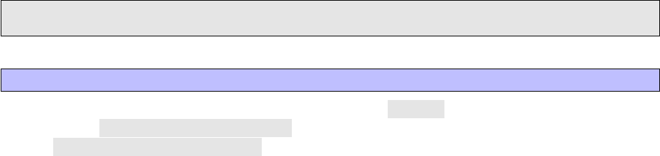
0.0025 0.0030 0.0035 0.0040 0.0045

|Vub|

500

1000

1500

probability

EOS v0.1.1

(a) Histogram of the marginal posterior of |Vub |, using 4×

7500 samples. Despite the poor quality of these samples, they

can be used to initialize the PMC run as described in the text.

0.0025 0.0030 0.0035 0.0040 0.0045

|Vub|

500

1000

1500

probability

EOS v0.1.1

(b) Histogram of the marginal posterior of |Vub|, using 106

samples.

Figure 2.1.: Histograms of the parameter of interest |Vub|in the two example ﬁts as described in sec-

tion 2.3, and plotted using the eos-plot-1d client; see section 2.7 for details.

-- scan "B -> pi :: b_ +^2 @ BCL2008 " -20 +20 -- prior flat \

-- constraint "B->pi:: f_+@IKMvD -2014" \

-- constraint "B^0->pi ^+ lnu ::BR@BaBar -2010 B" \

-- constraint "B^0->pi ^+ lnu ::BR@Belle -2010 A" \

-- constraint "B^0->pi ^+ lnu ::BR@BaBar -2012 D" \

-- constraint "B^0->pi ^+ lnu ::BR@Belle -2013 A" \

--pmc -initialize -from - file /tmp / mcmc_prerun_btopi +ff. hdf5 \

--hc -target - ncomponents 4 \

--hc -skip - initial 0.2 \

-- pmc -samples -per - component 500 \

-- pmc -group - by -r -value 1.5 \

-- pmc -final - samples 1000000 \

-- pmc -ignore -ess 1 \

-- pmc - relative - std - deviation - over - last - steps 0.05 4 \

-- output / tmp/pmc_monolithic_btopi+ff.hdf5

Both clients output copious amounts diagnostic data to the standard output, which include

• all information about the prior and the likelihood as speciﬁed on the command line (both clients);

• information about the convergence of the Markov chains within the parameter space, based on

the R-value criterion [8] (MCMC only);

• information about the convergence of the PMC run based on the perplexity and effective sam-

pling size (PMC only).

We display the outcome of both the MCMC (prerun) sampling as well as the PMC sampling steps in

ﬁgure 2.1.

2.4. Merging Markov Chains from multiple ﬁles

To run multiple Markov chains in parallel, one may use a compute cluster and submit independent

jobs, each of which creates its own output ﬁle with one or more chains inside. To initialize PMC, it is

necessary to have all Markov chains in a single HDF5 ﬁle. This is where eos-merge-mcmc comes into

play. It allows one to merge chains from multiple ﬁles into a single HDF5 ﬁle and optionally to apply a

2. Usage

cut such that chains that got stuck in irrelevant local modes in the prerun can be ﬁltered out. Note that

chains both from the prerun and main run are copied into the output ﬁle. eos-merge-mcmc accepts

the following command-line arguments:

Any number of input ﬁles created by eos-sample-mcmc

--cut-off NUMBER

Skip chains whose maximum log posterior in the prerun is below the cut-off.

--input-file-list LIST

List input ﬁles in a text ﬁle, one ﬁle per line. If other input ﬁles are passed directly on the command

line, then those take precedence but all ﬁles will be merged.

--output FILENAME

The name of the output ﬁle in which the chains are stored.

2.5. Finding the Mode of a Probability Density

The mode, best-ﬁt point, or simply the most-likely value, of some PDF P(⃗

θ)is regularly searched for

in physics analyses. EOS supplies the client eos-find-mode , which accepts the common set of

arguments describing the PDF as already discussed for the eos-sample-mcmc and eos-sample-pmc

clients, see section 2.3 for further information. In addition, it accepts the following command-line

arguments:

--starting-point { VALUE1 VALUE2 ... VALUEN }

Set the starting point for the maximization of the PDF P(⃗

θ)at θ= ( VALUE1 , . . . , VALUEN ).

--max-iterations INTEGER

The optimization algorithm is allowed to run at maximum NUMBER iterations.

--target-precision NUMBER

Attempt to determine the mode up to an uncertainty of NUMBER .

--output FILENAME

Write a YAML ﬁle with name FILENAME that contains the information of the mode in a machine-

readable format.

In order to illustrate the client’s usage, we use the same example as discussed in section 2.3. The

corresponding call then reads:

eos - find - mode \

--global -option model CKMScan \

-- global - option form - factors BCL2008 \

-- scan "CKM :: abs(V_ub )" 2e -3 5e -3 --prior flat \

-- nuisance "B -> pi :: f_ +(0) @B CL2008 " 0 1 -- prior flat \

-- nuisance "B -> pi :: b_ +^1 @BCL2008 " -20 +20 -- prior flat \

-- nuisance "B -> pi :: b_ +^2 @BCL2008 " -20 +20 -- prior flat \

-- constraint "B->pi:: f_+@IKMvD -2014" \

-- constraint "B^0->pi ^+ lnu ::BR@BaBar -2010 B" \

-- constraint "B^0->pi ^+ lnu ::BR@Belle -2010 A" \

-- constraint "B^0->pi ^+ lnu ::BR@BaBar -2012 D" \

-- constraint "B^0->pi ^+ lnu ::BR@Belle -2013 A" \

-- starting -point { 3.5e -3 0.31 0 0 } \

-- max - iterations 1000 \

--target -precision 1e -8 \

-- output /tmp/mode - btopipi - ff .yaml

2.6. Bayesian Uncertainty Propagation

The output starts with same diagnostic information on the composition of prior and likelihood as for

the sampling clients. The results are displayed in the last few lines, including

• the starting point for the mode-ﬁnding process;

• the coordinates of the best-ﬁt point; and

• the log-posterior at the best-ﬁt point.

# Starting optimization at ( 0.0035 0.31 0 0 )

# Found maximum at:

# ( 3.568778e-03 2.661032e-01 -2.670912e+00 2.231637e-02 )

# value = -3.101594e+02

2.6. Bayesian Uncertainty Propagation

EOS presently supports two ways to propagate theory uncertainties in the framework of Bayesian

statistics: First, by using prior PDFs that describes the nuisance parameters; second, by using samples

from a posterior PDF that have been obtained from running either eos-sample-mcmc or eos-sample-pmc .

It accepts the following command-line arguments:

--vary NAME --prior flat MIN MAX

--vary NAME [ABSMIN ABSMAX] --prior gaussian MIN CENTRAL MAX

These arguments add a parameter to the statistical analysis, with either a at or a Gaussian

prior. If ABSMIN and ABSMAX are speciﬁed, the prior will be cropped to this absolute interval.

--fix NAME VALUE

Fix parameter to a certain value. Use this to change default values for parameters that are not

varied.

--kinematics NAME VALUE

Within the scope of the next observable, declare a new kinematic variable with name NAME and

numerical value VALUE .

--observable NAME

Add a new observable with name NAME to the list of observables that shall be evaluated. All

previously issued --kinematics and --range arguments apply, and will be used by the new

obervable. The kinematics will be reset (i.e., all kinematic variables will be removed) in anticipa-

tion of the next --observable argument.

--global-option NAME VALUE

Set an option to a string value that applies to all following observables.

--samples NUMBER

Sets the number of samples that shall be produced per observable and worker thread.

--workers NUMBER

Sets the number of worker threads. Default: 4.

2. Usage

--parallel [0|1]

Activate multithreaded evaluation. Default: 1.

--mcmc-input HDF5FILE BEGIN END

Use the samples at index BEGIN up to index END from each chain in the ﬁle HDF5FILE . If

both preruns and main runs are present in the ﬁle, preference is give to the main run. To use all

samples, use BEGIN=0 and choose a value for END equal to or larger than the actual length of

any chain in the ﬁle.

Note: The ﬁle must have been produced by the eos-sample-mcmc client.

Note: If you have the HDF5 commandline tools available, use h5ls -r HDF5FILE to see the

number and length of the chains.

--mcmc-prefer-prerun [0|1]

Override the default setting to take samples from the prerun instead of the main run in case both

are present in the HDF5FILE . Default: 0.

--pmc-input HDF5FILE BEGIN END

Use the samples at index BEGIN up to index END from a named data set in the ﬁle HDF5FILE .

Note: The ﬁle must have been produced by the eos-sample-pmc client.

--pmc-sample-directory NAME

Use the named data set within the ﬁle speciﬁed with --pmc-input . Valid names are /data/X,

where X stands for either initial,final, or all numbers describing existing update steps that

were carried out in the PMC run.

Note: You should use /data/final unless you are debuging the PMC algorithm.

--output NAME

Set the output ﬁle name.

--store-parameters [0|1]

Store the parameter samples drawn from the prior into the output ﬁle. Has no effect with --mcmc-input

or --pmc-input . Default: 0.

--seed VALUE

Change the random number seed for generating parameter samples. Has no effect with --mcmc-input

or --pmc-input . By default a ﬁxed seed is chosen corresponding to VALUE=0 . To get different

samples on each invocation, use VALUE=time .

As an example of the ﬁrst way, we would like to predict the branching ratio for the decay B−→

τ−¯ντ. This prediction involves two parameters: First, the absolute value of Vub; and second, the value

of the B-meson decay constant fB. For the former, we choose the HFAG average of the inclusive

determination |Vub|= (4.45 ±0.26) ·10−3[9], while for the latter we use the FLAG average fB=

0.188±0.007 GeV [10]. Our intention translates to the following call to eos-propagate-uncertainty :

2.7. Plotting Random Samples

eos - propagate - uncert ainty \

--global -option model CKMScan \

-- global - option form - factors BCL2008 \

-- vary "CKM ::abs(V_ub )" 2e -3 5e -3 --prior gaussian 4.19e-3 4.45e-3 4.71e-3 \

-- vary "decay -constant :: B_u" 0.167 0.209 --prior gaussian 0.181 0.188 0.195 \

-- observable " B_u -> lnu :: BR ;l =tau " \

-- workers 4 \

-- samples 100000 \

-- output / tmp/unc_btotaunu . hdf5

As an exmple of the second way, we would like to use samples from the posterior PDF as obtained

in section 2.3 in order to predict the branching ratio of the differential decay ¯

B0→πe−¯νe, at various

points in the kinematic range as the decay to muons described previously. Our intention translates to

the following call to eos-propagate-uncertainty :

eos - propagate - uncert ainty \

-- kinematics s 0.00 --observable "B->pilnu :: dBR/ds;l=e,form -factors=BCL2008 ,model = CKMScan" \

-- kinematics s 0.25 --observable "B->pilnu :: dBR/ds;l=e,form -factors=BCL2008 ,model = CKMScan" \

-- kinematics s 0.50 --observable "B->pilnu :: dBR/ds;l=e,form -factors=BCL2008 ,model = CKMScan" \

-- kinematics s 0.75 --observable "B->pilnu :: dBR/ds;l=e,form -factors=BCL2008 ,model = CKMScan" \

-- kinematics s 1.00 --observable "B->pilnu :: dBR/ds;l=e,form -factors=BCL2008 ,model = CKMScan" \

-- kinematics s 1.50 --observable "B->pilnu :: dBR/ds;l=e,form -factors=BCL2008 ,model = CKMScan" \

-- kinematics s 2.00 --observable "B->pilnu :: dBR/ds;l=e,form -factors=BCL2008 ,model = CKMScan" \

-- kinematics s 2.50 --observable "B->pilnu :: dBR/ds;l=e,form -factors=BCL2008 ,model = CKMScan" \

-- kinematics s 3.00 --observable "B->pilnu :: dBR/ds;l=e,form -factors=BCL2008 ,model = CKMScan" \

-- kinematics s 3.50 --observable "B->pilnu :: dBR/ds;l=e,form -factors=BCL2008 ,model = CKMScan" \

-- kinematics s 4.00 --observable "B->pilnu :: dBR/ds;l=e,form -factors=BCL2008 ,model = CKMScan" \

-- kinematics s 6.00 --observable "B->pilnu :: dBR/ds;l=e,form -factors=BCL2008 ,model = CKMScan" \

-- kinematics s 7.00 --observable "B->pilnu :: dBR/ds;l=e,form -factors=BCL2008 ,model = CKMScan" \

-- kinematics s 8.00 --observable "B->pilnu :: dBR/ds;l=e,form -factors=BCL2008 ,model = CKMScan" \

-- kinematics s 9.00 --observable "B->pilnu :: dBR/ds;l=e,form -factors=BCL2008 ,model = CKMScan" \

-- kinematics s 10.00 --observable "B->pilnu :: dBR/ds;l=e ,form -factors = BCL2008 ,model=CKMScan " \

-- kinematics s 11.00 --observable "B->pilnu :: dBR/ds;l=e ,form -factors = BCL2008 ,model=CKMScan " \

-- kinematics s 12.00 --observable "B->pilnu :: dBR/ds;l=e ,form -factors = BCL2008 ,model=CKMScan " \

--pmc -input / tmp/pmc_monolithic_btopi +ff.hdf5 0 10000 \

-- pmc -sample - directo ry "/ data /final /" \

-- output / tmp/unc_btopilnu . hdf5

For both ways, the samples of the predictive distributions within the HDF5 ﬁles can be accessed using

the eos.data.UncertaintyDataFile Python class.

2.7. Plotting Random Samples

Once random samples have been obtained from either a posterior PDF (e.g. as described in sec-

tion 2.3) or a predictive PDF (e.g. as described in section 2.6), a visual inspection of the samples is the

next step. EOS provides scripts for this purpose, which plot histograms of either a marginalized 1D

(eos-plot-1d ) or heatmaps of 2D ( eos-plot-2d ) PDFs. Both scripts presently detect the output

format by inspection of the resepective HDF5 ﬁle name. Files containing MCMC samples should be

preﬁxed with mcmc_, while PMC sample ﬁles should be preﬁxed with pmc_monolithic_. Files contain-

ing samples from the uncertainty propagation should be preﬁxed with unc_.

The eos-plot-1d produces a 1D histogram of the samples for one parameter. It accepts the follow-

ing arguments:

HDF5FILE

The name of the HDF5 input ﬁle whose samples shall be plotted.

VAR

The name of the variable (either a Parameter or an Observable) whose density function shall

be plotted.

2. Usage

PDFFILE

The name of the PDF output ﬁle, into which the plot shall be saved.

--xmin XMIN ,--xmax XMAX

When speciﬁed, limit the plot range to the interval XMIN to XMAX . The default values are taken

from the description of the parameter within the HDF5 input ﬁle.

--kde [0|1]

When enabled, plots a univariate Kernel Density Estimate of the probability density based on the

available samples.

--kde-bandwidth KDEBANDWIDTH

When speciﬁed, multiplies the automatically determined KDE bandwidth parameter with KDEBANDWIDTH .

The eos-plot-2d produces a 2D heatmap of the samples for two parameters. It accepts the follow-

ing arguments

HDF5FILE

The name of the HDF5 input ﬁle whose samples shall be plotted.

XIDX

The numerical index for the parameter that shall be plotted on the xacis. XIDX starts with zero

YIDX

The numerical index for the parameter that shall be plotted on the yacis. YIDX starts with zero

PDFFILE

The name of the PDF output ﬁle, into which the plot shall be saved.

--xmin XMIN ,--xmax XMAX

When speciﬁed, limit the plot range on the xaxis to the interval XMIN to XMAX . The default

values are taken from the description of the parameter within the HDF5 input ﬁle.

--ymin YMIN ,--ymax YMAX

When speciﬁed, limit the plot range on the yaxis to the interval YMIN to YMAX . The default

values are taken from the description of the parameter within the HDF5 input ﬁle.

3. Library Interface

The rationale behind several of the design decisions of the EOS libraries are explained in section 3.1.

We document the core set of classes in section 3.2.

3.1. Design

To fulﬁll its intended use cases, the EOS libraries are designed by abiding to the follwing principles.

First, scalar quantities are treated as parameters. These include

• experimental inputs, such as particle masses and lifetimes;

• theoretically motivated quantities, such as quark masses (e.g.in the MS scheme) and the Wolfen-

stein parameters of the CKM matrix.

It is therefore straightforward to change a parameter’s role from one analysis to the next; e.g.from

being a nuisance parameter when producing theory estimates, to being a parameter of interest when

inferring knowedlge from experimental data. To differentiate between the various parameters, a nam-

ing scheme is put in place:

NAMESPACE::ID@TAG ,(3.1)

where the meta variables convey the following meaning:

NAMESPACE A short description of the context in which the parameter should be interpreted.

Possible namespaces include, but are not limited to: mass,decay-constants,

CKM, and others.

ID A descriptive handle for the parameter in its namespace.

TAG A forther pices of information that allows to distinguish between parameters with

the same ID.

Second, quantities that exhibit a functional dependence on either a parameter or a kinematic variable

are treated as plugins: An interface is created that allows implementing more than one realization of

the respective function. The actual implementations of this interface are then accesible via a factory

method.1Each implementation of a plugin can depend on its own subset of parameters. For clarity,

we use one of the hadronic form factor as an example. Consider the B→πvector form factor fBπ

One possible parametrization of this form factor has been proposed in [5] (denotes as BCL2008). It is

achieved in terms of three parameters:

• the normalization fBπ

+(0), and

1A good example for such a modular design is found within the scope of hadronic matrix elements, in particular hadronic

form factors.

3. Library Interface

• two shape parameters bBπ,+

1and bBπ,+

This parametrization is implemented within EOS as one of several options for a B→πform factor

parametrization. The relevant EOS parameters are contained in the namespace B->pi, and tagged for

the BCL2008 plugin:

B->pi::f_+(0)BCL2008 ,B->pi::b_+ˆ1BCL2008 ,and B->pi::b_+ˆ2BCL2008 .(3.2)

This removes the risk of namespace collisions among the various plugins’ parameters.

Observables that depend on the the B→πform factors can be implemented by relying on the

form factors interface, and leave the concrete parametrization to be a run-time option with name

form-factors. The BCL2008 parametrization can be selected by passing form-factors=BCL2008 to

the observable.

Third, data is only copied when explicitly requested. Copy constructors yield another object that points

to the same underlying data. This is achieved through extensive use of the Private Implementation

design pattern.2To make an independent copy, the EOS classes provide the clone() method.

3.2. Core Classes

At the core of the EOS API there are four classes:

Parameters which contains the whole set of Parameter known to EOS

Kinematics which contains the set of kinematic variables speciﬁc to one instance of Observable

Options which contains the set of options speciﬁc to one instance of Observable

Observable which encapsulates the numerical implemention of a single (pseudo-)observable

quantity.

3.2.1. Class Parameters

Implemented as a dictionary, with keys of type std:string and values of type Parameter. The default

set of parameters is loaded from the EOS-supplied YAML ﬁles. It can be loaded by using the static

Parameters::Defaults() method. Using the copy construtor does not yield an independent copy;

instead the second object uses the underlying data of the initial instance. To obtain an independent

copy with the same values as the present one, use the clone() method.

1Parame ters paramA = Para meter s :: D efaults () ;

2Parameters paramB(paramA );

4ObservablePtr obsA = Observable :: make("A", paramA , Kinematics{ }, Options { });

5ObservablePtr obsB = Observable :: make("A", paramB , Kinematics{ }, Options { });

You can access individual parameters via the array subscript operator. It takes a class QualifiedName

object as its key, which can be created implicitly from std::string or const char *. You can also

iterate over all parameters via the begin() and end() methods. In both cases, the underlying objects

are of class Parameter, which provides access to the current value via the evaluate() method.

2See https://cpppatterns.com/patterns/pimpl.html.

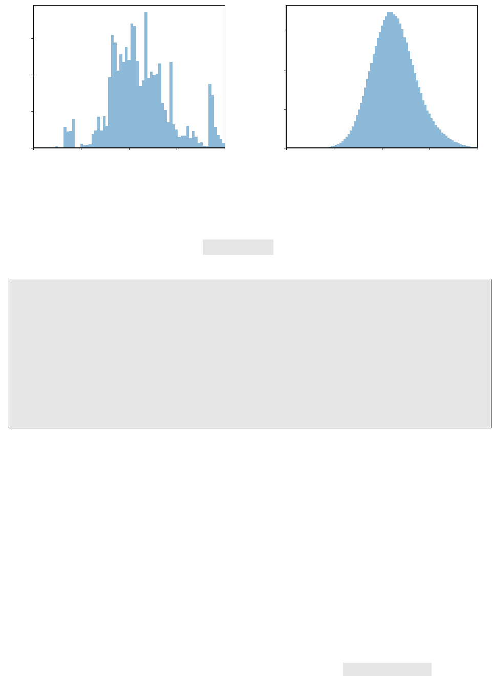
3.2. Core Classes

Parameter Data

paramA

depends

paramB

copy

depends

obsA

depends

obsB

depends

Figure 3.1.: Diagrammatic illustration that multiple observables can depend on the very same instance

of Parameters.

3.2.2. Class Kinematics

The class Kinematics is a dictionary from std::string-valued keys to KinematicVariable-valued

entries. Upon construction of an observable, a suitable instance of kinematics is bound to that ob-

servable. Acces to individual kinematic variables occurs through the array subscript operator. The

class is used for the run-time construction of observables. For this purpose, the variable names apply

only to a single observable and are not explicitly namespaced.

3.2.3. Class Options

The class Options is a dictionary from std::string-valued keys to std::string-valued entries. Upon

construction of an observable, a suitable instance of Options is bound to that observable. The under-

lying class’s constructor queries the options, and select the appropriate run-time behaviour.

Helper classes are available for repeated options-related task, e.g.the class SwitchOption.

3.2.4. Class Observable

The class Observable is an abstract base class. To create a new observable object, you must use the

static Observable::make() factory method. It requires three arguments:

• a class QualifiedName object n;

• a class Parameters object p; and

• a class Kinematics object k; and

• an class Options object o.

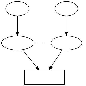
3. Library Interface

Observable A Observable A'

copy

Parameters A

mass::b(MSbar) = 4.20

Parameters B

mass::b(MSbar) = 4.16

(a) copy

Observable A Observable B

clone

Parameters A

mass::b(MSbar) = 4.20

Parameters B

mass::b(MSbar) = 4.16

(b) clone

Figure 3.2.: Diagrammatic illustration of the differences between copying an instance of Observable

via the copy-constructor, and cloning the observable via the clone method

To allow for more compact code, EOS’ internal observables are not implemented as individual classes.

Instead, related observables are bundled together into one class. Individual observable classes are

then created using the template <...> class ConcreteObservable. We refer to section 4.2 for de-

tails on how to extend EOS with the implementation of a new observable.

Note: Any changes to the Options object oafter construction of the observable do not affect the ob-

servable.

Note: All users of Observable must also support cloning. This allows to easily parallelize algorithms

acting on Observable.

4. Extending EOS

We discuss the three most common cases of extending EOS, by adding either a new parameter, a

new observable, or a new measurement. For extensions that do not fall in these categories please

contact the main authors, who will be happy to discuss your work with you. The most efﬁcient way to

contribute new code or modiﬁcations to EOS is via a pull request in the main Github repository.1

4.1. How to add a new parameter

Parameters are stored in YAML ﬁles below eos/parameters/, including the default values and range,

as well as metadata and the origin thereof. Each ﬁle contains key-to-value maps:

• Keys starting and ending with an @sign are considered to be metadata pertaining to the entire

ﬁle.

• All other keys declare a new parameter.

The values in this map are the deﬁnitions of a parameters, and are also structured as maps. Valid

parameter deﬁnitions must include all of the following entries:

central the default central value;

min the minimal value for the default range;

max the maximal value for the default range.

Optional entries include:

comment a comment on the purpose;

latex the LaTeX command for the display;

unit the unit in which the parameter is expressed.

Example

We introduce two new parameters: mass::X@Example, and decay-constant::X@Example, standing in

for the mass and decay constant of a hypothetical particle X. We add the ﬁle eos/parameters/x.yaml

with contents:

'mass :: X@Example ' :

central: +1.0

min: +0.5

max: +1.5

unit : 'GeV '

latex : '$M_X$ '

comment: 'The mass of the unmotivated X particle '

'decay - constant :: X@ Examp le ' :

central: +0.10

1https://github.com/eos/eos

4. Extending EOS

min: +0.09

max: +0.11

unit : 'GeV '

latex : '$f_X$ '

comment: 'The decay constant of the unmotivated X particle '

4.2. How to add a new observable

An Observable is implemented in EOS as follows:

• The numerical code is implemented as the method double P::o(...) const, where Pis the

underlying class, and the dots stand in for any number of const double & arguments, includ-

ing zero. The class P must inherit from class ParameterUser. It must have one constructor

accepting a class Parameters and a class Options instance in that order. Schematically:

1#include <eos/utils/ parameters.hh >

2#include <eos/utils/ options.hh >

4class P :

5public ParameterUser

7P(const Parameters \&, const Options \&};

8~P();

10 double obse rva ble _wi tho ut_ kin emat ics () const ;

11 double observable_with_one_kinematic_variable(const double &) const ;

12 };

• The method or methods are then associated with their names within the ﬁle eos/observable.cc

within the free-standing function make_observable_entries(). Within the existing map, new

entries are created through a call to make_observable(...). For a regular observable the ar-

guments are in order: the name of the observable; the pointer to its method; and the tuple

of std::strings that names the kinematic variables in the order the method expects them.

Schematically:

1#within eos/ observable .cc

2#[...]

3make _obs erva ble (" P:: ob serva ble1 " ,

4&P :: o bse rva ble _wi tho ut_ kine mat ics );

5make _obs erva ble (" P:: ob serva ble2 ( variab lena me )" ,

6&P::observable_with_one_kinematic_variable ,

7std :: m ake_ tuple (" vari able name ") );

8#[...]

4.3. How to add a new constraint

Constraints are stored in YAML ﬁles below eos/constraints/. New constraints can be added to

an existing ﬁle, or to an entirely new ﬁle. Each ﬁle contains key-to-value maps in which the top-level

keys declare a new constraint. The values in this map are the deﬁnitions of a constraint, and are also

structured as maps. Valid constraint deﬁnitions must at least include a type entry that governs the

functional form of the associated likelihood. EOS understands the following types of constraints:

•Amoroso,

•Gaussian,

4.3. How to add a new constraint

•MultivariateGaussian,

•MultivariateGaussian(Covariance).

4.3.1. Type Amoroso

Type Amoroso uses a likelihood arising from the PDF of the Amoroso distribution [11], a four-parameter

distribution. It is useful for the modeling of upper limits on as-of-yet undiscovered decays at given

probabilities. For example, the upper limits on the decay Bs→µ+µ−by the LHCb experiment prior to

the discovery of this decay are modeled using the Amoroso type of likelihood. The following keys are

required in the description of the constraint:

observable the qualiﬁed name for an Observable or a Parameter;

kinematics the map representation of the kinematic variables pertaining to the observable;

options the map representation of the options pertaining to the observable;

physical-limit the physical lower bound on the observable;

theta the θparameter of the Amoroso distribution;

alpha the αparameter of the Amoroso distribution;

beta the βparameter of the Amoroso distribution;

We strongly recommend contacting the EOS authors before adding your own constraint of type Amoroso.

4.3.2. Type Gaussian

Type Gaussian uses a univariate Gaussian or normally-distributed likelihood. The following keys are

required in the description of the constraint:

observable the qualiﬁed name of an Observable or a Parameter;

kinematics the map representation of the kinematic variables pertaining to the observable;

options the map representation of the options pertaining to the observable;

mean the mean of the distribution;

sigma-stat the map representation with keys hi and lo for the upper and lower statistical

uncertainty of the distribution, respectively;

sigma-sys the same as sigma-stat, but for the systematic uncertainty;

dof the degrees of freedom associated with this observation (should default to 1).

By default the uncertainties are symmetrized, and statistical and systematical uncertainties are added

in quadrature.

4. Extending EOS

4.3.3. Type MultivariateGaussian

Type MultivariateGaussian uses a multivariate Gaussian likelihood, parametrized in terms of its

mode and correlation matrix. The following keys are required in the description of the constraint:

dim the dimensionality of the multivariate distribution;

observable the list of size dim of qualiﬁed names for either Observables or Parameters;

kinematics the list of size dim of map representations of the kinematic variables pertaining

to each observable;

options the list of size dim of map representations of the options pertaining to each ob-

servable;

mean the list of size dim describing the mean of the distribution;

sigma-stat-hi the list of size dim for the upper statistical uncertainty of the distribution;

sigma-stat-lo the list of size dim for the lower statistical uncertainty of the distribution;

correlations the matrix of size dim ×dim for the statistical correlations;

sigma-sys the list of size dim for the systematic uncertainty;

dof the degrees of freedom associated with this observation (should default to dim).

By default the statistical and systematical uncertainties are added in quadrature, and the larger of the

upper and lower uncertainties are chosen as the standard deviation. The covariance matrix Σij is then

computed from the variances σiand the correlation matrix ρij as

Σij =σiσjρij .(4.1)

4.3.4. Type MultivariateGaussian(Covariance)

Type MultivariateGaussian(Covariance) uses a multivariate Gaussian likelihood, parametrized in

terms of its mode and covariance matrix. The following keys are required in the description of the

constraint:

dim the dimensionality of the multivariate distribution;

observable the list of size dim of qualiﬁed names for either Observables or Parameters;

kinematics the list of size dim of map representations of the kinematic variables pertaining

to each observable;

options the list of size dim of map representations of the options pertaining to each ob-

servable;

mean the list of size dim describing the mean of the distribution;

covariance the matrix of size dim ×dim for the covariance of the distribution;

dof the degrees of freedom associated with this observation (should default to dim).

4.3. How to add a new constraint

Example

We introduce a constraint to correlate the new parameters mass::X@Example, and decay-constant::X@Example

from section 4.1. The correlation is ﬁxed at 50%, and the means and standard deviations reect the

previous one. We add the ﬁle eos/constraints/x.yaml with contents:

X:: mass +decay -constant@Example :

type : MultivariateGaussian

dim: 2

obser vabl es : [ 'mass :: X@Exam ple ' , ' decay - const ant :: X@Example ']

kinematics: [{} , {}]

options: [{} , {}]

means : [1.0, 0.1]

covari ance : [[0.2 5 , 2.5 e-3] , [2.5 e-3 , 1.0 e -4]]

dof: 2

Physics

5. Effective Field Theories

The electro-weak decays of hadrons (mesons and baryons) with masses much smaller than the

electro-weak scale of order of the W-boson mass, mW, can be efﬁciently described using effective

ﬁeld theories (EFT) in the spirit of the well-known Fermi theory of the β-decay. This comprises prac-

tically all hadrons containing light quarks q= (u, d, s, c, b). In this context, speciﬁc avour-changing

higher-dimensional (dim > 4) operators arise in the standard model (SM) and it’s extensions, accom-

panied by effective couplings (Wilson coefﬁcients) giving rise to the generic structure of the effective

Lagrangian

LEFT =LQCD×QED(light particles) + 

iCi(µ)Oi+h.c. +. . . . (5.1)

The ﬁrst term describes the SU (3)c×U(1)em gauge interactions of all light quarks, q, and leptons,

ℓ= (e, µ, τ), with QCD and QED gauge bosons. The second part are the aforementioned operators

Oiand effective couplings Ci, where the latter depend on a factorization scale µlow that is usually

of the order of the mass of the decaying hadron. The operators are composed out of light degrees

of freedom, i.e. fermions qand ℓ, as well as SU (3)cand U(1)em gauge bosons. Beyond the SM, it

is conceivable that in principle additional light degrees of freedom exist, which however must have

escaped direct detection so far. The Wilson coefﬁcients are suppressed by inverse powers of the

electroweak scale or some new physics scale, depending on the dimension of their operators. Finally,

the dots denote higher-dimensional operators that have been neglected. In practical applications,

assuming the SM, they are suppressed at least by m2

b/m2

W∼0.004, where mbdenotes the bottom-

quark mass.

The EFT framework is sufﬁcient to describe interactions at and below the scale µlow, including hadronic

binding effects due to strong interactions as well as electro-magnetic virtual and real corrections to

observables. The implementation of according observables in EOS is thus based on universal EFT La-

grangians. All respective short-distance interactions above µlow are ﬁxed by the structure of the oper-

ators and the values of the Wilson coefﬁcients. In the spirit of Fermi, the according Wilson coefﬁcients

can be viewed as unknowns to be determined from experiment. This so-called model-independent ap-

proach implies the independence of all Wilson coefﬁcients and correlation among observables arise

from the assumption of which operators are included, i.e. have non-vanishing Wilson coefﬁcients at

the scale µlow (or some other).

The latter point is important in view of operator mixing (under QCD and QED), which is governed by

the anomalous dimension matrices (ADM) of the involved operators. In the case of operator mixing,

vanishing Wilson coefﬁcients at some scale µ0can become non-zero at some other scale µ1, de-

pending on their mixing and the initial conditions of Wilson coefﬁcients involved in the mixing. This is

summarized by the general solution of the renormalisation group equation (RGE)

Ci(µ1) = 

[U(µ1, µ0)]ij Cj(µ0).(5.2)

The evolution matrix Udepends on the ADM’s of the operators, the strong and electro-magnetic cou-

plings, αsand αerespectively, and their respective RG-functions (beta-functions). Throughout Wilson

coefﬁcients and couplings are MS-renormalized quantities.

5. Effective Field Theories

In the following we collect the conventions of the effective theories implemented in EOS for hadron

decays based on quark transitions

b→(d, s), . . . (5.3)

For an introduction to the topic, the reader is referred to the exhaustive review articles [12, 13].

The following abbreviations will be often used below for products of elements of the CKM quark mixing

matrix appearing in b-quark decays

λ(D)

U=VUbV∗

UD , D = (d, s), U = (u, c, t).(5.4)

5.1. |∆B|=|∆S|= 1

In this section we summarize the convention of the EFT for |∆B|=|∆S|= 1 decays covering transi-

tions

b→s+ (¯uu, ¯cc)current-current ,

b→s+ ¯qq QCD & QED penguin ,

b→s+ (γ, gluon)electro- & chromo-magnetic dipole ,

b→s+ (¯

ℓℓ, ¯νν)semi-leptonic ,

where the classiﬁcation corresponds to the origin of the operators from decoupling Wand Zbosons

and the top quark in the SM. The basis contains several blocks that are however related via operator

mixing and renders the RGE of the Wilson coefﬁcients non-trivial. The results for |∆B|=|∆D|= 1

transitions are obtained by the replacement s→d.

We start with the operators generated in the SM, where the initial Wilson coefﬁcients and ADM’s are

known at several orders in perturbation theory. The most appropriate choice of basis for higher order

QCD calculations of ADM’s was given in [14, 15] with according extension for QED corrections in [16,

17]. The Lagrangian

LEFT =LQCD×QED(q;ℓ) + 4GF

√2λ(s)



i=1 Ci(Oc

i− Ou

+4GF

√2λ(s)

t2



i=1 CiOc



i=3 CiOi+



i=3 CiQOiQ +CbOb+h.c. .

(5.5)

incorporates unitarity of the CKM matrix λ(s)

u+λ(s)

c+λ(s)

t= 0. All Wilson coefﬁcients Ciare evaluated

at µlow ∼mb. The up-quark sector ∼λ(s)

uis doubly-Cabibbo suppressed for b→stransitions and

leads to tiny CP-asymmetries in the SM.

The current-current (U=u, c) operators are deﬁned as

1= (¯sγµPLTaU)( ¯

UγµPLTab),OU

2= (¯sγµPLU)( ¯

UγµPLb),(5.6)

which arise already at tree-level from decoupling the W-boson in b→s+(¯uu, ¯cc)and mix into all other

operators, except the semi-leptonic O10. Here and below PL,R = (1∓γ5)/2 denote chirality projectors.

The QCD-penguin operators are

O3= (¯sγµPLb)

(¯qγµq),O5= (¯sγµνρPLb)

(¯qγµνρq),

O4= (¯sγµPLTab)

(¯qγµTaq),O6= (¯sγµνρPLTab)

(¯qγµνρTaq),

(5.7)

5.1. |∆B|=|∆S|= 1

where the sum extends over all q= (u, d, s, c, b)and Taare the generators of SU (3)c. Products of

several gamma matrices have been abbreviated γµνρ ≡γµγνγρ.

Analogous QED-penguin operators are deﬁned as

O3Q= (¯sγµPLb)

Qq(¯qγµq),O5Q= (¯sγµνρPLb)

Qq(¯qγµνρq),

O4Q= (¯sγµPLTab)

Qq(¯qγµTaq),O6Q= (¯sγµνρPLTab)

Qq(¯qγµνρTaq),

(5.8)

where Qqdenotes the quark charges as multiples of e. Further, an additional operator has to be con-

sidered

Ob=−1

3(¯sγµPLb)(¯

bγµb) + 1

12(¯sγµνρPLb)(¯

bγµνρb),(5.9)

receiving contributions from electro-weak boxes. In four dimension it would correspond to (¯sγµPLb)(¯

bγµPLb),

however the above form allows to avoid traces with γ5to all orders in QCD.

The electro- and chromo-magnetic dipole operators

O7=e

[¯sσµν (mbPR+msPL)b]Fµν ,˜

O8=1

[¯sσµν (mbPR+msPL)Tab]Ga

µν ,(5.10)

receive contributions from on-shell photon and gluon penguins. The appearing quark masses are

renormalized in the MS scheme.

In the SM there are two semi-leptonic operators

Oℓ

9=e2

(¯sγµPLb)(¯

ℓγµℓ),˜

Oℓ

10 =e2

(¯sγµPLb)(¯

ℓγµγ5ℓ),(5.11)

describing b→s+¯

ℓℓ transitions. In this case the lepton charge Qℓhas been pulled into the deﬁnition

of the Wilson coefﬁcient.

note deﬁnition of evanescent operators, without whom ADM’s and initial Wilson coefﬁcients are mean-

ingless ...

For the tilde operators the normalization to (4π/gs)2, the QCD coupling, has been chosen for practical

reasons such that the leading SM 1-loop correction to the initial Wilson coefﬁcients counts formally

as a strong correction rather then an electro-magnetic one. The initial Wilson coefﬁcients are known

up to NNLO in QCD and NLO in EW corrections

Ci(µ0) = . . . (5.12)

(ai≡αi/(4π)) For practical applications, however, we use operators without a tilde, which are related

via

Oi=g2

(4π)2˜

Oi.(5.13)

The full basis of semi-leptonic operators is spanned by O9,10 as above, and additionally

Oℓ

9′=e2

(4π)2(¯sγµPRb)(¯

ℓγµℓ),Oℓ

10′=e2

(4π)2(¯sγµPRb)(¯

ℓγµγ5ℓ),(5.14)

Oℓ

S=e2

(4π)2(¯sPRb)(¯

ℓℓ),Oℓ

P=e2

(4π)2(¯sPRb)(¯

ℓγ5ℓ),(5.15)

Oℓ

S′=e2

(4π)2(¯sPLb)(¯

ℓℓ),Oℓ

P′=e2

(4π)2(¯sPLb)(¯

ℓγ5ℓ),(5.16)

Oℓ

T=e2

(4π)2(¯sσµν b)(¯

ℓσµν ℓ),Oℓ

T5=e2

(4π)2(¯sσµν b)(¯

ℓσµν γ5ℓ).(5.17)

5. Effective Field Theories

Quantity Qualiﬁed Name

i= 7,7′

Re Ci(µb)b->s::Re{ci}

Im Ci(µb)b->s::Im{ci}

i= 9,9′,10,10′, S, S′, P, P ′, T, T 5

Re C(ℓ)

i(µb)b->sℓℓ::Re{ci}

Im C(ℓ)

i(µb)b->sℓℓ::Im{ci}

i= 1 . . . 6,8,8′

Ci(µb)b->s::ci

Table 5.1.: Naming scheme for the |∆B|=|∆S|= 1 operators.

For studies of NP effects in these operators the values of the respective Wilson coefﬁcients can be

changed within the EOS code at run time. For the changed to take effect, the observables must

be constructed with the option model set to WilsonScan. In that case, the coefﬁcients Ciwith i∈

{7,7′,9,9′,10,10′, S, S′, P, P ′, T, T 5}are treated as complex-valued parameters. Since EOS parame-

ters are real-valued only, this implies that real and imaginary part of these coefﬁcients can be adjusted

separately. The coefﬁcients CjUwith j={1,2}are presently U-avour-universal, and are simply

considered as two independent coefﬁcients Cj. The coefﬁcients with j={1. . . 6,8}are treated as

real-valued parameters. The naming scheme for these coefﬁcients is listed in table 5.1.

5.2. |∆B|=|∆U|= 1

The Lagrangian reads:

LEFT =LQCD×QED(q;ℓ)−4GF

√2Veff

ub 

XCXOX.(5.18)

Note the change of sign compared to the journal version of [18], which has a wrong but inconsequential

global factor of −1. The operators are deﬁned as

OV,L(R)≡¯uγµPL(R)b¯

ℓγµPLνℓ,

OS,L(R)≡¯uPL(R)b¯

ℓPLνℓ,

OT≡[¯uσµν b]¯

ℓσµν PLνℓ.

(5.19)

5.3. |∆B|=|∆C|= 1

The Lagrangian reads:

LEFT =LQCD×QED(q;ℓ)−4GF

√2Veff

cb 

XCXOX.(5.20)

5.3. |∆B|=|∆C|= 1

Note the change of sign compared to the journal version of [18], which has a wrong but inconsequential

global factor of −1. The operators are deﬁned as

OV,L(R)≡¯cγµPL(R)b¯

ℓγµPLνℓ,

OS,L(R)≡¯cPL(R)b¯

ℓPLνℓ,

OT≡[¯cσµν b]¯

ℓσµν PLνℓ.

(5.21)

A. List of default parameters

The complete list of default parameters is given in this appendix, in a series of tables.

Qualiﬁed Name Parameter Description

b->s::c1 ???

b->s::c2 ???

b->s::c3 ???

b->s::c4 ???

b->s::c5 ???

b->s::c6 ???

b->s::Re{c7} ???

b->s::Im{c7} ???

b->s::c8 ???

b->see::Re{c9} ???

b->see::Im{c9} ???

b->see::Re{c10} ???

b->see::Im{c10} ???

b->smumu::Re{c9} ???

b->smumu::Im{c9} ???

b->smumu::Re{c10} ???

b->smumu::Im{c10} ???

b->s::Re{c7'} ???

b->s::Im{c7'} ???

b->s::c8' ???

b->see::Re{c9'} ???

b->see::Im{c9'} ???

b->see::Re{c10'} ???

b->see::Im{c10'} ???

b->smumu::Re{c9'} ???

b->smumu::Im{c9'} ???

b->smumu::Re{c10'} ???

b->smumu::Im{c10'} ???

b->see::Re{cS} ???

b->see::Im{cS} ???

b->see::Re{cS'} ???

b->see::Im{cS'} ???

b->see::Re{cP} ???

b->see::Im{cP} ???

b->see::Re{cP'} ???

A. List of default parameters

b->see::Im{cP'} ???

b->see::Re{cT} ???

b->see::Im{cT} ???

b->see::Re{cT5} ???

b->see::Im{cT5} ???

b->smumu::Re{cS} ???

b->smumu::Im{cS} ???

b->smumu::Re{cS'} ???

b->smumu::Im{cS'} ???

b->smumu::Re{cP} ???

b->smumu::Im{cP} ???

b->smumu::Re{cP'} ???

b->smumu::Im{cP'} ???

b->smumu::Re{cT} ???

b->smumu::Im{cT} ???

b->smumu::Re{cT5} ???

b->smumu::Im{cT5} ???

Table A.2.: The list of parameters describing the b->sqqbar,gamma,ll Wilson coefﬁcients. See the EOS

manual for their physical deﬁnitions.

Qualiﬁed Name Parameter Description

HQET::lambda_1 λ1cf. [ALGH2001], Table 2, p. 13

HQET::lambda_2 λ2cf. [ALGH2001], Table 2, p. 13

B->B::mu_pi^2@1GeV µ2

π(1 GeV)cf. [BBMU2003], Eq. (19), p. 9

B->B::mu_G^2@1GeV µ2

G(1 GeV)cf. [BBMU2003], Eq. (17), p. 9

B->B::rho_D^3@1GeV ρ3

D(1 GeV)cf. [BBMU2003], between Eqs. (19),(20),

p. 9

B->B::rho_LS^3@1GeV ρ3

LS (1 GeV)cf. [BBMU2003], Eq. (20), p. 9

Lambda_b->Lambda_b::mu_pi^2@1GeV µ2

π(1 GeV)cf. [MvD2015]

Lambda_b->Lambda_b::rho_D^3@1GeV ρ3

D(1 GeV)cf. [MvD2015]

Table A.4.: The list of hadronic forward matrix elements of operators arising in the heavy quark expan-

sion. For the matrix elements µ2

π,G and similar, see [MTU2010] for the deﬁnition.

Qualiﬁed Name Parameter Description

CKM::A ACKM The Wolfenstein CKM parameter A

CKM::lambda λCKM The Wolfenstein CKM parameter λ

CKM::rhobar ¯ρCKM The Wolfenstein CKM parameter ¯ρ

CKM::etabar ¯ηCKM The Wolfenstein CKM parameter ¯η

CKM::abs(V_ud) |Vud|

CKM::arg(V_ud) arg Vud

CKM::abs(V_us) |Vus|

CKM::arg(V_us) arg Vus

CKM::abs(V_ub) |Vub|

CKM::arg(V_ub) arg Vub

CKM::abs(V_cd) |Vcd|

CKM::arg(V_cd) arg Vcd

CKM::abs(V_cs) |Vcs|

CKM::arg(V_cs) arg Vcs

CKM::abs(V_cb) |Vcb|

CKM::arg(V_cb) arg Vcb

CKM::abs(V_td) |Vtd|

CKM::arg(V_td) arg Vtd

CKM::abs(V_ts) |Vts|

CKM::arg(V_ts) arg Vts

CKM::abs(V_tb) |Vtb|

CKM::arg(V_tb) arg Vtb

Table A.6.: The list of parameters describing the CKM matrix. For the Wolfenstein parameters of the

CKM matrix see e.g. [UTFIT2013] for their deﬁnition.

Acronyms

HDF5 Hierarchical Data Format version 5. 4, 12, 13

LCSR Light-Cone Sum Rule. 14

MCMC Markov-Chain Monte Carlo. 11, 12

PDF Probability Density Function. 11, 14, 16, 27

PMC Population Monte Carlo. 4, 6, 13

RNG Random Number Generator. 12, 13

Bibliography

[1] The Python Software Foundation, Python Language Reference, version 2.7.

[2] J. T. M. Galassi, et al., GNU Scientiﬁc Library.

[3] The HDF Group, The HDF5 library and data format.

[4] M. Kilbinger, et al., CosmoPMC.

[5] C. Bourrely, I. Caprini, and L. Lellouch, “Model-independent description of B→πℓ¯νdecays and

a determination of |Vub|”, Phys.Rev. D79, 013008 (2009), arXiv:0807.2722 [hep-ph].

[6] F. Beaujean, “A bayesian analysis of rare b decays with advanced monte carlo methods”, PhD

thesis (Fakultät für Physik, Technische Universität München, 2012).

[7] I. Sentitemsu Imsong, A. Khodjamirian, T. Mannel, and D. van Dyk, “Extrapolation and unitarity

bounds for the B→πform factor”, JHEP 02, 126 (2015), arXiv:1409.7816 [hep-ph].

[8] A. Gelman, and D. B. Rubin, “Inference from Iterative Simulation Using Multiple Sequences”,

Statist. Sci. 7, 457 (1992).

[9] Y. Amhis, et al., “Averages of b-hadron, c-hadron, and τ-lepton properties as of summer 2014”,

(2014), arXiv:1412.7515 [hep-ex].

[10] S. Aoki, et al., “Review of lattice results concerning low-energy particle physics”, Eur. Phys. J. C74,

2890 (2014), arXiv:1310.8555 [hep-lat].

[11] G. E. Crooks, “The Amoroso Distribution”, 2010.

[12] G. Buchalla, A. J. Buras, and M. E. Lautenbacher, “Weak decays beyond leading logarithms”,

Rev.Mod.Phys. 68, 1125 (1996), arXiv:hep-ph/9512380 [hep-ph].

[13] A. J. Buras, “Weak Hamiltonian, CP violation and rare decays”, 281 (1998), arXiv:hep-ph/9806471

[hep-ph].

[14] K. G. Chetyrkin, M. Misiak, and M. Munz, “Weak radiative Bmeson decay beyond leading loga-

rithms”, Phys.Lett. B400, 206 (1997), arXiv:hep-ph/9612313 [hep-ph].

[15] K. G. Chetyrkin, M. Misiak, and M. Munz, “|∆F|= 1 nonleptonic effective Hamiltonian in a simpler

scheme”, Nucl.Phys. B520, 279 (1998), arXiv:hep-ph/9711280 [hep-ph].

[16] C. Bobeth, P. Gambino, M. Gorbahn, and U. Haisch, “Complete NNLO QCD analysis of B→

Xsℓ+ℓ−and higher order electroweak effects”, JHEP 0404, 071 (2004), arXiv:hep-ph/0312090

[hep-ph].

[17] T. Huber, E. Lunghi, M. Misiak, and D. Wyler, “Electromagnetic logarithms in B→Xsℓ+ℓ−”,

Nucl.Phys. B740, 105 (2006), arXiv:hep-ph/0512066 [hep-ph].

[18] T. Feldmann, B. Müller, and D. van Dyk, “Analyzing b→utransitions in semileptonic ¯

Bs→K∗+(→

Kπ)ℓ−¯νℓdecays”, Phys. Rev. D92, 034013 (2015), arXiv:1503.09063 [hep-ph].

Manual V0.2

Navigation menu

Versions of this User Manual:

Views

Navigation